Easy Graphical Animation and Formula Visualisation for ...

The B Method: from Research to Teaching June 16th, 2008, Nantes, France

Easy Graphical Animation and FormulaVisualisation for Teaching B 1

Michael Leuschel2 Mireille Samia3 Jens Bendisposto4 Li Luo

Softwaretechnik und ProgrammiersprachenInstitut fur Informatik, Heinrich-Heine-Universitat Dusseldorf

Universitatsstr. 1, 40225 Dusseldorf, Germany

Abstract

ProB is being used for teaching the B-method. In this paper, we present two new features of ProB that wehave introduced while teaching B. One feature allows a student (or an expert user) to graphically visualiseany predicate as a tree. The underlying algorithm can deal with undefined subformulas and tries to provideuseful feedback even for existentially quantified formulas which are false. This feature is especially usefulto inspect unexpected invariant violations or operations which are unexpectedly enabled or disabled. Theother feature enables a student or lecturer to easily and quickly write custom graphical state representations,to provide a better understanding of the model. With this method, one simply has to assemble a series ofpictures and to write an animation function in B itself, which stipulates which pictures should be shownwhere depending on the current state of the model. As an additional side-benefit, writing the animationfunction in B itself is a good exercise for students.

Keywords: B-Method, Tool Support, Animation

1 Introduction

There are two main proof activities in B: consistency checking, which is used to showthat the operations of a machine preserve the invariant, and refinement checking,which is used to show that one machine is a valid refinement of another. Theseactivities are supported by tools, such as Atelier-B, B4Free, and the B-toolkit. Inaddition to the proof activities, it is increasingly being realised that validation of theinitial specification is important to avoid deriving a “correct” implementation of anincorrect specification. This validation can come in the form of animation, e.g., tocheck that certain functionality is present in the specification. Another useful toolis model checking [6], whereby the specification can be systematically checked forproperties expressed in a temporal logic. In previous work [9], the ProB animator

1 This research is being carried out as part of the EU funded FP7 research project 214158: DEPLOY(Industrial deployment of advanced system engineering methods for high productivity and dependability).2 Email: [email protected] Email: [email protected] Email: [email protected]

c©2008 Published by Elsevier Science B. V.

mailto:[email protected]



Leuschel, Samia, Bendisposto, Luo

and model checker has been presented to support those activities. The tool can alsobe used to complement proof activities, as it supports automated consistency andrefinement checking of B machines.

ProB [9] is used at several universities for teaching the B-method. 5 Usuallythe feedback of students is very positive, and we feel that animation helps thestudents get a better understanding of the B formalism. The students have alsoprovided useful feedback about the tool, and over the years we have added manynew features to make the tool more useful. One such feature, which we present inSection 2, allows the student (but also the industrial user) to inspect formulas andgraphically visualise them as a tree. It is especially useful to analyse unexpectedinvariant violations or operations which are unexpectedly enabled or disabled.

The possibility to see and to explore the behaviour of a formal model is often in-valuable for students. ProB provides feedback about the current state, the enabledoperations and can be used to visualise the statespace of a model [10]. However,sometimes a more graphical, domain-specific visualisation of the current state of aformal model is desirable, to give the student a better understanding of the model.In earlier work [3], we have presented a flash-based animation engine. However, thisengine still requires careful setup and the development of gluing code together withFlash animations. It is thus usually too complicated for students to set up and usethemselves, and even for lecturers the overhead can be prohibitive. In this paper,we provide a very simple but effective way of producing custom animations of amodel. With this method, the student or lecturer simply has to assemble a series ofpictures and has to write an animation function in B itself, which stipulates whichpictures should be shown where depending on the current state of the system. As anadditional side-benefit, writing the animation function in B itself is a good exercisefor students.

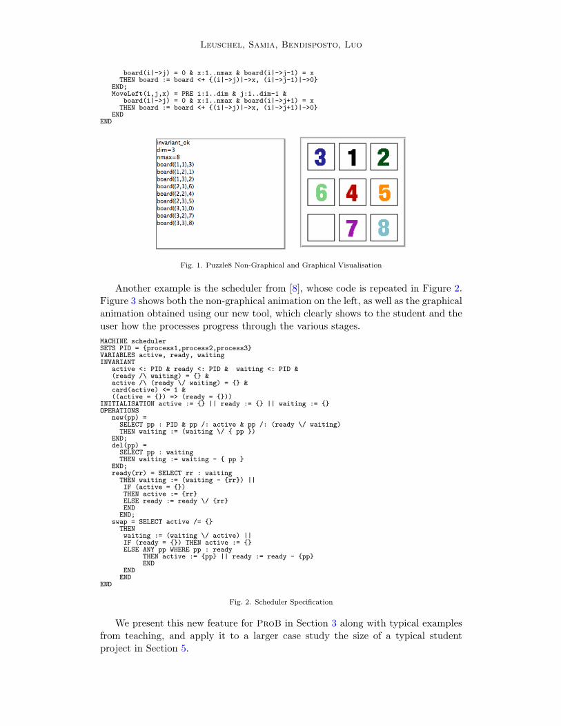
Take for example the following B machine describing the well-known sliding8-puzzle, where numbered tiles can be moved horizontally and vertically (into anempty square). The goal is to reach a configuration where all tiles are in order. Onthe left of Figure 1 you can see the non-graphical visualisation provided by ProB. Itis not unreadable, but the graphical visualisation on the right is clearly much moreinspiring and understandable. We now show how this animation can be achievedusing our new version of ProB with very little effort.MACHINE Puzzle8DEFINITIONS INV == (board: ((1..dim)*(1..dim)) -->> 0..nmax);GOAL == !(i,j).(i:1..dim & j:1..dim =>

board(i|->j) = j-1+(i-1)*dim);CONSTANTS dim, nmaxPROPERTIES dim:NATURAL1 & dim=3 & nmax:NATURAL1 & nmax = dim*dim-1VARIABLES boardINVARIANT INVINITIALISATION board : (INV & GOAL)OPERATIONS

MoveDown(i,j,x) = PRE i:2..dim & j:1..dim &board(i|->j) = 0 & x:1..nmax & board(i-1|->j) = x

THEN board := board <+ {(i|->j)|->x, (i-1|->j)|->0}END;MoveUp(i,j,x) = PRE i:1..dim-1 & j:1..dim &

board(i|->j) = 0 & x:1..nmax & board(i+1|->j) = xTHEN board := board <+ {(i|->j)|->x, (i+1|->j)|->0}

END;MoveRight(i,j,x) = PRE i:1..dim & j:2..dim &

5 For example, Besancon,Nantes in France; Southampton and Surrey in England; McMaster University, inCanada, Uppsala University in Sweden, and of course Dusseldorf in Germany.


board(i|->j) = 0 & x:1..nmax & board(i|->j-1) = xTHEN board := board <+ {(i|->j)|->x, (i|->j-1)|->0}

END;MoveLeft(i,j,x) = PRE i:1..dim & j:1..dim-1 &

board(i|->j) = 0 & x:1..nmax & board(i|->j+1) = xTHEN board := board <+ {(i|->j)|->x, (i|->j+1)|->0}

ENDEND

Fig. 1. Puzzle8 Non-Graphical and Graphical Visualisation

Another example is the scheduler from [8], whose code is repeated in Figure 2.Figure 3 shows both the non-graphical animation on the left, as well as the graphicalanimation obtained using our new tool, which clearly shows to the student and theuser how the processes progress through the various stages.MACHINE schedulerSETS PID = {process1,process2,process3}VARIABLES active, ready, waitingINVARIANT

active <: PID & ready <: PID & waiting <: PID &(ready /\ waiting) = {} &active /\ (ready \/ waiting) = {} &card(active) <= 1 &((active = {}) => (ready = {}))

INITIALISATION active := {} || ready := {} || waiting := {}OPERATIONS

new(pp) =SELECT pp : PID & pp /: active & pp /: (ready \/ waiting)THEN waiting := (waiting \/ { pp })

END;del(pp) =

SELECT pp : waitingTHEN waiting := waiting - { pp }

END;ready(rr) = SELECT rr : waiting

THEN waiting := (waiting - {rr}) ||IF (active = {})THEN active := {rr}ELSE ready := ready \/ {rr}END

END;swap = SELECT active /= {}

THENwaiting := (waiting \/ active) ||IF (ready = {}) THEN active := {}ELSE ANY pp WHERE pp : ready

THEN active := {pp} || ready := ready - {pp}END

ENDEND

END

Fig. 2. Scheduler Specification

We present this new feature for ProB in Section 3 along with typical examplesfrom teaching, and apply it to a larger case study the size of a typical studentproject in Section 5.


Fig. 3. Scheduler Non-Graphical and Graphical Visualisation

2 Visualising Formulas

Animation has the purpose of identifying unexpected behaviours of a model. If anunexpected behaviour does occur, the user often would like to know more about thesource of the problem.

• If the invariant is violated, one would like to know exactly which part of theinvariant is violated and why.

• If an operation is unexpectedly not enabled, or unexpectedly enabled, one wouldlike to know the reason.

• If the animator cannot find values for the constants which satisfy the propertiesof a machine, one would like to be able to locate the problematic properties.

For this, ProB had for quite some time the ability to inspect the invariant andalso to debug the properties. However, this view was often not precise enough, andwe have now implemented an algorithm which can take any B predicate or expressionand translates it into a graphical representation that can be inspected by the user.We believe this feature to be especially useful for students and newcomers to B, butwe also believe it to be important when animating complex specifications.

The algorithm basically uses the ProB interpreter to compute the value of anexpression or the truth-value of a predicate. It then tries to decompose the expres-sion or predicate into sub-expressions or -predicates. These are in turn recursivelyevaluated, until we reach sub-expressions or -predicates which can no longer be de-composed. The whole is then assembled into a graphical tree representation andrendered using the GraphViz package [2]. For example, Figure 4 contains a visu-alisation of the invariant of the scheduler machine, for the state already depictedearlier in Figure 3. For each expression, we have two lines of text: the first indicatesthe type of the node, i.e., the top-level operator. The second line gives the valueof evaluating the expression. For predicates, the situation is similar, except thatthere is a third line with the formula itself and that the nodes are coloured: truepredicates are green and false predicates are red.

Note that our algorithm also deals with undefined predicates. Those are renderedin orange. For example, the formula x ∈ dom(f) ∧ f(x) = 1, where f is the emptyfunction (and x some value aa) would be visualised as in Figure 5.


Fig. 4. Visualising the invariant of the scheduler for state of Figure 3

Fig. 5. Visualising a predicate with undefined sub-predicates

One interesting problem is what to do when an existentially quantified formulais false. In this case, our algorithm removes conjuncts from the end of the bodyof the quantified formula, until the formula becomes true. An example is shown inFigure 6, where we apply our algorithm to the guard of the new operation of thescheduler machine (for the state already depicted earlier in Figure 3). Note thatthe guard is modelled by an existential quantification over the parameters of theoperation. As can be seen, the existential formula is false, but our algorithm has de-


tected that by removing the first condition pp 6∈ active, the formula would becomesatisfiable. This information can be very valuable in detecting exactly where aninconsistency arises inside a formula. In previous works [5,11], different algorithmsbased on SAT solvers were developed to find a Minimal Unsatisfiable Subformula(MUS). Our approach to find a short unsatisfiable formula is simple. We are cur-rently interested in improving our algorithm by evaluating how the approaches in[5,11] can be applied to our Prolog constraint solving technique.

Fig. 6. Visualising the guard of new of the scheduler for the state of Figure 3

3 The new Graphical Animation Model

The animation model is very simple:

(i) The basic units are individual images. The images are given a number andtheir source file location is declared in the DEFINITIONS section of the an-imated machine. A definition ANIMATION IMGx == "filename", defines theimage with number x where filename is the path to a gif image file.

(ii) The graphical visualisation consists of a two-dimensional grid, each cell in thegrid can contain an image. The same image can appear multiple times in thegrid.

(iii) The graphical visualisation is recomputed for every state, by evaluating a user-defined animation function fa. The animation function fa is declared by defin-ing ANIMATION FUNCTION in the DEFINITIONS section and must be of typeINTEGER * INTEGER +-> INTEGER. If the function is defined for r and c, thismeans that the animator should display the image with number fa(r, c) at rowr and column c. If fa is undefined at r and c, then no image is displayed inthat cell.

The dimension of the grid is computed by looking at the minimum andmaximum coordinates that occur in the animation function. More precisely,the rows are in the range min(dom(dom(fa)))..max(dom(dom(fa))) and thecolumns are in the range min(ran(dom(fa)))..max(ran(dom(fa))).

For our 8-puzzle example, one could thus write the following animation function,together with an image declaration list. The result of using this animation functioncan be seen on the right of Figure 1.ANIMATION_FUNCTION == ( {r,c,i|r:1..dim & c:1..dim & i=0} <+ board);ANIMATION_IMG0 == "images/sm_empty_box.gif"; /* empty square */


ANIMATION_IMG1 == "images/sm_1.gif"; /* square with 1 inside */ANIMATION_IMG2 == "images/sm_2.gif";ANIMATION_IMG3 == "images/sm_3.gif";ANIMATION_IMG4 == "images/sm_4.gif";ANIMATION_IMG5 == "images/sm_5.gif";ANIMATION_IMG6 == "images/sm_6.gif";ANIMATION_IMG7 == "images/sm_7.gif";ANIMATION_IMG8 == "images/sm_8.gif"; /* square with lightblue 8 inside */

Each of the three integer types in the signature can be replaced by a deferred orenumerated set, in which case our tool translates elements of this set into numbers.In case of enumerated sets, the number is position of the element in the definition ofthe set in the SETS clause. Deferred set elements are numbered internally by ProB,and this number is used. (Note, however, that the whole animation function has tobe of the same type; otherwise the animator will complain about a type error.)

To avoid having to produce images for simple strings, one can use a declarationANIMATION STRx == "my string" to define image with number x to be automati-cally generated from the given string.

Typical patterns for the animation function are as follows:

• A useful way to obtain a function of the required signature is to write a setcomprehension of the following form:{row,col,img | row:1..NrRow & col:1..NrCols & P}, where P is a predicatewhich gives img a value depending on row and col.

• Another useful pattern is to write one function for default images, and then use theoverride operator to replace the default images only when needed: DefaultImages<+ CurrentImages. This results in much more concise and readable functions.This was used in the 8-Puzzle, by setting as default the empty square (image 0)overriden by the partially defined board function.

• Translation predicates between user sets and numbers (extension above can di-rectly handle user sets, but does not work well if we need a special image forundefined,...)

4 Further Examples

Below we show three more examples, which illustrate how our new animation modelcan be used. The examples also show that, despite its simplicity, the model ispowerful enough to provide interesting animations for a variety of models. This willbe further corroborated in Section 5.

4.1 Towers of Hanoi

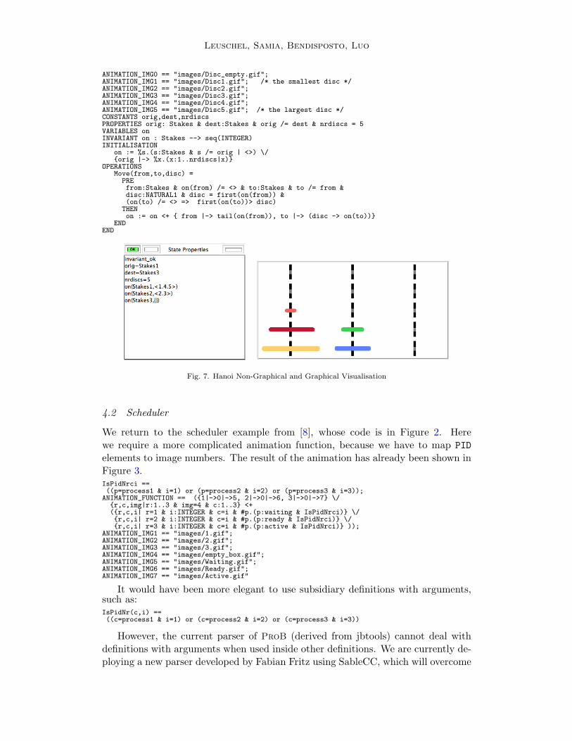
The Towers of Hanoi problem is widely used to teach recursion and problem solving.A B model of this problem is as follows. The animation function is surprisinglysimple (although we needed to make it slightly more complicated to ensure that thestakes are not shown upside down). The graphical result can be seen in Figure 7.MACHINE HanoiSETS StakesDEFINITIONS GOAL == (!s.(s:Stakes & s/=dest => on(s) = <>));scope_Stakes == 1..3;ANIMATION_FUNCTION == ({r,c,i|r:1..nrdiscs & c:Stakes & i=0} <+

{r,c,i|r:1..nrdiscs &c:Stakes & r-5+size(on(c)): dom(on(c)) &i = on(c)(r-5+size(on(c)))});


ANIMATION_IMG0 == "images/Disc_empty.gif";ANIMATION_IMG1 == "images/Disc1.gif"; /* the smallest disc */ANIMATION_IMG2 == "images/Disc2.gif";ANIMATION_IMG3 == "images/Disc3.gif";ANIMATION_IMG4 == "images/Disc4.gif";ANIMATION_IMG5 == "images/Disc5.gif"; /* the largest disc */CONSTANTS orig,dest,nrdiscsPROPERTIES orig: Stakes & dest:Stakes & orig /= dest & nrdiscs = 5VARIABLES onINVARIANT on : Stakes --> seq(INTEGER)INITIALISATION

on := %s.(s:Stakes & s /= orig | <>) \/{orig |-> %x.(x:1..nrdiscs|x)}

OPERATIONSMove(from,to,disc) =

PREfrom:Stakes & on(from) /= <> & to:Stakes & to /= from &disc:NATURAL1 & disc = first(on(from)) &(on(to) /= <> => first(on(to))> disc)

THENon := on <+ { from |-> tail(on(from)), to |-> (disc -> on(to))}

ENDEND

Fig. 7. Hanoi Non-Graphical and Graphical Visualisation

4.2 Scheduler

We return to the scheduler example from [8], whose code is in Figure 2. Herewe require a more complicated animation function, because we have to map PIDelements to image numbers. The result of the animation has already been shown inFigure 3.IsPidNrci ==((p=process1 & i=1) or (p=process2 & i=2) or (p=process3 & i=3));

ANIMATION_FUNCTION == ({1|->0|->5, 2|->0|->6, 3|->0|->7} \/{r,c,img|r:1..3 & img=4 & c:1..3} <+({r,c,i| r=1 & i:INTEGER & c=i & #p.(p:waiting & IsPidNrci)} \/{r,c,i| r=2 & i:INTEGER & c=i & #p.(p:ready & IsPidNrci)} \/{r,c,i| r=3 & i:INTEGER & c=i & #p.(p:active & IsPidNrci)} ));

ANIMATION_IMG1 == "images/1.gif";ANIMATION_IMG2 == "images/2.gif";ANIMATION_IMG3 == "images/3.gif";ANIMATION_IMG4 == "images/empty_box.gif";ANIMATION_IMG5 == "images/Waiting.gif";ANIMATION_IMG6 == "images/Ready.gif";ANIMATION_IMG7 == "images/Active.gif"

It would have been more elegant to use subsidiary definitions with arguments,such as:IsPidNr(c,i) ==((c=process1 & i=1) or (c=process2 & i=2) or (c=process3 & i=3))

However, the current parser of ProB (derived from jbtools) cannot deal withdefinitions with arguments when used inside other definitions. We are currently de-ploying a new parser developed by Fabian Fritz using SableCC, which will overcome


this problem.

4.3 Sudoku

For our course, we have also developed a B model of Sudoku, and show students howthey can use ProB to solve Sudoku puzzles. The machine has the variable Sudoku9of type 1..fullsize-->(1..fullsize+->NRS), where NRS is an enumerate set{n1, n2, ...} of cardinality fullsize. The animation function is as follows:

Nri == ((Sudoku9(r)(c)=n1 => i=1) & (Sudoku9(r)(c)=n2 => i=2) &(Sudoku9(r)(c)=n3 => i=3) & (Sudoku9(r)(c)=n4 => i=4) &(Sudoku9(r)(c)=n5 => i=5) & (Sudoku9(r)(c)=n6 => i=6) &(Sudoku9(r)(c)=n7 => i=7) & (Sudoku9(r)(c)=n8 => i=8) &(Sudoku9(r)(c)=n9 => i=9) );

ANIMATION_FUNCTION == ( {r,c,i|r:1..fullsize & c:1..fullsize & i=0} <+{r,c,i|r:1..fullsize & c:1..fullsize & c:dom(Sudoku9(r)) &

i:1.. fullsize & Nri} );

Figure 8 shows the non-graphical visualisation of a particular puzzle, then thegraphical visualisation of the puzzle as well as the visualisation of the solution foundby ProB (after a couple of seconds).

Fig. 8. Sudoku Non-Graphical and Graphical Visualisation

Note that it would have been nice to be able to replace Nri inside the animationfunction simply by i = Sudoku9(r)(c). While our visualisation algorithm canautomatically convert set elements to numbers, the problem is that there is a typeerror in the override: the left-hand side is a function of type INTEGER*INTEGER+->INTEGER

while the right-hand side now becomes a function of type INTEGER*INTEGER+->NRS. Onesolution is to extend our animator to accept multiple definitions of the animationfunction. We have done so, and the user can, in addition to the standard animationfunction, optionally define a default background animation function. The standardanimation function will override the default animation function, but the overridingis done within the graphical animator and not within a B formula. In this way, onecan now rewrite the above animation as follows:ANIMATION_FUNCTION_DEFAULT == ( {r,c,i|r:1..fullsize & c:1..fullsize & i=0} );ANIMATION_FUNCTION == ( {r,c,i|r:1..fullsize & c:1..fullsize &

c:dom(Sudoku9(r)) & i:1.. fullsize & i = Sudoku9(r)(c)} )

The scheduler animation from Section 4.2 can now also be rewritten more ele-gantly as follows:

ANIMATION_FUNCTION_DEFAULT ==( {1|->0|->5, 2|->0|->6, 3|->0|->7} \/ {r,c,img|r:1..3 & img=4 & c:1..3} );

ANIMATION_FUNCTION == ( {r,c,i| r=1 & i:PID & c=i & i:waiting} \/{r,c,i| r=2 & i:PID & c=i & i:ready} \/{r,c,i| r=3 & i:PID & c=i & i:active}

)


5 A more detailed case study: Formalising and Visual-ising a Lift

In this section, we provide a more detailed case study and apply our animationtechnology to a bigger specification, similar to a typical student project: the modelof a lift along with a controller that ensures that requests are eventually served.

Our experience was very positive, it was relatively straightforward to provide anappealing graphical visualisation of the model. This greatly enhanced the under-standability of the model, and allowed us to spot errors more quickly (e.g., in oneversion of the model, the lift could get stuck on the top floor, which was not thatobvious to spot in the non-graphical visualisation).

In the following, we actually present two models of a lift. The first model makesno distinction between internal and external call buttons. The second model is arefinement of the first, and here there are separate panel buttons inside the liftand external call buttons on each floor. In both cases, the lift can move between aground floor (constant groundf) and a top floor (constant topf). The state of bothlift models consists of the current floor the lift is on (variable cur floor), whetherits door is open or not (variable door open), whether it is currently moving up ordown (variable direction up) as well as the state of the buttons. In Figure 9, wepresent the graphics we used in the definition ANIMATION IMGx == "filename" anddescribe their associated event. Note that the images used before refinement arefrom x=0 to 6.

5.1 The Lift Model before Refinement

Below are the constants and variables of the first lift model.MODEL LiftMCONSTANTS groundf,topfPROPERTIES

topf : INTEGER &groundf : INTEGER &groundf = -1 &topf = 2 &groundf < topf

VARIABLES call_buttons,cur_floor,direction_up,do_count,door_open,inside_panel_buttons

INVARIANTcur_floor : groundf .. topf &door_open : BOOL &call_buttons : POW(groundf .. topf) &direction_up : BOOL &inside_panel_buttons : POW(groundf .. topf) &do_count : 0 .. 3...

Below is our animation function. The left part of the relational overriding <+gives the default values (i.e., images), and the right part gives the actual images.DEFINITIONS

Rconv == topf-r+groundf;ANIMATION_FUNCTION ==( {r,c,i|r:groundf..topf & ((c=2 & i=0) or (c=1 & i=2))} <+({r,c,i|r:groundf..topf & Rconv:call_buttons & c=2 & i=1} \/{r,c,i|r:groundf..topf & Rconv=cur_floor & c=1 &

((door_open=TRUE & i=3) or (door_open=FALSE & i=4))}) \/{r,c,i| r=topf+1 & c=1 & ((direction_up=TRUE & i=5)

or (direction_up=FALSE & i=6)) } );

Our default images are 0 and 2. Our current images are 1, 3, 4, 5 and 6.In our case, the lowest floor groundf and the highest floor topf are equal to −1


x "filename" Image Description of the Event 0 "images/lift/B_CallButtonOff.gif"

A call button is off. 1 "images/lift/B_CallButtonOn.gif" O

utsi

de

the

lift

A call button is on. 2 "images/lift/LiftEmpty.gif" The lift is not on a specific

floor.

3 "images/lift/B_LiftOpen.gif"

The lift’s door is opened.

4 "images/lift/B_LiftClosed.gif"

The lift’s door is closed.

5 "images/lift/B_up_arrow.gif" The lift’s direction up is on.

Before Refinement

6 "images/lift/B_down_arrow.gif" The lift’s direction down is off.

7 "images/lift/B_up_arrow_off.gif"

The lift’s direction up is off.8 "images/lift/B_floor_U1_off.gif"

The panel button U1 is off.

9 "images/lift/B_floor_U1_on.gif"

The panel button U1 is on.

10 "images/lift/B_floor_E_off.gif"

The panel button E is off.

11 "images/lift/B_floor_E_on.gif"

The panel button E is on.

12 "images/lift/B_floor_1_off.gif"

The panel button 1 is off.

13 "images/lift/B_floor_1_on.gif"

The panel button 1 is on.

14 "images/lift/B_floor_2_off.gif"

The panel button 2 is off.

15 "images/lift/B_floor_2_on.gif"

Insi

de th

e lif

t

The panel button 2 is on.

16 "images/lift/B_down_arrow_off.gif" The lift’s direction down is

off. 17 "images/lift/B_floor_U1.gif"

Floor U1

18 "images/lift/B_floor_E.gif"

Floor E

19 "images/lift/B_floor_1.gif"

Floor 1

ANIMATION_IMG

x =

= "f

ilena

me"

After Refinement

20 "images/lift/B_floor_2.gif"

Out

side

the

lift

Floor 2

Fig. 9. The Definition ANIMATION IMGx == "filename" and the Description of the Event associated to eachImage

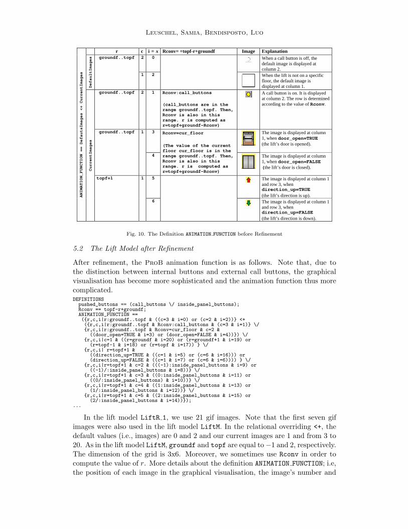
and 2, respectively. The minimum and maximum coordinates, which occur in theanimation function, are 2 and 5, respectively. Then, the dimension of the grid is3x2. To determine the value of r, we sometimes use Rconv==topf-r+groundf. Thevalues of Rconv are in the ranges groundf..topf. Rconv depends on the valuesobtained, when a call button is pushed or when the lift is on the current floor. Forinstance, if the current floor cur floor is equal to 2, then Rconv is also equal to2. Consequently, applying r==topf+groundf-Rconv, the row r is equal to −1. Ifdoor open=TRUE, then the image number i=3 is displayed at column 1. Otherwise,if door open=FALSE, then the image number i=4 appears at column 1. More detailsare presented in Figure 10. Due to space restrictions we do not show the graphicalvisualisation of this model, only of the more refined model later in Figure 12.


c i = x Rconv= =topf-r+groundf Image Explanation r 2 0

When a call button is off, the default image is displayed at column 2.

DefaultImages groundf..topf

1 2

When the lift is not on a specific floor, the default image is displayed at column 1.

groundf..topf 2 1 Rconv:call_buttons (call_buttons are in the range groundf..topf. Then, Rconv is also in this range. r is computed as r=topf+groundf-Rconv)

A call button is on. It is displayed at column 2. The row is determined according to the value of Rconv.

3

The image is displayed at column 1, when door_open=TRUE (the lift’s door is opened).

groundf..topf

1

4

Rconv=cur_floor (The value of the current floor cur_floor is in the range groundf..topf. Then, Rconv is also in this range. r is computed as r=topf+groundf-Rconv)

The image is displayed at column 1, when door_open=FALSE (the lift’s door is closed).

5

The image is displayed at column 1 and row 3, when direction_up=TRUE (the lift’s direction is up). A

NIMATION_FUNCTION == DefautsImages <+ CurrentImages

CurrentImages

topf+1 1

6

The image is displayed at column 1 and row 3, when direction_up=FALSE (the lift’s direction is down).

Fig. 10. The Definition ANIMATION FUNCTION before Refinement

5.2 The Lift Model after Refinement

After refinement, the ProB animation function is as follows. Note that, due tothe distinction between internal buttons and external call buttons, the graphicalvisualisation has become more sophisticated and the animation function thus morecomplicated.DEFINITIONS

pushed_buttons == (call_buttons \/ inside_panel_buttons);Rconv == topf-r+groundf;ANIMATION_FUNCTION ==({r,c,i|r:groundf..topf & ((c=3 & i=0) or (c=2 & i=2))} <+({r,c,i|r:groundf..topf & Rconv:call_buttons & (c=3 & i=1)} \/{r,c,i|r:groundf..topf & Rconv=cur_floor & c=2 &

((door_open=TRUE & i=3) or (door_open=FALSE & i=4))}) \/{r,c,i|c=1 & ((r=groundf & i=20) or (r=groundf+1 & i=19) or

(r=topf-1 & i=18) or (r=topf & i=17)) } \/{r,c,i| r=topf+1 &

((direction_up=TRUE & ((c=1 & i=5) or (c=6 & i=16))) or(direction_up=FALSE & ((c=1 & i=7) or (c=6 & i=6)))) } \/

{r,c,i|r=topf+1 & c=2 & (((-1):inside_panel_buttons & i=9) or((-1)/:inside_panel_buttons & i=8))} \/

{r,c,i|r=topf+1 & c=3 & ((0:inside_panel_buttons & i=11) or((0/:inside_panel_buttons) & i=10))} \/

{r,c,i|r=topf+1 & c=4 & ((1:inside_panel_buttons & i=13) or(1/:inside_panel_buttons & i=12))} \/

{r,c,i|r=topf+1 & c=5 & ((2:inside_panel_buttons & i=15) or(2/:inside_panel_buttons & i=14))});

...

In the lift model LiftR 1, we use 21 gif images. Note that the first seven gifimages were also used in the lift model LiftM. In the relational overriding <+, thedefault values (i.e., images) are 0 and 2 and our current images are 1 and from 3 to20. As in the lift model LiftM, groundf and topf are equal to−1 and 2, respectively.The dimension of the grid is 3x6. Moreover, we sometimes use Rconv in order tocompute the value of r. More details about the definition ANIMATION FUNCTION; i.e,the position of each image in the graphical visualisation, the image’s number and


r c i=x Rconv= = topf-r+groundf

Image Explanation

3 0

When a call button is off, the default image is displayed at column 3.

DefaultImages groundf..topf

2 2

When the lift is not on a specific floor, the default image is displayed at column 2.

groundf..topf 3 1 Rconv:call_buttons (call_buttons are in the range groundf..topf. Then, Rconv is also in this range. r is computed as r=topf+groundf-Rconv)

A call button is on. It is displayed at column 3. The row is determined according to the value of Rconv.

3 The image is displayed at column 2, when door_open=TRUE (the lift’s door is opened).

groundf..topf

2

4

Rconv=cur_floor (The value of the current floor cur_floor is in the range groundf..topf. Then, Rconv is also in this range. r is computed as r=topf+groundf-Rconv)

The image is displayed at column 2, when door_open=FALSE (the lift’s door is closed).

5

The image is displayed at column 1 and row 3, when direction_up=TRUE (the lift’s direction is up).

1

7

The image is displayed at column 1 and row 3, when direction_up=FALSE

6

The image is displayed at column 6 and row 3, when direction_up=FALSE (the lift’s direction is down).

topf+1

6

16

The image is displayed at column 6 and row 3, when direction_up=TRUE

groundf 20

The image is displayed at column 1 and row -1.

groundf+1 19

The image is displayed at column 1 and row 0.

topf-1 18

The image is displayed at column 1 and row 1.

topf

1

17

The image is displayed at column 1 and row 2

8

If (-1)/:inside_panel_buttons, the image is displayed at column 2 and row 3.

topf+1 2

9

If (-1):inside_panel_buttons, the image is displayed at column 2 and row 3.

10

If 0/:inside_panel_buttons, the image is displayed at column 3 and row 3.

topf+1 3

11

If 0:inside_panel_buttons, the image is displayed at column 3 and row 3.

12


topf+1 4

13


14


ANIMATION_FUNCTION == DefautsImages <+ CurrentImages

CurrentImages

topf+1 5

15


Fig. 11. The Definition ANIMATION FUNCTION after Refinement

the image’s associated event are provided in Figure 11.


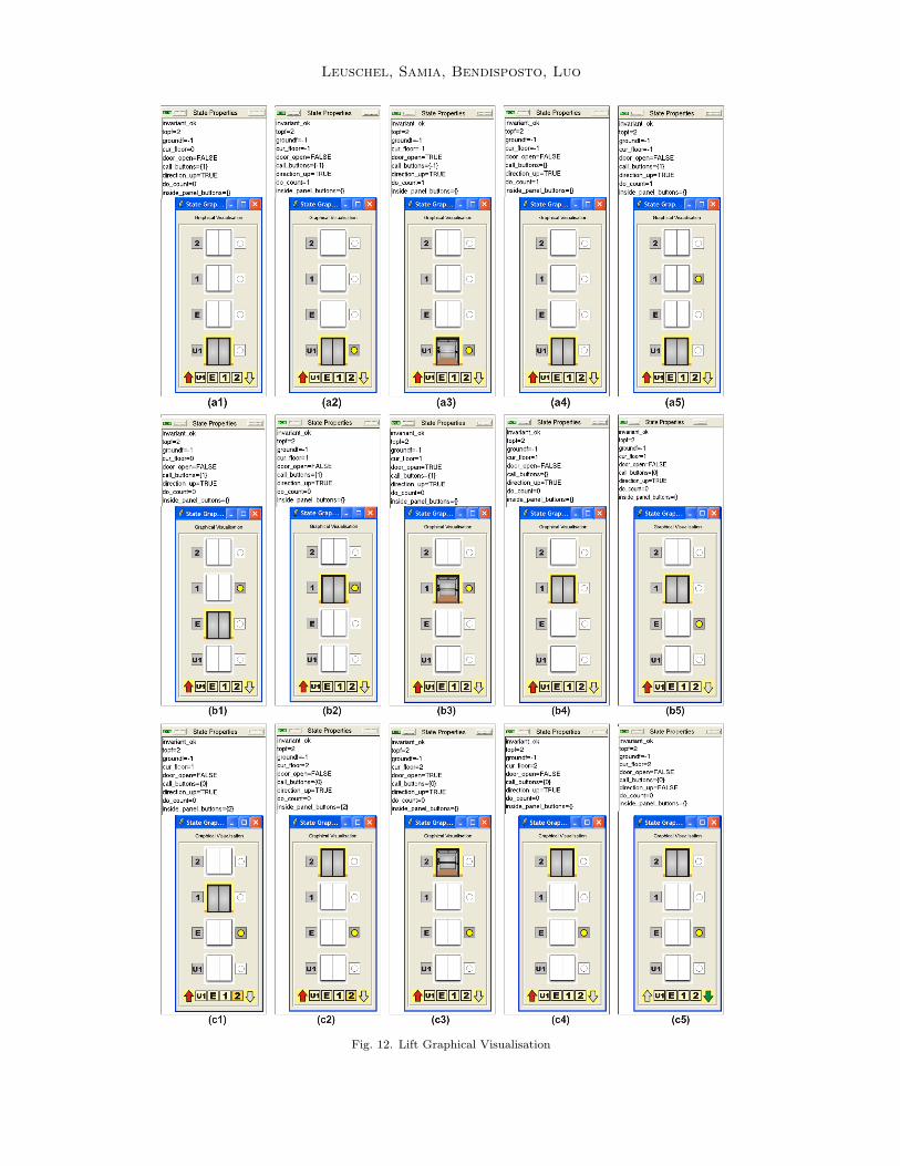
Figure 12 contains an animation sequence, starting from the initial state (a1),where the lift is on the ground floor, with its door closed, no buttons pressed and thelift controller being in upwards mode. Between states (a1) and (a2), the operationpush call button(-1) has been executed. The user can clearly see the effect ofthe operation. This operation now also enables the open door operation, afterwhose execution we reach state (a3). This enables the close door operation, whoseexecution leads us to state (a4). Here, we can clearly see that the call button tofloor U1 has been turned off again. After (a4), the user has executed the operationpush call button(1) leading to (a5). This enabled the move up operation, afterwhose execution we reach state (b1), etc...

6 Related Work and Conclusions

As far as related work is concerned, we would like to mention the Possum anima-tion tool [7] for Z. The latter is probably most related, as it allows the user to writecustom TclTk code that can query the state of a Z specification in order to providea custom graphical visualisation. The most closely related work on the B side is[4,1], which uses a special purpose constraint solver over sets (CLPS) to animateB and Z specifications using the so-called BZ-Testing-Tools. However, the focus ofthese tools is test-case generation and not verification, and the subset of B thatis supported is comparatively smaller (e.g., no set comprehensions or lambda ab-stractions, constants and properties nor multiple machines are supported). To ourknowledge no graphical visualisation for states is available.

In summary, we have provided two new graphical visualisation features for ProB:one to visualise predicates as a tree and the other to view the state of a B model in adomain-specific manner. We have shown the usefulness of these features on a seriesof examples. We hope that this provide further value to teaching B to students.

Acknowledgements

We would like to thank Daniel Plagge for his suggestions in Section 2. We also wishto extend our thanks to the reviewers for their helpful comments.

References

[1] F. Ambert, F. Bouquet, S. Chemin, S. Guenaud, B. Legeard, F. Peureux, M. Utting, and N. Vacelet.BZ-testing-tools: A tool-set for test generation from Z and B using constraint logic programming. InProceedings of FATES’02, Formal Approaches to Testing of Software, pages 105–120, August 2002.Technical Report, INRIA.

[2] AT&T Labs-Research. Graphviz - open source graph drawing software. Obtainable athttp://www.research.att.com/sw/tools/graphviz/.

[3] J. Bendisposto and M. Leuschel. A generic flash-based animation engine for ProB. In Proceedingsof the 7th International B Conference (B2007), LNCS 4355, pages 266–269, Besancon, France, 2007.Springer-Verlag.

[4] F. Bouquet, B. Legeard, and F. Peureux. CLPS-B - a constraint solver for B. In J.-P. Katoen andP. Stevens, editors, Tools and Algorithms for the Construction and Analysis of Systems, LNCS 2280,pages 188–204. Springer-Verlag, 2002.

[5] R. Bruni and A. Sassano. Restoring Satisfiability or Maintaining Unsatisfiability by Finding SmallUnsatisfiable Subformulae. In H. Kautz and B. Selman, editors, LICS 2001 Workshop on Theory andApplications of Satisfiability Testing (SAT 2001) Boston (Massachusetts, USA), June 14-15, 2001,Proceedings. Elsevier Science Pub., 2001.


[6] E. M. Clarke, O. Grumberg, and D. Peled. Model Checking. MIT Press, 1999.

[7] D. Hazel, P. Strooper, and O. Traynor. Requirements engineering and verification using specificationanimation. Automated Software Engineering, 00:302, 1998.

[8] B. Legeard, F. Peureux, and M. Utting. Automated boundary testing from Z and B. In ProceedingsFME’02, LNCS 2391, pages 21–40. Springer-Verlag, 2002.

[9] M. Leuschel and M. Butler. ProB: A model checker for B. In K. Araki, S. Gnesi, and D. Mandrioli,editors, FME 2003: Formal Methods, LNCS 2805, pages 855–874. Springer-Verlag, 2003.

[10] M. Leuschel and E. Turner. Visualizing larger states spaces in ProB. In H. Treharne, S. King,M. Henson, and S. Schneider, editors, Proceedings ZB’2005, LNCS 3455, pages 6–23. Springer-Verlag,April 2005.

[11] E. Torlak, F. S.-H. Chang, and D. Jackson. Finding minimal unsatisfiable cores of declarativespecifications. In J. Cuellar, T. Maibaum, and K. Sere, editors, FM 2008, volume 5014 of LectureNotes in Computer Science, pages 326–341. Springer, 2008.

A Sudoku Example

MACHINE SudokuSETS9SETSNRS = {n1,n2,n3,n4,n5,n6,n7,n8,n9}

DEFINITIONSColumn(jj) == %ii.(ii:1..fullsize & jj:dom(Sudoku9(ii)) | Sudoku9(ii)(jj));ColumnSol(jj) == %ii.(ii:1..fullsize | SudokuSol(ii)(jj));

SUBSqIndx == {1..3, 4..6, 7..9}CONSTANTS sqsize,fullsizePROPERTIES

fullsize = card(NRS) & sqsize:NAT1 & sqsize*sqsize = fullsizeVARIABLES Sudoku9, solvedINVARIANT

Sudoku9: 1..fullsize --> (1..fullsize +-> NRS) & solved:BOOLINITIALISATION

Sudoku9:= %i1.(i1:1..fullsize|{}) || solved := TRUEOPERATIONS

Set(i,j,nr) =PREi:1..fullsize & j:1..fullsize & j/: dom(Sudoku9(i)) &nr:NRS & nr/:ran(Sudoku9(i)) & nr/:ran(Column(j))

THEN Sudoku9(i) := Sudoku9(i) \/ {j |-> nr}END;StartSolve =PREsolved=TRUE

THEN solved := FALSEEND;SetPuzzle1 =BEGINSudoku9 := { 1 |-> { 1|->n7, 2|->n8, 3|->n1, 4|->n6, 6|->n2, 7|->n9, 9|->n5 },

2 |-> { 1|-> n9, 3|->n2, 4|->n7, 5|->n1 },3 |-> { 3|-> n6, 4|-> n8, 8|->n1, 9|->n2},4 |-> { 1|-> n2, 4|->n3, 7|->n8, 8|->n5, 9|->n1} ,5 |-> { 2|-> n7, 3|->n3, 4|->n5, 9|->n4} ,6 |-> { 3|-> n8, 6|->n9, 7|->n3, 8|->n6} ,7 |-> { 1|-> n1, 2|->n9, 6|->n7, 8|->n8} ,8 |-> { 1|-> n8, 2|->n6, 3|->n7, 6|->n3, 7|-> n4, 9|-> n9} ,9 |-> { 3|-> n5, 7|->n1} }

END;Solve =ANYSudokuSol

WHEREsolved=FALSE &SudokuSol: 1..fullsize --> (1..fullsize --> NRS) & /* all values are specified */!(i,j).(i:1..fullsize & j:1..fullsize & j:dom(Sudoku9(i))=> SudokuSol(i)(j) = Sudoku9(i)(j))& /*all existing values copied from current board*/

!(i,j1,j2).(i:1..fullsize & j1:1..fullsize & j2:1..fullsize &j2 > j1 => (SudokuSol(i)(j1) /= SudokuSol(i)(j2) & /* all different on a row */SudokuSol(j1)(i) /= SudokuSol(j2)(i) /* all diferent on a column */ )) &!(xi,yi).(xi: SUBSqIndx & yi: SUBSqIndx =>!(i1,j1,i2,j2).(i1:INTEGER & i2:INTEGER & j1:INTEGER & j2:INTEGER &

i1:xi & i2:xi & i2 >= i1 & j1:yi & j2:yi &(i2=i1 => j2>j1) /* (i1|->j1) /= (i2|->j2) */=> SudokuSol(i1)(j1) /= SudokuSol(i2)(j2))

THEN Sudoku9 := SudokuSol || solved := TRUEEND

END


Fig. 12. Lift Graphical Visualisation

Easy Graphical Animation and Formula Visualisation for ...

Documents

Transcript of Easy Graphical Animation and Formula Visualisation for ...