4 Juillet 2006 Financial Risk Management, Firm Structure ...

Université de Montréal & CIRANO

Rapport de Recherche de Maîtrise4 Juillet 2006

Financial Risk Management,Firm Structure & Valuation,An Empirical Analysis

David De Angelis

Directeur:

Professeur René Garcia

Résumé:

Ce rapport examine si les évidences empiriques sur la structure de l�entreprise,sa valeur marchande et la gestion des risques �nanciers soutiennent le modèlethéorique proposé par Boyer, Boyer and Garcia (2005). La base de donnéesest composée des �rmes américaines du S&P500 pour l�année 2004, les donnéescomptables et de marché sont extraites de 1993 à 2004, et celles pour l�utilisationdes produits dérivés et les portefeuilles des dirigeants à partir des rapports an-nuels de 2004. Nos résultats mettent en évidence une relation empirique entrela valeur de la �rme, son bêta et le taux sans risque. De plus, nous avonsdéveloppé un estimateur pour la �exibilité des activitées de l�entreprise. Ce fac-teur de �exibilité semble être un nouveau déterminant empirique de la gestiondes risques opérationnels. Finalement, concernant l�explication de l�utilisationdes produits dérivés, nous observons que les déterminants changent en fonctiondu type de risque couvert.

Mots-Clés: Flexibilité, Gestion de Portefeuille de Projets, Gestion desRisques Financiers, Valeur de l�Entreprise

1

Université de Montréal & CIRANO

Master ThesisJuly 4th, 2006

Financial Risk Management,Firm Structure & Valuation,An Empirical Analysis

David De Angelis1 ;2

Advisor:

Professor René Garcia3

Abstract:

This paper investigates if empirical evidence on the �rm structure, its marketvalue and its corporate hedging decisions support the theoretical model proposedby Boyer, Boyer and Garcia (2005). The database is composed by �rms of theUS S&P500 in 2004, market and accounting data are collected from 1993 to2004, then hedging and managerial shareholding data are extracted from 2004annual reports. Our results show empirical relations between the �rm marketvalue, its beta and the risk free rate. Moreover, we have created an estimatorfor the �exibility of the �rm�s activities. The Flexibility Factor is validated asa new empirical determinant of operational risk hedging decisions. Finally, forthe explanation of the use of derivatives, we provide evidence that signi�cantvariables change according to the type of risk hedged.

Keywords: Flexibility, Financial Risk Management, Firm Value, ProjectPortfolio Management

1Master Student, Université de Montréal. E-mail: [email protected] I would like to thank particularly René Garcia for his advice and his �nancial support

during my Master. I am also grateful to Marcel and Martin Boyer for helpful comments, JulienPicault for suggestions as discussant and Catherine Gendron for excellent research assistance.

3Hydro-Québec Professor of risk management and mathematical �nance, Université deMontréal, and Fellow of CIRANO and CIREQ. E-mail: [email protected]

2

Table of Contents

1 Introduction, p.4

2 Theoretical Model, p.6

2.1 BBG Model Presentation, p.62.2 BBG Model Propositions, p.82.3 Flexibility & Financial Risk Management, p.92.4 Theoretical Conclusion, p.9

3 Empirical Analysis, p.10

3.1 Databasa & Methodology, p.10

3.2 Risk Premium - Firm Structure, p.103.2.1 Market Data, p.103.2.2 E[CF] and SCOR Variations Analysis, p.113.2.3 Panel Data Analysis, p.12

3.3 Risk Free Rate - Market Value, p.143.2.1 Market Data, p.143.3.2 Market Value Variation Analysis, p.143.3.3 Linear Regression, p.153.3.4 Panel Data Analysis, p.16

3.4 Firm Structure Flexibility - Corporate Hedging, p.183.4.1 Firm Structure Flexibility Factor, p.183.4.2 Corporate Hedging Variable, p.203.4.3 Other Explanatory Variables, p.203.4.4 Level of Hedging, p.213.4.5 Decision of Hedging by type of risk, p.233.4.6 Number of risk hedged, p.273.4.7 Industry Analysis, p.28

4 Conclusion, p.30

References, p.31

5 Appendix, p.34

3

Figure & Tables

� Figure 1 - Firm Valuation Example, p.8

� Table 1 - Risk Premium, p.11

� Table 2 - SCOR & CF Variations: Statistics Results, p.12

� Table 3 - SCOR: Panel-Probit Results, p.13

� Table 4 - CF: Panel-Probit Results, p.14

� Table 5 - Risk Free Rate, p.15

� Table 6 - Market Value Variation: Statistics Results, p.15

� Table 7 - Regression Analysis, p.16

� Table 8 - Market Value: Panel-Probit Results, p.17

� Table 9 - Flexibility Factor - Correlation Table, p.20

� Table 10 - Heckman Selection Model - Two Step Estimates, p.23

� Table 11 - Tobit Estimates, p.24

� Table 12 - Hedging - Probit Estimates, p.25

� Table 13 - Foreign Exchange Risk - Probit Estimates, p.25

� Table 14 - Debt Financing Risk - Probit Estimates, p.26

� Table 15 - Commodity Risk - Probit Estimates, p.26

� Table 16 - Equity Risk - Probit Estimates, p.27

� Table 17 - Every Risk - Ordered Probit Estimates, p.28

� Table 18 - Operational Risk - Ordered Probit Estimates, p.29

� Table 19 - Industry Estimates, p.30

4

1 Introduction

Financial Risk Management is a new topic in the empirical �nance literaturethanks in part to the creation of new databases on hedging activities. Manyquestions have been raised and are still without satisfactory answers: What arethe value and the motivations of using these tools (i.e. derivatives)? Is there atheoretical framework that could explain these activities?There is a controversy in the �nance industry about the value of hedging.

Firms use derivatives in order to �x the price paid or/and received, this could beuseful as a tool to predict cash �ows expenses or/and income and for the �rm tobe able to produce less uncertain expected balance-sheet. Moreover, derivativescan be also used for speculation, for example on a speci�c commodity price, butthis is an uno¢ cial practice since risk management has normally no speculativepurpose. For portfolio managers, a �rm that hedges its activities seems lessrisky but hedging also erases exposition and so a speculative return. Hence,we observe a dual e¤ect and it is not trivial to determine the e¤ect of usingderivatives on the �rm market value.The aim of this paper is to check empirically the implications that could be

derived from the model proposed by Boyer, Boyer and Garcia (2005) (BBG)and to study a new determinant for the motivation of corporate hedging. Thestudy of their theoretical framework lead us to analyse two empirical relationsout of the �nancial risk management subject: the �rst one between the mix ofactivities chosen by the �rm (i.e. the �rm structure) and the risk premium; thesecond between the �rm market value and the risk free rate dependent on the�rm�s beta level. The third and last empirical relation is the �exibility of the�rm and the use of derivatives for hedging.For the theoretical literature4 review, we begin with the Modigliani and

Miller (M&M) world where the �rm value is determined by its activities andinvestment decisions and not by its �nancial structure. Therefore in this frame-work, �nancial risk management has no value. More recently, Smith and Stulz(1985) have relaxed the perfect market assumption made by M&M, �nding thata �rm which maximizes its value, hedges its activities for three reasons: taxes,�nancial distress cost and managers risk aversion. Thus, in this model, �nancialrisk management has some value for these �rst two reasons.In the empirical literature5 , many papers6 are related to a speci�c industry

(ex: natural gas) or to a speci�c risk (ex: currency risk and the use of currencyswaps or other currency derivatives). We can cite two papers which relateempirical results including almost every industry (with the exception of the

4See the Appendix for a complete theoretical literature review of �nancial risk managementmotivations and valuation.

5See the Appendix for a review of determinants of corporate hedging activities studiedin the empirical literature. We decompose the results in function of the dependant variable,which is either the level of hedging (for example the notionnal value of derivatives used) orthe decision of hedging (binary variable, equals 1 if the �rm uses derivatives).

6See for example: Allayannis, G. and Weston, J.P. (2001), Dionne, G. and Garand, M.(2003), Tufano, P. (1996), and Viswanathan, G. (1998).

5

�nancial industry because they are users and providers of derivatives). The�rst one from Mian (1996) underlines that the �nancial distress cost reason isnot empirically validated, and the one for taxes is mitigated; however, he hasfound a signi�cant size e¤ect. The second, from Graham and Rogers (2002),found a new empirical reason why �rms hedge: to increase debt capacity.This paper is organized as follows: in section 2, BBG model and three majors

theoretical relations are explained. In section 3, the empirical methodology andresults are exposed. Finally, section 4 concludes.

6

2 Theoretical Model

2.1 BBG Model Presentation7

A �rm is decomposed by realized and possible projects represented in a Ei �SCORim framework. Ei are the expected cash �ows from the project i. Thesecond component is the scaled correlation of the project i: SCORim = �im��i,where �im is the correlation of the cash �ows of the project i with the marketreturn m and �i is the standard deviation of the project i�s cash �ows.Given all the constraints faced by the �rm such as technology or regulation,

we can construct a frontier of possibilities for cash �ows. The envelope of allfeasible combinations is by construction concave. In our model, we assume thereis a single risk factor: the market portfolio. Hence, a �rm j is valued in termsof its expected cash �ows discounted by an expected rate of return given by theCAPM:

ERj = RF + �jm � (E[RM ]�RF )

with the risk free rate (RF ), the expected market return (E[RM ]) and itsbeta (�jm):For simplicity, we assume that cash �ows are constant through time. So the

value of the �rm is Vj =EjERj

where Ej are the total expected cash �ows of the�rm for the next period. We can express the security market line in terms ofcash �ows:

Ej = Vj � ERj = Vj �RF + Vj � �jm � (E[RM ]�RF ):

Vj � �jm represents the risk of the �rm�s cash �ows:

Vj � �jm = Vj �Cov[Rj ;Rm]�2[Rm] =

Cov[Vj�Rj ;Rm]�2[Rm] =

Cov[CFj ;Rm]�2[Rm] :

So we now have that:

Ej = Vj �RF + �jm � �j �(E[RM ]�RF )

�[Rm]

and therefore the value of the �rm is:

Vj =1RF[Ej � �jm � �j �

(E[RM ]�RF )�[Rm] ]:

An iso-value line represents combinations of Ej and SCORjm with the samemarket value. From the last equation, iso-value lines are linear and parallel, witha slope equal to the market price of risk: (E[RM ]�RF )

�[Rm] :

In order to calculate the �rm value, we can discount the zero-SCOR expectedcash �ows level (C) from the iso-value line at the risk free rate RF : V = C

RF:

7For more detailed proofs and explanations, see Boyer, Boyer and Garcia (2005).

7

5 0 5 10 15 205

0

5

10

15

C0

T0E

SCOR

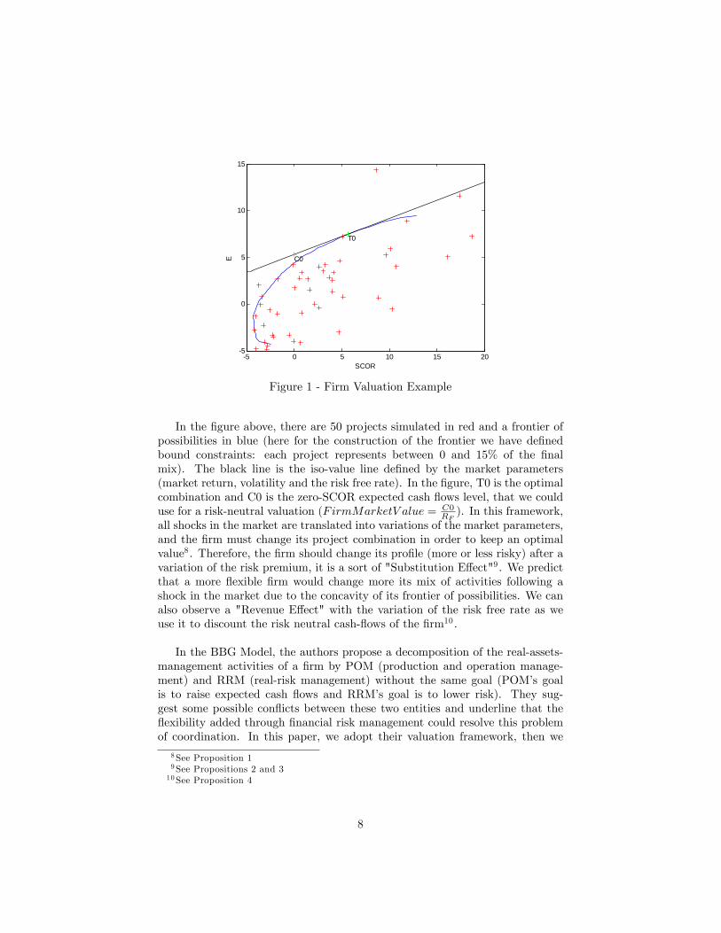
Figure 1 - Firm Valuation Example

In the �gure above, there are 50 projects simulated in red and a frontier ofpossibilities in blue (here for the construction of the frontier we have de�nedbound constraints: each project represents between 0 and 15% of the �nalmix). The black line is the iso-value line de�ned by the market parameters(market return, volatility and the risk free rate). In the �gure, T0 is the optimalcombination and C0 is the zero-SCOR expected cash �ows level, that we coulduse for a risk-neutral valuation (FirmMarketV alue = C0

RF). In this framework,

all shocks in the market are translated into variations of the market parameters,and the �rm must change its project combination in order to keep an optimalvalue8 . Therefore, the �rm should change its pro�le (more or less risky) after avariation of the risk premium, it is a sort of "Substitution E¤ect"9 . We predictthat a more �exible �rm would change more its mix of activities following ashock in the market due to the concavity of its frontier of possibilities. We canalso observe a "Revenue E¤ect" with the variation of the risk free rate as weuse it to discount the risk neutral cash-�ows of the �rm10 .

In the BBG Model, the authors propose a decomposition of the real-assets-management activities of a �rm by POM (production and operation manage-ment) and RRM (real-risk management) without the same goal (POM�s goalis to raise expected cash �ows and RRM�s goal is to lower risk). They sug-gest some possible con�icts between these two entities and underline that the�exibility added through �nancial risk management could resolve this problemof coordination. In this paper, we adopt their valuation framework, then we

8See Proposition 19See Propositions 2 and 310See Proposition 4

8

consider the POM-RRM decomposition and the problem of coordination for theexplanation of �nancial risk management.

2.2 BBG Model Propositions

In this subsection, we complete the analysis of the four propositions from theBBG paper:

Proposition 1 �To maximize its value, a �rm must equate its marginal rate ofsubstitution, the rate at which it can substitute POM and RRM activities whileremaining on its e¢ cient frontier, to the market price of risk:

�@(OM)@(RM) = �

@E@SCORM (CFj ;RM )

jH(E;SCORM )=0=(E[RM ]�RF )

�[Rm] :�

In other words, to maximize its value, a �rm takes a combination of projectswhich is on the possibility frontier and tangent to the iso-value line. This is aproject portfolio value maximization comparable to the one from asset manage-ment. To test this assumption, we need details on realized and possible �rmprojects. As it is really unlikely to obtain this very con�dential information, wecan not check this proposition.

Proposition 2 �A �rm reacts to an increase in the volatility of market returns,which reduces the price of risk, by modifying its RRM and POM activities toincrease both its expected cash �ows E and scaled correlation SCOR.�

Proposition 3 �A �rm reacts to an increase in the expected market return,which increases the price of risk, by modifying its RRM and POM activities toreduce both its expected cash �ows E and scaled correlation SCOR.�

Proposition 4 �An increase in the risk-free rate induces an increase in boththe risk taken by a �rm and its expected cash �ows. Firm value increases if itsoriginal beta is larger than 1. When the original beta is less than 1, the directe¤ect is to lower �rm value; a �rm can alleviate and even reverse this directe¤ect by optimally adjusting its portfolio of projects.�

Through propositions 2, 3 and 4, we �nd a relation between the market priceof risk variation and project portfolio management. The various market para-meters used in these propositions can be grouped together by the risk premium(i.e. the market price of risk: (E[RM ]�RF )

�[Rm] ) calculation. So the �rm structureshould be more(or less) risky for negative (or positive) variation of the risk pre-mium. The �rm structure represents the choice of projects by the �rm, and astructure more risky means higher SCOR and expected cash �ows.From proposition 4, there is a relation between the �rm market value, the

risk free rate variation and the beta of the �rm.

9

2.3 Flexibility & Financial Risk Management

From the BBG Model, the coordination problem from POM and ROM activi-ties could explain the use of derivatives to reach the optimal project portfolio.Their valuation framework allows to observe the value added by �nancial riskmanagement in case of coordination problems. As the �rm structure (i.e. theproject portfolio choice) moves with respect to the E-SCOR position, �nancialrisk management brings smoothness in their state-position variation. We canomit coordination con�icts and consider that hedging allows more �exibility inthe project portfolio management. Therefore, from the BBG model steams anew proposition that could be tested:

Proposition 5 �There exists a positive relation between the �rm structure �ex-ibility (i.e. variations of �rm�s activities) and the use of derivatives.�

2.4 Theoretical Conclusion

From the study of this framework, we detect three relations that could be em-pirically observed:

� Project portfolio management & risk premium

� Firm value, its beta & risk free rate

� Firm structure �exibility & �nancial risk management

Hence, through this model we explore new assumptions for the valuation ofa �rm and its choices of activities. Then, we �nd a new determinant for theuse of derivatives. In the next section, we empirically check these assumptionsand confront the �rm structure �exibility with other validated determinants forhedging explanation.

10

3 Empirical Analysis

3.1 Database & Methodology

The database was created from Compustat for accounting data, then Bloombergand CRSP for market data. The sample is composed of �rms from the USS&P500 selected in 2004. Firms lacking important data have been droppedfrom the sample. The �nal sample is made of 464 enterprises. The databasewas extracted for the years 1993 to 2004. Concerning the Flexibility Factordetermination, only �rms with complete data for the all time segment wereretained. Thus, the �nal sample for this subsection represents 270 enterprises;hedging, managerial11 shareholding and option ownership data were extractedfrom EDGAR US Database. Finally, for this empirical study, Matlab, Stataand Excel softwares were used.All the market data are selected at end of the year (example: 12/31/2004

for the year 2004), and the expected value is estimated by the realized one(hypothesis of perfect forecast). For instance, we consider the operating incomereported in the annual report for the estimation of expected cash �ows.

3.2 Risk Premium - Firm Structure

3.2.1 Market Data

D a t e T B 1m o n th Vo la t i l i ty R e t u rn R is k P r em ium V 1 . R i s k P r em ium V 2 . R i s k P r em ium

1 9 9 3 2 .9 4% 8 .6 8% 7 .0 6% 4 7 .4 2%

1 9 9 4 4 .7 4% 9 .9 3% -1 .5 4% -6 3 ;1 9% -2 3 3 .2 6% -1 1 0 .6 1%

1 9 9 5 4 .5 8% 7 .8 8% 3 4 .1 1% 3 7 4 .7 2% 6 9 2 .9 8% 4 3 7 .9 1%

1 9 9 6 4 .8 7% 1 1 .8 8% 2 0 .2 6% 1 2 9 .5 1% -6 5 .4 4% -2 4 5 .2 1%

1 9 9 7 5 .1 1% 1 8 .3 6% 3 1 .0 1% 1 4 1 .0 8% 8 .9 3% 1 1 .5 7%

1 9 9 8 4 .3 9% 2 0 .6 2% 2 6 .6 7% 1 0 8 .0 3% -2 3 .4 2% -3 3 .0 5%

1 9 9 9 5 .1 0% 1 8 .2 6% 1 9 .5 3% 7 9 .0 1% -2 6 .8 6% -2 9 .0 2%

2 0 0 0 5 .7 7% 2 2 .3 3% -1 0 .1 4% -7 1 .2 4% -1 9 0 .1 7% -1 5 0 .2 6%

2 0 0 1 1 .6 4% 2 2 .0 8% -1 3 .0 4% -6 6 .4 7% 6 .7 1% 4 .7 8%

2 0 0 2 1 .1 4% 2 6 .0 7% -2 3 .3 7% -9 4 .0 0% -4 1 .4 2% -2 7 .5 3%

2 0 0 3 0 .8 3% 1 7 .2 3% 2 6 .3 8% 1 4 8 .3 1% 2 5 7 .7 7% 2 4 2 .3 1%

2 0 0 4 1 .9 1% 1 1 .1 9% 8 .9 9% 6 3 .2 9% -5 7 .3 3% -8 5 .0 2%

Table 1 - Risk Premium12

11For the determination of managerial shareholding and option ownership, we analyse theportfolio of the top �ve executives of the �rm.12 In our paper, we use a risk premium by unit of volatility but denote it simply risk premium.

11

Note: TB means T-Bills (we select TB 1 Month as the risk free rate). Market Volatility

and Market Return are calculated from the US S&P500 return. Market Volatility is an

historical volatility calculated with n equals 260 (equivalent for the number of trading days in

a year). The risk premium, and its variations are calculated as follows:

RP = RM�RF

�[Rm]

V 1:RPt =RPt�RPt�1jRPt�1j13

V 2:RP t= RP t�RP t�1

Since the market return is on the nominator and the market volatility ison the denominator in RP calculation, we select years where variations of themarket volatility and return have opposite signs in order to obtain the sameexpectation from propositions 2 and 3 relating to E[CF] and SCOR variations.Thus, we will study the following years: 1994, 1995, 1996, 2000, 2002 and 2003.

3.2.2 E[CF] and SCOR Variations Analysis14

1 9 9 4 1 9 9 5 1 9 9 6 2 0 0 0 2 0 0 2 2 0 0 3

V .O m s ig n + - + + + -

V .R m s ig n - + - - - +

V .S C O R & C F , e x p e c t e d s ig n + - + + + -

N t o t a l 2 9 0 3 0 7 3 2 0 4 0 7 4 4 2 4 6 0

M e a n V .S C O R 0 .4 1 0 .2 2 3 .2 4 2 .4 2 0 .8 4 0 .2 1

M e a n V .C F 0 .2 5 0 .2 0 0 .4 6 0 .3 4 0 .9 1 0 .2 6

t -Te s t M e a n V .S C O R = 0 >0 >0 >0 >0 >0

t -Te s t M e a n V .C F = 0 >0 >0 >0 >0 >0

Table 2 - SCOR & CF Variations: Statistics Results

Note: V.Om and V.Rm are the Market Volatility and Return variations. V.SCOR and

V.CF are estimated with the following equation (absolute value in the denominator to keep

the direction of the variation as SCOR and the operating income could be negative): V:Xt =Xt�Xt�1jXt�1j : For the t-Test, the validated alternative is written (there is a blank if no conclusion

could be made on the sign of the variation with a 90% con�dence level).

The expected cash �ows of the �rm are estimated as the operating incomefrom the annual report. The SCOR is hard to estimate as it is the product ofthe cash �ows standard deviation with the correlation between the cash �owsand the market return. As it is proved below, we can estimate the SCOR of the

14Distribution estimations for CF and SCOR variations by the kernel-gaussian estimationmethod are set in the appendix.

12

�rm from its beta, its market value and the market volatility, which are easy to�nd. Firm market value is the total number of shares times the stock price.

SCOR [CFi; Rm] = � [CFi]� Corr [CFi; Rm] = � [CFi]� Cov[CFi;Rm]�[CFi] � �[Rm]

= � [CFi]� FirmMarketV aluei�Cov[Ri;Rm]�[CFi] � �[Rm]

= FirmMarketV aluei � � [Rm]� Cov[Ri;Rm]�2[Rm]

= FirmMarketV aluei � � [Rm]� �im

It should be a growth e¤ect as all means of V.SCOR and V.CF are positive(bear in mind that there is censure bias because we observe only �rms that havesurvived till 2004). V.SCOR�s means are by far lower when the predicted sign isnegative and for V.CF, it is the same (except for 2004). It seems that the dataare in the direction of our theoretical relation, but more precise work is neededto validate it. In the next subsection, we decompose the risk premium variationin its three market parameters and so we control for their di¤erent variations.

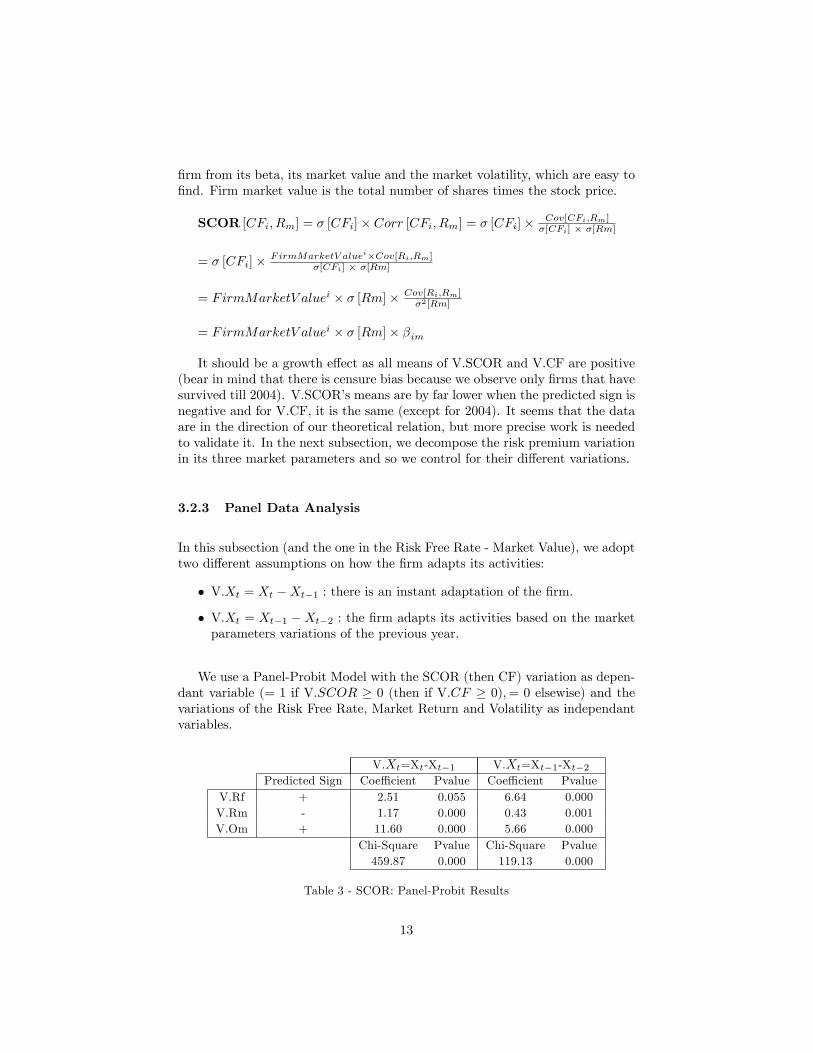
3.2.3 Panel Data Analysis

In this subsection (and the one in the Risk Free Rate - Market Value), we adopttwo di¤erent assumptions on how the �rm adapts its activities:

� V.Xt = Xt �Xt�1 : there is an instant adaptation of the �rm.

� V.Xt = Xt�1 �Xt�2 : the �rm adapts its activities based on the marketparameters variations of the previous year.

We use a Panel-Probit Model with the SCOR (then CF) variation as depen-dant variable (= 1 if V.SCOR � 0 (then if V.CF � 0);= 0 elsewise) and thevariations of the Risk Free Rate, Market Return and Volatility as independantvariables.

V.Xt=Xt-Xt�1 V.Xt=Xt�1-Xt�2Predicted Sign Coe¢ cient Pvalue Coe¢ cient Pvalue

V.Rf + 2.51 0.055 6.64 0.000V.Rm - 1.17 0.000 0.43 0.001V.Om + 11.60 0.000 5.66 0.000

Chi-Square Pvalue Chi-Square Pvalue459.87 0.000 119.13 0.000

Table 3 - SCOR: Panel-Probit Results

13


V.Rf + 18.37 0.000 10.80 0.000V.Rm - 0.32 0.005 0.85 0.000V.Om + 1.28 0.026 0.46 0.552


Table 4 - CF: Panel-Probit Results

In both cases, the sign observed for V.Rm is the opposite to the one pre-dicted. Therefore, with our results we can not conclude about the relationbetween the �rm structure and the risk premium. However, our statistics pre-sented in 3.2.2 lead us to believe that there may exist a relation and we needto adopt a more sophisticated approach for the determination of how the �rmadapts its activities. For instance, the �rm could predict the market parameterand react in function of the predicted value and the value of the previous period:V.Xt = cXt � Xt�1. The prediction would be based on the model used in theindustry, for instance a GARCH (1,1) for the prediction of the volatility.

14

3.3 Risk Free Rate - Market Value

3.3.1 Market Data

D a t e T B 1m o n th T B 3m o n th s F E D Ta r g e t R a t e V . T B 1m o n th

1 9 9 3 2 .9 4% 3 .0 5% 3 .0 0%

1 9 9 4 4 .7 4% 5 .6 4% 5 .5 0% 6 0 .8 4%

1 9 9 5 4 .5 8% 5 .0 5% 5 .5 0% -3 .2 3%

1 9 9 6 4 .8 7% 5 .1 4% 5 .2 5% 6 .3 7%

1 9 9 7 5 .1 1% 5 .3 1% 5 .5 0% 4 .8 0%

1 9 9 8 4 .3 9% 4 .4 3% 4 .7 5% -1 3 .9 8%

1 9 9 9 5 .1 0% 5 .3 3% 5 .5 0% 1 6 .1 1%

2 0 0 0 5 .7 7% 5 .8 4% 6 .5 0% 1 3 .0 7%

2 0 0 1 1 .6 4% 1 .7 1% 1 .7 5% -7 1 .6 4%

2 0 0 2 1 .1 4% 1 .1 9% 1 .2 5% -3 0 .5 6%

2 0 0 3 0 .8 3% 0 .9 3% 1 .0 0% -2 7 .2 0%

2 0 0 4 1 .9 1% 2 .2 2% 2 .2 5% 1 3 0 .7 1%

Table 5 - Risk Free Rate

1994, 2001 and 2004 are the years with the greatest variations, and 2001 isthe best year to observe the market value variation as the market volatility andreturn are not so far from being constant (see Risk Premium Table). So in 2001,we almost control for the two other parameters of the risk premium and shouldobserve only the risk free rate e¤ect on �rm market value.

3.3.2 Market Value Variation Analysis

1 9 9 4 2 0 0 1 2 0 0 4

V .M V E x p e c t e d s ig n , b e t a<1 - + -

V .M V E x p e c t e d s ig n , b e t a>1 + - +

N , b e t a<1 1 3 5 2 4 0 2 1 0

N , b e t a>1 1 7 1 2 0 4 2 5 4

N t o t a l 3 0 6 4 4 4 4 6 4

M e a n V .M V , b e t a<1 - 0 .0 0 5 5 0 .0 7 9 6 0 .1 9 4 0

M e a n V .M V , b e t a>1 0 .1 1 1 9 0 .0 1 8 0 0 .1 9 9 0

P r o p o r t io n V .M V>0 , b e t a<1 4 4 .4 4% 5 2 .0 8% 8 3 .8 1%

P ro p o r t io n V .M V>0 , b e t a>1 5 8 .4 8% 4 5 .5 9% 7 1 .2 6%

t -Te s t d i¤ e r e n c e V .M V b e t a<1 - V .M V b e t a>1 <0 >0

t -Te s t M e a n V .M V = 0 , b e t a<1 <0 >0 >0

t -Te s t M e a n V .M V = 0 , b e t a>1 >0 >0

Table 6 - Market Value Variation: Statistics Results

15

Note: MV is the Market Value, and V.MVt=MVt�MVt�1

MVt�1: For the t-Test, the validated

alternative is written (there is a blank if no conclusion could be made on the sign of the

variation with a 90% con�dence level).

For 2001, we observe the theoretical assumption: the proportion of �rmswith a positive market value variation is higher for �rms with a beta lowerthan 1. For 1994, the expectation is also correct but not for 2004 (but the riskpremium variation was high in this year). So to complete this study, we needregressions to control for the di¤erent parameters of the risk premium.15

3.3.3 Linear Regression

1994 2001 2004

Expected B sign + - +B beta 0.053 -0.050 -0.064Pvalue 0.311 0.234 0.098

R-square 0.3273 0.0645 0.1451B betasup1 0.020 -0.035 -0.037

Pvalue 0.509 0.444 0.214R-square 0.3224 0.0611 0.1407

Table 7 - Regression Analysis

Two regressions (with robust residuals) are done:

�FirmMarketV aluei = �0 +B � �i + �0 �Xi + "i

�FirmMarketV aluei = �0+B� �i+�0�Xi+�i, with �i = 1 if �i�1 and= 0 elsewise.

Xi is the vector of controling variables: dividend variation, dividend yield,cash �ows variation, book-market value ratio, long term debt-market value ratio,sales variation and total assets. B represents the regression coe¢ cient of thedummy � (B betasup1) or of � (B beta):

For 1994 and 2001 the results are coherent with the theoretical relation, butnot for 2004. Even if we control for individual characteristics, we must take intoaccount the risk premium e¤ect to indepth this study.

15Distribution estimations for the Market Value variation by the kernel-gaussian estimationmethod are set in the appendix.

16

3.3.4 Panel Data Analysis

We use a Panel-Probit Model with the Firm Market Value variation as depen-dant variable (= 1 if �MV � 0 ;= 0 elsewise) and the variations of the RiskFree Rate (with a coe¢ cient value depending on the beta value), Market Returnand Volatility as independant variables. We proceed by making two models, the�rst one with a decomposition if the beta is superior or inferior than the unity,and the second one with more gradual partitions. For the predicted signs ofthe �Rm and �Om coe¢ cients, we study the e¤ect of these market parame-ter variations on discounted CF and so the �rm value with the �gure "FirmValuation Example" in 2.1.


V.Rf beta<1 - 9.68 0.000 16.36 0.000V.Rf beta>1 + 14.90 0.000 27.93 0.000

V.Rm - 1.17 0.000 0.43 0.000V.Om + 11.60 0.034 5.66 0.000


V.Rf beta<0.5 - - 10.20 0.000 11.70 0.003V.Rf 0.5<beta<1 - 9.36 0.000 17.55 0.000V.Rf 1<beta<1.5 + 12.67 0.000 26.46 0.000V.Rf beta>1.5 + + 18.02 0.000 31.09 0.000

V.Rm - 1.73 0.000 1.22 0.000V.Om + -1.15 0.300 3.76 0.000


Table 8 - Market Value: Panel-Probit Results

Depending on the �rm�s adaptation assumption, we observe either the in-verse sign of the prediction for �Rm and �Om coe¢ cients or only for �Rmcoe¢ cient. Thus, we can not validate the implication of BBG Model on therelation between the �rm market value and the market parameters. However,given the results in 3.3.2, 3.3.3 and 3.3.4, we observe empirical evidences infavor of a relation between the risk free rate, the market value of the �rm andits beta. Firms with a higher beta seem to react more to a variation of the riskfree rate16 but we can not conclude whether there is a di¤erence on the signof the market value variation depending on the �rm�s beta. We need a more

16At �rst sight, this result seems obvious since the beta is the measure of how the �rm�sstock price reacts to variations in the market, but by de�nition beta is just correlated withthe market return, so we do not know exactly the relation with the risk free rate.

17

sophisticated model to conclude seriously; we can modify the �rm�s adaptationassumption, and take into account one with a predicted value of the marketparameters as proposed in 3.2.3.

18

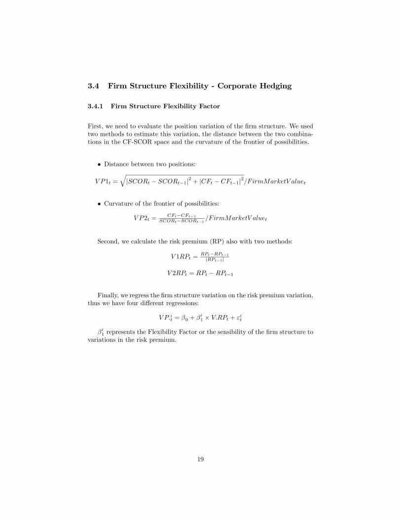
3.4 Firm Structure Flexibility - Corporate Hedging

3.4.1 Firm Structure Flexibility Factor

First, we need to evaluate the position variation of the �rm structure. We usedtwo methods to estimate this variation, the distance between the two combina-tions in the CF-SCOR space and the curvature of the frontier of possibilities.

� Distance between two positions:

V P1t =

qjSCORt � SCORt�1j2 + jCFt � CFt�1j2=F irmMarketV aluet

� Curvature of the frontier of possibilities:

V P2t =CFt�CFt�1

SCORt�SCORt�1=F irmMarketV aluet

Second, we calculate the risk premium (RP) also with two methods:

V 1RPt =RPt�RPt�1jRPt�1j

V 2RPt = RPt �RPt�1

Finally, we regress the �rm structure variation on the risk premium variation,thus we have four di¤erent regressions:

V P:it = �0 + �i1 � V:RPt + "it

�i1 represents the Flexibility Factor or the sensibility of the �rm structure tovariations in the risk premium.

19

VP1V1RP VP1V2RP VP2V1RP VP2V2RP

VP1V1RP 1.0000VP1V2RP 0.9251 1.0000VP2V1RP 0.0117 0.0083 1.0000VP2V2RP 0.0242 0.0236 0.9104 1.0000Beta 2004 -0.1427 -0.2498 0.0560 0.0517Beta 2001 -0.2892 -0.3852 0.0100 0.0140Beta 1994 -0.1347 -0.1948 0.0529 0.0771Assets 2004 0.0405 0.0594 0.0267 0.0398Assets 2001 0.0506 0.0642 0.0252 0.0370Assets 1994 0.0816 0.0894 0.0154 0.0303Mvalue 2004 0.0204 0.0603 -0.0021 0.0157Mvalue 2001 0.0150 0.0562 -0.0029 0.0116Mvalue 1994 0.0257 0.0620 -0.0002 0.0143DivYield2004 0.0056 0.0526 0.0068 0.0179BV/MV 2004 0.0079 -0.0648 0.0912 0.0400SCOR 2004 0.0040 0.0310 -0.0023 0.0162CF 2004 0.0626 0.0899 0.0067 0.0206

Table 9 - Flexibility Factor - Correlation Table

Through the study of the correlation table, we observe that VP1V2RP (i.e.�i1from the regression V P1it = �0+�

i1�V 2RPt+ "it) is the best estimator for the

�rm structure �exibility:

� Beta: there should be a negative relation between the beta of the �rmand its �exibility factor. A �rm that can change its activities easily aftera change in the market (i.e. a variation of the risk premium) should be less"risky", this is translated into a lower beta. As proposed by Stulz (2004),a �rm can become more �exible so that it has lower �xed costs in a cyclicaldownturn. It is coherent with the correlation analysis, VP1V2RP is morenegatively correlated in 2001.

� Size e¤ect: a big �rm should be more �exible as they have more projectsand so a more concave frontier of possibilities. Here it is estimated by thepositive correlation with the �rm market value and the �rm total assets(mv and assets).

� Growth opportunities: we can estimate the investment or growth opportu-nities by the ratio FirmMarketV alue

FirmBookV alue , here we observe a negative correlationwith the inverse of this ratio (BVMV2004). It is coherent with the intu-ition that a more �exible �rm should have more investment opportunities.

Therefore, we select VP1V2RP as the �exibilitor factor.

20

3.4.2 Corporate Hedging Variable

In this paper, we consider the use of derivatives as the only tool for hedging.We do not estimate "natural" hedging tools like foreign denominated debt insubstitution of currency Swap or the fact that cash out�ows and in�ows aresynchronized.To evaluate the use of derivatives, there are three instruments: a dummy

for hedging or not, the total notional value and the fair market value of deriv-atives. These informations are included in the annual report; the database wasextracted from EDGAR. The most reliable estimator is the last one as it is theactual value of the �rm position and it is not positively biased as the notionalvalue (because short and long positions have contrary �nancial e¤ects and sothe net position could be null).Therefore, our explained variable for the level of hedging is:

FRM = FairMarketV alueOfDerivativesTotalAssets

We will also study the level of hedging with the absolute value of the previousvariable.Then, we will consider the decision of hedging with a dummy (= 1 if the

�rm is hedged, = 0 elsewhere) and also if the �rm is hedged for the followingrisk: foreign exchange (currency), debt �nancing (interest rate), commodity andequity.

3.4.3 Other Explanatory Variables17

The literature gives us several determinants for the use of derivatives:

� Risk aversion of the managers (managerial shareholding [+] and manage-rial option ownership [-])

� Investment or growth opportunities (Market V alueBook V alue [+] and R&D Expenses

Total Assets[+])

� Firm size (Total Assets [+])

� Financial distress cost (Long Term DebtsMarket Value [+])

17Note that in parenthesis are variables we used to estimate determinants and in bracketsare predicted signs of the relation between determinants and the use of derivatives

21

� Dividend distributed (Dividend Yield [+])

� Firm liquidity (Quick Ratio: Current Assets - InventoriesCurrent Liabilities [-])

� Currency rate (Foreign SalesTotal Sales [+])

� Tax credits (Net Operating Loss Carry ForwardTotal Assets [+])

� Industry e¤ect (dummy industry, we will use it as a control variable andso we do not analyse the predicted relation in respect of the industry type)

3.4.4 Level of Hedging

In subsections 3.4.4, 3.4.5 and 3.4.6, we censor the �nance industry since theirquick ratio and foreign sales are calculated di¤erently. Thus, our sample forthese subsections represents 238 �rms with 190 �rms hedged. Moreover alleconometric results are presented with and without control of the industry (bi-nary variable for each type of industry).In order to study the level of hedging of the �rm, we use a Heckman selection

model. The �rst step is the decision of hedging or not, then for the ones whodecide to use derivatives, the second step is the determination of the level ofhedging (i.e. fair value of derivatives divided by total assets).

22

Not controlled by industry Controlled by industryPredictedsign Coe¢ cient Pvalue Coe¢ cient Pvalue

1) DECISIONFlexibility + 11.50 0.348 6.57 0.620Log(Assets) + 0.32 0.024 0.26 0.068

DividendYield + -0.001 0.847 -0.001 0.902MV / BV + 0.01 0.774 0.04 0.266

LT Debt / MV + 0.06 0.546 -0.01 0.803R&D / Assets + -2.25 0.480 -3.93 0.243Quick Ratio - -0.19 0.033 -0.20 0.024

FgSales / Sales + 1.72 0.001 1.69 0.004NOL / Assets + 3.42 0.209 4.01 0.176

Log (MngShare) + -0.02 0.755 -0.03 0.625Log(MngOption) - -0.15 0.066 -0.14 0.1202) LEVEL

Flexibility + -0.47 0.515 -0.19 0.784Log(Assets) + 0.001 0.809 0.004 0.460


LT Debt / MV + -0.0007 0.509 -0.0006 0.570R&D / Assets + 0.17 0.265 0.18 0.262Quick Ratio - 0.01 0.041 0.01 0.032

FgSales / Sales + -0.006 0.864 0.002 0.927NOL / Assets + -0.09 0.222 -0.07 0.261

Log (MngShare) + -0.004 0.217 -0.004 0.187Log(MngOption) - 0.001 0.741 0.0006 0.850


Table 10 - Heckman Selection Model - Two Step Estimates

Analysis of the decision of hedging or not will be done in next subsection.Here for the level of hedging we only observe the Quick Ratio as signi�cantvariable at a 3% level.

Finally we use a Tobit Model to analyse the absolute value of the level ofhedging as there is a boundary constraint at 0.

23

Not controlled by industry Controlled by industryPredictedsign Coe¢ cient Pvalue Coe¢ cient Pvalue

Flexibility + 0.11 0.852 0.06 0.911Log(Assets) + 0.01 0.028 0.01 0.054


LT Debt / MV + 0.0006 0.536 -0.0006 0.552R&D / Assets + 0.10 0.446 0.11 0.426Quick Ratio - 0.001 0.700 0.001 0.691

FgSales / Sales + 0.04 0.040 0.03 0.108NOL / Assets + -0.06 0.376 -0.06 0.382

Log (MngStock) + -0.004 0.112 -0.005 0.100Log(MngOption) - -0.002 0.447 -0.001 0.678

Pseudo R-square Pseudo R-square-0.0365 -0.0520

Table 11 - Tobit Estimates

There is only the size e¤ect signi�cant at 5%. Therefore, through these twomodels, we do not have conclusive remarks and we will focus on the decision ofhedging in the following subsections.

3.4.5 Decision of Hedging by type of risk

To analyse the decision of hedging (in general or by type of risk) we use a Probitmodel (i.e. = 1 if the �rme is hedged, = 0 elsewise).

24

Not Controlled by Industry Controlled by IndustryPredictedsign Coe¢ cient Pvalue Coe¢ cient Pvalue



LT Debt / MV + 0.0675131 0.524 -0.0171553 0.607R&D / Assets + -2.25837 0.489 -3.930239 0.246Quick Ratio - -0.1919256 0.026 -0.2073532 0.019FgSales/Sales + 1.721713 0.000 1.695177 0.001NOL / Assets + 3.428797 0.091 4.012649 0.074

Log (MngShare) + -0.0215893 0.727 -0.0391059 0.586Log (MngOption) - -0.155596 0.039 -0.147289 0.078

Pseudo R-square Pseudo R-square0.1864 0.2432

Table 12 - Hedging - Probit Estimates

We found six signi�cant coe¢ cients at a 10% level and coherent with theirpredicted sign. These determinants have already been empirically validated, sothis is an indication that our database respects results from the literature.Now, we will decompose the decision of hedging for four di¤erent risks. In

this way, �rms could use derivatives for foreign exchange risk (currency risk),debt �nancing risk (interest rate risk), commodity risk and equity risk (stockprice of their investments).



DividendYield + 0.0120924 0.143 0.0108115 0.223MV / BV + -0.002438 0.204 -0.0031078 0.092

LT Debt / MV + 0.0088812 0.597 0.0102492 0.515R&D / Assets + 1.8561214 0.585 -0.2841436 0.935Quick Ratio - -0.25965 0.008 -0.2523647 0.009


Log (MngShare) + 0.0352815 0.552 0.0514244 0.422Log (MngOption) - 0.0004915 0.994 -0.0024615 0.973


Table 13 - Foreign Exchange Risk - Probit Estimates

25

As expected, the foreign exposition (Foreign Sales / Sales) is the most sig-ni�cant coe¢ cient for the decision of currency hedging.


Flexibility + -4.155881 0.705 -7.975913 0.464Log(Assets) + 0.4263028 0.001 0.3745493 0.003

DividendYield + 0.0105719 0.191 0.0132397 0.148MV / BV + 0.0036536 0.838 0.010641 0.588

LT Debt / MV + 0.026474 0.623 0.0158687 0.655R&D / Assets + -10.04877 0.002 -10.12231 0.002Quick Ratio - -0.1379954 0.157 -0.156353 0.125


Log (MngShare) + 0.0037981 0.951 -0.0084541 0.905Log (MngOption) - -0.1178394 0.085 -0.104035 0.148


Table 14 - Debt Financing Risk - Probit Estimates

We notice two unexpected results here: �rst, the R&D coe¢ cient is the mostsigni�cant but not with the expected sign, and second the leverage coe¢ cientis not signi�cant for the decision of interest rate hedging.




LT Debt /MV + -0.0181029 0.375 -0.0281866 0.222R&D / Assets + -16.97719 0.001 -13.49775 0.003Quick Ratio - -0.0594772 0.644 -0.102821 0.463

FgSales / Sales + 0.2903347 0.529 0.1185039 0.817NOL / Assets + 0.002941 0.999 -0.0667766 0.964



Table 15 - Commodity Risk - Probit Estimates

26

Finally, for commodity risk, we observe the �exibility factor signi�cant at a2% level with the predicted sign. We also notice that the sign of the dividendyield coe¢ cient is negative and signi�cant. The theory behind the predictionof a positive sign is based on a lack of liquidity after a dividend payout, andtherefore an incentive to hedge due to �nancial distress cost. But we alreadyestimate the liquidity e¤ect with the Quick Ratio, thus the dividend yield couldbe perceived as an estimator of growth opportunities18 . The ratio Market Value/ Book Value is an estimator of growth opportunities established by �nancialmarkets but the dividend yield is an internal signal made by the �rm. So, thedividend yield has a dual e¤ect on the corporate hedging decision, and thisnegative sign has a �nancial analysis explanation.



DividendYield + -0.0018588 0.673 -0.0095536 0.107MV / BV + -0.0058059 0.788 -0.0011117 0.968

LT Debt / MV + -0.0059715 0.864 -0.0131152 0.725R&D / Assets + 6.376253 0.037 4.967401 0.123Quick Ratio - 0.1109778 0.197 0.0713692 0.425

FgSales / Sales + -0.3156646 0.564 -0.3033991 0.640NOL / Assets + 2.322472 0.167 2.233997 0.194

Log (MngShare) + 0.0106017 0.904 0.0661194 0.515Log (MngOption) - 0.0077272 0.940 -0.0332903 0.748


Table 16 - Equity Risk - Probit Estimates

The �exibility factor is signi�cant at a 6% level and we observed also asize e¤ect. The equity risk represents the �rm�s investment and mostly thesubsidiaries traded on �nancial markets.

Through these tables, we observed empirical evidences of the signi�cantdeterminants variations in accordance with the sort of risk. Therefore, even ifwe control for the type of industry, each kind of risk has speci�c determinants.The decomposition of the type of risk hedged (instead of just considering if the�rm is hedged or not) could lead �nancial analysts to a better evaluation of the�rm management and of �nancial risk management motivations.

18See Gaver & Gaver (1993), and Smith & Watts (1992).

27

3.4.6 Number of risks hedged

In connection with the type of risk decomposition considered previously, westudy now the number of risks hedged by the �rm. First, we consider all thefour risks presented before: �nancing, currency, commodity and equity risk.Firms could hedge between 0 and 4 sorts of risk; therefore, we use an OrderedProbit Model to estimate the number of risks hedged as it is a ranked discretedependant variable.




LT Debt / MV + 0.0005298 0.958 0.0012068 0.904R&D / Assets + -3.659068 0.079 -3.693538 0.101Quick Ratio - -0.1307459 0.079 -0.1648271 0.032




Table 17 - Every Risk - Ordered Probit Estimates

We recognize three signi�cant factors frequently validated in the empiricalliterature: size, liquidity and foreign exposure.

Second, we analyse the number of operational risks hedged. Since opera-tional risk is related to operations and not �nancing, we consider only currency,commodity and equity risk. Here, �rms could hedge between 0 and 3 sortsof risk, so we also use an Ordered Probit Model to estimate the number ofoperational risks hedged.

28



DividendYield + -0.0023691 0.403 -0.0053856 0.021MV / BV + -0.0012558 0.289 -0.0016622 0.150

LT Debt / MV + -0.0050441 0.584 -0.0044866 0.625R&D / Assets + -0.4415766 0.837 -0.6505316 0.781Quick Ratio - -0.096191 0.180 -0.1296876 0.076




Table 18 - Operational Risk - Ordered Probit Estimates

For operationnal risk, at a 5% level we have size, dividend yield (with anegative relation as explained in 3.4.5), liquidity, foreign exposure and �nally�exibility as signi�cant factors. This result is intuitive since �exiblity is morerelated to �rm activities (i.e. foreign exchange, commodity and equity risk) andnot to �nancing decision (i.e. debt �nancing risk).

3.4.7 Industry Analysis

We have used a market value weight for each industry (i.e. FirmMarketV alue =IndustryMarketV alue ), in order to calculate the mean of the variables below.Then we have ranked these industries by the Flexibility Factor (the most �exibleindustry is at the top). Note that the non-classi�ed industry is composed byonly two �rms: GE and Textron.

29

In d u s t r y F le x ib i l i ty # R is k # O p . R is k H e d g in g F X D eb t C om m E q u i ty F V /A s s e t s A b s F V /A s s e t s

U t i l i ty - 0 .0 0 2 3 2 .1 1 1 1 .2 0 6 1 0 .4 3 3 0 .9 0 6 0 .7 5 5 0 .0 1 8 0 .0 0 2 4 3 0 .0 0 7 1 4

Fo o d -0 .0 0 3 2 2 .6 2 2 1 .7 5 8 1 0 .9 8 2 0 .8 6 4 0 .5 3 0 0 .2 4 6 0 .0 1 1 3 7 0 .0 1 3 7 9

N o n -C la s s i�e d - 0 .0 0 3 5 3 2 1 1 1 0 1 0 .0 0 3 4 9 0 .0 0 3 4 9

M in in g - 0 .0 0 3 9 2 .0 4 3 1 .2 0 8 0 .9 3 7 0 .6 5 6 0 .8 3 5 0 .5 5 2 0 - 0 .0 0 5 6 4 0 .0 0 8 9 6

F in a n c ia l - 0 .0 0 4 2 2 .0 6 7 5 1 .1 3 0 3 1 0 .9 3 7 1 8 0 .5 1 5 0 .9 3 7 2 0 .2 1 2 2 3 0 .4 0 2 9 0 .0 0 7 9 9 0 .0 0 8 9 7 0 6

S e r v i c e - 0 .0 0 4 4 2 .4 6 2 1 .6 7 3 0 .9 1 2 0 .8 8 2 0 .7 8 9 0 .0 1 3 0 .7 7 7 - 0 .0 0 1 7 8 0 .0 0 5 6 7

R e t a i l - 0 .0 0 4 9 1 .2 9 3 0 .6 1 9 0 .7 1 3 0 .5 2 2 0 .6 7 4 0 .0 5 9 0 .0 3 9 0 .0 0 0 5 2 0 .0 0 1 8 1

W h o le s a l e - 0 .0 0 5 3 1 .0 3 0 0 .1 6 3 0 .8 6 7 0 0 .8 6 7 0 .1 6 3 0 - 0 .0 0 0 1 2 0 .0 0 0 6 2

M a nu fa c t u r in g - 0 .0 0 5 4 1 .6 0 8 6 1 .0 2 8 2 6 0 .8 3 3 2 6 0 .7 9 2 0 .5 8 0 3 0 .1 0 8 6 3 0 .1 2 7 5 0 .0 2 5 2 9 2 0 .0 2 7 2 9 9 9

C om m u n ic a t io n - 0 .0 0 6 7 1 .5 2 1 0 .5 2 1 1 0 .5 2 1 1 0 0 0 .0 0 1 4 2 0 .0 0 1 7 1

Tra n s p o r t a t io n - 0 .0 0 9 2 1 .8 2 4 0 .8 2 4 1 0 .4 6 4 1 0 .3 6 0 0 0 .0 1 0 8 7 0 .0 1 0 8 7

C o n s t r u c t io n - 0 .0 1 0 1 1 0 .4 0 1 1 0 .4 0 1 0 .5 9 9 0 0 0 .0 0 0 8 9 0 .0 0 1 5 1

Table 19 - Industry Estimates

We observe a clear dichotomy for the number of risks (total and operationnal)hedged. The six most �exible industries are the ones which have more typesof risk hedged. This analysis by type of industry supports the fact that more�exible �rms as we have calculated (i.e. �rm structure sensibility to variationsof the risk premium) hedge a higher number of risks.

30

4 Conclusion

In this paper, we have empirically examined three theoretical propositions basedon the BBG Model, namely: project portfolio management linked to variationsof the risk premium, stock price variation explained by the risk free rate de-pending on �rm beta, and �rm �exibility as a new determinant of corporatehedging decision.Concerning the link between the choice of projects and the risk premium, we

found no empirical evidence that could validate it, but as exposed in 3.2.2, basicstatistics deliver some hope for the existence of a relation. Further research isneeded, and one of the possible extensions could consist of the estimation of the�rm adaptation mechanism by predicted value of market parameters.The same conclusion applies for the second theoretical proposition, if we

consider every market parameter of the risk premium. However, our empiricalresults show a relation between �rm value, its beta and the risk free rate. Itseems that �rms with higher beta have their stock price more sensible to riskfree rate variations.We have constructed an estimator for �rm �exibility (i.e. �rm structure

sensibility to variations of the risk premium), and found evidence for the ex-planation of the number of operational risks hedged by the Flexibility Factor.Through an industry analysis, we reinforce our prediction : industries more�exible hedge a higher number of risks.We have also detected that the dividend yield could be an estimator of

growth opportunities in a �nancial risk management framework. Finally, thisstudy leads us to state that each kind of risk has speci�c determinants.

31

References1. Allayannis, G. and J.P. Weston (2001), �The Use of Foreign CurrencyDerivatives and Firm Market Value,�Review of Financial Studies 14: 243-276

2. Barclay, M. and C.W. Smith, Jr. (1995), �The Maturity Structure ofCorporate Debt,�Journal of Finance 50: 609-631

3. Bessembinder, H. (1991), �Forward Contracts and Firm Value: InvestmentIncentive and Contracting E¤ects,�Journal of Financial and QuantitativeAnalysis 26: 519-532

4. Berkman, H. and M.E. Bradbury (1996), �Empirical Evidence on the Cor-porate Use of Derivatives,�Financial Management 25: 5-13

5. Bodnar, G.M., G.S. Hayt and R.C. Marston (1998), �Wharton 1998 Sur-vey of Risk Management by US Non-Financial Firms,� Financial Man-agement 27: 70-91

6. Boyer, M., M. M. Boyer and R. Garcia (2005), �The Value of Real andFinancial Risk Management,�Working Paper, CIRANO

7. Clark, E. and A. Judge (2005), �Motives for Corporate Hedging: EvidenceFrom the UK,�Research in Financial Economics 1: 57-58

8. DeMarzo,P. and D.Du¢ e (1993), �Corporate Incentives for Hedging andHedge Accounting,�Journal of Applied Corporate Finance 6: 4-15

9. Dionne, G. and M. Garand (2003), �Risk Management Determinants Af-fecting Firms�Values in the Gold Mining Industry,�Economics Letters 79:43

10. Dolde, W. (1995), �Hedging, Leverage, and Primitive Risk,�The Journalof Financial Engineering 4: 187-216

11. Foo, M. and W.W. Yu (2005), �The Determinants of the Corporate Hedg-ing Decision: An Empirical Analysis,�Working Paper, Athabasca Univer-sity and Hong Kong Polytechnic University

12. Fok, R.C.W., C. Carroll and M.C. Chiou (1997), �Determinants of Cor-porate Hedging and Derivatives: A Revisit,� Journal of Economics andBusiness 49: 569-585

13. Francis, J. and J. Stephan (1993), �Characteristics of Hedging Firms: AnEmpirical Investigation,� in: R.J. Schwartz and C.W. Smith Jr., eds.Advanced Strategies in Financial Risk Management, (New York Instituteof Finance), 615-635

32

14. Froot, K.A., D.S. Scharfstein and J.C. Stein (1993), �Risk Management:Coordinating Corporate Investment and Financing Policies,� Journal ofFinance 48: 1629-1658

15. Gaver, J.J. and K.M. Gaver (1993), �Additional Evidence on the Associ-ation between the Investment Opportunity Set and Corporate Financing,Dividend and Compensation Policies,� Journal of Accounting and Eco-nomics 16: 125-160

16. Gay, G.D. and J. Nam (1998), �The Underinvestment Problem and Cor-porate Derivatives Use,�Financial Management 27: 53-69

17. Géczy, C., B.A. Minton and C. Schrand (1997),�Why Firms Use CurrencyDerivatives,�Journal of Finance 52: 1323-1354

18. Graham, J.R. and C.W. Smith (1999), �Tax Incentives to Hedge,�Journalof Finance 54: 2241-2261

19. Graham, J.R. and D.A. Rogers (2002), �Do Firms Hedge in Response toTax Incentives?,�Journal of Finance 57: 815-839

20. Haushalter, G.D. (2000),�Financing Policy, Basis Risk, and CorporateHedging: Evidence from Oil and Gas Producers,�Journal of Finance 55:107-152

21. Howton, S.D. and S.B. Perfect (1998), �Currency and Interest-Rate Deriv-atives Use in U.S. Firms,�Financial Management 27: 111-121

22. Leland, H. (1998), �Agency Costs, Risk Management, and Capital Struc-ture,�Journal of Finance 53: 1213-1243

23. Mayers, D. and C.W. Smith (1987), �Corporate Insurance and the Under-Investment Problem,�Journal of Risk and Insurance 54: 45-54

24. Mello, A.S., J.E. Parsons and A.J. Triantis (1995), �An Integrated Modelof Multinational Flexibility and Financial Hedging,�Journal of Interna-tional Economics 39: 27-51

25. Mian, S.L. (1996), �Evidence on Corporate Hedging Policy,� Journal ofFinancial and Quantitative Analysis 31: 419-439

26. Modigliani, F. and M.H. Miller (1958), �The cost of capital, corporation�nance, and the theory of investments,�American Economic Review 48:261-297

27. Myers, S.C. (1977), �Determinants of Corporate Borrowing,� Journal ofFinancial Economics 5: 147-175

28. Nance, D.R., C.W. Smith and C.W. Smithson (1993), �On the Determi-nants of Corporate Hedging,�Journal of Finance 48: 267-284

33

29. Smith, C.W. (1995), �Corporate Risk Management: Theory and Prac-tice,�Journal of Derivatives 2: 21-30

30. Smith, C.W. and R. Stulz (1985), �The Determinants of Firms�HedgingPolicies,�Journal of Financial and Quantitative Analysis 20: 391-405

31. Smith, C.W., Jr. and R.L. Watts (1992), �The Investment Opportu-nity Set and Corporate Financing, Dividend, and Compensation Policies,�Journal of Financial Economics 32: 263-292

32. Stulz, R. (1984), �Optimal Hedging Policies,� Journal of Financial andQuantitative Analysis 19: 127-139

33. Stulz, R. (1996), �Rethinking Risk Management,�Journal of Applied Cor-porate Finance 9 :8-24

34. Stulz, R.M. (2004), �Risk Management and Derivatives,�Thomson South-Western Publishers

35. Tufano, P. (1996), �Who Manages Risk? An Empirical Examination ofRisk Management Practices in the Gold Mining Industry,� Journal ofFinance 51: 1097-1137

36. Viswanathan, G. (1998), �Who Uses Interest Rate Swaps? A Cross Sec-tional Analysis,�Journal of Accounting, Auditing and Finance: 173-200

37. Warner, J.B. (1977), �Bankruptcy Costs: Some Evidence,� Journal ofFinance 32: 337-347

38. Wysocki, P (1995), �Determinants of Foreign Exchange Derivatives Use byU.S. Corporations: An Empirical Investigation,�Working Paper, SimonSchool of Business, University of Rochester

39. Wysocki, P (1996), �Managerial Motives and Corporate Use of Deriva-tives: Some Evidence,�Working Paper, Simon School of Business, Uni-versity of Rochester

34

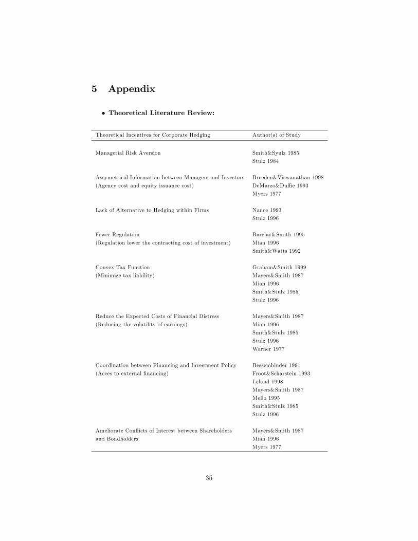
5 Appendix

� Theoretical Literature Review:

Theoretical Incentives for Corporate Hedging Author(s) of Study

Managerial Risk Aversion Smith&Syulz 1985

Stulz 1984

Assymetrical Information between Managers and Investors Breeden&Viswanathan 1998

(Agency cost and equity issuance cost) DeMarzo&Du¢ e 1993

Myers 1977

Lack of Alternative to Hedging within Firms Nance 1993

Stulz 1996

Fewer Regulation Barclay&Smith 1995

(Regulation lower the contracting cost of investment) Mian 1996

Smith&Watts 1992

Convex Tax Function Graham&Smith 1999

(Minimize tax liability) Mayers&Smith 1987

Mian 1996

Smith&Stulz 1985

Stulz 1996

Reduce the Expected Costs of Financial Distress Mayers&Smith 1987

(Reducing the volatility of earnings) Mian 1996

Smith&Stulz 1985

Stulz 1996

Warner 1977

Coordination between Financing and Investment Policy Bessembinder 1991

(Acces to external �nancing) Froot&Scharstein 1993

Leland 1998

Mayers&Smith 1987

Mello 1995

Smith&Stulz 1985

Stulz 1996

Ameliorate Con�icts of Interest between Shareholders Mayers&Smith 1987

and Bondholders Mian 1996

Myers 1977

35

� Empirical Literature Review - Hedging Level - First Part:

Variables Employed Hyp Results Author(s) of Study

LT Debt / MarketValue + Yes Dionne&Garand 2003, Gay&Nam 1998, Graham&Rogers 2000

Haushalter 2000(oil), Howton&Perfect 1998, Tufano 1996(gold)

No Allayanis 2001, Howton&Perfect 1998

Interest Cover - Yes

No Gay&Nam 1998, Howton&Perfect 1998

Credit Rating - Yes Haushalter 2000 (oil)

No Graham&Rogers 2000

Return on Assets Yes Graham&Rogers 2000 (weak)

No Allayanis 2001

R&D + Yes Allayanis 2001, Gay&Nam 1998, Graham&Rogers 2000

Howton&Perfect 1998

No

MarketValue/BookValue + Yes Gay&Nam 1998

No Allayanis 2001, Graham&Rogers 2000

DivYield (1) or Payout (2) + Yes Berkman&Bradbury 1996 (NZ) (2), Dionne&Garand 2003 (1)

No Allayanis 2001 (dummy), Graham&Rogers 2000 (1)

Haushalter 2000 (oil) (2)

Capital Expenditure + Yes Haushalter 2000 (oil, weak)

No Graham&Rogers 2000, Tufano 1996 (gold)

Price Earnings Ratio + Yes Gay&Nam 1998

No Berkman&Bradbury 1996 (NZ)

36

� Empirical Literature Review - Hedging Level - Second Part:


Cash Flows - Yes Howton&Perfect 1998

No

Managerial Share + Yes Graham&Rogers 2000, Tufano 1996 (gold)

No Berkman&Bradbury 1996 (NZ), Gay&Nam 1998, Haushalter 2000 (oil)

Managerial Option - Yes Haushalter 2000 (yes&no) (oil), Tufano 1996 (gold)

No Gay&Nam 1998, Graham&Rogers 2000

Convertible Debt +/- Yes

No Berkman&Bradbury 1996 (NZ), Gay&Nam 1998, Howton&Perfect 1998

Preference Capital +/- Yes

No Berkman&Bradbury 1996 (NZ), Gay&Nam 1998, Howton&Perfect 1998

Liquidity - Yes Howton&Perfect 1998, Tufano 1996 (oil)

No Allayanis 2001, Berkman&Bradbury 1996 (NZ), Haushalter 2000 (oil)

Diversi�cation - Yes

No Haushalter 2000 (oil), Tufano 1997 (gold)

Size + Yes Allayanis 2001, Berkman&Bradbury 1996 (NZ), Dionne&Garand 2003

Graham&Rogers 2000, Haushalter 2000 (oil)

No Gay&Nam 1998, Tufano 1996 (gold)

NOL carryforward + Yes Berkman&Bradbury 1996 (NZ), Dionne&Garand 2003

No Allayanis 2001, Gay&Nam 1998, Howton&Perfect 1998, Tufano 1996(gold)

Foreign Sales + Yes Allayanis 2001, Graham&Rogers 2000 (weak)

No

37

� Empirical Literature Review - Hedging Decision - First Part:


LT Debt / MarketValue + Yes Clark&Judge 2005 (UK), Dolde 1995, Foo&Yu 2005

No Allayanis 2001, Fok&Caroll 1997, Francis&Stephan 1993

Géczy&Minton 1997, Nance&Smith 1993, Wysocki 1996

Interest Cover - Yes Fok&Caroll 1997

No Francis&Stephan 1993, Nance&Smith 1993, Wisocki 1996

Credit Rating - Yes Clark&Judge 2005 (UK), Foo&Yu 2005

No Géczy&Minton 1997

R&D + Yes Allayanis 2001, Dolde 1995, Fok&Caroll 1997, Foo&Yu 2005

Géczy&Minton 1997, Nance&Smith 1993 (weak)

No Clark&Judge 2005 (UK)

MarketValue/BookValue + Yes Nance&Smith 1993, Wysocki 1996

No Allayanis 2001, Clark&Judge 2005 (UK), Fok&Caroll 1997

Géczy&Minton 1997, Mian 1996

DivYield(1) or Payout(2) + Yes Foo&Yu 2005 (1), Nance&Smith 1993 (2)

No Allayanis 2001(dummy), Fok&Caroll 1997(1), Wysocki 1996(1)

Managerial Share + Yes Wysocki 1996

No Fok&Caroll 1997, Géczy&Minton 1997

Managerial Option - Yes Foo&Yu 2005, Wysocki 1996

No Géczy&Minton 1997

38

� Empirical Literature Review - Hedging Decision - Second Part:


Convertible Debt +/- Yes Fok&Caroll 1997 (weak)

No Nance&Smith 1993, Wysocki 1996

Preference Capital +/- Yes

No Fok&Caroll 1997, Nance&Smith 1993, Wysocki 1996

Quick Ratio - Yes Clark&Judge 2005 (UK), Fok&Caroll 1997(weak), Foo&Yu 2005

Géczy&Minton 1997

No Allayanis 2001, Nance&Smith 1993

Diversi�cation - Yes

No Fok&Caroll 1997

Size + Yes Allayanis 2001, Fok&Caroll 1997, Foo&Yu 2005, Géczy&Minton 1997

Mian 1996, Nance&Smith 1993, Wysocki 1996

No

Total Sales + Yes Fok&Caroll 1997, Francis&Stephan 1993

No Dolde 1995

NOL carryforward + Yes Clark&Judge 2005 (UK), Foo&Yu 2005

No Allayanis 2001, Dolde 1995, Fok&Caroll 1997, Géczy&Minton 1997

Mian 1996, Nance&Smith 1993, Wysocki 1996

Foreign Sales + Yes Clark&Judge 2005 (UK), Wysocki 1996

No

39

� Distribution estimations for CF and SCOR variations by thekernel-gaussian estimation method:

1 0 . 5 0 0 . 5 1 1 . 5 2 2 . 50

0 . 5

1

1 . 5

2

2 . 5

M a r k e t V a l u e V a r i a t i o n

De

ns

ity

M a r k e t V a l u e V a r i a t i o n D i s t r i b u t i o n B e t a < 1 ( r e d l i n e ) a n d B e t a > 1 ( b l a c k l i n e ) 1 9 9 4

2 1 0 1 2 3 40

0 . 2

0 . 4

0 . 6

0 . 8

1

1 . 2

1 . 4

1 . 6

1 . 8

M a rk e t V a lu e V a r ia t io n

De

ns

ity

M a rk e t V a lu e V a r ia t io n D is t r ib u t i o n B e t a < 1 ( r e d l in e ) a n d B e t a > 1 ( b la c k l i n e ) 2 0 0 1

1 0 .5 0 0 . 5 1 1 .5 2 2 .50

0 . 5

1

1 . 5

2

2 . 5

M a rk e t V a lu e V a ri a t io n

De

ns

ity

M a rk e t V a lu e V a r ia t io n D is t rib u t io n B e t a < 1 (re d li n e ) a n d B e t a > 1 (b la c k l in e ) 2 0 0 4

40

2 1 0 1 2 3 4 50

0.2

0.4

0.6

0.8

1

1.2

1.4

Market Value Variation

Den

sity

Market Value Variation Distribution Beta < 1(red line) and Beta > 1(black line) 2001 Nasdaq

1.5 1 0.5 0 0.5 1 1.5 2 2.50

0.2

0.4

0.6

0.8

1

1.2

1.4

1.6

1.8

2

Market Value Variation

Dens

ity

Market Value Variation Distribution Beta < 1(red line) and Beta > 1(black line) 2001 NYSE

41

2 0 2 4 6 8 10 12

0.1

0.2

0.3

0.4

0.5

0.6

0.7

0.8

SCOR Value Variation

Den

sity

SCOR Value Variation Distribution 1994(red line), 1995(black line) and 1996(blue line)

0.5 0 0.5 1 1.50

0.5

1

1.5

2

CF Value Variation

Den

sity

CF Value Variation Distribution 1994(red line), 1995(black line) and 1996(blue line)

42

2 0 2 4 6 80

0.1

0.2

0.3

0.4

0.5

0.6

0.7

0.8

SCOR Value Variation

Dens

ity

SCOR Value Variation Distribution 2000(red line), 2001(black line),2002(blue line) and 2003(green line)

1.5 1 0.5 0 0.5 1 1.50

0.5

1

1.5

2

2.5

CF Value Variation

Den

sity

CF Value Variation Distribution 2000(red line), 2001(black line),2002(blue line) and 2003(green line)

43

� Correlation Table of the variables used in 3.4:

F le x L g (A s s ) D iv Y i M V /B V LT D /M V R & D Q u ick Fo r e ig n S N O L L g (M g S t k )

F le x ib i l i ty 1 .0 0

L o g (A s s e t s ) 0 .1 2 1 .0 0

D iv id e n d Y ie ld 0 .0 6 0 .5 5 1 .0 0

M Va lu e / B Va lu e 0 .0 3 - 0 .1 1 - 0 .0 1 1 .0 0

LT D eb t /M Va lu e 0 .0 1 - 0 .0 2 - 0 .0 1 0 .8 3 1 .0 0

R & D /A s s e t s - 0 .1 6 - 0 .2 1 0 .0 3 - 0 .0 5 - 0 .0 9 1 .0 0

Q u ick R a t io - 0 .1 9 - 0 .2 6 - 0 .0 4 - 0 .0 3 - 0 .0 7 0 .4 6 1 .0 0

Fo r e ig n S a le s / S a le s - 0 .0 7 0 .0 1 0 .0 7 - 0 .0 6 0 .0 0 0 .4 4 0 .2 7 1 .0 0

N O L /A s s e t s - 0 .0 1 - 0 .1 6 - 0 .0 7 - 0 .0 2 - 0 .0 2 0 .2 5 - 0 .0 2 0 .2 3 1 .0 0

L o g (M a n a g e r ia l S t o ck ) - 0 .0 3 0 .2 3 0 .1 5 0 .0 1 - 0 .0 8 - 0 .0 2 0 .0 4 - 0 .0 2 - 0 .1 2 1 .0 0

L o g (M a n a g e r ia l O p t io n ) 0 .0 0 0 .0 5 - 0 .0 1 0 .0 3 - 0 .0 3 0 .0 6 0 .1 6 0 .0 6 - 0 .0 7 0 .2 0

44

4 Juillet 2006 Financial Risk Management, Firm Structure ...

Documents

Transcript of 4 Juillet 2006 Financial Risk Management, Firm Structure ...