Classification of LIDAR Sensor Contaminations with DeepNeural Networks

Jyothish K. JamesUniversity of KaiserslauternKaiserslautern, Germanyjyothish@rhrk.uni-kl.de

Georg PuhlfürstValeo Schalter und Sensoren GmbH

Kronach, Germanygeorg.puhlfuerst@valeo.com

Vladislav GolyanikDFKI

Kaiserslautern, Germanyvladislav.golyanik@dfki.de

Didier StrickerDFKI

Kaiserslautern, Germanydidier.stricker@dfki.de

ABSTRACTLight detecting and ranging (LIDAR) sensors are extensively stud-ied in autonomous driving research. Monitoring the performanceof LIDAR sensors has become significantly important to ensuretheir reliability and hence guarantee the safety of the vehicle. Un-derestimation of sensor performance can give away reliable objectdata, overestimation may result in safety issues. Besides light andweather conditions, the performance is strongly affected by con-taminations on the sensor front plate. In this paper, we focus onclassifying different types of contaminations using a deep learn-ing approach. We train a deep neural network (DNN) following amulti-view concept. For the generation of training and test data,experiments have been conducted, in which the front plate of aLIDAR sensor has been contaminated artificially with various sub-stances. The recorded data is transformed to contain the essentialinformation in a compact format. The results are compared to clas-sical machine learning techniques to demonstrates the potential ofDNN approaches for the problem under consideration.

KEYWORDSLIDAR, Deep-learning, Multi-view, Transfer learning, Scan, Scan-points.

ACM Reference Format:Jyothish K. James, Georg Puhlfürst, Vladislav Golyanik, and Didier Stricker.2018. Classification of LIDAR Sensor Contaminations with Deep NeuralNetworks. In Proceedings of ACM Computer Science in Cars Symposium(MUNICH’18). ACM, New York, NY, USA, 8 pages. https://doi.org/10.475/123_4

1 INTRODUCTIONLight detecting and ranging (LIDAR) sensors [17] have becomean important aspect for the autonomous driving industry. Thesecomponents are used to detect lanes, cars, pedestrians and otherobjects [2, 11]. While a high performance of the corresponding

Permission to make digital or hard copies of part or all of this work for personal orclassroom use is granted without fee provided that copies are not made or distributedfor profit or commercial advantage and that copies bear this notice and the full citationon the first page. Copyrights for third-party components of this work must be honored.For all other uses, contact the owner/author(s).MUNICH’18, September 2018, Munich, Germany© 2016 Copyright held by the owner/author(s).ACM ISBN 123-4567-24-567/08/06.https://doi.org/10.475/123_4

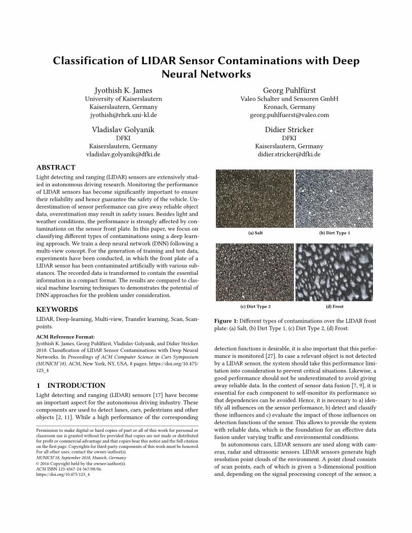
(a) Salt (b) Dirt Type 1

(c) Dirt Type 2 (d) Frost

Figure 1: Different types of contaminations over the LIDAR frontplate: (a) Salt, (b) Dirt Type 1, (c) Dirt Type 2, (d) Frost.

detection functions is desirable, it is also important that this perfor-mance is monitored [27]. In case a relevant object is not detectedby a LIDAR sensor, the system should take this performance limi-tation into consideration to prevent critical situations. Likewise, agood performance should not be underestimated to avoid givingaway reliable data. In the context of sensor data fusion [7, 9], it isessential for each component to self-monitor its performance sothat dependencies can be avoided. Hence, it is necessary to a) iden-tify all influences on the sensor performance, b) detect and classifythose influences and c) evaluate the impact of those influences ondetection functions of the sensor. This allows to provide the systemwith reliable data, which is the foundation for an effective datafusion under varying traffic and environmental conditions.

In autonomous cars, LIDAR sensors are used along with cam-eras, radar and ultrasonic sensors. LIDAR sensors generate highresolution point clouds of the environment. A point cloud consistsof scan points, each of which is given a 3-dimensional positionand, depending on the signal processing concept of the sensor, a

MUNICH’18, September 2018, Munich, Germany Jyothish K. James et al.

quantity representing the intensity of the corresponding signal.The main advantages of LIDAR sensors are high range and angu-lar resolutions in combination with large detection distances. Thedisadvantage of LIDAR sensors are the sensitivity to light, weatherand sensor front conditions.

Contaminations or damages on the sensor front reduce theamount of transmitted light both in the sender and the receiverpath. This is caused by scattering and absorption of the laser light.The point cloud is affected by this in various ways [21] a) The an-gular and range accuracy is decreased, b) the intensity of signals isreduced, which can lead up to c) missing scan points at certain dis-tances and d) increased intensity and amount of near field signals.Those effects depend on the particular contamination or damagescenario, of which there are various combinations of types1 (e.g. salt,dust, insects, snow, ice, scratches and stone chippings, few of whichare shown in Figure 1) and distribution (e.g. full or partial blockageswith different thicknesses of the blocking material). Hence, for theevaluation of the impact on the point cloud, not only the detectionof sensor front influences, but also the classification is relevant. Italso plays a significant role in improving the efficiency of heatingand cleaning procedures. Contamination like dirt or salt need tobe removed through cleaning procedures, snow or ice can only beremoved through heating, while damages can not be removed atall.

In section 2, related works are discussed in the context of LIDARperformance as well as multi-modal fusion. Section 3 focusses onthe experiments performed to record and generate the dataset,by applying different contaminations on the LIDAR sensor frontplate. Furthermore, in this sections we propose a novel solution forclassifying the contamination types with a deep neural network.The approach uses a multi-view deep neural network (LIDAR-Net),which fuses the front and the top view of the LIDAR sensors. Insection 4, we evaluate the proposed approach and demonstratethat our results outperform those of classical algorithms. In ourconclusion in section 5, we bring up possible aspects of futureworks.

2 RELATEDWORKIn this section we review the algorithms and related works andposition the proposed multi-view deep neural network among them.

2.1 Performance of laser scannersThe related work [21] tries to solve the problem of estimating theperformance of LIDAR sensors by quantify the influence of contam-inations on LIDAR sensors performance. The approach measuresthe transmission and reflecting properties and analyze LIDAR sen-sors position measurement accuracy, and identify potential forwardscattering caused by contaminations. Real-world contaminationssamples accumulated over the LIDAR front plate were collectedand analyzed in the experiments, which is similar to our data col-lection pipeline. Our proposed approach classifies various typesof contaminations. We measure the classification accuracy by per-forming various experiments, with different combinations of labels.In the related work [21], the influence of contaminations on the

1Different contamination types used for the experiments include Salt, Dirt type 1which is Arizona-Staub Quartz, Dirt type 2 which is KSL 11046 Prüfstaub and Frost.

position measurement is calculated as a standard deviation relativeto a clean sensor. The correlation between contaminations and thepresence of rain and the performance degradation has also beenstudied. In our approach, we estimate the classification accuracywith deep neural networks. We performed various experiments torecord the training and testing data from different traces. A part ofthe test dataset was used for validation, during the training phase.The final test results contributed to the classification accuracy.

2.2 Multi-modal FusionIn the related work [2] a multi-view concept is introduced, whichtakes LIDAR point cloud and RGB images as input to predict 3Dbounding boxes for object detection. The LIDAR point clouds aretransformed to the front and top view respectively. Finally, theinputs to the network [2] are front view, top view and the RGBimages. Similarly, in our approach we have introduced the multi-view concept by transforming the front and top view of the LIDARsensor to usable image formats, which is given as inputs to a deepneural network (LIDAR-Net). The related work [2] introduces theconcepts of early fusion, late fusion and deep fusion of deep neuralnetworks. In our approach, the multi-model fusion was inspired byFractal-Net [15] and Deeply-Fused Net [29], where we have adoptedthe late fusion over other fusion approaches. We implemented thelate fusion of the views by applying the concatenation operation.Finally, our method gives the highest classification accuracy forclassifying different types of LIDAR sensor front influences whichare similar to the high accuracy results of object detection in therelated work [2],

3 PROPOSED APPROACHIn this section we discuss a novel approach for classifying the con-tamination accumulated over the LIDAR sensor front plate. We usethe method of deep-learning for solving this problem. Two differentdeep-learning approaches were used 1. Transfer learning [30], forcarrying out the initial experiments and 2. Training a network fromscratch, which overcomes the shortcoming of the first approach.

Initial evaluations, whichwere carried out using the deep-learningapproach of transfer learning, are based on two image formats Aand B as shown in Figure 2 and 3, which represents the front viewand top view, respectively. Transfer Learning was performed sep-arately with these image formats, to compare the performance oftheir classification. Later, we introduce a multi-view deep-learningnetwork (LIDAR-Net), which takes image formats A and B as inputto concatenate its features.

For the data acquisition, we performed various experiments toapply and record different contaminations over the LIDAR sensorfront plate. The following contaminations were applied for the ex-periments: Salt, Dirt Type 1, Dirt Type 2 and Frost. All experimentswere carried out manually. The recorded data transformed to imageformats A and B were labeled with their respective contaminationname type.

Classification of LIDAR Sensor Contaminations with Deep Neural Networks MUNICH’18, September 2018, Munich, Germany

Laye

r nu

mbe

r al

ong

vert

ical

axi

s

Angle along horizontal axis

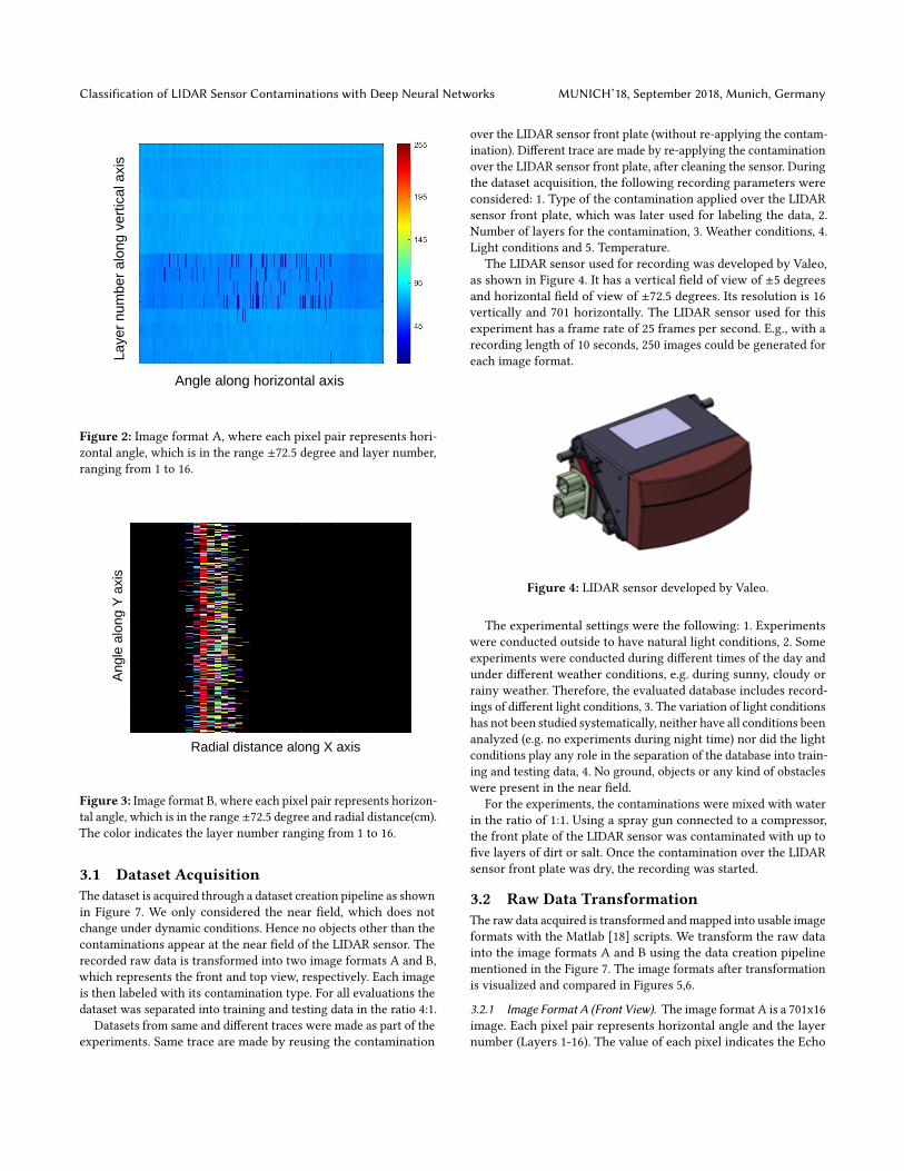
Figure 2: Image format A, where each pixel pair represents hori-zontal angle, which is in the range ±72.5 degree and layer number,ranging from 1 to 16.

Ang

le a

long

Y a

xis

Radial distance along X axis

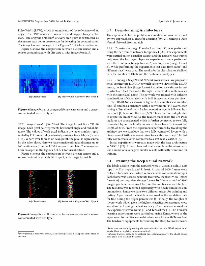
Figure 3: Image format B, where each pixel pair represents horizon-tal angle, which is in the range ±72.5 degree and radial distance(cm).The color indicates the layer number ranging from 1 to 16.

3.1 Dataset AcquisitionThe dataset is acquired through a dataset creation pipeline as shownin Figure 7. We only considered the near field, which does notchange under dynamic conditions. Hence no objects other than thecontaminations appear at the near field of the LIDAR sensor. Therecorded raw data is transformed into two image formats A and B,which represents the front and top view, respectively. Each imageis then labeled with its contamination type. For all evaluations thedataset was separated into training and testing data in the ratio 4:1.

Datasets from same and different traces were made as part of theexperiments. Same trace are made by reusing the contamination

over the LIDAR sensor front plate (without re-applying the contam-ination). Different trace are made by re-applying the contaminationover the LIDAR sensor front plate, after cleaning the sensor. Duringthe dataset acquisition, the following recording parameters wereconsidered: 1. Type of the contamination applied over the LIDARsensor front plate, which was later used for labeling the data, 2.Number of layers for the contamination, 3. Weather conditions, 4.Light conditions and 5. Temperature.

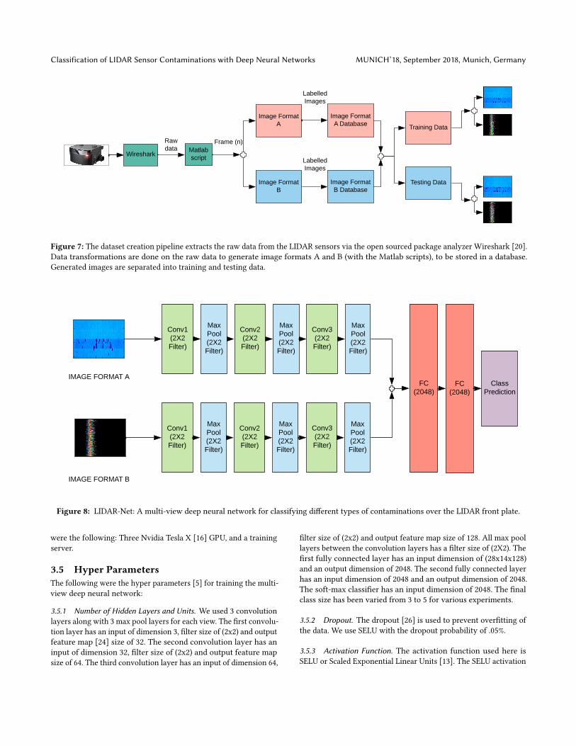
The LIDAR sensor used for recording was developed by Valeo,as shown in Figure 4. It has a vertical field of view of ±5 degreesand horizontal field of view of ±72.5 degrees. Its resolution is 16vertically and 701 horizontally. The LIDAR sensor used for thisexperiment has a frame rate of 25 frames per second. E.g., with arecording length of 10 seconds, 250 images could be generated foreach image format.

Figure 4: LIDAR sensor developed by Valeo.

The experimental settings were the following: 1. Experimentswere conducted outside to have natural light conditions, 2. Someexperiments were conducted during different times of the day andunder different weather conditions, e.g. during sunny, cloudy orrainy weather. Therefore, the evaluated database includes record-ings of different light conditions, 3. The variation of light conditionshas not been studied systematically, neither have all conditions beenanalyzed (e.g. no experiments during night time) nor did the lightconditions play any role in the separation of the database into train-ing and testing data, 4. No ground, objects or any kind of obstacleswere present in the near field.

For the experiments, the contaminations were mixed with waterin the ratio of 1:1. Using a spray gun connected to a compressor,the front plate of the LIDAR sensor was contaminated with up tofive layers of dirt or salt. Once the contamination over the LIDARsensor front plate was dry, the recording was started.

3.2 Raw Data TransformationThe raw data acquired is transformed andmapped into usable imageformats with the Matlab [18] scripts. We transform the raw datainto the image formats A and B using the data creation pipelinementioned in the Figure 7. The image formats after transformationis visualized and compared in Figures 5,6.

3.2.1 Image Format A (Front View). The image format A is a 701x16image. Each pixel pair represents horizontal angle and the layernumber (Layers 1-16). The value of each pixel indicates the Echo

MUNICH’18, September 2018, Munich, Germany Jyothish K. James et al.

Pulse Width (EPW), which is an indicator of the reflectance of anobject. The EPW values are normalized and mapped to a jet colormap. Here only the first echo2 of every scan point is considered, asthe nearest scan points are relevant for detecting the contamination.The image has been enlarged in the Figures 2, 3, 5, 6 for visualization.

Figure 5 shows the comparison between a clean sensor and asensor contaminated with dirt type 1, with image format A.

(a) Clean Sensor (b) Sensor with 5 layers of Dirt Type 1

Figure 5: Image format A compared for a clean sensor and a sensorcontaminated with dirt type 1.

3.2.2 Image Format B (Top View). The image format B is a 710x40image. Each pixel pair represents horizontal angle and radial dis-tance. The values of each pixel indicate the layer number repre-sented by RGB color code, exclusively assigned to each layer (Layers1-16). Where ever there is no scan point, the pixel is representedby the color black. Here we have considered radial distance up to160 centimeters from the LIDAR sensor front plate. The image hasbeen enlarged in the Figures 2, 3, 5, 6 for visualization.

Figure 6 shows the comparison between a clean sensor and asensor contaminated with Dirt type 1, with image format B.

(a) Clean Sensor (b) Sensor with 5 layers of Dirt Type 1

Figure 6: Image format B compared for a clean sensor and a sensorcontaminated with dirt type 1.

2Every laser shot receives 3 echoes, each echo represents a scan point in the order ofdistance.

3.3 Deep-learning ArchitecturesThe experiments for the problem of classification was carried outby two approaches: 1. Transfer Learning [30], 2. Training a DeepNeural Network from scratch.

3.3.1 Transfer Learning. Transfer Learning [30] was performedusing the per-trained network InceptionV4 [28] . The experimentswere carried out on a smaller dataset and the network was trainedonly over the last layer. Separate experiments were performedwith the front view (image format A) and top view (image formatB). While performing the experiments test data from same3 anddifferent trace4 were used. The results for the classification declinedover the number of labels and the contamination types.

3.3.2 Training a Deep Neural Network from scratch. We propose anovel architecture LIDAR-Net which takes two views of the LIDARsensor, the front view (image format A) and top view (image formatB) which are feed forwarded through the network simultaneously,with the same label name. The network was trained with differentcombinations of class labels with 2400 images per class per view.

The LIDAR-Net as shown in Figure 8, is a multi-view architec-ture [2] and has a structure with 3 convolution [14] layers, eachhaving a filter size of (2x2). Each convolution layer is followed by amax pool [8] layer of filter size (2x2). This structure is duplicatedto create the multi-view, i.e the feature maps from the 3rd Pool-ing layer are concatenated which is further connected to two fullyconnected layers. Each fully connected layer has a 1-Dimensionallength of 2048. From the experiments performed by tweaking thearchitecture, we conclude that two fully connected layers with adimension of 2048 was converging to a stable accuracy. The lastfully connected layer is connected to a soft-max classifier [6].

Initial experiments were also made with the base architectureas VGG16 [23]. It was observed that a simple architecture withless number of layers gave similar results with better run time fortraining.

3.4 Training the Deep Neural NetworkThe labels used to train the network were 1. Clean, 2. Salt, 3. Dirttype 1, 4. Dirt type 2, and 5. Frost. A total of 2400 frames werecollected for each label, which represents the contamination types.Each frame was used to generate two view, the front view (imageformat A) and top view (image format B). Hence a total of 4800images per label were used to train the multi-view architecture.The test data was recorded separately with newly simulated con-taminations, hence we have two different traces for training andtesting. A portion of the test data was used as the validation datafor fine tuning the hyper-parameters [5]. Finally, the weights ofthe network which gave the highest classification accuracy weresaved for performing the test accuracy. The frameworks used forthe experiments were Keras [3] and Tensorflow [1]. The Transferlearning experiments were carried out using Keras, where as theexperiment for multi-view architecture was done with Tensorflow.The hardware equipments for training the Deep Neural Network

3Same trace are made by reusing the contamination over the LIDAR sensor frontplate(without re-applying the contamination).4Different trace are made by re-applying the contamination over the LIDAR sensorfront plate, after cleaning the sensor.

Classification of LIDAR Sensor Contaminations with Deep Neural Networks MUNICH’18, September 2018, Munich, Germany

Frame (n)

Labelled Images

WiresharkMatlab script

Image Format A

Image Format B

Raw data

Image Format B Database

Image Format A Database

Labelled Images

Testing Data

Training Data

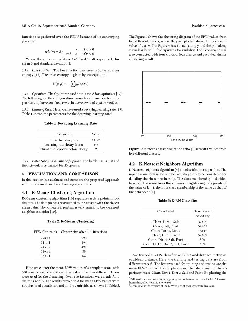
Figure 7: The dataset creation pipeline extracts the raw data from the LIDAR sensors via the open sourced package analyzer Wireshark [20].Data transformations are done on the raw data to generate image formats A and B (with the Matlab scripts), to be stored in a database.Generated images are separated into training and testing data.

Conv1 (2X2 Filter)

Conv2 (2X2 Filter)

Conv3 (2X2 Filter)

Max Pool (2X2 Filter)

Max Pool (2X2 Filter)

Max Pool (2X2 Filter)

FC (2048)

FC (2048)

Class Prediction

IMAGE FORMAT A

IMAGE FORMAT B

Conv1 (2X2 Filter)

Conv2 (2X2 Filter)

Conv3 (2X2 Filter)

Max Pool (2X2 Filter)

Max Pool (2X2 Filter)

Max Pool (2X2 Filter)

Figure 8: LIDAR-Net: A multi-view deep neural network for classifying different types of contaminations over the LIDAR front plate.

were the following: Three Nvidia Tesla X [16] GPU, and a trainingserver.

3.5 Hyper ParametersThe following were the hyper parameters [5] for training the multi-view deep neural network:

3.5.1 Number of Hidden Layers and Units. We used 3 convolutionlayers along with 3 max pool layers for each view. The first convolu-tion layer has an input of dimension 3, filter size of (2x2) and outputfeature map [24] size of 32. The second convolution layer has aninput of dimension 32, filter size of (2x2) and output feature mapsize of 64. The third convolution layer has an input of dimension 64,

filter size of (2x2) and output feature map size of 128. All max poollayers between the convolution layers has a filter size of (2X2). Thefirst fully connected layer has an input dimension of (28x14x128)and an output dimension of 2048. The second fully connected layerhas an input dimension of 2048 and an output dimension of 2048.The soft-max classifier has an input dimension of 2048. The finalclass size has been varied from 3 to 5 for various experiments.

3.5.2 Dropout. The dropout [26] is used to prevent overfitting ofthe data. We use SELU with the dropout probability of .05%.

3.5.3 Activation Function. The activation function used here isSELU or Scaled Exponential Linear Units [13]. The SELU activation

MUNICH’18, September 2018, Munich, Germany Jyothish K. James et al.

functions is preferred over the RELU because of its convergingproperty.

selu(x) = λ

{x , i f x > 0

αex − α , i f x ≤ 0Where the values α and λ are 1.673 and 1.050 respectively for

mean 0 and standard deviation 1.

3.5.4 Loss Function. The loss function used here is Soft-max crossentropy [19]. The cross entropy is given by the equation:

H (y,p) = −∑iyi loд(pi )

3.5.5 Optimizer. TheOptimizer used here is the Adamoptimizer [12].The following are the configuration parameters for an ideal learningproblem, alpha=0.001, beta1=0.9, beta2=0.999 and epsilon=10E-8.

3.5.6 Learning Rate. Here, we have used a decaying learning rate [25].Table 1 shows the parameters for the decaying learning rate:

Table 1: Decaying Learning Rate

Parameters Value

Initial learning rate 0.0001Learning rate decay factor 0.7

Number of epochs before decay 2

3.5.7 Batch Size and Number of Epochs. The batch size is 128 andthe network was trained for 20 epochs.

4 EVALUATION AND COMPARISONIn this section we evaluate and compare the proposed approachwith the classical machine learning algorithms.

4.1 K-Means Clustering AlgorithmK-Means clustering algorithm [10] separates n data points into kclusters. The data points are assigned to the cluster with the closestmean value. The k-means algorithm is very similar to the k-nearestneighbor classifier [10].

Table 2: K-Means Clustering

EPW Centroids Cluster size after 100 iterations

278.18 990211.44 494245.06 491326.41 38252.24 487

Here we cluster the mean EPW values of a complete scan, with500 scan for each class. Mean EPW values from five different classeswere used for the clustering. Over 100 iterations were made for acluster size of 5. The results proved that the mean EPW values werenot clustered equally around all the centroids, as shown in Table 2.

The Figure 9 shows the clustering diagram of the EPW values fromfive different classes, where they are plotted along the x axis withvalue of y as 0. The Figure 9 has no axis along y and the plot alongx axis has been shifted upwards for visibility. The experiment wasalso conducted with four clusters, four classes and provided similarclustering results.

Figure 9: K means clustering of the echo pulse width values fromfive different classes.

4.2 K-Nearest Neighbors AlgorithmK-Nearest neighbors algorithm [4] is a classification algorithm. Theinput parameter k is the number of data points to be considered fordeciding the class membership. The class membership is decidedbased on the score from the k nearest neighboring data points. Ifthe value of k = 1, then the class membership is the same as that ofthe data point [4].

Table 3: K-NN Classifier

Class Label ClassificationAccuracy

Clean, Dirt 1, Salt 66.66%Clean, Salt, Frost 66.66%

Clean, Dirt 1, Dirt 2 47.61%Clean, Dirt 1, Frost 66.66%

Clean, Dirt 1, Salt, Frost 50%Clean, Dirt 1, Dirt 2, Salt, Frost 40%

We trained a K-NN classifier with k=4 and distance metric aseuclidean distance. Here, the training and testing data are fromdifferent traces5. The features used for training and testing are themean EPW6 values of a complete scan. The labels used for the ex-periment were Clean, Dirt 1, Dirt 2, Salt and Frost. By plotting the5Different trace are made by re-applying the contamination over the LIDAR sensorfront plate, after cleaning the sensor.6Mean EPW is the average of the EPW values of each scan point in a scan.

Classification of LIDAR Sensor Contaminations with Deep Neural Networks MUNICH’18, September 2018, Munich, Germany

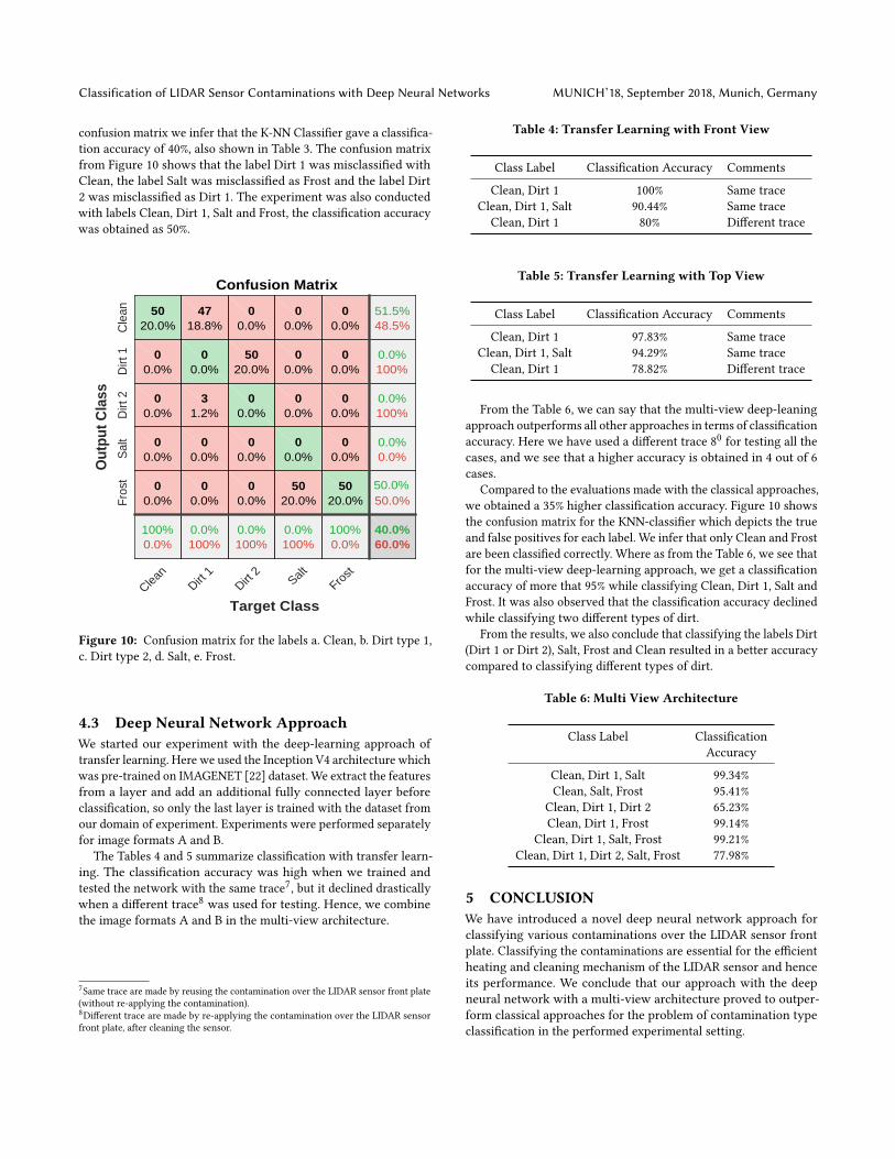
confusion matrix we infer that the K-NN Classifier gave a classifica-tion accuracy of 40%, also shown in Table 3. The confusion matrixfrom Figure 10 shows that the label Dirt 1 was misclassified withClean, the label Salt was misclassified as Frost and the label Dirt2 was misclassified as Dirt 1. The experiment was also conductedwith labels Clean, Dirt 1, Salt and Frost, the classification accuracywas obtained as 50%.

Clean

Dirt 1

Dirt 2

SaltFro

st

Target Class

Cle

anD

irt 1

Dirt

2S

alt

Fros

t

Out

put C

lass

Confusion Matrix

5020.0%

00.0%

00.0%

00.0%

00.0%

100%0.0%

4718.8%

00.0%

31.2%

00.0%

00.0%

0.0%100%

00.0%

5020.0%

00.0%

00.0%

00.0%

0.0%100%

00.0%

00.0%

00.0%

00.0%

5020.0%

0.0%100%

00.0%

00.0%

00.0%

00.0%

5020.0%

100%0.0%

51.5%48.5%

0.0%100%

0.0%100%

0.0%0.0%

50.0%50.0%

40.0%60.0%

Figure 10: Confusion matrix for the labels a. Clean, b. Dirt type 1,c. Dirt type 2, d. Salt, e. Frost.

4.3 Deep Neural Network ApproachWe started our experiment with the deep-learning approach oftransfer learning. Here we used the Inception V4 architecture whichwas pre-trained on IMAGENET [22] dataset. We extract the featuresfrom a layer and add an additional fully connected layer beforeclassification, so only the last layer is trained with the dataset fromour domain of experiment. Experiments were performed separatelyfor image formats A and B.

The Tables 4 and 5 summarize classification with transfer learn-ing. The classification accuracy was high when we trained andtested the network with the same trace7, but it declined drasticallywhen a different trace8 was used for testing. Hence, we combinethe image formats A and B in the multi-view architecture.

7Same trace are made by reusing the contamination over the LIDAR sensor front plate(without re-applying the contamination).8Different trace are made by re-applying the contamination over the LIDAR sensorfront plate, after cleaning the sensor.

Table 4: Transfer Learning with Front View

Class Label Classification Accuracy Comments

Clean, Dirt 1 100% Same traceClean, Dirt 1, Salt 90.44% Same traceClean, Dirt 1 80% Different trace

Table 5: Transfer Learning with Top View

Class Label Classification Accuracy Comments

Clean, Dirt 1 97.83% Same traceClean, Dirt 1, Salt 94.29% Same traceClean, Dirt 1 78.82% Different trace

From the Table 6, we can say that the multi-view deep-leaningapproach outperforms all other approaches in terms of classificationaccuracy. Here we have used a different trace 80 for testing all thecases, and we see that a higher accuracy is obtained in 4 out of 6cases.

Compared to the evaluations made with the classical approaches,we obtained a 35% higher classification accuracy. Figure 10 showsthe confusion matrix for the KNN-classifier which depicts the trueand false positives for each label. We infer that only Clean and Frostare been classified correctly. Where as from the Table 6, we see thatfor the multi-view deep-learning approach, we get a classificationaccuracy of more that 95% while classifying Clean, Dirt 1, Salt andFrost. It was also observed that the classification accuracy declinedwhile classifying two different types of dirt.

From the results, we also conclude that classifying the labels Dirt(Dirt 1 or Dirt 2), Salt, Frost and Clean resulted in a better accuracycompared to classifying different types of dirt.

Table 6: Multi View Architecture

Class Label ClassificationAccuracy

Clean, Dirt 1, Salt 99.34%Clean, Salt, Frost 95.41%

Clean, Dirt 1, Dirt 2 65.23%Clean, Dirt 1, Frost 99.14%

Clean, Dirt 1, Salt, Frost 99.21%Clean, Dirt 1, Dirt 2, Salt, Frost 77.98%

5 CONCLUSIONWe have introduced a novel deep neural network approach forclassifying various contaminations over the LIDAR sensor frontplate. Classifying the contaminations are essential for the efficientheating and cleaning mechanism of the LIDAR sensor and henceits performance. We conclude that our approach with the deepneural network with a multi-view architecture proved to outper-form classical approaches for the problem of contamination typeclassification in the performed experimental setting.

MUNICH’18, September 2018, Munich, Germany Jyothish K. James et al.

The data recorded with the recording setup originated from thesame LIDAR sensor. We could bring more complexity to the datasetby making the data recording with multiple LIDAR sensors, whichcan be considered for the future works. Similarly, all the data record-ing experiments were conducted by applying full contaminationover the LIDAR sensor, the application of partial contaminationcan be considered for future works. We can also consider the sys-tematic variation of light or temperature conditions as a factor fordata recording in the future works. In a real-world scenario wherethere are a mixture of contaminations (mixture of dust,salt or ice),the performance of the DNN approach has to be evaluated basedon the classification accuracy, which also has a great potential forfuture work.

ACKNOWLEDGMENTSThe first authorwould like to thankDr. Georg Puhlfürst andVladislavGolyanik for their supervision. The author would also like to thankProf. Dr. Didier Stricker for providing an opportunity to work withDFKI.

The first author would also like to thank anonymous refereesfor their valuable comments and helpful suggestions. The workis a part of the master’s thesis supported by Valeo Schalter undSensoren GmbH.

REFERENCES[1] Martín Abadi, Paul Barham, Jianmin Chen, Zhifeng Chen, Andy Davis, Jeffrey

Dean, Matthieu Devin, Sanjay Ghemawat, Geoffrey Irving, Michael Isard, Man-junath Kudlur, Josh Levenberg, Rajat Monga, Sherry Moore, Derek G. Murray,Benoit Steiner, Paul Tucker, Vijay Vasudevan, Pete Warden, Martin Wicke, YuanYu, and Xiaoqiang Zheng. 2016. TensorFlow: A System for Large-scale MachineLearning. In Proceedings of the 12th USENIX Conference on Operating SystemsDesign and Implementation (OSDI’16). USENIX Association, Berkeley, CA, USA,265–283. http://dl.acm.org/citation.cfm?id=3026877.3026899

[2] Xiaozhi Chen, Huimin Ma, Ji Wan, Bo Li, and Tian Xia. 2016. Multi-View 3DObject Detection Network for Autonomous Driving. CoRR abs/1611.07759 (2016).arXiv:1611.07759 http://arxiv.org/abs/1611.07759

[3] François Chollet et al. 2015. Keras. https://keras.io.[4] T. Cover and P. Hart. 2006. Nearest Neighbor Pattern Classification. IEEE Trans.

Inf. Theor. 13, 1 (Sept. 2006), 21–27. https://doi.org/10.1109/TIT.1967.1053964[5] Gonzalo I. Diaz, Achille Fokoue, Giacomo Nannicini, and Horst Samulowitz. 2017.

An effective algorithm for hyperparameter optimization of neural networks.CoRR abs/1705.08520 (2017). arXiv:1705.08520 http://arxiv.org/abs/1705.08520

[6] KaiboDuan, S. Sathiya Keerthi,Wei Chu, Shirish Krishnaj Shevade, andAunNeowPoo. 2003. Multi-category Classification by Soft-max Combination of BinaryClassifiers. In Proceedings of the 4th International Conference on Multiple ClassifierSystems (MCS’03). Springer-Verlag, Berlin, Heidelberg, 125–134. http://dl.acm.org/citation.cfm?id=1764295.1764312

[7] D. Göhring, M. Wang, M. Schnürmacher, and T. Ganjineh. 2011. Radar/Lidarsensor fusion for car-following on highways. In The 5th International Conferenceon Automation, Robotics and Applications. 407–412. https://doi.org/10.1109/ICARA.2011.6144918

[8] Benjamin Graham. 2014. Fractional Max-Pooling. CoRR abs/1412.6071 (2014).arXiv:1412.6071 http://arxiv.org/abs/1412.6071

[9] T. Herpel, C. Lauer, R. German, and J. Salzberger. 2008. Multi-sensor data fu-sion in automotive applications. In 2008 3rd International Conference on SensingTechnology. 206–211. https://doi.org/10.1109/ICSENST.2008.4757100

[10] T. Kanungo, D. M. Mount, N. S. Netanyahu, C. D. Piatko, R. Silverman, and A. Y.Wu. 2002. An efficient k-means clustering algorithm: analysis and implemen-tation. IEEE Transactions on Pattern Analysis and Machine Intelligence 24, 7 (Jul2002), 881–892. https://doi.org/10.1109/TPAMI.2002.1017616

[11] D. U. Kim, S. H. Park, J. H. Ban, T. M. Lee, and Y. Do. 2016. Vision-based au-tonomous detection of lane and pedestrians. In 2016 IEEE International Confer-ence on Signal and Image Processing (ICSIP). 680–683. https://doi.org/10.1109/SIPROCESS.2016.7888349

[12] Diederik P. Kingma and JimmyBa. 2014. Adam: AMethod for Stochastic Optimiza-tion. CoRR abs/1412.6980 (2014). arXiv:1412.6980 http://arxiv.org/abs/1412.6980

[13] Günter Klambauer, Thomas Unterthiner, Andreas Mayr, and Sepp Hochre-iter. 2017. Self-Normalizing Neural Networks. CoRR abs/1706.02515 (2017).

arXiv:1706.02515 http://arxiv.org/abs/1706.02515[14] Alex Krizhevsky, Ilya Sutskever, and Geoffrey E. Hinton. 2012. ImageNet Classi-

fication with Deep Convolutional Neural Networks. In Proceedings of the 25thInternational Conference on Neural Information Processing Systems - Volume 1(NIPS’12). Curran Associates Inc., USA, 1097–1105. http://dl.acm.org/citation.cfm?id=2999134.2999257

[15] Gustav Larsson, Michael Maire, and Gregory Shakhnarovich. 2016. FractalNet:Ultra-Deep Neural Networks without Residuals. CoRR abs/1605.07648 (2016).arXiv:1605.07648 http://arxiv.org/abs/1605.07648

[16] E. Lindholm, J. Nickolls, S. Oberman, and J. Montrym. 2008. NVIDIA Tesla: AUnified Graphics and Computing Architecture. IEEE Micro 28, 2 (March 2008),39–55. https://doi.org/10.1109/MM.2008.31

[17] G. Lu and M. Tomizuka. 2006. LIDAR Sensing for Vehicle Lateral Guidance:Algorithm and Experimental Study. IEEE/ASME Transactions on Mechatronics 11,6 (Dec 2006), 653–660. https://doi.org/10.1109/TMECH.2006.886192

[18] MATLAB. 2018. version 9.4.0 (R2018a). The MathWorks Inc., Natick, Mas-sachusetts.

[19] G. E. Nasr, E. A. Badr, and C. Joun. 2002. Cross Entropy Error Function inNeural Networks: Forecasting Gasoline Demand. In Proceedings of the FifteenthInternational Florida Artificial Intelligence Research Society Conference. AAAIPress, 381–384. http://dl.acm.org/citation.cfm?id=646815.708603

[20] Angela Orebaugh, Gilbert Ramirez, Jay Beale, and JoshuaWright. 2007. Wireshark& Ethereal Network Protocol Analyzer Toolkit. Syngress Publishing.

[21] J. R. V. Rivero, I. Tahiraj, O. Schubert, C. Glassl, B. Buschardt, M. Berk, and J.Chen. 2017. Characterization and simulation of the effect of road dirt on theperformance of a laser scanner. In 2017 IEEE 20th International Conference onIntelligent Transportation Systems (ITSC). 1–6. https://doi.org/10.1109/ITSC.2017.8317784

[22] Olga Russakovsky, Jia Deng, Hao Su, Jonathan Krause, Sanjeev Satheesh, SeanMa, Zhiheng Huang, Andrej Karpathy, Aditya Khosla, Michael S. Bernstein,Alexander C. Berg, and Fei-Fei Li. 2014. ImageNet Large Scale Visual RecognitionChallenge. CoRR abs/1409.0575 (2014). arXiv:1409.0575 http://arxiv.org/abs/1409.0575

[23] Karen Simonyan and Andrew Zisserman. 2014. Very Deep ConvolutionalNetworks for Large-Scale Image Recognition. CoRR abs/1409.1556 (2014).arXiv:1409.1556 http://arxiv.org/abs/1409.1556

[24] A. Sluzek. 2003. Feature maps: a new approach in hierarchical interpretation ofimages. In Proceedings. 2003 International Conference on Cyberworlds. 245–250.https://doi.org/10.1109/CYBER.2003.1253461

[25] Leslie N. Smith. 2015. No More Pesky Learning Rate Guessing Games. CoRRabs/1506.01186 (2015). arXiv:1506.01186 http://arxiv.org/abs/1506.01186

[26] Nitish Srivastava, Geoffrey Hinton, Alex Krizhevsky, Ilya Sutskever, and RuslanSalakhutdinov. 2014. Dropout: A Simple Way to Prevent Neural Networks fromOverfitting. Journal of Machine Learning Research 15 (2014), 1929–1958. http://jmlr.org/papers/v15/srivastava14a.html

[27] M. Stampfle, D. Holz, and J. C. Becker. 2005. Performance evaluation of automotivesensor data fusion. In Proceedings. 2005 IEEE Intelligent Transportation Systems,2005. 50–55. https://doi.org/10.1109/ITSC.2005.1520114

[28] Christian Szegedy, Sergey Ioffe, and Vincent Vanhoucke. 2016. Inception-v4,Inception-ResNet and the Impact of Residual Connections on Learning. CoRRabs/1602.07261 (2016). arXiv:1602.07261 http://arxiv.org/abs/1602.07261

[29] Jingdong Wang, Zhen Wei, Ting Zhang, and Wenjun Zeng. 2016. Deeply-FusedNets. CoRR abs/1605.07716 (2016). arXiv:1605.07716 http://arxiv.org/abs/1605.07716

[30] Jason Yosinski, Jeff Clune, Yoshua Bengio, andHod Lipson. 2014. How transferableare features in deep neural networks? CoRR abs/1411.1792 (2014). arXiv:1411.1792http://arxiv.org/abs/1411.1792