bitp.kiev.uabitp.kiev.ua/files/doc/thesis/2010/diser_Karpenko.pdf · UNIVERSITE DE NANTES´ FACULTE...
163
UNIVERSIT ´ E DE NANTES FACULT ´ E DES SCIENCES ET TECHNIQUES ———— ´ ECOLE DOCTORALE Mat´ eriaux Mati` ere Mol´ ecule en Pays de Loire Ann´ ee : 2010 N ◦ attribu´ e par la biblioth` eque D´ eveloppement d’approches hydrodynamique et hydrocin´ etique aux collisions noyau-noyau ultra-relativistes TH ` ESE DE DOCTORAT Discipline : Physique Nucl´ eaire Sp´ ecialit´ e : Physique des Ions Lourds Pr´ esent´ ee et soutenue publiquement par Iurii KARPENKO Le 25 mai 2010, devant le jury ci-dessous Pr´ esident M. Smilga A., Pr. Universit´ e, Subatech, Nantes Rapporteurs M. Lednicky R., Directeur de recherche, Joint Institute for Nuclear Research, Dubna M. Ollitrault J.-Y., Directeur de recherche CNRS, CEA Saclay, Gif-Sur-Yvette Examinateurs M. Sinyukov Yu., Directeur de recherche, Bogolyubov Institute for Theoretical Physics, Kiev M. Werner K., Pr. Universit´ e, Subatech, Nantes Co-directeurs de th` ese : M. Sinyukov Yu., Directeur de recherche, Bogolyubov Institute for Theoretical Physics, Kiev M. Werner K., Pr. Universit´ e, Subatech, Nantes N ◦ ED −−−−−−−−−−−
Transcript of bitp.kiev.uabitp.kiev.ua/files/doc/thesis/2010/diser_Karpenko.pdf · UNIVERSITE DE NANTES´ FACULTE...

UNIVERSITE DE NANTESFACULTE DES SCIENCES ET TECHNIQUES
————ECOLE DOCTORALE
Materiaux Matiere Molecule en Pays de Loire
Annee : 2010N◦ attribue par la bibliotheque
Developpement d’approches
hydrodynamique et hydrocinetique aux
collisions noyau-noyau ultra-relativistes
THESE DE DOCTORAT
Discipline : Physique Nucleaire
Specialite : Physique des Ions Lourds
Presentee et soutenue publiquement par
Iurii KARPENKO
Le 25 mai 2010, devant le jury ci-dessous
President M. Smilga A., Pr. Universite, Subatech, NantesRapporteurs M. Lednicky R., Directeur de recherche,
Joint Institute for Nuclear Research, DubnaM. Ollitrault J.-Y., Directeur de recherche CNRS, CEA Saclay, Gif-Sur-Yvette
Examinateurs M. Sinyukov Yu., Directeur de recherche,Bogolyubov Institute for Theoretical Physics, Kiev
M. Werner K., Pr. Universite, Subatech, Nantes
Co-directeurs de these : M. Sinyukov Yu., Directeur de recherche,Bogolyubov Institute for Theoretical Physics, Kiev
M. Werner K., Pr. Universite, Subatech, Nantes
N◦ ED −−−−−−−−−−−

UNIVERSITE DE NANTES
Development of hydrodynamic and
hydrokinetic approaches to
ultrarelativistic nucleus-nucleus
collisions
PhD thesis
Iurii KARPENKO
SUBATECH (Nantes, France) and
BITP (Kiev, Ukraine), 2010

iv
CONTENTS
1 Literature review 11.1 Introduction . . . . . . . . . . . . . . . . . . . . . . . . . . . . . . . 11.2 Particle distributions . . . . . . . . . . . . . . . . . . . . . . . . . . 21.3 Correlation functions . . . . . . . . . . . . . . . . . . . . . . . . . . 41.4 Evolution picture . . . . . . . . . . . . . . . . . . . . . . . . . . . . 61.5 Dynamic models . . . . . . . . . . . . . . . . . . . . . . . . . . . . 71.6 Outline of the thesis . . . . . . . . . . . . . . . . . . . . . . . . . . 9
2 Hydrodyamic solutions 112.1 Introduction . . . . . . . . . . . . . . . . . . . . . . . . . . . . . . . 112.2 General analysis . . . . . . . . . . . . . . . . . . . . . . . . . . . . . 122.3 Gradient-like velocity ansatz . . . . . . . . . . . . . . . . . . . . . . 132.4 Relativistic ellipsoidal solutions . . . . . . . . . . . . . . . . . . . . 142.5 Generalization of the Hubble-like flows . . . . . . . . . . . . . . . . 172.6 Conclusions . . . . . . . . . . . . . . . . . . . . . . . . . . . . . . . 20
3 Fast MC freeze-out generator 213.1 Introduction . . . . . . . . . . . . . . . . . . . . . . . . . . . . . . . 213.2 Hadron multiplicities . . . . . . . . . . . . . . . . . . . . . . . . . . 223.3 Hadron momentum distributions . . . . . . . . . . . . . . . . . . . 253.4 Generalization of the Cooper-Frye prescription . . . . . . . . . . . . 263.5 Freeze-out surface parameterizations . . . . . . . . . . . . . . . . . 273.6 Hadron generation procedure . . . . . . . . . . . . . . . . . . . . . 303.7 Validation of the MC procedure . . . . . . . . . . . . . . . . . . . . 323.8 Input parameters and results . . . . . . . . . . . . . . . . . . . . . . 333.9 Freeze-out for non-central collisions . . . . . . . . . . . . . . . . . . 433.10 Different chemical and thermal freeze-outs . . . . . . . . . . . . . . 483.11 Results for non-central collisions . . . . . . . . . . . . . . . . . . . . 493.12 Conclusions . . . . . . . . . . . . . . . . . . . . . . . . . . . . . . . 62
v
vi CONTENTS
4 Hybrid model 634.1 Introduction . . . . . . . . . . . . . . . . . . . . . . . . . . . . . . . 634.2 Initial state model : EPOS . . . . . . . . . . . . . . . . . . . . . . . 664.3 Hydrodynamic evolution, realistic equation-of-state . . . . . . . . . 70
4.3.1 Hydrodynamic algorithm . . . . . . . . . . . . . . . . . . . . 734.3.2 Resonance gas . . . . . . . . . . . . . . . . . . . . . . . . . . 764.3.3 Ideal QGP . . . . . . . . . . . . . . . . . . . . . . . . . . . . 77
4.4 Freeze-out . . . . . . . . . . . . . . . . . . . . . . . . . . . . . . . . 784.5 UrQMD afterburner . . . . . . . . . . . . . . . . . . . . . . . . . . 804.6 Results: Elliptical flow . . . . . . . . . . . . . . . . . . . . . . . . . 814.7 Transverse momentum spectra and yields . . . . . . . . . . . . . . . 844.8 Femtoscopy . . . . . . . . . . . . . . . . . . . . . . . . . . . . . . . 874.9 Summary and conclusions . . . . . . . . . . . . . . . . . . . . . . . 92
5 Hydro-kinetic model 935.1 Introduction . . . . . . . . . . . . . . . . . . . . . . . . . . . . . . . 935.2 General formalism . . . . . . . . . . . . . . . . . . . . . . . . . . . 955.3 Cooper-Frye prescription . . . . . . . . . . . . . . . . . . . . . . . . 985.4 Initial conditions for hydro-evolution . . . . . . . . . . . . . . . . . 105
5.4.1 Pre-thermal flows . . . . . . . . . . . . . . . . . . . . . . . . 1055.4.2 Glauber-like initial transverse profile . . . . . . . . . . . . . 1065.4.3 Initial conditions motivated by Color Glass Condensate model107
5.5 Equation of state . . . . . . . . . . . . . . . . . . . . . . . . . . . . 1105.5.1 The EoS in the equilibrated space-time domain. . . . . . . . 1115.5.2 The EoS in the chemically non-equilibrated domain. . . . . . 111
5.6 Kinetics in the non-equilibrium hadronic zone . . . . . . . . . . . . 1145.6.1 Emission functions in hyperbolic coordinates and spectra
formation . . . . . . . . . . . . . . . . . . . . . . . . . . . . 1145.6.2 Resonance decays in multi-component gas . . . . . . . . . . 1175.6.3 Collision rates . . . . . . . . . . . . . . . . . . . . . . . . . . 118
5.7 Hydrodynamics . . . . . . . . . . . . . . . . . . . . . . . . . . . . . 1205.8 Results: femtoscopy at RHIC . . . . . . . . . . . . . . . . . . . . . 1215.9 Space-time scales for SPS, RHIC, LHC . . . . . . . . . . . . . . . . 1265.10 Conclusions . . . . . . . . . . . . . . . . . . . . . . . . . . . . . . . 129
6 Conclusions 133Glossary . . . . . . . . . . . . . . . . . . . . . . . . . . . . . . . . . . . 136Bibliography . . . . . . . . . . . . . . . . . . . . . . . . . . . . . . . . 136
LIST OF FIGURES
3.1 The validation of the MC procedure: the transverse momentumspectra and the corresponding MC results. Also shown are the MCresults obtained with a constant residual weight. . . . . . . . . . . . 33
3.2 The π+ emission transverse x-coordinate and time generated in theBjorken-like model: all π+’s, direct π+’s, decay π+’s from ρ, ω,K∗(892) and ∆. . . . . . . . . . . . . . . . . . . . . . . . . . . . . . 35
3.3 The π+ emission transverse x-coordinate and time generated in theHubble-like model: all π+’s, direct π+’s, decay π+’s from ρ, ω,K∗(892) and ∆. . . . . . . . . . . . . . . . . . . . . . . . . . . . . . 35
3.4 The pseudo-rapidity (− ln tan(θ/2), θ is the particle production an-gle) distributions of charged particles in central Au + Au collisionsat
√sNN = 200 GeV from the PHOBOS experiment and the MC
calculations within the Bjorken-like and Hubble-like models. . . . . 37
3.5 The π+, K+ and proton transverse momentum spectra at mid-rapidity y ≈ 0 in central Au + Au collisions at
√sNN = 200 GeV
from PHENIX experiment and the MC calculations within the Bjorken-like and Hubble-like models. Model results obtained with the strangenesssuppression parameter γs = 0.8. . . . . . . . . . . . . . . . . . . . . 38
3.6 The contributions to the π+ transverse momentum spectrum atmid-rapidity in central Au + Au collisions at
√sNN = 200 GeV
calculated within the Bjorken-like model. . . . . . . . . . . . . . . . 39
3.7 The π±π± correlation radii and the suppression parameter λ at mid-rapidity in central Au+Au collisions at
√sNN = 200 GeV from the
STAR experiment and the MC calculations within the Bjorken-likemodel in different intervals of the pair transverse momentum kt. . . 41
3.8 The typical hydrodynamic evolution scenario. . . . . . . . . . . . . 45
vii
viii LIST OF FIGURES
3.9 mt-spectra (in c4/GeV2) measured by the STAR Collaboration forπ+, K+ and p at 0 − 5% centrality in comparison with FASTMCcalculations. . . . . . . . . . . . . . . . . . . . . . . . . . . . . . . . 52
3.10 mt-spectra (in c4/GeV2) measured by the STAR Collaboration forπ+, K+ and p at different centralities in comparison with fast MCcalculations. . . . . . . . . . . . . . . . . . . . . . . . . . . . . . . . 54
3.11 The pt-dependence of v2 measured by the STAR Collaboration [98]for charged particles at different centralities in comparison with fastMC calculations. . . . . . . . . . . . . . . . . . . . . . . . . . . . . 56
3.12 The pt-dependence of v2 measured by the STAR Collaboration forcharged particles at centrality 20−30% in comparison with fast MCcalculations under assumption of the single freeze-out. . . . . . . . . 57
3.13 The π+ correlation radii at mid-rapidity in central Au+Au collisionsat
√sNN = 200 GeV from the STAR experiment and MC calcula-
tions within the Bjorken-like model in different intervals of the pairtransverse momentum kt. . . . . . . . . . . . . . . . . . . . . . . . . 59
3.14 Squared correlation radii simulated with FASTMC versus the az-imuthal angle Φ of the π+π+ pair with respect to the reaction plane,20-30 % centrality events in different kT (GeV/c) intervals. . . . . . 61
4.1 The energy density over T 4 as a function of the temperature T . . . 64
4.2 Particle ratios from hybrid model calculations as compared to thestatistical model, and to data. . . . . . . . . . . . . . . . . . . . . . 65
4.3 Elementary parton-parton scattering. The symbolic parton ladderis used. . . . . . . . . . . . . . . . . . . . . . . . . . . . . . . . . . . 67
4.4 The complete picture of initial conditions, including remnants. . . . 67
4.5 Inner contributions, from the parton ladder (full lines), and “outer”contributions, from the remnants, to the rapidity distribution ofhadrons. . . . . . . . . . . . . . . . . . . . . . . . . . . . . . . . . . 68
4.6 The two elements of the multiple scattering theory: open ladders,representing inelastic interactions, and closed ladders, representingelastic interactions. . . . . . . . . . . . . . . . . . . . . . . . . . . . 69
4.7 Energy density versus temperature, for our equation-of-state X3F,compared to lattice data, and some other EoS choices. . . . . . . . 72
4.8 Pressure versus temperature, for our equation-of-state X3F, com-pared to lattice data, and some other EoS choices. . . . . . . . . . . 73
4.9 Centrality dependence of the ratio of v2 over eccentricity. . . . . . . 82
4.10 Centrality dependence of the ratio of v2 over eccentricity,for differentscenario. . . . . . . . . . . . . . . . . . . . . . . . . . . . . . . . . . 83
LIST OF FIGURES ix
4.11 Pseudorapidity distributions of the elliptical flow v2 for minimumbias events and different centrality classes, in Au-Au collisions at200 GeV. . . . . . . . . . . . . . . . . . . . . . . . . . . . . . . . . 84
4.12 Production of pions in Au-Au collisions at 200 GeV: transverse mo-mentum spectra for central collisions at different rapidities. . . . . . 85
4.13 Production of lambdas (left) and antilambdas (right) in Au-Au col-lisions at 200 GeV: transverse momentum distributions at rapidityzero for different centrality classes, the 0-5%, the 20-30%, and the40-50% most central collisions. . . . . . . . . . . . . . . . . . . . . . 86
4.14 Femtoscopic radii Rout, Rside, and Rlong, as well as λ as a function ofmT for different centralities (0-5% most central, 5-10% most central,and so on). . . . . . . . . . . . . . . . . . . . . . . . . . . . . . . . 88
4.15 The mean transverse momentum component px of π+ as a functionof the x coordinate of the emission point. Also shown is the numberof produced π+ as a function of x. . . . . . . . . . . . . . . . . . . . 89
4.16 Same as fig. 4.15, but for the calculation without hadronic cascade. 89
4.17 Same as fig. 4.15, but for the full thermal scenario (freeze-out at130 MeV). . . . . . . . . . . . . . . . . . . . . . . . . . . . . . . . . 90
4.18 Same as fig. 4.14, but the calculations are done without hadroniccascade or with a hydrodynamic evolution through the hadronicphase with freeze-out at 130 MeV. . . . . . . . . . . . . . . . . . . . 91
5.1 The pion emission function for different pT in hydro-kinetic model(HKM). . . . . . . . . . . . . . . . . . . . . . . . . . . . . . . . . . 103
5.2 Transverse momentum spectrum of π− in HKM, compared with thesudden freeze-out ones at temperatures of 80 and 160 MeV witharbitrary normalization. . . . . . . . . . . . . . . . . . . . . . . . . 104
5.3 The emission function in HKM for particles with momentum di-rected along the radius vector at the emission points and for thoseones in the opposite direction to the radius vector. . . . . . . . . . . 105
5.4 Equation of state p(ε) used in the HKM calculations. . . . . . . . . 122
5.5 The transverse momentum spectra of negative pions, negative kaonsand interferometry radii and Rout/Rside ratio for π−π− pairs andmixture of K−K− and K+K+ pairs, all calculated in the HKMmodel. The experimental data are taken from the STAR and PHENIXcollaborations. . . . . . . . . . . . . . . . . . . . . . . . . . . . . . . 124
5.6 The φp-integrated emission functions of negative pions and negativekaons with different momenta at the Glauber IC. . . . . . . . . . . 125

x LIST OF FIGURES
5.7 The pT -integrated emission functions of negative pions for the topSPS, RHIC and LHC energies (top); the interferometry radii (mid-dle) Rout/Rside ratio and transverse momentum spectra (bottom) ofnegative pions at different energy densities, all calculated in HKMmodel. The experimental data are taken from CERES, NA-49 (SPSCERN), STAR, PHENIX (RHIC BNL) collaborations. . . . . . . . 127
LIST OF TABLES
3.1 FASTMC model parameters for central Au + Au collisions at√sNN =
200 GeV for different freeze-out parametrizations. . . . . . . . . . . 343.2 Particle number ratios near mid-rapidity in central Au + Au colli-
sions at√sNN = 130 GeV calculated in FASTMC. . . . . . . . . . . 36
3.3 Particle number ratios near mid-rapidity in central Au + Au col-lisions at
√sNN = 200 GeV calculated in FASTMC with different
set of thermodynamic parameters. . . . . . . . . . . . . . . . . . . . 363.4 FASTMC model parameters for central Au + Au collisions at
√sNN =
200 GeV with separate chemical and thermal freeze-outs. . . . . . . 513.5 FASTMC model parameters for Au + Au collisions at
√sNN =
200 GeV at different centralities. . . . . . . . . . . . . . . . . . . . 51
xi

xii LIST OF TABLES

CHAPTER
ONE
Literature review
1.1 Introduction
The idea of exploiting the laws of ideal hydrodynamics to describe the expansionof the strongly interacting matter that is formed in high energy hadronic collisionswas first formulated by Landau [1] in 1953 as an improvement over the Fermistatistical model [2] for the multiple particle production phenomena in high-energynuclear collisions. At that time, these phenomena were observed in cosmic rays.Although the Fermi model offered an ingenious insight into the mechanism ofthe high-energy nuclear collision processes and gave a prediction for the energydependence of the multiplicity, which was verified by the data, it was known thatit had troubles in reproducing particle spectra and relative abundance of K overπ.
These problems were solved by letting the hot and dense matter to expandand equilibrate before particle emission takes place, reducing thus heavy-particlemultiplicities, because of the Boltzmann factor, and giving at the same time alon-gated momentum spectra, due to a violent longitudinal expansion caused by alarge pressure gradient in the beam direction. A nice feature of this model is that,since the entropy is conserved in the ideal case Landau studied, the energy depen-dence of the total particle multiplicity predicted by the Fermi model, and verifiedexperimentally, is preserved.
When accelerator data on multiparticle production began to appear, first in ppcollisions at CERN ISR, and later in pp collisions at SppS collider, Carruthers [3]revived this Heretical Model in 1974, showing that several aspects of those phenom-ena may be well understood within Hydrodynamic Model. When laboratory studyof high-energy heavy-nucleus collisions started, Hydrodynamic Model became oneof the essential tools for these investigations.
1
2 CHAPTER 1. LITERATURE REVIEW
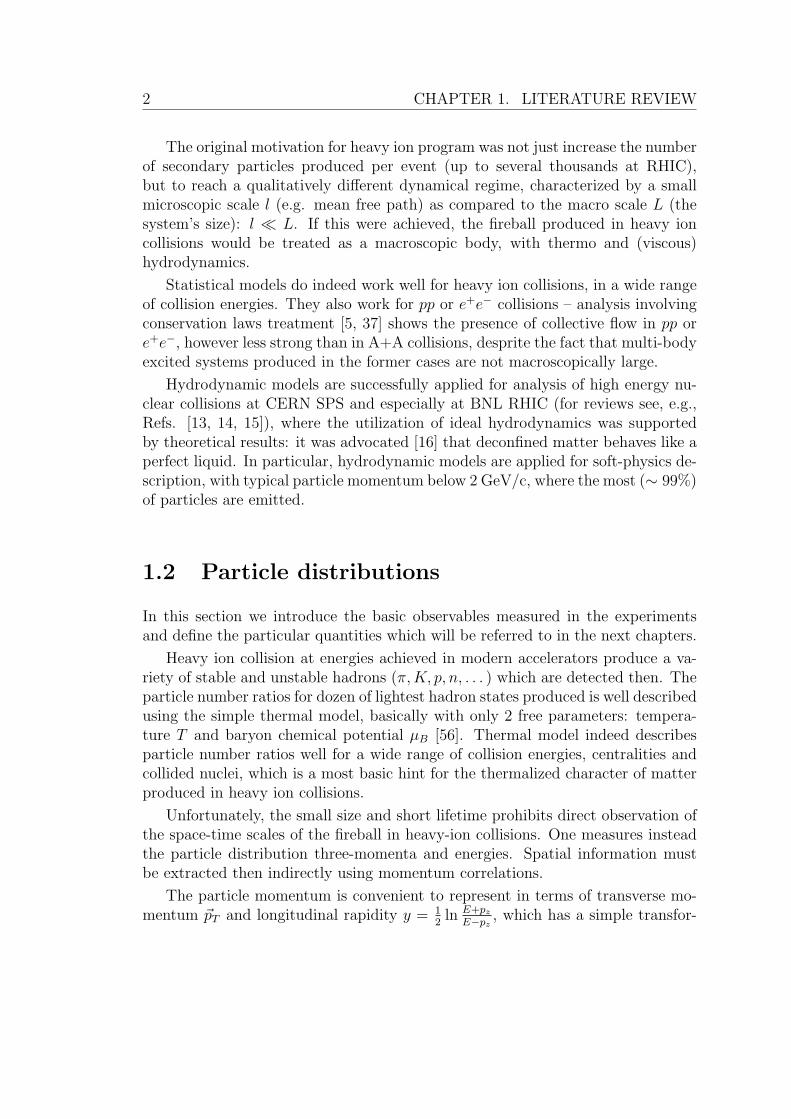
The original motivation for heavy ion program was not just increase the numberof secondary particles produced per event (up to several thousands at RHIC),but to reach a qualitatively different dynamical regime, characterized by a smallmicroscopic scale l (e.g. mean free path) as compared to the macro scale L (thesystem’s size): l � L. If this were achieved, the fireball produced in heavy ioncollisions would be treated as a macroscopic body, with thermo and (viscous)hydrodynamics.
Statistical models do indeed work well for heavy ion collisions, in a wide rangeof collision energies. They also work for pp or e+e− collisions – analysis involvingconservation laws treatment [5, 37] shows the presence of collective flow in pp ore+e−, however less strong than in A+A collisions, desprite the fact that multi-bodyexcited systems produced in the former cases are not macroscopically large.
Hydrodynamic models are successfully applied for analysis of high energy nu-clear collisions at CERN SPS and especially at BNL RHIC (for reviews see, e.g.,Refs. [13, 14, 15]), where the utilization of ideal hydrodynamics was supportedby theoretical results: it was advocated [16] that deconfined matter behaves like aperfect liquid. In particular, hydrodynamic models are applied for soft-physics de-scription, with typical particle momentum below 2 GeV/c, where the most (∼ 99%)of particles are emitted.
1.2 Particle distributions
In this section we introduce the basic observables measured in the experimentsand define the particular quantities which will be referred to in the next chapters.
Heavy ion collision at energies achieved in modern accelerators produce a va-riety of stable and unstable hadrons (π,K, p, n, . . . ) which are detected then. Theparticle number ratios for dozen of lightest hadron states produced is well describedusing the simple thermal model, basically with only 2 free parameters: tempera-ture T and baryon chemical potential µB [56]. Thermal model indeed describesparticle number ratios well for a wide range of collision energies, centralities andcollided nuclei, which is a most basic hint for the thermalized character of matterproduced in heavy ion collisions.
Unfortunately, the small size and short lifetime prohibits direct observation ofthe space-time scales of the fireball in heavy-ion collisions. One measures insteadthe particle distribution three-momenta and energies. Spatial information mustbe extracted then indirectly using momentum correlations.
The particle momentum is convenient to represent in terms of transverse mo-mentum ~pT and longitudinal rapidity y = 1
2ln E+pz
E−pz, which has a simple transfor-
1.2. PARTICLE DISTRIBUTIONS 3
mational properties under the Lorentz transformations (boosts) in z direction.
p0d3ni
d3~pi
=d3ni
d2~pTdy(1.1)
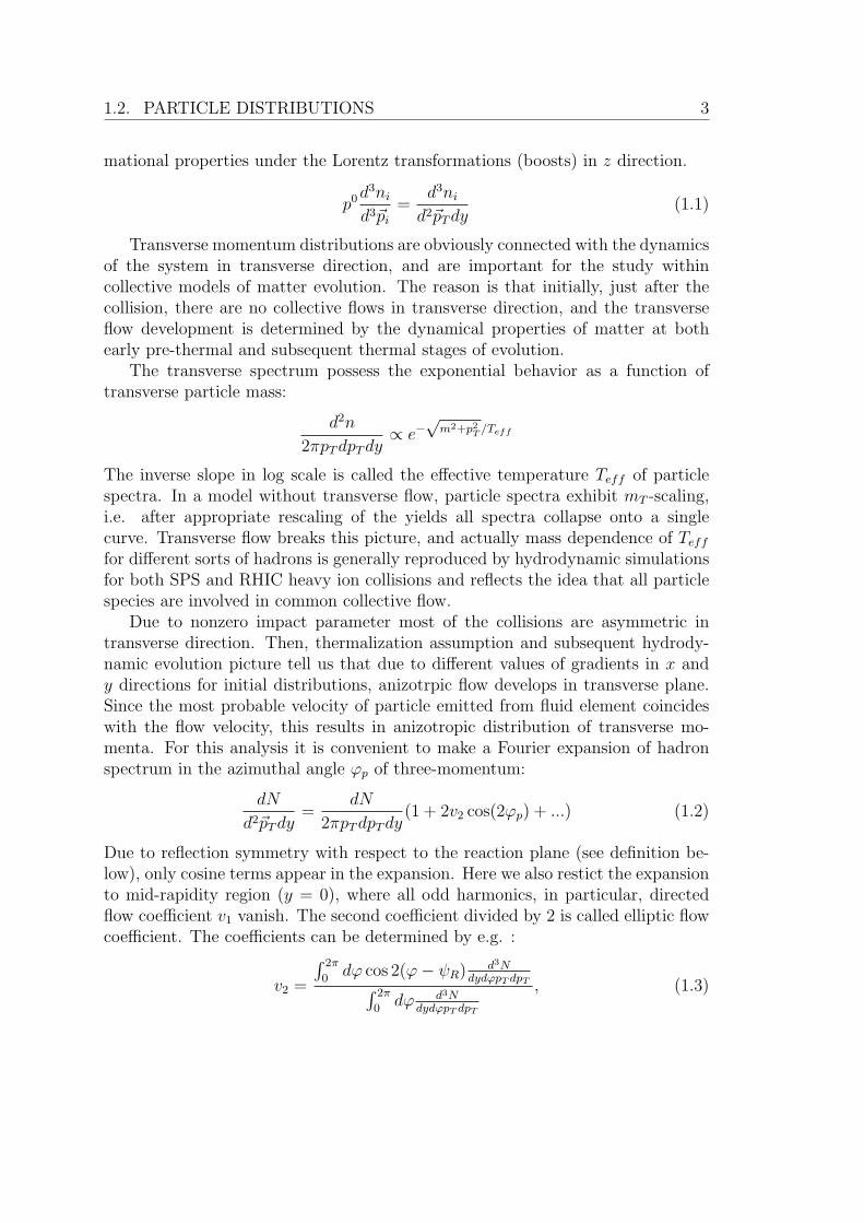
Transverse momentum distributions are obviously connected with the dynamicsof the system in transverse direction, and are important for the study withincollective models of matter evolution. The reason is that initially, just after thecollision, there are no collective flows in transverse direction, and the transverseflow development is determined by the dynamical properties of matter at bothearly pre-thermal and subsequent thermal stages of evolution.
The transverse spectrum possess the exponential behavior as a function oftransverse particle mass:
d2n
2πpTdpTdy∝ e−
√m2+p2
T /Teff
The inverse slope in log scale is called the effective temperature Teff of particlespectra. In a model without transverse flow, particle spectra exhibit mT -scaling,i.e. after appropriate rescaling of the yields all spectra collapse onto a singlecurve. Transverse flow breaks this picture, and actually mass dependence of Teff
for different sorts of hadrons is generally reproduced by hydrodynamic simulationsfor both SPS and RHIC heavy ion collisions and reflects the idea that all particlespecies are involved in common collective flow.
Due to nonzero impact parameter most of the collisions are asymmetric intransverse direction. Then, thermalization assumption and subsequent hydrody-namic evolution picture tell us that due to different values of gradients in x andy directions for initial distributions, anizotrpic flow develops in transverse plane.Since the most probable velocity of particle emitted from fluid element coincideswith the flow velocity, this results in anizotropic distribution of transverse mo-menta. For this analysis it is convenient to make a Fourier expansion of hadronspectrum in the azimuthal angle ϕp of three-momentum:
dN
d2~pTdy=
dN
2πpTdpTdy(1 + 2v2 cos(2ϕp) + ...) (1.2)
Due to reflection symmetry with respect to the reaction plane (see definition be-low), only cosine terms appear in the expansion. Here we also restict the expansionto mid-rapidity region (y = 0), where all odd harmonics, in particular, directedflow coefficient v1 vanish. The second coefficient divided by 2 is called elliptic flowcoefficient. The coefficients can be determined by e.g. :
v2 =
∫ 2π
0dϕ cos 2(ϕ− ψR) d3N
dydϕpT dpT∫ 2π
0dϕ d3N
dydϕpT dpT
, (1.3)
4 CHAPTER 1. LITERATURE REVIEW
where ψR is so-called reaction plane angle. Reaction plane is defined as the planebuilt by the vectors of impact parameter of collision and z axis (collision axis)basis vector.
The elliptic flow coefficients v2 are measured for most abundant particle species: π±, K±, p, p, etc, and by the definition reflect the anisotropy of the transversemomentum distribution. One of the most spectacular features of the RHIC datais 50% bigger elliptic flow [81] compared to the observations at CERN SPS [17].The development of a strong flow is well described by the hydrodynamic modelsand is underestimated in transport models, which points to the essential propertyof strong interaction of matter created in RHIC collisions. It was argued thatelliptic flow description requires small thermalization time τ0 less than 1 fm/c,which defines the start of hydrodynamic expansion. Such fast thermalization ishard to prove theoretically. However, recent developments show that whereas theassumption of thermalization in relativistic A + A collisions is really crucial toexplain soft physics observables in general (and particularly v2), the hypotheses ofearly thermalization at times less than 1 fm/c is not necessary [6, 18].
1.3 Correlation functions
Another class of measurements in A+A collisions are two-particle correlations,measured primarily for pions, but also for kaons. The two-particle correlationfunction is defined as the ratio of Lorentz-invariant two-particle distribution tothe product of the two single particle distributions :
C(~p1, ~p2) =p0
1p02d
6n/d3~p1d3~p2
(p01d
3n/d3~p1) (p02d
3n/d3~p2)(1.4)
First in pp collisions at Bevatron, an enhancement of pion pairs at small rel-ative momenta (the ’GGLP-effect’), was found by G. Goldhaber, S. Goldhaber,W.Y. Lee and A. Pais [63] and explained in terms of the finite space-time extent ofthe decaying pp-system and Bose-Einstein statistics of the detected identical pions.Since the width of the correlation effect is related to the characteristic space-timeseparation of the pion emitters, the corresponding technique acquired the nameCorrelation femtoscopy. As noticed by G.I. Kopylov and M.I. Podgoretsky, a simi-lar though orthogonal effect exists in astrophysics and is the base of intensity inter-ferometry proposed by the radio astronomer Robert Hanbury Brown and RichardTwiss to measure the angular radii of distant stellar objects. They demonstrated[75] that photons in an apparently uncorrelated thermal beam tend to be detectedin close-by pairs. This photon bunching or HBT-effect, first explained theoreti-cally by Purcell [134]. Since the width of the space-time bunching (HBT) effect is
1.3. CORRELATION FUNCTIONS 5
related to the characteristic spread of the photon wave vectors (three-momenta),the corresponding technique acquired the name Correlation spectroscopy.
Basically, identical particles which sit nearby in phase-space experience quan-tum statistical effects resulting from the (anti)symmetrization of the multiparticlewave function. For bosons, therefore, the two-particle probability shows an en-hancement at small momentum difference between the particles.
The most direct connection between the measured two-particle correlations inmomentum space and the source distribution in coordinate space can be estab-lished if the particles are emitted independently (’chaotic source’) and propagatefreely from source to detector. Basically, particles with particular value of veloictyare emitted most probably from the region with the same value of collective flowvelocity, which gives the connection of momentum and coordinate correlation.
The two-particle correlator yields rms widths of the effective source of particleswith momentum p. In general, these width parameters do not characterize thetotal extension of the collision region. They rather measure the size of the systemthrough a filter of wavelength p. In the language introduced by Sinyukov [9] thissize is the local ’region of homogeneity’, the region from which particle pairs withmomentum K are most likely emitted. From the other hand, the local length ofhomogenity is defined by the behavior of the Wigner function : it means the lenghtwithin which the deviation of Wigner function is relatively small and is about thefunction value.
From the data of relativistic heavy-ion experiments, the two-particle correlatoris usually constructed as a ratio of two-particle distribution in samples of so-calledactual pairs and ’mixed’ pairs or reference pairs. One starts by selecting eventsfrom the primary data set. Actual pairs are pairs of particles that belong to thesame event. Reference pair partners are picked randomly from different eventswithin the set of events that yielded the actual pairs. The correlation function isthen constructed by taking the ratio, bin by bin, of the distribution DA of theseactual pairs with the distribution DR of the reference pairs [8, 12]
DA(∆q,∆K) =number of actual pairs in bin (∆q,∆K)
number of actual pairs in sample, (1.5)
DR(∆q,∆K) =number of reference pairs in bin (∆q,∆K)
number of reference pairs in sample, (1.6)
C(∆q,∆K) =DA(∆q,∆K)
DR(∆q,∆K). (1.7)
Momentum correlations between identical particles can originate not only fromquantum statistics but also from conservation laws and final state interactions.Energy-momentum conservation constrains the momentum distribution of pro-duced particles near the kinematical boundaries. In high multiplicity heavy-ion

6 CHAPTER 1. LITERATURE REVIEW
collisions its effects on two-particle correlations at low relative momenta are negligi-ble. Similarly, constraints from the conservation of quantum numbers (e.g. chargeor isospin) become less important with increasing event multiplicity. Strong corre-lations exist between the decay products of resonances, but since resonance decaysrarely lead to the production of identical particle pairs, they do not matter inpractice. This leaves final state interactions as the most important source of ad-ditional femtoscopic correlations. For the small relative momenta q < 100 MeVwhich are sampled in the two-particle correlator, effects of the strong interactionsare negligible for identical charged pions. For protons, however, they dominate thetwo-particle correlations. On the other hand, for pions, the long-range Coulombinteractions distort significantly the observed momentum correlations, dominatingover the Bose-Einstein effect for small relative momenta. The aim of Coulomb cor-rections is to modify the measured two-particle correlations in such a way that theresulting correlator contains only Bose-Einstein correlations, while the effects of fi-nal state interactions have been subtracted. For this, several simplified procedureshave been used in the literature. The effective method of subtraction of effects fromthe long-lived resonances and Coulomb final state interaction is Bowler-Sinyukovprocedure [10], now used by majority of experimental collaborations.
1.4 Evolution picture
From the dynamical point of view, a process of heavy ion collision at ultra-relativistic energies can be divided into several stages. The matter produced duringthe collision have different properties at different stages. So, one can distinguish:
• the initial conditions for the collision at τ < 0 are two nuclei approachingeach other with velocity v > 0.99999c (at RHIC).
• There are several microscopic models of initial, pre-equilibrium stage of col-lision:
– in Color Glass Condensate (CGC) approach, the initial state of collidingnuclei is described in terms of dense gluon walls, see Section 5.4.3;
– EPOS is a flux-tube approach, compatible with accelerator data forproton-proton, proton-nucleus collisions, and cosmic-ray data for airshower simulations (for more details, see Section 4.2).
In this very early pre-equilibrium stage, the primary collisions between fastpartons inside the colliding nuclei also generate “hard probes” with eitherlarge mass or large transverse momentum, such as heavy quark pairs (cc andbb), pre-equilibrium real or virtual photons, and very energetic quarks and

1.5. DYNAMIC MODELS 7
gluons with large transverse momentum (from which jets are formed afterhadronization).
As a result of initial stage, the matter is supposed to become locally ther-malized, thus forming the initial conditions for the next stage of evolution.The conventional thermalization time for v2 data reproduction is less than 1fm/c (at RHIC), however, recent developments show that hypothesis of earlythermalization at times less than 1 fm/c is not necessary [6, 18].
• The subsequent evolution of thermalized medium can be described using theequations of relativistic hydrodynamics. This approach allows one to accountfor the complicated evolution of the system at a preconfined stage and inthe vicinity of the possible phase transitions by means of a correspondingequation of state (EoS). The quesion concerning the viscosity coefficients isstill open.
• However, hydrodynamic picture implies the picture of continuous medium.Thus, hydrodynamic stage continues until the picture of the continuousmedium is destroyed. Roughly, it happens when the mean free path of par-ticles (connected with the rate of collisions) becomes comparable with thesmallest characteristic dimension of the system: its geometrical size or hy-drodynamic length. This condition determies the space-time region, wherehydrodynamic picture is applicable.
• The further expansion makes the system to be more and more rarefied, how-ever hadrons continue to interact, mostly via elastic scatterings. At this(kinteic) stage of evolution, the appropriate tools are cascade models. Cas-cade model studies show us that the tails of interactions (collisions) continueupto 50-100 fm/c. The decays of long-lived resonances happen much later.Finally, free particles propagate to detectors.
1.5 Dynamic models
To complete hydrodymanic model, particularly model based on ideal fluid approx-imation, one needs the initial conditions for hydrodynamic evolution, equation ofstate (which close the set of hydrodynamic equations), boundary conditions andthe criterion to stop hydrodynamic evolution (final conditions). The most clearpart is boundary conditions, which are usually taken to be non-reflective, whichcorresponds to the matter, expanding into vacuum. The rest of the conditionshave to be obtained from, e.g. microscopic models, which are external to hydro-dynamics.
8 CHAPTER 1. LITERATURE REVIEW
Evidently, the simplest receipt of final conditions for hydrodynamic evolutionis the Cooper-Frye prescription (CFp) [44] which ignores the post-hydrodynamic(kinetic) stage of matter evolution and assumes that perfect fluid hydrodynamicsis valid till some 3D hypersurface, e.g., as was supposed by Landau [1], till theisotherm T ' mπ, where sudden transition from local thermal equilibrium to freestreaming is assumed. This approach is extensively used in modern hydrodynam-ical models of evolution for A+A collisions.
Concerning final conditions and post-hydrodynamical stage treatment, differentscenarios have been used so far.
The most simple scenariois “Blast-wave” model, first appeared in the attemptto interpret RHIC data [11]. In such models, a parametrization of freeze-outhypersurface and velocity distribution on it, instead of preceding hydrodynamicevolution calculation, is used. More sophisticated blast-wave-type models areused to fit experimental data. Successful attempts to describe simultaneously themomentum-space measurements and the freeze-out coordinate-space data weredone in several models: “Kiev-Nantes” model [48], “Blast-Wave” parametriza-tions [37], “Buda-Lund” hydro-inspired approach [89]. Some parametrizations,e.g. [48] can be justified by the qualitative agreement with isotherms obtained inhydrodynamic calculations.
More sophisticated models treat the decays of resonances created at freeze-out hypersurface together with stable particles (e.g. THERMINATOR code in itsinitial form [87, 88], or FASTMC code [79, 80]). Freeze-out can be obtained fromhydrodynamic calculations or parametrized.
However, sharp freeze-out at some 3D hypersurfaces is a rather rough approx-imation of the spectrum formation, because the process of particle emission fromfireballs created in high energy heavy ion collisions is gradual in time. Results ofmany studies based on cascade models (see below) contradict the idea of suddenfreeze-out and demonstrate that in fact particles are emitted from the 4D vol-ume during the whole period of the system evolution, and deviations from localequilibrium conditioned by continuous emission should take place (see, e.g., [93]).Moreover, freeze-out hypersurfaces typically contain non-space-like parts that leadto a problem with energy-momentum conservation law in realistic dynamical mod-els [47].
To overcome the difficulties of Landau/Cooper-Frye prescription, one can simu-late matter dynamics at the late stages of system evolution by the means of kineticcodes which treat classical particle interactions with given cross-sections. The hy-drodynamic evolution should be coupled then to kinetic code at e.g. isotherm ofsufficiently low temperature, where hydrodynamic picture is destroyed (switchinghypersurface). At this hypersurface the continuous medium converses into the setof particles acording to the thermal distribution. Such “hybrid” scheme is imple-
1.6. OUTLINE OF THE THESIS 9
mented in a number of calculations, see e.g. [13, 14, 15]. However, the remarksconcerning non-space-like parts of switching hypersurface are applicable as well forhybrid models. Also in hybrid picture the initial conditions for hadronic cascadecalculations, formulated also on space-like part of hypersurface where, however,hadronic distributions deviate from the local equilibrium, in particular, because ofan opacity effect for hadrons which are created during a “mixed” stage of phasetransition. These nonequilibrium effects can seriously influence the results of hy-brid models in their modern form [201].
Generally, the realizations of hybrid scheme, desprite of its physical superiorityover the simple Cooper-Frye prescription, did not give a good description of two-particle correlation functions reflected in femtoscopic radii, being the measure ofspace-time scales of collision process.
Most exsisting calculations with hybrid models are still done using an unre-alistic equation-of-state with a first order phase transition, based on ideal gasesof quarks & gluons and hadrons. As shown later, it actually makes a big dif-ference using a realistic equation-of-state, which is for µB = 0 compatible withlattice results. In particular, HBT radii cannot be reproduced together with otherobservables using the EoS with first-order phase transition.
The calculations of [115, 116] manage to reproduce both particle yields andtransverse momentum spectra of pions, kaons, and protons within 30%, for pt
values below 1.5 GeV/c. The net baryon yield cannot be reproduced, since thecalculations are done for zero baryon chemical potential, another systematic prob-lem is due to a relatively small hadron set. A bigger hadron set will produceessentially more pions and will thus reduce for example the pion / kaon ratio.
The calculations [7, 190] reproduce simultaneously the pion, kaon and protontransverse momentum spectra, v2 and pion HBT radii. However, the value thevalue of chemical freeze-out temperature used is not compatible with the resultsfrom particle number ratios analysis. This also results in inability to describe theyields for massive hadrons (Λ,Ξ).
Some sophisticated hybrid models (e.g. AMPT [86]) reproduce the elliptic flowand the correlation radii but with different sets of model parameters. Only recentlythe results obtained from hydrodynamic model connected with THERMINATORafterburner, qualitatively describe HBT radii together with momentum spectraand anizotropy coefficient v2, however the parameters used are not physical.
1.6 Outline of the thesis
Thus, the aim of the present work is to construct dynamic model for A+A colli-sions, compartible with HBT measurements.
In the thesis, the results of this research are presented in a following order. In
10 CHAPTER 1. LITERATURE REVIEW
Chapter 2, new class of analytic solutions of the equations of relativistic hydrody-namics is presented, its possible applications to the dynamics of A+A collisionsare discussed. In Chapter 3, event generator, based on freeze-out hypersurfaceparametrization is constructed. As a continuation of research towards construc-tion of realistic dynamical model for A+A collisions, a hybrid dynamical model(initial state + hydrodynamics + cascade) is presented in Chapter 4. Finally, inChapter 5 the hydro-kinetic model is presented, as a combination of hydrodynamicand kinetic approaches.
CHAPTER
TWO
Hydrodyamic solutions
In this chapter, the new family of solutions of relativistic hydrodynamic equationsfor ideal fluid case is presented. In particular, solutions corresponding to ellip-soidally symmetric expansion of finite systems into vacuum are analyzed. Theproperties of the solution obtained, as well as possible applications to A+A colli-sions dynamics, are discussed.
2.1 Introduction
The equations of the relativistic hydrodynamics have highly nonlinear nature and,therefore, only a few analytical solutions are known until now. For the first timeone-dimensional, or (1+1), analytical solution for Landau initial conditions - hotpion gas in Lorentz contracted thin disk [1], has been obtained by Khalatnikov [19].The equation of state (EoS) was chosen as ultrarelativistic one: p = c20ε, c
20 = 1/3.
It is noteworthy that according to that solution the longitudinal flows developedto the end of hydrodynamic expansion, at freeze-out, are quasi-inertial: v ≈ xL/t.Much later, in the papers [20] the infinite (1+1) boost-invariant solution have beenfound for the same EoS. For finite systems the similar approach was developed inRef.[21]. The property of quasi-inertia preserves in these solutions during thewhole stage of the evolution. Bjorken [22] utilized these solutions as the basis ofthe hydrodynamic model for ultra-relativistic A+A collisions.
The spherically symmetric variant of such a kind of flows with the Hubble ve-locity distribution, v = r/t, has been considered in Ref. [23]. Some generalizationof these results was proposed in a case of the Hubble flow for EoS of massive gaswith conserved particle number in Ref.[24] and for the cylindrically symmetricboost-invariant expansion with a constant pressure in [25].
All these solutions were used for an analysis of ultra-relativistic heavy ion col-
11
12 CHAPTER 2. HYDRODYAMIC SOLUTIONS
lisions. Since the longitudinal boost-invariance in a fairly wide rapidity region isnot observed even at RHIC, as it was expected, the Hubble-like models are alsoused now for a description of the experimental data [26]. It is natural, however,that unlike to the Hubble type flows, the velocity gradients should be different indifferent directions since there is an initial asymmetry between longitudinal andtransverse directions in central A+A collisions and, in addition, between in-planeand off-plane transverse ones in non-central collisions. In this letter we make ageneral analysis of the hydrodynamic equations for the quasi-inertial flows aimingto find a new class of analytical solutions with 3D asymmetric relativistic flows.
2.2 General analysis
Let us start from the equations of relativistic hydrodynamics:
∂νTµν = 0, (2.1)
where the energy-momentum tensor corresponds to a perfect fluid:
T µν = (ε+ p)uµuν − p · gµν (2.2)
We can attempt to find a particular class of solutions and therefore have to makesome simplifications of (2.1). We do not fix EoS at this stage.
• Let us put the condition of quasi-inertiality
uν∂νuµ = 0 (2.3)
which means that flow is accelerationless in the rest systems of each fluidelement; this property holds for the known Bjorken (boost-invariant) andHubble flows.
Then, we find that uµ[(ε + p)∂νuν + uν∂νε] + [uµuν∂νp − ∂µp] = 0. Contracting
this equation with uµ we get
(ε+ p)∂νuν + uν∂νε = 0. (2.4)
Obviously, the remaining equation to satisfy is:
uµuν∂νp− ∂µp = 0 (2.5)
The task is to find solution of the system (2.3),(2.4) and (2.5). As one can see,the number of equations exceeds the number of independent variables. So, theequations must be self-consistent in order to have nontrivial solutions.
2.3. GRADIENT-LIKE VELOCITY ANSATZ 13
We see that Eq.(2.4) can be rewritten in the form:
uµ∂µε = −F (ε)(∂νuν) (2.6)
where F (ε) = ε+ p, and Eq.(2.5) as the following:
p′(ε)(uµuν∂νε− ∂µε) = 0, (2.7)
supposing EoS in the form p = p(ε). If p′(ε) 6= 0
uµF (ε)(∂νuν) + ∂µε = 0. (2.8)
Normally F (ε) 6= 0, and we can divide the last equation by F (ε) and introducethe function Φ(ε) by the definition 1
ε+p(ε)= Φ′(ε), so that
∂µΦ(ε) = −uµ(∂νuν) (2.9)
Then, the conditions of consistency of equations (2.4) and (2.5) can be writtenas:
∂λ(uµ∂νuν) = ∂µ(uλ∂νu
ν) (2.10)
In general case, there are 6 independent equations.Finally, the relativistic hydrodynamics of quasi-inertial flows is described by the
equations (2.3) and (2.10) for the hydrodynamic velocities uµ, and the equations(2.9) for the energy density: one should use derivative 1
ε+p(ε)= Φ′(ε) at any EoS
p = p(ε) to find function ε(x). A serious problem is, however, to find non-trivialsolutions for the field uµ(x) of hydrodynamic 4-velocities.
2.3 Gradient-like velocity ansatz
One can try to satisfy to Eqs. (2.3),(2.10) for velocity profile by a use of gradient-like representation for it, namely,
uµ = ∂µφ. (2.11)
with condition of normalization, uµuµ = 1:
∂µφ∂µφ = 1 (2.12)
Then one can check that (2.3) is satisfied automatically, and (2.10) leads to:
∂λ(∂µφ · �φ) = ∂µ(∂λφ · �φ) (2.13)
Thus, gradient-like velocity ansatz (2.11) reduce the problem to equations (2.12),(2.13).

14 CHAPTER 2. HYDRODYAMIC SOLUTIONS
One can see that the above equation can be, in particular, reduced to:
�φ = F (φ) (2.14)
with any real function F that have to be solved together with (2.12). Note that ifF (φ) = a+ bφ then (2.14) is the linear inhomogeneous partial differential equation(PDE) and its any solution is a partial solution φih of inhomogeneous PDE, plusgeneral solution φh of correspondent homogenous PDE (if b 6= 0):
φih ∼ (t2 − x2), b = 0φih ∼ −a
b, b 6= 0
(2.15)
and
φh =
∫d4pδ(p2 − b)f(p)eipx (2.16)
where f(p) is arbitrary function with properties f ∗(k) = f(−k). Then the problemis reduced to a solution of the nonlinear integral equation (2.12) for f(p). Ifa = b = 0, the only potential φ = c+c0t+
∑cixi (i = 1, 2, 3) with the constrain on
the constants cν : c20 −∑c2i = 1 satisfies these equations. It describes a relativistic
motion of a medium as a whole. It is an open problem whether there are analyticalsolutions at a 6= 0 and/or b 6= 0.
The known quasi-inertial solutions correspond to F (φ) = n/φ in Eq.(2.14).The value n = 1 generates gradient ansatz φ =
√t2 − z2 that gives the (1+1)
boost-invariant Bjorken expansion along axis z, v = z/t; n = 2 leads to φ =√t2 − x2 − y2, and, correspondingly, to the two-dimensional (1+2) Hubble-like
flow with cylindrical symmetry; at n = 3 one can get solution of (2.14) for φ inthe form φ = τ
.=
√t2 − x2 − y2 − z2 describing spherically symmetric Hubble
flow uµ = xµ/τ . The equation (2.9) has the form ∂µΦ(ε) = nxµ/τ 2 where numberof space coordinates is equal to n. Then the energy density is described by thefollowing expression
ε(τ)∫ε(τ0)
dε
ε+ p(ε)= ln(
τ0τ
)n. (2.17)
2.4 Relativistic ellipsoidal solutions
One more possibility to satisfy to Eqs. (2.5) or (2.7) besides of the gradient-likeflows is to suppose a constant pressure in the EoS: p′(ε) = const. This possibilitywas first used in [25] as physically corresponding to a thermodynamic state of thesystem in the softest point with the velocity of sound c2s = 0. Such a state could beassociated with the first order phase transition. In A+A collisions it corresponds,
2.4. RELATIVISTIC ELLIPSOIDAL SOLUTIONS 15
probably, to transition between hadron and quark-gluon matter at SPS energies.The solution proposed in [25] has the cylindrical symmetry in the transverse planeand the longitudinal boost invariance:
uµ = γ(t
τ, vx
r, vy
r,z
τ), (2.18)
where τ =√t2 − z2, γ = (1 − v2)−1/2 and r is transverse radius, r =
√x2 + y2,
v =α
1 + ατr (2.19)
describes axially symmetric transverse flow.The above solution has, however, a limited region of applicability since the
boost invariance is not expected at SPS energies and can be used only in a smallmid-rapidity interval [27], it is not reached even at RHIC energies [28]. Mostimportant, however, is that in non-central collisions there is no axial symmetryand, therefore, one needs transversely asymmetric solutions to describe the ellipticflows in these collisions, e.g., v2 coefficients. Now we propose a new class of analyticsolutions of the relativistic hydrodynamics for 3D asymmetric flows.
First we construct the ansatz for normalized 4-velocity:
uµ = { t√t2 −
∑a2
i (t)x2i
,ak(t)xk√
t2 −∑a2
i (t)x2i
} (2.20)
where the Latin indexes denote spatial coordinates and ai are functions of timeonly. In this case a set of nonequal ai induces 3D elliptic flow with velocitiesvi = ai(t)xi/t: at any time t the absolute value of velocity is constant, v2 = const,at an ellipsoidal surface
∑a2
ix2i = const. Note that this solution is not gradient-
like, so we follow in a specific way the analysis starting from (2.3).The condition (2.3) of accelerationless in this case is reduced to the ordinary
differential equation (ODE) for the functions ai(t):
dai
dt=ai − a2
i
t, (2.21)
the general solution of which is:
ai(t) =t
t+ Ti
, (2.22)
where Ti is some set of 3 parameters (integration constants) having the dimensionof time. The different values T1, T2 and T3 result in anisotropic 3D expansion withthe ellipsoidal flows.
16 CHAPTER 2. HYDRODYAMIC SOLUTIONS
The equation (2.5) is satisfied since we assume the constant pressure profile:p = p0 = const. The next step is to find solution of Eq. (2.4) for energy densityε. Taking into account that ∂µu
µ =∑ai/τ , where
τ =√t2 −
∑a2
ix2i , (2.23)
one can get
(ε+ p0)∑
i
ai(t) + t∂tε+∑
i
ai(t)xi∂iε = 0. (2.24)
General solution of the equation is
ε+ p0 =Fε(
x1
t+T1, x2
t+T2, x3
t+T3)
(t+ T1)(t+ T2)(t+ T3)(2.25)
where Fε is an arbitrary function of its variables. If one fixes the parametersTi that define the velocity profile, then the function Fε is completely determinedby the initial conditions for the enthalpy profile, say, at the initial time t = 0:ε(t = 0,x) + p0 = Fε(
x1
T1, x2
T2, x3
T3)/T1T2T3.
If some value, associated with a quantum number or with particle number ina case of chemically frozen evolution is conserved [27] then one should add thecorresponding equation to the basic ones. Such an equation has the standard form[29]:
n∂νuν + uµ∂µn = 0 (2.26)
where n is associated with density of the correspondent conserved value, e.g., withthe baryon or particle densities. A general structure of this equation is similar towhat Eq. (2.24) has and, therefore, the solution looks like as (2.25):
n =Fn( x1
t+T1, x2
t+T2, x3
t+T3)
(t+ T1)(t+ T2)(t+ T3)(2.27)
where the function Fn is an arbitrary function of its arguments and can be fixed bythe initial conditions for (particle) density n: n(t = 0,x)T1T2T3 = Fn(x1
T1, x2
T2, x3
T3).
To establish a behavior of other thermodynamic values we use link betweendifferent thermodynamic potentials ε = Ts−p+µn and utilize the thermodynamicequations based on the free energy density f(n, T ) = ε − Ts = µn − p. Sincethe volume is fixed (it is unit) the free energy depends on T and n only, df =−sdT + µdn, and the chemical potential µ = f,n|T=const and the entropy densitys = −f,T |n=const.
In a case of chemically equilibrated expansion of the ultrarelativistic gas whenthe particle number is uncertain and is defined by the conditions and parameters ofthe thermodynamic equilibrium, e.g., by the temperature T , the chemical potential
2.5. GENERALIZATION OF THE HUBBLE-LIKE FLOWS 17
µ ≡ 0 (we suppose here that there are no other conserved values associated withcharges, or the corresponding chemical potentials are zero or close to zero). Thenf = −p0 = const, df = −sdT = 0 that means the temperature T = const for sucha system and the entropy s = (ε(t,x) + p0)/T where ε(t, x) is defined by (2.25).
If chemically frozen evolution takes place, the chemical potential associatedwith conserved particle number is not zero and describes the deviation fromchemical equilibrium in relativistic systems. The solution of differential equationnf,n|T=const − p0 = f(n, T ) is f(n, T ) = nc(T )− p0, where c(T ) is some function ofthe temperature. Then it follows directly from the thermodynamic identities that
ε(t,x) + p0 = n(t,x)(c(T ) − Tc′(T )) (2.28)
Since the structures of general solutions for n and ε are found as (2.25) and (2.27),the temperature profile has the form
T (t,x) = FT (x1
t+ T1
,x2
t+ T2
,x3
t+ T3
) (2.29)
where FT is some function of its arguments that is defined by the initial conditionsfor ε and n and also by EoS ε = ε(n, T ). The latter can be fixed by a choice of thefunction c(T ) in Eq. (2.28). If the initial enthalpy density profile is proportionalto the particle density profile, Fn(x1
T1, x2
T2, x3
T3) ∼ Fε(
x1
T1, x2
T2, x3
T3), then T = const (and
so µ = c(T ) = const) during the system’s evolution for any function c(T ) exceptthe linear one: c(T ) = a − bT when T is not defined by the equation (2.28). Inthe last case n = (ε+ p0)/a, s = bn. In another particular case which correspondsto EoS ε+ p0 = anT with c(T ) = −aT ln(bT ) one can get:
T (t,x) = (ε+ p0)/(an), s(t,x) = an(ln(bT ) + 1) (2.30)
2.5 Generalization of the Hubble-like flows
Let us describe some important particular solutions of the equations for relativis-tic ellipsoidal flows. If one defines the initial conditions on the hypersurface ofconstant time, say t = 0, then t is a natural parameter of the evolution. Such arepresentation of the solutions similar to the Bjorken and Hubble ones with ve-locity field vi = aixi/t has property of an infinite velocity increase at x → ∞.A real fluid, therefore, can occupy only the space-time region where |v| < 1, orτ 2 > 0. To guarantee the energy-momentum conservation of the system duringthe evolution, all thermodynamic densities have to be zero at the boundary of thephysical region, otherwise one should consider the boundary as the massive shell[21]. Hence in the standard hydrodynamic approach the enthalpy and particledensity must be zero at the surface defined by |v(t,x)| = 1 at any time t. A
18 CHAPTER 2. HYDRODYAMIC SOLUTIONS
simple form of such a solution (for the case of particle number conservation) can
be obtained from (2.25),(2.27) choosing Fε,n ∼ exp(−b2ε t2
eτ2
):
ε(t) + p0 =Cε∏
i(t+ Ti)exp
(−b2ε
t2
τ 2
), (2.31)
n =Cn∏
i(t+ Ti)exp
(−b2n
t2
τ 2
)(2.32)
where τ is defined by (2.23), and the constants Cε, Cn, bε and bn are determinedby the initial conditions as described in the previous section. As one can see,the enthalpy density tends to zero when |x| becomes fairly large approaching theboundary surface defined by |v(t,x)| = 1, in other words, when τ → 0. Thusthe physically inconsistent situation when massive fluid elements move with thevelocity of light at the surface τ = 0 is avoided. Of course, in such a solution theconstant pressure should vanish, p0 = 0.
As it follows from the analysis of a behavior of the thermodynamic values inthe previous section, the temperature is constant if bε = bn, otherwise one canchoose the temperature approaching zero at the system’s boundary, e.g., for EoSwhich is linear in temperature, the latter has the form
T = const bε = bn
(2.33)
T ∼ e−(b2ε−b2n) t2
τ2 → 0, |v(x)| → 1 bε > bn
according to (2.30).
Note that in the region of non-relativistic velocities, v2 =∑ a2
i x2i
t2� 1 the space
distributions of the thermodynamical quantities (2.31),(2.32) have the Gaussianprofile:
ε+ p0 ' CεQ
i(t+Ti)e−b2ε
P
a2i
x2i
t2 , (2.34)
n ' CnQ
i(t+Ti)e−b2n
P
a2i
x2i
t2
The forms of solutions (2.34) are similar to what was found in Ref. [30] as theelliptic solutions of the non-relativistic hydrodynamics equations. In this sense thesolution proposed could be considered as the generalization (at vanishing pressure)of the corresponding non-relativistic solutions allowing one to describe relativisticexpansion of the finite system into vacuum.
One can note that the case of equal flow parameters Ti = 0 and bε = bn = 0induces formally Hubble-like velocity profile with the behavior of the density andenthalpy similar to (2.17) at n=3, p = p0, and with the substitution τ → t.
2.5. GENERALIZATION OF THE HUBBLE-LIKE FLOWS 19
The direct physical generalization of the Hubble solution for asymmetric caseshould be associated with the hypersurfaces of the pseudo-proper time τ rather
than with time t, that eliminates the problem of infinite velocities: v2 =∑ a2
i x2i
t2< 1
at any hypersurface τ 2 = const > 0. It can be reached if one chooses the functionsFε and Fn in (2.25), (2.27) in the form
F ∼(t
τ
)3
. (2.35)
Then the generalized Hubble solution is
uµ = { tτ,a1x
1
τ,a2x
2
τ,a3x
3
τ},
ε+ p0 = Cεa1a2a3
τ 3, (2.36)
n = Cna1a2a3
τ 3
where τ =√t2 −
∑a2
ix2i , ai ≡ ai(t) = t/(t + Ti) and constants are: Cε =
T1T2T3(ε(0,0) + p0), Cn = T1T2T3n(0,0). Again, the proportionality between εand n results in the temperature to be a constant during the evolution. If allparameters Ti are equal to each other, then ai are also equal and solution (2.36)just corresponds to spherically symmetric Hubble flow (at constant pressure) andτ is the proper time of fluid element, τ = τ . Note that comparing to the standardrepresentation of the Hubble solution the origin of a time scale is shifted, t→ t+Ti,and therefore the singularity at t = 0 is absent. Thus, if this solution is applied toa description of heavy ion collision, Ti should be interpreted as the initial propertime of thermalization and hydrodynamic expansion to which the origin of a timescale is shifted, typically τ0 = Ti ' 1fm/c. As to a general case of an asymmetricexpansion, the minimal parameter Ti can be considered as the initial time t (atx = 0) of the beginning of the hydrodynamic evolution. In analogy with theHubble flow the initial conditions in asymmetric case (2.36) can be ascribed to thehypersurface σ : τ = const so that tσ(x = 0) = 0. Note, that such a hypersurfaceat |x| → ∞ tends to the hyperbolical hypersurface τ = const since tσ(x) → ∞ inthis limit and so all ai → 1.
The boost-invariant (1+1) solutions are also contained in general ellipsoidalsolutions (2.25),(2.27) for quasi-inertial flow. To get it one has to choose functionsFε and Fn in the form (2.35) with another power: 3 → 1; it leads to the same formof solution as (2.36) with replacement τ 3 → τ 1. The next step is to suppress thetransverse flow by setting T1 → ∞, T2 → ∞ (as usual, x1 and x2 denote coordinatesin the transverse plane and x3 is the longitudinal one), while the parameter T3 isfinite. This limit approach gives us a1 = a2 = 0 and τ → τ =
√(t+ T3)2 − x2
3
20 CHAPTER 2. HYDRODYAMIC SOLUTIONS
and results directly in the Bjorken solution at T3 = 0. Since Ti is a shift of a timescale to the beginning of hydrodynamic expansion, it is natural to consider T3 6= 0as this was discussed above for the Hubble-like solution. This value transforms asT3 → T ′
3 = T3/γ at Lorentz boosts along axis x3.Note, that if one does not change the power 3 → 1 in (2.35) and proceeds to the
limit directly in the equation (2.36), the particle density (and enthalpy) behaviorwill differ from the boost-invariant one as the following:
n ∼ τ−1 → n ∼ τ−1
(1 − x2
3
(t+ T3)2
)−1
(2.37)
It is also the solution of (1+1) relativistic hydrodynamics at p = const but itobviously violates the boost-invariance: the particle and energy densities are notconstant at any hypersurface and their analytic forms are changed in new coordi-nates after Lorentz boosts.
It is worthily to emphasize that the physical solutions with non-zero constantpressure have a limited region of applicability in time-like direction: if one wants tocontinue the solutions to asymptotically large times, then (ε + p0)t→∞ ≈ C
t3→ 0,
and this results in non-physical asymptotical behavior ε → −p0, unless we setp0 = 0. Therefore, it is natural to utilize such kind of solutions in a region of thefirst order phase transition, characterized by the constant temperature and softEoS, c2s = ∂p/∂ε ≈ 0, or at the final stage of the evolution that always correspondsto the quasi-inertial flows.
2.6 Conclusions
In this chapter, a general analysis of quasi-inertial flows in the relativistic hydro-dynamics is done. The known analytical solutions, like the Hubble and Bjorkenones, are reproduced based on the developed approach. A new class of analyticsolutions for 3D relativistic expansion with anisotropic flows is found. The ellip-soidal generalization of the spherically symmetric Hubble flow is considered withinthis class. These solutions can also describe the relativistic expansion of the finitesystems into vacuum.
Specific equation of state makes the application to the whole hydrodynamicstage of evolution in heavy ion collisions to be problematic. However, the solutionscan still be applicable during deconfinement phase transition and the final stage ofevolution of hadron systems. Also, the solutions can serve as a test for numericalcodes describing 3D asymmetric flows in the relativistic hydrodynamics.
CHAPTER
THREE
Fast MC freeze-out generator
In this chapter the Monte-Carlo event generator, which simulates the final (freeze-out) stage of heavy ion collision, is presented. For comparison with other modelsand experimental data the results based on the standard parameterizations ofthe hadron freeze-out hypersurface and flow velocity profile are shown. Also, thehadron generation procedure is extended for the case of noncentral A+A collisions,and includes different chemical and thermal freeze-outs. In this event generator,we reach simultaneous description of single-particle pT spectra for pions, kaonsand protons and pion interferometry radii. The analysis of parameters, leading tosuch description, is important for building true dynamical models, like presentedin the next chapters.
3.1 Introduction
Ongoing and planned experimental studies of relativistic heavy ion collisions ina wide range of beam energies require a development of new event generatorsand improvement of the existing ones [31]. Especially for Large Hadron Collider(LHC) experiments, because of very high hadron multiplicities, one needs fairlyfast Monte-Carlo (MC) generators for event simulation.
A successful but oversimplified attempt of creating a fast hadron generatormotivated by hydrodynamics was done in Ref. [32, 33, 34, 35]. The present workis an extension of this approach. We formulate a fast MC procedure to generatehadron multiplicities, four-momenta and four-coordinates for any kind of freeze-out hypersurface. Decays of hadronic resonances are taken into account. Weconsider hadrons consisting of light u,d and s quarks only, but the extension toheavier quarks is possible. The generator code is written in the object-orientedC++ language under the ROOT framework [36].
21
22 CHAPTER 3. FAST MC FREEZE-OUT GENERATOR
In this chapter we discuss both central and non-central collisions of nuclei us-ing the Bjorken-like and Hubble-like freeze-out parameterizations used in so-called”blast wave” [37] and ”Cracow” models [38], respectively. The same parametriza-tions have been used in the hadron generator referred as THERMINATOR [87]that appears however less efficient than our generator (see sections 3.2, 3.6).
This section is now organized as follows. Subsections 3.2-3.5 are devoted tothe description of the physical framework of the model. In Subsection 3.6, theMonte Carlo simulation procedure is formulated. The validation of this procedureis presented in Subsection 3.7. In Subsection 3.8, the example calculations arecompared with the Relativistic Heavy Ion Collider (RHIC) experimental data. Themodel extensions to non-central collisions and to different chemical and thermalfreeze-outs are presented in Subsections 3.9, 3.10, with the results presented in3.11. We summarize and conclude in Subsection 3.12.
3.2 Hadron multiplicities
We give here the basic formulae for the calculation of particle multiplicities. Weconsider the hadronic matter created in heavy-ion collisions as a hydrodynamicallyexpanding fireball with the equation of state of an ideal hadron gas.
The mean number Ni of particles species i crossing the space-like freeze-outhypersurface σ(x) in Minkowski space can be computed as [39]
Ni =
∫σ(x)
d3σµ(x)jµi (x). (3.1)
Here the four-vector d3σµ(x) = nµ(x)d3σ(x) is the element of the freeze-out hy-persurface directed along the hypersurface normal unit four-vector nµ(x) with apositively defined zero component (n0(x) > 0) and d3σ(x) = |d3σµd
3σµ|1/2 is theinvariant measure of this element. The normal to the space-like hypersurface istime-like, i.e. nµnµ = 1; generally, for hypersurfaces including non-space-like sec-tors, the normal can also be a space-like so then nµnµ = −1. The four-vector jµ
i (x)is the current of particle species i determined as:
jµi (x) =
∫d3~p
p0pµfi(x, p), (3.2)
where fi(x, p) is the Lorentz invariant distribution function of particle freeze-outfour-coordinate x = {x0, ~x} and four-momentum p = {p0, ~p}. In the case of localequilibrium
fi(x, p) = f eqi (p·u(x);T (x), µ(x)) =
1
(2π)3
gi
exp ([p · u(x) − µi(x)]/T (x)) ± 1, (3.3)
3.2. HADRON MULTIPLICITIES 23
where p · u ≡ pµuµ, gi = 2Ji + 1 is the spin degeneracy factor, T (x) and µi(x)are the local temperature and chemical potential respectively, u(x) = γ{1, ~v} isthe local collective four-velocity, γ = (1 − v2)−1/2, uµuµ = 1. The signs ± in thedenominator account for the proper quantum statistics of a fermion or a boson,respectively.
The Lorentz scalar local particle density is defined as:
ρi(x) = uµ(x)jµi (x) =
∫d3~p
p0pµu
µ(x)fi(x, p). (3.4)
For a system in local thermal equilibrium, the particle density in the fluid elementrest frame, where u∗µ = {1, 0, 0, 0}, is solely determined by the local temperatureT (x∗) and chemical potential µi(x
∗) for each particle species i:
ρeqi (T (x∗), µi(x
∗)) = u∗µjeqµi (x∗) =
∫d3~p ∗f eq
i (p∗0;T (x∗), µi(x∗)); (3.5)
the four-vectors in fluid element rest frames are denoted by star.In the case of local equilibrium, the particle current is proportional to the fluid
element four-velocity: jeqµi (x) = ρeq
i (T (x), µi(x))uµ(x). So the mean number of
particles of species i is expressed directly through the equilibrated density:
Ni =
∫σ(x)
d3σµ(x)uµ(x)ρeqi (T (x), µi(x)). (3.6)
In the case of constant temperature and chemical potential, T (x) = T andµi(x) = µi, one has
Ni = ρeqi (T, µi)
∫σ(x)
d3σµ(x)uµ(x) = ρeqi (T, µi)Veff , (3.7)
i.e. the total yield of particle species i is determined by the freeze-out temperatureT , chemical potential µi and by the total co-moving volume Veff , so called effectivevolume of particle production which is a functional of the field of collective veloc-ities uµ(x) on the hypersurface σ(x). The effective volume absorbs the collectivevelocity profile and the form of hypersurface and cancels out in all particle num-ber ratios. Therefore, the particle number ratios do not depend on the freeze-outdetails as long as the local thermodynamic parameters are independent of x. Theconcept of the effective volume and factorization property similar to Eq. (3.7) hasbeen considered first in Ref. [40], repeatedly used for the analysis of particle num-ber ratios (see, e.g., Ref. [27]) and recently generalized for a study of the averagedphase space densities [41] and entropy [42]. One can apply this concept also in alimited rapidity window [40, 41, 42].
24 CHAPTER 3. FAST MC FREEZE-OUT GENERATOR
The concept of the effective volume can be applied to calculate the hadroniccomposition at both chemical and thermal freeze-outs [27]. At the former one,which happens soon after hadronization, the chemically equilibrated hadronic com-position is assumed to be established and frozen in further evolution. The chemicalpotential µi for any particle species i at the chemical freeze-out is entirely deter-mined by chemical potentials µq per a unit charge, i.e. per unit baryon numberB, strangeness S, electric charge Q, charm C, etc. It can be expressed as a scalarproduct:
µi = ~qi~µ, (3.8)
where ~qi = {Bi, Si, Qi, Ci, ...} and ~µ = {µB, µS, µQ, µC , ..}. Assuming constanttemperature and chemical potentials on the chemical freeze-out hypersurface, thetotal quantum numbers ~q = {B,S,Q,C, ...} of the selected thermal part of pro-duced hadronic system (e.g., in a rapidity interval near y = 0) with correspondingVeff can be calculated as ~q = Veff
∑i ρ
eqi ~qi. For example:
B = Veff
n∑i=1
ρeqi (T, µi)Bi, (3.9)
S = Veff
n∑i=1
ρeqi (T, µi)Si, (3.10)
Q = Veff
n∑i=1
ρeqi (T, µi)Qi. (3.11)
The potentials µq are not independent. Thus, taking into account baryon, strangenessand electrical charges only and fixing the total strangeness S and the total elec-tric charge Q, µS and µQ can be expressed through baryonic potential µB usingEqs. (3.10) and (3.11). Therefore the mean numbers of each particle and reso-nance species at chemical freeze-out are determined solely by the temperature Tand baryonic chemical potential µB.
In practical calculations, we use the phenomenological observation [43] thatparticle yields in central Au+Au or Pb+Pb collisions in a wide center-of-massenergy range
√sNN = 2.2− 200 GeV can be described within the thermal statisti-
cal approach using the following parametrizations of the temperature and baryonchemical potential [43]:
T (µB) = a− bµ2B − cµ4
B, (3.12)
µB(√sNN) =
d
1 + e√sNN
, (3.13)

3.3. HADRON MOMENTUM DISTRIBUTIONS 25
a = 0.166 ± 0.002 GeV, b = 0.139 ± 0.016 GeV−1, c = 0.053 ± 0.021 GeV−3 andd = 1.308 ± 0.028 GeV, e = 0.273 ± 0.008 GeV−1.
In practical calculations we determine all macroscopic characteristics of a par-ticle system with the temperature T and chemical potentials µi via a set of equi-librium distribution functions in the fluid element rest frame:
f eqi (p∗0;T, µi) =
1
(2π)3
gi
exp ([p∗0 − µi]/T ) ± 1. (3.14)
Eq. (3.5) for the particle number density then reduces to
ρeqi (T, µi) = 4π
∫ ∞
0
dp∗p∗2f eqi (p∗0;T, µi). (3.15)
Using the expansion
f eqi (p∗0;T, µi) =
gi
(2π)3
∞∑k=1
(∓)k+1 exp(kµi − p∗0i
T), (3.16)
the density can be represented in a form of a fast converging series:
ρeqi (T, µi) =
gi
2π2m2
iT
∞∑k=1
(∓)k+1
kexp(
kµi
T)K2(
kmi
T), (3.17)
where K2 is the modified Bessel function of the second order.We assume that the calculated mean particle numbers Ni = ρeq
i Veff correspondto a grand canonical ensemble. The probability that the ensemble consists of Ni
particles is thus given by Poisson distribution:
P (Ni) = exp (−Ni)(Ni)
Ni
Ni!. (3.18)
3.3 Hadron momentum distributions
We suppose that a hydrodynamic expansion of the fireball ends by a sudden systembreakup at given temperature and chemical potentials. In this case the momentumdistribution of the produced hadrons keeps the thermal character of the equilibriumdistribution (3.3). Similar to Eqs. (3.1), (3.2), this distribution is then calculatedaccording to the Cooper-Frye formula [44]:
p0d3Ni
d3p=
∫σ(x)
d3σµ(x)pµf eqi (p · u(x);T, µi). (3.19)
26 CHAPTER 3. FAST MC FREEZE-OUT GENERATOR
The integral in Eq. (3.19) can be calculated with the help of the invariant weight
Wσ,i(x, p) ≡ p0 d6Ni
d3σd3~p= nµ(x)pµf eq
i (p · u(x);T, µi). (3.20)
It is convenient to transform the four-vectors into the fluid element rest frame,e.g.,
n∗0 = nµuµ = γ(n0 − ~v~n),~n∗ = ~n− γ(1 + γ)−1(n∗0 + n0)~v
(3.21)
and calculate the weight in this frame:
Wσ,i(x, p) = W ∗σ,i(x
∗, p∗) = n∗µ(x)p∗µf eq
i (p∗0;T, µi). (3.22)
Particulary, in the case when the normal four-vector nµ(x) coincides withthe fluid element flow velocity uµ(x), i.e. n∗µ = u∗µ = {1, 0, 0, 0}, the weightW ∗
σ,i(x∗, p∗) = p∗0f eq
i (p∗0;T, µ) is independent of x and isotropic in the three-momentum ~p ∗. A simple and 100% efficient simulation procedure can then berealized in this frame and the four-momenta of the generated particles transformedback to the fireball rest frame using the velocity field ~v(x):
p0 = γ(p0∗ + ~v~p ∗),~p = ~p ∗ + γ(1 + γ)−1(p0∗ + p0)~v.
(3.23)
There are two well-known examples of the models giving nµ(x) = uµ(x): theBjorken model with hypersurface τB = (t2 − z2)1/2 = const and absent transverseflow and the model with hypersurface τH = (t2 − x2 − y2 − z2)1/2 = const andspherically symmetric Hubble flow. In general case nµ(x) may differ from uµ(x)and one should account for the x−p correlation and the corresponding anisotropydue to the factor nµp
µ even in the fluid element rest frame [45].
3.4 Generalization of the Cooper-Frye prescrip-
tion
It is well known that the Cooper-Frye freeze-out prescription in Eq. (3.19) is notvalid for the part of the freeze-out hypersurface characterized by a space-like nor-mal four-vector nµ. In this case |n0| < |~n| and so pµnµ < 0 for some particlemomenta thus leading to negative contributions to particle numbers. Usually,the negative contributions are simply rejected [46, 47]. This procedure howeverviolates the continuity condition of the flow ρiu
µnµ through the freeze-out hyper-surface. Taking into account the continuity of the particle flow, the generalization
3.5. FREEZE-OUT SURFACE PARAMETERIZATIONS 27
of Eq. (3.19) has the form [46]:
p0d3Ni
d3p=
∫σ(x)
d3σµ(x)πµ(x, p)f eqi (T (x), µi(x)), (3.24)
where
πµ(x, p) = pµθ(1 − |λ(x, p)|) + uµ(x) p · u(x) θ(|λ(x, p)| − 1),
λ(x, p) = 1 − p · n(x) [p · u(x) n(x) · u(x)]−1,(3.25)
θ(x) = 1 for x ≥ 0, θ(x) = 0 for x < 0.Passing to the fluid element rest frames at each point x and using Lorentz
transformation properties of the quantities in Eq. (3.24), one arrives at the sameform of the four-vector of particle flow as in the case of the freeze-out hypersurfacewith the time-like normal nµ(x):
jµ(x) =
∫d3~p
p0
πµ(x, p)f eqi (T (x), µi(x)) = ρeq
i (T (x), µi(x))uµ(x). (3.26)
Therefore the factorization of the freeze-out details in the effective volume inthe case of constant temperature and chemical potentials, i.e. Eq. (3.7), is valid forany type of hypersurface [41]. It follows from Eqs. (3.24), (3.25) that the invariantweight in the fluid element rest frame has then the form:
W ∗σ,i(x
∗, p∗) =
[p∗µn∗
µ θ
(1 −
∣∣∣∣~p ∗~n ∗
p∗0n∗0
∣∣∣∣) + p∗0n∗0 θ
(∣∣∣∣~p ∗~n ∗
p∗0n∗0
∣∣∣∣ − 1
)]×
× f eqi (p∗0;T, µi). (3.27)
For the time-like normal nµ(x), Eq. (3.27) reduces to Eq. (3.22).It is worth noting that though the bulk of particles is likely associated with
the volume decay, the particle emission from the surface of expanding system,or formally, from a non-space-like part of the freeze-out hypersurface enclosed inMinkowski space, is essential for a description of hadronic spectra and like pioncorrelations at relatively large pT [48].
3.5 Freeze-out surface parameterizations
In principle, one can specify the fireball initial conditions (e.g., Landau- or Bjorken-like) and equation of state to follow the fireball dynamic evolution until the freeze-out stage with the help of relativistic hydrodynamics. The corresponding freeze-outfour-coordinates xµ, the hypersurface normal four-vectors nµ(x) and the collectiveflow four-velocities uµ(x) can then be used to calculate particle spectra according
28 CHAPTER 3. FAST MC FREEZE-OUT GENERATOR
to generalized Cooper-Frye prescription. This possibility is forseen as an option inour MC generator. In this work, we however do not consider the fireball evolution,we demonstrate our fast MC procedure utilizing the simple and frequently usedparametrizations of the freeze-out.
At relativistic energies, due to dominant longitudinal motion, it is convenientto substitute the Cartesian coordinates t, z by the Bjorken ones
τ = (t2 − z2)1/2, η =1
2lnt+ z
t− z(3.28)
and introduce the the radial vector ~r ≡ {x, y} = {r cosφ, r sinφ}, i.e.:
xµ = {τ cosh η, ~r, τ sinh η} = {τ cosh η, r cosφ, r sinφ, τ sinh η}. (3.29)
Similarly, it is convenient to parameterize the fluid flow four-velocity uµ(x) =γ(x){1, ~v(x)} ≡ γ(x){1, ~vr(x), vz(x)} at a point x in terms of the longitudinal (z)and transverse (r) fluid flow rapidities
ηu(x) =1
2ln
1 + vz(x)
1 − vz(x), ρu(x) =
1
2ln
1 + vr(x) cosh ηu(x)
1 − vr(x) cosh ηu(x), (3.30)
where vr = |~vr| is the magnitude of the transverse component of the flow three-velocity ~v = {vr cosφu, vr sinφu, vz}, i.e.
uµ(x) = {cosh ρu cosh ηu, sinh ρu cosφu, sinh ρu sinφu, cosh ρu sinh ηu}= {(1 + u2
r)1/2 cosh ηu, ~ur, (1 + u2
r)1/2 sinh ηu},
(3.31)
~ur = γ~vr = γr cosh ηu~vr, γr = cosh ρu. For the considered central collisions of sym-metric nuclei, φu = φ. Representing the freeze-out hypersurface by the equationτ = τ(η, r, φ), the hypersurface element in terms of the coordinates η, r, φ becomes
d3σµ = εµαβγdxαdxβdxγ
dηdrdφdηdrdφ, (3.32)
where εµαβγ is the completely antisymmetric Levy-Civita tensor in four dimensionswith ε0123 = −ε0123 = 1. Particulary, for azimuthaly symmetric hypersurfaceτ = τ(η, r), Eq. (3.51) yields [27]:
d3σµ = τ(~r, η)d2~rdη× (3.33)
× {1
τ
dτ
dηsinh η + cosh η,−dτ
drcosφ,−dτ
drsinφ,−1
τ
dτ
dηcosh η − sinh η}.
Generally, the freeze-out hypersurface is represented by a set of equations τ =τj(η, r, φ) and Eq. (3.51) should be substituted by the sum of the correspondinghypersurface elements.
3.5. FREEZE-OUT SURFACE PARAMETERIZATIONS 29
To simplify the situation, besides the azimuthal symmetry, we further assumethe longitudinal boost invariance [49]. The local quantities (such as particle den-sity) are then functions of τ and r only. The hypersurface then takes the formτ = τ(r), the flow rapidities ηu = η (i.e. vz = z/t), ρu = ρu(r) and Eq. (3.33)yields
d3σµ = τ(r)d2~rdη{cosh η,−dτdr
cosφ,−dτdr
sinφ,− sinh η},d3σ = |1 − (dτ
dr)2|1/2τ(r)d2~rdη,
nµ(x) = |1 − (dτdr
)2|−1/2{cosh η, dτdr
cosφ, dτdr
sinφ, sinh η}.(3.34)
Note that the normal four-vector nµ becomes space-like (nµnµ = −1) for |dτ/dr| >1.
For the simplest freeze-out hypersurface τ = const one has
d3σ = τd2~rdη,nµ(x) = {cosh η, 0, 0, sinh η}. (3.35)
In this case the normal nµ(x) is time-like (nµnµ = 1) but generally different fromthe flow four-velocity uµ(x) except for the case of absent transverse flow (i.e. ρu =0). Assuming φu = φ and the linear transverse flow rapidity profile (effectivelytaking into account a positive flow - radius correlation up to the radii close tothe fireball boundary as indicated by numerical solutions of (3+1)-dimensionalrelativistic hydrodynamics, see, e.g., [50]):
ρu =r
Rρmax
u , (3.36)
where R is the fireball transverse radius, the total effective volume for particleproduction at τ = const is
Veff =
∫σ(x)
d3σµ(x)uµ(x) = τ
∫ R
0
γrrdr
∫ 2π
0
dφ
∫ ηmax
ηmin
dη =
= 2πτ∆η
(R
ρmaxu
)2
(ρmaxu sinh ρmax
u − cosh ρmaxu + 1), (3.37)
where ∆η = ηmax − ηmin. For small values of the maximal transverse flow rapidityρmax
u , Eq. (3.68) reduces to Veff = πτR2∆η [27].We shall refer the above choice of the freeze-out hyper-surface and the flow
four-velocity profile as the Bjorken-like parametrization or Bjorken model scenariofor particle freeze-out with transverse flows [49].
We also consider so called Cracow model scenario [38] corresponding to theHubble-like freeze-out hypersurface τH = (t2 − x2 − y2 − z2)1/2 = const and flowfour-velocity
uµ(x) = xµ/τH . (3.38)
30 CHAPTER 3. FAST MC FREEZE-OUT GENERATOR
Introducing the longitudinal space-time rapidity η according to Eq. (3.49) and thetransverse space-time rapidity ρ = sinh−1(r/τH), one has [51]
xµ = τH{cosh η cosh ρ, sinh ρ cosφ, sinh ρ sinφ, sinh η cosh ρ}, (3.39)
τH = τB/ cosh ρ. Representing the freeze-out hypersurface by the equation τH =τH(η, ρ, φ) = const, one finds from Eq. (3.51):
d3σ = τ 3H sinh ρ cosh ρdηdρdφ = τHdηd
2~r,nµ(x) = uµ(x).
(3.40)
The effective volume corresponding to r = τH sinh ρ < R and ηmin ≤ η ≤ ηmax is
Veff =
∫σ(x)
d3σµ(x)uµ(x) = τH
∫ R
0
rdr
∫ 2π
0
dφ
∫ ηmax
ηmin
dη = πτHR2∆η. (3.41)
3.6 Hadron generation procedure
Our MC procedure to generate the freeze-out hadron multiplicities, four-momentaand four-coordinates is the following:
1. First, the parameters of the chosen freeze-out model are initialized. Partic-ularly, for the models with constant freeze-out temperature T and chemicalpotentials µi, the phenomenological formulae (3.12), (3.13) are implementedas an option allowing to calculate T and µi at the chemical freeze-out in cen-tral Au+Au or Pb+Pb collisions specifying only the center-of-mass energy√sNN . In the scenario with the thermal freeze-out occurring at a tempera-
ture T th < T ch, the chemical potentials µthi are no more given by Eq. (3.8).
At given thermal freeze-out temperature T th and effective volume V theff , they
are set according to the procedure described in section 3.2. So far, only thestable particles and resonances consisting of u, d, s quarks are incorporatedin the model. They are taken from the ROOT particle data table [36, 52].
2. Next, the effective volume corresponding to a given freeze-out model is deter-mined, e.g., according to Eq. (3.68) or (3.73) and particle number densitiesare calculated with the help of Eq. (3.75). The mean multiplicity of each par-ticle species is then calculated according to Eq. (3.7). A more general optionto calculate the mean multiplicities, e.g., in the case of the freeze-out hyper-surface obtained from relativistic hydrodynamics, is the direct integrationof Eq. (3.24). The multiplicity corresponding to the mean one is simulatedaccording to Poisson distribution in Eq. (3.76).
3.6. HADRON GENERATION PROCEDURE 31
3. The particle freeze-out four-coordinates xµ = {τ cosh η, r cosφ, r sinφ, τ sinh η}in the fireball rest frame are then simulated on each hypersurface segment τ =τj(r) according to the element d3σµu
µ = d3σ∗0 = n∗
0(r)|1−(dτ/dr)2|1/2τ(r)d2~rdη,assuming n∗
0 and τ functions of r (i.e. independent of η, φ), by sampling uni-formly distributed η in the interval [ηmin, ηmax], φ in the interval [0, 2π] andgenerating r in the interval [0, R]) using a 100% efficient procedure similarto ROOT routine GetRandom(). In the Bjorken- and Hubble-like models:τ(r) = τB = const, n∗
0 = cosh ρu = γr and |1−(dτ/dr)2|1/2τ(r) = τH = const,n∗
0 = 1, respectively. Note that if n∗0 and τ were depending on two or three
variables, a generalization of the routine GetRandom() to more dimensionsis possible. A less efficient possibility is to simulate ~r, η according to theelement d2~rdη and include the factor d3σn∗
0/d2~rdη in the residual weight in
the step 6. Also note that the particle freeze-out coordinates calculated fromrelativistic hydrodynamics are distributed according to the element d3σµu
µ.
4. The corresponding collective flow four-velocities uµ(x) are calculated using,e.g., Eqs. (3.59), (3.36) or Eq. (3.38).
5. The particle three-momenta p∗{sin θ cosφ, sin θ sinφ, cos θ} are then gener-ated in the fluid element rest frames according to the probability f eq
i (p0∗;T, µi)p∗2dp∗d cos θ∗pdφ
∗p
by sampling uniformly distributed cos θ∗p in the interval [−1, 1], φ∗p in the in-
terval [0, 2π] and generating p∗ using a 100% efficient procedure similar toROOT routine GetRandom().
6. Next, the standard von Neumann rejection/acceptance procedure is used toaccount for the difference between the true probability W ∗
σ,id3σd3~p ∗/p0∗ (see
Eqs. (3.20), (3.22), (3.27)) and the probability f eqi (p0∗;T, µi)d
3σµuµd3~p∗ =
f eqi (p0∗;T, µi)n
0∗d3σd3~p∗ corresponding to the simulation steps 3-5. Thus theresidual weight
W resi =
W ∗σ,id
3σd3~p∗
n0∗p0∗f eqi d
3σd3~p∗(3.42)
is calculated and the simulated particle four-coordinate and four-momentumare accepted provided that this weight is larger than a test variable randomlysimulated in the interval [0,max(W res
i )]. Otherwise, the simulation returnsto step 3. Note that for the freeze-out parametrizations considered in thiswork,
W resi =
(1 − ~n ∗~p ∗
n0∗p0∗
)(3.43)
and the maximal weight max(W resi ) can be calculated analytically. Partic-
ularly, in the Bjorken-like model and ηmax � 1, W resi is distributed in the
interval [1 − tanh ρmaxu , 1 + tanh ρmax
u ]. The step 6 can be omitted for the
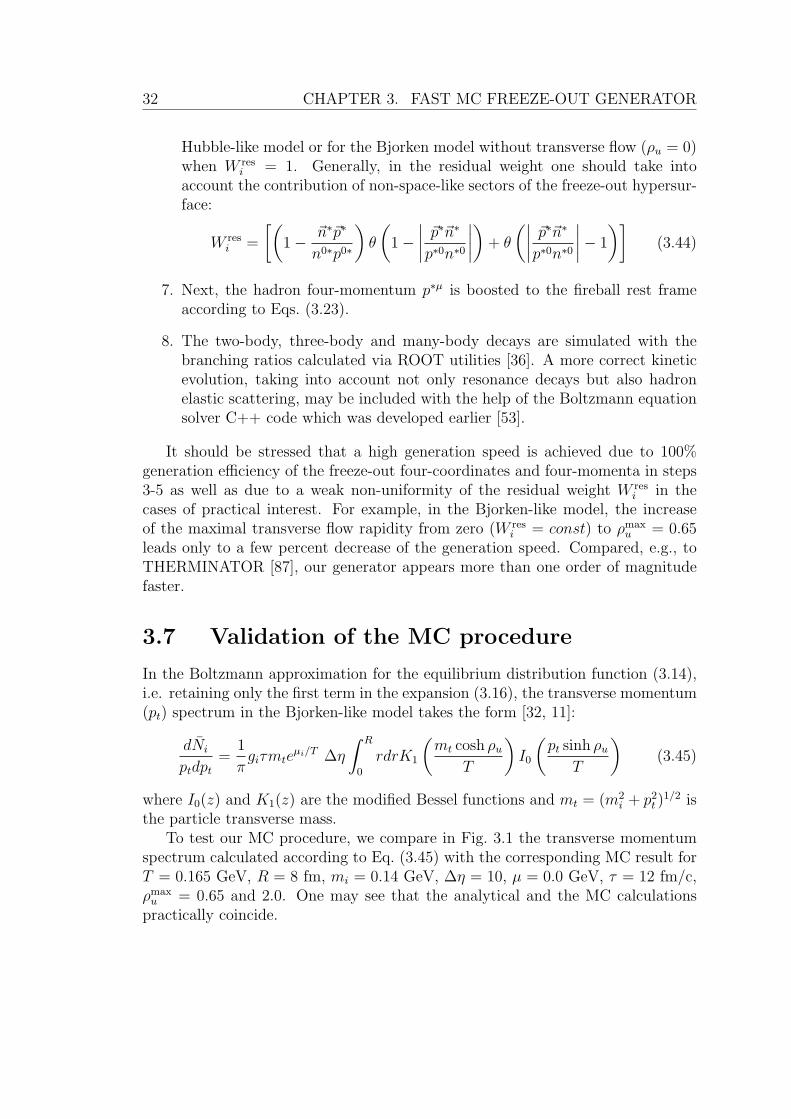
32 CHAPTER 3. FAST MC FREEZE-OUT GENERATOR
Hubble-like model or for the Bjorken model without transverse flow (ρu = 0)when W res
i = 1. Generally, in the residual weight one should take intoaccount the contribution of non-space-like sectors of the freeze-out hypersur-face:
W resi =
[(1 − ~n∗~p∗
n0∗p0∗
)θ
(1 −
∣∣∣∣ ~p∗~n∗
p∗0n∗0
∣∣∣∣) + θ
(∣∣∣∣ ~p∗~n∗
p∗0n∗0
∣∣∣∣ − 1
)](3.44)
7. Next, the hadron four-momentum p∗µ is boosted to the fireball rest frameaccording to Eqs. (3.23).
8. The two-body, three-body and many-body decays are simulated with thebranching ratios calculated via ROOT utilities [36]. A more correct kineticevolution, taking into account not only resonance decays but also hadronelastic scattering, may be included with the help of the Boltzmann equationsolver C++ code which was developed earlier [53].
It should be stressed that a high generation speed is achieved due to 100%generation efficiency of the freeze-out four-coordinates and four-momenta in steps3-5 as well as due to a weak non-uniformity of the residual weight W res
i in thecases of practical interest. For example, in the Bjorken-like model, the increaseof the maximal transverse flow rapidity from zero (W res
i = const) to ρmaxu = 0.65
leads only to a few percent decrease of the generation speed. Compared, e.g., toTHERMINATOR [87], our generator appears more than one order of magnitudefaster.
3.7 Validation of the MC procedure
In the Boltzmann approximation for the equilibrium distribution function (3.14),i.e. retaining only the first term in the expansion (3.16), the transverse momentum(pt) spectrum in the Bjorken-like model takes the form [32, 11]:
dNi
ptdpt
=1
πgiτmte
µi/T ∆η
∫ R
0
rdrK1
(mt cosh ρu
T
)I0
(pt sinh ρu
T
)(3.45)
where I0(z) and K1(z) are the modified Bessel functions and mt = (m2i + p2
t )1/2 is
the particle transverse mass.To test our MC procedure, we compare in Fig. 3.1 the transverse momentum
spectrum calculated according to Eq. (3.45) with the corresponding MC result forT = 0.165 GeV, R = 8 fm, mi = 0.14 GeV, ∆η = 10, µ = 0.0 GeV, τ = 12 fm/c,ρmax
u = 0.65 and 2.0. One may see that the analytical and the MC calculationspractically coincide.
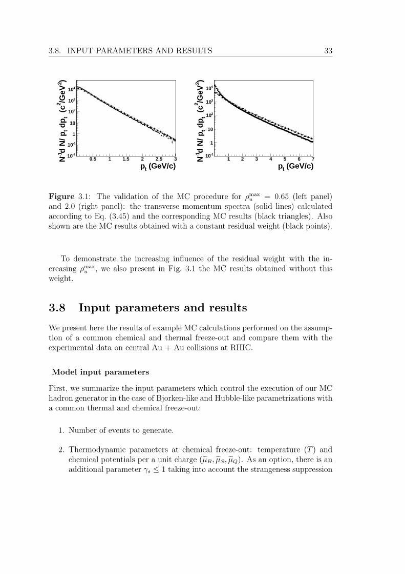
3.8. INPUT PARAMETERS AND RESULTS 33
(GeV/c)tp0.5 1 1.5 2 2.5 3
)2/G
eV2
(c
t d
pt
d N
/ p-1
N
-210
-110
1
10
210
310
410
(GeV/c)tp1 2 3 4 5 6 7
)2/G
eV2
(c
t d
pt
d N
/ p-1
N
-110
1
10
210
310
410
Figure 3.1: The validation of the MC procedure for ρmaxu = 0.65 (left panel)
and 2.0 (right panel): the transverse momentum spectra (solid lines) calculatedaccording to Eq. (3.45) and the corresponding MC results (black triangles). Alsoshown are the MC results obtained with a constant residual weight (black points).
To demonstrate the increasing influence of the residual weight with the in-creasing ρmax
u , we also present in Fig. 3.1 the MC results obtained without thisweight.
3.8 Input parameters and results
We present here the results of example MC calculations performed on the assump-tion of a common chemical and thermal freeze-out and compare them with theexperimental data on central Au + Au collisions at RHIC.
Model input parameters
First, we summarize the input parameters which control the execution of our MChadron generator in the case of Bjorken-like and Hubble-like parametrizations witha common thermal and chemical freeze-out:
1. Number of events to generate.
2. Thermodynamic parameters at chemical freeze-out: temperature (T ) andchemical potentials per a unit charge (µB, µS, µQ). As an option, there is anadditional parameter γs ≤ 1 taking into account the strangeness suppression
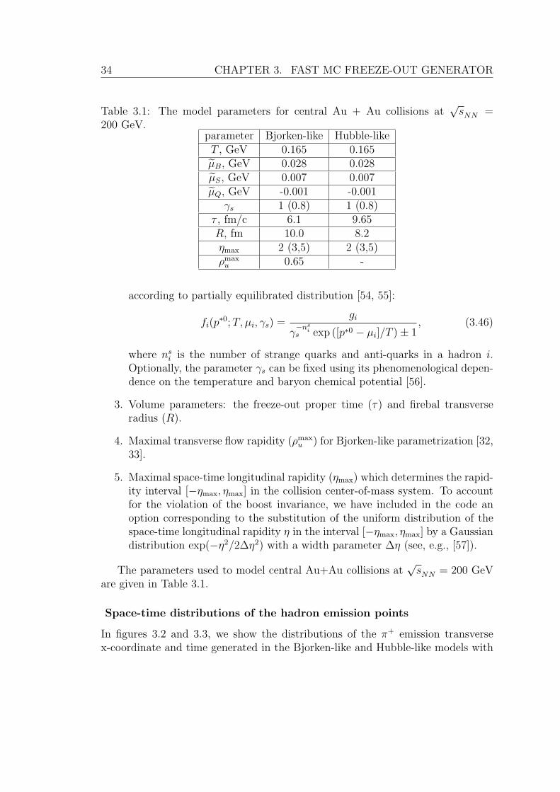
34 CHAPTER 3. FAST MC FREEZE-OUT GENERATOR
Table 3.1: The model parameters for central Au + Au collisions at√sNN =
200 GeV.parameter Bjorken-like Hubble-likeT , GeV 0.165 0.165µB, GeV 0.028 0.028µS, GeV 0.007 0.007µQ, GeV -0.001 -0.001
γs 1 (0.8) 1 (0.8)τ , fm/c 6.1 9.65R, fm 10.0 8.2ηmax 2 (3,5) 2 (3,5)ρmax
u 0.65 -
according to partially equilibrated distribution [54, 55]:
fi(p∗0;T, µi, γs) =
gi
γ−ns
is exp ([p∗0 − µi]/T ) ± 1
, (3.46)
where nsi is the number of strange quarks and anti-quarks in a hadron i.
Optionally, the parameter γs can be fixed using its phenomenological depen-dence on the temperature and baryon chemical potential [56].
3. Volume parameters: the freeze-out proper time (τ) and firebal transverseradius (R).
4. Maximal transverse flow rapidity (ρmaxu ) for Bjorken-like parametrization [32,
33].
5. Maximal space-time longitudinal rapidity (ηmax) which determines the rapid-ity interval [−ηmax, ηmax] in the collision center-of-mass system. To accountfor the violation of the boost invariance, we have included in the code anoption corresponding to the substitution of the uniform distribution of thespace-time longitudinal rapidity η in the interval [−ηmax, ηmax] by a Gaussiandistribution exp(−η2/2∆η2) with a width parameter ∆η (see, e.g., [57]).
The parameters used to model central Au+Au collisions at√sNN = 200 GeV
are given in Table 3.1.
Space-time distributions of the hadron emission points
In figures 3.2 and 3.3, we show the distributions of the π+ emission transversex-coordinate and time generated in the Bjorken-like and Hubble-like models with
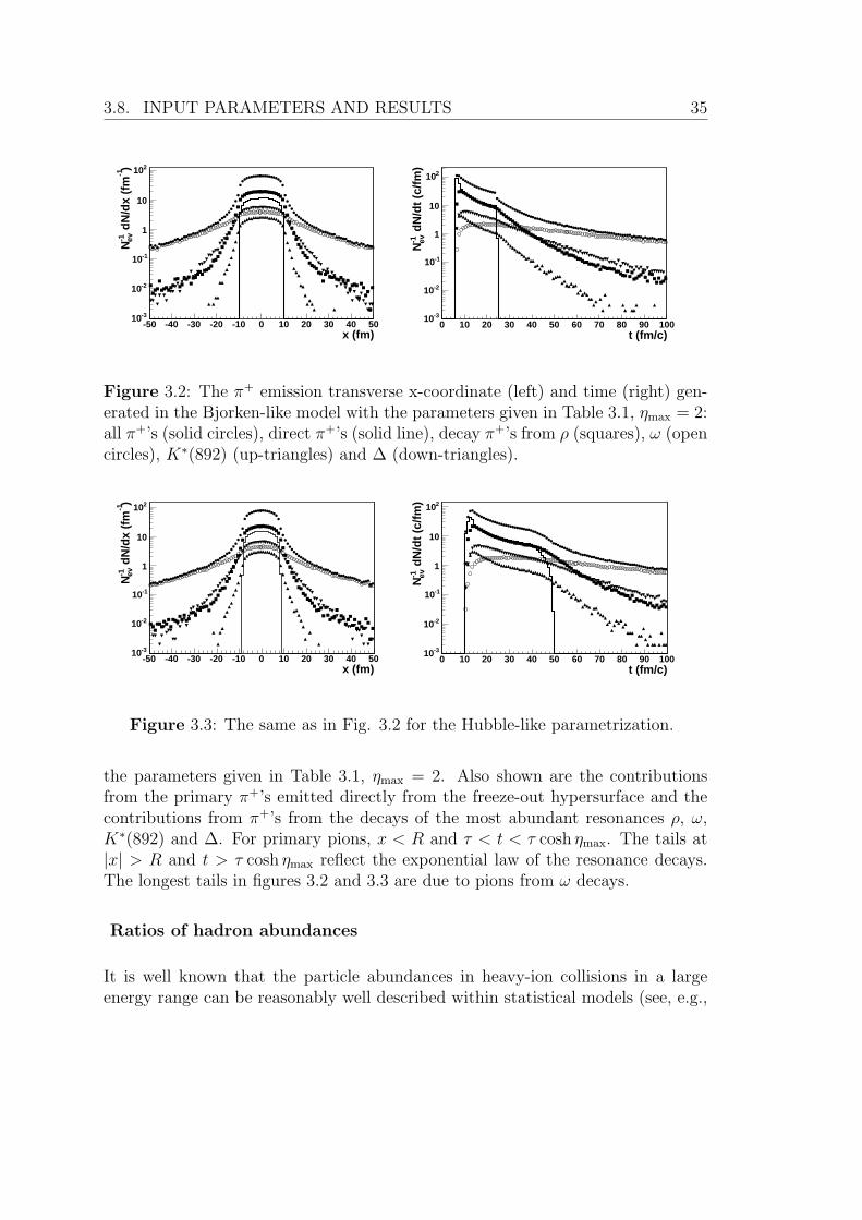
3.8. INPUT PARAMETERS AND RESULTS 35
x (fm)-50 -40 -30 -20 -10 0 10 20 30 40 50
)-1
dN
/dx
(fm
-1 ev N
-310
-210
-110
1
10
210
t (fm/c)0 10 20 30 40 50 60 70 80 90 100
dN
/dt
(c/f
m)
-1 evN
-310
-210
-110
1
10
210
Figure 3.2: The π+ emission transverse x-coordinate (left) and time (right) gen-erated in the Bjorken-like model with the parameters given in Table 3.1, ηmax = 2:all π+’s (solid circles), direct π+’s (solid line), decay π+’s from ρ (squares), ω (opencircles), K∗(892) (up-triangles) and ∆ (down-triangles).
x (fm)-50 -40 -30 -20 -10 0 10 20 30 40 50
)-1
dN
/dx
(fm
-1 ev N
-310
-210
-110
1
10
210
t (fm/c)0 10 20 30 40 50 60 70 80 90 100
dN
/dt
(c/f
m)
-1 evN
-310
-210
-110
1
10
210
Figure 3.3: The same as in Fig. 3.2 for the Hubble-like parametrization.
the parameters given in Table 3.1, ηmax = 2. Also shown are the contributionsfrom the primary π+’s emitted directly from the freeze-out hypersurface and thecontributions from π+’s from the decays of the most abundant resonances ρ, ω,K∗(892) and ∆. For primary pions, x < R and τ < t < τ cosh ηmax. The tails at|x| > R and t > τ cosh ηmax reflect the exponential law of the resonance decays.The longest tails in figures 3.2 and 3.3 are due to pions from ω decays.
Ratios of hadron abundances
It is well known that the particle abundances in heavy-ion collisions in a largeenergy range can be reasonably well described within statistical models (see, e.g.,
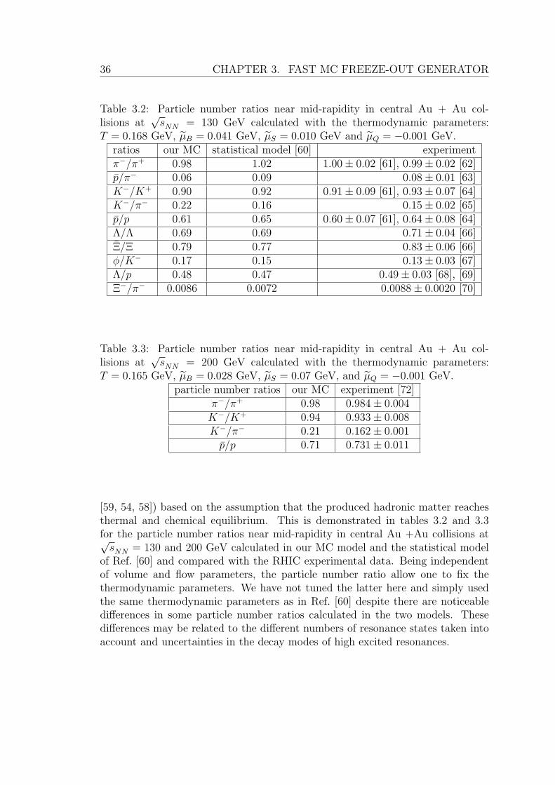
36 CHAPTER 3. FAST MC FREEZE-OUT GENERATOR
Table 3.2: Particle number ratios near mid-rapidity in central Au + Au col-lisions at
√sNN = 130 GeV calculated with the thermodynamic parameters:
T = 0.168 GeV, µB = 0.041 GeV, µS = 0.010 GeV and µQ = −0.001 GeV.ratios our MC statistical model [60] experimentπ−/π+ 0.98 1.02 1.00 ± 0.02 [61], 0.99 ± 0.02 [62]p/π− 0.06 0.09 0.08 ± 0.01 [63]K−/K+ 0.90 0.92 0.91 ± 0.09 [61], 0.93 ± 0.07 [64]K−/π− 0.22 0.16 0.15 ± 0.02 [65]p/p 0.61 0.65 0.60 ± 0.07 [61], 0.64 ± 0.08 [64]Λ/Λ 0.69 0.69 0.71 ± 0.04 [66]Ξ/Ξ 0.79 0.77 0.83 ± 0.06 [66]φ/K− 0.17 0.15 0.13 ± 0.03 [67]Λ/p 0.48 0.47 0.49 ± 0.03 [68], [69]Ξ−/π− 0.0086 0.0072 0.0088 ± 0.0020 [70]
Table 3.3: Particle number ratios near mid-rapidity in central Au + Au col-lisions at
√sNN = 200 GeV calculated with the thermodynamic parameters:
T = 0.165 GeV, µB = 0.028 GeV, µS = 0.07 GeV, and µQ = −0.001 GeV.particle number ratios our MC experiment [72]
π−/π+ 0.98 0.984 ± 0.004K−/K+ 0.94 0.933 ± 0.008K−/π− 0.21 0.162 ± 0.001p/p 0.71 0.731 ± 0.011
[59, 54, 58]) based on the assumption that the produced hadronic matter reachesthermal and chemical equilibrium. This is demonstrated in tables 3.2 and 3.3for the particle number ratios near mid-rapidity in central Au +Au collisions at√sNN = 130 and 200 GeV calculated in our MC model and the statistical model
of Ref. [60] and compared with the RHIC experimental data. Being independentof volume and flow parameters, the particle number ratio allow one to fix thethermodynamic parameters. We have not tuned the latter here and simply usedthe same thermodynamic parameters as in Ref. [60] despite there are noticeabledifferences in some particle number ratios calculated in the two models. Thesedifferences may be related to the different numbers of resonance states taken intoaccount and uncertainties in the decay modes of high excited resonances.
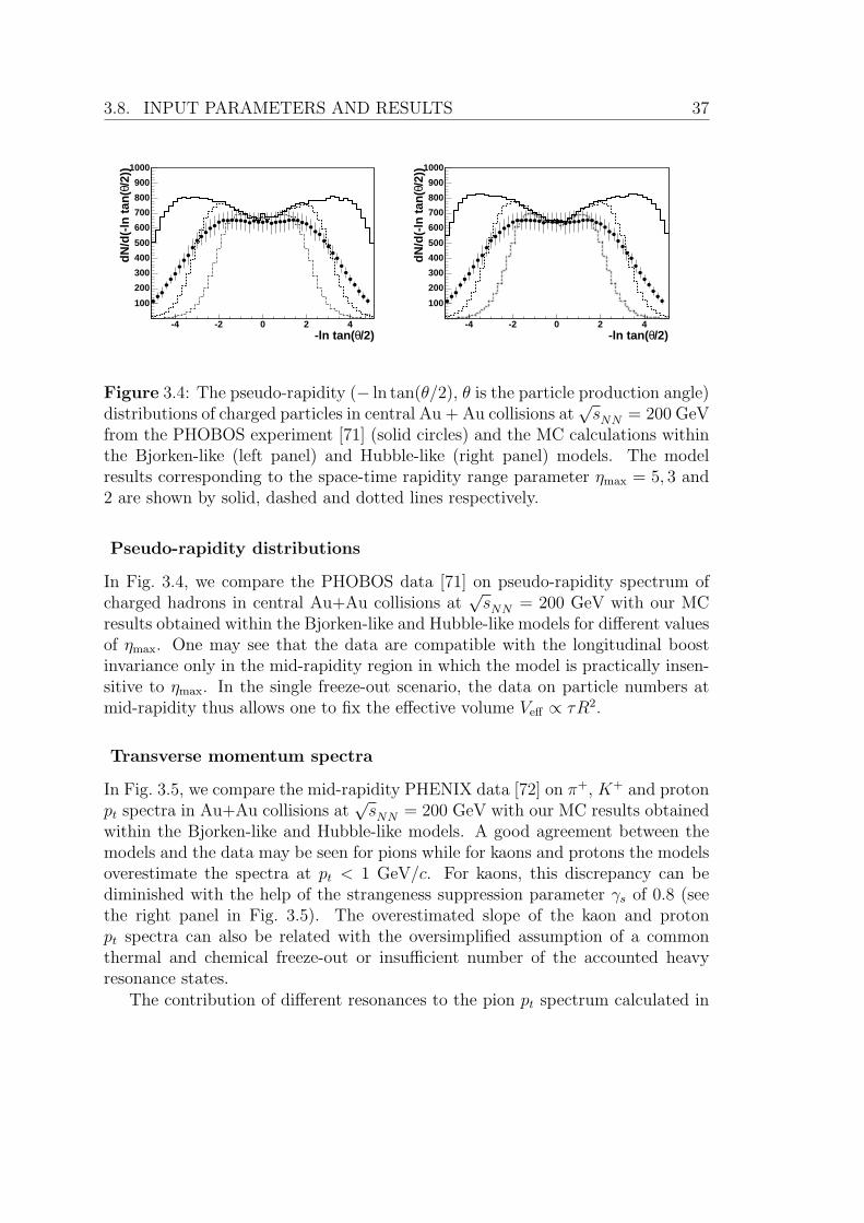
3.8. INPUT PARAMETERS AND RESULTS 37
/2)θ-ln tan(-4 -2 0 2 4
/2))
θd
N/d
(-ln
tan
(
100
200
300
400
500
600
700
800
900
1000
/2)θ-ln tan(-4 -2 0 2 4
/2))
θd
N/d
(-ln
tan
(
100
200
300
400
500
600
700
800
900
1000
Figure 3.4: The pseudo-rapidity (− ln tan(θ/2), θ is the particle production angle)distributions of charged particles in central Au + Au collisions at
√sNN = 200 GeV
from the PHOBOS experiment [71] (solid circles) and the MC calculations withinthe Bjorken-like (left panel) and Hubble-like (right panel) models. The modelresults corresponding to the space-time rapidity range parameter ηmax = 5, 3 and2 are shown by solid, dashed and dotted lines respectively.
Pseudo-rapidity distributions
In Fig. 3.4, we compare the PHOBOS data [71] on pseudo-rapidity spectrum ofcharged hadrons in central Au+Au collisions at
√sNN = 200 GeV with our MC
results obtained within the Bjorken-like and Hubble-like models for different valuesof ηmax. One may see that the data are compatible with the longitudinal boostinvariance only in the mid-rapidity region in which the model is practically insen-sitive to ηmax. In the single freeze-out scenario, the data on particle numbers atmid-rapidity thus allows one to fix the effective volume Veff ∝ τR2.
Transverse momentum spectra
In Fig. 3.5, we compare the mid-rapidity PHENIX data [72] on π+, K+ and protonpt spectra in Au+Au collisions at
√sNN = 200 GeV with our MC results obtained
within the Bjorken-like and Hubble-like models. A good agreement between themodels and the data may be seen for pions while for kaons and protons the modelsoverestimate the spectra at pt < 1 GeV/c. For kaons, this discrepancy can bediminished with the help of the strangeness suppression parameter γs of 0.8 (seethe right panel in Fig. 3.5). The overestimated slope of the kaon and protonpt spectra can also be related with the oversimplified assumption of a commonthermal and chemical freeze-out or insufficient number of the accounted heavyresonance states.
The contribution of different resonances to the pion pt spectrum calculated in
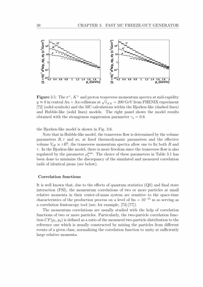
38 CHAPTER 3. FAST MC FREEZE-OUT GENERATOR
(GeV/c)tp0.2 0.4 0.6 0.8 1 1.2 1.4 1.6 1.8 2
)2/G
eV2
dy
(ct
dp
tN
/p2
d-1
N)
π(2
-210
-110
1
10
210 +K
p
+π
(GeV/c)tp0.2 0.4 0.6 0.8 1 1.2 1.4 1.6 1.8 2
)2/G
eV2
dy
(ct
dp
tN
/p2
d-1
N)
π(2
-210
-110
1
10
210+K
p
+π
Figure 3.5: The π+, K+ and proton transverse momentum spectra at mid-rapidityy ≈ 0 in central Au + Au collisions at
√sNN = 200 GeV from PHENIX experiment
[72] (solid symbols) and the MC calculations within the Bjorken-like (dashed lines)and Hubble-like (solid lines) models. The right panel shows the model resultsobtained with the strangeness suppression parameter γs = 0.8.
the Bjorken-like model is shown in Fig. 3.6.
Note that in Hubble-like model, the transverse flow is determined by the volumeparameters R, τ and so, at fixed thermodynamic parameters and the effectivevolume Veff ∝ τR2, the transverse momentum spectra allow one to fix both R andτ . In the Bjorken-like model, there is more freedom since the transverse flow is alsoregulated by the parameter ρmax
u . The choice of these parameters in Table 3.1 hasbeen done to minimize the discrepancy of the simulated and measured correlationradii of identical pions (see below).
Correlation functions
It is well known that, due to the effects of quantum statistics (QS) and final stateinteraction (FSI), the momentum correlations of two or more particles at smallrelative momenta in their center-of-mass system are sensitive to the space-timecharacteristics of the production process on a level of fm = 10−15 m so serving asa correlation femtoscopy tool (see, for example, [73]-[77]).
The momentum correlations are usually studied with the help of correlationfunctions of two or more particles. Particularly, the two-particle correlation func-tion CF (p1, p2) is defined as a ratio of the measured two-particle distribution to thereference one which is usually constructed by mixing the particles from differentevents of a given class, normalizing the correlation function to unity at sufficientlylarge relative momenta.
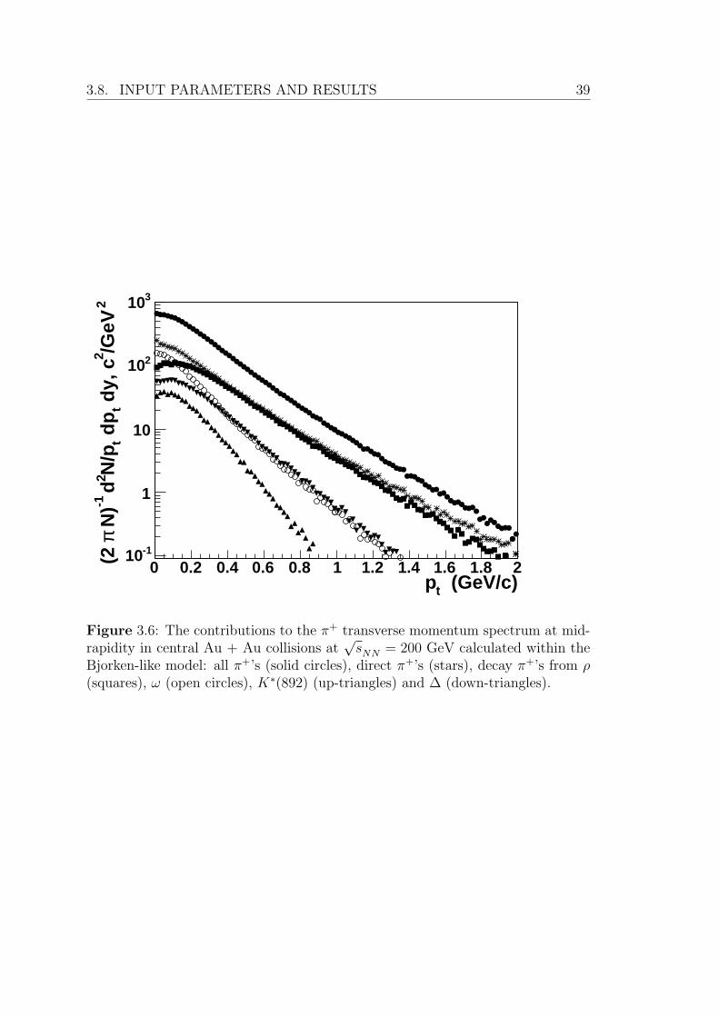
3.8. INPUT PARAMETERS AND RESULTS 39
(GeV/c)tp0 0.2 0.4 0.6 0.8 1 1.2 1.4 1.6 1.8 2
2/G
eV2
dy,
ct
dp
tN
/p2
d-1
N)
π(2
-110
1
10
210
310
Figure 3.6: The contributions to the π+ transverse momentum spectrum at mid-rapidity in central Au + Au collisions at
√sNN = 200 GeV calculated within the
Bjorken-like model: all π+’s (solid circles), direct π+’s (stars), decay π+’s from ρ(squares), ω (open circles), K∗(892) (up-triangles) and ∆ (down-triangles).
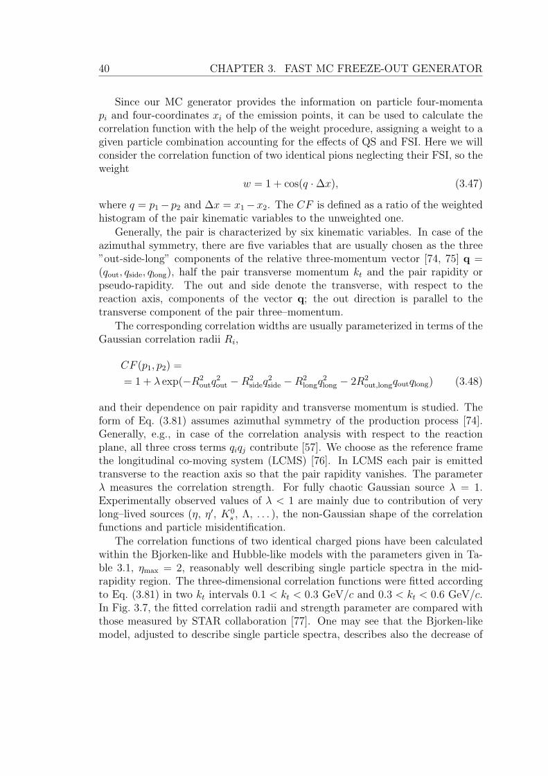
40 CHAPTER 3. FAST MC FREEZE-OUT GENERATOR
Since our MC generator provides the information on particle four-momentapi and four-coordinates xi of the emission points, it can be used to calculate thecorrelation function with the help of the weight procedure, assigning a weight to agiven particle combination accounting for the effects of QS and FSI. Here we willconsider the correlation function of two identical pions neglecting their FSI, so theweight
w = 1 + cos(q · ∆x), (3.47)
where q = p1 − p2 and ∆x = x1 −x2. The CF is defined as a ratio of the weightedhistogram of the pair kinematic variables to the unweighted one.
Generally, the pair is characterized by six kinematic variables. In case of theazimuthal symmetry, there are five variables that are usually chosen as the three”out-side-long” components of the relative three-momentum vector [74, 75] q =(qout, qside, qlong), half the pair transverse momentum kt and the pair rapidity orpseudo-rapidity. The out and side denote the transverse, with respect to thereaction axis, components of the vector q; the out direction is parallel to thetransverse component of the pair three–momentum.
The corresponding correlation widths are usually parameterized in terms of theGaussian correlation radii Ri,
CF (p1, p2) =
= 1 + λ exp(−R2outq
2out −R2
sideq2side −R2
longq2long − 2R2
out,longqoutqlong) (3.48)
and their dependence on pair rapidity and transverse momentum is studied. Theform of Eq. (3.81) assumes azimuthal symmetry of the production process [74].Generally, e.g., in case of the correlation analysis with respect to the reactionplane, all three cross terms qiqj contribute [57]. We choose as the reference framethe longitudinal co-moving system (LCMS) [76]. In LCMS each pair is emittedtransverse to the reaction axis so that the pair rapidity vanishes. The parameterλ measures the correlation strength. For fully chaotic Gaussian source λ = 1.Experimentally observed values of λ < 1 are mainly due to contribution of verylong–lived sources (η, η′, K0
s , Λ, . . . ), the non-Gaussian shape of the correlationfunctions and particle misidentification.
The correlation functions of two identical charged pions have been calculatedwithin the Bjorken-like and Hubble-like models with the parameters given in Ta-ble 3.1, ηmax = 2, reasonably well describing single particle spectra in the mid-rapidity region. The three-dimensional correlation functions were fitted accordingto Eq. (3.81) in two kt intervals 0.1 < kt < 0.3 GeV/c and 0.3 < kt < 0.6 GeV/c.In Fig. 3.7, the fitted correlation radii and strength parameter are compared withthose measured by STAR collaboration [77]. One may see that the Bjorken-likemodel, adjusted to describe single particle spectra, describes also the decrease of
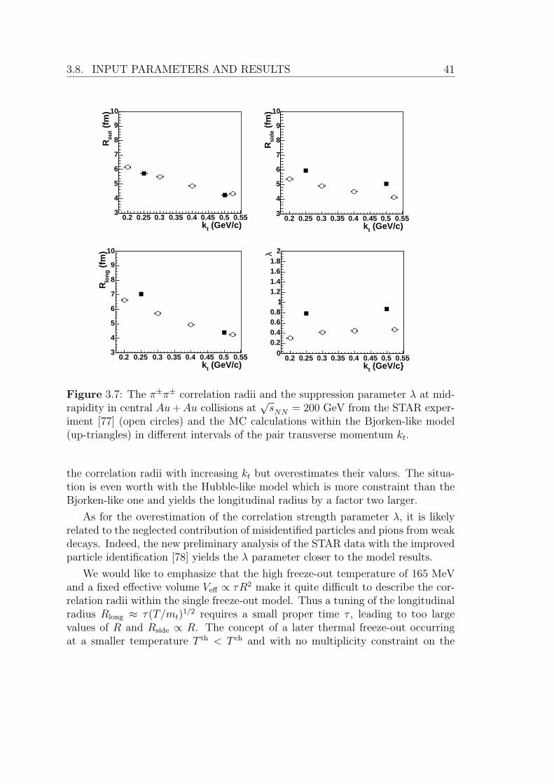
3.8. INPUT PARAMETERS AND RESULTS 41
(GeV/c)tk0.2 0.25 0.3 0.35 0.4 0.45 0.5 0.55
(fm
)o
ut
R
3
4
5
6
7
8
9
10
(GeV/c)tk0.2 0.25 0.3 0.35 0.4 0.45 0.5 0.55
(fm
)si
de
R
3
4
5
6
7
8
9
10
(GeV/c)tk0.2 0.25 0.3 0.35 0.4 0.45 0.5 0.55
(fm
)lo
ng
R
3
4
5
6
7
8
9
10
(GeV/c}tk0.2 0.25 0.3 0.35 0.4 0.45 0.5 0.55
λ
00.20.40.60.8
11.21.41.61.8
2
Figure 3.7: The π±π± correlation radii and the suppression parameter λ at mid-rapidity in central Au+Au collisions at
√sNN = 200 GeV from the STAR exper-
iment [77] (open circles) and the MC calculations within the Bjorken-like model(up-triangles) in different intervals of the pair transverse momentum kt.
the correlation radii with increasing kt but overestimates their values. The situa-tion is even worth with the Hubble-like model which is more constraint than theBjorken-like one and yields the longitudinal radius by a factor two larger.
As for the overestimation of the correlation strength parameter λ, it is likelyrelated to the neglected contribution of misidentified particles and pions from weakdecays. Indeed, the new preliminary analysis of the STAR data with the improvedparticle identification [78] yields the λ parameter closer to the model results.
We would like to emphasize that the high freeze-out temperature of 165 MeVand a fixed effective volume Veff ∝ τR2 make it quite difficult to describe the cor-relation radii within the single freeze-out model. Thus a tuning of the longitudinalradius Rlong ≈ τ(T/mt)
1/2 requires a small proper time τ , leading to too largevalues of R and Rside ∝ R. The concept of a later thermal freeze-out occurringat a smaller temperature T th < T ch and with no multiplicity constraint on the
42 CHAPTER 3. FAST MC FREEZE-OUT GENERATOR
thermal effective volume (see section 3.2) can help to resolve this problem (see,e.g., [37]).
To get a valuable information from the correlation data, one should considermore realistic models as compared with the simple Bjorken-like and Hubble-likeones (particularly, consider a more complex form of the freeze-out hypersurfacetaking into account particle emission from the surface of expanding system [48])and study the problem of particle rescattering and resonance excitation after thechemical and/or thermal freeze-out (only minor effect of elastic rescatterings onparticle spectra and correlations is expected [53]). For the latter, our earlier de-veloped C++ kinetic code [53] can be coupled to the MC freeze-out generator.
3.9. FREEZE-OUT FOR NON-CENTRAL COLLISIONS 43
3.9 Freeze-out surface parametrizations for non-
central collisions
The extension of our MC generator to noncentral collisions demands mainly themodifications of freeze-out hypersurface parametrizations (Sec. V of Ref. [79])and does not practically influence the generation procedure itself (Sec. VI ofRef. [79]). Therefore we focus on these modifications only considering the popu-lar Bjorken-like and Hubble-like freeze-out parametrizations respectively used inso-called blast wave [37] and Cracow [38] models as the example options in ourMC generator. Similar parametrizations have been used in the hadron generatorTHERMINATOR [87].
As usual, in the Bjorken-like parametrization, we substitute the Cartesian co-ordinates t, z by the Bjorken ones [49]
τ = (t2 − z2)1/2, η =1
2lnt+ z
t− z, (3.49)
and introduce the the radial vector ~r ≡ {x, y} = {r cosφ, r sinφ}, i.e.,
xµ = {τ cosh η, ~r, τ sinh η} = {τ cosh η, r cosφ, r sinφ, τ sinh η}. (3.50)
For a freeze-out hypersurface represented by the equation τ = τ(η, r, φ), thehypersurface element in terms of the coordinates η, r, φ becomes
d3σµ = εµαβγdxαdxβdxγ
dηdrdφdηdrdφ, (3.51)
where εµαβγ is the completely antisymmetric Levy-Civita tensor in four dimensionswith ε0123 = −ε0123 = 1. Generally, the freeze-out hypersurface is represented bya set of equations τ = τj(η, r, φ) and Eq. (3.51) should be substituted by the sumof the corresponding hypersurface elements. For the simplest and frequently usedfreeze-out hypersurface τ = const, one has
d3σµ = nµd3σ = τd2~rdη{cosh η, 0, 0,− sinh η},
d3σ = τd2~rdη,nµ = {cosh η, 0, 0, sinh η}.
(3.52)
In noncentral collisions the shape of the emission region in the transverse (x-y)plane can be approximated by an ellipse (as usual, the z-x plane coincides withthe reaction plane). The ellipse radii Rx(b) and Ry(b) at a given impact parameterb are usually parametrized [37, 90, 91, 60] in terms of the spatial anisotropy ε(b) =(R2
y −R2x)/(R
2x +R2
y) and the scale factor Rs(b) = [(R2x +R2
y)/2]1/2,
Rx(b) = Rs(b)√
1 − ε(b), Ry(b) = Rs(b)√
1 + ε(b). (3.53)
44 CHAPTER 3. FAST MC FREEZE-OUT GENERATOR
Then from the ellipse equation,
x2
R2x
+y2
R2y
= 1, (3.54)
follows the explicit dependence of the fireball transverse radius R(b, φ) on theazimuthal angle φ:
R(b, φ) = Rs(b)
√1 − ε2(b)√
1 + ε(b) cos 2φ; (3.55)
particularly, R(b, 0) = Rx(b) and R(b, π/2) = Ry(b). To reduce the number of freeparameters, we assume here a simple scaling option [35]
Rs(b) = Rs(b = 0)√
1 − εs(b), (3.56)
where Rs(b = 0) ≡ R is the fireball freeze-out transverse radius in central colli-sions. It means that the dimensionless ratio Rs(b)/Rs(0) at the freeze-out momentdepends on the collision energy, the radius RA of the colliding (identical) nucleiand the impact parameter b through a dimensionless εs(b) only. It should be notedthat both εs(b) and the fireball freeze-out eccentricity ε(b) are determined by theeccentricity ε0(b) = b/(2RA) of the elliptical overlap of the colliding nuclei at theinitial moment, when
Rs(b)
Rs(b = 0)
∣∣∣ε(b)=ε0(b)
≡ Rs(b)initial
RA
=√
1 − ε0(b). (3.57)
Since εs(0) = ε(0) = ε0(0) = 0, one can can assume that εs(b) ' ε(b) at sufficientlysmall values of the impact parameter b. It appears that the use of the simpleansatz εs(b) = ε(b) allows one to achieve the absolute normalization of particlespectra correct within ∼ 10% up to b ' RA (see section 3.11).
If the system evolution were driven by the pressure gradients, the expansionwould be stronger in the direction of the short ellipse x-axis (in the reaction plane),where the pressure gradient is larger than in the direction of the long ellipse y-axis(see, e.g., [82]). The typical hydrodynamic evolution scenario is shown in Fig. 3.8.During the evolution, the initial system coordinate anisotropy ε0(b) is transformedinto the momentum anisotropy δ(b). According to the hydrodynamical calcula-tions, the spatial eccentricity almost disappears and the momentum anisotropysaturates at rather early evolution stage before freeze-out. As we do not trace theevolution here, we will consider the spatial and momentum anisotropies ε(b) andδ(b) as free parameters.
For central collisions the fluid flow four-velocity uµ(t, ~x) = γ(t, ~x){1, ~v(t, ~x)} ≡γ(t, ~x){1, ~v⊥(t, ~x), vz(t, ~x)} at a point ~x and time t was parametrized [79] in terms

3.9. FREEZE-OUT FOR NON-CENTRAL COLLISIONS 45
Figure 3.8: The typical hydrodynamic evolution scenario.
of the longitudinal (z) and transverse (⊥) fluid flow rapidities
ηu(t, ~x) =1
2ln
1 + vz(t, ~x)
1 − vz(t, ~x), ρu(t, ~x) =
1
2ln
1 + v⊥(t, ~x) cosh ηu(t, ~x)
1 − v⊥(t, ~x) cosh ηu(t, ~x), (3.58)
where v⊥ = |~v⊥| is the magnitude of the transverse component of the flow three-velocity ~v = {v⊥ cosφu, v⊥ sinφu, vz}, i.e.,
uµ(t, ~x) = {cosh ρu cosh ηu, sinh ρu cosφu, sinh ρu sinφu, cosh ρu sinh ηu}= {(1 + u2
⊥)1/2 cosh ηu, ~u⊥, (1 + u2⊥)1/2 sinh ηu},
(3.59)
~u⊥ = γ~v⊥ = γ⊥ cosh ηu~v⊥, γ⊥ = cosh ρu. However, unlike the transverse isotropicparametrization (φu = φ), now the azimuthal angle φu of the fluid velocity vectoris not necessarily identical to the spatial azimuthal angle φ, because of the nonzeroflow anisotropy parameter δ(b) [91, 60] :
uµ(t, ~x) = {γφ cosh ρu cosh ηu,√
1 + δ(b) sinh ρu cosφ,√1 − δ(b) sinh ρu sinφ, γφ cosh ρu sinh ηu},
(3.60)
where
γφ =
√1 + δ(b) tanh2 ρu cos 2φ, (3.61)
tanφu =
√1 − δ(b)
1 + δ(b)tanφ. (3.62)
The transverse flow rapidity ρu is related to ρu by:
u⊥ = sinh ρu =√
1 + δ(b) cos 2φ sinh ρu. (3.63)

46 CHAPTER 3. FAST MC FREEZE-OUT GENERATOR
Note, that for δ(b) = 0 (i.e. φu = φ), Eq. (3.60) reduces to Eq. (3.59) whichwas applied in Refs. [35, 92]. In Ref. [60], δ(b) is obtained by fitting the modelprediction to the measured elliptic flow coefficient v2.
Further we assume the longitudinal boost invariance [49] ηu = η, which is agood approximation for the highest RHIC energies at the midrapidity region. Toaccount for the violation of the boost invariance, we have also included in thecode an option corresponding to the substitution of the uniform distribution ofthe space-time longitudinal rapidity η in the interval [−ηmax, ηmax] by a Gaussiandistribution exp(−η2/2∆η2) with a width parameter ∆η = ηmax. The presenceof the “oscillation term”
√1 + δ(b) cos 2φ in the transverse component u⊥ of the
flow velocity in Eq. (3.63) allows us to use the simple linear profile for ρu with-out introduction of the additional parameters for each centrality (b) unlike othermodels, namely:
ρu =r
Rs(b)ρmax
u (b = 0), (3.64)
where ρmaxu (b = 0) is the maximal transverse flow rapidity for central collisions.
At such normalization and δ(b) > ε(b) the maximal transverse flow (u⊥, ρu) isachieved at φ = 0, i.e. along x-axix as it should be according to the hydrodynamicscenario described above (Fig. 3.8). (although ρu has a maximum at φ = π/2!)
Here one should note that the “popular parametrization” of transverse flowrapidity used in Ref. [37] (and implemented as an option in our MC generatoralso):
ρu = r[ρ0(b) + ρ2(b) cos 2φu], (3.65)
where
r ≡
√(r cosφ
Rx
)2
+(r sinφ
Ry
)2
=r
R(b, φ)(3.66)
is the “normalized elliptical radius”, ρ0(b) and ρ2(b) are the two fitting parameters,is close to our parametrization and gives the similar results for observables underconsideration. In parametrization of Ref. [37] the boost is perpendicular to theelliptical subshell on which the source element is found: tanφu = (R2
x/R2y) tanφ =
(1 − ε)/(1 + ε) tanφ and δ(b) = 2ε(b)/(1 + ε2(b)). It is interesting to note that forsufficiently weak transverse flows, ρu ≤ 1, considered here, one can put sinh ρu ' ρu
and obtain our parametrization from that of Ref. [37] by substitutions
ρ0(b)
R(b, φ)→ ρmax
u (b = 0)
Rs(b)1 +
ρ2(b)
ρ0(b)cos 2φu →
√1 + δ(b) cos 2φ. (3.67)
Thus, in the case of moderate transverse flows, one can obtain the same resulteither by fixing the direction of the flow velocity vector but allowing for the az-imuthal dependence of the flow rapidity or by allowing for arbitrary direction ofthe flow velocity vector but assuming azimuthally independent flow rapidity.
3.9. FREEZE-OUT FOR NON-CENTRAL COLLISIONS 47
At τ = const, the total effective volume for particle production in the case ofnoncentral collisions becomes
Veff =
∫σ(t,~x)
d3σµ(t, ~x)uµ(t, ~x) = τ
∫ 2π
0
dφ
∫ R(b,φ)
0
(nµuµ)rdr
∫ ηmax
ηmin
dη (3.68)
where (nµuµ) = cosh ρu
√1 + δ(b) tanh2 ρu cos 2φ .
We also consider the Cracow model scenario [38] corresponding to the Hubble-like freeze-out hypersurface τH = (t2 − x2 − y2 − z2)1/2 = const. Introducingthe longitudinal space-time rapidity η according to Eq. (3.49) and the transversespace-time rapidity ρ = sinh−1(r/τH), one has [51]
xµ = τH{cosh η cosh ρ, sinh ρ cosφ, sinh ρ sinφ, sinh η cosh ρ}, (3.69)
τH = τB/ cosh ρ. Representing the freeze-out hypersurface by the equation τH =τH(η, ρ, φ) = const, one finds from Eq. (3.51):
d3σ = τ 3H sinh ρ cosh ρdηdρdφ = τHdηd
2~r,nµ(t, ~x) = xµ(t, ~x)/τH .
(3.70)
With the additional flow anisotropy parameter δ(b) the flow four-velocity is parametrizedas [60]:
uµ(t, ~x) = {γHφ cosh ρ cosh η,
√1 + δ(b) sinh ρ cosφ,√
1 − δ(b) sinh ρ sinφ, γHφ cosh ρ sinh η},
(3.71)
where
γHφ =
√1 + δ(b) tanh2 ρ cos 2φ. (3.72)
The effective volume corresponding to r = τH sinh ρ < R(b, φ) and ηmin ≤ η ≤ ηmax
is
Veff =
∫σ(t,~x)
d3σµ(t, ~x)uµ(t, ~x) = τH
∫ 2π
0
dφ
∫ R(b,φ)
0
(nµuµ)rdr
∫ ηmax
ηmin
dη (3.73)
with
(nµuµ) = cosh2 ρ
(√1 + δ(b) tanh2 ρ cos 2φ
− tanh2 ρ(√
1 + δ(b) cos2 φ+√
1 − δ(b) sin2 φ))' 1 + o(δ2(b)).
(3.74)
Our MC procedure to generate the freeze-out hadron multiplicities, four-momentaand four-coordinates for central collisions has been described in detail in Ref. [79].For noncentral collisions, only the generation of the transverse radius r is slightlydifferent, taking place in the azimuthally dependent interval [0, R(b, φ)].

48 CHAPTER 3. FAST MC FREEZE-OUT GENERATOR
3.10 Different chemical and thermal freeze-outs
Since the assumption of a common chemical and thermal freeze-out can hardlybe justified (see, e.g., [27]), we consider here a more complicated scenario withdifferent chemical and thermal freeze-outs.
The mean particle numbers N thi at thermal freeze-out can be determined using
the following procedure [27]. Above in this chapter, the temperature and chem-ical potentials at chemical freeze-out have been fixed by fitting the ratios of thenumbers of (quasi)stable particles. The common factor, V ch
eff , and, thus, the abso-lute particle and resonance numbers was fixed by pion multiplicities. Within theconcept of chemically frozen evolution these numbers are assumed to be conservedexcept for corrections due to decay of some part of short-lived resonances thatcan be estimated from the assumed chemical to thermal freeze-out evolution time.Then one can calculate the mean numbers of different particles and resonancesreaching a (common) thermal freeze-out hypersurface. At a given thermal freeze-out temperature T th these mean numbers can be expressed through the thermaleffective volume V th
eff and the chemical potentials for each particle species µthi . The
latter can no longer be expressed in the form µi = ~qi~µ, which is valid only for chem-ically equilibrated systems. For a given parametrization of the thermal freeze-outhypersurface, the thermal effective volume V th
eff (and thus all µthi ) can be fixed with
the help of pion interferometry data.In practical calculations the particle number density ρeq
i (T, µi) is representedin the form of a fast converging series [79]:
ρeqi (T, µi) =
gi
2π2m2
iT∞∑
k=1
(∓)k+1
kexp(
kµi
T)K2(
kmi
T), (3.75)
where K2 is the modified Bessel function of the second order, mi and gi = 2Ji + 1are the mass and the spin degeneracy factor of particle i respectively.
Using Eq. (3.75) and the assumption of the conservation of the particle num-ber ratios from the chemical to thermal freeze-out evolution time, we obtain thefollowing ratios for i-particle specie to π+:
ρeqi (T ch, µi)
ρeqπ (T ch, µch
i )=
ρeqi (T th, µth
i )
ρeqπ (T th, µeff th
π ). (3.76)
The absolute values of particles densities ρeqi (T th, µth
i ) are determined by thechoice of the free parameter of the model: effective pion chemical potential µeff th
π
at the temperature of thermal freeze-out T th. Assuming for the other particles(heavier then pions) the Boltzmann approximation in Eq. (3.75) one deduces fromEqs. (3.75) - (3.76) the chemical potentials of particles and resonances at thermal
3.11. RESULTS FOR NON-CENTRAL COLLISIONS 49
freeze-out:
µthi = T th ln(
ρeqi (T ch, µch
i )
ρeqi (T th, µi = 0)
ρeqπ (T th, µeff th
π )
ρeqπ (T ch, µch
i )). (3.77)
The correct way to determine the best set of model parameters would beachieved by fitting all the observables together as it was suggested in Ref. [57],but for our MC-type model it is technically impossible. For the example calcu-lations with our model at RHIC energies we choose T ch = 0.165 GeV and thethermal temperatures as in the analytical models which performed the success-ful fitting of RHIC data: T th = T ch = 0.165 GeV (Cracow model [38]) andT th = 0.100 GeV (Blast-Wave model [37]), and some arbitrary intermediate tem-perature T th = 0.130 GeV. It is well known (see, e.g., [27]) that the pion transversespectra at thermal freeze-out can be described in two regimes: low temperature andlarge transverse flow on the one hand, and higher temperature and non-relativistictransverse flow on the other hand (see section 3.11). The low temperature regimeseems to be preferable because the strong transverse flow is expected to describethe large inverse slopes of transverse spectra of the heavy hadrons (especially pro-tons) and small correlation radii obtained at RHIC better [37, 48]. We present thecalculated correlation radii in section 3.11.
In the considered here last version of FASTMC the new table of resonanceswas included. It contains 360 resonances and stable particles, instead of 85 onesincluded in the previous versions. This particle table is produced from the SHARE[94] particle table excluding not well established resonances states. The decays ofresonances are controlled by its lifetime 1/Γ, there Γ is the width of resonance spec-ified in the particle table, and they occur with the probability density Γexp(−Γτ)in the resonance rest frame. Then the decay products are boosted to the refer-ence frame in which the freeze-out hypersurface was defined. Because we need tocompare our calculations with data from different experiments we made possibleto switch on/off different decays based on their lifetime (i.e. turn on/off weakdecays). Only the two- and three-body decays are considered in our model. Thebranching ratios are also taken from the particle decay table produced from theSHARE decay table [94]. The cascade decays are also possible.
3.11 Input parameters and results for non-central
collisions
Model input parameters
First, we summarize the input parameters which control the execution of our MChadron generator in the case of Bjorken-like and Hubble-like parametrizations, andshould be specified for different energies, ion beams and event centralities.

50 CHAPTER 3. FAST MC FREEZE-OUT GENERATOR
1. Thermodynamic parameters at chemical freeze-out: temperature T ch andchemical potentials per a unit charge µB, µS, µQ. As an option, an additionalparameter γs ≤ 1 takes into account the strangeness suppression accordingto the partially equilibrated distribution [54, 55]:
fi(p∗0;T, µi, γs) =
gi
γ−ns
is exp ([p∗0 − µi]/T ) ± 1
, (3.78)
where nsi is the number of strange quarks and antiquarks in a hadron i,
p∗0 is the hadron energy in the fluid element rest frame, gi = 2Ji + 1 isthe spin degeneracy factor Optionally, the parameter γs can be fixed usingits phenomenological dependence on the temperature and baryon chemicalpotential [56].
2. Volume parameters: the fireball transverse radius R(b = 0) (determined incentral collisions; in noncentral collisions we use the scaling option (3.56,3.57)to recalculate R(b) from R(b = 0)), the freeze-out proper time τ and itsstandard deviation ∆τ (emission duration) [93].
3. Maximal transverse flow rapidity ρmaxu (b = 0) for Bjorken-like parametriza-
tion in central collisions.
4. Maximal space-time longitudinal rapidity ηmax which determines the rapid-ity interval [−ηmax, ηmax] in the collision center-of-mass system. To accountfor the violation of the boost invariance, we have included in the code anoption corresponding to the substitution of the uniform distribution of thespace-time longitudinal rapidity η in the interval [−ηmax, ηmax] by a Gaussiandistribution exp(−η2/2∆η2) with a width parameter ∆η = ηmax (see, e.g.,[57, 35]).
5. Impact parameter range: minimal bmin and maximal bmax impact parameters.
6. Flow anisotropy parameter δ(b) in Bjorken-like and Hubble-like parametriza-tions (or ρ0(b) and ρ2(b) in the “Blast-Wave” parametrization of Ref. [37]).
7. Coordinate anisotropy parameter ε(b).
8. Thermal freeze-out temperature T th (if single freeze-out is considered, T th =T ch).
9. Effective chemical potential of π+ at thermal freeze-out µeff thπ (0, if single
freeze-out is considered).
10. Parameter which enables/disables weak decays.

3.11. RESULTS FOR NON-CENTRAL COLLISIONS 51
Table 3.4: Model parameters for central Au + Au collisions at√sNN = 200 GeV.
Chemical freeze-out parameters: T ch=0.165 GeV, µB=0.028 GeV, µS=0.007 GeV,µQ= – 0.001 GeV.
T th, GeV 0.165 0.130 0.100τ , fm/c 7.0 7.2 8.0
∆τ , fm/c 2.0 2.0 2.0R(b = 0), fm 9.0 9.5 10.0ρmax
u (b = 0) 0.65 0.9 1.1µeff th
π 0. 0.10 0.11
Table 3.5: Model parameters for Au + Au collisions at√sNN = 200 GeV at differ-
ent centralities. Chemical freeze-out parameters: T ch=0.165 GeV, µB=0.028 GeV,µS=0.007 GeV, µQ= – 0.001 GeV. Thermal freeze-out parameters: T th=0.1 GeV,µeff th
π =0.11 GeV. Volume parameters determined in the central collisions: R(b =0) =10.0 fm, τ =8.0 fm/c, ρmax
u (b = 0) = 1.1centrality c=0-5% c=5-10% c=10-20% c=20-30% c=30-40% c=40-60%bmin/RA 0. 0.447 0.632 0.894 1.095 1.265bmax/RA 0.447 0.632 0.894 1.095 1.265 1.549ε(b) 0 0 0 0.1 0.15 0.15δ(b) 0.05 0.08 0.12 0.25 0.34 0.36
The parameters used to simulate central collisions are given in Table 3.4. Theparameters determined in central collisions for T th=0.1 GeV: τ=8.0 fm/c, R(b =0)=10. fm, ∆τ=2.0 fm/c; ρmax
u (b = 0) = 1.1 (3-th column in Table 3.4) were usedto simulate Au+Au collisions at
√sNN = 200 GeV at different centralities. The
additional parameters needed only for noncentral collisions are given in Table 3.5.
mt-spectra
In Fig. 3.9 the mt-spectra measured by the STAR Collaboration [95] at 0 − 5%centrality are shown for π+, K+ and p in comparison with the model calculationsunder the assumption of the common chemical and thermal freeze-out at T th =T ch = 0.165 GeV (Fig. 3.9(a)) and under the assumption that the thermal freeze-out at T th = 0.100, 0.130 GeV occurs after the chemical one (Fig. 3.9(b, c)).
The correction on weak decays was introduced by the STAR Collaborationin pion spectra only [95]. It was approximately 12% and was estimated from themeasured K0
s and Λ decays. In Ref. [95] the STAR Collaboration doesn’t introducethe weak decay correction in proton spectra. To reproduce the STAR weak decaycorrection procedure, we excluded pions from K0
s and Λ decays from pions mt-

52 CHAPTER 3. FAST MC FREEZE-OUT GENERATOR
0 0.1 0.2 0.3 0.4 0.5 0.6
dY
)t
dm
t N
mπ
N/ (
2 2
d
-110
1
10
210
310
410FASTMC: T= 0.165 GeV
a
0 0.1 0.2 0.3 0.4 0.5 0.6
dY
)t
dm
t N
mπ
N/ (
2 2
d -110
1
10
210
310
410FASTMC: T= 0.13 GeV
b
)2 (GeV/ctm0 0.1 0.2 0.3 0.4 0.5 0.6
dY
) t
dm
t N
mπ
N/ (
2 2
d
-110
1
10
210
310
410FASTMC: T= 0.10 GeVc
Figure 3.9: mt-spectra (in c4/GeV2) measured by the STAR Collaboration [95] forπ+ (circles), K+ (squares) and p (up-triangles)at 0− 5% centrality in comparisonwith the model calculations at T th = 0.165(a), 0.130(b), 0.100(c) GeV , with theparameters from Table 3.4, for protons weak decays are taken into account (solidlines); for protons weak decays are not taken into account (dashed lines). Thedirect π+ , K+ and p contributions are shown on (c) by dotted lines.
3.11. RESULTS FOR NON-CENTRAL COLLISIONS 53
spectra in Fig. 3.9. The contribution of weak decays in the simulated protonspectra can be estimated from Fig. 3.9 by comparison of the solid lines (protonsfrom K0
s and Λ decays are included) and the dashed lines (without contribution ofprotons from the weak decays). The model parameters at different temperaturesare presented in Table 3.4. The parameters were optimized this way to obtainthe good description of the pion mt-spectra and the correlation radii. The bestdescription of the mt-spectra was achieved at T th = 0.100 GeV (Fig. 3.9(c)).
The same set of parameters T, ρmaxu , R and τ which was determined for central
collisions (Table 3.4) was used for noncentral ones. The additional parameters ofthe model for noncentral collisions were coordinate and momentum asymmetries:ε and δ (Table 3.5). At the freeze-out moment we consider them as free parametersbecause we do not trace the evolution here. The influence of the choice of ε andδ on mt-spectra averaged over azimuthal angle ϕ is negligible. The decrease ofthe effective volume in noncentral collisions (Eq. 3.68) due to nonzero values of εand δ allows us to obtain the correct absolute normalization of mt-spectra withoutintroduction of the additional parameters. In Fig. 3.10 the mt-spectra measuredby the STAR Collaboration [95] are shown for π+, K+ and p at centralities: 0 −5%, 5−10%, 10−20%, 20−30%, 30−40%, 40−50% in comparison with the modelcalculations which assume that the thermal freeze-out at T th = 0.1 GeV occursafter the chemical one (solid lines). It appears that the procedure described insection 3.9 allows one to achieve the absolute normalization of pion spectra correctwithin ∼ 13%.
Elliptic flow
Following a standard procedure [96, 97] we make a Fourier expansion of the hadrondistribution in the azimuthal angle ϕ at mid-rapidity:
dN
d2ptdy=
dN
2πptdptdy(1 + 2v2 cos 2ϕ+ 2v4 cos 4ϕ+ ...). (3.79)
The elliptic flow coefficient, v2, is defined as the second order Fourier coefficient,
v2 =
∫ 2π
0dϕ cos 2(ϕ− ψR) d3N
dydϕptdpt∫ 2π
0dϕ d3N
dydϕptdpt
, (3.80)
where ψR is the reaction plane angle (in our generation ψR = 0), y and pt are therapidity and transverse momentum of particle under consideration, respectively.
The value of v2 is an important signature of the physics occurring in heavyion collisions. According to the typical hydrodynamic scenario shown in Fig. 3.8,the elliptic flow is generated mainly during the high density phase of the fireballevolution. The system driven by the internal pressure gradients expands more
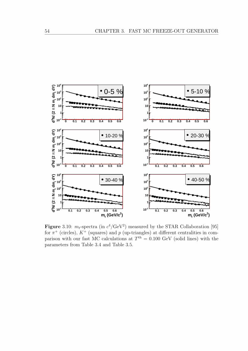
54 CHAPTER 3. FAST MC FREEZE-OUT GENERATOR
0 0.1 0.2 0.3 0.4 0.5 0.6
dY
)t
dm
t N
mπ
N/ (
2 2
d
-110
1
10
210
310
410
0-5 %
0 0.1 0.2 0.3 0.4 0.5 0.6-110
1
10
210
310
410
5-10 %
0 0.1 0.2 0.3 0.4 0.5 0.6
dY
)t
dm
t N
mπ
N/ (
2 2
d
-110
1
10
210
310
410
10-20 %
0.1 0.2 0.3 0.4 0.5 0.6-110
1
10
210
310
410
20-30 %20-30 %
)2 (GeV/ctm0.1 0.2 0.3 0.4 0.5 0.6
dY
)t
dm
t N
mπ
N/ (
2 2
d
-110
1
10
210
310
410
30-40 %
)2 (GeV/ctm0.1 0.2 0.3 0.4 0.5 0.6
-110
1
10
210
310
410
40-50 %
Figure 3.10: mt-spectra (in c4/GeV2) measured by the STAR Collaboration [95]for π+ (circles), K+ (squares) and p (up-triangles) at different centralities in com-parison with our fast MC calculations at T th = 0.100 GeV (solid lines) with theparameters from Table 3.4 and Table 3.5.
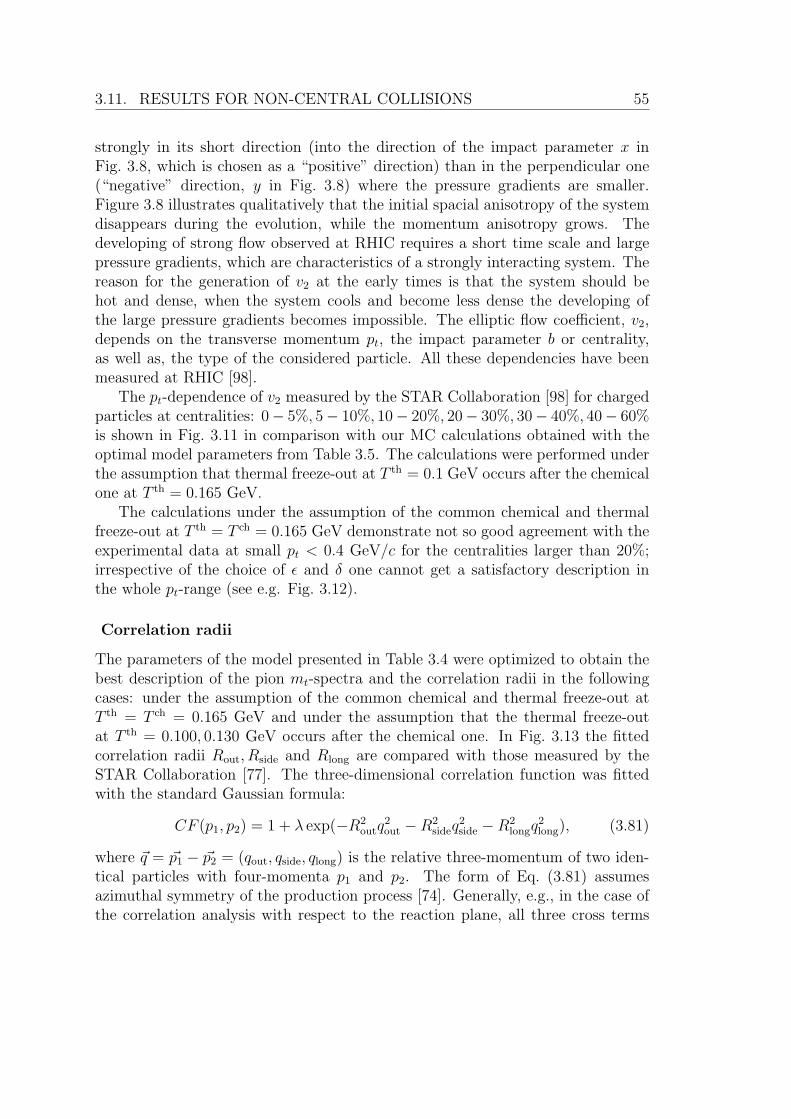
3.11. RESULTS FOR NON-CENTRAL COLLISIONS 55
strongly in its short direction (into the direction of the impact parameter x inFig. 3.8, which is chosen as a “positive” direction) than in the perpendicular one(“negative” direction, y in Fig. 3.8) where the pressure gradients are smaller.Figure 3.8 illustrates qualitatively that the initial spacial anisotropy of the systemdisappears during the evolution, while the momentum anisotropy grows. Thedeveloping of strong flow observed at RHIC requires a short time scale and largepressure gradients, which are characteristics of a strongly interacting system. Thereason for the generation of v2 at the early times is that the system should behot and dense, when the system cools and become less dense the developing ofthe large pressure gradients becomes impossible. The elliptic flow coefficient, v2,depends on the transverse momentum pt, the impact parameter b or centrality,as well as, the type of the considered particle. All these dependencies have beenmeasured at RHIC [98].
The pt-dependence of v2 measured by the STAR Collaboration [98] for chargedparticles at centralities: 0− 5%, 5− 10%, 10− 20%, 20− 30%, 30− 40%, 40− 60%is shown in Fig. 3.11 in comparison with our MC calculations obtained with theoptimal model parameters from Table 3.5. The calculations were performed underthe assumption that thermal freeze-out at T th = 0.1 GeV occurs after the chemicalone at T th = 0.165 GeV.
The calculations under the assumption of the common chemical and thermalfreeze-out at T th = T ch = 0.165 GeV demonstrate not so good agreement with theexperimental data at small pt < 0.4 GeV/c for the centralities larger than 20%;irrespective of the choice of ε and δ one cannot get a satisfactory description inthe whole pt-range (see e.g. Fig. 3.12).
Correlation radii
The parameters of the model presented in Table 3.4 were optimized to obtain thebest description of the pion mt-spectra and the correlation radii in the followingcases: under the assumption of the common chemical and thermal freeze-out atT th = T ch = 0.165 GeV and under the assumption that the thermal freeze-outat T th = 0.100, 0.130 GeV occurs after the chemical one. In Fig. 3.13 the fittedcorrelation radii Rout, Rside and Rlong are compared with those measured by theSTAR Collaboration [77]. The three-dimensional correlation function was fittedwith the standard Gaussian formula:
CF (p1, p2) = 1 + λ exp(−R2outq
2out −R2
sideq2side −R2
longq2long), (3.81)
where ~q = ~p1 − ~p2 = (qout, qside, qlong) is the relative three-momentum of two iden-tical particles with four-momenta p1 and p2. The form of Eq. (3.81) assumesazimuthal symmetry of the production process [74]. Generally, e.g., in the case ofthe correlation analysis with respect to the reaction plane, all three cross terms
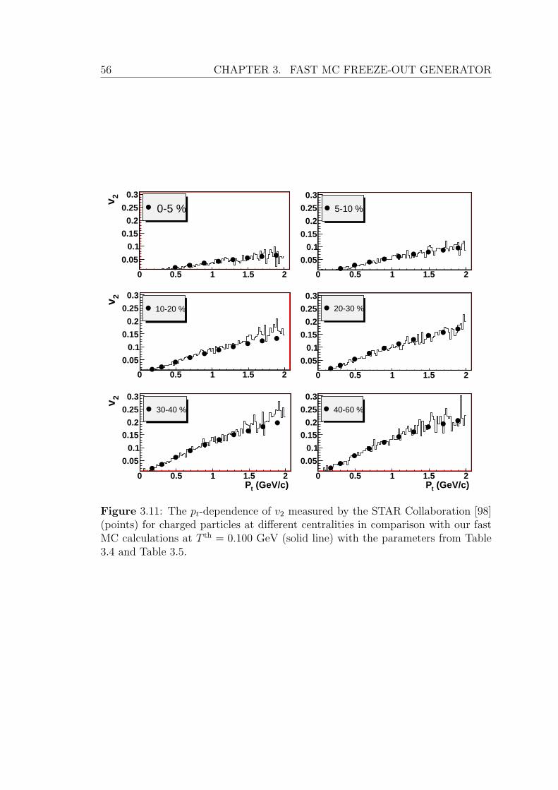
56 CHAPTER 3. FAST MC FREEZE-OUT GENERATOR
0 0.5 1 1.5 2
2 v
0.05
0.1
0.15
0.2
0.25
0.3
0-5 %
0 0.5 1 1.5 2
0.05
0.1
0.15
0.2
0.25
0.3
5-10 %
0 0.5 1 1.5 2
2 v
0.05
0.1
0.15
0.2
0.25
0.3
10-20 %
0 0.5 1 1.5 2
0.05
0.1
0.15
0.2
0.25
0.3 20-30 %
(GeV/c) t P0 0.5 1 1.5 2
2 v
0.05
0.1
0.150.2
0.25
0.3
30-40 %
(GeV/c) t P0 0.5 1 1.5 2
0.05
0.1
0.150.2
0.25
0.3
40-60 %
Figure 3.11: The pt-dependence of v2 measured by the STAR Collaboration [98](points) for charged particles at different centralities in comparison with our fastMC calculations at T th = 0.100 GeV (solid line) with the parameters from Table3.4 and Table 3.5.
3.11. RESULTS FOR NON-CENTRAL COLLISIONS 57
(GeV/c)t
p0 0.2 0.4 0.6 0.8 1 1.2 1.4 1.6 1.8
2v
0
0.02
0.04
0.06
0.08
0.1
0.12
0.14
0.16
=0.1∈=0.3; δ=0.2∈=0.4 δ
=0.1∈=0.4; δ=0.2∈=0.5; δ
Figure 3.12: The pt-dependence of v2 measured by the STAR Collaboration [98](points) for charged particles at centrality 20−30% in comparison with our fast MCcalculations under assumption of the single freeze-out at T th = T ch = 0.165 GeV.The different sets of coordinate and momentum assymetries parameters were tried:ε = 0.1, δ = 0.3 (solid line), ε = 0.2, δ = 0.4 (dotted line), ε = 0.1, δ = 0.4 (solidline), ε = 0.2, δ = 0.5 (dotted line), ε = 0.15, δ = 0.4 (dashed line)
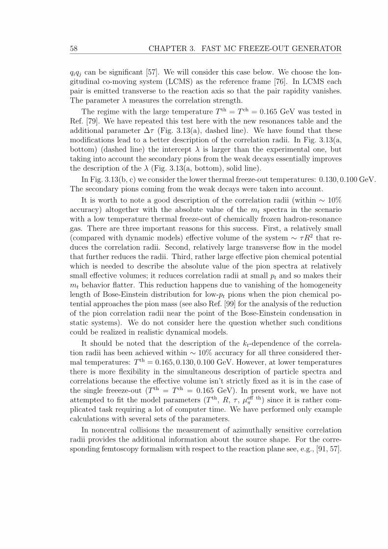
58 CHAPTER 3. FAST MC FREEZE-OUT GENERATOR
qiqj can be significant [57]. We will consider this case below. We choose the lon-gitudinal co-moving system (LCMS) as the reference frame [76]. In LCMS eachpair is emitted transverse to the reaction axis so that the pair rapidity vanishes.The parameter λ measures the correlation strength.
The regime with the large temperature T th = T ch = 0.165 GeV was tested inRef. [79]. We have repeated this test here with the new resonances table and theadditional parameter ∆τ (Fig. 3.13(a), dashed line). We have found that thesemodifications lead to a better description of the correlation radii. In Fig. 3.13(a,bottom) (dashed line) the intercept λ is larger than the experimental one, buttaking into account the secondary pions from the weak decays essentially improvesthe description of the λ (Fig. 3.13(a, bottom), solid line).
In Fig. 3.13(b, c) we consider the lower thermal freeze-out temperatures: 0.130, 0.100 GeV.The secondary pions coming from the weak decays were taken into account.
It is worth to note a good description of the correlation radii (within ∼ 10%accuracy) altogether with the absolute value of the mt spectra in the scenariowith a low temperature thermal freeze-out of chemically frozen hadron-resonancegas. There are three important reasons for this success. First, a relatively small(compared with dynamic models) effective volume of the system ∼ τR2 that re-duces the correlation radii. Second, relatively large transverse flow in the modelthat further reduces the radii. Third, rather large effective pion chemical potentialwhich is needed to describe the absolute value of the pion spectra at relativelysmall effective volumes; it reduces correlation radii at small pt and so makes theirmt behavior flatter. This reduction happens due to vanishing of the homogeneitylength of Bose-Einstein distribution for low-pt pions when the pion chemical po-tential approaches the pion mass (see also Ref. [99] for the analysis of the reductionof the pion correlation radii near the point of the Bose-Einstein condensation instatic systems). We do not consider here the question whether such conditionscould be realized in realistic dynamical models.
It should be noted that the description of the kt-dependence of the correla-tion radii has been achieved within ∼ 10% accuracy for all three considered ther-mal temperatures: T th = 0.165, 0.130, 0.100 GeV. However, at lower temperaturesthere is more flexibility in the simultaneous description of particle spectra andcorrelations because the effective volume isn’t strictly fixed as it is in the case ofthe single freeeze-out (T th = T ch = 0.165 GeV). In present work, we have notattempted to fit the model parameters (T th, R, τ , µeff th
π ) since it is rather com-plicated task requiring a lot of computer time. We have performed only examplecalculations with several sets of the parameters.
In noncentral collisions the measurement of azimuthally sensitive correlationradii provides the additional information about the source shape. For the corre-sponding femtoscopy formalism with respect to the reaction plane see, e.g., [91, 57].
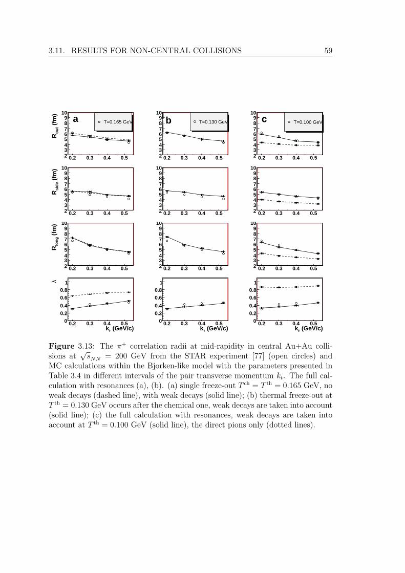
3.11. RESULTS FOR NON-CENTRAL COLLISIONS 59
0.2 0.3 0.4 0.5
(fm
) o
ut
R
23456789
10
T=0.165 GeVa
0.2 0.3 0.4 0.523456789
10
T=0.130 GeVb
0.2 0.3 0.4 0.523456789
10
T=0.100 GeVc
0.2 0.3 0.4 0.5
(fm
) si
de
R
23456789
10
0.2 0.3 0.4 0.523456789
10
0.2 0.3 0.4 0.523456789
10
0.2 0.3 0.4 0.5
(fm
) lo
ng
R
23456789
10
0.2 0.3 0.4 0.523456789
10
0.2 0.3 0.4 0.523456789
10
(GeV/c)tk0.2 0.3 0.4 0.5
λ
0
0.2
0.4
0.6
0.81
(GeV/c)tk0.2 0.3 0.4 0.50
0.2
0.4
0.6
0.81
(GeV/c)tk0.2 0.3 0.4 0.50
0.2
0.4
0.6
0.81
Figure 3.13: The π+ correlation radii at mid-rapidity in central Au+Au colli-sions at
√sNN = 200 GeV from the STAR experiment [77] (open circles) and
MC calculations within the Bjorken-like model with the parameters presented inTable 3.4 in different intervals of the pair transverse momentum kt. The full cal-culation with resonances (a), (b). (a) single freeze-out T ch = T th = 0.165 GeV, noweak decays (dashed line), with weak decays (solid line); (b) thermal freeze-out atT th = 0.130 GeV occurs after the chemical one, weak decays are taken into account(solid line); (c) the full calculation with resonances, weak decays are taken intoaccount at T th = 0.100 GeV (solid line), the direct pions only (dotted lines).
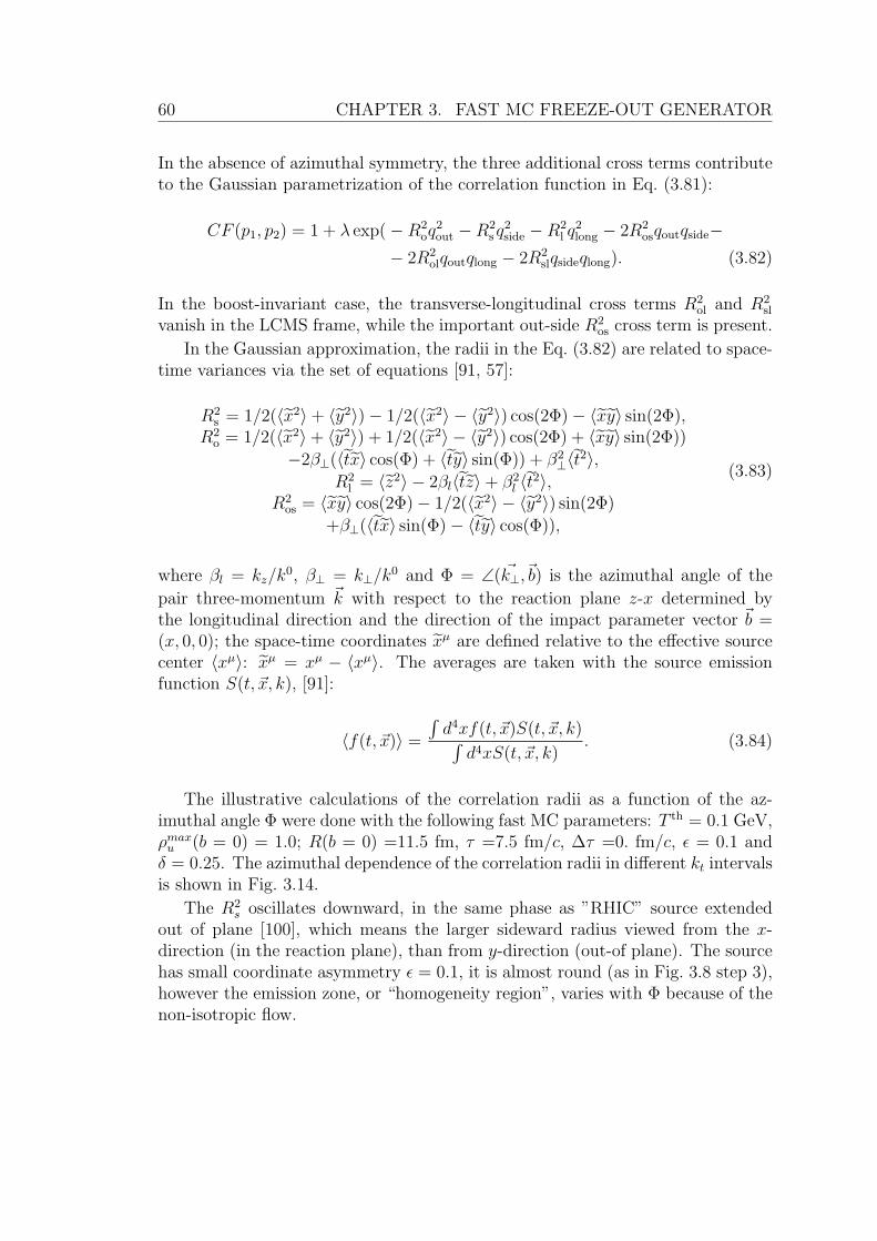
60 CHAPTER 3. FAST MC FREEZE-OUT GENERATOR
In the absence of azimuthal symmetry, the three additional cross terms contributeto the Gaussian parametrization of the correlation function in Eq. (3.81):
CF (p1, p2) = 1 + λ exp( −R2oq
2out −R2
sq2side −R2
l q2long − 2R2
osqoutqside−− 2R2
olqoutqlong − 2R2slqsideqlong). (3.82)
In the boost-invariant case, the transverse-longitudinal cross terms R2ol and R2
sl
vanish in the LCMS frame, while the important out-side R2os cross term is present.
In the Gaussian approximation, the radii in the Eq. (3.82) are related to space-time variances via the set of equations [91, 57]:
R2s = 1/2(〈x2〉 + 〈y2〉) − 1/2(〈x2〉 − 〈y2〉) cos(2Φ) − 〈xy〉 sin(2Φ),
R2o = 1/2(〈x2〉 + 〈y2〉) + 1/2(〈x2〉 − 〈y2〉) cos(2Φ) + 〈xy〉 sin(2Φ))
−2β⊥(〈tx〉 cos(Φ) + 〈ty〉 sin(Φ)) + β2⊥〈t2〉,
R2l = 〈z2〉 − 2βl〈tz〉 + β2
l 〈t2〉,R2
os = 〈xy〉 cos(2Φ) − 1/2(〈x2〉 − 〈y2〉) sin(2Φ)
+β⊥(〈tx〉 sin(Φ) − 〈ty〉 cos(Φ)),
(3.83)
where βl = kz/k0, β⊥ = k⊥/k
0 and Φ = ∠( ~k⊥,~b) is the azimuthal angle of the
pair three-momentum ~k with respect to the reaction plane z-x determined bythe longitudinal direction and the direction of the impact parameter vector ~b =(x, 0, 0); the space-time coordinates xµ are defined relative to the effective sourcecenter 〈xµ〉: xµ = xµ − 〈xµ〉. The averages are taken with the source emissionfunction S(t, ~x, k), [91]:
〈f(t, ~x)〉 =
∫d4xf(t, ~x)S(t, ~x, k)∫
d4xS(t, ~x, k). (3.84)
The illustrative calculations of the correlation radii as a function of the az-imuthal angle Φ were done with the following fast MC parameters: T th = 0.1 GeV,ρmax
u (b = 0) = 1.0; R(b = 0) =11.5 fm, τ =7.5 fm/c, ∆τ =0. fm/c, ε = 0.1 andδ = 0.25. The azimuthal dependence of the correlation radii in different kt intervalsis shown in Fig. 3.14.
The R2s oscillates downward, in the same phase as ”RHIC” source extended
out of plane [100], which means the larger sideward radius viewed from the x-direction (in the reaction plane), than from y-direction (out-of plane). The sourcehas small coordinate asymmetry ε = 0.1, it is almost round (as in Fig. 3.8 step 3),however the emission zone, or “homogeneity region”, varies with Φ because of thenon-isotropic flow.
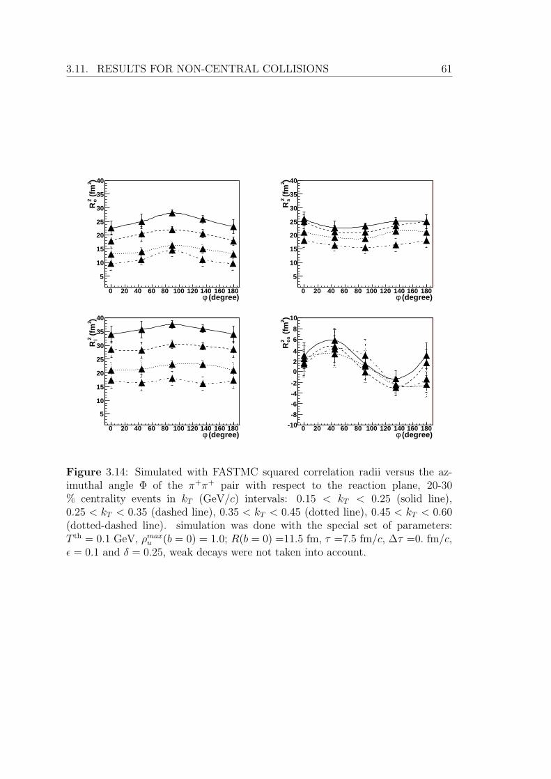
3.11. RESULTS FOR NON-CENTRAL COLLISIONS 61
(degree)φ0 20 40 60 80 100 120 140 160 180
)2 (
fm2 o
R
5
10
15
20
25
30
35
40
(degree)φ0 20 40 60 80 100 120 140 160 180
)2 (
fm2 s
R5
10
15
20
25
30
35
40
(degree)φ0 20 40 60 80 100 120 140 160 180
) 2 (
fm2 l
R
5
10
15
20
25
30
35
40
(degree)φ0 20 40 60 80 100 120 140 160 180
)2 (
fm2 o
sR
-10
-8
-6
-4
-2
02
4
6
8
10
Figure 3.14: Simulated with FASTMC squared correlation radii versus the az-imuthal angle Φ of the π+π+ pair with respect to the reaction plane, 20-30% centrality events in kT (GeV/c) intervals: 0.15 < kT < 0.25 (solid line),0.25 < kT < 0.35 (dashed line), 0.35 < kT < 0.45 (dotted line), 0.45 < kT < 0.60(dotted-dashed line). simulation was done with the special set of parameters:T th = 0.1 GeV, ρmax
u (b = 0) = 1.0; R(b = 0) =11.5 fm, τ =7.5 fm/c, ∆τ =0. fm/c,ε = 0.1 and δ = 0.25, weak decays were not taken into account.
62 CHAPTER 3. FAST MC FREEZE-OUT GENERATOR
3.12 Conclusions
A MC simulation procedure is developed as well as corresponding C++ code, thatallows a fast realistic description of multiple hadron production both in central andnoncentral relativistic heavy ion collisions. A high generation speed and an easycontrol through input parameters make our MC generator code particularly usefulfor detector studies. As options, we have implemented two freeze-out scenarioswith coinciding and with different chemical and thermal freeze-outs. We havecompared the RHIC experimental data with our MC generation results obtainedwithin the single and separated freeze-out scenarios with Bjorken-like freeze-outsurface parameterization.
Fixing the temperatures of the chemical and thermal freeze-out at 0.165 GeVand 0.100 GeV respectively, and, using the same set of the model parametersas for the central collisions, we have described single particle spectra at differentcentralities with the absolute normalization correct within ∼ 13%.
The comparison of the RHIC v2 measurements with our MC generation resultsshows that the scenario with two separated freeze-outs is more favorable for thedescription of the pt-dependence of the elliptic flow.
The description of the kt-dependence of the correlation radii has been achievedwithin ∼ 10% accuracy. The experimentally observed values of the correlationstrength parameter λ has been reproduced due to the account of the weak decays.
The analysis of the azimutal dependence of the correlation radii indicates thatthe source considered in the model oscillates downward, in the same phase as”RHIC” source extended out of plane.
The achieved understanding of the reasons leading to a good simultaneous de-scription of particle spectra, elliptic flow and femtoscopic correlations within theconsidered simple model could be useful for building of the complete dynamic pic-ture of the matter evolution in A+A collisions, like presented in the next chapters.
CHAPTER
FOUR
Hybrid model
The material presented in this chapter is a continuation of studies towards buildingrealistic dynamical models for matter evolution in ultrarelativistic A+A collisions.The model presented here is a truly dynamical model, based on numerical solutionof equations of relativistic hydrodynamics, together with microscopic initial statemodel and UrQMD code for final stage. The realistic features of ultrarelativisticheavy ion collisions are included in the model, and lead to a good description ofwide range of experimental data collected in 200A GeV Au+Au collisions at RHIC.
4.1 Introduction
In this chapter, we present a realistic treatment of the hydrodynamic evolution ofultrarelativistic heavy ion collisions. The present model has several inprovementscompared to existing ones:
• initial conditions obtained from a flux tube approach (EPOS) [141], compat-ible with the string model used since many years for elementary collisions(electron-positron, proton proton), and the color glass condensate picture;
• consideration of the possibility to have a (moderate) initial collective trans-verse flow;
• event-by-event procedure, taking into the account the highly irregular spacestructure of single events.
• core-corona separation [149], considering the fact that only a part of thematter thermalizes;
63
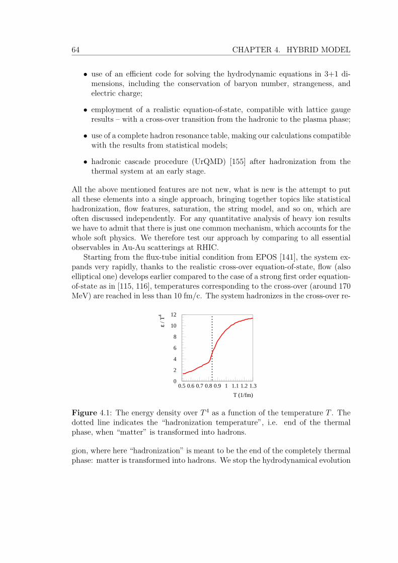
64 CHAPTER 4. HYBRID MODEL
• use of an efficient code for solving the hydrodynamic equations in 3+1 di-mensions, including the conservation of baryon number, strangeness, andelectric charge;
• employment of a realistic equation-of-state, compatible with lattice gaugeresults – with a cross-over transition from the hadronic to the plasma phase;
• use of a complete hadron resonance table, making our calculations compatiblewith the results from statistical models;
• hadronic cascade procedure (UrQMD) [155] after hadronization from thethermal system at an early stage.
All the above mentioned features are not new, what is new is the attempt to putall these elements into a single approach, bringing together topics like statisticalhadronization, flow features, saturation, the string model, and so on, which areoften discussed independently. For any quantitative analysis of heavy ion resultswe have to admit that there is just one common mechanism, which accounts for thewhole soft physics. We therefore test our approach by comparing to all essentialobservables in Au-Au scatterings at RHIC.
Starting from the flux-tube initial condition from EPOS [141], the system ex-pands very rapidly, thanks to the realistic cross-over equation-of-state, flow (alsoelliptical one) develops earlier compared to the case of a strong first order equation-of-state as in [115, 116], temperatures corresponding to the cross-over (around 170MeV) are reached in less than 10 fm/c. The system hadronizes in the cross-over re-
0
2
4
6
8
10
12
0.5 0.6 0.7 0.8 0.9 1 1.1 1.2 1.3
T (1/fm)
ε /
T4
Figure 4.1: The energy density over T 4 as a function of the temperature T . Thedotted line indicates the “hadronization temperature”, i.e. end of the thermalphase, when “matter” is transformed into hadrons.
gion, where here “hadronization” is meant to be the end of the completely thermalphase: matter is transformed into hadrons. We stop the hydrodynamical evolution
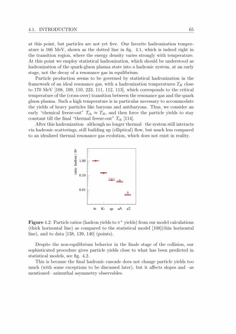
4.1. INTRODUCTION 65
at this point, but particles are not yet free. Our favorite hadronization temper-ature is 166 MeV, shown as the dotted line in fig. 4.1, which is indeed right inthe transition region, where the energy density varies strongly with temperature.At this point we employ statistical hadronization, which should be understood ashadronization of the quark-gluon plasma state into a hadronic system, at an earlystage, not the decay of a resonance gas in equilibrium.
Particle production seems to be governed by statistical hadronization in theframework of an ideal resonance gas, with a hadronization temperatures TH closeto 170 MeV [108, 109, 110, 223, 111, 112, 113], which corresponds to the criticaltemperature of the (cross-over) transition between the resonance gas and the quarkgluon plasma. Such a high temperature is in particular necessary to accommodatethe yields of heavy particles like baryons and antibaryons. Thus, we consider anearly “chemical freeze-out” Tch ≈ TH , and then force the particle yields to stayconstant till the final “thermal freeze-out” Tth [114].
After this hadronization –although no longer thermal– the system still interactsvia hadronic scatterings, still building up (elliptical) flow, but much less comparedto an idealized thermal resonance gas evolution, which does not exist in reality.
rat
io h
adro
n / π
+
π- K- ap aΛ aΞ
1.00
0.10
0.01
Figure 4.2: Particle ratios (hadron yields to π+ yields) from our model calculations(thick horizontal line) as compared to the statistical model [108](thin horizontalline), and to data [138, 139, 140] (points).
Despite the non-equilibrium behavior in the finale stage of the collision, oursophisticated procedure gives particle yields close to what has been predicted instatistical models, see fig. 4.2.
This is because the final hadronic cascade does not change particle yields toomuch (with some exceptions to be discussed later), but it affects slopes and –asmentioned– azimuthal asymmetry observables.
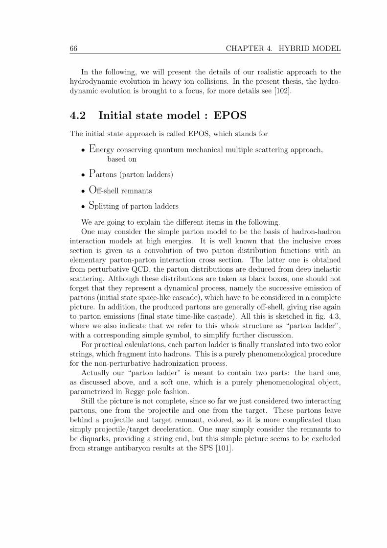
66 CHAPTER 4. HYBRID MODEL
In the following, we will present the details of our realistic approach to thehydrodynamic evolution in heavy ion collisions. In the present thesis, the hydro-dynamic evolution is brought to a focus, for more details see [102].
4.2 Initial state model : EPOS
The initial state approach is called EPOS, which stands for
• Energy conserving quantum mechanical multiple scattering approach,based on
• Partons (parton ladders)
• Off-shell remnants
• Splitting of parton ladders
We are going to explain the different items in the following.One may consider the simple parton model to be the basis of hadron-hadron
interaction models at high energies. It is well known that the inclusive crosssection is given as a convolution of two parton distribution functions with anelementary parton-parton interaction cross section. The latter one is obtainedfrom perturbative QCD, the parton distributions are deduced from deep inelasticscattering. Although these distributions are taken as black boxes, one should notforget that they represent a dynamical process, namely the successive emission ofpartons (initial state space-like cascade), which have to be considered in a completepicture. In addition, the produced partons are generally off-shell, giving rise againto parton emissions (final state time-like cascade). All this is sketched in fig. 4.3,where we also indicate that we refer to this whole structure as “parton ladder”,with a corresponding simple symbol, to simplify further discussion.
For practical calculations, each parton ladder is finally translated into two colorstrings, which fragment into hadrons. This is a purely phenomenological procedurefor the non-perturbative hadronization process.
Actually our “parton ladder” is meant to contain two parts: the hard one,as discussed above, and a soft one, which is a purely phenomenological object,parametrized in Regge pole fashion.
Still the picture is not complete, since so far we just considered two interactingpartons, one from the projectile and one from the target. These partons leavebehind a projectile and target remnant, colored, so it is more complicated thansimply projectile/target deceleration. One may simply consider the remnants tobe diquarks, providing a string end, but this simple picture seems to be excludedfrom strange antibaryon results at the SPS [101].
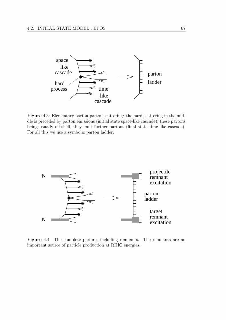
4.2. INITIAL STATE MODEL : EPOS 67
parton
laddertime like
cascade
space
cascade
hardprocess
like
Figure 4.3: Elementary parton-parton scattering: the hard scattering in the mid-dle is preceded by parton emissions (initial state space-like cascade); these partonsbeing usually off-shell, they emit further partons (final state time-like cascade).For all this we use a symbolic parton ladder.
N
N
remnantprojectile
excitation
targetremnantexcitation
partonladder
Figure 4.4: The complete picture, including remnants. The remnants are animportant source of particle production at RHIC energies.
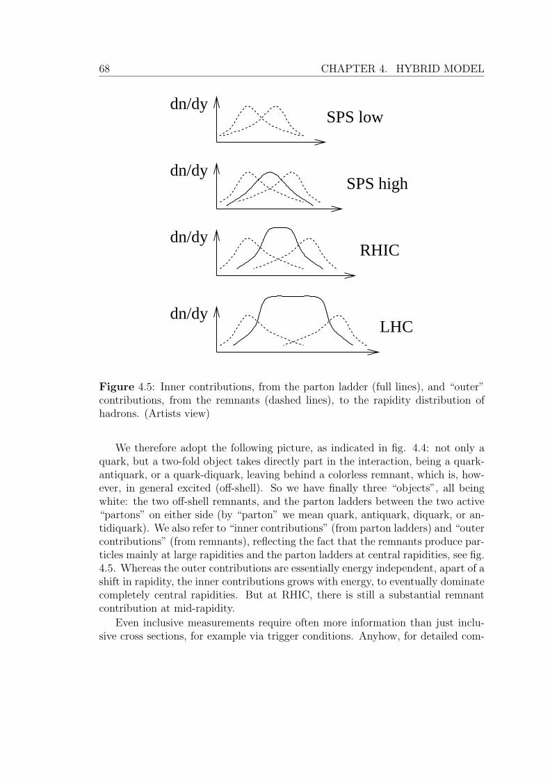
68 CHAPTER 4. HYBRID MODEL
SPS lowdn/dy
dn/dy
dn/dy
SPS high
dn/dyLHC
RHIC
Figure 4.5: Inner contributions, from the parton ladder (full lines), and “outer”contributions, from the remnants (dashed lines), to the rapidity distribution ofhadrons. (Artists view)
We therefore adopt the following picture, as indicated in fig. 4.4: not only aquark, but a two-fold object takes directly part in the interaction, being a quark-antiquark, or a quark-diquark, leaving behind a colorless remnant, which is, how-ever, in general excited (off-shell). So we have finally three “objects”, all beingwhite: the two off-shell remnants, and the parton ladders between the two active“partons” on either side (by “parton” we mean quark, antiquark, diquark, or an-tidiquark). We also refer to “inner contributions” (from parton ladders) and “outercontributions” (from remnants), reflecting the fact that the remnants produce par-ticles mainly at large rapidities and the parton ladders at central rapidities, see fig.4.5. Whereas the outer contributions are essentially energy independent, apart of ashift in rapidity, the inner contributions grows with energy, to eventually dominatecompletely central rapidities. But at RHIC, there is still a substantial remnantcontribution at mid-rapidity.
Even inclusive measurements require often more information than just inclu-sive cross sections, for example via trigger conditions. Anyhow, for detailed com-
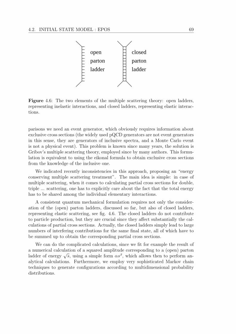
4.2. INITIAL STATE MODEL : EPOS 69
parton
ladder
parton
ladder
closedopen
Figure 4.6: The two elements of the multiple scattering theory: open ladders,representing inelastic interactions, and closed ladders, representing elastic interac-tions.
parisons we need an event generator, which obviously requires information aboutexclusive cross sections (the widely used pQCD generators are not event generatorsin this sense, they are generators of inclusive spectra, and a Monte Carlo eventis not a physical event). This problem is known since many years, the solution isGribov’s multiple scattering theory, employed since by many authors. This formu-lation is equivalent to using the eikonal formula to obtain exclusive cross sectionsfrom the knowledge of the inclusive one.
We indicated recently inconsistencies in this approach, proposing an “energyconserving multiple scattering treatment”. The main idea is simple: in case ofmultiple scattering, when it comes to calculating partial cross sections for double,triple ... scattering, one has to explicitly care about the fact that the total energyhas to be shared among the individual elementary interactions.
A consistent quantum mechanical formulation requires not only the consider-ation of the (open) parton ladders, discussed so far, but also of closed ladders,representing elastic scattering, see fig. 4.6. The closed ladders do not contributeto particle production, but they are crucial since they affect substantially the cal-culations of partial cross sections. Actually, the closed ladders simply lead to largenumbers of interfering contributions for the same final state, all of which have tobe summed up to obtain the corresponding partial cross sections.
We can do the complicated calculations, since we fit for example the result ofa numerical calculation of a squared amplitude corresponding to a (open) partonladder of energy
√s, using a simple form αsβ, which allows then to perform an-
alytical calculations. Furthermore, we employ very sophisticated Markov chaintechniques to generate configurations according to multidimensional probabilitydistributions.
70 CHAPTER 4. HYBRID MODEL
Important concerning numerical results: There are a couple of parameterswhich determine the parameterization of the soft elementary interaction (softPomeron), which are essentially fixed to get the pp cross sections right. The pQCDparameters (soft virtuality cutoff, K-factor, parton emission cutoff, parton-hadroncoupling) are fixed to provide a reasonable parton distribution function (which wecalculate, it is not input!).
We assume the remnants to be off-shell with probability pO, a mass distributiongiven as
prob ∝M−2αO , (4.1)
with parameter values which are not necessarily the same for diffractive and non-diffractive interactions (the latter ones being defined to be those without partonladders). We use currently for pO 0.75 (dif) and 0.95 (nondif), and for αO 0.75(dif) and 1.1 (nondif). Those excitation exponents may give rise to quite high massremnants, RHIC and also SPS data seem to support this. High mass remnantswill be treated as strings.
There are four important fragmentation parameters: the break probability (perunit space-time area) pB, which determines whether a string breaks earlier or later,the diquark break probability pD, the strange break probability pS, and the meantransverse momentum pt of a break, with obvious consequences for baryon andstrangeness production, and the pt of the produced hadrons. We use three setsof these parameters, for the three types of strings: soft-, kinky(hard)-, remnant-strings. We do not really use the full freedom of these parameters, but one singleset would not work – if we are interested in high precision. Somewhat surprising:pS is 0.14 for soft and 0.06 for kinky strings. Maybe this reflects the fact that softstrings may have low masses, where strangeness is suppressed, and which needssome compensation. The parameter pD is as well bigger for soft compared to kinkystrings.
4.3 Hydrodynamic evolution, realistic equation-
of-state
Having fixed the initial conditions, the core evolves according to the equations ofideal hydrodynamics, namely the local energy-momentum conservation
∂µTµν = 0, ν = 0, ..., 3 , (4.2)
and the conservation of net charges,
∂Nµk = 0, k = B, S,Q , (4.3)
4.3. HYDRODYNAMIC EVOLUTION, REALISTIC EQUATION-OF-STATE71
with B, S, and Q referring to respectively baryon number, strangeness, and electriccharge. In this thesis we treat ideal hydrodynamic, so we use the decomposition
T µν = (ε+ p)uµuν − p gµν , (4.4)
Nµk = nku
µ, (4.5)
where u is the four-velocity of the local rest frame. Solving the equations, as dis-cussed above, provides the evolution of the space-time dependence of the macro-scopic quantities energy density ε(x), collective flow velocity ~v(x), and the netflavor densities nk(x). Here, the crucial ingredient is the equation of state, whichcloses the set of equations by providing the ε-dependence of the pressure p. Theequation-of-state should fulfill the following requirements:
• flavor conservation, using chemical potentials µB, µS, µQ;
• compatibility with lattice gauge results in case of µB =µS =µQ = 0.
The starting point for constructing this “realistic” equation-of-state is the pres-sure pH of a resonance gas, and the pressure pQ of an ideal quark gluon plasma,including bag pressure. Be Tc the temperature where pH and pQ cross. The correctpressure is assumed to be of the form
p = pQ + λ (pH − pQ), (4.6)
where the temperature dependence of λ is given as
λ = exp
(−T − Tc
δ
)Θ(T − Tc) + Θ(Tc − T ), (4.7)
with
δ = δ0 exp(−(µB/µc)
2) (
1 +T − Tc
2Tc
). (4.8)
From the pressure one obtains the entropy density S as
S =∂p
∂T= SQ + λ (SH − SQ) +
∂λ
∂T(pH − pQ), (4.9)
and the flavor densities ni as
ni =∂p
∂µi= ni
Q + λ (niH − ni
Q) +∂λ
∂µi(pH − pQ). (4.10)
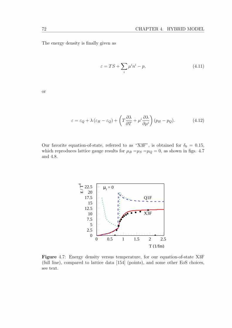
72 CHAPTER 4. HYBRID MODEL
The energy density is finally given as
ε = TS +∑
i
µini − p, (4.11)
or
ε = εQ + λ (εH − εQ) +
(T∂λ
∂T+ µi ∂λ
∂µi
)(pH − pQ). (4.12)
Our favorite equation-of-state, referred to as “X3F”, is obtained for δ0 = 0.15,which reproduces lattice gauge results for µB =µS =µQ = 0, as shown in figs. 4.7and 4.8.
02.5
57.510
12.515
17.520
22.5
0 0.5 1 1.5 2 2.5
T (1/fm)
ε /
T4
µi = 0
Q1F
X3F
Figure 4.7: Energy density versus temperature, for our equation-of-state X3F(full line), compared to lattice data [154] (points), and some other EoS choices,see text.

4.3. HYDRODYNAMIC EVOLUTION, REALISTIC EQUATION-OF-STATE73
0
1
2
3
4
5
6
7
8
0 0.5 1 1.5 2 2.5
T (1/fm)
p /
T4
µi = 0
Q1F
X3F
Figure 4.8: Pressure versus temperature, for our equation-of-state X3F (full line),compared to lattice data [154] (points), and some other EoS choices, see text.
The symbol X3F stands for “cross-over” and “3 flavor conservation”. Alsoshown in the figures is the EoS Q1F, referring to a simple first order equation-of-state, with baryon number conservation, which we will use as a reference tocompare with. Many current calculations are still based on this simple choice, asfor example the one in [115, 116], shown as dotted lines in figs. 4.7 and 4.8.
In the next subsections, the details of the equation of state are described.
4.3.1 Hydrodynamic algorithm
The algorithm is based on the Godunov method: one introduces finite cells andcomputes fluxes between cells using the (approximate) Riemann problem solutionfor each cell boundary. A relativistic HLLE solver is used to solve the Riemannproblem. To achieve more accuracy in time, a predictor-corrector scheme is usedfor the second order of accuracy in time, i.e. the numerical error is O(dt3), insteadof O(dt2). To achieve more accuracy in space, namely a second order scheme, thelinear distributions of quantities (conservative variables) inside cells are used. Theconservative quantities are (e+ p ∗ v2)/(1 − v2), (e+ p) ∗ v/(1 − v2) .
We rewrite equations in hyperbolic coordinates. These coordinates are suitablefor the dynamical description at ultrarelativistic energies. It is convenient to write
74 CHAPTER 4. HYBRID MODEL
the equations in conservative form, the conservative variables are
~Q =
Qτ
Qx
Qy
Qη
QB
QS
=
γ2(ε+ p) − pγ2(ε+ p)vx
γ2(ε+ p)vy
γ2(ε+ p)vη
γnB
γnS
γnQ
, (4.13)
where nB, nS, nQ are the densities of the conserved quantities B, S, and Q. Thecomponents Qm are conservative variables in the sense that the integral (discretesum over all cells) of Qm gives the total energy, momentum, and the total B, S,and Q, which are conserved up to the fluxes at the grid boundaries. The velocitiesin these expressions are defined in the “Bjorken frame” related to velocities inlaboratory frame as
vx = vlabx · cosh y
cosh(y − ηs)
vy = vlaby · cosh y
cosh(y − ηs)
vη = tanh(y − ηs) (4.14)
where y = 12ln[(1+vlab
z )/(1−vlabz )] is the longitudinal rapidity of the fluid element,
ηs = 12ln[(t+z)/(t−z)] is space-time rapidity. The full hydrodynamical equations
are then
∂τ
Qτ
Qx
Qy
Qη
QB
QS
︸ ︷︷ ︸quantities
+~∇ ·
Qτ
Qx
Qy
Qη
QB
QS
~v +
~∇(p · ~v)∂xp∂yp1τ∂ηp000
︸ ︷︷ ︸
fluxes
+
(Qτ + p)(1 + v2η)/τ
Qx/τQy/τ2Qη/τQB/τQS/τQQ/τ
︸ ︷︷ ︸
sources
= 0
(4.15)
with ~∇ =(∂x, ∂y,
1τ∂η
).
We base our calculations on the finite-volume approach : we discretize thesystem on a fixed grid in the calculational frame and interpret Qn
m,ijk as averagevalue over some space interval ∆Vijk, which is called a cell. The index n refers tothe discretized time.
4.3. HYDRODYNAMIC EVOLUTION, REALISTIC EQUATION-OF-STATE75
The values of Qnm,ijk are then updated after each time-step according to the
fluxes on the cell interface during the time-step ∆tn. One has the following updateformula :
Qn+1m,ijk =Qn
m,ijk −∆t
∆x1
(F(i+1/2),jk + F(i−1/2),jk)
− ∆t
∆x2
(Fi(,j+1/2),k + Fi,(j−1/2),k) (4.16)
− ∆t
∆x3
(Fij,(k+1/2) + Fij,(k−1/2)),
where F is the average flux over the cell boundary, the indexes +1/2 and −1/2correspond to the right and the left cell boundary in each direction. This is the baseof the Godunov method [192], which also implies that the distributions of variablesinside a cell are piecewise linear (or piecewise parabolic etc, depending on the orderof the numerical scheme), which forms a Riemann problem at each cell interface.Then the flux through each cell interface depends only on the solution of a singleRiemann problem, supposing that the waves from the neighboring discontinuitiesdo not intersect. The latter is satisfied with the Courant-Friedrichs-Lewy (CFL)condition [193].
To solve the Riemann problems at each cell interface, we use the relativisticHLLE solver [194], which approximates the wave profile in the Riemann problemby a single intermediate state between two shock waves propagating away fromthe initial discontinuity. Together with the shock wave velocity estimate, in thisapproximation one can obtain an analytical dependence of the flux on the initialconditions for the Riemann problem, which makes the algorithm explicit.
We proceed then to construct a higher-order numerical scheme:
• in time: the predictor-corrector scheme is used for the second order accuracyin time, i.e. the numerical error is O(dt3), instead of O(dt2)
• in space: in the same way, to achieve the second order scheme, the lineardistributions of quantities (conservative variables) inside cells are used.
Some final remarks:At each time-step, we compute and sum the fluxes for each cell with all its
neighbors and update the value of conservative variables with the total flux. Thus,we do not use operator splitting (dimensional splitting) and thus avoid the numer-ical artifacts introduced by this method, e.g. artificial spatial asymmetry.
To treat grid boundaries, we use the method of ghost cells. We include 2additional cells on either end of grid in each direction, and set the quantities inthese cells at the beginning of each time-step. For simplicity, we set the quantities
76 CHAPTER 4. HYBRID MODEL
in ghost cells to be equal to these in the nearest ”real” cell, thus implementing non-reflecting boundary conditions (outflow boundary). This physically correspond toboundary which does not reflect any wave, which is consistent with expansion intovacuum.
In our simulations we deal with spatially finite systems expanding into vacuum.Thus the computational grid in Eulerian algorithm must initially contain bothsystem and surrounding vacuum. To account for the finite velocity of the expansioninto the vacuum, which equals c for an infinitesimal slice of matter on the boundary,we introduce additional (floating-point) variables in each cell which keep the extentof matter expansion within a cell, having the value unity for the complete cell, zerofor a cell with vacuum only. The matter is allowed to expand in the next vacuumcell only if the current cell is filled with matter.
4.3.2 Resonance gas
Whereas for hadronization we employ the correct quantum statistics, we use theBoltzmann approximation for the calculation of the equation of state. This is rea-sonable even for pions at zero chemical potential, the excluded volume correctionat nonzero chemical potentials is considerably bigger than the difference comingfrom quantum statistical treatment. We account for all well known hadrons madefrom u, d, s quarks from the PDG table For energy density, pressure and netcharges we get :
ε =∑
i
gi
2π2m2
iT[3TK2(
mi
T) +
mi
2K1(
mi
T)]exp(µi/T )
· (4.17)
p =∑
i
gi
2π2m2
iT2 ·K2(
mi
T) · exp(µi/T ) (4.18)
nB =∑
i
Bigi
2π2m2
iT ·K2(mi
T) · exp(µi/T ) (4.19)
nQ =∑
i
Qigi
2π2m2
iT ·K2(mi
T) · exp(µi/T ) (4.20)
nS =∑
i
Sigi
2π2m2
iT ·K2(mi
T) · exp(µi/T ) (4.21)
withµi = BiµB +QiµQ + SiµS, (4.22)
where µB, µS, µQ are the chemical potentials associated to B, S, Q, and Bi, Si,Qi are the baryon charge, strangeness, and the electric charge of i-th hadron state,gi = (2Ji + 1) is degeneracy factor.
4.3. HYDRODYNAMIC EVOLUTION, REALISTIC EQUATION-OF-STATE77
For large baryon chemical potential the EoS correction for the deviations fromideal gas due to particle interactions becomes more important. We employ thiscorrection in a form of an excluded volume effect, like a Van der Waals hard corecorrection. According to this prescription,
p(T, µB, µQ, µS) =∑
i
pboltzi (T, µi), (4.23)
µi = µi − vi · p . (4.24)
If one supposes equal volume vi = v for all particle species, then the correctioncan be computed as a solution p(T, µB, µQ, µS) of a fairly simple, however tran-scendental equation,
p(T, µB, µQ, µS) = pboltz(T, µB, µQ, µS)e−vp(T,µB ,µQ,µS)/T (4.25)
We take the value v ≈ 1.44 fm3, which corresponds to the hard core radiusr = 0.7fm.
4.3.3 Ideal QGP
In this ideal phase, matter is made from massless u, d quarks and massive s-quark (+antiquarks). Due to the possibility of a large strange quark chemicalpotential, comparable to its massms = 120 MeV which is taken in our calculations,we perform the integration of the strange quark contribution to thermodynamicquantities exactly, without Boltzmann or zero-mass approximation. So we have
p =gl
6π2
[1
4µ4
u +π2
2µ2
uT2 +
7π4T 4
60
](4.26)
+gl
6π2
[1
4µ4
d +π2
2µ2
dT2 +
7π4T 4
60
]+
+ ps(T, µs) + ps(T, µs) +ggπ
2
90T 4 −B,
with ps(T, µs) = ps(T,−µs), and
ps(T, µs) =glT
2π2
∫ ∞
0
p2 ln
[1+exp
(1
T
√p2 +m2
s +µs
T
)]dp, (4.27)
78 CHAPTER 4. HYBRID MODEL
where we use the degeneracy factors gl = 6 for light quarks, gg = 16 for gluons,and a bag constant B = 0.38 GeV/fm3. Quark chemical potentials are
µu =1
3µB +
2
3µQ , (4.28)
µd =1
3µB − 1
3µQ , (4.29)
µs =1
3µB − 1
3µQ − µS . (4.30)
Using the relations ni = ∂p/∂µi, s = ∂p/∂T , ε = Ts+∑µini − p, we get
ε = 3(p− ps − ps +B) + εs + εs +B (4.31)
nB =1
3
gl
6π2
[µ3
u + π2µuT2 + µ3
d + π2µdT2]+ (4.32)
+1
3[ns(T, µs) − ns(T,−µs)]
nQ =1
3
gl
6π2
[2µ3
u + 2π2µuT2 − µ3
d − π2µdT2]− (4.33)
− 1
3[ns(T, µs) − ns(T,−µs)]
nS = − [ns(T, µs) − ns(T,−µs)] (4.34)
with εs(T, µs) = εs(T,−µs), and
εs(T, µs) =gl
2π2
∞∫0
p2√p2 +m2
s
exp(
1T
√p2 +m2
s −µs
T
)+ 1
dp, (4.35)
ns(T, µs) =gl
2π2
∞∫0
p2
exp(
1T
√p2 +m2
s −µs
T
)+ 1
dp. (4.36)
4.4 Freeze-out
When the evolution reaches the hadronization hypersurface, defined by a giventemperature TH, we switch from “matter” description to particles, using the Cooper-Frye description. Particles may still interact, as discussed below, so hadronizationhere means an intermediate stage, particles are not yet free streaming, but theyare not thermalized any more.
We parametrize the hadronization hyper-surface xµ = xµ(τ, ϕ, η) as
x0 = τ cosh η, x1 = r cosϕ, x2 = r sinϕ, x3 = τ sinh η, (4.37)

4.4. FREEZE-OUT 79
with r = r(τ, ϕ, η) being some function of the three parameters τ, ϕ, η. Thehypersurface element is
dΣµ = εµνκλ∂xν
∂τ
∂xκ
∂ϕ
∂xλ
∂ηdτdϕdη, (4.38)
with εµνκλ = −εµνκλ = 1. Computing the partial derivatives ∂xµ/dα, with α = τ,ϕ, η, one gets
dΣ0 =
{−r ∂r
∂ττ cosh η + r
∂r
∂ηsinh η
}dτdϕdη, (4.39)
dΣ1 =
{∂r
∂ϕτ sinϕ+ r τ cosϕ
}dτdϕdη, (4.40)
dΣ2 =
{− ∂r
∂ϕτ cosϕ+ r τ sinϕ
}dτdϕdη, (4.41)
dΣ3 =
{r∂r
∂ττ sinh η − r
∂r
∂ηcosh η
}dτdϕdη. (4.42)
Cooper-Frye hadronization amounts to calculating
Edn
d3p=
∫dΣµp
µf(up),
with u being the flow four-velocity in the global frame, which can be expressed interms of the four-velocity u in the “Bjorken frame” as
u0 = u 0 cosh η + u 3 sinh η , (4.43)
u1 = u 1 , (4.44)
u2 = u 2 , (4.45)
u3 = u 0 sinh η + u 3 cosh η . (4.46)
In a similar way one may express p in terms of p in the Bjorken frame. Usingγ = u 0 and the flow velocity vµ = u µ/γ, we get
dn
dydφdp⊥= (4.47)
p⊥
∫ {−r ∂r
∂ττ p 0 + r τ p r +
∂r
∂ϕτ p t − r
∂r
∂ηp 3
}f(x, p),
with p r = p 1 cosϕ + p 2 sinϕ and p t = p 1 sinϕ − p 2 cosϕ being the radial andthe tangential transverse momentum components. Our Monte Carlo generationprocedure is based on the invariant volume element moving through the FO surface,
dV ∗ = dΣµuµ = w dτdϕdη, (4.48)

80 CHAPTER 4. HYBRID MODEL
with
w = γ
{−r ∂r
∂ττ + r τ vr +
∂r
∂ϕτvt − r
∂r
∂ηv3
}, (4.49)
and with vr = v1 cosϕ + v2 sinϕ and vt = v1 sinϕ − v2 cosϕ being the radialand the tangential transverse flow. Freeze out is the done as follows (equivalentto Cooper-Frye): the proposal of isotropic particles production in the local restframe as
dni = α d3p∗ dV ∗ fi(E∗), (4.50)
is accepted with probability
κ =dΣµ p
µ
α dV ∗E∗ . (4.51)
In case of acceptance, the momenta are boosted to the global frame.After the “intermediate” hadronization, the particles at their hadronization
positions (on the corresponding hypersurface) are fed into the hadronic cascademodel UrQMD [155, 156], performing hadronic interaction until the system isso dilute that no interaction occur any more. The “final” freeze out position ofthe particles is the last interaction point of the cascade process, or the hydrohadronization position, if no hadronic interactions occurs.
4.5 UrQMD afterburner
The UrQMD-model [155] is a microscopic transport theory based on the covariantpropagation of all hadrons on classical trajectories in combination with stochasticbinary scatterings, color string formation and resonance decay. It represents aMonte Carlo solution of a large set of coupled partial integro-differential equationsfor the time evolution of the various phase space densities fi(x, p) of particle speciesi = N,∆,Λ, etc., which non-relativistically assumes the Boltzmann form:
dfi(x, p)
dt≡ ∂p
∂t
∂fi(x, p)
∂p+∂x
∂t
∂fi(x, p)
∂x+∂fi(x, p)
∂t= Stfi(x, p) , (4.52)
where x and p are the position and momentum of the particle, respectively, andStfi(x, p) denotes the collision (or rather source-) term of these particle species,which are connected to any other particle species fk.
The exchange of electric and baryonic charge, strangeness and four momentumin the t-channel is considered for baryon-baryon (BB) collisions at low energies,while meson-baryon (MB) and meson-meson (MM) interactions are treated viathe formation and decay of resonances, i.e. the s-channel reactions. t-channelreactions for MB and MM collisions are taken into account from
√s > 3 GeV on
increasing to the only MB, MM interaction type above√s = 6 GeV. For nucleus-
nucleus collisions the soft binary and ternary interactions between nucleons can

4.6. RESULTS: ELLIPTICAL FLOW 81
be described by the real part of the in-medium G-Matrix, which is approximatedby a non-relativistic density-dependent Skyrme potential of the form
V Sk =1
2!t1
∑i 6=j
δ(~xi − ~xj) +1
3!t2
∑i6=j 6=k
δ(~xi − ~xj)δ(~xj − ~xk) , (4.53)
where ~xα denotes the coordinate variable in the quantum phase space. The firstterm simulates the attractive potential of the NN-interaction, and the second oneyields the saturation. In addition, Yukawa and Coulomb potentials are imple-mented in the model. The potentials allow to calculate the equation of state of theinteracting many body system, as long as it is dominated by nucleons. Note thatthese potential interactions are only used in the model for baryons/nucleons withrelative momenta ∆p of less than 2 GeV/c. For the hadronic collisions discussedhere, the potential interactions are omitted. Further details of the application ofthe UrQMD model to heavy-ion reactions may be found in [155].
This framework allows to bridge with one concise model the entire availablerange of energies from the SIS energy region (
√s ≈ 2 GeV) to the RHIC en-
ergy (√s = 200 GeV). At the highest energies, a huge number of different particle
species can be produced. The model should allow for subsequent rescatterings. Thecollision term in the UrQMD model includes more than fifty baryon species and fivemeson nonetts (45 mesons). In addition, their antiparticles have been implementedusing charge-conjugation to assure full baryon-antibaryon symmetry. The imple-mented meson multiplets are: pseudo-scalar, vector, scalar, pseudo-vector and thetensor mesons as well as the heavy vector meson resonances ρ(1450), ρ(1700),ω(1420), and ω(1600). Extremely heavy meson resonances (m > 2 GeV) are notexplicitly implemented, however they may be important when investigating, e.g.the dynamics of ΦΦ correlations in future experiments.
All particles can be produced in hadron-hadron collisions and can interactfurther with each other. The different decay channels all nucleon-, ∆- and hyperon-resonances up to 2.25 GeV/c2 mass as well as the meson (e.g. K∗) decays etc. areimplemented. At higher energies we take advantage of the hadron universalityand use a string model for the decay of intermediate states. The cross-sectionsof various hadronic processes as well as the formation and fragmentation of thestrings are described in details in [155]
4.6 Results: Elliptical flow
In this and the next sections, the results for the model application to 200A GeVRHIC data description are presented. As it was already said, important informa-tion about the space-time evolution of the system is provided by the study of the
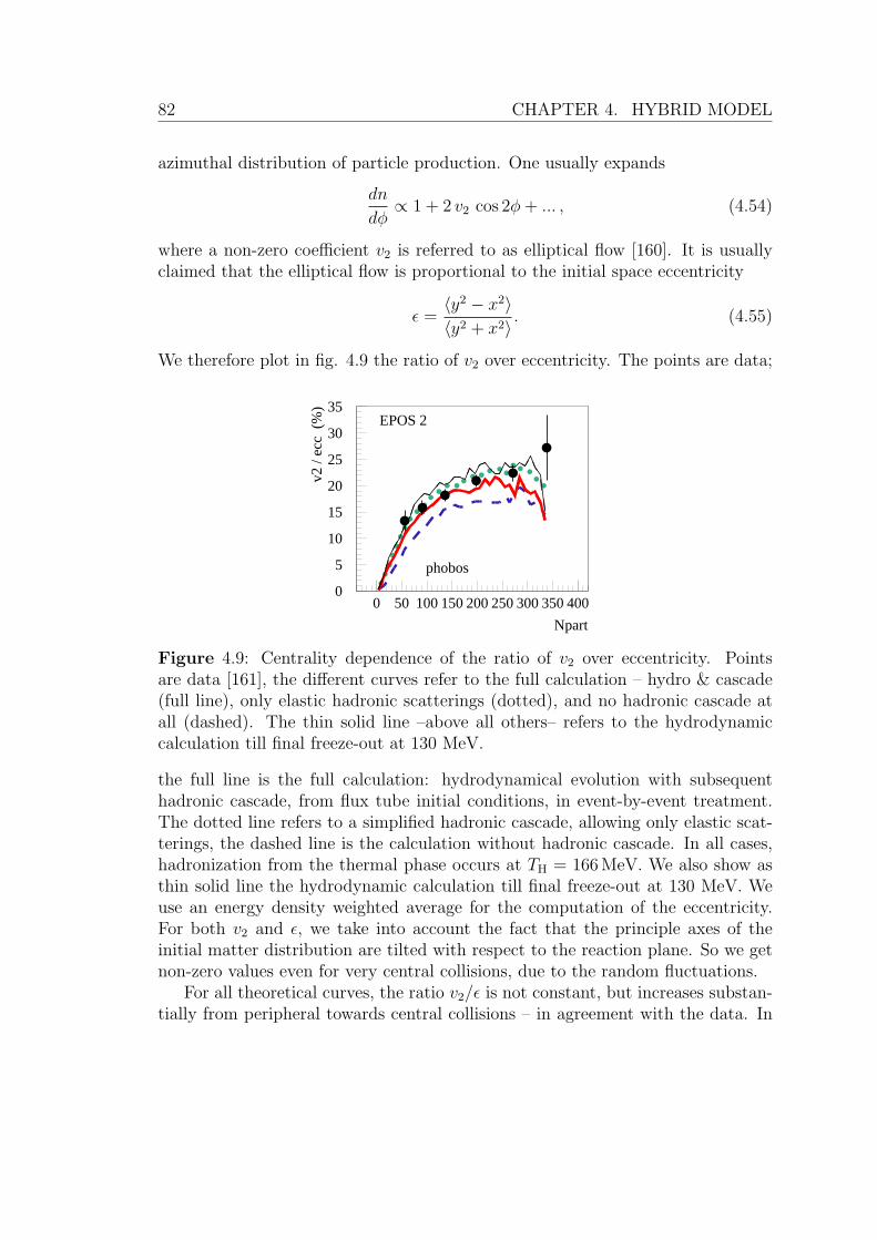
82 CHAPTER 4. HYBRID MODEL
azimuthal distribution of particle production. One usually expands
dn
dφ∝ 1 + 2 v2 cos 2φ+ ... , (4.54)
where a non-zero coefficient v2 is referred to as elliptical flow [160]. It is usuallyclaimed that the elliptical flow is proportional to the initial space eccentricity
ε =〈y2 − x2〉〈y2 + x2〉
. (4.55)
We therefore plot in fig. 4.9 the ratio of v2 over eccentricity. The points are data;
0
5
10
15
20
25
30
35
0 50 100 150 200 250 300 350 400
Npart
v2
/ ecc
(%
)
EPOS 2
phobos
Figure 4.9: Centrality dependence of the ratio of v2 over eccentricity. Pointsare data [161], the different curves refer to the full calculation – hydro & cascade(full line), only elastic hadronic scatterings (dotted), and no hadronic cascade atall (dashed). The thin solid line –above all others– refers to the hydrodynamiccalculation till final freeze-out at 130 MeV.
the full line is the full calculation: hydrodynamical evolution with subsequenthadronic cascade, from flux tube initial conditions, in event-by-event treatment.The dotted line refers to a simplified hadronic cascade, allowing only elastic scat-terings, the dashed line is the calculation without hadronic cascade. In all cases,hadronization from the thermal phase occurs at TH = 166 MeV. We also show asthin solid line the hydrodynamic calculation till final freeze-out at 130 MeV. Weuse an energy density weighted average for the computation of the eccentricity.For both v2 and ε, we take into account the fact that the principle axes of theinitial matter distribution are tilted with respect to the reaction plane. So we getnon-zero values even for very central collisions, due to the random fluctuations.
For all theoretical curves, the ratio v2/ε is not constant, but increases substan-tially from peripheral towards central collisions – in agreement with the data. In
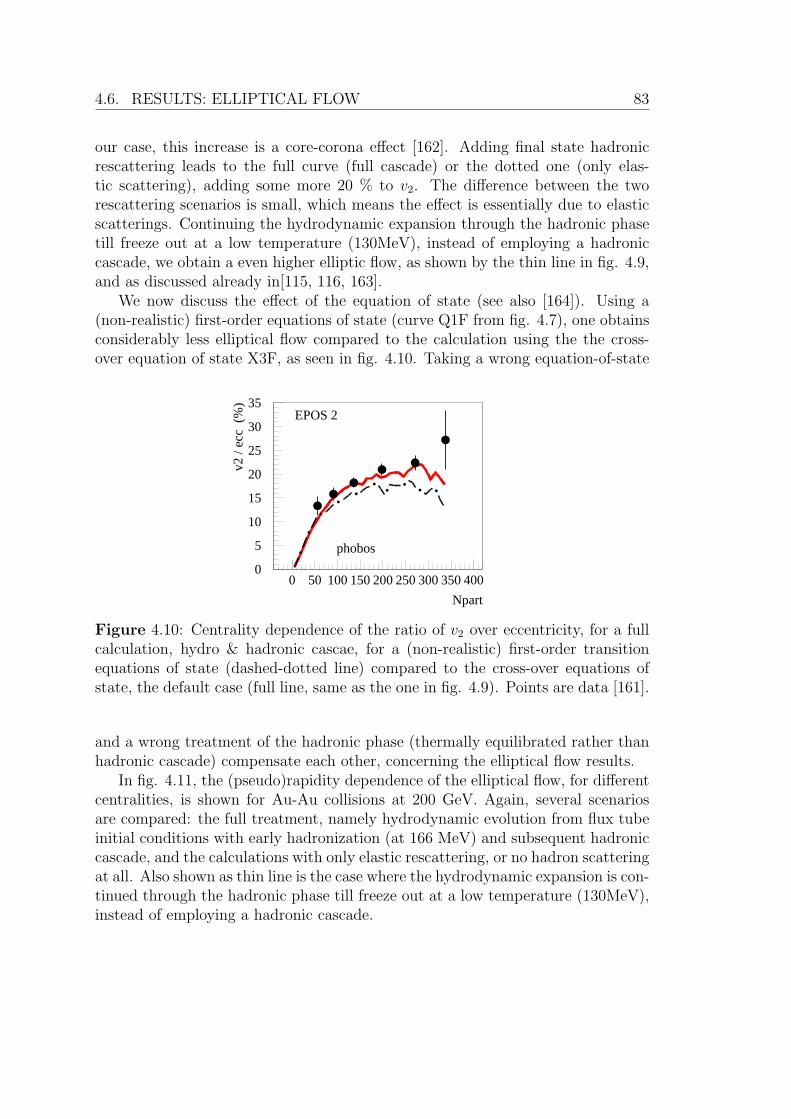
4.6. RESULTS: ELLIPTICAL FLOW 83
our case, this increase is a core-corona effect [162]. Adding final state hadronicrescattering leads to the full curve (full cascade) or the dotted one (only elas-tic scattering), adding some more 20 % to v2. The difference between the tworescattering scenarios is small, which means the effect is essentially due to elasticscatterings. Continuing the hydrodynamic expansion through the hadronic phasetill freeze out at a low temperature (130MeV), instead of employing a hadroniccascade, we obtain a even higher elliptic flow, as shown by the thin line in fig. 4.9,and as discussed already in[115, 116, 163].
We now discuss the effect of the equation of state (see also [164]). Using a(non-realistic) first-order equations of state (curve Q1F from fig. 4.7), one obtainsconsiderably less elliptical flow compared to the calculation using the the cross-over equation of state X3F, as seen in fig. 4.10. Taking a wrong equation-of-state
0
5
10
15
20
25
30
35
0 50 100 150 200 250 300 350 400
Npart
v2
/ ecc
(%
)
EPOS 2
phobos
Figure 4.10: Centrality dependence of the ratio of v2 over eccentricity, for a fullcalculation, hydro & hadronic cascae, for a (non-realistic) first-order transitionequations of state (dashed-dotted line) compared to the cross-over equations ofstate, the default case (full line, same as the one in fig. 4.9). Points are data [161].
and a wrong treatment of the hadronic phase (thermally equilibrated rather thanhadronic cascade) compensate each other, concerning the elliptical flow results.
In fig. 4.11, the (pseudo)rapidity dependence of the elliptical flow, for differentcentralities, is shown for Au-Au collisions at 200 GeV. Again, several scenariosare compared: the full treatment, namely hydrodynamic evolution from flux tubeinitial conditions with early hadronization (at 166 MeV) and subsequent hadroniccascade, and the calculations with only elastic rescattering, or no hadron scatteringat all. Also shown as thin line is the case where the hydrodynamic expansion is con-tinued through the hadronic phase till freeze out at a low temperature (130MeV),instead of employing a hadronic cascade.

84 CHAPTER 4. HYBRID MODEL
00.5
11.5
22.5
33.5
44.5
5
-4 -2 0 2 4 η
v2
(%
)
EPOS 2 chrgdMB
phobos
0
0.5
1
1.5
2
2.5
3
3.5
4
-4 -2 0 2 4 η
EPOS 2 chrgd3-15%
phobos
0
1
2
3
4
5
6
-4 -2 0 2 4 η
v2
(%
)
EPOS 2 chrgd15-25%
phobos
0
1
2
3
4
5
6
7
8
-4 -2 0 2 4 η
EPOS 2 chrgd25-50%
phobos
Figure 4.11: Pseudorapidity distributions of the elliptical flow v2 for minimumbias events (upper left) and different centrality classes, in Au-Au collisions at 200GeV. Points are data [166], the different curves refer to the full calculation – hydro& cascade (full thick line), only elastic hadronic scatterings (dotted), no hadroniccascade at all (dashed), and hydrodynamic calculation till final freeze-out at 130MeV (thin line).
4.7 Transverse momentum spectra and yields
The next results show that the model created actually reproduces more elemen-tary observables like simple transverse momentum (pt) spectra and the integratedparticle yields, for identified hadrons. We will restrict the following pt spectrato values less than 1.5 GeV (2 GeV in some cases), mainly in order to limit theordinate to three or at most four orders of magnitude, which allows still to see10% differences between calculations and data.
In the upper panel of fig. 4.12, we show the pt spectra of π+(left) and π− (right)in central Au-Au collisions, for rapidities (from top to bottom) of 0, 2, and 3. Themiddle panels show the transverse momentum / transverse mass spectra of π+ andπ−, for different centralities, and the lower panel the centrality dependence of theintegrated particle yields per participant for charged particles and π− mesons. In

4.7. TRANSVERSE MOMENTUM SPECTRA AND YIELDS 85
10-1
1
10
10 2
0 0.5 1 1.5 pt
1/2
πpt d
n/dp
tdy
π+ 0-5%
y=0,2,3
brahms10
-1
1
10
10 2
0 0.5 1 1.5 pt
1/2
πpt d
n/dp
tdy
π- 0-5%
y=0,2,3
brahms
1
10
10 2
10 3
0 0.2 0.4 0.6 mt-m
1/2
πmt d
n/dm
tdy
EPOS 2
π+
0-5%
20-30%
40-50%
star1
10
10 2
10 3
0 0.2 0.4 0.6 mt-m
1/2
πmt d
n/dm
tdy
EPOS 2
π-
0-5%
20-30%
40-50%
star
1
10
10 2
10 3
0 0.5 1 1.5 pt
1/2
πpt d
n/dp
tdy
EPOS 2
π+
0-5%
20-30%
40-50%
phenix 1
10
10 2
10 3
0 0.5 1 1.5 pt
1/2
πpt d
n/dp
tdy
EPOS 2
π-
0-5%
20-30%
40-50%
phenix
0
0.5
1
1.5
2
2.5
10 102
Npart
yie
ld /
Npa
rt EPOS 2
charged
phobos
0
0.2
0.4
0.6
0.8
1
1.2
1.4
10 102
Npart
yie
ld /
Npa
rt EPOS 2
π-
phenix
Figure 4.12: Production of pions in Au-Au collisions at 200 GeV. Upper panel:transverse momentum spectra for central collisions at different rapidities (fromtop to bottom: 0, 2, 3). The lower curves are scaled by factors of 1/2 and 1/4,for better visibility. Middle panels: transverse momentum (mass) distributionsat rapidity zero for different centrality classes: from top to bottom: the 0-5%,the 20-30%, and the 40-50% most central collisions. Lower panel: the centralitydependence of the integrated yields for charged particles and pions. The symbolsrefer to data [173, 95, 72, 174], the full lines to our full calculations, the dottedlines to the calculations without hadronic cascade.

86 CHAPTER 4. HYBRID MODEL
10-2
10-1
1
10
0 0.5 1 1.5 2 pt
1/2
πpt d
n/dp
tdy
EPOS 2
Λ
0-5%10-20%20-40%40-60%
star10
-2
10-1
1
10
0 0.5 1 1.5 2 pt
1/2
πpt d
n/dp
tdy
EPOS 2
aΛ
0-5%10-20%20-40%40-60%
star
0
1
2
3
4
5
6
10 102
Npart
yie
ld /
Npa
rt *
100 EPOS 2
Λ
star
0
1
2
3
4
5
6
10 102
Npart
yie
ld /
Npa
rt *
100 EPOS 2
aΛ
star
Figure 4.13: Production of lambdas (left) and antilambdas (right) in Au-Aucollisions at 200 GeV. Upper panel: transverse momentum distributions at rapidityzero for different centrality classes: from top to bottom: the 0-5%, the 20-30%,and the 40-50% most central collisions. The lower curves are scaled by factors of1/2, 1/4, and 1/8, for better visibility. Lower panel: the centrality dependenceof the integrated yields. The symbols refer to data [140], the full lines to our fullcalculations, the dotted lines to the calculations without hadronic cascade. Thethin line refers to a hydrodynamic calculation till final freeze-out at 130 MeV.
the upper panels, for the y = 2 and y = 3 curves, we apply scaling factors of 1/2and 1/4, for better visibility, all other curves are unscaled. We present always twocalculations: the full one (full lines), namely hydrodynamic evolution plus finalstate hadronic cascade, and the calculation without cascade (dotted lines). Thereis a slight increase of pion production in particular at low pt during the hadronicrescattering phase, but the difference between the two scenarios is not very big.We see almost no difference between between the calculation with and withouthadronic rescattering in case of kaons. For both, pions and kaons, we observe achange of slope of the pt distributions with rapidity. Concerning the centralitydependence, we observe an increase of the yields per participant.
In fig. 4.13 we show pt spectra and centrality dependence of particle yieldsper participant, for the (multi)strange baryons Λ, Λ, Ξ, and Ξ. Same conventions

4.8. FEMTOSCOPY 87
as for the previous plots. Here we see a big effect due to rescattering: for thelambdas, the yields are not affected too much, but the pt spectra get much softer,when comparing the full calculation with the one without rescattering. Similarlythe slopes for the Ξ, and Ξ get softer due to rescattering.
To summarize the above discussion on yields and pt spectra: an early hadroniza-tion at 166 MeV gives a reasonable description of the particle yields, which are notmuch affected by the hadronic final state rescattering, except for the protons. Themain effect of the hadronic cascade is a softening of the pt spectra of the baryons.
4.8 Femtoscopy
All the observables discussed so-far are strongly affected by the space-time evo-lution of the system, nevertheless we investigate the momentum space, and con-clusions about space-time are indirect, as for example our conclusions about earlyhadronization based on particle yields and elliptical flow results. A direct insightinto the space-time structure at hadronization is obtained from using femtoscopicalmethods [175, 176, 75, 177, 178].
In this section, π+– π+ correlations are investigated. Here, we only considerquantum statistics for Ψ, no final state interactions, to compare with Coulomb cor-rected data. To compute the discretized correlation function Cij = C(Pi,qj), wedo our event-by-event simulations, and compute for each event C ′
ij =∑
pairs |Ψ(q′, r′)|2,where the sum extends over all π+ pairs with P and q within elementary momentum-space-volumes at respectively Pi and qj. Then we compute the number of pairsNij for the corresponding pairs from mixed events, being used to obtain the prop-erly normalized correlation function Cij = C ′
ij/Nij. The correlation function willbe parametrized as
C(P,q) = (4.56)
1 + λ exp(−R2
out q2out −R2
side q2side −R2
long q2long
),
where ”long” refers to the beam direction, ”out” is parallel to projection of Pperpendicular to the beam, and ”side” is the direction orthogonal to ”long” and”out” [180, 181, 182]. In fig. 4.14, we show the results for the fit parameters λ,Rout, Rside, and Rlong, for five different centrality classes and for four kT intervalsdefined as (in MeV): KT1= [150, 250], KT2= [250, 350], KT3= [350, 450], KT4=[450, 600], where kT of the pair is defined as
kT =1
2(|~pT (pion 1) + ~pT (pion 2)|) . (4.57)
Despite what appears in [77], this is the correct definition of kT used by STAR in
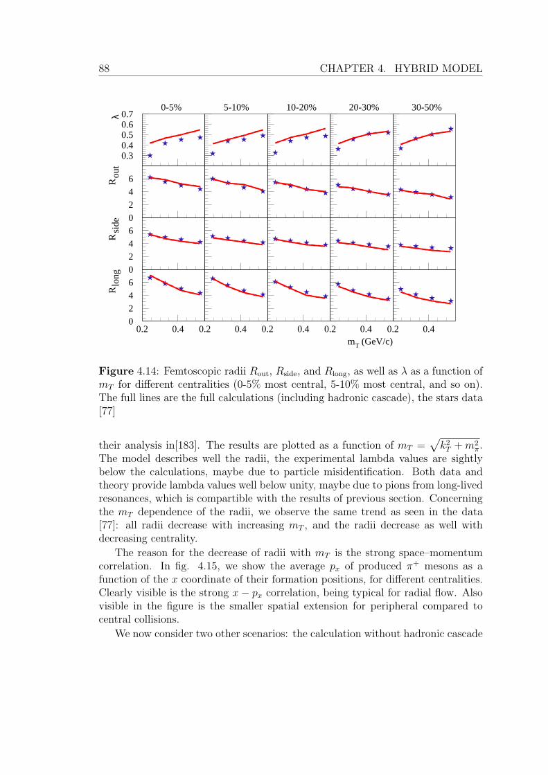
88 CHAPTER 4. HYBRID MODEL
0.30.40.50.60.7
0.2 0.4
λ0-5% 5-10% 10-20% 20-30% 30-50%
0.2 0.4 0.2 0.4 0.2 0.4 0.2 0.4
0246
0.2 0.4
out
R
0.2 0.4 0.2 0.4 0.2 0.4 0.2 0.4
0246
0.2 0.4
sid
eR
0.2 0.4 0.2 0.4 0.2 0.4 0.2 0.4
0246
0.2 0.4
long
R
0.2 0.4 0.2 0.4 0.2 0.4 mT (GeV/c)
0.2 0.4
Figure 4.14: Femtoscopic radii Rout, Rside, and Rlong, as well as λ as a function ofmT for different centralities (0-5% most central, 5-10% most central, and so on).The full lines are the full calculations (including hadronic cascade), the stars data[77]
their analysis in[183]. The results are plotted as a function of mT =√k2
T +m2π.
The model describes well the radii, the experimental lambda values are sightlybelow the calculations, maybe due to particle misidentification. Both data andtheory provide lambda values well below unity, maybe due to pions from long-livedresonances, which is compartible with the results of previous section. Concerningthe mT dependence of the radii, we observe the same trend as seen in the data[77]: all radii decrease with increasing mT , and the radii decrease as well withdecreasing centrality.
The reason for the decrease of radii with mT is the strong space–momentumcorrelation. In fig. 4.15, we show the average px of produced π+ mesons as afunction of the x coordinate of their formation positions, for different centralities.Clearly visible is the strong x− px correlation, being typical for radial flow. Alsovisible in the figure is the smaller spatial extension for peripheral compared tocentral collisions.
We now consider two other scenarios: the calculation without hadronic cascade

4.8. FEMTOSCOPY 89
-0.5-0.4-0.3-0.2-0.1
00.10.20.30.40.5
-10 -8 -6 -4 -2 0 2 4 6 8 10 x (fm)
mean px (GeV/c)
dn/dx (a.u.)
Figure 4.15: The mean transverse momentum component px of π+ as a functionof the x coordinate of the emission point. Also shown is the number of producedπ+ as a function of x. The different curves refer to different centralities: 0-5% =full line, 10-20% = dashed, 30-50% = dotted.
(final freeze out at 166 MeV), and the fully thermal scenario, where we continuethe hydrodynamical evolution till a late freeze-out at 130 MeV (and no cascadeafterwards either). In figs. 4.16 and 4.17, we see a similar space–momentum corre-lation as for the complete calculation in fig. 4.15: the mean transverse momentum
-0.5-0.4-0.3-0.2-0.1
00.10.20.30.40.5
-10 -8 -6 -4 -2 0 2 4 6 8 10 x (fm)
mean px (GeV/c)
dn/dx (a.u.)
Figure 4.16: Same as fig. 4.15, but for the calculation without hadronic cascade.
components px is roughly a linear function of the transverse coordinate x, in theregion where the particle density is non-zero. The maximum mean px is smaller inthe no-cascade case, and bigger in the fully thermal case, as compared to the com-plete calculation. Interesting are the dn/dx distributions: the no-cascade results
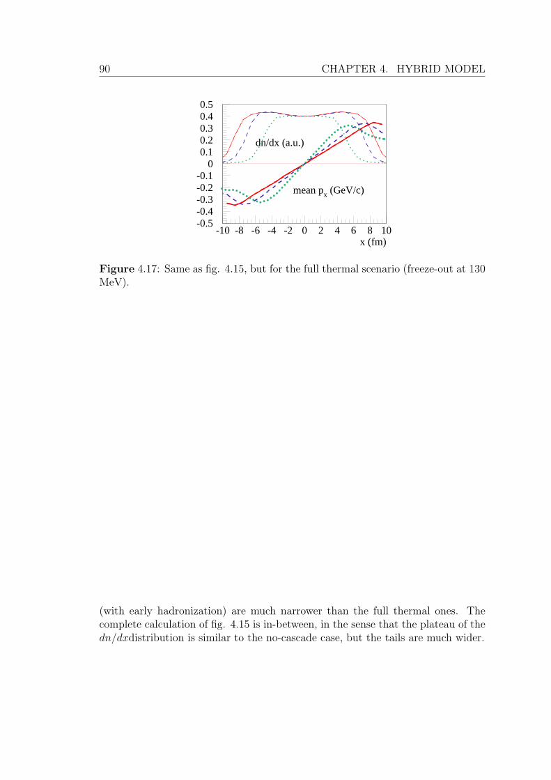
90 CHAPTER 4. HYBRID MODEL
-0.5-0.4-0.3-0.2-0.1
00.10.20.30.40.5
-10 -8 -6 -4 -2 0 2 4 6 8 10 x (fm)
mean px (GeV/c)
dn/dx (a.u.)
Figure 4.17: Same as fig. 4.15, but for the full thermal scenario (freeze-out at 130MeV).
(with early hadronization) are much narrower than the full thermal ones. Thecomplete calculation of fig. 4.15 is in-between, in the sense that the plateau of thedn/dxdistribution is similar to the no-cascade case, but the tails are much wider.
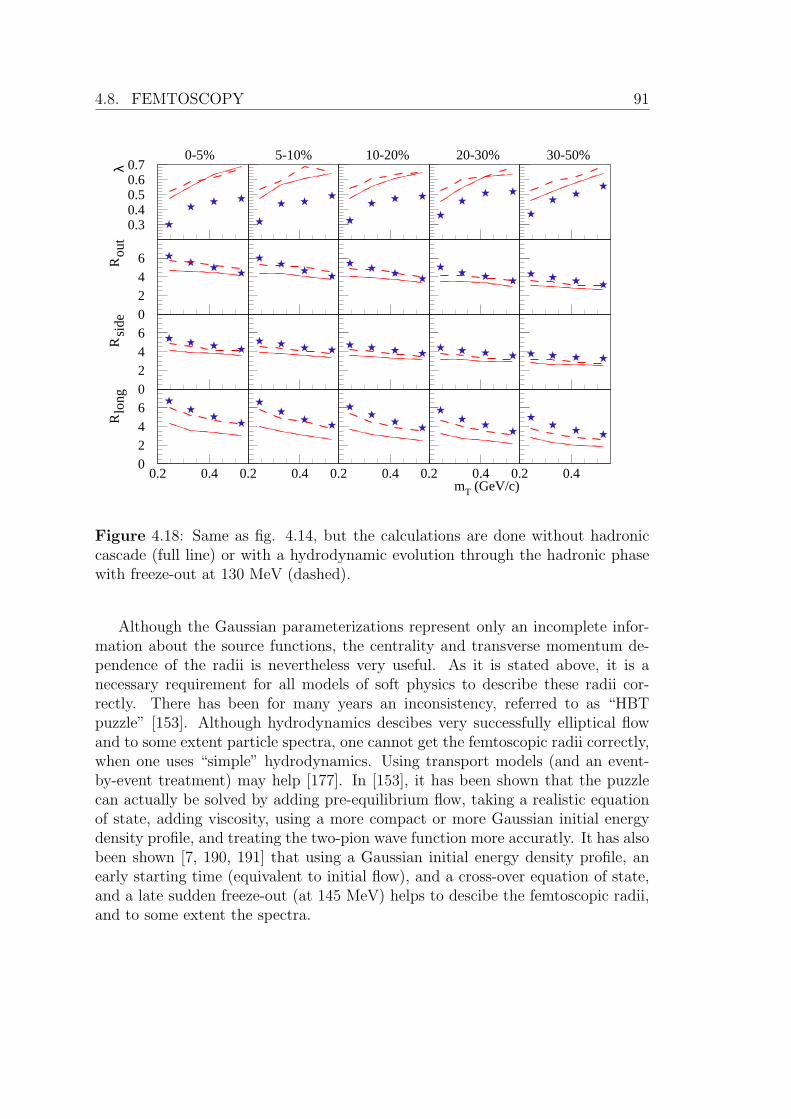
4.8. FEMTOSCOPY 91
0.30.40.50.60.7
0.2 0.4
λ
0-5% 5-10% 10-20% 20-30% 30-50%
0.2 0.4 0.2 0.4 0.2 0.4 0.2 0.4
0246
0.2 0.4
out
R
0.2 0.4 0.2 0.4 0.2 0.4 0.2 0.4
0246
0.2 0.4
sid
eR
0.2 0.4 0.2 0.4 0.2 0.4 0.2 0.4
0246
0.2 0.4
long
R
0.2 0.4 0.2 0.4 0.2 0.4 mT (GeV/c)
0.2 0.4
Figure 4.18: Same as fig. 4.14, but the calculations are done without hadroniccascade (full line) or with a hydrodynamic evolution through the hadronic phasewith freeze-out at 130 MeV (dashed).
Although the Gaussian parameterizations represent only an incomplete infor-mation about the source functions, the centrality and transverse momentum de-pendence of the radii is nevertheless very useful. As it is stated above, it is anecessary requirement for all models of soft physics to describe these radii cor-rectly. There has been for many years an inconsistency, referred to as “HBTpuzzle” [153]. Although hydrodynamics descibes very successfully elliptical flowand to some extent particle spectra, one cannot get the femtoscopic radii correctly,when one uses “simple” hydrodynamics. Using transport models (and an event-by-event treatment) may help [177]. In [153], it has been shown that the puzzlecan actually be solved by adding pre-equilibrium flow, taking a realistic equationof state, adding viscosity, using a more compact or more Gaussian initial energydensity profile, and treating the two-pion wave function more accuratly. It has alsobeen shown [7, 190, 191] that using a Gaussian initial energy density profile, anearly starting time (equivalent to initial flow), and a cross-over equation of state,and a late sudden freeze-out (at 145 MeV) helps to descibe the femtoscopic radii,and to some extent the spectra.
92 CHAPTER 4. HYBRID MODEL
The scenario in [7, 190, 191] is compatible with our scenario “hydrodynamicalevolution till final freeze-out at 130MeV”, which allows us to get the femtoscopicradii correctly (see fig. 4.18), as well as some v2 results and some spectra. Onecannot describe, however, yields and spectra of lambdas and xis.
4.9 Summary and conclusions
In this chapter, the new hybrid dynamical model for matter evolution in ultrarela-tivistic heavy ion collisions is presented. It has many improvements, as comparedto existing ones: flux-tube initial conditions (EPOS), event-by-event treatment,use of an efficient (3+1)D hydro code including flavor conservation, employmentof a realistic equation-of-state, use of a complete hadron resonance table, and ahadronic cascade procedure after an hadronization from thermal matter at an earlytime.
The approach is able to describe simultaneously different soft observables:transverse spectra for pions, kaons, protons, lambdas, xis; v2-coefficients for pi-ons, protons and kaons; interferometry (HBT)-radii for pions.
An agreement with experimental data supports the dynamical picture, realizedin this model: a hydrodynamic evolution starting from EPOS initial conditions,till hadronization at an early time in the cross-over region of the phase transition,with subsequent hadronic rescatterings.
CHAPTER
FIVE
Hydro-kinetic model
In this chapter, the hydrokinetic approach, which incorporates hydrodynamic ex-pansion of the systems formed in A+A collisions and their dynamical decoupling,is presented. The approach provides the alternative way of connection betweenthe dense hydrodynamic stage and kinetic stage, and allows to account for thedeviations from local equilibrium at hydrodynamic stage. It is demonstrated howthe approximation of sudden freeze-out can be obtained within this dynamicalpicture of continuous emission. The approach is extended to include realistic fea-tures of A+A collisions and applied then to describe pion and kaon HBT dataat RHIC collisions. Finally, a study of energy behavior of the pion spectra andinterferometry scales is carried out for the top SPS, RHIC and LHC energies.
5.1 Introduction
It has been known for a long time that CFp leads to inconsistencies [46, 47],if the freeze-out hypersurface contains the non-space-like sectors, and should bemodified to exclude formally negative contributions to the particle number at thecorresponding momenta. The simplest prescription is to present the distributionfunction as a product of a local thermal distribution and the step function likeθ(pµn
µ(x)) [47], nµnµ = ±1, where nµ is a time-like or space-like outward normalto a freeze-out hypersurface σ. Thereby freeze-out is restricted to those particlesfor which pµn
µ(x) is positive. This receipt was used in Ref. [48] to describe particleemission from enclosed freeze-out hypersurface with non-space-like sectors and itwas found that a satisfactory description of central Au+Au collisions at RHICcan be reached for a physically reasonable set of parameters. The main featuresof the experimental data were reproduced: in particular, the obtained ratio ofthe outward to sideward interferometry radii is less than unity and decreases with
93
94 CHAPTER 5. HYDRO-KINETIC MODEL
increasing transverse momenta of pion pairs. Thereby, the results of Ref. [48]clearly indicate that early particle emission off the surface of the hydrodynamicallyexpanding fireball could be essential for proper description of matter evolution inA+A collisions.
However, sharp freeze-out at some 3D hypersurfaces is a rather rough ap-proximation of the spectrum formation, because the particle emission process offireballs created in high energy heavy ion collisions is gradual in time. Results ofmany studies based on cascade models contradict the idea of sudden freeze-out anddemonstrate that in fact particles are emitted from the 4D volume during the wholeperiod of the system evolution, and deviations from local equilibrium conditionedby continuous emission should take place (see, e.g., [93]). Moreover, freeze-outhypersurfaces typically contain non-space-like parts that lead to a problem withenergy-momentum conservation law in realistic dynamical models [47]. This con-cerns also hybrid models [201] where the transport model matches hydrodynamicson such a kind of isothermal hypersurface of hadronization [198].1
An attempt to introduce 4D continuous emission in hydrodynamic frameworkhas been done in Ref. [200] within a simple ideal hydrodynamics, and also sup-ported by numerical transport codes calculations.It was found in these papers thatthe transport freeze-out process is similar to evaporation: high-pT particles freezeout early from the surface, while low-pT ones decouple later from the system’scenter.
The idea of continuous decoupling was further developed based on Boltzmannequations in Ref. [199] where, in particular, an approximate method that accountsfor the back reaction of the emission on the fluid dynamics was proposed. It isworth noting that the back reaction is not reduced just to an energy-momentumrecoiling of emitted particles on the expanding thermal medium, but also leadsto a rearrangement of the medium, producing a deviation of its state from thelocal equilibrium, accompanied by changing of the local temperature, densitiesand collective velocity field. This complex effect is mainly a consequence of theimpossibility to split the evolution of the single finite system of hadrons into thetwo components: expansion of the interacting locally equilibrated medium andfree streaming of emitted particles, which the system consists of. Such a splitting,accounting only for the momentum-energy conservation law, contradicts the un-derlying dynamical equations such as a Boltzmann one [199]. In view of this, theideas proposed and results obtained in the quasiclassical approach should be a cluefor a quantum treatment of the problem which recently started to to be developed
1Note that in this hybrid picture the initial conditions for hadronic cascade calculationscould be formulated also on some (arbitrary) space-like hypersurface where, however, hadronicdistributions deviate from the local equilibrium, in particular, because of an opacity effect forhadrons which are created during a “mixed” stage of phase transition. These nonequilibriumeffects could seriously influence the results of hybrid models in its modern form [201].

5.2. GENERAL FORMALISM 95
[196].Note, however, that the estimates of the influence of the quantum effects, suchas the distortion of the wave function, on the spectra and Bose-Einstein correla-tions testify to be relatively small corrections to the quasiclassical approximation[197].
5.2 General formalism
It was proposed in Ref. [199] to describe the hadronic momentum spectra in A+Acollisions based on the escape function of particles which are gradually liberatedfrom hydrodynamically expanding systems. The escape function, introduced in[200], is calculated within the Boltzmann equations in a specific approximationbased on a hydrodynamic approach. It was shown that such a picture correspondsto a relativistic kinetic equation with the relaxation time approximation for thecollision term, where the relaxation time tends to infinity, τrel → ∞, when t→ ∞,indicating a transition to the free streaming regime. For one component systemthe equation has the form:
pµ
p0
∂f(x, p)
∂xµ= −f(x, p) − f l eq(x, p)
τrel(x, p). (5.1)
Here f(x, p) is the phase-space distribution function, f l eq(x, p) is the local equi-librium distribution with local velocities, temperatures, and chemical potentialsthat should be found from Eq. (5.1) and the initial f0(x, p), and τrel(x, p) is therelaxation time (inverse rate of collisions in gases),
τrel(x, p) =p0τ
∗rel(x, p)
pµuµ
. (5.2)
Here τ ∗rel(x, p) is related to the local fluid rest frame (local rest frame of the energyflow) where the collective four-velocity is uµ = (1,0). The relaxation time dependson the cross section and is a functional of f l eq(x, p).
As it is well known , such kinds of equations at τrel � τexp (inverse of expansionrate) describe in the first approximation the viscosity effects in gases with a coeffi-cient of shear viscosity η ∝ τrelnT . Therefore the method explained below catchesin the first approximation also the viscosity effects in an expanding hadronic gas,characterized by fields of temperatures T and particle densities n. The viscosityeffects in the quark-gluon plasma (QGP) evolution cannot be described in this waybecause strongly interacting QGP is not a gas, but almost an ideal liquid [16].
96 CHAPTER 5. HYDRO-KINETIC MODEL
The formal solution of Eq. (5.1) can be presented in the following form:
f(t, r, p) = f(t0, r −p
p0
(t− t0), p) exp
−t∫t0
1
τrel(s, r − pp0
(t− s), p)ds
+
+
t∫t0
f l eq(t′, r − pp0
(t− t′), p)
τrel(t′, r − pp0
(t− t′), p)exp
−t∫t′
1
τrel(s, r − pp0
(t− s), p)ds
dt′, (5.3)
where f(t0, r, p) is the initial distribution at t = t0. The relaxation time τ ∗rel aswell as the local equilibrium distribution function f l eq are functionals of hydrody-namic variables: temperature T , chemical potential µ, and collective four-velocityuµ. The space-time dependence of the corresponding variables is determined bydemanding the local conservation of the energy-momentum, with tensor T µν(x)and, if necessary, net particle number, with current nµ(x) (assuming no particleproduction)
∂µTµν(x) = 0, (5.4)
∂µnµ(x) = 0, (5.5)
where (see, e.g., Ref. [39])
T µν(x) =
∫d3k
k0
kµνf(x, k), (5.6)
nµ(x) =
∫d3k
k0
kµf(x, k). (5.7)
These conservation laws lead to rather complicated equations for hydrodynamicvariables. It is worth noting that for an expanding system the relaxation timeτ ∗rel(x, p) increases with time and, therefore, the deviations from local equilibriumincrease too, thereby preventing a use of the widely applied approximate methodsbased on the expansion of the distribution function in the vicinity of the localequilibrium.
Then to solve the kinetic equation (5.1), in accordance with the conservationlaws (5.4) and (5.5), we need an approximate method that could be applied evenfor strong deviations from local equilibrium. It is not our aim here to suggest anexclusive solution of the problem. Rather some arguments are presented below bythe example of the relativistic one component Boltzmann gas with particle numberconservation,
f l eq(x, p) = (2π)−3 exp
(−p
µuµ + µ
T
), (5.8)
5.2. GENERAL FORMALISM 97
to show that such a method could be developed based on the following procedure.To take into account nonequilibrium effects accompanying the particle emission
in inhomogeneous violently expanding systems, we utilize the integral representa-tion (5.3) of kinetic equation (5.1). Then, performing a partial integration of thesecond term in Eq. (5.3) and, assuming that f(t0, r, p) = f l eq(t0, r, p), one candecompose the distribution function to a local equilibrium part, f l eq, and a partdescribing a deviation from the local equilibrium behavior, g:
f = f l eq(x, p) + g(x, p), (5.9)
where
g(x, p) = −t∫t0
df l eq(t′, r − pp0
(t− t′), p)
dt′×
× exp
−t∫t′
1
τrel(s, r − pp0
(t− s), p)ds
dt′. (5.10)
Note that both functions, f l eq and g, are functionals of hydrodynamic variables,g depends also on the relaxation time τrel that defines the mean time intervalbetween collisions, and τrel depends in its turn on the distribution function f l eq
and the cross section. The evolution of the distribution function f(x, p) shouldsatisfy the energy-momentum conservation and, because T µν [f ] = T µν [f l eq + g] =T µν [f l eq] + T µν [g] for systems where the interaction energy can be neglected, ittakes the form of hydrodynamic equations for the perfect fluid with “source”,
∂νTνβ[f l eq] = Gβ[g], (5.11)
where
Gβ[g] = −∂νTνβ[g]. (5.12)
The equation that takes into account the conservation of particle number has asimilar form:
∂νnν [f l eq] = S[g], (5.13)
where
S[g] = −∂νnν [g]. (5.14)
To find an approximate solution of Eqs. (5.11)-(5.14), one can solve the equa-tions
∂νTνµ[f l eq] = 0, (5.15)
∂νnν [f l eq] = 0, (5.16)
98 CHAPTER 5. HYDRO-KINETIC MODEL
and, thereby, utilize the hydrodynamic variables in the perfect fluid approxima-tion. Namely, the hydrodynamic variables in this approximation can be used tocalculate the deviation from local equilibrium g(x, p) according to Eq. (5.10) and,then, “source” terms Gβ[g] and S[g] on the right-hand sides of Eqs. (5.11) and(5.13). Then the left-hand sides of these equations are functionals of local equi-librium functions and have the simple ideal fluid forms, while the right-hand sidesassociated with a “source” are explicit functions which describe a deviation fromthe local equilibrium and depend on hydrodynamic variables in the perfect fluidapproximation:
∂νTνβ[f l eq(T, uµ, µ)] = Gβ[Tid, u
idµ , µid, τ
idrel], (5.17)
∂νnν [f l eq(T, uµ, µ)] = S[Tid, u
idµ , µid, τ
idrel], (5.18)
where, for one component Boltzmann gas with elastic collisions only, the relaxationtime τ id
rel is the inverse of collision rate in ideal fluid, Rid(x, p), and has the followingform (in the co-moving frame):
1
τ id∗rel (x, p)
= Rid(x, p) =
=
∫d3k
(2π)3exp
(−Ek − µid(x)
Tid(x)
)σ(s)
√s(s− 4m2)
2EpEk
. (5.19)
Here Ep =√
p2 +m2, Ek =√
k2 +m2, s = (p+ k)2 is the squared c.m. energy ofthe pair, and σ(s) is the corresponding cross section. A solution (T (x), uµ(x), µ(x))of Eqs. (5.17), (5.18) accounts for the back reaction of the emission process onhydro-evolution and provides us with the hydrodynamic parameters which finallyshould be used to calculate the locally equilibrated part f l eq(x, p) of the completedistribution function f(x, p). Then, the distribution function obtained in this way,f(x, p) = f l eq[T, uµ, µ] + g[Tid, u
idµ , µid, τ
idrel], satisfies the conservation laws, takes
into account the nonequilibrium peculiarities of the evolution and is constructed inagreement with the corresponding EoS. Of course, this scheme allows us to makethe next iterations in solving Eq. (5.1). Note also that because the “source” termon the right-hand side of Eq. (5.17) is a known function, the causality is preservedin this description of dissipative systems.
5.3 Cooper-Frye prescription
In this section, we will try to derive the Cooper-Frye approximation within theapproach. Let us start from Boltzmann equation in general form:
pµ
p0
∂fi(x, p)
∂xµ= Gi(x, p) − Li(x, p). (5.20)
5.3. COOPER-FRYE PRESCRIPTION 99
The expressions Gi(x, p) and Li(x, p) = Ri(x, p)fi(x, p) are so-called (G)ainand (L)oss terms for the particle of species i. Typically, Ri is a rate of collisionsof i-th particle. Below we will omit index i, the corresponding expression can berelated then, e.g., to pions.
The probability Pt→t′(x, p) for a particle to reach the point x′ = (t′, r′) startingfrom the point x = (t, r) without collisions is
Pt→t′(x, p) = exp
−t′∫
t
dtR(xt, p)
, (5.21)
where
xt = (t, r +p
p0(t− t)).
In terms of this probability, the Boltzmann equation can be rewritten in the fol-lowing integral form
f(t, r, p) = f(t0, r −p
p0(t− t0), p)Pt0→t(t0, r −
p
p0(t− t0), p)
+
t∫t0
G(τ, r − p
p0(t− τ), p)Pτ→t(τ, r −
p
p0(t− τ), p)dτ. (5.22)
Let us integrate the distribution (5.22) over the space variables to representthe particle momentum density at large enough time, t → ∞, when particlesin the system stop to interact. To simplify notation let us introduce the escapeprobability for the particle with momentum p in the point x = (t, r) to leavesystem without collisions: P(t, r, p) ≡ Pt→(τ→∞)(t, r, p). Then the result can bepresented in the general form found in Ref. [199]:
n(t→ ∞, p) ≡ n(p) =
∫d3rf(t0, r, p)P(t0, r, p)
+
∫d3r
∞∫t0
dt′G(t′, r, p)P(t′, r, p). (5.23)
The first term in Eq. (5.23) describes the contribution to the momentumspectrum from particles that are emitted from the very initial time, while thesecond one describes the continuous emission with emission density S(x, p) =G(t, r, p)P(t, r, p) from 4D volume delimited by the initial and final (where parti-cles stop to interact) 3D hypersurfaces.

100 CHAPTER 5. HYDRO-KINETIC MODEL
In what follows we will use the (generalized) relaxation time approximationproposed in [199], which is the basis of the hydro-kinetic approach, described indetail in [202]. Namely, it was argued [199] that there is such a local equilibriumdistribution function fl.eq.(T (x), uν(x), µ(x)) that, in the region of not very smalldensities where term G ∼ S gives noticeable contribution to particle spectra,the function f is approximately equal to that one which would be obtained if allfunctions in r.h.s. of Eq. (5.22) calculated by means of that function fl.eq.. Thefunction fl.eq. is determined from the local energy-momentum conservation lawsbased on the non-equilibrium function f in the way specified in [202]. Then, inaccordance with this approach we use
R(x, p) ≈ Rl.eq.(x, p), G ≈ Rl.eq.(x, p)fl.eq.(x, p). (5.24)
The “relaxation time” τrel = 1/Rl.eq. grows with time in this method.Let us generalize now the Landau/Cooper-Frye prescription (CFp) of sudden
freeze-out. For this aim we apply the saddle point method to calculate the integralin the expression for spectra (5.23) with account of (5.24). To simplify notationwe neglect the contribution to the spectra from hadrons which are already free atthe initial thermalization time t0 ∼ 1 fm/c and thus omit the first term in (5.22).
To provide straightforward calculations leading to the Cooper-Frye form let usshift the spacial variables, r′ = r + p
p0(t0 − t′), in (5.23) aiming to eliminate the
variable t′ in the argument of the function R which is the integrand in P(t′, r, p).Then
n(p) ≈∫d3r′
∞∫t0
dt′fl.eq.(t′, r′ +
p
p0
(t′ − t0), p)Q(t′, r′,p), (5.25)
where
Q(t′, r′, p) = R(t′, r′ +p
p0
(t′ − t0), p)×
× exp
−∞∫t′
R(s, r′ +p
p0
(s− t0), p)ds
(5.26)
Note that
Q(t′, r′, p) =d
dt′P (t′, r′,p), (5.27)
where P (t′, r′, p) is connected with the escape probability P :
P (t′, r′, p) = P(t′, r′ +p
p0
(t′ − t0), p). (5.28)
5.3. COOPER-FRYE PRESCRIPTION 101
Therefore∞∫t0
dt′Q(t′, r′, p) = 1 −P(t0, r′, p) ≈ 1. (5.29)
The saddle point tσ(r, p) is defined by the standard conditions:
dQ(t′, r′, p)
dt′|t′=t′σ = 0,
d2Q(t′, r′, p)
dt′2|t′=t′σ < 0. (5.30)
Then one can get from (5.27), (5.28) the condition of the maximum of emission:
−pµ∂µR(t′, r, p)
R(t′σ, r, p)|t′=t′σ,r=r′+ p
p0(t′σ−t0) = p0R(t′σ, r
′ +p
p0
(t′σ − t0), p) . (5.31)
If one neglects terms p∗∂r∗R in l.h.s. and supposes that in the rest frame(marked be asterisk) of the fluid element with four-velocity u(x) the collision rate,
R∗(x, p) = p0R(x,p)pµuµ
, does not depend on particle momentum: R∗(x) ≈ 〈v∗σ〉(x)n∗(x)
(here n(x) is particle density, σ is the particle cross-section, v is the relative ve-locity, < ... > means the average over all momenta), then the conditions (5.31)are equivalent to the requirement that at the temporal point of maximum of theemission function the rate of collisions is equal to the rate of system expansion[202]. This is the heuristic freeze-out criterion for sudden freeze-out [204]. How-ever, as we will demonstrate, the neglect of momentum dependence leads to quitesignificant errors.
To pass to the Cooper-Frye representation we use the variables which includethe saddle point:
r = r′ +p
p0
(t′σ(r′, p) − t0). (5.32)
Then the expression for the spectrum takes the form:
n(p) ≈∫d3r
∣∣∣∣1 − p
p0
∂tσ∂r
∣∣∣∣∞∫t0
dt′S(t′, r, p), (5.33)
where the emission density in saddle point representation is (tσ ≡ (tσ(r, p))
S(t′, r, p) = fl.eq.(t′, r +
p
p0
(t′ − tσ), p)
×R(tσ, r, p)P(tσ, r, p) exp(−(t′ − tσ)2/2D2(tσ, r, p)). (5.34)
102 CHAPTER 5. HYDRO-KINETIC MODEL
According to Eq. (5.21) P(tσ, r, p) = e−1, since the freeze-out zone is the regionof the last collision for the particle. Then the normalization condition for Q (Qis presented by the bottom line in (5.34)) allows one to determine the temporalwidth of the emission at the point (tσ(r, p), r, p):
D(tσ, r, p) =e√2π
1
R(tσ, r, p)≈ τrel(tσ, r, p). (5.35)
Therefore if the temporal homogeneity length λ(t, r, p) of the distribution func-tion fl.eq. near the 4-point (tσ(r, p), r) is much larger than the width of the emissionzone, λ(tσ, r, p) � τrel(tσ, r, p), then one can approximate fl.eq.(t
′, r+ pp0
(t′−tσ), p)
by fl.eq.(tσ, r, p) in Eq. (5.33) and perform integration over t′ accounting for nor-malization condition (5.29). As a result we get from (5.33) and (5.34) the momen-tum spectrum in a form similar to the Cooper-Frye one (3.19):
p0n(p) = p0d3N
d3p≈
∫σ(p)
dσµpµfl.eq.(x, p). (5.36)
It is worthy to note that the representation of the spectrum through emissionfunction (5.23) is the result of the integration of the total non-equilibrium distri-bution function f(x, p), Eqs. (5.22), (5.24), over the asymptotical hypersurface intime, while the approximate representation of the spectrum, Eq. (5.36), uses onlythe local equilibrium part fl.eq. of the total function f(x, p) at the set of points ofmaximal emission - at hypersurface (tσ(r, p), r).
Generalized Cooper-Frye prescriptionNow let us summarize the conditions when the Landau/Cooper-Frye form for
sudden freeze-out can be used. They are the following:
i) For each momentum p, there is a region of r where the emission function aswell as the function Q, Eq. (5.26), have a clear maximum. The temporal width ofthe emission D, defined by Eq. (5.34), which is found to be equal to the relaxationtime (inverse of collision rate), should be smaller than the corresponding tempo-ral homogeneity length of the distribution function: λ(tσ, r, p) � D(tσ, r, p) 'τrel(tσ, r, p).
ii) The contribution to the spectrum from the residual region of r, where thesaddle point method (Gaussian approximation (5.34) and/or condition τrel � λ)is violated, does not affect essentially the particle momentum density.
If these conditions are satisfied, then the momentum spectra can be presentedin the Cooper-Frye form despite the fact that actually it is not sudden freeze-outand the decoupling region has a finite temporal width τrel(tσ, r, p).
The analytical results as for the temporal width of the spectra agree remarkablywith the numerical calculations of pion emission function within hydro-kinetic

5.3. COOPER-FRYE PRESCRIPTION 103
[fm]tr0 2 4 6 8 10 12 14
[fm
/c]
τ
5
10
15
20
25
]−2
GeV
−3 [f
mφ
<S
>τ
Tp
0
0.02
0.04
0.06
0.08
0.1
0.12
=0.2 GeVT
p
[fm]tr0 2 4 6 8 10 12 14
[fm
/c]
τ
5
10
15
20
25
]−2
GeV
−3 [f
mφ
<S
>τ
Tp
0
0.05
0.1
0.15
0.2
0.25
0.3
0.35
0.4
−310×
=1.2 GeVT
p
Figure 5.1: The pion emission function for different pT in hydro-kinetic model(HKM) [202]. The isotherms of 80 MeV (left) and 135 MeV (right) are superim-posed.
model (HKM) [202]. For example, near the point of maximum, τ = 16.5 fm/c,r = 0, pT = 0.2 GeV, the “experimental” temporal width DHKM obtained bynumerical solution of the complete hydro-kinetic equations is DHKM ≈ 4.95 fm(see Fig. 5.3, left). Our theoretical estimate is D = e√
2πR≈ 5.00 fm, since the
rate of collisions in this phase-space point is R(τσ(r, p) = 16.5 fm/c, r = 0, pT =0.2 GeV, pL = 0) ≈ 0.217 c/fm.
It is worthy to emphasize that such a generalized Cooper-Frye representation isrelated to freeze-out hypersurfaces that depend on the momentum p and typicallydo not enclose the initially dense matter. In Fig. 5.3, one can see the structureof the emission domains for different pT in HKM [202] for initially (at τ=1 fm/c)Gaussian energy density profile with εmax= 6 GeV/fm3. The maximal emissionregions for different pT are crossed by isotherms with different temperatures: 80MeV for low momenta and 135 MeV for high ones. This is completely reflectedin the concave structure of the transverse momentum spectrum as one can see inFig. 5.3.
If a part of the hypersurface tσ(r, p) is non-space-like and corresponds to themaximum of the emission of particles with momentum p, directed outward thesystem, the same part of the hypersurface cannot correspond to the maximalemission for particles with momentum directed inward the system. It is clear thatthe emission function at these points is close to zero for such particles. Evenformally, in the Gaussian approximation (5.34) for Q, validated in the region of its
maximal value, the integral∞∫tσ
dsR(s, r + pp0 (s − tσ(r, p), p) � 1, if particle world
line crosses almost the whole system. The latter results in Q → 0 and, therefore,completely destroys the saddle-point approximation (5.30) for Q and then theCooper-Frye form (5.36) for spectra. Recall that if a particle crosses some non-space-like part of the hypersurface σ moving inward the system, this corresponds

104 CHAPTER 5. HYDRO-KINETIC MODEL
0.2 0.4 0.6 0.8 1 1.2 1.4 1.6
−210
−110
1
10
210=80MeV
fCFp, T
=135MeVf
CFp, T
HKM model
spectraπ
Figure 5.2: Transverse momentum spectrum of π− in HKM, compared with thesudden freeze-out ones at temperatures of 80 and 160 MeV with arbitrary normal-ization.
to the condition pµdσµ < 0 [46]. Hence the value pµdσµ(p) in the generalizedCooper-Frye formula (5.36) should be always positive: pµdσµ(p) > 0 across thehypersurface where fairly sharp maximum of emission of particles with momentump is situated; and so requirement pµdσµ(p) > 0 is a necessary condition for tσ(r, p)to be a true hypersurface of the maximal emission. It means that hypersurfacesof maximal emission for a given momentum p may be open in the space-time, notenclosing the high-density matter at the initial time t0, and different for different p.All this is illustrated in Fig. 5.3, where the structure of particle emission domainis shown for two groups of particles. In the first one, the momentum is directedas the radius vector to the point of particle localization (they move outward thesystem), in the second one - in opposite direction (they move inward). The pointsof maximum for different pT , where Cooper-Frye form can be applied, do notoverlap. The calculations have been done in HKM [202].
Therefore, there are no negative contributions to the particle momentum den-sity from non-space-like sectors of the freeze-out hypersurface, that is a well knownshortcoming of the Cooper-Frye prescription [46, 47]; the negative contributionscould appear only as a result of utilization of improper freeze-out hypersurfacethat roughly ignores its momentum dependence and so is common for all p. If,anyhow, such a common hypersurface will be used, e.g. as the hypersurface of themaximal particle number emission (integrated over p), there is no possibility tojustify the approximate expression for momentum spectra similar to Eq. (5.36).
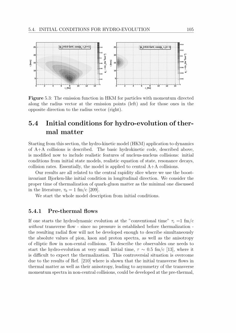
5.4. INITIAL CONDITIONS FOR HYDRO-EVOLUTION 105
[fm]tr0 2 4 6 8 10 12 14
[fm
/c]
τ
5
10
15
20
25
]−2
GeV
−3 [f
mφ
<S
>τ
Tp
0
0.02
0.04
0.06
0.08
0.1
0.12
0.14)=+1T rT
|=0.6 GeV, cos(pT
|p
[fm]tr0 2 4 6 8 10 12 14
[fm
/c]
τ
5
10
15
20
25
]−2
GeV
−3 [f
mφ
<S
>τ
Tp
0
0.002
0.004
0.006
0.008
0.01
0.012
0.014
)=−1T rT
|=0.6 GeV, cos(pT
|p
Figure 5.3: The emission function in HKM for particles with momentum directedalong the radius vector at the emission points (left) and for those ones in theopposite direction to the radius vector (right).
5.4 Initial conditions for hydro-evolution of ther-
mal matter
Starting from this section, the hydro-kinetic model (HKM) application to dynamicsof A+A collisions is described. The basic hydrokinetic code, described above,is modified now to include realistic features of nucleus-nucleus collisions: initialconditions from initial state models, realistic equation of state, resonance decays,collision rates. Essentially, the model is applied to central A+A collisions.
Our results are all related to the central rapidity slice where we use the boost-invariant Bjorken-like initial condition in longitudinal direction. We consider theproper time of thermalization of quark-gluon matter as the minimal one discussedin the literature, τ0 = 1 fm/c [209].
We start the whole model description from initial conditions.
5.4.1 Pre-thermal flows
If one starts the hydrodynamic evolution at the ”conventional time” τi =1 fm/cwithout transverse flow - since no pressure is established before thermalization -the resulting radial flow will not be developed enough to describe simultaneouslythe absolute values of pion, kaon and proton spectra, as well as the anisotropyof elliptic flow in non-cental collisions. To describe the observables one needs tostart the hydro-evolution at very small initial time, τ ∼ 0.5 fm/c [13], where itis difficult to expect the thermalization. This controversial situation is overcomedue to the results of Ref. [210] where is shown that the initial transverse flows inthermal matter as well as their anisotropy, leading to asymmetry of the transversemomentum spectra in non-central collisions, could be developed at the pre-thermal,
106 CHAPTER 5. HYDRO-KINETIC MODEL
either classical field (Glasma) [211], string [141] or partonic stages, with even moreefficiency than in the case of very early hydrodynamics. So, the hypothesis of earlythermalization at times less than 1 fm/c is not necessary: the radial and ellipticflows develop no matter whether a pressure already established. The general reasonfor them is an essential finiteness of the system in transverse direction. Thenthe flows of particle number or energy directed outward the system cannot becompensated by the inward directed (from periphery to the center) flows. Thisdifference means the non-zero net flows no matter how the collective velocity isdefined: according to Ekkart or to Landau-Lifshitz. The further development andexploitation of these results were done in Refs. [212, 6, 213].
The initial transverse rapidity profile is supposed to be linear in radius rT :
yT = αrT
RT
, where RT =√< r2
T >, (5.37)
here α is the second fitting parameter. Note that the fitting parameter α shouldinclude also a positive correction for underestimated resulting transverse flow sincein this work we did not account in direct way for the viscosity effects [208] neither atQGP stage nor at hadronic one. In formalism of HKM [202] the viscosity effects athadronic stage are incorporated in the mechanisms of the back reaction of particleemission on hydrodynamic evolution which we ignore in current calculations. Sincethe corrections to transverse flows which depend on unknown viscosity coefficientsare unknown, we use fitting parameter α to describe the ”additional unknownportions” of flows, caused by both factors: by a developing of the pre-thermalflows and the viscosity effects in quark-gluon plasma.
5.4.2 Glauber-like initial transverse profile
A simple Glauber model initialization assumes that the initial energy density inthe transverse plane is proportional to the participant nucleon density [214],
ε(b,xT ) = ε0ρ(b,xT )
ρ0
(5.38)
with ρ0 ≡ ρ(0, 0) and
ρ(b,xT ) = (T (xT + b/2)S(xT − b/2) + T (xT − b/2)S(xT + b/2)),
S(xT ) =
[1 −
(1 − σNN
T (xT )
A
)A], (5.39)
whereA is atomic number, equal to 197 for Au+Au collision, and σNN = 51 mb(=5.1 fm2)is the nucleon-nucleon cross-section at
√sNN = 200 AGeV. The impact parameter
5.4. INITIAL CONDITIONS FOR HYDRO-EVOLUTION 107
b = (b, 0) is equal to zero, b=0, in the considered case of central collision. The pa-rameter ε0 ≡ ε(b = 0,xT = 0) is the maximal energy density at the initial momentof thermalization. The thickness T (xT ) is expressed through the Woods-Saxondistribution profile:
T (xT ) =
∞∫−∞
FWS(x)dxL, (5.40)
where
FWS(x) =a
exp[(√
x2L + x2
T −RA
)/δ]
+ 1. (5.41)
Here we use that RA = 1.12A1/3 − 0.86A−1/3 ≈ 6.37 fm, δ = 0.54 fm. Constant ais obtained from normalization condition:∫
T (xT )d2xT = A. (5.42)
One can think that transversal Glauber-like ε-profile has been formed to someinitial time τ0 ≈ 0.1 − 0.3 fm/c (see below) when the system is not thermalyet. However, the form of the profile is, practically, not modified to supposedthermalization time τ0 ∼ 1 fm/c because the transverse velocities reached to thistime are relatively small. At the same time, the absolute values of energy densitycan change significantly because of the strong longitudinal expansion. We use themaximal energy density ε0 at time τi = 1 fm/c as the second fitting parameter.
5.4.3 Initial conditions motivated by Color Glass Conden-sate model
Within CGC effective field theory some important physical properties of the fieldare defined by the parameter Λs = g2µ where g2 = 4παs and µ2 is dimensionlessparameter, which is the variance of the Gaussian weight over the color charges ρof partons. The value of Λs0 is approximately equal to the saturation scale value,Qs, and for the RHIC energies one can use Λs0 ≈ Qs ≈ 2 GeV2 [215]. Accordingto the results of Refs. [216, 217], (proper) time τ0 ≈ 3/Λs is an appropriate scalecontrolling the formation of gluons with a physically well-defined energy. At latertimes the dynamics of the classical Yang-Mills fields produced in nucleus-nucleuscollisions can be linearized and approximated by that of a system of weakly coupledharmonic oscillators. Then one can compute the field amplitudes squared in mo-mentum space and find corresponding distribution for the gluon number [217, 218]for cylindrically homogeneous transverse profile. It has the form at pT < 1.5Λs
108 CHAPTER 5. HYDRO-KINETIC MODEL
and η = 12ln t+xL
t−xL' 0,
dN
d2pTd2xTdη≡ f(Teff)
=a1
g2
[exp
(√p2
T +m2eff
/Teff
)− 1
]−1
, (5.43)
where meff = a2Λs0, Teff = a3Λs; a2 = 0.0358, a3 = 0.465. The constant a1/g2 will
be absorb into factor ε0 which is our fitting parameter.The dependence of the distribution (5.43) on transverse coordinates xT is con-
structed as follows [217]:
Λ2s(xT ) = Λ2
s0
ρ(b,xT )
ρ0
. (5.44)
where the participant density at a particular position in the transverse plane isdefined by (5.39).
To define the initial energy density profile we need the partonic phase-spacedistribution f 0(x, p) = dN/d3xd3p. Note, that it is associated with the hypersur-faces t = const. To express the phase-space density through the values dN
d2xT d2pdη
defined at√t2 − x2
L = τ0, one should take into account that the density of partonswith momentum p crossing element d3σ(x) of this hypersurface is
p0 dN
d3p
∣∣∣∣dσ(x)
= pµdσµ(x)f0(x, p)
= f0(x, p)τ0pT cosh θd2xTdη, (5.45)
where θ = y − η, y is rapidity of partons (in momentum space). Therefore
f0(x, p) =1
τ0mT cosh θ
dN
d2xTd2pTdηdy. (5.46)
One can formally get the d6N distribution from (5.43) by multiplying it byδ–function:
dN
d2pTd2xTdηdy= f(Teff)δ(y − η). (5.47)
Such a phase-space distribution, corresponding the CGC asymptotic results [219],is widely used for a description of the initial state in A+A collisions [220]. However,a presence of the delta-function in the phase-space density contradicts evidentlyto the basic principle of the quantum mechanics. Indeed, the classical phase-space density has to follow from the quantum mechanical one in some limit. TheWigner function fW(x, p) [221], that is the quantum mechanical analog of theclassical phase-space density f(x, p), satisfies the restriction
∫f2
W(x, p)d3pd3x ≤
5.4. INITIAL CONDITIONS FOR HYDRO-EVOLUTION 109
(2π~)−3 (see e.g. [222], note that the equality takes place for a pure state only),here the normalization condition
∫fW(x, p)d3pd3x = 1 is supposed. It evidently
excludes utilization of the delta-function as factor in the structure of the Wignerfunction. Therefore, in order to escape contradiction with quantum mechanics,another prescription, instead of utilization of delta function, should be used forthe longitudinal part of distribution f(x, p); it can be, for example, the boost-invariant prescriptions used in Ref. [213]. Following to this recept we smear theδ-function at hypersurface τ0 in (5.47) as follows
dN
d2pTd2xTdηdy= f
(Teff
cosh (η − y)
). (5.48)
In this way we fix the phase-space density (5.46). This may correspond to quasi-thermal averaged partonic distribution which can be reached at moment τ0 due toquantum effects (uncertainly principle), different kind of turbulences and Schwinger-like mechanism of pair production in the pulse of strong color field. It does notmean that the true thermalization which should be supported by a permanentmechanism of partonic interactions is reached at τ0 ≈ 3/Λs ≈ 3 fm/c.
As a result we use the following form of boost-invariant phase-space distributionfor gluons at the initial hypersurface τ0:
f0 = g−2 a1(τ0mT cosh θ)−1
exp(√
m2eff(xT ) + p2
T cosh θ/Teff(xT )
)− 1
, (5.49)
here θ = η − y, xT = (X,Y ) = (xT cosϕ, xT sinϕ) and we consider gluons asmassless particles, mT = pT . Such a distribution depends on the effective massmeff(xT ) = a2Λs(xT ) and the temperature Teff(xT ) = a3Λs(xT ) (numerical valuesfor a2 and a3 are the same as in Eq. (5.43)), which, in accordance with Ref. [217],are determined by the local scale Λs(xT ) (5.44).
The components of the energy-momentum tensor in the pseudo-Cartesian co-ordinates reads
T µν(x) =
∫pµpνf(x, p)pTdpTdydφ, (5.50)
where the Lorentz-invariant integration measure d3p/p0 in the Cartesian variablesis already re-written in Bjorken variables as pTdpTdydφ.
We numerically calculate the components of the energy-momentum tensor withthe distribution function, following from Eq. (5.49), at η = 0.
Note that, at τ = τ0, the energy-momentum tensor takes the form
T µν0 (xT , xL = 0) =
a1
g2τ0Λ3
s(xT )tµν , (5.51)
110 CHAPTER 5. HYDRO-KINETIC MODEL
where tµν are the constant coefficients fixed by the constants a2 and a3. Therefore,the energy profile in transverse plane at τ0 in central collisions can be presentedin the form (see (5.44))
ε(xT ) = ε0ρ3/2(0, xT )
ρ3/20
, (5.52)
where the number of participants is defined by (5.39). Under the same reason as forthe Glauber-like IC we use the form of this profile to build the IC for hydrokineticevolution at the thermalization time τi = 1 fm/c. The maximal energy density ε0at (proper) time τi is the fitting parameter as in the case of the Glauber IC.
5.5 The thermal matter in A+A collision and
equation of state
Here we describe the matter properties and its thermodynamic characteristics,e.g. equation of state, that are necessary components of the hydrokinetic model.We suppose that soon after thermalization the matter created in A+A collisionat RHIC energies is in the quark gluon plasma (QGP) state. Also at time τi,there is a peripheral region with relatively small initial energy densities: ε(r) <0.5 GeV/fm3. This part of the matter (”corona”) does not transform into QGPand has no chance to be involved in thermalization process [149]. By itself thecorona gives no essential contribution to the hadron spectra [149]. One shouldconsider it separately from the thermal bulk of the matter and should not includein hydrodynamic evolution. Therefore we cut the initial Glauber or CGC-likeprofiles at ε(r) ≤ 0.5 GeV/fm3 when consider IC for hydrodynamic evolution ofthe system.
During the system evolution the QGP is cooling and finally transforms intohadron phase, most probably, according to the crossover scenario. Such a trans-formation may occur in the interval of the temperatures 170-190 MeV. At thetemperature T = Tch ≈ 165 MeV the chemical freeze-out happens, as demon-strates an analysis of the particle number ratios [223, 110]. The conception of thechemical freeze-out means that at the temperatures T ≥ Tch the bulk of the ex-panding matter is in the local thermal and chemical equilibrium while at T < Tch
the chemical composition becomes in some sense frozen: one can neglect the ma-jority of inelastic reactions except for decays of resonances and recombinationprocesses. The hadronic matter in the later thermodynamic region is not in thechemical equilibrium, moreover, the hadronic medium gradually emits particlesbeing in this zone and, so, loose, in addition, also the local thermal equilibrium.Therefore, one should consider in different ways the matter evolution in the two 4Dspace-time zones separated by the 3D hypersurface corresponding to the isotherm
5.5. EQUATION OF STATE 111
T = Tch ≈ 165 MeV. Let us describe the thermodynamic properties of matter inboth these regions.
5.5.1 The EoS in the equilibrated space-time domain.
At high temperatures corresponding to the QGP phase and crossover transitionto hadron phase we use a realistic EoS [225] adjusted to the lattice QCD resultsfor zero baryonic chemical potential so that it is matched with an ideal chemicallyequilibrated multicomponent hadron resonance gas at Tc = 175 MeV. To take intoaccount a conservation of the net baryon number, electric charge and strangenessin the QGP phase, one has first to make corrections to thermodynamic quantitiesfor nonzero chemical potentials. As it is proposed in [226], a modification of theEoS can be evaluated by using of the Taylor series expansion in terms of thelight and strange quark chemical potentials, or analogously in baryon and strangehadronic chemical potentials:
p(T, µB, µS)
T 4=p(T, 0, 0)
T 4+
1
2
χB
T 2
(µB
T
)2
+1
2
χS
T 2
(µS
T
)2
+χBS
T 2
µB
T
µS
T(5.53)
The expansion coefficients χB and χS are the baryon number and strangenesssusceptibilities which are related to thermal fluctuations of baryon number andstrangeness in a thermal medium at zero chemical potentials.
To obtain the EoS in the equilibrium zone we use the numerical results for χB
and χS as a function of the temperature given in [226]. The values for the ratiosµq/T in (5.53) during the system evolution can be determined approximately. If atsome hypersurface corresponding to an isotherm, like as at the chemical freeze-outhypersurface, the chemical potentials are uniform, then the following ratios remainconstant
µq
T= constq, where q = B, S,E
during the chemically equilibrated isoentropic evolution of the Boltzmann masslessgas. In our approximation we use these constraints and find the correspondingconstants from the chemical potentials obtained together with Tch from an analysisof the particle number ratios. In concrete calculations we use the chemical freeze-out temperature Tch = 165 MeV, corresponding chemical potentials µB =29 MeV,µS =7 MeV, µE =-1 MeV and also the strangeness suppression factor γS = 0.935which are dictated by 200A GeV RHIC particle number ratios analysis done inthe statistical model [223, 110].
5.5.2 The EoS in the chemically non-equilibrated domain.
At the chemical freeze-out temperature Tch the ”lattice” EoS taken from [225]and corrected for non-zero chemical potentials is matched with good accuracy
112 CHAPTER 5. HYDRO-KINETIC MODEL
with ideal Boltzmann hadronic resonance gas which includes N = 359 hadronstates made of u, d, s quarks with masses up to 2.6 GeV. Essentially, we usethe same particle set in the FASTMC event generator [227]. Technically, in thenumerical code, we input the corresponding N functions - the densities ni of eachhadron i and the equations for ni already at the very beginning of the systemevolution; however, these densities are meaningless in the QGP phase and theirevaluation does not influence the system evolution in the equilibrated zone. Thesefunctions are brought into play at T < Tch. If this thermodynamic region wouldcorrespond to the complete conservation of the particle numbers then, in additionto the energy-momentum conservation, one would account for the conservationequations for particle number flows in the form:
∂µ(niuµ) = 0, i = 1 . . . N (5.54)
In our problem, however, during the system evolution in the non-equilibratedzone T < Tch the resonance decays have to be taken into account. The decay lawin a homogeneous medium with T � mi (mi is the resonances mass) implies asumming up of a decrease of unstable ith particle number due to decays and anincrease because of decays of heavier jth resonance into ith particle:
dNi
dt= −ΓiNi +
∑j
bijΓjNj (5.55)
where Γi is the total width of resonance i, bij = BijMij denote the average numberof ith particles coming from arbitrary decay of jth resonance, Bij = Γij/Γj,tot isbranching ratio, Mij is a number of ith particles produced in j → i decay channel.The set on N equations (5.55), solved together, takes into account all possiblecascade decays i → j → k → . . . . This also conserves net charges, e.g. baryon,electric charge and strangeness, since the charges are conserved in resonance decayprocess. If one relates the Eq. (5.55) to the fluid element of some volume ∆Vmoving with four-velocity uµ, then a covariant relativistic extension of the decaylaw for a hydrodynamic medium leads to the equation (5.54):
∂µ(ni(x)uµ(x)) = −Γini(x) +
∑j
bijΓjnj(x) (5.56)
when one neglects a thermal motion of the resonance j, that can be justifiedbecause post (chemical) freeze-out temperatures are much less than the mass ofthe lightest known resonance. Also, Eq. (5.56) for the hydrodynamic evolutionis written under supposition of an instant thermalization of the decay products,that is consistent with the ideal fluid approximation (mean free path is zero). Inthe kinetic part of the HKM we consider the next approximation when the non-equilibrium character of the distribution functions and the kinetics of resonance
5.5. EQUATION OF STATE 113
decays are taken into account. We also can approximately account for a recombina-tion in the processes of resonance decays into expanding medium just by utilizingthe effective decay width Γi,eff = γΓi in Eq. (5.56). We use γ = 0.75 [228] forthe resonances containing u and d quarks supposing thus that about 30% of suchresonances are recombining during the evolution.
The equations (5.56) together with the hydrodynamic equations and the equa-tion of state should give one the energy density and composition of the gas ineach space-time points. To find the EoS p = p(ε, {ni}) for the mixture of hadrongases we start with the expressions for energy density and particle density for ithcomponent of multicomponent Boltzmann gas :
εi =gi
2π2m2
iT (3TK2(mi/T ) +mK1(mi/T )) exp(µi/T )
ni =gi
2π2m2
iTK2(mi/T ) exp(µi/T ). (5.57)
Then, the equation for the temperature is:
ε = 3nT +∑
i
nimiK1(mi/T )
K2(mi/T ), (5.58)
where n =∑
i ni. Having solved this equation numerically for given ε and {ni},we get the temperature and then find the pressure using simple relation for mul-ticomponent Boltzmann gas:
p = nT (5.59)
The equations (5.58), (5.59) define p = p(ε, {ni}).Thus, we follow the evolution of all N densities of hadron species in hydro
calculation, and compute EoS dynamically for each chemical composition of Nsorts of hadrons in every hydrodynamic cell in the system during the evolution.Using this method, we do not limit ourselves in chemically frozen or equilibratedevolution, keeping nevertheless thermodynamically consistent scheme.
As it was mentioned before, we use the Boltzmann approximation in the EoScalculation to decrease computational time. However, for emission function andspectra calculation we use quantum Bose-Einstein/Fermi-Dirac distribution func-tions with chemical potentials calculated to give the same particle densities as inthe Boltzmann case. We checked that the measure of relative divergence in theenergy density if one uses the quantum distribution functions instead of the Boltz-mann one, is not bigger than 3% in the thermodynamic region which is actuallycontributing to formation of hadronic spectra.

114 CHAPTER 5. HYDRO-KINETIC MODEL
5.6 Kinetics in the non-equilibrium hadronic zone
To describe the non-equilibrium evolution and decay of hadronic system we startfrom the Boltzmann equations for the mixture of hadrons, most of which havefinite lifetimes and decay widths compatible with particle masses. The set of suchequations for i-components of the hadron resonance gas which account for the onlybinary interactions (elastic scattering) and resonance decays are:
pµi
p0i
∂fi(x, p)
∂xµ= Gscatt
i (x, p) − Lscatti (x, p) +Gdecay
i (x, p) − Ldecayi (x, p) ≡
≡ Gi(x, p) − Li(x, p). (5.60)
Here we ignore the processes of resonance recombination which is simpler toaccount phenomenologically (see the previous Section). The term gain (G) de-scribes an income of the particles into phase-space point (x, p) due to scatters andresonance decays. The term loss (L) is related to a decrease of particles in thevicinity of the phase space point (x, p) due to re-scattering and decays of reso-nances. The loss term is proportional to the particle number density in the pointx and so Lscatt
i (x, p) = fiRi, Ldecayi (x, p) = fiDi where R is scattering rate, and
D is decay rate. If one considers the equations for stable or quasi-stable particles,then Ldecay
i (x, p) = 0 (Di ≡ 0).The method allowing to find the emission function of the hadrons based on
the Boltzmann equations in the (generalized) relaxation time approximation wasproposed in Refs. [199, 202]. Following this method we put: Ji(x, p) ≈ Ri,l.eq.(x, p),
Gi ≈ Ri,l.eq.(x, p)fi,l.eq.(x, p) +Gdecayi (x, p). The quantity R(x, p) = τ−1
rel (x, p) is theinverse relaxation time, or collision rate in global reference frame. Then,
pµ
p0∂µfi(x, p) = (f l.eq.
i (x, p) − fi(x, p))Ri(x, p)+
+Gdecayi (x, p) − Ldecay
i (x, p) (5.61)
The explicit form of Gdecayi (x, p) term will be derived later. In the first approxi-
mation to hydro-kinetic evolution the parameters of the locally equilibrium distri-bution function fi,l.eq.(x, p), e.g. the temperature T (x), chemical potentials µi(x)are determined by the hydrodynamic evolution. The details of hydrodynamic ap-proach used in the model are described in the next section.
5.6.1 Emission functions in hyperbolic coordinates and spec-tra formation
All our results are related to the very central rapidity interval, y ≈ 0, and we willuse the boost-invariant approach to describe strong longitudinal matter expansion
5.6. KINETICS IN THE NON-EQUILIBRIUM HADRONIC ZONE 115
observed at RHIC. For such an approach the hyperbolic coordinates in (t, xL)directions are more suitable than the Cartesian ones. Then the kinetic equationstake a form
1
mT cosh y
(mT cosh θ
∂
∂τ− mT sinh θ
τ
∂
∂η+ ~pT
∂
∂~rT
)fi(τ, θ, rT ,pT ) =[
f l.eq.i (τ, θ, rT ,pT ) − fi(τ, θ, rT ,pT )
]Ri(τ, θ, rT ,pT ) +Gdecay
i (τ, θ, rT ,pT ) (5.62)
where τ =√t2 − x2
L is a proper time, mT =√m2 + p2
T is a transverse mass,θ = η − y, η is a space-time rapidity, defined above Eq. (5.43), and y is a particlerapidity.
The formal solutions of (5.62) correspond to the non-equilibrium distributionfunctions in expanding and decaying multi-hadronic system:
fi(τ, θ, rT ,pT ) = f l.eq.i (τ0, θ
(τ0)(τ), r(τ0)T (τ),pT )×
× exp
−τ∫
τ0
Ri(s, θ(s)(τ), r
(s)T (τ),pT )ds
+ (5.63)
+
τ∫τ0
dλ[f l.eq.
i (λ, θ(λ)(τ), r(λ)T (τ),pT )Ri(λ, θ
(λ)(τ), r(λ)T (τ),pT )+
+Gdecayi (λ, θ(λ)(τ), r
(λ)T (τ),pT )
]exp
−τ∫
λ
Ri(s, θ(s)(τ), r
(s)T (τ),pT )ds
here Ri(λ, θ, rT ,pT ) = cosh y
cosh θRi(λ, θ, rT ,pT ),
Gdecayi (λ, θ, rT ,pT ) =
cosh y
cosh θGdecay
i (λ, θ, rT ,pT ).
Here we use the notation{sinh θ(τ0)(τ) = τ
τ0sinh θ
r(τ0)T (τ) = rT − pT
mT(τ cosh θ −
√τ 20 + τ 2 sinh2 θ)
(5.64)
The invariant value is p0Ri(x, p) = p∗0R∗i (x, p), where the asterisk ∗ denotes a
value in the local rest frame of the fluid element in point x, so
Ri(x, p) =cosh y
cosh θRi(x, p) =
cosh y
cosh θ
pµuµ
p0R∗
i (p, T ) =pµuµ
mT cosh θR∗
i (p, T ) (5.65)

116 CHAPTER 5. HYDRO-KINETIC MODEL
To connect the formal solution (5.63) with observables, e.g. particle spectrum,we use the equality
p0d3n
d3p=
d2n
2πpTdpTdy=
∫σout
dσµpµf(x, p) (5.66)
where σout is a ”distant” hypersurface of large τ = const, where all the interactionsamong hadrons are ceased.
In what follows we use the variable substitution in the first term of (5.63)describing the ”initial emission” :{
sinh θ = τ0τ
sinh θ′
rT = r′T + pT
mT(τ cosh θ −
√τ 20 + τ 2 sinh2 θ)
(5.67)
and the substitution :{sinh θ = λ
τsinh θ′
rT = r′T + pT
mT(τ cosh θ −
√λ2 + τ 2 sinh2 θ)
(5.68)
in the second term of (5.63) related to the ”4-volume emission”. After transfor-mation to new variables {τ, θ′, ~r′} we arrive at the result:∫
σout
dσµpµf(x, p) =
∫σ0
dσµ0 pµf
l.eq.i (τ0, θ
′, r′T , p)×
× exp
−∞∫
τ0
Ri(s, θ(s)(τ0), r
(s)T (τ0),pT )ds
+
τ∫τ0
dλ
∫σ(λ)
dσµ(λ)pµ[f l.eq.
i (λ, θ′, r′T ,pT )Ri(λ, θ′, r′T ,pT )+
Gdecayi (λ, θ′, r′T ,pT )
]exp
−∞∫
λ
Ri(s, θ(s)(λ), r
(s)T (λ),pT )ds
= p0d3N
d3p
where σ(λ) is τ = λ = const hypersurface, so dσµ(λ)pµ = λmT cosh θ′dθ′d2~r′T . Theexponential values in these expressions are the escape probabilities
P(τ, rT , θ,pT ) = exp
−∞∫
τ
Ri(s, θ(s)(τ), r
(s)T (τ),pT )ds
(5.69)
5.6. KINETICS IN THE NON-EQUILIBRIUM HADRONIC ZONE 117
for particles with momentum p at space-time point (τ, rT , η = θ+y) (in hyperboliccoordinates) to become free without any collision [199, 202].
In the expression above we can separate the 4-volume emission function
Si(λ, θ, rT ,pT ) = (5.70)
=[f l.eq.
i (λ, θ, rT , p)Ri(λ, θ, rT , p) + Gdecayi (λ, θ, rT ,pT )
]P(λ, rT , θ,pT )
and the initial emission function:
Si,0(θ, rT ,pT ) = f l.eq.i (τ0, θ, rT ,pT )P(τ0, rT , θ,pT ) (5.71)
These expressions demonstrate obviously that the particle emission is formedby the particles which undergo their last interaction or are already free initially.These expressions for the hadron emission function are the basic functions forcalculations of the single- and multi- particle spectra [199]. To evaluate thesequantities for observed (quasi) stable particles one needs to find the term gainGdecay
i for resonance decays and the collision rates Ri.
5.6.2 Resonance decays in multi-component gas
We suppose that in the first (hydrodynamic) approximation the products of reso-nance decays which interact with medium are thermalized and they become freelater, after the last collision with one of other particles. However, at the latestages of matter evolution the system becomes fairly dilute, so that some of theseproduced particles get a possibility to escape without any collisions: P > 0. Todescribe this we use the following form for Ldecay
i and Gdecayi terms (for 2-particle
resonance decay) [229]:
p0iL
decayi (x, pi) =
∑k
∑l
∫d3pk
p0k
∫d3pl
p0l
Γi→klfi(x, pi)×
× mi
Fi→kl
δ(4)(pi − pk − pl) = miΓifi(x, pi) (5.72)
where resonance i decays into particles or resonances k and l.
p0iG
decayi (x, pi) =
∑j
∑k
∫d3pj
p0j
∫d3pk
p0k
Γj→ikfj(x, pj)mj
Fj→ik
δ(4)(pj − pk − pi)
(5.73)where the resonance j decays into particles i and k with partial width Γj→ik forthis decay channel, and
Fj→ik =
∫d3pk
p0k
∫d3pi
p0i
δ(4)(pj−pk−pi) =2π
m2j
((m2j−m2
k−m2i )
2−4m2im
2k)
1/2 (5.74)
118 CHAPTER 5. HYDRO-KINETIC MODEL
To escape the complicated problem of satisfying the thermodynamic identitiesin hadron resonance gas we utilize in what follows the mass shell approximationfor resonances, supposing that mi = 〈mi〉. Also, as it was already discussed, wetake into account that the resonance mass in hadron resonance gas is much largerthan the temperature, mi >> Tc. Then the most probable velocity of resonance
in the rest system of a fluid element is small, vi ≈√
2Tmi
, and one can use the
approximationpµ
i ≈ miuµ. (5.75)
So the resonance distribution function takes the form
fj(x, pi) ≈p0
j
mj
nj(x)δ3(pj −mju(x)), (5.76)
It allows us to perform integrations in (5.73) over pj, pk analytically and get :
Gdecayi (x, pi) =
∑j
∑k
Γj→iknj(x)
p0i p
0kFj→ik
δ(mju0(x) − p0
k − p0i ) (5.77)
where p0k =
√m2
k + (mju(x) − pi)2.Just this form of gain term is used when spectra are evaluated according to
Eq. (5.6.1). Note that in practical calculations we substitute δ-function by itsGaussian representation:
δ(x) =1
R√πe−x2/R2
and take a finite parameter value R = 50MeV .
5.6.3 Collision rates
The collision rate R(x, p) = 1τrel(x,p)
is one of the basic value for calculation ofthe intensity of the interactions in the expanding system and its decoupling. Thelatter is described through the escape probability P(x, p) (5.69) - the integral valueof R along the possible trajectory of a particle with momentum p running freelythrough the whole expanding system. The rate of collisions in the rest frame ofsome fluid element that accounts for scatters of given particle with any other ithhadronic species in the thermal Boltzmann system depends only on particle energyE∗
p = pµuµ and the thermodynamic parameters of this fluid element [230]:
R∗(E∗p , T, {µi}) =
∑i
∫d3ki
gi
(2π)3exp
(−Ek,i − µi(x)
T (x)
)×
× σi(si)
√(si − (m−mi)2)(si − (m+mi)2)
2E∗pEk,i
(5.78)

5.6. KINETICS IN THE NON-EQUILIBRIUM HADRONIC ZONE 119
Here gi = (2ji + 1), Ep =√
p∗2 +m2, Ek,i =√
k2i +m2
i , si = (p∗ + ki)2 is the
squared c.m. energy of the pair, and σi(s) is the total cross section of selectedparticle with particle i in the corresponding binary collision. One can change theintegration variable to squared center of mass energy s, energy of scattering partnerEk and momentum angle φ, and perform Ek and φ-integration analytically, whichgives the expression for remaining integral:
R∗(E∗p , T, {µi}) =
∑i
giTeµi/T
8π2p∗E∗p
∞∫(m+mi)2
dsσi(s)√
(s−m2 −m2i )
2 − 4m2im
2×
× sinh
(p∗
2Tm2
√(s−m2 −m2
i )2 − 4m2
im2
)exp
(−
(s−m2 −m2i )E
∗p
2Tm2
)(5.79)
We calculate σi(s) in a way similar to UrQMD code [231]:
• Breit-Wigner formula is applied for meson-meson and meson-baryon scatter-ing:
σMBtotal(
√s) =
∑R=∆,N∗
〈jB,mB, jM ,mM‖JR,MR〉2SR + 1
(2SB + 1)(2SM + 1)
× π
p2cm
ΓR→MBΓtotal
(MR −√s)2 + Γ2
tot/4,
where Γtotal =∑
(channels)
ΓR→MB, with√s-dependent parametrization of partial
decay widths:
ΓR→MB(M) = ΓRMR
M
(pCMS(M)
pCMS(MR)
)2l+11.2
1 + 0.2(
pCMS(M)pCMS(MR)
)2l
chosen to depend on absolute value of particle momentum in two-particlerest frame:
pCMS(√s) =
1
2√s
√(s−m2
1 −m22)
2 − 4m21m
22
In the case of meson-meson scattering a constant elastic cross section of 5mb is added in order to fully reproduce the measured cross section.
• PDG table data for p− p, p− n, p− p, etc. scattering
• other baryon-baryon scattering: additive quark model:
σtotal = 40
(2
3
)m1+m2(
1 − 0.4s1
3 −m1
)(1 − 0.4
s2
3 −m2
)[mb] ,
120 CHAPTER 5. HYDRO-KINETIC MODEL
mi = 1(0) corresponds to meson(baryon), si - number of strange quarks inhadron i.
Note that all relevant resonance states (see above), 359 different species - are takeninto account for the calculation of σi(s).
5.7 Hydrodynamics
We describe the system evolution in the equilibrium zone at T > Tch by the perfecthydrodynamics. The small shear viscosity effect, which leads to an increase of thetransverse flows [208], is taken into account phenomenologically in the parameterα of initial velocity as described above.
The matter evolution in this zone is described by the relativistic hydrody-namical equations related to the conservation of energy-momentum, ∂νT
µν = 0,together with the equations for particle number densities (5.56).
At T < Tch the equations for the system evolution in the first approximation(fi = f l.eq
i ) can be derived from the basic equation (5.61). Namely, integratingthe left and right hand sides of Eq.(5.61) over d3p one arrives at equation (5.56)for particle number flow in the non-equilibrium zone, and also to hydrodynamicequation by integrating Eq. (5.61) over pν
i d3pi and summing over index i.
Note that in this work we limit ourselves by the first approximation when thematter evolution is described by the equations of ideal hydrodynamics while thedistribution function (5.63) in decaying system is non-equilibrium.
For the resolution of hydrodynamic equations we use essentially the same nu-merical algorithm as described in Section 4.3.1.
However, here for hydrodynamic calculations related to midrapidity region oncentral A+A collisions we impose longitudinal symmetry and cylindrical symmetryin transverse direction. This actually means that tangential (in transverse direc-tion) and longitudinal velocities in LCMS vanish, so Qφ = Qη = 0, as well as thefluxes in φ and η directions. Then, one has to solve the following set of equations:
∂τ
Qτ
Qr
{Qni}
︸ ︷︷ ︸
quantities
+∂r·
(Qτ + p)vr
Qrvr + p{Qni
vr}
︸ ︷︷ ︸
fluxes
+
(Qτ + p)(1 + v2η)/τ − (Qτ + p)vr/r
Qr/τ −Qrvr/r{Qni
/τ −Qnivr/r}
︸ ︷︷ ︸
sources
= 0
(5.80)Practically vr/r is ambiguous at r = 0, so we put vr/r = α there and use α valueinterpolated from the neighboring points.
Here the expression in curly brackets denote N variables associated with theparticle densities for each sort of hadrons, as in (5.54).

5.8. RESULTS: FEMTOSCOPY AT RHIC 121
Thus, hydrodynamic algorithm (Section 4.3.1) is modified to solve equations5.80 instead of 4.15, and to account for additional N particle number densities.
5.8 Results: pion and kaon femtoscopy at top
RHIC energy
Our goal here is to apply the hydrokinetic model for an analysis of the space-time picture of Au+Au collisions at the top RHIC energies. Such an analysisprovided in the evolutionary models of heavy ion collisions should be based ona detailed description of the pion and kaon femtoscopic scales as well as on thedescription of the absolute values of the spectra (not only spectra slopes) of theparticles. As it was noted in Ref. [202], the following factors are favored by thesimultaneous description of the mentioned data: a relatively hard EoS (crossovertransition between hadronic and quark-gluon matters, not the first order phasetransition), the pre-thermal transverse flows developed prior the thermalizationtime, an account for an ”additional portion” of the transverse flows due to theshear viscosity effect [208], a correct description of the gradual decay of the systemat the late stage of the expansion. All these factors are included in the presentversion of the HKM.
We use both the Glauber-like (Section 5.4.2) and CGC-like (Section 5.4.3)initial conditions. In the former case the mean transverse radius, defined by (5.37)is RT = 4.137 fm for the top RHIC energy. The best fit for the Glauber IC isreached at the following values of the two fitting parameters related to the propertime τ = 1 fm/c: ε0 = 16.5 GeV/fm3 (〈ε〉 = 11.69 GeV/fm3) and parameter ofthe initial velocity defined by (5.37), α = 0.248 (〈vT 〉 = 0.224). In the case of theCGC-like initial conditions RT = 3.88 fm, the fitting parameters leading to thebest data description are ε0 = 19.5 GeV/fm3 (〈ε〉 = 13.22 GeV/fm3) and α = 0.23(〈vT 〉 = 0.208). The parameters α for the initial transverse flows are somewhatlarger than they are for the free streaming approximation of the pre-thermal stage[213]. The reason is, as it is explained in Section 5.4, that the fitting parameterα is related to the ”unknown portions” of flows, caused by the two factors: adeveloping of the pre-thermal flows and the viscosity effects in the quark-gluonplasma. In addition, an account of the event-by-event fluctuations of the initialconditions also leads to an increase of the ”effective” transverse flows, obtainedby averaging at the final stage, as compared with the results based on the initialconditions averaged over initial fluctuations [232]. Since we use the later kind ofIC, it should lead also to an increase of the effective parameter α.
As it was discussed in Section 5.5, the chemically non-equilibrated evolutionat the late stage, T < Tch = 165 MeV, is not characterized by a simple EoS,
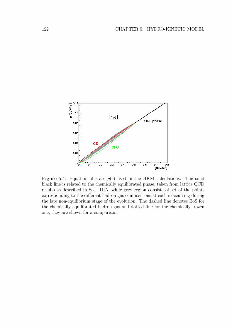
122 CHAPTER 5. HYDRO-KINETIC MODEL
Figure 5.4: Equation of state p(ε) used in the HKM calculations. The solidblack line is related to the chemically equilibrated phase, taken from lattice QCDresults as described in Sec. IIIA, while grey region consists of set of the pointscorresponding to the different hadron gas compositions at each ε occurring duringthe late non-equilibrium stage of the evolution. The dashed line denotes EoS forthe chemically equilibrated hadron gas and dotted line for the chemically frozenone, they are shown for a comparison.
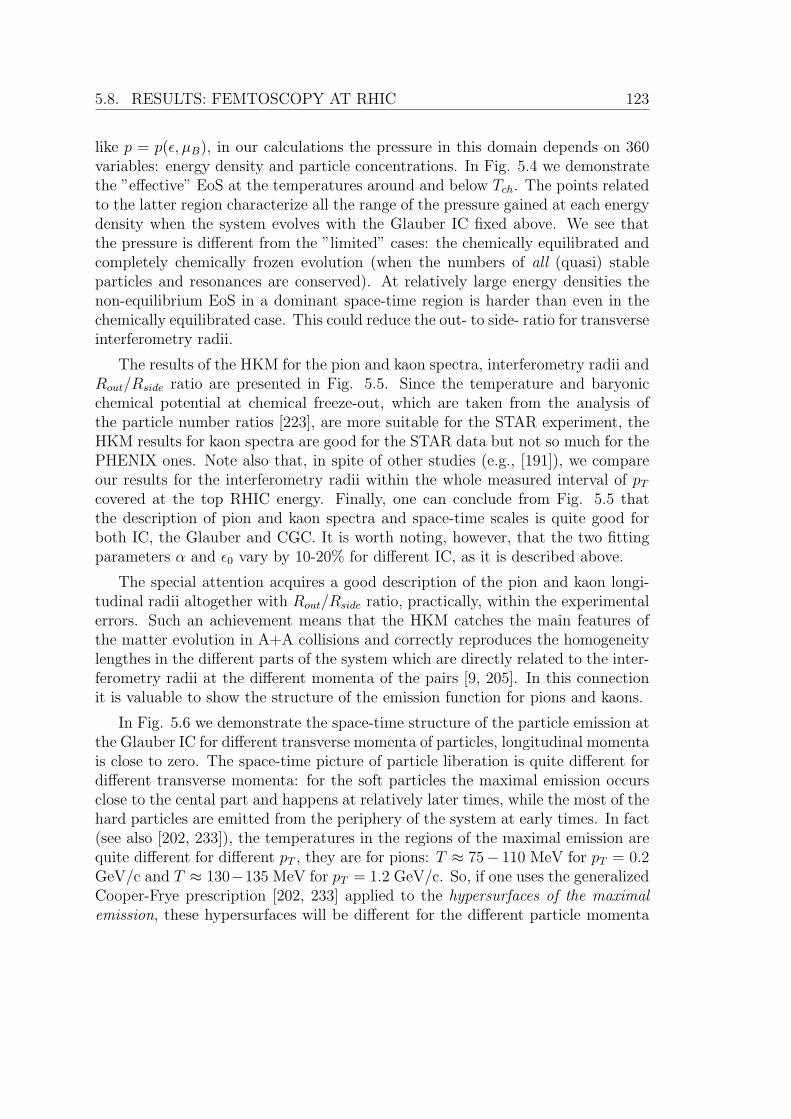
5.8. RESULTS: FEMTOSCOPY AT RHIC 123
like p = p(ε, µB), in our calculations the pressure in this domain depends on 360variables: energy density and particle concentrations. In Fig. 5.4 we demonstratethe ”effective” EoS at the temperatures around and below Tch. The points relatedto the latter region characterize all the range of the pressure gained at each energydensity when the system evolves with the Glauber IC fixed above. We see thatthe pressure is different from the ”limited” cases: the chemically equilibrated andcompletely chemically frozen evolution (when the numbers of all (quasi) stableparticles and resonances are conserved). At relatively large energy densities thenon-equilibrium EoS in a dominant space-time region is harder than even in thechemically equilibrated case. This could reduce the out- to side- ratio for transverseinterferometry radii.
The results of the HKM for the pion and kaon spectra, interferometry radii andRout/Rside ratio are presented in Fig. 5.5. Since the temperature and baryonicchemical potential at chemical freeze-out, which are taken from the analysis ofthe particle number ratios [223], are more suitable for the STAR experiment, theHKM results for kaon spectra are good for the STAR data but not so much for thePHENIX ones. Note also that, in spite of other studies (e.g., [191]), we compareour results for the interferometry radii within the whole measured interval of pT
covered at the top RHIC energy. Finally, one can conclude from Fig. 5.5 thatthe description of pion and kaon spectra and space-time scales is quite good forboth IC, the Glauber and CGC. It is worth noting, however, that the two fittingparameters α and ε0 vary by 10-20% for different IC, as it is described above.
The special attention acquires a good description of the pion and kaon longi-tudinal radii altogether with Rout/Rside ratio, practically, within the experimentalerrors. Such an achievement means that the HKM catches the main features ofthe matter evolution in A+A collisions and correctly reproduces the homogeneitylengthes in the different parts of the system which are directly related to the inter-ferometry radii at the different momenta of the pairs [9, 205]. In this connectionit is valuable to show the structure of the emission function for pions and kaons.
In Fig. 5.6 we demonstrate the space-time structure of the particle emission atthe Glauber IC for different transverse momenta of particles, longitudinal momentais close to zero. The space-time picture of particle liberation is quite different fordifferent transverse momenta: for the soft particles the maximal emission occursclose to the cental part and happens at relatively later times, while the most of thehard particles are emitted from the periphery of the system at early times. In fact(see also [202, 233]), the temperatures in the regions of the maximal emission arequite different for different pT , they are for pions: T ≈ 75− 110 MeV for pT = 0.2GeV/c and T ≈ 130−135 MeV for pT = 1.2 GeV/c. So, if one uses the generalizedCooper-Frye prescription [202, 233] applied to the hypersurfaces of the maximalemission, these hypersurfaces will be different for the different particle momenta
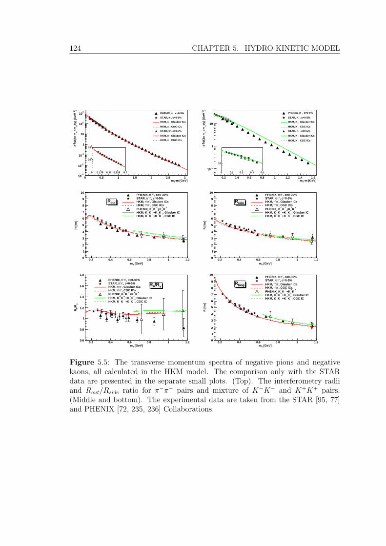
124 CHAPTER 5. HYDRO-KINETIC MODEL
-m [GeV]Tm0 0.5 1 1.5 2 2.5 3
]-2
dy)
[G
eVT
dm
T mπ
N/(
22
d
-310
-210
-110
1
10
210
310 , c=0-5%-πPHENIX,
, c=0-5%-πSTAR,
, Glauber ICs-πHKM,
, CGC ICs-πHKM,
, c=0-5%-πSTAR,
, Glauber ICs-πHKM,
, CGC ICs-πHKM,
0 0.175 0.35 0.525 0.7
210
310
-m [GeV]Tm0.2 0.4 0.6 0.8 1 1.2 1.4 1.6
]-2
dy)
[G
eVT
dm
T mπ
N/(
22
d
-110
1
10
, c=0-5%--PHENIX, K
, c=0-5%--STAR, K
, Glauber ICs-HKM, K
, CGC ICs-HKM, K
, c=0-5%--STAR, K
, Glauber ICs-HKM, K
, CGC ICs-HKM, K
0 0.1 0.2 0.3 0.4
10
[GeV]Tm0.2 0.4 0.6 0.8 1 1.2
R [
fm]
0
1
2
3
4
5
6
7
8
9
10, c=0-30%-π-πPHENIX,
, c=0-5%-π-πSTAR, , Glauber ICs-π-πHKM, , CGC ICs-π-πHKM,
+K
++K
--K
--PHENIX, K
, Glauber IC+
K+
+K--
K--
HKM, K, CGC IC
+K
++K
--K
--HKM, K
outR
[GeV]Tm0.2 0.4 0.6 0.8 1 1.2
R [
fm]
0
1
2
3
4
5
6
7
8
9
10, c=0-30%-π-πPHENIX,
, c=0-5%-π-πSTAR, , Glauber ICs-π-πHKM, , CGC ICs-π-πHKM,
+K
++K
--K
--PHENIX, K
, Glauber IC+
K+
+K--
K--
HKM, K, CGC IC
+K
++K
--K
--HKM, K
sideR
[GeV]Tm0.2 0.4 0.6 0.8 1 1.2
s/R o
R
0.6
0.8
1
1.2
1.4
1.6
1.8
, c=0-30%-π-πPHENIX, , c=0-5%-π-πSTAR,
, Glauber ICs-π-πHKM, , CGC ICs-π-πHKM,
+K
++K
--K
--PHENIX, K
, Glauber IC+
K+
+K--
K--
HKM, K, CGC IC
+K
++K
--K
--HKM, K
s/RoR
[GeV]Tm0.2 0.4 0.6 0.8 1 1.2
R [
fm]
0
1
2
3
4
5
6
7
8
9
10, c=0-30%-π-πPHENIX,
, c=0-5%-π-πSTAR, , Glauber ICs-π-πHKM, , CGC ICs-π-πHKM,
+K
++K
--K
--PHENIX, K
, Glauber IC+
K+
+K--
K--
HKM, K, CGC IC
+K
++K
--K
--HKM, K
longR
Figure 5.5: The transverse momentum spectra of negative pions and negativekaons, all calculated in the HKM model. The comparison only with the STARdata are presented in the separate small plots. (Top). The interferometry radiiand Rout/Rside ratio for π−π− pairs and mixture of K−K− and K+K+ pairs.(Middle and bottom). The experimental data are taken from the STAR [95, 77]and PHENIX [72, 235, 236] Collaborations.
5.8. RESULTS: FEMTOSCOPY AT RHIC 125
[fm]tr0 2 4 6 8 10 12 14 16 18 20
[fm
/c]
τ
5
10
15
20
25
30
]-3
GeV
-3 [
fmφ
<S
>τ
0
0.05
0.1
0.15
0.2
0.25
0.3=0.2 GeV
T, p--π
[fm]tr0 2 4 6 8 10 12 14 16 18 20
[fm
/c]
τ
5
10
15
20
25
30
]-3
GeV
-3 [
fmφ
<S
>τ
0
0.01
0.02
0.03
0.04
0.05
0.06
0.07
0.08
0.09=0.85 GeVT
, p--π
[fm]tr0 2 4 6 8 10 12 14 16 18 20
[fm
/c]
τ
5
10
15
20
25
30
]-3
GeV
-3 [
fmφ
<S
>τ
0
0.002
0.004
0.006
0.008
0.01
0.012
0.014=1.2 GeVT
, p--π
[fm]tr0 2 4 6 8 10 12 14 16 18 20
[fm
/c]
τ
5
10
15
20
25
30
]-3
GeV
-3 [
fmφ
<S
>τ
0
0.005
0.01
0.015
0.02
0.025
0.03
0.035=0.2 GeVT
, p--K
[fm]tr0 2 4 6 8 10 12 14 16 18 20
[fm
/c]
τ
5
10
15
20
25
30
]-3
GeV
-3 [
fmφ
<S
>τ
0
0.005
0.01
0.015
0.02
0.025=0.7 GeV
T, p
--K
[fm]tr0 2 4 6 8 10 12 14 16 18 20
[fm
/c]
τ
5
10
15
20
25
30]
-3G
eV-3
[fm
φ <
S>
τ
0
0.001
0.002
0.003
0.004
0.005
0.006
0.007
0.008=1.2 GeVT
, p--
K
Figure 5.6: The φp-integrated emission functions of negative pions and negativekaons with different momenta at the Glauber IC. The values of pT in the middlerow correspond to the same transverse mass for pions and kaons mT = 0.86 GeV.
126 CHAPTER 5. HYDRO-KINETIC MODEL
and does not correspond to common isotherm [202, 233].
One can see in Fig. 5.6, the top plots, that at equal transverse momentumpT the maximal emission of kaons happens earlier than pions as one can expectsince the kaons interact weaker. At the same time the kaon interferometry radii inFig. 5.5 follow approximately the pion radii, demonstrating the approximate mT -scaling [234] with deviations to the slightly bigger values than pion radii have. Theexplanations can be gained from the middle row in Fig. 5.6 where the comparisonis done for the same transverse mass of pions and kaons. Then the maxima of pionand kaon emissions become closer and the majority of kaons leave system evensomewhat later than pions at the same mT , opposite to the comparison at thesame pT . Since in simplest situations the homogeneity lengths for bosons dependon mT [234], one could say that the approximate mT -scaling could indicate thesimilarity of the freeze-out picture for kaons and pions. However, probably, sucha conclusion is very approximate since the real structure of the emission processesin A+A collisions is quite complicated as one can see from the details in Fig. 5.6.
5.9 Results: space-time scales for SPS, RHIC,
LHC
The above formulated model is then applied to the description of particle spectraand space-time scales observed at SPS and RHIC experiments.
The pion emission function per unit (central) rapidity, integrated over az-imuthal angle and transverse momenta, is presented in Fig. 5.7 for the top SPS,RHIC and LHC energies as a function of transverse radius r and proper time τ .The two fitting parameters ε0 and 〈vT 〉 are fixed as discussed above and marked infigures. The pion transverse momentum spectrum, its slope as well as the absolutevalue, and the interferometry radii, including Rout to Rside ratio, are in a goodagreement with the experimental data both for the top SPS and RHIC energies.
As one can see particle emission lasts all the lifetime of the fireballs; in thecental part, r ≈ 0, the duration is half of the lifetime. Nevertheless, according tothe results above in this chapter, the Landau/Cooper-Frye prescription of suddenfreeze-out could be applied in a generalized form accounting for momentum depen-dence of the freeze-out hypersurface σp(x); now σp(x) corresponds to the maximumof emission function S(tσ(r, p), r, p) at fixed momentum p in an appropriate regionof r. This finding gives one possibility to keep in mind the known results based onthe Cooper-Frye formalism, applying them to a surface of the maximal emissionfor given p. Then the typical features of the energy dependence can be understoodas follows. The inverse of the spectra slopes, Teff , grows with energy, since as onesees from the emission functions, the duration of expansion increases with initial
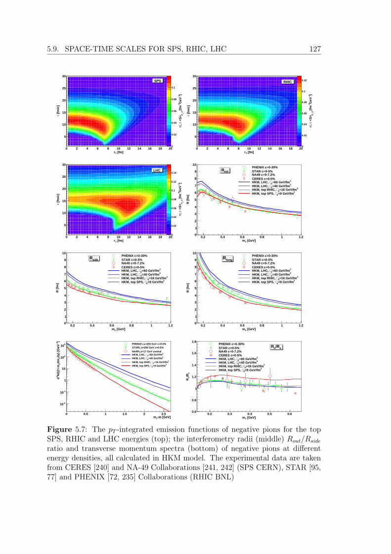
5.9. SPACE-TIME SCALES FOR SPS, RHIC, LHC 127
[fm]Tr0 2 4 6 8 10 12 14 16 18 20
[fm
/c]
τ
5
10
15
20
25
30
]-1
GeV
-3 [
fmφ,
Tp
<S
>τ, - π
0
0.02
0.04
0.06
0.08
0.1
SPS
[fm]Tr0 2 4 6 8 10 12 14 16 18 20
[fm
/c]
τ
5
10
15
20
25
30
]-1
GeV
-3 [
fmφ,
Tp
<S
>τ, - π
0
0.02
0.04
0.06
0.08
0.1
0.12RHIC
[fm]Tr0 2 4 6 8 10 12 14 16 18 20
[fm
/c]
τ
5
10
15
20
25
30
]-1
GeV
-3 [
fmφ,
Tp
<S
>τ, - π
0
0.02
0.04
0.06
0.08
0.1
0.12
0.14LHC
[GeV]Tm0.2 0.4 0.6 0.8 1 1.2
R [
fm]
0
1
2
3
4
5
6
7
8
9
10PHENIX c=0-30%STAR c=0-5%NA49 c=0-7.2%CERES c=0-5%
3=60 GeV/fm0∈HKM, LHC, 3=40 GeV/fm0∈HKM, LHC,
3=16 GeV/fm0∈HKM, top RHIC, 3=9 GeV/fm0∈HKM, top SPS,
outR
[GeV]Tm0.2 0.4 0.6 0.8 1 1.2
R [
fm]
0
1
2
3
4
5
6
7
8
9
10PHENIX c=0-30%STAR c=0-5%NA49 c=0-7.2%CERES c=0-5%
3=60 GeV/fm0∈HKM, LHC, 3=40 GeV/fm0∈HKM, LHC,
3=16 GeV/fm0∈HKM, top RHIC, 3=9 GeV/fm0∈HKM, top SPS,
sideR
[GeV]Tm0.2 0.4 0.6 0.8 1 1.2
R [
fm]
0
1
2
3
4
5
6
7
8
9
10PHENIX c=0-30%STAR c=0-5%NA49 c=0-7.2%CERES c=0-5%
3=60 GeV/fm0∈HKM, LHC, 3=40 GeV/fm0∈HKM, LHC,
3=16 GeV/fm0∈HKM, top RHIC, 3=9 GeV/fm0∈HKM, top SPS,
longR
-m [GeV]Tm0 0.5 1 1.5 2 2.5
]-2
dy)
[G
eVT
dm
T mπ
N/(
22
d
-210
-110
1
10
210
310=200 GeV c=0-5%sPHENIX
=200 GeV c=0-5%sSTAR
=17 GeV centralsNA49 3=60 GeV/fm0∈HKM, LHC, 3=40 GeV/fm0∈HKM, LHC,
3=16 GeV/fm0∈HKM, top RHIC, 3=9 GeV/fm0∈HKM, top SPS,
[GeV]Tm0.2 0.3 0.4 0.5 0.6
s/R o
R
0.6
0.8
1
1.2
1.4
1.6
1.8PHENIX c=0-30%STAR c=0-5%NA49 c=0-7.2%CERES c=0-5%
3=60 GeV/fm0∈HKM, LHC, 3=40 GeV/fm0∈HKM, LHC,
3=16 GeV/fm0∈HKM, top RHIC, 3=9 GeV/fm0∈HKM, top SPS,
s/RoR
Figure 5.7: The pT -integrated emission functions of negative pions for the topSPS, RHIC and LHC energies (top); the interferometry radii (middle) Rout/Rside
ratio and transverse momentum spectra (bottom) of negative pions at differentenergy densities, all calculated in HKM model. The experimental data are takenfrom CERES [240] and NA-49 Collaborations [241, 242] (SPS CERN), STAR [95,77] and PHENIX [72, 235] Collaborations (RHIC BNL)
128 CHAPTER 5. HYDRO-KINETIC MODEL
energy density and, therefore, the fluid element get higher transverse collective ve-locities vT when reaching a decoupling energy densities. Therefore the blue shift ofthe spectra becomes stronger. A rise of the transverse collective flow with energyleads to some compensation of an increase of Rside: qualitatively the homogeneitylength at decoupling stage is Rside = RGeom/
√1 + 〈v2
T 〉mT/2T , (see, e.g., [237]).So, despite a significant increase of the transverse emission region, RGeom, seen inFig.1, a magnification of collective flow partially compensates this. As a resultthere is only a moderate increase of the Rside with energy. Since the temperaturesin the regions of the maximal emission decrease very slowly when initial energydensity grows (e.g., the temperatures for SPS, RHIC and LHC are correspond-ingly 0.105, 0.103 and 0.95 MeV for pT = 0.3 GeV/c ) the Rlong ∼ τ
√T/mT
[234] grows proportionally to an increase of the proper time associated with thehypersurface σpT
(x) of maximal emission. As we see from Fig. 5.5 this time growsquite moderately with the collision energy.
A non trivial result concerns the energy behavior of the Rout/Rside ratio. Itslowly drops when energy grows and apparently is saturated at fairly high en-ergies at the value close to unity (Fig.1). To clarify the physical reason of itlet us make a simple semi-quantitative analysis. As one can see in Fig. 1, thehypersurface of the maximal emission can be approximated as consisting of twoparts: the ”volume” emission (V ) at τ ≈ const and ”surface” emission (S). Asimilar picture within the Cooper-Frye prescription, which generalizes the blast-wave model by means of including the surface emission has been considered inRef. [48]. If the hypersurface of maximal emission τ(r) is double-valued func-tion, as in our case, then at some transverse momentum pT the transverse spectraand HBT radii will be formed mostly by the two contributions from the differ-ent regions with the homogeneity lengths λi,V =
√< (∆ri)2 > (i = side, out) at
the V -hypersurface and with the homogeneity lengths λi,S at the S-hypersurface.Similar to Ref.[237], one can apply at mT/T � 1 the saddle point methodwhen calculating the single and two particle spectra using the boost-invariantmeasures µV = dσV
µ pµ = τ(r)rdrdφdη(mT cosh(η − y) − pT
deτ(r)dr
cos(φ − α)) and
µS = dσSµp
µ = r(τ)τdτdφdη(−mT cosh(η − y)der(τ)dτ
+ pT cos(φ − α)) for V - andS- parts of freeze-out hypersurface correspondingly (here η and y are space-timeand particle pair rapidities, the similar correspondence is for angles φ and α, alsonote that pT
mT> der(τ)
dτ[202, 233]). Then one can write, ignoring for simplicity the
interference (cross-terms) between the surface and volume contributions,
R2side = c2V λ
2side,V + c2Sλ
2side,S (5.81)
R2out = c2V λ
2out,V + c2Sλ
2out,S(1 − dr
dτ)2, (5.82)
where the coefficients c2V + c2S ≤ 1 and we take into account that at p0/T � 1 for
5.10. CONCLUSIONS 129
pions βout = pout/p0 ≈ 1. All homogeneity lengths depend on mean transverse mo-
mentum of the pion pairs pT . The slope drdτ
in the region of homogeneity expressesthe strength of r − τ correlations between the space and time points of particleemission at the S-hypersurface r(τ). The picture of emission in Fig. 1 shows thatwhen the energy grows the correlations between the time and radial points of theemission becomes positive, dr
dτ> 0, and they increase with energy density. The pos-
itivity is caused by the initial radial flows [212] ur(τ0), which are developed at thepre-thermal stage, and the strengthening of the r−τ correlations happens becausethe non-central ith fluid elements, which produce after their expansion the surfaceemission, need more time τi(ε0) to reach the decoupling density if they initiallyhave higher energy density ε0. (Let us characterize this effect by the parameter
κ = dτi(ε0)dε0
> 0). Then the fluid elements before their decays run up to larger radialfreeze-out position ri: if a is the average Lorentz-invariant acceleration of thosefluid elements during the system expansion, then roughly for ith fluid elementswhich decays at time τi we have at aτi � 1: ri(τi) ≈ ri(τ0) + τi + (ur
i (τ0) − 1)/a.Then the level of r − τ correlations within the homogeneous freeze-out ”surface”region, which is formed by the expanding matter that initially at τ0 occupies theregion between the transversal radii r1(τ0) and r2(τ0) > r1(τ0), is
dr
dτ≈ r1(τ1) − r2(τ2)
τ1 − τ2≈ 1 − R
ε0κ(5.83)
and, therefore, the strength of r− τ correlations grows with energy: dτdr
→ 1. Note
that here we account for τ2 − τ1 ≈ κ(ε0(r2(τ0)) − ε0(r1(τ0))) and that dε0(r)dr
≈ − ε0R
where ε0 ≡ ε0(r = 0) and R is radius of nucleus. As a result the second S-term in Eq. (5.82) tends to zero at large ε0 , reducing, therefore, the Rout/Rside
ratio. In particular, if λ2side,V � λ2
side,S then, accounting for a similarity of thevolume emission in our approximation and in the blast wave model, where asknown λside,V ≈ λout,V , one can get: Rout
Rside≈ 1 + const · R
ε0κ→ 1 at ε0 → ∞. It is
worthy to note that also measure µS tends to zero when dτdr
→ 1 that again reducesthe surface contribution to side− and out− radii at large pT .
The presented qualitative, in fact, analysis demonstrates the main mechanismsleading to the non-trivial behavior of Rout to Rside ratio exposed in detailed HKMcalculations, see Fig.1 (bottom, right).
5.10 Conclusions
The hydrokinetic approach to A+A collisions is developed. It allows one to de-scribe the continuous particle emission from a hot and dense finite system, expand-ing hydrodynamically into vacuum, in the way which is consistent with Boltzmannequations and conservation laws, and accounts also for the opacity effects.
130 CHAPTER 5. HYDRO-KINETIC MODEL
The analysis and numerical calculations show that the widely used phenomeno-logical Landau/ Cooper-Frye prescription for calculation of pion (or other particle)spectrum is too rough if the freeze-out hypersurface is considered as common forall momenta of pions. The Cooper-Frye formula, however, could be applied ingeneralized form accounting for direct momentum dependence of the freeze-outhypersurface σ(p); the latter corresponds to the maximum of emission functionS(tσ(r, p), r, p) at fixed momentum p in an appropriate region of r.
The hydro-kinetic model is then developed for a detailed study of the matterevolution and space-time picture of hadronic emission from rapidly expandingfireballs in A+A collisions. The model allows one to describe the evolution ofthe QGP as well as the gradually decoupling hadronic fluid - a chemically non-equilibrium matter, where the equation of state is defined at each space-time pointand accounts for decays of resonances into the non-equilibrated medium.
The HKM is applied to restore the initial conditions and space-time picture ofthe matter evolution in central Au+Au collisions at the top RHIC energy. Theanalysis, which is based on a detailed reproduction of the pion and kaon mo-mentum spectra and measured femtoscopic scales, demonstrates that basically thepictures of the matter evolution and particle emission are similar at both Glauberand CGC initial conditions (IC) with, however, the different initial maximal en-ergy densities: it is about 20% more for the CGC initial conditions. The initialpre-thermal flow is slightly less for the CGC IC. The main factors allowing oneto describe well simultaneously the spectra and femtoscopic scales are: a rela-tively hard EoS (crossover transition and chemically non-equilibrium compositionof hadronic matter), pre-thermal transverse flows developed prior to thermaliza-tion time, an account for an “additional portion” of the transverse flows due to theshear viscosity effect and fluctuation of initial conditions, a correct description ofa gradual decay of the non-equilibrium fluid at the late stage of expansion. Thenone does not require the too early thermalization time, τi < 1 fm/c, to describethe data well. All these factors are included in the present version of the HKMand it allows one to describe observables with only the two parameters.
An analysis of the emission function at the top RHIC energies demonstratesthat the process of decoupling of the fireballs created in Au+Au collision lastsfrom about 8 to 20 fm/c, more than the half of fireball’s total lifetime. Thetemperatures in the regions of the maximal emission are different at the differenttransverse momenta of emitting pions: T ≈ 75 − 110 MeV for pT = 0.2 GeV/cand T ≈ 130− 135 MeV for pT = 1.2 GeV/c. A comparison of the pion and kaonemissions at the same transverse mass demonstrates the similarity of the positionsof emission maxima, that could point to the reason for an approximate mT scaling.
Finally, the model is applied for the description of behavior of interferometryradii as a function of collision energy. Then the main mechanisms that lead to the
5.10. CONCLUSIONS 131
paradoxical behavior of the interferometry scales find a natural explanation. Inparticular, a slow decrease and apparent saturation ofRout/Rside ratio around unityat high energy happens due to a strengthening of positive correlations betweenspace and time positions of pions emitted at the radial periphery of the system.Such an effect is a consequence of the two factors accompanying an increase ofcollision energy: a developing of the pre-thermal collective transverse flows and anincrease of initial energy density in the fireball.
Further developments of the hydrokinetic approach and an analysis of the datain non-central A+A collisions will be the subject of a follow-up work.

132 CHAPTER 5. HYDRO-KINETIC MODEL
CHAPTER
SIX
Conclusions
In Chapter 2, a new class of analytic solutions for 3D relativistic expansion withanisotropic flows is found. The ellipsoidal generalization of the spherically symmet-ric Hubble flow is considered within this class. These solutions can also describethe relativistic expansion of the finite systems into vacuum. Specific equationof state makes the application to the whole hydrodynamic stage of evolution inheavy ion collisions to be problematic. However, the solutions can still be appicableduring deconfinement phase transition and the final stage of evolution of hadronsystems. Also, the solutions can serve as a test for numerical codes describing 3Dasymmetric flows in the relativistic hydrodynamics.
A fast MC event generator (FASTMC) based on Landau/Cooper-Frye freeze-out prescription is presented in Chapter 3. It accounts for the decays of unstableresonances and weak decays. FASTMC allows to describe both central and non-central heavy ion collisions. The description of the kt-dependence of the correlationradii at
√s = 200AGeV RHIC collisions has been achieved within ∼ 10% accuracy.
The comparison of the RHIC v2 measurements with the MC generation resultsshows that the scenario with two separated freeze-outs is more favorable for thedescription of the pt-dependence of the elliptic flow.
The new hybrid dinamical model for matter evolution in ultrarelativistic heavyion collisions is presented in Chapter 4. It has many improvements, as comparedto existing ones: flux-tube initial conditions (EPOS), event-by-event treatment,use of an efficient (3+1)D hydro code including flavor conservation, employmentof a realistic equation-of-state, use of a complete hadron resonance table, and ahadronic cascade procedure after an hadronization from thermal matter at an earlytime.
The model is able to describe simultaneously different soft observables: trans-verse spectra for pions, kaons, protons, lambdas, xis; v2-coefficients for pions,protons and kaons; interferometry (HBT)-radii for pions.
133

134 CHAPTER 6. CONCLUSIONS
Finally, in Chapter 5, the hydrokinetic approach to A+A collisions is devel-oped. It allows one to describe the continuous particle emission from a hot anddense finite system, expanding hydrodynamically into vacuum, in the way whichis consistent with Boltzmann equations and conservation laws, and accounts alsofor the opacity effects. The conditions of applicability of generalized Cooper-Fryedistribution are found and proved by numerical calculations.
The hydro-kinetic model is then developed for a detailed study of the matterevolution and space-time picture of hadronic emission from rapidly expandingfireballs in A+A collisions. The model allows one to describe the evolution ofthe QGP as well as the gradually decoupling hadronic fluid - a chemically non-equilibrium matter, where the equation of state is defined at each space-time pointand accounts for decays of resonances into the non-equilibrated medium.
The HKM is applied to restore the initial conditions and space-time picture ofthe matter evolution in central Au+Au collisions at the top RHIC energy. Themodel is able to reproduce pion and kaon spectra together with pion and kaoninterferometry radii. The main factors, which allows one to describe well simulta-neously the spectra and femtoscopic scales are: a relatively hard EoS (crossovertransition and chemically non-equilibrium composition of hadronic matter), pre-thermal transverse flows developed to thermalization time, an account for an “ad-ditional portion” of the transverse flows due to the shear viscosity effect and fluc-tuation of initial conditions, a correct description of a gradual decay of the non-equilibrium fluid at the late stage of expansion. Then one does not require the tooearly thermalization time, τi < 1 fm/c, to describe the data well. All these factorsare included in the presented version of the HKM and it allows one to describeobservables with only the two parameters.
One can note the presence of the same factors (crossover EoS, pre-thermaltransverse flows) in both hybrid and hydrokinetic model, being important for thesimultaneous reproduction of particle spectra and femtoscopic scales. This stressesthe importance and solidity of the results obtained.
An analysis of the emission function at the top RHIC energies demonstratesthat the process of decoupling of the fireballs created in Au+Au collision lastsfrom about 8 to 20 fm/c, more than the half of fireball’s total lifetime.
A comparison of the pion and kaon emissions at the same transverse massdemonstrates the similarity of the positions of emission maxima, that could pointout to the reason for an approximate mT scaling.
Finally, the hydro-kinetic model is applied for the description of behavior ofinterferometry radii as a function of collision energy. Then the main mechanismsthat lead to the paradoxical behavior of the interferometry scales find a naturalexplanation. In particular, a slow decrease and apparent saturation of Rout/Rside
ratio around unity at high energy happens due to a strengthening of positive cor-
135
relations between space and time positions of pions emitted at the radial peripheryof the system. Such an effect is a consequence of the two factors accompanying anincrease of collision energy: a development of the pre-thermal collective transverseflows and an increase of initial energy density in the fireball.
Further elaboration of the hydrokinetic approach and an analysis of the datain non- central A+A collisions will be the subject of a follow-up work.
136 CHAPTER 6. CONCLUSIONS
Glossary
BNL − Brookheaven National LaboratoryCERN − Conseil Europeen pour la Recherche NucleaireSPS − Super Proton SynchrotronRHIC − Relativistic Heavy Ion ColliderLHC − Large Hadron ColliderHBT − Hanburry-Brown-Twiss

BIBLIOGRAPHY
[1] L.D. Landau, Izv. Akad. Nauk SSSR 17 (1953) 51; S.Z. Belenkij and L.D.Landau, Usp. Fiz. Nauk 56 (1955) 309;
[2] E. Fermi, Prog. Theor. Phys. 5 (1050) 57
[3] P. Carruthers, Annals N.Y. Acad. Sci. 229 (1974) 91.
[4] E. V. Shuryak and 0. V. Zhirov, Phys.Lett. B89 (1979) 253.
[5] Yu.M. Sinyukov, S.V. Akkelin, N. Xu, Phys.Rev. C59 (1999) 3437.
[6] Yu.M. Sinyukov, A.N. Nazarenko, Iu.A. Karpenko, Acta Phys.Polon. B40(2009), 1109.
[7] W. Broniowski, M. Chojnacki, W. Florkowski, A. Kisiel, Phys.Rev.Lett.101(2008), 022301.
[8] W.A. Zajc, Two Pion Correlations in Heavy Ion Collisions. PhD thesis,University of California, 1982 (available as LBL-14864).
[9] Sinyukov Yu. In Hot Hadronic Matter: Theory and Experiment, ed. J. Rafel-ski. New York: Plenum, NATO ASI Series B 346:309 (1995)
[10] M.G. Bowler, Phys. Lett. B 270, 69 (1991); Yu.M. Sinyukov et al., Phys.Lett. B 432, 249 (1998).
[11] E. Schnedermann, J. Sollfank, U. Heinz, Phys. Rev. C48 (1993), 2462 (nucl-th/93070200).
[12] W.A. Zajc et al., Phys. Rev. C 29 (1984) 2173.
[13] U. Heinz, J. Phys. G: Nucl. Part. Phys. 31, S717 (2005); arXiv:nucl-th/0512051; P. Huovinen, P.V. Ruuskanen, Annu. Rev. Nucl. Part. Sci. 56,163 (2006); T. Hirano, Nucl. Phys. A 774, 531 (2006).
137

138 BIBLIOGRAPHY
[14] Y. Hama, T. Kodama, O. Socolowski Jr., Braz. J. Phys. 35, 24 (2005).
[15] C. Nonaka, J. Phys. G: Nucl. Part. Phys. 34, S313 (2007); T. Hirano,arXiv:0704.1699 [nucl-th].
[16] E.V. Shuryak, Prog. Part. Nucl. Phys. 53, 273 (2004); arXiv:hep-ph/0703208; arXiv:0709.2175 [hep-ph]; arXiv:0804.1373 [hep-ph].
[17] E.V.Shuryak, Nucl.Phys. A750 (2005) 64-83; arXiv:hep-ph/0405066.
[18] W. Broniowski, W. Florkowski, M. Chojnacki, A. Kisiel, Acta Phys. Polon.B40:979-986, 2009.
[19] I.M. Khalatnikov, Sov. JETF, 26 (1954) 529.
[20] R.C. Hwa, Phys.Rev. D10 (1974) 2260; F. Cooper, G. Frye, E. Schonberg,Phys.Rev. D11 (1975) 192.
[21] M.I.Gorenstein,Yu.M.Sinyukov,V.I.Zhdanov: Phys.Lett. B71 (1977) 199,and Zh.Eksp. Theor.Fiz.- ZETF (USSR) 74 (1978), 833.
[22] J. D. Bjorken, Phys. Rev. D27 (1983) 140.
[23] C.B. Chiu, E.C.G. Sudarshan, Kuo-Hsiang Wang, Phys.Rev. D12 (1975)902.
[24] T. Csorgo, Heavy Ion Phys. A21 (2004) 73-84.
[25] T. S. Biro, Phys.Lett. B474 (2000) 21-26, T. S. Biro, Phys.Lett. B487(2000) 133-139.
[26] W. Broniowski, W. Florkowski, Nucl. Phys A 715, 875c (2003); W. Bro-niowski, W. Florkowski, B. Hiller, Phys. Rev. C 68, 034911 (2003).
[27] S.V. Akkelin, P. Braun-Munzinger, Yu.M. Sinyukov. Nucl.Phys. A710(2002) 439.
[28] W. Busza, Acta Physica Polonica B35 (2004) 2873.
[29] L.D. Landau, E.M. Lifshitz ”Fluid Mechanics”, Addison-Westley, Reading,Mass., 1959.
[30] S.V. Akkelin, T. Csorgo, B. Lukacs, Yu.M. Sinyukov and M. Weiner, Phys.Lett. B505 (2001) 64.
[31] Proc. of the Conference ”Quark Matter 2005”, Nucl. Phys. A 774 (2006).
BIBLIOGRAPHY 139
[32] I.P. Lokhtin and A.M. Snigirev, Phys. Lett. B 378, 247 (1996).
[33] N.A. Kruglov, I.P. Lokhtin, L.I. Sarycheva and A.M. Snigirev, Z. Phys. C76, 99 (1997).
[34] I.P. Lokhtin and A.M. Snigirev, Preprint SINP MSU 2004-14/753, hep-ph/0312204.
[35] I.P. Lokhtin and A.M. Snigirev, Eur. Phys. J. C 45, 211 (2006).
[36] R. Brun and F. Rademakers, Nucl. Instrum. Meth. A 389, 81 (1997),(http://root.cern.ch).
[37] F. Retiere and M. Lisa, Phys. Rev. C 70, 044907 (2004).
[38] W. Florkowski and W. Broniowski, Acta. Phys. Pol. 35, 2855 (2004).
[39] S.R. de Groot, W.A. van Leeuwen, Ch.G. van Weert, Relativistic kinetictheory. Principles and Applications, North-Holland Publishing Company,Amsterdam-New York-Oxford, 1980.
[40] Yu.M. Sinyukov, S.V. Akkelin and A.Yu. Tolstykh, Nukleonika 43, 369(1998).
[41] S.V. Akkelin and Yu.M. Sinyukov, Phys. Rev. C 70, 064901 (2004).
[42] S.V. Akkelin and Yu.M. Sinyukov, Phys. Rev. C 73, 034908 (2006).
[43] J. Cleymans, H. Oeschler, K. Redlich and S. Wheaton, Phys. Rev.C 73,034905 (2006).
[44] F. Cooper and G. Frye, Phys. Rev.D 10, 186 (1974).
[45] M.I. Gorenstein and Yu.M. Sinyukov, Phys. Lett. B 142, (1985) 425.
[46] Yu.M. Sinyukov, Z. Phys. C 43, 401 (1989).
[47] K.A. Bugaev, Nucl. Phys. A 606, 559 (1996); Cs. Anderlik et al., Phys. Rev.C 59, 3309 (1999).
[48] M.S. Borysova, Yu.M. Sinyukov, S.V. Akkelin, B. Erazmus andIu.A. Karpenko, Phys. Rev. C 73, 024903 (2006).
[49] J.D. Bjorken, Phys. Rev. D 27, 140 (1983).
[50] R. Morita, S. Muroya, H. Nakamura and C. Nonaka, Phys. Rev. C 61,034904 (2000).
140 BIBLIOGRAPHY
[51] T. Csorgo and B. Lorstad, Phys. Rev. C 54, 1390 (1996).
[52] Particle Data Group, K. Hagiwara et al., Phys. Rev. D 66, 010001 (2002).
[53] N.S. Amelin, R. Lednicky, L.V. Malinina, T.A. Pocheptsov andY.M. Sinyukov, Phys. Rev. C 73, 044909 (2006).
[54] G. Yen, M.I. Gorenstein, W. Greiner and S.N. Yang, Phys. Rev. C 56, 2210(1997).
[55] J. Rafelski, Phys. Lett. B 262, 333 (1981).
[56] F. Becattini, J. Mannien, M. Gazdzicki, Phys. Rev. C 73, 044905 (2006).
[57] U.A. Wiedemann and U. Heinz, Phys. Rept. 319, 145 (1999).
[58] S. Wheaton and J. Clemans, arXiv:hep-ph/0407174.
[59] P. Braun-Munzinger et al., Phys. Lett. B 344, 43 (1995), ibid. B 365, 1(1996), ibid. B 465, 15 (1999).
[60] W. Florkowski and W. Broniowski, AIP Conf. Proc. 660, 177 (2003); nucl-th/0212052 v1.
[61] B.B. Back at al., PHOBOS Collaboration, Phys. Rev. Lett. 87, 102301(2001).
[62] I.G. Bearden et al., BRAHMS Collaboration, Nucl. Phys. A 698, 667c(2002).
[63] J. Harris et al., STAR Collaboration, Nucl. Phys. A 698, 64c (2002).
[64] H. Ohnishi et al., PHENIX Collaboration, Nucl. Phys. A 698, 659c (2002).
[65] H. Caines et al., STAR Collaboration, Nucl. Phys A 698, 112c (2002).
[66] J. Adams et al., STAR Collaboration, Phys.Lett. B 567, 167 (2003).
[67] C. Adler et al., STAR Collaboration, Phys. Rev. C 65, 041901 (2002).
[68] C. Adler et al., STAR Collaboration, Phys. Rev. Lett. 89, 092301 (2002).
[69] C. Adler et al., STAR Collaboration, Phys. Rev. Lett. 87, 262302 (2001).
[70] J. Castillo et al., STAR Collaboration, nucl-ex/0210032.
[71] B.B. Back et al., PHOBOS Collaboration, Nucl.Phys. A 757, 28 (2005).

BIBLIOGRAPHY 141
[72] S.S. Adler et al., PHENIX Collaboration, Phys.Rev. C 69, 034909 (2004).
[73] R. Lednicky, Proc. of the Conference ”Quark Matter 2005”, Nucl. Phys. A774, 189 (2006).
[74] M.I. Podgoretskii, Sov. J. Nucl. Phys. 37, 272 (1983).
[75] S. Pratt, Phys. Rev. Lett. 53, 1219 (1984).
[76] T. Csorgo and S. Pratt, Proc. of the Workshop on Heavy Ion Physics, KFKI-1991-28/A, 75.
[77] J. Adams et al., STAR Collaboration, Phys. Rev. C 71, 044906 (2005).
[78] M. Bystersky, STAR Collaboration, AIP Conf. Proc. 828, 533 (2006); nucl-ex/0511053.
[79] N.S. Amelin, R. Lednicky, T.A. Pocheptsov, I.P. Lokhtin, L.V. Malinina,A.M. Snigirev, Iu.A. Karpenko, and Yu.M. Sinyukov, Phys. Rev. C 74,064901 (2006).
[80] N. S. Amelin, R. Lednicky, I. P. Lokhtin, L. V. Malinina, A. M. Snigirev,Iu. A. Karpenko, Yu. M. Sinyukov, I. Arsene, and L. Bravina, Phys. Rev. C77, 014903 (2008).
[81] C. Adler et al. (STAR Collaboration), Phys. Rev. Lett. 87, 182301 (2001).
[82] P.F. Kolb, J. Sollfrank, and U.W. Heinz, Phys. Lett. B459, 667 (1999).
[83] D. Hardtke and S.A. Voloshin, Phys. Rev. C 61, 024905 (2000).
[84] R.J.M. Snellings, A.M.Poskanzer, and S.A. Voloshin, nucl-ex/9904003.
[85] M. Bleicher and H. Stoecker, Phys. Lett. B526, 309 (2002).
[86] B. Zhang, C.M. Ko, B.A. Li, and Z.W. Lin, Phys. Rev. C 61, 067901 (2000);Z.W. Lin, S. Pal, C.M. Ko, B.A. Li, and B. Zhang, Phys. Rev. C 64, 011902(2001).
[87] A. Kisiel, T. Taluc, W. Broniowski, and W. Florkowski, Comput. Phys.Commun. 174, 669 (2006).
[88] W. Florkowski, W. Broniowski, A. Kisiel, and J. Pluta, Acta Phys. Polon.B37, 3381 (2006).
[89] M. Csanad, T. Csorgo and B. Lorstad, Nucl. Phys. A 742, 80 (2004).
142 BIBLIOGRAPHY
[90] P. Huovinen, P.F. Kolb, U. Heinz, P.V. Ruuskanen, and S.A. Voloshin, Phys.Lett. B503, 58 (2001).
[91] U.A. Wiedemann, Phys. Rev. C 57, 266 (1998).
[92] U.W. Heinz and S.M.H. Wong, Phys. Rev. C 66, 014907 (2002).
[93] L.V. Bravina et al., Nucl. Phys. A 698, 383 (2002).
[94] G. Torrieri et al., nucl-th/0404083 (2004).
[95] J. Adams et al. (STAR Collaboration), Phys. Rev. Lett. 92, 112301 (2004).
[96] S. Voloshin and Y. Zang, Z. Phys. C 70, 665 (1996).
[97] A.M. Poskanzer and S.A. Voloshin, Phys. Rev. C 58, 1671 (1998).
[98] J. Adams et al. (STAR Collaboration), Phys. Rev. C 72, 014904 (2005).
[99] R. Lednicky, V. Lyuboshitz, K. Mikhailov, Yu. Sinyukov, A. Stavinsky andB. Erazmus, Phys. Rev. C 61 034901 (2000).
[100] J. Adams et al. (STAR Collaboration), Phys. Rev. Lett. 93, 012301 (2004).
[101] M. Bleicher, F. M. Liu, A. Kernen, J. Aichelin, S.A. Bass, F. Becattini, K.Redlich, and K. Werner, Phys.Rev.Lett.88, 202501, 2002.
[102] K. Werner, Iu. Karpenko, T. Pierog, M. Bleicher, K. Mikhailov,arXiv:1004.0805.
[103] STAR Collaboration: J. Adams, et al, Nucl. Phys. A757:102, 2005.
[104] PHENIX Collaboration, K. Adcox, et al, Nucl. Phys. A757:184-283, 2005.
[105] BRAHMS Collaboration, I. Arsene et al., Nucl. Phys. A757:1-27, 2005.
[106] P. Huovinen, in Quark-Gluon Plasma 3, eds. R. C. Hwa and X. N. Wang(World Scientific, Singapore, 2004).
[107] P. F. Kolb and U. Heinz, in Quark-Gluon Plasma 3, eds. R. C. Hwa and X.N. Wang (World Scientific, Singapore, 2004).
[108] P. Braun-Munzinger, K. Redlich, J. Stachel, arXiv:nucl-th/0304013, inQuark Gluon Plasma 3, eds. R. C. Hwa and Xin-Nian Wang, World Sci-entific Publishing.
[109] A. Andronic, P. Braun-Munzinger, J. Stachel, Phys.Lett.B673:142,2009.
BIBLIOGRAPHY 143
[110] A. Andronic, P. Braun-Munzinger, J. Stachel, arXiv:0901.2909, ActaPhys.Polon.B40:1005-1012,2009.
[111] F. Becattini, R. Fries, arXiv:0907.1031, accepted for publication in Landolt-Boernstein Volume 1-23A
[112] Giorgio Torrieri, Johann Rafelski, arXiv:nucl-th/0212091, Phys.Rev. C68(2003) 034912
[113] J. Cleymans, B. Kampfer, S. Wheaton, Phys. Rev. C65:027901, 2002
[114] T. Hirano and K. Tsuda, Phys. Rev. C 66 (2002) 054905T.
[115] T. Hirano, U.W.Heinz, D. Kharzeev, R. Lacey and Y. Nara, Phys. Lett. B636 (2006) 299
[116] T. Hirano, U. Heinz, D. Kharzeev, R. Lacey, Y. Nara, Phys.Rev.C77:044909,2008,
[117] D. Teaney, J. Lauret and E. V. Shuryak, Phys. Rev. Lett.86, 4783 (2001)
[118] C. Nonaka and S. A. Bass, Nucl. Phys. A 774, 873 (2006); and Phys. Rev.C 75, 014902 (2007)
[119] H. J. Drescher, M. Hladik, S. Ostapchenko, T. Pierog and K. Werner, Phys.Rept. 350, 93, 2001
[120] H. J. Drescher, S. Ostapchenko, T. Pierog, and K.Werner,Phys.Rev.C65:054902, 2002, arXiv:hep-ph/0011219
[121] (Mini)symposium on Proton-Proton Interactions, February 14 - 17 2010,Frankfurt am Main, Germany. Results to be published
[122] T. Pierog, Klaus Werner. Phys. Rev. Lett. 101, 171101 (2008), arXiv:astro-ph/0611311
[123] P. Romatschke, U. Romatschke, Phys. Rev. Lett. 99 172301, 2007
[124] H. Song and U. Heinz, Phys. Lett. B 658 279, 2008
[125] K. Dusling and D. Teaney, Phys. Rev. C 77 034905, 2008
[126] M. Luzum and P. Romatschke, Phys. Rev. C 78 034915, 2008
[127] D. Molnar and P. Huovinen, J. Phys. G: Nucl.Part.Phys. 35, 1041, (2008)
[128] Huichao Song, Ulrich W. Heinz, J. Phys. G36:064033, 2009
144 BIBLIOGRAPHY
[129] B. Andersson, G. Gustafson, G. Ingelman, and T. Sjostrand, Phys. Rept.97, 31, 1983
[130] K. Werner, Phys. Rep. 232, 87, 1993
[131] A. Capella, U. Sukhatme, C.-I. Tan, and J. {Tran Thanh Van}, Phys. Rept.236, 225, 1994
[132] L.D. McLerran, R. Venugopalan, Phys. Rev. D 49, 2233 (1994). ibid. D49,3352 (1994); D 50, 2225 (1994)
[133] Yu.V. Kovchegov, Phys. Rev. D 54, 5463 (1996)
[134] E. Iancu, R. Venugopalan, Quark Gluon Plasma 3, Eds. R.C. Hwa,X.N.Wang, World Scientific, hep-ph/0303204
[135] A. Kovner, L.D. McLerran, H. Weigert, Phys. Rev. D 52, 3809 (1995); ibid.,D 52, 6231 (1995).
[136] F. Gelis, E. Iancu, J. Jalilian-Marian, R. Venugopalan, arXiv:1002.0333,submitted to the Annual Review of Nuclear and Particle Sciences
[137] Adrian Dumitru, Francois Gelis, Larry McLerran, Raju Venugopalan,arXiv:0804.3858, Nucl.Phys.A810:91,2008
[138] BRAHMS collaboration, I. G. Bearden, Phys Rev Lett 94, 162301 (2005)
[139] BRAHMS collaboration, I. Arsene, Phys. Rev. C 72, 014908 (2005)
[140] STAR Collaboration, J.Adams, et al, Phys. Rev. Lett. 98 (2007) 62301, nucl-ex/0606014
[141] Klaus Werner, Fu-Ming Liu, Tanguy Pierog, Phys. Rev. C 74, 044902 (2006),arXiv: hep-ph/0506232
[142] F.M. Liu, J.Aichelin, M.Bleicher, H.J. Drescher, S. Ostapchenko, T. Pierog,and K. Werner, Phys. Rev. D67, 034011, 2003
[143] Y. Nambu, Proc. Intl. Conf. on Symmetries and Quark Models, Wayne StateUniv., 1969
[144] J. Scherk, Rev. Mod. Phys. 47, 123 (1975)
[145] C. Rebbi, Phys. Rep. 12 (1974) 1
[146] X. Artru and G. Mennessier, Nucl. Phys. B70, 93 (1974)
BIBLIOGRAPHY 145
[147] X. Artru, Phys. Rep. 97, 147 (1983)
[148] D. A. Morris, Nucl. Phys. B288, 717, 1987
[149] K. Werner, Phys. Rev. Lett. 98, 152301 (2007)
[150] J. Aichelin, K. Werner, Phys.Rev.C79:064907, 2009
[151] F. Becattini, J. Manninen, Phys.Lett.B673:19-23, 2009
[152] T. Kodama, private communication
[153] S. Pratt,, Nucl. Phys. A830:51C-57C, 2009, arXiv:0907.1094
[154] Y. Aoki, Z. Fodor, S.D. Katz , K.K. Szabo, JHEP 0601:089, 2006
[155] M. Bleicher et al., J. Phys. G25 (1999) 1859
[156] H. Petersen, J. Steinheimer, G. Burau, M. Bleicher and H. Stocker, Phys.Rev. C78 (2008) 044901
[157] J. Takahashi et al. Phys. Rev.Lett. 103 (2009) 242301
[158] R.P.G. Andrade, F. Grassi, Y. Hama, W.L. Qian, arXiv:0912.0703
[159] STAR Collaboration, B. Abelev et al., Phys. Rev. C 80 (2009) 64192
[160] J.-Y. Ollitrault, Nucl. Phys. A 638 (1998) 195c
[161] PHOBOS Collaboration, B. Alver, et al, Phys. Rev. Lett. 98, 242302 (2007),nucl-ex/0610037
[162] J. Aichelin, K. Werner, to be published in the proceedings of SQM 2009
[163] K. Werner, T. Hirano, Iu. Karpenko, T. Pierog, S. Porteboeuf, M. Bleicher,S. Haussler, J. Phys. G: Nucl. Part. Phys. 36 (2009) 064030, arXiv:0907.5529
[164] Pasi Huovinen, Nucl.Phys.A761:296-312,2005, nucl-th/0505036
[165] R.S. Bhalerao, J.-P. Blaizot , N. Borghini, J.-Y. Ollitrault, Phys. Lett.B627:49-54, 2005
[166] PHOBOS Collaboration, Phys.Rev. C72 (2005) 051901, and Phys.Rev.Lett.94 (2005) 122303
[167] STAR Collaboration, J. Adams et al, Phys. Rev. Lett. 92 (2004) 052302,nucl-ex/0306007

146 BIBLIOGRAPHY
[168] PHENIX Collaboration, S.S. Adler et al, Phys.Rev.Lett. 91 (2003) 182301,nucl-ex/0305013
[169] PHENIX Collaboration, S. Afanasiev et al, Phys. Rev. Lett. 99 (2007)052301, nucl-ex/0703024
[170] A. Adil, H. J. Drescher, A. Dumitru, A. Hayashigaki and Y. Nara, Phys.Rev. C 74, 044905 (2006).
[171] H.-J. Drescher , Adrian Dumitru, Arata Hayashigaki, Yasushi Nara,Phys.Rev.C74:044905,2006
[172] Tables of curves kindly provided by T. Hirano
[173] BRAHMS Collaboration, I. G. Bearden et al., Phys. Rev. Lett. 93, 102301(2004); PhD thesis, Djamel Ouerdane, Univ. of Copenhagen, 2003; Phys.Rev. Lett. 94, 162301 (2005).
[174] PHOBOS Collaboration, B.B.Back et al, Phys.Rev. C70 (2004) 021902, nucl-ex/0405027
[175] G. I. Kopylov and M. I. Podgoretsky, Sov. J. Nucl. Phys. 15, 219 (1972)
[176] G. I. Kopylov and M. I. Podgoretsky, Sov. J. Nucl. Phys. 18, 336 (1974).
[177] M. A. Lisa, Scott Pratt , Ron Soltz, Urs Wiedemann, Ann. Rev. Nucl.Part.Sci.55:357-402, 2005, nucl-ex/0505014
[178] A. Kisiel, W. Florkowski, W. Broniowski, Phys.Rev.C73:064902,2006, nucl-th/0602039
[179] R. Lednicky, Physics of Particles and Nuclei 40 (2009) 307
[180] G. F. Bertsch, M. Gong, and M. Tohyama, Phys. Rev. C 37, 1896 (1988)
[181] S. Pratt, Phys. Rev. D 33, 1314 (1986)
[182] S. Chapman, P. Scotto, and U. W. Heinz, Phys. Rev. Lett. 74, 4400 (1995).
[183] M. Lisa, private communication, 26.3.2010
[184] G. Verde et al. Phys. Rev. C65:054609, 2002
[185] S. Y. Panitkin et al. Phys. Rev. Lett. 87:112304, 2001
[186] D. A. Brown and P. Danielewicz. Phys. Rev. C64:014902, 2001
BIBLIOGRAPHY 147
[187] David A. Brown, Fu-qiang Wang, and Pawel Danielewicz. Phys. Lett.B470:33-38, 1999
[188] D.A. Brown and P. Danielewicz. Phys. Lett. B398:252-258, 1997
[189] P. Chung et al. Phys. Rev. Lett. 91:162301, 2003
[190] W. Florkowski , W. Broniowski , M. Chojnacki , A. Kisiel, ActaPhys.Polon.B40:1093-1098, 2009
[191] W. Florkowski , W. Broniowski, M. Chojnacki, A. Kisiel,Nucl.Phys.A830:821c-824c, 2009
[192] M. Holt, ”Numerical methods in fluid dynamics”, Springer Series in Comput.Physics (Springer, Berlin, 1977).
[193] R. Courant, K. Friedrichs and H. Lewy, ”On the partial difference equationsof mathematical physics”, IBM Journal, March 1967, pp. 215-234.
[194] V. Schneider et al., J. Comput. Phys. 105 (1993) 92.
[195] G. Colangelo, J. Gasser, H. Leutwyler, Nucl. Phys. B603 (2001) 125
[196] G.A. Miller, J.G. Cramer, J. Phys. G: Nucl. Part. Phys. 34, 703 (2007).
[197] S. Pratt, Phys. Rev. C 73, 024901 (2006).
[198] K.A. Bugaev, Phys. Rev. Lett. 90, 252301 (2003).
[199] Yu.M. Sinyukov, S.V. Akkelin, Y. Hama, Phys. Rev. Lett. 89, 052301 (2002).
[200] F. Grassi, Y. Hama, T. Kodama, Phys. Lett. B355, 9 (1995); Z. Phys. C73,153 (1996).
[201] S.A. Bass, A. Dumitru, Phys. Rev. C61, 064909 (2000); D. Teaney, J. Lauret,E.V. Shuryak, Phys. Rev. Lett. 86, 4783 (2001); arXiv: nucl-th/0110037; C.Nonaka, S.A. Bass, Phys. Rev. C75, 014902 (2007).
[202] S.V. Akkelin, Y. Hama, Iu.A. Karpenko, and Yu.M. Sinyukov, Phys. Rev.C78, 034906 (2008).
[203] S.V. Akkelin, M.S. Borysova, Yu.M. Sinyukov, Acta Phys. Hung. A: HeavyIon Physics 22, 165 (2005).
148 BIBLIOGRAPHY
[204] J. Bondorf, S. Garpman, J. Zimanyi, Nucl. Phys. A296, 320 (1978); K.S.Lee, U. Heinz, E. Schnedermann, Z. Phys. C48, 525 (1990); F.S. Navarra,M.C. Nemes, U. Ornik, and S. Paiva, Phys. Rev. C45, R2552 (1992); E.Schnedermann, U. Heinz, Phys. Rev. C47, 1738 (1993)
[205] Yu.M. Sinyukov, Nucl.Phys. A566, 589c (1994).
[206] Yu.M. Sinyukov, S.V. Akkelin, Iu.A. Karpenko. Physics of Atomic Nuclei71, 1619 (2008).
[207] Yu.M. Sinyukov, Iu.A. Karpenko, Nonlinear Phenomena in Complex Sys-tems, 12, 496 (2009) [arXiv:0911.4439].
[208] D. Teaney, Phys. Rev. C 68, 034913 (2003).
[209] Z. Xu, L. Cheng, A. El, K. Gallmeister, C. Greiner, J. Phys. G: Nucl.Part.Phys. 36, 064035 (2009) [arXiv:0812.3839].
[210] Yu.M. Sinyukov, Acta Phys. Polon. B 37, 4333 (2006); M. Gyulassy, Iu.A.Karpenko, A.V. Nazarenko, Yu.M. Sinyukov, Braz. J. Phys. 37, 1031 (2007).
[211] T. Lappi, L. McLerran, Nucl. Phys. A 772, 200 (2006) [arXiv:hep-ph/0602189].
[212] J. Vredevoogd, S. Pratt,arXiv:0810.4325; S. Pratt, arXiv:0903.1469; W. Bro-niowski, W. Florkowski, M. Chojnacki, A. Kisiel, Phys.Rev.C 80, 034902(2009).
[213] Yu.M. Sinyukov, Iu.A. Karpenko, A.V. Nazarenko, J. Phys. G: Nucl. Part.Phys. 35, 104071 (2008).
[214] P. F. Kolb, J. Sollfrank, and U. W. Heinz, Phys. Lett.B 459 (1999) 667; U.W. Heinz and H. Song, J. Phys. G 35 104126 (2008).
[215] T. Lappi, Phys. Lett. B 643, 11 (2006) [arXiv:hep-ph/0606207].
[216] A. Krasnitz, R. Venugopalan, Phys. Rev. Lett. 84, 4309 (2000).
[217] A. Krasnitz, Y. Nara, R. Venugopalan, Nucl. Phys. A717, 268 (2003).
[218] A.Krasnitz et al., Nucl. Phys. A727, 427 (2003).
[219] A. Kovner, L. McLerran, H. Weigert, Phys. Rev. D52, 6231 (1995).
[220] A. El, Z. Xu, C. Greiner, Nucl. Phys. A 806, 287 (2008) [arXiv:0712.3734]
BIBLIOGRAPHY 149
[221] E. Wigner, Phys. Rev. 40, 749 (1932).
[222] M. Hillery, R.F. O’Connell, M.O. Scully, and E.P. Wigner, Phys. Rep. 106,121 (1984); H.-W. Lee, Phys. Rep. 259, 147 (1995); W.P. Schleich, QuantumOptics in phase space (Wiley-VCH, 2001).
[223] F. Becattini, J. Manninen J. Phys. G 35, 104013 (2008); J. Manninen, F.Becattini, Phys. Rev. C 78, 054901 (2008);
[224] A. Andronic, P. Braun-Munzinger, J. Stachel, Acta Phys.Polon. B 40, 1005(2009).
[225] M. Laine, Y. Schroder Phys. Rev. D 73, 085009 (2006).
[226] F. Karsch, PoS CPOD07:026, 2007.
[227] N.S. Amelin et al., Phys. Rev. C 77, 014903 (2008).
[228] Iu.A. Karpenko, Yu.M. Sinyukov, Phys. Lett. B in press (2010),[arXiv:0912.3457].
[229] S. Mrowczynski, Ann.Phys. 169, 48 (1986).
[230] M. Prakash, M. Prakash, R. Venugopalan, and G. Welke, Phys. Rep. 227,321 (1993).
[231] S.A. Bass et al., Prog. Part. Nucl. Phys. 41, 225 (1998).
[232] R.P.G. Andrade, F. Grassi, Y. Hama, T. Kodama, and W.L. Qian,Phys.Rev.Lett.101:112301 (2008).
[233] Yu.M. Sinyukov, S.V. Akkelin, Iu.A. Karpenko, Y. Hama, Acta Phys.Polon.B 40, 1025 (2009).
[234] V.A. Averchenkov, A.N. Makhlin, Yu.M. Sinyukov, Sov. J. Nucl. Phys. 46,905 (1987); A. N. Makhlin, Yu. M. Sinyukov, Z. Phys. C 39, 69 (1988); Yu.M. Sinyukov, Nucl. Phys. A 498, 151 (1989).
[235] S.S. Adler et al, PHENIX Collaboration, Phys. Rev. Lett. 93, 152302 (2004).
[236] S. Afanasiev et al., PHENIX Collaboration, Phys. Rev. Lett. 103, 142301(2009).
[237] S.V. Akkelin, Yu.M. Sinyukov, Phys. Lett. B 356 (1995) 525; S.V. Akkelin,Yu.M. Sinyukov, Z. Phys. C 72 (1996) 501.

150 BIBLIOGRAPHY
[238] U. Heinz, Nucl. Phys. A 721 (2003) 30; S. Pratt, Nucl. Phys. A 715 (2003)389c; S. Soff, S. Bass, D. Hardtke, S. Panitkin, Nucl. Phys. A 715 (2003)801c.
[239] G. Bertsch, Phys. Rev. C 40 (1989) 1830; D.H. Rischke, M. Gyulassy, Nucl.Phys. A 608 (1996) 479.
[240] Dariusz Antonczyk, Acta Phys. Polon. B 40 (2009), 1137.
[241] S. V. Afanasiev et al, NA49 Collaboration, Phys. Rev. C 66 (2002), 054902.
[242] C. Alt et al, NA49 Collaboration, Phys. Rev. C 77 (2008), 064908.
Development of hydrodynamic and hydrokinetic approaches toultrarelativistic nucleus-nucleus collisions
Iurii KARPENKO
Resume :
La motivation principale pour etudier la physique des collisions d’ions lourds a des energies ultrarela-tivistes est de recreer les conditions physiques semblables a celles qui existaient dans l’Univers quelquesmicrosecondes apres le Big Bang. On pense que la nouvelle forme fondamentale de la matiere, le plasmade quarks et de gluons a ete cree dans ces collisions. L’analyse des donnees experimentales fournies ducollisionneur RHIC suggere que les systemes quasi-macroscopiques (boules de feu), crees en collisionsnoyau-noyau montrent un comportement hydrodynamique a un certain moment de leur evolution.L’objectif du travail presente dans cette these est de construire le modele dynamique de collisions noyau-noyau, compatible avec les echelles d’espace-temps qui sont mesures dans les experiences. Enfin, deuxmodeles sont presentes. Le premier est ce qu’on appelle un modele hybride, qui combine l’approche hydro-dynamique pour les systemes denses de quark-gluon et d’hadrons, constitue en collisions noyau-noyau, etl’approche cinetique pour traiter le gaz rarefie d’hadrons forme a un stade tardif de collision. L’utilisationde plusieurs ameliorations (equation d’etat crossover, les conditions initiales de l’approche EPOS, simula-tion evenement-par-evenement) est soulignee et conduit a une bonne description de l’ensemble des donneesexperimentales “mous” pour les collisions noyau-noyau aupres de RHIC.Le deuxieme modele est base sur l’approche hydro-cinetique, qui integre une expansion hydrodynamique desystemes constitues en collisions noyau-noyau et de leur decouplage dynamique decrite par les probabilitesde liberation. Le modele est etendu pour inclure les caracteristiques realistes de collisions d’ions lourdset appliquee pour decrire les spectres transversales pour la plupart des hadrons et des rayons HBT danscollisions noyau-noyau aupres de RHIC.Mots cles : Collisions noyau-noyau, hadrons, hydrodynamique, interferometrie, cinetique, generateurd’evenement.
Abstract :
The primary physics motivation of studying heavy ion collisions at ultrarelativistic energies is to recreatethe physical conditions similar to those which existed in early universe just several microseconds afterthe beginning of the Big Bang. The new, fundamental form of matter, quark-gluon plasma is believedto be created in these collisions. The analysis of experimental data from RHIC collider suggests thatthe quasi-macroscopical systems (fireballs) created in A+A collisions show hydrodynamical behavior atcertain stage of their evolution.The goal of the work presented in this thesis is to construct the dynamical model of A+A collision,consistent with space-time scales measured in the experiments. Finally, two models are presented. Thefirst one is so-called hybrid model, which combines hydrodynamic approach for dense quark-gluon andhadron systems, formed in A+A collisions, and kinetic approach to treat rarefied hadron gas formed atlate stages of collision. The use of several improvements (crossover equation of state, initial conditionsfrom EPOS approach, event-by-event simulation) is stressed and lead to good description of wide rangeof soft sector experimental data for 200A GeV RHIC Au+Au collisions.The second model is based on hydro-kinetic approach, which incorporates a hydrodynamical expansion ofthe systems formed in A+A collisions and their dynamical decoupling described by escape probabilities.The model is extended to include realistic features of heavy ion collisions and applied as well to describetransverse spectra for most abundant hadrons and HBT radii in 200A GeV RHIC Au+Au collisions.
Keywords : Heavy ion collisions, hadrons, hydrodynamics, interferometry, kinetics, event generator.