UNIVERSITE PIERRE ET MARIE CURIE - PARIS 6

ECOLE DOCTORALE EDITE

T H E S Epour obtenir le titre de

Docteur en Sciencesde l’Universite Pierre et Marie Curie - Paris 6

Mention : INFORMATIQUE

Presentee et soutenue par

Pierre-Jean SPAENLEHAUER

RESOLUTION DE SYSTEMESMULTI-HOMOGENES ET DETERMINANTIELS

ALGORITHMES – COMPLEXITE – APPLICATIONS

These dirigee par Jean-Charles Faugere et Mohab Safey El Dinpreparee au Laboratoire d’Informatique de Paris 6 (UPMC)

Soutenue le 9 Octobre 2012 apres avis des rapporteurs :

Bernd STURMFELS - Professor, University of California, BerkeleyGilles VILLARD - Directeur de Recherche CNRS, ENS Lyon

devant le jury compose de

Jean-Claude BAJARD - Professeur, Universite Pierre et Marie CurieJean-Charles FAUGERE - Directeur de Recherche INRIA, CRI Paris-RocquencourtAntoine JOUX - Professeur associe, Universite de VersaillesMohab SAFEY EL DIN - Professeur, Universite Pierre et Marie CurieBruno SALVY - Directeur de Recherche INRIA, ENS LyonGilles VILLARD - Directeur de Recherche CNRS, ENS Lyon

Remerciements

Mes premiers remerciements vont a Jean-Charles Faugere et Mohab Safey El Din pour leur disponi-bilite, leurs encouragements, et pour le temps qu’ils ont consacre aux relectures de ce manuscrit et desarticles ecrits pendant ces trois ans. Ils m’ont fait decouvrir le domaine du calcul formel et c’est gracea eux que je souhaite continuer dans le monde de la recherche. Malgre leurs emplois du temps charges,ils ont toujours pris le temps de me conseiller. Si cette these existe, c’est grace a leur encadrement ala fois exigeant, mais toujours stimulant et rempli de nouveaux challenges a relever.

Je remercie vivement Gilles Villard et Bernd Sturmfels, qui m’ont fait l’honneur de rapporter mathese. L’interet qu’ils ont porte a mes travaux et leur lecture minutieuse ont grandement contribue al’amelioration de ce manuscrit.

Je remercie chaleureusement Jean-Claude Bajard, Antoine Joux et Bruno Salvy d’avoir acceptede faire partie de mon jury de these. Bruno a notamment ete present depuis mes balbutiements dansle monde de la recherche lors du cours du MPRI (j’en profite pour remercier Alin Bostan, FredericChyzak et Marc Giusti) qui n’est pas etranger a mon choix de me lancer dans une these en calculformel il y a trois ans.

Ma these s’est deroulee au sein de l’equipe POLSYS du LIP6, et j’ai eu beaucoup de plaisir ay vivre durant ces trois annees. Je remercie tous les membres que j’y ai cotoyes : Ludovic Perret,pour m’avoir encadre lors de mes stages de M1 et de M2 et pour m’avoir coache lors de mon premierexpose scientifique a l’etranger ; Guenael Renault, pour sa bonne humeur constante et les innom-brables surnoms qu’il a pu m’attribuer (et pour le “MIAU”) ; Daniel Lazard, pour les discussionsscientifiques toujours riches en enseignements. Durant la plus grande partie de ces trois annees, j’aipasse mes journees dans le bureau 338 ou regnait une ambiance toujours chaleureuse entre ses oc-cupants : par ordre chronologique approximatif, Luk, Wei, Christopher, Chenqi, Aurelien, Louise,Mourad, Frederic, Rina, Jules et Thibaut. Entre les debats scientifiques au tableau, les nocturnesau labo les veilles de deadlines, les pauses cafe, les verres apres le travail et les soirees et sorties,l’ambiance etait toujours a la camaraderie et au soutien lors des moments difficiles. Merci pour tousces moments passes ensemble.

Je remercie l’ensemble de l’equipe POLSYS, notamment ceux que j’ai cotoyes pendant desperiodes plus courtes : Guillaume, Sajjad, Martin, Alexandre, Adrien, Elias et Jeremy. Merciegalement aux membres de l’equipe PEQUAN, et en particulier Pierre, Stef et Fabienne avec quij’ai partage un bureau lors de mon arrivee au LIP6.

Durant ces trois annees de these, j’ai aussi eu le plaisir d’enseigner, et je remercie ValerieMenissier-Morain, Jean-Claude Bajard, Bernd Amann et Beatrice Berard de m’avoir donne cette op-portunite.

Durant cette periode qu’est la these, les doutes et remises en question sont inevitables. Je remerciema mere, ma soeur, mon pere ainsi que mes amis qui m’ont toujours soutenu, chacun a leur maniere.Je pense notamment a Thomas, Helene, Mathieu, Ariadna, Melanie, Rodolfo, Laurent et Kevin. Mercia Ben et Fred, mes compagnons de musique depuis maintenant plus de onze ans. Une mention specialea Thomas, pour les soirees guitare et les (nombreuses) versions acoustiques de “Sober”, qui ont ete leleitmotiv de cette derniere annee de these.

Enfin, je ne peux conclure qu’en remerciant Sophie pour sa presence et son soutien indefectibledurant cette periode intense de fin de these.

2

Resume

De nombreux systemes polynomiaux multivaries apparaissant en Sciences del’Ingenieur possedent une structure algebrique specifique. En particulier, les struc-tures multi-homogenes, determinantielles et les systemes booleens apparaissent dansune variete d’applications. Une methode classique pour resoudre des systemes poly-nomiaux passe par le calcul d’une base de Grobner de l’ideal associe au systeme. Cettethese presente de nouveaux outils pour la resolution de tels systemes structures.D’une part, ces outils permettent d’obtenir sous des hypotheses de genericite desbornes de complexite du calcul de base de Grobner de plusieurs familles de systemespolynomiaux structures (systemes bilineaires, systemes determinantiels, systemesdefinissant des points critiques, systemes booleens). Ceci permet d’identifier desfamilles de systemes pour lequels la complexite arithmetique de resolution est polyno-miale en le nombre de solutions.D’autre part, cette these propose de nouveaux algorithmes qui exploitent ces structuresalgebriques pour ameliorer l’efficacite du calcul de base de Grobner et de la resolution(systemes multi-homogenes, systemes booleens). Ces resultats sont illustres par desapplications concretes en cryptologie (cryptanalyse des systemes MinRank et ASC),en optimisation et en geometrie reelle effective (calcul de points critiques).

Abstract

Multivariate polynomial systems arising in Engineering Science often carry algebraicstructures related to the problems they stem from. In particular, multi-homogeneous,determinantal structures and boolean systems can be met in a wide range of applica-tions. A classical method to solve polynomial systems is to compute a Grobner basisof the ideal associated to the system. This thesis provides new tools for solving suchstructured systems in the context of Grobner basis algorithms.On the one hand, these tools bring forth new bounds on the complexity of the com-putation of Grobner bases of several families of structured systems (bilinear systems,determinantal systems, critical point systems, boolean systems). In particular, it allowsthe identification of families of systems for which the complexity of the computationis polynomial in the number of solutions.On the other hand, this thesis provides new algorithms which take profit of these al-gebraic structures for improving the efficiency of the Grobner basis computation andof the whole solving process (multi-homogeneous systems, boolean systems). Theseresults are illustrated by applications in cryptology (cryptanalysis of MinRank), in op-timization and in effective real geometry (critical point systems).

Contents

Introduction 7

I Preliminaries 23

1 Grobner bases 251.1 Polynomial Rings and Ideals . . . . . . . . . . . . . . . . . . . . . . . . . . . . . . 25

1.1.1 Definitions . . . . . . . . . . . . . . . . . . . . . . . . . . . . . . . . . . . 251.1.2 Modules, algebras and free resolutions . . . . . . . . . . . . . . . . . . . . . 271.1.3 Primary decomposition and associated primes . . . . . . . . . . . . . . . . . 28

1.2 Monomial orderings and Grobner bases . . . . . . . . . . . . . . . . . . . . . . . . 291.2.1 Definitions . . . . . . . . . . . . . . . . . . . . . . . . . . . . . . . . . . . 291.2.2 Gradings on polynomial rings . . . . . . . . . . . . . . . . . . . . . . . . . 321.2.3 Regular and Semi-regular Sequence . . . . . . . . . . . . . . . . . . . . . . 371.2.4 Boolean semi-regular systems. . . . . . . . . . . . . . . . . . . . . . . . . . 40

1.3 Polynomial system solving . . . . . . . . . . . . . . . . . . . . . . . . . . . . . . . 411.3.1 Grobner basis Algorithms . . . . . . . . . . . . . . . . . . . . . . . . . . . 421.3.2 Matrix F5 Algorithm . . . . . . . . . . . . . . . . . . . . . . . . . . . . . . 451.3.3 FGLM Algorithm . . . . . . . . . . . . . . . . . . . . . . . . . . . . . . . . 45

1.4 Degree bounds . . . . . . . . . . . . . . . . . . . . . . . . . . . . . . . . . . . . . 471.4.1 Definitions . . . . . . . . . . . . . . . . . . . . . . . . . . . . . . . . . . . 471.4.2 Degree of regularity . . . . . . . . . . . . . . . . . . . . . . . . . . . . . . 491.4.3 Relations between notions of regularity . . . . . . . . . . . . . . . . . . . . 50

1.5 Complexity . . . . . . . . . . . . . . . . . . . . . . . . . . . . . . . . . . . . . . . 511.5.1 Complexity model . . . . . . . . . . . . . . . . . . . . . . . . . . . . . . . 511.5.2 Complexity of Grobner basis algorithms . . . . . . . . . . . . . . . . . . . . 521.5.3 Complexity of solving affine systems . . . . . . . . . . . . . . . . . . . . . 531.5.4 Complexity and degree of the ideal . . . . . . . . . . . . . . . . . . . . . . 53

2 Algebraic Systems in Applications 552.1 MinRank . . . . . . . . . . . . . . . . . . . . . . . . . . . . . . . . . . . . . . . . 55

2.1.1 Description of the MinRank problem . . . . . . . . . . . . . . . . . . . . . 552.1.2 Algebraic techniques for solving the MinRank problem . . . . . . . . . . . . 56

2.2 Cryptology and Information Theory . . . . . . . . . . . . . . . . . . . . . . . . . . 572.2.1 Courtois Authentication Scheme . . . . . . . . . . . . . . . . . . . . . . . . 572.2.2 Rank metric codes . . . . . . . . . . . . . . . . . . . . . . . . . . . . . . . 582.2.3 Hidden Field Equations (HFE) . . . . . . . . . . . . . . . . . . . . . . . . . 582.2.4 McEliece PKC. . . . . . . . . . . . . . . . . . . . . . . . . . . . . . . . . . 59

3

4 CONTENTS

2.2.5 QUAD . . . . . . . . . . . . . . . . . . . . . . . . . . . . . . . . . . . . . 602.2.6 The Algebraic Surface Cryptosystem . . . . . . . . . . . . . . . . . . . . . 60

2.3 Real Solving and Optimization . . . . . . . . . . . . . . . . . . . . . . . . . . . . . 612.3.1 Problem statements . . . . . . . . . . . . . . . . . . . . . . . . . . . . . . . 622.3.2 Algebraic Tools for Real Solving . . . . . . . . . . . . . . . . . . . . . . . 63

3 Determinantal and multi-homogeneous systems 653.1 Determinantal systems . . . . . . . . . . . . . . . . . . . . . . . . . . . . . . . . . 653.2 Structure of multi-homogeneous ideals . . . . . . . . . . . . . . . . . . . . . . . . . 663.3 Affine bilinear systems . . . . . . . . . . . . . . . . . . . . . . . . . . . . . . . . . 69

II Contributions 73

4 Determinantal Systems 754.1 Introduction . . . . . . . . . . . . . . . . . . . . . . . . . . . . . . . . . . . . . . . 754.2 Notations and preliminaries . . . . . . . . . . . . . . . . . . . . . . . . . . . . . . . 774.3 Transferring determinantal properties . . . . . . . . . . . . . . . . . . . . . . . . . 784.4 The case n ≥ (p− r)(q − r) . . . . . . . . . . . . . . . . . . . . . . . . . . . . . . 824.5 The over-determined case . . . . . . . . . . . . . . . . . . . . . . . . . . . . . . . . 864.6 Complexity analysis . . . . . . . . . . . . . . . . . . . . . . . . . . . . . . . . . . . 88

4.6.1 Positive dimension . . . . . . . . . . . . . . . . . . . . . . . . . . . . . . . 904.6.2 The 0-dimensional affine case . . . . . . . . . . . . . . . . . . . . . . . . . 91

4.7 Case studies . . . . . . . . . . . . . . . . . . . . . . . . . . . . . . . . . . . . . . . 934.7.1 D grows, p, q, r are fixed . . . . . . . . . . . . . . . . . . . . . . . . . . . . 934.7.2 p grows, q, r,D are fixed . . . . . . . . . . . . . . . . . . . . . . . . . . . . 934.7.3 The case r = q − 1 . . . . . . . . . . . . . . . . . . . . . . . . . . . . . . . 944.7.4 Experimental results . . . . . . . . . . . . . . . . . . . . . . . . . . . . . . 95

5 Critical Point Systems 995.1 Introduction . . . . . . . . . . . . . . . . . . . . . . . . . . . . . . . . . . . . . . . 995.2 Preliminaries . . . . . . . . . . . . . . . . . . . . . . . . . . . . . . . . . . . . . . 1035.3 The homogeneous case . . . . . . . . . . . . . . . . . . . . . . . . . . . . . . . . . 104

5.3.1 Auxiliary results . . . . . . . . . . . . . . . . . . . . . . . . . . . . . . . . 1065.3.2 Proof of Proposition 5.7 . . . . . . . . . . . . . . . . . . . . . . . . . . . . 107

5.4 The affine case . . . . . . . . . . . . . . . . . . . . . . . . . . . . . . . . . . . . . 1085.5 Complexity . . . . . . . . . . . . . . . . . . . . . . . . . . . . . . . . . . . . . . . 1095.6 Experimental Results . . . . . . . . . . . . . . . . . . . . . . . . . . . . . . . . . . 1115.7 Mixed systems . . . . . . . . . . . . . . . . . . . . . . . . . . . . . . . . . . . . . 114

5.7.1 Eagon-Northcott complex . . . . . . . . . . . . . . . . . . . . . . . . . . . 1145.7.2 Hilbert series, degree of regularity . . . . . . . . . . . . . . . . . . . . . . . 1155.7.3 Complexity . . . . . . . . . . . . . . . . . . . . . . . . . . . . . . . . . . . 117

6 Multi-Homogeneous Systems 1216.1 Introduction . . . . . . . . . . . . . . . . . . . . . . . . . . . . . . . . . . . . . . . 1216.2 Computing Grobner bases of bilinear systems . . . . . . . . . . . . . . . . . . . . . 124

6.2.1 Overview . . . . . . . . . . . . . . . . . . . . . . . . . . . . . . . . . . . . 1246.2.2 Jacobian matrices of bilinear systems and syzygies . . . . . . . . . . . . . . 1256.2.3 Maximal minors of linear matrices . . . . . . . . . . . . . . . . . . . . . . . 1276.2.4 An extension of the F5 criterion for bilinear systems . . . . . . . . . . . . . 128

CONTENTS 5

6.3 F5 without reduction to zero for generic bilinear systems . . . . . . . . . . . . . . . 1306.3.1 Main results . . . . . . . . . . . . . . . . . . . . . . . . . . . . . . . . . . . 1306.3.2 Kernel of matrices whose entries are linear forms . . . . . . . . . . . . . . . 1306.3.3 Structure of generic bilinear systems . . . . . . . . . . . . . . . . . . . . . . 131

6.4 Hilbert bi-series of bilinear systems . . . . . . . . . . . . . . . . . . . . . . . . . . 1366.5 Towards complexity results . . . . . . . . . . . . . . . . . . . . . . . . . . . . . . . 139

6.5.1 A multihomogeneous F5 Algorithm . . . . . . . . . . . . . . . . . . . . . . 1396.5.2 Complexity estimates . . . . . . . . . . . . . . . . . . . . . . . . . . . . . . 1406.5.3 Number of reductions to zero . . . . . . . . . . . . . . . . . . . . . . . . . 1416.5.4 Structure of generic affine bilinear systems . . . . . . . . . . . . . . . . . . 1426.5.5 Affine bilinear systems – maximal degree reached . . . . . . . . . . . . . . 143

6.6 Bi-homogeneous systems of bi-degree (D, 1) . . . . . . . . . . . . . . . . . . . . . 146

7 Boolean Systems 1517.1 Introduction . . . . . . . . . . . . . . . . . . . . . . . . . . . . . . . . . . . . . . . 1517.2 Algorithm . . . . . . . . . . . . . . . . . . . . . . . . . . . . . . . . . . . . . . . . 154

7.2.1 Macaulay matrix . . . . . . . . . . . . . . . . . . . . . . . . . . . . . . . . 1557.2.2 Witness degree . . . . . . . . . . . . . . . . . . . . . . . . . . . . . . . . . 1557.2.3 Algorithm . . . . . . . . . . . . . . . . . . . . . . . . . . . . . . . . . . . . 1567.2.4 Testing Consistency of Sparse Linear Systems . . . . . . . . . . . . . . . . . 156

7.3 Complexity Analysis . . . . . . . . . . . . . . . . . . . . . . . . . . . . . . . . . . 1577.3.1 Sizes of Macaulay Matrices . . . . . . . . . . . . . . . . . . . . . . . . . . 1587.3.2 Bound on the Witness Degree of Inconsistent Systems . . . . . . . . . . . . 1587.3.3 Complexity . . . . . . . . . . . . . . . . . . . . . . . . . . . . . . . . . . . 162

7.4 Numerical Experiments on Random Systems . . . . . . . . . . . . . . . . . . . . . 1657.4.1 γ-strong semi-regularity . . . . . . . . . . . . . . . . . . . . . . . . . . . . 1657.4.2 Numerical estimates of the complexity . . . . . . . . . . . . . . . . . . . . . 168

7.5 Extensions and Applications . . . . . . . . . . . . . . . . . . . . . . . . . . . . . . 1697.5.1 Adding Redundancy to Avoid Rank Defects . . . . . . . . . . . . . . . . . 1697.5.2 Improving the quality of the filtering for small values of n . . . . . . . . . . 1717.5.3 Cases with Low Degree of Regularity . . . . . . . . . . . . . . . . . . . . . 172

8 Application to Cryptology 1738.1 Cryptanalysis of the Algebraic Surface Cryptosystem . . . . . . . . . . . . . . . . . 173

8.1.1 Introduction . . . . . . . . . . . . . . . . . . . . . . . . . . . . . . . . . . . 1738.1.2 Description of the cryptosystem . . . . . . . . . . . . . . . . . . . . . . . . 1758.1.3 Description of the attack . . . . . . . . . . . . . . . . . . . . . . . . . . . . 1778.1.4 Level 1 Attack: decomposition of ideals. . . . . . . . . . . . . . . . . . . . 1788.1.5 Level 2 Attack: computing in the field of fractions GFp(t) . . . . . . . . . . 1798.1.6 Level 3 Attack: computing in finite fields GFpm . . . . . . . . . . . . . . . . 1808.1.7 Complexity analysis . . . . . . . . . . . . . . . . . . . . . . . . . . . . . . 1828.1.8 Experimental results . . . . . . . . . . . . . . . . . . . . . . . . . . . . . . 1848.1.9 Conclusion . . . . . . . . . . . . . . . . . . . . . . . . . . . . . . . . . . . 1868.1.10 Toy example . . . . . . . . . . . . . . . . . . . . . . . . . . . . . . . . . . 1868.1.11 MAGMA code for the Level 1 Attack . . . . . . . . . . . . . . . . . . . . . . 188

8.2 Cryptanalysis of MinRank . . . . . . . . . . . . . . . . . . . . . . . . . . . . . . . 1898.2.1 Computing the minors . . . . . . . . . . . . . . . . . . . . . . . . . . . . . 1898.2.2 The well-defined case . . . . . . . . . . . . . . . . . . . . . . . . . . . . . 1898.2.3 Solving the challenge C of the Courtois authentication scheme . . . . . . . . 190

6 CONTENTS

8.3 Analysis of QUAD . . . . . . . . . . . . . . . . . . . . . . . . . . . . . . . . . . . 191Index . . . . . . . . . . . . . . . . . . . . . . . . . . . . . . . . . . . . . . . . . . . . . 193Index of Notations . . . . . . . . . . . . . . . . . . . . . . . . . . . . . . . . . . . . . . . 195

Introduction

Problem statement

Investigating algebraic systems from a computational viewpoint is of first importance since such sys-tems arise in many areas of Engineering Sciences and Computer Science. For instance, the security ofseveral cryptographic primitives is strongly related to the difficulty of solving algebraic systems. Suchsystems also appear naturally in optimization problems, when the constraints are given by polynomialequalities or inequalities. Among other applications, Effective Geometry, Computer Aided GeometricDesign, Game Theory, Control Theory are areas where such systems arise frequently.

Polynomial System Solving (PoSSo for short) and elimination theory have a long history and werealready studied by Lagrange in the 18th century. Following works initiated by Kronecker and Hilbert,a new milestone was reached in the beginning of the 20th century by Macaulay with the definitionof the multivariate resultant. The next algorithmic breakthrough was obtained by Buchberger in hisPh.D. thesis [Buc65] where he defined the notion of Grobner bases and gave the first algorithm tocompute them.

With the advent of computers and computer algebra during the last decades, Grobner basis algo-rithms have been thoroughly investigated. In particular, the F4 algorithm [Fau99] uses linear algebrato obtain huge speed-ups compared to Buchberger algorithm. In the F5 algorithm [Fau02], a new cri-terion is used to avoid useless computations. These algorithms are nowadays among the most standardtechniques to solve symbolically polynomial systems coming from applications.

From a theoretical viewpoint, the PoSSo problem in finite fields is NP-hard: it is intrinsically ofexponential complexity in the number of variables. Indeed, the Bezout bound states that the numberof solutions of generic systems with as many equations as variables over an algebraically closed fieldis exponential in the number of variables. However, systems coming from practical applications arenot generic: they carry structures arising from the problem they stem from. In particular, their numberof solutions is less than that of a dense generic system.

In this thesis, we will mainly focus on determinantal, multi-homogeneous and quadratic booleansystems, which arise for instance in Cryptology, in Optimization and in Real geometry. Experimen-tally, these systems are easier to solve than generic dense systems of the same degrees. Consequently,it is natural to ask the following questions:

1. What is the asymptotic complexity of Grobner basis algorithms when the input is such a system?

2. Can we solve generic determinantal, multi-homogeneous and critical point systems with a com-plexity which is asymptotically polynomial in the number of solutions?

3. Explain the experimental behavior observed in the case of structured systems. Can the practicaltimings and memory requirements for solving structured systems be estimated a priori?

4. Can we design variants of Grobner basis algorithms dedicated to such systems in order to obtainpractical speed-ups?

7

8 INTRODUCTION

Motivations

Applications in Cryptology, Geometry and Optimization

Systems of polynomial equations arise in several applicative fields. For instance, in Cryptology, sev-eral schemes can be modeled by polynomial systems such that their solutions correspond to secretinformation. Therefore, the security of such cryptosystems is directly related to the difficulty of solv-ing the corresponding algebraic systems. This process of retrieving secret information by solvingalgebraic systems is called Algebraic Cryptanalysis. These polynomial systems are usually structuredsince the cryptosystems they stem from have to verify a set of properties. We give below examples ofsuch properties.

• Trapdoor. In asymmetric Cryptology, the plaintext should be easily recoverable from the ci-phertext once the secret key is known. This yields structure that can be exploited algebraically.Recent examples of such algebraic cryptanalysis are HFE (and variants) [FJ03] and IP [FP06].In both cases, structured systems have to be solved.

• Key reduction. The McEliece cryptosystem is a typical example of an asymmetric schemewhose main drawback is the size of the keys. Therefore, tremendous efforts have been madeto reduce the sizes of the keys. This is generally achieved by adding structure to the cryptosys-tem (see e.g. [BCGO09, MB09]). However, in [FOPT10], the authors show that the key canbe retrieved by solving a “quasi-bilinear” system and that the corresponding structure in thealgebraic system leads to significant reduction of the security.

• Zero-knowledge authentication. In zero-knowledge authentication schemes, someone wantsto prove their identity (i.e. to prove that they know a secret which is not shared with anybodyelse) without revealing any information. This is usually achieved by designing a protocol wherethe prover has to be able to answer a family of problems with the secret. It means that there areinvariance properties which can be translated to the corresponding algebraic system. A typicalexample is the MinRank authentication scheme [Cou01]. In Section 8.2, we show how thisstructure can be algorithmically exploited by solving a determinantal system.

Another field of application is geometry over the real field R and optimization. Indeed, local op-tima of a polynomial function P under polynomial constraints f1 = . . . = fp = 0 are reached at pointswhere a Jacobian matrix is rank defective. Therefore these points can be computed by consideringthe algebraic system (f1, . . . , fp) and the maximal minors of the latter Jacobian matrix. Computingcritical points of such applications is also an important routine of the so-called critical point method,which can be used for answering several problems in real geometry: quantifier elimination [HS11],deciding whether a semi-algebraic set is empty or not, computing at least one point by connectedcomponent in a semi-algebraic set [SS03], answering connectivity queries [Can93, SS10],. . .

There are also several other fields where structured algebraic systems appear: game theory[HKL+11], control theory [Hen08], computer aided geometric design [ELLS09], coding theory[OJ02],. . .

Polynomial System Solving

Representation of the solutions

Before going further, it is important to state what we mean by “Solving Systems of Polynomial Equa-tions”. Let K be a perfect field (i.e. all its finite extensions are separable; finite fields and fields ofcharacteristic 0 are perfect) and f1(x1, . . . , xn) = · · · = fm(x1, . . . , xn) = 0 be an algebraic system

INTRODUCTION 9

in K[x1, . . . , xn]. In this thesis, we mainly consider systems which have finitely-many solutions inthe algebraic closure K of K (i.e. 0-dimensional systems). A good representation of the solutions isanother system from which properties of the solutions can be read off easily.

Solving 0-dimensional systems in algebraically closed fields. A good representation of thesolutions in K is given by a rational parametrization: it is given by a univariate polynomial h ∈ K[u]and by n rational functions g1, . . . , gn ∈ K(u) such that the solutions of the polynomial system areparametrized by the solutions of h:

f1(x1, . . . , xn) = · · · = fm(x1, . . . , xn) = 0m

∃u ∈ K, h(u) = 0, x1 = g1(u), . . . , xn = gn(u).

Such representation does not always exist. However it exists after almost all linear change ofcoordinates on the xi variables. Under genericity assumptions such a parametrization is given by alexicographical Grobner basis of the ideal 〈f1, . . . , fm〉.

Solving in finite fields. For several applications (especially in Cryptology), we want to find solu-tions of polynomial systems in Kn, where K is a finite field. In that case, we want the list of solutionsas vectors in Kn. For some applications, we only need one solution of the system. These vectors inKn can be easily computed as soon as a lexicographical Grobner basis of the ideal 〈f1, . . . , fm〉 isknown.

A Grobner basis is a set of generators of the ideal verifying useful properties. Consequently thespecification of what we mean by “Solving Polynomial System” in this thesis is

Algorithm 1 Specification: Solving 0-Dimensional Polynomial SystemsInput: f1, . . . , fm ∈ K[x1, . . . , xn] such that these polynomials vanish on finitely-many points in the

algebraic closure Kn.Output: G a lexicographical Grobner basis of the ideal 〈f1, . . . , fm〉.

We focus in this thesis on the arithmetic complexity of the algorithms involved, i.e. the numberof operations in K. In the case of finite fields, this provides good estimates of the running time ofGrobner basis engines.

Grobner basis algorithms

Grobner bases were introduced by Buchberger in his Ph.D. thesis [Buc65] to solve the so-calledIdeal Membership Problem, i.e. given a finite family of polynomials f1, . . . , fm, h ∈ K[x1, . . . , xn],deciding whether h belongs to the ideal 〈f1, . . . , fm〉. The main idea to solve this problem is touse pseudo-division algorithms: given a monomial ordering ≺ and denoting by LM≺(·) the leadingmonomial of a polynomial, if g1 and g2 are two polynomials and LM≺(g2) divides LM≺(g1), we candefine the top-reduction of g1 by g2:

g1g2−→ g1 −

LM≺(g1)

LM≺(g2)g2.

Consequently, the leading monomial of the reduced polynomial is smaller than that of g1. This canbe seen as a term rewriting rule LM(g2) → LM≺(g2) − g2. The set of such rewriting rules for thepolynomials f1, . . . , fm is Noetherian but not confluent.

A Grobner basis of the ideal is a family of polynomials generating the same ideal such that this setof rewriting rules is confluent. Therefore, a polynomial belongs to the ideal if and only if it reduces tozero.

10 INTRODUCTION

The main principle of Buchberger’s algorithm is to find critical pairs, to reduce them and to addthe newly found rules to the rewriting system. This operation is repeated until the system becomesconfluent.

In the last decades, the algorithms F4 [Fau99] and F5 [Fau02] improved Buchberger’s algorithm.In the F4 algorithm, row echelon form computations are used to reduce simultaneously several criticalpairs. In the F5 algorithm, a criterion detects useless critical pairs and thus avoids their reduction.These two improvements led to huge practical speed-ups for computing Grobner bases.

Another important algorithm is the so-called FGLM algorithm [FGLM93, FM11]. This algorithmis used for 0-dimensional systems (i.e. systems which have finitely-many solutions); it takes as inputa Grobner basis for some monomial ordering ≺1 and another monomial ordering ≺2 and it outputs aGrobner basis for ≺2.

Solving strategy for 0-dimensional systems. The FGLM algorithm is central for solving 0-dimensional systems since it is usually more efficient to compute first a Grobner basis for the so-calledgraded reverse lexicographical ordering (grevlex) with the F5 algorithm and then to convert it intoa Grobner basis for the lexicographical ordering (lex) by using the FGLM algorithm. Indeed, thedegrees of the polynomials occurring in the grevlex Grobner basis are significantly smaller than thedegrees in the lex basis. Hence the F5 algorithm computes grevlex Grobner bases more efficiently thanlex bases. Moreover, the complexity of the FGLM algorithm is well understood and is polynomial inthe number of solutions of the system. This solving strategy (i.e. using successively the F5 algorithmand the FGLM algorithm) is used in most of the chapters of this thesis.

Related algorithms

There exist a wide range of methods and algorithms for solving algebraic systems. In this section, afew of the most standard methods for solving polynomial systems are briefly described. It is not easyto compare these methods since they all have their own specificities and their complexity bounds donot involve the same parameters of the systems.

Resultants. Historically, the first algorithms for eliminating variables were obtained by comput-ing resultants. If f, g ∈ K[t] are two univariate polynomials, their resultant (i.e. the determinantof the Sylvester matrix) is a polynomial function of their coefficients which is equal to zero if andonly if the two polynomials share a common root. This notion was generalized by Macaulay tothe multivariate case: if f1, . . . , fn ∈ R[x1, . . . , xn] are homogeneous polynomials (where R is aunique factorization domain), their multivariate resultant is a polynomial function of their coefficientsthat is zero if they share a common non-zero root. This can be used for elimination as follows: ifF = (f1, . . . , fn) ∈ K[x1, . . . , xn]n is a non-homogeneous family of polynomials, we can treat eachfi as a polynomial in the ring K[x1][x2, . . . , xn]. By adding a homogenizing variable h, we obtaina homogeneous system of n equations in n unknowns in K[x1][x2, . . . , xn, h] (coefficients are inK[x1]). Their multivariate resultant is a univariate polynomial in K[x1] and its roots correspond to thefirst coordinates of the solutions of the system f1 = · · · = fn = 0 in generic situations.

Such resultant techniques have been extended to a general theory including specific systems (seee.g. [EM09, DE03] for multi-homogeneous resultants and [Bus04] for determinantal resultants).

Geometric resolution. The Geometric resolution was proposed in [GLS01]. It relies on geo-metric techniques such as lifting points into curves by using Newton iteration and then intersectingthem with hypersurfaces. This algorithm is probabilistic since it relies on random choices of linearchanges of coordinates but the probability that it fails is negligible. It has been implemented in theMAGMA package Kronecker1. From a theoretical viewpoint, one of the main feature of this algo-

1available at http://lecerf.perso.math.cnrs.fr/software/kronecker/distribution.html

INTRODUCTION 11

rithm is that its complexity is polynomial in the maximum of the degrees of the intermediate ideals〈f1〉, 〈f1, f2〉, . . . , 〈f1, . . . , fm〉.

Homotopy continuation. In the last decades, tremendous efforts have been put into semi-numerical algorithms for solving numerically systems of polynomial equations. One of the mostsuccessful framework, from the viewpoint of numerical stability as well as efficiency, is the homotopycontinuation method. In order to solve a system f1 = · · · = fm = 0 which has DEG(〈F〉) isolatedsolutions, the general idea is to start with another system with DEG(〈F〉) known solutions, and thento deform step by step the system, and recompute the approximate solutions of the deformed system.This is done usually with Newton iteration techniques. At the end of the path, we obtain approximatesolutions of the system f1 = · · · = fm = 0. Variants of homotopy methods dedicated to multi-homogeneous and determinantal systems have been also proposed [MS87, HSS98]. Also, efficientimplementations of these tools are available in the packages Bertini2 and PHCpack3 [Ver11], andthere exist tools for certifying the correctness of the approximations [BL09, HS10].

Structured systems

In this thesis, we focus essentially on four kinds of structured systems:

1. (Multi-homogeneous systems.) These systems are homogeneous with respect to several blocksof variables. Roughly speaking, they generalize multi-linear systems by allowing higher de-grees. They arise in practical applications as soon as there are blocks of variables representingquantities of different nature.

2. (Determinantal systems.) These systems are related to the so-called Generalized MinRankProblem: given a matrix M whose entries are multivariate polynomials, find the points wherethe rank of the evaluation of M is at most a given value r ∈ N. These points are zeros of allminors of size r + 1 of M .

3. (Critical point systems.) The critical points of a polynomial map restricted to an algebraicvariety V are defined by the points of the variety such that a Jacobian matrix is rank defective.Consequently, they are the intersection of V and of the solutions of a generalized MinRankproblem. Computing these points is a central subroutine of several algorithms in Optimizationand in Effective Real Geometry.

4. (Quadratic boolean systems.) Searching for boolean solutions of quadratic polynomial sys-tems is a crucial NP-hard problem and the security of several modern multivariate cryptosys-tems directly relies on its difficulty. Properly speaking, these systems are not really structured.The structure comes from the fact that we are searching for solutions in the field GF2 (and not inits algebraic closure): the Frobenius relations x2

i = xi add a specific combinatorial structure tothe ideal generated by the polynomials. Moreover, the tools used for investigating these systems(Hilbert series, degree of regularity,. . . ) are similar to those used for structured systems.

In the next section, we present the main results obtained. We focus on four aspects of thesestructured systems:

1. (Complexity.) New asymptotic complexity bounds for Grobner basis algorithms when the inputis such a system.

2. (Algorithms.) New Grobner basis algorithms dedicated to these systems.2available at http://www.nd.edu/˜sommese/bertini/3available at http://homepages.math.uic.edu/˜jan/download.html

12 INTRODUCTION

3. (Structural results.) Theoretical results on the combinatorial structure of ideals generated bythese systems under genericity assumptions.

4. (Applications in Cryptology.) We present results obtained by applying the complexity andtheoretical results to systems arising from applications.

Genericity. Many results in this thesis are true under genericity assumptions. This means thatthere holds for almost all systems of a given shape (multi-homogeneous, determinantal, critical pointsystems,. . . ). This is usually achieved by considering the coefficients of these systems as formalparameters (which are thus algebraically independent). Then properties of this generic system areproved, and then it is sufficient to show that for almost every specialization of these parameters, thespecialized system verifies the same properties (by “almost all”, we mean “outside a Zariski properclosed subset of the space of coefficients”).

Main results

Complexity results

We give in this thesis new complexity bounds for solving these systems. In the following, ω is afeasible exponent for the matrix multiplication (ω = 2.373 with Williams’ algorithm [Vas11]).

One of the main tools used for the analysis of the combinatorial structure of ideals is the so-calledHilbert series. It provides information on the combinatorial structure of graded algebras, and is relatedto the ranks of the matrices that appear during the execution of the F5 algorithm.

If R is a graded K-algebra, its Hilbert series is the power series

HSR(t) =∑d∈N

dimK(Rd)td ∈ N[[t]]

where Rd is the K-vector space of homogeneous elements of degree d.In this introduction, we focus on the Hilbert series of the quotient algebra K[x1, . . . , xn]/I , where

I is a 0-dimensional ideal. In particular, when a system f1 = · · · = fm = 0 has finitely-manysolutions and when the ideal generated by the homogeneous parts of highest degrees 〈fh1 , . . . , fhm〉has dimension 0, then the Hilbert series

HSK[x1,...,xn]/〈fh1 ,...,fhm〉(t)

is a polynomial and we can read from it the so-called degree of regularity of the system:

dreg(f1, . . . , fm) = 1 + deg(HSK[x1,...,xn]/〈fh1 ,...,fhm〉).

The degree of regularity of algebraic systems is an important indicator of the complexity of Grobnerbasis computations, since a Grobner basis with respect to the reverse graded lexicographical orderingof 〈f1, . . . , fm〉 can be computed within O(m

(n+dreg(f1,...,fm)

n

)ω) arithmetic operations in K. The

degree of regularity actually bounds the highest degree reached during the computation of the Grobnerbasis with the F4 Algorithm. This value is a strong indicator of the complexity of the computationsince the sizes of the largest matrices that have to be reduced during the F4 algorithm are exponentialin the degree of regularity.

Another central indicator of the complexity is the degree of the ideal. When a system has finitely-many solutions, this value corresponds to the number of solutions counted with multiplicities. Forhomogeneous 0-dimensional systems, it can be read off from the Hilbert series:

INTRODUCTION 13

DEG(〈fh1 , . . . , fhm〉) = HSK[x1,...,xn]/〈fh1 ,...,fhm〉(1).

In this case, a lexicographical Grobner basis of the ideal 〈f1, . . . , fm〉 which gives an explicitalgebraic description of the solutions can be computed within

O

(m

(n+ dreg(f1, . . . , fm)

n

)ω+ nDEG(〈fh1 , . . . , fhm〉)3

)arithmetic operations by using the algorithms F5 and FGLM. Consequently, our goal is to give explicitformulas for the Hilbert series of structured systems under genericity assumptions, which then providecomplexity bounds. We report below the new formulas that we have obtained for ideals generated bypolynomial families having the previously mentioned structure.

1. (Bilinear systems.) The first kind of multi-homogeneous systems that are encountered in prac-tical applications are bilinear systems, and more particularly affine bilinear systems where eachpolynomial fi ∈ K[x1, . . . , xnx , y1, . . . , yny ] has the following shape:

fi =∑

1≤j≤nx1≤k≤ny

a(i)j,kxjyk +

∑1≤j≤nx b

(i)j xj +

∑1≤k≤ny c

(i)k yk + d(i),

a(i)j,k, b

(i)j , c

(i)k , d

(i) ∈ K.

Under genericity assumptions on the input system, we prove a new complexity bound on thecomplexity of computing Grobner bases of affine bilinear systems with as many equations asunknowns:

Result. Under genericity assumptions, the arithmetic complexity of computinga graded reverse lexicographical Grobner basis of an affine bilinear systemf1, . . . , fnx+ny ∈ K[x1, . . . , xnx , y1, . . . , yny ] with the F4 Algorithm is bounded by

O

(min(nx, ny)(nx + ny)

(nx + ny + min(nx + 2, ny + 2)

min(nx + 2, ny + 2)

)ω).

The main feature of this complexity bound is that the exponential part depends mainly onmin(nx, ny). Consequently, this bound is polynomial in the number of variables when thesize of one block is fixed. For instance, if nx = 2, the complexity is bounded by O(n1+4ω

y ).This should be compared with the best previous bound available (which does not take into ac-count the bilinear structure): the Macaulay bound for generic dense quadratic systems yieldsa complexity bound O

((nx + ny)

(2(nx+ny)+1nx+ny

)ω). When nx = 2, this latter bound becomes

O(4nyω) which is exponential in ny.

The bound is proved by showing that during the execution of the Algorithms F4 and F5, thedegrees of all polynomials occurring are bounded above by min(nx, ny)+2 (see Section 6.5.5).This explains why in practice, bilinear systems with unbalanced sizes of blocks of variables areeasier to solve than balanced ones. We also propose a dedicated variant of the F5 Algorithm tocompute Grobner bases of multi-homogeneous ideals. Although there is no efficient low-levelimplementation of it so far, we expect important practical speed-ups (see Section 6.5.1).

2. (Affine multi-homogeneous systems of bi-degree (D, 1).) The complexity result for bilinearsystems is generalized for affine systems of bi-degree (D, 1): we give an algorithm to compute

14 INTRODUCTION

a rational parametrization of such systems. Its arithmetic complexity is bounded from above by

O

((nx + nynx − 1

)(D(nx + ny) + 1

nx

)ω+ nx

(Dnx

(nx + nynx

))3).

Notice that this complexity is polynomial in the number of variables (n = nx + ny) when thesize nx of the first block is fixed. This bound comes from the fact that the biggest polynomialsarising during the computations are polynomials of degree (D−1)nx+Dny+1 in nx variables.For instance, for D = 3, nx = 5, ny = 2, the highest degree reached is 17. To the best of ourknowledge, the previous best bound is obtained by considering the system as generic denseof degree D + 1: in that case the biggest polynomials occurring during the computations arepolynomials of degree D(nx + ny) + 1 in nx + ny variables. For D = 3, nx = 5, ny = 2, thisdegree is 22.

3. (Determinantal systems.) Actually, the results on bilinear systems and systems of bidegree(D, 1) have been achieved by investigating determinantal ideals. Indeed, solutions of suchsystems correspond to points where an associated Jacobian matrix is rank defective: its maximalminors simultaneously vanish.

Let r ∈ N be an integer and M is a p× q matrix (with q ≤ p) whose entries are polynomials ofdegree D in K[x1, . . . , xn].

Result. Under genericity assumptions on M , the arithmetic complexity of computinga lexicographical Grobner basis of the ideal I generated by the minors of size r + 1of M is bounded by

O

((p

r + 1

)(q

r + 1

)(dreg(I) + n

n

)ω+ n (DEG(I))3

),

where 2 ≤ ω ≤ 3 is a feasible exponent for the matrix multiplication and

• if n = (p− r)(q − r), then

dreg(I) ≤ Dr(q − r) + (D − 1)n+ 1,

DEG(I) ≤ D(p−r)(q−r)∏q−r−1i=0

i!(p+i)!(q−1−i)!(p−r+i)! .

• if n < (p− r)(q− r), then assuming that a conjecture is true (Conjecture 1.53,page 40),

dreg(I) ≤ deg(P (t)) + 1,DEG(I) ≤ P (1)

where P (t) is the polynomial obtained by truncating the series

(1− tD)(p−r)(q−r) detAp,qr (tD)

tD(r2)(1− t)n

at its first non-positive coefficient, and where Ap,qr (t) is the r × r matrix whose(i, j)-entry is

∑k

(p−ik

)(q−jk

)tk.

These complexity results allow us to identify sub-families of generalized MinRank problemsfor which the complexity is polynomial in the size of the output. For instance, in the case of

INTRODUCTION 15

maximal minors (i.e. r = q−1), or whenD (or p) is the only variable parameter, the complexityof the computation is polynomial in the degree of the ideal. Also, one of the main feature of thecomplexity bound is that, ifD = 1, then the degree of regularity does not depend on the numberof variables n. For given values of (p, q, r,D, n), we report in Table 1, the number of equationsand the degree of the equations of the determinantal system, and then we give the degree andthe degree of regularity of the ideal. This gives an idea of the size and the complexity of thesystems that can be solved.

(p,q,r,D,n) nb. eq. deg. eq. DEG dreg

(6,4,3,1,3) 15 4 20 4(5,4,2,2,6) 40 6 3200 15(4,4,2,3,4) 16 9 1620 21

(11,11,8,1,9) 3025 9 259545 25

Table 1: Sizes of determinantal systems; Degree and degree of regularity

4. (Critical point systems.) We investigate the problem of finding critical points of the projectionπ1 : (x1, . . . , xn) 7→ x1 restricted to the zero set V of a family of polynomials f1, . . . , fp ∈K[x1, . . . , xn] of degree D ∈ N. We show that, under genericity assumptions, the arithmeticcomplexity of computing a lexicographical Grobner basis of the ideal Icrit vanishing on thecritical points is uniformly polynomial in the number of critical points:

Result. For D ≥ 3, p ≥ 2 and n ≥ 2, there exists a non-empty Zariski open subsetO ⊂ K[X]pD, such that, for F ∈ O ∩ K[X]p, the arithmetic complexity of computinga lexicographical Grobner basis of Icrit is bounded by

O(DEG (Icrit)

4.03ω).

We also prove that if D = 2, the complexity is polynomial in n and exponential in p:

Result. IfD = 2, then there exists a non-empty Zariski open subset O ⊂ K[X]p2, suchthat for all F ∈ O ∩K[X]p, the arithmetic complexity of computing a lexicographicalGrobner basis of Icrit is bounded by

O

((p+

(n− 1

p

))(n+ 2p

2p

)ω+ n23p

(n− 1

p− 1

)3).

Moreover, if p is constant and D = 2, the arithmetic complexity is bounded byO(np(2ω+1)

).

We also generalize these complexity results to the mixed case where all polynomials f1, . . . , fpdo not share the same degree: we show that the complexity of the computation is polynomialin the generic number of critical points when the degrees of the polynomials f1, . . . , fp arebounded above by a constant D ∈ N.

5. (Boolean systems.) Under algebraic assumptions on the input system, we give an algorithmfor solving quadratic boolean systems with n unknowns and n equations whose asymptoticcomplexity is bounded by O(20.841n) in a deterministic variant and by O(20.792n) in a proba-bilistic Las Vegas variant. More generally, for quadratic boolean systems of dαne equations inn unknowns with α ≥ 1, we give estimates of the complexity:

16 INTRODUCTION

(nx, ny)Nb. useful red.

(Buch./F4)Nb red. to 0(Buch./F4)

Nb red. to 0(F5)

Nb red. to 0(F5 with new criterion)

(5, 6) 1484 13063 495 0(6, 7) 5866 64093 2002 0(4, 9) 2869 31737 1794 0(3, 10) 1212 13156 1300 0(3, 12) 2123 27295 3018 0

Table 2: Experimental number of reductions to zero

Result. Let S = (f1, . . . , fm) be a system of quadratic polynomials inGF2[x1, . . . , xn], with m = dαne and α ≥ 1. Then, under precise algebraic assump-tions, Algorithm BooleanSolve finds all its roots in GFn2 with a number of arithmeticoperations in GF2 that is

• O(2(1−0.159α)n) with a deterministic variant;

• of expectation O(2(1−0.208α)n) with a Las Vegas probabilistic variant.

The algorithm relies on a combination of efficient sparse linear algebra on the Macaulay matrixand exhaustive search. This complexity can be compared with the best worst case complexitybound: 4 log2(n)2n bit operations with a modified exhaustive search [BCC+10].

Structural results

1. (Bilinear systems.) If (f1, . . . , fm) ∈ K[x0, . . . , xnx , y0, . . . , yny ]m (with m ≤ nx + ny) is a

generic bilinear family of polynomials, the Hilbert series can be extended to the Hilbert bi-series

mHSK[x0,...,xnx ,y0,...,yny ]/I(t1, t2) =∑

d1,d2∈NdimK(K[X,Y ]d1,d2/Id1,d2)td11 t

d22 ,

where K[X,Y ]d1,d2 (resp. Id1,d2) denotes the vector-space of bi-homogeneous polynomials ofbi-degree (d1, d2) in K[x0, . . . , xnx , y0, . . . , yny ] (resp. 〈f1, . . . , fm〉). We show that it is givenby the formula:

mHSK[x0,...,xnx ,y0,...,yny ]/I(t1, t2) =(1− t1t2)m +Nm(t1, t2)

(1− t1)nx+1(1− t2)ny+1,

Nm(t1, t2) =∑m−(ny+1)

`=1 (1− t1t2)m−(ny+1)−`t1t2(1− t2)ny+1[1− (1− t1)`

∑ny+1

k=1 tny+1−k1

(`+ny−kny+1−k

)]+∑m−(nx+1)

`=1 (1− t1t2)m−(nx+1)−`t1t2(1− t1)nx+1[1− (1− t2)`

∑nx+1k=1 tnx+1−k

2

(`+nx−knx+1−k

)].

This formula is obtained by giving a complete description of the syzygy module of the system(f1, . . . , fm) under genericity assumptions and by investigating its combinatorial properties.This description of the syzygy module also leads to an extension of the F5 criterion to avoidall reductions to 0 (which are useless computations) when the input of the F5 algorithm is ageneric bilinear system. Table 2 compares the number of reductions to 0 with the number ofuseful reductions for different Grobner algorithms when the input is a random bilinear systemof nx + ny equations in K[x0, . . . , xnx , y0, . . . , yny ] (for these experiments, K = GF65521 andthe bilinear systems are picked uniformly at random in K[x0, . . . , xnx , y0, . . . , yny ]).

INTRODUCTION 17

2. (Determinantal systems.) Let f1,1, . . . , fp,q ∈ K[x1, . . . , xn] be homogeneous polynomials ofdegree D ∈ N and M be the p × q matrix whose (i, j)-th entry is fi,j . We let I be the idealgenerated by the minors of size (r + 1) ∈ N of M . If n ≥ (p− r)(q − r) and under genericityassumptions, the ideal I has dimension n − (p − r)(q − r) and we show that its Hilbert seriesis given by the formula:

HSK[x1,...,xn]/I(t) =det(Ap,qr (tD)

)(1− tD)(p−r)(q−r)

tD(r2)(1− t)n,

where Ap,qr (t) is the r × r matrix whose (i, j)-entry is∑

k

(p−ik

)(q−jk

)tk. In the 0-dimensional

case (i.e. when n = (p − r)(q − r)), the degree of regularity and the degree of the ideal I canbe deduced:

dreg(I) = Dr(q − r) + (D − 1)n+ 1

DEG(I) = D(p−r)(q−r)q−r−1∏i=0

i!(p+ i)!

(q − 1− i)!(p− r + i)!.

These results are also generalized to the over-determined case (i.e. when n < (p − r)(q − r))by assuming a variant of the Froberg’s conjecture.

In the case of maximal minors of a linear matrix (i.e. r = q − 1, D = 1), we prove that undergenericity assumptions the reduced grevlex Grobner basis of I is a linear combination of themaximal minors ofM . This is a variant of the result in [BZ93, SZ93] which states that the set ofmaximal minors of a matrix whose entries are algebraically independent variables is a universalGrobner basis (i.e. a Grobner basis with respect to every admissible monomial ordering).

3. (Critical point systems.) If f1, . . . , fp ∈ K[x1, . . . , xn] are polynomials of degree D, the idealIcrit vanishing on the critical points of the projection π1 restricted to the variety V associated tof1, . . . , fp is generated by the polynomials f1, . . . , fp and by the maximal minors of the matrix

∂f1∂x2

. . . ∂f1∂xn

......

...∂fp∂x2

. . .∂fp∂xn

We show that under genericity assumptions on the polynomials f1, . . . , fp, the Hilbert series ofIcrit is

HSK[x1,...,xn]/Icrit(t) =det(Ap,n−1

p−1 (tD−1))

t(D−1)(p−12 )

(1− tD)p(1− tD−1)n−p

(1− t)n .

This formula is obtained by considering the properties of the determinantal part of the idealIcrit. By giving a free resolution of this determinantal component, we also extend the result tothe mixed case, i.e. when the polynomials f1, . . . , fp do not share the same degree. In that case,we let di denote the degree of fi and we obtain the following formula for HSK[x1,...,xn]/Icrit(t):

∏1≤i≤p(1− t

di)(1− tdi−1)n−1

(1−

[ ∑0≤k≤n−p−1

[(−1)k

∑i1+...+ip=k

(n−1p+k

)t

∑1≤j≤p

(ij+1)(dj−1)]])

(1− t)n∏

1≤i≤p(1− tdi−1)n−1.

18 INTRODUCTION

This is actually a polynomial, and its degree can be computed

dreg(Icrit) = deg(HSK[x1,...,xn]/Icrit) + 1= (n− p− 1) max(di)− 2n+ 2 + 2

∑1≤i≤p di.

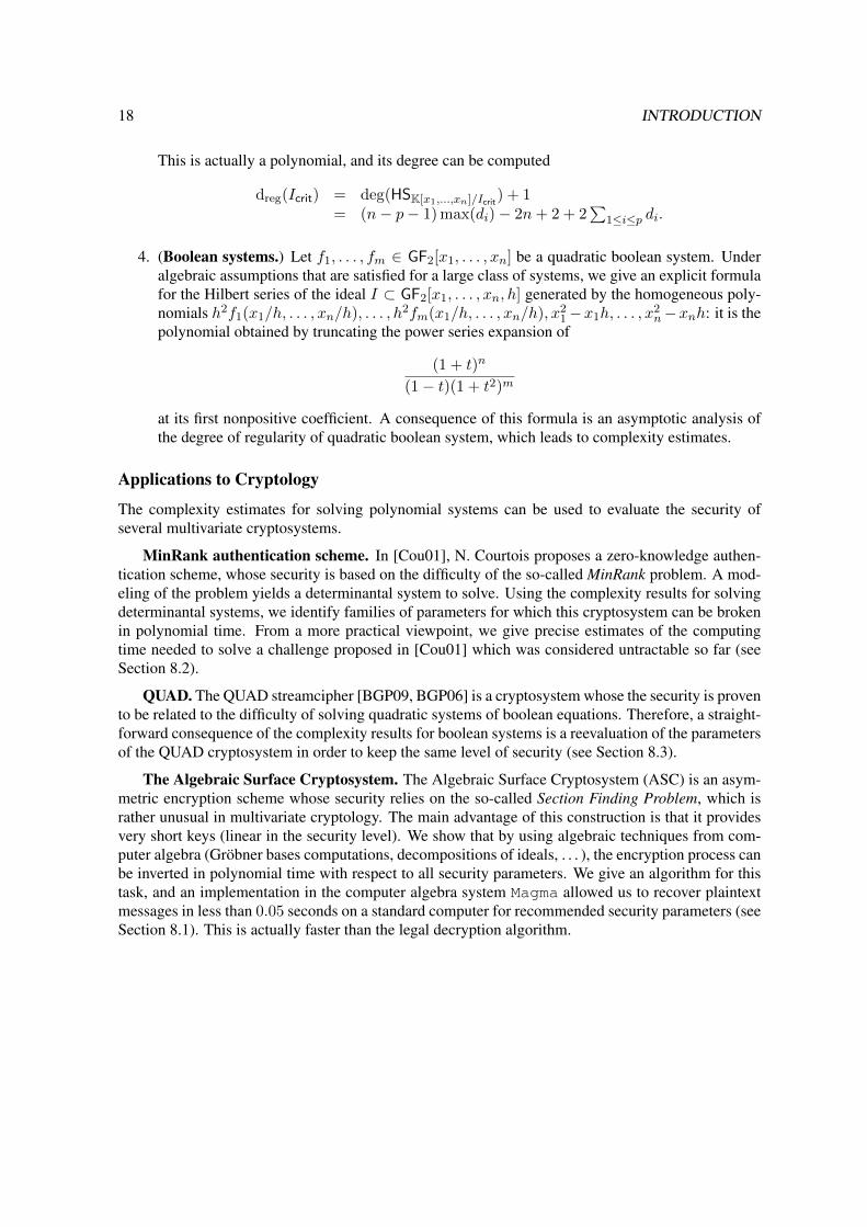
4. (Boolean systems.) Let f1, . . . , fm ∈ GF2[x1, . . . , xn] be a quadratic boolean system. Underalgebraic assumptions that are satisfied for a large class of systems, we give an explicit formulafor the Hilbert series of the ideal I ⊂ GF2[x1, . . . , xn, h] generated by the homogeneous poly-nomials h2f1(x1/h, . . . , xn/h), . . . , h2fm(x1/h, . . . , xn/h), x2

1−x1h, . . . , x2n−xnh: it is the

polynomial obtained by truncating the power series expansion of

(1 + t)n

(1− t)(1 + t2)m

at its first nonpositive coefficient. A consequence of this formula is an asymptotic analysis ofthe degree of regularity of quadratic boolean system, which leads to complexity estimates.

Applications to Cryptology

The complexity estimates for solving polynomial systems can be used to evaluate the security ofseveral multivariate cryptosystems.

MinRank authentication scheme. In [Cou01], N. Courtois proposes a zero-knowledge authen-tication scheme, whose security is based on the difficulty of the so-called MinRank problem. A mod-eling of the problem yields a determinantal system to solve. Using the complexity results for solvingdeterminantal systems, we identify families of parameters for which this cryptosystem can be brokenin polynomial time. From a more practical viewpoint, we give precise estimates of the computingtime needed to solve a challenge proposed in [Cou01] which was considered untractable so far (seeSection 8.2).

QUAD. The QUAD streamcipher [BGP09, BGP06] is a cryptosystem whose the security is provento be related to the difficulty of solving quadratic systems of boolean equations. Therefore, a straight-forward consequence of the complexity results for boolean systems is a reevaluation of the parametersof the QUAD cryptosystem in order to keep the same level of security (see Section 8.3).

The Algebraic Surface Cryptosystem. The Algebraic Surface Cryptosystem (ASC) is an asym-metric encryption scheme whose security relies on the so-called Section Finding Problem, which israther unusual in multivariate cryptology. The main advantage of this construction is that it providesvery short keys (linear in the security level). We show that by using algebraic techniques from com-puter algebra (Grobner bases computations, decompositions of ideals, . . . ), the encryption process canbe inverted in polynomial time with respect to all security parameters. We give an algorithm for thistask, and an implementation in the computer algebra system Magma allowed us to recover plaintextmessages in less than 0.05 seconds on a standard computer for recommended security parameters (seeSection 8.1). This is actually faster than the legal decryption algorithm.

INTRODUCTION 19

Structure Complexity Algorithms Structural results ApplicationsBilinear 6.5 6.2.2, 6.5 6.3, 6.4

Bihom. of bideg. (D, 1) 6.6 6.6Determinantal 4.6, 4.7 4.4, 4.5 8.2Critical points 5.5, 5.7.3 5.3, 5.7.2

Boolean 7.3 7.2 7.3.2 7.5

Table 3: Contributions and references of sections

Conclusion

In this thesis, we provide under genericity assumptions new complexity bounds for solving

1. affine bilinear systems;

2. affine bihomogeneous systems of bi-degree (D, 1);

3. determinantal systems in the unmixed case: all polynomials in the matrix share the same degree;

4. mixed and unmixed critical point systems;

5. boolean quadratic systems.

We also give new algorithms for

1. computing Grobner bases of bilinear systems without reductions to zero;

2. computing rational parametrizations of affine bi-homogeneous systems of bi-degree (D, 1);

3. computing Grobner bases of multi-homogeneous systems;

4. solving quadratic boolean systems.

We provide theoretical results:

1. an explicit form of the Hilbert bi-series of ideals generated by bilinear forms;

2. a description of the syzygy module of bilinear systems;

3. a formula for the Hilbert series of unmixed determinantal systems, mixed and unmixed criticalpoint systems, and for homogenized boolean systems;

4. we identify families of determinantal systems and of critical point systems, for which the com-plexity of computing a lexicographical Grobner basis is polynomial in the size of the output.

Finally, we give concrete applications in Cryptology:

1. precise estimates of the computing power needed to solve cryptographic challenges proposedin [Cou01] which are related to the MinRank;

2. an efficient and practical message-recovery attack on the Algebraic Surface Cryptosystem;

3. a reevaluation of the security parameters of the QUAD cryptosystem.

In Table 3, we report the sections of this thesis where the results are presented.

20 INTRODUCTION

Further impact of these results

The results in this thesis have had impacts in other publications:

• In [BFP11, BFP12a], the authors obtain complexity estimates for algebraic attacks on the cryp-tosystem HFE (and variants). During this complexity analysis, the bounds on the degree ofregularity of determinantal systems (Chapter 3) are used to get complexity estimates of Grobnerbases computations.

• In [FOPT10], the bound on the maximal degree reached during the computation of Grobnerbases of affine bilinear systems (Section 6.5.5) allows explaining the efficiency of the attackproposed on compact variants of the McEliece cryptosystem.

Perspectives.

Some points still need to be investigated. In this section, we report future possible developments ofthe results presented in this thesis and related open problems.

(Multi-homogeneous systems.) For bilinear systems, we give an explicit description of thesyzygy module and we obtain from this a criterion to remove reductions to 0 during the F5 algo-rithm. The next step is to generalize these results to multi-homogeneous systems. Similarly, obtainingan explicit formula for the generic multi-Hilbert series of multi-homogeneous system is still an openquestion. Before investigating general multi-homogeneous systems, a first step is to understand biho-mogeneous systems.

(Affine multi-homogeneous systems.) In the case of affine bilinear systems, we observe thatdegree falls play an important role during the computation of Grobner bases. The analysis is moredifficult in that case than it is for homogeneous systems. The next step here is to develop a sys-tematic approach to investigate affine systems which do not behave similarly to their homogeneouscounterparts. Indeed, having sharp bounds on the maximal degree reached during the computationof Grobner bases of affine multi-homogeneous systems is an open problem which is crucial to obtainpractical bounds on the complexity of such computations.

(Determinantal systems.) We give in this thesis an analysis of the complexity and of the combi-natorial structure of unmixed determinantal systems (i.e. all polynomials in the matrix share the samedegree). The next step would be to understand how this structure can be used to design Grobner basisalgorithms dedicated to this family of systems. Also, investigating how the results in this thesis couldbe generalized to the mixed case is a natural follow-up of this work.

(Critical point systems.) Following the results in Section 5.7, the Eagon-Northcott complexyields a free resolution of the determinantal part of the ideal vanishing on the critical points. Thiscould lead to an analysis of the syzygy module and yield a criterion to remove reductions to zero inthe F5 algorithm when the input is a critical point system. We plan to investigate this question infuture works.

(Implementation.) In this thesis, several algorithms are proposed (solving boolean systems, com-puting rational parametrization of bihomogeneous systems of bidegree (D, 1), computing Grobnerbases of multi-homogeneous systems). The next step is to implement these algorithms in a low-levellanguage (C, C++,. . . ) in order to solve larger structured polynomial systems.

(Rational coefficients.) In this thesis, we focus on the arithmetic complexity. This is a representa-tive measure of the execution time when the base field is a finite field (this is the case in Cryptology).For applications in Geometry and Optimization, the ground field is often the field of rational numbers.

INTRODUCTION 21

In that case, the arithmetic complexity is a first step but it would also be interesting to have estimatesof the size of the coefficients in rational parametrizations in order to have a better understanding ofthe bit complexity. Such bounds are related to the height of the corresponding variety [KPS01], whichcan be bounded by using Chow forms in the sense of Philippon [Phi86].

(Generalization of determinantal ideals.) The entries of the Jacobian matrices of general multi-homogeneous systems are multi-homogeneous polynomials. Therefore, we plan to investigate thestructure of determinantal systems when the entries of the matrix are themselves structured (for in-stance multi-homogeneous or boolean,. . . ). In particular, this could lead to a better understandingof bihomogeneous ideals. Indeed, the structure of ideals generated by bihomogeneous polynomialsis closely related to the combinatorial properties of the determinantal ideal generated by minors ofthe Jacobian matrices with respect to each block of variables. The entries of these matrices are alsobihomogeneous. Therefore the next step to generalize the results on bilinear systems is to investigatethe properties of these bihomogeneous determinantal ideals.

(Related problems in Symbolic Computation.) Determinantal ideals are basic objects of enu-merative geometry and Schubert calculus. Consequently, we plan to investigate in future works howthe results in this thesis can be extended to Schubert problems.

Organization of the thesis

In the first part of the thesis, we recall known facts about Grobner bases. Chapter 1 is devoted to basicnotions of Grobner basis theory and commutative algebra that are used throughout the thesis. Thenin Chapter 2, we give examples of applications in Engineering Sciences where structured algebraicsystems naturally appear. Finally in Chapter 3, we recall known facts about determinantal and bi-homogeneous systems.

The second part of the thesis is devoted to contributions. Most parts of Chapters and Sectionsare published or submitted articles. Therefore, these chapters are mostly self-contained and a fewstatements appear in different chapters. We list the references of these papers below (author namesare in alphabetical order):

• Chapter 3 and Section 6.6: On the Complexity of the Generalized MinRank Prob-lem. Jean-Charles Faugere, Mohab Safey El Din, Pierre-Jean Spaenlehauer. Submitted,arXiv:1112.4411 [cs.SC].

• Chapter 5: Critical Points and Grobner Bases: the Unmixed Case. Jean-Charles Faugere,Mohab Safey El Din, Pierre-Jean Spaenlehauer. Proceedings of the 37th International Sympo-sium on Symbolic and Algebraic Computation (ISSAC 2012).

• Chapter 6: Grobner Bases of Bihomogeneous Ideals generated by Polynomials of Bidegree(1,1): Algorithms and Complexity. Jean-Charles Faugere, Mohab Safey El Din, Pierre-JeanSpaenlehauer. Journal of Symbolic Computation, 46(4):406-437, 2011.

• Chapter 7: On the Complexity of Solving Quadratic Boolean Systems. Magali Bardet, Jean-Charles Faugere, Bruno Salvy, Pierre-Jean Spaenlehauer. Accepted for publication in Journalof Complexity, arXiv:1112.6263 [cs.SC].

• Section 8.1: Algebraic Cryptanalysis of the PKC’2009 Algebraic Surface Cryptosystem.Jean-Charles Faugere, Pierre-Jean Spaenlehauer. Proceedings of the 13th International Confer-ence on Practice and Theory in Public Key Cryptography (PKC 2010).

22 INTRODUCTION

• Section 8.2: Computing Loci of Rank Defects of Linear Matrices using Grobner Basesand Applications to Cryptology. Jean-Charles Faugere, Mohab Safey El Din, Pierre-JeanSpaenlehauer. Proceedings of the 35th International Symposium on Symbolic and AlgebraicComputation (ISSAC 2010).

Acknowledgements

I am grateful to L. Perret and I. Emiris for their comments on the papers on bilinear systems and onthe problem MinRank. I also wish to thank D. Bernstein, C. Diem, E. Kaltofen for valuable commentsand pointers to important references on the topic of boolean systems.

Part I

Preliminaries

23

Chapter 1

Preliminaries on Grobner Bases

In this chapter, we recall definitions, algorithms and properties of Grobner bases algorithms that areused throughout this thesis. We refer the reader to [CLO97] for a more detailed exposition of Grobnerbases theory.

1.1 Polynomial Rings and Ideals

1.1.1 Definitions

Notations 1.1. In the whole document, K is either a finite field or a field of characteristic 0 (andhence K is a perfect field). Its algebraic closure is denoted by K. The finite field of cardinality qis denoted by GFq. The notation X stands for the set of variables x1, . . . , xn. If R is a ring andF = r1, . . . , rm ⊂ R is a family of elements of R, we let 〈F〉 ⊂ R denote the ideal generated byF. If I and J are ideals of K[X], then the following subsets of K[X] are also ideals of K[X]:

sum I + J = f + g | f ∈ I, g ∈ J;product IJ = fg | f ∈ I, g ∈ J;intersection I ∩ J ;

radical√I = f ∈ K[X] | ∃k ∈ N s.t. fk ∈ I;

colon ideal I : J = f ∈ K[X] | fJ ⊂ I;saturation I : J∞ = f ∈ K[X] | ∃k ∈ N s.t. fJk ⊂ I.

In this thesis, we mainly focus on systems of polynomial equations that have a finite numberof solutions in Kn: the polynomials generate a 0-dimensional ideal of K[X]. Indeed, even whenwe study varieties of positive dimension, we will investigate subsets of points that are defined by0-dimensional systems (for instance by computing the critical points of a projection restricted to thevariety in Chapter 5).

Definition 1.2. We call dimension of an ideal I ⊂ K[X] the Krull dimension of the quotient ringK[X]/I , i.e. the supremum of the number of strict inclusions in a chain of prime ideals of K[X]/I .

This is a theoretical definition of the dimension. We give below in Proposition 1.43 a more algo-rithmic equivalent definition with the Hilbert series.

Example 1.3. • The dimension of the ideal 〈(x1− 1)(x1− 2), x2 + 3〉 ⊂ K[x1, x2] is 0 since theonly prime ideals of K[x1, x2]/〈(x1− 1)(x1− 2), x2 + 3〉 are 〈x1− 1〉 and 〈x1− 2〉, and thereare no inclusion relation between these two ideals (notice that in K[x1, x2]/〈(x1 − 1)(x1 −2), x2 + 3〉, the ideal 〈0〉 is not prime).

25

26 CHAPTER 1. GROBNER BASES

• The dimension of the ideal 〈x1 + 1〉 ⊂ K[x1, x2] is 1 since a longest chain of prime ideals ofK[x1, x2]/〈x1 + 1〉 is 〈0〉 ⊂ 〈x2〉 which has 1 inclusion.

The degree is an important indicator of the “complexity” of a 0-dimensional ideal. It counts thenumber of solutions (with multiplicities) of the system of polynomial equations.

Definition – Proposition 1.4. Let I ⊂ K[X] be a 0-dimensional ideal. Then K[X]/I is a K-vectorspace of finite dimension. The dimension dimK(K[X]/I) is called degree of I and is denoted byDEG(I).

Proof. The proof that K[X]/I is a K-vector space of finite dimension when I is 0-dimensional ispostponed at the end of Section 1.1.3.

The degree of an ideal can also be defined for ideals of positive dimension, but we will not needthis notion in this thesis. As the dimension, the degree can be read off from the Hilbert series (Propo-sition 1.43).

The geometrical objects corresponding to ideals of K[X] are affine varieties of Kn (also calledalgebraic sets). They are the sets of points where all polynomials in an ideal simultaneously vanish.Actually, if a family of polynomials simultaneously vanish on a subset V ⊂ Kn, then any algebraiccombination of these polynomials also vanish on V . Therefore, the entire ideal 〈F 〉 vanish on V .

Proposition 1.5. Let I ⊂ K[X] be an ideal generated by a family F = (f1, . . . , fm) ∈ K[X]m. LetZ(F) (resp. Z(I)) denote the set x ∈ K` | f1(x) = · · · = fm(x) = 0 (resp. x ∈ K` | ∀f ∈I, f(x) = 0). Then Z(F) = Z(I).

Proof. Clearly F ⊂ I , and hence Z(I) ⊂ Z(F). Conversely, let x ∈ K` be an element of Z(F).For any polynomial h ∈ I , there exist h1, . . . , hm ∈ K[X] such that h =

∑mi=1 hifi. Therefore

h(x) =∑m

i=1 hi(x)fi(x) = 0 and consequently Z(F) ⊂ Z(I).

Notations 1.6. If S is a subset of Kn, we let I(S) ⊂ K[X] denote the ideal of the polynomials

vanishing on all points of S. Notice that I(S) is radical by Hilbert’s Nullstellensatz [CLO97, Ch. 4,§1, Thm.2].

An important property of algebraic sets of Kn is that they define a topology on Kn:

Definition – Proposition 1.7 (Zariski topology). A subset V of Knis called algebraic set if there

exists an ideal I ⊂ K[X] such that V = Z(I). Algebraic sets have the following properties:

• any intersection of algebraic sets is an algebraic set;

• any finite union of algebraic sets is an algebraic set;

• K`is an algebraic set;

• ∅ is an algebraic set.

Therefore the algebraic sets are the closed sets of a topology, called the Zariski topology.

Proof. • Let V``∈L be a family of algebraic sets. Then there exist families of polynomialsF``∈L such that V` = Z(F`). Therefore ∩`∈LV` = Z(〈F`〉`∈L), hence ∩`∈LV` is an alge-braic set;

1.1. POLYNOMIAL RINGS AND IDEALS 27

• let V1 = Z(f1, . . . , fs) and V2 = Z(h1, . . . , ht) be two algebraic sets. Then V1 ∪ V2 =Z(∏1≤i≤s

1≤j≤tfihj) is also an algebraic set. By induction, any finite union of algebraic sets is

an algebraic set;

• K`= Z(〈0〉);

• ∅ = Z(K[X]).

The Zariski topology has several interesting properties. First, notice that any nonempty opensubset of Kn is dense. Also, finite intersections of nonempty open subsets are nonempty.

In particular, this topology will be useful for defining an algebraic notion of genericity for struc-tured systems: a property of a family of systems F ⊂ K[X] which is a K-vector space of finitedimension is said to be generic if this property is satisfied on a nonempty Zariski open subset of F(which is thus dense in F ).

1.1.2 Modules, algebras and free resolutions

In this section, we recall definitions of tools of commutative algebra which will be useful in Chapter5.7. Modules are among the main objects of study in commutative algebra. They are to commutativerings what vector spaces are to fields:

Definition 1.8 (Module). Let R be a commutative ring. A R-module is an abelian group (M,+) andan operation R×M →M such that

• (distributivity) ∀r, s ∈ R,∀m,n ∈M, r(m+ n) = rm+ rn and (r + s)m = rm+ sm;

• (associativity) ∀r, s ∈ R,∀m ∈M, (rs)m = r(sm);

• ∀m ∈M, 1Rm = m.

Definition 1.9 (Free module). The free module Rr of rank r is the module of r-tuples of elements inR with component-wise addition.

Two basic operations on modules are the direct sum and the tensor product. The tensor productM ⊗R N of two modules M and N can be seen as the smallest R-module such that we can expressall R-bilinear maps from M ×N to another module.

Definition 1.10 (Tensor product). Let M and N be two R-modules. The tensor product M ⊗R N(noted M ⊗N when the ring is obvious) is the R-module with generators m⊗ n | m ∈M,n ∈ Nand relations

∀r1, r2, s1, s2 ∈ R,∀m1,m2 ∈M,∀n1, n2 ∈ N,(r1m1 + r2m2)⊗ (s1n1 + s2n2) = r1s1m1 ⊗ n1 + r1s2m1 ⊗ n2 + r2s1m2 ⊗ n1 + r2s2m2 ⊗ n2.

The so-called tensor algebra is built by tensoring successively a module with itself.

Definition 1.11 (Tensor algebra). Let M be a R-module. The tensor algebra of M is defined as thedirect sum

T (M) = R⊕M ⊕ (M ⊗M)⊕ . . . .The product of two elements x1 ⊗ · · · ⊗ xm and y1 ⊗ · · · ⊗ yn is x1 ⊗ · · · ⊗ xm ⊗ y1 ⊗ · · · ⊗ yn.

28 CHAPTER 1. GROBNER BASES

Finally, we need two more definitions, the symmetric and the exterior algebras of M , which areobtained by imposing commutativity (resp. skew-commutativity).

Definition 1.12 (Symmetric algebra). The symmetric algebra of the R-module M is the quotient ofthe algebra T (M) by the ideal generated by the relations x⊗y−y⊗x for all x, y ∈M . It is denotedby Sym(M).

Definition 1.13 (Exterior algebra). The exterior algebra of the R-module M is the quotient of thealgebra T (M) by the ideal generated by the relations x⊗ x for all x ∈M . It is denoted by ∧M .

Notice that the exterior algebra is skew-commutative since in ∧M , x⊗ y+ y⊗ x = x⊗ x+ y⊗y + x⊗ y + y ⊗ x = (x+ y)⊗ (x+ y) = 0.

Resolutions are mathematical objects which yield information on the structure of polynomial ide-als (and more generally commutative rings and modules). The following result is known as the Hilbertsyzygy theorem. See [Eis95, Corollary 15.11] for a constructive proof.

Definition – Proposition 1.14 (Hilbert Syzygy Theorem). Let I ⊂ K[X] be a polynomial ideal. Thenthere exists a finite exact sequence of free K[X]-modules

F : 0→ Frϕn−−→ . . .

ϕ2−→ F1ϕ1−→ F0

such that K[X]/I ∼= F0/Im(ϕ1) and r ≤ n. Such a sequence is called a free resolution of I .

Free resolutions yield a good view of the structure of graded ideals. Many useful informationcan be read off from such objects: dimension, Hilbert series, Betti numbers, etc. . . We will use freeresolutions to obtain information about the structure of mixed critical point systems in Chapter 5.7.

1.1.3 Primary decomposition and associated primes

Another useful tool for describing ideals (and varieties) is the decomposition into irreducible com-ponents. Indeed, from a geometrical viewpoint, affine varieties can be uniquely decomposed intoirreducible varieties. An irreducible variety V ⊂ Kn is an algebraic set verifying the following prop-erty: if V1, V2 ⊂ Kn are algebraic sets such that V = V1 ∪ V2, then V1 = V or V2 = V .

Here, for simplicity, we will only consider decompositions over algebraically closed fields. Butthe definitions and properties can be extended for any field.

Theorem 1.15 (Irreducible decomposition of varieties). [CLO97, Ch. 4, §6, Thm.4] Let V ⊂ Kn

be an affine variety. Then there exists a unique finite set of algebraic sets V1, . . . , V` such thatV = V1 ∪ · · · ∪ V` and for all i, j ∈ 1, . . . , `, Vi 6⊂ Vj .

A proper ideal I is called primary if fg ∈ I implies that either f ∈ I or there exists n ∈ N suchthat gn ∈ I . If I is primary, then its radical

√I is prime.

Similarly to Theorem 1.15, ideals can be decomposed into irreducible components. However, thisdecomposition is not necessarily unique.

Theorem 1.16 (Irreducible decomposition of ideals). [Eis95, Thm. 3.10] Let I ⊂ K[X] be an ideal.Then there exists a minimal primary decomposition of I , i.e. a finite set of primary ideals I1, . . . , I`such that I = I1 ∩ · · · ∩ I` and for all i, j, Ii 6⊂ Ij . This decomposition is not necessarily unique, butall minimal primary decompositions of I share the same cardinality.

Although minimal primary decompositions are not uniquely defined, the radicals of the primaryideals are the same for any decomposition:

1.2. MONOMIAL ORDERINGS AND GROBNER BASES 29

Definition – Proposition 1.17 (Associated primes). [Eis95, Ch. 3] Let I ⊂ K[X] be an ideal. We letAss(I) denote the set of prime ideals P ⊃ I such that there exists f ∈ K[X] \ I with (I : f) = P .The family Ass(I) satisfies the following properties:

• Ass(I) is finite;

• If I1 ∩ · · · ∩ I` is a minimal primary decomposition of I , then Ass(I) = √I1, . . . ,√I`.

The primes in Ass(I) are called primes associated to I . Let P1 ∈ Ass(I) be an associated prime ofI . If there exists P2 ∈ Ass(I) such that P2 ⊂ P1, then we say that P1 is an embedded prime of I ,else P is called an isolated prime. Moreover, the radical of I is the intersection of the isolated primesassociated to I .

These notions will be useful in the study of multi-homogeneous ideals (see Chapter 6). Decompo-sitions of ideals will also be a crucial part of the attack on the cryptosystem ASC presented in Section8.1.

We can now prove that if I is a 0-dimensional ideal, then K[X]/I is a vector space of finitedimension over K.

Proof of Definition-Proposition 1.4. Let I be a zero dimensional ideal. Since I ⊂√I ,√I is also

0-dimensional as an ideal of K[X] and is included in all isolated primes (since√I is equal to the

intersection of isolated primes). By Krull’s Theorem and by the definition of dimension, all associatedprimes are maximal ideals of K[X]. Any maximal ideal of K[X] has the form 〈x1−α1, . . . , xn−αn〉,where αi ∈ K. Consequently, there exist α(1)

1 , . . . , α(`)n ∈ K such that

√I =

⋂1≤i≤`

〈x1 − α(i)1 , . . . , xn − α(i)

n 〉.

Next, notice that the elements α(1)1 , . . . , α

(`)1 are algebraic over K, therefore there exists a univariate

polynomial P1 ∈ K[x] which vanishes on α(1)1 , . . . , α

(`)1 . By the Hilbert’s Nullstellensatz, P1(x1) ∈√

I , hence there exists a power Q1 of P1 such that Q1(x1) ∈ I . Similarly, there exist univariatepolynomials Q2(x2), . . . , Qn(xn) ∈ I . Therefore K[X]/I ⊂ K[X]/〈Q1(x1), . . . , Qn(xn)〉 which isa K-vector space of finite dimension.

1.2 Monomial orderings and Grobner bases

In this section, we recall the basic definitions and some properties of monomial orderings and Grobnerbases. We also show how Grobner bases preserve the graded structure in the context of homogeneous,quasi-homogeneous and multi-homogeneous ideals.

1.2.1 Definitions

A Grobner basis of an ideal I is a set of generators of this ideal which has good properties. It gen-eralizes Row Echelon bases for linear systems. For univariate systems, it corresponds to the greatestcommon divisor of the polynomials.

Grobner bases are defined with respect to a total well-ordering on the monomials of K[X]:

Definition 1.18. [CLO97, Ch.2, §2, Def.1] A monomial ordering ≺ on K[X] is a relation on Nn (oron the monomials of K[X] by identification) satisfying:

• ≺ is a total ordering on Nn;

30 CHAPTER 1. GROBNER BASES

• if α ≺ β and γ ∈ Nn, then α+ γ ≺ β + γ;

• ≺ is a well-ordering: every nonempty subset of Nn has a smallest element.

In this thesis, we focus mainly on the so-called grevlex (graded reverse lexicographical) and lex(lexicographical) orderings. The grevlex ordering is particularly well-suited for Grobner bases com-putations, while the lex ordering yields a more explicit description of the solutions of a polynomialsystem.

The grevlex ordering is a graded ordering, i.e. monomials are first sorted by degree. This orderingalso has other structural properties. For instance, in a homogeneous polynomial the first monomial isa monomial involving only the variable x1, then come the monomials involving the variable x1 andx2, then the ones where the variables x1, x2 and x3 appear, etc. . . .

Definition 1.19 (Graded Reverse Lexicographical Ordering). [CLO97, Ch. 2, §2, Def. 6] Let α, β ∈Nn; α ≺grevlex β if either: ∑n

i=1 αi <∑n

i=1 βior∑n

i=1 αi =∑n

i=1 βi and the rightmost entry of α− β is positive.

Example 1.20. • x21 ≺grevlex x

33;

• x21x3 ≺grevlex x

32.

For solving systems, the lex ordering is well-suited since it is a typical example of eliminationordering: if G is a lex Grobner basis of an ideal I ⊂ K[X], then G ∩ K[xk, . . . , xn] is a lex Grobnerbasis of I ∩K[xk, . . . , xn] for any i ∈ 1, . . . , n.

Definition 1.21 (Lexicographical Orderings). [CLO97, Ch. 2, §2, Def. 3] Let α, β ∈ Nn; α ≺lex β ifthe leftmost entry of α− β is negative.

Example 1.22. • x95 ≺lex x1;

• x21x

23 ≺lex x

21x2.

Definition 1.23 (Leading Monomial). [CLO97, Ch. 2, §2, Def. 7] Let ≺ be a monomial ordering,and f =

∑α∈Nn aαx

α ∈ K[X] (resp. I ∈ K[X]) be a polynomial (resp. an ideal). Then its leadingmonomial (resp. its leading monomial ideal) with respect to ≺ is LM≺(f) = xmax≺α∈Nn:aα 6=0

(resp. LM≺(I) = 〈LM≺(f) : f ∈ I〉).

We can now give the definition of a Grobner basis:

Definition 1.24 (Grobner Basis). [CLO97, Ch. 2, §5, Def. 5] Let ≺ be a monomial ordering, andI ⊂ K[X] be an ideal. A Grobner basis of I with respect to≺ is a finite subset G = g1, . . . , g` ⊂ Isuch that

LM≺(I) = 〈LM≺(g1), . . . , LM≺(g`)〉 .

The following proposition shows a direct consequence of Definition 1.24: a Grobner basis of anideal generates it.

Proposition 1.25. [CLO97, Ch. 2, §5, Cor. 6] Let G = g1, . . . , g` be a Grobner basis of an idealI ⊂ K[X] with respect to a monomial ordering ≺. Then 〈G〉 = I .

1.2. MONOMIAL ORDERINGS AND GROBNER BASES 31

Proof. Let f1 6= 0 be a polynomial in I . Therefore, LM≺(f1) ∈ LM≺(I) and hence there exists t ∈1, . . . , ` such that LM≺(gt) divides LM≺(f1). Let f2 be the polynomial f2 = f1 − LM≺(f1)

LM≺(gi)gi ∈ I .

Notice that LM≺(f2) ≺ LM≺(f1). By repeating this process, one can construct a sequence f1, f2, . . .such that for every i, fi ∈ I and LM≺(fi+1) ≺ LM≺(fi). By Definition 1.18, ≺ is a well-ordering,and hence every strictly decreasing sequence of monomials terminates. Consequently, there existsj ∈ N such that fj = 0. Finally, an induction on i from j to 1 shows that f1 ∈ 〈g1, . . . , g`〉.

Notice that in Definition 1.24, Grobner bases are not uniquely defined: if G is a Grobner basis ofI and G′ is a finite family such that G ⊂ G′ ⊂ I , then G′ is also a Grobner basis of I .

Grobner bases which are minimal for the inclusion are called minimal Grobner bases. However,minimality is not sufficient for unicity: for instance, G = x2

1, x22 and G′ = x2

1 + x22, x

22 are two

minimal Grobner bases of the same ideal for any monomial ordering.Unicity can be obtained by considering reduced Grobner basis.

Definition 1.26. Let I ⊂ K[X] be an ideal and ≺ monomial ordering. A Grobner basis G of I withrespect to ≺ is called

• minimal if for all gi, gj ∈ G such that gi 6= gj , LM(gi) does not divide LM(gj);

• reduced if the leading coefficient of all basis elements is 1 and for all g =∑aαx

α ∈ G and allα ∈ Nn such that aα 6= 0, xα /∈ LM (〈G \ g〉).

Notice that a reduced Grobner basis is minimal and is uniquely defined.

Once a Grobner basis of an ideal I is computed, it can be used to compute a normal form withrespect to I , which is a projection of K[X] whose kernel is I . This gives an algorithm to solve theIdeal Membership Problem since a polynomial f belongs to an ideal I if and only if the normal formof f with respect to I is 0.

Definition 1.27 (Normal form). Let ≺ be a monomial ordering, I ⊂ K[X] be an ideal and f ∈ K[X]

be a polynomial. Then there exist unique polynomials f and g such that:

• f = f + g;

• g ∈ I;

• no monomials appearing in f are in LM≺(I).

The polynomial f is called the normal form of f with respect to I and≺ and is denoted by NF≺,I(f).

Proof. Unicity. Let f1, f2, g1, g2 be such that

• f = f1 + g1 = f2 + g2;

• g1, g2 ∈ I;

• no monomials appearing in f1, f2 are in LM≺(I).

Then f1 − f2 = g2 − g1 ∈ I , hence LM≺(f1 − f2) ∈ LM≺(I). Since no monomials appearing inf1, f2 are in LM≺(I), f1 − f2 = 0. Consequently, f1 = f2 and g1 = g2.

Existence. The existence of the normal form is ensured by the correctness and termination ofAlgorithm 3 below.

Proposition 1.28. Let I ⊂ K[X] be an ideal, and f ∈ K[X] be a polynomial. The following state-ments are equivalent:

32 CHAPTER 1. GROBNER BASES

• f ∈ I;

• For any monomial ordering ≺, NF≺,I(f) = 0.

Proof. From the unicity of g in Definition 1.27, if f ∈ I , then g = f and hence NF≺,I(f) = 0 forany monomial ordering ≺. Conversely, if NF≺,I(f) = 0, then f = f −NF≺,I(f) ∈ I .

1.2.2 Homogeneous, quasi-homogeneous and multi-homogeneous gradings on K[X]

Grobner bases have a useful property: they preserve the gradation (or multi-gradation) of ideals.Indeed, the only arithmetic operations used in Buchberger’s Algorithm [Buc65] and in F4/F5 Algo-rithms [Fau99, Fau02] are multiplication of polynomials by monomials and sum of polynomials withsame leading monomials. Therefore, if the input system is homogeneous (resp. quasi-homogeneous,multi-homogeneous), then a Grobner basis computed with any of these algorithms will be homoge-neous (resp. quasi-homogeneous, multi-homogeneous). Moreover, the gradation allows us to decom-pose the analysis of the structure of polynomial ideals and to understand the combinatorial propertiesof structured systems.

In this section, we give definitions and properties of N`-graded ideals. The most common case isthe classical homogeneous grading: all monomials in a homogeneous polynomial share the same totaldegree. This notion can be extended in two ways. In the quasi-homogeneous case, a weight is attachedto each variable: all monomials in a quasi-homogeneous polynomial share the same weighted degree.In a multi-homogeneous polynomial, each variable belongs to a block of variables and all monomialsshare the same degrees with respect to each block of variables.

Definition 1.29. An N`-graded ring R is a ring and a decomposition into a family of additive groupsRdd∈N` such that

R =⊕

d∈N`Rd, and

∀d1,d2 ∈ N`, Rd1Rd2 ⊂ Rd1+d2 .

The first example of graded polynomial ring is given by the classical homogeneous grading:

Definition 1.30. The homogeneous grading on K[X] is given by the decomposition

K[X] =⊕d∈N

K[X]d,

where K[X]d is the K-vector space generated by all monomials of degree d. An element of K[X]d iscalled homogeneous of degree d.

Example 1.31. The polynomial 3x21 + 5x1x2 + 8x2

2 ∈ Q[x1, x2]2 is homogeneous of degree 2.

The homogeneous grading can be tweaked by adding a weight on variables, giving rise to thequasi-homogeneous grading:

Definition 1.32. Let w = (w1, . . . , wn) ∈ Nn. The weight degree of a monomial w.r.t. w is definedby

wdegw(xi11 . . . xinn ) =

n∑j=1

wjij .

The quasi-homogeneous grading on K[X] (w.r.t. w) is given by the decomposition

K[X] =⊕d∈N

K[X](w)d ,

1.2. MONOMIAL ORDERINGS AND GROBNER BASES 33

where K[X](w)d is the K-vector space generated by all monomials of weight degree d. An element of

K[X](w)d is called quasi-homogeneous of weight degree d.

Example 1.33. The polynomial 2x21x3+4x2

1x22+8x2

2x3+9x23 ∈ Q[x1, x2, x3]4 is quasi-homogeneous

of weight degree 4, with respect to the weight vector w = (1, 1, 2).

The multi-homogeneous grading provides a more refined decomposition of the polynomial ring:

Definition 1.34. LetX1, . . . , X` be a partition of the set of variables. Since K[X] =⊗`

j=1 K[Xj ], themulti-homogeneous grading on K[X] (w.r.t. the partitionX = ∪`i=1Xi) is given by the decomposition

K[X] =⊕

(d1,...,d`)∈N`K[X](d1,...,d`),

where K[X](d1,...,d`) is the K-vector space K[X1]d1 ⊗ · · · ⊗ K[X`]d` and where the tensor productis done over K. An element of f ∈ K[X]d is called multi-homogeneous of multi-degree d ∈ N`(mdeg(f) = d).

Example 1.35. The polynomial 2x21y1 + 7x2

1y2 + x1x2y1 + 4x1x2y2 + 8x22y1 + 8x2

2y2 ∈Q[x1, x2, y1, y2](2,1) is multi-homogeneous of multi-degree (2, 1) with respect to the partitionx1, x2 ∪ y1, y2.

Notice that the extreme case is the multi-homogeneous grading given by the partition x1∪ · · ·∪xn. In that case, we see K[X] as the direct sum of vector spaces of dimension 1 (each vector spacebeing generated by a monomial).

By extension, we also use the degree, weighted degree and multi-degree for non-homogeneouspolynomials. The degree deg(f) of a polynomial f ∈ K[X] is the usual total degree, and theweighted degree wdegw(f) is the maximum of the weighted degrees of its monomials. The multi-degree mdeg(f) of f with respect to a partition of the variables X = ∪`i=1Xi is the `-tuple(degX1

(f), . . . ,degX`(f)) ∈ N` where degXi(f) is the degree of f with respect to the variablesin the block Xi.

These gradings of K[X] are important when we consider ideals compatible with this structure:

Notations 1.36. Let I ⊂ K[X] be an ideal. The notations Id, I(w)d and Id stand for

Id = I ∩K[X]d;

I(w)d = I ∩K[X]

(w)d ;

Id = I ∩K[X]d.

Definition 1.37. An ideal I ⊂ K[X] is called

• homogeneous if I = ⊕∞d=0Id;

• quasi-homogeneous w.r.t. w ∈ Nn if I = ⊕∞d=0I(w)d ;

• multi-homogeneous w.r.t. a partition X = ∪`i=1Xi if I = ⊕d∈N`Id.

Proposition 1.38. An ideal I ⊂ K[X] is homogeneous (resp. quasi-homogeneous, multi-homogeneous) if and only if there exists a set of homogeneous (resp. quasi-homogeneous, multi-homogeneous) generators.

34 CHAPTER 1. GROBNER BASES

Proof. The proof is done here in the homogeneous context (it is similar for quasi-homogeneous andmulti-homogeneous systems). Let f1, . . . , fm be a set of homogeneous generators of I and g =∑λtt ∈ I . Let g(d) be its homogeneous component of degree d (i.e. g(d) =

∑deg(t)=d

λtt). Therefore

g =∑d∈N

g(d). Since g ∈ I , there exists h1, . . . hp ∈ K[X] such that

g =m∑i=1

hifi.

Since products of homogeneous polynomials are also homogeneous, g(d) =∑m

i=1 h(d−deg(fi))i fi be-

longs to Id (where h(d−deg(fi))i denotes the homogeneous component of hi of degree d−deg(fi)) and

hence I is equal to⊕

d∈N Id.

Conversely, let I =⊕

d∈N Id be a homogeneous ideal and let F = (f1, . . . , fm) ∈ K[X] be agenerating family. Then the homogeneous parts of f1, . . . , fm are in I and thus yield a homogeneousfamily of generators of I .

Notice that if 〈F〉 is a homogeneous ideal, then its variety can be seen as a subvariety of theprojective space Pn−1K since if x ∈ Z(F), then for any λ ∈ K, λx ∈ Z(F). In that case, we use thenotation Z(F,Pn−1) ⊂ Pn−1K to denote this projective variety.

Similarly, if 〈F〉 is a multi-homogeneous ideal, we let Z(F,P|X(1)|−1 × · · · × P|X(`)|−1) ⊂P|X(1)|−1K× · · · × P|X(`)|−1K denote the associated multi-projective variety.

An another interesting object to study the combinatorial properties of graded ideals are the so-called Hilbert function and Hilbert series of their quotient rings:

Definition 1.39. [Eis95, Ex. 10.11] Let I ⊂ K[X] be a homogeneous (resp. quasi-homogeneous,multi-homogeneous) ideal. Then the Hilbert function HFK[X]/I : N → N (resp. the weighted Hilbertfunction wHFK[X]/I : N → N, the multi-Hilbert function mHFK[X]/I : N` → N) and the Hilbertseries HSK[X]/I ∈ N[[t]] (resp. the weighted Hilbert series wHSK[X]/I ∈ N[[t]], the multi-Hilbertseries mHSK[X]/I ∈ N[[t1, . . . , t`]]) of the quotient ring K[X]/I are defined by:

HFK[X]/I(d) = dimK(K[X]d/Id); HSK[X]/I(t) =

∞∑d=0

HFK[X]/I(d)td;

wHFK[X]/I(d) = dimK(K[X](w)d /Id); wHSK[X]/I(t) =

∞∑d=0

wHFK[X]/I(d)td;

mHFK[X]/I(d) = dimK(K[X]d/Id); mHSK[X]/I(t1, . . . , t`) =∑d∈N`

mHFK[X]/I(d)∏j=1

tdjj

.

Proposition 1.40. The Hilbert series, weighted Hilbert series and multi-Hilbert series of K[X] arerespectively

• HSK[X](t) =1

(1− t)n ;

• wHS(w)K[X](t) =

1∏ni=1(1− twi) ;

1.2. MONOMIAL ORDERINGS AND GROBNER BASES 35

• mHSK[X](t1, . . . , t`) =1∏n

i=1(1− ti)|X(i)|.

Proof. First, we prove the formula for the weighted Hilbert series of K[X] (the homogeneous caseis obtained by choosing the weight vector w = (1, . . . , 1)). This is achieved by a combinatorialargument: wHSK[X](t) is the generating series of Nn where the size of an element d ∈ Nn is the dotproduct d ·w:

wHSK[X](t) =∑d∈Nn

td·w.

Therefore Nn is the combinatorial product of n copies of N where the size of an element d of the jthcopy of N is dwj . The generating series of the product of combinatorial classes is the product of theirgenerating series:

wHSK[X](t) =n∏j=1

(∑d∈N

tdwj

)=

1n∏j=1

(1− twj ).

Similarly for the multi-homogeneous case,

mHSK[X](t1, . . . , t`) =∑d∈N

m∈Monomials(K[X],d)

tmdeg(m)

=∏i=1

HSK[X(i)](ti)

=∏i=1

1

(1− ti)|X(i)|.

In the following proposition, we show that algebraic properties yield relations between Hilbertseries. These relations will be often used in this thesis to obtain explicit formulas for the Hilbert seriesof structured ideals.

Proposition 1.41. Let I ⊂ K[X] be a homogeneous ideal (resp. quasi-homogeneous, multi-homogeneous) and f ∈ K[X]d be a homogeneous polynomial of degree d ∈ N (resp. f ∈ K[X]

(w)d

be a quasi-homogeneous polynomial of weight degree d ∈ N, f ∈ K[X]d be a multi-homogeneouspolynomial of multi-degree d ∈ N`). If f does not divide 0 in the ring K[X]/I , then

HSK[X]/(I+〈f〉)(t) = (1− td)HSK[X]/I(t);

wHS(w)K[X]/(I+〈f〉)(t) = (1− td)wHS(w)

K[X]/I(t);

mHSK[X]/(I+〈f〉)(t1, . . . , t`) = (1−∏`j=1 t

djj )mHSK[X]/I(t1, . . . , t`).

Proof. The proof is done here in the homogeneous context; the proofs for the quasi-homogeneousand multi-homogeneous gradings are similar. For every ` ∈ N, consider the following sequence ofK-vector spaces:

0 −→ K[X]`/I`×f−−→ K[X]`+d/I`+d

π−→ K[X]`+d/(I + 〈f〉)`+d −→ 0,

36 CHAPTER 1. GROBNER BASES

where π is the canonical projection. Since f does not divide 0 in K[X]/I , this sequence is exact.Therefore the alternate sum of the dimensions of these vector spaces is equal to 0. Consequently,HFK[X]/I(`) − HFK[X]/I(` + d) + HFK[X]/(I+〈f〉)(` + d) = 0, thus by multiplying this relation bytd+` and by summing over ` ∈ Z,

tdHSK[X]/I(t)− HSK[X]/I(t) + HSK[X]/(I+〈f〉)(t) = 0.

A non-trivial property of Hilbert series of quotients K[X]/I is that they are always power seriesexpansions of rational functions. This can be seen as a consequence of the Hilbert Syzygy Theorem(see Definition-Proposition 1.14). The numerator of this rational function is called the K-polynomialin [MS05].

Proposition 1.42. [MS05, Theorem 8.20] Let I ⊂ K[X] be a homogeneous (resp. quasi-homogeneous, multi-homogeneous) ideal. Then there exists a polynomial N(t) ∈ Z[t] (resp.N(t) ∈ Z[t], N(t1, . . . , t`) ∈ Z[t1, . . . , t`]) such that:

HSK[X]/I(t) =N(t)

(1− t)n ;

wHSwK[X]/I(t) =N(t)∏n

i=1(1− twi) ;

mHSK[X]/I(t1, . . . , t`) =N(t1, . . . , t`)∏ni=1(1− ti)|X(i)|

.

Proof. The proof is done in the homogeneous context, but the proofs for quasi-homogeneous andmulti-homogeneous ideals are exactly similar. By Hilbert Syzygy Theorem [Eis95, Thm. 1.13], I hasa graded finite free resolution of length r ≤ n. Therefore, for any d ∈ N, there is an exact sequenceof K-vector spaces

0→ir⊕j=1

K[X]d−dr,jϕn−−→ . . .

ϕ1−→i0⊕j=1

K[X]d−d0,j → K[X]d/Id → 0,

where di,j ≤ d for all i, j. Since the alternate sum of the dimensions in an exact sequence of vectorspaces is 0, we obtain that

dim(K[X]d/Id) =r∑

k=0

(−1)kik∑j=1

dim(K[X]d−dk,j ).

Then, by letting [td]S(t) denote the coefficient of td in a power series S ∈ Z[[t]], notice that

dim(K[X]d−dk,j ) =

(n+ d− dk,j − 1

d− dk,j

)= [td−dk,j ]

1

(1− t)n

= [td]tdk,j

(1− t)n .

1.2. MONOMIAL ORDERINGS AND GROBNER BASES 37

Therefore, by summing over d, we get

HSK[X]/I(t) =∑d≥0

dim(K[X]d/Id)td

=r∑

k=0

(−1)kik∑j=1

tdk,j

(1− t)n .

In the homogeneous case, the degree and the dimension can be read off from the Hilbert series.

Proposition 1.43. Let I ⊂ K[X] be a proper homogeneous ideal and HSK[X]/I(t) = N(t)(1−t)d be the

irreducible form of its Hilbert series (i.e. N(1) 6= 0). Then dim(I) = d. Moreover, if d = 0, thenHSK[X]/I(t) is a polynomial and DEG(I) = HSK[X]/I(1).

Proof. In [CLO97, Ch. 9, §3, Thm.11], it is proved that the degree of the Hilbert polynomialHPK[X]/I is equal to the projective dimension of I , which is dim(I) + 1. Since a power se-

ries N(t)(1−t)d is the generating series of the polynomial of degree d − 1 if deg(N(t)) < d (see the

proof of Definition - Proposition 1.65 for more details), we obtain dim(I) = d. If d = 0, thenHSK[X]/I(1) =

∑d∈N dimK(K[X]d/Id) = dimK(K[X]/I) = DEG(I).

1.2.3 Regular and Semi-regular Sequence

Regular and semi-regular sequences are important families of polynomial systems. Indeed, being reg-ular is a generic property. Semi-regular sequences are also conjectured to be generic (see Conjecture1.53 below).

Regular sequences

Definition 1.44. A sequence of non-zero homogeneous polynomials F = (f1, . . . , fm) ∈ K[X]m iscalled regular if for all i ∈ 1, . . . ,m− 1, fi+1 does not divide 0 in the ring K[X]/〈f1, . . . , fi〉.Proposition 1.45. Let F = (f1, . . . , fm) ∈ K[X]m be a sequence of homogeneous polynomials. Thefollowing statements are equivalent:

1. F is a regular sequence;

2. for all i ∈ 1, . . . ,m, Fi = (f1, . . . , fi) is a regular sequence;

3. for all i ∈ 1, . . . ,m− 1, 〈Fi〉 : fi+1 = 〈Fi〉;4. for all i ∈ 1, . . . ,m− 1 and all P ∈ Ass(〈f1, . . . , fi〉), fi+1 6∈ P ;

5. for all i ∈ 1, . . . ,m, dim(〈Fi〉) = n− i.Proof. By definition of regular sequences, the statements (1), (2) and (3) are clearly equivalent. Let〈f1, . . . , fi〉 = I1∩· · ·∩I` be a minimal primary decomposition of 〈f1, . . . , fi〉. Suppose first that fi+1

does divide 0 in K[X]/〈f1, . . . , fi〉. Thus there exists g /∈ 〈f1, . . . , fi〉 such that fi+1g ∈ 〈f1, . . . , fi〉.Since g /∈ 〈f1, . . . , fi〉, there exists j such that g /∈ Ij . Since Ij is primary, there exists k ∈ Nsuch that fki+1 ∈ Ij , and consequently, fi+1 ∈

√Ij ∈ Ass(〈f1, . . . , fi〉). Conversely, suppose that

fi+1 ∈ P , with P ∈ Ass(〈f1, . . . , fi〉). Then by definition of Ass, there exists g /∈ 〈f1, . . . , fi〉 suchthat gP ⊂ I . Therefore fi+1g ∈ I and hence fi+1 divides 0 in K[X]/〈f1, . . . , fi〉.

The fact that (1) is equivalent to (5) will be proved in Theorem 1.48.

38 CHAPTER 1. GROBNER BASES

Regular sequences have an interesting property: all algebraic relations in a regular sequence canbe deduced from the commutativity of K[X], i.e. from the relations fifj − fjfi. Intuitively, thismeans that the ideal generated by a sequence F = (f1, . . . , fm) (with m ≤ n) is “largest” when Fis a regular sequence. This notion of algebraic relations is formalized in the following definition andproposition.

Definition 1.46 (Syzygy). Let F = (f1, . . . , fm) ∈ K[X]m be a sequence of polynomials. Thesyzygy module of F is the submodule Syz(F) ⊂ K[X]m of all vectors (s1, . . . , sm) ∈ K[X]m suchthat

∑mi=1 sifi = 0. The degree of a syzygy s ∈ Syz(F) is defined as deg(s) = max1≤i≤mdeg(si)+

deg(fi).

Proposition 1.47. Let F = (f1, . . . , fm) ∈ K[X]m be a polynomial family. The two followingstatements are equivalent:

• F is a regular sequence;

• the syzygy module of F is generated by the syzygies coming from the commutativity of K[X]:

Syz(F) = 〈fiej − fjei〉,

where ei = (0, . . . , 0, 1, 0, . . . , 0) ∈ K[X]m is the vector whose only nonzero entry is at thei-th position.

Proof. We prove this proposition by induction on m. Let s ∈ Syz(F) be a syzygy. If m = 1, thenF = (f1) with f1 6= 0 (since F is a regular sequence) and hence Syz(F) = 0 ∈ K[X]. Now assumethat m > 1. Then

m∑i=1

sifi = 0.

Therefore sm belongs to the colon ideal 〈f1, . . . , fm−1〉 : fm. By Definition 1.44, 〈f1, . . . , fm−1〉 =〈f1, . . . , fm−1〉 : fm and hence sm can be written as

sm =

m−1∑i=1

fihi.

Now, consider the syzygy s′ = s − hi(fiem − fmei). Then s′m = 0 and∑m−1

i=1 s′ifi = 0. Thereforeby the inductive hypothesis, s′ is in the module generated by the syzygies 〈fiej − fjei〉1≤i,j≤m−1 ⊂〈fiej − fjei〉1≤i,j≤m. Therefore s = s′ + hi(fiem − fmei) ∈ 〈fiej − fjei〉.

Conversely, form = 1, it is clear that Syz(F) = 0 if and only if f1 6= 0. By induction, assume nowthat (f1, . . . , fm−1) is a regular sequence. Let sm ∈ 〈f1, . . . , fm−1〉 : fm be a polynomial. Then thereexists s1, . . . , sm−1 ∈ K[X] such that s = (s1, . . . , sm) is a syzygy. Since Syz(F) = 〈fiej − fjei〉, itfollows that sm ∈ 〈f1, . . . , fm−1〉 and hence 〈f1, . . . , fm−1〉 : fm = 〈f1, . . . , fm−1〉. Consequently,F is a regular sequence.

The Hilbert series of regular systems is a direct consequence of Proposition 1.41:

Theorem 1.48. [Bar04, BFS04, BFSY04] Let F = (f1, . . . , fm) ∈ K[X]m be a homogeneous systemwith m ≤ n. The three following statements are equivalent:

• F is regular;

1.2. MONOMIAL ORDERINGS AND GROBNER BASES 39

• the Hilbert series of K[X]/〈F〉 is

HSK[X]/〈F〉(t) =

m∏i=1

(1− tdeg(fi))

(1− t)n ;

• dim(〈F〉) = n−m.

This notion of regularity is essential since the regular (and semi-regular) sequences correspondexactly to the systems such that there is no reduction to zero during the computation of a Grobner basiswith the F5 Algorithm (see [Fau02]). Moreover, generic systems with less equations than variablesare regular, as shown by the following theorem:

Theorem 1.49 (Genericity of homogeneous regular sequences). Let m ≤ n and (d1, . . . , dm) ∈ Nmbe a sequence of degrees. Then there exists a Zariski open subset O ⊂ K[X]d1 × · · · ×K[X]dm suchthat any F ∈ O is a regular sequence.

Proof. See [Par10, Section 2].

Homogeneous semi-regular sequences

Semi-regular sequences extend the notion of regularity when there are more equations than variables.The Hilbert series of semi-regular sequences is known and is given below.

Notations 1.50. Let S ∈ Z[[t]] be a power series. We let [S]+ ∈ N[[t]] denote the series obtained bytruncating S at its first non-positive coefficient. Notice that if there is a non-positive coefficient in S,then [S]+ is a polynomial.

Theorem 1.51. [Bar04, BFS04, BFSY04, Die] Let F = (f1, . . . , fm) ∈ K[X]m be a homogeneoussystem with m ≥ n. The three following statements are equivalent:

• the Hilbert series of K[X]/〈F〉 is

HSK[X]/〈F〉(t) =

m∏i=1

(1− tdeg(fi))

(1− t)n

+

;

• the ideal 〈F〉 has dimension 0 and every syzygy of F of degree at most deg(HSK[X]/〈F〉) is inthe module generated by the trivial syzygies 〈fiej − fjei〉.

If the sequence F verifies these properties, it is called semi-regular.

Another genericity property is given below, it yields a sufficient condition for a sequence to besemi-regular:

Proposition 1.52. Let F = (f1, . . . , fm) ∈ K[X]m be a sequence of homogeneous non-zero polyno-mials. If for all i ∈ 1, . . . ,m− 1, and for all d ∈ N, the linear map

K[X]d/〈f1, . . . , fi〉d×fi−−→ K[X]d+deg(fi)/〈f1, . . . , fi〉d+deg(fi)

is of maximal rank (i.e. it is either injective or surjective), then the sequence F is semi-regular.

40 CHAPTER 1. GROBNER BASES

The analysis of semi-regular systems is crucial for understanding the behavior of Grobner basisalgorithms, since it has been observed that in practice, random systems are semi-regular. However,this is not proved and is expressed by the famous Froberg’s conjecture (which is reformulated here,see [Fro85] for the original statement):

Conjecture 1.53 (Froberg’s Conjecture). [Fro85] Let (d1, . . . , dm) ∈ Nm be a sequence of integersand S be the K-vector space of homogeneous systems F = (f1, . . . , fm) ∈ K[X]m such that for alli ∈ 1, . . . ,m, deg(fi) = di. Then there exists a non-empty Zariski open subset O ⊂ S such thatevery system F ∈ O is semi-regular.

Although this conjecture remains an important open problem in commutative algebra, it has beenproved in several cases:

• when n ≥ m (see Theorem 1.49);

• n = 2;

• n = 3 in characteristic 0;

• m = n+ 1;

• when the system is quadratic and n ≤ 11;

• when the system is cubic and n ≤ 8.

We refer to [Bar04] for more details on semi-regular systems.

Affine semi-regular systems

In [Bar04, BFS04, BFSY04], the definition of semi-regular systems is extended to affine systems(since in applications, systems arising are usually affine) by considering the homogeneous part ofhighest degree.

Definition 1.54 (Affine Semi-Regular Sequence). Let F = (f1, . . . , fm) ∈ K[X]m be a poly-nomial system. F is called semi-regular if the system of homogeneous parts of highest degreesF(h) = (f

(h)1 , . . . , f

(h)m ) is semi-regular.

We will use similar definitions and techniques for the analysis of overdetermined systems in Sec-tion 4.5 in the context of determinantal systems.

1.2.4 Boolean semi-regular systems.

When K is the boolean field GF2 and when we want to find boolean solutions in GF2, a standardstrategy is to add the so-called field equations x2

i −xi = 0. Systems with field equations are not semi-regular in the sense of Definition 1.54. Consequently, in [Bar04, BFSY04], a notion of semi-regularityover GF2 is introduced which takes into account the relation f2 = f mod 〈x2

1 − x1, . . . , x2n − xn〉

for any polynomial f ∈ GF2[X].

Definition 1.55 (semi-regular sequence over GF2). [Bar04, BFSY04] Let F = (f1, . . . , fm) ∈GF2[X]m be a polynomial system. It is called boolean semi-regular if the system of homoge-neous parts of highest degrees F(h) = (f

(h)1 , . . . , f

(h)m ) verifies the following property: for all

i ∈ 1, . . . ,m and for all g ∈ GF2[X] such that f (h)i g ∈ 〈f (h)

1 , . . . , f(h)i−1, x

21, . . . , x

2n〉 and

deg(f(h)i g) ≤ ireg(〈f (h)

1 , . . . , f(h)i , x2

1, . . . , x2n〉) (where ireg is the index of regularity, see Definition-

Proposition 1.65), then g ∈ 〈f (h)1 , . . . , f

(h)i 〉.

1.3. POLYNOMIAL SYSTEM SOLVING 41

In Chapter 7, we define another notion of boolean semi-regularity by investigating properties ofhomogenized boolean systems with homogenized field equations x2

i − xih = 0.

1.3 Polynomial System Solving with Grobner Bases

Historically, Grobner bases were introduced by Buchberger [Buc65] in order to solve the Ideal Mem-bership Problem, i.e. given polynomials f, f1, . . . , fm ∈ K[X], decide whether f belongs to the ideal〈f1, . . . , fm〉 or not. Nowadays Grobner basis is also one the most standard tools for solving sym-bolically algebraic systems of multivariate equations. In particular, Grobner bases with respect to thelexicographical ordering have interesting properties for polynomial system solving.

But first, we need to define what “Polynomial System Solving” exactly means. Indeed, in thisthesis, we focus on explicit and exact solutions of polynomial systems. When K is a finite field, asolving algorithm outputs the list of all solutions. These can be obtained from a lex Grobner basis bysolving a sequence of univariate polynomials (see Proposition 1.56 below).

When K has characteristic 0, we want an algebraic description of the solutions from which proper-ties can be easily extracted (as well as certified approximations of the solutions). This can be achievedfor instance with the lextriangular algorithm [Laz92] which takes as input a lexicographical Grobnerbasis and outputs a decomposition in triangular sets.

Therefore, in the whole thesis, we will focus on computing lex Grobner bases of polynomialsystems. This is also motivated by the triangular structure of 0-dimensional lex Grobner bases, whichis described in the following proposition.

Proposition 1.56. Let I ⊂ K[X] be a 0-dimensional ideal and G = g1, . . . , g` be a minimalGrobner basis of I with respect to ≺lex, such that LM(g`) ≺lex . . . ≺lex LM(g1). Then g` ∈ K[xn]and there exists a strictly increasing sequence 1 = i1 < i2 < · · · < in = `, such that for allj ∈ 1, . . . , n− 1 and all k ∈ ij , . . . , ij+1 − 1, gk ∈ K[xj , . . . , xn] and gk /∈ K[xj+1, . . . , xn]:

G =

g1(x1, . . . , xn)...

gi2−1(x1, . . . , xn)gi2(x2, . . . , xn)

...gi3(x3, . . . , xn)

...g`−1(xn−1, xn)

g`(xn)

If K is a finite field, a possible strategy to obtain the solutions in Kn (or in a finite extension of

K) of a polynomial system of equations is to compute a lexicographical Grobner basis of the idealgenerated by the polynomials. Then by solving the univariate polynomial g`, we recover the possiblevalues of the variable xn. Substituting these values in the equations involving xn−1 and xn, we canrecover the possible values of xn−1. By repeating this process, all solutions of the initial system canbe recovered by solving a sequence of univariate equations.

Often, the lex Grobner basis of a 0-dimensional ideal already yields a rational parametrizationof the variety: under some assumptions that are satisfied generically, a lex Grobner basis is in theso-called shape position.

42 CHAPTER 1. GROBNER BASES

Definition 1.57 (Shape position). Let F = (f1, . . . , fm) ∈ K[X]m be a 0-dimensional polynomialsystem. The system F is said to be in shape position if the reduced lex Grobner basis of 〈F〉 has thefollowing shape:

G =

x1 − h1(xn)

...xn−1 − hn−1(xn)

hn(xn)

,

where h1, . . . , hn are univariate polynomials

When the system is in shape position, then after computing a lex Grobner basis, the solutions ofthe univariate polynomial hn give an explicit description of the zeroes of the system. Moreover, it hasbeen proved in [BMMT94] that, if the ideal 〈F〉 is radical, then the probability that it becomes in shapeposition after a random linear change of coordinates is overwhelming (provided that the cardinality ofthe field K is large enough).

1.3.1 Grobner basis Algorithms

In this section, we describe algorithmic tools used for computing Grobner basis. Notice that thesealgorithms are simplified variants of what is implemented in practice (for instance in the FGb library1).These simplifications are made in order to make the complexity analysis easier. We refer the reader tothe articles [Fau99, Fau02, FGLM93, FM11, FL10] and to references therein for a precise descriptionof the state of art algorithms for computing Grobner bases.

Definition 1.58. Let ≺ be a monomial ordering, F = (f1, . . . , fm) ∈ K[X]m be homogeneouspolynomials of respective degrees (d1, . . . , dm) ∈ Nm. The Macaulay matrix of f1, . . . , fm in degreeD is the matrix Mac≺,D(F) with entries in K such that:

• the number of rows is∑m

i=1

(n+D−di−1

n

); a signature (i, t) is attached to each row, where

i ∈ 1, . . . ,m and t ∈ K[X] is a monomial of degree D − di. The rows are sorted indecreasing order as follows:

(i1, t1) > (i2, t2)⇔i1 < i2 or(i1 = i2 and t2 ≺ t1);

• the number of columns is(n+D−1

n

), a signature (u) is attached to each column, where u ∈ K[X]

is a monomial of degree D. They are sorted in decreasing ordering with respect to ≺;

• the element in Mac≺,D(F) at the intersection of the row (i, t) and the column (u) is the coeffi-cient of the monomial u in the polynomial tfi.

The Macaulay matrices up to some degree d can be used to compute a partial Grobner basis, calledd-Grobner basis:

Definition 1.59 (d-Grobner basis). Let≺ be a monomial ordering, I ⊂ K[X] be a homogeneous idealand d ∈ N. A d-Grobner basis of I with respect to ≺ is a finite subset G = g1, . . . , g` ⊂ I suchthat, for every polynomial f ∈ I of degree at most d,

LM≺(f) ∈ 〈LM≺(g1), . . . , LM≺(g`)〉 .1Available at http://www-calfor.lip6.fr/˜jcf/Software/

1.3. POLYNOMIAL SYSTEM SOLVING 43

This notion of d-Grobner basis is motivated by the fact that for d large enough, d-Grobner basesare actually Grobner bases:

Proposition 1.60. Let ≺ be a monomial ordering and I ⊂ K[X] be a homogeneous ideal. Thereexists an integer d0 ∈ N such that for every d ≥ d0, every d-Grobner basis of I is a Grobner basis ofI .

Proof. Consider the following increasing sequence of ideals

〈LM≺(I0)〉 ⊂ 〈LM≺(I0) ∪ LM≺(I1)〉 ⊂ · · · ⊂ 〈∪d`=0 LM≺(I`)〉 ⊂ . . . .

Since K[X] is Noetherian, there exists d0 ∈ N such that this chain stabilizes

∀d ≥ d0,

⟨d⋃`=0

LM≺ (I`)

⟩=

⟨d0⋃`=0

LM≺ (I`)

⟩.

Notice that LM(I) = 〈⋃∞`=0 LM≺ (I`)〉 =⟨⋃d0

`=0 LM≺ (I`)⟩

. Let d ≥ d0, G = (g1, . . . , gt) be

a d-Grobner basis of I and t ∈ LM≺(I) be a monomial. Then t belongs to⟨⋃d0

`=0 LM≺ (I`)⟩

.

Consequently there exists a monomial u ∈ ⋃d0`=0 LM≺ (I`) of degree at most d0 which divides t.

Therefore, u ∈ 〈LM≺(G)〉, hence t ∈ 〈LM≺(G)〉. Consequently, G is a Grobner basis of I .

Algorithm 2 Homogeneous Lazard’s algorithmInput: F = (f1, . . . , fm) ∈ K[X]m a homogeneous family of polynomials of degrees (d1, . . . , dm);≺ a monomial ordering;an integer D.

Output: G a D-Grobner basis of 〈F 〉 w.r.t. ≺.1: G← ∅.2: for d from 1 to D do3: Md ←

(n+d−1

d

)× 1 vector of monomials of degree d in K[X] sorted in decreasing ordering

with respect to ≺.4: Mac′≺,d(F)← RowEchelonForm(Mac≺,d(F)).5: Rd ← Mac′≺,d(F) ·Md.6: G← G ∪ h ∈ R | ∀g ∈ G, LM≺(g) does not divide LM≺(h).7: end for8: Return G.

Theorem 1.61. Algorithm 2 terminates and returns a D-Grobner basis of 〈F〉.Proof. The termination is straightforward since the algorithm enters the main loop a fixed numberof times and there is no recursive call. We prove now that the output is a D-Grobner basis of 〈F〉.Notice that for all d, the rows of Mac≺,d(F) generate the vector space 〈F〉d. Since Mac′≺,d(F) is arow echelon basis of 〈F〉d, we obtain

LM≺(h) | h ∈ 〈F〉d = LM≺(h) | h ∈ Rd.

Therefore, for any h ∈ 〈F〉 of degree at mostD, there exists a polynomial h′ in Rdeg(LM≺(h)) such thatLM≺(h) = LM≺(h′), hence there exists g ∈ G such that LM≺(g) divides LM≺(h). By construction ofG, there cannot be two polynomials g1, g2 ∈ G such that LM≺(g1) divides LM≺(g2). Consequently,G is a minimal D-Grobner basis.

44 CHAPTER 1. GROBNER BASES

Notice that the Macaulay matrices Mac≺,d(F) usually have a huge rank defect. Therefore, duringthe row echelon form computation, a lot of rows will become zero. This corresponds to uselesscomputations. The F5 criterion identifies some of those useless rows:

Theorem 1.62 (F5 criterion). [Fau02] Let (i, t) be the signature of a row of Mac≺,d(F). If t ∈LM≺(〈f1, . . . , fi−1〉), then the row (i, t) is a linear combination of the rows on top of it.

Proof. Since t ∈ LM≺(〈f1, . . . , fi−1〉), there exist homogeneous polynomials h(j) =∑m∈Monomials(K[X],d−deg(fj))

h(j)m mj∈1...i such that h(j)

m ∈ K and

h(i) =

i−1∑`=1

f`h(`), and LM(h(i)) = t.

Consequently,tfi = h(i)fi − (h(i) − t)fi

=(∑i−1

`=1 f`(fih(`)))− (h(i) − t)fi

Notice that the polynomials f`(fih(`)) are linear combination of the rows with signature (`, t′) with` < i and that the polynomial (h(i) − t)fi is a linear combination of the rows (i, t′) with t′ ≺ t. Allthese rows are on top of the row (i, t) in Mac≺,d(F).

When the input of Lazard’s algorithm is 0-dimensional, then the parameter D is not needed: astermination criterion, we can detect when all monomials of degree d are in 〈LM(G)〉, ensuring that Gis a Grobner basis.

Actually, in the F4 algorithm, even if the system is not 0-dimensional and the parameter D isnot given, the termination is ensured since the matrices are constructed from critical pairs (they aresubmatrices of the Macaulay matrix). Therefore, when the set of critical pairs becomes empty, thealgorithms returns the Grobner basis.

The normal forms (Definition 1.27) can be computed as soon as a Grobner basis of the ideal isknown, as shown in Algorithm 3.

Algorithm 3 Normal formInput: ≺ a monomial ordering;

G a Grobner basis of an ideal I ⊂ K[X] w.r.t. ≺;f ∈ K[X] a polynomial.

Output: NF≺,I(f).1: f ← f .2: while there exists a monomial t in f and a polynomial g ∈ G such that LM≺(g) divides t do

3: f ← f − t

LM≺(g)g

4: end while5: Return f .

Proposition 1.63. Algorithm 3 terminates and is correct.

Proof. Termination. During the execution of Algorithm 3, a reducible monomial f is replaced bysmaller monomials each time the loop is entered. Since there is no infinitely decreasing sequence ofmonomials (Definition 1.18), Algorithm 3 terminates.

Correction. At the end of Algorithm 3, there is no monomial in f which is in 〈LM≺(G)〉 =

LM≺(I). Therefore, by definition of the normal form, f = NF≺,I(f).

1.3. POLYNOMIAL SYSTEM SOLVING 45

1.3.2 Matrix F5 Algorithm

In this section, we give a description of a variant of the F5 Algorithm [Fau02, FR09], called MatrixF5 Algorithm, which is suitable for the complexity analysis (see [BFS04, BFSY04, Bar04]).

Given a set of generators (f1, . . . , fm) of a homogeneous polynomial ideal I ⊂ K[X], an integerD and a monomial ordering ≺, the Matrix F5 Algorithm computes a D-Grobner basis of I withrespect to ≺. It performs incrementally by considering the ideals Ii = 〈f1, . . . , fi〉 for 1 ≤ i ≤ m.

As in [Fau02] and [BFSY04], we use a definition of the row echelon form of a matrix which isslightly different from the usual definition: we call row echelon form the matrix obtained by applyingthe Gaussian elimination Algorithm without permuting the rows. The idea of the Matrix F5 Algorithm(see Algorithm 5 below) is to calculate triangular bases of the vector spaces Ii∩K[X]d for 1 ≤ d ≤ Dand 1 ≤ i ≤ m and to deduce from them a d-basis of Ii+1. These triangular bases are obtained bycomputing row echelon forms of the Macaulay matrices.

When the row echelon form of a Macaulay matrix is computed, the rows which are linear combi-nations of preceding rows are reduced to zero. Such computations are useless: removing these rowsbefore computing the row echelon form will not modify the result but lead to significant practicalimprovements. The F5 criterion (see [Fau02]) is used to detect these reductions to zero and is givenbelow in its algorithmic form (see Theorem 1.62 for the theoretical statement of the criterion). InAlgorithm 5, the matricesMd,i are similar to Macaulay matrices: their rows and their columns aresorted with the same orderings and their rows span the same vector spaces. Moreover, if (f1, . . . , fm)

is a regular sequence, then the rows of their row echelon form Md,i are bases of the vector spacesIi ∩K[X]d.

We give in Algorithms 4 and 5 a description of F5 criterion and of the Matrix F5 Algorithm.

Algorithm 4 MatrixF5criterion - returns a boolean

Input:

(t, fi) the signature of a row;

A matrixM in row echelon form.Output: A boolean.

1: If t is the leading monomial of a row ofM, then return true,2: else return false.

The rows eliminated by the F5 criterion correspond to the trivial syzygies, i.e. the syzygies(s1, . . . , sm) such that for all i ∈ 1, . . . ,m, si ∈ 〈f1, . . . , fi−1, fi+1, . . . , fm〉. These particularsyzygies come from the commutativity of K[X] (for all 1 ≤ i, j ≤ m, fifj − fjfi = 0). We recallthat in the generic case when m ≤ n (regular sequences), the syzygy module of a polynomial systemis generated by the trivial syzygies (see Proposition 1.47).

1.3.3 FGLM Algorithm

Another useful algorithm is the so-called FGLM algorithm. This algorithm does not compute aGrobner basis from a polynomial, but takes as input a Grobner basis of a 0-dimensional ideal withrespect to some ordering, and outputs a Grobner basis with respect to another ordering.

Proposition 1.64. [FGLM93] Let I ⊂ K[X] be a 0-dimensional ideal, ≺1 and ≺2 be two monomialorderings, and G be a Grobner basis of I w.r.t. ≺1. The FGLM computes a Grobner basis of Iw.r.t. ≺2 from G with complexity O(nDEG(I)3), where DEG(I) is the degree of the ideal I , i.e. thedimension of K[X]/I as a K-vector space.

This complexity analysis comes from the first version of the algorithm [FGLM93]. Recently, theauthors of [FM11, FGHR12] have shown sharper complexity bounds when some assumptions are

46 CHAPTER 1. GROBNER BASES

Algorithm 5 Matrix F5 Algorithm [FR09, BFSY04, Fau02]

Input:

(f1, . . . , fm) homogeneous polynomials of degree d1 ≤ d2 ≤ . . . ≤ dm;

D an integer;a monomial ordering ≺ .

Output: G is a D-Grobner basis of 〈f1, . . . , fm〉 for ≺.1: G← f1, . . . , fm2: for d from d1 to D do3: Md,0 ← matrix with 0 rows4: for i from 1 to m do5: ConstructMd,i by adding to Md,i−1 the following rows:6: if di = d then7: add the row fi with signature (1, fi)8: end if9: if d > di then

10: for all f from Md−1,i with signature (e, fi), such that xλ is the11: greatest variable of e, add the n− λ+ 1 rows xλf, xλ+1f, . . . , xnf with the12: signatures (xλe, fi), (xλ+1e, fi), . . . , (xne, fi) except those which satisfy:13: MatrixF5criterion ((xλ+ke, fi),Md−di,i−1)=true14: end if15: Compute Md,i the row echelon form ofMd,i

16: Add to G the polynomials corresponding to rows of Md,i such that their17: leading monomial is different from the leading monomial of18: the row with same signature inMd,i

19: end for20: end for21: return G

1.4. DEGREE BOUNDS 47

satisfied (for instance the exponent 3 can be replaced by ω when the system is in shape position).

0-dimensional solving strategy. As we mentioned in Section 1.3, we need a lex Grobner basis inorder to solve 0-dimensional systems. However, the grevlex ordering is usually more efficient forcomputing a Grobner basis with the F4/F5 Algorithms. Therefore, an efficient solving strategy is tocompute first a grevlex Grobner basis with the F5 Algorithm, and then compute a lex Grobner basisby using the FGLM Algorithm.

1.4 Bounds on the Degree and Degree of Regularity

This section is devoted to bounds on the degree and on the degree of regularity of polynomial systems,which will be used in the next section in order to obtain complexity estimates of the Grobner basescomputations.

1.4.1 Definitions

Crucial indicators of the complexity of Grobner basis algorithms are the degree of the ideal(Definition-Proposition 1.4) and the so-called index of regularity, since in the 0-dimensional homoge-neous case, it bounds the maximal degree in a minimal Grobner basis.

Definition – Proposition 1.65. Let I ⊂ K[X] be a homogeneous ideal. There exists a polynomialHPK[X]/I(t) ∈ Z[t] of degree dim(I) − 1 (with the convention that the null polynomial has degree−1) and an integer d0 ∈ N such that, for all d ≥ d0,

HFK[X]/I(d) = HPK[X]/I(d).

The polynomial HPK[X]/I is called the Hilbert polynomial of K[X]/I and the smallest integer d0

verifying this property is called the index of regularity and is denoted by ireg(I).

Proof. By Proposition 1.42 and Proposition 1.43, the Hilbert series of K[X]/I is a rational functionHSK[X]/I(t) = N(t)

(1−t)dim(I) , where N(t) ∈ Z[t] and N(1) 6= 0. Partial fraction expansion yields

HSK[X]/I(t) = Q(t) +

dim(I)∑i=1

ai(1− t)i ,

where Q(t) ∈ Z[t], a1, . . . , adim(I) ∈ Z and adim(I) 6= 0. Notice that [td] ai(1−t)i = ai

(i+d−1i−1

),

which is polynomial in d of degree i − 1. Consequently, for all d > deg(Q(t)), HFK[X]/I(d)

is a polynomial function HPK[X]/I(d) =∑dim(I)

i=1 ai(i+d−1i−1

)of degree dim(I) − 1. Moreover,

HFK[X]/I(deg(Q(t))) 6= HPK[X]/I(deg(Q(t))). Therefore, ireg(I) = deg(Q(t)) + 1.

In the 0-dimensional case, the index of regularity can be easily read off from the Hilbert series(which is a polynomial):

Corollary 1.66. If I ⊂ K[X] is a 0-dimensional homogeneous ideal, then ireg(I) = deg(HSK[X]/I)+1. Moreover, for any monomial ordering ireg(I) bounds the degree of all polynomial in a minimalhomogeneous Grobner basis of I .

48 CHAPTER 1. GROBNER BASES

Proof. When I ⊂ K[X] is a homogeneous 0-dimensional ideal, then HPK[X]/I(d) = 0 and thusireg(I) is the first null coefficient of HSK[X]/I(t). Consequently, ireg(I) = deg(HSK[X]/I) + 1. More-over, Iireg(I) = K[X]ireg(I): all monomials of degree ireg(I) are in I . By contradiction, assume thatthere is a homogeneous polynomial f of degree larger than ireg(I) in a minimal Grobner basis G ofI . Then there exists a monomial of degree ireg(I) that divides LM(g). Since this monomial is in I , bydefinition of a Grobner basis there exists g ∈ G such that LM(g) divides LM(f), and hence G is notminimal.

In the case of homogeneous and quasi-homogeneous regular sequences, explicit formulas for theHilbert series can be computed.

Theorem 1.67. Let w ∈ Nn be a weight vector and F = (f1, . . . , fn) ∈ K[X]n be a family ofquasi-homogeneous polynomials of respective weight degrees (d1, . . . , dn) ∈ Nn, generating a 0-dimensional ideal I = 〈f1, . . . , fn〉. Then, the weighted Hilbert series of the ring K[X]/I is

wHSK[X]/I(t) =

∏nj=1(1− tdj )∏nj=1(1− twj ) .

Proof. By Theorem 1.48, if F = (f1, . . . , fn) generates a 0-dimensional ideal in the ringK[x1, . . . , xn], then F is a regular sequence: for all i ∈ 2, . . . , n, fi does not divide 0 in thering K[X]/〈f1, . . . , fi−1〉. Consequently, by Proposition 1.41,

wHSK[X]/〈f1,...,fi〉(t) = (1− tdi)wHSK[X]/〈f1,...,fi−1〉(t).

Therefore, by induction on i, the following holds

wHSK[X]/I(t) =∏nj=1(1− tdj )wHSK[X](t)

=

∏nj=1(1− tdj )∏nj=1(1− twj ) .

Notice that Theorem 1.67 also gives an explicit formula for the Hilbert series of homogeneousregular sequences by considering the weight vector w = (1, . . . , 1).

From the Hilbert series, one can compute the value of the degree of an ideal, its dimension and itsindex of regularity.

Corollary 1.68. Let F = (f1, . . . , fn) ∈ K[X]n be a family of homogeneous polynomials of respec-tive degrees (d1, . . . , dn) ∈ Nn, generating a 0-dimensional ideal I = 〈f1, . . . , fn〉. Then

• (Bezout bound) the degree of I is DEG(I) =

n∏j=1

dj ;

• (Macaulay bound) the index of regularity of I is ireg(I) = 1 +

n∑j=1

(dj − 1).

Proof. By Theorem 1.67, the Hilbert series of K[X]/I is

HSK[X]/I(t) =

∏nj=1(1− tdj )(1− t)n ,

1.4. DEGREE BOUNDS 49

which is a polynomial, and thus

DEG(I) = dimK(K[X]/I)= HSK[X]/I(1)

=n∏j=1

dj ;

ireg(I) = 1 + deg(HSK[X]/I(t))= 1 +

∑nj=1(dj − 1).

A bound similar to the Bezout bound exist for counting the number of isolated solutions of multi-homogeneous systems:

Theorem 1.69 (Multi-homogeneous Bezout number). [MS87] Let F = (f1, . . . , fn) ∈K[X(1), . . . , X(`)]n be a system (non-homogeneous) of multi-degrees mdeg(fi) = (di,1, . . . , di,`).

Then the number of isolated zeroes of F is bounded above by the coefficient of α|X(1)|

1 . . . α|X(`)|` in

the polynomial(d1,1α1 + · · ·+ d1,`α`) . . . (dn,1α1 + · · ·+ dn,`α`).

1.4.2 Affine 0-dimensional systems – Degree of regularity

For affine polynomial systems, [Bar04] provides a generalization of the notion of index of regularityby considering the homogeneous components of highest degrees of the system:

Definition – Proposition 1.70. Let F = (f1, . . . , fm) ∈ K[X]m be a polynomial system (non neces-sarily homogeneous). Let F(h) = (f

(h)1 , . . . , f

(h)m ) be the homogeneous components of highest degree

of F. If dim(〈F(h)〉) = 0, then dim(F) = 0 and we call degree of regularity of F (denoted bydreg(F)) the index of regularity of 〈F(h)〉.

Notice that if F is homogeneous and 0-dimensional, then the notions of degree of regularity andindex of regularity coincide: dreg(F) = ireg(〈F〉) since F(h) = F.

However, in the non-homogeneous case, the degree of regularity is not an invariant of the ideal:two families of polynomials generating the same ideal do not necessarily share the same degree ofregularity (for instance 〈x〉 = 〈x2 + x, x2〉, but dreg(x) = 1 and dreg(x2 + x, x2) = ireg(〈x2〉) = 2).

By slight abuse of notation, in the next chapters, we will sometimes use dreg for ideals when thereis no possible confusion on the polynomial family generating it.

From the algorithmic viewpoint, Lazard’s algorithm can be used in the affine context too, butusing it directly has the drawback that we do not take profit of degree falls. Indeed, when dealing withaffine systems, reductions of polynomials of degree d can give rise to polynomials of lower degrees.In that case, in order to speed-up the algorithm, it is efficient to restart the computations at a lowerdegree. This is handled in a general way by the so-called normal strategy in the F4 algorithm [Fau99]:when a new polynomial is found during a reduction step and his degree is lower than the degree ofthe matrix, the algorithm F4 continues by constructing matrices in lower degree in order to use thisnew information. Formally speaking, the normal strategy consists in reducing at each step the criticalpairs with the smallest degree before proceeding to the next step.

In order to study the behavior of Grobner basis algorithms when the input system is affine andwhen the normal strategy is used, we introduce the following notation.

50 CHAPTER 1. GROBNER BASES

homogenous/affine systems dimensiondepends on the

monomial orderingireg homogeneous any no Definition 1.65dreg both 0 no Definition 1.70

dmax≺ both any yes Page 50dwit both any yes Definition 7.4

degree max in aminimal Grobner basis homogeneous any yes Section 4.6.1

Table 1.1: Different notions of regularity

Definition 1.71. Let V denote the set of K-vector subspaces of finite dimension of K[X]. We let χdenote the application

χ : N× V → V

(d, V ) 7→ finite sums∑

h∈K[X]f∈V

deg(h)+deg(f)≤d

hf

Therefore, for several d, the F4 algorithm computes bases of the successive vector spaces Si =χ(d, Si−1) until a complete Grobner basis is obtained.

We define dmax≺(F) as the highest degree reached during the computation of a Grobner basiswith the F4 algorithm:

dmax≺(F) = mind∈Nd | ∃` ∈ N,∃V0, . . . , V` ∈ V s.t.

V0 = F, for all i, Vi = χ(d, Vi−1) andV` contains a Grobner basis of 〈F〉 with respect to ≺

This notion will be useful in Section 6.5.5 for estimating the complexity of computing Grobnerbases of affine bilinear systems.

1.4.3 Relations between notions of regularity

In this thesis, several notions of regularity are used. There are slight differences between them butthey are all related with the highest degree occurring during the computation of a Grobner basis.Consequently, they main role is to bound the complexity of Grobner bases algorithms. All thesenotions are reported in Table 1.1. It is worth noticing that there exist other notions of regularity in theliterature (e.g. the Castelnuovo-Mumford regularity [Eis95, Section 20.5]).

There exist relations between these degrees. First, recall that the index of regularity and the degreeof regularity coincide for 0-dimensional homogeneous systems.

Let F = (f1, . . . , fm) ∈ K[x1, . . . , xn]m be an affine system, F(h) = (f(h)1 , . . . , f

(h)m ) ∈

K[x1, . . . , xn]m be the system of its homogeneous components of highest degrees, and F =

(f1, . . . , fm) ∈ K[x1, . . . , xn, h]m be its homogenized system (i.e. fi(x1, . . . , xn, h) =

hdeg(fi)fi(x1/h, . . . , xn/h)). Also, let G (resp. G(h), G) be a minimal grevlex Grobner basis of 〈F〉(resp.

⟨F(h)

⟩,⟨F⟩

). Then the following equalities between the maximal degrees in these Grobnerbases hold:

max(deg(G)) ≤ max(deg(G(h))) ≤ max(deg(G)).

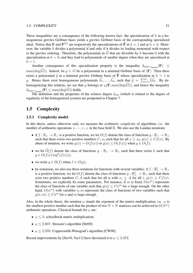
1.5. COMPLEXITY 51

These inequalities are a consequence of the following known fact: the specialization of h in a ho-mogeneous grevlex Grobner basis yields a grevlex Grobner basis of the corresponding specializedideal. Notice that F and F(h) are respectively the specializations of F at h = 1 and at h = 0. More-over, the variable h divides a polynomial if and only if it divides its leading monomial with respectto the grevlex ordering. Therefore, the polynomials in G that are divisible by h become 0 with thespecialization at h = 0, and they lead to polynomials of smaller degree when they are specialized ath = 1.

Another consequence of this specialization property is the inequality dmax≺grevlex(F) ≤

max(deg(G)). Indeed, let g ∈ G be a polynomial in a minimal Grobner basis of 〈F〉. Then thereexists a polynomial g in a minimal grevlex Grobner basis of F whose specialization at h = 1 isg. Hence there exist homogeneous polynomials h1, . . . , hm such that g =

∑mi=1 fihi. By de-

homogenizing this relation, we see that g belongs to χ(F,max(deg(G)), and hence the inequalitydmax≺grevlex

(F) ≤ max(deg(G)) holds.The definition and the properties of the witness degree dwit (which is related to the degree of

regularity of the homogenized system) are postponed to Chapter 7.

1.5 Complexity

1.5.1 Complexity model

In this thesis, unless otherwise said, we measure the arithmetic complexity of algorithms, i.e. thenumber of arithmetic operations +,−,×,÷ in the base field K. We also use the Landau notations:

• if f : R+ → R+ is a positive function, we let O(f) denote the class of functions g : R+ → R+

such that there exists two positive numbers C, x0 such that for all x ≥ x0, g(x) ≤ Cf(x). Byabuse of notation, we write g(x) = O(f(x)) or g(x) ≤ O(f(x)) when g ∈ O(f);

• we let O(f) denote the class of functions g : R+ → R+ such that there exists k such thatg ∈ O(f(x) logk(f(x)));

• we write g ∈ Ω(f) when f ∈ O(g);

• by extension, we also use these notations for functions with several variables: if f : R`+ → R+

is a positive function, we let O(f) denote the class of functions g : R`+ → R+ such that thereexist two positive numbers C,A such that for all x with xi ≥ A for all i, g(x) ≤ Cf(x).Sometimes, we explicitly fix some parameters. For instance, if m is fixed, O(nm) representsthe class of functions of one variable such that g(n) ≤ Cnm for n large enough. On the otherhand, O(nm) with variables n,m represents the class of functions of two variables such thatg(n,m) ≤ Cnm for n and m large enough.

Also, in the whole thesis, the notation ω stands the exponent of the matrix multiplication, i.e. ω isthe smallest positive number such that the product of two N ×N matrices can be achieved in O(Nω)arithmetic operations. Classical bounds for ω are:

• ω ≤ 3: schoolbook matrix multiplication;

• ω ≤ 2.807: Strassen’s algorithm [Str69];

• ω ≤ 2.376: Coppersmith-Winograd’s algorithm [CW90].

Recent improvements by [Sto10, Vas11] have decreased it to ω ≤ 2.373.

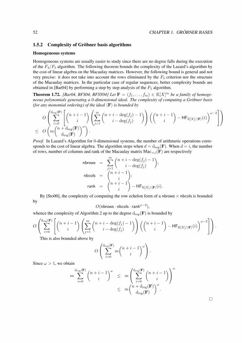
52 CHAPTER 1. GROBNER BASES

1.5.2 Complexity of Grobner basis algorithms

Homogeneous systems

Homogeneous systems are usually easier to study since there are no degree falls during the executionof the F4/F5 algorithm. The following theorem bounds the complexity of the Lazard’s algorithm bythe cost of linear algebra on the Macaulay matrices. However, the following bound is general and notvery precise: it does not take into account the rows eliminated by the F5 criterion nor the structureof the Macaulay matrices. In the particular case of regular sequences, better complexity bounds areobtained in [Bar04] by performing a step by step analysis of the F5 algorithm.

Theorem 1.72. [Bar04, BFS04, BFSY04] Let F = (f1, . . . , fm) ∈ K[X]m be a family of homoge-neous polynomials generating a 0-dimensional ideal. The complexity of computing a Grobner basis(for any monomial ordering) of the ideal 〈F〉 is bounded by

O

dreg(F)∑i=0

(n+ i− 1

i

) m∑j=1

(n+ i− deg(fj)− 1

i− deg(fj)

)((n+ i− 1

i

)− HFK[X]/〈F〉(i)

)ω−2

≤ O

(m

(n+ dreg(F)

dreg(F)

)ω).

Proof. In Lazard’s Algorithm for 0-dimensional systems, the number of arithmetic operations corre-sponds to the cost of linear algebra. The algorithm stops when d = dreg(F). When d = i, the numberof rows, number of columns and rank of the Macaulay matrix Mac≺,i(F) are respectively

nbrows =m∑j=1

(n+ i− deg(fj)− 1

i− deg(fj)

);

nbcols =

(n+ i− 1

i

);

rank =

(n+ i− 1

i

)− HFK[X]/〈F〉(i).

By [Sto00], the complexity of computing the row echelon form of a nbrows× nbcols is boundedby

O(nbrows · nbcols · rankω−2),

whence the complexity of Algorithm 2 up to the degree dreg(F) is bounded by

O

dreg(F)∑i=0

(n+ i− 1

i

) m∑j=1

(n+ i− deg(fj)− 1

i− deg(fj)

)((n+ i− 1

i

)− HFK[X]/〈F〉(i)

)ω−2 .

This is also bounded above by

O

dreg(F)∑i=0

m

(n+ i− 1

i

)ω .

Since ω > 1, we obtain

m

dreg(F)∑i=0

(n+ i− 1

i

)ω≤ m

dreg(F)∑i=0

(n+ i− 1

i

)ω

≤ m

(n+ dreg(F)

dreg(F)

)ω.

1.5. COMPLEXITY 53

1.5.3 Complexity of solving affine systems

For affine systems, it is more difficult to obtain complexity bounds because of the degree falls. How-ever, when the homogeneous part of highest degree is 0-dimensional, it is possible to obtain similarbounds as in the homogeneous case. The following theorem is from a personal communication withJ.-C. Faugere and it is a work in progress by M. Bardet, J.-C. Faugere and B. Salvy.

Theorem 1.73. Let F = (f1, . . . , fm) ∈ K[X]m be a polynomial family and let F(h) denote thefamily of homogeneous components of highest degree. If 〈F(h)〉 is 0-dimensional, then the complexityof computing a Grobner basis of F (for any graded monomial ordering) is bounded by

O

(m

(n+ dreg(F(h))

dreg(F(h))

)ω+ nDEG

(⟨F(h)

⟩)3).

1.5.4 Relation between the complexity and the degree of the ideal

If I is a 0-dimensional ideal, the arithmetic size of a Grobner basis of I (i.e. the number of coefficientsin K) is closely related to DEG(I), especially if the system generating the ideal is in shape position.Experimentally, Grobner bases algorithms seem to be output-sensitive: their practical running timeoften depends on the degree of the ideal and on the size of the output. However, from a theoreticalviewpoint, there are few families of systems for which it is proved that the complexity is related toDEG(I).

Proposition 1.74. Let F ∈ K[X]m be a 0-dimensional ideal in shape position, and G be the reducedGrobner basis of 〈F〉 with respect to ≺lex. Then the number of monomials in G is bounded above bynDEG(〈F〉).

Proof. The shape position states that

G =

x1 − h1(xn)

...xn−1 − hn−1(xn)

hn(xn)

,

where deg(hn) = DEG(I) and for all i ∈ 1, . . . , n− 1, deg(hi) < DEG(I). Therefore the numberof monomials in G is bounded by nDEG(I).

Even when a 0-dimensional system is not in shape position, the size of the reduced Grobner basis(for any monomial ordering) is still polynomial in the degree of the ideal:

Proposition 1.75. [FGLM93] Let F ∈ K[X]m be a 0-dimensional system, and G be the reducedGrobner basis of 〈F〉 with respect to a monomial ordering ≺. Then the number of monomials in G isbounded above by nDEG(〈F〉)(1 + DEG(〈F〉)).

Proof. In [FGLM93, Corollary 2.1], it is proven that the number of polynomials in a reducedGrobner basis is bounded by nDEG(〈F〉). Each polynomial g ∈ G has the form g = LM≺(g) +∑

m monomialm/∈LM(〈F〉)

amm. Consequently, the number of monomials in g is bounded by 1 + DEG(〈F〉).

Therefore, it is interesting to identify families of systems for which the complexity is polynomialin the degree of the corresponding ideal. As far as we know, there are few such bounds for Grobnerbases algorithms.

One family of systems for which such a bound is reached are regular sequences of polynomials ofthe same degrees.

54 CHAPTER 1. GROBNER BASES

Proposition 1.76. Let F = (f1, . . . , fn) ∈ K[X]n be a homogeneous regular sequence of polynomialsof degree d. Then, for a fixed d, as n→∞, the complexity of Algorithm 2 up to the degree of regularityis bounded by

O(

2nω(d log2(d)−(d−1) log2(d−1))),

which is polynomial in DEG(〈F〉) = dn.

Proof. By Theorem 1.72, the complexity of Algorithm 2 is bounded by O(n(n+ireg(〈F〉)

ireg(〈F〉))ω)

. Forregular sequences of degree d, the index of regularity is ireg(〈F〉) = (d − 1)n + 1 (Corollary 1.68).Consequently,

n(n+ireg(〈F〉)

ireg(〈F〉))ω

= n(dn+1n

)ω=

(n(dn+1)

(d−1)n+1

(dnn

))ωBy Stirling’s formula, as n grows, we obtain(

dn

n

)=

n→∞O(

2n(d log2(d)−(d−1) log2(d−1))).

Therefore the complexity of Algorithm 2 is bounded by

O(

2nω(d log2(d)−(d−1) log2(d−1))).

This is polynomial in dn since

2nω(d log2(d)−(d−1) log2(d−1)) = (dn)ω(d−(d−1) log2(d−1)/ log2(d)).

We would like to point out that the complexity bound

O

(m

(n+ dreg(F(h))

dreg(F(h))

)ω+ nDEG

(⟨F(h)

⟩)3)

is not uniformly polynomial in the Bezout bound for regular sequences. For instance, consider thefollowing family of sequences of degrees:

di = (2i, 2, 2, . . . , 2) ∈ Ni.

Now let Fi ∈ K[x1, . . . , xi]i be a homogeneous regular sequence of degrees di ∈ Ni. The Bezout

bound yields DEG(〈Fi〉) = 22i−1 and the Macaulay bound gives dreg(Fi) = 2i + i. Consequently(i+dreg(F(h))

dreg(F(h))

)=(

2i+2ii

)≥ 2i

2

ii= 2i

2−i log2 i which is not polynomial in the Bezout bound 22i−1.However, the complexity bound for Grobner basis algorithms is only an upper bound and hence

deciding if the complexity of Grobner basis algorithms is uniformly polynomial in the Bezout boundfor 0-dimensional regular sequences is still an open problem.

Chapter 2

Algebraic Systems in Applications

This thesis deals with polynomial system solving of “structured systems”, i.e. systems whose struc-tural properties can be exploited in order to obtain sharp complexity bounds or dedicated algorithms.This structure sometimes comes from the shape of the equations (multi-homogeneous, determinantalsystems). It can also stem from the set of solutions that we are investigating (e.g. finding one booleansolution of a boolean system), even if the system itself is not structured.

This is motivated by applications in Engineering sciences. We focus here on systems comingfrom Cryptology, Coding Theory, Geometry and Optimization. We present in this chapter wherethese algebraic systems come from and what the current state of the art is.

We first describe cryptosystems whose security is directly related to the difficulty of solving struc-tured systems. In particular, attacks on the MinRank authentication scheme and on the HFE cryp-tosystem can be modeled by a rank condition on a polynomial matrix. Finding points where thiscondition holds is the so-called MinRank problem and can be modeled by a multi-homogeneous andby a determinantal system. These kinds of systems also appear during the analysis of rank-metriccodes, which are a special kind of linear codes where the distance between words is not the usualHamming distance. We also describe a multi-homogeneous modeling of the McEliece cryptosystem,and we give a short description of the QUAD streamcipher, whose security relies on the difficulty ofsolving boolean quadratic systems.

Then we describe some fundamental problems in Real Geometry and Optimization: polynomialprograms, quantifier elimination, roadmap computations, and computing at least one point by con-nected component in a real semi-algebraic set. Recent algorithms for solving these problems need tocompute Grobner bases of determinantal or multi-homogeneous systems as a central subroutine.

2.1 MinRank

2.1.1 Description of the MinRank problem

The MinRank problem is a classical problem from linear algebra which appears in several applications(Cryptology, Information theory, Optimization, Geometry,. . . ), and which is related to determinantaland to multi-homogeneous systems.

MinRank. Given three integers r, p, q ∈ N such that r ≤ q ≤ p, and a family of p × q matricesM0, . . . ,Mn ∈ Kp×q, find λ1, . . . , λn ∈ K (or in K, depending on the context) such that

Rank(M0 −n∑i=1

λiMi) ≤ r.

55

56 CHAPTER 2. ALGEBRAIC SYSTEMS IN APPLICATIONS

This problem is NP-hard as soon as K is a finite field [BFS99]. Random instances are also dif-ficult to solve, and consequently this problem has been used to design cryptosystems whose securityrelies on its difficulty. The MinRank problem can also be seen as a multivariate generalization of theclassical Eigenvalue problem. Indeed, if n = 1, p = q and r = q − 1, then the MinRank problem canbe reduced to the problem of finding the eigenvalues of a square matrix.

In Chapter 4, we study a generalization of the MinRank problem, where the dependency on thevariables can be polynomial (and not necessarily linear as in the classical MinRank problem).

Generalized MinRank Problem: given a field K, a p×q matrix M whose entries are polynomialsof degree D over K[x1, . . . , xn], and r < min(p, q) an integer, compute the set of points at which theevaluation of the matrix has rank at most r.

2.1.2 Algebraic techniques for solving the MinRank problem

Minors modeling. The direct and most straightforward way to represent the MinRank as a system ofpolynomial equations is to consider the set of all minors of size r+ 1 of the matrix M0−

∑ni=1 λiMi.

Indeed, those minors simultaneously vanish exactly at the solutions of the MinRank problem. How-ever, the drawback of this modeling is the size of the polynomial system. For instance, if n = 9,r = 9, p = q = 12, there are 220 minors of size 10, and each one is a dense polynomial of degree 10in 9 variables: each one is the sum of

(1910

)= 92378 monomials.

Kipnis-Shamir modeling. The Kipnis-Shamir modeling was introduced in [KS99] and yields away to represent MinRank problems as systems of bilinear equations. Roughly speaking, the ideato represent the locus of rank defect of the matrix M is to introduce fresh variables representing thekernel of the matrix. This is in the same spirit as Lagrange multipliers in optimization. It is done bylooking for a triangular basis of the right kernel of the matrix M0 −

∑ni=1 λiMi. Indeed, this matrix

has rank at most r if and only if its right kernel has dimension at least q − r. We assume moreoverthat this right kernel is in systematic form, i.e. that the projection on the last coordinates

KerR(M0 −∑n

i=1 λiMi) → Kq−r

(y1, . . . , yq) 7→ (yr+1, . . . , yq)

is injective. This condition can be easily verified if the cardinality of K is large enough by perform-ing first a random invertible linear change of coordinates on the variables λi. Then we introduce(q − r)r new variables y(1)

1 , . . . , y(q−r)r , and we look for solutions of the bilinear system obtained by

considering the matrix relation

(M0 −

n∑i=1

λiMi

)·

y(1)1 y

(2)1 . . . y

(q−r)1

......

......

y(1)r y

(2)r . . . y

(q−r)r

1 0 . . . 0...

......

...0 0 . . . 1

= 0.

This yields an algebraic system of p(q−r) bilinear equations in n+r(q−r) variables. Notice thatthis system has as many equations as variables if n = (p− r)(q − r). In fact, in that case, the systemis 0-dimensional if genericity assumptions on the matrices Mi are verified (see Chapter 4). The mainadvantage of this representation is the size of the system. For n = 9, r = 9, p = q = 12, it is asystem of 108 equations. Moreover, each of these equations is represented by only 100 monomials.Consequently, the system is much smaller than the system obtained by the minors modeling.

2.2. CRYPTOLOGY AND INFORMATION THEORY 57

Algebraic properties of this bilinear system were investigated in [FLP08]. In this paper, the authorsshow that Grobner basis algorithms have a specific behavior on these systems. Also, Challenges Aand B from Table 2.1 were solved by using this modeling and Grobner bases algorithms.

2.2 Cryptology and Information Theory

2.2.1 Courtois Authentication Scheme

In [Cou01], the author proposes a zero-knowledge authentication scheme, and proves that its securitycan be reduced to the difficulty of solving the MinRank problem. We give here a short description ofthis cryptosystem. For simplicity of notations, we restrict ourselves to the case where the matrices aresquare, but this can be generalized without any major modification (see [Cou01] for more details).

We recall that in a zero-knowledge authentication scheme, the prover knows a secret key (whichproves his identity), and a protocol allows him to convince any verifier with overwhelming probabilitythat he knows this secret without revealing any information about it.

Public key. A integer r and a set of p × p matrices M0, . . . ,Mn ∈ GFp×pq such that there exists(x1, . . . , xn) ∈ GFnq satisfying Rank (M0 −

∑ni=1 xiMi) ≤ r.

Secret key. A vector (α1, . . . , αn) ∈ GFnq such that Rank (M0 −∑n

i=1 αiMi) = r. We denoteby M the matrix M = M0 −

∑ni=1 αiMi.

For this zero-knowledge authentication scheme, we need a collision-resistant hash function H ,i.e. a function which takes as input a finite sequence of elements in GFq (the set of all finite sequencesis denoted by GF

(N)q ) and returns an element in a finite set S

H : GF(N)q −→ S.

Collision-resistance means that it should be computationally infeasible to find a collision, i.e. twofinite sequences a, b ∈ GF

(N)q with a 6= b and H(a) = H(b). Usual hash-functions such as SHA-2

have this property (no such collisions have been found so far).In the sequel, the owner of the secret key is called the prover, and the one who wants to verify its

identity is called the verifier.

One round of authentication:

1. The prover chooses two p× p random invertible matrices S, T ∈ GFp×pq , and a random matrixX ∈ GFp×pq .

2. The prover chooses β1 = (β1,1, . . . , β1,n) ∈ GFnq at random. Let β2 = β1 + α ∈ GFnq , N1 =∑pi=1 β1,iMi ∈ GFp×pq , and N2 =

∑pi=1 β2,iMi ∈ GFp×pq (and hence N2 −N1 = M0 −M ).

3. The prover sends to the verifier

H(S | T | X), H(T ·N1 · S +X), H(T ·N2 · S +X − T ·M0 · S),

where S | T | X denotes the concatenation of S, T and X .

4. The verifier chooses Q ∈ 0, 1, 2 and sends it to the chooser.

5. If Q = 0, the prover reveals (T ·N1 · S +X) and (T ·N2 · S +X − T ·M0 · S). The verifierthen checks that H(T ·N1 · S +X) and H(T ·N2 · S +X − T ·M0 · S) are correct, then hecomputes (T ·N1 · S +X)− (T ·N2 · S +X − T ·M0 · S) = T ·M · S and checks that it isindeed of rank r.

58 CHAPTER 2. ALGEBRAIC SYSTEMS IN APPLICATIONS

Parameter set n p r K Security boundA 10 6 3 GF65521 2106

B 10 7 4 GF65521 2122

C 10 11 8 GF65521 2138

D 81 19 10 GF2 264

E 121 21 10 GF2 281

F 190 29 15 GF2 2128

Table 2.1: Courtois MinRank challenges

6. If Q = 1 or Q = 2, the prover reveals S, T , X and βQ. The verifier checks that S, T areinvertible and that H(S | T | X) is correct. Then he computes T ·NQ · S =

∑pi=1 βQ,iMi and

verifies that H(T ·N1 · S + X) (if Q = 1) or H(T ·N2 · S + X − T ·M0 · S) (if Q = 2) iscorrect.

In [Cou01], Courtois shows that any cheater (i.e. someone who does not know α) can be detectedby the verifier with probability at least 1/3. Therefore, if someone succeeds ` rounds of authentication,then the verifier knows that this person knows α with probability at least 1− (2/3)`. More precisely,he shows that, assuming that H is collision-resistant, a false prover can answer the questions of theverifier with probability more than 2/3 only if he knows a solution of the MinRank problem.

Therefore, the security of this scheme directly relies on the difficulty of the MinRank problem.Courtois proposed several sets of parameters for which the MinRank problem seemed untractable,yielding secure parameters for the authentication scheme. We report them in Table 2.1.

2.2.2 Rank metric codes

Rank metric codes are a class of linear error-correcting codes where the metric between words isdifferent from the classical Hamming distance. They are defined over an extension GFqe of a finitefield. The distance between two vectors a = (a1, . . . , an) ∈ GFnqe and b = (b1, . . . , bn) ∈ GFnqe isgiven by the rank of the e × n matrix (a1 − b1, . . . , an − bn) ∈ GFnqe where each element is seen asa vector in GFeq by identifying GFqe and GFeq as GFq-vector spaces (by fixing a basis (β1, . . . , βe) ∈GFqe of linearly independent vectors over GFq).

A rank-metric code is a vector subspace of dimension k of GFnqe (which is seen as a GFq-vectorspace). Given a set of generators G1, . . . , Gk ∈ GFnqe (which can be represented by matrices inGFe×nq ), and a received word W ∈ GFnqe , decoding W means finding the closest word in the code forthe rank-metric.

This is a MinRank problem since it is equivalent to finding a vector (x1, . . . xn) ∈ GFnq such thatthe rank of W −∑q

i=1 xiGi is minimal.In particular, these rank-metric codes have been used to design cryptosystems. We refer the reader

to [Gab85, OJ02, Ove05] for a detailed exposition.

2.2.3 Hidden Field Equations (HFE)

Hidden Field Equations (HFE for short) is an asymmetric encryption scheme proposed in [Pat96]. Itssecurity against message recovery attacks relies on the difficulty of solving boolean systems. However,in [FJ03], the authors show that these boolean systems are actually structured and that this structurecan be exploited during Grobner basis computations. We give here a short and simplified descriptionof HFE. We refer the reader to [KS99] for more details.

2.2. CRYPTOLOGY AND INFORMATION THEORY 59

The main idea of HFE is that the secret key is a univariate polynomial over an extension fieldGFqn . This polynomial has a special shape:

P (x) =∑

0≤i,j≤rai,jx

qi+qj .

By choosing a basis of GFqn as a GFq-vector space, the map x 7→ P (x) yields a map

S : GFnq → GFnqx 7→ (f1(x), . . . , fn(x))

,

where each polynomial fi is a quadratic polynomial (since each monomial of P has the form xqi+qj ).

Therefore fi can be represented by a n × n matrix. Then the structure is hidden by performinginvertible linear transforms in GFnq on the variables and on the polynomials fi.

In order to be able to decrypt, the polynomialP should have a relatively low degree so that it can beeasily factored in GFqn [x]. Therefore r n, and each quadratic polynomial fi is represented by a lowrank matrix. These low rank matrices (or matrices corresponding to equivalent keys) can be recoveredby solving a MinRank problem involving the polynomials of the public key [KS99, BFP11, BFP12a].

2.2.4 McEliece PKC.

The McEliece PKC is an asymmetric encryption scheme based on coding theory. In its originalversion, it is built upon Goppa codes, which are a family of codes which are easy to decode when it isknown how they were constructed. However, knowing a generator matrix of this code is not sufficientto be able to decode efficiently.

The general framework of the McEliece PKC is described below.

Public key. A generator k × n matrix G of a linear code C ⊂ GFnq and an integer e ∈ N.

Private key. An efficient algorithm for decoding C up to e errors.

Encryption. To encrypt a vector v ∈ GFkq , compute v ·G and add e random errors.

Decryption. Use the decoding algorithm to recover v · G, then recover v by solving a linearsystem.

In the classical version of McEliece, Goppa codes are proposed as codes whose structure can beeasily hidden by linear transforms. These codes are part of a larger family called alternant codes. Themain specificity of these codes is that there exists a special parity check matrix (a matrix such thatH · tG = 0) with the following shape:

H =

y0 y1 . . . yn−1

x0y0 x1y1 . . . xn−1yn−1...

......

...xδ−1

0 y0 xδ−11 y1 . . . xδ−1

n−1yn−1

,where the xi are pairwise distinct in an extension GFqm , and the yi are nonzero elements of GFqm .Once the xi and the yi are known, there is an efficient algorithm to decode such codes (see e.g. [FJ98]).

Therefore, one way to attack the McEliece cryptosystem is to solve the algebraic system obtainedby the relation H · tG = 0:

60 CHAPTER 2. ALGEBRAIC SYSTEMS IN APPLICATIONS

n−1∑i=0

g1,i+1yi = 0,

n−1∑i=0

g2,i+1xiyi = 0,

...n−1∑i=0

gδ,i+1xδ−1i yi = 0.

(2.1)

This system is overdetermined and bihomogeneous, and finding its solutions in GFqm would breakthe McEliece cryptosystem. However, for practical parameters this algebraic system seems to be un-tractable. Nevertheless some variants of the cryptosystem were recently proposed: in [BCGO09], theauthors use quasi-cyclic alternant codes; in [MB09], dyadic Goppa codes are used. The goal is toreduce the sizes of the keys (which is the main drawback of the McEliece cryptosystem) by addingstructure to the system. In [FOPT10], the authors show that this structure adds redundancy to thealgebraic system and thus propose theoretical and practical attacks on these variants of McEliece bysolving bilinear systems. More precisely, they show that the quasi-cyclic and the dyadic structures addlinear equations to the modeling of the Mc Eliece cryptosystem. As a result, they can extract a sub-system of “quasi-bilinear equations” where the size of one block of variables is very small comparedto the other block of variables.

In Chapter 6, we show that Grobner bases of affine bilinear systems are easier to compute thanGrobner bases of general quadratic systems and that the maximal degree reached during the computa-tion depends only on the smaller block of variables. This explains the efficiency of the attack proposedin [FOPT10].

2.2.5 QUAD

QUAD is a stream cipher proposed in [BGP09, BGP06]; its security relies on the difficulty of solvingquadratic algebraic systems over finite fields. We give here a short and simplified description of thecipher over GF2. We refer the reader to [BGP09, BGP06] for more details.

In QUAD, we consider a publicly known system S = (f1, . . . , f2n) of 2n quadratic equations inn variables over GF2. The internal state of the system x ∈ GFn2 is a vector of n bits. At each round,this internal state is updated as follows

x← (f1(x), . . . , fn(x)).

Then n bits of output are generated by computing (fn+1(x), . . . , f2n(x)). This process is iterated inorder to generate any number of bits.

The designers of this cryptosystem give in [BGP09] a proof that the security of QUAD is relatedto the difficulty of solving boolean systems. Therefore, in order to estimate secure parameters forQUAD (for instance the value of n), it is important to have good estimates of the complexity ofsolving boolean systems. This issue is investigated in Chapter 7: we provide an algorithm to exploitthe fact that we are looking for solutions in GFn2 (and not in the algebraic closure).

2.2.6 The Algebraic Surface Cryptosystem

The Algebraic Surface Cryptosystem is an algebraic asymmetric scheme proposed in [AGM09] (aprevious version have been given in [AG04]); the design of this cryptosystem was partially supportedby Toshiba. It is based on an unusual algebraic problem, the Section Finding Problem:

2.3. REAL SOLVING AND OPTIMIZATION 61

Section Finding Problem (SFP). Given an algebraic surface defined by the polynomialX(x, y, t) ∈ GFp[x, y, t], find two polynomials ux(t), uy(t) ∈ GFp[t] of degree d, such thatX(ux(t), uy(t), t) = 0.

We give here a brief description of ASC (see Section 8.1.2 for more details). We consider the ringof polynomials GFp[x, y, t] where p is a prime number. For any polynomial P ∈ GFp[x, y, t], ΛPdenotes its support in GFp(t)[x, y] (that is to say the set of couples (i, j) ∈ N2 such that t`xiyj is amonomial of P ).

Secret key. A pair of polynomials (ux(t), uy(t)) ∈ GFp[t] of degree d.Public key. A surface described by an irreducible polynomial X(x, y, t) ∈ GFp[x, y, t] such that

X(ux(t), uy(t), t) = 0.

There are some additional technical conditions in order to be able to encrypt and decrypt.

Encryption. Consider a plaintext embedded into a polynomial

m(x, y, t) =∑

(i,j)∈Λm

mij(t)xiyj

where deg(mij(t)) = d(m)ij . Choose a random divisor polynomial

f(x, y, t) =∑

fij(t)xiyj

where the degrees of the polynomials fij are given. Then select four random polynomials r0, r1, s0, s1

such that, for ` ∈ 0, 1, ri has the same monomials as f (only the coefficients are different), and sihas the same shape as X .

The ciphertext (F0(x, y, t), F1(x, y, t)) is equal to m masked by the polynomials f , ri, si and X:

F0(x, y, t) = m(x, y, t) + f(x, y, t)s0(x, y, t) +X(x, y, t)r0(x, y, t),F1(x, y, t) = m(x, y, t) + f(x, y, t)s1(x, y, t) +X(x, y, t)r1(x, y, t).

Decryption. For ` ∈ 0, 1, consider h`(t) = F`(ux(t), uy(t), t) and compute the differenceh0(t) − h1(t) = f(ux(t), uy(t), t)(s0(ux(t), uy(t), t) − s1(ux(t), uy(t), t)). Next, find a factor ofh0(t)− h1(t) whose degree matches deg(f(ux(t), uy(t), t)). Let f(t) denote this factor. Then com-pute m(ux(t), uy(t), t) = h0(t) mod f(t). Finally, retrieve m(x, y, t) by solving the linear system:

m(ux(t), uy(t), t) =∑

mijkux(t)iuy(t)jtk.

We show in Section 8.1 how Grobner bases techniques and algebraic tools (normal forms, decom-positions of ideals, Grobner basis computations) can be used to fully break this system: we proposean attack which recovers the plaintext message m in less than 0.05s for recommended parameters.The general principle of the attack in to replace the factorization process in the decryption algorithmby decomposition of ideals.

2.3 Real Solving and Optimization

The critical point method has recently been given a lot of attention for studying properties of realalgebraic and semi-algebraic sets. In particular, this method is a subroutine in algorithms for solvingoptimization problems, for quantifier elimination [HS11], for answering connectivity queries [SS10],or for computing at least one point by connected component in semi-algebraic sets [BPR96, BPR98,GV88, HRS89, HRS93].

62 CHAPTER 2. ALGEBRAIC SYSTEMS IN APPLICATIONS

2.3.1 Problem statements

Real semi-algebraic sets are sets of points x ∈ Rn satisfying equalities f1(x) = . . . = fm(x) = 0and inequalities g1(x) > 0, . . . , gk(x) > 0 (f1, . . . , fm, g1, . . . , gk ∈ R[x1, . . . , xn]) or finite unionsof such sets. Real algebraic sets appear frequently in engineer sciences (in fact, as soon as there arepolynomial constraints). For instance, recent results show that geometrical results can yield importantresults in control theory [Hen08] or in game theory (see e.g. [HKL+11]).

Therefore, it is crucial to develop efficient tools for studying semi-algebraic sets. In particular, wegive here three examples of central problems in effective real geometry.

Polynomial Program. Polynomial programs are families of hard optimization problems:Given P, f1, . . . , fp ∈ Q[X], find (if it exists) xmin ∈ R such that

P (xmin) = minx∈Z(f1,...,fp)∩Rn

P (x).

Polynomial programs are usually hard to tackle with numerical algorithms for many reasons. First,the feasible region Z(f1, . . . , fp)∩Rn is in general neither convex nor finite. Also there are usually alot of local extrema, and consequently it is difficult to adapt iterative methods (for instance based onNewton iteration) in this context.

Quantifier elimination. In 1951, Tarski showed in [Tar51] that the theory of real closed fieldsadmits quantifier elimination and is decidable. This means that, over a real closed field (for instanceR), any quantified formula of the form

∃(y1, . . . , y`) ∈ R`, (h1(X,Y ) ./ 0, . . . , hi(X,Y ) ./ 0),

where ./ is either = or > is equivalent to a disjunction of quantifier-free formulas of the form

f1(X) = . . . = fm(X) = 0, g1(X) > 0, . . . , gk(X) > 0.

An equivalent statement is that if ϕ is a first-order formula with n free variables, then the set of points(x1, . . . , xn) ∈ Rn which satisfy ϕ is a semi-algebraic set. The corresponding computational prob-lem is to compute from a quantified formula an equivalent quantifier-free formula. It was proved in[DH88] that the size of the quantifier-free formula can be doubly-exponential in the size of the quan-tified formula. While there exist doubly exponential algorithms solving this problem (for instance thecylindrical algebraic decomposition [Col75]), recent results show that in several applicative contexts,the output of the algorithm (i.e. the quantifier free formula) can be weakened but still contains allthe useful information. For instance, in [HS11], the authors describe the stability region of the Mac-Cormack scheme (which is the finite difference scheme used to study numerically hyperbolic partialdifferential equations) by the implementation of a singly exponential algorithm based on the criticalpoint method and Grobner bases algorithms.

Connectivity queries. Another fundamental problem in real algebraic geometry is to answerconnectivity queries, i.e. given a semi-algebraic set V ⊂ Rn and two points x1,x2 ∈ V , decidewhether x1 and x2 are in the same connected component of V . If so, we also want an algorithmwhich outputs a path from x1 to x2. In order to answer this question, Canny introduced the notion ofroadmap in [Can88, Can93]. Roughly speaking, a roadmap of V is a 1-dimensional semi-algebraicsubset of V which is connected inside each connected component of V . Once a roadmap is computed,it is used as a skeleton to answer connectivity queries. Algorithms for computing roadmaps rely onthe critical point method and practical software computing them make intensive use of Grobner basescomputations on critical point systems (see e.g. [SS10] and references therein).

2.3. REAL SOLVING AND OPTIMIZATION 63

At least one point by connected component. In order to describe the topology of a semi-algebraic set V ∈ Rn given by a set of equations and inequalities (or even to decide whether V isempty or not), an important routine is to compute at least one point by connected component of V .Several methods exist to do this and in conjunction with roadmaps, they yield a description of thetopology of V . Optimal complexity bounds were achieved by using infinitesimal transformations in[BPR96, BPR98], however these algorithms did not lead to software able to solve this problem inpractice. Recently, algorithms based on polar varieties and critical point methods were proposed (seee.g. [SS03, SS04] and references therein). They have been implemented in the Maple RAGlib libraryand rely heavily on Grobner bases computations of structured systems.

2.3.2 Algebraic Tools for Real Solving

Critical Point Method. The problem of polynomial optimization can be algebraically represented asfollows: a local extrema x of P restricted to the real trace of V = Z(f1, . . . , fp) is also a critical pointof the restriction of P to V . Therefore, the evaluation at any local extrema x of the Jacobian matrix

jac(P, f1, . . . , fp) =

∂P∂x1

. . . ∂P∂xn

∂f1∂x1

. . . ∂f1∂xn

......

...∂fp∂x1

. . .∂fp∂xn

is rank defective. Therefore, xmin is a real zero of the system of polynomials f1, . . . , fp ∪MaxMinors(jac(P, f1, . . . , fp)).

Under mild genericity assumptions, this system is 0-dimensional (see Chapter 5), so Grobner basistechniques can be used to obtain a rational parametrization of the real local extrema of the restrictionof P to V .

Under these genericity assumptions, the system f1, . . . , fp ∪ MaxMinors(jac(P, f1, . . . , fp))is the union of a regular sequence (f1, . . . , fp) and of a determinantal systemMaxMinors(jac(P, f1, . . . , fp)). This kind of systems is studied in Chapter 5. Notice that it isalso possible to express the rank condition of the Jacobian matrix by using Lagrange multipliers, i.e.a set of fresh variables modeling a vector in the kernel.

More generally, the critical point method can be used to study any semi-algebraic set V : thecritical points of the projection on the first coordinate

πi : V ∩ Rn −→ Ri(x1, . . . , xn) 7−→ (x1, . . . , xi)

yield useful information on the geometry of V and their computation is a subroutine of several algo-rithms for real solving.

In [SS03], the authors show that the set of such critical points is a 0-dimensional variety un-der mild genericity assumptions on the polynomials f1, . . . , fp defining the variety V . Algorithmsfor computing such points are given in [BGHM01, BGHM97, BGHP05, BGHP04, BGH+10, SS03,ARS02, FMRS08]. The RAGlib maple package implements the algorithms given in [SS03, FMRS08]using Grobner bases.

Most known complexity results for computing critical points are based on the complexity of ge-ometric resolution [BGHM01, BGHM97, BGHP05, BGHP04]. However, in practice, it has beenobserved that Grobner bases algorithms are also efficient for solving critical point systems and sev-eral challenges and open problems have been solved by using the RAGlib maple package with the

64 CHAPTER 2. ALGEBRAIC SYSTEMS IN APPLICATIONS

FGb Grobner engine. We give in Chapter 5 first theoretical complexity estimates which explain thisbehavior.

Polar varieties. Polar varieties can be seen as generalizations of critical points of the projectionπ1 and their computation is a subroutine of several algorithms for studying properties of real (semi-)algebraic sets.

Let f1, . . . , fp ∈ Q[X] be polynomials generating a radical ideal such that their zero set V ⊂ Cnis equidimensional of dimension d (i.e. all irreducible components of the variety have dimension d,see Theorem 1.15). Let πi denote the restriction to V ∩Rn of the projection on the i first coordinates:

πi : V ∩ Rn −→ Ri(x1, . . . , xn) 7−→ (x1, . . . , xi)

Then for i from 1 to d, the n − i + 1-th polar variety is defined as the critical points of πi, i.e. thepoints of V ∩ Rn where the rank of the truncated Jacobian matrix

jac(F, i) =

∂f1∂xi+1

. . . ∂f1∂xn

......

...∂fp∂xi+1

. . .∂fp∂xn

is less than n − d. Therefore the n − i + 1-th polar variety, denoted by Wi, is definedby the vanishing of the polynomials f1, . . . , fp and of the minors of size n − d of jac(F, i):Z(f1, . . . , fp,Minors(jac(F, i), n − d)). Following [SS03], under some properness assumptions thatare satisfied generically, the dimension of Wi is equal to i − 1. These varieties play a central rolein several algorithms in effective real algebra (see e.g. [BGHM01, BGHM97, BGHP05, BGHP04,SS03, BGH+10, GS11]) Therefore it is important to be able to compute Grobner bases of the ideal〈f1, . . . , fp,Minors(jac(F, i), n− d)〉 and to estimate the complexity of such computations.

Chapter 3

Preliminaries on Determinantal andMulti-homogeneous systems

As shown in Chapter 2, determinantal and multi-homogeneous ideals appear frequently in severalareas. We recall in this chapter several known results on their structural properties.

3.1 Determinantal systems

In this section, we focus on the structure of the determinantal ideal Dr ⊂ K[U ] generated by the setof (r + 1)-minors of the matrix

U =

u1,1 . . . u1,q...

......

up,1 . . . up,q

Without loss of generality, we assume that q ≤ p.The ideal Dr has been extensively studied during last decades. In particular, explicit formulas for

its degree and for its Hilbert series are known (see e.g. [Ful97, Example 14.4.14] and [CH94]), aswell as structural properties such as Cohen-Macaulayness and primality [HE70, HE71].

Notations 3.1. We let U denote the set of variables u1,1, . . . , up,q. The notation Ap,qr (t) ∈ Z[t]r×r

stands for the r × r-matrix whose (i, j)-entry is∑

`∈N(p−i`

)(q−j`

).

The formula for the Hilbert series of K[U ]/Dr is related to combinatorial properties of the idealDr. In particular, in [CH94], the authors show a relation between this series and the combinatorialstructure of a class of non-intersecting path; [Kra93, Kul96] enumerates such paths, and these formu-las are used in [CH94] to obtain the Hilbert series of K[U ]/Dr.

Theorem 3.2. [Abh88, CH94, Kra93, Kul96] The Hilbert series of the ring K[U ]/Dr is

HSK[U ]/Dr(t) =det (Ap,qr (t))

t(r2)(1− t)(p+q−r)r

.

By Proposition 1.43, the dimension and the degree can be read off from the Hilbert series:

Corollary 3.3. The dimension and the degree of the ideal Dr ⊂ K[U ] are respectively

• dim(Dr) = (p+ q − r)r;

65

66 CHAPTER 3. DETERMINANTAL AND MULTI-HOMOGENEOUS SYSTEMS

• DEG(Dr) =

q−r−1∏i=0

i!(p+ i)!

(q − 1 + i)!(p− r + i)!.

Proof. For the formula for the degree, we refer the reader to [Ful97, Example A.9.4, Example14.4.14]. In particular, [Ful97, Example A.9.4] shows that det(Ap,qr (1)) 6= 0. Therefore, the di-mension of Dr ⊂ K[U ] is equal to the exponent of (1− t) in the denominator of the rational functiongiven in Theorem 3.2, namely dim(Dr) = (p+ q − r)r.

An interesting feature of determinantal ideal is that they provide a class of non-trivial Cohen-Macaulay domains.

Proposition 3.4. [BV88] The ring K[U ]/Dr is a Cohen-Macaulay domain: if h1, . . . , h` ∈ K[U ]are homogeneous polynomials such that dim(D + 〈h1, . . . , h`〉) = dim(Dr) − ` then (h1, . . . , h`)is a K[U ]/Dr-regular sequence, i.e. for all i ∈ 1, . . . , `, hi does not divide 0 in the ringK[U ]/ (Dr + 〈h1, . . . , hi−1〉).

In Chapters 4 and 5, the results above are the cornerstones of the proofs for analyzing the structureof ideals corresponding to Generalized MinRank problems and critical point systems.

3.2 Structure of multi-homogeneous ideals

In this section, we recall several known results on multi-homogeneous ideals. For simplicity of no-tations, most results are only stated for bilinear systems but they can be easily extended to multi-homogeneous systems.

When f1, . . . , fm is a bi-homogeneous system in K[x0, . . . , xnx , y0, . . . , yny ] (with degree at least1 with respect to each block of variables), there is a set of trivial solutions that we need to take intoaccount: the varieties Z(x0, . . . , xnx) and Z(y0, . . . , yny) are necessarily subsets of Z(f1, . . . , fm).The corresponding ideals 〈x0, . . . , xnx〉 and 〈y0, . . . , yny〉 are called the irrelevant ideals. Contraryto the classical homogeneous case, these irrelevant ideals are not maximal, and this fact has severalconsequences: for instance, as soon as m ≥ nx + 1, regular bi-homogeneous sequences of size m donot exist.

In the section, we recall tools to transpose some results on homogeneous ideals in this context.Roughly speaking, the objective is to show that there exists a generic property of bi-homogeneoussystems which is similar to regularity for homogeneous systems.

We use the following notations:

Notations 3.5. • BL K(nx, ny) the K-vector space of bilinear forms in K[X,Y ] =K[x0, . . . , xnx , y0, . . . , yny ];

• X (resp. Y ) is the ideal 〈x0, . . . , xnx〉 (resp. 〈y0, . . . , yny〉);

• An ideal is called bihomogeneous if it admits a set of bihomogeneous generators.

• If (f1, . . . , fm) ∈ BL K(nx, ny)m is a family of bilinear forms, Ii denotes the ideal 〈f1, . . . , fi〉

and Ji denotes the saturated ideal Ii : (X ∩ Y )∞;

• Given a polynomial sequence F = (f1, . . . , fm), we denote by Syztriv(F) the module oftrivial syzygies, i.e. the set of all syzygies (s1, . . . , sm) such that for all i ∈ 1, . . . ,m,si ∈ 〈f1, . . . , fi−1, fi+1, . . . , fm〉;

• A primary ideal P ⊂ K[X,Y ] is called admissible if X 6⊂√P and Y 6⊂

√P ;

3.2. STRUCTURE OF MULTI-HOMOGENEOUS IDEALS 67

Lemma 3.6. [ST06] Let f1, . . . , fm ∈ K[X,Y ] be polynomials, Im = ∩P`∈L be a minimal primarydecomposition of Im and let Adm = P` | X 6⊂

√P` and Y 6⊂ √P` be the set of the admissible

ideals of the decomposition. Then Jm = ∩P∈AdmP .

Proof. Let h ∈ Jm be a polynomial. Since Jm = Im : (X ∩ Y )∞, there exists an integer k ∈ Nsuch that h(X ∩ Y )k ⊂ Im. Consequently, for all ` ∈ L, h(X ∩ Y )k ⊂ P`. The ideal P` isprimary, therefore if h /∈ P`, then there exists an integer k′ ∈ N such that (X ∩ Y )k

′ ⊂ P`. Hence(X ∩ Y ) ⊂ √P` and thus, since

√P` is prime, X ⊂ √P` or Y ⊂ √P`. It follows that P` is not an

admissible ideal. Conversely, let h ∈ ∩P∈AdmP be a polynomial. Let P` be a non-admissible primaryideal of the decomposition. Therefore there exists an integer k` ∈ N such that (X ∩ Y )k` ⊂ P`. Letk′ ∈ N be the integer defined by

k′ = max`∈L

(X∩Y )⊂√P`

k`.

Then notice that h(X ∩ Y )k′

is a subset of all ideals in the primary decomposition of Im, and henceh(X ∩ Y )k

′ ⊂ Im. Consequently, h ∈ Jm.

The polynomial fm always divides 0 in the ring K[X,Y ]/〈f1, . . . , fm−1〉 if the polynomialsf1, . . . , fm are bilinear and m ≥ minnx, ny + 1. However, this is due to the irrelevant ideals. There-fore, we have to consider the ideals after saturation by these irrelevant ideals:

Proposition 3.7. let f1, . . . , fm ∈ K[X,Y ] be polynomials with m ≤ nx + ny, and Ass(Ii−1) be theset of prime ideals associated to Ii−1. The following assertions are equivalent:

1. for all i ∈ 2, . . . ,m, fi is not a divisor of 0 in K[X,Y ]/Ji−1.

2. for all i ∈ 2, . . . ,m, (fi ∈ P, P ∈ Ass(Ii−1))⇒ P is non-admissible.

Proof. It is a straightforward consequence of Lemma 3.6.

In the following, let a be the set

a = a(i)j,k | 1 ≤ i ≤ m, 0 ≤ j ≤ nx, 0 ≤ k ≤ ny.

We consider generic polynomials f1, . . . , fm in K(a)[x0, . . . , xnx , y0, . . . , yny ]:

fi =∑

a(i)j,kxjyk

and we denote by I ⊂ K(a)[x0, . . . , xnx , y0, . . . , yny ] the ideal they generate.

Lemma 3.8. Let P be an admissible prime ideal of K[X,Y ]. The set of bilinear polynomials f ∈BL K(nx, ny) such that f /∈ P contains a non-empty Zariski open set of BL K(nx, ny) (which isseen as a K-vector space of dimension (nx + 1)(ny + 1).

Proof. Let f be the generic bilinear polynomial

f =∑j,k

aj,kxjyk

in K(aj,k0≤j≤nx,0≤k≤ny)[x0, . . . , xnx , y0, . . . , yny ]. Since P is admissible, there exists xj0yk0 suchthat xj0yk0 /∈ P (this shows the non-emptiness). Let ≺ be an admissible order. Then consider thenormal form for this order

NF≺,P (f) =∑

t monomial

ht(a0,0 . . . , anx,ny)t.

68 CHAPTER 3. DETERMINANTAL AND MULTI-HOMOGENEOUS SYSTEMS

By multiplying by the least common multiple of the denominators, we can assume without loss ofgenerality that for each t, ht is a polynomial. Thus, if a bilinear polynomial is in P , then its coefficientsare solutions of the polynomial equation ht(a0,0, . . . , anx,ny) = 0 for any monomial t.

Lemma 3.9. For all i ∈ 1, . . . ,m − 1, fi+1 does not divide 0 in K(a)[X,Y ]/(〈f1, . . . , fi〉 : (X ∩Y )∞).

Proof. Let P be an admissible prime associated to 〈f1, . . . , fi〉. Then there exists a family of genera-tors of P which involves only the parameters a(`)

j,k with ` ≤ i. By an argument similar to the proof ofLemma 3.8, NFP (fi+1) 6= 0. Since this is true for every admissible prime in Ass(〈f1, . . . , fi〉), fi+1

does not divide 0 in K(a)[X,Y ]/(〈f1, . . . , fi〉 : (X ∩ Y )∞).

We can now define a property similar to regularity for bi-homogeneous systems (and by extensionfor multi-homogeneous systems):

Proposition 3.10. Let m ≤ nx + ny and f1, . . . , fm be bilinear polynomials such that for all i ∈1, . . . ,m− 1, fi+1 is not a divisor of 0 in K[X,Y ]/Ji. Then for all i ∈ 1, . . . ,m, the ideal Ji isequidimensional and its codimension is i.

Proof. We prove the Proposition by induction on m.

• J1 = I1 is equidimensional and codim(I1) = 1;

• Suppose that Ji−1 is equidimensional of codimension i−1. Then Ji = (Ji−1 +fi) : (X∩Y )∞.fi does not divide 0 in K[X,Y ]/Ji−1, thus Ji−1 + fi is equidimensional of codimension i. Thesaturation does not decrease the dimension of any primary component of Ji−1+〈fi〉. Therefore,Ji is equidimensional and its codimension is i.

Corollary 3.11. If m ≤ nx + ny then for all i ∈ 2, . . . ,m, the ideals 〈f1, . . . , fi〉 : (X ∩ Y )∞ and〈f1, . . . , fi−1〉 : (X ∩ Y )∞ + 〈fi〉 are equidimensional of codimension i.

Proof. This is a direct consequence of Lemma 3.9 and of Proposition 3.10.

Theorem 3.12 states that the property of non-divisibility of zero with respect to the saturated idealis a generic property, similarly to regularity for homogeneous systems.

Theorem 3.12. Letm,nx, ny ∈ N such thatm ≤ nx+ny. Then there exists a non-empty Zariski opensubset O ⊂ BL K(nx, ny)

m such that, for all bilinear system (f1, . . . , fm) ∈ O ∩BL K(nx, ny)m,

fi+1 does not divide 0 in K[X,Y ]/Ji.

Proof. There exists an algorithm which computes the equidimensional decomposition of a polynomialideal by using only arithmetic operations on the coefficients of the polynomial system [Lec03]. Duringthe computation of the equidimensional decompositions of all ideals 〈f1, . . . , fi〉 with this algorithm,a finite number of rational functions in K(a) appear. Therefore there exists a non-empty Zariski opensubset O ⊂ BL K(nx, ny)

m such that, for all bilinear system (f1, . . . , fm) ∈ O ∩BL K(nx, ny)m,

the numerators and the denominators of these rational functions do not vanish, and hence the equidi-mensional decomposition of 〈f1, . . . , fi〉 is equal to the specialization of that of 〈f1, . . . , fi〉. Thereforecodim (〈f1, . . . , fi〉 : (X ∩ Y )∞) = i and codim (〈f1, . . . , fi〉 : (X ∩ Y )∞ + 〈fi+1〉) = i+ 1. Con-sequently fi+1 does not divide 0 in K[X,Y ]/Ji.

3.3. AFFINE BILINEAR SYSTEMS 69

3.3 Ideals generated by generic affine bilinear systems

In this section, we focus on structural properties of ideals generated by affine bilinear systems (theseresults are not true for general multi-homogeneous systems). In particular, we show that the projectionof the variety of an affine bilinear system on the space defined by one block of variables is exactly thezero set of a determinantal system. This establishes a correspondence between determinantal systems(where the entries of the matrix are linear) and bilinear systems.

We assume here that K is a field of characteristic 0: this is needed in the proof of Lemma 3.14to use an algebraic version of Sard’s Theorem (however there exist variants of Sard’s Theorem inpositive characteristic, see e.g. [Eis95, Corollary 16.23]). Let m = nx + ny denote the number ofequations, and a be the set

a = a(i)j,k | 1 ≤ i ≤ m, 0 ≤ j ≤ nx, 0 ≤ k ≤ ny.

We consider generic polynomials f1, . . . , fm in K(a)[x0, . . . , xnx , y0, . . . , yny ]:

fi =∑

a(i)j,kxjyk

and we denote by I ⊂ K(a)[x0, . . . , xnx , y0, . . . , yny ] the ideal they generate. In the sequel of thissection, ϑ denotes the dehomogenization morphism:

K[x0, . . . , xnx , y0, . . . , yny ] −→ K[x0, . . . , xnx−1, y0, . . . , yny−1]f(x0, . . . , xnx , y0, . . . , yny) 7−→ f(x0, . . . , xnx−1, 1, y0, . . . , yny−1, 1)

.

For a ∈ Km(nx+1)(ny+1), ϕa stands for the specialization:

ϕa : K(a)[x0, . . . , xnx , y0, . . . , yny ] → K[x0, . . . , xnx , y0, . . . , yny ]f(a)(x0, . . . , xnx , y0, . . . , yny) 7→ f(a)(x0, . . . , xnx , y0, . . . , yny)

Also ϕa(I) denotes the ideal 〈ϕa(f1), . . . , ϕa(fm)〉 ⊂ K[X,Y ] and Z(ϕa(I),Pnx × Pny) ⊂PnxK× PnyK (resp. Z(ϑ ϕa(I)) ⊂ Knx+ny ) denotes the variety of ϕa(I) (resp. ϑ ϕa(I)).

First, we recall that generically all isolated solutions of a bilinear system are located on an affinechart.

Lemma 3.13. There exists a nonempty Zariski open set O1 ⊂ Km(nx+1)(ny+1)such that if a ∈

O1 ∩Km(nx+1)(ny+1), then for all (α0, . . . , αnx , β0, . . . , βny) ∈ Z(ϕa(I),Pnx × Pny), αnx 6= 0 andβny 6= 0. This implies that the application

Z(ϑ ϕa(I)) −→ Z(ϕa(I),Pnx × Pny)(α0, . . . , αnx−1, β0, . . . , βny−1) 7−→ ((α0 : · · · : αnx−1 : 1), (β0 : . . . : βny−1 : 1))

is a bijection.

Proof. See [Van29, page 751].

Lemma 3.14. There exists a nonempty Zariski open set O2 ⊂ Km(nx+1)(ny+1), such that if a ∈

O2 ∩Km(nx+1)(ny+1), then the ideal ϑ ϕa(I) is radical.

Proof. Denote by F the polynomial family (f1, . . . , fm) ∈ K[a, X, Y ]m. Let J ⊂ K[a] be the ideal(I + 〈det(jacX,Y (F))〉

)∩K[a] andZ(J) be its associated algebraic variety. By the Jacobian Criterion

(see e.g. [Eis95, Theorem 16.19]), if a does not belong to Z(J), then ϑ ϕa(I) is radical. Thus, it issufficient to prove that Km(nx+1)(ny+1)) \ Z(J) is non-empty.

70 CHAPTER 3. DETERMINANTAL AND MULTI-HOMOGENEOUS SYSTEMS

To do that, we prove that for all a ∈ Km(nx+1)(ny+1), there exists (ε1, . . . , εm) such that the ideal〈ϑ ϕa(f1) + ε1, . . . , ϑ ϕa(fm) + εm〉 is radical. For i ∈ 1, . . . ,m, let gi denote the polynomialϑ ϕa(fi) and consider the mapping Ψ

x ∈ Km → (g1(x), . . . , gm(x)) ∈ Km.

Suppose first that Ψ(Km) is not dense in Km. Since Ψ(Km) is a constructible set, it is contained in

a Zariski-closed subset of Km and there exists (ε1, . . . , εm) such that the algebraic variety defined byg1 − ε1 = · · · = gm − εm = 0 is empty. Since there exists a′ such that gi − εi = ϑ ϕa′(fi), weconclude that ϑ ϕa′(I) = 〈1〉. This implies that a′ /∈ Z(J).

Suppose now that Ψ(Km) is dense in Km. By Sard’s Theorem [Sha94, Chap. 2, Section 6.2,

Theorem 2], there exists (ε1, . . . , εm) ∈ Km which does not lie in the set of critical values of Ψ. Thisimplies that at any point of the algebraic variety defined by g1 − ε1 = · · · = gm − εm = 0, ϑ ϕa(det(jacX,Y (F))) does not vanish. Remark now that there exists a′ such that gi− εi = ϑϕa′(fi).We conclude that a′ ∈ Km(nx+1)(ny+1) \ Z(J), which ends the proof.

The following lemma establishes the relation between the solutions of bilinear systems and thelocus of rank defect of linear matrices.

Lemma 3.15. There exists a nonempty Zariski open set O3 ⊂ Km(nx+1)(ny+1), such that if a ∈

O3 ∩Km(nx+1)(ny+1),√〈MaxMinors(ϑ ϕa(jacy(F)))〉 = 〈ϑ ϕa(f1), . . . , ϑ ϕa(fm)〉 ∩K[x0, . . . , xnx−1].

Proof. Let a be an element in O2 (as defined in Lemma 3.14). Thus ϑ ϕa(I) is radical. Now let(v0, . . . , vnx−1, w0, . . . , wny−1) ∈ Z(ϑ ϕa(I)) be an element of the variety. Then

(ϑ ϕa(jacy(F))xi=vi

)·

w0...

wny−1

1

=

0...0

.

This implies that Rank(ϑ ϕa(jacy(F))xi=vi) < ny + 1, and therefore

(v0, . . . , vnx−1) ∈ Z(〈MaxMinors(ϑ ϕa(jacy(F)))〉).Conversely, let (v0, . . . , vnx−1) ∈ Z(〈MaxMinors(ϑ ϕa(jacy(F)))〉). Thus there exists a

non trivial vector (w0, . . . , wny) in the right kernel Ker(ϑ ϕa(jacy(F))xi=vi). This means that(v0, . . . , vnx−1, 1, w0, . . . , wny) is in the variety of ϕa(I):

(v0, . . . , vnx−1, 1, w0, . . . , wny) ∈ Z(ϕa

(jacy(F)

)·

y0...yny

)

From Lemma 3.13, there exists a nonempty Zariski open setO1 such that, if F ∈ O1, wny 6= 0. Hence

(v0, . . . , vnx−1,w0

wny, . . . ,

wny−1

wny) ∈ Z(ϑ ϕa(I)).

Finally, we have

Z(〈MaxMinors(ϑ ϕa(jacy(F)))〉) = Z(〈ϑ ϕa(f1), . . . , ϑ ϕa(fm)〉 ∩K[x0, . . . , xnx−1])

and ϑ ϕa(I) is radical (Lemma 3.14). The Nullstellensatz concludes the proof.

3.3. AFFINE BILINEAR SYSTEMS 71

Corollary 3.16. There exists a nonempty Zariski open set O4 ⊂ Km(nx+1)(ny+1), such that if a ∈

O4 ∩Km(nx+1)(ny+1), the set Z(ϑ ϕa(I)) is finite and its cardinality is

card(Z(ϑ ϕa(I))) = DEG(ϑ ϕa(I)) =

(nx + nynx

)Proof. According to Lemmas 3.14 and 3.13, if a ∈ O1 ∩ O2, then deg(ϑ ϕa(I)) = card(Z(ϑ ϕa(I)) = card(Z(ϕa(I))). This value is the so-called multihomogeneous Bezout number of ϕa(I),i.e. the coefficient of znx1 z

ny2 in (z1 + z2)nx+ny (see e.g. [MS87]), namely

(nx+nynx

).

72 CHAPTER 3. DETERMINANTAL AND MULTI-HOMOGENEOUS SYSTEMS

Part II

Contributions

73

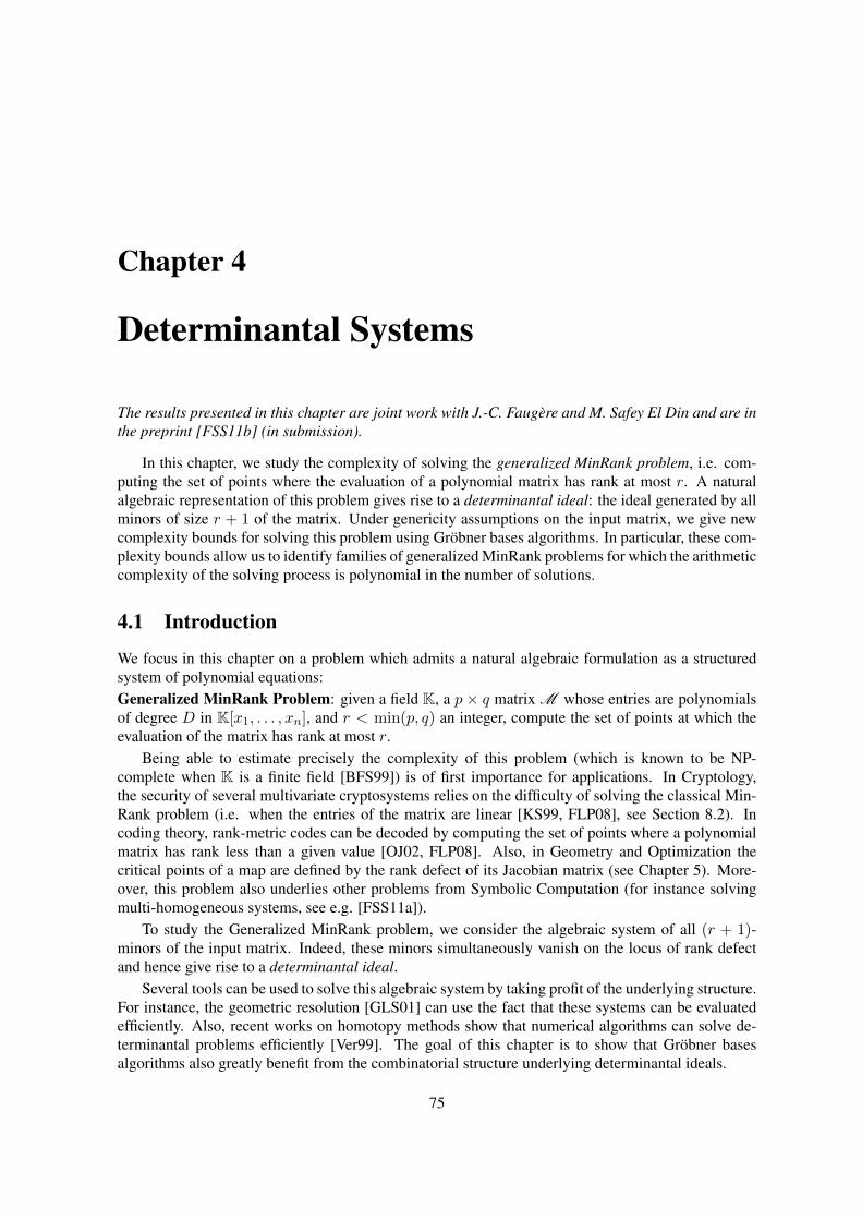
Chapter 4

Determinantal Systems

The results presented in this chapter are joint work with J.-C. Faugere and M. Safey El Din and are inthe preprint [FSS11b] (in submission).

In this chapter, we study the complexity of solving the generalized MinRank problem, i.e. com-puting the set of points where the evaluation of a polynomial matrix has rank at most r. A naturalalgebraic representation of this problem gives rise to a determinantal ideal: the ideal generated by allminors of size r + 1 of the matrix. Under genericity assumptions on the input matrix, we give newcomplexity bounds for solving this problem using Grobner bases algorithms. In particular, these com-plexity bounds allow us to identify families of generalized MinRank problems for which the arithmeticcomplexity of the solving process is polynomial in the number of solutions.

4.1 Introduction

We focus in this chapter on a problem which admits a natural algebraic formulation as a structuredsystem of polynomial equations:Generalized MinRank Problem: given a field K, a p × q matrix M whose entries are polynomialsof degree D in K[x1, . . . , xn], and r < min(p, q) an integer, compute the set of points at which theevaluation of the matrix has rank at most r.

Being able to estimate precisely the complexity of this problem (which is known to be NP-complete when K is a finite field [BFS99]) is of first importance for applications. In Cryptology,the security of several multivariate cryptosystems relies on the difficulty of solving the classical Min-Rank problem (i.e. when the entries of the matrix are linear [KS99, FLP08], see Section 8.2). Incoding theory, rank-metric codes can be decoded by computing the set of points where a polynomialmatrix has rank less than a given value [OJ02, FLP08]. Also, in Geometry and Optimization thecritical points of a map are defined by the rank defect of its Jacobian matrix (see Chapter 5). More-over, this problem also underlies other problems from Symbolic Computation (for instance solvingmulti-homogeneous systems, see e.g. [FSS11a]).

To study the Generalized MinRank problem, we consider the algebraic system of all (r + 1)-minors of the input matrix. Indeed, these minors simultaneously vanish on the locus of rank defectand hence give rise to a determinantal ideal.

Several tools can be used to solve this algebraic system by taking profit of the underlying structure.For instance, the geometric resolution [GLS01] can use the fact that these systems can be evaluatedefficiently. Also, recent works on homotopy methods show that numerical algorithms can solve de-terminantal problems efficiently [Ver99]. The goal of this chapter is to show that Grobner basesalgorithms also greatly benefit from the combinatorial structure underlying determinantal ideals.

75

76 CHAPTER 4. DETERMINANTAL SYSTEMS

In this chapter, an algebraic representation of the locus of rank defect is obtained by computinga lexicographical Grobner basis with the algorithms F5 [Fau02] and FGLM [FGLM93]. Indeed,experiments suggest that these algorithms take profit of the determinantal structure. The aim of thiswork is to give an explanation of this behavior from the viewpoint of asymptotic complexity analysis.

Main results

The goal of this chapter is to obtain complexity bounds for Grobner bases algorithms when the inputsystem is the set of (r + 1)-minors of a p × q matrix M , whose entries are polynomials of degreeD with generic coefficients. By generic, we mean that there exists a non-identically null multivariatepolynomial h such that the complexity results holds when this polynomial does not vanish on thecoefficients of the polynomials in the matrix. Therefore, from a practical viewpoint, the complexitybounds can be used in applications where the cardinality of the base field K is large enough: in thatcase, the probability that the coefficients of M do not belong to the zero set of h is close to 1.

We start by studying the homogeneous generalized MinRank problem (i.e. when the entries of Mare homogeneous polynomials) and by proving an explicit formula for the Hilbert series of the idealIr generated by the (r + 1)-minors of the matrix M . The general framework of the proofs is thefollowing: we consider the ideal Dr ⊂ K[U ] generated by the (r+ 1)-minors of a matrix U = (ui,j)

whose entries are variables. Then we consider the ideal Dr = Dr + 〈g1, . . . , gpq〉 ⊂ K[U,X],where the polynomials gi are quasi-homogeneous forms that are the sum of a linear form in K[U ]and a homogeneous polynomial of degree D in K[X]. If some conditions on the gi are verified, byperforming a linear combination of the generators there exist f1,1, . . . , fp,q ∈ K[X] such that

Dr = Dr + 〈u1,1 − f1,1, . . . , up,q − fp,q〉.

Then we use the fact that (Dr + 〈u1,1 − f1,1, . . . , up,q − fp,q〉)∩K[X] = Ir to prove that propertiesof Dr transfer to Ir when the entries of the matrix M are generic. This allows us to use results knownabout the ideal Dr to study the algebraic structure of Ir.

We study separately three different cases:

• n > (p − r)(q − r). Under genericity assumptions on the input, the dimension of the set ofsolutions of the generalized MinRank problem is positive.

• n = (p − r)(q − r). This is the 0-dimensional case, where the problem has finitely-manysolutions under genericity assumptions.

• n < (p− r)(q− r). In the over-determined case, we need to assume that a variant of Froberg’sConjecture holds in order to generalize the results in [FSS10].

In particular, when n ≥ (p − r)(q − r), we prove that the Hilbert series of the quotient ringK[X]/Ir is the power series expansion of the rational function

HSK[X]/Ir(t) =detAp,qr (tD)(1− tD)(p−r)(q−r)

tD(r2)(1− t)n,

where Ap,qr (t) is the r × r matrix whose (i, j)-entry is∑

k

(p−ik

)(q−jk

)tk. Assuming w.l.o.g. that

q ≤ p, we also prove that the degree of Ir is equal to

DEG(Ir) = D(p−r)(q−r)q−r−1∏i=0

i!(p+ i)!

(q − 1− i)!(p− r + i)!.

4.2. NOTATIONS AND PRELIMINARIES 77

From these explicit formulas, complexity bounds can be deduced. Indeed, one way to get a rep-resentation of the solutions of the problem in the 0-dimensional case is to compute a lexicographicalGrobner basis of the ideal generated by the minors. As shown in Chapter 1, this can be achieved byusing first the F5 algorithm [Fau02] to compute a Grobner basis for the so-called grevlex ordering andthen use the FGLM algorithm [FGLM93] to convert it into a lexicographical Grobner basis. The com-plexities of these algorithms are respectively governed by the degree of regularity and by the degreeof the ideal.

Therefore the theoretical results on the structure of Ir yield bounds on the complexity ofsolving the generalized MinRank problem with Grobner bases algorithms. More precisely, whenn = (p− r)(q − r) and under genericity assumptions on the input polynomial matrix, we prove thatthe arithmetic complexity for computing a lexicographical Grobner basis of Ir is bounded above by

O

((p

r + 1

)(q

r + 1

)(dreg(Ir) + n

n

)ω+ n (DEG (Ir))

3

),

where 2 ≤ ω ≤ 3 is a feasible exponent for the matrix multiplication, and

dreg(Ir) = Dr(q − r) + (D − 1)n+ 1.

This complexity bound allows us to identify families of Generalized MinRank problems for whichthe number of arithmetic operations during the Grobner basis computations is polynomial in the num-ber of solutions.

In the over-determined case (i.e. n < (p − r)(q − r)), we obtain similar complexity results, byassuming a variant of Froberg’s Conjecture which is supported by experiments.

Organization of the chapter

Section 4.2 provides notations used throughout this chapter and preliminary results. In Section 4.3,we show how properties of the ideal Dr generated by the (r + 1)-minors of U transfer to the idealIr. Then, the case when the homogeneous Generalized MinRank Problem has non-trivial solutions(under genericity assumptions) is studied in Section 4.4. Section 4.5 is devoted to the study of theover-determined MinRank Problem (i.e. when n < (p− r)(q − r)). Then, the complexity analysis isperformed in Section 4.6. Some consequences of this complexity analysis are drawn in Section 4.7.Experimental results are given in Section 4.7.4

4.2 Notations and preliminaries

In the sequel, p, q, r and n and D are positive integers with r < q ≤ p. For d ∈ N,Monomials(K[X], d) denotes the set of monomials of degree d in the polynomial ring K[X] =

K[x1, . . . , xn]. Its cardinality is #Monomials(K[X], d) =(d−1+n

d

).

We denote by a the set of parameters a(i,j)t : 1 ≤ i ≤ p, 1 ≤ j ≤ q, t ∈ Monomials(K[X], d).

The set of variables ui,j : 1 ≤ i ≤ p, 1 ≤ j ≤ q is denoted by U .For 1 ≤ i ≤ p, 1 ≤ j ≤ q, we denote by fi,j ∈ K(a)[X] the generic form of degree D

fi,j =∑

t∈Monomials(K[X],D)

a(i,j)t t.

Let Ir ⊂ K(a)[X] be the ideal generated by the (r + 1)-minors of the p× q matrix

M =

f1,1 . . . f1,q...

. . ....

fp,1 . . . fp,q

,

78 CHAPTER 4. DETERMINANTAL SYSTEMS

and Dr ⊂ K(a)[U,X] be the determinantal ideal generated by the (r + 1)-minors of the matrix

U =

u1,1 . . . u1,q...

. . ....

up,1 . . . up,q

.

We define Ir as the quasi-homogeneous ideal Dr + 〈ui,j − fi,j〉1≤i≤p,1≤j≤q ⊂ K(a)[U,X]:the quasi-homogeneous grading is given by wdeg(xi) = 1, wdeg(ui,j) = D. Notice that Ir =

Ir + 〈ui,j − fi,j〉1≤i≤p,1≤j≤q ⊂ K(a)[U,X]. Therefore, Ir = Ir ∩K(a)[X].

4.3 Transferring determinantal properties

In this section, we prove that generic structural properties (such as the dimension, the structure ofthe leading monomial ideal,. . . ) of the ideal Ir are the same as properties of the ideal Dr whereseveral generic forms have been added. Hence several classical properties of the determinantal idealDr transfer to the ideal Ir. In particular, this technique permits to obtain an explicit formula of theHilbert series of the ideal Ir.

In the following, we let b and c denote the following sets of parameters:

b = b(`)t | t ∈ Monomials(K[X], D), 1 ≤ ` ≤ pq;

c = c(`)i,j | 1 ≤ i ≤ p, 1 ≤ j ≤ q, 1 ≤ ` ≤ pq.

Also, g1, . . . , gpq ∈ K(b, c)[U,X] are generic quasi-homogeneous forms of type (D, 1) and ofweight degree D:

g` =∑

t∈Monomials(K[X],D)

b(`)t t+

∑1≤i≤p1≤j≤q

c(`)i,j ui,j .

We let Dr denote the ideal Dr + 〈g1, . . . , gpq〉 ⊂ K(b, c)[U,X]. For a ∈ Kpq(D−1+nD ), we denote

by ϕa the following evaluation morphism:

ϕa : K[a] −→ Kf(a) 7−→ f(a)

Also, for (b, c) ∈ Kpq((D−1+nD )+pq), we denote by ψb,c the evaluation morphism:

ψb,c : K[b, c] −→ Kf(b, c) 7−→ f(b, c)

By abuse of notation, we let ϕa(Ir) (resp. ψb,c(Dr)) denote the ideal Dr + 〈ui,j − ϕa(fi,j)〉 ⊂K[U,X] (resp. Dr + 〈ψb,c(g1), . . . , ψb,c(gpq)〉 ⊂ K[U,X]).

We call property a map from the set of ideals of K[U,X] to true, false:

P : Ideals(K[U,X]) → true, false .

Definition 4.1. Let P be a property. We say that P is

4.3. TRANSFERRING DETERMINANTAL PROPERTIES 79

• Ir-generic if there exists a non-empty Zariski open subset O ⊂ Kpq(D−1+nD ) such that

a ∈ O ⇒P(ϕa

(Ir

))= true;

• Dr-generic if there exists a non-empty Zariski open subset O ⊂ Kpq((D−1+nD )+pq) such that

(b, c) ∈ O ⇒P(ψb,c

(Dr

))= true.

The following lemma is the main result of this section:

Lemma 4.2. A property P is Ir-generic if and only if it is Dr-generic.

Proof. To obtain a representation of ϕa

(Dr

)for a generic a as a specialization of Ir, it is sufficient

to perform a linear combination of the generators. This proof shows that genericity is preserved duringthis linear transform.

In the sequel we denote by A,B and C the following matrices (of respective sizes pq ×(D−1+n

D

),

pq ×(D−1+n

D

)and pq × pq):

A =

a

(1)

xD1a

(1)

xD−11 x2

. . . a(1)

xDn...

......

...a

(pq)

xD1a

(pq)

xD−11 x2

. . . a(pq)

xDn

B =

b

(1)

xD1b

(1)

xD−11 x2

. . . b(1)

xDn...

......

...b

(pq)

xD1b

(pq)

xD−11 x2

. . . b(pq)

xDn

C =

c(1)1,1 . . . c

(1)p,q

......

...c(pq)1,1 . . . c

(pq)p,q

.

Therefore, we have

u1,1 − f1,1...

up,q − fp,q

= Idpq ·

u1,1...

up,q

− A ·

xD1

xD−11 x2

...xDn

g1

...gpq

= C ·

u1,1...

up,q

+ B ·

xD1

xD−11 x2

...xDn

In this proof, for a ∈ Kpq(D−1+n

D ) (resp. b ∈ Kpq(D−1+nD ), c ∈ Kp2q2), the notation A (resp. B,C)

stands for the evaluation of the matrix A (resp. B,C) at a (resp. b, c). Also, we implicitly identify Awith a (resp. B with b, C with c, A with a, B with b, C with c).

80 CHAPTER 4. DETERMINANTAL SYSTEMS

• Let P be a Ir-generic property. Thus there exists a non-zero polynomial h1(A) ∈ K[a] suchthat if h1(A) 6= 0 then P

(ϕa(Ir)

)= true.

Let adj(C) denote the adjugate of C (i.e. adj(C) = det(C) · C−1 in K(c)). Consider the poly-nomial h1 defined by h1(B,C) = h1(−adj(C) · B) ∈ K[b, c]. The polynomial inequality

det(C)h1(B,C) 6= 0 defines a non-empty Zariski open subset O ⊂ Kpq((D−1+nD )+pq)

. Let(B,C) ∈ O be an element in this set, then C is invertible since det(C) 6= 0. Let A be thematrix A = −adj(C) ·B. Therefore the generators of the ideal ϕa

(Ir

)are an invertible linear

combination of the generators of ψb,c

(Dr

). Consequently, ϕa

(Ir

)= ψb,c

(Dr

). Moreover,

h1(A) = h1(B,C) 6= 0 implies that the polynomial h1 is not identically 0. Therefore,

∀(b, c) ∈ O,P(ψb,c

(Dr

))= P

(ϕa

(Ir

))= true,

and hence P is a Dr-generic property.

• Conversely, consider a Dr-generic property P . Thus, there exists a non-zero polynomialh2(B,C) ∈ K[b, c] such that if h2(b, c) 6= 0 then P

(ψb,c(Dr)

)= true. Since P is

Dr-generic, there exists (b, c) such that h2(b, c) det(c) 6= 0. Let h2 be the polynomialh2(b) = h2(−C ·B,C).

Since det(C) 6= 0, the matrix C is invertible and h2(−C−1 ·B) = h2(B,C) 6= 0 and hence thepolynomial h2 is not identically 0. Moreover, if a ∈ Kpq(D−1+n

D ) is such that h2(A) 6= 0, thenh2(−C ·A,C) 6= 0 and thus P

(ψ−C·A,C(Dr)

)= true. Finally, ψ−C·A,C(Dr) = ϕA(Ir)

since the generators of ψ−C·A,C(Dr) are an invertible linear combination of that of ϕa(Ir)(the linear transformation is given by the invertible matrix C) and hence they generate the sameideal. Therefore, the property P is Ir-generic.

In the sequel, ≺ is an admissible monomial ordering (see Definition 1.18). If I is an ideal ofK[U,X], K(a)[U,X], or K(b, c)[U,X], we let LM≺(I) denote the ideal generated by the leadingmonomials of the polynomials.

By slight abuse of notation, if I1 and I2 are ideals of K[U,X], K(a)[U,X], or K(b, c)[U,X](I1 and I2 are not necessarily ideals of the same ring), we write LM≺(I1) = LM≺(I2) if the setsLM≺(f) | f ∈ I1 and LM≺(f) | f ∈ I2 are equal.

Lemma 4.3. Let PIr

and PDr

be the properties defined by

PIr

(I) =

true if LM≺(I) = LM≺

(Ir

);

false otherwise.

PDr

(I) =

true if LM≺(I) = LM≺

(Dr

);

false otherwise.

Then PIr

(resp. PDr

) is a Ir-generic (resp. Dr-generic) property.

4.3. TRANSFERRING DETERMINANTAL PROPERTIES 81

Proof. We prove here that PIr

is Ir-generic (the proof for PDr

is similar).

The outline of this proof is the following: during the computation of a Grobner basis G of Ir

in K(a)[U,X] (for instance with Buchberger’s algorithm), a finite number of polynomials are con-structed. Let ϕa be a specialization. If the images by ϕa of the leading coefficients of all non-zeropolynomials arising during the computation do not vanish, then ϕa(G) ⊂ ϕa(Ir) is a Grobner basisof the ideal it generates. It remains to prove that ϕa(G) is a Grobner basis of ϕa(Ir). This is achievedby showing that generically, the normal form (with respect to ϕa(G)) of the generators of ϕa(Ir) isequal to zero.

For polynomials f1, f2, we let LC(f1) (resp. LC(f2)) denote the leading coefficient of f1 (resp.f2) and Spol(f1, f2) = LCM(LM≺(f1),LM≺(f2))

LC(f1) LM≺(f1) f1 − LCM(LM≺(f1),LM≺(f2))LC(f2) LM≺(f2) f2 denote the S-polynomial

of f1 and f2.

We prove first that there exists a non-empty Zariski open subset O1 ⊂ Kpq(D−1+nD ) such that

a ∈ O1 ⇒ LM≺(ϕa(Ir)) = LM≺(Ir).

To do so, consider a Grobner basis G ⊂ K(a)[U,X] of Ir such that each polynomial g can be writtenas a combination g =

∑h`f`, where the f`’s range over the set of minors of size r + 1 of U and

the polynomials ui,j − fi,j , and h` ∈ K[a][U,X]. Buchberger’s criterion states that S-polynomialsof polynomials in a Grobner basis reduce to zero [CLO97, Chapter 2, §6, Theorem 6]. Thus eachS-polynomial of gi, gj ∈ G can be rewritten as an algebraic combination

Spol(gi, gj) =t∑

`=1

h′`g`,

where the polynomials h′` belong to K(a)[U,X] and such that g1, . . . , gt ⊂ G and for each 1 ≤ s ≤t, LM≺(gs) divides LM≺(Spol(g, g′)−∑s−1

`=1 h′`g`). Next, consider:

• the product Q1(a) =∏g∈G LC(g) of the leading coefficients of the polynomials in the Grobner

basis;

• for all (gi, gj) ∈ G2 such that Spol(gi, gj) 6= 0, the product Q2(a) of the numerators anddenominators of the leading coefficients arising during the reduction of Spol(gi, gj).

These coefficients belong to K[a]. Let Q(a) = Q1(a)Q2(a) ∈ K[a] denote their product. The

inequality Q(a) 6= 0 defines a non-empty Zariski open subset O1 ⊂ Kpq(D−1+nD ). If a ∈ O1, then

ϕa(Spol(g, g′)) =

t∑`=1

ϕa(h′`)ϕa(g`),

and for each 1 ≤ i ≤ t, LM≺(ϕa(gi)) divides LM≺(ϕa(Spol(g, g′)) −∑i−1`=1 ϕa(h′`)ϕa(g`)). Thus

ϕa(G) is a Grobner basis of the ideal it spans. Moreover, 〈ϕa(G)〉 ⊂ ϕa(Ir).We prove now that there exists a non-empty Zariski open set where the other inclusion ϕa(Ir) ⊂

〈ϕa(G)〉 holds. Let NFG(·) be the normal form associated to this Grobner basis (as defined as theremainder of the division by G in [CLO97, Chapter 2, §6, Proposition 1]). For each generator f ofIr (i.e. either a maximal minor of the matrix U , or a polynomial ui,j − fi,j), we have NFG(f) = 0.During the computation of NFG(f) by using the division Algorithm in [CLO97, Chapter 2, §3], a

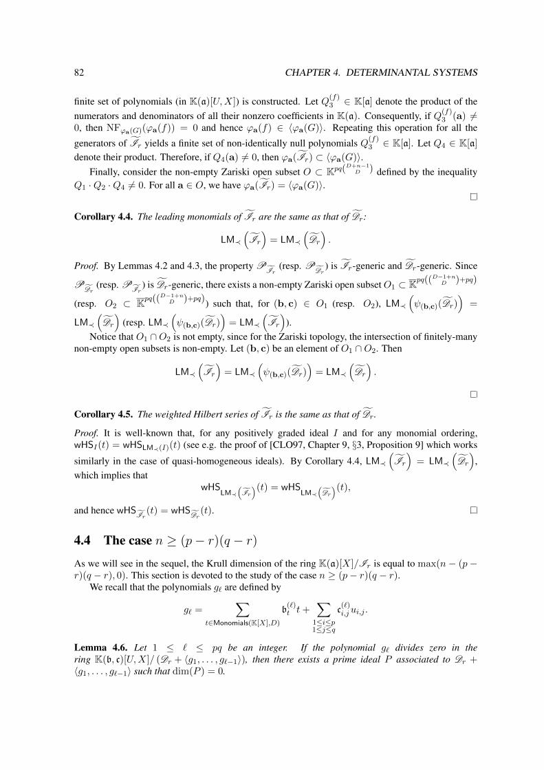
82 CHAPTER 4. DETERMINANTAL SYSTEMS

finite set of polynomials (in K(a)[U,X]) is constructed. Let Q(f)3 ∈ K[a] denote the product of the

numerators and denominators of all their nonzero coefficients in K(a). Consequently, if Q(f)3 (a) 6=

0, then NFϕa(G)(ϕa(f)) = 0 and hence ϕa(f) ∈ 〈ϕa(G)〉. Repeating this operation for all the

generators of Ir yields a finite set of non-identically null polynomials Q(f)3 ∈ K[a]. Let Q4 ∈ K[a]

denote their product. Therefore, if Q4(a) 6= 0, then ϕa(Ir) ⊂ 〈ϕa(G)〉.Finally, consider the non-empty Zariski open subset O ⊂ Kpq(D+n−1

D ) defined by the inequalityQ1 ·Q2 ·Q4 6= 0. For all a ∈ O, we have ϕa(Ir) = 〈ϕa(G)〉.

Corollary 4.4. The leading monomials of Ir are the same as that of Dr:

LM≺(Ir

)= LM≺

(Dr

).

Proof. By Lemmas 4.2 and 4.3, the property PIr

(resp. PDr

) is Ir-generic and Dr-generic. Since

PDr

(resp. PIr

) is Dr-generic, there exists a non-empty Zariski open subsetO1 ⊂ Kpq((D−1+nD )+pq)

(resp. O2 ⊂ Kpq((D−1+nD )+pq)) such that, for (b, c) ∈ O1 (resp. O2), LM≺

(ψ(b,c)(Dr)

)=

LM≺(Dr

)(resp. LM≺

(ψ(b,c)(Dr)

)= LM≺

(Ir

)).

Notice that O1 ∩O2 is not empty, since for the Zariski topology, the intersection of finitely-manynon-empty open subsets is non-empty. Let (b, c) be an element of O1 ∩O2. Then

LM≺(Ir

)= LM≺

(ψ(b,c)(Dr)

)= LM≺

(Dr

).

Corollary 4.5. The weighted Hilbert series of Ir is the same as that of Dr.

Proof. It is well-known that, for any positively graded ideal I and for any monomial ordering,wHSI(t) = wHSLM≺(I)(t) (see e.g. the proof of [CLO97, Chapter 9, §3, Proposition 9] which works

similarly in the case of quasi-homogeneous ideals). By Corollary 4.4, LM≺(Ir

)= LM≺

(Dr

),

which implies thatwHS

LM≺(Ir)(t) = wHS

LM≺(Dr)(t),

and hence wHSIr

(t) = wHSDr

(t).

4.4 The case n ≥ (p− r)(q − r)As we will see in the sequel, the Krull dimension of the ring K(a)[X]/Ir is equal to max(n− (p−r)(q − r), 0). This section is devoted to the study of the case n ≥ (p− r)(q − r).

We recall that the polynomials g` are defined by

g` =∑

t∈Monomials(K[X],D)

b(`)t t+

∑1≤i≤p1≤j≤q

c(`)i,j ui,j .

Lemma 4.6. Let 1 ≤ ` ≤ pq be an integer. If the polynomial g` divides zero in thering K(b, c)[U,X]/ (Dr + 〈g1, . . . , g`−1〉), then there exists a prime ideal P associated to Dr +〈g1, . . . , g`−1〉 such that dim(P ) = 0.

4.4. THE CASE N ≥ (P −R)(Q−R) 83

Proof. If g` divides zero in K(b, c)[U,X]/ (Dr + 〈g1, . . . , g`−1〉), then there exists a prime ideal Passociated to Dr + 〈g1, . . . , g`−1〉 such that g` ∈ P . For ` ≤ pq, let b(≤`) and c(≤`) denote the sets ofparameters

b(≤`) = b(s)t | t ∈ Monomials(K[X], D), 1 ≤ s ≤ `

c(≤`) = c(s)i,j | 1 ≤ i ≤ p, 1 ≤ j ≤ q, 1 ≤ s ≤ `.

Since (Dr + 〈g1, . . . , g`−1〉) is an ideal of K(b(≤`−1), c(≤`−1))[U,X], and P is an associatedprime, there exists a Grobner basis GP of P (for any monomial ordering ≺) which is a finite sub-set of K(b(≤`−1), c(≤`−1))[U,X].

Let NFP,≺(·) denote the normal form associated to this Grobner basis (as defined as the remainderof the division by GP in [CLO97, Chapter 2, §6, Proposition 1]).

Since g` ∈ P , we have NFP,≺(g`) = 0. By linearity of NFP,≺(·), we obtain∑t∈Monomials(K[X],D)

b(`)t NFP,≺(t) +

∑1≤i≤p1≤j≤q

c(`)i,j NFP,≺(ui,j) = 0.

Since Gp ⊂ K(b(≤`−1), c(≤`−1))[U,X], we can deduce that for any monomial t, NFP,≺(t) ∈K(b(≤`−1), c(≤`−1))[U,X]. Therefore, by algebraic independence of the parameters, the followingproperties hold: for all t ∈ Monomials(K[X], D), NFP,≺(t) = 0, and for all i, j, NFP,≺(ui,j) =0. Consequently, all monomials of weight degree D in K(b, c)[U,X] are in P , and hence P hasdimension 0.

Lemma 4.7. For all ` ∈ 2, . . . , pq, the polynomial g` does not divide zero in the ringK(b, c)[U,X]/(Dr + 〈g1, . . . , g`−1〉) and dim(Dr + 〈g1, . . . , g`〉) = n+ (p+ q − r)r − `.

Proof. We prove the Lemma by induction on `. According to [HE70, Corollary 2 of Theorem 1],the ring K(b, c)[U,X]/Dr is Cohen-Macaulay and purely equidimensional. First, notice that thedimension is equal to n+ (p+ q − r)r for ` = 0 since the dimension of the ideal Dr ⊂ K[U ] is (p+q − r)r (see e.g. [CH94] and references therein). Now, suppose that the dimension of the ideal Dr +〈g1, . . . , g`−1〉 ⊂ K(b, c)[U,X] is n+(p+q−r)r−`+1. Since the ring K(b, c)[U,X]/Dr is Cohen-Macaulay and 〈g1, . . . , g`−1〉 has co-dimension `−1 in K(b, c)[U,X]/Dr, the Macaulay unmixednessTheorem [Eis95, Corollary 18.14] implies that Dr + 〈g1, . . . , g`−1〉 as an ideal in K(b, c)[U,X] hasno embedded component and is equidimensional. By contradiction, suppose now that g` divideszero in K(b, c)[U,X]/(Dr + 〈g1, . . . , g`−1〉). By Lemma 4.6, there exists a prime P associated toDr + 〈g1, . . . , g`−1〉 such that dim(P ) = 0, which contradicts the fact that Dr + 〈g1, . . . , g`−1〉 ispurely equidimensional of dimension n+ (p+ q − r)r − `+ 1 > 0.

Lemma 4.8. The Hilbert series HSK(a)[X]/Ir(t) is equal to the weighted Hilbert serieswHSK(a)[X,U ]/Ir

(t).

Proof. Let ≺lex denote a lexicographical ordering on K(a)[X,U ] such that xk ≺lex ui,j for allk, i, j. By [CLO97, Section 9.3, Proposition 9], HSK(a)[X]/Ir(t) = HSK(a)[X]/ LM≺lex

(Ir)(t) andwHSK(a)[U,X]/Ir

(t) = wHSK(a)[U,X]/ LM≺lex(Ir)

(t). Since LM≺lex(ui,j − fi,j) = ui,j , we deduce that

all monomials which are multiples of a variable ui,j are in LM≺lex(Ir). Therefore, the remaining

monomials in LM≺lex(Ir) are in K(a)[X]:

LM≺lex(Ir) =

⟨ui,j ∪ LM≺lex

(Ir ∩K(a)[X])⟩

= 〈ui,j ∪ LM≺lex(Ir)〉 .

84 CHAPTER 4. DETERMINANTAL SYSTEMS

Therefore, K(a)[U,X]

LM≺lex(Ir)

is isomorphic (as a graded K(a)-algebra) to K(a)[X]LM≺lex

(Ir). Thus

HSK(a)[X]/ LM≺lex(Ir)(t) = wHSK(a)[U,X]/ LM≺lex

(Ir)(t),

and henceHSK(a)[X]/Ir(t) = wHSK(a)[U,X]/Ir

(t).

In the sequel, Ap,qr (t) denotes the r × r matrix whose (i, j)-entry is∑

k

(p−ik

)(q−jk

)tk. The fol-

lowing theorem is the main result of this section:

Theorem 4.9. The dimension of the ideal Ir is n− (p− r)(q − r) and its Hilbert series is

HSK(a)[X]/Ir(t) =det(Ap,qr (tD)

)(1− tD)(p−r)(q−r)

tD(r2)(1− t)n.

Proof. According to [CH94, Corollary 1] (and references therein), the ideal Dr seen as an ideal ofK[U ] has dimension (p+ q − r)r and its Hilbert series (for the standard gradation: deg(ui,j) = 1) isthe power series expansion of

HSK[U ]/Dr(t) =detAp,qr (t)

t(r2)(1− t)(p+q−r)r

.

By putting a weight D on each variable ui,j (i.e. deg(ui,j) = D), the weighted Hilbert series ofDr ⊂ K[U ] is

wHSK[U ]/Dr(t) =detAp,qr (tD)

tD(r2)(1− tD)(p+q−r)r.

By considering Dr as an ideal of K(b, c)[U,X], the dimension becomes n + (p + q − r)r and itsweighted Hilbert series is

wHSK(b,c)[U,X]/Dr(t) =detAp,qr (tD)

tD(r2)(1− t)n(1− tD)(p+q−r)r.

According to Lemma 4.7, for each ` ≤ pq, the polynomial g` does not divide zero in the ringK(b, c)[U,X]/(Dr + 〈g1, . . . , g`−1〉). This implies the following relations:

dim (Dr + 〈g1, . . . , g`〉) = dim (Dr + 〈g1, . . . , g`−1〉)− 1wHSK(b,c)[U,X]/(Dr+〈g1,...,g`〉)(t) = (1− tD)wHSK(b,c)/(Dr+〈g1,...,g`−1〉)(t).

Therefore the dimension of Dr is n− (p− r)(q − r) and its weighted Hilbert series is

wHSK(b,c)[U,X]/Dr(t) =

det(Ap,qr (tD)

)tD(r2)(1− t)n(1− tD)(p+q−r)r−pq

=det(Ap,qr (tD)

)(1− tD)(p−r)(q−r)

tD(r2)(1− t)n.

By Corollary 4.5, the ideal Ir has the same weighted Hilbert series. Finally, by Lemma 4.8, theHilbert series of Ir = Ir ∩K(a)[X] is the same as that of Ir.

4.4. THE CASE N ≥ (P −R)(Q−R) 85

Corollary 4.10. The degree of the ideal Ir is:

DEG(Ir) = D(p−r)(q−r)q−r−1∏i=0

i!(p+ i)!

(q − 1− i)!(p− r + i)!

= D(p−r)(q−r)q−r−1∏i=0

(p+q−r−1

r+i

)(p+q−r−1

i

) .Proof. From [Ful97, Example 14.4.14], the degree of the ideal Dr is

q−r−1∏i=0

i!(p+ i)!

(q − 1− i)!(p− r + i)!.

Since the degree is equal to the numerator of the Hilbert series of Dr evaluated at t = 1,

detAp,qr (1) =

q−r−1∏i=0

i!(p+ i)!

(q − 1− i)!(p− r + i)!.

By Theorem 4.9, the Hilbert series of Ir is

HSK(a)[X]/Ir(t) =det(Ap,qr (tD)

)(1− tD)(p−r)(q−r)

tD(r2)(1− t)n

=detAp,qr (tD)(1 + t+ · · ·+ tD−1)(p−r)(q−r)

tD(r2)(1− t)n−(p−r)(q−r).

Thus, the evaluation of the numerator at t = 1 yields

DEG(Ir) = D(p−r)(q−r)q−r−1∏i=0

i!(p+ i)!

(q − 1− i)!(p− r + i)!.

To prove the second equality, notice that

q−r−1∏i=0

(p+q−r−1

r+i

)(p+q−r−1

i

) =

q−r−1∏i=0

i!(p+ q − r − i− 1)!

(r + i)!(p+ q − 2r − i− 1)!.

By substituting i by q − r − 1− i, we obtain that

q−r−1∏i=0

(p+ q − r − i− 1)! =

q−r−1∏i=0

(p+ i)!

q−r−1∏i=0

(r + i)! =

q−r−1∏i=0

(q − i− 1)!

q−r−1∏i=0

(p+ q − 2r − i− 1)! =

q−r−1∏i=0

(p− r + i)!.

Consequently,q−r−1∏i=0

i!(p+ i)!

(q − 1− i)!(p− r + i)!=

q−r−1∏i=0

(p+q−r−1

r+i

)(p+q−r−1

i

) .

86 CHAPTER 4. DETERMINANTAL SYSTEMS

4.5 The over-determined case

To study the over-determined case (n < (p − r)(q − r)), we need to assume that a determinantalvariant of Froberg’s Conjecture holds [Fro85]:

Conjecture 4.11. Let D`,i denote the vector space of quasi-homogeneous polynomials of weight de-gree i in Dr + 〈g1, . . . , g`〉. Then the linear map

K(b, c)[U,X]i/D`,i −→ K(b, c)[U,X]i+D/D`,i+D

f 7−→ fg`+1

has maximal rank, i.e. it is either injective or onto.

Remark 4.12. If n + (p + q − r)r − ` > 0, then Conjecture 4.11 is proved by Lemma 4.7: g`+1

does not divide zero in K(b, c)[U,X]/ (Dr + 〈g1, . . . , g`〉) and hence the linear map is injective forall i ∈ N.

Notation. Given a power series S(t) ∈ Z[[t]], we let [ti]S(t) denote the coefficient of ti and[S(t)]+ denote the power series obtained by truncating S(t) at its first non positive coefficient.

Lemma 4.13. If Conjecture 4.11 is true, then the Hilbert series of Dr + 〈g1, . . . , g`+1〉 is

wHSK(b,c)[U,X]/(Dr+〈g1,...,g`+1〉)(t) =[(1− tD)wHSK(b,c)[U,X]/(Dr+〈g1,...,g`〉)(t)

]+.

Proof. In this proof, for simplicity of notation, we let R denote the ring K(b, c)[U,X]. If S(t) =∑i∈N sit

i ∈ Z[[t]] is a power series, [S(t)]≥0 denotes the series

[S(t)]≥0 =∑i∈N

max(si, 0)ti.

Let ann(g`+1) be the ideal f ∈ R | fg`+1 ∈ Dr + 〈g1, . . . , g`〉. For i ∈ N, consider the followingexact sequence:

0→ ann(g`+1)i → Ri/D`,i×g`+1−−−−→ Ri+D/D`,i+D →→ Ri+D/D`+1,i+D → 0.

Conjecture 4.11 states that

dim(ann(g`+1)i) = max(0, dim(Ri/D`,i)− dim(Ri+D/D`,i+D)).

Since the alternate sum of the dimensions of the vector spaces occurring in an exact sequence is zero,it follows that

dim(Ri+D/D`+1,i+D) = dim(Ri+D/D`,i+D)− dim(Ri/D`,i)+max(0,dim(Ri/D`,i)− dim(Ri+D/D`,i+D))

= max(0,dim(Ri+D/D`,i+D)− dim(Ri/D`,i)).

Multiplying this equation by ti+D yields[ti+D

]wHSK(b,c)[U,X]/(Dr+〈g1,...,g`+1〉)(t) = dim

(Ri+D/D`+1,i+D)

)= max (0, dim(Ri+D/D`,i+D)− dim(Ri/D`,i))= max

(0, [ti+D](1− tD)wHSK(b,c)[U,X]/(Dr+〈g1,...,g`〉)(t)

)= [ti+D]

[(1− tD)wHSK(b,c)[U,X]/(Dr+〈g1,...,g`〉)(t)

]≥0.

4.5. THE OVER-DETERMINED CASE 87

Since any monomial in K(a)[X,U ] of weight degree greater that D is a multiple of a monomial ofweight degree D, we deduce that if there exists i0 ≥ D such that[

ti0]wHSK(b,c)[U,X]/(Dr+〈g1,...,g`+1〉)(t) = 0,

then for all i > i0,[ti]wHSK(b,c)[U,X]/(Dr+〈g1,...,g`+1〉)(t) = 0. Therefore[

ti+D]wHSK(b,c)[U,X]/(Dr+〈g1,...,g`+1〉)(t) = [ti+D]

[(1− tD)wHSK(b,c)[U,X]/(Dr+〈g1,...,g`〉)(t)

]+,

Finally, by summing over i, we get

wHSK(b,c)[U,X]/(Dr+〈g1,...,g`+1〉)(t) =[(1− tD)HSK(b,c)[U,X]/(Dr+〈g1,...,g`〉)(t)

]+.

Theorem 4.14. If Conjecture 4.11 is true, then the Hilbert series of Ir is

HSK(a)[X]/Ir(t) =

[(1− tD)(p−r)(q−r) det

(Ap,qr (tD)

)tD(r2)(1− t)n

]+

,

where Ap,qr (t) is the r × r matrix whose (i, j)-entry ismin(p−i,q−j)∑

k=0

(p− ik

)(q − jk

)tk.

Proof. By applying pq times Lemma 4.13, we obtain that

wHSK(b,c)[U,X]/Dr(t) =

(1− tD)

[(1− tD) . . .

[(1− tD)

detAp,qr (tD)

tD(r2)(1− t)n(1− tD)(p+q−r)r

]+

. . .

]+

+

.

Let S =∑

0≤i aiti ∈ Z[[t]] be a power series such that a0 > 0, and let i0 ∈ N ∪ ∞ be defined as

i0 =

∞ if for all i ≥ 0, ai > 0;

min(i | ai ≤ 0) otherwise.

Therefore, [S(t)]+ =∑

0≤i<i0 aiti. By convention, for i < 0, we put ai = 0. Then

(1− tD)S(t) =∑

0≤i(ai − ai−D)ti

(1− tD) [S(t)]+ =∑

0≤i<i0(ai − ai−D)ti.

Consequently, the coefficients of (1− tD)S(t) and of (1− tD) [S(t)]+ are equal up to the index i0.

• If i0 =∞, then (1− tD)S(t) = (1− tD) [S(t)]+ and hence[(1− tD)S(t)

]+

=[(1− tD) [S(t)]+

]+

;

• if i0 < ∞, then ai0−D is positive and thus ai0 − ai0−D is negative. Let i1 be the index of thefirst non-positive coefficient of (1 − tD)S(t). Then i1 < i0, and hence

[(1− tD)S(t)

]+

=[(1− tD) [S(t)]+

]+

.

88 CHAPTER 4. DETERMINANTAL SYSTEMS

Therefore, for all power series S ∈ Z[[t]] such that S(0) > 0, we have[(1− tD) [S]+

]+

=[(1− tD)S

]+.

Consequently, an induction shows that

wHSK(b,c)[U,X]/Dr(t) =

[(1− tD)(p−r)(q−r) detA(tD)

tD(r2)(1− t)n

]+

.

Then, by Corollary 4.5, wHSK(b,c)[U,X]/Dr(t) = wHSK(a)[U,X]/Ir

(t). Finally, by Lemma 4.8, weconclude that HSK(a)[X]/Ir(t) = wHSK(a)[U,X]/Ir

(t).

4.6 Complexity analysis

Using the previous results on the Hilbert series of Ir, we analyze now the arithmetic complexity ofsolving the generalized MinRank problem with Grobner bases algorithms. In the first part of thissection (until Section 4.6.2), we consider the homogeneous MinRank problem (i.e. the polynomialsfi,j are homogeneous).

Computing a Grobner basis of the ideal ϕa(Ir) for the lexicographical ordering yields an explicitdescription of the set of points V such that the matrix

ϕa(M ) =

ϕa(f1,1) . . . ϕa(f1,q)...

. . ....

ϕa(fp,1) . . . ϕa(fp,q)

has rank less than r + 1. In this section, we study the complexity of this computation when a ∈ Kpq

is generic (i.e. a belongs to a given non-empty Zariski open subset of Kpq) by using the theoreticalresults from Sections 4.4 and 4.5. We focus on the 0-dimensional cases k = (p − r)(q − r) andn < (p − r)(q − r) (over-determined case). Therefore, the set of points where the evaluation of thematrix ϕa(M ) has rank less than r + 1 is finite.

In order to compute this set of points, we use the following strategy:

• compute a Grobner basis of ϕa(Ir) for the grevlex (graded reverse lexicographical) orderingwith the F5 algorithm [Fau02];

• convert it into a lexicographical Grobner basis of ϕa(Ir) by using the FGLM algorithm[FGLM93, FM11].

First, we recall some results about the complexity of the algorithms F5 and FGLM. The twoquantities which allow us to estimate their complexity are respectively the degree of regularity andthe degree of the ideal. If I is a homogeneous 0-dimensional ideal, the degree of regularity of ahomogeneous ideal I is an upper bound on the maximum degree in a minimal Grobner basis. It isalso the smallest integer d such that all monomials of degree d are in I and it is independent on themonomial ordering. Moreover, in the 0-dimensional case, the Hilbert series is a polynomial fromwhich the degree of regularity can be read off: dreg(I) = deg(HSK[X]/I(t)) + 1.

Lemma 4.15. If n = (p− r)(q − r), then the degree of regularity of Ir is

dreg (Ir) = Dr(q − r) + (D − 1)n+ 1.

4.6. COMPLEXITY ANALYSIS 89

Proof. According to Theorem 4.9, the Hilbert series of Ir is

HSK(a)[X]/Ir(t) =detAp,qr (tD)(1− tD)(p−r)(q−r)

tD(r2)(1− t)n.

By definition of the matrix Ap,qr (t), the highest degree on each row is reached on the diagonal. Thus,the degree of det(Ap,qr (t)) is the degree of the product of its diagonal elements:

deg(det(Ap,qr (t))) =r∑i=1

(min(p, q)− i) = rq −(r + 1

2

).

Therefore, we can compute the degree of the Hilbert series which is a polynomial since the ideal is0-dimensional:

dreg (Ir) = deg(HSK(a)[X]/Ir(t)) + 1= deg(det(Ap,qr (tD))) +D (p− r) (q − r)−D

(r2

)− n+ 1

= D(rq −(r+1

2

)+ pq − (p+ q − r)r −

(r2

))− n+ 1

= Dr(q − r) + (D − 1)n+ 1.

Corollary 4.16. If n = (p − r)(q − r), then there exists a non-empty Zariski open subset O ⊂Kpq(D−1+n

D ) such that for all a ∈ O, the degree of regularity of ϕa(Ir) is

dreg (ϕa(Ir)) = Dr(q − r) + (D − 1)n+ 1.

Proof. According to Lemma 4.3, there exists a Zariski open subset O such that for all a ∈ O,LM (Ir) = LM (ϕa(Ir)). Consequently, the Hilbert series of both ideals are equal, and hencedreg (ϕa(Ir)) = dreg (Ir). Lemma 4.15 concludes the proof.

The degree of regularity governs the complexity of the Grobner basis computation with respect tothe grevlex ordering. The complexity of the algorithm FGLM is bounded by O(n · DEG(I)3) whichis polynomial in the degree of the ideal [FGLM93, FM11].

Consequently, we can now state the main complexity result:

Theorem 4.17. There exists a non-empty Zariski open subset O ⊂ Kpq(D−1+nD ) such that for any

a ∈ O, the arithmetic complexity of computing a lexicographical Grobner basis of the ideal generatedby the (r + 1)× (r + 1)-minors of the matrix ϕa(M ) is bounded by

O

((p

r + 1

)(q

r + 1

)(dreg +n

n

)ω+ n (DEG (ϕa(Ir)))

3

),

where 2 ≤ ω ≤ 3 is a feasible exponent for the matrix multiplication, and

• if n = (p− r)(q − r), then

dreg = deg(HSK[X]/ϕa(Ir)(t)) + 1 = Dr(q − r) + (D − 1)n+ 1

and DEG(ϕa(Ir)) = HSK[X]/ϕa(Ir)(1) = D(p−r)(q−r)∏q−r−1i=0

i!(p+i)!(q−1−i)!(p−r+i)! .

90 CHAPTER 4. DETERMINANTAL SYSTEMS

• if n < (p− r)(q − r), then assuming that Conjecture 1.53 is true,

dreg = deg(HSK[X]/ϕa(Ir)(t)) + 1

and DEG(ϕa(Ir)) = HSK[X]/ϕa(Ir)(1) where

HSK[X]/ϕa(Ir)(t) =

[(1− tD)(p−r)(q−r) detAp,qr (tD)

tD(r2)(1− t)n

]+

.

Proof. The number of (r+1)-minors of the matrix ϕa(M ) is(pr+1

)(qr+1

). Consequently, the theorem

is a straightforward consequence of the bounds on the complexity of the F5 algorithm (Theorem 1.72)and of the FGLM algorithm [FGLM93, FM11], together with the formulas for the degree of regularity(Corollary 4.16) and for the degree (Corollary 4.10).

4.6.1 Positive dimension

When n > (p− r)(q − r), the dimension of the ideal Ir is positive. To obtain complexity bounds inthat case, we need upper bounds on the maximal degree in the reduced Grobner basis of Ir.

Lemma 4.18. If n > (p− r)(q − r), then the maximal degree in a reduced Grobner basis of Ir is

Dr(q − r) + (D − 1)(p− r)(q − r) + 1.

Proof. Consider the ideal J obtained by specializing the last n − (p − r)(q − r) to zero in Ir. Weprove now that LM(Ir) = LM(J). First, notice that for the grevlex ordering, LM(J) ⊂ LM(Ir).According to Theorem 4.9, the Hilbert series of the ideal J ∩K(a)[x1, . . . , x(p−r)(q−r)] is equal to

detAp,qr (tD)(1− tD)(p−r)(q−r)

tD(r2)(1− t)(p−r)(q−r).

Consequently the Hilbert series of J as an ideal of K(a)[x1, . . . , xn] is equal to

detAp,qr (tD)(1− tD)(p−r)(q−r)

tD(r2)(1− t)n,

which is equal to the Hilbert series of Ir.Since HSJ(t) = HSIr(t) and LM(J) ⊂ LM(Ir), we can deduce that LM(J) = LM(Ir).Consequently, the leading monomials in the reduced Grobner bases of J and Ir are the same.

Hence, the polynomials in both Grobner bases have the same degrees since they are homogeneous.Finally, notice that the Grobner basis of the ideal J is the same as that of the ideal J ∩

K(a)[x1, . . . , x(p−r)(q−r)] which, by Lemma 4.15, is a zero-dimensional ideal whose degree of regu-larity is Dr(q − r) + (D − 1)(p− r)(q − r) + 1. Therefore the maximal degree of the polynomialsin the minimal reduced Grobner basis of Ir is Dr(q − r) + (D − 1)(p− r)(q − r) + 1.

Using a proof similar to that of Corollary 4.16, we deduce that

Corollary 4.19. If n > (p − r)(q − r), then there exists a non-empty Zariski open subset O ⊂Kpq(D−1+n

D ) such that, for a ∈ O, the maximal degree of the polynomials in a minimal grevlex Grobnerbasis of ϕa(Ir) is

Dr(q − r) + (D − 1)(p− r)(q − r) + 1.

4.6. COMPLEXITY ANALYSIS 91

Theorem 4.20. If n > (p − r)(q − r), then there exists a non-empty Zariski open subset O ⊂Kpq(D−1+n

D )such that for any a ∈ O, the arithmetic complexity of computing a grevlex Grobner basisof ϕa(Ir) is bounded by

O

((p

r + 1

)(q

r + 1

)(Dr(q − r) + (D − 1)(p− r)(q − r) + 1 + n

n

)ω).

Proof. This is a consequence of Corollary 4.19. The complexity bound is obtained by bounding thecomplexity of linear algebra on the Macaulay matrices up to the maximal degree in the Grobner basis(see Theorem 1.72 for similar complexity estimates for 0-dimensional systems).

4.6.2 The 0-dimensional affine case

For practical applications, the affine case (i.e. when the entries of the input matrix M are affinepolynomials of degree D) is more often encountered than the homogeneous one. In this case, thematrix M is defined as follows

M =

f1,1 . . . f1,q...

. . ....

fp,1 . . . fp,q

fi,j =D∑`=0

∑t∈Monomials(K[X],`)

a(i,j)t t.

We show in this section that the complexity results (Theorems 4.17 and 4.20) still hold in the affinecase. This is achieved by considering the homogenized system:

Definition 4.21. [CLO97, Chapter 8, §2, Proposition 7] Let (s1, . . . , s`) ∈ K[x1, . . . , xn]` be anaffine 0-dimensional polynomial system. We let (s1, . . . , s`) ∈ K[x1, . . . , xn, xn+1]` denote its ho-mogenized system defined by

∀i, s.t. 1 ≤ i ≤ `, si(x1, . . . , xn, xn+1) = xdeg(si)n+1 si

(x1

xn+1, . . . ,

xnxn+1

).

Notice that if an affine polynomial system has solutions, then the dimension of the ideal generatedby its homogenized system is positive.

The study of the homogenized system is motivated by the fact that, for the grevlex ordering, thedehomogenization of a Grobner basis of 〈s1, . . . , s`〉 is a Grobner basis of 〈s1, . . . , s`〉. Therefore, inorder to compute a Grobner basis of the affine system, it is sufficient to compute a Grobner basis ofthe homogenized system (for which we have complexity estimates by Theorems 4.17 and 4.20).

To estimate the complexity of the change of ordering, we need bounds on the degree of the idealin the affine case:

Lemma 4.22. The degree of the ideal 〈s1, . . . , s`〉 is bounded above by that of 〈s1, . . . , s`〉.Proof. The rings K[x1, . . . , xn]/〈s1, . . . , s`〉 and K[x1, . . . , xn, xn+1]/〈s1, . . . , s`, xn+1−1〉 are iso-morphic. Therefore the degrees of the ideals 〈s1, . . . , s`〉 and 〈s1, . . . , s`, xn+1 − 1〉 are equal. Sincedeg(xn+1 − 1) = 1, we obtain:

DEG (〈s1, . . . , s`〉) = DEG (〈s1, . . . , s`, xn+1 − 1〉)≤ DEG (〈s1, . . . , s`〉) .

Lemma 4.23. The degree of regularity with respect to the grevlex ordering of the system (s1, . . . , s`)is bounded above by the maximal degree in a reduced Grobner basis of 〈s1, . . . , s`〉.

92 CHAPTER 4. DETERMINANTAL SYSTEMS

Proof. Let θ denote the dehomogenization morphism:

θ : K[x1, . . . , xn+1] −→ K[x1, . . . , xn]f(x1, . . . , xn, xn+1) 7−→ f(x1, . . . , xn, 1)

If G is a grevlex Grobner basis of 〈s1, . . . , s`〉, then θ(G) is a grevlex Grobner basis of 〈s1, . . . , s`〉(this is a consequence of the following property of the grevlex ordering: for all f ∈ K[x1, . . . , xn+1]

homogeneous, LM(θ(f)) = θ(LM(f))). Also, notice that for each g ∈ G, any relation g =∑`

i=1 sihigives a relation θ(g) =

∑`i=1 siθ(hi) of lower degree since

deg(θ(si)θ(hi)) ≤ deg(sihi).

Consequently, a Grobner basis of 〈s1, . . . , s`〉 can be obtained by computing the row echelon form ofthe Macaulay matrix of (s1, . . . , s`) in degree dreg(〈s1, . . . , s`〉). Therefore, the degree of regularitywith respect to the grevlex ordering of the system (s1, . . . , s`) is bounded above by the maximaldegree in a reduced Grobner basis of 〈s1, . . . , s`〉.

We can now state the main complexity result for the affine generalized MinRank problem:

Theorem 4.24. Suppose that the matrix M contains generic affine polynomials of degree D:

M =

f1,1 . . . f1,q...

. . ....

fp,1 . . . fp,q

fi,j =D∑`=0

∑t∈Monomials(K[X],`)

a(i,j)t t.

There exists a non identically null polynomial h ∈ K[a] such that for any a ∈ Kpq(D+nD ) such that

h(a) 6= 0, the overall arithmetic complexity of computing the set of points such that the matrix ϕa(M )has rank at most r with Grobner basis algorithms is bounded by

O

((p

r + 1

)(q

r + 1

)(dreg +n

n

)ω+ n (DEG(ϕa(Ir))

3

),

where 2 ≤ ω ≤ 3 is a feasible exponent for the matrix multiplication and

• if n = (p− r)(q − r), then

dreg ≤ Dr(q − r) + (D − 1)n+ 1,

DEG(ϕa(Ir)) ≤ D(p−r)(q−r)q−r−1∏i=0

i!(p+ i)!

(q − 1− i)!(p− r + i)!.

• if n < (p− r)(q − r), then assuming that Conjecture 1.53 is true,

dreg ≤ deg(P (t)) + 1,

and DEG(ϕa(Ir)) ≤ P (1) where

P (t) =

[(1− tD)(p−r)(q−r) detAp,qr (tD)

tD(r2)(1− t)n

]+

.

Proof. This is a direct consequence of Theorem 1.72, Lemma 4.22, Lemma 4.23 and the complexityof the FGLM algorithm [FGLM93, FM11] (O(nDEG(ϕa(Ir)

3)).

4.7. CASE STUDIES 93

4.7 Case studies

The aim of this section is to compare the complexity of the grevlex Grobner basis computation withthe degree of the ideal in the 0-dimensional case (i.e. the number of solutions of the MinRank problemcounted with multiplicities). Since the “arithmetic size” (i.e. the number of monomials) of the lexi-cographical Grobner basis is close to the degree of the ideal in the 0-dimensional case (Propositions1.74 and 1.75), it is interesting to identify families of parameters for which the arithmetic complexityof the computation is polynomial in this degree under genericity assumptions.

Throughout this section, we focus on the 0-dimensional case: n = (p−r)(q−r). Under genericityassumptions, we recall that, by Corollary 4.10 and Lemma 4.15,

dreg = Dr(q − r) + (D − 1)n+ 1

DEG = D(p−r)(q−r)q−r−1∏i=0

i!(p+ i)!

(q − 1− i)!(p− r + i)!.

According to Theorem 4.24, the complexity of the computation of the grevlex Grobner basis is thenbounded by

O

((p

r + 1

)(q

r + 1

)(Dr(q − r) + (D − 1)n+ 1

n

)ω+ n (DEG (Ir))

3

).

Since the complexity of FGLM is polynomial in the degree of the ideal, we focus on the complexityof the F5 algorithm. To this end, we introduce the notation

Compl =

(p

r + 1

)(q

r + 1

)(Dr(q − r) + (D − 1)n+ 1

n

)ω.

The goal here is to prove that the complexity bound of the F5 algorithm is polynomial in the degreeof the ideal I for subfamilies of generalized MinRank problems. This is done by showing that theratio log(Compl)/ log(DEG(I ) is bounded by a constant. As proved and verified experimentallybelow, this is true for several subfamilies of problems.

However, Figure 4.3 seems to show experimentally that this is not always the case. This fact canhave two different explanation: the actual complexity of the F5 algorithm may not be polynomial inthe degree of the ideal or it is also possible that the complexity bound used for the analysis is notprecise enough for these families of parameters. This remains an important open question.

4.7.1 D grows, p, q, r are fixed

We first study the case where p, q and r are fixed (and thus n = (p− r)(q− r) is constant too), and Dgrows. In that case, the arithmetic complexity of the grevlex Grobner basis computation is boundedby O(Dnω), and the degree of Ir is lower bounded by Ω(Dn). Therefore the arithmetic complexityof the Grobner basis computation is polynomial in the degree of the ideal for these parameters.

4.7.2 p grows, q, r,D are fixed

This section is devoted to the study of the subfamilies of Generalized MinRank problems when theparameters q, r and D are constant values and p grows. Let ` denote the constant value ` = q − r.First, we assume that D = 1. When p grows, by Corollary 4.10 we have

log(DEG) = log

(`−1∏i=0

(p+`−1r+i

)(p+`−1

i

))∼

p→∞r` log(p)

94 CHAPTER 4. DETERMINANTAL SYSTEMS

On the other hand,

log(Compl) = ω log

((p− r)`+ r`+ 1

(p− r)`

)+ log

(p

r + 1

)+ log

(q

r + 1

)= ω log

(p`+ 1

r`+ 1

)+ log

(p

r + 1

)+ log

(q

r + 1

)∼

p→∞(ω(r`+ 1) + r + 1) log(p).

Therefore, log(Compl)/ log(DEG) ∼p→∞

ω(r`+ 1) + r + 1

r`and hence the number of arithmetic op-

erations is polynomial in the degree of the ideal.Also, if D ≥ 2 is constant, a similar analysis yields

log(DEG) = (p− r)` log(D) + log

(`−1∏i=0

(p+`−1r+i

)(p+`−1

i

))∼

n→∞log(D)`p.

log(Compl) = ω log

(n+Dr`+ (D − 1)n+ 1

n

)+ log

(p

r + 1

)+ log

(q

r + 1

)= ω log

(Dp`+ 1

(p− r)`

)+ log

(p

r + 1

)+ log

(q

r + 1

)∼

p→∞ω log

(Dp`

p`

).

Then, using the fact that log

(αp

βp

)∼

p→∞p (α log(α)− β log(β)− (α− β) log(α− β)), we obtain

thatlog(Compl) ∼

p→∞pω`(D log(D)− (D − 1) log(D − 1)).

Therefore, log(Compl)/ log(DEG) is bounded above by a constant value and hence the arithmeticcomplexity of the Grobner basis computation is also polynomial in the degree of the ideal for thissubclass of Generalized MinRank problems under genericity assumptions.

4.7.3 The case r = q − 1

The case r = q − 1 is a special case of the setting studied in Section 4.7.2 which arises in severalapplications, since it is the problem of finding the points where the evaluation of a polynomial matrixis rank defective. In this setting, the formulas in Theorem 4.24 are much simpler:

• the 0-dimensional condition yields n = p− q + 1;

• dreg ≤ Dp− (p− q);

• DEG ≤ Dp−q+1

(p

q − 1

).

Therefore, the arithmetic complexity of the Grobner basis computation is Compl = O((Dp+1p−q+1

)ω).

If D > 1 and q are fixed, log((

Dp+1p−q+1

)ω) ∼p→∞

ω log(Dpp

)and a direct application of Stirling’s

formula shows that

ω log

(Dp

p

)∼

p→∞ω(D logD − (D − 1) log(D − 1))p.

4.7. CASE STUDIES 95

(p,q,D,r,n) degree dreg F4 time(Magma)FGLM time(Magma)F5 time/nb.ops(FGb)FGLM time(FGb)(6,5,2,4,2) 60 11 0.001s 0.001s 0.00s/213.32 0.00s(6,5,3,4,2) 135 17 0.002s 0.019s 0.00s/215.29 0.00s(6,5,4,4,2) 240 23 0.004s 0.09s 0.01s/216.79 0.01s(5,5,2,3,4) 800 17 0.25s 6.3s 0.24s/225.56 0.19s(8,5,2,4,4) 1120 13 0.7s 20s 0.43s/226.71 0.58s(5,5,3,3,4) 4050 27 6.7s 567s 5.43s/230.68 3s(6,5,2,3,6) 11200 19 479s 17703s 94.85s/235.7 203s

Table 4.1: Experimental results

On the other hand, log(DEG) ∼p→∞

p logD. Therefore, log(Compl)/ log(DEG) has a finite limit

when p grows and q is fixed, showing that in this setting the arithmetic complexity is polynomial inthe degree of the ideal.

4.7.4 Experimental results

In this section, we present experimental results obtained by using the Grobner bases package FGband the implementation of the F4 algorithm in the MAGMA computer algebra system [BCP97]. Allinstances were constructed as uniformly random 0-dimensional MinRank problems (i.e. (p− r)(q −r) = n) over the finite field GF65521. All experiments were conducted on a 2.93 GHz Intel Xeon with132 GB RAM.

Useful information can be read from Table 4.1. First, the experimental values of the degree ofregularity and of the degree match exactly the theoretical values given in Lemma 4.15 and in Corol-lary 4.10. Also, it can be noted that the most relevant indicator of the complexity of the Grobner basiscomputation seems to be the degree of the ideal.

The comparison between the complexity bound and the degree of the ideal is illustrated in Figures4.1 and 4.2. First, Figure 4.1 shows that the bound on the complexity of the Grobner computa-tion is polynomial in the degree of the ideal when D grows (p = q = 20, r = 10 fixed), sincelog(Compl)/ log(DEG) is bounded by 5. This is in accordance with the analysis performed in Section4.7.1.

Then Figure 4.2 shows empirically that if q = bβpc and r = bαpc − 1 (with 0 < α ≤ β ≤ 1) andp grows, then the complexity bound is also polynomial in the degree of the ideal.

However, there also exist families of generalized MinRank problem such that the complexitybound for the Grobner basis computation is not polynomial in the degree of ideal. For instance,taking p = q and fixing the values of r and D yields such a family. The experimental behavior oflog(Compl)/ log(DEG) with this setting is plotted in Figure 4.3. We would like to point out that thisdoes not necessarily mean that the complexity of the Grobner basis computation is not polynomialin the degree of the ideal. Indeed, the complexity bound O

((pr+1

)(qr+1

)(n+dreg

n

)ω)is only an upper

bound and the figure only indicates that this bound is not polynomial.The problem of showing whether the actual arithmetic complexity of the F5 algorithm is poly-

nomial or not in the degree of the ideal for all families of parameters of the generalized MinRankproblem remains an open question.

96 CHAPTER 4. DETERMINANTAL SYSTEMS

0 10 20 30 403

3.5

4

4.5

5

D

log(C

ompl)/log(D

EG) n = 20;m = 20; r = 10

Figure 4.1: Numerical values of log(Compl)/ log(DEG), for p = q = 20, r = 10, n = (p− r)(q− r).

50 100 150 200

2

4

6

n

log(C

ompl)/log(D

EG)

α = 0.3; β = 0.5

α = 0.3; β = 1

α = 0.5; β = 0.7

α = 0.5; β = 1

Figure 4.2: Numerical values of log(Compl)/ log(DEG), for q = bβpc, r = bαpc − 1, D = 1, n =(p− r)(q − r).

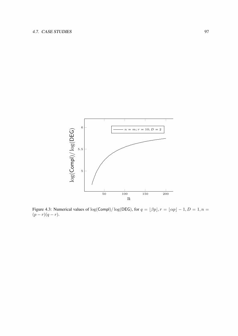
4.7. CASE STUDIES 97

50 100 150 200

5

5.5

6

n

log(C

ompl)/log(D

EG) n = m; r = 10;D = 2

Figure 4.3: Numerical values of log(Compl)/ log(DEG), for q = bβpc, r = bαpc − 1, D = 1, n =(p− r)(q − r).

98 CHAPTER 4. DETERMINANTAL SYSTEMS

Chapter 5

Critical Point Systems

The results presented in this chapter are joint work with J.-C. Faugere and M. Safey El Din. Sections5.1 to 5.6 are published in [FSS12].

In this chapter, we consider the problem of computing critical points of the restriction of a polyno-mial map to an algebraic variety. This is of first importance since the global minimum of such a map isreached at a critical point. Thus, these points appear naturally in non-convex polynomial optimizationwhich occurs in a wide range of scientific applications (control theory, chemistry, economics,...).

Critical points also play a central role in recent algorithms of effective real algebraic geometry.Experimentally, it has been observed that Grobner basis algorithms are efficient to compute suchpoints. Therefore, recent software based on the so-called Critical Point Method are built on Grobnerbases engines.

Let f1, . . . , fp be polynomials in Q[x1, . . . , xn] of degree D, V ⊂ Cn be their complex varietyand π1 be the projection map (x1, . . . , xn) 7→ x1. The critical points of the restriction of π1 to Vare defined by the vanishing of f1, . . . , fp and some maximal minors of the Jacobian matrix associ-ated to f1, . . . , fp. Such a system is algebraically structured: the ideal it generates is the sum of adeterminantal ideal and the ideal generated by f1, . . . , fp.

We provide the first complexity estimates on the computation of Grobner bases of such systemsdefining critical points. We prove that under genericity assumptions on f1, . . . , fp, the complexity ispolynomial in the generic number of critical points, i.e. Dp(D − 1)n−p

(n−1p−1

). More particularly, in

the quadratic case D = 2, the complexity of such a Grobner basis computation is polynomial in thenumber of variables n and exponential in p. We also give experimental evidence supporting thesetheoretical results.

5.1 Introduction

Motivations and problem statement. The local extrema of the restriction of a polynomial map toa real algebraic variety are reached at the critical points of the map under consideration. Hence,computing these critical points is of first importance for polynomial optimization which arises in awide range of applications in engineering sciences (control theory, chemistry, economics, etc.).

Computing critical points is also the cornerstone of algorithms for asymptotically optimal algo-rithms for polynomial system solving over the reals (singly exponential in the number of variables).Indeed, for computing sample points in each connected component of a semi-algebraic set, the al-gorithms based on the so-called critical point method rely on a reduction of the initial problem topolynomial optimization problems. In [BPR96, BPR98] (see also [GV88, HRS89, HRS93]), the best

99

100 CHAPTER 5. CRITICAL POINT SYSTEMS

complexity bounds are obtained using infinitesimal deformation techniques of semi-algebraic geom-etry, nevertheless obtaining efficient implementations of these algorithms remains an issue.

Tremendous efforts have been made to obtain fast implementations relying on the critical pointmethod (see [SS03, ELLS09, Saf07, HS11, HS09, FMRS08, SS04]). This is achieved with tech-niques based on algebraic elimination and complex algebraic geometry. For instance, when the inputpolynomial system (F) : f1 = · · · = fp = 0 in Q[x1, . . . , xn] satisfies genericity assumptions, oneis led to compute the set of critical points of the restriction of the projection on the first coordinateπ1 : (x1, . . . , xn) 7→ x1 to the algebraic variety Z(F) ⊂ Cn defined by F; this set is denoted bycrit(π1, Z(F)).

The set crit(π1, Z(F)) is defined by F and the vanishing of the maximal minors of the truncatedJacobian matrix of F obtained by removing the partial derivatives with respect to x1. This system ishighly-structured: algebraically, we are considering the sum of a determinantal ideal with the ideal〈f1, . . . , fp〉.

In practice, we compute a rational parametrization of this set through Grobner bases computationswhich are fast in practice. We have observed that the behavior of Grobner bases on these systems isspecific: the highest degree reached during the computations is unexpectedly small. In the particularcase of quadratic equations, the complexity of the computation seems to be polynomial in n and ex-ponential in p which meets the best complexity known bound for the quadratic minimization problem:an approximation algorithm with such a complexity is given in [Bar93] (see also [GP05] for generalpolynomial algorithms in optimization). Understanding the complexity of these computations is afirst step towards the design of dedicated Grobner bases algorithms, so we focus on the followingimportant open problems:

(A) Can we provide complexity estimates for the computation of Grobner bases of ideals defined bysuch structured algebraic systems?

(B) Is this computation polynomial in the generic number of critical points?

(C) In the quadratic case, is this computation polynomial in the number of variables (and exponen-tial in the codimension)?

Under genericity assumptions, we actually provide affirmative answers to all these questions.Computational methodology and related complexity issues. Grobner bases are computed us-

ing multi-modular arithmetics and we will focus only on arithmetic complexity results; so we mayconsider systems defining critical points with coefficients not only in Q but also in a prime field.

Let K be a field, K be its algebraic closure and F = (f1, . . . , fp) be a family of polynomials inK[x1, . . . , xn] of degree D and Z(F) be their set of common zeroes in Kn.

We denote the Jacobian matrix ∂f1∂x1

· · · ∂f1∂xn

......

∂fp∂x1

· · · ∂fp∂xn

by jac(F) and the submatrix obtained by removing the first i columns by jac(F, i). The set of maximalminors of a given rectangular matrix M will be denoted by MaxMinors(M).

Finally, let I(F, 1) be the ideal 〈F〉 + 〈MaxMinors(jac(F, 1))〉. When F is a reduced regularsequence and Z(F) is smooth, the algebraic variety associated to I(F, 1) is exactly crit(π1, Z(F)).

So, to compute a rational parametrization of crit(π1, Z(F)), we use the classical solving strategywhich proceeds in two steps:

(i) compute a Grobner basis for a grevlex ordering of I(F, 1) using the F5 algorithm (see [Fau02]);

5.1. INTRODUCTION 101

(ii) use the FGLM algorithm [FGLM93, FM11] to obtain a Grobner basis of I(F, 1) for the lexico-graphical ordering or a rational parametrization of

√I(F, 1).

Algorithm F5 (Step (i)) computes Grobner bases by row-echelon form reductions of submatrices ofthe Macaulay matrix up to a given degree. This latter degree is called degree of regularity. Whenthe input satisfies regularity properties, this complexity of this step can be analyzed by estimating thedegree of regularity.

FGLM algorithm [FGLM93] (Step (ii)) and its recent efficient variant [FM11] are based on com-putations of characteristic polynomials of linear endomorphisms in K[x1, . . . , xn]/I(F, 1). This isdone by performing linear algebra operations of size the degree of I(F, 1) (which is the number ofsolutions counted with multiplicities).

Thus, we are faced to the following problems:

(1) estimate the degree of regularity of the ideal generated by the homogeneous components ofhighest degree of the set of generators F,MaxMinors(jac(F, 1)) and bound the complexity ofcomputing a grevlex Grobner basis of I(F, 1);

(2) provide sharp bounds on the degree of the ideal I(F, 1).

As far as we know, no results are known for problem (1). Problem (2) has already been investigatedin the literature: see [NR09] where some bounds are given on the cardinality of crit(π1, Z(F)). Wegive here a new algebraic proof of these bounds.

Main results. Let K[x1, . . . , xn]D denote f ∈ K[x1, . . . , xn] | deg(f) = D and note that itis a finite-dimensional vector space. In the following, we solve the three aforementioned problemsunder a genericity assumption on F: we actually prove that there exists a non-empty Zariski open setO ⊂ K[x1, . . . , xn]pD such that for all F ∈ O:

(1) the degree of regularity of the ideal generated by the homogeneous components of largest degreeof F,MaxMinors(jac(F, 1)) is dreg = D(p− 1) + (D − 2)n+ 2 (see Theorem 5.5);

(2) the degree of I(F, 1) is ≤ δ = Dp(D − 1)n−p(n−1p−1

).

The degree of regularity given in (1) is obtained thanks to an explicit formula for the Hilbert seriesof the homogeneous ideal under consideration (see Proposition 5.7). This is obtained by taking intoaccount the determinantal structure of some of the generators of the ideal we consider. The aboveestimates are the key results which enable us to provide positive answers to questions A, B and Cunder genericity assumptions.

Before stating complexity results on the computation of critical points with Grobner bases, weneed to introduce a standard notation. Let ω be a real number such that a row echelon form of an× n-matrix with entries in K is computed within O(nω) arithmetic operations in K.

We prove that there exists a non-empty Zariski open set O ⊂ K[x1, . . . , xn]pD such that for allF ∈ O ∩K[x1, . . . , xn]p:

(A) computing a grevlex Grobner basis of I(F, 1) can be done within O((p+

(n−1p

)) (n+dreg

n

)ω)arithmetic operations in K (see Theorem 5.15);

(B) computing a rational parametrization of crit(π1, Z(F)) using Grobner bases can be done withinO(δ4.03ω

)arithmetic operations in K (see Corollary 5.18);

(C) when D = 2 (quadratic case), a rational parametrization of crit(π1, Z(F)) using Grobner basescan be computed within O

((n+2p

2p

)ω+ n23p

(n−1p−1

)3)arithmetic operations in K, this is poly-

nomial in n and exponential in p (see Corollary 5.16).

102 CHAPTER 5. CRITICAL POINT SYSTEMS

We also provide more accurate complexity results. The uniform complexity bound given for an-swering question (B) is rather pessimistic. The exponent 4.03ω being obtained after majorationswhich are not sharp; numerical experiments are given to support this (see Section 5.6). Moreover,under the above genericity assumption, we prove that, when p and D are fixed, computing a rationalparametrization of crit(π1, Z(F)) using Grobner bases is done within O(D3.57n) arithmetic opera-tions in K (see Corollary 5.17).

We also give timings for computing grevlex and lex Grobner bases of I(F, 1) with the MAGMAcomputational algebra system and with the FGb library when K = GF(65521). These experimentsshow that the theoretical bounds on the degree of regularity and on the degree of I(F, 1) (Theorem5.12) are sharp. They also provide some indication on the size of problems that can be tackled inpractice: e.g. when D = 2 and p = 3 (resp. D = 3 and p = 1), random dense systems with n ≤ 21(resp. n ≤ 14) can be tackled (see Section 5.6).

Related works. As far as we know, dedicated complexity analysis of Grobner bases on idealsdefining critical points has not been investigated before. However, as we already mentioned, thedeterminantal structure of the system defining crit(π1, Z(F)) plays a central role in this chapter.

In [FSS10], we provided complexity estimates for the computation of Grobner bases of idealsgenerated by minors of a linear matrix. This is generalized in [FSS11b] for matrices with entriesof degree D. Nevertheless, the analysis which is done here differs significantly from these previousworks. Indeed, in [FSS10, FSS11b] a genericity assumption is done on the entries of the consideredmatrix. We cannot follow the same reasonings since MaxMinors(jac(F, 1)) depends on F. Neverthe-less, it is worthwhile to note that, as in [FSS10, FSS11b], we use properties of determinantal idealsgiven in [CH94].

Bounds on the number of critical points (under genericity assumptions) are given in [NR09] usingthe Giambelli-Thom-Porteous degree bounds on determinantal varieties (see [Ful97, Ex. 14.4.14]).

In [Bar93], the first polynomial time algorithms in n for deciding emptiness of a quadraticsystem of equations over the reals is given. Further complexity results in the quadratic case foreffective real algebraic geometry have been given in [GP05]. In the general case, algorithmsbased on the so-called critical point method are given in [BPR96, BPR98, GV88, HRS89, HRS93].Critical points defined by systems F,MaxMinors(jac(F, 1)) are computed in algorithms given in[BGHM01, BGHM97, BGHP05, BGHP04, BGH+10, SS03, ARS02, FMRS08]. The RAGlib maplepackage implements the algorithms given in [SS03, FMRS08] using Grobner bases.

The systems F,MaxMinors(jac(F, 1)) define polar varieties: indeed, this notion coincides withcritical points in the regular case. In [BGHM01, BGHM97, BGHP05, BGHP04, BGH+10], rationalparametrizations are obtained using the geometric resolution algorithm [GLS01] and a local descrip-tion of these polar varieties. This leads to algorithms computing critical points running in probabilistictime polynomial in Dp(p(D − 1))n−p. Note that this bound for D = 2 and p = n/2 is not satisfac-tory. In this chapter, we also provide complexity estimations for computing critical points but usingGrobner bases, which is the engine we use in practice. Our results provide an explanation of the goodpractical behavior we have observed.

We would like to mention that other dedicated algebraic techniques exist for elimination in deter-minantal varieties. In particular, the determinantal resultant introduced and studied in [Bus04] can beused for this task. It is implemented in the Macaulay2 package Resultants1.

Organization of the chapter. Section 5.2 recalls well-known properties of generic polynomialsystems. Problem (1) mentioned above is tackled in Sections 5.3 and 5.4. Problem (2) is solved atthe end of Section 5.4. Complexity results are derived in Section 5.5. Experimental results supportingthe theoretical results are given in Section 5.6. In Section 5.7, we extend the give a formula for theHilbert series in the mixed case and we generalize the complexity results.

1written by L. Buse, N. Botbol and M. Dubinsky

5.2. PRELIMINARIES 103

5.2 Preliminaries

Notations 5.1. The set of variables x1, . . . , xn is denoted by X . For d ∈ N, Monomials(d) denotesthe set of monomials of degree d in the polynomial ring K[X] (where K is a field, its algebraicclosure being denoted by K). We let a denote the finite set of parameters a(i)

m : 1 ≤ i ≤ p,m ∈⋃0≤d≤DMonomials(d).

We also introduce the following generic systems:

• F = (f1, . . . , fp) ∈ K(a)[X]p is the generic polynomial system of degree D:

fi =∑

m monomialdeg(m)≤D

a(i)m m;

• Fh = (fh1 , . . . , fhp) ∈ K(a)[X]p is the generic homogeneous polynomial system of degree D:

fi =∑

m monomialdeg(m)=D

a(i)m m.

We let Z(F) ⊂ Kndenote the variety of F = (f1, . . . , fp). The projective variety of a homo-

geneous family of polynomials Fh is denoted in this chapter by W (Fh). The projection on the firstcoordinate is denoted by π1, and the critical points of the restriction of π1 to Z(F) are denoted bycrit(π1, Z(F)) ⊂ Z(F). Also, I(F, 1) denotes the ideal generated by F and by the maximal minorsof the truncated Jacobian matrix jac(F, 1).

The goal of this section is to prove that the ideal I(Fh, 1) is 0-dimensional. This will be done inLemma 5.4 below; to do that we will use geometric statements of Sard’s Theorem which require K tohave characteristic 0. This latter assumption can be weakened using algebraic equivalents of Sard’sTheorem (see [Eis95, Corollary 16.23]).

Lemma 5.2. Let I(F, 0) be the ideal generated by F and by the maximal minors of its Jacobian matrix.Its variety Z(I(F, 0)) ⊂ K(a)

nis empty and hence Z(F) is smooth.

Proof. To simplify notations hereafter, we denote by h1, . . . , hp the polynomials obtained fromf1, . . . , fp by removing their respective constant terms a

(1)1 , . . . , a

(p)1 . We will also denote by A the

remaining parameters in h1, . . . , hp. Let ψ denote the mapping

ψ : K(A )n −→ K(A )

p

c 7−→ (h1(c), . . . , hp(c))

Suppose first that ψ(K(A )n) is not dense (for the Zariski topology) in K(A )

p. Since the image

ψ(K(A )n) is a constructible set, it is contained in a proper Zariski closed subset W ⊂ K(A )

p.

Since there is no algebraic relation between a(1)1 , . . . , a

(p)1 and the parameters in A , this implies that

the variety defined by h1 + a(1)1 = · · · = hp + a

(p)1 = 0 is empty and consequently smooth. Since

hi + a(1)i = fi, our statement follows.

Suppose now that ψ(K(A )n) is dense in K(A )

p. Let K0 ⊂ K(A )

pbe the set of critical values

of ψ. By Sard’s Theorem [Sha94, Chap. 2, Sec. 6.2, Thm 2], K0 is contained in a proper closedsubset of K(A )

p. Again, there is no algebraic relation between a

(1)1 , . . . , a

(p)1 and the parameters in

A . Consequently, the variety associated to the ideal generated by the system f1, . . . , fp and by themaximal minors of jac(F) is empty.

104 CHAPTER 5. CRITICAL POINT SYSTEMS

Corollary 5.3. Let I(Fh, 0) be the ideal generated by Fh and by the maximal minors of its Jacobianmatrix. Then the associated projective variety W (I(Fh, 0)) ⊂ Pn−1K(a) is empty.

Proof. For 1 ≤ i ≤ n, we denote by Oi the set

(c1 : . . . : cn) | ci 6= 0 ⊂ Pn−1K(a)

and we consider the canonical open covering of Pn−1K(a):

Pn−1K(a) =⋃

1≤i≤nOi.

Therefore W (I(Fh, 0)) =⋃

1≤i≤n(W (I(Fh, 0)) ∩ Oi). Denote by Fi the system obtained by substi-tuting the variable xi by 1 in Fh. According to Lemma 5.2 applied to Fi, the variety Z(I(Fi, 0)) isempty. Therefore, the set W (I(Fh, 0)) ∩Oi is also empty. Consequently, W (I(Fh, 0)) = ∅.

We can now deduce the following result.

Lemma 5.4. The projective variety W (I(Fh, 1)) ⊂ Pn−1K(a) is empty, and hence dim(I(Fh, 1)) =0.

Proof. We let ϕ0 and ϕ1 denote the two following morphisms:

ϕ0 : K(a)[x1, . . . , xn] → K(a)[x2, . . . , xn]g(x1, . . . , xn) 7→ g(0, x2, . . . , xn)

ϕ1 : K(a)[x1, . . . , xn] → K(a)[x2, . . . , xn]g(x1, . . . , xn) 7→ g(1, x2, . . . , xn)

ThenW (I(Fh, 1)) can be identified with the disjoint union of the variety Z(ϕ1(I(Fh, 1))) ⊂ K(a)n−1

and the projective variety W (ϕ0(I(Fh, 1))) ⊂ Pn−2K(a).

• Notice that ϕ1(I(Fh, 1)) = I(ϕ1(Fh), 0). Therefore, the ideal ϕ1(I(Fh, 1)) ⊂K(a)[x2, . . . , xn] is spanned by ϕ1(Fh) (which is a generic system of degree D in n − 1 vari-ables) and by the maximal minors of its Jacobian matrix. According to Lemma 5.2, the varietyZ(ϕ1(I(Fh, 1))) is empty.

• Similarly, ϕ0(I(Fh, 1)) = I(ϕ0(Fh), 0) ⊂ K(a)[x2, . . . , xn] is generated by the homogeneouspolynomials ϕ0(Fh) and by the maximal minors of the Jacobian matrix jac(ϕ0(Fh)). Thus,according to Corollary 5.3, the variety W (ϕ0(I(Fh, 1))) is also empty.

5.3 The homogeneous case

In this section, our goal is to estimate the degree of regularity of the ideal I(Fh, 1) ⊂ K(a)[X] whichis a homogeneous ideal generated by Fh and MaxMinors(Fh, 1) (see Notations 5.1). Recall that thedegree of regularity dreg(I) of a 0-dimensional homogeneous ideal I is the smallest positive integersuch that all monomials of degree dreg(I) are in I . Notice that dreg(I) is an upper bound on thedegrees of the polynomials in a minimal Grobner basis of I with respect to the grevlex ordering.

5.3. THE HOMOGENEOUS CASE 105

Theorem 5.5. The degree of regularity of the ideal I(Fh, 1) is

dreg(I(Fh, 1)) = D(p− 1) + (D − 2)n+ 2.

Notations 5.6. To prove Theorem 5.5, we need to introduce a few more objects and notations.

• A set of new variables ui,j : 1 ≤ i ≤ p, 2 ≤ j ≤ n which is denoted by U ;

• the determinantal ideal D ⊂ K[U ] generated by the maximal minors of the matrix u1,2 . . . u1,n...

......

up,2 . . . up,n

.• g1, . . . , gp(n−1) which denote the polynomials ui,j − ∂fhi

∂xj, for 1 ≤ i ≤ p, 2 ≤ j ≤ n and

gp(n−1)+1, . . . , gpn which denote the polynomials fh1 , . . . , fhp ;

• the ideals I(`) = D + 〈g1, . . . , g`〉 ⊂ K(a)[U,X];

• if g ∈ K[X] (resp. I ⊂ K[X]) is a polynomial and≺ is a monomial ordering (see e.g. [CLO97,Ch. 2, §2, Def. 1]), LM≺(g) (resp. LM≺(I)) denotes its leading monomial (resp. the idealgenerated by the leading monomials of the polynomials in I);

• a degree ordering is a monomial ordering ≺ such that for all pair of monomials m1,m2 ∈K[X], deg(m1) < deg(m2) implies m1 ≺ m2.

Obviously the polynomials gk for 1 ≤ k ≤ p(n − 1) will be used to mimic the process of

substituting the new variables ui,j by ∂fhi∂xj

; indeed we have I(pn) ∩K[X] = I(Fh, 1).

Our strategy to prove Theorem 5.5 will be to deduce the degree of regularity of I(Fh, 1) from anexplicit form of its Hilbert series.

Proposition 5.7. The Hilbert series of the homogeneous ideal I(Fh, 1) ⊂ K(a)[X] is

HSK(a)[X]/I(Fh,1)(t) =det(A(tD−1))

t(D−1)(p−12 )

(1− tD)p(1− tD−1)n−p

(1− t)n ,

where A(t) is the (p− 1)× (p− 1) matrix whose (i, j)-entry is∑

k

(p−ik

)(n−1−jk

)tk.

The proof of Proposition 5.7 is postponed to Section 5.3.2.

Proof of Theorem 5.5. By definition, the Hilbert series of a zero-dimensional homogeneous ideal isa polynomial of degree dreg−1. By Lemma 5.4, I(Fh, 1) has dimension 0. Thus, using Proposition5.7, we deduce that:

dreg(I(Fh, 1)) = 1 + deg

(det(A(tD−1))

t(D−1)

(p−12

) (1− tD)p(1− tD−1)n−p

(1− t)n

).

The highest degree on each row of A(t) is reached on the diagonal. Thus deg(detA(t)) = p(p−1)2

and a direct degree computation yields dreg(I(Fh, 1)) = D(p− 1) + (D − 2)n+ 2.

From Proposition 5.7, one can also deduce the degree of I(Fh, 1); this provides an alternate proofof [NR09, Theorem 2.2].

106 CHAPTER 5. CRITICAL POINT SYSTEMS

Corollary 5.8. The degree of the ideal I(Fh, 1) is

DEG(I(Fh, 1)) =

(n− 1

p− 1

)Dp(D − 1)n−p.

Proof. By definition of the Hilbert series, the degree of the 0-dimensional homogeneous idealI(Fh, 1) is equal to HSK(a)[X]/I(Fh,1)(1). By Proposition 5.7, direct computations show thatHSK(a)[X]/I(Fh,1)(1) = det(A(1))Dp(D − 1)n−p. The determinant of the matrix A(1) can beevaluated by using Vandermonde’s identity and a formula by Harris-Tu (see e.g. [Ful97, Example14.4.14, Example A.9.4]). We deduce that det(A(1)) =

(n−1p−1

)and hence HSK(a)[X]/I(Fh,1)(1) =(

n−1p−1

)Dp(D − 1)n−p.

It remains to prove Proposition 5.7. This is done in the next sections following several steps:

• provide an explicit form of the Hilbert series of the ideal D ; this is actually already done in[CH94]; we recall the statement of this result in Lemma 5.9;

• deduce from it an explicit form of Hilbert series of the ideal I(pn) using genericity propertiessatisfied by the polynomials gk and properties of quasi-homogeneous ideals; this is done inLemma 5.10;

• deduce from it the Hilbert series associated to I(Fh, 1).

5.3.1 Auxiliary results

We start by restating a special case of [CH94, Cor. 1].

Lemma 5.9 ([CH94, Corollary 1]). The Hilbert series of the ideal D ⊂ K[U ] is HSK[U ]/D(t) =detA(t)

t(p−12 )(1−t)n(p−1)

.

Lemma 5.10. For each 2 ≤ ` ≤ np, g` does not divide 0 in K(a)[U,X]/I(`−1).

Proof. According to [HE70, Thm. 2][HE71], the ring K(a)[U ]/D is a Cohen-Macaulay domain ofKrull dimension (n− 1 + p− (p− 1))(p− 1) = n(p− 1). Therefore, the ring K(a)[U,X]/D is alsoa Cohen-Macaulay domain, and has dimension np.

Consider now the ideal 〈g1, . . . , gnp〉 ⊂ (K(a)[U ]/D)[X]. According to Lemma 5.4, the idealI(Fh, 1) = (D + 〈g1, . . . , gn(p−1)〉) ∩ K(a)[X] is zero-dimensional. Let ≺ denote a lexicographicalmonomial ordering such that for all i, j, k, ui,j xk. Since the variables U can be expressed asfunctions of X (ui,j − ∂fi

∂xj∈ I(pn)), we have LM≺(D + 〈g1, . . . , gnp〉) = 〈ui,j〉 + LM≺(I(Fh, 1))

which is zero-dimensional. Therefore, the ideal D + 〈g1, . . . , gnp〉 ⊂ K(a)[U,X] is zero-dimensionaland hence so is 〈g1, . . . , gnp〉 ⊂ K(a)[U,X]/D . Now suppose by contradiction that there exists `such that g` divides 0 in K(a)[U,X]/I(`−1). Let `0 be the smallest integer satisfying this property.Since D is equidimensional and for all ` < `0, g` does not divide 0 in K(a)[U,X]/I(`−1), the ideal〈g1, . . . , g`0−1〉 ⊂ K(a)[U,X]/D is equidimensional, has codimension `0 − 1, and thus has no em-bedded components by the unmixedness Theorem [Eis95, Corollary 18.14]. Since g`0 divides 0 in thering K(a)[U,X]/(D + 〈g1, . . . , g`0−1〉), the ideal 〈g1, . . . , g`0〉 ⊂ K(a)[U,X]/D has also codimen-sion `0 − 1. Therefore the codimension of 〈g1, . . . , gnp〉 ⊂ K(a)[U,X]/D is strictly less than np,which leads to a contradiction since we have proved that the dimension of this ideal is 0.

5.3. THE HOMOGENEOUS CASE 107

The degrees in the matrix whose entries are the variables ui,j have to be balanced with D− 1, thedegree of the partial derivatives. This is done by changing the gradation by putting a weight on thevariables ui,j , giving rise to quasi-homogeneous polynomials.

The following lemma and its proof are similar to Lemma 4.8.

Lemma 5.11. The Hilbert series of I(Fh, 1) ⊂ K(a)[X] and the weighted Hilbert series of I(pn) ⊂K(a)[U,X] are equal.

Proof. Let≺lex be a lex ordering on the variables of the polynomial ring K(a)[U,X] such that xk ≺lex

ui,j for all k, i, j. By [CLO97, Sec. 6.3, Prop. 9], HSK(a)[X]/I(Fh,1)(t) = HSK(a)[X]/ LM≺lex(I(Fh,1))(t)

and wHSK(a)[U,X]/I(p(n−1))(t) = wHSK(a)[U,X]/ LM≺lex

(I(p(n−1)))(t). Since LM≺lex(ui,j − fi,j) = ui,j

and I(pn) ∩K[X] = I(Fh, 1), we deduce that

LM≺lex(I(pn)) =

⟨ui,j ∪ LM≺lex

(I(pn) ∩K(a)[X])⟩

=⟨ui,j ∪ LM≺lex

(I(Fh, 1))⟩.

Therefore, K(a)[U,X]LM≺lex

(I(pn))is isomorphic (as a graded K(a)-algebra) to K(a)[X]

LM≺lex(I(Fh,1))

.

Thus, HSK(a)[X]/ LM≺lex(I(Fh,1))(t) = wHSK(a)[U,X]/ LM≺lex

(I(pn))(t), and henceHSK(a)[X]/I(Fh,1)(t) = wHSK(a)[U,X]/I(pn)(t).

5.3.2 Proof of Proposition 5.7

We reuse Notations 5.6: I(Fh, 1) = (D + 〈g1, . . . , gpn〉) ∩ K(a)[X]. According to Lemma 5.9 andby putting a weight D − 1 on the variables U , the weighted Hilbert series of D ⊂ K(a)[U ] is

wHSK(a)[U ]/D(t) =detA(tD−1)

t(D−1)(p−12 )(1− tD−1)n(p−1)

.

Considering D as an ideal of K(a)[U,X], we obtain

wHSK(a)[U,X]/D(t) =1

(1− t)n wHSK(a)[U ]/D(t).

If I ⊂ K(a)[U,X] is a quasi-homogeneous ideal and if g is a quasi-homogeneous polynomial ofweight degree d which does not divide 0 in the quotient ring K(a)[U,X]/I , then the Hilbert series ofthe ideal I + 〈g〉 is equal to (1− td) multiplied by the Hilbert series of I (Proposition 1.41).

Notice that the polynomials g1, . . . , gp(n−1) are quasi-homogeneous of weight degree D − 1

(these polynomials have the form ui,j − ∂fi∂xj

) and the polynomials gp(n−1)+1, . . . , gpn are quasi-homogeneous of weight degree D (these polynomials are f1, . . . , fp). Since g` does not divide 0in K(a)[U,X]/I(`−1) (Lemma 5.10), the Hilbert series of the ideal I(pn) ⊂ K(a)[U,X] is

wHSK(a)[U,X]/I(pn)(t) =detA(tD−1)

t(D−1)(p−12 )

(1− tD)p(1− tD−1)n−p

(1− t)n .

Finally, by Lemma 5.11, wHSK(a)[U,X]/I(pn)(t) = HSK(a)[X]/I(Fh,1)(t).

108 CHAPTER 5. CRITICAL POINT SYSTEMS

5.4 The affine case

The degree of regularity of a polynomial system is the highest degree reached during the computa-tion of a Grobner basis with respect to the grevlex ordering with the F5 algorithm. Therefore, it is acrucial indicator of the complexity of the Grobner basis computation. On the other hand, the com-plexity of the FGLM algorithm depends on the degree of the ideal I(F, 1) since this value is equal todimK (K[X]/I(F, 1)).

In this section, we show that the bounds on the degree and the degree of regularity of the idealI(Fh, 1) are also valid for (not necessarily homogeneous) polynomial families in K[X] under gener-icity assumptions.

Theorem 5.12. There exists a non-empty Zariski open subset O ⊂ K[X]pD such that, for any F inO ∩K[X]p,

dreg(I(F, 1)) ≤ D(p− 1) + (D − 2)n+ 2,

DEG(I(F, 1)) ≤(n−1p−1

)Dp(D − 1)n−p.

In the sequel, K[X]D denotes f ∈ K[X] | deg(f) = D, and K[X]D,hom denotes the homoge-neous polynomials in K[X]D. In order to prove Theorem 5.12 (the proof is postponed to the end ofthis section), we first need two technical lemmas.

Lemma 5.13. There exists a non-empty Zariski open subset O ⊂ K[X]pD,hom such that for all Fh ∈O ∩K[X]p, LM≺(I(Fh, 1)) = LM≺(I(Fh, 1)).

Proof. See e.g. [FSS11b, Proof of Lemma 2] for a similar proof.

Lemma 5.14. Let G = (g1, . . . , gm) be a polynomial family and let Gh = (gh1 , . . . , ghm) denote the

family of homogeneous components of highest degree of G. If the dimension of the ideal 〈Gh〉 is 0,then DEG(〈G〉) ≤ DEG(〈Gh〉).

Proof. Let ≺ be an admissible degree monomial ordering. Let LM≺(h) denote the leading mono-mial of a polynomial h with respect to ≺. Let m ∈ LM≺(〈Gh〉) be a monomial. Then thereexist polynomials s1, . . . , sm such that LM≺

(∑mi=1 sig

hi

)= m. Since ≺ is a degree ordering,

LM≺ (∑m

i=1 sigi) = m. Therefore LM≺(〈Gh〉) ⊂ LM≺(〈G〉). If the ideal 〈Gh〉 is 0-dimensional,then so is 〈G〉 and DEG(LM≺(〈G〉)) ≤ DEG(LM≺(〈G〉)). Since DEG(I) = DEG(LM≺(I)), weobtain DEG(〈G〉) ≤ DEG(〈Gh〉).

Proof of Theorem 5.12. Let≺ be a degree monomial ordering, and Fh = (fh1 , . . . , fhp ) ∈ K[X]pD,hom

denote the homogeneous system where fhi is the homogeneous component of highest degree of fi. ByLemma 5.13, there exists a non-empty Zariski subset O ⊂ K[X]pD such that, for any F in O ∩K[X]p,LM≺(I(Fh, 1)) = LM≺(I(Fh, 1)). By [CLO97, Ch.9, §3, Prop.9], the Hilbert series (and thus thedimension, the degree, and the degree of regularity) of a homogeneous ideal is the same as that of itsleading monomial ideal. Hence, by Lemma 5.4,

dim(I(Fh, 1)) = dim(LM≺(I(Fh, 1))) = dim(LM≺(I(Fh, 1)))= dim(I(Fh, 1)) = 0.

Similarly, by Theorem 5.5,

dreg(I(Fh, 1)) = dreg(I(Fh, 1)) = D(p− 1) + (D − 2)n+ 2.

5.5. COMPLEXITY 109

The highest degree reached during the F5 Algorithm is bounded above by the degree of regularityof the ideal generated by the homogeneous components of highest degree of the generators whenthis homogeneous ideal has dimension 0 (see e.g. [BFSY04] and references therein). Therefore, thehighest degree reached during the computation of a Grobner basis of I(F, 1) with the F5 Algorithmwith respect to a degree ordering is bounded above by

dreg ≤ D(p− 1) + (D − 2)n+ 2.

The bound on the degree is obtained by Corollary 5.8 and Lemma 5.14,

DEG(I(F, 1)) ≤ DEG(I(Fh, 1)) ≤ DEG(LM≺(I(Fh, 1)))

≤(n−1p−1

)Dp(D − 1)n−p.

5.5 Complexity

In the sequel, ω is a real number such that there exists an algorithm which computes the row echelonform of n×n matrix in O(nω) arithmetic operations (the best known value is ω ≈ 2.376 by using theCoppersmith-Winograd algorithm, see [Sto00]).

Theorem 5.15. There exists a non-empty Zariski open subset O ⊂ K[X]pD, such that, for all F ∈O ∩ K[X]p, the arithmetic complexity of computing a lexicographical Grobner basis of I(F, 1) isbounded by

O

((p+

(n− 1

p

))(D(p− 1) + (D − 1)n+ 2

D(p− 1) + (D − 2)n+ 2

)ω+ n

(n− 1

p− 1

)3

D3p(D − 1)3(n−p)

).

Proof. According to [BFS04, BFSY04], the complexity of computing a Grobner basis with the F5 Al-gorithm with respect to the grevlex ordering of a zero-dimensional ideal is bounded by O

(m(n+dreg

dreg

)ω)where dreg is the highest degree reached during the computation and m is the number of polynomialsgenerating the ideal. In order to obtain a lexicographical Grobner basis, one can use the FGLM al-gorithm [FGLM93]. Its complexity is O

(nDEG(I(F, 1))3

)(better complexity bounds are known in

specific cases, see [FM11]).According to Theorem 5.12, there exists a non-empty Zariski open subset O ⊂ K[X]pD such that,

for all F in O ∩K[X]p,

dreg(I(F, 1)) ≤ D(p− 1) + (D − 2)n+ 2,

DEG(I(F, 1)) ≤(n−1p−1

)Dp(D − 1)n−p.

Therefore, for all F in O ∩K[X]p, the total complexity of computing a lexicographical Grobner basisof I(F, 1):

O

((p+

(n− 1

p

))(D(p− 1) + (D − 1)n+ 2

D(p− 1) + (D − 2)n+ 2

)ω+ n

(n− 1

p− 1

)3

D3p(D − 1)3(n−p)

).

110 CHAPTER 5. CRITICAL POINT SYSTEMS

Corollary 5.16. If D = 2, then there exists a non-empty Zariski open subset O ⊂ K[X]p2, such thatfor all F ∈ O ∩ K[X]p, the arithmetic complexity of computing a lexicographical Grobner basis ofI(F, 1) is bounded by

O

((p+

(n− 1

p

))(n+ 2p

2p

)ω+ n23p

(n− 1

p− 1

)3).

Moreover, if p is constant and D = 2, the arithmetic complexity is bounded by O(np(2ω+1)

).

Proof. This complexity is obtained by putting D = 2 in the formula from Theorem 5.15.

In the sequel, the binary entropy function is denoted by h2:

∀x ∈ [0, 1], h2(x) = −x log2(x)− (1− x) log2(1− x).

Corollary 5.17. LetD > 2 and p ∈ N be constant. There exists a non-empty Zariski open subset O ⊂K[X]pD, such that, for all F ∈ O ∩K[X]p, the arithmetic complexity of computing a lexicographicalGrobner basis of I(F, 1) is bounded by

O

(np√n

2(D−1)h2( 1D−1)nω

)= O

((D − 1)3.57n

).

Proof. Let x be a real number in [0, 1]. Then by applying Stirling’s Formula, we obtain that(nxn

)=

O(

1√n

2h2(x)n). Therefore,

((D−1)n

n

)= O

(1√n

2(D−1)h2( 1D−1)n

)= O

(1√n

((D − 1)e)n).

Let C denote the constant D(p− 1) + 2. Then(D(p−1)+(D−1)n+2D(p−1)+(D−2)n+2

)=

((D−1)n+C

n

)= O

(((D−1)n

n

))= O

(1√n

2(D−1)h2( 1D−1)n

).

The right summand in the complexity formula given in Theorem 5.15 is O(n3p(D − 1)3n

)when p

and D are constants; this is bounded by O(

1√n

2(D−1)h2( 1D−1)nω

). Let O be the non-empty Zariski

open subset defined in Theorem 5.15. For all F ∈ O∩K[X]p, the arithmetic complexity of computinga grevlex Grobner basis of F is bounded by

O(np√n

2(D−1)h2( 1D−1)nω

)=O

(np√n

((D − 1)e)nω)

= O((D − 1)(1+1/ log(D−1))nω

)= O

((D − 1)3.57n

),

since D ≥ 3 and ω ≤ 2.376 with the Coppersmith-Winograd algorithm. On the other hand theasymptotic complexity of the FGLM part of the solving process is

O(n3(p−1)+1(D − 1)3n

)= O

((D − 1)3n

),

which is bounded above by the complexity of the grevlex Grobner basis computation.

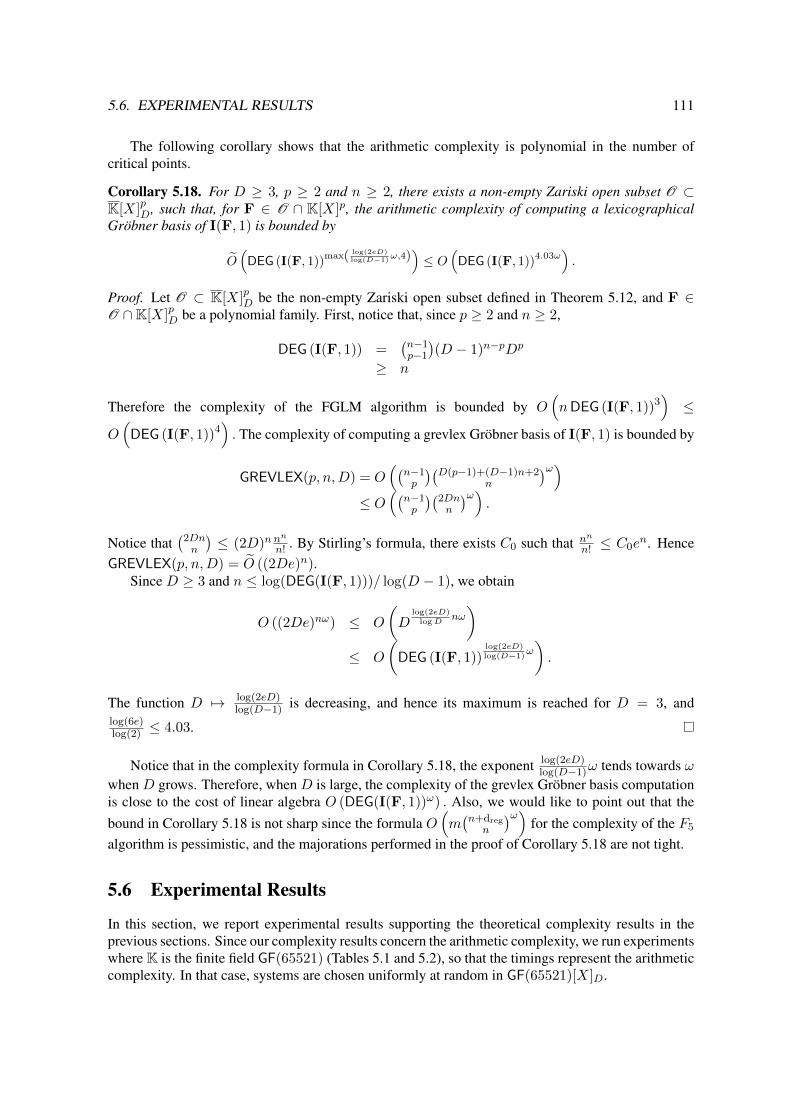
5.6. EXPERIMENTAL RESULTS 111

The following corollary shows that the arithmetic complexity is polynomial in the number ofcritical points.

Corollary 5.18. For D ≥ 3, p ≥ 2 and n ≥ 2, there exists a non-empty Zariski open subset O ⊂K[X]pD, such that, for F ∈ O ∩ K[X]p, the arithmetic complexity of computing a lexicographicalGrobner basis of I(F, 1) is bounded by

O(DEG (I(F, 1))

max( log(2eD)log(D−1)

ω,4))≤ O

(DEG (I(F, 1))

4.03ω).

Proof. Let O ⊂ K[X]pD be the non-empty Zariski open subset defined in Theorem 5.12, and F ∈O ∩K[X]pD be a polynomial family. First, notice that, since p ≥ 2 and n ≥ 2,

DEG (I(F, 1)) =(n−1p−1

)(D − 1)n−pDp

≥ n

Therefore the complexity of the FGLM algorithm is bounded by O(nDEG (I(F, 1))3

)≤

O(DEG (I(F, 1))4

). The complexity of computing a grevlex Grobner basis of I(F, 1) is bounded by

GREVLEX(p, n,D) = O((

n−1p

)(D(p−1)+(D−1)n+2

n

)ω)≤ O

((n−1p

)(2Dnn

)ω).

Notice that(

2Dnn

)≤ (2D)n n

n

n! . By Stirling’s formula, there exists C0 such that nn

n! ≤ C0en. Hence

GREVLEX(p, n,D) = O ((2De)n).Since D ≥ 3 and n ≤ log(DEG(I(F, 1)))/ log(D − 1), we obtain

O ((2De)nω) ≤ O

(D

log(2eD)logD

nω)

≤ O

(DEG (I(F, 1))

log(2eD)log(D−1)

ω).

The function D 7→ log(2eD)log(D−1) is decreasing, and hence its maximum is reached for D = 3, and

log(6e)log(2) ≤ 4.03.

Notice that in the complexity formula in Corollary 5.18, the exponent log(2eD)log(D−1)ω tends towards ω

when D grows. Therefore, when D is large, the complexity of the grevlex Grobner basis computationis close to the cost of linear algebra O (DEG(I(F, 1))ω) . Also, we would like to point out that thebound in Corollary 5.18 is not sharp since the formula O

(m(n+dreg

n

)ω)for the complexity of the F5

algorithm is pessimistic, and the majorations performed in the proof of Corollary 5.18 are not tight.

5.6 Experimental Results

In this section, we report experimental results supporting the theoretical complexity results in theprevious sections. Since our complexity results concern the arithmetic complexity, we run experimentswhere K is the finite field GF(65521) (Tables 5.1 and 5.2), so that the timings represent the arithmeticcomplexity. In that case, systems are chosen uniformly at random in GF(65521)[X]D.

112 CHAPTER 5. CRITICAL POINT SYSTEMS

n p D dreg DEG F4 time FGLM time9 4 2 8 896 3.12s 18.5s

11 4 2 8 1920 61s 202s13 4 2 8 3520 369s 1372s15 4 2 8 5824 2280s 7027s17 4 2 8 8960 10905s >1d30 2 2 4 116 3.00s 0.14s35 2 2 4 136 7.5s 0.36s40 2 2 4 156 13.3s 0.64s6 4 3 17 3240 16s 400s8 4 3 19 45360 35593s >1d7 2 3 12 1728 9.9s 91s8 2 3 13 4032 121s 1169s9 2 3 14 9216 736s >1d

Table 5.1: Timings using MAGMA and K = GF(65521).

n p D DEG(I(F, 1)) F5 time FGLM time matrix density16 3 2 840 2.20s 0.03s 36.91%18 3 2 1088 4.62s 0.12s 37.00%20 3 2 1368 9.54s 0.10s 37.07%15 4 2 5824 131.65 10.66s 33.53%17 4 2 8960 480.9s 68.9s 34.00%19 4 2 13056 1600.1s 215.1s 34.35%21 4 2 18240 10371.7s 590.3s 34.62%10 1 3 1536 1.5s 0.15s 20.84%12 1 3 6144 19.6s 2.46s 19.32%14 1 3 24576 1759s 587s 18.08%7 2 3 1728 1.4s 0.14s 20.73%9 2 3 9216 105s 37s 19.47%

10 2 3 20736 909s 504s 19.08%7 3 3 6480 31.3s 3.81s 17.39%8 4 3 45360 5126.9s 3833.9s 15.15%8 2 4 81648 21362.6s 19349.4s 13.26%7 3 4 77760 13856.8s 16003s 11.83%

Table 5.2: Timings using the FGb library and K = GF(65521).

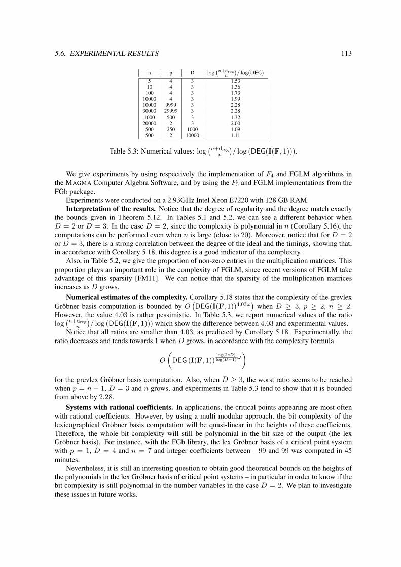
5.6. EXPERIMENTAL RESULTS 113

n p D log(n+dreg

n

)/ log(DEG)

5 4 3 1.5310 4 3 1.36100 4 3 1.73

10000 4 3 1.9910000 9999 3 2.2830000 29999 3 2.281000 500 3 1.3220000 2 3 2.00

500 250 1000 1.09500 2 10000 1.11

Table 5.3: Numerical values: log(n+dreg

n

)/ log (DEG(I(F, 1))).

We give experiments by using respectively the implementation of F4 and FGLM algorithms inthe MAGMA Computer Algebra Software, and by using the F5 and FGLM implementations from theFGb package.

Experiments were conducted on a 2.93GHz Intel Xeon E7220 with 128 GB RAM.Interpretation of the results. Notice that the degree of regularity and the degree match exactly

the bounds given in Theorem 5.12. In Tables 5.1 and 5.2, we can see a different behavior whenD = 2 or D = 3. In the case D = 2, since the complexity is polynomial in n (Corollary 5.16), thecomputations can be performed even when n is large (close to 20). Moreover, notice that for D = 2or D = 3, there is a strong correlation between the degree of the ideal and the timings, showing that,in accordance with Corollary 5.18, this degree is a good indicator of the complexity.

Also, in Table 5.2, we give the proportion of non-zero entries in the multiplication matrices. Thisproportion plays an important role in the complexity of FGLM, since recent versions of FGLM takeadvantage of this sparsity [FM11]. We can notice that the sparsity of the multiplication matricesincreases as D grows.

Numerical estimates of the complexity. Corollary 5.18 states that the complexity of the grevlexGrobner basis computation is bounded by O

(DEG(I(F, 1))4.03ω

)when D ≥ 3, p ≥ 2, n ≥ 2.

However, the value 4.03 is rather pessimistic. In Table 5.3, we report numerical values of the ratiolog(n+dreg

n

)/ log (DEG(I(F, 1))) which show the difference between 4.03 and experimental values.

Notice that all ratios are smaller than 4.03, as predicted by Corollary 5.18. Experimentally, theratio decreases and tends towards 1 when D grows, in accordance with the complexity formula

O

(DEG (I(F, 1))

log(2eD)log(D−1)

ω)

for the grevlex Grobner basis computation. Also, when D ≥ 3, the worst ratio seems to be reachedwhen p = n − 1, D = 3 and n grows, and experiments in Table 5.3 tend to show that it is boundedfrom above by 2.28.

Systems with rational coefficients. In applications, the critical points appearing are most oftenwith rational coefficients. However, by using a multi-modular approach, the bit complexity of thelexicographical Grobner basis computation will be quasi-linear in the heights of these coefficients.Therefore, the whole bit complexity will still be polynomial in the bit size of the output (the lexGrobner basis). For instance, with the FGb library, the lex Grobner basis of a critical point systemwith p = 1, D = 4 and n = 7 and integer coefficients between −99 and 99 was computed in 45minutes.

Nevertheless, it is still an interesting question to obtain good theoretical bounds on the heights ofthe polynomials in the lex Grobner basis of critical point systems – in particular in order to know if thebit complexity is still polynomial in the number variables in the case D = 2. We plan to investigatethese issues in future works.

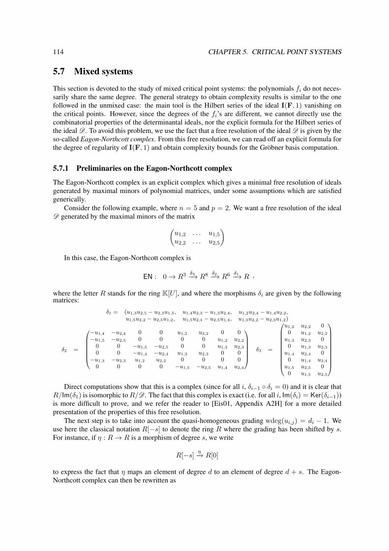
114 CHAPTER 5. CRITICAL POINT SYSTEMS

5.7 Mixed systems

This section is devoted to the study of mixed critical point systems: the polynomials fi do not neces-sarily share the same degree. The general strategy to obtain complexity results is similar to the onefollowed in the unmixed case: the main tool is the Hilbert series of the ideal I(F, 1) vanishing onthe critical points. However, since the degrees of the fi’s are different, we cannot directly use thecombinatorial properties of the determinantal ideals, nor the explicit formula for the Hilbert series ofthe ideal D . To avoid this problem, we use the fact that a free resolution of the ideal D is given by theso-called Eagon-Northcott complex. From this free resolution, we can read off an explicit formula forthe degree of regularity of I(F, 1) and obtain complexity bounds for the Grobner basis computation.

5.7.1 Preliminaries on the Eagon-Northcott complex

The Eagon-Northcott complex is an explicit complex which gives a minimal free resolution of idealsgenerated by maximal minors of polynomial matrices, under some assumptions which are satisfiedgenerically.

Consider the following example, where n = 5 and p = 2. We want a free resolution of the idealD generated by the maximal minors of the matrix(

u1,2 . . . u1,5

u2,2 . . . u2,5

)In this case, the Eagon-Northcott complex is

EN : 0→ R3 δ3−→ R8 δ2−→ R6 δ1−→ R ,

where the letter R stands for the ring K[U ], and where the morphisms δi are given by the followingmatrices:

δ1 = (u1,3u2,5 − u2,3u1,5, u1,4u2,3 − u1,3u2,4, u1,2u2,4 − u1,4u2,2,u1,5u2,2 − u2,5u1,2, u1,5u2,4 − u2,5u1,4, u1,3u2,2 − u2,3u1,2)

δ2 =

−u1,4 −u2,4 0 0 u1,2 u2,2 0 0−u1,5 −u2,5 0 0 0 0 u1,2 u2,2

0 0 −u1,5 −u2,5 0 0 u1,3 u2,3

0 0 −u1,4 −u2,4 u1,3 u2,3 0 0−u1,3 −u2,3 u1,2 u2,2 0 0 0 0

0 0 0 0 −u1,5 −u2,5 u1,4 u2,4

δ3 =

u1,2 u2,2 00 u1,2 u2,2

u1,3 u2,3 00 u1,3 u2,3

u1,4 u2,4 00 u1,4 u2,4

u1,5 u2,5 00 u1,5 u2,5

Direct computations show that this is a complex (since for all i, δi−1 δi = 0) and it is clear that

R/Im(δ1) is isomorphic toR/D . The fact that this complex is exact (i.e. for all i, Im(δi) = Ker(δi−1))is more difficult to prove, and we refer the reader to [Eis01, Appendix A2H] for a more detailedpresentation of the properties of this free resolution.

The next step is to take into account the quasi-homogeneous grading wdeg(ui,j) = di − 1. Weuse here the classical notation R[−s] to denote the ring R where the grading has been shifted by s.For instance, if η : R→ R is a morphism of degree s, we write

R[−s] η−→ R[0]

to express the fact that η maps an element of degree d to an element of degree d + s. The Eagon-Northcott complex can then be rewritten as

5.7. MIXED SYSTEMS 115

EN : 0→ R[−3d1 − d2 − 4]⊕R[−2d1 − 2d2 − 4]⊕R[−d1 − 3d2 − 4]δ4−→

(R[−2d1 − d2 − 3]⊕R[−d1 − 2d2 − 3])4 δ3−→ R[−d1 − d2 − 2]6δ2−→ R[0]

δ1−→ R/D → 0.

This approach can be generalized as follows. Let R be a ring. Following the notations in [Eis01,Appendix A2H], we write F = Rf and G = Rg, where f and g are two integers such that g < f .For a g × f matrix whose entries are in R, we let α : F → G denote the corresponding morphism ofmodules. The Eagon-Northcott complex is then defined by:

EN(α) : 0→ (Symf−gG)∗ ⊗∧f Fδf−g−1−−−−→ (Symf−g−1G)∗ ⊗∧f−1 F

δf−g−−−→· · · → (Sym2G)∗ ⊗∧g+2 F

δ3−→ G∗ ⊗∧g+1 Fδ2−→ ∧g F

∧gα−−→ ∧g G,

where SymiG is the R-module of elements of order i in the symmetric algebra Sym(G).First, notice that as a R-module, SymiG, (and hence also its dual (SymiG)∗) is a free module

isomorphic to R(i+g−1i ). Similarly,

∧i F is isomorphic to R(fi).For a detailed description of the maps δi, we refer the reader to [Eis01, Appendix A2H],[Eis95,

Appendix A2.6]. In the context of this chapter, f = n− 1, g = p, R = K[U ] with the gradation givenby wdeg(ui,j) = di − 1, and the morphism α corresponds to the matrix

U =

u1,2 . . . u1,n...

......

up,2 . . . up,n

.

Using the notation s =∑

1≤i≤p(di − 1), and taking into account the gradation of K[U ], the complexcan be rewritten as

EN(α) : 0→ ⊕i1+...+ip

=n−p−1

R

[−s− ∑

1≤j≤pij(dj − 1)

]δf−g−1−−−−→ ⊕

i1+...+ip=

n−p−2

R

[−s− ∑

1≤j≤pij(dj − 1)

](n−1n−2)

δf−g−−−→

→ ⊕i1+...+ip

= 2

R

[−s− ∑

1≤j≤pij(dj − 1)

](n−1p+2)

δ3−→ ⊕1≤i≤p

R [−s− (di − 1)](n−1p+1) δ2−→

→ R[−s](n−1p ) ∧gα−−→ R[0].

5.7.2 Hilbert series and degree of regularity in the mixed case

In this section, we use the Eagon-Northcott complex to obtain an explicit formula for the Hilbertseries and the degree of regularity of the ideal I(F, 1) in the mixed case. Indeed, the Hilbert seriesof an ideal I can be computed when a free resolution is known, since the Hilbert series of I is equalto the alternate sum of the Hilbert series of the modules occurring in the resolution (see e.g. [Eis01,Theorem 1.11] for more details).

This is a generalization of the results in the unmixed case. However, in the unmixed case, we wereable to use the combinatorial properties of the ideal D in order to obtain a compact formula for thenumerator of the rational function wHSK[U ]/D(t) (where the determinantal structure appears as thedeterminant of the matrix Ap,qr (t)).

In the mixed case, the analysis is more complicated, but it also leads to an explicit formula for thedegree of regularity of the ideal I(F, 1).

116 CHAPTER 5. CRITICAL POINT SYSTEMS

Proposition 5.19. The weighted Hilbert series of the ideal D ⊂ K[U ] generated by the maximalminors of the matrix U with wdeg(ui,j) = di − 1 is the power series expansion of the rationalfunction

wHSK[U ]/D(t) =

1−[ ∑

0≤k≤n−p−1

[(−1)k

∑i1+...+ip=k

(n−1p+k

)t

∑1≤j≤p

(ij+1)(dj−1)]]

∏1≤i≤p(1− tdi−1)n−1

.

Proof. According to [Eis01, Theorem 1.11], the Hilbert series of a graded ideal can be computed froma minimal free resolution: it is equal to the alternate sum of the Hilbert series of the free modulesoccurring in the resolution. For i, j ∈ N, the Hilbert series of R[−i]j is equal to

wHSR[−i]j (t) =jti∏

1≤i≤p(1− tdi−1)n−1.

Moreover, the Hilbert series of a direct sum of modules is equal to the sum of their Hilbert series.Therefore, by using the Eagon-Northcott complex which is a free resolution of D , direct computationsyield the formula for the weighted Hilbert series of D .

Corollary 5.20. Let Fh is a generic system of homogeneous polynomial equations of degrees(d1, . . . , dp), with di ≥ 2 for all i. The Hilbert series of I(Fh, 1) ⊂ K(a)[X] is

HSK(a)[X]/I(Fh,1)(t) = wHSK[U ]/D(t) ·∏

1≤i≤p(1− tdi)(1− tdi−1)n−1

(1− t)n .

Proof. Let D denote the ideal D ·K(a)[X,U ] ⊂ K(a)[X,U ] (where the quasi-homogeneous gradingof K(a)[X,U ] is given by wdeg(xi) = 1, wdeg(ui,j) = di − 1). Therefore, the Hilbert series of D is

wHSK(a)[U,X]/D(t) =

wHSK(a)[U ]/D(t)

(1− t)n .

We recall that, with the notations of Lemma 5.10,

I(Fh, 1) =(D + 〈g1, . . . , gnp〉

)∩K(a)[X].

According to Lemma 5.10, for each 2 ≤ ` ≤ np, g` does not divide 0 in R/I`−1. Therefore, aproof similar to that of Proposition 5.7 shows that the Hilbert series of I(Fh, 1) is equal to

HSK(a)[X]/I(Fh,1)(t) = wHSK(a)[U,X]/D(t)∏

1≤i≤p(1− tdi)(1− tdi−1)n−1

= wHSK(a)[U ]/D(t) ·∏

1≤i≤p(1− tdi)(1− tdi−1)n−1

(1− t)n .

Corollary 5.21. The degree of regularity of I(Fh, 1) is

dreg(I(Fh, 1)) = (n− p− 1) maxdi − 1 − n− p+ 1 + 2∑

1≤i≤pdi.

5.7. MIXED SYSTEMS 117

Proof. According to Lemma 5.4, the ideal I(Fh, 1) is 0-dimensional. Consequently, HSK(a)[X]/I(Fh,1)

is a polynomial and dreg = deg(HSK(a)[X]/I(Fh,1)) + 1. Let j0 be the index of one of the maximaldegrees of the polynomials fj : deg(fj0) = maxdeg(fj). In the sums in the numerator of theformula given in Proposition 5.19, the maximal degree is reached when k = n− p− 1, ij0 = k, andij = 0 for j 6= j0. Therefore the degree of the numerator of wHSK(a)[U ]/D(t) is equal to

deg

(1−

[ ∑0≤k≤n−p−1

[(−1)k

∑i1+...+ip=k

(n−1p+k

)t

∑1≤j≤p

(ij+1)(dj−1)]])

= (n− p− 1)(maxdj − 1) +∑

1≤j≤p(dj − 1).

On the other hand, we have

deg

∏1≤i≤p

(1− tdi−1)n−1

= (n− 1)∑

1≤i≤p(di − 1);

deg

∏1≤i≤p

(1− tdi)(1− tdi−1)n−1

=∑

1≤i≤pdi + (n− 1)

∑1≤i≤p

(di − 1);

deg ((1− t)n) = n.

Therefore, using the formula in Corollary 5.20, we obtain

deg(HSK(a)[X]/I(Fh,1)) = (n− p− 1)(maxdj − 1) +∑

1≤j≤p(dj − 1)− (n− 1)

∑1≤i≤p

(di − 1)+∑1≤i≤p

di + (n− 1)∑

1≤i≤p(di − 1)− n

= (n− p− 1) maxdi − 1 − n− p+ 2∑

1≤i≤pdi,

and hence dreg = (n− p− 1) maxdi − 1 − n− p+ 1 + 2∑

1≤i≤pdi.

5.7.3 Complexity

In this section, we show that under genericity assumptions Grobner bases of mixed critical pointsystems can be computed with a complexity which is polynomial in the generic number of criticalpoints in two cases:

1. when p is a constant;

2. when all degrees are bounded above by a constant D ∈ N.

Theorem 5.22. Let p ∈ N be a fixed integer and di ≥ 2 for all i ∈ 1, . . . , p, then there exists anonempty Zariski open subset O ⊂ K[X]d1 × · · · × K[X]dp , such that for all F ∈ O ∩ K[X]p, thecomplexity of computing a lexicographical Grobner basis of I(F, 1) is polynomial in the number ofcritical points:

∀p ∈ N∗, ∃b > 0, ∃c > 0, ∀(d1, . . . , dp) ∈ 2, 3, . . .p, ∃ a nonempty Zariskiopen subset O ⊂ K[X]d1 × · · · ×K[X]dp , s.t.

F ∈ O ∩K[X]p ⇒ (Compl ≤ b ·# critc),

118 CHAPTER 5. CRITICAL POINT SYSTEMS

where Compl denotes the number of arithmetic operations during the computation of a lex Grobnerbasis of I(F, 1) with the algorithms F5 and FGLM, and # crit =

(∏1≤i≤p di

)∑i1+···+ip=n−p(d1 −

1)i1 . . . (dp − 1)ip is the generic number of critical points.

Proof. Since the algorithm FGLM is polynomial in the degree of the ideal, it is sufficient to provethat computing a grevlex Grobner basis of I(F, 1) is also polynomial in # crit. If all polynomialsf1, . . . , fp are quadratic, then Corollary 5.18 concludes the proof. Therefore, we assume in the sequelthat max(di) ≥ 3. According to [NR09],

# crit =

∏1≤i≤p

di

∑i1+···+ip=n−p

(d1 − 1)i1 . . . (dp − 1)ip .

Let A (resp. G) be the arithmetic (resp. geometric) average of the set

(d1 − 1, . . . , dp − 1,maxdi − 1, . . . ,maxdi − 1︸ ︷︷ ︸n−p

),

A =1

n((n− p) maxdi − 1+

∑1≤i≤p

(di − 1))

G = (maxdi − 1n−p∏

1≤i≤p(di − 1))1/n.

Consequently, # crit > Gn and the complexity is bounded above by(n− 1

p

)(n+ dreg

n

)ω≤

(n− 1

p

)(2An

n

)ω≤ np

((2An)n

n!

)ω≤ O(np(2Ae)nω).

Also, notice that # crit is bounded below by 2p(n−1p

)and hence log(np)/ log(# crit) = O(1) since

p is constant. The next step is to notice that A ≤ maxdi − 1 and G ≥ maxdi − 1(n−p)/n ≥ 2.Consequently, logA

logG is bounded above by nn−p ≤ p+ 1, and

log((n+dreg

n

)ω)

log(# crit)≤ log(

(n+dreg

n

)ω)

n log(G)≤ ω log(2Ae)/ logG≤ ω (logA/ logG+ log(2e)/ logG)≤ ω(p+ 1 + log(2e)/ log(2)),

and hence log(Compl)/ log(# crit) is bounded by a constant.

Theorem 5.23. Let D ∈ N be an integer. Then for all p ∈ N∗ and for all (d1, . . . , dp) ∈ Np with2 ≤ di ≤ D, there exists a nonempty Zariski open subset O ⊂ K[X]d1 × · · · × K[X]dp , such thatfor all F ∈ O ∩ K[X]p, the complexity of computing a lexicographical Grobner basis of I(F, 1) ispolynomial in the number of critical points:

∀D ∈ N∗, ∃b > 0, ∃c > 0, ∀p ∈ N∗, ∀(d1, . . . , dp) ∈ 2, 3, . . . , Dp, ∃ anonempty Zariski open subset O ⊂ K[X]d1 × · · · ×K[X]dp , s.t.

F ∈ O ∩K[X]p ⇒ (Compl ≤ b ·# critc),

5.7. MIXED SYSTEMS 119

where Compl denotes the number of arithmetic operations during the computation of a lex Grobnerbasis of I(F, 1) with the algorithms F5 and FGLM, and # crit =

(∏1≤i≤p di

)∑i1+···+ip=n−p(d1 −

1)i1 . . . (dp − 1)ip is the generic number of critical points.

Proof. In this proof, we use the same notations as in the proof of Theorem 5.22. In this case, A ≤ Dand G ≥ 2. Therefore logA

logG is bounded above by log2(D). Then a proof similar to that of Theorem5.22 shows that

log((

n+dreg

n

)ω)log(# crit)

≤ ω log2(2De).

As a consequence, log(Compl)/ log(# crit) is bounded above by a constant.

120 CHAPTER 5. CRITICAL POINT SYSTEMS

Chapter 6

Multi-Homogeneous Systems

The results presented in this chapter are joint work with J.-C. Faugere and M. Safey El Din. Sections6.1 to 6.5 come from the article [FSS11a]. Compared to the published version, the section 6.5.5 on thecomplexity of solving affine bilinear systems has been improved. Section 6.6 comes from the preprint[FSS11b] (in submission).

6.1 Introduction

In this chapter, we consider multi-homogeneous systems, which are not regular sequences. Suchsystems can appear in cryptography [FLP08], in coding theory [OJ02] or in effective geometry [SS03,ST06].

A multi-homogeneous polynomial is defined with respect to a partition of the unknowns, and ishomogeneous with respect to each subset of variables. The finite sequence of degrees is called themulti-degree of the polynomial. For instance, a bi-homogeneous polynomial f of bidegree (d1, d2) inK[x0, . . . , xnx , y0, . . . , yny ] (K[X,Y ] for short) is a polynomial such that

∀λ, µ, f(λx0, . . . , λxnx , µy0, . . . , µyny) = λd1µd2f(x0, . . . , xnx , y0, . . . , yny).

In general, multi-homogeneous systems are not regular. Consequently, the F5 criterion does notremove all the reductions to zero. Our goal is to understand the underlying structure of these multi-homogeneous algebraic systems, and then use it to speed up the computation of a Grobner basis inthe context of the F5 Algorithm. In this chapter, we focus on bi-homogeneous ideals generated bypolynomials of bidegree (1, 1).

Main results

Let K be a field, f1, . . . fm ∈ K[x0, . . . , xnx , y0, . . . , yny ] be bilinear polynomials. We denote by Fithe polynomial family (f1, . . . , fi) and by Ii the ideal 〈Fi〉. We start by describing the algorithmicresults of this chapter, obtained by exploiting the algebraic structure of bilinear systems.

In order to understand this structure, we study properties of the Jacobian matrices with respect tothe two subsets of variables x0, . . . , xnx and y0, . . . , yny :

jacx(Fi) =

∂f1∂x0

· · · ∂f1∂xnx

......

...∂fi∂x0

· · · ∂fi∂xnx

jacy(Fi) =

∂f1∂y0

· · · ∂f1∂yny

......

...∂fi∂y0

· · · ∂fi∂yny

121

122 CHAPTER 6. MULTI-HOMOGENEOUS SYSTEMS

We show that the kernels of those matrices (whose entries are linear forms) correspond to thereductions to zero not detected by the classical F5 criterion. In general, all the elements in thesekernels are vectors of maximal minors of the Jacobian matrices (Lemma 6.1). For instance, if nx =ny = 2 and m = 4, consider

v = (minor(jacx(F4), 1),−minor(jacx(F4), 2),minor(jacx(F4), 3),−minor(jacx(F4), 4))

and

w = (minor(jacy(F4), 1),−minor(jacy(F4), 2),minor(jacy(F4), 3),−minor(jacy(F4), 4)),

where minor(jacx(F4), k) (resp. minor(jacy(F4), k)) denotes the determinant of the matrix obtainedfrom jacx(F4) (resp. jacy(F4)) by removing the k-th row. The generic syzygies corresponding toreductions to zero which are not detected by the classical F5 criterion are

v ∈ KerL(jacx(F4)) and w ∈ KerL(jacy(F4)).

We show (Corollary 6.17) that, in general, the ideal Ii−1 : fi is spanned by Ii−1 and by themaximal minors of jacx(Fi−1) (if i > nx+ 1) and jacy(Fi−1) (if i > ny + 1). The leading monomialideal of Ii−1 : fi describes the reductions to zero associated to fi. Thus we need results about idealsgenerated by maximal minors of matrices whose entries are linear forms in order to get a description ofthe syzygy module. In particular, we prove that, in general, grevlex Grobner bases of those ideals arelinear combinations of the generators (Theorem 6.5). Based on this result, one can compute efficientlya Grobner basis of Ii−1 : fi once a Grobner basis of Ii−1 is known.

This allows us to design an Algorithm (Algorithm 7) dedicated to bilinear systems, which yieldsan extension of the classical F5 criterion. This subroutine, when merged within a matrix version of theF5 Algorithm (Algorithm 5), eliminates all the reductions to zero during the computation of a Grobnerbasis of a generic bilinear system. For instance, during the computation of a grevlex Grobner basisof a system of 12 generic bilinear equations over K[x0, . . . , x6, y0, . . . , y6], the new criterion detects990 reductions to zero which are not found by the usual F5 criterion. Even if this new criterionseems more complicated than the usual F5 criterion (some precomputations have to be performed),we prove that the cost induced by those precomputations is negligible compared to the cost of thewhole computation.

Next, we introduce a notion of bi-regularity which describes the structure of generic bilinearsystems. When the input of Algorithm 7 is a bi-regular system, then it returns all the reductions tozero not found by the F5 criterion. We also give a complete description of the syzygy module of suchsystems, up to a conjecture (Conjecture 6.7) on a linear algebra problem over rings. This conjectureis supported by practical experiments. We also prove that there are no reduction to zero with theclassical F5 criterion for affine bilinear systems (Proposition 6.26), which is important for practicalapplications.

We describe now the main complexity results of the chapter. For bi-regular bilinear system, wegive an explicit form of these series (Theorem 6.22):

mHSK[x1,...,xnx ,y1,...,yny ]/I(t1, t2) =(1− t1t2)m +Nm(t1, t2) +Nm(t2, t1)

(1− t1)nx+1(1− t2)ny+1,

Nm(t1, t2) =

m−(ny+1)∑`=1

(1− t1t2)m−(ny+1)−`t1t2(1− t2)ny+1

1− (1− t1)`ny+1∑k=1

tny+1−k1

(`+ ny − kny + 1− k

)We propose a variant of the Matrix F5 Algorithm dedicated to multi-homogeneous systems. The

key idea is to decompose the Macaulay matrices into a set of smaller matrices whose row echelon

6.1. INTRODUCTION 123

forms can be computed independently. We provide some experimental results of an implementation ofthis algorithm in Magma2.15. This multi-homogeneous variant can be more than 20 times faster forbi-homogeneous systems than our Magma implementation of the classical Matrix F5 Algorithm. Weperform a theoretical complexity analysis based on the Hilbert series in the case of bilinear systems,which provides an explanation of this gap. Indeed, the coefficients of the Hilbert series provide thesizes of all matrices occurring during the execution of the F5 algorithm.

We also establish a sharp upper bound on the highest degree during the F5 algorithm for 0-dimensional affine bilinear systems (Proposition 6.29). Let F = (f1, . . . , fnx+ny) be an affine bilinearsystem of K[x0, . . . , xnx−1, y0, . . . , yny−1], then the maximal degree reached during the computationof a Grobner basis with respect to the grevlex ordering is bounded above by:

dmax≺grevlex(F) ≤ min (nx + 2, ny + 2) .

This bound permits to derive complexity estimates for solving bilinear systems (Corollary 6.30) whichcan be applied to practical problems (see for instance [FSS10] for an application to the MinRankproblem).

Finally, we give an algorithm to compute a rational parametrization of the solutions of an affinesystem of bidegree (D, 1). Its complexity is strongly related to the complexity of solving an underly-ing Generalized MinRank Problem.

Related works

The complexity analysis that we perform by proving properties on the Hilbert bi-series of bilinearideals follows a path which is similar to the one used to analyze the complexity of the F5 algorithmin the case of homogeneous regular sequences (see [BFSY04]). In [KRHV02], the properties ofBuchberger’s Algorithm are investigated in the context of multi-graded rings. [CDS07] gives ananalysis of the structure of the syzygy module in the case of three bi-homogeneous equations with nocommon solution in the biprojective space.

The algorithmic use of multi-homogeneous structures has been investigated mostly in the frame-work of multivariate resultants (see [DE03, EM09] and references therein for the most recent results)following the line of work initiated by [McC33]. In the context of solving polynomial systems by us-ing straight-line programs as data-structures, [JS07] provides an alternative way to compute resultantformula for multi-homogeneous systems.

As we have seen in the description of the main results, the knowledge of Grobner bases of idealsgenerated by maximal minors of linear matrices plays a crucial role. Theorem 6.5 which states thatsuch Grobner bases are obtained by a single row echelon form computation is a variant of the mainresults in [SZ93] and [BZ93].

More generally, the theory of multi-homogeneous elimination is investigated in [Rem01a,Rem01b] providing tools to generalize some well-known notions (e.g. Chow forms, resultant for-mula, heights) in the homogeneous case to multi-homogeneous situations. Such works are initiated in[Van29] where the Hilbert bi-series of bi-homogeneous ideals is introduced.

Organization of the chapter

This chapter is articulated as follows. In Section 6.2.2, we investigate the case of bilinear systems andpropose an algorithm to remove all the reductions to zero during the Grobner basis computation. Thenwe prove its correctness and explain why it is efficient for generic bilinear systems in Section 6.3. Tocontinue our study of the structure of bilinear ideals, we give in Section 6.4 the explicit form of theHilbert bi-series of generic bilinear ideals. We prove in Section 6.5 a new bound on the maximal

124 CHAPTER 6. MULTI-HOMOGENEOUS SYSTEMS

degree reached during the computation of a grevlex Grobner basis of generic affine bilinear systemsand we use it to derive new complexity bounds. Finally, we generalize some of these results in Section6.6 to affine systems of bi-degree (D, 1).

6.2 Computing Grobner bases of bilinear systems

6.2.1 Overview

Let F = (f1, . . . , f4) ∈ K[X]4 be four bilinear polynomials in K[x0, x1, x2, y0, y1, y2], I be theideal generated by F and Z(F) ⊂ C6 be its associated algebraic variety. As above, Ii denotes theideal 〈f1, . . . , fi〉, and we consider the grevlex ordering with x0 grevlex . . . grevlex xnx grevlex

y0 grevlex . . . grevlex yny . Since f1, . . . , f4 are bilinear, for all (a0, a1, a2) ∈ K3 and 1 ≤ i ≤ 4,fi(a0, a1, a2, 0, 0, 0) = 0. Hence, Z(F) contains the linear affine subspace defined by y0 = y1 =y2 = 0 which has dimension 3. We conclude that Z(F) has dimension at least 3.

Consequently, the sequence (f1, f2, f3, f4) is not regular (since the codimension of an ideal gen-erated by a regular sequence is equal to the length of the sequence). Hence, there are reductions tozero during the computation of a Grobner basis with the F5 Algorithm (see [Fau02]).

When the four polynomials are chosen randomly, one remarks experimentally that these reduc-tions correspond to the rows with signatures (x3

0, f4) and (y30, f4). This experimental observation can

be explained as follows.Consider the Jacobian matrices

jacx(F) =

∂f1∂x0

∂f1∂x1

∂f1∂x2

......

...∂f4∂x0

∂f4∂x1

∂f4∂x2

and jacy(F) =

∂f1∂y0

∂f1∂y1

∂f1∂y2

......

...∂f4∂y0

∂f4∂y1

∂f4∂y2

and the vectors of variables X and Y. By Euler’s formula, it is immediate that for any sequence ofpolynomials (q1, q2, q3, q4),

(q1, . . . , q4). jacx(F).X =4∑i=1

qifi and (q1, . . . , q4). jacy(F).Y =4∑i=1

qifi (6.1)

Let KerL(jacx(F)) (resp. KerL(jacy(F))) denote the left kernel of jacx(F) (resp. jacy(F)).Therefore, if (q1, . . . , q4) belongs to KerL(jacx(F)) (resp. KerL(jacy(F))), then the relation (6.1)

implies that (q1, . . . , q4) belongs to the syzygy module of F.Given a (k+ 1, k)-matrix M, denote by minor(M, j) the minor obtained by removing the j-th row

from M. Consider

v = (minor(jacx(F), 1),−minor(jacx(F), 2),minor(jacx(F), 3),−minor(jacx(F), 4)).

By Cramer’s rule, v belongs to KerL(jacx(F)). A symmetric statement can be made for jacy(F).From this observation, one deduces that minor(jacx(F), 4)f4 (resp. minor(jacy(F), 4)f4) belongs toI3 = 〈f1, f2, f3〉.

We conclude that the rows with signature

(LM(minor(jacx(F), 4)), f4) and (LM(minor(jacy(F), 4)), f4)

are reduced to zero when performing the Matrix F5 Algorithm described in the previous section.A straightforward computation shows that if F contains polynomials which are chosen randomly,LM(minor(jacx(F), 4)) = y3

0 and LM(minor(jacy(F), 4)) = x30.

6.2. COMPUTING GROBNER BASES OF BILINEAR SYSTEMS 125

In this section, we generalize this approach to sequences of bilinear polynomials of arbitrarylength. Hence, the Jacobian matrices have a number of rows which is not the number of columnsincremented by 1. But, even in this more general setting, we exhibit a relationship between the leftkernels of the Jacobian matrices and the syzygy module of the sequence F. This allows us to provea new F5-criterion dedicated to bilinear systems. On the one hand, when plugged into the MatrixF5 Algorithm (Algorithm 5), this criterion detects reductions to zero which are not detected by theclassical criterion. On the other hand, we prove that aD-Grobner basis is still computed by the MatrixF5 Algorithm when it uses the new criterion.

6.2.2 Jacobian matrices of bilinear systems and syzygies

From now on, we use the following notations:

• R = K[x0, . . . , xnx , y0, . . . , yny ];

• F = (f1, . . . , fm) ⊂ Rm is a sequence of bilinear polynomials and Fi = (f1, . . . , fi) for1 ≤ i ≤ m;

• I is the ideal generated by F and Ii is the ideal generated by Fi;

• Let M be a `× c matrix, with ` > c. We call maximal minors of M the determinants of the c× csub-matrices of M;

• jacx(Fi) and jacy(Fi) are respectively the Jacobian matrices∂f1∂x0

· · · ∂f1∂xnx

......

...∂fi∂x0

· · · ∂fi∂xnx

and

∂f1∂y0

· · · ∂f1∂yny

......

...∂fi∂y0

· · · ∂fi∂yny

;

• Given a matrix M, we let KerL(M) denote the left kernel of M;

• X is the vector [x0, . . . , xnx ]t and Y is the vector [y0, . . . , yny ]t;

Lemma 6.1. Let i > nx + 1 (resp. i > ny + 1), and let s be a maximal minor of jacx(Fi−1) (resp.jacy(Fi−1)). Then there exists a vector (s1, . . . , si−1, s) in KerL(jacx(Fi)) (resp. KerL(jacy(Fi))).

Proof. The proof is done when considering s as a maximal minor of jacx(Fi−1) with i > nx+1. Thecase where s is a maximal minor of jacy(Fi−1) with i > ny + 1 is proved similarly.

Notice that jacx(Fi−1) is a matrix with i − 1 rows and nx + 1 columns and i − 1 ≥ nx + 1.Denote by (j1, . . . , ji−nx−2) the rows deleted from jacx(Fi−1) to construct its submatrix J whosedeterminant is s.

Consider now the i × (i − nx − 2)-matrix T such that its (`, k) entry is 1 if and only if ` = jk,else it is 0. N denotes the following i× (i− 1) matrix:

N =[jacx(Fi) T

].

A straightforward use of Cramer’s rule shows that

(minor(N, 1),−minor(N, 2), . . . , (−1)i+1 minor(N, i)) ∈ KerL(N).

Notice that this implies

(minor(N, 1),−minor(N, 2), . . . , (−1)i+1 minor(N, i)) ∈ KerL(jacx(Fi)).

Computing minor(N, i) by going across the last columns of N shows that minor(N, i) = ±s.

126 CHAPTER 6. MULTI-HOMOGENEOUS SYSTEMS

Theorem 6.2. Let i > nx + 1 (resp. i > ny + 1) and let s be a linear combination of maximal minorsof jacx(Fi−1) (resp. jacy(Fi−1)). Then s ∈ Ii−1 : fi.

Proof. By assumption, s =∑

` a` s` where each s` is a maximal minor of jacx(Fi−1). According toLemma 6.1, for each minor s` there exists (s

(`)1 , . . . , s

(`)i−1) such that

(s(`)1 , . . . , s

(`)i−1, s`) ∈ KerL(jacx(Fi))

Thus, by summation over `, one obtains(∑`

a`s(`)1 , . . . ,

∑`

a`s(`)i−1, s

)∈ KerL(jacx(Fi)). (6.2)

Moreover, by Euler’s formula(∑`

a`s(`)1 , . . . ,

∑`

a`s(`)i−1, s

)jacx(Fi)X = s fi +

i−1∑j=1

(∑`

a`s(`)j

)fj .

By Relation (6.2), s fi +∑i−1

j=1

(∑` a`s

(`)j

)fj = 0, which implies that s ∈ Ii−1 : fi.

Corollary 6.3. Let i > nx + 1 (resp. i > ny + 1), M (i)x (resp. M (i)

y ) be the ideal generated by themaximal minors of jacx(Fi) (resp. jacy(Fi)). Then M (i−1)

x ⊂ Ii−1 : fi (resp. M (i−1)y ⊂ Ii−1 : fi).

Proof. By Theorem 6.2, all minors of jacx(Fi−1) (resp. jacy(Fi−1)) are elements of Ii−1 : fi. Thus,

Ii−1 : fi contains a set of generators of M (i−1)x (resp. M (i−1)

y ).

Example 6.4. Consider the following bilinear system in GF7[x0, x1, x2, y0, y1, y2, y3]:

f1 = x0y0 + 5x1y0 + 4x2y0 + 5x0y1 + 3x1y1 + x0y2 + 4x1y2 + 5x2y2 + 5x0y3 + x1y3 + 2x2y3,f2 = 2x0y0 + 4x1y0 + 6x2y0 + 2x0y1 + 5x1y1 + 6x0y2 + 4x2y2 + 3x0y3 + 2x1y3 + 4x2y3,f3 = 5x0y0 + 5x1y0 + 2x2y0 + 4x0y1 + 6x1y1 + 4x2y1 + 6x1y2 + 4x2y2 + x0y3 + x1y3 + 5x2y3,f4 = 6x0y0 + 5x2y0 + 4x0y1 + 5x1y1 + x2y1 + x0y2 + x1y2 + 6x2y2 + 2x0y3 + 4x1y3 + 5x2y3,f5 = 6x0y0 + 3x1y0 + 6x2y0 + 3x0y1 + 5x2y1 + 2x0y2 + 4x1y2 + 5x2y2 + 2x0y3 + 4x1y3 + 5x2y3.

Its Jacobian matrices jacx(F4) and jacy(F4) are:

jacx(F4) =

y0 + 5y1 + y2 + 5y3 5y0 + 3y1 + 4y2 + y3 4y0 + 5y2 + 2y32y0 + 2y1 + 6y2 + 3y3 4y0 + 5y1 + 2y3 6y0 + 4y2 + 4y3

5y0 + 4y1 + y3 5y0 + 6y1 + 6y2 + y3 2y0 + 4y1 + 4y2 + 5y36y0 + 4y1 + y2 + 2y3 5y1 + y2 + 4y3 5y0 + y1 + 6y2 + 5y3

.

jacy(F4) =

x0 + 5x1 + 4x2 5x0 + 3x1 x0 + 4x1 + 5x2 5x0 + x1 + 2x22x0 + 4x1 + 6x2 2x0 + 5x1 6x0 + 4x2 3x0 + 2x1 + 4x25x0 + 5x1 + 2x2 4x0 + 6x1 + 4x2 6x1 + 4x2 x0 + x1 + 5x2

6x0 + 5x2 4x0 + 5x1 + x2 x0 + x1 + 6x2 2x0 + 4x1 + 5x2

.

An straightforward computation shows that the maximal minors of the matrix jacx(F4) and jacy(F4)are in 〈f1, f2, f3, f4〉 : f5, in accordance with Corollary 6.3. An example of a corresponding syzygyis obtained by the vanishing of the determinant

det [jacx(F5)|T |F5]=det

y0 + 5y1 + y2 + 5y3 5y0 + 3y1 + 4y2 + y3 4y0 + 5y2 + 2y3 1 f1

2y0 + 2y1 + 6y2 + 3y3 4y0 + 5y1 + 2y3 6y0 + 4y2 + 4y3 0 f25y0 + 4y1 + y3 5y0 + 6y1 + 6y2 + y3 2y0 + 4y1 + 4y2 + 5y3 0 f3

6y0 + 4y1 + y2 + 2y3 5y1 + y2 + 4y3 5y0 + y1 + 6y2 + 5y3 0 f46y0 + 3y1 + 2y2 + 2y3 3y0 + 4y2 + 4y3 6y0 + 5y1 + 5y2 + 5y3 0 f5

= 0.

6.2. COMPUTING GROBNER BASES OF BILINEAR SYSTEMS 127

The above results imply that for all g ∈ M(i−1)x (resp. g ∈ M

(i−1)y ), the rows of signature

(LM(g), fi) are reduced to zero during the Matrix F5 Algorithm. In order to remove these rows, it iscrucial to compute a Grobner basis of the ideals M (i−1)

x and M (i−1)y . These ideals are generated by

the maximal minors of matrices whose entries are linear forms. The goal of the following section isto understand the structure of such ideals and how Grobner bases can be efficiently computed in thatcase.

6.2.3 Grobner bases and maximal minors of matrices with linear entries

Let L be the set of homogeneous linear forms in the ring RX = K[x0, . . . , xnx ], ≺ be the grevlexordering on RX (with x0 · · · xnx) and MatL (p, q) be the set of p × q matrices with entries inL with p ≥ q and nx ≥ p− q. Note that MatL (p, q) is a K-vector space of finite dimension.

Given M ∈ MatL (p, q), we denote by MaxMinors(M) the set of maximal minors of M. We recallthat Mac≺,q(MaxMinors(M)) denote the Macaulay matrix in degree q associated to MaxMinors(M)and to the ordering≺ (each row represents a polynomial of MaxMinors(M) and the columns representthe monomials of degree q in K[x0, . . . , xnx ] sorted by ≺, see Definition 1.58).

The main result of this paragraph lies in the following theorem: it states that, in general, a Grobnerbasis of 〈MaxMinors(M)〉 is a linear combination of the generators.

Theorem 6.5. There exists a nonempty Zariski-open set O in MatL (p, q) such that for all M ∈ O,a grevlex Grobner basis of 〈MaxMinors(M)〉 with respect to ≺ is obtained by computing the rowechelon form of Mac≺,q(MaxMinors(M)).

This theorem is related with a result from Sturmfels, Bernstein and Zelevinsky [BZ93, SZ93],which states that the ideal generated by the maximal minors of a matrix whose entries are variables isa universal Grobner Basis. We tried without success to use this result in order to prove Theorem 6.5.

In [FSS11a], we gave an ad-hoc proof of Theorem 6.5. In this thesis, we provide a short proofbased on the results on determinantal ideals (Chapter 4).

Proof of Theorem 6.5. By Lemma 4.18 (with D = 1 and r = q − 1)), there exists a nonemptyZariski-open set O in MatL (p, q) such that for all M ∈ O, the maximal degree in a reducedgrevlex Grobner basis of M is q. Since the maximal minors of M have degree q, a grevlex Grobnerbasis of 〈MaxMinors(M)〉 with respect to ≺ is obtained by computing the row echelon form ofMac≺,q(MaxMinors(M)).

In [FSS11a], we gave an explicit example of linear matrix in order to prove that the Zariski openset in Theorem 6.5 is nonempty. Although this explicit example is not necessary here (the proof aboveimplies that the Zariski open set is nonempty), we still report it for its combinatorial properties:

Proof that O in Theorem 6.5 is nonempty. In order to prove that the Zariski open set O is nonempty,we exhibit an explicit element. Consider the matrix M of MatL (p, q) whose (i, j)-entry is xi+j−2 if0 ≤ i+ j − 2 ≤ p− q and i ≥ j, else it is 0.

M =

x0 0 . . . 0

x1 x0. . . 0

... x1. . .

...

xp−q. . . . . .

......

. . . . . . xp−q−1

0 0 . . . xp−q

.

128 CHAPTER 6. MULTI-HOMOGENEOUS SYSTEMS

Notice that MaxMinors(M) ⊂ K[x0, . . . , xp−q]. We prove in the sequel that the leading monomi-als of the maximal minors of M are exactly Monomialsp−q(q)

A first observation is that the cardinality of MaxMinors(M) equals the cardinality ofMonomialsp−q(q). Let m be a maximal minor of M. Thus m is the determinant of a q × q sub-matrix M′ obtained by removing p − q rows from M. Let i1, . . . , ip−q be the indices of theserows (with i1 < . . . < ip−q). Denote by ? the product coefficient by coefficient of two ma-trices (i.e. the Hadamard product) and let Sq be the set of q × q permutation matrices. Thusm =

∑σ∈Sq(−1)sgn(σ) det(σ ?M′).

Since for all σ ∈ Sq, det(σ ? M′) is a monomial, there exists σ0 ∈ Sq such that LM(m) =±det(σ0 ?M′)

We prove now that σ0 = id. Suppose by contradiction that σ0 6= id. In the sequel, we denote by

• M′[i, j] the (i, j)-entry of M′.

• ei the q × 1 unit vector whose i-th coordinate is 1 and all its other coordinates are 0;

• σ0j is the integer i such that σ0ej = ei.

Since, by assumption, σ0 6= id, there exists 1 ≤ i < j ≤ q such that σ0j > σ0

i . Because of thestructure of M, we know that for the grevlex ordering x0 · · · xnx ,

M′[i, σ0j ]M

′[j, σ0i ] M′[i, σ0

i ]M′[j, σ0

j ].

Let σ′ be defined by

σ′k =

σ0k if k 6= i and k 6= j

σ0j if k = i

σ0i if k = j

Then det(σ′ ?M′) det(σ0 ?M′) and by induction det(id ?M′) det(σ0 ?M′). This also provesthat the coefficient of det(id ? M′) in MaxMinors(M) is 1 and contradicts the fact that LM(m) =±det(σ0 ?M′).

This proves that LM(m) = | det(id ?M′)|. Consequently,

det(id ?M′) = xi1−10 xi2−i1−1

1 xi3−i2−12 . . . x

p−ip−q−1p−q .

Thus if m1,m2 are distinct elements in MaxMinors(M), then LM(m1) 6= LM(m2). Since for allm in MaxMinors(M), LM(m) ∈ Monomialsp−q(q), and MaxMinors(M) has the same cardinality asMonomialsp−q(q), we can deduce that LM(MaxMinors(M)) = Monomialsp−q(q).

6.2.4 An extension of the F5 criterion for bilinear systems

We can now present the main algorithm of this section. Given a sequence of homogeneous bilinearforms F = (f1, . . . , fm) ∈ Rm generating an ideal I ⊂ R and ≺ a monomial ordering, it returns aset of pairs (g, fi) such that g ∈ Ii−1 : fi and g /∈ Ii−1 (for i > min(nx + 1, ny + 1)). FollowingTheorem 6.2 and 6.5, this is done by considering the matrices jacx(Fi) (resp. jacy(Fi)) for i > nx+1(resp. i > ny + 1) and performing a row echelon form on Mac≺,nx+1(MaxMinors(jacx(Fi))) (resp.Mac≺,ny+1(MaxMinors(jacy(Fi)))).

First we describe the subroutine Reduce (Algorithm 6) which reduces a set of homogeneouspolynomials of the same degree:

The main algorithm uses this subroutine in order to compute a row echelon form ofMac≺,nx+1(MaxMinors(jacx(Fi))) (resp. Mac≺,ny+1(MaxMinors(jacy(Fi)))):

The following proposition explains how the output of Algorithm 7 is related to reductions to zerooccurring during the Matrix F5 Algorithm.

6.2. COMPUTING GROBNER BASES OF BILINEAR SYSTEMS 129

Algorithm 6 ReduceInput: ≺ a monomial ordering and (S, q) where S is a set of homogeneous polynomials of degree q.Output: T is a reduced set of homogeneous polynomials of degree q.

1: M← Mac≺,q(S).2: M← RowEchelonForm(M).3: Return T the set of polynomials corresponding to the rows of M.

Algorithm 7 BLcriterion

Input:

m bilinear polynomials f1, . . . , fm such that m ≤ nx + ny.

≺ a monomial ordering over K[x0, . . . , xnx , y0, . . . , yny ]

Output: V a set of pairs (h, fi) such that h ∈ Ii−1 : fi and h /∈ Ii−1.1: V ← ∅2: for i from 2 to m do3: if i > ny + 1 then4: T ← Reduce(MaxMinors(jacy(Fi−1)), ny + 1).5: for h in T do6: V ← V ∪ (h, fi)7: end for8: end if9: if i > nx + 1 then

10: T ′ ← Reduce(MaxMinors(jacx(Fi−1)), nx + 1).11: for h in T ′ do12: V ← V ∪ (h, fi)13: end for14: end if15: end for16: Return V

130 CHAPTER 6. MULTI-HOMOGENEOUS SYSTEMS

Proposition 6.6 (Extended F5 criterion for bilinear systems). Let f1, . . . , fm be bilinear polynomialsand ≺ be a monomial ordering. Let (t, fi) be the signature of a row during the Matrix F5 Algorithmand let V be the output of Algorithm BLCRITERION. Then if there exists (h, fi) in V such thatLM(h) = t, then the row with signature (t, fi) will be reduced to zero.

Proof. According to Theorem 6.2, hfi ∈ Ii−1. Therefore

tfi = (h− t)fi +i−1∑j=1

gjfj .

This implies that the row with signature (t, fi) is a linear combination of preceding rows inMac≺,deg(tfi)(Fi). Hence this row will be reduced to zero.

Now we can merge this extended criterion with the Matrix F5 Algorithm. To do so, we denote byV the output of BLCRITERION (V has to be computed at the beginning of Matrix F5 Algorithm), andwe replace in Algorithm 5 the F5CRITERION by the following BILINF5CRITERION:

BILINF5CRITERION - returns a boolean

Input:

(t, fi) the signature of a rowA matrixM in row echelon form

1: Return true if

t is the leading monomial of a row ofM or∃(h, fi) ∈ V such that LM(h) = t

6.3 F5 without reduction to zero for generic bilinear systems

6.3.1 Main results

The goal of this part of the chapter is to show that Algorithm 7 finds all reductions to zero for genericbilinear systems. In order to describe the structure of ideals generated by generic bilinear systems,we define a notion of bi-regularity (Definition 6.9). For bi-regular systems, we give a complete de-scription of the syzygy module (Proposition 6.15 and Corollary 6.17). Finally, we show that, for suchsystems, Algorithm 7 finds all reductions to zero and that generic bilinear systems are bi-regular (The-orem 6.18), assuming a conjecture about the kernel of generic matrices whose entries are linear forms(Conjecture 6.7).

6.3.2 Kernel of matrices whose entries are linear forms

Consider a monomial ordering ≺ such that its restriction to K[x0, . . . , xnx ] (resp. K[y0, . . . , yny ]) isthe grevlex ordering (for instance the usual grevlex ordering with x0 grevlex x1 grevlex . . . grevlex

y0 grevlex . . . grevlex yny ).Let `, c, nx be integers such that c < ` ≤ nx + c − 1. LetM be the set of matrices ` × c whose

coefficients are linear forms in K[x0, . . . , xnx ]. Let T be the set of ` × (` − c − 1) matrices T suchthat:

• each column of T has exactly one 1 and the rest of the coefficients are 0;

• each row of T has at most one 1 and all the other coefficients are 0;

6.3. F5 WITHOUT REDUCTION TO ZERO FOR GENERIC BILINEAR SYSTEMS 131

• (T[i1, j1] = T[i2, j2] = 1 and i1 < i2)⇒ j1 < j2.

If T ∈ T and M ∈M, we denote by MT the `× (`− 1) matrix obtained by adding to M the columnsof T. According to the proof of Lemma 6.1, some elements of the left kernel of a matrix M can beexpressed as vectors of maximal minors:

∀T ∈ T ,

minor(MT, 1)−minor(MT, 2)

...(−1)m+1minor(MT,m)

∈ KerL(M).

Actually, we observed experimentally that kernels of random matrices M ∈ M are generated bythose vectors of minors. This leads to the formulation of the following conjecture:

Conjecture 6.7. The set of matrices M ∈M such that

KerL(M) =

⟨

minor(MT, 1)−minor(MT, 2)

...(−1)m+1minor(MT,m)

T∈T

⟩

contains a nonempty Zariski open subset ofM.

This conjecture is proved when the matrix M contains independent variables (see e.g. [Onn94]).In future works, we intend to study how the results in [Onn94] can be applied when the matrix Mcontains generic polynomials; this could lead to a proof of Conjecture 6.7.

6.3.3 Structure of generic bilinear systems

With the following definition, we give an analog of regular sequences for bilinear systems. Thisdefinition is closely related to the generic behavior of Algorithm 7.

Remark 6.8. In the following, Monomialsxn(d) (resp. Monomialsyn(d)) denotes the set of monomialsof degree d in K[x0, . . . , xn] (resp. K[y0, . . . , yn]). If n < 0, we use the convention Monomialsxn(d) =Monomialsyn(d) = ∅.Definition 6.9. Let ≺ be a monomial ordering such that its restriction to K[x0, . . . , xnx ] (resp.K[y0, . . . , yny ]) is the grevlex ordering. Let m ≤ nx + ny and f1, . . . , fm be bilinear polynomi-als of R. We say that the polynomial sequence (f1, . . . , fm) is a bi-regular sequence if m = 1 or if(f1, . . . , fm−1) is a bi-regular sequence and

LM(Im−1 : fm) = 〈Monomialsxm−ny−2(ny + 1)〉+〈Monomialsym−nx−2(nx + 1)〉

+ LM(Im−1)

In the following, we use the notations:

• BL K(nx, ny) the K-vector space of bilinear polynomials in K[x0, . . . , xnx , y0, . . . , yny ];

• X (resp. Y ) is the ideal 〈x0, . . . , xnx〉 (resp. 〈y0, . . . , yny〉);

• An ideal is called bihomogeneous if it admits a set of bihomogeneous generators;

132 CHAPTER 6. MULTI-HOMOGENEOUS SYSTEMS

• Ji denotes the saturated ideal Ii : (X ∩ Y )∞;

• Given a polynomial sequence F = (f1, . . . , fm), we denote by Syztriv(F) the module of trivialsyzygies, i.e. the set of all syzygies (s1, . . . , sm) such that

∀i, si ∈ 〈f1, . . . , fi−1, fi+1, . . . , fm〉;

• A primary ideal P ⊂ R is called admissible if X 6⊂√P and Y 6⊂

√P ;

• Let E be a K-vector space such that dim(E) < ∞. We say that a property P is genericif it is satisfied on a nonempty open subset of E (for the Zariski topology), i.e. ∃h ∈K[a1, . . . , adim(E)], h 6= 0, such that

P does not hold on (a1, . . . , adim(E))⇒ h(a1, . . . , adim(E)) = 0.

Without loss of generality, we suppose in the sequel that nx ≤ ny.

Lemma 6.10. Let Im be an ideal spanned by m generic bilinear equations f1, . . . , fm and Im =∩P∈PP be a minimal primary decomposition.

• If m < nx + 1, then all components of Im are admissible.

• If nx + 1 ≤ m < ny + 1 and P0 ∈ P is a primary non-admissible component, then Y 6⊂ √P0.

Proof. We prove that if m < nx + 1 (resp. m < ny + 1) and P0 is a primary non-admissiblecomponent, then X 6⊂ √P0 (resp. Y 6⊂ √P0). Lemma 6.10 is a consequence of this fact.

Consider the field K′ = K(y0, . . . , yny) and the canonical inclusion

ψ : R→ K′[x0, . . . , xnx ].

ψ(Im) is an ideal of K′[x0, . . . , xnx ] spanned by m polynomials in K′[x0, . . . , xnx ]. Thus thereexists an polynomial f ∈ X (homogeneous in the xis) such that ψ(f) is not a divisor of 0 inK′[x0, . . . , xnx ]/ψ(Im). This means that ψ(Im) : ψ(f) = ψ(Im). Suppose the assertion of Lemma6.10 is false. Then X ⊂ √P0 and hence, f ∈ √P0. Therefore there exists g ∈ K[y0, . . . , yny ]

such that, in R, gf ∈ √Im (take g in (∩P∈P\P0√P ) \ √P0 which is nonempty). Thus ψ(f) ∈√

ψ(Im) (since ψ(g) is invertible in K′), which is impossible since ψ(Im) : ψ(f) = ψ(Im).

Lemma 6.11. • If m ≤ nx there exists a nonempty Zariski-open set O ⊂ BL K(nx, ny)m such

that (f1, . . . , fm) ∈ O ∩ BL K(nx, ny)m implies that Im has codimension m and all the

components of a minimal primary decomposition of Im are admissible;

• if nx + 1 ≤ m, then there exists a nonempty Zariski-open set O ⊂ BL K(nx, ny)m such that

(f1, . . . , fm) ∈ O ∩BL K(nx, ny)m implies that X is a prime associated to

√Im;

• if ny + 1 ≤ m, then there exists a nonempty Zariski-open set O ⊂ BL K(nx, ny)m such that

(f1, . . . , fm) ∈ O ∩BL K(nx, ny)m implies that Y is a prime associated to

√Im.

Proof. • If m ≤ nx, then by Lemma 6.10, Jm = Im. Then according to Theorem 3.12, there ex-ists a nonempty Zariski-open setO ⊂ BL K(nx, ny)

m such that (f1, . . . , fm) ∈ O implies that(f1, . . . , fm) is a regular sequence. Therefore, Im has codimension m and all the componentsof a minimal primary decomposition of Im are admissible.

6.3. F5 WITHOUT REDUCTION TO ZERO FOR GENERIC BILINEAR SYSTEMS 133

• If nx + 1 ≤ m, then according to Proposition 3.10, Jm = (Im : Y∞) : X∞ is equidimensionalof codimension m. Let Vx be the set (0, . . . , 0, a0, . . . , any)|ai ∈ K. Since Vx ⊂ Z(Im :Y∞) and codim(Vx) = nx + 1, it can be deduced that Vx 6⊂ Z(Jm) and Z(Im : Y∞) =Z(Jm) ∪ Vx. This means that

√Im : Y∞ =

√Jm ∩ X and

√Jm 6⊂ X . Thus X is a prime

associated to√Im : Y∞. Since Y is not a subset of X , X is also a prime ideal associated to√

Im.

• Similar proof in the case ny + 1 ≤ m.

Lemma 6.12. Suppose that the local ring RX/IX (resp. RY /IY ) is regular and that X (resp. Y )is a prime ideal associated to

√I and let Q be an isolated primary component of a minimal primary

decomposition of I containing X (resp. Y ). Then Q = X (resp. Q = Y ).

Proof. By assumption, X is a prime ideal associated to√I . Then, there exists an isolated primary

component of a minimal primary decomposition of I which contains a power of X and does not meetR \X . This proves that IX does not contain a unit in RX .

By assumption RX/IX is regular and local, then RX/IX is an integral ring (see e.g. [Eis95,Corollary 10.14]) which implies that IX is prime and does not contain a unit in RX .

Let I = Q1 ∩ · · · ∩ Qs be a minimal primary decomposition of I . In the sequel, QiX denotesthe localization of Qi by X . Suppose first that there exists 1 ≤ i ≤ s such that IX = QiX with Qinon-admissible which does not meet the multiplicatively closed part R \ X . Then QiX is obviouslyprime which implies that Qi itself is prime [AM69, Proposition 3.11 (iv)]. Our claim follows.

It remains to prove that IX = QiX for some 1 ≤ i ≤ s. Suppose that the Qi’s are numberedsuch that Qj meets the multiplicatively closed set R \ X for r + 1 ≤ j ≤ s but not Q1, . . . , Qr.IX = Q1X ∩ · · · ∩QrX and it is a minimal primary decomposition [AM69, Proposition 4.9]. Hence,since IX is prime, r = 1 and Q1 is the isolated minimal primary component containing X .

Proposition 6.13. Let K be a field of characteristic 0. There exists a nonempty Zariski-open setO ⊂ BL K(nx, ny)

m such that for all (f1, . . . , fm) ∈ O ∩ BL K(nx, ny)m the non-admissible

components of a minimal primary decomposition of 〈f1, . . . , fm〉 are either X or Y .

Proof. Suppose that nx+1 ≤ m. Then, by Lemma 6.11, there exists a nonempty Zariski-open setO1

such that X is an associated prime to√I . Note also that this implies that IX has codimension nx + 1.

Thus, by Lemma 6.12, it is sufficient to prove that there exists a nonempty Zariski-open set O2 suchthat for all (f1, . . . , fm) ∈ O1 ∩O2, RX/IX is a regular local ring.

From the Jacobian Criterion (see e.g. [Eis95], Theorem 16.19), the local ring RX/IX is regular ifand only if jac(f1, . . . , fm) taken modulo X has codimension nx + 1. Since the generators of I arebilinear, the latter condition is equivalent to saying that the matrix

JX =

∂f1∂x0

· · · ∂f1∂xnx

... · · · ...∂fm∂x0

· · · ∂fm∂xnx

has rank nx + 1. We prove below that there exists a nonempty Zariski-open set O3 such that for all(f1, . . . , fm) ∈ O3, JX has rank nx + 1.

Let c1, . . . , cm be vectors of coordinates of BL K(nx, ny)m, M be the vector of all bilinear

monomials in R and K be the field of rational functions K(c1, . . . , cm). Consider the polynomials

134 CHAPTER 6. MULTI-HOMOGENEOUS SYSTEMS

gi = M.cTi for 1 ≤ i ≤ m and the Zariski-open set O3 in BL K(nx, ny)m defined by the non-

vanishing of all the coefficients of the maximal minors of the generic matrix

JX =

∂g1∂x0

· · · ∂g1∂xnx

... · · · ...∂gm∂x0

· · · ∂gm∂xnx

.Then (f1, . . . , fm) ∈ O3 implies that JX has rank nx + 1; our claim follows.

In the case where ny ≤ m, the proof follows the same pattern using Lemmas 6.11 and 6.12and the Jacobian criterion. The only difference is that one has to prove that there exists a nonemptyZariski-open set O4 such that for all (f1, . . . , fm) ∈ O4 the matrix

JY =

∂f1∂y0

· · · ∂f1∂ynx

... · · · ...∂fm∂y0

· · · ∂fm∂yny

has rank ny + 1, which is done as above.

Remark 6.14. The proof of Proposition 6.13 relies on the use of the Jacobian Criterion. From [Eis95,Theorem 16.19], it remains valid if the characteristic of K is large enough so that the residue classfield of X (resp. Y ) is separable.

The two following propositions explain why the rows reduced to zero in the generic case duringthe F5 Algorithm have a signature (t, fi) such that t ∈ K[x0, . . . , xnx ] or t ∈ K[y0, . . . , yny ].

Proposition 6.15. Let m be an integer such that m ≤ nx + ny. Then there exists a nonemptyZariski open subset O ⊂ BL K(nx, ny)

m such that for all bilinear system F = (f1, . . . , fm) ∈ O ∩BL K(nx, ny)

m, Syz(F) = 〈(Syz(F)∩K[x0, . . . , xnx ]m)∪(Syz(F)∩K[y0, . . . , yny ]m)∪Syztriv(F)〉.

Proof. Let s = (s1, . . . , sm) be a syzygy. Thus, sm is in Im−1 : fm. We can suppose without loss ofgenerality that the si are bihomogeneous of same bidegree (Proposition 1.38). According to Theorem3.12, there exists a nonempty Zariski open setO1 ⊂ BL K(nx, ny)

m, such that if (f1, . . . , fm) ∈ O1,then fm is not a divisor of 0 in R/Jm−1. We deduce from this observation that sm ∈ Jm−1. So eithersm ∈ Im−1 or there exists P a non-admissible primary component of Im−1 such that sm /∈ P .Assume that sm /∈ Im−1. From Proposition 6.13, there exists a nonempty Zariski open set O2 ⊂BL K(nx, ny)

m, such that if (f1, . . . , fm) ∈ O2, then 〈x0, . . . , xnx〉 = P (or 〈y0, . . . , yny〉 = P ),which implies that sm ∈ K[y0, . . . , yny ] (or sm ∈ K[x0, . . . , xnx ]).

Finally, we see that, if (f1, . . . , fm) ∈ O1∩O2, then sm ∈ Im−1∪K[y0, . . . , yny ]∪K[x0, . . . , xnx ].Since the syzygy module of a bihomogeneous system is generated by bihomogeneous syzygies, it canbe deduced that Syz(F) = 〈(Syz(F)∩K[x0, . . . , xnx ]m)∪ (Syz(F)∩K[y0, . . . , yny ]

m)∪Syztriv(F)〉.

Proposition 6.16. Let V be the output of Algorithm BLCRITERION and let (h, fi) be an element ofV . Then

• if h ∈ K[x0, . . . , xnx ], then for all j, yjh ∈ Ii−1.

• if h ∈ K[y0, . . . , yny ], then for all j, xjh ∈ Ii−1.

6.3. F5 WITHOUT REDUCTION TO ZERO FOR GENERIC BILINEAR SYSTEMS 135

Proof. Suppose that h ∈ K[x0, . . . , xnx ] is a maximal minor of jacy(Fi−1) (the proof is similar ifh ∈ K[y0, . . . , yny ]). Consider the matrix jacy(Fi−1) as defined in Algorithm 7. Then there existsan (i − 1) × (i − 1) extension MT of jacy(Fi−1) such that det(MT ) = h (similarly to the proof ofLemma 6.1). Let 0 ≤ j ≤ ny be an integer. Consider the polynomials h1, . . . , hi−1, where hk is thedeterminant of the (i− 2)× (i− 2) matrix obtained by removing the (j + 1)-th column and the k-throw from MT .

Then we can remark that(h1 −h2 . . . (−1)ihi−1

)·MT =

(0 . . . 0 (−1)j det(MT ) 0 . . . 0

)where the only non-zero component is in the (j+ 1)th column. Keeping only the ny + 1 first columnsof MT , we obtain(

h1 −h2 . . . (−1)ihi−1

)· jacy(Fi−1) =

(0 . . . 0 (−1)j det(MT ) 0 . . . 0

)Since jacy(Fi−1) ·

y0...yny

=

f1...

fi−1

, the following equality holds

(h1 −h2 . . . (−1)i−1hi−2 (−1)ihi−1

)·

f1...

fi−1

= yj det(MT ) = yjh.

This implies that yjh ∈ Ii−1.

Corollary 6.17. Let m be an integer such that m ≤ nx +ny and let F = (f1, . . . , fm) be a sequenceof bilinear polynomials. Let V be the output of Algorithm BLCRITERION. Assume that

(Im−1 : fm) ∩K[x0, . . . , xnx ] = 〈h ∈ K[x0, . . . , xnx ] : (h, fm) ∈ V 〉.(Im−1 : fm) ∩K[y0, . . . , yny ] = 〈h ∈ K[y0, . . . , yny ] : (h, fm) ∈ V 〉.

Let Gx (resp Gy) be a Grobner basis of (Im−1 : fm) ∩ K[x0, . . . , xnx ] (resp. (Im−1 :fm) ∩ K[y0, . . . , yny ]) and let Gm−1 be a Grobner basis of Im−1. If Syz(F) = 〈(Syz(F) ∩K[x0, . . . , xnx ]m) ∪ (Syz(F) ∩K[y0, . . . , yny ]

m) ∪ Syztriv(F)〉, then Gx ∪Gy ∪Gm−1 is a Grobnerbasis of Im−1 : fm.

Proof. Let f ∈ Im−1 : fm be a polynomial. Thus there exist s1, . . . , sm−1 such that(s1, . . . , sm−1, f) ∈ Syz(F). Since Im−1 and fm are bihomogeneous, we can suppose without lossof generality that f is bihomogeneous (Proposition 1.38). Let (d1, d2) denote its bidegree.

• If d2 = 0 (resp. d1 = 0), then f ∈ 〈Gx〉 (resp. f ∈ 〈Gy〉).

• Let Gx = g(x)i 1≤i≤card(Gx) and Gy = g(y)

i 1≤i≤card(Gy). If d1 6= 0 and d2 6= 0 then, sinceSyz(F) = 〈(Syz(F) ∩K[x0, . . . , xnx ]m) ∪ (Syz(F) ∩K[y0, . . . , yny ]

m) ∪ Syztriv(F)〉,

f =∑

1≤i≤card(Gx)

qig(x)i +

∑1≤i≤card(Gy)

q′ig(y)i + t

where t ∈ Im−1 is a bihomogeneous polynomial and the qi and q′i are also bihomogeneous.Since d2 6= 0 and g(x)

i ∈ K[x0, . . . , xnx ], qi must be in 〈y0, . . . , yny〉. According to Proposition

6.16, for all i, qig(x)i ∈ Im−1. By a similar argument, for all i, q′ig

(y)i ∈ Im−1. Finally,

f ∈ Im−1.

136 CHAPTER 6. MULTI-HOMOGENEOUS SYSTEMS

We just proved that Im−1 : fm ⊂ Im−1 ∪ 〈Gx〉 ∪ 〈Gy〉. By construction, we also have the otherinclusion Im−1 ∪ 〈Gx〉 ∪ 〈Gy〉 ⊂ Im−1 : fm. Thus, Gx ∪ Gy ∪ Gm−1 is a Grobner basis of Im−1 :fm.

Corollary 6.17 shows that, when a bilinear system is bi-regular, it is possible to find a Grobnerbasis of Im−1 : fm (which yields the monomials t such that the row (t, fm) reduces to zero) as soonas we know the three Grobner bases Gx, Gy, and Gm−1. In fact, we only need Gx and Gy sincethe reductions to zero corresponding to Gm−1 are eliminated by the usual F5 criterion. Fortunately,we can obtain Gx and Gy just by performing linear algebra over the maximal minors of a matrix(Theorem 6.5).

We now present the main result of this section. If we suppose that Conjecture 6.7 is true, then thefollowing Theorem shows that generic bilinear systems are bi-regular.

Theorem 6.18. Let m,nx, ny ∈ N such that m < nx +ny. If Conjecture 6.7 is true, then there existsa nonempty Zariski open subset O ⊂ BL K(nx, ny)

m such that every sequence F = (f1, . . . , fm) ∈O ∩BL K(nx, ny)

m is bi-regular. Moreover, if (f1, . . . , fm) is a bi-regular sequence, then there areno reductions to zero with the extended F5 criterion.

Proof. Let Gm be a minimal Grobner basis of Im−1 : fm. The reductions to zero (t, fm) which arenot detected by the usual F5 criterion are exactly those such that t ∈ LM(Gm) and t /∈ LM(Im−1). Weshowed that there exists a nonempty Zariski open subset O1 of BL K(nx, ny) such that if fm ∈ O1,then t ∈ LM(Im−1 : fm∩K[x0, . . . , xnx ]) or t ∈ LM(Im−1 : fm∩K[y0, . . . , yny ]) (Proposition 6.15).If we suppose that Conjecture 6.7 is true, then there exists a nonempty Zariski open subset O2 ofBL K(nx, ny) such that if fm ∈ O2, Im−1 : fm∩K[x0, . . . , xnx ] (resp. Im−1 : fm∩K[y0, . . . , yny ])is spanned by the maximal minors of jacx(Fm−1) (resp. jacy(Fm−1)). Thus, by Theorem 6.5, thereexists a nonempty Zariski open subset O3 of BL K(nx, ny) such that if fm ∈ O3, LM(Im−1 :fm ∩ K[x0, . . . , xnx ]) = Monomialsxm−ny−2(ny + 1)〉 (resp. LM(Im−1 : fm ∩ K[y0, . . . , yny ]) =

Monomialsym−nx−2(nx + 1)〉). Suppose that fm ∈ O1 ∩O2 ∩O3 (which is a nonempty Zariski opensubset) and that (t, fm) is a reduction to zero such that t /∈ LM(Im−1). Then

t ∈ 〈Monomialsxm−ny−2(ny + 1)〉or

t ∈ 〈Monomialsym−nx−2(nx + 1)〉.By Theorem 6.5, t is a leading monomial of a linear combination of the maximal minors ofjacx(Fm−1) (or jacy(Fm−1)). Consequently, the reduction to zero (t, fm) is detected by the extendedF5 criterion.

Remark 6.19. Thanks to the analysis of Algorithm 7, we know exactly which reductions to zero canbe avoided during the computation of a Grobner basis of a bilinear system. If a bilinear system isbi-regular, then Algorithm 7 finds all reductions to zero. Indeed, this algorithm detects reductionsto zero coming from linear combinations of maximal minors of the matrices jacx(Fi) and jacy(Fi).According to Theorem 6.18, there are no other reductions to zero for bi-regular systems.

Example 6.20. The system f1, . . . , f5 given in Example 6.4 is bi-regular and there are no reductionto zero during the computation of a Grobner basis with the extended F5 criterion.

6.4 Hilbert bi-series of bilinear systems

An important tool to describe ideals spanned by bilinear equations is the so-called Hilbert series.In the homogeneous case, complexity results for F5 were obtained with this tool (see e.g. [BFSY04,

6.4. HILBERT BI-SERIES OF BILINEAR SYSTEMS 137

Bar04]). In this section, we provide an explicit form of the Hilbert bi-series – a bihomogeneous analogof the Hilbert series – for ideals spanned by generic bilinear systems. To find this bi-series, we usethe combinatorics of the syzygy module of bi-regular systems. With this tool, we will be able to do acomplexity analysis of a special version of the F5 which will be presented in the next section.

The following notation will be used throughout this chapter: the vector space of bihomogeneouspolynomials of bidegree (α, β) will be denoted by Rα,β . If I is a bihomogeneous ideal, then Iα,β willdenote the vector space I ∩Rα,β .

Let I be a bihomogeneous ideal of R. We recall that the Hilbert bi-series is defined by

mHSR/I(t1, t2) =∑

(α,β)∈N2

dim(Rα,β/Iα,β)tα1 tβ2 .

Remark 6.21. The usual univariate Hilbert series for homogeneous ideals can easily be deducedfrom the Hilbert bi-series by putting t1 = t2 (see [ST06]).

We can now present the main result of this section: an explicit form of the bi-series for bi-regularbilinear systems.

Theorem 6.22. Let f1, . . . , fm ∈ R be a bi-regular bilinear sequence, with m ≤ nx + ny. Then itsHilbert bi-series is

mHSK[x1,...,xnx ,y1,...,yny ]/I(t1, t2) =(1− t1t2)m +Nm(t1, t2) +Nm(t2, t1)

(1− t1)nx+1(1− t2)ny+1,

Nm(t1, t2) =

m−(ny+1)∑`=1

(1− t1t2)m−(ny+1)−`t1t2(1− t2)ny+1

1− (1− t1)`ny+1∑k=1

tny+1−k1

(`+ ny − kny + 1− k

)

We decompose the proof of this theorem into a sequence of lemmas.

If I is an ideal of R and f is a polynomial, we denote by f the equivalence class of f in R/I and

annR/I(f) = v ∈ R/I : vf = 0,

annR/I(f)α,β = v ∈ R/I of bidegree (α, β) : vf = 0.If I is a bihomogeneous ideal and f is a bihomogeneous polynomial, we use the following notation:

GI,f (t1, t2) =∑

(α,β)∈N2

dim(annR/I(f)α,β)tα1 tβ2 .

Lemma 6.23. Let f1, . . . , fm ∈ R be bihomogeneous polynomials, with 1 < m ≤ nx + ny. Let(d1, d2) be the bidegree of fm. Then

mHSR/Im(t1, t2) = (1− td11 td22 )mHSR/Im−1

+td11 td22 GIm−1,f (t1, t2).

Proof. We have the following exact sequence:

0→ annR/Im−1(f)

ϕ1−→ R/Im−1ϕ2−→ R/Im−1

ϕ3−→ R/Im → 0.

where ϕ1 and ϕ3 are the canonical inclusion and projection, and ϕ2 is the multiplication by fm.

138 CHAPTER 6. MULTI-HOMOGENEOUS SYSTEMS

From this exact sequence of ideals, we can deduce an exact sequence of vector spaces:

0→ (annR/Im−1(f))α,β

ϕ1−−→(

R

Im−1

)α,β

ϕ2−−→(

R

Im−1

)α+d1,β+d2

ϕ3−−→(R

Im

)α+d1,β+d2

→ 0.

Thus the alternate sum of the dimensions of vector spaces of an exact sequence is 0:

dim((annR/Im−1(f))α,β)− dim

((R

Im−1

)α,β

)+

dim

((R

Im−1

)α+d1,β+d2

)− dim

((RIm

)α+d1,β+d2

)= 0.

By multiplying this relation by tα1 tβ2 and by summing over (α, β), we obtain the claimed relation:

mHSR/Im(t1, t2) = (1− td11 td22 )mHSR/Im−1

+td11 td22 GIm−1,f (t1, t2).

Lemma 6.24. Let f1, . . . , fm ∈ R be a bi-regular bilinear sequence, with m ≤ nx + ny. Then, forall 2 ≤ i ≤ m,

GIi−1,fi(t1, t2) = g(i−1)x (t1) + g(i−1)

y (t2),

where

g(i−1)x (t) =

0 if i ≤ ny + 1

1(1−t)nx+1 −

∑1≤j≤ny+1

( i−1−jny+1−j)t

ny+1−j

(1−t)nx+ny−i+2

.

g(i−1)y (t) =

0 if i ≤ nx + 1

1(1−t)ny+1 −

∑1≤j≤nx+1

( i−1−jnx+1−j)t

nx+1−j

(1−t)nx+ny−i+2

.

Proof. Saying that v ∈ annR/Ii−1(fi) is equivalent to saying that the row with signature (LM(v), fi)

is not detected by the classical F5 criterion. According to Theorem 6.18, if the system is bi-regular,the reductions to zero corresponding to non-trivial syzygies are exactly:

m⋃i=nx+2

(t, fi) : t ∈ Monomialsyi−nx−2(nx + 1)m⋃

i=ny+2

(t, fi) : t ∈ Monomialsxi−ny−2(ny + 1).

By Proposition 6.16, we know that if P ∈ K[x0, . . . , xnx ]∩ (Ii−1 : fi) (resp. K[y0, . . . , yny ]∩ (Ii−1 :fi)), then ∀j, yjP ∈ Ii−1 (resp. xjP ∈ Ii−1). Thus GIi−1,fi(t1, t2) is the generating bi-series of themonomials in K[x0, . . . , xnx ] which are a multiple of a monomial of degree ny+1 in x0, . . . , xi−ny−2

and of the monomials in K[y0, . . . , yny ] which are a multiple of a monomial of degree nx + 1 in

y0, . . . , yi−nx−2. Denote by g(i−1)x (t) (resp. g

(i−1)y (t)) the generating series of the monomials in

K[x0, . . . , xnx ] (resp. K[y0, . . . , yny ]) which are a multiple of a monomial of degree ny + 1 (resp.nx + 1) in x0, . . . , xi−ny−2 (resp. y0, . . . , yi−nx−2). Then we have

GIi−1,fi(t1, t2) = g(i−1)x (t1) + g(i−1)

y (t2).

Next we use combinatorial techniques to give an explicit form of g(i−1)x (t) and g(i−1)

y (t). Let c(t)denote the generating series of the monomials in K[xi−ny−1, . . . , xnx ]:

c(t) =

∞∑j=0

(nx + ny − i+ j + 1

j

)tj =

1

(1− t)nx+ny−i+2.

6.5. TOWARDS COMPLEXITY RESULTS 139

Let Bj denote the number of monomials in K[x0, . . . , xi−ny−2] of degree j. Then

1

(1− t)nx+ny+2= c(t) +B1c(t)t+ · · ·+Bnyc(t)t

ny + g(i−1)x (t).

Since Bj =(i−ny−1+j

j

), we can conclude:

g(i−1)x (t) =

0 if i ≤ ny + 1

1(1−t)nx+1 −

∑1≤j≤ny+1

( i−1−jny+1−j)t

ny+1−j

(1−t)nx+ny−i+2

.

Proof of Theorem 6.22. Since the polynomials are bilinear, by Lemma 6.23, we have

mHSR/Ii(t1, t2) = (1− t1t2)mHSR/Ii−1+t1t2GIi−1,fi(t1, t2).

Lemma 6.24 gives the value of GIi−1,fi(t1, t2). To initiate the induction, we need

mHSR/I0(t1, t2) = mHSR/〈0〉(t1, t2) =1

(1− t1)nx+1(1− t2)ny+1.

Then we obtain the claimed form of the bi-series by induction:

mHSR/Ii(t1, t2) =(1− t1t2)i +Ni(t1, t2)

(1− t1)nx+1(1− t2)ny+1

Ni(t1, t2) =

m−1∑j=0

t1t2(1− t1t2)jGIj ,fj+1(t1, t2).

Example 6.25. The Hilbert bi-series of the ideal generated by the five polynomials of Example 6.4 is

mHSR/I5(t1, t2) = 1(1−t1)3(1−t2)4

(t15t2

5 − 4t15t2

4 + 6t15t2

3 − 4t15t2

2 + t15t2 − 6t1

3t25+

15t13t2

4 − 10t13t2

3 + 8t12t2

5 − 15t12t2

4 + 10t12t2

2 − 3t1t25 + 5t1t2

4 − 5t1t2 + 1),

and is in accordance with the formula given in Theorem 6.22. Also, notice that the intermediate seriesgx(t) and gy(t) match the theoretical values. For instance:

g(3)y (t) =

t3

(1− t)4.

6.5 Towards complexity results

6.5.1 A multihomogeneous F5 Algorithm

We now describe how it is possible to use the multihomogeneous structure of the matrices arising inthe Matrix F5 Algorithm to speed-up the computation of a Grobner basis. In order to have simplenotations, the description is made in the context of bihomogeneous systems, but it can be easilytransposed in the context of multihomogeneous systems.

Let f1, . . . , fm be a sequence of bihomogeneous polynomials. Consider the matricesMd in degreed appearing during the Matrix F5 Algorithm. Notice that each row represents a bihomogeneouspolynomial. Let (d1, d2) be the bidegree of one row of this matrix. Then the only non-zero coefficientson this row are in columns which represent a monomial of bidegree (d1, d2). Therefore a possiblestrategy to use the bihomogeneous structure is the following:

140 CHAPTER 6. MULTI-HOMOGENEOUS SYSTEMS

Multihomogeneous Homogeneousnx ny m bidegree D time memory time memory speed-up3 4 7 (1, 1) 6 16.9s 30MB 265.7s 280MB 163 4 7 (1, 1) 7 105s 92MB 2018s 1317MB 194 4 8 (1, 1) 7 582s 275MB 13670s 4210MB 235 4 9 (1, 1) 7 3343s 957MB 66371s 12008MB 205 5 10 (1, 1) 6 645s 435MB 10735s 4330MB 172 2 4 (1, 2) 10 11.4s 19MB 397s 299MB 352 2 4 (1, 2) 8 1.7s 10MB 16s 52MB 93 3 6 (1, 2) 8 67s 80MB 1146s 983MB 174 4 8 (1, 2) 8 2222s 1031MB 40830s 12319MB 632 2 4 (2, 2) 11 29s 27MB 899s 553MB 313 3 6 (2, 2) 8 27s 47MB 277s 452MB 103 3 6 (2, 2) 9 152s 154MB 2380s 1939MB 163 4 7 (2, 2) 9 1034s 505MB 18540s 7658MB 184 4 8 (2, 2) 8 690s 385MB 7260s 4811MB 114 4 8 (2, 2) 9 6355s 2216MB — >20000MB —

Table 6.1: Execution time and memory usage of the multihomogeneous variant of F5

• For each couple (d1, d2) such that d1 + d2 = d, construct the matrix Md1,d2 . The rows ofthis matrix represent the polynomials of Md of bidegree (d1, d2) and the columns represent themonomials of Rd1,d2 .

• Compute the row echelon form of the matrices Md1,d2 . This gives bases of Id1,d2 .

• The union of the bases gives a basis of Id since Id =⊕

d1+d2=d Id1,d2 .

This way, instead of computing the row echelon form of a big matrix, we can decompose theproblem and compute independently the row echelon form of smaller matrices. This strategy can beextended to multihomogeneous systems.

In Table 6.1, the execution time and the memory usage of this multihomogeneous variant of F5

are compared to the classical homogeneous Matrix F5 Algorithm for computing a D-Grobner basisfor random bihomogeneous systems (for the grevlex ordering). Both implementations are made inMagma2.15-7 and follow the general framework of Algorithm 5. However, the row echelon formcomputation are performed with the naive algorithm (without taking advantage of the sparseness andof the structure of the Macaulay matrices). The experimental results have been obtained with a Xeonprocessor 2.50GHz cores and 20 GB of RAM. We are aware that we should compare efficient im-plementations (in a low-level language and with linear algebra routines adapted to the shape of theMacaulay matrices) of these two algorithms to have a more precise evaluation of the speed-up we canexpect for practical applications. However, these experiments give a first estimation of that speed-up.Furthermore, we can also expect to save a lot of memory by decomposing the Macaulay matrix intosmaller matrices. This is crucial for practical applications, since untractability is often due to the lackof memory.

6.5.2 Complexity estimates

In this section, we provide a theoretical explanation of the speed-up observed when using the biho-mogeneous structure of bilinear systems. To estimate the complexity of the Matrix F5 Algorithm,we consider that the cost is dominated by the cost of the reductions of the matrices with the highestdegree. By using the new criterion described in Section 6.2.4, all the matrices appearing during the

6.5. TOWARDS COMPLEXITY RESULTS 141

nx ny m D experimentalspeed−up F(nx, ny,m,D)

3 4 7 6 16 293 4 7 7 19 344 4 8 7 23 345 4 9 7 20 325 5 10 6 17 27

Table 6.2: Decomposing the matrices: experimental speed-up

computations have full rank for generic inputs (these ranks are the dimensions of the K-vector spacesId1,d2). We consider that the complexity of reducing a r× c matrix with Gauss elimination is O(r2c).Thus the complexity of computing a D-Grobner basis with the usual Matrix F5 Algorithm and theextended criterion for a bilinear system of m equations over K[x0, . . . , xnx , y0, . . . , yny ] is

Thom = C1

(((D + nx + ny + 1

D

)− [tD]mHS(t, t)

)2(D + nx + ny + 1

D

)).

When using the multihomogeneous structure, the complexity becomes:

Tmultihom = C2

∑d1+d2=D

1≤d1,d2≤D−1

(dim(Rd1,d2)− [td11 t

d22 ]mHS(t1, t2)

)2dim(Rd1,d2)

,

where dim(Rd1,d2) =(d1+nxd1

)(d2+nyd2

). Thus the theoretical speed-up that we expect is:

speedupth = C3F(nx, ny,m,D)

where C3 = C1C2

is a constant and

F(nx, ny,m,D) =

((D+nx+ny+1

D

)− [tD]mHS(t, t)

)2 (D+nx+ny+1D

)∑

d1+d2=D1≤d1,d2≤D−1

(dim(Rd1,d2)− [td11 t

d22 ]mHS(t1, t2)

)2dim(Rd1,d2)

.

Now let us compare this theoretical speed-up with the one observed in practice. We can see in Table6.2 that experimental results match the theoretical complexity:

speedup ≈ 0.6F(nx, ny,m,D).

6.5.3 Number of reductions to zero removed by the extended F5 criterion

Table 6.3 shows the number of reductions to zero during the execution of the Buchberger, F4

and F5 algorithm. The input systems are random bilinear systems of nx + ny equations over

142 CHAPTER 6. MULTI-HOMOGENEOUS SYSTEMS

(nx, ny)Nb. useful red.

(Buch./F4)Nb red. to 0(Buch./F4)

Nb red. to 0(F5)

(5, 5) 752 5772 240(5, 6) 1484 13063 495(6, 6) 3009 29298 990(6, 7) 5866 64093 2002(4, 8) 1912 19055 990(4, 9) 2869 31737 1794(3, 10) 1212 13156 1300(3, 11) 1665 19780 2016(3, 12) 2123 27295 3018

Table 6.3: Experimental number of reductions to zero

GF65521[x0, . . . , xnx , y0, . . . , yny ]. Experimentally, there is no reduction to zero when using the ex-tended criterion (Algorithm 7). Notice that the number of reductions to zero which are not detectedby the classical F5 criterion matches the theoretical value for a bi-regular system (Definition 6.9):

nx+ny−1∑i=ny+1

(i

ny + 1

)+

nx+ny−1∑i=nx+1

(i

nx + 1

).

Although the number of reductions to zero removed by the extended criterion is not small comparedto the number of useful reductions, they arise in low degree (nx + 1 and ny + 1). Hence, it is not clearwhat speed-up could be expected with an efficient implementation.

6.5.4 Structure of generic affine bilinear systems

In this part, m, nx and ny are three integers such that m = nx + ny. We consider affine systems ofbilinear polynomials F = (f1, . . . , fm) ∈ K[x1, . . . , xnx , y1, . . . , yny ]

m. ϑ denotes the dehomoge-nization morphism:

K[x0, . . . , xnx , y0, . . . , yny ] −→ K[x1, . . . , xnx , y1, . . . , yny ]f(x0, . . . , xnx , y0, . . . , yny) 7−→ f(1, x1, . . . , xnx , 1, y1, . . . , yny)

.

We denote by BL aK(nx, ny) ⊂ K[x1, . . . , xnx , y1, . . . , yny ] the set of affine bilinear polynomi-

als, i.e. the image under ϑ of BL K(nx, ny) (ϑ is actually a bijection between BL aK(nx, ny) and

BL K(nx, ny)).We still assume without loss of generality that nx ≤ ny. We also assume in this part of the

chapter that the characteristic of K is 0 (although the results remain true when the characteristic islarge enough).

First, we show that generic affine bilinear systems have a particular structure: they are regular(Definition 1.44). Consequently, the usual F5 criterion removes all reductions to zero.

Proposition 6.26. Let S be the set of affine bilinear systems over K[x1, . . . , xnx , y1, . . . , yny ] withm ≤ nx + ny equations. Then the subset

(f1, . . . , fm) ∈ S : (f1, . . . , fm) is a regular sequence

contains a Zariski nonempty open subset of S.

6.5. TOWARDS COMPLEXITY RESULTS 143

Proof. Let (f1, . . . , fm) be a generic affine bilinear system. Assume that it is not regular. Then forsome i, there exists g ∈ R such that g /∈ Ii−1 and gfi ∈ Ii−1. Denote by gh the bi-homogenizationof g. Then gh ∈ 〈fh1 , . . . , fhi−1〉 : fhi . (fh1 , . . . , f

hm) is a generic bilinear system, hence it is bi-

regular (Theorem 6.18). Thus gh ∈ K[x0, . . . , xnx ] or gh ∈ K[y0, . . . , yny ]. Let us suppose thatgh ∈ K[x0, . . . , xnx ] (the proof is similar if gh ∈ K[y0, . . . , yny ]). Therefore ynyg

h ∈ 〈fh1 , . . . , fhi−1〉when the system is bi-regular (Proposition 6.16). By putting xnx = 1 and yny = 1, we see that inthis case, g ∈ Ii−1, which yields a contradiction. This shows that generic affine bilinear systems areregular.

6.5.5 Maximal degree reached during the computation of affine bilinear systems

The goal of this section is to give an upper bound on the maximal degree reached during the computa-tion of a grevlex Grobner basis of a generic affine bilinear system with m equations and m variables.In the following, ≺ still denotes the grevlex ordering.

First we prove that all monomials in K[Y ] of degree nx + 1 can be obtained by computing therow echelon form of the affine Macaulay matrix in degree nx + 2. To do this we use the notation χintroduced in Definition 1.71. We recall that χ(nx + 2,F) is the vector space of the polynomials thatare algebraic combination of degree at most nx + 2 of f1, . . . , fm.

Lemma 6.27. There exists a non-empty Zariski open subset O ⊂ BL aK(nx, ny)

m such that, for anyF ∈ O, all monomials in K[Y ] of degree nx + 1 are in the set LM(f) | f ∈ χ(nx + 2,F)

Proof. For F = (f1, . . . , fm) ∈ BL aK(nx, ny)

m, we let AF be the m× (nx + 1)-matrix defined by

AF =

∂f1∂x1

. . . ∂f1∂xnx

f1(0, . . . , 0, y1, . . . , yny)...

......

...∂fm∂x1

. . . ∂fm∂xnx

fm(0, . . . , 0, y1, . . . , yny)

We first prove that all maximal minors ofAF belong to χ(nx+2,F). Let 1 ≤ `1 < · · · < `nx+1 ≤ mbe a sequence of indices of rows of AF and let M ∈ K[Y ] be the determinant of the submatrix of AF

obtained by considering only the rows `1, . . . , `nx+1. Now let v be the 1×m vector defined by

vi =

0 if i 6∈ `1, . . . , `nx+1(−1)kminor(jacx(F), (`1, . . . , `k−1, `k+1, . . . , `nx+1)) if `k = i

By definition of v, we have for each i ∈ 1, . . . , nx

v ·

∂f1∂xi...

∂fm∂xi

= det

∂f`1∂xi

∂f`1∂x1

. . .∂f`1

∂xnx+1

......

......

∂f`nx+1

∂xi

∂f`nx+1

∂x1. . .

∂f`nx+1

∂xnx+1

= 0.

Moreover,

v·

f1(0, . . . , 0, y1, . . . , yny)...

fm(0, . . . , 0, y1, . . . , yny)

= det

f`1(0, . . . , 0, y1, . . . , yny)

∂f`1∂x1

. . .∂f`1

∂xnx+1

......

......

f`nx+1(0, . . . , 0, y1, . . . , yny)∂f`nx+1

∂x1. . .

∂f`nx+1

∂xnx+1

= M.

144 CHAPTER 6. MULTI-HOMOGENEOUS SYSTEMS

Now notice that f1...fm

= jacx(F) ·

x1...xnx

+

f1(0, . . . , 0, y1, . . . , yny)...

fm(0, . . . , 0, y1, . . . , yny)

.Consequently,

v ·

f1...fm

= M,

and the degree of this relation is nx + 2, hence M ∈ χ(nx + 2,F). This can be repeated for anymaximal minor of AF.

Next, Theorem 6.5 states that there exists a non-empty Zariski open subset O ⊂ BL aK(nx, ny)

such that, if F ∈ O then the homogeneous part of highest degree of all maximal minors of AF are alinear combination of a grevlex Grobner basis. Therefore, all monomials in K[Y ] of degree nx + 1are in LM(f) | f ∈ χ(nx + 2,F).

Lemma 6.28. There exists a non-empty Zariski open subset O ⊂ BL aK(nx, ny)

m such that, for anyF ∈ O, for any i ∈ 1, . . . , nx and for any monomial m in K[Y ] of degree at most nx, there exists apolynomial h ∈ K[Y ] of degree at most nx such that xim− h ∈ χ(nx + 2,F).

Proof. Let i ∈ 1, . . . , nx. First, we show that for any maximal minor M ∈ K[Y ] of jacx(F), thereexists a polynomial hM ∈ K[Y ] of degree nx + 1 such that xiM − hM ∈ χ(nx + 2,F). This isessentially Cramer’s rule: we are searching for a vector v such that

v ·

jacx(F) ·

x1...xnx

+

f1(0, . . . , 0, y1, . . . , yny)...

fm(0, . . . , 0, y1, . . . , yny)

= xiM − h′.

Let `1, . . . , `nx be the indices of the rows of the submatrix of jacx(F) whose determinant is M. Thefollowing vector v gives the wanted relation:

vj =

0 if j 6∈ `1, . . . , `nx(−1)kminor(Ai, `1, . . . , `k−1, `k+1, . . . , `nx) if `k = j

where Ai is the matrix jacx(F) where the ith column has been removed. Consequently, direct com-

putations show that v · jacx(F) = xiM and h′M = v ·

f1(0, . . . , 0, y1, . . . , yny)...

fm(0, . . . , 0, y1, . . . , yny)

∈ K[Y ] is a

polynomial of degree at most ny + 1.Notice that there are exactly

(nx+nynx

)maximal minors of jacx(F), which is equal to the number

of monomials of degree at most nx in K[Y ]. By Theorem 6.5, there exists a non-empty Zariskiopen subset O1 ⊂ BL a

K(nx, ny)m, such that for F ∈ O1, these minors are linearly independent

over K. Therefore, by a linear combination of the polynomials xiM − h′M ∈ χ(nx + 2,F) (recallthat χ(nx + 2,F) is a K-vector space), we get polynomials xim − h′m ∈ χ(nx + 2,F), where thepolynomials h′m have degree at most nx + 1. By Lemma 6.27, there exists a non-empty Zariski opensubset O2 ⊂ BL a

K(nx, ny)m such that, for any F ∈ O, all monomials in K[Y ] of degree nx + 1 are

in the set LM(f) | f ∈ χ(nx + 2,F). Therefore, if F ∈ O1 ∩O2 and by reducing the polynomialsh′m, we obtain polynomials hm in K[Y ] of degree at most nx.

6.5. TOWARDS COMPLEXITY RESULTS 145

In the following proposition, we use the notation S0 to represent the K-vector space generated byF, and for i ∈ N\0, we let Si denote the vector space χ(nx+2, Si−1). Therefore, S0 ⊂ · · · ⊂ Snx .

Proposition 6.29. There exists a non-empty Zariski open subset O ⊂ BL aK(nx, ny)

m such that, forany F ∈ O, all monomials in K[X,Y ] are in LM(f) | f ∈ Snx. Moreover, the minimal reducedGrobner basis G of 〈F 〉 is contained in Snx .

Proof. By Lemmas 6.27 and 6.28, there exists a non-empty Zariski open subset O1 ⊂BL a

K(nx, ny)m such that, for any F ∈ O1, all monomials in K[Y ] of degree nx + 1 are leading

monomials in S1 and for any i ∈ 1, . . . , nx and for any monomial m in K[Y ] of degree at most nx,there exists a polynomial h ∈ K[Y ] of degree at most nx such that xim− h ∈ S1.

Let F be a polynomial system inO1. First, we prove by induction that for any i ∈ 1, . . . , nx+1,for any monomial mx ∈ K[X] of degree i and for any monomial my ∈ K[Y ] of degree at mostnx − i+ 1, there exists a polynomial h ∈ K[Y ] of degree at most nx such that mxmy − h ∈ Si−1.

• Initialization. For i = 1, this is a direct consequence of Lemma 6.27.

• Induction. Let mx ∈ K[X] be a monomial of degree i ≥ 2 and my ∈ K[Y ] be a monomialof degree at most nx − i + 1. Let j ∈ 1, . . . , nx such that xj divides mx. By induction,there exists h′ ∈ K[Y ] of degree at most nx such that mxmy

xj− h′ ∈ Si−2. Consequently, by

multiplying by xj ,mxmy − xjh′ ∈ χ(nx + 2, Si−2) = Si−1.

By Lemma 6.28, each monomial in xjh′ can be reduced to a polynomial in K[Y ] of degreeat most nx. Therefore, there exists a polynomial h ∈ K[Y ] of degree at most nx such thatmxmy − h ∈ Si−1.

Applying this result with i = nx, since S0 ⊂ · · · ⊂ Snx , we obtain that for any monomial m ∈K[X,Y ] of degree nx + 1 there exists h ∈ K[Y ] of degree at most nx such that m− h ∈ Snx . Sincethe grevlex ordering is a degree ordering, LM(m− h) = m.

It remains to prove that Snx contains a Grobner basis of 〈F〉. By the multi-homogeneous Bezoutbound (Theorem 1.69), there exists a non-empty Zariski open subset O2 ⊂ BL a

K(nx, ny)m such

that, for any F ∈ O2, DEG(〈F〉) =(nx+nynx

). Let F ∈ O1 ∩ O2 be a bilinear system, and

K[X,Y ]≤nx+1 denote the K-vector space of all polynomials of total degree at most nx + 1. Thena basis of the K-vector space K[X,Y ]≤nx+1/ (LM(Snx) ∩K[X,Y ]≤nx+1) is given by all monomi-als which are not in LM(Snx), namely all monomials in K[Y ] of degree at most nx. Consequently,dim (K[X,Y ]≤nx+1/ (LM(Snx) ∩K[X,Y ]≤nx+1)) =

(nx+nynx

)= DEG(〈F〉), and hence, Snx con-

tains the minimal reduced Grobner basis of 〈F〉.

With the notations introduced in Section 1.4.2, a direct consequence of Proposition 6.29 is thatdmax(F) ≤ nx + 2.

Corollary 6.30. The arithmetic complexity of computing a Grobner basis of a generic bilinear systemf1, . . . , fnx+ny ∈ K[x0, . . . , xnx−1, y0, . . . , yny−1] with the F4 Algorithm is bounded by

O

(min(nx, ny)(nx + ny)

(nx + ny + min(nx + 2, ny + 2)

min(nx + 2, ny + 2)

)ω),

where 2 ≤ ω ≤ 3 is the linear algebra constant.

Proof. By Proposition 6.29, when nx ≤ ny, we have to compute at most nx times the row echelonform of a submatrix of the Macaulay matrix in degree nx + 2 during the F4 algorithm to obtain aGrobner basis. Each of these computations costs O

((nx + ny)

(nx+ny+min(nx+2,ny+2)min(nx+2,ny+2)

)ω)arithmetic

operations in K.

146 CHAPTER 6. MULTI-HOMOGENEOUS SYSTEMS

nx ny nb. eq. dmax nb. reductions to 0

2 3 5 3 02 4 6 3 03 10 13 4 05 8 13 6 06 6 12 7 02 7 9 4 0

Table 6.4: Experimental results: degree maximal and reductions to zero for random affine bilinearsystems

Remark 6.31. This bound on dmax(F) should be compared with the degree of regularity of a regularquadratic system with n equations and n variables. The Macaulay bound (see [Laz83]) says that thedegree of regularity (and dmax) of such systems is n+1. The complexity of computing a Grobner basisof a generic quadratic system of n equations in K[x1, . . . , xn] is bounded by O

((n(

2nn+1

))ω), which

is larger than O(

min(nx, ny)(nx + ny)(nx+ny+min(nx+2,ny+2)

min(nx+2,ny+2)

)ω)when n = nx + ny. Notice also

that if min(nx, ny) is constant, then the complexity of computing a Grobner basis of a 0-dimensionalgeneric affine bilinear system is polynomial in the number of unknowns n = nx + ny. Moreover,the inequality dmax(F) ≤ min(nx + 2, ny + 2) is sharp but often a bit pessimistic: for most valuesof nx, ny, dmax(F) is equal to min(nx + 1, ny + 1) (see Table 6.4). However, there exist sets ofparameters for which this bound is reached, e.g. nx = 2, ny = 7.

6.6 Application to bi-homogeneous systems of bi-degree (D, 1)

In this section, we show that the complexity analysis made in Chapter 4 for the generalized MinRankproblem can be used to obtain bounds on the complexity of solving bi-homogeneous systems of bi-degree (D, 1) by using Grobner bases algorithms. Under genericity assumptions, such systems havea finite number of solutions on the biprojective space Pnx ×Pny . One way to compute them is to startby computing their projection on Pnx , and then lift them to Pnx × Pny by solving linear systems (thiscan be done since the equations are linear with respect the variables y0, . . . , yny ).

The following proposition shows that computing the projection on Pny can be computed by solv-ing a homogeneous generalized MinRank problem.

Proposition 6.32. Let f1, . . . , fm ∈ K[X,Y ] be a bi-homogeneous system of bi-degree (D, 1). Ifm > ny, then (x0 : . . . : xnx , y0 : . . . : yny) ∈ Pnx × Pny is a zero of this system if and only if thematrix

jacY (x0, . . . , xnx) =

∂f1∂y0

. . . ∂f1∂yny

......

...∂fm∂y0

. . . ∂fm∂yny

is rank defective.

Proof. First, notice that f1...fm

= jacY (x0, . . . , xnx) ·

y0...yny

.

6.6. BI-HOMOGENEOUS SYSTEMS OF BI-DEGREE (D, 1) 147

Therefore, (x0 : . . . : xnx , y0 : . . . : yny) ∈ Pnx × Pny is a zero of the system if and only if(y0, . . . , yny) belongs to the kernel of jacY . Since m > ny, the number of rows is greater than orequal to the number of columns of jacY , and hence jacY is rank defective.

In applications, most of bi-homogeneous systems occurring are affine: A polynomial f ∈K[x1, . . . , xnx , y1, . . . , yny ] is called affine of bi-degree (D, 1) if there exists a bi-homogeneous poly-nomial fh ∈ K[x0, . . . , xnx , y0, . . . , yny ] of bi-degree (D, 1) such that

f(x1, . . . , xnx , y1, . . . , yny) = fh(1, x1, . . . , xnx , 1, y1, . . . , yny).

This means that each monomial occurring in f has bi-degree (i, j) with i ≤ D and j ≤ 1. Notice thatthe polynomial fh is uniquely defined and that Proposition 6.32 also holds in the affine context:

Proposition 6.33. Let f1, . . . , fm ∈ K[x1, . . . , xnx , y1, . . . , yny ] be an affine system of bi-degree(D, 1). If m > ny and (x1, . . . , xnx , y1, . . . , yny) ∈ Knx × Kny is a zero of the system, then them× (ny + 1) matrix

jacaY (x1, . . . , xnx) =

f1(x1, . . . , xnx , 0, . . . , 0) ∂f1

∂y1. . . ∂f1

∂yny...

......

fm(x1, . . . , xnx , 0, . . . , 0) ∂fm∂y0

. . . ∂fm∂yny

is rank defective.

Proof. The proof is similar to that of Proposition 6.32 since

f1...fm

= jacaY (x1, . . . , xnx) ·

1y1...yny

.

Therefore, if (x1, . . . , xnx , y1, . . . , yny) is a zero of the system then there is a non-zero vector in thekernel of jacaY (however in the affine case, the converse is not true). Since m > ny, the number ofrows is greater than or equal to the number of columns of jacaY , and hence jacaY is rank defective.

An algebraic description of the variety V of a 0-dimensional polynomial system can be obtainedby computing a rational parametrization, i.e. a polynomial g(u) ∈ K[u] and a set of rational functionsg1, . . . , gnx , h1, . . . , hny ∈ K(u) such that

(x1, . . . , xnx , y1, . . . , yny) ∈ Vm

∃u ∈ K, s.t.g(u) = 0, ∀i ∈ 1, . . . , nx, xi = gi(u), ∀j ∈ 1, . . . , ny, yj = hj(u).

To obtain a rational parametrization, we need a separating element: a linear form which takesdifferent values on all points of V . Therefore, a rational parametrization exists only if the cardinalityof the field K is 0 or large enough.

Under the assumption that the field K is sufficiently large, Algorithm 8 uses the property describedin Proposition 6.33 to find a rational parametrization of the zeroes of a radical and 0-dimensionalsystem of nx +ny affine polynomials of bi-degree (D, 1). The algorithm proceeds by first computinga rational parametrization of the projection of the zero set on Knx . This is done by computing alexicographical Grobner basis of a Generalized MinRank Problem. Then this parametrization is lifted

148 CHAPTER 6. MULTI-HOMOGENEOUS SYSTEMS

to the whole space by solving a linear system (this can be done since the equations are linear withrespect to the variables y1, . . . , yny ).

The success of Algorithm 8 depends on the choice of the parameters α (a linear change of coor-dinates such that xn is a separating element) and M . However, as we will see in Theorem 6.34, if thecardinality of K is infinite or large enough, then almost all choices of α and M are good. Therefore,these parameters can be chosen at random. If Algorithm 8 unluckily fails, then it can be restarted withthe same algebraic system and different values of α and M .

We prove now that the complexity of Algorithm 8 is bounded by the complexity of the underlyinggeneralized MinRank problem and that most choices of (α1, . . . , αnx−1) and M do not fail.

Theorem 6.34. Let f1, . . . , fnx+ny ∈ K[X,Y ] be an affine system of bi-degree (D, 1) such that theideal 〈f1, . . . , fnx+ny〉 is radical and 0-dimensional. Then there exist non-identically null polynomialsh1 ∈ K[z1, . . . , znx−1] and h2 ∈ K[z1, . . . , zny ,nx+ny ] such that, for any choice of (α1, . . . , αnx−1)

and M = (mi,j) ∈ Kny×(nx+ny) verifying:

• the matrix jacaY (f1, . . . , fnx+ny) verifies the conditions of Theorem 4.24;

• h1(α1, . . . , αnx−1)h2(m1,1, . . . ,mny ,nx+ny) 6= 0,

Algorithm 8 returns a rational parametrization of the solutions of the system and its complexity isbounded by

O

((nx + nynx − 1

)(D(nx + ny) + 1

nx

)ω+ nx

(Dnx

(nx + nynx

))3).

Proof. Let I denote the ideal generated by f1, . . . , fnx+ny . According to [Lak90, BMMT94], for anyradical 0-dimensional ideal, there exists a polynomial h1 such that if h1(α1, . . . , αnx−1) 6= 0, thenthe system is in shape position after the change of coordinates

xnx 7→ xnx −nx−1∑`=1

α`x`.

The polynomial h2 is chosen such that if h2(mi,j) 6= 0, then the linear system f1 = · · · =

fny = 0 in K(u)[Y ] has rank exactly ny. Therefore h2 can be chosen as a nonzero coeffi-cient in K[z1,1, . . . , zny ,nx+ny ] of a term uβ in the determinant of the following linear system inK[z1,1, . . . , zny ,nx+ny , u][Y ] (where the variables are y1, . . . , yny ): z1,1 . . . z1,nx+ny

......

...zny ,1 . . . zny ,nx+ny

· f1(g1(u), . . . , gnx−1(u), u, y1, . . . , yny) mod g(u)

...fnx+ny(g1(u), . . . , gnx−1(u), u, y1, . . . , yny) mod g(u)

= 0.

Since the ideal generated by the input system (f1, . . . , fnx+ny) is 0-dimensional and proper, it hasfinitely-many solutions, this determinant (which lies in K[z1,1, . . . , zny ,nx+ny , u]) is not zero. There-fore the evaluation of this determinant is not null if and only if h2 does not vanish.

• The complexity of the substitution for computing the polynomials fi is bounded by O((nx +ny)Dnxny).

6.6. BI-HOMOGENEOUS SYSTEMS OF BI-DEGREE (D, 1) 149

Algorithm 8 Rational parametrization of systems of bi-degree (D, 1)

Input: f1, . . . , fnx+ny ∈ K[X,Y ] a system of affine polynomials of bi-degree (D, 1) such that theideal they generate is radical and 0-dimensional;(α1, . . . , αnx−1) ∈ Knx−1;a full rank matrix M = (mi,j) ∈ Kny×(nx+ny).

Output: Returns a rational parametrization of the variety of the system or “fail”.1: Compute for each i ∈ 1, . . . , nx + ny,

fi(x1, . . . , xnx−1, u, y1, . . . , yny) = fi(x1, . . . , xnx−1, u−nx−1∑`=1

α`x`, y1, . . . , yny).

2: Compute the matrix jacaY (f1, . . . , fnx+ny).3: Compute a lex Grobner basis G of the ideal I ⊂ K[x1, . . . , xnx−1, u] generated by the maximal

minors of the matrix jacaY (f1, . . . , fnx+ny). If the Grobner basis has the following shape (theshape position):

x1 − g1(u)x2 − g2(u)

...xnx−1 − gnx−1(u)

g(u),

then continue to Step 4, else return “fail”.4: Using M , compute a linear combination of the polynomials of the system evaluated at

(g1(u), . . . , gnx−1(u)): f1(y1, . . . , yny , u)...

fny(y1, . . . , yny , u)

= M ·

f1(g1(u), . . . , gnx−1(u), u, y1, . . . , yny) mod g(u)...

fnx+ny(g1(u), . . . , gnx−1(u), u, y1, . . . , yny) mod g(u)

5: If the linear system f1 = . . . = fny = 0 has rank ny (as a linear system in K(u)[Y ] where the

variables are y1, . . . , yny ), continue to Step 6, else return “fail”.6: Using Cramer’s rule, solve the system f1 = . . . = fny = 0 as a linear system in K(u)[Y ]. This

yields rational functions hi(u) ∈ K(u) such that, for i ∈ 1, . . . , ny, yi − hi(u) = 0.7: Return the rational parametrization

g(u) = 0x1 = g1(u) y1 = h1(u)

......

xnx−1 = gnx−1(u) yny−1 = hny−1(u)

xnx = u−nx−1∑`=1

α`g`(u) yny = hny(u)

150 CHAPTER 6. MULTI-HOMOGENEOUS SYSTEMS

• By Theorem 4.24, the complexity of the Grobner basis computation is bounded by

O

((nx + nynx − 1

)(D(nx + ny) + 1

nx

)ω+ nx (DEG(I))3

).

• Since deg(gnx) ≤ DEG(I), a monomial unx∏nx−1i=1 xαii of degree D can be evaluated in

the univariate polynomials (g1(u), . . . , gnx−1(u)) modulo g(u) in complexity O(DDEG(I))by using a subproduct tree [BS05], quasi-linear multiplication of univariate polynomialsand quasi-linear modular reduction. Since there are at most (nx + ny)(ny + 1)

(nx+Dnx

)such monomials in the system f1, . . . , fnx+ny , the Step 4 of the algorithm needs at most

O(

(nx + ny)ny(nx+Dnx

)DDEG(I)

)arithmetic operations in K.

Notice that nx + ny ≤(nx+nynx−1

)and DEG(I) ≤

(D(nx+ny)+1

nx

).

– If D ≥ 2: for any a, b, c ∈ N such that b < a, we have(ab

)c ≤

(a+cb

). Therefore,

Dny(nx+Dnx

)≤(nx+ny+2D

nx

). Also, notice that for D ≥ 2 and for any nx, ny such that

nxny > 1, we obtain nx + ny + 2D ≤ D(nx + ny) + 1. Consequently,

O

((nx + ny)ny

(nx +D

nx

)DDEG(I)

)≤ O

((nx + nynx − 1

)(D(nx + ny) + 1

nx

)2).

– If D = 1: (nx + ny)ny(nx+1nx

)= (nx + ny)nynx is bounded by

(nx+nynx−1

)((nx+ny)+1

nx

).

Therefore, the complexity of the Step 4 of Algorithm 8 is bounded above by the complexity ofthe Grobner basis computation: O

((nx+nynx−1

)(D(nx+ny)+1

nx

)ω).

• To solve the linear system by using Cramer’s rule, we need to compute nx + 1 determinants of(nx×nx)-matrices whose entries are univariate polynomials of degreeD. This can be achievedby using a fast evaluation-interpolation strategy with complexity O

(Dnω+1

x

)(since multi-set

evaluation and interpolation of univariate polynomials can be done in quasi-linear time, see e.g.[BS05]).

Since DEG(I) is bounded by Dnx(nx+nynx

), the sum of all these complexities is bounded by

O

((nx + nynx − 1

)(D(nx + ny) + 1

nx

)ω+ nx

(Dnx

(nx + nynx

))3).

Remark 6.35. According to Corollary 3.16 and Lemma 3.14, if D = 1, there exists a non-emptyZariski open subset O1 of the set of systems of bi-degree (1, 1) which are 0-dimensional and radical.The proofs are similar for systems of bi-degree (D, 1) with D ∈ N.

Chapter 7

Boolean Systems

The results presented in this chapter are joint work with M. Bardet, J.-C. Faugere and B. Salvy andare accepted for publication in Journal of Complexity [BFSS12].

A fundamental problem in computer science is to find all the common zeroes of m quadraticpolynomials in n unknowns over F2. The cryptanalysis of several modern ciphers reduces to thisproblem. Up to now, the best complexity bound was reached by an exhaustive search in 4 log2 n 2n

operations. We give an algorithm that reduces the problem to a combination of exhaustive searchand sparse linear algebra. This algorithm has several variants depending on the method used for thelinear algebra step. Under precise algebraic assumptions, we show that the deterministic variant ofour algorithm has complexity bounded by O(20.841n) when m = n, while a probabilistic variant ofthe Las Vegas type has expected complexity O(20.792n). Experiments on random systems show thatthe algebraic assumptions are satisfied with probability very close to 1. We also give a rough estimatefor the actual threshold between our method and exhaustive search, which is as low as 200, and thusvery relevant for cryptographic applications.

7.1 Introduction

Motivation and Problem Statement. Solving multivariate quadratic polynomial systems is a funda-mental problem in Information Theory. Moreover, random instances seem difficult to solve. Conse-quently, the security of several multivariate cryptosystems relies on its hardness, either directly (e.g.,HFE [Pat96], UOV [KPG99],. . . ) or indirectly (e.g., McEliece [FOPT10]). In some cases, systemsof special types have to be solved, but recent proposals like the new Polly Cracker type cryptosystem[AFFP11] rely on the hardness of solving random systems of equations. This motivates the studyof the complexity of generic polynomial systems. A particularly important case for applications incryptology is the Boolean case; in that case both the coefficients and the solutions of the system areover GF2. The main problem to be solved is the following:

The Boolean Multivariate Quadratic Polynomial Problem (Boolean MQ)Input: (f1, . . . , fm) ∈ GF2[x1, . . . , xn]m with deg(fi) = 2 for i = 1, . . . ,m.Question: Find – if any – all z ∈ GFn2 such that f1(z) = · · · = fm(z) = 0.

Another related problem stems from the fact that in many cryptographic applications, it is sufficient tofind at least one solution of the corresponding polynomial system (in that case a solution is the originalclear message or is related to the secret key). For instance, the stream cipher QUAD [BGP06, BGP09]relies on the iteration of a set of multivariate quadratic polynomials over GF2 so that the security of

151

152 CHAPTER 7. BOOLEAN SYSTEMS

the keystream generation is related to the difficulty of finding at least one solution of the Boolean MQproblem. Thus, we also consider the following variant of the Boolean MQ problem:

The Boolean Multivariate Quadratic Polynomial Satisfiability Problem (BooleanMQ SAT)Input: (f1, . . . , fm) ∈ GF2[x1, . . . , xn]m with deg(fi) = 2 for i = 1, . . . ,m.Question: Find – if any – one z ∈ GFn2 such that f1(z) = · · · = fm(z) = 0.

Testing for the existence of a solution is an NP-complete problem (it is plainly in NP and 3-SAT canbe reduced to it [FY79]). Clearly, the Boolean MQ problem is at least as hard as Boolean MQ SAT,while an exponential complexity is achieved by exhaustive search.

Throughout this chapter, random means distributed according to the uniform distribution (givenm and n, a random quadratic polynomial is uniformly distributed if all its coefficients are indepen-dently and uniformly distributed over GF2). The relation between the difficulties of Boolean MQ andBoolean MQ SAT depends on the relative values of m and n. When m > n, the number of solutionsof the algebraic system is 0 or 1 with large probability and thus finding one or all solutions is verysimilar, while when m = n, the probability that a random system has at least one solution over GF2

tends to 1 − 1e ≈ 0.63 for large n [FB07]. Hence if we have to find at least one solution of a system

with m < n equations in n variables it is enough to specialize n − m variables randomly in GF2;the resulting system has at least one solution with limit probability 0.63 and is easier to solve (sincethe number of equations and variables is only m). Consequently, in the remainder of this article werestrict ourselves to the case m ≥ n.

To the best of our knowledge, in the worst case, the best complexity bound to solve the BooleanMQ problem is obtained by a modified exhaustive search in 4 log2(n)2n operations [BCC+10]. Beingable to decrease significantly this complexity is a long-standing open problem and is the main goal ofthis article. It is crucial for practical applications to have estimates of the asymptotic complexity: itis especially important in the cryptographic context where this value may have a strong impact on thesizes of the keys needed to reach a given level of security.

Main results. We describe a new algorithm BooleanSolve that solves Boolean MQ for determinedor overdetermined systems (m = αn with α ≥ 1). We show how to adapt it to solve the Boolean MQSAT problem. This algorithm has deterministic and Las Vegas variants, depending on the choice ofsome linear algebra subroutines. Our main result is:

Theorem 7.1. The Boolean MQ Problem is solved by Algorithm BooleanSolve. If m = n and thesystem fulfills algebraic assumptions detailed in Theorem 7.20, then this algorithm uses a number ofarithmetic operations in GF2 that is:

• O(20.841n) using the deterministic variant;

• of expectation O(20.792n) using the Las Vegas probabilistic variant.

Recall that for a probabilistic algorithm of the Las Vegas type, the result is always correct, but thecomplexity is a random variable. Here its expectation is controlled well. Actually, the expectation ofthe complexity of the probabilistic variant behaves as the complexity of the deterministic algorithmwhere linear algebra would be performed in quadratic time.Outline. Our algorithm is a variant of the hybrid approach by [BFP09, BFP12b]: we specialize thelast k variables to all possible values, and check the consistency of the specialized overdeterminedsystems (f1, . . . , fm) in the remaining variables x1, . . . , xn−k.

This consistency check is done by searching for polynomials h1, . . . , hm+n−k in x1, . . . , xn−ksuch that

h1f1 + · · ·+ hmfm + hm+1x1(1− x1) + · · ·+ hm+n−kxn−k(1− xn−k) = 1. (7.1)

7.1. INTRODUCTION 153

If such polynomials exist then obviously the system is not consistent. Given a bound d on the degreesof the polynomials hifi and hm+ixi(1−xi), the existence of the hi can be checked by linear algebra.The corresponding matrix is known as the Macaulay matrix in degree d. It is a matrix whose rowscontain the coefficients of the polynomials fi and xi(1−xi) multiplied by all monomials of degree atmost d − 2, each column corresponding to a monomial of degree at most d. Taking into account thespecial shape of the polynomials xi(1− xi) leads to a more compact variant that we call the booleanMacaulay matrix (see Section 7.2).

When linear algebra on the Macaulay matrix in degree d produces a solution of Equation (7.1),the corresponding hi’s give a certificate of inconsistency. Otherwise, our algorithm proceeds withan exhaustive search in the remaining variables. In summary, our algorithm is a partial exhaustivesearch where the Macaulay matrices permit to prune branches of the search tree. The correctness ofthe algorithm is clear.

The key point making the algorithm efficient is the choice of k and d. If d is large, then the cost ofthe linear algebra stage becomes high. If d is small, the matrices are small, but many branches with nosolutions are not pruned and require an exhaustive search. This is where we use the relation betweenthe Macaulay matrix and Grobner bases. We define a witness degree dwit, which has the property thatany polynomial in a minimal Grobner basis of the system is obtained as a linear combination of therows of the Macaulay matrix in degree dwit. Hilbert’s Nullstellensatz states that the system has nosolution if and only if 1 belongs to the ideal generated by the polynomials, which implies that 1 is alinear combination of the rows of the Macaulay matrix in degree dwit, making dwit an upper boundfor the choice of d in Equation (7.1).

Our complexity estimates rely on a good control of the witness degree. For a homogeneouspolynomial ideal, the classical Hilbert function of the degree d is the dimension of the vector spaceobtained as the quotient of the polynomials of degree d by the polynomials of degree d in the ideal. Thewitness degree is bounded by the first degree where the Hilbert function of the ideal generated by thehomogenized equations is 0 (i.e. it is bounded by the degree of regularity of the homogenized system).Under the algebraic assumption of boolean semi-regularity (see Definition 7.13), we obtain an explicitexpression for the generating series of the Hilbert function, known as the Hilbert series of the ideal.From there, in Proposition 7.16, using the saddle-point method as in [BFS04, BFSY04, Bar04], weshow that when m = αn and n → ∞, the witness degree behaves like dwit ≤ cαn for a constant cαthat we determine explicitly. Informally, boolean semi-regularity amounts to demanding a “sufficient”independence of the equations. In the case of infinite fields, a classical conjecture by [Fro85] states thatgeneric systems are semi-regular. In our context where the field is GF2, we give strong experimentalevidence (Section 7.4.1) that for n sufficiently large, boolean semi-regularity holds with probabilityvery close to 1 for random systems. Thus, our complexity estimates for boolean semi-regular systemsapply to a large class of systems in practice.

Once the witness degree is controlled, the size of the Macaulay matrix depends only on the choiceof k and the optimal choice depends on the complexity of the linear algebra stage. In the Las Ve-gas version of Algorithm BooleanSolve, we exploit the sparsity of this matrix by using a variant ofWiedemann’s algorithm [GLS98] (following [Wie86, KS91, Vil97]) for solving singular linear sys-tems. One of the main feature of the algorithm in [GLS98] is that it yields a certificate of inconsistencywhen the linear system has no solution. In the deterministic version, we do not know of efficient waysto take advantage of the sparsity of the matrix, whence a slightly higher complexity bound. We canthen draw conclusions and obtain a complexity estimate of the algorithm depending on k/n and n(Proposition 7.17). The optimal value for k is ' 0.45n in the Las Vegas setting and ' 0.59n in thedeterministic variant, completing the proof of our main theorem.

The complexity analysis is especially important for practical applications in multivariate Cryptol-ogy based on the Boolean MQ problem, since it shows that in order to reach a security of 2s (with slarge), one has to construct systems of boolean quadratic equations with at least s/0.7911 ' 1.264s

154 CHAPTER 7. BOOLEAN SYSTEMS

variables.

Related works. Due to its practical importance, many algorithms have been designed to solve the MQproblem in a wide range of contexts. First, generic techniques for solving polynomial systems can beused. In particular, Grobner basis algorithms (such as Buchberger’s algorithm [Buc65], F4 [Fau99],F5 [Fau02], and FGLM [FGLM93]) are well suited for this task. For instance, the F5 algorithm hasbroken several challenges of the HFE public-key cryptosystem [FJ03]. In the cryptanalysis context,the XL algorithm [KS99] (which can be seen as a variant of Grobner basis algorithms [AFI+04])has given rise to a large family of variants. All these techniques are closely related to the Macaulaymatrix, introduced by [Mac02] as a tool for elimination. In order to reduce the cost of linear algebrafor the efficient computation of the resultant of multivariate polynomial systems, the idea of usingWiedemann’s algorithm on the Macaulay matrix has been proposed by [CKY89]; however since thespecificities of the Boolean case are not taken into account, the complexity of applying [CKY89] toquadratic equations is O(24n).

[YC04] propose a heuristic analysis of the FXL algorithm leading them to an upper boundO(20.875n) for the complexity of solving the MQ problem over GF2. In particular, they give anexplicit formula for the Hilbert series of the ideal generated by the polynomials. However, the exactassumptions that have to be verified by the input systems are unclear. Also, similar results have beenannounced in [YCC04, Section 2.2], but the analysis there relies on algorithmic assumptions (e.g.,row echelon form of sparse matrices in quadratic complexity) that are not known to hold currently.Under these assumptions, the authors show that the best trade-off between exhaustive search and rowechelon form computations in the FXL algorithm is obtained by specializing 0.45n variables. This isthe same value we obtain and prove with our algorithm. Also, a limiting behavior of the cost of thehybrid approach is obtained in [BFP12b] when the size of the finite field is big enough; these resultsare not applicable over GF2.

Other algorithms have been proposed when the system has additional structural properties. Inparticular, the Boolean MQ problem also arises in satisfiability problems, since boolean quadraticpolynomials can be used for representing constraints. In these contexts, the systems are sparse and forsuch systems of higher degree the 2n barrier has been broken [Sem08, Sem09]; similar results alsoexist for the k-SAT problem. Our algorithm does not exploit the extra structure induced by this typeof sparsity and thus does not improve upon those results.

Organization of the chapter. The main algorithm and the algebraic tools that are used throughoutthe article are described in Section 7.2. Then a complexity analysis is performed in Section 7.3 bystudying the asymptotic behavior of the witness degree and the sizes of the Macaulay matrices in-volved, under algebraic assumptions. In Section 7.4, we provide a conjecture and strong experimentalevidence that these algebraic assumptions are verified with probability close to 1 for n sufficientlylarge. Finally, in Section 7.5 we propose an extension of the main algorithm that improves the qualityof the linear filtering when n is small.

7.2 Algorithm

Notations. Let m and n be two positive integers and let R be the ring GF2[x1, . . . , xn]. In thefollowing, the notation Monomials(d) stands for the set of monomials in R of degree at most d.

Since we are looking for solutions of the system in GF2 (and not in its algebraic closure), we haveto take into account the relations x2

i − xi = 0. Therefore, we consider the application ϕ mapping amonomial to its square-free part (ϕ(

∏ni=1 x

aii ) =

∏ni=1 x

min(ai,1)i ) and extended to R by linearity.

If (f1, . . . , fm) ∈ GF2[x1, . . . , xn]m is a system of polynomials, its homogenization is denoted

7.2. ALGORITHM 155

by (f(h)1 , . . . , f

(h)m ) ∈ GF2[x1, . . . , xn, h] and is defined by

f(h)i (x1, . . . , xn, h) = hdeg (fi)fi

(x1

h, . . . ,

xnh

).

In the sequel, we consider the classical grevlex monomial ordering (graded reverselexicographical), as defined for instance in [CLO97, §2.2, Defn. 6]. Also, if f is a polynomial,LM(f) denotes its leading monomial for that order. If I is an ideal, then LM(I) denotes the idealgenerated by the leading monomials of all polynomials in I .

7.2.1 Macaulay matrix

Definition 7.2. Let (f1, . . . , fm) be polynomials in R. The boolean Macaulay matrix in degree d (de-noted by Macaulay(d)) is the matrix whose rows contain the coefficients of the polynomials ϕ(tfj)where 1 ≤ j ≤ m, t is a squarefree monomial, and deg(tfj) = d. The columns correspond to thesquarefree monomials in R of degree at most d and are ordered in descending order with respect tothe grevlex ordering. The element in the row corresponding to ϕ(tfj) and the column correspondingto the monomial m is the coefficient of m in the polynomial ϕ(tfj).

Note that the boolean Macaulay matrix can be obtained as a submatrix of the classical Macaulaymatrix of the system 〈f1, . . . , fm, x

21 − x1, . . . , x

2n − xn〉 after Gaussian reduction by the rows corre-

sponding to the polynomials (x21 − x1, . . . , x

2n − xn).

Lemma 7.3. Let M be the rMac×cMac boolean Macaulay matrix of the system (f1, . . . , fm) in degreed. Let r denote the 1 × cMac vector r = (0, . . . , 0, 1). If the linear system u ·M = r has a solution,then the system f1 = · · · = fm = 0 has no solution in GFn2 .

Proof. If the system u · M = r has a solution, then there exists a linear combination of the rowsof the Macaulay matrix which yields the constant polynomial 1. Therefore, 1 ∈ 〈f1, . . . , fm, x

21 −

x1, . . . , x2n − xn〉.

7.2.2 Witness degree

We consider an indicator of the complexity of affine polynomial systems: the witness degree. It has theproperty that a Grobner basis of the ideal generated by the polynomials can be obtained by performinglinear algebra on the Macaulay matrix in this degree. In particular, if the system has no solution, thenthe witness degree is closely related to the classical effective Nullstellensatz (see e.g., [Jel05]).

Definition 7.4. Let F = (f1, . . . , fm, x21−x1, . . . , x

2n−xn) be a sequence of polynomials and I = 〈F〉

the ideal it generates. Denote by I≤d and by J≤d the GF2-vector spaces defined by

I≤d = p | p ∈ I, deg(p) ≤ d,J≤d = p | ∃h1, . . . , hm+n, ∀i ∈ 1, . . . ,m+ n, deg(hi) ≤ d− 2,

p =∑m

i=1 hifi +∑n

j=1 hm+j(x2j − xj).

We call witness degree (dwit) of F the smallest integer d0 such that I≤d0 = J≤d0 and 〈LM(f) | f ∈I≤d0〉 = LM(I).

Consider a row echelon form of the boolean Macaulay matrix in degree d of the system(f1, . . . , fm) of polynomials. Then the first nonzero element of each row corresponds to a leadingmonomial of an element of I , belonging to LM(I). For large enough d, Dickson’s lemma [CLO97,§2.4, Thm. 5] implies that the collection of those monomials up to degree d generates LM(I) and thusthe polynomials corresponding to those rows together with x2

1 − x1, . . . , x2n − xn form a Grobner

basis of I with respect to the grevlex ordering. Another interpretation of the witness degree is thatit is precisely the smallest such d. Also, the witness degree is bounded from above by the degree ofregularity of the corresponding homogenized system (see Proposition 7.10 below).

156 CHAPTER 7. BOOLEAN SYSTEMS

7.2.3 Algorithm

Algorithm 9 BooleanSolveInput: m,n, k ∈ N such that m ≥ n > k and f1, . . . , fm quadratic polynomials in GF2[x1, . . . , xn].Output: The set of boolean solutions of the system f1 = · · · = fm = 0.

1: S := ∅.2: d0 := index of the first nonpositive coefficient in the series expansion at 0 of the rational function

(1+t)n−k

(1−t)(1+t2)m.

3: for all (an−k+1, . . . , an) ∈ GFk2 do4: for i from 1 to m do5: fi(x1, . . . , xn−k) := fi(x1, . . . , xn−k, an−k+1, . . . , an) ∈ GF2[x1, . . . , xn−k].6: end for7: M := boolean Macaulay matrix of (f1, . . . , fm) in degree d0.8: if the system u ·M = r is inconsistent then . r as defined in Lemma 7.39: T := solutions of the system (f1 = · · · = fm = 0) (exhaustive search).

10: for all (t1, . . . , tn−k) ∈ T do11: S := S ∪ (t1, . . . , tn−k, an−k+1, . . . , an).12: end for13: end if14: end for15: return S.

Our algorithm is given in Algorithm 9. The general principle is to perform an exhaustive searchin two steps, using a test of consistency of the Macaulay matrix to prune most of the branches of thesecond step of the search.

When the system u ·M = r is consistent, the corresponding branch of the searching tree is notexplored. In that case, by Lemma 7.3, any solution of the linear system u ·M = r can be used as acertificate that there exists no solution of the polynomial system f1 = · · · = fm = 0 in this branch.

Proposition 7.5. Algorithm BooleanSolve is correct and solves the Boolean MQ problem.

Proof. By Lemma 7.3, if the test in line 8 finds the linear system to be consistent, then there can beno solution with the given values of (an−k+1, . . . , an). Otherwise, the exhaustive search proceeds andcannot miss a solution. It is important to note that the choice of the actual value d0 does not have anyimpact on the correctness of the algorithm.

Algorithm BooleanSolve is easily be adapted to solve the Boolean MQ SAT problem by replac-ing lines 9-12 of the previous algorithm by:

9: T := at least one solution of the system (f1 = · · · = fm = 0) (modified exhaustive search).10: if T 6= ∅ then11: return (t1, . . . , tn−k, an−k+1, . . . , an) | (t1, . . . , tn−k) ∈ T12: end if

7.2.4 Testing Consistency of Sparse Linear Systems

The choice of the algorithm to test whether the sparse linear system u · M = r is consistent or notis crucial for the efficiency of Algorithm BooleanSolve. A simple deterministic algorithm consists

7.3. COMPLEXITY ANALYSIS 157

in computing a row echelon form of the matrix: the linear system is consistent if and only if the lastnonzero row of the row echelon form is equal to the vector r. We show in Section 7.3 that this issufficient to pass below the 2n complexity barrier. We recall for future use the complexity of thismethod.

Proposition 7.6 ([Sto00], Proposition 2.11). The row echelon form of anN ×M matrix over a field kcan be computed in O(NMrω−2) arithmetic operations in k, where r is the rank of the matrix andω ≤ 3 is such that any two n × n matrices over k can be multiplied in O(nω) arithmetic operationsin k.

Here, ω = 3 is the cost of classical matrix multiplication and in this case a simple Gaussianreduction to row echelon form is sufficient. The best known value for ω has been 2.376 for a longtime, by a result of [CW90]. Recent improvements of that method by [Sto10, Vas11] have decreasedit to 2.3727, but this does not have a significant impact on our analysis.

This result does not exploit the sparsity of Macaulay matrices. We do not know of an efficientdeterministic algorithm for row reduction that exploits this sparsity. Instead, we use an efficient LasVegas variant of Wiedemann’s algorithm due to [GLS98], whose specification is summarized in Algo-rithm TestConsistency. In this algorithm, the matrix A is given by two black boxes performing theoperations x 7→ Ax and u 7→ Atu. The complexity is expressed in terms of the number of evaluationsof these black boxes, which in our context will each have a cost bounded by the number of nonzerocoefficients of Macaulay matrices. The algorithm is presented in [GLS98] for matrices with entriesin an arbitrary field. We specialize it here in the case where the field is GF2. The key ideas are apreconditioning of the matrix by multiplying it by random Toeplitz matrices and working in a suitablefield extension to get access to sufficiently many points for picking random elements.

Algorithm 10 TestConsistency [GLS98]

Input: • A black box for x 7→ A · x, where A ∈ KN×N .

• A black box for u 7→ At · u.

• b ∈ KN×1.Output: • (“consistent”,x) with A · x = b if the system has a solution

• (“inconsistent”,u) if the system does not have a solution, with ut · A = 0 and ut · b 6= 0,certifying the inconsistency.

Proposition 7.7 ([GLS98]). Algorithm 10 determines the consistency of an N × N matrix with ex-pected complexityO(N logN) evaluations of the black boxes andO(N2 log2N log logN) additionaloperations in GF2.

Macaulay matrices are rectangular. We therefore first make them square by padding with zeroes.The complexity estimate is then used with N the maximum of the row and column dimensions of thematrices.

7.3 Complexity Analysis

Algorithm BooleanSolve deals with a large number of Macaulay matrices in degree d0. We firstobtain bounds on the row and column dimensions of Macaulay matrices, as well as their number ofnonzero entries, in terms of the degree. We then bound the witness degree by d0. The complexityanalysis is concluded by optimizing the value of the ratio k/n that governs the number of variablesevaluated in the first exhaustive search.

158 CHAPTER 7. BOOLEAN SYSTEMS

7.3.1 Sizes of Macaulay Matrices

Proposition 7.8. Let (f1, . . . , fm) be quadratic polynomials in GF2[x1, . . . , xn]. Denote by rMac

(resp. cMac, sMac) the number of rows (resp. columns, number of nonzero entries) of the associatedboolean Macaulay matrix in degree d. If 1 ≤ d < n/2, then

cMac <1− x1− 2x

(n

d

), rMac < m

x2

(1− 2x)(1− x)

(n

d

), sMac < mn2 x2

(1− 2x)(1− x)

(n

d

), (7.2)

where x = d/n.

Proof. The number of columns of the boolean Macaulay matrix is simply the number of squarefreemonomials of degree at most d in n variables. The number of rows is that same number of monomialsfor degree d − 2, multiplied by the number m of polynomials. Finally, each row corresponding to apolynomial fi has a number of nonzero entries bounded by the number of squarefree monomials ofdegree at most 2 in n variables. Standard combinatorial counting thus gives

cMac =d∑i=0

(n

i

), rMac = m

d−2∑i=0

(n

i

), sMac ≤

(1 + n+

(n

2

))rMac ≤ n2rMac, (7.3)

where in the last inequality we use the fact that n ≥ 2. Now, the bounds come from a well-knowninequality on binomial coefficients: for 0 ≤ d < n/2,

d∑i=0

(n

i

)<

1

1− d/(n− d)

(n

d

).

Indeed, the sequence(ni

)is increasing for 0 ≤ i ≤ n/2. Factoring out

(nd

)leaves a sum that is

bounded by the geometric series 1 + d/(n − d) + · · · . This gives the bound for cMac. The boundfor rMac is obtained by evaluating this bound at d − 2, writing

(nd−2

)as a rational function times

(nd

)and finally bounding x(x− 1/n)/((1− 2x+ 4/n)((1− x) + 1/n)) by x2/((1− 2x)(1− x)).

7.3.2 Bound on the Witness Degree of Inconsistent Systems

First, we prove that the witness degree can be bounded above by the so-called degree of regularityof the homogenized system. Here and subsequently, we call dimension of an ideal I ⊂ R the Krulldimension of the quotient ring R/I (see e.g., [Eis95, §8]).

Definition 7.9. The degree of regularity dreg(I) of a homogeneous ideal I of dimension 0 is definedas the smallest integer d such that all homogeneous polynomials of degree d are in I .

Proposition 7.10. Let F =(f1, . . . , fm, x

21 − x1, . . . , x

2n − xn

)be a sequence of polynomials such

that the system F = 0 has no solution. Then the ideal generated by the homogenized system

I(h) =⟨f

(h)1 , . . . , f (h)

m , x21 − x1h, . . . , x

2n − xnh

⟩has dimension 0 and dwit(F) ≤ dreg(I(h)).

Proof. By Hilbert’s Nullstellensatz, the ideal I generated by F contains 1 (hence 1 is a Grobner basisof I). Therefore, there exists α ∈ N \ 0 such that hα ∈ I(h). Consequently, for the grevlexordering, 〈x2

1, . . . , x2n, h

α〉 ⊂ LM(I(h)) and thus the dimension of LM(I(h)) is 0. As a consequence(see [CLO97, §9.3, Prop. 9]), dim(I(h)) = dim(LM(I(h))) = 0.

7.3. COMPLEXITY ANALYSIS 159

Let G(h) be a minimal Grobner basis of the homogenized ideal I(h) for the grevlex ordering.By definition of the degree of regularity, there exist polynomials `i and `′j such that hdreg(I(h)) =∑

1≤i≤m f(h)i `i+

∑1≤j≤n(x2

j−xjh)`′j . The ideal I(h) being homogeneous, it is possible to find such

a combination with deg(f(h)i `i) ≤ dreg(I(h)),deg((x2

j − xjh)`′j) ≤ dreg(I(h)) for all i, j. Evaluatingthis identity at h = 1 shows that 1 belongs to the vector space generated by the rows of the booleanMacaulay matrix in degree dreg(I(h)).

The next step is to obtain information on the Hilbert series for a large class of systems. To thisend, we consider the so-called syzygy module, which describes the algebraic relations between thepolynomials of a system.

Definition 7.11. Let (g1, . . . , g`) ∈ (R(h))` be a polynomial system. A syzygy of (g1, . . . , g`) isa `-tuple (s1, . . . , s`) ∈ (R(h))` such that

∑`i=1 sigi = 0. The set of all syzygies of (g1, . . . , g`)

is a submodule of (R(h))`. The degree of a syzygy s = (s1, . . . , s`) is defined as deg(s) =max1≤i≤` deg(gisi).

Obviously, for any such polynomial system, commutativity induces syzygies of the type

gigj − gjgi = 0. (7.4)

Moreover, for any constant a ∈ GF2 we have a2 = a, thus expanding the square of a polyno-mial

∑α∈Nk aαx

α ∈ GF2[x1, . . . , xk] gives∑

α∈Nk aαx2α. As a consequence, for a homogeneous

quadratic polynomial f (h)i =

∑1≤j,k≤n aj,k xjxk +

∑1≤j≤n bj xjh+ c h2 ∈ GF2[x1, . . . , xn, h], we

obtain the following syzygy of the system (f(h)i , x2

1 − x1h, . . . , x2n − xnh):

(f(h)i −h2)f

(h)i +

∑1≤j,k≤n

aj,k(x2k(x

2j − xjh) + xjh(x2

k − xkh))+∑

1≤j≤nbjh

2(x2j−xjh) = 0. (7.5)

Definition 7.12. Let F(h) = (f(h)1 , . . . , f

(h)n , x2

1 − x1h, . . . , x2n − xnh) be a system of homogeneous

quadratic polynomials over GF2. We call trivial syzygies of F(h) and note Syztriv the module gener-ated by the syzygies of types (7.4) and (7.5).

Definition 7.13. A boolean homogeneous system (f(h)1 , . . . , f

(h)m ) is called

• boolean semi-regular in degree D if any syzygy whose degree is less than D belongs to Syztriv;

• boolean semi-regular if it is boolean semi-regular in degree dreg(〈f (h)1 , . . . , f

(h)m , x2

1 −x1h, . . . , x

2n − xnh〉).

(This notion is slightly different from the semi-regularity over GF2 defined in [BFS04, BFSY04].)In the sequel we use the following notations: if S ∈ Z[[t]] is a power series, then [S] denotes the

series obtained by truncating S just before the index of its first nonpositive coefficient. Also, [td]S(t)denotes the coefficient of td in S.

Proposition 7.14. Let (f(h)1 , . . . , f

(h)m ) be a boolean homogeneous system. Let D0 denote the

degree of regularity of the system (f(h)1 , . . . , f

(h)m , x2

1 − x1h, . . . , x2n − xnh). If the systems

(f(h)1 , . . . , f

(h)i−1, f

(h)i − h2) and (f

(h)1 , . . . , f

(h)i−1, f

(h)i ) are D0 − 2 (resp. D0)-boolean semi-regular

for each i ∈ 2, . . . ,m, then the Hilbert series of the homogeneous ideal 〈f (h)1 , . . . , f

(h)m , x2

1 −x1h, . . . , x

2n − xnh〉 is

HSn,m(t) :=

[(1 + t)n

(1− t)(1 + t2)m

].

160 CHAPTER 7. BOOLEAN SYSTEMS

Proof. Let Si (resp. S′i) denote the system (f(h)1 , . . . , f

(h)i , x2

1 − x1h, . . . , x2n − xnh) (resp.

(f(h)1 , . . . , f

(h)i −h2, x2

1−x1h, . . . , x2n−xnh)). The general framework of this proof is rather classical:

we prove by induction on i and d that for all i ≤ m and d < D0, HFR(h)/〈Si〉(d) = HFR(h)/〈S′i〉(d) =

[td] (1+t)n

(1−t)(1+t2)i.

First, notice that a basis of the GF2-vector space R/〈x21− x1h, . . . , x

2n− xnh〉 is the set of mono-

mials S = xδ11 · · ·xδnn h` | δ1, . . . , δn ∈ 0, 1, ` ∈ N. The generating function of this set is∑m∈S

tdeg(m) =(1 + t)n

(1− t) .

Therefore, the initialization of the recurrence comes from the relationsHFR(h)/〈x21−x1h,...,x2n−xnh〉

(d) = [td] (1+t)n

(1−t) for all d ∈ N;

HFR(h)/〈Si〉(0) = HFR(h)/〈S′i〉(0) = 1 and HFR(h)/〈Si〉(1) = HFR(h)/〈S′i〉

(1) = n+ 1 for all i ≤ m.

In the following, 2 ≤ d < D0 and 1 ≤ i ≤ m are two integers, and we assume by induction thatfor all (`, j) ∈ N2 such that ` < d or (` = d and j < i), we have

HFR(h)/〈Sj〉(`) = HFR(h)/〈S′j〉(`) = [t`]

(1 + t)n

(1− t)(1 + t2)j.

Consider the following sequences

0→ R(h)d−2/(Si−1 + 〈f (h)i − h2〉)d−2

×f(h)i−−−−→ R

(h)d /(Si−1)d → R

(h)d /(Si)d → 0

0→ R(h)d−2/(Si−1 + 〈f (h)i 〉)d−2

×(f(h)i −h2)−−−−−−−→ R

(h)d /(Si−1)d → R

(h)d /(S′i)d → 0,

where the last arrow of each sequence is the canonical projection. Let g be in the kernel of theapplication

R(h)d−2/(Si−1 + 〈f (h)

i − h2〉)d−2×f (h)i−−−→ R

(h)d /(Si−1)d.

Then gf (h)i belongs to (Si−1)d, which implies that there exist polynomials g1, . . . , gi−1, h1, . . . , hn

such that (g1, . . . , gi−1, g, h1, . . . , hn) is a syzygy of degree d of the system Si. By the boolean semi-regularity assumption, this syzygy belongs to Syztriv, and hence g ∈ 〈Si−1〉+ 〈f (h)

i − h2〉. Thereforethe application ×f (h)

i is injective and the first sequence is exact. One can prove similarly that thesecond sequence is also exact.

These exact sequences yield relations between the Hilbert functions:

HFR(h)/S′i(d− 2)− HFR(h)/Si−1

(d) + HFR(h)/Si(d) = 0, (7.6)

HFR(h)/Si(d− 2)− HFR(h)/Si−1

(d) + HFR(h)/S′i(d) = 0. (7.7)

Moreover, we have the relation

[t`](1 + t)n

(1− t)(1 + t2)j= [t`]

(1 + t)n

(1− t)(1 + t2)j−1− [t`−2]

(1 + t)n

(1− t)(1 + t2)j. (7.8)

Using Relations (7.6) and (7.7), and the induction hypothesis, we get the desired result.The proof is completed by showing thatD0 is equal to the index of the first nonpositive coefficient

of HSR(h)/Sm(t). First, by definition of the degree of regularity, the coefficients [td]HSR(h)/Sm

(t) are

7.3. COMPLEXITY ANALYSIS 161

zero for d ≥ D0. Next, that the coefficient [tD0 ] (1+t)n

(1−t)(1+t2)mis nonpositive follows from the following

property (easily proved by induction on i, 0 ≤ i ≤ m using (7.7–7.8)):

[tD0 ](1 + t)n

(1− t)(1 + t2)i≤ HFSi(D0).

Putting everything together, we have obtained the following.

Corollary 7.15. With the same notation as in Proposition 7.10, if the homogenized system verifies theconditions of Proposition 7.14, then the witness degree of the system

(f1, . . . , fm, x21 − x1, . . . , x

2n − xn)

is bounded by the degree of the polynomial HSn,m(t).

At this stage, it might seem that choosing the degree of HSn−k,m for d0 in Algorithm Boolean-Solve amounts to making a very strong assumption on the nature of the systems obtained by spe-cialization followed by homogenization. In Section 7.4, we discuss experiments showing that thisassumption is actually quite reasonable.

Finally, in order to compute the asymptotic behavior of our complexity estimates in the nextsection, we need the following.

Proposition 7.16. Let α ≥ 1 be a real number. Then, as n→∞,

deg(HSn,dαne(t)

)∼M(α)n,

with M(x) := −x+1

2+

1

2

√2x2 − 10x− 1 + 2(x+ 2)

√x(x+ 2).

Proof. We follow the approach of [BFS04, BFSY04]. We start from a representation of the coefficientas a Cauchy integral:

[td](1 + t)n

(1− t)(1 + t2)m=

1

2πı

∮(1 + z)n

(1− z)(1 + z2)dαne1

zd+1dz,

where the contour is a circle centered in 0 whose radius is smaller than 1. We are searching for avalue of d where this integral vanishes, for large n. We first estimate the asymptotic behaviour of theintegral for fixed d. The integrand has the form exp(nf(z)) with

f(z) = log(1 + z)− dαnen

log(1 + z2)− log(1− z) + (d+ 1) log(z)

n.

As n increases, the integral concentrates in the neighborhood of one or several saddle points, solutionsto the saddle-point equation zf ′ = 0, which rewrites

d

n=

z

1 + z− 2 dαnen z2

1 + z2− 1− 2z

n(1− z) =: φ(z) +O(1/n). (7.9)

In [BFS04], it is shown that for the contributions of saddle points to cancel out, two of them mustcoalesce and give rise to a double saddle point, given by the smallest positive double real root of thesaddle-point equation, which is therefore such that (zf ′)′ = 0. When n grows, the solutions of thisequation tend towards the roots of φ′(z) = 0. Let z0 be the smallest positive real root of this equation.

162 CHAPTER 7. BOOLEAN SYSTEMS

The saddle-point equation (7.9) then gives d ∼ φ(z0)n. Finally, eliminating z0 using φ′(z0) = 0 by aresultant computation yields

d ∼(−α+

1

2+

1

2

√2α2 − 10α− 1 + 2(α+ 2)

√α(α+ 2)

)n.

Figure 7.1: Comparison of deg(HSn,dn/.55e)/n (black) with its limit (red).

Figure 7.1 shows the actual values of deg(HSn,dαne)/n for α = 1/.55. Notice that this sequenceconverges rather slowly. This is due to the fact that we only take into account the first term in theasymptotic expansion of deg(HSn,dαne). It would be possible to obtain the full asymptotic expan-sion using techniques similar to those in [BFS04, BFSY04]. However, this would not change theasymptotic complexity of Algorithm 9.

7.3.3 Complexity

We now estimate the complexity of Algorithm BooleanSolve by going through its steps and makingall necessary hypotheses explicit. We consider the case when the number of variables n and thenumber of polynomials m are related by m ∼ αn for some α ≥ 1 and n is large. Also we assumethat the ratio k/n is controlled by a parameter γ ∈ [0, 1], i.e., k = (1− γ)n.

The first step (lines 4 to 6 in the algorithm) is to evaluate the polynomials fi from the poly-nomials fi. With no arithmetic operations, the polynomials fi can first be written as polynomialsin (x1, . . . , xn−k) with coefficients that are polynomials of degree at most 2 in xn−k+1, . . . , xn and atmost 1 in each variable. Each such coefficient has at most 1 + k+

(k2

)monomials, each of which can

be evaluated with at most one arithmetic operation. The total number of these polynomial coefficientsis at most m(1 + n − k +

(n−k

2

)). Thus the total cost of all the evaluations of the coefficients of the

polynomials fi is at most O(n52(1−γ)n). This turns out to be asymptotically negligible compared tothe next steps.

7.3. COMPLEXITY ANALYSIS 163

The next stage (line 8) of our algorithm consists in performing tests of inconsistency of theMacaulay matrices.

Proposition 7.17. For any ε > 0, α ≥ 1 and sufficiently large m = dαne, the complexity of all testsof consistency of Macaulay matrices in Algorithm BooleanSolve with parameters (m,n, k) is

• O(2(1−γ+ωFα(γ)+ε)n) in the deterministic variant;

• of expectation O(2(1−γ+2Fα(γ)+ε)n) in the probabilistic variant,

where γ = 1 − k/n, Fα(γ) = −γ log2(DD(1 −D)1−D) with D = M(α/γ), the function M as inProposition 7.16 and ω the complexity of linear algebra as in Proposition 7.6.

A feature of this result is that in terms of complexity, the probabilistic variant of our algorithmbehaves as the deterministic one where the linear algebra would be performed in quadratic complexity(i.e., with ω = 2).

Proof. We first estimate the size of the Macaulay matrices. By Proposition 7.16, the index d0, whichis 1 + deg(HSn−k,m) behaves asymptotically like γDn. The function M(x) is decreasing for x ≥ 1,so that D ≤ M(1) < 1/2. Thus, d0 < γn/2 for n sufficiently large and Proposition 7.8 applieswith d = d0, m = dαne equations and n − k = γn variables. For n sufficiently large, the boundfor rMac is larger than that for cMac, since the quotient of these two bounds is m/(γnd0 − 1)2, whichgrows linearly with n.

Next, we turn to the tests of inconsistency. The previous bounds and Proposition 7.6 imply that thenumber of operations required for the computation of the row echelon form is O(n

(γnd0

)ω). Similarly,

by Proposition 7.7, the complexity of checking the consistency of each matrix by the probabilisticmethod is O(rMac log(rMac)sMac) = O(n4

(γnd0

)2log(γnd0

)) and that bound dominates the cost of the

additional operations in GF2. Now, Stirling’s formula implies that for any 0 < b < a, log(anbn

)∼

n log(aa/(bb(a − b)a−b)). Setting a = γ and b = γD gives the result, the extra factor being due tothe exhaustive search that performs this consistency check 2(1−γ)n times.

In the cases where the linear system u ·M = r is found inconsistent, then the polynomial systemitself may be consistent and the algorithm proceeds with an exhaustive search (line 9) in a system withγn unknowns. Each such search has cost O(2(γ+ε)n). As long as the number of these searches doesnot exceedO(2(1−2γ+2Fα(γ))n), the overall complexity of the algorithm is bounded by the complexitygiven in Proposition 7.17. There can be two causes for the inconsistency of the linear system thattriggers such a search: the existence of an actual solution with xn = an, . . . , xn−k+1 = an−k+1; awitness degree of the specialized system larger than d0 (e.g., if the homogenized specialized systemis not boolean semi-regular). We now define a class of systems where this does not happen too much.

Definition 7.18. Let S = (f1, . . . , fm) be quadratic polynomials in GF2[x1, . . . , xn], 0 ≤ k =(1− γ)n < n, α = m/n and d0 = 1 + deg(HSn−k,m). The system S is called γ-strong semi-regularif both the set of its solutions in GFn2 and the set

(an−k+1, . . . , an) ∈ GFk2 |dwit(f1(x1, . . . , xn−k, an−k+1, . . . , an), . . . , fm(x1, . . . , xn−k, an−k+1, . . . , an)) > d0

have cardinality at most 2(1−2γ+2Fα(γ))n, with Fα as in Proposition 7.17.

Note that since 1− 2γ + 2Fα(γ) is a decreasing function of γ, a γ-strong semi-regular system isalso γ′-strong semi-regular for any γ′ < γ.

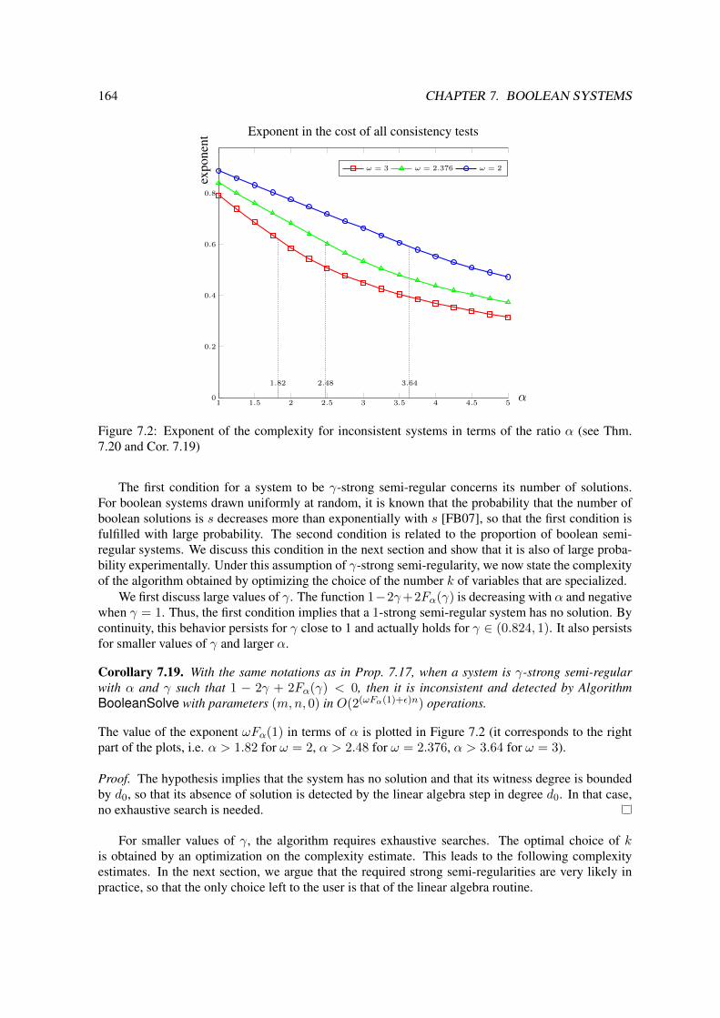
164 CHAPTER 7. BOOLEAN SYSTEMS

1 1.5 2 2.5 3 3.5 4 4.5 50

0.2

0.4

0.6

0.8

1.82 2.48 3.64

α

expo

nent

Exponent in the cost of all consistency tests

ω = 3 ω = 2.376 ω = 2

Figure 7.2: Exponent of the complexity for inconsistent systems in terms of the ratio α (see Thm.7.20 and Cor. 7.19)

The first condition for a system to be γ-strong semi-regular concerns its number of solutions.For boolean systems drawn uniformly at random, it is known that the probability that the number ofboolean solutions is s decreases more than exponentially with s [FB07], so that the first condition isfulfilled with large probability. The second condition is related to the proportion of boolean semi-regular systems. We discuss this condition in the next section and show that it is also of large proba-bility experimentally. Under this assumption of γ-strong semi-regularity, we now state the complexityof the algorithm obtained by optimizing the choice of the number k of variables that are specialized.

We first discuss large values of γ. The function 1−2γ+2Fα(γ) is decreasing with α and negativewhen γ = 1. Thus, the first condition implies that a 1-strong semi-regular system has no solution. Bycontinuity, this behavior persists for γ close to 1 and actually holds for γ ∈ (0.824, 1). It also persistsfor smaller values of γ and larger α.

Corollary 7.19. With the same notations as in Prop. 7.17, when a system is γ-strong semi-regularwith α and γ such that 1 − 2γ + 2Fα(γ) < 0, then it is inconsistent and detected by AlgorithmBooleanSolve with parameters (m,n, 0) in O(2(ωFα(1)+ε)n) operations.

The value of the exponent ωFα(1) in terms of α is plotted in Figure 7.2 (it corresponds to the rightpart of the plots, i.e. α > 1.82 for ω = 2, α > 2.48 for ω = 2.376, α > 3.64 for ω = 3).

Proof. The hypothesis implies that the system has no solution and that its witness degree is boundedby d0, so that its absence of solution is detected by the linear algebra step in degree d0. In that case,no exhaustive search is needed.

For smaller values of γ, the algorithm requires exhaustive searches. The optimal choice of kis obtained by an optimization on the complexity estimate. This leads to the following complexityestimates. In the next section, we argue that the required strong semi-regularities are very likely inpractice, so that the only choice left to the user is that of the linear algebra routine.

7.4. NUMERICAL EXPERIMENTS ON RANDOM SYSTEMS 165

Theorem 7.20. Let S = (f1, . . . , fm) be a system of quadratic polynomials in GF2[x1, . . . , xn], withm = dαne and α ≥ 1. Then Algorithm BooleanSolve finds all its roots in GFn2 with a number ofarithmetic operations in GF2 that is

• O(2(1−0.112α)n) if S is (.27α)-strong semi-regular using Gaussian elimination for the linearalgebra step;

• O(2(1−0.159α)n) if S is (.40α)-strong semi-regular using computation of the row echelon formwith Coppersmith-Winograd multiplication;

• of expectation O(2(1−0.208α)n) if S is (.55α)-strong semi-regular using the probabilistic Algo-rithm 10.

In all cases, the value of k passed to the algorithm is dn(1 − γ)e with γ corresponding to the strongsemi-regularity.

Proof. The correctness of the algorithm has already been proved in Proposition 7.5. Only the com-plexity remains to be proved.

By definition of strong semi-regularity, the number of exhaustive searches that need be performedin line 9 of the Algorithm isO(2(1−2γ+2Fα(γ))n), each of them usingO(2(γ+ε)n) arithmetic operationsfor any ε > 0. It follows that the overall cost of these exhaustive searches is O(2(1−γ+2Fα(γ)+ε)n); itis bounded by the cost of the tests of inconsistency. We now choose γ in such a way as to minimizethis cost, in terms of α. Direct computations lead to the following numerical results, that conclude theproof.

Lemma 7.21. With the same notation as in Proposition 7.17, the function 1−γ+ωFα(γ) is boundedby

• 1− 0.112α when ω = 3 and γ = 0.27α;

• 1− 0.159α when ω = 2.376 and γ = 0.40α;

• 1− 0.208α when ω = 2 and γ = 0.55α.

Proof. The function 1 − γ + ωFα(γ) has two parameters but its extrema can be found by reducingit to a one parameter function. Indeed, this function is maximal for α ≥ 1 and γ ∈ [0, 1] when(−γ + ωFα(γ))/α is. Setting λ = γ/α, this is exactly −λ + ωF1(λ), with λ ∈ [0, 1/α]. Directcomputations lead to the optimal λ’s: λ = min(1/α, 0.27) when ω = 3, λ = min(1/α, 0.40) whenω = 2.376, λ = min(1/α, 0.55) when ω = 2.

7.4 Numerical Experiments on Random Systems

Probabilistic model. In this section, we study experimentally the behavior of Algorithm Boolean-Solve of random quadratic systems where each coefficient is 0 or 1 with probability 1/2. Theserandom boolean quadratic systems appear naturally in Cryptology since the security of several recentcryptosystems relies directly on the difficulty of solving such systems (see e.g., [BGP06, BGP09]).

7.4.1 γ-strong semi-regularity

The goal of this section is to give experimental evidence that the assumption of γ-strong semi-regularity is not a strong condition for random boolean systems. This is related to the notoriously

166 CHAPTER 7. BOOLEAN SYSTEMS

difficult conjecture by [Fro85], which states that in characteristic 0, almost all systems are semi-regular (with the meaning of semi-regularity given in [BFSY04]), see also [MS03].

Consequently, we propose the following conjecture, which can be seen as a variant of Froberg’sconjecture for boolean systems:

Conjecture 7.22. For any α ≥ 1 and γ < 1 such that 1−2γ+2Fα(γ) > 0, the proportion of γ-strongsemi-regular systems of dαne quadratic polynomials in GF2[x1, . . . , xn] tends to 1 when n→∞.

The rest of this section is devoted to providing experiments supporting this conjecture.In Figure 7.3, we show the relation between the value of the first nonpositive coefficient of the

power series expansion of HSbγnc,n and γ-strong semi-regularity for small values of n = m (i.e.α = 1). For each n, the experiments are conducted on 1000 random quadratic boolean systems. Foreach of these systems, we compute the 2d(1−γ)ne specialized systems and we count the number ofspecializations for which the filtering linear system is inconsistent.

Four curves are represented on each chart in Figure 7.3. The red (resp. green) one represents theaverage (resp. maximal) number of specializations for which the linear system (step 8 of AlgorithmBooleanSolve) is inconsistent. In contrast, the blue curve shows the upper bound on this number ofspecializations required to be γ-strong semi-regular (see Definition 7.18). The black curve shows theabsolute value of the first nonpositive coefficient of the corresponding power series (i.e. HSbγnc,n).The y-axis is represented in logarithmic scale. The value γ = 0.1 is never used in the complexityanalysis (since in Theorem 7.20, γ ≥ .27 for any value of α ≥ 1). However, it is still interesting tostudy the behavior of Algorithm 9 when almost all variables are specialized: the filtering remains veryefficient in this case, and the branches which are explored during the second stage of the exhaustivesearch correspond to those containing solutions of the system.

Interpretation of Figure 7.3. First, notice that for γ ≤ 0.55 the green curve is always below theblue one (except for the case γ = .55, n = 23), meaning that during our experiments, all randomlygenerated systems with those parameters were γ-strong semi-regular.

Next, in most curves (except γ = 0.27), the average (resp. maximal) number of points where thespecialization leads to an inconsistent linear system is close to 1 (resp. 5). This can be explained bya simple Poisson model. Indeed, the number of solutions of a random boolean system with as manyequations as unknowns follows a Poisson law with parameter 1 (see [FB07]). Therefore, the expec-tation of the number of solutions is 1. The expectation of the maximum of the number of solutionsof 1000 random systems is then given as the maximum of 1000 iid random variables P1, . . . , P1000

following a Poisson law of parameter 1:

E(max(P1, . . . , P1000)) =∑k≥1

k

((e−1

k∑i=0

1

i!)1000 − (e−1

k−1∑i=0

1

i!)1000

)' 5.51,

which explains very well the observed behaviour.This means that during Algorithm 9 with these parameters, almost all specializations giving rise

to an inconsistent system correspond to a branch of the exhaustive search which contains an actualsolution of the system. Therefore, the filtering is very efficient for those parameters.

Few specializations. In the case γ = 0.9, the blue curve has a negative slope. This is due to thefact that the quantity 1 − 2γ + 2Fα(γ) (see Definition 7.18) is negative for α = 1 and γ > 0.82308.Therefore, we cannot expect that a large proportion of boolean systems are γ-strong semi-regular inthis setting. A limit case is investigated in the chart corresponding to γ = 0.81. There, 1 − 2γ +2Fα(γ) ≈ 0.0102 is positive but very close to zero. Experiments show that random boolean systemswith these parameters and 10 ≤ n ≤ 24 are γ-strong semi-regular with probability approximatelyequal to 0.75.

7.4. NUMERICAL EXPERIMENTS ON RANDOM SYSTEMS 167

10 12 14 16 18 20 22 24

2−1

20

21

22

n

avg,

max,

bou

nd

γ = 0.900

average max bound

26

27

28

29

210

211

212

abs.

valu

eof

the

firs

tn

on-p

os.

coeff

.coeffHS

10 12 14 16 18 20 22 24

20

21

22

n

avg,

max,

bou

nd

γ = 0.810

average max bound

22

24

26

28

210

212

abs.

valu

eof

the

firs

tn

on

-pos.

coeff

.

coeffHS

10 12 14 16 18 20 22 242−1

21

23

25

27

29

n

avg,

max,

bou

nd

γ = 0.550

average max bound

2−4

2−1

22

25

28

abs.

valu

eof

the

firs

tnon-p

os.

coeff

.

coeffHS

10 12 14 16 18 20 22 24 26

2−1

23

27

211

215

n

avg,

max,

bou

nd

γ = 0.270

average max bound

2−4

2−1

22

25

abs.

valu

eof

the

firs

tn

on-p

os.

coeff

.

coeffHS

10 12 14 16 18

2−1

23

27

211

215

n

avg,

max

,b

oun

d

γ = 0.100

average max bound

23

24

abs.

valu

eof

the

firs

tn

on-p

os.

coeff

.

coeffHS

Figure 7.3: Relation between the quality of the filtering, the value of the first nonpositive coefficient ofHSbγnc,n, and γ-strong semi-regularity. In red (resp. green), the average (resp. maximum) number ofspecializations for which the linear system is inconsistent. In blue, the bound for γ-strong regularity.Dashed line: absolute value of the first non positive coefficient of HSbγnc,n.

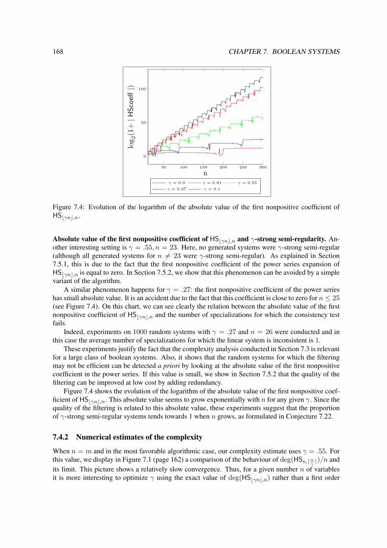
168 CHAPTER 7. BOOLEAN SYSTEMS

50 100 150 200 250 300

0

50

100

n

log2(1+|H

Sco

eff|)

γ = 0.9 γ = 0.81 γ = 0.55

γ = 0.27 γ = 0.1

Figure 7.4: Evolution of the logarithm of the absolute value of the first nonpositive coefficient ofHSbγnc,n.

Absolute value of the first nonpositive coefficient of HSbγnc,n and γ-strong semi-regularity. An-other interesting setting is γ = .55, n = 23. Here, no generated systems were γ-strong semi-regular(although all generated systems for n 6= 23 were γ-strong semi-regular). As explained in Section7.5.1, this is due to the fact that the first nonpositive coefficient of the power series expansion ofHSbγnc,n is equal to zero. In Section 7.5.2, we show that this phenomenon can be avoided by a simplevariant of the algorithm.

A similar phenomenon happens for γ = .27: the first nonpositive coefficient of the power serieshas small absolute value. It is an accident due to the fact that this coefficient is close to zero for n ≤ 25(see Figure 7.4). On this chart, we can see clearly the relation between the absolute value of the firstnonpositive coefficient of HSbγnc,n and the number of specializations for which the consistency testfails.

Indeed, experiments on 1000 random systems with γ = .27 and n = 26 were conducted and inthis case the average number of specializations for which the linear system is inconsistent is 1.

These experiments justify the fact that the complexity analysis conducted in Section 7.3 is relevantfor a large class of boolean systems. Also, it shows that the random systems for which the filteringmay not be efficient can be detected a priori by looking at the absolute value of the first nonpositivecoefficient in the power series. If this value is small, we show in Section 7.5.2 that the quality of thefiltering can be improved at low cost by adding redundancy.

Figure 7.4 shows the evolution of the logarithm of the absolute value of the first nonpositive coef-ficient of HSbγnc,n. This absolute value seems to grow exponentially with n for any given γ. Since thequality of the filtering is related to this absolute value, these experiments suggest that the proportionof γ-strong semi-regular systems tends towards 1 when n grows, as formulated in Conjecture 7.22.

7.4.2 Numerical estimates of the complexity

When n = m and in the most favorable algorithmic case, our complexity estimate uses γ = .55. Forthis value, we display in Figure 7.1 (page 162) a comparison of the behaviour of deg(HSn,dn

γe)/n and

its limit. This picture shows a relatively slow convergence. Thus, for a given number n of variablesit is more interesting to optimize γ using the exact value of deg(HSbγnc,n) rather than a first order

7.5. EXTENSIONS AND APPLICATIONS 169

Figure 7.5: Left: optimal values of γ for the probabilistic variant (red), the deterministic variant withGaussian elimination (black) and Coppersmith-Winograd matrix multiplication (blue), and their lim-its. Right: corresponding values of log2N/n, withN given by Eq. (7.10). The green line correspondsto an exhaustive search.

asymptotic estimate. In the same spirit, one can also use the actual values given by Eq. (7.2) for theMacaulay matrix. Thus we seek to find γ that minimizes the following bounds on the number ofoperations:

2(1−γ)nrMaccMac min(rMac, cMac)ω−2,

resp. 2(1−γ)n max(rMac, cMac) log max(rMac, cMac)sMac(7.10)

in the deterministic (resp. probabilistic) variants, using Eq. (7.3) with n equations, bγnc variablesand d = deg(HSbγnc,n). The corresponding values of γ are given in Figure 7.5, together with thecorresponding values of the quantities in Eq. (7.10). Although these values do not take into account theconstants hidden in theO() estimates of the complexity, they suggest the relevance of these algorithmsin the cryptographic sizes: the threshold between exhaustive search and our algorithm with Gaussianelimination is n ' 280, while the asymptotically faster Las Vegas variant starts being faster thanexhaustive search for n larger than 200 and beats deterministic Gaussian elimination for n largerthan 160.

7.5 Extensions and Applications

7.5.1 Adding Redundancy to Avoid Rank Defects

We showed in Section 7.4.1 that when the first nonpositive coefficient of HSn−k,n is close to zero,then the linear filtering may not be as efficient as expected (for instance in the case γ = .55, n = 23 inFigure 7.3). Another case is shown in Figure 7.6. The curve δ = 0 shows the behavior of Algorithm9 on random square systems (m = n) where k is chosen as small as possible such that the witnessdegree is dwit = 2: this is obtained by choosing k =

⌈1/2 + n−

√−7+8n

2

⌉(that is d0 = 2).

First, we observe that specializing a uniformly distributed random quadratic polynomial P ∈GF2[x1, . . . , xn] at a uniformly distributed random point in GFk2 yields a random polynomial that isalso uniformly distributed in GF2[x1, . . . , xn−k]. We assume here that P is reduced modulo the field

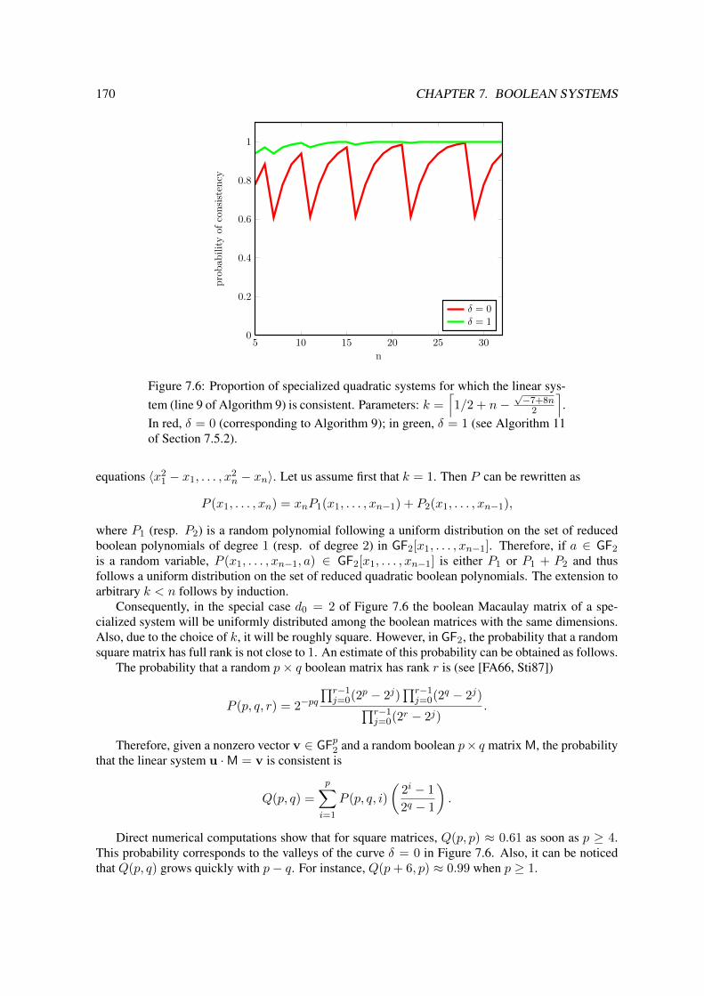
170 CHAPTER 7. BOOLEAN SYSTEMS

5 10 15 20 25 300

0.2

0.4

0.6

0.8

1

n

probab

ilityof

consisten

cy

δ = 0δ = 1

Figure 7.6: Proportion of specialized quadratic systems for which the linear sys-tem (line 9 of Algorithm 9) is consistent. Parameters: k =

⌈1/2 + n−

√−7+8n

2

⌉.

In red, δ = 0 (corresponding to Algorithm 9); in green, δ = 1 (see Algorithm 11of Section 7.5.2).

equations 〈x21 − x1, . . . , x

2n − xn〉. Let us assume first that k = 1. Then P can be rewritten as

P (x1, . . . , xn) = xnP1(x1, . . . , xn−1) + P2(x1, . . . , xn−1),

where P1 (resp. P2) is a random polynomial following a uniform distribution on the set of reducedboolean polynomials of degree 1 (resp. of degree 2) in GF2[x1, . . . , xn−1]. Therefore, if a ∈ GF2

is a random variable, P (x1, . . . , xn−1, a) ∈ GF2[x1, . . . , xn−1] is either P1 or P1 + P2 and thusfollows a uniform distribution on the set of reduced quadratic boolean polynomials. The extension toarbitrary k < n follows by induction.

Consequently, in the special case d0 = 2 of Figure 7.6 the boolean Macaulay matrix of a spe-cialized system will be uniformly distributed among the boolean matrices with the same dimensions.Also, due to the choice of k, it will be roughly square. However, in GF2, the probability that a randomsquare matrix has full rank is not close to 1. An estimate of this probability can be obtained as follows.

The probability that a random p× q boolean matrix has rank r is (see [FA66, Sti87])

P (p, q, r) = 2−pq∏r−1j=0(2p − 2j)

∏r−1j=0(2q − 2j)∏r−1

j=0(2r − 2j).

Therefore, given a nonzero vector v ∈ GFp2 and a random boolean p× q matrix M, the probabilitythat the linear system u ·M = v is consistent is

Q(p, q) =

p∑i=1

P (p, q, i)

(2i − 1

2q − 1

).

Direct numerical computations show that for square matrices, Q(p, p) ≈ 0.61 as soon as p ≥ 4.This probability corresponds to the valleys of the curve δ = 0 in Figure 7.6. Also, it can be noticedthat Q(p, q) grows quickly with p− q. For instance, Q(p+ 6, p) ≈ 0.99 when p ≥ 1.

7.5. EXTENSIONS AND APPLICATIONS 171

Consequently, it is interesting to specialize more variables than k in some cases (especially whenthe first nonpositive coefficient of (1 + t)n−k/((1− t)(1 + t2)m) has small absolute value): doingso increases the difference between the dimensions of the Macaulay matrices. This does not changethe correctness of the algorithm (nor its asymptotic complexity), but increases the effectiveness of thefiltering performed by linear algebra.

7.5.2 Improving the quality of the filtering for small values of n

In this section, we propose an extension of Algorithm BooleanSolve which takes an extra argumentδ, in order to avoid the behavior of the algorithm shown in Section 7.5.1. The main idea is to specializek+δ variables, but to take only k into account for the computation of d0. Consequently, the differencebetween the number of columns and the rank of the Macaulay matrix is not too small, and hence thelinear filtering performs better. The resulting algorithm is given in Algorithm 11.

Algorithm 11 improved BooleanSolve.Input: m,n, k, δ ∈ N such that k + δ < n ≤ m and f1, . . . , fm quadratic polynomials in

GF2[x1, . . . , xn].Output: The set of boolean solutions of the system f1 = · · · = fm = 0.

1: S := ∅.2: d0 := index of the first nonpositive coefficient in the series expansion of the rational function

(1+t)n−k

(1−t)(1+t2)m.

3: for all (an−k−δ+1, . . . , an) ∈ GFk+δ2 do

4: for i from 1 to m do5: fi(x1, . . . , xn−k−δ) := fi(x1, . . . , xn−k−δ, an−k−δ+1, . . . , an).6: end for7: M := boolean Macaulay matrix of (f1, . . . , fm) in degree d0.8: if the system u ·M = r is inconsistent then . r as defined in Lemma 7.39: T := solutions of the system (f1 = · · · = fm = 0) (exhaustive search).

10: for all (t1, . . . , tn−k−δ) ∈ T do11: S := S ∪ (t1, . . . , tn−k−δ, an−k−δ+1, . . . , an).12: end for13: end if14: end for15: return S.

In Figure 7.6, we show the role of the parameter δ when k is chosen minimal such that d0 = 2:adding redundancy by choosing a nonzero δ can greatly improve the quality of the filtering (in practice,choosing δ = 1 is sufficient).

172 CHAPTER 7. BOOLEAN SYSTEMS

10 12 14 16 18 20 22 24

20

21

22

23

24

25

26

n

avg,

max,bound

γ = 0.550, δ = 1

average max bound

10 12 14 16 18 20 22 24 26

2−1

23

27

211

215

n

avg,

max

,bou

nd

γ = 0.270, δ = 1

average max bound

Figure 7.7: Quality of the filtering with δ = 1.

Figure 7.7 shows further experimental evidence that adding redundancy by choosing δ = 1 permitsto avoid problems occurring when the first nonpositive coefficient of HSn−k,m is close to zero. Forinstance, the peak at γ = .55, n = 23 that appeared in Figure 7.3 disappears when δ = 1.

7.5.3 Cases with Low Degree of Regularity

In some cases, when the boolean system is not random, the choice of d0 proposed in AlgorithmBooleanSolve may be too large. This happens for instance for systems that have inner structure,which has an impact on the algebraic structure of the ideal generated by the polynomials. Examplesof such structure can be found in Cryptology, for instance with boolean systems coming for the HFEcryptosystem [Pat96], as shown in [FJ03].

For these systems, the choice of d0 as the index of the first non-positive coefficient of HSn,mwould be very pessimistic, since the Macaulay matrices in degree d0 would be larger than necessary.However, if estimates of the witness degree are known (this is the case for HFE), then d0 can bechosen accordingly as a parameter of the Algorithm BooleanSolve.

Chapter 8

Application to Cryptology

Section 8.1 is joint work with J.-C. Faugere and the results are published in [FS10]. Section 8.2 isjoint work with J.-C. Faugere and M. Safey El Din and the results are published in [FSS10]. Section8.3 is joint work with M. Bardet, J.-C. Faugere and B. Salvy and is a part of [BFSS12].

8.1 Cryptanalysis of the Algebraic Surface Cryptosystem

Notation for this section. In this section, to avoid any confusion between the symbols w and ω, weuse the notation ϑ for the exponent in the complexity of linear algebra (i.e. two n×n matrices can becomputed within O(nϑ) arithmetic operations).

In this section, we propose an algebraic attack on the Algebraic Surface Cryptosystem (ASCfor short) proposed at PKC’2009 [AGM09]. This cryptosystem is based on an unusual problem inmultivariate cryptography: the Section Finding Problem. Given w ∈ N and an algebraic surfaceX(x, y, t) ∈ GFp[x, y, t] such that degxyX(x, y, t) = w, the problem is to find a pair of polynomialsof degree d, ux(t) and uy(t), such that X(ux(t), uy(t), t) = 0. In ASC, the public key is the surface,and the secret key is the section. This asymmetric encryption scheme enjoys small sizes of the keys:for recommended parameters, the size of the secret key is only 102 bits and the size of the publickey is 500 bits. We propose a message recovery attack whose complexity is quasi-linear in the sizeof the secret key. The main idea of this algebraic attack is to decompose ideals constructed fromthe ciphertext in order to avoid to solve the section finding problem. Experimental results show thatwe can break the cipher for recommended parameters (the security level is 2102) in 0.05 seconds.Furthermore, the attack still applies even when the secret key is very large (more than 10000 bits).The complexity of the attack is O(w2ϑ+1d log(p)) which is polynomial with respect to all securityparameters. In particular, it is quasi-linear in the size of the secret key which is (2d+ 2) log(p). Thisresult is rather surprising since the algebraic attack is often more efficient than the legal decryptionalgorithm.

8.1.1 Introduction

In 1994, Shor designed a quantum algorithm to compute efficiently discrete logarithm and factoriza-tion [Sho94]. Hence, if one could construct a quantum computer, a huge number of well-establishedpublic key cryptosystems – for instance, RSA or Elliptic Curve based systems – would be seriouslythreatened. Therefore, cryptographers are searching for post-quantum alternatives. The first stepto design new cryptosystems is to identify hard problems to use as trapdoors. So far, most of theproblems used in post-quantum cryptology can be classified into three main categories: Multivariatecryptography, Code-based cryptography and Lattice-based cryptography.

173

174 CHAPTER 8. APPLICATION TO CRYPTOLOGY

In this context, Akiyama, Goto, and Miyake propose a new multivariate public-key algorithm atPKC’2009: the Algebraic Surface Cryptosystem (ASC for short) [AGM09]. Interestingly, its securityis based on an uncommon difficult problem which:Section Finding Problem (SFP). Given an algebraic surface defined by the polynomial X(x, y, t) ∈GFp[x, y, t] (where GFp denotes the finite field of cardinality p), find two polynomials ux(t), uy(t) ∈GFp[t] of degree d, such that X(ux(t), uy(t), t) = 0.

As stated in [AGM09], this problem is computationally hard: the only algorithm known so farinduces to find roots of a huge multivariate polynomial system. Hence the idea of ASC is to use thesurface as public key and the knowledge of a section of this surface as the trapdoor. In comparisonto HFE [Pat96] or other multivariate systems, ASC has several interesting and unusual properties.In particular, the keys are very short. The security of multivariate systems is usually related to thedifficulty of finding a zero of a system of low degree polynomials (often quadratic) in a huge numberof variables. For instance, in the case of HFE, the size of the public key is precisely the size of themultivariate system: 265680 bits for a security of 280. In contrast with HFE, ASC enjoys a smallpublic key of 500 bits for a security of 2102. More generally, for a security level of 2d, the size of thepublic key of HFE isO(d3). In comparison, the public key of ASC is a unique high degree polynomialin only three variables: its size is O(d) bits for a security of 2d. Actually, the designers explain thatthe keys of ASC are among the shortest of known post-quantum cryptosystems. More precisely, let wdenote the degree of the public surface X in x and y. For a security level of p2d, the size of the secretkey is 2d log(p) bits and the size of the public key is about wd log(p). The main observation is thatthe sizes of the keys are linear in d log(p), which is the logarithm of the security level.

Although a completely different version of ASC [AG04] has been attacked by Ivanov and Voloch[IV09], by Uchiyama and Tokunaga [UT07] and by Iwami [Iwa07], the new version of ASC, presentedat PKC’2009, is resistant to all known attacks. We would like to mention that the decryption algorithmraises some questions. Indeed, one step of this algorithm is to recover some factors of given degreeD of a univariate polynomial. In order to find those factors, the designers propose to recombine theirreducible factors of the polynomial by solving a knapsack. However, this problem is known to beNP-hard [GJ79]. Therefore, it is not clear if the cryptosystem remains practical for high securityparameters.

Main results. We describe a message recovery attack which can break ASC in polynomial time.One important step of the legal decryption algorithm is the factorization of a univariate polynomial.The key idea of the algebraic attack is to perform this factorization step implicitly by decomposingideals deduced from the ciphertext. Indeed, decomposition of ideals can be seen as a generalizationof the standard factorization of polynomials. Hence, this technique allows us to bypass the SectionFinding Problem, which is hard.

We present three versions of this attack. The Level 1 Attack is high-level, deterministic, offers agood view of the mechanisms involved, and can be implemented straightforwardly into a ComputerAlgebra System such as MAGMA (code given in Section 8.1.11). However, this version is not veryefficient and cannot break ASC for the recommended parameters. The Level 2 Attack is based onthe following observation: the polynomials occurring in ASC have a high degree in t and rather lowdegrees in x and y. Thus, it is natural to see expressions in t as coefficients instead of polynomialsin t; in other words, in order to speed up the attack, we have to perform the computations in the ringGFp(t)[x, y] (where GFp(t) is the field of fractions of GFp[t]) instead of GFp[x, y, t]. In the Level3 Attack, we replace the ground field GFp(t) by a finite field GFpD ≈ GFp[t]/(P (t)) for a largeenough D to avoid the swelling of the intermediate coefficients and to recover the initial messagemodulo P (t). Even more efficiently, we can split P (t) into several irreducible factors Pi(t) of smalldegree; the Chinese Remainder Theorem is then used to recombine the congruences and retrieve the

8.1. CRYPTANALYSIS OF THE ALGEBRAIC SURFACE CRYPTOSYSTEM 175

original message. In this third version of the attack, the size of the plaintext determines the numberof congruences required as well as the size of the finite fields considered. Therefore, the complexityof the Level 3 Attack is expected to be quasi-linear in the size of the secret key. This behavior isconfirmed by experimental results together with a complexity analysis. The binary complexity1 of theLevel 3 Attack is (Theorem 8.11):

O(w2ϑ size(m))

where size(m) denotes the binary size of the plaintext, w is the degree of X in the variables x and yand O() is the “soft Oh” notation (see e.g. [VZGG03, Definition 25.8]). Since the size of the secretkey is smaller than size(m), the attack is also quasi-linear in the size of the secret key. In practice,size(m) ≈ dw log(p) (where d is the degree of the secret section). Thus the complexity of the attackis

O(w7d log(p)).

This can be compared with a lower bound on the binary complexity (see page 184) of the decryptionalgorithm:

O(log(p)(wϑdϑ + dw log(p))).

It can be noted that the decryption algorithm is cubic in the size of the secret key. Therefore, increasingthe size of the secret key does not secure the system, since the cost of the decryption algorithmincreases faster than the cost of the attack.

We implemented in MAGMA 2.15-7 the three variants. The Level 3 Attack can break ASC withparameters recommended in [AGM09] (d = 50, p = 2, w = 5) in only 0.05 seconds. Experimentsconfirm that increasing the size of the secret key with the parameters p and d does not really increasethe security of the system. We are still able to break it in few seconds, even when the size of thesecret key is more than 10000 bits! We also try to increase the parameter w (the degree in x and yof the public surface). For a reasonable size of the public key (less than 4000 bits), the message canbe recovered in few hours. Finally, we try to figure out whether it is possible to secure the systemby increasing the size of the support of the surface (the parameter k). However, as predicted by thecomplexity analysis, this parameter has very few effect on the complexity of the attack.

Structure of this section. After this introduction, this section is organized as follows. In Section8.1.2, we give a short description of the ASC cryptosystem as it is presented in [AGM09]. Then, weexplain the theoretical foundations of the attack. In Section 8.1.3, we describe the three variants of theattack and we show a concrete example by applying it to the toy example given in [AGM09]. We alsoperform a precise complexity analysis in Section 8.1.7. Finally, we give some experimental resultsshowing that the attack is scalable.

8.1.2 Description of the cryptosystem

We give here a short description of ASC. For a more detailed presentation of this cryptosystem, werefer the reader to [AGM09]. We consider the ring of polynomials GFp[x, y, t] where p is a primenumber. In Section 8.1.10, a concrete example of encryption/decryption on a toy example is given.For any polynomial P ∈ GFp[x, y, t], ΛP denotes its support in GFp(t)[x, y] (that is to say the set ofcouples (i, j) ∈ N2 such that t`xiyj is a monomial of P ).

1The binary complexity is the number of arithmetic operations on bits, whereas the arithmetic complexity is the numberof arithmetic operations in the base ring.

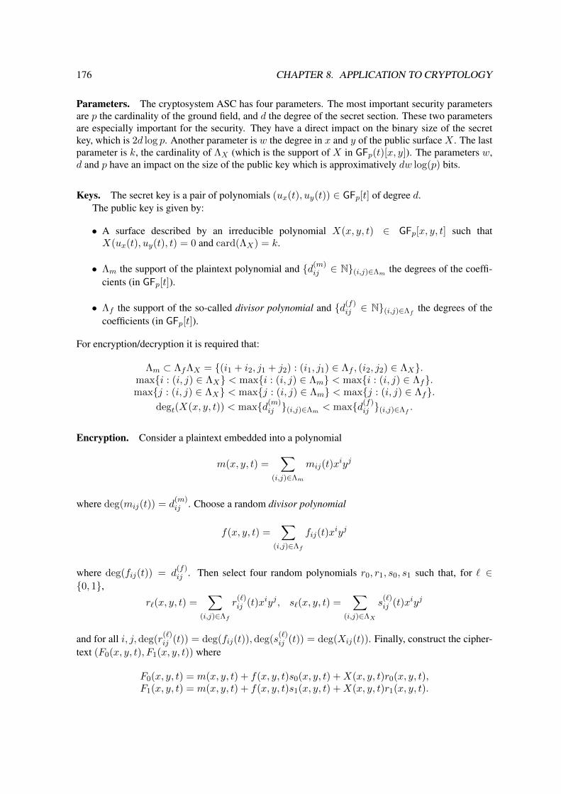
176 CHAPTER 8. APPLICATION TO CRYPTOLOGY

Parameters. The cryptosystem ASC has four parameters. The most important security parametersare p the cardinality of the ground field, and d the degree of the secret section. These two parametersare especially important for the security. They have a direct impact on the binary size of the secretkey, which is 2d log p. Another parameter is w the degree in x and y of the public surface X . The lastparameter is k, the cardinality of ΛX (which is the support of X in GFp(t)[x, y]). The parameters w,d and p have an impact on the size of the public key which is approximatively dw log(p) bits.

Keys. The secret key is a pair of polynomials (ux(t), uy(t)) ∈ GFp[t] of degree d.The public key is given by:

• A surface described by an irreducible polynomial X(x, y, t) ∈ GFp[x, y, t] such thatX(ux(t), uy(t), t) = 0 and card(ΛX) = k.

• Λm the support of the plaintext polynomial and d(m)ij ∈ N(i,j)∈Λm the degrees of the coeffi-

cients (in GFp[t]).

• Λf the support of the so-called divisor polynomial and d(f)ij ∈ N(i,j)∈Λf the degrees of the

coefficients (in GFp[t]).

For encryption/decryption it is required that:

Λm ⊂ ΛfΛX = (i1 + i2, j1 + j2) : (i1, j1) ∈ Λf , (i2, j2) ∈ ΛX.maxi : (i, j) ∈ ΛX < maxi : (i, j) ∈ Λm < maxi : (i, j) ∈ Λf.maxj : (i, j) ∈ ΛX < maxj : (i, j) ∈ Λm < maxj : (i, j) ∈ Λf.

degt(X(x, y, t)) < maxd(m)ij (i,j)∈Λm < maxd(f)

ij (i,j)∈Λf .

Encryption. Consider a plaintext embedded into a polynomial

m(x, y, t) =∑

(i,j)∈Λm

mij(t)xiyj

where deg(mij(t)) = d(m)ij . Choose a random divisor polynomial

f(x, y, t) =∑

(i,j)∈Λf

fij(t)xiyj

where deg(fij(t)) = d(f)ij . Then select four random polynomials r0, r1, s0, s1 such that, for ` ∈

0, 1,r`(x, y, t) =

∑(i,j)∈Λf

r(`)ij (t)xiyj , s`(x, y, t) =

∑(i,j)∈ΛX

s(`)ij (t)xiyj

and for all i, j, deg(r(`)ij (t)) = deg(fij(t)),deg(s

(`)ij (t)) = deg(Xij(t)). Finally, construct the cipher-

text (F0(x, y, t), F1(x, y, t)) where

F0(x, y, t) = m(x, y, t) + f(x, y, t)s0(x, y, t) +X(x, y, t)r0(x, y, t),F1(x, y, t) = m(x, y, t) + f(x, y, t)s1(x, y, t) +X(x, y, t)r1(x, y, t).

8.1. CRYPTANALYSIS OF THE ALGEBRAIC SURFACE CRYPTOSYSTEM 177

Decryption. For ` ∈ 0, 1, consider h`(t) = F`(ux(t), uy(t), t) and compute the differenceh0(t) − h1(t) = f(ux(t), uy(t), t)(s0(ux(t), uy(t), t) − s1(ux(t), uy(t), t)). Next, find a factor ofh0(t)− h1(t) whose degree matches deg(f(ux(t), uy(t), t)). Let f(t) denote this factor. Then com-pute m(ux(t), uy(t), t) = h0(t) mod f(t). Finally, retrieve m(x, y, t) by solving the linear system:

m(ux(t), uy(t), t) =∑

mijkux(t)iuy(t)jtk.

There are potentially several factors of h0(t) − h1(t) whose degree is equal todeg(f(ux(t), uy(t), t)). So, we have to verify that we picked the good one. To do so, the design-ers of ASC propose to use a Message Authentication Code (roughly speaking a cryptographic hashfunction with a key) to verify that m(x, y, t) = m(x, y, t). If the verification fails, we start again byconsidering another factor of h0(t)− h1(t).

To find factors of h0(t) − h1(t) whose degree matches deg(f(ux(t), uy(t), t)), the designerspropose to factor h0(t)−h1(t), then recombine its irreducible factors by solving a knapsack problem.However, the knapsack problem is NP-hard [GJ79]. Therefore, as pointed out in [AGM09], it is notclear if the decryption algorithm remains practicable when the security parameters are high.

Security of the system. The designers of the cryptosystem propose the following parameters:

• p = 2;

• d should be greater than 50;

• w = degxy(X) = maxi+ j : (i, j) ∈ ΛX should be greater than 5;

• The lower bound on k is 3.

The size of the secret key is around 100 bits and the size of the public key is close to 500 bits.According to the designers of ASC, there is so far no known attack faster than exhaustive search forthese parameters. Therefore, the security level of ASC is expected to be the cost of exhaustive searchof the secret key, namely p2d+2.

8.1.3 Description of the attack

Overview of the attack. In this section, we propose a message recovery attack on the cryptosystemdescribed above.

The main point of the attack is to decompose ideals, instead of factoring the univariate polynomialobtained by evaluating F0−F1 in the section (ux, uy). This way, we can implicitly manipulate the so-called divisor polynomial f occurring in the decryption process. Consequently, we can avoid to solvethe underlying Section Finding Problem, and we obtain an attack on ASC in polynomial complexity.

First, we present a high-level and deterministic version of the attack (Algorithm 12) based on twofundamental lemmas. Then, the algorithm is speeded-up by computing in the field of fractions GFp(t)(Algorithm 13). Indeed, polynomials occurring in ASC have a high degree in t. Since the complex-ity of Grobner bases algorithms is linear in the complexity of the arithmetic in the ground field, it isnatural to compute in the field of fractions GFp(t). Finally, we use a modular approach to implementefficiently the attack: we perform computations in some well-chosen finite fields GFp[t]/(P ) and re-combine the results by using the Chinese Remainder Theorem (Algorithm 14). Doing this, the size ofthe coefficients of intermediate values are bounded (these coefficients can be huge when computationsare performed in the field of fractions). This allows us to break bigger instances of ASC. In particular,we are able to break the system with recommended parameters in 0.05 seconds. Furthermore, this will

178 CHAPTER 8. APPLICATION TO CRYPTOLOGY

allow us to perform a precise complexity analysis and to show that this attack is quasi-linear in thesize of the secret key. Experimentally, we are able to break with this technique some instances wherethe size of the secret key is greater than 10000 bits.

Now we compare the efficiency of the three versions of the attack on a small example. For in-stance, we consider the following parameters p = 11, d = 8, w = 5 and k = 3 and we use ourMAGMA implementation. The Level 1 Attack (code given in Section 8.1.11) recovers the plaintextin 136 seconds. As predicted, the Level 2 Attack is faster and can break the system in 74 seconds.Using the modular approach in the Level 3 Attack really speeds up the computations: it retrieves theplaintext in 0.05 seconds.

8.1.4 Level 1 Attack: decomposition of ideals.

The two following lemmas are the key elements of the attack.

Lemma 8.1. Let I be the ideal I = 〈F0 − F1, X〉 ⊂ GFp[x, y, t]. Then I = I1∩I2 where I1 = 〈f,X〉and I2 = 〈s0 − s1, X〉. Generically, the ideals I1 and I2 are prime ideals of GFp[x, y, t].

Proof. I = 〈F0 − F1, X〉 = 〈f (s0 − s1), X〉 = I1 ∩ I2.

Lemma 8.1 shows that, once we managed to decompose the ideal 〈F0 − F1, X〉 =〈f (s0 − s1), X〉, we can manipulate implicitly the polynomial f through I1.

Remark 8.2. In order to decompose I , a strategy is to eliminate x from I by computing a Grobnerbasis of I ∩ GFp[y, t]. Generically, this Grobner basis contains only one polynomial Q. If p isbig enough, Q has in general two factors which depend on y and t (we do not consider the factorswhich are in GFp[t]). This fact is confirmed experimentally. The two factors correspond to I1 and I2.Then, we can construct I1 (resp. I2) by adding to I an appropriate factor of Q. Since degy(f) >degy(s1 − s0), the factor of Q with the highest degree in y is the one corresponding to I1. To factorefficiently the bivariate polynomial Q, we can use for instance the algorithm in [Lec10].

Lemma 8.3. Let J be the ideal of GFp[x, y, t] generated by J = 〈F0, F1, X〉+ I1. Then m(x, y, t) ∈J. Moreover, J is a zero-dimensional ideal.

Proof. J = 〈F0, F1, X〉+ I1 = 〈F0, F1, X, f〉 = 〈m, f,X〉.

Remark 8.4. Lemma 8.3 shows that we can compute explicitly a multivariate ideal which containsm. Since we know Λm, we can recover m by solving the following linear system:

NFJ(m) =∑

(i,j)∈Λm

d(m)ij∑k=0

mijk NFJ(xiyjtk) = 0

where NFJ denotes the normal form with respect to the ideal J for a chosen monomial ordering.Since λm ∈ J for all λ ∈ GFp, we retrieve m up to multiplication by a scalar.

Remark 8.5. For efficiency purpose, we compute the Grobner bases with respect to the graded reverselexicographical ordering (Definition 1.19). Instead of computing the Grobner basis of 〈F0−F1, X〉∩GFp[y, t], it is also possible to compute a resultant to eliminate the variable x.

8.1. CRYPTANALYSIS OF THE ALGEBRAIC SURFACE CRYPTOSYSTEM 179

Algorithm 12 Level 1 Attack.1: Compute a Grobner basis of the ideal 〈F0 − F1, X〉 ∩ GFp[y, t]. Generically this Grobner basis

contains only one polynomial Q(y, t).2: Factor Q =

∏Qi(y, t). Let Q0(y, t) ∈ GFp[y, t] denote an irreducible factor with highest degree

with respect to y.3: Compute a Grobner basis of the ideal J = 〈F0, F1, X,Q0〉.4: To retrieve the plaintext (up to multiplication by a scalar in GFp), solve the linear system over

GFp ∑(i,j)∈Λm

d(m)ij∑k=0

mijk NFJ(xiyjtk) = 0.

If the system has no solution, go back to Step 2 and pick another factor of Q.

Remark 8.6. The normal form NFJ is a linear application from GFp[x, y, t] onto GFp[x, y, t]/J .In the last step of the attack, we are searching for the intersection of its kernel with the GFp-linear subspace generated by Γm (where Γm denotes the support of m in GFp[x, y, t]). Therefore,the linear system has card(Γm) unknowns and deg(J) equations (deg(J) = dim(GFp[x, y, t]/J)when GFp[x, y, t]/J is seen as a GFp-vector space). From the Bezout bound [Laz83], deg(J) ≈deg(m) deg(X) deg(f). The decryption algorithm requires that deg(m(ux, uy, t)) ≥ card(Γm) (inorder to solve the final linear system) and one can remark that deg(X) deg(f) > deg(m(ux, uy, t)) ≈ddegxy(m) + degt(m) (since degxy(f) > degxy(m),degt(f) > degt(m) and deg(X) > d).Therefore, the linear system has more equations than unknowns: card(Γm) ≤ deg(m(ux, uy, t)) ≤deg(X) deg(f) ≤ deg(J).

8.1.5 Level 2 Attack: computing in the field of fractions GFp(t)

Polynomials appearing in ASC have a high total degree, but their degree in the variables x and y is low.Hence, it is natural to consider these polynomials as bivariate polynomials in x and y over the field offractions GFp(t). Indeed, the degrees in x and y are completely independent of the security parameterd. In this section, we explain how to adapt the attack in this context. Doing that, we expect to have alower complexity. Indeed, many operations on ideals – for instance Grobner basis computations – arelinear in the complexity of the arithmetic in the ground field.

From now on, K denotes the field of fractions GFp(t).First, we need to transpose the key lemmas in this new context. This can be done for Lemma 8.1

without any major modification:

Lemma 8.7. Let I be the ideal I = 〈F0 − F1, X〉 (seen as an ideal of K[x, y]). Then there exist I1

and I2 two proper ideals of K[x, y] such that I = I1 ∩ I2 and 〈f,X〉 ⊂ I1.

Unfortunately, Lemma 8.3 cannot be directly transposed in the context of the field of fractions.Indeed, the variety of the ideal J = 〈F0, F1, X〉 + I1 = 〈m, f,X〉 (seen as an ideal of K[x, y])is generically empty since it is generated by three independent equations. Therefore we have tointroduce a new variable z if we want to keep the ideal zero-dimensional and strictly included inK[x, y, z]. Roughly speaking, the role of z is to deform the ideal 〈m, f,X〉 in order to introduce newelements in the variety:

Lemma 8.8. Let J ⊂ K[x, y, z] be the ideal J = 〈F0 + z, F1 + z,X〉+ I1. Then m(x, y, t) + z ∈ J.Moreover, J is a zero-dimensional ideal.

180 CHAPTER 8. APPLICATION TO CRYPTOLOGY

Proof. 〈F0 + z, F1 + z,X〉+ I1 = 〈F0 + z, F1 + z,X, f〉 = 〈m+ z, f,X〉 .

Algorithm 13 Level 2 Attack: computing in the field of fractions K = GFp(t).1: Compute the resultant Resx(F0 − F1, X) ∈ K[y].2: Factor the resultant Resx(F0−F1, X) =

∏Qi(y). LetQ0(y) ∈ K[y] denote an irreducible factor

of highest degree in y.3: Compute a grevlex-Grobner basis of the ideal J = 〈F0 + z, F1 + z,X,Q0〉 ⊂ K[x, y, z].4: Consider the following linear system over K:

NFJ(z) +∑

(i,j)∈Λm

mij(t) NFJ(xiyj) = 0.

If the system has no solution, then go back to Step 2 and choose another factor of the resultant.5: Return m =

∑(i,j)∈Λm

mij(t)xiyj where (mij(t)) is the unique solution of the linear system.

To be able to recover the plaintext, we need to solve a linear system with card(Λm) unknowns anddeg(J) equations. In practice, there are more equations than unknowns. Thus, if we choose a wrongfactor of the resultant (a factor which is not a divisor of f ), then the linear system has generically nosolution, and we just have to restart from Step 2 until we find an appropriate factor. In practice, theirreducible factor of the resultant with the highest degree in y is almost always a good choice.

Remark 8.9. It is also possible to combine the two versions of the attack by computing a Grobnerbasis of the elimination ideal and factoring it in GFp[x, y, t], as in Level 1 attack (Steps 1 and 2 inAlgorithm 12). Then, once we found Q0 ∈ GFp[x, y, t], we retrieve the message by computing aGrobner Basis of J = 〈F0 + z, F1 + z,X,Q0〉 ⊂ K[x, y, z] in the field of fractions (Steps 3, 4, 5 inAlgorithm 13).

8.1.6 Level 3 Attack: computing in finite fields GFpm

In this section, we study how to implement efficiently the attack in practice. In order to speed upthe attack and to compute efficiently in the field of fractions, we perform all computations modulopolynomials of GFp[t]. Indeed, a bound on the degree ofmwith respect to t is known since degt(m) ≤maxd(m)

i,j .We choose a constantC and n = degt(m) log(p)/C irreducible polynomialsP1, . . . , Pn of degree

close to C/ log(p) such that∑

deg(Pi) > degt(m). Then for each Pi, we consider

GFp[t]/(Pi) = GFpdeg(Pi) .

Considering all computations in K = GFp[t]/(Pi) instead of GFp(t), the attack yields m mod Pi.Finally we use the Chinese Remainder Theorem (CRT) to recoverm mod

∏Pi. Since deg(

∏Pi) >

degt(m), we retrieve the plaintext.

Remark 8.10. The linear system at step 7 in Algorithm 14 has only card(Λm) unknowns anddeg(J) ≈ degxy(m) degxy(f) degxy(X) equations. For practical parameters, card(Λm) ≈ k issmaller than deg(J), thus the linear system is overdetermined and has in general only one solution.This fact is confirmed by experiments.

The value∑

deg(Pi) ≈ degt(m) is only dependent of the size of the plaintext. Therefore, thenumber of times we have to run the main loop of Algorithm 14 is linear in the size of the plaintext.Since the cost of arithmetic operations in GFp[t]/(P ) only depends on C (which is a constant chosen

8.1. CRYPTANALYSIS OF THE ALGEBRAIC SURFACE CRYPTOSYSTEM 181

Algorithm 14 Level 3 Attack: computing in the finite fields K = GFp[t]/(P ).1: Choose n ≈ degt(m) log(p)/C irreducible polynomials of degree ≈ C/ log(p) such that∑

deg(Pi) > degt(m).2: for i from 1 to n do3: Consider K = GFp[t]/(Pi).4: Compute the resultant Resx(F0 − F1, X) ∈ K[y].5: Factor the resultant Resx(F0 − F1, X) =

∏Qi(y). Let Q0(y) ∈ K[y] denote an irreducible

factor of highest degree in y.6: Compute a grevlex-Grobner basis of the ideal J = 〈F0 + z, F1 + z,X,Q0〉 ⊂ K[x, y, z].7: Consider the following linear system over K:

NFJ(z) +∑

(i,j)∈Λm

mij(t) NFJ(xiyj) = 0.

If the system has no solution, then go back to Step 2 and choose another factor of the resultant.8: Retrieve a congruencem mod Pi =

∑(i,j)∈Λm

mij(t)xiyj where (mij(t)) is the solution of

the linear system.9: end for

10: Use the CRT to retrieve m = m mod∏Pi.

by the attacker), we expect this Level 3 Attack to be linear or quasi-linear in the size of the plaintext.This expectation will be confirmed by a complexity analysis and by experimental results. Besides, wewould also like to mention that the main loop of Algorithm 14 can be easily computed in parallel.

A concrete example. We consider here the toy example given in [AGM09]. We have

• p = 17.

• The secret key is (ux, uy) = (14t3 + 12t2 + 5t+ 1, 11t3 + 3t2 + 5t+ 4).

• The public surface isX = (t+ 10)x3y2 + (16t2 + 7t+ 4)xy2 + (3t16 + 8t15 + 13t14 + 8t13 + 3t12 + 12t11 + 4t10 +8t9 + 7t8 + 4t7 + 13t6 + 2t5 + 5t4 + 4t3 + 14t2 + 9t+ 14).

• The support of m and f are

Λm = (4, 4), (0, 0), dm00 = 17, dm44 = 17,

Λf = (5, 5), (1, 2), (0, 0), df00 = 13, df12 = 11, df55 = 18.

Here we show how to recover the message m from the ciphertext (F0, F1) (given in [AGM09])with the Level 3 Attack:

1. Since degt(m) = 17, we choose (for instance) P1, P2, P3, P4 ∈ GFp[t] irreducible such that∑deg(Pi) ≥ 18. In particular,

P1 = t5 + t+ 14,P2 = t5 + 14t4 + 4t3 + 4t+ 4,

P3 = t5 + 9t4 + 15t3 + 8t2 + 4t+ 8,P4 = t5 + 11t4 + 11t3 + 8t2 + 7t+ 8.

First, we consider the finite field K = GFp[t]/(P1).

182 CHAPTER 8. APPLICATION TO CRYPTOLOGY

2. Compute the resultant in K[y]:Resx(F0−F1, X) = (9t4 +14t3 +4t2 +6t+13)y30 +(5t4 + t3 +14t2 +15t+8)y27 +(6t4 +9t3 + 10t2 + 7t+ 14)y26 + (7t4 + 4t3 + 8t2 + 5t+ 8)y25 + (8t4 + 4t3 + 7t2 + 7t+ 6)y24 +(12t4 +9t3 +8t2 +13t)y23 +(9t4 +4t3 +9t2 +15t+6)y22 +(3t4 +6t3 +10t2 +6t+6)y21 +(9t4 + 9t3 + 13t2 + 15t+ 6)y20 + (4t4 + 4t3 + 15t2)y19 + (2t4 + 11t3 + 2t2 + 5t+ 2)y16.

3. Then factor it in K[y]:Resx(F0−F1, X) = y16(y+8t4+3t3+16t2+8t+2)(y2+2t4+14t3+14t2+6t+10)(y2+15t4+3t3+3t2+11t+7)(y2+(14t4+7t3+4t)y+13t4+10t3+7t2+8t+1)(y7+(12t4+7t3+t2+5t+15)y6+(t4+5t3+7t2+12t+11)y5+(9t4+14t3+5t2+10t+10)y4+(4t4+7t3+t2+7t+14)y3+(11t4 +13t3 +12t2 +8t+4)y2 +(15t4 +9t3 +16t2 +14t+14)y+14t4 +3t3 +9t2 +15t+8).

4. Consider Q0 an irreducible factor with highest degree:Q0 = y7 + (12t4 + 7t3 + t2 + 5t+ 15)y6 + (t4 + 5t3 + 7t2 + 12t+ 11)y5 + (9t4 + 14t3 +5t2 + 10t+ 10)y4 + (4t4 + 7t3 + t2 + 7t+ 14)y3 + (11t4 + 13t3 + 12t2 + 8t+ 4)y2 + (15t4 +9t3 + 16t2 + 14t+ 14)y + (14t4 + 3t3 + 9t2 + 15t+ 8).

5. Compute a Grobner basis G with respect to the grevlex ordering of the ideal J =〈F0 + z, F1 + z,X,Q0〉 ⊂ K[x, y, z].

6. Since Λm = (0, 0), (4, 4) compute NFJ(x4y4):NFJ(x4y4) = N1z +N2 = (15t4 + 3t3 + t2 + 13t+ 16)z + (5t4 + 11t2 + t+ 7).

7. Solve the linear system z +m44 NFJ(x4y4) +m00 = 0 over K:m00 = N2/N1 mod P1

m44 = −1/N1 mod P1.

8. Recover a congruence: m = m00 +m44x4y4 mod P1.

9. Repeat the process with P2, P3 and P4.

10. Use the CRT to retrieve m = m mod∏Pi:

m = (5t17 + 15t16 + 4t15 + 9t14 + 7t13 + 2t12 + 3t11 + 8t10 + 11t9 + 6t17 + 6t8 + 3t16 +10t7 + 11t15 + 7t6 + t5 + t13 + 14t4 + 10t12 + 3t3 + 3t11 + 12t2 + 8t10 + 11t+ 6t9 + 2)x4y4 +(13t8 + 2t7 + 2t6 + 10t5 + 5t4 + 2t3 + 15t2 + 3t+ 11).

8.1.7 Complexity analysis

In this part, we investigate the complexity of the Level 3 Attack. To simplify the notations, we supposehere that the complexity of multiplying two n × n matrices is O(n3). We note that C is a parameterchosen by the attacker. This parameter fixes the size of the finite fields considered. Indeed, we choosefinite fields K = GFp /(Pi) with deg(Pi) ≈ C/ log(p). Hence, log(card(K)) ≈ C.

1. First, we estimate the complexity of the computation of the resultant with respect to x in K[x, y](where K = GFp[t]/(Pi)). According to [VZGG03] (Corollary 11.18), this can be done inO(wϑ) operations in K, and the degree of the resultant is O(w2).

2. The probabilistic Cantor-Zassenhaus algorithm [VZGG03] factors a polynomial of degree nover a finite field GFq in O(n2+n log(q)) arithmetic operations in GFq. Therefore the arithmeticcomplexity in K of the factorization of the resultant is

O(w4 + w2 log(card(K))) = O(w4 + w2C).

8.1. CRYPTANALYSIS OF THE ALGEBRAIC SURFACE CRYPTOSYSTEM 183

3. The degree of regularity of an ideal is an important indicator of the complexity of computing itsGrobner basis with respect to the grevlex ordering: it is the highest degree of the polynomialsoccurring in the F5 Algorithm. According to [Laz83, BFSY04, BFS04], if an ideal is spannedby m generic equations in n variables, then the complexity of computing a Grobner basis is:

O

(mϑ

(dreg +n− 1

n− 1

)ϑ).

Since the ideal J = 〈m+ z, f,X〉 is generated by three independent equations, its degree ofregularity can be estimated from the Macaulay bound (see [Laz83]) as

dreg(J) = (degxy(m+ z)− 1) + (degxy(f)− 1) + (deg(X)xy − 1) + 1.

For practical parameters, degxy(m+ z) ≈ degxy(f) ≈ deg(X)xy ≈ w. Therefore, dreg ≈ 3w.The arithmetic complexity in K of the Grobner basis computation is then:

O

(3ϑ(

dreg(J) + 2

2

)ϑ)= O(w2ϑ).

4. Finally we have a linear system to solve. The number of variables is card(Λm). For practicalparameters, card(Λm) ≈ k, which is less than 1000 (the recommended parameter is k = 3).Hence, this step is negligible in practice compared to the Grobner basis computation, since anoverdetermined linear system with less than 1000 variables in a finite field can be easily solved.Furthermore, this step is analog to the linear system which is solved in the legal decryptionalgorithm. Therefore this step of the attack is faster than the decryption algorithm which has tobe efficient for practical parameters.

The cost of an arithmetic operation in K is quasi-linear in log(card(K)) ≈ C. The number oftimes we have to run the main loop of the attack is size(m)/C. The complexity of the CRT isO(size(m) log(size(m))) [VZGG03]. Putting all the steps together, we find the total complexityof the attack:

Theorem 8.11. The total binary complexity of the Level 3 Attack is

O(size(m)wϑ) + O(size(m)(w4 + w2C)) + O(size(m)w2ϑ) + O(size(m)).resultant factorization Grobner CRT

Hence, the total binary asymptotic complexity of the attack is bounded by

O(w2ϑ size(m)).

Corollary 8.12. If we assume that size(m) ≈ wd log(p) (which is the case in practice), then thebinary complexity of the attack is: O(dw2ϑ+1 log(p)).

Consequently, the attack is polynomial in all the security parameters and it is quasi-linear in thesize of the secret key which is 2d log(p). It can be noted that the parameter k has few effect on thecomplexity of the attack.

184 CHAPTER 8. APPLICATION TO CRYPTOLOGY

A lower bound on the complexity of the decryption algorithm.

The complexity of this attack has to be compared with a lower bound on the cost of the decryptionprocess. During the decryption algorithm, one has to factor (F0 − F1)(ux(t), uy(t), t) over GFp[t].The degree of this polynomial is at least dw. To the best of our knowledge, the best probabilisticfactorization algorithms have an arithmetic complexity of O(d2w2 + dw log(p)) [VZGG03]. More-over, there is also a knapsack to solve after the factorization. The complexity of this step is difficultto estimate so we do not consider it here (remember that we try to establish a lower bound). The laststep of the decryption process is the resolution of a linear system withO(dw) variables: the arithmeticcomplexity of this step is O(wϑdϑ). Finally, the total binary complexity of the decryption algorithmis unsharply lower bounded by O(log(p)(wϑdϑ + dw log(p))) which is cubic in the parameters d andw, and quadratic in log(p). In comparison, the attack is quasi-linear in d and log(p), and polynomialof degree 2ϑ+ 1 in w.

8.1.8 Experimental results

Workstation.

The experimental results have been obtained with a Xeon bi-processor 3.2 GHz, with 64 GB of RAM.The instances of ASC have been generated with MAGMA2.15-7. To compute the Grobner basis, weuse the F4 [Fau99] implementation in MAGMA.

To generate our instances, we pick `, d ∈ N and we consider the following parameters:

• w = 2`+ 5.

• Λm = (4 + `, 4 + `), (0, 0).

• ΛX = (3 + `, 2 + `), (1 + `, 2 + `), (0, 0).

• Λf = (5 + `, 5 + `), (1 + `, 2 + `), (1, 2), (0, 0).

• ∀(i, j) ∈ Λm, d(m)ij = (2`+ 5)d+ 21.

• ∀(i, j) ∈ Λm, d(f)ij = (2`+ 5)d+ 22.

Construction of X , ux and uy.

ux, uy ∈ GFp[t] are random polynomials of degree d.To construct X(x, y, t), we pick two random polynomials R1, R2 ∈ GFp[t] of degree 20 and weconsider

X = R1(t)(x3+`y2+` − ux(t)3+`uy(t)2+`) +R2(t)(x1+`y2+` − ux(t)1+`uy(t)

2+`).

Then we verify that X(x, y, t) is irreducible. If not, we restart by picking another R1 and another R2.

Table 8.1 shows the complexity of the Level 3 Attack for different values of p and d. Each entry inthe table is obtained by considering the average results over 20 random instances of the cryptosystem.

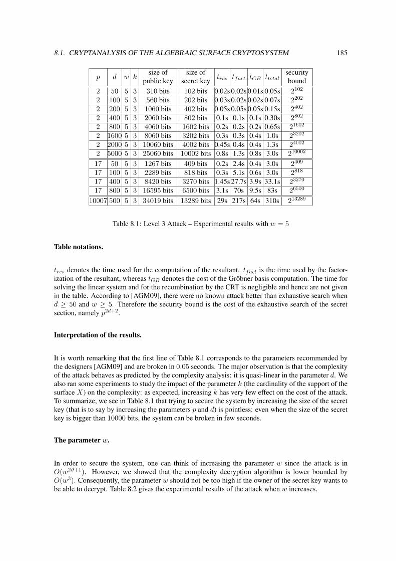
8.1. CRYPTANALYSIS OF THE ALGEBRAIC SURFACE CRYPTOSYSTEM 185

p d w ksize of

public keysize of

secret key tres tfact tGB ttotalsecuritybound

2 50 5 3 310 bits 102 bits 0.02s 0.02s 0.01s 0.05s 2102

2 100 5 3 560 bits 202 bits 0.03s 0.02s 0.02s 0.07s 2202

2 200 5 3 1060 bits 402 bits 0.05s 0.05s 0.05s 0.15s 2402

2 400 5 3 2060 bits 802 bits 0.1s 0.1s 0.1s 0.30s 2802

2 800 5 3 4060 bits 1602 bits 0.2s 0.2s 0.2s 0.65s 21602

2 1600 5 3 8060 bits 3202 bits 0.3s 0.3s 0.4s 1.0s 23202

2 2000 5 3 10060 bits 4002 bits 0.45s 0.4s 0.4s 1.3s 24002

2 5000 5 3 25060 bits 10002 bits 0.8s 1.3s 0.8s 3.0s 210002

17 50 5 3 1267 bits 409 bits 0.2s 2.4s 0.4s 3.0s 2409

17 100 5 3 2289 bits 818 bits 0.3s 5.1s 0.6s 3.0s 2818

17 400 5 3 8420 bits 3270 bits 1.45s 27.7s 3.9s 33.1s 23270

17 800 5 3 16595 bits 6500 bits 3.1s 70s 9.5s 83s 26500

10007 500 5 3 34019 bits 13289 bits 29s 217s 64s 310s 213289

Table 8.1: Level 3 Attack – Experimental results with w = 5

Table notations.

tres denotes the time used for the computation of the resultant. tfact is the time used by the factor-ization of the resultant, whereas tGB denotes the cost of the Grobner basis computation. The time forsolving the linear system and for the recombination by the CRT is negligible and hence are not givenin the table. According to [AGM09], there were no known attack better than exhaustive search whend ≥ 50 and w ≥ 5. Therefore the security bound is the cost of the exhaustive search of the secretsection, namely p2d+2.

Interpretation of the results.

It is worth remarking that the first line of Table 8.1 corresponds to the parameters recommended bythe designers [AGM09] and are broken in 0.05 seconds. The major observation is that the complexityof the attack behaves as predicted by the complexity analysis: it is quasi-linear in the parameter d. Wealso ran some experiments to study the impact of the parameter k (the cardinality of the support of thesurface X) on the complexity: as expected, increasing k has very few effect on the cost of the attack.To summarize, we see in Table 8.1 that trying to secure the system by increasing the size of the secretkey (that is to say by increasing the parameters p and d) is pointless: even when the size of the secretkey is bigger than 10000 bits, the system can be broken in few seconds.

The parameter w.

In order to secure the system, one can think of increasing the parameter w since the attack is inO(w2ϑ+1). However, we showed that the complexity decryption algorithm is lower bounded byO(w3). Consequently, the parameter w should not be too high if the owner of the secret key wants tobe able to decrypt. Table 8.2 gives the experimental results of the attack when w increases.

186 CHAPTER 8. APPLICATION TO CRYPTOLOGY

p d w ksize of

public keysize of

secret key tres tfact tGB tLinSys ttotalsecuritybound

2 50 5 3 310 bits 102 bits 0.02s 0.02s 0.01s 0.001s 0.05s 2102

2 50 15 3 810 bits 102 bits 0.7s 0.3s 4.4s 0.03s 5.4s 2102

2 50 25 3 1310 bits 102 bits 3s 1s 32s 0.2s 37s 2102

2 50 35 3 1810 bits 102 bits 10s 3s 260s 1s 274s 2102

2 50 45 3 2310 bits 102 bits 30s 7s 1352s 4s 1393s 2102

2 50 55 3 2810 bits 102 bits 70s 12s 4619s 13s 4714s 2102

2 50 65 3 3310 bits 102 bits 147s 22s 12408s 27s 12604s 2102

2 50 75 3 3810 bits 102 bits 288s 38s 37900s 56s 38280s 2102

Table 8.2: Level 3 Attack – Experimental results: increasing w

Interpretation of the results.

The main observation is that the complexity of the attack still behaves as predicted: when w is in-creased, the Grobner basis computation is the most expensive step. Increasing w seems to be thebest counter-measure against the attack. However, it should be noted that the attack is still feasible inpractice, even when the public key is big.

8.1.9 Conclusion

In this section, we analyze the security of the PKC’2009 Algebraic Surface Cryptosystem. We providethree variants of a message recovery attack. We also estimate very precisely the complexity of theLevel 3 Attack and we show that it is polynomial in all the parameters of the system. Furthermore, itis quasi-linear in the size of the secret key, whereas the decryption algorithm proposed in [AGM09] iscubic.

Experimental results confirm the theoretical analysis. We show that the attack can easily breakASC with recommended parameters. The best choice to try to secure ASC against the attack is totake p and d as small as possible (p = 2 and d = 50) and increase w. However our implementationis polynomial in w and can break the system in few hours, even when w = 75 (this value can becompared to the initial recommended w = 5).

Thereby, we consider that the system is fully broken, but we believe that the section findingproblem is still an interesting problem for the design of cryptographic schemes; in this section, wehave simply shown how to avoid to solve it in the context of ASC.

8.1.10 Toy example

We describe here the toy example given in [AGM09]:

• K = F17.

• w = 5.

• d = 3.

• k = 5.

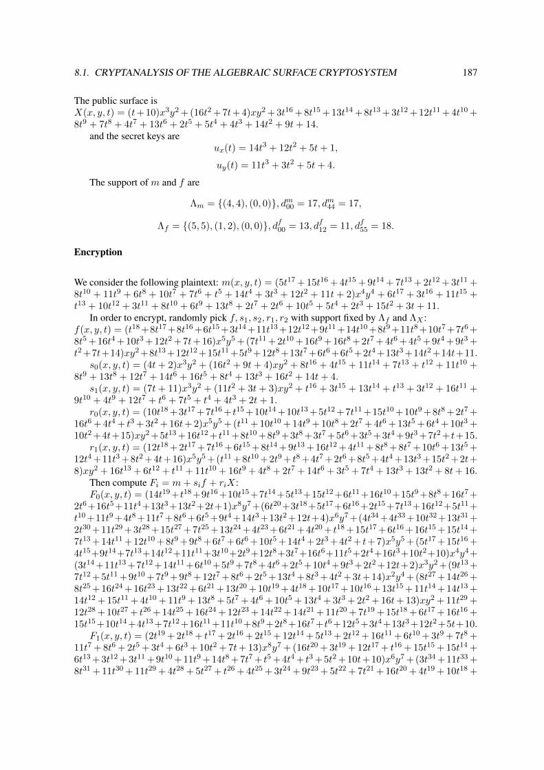
8.1. CRYPTANALYSIS OF THE ALGEBRAIC SURFACE CRYPTOSYSTEM 187

The public surface isX(x, y, t) = (t+ 10)x3y2 + (16t2 + 7t+ 4)xy2 + 3t16 + 8t15 + 13t14 + 8t13 + 3t12 + 12t11 + 4t10 +8t9 + 7t8 + 4t7 + 13t6 + 2t5 + 5t4 + 4t3 + 14t2 + 9t+ 14.

and the secret keys areux(t) = 14t3 + 12t2 + 5t+ 1,

uy(t) = 11t3 + 3t2 + 5t+ 4.

The support of m and f are

Λm = (4, 4), (0, 0), dm00 = 17, dm44 = 17,

Λf = (5, 5), (1, 2), (0, 0), df00 = 13, df12 = 11, df55 = 18.

Encryption

We consider the following plaintext: m(x, y, t) = (5t17 + 15t16 + 4t15 + 9t14 + 7t13 + 2t12 + 3t11 +8t10 + 11t9 + 6t8 + 10t7 + 7t6 + t5 + 14t4 + 3t3 + 12t2 + 11t+ 2)x4y4 + 6t17 + 3t16 + 11t15 +t13 + 10t12 + 3t11 + 8t10 + 6t9 + 13t8 + 2t7 + 2t6 + 10t5 + 5t4 + 2t3 + 15t2 + 3t+ 11.

In order to encrypt, randomly pick f, s1, s2, r1, r2 with support fixed by Λf and ΛX :f(x, y, t) = (t18 +8t17 +8t16 +6t15 +3t14 +11t13 +12t12 +9t11 +14t10 +8t9 +11t8 +10t7 +7t6 +8t5 + 16t4 + 10t3 + 12t2 + 7t+ 16)x5y5 + (7t11 + 2t10 + 16t9 + 16t8 + 2t7 + 4t6 + 4t5 + 9t4 + 9t3 +t2 +7t+14)xy2 +8t13 +12t12 +15t11 +5t9 +12t8 +13t7 +6t6 +6t5 +2t4 +13t3 +14t2 +14t+11.

s0(x, y, t) = (4t+ 2)x3y2 + (16t2 + 9t+ 4)xy2 + 8t16 + 4t15 + 11t14 + 7t13 + t12 + 11t10 +8t9 + 13t8 + 12t7 + 14t6 + 16t5 + 8t4 + 13t3 + 16t2 + 14t+ 4.

s1(x, y, t) = (7t+ 11)x3y2 + (11t2 + 3t+ 3)xy2 + t16 + 3t15 + 13t14 + t13 + 3t12 + 16t11 +9t10 + 4t9 + 12t7 + t6 + 7t5 + t4 + 4t3 + 2t+ 1.

r0(x, y, t) = (10t18 +3t17 +7t16 + t15 +10t14 +10t13 +5t12 +7t11 +15t10 +10t9 +8t8 +2t7 +16t6 + 4t4 + t3 + 3t2 + 16t+ 2)x5y5 + (t11 + 10t10 + 14t9 + 10t8 + 2t7 + 4t6 + 13t5 + 6t4 + 10t3 +10t2 +4t+15)xy2 +5t13 +16t12 + t11 +8t10 +8t9 +3t8 +3t7 +5t6 +3t5 +3t4 +9t3 +7t2 + t+15.

r1(x, y, t) = (12t18 +2t17 +7t16 +6t15 +8t14 +9t13 +16t12 +4t11 +8t8 +8t7 +10t6 +13t5 +12t4 +11t3 +8t2 +4t+16)x5y5 +(t11 +8t10 +2t9 + t8 +4t7 +2t6 +8t5 +4t4 +13t3 +15t2 +2t+8)xy2 + 16t13 + 6t12 + t11 + 11t10 + 16t9 + 4t8 + 2t7 + 14t6 + 3t5 + 7t4 + 13t3 + 13t2 + 8t+ 16.

Then compute Fi = m+ sif + riX:F0(x, y, t) = (14t19 +t18 +9t16 +10t15 +7t14 +5t13 +15t12 +6t11 +16t10 +15t9 +8t8 +16t7 +

2t6+16t5+11t4+13t3+13t2+2t+1)x8y7+(6t20+3t18+5t17+6t16+2t15+7t13+16t12+5t11+t10 +11t9 +4t8 +11t7 +8t6 +6t5 +9t4 +14t3 +13t2 +12t+4)x6y7 +(4t34 +4t33 +10t32 +13t31 +2t30 +11t29 +3t28 +15t27 +7t25 +13t24 +4t23 +6t21 +4t20 + t18 +15t17 +6t16 +16t15 +15t14 +7t13 +14t11 +12t10 +8t9 +9t8 +6t7 +6t6 +10t5 +14t4 +2t3 +4t2 + t+7)x5y5 +(5t17 +15t16 +4t15+9t14+7t13+14t12+11t11+3t10+2t9+12t8+3t7+16t6+11t5+2t4+16t3+10t2+10)x4y4+(3t14 +11t13 +7t12 +14t11 +6t10 +5t9 +7t8 +4t6 +2t5 +10t4 +9t3 +2t2 +12t+2)x3y2 +(9t13 +7t12 +5t11 +9t10 +7t9 +9t8 +12t7 +8t6 +2t5 +13t4 +8t3 +4t2 +3t+14)x2y4 +(8t27 +14t26 +8t25 +16t24 +16t23 +13t22 +6t21 +13t20 +10t19 +4t18 +10t17 +10t16 +13t15 +11t14 +14t13 +14t12 + 15t11 + 4t10 + 11t9 + 13t8 + 5t7 + 4t6 + 10t5 + 13t4 + 3t3 + 2t2 + 16t+ 13)xy2 + 11t29 +12t28 + 10t27 + t26 + 14t25 + 16t24 + 12t23 + 14t22 + 14t21 + 11t20 + 7t19 + 15t18 + 6t17 + 16t16 +15t15 +10t14 +4t13 +7t12 +16t11 +11t10 +8t9 +2t8 +16t7 +t6 +12t5 +3t4 +13t3 +12t2 +5t+10.

F1(x, y, t) = (2t19 + 2t18 + t17 + 2t16 + 2t15 + 12t14 + 5t13 + 2t12 + 16t11 + 6t10 + 3t9 + 7t8 +11t7 + 8t6 + 2t5 + 3t4 + 6t3 + 10t2 + 7t+ 13)x8y7 + (16t20 + 3t19 + 12t17 + t16 + 15t15 + 15t14 +6t13 +3t12 +3t11 +9t10 +11t9 +14t8 +7t7 + t5 +4t4 + t3 +5t2 +10t+10)x6y7 +(3t34 +11t33 +8t31 + 11t30 + 11t29 + 4t28 + 5t27 + t26 + 4t25 + 3t24 + 9t23 + 5t22 + 7t21 + 16t20 + 4t19 + 10t18 +

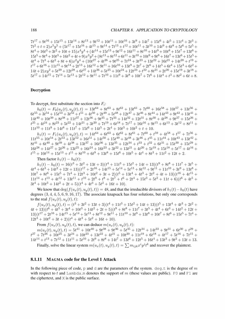
188 CHAPTER 8. APPLICATION TO CRYPTOLOGY

7t17 + 9t16 + 15t15 + 13t14 + 8t13 + 9t12 + 10t11 + 10t10 + 3t9 + 14t7 + 15t6 + 4t5 + 11t4 + 2t3 +7t2 + t+ 2)x5y5 + (5t17 + 15t16 + 4t15 + 9t14 + 7t13 + t12 + 10t11 + 3t10 + 14t9 + 6t8 + 5t6 + 5t5 +8t4 +16t3 +3t2 +10t+15)x4y4 +(4t14 +15t13 +9t12 +16t11 +8t10 +14t9 +10t8 +15t7 +13t6 +15t5 +9t4 +10t3 +16t2 +4t+9)x3y2 +(8t13 +8t12 +6t11 +3t10 +10t9 +9t8 +16t7 +13t6 +15t5 +4t4 + 7t3 + 6t2 + 8t+ 6)x2y4 + (10t27 + 4t26 + 9t25 + 7t24 + 3t23 + 13t22 + 16t21 + 14t20 + t19 +t17 +6t16 +11t15 +9t14 +2t13 +16t12 +9t11 +16t10 +13t9 +2t7 +2t6 +14t5 +6t4 +15t3 +6t2 +14t+2)xy2 +5t29 +12t28 +6t27 +14t26 +5t25 +10t24 +12t23 + t22 +8t21 +2t20 +15t19 +3t18 +5t17 + 14t15 + 7t14 + 5t13 + 2t12 + 9t11 + 7t10 + 11t9 + 3t8 + 10t7 + 7t6 + 14t4 + t3 + 8t2 + 6t+ 8.

Decryption

To decrypt, first substitute the section into Fi:h0(t) = F0(ux(t), uy(t), t) = 13t64 + 8t63 + 8t62 + 13t61 + 7t60 + 16t58 + 10t57 + 13t56 +

6t55 + 3t54 + 15t53 + 3t52 + t51 + 4t50 + 2t49 + 5t48 + 12t47 + 3t46 + 8t44 + 14t43 + 9t42 + 13t41 +14t40 + 10t39 + 8t38 + 11t37 + 12t36 + 9t35 + 7t33 + 14t32 + 12t31 + 8t30 + 4t28 + 9t27 + 15t26 +t25 + 4t24 + 8t23 + 5t22 + 14t21 + 3t20 + 7t19 + 6t18 + 7t17 + 16t16 + 9t15 + 6t13 + 3t12 + 8t11 +11t10 + 11t9 + 14t8 + 11t7 + 15t6 + 14t5 + 2t4 + 10t3 + 10t2 + t+ 10.

h1(t) = F1(ux(t), uy(t), t) = 14t64 + 6t63 + 6t62 + 8t61 + 7t60 + t59 + 4t58 + t57 + 7t56 +11t55 + 10t54 + 2t53 + 13t52 + 16t51 + 14t50 + 15t49 + 3t48 + 3t46 + t45 + 11t44 + 10t43 + 13t42 +8t41 + 6t40 + 9t39 + 4t38 + 13t37 + 16t36 + 13t35 + 12t34 + t33 + t32 + 6t31 + 15t30 + 15t29 +16t28 + 14t27 + 2t26 + 13t25 + 16t24 + 16t23 + 3t22 + 13t21 + 4t20 + 5t19 + 15t18 + 5t17 + 4t16 +t15 + 10t14 + 15t13 + t11 + 8t10 + 6t9 + 13t8 + 15t6 + 10t5 + 4t4 + 8t3 + 11t2 + 12t+ 2.

Then factor h1(t)− h0(t):h1(t)− h0(t) = 16(t3 + 3t2 + 13t+ 3)(t4 + 11t3 + 15t2 + 14t+ 13)(t9 + 8t8 + 11t7 + 3t5 +

4t4 + 6t3 + 14t2 + 12t+ 13)(t17 + 2t16 + 14t15 + 5t14 + 5t13 + 8t12 + 9t11 + 11t10 + 3t9 + 13t8 +10t7 + 8t6 + 15t5 + 7t4 + 12t3 + 10t2 + 3t + 2)(t5 + 13t4 + 4t3 + 2t2 + 4t + 13)(t16 + 4t15 +11t14 + t13 + 4t12 + 13t11 + t10 + 2t9 + t8 + 2t7 + t6 + 2t4 + 15t3 + 5t2 + 11t + 6)(t6 + 4t5 +3t4 + 10t3 + 14t2 + 2t+ 5)(t4 + 4t3 + 5t2 + 16t+ 10).

We know that deg(f(ux(t), uy(t), t)) = 48, and that the irreducible divisors of h1(t)−h0(t) havedegrees (3, 4, 4, 5, 6, 9, 16, 17). The associate knapsack has four solutions, but only one correspondsto the real f(ux(t), uy(t), t):

f(ux(t), uy(t), t) = (t3 + 3t2 + 13t+ 3)(t4 + 11t3 + 15t2 + 14t+ 13)(t5 + 13t4 + 4t3 + 2t2 +4t+ 13)(t6 + 4t5 + 3t4 + 10t3 + 14t2 + 2t+ 5)(t9 + 8t8 + 11t7 + 3t5 + 4t4 + 6t3 + 14t2 + 12t+13)(t17 + 2t16 + 14t15 + 5t14 + 5t13 + 8t12 + 9t11 + 11t10 + 3t9 + 13t8 + 10t7 + 8t6 + 15t5 + 7t4 +12t3 + 10t2 + 3t+ 2)(t4 + 4t3 + 5t2 + 16t+ 10).

From f(ux(t), uy(t), t), we can deduce m(ux(t), uy(t), t):m(ux(t), uy(t), t) = 5t41 + 10t40 + 9t38 + 9t36 + 5t35 + 12t34 + 14t33 + 9t31 + 6t30 + t29 +

t27 + 7t26 + 10t25 + 3t24 + 10t23 + 13t22 + 4t21 + 10t20 + 11t19 + 6t18 + 4t17 + 5t16 + 7t15 +14t14 + t13 + 7t12 + 11t11 + 5t10 + 2t9 + 8t8 + 14t7 + 13t6 + 12t5 + 16t4 + 13t3 + 9t2 + 13t+ 13.

Finally, solve the linear system m(ux(t), uy(t), t) =∑mijkx

iyjtk and recover the plaintext.

8.1.11 MAGMA code for the Level 1 Attack

In the following piece of code, p and d are the parameters of the system. deg t is the degree of mwith respect to t and Lambda m denotes the support of m (these values are public). F0 and F1 arethe ciphertext, and X is the public surface.

8.2. CRYPTANALYSIS OF MINRANK 189

R<x,y,t>:=PolynomialRing(GF(p),3,"grevlex");Res:=Resultant(R!(F0-F1),R!X,x); // Eliminate xF:=Factorization(Res); // Factor the resultant// Pick the irreducible factor of highest degree in ymaxdeg:=Max([Degree(R!f[1],R!y) : f in F]);exists(Q0)f[1]:f in F| Degree(R!f[1],R!y) eq maxdeg;J:=Ideal([R!Q0,R!X,R!F0,R!F1]);Groebner(J); // Compute the Gr\"obner basis of JCoeffm:=PolynomialRing(GF(p),#Lambda_m*(deg_t+1));R2<x,y,t>:=PolynomialRing(Coeffm,3);// Construct the linear systemplaintext:=&+[Coeffm.((i-1)*(deg_t+1)+j)*

R2!NormalForm(R!xˆLambda_m[i][1]*R!yˆLambda_m[i][2]*R!tˆ(j-1),J) :i in [1..#Lambda_m], j in [1..deg_t+1]];

// Solve the linear system:V:=Variety(Ideal(Coefficients(plaintext)));

8.2 Cryptanalysis of MinRank

In this section, we show how Grobner basis techniques can be used to study the security of the authen-tication scheme proposed in [Cou01] (see Section 2.2.1). In particular, we study the challenges A, Band C from Table 2.1. The security of the cryptosystem relies on the difficulty of a particular MinRankproblem: it is defined in the finite field GF65521 and one solution of the problem lies in GFn65521.

In order to assess the security of the system against algebraic attacks, we focus on the minorsmodeling (see Section 2.1.2): we consider the set of minors of size r + 1, which gives rise to adeterminantal system.

Workstation. Experimental results have been obtained with 24 Xeon quadricore processors 3.2GHz, with 64 GB of RAM.

8.2.1 Computing the minors

The minors modeling raises questions about how to generate the equations. It is not clear how tocompute efficiently all minors of size r + 1 of a big matrix. For a p × p matrix, there are

(pr+1

)2such minors, and each is a polynomial of degree r + 1 in n variables. For instance, for an affineproblem with K = GF65521, p = 11, n = 9 and r = 8, it took 14 days on one CPU (with Maple).Fortunately, this computation can be parallelized: with 120 processes running simultaneously on 24CPU, the computation lasted 12 hours. The size of the resulting algebraic system is 3466 MB.

For this computation, we used naive algorithms (each determinant was computed independently)but we believe that there is room for improvement by using more sophisticated algorithms.

8.2.2 The well-defined case

Here, n = (p− r)2 and the ground field is K = GF65521.Generation of the instances. For (p, n, r) ∈ N3, we generate a p× p matrix M = (Mi,j) where

the Mi,j are affine linear forms in n variables: Mi,j = a(0)i,j +

∑n`=1 a

(`)i,j x`, where the a(`)

i,j are chosenuniformly at random in GF65521.

Interpretation of the results. Table 8.3 describes experimental results, for different values of thetriplet (p, n, r). In particular, we consider sets of parameters used in Cryptology for a MinRank-based

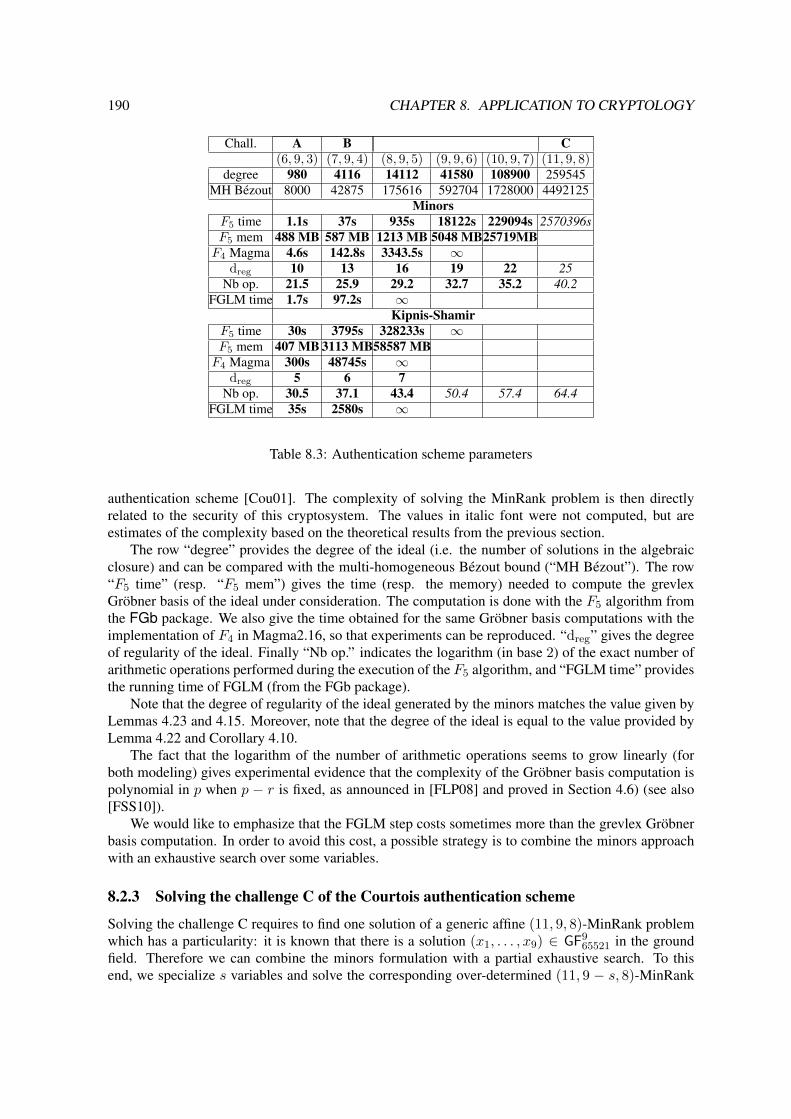
190 CHAPTER 8. APPLICATION TO CRYPTOLOGY

Chall. A B C(6, 9, 3) (7, 9, 4) (8, 9, 5) (9, 9, 6) (10, 9, 7) (11, 9, 8)

degree 980 4116 14112 41580 108900 259545MH Bezout 8000 42875 175616 592704 1728000 4492125

MinorsF5 time 1.1s 37s 935s 18122s 229094s 2570396sF5 mem 488 MB 587 MB 1213 MB 5048 MB25719MBF4 Magma 4.6s 142.8s 3343.5s ∞

dreg 10 13 16 19 22 25Nb op. 21.5 25.9 29.2 32.7 35.2 40.2

FGLM time 1.7s 97.2s ∞Kipnis-Shamir

F5 time 30s 3795s 328233s ∞F5 mem 407 MB 3113 MB58587 MBF4 Magma 300s 48745s ∞

dreg 5 6 7Nb op. 30.5 37.1 43.4 50.4 57.4 64.4

FGLM time 35s 2580s ∞

Table 8.3: Authentication scheme parameters

authentication scheme [Cou01]. The complexity of solving the MinRank problem is then directlyrelated to the security of this cryptosystem. The values in italic font were not computed, but areestimates of the complexity based on the theoretical results from the previous section.

The row “degree” provides the degree of the ideal (i.e. the number of solutions in the algebraicclosure) and can be compared with the multi-homogeneous Bezout bound (“MH Bezout”). The row“F5 time” (resp. “F5 mem”) gives the time (resp. the memory) needed to compute the grevlexGrobner basis of the ideal under consideration. The computation is done with the F5 algorithm fromthe FGb package. We also give the time obtained for the same Grobner basis computations with theimplementation of F4 in Magma2.16, so that experiments can be reproduced. “dreg” gives the degreeof regularity of the ideal. Finally “Nb op.” indicates the logarithm (in base 2) of the exact number ofarithmetic operations performed during the execution of the F5 algorithm, and “FGLM time” providesthe running time of FGLM (from the FGb package).

Note that the degree of regularity of the ideal generated by the minors matches the value given byLemmas 4.23 and 4.15. Moreover, note that the degree of the ideal is equal to the value provided byLemma 4.22 and Corollary 4.10.

The fact that the logarithm of the number of arithmetic operations seems to grow linearly (forboth modeling) gives experimental evidence that the complexity of the Grobner basis computation ispolynomial in p when p − r is fixed, as announced in [FLP08] and proved in Section 4.6) (see also[FSS10]).

We would like to emphasize that the FGLM step costs sometimes more than the grevlex Grobnerbasis computation. In order to avoid this cost, a possible strategy is to combine the minors approachwith an exhaustive search over some variables.

8.2.3 Solving the challenge C of the Courtois authentication scheme

Solving the challenge C requires to find one solution of a generic affine (11, 9, 8)-MinRank problemwhich has a particularity: it is known that there is a solution (x1, . . . , x9) ∈ GF9

65521 in the groundfield. Therefore we can combine the minors formulation with a partial exhaustive search. To thisend, we specialize s variables and solve the corresponding over-determined (11, 9 − s, 8)-MinRank

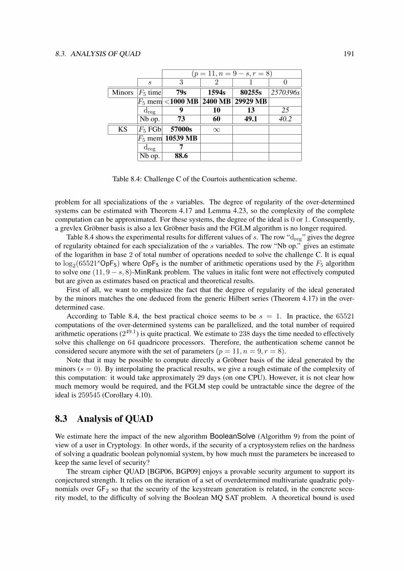
8.3. ANALYSIS OF QUAD 191

(p = 11, n = 9− s, r = 8)s 3 2 1 0

Minors F5 time 79s 1594s 80255s 2570396sF5 mem <1000 MB 2400 MB 29929 MB

dreg 9 10 13 25Nb op. 73 60 49.1 40.2

KS F5 FGb 57000s ∞F5 mem 10539 MB

dreg 7Nb op. 88.6

Table 8.4: Challenge C of the Courtois authentication scheme.

problem for all specializations of the s variables. The degree of regularity of the over-determinedsystems can be estimated with Theorem 4.17 and Lemma 4.23, so the complexity of the completecomputation can be approximated. For these systems, the degree of the ideal is 0 or 1. Consequently,a grevlex Grobner basis is also a lex Grobner basis and the FGLM algorithm is no longer required.

Table 8.4 shows the experimental results for different values of s. The row “dreg” gives the degreeof regularity obtained for each specialization of the s variables. The row “Nb op.” gives an estimateof the logarithm in base 2 of total number of operations needed to solve the challenge C. It is equalto log2(65521sOpF5) where OpF5 is the number of arithmetic operations used by the F5 algorithmto solve one (11, 9− s, 8)-MinRank problem. The values in italic font were not effectively computedbut are given as estimates based on practical and theoretical results.

First of all, we want to emphasize the fact that the degree of regularity of the ideal generatedby the minors matches the one deduced from the generic Hilbert series (Theorem 4.17) in the over-determined case.

According to Table 8.4, the best practical choice seems to be s = 1. In practice, the 65521computations of the over-determined systems can be parallelized, and the total number of requiredarithmetic operations (249.1) is quite practical. We estimate to 238 days the time needed to effectivelysolve this challenge on 64 quadricore processors. Therefore, the authentication scheme cannot beconsidered secure anymore with the set of parameters (p = 11, n = 9, r = 8).

Note that it may be possible to compute directly a Grobner basis of the ideal generated by theminors (s = 0). By interpolating the practical results, we give a rough estimate of the complexity ofthis computation: it would take approximately 29 days (on one CPU). However, it is not clear howmuch memory would be required, and the FGLM step could be untractable since the degree of theideal is 259545 (Corollary 4.10).

8.3 Analysis of QUAD

We estimate here the impact of the new algorithm BooleanSolve (Algorithm 9) from the point ofview of a user in Cryptology. In other words, if the security of a cryptosystem relies on the hardnessof solving a quadratic boolean polynomial system, by how much must the parameters be increased tokeep the same level of security?

The stream cipher QUAD [BGP06, BGP09] enjoys a provable security argument to support itsconjectured strength. It relies on the iteration of a set of overdetermined multivariate quadratic poly-nomials over GF2 so that the security of the keystream generation is related, in the concrete secu-rity model, to the difficulty of solving the Boolean MQ SAT problem. A theoretical bound is used

192 CHAPTER 8. APPLICATION TO CRYPTOLOGY

in [BGP09] to obtain secure parameters for a given security bound T and a given maximal length Lof the keystream sequence that can be generated with a pair (key, IV): for instance (see [BGP09] p.1711), for T = 280, L = 240, k = 2 and an advantage of more than ε = 1/100, the bound givesn ≥ 331. We report in the following table various values of n depending on L, T and ε:

T L ε n280 240 1/100 331280 222 1/100 2532160 280 1/100 6132160 240 1/100 4452160 240 1/1000 4482160 240 1/10000 4672256 240 1/100 5842256 280 1/100 758

Security parameters for the stream cipher QUAD [BGP09]

Now, the question is to achieve a security bound for T = 2256; what are the minimal values ofm and n ensuring that solving the Boolean MQ SAT requires at least T bit-operations? Using thecomplexity analysis of the BooleanSolve algorithm we can derive useful lower bounds for n whenm = n or m = 2n (m = 2n corresponds to the recommended parameters for QUAD). In thefollowing table we report the corresponding values:

Security Bound T 2128 2256 2512 21024

Minimal value of n when m = n 128 270 576 1202Minimal value of n when m = 2n 145 335 738 1580

Comparing with exhaustive search we can see from this table that:

• our algorithm does not improve upon exhaustive search when n is small (for instance whenm = n and T = 2128 that are the recommended parameters);

• by contrast, our algorithm can take advantage of the overdeterminedness of the algebraic sys-tems: this explains why the values we recommend are larger than expected when n is largeand/or m/n > 1.

INDEX 193

Index

F5 Algorithmmatrix F5, 43multi-homogeneous variant, 137

F5 criterion, 42γ-strong semi-regularity, 163Dr-genericity, 77Ir-genericity, 77

ASC, 58, 171associated primes, 27

critical point method, 61

degree of a 0-dimensional ideal, 24Bezout bound, 46multi-homogeneous Bezout bound, 47

degree of regularity, 47determinantal ideal

Cohen-Macaulay, 64degree, 63dimension, 63Hilbert series, 63

dimensionKrull dimension of a ring, 23of an ideal, 23

Eagon-Northcott complex, 112

FGLMcomplexity, 44

Froberg’s conjecture, 38free resolution, 26

Grobner basis, 28d-Grobner basis, 40complexity, 49, 50minimal, 29reduced, 29

HFE, 56Hilbert function, 32Hilbert polynomial, 45Hilbert series, 32

of a regular sequence, 36Hilbert syzygy Theorem, 26homogeneous grading on K[X], 30

ideal

admissible, 64homogeneous, 31multi-homogeneous, 31quasi-homogeneous, 31

index of regularity, 45Macaulay bound, 46

irreducible decomposition of ideals, 26irreducible decomposition of varieties, 26

Lazard’s algorithmhomogeneous, 41

leading monomial, 28

Macaulay matrix, 40boolean, 153

matrix F5 algorithm, 44McEliece, 57MinRank, 53, 187

Courtois Authentication Scheme, 55generalized, 54, 73

module, 25exterior algebra, 26free module, 25symmetric algebra, 26tensor algebra, 25tensor product, 25

monomial ordering, 27grevlex ordering, 28lex ordering, 28

multi-homogeneous grading on K[X]irrelevant ideals, 64

multi-homogeneous grading on K[X], 31

normal form, 29algorithm, 42

QUAD, 58, 189quasi-homogeneous grading on K[X], 30

Rank Metric Codes, 56regular sequence, 35

Hilbert series, 36weighted Hilbert series, 46

semi-regular sequenceaffine, 38homogeneous, 37over GF2, 38

194 INDEX

shape position, 39syzygy, 36

witness degree, 153

Zariski topology, 24

INDEX OF NOTATIONS 195

Index of Notations

IId, 31Id, 31I

(w)d , 31

O, 48T (M), 25W (Fh), 101Z(I), 24Z(F), 24[S]+, 37Ass(I), 27BL K(nx, ny), 64DEG, 24Dr, 63GFq, 23HF, 32

mHF, 32wHF, 32

HS, 32mHS, 32wHS, 32

K, 23K[X], 23

K[X]d, 31K[X]d, 30K[X]

(w)d , 30

K, 23LM≺, 28NF≺,I , 29Ω, 48χ, 47crit(π1, Z(F)), 101dmax≺, 48dreg, 47dwit, 153Ir, 76ireg, 45jac(F), 61jac(F, i), 62Mac≺,D, 40M , 76V , 47Sym(M), 26π1, 61, 101≺, 27≺grevlex, 28

≺lex, 28ψb,c, 76I(F, 1), 101Syz, 36Syztriv(F), 64ϕa, 76ϑ, 67∧M , 26Dr, 76Ir, 76

196 INDEX OF NOTATIONS

Bibliography

[Abh88] S.S. Abhyankar. Enumerative combinatorics of Young tableaux. Marcel Dekker, 1988.

[AFFP11] M. Albrecht, J.-C. Faugere, P. Farshim, and L. Perret. Polly cracker, revisited. In Pro-ceedings of Asiacrypt 2011, Lecture Notes in Computer Science, pages 1–14. SpringerVerlag, 2011.

[AFI+04] G. Ars, J.-C. Faugere, H. Imai, M. Kawazoe, and M. Sugita. Comparison between XLand Grobner basis algorithms. In Advances in Cryptology – AsiaCrypt 2004, volume3329/2004 of LNCS, pages 157–167, 2004.

[AG04] K. Akiyama and Y. Goto. An algebraic surface public-key cryptosystem. IEIC Tech-nical Report (Institute of Electronics, Information and Communication Engineers),104(421):13–20, 2004.

[AGM09] K. Akiyama, Y. Goto, and H. Miyake. An algebraic surface cryptosystem. In Pro-ceedings of the 12th International Conference on Practice and Theory in Public KeyCryptography: PKC’09, page 442. Springer, 2009.

[AM69] M.F. Atiyah and I.G. MacDonald. Introduction to Commutative Algebra. Addison-Wesley Publishing Company, 1969.

[ARS02] P. Aubry, F. Rouillier, and M. Safey El Din. Real solving for positive dimensional sys-tems. Journal of Symbolic Computation, 34(6):543–560, 2002.

[Bar93] A.I. Barvinok. Feasibility testing for systems of real quadratic equations. Discrete &Computational Geometry, 10(1):1–13, 1993.

[Bar04] M. Bardet. Etude des systemes algebriques surdetermines. Applications aux codes cor-recteurs et a la cryptographie. PhD thesis, Universite Paris 6, 2004.

[BCC+10] C. Bouillaguet, H.-C. Chen, C.-M. Cheng, Tung Chou, R. Niederhagen, A. Shamir, andB.-Y. Yang. Fast exhaustive search for polynomial systems in F2. In CryptographicHardware and Embedded Systems, CHES 2010, volume 6225 of LNCS, pages 203–218,2010.

[BCGO09] T. Berger, P.L. Cayrel, P. Gaborit, and A. Otmani. Reducing key length of the McEliececryptosystem. Progress in Cryptology–AFRICACRYPT 2009, pages 77–97, 2009.

[BCP97] W. Bosma, J. Cannon, and C. Playoust. The Magma algebra system. I. The user language.Journal of Symbolic Computation, 24(3–4):235–265, 1997.

[BFP09] L. Bettale, J.-C. Faugere, and L. Perret. Hybrid approach for solving multivariate systemsover finite fields. Journal of Mathematical Cryptology, 3:177–197, 2009.

197

198 BIBLIOGRAPHY

[BFP11] L. Bettale, J.-C. Faugere, and L. Perret. Cryptanalysis of multivariate and odd-characteristic HFE variants. In Public Key Cryptography – PKC 2011, volume 6571of Lecture Notes in Computer Science, pages 441–458. Springer, 2011.

[BFP12a] L. Bettale, J.-C. Faugere, and L. Perret. Cryptanalysis of HFE, multi-HFE and variantsfor odd and even characteristic. Design, Codes and Cryptography, 2012.

[BFP12b] L. Bettale, J.-C. Faugere, and L. Perret. Solving polynomial systems over finite fields:Improved analysis of the hybrid approach. In International Symposium on Symbolic andAlgebraic Computation – ISSAC 2012. ACM, 2012.

[BFS99] J.F. Buss, G.S. Frandsen, and J. Shallit. The computational complexity of some problemsof linear algebra. Journal of Computer and System Sciences, 58(3):572–596, 1999.

[BFS04] M. Bardet, J.-C. Faugere, and B. Salvy. On the complexity of Grobner basis computationof semi-regular overdetermined algebraic equations. In Proceedings of the InternationalConference on Polynomial System Solving (ISCPP), pages 71–74, 2004.

[BFSS12] M. Bardet, J.-C. Faugere, B. Salvy, and P.-J. Spaenlehauer. On the complexity of solvingquadratic boolean systems. Journal of Complexity, 2012. Accepted for publication.

[BFSY04] M. Bardet, J.-C. Faugere, B. Salvy, and B.-Y. Yang. Asymptotic expansion of the degreeof regularity for semi-regular systems of equations. In Effective Methods in AlgebraicGeometry (MEGA), pages 71–74, 2004.

[BGH+10] B. Bank, M. Giusti, J. Heintz, M. Safey El Din, and E. Schost. On the geometry ofpolar varieties. Applicable Algebra in Engineering, Communication and Computing,21(1):33–83, 2010.

[BGHM97] B. Bank, M. Giusti, J. Heintz, and G.-M. Mbakop. Polar varieties and efficient realequation solving: the hypersurface case. Journal of Complexity, 13(1):5–27, 1997.

[BGHM01] B. Bank, M. Giusti, J. Heintz, and G.-M. Mbakop. Polar varieties and efficient realelimination. Mathematische Zeitschrift, 238(1):115–144, 2001.

[BGHP04] B. Bank, M. Giusti, J. Heintz, and L.-M. Pardo. Generalized polar varieties and efficientreal elimination procedure. Kybernetika, 40(5):519–550, 2004.

[BGHP05] B. Bank, M. Giusti, J. Heintz, and L.-M. Pardo. Generalized polar varieties: Geometryand algorithms. Journal of complexity, 21(4):377–412, 2005.

[BGP06] C. Berbain, H. Gilbert, and J. Patarin. QUAD: A practical stream cipher with prov-able security. In Serge Vaudenay, editor, Advances in Cryptology - EUROCRYPT 2006,volume 4004 of Lecture Notes in Computer Science, pages 109–128. Springer Berlin /Heidelberg, 2006.

[BGP09] C. Berbain, H. Gilbert, and J. Patarin. QUAD: A multivariate stream cipher with provablesecurity. Journal of Symbolic Computation, 44:1703–1723, December 2009.

[BL09] C. Beltran and A. Leykin. Certified numerical homotopy tracking. Arxiv preprintarXiv:0912.0920, 2009.

[BMMT94] E. Becker, T. Mora, M.G. Marinari, and C. Traverso. The shape of the Shape Lemma.In Proceedings of the international symposium on Symbolic and algebraic computation,ISSAC ’94, pages 129–133, New York, NY, USA, 1994. ACM.

BIBLIOGRAPHY 199

[BPR96] S. Basu, R. Pollack, and M.-F. Roy. On the combinatorial and algebraic complexity ofquantifier elimination. Journal of ACM, 43(6):1002–1045, 1996.

[BPR98] S. Basu, R. Pollack, and M.-F. Roy. A new algorithm to find a point in every cell de-fined by a family of polynomials. In Quantifier elimination and cylindrical algebraicdecomposition. Springer-Verlag, 1998.

[BS05] A. Bostan and E. Schost. Polynomial evaluation and interpolation on special sets ofpoints. Journal of Complexity, 21(4):420–446, 2005.

[Buc65] B. Buchberger. An algorithm for finding the basis elements of the residue class ring of azero dimensional polynomial ideal. PhD thesis, University of Innsbruck, 1965.

[Bus04] L. Buse. Resultants of determinantal varieties. Journal of Pure and Applied Algebra,193(1-3):71–97, 2004.

[BV88] W. Bruns and U. Vetter. Determinantal Rings. Springer, 1988.

[BZ93] D. Bernstein and A. Zelevinsky. Combinatorics of maximal minors. Journal of AlgebraicCombinatorics, 2(2):111–121, 1993.

[Can88] J.F. Canny. Complexity of Robot Motion Planning. PhD thesis, Massachusetts Instituteof Technology, 1988.

[Can93] J.F. Canny. Computing roadmaps of general semi-algebraic sets. The Computer Journal,36(5):504–514, 1993.

[CDS07] D. Cox, A. Dickenstein, and H. Schenck. A case study in bigraded commutative algebra.In I. Peeva, editor, Syzygies and Hilbert functions, Lecture Notes in Pure and AppliedMathematics. CRC Press, 2007.

[CH94] A. Conca and J. Herzog. On the Hilbert function of determinantal rings and their canoni-cal module. Proceedings of the American Mathematical Society, 122(3):677–681, 1994.

[CKY89] J. F. Canny, E. Kaltofen, and L. Yagati. Solving systems of nonlinear polynomial equa-tions faster. In Proceedings of the ACM-SIGSAM 1989 International Symposium onSymbolic and Algebraic Computation, ISSAC ’89, pages 121–128, New York, NY, USA,1989. ACM.

[CLO97] D. Cox, J. Little, and D. O’Shea. Ideals, Varieties and Algorithms. Springer, 3rd edition,1997.

[Col75] G. Collins. Quantifier elimination for real closed fields by Cylindrical Algebraic Decom-position. In Automata Theory and Formal Languages 2nd GI Conference Kaiserslautern,May 20–23, 1975, pages 134–183. Springer, 1975.

[Cou01] N. Courtois. Efficient zero-knowledge authentication based on a linear algebra problemMinRank. In Advances in Cryptology - ASIACRYPT 2001, volume 2248 of LNCS, pages402–421. Springer, 2001.

[CW90] D. Coppersmith and S. Winograd. Matrix multiplication via arithmetic progressions.Journal of Symbolic Computation, 9(3):251–280, 1990.

[DE03] A. Dickenstein and I. Emiris. Multihomogeneous resultant formulae by means of com-plexes. Journal of Symbolic Computation, 36(3-4):317–342, 2003.

200 BIBLIOGRAPHY

[DH88] J.H. Davenport and J. Heintz. Real quantifier elimination is doubly exponential. Journalof Symbolic Computation, 5(1-2):29–35, February 1988.

[Die] C. Diem. Bounded regularity. 2012.

[Eis95] D. Eisenbud. Commutative Algebra with a View Toward Algebraic Geometry. Springer,1995.

[Eis01] D. Eisenbud. The geometry of syzygies. Springer Verlag, 2001.

[ELLS09] H. Everett, D. Lazard, S. Lazard, and M. Safey El Din. The Voronoi diagram of threelines. Discrete & Computational Geometry, 42(1):94–130, 2009.

[EM09] I. Emiris and A. Mantzaflaris. Multihomogeneous resultant formulae for systems withscaled support. In Proceedings of the 2009 International Symposium on Symbolic andAlgebraic Computation, pages 143–150. ACM, 2009.

[FA66] S.D. Fisher and M.N. Alexander. Matrices over a finite field. The American Mathemati-cal Monthly, 73(6):639–641, 1966.

[Fau99] J.-C. Faugere. A new efficient algorithm for computing Grobner bases (F4). Journal ofPure and Applied Algebra, 139(1–3):61–88, 1999.

[Fau02] J.-C. Faugere. A new efficient algorithm for computing Grobner bases without reductionsto zero (F5). In Teo Mora, editor, Proceedings of the 2002 International Symposium onSymbolic and Algebraic Computation (ISSAC), pages 75–83. ACM Press, 2002.

[FB07] G. Fusco and E. Bach. Phase transition of multivariate polynomial systems. In Theoryand Applications of Models of Computation (TAMC 2007), volume 4484/2007 of LNCS,pages 632–645, 2007.

[FGHR12] J.-C. Faugere, P. Gaudry, L. Huot, and G. Renault. Fast change of ordering with expo-nent ω. Poster at the conference ISSAC2012, 2012.

[FGLM93] J.-C. Faugere, P. Gianni, D. Lazard, and T. Mora. Efficient computation of zero-dimensional Grobner bases by change of ordering. Journal of Symbolic Computation,16(4):329–344, 1993.

[FJ98] P. Fitzpatrick and S.M. Jennings. Comparison of two algorithms for decoding alternantcodes. Applicable Algebra In Engineering, Communication and Computing, 9(3):211–220, 1998.

[FJ03] J.-C. Faugere and A. Joux. Algebraic cryptanalysis of Hidden Field Equation (HFE)cryptosystems using Grobner bases. In Advances in Cryptology - CRYPTO 2003, volume2729 of LNCS, pages 44–60. Springer, 2003.

[FL10] J.-C. Faugere and S. Lachartre. Parallel Gaussian elimination for Grobner bases compu-tations in finite fields. In PASCO, pages 89–97, 2010.

[FLP08] J.-C. Faugere, F. Levy-dit-Vehel, and L. Perret. Cryptanalysis of MinRank. In Advancesin Cryptology - CRYPTO 2008, volume 5157 of LNCS, pages 280–296. Springer, 2008.

BIBLIOGRAPHY 201

[FM11] J.-C. Faugere and C. Mou. Fast algorithm for change of ordering of zero-dimensionalGrobner bases with sparse multiplication matrices. In Proceedings of the 36th interna-tional symposium on Symbolic and algebraic computation (ISSAC ’11, pages 115–122.ACM, 2011.

[FMRS08] J.C. Faugere, G. Moroz, F. Rouillier, and M. Safey El Din. Classification of theperspective-three-point problem, discriminant variety and real solving polynomial sys-tems of inequalities. In Proceedings of the twenty-first international symposium on Sym-bolic and algebraic computation, pages 79–86. ACM, 2008.

[FOPT10] J.-C. Faugere, A. Otmani, L. Perret, and J.-P. Tillich. Algebraic cryptanalysis ofMcEliece variants with compact keys. In Proceedings of Eurocrypt 2010, volume 6110of Lecture Notes in Computer Science, pages 279–298. Springer Verlag, 2010.

[FP06] J.-C. Faugere and L. Perret. Polynomial equivalence problems: Algorithmic and theo-retical aspects. In Advances in Cryptology - EUROCRYPT 2006, volume 4004 of LNCS,pages 30–47. Springer, 2006.

[FR09] J.-C. Faugere and S. Rahmany. Solving systems of polynomial equations with symme-tries using SAGBI-Grobner bases. In Proceedings of the 2009 International Symposiumon Symbolic and Algebraic Computation, pages 151–158. ACM, 2009.

[Fro85] R. Froberg. An inequality for Hilbert series of graded algebras. Mathematica Scandi-navica, 56:117–144, 1985.

[FS10] J.-C. Faugere and P.-J. Spaenlehauer. Algebraic cryptanalysis of the PKC’2009 Alge-braic Surface Cryptosystem. In Proceedings of the 13th International Conference onPractice and Theory in Public Key Cryptography, volume 6056 of LNCS, pages 35–52.Springer, 2010.

[FSS10] J.-C. Faugere, M. Safey El Din, and P.-J. Spaenlehauer. Computing loci of rank defects oflinear matrices using Grobner bases and applications to cryptology. In Stephen M. Watt,editor, Proceedings of the 2010 International Symposium on Symbolic and AlgebraicComputation (ISSAC 2010), pages 257–264, 2010.

[FSS11a] J.-C. Faugere, M. Safey El Din, and P.-J. Spaenlehauer. Grobner bases of bihomogeneousideals generated by polynomials of bidegree (1,1): Algorithms and complexity. JournalOf Symbolic Computation, 46(4):406–437, 2011. Available online 4 November 2010.

[FSS11b] J.-C. Faugere, M. Safey El Din, and P.-J. Spaenlehauer. On the complexity of the Gen-eralized MinRank Problem. CoRR, abs/1112.4411, 2011. submitted.

[FSS12] J.-C. Faugere, M. Safey El Din, and P.-J. Spaenlehauer. Critical points and Grobnerbases: the unmixed case. In Proceedings of the 2012 International Symposium on Sym-bolic and Algebraic Computation (ISSAC 2012), pages 162–169, 2012.

[Ful97] W. Fulton. Intersection Theory. Springer, 2nd edition, 1997.

[FY79] A. S. Fraenkel and Y. Yesha. Complexity of problems in games, graphs and algebraicequations. Discrete Appl. Math., 1(1-2):15–30, 1979.

[Gab85] E.M. Gabidulin. Theory of codes with maximum rank distance. Problemy PeredachiInformatsii, 21(1):3–16, 1985.

202 BIBLIOGRAPHY

[GJ79] M.R. Garey and D.S. Johnson. Computers and Intractability: A Guide to the Theory ofNP-completeness. wh freeman San Francisco, 1979.

[GLS98] M. Giesbrecht, A. Lobo, and D. Saunders. Certifying inconsistency of sparse linear sys-tems. In Proceedings of the 1998 International Symposium on Symbolic and AlgebraicComputation (ISSAC 1998), pages 113–119, 1998.

[GLS01] M. Giusti, G. Lecerf, and B. Salvy. A grobner free alternative for polynomial systemsolving. Journal of Complexity, 17(1):154–211, 2001.

[GP05] D. Grigoriev and D.V. Pasechnik. Polynomial-time computing over quadratic maps i:sampling in real algebraic sets. Computational Complexity, 14(1):20–52, April 2005.

[GS11] A. Greuet and M. Safey El Din. Deciding reachability of the infimum of a multivariatepolynomial. In ISSAC, pages 131–138, 2011.

[GV88] D. Grigoriev and N. Vorobjov. Solving systems of polynomials inequalities in subexpo-nential time. Journal of Symbolic Computation, 5:37–64, 1988.

[HE70] M. Hochster and J.A Eagon. A class of perfect determinantal ideals. Bulletin of theAmerican Mathematical Society, 76(5):1026–1029, 1970.

[HE71] M. Hochster and J.A. Eagon. Cohen-Macaulay rings, invariant theory, and the genericperfection of determinantal loci. American Journal of Mathematics, 93(4):1020–1058,1971.

[Hen08] D. Henrion. Polynomials and convex optimization for robust control. Habilitation Thesis,2008.

[HKL+11] K.A. Hansen, M. Koucky, N. Lauritzen, P.B. Miltersen, and E.P. Tsigaridas. Exact algo-rithms for solving stochastic games. In STOC 2011, 2011.

[HRS89] J. Heintz, M.-F. Roy, and P. Solerno. On the complexity of semi-algebraic sets. InProceedings IFIP’89 San Francisco, North-Holland, 1989.

[HRS93] J. Heintz, M.-F. Roy, and P. Solerno. On the theoretical and practical complexity of theexistential theory of the reals. The Computer Journal, 36(5):427–431, 1993.

[HS09] H. Hong and M. Safey El Din. Variant real quantifier elimination: algorithm and appli-cation. In Proceedings of the 2009 International Symposium on Symbolic and AlgebraicComputation, pages 183–190. ACM, 2009.

[HS10] J.D. Hauenstein and F. Sottile. alphaCertified: certifying solutions to polynomial sys-tems. Arxiv preprint arXiv:1011.1091, 2010.

[HS11] H. Hong and M. Safey El Din. Variant quantifier elimination. Journal of SymbolicComputation, 2011.

[HSS98] B. Huber, F. Sottile, and B. Sturmfels. Numerical schubert calculus. Journal of SymbolicComputation, 26(6):767–788, 1998.

[IV09] P. Ivanov and J.F. Voloch. Breaking the Akiyama-Goto cryptosystem. Arithmetic, Ge-ometry, Cryptography and Coding Theory, 487, 2009.

BIBLIOGRAPHY 203

[Iwa07] M. Iwami. A reduction attack on Algebraic Surface public-key Cryptosystems. In Work-shop of Research Institute for Mathematical Sciences (RIMS) Kyoto University, New de-velopment of research on Computer Algebra, RIMS Kokyuroku, volume 1572. Springer,2007.

[Jel05] Z. Jelonek. On the effective Nullstellensatz. Inventiones Mathematicae, 162(1):1–17,2005.

[JS07] G. Jeronimo and J. Sabia. Computing multihomogeneous resultants using straight-lineprograms. Journal of Symbolic Computation, 42(1-2):218–235, 2007.

[KPG99] A. Kipnis, J. Patarin, and L. Goubin. Unbalanced Oil and Vinegar signature schemes.In Advances in Cryptology – Eurocrypt 99, volume 1592/1999 of LNCS, pages 206–222,1999.

[KPS01] T. Krick, L.M. Pardo, and M. Sombra. Sharp estimates for the arithmetic Nullstellensatz.Duke Mathematical Journal, 109(3):521–598, 2001.

[Kra93] C. Krattenthaler. Non-crossing two-rowed arrays and summations for Schur functions.In Proc. of the 5th Conference on Formal Power Series and Algebraic Combinatorics,Florence, pages 301–314. Citeseer, 1993.

[KRHV02] M. Kreuzer, L. Robbiano, J. Herzog, and V. Vulutescu. Basic tools for computing inmultigraded rings. In Commutative Algebra, Singularities and Computer Algebra, Proc.Conf. Sinaia, pages 197–216, 2002.

[KS91] E. Kaltofen and D.B. Saunders. On Wiedemann’s method of solving sparse linear sys-tems. Applied Algebra, Algebraic Algorithms and Error-Correcting Codes, pages 29–38,1991.

[KS99] A. Kipnis and A. Shamir. Cryptanalysis of the HFE public key cryptosystem by relin-earization. In Advances in Cryptology - CRYPTO’ 99, volume 1666 of LNCS, pages19–30. Springer, 1999.

[Kul96] D.M. Kulkarni. Counting of paths and coefficients of the Hilbert polynomial of a deter-minantal ideal. Discrete Mathematics, 154(1):141–151, 1996.

[Lak90] Y.N. Lakshman. On the complexity of computing a Grobner basis for the radical of azero dimensional ideal. In Proceedings of the twenty-second annual ACM symposium onTheory of computing, STOC ’90, pages 555–563, New York, NY, USA, 1990. ACM.

[Laz83] D. Lazard. Grobner bases, Gaussian elimination and resolution of systems of algebraicequations. In Computer Algebra, EUROCAL’83, volume 162 of LNCS, pages 146–156.Springer, 1983.

[Laz92] D. Lazard. Solving zero-dimensional algebraic systems. Journal of symbolic computa-tion, 13(2):117–131, 1992.

[Lec03] G. Lecerf. Computing the equidimensional decomposition of an algebraic closed set bymeans of lifting fibers. J. of Complexity, 19(4):564–596, 2003.

[Lec10] G. Lecerf. New recombination algorithms for bivariate polynomial factorization basedon Hensel lifting. Applicable Algebra in Engineering, Communication and Computing,21(2):151–176, 2010.

204 BIBLIOGRAPHY

[Mac02] F.S. Macaulay. Some formulæ in elimination. Proceedings of the London MathematicalSociety, s1-35(1):3–38, 1902.

[MB09] R. Misoczki and P. Barreto. Compact McEliece keys from goppa codes. In SelectedAreas in Cryptography, pages 376–392. Springer, 2009.

[McC33] N.H. McCoy. On the resultant of a system of forms homogeneous in each of several setsof variables. Transactions of the American Mathematical Society, pages 215–233, 1933.

[MS87] A. Morgan and A. Sommese. A homotopy for solving general polynomial systems thatrespects m-homogeneous structures. Applied Mathematics and Computation, 24(2):101–113, 1987.

[MS03] G. Moreno-Socıas. Degrevlex Grobner bases of generic complete intersections. Journalof Pure and Applied Algebra, 180(3):263–283, 2003.

[MS05] E. Miller and B. Sturmfels. Combinatorial commutative algebra, volume 227. SpringerVerlag, 2005.

[NR09] J. Nie and K. Ranestad. Algebraic degree of polynomial optimization. SIAM Journal onOptimization, 20(1):485–502, 2009.

[OJ02] A.V. Ourivski and T. Johansson. New technique for decoding codes in the rank metricand its cryptography applications. Problems of Information Transmission, 38(3):237–246, 2002.

[Onn94] S. Onn. Hilbert series of group representations and Grobner bases for generic modules.Journal of Algebraic Combinatorics, 3(2):187–206, 1994.

[Ove05] R. Overbeck. A new structural attack for GPT and variants. Progress in Cryptology–Mycrypt 2005, pages 50–63, 2005.

[Par10] K. Pardue. Generic sequences of polynomials. Journal of Algebra, 324(4):579–590,2010.

[Pat96] J. Patarin. Hidden Fields Equations (HFE) and Isomorphisms of Polynomials (IP): Twonew families of asymmetric algorithms. In Advances in Cryptology - EUROCRYPT ’96,volume 1070 of LNCS, pages 33–48. Springer, 1996.

[Phi86] P. Philippon. Criteres pour l’independance algebrique. Publications Mathematiques del’IHES, 64(1):5–52, 1986.

[Rem01a] G. Remond. Elimination multihomogene. Introduction to Algebraic Independence The-ory. Lect. Notes Math, 1752:53–81, 2001.

[Rem01b] G. Remond. Geometrie diophantienne multiprojective, chapitre 7 de introduction toalgebraic independence theory. Lecture Notes in Math, pages 95–131, 2001.

[Saf07] M. Safey El Din. Testing sign conditions on a multivariate polynomial and applications.Mathematics in Computer Science, 1(1):177–207, 2007.

[Sem08] I. Semaev. On solving sparse algebraic equations over finite fields. Design, Codes andCryptography, 49(1-3):47–60, 2008.

BIBLIOGRAPHY 205

[Sem09] I. Semaev. Sparse algebraic equations over finite fields. SIAM Journal on Computing,39(2):388–409, 2009.

[Sha94] I.R. Shafarevich. Basic Algebraic Geometry I. Springer, second, revised and expandededition, 1994.

[Sho94] P. W. Shor. Algorithms for quantum computation: discrete logarithms and factoring.In SFCS ’94: Proceedings of the 35th Annual Symposium on Foundations of ComputerScience, pages 124–134, Washington, DC, USA, 1994. IEEE Computer Society.

[SS03] M. Safey El Din and E. Schost. Polar varieties and computation of one point in eachconnected component of a smooth real algebraic set. In Proceedings of the 2003 In-ternational Symposium on Symbolic and Algebraic Computation, pages 224–231. ACMNew York, NY, USA, 2003.

[SS04] M. Safey El Din and E. Schost. Properness defects of projections and computation of onepoint in each connected component of a real algebraic set. Discrete and ComputationalGeometry, 32(3):417–430, 2004.

[SS10] M. Safey El Din and E Schost. A baby steps/giant steps probabilistic algorithm forcomputing roadmaps in smooth bounded real hypersurface. Discrete & ComputationalGeometry, February 2010.

[ST06] M. Safey El Din and P. Trebuchet. Strong bi-homogeneous Bezout theorem and its usein effective real algebraic geometry. Arxiv preprint cs/0610051, 2006.

[Sti87] E.L. Stitzinger. The probability that a linear system is consistent. Linear and MultilinearAlgebra, 21(4):367–371, 1987.

[Sto00] A. Storjohann. Algorithms for Matrix Canonical Forms. PhD thesis, University of Wa-terloo, 2000.

[Sto10] A. Stothers. On the Complexity of Matrix Multiplication. PhD thesis, University ofEdinburgh, 2010.

[Str69] V. Strassen. Gaussian elimination is not optimal. Numerische Mathematik, 13(4):354–356, 1969.

[SZ93] B. Sturmfels and A. Zelevinsky. Maximal minors and their leading terms. Advances inmathematics, 98(1):65–112, 1993.

[Tar51] A. Tarski. A decision method for elementary algebra and geometry. Bulletin of theAmerican Society, 59, 1951.

[UT07] S. Uchiyama and H. Tokunaga. On the security of the Algebraic Surface public-keyCryptosystems. In Proceedings of SCIS, 2007.

[Van29] B.L. Van der Waerden. On Hilbert’s function, series of composition of ideals and a gen-eralization of the theorem of Bezout. In Proceedings of the Royal Academy of Sciences,Amsterdam, volume 31, pages 749–770, 1929.

[Vas11] V. Vassilevska Williams. Breaking the Coppersmith-Winograd barrier. Technical report,UC Berkeley, 2011.

206 BIBLIOGRAPHY

[Ver99] J. Verschelde. Polynomial homotopies for dense, sparse and determinantal systems,1999. arXiv:math/9907060.

[Ver11] J. Verschelde. Polynomial homotopy continuation with PHCpack. ACM Communica-tions in Computer Algebra, 44(3/4):217–220, 2011.

[Vil97] G. Villard. Further analysis of Coppersmith’s block Wiedemann algorithm for the solu-tion of sparse linear systems. In Proceedings of the 1997 International Symposium onSymbolic and Algebraic Computation (ISSAC), pages 32–39. ACM, 1997.

[VZGG03] J. Von Zur Gathen and J. Gerhard. Modern computer algebra. Cambridge UniversityPress, 2003.

[Wie86] D. Wiedemann. Solving sparse linear equations over finite fields. IEEE Transactions onInformation Theory, 32(1):54–62, 1986.

[YC04] B.-Y. Yang and J.-M. Chen. Theoretical analysis of XL over small fields. In InformationSecurity and Privacy 2004, volume 3108/2004 of LNCS, pages 277–288, 2004.

[YCC04] B.-Y. Yang, J.-M. Chen, and N.T. Courtois. On asymptotic security estimates in XLand Grobner bases-related algebraic cryptanalysis. In ICICS 2004, LNCS 3269, pages401–413. Springer-Verlag, 2004.