TRADE AND AFRICAN REGIONAL AGREEMENTS: A SPATIAL ...
22
L’Actualité économique, Revue d’analyse économique, vol. 95, n o 4, décembre 2019 TRADE AND AFRICAN REGIONAL AGREEMENTS: A SPATIAL ECONOMETRIC APPROACH Wilfried KOCH Université du Québec à Montréal [email protected] Aligui TIENTAO Université Bourgogne Franche-Comté Laboratoire d’Économie de Dijon [email protected] Diègo LEGROS Université Bourgogne Franche-Comté Laboratoire d’Économie de Dijon [email protected] RÉSUMÉ – Le but de cet article est d’évaluer l’impact des blocs régionaux africains sur les flux commerciaux africains tout en permettant l’interdépendance spatiale entre les flux commerciaux. À cette fin, nous dérivons une équation de gravité spatiale en supprimant l’hypothèse implicite que les flux commerciaux entre deux partenaires commerciaux sont indépendants de ce qui se passe dans le reste du monde commercial. Nous estimons les effets de frontière pour cinq blocs régionaux sub-sahariens (CEMAC, COMEA, ECOWAS, SADC et WAEMU). Nous décomposons l’effet frontière en deux composantes : un effet intra-bloc stimulant le commerce et un effet inter-bloc réduisant le commerce. Nos ré- sultats montrent que les accords commerciaux produisent des effets positifs sur les flux commerciaux intra-bloc et que ces effets sont particulièrement importants lorsque les blocs sont avancés dans leur processus d’intégration. En outre, l’interdépendance spatiale entre les flux commerciaux se traduit par une relation négative, comme le suggère le modèle théorique, indiquant une mesure naturelle de la concurrence spatiale. ABSTRACT – The purpose of this paper is to evaluate the impact of African regional blocs on African trade flows while allowing for spatial interdependence between trade flows. To this end, we derive a spatial gravity equation by removing the implicit assumption that
Transcript of TRADE AND AFRICAN REGIONAL AGREEMENTS: A SPATIAL ...
L’Actualité économique, Revue d’analyse économique, vol. 95, no 4, décembre 2019
TRADE AND AFRICAN REGIONAL AGREEMENTS:A SPATIAL ECONOMETRIC APPROACH
Wilfried KOCHUniversité du Québec à Montré[email protected]
Aligui TIENTAOUniversité Bourgogne Franche-ComtéLaboratoire d’Économie de [email protected]
Diègo LEGROSUniversité Bourgogne Franche-ComtéLaboratoire d’Économie de [email protected]
RÉSUMÉ – Le but de cet article est d’évaluer l’impact des blocs régionaux africains surles flux commerciaux africains tout en permettant l’interdépendance spatiale entre les fluxcommerciaux. À cette fin, nous dérivons une équation de gravité spatiale en supprimantl’hypothèse implicite que les flux commerciaux entre deux partenaires commerciaux sontindépendants de ce qui se passe dans le reste du monde commercial. Nous estimons leseffets de frontière pour cinq blocs régionaux sub-sahariens (CEMAC, COMEA, ECOWAS,SADC et WAEMU). Nous décomposons l’effet frontière en deux composantes : un effetintra-bloc stimulant le commerce et un effet inter-bloc réduisant le commerce. Nos ré-sultats montrent que les accords commerciaux produisent des effets positifs sur les fluxcommerciaux intra-bloc et que ces effets sont particulièrement importants lorsque les blocssont avancés dans leur processus d’intégration. En outre, l’interdépendance spatiale entreles flux commerciaux se traduit par une relation négative, comme le suggère le modèlethéorique, indiquant une mesure naturelle de la concurrence spatiale.
ABSTRACT – The purpose of this paper is to evaluate the impact of African regional blocson African trade flows while allowing for spatial interdependence between trade flows. Tothis end, we derive a spatial gravity equation by removing the implicit assumption that

2 L’ACTUALITÉ ÉCONOMIQUE
trade flows between two trading partners are independent of what happens in the rest of thetrading world. We estimate the border effects for five Sub-Saharan regional blocs (CEMAC,COMESA, ECOWAS, SADC and WAEMU). We decompose the border effect into two compo-nents: a trade-boosting intra-bloc effect and a trade-reducing inter-bloc effect. Our findingsshow that trade agreements produce positive effects on intra-bloc trade flows and these ef-fects are particularly prominent when the blocs are advanced in their integration process.In addition, the spatial interdependence between trade flows is reflected in a negative re-lationship as implied by the theoretical model, suggesting a natural measure of spatialcompetition.
INTRODUCTION
For more than two decades now we have witnessed the proliferation of re-gional blocs among developing countries (Collier and Venables, 2009). Theirimpact on trade flows is generally seen as positive in most developing countriesespecially in Africa which is marginalized in world trade. Through these regionalblocs, African countries hope to increase the size of their markets and to securethe welfare associated with increased trade.
A number of authors have attempted to evaluate the effect of regional blocs onthe trade flows of Sub-Saharan African countries. Foroutan and Pritchett (1993)compared actual trade with what a traditional gravity model would predict. Theyfound that trade flows between African countries are not below expectations. Themedian Sub-Saharan African share of intra-trade averages 8.1% while the pre-dicted value is just slightly lower at 7.5%. Carrère (2004) showed that Africantrade agreements have generated a significant increase in trade among members.Musila (2005) reported positive effects for ECOWAS and COMESA. According toBehar and Edwards (2011), SADC countries trade with each other more than twiceas much as other pairs do. This literature claims that the regional agreements inAfrica have slightly increased intra-zone trade flows.
Other authors argue, on the contrary, that regional agreements do not havea significant impact on trade flows. Longo and Sekkat (2004) showed that, be-sides traditional gravity variables, poor infrastructure, economic policy misman-agement, and internal political tensions have a negative impact on trade amongAfrican countries. Except for political tensions, the identified obstacles are spe-cific to intra-African trade, since they have no impact on African trade with devel-oped countries. Coulibaly and Fontagné (2006) analyzed the location of countries,whether they are landlocked or not, and the quality of their road infrastructures.They found that the lower the percentage of paved tracks between countries, thegreater the impact of this infrastructure improvement on import flows. Geda andKebret (2008), investigating the case of COMESA, showed that regional blocs hadan insignificant effect on bilateral trade flows. The performance of regional blocsis mainly constrained by problems of variation in initial conditions, compensationissues, real political commitment, overlapping membership, policy harmoniza-tion, lack of diversification and poor private sector participation (Geda and Kebret,

TRADE AND AFRICAN REGIONAL AGREEMENTS: A SPATIAL ECONOMETRIC... 3
2008). Introducing into the gravity equation a variable that captures informal mar-kets trade, Agbodji (2007) argued that the existence of these markets significantlyreduced formal trade across Sub-Saharan Africa. More recent works also high-light the poor quality of infrastructures to explain the low level of intra-Africantrade flows (Bosker and Garretsen, 2012; De Sousa and Lochard, 2012)
Several methods have been used to assess the impact of regional blocs, espe-cially the gravity approach (Aitken, 1973; Sapir, 1981). Initially, there was notheoretical foundation for the gravity equation. The first theoretical developmentwas given by Anderson (1979) and was based on constant elasticity of substitution(CES) utility.
Other theoretical frameworks were developed to account for the gravity rela-tionship in the 1980s (Bergstrand, 1985; Helpman, 1984). These authors took intoaccount two key determinants characterizing new trade theory models: economiesof scale combined with product differentiation and transport costs. Baier andBergstrand (2001) developed a gravity model based on monopolistic competition,whereas other approaches focused on Heckscher and Ohlin’s model (Deardorff,1998; Evenett and Keller, 2002), or technological differences between countries(Eaton and Kortum, 2002).
The disturbing common feature of the previously mentioned studies resides inthe implicit assumption that trade flows between two trading partners are indepen-dent of what happens to the rest of the trading world. This is clearly a very strongassumption that is unlikely to hold and, therefore, may lead to biased and incon-sistent estimates of the gravity equation. Paul Krugman (1991) pointed this outand presented a model of trade between two regions. Following the publicationof his paper, several studies have tried to model space and to demonstrate howspace, via transport costs, can explain several puzzles in international economics.Anderson and Van Wincoop (2003, 2004) show that the relevant export costs forexports from country i to country j, is the cost of exporting from i to country jrelative to the cost of exporting from i to all other potential importing competi-tors of j. They demonstrate that after taking into account their size, trade flowsbetween two regions decrease with their bilateral trade barrier, relative to the av-erage barrier of the two regions in trade with their partners. The average trade bar-rier is called “multilateral resistance”. Feenstra (2002) used an alternative methodto control for multilateral resistance by including exporter and importer-specificfixed effects. A further method was introduced by Baier and Bergstrand (2009)and applied to free trade agreements by Behar and Cirera-i Crivillé (2013), whichlinearizes the Anderson and van Wincoop’s system in such a way that multilateralresistance is captured by a linear function of observable trade costs. They use aTaylor-series expansion to solve for multilateral resistances. But this approach re-quires a normalization of the resistances to a reference country, so each computedmultilateral resistance must be interpreted relative to a particular country that hasto be chosen in advance. Kelejian et al. (2012) specify and estimate a generaliza-tion of the typical gravity model which includes country pair fixed effects, third
4 L’ACTUALITÉ ÉCONOMIQUE
country effects, endogenous regressors, and error terms that are both spatially andtime autocorrelated. Behrens et al. (2012) takes into account the spatial interde-pendence between trade flows a spatial gravity model to control for multilateralresistance.
Furthermore, one notable characteristic of regional integration in Africa hasbeen the multitude of regional integration initiatives and consequently the partic-ipation of African countries in several of these regional trade agreements (RTAs).Many African countries hold multiple memberships. Of the 54 countries, 27 aremembers of two regional groupings, 18 belong to three, and one country is a mem-ber of four. Only seven countries have maintained membership of one bloc. Thereare some obvious limitations to this overly-complex regional integration architec-ture. Multiple arrangements and institutions, as well as overlapping membershipin the same region, tend to confuse integration goals and lead to counterproduc-tive competition between countries and institutions (UNECA, 2008). Indeed, theRTAs pursue their own separate mandates and approaches to regional integration,imposing conflicting requirements on countries that are members of more thanone grouping and wasting scarce administrative and financial resources.
The overlapping of regional blocs shows that what happens in one bloc de-pends on what happens in another bloc. This means that there is a spatial inter-dependence between trade flows. And yet, this interdependence can be the sourceof spatial autocorrelation or spatial heterogeneity. While spatial heterogeneity cangenerally be treated by using standard econometric tools, the presence of spatialautocorrelation substantially changes the properties of estimators and the statisti-cal inferences based on these estimators (LeSage, 2008). If there is spatial inter-dependence, the model of Anderson and Van Wincoop (2003) and the subsequentstudies are likely to yield biased estimators. Thereby, we use spatial econometricstools to avoid this problem. The first model that takes into account the spatialinterdependence is that of Behrens et al. (2012). This model makes it possiblenot only to control for multilateral resistance but also to take into account spatialinterdependence between trade flows. In what follows, we draw on Behrens et al.(2012) to derive a spatial gravity equation from the quantity-based version of CES.
To the best of our knowledge, there are no analytical studies of African tradeflows that take into account this interdependence. This paper aims to contributeto a wide literature on African regional agreements by assessing the effect of re-gional blocs on the trade flows of Sub-Saharan African countries. We put the mainfocus on spatial interdependence between trade flows by estimating the border ef-fects for five African regional blocs: Communauté Économique et Monétaire del’Afrique Centrale (CEMAC); Common Market for Eastern and Southern Africa(COMESA); Economic Community of West African States (ECOWAS); SouthernAfrican Development Community (SADC) and West African Economic and Mon-etary Union (WAEMU) (see Table A1 in Appendix for the member countries ofthese blocs). These five blocs are the main trade agreements in Africa (Carrère,2004).

TRADE AND AFRICAN REGIONAL AGREEMENTS: A SPATIAL ECONOMETRIC... 5
All of the previously mentioned blocs differ in their degree of integration. Weconsider that WAEMU and CEMAC are closely integrated compared to other blocs,1
although intra-bloc trade still experiences difficulties (Goretti and Weisfeld, 2008;Martijn and Tsangarides, 2008). We expect a strong border effect for WAEMU andCEMAC. In terms of deeper integration, SADC is commonly viewed as the thirdmost integrated bloc in Africa. Even if SADC countries do not form a customsunion or do not have a common currency, they have nevertheless successfullyimplemented a free trade area (Behar and Edwards, 2011).
The aim of ECOWAS is to promote economic integration and cooperation witha view to creating an economic and monetary union for fostering economic growthand development in West Africa even if ECOWAS has not yet achieved its goals(Carrère, 2004; Musila, 2005). As regards COMESA, it tries to achieve the removalof all physical, technical, fiscal and monetary barriers to intra-regional trade andcommercial exchanges. However, like ECOWAS, COMESA is struggling to achieveits goals (Geda and Kebret, 2008).
Our methodology consists in removing the implicit assumption that trade flowsbetween two trading partners are independent of what happens in the rest of thetrading world. The basic idea is to get rid of prices and price indexes by usinginverse demand functions and the fact that price indexes depend on trade flows.By doing so, we obtain a gravity equation that depends exclusively on observablevariables and on a spatial autoregressive structure in trade flows. We decomposethe border effect into two components: a trade-boosting intra-bloc effect and atrade-reducing inter-bloc effect. Our findings show that trade agreements producepositive effects on intra-bloc trade flows and these effects are particularly promi-nent when the blocs are advanced in their integration process. With respect tothe spatial effect, we find a negative relationship between trade flows that can beinterpreted as spatial competition.
The remainder of the paper is organized as follows: Section 1 presents thetheoretical model. In Section 2, we discuss our empirical results and Section 3concludes the discussions.
1. THE THEORETICAL MODEL
We follow Behrens et al. (2012) by deriving a system of gravity equations thatdoes not depend on unobservable price indexes, yet encapsulates the general equi-librium interdependencies of the full trading system. To this end, we build upona CES trade model like those of Dixit and Stiglitz (1977) and Krugman (1980).More specifically, we derive a gravity equation from the quantity-based version ofthe CES model by exploiting the fact that the price indexes are themselves implicitfunctions of trade flows. We obtain an implicit equation system that depends on
1. Because they have managed to establish common external tariffs and they each have a commoncurrency.

6 L’ACTUALITÉ ÉCONOMIQUE
observable variables only and that can be estimated using techniques borrowedfrom the spatial econometrics literature.
1.1 Consumers
We consider an economy with n countries. Each country i is endowed with Liconsumers/workers and each one supplies inelastically one unit of labour. Labouris the only production factor so that Li stands for both the size of, and the ag-gregate labor supply in country i. All consumers have identical and homotheticpreferences over a continuum of horizontally differentiated product varieties (An-derson and van Wincoop, 2003). A representative consumer in country j solvesthe following problem:
max U j ≡∑i
∫Ωi
qi j(ν)σ−1
σ dν s.t. ∑i
∫Ωi
qi j(ν)pi j(ν)dν = y j (1)
where σ > 1 denotes the constant elasticity of substitution between any two vari-eties; y j stands for individual income in country j; pi j(ν) and qi j(ν) denote theconsumer price and per capita consumption of variety ν produced in country i;and Ωi denotes the set of varieties produced in country i. Since varieties producedin the same country are assumed to be symmetric, in what follows we alleviatethe notation by dropping the variety index ν . Let mk stand for the measure of Ωk(i.e., the mass of varieties produced in country k). The aggregate inverse demandfunctions for each variety are given by:
pi j =Q−1/σ
i j
∑k mkQ1−1/σ
k j
Yj (2)
where Qi j ≡ L jqi j denotes the aggregate demand in country j for a variety pro-duced in country i; and where Yj ≡ L jy j stands for the aggregate income in countryj.
1.2 Firms
It is assumed that the products are horizontally differentiated and that eachvariety is produced by a single firm only. The production of each variety is subjectto increasing returns with a common technology for all countries. Labour is theonly factor of production, and in order to produce q units of output, cq+F unitsof labour are required, where c is the marginal cost and F the fixed cost. Sinceshipping varieties both within and across countries is costly, shipping one unit ofany variety between countries j and k requires dispatching τ jk > 1 units from the
TRADE AND AFRICAN REGIONAL AGREEMENTS: A SPATIAL ECONOMETRIC... 7
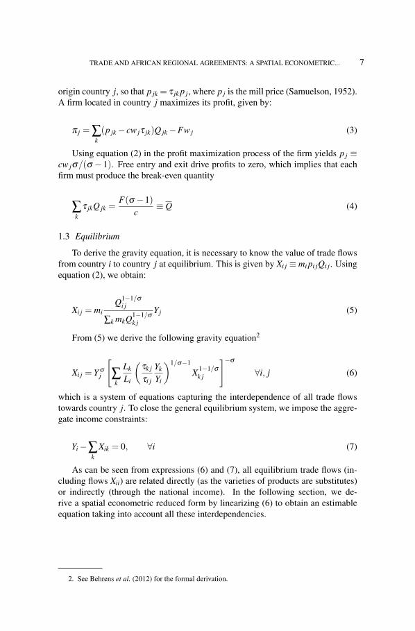
origin country j, so that p jk = τ jk p j, where p j is the mill price (Samuelson, 1952).A firm located in country j maximizes its profit, given by:
π j = ∑k(p jk− cw jτ jk)Q jk−Fw j (3)
Using equation (2) in the profit maximization process of the firm yields p j ≡cw jσ/(σ − 1). Free entry and exit drive profits to zero, which implies that eachfirm must produce the break-even quantity
∑k
τ jkQ jk =F(σ −1)
c≡ Q (4)
1.3 Equilibrium
To derive the gravity equation, it is necessary to know the value of trade flowsfrom country i to country j at equilibrium. This is given by Xi j ≡mi pi jQi j. Usingequation (2), we obtain:
Xi j = miQ1−1/σ
i j
∑k mkQ1−1/σ
k j
Yj (5)
From (5) we derive the following gravity equation2
Xi j = Y σj
[∑k
Lk
Li
(τk j
τi j
Yk
Yi
)1/σ−1
X1−1/σ
k j
]−σ
∀i, j (6)
which is a system of equations capturing the interdependence of all trade flowstowards country j. To close the general equilibrium system, we impose the aggre-gate income constraints:
Yi−∑k
Xik = 0, ∀i (7)
As can be seen from expressions (6) and (7), all equilibrium trade flows (in-cluding flows Xii) are related directly (as the varieties of products are substitutes)or indirectly (through the national income). In the following section, we de-rive a spatial econometric reduced form by linearizing (6) to obtain an estimableequation taking into account all these interdependencies.
2. See Behrens et al. (2012) for the formal derivation.

8 L’ACTUALITÉ ÉCONOMIQUE
1.4 Econometric specification
To obtain an econometric specification, we take equation (6) in logarithmicform:
lnXi j = σ lnYj−σ ln
[∑k
Lk
Li
(τk jYk
τi jYi
)1/σ−1
X1−1/σ
k j
](8)
Clearly, there is interdependence across trade flows as Xi j depends negativelyon the nominal sales of the other countries in market j. To obtain a specifica-tion that can be estimated using spatial econometric techniques, we linearize (8)around σ = 1. Doing so yields the following equation:
lnZi j =−σ lnL− (σ −1)
(lnτi j−∑
k
Lk
Llnτk j
)−σ lnwi
− (σ −1)∑k
Lk
LlnZk j
(9)
where Zi j ≡ Xi j/(YiYj)3 is a GDP-standardized trade flow (but which we will re-
fer to as trade flow for short); and where L ≡ ∑k Lk denotes the total population.Expression (9) reveals the essence of spatial interdependence in the gravity equa-tion: the trade flow Xi j from country i to country j also depends on all the tradeflows from the other countries k to country j. Several comments are in order.First, trade flows from i to j are affected by relative trade barriers, as measured bythe deviation of bilateral trade barriers τi j from the population weighted average(second term). Put differently, relative accessibility matters. Second, trade flowsfrom i to j are negatively affected by wages wi in the origin country (third term).Higher wages raise production costs and make country i’s firms less competitivein market j, thereby reducing trade flows. Last, trade flows from i to j decreasewith trade flows Zk j from any third country k into the destination market, becausevarieties are substitutes. This effect is stronger the closer substitutes the varietiesare (i.e., the larger the value of σ ). In our estimations, interdependence will becaptured by an autoregressive interaction coefficient, and this coefficient can beseen as a measure of “spatial competition” encapsulating both aspects related tomarket power and consumer preference for diversity (via the parameter σ ).
As regards the functional form of trade costs, we assume that τi j is a log-linearfunction of distance, border effect, landlocked position/status, common language,
3. Doing so, we can control for a possible endogeneity of the two variables trade flows and GDP.See Emlinger et al. (2008)

TRADE AND AFRICAN REGIONAL AGREEMENTS: A SPATIAL ECONOMETRIC... 9
common currency and an error4 term as follows (Anderson and Van Wincoop,2004):
τi j ≡ dγ
i jeξ bi j+ζ ei j−ς li j−ηci j+εi j (10)
where di j denotes the distance between country i and j; where bi j is a dummyvariable taking the value 1, if the flow Xi j takes place between a country belongingto a certain regional-bloc (like a monetary, economic or customary zone) and acountry not belonging to this bloc, and 0 otherwise.5 Where ei j takes value 1, ifat least one of the two countries is landlocked, and 0 otherwise (see Faye et al.(2004); li j is a dummy variable taking value 1, if both partners have a commonlanguage6 and 0 otherwise (Melitz, 2008); and ci j is an another dummy that equalsvalue 1, if the two countries have a common currency, and 0 otherwise (Frankeland Rose, 2002). The terms εi j are assumed i.i.d error terms. Substituting equation(10) in equation (9) then yields the following equation:
lnZi j =−σ lnL− (σ −1)γ ln di j− (σ −1)ξ bi j− (σ −1)ζ ei j
− (σ −1)ς li j− (σ −1)η ci j−σ lnwi− (σ −1)∑k
Lk
LlnZk j + εi j
(11)
where di j ≡ di j/ΠkdLk/Lk j are relative distances; bi j ≡ bi j −∑k
LkL bk j are relative
borders. More precisely, equation (11) reflects the trade resistance across blocs ascompared to trade within blocs. ei j ≡ ei j−∑k
LkL ek j capture the relative effects of
countries being landlocked; li j ≡ li j−∑kLkL lk j are the relative impacts of a com-
mon language use; and ci j ≡ ci j−∑kLkL ck j are the relative effects of a common
currency use. As regards the error structure, there are many ways of modelling theerror structure about which theory has little to say. Behrens et al. (2012) pointedout that he error terms exhibit some form of cross-sectional correlation as:
εi j = λ ∑kLkL uk j + ui j, where ui j ≡ −(σ − 1)εi j is an iid error term. Note
that, from equation (11) all variables superscripted with a tilde are measured asdeviations from their population weighted averages, that allowing us to implicitlycontrol for multilateral resistance. Moreover, equation (11) allows us to capture apossible spatial autocorrelation in error terms.
Since wages are unobserved for most countries, rather than taking GDP percapita as proxies (as in Redding and Venables, 2004) which is clearly an endoge-nous variable in particular when we include intra-trade flow Xii, we prefer to intro-
4. The error term can enter the model in many ways. Here we introduce it via the trade cost τi j .Doing so can be justified on the basis that trade costs are observed imperfectly.
5. This dummy is intended to estimate the border effect of different blocs in Africa, and is mademore explicit below.
6. Here we consider each country’s first official language only.
10 L’ACTUALITÉ ÉCONOMIQUE
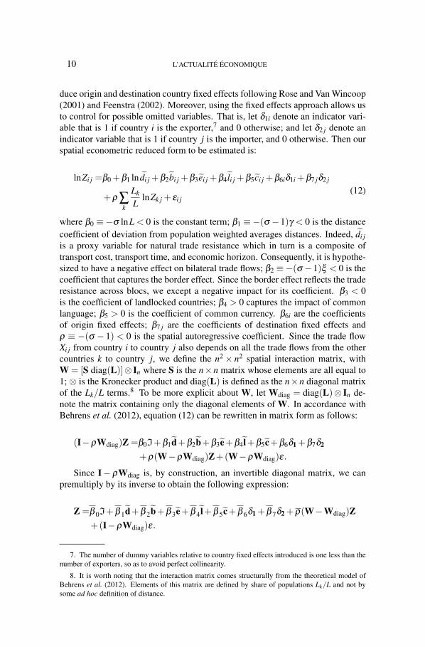
duce origin and destination country fixed effects following Rose and Van Wincoop(2001) and Feenstra (2002). Moreover, using the fixed effects approach allows usto control for possible omitted variables. That is, let δ1i denote an indicator vari-able that is 1 if country i is the exporter,7 and 0 otherwise; and let δ2 j denote anindicator variable that is 1 if country j is the importer, and 0 otherwise. Then ourspatial econometric reduced form to be estimated is:
lnZi j =β0 +β1 ln di j +β2bi j +β3ei j +β4 li j +β5ci j +β6iδ1i +β7 jδ2 j
+ρ ∑k
Lk
LlnZk j + εi j
(12)
where β0 ≡−σ lnL < 0 is the constant term; β1 ≡−(σ −1)γ < 0 is the distancecoefficient of deviation from population weighted averages distances. Indeed, di jis a proxy variable for natural trade resistance which in turn is a composite oftransport cost, transport time, and economic horizon. Consequently, it is hypothe-sized to have a negative effect on bilateral trade flows; β2 ≡−(σ −1)ξ < 0 is thecoefficient that captures the border effect. Since the border effect reflects the traderesistance across blocs, we except a negative impact for its coefficient. β3 < 0is the coefficient of landlocked countries; β4 > 0 captures the impact of commonlanguage; β5 > 0 is the coefficient of common currency. β6i are the coefficientsof origin fixed effects; β7 j are the coefficients of destination fixed effects andρ ≡ −(σ − 1) < 0 is the spatial autoregressive coefficient. Since the trade flowXi j from country i to country j also depends on all the trade flows from the othercountries k to country j, we define the n2 × n2 spatial interaction matrix, withW = [S diag(L)]⊗ In where S is the n×n matrix whose elements are all equal to1; ⊗ is the Kronecker product and diag(L) is defined as the n×n diagonal matrixof the Lk/L terms.8 To be more explicit about W, let Wdiag = diag(L)⊗ In de-note the matrix containing only the diagonal elements of W. In accordance withBehrens et al. (2012), equation (12) can be rewritten in matrix form as follows:
(I−ρWdiag)Z =β0I+β1d+β2b+β3e+β4l+β5c+β6δ1 +β7δ2
+ρ(W−ρWdiag)Z+(W−ρWdiag)ε.
Since I− ρWdiag is, by construction, an invertible diagonal matrix, we canpremultiply by its inverse to obtain the following expression:
Z =β 0I+β 1d+β 2b+β 3e+β 4l+β 5c+β 6δ1 +β 7δ2 +ρ(W−Wdiag)Z+(I−ρWdiag)ε.
7. The number of dummy variables relative to country fixed effects introduced is one less than thenumber of exporters, so as to avoid perfect collinearity.
8. It is worth noting that the interaction matrix comes structurally from the theoretical model ofBehrens et al. (2012). Elements of this matrix are defined by share of populations Lk/L and not bysome ad hoc definition of distance.

TRADE AND AFRICAN REGIONAL AGREEMENTS: A SPATIAL ECONOMETRIC... 11
The elements between positions (i×n)+1 and (i+1)×n of (I−ρWdiag)−1,
given by[1+(σ −1)Li
L
]−1, depend on the origin index i only which is fixed
and identical for all destinations. Therefore, the components of the transformed(overlined) vectors of coefficients are given by:
β 1i ≡ β1
[1+(σ −1)
Li
L
]−1
, β 2i ≡ β2
[1+(σ −1)
Li
L
]−1
,
β 3i ≡ β3
[1+(σ −1)
Li
L
]−1
, β 4i ≡ β4
[1+(σ −1)
Li
L
]−1
,
β 5i ≡ β5
[1+(σ −1)
Li
L
]−1
, β 6i ≡ β6
[1+(σ −1)
Li
L
]−1
,
β 7i ≡ β7
[1+(σ −1)
Li
L
]−1
, ρ i ≡ ρi
[1+(σ −1)
Li
L
]−1
.
We obtain a specification with a distinct set parameters for each country. Thefull model, therefore, has a “club” structure since all parameters (including thespatial autoregressive ones) must be estimated locally for each country. Behrenset al. (2012) refer to this model as the heterogeneous coefficients model. Since oneof our objectives is to assess the impact of different regional agreements, we don’tneed to estimate all parameters (including the spatial autoregressive ones) locallyfor each country. Therefore, we constrain all coefficients to be identical acrosscountries, which Behrens et al. (2012) refer to as the homogeneous coefficientsmodel. In addition, in most studies on gravity model the coefficients are supposedto be homogeneous across countries (Anderson and Van Wincoop, 2003, 2004;Baier and Bergstrand, 2001, 2009). Constraining the coefficients to be identicalamounts to assuming that the diagonal elements of W are equal to zero in equation(12). In that case, the model simplifies substantially and can readily be estimatedusing standard spatial econometric techniques. Moreover, in the spatial econo-metrics literature, an observation is not neighbour to itself by convention, so thatthe diagonal elements are zero (wii = 0) (see Anselin and Bera, 1998).
1.5 Intra- and inter-bloc effects
From equation (12) we decompose the border effect into two components:the trade-boosting intra-bloc effect and the trade-reducing inter-bloc effect of theborder.9 To disentangle the two components and to retrieve the full implied bordereffects (both intra-bloc and inter-bloc), we proceed as follows. First, we define the
9. Trade flows between a bloc member country and a non-member country.

12 L’ACTUALITÉ ÉCONOMIQUE
border as the ratio of trade flows in a world with borders (Zi j) to that which wouldprevail in a borderless world (Zi j). Using (9) and (10), we then have:
Bi j ≡Zi j
Zi j= eθ [bi j−∑k
LkL bk j ]∏
k
(Zi j
Zi j
)ρLkL
, (13)
where the term eθ [bi j−∑kLkL bk j ] subsumes the border frictions as a deviation from
their population weighted average. Note that (13) defines a log-linear system ofall the relative trade flows, which depend on all border effects. Let B stand forthe n2× 1 vector of ln( Zi j
Zi j) and let b stand for n2× 1 vector of [bi j −∑k
LkL bk j].
The log-linearized version of the system has the following solution, B = θ(I−ρW)−1b, which allows us to retrieve the border effect as the exponential of theforegoing expression.
Note that (13) quite naturally depends upon where countries i and j are lo-cated. Four cases may therefore arise with respect to intra-bloc and inter-bloctrade. Let popbloc ≡∑k∈bloc
LkL (resp., popROW ≡∑k/∈bloc
LkL ) stand for the regional-
bloc (resp., the rest of the world) population shares. It is readily verified that10
lnBi j =
−θ popROW if (i ∈ BLOC and j ∈ BLOC)
θ popROW if (i ∈ BLOC and j /∈ BLOC)θ popBLOC if (i /∈ BLOC and j ∈ BLOC)−θ popBLOC if (i /∈ BLOC and j /∈ BLOC)
(14)
Equation (14) reveals several interesting points. First, the expressions forBLOC-BLOC and ROW-ROW can be interpreted as the trade-boosting effect gener-ated by the presence of borders which increases trade flows within each bloc. Thetrade flows within each bloc will be larger in a world with borders than in a bor-derless world. The reason is that borders protect regional firms from competitionand give them an advantage in the regional market. Second, the expressions forBLOC-ROW and ROW-BLOC can be interpreted as the trade-reducing effect of theborder on trade flows across countries located in different blocs. The trade flowsacross blocs will be smaller in a world with borders than in a borderless world.Third, as in Anderson and Van Wincoop (2003), smaller blocs will have larger im-plied border effects than large blocs since their magnitude depends positively onthe size of the trading partner, as measured by its share of population. The reasonis that the border affects smaller blocs more than it does larger blocs, as it createstrade frictions for a larger share of the total demand served by its firms. Finally,the full border effect (combining the trade-boosting and trade-reducing effects),is given by e−2θpopROW for countries belonging to the bloc and by e−2θpopBLOC forcountries not belonging to the bloc.11
10. See Behrens et al. (2012)
11. In this study, we focus only on countries belonging to the bloc.

TRADE AND AFRICAN REGIONAL AGREEMENTS: A SPATIAL ECONOMETRIC... 13
To measure the intensity of the border effect we are interested in the five mainAfrican regional blocs: WAEMU, CEMAC, ECOWAS, COMESA and SADC. The firsttwo are simultaneously preferential trade blocs and monetary unions with a com-mon currency (the franc CFA). WAEMU and CEMAC each have their own singlecurrency (with the same acronym, franc CFA) and/each of which is pegged to theeuro. Although these two currencies are commonly referred to by the same name(franc CFA) and have the same value, they are not interchangeable or mutuallyconvertible, so this is not one common currency bloc but two juxtaposed blocs(Abdih and Tsangarides, 2010).
2. EMPIRICAL EVIDENCE
2.1 Data and econometrics
Our sample contains 150 countries with 22 500 pairs of trade flows; 37 ofcountries are African countries, 36 American countries, 34 Asian countries, 38European countries and 5 Oceanic countries. The data set includes exports Xi j(including internal absorption Xii) between countries, GDPs Yi and Yj of trad-ing partners all measured in millions of US dollars for the year 2010. We thenuse cross-sectional data for the year 2010. We compute internal absorption asXii ≡ GDPi−∑ j Xi j. Trade flows are from the UN COMTRADE database.12 GDP,national currency and population (also in 2010) data are obtained from the PennWorld Table 7.0.13 The data set also contains bilateral distances (in kilometers)between capital cities and are from the CEPII database.14 They are computed usingthe great circle distance formula applied to the capitals’ geographic coordinates.As regards the internal distances of the countries, we follow Redding and Venables(2004) by computing internal distances as dii ≡ κ
√surfacei/π . As estimation re-
sults are known to be somewhat sensitive to the measurement of internal distance(Head and Mayer, 2002) we use 1/3, 2/3 and 1 for κ . However, since our resultsare quite robust to these different values of κ , we report only for κ = 2/3.15 Land-locked position and language also come from the CEPII database. In our study, weconstructed the theoretically implied interaction matrix W using the populationshare of each exporting country in our sample.16 To deal with potential endogene-ity of population shares, we use three–year lagged values of this variable. Resultsare robust with respect to different lags. We also ran the regressions using the“current year” (i.e., 2010), and results were little sensitive (with no change at allin the qualitative results). That why we report only the results for the year 2010.
Insofar as one of our objectives is to assess the impact of different regionalagreements in Africa, we further have to deal with the well-known problem of zero
12. http://comtrade.un.org/
13. https://pwt.sas.upenn.edu.
14. http://www.cepii.fr/
15. Results using 1/3 and 1 for κ are available upon request.
16. The interaction matrix W is normalized by its eigenvalues.
14 L’ACTUALITÉ ÉCONOMIQUE
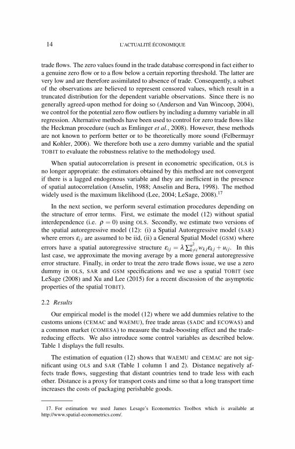
trade flows. The zero values found in the trade database correspond in fact either toa genuine zero flow or to a flow below a certain reporting threshold. The latter arevery low and are therefore assimilated to absence of trade. Consequently, a subsetof the observations are believed to represent censored values, which result in atruncated distribution for the dependent variable observations. Since there is nogenerally agreed-upon method for doing so (Anderson and Van Wincoop, 2004),we control for the potential zero flow outliers by including a dummy variable in allregression. Alternative methods have been used to control for zero trade flows likethe Heckman procedure (such as Emlinger et al., 2008). However, these methodsare not known to perform better or to be theoretically more sound (Felbermayrand Kohler, 2006). We therefore both use a zero dummy variable and the spatialTOBIT to evaluate the robustness relative to the methodology used.
When spatial autocorrelation is present in econometric specification, OLS isno longer appropriate: the estimators obtained by this method are not convergentif there is a lagged endogenous variable and they are inefficient in the presenceof spatial autocorrelation (Anselin, 1988; Anselin and Bera, 1998). The methodwidely used is the maximum likelihood (Lee, 2004; LeSage, 2008).17
In the next section, we perform several estimation procedures depending onthe structure of error terms. First, we estimate the model (12) without spatialinterdependence (i.e. ρ = 0) using OLS. Secondly, we estimate two versions ofthe spatial autoregressive model (12): (i) a Spatial Autoregressive model (SAR)where errors εi j are assumed to be iid, (ii) a General Spatial Model (GSM) whereerrors have a spatial autoregressive structure εi j = λ ∑
n2
k 6=i wk jεk j + ui j. In thislast case, we approximate the moving average by a more general autoregressiveerror structure. Finally, in order to treat the zero trade flows issue, we use a zerodummy in OLS, SAR and GSM specifications and we use a spatial TOBIT (seeLeSage (2008) and Xu and Lee (2015) for a recent discussion of the asymptoticproperties of the spatial TOBIT).
2.2 Results
Our empirical model is the model (12) where we add dummies relative to thecustoms unions (CEMAC and WAEMU), free trade areas (SADC and ECOWAS) anda common market (COMESA) to measure the trade-boosting effect and the trade-reducing effects. We also introduce some control variables as described below.Table 1 displays the full results.
The estimation of equation (12) shows that WAEMU and CEMAC are not sig-nificant using OLS and SAR (Table 1 column 1 and 2). Distance negatively af-fects trade flows, suggesting that distant countries tend to trade less with eachother. Distance is a proxy for transport costs and time so that a long transport timeincreases the costs of packaging perishable goods.
17. For estimation we used James Lesage’s Econometrics Toolbox which is available athttp://www.spatial-econometrics.com/.

TRADE AND AFRICAN REGIONAL AGREEMENTS: A SPATIAL ECONOMETRIC... 15
TABLE 1
ESTIMATION RESULTS
Model OLS SAR SAC TOBIT
distance −1.486∗∗∗ −1.479∗∗∗ −1.378∗∗∗ −1.852∗∗∗
(0.022) (0.020) (0.022) (0.024)WAEMU −0.236 −0.250 −0.459∗∗ −0.882∗∗∗
(0.217) (0.187) (0.190) (0.225)ECOWAS −0.519∗∗∗ −0.513∗∗∗ −1.539∗∗∗ −0.554∗∗∗
(0.143) (0.121) (0.124) (0.143)CEMAC −0.403 −0.411 −0.536∗ −0.931∗∗
(0.646) (0.324) (0.311) (0.373)COMESA −0.438∗∗∗ −0.434∗∗∗ −0.315∗∗∗ −0.736∗∗∗
(0.116) (0.091) (0.097) (0.103)SADC −0.701∗∗∗ −0.702∗∗∗ −0.720∗∗∗ −0.593∗∗∗
(0.136) (0.129) (0.134) (0.153)landlocked −0.429∗∗∗ −0.424∗∗∗ −0.306∗∗∗ −0.427∗∗∗
(0.082) (0.082) (0.081) (0.096)language 1.069∗∗∗ 1.064∗∗∗ 0.860∗∗∗ 1.344∗∗∗
(0.052) (0.049) (0.042) (0.059)Currency 1.171∗∗∗ 1.164∗∗∗ 1.025∗∗∗ 0.414∗∗∗
(0.121) (0.109) (0.104) (0.130)Dummy-Zero −3.569∗∗∗ −3.562∗∗∗ −3.556∗∗∗
(0.047) (0.040) (0.040)ρ −1.070∗∗∗ −0.114∗∗∗ −0.040∗∗
(0.037) (0.005) (0.021)λ −28.747∗∗∗
(0.096)
R2 0.683AIC −3.397 −3.273 −3.164BIC −3.287 −3.163 −3.068
NOTE: Standard errors are given in parentheses. ∗∗∗ significant at 1%; ∗∗ significant at 5% and ∗ significant at 10%.The number of observations is 22 500. AIC and BIC stand for the Akaike and the Schwarz information criteria,respectively.
We note that the theoretical model predicts that the spatial autocorrelation co-efficient ρ should be negative. This means that trade flow from i to j decreaseswith the value of sales Xk j from any third country k into the destination market,because varieties are gross substitutes. Since spatial interdependence is capturedby the spatial autoregressive coefficient in our estimating equations, this coeffi-cient may be interpreted as a measure of “spatial competition” encapsulating bothaspects of market power and consumer preference for diversity. Moreover, sincethe estimate for the parameter ρ is significantly different from zero, least-squaresestimates are biased and inconsistent. In what follows we will focus on the resultsgiven by the spatial models (especially GSM and TOBIT models) that result fromthe theoretical model.
As regards the border effects, the coefficients associated with all relative bor-ders are negative and significant. These coefficients allow us to capture relativetrade resistance due to regional blocs. To assess the magnitudes of impacts aris-ing from regional blocs, we turn to the summary measures of intra-bloc effects,inter-bloc effects and total impacts presented in Table 2.

16 L’ACTUALITÉ ÉCONOMIQUE
TABLE 2
BORDER EFFECTS
Area WAEMU ECOWAS CEMAC COMESA SADC
OLS
Intra 1.261ns 1.642 1.493ns 1.512 1.976Inter 0.792ns 0.608 0.669ns 0.661 0.506Full 1.592ns 2.697 2.230ns 2.287 3.905
SAR FE
Intra 1.279ns 1.633 1.505ns 1.506 1.977Inter 0.781ns 0.612 0.664ns 0.663 0.505Full 1.637ns 2.667 2.267ns 2.270 3.911
SAC FE
Intra 1.573 1.542 1.706 1.347 2.013Inter 0.635 0.648 0.586 0.742 0.496Full 2.474 2.377 2.910 1.815 4.052
TOBIT FE
Intra 2.385 1.699 2.526 2.003 1.779Inter 0.419 0.588 0.395 0.499 0.562Full 5.690 2.887 6.3840 4.013 3.165
NOTE: ns = not significant.
The results suggest that regional integration substantially increases trade be-tween WAEMU countries. Indeed, our results show that trade between WAEMUcountries is 5.7 times higher than trade between WAEMU countries and non WAEMUcountries. Furthermore, the trade-boosting intra-bloc coefficient shows that thetrade flows within WAEMU are 2.4 times larger in a world with borders (worldwith blocs) than in a world without borders (world without blocs). As regards thetrade-reducing inter-bloc effect, we find that the trade flows across WAEMU are0.4 times smaller in a world with borders than in a world without borders. Put dif-ferently, the trade flows across the blocs experience the border effect, which hasthe consequence of reducing these trade flows. For CEMAC, the full border coeffi-cient indicates that trade flows within CEMAC are 6.4 times higher than trade flowsacross CEMAC. The creation of CEMAC boosts trade between member countriesby 2.6 times and reduces trade flows with the rest of the world by a factor of 0.4.
Our estimations for SADC show that the coefficient of the full border effectis 3.2, the trade-boosting effect is 1.8 and the trade-reducing effect is 0.6. Theseresults show that intra-SADC trade increased compared with non-SADC trade. Im-plementation of SADC led to an increase in intra-SADC and a reduction in tradewith non-members. Note that South Africa was initially not in this bloc but nowit constitutes a dominant member as in Africa as a whole. The region is there-
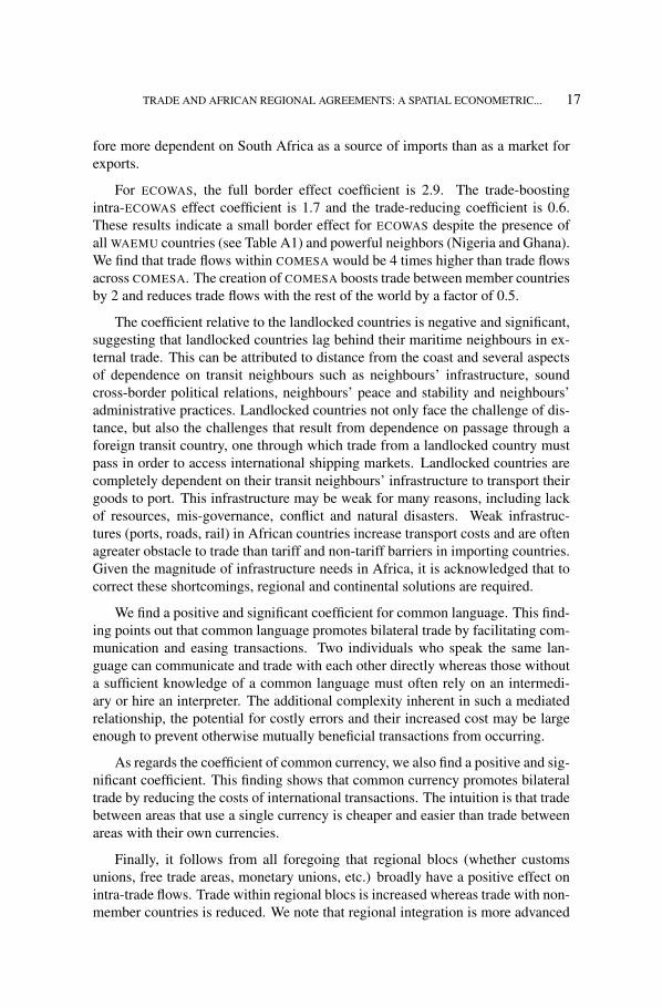
TRADE AND AFRICAN REGIONAL AGREEMENTS: A SPATIAL ECONOMETRIC... 17
fore more dependent on South Africa as a source of imports than as a market forexports.
For ECOWAS, the full border effect coefficient is 2.9. The trade-boostingintra-ECOWAS effect coefficient is 1.7 and the trade-reducing coefficient is 0.6.These results indicate a small border effect for ECOWAS despite the presence ofall WAEMU countries (see Table A1) and powerful neighbors (Nigeria and Ghana).We find that trade flows within COMESA would be 4 times higher than trade flowsacross COMESA. The creation of COMESA boosts trade between member countriesby 2 and reduces trade flows with the rest of the world by a factor of 0.5.
The coefficient relative to the landlocked countries is negative and significant,suggesting that landlocked countries lag behind their maritime neighbours in ex-ternal trade. This can be attributed to distance from the coast and several aspectsof dependence on transit neighbours such as neighbours’ infrastructure, soundcross-border political relations, neighbours’ peace and stability and neighbours’administrative practices. Landlocked countries not only face the challenge of dis-tance, but also the challenges that result from dependence on passage through aforeign transit country, one through which trade from a landlocked country mustpass in order to access international shipping markets. Landlocked countries arecompletely dependent on their transit neighbours’ infrastructure to transport theirgoods to port. This infrastructure may be weak for many reasons, including lackof resources, mis-governance, conflict and natural disasters. Weak infrastruc-tures (ports, roads, rail) in African countries increase transport costs and are oftenagreater obstacle to trade than tariff and non-tariff barriers in importing countries.Given the magnitude of infrastructure needs in Africa, it is acknowledged that tocorrect these shortcomings, regional and continental solutions are required.
We find a positive and significant coefficient for common language. This find-ing points out that common language promotes bilateral trade by facilitating com-munication and easing transactions. Two individuals who speak the same lan-guage can communicate and trade with each other directly whereas those withouta sufficient knowledge of a common language must often rely on an intermedi-ary or hire an interpreter. The additional complexity inherent in such a mediatedrelationship, the potential for costly errors and their increased cost may be largeenough to prevent otherwise mutually beneficial transactions from occurring.
As regards the coefficient of common currency, we also find a positive and sig-nificant coefficient. This finding shows that common currency promotes bilateraltrade by reducing the costs of international transactions. The intuition is that tradebetween areas that use a single currency is cheaper and easier than trade betweenareas with their own currencies.
Finally, it follows from all foregoing that regional blocs (whether customsunions, free trade areas, monetary unions, etc.) broadly have a positive effect onintra-trade flows. Trade within regional blocs is increased whereas trade with non-member countries is reduced. We note that regional integration is more advanced
18 L’ACTUALITÉ ÉCONOMIQUE
in WAEMU and CEMAC than in other regional blocs. Furthermore, WAEMU andCEMAC are a major export markets for the dominant countries in the two blocs(Cameroon for CEMAC and Senegal, Benin and Côte d’Ivoire for WAEMU). Theyare the prime export market for landlocked countries in both blocs. The smallborder effect for ECOWAS can be attributed to the failure by the members of theseblocs to reduce both tariff and non-tariff barriers to trade. We also note that theborder effect is high for the blocs that are well advanced in their integration pro-cess, and it is small for the blocs lagging behind in their integration process. Weconclude that the more advanced the integration process is, the more membercountries tend to trade with each other and to reduce their imports and exportswith third countries.
CONCLUSION
In this paper we estimated the border effect by breaking it down into twocomponents: the trade-boosting intra-bloc effect and the trade-reducing inter-bloceffect. To estimate both trade-boosting and trade-reducing effects we based ourapproach on Behrens et al. (2012) by deriving a gravity equation and taking intoaccount spatial interdependence between trade flows. Doing so yields a spatialeconometrics reduced form where we explore different specifications of errorterms or the treatment of zeros trade flows (SAR, GSM and spatial TOBIT). Wefind that regional blocs (whether customs union, free trade area, monetary union,or whatever) have a positive effect on intra-trade flows. Regional blocs not onlyincrease intra-trade flows but also reduce trade with other outside countries. Wealso note that the border effect is high for the blocs that are well advanced in theirintegration process, and it is small for the blocs lagging behind in their integrationprocess. As regards the spatial effect, we find that the spatial interdependence be-tween trade flows is reflected in a negative relationship. Moreover, we also controlfor common language, landlocked countries, and common currency and they arefound to be important determinants as distance in explaining trade flows.

TRADE AND AFRICAN REGIONAL AGREEMENTS: A SPATIAL ECONOMETRIC... 19
APPENDIX
TABLE A1
LIST OF COUNTRIES FOR EACH BLOC
CEMAC COMESA ECOWAS SADC WAEMU
Cameroon Angola Benin Angola BeninCAR Burundi Burkina Faso Botswana Burkina FasoChad Comoros Cape Verde RDC Côte d’IvoireCongo RDC Côte d’Ivoire Lesotho Bissau GuineaEquatorial Guinea Djibouti Gambia Madagascar MaliGabon Egypt Ghana Malawi Niger
Eritrea Guinea Mauritius SenegalEthiopia Bissau Guinea Mozambique TogoKenya Liberia NamibiaLibya Mali SwazilandMadagascar Niger SeychellesMalawi Nigeria South AfricaMauritius Senegal TanzaniaRwanda Sierra Leone ZambiaSeychelles Togo ZimbabweSouth SudanSudanSwazilandUgandaZambiaZimbabwe
NOTE: CAR = Central African of Republic. Botswana, Namibia, Swaziland are not in our sample. South Sudan andSudan constitute a single country.
BIBLIOGRAPHY
ABDIH, Y. and TSANGARIDES, C. (2010). Feer for the cfa franc. Applied Eco-nomics, 42 (16), 2009–2029.
AGBODJI, A. E. (2007). Intégration et échanges commerciaux intra sous-régionaux: le cas de l’uemoa. Revue africaine de l’intégration, 1 (1), 161–188.
AITKEN, N. D. (1973). The effect of the eec and efta on european trade: A tem-poral cross-section analysis. The American Economic Review, 63 (5), 881–892.
ANDERSON, J. E. (1979). A theoretical foundation for the gravity equation. TheAmerican economic review, 69 (1), 106–116.
— and VAN WINCOOP, E. (2003). Gravity with gravitas: A solution to the borderpuzzle. American economic review, 93 (1), 170–192.
— and — (2004). Trade costs. Journal of Economic literature, 42 (3), 691–751.ANSELIN, L. (1988). A test for spatial autocorrelation in seemingly unrelated
regressions. Economics Letters, 28 (4), 335–341.— and BERA, A. K. (1998). Introduction to spatial econometrics. Handbook of
applied economic statistics, 237.

20 L’ACTUALITÉ ÉCONOMIQUE
BAIER, S. L. and BERGSTRAND, J. H. (2001). The growth of world trade: tar-iffs, transport costs, and income similarity. Journal of international Economics,53 (1), 1–27.
— and — (2009). Bonus vetus ols: A simple method for approximating inter-national trade-cost effects using the gravity equation. Journal of InternationalEconomics, 77 (1), 77–85.
BEHAR, A. and CIRERA-I CRIVILLÉ, L. (2013). Does it matter who you signwith? comparing the impacts of n orth–s outh and s outh–s outh trade agree-ments on bilateral trade. Review of International Economics, 21 (4), 765–782.
— and EDWARDS, L. (2011). How integrated is SADC? Trends in intra-regionaland extra-regional trade flows and policy. The World Bank.
BEHRENS, K., ERTUR, C. and KOCH, W. (2012). ‘dual’gravity: Using spa-tial econometrics to control for multilateral resistance. Journal of AppliedEconometrics, 27 (5), 773–794.
BERGSTRAND, J. H. (1985). The gravity equation in international trade: somemicroeconomic foundations and empirical evidence. The review of economicsand statistics, pp. 474–481.
BOSKER, M. and GARRETSEN, H. (2012). Economic geography and economicdevelopment in sub-saharan africa. The World Bank Economic Review, 26 (3),443–485.
CARRÈRE, C. (2004). African regional agreements: impact on trade with orwithout currency unions. Journal of African Economies, 13 (2), 199–239.
COLLIER, P. and VENABLES, A. J. (2009). Commerce et performanceéconomique: la fragmentation de l’afrique importe-t-elle? Revue d’économiedu développement, 17 (4), 5–39.
COULIBALY, S. and FONTAGNÉ, L. (2006). South–south trade: geography mat-ters. Journal of African Economies, 15 (2), 313–341.
DE SOUSA, J. and LOCHARD, J. (2012). Trade and colonial status. Journal ofAfrican Economies, 21 (3), 409–439.
DEARDORFF, A. (1998). Determinants of bilateral trade: does gravity work in aneoclassical world? In The regionalization of the world economy, University ofChicago Press, pp. 7–32.
DIXIT, A. K. and STIGLITZ, J. E. (1977). Monopolistic competition and opti-mum product diversity. The American economic review, 67 (3), 297–308.
EATON, J. and KORTUM, S. (2002). Technology, geography, and trade. Econo-metrica, 70 (5), 1741–1779.
EMLINGER, C., JACQUET, F. and LOZZA, E. C. (2008). Tariffs and other tradecosts: assessing obstacles to mediterranean countries’ access to eu-15 fruitand vegetable markets. European Review of Agricultural Economics, 35 (4),409–438.
EVENETT, S. J. and KELLER, W. (2002). On theories explaining the success ofthe gravity equation. Journal of political economy, 110 (2), 281–316.
TRADE AND AFRICAN REGIONAL AGREEMENTS: A SPATIAL ECONOMETRIC... 21
FAYE, M. L., MCARTHUR, J. W., SACHS, J. D. and SNOW, T. (2004). Thechallenges facing landlocked developing countries. Journal of Human Devel-opment, 5 (1), 31–68.
FEENSTRA, R. C. (2002). Border effects and the gravity equation: Consistentmethods for estimation. Scottish Journal of Political Economy, 49 (5), 491–506.
FELBERMAYR, G. J. and KOHLER, W. (2006). Exploring the intensive and ex-tensive margins of world trade. Review of World Economics, 142 (4), 642–674.
FOROUTAN, F. and PRITCHETT, L. (1993). Intra-sub-saharan african trade: is ittoo little? Journal of African Economies, 2 (1), 74–105.
FRANKEL, J. and ROSE, A. (2002). An estimate of the effect of common cur-rencies on trade and income. The quarterly journal of economics, 117 (2),437–466.
GEDA, A. and KEBRET, H. (2008). Regional economic integration in africa: A re-view of problems and prospects with a case study of comesa. Journal of Africaneconomies, 17 (3), 357–394.
GORETTI, M. and WEISFELD, H. (2008). Trade in the WAEMU: Developmentsand Reform Opportunities. Tech. Rep. 8-68, International Monetary Fund.
HELPMAN, E. (1984). A simple theory of international trade with multinationalcorporations. Journal of political economy, 92 (3), 451–471.
KELEJIAN, H., TAVLAS, G. S. and PETROULAS, P. (2012). In the neighbor-hood: The trade effects of the euro in a spatial framework. Regional Scienceand Urban Economics, 42 (1-2), 314–322.
KRUGMAN, P. (1980). Scale economies, product differentiation, and the patternof trade. The American Economic Review, 70 (5), 950–959.
KRUGMAN, P. R. (1991). Geography and trade. MIT press.LEE, L.-F. (2004). Asymptotic distributions of quasi-maximum likelihood esti-
mators for spatial autoregressive models. Econometrica, 72 (6), 1899–1925.LESAGE, J. P. (2008). An introduction to spatial econometrics. Revue d’économie
industrielle, (123), 19–44.LONGO, R. and SEKKAT, K. (2004). Economic obstacles to expanding intra-
african trade. World Development, 32 (8), 1309–1321.MARTIJN, J. and TSANGARIDES, C. (2008). Trade in cemac: Developments and
reform opportunities. The CFA Franc Zone: Common Currency, UncommonChallenges. IMF, Washington, DC, pp. 335–363.
MELITZ, J. (2008). Language and foreign trade. European Economic Review,52 (4), 667–699.
MUSILA, J. W. (2005). The intensity of trade creation and trade diversionin comesa, eccas and ecowas: A comparative analysis. Journal of africanEconomies, 14 (1), 117–141.
REDDING, S. and VENABLES, A. J. (2004). Economic geography and interna-tional inequality. Journal of international Economics, 62 (1), 53–82.

22 L’ACTUALITÉ ÉCONOMIQUE
ROSE, A. K. and VAN WINCOOP, E. (2001). National money as a barrier to inter-national trade: The real case for currency union. American Economic Review,91 (2), 386–390.
SAMUELSON, P. A. (1952). Spatial price equilibrium and linear programming.The American economic review, 42 (3), 283–303.
SAPIR, A. (1981). Trade benefits under the eec generalized system of preferences.European Economic Review, 15 (3), 339–355.
UNECA, . A. (2008). Assessing regional integration in africa iii: Towardsmonetary and financial integration in africa.
XU, X. and LEE, L.-F. (2015). Maximum likelihood estimation of a spatialautoregressive tobit model. Journal of Econometrics, 188 (1), 264–280.