La prévision est un art difficile … surtout quand elle ... · La prévision est un art difficile...
74
P.Batteau ECCOREV Journée modélisation Février 2010 La prévision est un art difficile … surtout quand elle concerne l’avenir Mark Twain (Et Pierre Dac) Marchés financiers et climat Modéliser les extravagances
Transcript of La prévision est un art difficile … surtout quand elle ... · La prévision est un art difficile...

P.Batteau ECCOREV Journée modélisation Février 2010
La prévision est un art difficile … surtout quand elle concerne l’avenir
Mark Twain (Et Pierre Dac)
Marchés financiers et climat Modéliser les extravagances

P.Batteau ECCOREV Journée modélisation Février 2010
Marchés financiers et climats : modéliser les extravagances.
0) Remarques sur la modèlisation 1) Histoire de la marche de l'homme saoul : Louis, Albert, Norbert et les autres... 2) Processus stochatiques et mémoire
- Dame Nature souffre-t-elle d'amnésie? à court terme? à long terme? - Les marchés financiers ont-ils de la mémoire ? - Trend or no trend et changements de régime
3) Observer les extravagances de la kurtosis : le risque des “queues épaisses“ (fat tails)
4) Saisir les extravagances de la volatilité : modèles Arch, Garch etc
5) Les liaisons dangereuses dans les périodes chaudes : l’approche par “copules".
P.Batteau ECCOREV Journée modélisation Février 2010
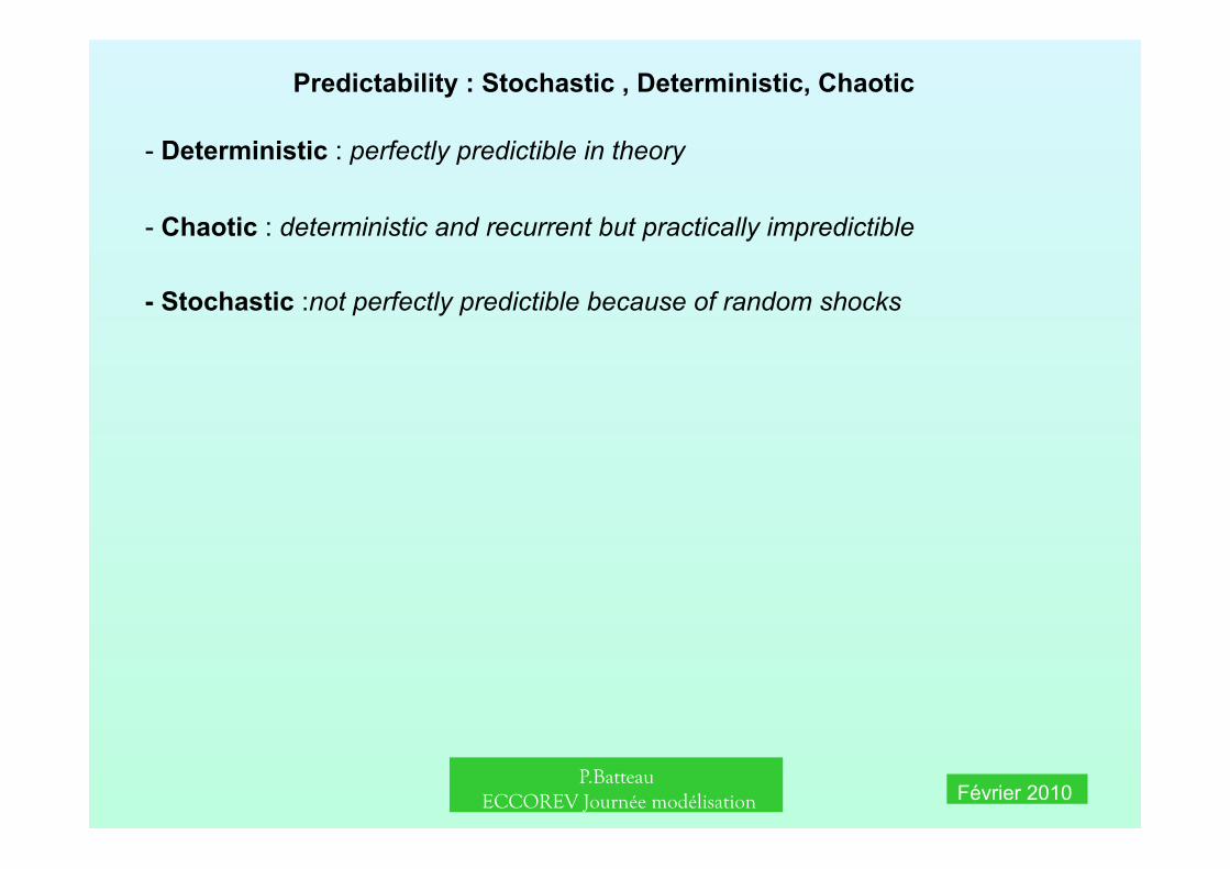
Predictability : Stochastic , Deterministic, Chaotic
- Deterministic : perfectly predictible in theory
- Chaotic : deterministic and recurrent but practically impredictible
- Stochastic :not perfectly predictible because of random shocks
P.Batteau ECCOREV Journée modélisation Février 2010
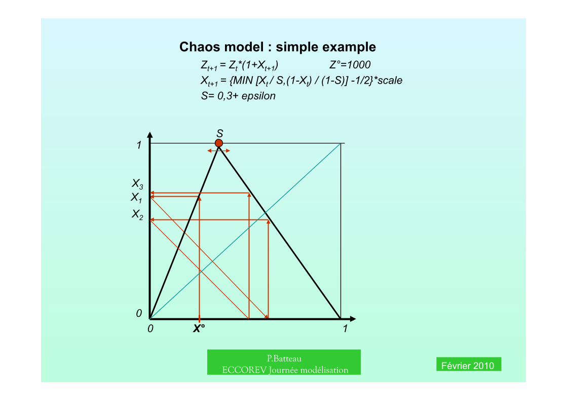
Chaos model : simple example Zt+1 = Zt*(1+Xt+1) Z°=1000 Xt+1 = {MIN [Xt / S,(1-Xt) / (1-S)] -1/2}*scale S= 0,3+ epsilon
0 1 0
1 S
X°
X1
X2
X3
P.Batteau ECCOREV Journée modélisation Février 2010
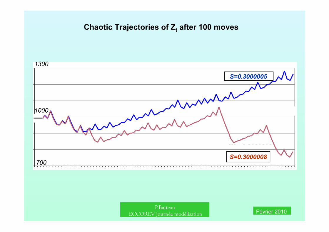
Chaotic Trajectories of Zt after 100 moves
700
1300
1000
S=0.3000005
S=0.3000008
P.Batteau ECCOREV Journée modélisation Février 2010
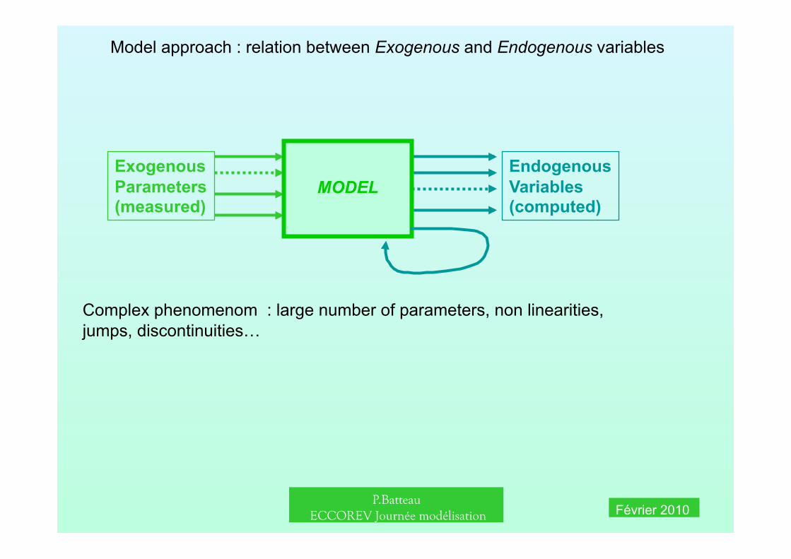
Model approach : relation between Exogenous and Endogenous variables
Endogenous Variables (computed)
Exogenous Parameters (measured)
MODEL
Complex phenomenom : large number of parameters, non linearities, jumps, discontinuities…
P.Batteau ECCOREV Journée modélisation Février 2010
Models of complex systems

P.Batteau ECCOREV Journée modélisation Février 2010
Global Climate Model
P.Batteau ECCOREV Journée modélisation Février 2010
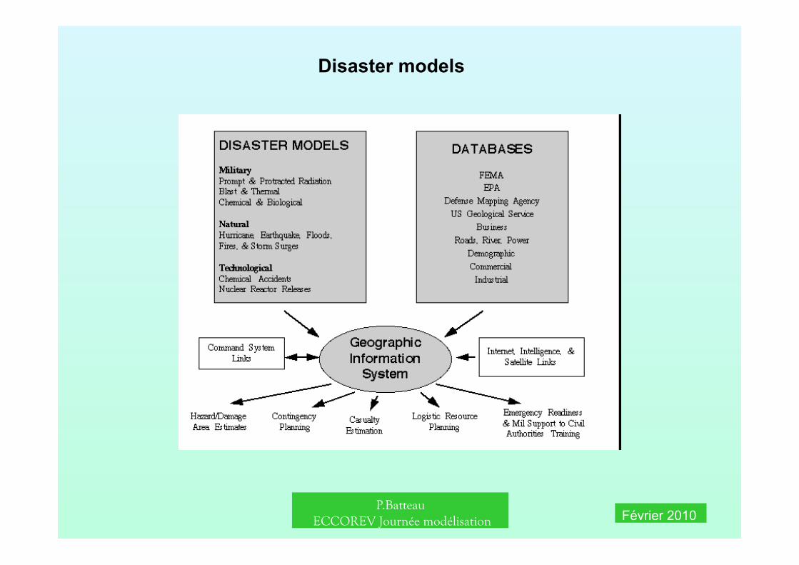
Disaster models
P.Batteau ECCOREV Journée modélisation Février 2010
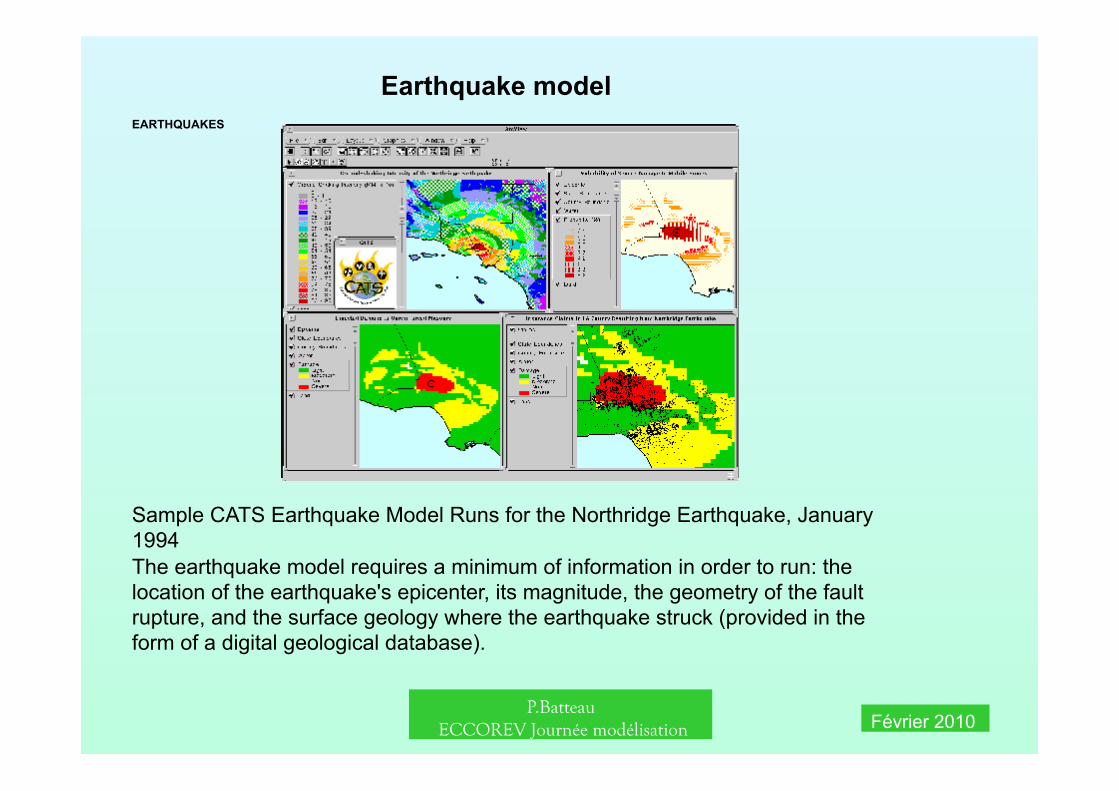
EARTHQUAKES
Sample CATS Earthquake Model Runs for the Northridge Earthquake, January 1994 The earthquake model requires a minimum of information in order to run: the location of the earthquake's epicenter, its magnitude, the geometry of the fault rupture, and the surface geology where the earthquake struck (provided in the form of a digital geological database).
Earthquake model
P.Batteau ECCOREV Journée modélisation Février 2010
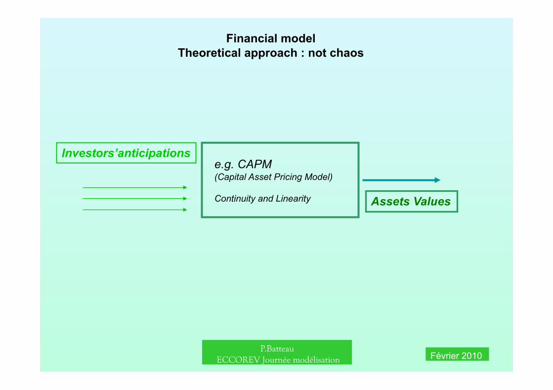
Financial model Theoretical approach : not chaos
Investors’anticipations
Assets Values
e.g. CAPM (Capital Asset Pricing Model)
Continuity and Linearity
P.Batteau ECCOREV Journée modélisation Février 2010
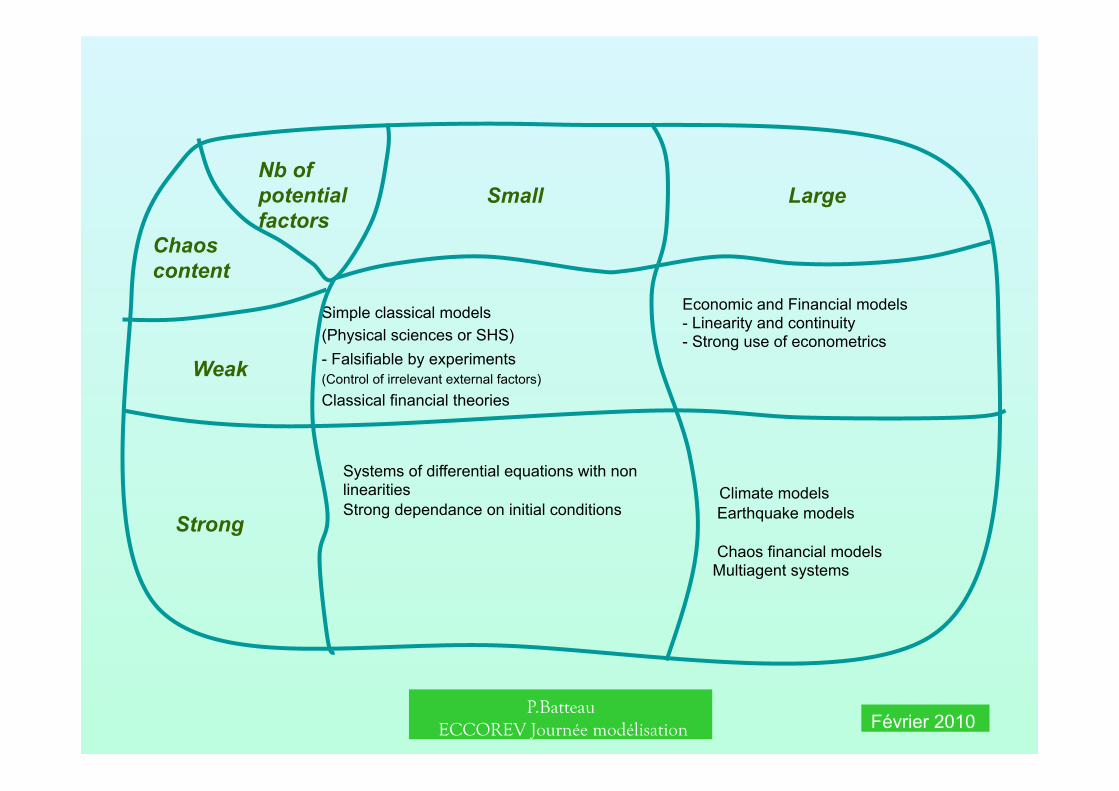
Simple classical models (Physical sciences or SHS) - Falsifiable by experiments (Control of irrelevant external factors) Classical financial theories
Economic and Financial models - Linearity and continuity - Strong use of econometrics
Systems of differential equations with non linearities Strong dependance on initial conditions
Climate models Earthquake models
Chaos financial models Multiagent systems
Small Large
Weak
Strong
Nb of potential factors
Chaos content
P.Batteau ECCOREV Journée modélisation Février 2010
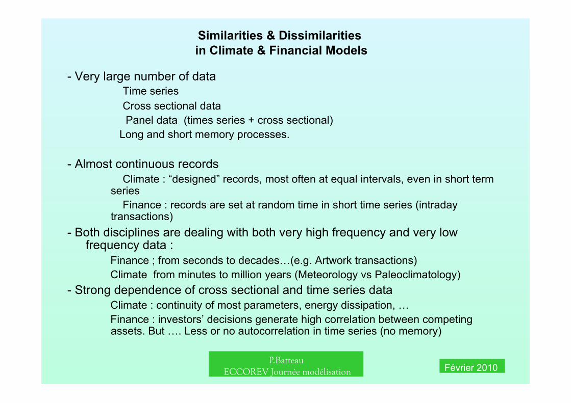
Similarities & Dissimilarities in Climate & Financial Models
- Very large number of data Time series Cross sectional data Panel data (times series + cross sectional) Long and short memory processes.
- Almost continuous records Climate : “designed” records, most often at equal intervals, even in short term series
Finance : records are set at random time in short time series (intraday transactions)
- Both disciplines are dealing with both very high frequency and very low frequency data :
Finance ; from seconds to decades…(e.g. Artwork transactions) Climate from minutes to million years (Meteorology vs Paleoclimatology)
- Strong dependence of cross sectional and time series data Climate : continuity of most parameters, energy dissipation, … Finance : investors’ decisions generate high correlation between competing assets. But …. Less or no autocorrelation in time series (no memory)
P.Batteau ECCOREV Journée modélisation Février 2010
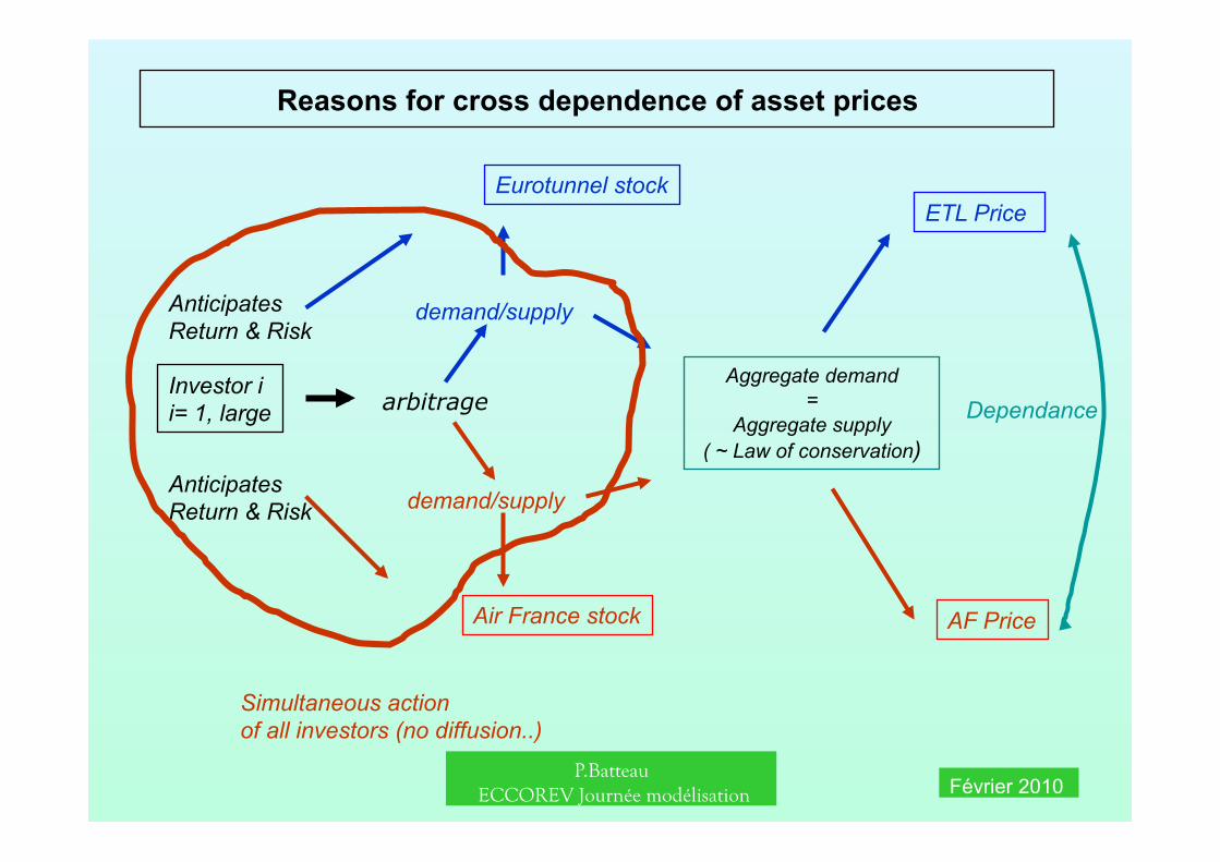
Reasons for cross dependence of asset prices
demand/supply
demand/supply
Investor i i= 1, large
Eurotunnel stock ETL Price
Air France stock
Aggregate demand =
Aggregate supply ( ~ Law of conservation)
AF Price
Dependance
Anticipates Return & Risk
Anticipates Return & Risk
arbitrage
Simultaneous action of all investors (no diffusion..)
P.Batteau ECCOREV Journée modélisation Février 2010
Reasons for dependence in climate data
Geographical correlations : Smooth processes, diffusion, conservation of moments…
Correlation without lags (ex Southern Oscillation Index) at equilibrium at each moment of time
Correlation with lags : smooth diffusion with inertia
Correlation among “internal” variables :
e.g. : Δ(CO²) & Δ(mean annual temperature)
What does the model say ? What do the data say ?
P.Batteau ECCOREV Journée modélisation Février 2010
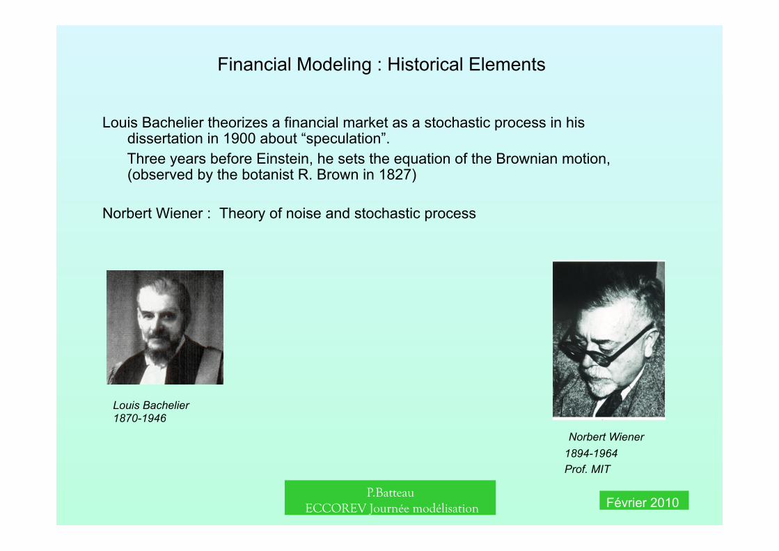
Financial Modeling : Historical Elements
Louis Bachelier theorizes a financial market as a stochastic process in his dissertation in 1900 about “speculation”.
Three years before Einstein, he sets the equation of the Brownian motion, (observed by the botanist R. Brown in 1827)
Norbert Wiener : Theory of noise and stochastic process
Norbert Wiener 1894-1964 Prof. MIT
Louis Bachelier 1870-1946
P.Batteau ECCOREV Journée modélisation Février 2010
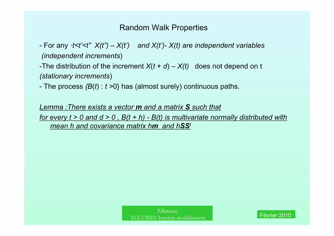
Random Walk Properties
- For any ·t<t’<t” X(t”) – X(t’) and X(t’)- X(t) are independent variables (independent increments) -The distribution of the increment X(t + d) – X(t) does not depend on t (stationary increments) - The process {B(t) : t >0} has (almost surely) continuous paths.
Lemma :There exists a vector m and a matrix S such that for every t > 0 and d > 0 , B(t + h) - B(t) is multivariate normally distributed with
mean h and covariance matrix hm and hSSt

P.Batteau ECCOREV Journée modélisation Février 2010
Unidimensional Random Walk
X Y’
Y
1- X and Y are independent 2- Y and Y’ : same distribution 3 – X, Y, Y’ : normal distribution with variance proportional to time
X
P.Batteau ECCOREV Journée modélisation Février 2010
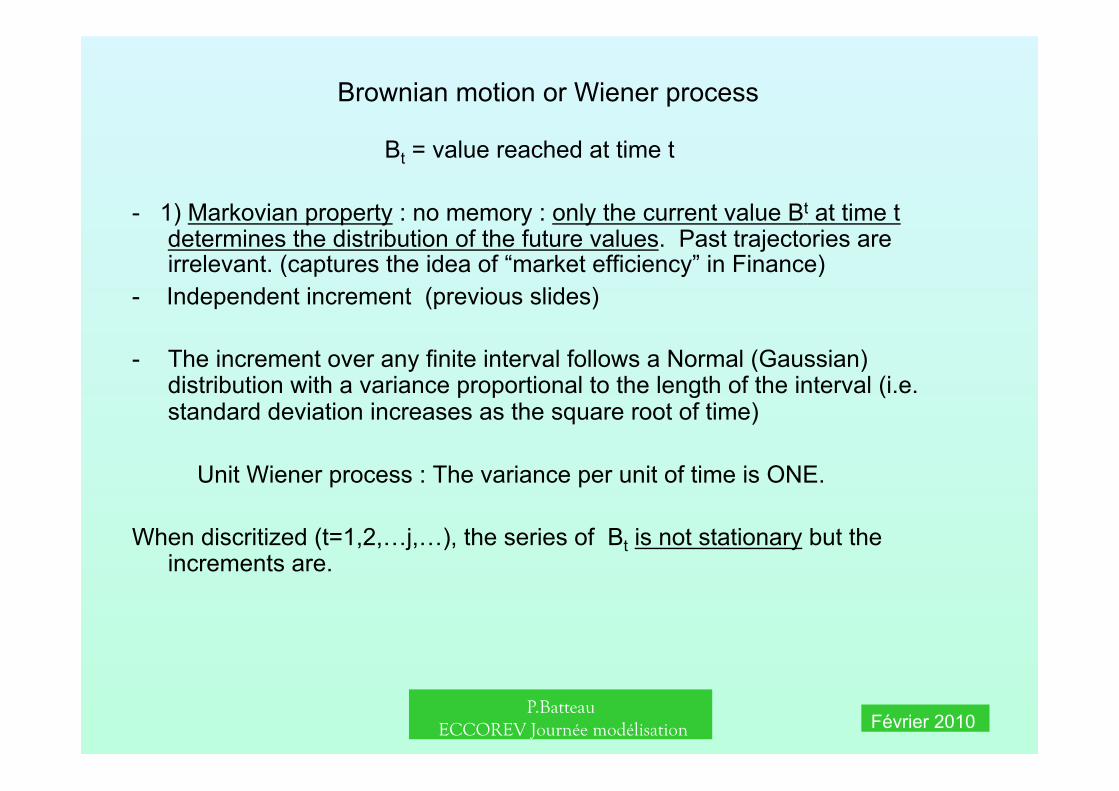
Brownian motion or Wiener process
Bt = value reached at time t
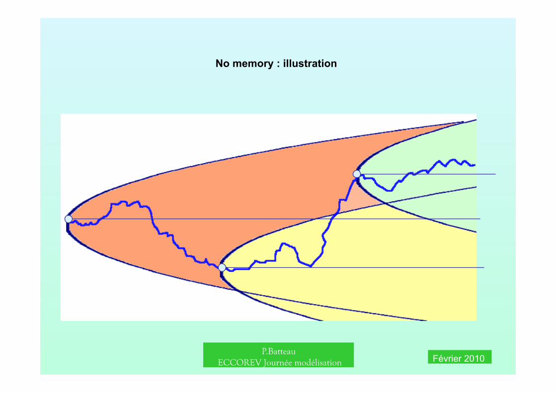
- 1) Markovian property : no memory : only the current value Bt at time t determines the distribution of the future values. Past trajectories are irrelevant. (captures the idea of “market efficiency” in Finance)
- Independent increment (previous slides)
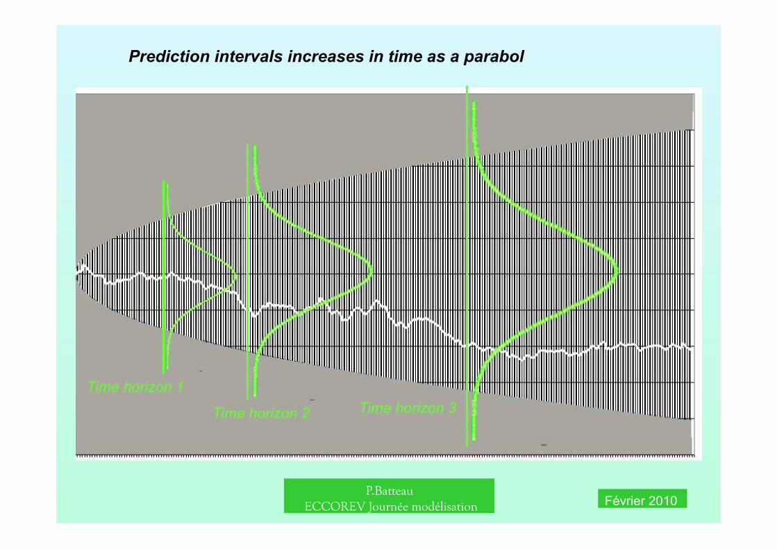
- The increment over any finite interval follows a Normal (Gaussian) distribution with a variance proportional to the length of the interval (i.e. standard deviation increases as the square root of time)
Unit Wiener process : The variance per unit of time is ONE.
When discritized (t=1,2,…j,…), the series of Bt is not stationary but the increments are.
P.Batteau ECCOREV Journée modélisation Février 2010
Time horizon 1
Time horizon 2 Time horizon 3
Prediction intervals increases in time as a parabol
P.Batteau ECCOREV Journée modélisation Février 2010
No memory : illustration
P.Batteau ECCOREV Journée modélisation Février 2010
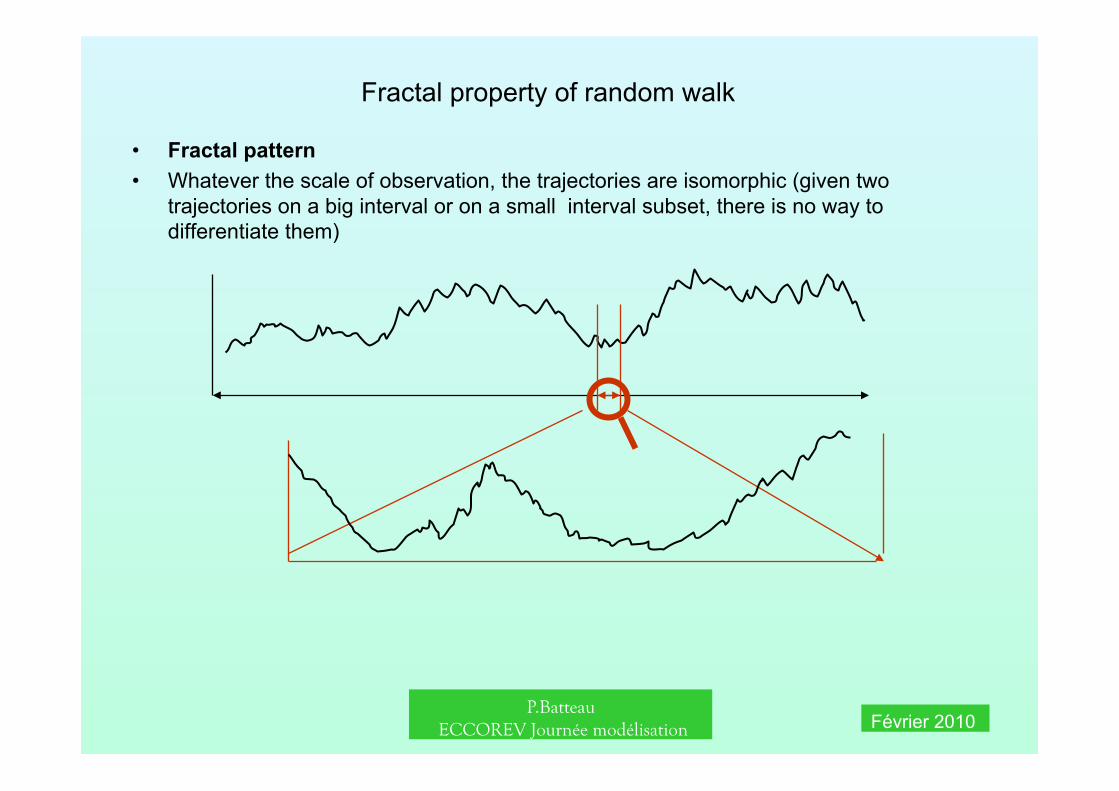
Fractal property of random walk
• Fractal pattern • Whatever the scale of observation, the trajectories are isomorphic (given two
trajectories on a big interval or on a small interval subset, there is no way to differentiate them)
P.Batteau ECCOREV Journée modélisation Février 2010
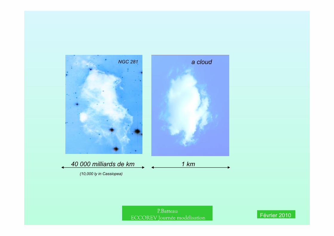
40 000 milliards de km 1 km
a cloud NGC 281
(10,000 ly in Cassiopea)

P.Batteau ECCOREV Journée modélisation Février 2010
Applications in Finance
P.Batteau ECCOREV Journée modélisation Février 2010
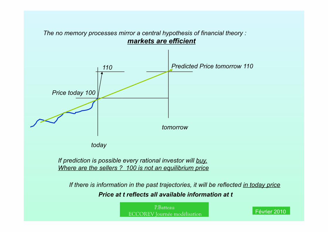
The no memory processes mirror a central hypothesis of financial theory : markets are efficient
today
Price today 100
tomorrow
Predicted Price tomorrow 110
If prediction is possible every rational investor will buy. Where are the sellers ? 100 is not an equilibrium price
110
If there is information in the past trajectories, it will be reflected in today price Price at t reflects all available information at t
P.Batteau ECCOREV Journée modélisation Février 2010
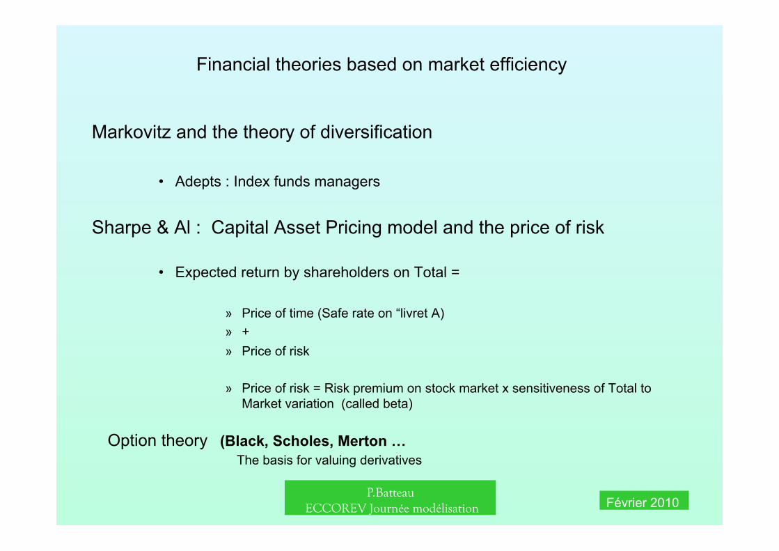
Financial theories based on market efficiency
Markovitz and the theory of diversification
• Adepts : Index funds managers
Sharpe & Al : Capital Asset Pricing model and the price of risk
• Expected return by shareholders on Total =
» Price of time (Safe rate on “livret A) » + » Price of risk
» Price of risk = Risk premium on stock market x sensitiveness of Total to Market variation (called beta)
Option theory (Black, Scholes, Merton … The basis for valuing derivatives
P.Batteau ECCOREV Journée modélisation Février 2010
The mysteries of derivatives
• Every day several hundred billions dollars of derivative contratcs are exchanged on the financial markets and among banks
P.Batteau ECCOREV Journée modélisation Février 2010
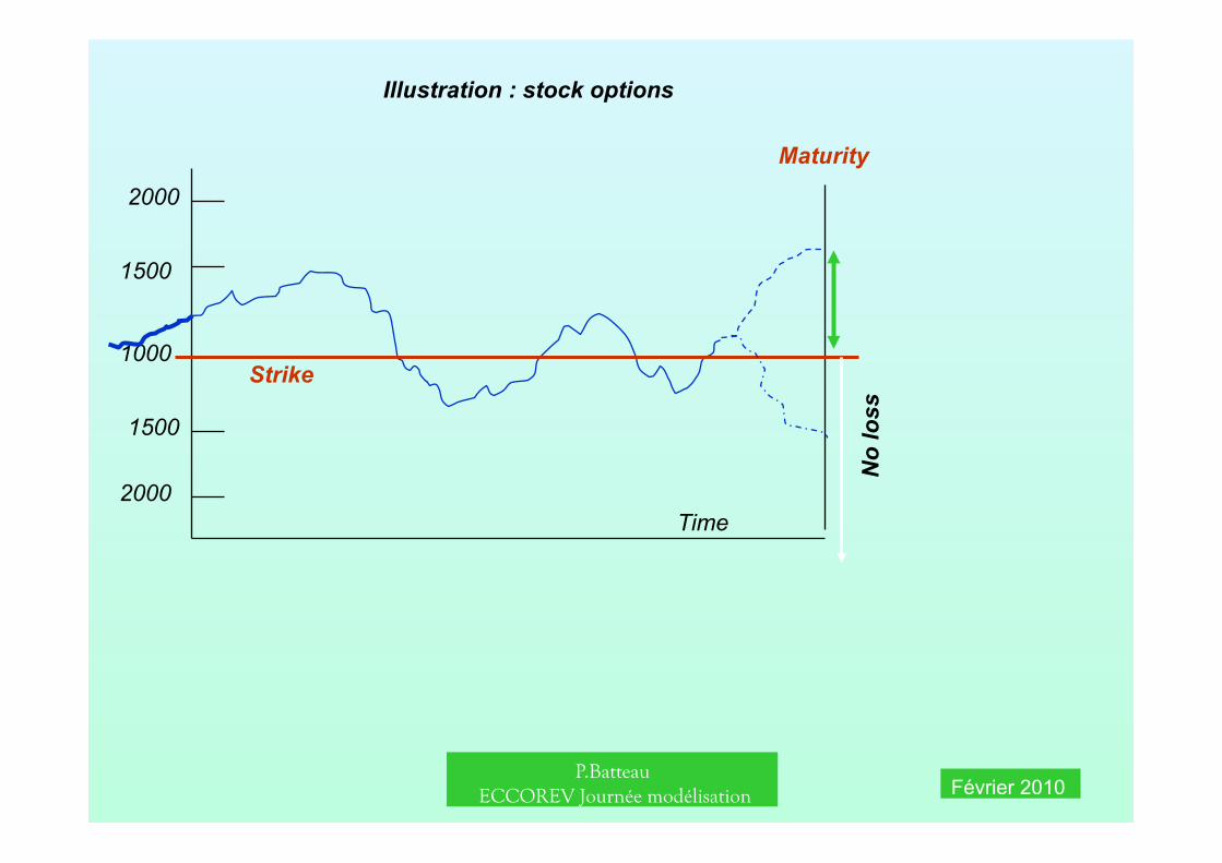
Illustration : stock options
Time
1000
1500
2000
2000
1500
Strike
Maturity
No
loss
P.Batteau ECCOREV Journée modélisation Février 2010
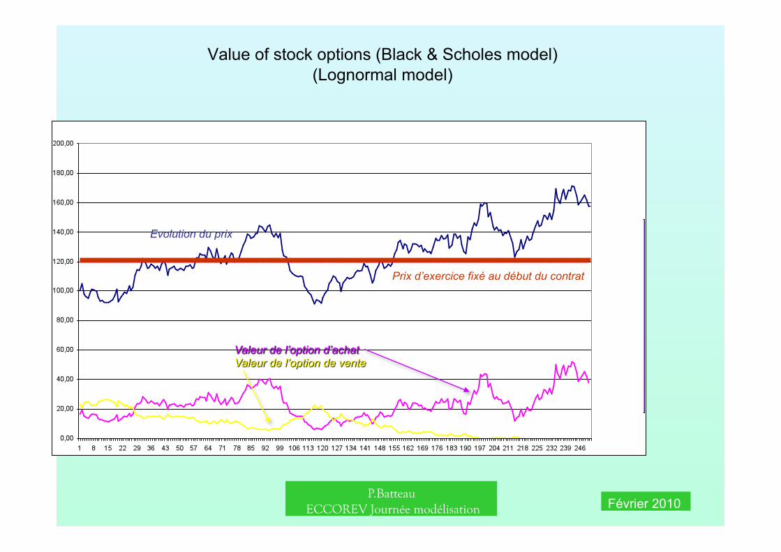
Value of stock options (Black & Scholes model) (Lognormal model)
Prix d’exercice fixé au début du contrat
Evolution du prix
P.Batteau ECCOREV Journée modélisation Février 2010
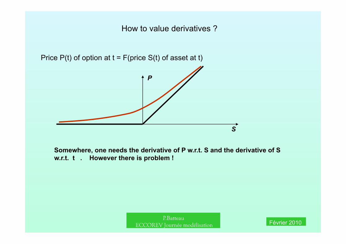
How to value derivatives ?
Price P(t) of option at t = F(price S(t) of asset at t)
S
P
Somewhere, one needs the derivative of P w.r.t. S and the derivative of S w.r.t. t . However there is problem !
P.Batteau ECCOREV Journée modélisation Février 2010
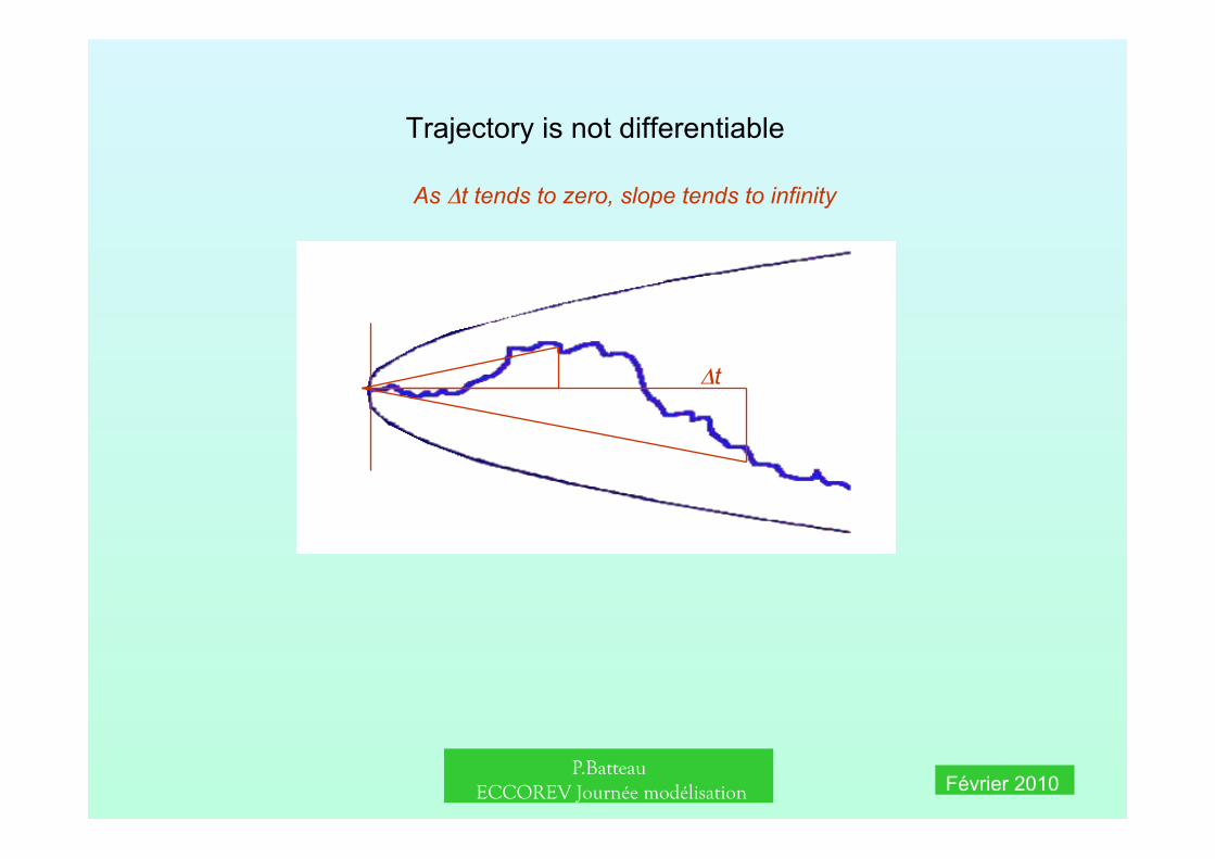
Trajectory is not differentiable
Δt
As Δt tends to zero, slope tends to infinity
P.Batteau ECCOREV Journée modélisation Février 2010
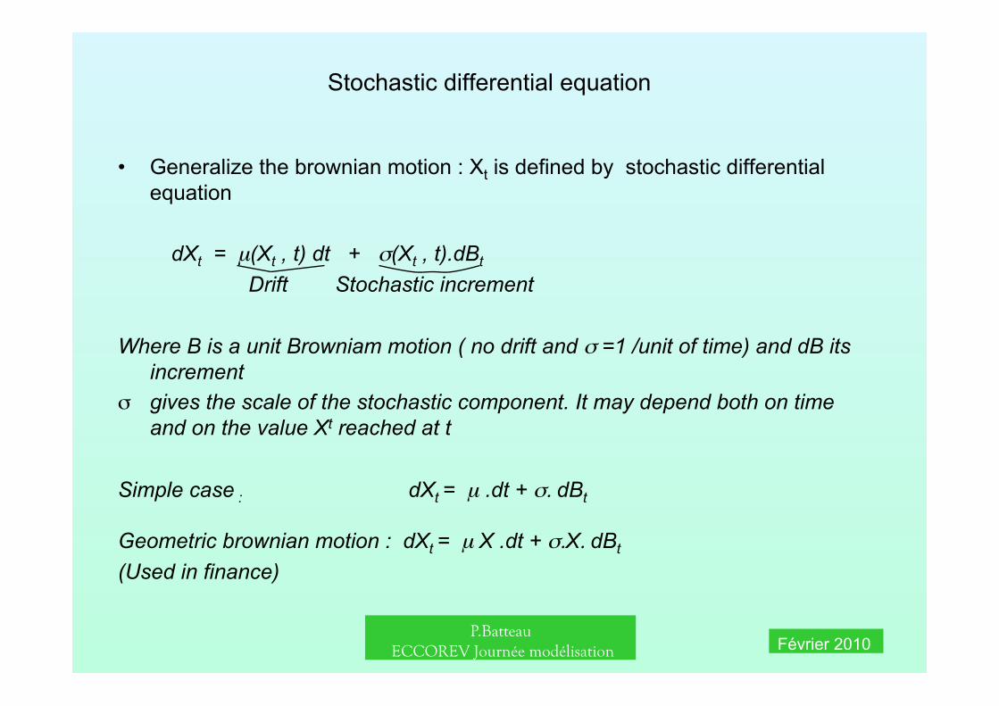
Stochastic differential equation
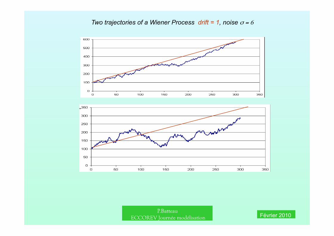
• Generalize the brownian motion : Xt is defined by stochastic differential equation
dXt = µ(Xt , t) dt + σ(Xt , t).dBt
Drift Stochastic increment
Where B is a unit Browniam motion ( no drift and σ =1 /unit of time) and dB its increment
σ gives the scale of the stochastic component. It may depend both on time and on the value Xt reached at t
Simple case : dXt = µ .dt + σ. dBt
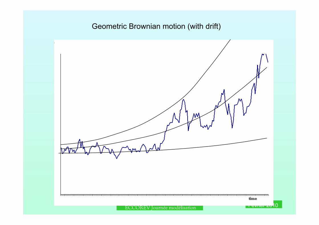
Geometric brownian motion : dXt = µ X .dt + σ.X. dBt
(Used in finance)
P.Batteau ECCOREV Journée modélisation Février 2010
Two trajectories of a Wiener Process drift = 1, noise σ = 6
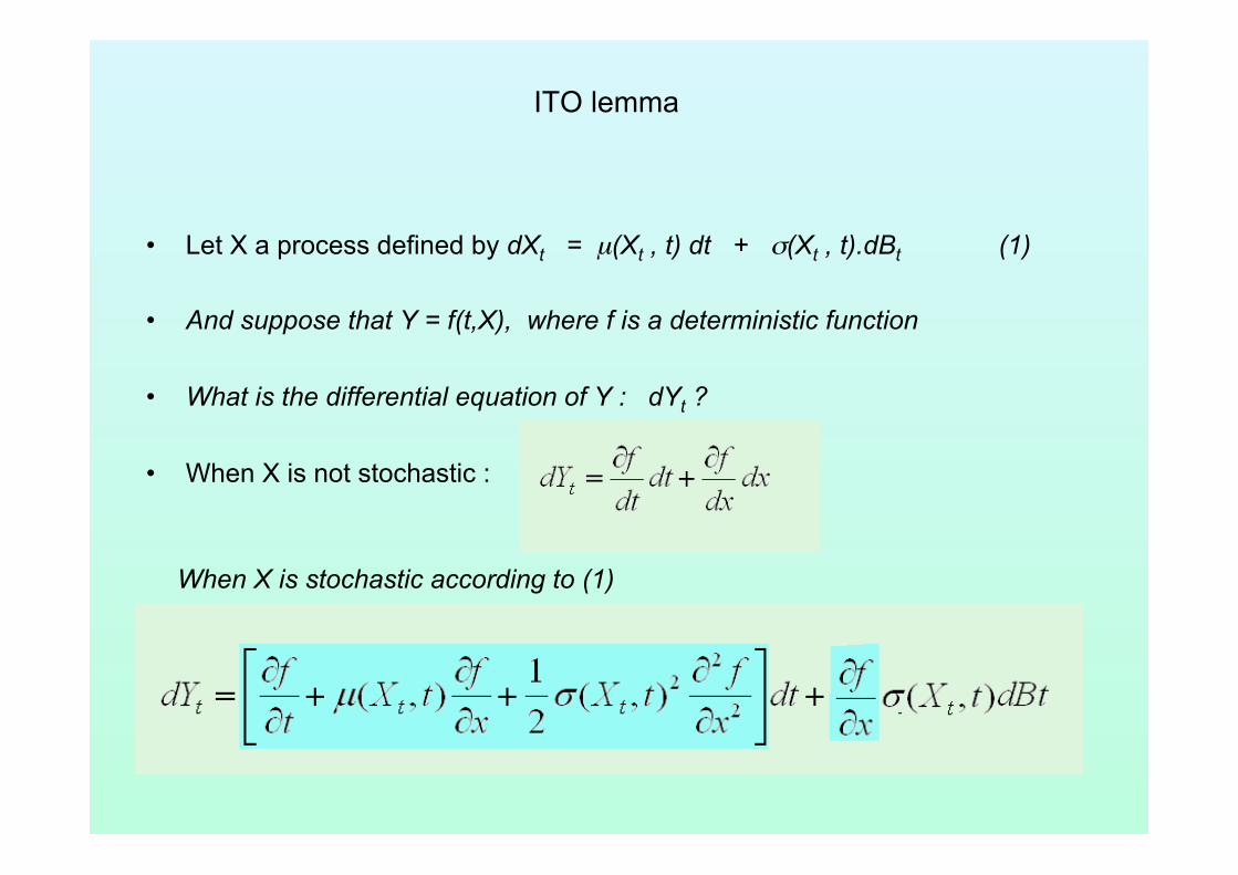
ITO lemma
• Let X a process defined by dXt = µ(Xt , t) dt + σ(Xt , t).dBt (1)
• And suppose that Y = f(t,X), where f is a deterministic function
• What is the differential equation of Y : dYt ?
• When X is not stochastic :
When X is stochastic according to (1)
P.Batteau ECCOREV Journée modélisation Février 2010
Geometric Brownian motion (with drift)
P.Batteau ECCOREV Journée modélisation Février 2010
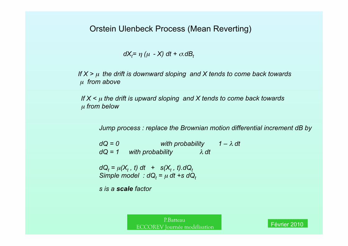
Orstein Ulenbeck Process (Mean Reverting)
dXt= η (µ - X) dt + σ.dBt
If X > µ the drift is downward sloping and X tends to come back towards µ from above
If X < µ the drift is upward sloping and X tends to come back towards µ from below
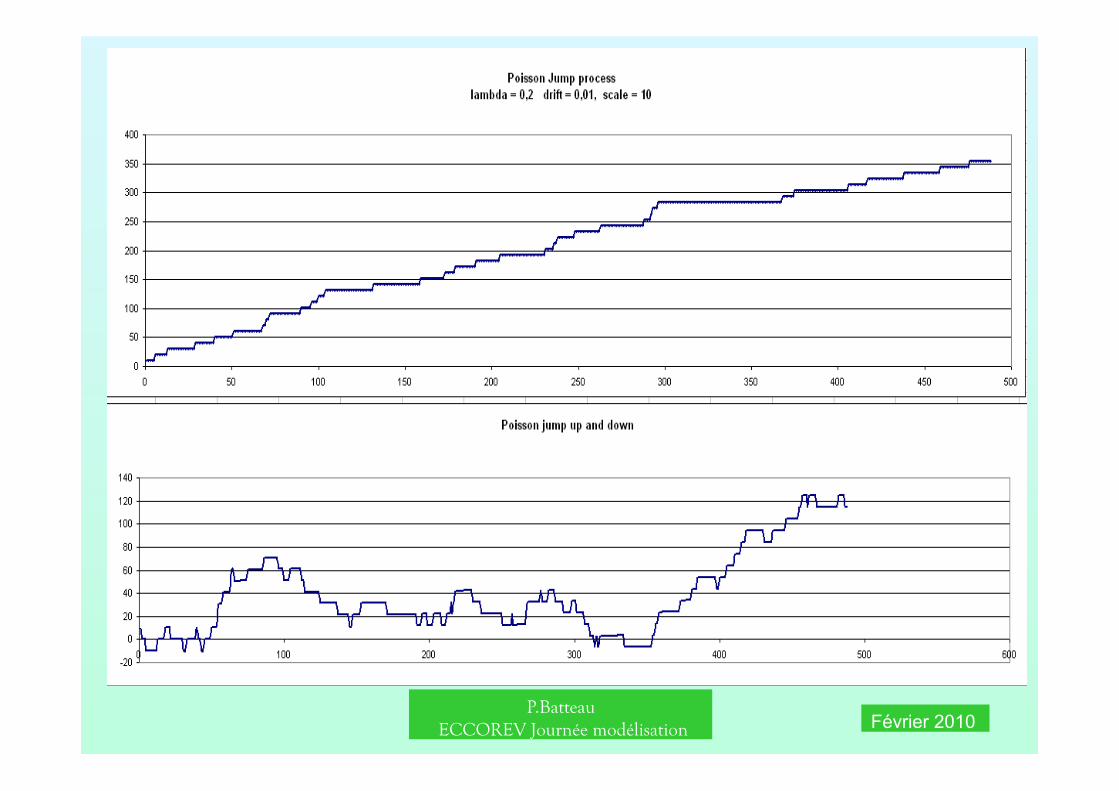
Jump process : replace the Brownian motion differential increment dB by
dQ = 0 with probability 1 – λ dt dQ = 1 with probability λ dt
dQt = µ(Xt , t) dt + s(Xt , t).dQt Simple model : dQt = µ dt +s dQt
s is a scale factor
P.Batteau ECCOREV Journée modélisation Février 2010
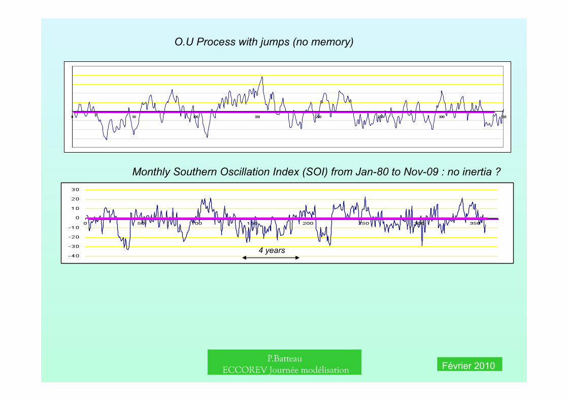
4 years
Monthly Southern Oscillation Index (SOI) from Jan-80 to Nov-09 : no inertia ?
O.U Process with jumps (no memory)
P.Batteau ECCOREV Journée modélisation Février 2010
P.Batteau ECCOREV Journée modélisation Février 2010
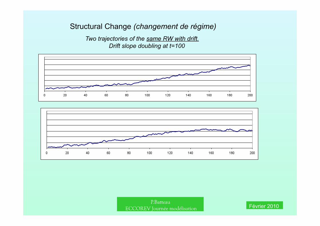
Structural Change (changement de régime) Two trajectories of the same RW with drift. Drift slope doubling at t=100
P.Batteau ECCOREV Journée modélisation Février 2010
,
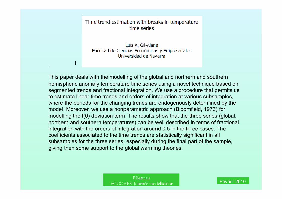
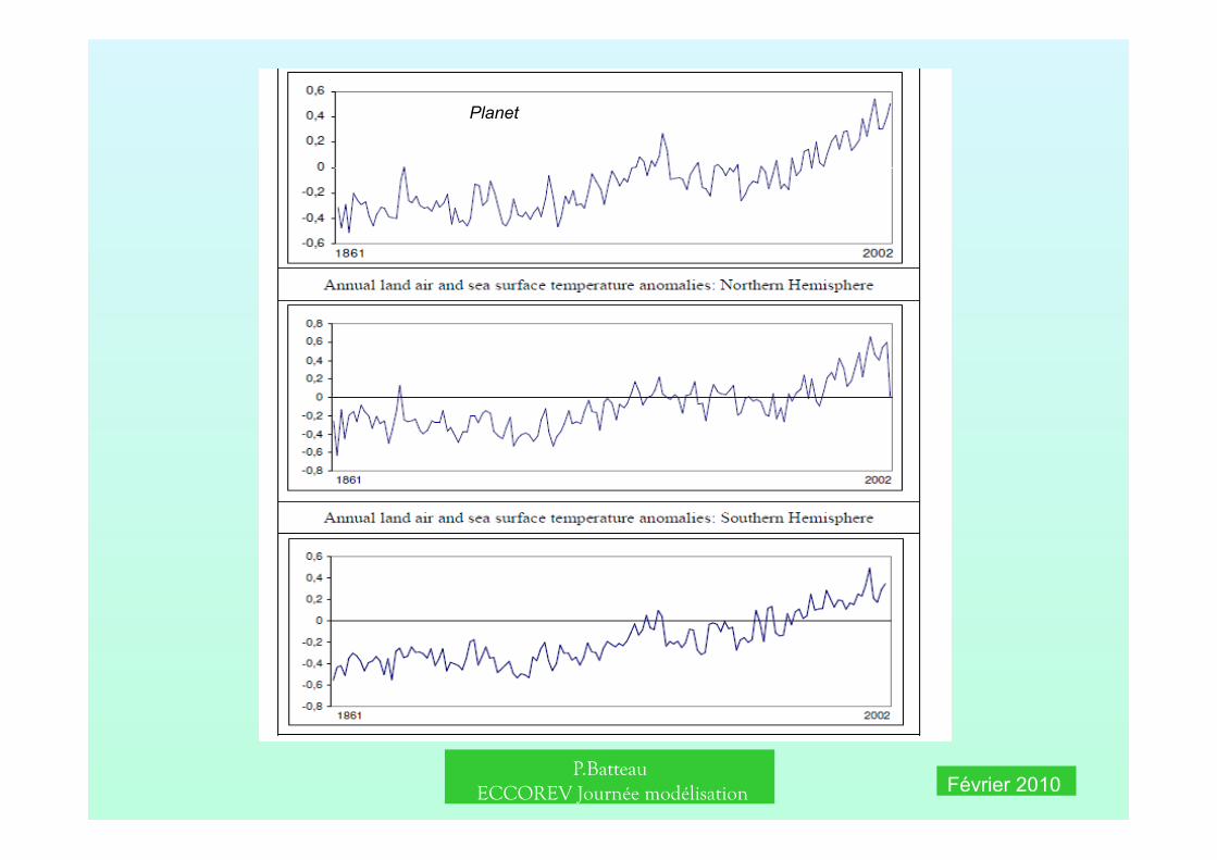
This paper deals with the modelling of the global and northern and southern hemispheric anomaly temperature time series using a novel technique based on segmented trends and fractional integration. We use a procedure that permits us to estimate linear time trends and orders of integration at various subsamples, where the periods for the changing trends are endogenously determined by the model. Moreover, we use a nonparametric approach (Bloomfield, 1973) for modelling the I(0) deviation term. The results show that the three series (global, northern and southern temperatures) can be well described in terms of fractional integration with the orders of integration around 0.5 in the three cases. The coefficients associated to the time trends are statistically significant in all subsamples for the three series, especially during the final part of the sample, giving then some support to the global warming theories.
!
P.Batteau ECCOREV Journée modélisation Février 2010
Planet
P.Batteau ECCOREV Journée modélisation Février 2010
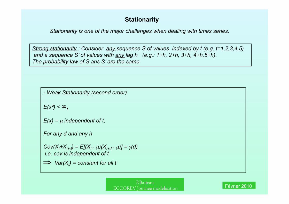
Strong stationarity : Consider any sequence S of values indexed by t (e.g. t=1,2,3,4,5) and a sequence S’ of values with any lag h (e.g.: 1+h, 2+h, 3+h, 4+h,5+h). The probability law of S ans S’ are the same.
Stationarity
- Weak Stationarity (second order)
E(x²) < ∞,
E(x) = µ independent of t,
For any d and any h
Cov(Xt+Xt+d) = E[(Xt - µ)(Xt+d - µ)] = γ(d) i.e. cov is independent of t
⇒ Var(Xt) = constant for all t
Stationarity is one of the major challenges when dealing with times series.
P.Batteau ECCOREV Journée modélisation Février 2010
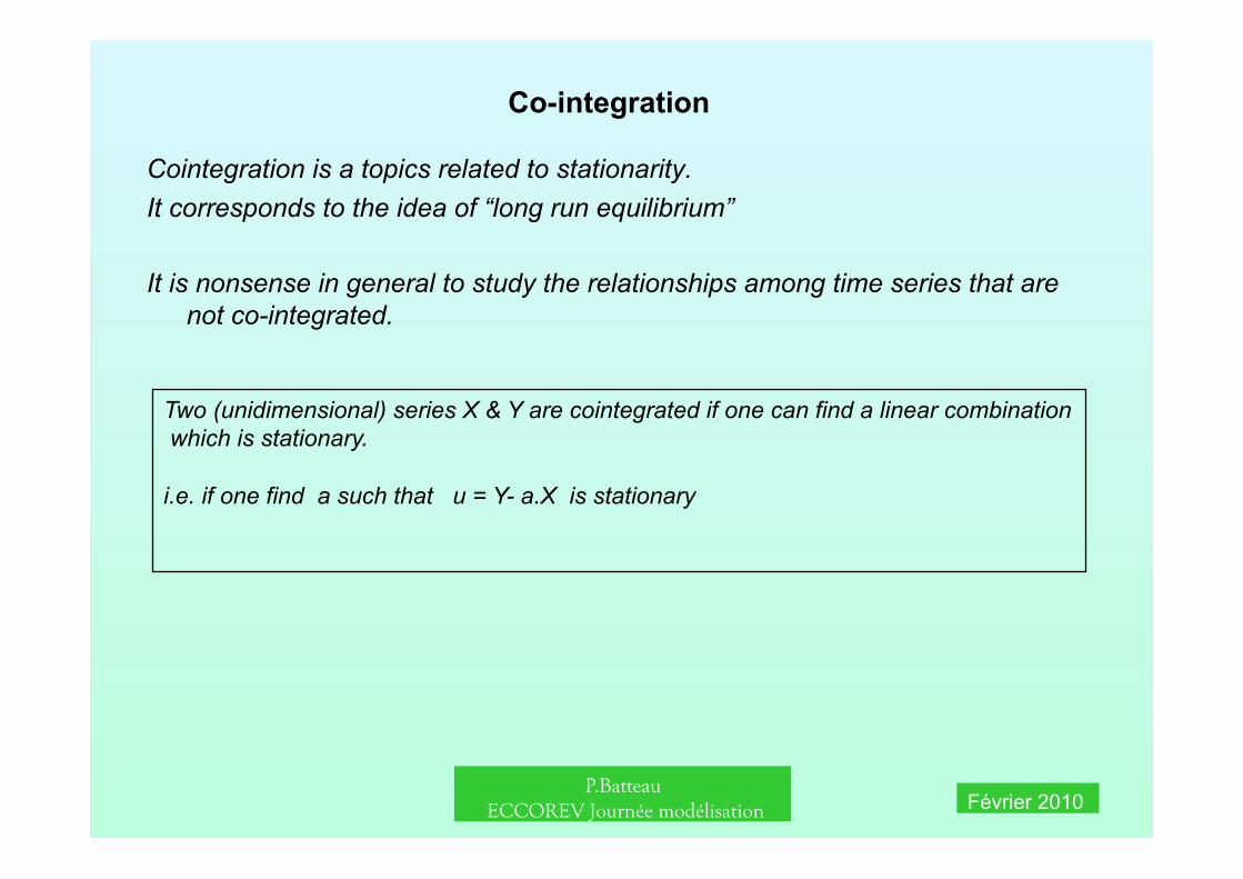
Co-integration
Cointegration is a topics related to stationarity. It corresponds to the idea of “long run equilibrium”
It is nonsense in general to study the relationships among time series that are not co-integrated.
Two (unidimensional) series X & Y are cointegrated if one can find a linear combination which is stationary.
i.e. if one find a such that u = Y- a.X is stationary
P.Batteau ECCOREV Journée modélisation Février 2010
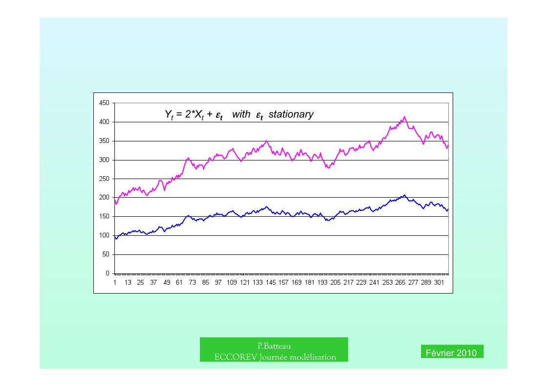
Yt = 2*Xt + εt with εt stationary
P.Batteau ECCOREV Journée modélisation Février 2010
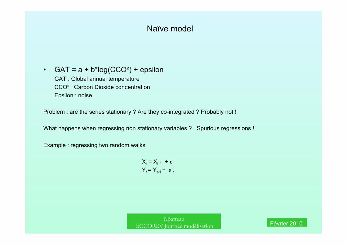
Naïve model
• GAT = a + b*log(CCO²) + epsilon GAT : Global annual temperature CCO² Carbon Dioxide concentration Epsilon : noise
Problem : are the series stationary ? Are they co-integrated ? Probably not !
What happens when regressing non stationary variables ? Spurious regressions !
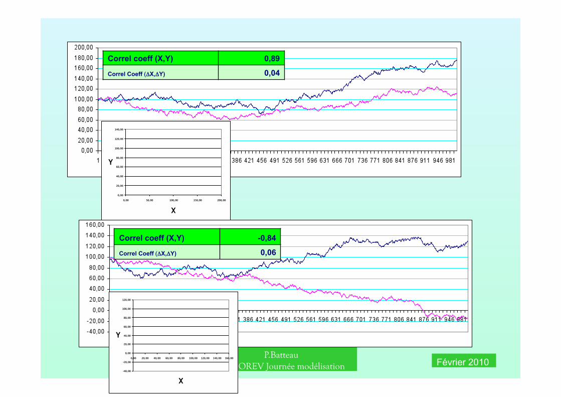
Example : regressing two random walks
Xt = Xt-1 + εt
Yt = Yt-1 + ε’t
P.Batteau ECCOREV Journée modélisation Février 2010
Correl coeff (X,Y) 0,89
Correl Coeff (ΔX,ΔY) 0,04
Correl coeff (X,Y) -0,84
Correl Coeff (ΔX,ΔY) 0,06
P.Batteau ECCOREV Journée modélisation Février 2010
Extrem risks
A story of fat tails
P.Batteau ECCOREV Journée modélisation Février 2010
P.Batteau ECCOREV Journée modélisation Février 2010
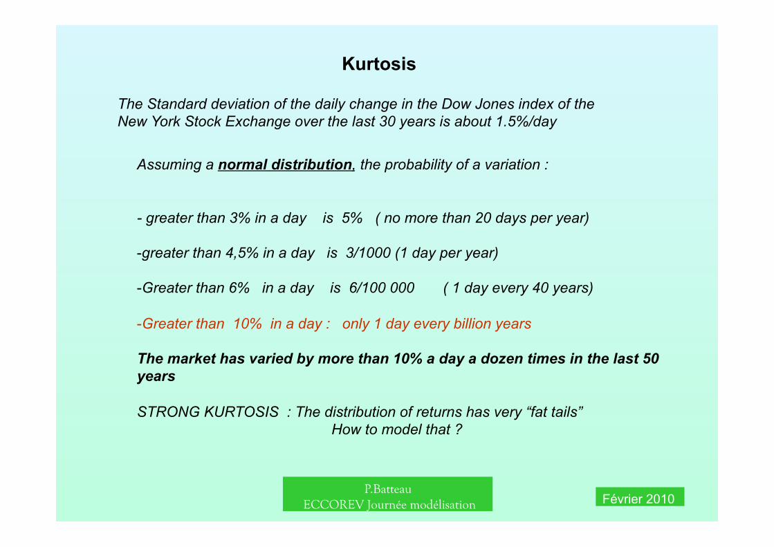
Kurtosis
The Standard deviation of the daily change in the Dow Jones index of the New York Stock Exchange over the last 30 years is about 1.5%/day
Assuming a normal distribution, the probability of a variation :
- greater than 3% in a day is 5% ( no more than 20 days per year)
- greater than 4,5% in a day is 3/1000 (1 day per year)
- Greater than 6% in a day is 6/100 000 ( 1 day every 40 years)
- Greater than 10% in a day : only 1 day every billion years
The market has varied by more than 10% a day a dozen times in the last 50 years
STRONG KURTOSIS : The distribution of returns has very “fat tails” How to model that ?
P.Batteau ECCOREV Journée modélisation Février 2010
Unstable volatility
Volatility is assumed constant over the time horizon in many applications in finance as well as other fields. Early versions of the models for valuing The financial instruments called “derivatives”, were based on the assumption of constant volatility. There are many reasons however to believe that volatility is unstable. Which models are suitable for that ?
1 - At each t volatility is explained by a set of exogenous variables
2 - ARCH, GARCH models
3 - Stochastic volatility models
P.Batteau ECCOREV Journée modélisation Février 2010
P.Batteau ECCOREV Journée modélisation Février 2010
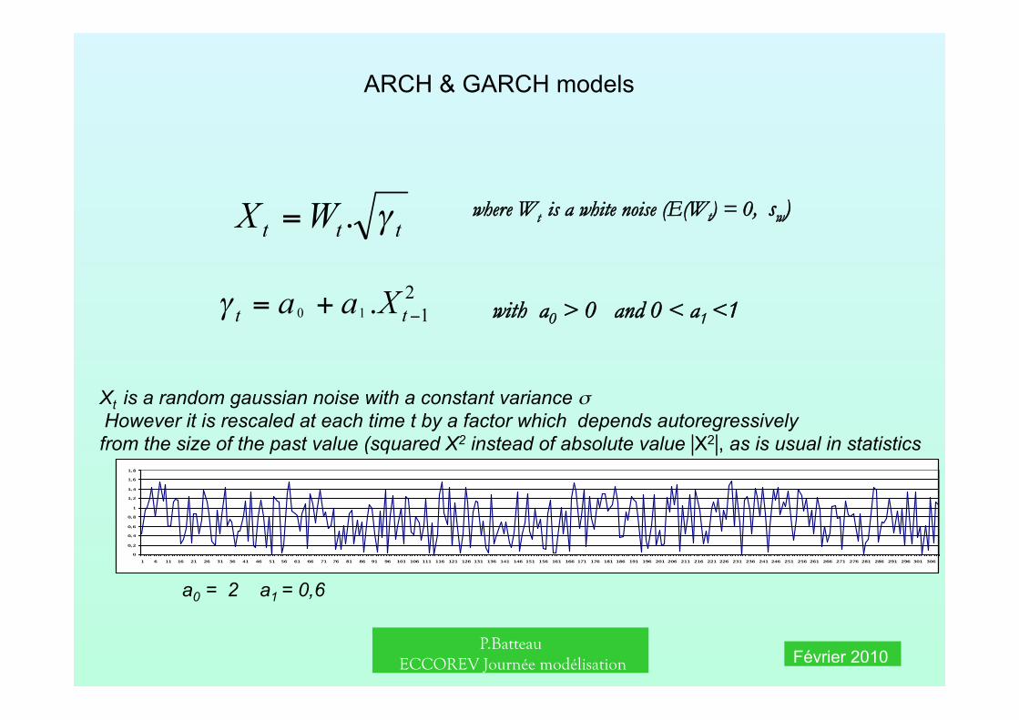
ARCH & GARCH models
where Wt is a white noise (E(Wt) = 0, sw)
with a0 > 0 and 0 < a1 <1
Xt is a random gaussian noise with a constant variance σ However it is rescaled at each time t by a factor which depends autoregressively from the size of the past value (squared X2 instead of absolute value |X2|, as is usual in statistics
a0 = 2 a1 = 0,6
P.Batteau ECCOREV Journée modélisation Février 2010
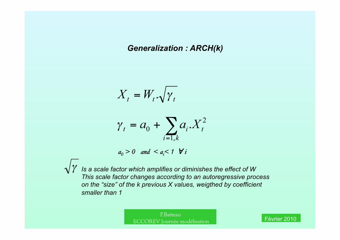
Generalization : ARCH(k)
Is a scale factor which amplifies or diminishes the effect of W This scale factor changes according to an autoregressive process on the “size” of the k previous X values, weigthed by coefficient smaller than 1
a0 > 0 and < ai< 1 ∀ i
P.Batteau ECCOREV Journée modélisation Février 2010
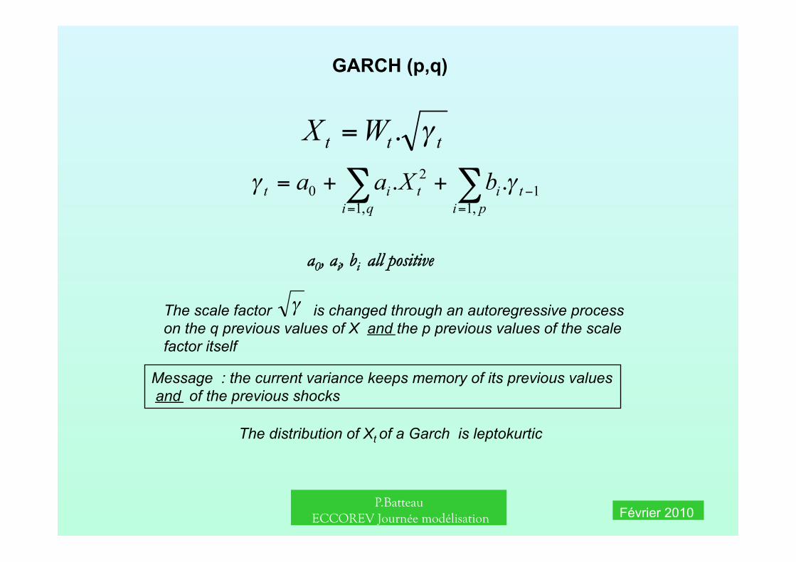
GARCH (p,q)
a0, ai, bi all positive
The scale factor is changed through an autoregressive process on the q previous values of X and the p previous values of the scale factor itself
Message : the current variance keeps memory of its previous values and of the previous shocks
The distribution of Xt of a Garch is leptokurtic
P.Batteau ECCOREV Journée modélisation Février 2010
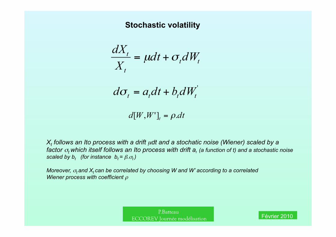
Stochastic volatility
Xt follows an Ito process with a drift µdt and a stochatic noise (Wiener) scaled by a factor σt which itself follows an Ito process with drift at (a function of t) and a stochastic noise scaled by bt (for instance bt = β.σt )
Moreover, σt and Xt can be correlated by choosing W and W’ according to a correlated Wiener process with coefficient ρ
P.Batteau ECCOREV Journée modélisation Février 2010
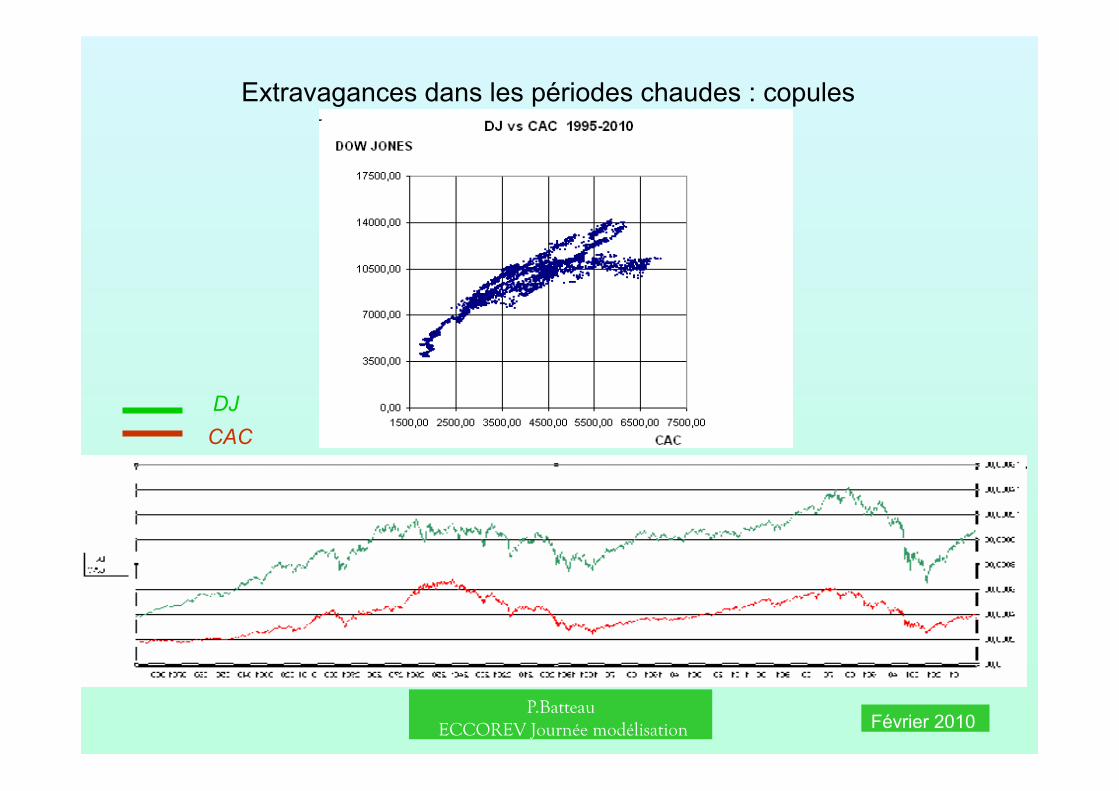
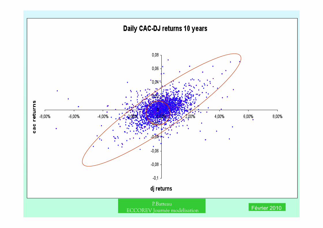
Extravagances dans les périodes chaudes : copules
DJ CAC
P.Batteau ECCOREV Journée modélisation Février 2010
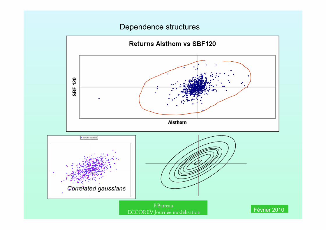
Dependence structures
Correlated gaussians
P.Batteau ECCOREV Journée modélisation Février 2010
P.Batteau ECCOREV Journée modélisation Février 2010
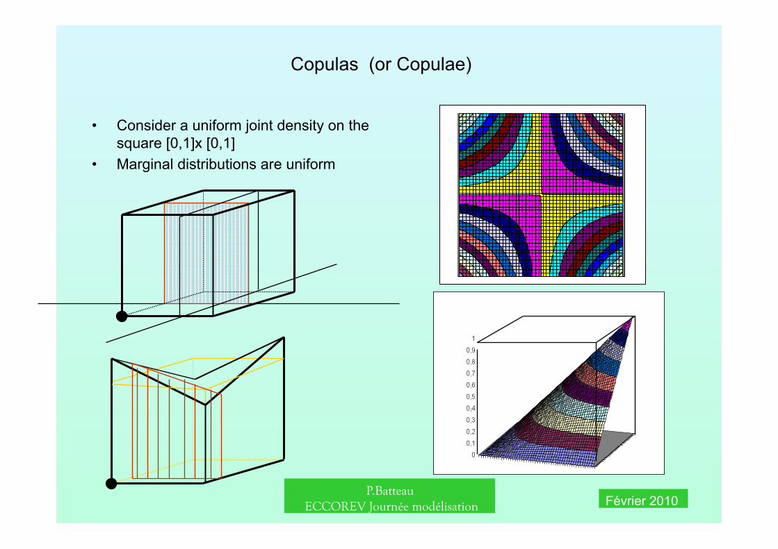
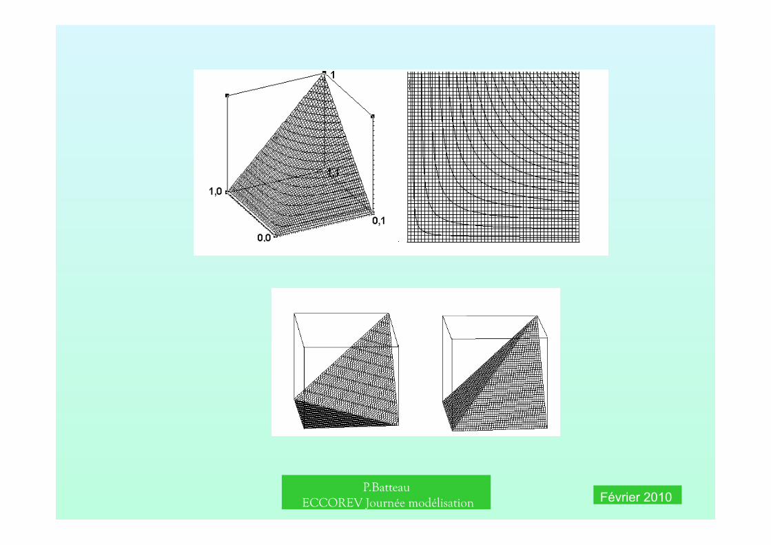
Copulas (or Copulae)
• Consider a uniform joint density on the square [0,1]x [0,1]
• Marginal distributions are uniform
P.Batteau ECCOREV Journée modélisation Février 2010
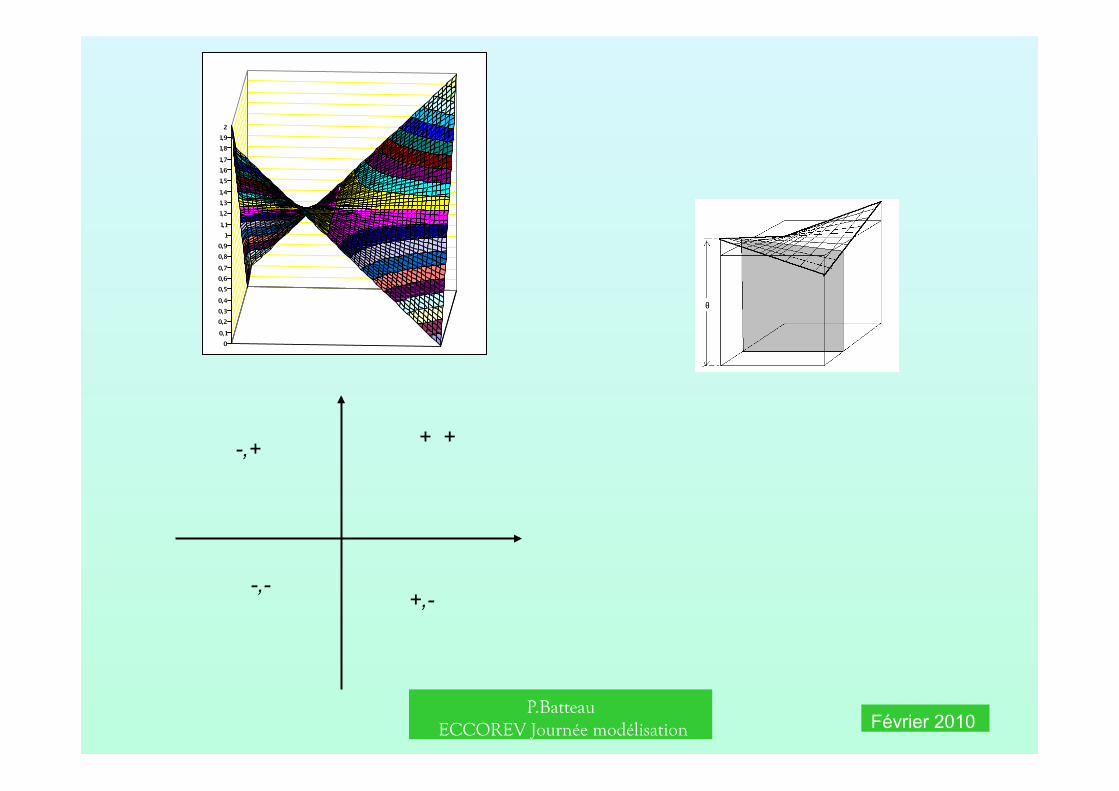
+ + -,+
+,- -,-
P.Batteau ECCOREV Journée modélisation Février 2010
P.Batteau ECCOREV Journée modélisation Février 2010
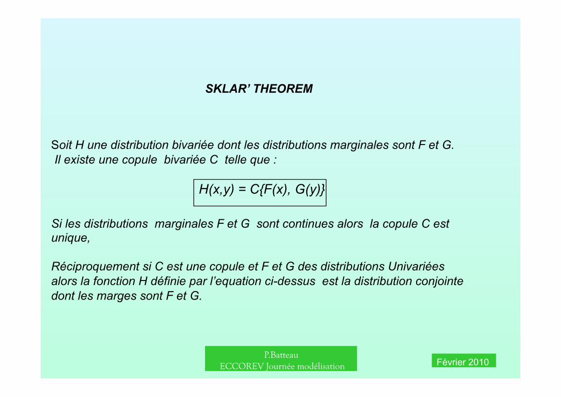
Soit H une distribution bivariée dont les distributions marginales sont F et G. Il existe une copule bivariée C telle que :
H(x,y) = C{F(x), G(y)}
Si les distributions marginales F et G sont continues alors la copule C est unique,
Réciproquement si C est une copule et F et G des distributions Univariées alors la fonction H définie par l’equation ci-dessus est la distribution conjointe dont les marges sont F et G.
SKLAR’ THEOREM
P.Batteau ECCOREV Journée modélisation Février 2010
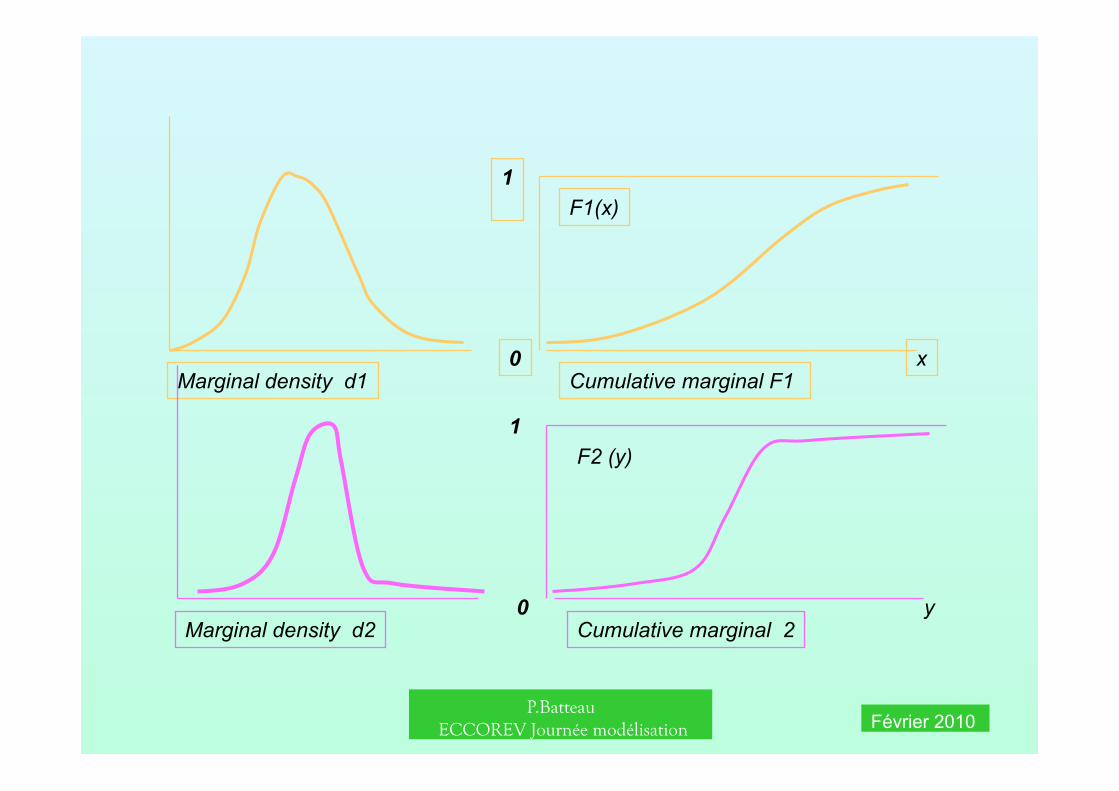
Marginal density d1 Cumulative marginal F1
F1(x)
x 0
1
Marginal density d2 Cumulative marginal 2
F2 (y)
y 0
1
P.Batteau ECCOREV Journée modélisation Février 2010
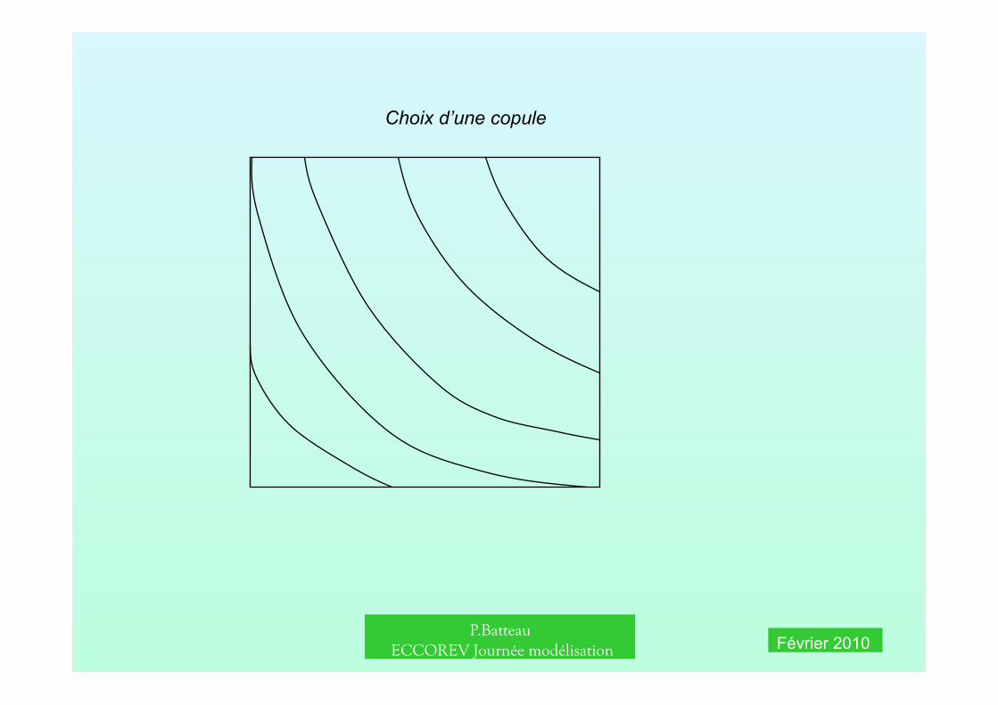
Choix d’une copule

P.Batteau ECCOREV Journée modélisation Février 2010
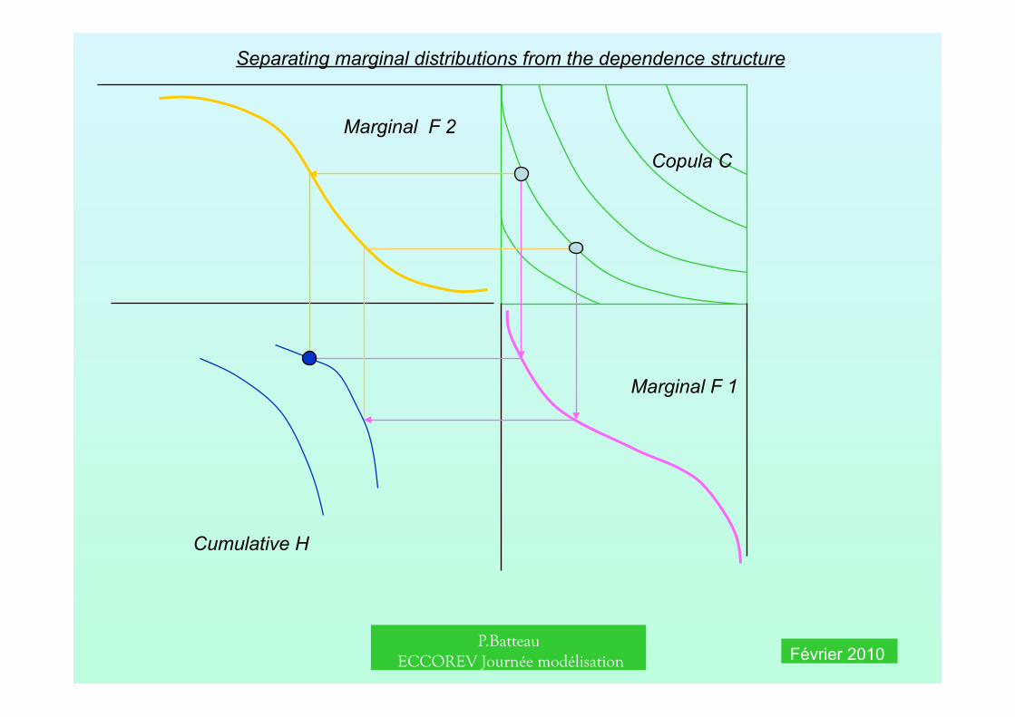
Cumulative of r1
Cumulative of r2 Joint density isolines
Copula isolines
Separating marginal distributions from the dependence structure
P.Batteau ECCOREV Journée modélisation Février 2010
Copula C
Marginal F 1
Marginal F 2
Cumulative H
Separating marginal distributions from the dependence structure
P.Batteau ECCOREV Journée modélisation Février 2010
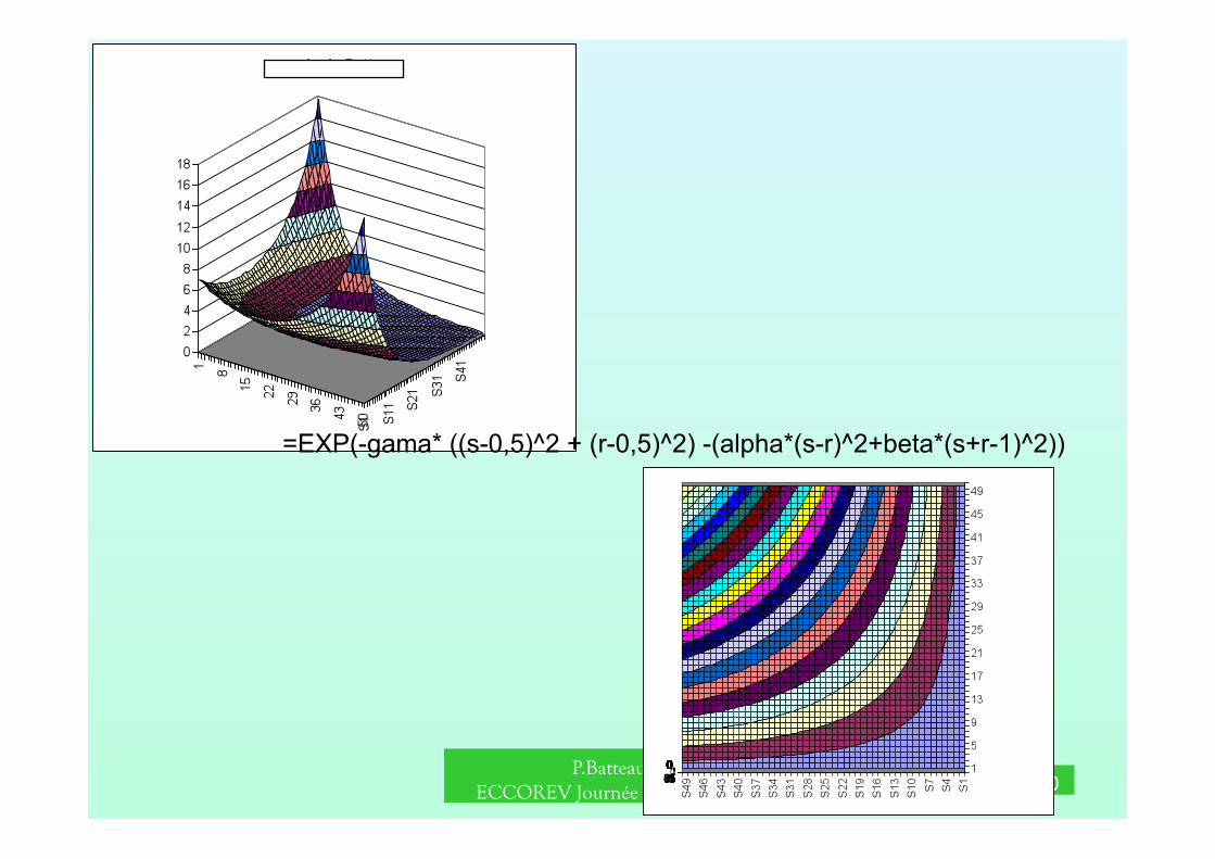
=EXP(-gama* ((s-0,5)^2 + (r-0,5)^2) -(alpha*(s-r)^2+beta*(s+r-1)^2))
P.Batteau ECCOREV Journée modélisation Février 2010
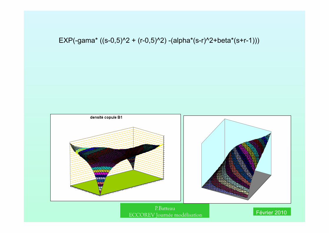
EXP(-gama* ((s-0,5)^2 + (r-0,5)^2) -(alpha*(s-r)^2+beta*(s+r-1)))
P.Batteau ECCOREV Journée modélisation Février 2010
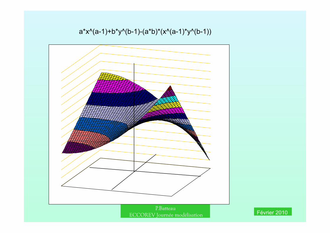
a*x^(a-1)+b*y^(b-1)-(a*b)*(x^(a-1)*y^(b-1))
P.Batteau ECCOREV Journée modélisation Février 2010
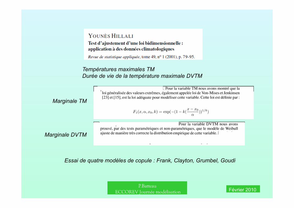
Températures maximales TM Durée de vie de la température maximale DVTM
Marginale DVTM
Marginale TM
Essai de quatre modèles de copule : Frank, Clayton, Grumbel, Goudi

P.Batteau ECCOREV Journée modélisation Février 2010
Modélisation multivariée des précipitations max-annuelles par copules pour l’étude de stationnarité des pluies méditerranéennes françaises. Nicolas PUJOL(1), Luc NEPPEL(1), Robert SABATIER(2) (1) Université Montpellier 2 – Maison des Sciences de l’Eau – UMR 5569 Hydrosciences – UM2 / CNRS / IRD [email protected], [email protected] (2) Laboratoire de physique industrielle et traitement de l’information – UFR Pharmacie, UM1 et EA 2415
Résumé : cet article étudie la modélisation multivariée des précipitations extrêmes via les copules gaussienne, de Student, et de Gumbel, et examine quelles sont les conséquences du choix de la modélisation sur l’étude régionale de stationnarité. Les illustrations montrent que ces trois modélisations engendrent des résultats très différents, tant au niveau du calcul des quantiles, en raison de l’estimation du paramètre de forme de la loi marginale GEV (Generalized Extreme Value), qu’aux niveaux du test de stationnarité et de l’ampleur des tendances qui varient du simple au double suivant la copule choisie.

P.Batteau ECCOREV Journée modélisation Février 2010
Le monde antique concevait l’incertitude comme relevant de l’action de trois femmes (les Parques) et les haruspices s’efforçaient de percer leur humeur. François 1er aussi voyait l’incertitude au féminin (“souvent femme varie et bien fol est qui s’y fie”) Nous attribuons aujourd’hui le risque aux caprices d’une Dame Nature et nos modèles s’efforcent de les prévoir.
Si le hasard est effectivement une invention conçue par une Grande Prêtresse, alors admirons sa subtilité, sa malice et sa profondeur, qualités que nous prêtons à la sensibilité féminine et reconnaissons humblement l’étendue de notre ignorance de son jeu, malgré la sophistication de nos modèles.

P.Batteau ECCOREV Journée modélisation Février 2010

P.Batteau ECCOREV Journée modélisation Février 2010