Fibonacci Binning
4
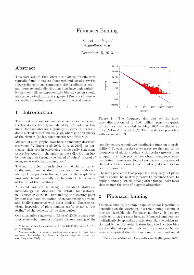
Fibonacci Binning Sebastiano Vigna * [email protected] December 15, 2013 Abstract This note argues that when dot-plotting distributions typically found in papers about web and social networks (degree distributions, component-size distributions, etc.), and more generally distributions that have high variabil- ity in their tail, an exponentially binned version should always be plotted, too, and suggests Fibonacci binning as a visually appealing, easy-to-use and practical choice. 1 Introduction The literature about web and social networks has been in the last decade literally inundated by dot plots like Fig- ure 1: for each abscissa x (usually, a degree or a size), a dot is plotted at coordinates hx, yi, where y the frequency of the element (nodes, components) with feature x. Misuses of such graphs have been abundantly described elsewhere [Willinger et al.:2009, Li et al.:2005]—in par- ticular, their role in convincing people easily that some power law would fit the empirical data distribution just by plotting lines through the “cloud of points” instead of using some statistically sound test. 1 The main problem of such plots is that the tail is, ac- tually, unfathomable: due to the sparsity and high vari- ability of the points in the right part of the graph, it is impossible to infer visually anything about the behavior of the tail of the distribution. A sound solution is using a standard statistical methodology as discussed in detail, for instance, in [Clauset et al.:2009]: first finding the starting point by max-likelihood estimation, then computing a p-value, and finally comparing with other models. Nonetheless, visual inspection of plots remains useful to get a “gut feeling” of the behavior of the distribution. One alternative suggested in [Li et al.:2005] is using size- rank plots —the numerosity-based discrete analog of the * The author has been supported by the EU-FET grant NADINE (GA 288956). 1 Interestingly, the same considerations appear to have been common knowledge at least a decade ago in other ar- eas [Hergarten:2002]. 0.0001 0.01 1 100 10000 1e+06 1e+08 1e+10 0 9 99 999 9999 99999 999999 frequency indegree Power law Figure 1: The frequency dot plot of the inde- gree distribution of a 106 million pages snapshot of the .uk web crawled in May 2007 (available at http://law.di.unimi.it/). The line shows a power law with exponent 1.89. complementary cumulative distribution function in prob- ability. 2 To each abscissa x we associate the sum of the frequencies of all data points with abscissa greater than or equal to x. The plot we now obtain is monotonically decreasing, there is no cloud of points, and the shape of the tail will be a straight line if and only if the distribu- tion is a power law. The main problem is that people love frequency dot plots, and it should be relatively easier to convince them to apply a binning (which, among other things, looks nice) than change the type of diagram altogether. 2 Fibonacci binning Fibonacci binning is a simple exponential (or logarithmic, depending on the viewpoint) discrete binning technique: bins are sized like the Fibonacci numbers. It displays nicely on a log-log scale because Fibonacci numbers are multiplicatively spaced approximately like the golden ra- tio, and it has the useful feature that the first two bins are actually data points. This feature comes very handy as most empirical distributions found in web and social 2 Limitations of size-rank plots are discussed in [Hergarten:2002]. 1
description
Fibonacci binning
Transcript of Fibonacci Binning
Fibonacci Binning
Sebastiano Vigna∗
December 15, 2013
Abstract
This note argues that when dot-plotting distributionstypically found in papers about web and social networks(degree distributions, component-size distributions, etc.),and more generally distributions that have high variabil-ity in their tail, an exponentially binned version shouldalways be plotted, too, and suggests Fibonacci binning asa visually appealing, easy-to-use and practical choice.
1 Introduction
The literature about web and social networks has been inthe last decade literally inundated by dot plots like Fig-ure 1: for each abscissa x (usually, a degree or a size), adot is plotted at coordinates 〈x, y〉, where y the frequencyof the element (nodes, components) with feature x.
Misuses of such graphs have been abundantly describedelsewhere [Willinger et al.:2009, Li et al.:2005]—in par-ticular, their role in convincing people easily that somepower law would fit the empirical data distribution justby plotting lines through the “cloud of points” instead ofusing some statistically sound test.1
The main problem of such plots is that the tail is, ac-tually, unfathomable: due to the sparsity and high vari-ability of the points in the right part of the graph, it isimpossible to infer visually anything about the behaviorof the tail of the distribution.
A sound solution is using a standard statisticalmethodology as discussed in detail, for instance,in [Clauset et al.:2009]: first finding the starting pointby max-likelihood estimation, then computing a p-value,and finally comparing with other models. Nonetheless,visual inspection of plots remains useful to get a “gutfeeling” of the behavior of the distribution.
One alternative suggested in [Li et al.:2005] is using size-rank plots—the numerosity-based discrete analog of the
∗The author has been supported by the EU-FET grant NADINE(GA 288956).
1Interestingly, the same considerations appear to have beencommon knowledge at least a decade ago in other ar-eas [Hergarten:2002].
0.0001
0.01
1
100
10000
1e+06
1e+08
1e+10
0 9 99 999 9999 99999 999999fr
equen
cy
indegree
Power law
Figure 1: The frequency dot plot of the inde-gree distribution of a 106 million pages snapshotof the .uk web crawled in May 2007 (available athttp://law.di.unimi.it/). The line shows a power lawwith exponent 1.89.
complementary cumulative distribution function in prob-ability.2 To each abscissa x we associate the sum of thefrequencies of all data points with abscissa greater thanor equal to x. The plot we now obtain is monotonicallydecreasing, there is no cloud of points, and the shape ofthe tail will be a straight line if and only if the distribu-tion is a power law.
The main problem is that people love frequency dot plots,and it should be relatively easier to convince them toapply a binning (which, among other things, looks nice)than change the type of diagram altogether.
2 Fibonacci binning
Fibonacci binning is a simple exponential (or logarithmic,depending on the viewpoint) discrete binning technique:bins are sized like the Fibonacci numbers. It displaysnicely on a log-log scale because Fibonacci numbers aremultiplicatively spaced approximately like the golden ra-tio, and it has the useful feature that the first two binsare actually data points. This feature comes very handyas most empirical distributions found in web and social
2Limitations of size-rank plots are discussed in [Hergarten:2002].
1

1
10
100
1000
10 100 1000 10000
Figure 2: A dot plot of two distribution describedin [Li et al.:2005]. Can you guess which one comes froma power law?
networks have slightly different behavior on the first oneor two data points.3 Moreover, Fibonacci binning isless coarse than the common power-of-b binnings (e.g.,b = 2, 10), which should make the visual representationmore accurate [Virkar and Clauset:2013].
Binning is essential for getting a graphical understand-ing of the tail of dot plots.4 Consider, for instance, thefamous pathological example shown in Figure 2, which isdiscussed in [Li et al.:2005].5 The figure shows two typi-cal frequency dot plots. The (obvious) reason the exam-ple is pathological is that the plot looking like a straightline is a sample from an exponential distribution, whereasthe curved plot is a sample from a power-law distribution.Of course, you are supposed to think the exact contrary,and if you’ve seen many dot plots like Figure 1 some rea-sonable doubts about “visual distribution fitting” usingfrequency plots should surface to your mind.
Binning, however, comes to help. By averaging the valuesacross a contiguous segment of abscissas, we obtain amore regular set of points (essentially, the midpoints ofthe histograms on the same intervals) that we can connectto get more insight on the actual shape of the curve.Note that the lines connecting the point are absolutelyimaginary; they’re just a visual clue—they are not partof the data.
Kernel density estimation is another technique widelyused for this purpose, but it does not really work wellwith discrete distributions and in particular with distri-butions with a “starting point”.
3This issue is actually solved in most papers by not plotting thevalue for abscissa zero, which happens automatically if you chooseto plot in log-log scale in any plotting package known to the author.
4Exponential binning is discussed in detail in [Milojevic:2010],where the authors suggest it as a better way to fit power laws, evenwith respect to size-rank plots.
5The code to generate the pathological example can be found athttp://hot.caltech.edu/topology/RankVsFreq.m.
0.0001
0.001
0.01
0.1
1
10
100
100 1000 10000
Power lawFibonacci binning
Figure 3: A dot plot of the pathological sample from apower-law distribution from [Li et al.:2005], its Fibonaccibinning and the original power-law distribution used togenerate the sample.
More in detail, let F0 = 1, F1 = 1, Fn = Fn−1 + Fn−2,6
assume that we have a starting offset s (usually 0 or 1)and data 〈xi, yi〉 with xi distinct integers satisfying xi ≥s. The binning intervals [`j . . rj), j ≥ 0, are then builtstarting at s using lengths F0, F1, F2, . . . :
[`0 . . r0) = [s+ F1 − 1 . . s+ F2 − 1)
[`1 . . r1) = [s+ F2 − 1 . . s+ F3 − 1)
. . .
[`j . . rj) = [s+ Fj+1 − 1 . . s+ Fj+2 − 1)
. . .
Note that rk− `k = Fk, and that if s = 1 the extremes ofthe intervals are exactly consecutive Fibonacci numbers.The resulting binned sequence 〈pk,mk〉, k ≥ 0 is
〈pk,mk〉 =
⟨`k +
Fk − 1
2,
1
Fk
∑xi∈[`k ..rk)
yi
⟩.
Figures 3 and 4 show the result of Fibonacci binning onthe pathological curves: the truth is easily revealed, andwe obtain a very close fit with the distribution used togenerate the sample.
We remark that, in fact, the pathological power-law curveis not so pathological: plfit7 provides a best max-likelihood fitting starting at 100 with α = 2.59 and ap-value 0.154± 0.01, thus essentially recovering the orig-inal distribution, which has exponent 2.5.
6It is also customary to use F0 = 0, F1 = 1 as initial condi-tion for the Fibonacci numbers, but our choice makes the followingnotation slightly easier to read.
7https://github.com/ntamas/plfit
2
0.0001
0.001
0.01
0.1
1
10
100
1000
10 100 1000 10000
Power lawFibonacci binning
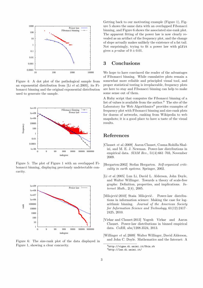
Figure 4: A dot plot of the pathological sample froman exponential distribution from [Li et al.:2005], its Fi-bonacci binning and the original exponential distributionused to generate the sample.
1e-06
0.0001
0.01
1
100
10000
1e+06
1e+08
1e+10
0 9 99 999 9999 99999 999999
freq
uen
cy
indegree
Fibonacci binningPower law
Figure 5: The plot of Figure 1 with an overlapped Fi-bonacci binning, displaying previously undetectable con-cavity.
1
10
100
1000
10000
100000
1e+06
1e+07
1e+08
1e+09
0 9 99 999 9999 99999 999999
ran
k
indegree
Power law
Figure 6: The size-rank plot of the data displayed inFigure 1, showing a clear concavity.
Getting back to our motivating example (Figure 1), Fig-ure 5 shows the same data with an overlapped Fibonaccibinning, and Figure 6 shows the associated size-rank plot.The apparent fitting of the power law is now clearly re-vealed as an artifact of the frequency plot, and the changeof slope actually makes unlikely the existence of a fat tail.Not surprisingly, trying to fit a power law with plfit
gives a p-value of 0± 0.01.
3 Conclusions
We hope to have convinced the reader of the advantagesof Fibonacci binning. While cumulative plots remain asomewhat more reliable and principled visual tool, andproper statistical testing is irreplaceable, frequency plotsare here to stay and Fibonacci binning can help to makesome sense out of them.
A Ruby script that computes the Fibonacci binning of alist of values is available from the author.8 The site of theLaboratory for Web Algorithmics9 provides examples offrequency plot with Fibonacci binning and size-rank plotsfor dozens of networks, ranking from Wikipedia to websnapshots; it is a good place to have a taste of the visualresults.
References
[Clauset et al.:2009] Aaron Clauset, Cosma Rohilla Shal-izi, and M. E. J. Newman. Power-law distributions inempirical data. SIAM Rev., 51(4):661–703, November2009.
[Hergarten:2002] Stefan Hergarten. Self-organized criti-cality in earth systems. Springer, 2002.
[Li et al.:2005] Lun Li, David L. Alderson, John Doyle,and Walter Willinger. Towards a theory of scale-freegraphs: Definition, properties, and implications. In-ternet Math., 2(4), 2005.
[Milojevic:2010] Stasa Milojevic. Power-law distribu-tions in information science: Making the case for log-arithmic binning. Journal of the American Societyfor Information Science and Technology, 61(12):2417–2425, 2010.
[Virkar and Clauset:2013] Yogesh Virkar and AaronClauset. Power-law distributions in binned empiricaldata. CoRR, abs/1208.3524, 2013.
[Willinger et al.:2009] Walter Willinger, David Alderson,and John C. Doyle. Mathematics and the Internet: A
8http://vigna.di.unimi.it/fbin.rb9http://law.di.unimi.it/
3

source of enormous confusion and great potential. No-tices of the American Mathematical Society, 56(5):586–599, 2009.
4


![NOMBRES DE FIBONACCI ET POLYNOMESˆ …irma.math.unistra.fr/~foata/paper/pub71.pdf · NOMBRES DE FIBONACCI ET POLYNOMES ORTHOGONAUXˆ Mignotte et Piras [CeMi87]). Comme aussi indiqu´e](https://static.fdocuments.fr/doc/165x107/5c5b590c09d3f254368b8f03/nombres-de-fibonacci-et-polynomes-irmamath-foatapaperpub71pdf-nombres.jpg)