Documents de travail

Faculté des sciences économiques et de

gestion Pôle européen de gestion et

d'économie (PEGE)

61 avenue de la Forêt Noire

F-67085 Strasbourg Cedex

Secrétariat du BETA

Géraldine Del Fabbro

Tél. : (33) 03 68 85 20 69

Fax : (33) 03 68 85 20 70

g.delfabbro @unistra.fr

www.beta-umr7522.fr

« Lottery- and survey-based risk attitudes linked through a multichoice elicitation task »

Auteurs

Giuseppe Attanasi, Nikolaos Georgantz ís, Valentina Rotondi, Daria Vigani

Document de Travail n° 2016 – 24

Avril 2016

Lottery- and survey-based risk attitudes linked

through a multichoice elicitation task

Giuseppe Attanasi∗

Nikolaos Georgantzıs †

Valentina Rotondi‡

Daria Vigani§

April 14, 2016

Abstract

In this paper we compare two mutually uncorrelated risk-attitude elic-itation tasks. In particular, we test for correlation of the elicited degreesof monetary risk aversion at a within-subject level. We show that suffi-ciently similar incentivized mechanisms elicit correlated decisions in termsof monetary risk aversion only if other risk-related attitudes are accountedfor. Furthermore, we ask subjects to self-report their general willingness totake risks. We find evidence of some external validity of the two tasks aspredictors of self-reported risk attitudes in general human domains.

Keywords: Risk aversion, Elicitation method, Lottery choices.

JEL classification: D81, C91

∗Corresponding author: University of Strasbourg (BETA), France. 61 Avenue de laForet Noire, 67000 Strasbourg. Email: attanasi@unistra.fr. Phone: +33 (0)6 59 20 01 32.G. Attanasi gratefully acknowledges financial support by the European Research Council(ERC) [Starting Grant DU 283953], and by the project “Creative, Sustainable Economiesand Societies” (CSES) coordinated by Robin Cowan, funded through the University ofStrasbourg IDEX Unistra. The authors wish to thank Omotuyole Ambali, Luca Corazzini,Astrid Gamba, Lucio Picci, Matteo Rizzolli, and Luca Stanca for useful comments andinputs.

†University of Reading, UK‡Catholic University of the Sacred Heart, Milan, Italy§Catholic University of the Sacred Heart, Milan, Italy

1

1 Introduction

Experimental evidence and recent theories of individual decision making haveacknowledged the fact there is more to a decision maker’s attitude to risk thanrisk aversion alone. Concepts like loss aversion, reference points or aspirationlevels, probability weighting and even violations of stochastic dominance arenon-negligible aspects which are jointly or separately accounted for by mod-ern theories aiming at accommodating previously disturbing and paradoxicalphenomena.

However, several practitioners and the vast majority of experimental re-searchers seem to rely on risk aversion alone, when (the former) pricing arisky asset and (the latter) eliciting subjects’ risk attitudes as an explanatoryvariable of their behavior in another decision making context. For example,in more than half of the occasions in which experimental economists wish toaccount for their subjects’ risk attitudes as a primary or secondary aspectof their behavior, the Holt and Laury (2002) – HL hereafter – procedure isadopted, which is primarily a uni-dimensional test often used to map de-cisions on a uni-parametric utility function. A different procedure involvesa survey question asking subjects to assess their attitude towards risk (self-assessed risk attitude). Interestingly, whether this is done by a single questionor with a more complex test like Zuckerman’s Sensation Seeking Scale (Zuck-erman, 1994), even in this literature the variable used is a uni-dimensionalconstruct assessing a person’s overall riskiness. 1

In this paper, we contrast both aforementioned methods, to choices in aLottery-Panel Test (Sabater-Grande and Georgantzis, 2002) – SG hereafter–, this method disclosing more information on a decision maker’s risk atti-tudes. Specifically, each participant makes a choice among a series (panel)of alternative lotteries. Four panels are constructed, each of which providessubjects with a different incentive (risk premium) to make riskier choices. Aparametric approach to the test can offer a simple prediction on subjects’ be-havior across panels and is easily comparable with uni-dimensional mappingon the utility parameter space like in HL. The richness of patterns emergingas deviations from the expected-utility predicted behavior across panels, al-lows us to classify subjects according to criteria which are not applicable insimple models.

A rather surprising finding that is recurrently reported by different ex-perimental studies is that risk attitudes elicited through different methods

1Weber et al. (2002) have introduced in the literature a psychometric scale that as-sesses risk taking in five different domains: financial decisions (separately for investingvs. gambling), health/safety, recreational, ethical, and social decisions. However, theirelicitation method is uni-dimensional and it is the same across domains, unless framing ofthe question used to elicit self-assessed risk attitude in a specific domain. Furthermore, inthis paper we do not focus on individual risk-taking behavior in different human domains.Rather, we measure the correlation across two incentivized tasks – a uni-dimensional and amulti-dimensional one – and between the former and self-assessed risk attitude in general

human domains.

2

differ significantly from each other.2 Several aspects of this finding relate tothe mere nature of the tasks. For example, tasks with losses are naturallyexpected to capture different dimensions of subjects’ psychological attitudesas compared to tasks limited to the gains domain. Furthermore, it is rathereasily accepted that tasks covering different payoff ranges would also lead tosignificant differences in the elicited attitudes.

The consequences of accepting such differences as natural can be of twotypes. First, those concerning the relation between the elicitation task andthe underlying theoretical decision-making model under risk, and, second,those related to the usefulness of the task as a method of obtaining an ex-planatory variable to empirically capture the role of subjects’ risk attitudeon his/her behavior in a different task. Both issues are largely neglected, notso much by the studies specifically designed to compare risk attitudes elicitedthrough different tasks, but by those acting as simple users of the tasks asa method of generating a risk-attitude related explanatory variable for theirprimary data from an experiment.

Regarding the first issue, the most striking feature of a number of broadlyused tasks is their dependence on a single choice made by each subject. It isstraightforward to see why such a strategy is both tautologically consistentwith any uniparametric description of the decision problem solved by thedecision maker, and in dissonance with all modern theories based by defini-tion on more than the product of probabilities with the uniparametric utilitytransformation of the associated monetary outcomes.3

Regarding the second issue, we feel that it can be, at the same time, moreurgent to address and less problematic. This is so because there seems tobe some consensus on the intuitive but not sufficiently supported fact thatdecisions made across similar tasks should be expected to elicit attitudeswhich do not significantly differ from each other. Of course, one shouldnot forget that even the repetition of exactly the same task by the sameindividual would most probably lead to differences. But such differencesfollow specific patterns, some of which have been documented empirically,4

2For a recent example of five elicitation methods and reference to such results, seeCrosetto and Filippin (2015). As in previous experimental studies on the topic, they alsofind that the estimated risk aversion parameters vary greatly across tasks.

3Anecdotally, we would like to refer to the case of a referee stating and an editor agreeingthat “to elicit one’s risk parameter from a single choice is not problematic, whereas toobtain it from many decisions generally leads to inconsistencies”.

4For example, regression to the mean has been found to affect repeated choices in thesame task by Garcıa-Gallego et al. (2011). Furthermore, Levy-Garboua et al. (2012) founda significantly higher elicited risk aversion in sequential than in simultaneous treatment, indecreasing and random than in increasing treatment, in high than in low-payoff condition.Their findings suggest that subjects use available information that has no value for nor-mative theories. Cox et al. (2014) have rationalized some of these findings by showing therole of the payment mechanism in these distortions. Indeed, they find that random-lotteryincentive mechanisms – as those usually employed in risk-elicitation tasks – may decreasethe proportion of risky choices in the population, if compared to a one-task design. Thiscould explain why significantly more risk aversion emerges under multiple-task than under

3

and even conform to the well-known paradigm of preference imprecision.5

Thus, even when choices by the same subject in the same task over differ-ent trials are different, attitudes elicited in similar tasks should be related tosome extent, even through correlation of the ranking that subjects receivedby their choices in the overall population. If this desideratum is satisfied,then eliciting risk attitudes as an explanatory variable of behavior in anothertask can be considered a meaningful strategy. On the contrary, if any ar-bitrarily small change of the context produces different attitude elicitationsthat are not systematically related across tasks, we risk failing to satisfacto-rily answer the question “does any of what we are observing in the lab relateat all with what anyone (even the same subject) does outside the lab?”

In this paper, we aim at shedding light on the reliability of HL, the methodmainly used in the last decade to elicit risk attitudes across a wide array ofcontexts and environments. To achieve this goal, we compare it experimen-tally to another risk-elicitation method, SG, which is made by a series offour tasks that we think can help us in identifying risk-related attitudes dis-regarded by the implementation of HL alone. Using the type classificationemerging from the choices made in SG, we want to see 1. whether the correla-tion between the risk-aversion orderings under the two elicitation proceduresincreases, and 2. whether any of these two monetary-incentivized mecha-nism is a good predictor of self-assessed risk attitudes (e.g. elicited througha hypothetical question about one’s general willingness to take risks).

We report two rather exceptionally positive findings which can contributeto a literature full of negative or contrasting results. First, we find evidenceof some external validity of these two mutually uncorrelated risk-attitudeelicitation methods – HL and SG – as predictors of self-reported risk atti-tudes in general human domains. Second, and more importantly, we showthat sufficiently similar incentivized mechanisms elicit correlated decisionsin terms of monetary risk aversion only if other risk-related attitudes aredisentangled. Considered together, our results indicate that, whereas bothHL and SG are reasonably good predictors of self-assessed risk attitudes, theuse of a more complete description of subjects’ risk attitudes is helpful whenstating the ability of each test to predict self-reported attitudes.

The rest of the paper is structured as follows. In Section 4.2 we reviewthe literature on risk-aversion elicitation, and show more in depth the spe-cific issues on which our study aims at contributing. Section 4.3 presents ourexperimental design. In Section 4.4 specific behavioral hypotheses are intro-duced. Section 4.5 analyzes the experimental results, which are discussed inthe concluding section.

one-task elicitation methods.5See Butler and Loomes (2007).

4

2 Literature review

Assessing and measuring individuals’ risk preferences is a fundamental issuefor economic analysis and policy prescriptions (Charness et al., 2013). Asa result, economists and other social scientists have developed a wide vari-ety of experimental methodologies to elicit individual risk attitudes. Riskpreferences have been indirectly derived from first-price sealed bid auctions(e.g. Cox et al., 1982, 1985, 1988), or elicited as lottery certainty equivalents(Becker et al., 1964). Individual degrees of risk aversion have also been ex-perimentally measured through asking subjects to input a value for one ofthe outcomes of a lottery that would make them indifferent with respectto another proposed lottery (the so-called trade-off method by Wakker andDeneffe, 1996).

Survey methods have also been employed, where subjects are asked toself-report their risk preferences through a series of hypothetical questionsconcerning a general willingness to take risks (see, e.g., Dohmen et al. (2011),for a representative sample of roughly 22,000 German subjects) or a specificwillingness to participate in a lottery (see, e.g., Attanasi et al. (2013), for asample of about 10,000 Italian subjects over five consecutive years).

Today, the most common and widespread procedure used by economiststo measure risk preferences in the laboratory is to ask subjects to choose onelottery (single decision) among a panel of lotteries. These lotteries can eitherentail a single choice among a set of predetermined prospects, presented in anabstract way (Eckel and Grossman, 2008), or can be framed as an investmentdecision (Charness and Gneezy, 2010), or still can be presented by means ofa visual task, without making any explicit reference to probabilities (Lejuezet al., 2002; Crosetto and Filippin, 2013).

As an extension of the previous methods, subjects were asked to makemultiple decisions between pairs or panels of risky lotteries. This is the caseunder investigation in this paper. As a matter of fact, both Holt and Laury(2002) and Sabater-Grande and Georgantzis (2002) use this last method inorder to elicit risk aversion. Holt and Laury (2002) – and follow-up papers6

– is the most well-known example of a “multiple price list design” which, ac-cording to Cox and Harrison (2008), was first used in Miller et al. (1969). Therisk-elicitation procedure used in Sabater-Grande and Georgantzis (2002) isa slightly revised version of the “ternary lotteries approach” (see, e.g., Rothand Malouf, 1979).

In this paper two risk-elicitation methods are proposed in a within-subjectdesign. Besides the original version, the multiple pairwise comparison in HLhas been usually implemented with two non-mutually-exclusive variants. Thefirst one – “switching multiple price list” – was introduced by Harrison et al.(2005) and studied at length by Andersen et al. (2006): Monotonicity is

6See Harrison et al. (2005) and Holt and Laury (2005): the former demonstrated andthe latter confirmed the possibility of order effects in Holt and Laury (2002) original designby scaling up real payments by 10 or 20 times.

5

enforced, i.e. the subject is asked to pick the switch point from one lotteryto the other and non-switch choices are filled automatically. The second oneconcerns doubling the number of outcome probabilities for which the twolotteries are compared, in order to allow the subject to make choices fromrefined options: This second variant, together with enforced monotonicity,has been implemented by Attanasi et al. (2014a), where HL is made of 20lottery pairs instead of 10. The second risk-elicitation method is the sameas the one used in Sabater-Grande and Georgantzis (2002) and follow-uppapers.7

As anticipated in the Introduction, our choice of analyzing and compar-ing two alternative methods of measuring risk preferences is partly due toa puzzling result in experimental economics: The degree of risk aversionshown by subjects in the laboratory is often varying across different elicita-tion techniques (see, e.g., Isaac and James, 2000; Dave et al., 2010), althoughsome correlations are found among monetary-incentivized instruments andsurvey-based methods (see, e.g., Vieider et al., 2015).

In recent years, a growing literature is investigating different risk-elicitationmethods, comparing their effectiveness in eliciting risk attitudes in non-interactive settings. Harrison and Rutstrom (2008) review experimental ev-idence on risk aversion in controlled laboratory experiments. The authorsexamine the experimental design of several procedures that allow direct esti-mation of risk preferences from subjects’ choices, as well as the way to drawinference about laboratory behavior. Furthermore, they provide an investi-gation on how the data generated by these procedures should be analyzed.In the same line, Charness et al. (2013) provide a discussion of a series ofprevailing methods for eliciting risk preferences. They outline the strengthsand weaknesses of each of these methods. In particular, they highlight thatchoosing which method to utilize is largely dependent on the question theresearcher wants to answer. Both these reviews of risk-elicitation methodsinclude a thorough discussion of HL.

Among experimental studies that compare HL with other risk-elicitationmethods, two are relevant for our paper. Charness and Viceisza (2015) com-pare two incentivized risk-elicitation methods in a between-subject design,namely HL, and the modified version of the Gneezy-Potters method as pre-sented in Charness and Gneezy (2010). In both treatments, subjects alsoself-report their risk attitude by answering a hypothetical question similar tothe one in Dohmen et al. (2011). The experiment was run in rural Senegal,with the aim of providing guidance to experimenters wishing to use risk-elicitation mechanisms in the rural developing world. Crosetto and Filippin(2015) compare five incentivized risk-elicitation methods in a between-subjectdesign: HL, Eckel and Grossman (2008), Charness and Gneezy (2010),Lejuezet al. (2002), and Crosetto and Filippin (2013). All experimental sessions be-ing run in Jena (Germany), they find that subjects’ estimated risk aversion

7See Georgantzıs and Navarro-Martınez (2010), and Garcıa-Gallego et al. (2011).

6

parameters vary greatly across tasks. Our work is positioned exactly in thisbranch of the literature.

Using original data from a homogeneous population of Italian subjects,we provide an experimental comparison of HL with another incentivized risk-elicitation method (SG), and a self-assessment measure of risk attitude (ahypothetical question similar to the one in Dohmen et al., 2011). Differentlyfrom the previous literature, this comparison is made through a within-subjectdesign: each subject in our experiment goes through the three risk-elicitationprocedures, and we control for other effects. Furthermore, we compare twomultiple-decision methods, while in previous studies HL has only been com-pared to single-decision methods. In fact, we think that coupling HL withanother multiple-decision mechanism could help shed more light on the reli-ability of the former.

As underlined above, HL is the most widely used risk-elicitation methodin experimental economic analyses in the last ten years: When risk aversion isconsidered as an explanatory variable for subject’s behavior in an individualor strategic decision setting, a preliminary test of risk aversion (preliminarywith respect to the main decision setting where subjects’ behavior should beanalyzed) is needed. In this regard, HL has a clear advantage with respect tomany other risk-elicitation methods: especially when enforcing monotonicity– as it is more frequently the case in economic experiments – it allows tocompletely describe a subject’s risk attitude through just one subject’s choice.

It is well known that this requires assuming that the subject is a vonNeumann-Morgenstern expected utility maximizer. Many papers have shownthat this assumption is questionable (see Wakker (2010) for a review), al-though other models (e.g., prospect theory) do not seem to have signifi-cantly higher explanatory power than expected utility (Harrison and Rut-strom, 2009). However, the goal of our exercise is not to test the expectedutility assumption in HL. Rather, we are interested in other risk-related at-titudes that are not taken into account when analyzing HL data, since withjust one choice per subject, by construction, attention is restricted to thecurvature of the uniparametric (Bernoullian) utility function.8 Therefore,other relevant risk-related attitudes may be disregarded.

The intuition behind our exercise is that the series of four tasks thatconstitute SG can help us in identifying some of these further risk-relatedattitudes. This is the main reason why we focus on the comparison betweenHL and SG. Using the type classification emerging from the choices made inSG, we want to see whether the correlation between the risk-aversion order-

8Notice that this problem would emerge also in the absence of enforced monotonicity.In fact, when HL is performed – as in the original paper – by asking subjects to make achoice between the two options for each of the 10 outcome probabilities, a subject whoswitches from one lottery to the other more than once as the probability of the bestoutcome increases, is still considered as if he/she has made just one choice (one switch).This is done by assigning to this subject as switch point from one lottery to the other theone corresponding to the number of safe choices the subject has made.

7

ings under the two elicitation procedures increases. Furthermore, and moreimportantly, we want to check whether, by disentangling subjects accordingto these further attitudes, the correlation between a subject’s self-reportedsensitivity to risk and the monetary-incentivized choice made respectivelyin HL and in SG is higher. A positive answer to the last question – that iswhat we actually found in this paper – should help explain why experimentaleconomists (rather than psychologists) usually do not rely on self-reportedmeasures of risk: The hypothetical questions used to let subjects self-assesstheir level of risk attitude might hide risk-related motivations other thanmonetary risk aversion, i.e., the curvature of the uniparametric expectedutility function.

3 Experimental design

Participants were 62 undergraduate students in Economics, recruited at Boc-coni University in Milan on October 2013. Each subject could only partici-pate in one session: Two sessions were run with 31 subjects each in a com-puterized room of Bocconi University, with subjects being seated at spacedintervals.

In each session, subjects faced two risk-elicitation tasks (HL and SG)on a within-subject base. In the two sessions, the two tasks were shown inreverse order. Only one of the two tasks was used to determine subjects’ finalearnings. The choice of the task to be paid was made in a random way, byflipping a coin. Payment was preceded by a questionnaire, which included aquestion about self-assessment of risk attitude.

Average earnings were e 15.90, including a e 3.00 show-up fee. The aver-age duration of a session was 45 minutes, including instructions and payment.The experiment was programmed and implemented using the z-Tree software(Fischbacher, 2007).

3.1 Task 1 (HL)

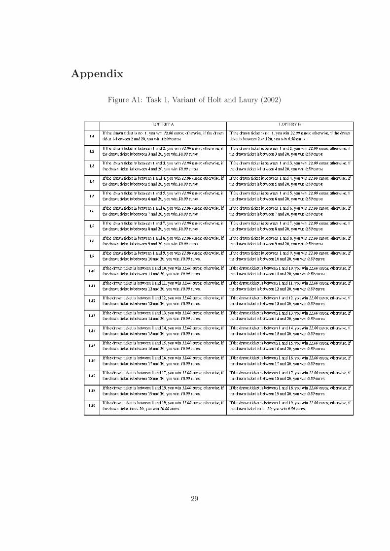
The first task was HL with the two variants of enforced monotonicity and 20(rather than 10) lottery pairs, and set of lottery payoffs as in Attanasi et al.(2014a). See Figure A1 in the Appendix.

3.1.1 Features of the task

• Subjects were presented with a battery of 19 pairs of two-outcomelotteries, numbered from line L1 to line L19, and a last (empty) lineL20 (bottom line of Figure A1).

• Each pair described two lotteries called A and B.

8

• Each lottery presented two positive monetary outcomes and their as-sociated probabilities.

• The two monetary outcomes of each lottery were kept constant: Foreach line L1–L19, lottery A always had the two outcomes, xA =e 12.00,xA =e 10.00, and lottery B always had the two outcomes, xB =e 22.00,xB =e 0.50.

• Within each pair, xA and xB were attached the same probability p,with p increasing – gradually and monotonically – when moving fromthe top (L1) to the bottom (L19) of the battery of lottery pairs.

• Probabilities were framed by means of an urn that contained 20 tickets,numbered from 1 to 20, the number of tickets associated to the highestof the two outcomes, xk , being independent of the lottery (k = A,B)and varying with the line. In particular, in L1 the highest outcome wasassigned ticket no. 1; in L2, tickets no. 1 and 2; . . . ; in L19, all ticketsbut no. 20. Hence, in the light of a final random draw of a ticket fromthe urn, the probabilities of xk and of xk were respectively: 1/20 and19/20 in L1; 2/20 and 18/20 in L2; . . . ; 19/20 and 1/20 in L19.

3.1.2 What subjects were asked to do

Given the battery of lotteries, each subject was asked to choose the switchline, i.e. the pair of lotteries starting from which he/she preferred lottery B

to lottery A. Thus, for all pairs of lotteries above the switch line, a subjectpreferred lottery A to lottery B, while starting from the pair on the switchline and for all the pairs below, he/she preferred lottery B to lottery A. Asubject preferring lottery A to lottery B for all the 19 pairs, selected the last(empty) line L20.

3.1.3 Determination of the subject’s earnings

Suppose that task 1 was randomly selected (by flipping a coin) at the end ofthe experiment to determine subjects’ earnings. Then, for each subject thecomputer would randomly select a pair of lotteries, i.e. one of the 19 lines ofthe battery of lotteries. The randomly-selected line indicated the number oftickets assigned to the highest outcome, hence the probability associated tothe two outcomes of both lottery A and lottery B.

If a subject’s switch line was below the randomly-selected line, then thetwo lottery outcomes for which that subject played were xA =e 12.00 andxA =e 10.00; otherwise, the two lottery outcomes for which that subjectplayed were xB =e 22.00 and xB =e 0.50.

Then, an experimenter randomly drew one of the 20 tickets contained in

9

the urn (physical implementation).9 The ticket drawn by the experimenterwas used to determine whether each subject earned the higher or the loweroutcome of the chosen lottery in the randomly-selected line.

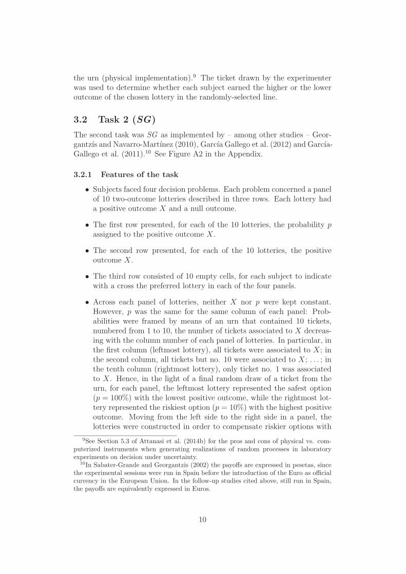
3.2 Task 2 (SG)

The second task was SG as implemented by – among other studies – Geor-gantzıs and Navarro-Martınez (2010), Garcıa Gallego et al. (2012) and Garcıa-Gallego et al. (2011).10 See Figure A2 in the Appendix.

3.2.1 Features of the task

• Subjects faced four decision problems. Each problem concerned a panelof 10 two-outcome lotteries described in three rows. Each lottery hada positive outcome X and a null outcome.

• The first row presented, for each of the 10 lotteries, the probability p

assigned to the positive outcome X.

• The second row presented, for each of the 10 lotteries, the positiveoutcome X.

• The third row consisted of 10 empty cells, for each subject to indicatewith a cross the preferred lottery in each of the four panels.

• Across each panel of lotteries, neither X nor p were kept constant.However, p was the same for the same column of each panel: Prob-abilities were framed by means of an urn that contained 10 tickets,numbered from 1 to 10, the number of tickets associated to X decreas-ing with the column number of each panel of lotteries. In particular, inthe first column (leftmost lottery), all tickets were associated to X; inthe second column, all tickets but no. 10 were associated to X; . . . ; inthe tenth column (rightmost lottery), only ticket no. 1 was associatedto X. Hence, in the light of a final random draw of a ticket from theurn, for each panel, the leftmost lottery represented the safest option(p = 100%) with the lowest positive outcome, while the rightmost lot-tery represented the riskiest option (p = 10%) with the highest positiveoutcome. Moving from the left side to the right side in a panel, thelotteries were constructed in order to compensate riskier options with

9See Section 5.3 of Attanasi et al. (2014b) for the pros and cons of physical vs. com-puterized instruments when generating realizations of random processes in laboratoryexperiments on decision under uncertainty.

10In Sabater-Grande and Georgantzis (2002) the payoffs are expressed in pesetas, sincethe experimental sessions were run in Spain before the introduction of the Euro as officialcurrency in the European Union. In the follow-up studies cited above, still run in Spain,the payoffs are equivalently expressed in Euros.

10

increases in the expected payoff pX. Thus, the positive outcome X

increases with the column number of each panel of lotteries.

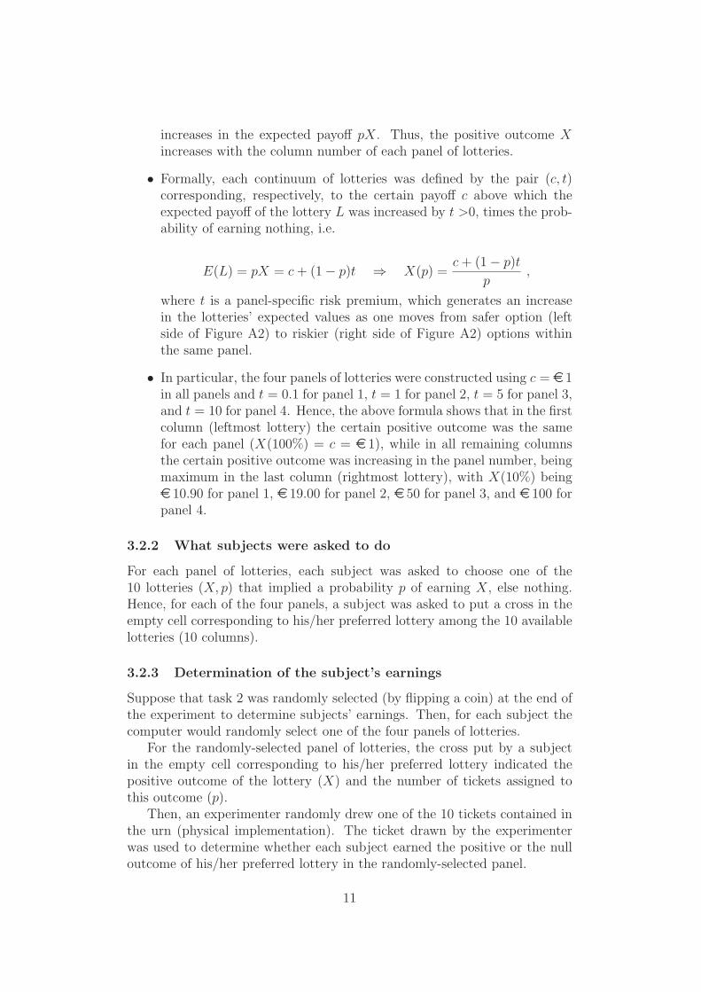
• Formally, each continuum of lotteries was defined by the pair (c, t)corresponding, respectively, to the certain payoff c above which theexpected payoff of the lottery L was increased by t >0, times the prob-ability of earning nothing, i.e.

E(L) = pX = c+ (1− p)t ⇒ X(p) =c+ (1− p)t

p,

where t is a panel-specific risk premium, which generates an increasein the lotteries’ expected values as one moves from safer option (leftside of Figure A2) to riskier (right side of Figure A2) options withinthe same panel.

• In particular, the four panels of lotteries were constructed using c = e 1in all panels and t = 0.1 for panel 1, t = 1 for panel 2, t = 5 for panel 3,and t = 10 for panel 4. Hence, the above formula shows that in the firstcolumn (leftmost lottery) the certain positive outcome was the samefor each panel (X(100%) = c = e 1), while in all remaining columnsthe certain positive outcome was increasing in the panel number, beingmaximum in the last column (rightmost lottery), with X(10%) beinge 10.90 for panel 1, e 19.00 for panel 2, e 50 for panel 3, and e 100 forpanel 4.

3.2.2 What subjects were asked to do

For each panel of lotteries, each subject was asked to choose one of the10 lotteries (X, p) that implied a probability p of earning X, else nothing.Hence, for each of the four panels, a subject was asked to put a cross in theempty cell corresponding to his/her preferred lottery among the 10 availablelotteries (10 columns).

3.2.3 Determination of the subject’s earnings

Suppose that task 2 was randomly selected (by flipping a coin) at the end ofthe experiment to determine subjects’ earnings. Then, for each subject thecomputer would randomly select one of the four panels of lotteries.

For the randomly-selected panel of lotteries, the cross put by a subjectin the empty cell corresponding to his/her preferred lottery indicated thepositive outcome of the lottery (X) and the number of tickets assigned tothis outcome (p).

Then, an experimenter randomly drew one of the 10 tickets contained inthe urn (physical implementation). The ticket drawn by the experimenterwas used to determine whether each subject earned the positive or the nulloutcome of his/her preferred lottery in the randomly-selected panel.

11

3.3 Questionnaire

A questionnaire about some idiosyncratic features has been submitted at theend of the experiment. Each subject was asked his/her gender, age, year andfield of study, previous attendance of an advanced course in Decision/GameTheory, and a question about self-assessment of general attitude towards risk,similar to the one used in Dohmen et al. (2011). In particular, the questionwas posed using the same wording of Bernasconi et al. (2014), which alsorun their experiments with Italian subjects: “In a scale from 1 to 10, howwould you rate your attitude towards risk: are you a person always avoidingrisk or do you love risk-taking behavior?”, where 1 was associated with thestatement “I always choose the safest option and try to avoid any possiblerisk” and 10 referred to “I love risk and I always choose the more riskyalternative”.

4 Behavioral Hypotheses

Each task is mainly targeted to elicit a subject’s degree of (monetary) riskaversion, through a different method. However, task 1 (HL) being character-ized by less “flexibility” in the subject’s available choices with respect to task2 (SG), the latter can be used to disclose and disentangle other risk-relatedmotivations. In fact, while in this variant of HL a subject is asked tochoose the line (pair of lotteries) starting from which she preferredlottery B to lottery A (with the same associated probabilities),in each panel of lotteries in SG the subject is asked to pick the preferredoutcome-probability combination, with both the positive outcome and itsassociated probability being different for each lottery. With this in mind,our first aim is to use subject’s four choices in SG to disentangle his/herrisk-related motivations behind the unique choice (switch line) in HL.

A Constant Relative Risk Averse (CRRA hereafter) utility function of theform U(x) = x1−r

1−ris assumed to elicit a subject’s (monetary) risk attitude in

both HL and SG, implying risk aversion for r > 0, risk neutrality for r = 0,and risk proneness for r < 0.

In HL, given the structure of the battery of lotteries (see Figure A1 inthe Appendix), the higher the number of the switch line (pairwise compar-ison at which a subject chooses to switch from lottery A to lottery B), thehigher his/her disclosed degree r of relative risk aversion (see Table A1 inthe Appendix). In particular: a switch line from L1 to L9 would reveal riskproneness (the smaller the number of the switch line, the higher |r|, the de-gree of risk proneness). A risk-neutral subject would indicate L10 as switchline; a switch line from L11 to L19 would reveal risk aversion (the greaterthe number of the switch line, the higher r, the degree of risk aversion).

In the original version of HL, subjects had to choose the preferred lotterybetween A and B in each of the 10 lines of the battery, giving rise to the

12

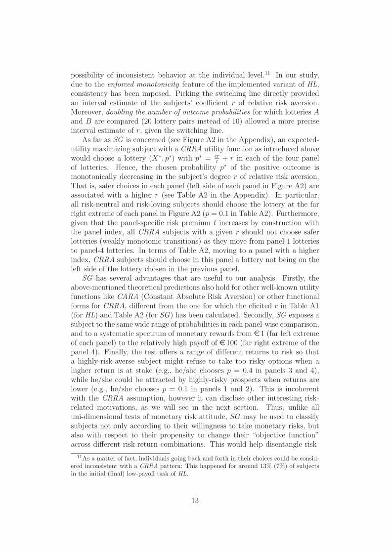
possibility of inconsistent behavior at the individual level.11 In our study,due to the enforced monotonicity feature of the implemented variant of HL,consistency has been imposed. Picking the switching line directly providedan interval estimate of the subjects’ coefficient r of relative risk aversion.Moreover, doubling the number of outcome probabilities for which lotteries Aand B are compared (20 lottery pairs instead of 10) allowed a more preciseinterval estimate of r, given the switching line.

As far as SG is concerned (see Figure A2 in the Appendix), an expected-utility maximizing subject with a CRRA utility function as introduced abovewould choose a lottery (X∗, p∗) with p∗ = cr

t+ r in each of the four panel

of lotteries. Hence, the chosen probability p∗ of the positive outcome ismonotonically decreasing in the subject’s degree r of relative risk aversion.That is, safer choices in each panel (left side of each panel in Figure A2) areassociated with a higher r (see Table A2 in the Appendix). In particular,all risk-neutral and risk-loving subjects should choose the lottery at the farright extreme of each panel in Figure A2 (p = 0.1 in Table A2). Furthermore,given that the panel-specific risk premium t increases by construction withthe panel index, all CRRA subjects with a given r should not choose saferlotteries (weakly monotonic transitions) as they move from panel-1 lotteriesto panel-4 lotteries. In terms of Table A2, moving to a panel with a higherindex, CRRA subjects should choose in this panel a lottery not being on theleft side of the lottery chosen in the previous panel.

SG has several advantages that are useful to our analysis. Firstly, theabove-mentioned theoretical predictions also hold for other well-known utilityfunctions like CARA (Constant Absolute Risk Aversion) or other functionalforms for CRRA, different from the one for which the elicited r in Table A1(for HL) and Table A2 (for SG) has been calculated. Secondly, SG exposes asubject to the same wide range of probabilities in each panel-wise comparison,and to a systematic spectrum of monetary rewards from e 1 (far left extremeof each panel) to the relatively high payoff of e 100 (far right extreme of thepanel 4). Finally, the test offers a range of different returns to risk so thata highly-risk-averse subject might refuse to take too risky options when ahigher return is at stake (e.g., he/she chooses p = 0.4 in panels 3 and 4),while he/she could be attracted by highly-risky prospects when returns arelower (e.g., he/she chooses p = 0.1 in panels 1 and 2). This is incoherentwith the CRRA assumption, however it can disclose other interesting risk-related motivations, as we will see in the next section. Thus, unlike alluni-dimensional tests of monetary risk attitude, SG may be used to classifysubjects not only according to their willingness to take monetary risks, butalso with respect to their propensity to change their “objective function”across different risk-return combinations. This would help disentangle risk-

11As a matter of fact, individuals going back and forth in their choices could be consid-ered inconsistent with a CRRA pattern: This happened for around 13% (7%) of subjectsin the initial (final) low-payoff task of HL.

13

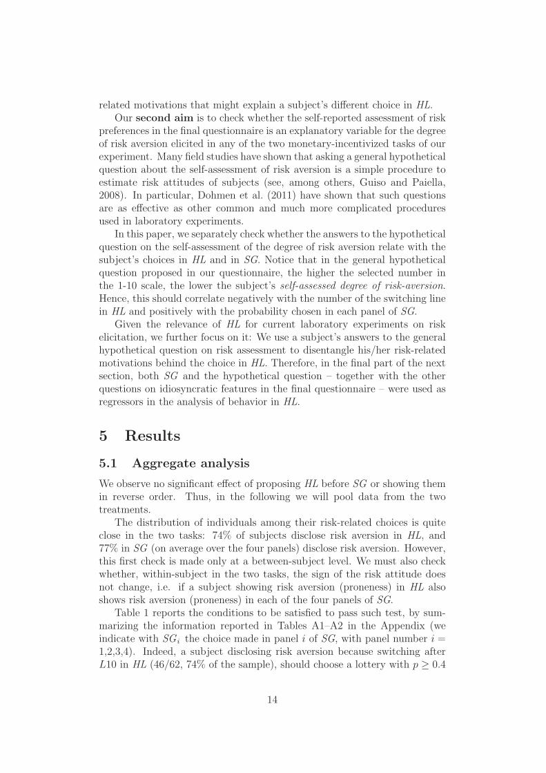
related motivations that might explain a subject’s different choice in HL.Our second aim is to check whether the self-reported assessment of risk

preferences in the final questionnaire is an explanatory variable for the degreeof risk aversion elicited in any of the two monetary-incentivized tasks of ourexperiment. Many field studies have shown that asking a general hypotheticalquestion about the self-assessment of risk aversion is a simple procedure toestimate risk attitudes of subjects (see, among others, Guiso and Paiella,2008). In particular, Dohmen et al. (2011) have shown that such questionsare as effective as other common and much more complicated proceduresused in laboratory experiments.

In this paper, we separately check whether the answers to the hypotheticalquestion on the self-assessment of the degree of risk aversion relate with thesubject’s choices in HL and in SG. Notice that in the general hypotheticalquestion proposed in our questionnaire, the higher the selected number inthe 1-10 scale, the lower the subject’s self-assessed degree of risk-aversion.Hence, this should correlate negatively with the number of the switching linein HL and positively with the probability chosen in each panel of SG.

Given the relevance of HL for current laboratory experiments on riskelicitation, we further focus on it: We use a subject’s answers to the generalhypothetical question on risk assessment to disentangle his/her risk-relatedmotivations behind the choice in HL. Therefore, in the final part of the nextsection, both SG and the hypothetical question – together with the otherquestions on idiosyncratic features in the final questionnaire – were used asregressors in the analysis of behavior in HL.

5 Results

5.1 Aggregate analysis

We observe no significant effect of proposing HL before SG or showing themin reverse order. Thus, in the following we will pool data from the twotreatments.

The distribution of individuals among their risk-related choices is quiteclose in the two tasks: 74% of subjects disclose risk aversion in HL, and77% in SG (on average over the four panels) disclose risk aversion. However,this first check is made only at a between-subject level. We must also checkwhether, within-subject in the two tasks, the sign of the risk attitude doesnot change, i.e. if a subject showing risk aversion (proneness) in HL alsoshows risk aversion (proneness) in each of the four panels of SG.

Table 1 reports the conditions to be satisfied to pass such test, by sum-marizing the information reported in Tables A1–A2 in the Appendix (weindicate with SG i the choice made in panel i of SG, with panel number i =1,2,3,4). Indeed, a subject disclosing risk aversion because switching afterL10 in HL (46/62, 74% of the sample), should choose a lottery with p ≥ 0.4

14

in panel 1, and a lottery with p ≥ 0.2 in the other three panels of SG. Allother subjects should choose a lottery with p ≤ 0.3 in panel 1, and a lotterywith p = 0.1 in the other three panels of SG.

Table 1: Threshold levels for coherent choices according to the sign of r

Switch Line Chosen Probability

HL SG1 SG2-SG4

Risk averse (r > 0.038) L11-L20 0.4 ≤ p ≤ 1 0.2 ≤ p ≤ 1

Risk loving and risk neutral (r < 0.038) L1-L10 p ≤ 0.3 p = 0.1

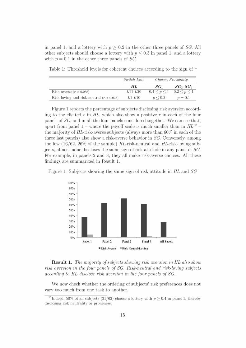
Figure 1 reports the percentage of subjects disclosing risk aversion accord-ing to the elicited r in HL, which also show a positive r in each of the fourpanels of SG, and in all the four panels considered together. We can see that,apart from panel 1 – where the payoff scale is much smaller than in HL12 –the majority of HL-risk-averse subjects (always more than 60% in each of thethree last panels) also show a risk-averse behavior in SG. Conversely, amongthe few (16/62, 26% of the sample) HL-risk-neutral and HL-risk-loving sub-jects, almost none discloses the same sign of risk attitude in any panel of SG.For example, in panels 2 and 3, they all make risk-averse choices. All thesefindings are summarized in Result 1.

Figure 1: Subjects showing the same sign of risk attitude in HL and SG

Result 1. The majority of subjects showing risk aversion in HL also showrisk aversion in the four panels of SG. Risk-neutral and risk-loving subjectsaccording to HL disclose risk aversion in the four panels of SG.

We now check whether the ordering of subjects’ risk preferences does notvary too much from one task to another.

12Indeed, 50% of all subjects (31/62) choose a lottery with p ≥ 0.4 in panel 1, therebydisclosing risk neutrality or proneness.

15

The controls for SG work as they should: A significant positive correla-tion (at least 50%, always significant at the 1% level) is found among theordering of any randomly-chosen pair of panels of SG. Furthermore, the levelof accepted risk decreases (on average across all subjects) with the panelnumber, coherently with the assumption of CRRA (moving from panel 1 topanel 4 we have increasing stakes for the same number of tickets assigned tothe positive outcome).

We perform the Spearman rank correlation test among choices made ineach of the four panels in SG, and choices in HL, and between the latterand a variable representing the average choice in the four panels (SGAvg ).Results are reported in Table 2.

Recall that: In HL, the larger the number of the switch line, the smallerthe number of tickets assigned at this line to the lower of the two outcomes(see Figure A1 in the Appendix), and the higher the subject’s disclosed degreeof risk aversion (see Table A1 in the Appendix); in each panel of SG, morein the left the chosen lottery is, the smaller the number of tickets assignedto the null outcome (see Figure A2 in the Appendix), and the higher thesubject’s disclosed degree of risk aversion (see Table A2 in the Appendix).Therefore, from now on, when analyzing results for HL, we consider as indexthe number of tickets assigned in the switch line to the lower outcome; whenanalyzing results for each panel of SG, we consider as index the number oftickets assigned in the chosen lottery to the null outcome. Hence, a positivecorrelation between these two indexes would mirror the positive correlationbetween disclosed risk attitudes in the two tasks.

Table 2: Rank correlations between self-assessed risk and average choices inthe two tasks, by panel.

HL – SG1 HL – SG2 HL – SG3 HL – SG4 HL – SGAvg

Spearman’s rho 0.11 0.04 0.11 0.04 0.13

p-value 0.39 0.78 0.37 0.76 0.31

Rank correlations in Table 2 lead to the following:

Result 2. A positive but small and not significant correlation is foundbetween subjects’ risk ordering in HL and their risk ordering in any of thefour panels of SG.

Thus, different risk-elicitation instruments seem to lead to different order-ings of the relative risk aversion coefficient r, if Expected Utility is assumedfor all subjects. Note that this result still holds when conditioning on age,gender, and for past attendance of a course in decision/game theory. How-ever, a positive and quite surprising finding emerges if looking at subjects’self-reported risk through the hypothetical question in the final questionnaire.

In particular, we make use of the self-assessed risk variable in order tocheck on the rank correlation between this subjective measure and the risk-

16

related choices made by the subjects in the two tasks. Recall that in thequestion about self-assessment of general risk attitude, the smaller (closer to1) the chosen number, the higher the self-assessed general aversion to risk.Hence, a positive correlation between this choice and the above defined indexin a risk-elicitation task (HL or SG) would mirror the positive correlationbetween self-assessment of risk and the disclosed monetary risk attitude inthe task.This check leads to the following:

Result 3. Significant positive correlation is found between subjects’ or-dering expressed by self-reported risk and the risk ordering in HL (rho =0.47, p-value = 0.000). Significant positive correlation is also found betweenthe ordering expressed by self-reported risk and the risk ordering in SG (rho= 0.48, p-value = 0.000).

As can be noticed, the two correlation coefficients are very close. Bothmethods seem to be able to account for a good amount of inter-individualdifferences in general aversion to risk, with similarly high explanatory power.

From these preliminary results, three questions arise:1) Why are the rankings produced by the two methods not correlated while

instead each of them is correlated with self-assessed general aversion to risk?2) Why are the correlation coefficients of each method with self-assessed

general aversion to risk smaller than 50%?3) Why are the correlation coefficients of each method with self-assessed

general aversion to risk so close?The analysis in the next subsection, which account for both idiosyncratic

features (elicited in the questionnaire) and other risk-related motivations (asemerging from choices in the four panels of SG) is meant to answer the abovequestions. The reliability of HL as instrument for risk-aversion elicitationcrucially depends on the answers to the previous questions.

5.2 Type classification analysis

Results 1–3 above lead us to think that there can be other subjects’ fea-tures and motivations (other than monetary risk aversion) orienting subjects’choices in each of the two analyzed instruments. If we disentangle subjectsaccording to these motivations, we should find individuals who better dis-close their self-reported risk aversion in HL and others who better disclose itin SG.

First, we check whether idiosyncratic features (gender, age, education,etc.), elicited through the final questionnaire, are of some help in providing acoherent explanation for the previous findings. Furthermore, since HL onlyrequires one choice for each subject, while SG requires four choices for eachsubject, we use this second instrument in order to disentangle risk-relatedmotivations.

17

5.2.1 Individual characteristics

We run again the Spearman rank correlation tests between self-assessed riskand individuals’ choice in both HL and the average choices in SG by sub-groups of population.

First of all, with respect to gender we find that females show a signifi-cantly higher correlation between self-assessed risk and risk behavior in bothHL and SGAvg. The two correlation coefficients are again of the same mag-nitude: rho = 0.60 for HL (p-value = 0.038), rho = 0.61 for SG (p-value= 0.035). The correlation coefficients for the sub-group of males, thoughsignificant, are lower than those obtained for the whole sample: rho = 0.31for HL (p-value = 0.050), rho = 0.42 for SG (p-value = 0.006).

Another interesting issue is whether having attended an advanced coursein decision or game theory could strengthen the correspondence between sub-jects’ self-assessed risk and their actual risk-related choices in the two tasks.Our auxiliary assumption is that such attendance should indicate some back-ground in mathematically-related disciplines (recall that our subjectsare undergraduate students in Economics). The usual test reveals that theprevious attendance of a decision/game theory course increases the correla-tion between self-reported risk and average choice in SG, while the oppositeeffect is found with regards to HL (see Table 3).

Table 3: Rank correlations between self-assessed risk and the two tasks,disentangled by gender and backgroungd in decision/game theory

Female Male

Self-assess and HL 0.61*** 0.31*Self-assess and SGAvg 0.60** 0.42***

Game Theory No Game Theory

Self-assess and HL 0.43** 0.52***Self-assess and SGAvg 0.54*** 0.37*

Significance level: * p < 0.1, ** p < 0.05, *** p < 0.01.

The former result could be explained by the higher level of complexity ofSG – where both probability and outcome are different for each lottery ineach of the four panels – with respect to HL, where the two pairs of outcomesare fixed for all pairwise comparisons. Thus, having some background inmathematically-related disciplines could be helpful in understanding a risk-elicitation task (in our case, SG), although Branas-Garza et al. (2008) foundno such effect across several risk-elicitation tasks.

Our interpretation is partially supported by a correlation coefficient (be-tween self-assessed risk and the instrument) increasing in the years of studyat the university for undergraduate students (from first to third year), ifconsidering either SGAvg or HL as risk-elicitation instrument (see Table 4).Notice that, although quite high, few correlations are statistically significant,due to few observations in each subset of subjects.

18

Table 4: Rank correlations between self-assessed risk and the two tasks,disentangled by the years of study at the university

First Second Third Fourth Fifth

rho p-value rho p-value rho p-value rho p-value rho p-value

Self-assess and SGAvg 0.30 0.160 0.59 0.070 0.62 0.055 0.53 0.140 -0.01 0.980Self-assess and HL 0.24 0.270 0.79 0.006 0.67 0.030 0.08 0.840 0.57 0.140

5.2.2 Risk-related motivations

A further step is to consider the possibility that there are several risk-relatedmotivations that drive subjects’ choices among lotteries in SG. With this inmind, we split the sample into three categories, according to the three mainpatterns of choices a subject can show in the four panels of SG.

The baseline category is the one comprising subjects whose behavioralpattern across panels is coherent with a Constant Relative Risk Aversionutility function (CRRA-coherent subjects). In our sample, subjects show-ing such compatibility are 14/62: They make weakly-increasing choices (interms of risk-taking) in the four panels. For example, a subject belongingto this category select a number of tickets assigned to a positive outcome of7/10 in panel 1, of 6/10 in panel 2, of 6/10 in panel 3, and of 2/10 in panel 4.Due to the discreteness of the decision settings, we include in this group alsosubjects who always made the same choice in the four panels: Although, aswe will see below, they could reasonably belong to the other two categories,their behavior do not show incoherence with CRRA.

The second category includes subjects with weakly-decreasing choices (interms or risk) in the four panels, hence incoherent with expected-utility max-imization. In our sample, subjects showing this behavior are 17/62. We callthem Aspiration-level subjects. Indeed, it is well known in the literature(Camerer et al., 1997; Diecidue and Van De Ven, 2008) that the concept ofaspiration level is related to the subject’s willingness to reach a particularoutcome. In the paper by Camerer et al. (1997) the idea of aspiration levelis explained through the cab drivers example: Cab drivers are willing to earna daily target return, so that they adjust this behavior in order to achievetheir goal. Other examples have been proposed in the literature such asfarmers who want to prevent themselves from falling below the subsistencelevel (Lopes, 1987) or investors with the desired target rate of returns toachieve (Payne et al., 1980). In our framework, the idea of aspiration levelcould be explained by the willingness of our subjects to earn “around a givenpositive amount”. Given the structure of the four panels in SG, the risk thatone should take to get the “same” positive amount is smaller (the number ofwinning tickets is higher) the higher the panel number. For example, supposethat a subject wants to earn around e 8 in each of the four panels. This isconsistent with selecting a number of tickets assigned to this outcome equalto 1/10 in panel 1, equal to 2/10 in panel 2, equal to 4/10 in panel 3, andequal to 6/10 in panel 4.

19

The residual category is composed by individuals who show non-monotonicchoices in the four panels: They “move right and left” across the four panels.We call them Non-monotonic subjects. These subjects might interpret thefour panels in SG as a portfolio of contingent assets (indeed, only one of thefour panels is randomly selected for payment), where they can compensatethe greater risk taken in some state of the world (e.g., in panel 1 and in panel3) by choosing less risky assets in the complementary states (e.g., in panel 2and in panel 4). In our sample, subjects showing this behavior are 31/62.

Both Aspiration-level and Non-monotonic can be viewed as additionalrisk-related motivations (additional with respect to CRRA). Therefore, twobehavioral hypotheses can be drawn about behavior in SG :

H1) Aspiration-level vs. CRRA-coherent. Subjects with a givenaspiration level pick a willing-to-win amount in the first panel of lotteries (theone with the lowest payoffs) and then decrease the probability of winning inthe next panels, where payoffs are increased, in order to get around thisamount. This ends up in a more risk-averse behavior in SG than the onedisclosed in the same task by CRRA-coherent subjects. Indeed, the structureof SG contraints choices of an Aspiration-level subject in the four panels notto be too “far away” from one another, i.e. he/she chooses lotteries withclose numbers of winning tickets in the four panels (e.g. earning around e 5requires choosing a lottery with 2/10, 3/10, 6/10 and 7/10 tickets assignedto the positive outcome respectively in panel 1, 2, 3 and 4 – see Figure A2in the Appendix). This ends up in a lower variance of the expected valuesof the chosen lotteries in the four panels, with respect to CRRA-coherentsubjects. The latter, given a degree of risk aversion r, when moving frompanel i to panel i + 1, are “free” to choose lotteries with higher expectedvalues, i.e. with number of winning tickets in panel i + 1 potentially muchhigher than in panel i (e.g. a CRRA-coherent subject with r = 0.091 wouldchoose a lottery with 10/10, 2/10, 1/10 and 1/10 tickets assigned to thepositive outcome respectively in panel 1, 2, 3 and 4 – see Table A2 in theAppendix).

H2) Non-monotonic vs. CRRA-coherent. Subjects who exertnon-monotonic behavior among lottery panels in SG are more risk-aversethan pure CRRA-coherent subjects. Indeed, moving “right and left” acrossthe four panels introduces additional constrains to the set of lotteries a sub-ject can choose in panel i given the choice made in the other three panelsj 6= i. For example, a CRRA-coherent subject with r > 0.1 would choose alottery with 10/10 winning tickets in panel 1 and with 1/10 winning ticketsin panel 4. A Non-monotonic subject with the same r would risk more whenstakes are smaller (e.g., by choosing 5/10 winning tickets in panel 1), com-pensating this riskier choice by risking less when stakes are bigger (e.g., bychoosing 5/10 winning tickets in panel 4). This ultimately leads to a lowervariance of the expected values of the chosen lotteries in the four panels, withrespect to CRRA-coherent subjects.

In order to test H1 and H2 we look at the variance among the expected

20

values in the four chosen lotteries in SG, for each subject and for each cate-gory of subjects. In this task, the variance for each subject is a measure ofthe dispersion of the four choices with respect to the mean choice.

We find that both Aspiration-level subjects and Non-monotonic subjectshave a lower average variance across panels of lottery expected values (re-spectively, 4.62 and 6.98) with respect to CRRA-coherent subjects (9.50).Both these differences are significant at the 5% level.

As a further round of investigation we perform a Mann-Whitney test bycategories on standard deviations of “chosen” expected values in the fourpanels. Taking CRRA-coherent subjects are reference category, we findthat the rank of these standard deviations is significantly lower for bothAspiration-level subjects (p-value=0.008) and for Non-monotonic. subjects(p-value=0.000). All this is summarized in the following:

Result 4. Both Aspiration-level and Non-monotonic subjects disclose in SGa more risk-averse behavior than CRRA-coherent subjects.

Furthermore we check whether by disentangling the sample according tothe three above categories, the correlation between disclosed orderings of riskbehavior in the two instruments increases. To this goal, we run another rankcorrelation test, and we find that the coefficients are higher with respect tothe whole sample but still not significant (see Table 5).

Table 5: Rank correlations among instruments (HL and SGAvg), disentangledby category of subjects

SG

Whole Sample CRRA Aspiration Non-monotonic

HL 0.13 0.21 0.22 0.19Significance level: * p < 0.1, ** p < 0.05, *** p < 0.01

The following statement extends Result 2:

Result 5. If we disentangle by different risk-related motivations, the rankcorrelation between risk orderings in HL and SG increases. However, thecorrelation is still not significant.

Going back to Result 3, we can improve the analysis of the goodness ofthe two instruments in disclosing subjects’ self-assessed general risk aversion,by running the usual Spearman correlation test on each of the above definedcategories of risk-related motivations (see Table 6). Disentangling by risk-related motivation, we find that HL performs on average better than SGin disclosing a subject’s self-assessed general risk aversion. However, whileCRRA-coherent subjects show a greater rank correlation with self-reportedrisk in HL than in SG, the latter better captures self-assessed risk aversionof Non-monotonic subjects. None of the instruments is able to elicit theself-assessed general risk aversion of Aspiration-level subjects.

21

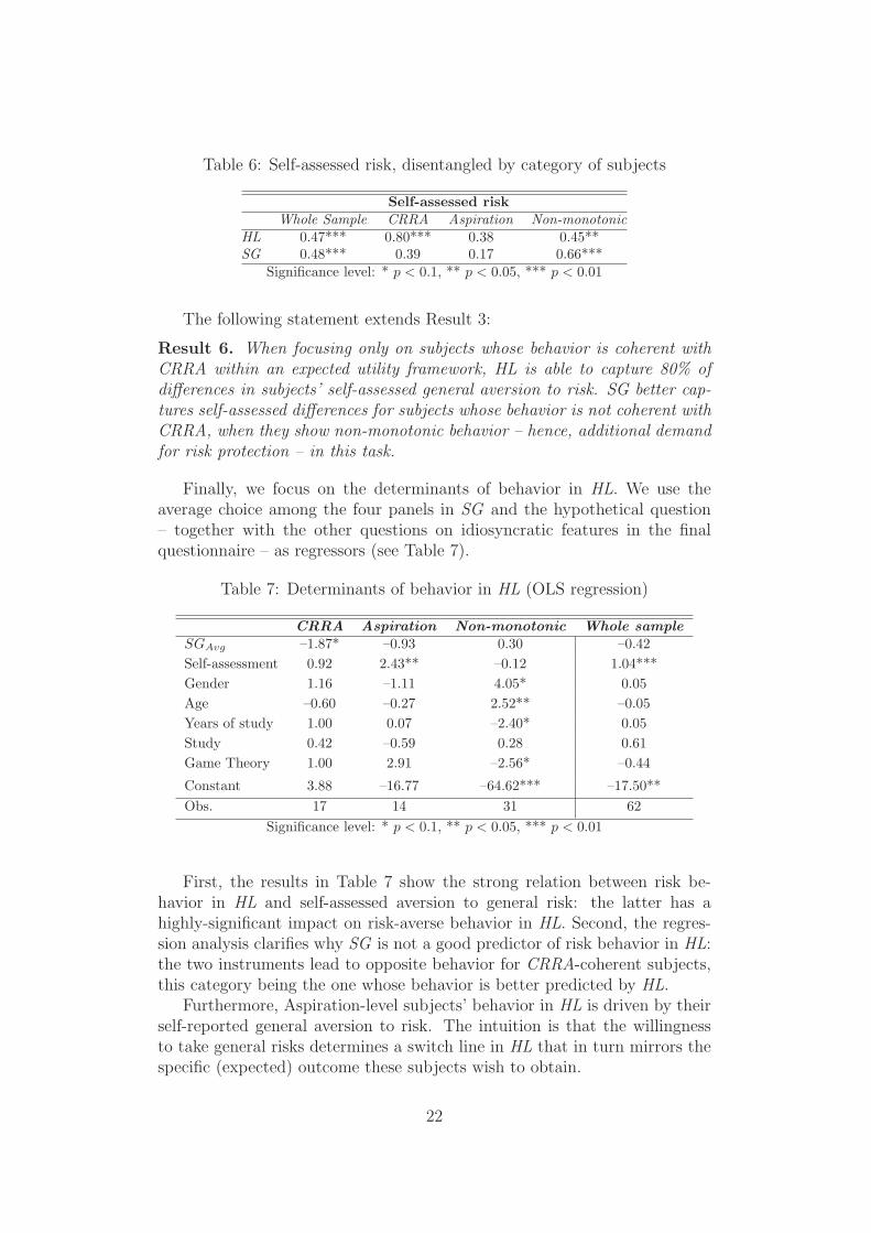
Table 6: Self-assessed risk, disentangled by category of subjects

Self-assessed risk

Whole Sample CRRA Aspiration Non-monotonic

HL 0.47*** 0.80*** 0.38 0.45**SG 0.48*** 0.39 0.17 0.66***

Significance level: * p < 0.1, ** p < 0.05, *** p < 0.01

The following statement extends Result 3:

Result 6. When focusing only on subjects whose behavior is coherent withCRRA within an expected utility framework, HL is able to capture 80% ofdifferences in subjects’ self-assessed general aversion to risk. SG better cap-tures self-assessed differences for subjects whose behavior is not coherent withCRRA, when they show non-monotonic behavior – hence, additional demandfor risk protection – in this task.

Finally, we focus on the determinants of behavior in HL. We use theaverage choice among the four panels in SG and the hypothetical question– together with the other questions on idiosyncratic features in the finalquestionnaire – as regressors (see Table 7).

Table 7: Determinants of behavior in HL (OLS regression)

CRRA Aspiration Non-monotonic Whole sample

SGAvg –1.87* –0.93 0.30 –0.42

Self-assessment 0.92 2.43** –0.12 1.04***

Gender 1.16 –1.11 4.05* 0.05

Age –0.60 –0.27 2.52** –0.05

Years of study 1.00 0.07 –2.40* 0.05

Study 0.42 –0.59 0.28 0.61

Game Theory 1.00 2.91 –2.56* –0.44

Constant 3.88 –16.77 –64.62*** –17.50**

Obs. 17 14 31 62

Significance level: * p < 0.1, ** p < 0.05, *** p < 0.01

First, the results in Table 7 show the strong relation between risk be-havior in HL and self-assessed aversion to general risk: the latter has ahighly-significant impact on risk-averse behavior in HL. Second, the regres-sion analysis clarifies why SG is not a good predictor of risk behavior in HL:the two instruments lead to opposite behavior for CRRA-coherent subjects,this category being the one whose behavior is better predicted by HL.

Furthermore, Aspiration-level subjects’ behavior in HL is driven by theirself-reported general aversion to risk. The intuition is that the willingnessto take general risks determines a switch line in HL that in turn mirrors thespecific (expected) outcome these subjects wish to obtain.

22

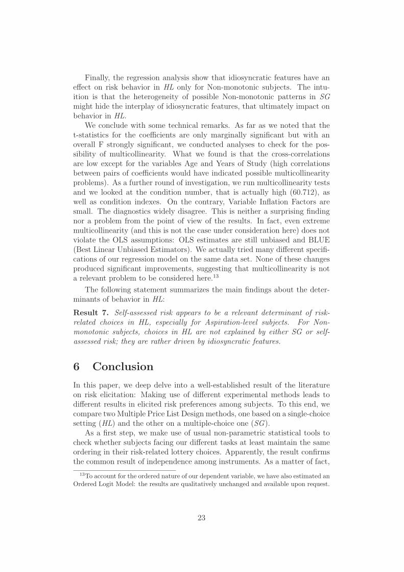
Finally, the regression analysis show that idiosyncratic features have aneffect on risk behavior in HL only for Non-monotonic subjects. The intu-ition is that the heterogeneity of possible Non-monotonic patterns in SGmight hide the interplay of idiosyncratic features, that ultimately impact onbehavior in HL.

We conclude with some technical remarks. As far as we noted that thet-statistics for the coefficients are only marginally significant but with anoverall F strongly significant, we conducted analyses to check for the pos-sibility of multicollinearity. What we found is that the cross-correlationsare low except for the variables Age and Years of Study (high correlationsbetween pairs of coefficients would have indicated possible multicollinearityproblems). As a further round of investigation, we run multicollinearity testsand we looked at the condition number, that is actually high (60.712), aswell as condition indexes. On the contrary, Variable Inflation Factors aresmall. The diagnostics widely disagree. This is neither a surprising findingnor a problem from the point of view of the results. In fact, even extrememulticollinearity (and this is not the case under consideration here) does notviolate the OLS assumptions: OLS estimates are still unbiased and BLUE(Best Linear Unbiased Estimators). We actually tried many different specifi-cations of our regression model on the same data set. None of these changesproduced significant improvements, suggesting that multicollinearity is nota relevant problem to be considered here.13

The following statement summarizes the main findings about the deter-minants of behavior in HL:

Result 7. Self-assessed risk appears to be a relevant determinant of risk-related choices in HL, especially for Aspiration-level subjects. For Non-monotonic subjects, choices in HL are not explained by either SG or self-assessed risk; they are rather driven by idiosyncratic features.

6 Conclusion

In this paper, we deep delve into a well-established result of the literatureon risk elicitation: Making use of different experimental methods leads todifferent results in elicited risk preferences among subjects. To this end, wecompare two Multiple Price List Design methods, one based on a single-choicesetting (HL) and the other on a multiple-choice one (SG).

As a first step, we make use of usual non-parametric statistical tools tocheck whether subjects facing our different tasks at least maintain the sameordering in their risk-related lottery choices. Apparently, the result confirmsthe common result of independence among instruments. As a matter of fact,

13To account for the ordered nature of our dependent variable, we have also estimated anOrdered Logit Model: the results are qualitatively unchanged and available upon request.

23

the rank correlation between the two instruments turns out to be negligibleand not significant.

Our analysis goes beyond by making use of a self-assessed measure ofsubjects’ risk preferences, to check whether our instruments are capable tomeasure differences in self-reported attitudes towards risk.

What we find is that for both risk-elicitation procedures, risk prefer-ences disclosed by subjects’ choices are significantly correlated with theirself-reported risk. This result is even stronger when we run a by-group anal-ysis on different idiosyncratic controls.

Furthermore, and more importantly, we check whether other subjects’risk-related motivations could explain the correlation between elicited riskbehavior through monetary-incentivized methods and self-assessed risk.

Since a multiple-choice risk elicitation method is available (SG), we useit so as to disentangle subjects according to three risk-related behaviors: thebaseline behavioral category comprising CRRA-coherent individuals, a groupof Aspiration-level subjects, and a last category of Non-monotonic subjects.

What is found is that in SG both Aspiration-level and Non-monotonicsubjects make on average less risky choices than CRRA-coherent subjects.This confirms the intuition that both these categories hide an additionalrisk-related motivation (additional with respect to the curvature of the uni-parametric utility function), that cannot be disentangled by only looking atbehavior in HL.

It is not surprising that if we exclude the two above categories and weonly focus on subjects whose behavior in SG is coherent with CRRA, HL isable to capture 80% of differences in subjects’ self-assessed general aversionto risk. A regression analysis confirms that self-assessed risk is a relevantdeterminant of risk-related choices in HL.

This result is even more striking when considering that it was obtainedin a within-subject design. Indeed, as (Crosetto and Filippin, 2015) notice,proposing several risky choices on a within-subject base is likely to inducesome form of hedging across tasks by non-risk-averse subjects. This coulddetermine a negative correlation across tasks. Therefore, the low correlationbetween the behavior in different tasks could in part be an artifact of thedesign. We have shown that once this motivation is set aside (i.e. onlyCRRA-coherent subjects are considered), despite no correlation between HLand SG, an extremely high correlation between the risk behavior in the formermethod and self-reported risk attitude emerges. Thus, the positive results byVieider et al. (2015) might hold even stronger if we account for heterogeneitystemming from more complex behavioral patterns like aspiration levels andhedging.

This result is relevant for experimental economists who wish to accountfor their subjects’ risk attitudes as a determinant of behavior, being HL theexperimental method mainly used in the last decade to elicit risk attitudesin the laboratory and in the field.

24

References

Andersen, S., Harrison, G. W., Lau, M. I., and Rutstrom, E. E. (2006). Elic-itation using multiple price list formats. Experimental Economics, 9:383–405.

Attanasi, G., Casoria, F., Centorrino, S., and Urso, G. (2013). Cultural in-vestment, local development and instantaneous social capital: A case studyof a gathering festival in the south of italy. Journal of Socio-Economics,47:228–247.

Attanasi, G., Corazzini, L., Georgantzıs, N., and Passarelli, F. (2014a). Riskaversion, overconfidence and private information as determinants of ma-jority thresholds. Pacific Economic Review, 19:355–386.

Attanasi, G., Gollier, C., Montesano, A., and Pace, N. (2014b). Elicitingambiguity aversion in unknown and in compound lotteries: A smooth am-biguity model experimental study. Theory and Decision, 77:485–530.

Becker, G. M., DeGroot, M. H., and Marschak, J. (1964). Measuring utilityby a single-response sequential method. Behavioral Science, 9:226–232.

Bernasconi, M., Corazzini, L., and Seri, R. (2014). Reference dependentpreferences, hedonic adaptation and tax evasion: Does the tax burdenmatter? Journal of Economic Psychology, 40:103–118.

Branas-Garza, P., Guillen, P., and del Paso, R. L. (2008). Math skills andrisk attitudes. Economics Letters, 99:332–336.

Butler, D. J. and Loomes, G. C. (2007). Imprecision as an account of thepreference reversal phenomenon. American Economic Review, 97:277–297.

Camerer, C., Babcock, L., Loewenstein, G., and Thaler, R. (1997). Laborsupply of new york city cabdrivers: One day at a time. Quarterly Journalof Economics, 112:407–441.

Charness, G. and Gneezy, U. (2010). Portfolio choice and risk attitudes: Anexperiment. Economic Inquiry, 48:133–146.

Charness, G., Gneezy, U., and Imas, A. (2013). Experimental methods:Eliciting risk preferences. Journal of Economic Behavior and Organization,87:43–51.

Charness, G. and Viceisza, A. (2015). Three risk-elicitation methods in thefield: Evidence from rural senegal. Review of Behavioral Economics, forth-coming.

Cox, J. C. and Harrison, G. W. (2008). Risk aversion in experiments. Emer-ald: Research in Experimental Economics, Vol. 12.

25

Cox, J. C., Roberson, B., and Smith, V. L. (1982). Theory and behavior ofsingle object auctions. Research in Experimental Economics, 2:1–43.

Cox, J. C., Sadiraj, V., and Schmidt, U. (2014). Paradoxes and mechanismsfor choice under risk. Experimental Economics, 18:215–250.

Cox, J. C., Smith, V. L., and Walker, J. M. (1985). Experimental develop-ment of sealed-bid auction theory; calibrating controls for risk aversion.American Economic Review, pages 160–165.

Cox, J. C., Smith, V. L., and Walker, J. M. (1988). Theory and individualbehavior of first-price auctions. Journal of Risk and Uncertainty, 1:61–99.

Crosetto, P. and Filippin, A. (2013). The “bomb” risk elicitation task. Jour-nal of Risk and Uncertainty, 47:31–65.

Crosetto, P. and Filippin, A. (2015). A theoretical and experimental appraisalof five risk elicitation methods. Experimental Economics, forthcoming.

Dave, C., Eckel, C. C., Johnson, C. A., and Rojas, C. (2010). Eliciting riskpreferences: When is simple better? Journal of Risk and Uncertainty,41:219–243.

Diecidue, E. and Van De Ven, J. (2008). Aspiration level, probability ofsuccess and failure, and expected utility. International Economic Review,49:683–700.

Dohmen, T., Falk, A., Huffman, D., Sunde, U., Schupp, J., and Wagner,G. G. (2011). Individual risk attitudes: Measurement, determinants, andbehavioral consequences. Journal of the European Economic Association,9:522–550.

Eckel, C. C. and Grossman, P. J. (2008). Forecasting risk attitudes: Anexperimental study using actual and forecast gamble choices. Journal ofEconomic Behavior and Organization, 68:1–17.

Fischbacher, U. (2007). z-tree: Zurich toolbox for ready-made economicexperiments. Experimental Economics, 10:171–178.

Garcıa Gallego, A., Georgantzıs, N., Jaramillo Gutierrez, A., and Parravano,M. (2012). The lottery-panel task for bi-dimensional parameter-free elici-tation of risk attitudes. Revista Internacional de Sociologia, 70:53–72.

Garcıa-Gallego, A., Georgantzıs, N., Navarro-Martınez, D., and Sabater-Grande, G. (2011). The stochastic component in choice and regressionto the mean. Theory and Decision, 71:251–267.

Georgantzıs, N. and Navarro-Martınez, D. (2010). Understanding the wta–wtp gap: Attitudes, feelings, uncertainty and personality. Journal of Eco-nomic Psychology, 31:895–907.

26

Guiso, L. and Paiella, M. (2008). Risk aversion, wealth, and background risk.Journal of the European Economic association, 6:1109–1150.

Harrison, G. W., Johnson, E., McInnes, M. M., and Rutstrom, E. E. (2005).Risk aversion and incentive effects: Comment. American Economic Re-view, 95:897–901.

Harrison, G. W. and Rutstrom, E. E. (2008). Risk aversion in the laboratory.In Harrison, G. W. and Cox, J., editors, Risk aversion in experiments,pages 41–196. Emerald: Research in Experimental Economics, Vol. 12.

Harrison, G. W. and Rutstrom, E. E. (2009). Expected utility theory andprospect theory: One wedding and a decent funeral. Experimental Eco-nomics, 12:133–158.

Holt, C. A. and Laury, S. K. (2002). Risk aversion and incentive effects.American Economic Review, 92:1644–1655.

Holt, C. A. and Laury, S. K. (2005). Risk aversion and incentive effects: Newdata without order effects. American Economic Review, 95:902–904.

Isaac, R. M. and James, D. (2000). Just who are you calling risk averse?Journal of Risk and Uncertainty, 20:177–187.

Lejuez, C. W., Read, J. P., Kahler, C. W., Richards, J. B., Ramsey, S. E.,Stuart, G. L., Strong, D. R., and Brown, R. A. (2002). Evaluation of abehavioral measure of risk taking: the balloon analogue risk task (bart).Journal of Experimental Psychology: Applied, 8:75–84.

Levy-Garboua, L., Maafi, H., Masclet, D., and Terracol, A. (2012). Riskaversion and framing effects. Experimental Economics, 15:128–144.

Lopes, L. L. (1987). Between hope and fear: The psychology of risk. Advancesin Experimental Social Psychology, 20:255–295.

Miller, L., Meyer, D. E., and Lanzetta, J. T. (1969). Choice among equalexpected value alternatives: Sequential effects of winning probability levelon risk preferences. Journal of Experimental Psychology, 79:419–423.

Payne, J. W., Laughhunn, D. J., and Crum, R. (1980). Translation of gamblesand aspiration level effects in risky choice behavior. Management Science,26:1039–1060.

Roth, A. E. and Malouf, M. W. (1979). Game-theoretic models and the roleof information in bargaining. Psychological Review, 86:574.

Sabater-Grande, G. and Georgantzis, N. (2002). Accounting for risk aversionin repeated prisoners’ dilemma games: An experimental test. Journal ofEconomic Behavior and Organization, 48:37–50.

27

Vieider, F. M., Lefebvre, M., Bouchouicha, R., Chmura, T., Hakimov, R.,Krawczyk, M., and Martinsson, P. (2015). Common components of riskand uncertainty attitudes across contexts and domains: Evidence from 30countries. Journal of the European Economic Association, 13:421–452.

Wakker, P. and Deneffe, D. (1996). Eliciting von neumann-morgenstern util-ities when probabilities are distorted or unknown. Management Science,pages 1131–1150.

Wakker, P. P. (2010). Prospect theory: For risk and ambiguity. CambridgeUniversity Press.

Weber, E. U., Blais, A.-R., and Betz, N. E. (2002). A domain-specific risk-attitude scale: Measuring risk perceptions and risk behaviors. Journal ofbehavioral decision making, 15:263–290.

Zuckerman, M. (1994). Behavioral expressions and biosocial bases of sensa-tion seeking. Cambridge university press.

28

Appendix

Figure A1: Task 1, Variant of Holt and Laury (2002)

29

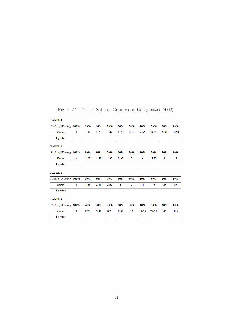
Figure A2: Task 2, Sabater-Grande and Georgantzis (2002)

30

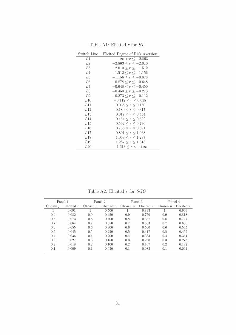
Table A1: Elicited r for HL

Switch Line Elicited Degree of Risk AversionL1 −∞ < r ≤ −2.863L2 −2.863 ≤ r ≤ −2.010L3 −2.010 ≤ r ≤ −1.512L4 −1.512 ≤ r ≤ −1.156L5 −1.156 ≤ r ≤ −0.878L6 −0.878 ≤ r ≤ −0.648L7 −0.648 ≤ r ≤ −0.450L8 −0.450 ≤ r ≤ −0.273L9 −0.273 ≤ r ≤ −0.112L10 −0.112 ≤ r ≤ 0.038L11 0.038 ≤ r ≤ 0.180L12 0.180 ≤ r ≤ 0.317L13 0.317 ≤ r ≤ 0.454L14 0.454 ≤ r ≤ 0.592L15 0.592 ≤ r ≤ 0.736L16 0.736 ≤ r ≤ 0.891L17 0.891 ≤ r ≤ 1.068L18 1.068 ≤ r ≤ 1.287L19 1.287 ≤ r ≤ 1.613L20 1.613 ≤ r < +∞

Table A2: Elicited r for SGG

Panel 1 Panel 2 Panel 3 Panel 4Chosen p Elicited r Chosen p Elicited r Chosen p Elicited r Chosen p Elicited r

1 0.091 1 0.500 1 0.833 1 0.9090.9 0.082 0.9 0.450 0.9 0.750 0.9 0.8180.8 0.073 0.8 0.400 0.8 0.667 0.8 0.7270.7 0.064 0.7 0.350 0.7 0.583 0.7 0.6360.6 0.055 0.6 0.300 0.6 0.500 0.6 0.5450.5 0.045 0.5 0.250 0.5 0.417 0.5 0.4550.4 0.036 0.4 0.200 0.4 0.333 0.4 0.3640.3 0.027 0.3 0.150 0.3 0.250 0.3 0.2730.2 0.018 0.2 0.100 0.2 0.167 0.2 0.1820.1 0.009 0.1 0.050 0.1 0.083 0.1 0.091

31

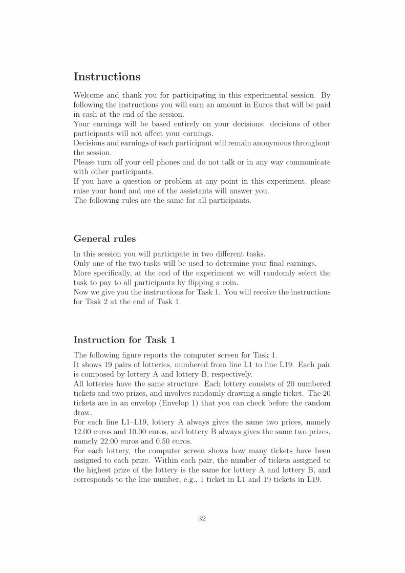
Instructions

Welcome and thank you for participating in this experimental session. Byfollowing the instructions you will earn an amount in Euros that will be paidin cash at the end of the session.Your earnings will be based entirely on your decisions: decisions of otherparticipants will not affect your earnings.Decisions and earnings of each participant will remain anonymous throughoutthe session.Please turn off your cell phones and do not talk or in any way communicatewith other participants.If you have a question or problem at any point in this experiment, pleaseraise your hand and one of the assistants will answer you.The following rules are the same for all participants.

General rules

In this session you will participate in two different tasks.Only one of the two tasks will be used to determine your final earnings.More specifically, at the end of the experiment we will randomly select thetask to pay to all participants by flipping a coin.Now we give you the instructions for Task 1. You will receive the instructionsfor Task 2 at the end of Task 1.

Instruction for Task 1

The following figure reports the computer screen for Task 1.It shows 19 pairs of lotteries, numbered from line L1 to line L19. Each pairis composed by lottery A and lottery B, respectively.All lotteries have the same structure. Each lottery consists of 20 numberedtickets and two prizes, and involves randomly drawing a single ticket. The 20tickets are in an envelop (Envelop 1) that you can check before the randomdraw.For each line L1–L19, lottery A always gives the same two prices, namely12.00 euros and 10.00 euros, and lottery B always gives the same two prizes,namely 22.00 euros and 0.50 euros.For each lottery, the computer screen shows how many tickets have beenassigned to each prize. Within each pair, the number of tickets assigned tothe highest prize of the lottery is the same for lottery A and lottery B, andcorresponds to the line number, e.g., 1 ticket in L1 and 19 tickets in L19.

32

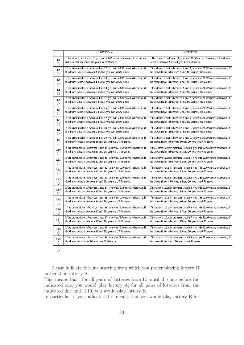
Please indicate the line starting from which you prefer playing lottery Brather than lottery A.This means that: for all pairs of lotteries from L1 until the line before theindicated one, you would play lottery A; for all pairs of lotteries from theindicated line until L19, you would play lottery B.In particular, if you indicate L1 it means that you would play lottery B for

33

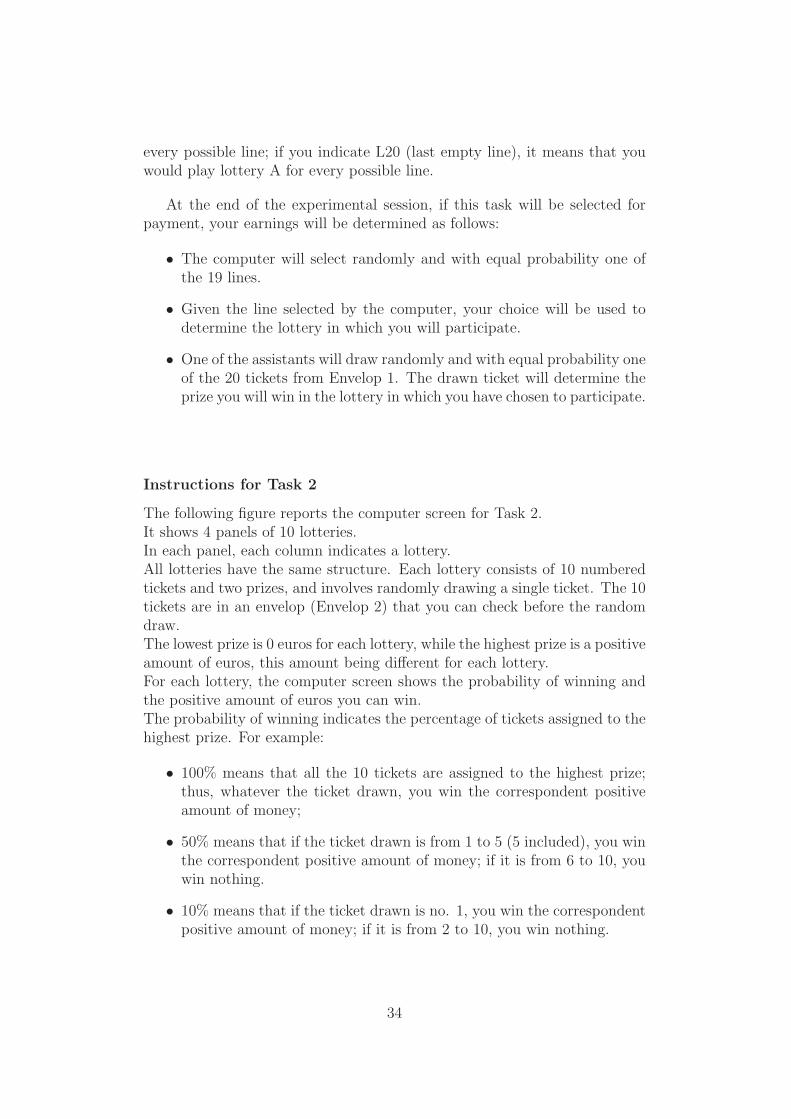
every possible line; if you indicate L20 (last empty line), it means that youwould play lottery A for every possible line.

At the end of the experimental session, if this task will be selected forpayment, your earnings will be determined as follows:

• The computer will select randomly and with equal probability one ofthe 19 lines.

• Given the line selected by the computer, your choice will be used todetermine the lottery in which you will participate.

• One of the assistants will draw randomly and with equal probability oneof the 20 tickets from Envelop 1. The drawn ticket will determine theprize you will win in the lottery in which you have chosen to participate.

Instructions for Task 2

The following figure reports the computer screen for Task 2.It shows 4 panels of 10 lotteries.In each panel, each column indicates a lottery.All lotteries have the same structure. Each lottery consists of 10 numberedtickets and two prizes, and involves randomly drawing a single ticket. The 10tickets are in an envelop (Envelop 2) that you can check before the randomdraw.The lowest prize is 0 euros for each lottery, while the highest prize is a positiveamount of euros, this amount being different for each lottery.For each lottery, the computer screen shows the probability of winning andthe positive amount of euros you can win.The probability of winning indicates the percentage of tickets assigned to thehighest prize. For example:

• 100% means that all the 10 tickets are assigned to the highest prize;thus, whatever the ticket drawn, you win the correspondent positiveamount of money;

• 50% means that if the ticket drawn is from 1 to 5 (5 included), you winthe correspondent positive amount of money; if it is from 6 to 10, youwin nothing.

• 10% means that if the ticket drawn is no. 1, you win the correspondentpositive amount of money; if it is from 2 to 10, you win nothing.

34

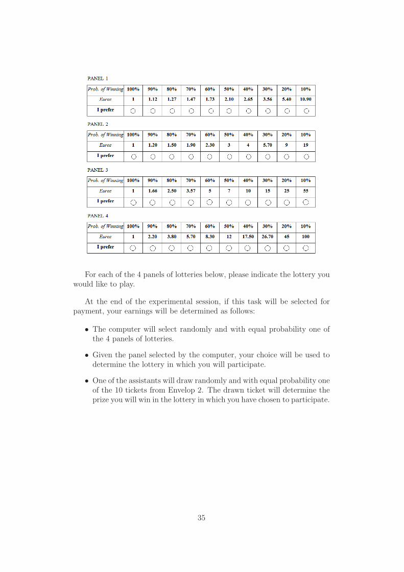
For each of the 4 panels of lotteries below, please indicate the lottery youwould like to play.

At the end of the experimental session, if this task will be selected forpayment, your earnings will be determined as follows:

• The computer will select randomly and with equal probability one ofthe 4 panels of lotteries.

• Given the panel selected by the computer, your choice will be used todetermine the lottery in which you will participate.

• One of the assistants will draw randomly and with equal probability oneof the 10 tickets from Envelop 2. The drawn ticket will determine theprize you will win in the lottery in which you have chosen to participate.

35