
l'Amélioration de l'Accueil Des Usagers Dans l'Administration
Upload
hoangkhanhCategory
view
219download
3
et discipline ou spécialité
Jury :
le
Institut Supérieur de l’Aéronautique et de l’Espace (ISAE)
Francesco VITILLO
vendredi 21 novembre 2014
Contribution expérimentale et numérique à l'amélioration de l'échangethermique des échangeurs de chaleur compacts à plaques
Experimental and numerical contribution to heat transfer enhancement incompact plate heat exchangers
ED MEGeP : Energétique et transferts
Équipe d'accueil ISAE-ONERA EDyF
M. Philippe MARTY - Président du JuryM. Jean-Marie BUCHLIN - Rapporteur
M. Lionel CACHONM. Gianfranco CARUSOM. Emmanuel LAROCHE
M. Frédéric PLOURDE - RapporteurM. Pierre MILLAN - Directeur de thèse
M. Pierre MILLAN (directeur de thèse)M. Philippe REULET (co-directeur de thèse)

2
3
PHD THESIS
EXPERIMENTAL AND NUMERICAL
CONTRIBUTION TO HEAT TRANSFER
ENHANCEMENT IN COMPACT PLATE
HEAT EXCHANGERS
PHD CANDIDATE: FRANCESCO VITILLO
THESIS SUPERVISOR: PIERRE MILLAN
THESIS CO-SUPERVISOR: LIONEL CACHON
THESIS CO-SUPERVISOR: PHILIPPE REULET
THESIS CO-SUPERVISOR: EMMANUEL LAROCHE

4
A NONNA,
LA MIA PRIMA MAESTRA
Tu, che abiti al riparo del Signore e che dimori alla sua ombra,
di al Signore: mio Rifugio, mia Roccia in cui confido.
5
Remerciements
Tout d’abord je souhaite remercier les membres du jury de thèse pour avoir accepté d’évaluer ce
travail : en particulier merci à M. Jean-Marie Buchlin et M.Frédéric Plourde pour avoir dédié
leur temps à la relecture de ce manuscrit et pour l’avoir enrichi avec leurs commentaires ; merci
aussi à M. Philippe Marty et M.Gianfranco Caruso pour leur présence et participation.
Je remercie mon directeur de thèse, M. Pierre Millan, pour m’avoir permis de mener ce travail et
pour m’avoir motivé pendant ces trois ans.
Je ne remercierai jamais assez mon encadrant au CEA Cadarache, M.Lionel Cachon, pour son
soutien quotidien : pour m’avoir choisi, pour m’avoir suivi, pour m’avoir permis de mener à bien
ce projet, pour les milliers de pages qu’il a relu, pour toutes les activités faites ensemble et
surtout pour son sourire. Au travers son exemple il a confirmé que les vrais leaders sont ceux qui
arrivent à vous faire sentir important en tous moments.
Je tiens à remercier aussi mes encadrants de l’ONERA, M. Emmanuel Laroche, pour ses
remarques et ses conseils qui m’ont permis d’élargir beaucoup mes conaissance et surtout M.
Philippe Reulet, qui, toujours en souriant, m’a supporté pendant les essais LDV, qui a lu des
dizaines de fois ce manuscrit et qui a apporté une contribution primordiale à la comparaison de
différents motifs d’échange.
Je souhaite remercier aussi M. Sylvain Madeleine, pour m’avoir accueilli au sein du LCIT et
pour avoir toujours compris mes besoins et mes requêtes.
Merci tout particulièrement à Thomas Marchiollo, qui a été mon bras droit (et souvent même
gauche!) pendant longtemps et notamment lors de la conception et mise-en-service des manips
PIV et VHEGAS. Sa motivation a été primordiale pour la réussite de ce travail.
Merci aussi à Chiara Galati et Julien Nave, qui se sont chargés de plusieurs parties importantes
de ce travail et qui m’ont permis d’avancer énormément dans des axes de recherche que je
n’aurais jamais pu investiguer autrement.
Merci mille fois à Pierre Charvet, pour sa patience infinie avec nous les thésards, toujours en
comprenant nos (mes) besoins et pour la bonne humeur qu’il porte toujours avec lui.

6
Merci à M.Francis Micheli, M.Jean-François Breil (M.Théodolite !) et M.Christian Pelissier pour
leurs efforts sur la manip LDV.
Merci également à Mme Isabelle Tkatschenko, Mme Fabienne Bazin et Mme Valerie Biscay
pour leur soutien lors de la mise-en-place de la manip PIV. Sans leur engagement il n’aurait pas
été possible de mener à bien ces mesures.
Merci à Pascal Defrasne, pour son soutien primordial à l’instrumentation des manips PIV et
VHEGAS.
Merci à M. Jean Stefanini pour l’assistance lors de la conception et mise-en-place de la manip
PIV.
Merci à M. Denis Tschumperlé pour la patience et le support de toute l’équipe d’ANSYS Fluent.
Merci à M.Emilio Baglietto qui, avec seulement à deux ou trois conversations de dix minutes, a
été capable, grâce à sa grande compétence, de me donner énormément d’inspiration pour ce
travail.
Je n’aurais pas pu mener à bien ce travail sans la présence et le soutien de toutes les personnes du
LCIT, en particulier : Christine Biscarrat, elle m’a vraiment compris et apprécié pendant nos
discussions, pas que sur le travail. Je remercie Christophe Garnier pour son amitié et pour son
attention ; Sebastien Christin, qui m’a aidé lorsque j’étais en difficulté et qui m’a toujours donné
son amitié ; Xavier Jeanningros, qui m’a soutenu et encouragé pendant cette dernière année;
Corinne Jaloux, pour son aide continue depuis mon premier jour à Cadarache. Merci aussi à tous
les autres membres du LCIT : Alexandre, Aurelien, Damien, Fabrice, Frank, Frédéric, Guilhem,
Laurent, Stephan, Xavier, Sebastien, Sylvain.
Merci à tous les thésards du DTN avec qui j’ai partagé ces trois ans, en particulier à Linards,
Aurelien, Jeremy.
Merci à Ghislaine et Bruno, qui m’ont accueilli chez eux quand je suis arrivé en France et qui
m’ont appris le Français.

7
Merci à tous mes potes romains, qui de loin m’ont supporté et qui ont toujours été heureux à
chaque fois que je rentrais chez moi. Ce n’est ni la distance ni le temps qui passe qui peut
changer notre amitié.
Un merci spécial à Daniele Vivaldi, qui a été mon « parrain » au tout début et qui m’a enseigné
(beaucoup plus que ce qu’il pense) à ne pas se contenter de ce qui nous est proposé et à aller
toujours au-delà. Ceci est exactement le travail d’un chercheur. Merci pour les belles soirées
passées ensemble, pour tous les moments vécus dans la salle calcoule et pour sa vraie amitié.
Merci aux « Italièns », qui m’ont fait me sentir chez moi à l’étranger : mes colocs Antonello et
Lavinia, Damiano (que je suis sans arrêt, pour l’instant), Nicholas (pour sa capacité à me faire
rire une journée entière avec un seul mot), Miro (pour sa joie et pour ses expressions) et surtout
Michele, qui a été plus qu’un coloc (coupe du monde), plus qu’un coéquipier, plus que un
Copain de non Elucidés : tout simplement il a été là.
Merci à tous ceux qui étaient là au début de cette thèse et qui ne sont plus là aujourd’hui. Dans
cette thèse il y a aussi chacun de vous.
Et enfin merci à ma famille, qui après tout m’a supporté toujours durant cette thèse et qui a
supporté en même temps le fait d’avoir un fils à l’étranger. C’est difficile pour tous, mais je ne
serais pas là aujourd’hui si vous ne m’aviez pas permis de faire ce que je souhaitais de ma vie.
C’est pourquoi aujourd’hui c’est grâce à vous qu’on partage ce moment. Merci.
8
Table of Contents
Remerciements............................................................................................................................................ 5
Table of Contents ........................................................................................................................................ 8
List of Figures ........................................................................................................................................... 11
List of Tables ............................................................................................................................................. 16
List of Acronyms ...................................................................................................................................... 17
Chapitre 1: Introduction .......................................................................................................................... 19
Chapter 1: Introduction ........................................................................................................................... 22
1. Fission Reactor Energy Production and challenges ...................................................................... 22
2. French experience with nuclear Power .......................................................................................... 26 2.1 Thermal Reactors .................................................................................................................... 26 2.2 Fast Reactors .......................................................................................................................... 26
3. The ASTRID Project ....................................................................................................................... 27
4. PhD Thesis outlook ......................................................................................................................... 30
Chapitre 2: Echangeurs de chaleurs à plaques embouties - (PSHE) Etude technique et
bibliographique ......................................................................................................................................... 32
Chapter 2: Plate Stamped Heat Exchanger (PSHE) Technical Bibliographic Review ...................... 34
1. General Overview ........................................................................................................................... 34 1.1 PSHE Description ................................................................................................................... 34 1.2 Plate geometrical characteristics ............................................................................................. 36 1.3 Hydraulic diameter definition ................................................................................................. 39 1.4 Final definition of the parameters of interest .......................................................................... 40
2. Flow Characteristics ...................................................................................................................... 40 2.1 Flow Pattern............................................................................................................................ 40 2.2 Local thermal performance of wavy channel corrugation ...................................................... 44
3. Correlations .................................................................................................................................... 51 3.1 Semi-theoretical correlations .................................................................................................. 52 3.2 Non-theoretical correlations ................................................................................................... 53 3.3 Correlations background ......................................................................................................... 54 3.4 Heat transfer correlation comparison ...................................................................................... 55 3.5 Friction factor Correlation comparison................................................................................... 60
4. Parameters of interest .................................................................................................................... 64 4.1 Aspect ratio (λ/b ratio) ............................................................................................................ 64 4.2 Chevron angle β ...................................................................................................................... 66 4.3 Area enlargement factor ......................................................................................................... 68
5. Other Corrugation geometries ....................................................................................................... 69
6. CFD Model ..................................................................................................................................... 71
7. Engineering Performance Comparison Methods ........................................................................... 78 7.1 Area Goodness Factor ............................................................................................................ 78 7.2 Volume Goodness Factor ....................................................................................................... 78 7.3 Performance Parameters ......................................................................................................... 79
9
8. Conclusions .................................................................................................................................... 80
9. Adopted Strategy for the Present Work .......................................................................................... 83 9.1 Innovative Geometry Description and Motivation ................................................................. 83 9.2 Numerical Approach............................................................................................................... 89 9.3 Experimental Approach .......................................................................................................... 90
Chapitre 3: Définition du modèle numérique ........................................................................................ 91
Chapter 3: Numerical Model Definition ................................................................................................. 93
1. Introduction .................................................................................................................................... 93 1.1 Section Goals and Motivation ................................................................................................ 93 1.2 Selection of the Preliminary Validation Test-Cases ............................................................... 94
2. Turbulence Models Used ................................................................................................................ 95
2.1 The Shear Stress Transport (SST) Model ................................................................................... 95
2.2 The Stress Omega Reynolds Stress Model .................................................................................. 97
2.3 The Anisotropic Shear Stress Transport (ASST) Model ............................................................. 98 2.3.1 Model Background and Formulation .............................................................................. 98 2.3.2 Logarithmic layer model analysis ................................................................................. 105
2.4 Thermal modelling approach ................................................................................................... 108
3. Model Verification and Validation ............................................................................................... 109
3.1 Channel Flow ........................................................................................................................... 109 3.1.1 Motivation .................................................................................................................... 109 3.1.2 Test Configuration ........................................................................................................ 110 3.1.3 Numerical discretization ............................................................................................... 110 3.1.4 Mesh convergence evaluation ....................................................................................... 111 3.1.5 Results .......................................................................................................................... 111 3.1.6 Conclusions .................................................................................................................. 116
3.2 Backward Facing Step .............................................................................................................. 116 3.2.1 Motivation .................................................................................................................... 116 3.2.2 Test configuration ......................................................................................................... 117 3.2.3 Numerical Discretization .............................................................................................. 118 3.2.4 Mesh convergence evaluation ....................................................................................... 118 3.2.5 Results .......................................................................................................................... 119 3.2.6 Conclusions .................................................................................................................. 125
3.3 Turbulent Developing Flow in a 90° Bend ............................................................................... 125 3.3.1 Motivation .................................................................................................................... 125 3.3.2 Test Configuration ........................................................................................................ 125 3.3.3 Numerical Discretization .............................................................................................. 126 3.3.4 Mesh Convergence Evaluation ..................................................................................... 126 3.3.5 Results .......................................................................................................................... 128 3.3.6 Conclusions .................................................................................................................. 135
3.4 Turbulence-Driven Secondary Motion in Straight-Duct of Square Cross-Section ................... 135 3.4.1 Motivation .................................................................................................................... 135 3.4.2 Test configuration ......................................................................................................... 136 3.4.3 Numerical discretization ............................................................................................... 137 3.4.4 Mesh convergence evaluation ....................................................................................... 137 3.4.5 Results .......................................................................................................................... 137 3.4.6 Conclusions .................................................................................................................. 138
3.5 Secondary Motion in Tight Lattice Rod Bundle ........................................................................ 138 3.5.1 Motivation .................................................................................................................... 138 3.5.2 Test configuration ......................................................................................................... 138
10
3.5.3 Numerical discretization ............................................................................................... 139 3.5.4 Mesh convergence evaluation ....................................................................................... 139 3.5.5 Results .......................................................................................................................... 140 3.5.6 Conclusions .................................................................................................................. 141
4. Conclusions .................................................................................................................................. 141
Chapitre 4: Acquisition de la base de données expérimentales .......................................................... 143
Chapter 4: Experimental database acquisition .................................................................................... 145
1. Laser Doppler Velocimetry measurements ................................................................................... 145 1.1 Laser Doppler Velocimetry Technique Description ............................................................. 145 1.2 Experimental facility and calibration .................................................................................... 147
1.2.1 Experimental facility description .................................................................................. 147 1.2.2 Calibration and testing .................................................................................................. 152 1.2.3 Flow stability visualization and control ........................................................................ 155
1.3 Experimental Campaign Description .................................................................................... 157 1.3.1 Experimental measurement program definition ............................................................ 157 1.3.2 Preliminary tests: Measurement statistical convergence............................................... 162 1.3.3 Experimental uncertainty evaluation ............................................................................ 163
1.4 LDV Experimental Measurements ....................................................................................... 167 1.4.1 Flow Inlet Conditions ................................................................................................... 167 1.4.2 Flow Development ....................................................................................................... 171 1.4.3 Flow Symmetry ............................................................................................................ 173
1.5 Conclusions on the LDV measurements ............................................................................... 175
2. Particle ImageVelocimetry measurements ................................................................................... 175 2.1 Particle Image Velocimetry Technique Description ............................................................. 175 2.2 Experimental facility and calibration .................................................................................... 178
2.2.1 Experimental facility description .................................................................................. 178 2.2.2 Calibration and testing .................................................................................................. 181
2.3 Experimental Campaign Description .................................................................................... 183 2.3.1 Experimental measurement program definition ............................................................ 183 2.3.2 Measurements statistical convergence and experimental uncertainty evaluation ......... 185
2.4 PIV Experimental Measurements ......................................................................................... 189 2.4.1 Flow Inlet Conditions ................................................................................................... 189 2.4.2 Flow Development ....................................................................................................... 191 2.4.3 Flow Symmetry ............................................................................................................ 193
2.5 Conclusions on the PIV measurements ................................................................................ 194
3. “VHEGAS” Thermal validation experimental test-section .......................................................... 195 3.1 Experimental test section Motivation and Description ......................................................... 195 3.2 Experimental Campaign Description .................................................................................... 201 3.3 Flow Stability Visualization and control .............................................................................. 202 3.4 Experimental uncertainty evaluation .................................................................................... 205 3.5 Final global heat transfer coefficient evaluation ................................................................... 207
3.5.1 “High Heat Flux” Case ................................................................................................. 207 3.5.2 “Low Heat Flux” Case .................................................................................................. 209
3.6 Conclusions on VHEGAS measurements............................................................................. 211
4. Conclusions .................................................................................................................................. 211
Chapitre 5: Analyse de l’écoulement .................................................................................................... 212
Chapter 5: Flow Analysis ....................................................................................................................... 214
1. Introduction .................................................................................................................................. 214
2. Selection of the reference model for the analysis ......................................................................... 214
3. Model Validation and Flow Analysis ........................................................................................... 220

11
3.1 In-bend flow ......................................................................................................................... 220 3.1.1 Principal flow ............................................................................................................... 220 3.1.2 Secondary flow ............................................................................................................. 226
3.2 Mixing zone Flow ................................................................................................................. 232 3.3 Thermal Model Validation ................................................................................................... 240
3.3.1 VHEGAS channel model description ........................................................................... 240 3.3.2 VHEGAS “High Heat Flux” case thermal validation ................................................... 242 3.3.3 VHEGAS “Low Heat Flux” case thermal validation .................................................... 244
4. Heat transfer and pressure drop correlations .............................................................................. 247 4.1 Introduction .......................................................................................................................... 247 4.2 Numerical model definition .................................................................................................. 247 4.3 Hydraulic diameter definition ............................................................................................... 250 4.4 Heat transfer and Pressure drop correlations ........................................................................ 252
5. Comparison of different heat exchanger technologies ................................................................. 259 5.1 Preliminary Considerations .................................................................................................. 259 5.2 Compactness Comparison Strategy ...................................................................................... 262 5.3 Performance Comparison ..................................................................................................... 267
6. Proposed design for ASTRID Na/N2 heat exhanger ..................................................................... 269
7. Conclusions .................................................................................................................................. 273
Chapitre 6: Conclusions et Perspectives ............................................................................................... 275
Chapter 6: Conclusions and Perspectives............................................................................................. 279
1. Conclusions .................................................................................................................................. 279
2. Perspectives .................................................................................................................................. 282
Appendix A – Differently defined PSHE correlation conversion factors .............................................. 285
Appendix B – Anisotropic formulations of the Reynolds stress Tensor ................................................ 286
Appendix C – Example of LDV Calibration File .................................................................................. 289
Appendix D –LDV mockup dimensions verification ............................................................................. 291
Appendix E – PIV Mockup plate ........................................................................................................... 292
Appendix F – ASST vs Velocity fluctuations measurements comparison ............................................. 293
References ............................................................................................................................................ 303
List of Figures
Figure 1.1 - Nuclear Energy Production from 1971 to 2010 by Region (TWh)1 ........................................ 22
Figure 1. 2 - Example of a fission chain ..................................................................................................... 22
Figure 1.3 - OECD number of units and capacity connected to the grid by type of reactor (2012)3 .......... 23
Figure 1.4 - PWR uranium actinide decay time to natural uranium radiotoxicity level ............................. 23
Figure 1.5 - Global Clean Energy Need and Supply4 ................................................................................. 24
Figure 1.6 - Generations of nuclear reactors .............................................................................................. 25
Figure 1.7 – Pool-type Sodium-cooled Fast Reactor .................................................................................. 27
Figure 1.8 - Gas Power Conversion System (PCS) Layout ........................................................................ 29
Figure 1.9 - Cycle net efficiency evaluation versus turbine inlet pressure for the gas PCS ....................... 29
Figure 2. 1 - PSHE assembly ...................................................................................................................... 34
Figure 2. 2 - Different types of plate: (a) Washboard, (b) Zig-zag ,(c) Chevron/Herringbone, (d)
Protrusions and depressions, (e) Washboard with secondary corrugations, (f) Oblique washboard 14
....... 34
Figure 2. 3 - PSHE fluid passages .............................................................................................................. 35

12
Figure 2. 4 - Two of the four plate ports 14
................................................................................................. 35
Figure 2. 5 - PSHE flow scheme ............................................................................................................... 35
Figure 2. 6 - Possible flow arrangement scheme ........................................................................................ 36
Figure 2. 7 - Chevron-type plate ................................................................................................................ 36
Figure 2. 8 - Hydraulic channel cross-section at different axial locations ................................................. 37
Figure 2. 9 - Alternative geometrical definitions ....................................................................................... 38
Figure 2. 10 - Furrow and Contact Point visual definition ......................................................................... 41
Figure 2. 11 - Flow patterns depending on the chevron angle 23
................................................................ 42
Figure 2. 12 - Momentum influence on PSHE flow pattern ....................................................................... 43
Figure 2. 13 - Flow pattern from CFD simulation for β=60° and Re=1565 20
............................................ 43
Figure 2. 14 - Different single wavy channel flow patterns as a function of Reynolds number 28
............. 45
Figure 2. 15 - Influence of recirculation zone on heat transfer 29
............................................................... 46
Figure 2. 16 - Influence of recirculation zone on local Nusselt number 30
................................................. 47
Figure 2. 17 - Pressure drop and heat transfer coefficient local distribution 31
........................................... 48
Figure 2. 18 - Local heat transfer coefficient 32
.......................................................................................... 49
Figure 2. 19 - Local Nusselt number 18 ..................................................................................................... 50
Figure 2. 20 - Recommended value of the superscript of Prandtl number in the Nusselt number
correlation59
................................................................................................................................................ 59
Figure 2. 21 - Comparison of Nusselt number existing correlations for β=60° .......................................... 60
Figure 2. 22 - Comparison of friction factor existing correlations for β=60° ............................................. 64
Figure 2. 23 - Effect of aspect ratio on PSHE's thermal performance26
..................................................... 65
Figure 2. 24 - Effect of aspect ratio on thermal-hydraulic performance according to Blomerius and Mitra60
.................................................................................................................................................................... 65
Figure 2. 25 - ϕ versus λ/b plot ................................................................................................................... 66
Figure 2. 26 - Influence of β on heat transfer23
........................................................................................... 67
Figure 2. 27 - Influence of β on friction factor23
........................................................................................ 67
Figure 2. 28 - Influence of the area enlargement factor 𝝓 on heat transfer19
............................................. 68
Figure 2. 29 - Triangular wavy channels61
................................................................................................. 69
Figure 2. 30 - Triangular channel performance 61
...................................................................................... 69
Figure 2. 31 - Corrugation profiles62
.......................................................................................................... 70
Figure 2. 32 - Thermal-hydraulic performance of the different corrugation profiles 62
.............................. 70
Figure 2. 33 - Unitary cell approach ........................................................................................................... 71
Figure 2. 34 - Unit Cell domain definition with regard to a plate stack ..................................................... 72
Figure 2. 35 - Single channel approach ...................................................................................................... 72
Figure 2. 36 - Whole plate approach .......................................................................................................... 73
Figure 2. 37 – Influence of β on Friction factor: CFD vs experimental results in Ciofalo et al.63
.............. 77
Figure 2. 38 - CFD vs experimental results in Kanaris et al.50
................................................................... 77
Figure 2. 39 - PCHE plate (on the left) and stack (on the right) ................................................................. 84
Figure 2. 40 - PCHE performance chart ..................................................................................................... 84
Figure 2. 41 - Superposed channels identification ...................................................................................... 85
Figure 2. 42 - Innovative geometry concept ............................................................................................... 85
Figure 2. 43 - Example of the innovative fluid stream configuration (actual cross-section will be defined
later) ........................................................................................................................................................... 86
Figure 2. 44 - Bend definition for each pair of channel .............................................................................. 86
Figure 2. 45 - Mixing zone and mixing plane visualization ....................................................................... 87
Figure 2. 46 - Innovative channel reference cross-section (bottom figure) compared to the reference
PCHE reference cross-section (upper figure) ............................................................................................. 88
Figure 2. 47 - Channel main geometrical parameters ................................................................................. 89
Figure 2. 48 - Superposed channels identification .................................................................................... 280
Figure 2. 49 - Innovative geometry concept ............................................................................................. 280
Figure 3. 1 - Channel Flow Geometry ..................................................................................................... 110
Figure 3. 2 - Channel Flow Mesh ............................................................................................................. 111
Figure 3. 3 - Channel Flow law of the wall verification ........................................................................... 113
Figure 3. 4 - Non-dimensional turbulence kinetic energy distribution for Re=14000 (Kim et al.) .......... 113
Figure 3. 5 - Fluctuating velocity components compared with experimental data of Laurer for Re = 14 000
.................................................................................................................................................................. 114
Figure 3. 6 - Channel flow mixed Reynolds stress distribution for Re=5600 (Kim et al.) ....................... 115
13
Figure 3. 7 - Channel Flow anisotropy distribution at Re = 14 000 (Laufer85
) ......................................... 115
Figure 3. 8 - Concept of Backward Facing Step ....................................................................................... 117
Figure 3. 9 - Backward Facing Step mesh B ............................................................................................ 119
Figure 3. 10 - Backward Facing Step velocity upstream the step at X/H = -4.......................................... 119
Figure 3. 11 - Backward Facing Step mixed Reynolds Stress upstream the step at X/H = -4 .................. 120
Figure 3. 12 - Backward Facing Step pressure coefficient distribution downstream the step .................. 121
Figure 3. 13 - Velocity profiles downstream the step ............................................................................... 122
Figure 3. 14 - Backward Facing Step skin friction coefficient downstream the step ............................... 123
Figure 3. 15 - Normalized Stanton number downstream a backward facing step .................................... 124
Figure 3. 16 - 90° bend geometrical configuration ................................................................................... 126
Figure 3. 17 - 90° bend mesh example ..................................................................................................... 127
Figure 3. 18 - 90° bend studied profiles ................................................................................................... 128
Figure 3. 19 - AA line inlet principal velocity distribution ...................................................................... 128
Figure 3. 20 - AA line inlet radial velocity distribution ........................................................................... 129
Figure 3. 21 - AA line inlet principal mixed Reynolds stress distribution ............................................... 129
Figure 3. 22 - AA line outlet principal velocity distribution .................................................................... 130
Figure 3. 23 - AA line outlet radial velocity distribution ......................................................................... 130
Figure 3. 24 - AA line outlet mixed Reynolds stress distribution ............................................................ 130
Figure 3. 25 - BB line inlet principal velocity distribution ....................................................................... 131
Figure 3. 26 - BB line inlet radial velocity distribution ............................................................................ 132
Figure 3. 27 - BB line inlet Reynolds Stress distribution ......................................................................... 132
Figure 3. 28 - BB line outlet principal velocity distribution ..................................................................... 133
Figure 3. 29 - BB line outlet radial velocity distribution .......................................................................... 134
Figure 3. 30 - BB line outlet mixed Reynolds stress distribution ............................................................. 134
Figure 3. 31 - Corner vortices as shown by Speziale90
............................................................................. 136
Figure 3. 32 - Straight duct of squared cross-section configuration ......................................................... 136
Figure 3. 33 - Vertical velocity for a straight duct of squared cross-section ............................................ 138
Figure 3. 34 - Tight lattice rod bundle test configuration88
...................................................................... 139
Figure 3. 35 - Tight lattice rod bundle final mesh .................................................................................... 140
Figure 3. 36 - Non-dimensional wall shear stress versus angular position ............................................... 141
Figure 4. 1 - LDV technique principle ..................................................................................................... 145
Figure 4. 2 - Light signal of a single measurement .................................................................................. 146
Figure 4. 3 - Global view of the LDV test section .................................................................................... 148
Figure 4. 4 - LDV test section material description .................................................................................. 148
Figure 4. 5 - General scheme of the LDV experimental facility .............................................................. 149
Figure 4. 6 - LDV Laser generator ........................................................................................................... 149
Figure 4. 7 - LDV Laser emission ............................................................................................................ 150
Figure 4. 8 - LDV displacing system and laser reception ......................................................................... 150
Figure 4. 9 - LDV volume of measurment (on laser beams crossing point) ............................................. 151
Figure 4. 10 - LDV acquisition chain ....................................................................................................... 151
Figure 4. 11 - LDV feeding system .......................................................................................................... 152
Figure 4. 12 - DEHS droplet size map ...................................................................................................... 152
Figure 4. 13 - LDV laser beam measurement domain .............................................................................. 153
Figure 4. 14 - Laser emission double configuration (upwards and downwards) respectively .................. 154
Figure 4. 15 - Theodolite used for laser calibration .................................................................................. 154
Figure 4. 16 - Flow control station ........................................................................................................... 155
Figure 4. 17 - Flow velocity control over a day ....................................................................................... 156
Figure 4. 18 - System of coordinates for LDV measurements ................................................................. 158
Figure 4. 19 - Inlet section measured profiles .......................................................................................... 159
Figure 4. 20 - Bend and mixing zone experimental campaign description ............................................... 159
Figure 4. 21 - Measurements of the In-bend flow .................................................................................... 160
Figure 4. 22 - Measurements in the mixing zone ..................................................................................... 160
Figure 4. 23 - Principal Velocity U convergence tests ............................................................................. 163
Figure 4. 24 - Principal root-mean-square of the U velocity (u') convergence tests ................................. 163
Figure 4. 25 - Position uncertainty visual explanation ............................................................................. 164
Figure 4. 26 - Coincidence criterion with regard to experimental uncertainties ....................................... 166
Figure 4. 27 -Inlet section feeding particle population for y-15 and z50 profiles .................................... 168
14
Figure 4. 28 - Inlet Section Measured Velocity profiles along Z direction .............................................. 168
Figure 4. 29 - Inlet Section Measured velocity fluctuations along Z direction......................................... 168
Figure 4. 30 - Measured W Velocity on a proper visual scale .................................................................. 169
Figure 4. 31 - Inlet Section Measured Velocity profiles along Y direction .............................................. 170
Figure 4. 32 - Inlet Section Measured velocity fluctuations along Y direction ........................................ 170
Figure 4. 33 - U and W Velocities and velocity fluctuations profiles on the y0 line with regard to flow
development ............................................................................................................................................. 171
Figure 4. 34 - U and W Velocities and velocity fluctuations profiles on the z30 line with regard to flow
development ............................................................................................................................................. 172
Figure 4. 35 - U and W Velocities and velocity fluctuations profiles on the y0 line with regard to flow
symmetry .................................................................................................................................................. 173
Figure 4. 36 - U and W Velocities and velocity fluctuations profiles on the z30 line with regard to flow
symmetry .................................................................................................................................................. 174
Figure 4. 37 - PIV technique principles .................................................................................................... 176
Figure 4. 38 - Example of PIV pixel division ........................................................................................... 177
Figure 4. 39 - Example of PIV pixel cross-correlation ............................................................................. 177
Figure 4. 40 - PIV experimental PMMA mockup .................................................................................... 178
Figure 4. 41 - Global view of the PIV test section ................................................................................... 179
Figure 4. 42 - PIV Laser generator ........................................................................................................... 179
Figure 4. 43 - PIV laser and camera configuration ................................................................................... 180
Figure 4. 44 - PIV feeding system ............................................................................................................ 180
Figure 4. 45 - Insight 4G software ............................................................................................................ 181
Figure 4. 46 - PIV calibration first method............................................................................................... 181
Figure 4. 47 - PIV calibration second method .......................................................................................... 182
Figure 4. 48 - System of coordinates for PIV measurements ................................................................... 183
Figure 4. 49 - Inlet section measured planes ............................................................................................ 184
Figure 4. 50 - Measurements of the In-bend flow .................................................................................... 184
Figure 4. 51 - Measurements in the mixing zone ..................................................................................... 184
Figure 4. 52 - PIV number of images convergence test of velocity field ................................................. 186
Figure 4. 53 - PIV accurate measurement statistical convergence evaluation .......................................... 187
Figure 4. 54 - Inlet Flow Velocity field distribution................................................................................. 190
Figure 4. 55 - Inlet Flow u' velocity fluctuation field distribution............................................................ 191
Figure 4. 56 - PIV Flow development evaluation: velocity field ............................................................. 192
Figure 4. 57 - PIV Flow development evaluation: u' velocity fluctuation ................................................ 192
Figure 4. 58 - PIV Flow symmetry evaluation: velocity field .................................................................. 193
Figure 4. 59 - PIV Flow symmetry evaluation: u' velocity fluctuation field ............................................ 194
Figure 4. 60 - LDV/PIV measurements double-check ............................................................................. 195
Figure 4. 61 - VHEGAS test section ........................................................................................................ 196
Figure 4. 62 - VHEGAS innovative channel mockup .............................................................................. 196
Figure 4. 63 - Holes for TCs position ....................................................................................................... 197
Figure 4. 64 - VHEGAS TCs description ................................................................................................. 198
Figure 4. 65 - VHEGAS heating plates .................................................................................................... 198
Figure 4. 66 - VHEGAS heating plates control system ............................................................................ 199
Figure 4. 67 - VHEGAS insulating box.................................................................................................... 199
Figure 4. 68 - VHEGAS flowmeter .......................................................................................................... 200
Figure 4. 69 - VHEGAS acquisition system ............................................................................................. 201
Figure 4. 70 - "High heat flux case" flow stability ................................................................................... 202
Figure 4. 71 - "High heat flux" case thermal transient evaluation ............................................................ 202
Figure 4. 72 – “High Heat Flux” case evaluation of thermal transient by mockup thermal power
absorption ................................................................................................................................................. 203
Figure 4. 73 - "Low heat flux case" flow stability .................................................................................... 204
Figure 4. 74 - "Low heat flux" case thermal transient evaluation ............................................................. 204
Figure 4. 75 – “Low Heat Flux” case evaluation of thermal transient by mockup thermal power absorption
.................................................................................................................................................................. 205
Figure 4. 76 – “High Heat Flux” case fluid temperature distribution inside the channel ......................... 208
Figure 4. 77 - “Low Heat Flux” case fluid temperature distribution inside the channel .......................... 210
Figure 5. 1 - Innovative channel compotation boundary conditions......................................................... 215
15
Figure 5. 2 - Innovative channel study reference mesh: bend (on top) and mixing zone (on bottom) ..... 216
Figure 5. 3 - Chosen profiles for turbulence model comparison .............................................................. 216
Figure 5. 4 - Experimental vs numerical in-bend 45° Y0 profile principal velocity ................................ 217
Figure 5. 5 - Experimental vs numerical in-bend 45° Y0 profile radial velocity ..................................... 217
Figure 5. 6 - Experimental vs numerical mixing zone central Y profile principal velocity ...................... 217
Figure 5. 7 - Experimental vs numerical mixing zone central Y profile u'w' mixed Reynolds stress ...... 218
Figure 5. 8 - ASST vs SST model computed F1 function in the in-bend 45° Y0 profile ......................... 219
Figure 5. 9 - ASST vs SST model computed F1 function in the mixing zone central Y profile .............. 219
Figure 5. 10 - LDV/ASST Y0 principal velocity profiles for in-bend flow ............................................. 221
Figure 5. 11 - LDV/ASST Y+10 principal velocity profiles for in-bend flow ......................................... 221
Figure 5. 12 - LDV/ASST Y-10 principal velocity profiles for in-bend flow .......................................... 222
Figure 5. 13 - Velocity field on bend middle plane comparison (PIV data on top, ASST computation on
PIV channel geometry in the middle and ASST computation on LDV channel on the bottom at
Y*=15mm/30mm) .................................................................................................................................... 223
Figure 5. 14 - Velocity field on bend middle plane plus 4 mm comparison (PIV data on top, ASST
computation on PIV channel geometry in the middle and ASST computation on LDV channel on the
bottom at 24mm/30mm) ........................................................................................................................... 224
Figure 5. 15 - Velocity field on bend middle plane minus 4 mm comparison (PIV data on top, ASST
computation on PIV channel geometry in the middle and ASST computation on LDV channel on the
bottom at 6mm/30mm) ............................................................................................................................. 225
Figure 5. 16 - LDV/ASST data on radial velocity at bend 0° plane (on the left) and ASST computed
secondary motions (on the right) .............................................................................................................. 227
Figure 5. 17 - LDV/ASST data on radial velocity at bend 30° plane (on the left) and ASST computed
secondary motions (on the right) .............................................................................................................. 227
Figure 5. 18 - LDV/ASST data on radial velocity at bend 45° plane (on the left) and ASST computed
secondary motions (on the right) .............................................................................................................. 228
Figure 5. 19 - LDV/ASST data on radial velocity at bend 60° plane (on the left) and ASST computed
secondary motions (on the right) .............................................................................................................. 228
Figure 5. 20 - LDV/ASST data on radial velocity at bend 90° plane (on the left) and ASST computed
secondary motions (on the right) .............................................................................................................. 229
Figure 5. 21 - 90° bend secondary motion according to Adachi et al. ...................................................... 230
Figure 5. 22 - 30° plane ASST computed principal vorticity profiles ...................................................... 231
Figure 5. 23 - In-bend flow ASST computed secondary motion evolution .............................................. 232
Figure 5. 24 - Mixing zone investigated planes ........................................................................................ 233
Figure 5. 25 - LDV/ASST data on principal and radial velocity at mixing zone inlet plane (on the left) and
ASST computed secondary velocity vectors (on the right) ...................................................................... 234
Figure 5. 26 - LDV/ASST data on principal and radial velocity at mixing zone middle plane (on the left)
and ASST computed secondary velocity vectors (on the right) ............................................................... 235
Figure 5. 27 - LDV/ASST data on principal and radial velocity at mixing zone outlet plane (on the left)
and ASST computed secondary velocity vectors (on the right) ............................................................... 235
Figure 5. 28 - PIV/ASST velocity field at mixing zone top channel middle + 8 mm plane ..................... 237
Figure 5. 29 - PIV/ASST velocity field at mixing zone top channel middle + 4 mm plane ..................... 237
Figure 5. 30 - PIV/ASST velocity field at mixing zone top channel middle plane .................................. 238
Figure 5. 31 - PIV/ASST velocity field at mixing zone top channel middle - 4 mm plane ...................... 238
Figure 5. 32 - PIV/ASST velocity field at mixing zone top channel middle - 8 mm plane ...................... 239
Figure 5. 33 – Example of ASST computed velocity field and vectors at mixing plane and related
secondary motion at bend inlet for LDV channel geometry ..................................................................... 240
Figure 5. 34 - VHEGAS channel study reference mesh: bend (on top) and mixing zone (on bottom) .... 241
Figure 5. 35 - VHEGAS "High Heat Flux" Case channel temperature evaluation comparison ............... 242
Figure 5. 36 - VHEGAS "High Heat Flux" case local contribution to the heat transfer ........................... 244
Figure 5. 37 - VHEGAS "Low Heat Flux" Case channel temperature evaluation comparison ................ 245
Figure 5. 38 - VHEGAS "Low Heat Flux" case local contribution to the heat transfer ........................... 246
Figure 5. 39 - Friction factor as a function of the number of bends for the innovative geometry ............ 249
Figure 5. 40 - Heat transfer coefficient as a function of the number of bends for the innovative geometry
.................................................................................................................................................................. 249
Figure 5. 41 - Innovative channel hydraulic diameter .............................................................................. 251
Figure 5. 42 - Friction factor correlation for innovative channel with α=45° and D=2 mm ..................... 253
Figure 5. 43 – Nusselt number correlation for innovative channel with α=45° and D=2 mm .................. 254

16
Figure 5. 44 - Friction factor correlation for innovative channel with α=20° and D=3 mm ..................... 255
Figure 5. 45 - Nusselt number correlation for innovative channel with α=20° and D=3 mm .................. 255
Figure 5. 46 - Triple innovative channel description ................................................................................ 257
Figure 5. 47 - Friction factor correlation for triple innovative channel with α=45° and D=2 mm ........... 258
Figure 5. 48 – Nusselt number correlation for triple innovative channel with α=45° and D=2 mm ........ 258
Figure 5. 49 - Compact heat exchanger design process ............................................................................ 260
Figure 5. 50 - Compact heat exchanger major dimensions ....................................................................... 261
Figure 5. 51 - Compactness comparison strategy illustration ................................................................... 263
Figure 5. 52 - Different technologies performance comparison ............................................................... 268
Figure 5. 53 - Single machined plate for innovative channel geometry based ASTRID Sodium-gas heat
exchnager ................................................................................................................................................. 270
Figure 5. 54 - ASTRID Sodium-gas heat exchanger design comparison (note that horizontal dimensions
are not to scale)......................................................................................................................................... 271
Figure 6. 1 - Possible innovative channel cross-section geometries to be studied ................................... 284
List of Tables
Table 1. 1 - Six Generation IV reactor technologies 25
Table 1. 2 - French Sodium-cooled Fast Reactors main information 26
Table 2. 1 - Correlation preliminary information ....................................................................................... 55
Table 2. 2 - Heat transfer correlation differences ....................................................................................... 58
Table 2. 3 - Friction factor correlation differences ..................................................................................... 63
Table 2. 4 - Turbulence Model Comparison ............................................................................................... 75
Table 3. 1 - List of selected validation test cases ....................................................................................... 95
Table 3. 2 – Examples of non-linear eddy viscosity models ...................................................................... 99
Table 3. 3 -- NLEVM closure coefficient in reference91 and 96 ............................................................. 103
Table 3. 4 - NLEVM closure coefficient in present ASST model ............................................................ 103
Table 3. 5 - Channel flow reference flow conditions ............................................................................... 110
Table 3. 6 - Channel flow used grids ........................................................................................................ 111
Table 3. 7 - Channel flow grid convergence evaluation ........................................................................... 111
Table 3. 8 - Backward Facing Step grid convergence evaluation ............................................................. 118
Table 3. 9 - Backward Facing Step calculated reattachment lengths........................................................ 123
Table 3. 10 - 90° bend used grids ............................................................................................................. 127
Table 3. 11 - 90° bend mesh convergence evaluation .............................................................................. 127
Table 3. 12 - Straight duct of squared cross-section grid independence evaluation ................................. 137
Table 3. 13 - Rod bundle grid convergence evaluation ............................................................................ 139
Table 4. 1 - LDV channel geometrical characteristics .............................................................................. 148
Table 4. 2 - Laser Beams major parameters ............................................................................................. 153
Table 4. 3 - LDV local systems of coordinates description ...................................................................... 158
Table 4. 4 -Experimental campaign description ....................................................................................... 161
Table 4. 5 - Velocity U Uncertainty Analysis .......................................................................................... 165
Table 4. 6 - Velocity W Uncertainty Analysis ......................................................................................... 165
Table 4. 7 – u’ Reynolds Stress Uncertainty Analysis ............................................................................. 165
Table 4. 8 – w’ Reynolds Stress Uncertainty Analysis............................................................................. 166
Table 4. 9 - PIV channel geometrical characteristics ............................................................................... 178
Table 4. 10 - PIV measured plane used notation ...................................................................................... 183
Table 4. 11 - Experimental campaign description .................................................................................... 185
Table 4. 12 - PIV experimental uncertainty evaluation ............................................................................ 189
Table 4. 13 - VHEGAS channel geometrical description ......................................................................... 197
Table 4. 14 - "High heat flux" temperature uncertainties ......................................................................... 206

17
Table 4. 15 - "Low heat flux" temperature uncertainties .......................................................................... 207
Table 4. 16 - "High heat flux" derived uncertainties ................................................................................ 207
Table 4. 17 - "Low heat flux" derived uncertainties ................................................................................. 209
Table 5. 1 - Innovative channel LDV geometry mesh convergence evaluation ....................................... 215
Table 5. 2 - VHEGAS channel geometry mesh convergence evaluation ................................................. 241
Table 5. 3 - VHEGAS "High Heat Flux" Case numerical vs experimental heat transfer coefficient
comparison ............................................................................................................................................... 243
Table 5. 4 - VHEGAS "Low Heat Flux" Case numerical vs experimental heat transfer coefficient
comparison ............................................................................................................................................... 245
Table 5. 5 – Reference innovative channel geometry for performance evaluation .................................. 247
Table 5. 6 – Influence of thermal gradients for 45° innovative channel geometry flow .......................... 253
Table 5. 7 – Alternative innovative channel geometry for performance evaluation ................................. 254
Table 5. 8 - Influence of thermal gradients for 20° innovative channel geometry flow ........................... 254
Table 5. 9 – Friction factor difference between innovative channel with α = 45° and α =20° ................. 255
Table 5. 10 – Heat transfer coefficient difference between innovative channel with α = 45° and α =20° 255
Table 5. 11 - Correlation comparison ....................................................................................................... 256
Table 5. 12 - Pressure drop difference between single and triple innovative channel with α = 45° and α
=20° .......................................................................................................................................................... 257
Table 5. 13 – Heat transfer coefficient difference between single and triple innovative channel with α =
45° and α =20° .......................................................................................................................................... 258
Table 5. 14 - Compactness comparison of different geometries for ASTRID Sodium-Has Heat Exchanger
conditions ................................................................................................................................................. 268
Table 5. 15 - Design comparison of the ASTRID Sodium-Gas Heat Exchanger (innovative channel
geometry on the left and straight tube geometry on the right)112
.............................................................. 272
List of Acronyms
OECD: Organization for Economic Co-operation and Development
ASTRID: Advanced Sodium Technological Reactor for Industrial Demonstration
PSHE: Plate Stamped Heat Exchanger
PCHE: Printed Circuit Heat Exchanger
Re: Reynolds number
Nu: Nusselt number
Pr: Prandtl number
RANS: Reynolds-Averaged Navier Stokes
LES: Large Eddy Simulation
DNS: Direct Numerical Simulation
RSM: Reynolds Stress transport Model
Low-Re: (referred to a turbulence model) model with modified terms of the turbulent
transport equations to take into account near-wall turbulence damping
High-Re (referred to a turbulence model) model with no near-wall turbulence damping
modification

18
SST: Shear Stress Transport model
ASST: Anisotropic Shear Stress Transport model
RNG (referred to a k-ε model): Re-Normalization Group k-ε model
NEWF: Non-Equilibrium Wall Functions
U: Average velocity component of the Reynolds velocity decomposition
u’: Fluctuating velocity component of the Reynolds velocity decomposition
𝑢′𝑖𝑢′𝑗 : Reynolds stress tensor
19
Chapitre 1: Introduction
L'énergie nucléaire fournit aujourd'hui (données 2012) environ 13% de la
consommation d'électricité dans le monde, avec 437 réacteurs nucléaires en
exploitation.
Dans le cadre des réacteurs de fission, la technologie nucléaire la plus utilisée pour la
production d'énergie est celle des réacteurs à eau pressurisée (REP), suivi par les
réacteurs à eau bouillante (REB). L’expérience française avec l'énergie nucléaire
commence le 29 Septembre 1956 avec la première génération d’électricité d’origine
nucléaire dans le centre de Marcoule. Aujourd’hui, il y a 58 réacteurs en exploitation en
France pour une puissance électrique de 36,1 GWe connectée au réseau. Les 58
réacteurs sont tous des réacteurs à eau pressurisée. La France produit environ 77% de sa
puissance électrique grâce au nucléaire, en étant le pays le plus «nucléarisé» dans le
monde en termes de production nucléaire par rapport aux besoins de puissance
électrique totale.
Même si les activités françaises ont été concentrées sur les REP, la France a une
expérience importante avec les réacteurs à neutrons rapides refroidis au sodium, RNR-
Na. En effet, la France a déjà construit trois RNR-Na. Un RNR-Na se compose de trois
boucles: la boucle primaire de sodium, qui refroidit le cœur. Le cœur est confiné dans
un grand bassin de sodium, qui contient également l'échangeur intermédiaire de chaleur
(IHX), où le transfert de chaleur entre le circuit de sodium primaire et secondaire se
produit. La boucle de sodium secondaire, même si l'on peut la considérer comme une
perte en termes d'efficacité thermique, permet de découpler deux risques principaux que
sont le risque nucléaire du circuit primaire et le risque pression du circuit tertiaire,
auquel il faut ajouter le risque chimique (réaction sodium eau) dans le cas d’un tertiaire
en eau/vapeur. Enfin, la boucle secondaire de sodium, transfère l'énergie thermique pour
le système de conversion de l’énergie (SCE), qui utilise généralement de la vapeur d'eau
pour convertir l'énergie thermique en énergie électrique par des turbines à vapeur. La loi
française N ° 2006-739 (28 Juin 2006) prévoit un réacteur de génération IV en France
pour faire face à la gestion des déchets radioactifs et des actinides mineurs, ainsi que
pour accroitre son indépendance énergétique avec une meilleure utilisation de son
combustible. Dans ce cadre, la Commissariat à l’Energie Atomique et aux Energies

20
Alternatives (CEA) a pour mission avec des partenaires industriels de développer un
réacteur à neutrons rapides en mesure de faire face à cette question. Le projet a été
appelé ASTRID, qui est l'acronyme de "Advanced Sodium Technological Reactor for
Industrial Demonstration". Ce réacteur devra, entre autre, démontrer qu’un RNR Na
pourra atteindre les standards actuels en termes de sureté et de disponibilité. Pour cela,
un système innovant de conversion d’énergie à gaz, étudié au CEA depuis le début des
années 2000 se pose comme étant la référence. Son principal intérêt est dû à
l'élimination pratique du risque associé à l'interaction sodium-eau présente dans les
générateurs de vapeur équipant le système de conversion d’énergie plus classique en
eau/ vapeur, en cas de rupture d’un des tubes. Les études préliminaires ont montré que
le gaz présentant le meilleur compromis en termes de rendement global, rendement des
machines tournantes, taille des composants d’échange, facilité de mise en œuvre, est de
l'azote à 180 bar. Dans ce cadre, un des composants présentant un enjeux important est
l'échangeur sodium-gaz (ECSG). Il remplacera le GV du SCE eau vapeur, et comme ce
dernier permettra de transmettre la chaleur du sodium secondaire au gaz pressurisé. A la
sortie de l’ECSG le gaz se détendra dans les turbines. En raison de la faible capacité de
transfert de chaleur de l'azote par rapport à celle de l'eau bouillante, les technologies
d’échangeur compact sont incontournables pour l’application visée. En effet, l’objectif
est d’avoir une installation générale peu impactée par le choix du fluide tertiaire en
termes d’encombrement; cela se traduit par la conception d’un composant le plus
compact possible. Les études préliminaires effectuées au CEA ont montré que la
technologie des Printed Circuit Heat Exchangers (PSHE) est une des plus intéressantes
en raison de sa compacité. Par conséquent, l’étude bibliographique (Chapitre 2)
commence à étudier la technologie des PSHE, pour évaluer leur comportement thermo-
hydraulique et pour comprendre les phénomènes physiques fournissant le transfert de
chaleur efficace. La compréhension de la physique sera utilisée pour proposer le motif
d’échange qui sera le support du travail de recherche, décrit dans ce document, visant à
le caractériser.
L’échange thermique dans cet échangeur étant limité par le coté gaz, ce travail sera
focalisé sur ce dernier.
Pour ce faire, un modèle numérique a été développé et proposé afin d’étudier les
performances thermo-hydrauliques du motif d’échange innovant (Chapitre 3). Les bancs

21
d’essai expérimentaux utilisés pour la validation du modèle sont décrits (Chapitre 4),
pour pouvoir montrer la validation du modèle numérique ainsi que l’analyse de
l’écoulements. Ensuite, les performances d’échange thermique et frottement sont
étudiées pour pouvoir comparer le motif innovant à d’autres géométries existantes
(Chapitre 5). Enfin, les conclusions et perspectives de ce travail seront discutées
(Chapitre 6).
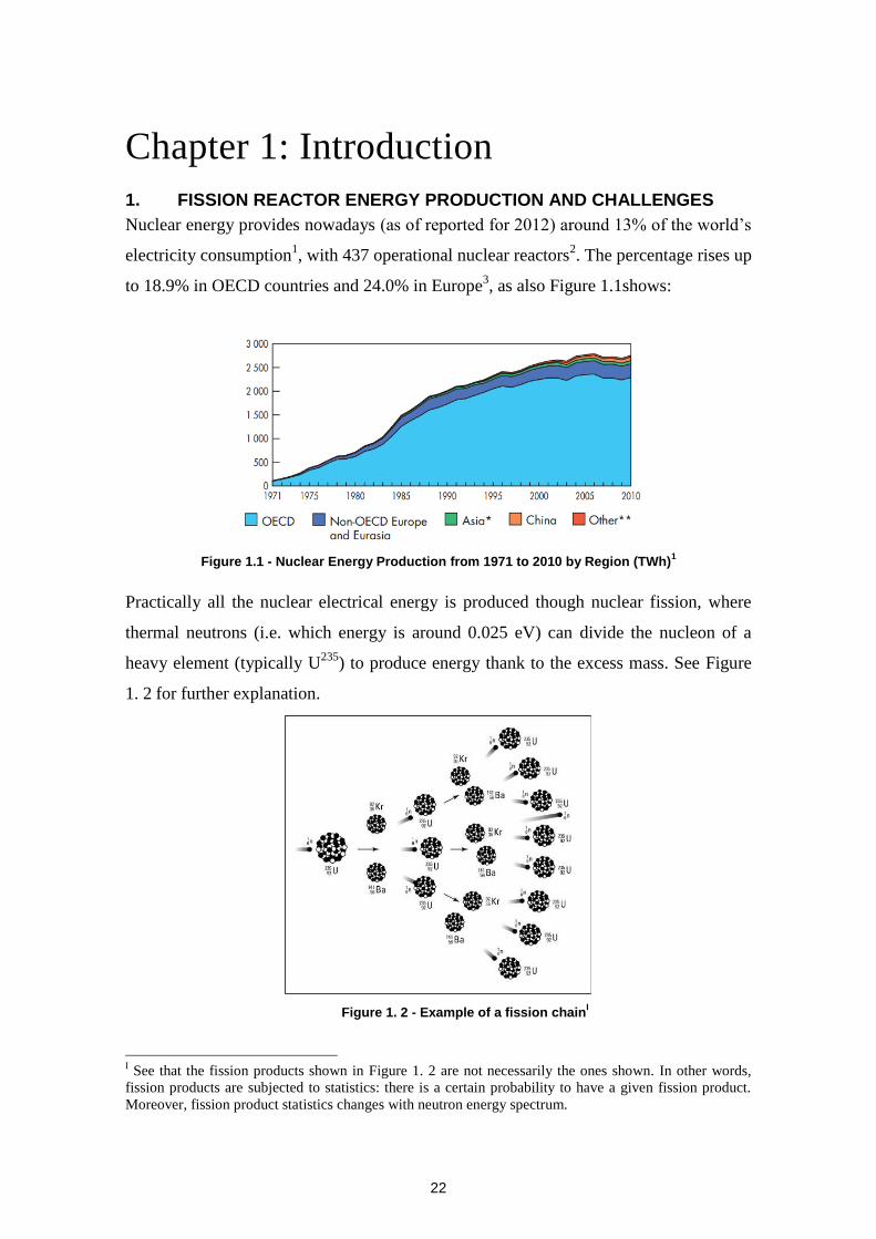
22
Chapter 1: Introduction
1. FISSION REACTOR ENERGY PRODUCTION AND CHALLENGES
Nuclear energy provides nowadays (as of reported for 2012) around 13% of the world’s
electricity consumption1, with 437 operational nuclear reactors
2. The percentage rises up
to 18.9% in OECD countries and 24.0% in Europe3, as also Figure 1.1shows:
Figure 1.1 - Nuclear Energy Production from 1971 to 2010 by Region (TWh)1
Practically all the nuclear electrical energy is produced though nuclear fission, where
thermal neutrons (i.e. which energy is around 0.025 eV) can divide the nucleon of a
heavy element (typically U235
) to produce energy thank to the excess mass. See Figure
1. 2 for further explanation.
Figure 1. 2 - Example of a fission chainI
I See that the fission products shown in Figure 1. 2 are not necessarily the ones shown. In other words,
fission products are subjected to statistics: there is a certain probability to have a given fission product.
Moreover, fission product statistics changes with neutron energy spectrum.
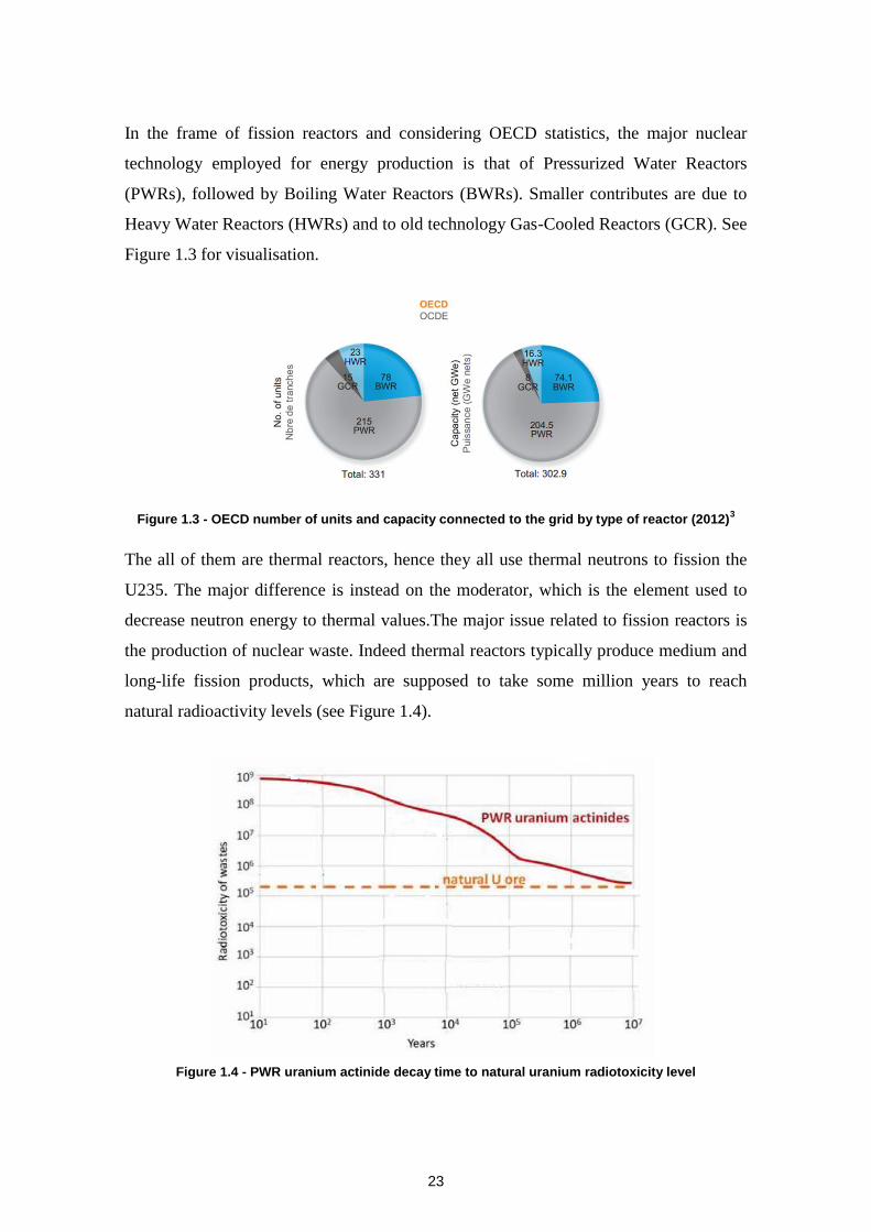
23
In the frame of fission reactors and considering OECD statistics, the major nuclear
technology employed for energy production is that of Pressurized Water Reactors
(PWRs), followed by Boiling Water Reactors (BWRs). Smaller contributes are due to
Heavy Water Reactors (HWRs) and to old technology Gas-Cooled Reactors (GCR). See
Figure 1.3 for visualisation.
Figure 1.3 - OECD number of units and capacity connected to the grid by type of reactor (2012)3
The all of them are thermal reactors, hence they all use thermal neutrons to fission the
U235. The major difference is instead on the moderator, which is the element used to
decrease neutron energy to thermal values.The major issue related to fission reactors is
the production of nuclear waste. Indeed thermal reactors typically produce medium and
long-life fission products, which are supposed to take some million years to reach
natural radioactivity levels (see Figure 1.4).
Figure 1.4 - PWR uranium actinide decay time to natural uranium radiotoxicity level
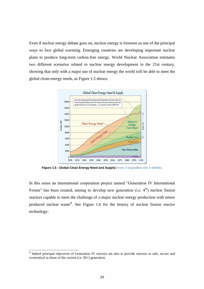
24
Even if nuclear energy debate goes on, nuclear energy is foreseen as one of the principal
ways to face global warming. Emerging countries are developing important nuclear
plans to produce long-term carbon-free energy. World Nuclear Association estimates
two different scenarios related to nuclear energy development in the 21st century,
showing that only with a major use of nuclear energy the world will be able to meet the
global clean-energy needs, as Figure 1.5 shows:
Figure 1.5 - Global Clean Energy Need and SupplyErrore. Il segnalibro non è definito.
In this sense an international cooperation project named “Generation IV International
Forum” has been created, aiming to develop new generation (i.e. 4th
) nuclear fission
reactors capable to meet the challenge of a major nuclear energy production with minor
produced nuclear wasteII. See Figure 1.6 for the history of nuclear fission reactor
technology:
II Indeed principal objectives of Generation IV reactors are also to provide reactors as safe, secure and
economical as those of the current (i.e. III+) generation.
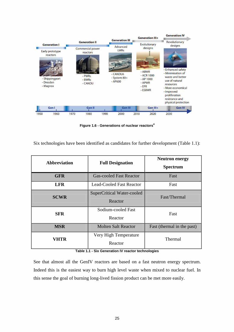
25
Figure 1.6 - Generations of nuclear reactors4
Six technologies have been identified as candidates for further development (Table 1.1):
Abbreviation Full Designation Neutron energy
Spectrum
GFR Gas-cooled Fast Reactor Fast
LFR Lead-Cooled Fast Reactor Fast
SCWR SuperCritical Water-cooled
Reactor Fast/Thermal
SFR Sodium-cooled Fast
Reactor Fast
MSR Molten Salt Reactor Fast (thermal in the past)
VHTR Very High Temperature
Reactor Thermal
Table 1.1 - Six Generation IV reactor technologies
See that almost all the GenIV reactors are based on a fast neutron energy spectrum.
Indeed this is the easiest way to burn high level waste when mixed to nuclear fuel. In
this sense the goal of burning long-lived fission product can be met more easily.

26
2. FRENCH EXPERIENCE WITH NUCLEAR POWER
2.1 THERMAL REACTORS
French experience with nuclear power starts on September, 29th 1956 with the first
electrical power generation in Marcoule G-1 (UNGG) plant5. As of 2011, there are 58
operating reactors in France for a 36.1 GWe electrical power connected to the grid. All
of the 58 reactors are Pressurized Water Reactors. France produces about 77% of its
electrical power needs through nuclear power, being the most “nuclearized” country in
the world in terms of nuclear production over total electrical power needs.
A new generation (i.e. III+) European Pressurized Reactor (EPR) is under construction
in the site of Flamanville, the first criticality been expected in 2016.
2.2 FAST REACTORS
Even though French activities were concentrated on thermal PWRs, France has quite an
important experience with fast reactor, in particular with SFRs. In fact, France already
built three SFRs: Table 1.2 provides some information about the three French SFRs.
Name First
Criticality
Final
Shutdown
Thermal
Power
[MWth]
Gross
Electrical
Power [MWe]
Rapsodie January 1967 April 1983 40 0
Phénix 1973 2010 563III
255
Super-Phénix 1985 1998 2990 1242
Table 1.2 - French Sodium-cooled Fast Reactors main information
All of them are pool-type SFRs, as those shown in Figure 1.7:
III
Since 1993 the Phénix reactor has been used as a support to French CEA R&D Program: hence its
thermal power has been limited to 350 MWth corresponding to 145 MWe.
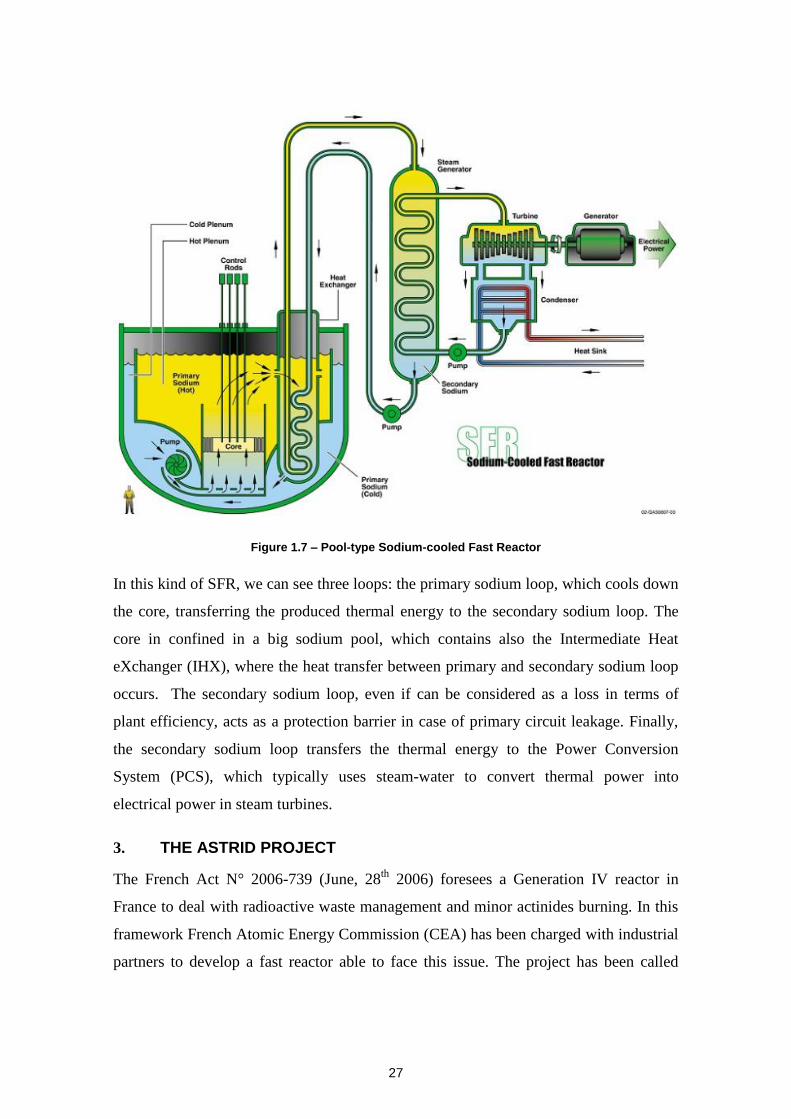
27
Figure 1.7 – Pool-type Sodium-cooled Fast Reactor
In this kind of SFR, we can see three loops: the primary sodium loop, which cools down
the core, transferring the produced thermal energy to the secondary sodium loop. The
core in confined in a big sodium pool, which contains also the Intermediate Heat
eXchanger (IHX), where the heat transfer between primary and secondary sodium loop
occurs. The secondary sodium loop, even if can be considered as a loss in terms of
plant efficiency, acts as a protection barrier in case of primary circuit leakage. Finally,
the secondary sodium loop transfers the thermal energy to the Power Conversion
System (PCS), which typically uses steam-water to convert thermal power into
electrical power in steam turbines.
3. THE ASTRID PROJECT
The French Act N° 2006-739 (June, 28th
2006) foresees a Generation IV reactor in
France to deal with radioactive waste management and minor actinides burning. In this
framework French Atomic Energy Commission (CEA) has been charged with industrial
partners to develop a fast reactor able to face this issue. The project has been called

28
ASTRID, which is the acronym of “Advanced Sodium Technological Reactor for
Industrial Demonstration”.
ASTRID main goals are identified as6:
Keep safety and security level at least to the same extent as current Generation
III+ reactors;
Specifically reducing the risk associated with the Sodium-water interaction in
Steam Generators;
Demonstrating the technological feasibility of sodium fast reactors to electrical
energy production;
Minor actinides and long life radioactive waste burning;
Better use of uranium natural resources.
In order to meet these goals, some design guidelines have been identified6:
1. Improved core design to lower the probability of core meltdown and/or the
energy release following during an accident scenario7,
8;
2. Better in-service and out-of-service inspection methods and instrumentation;
3. Civil structures have to account for mechanical integrity in case of internal or
external (see aeroplane impact) hazards;
4. Three independent shutdown systems;
5. Innovative gas power conversion system.
In particular, an innovative gas power conversion system is of primary interest for the
present work. Gas power conversion system has been studied at CEA from early 2000s9.
Its main interest is due to practical elimination of the risk associated with the sodium-
water interaction10
,11
, since no steam generator is necessary anymore. Therefore the
plant layout is shown in Figure 1.8 and in is composed by the primary sodium loop
cooling the reactor core, a secondary sodium loop to mitigate the radioactive release in
case of failure of the primary circuit and a tertiary gas loop ending in the turbine-
generator group producing electrical power.
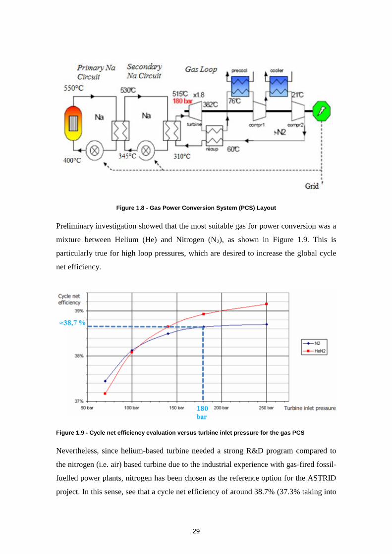
29
Figure 1.8 - Gas Power Conversion System (PCS) Layout
Preliminary investigation showed that the most suitable gas for power conversion was a
mixture between Helium (He) and Nitrogen (N2), as shown in Figure 1.9. This is
particularly true for high loop pressures, which are desired to increase the global cycle
net efficiency.
Figure 1.9 - Cycle net efficiency evaluation versus turbine inlet pressure for the gas PCS
Nevertheless, since helium-based turbine needed a strong R&D program compared to
the nitrogen (i.e. air) based turbine due to the industrial experience with gas-fired fossil-
fuelled power plants, nitrogen has been chosen as the reference option for the ASTRID
project. In this sense, see that a cycle net efficiency of around 38.7% (37.3% taking into

30
account electrical power generator efficiency) is obtained, which is slightly lower than
that obtained with a steam-water power conversion cycle due to the lack of boiling
phenomena increasing the heat transfer. The selected operating pressure is 180 bar
which represent the best trade-off between cycle efficiency and mechanical resistance
that the tertiary loop component must withstand.
In this framework the most crucial component to be designed is the sodium-nitrogen
heat exchanger. In fact it is responsible for the effective heat transfer from the
secondary sodium to the gas that will eventually go through the turbines. It has been
already shown9 that its contribution to the gas circuit total pressure drop is of primary
importance for the cycle efficiency: hence the design choice is to limit the sodium/gas
heat exchanger pressure drop at 1 bar at maximum on the gas side. This is one of the
most important design constraints to be respected.
Compact technologies are necessary for the present application because of the low heat
transfer capacity of the nitrogen compared to that of boiling water. In this sense, the
goal is to design a component being as compact as possible. Preliminary investigations
done at CEA12
showed that one technology is of primary interest due to its
compactness: the Plate Stamped Heat Exchanger, which is potentially the most compact
technology among those studies12
. Therefore the present work starts studying the PSHE
technology, to investigate its thermal-hydraulic behavior and to understand the physical
phenomena providing the efficient heat transfer. The physical understanding will be
used to determine the research pattern that will be followed in this PhD work aiming to
increase the thermal-hydraulic performance of the compact sodium-gas heat exchanger.
Note that, since the heat transfer performance of the heat exchanger (i.e. its heat transfer
coefficient) is primary determined by the thermal-hydraulic behavior of the gas-side due
to its higher thermal resistance, the present work will only focus on the gas (nitrogen)
side of the heat exchanger itself.
4. PHD THESIS OUTLOOK
Given the design constraints described in Section 3, the PhD work will consist in:
A bibliographic overview on the PSHE technology, to evaluate why it can
provide superior heat transfer performance than the other solutions. The

31
bibliographical research will also investigate the numerical approach to study
such components, in particular with regard to the computational domain and the
turbulence modeling approach. A final innovative heat transfer geometry
consisting in an innovative channel will be proposed to increase the heat transfer
in the sodium-gas heat exchanger. This will be done in Chapter 2.
A preliminary numerical model validation based on the conclusions of Chapter
2. Three different turbulence modeling approaches will be tested against basic
validation test cases. This will be described in Chapter 3.
An experimental facility description to acquire an experimental database that
will be useful to actually validate the numerical model and to study the fluid
flow inside the innovative channel. Some preliminary tests will be also
described, to validate the database. This will be shown in Chapter 4.
Final model validation and flow analysis with regard to mixing and swirling
flow inside the innovative channel will be shown. Once the model is validated, a
performance comparison among the existing technology and the innovative
geometry will be provided, showing the gain obtained by the innovative
solution. This will be done in Chapter 5.
Conclusions and perspectives of the present work will be presented in Chapter
6.
32
Chapitre 2: Echangeurs de chaleur à
plaques embouties - (PSHE) Etude
technique et bibliographique
Une étude bibliographique sur les échangeurs de chaleur compacts à plaques a été
réalisée. Parmi les différents types d'échangeurs de chaleur compacts (à savoir les
échangeurs de chaleur à circuit imprimé - PCHE, les échangeurs de chaleur plaques-
ailettes-PFHE et les échangeurs de chaleur à tôles embouties -PSHE), une recherche
bibliographique approfondie a été effectuée sur les PSHEs afin de mieux comprendre le
comportement thermo-hydraulique de ces composants.
Les PSHEs consistent essentiellement en un certain nombre de plaques de différentes
formes empilées.. Les plaques empilées se touchent dans de nombreux points de
contact: cette configuration donne de la résistance mécanique en compression, améliore
le transfert de chaleur et diminue le colmatage grâce à un haut niveau de turbulence. Les
caractéristiques géométriques les plus importantes en ce qui concerne la géométrie des
plaques PSHE type chevron ont été identifiées. L'identification précise de l'écoulement
fluide pour un PSHE est très difficile parce qu’il n'existe pas de configuration bien
identifiée entre les plaques en raison de l'absence de canaux bien définis.
Un vaste ensemble de corrélations pour le transfert de chaleur et la perte de charge a été
présenté sur la base de considérations théoriques ou semi-empiriques. Une grande
dispersion des données a été montrée, ce qui est probablement dû à la très large gamme
de nombres de Reynolds et de paramètres géométriques des plaques pour chaque cas.
Pour mieux étudier ces effets géométriques, un aperçu de l'influence de la géométrie de
la plaque sur l’échange thermique ainsi que sur le frottement a été présenté, ce qui
montre que le facteur de forme ainsi que l'angle chevron sont les principaux paramètres
d'intérêt pour le concepteur.
Différents paramètres géométriques définissant l’emboutissage de la plaque ont été
étudiés pour vérifier leur effet sur les performance thermo-hydraulique..

33
Conjointement avec les mesures expérimentales, plusieurs études numériques ont été
effectuées pour étudier l'écoulement de fluide à l'intérieur des plaques. Les résultats
dépendent à la fois du domaine de calcul et du modèle adopté.
Enfin, des critères d'évaluation des performances ont été présentés, en essayant
d'évaluer lequel est potentiellement le plus utile pour définir la compacité de différentes
géométries. Cela sera d'une importance primordiale pour statuer sur l’atteinte de
l'objectif de ce travail de thèse (l’amélioration du transfert de chaleur avec des
contraintes sur la perte de charge dans l'échangeur de chaleur compact à plaques).
L’idée de base de ce travail est de qualifier un motif d’échange innovant où
l'écoulement du fluide est le plus tridimensionnel possible, ce qui est censé augmenter
l’échange thermique .
Un dernier volet de l’étude bibliographique concerne la modélisation. Une approche
numérique de type RANS à bas nombre de Reynolds fournit théoriquement les
informations les plus exactes sur l'écoulement du fluide. En ce sens, et en tenant compte
également de la géométrie de canal, le modèle de turbulence le plus adapté semble être
un modèle basé sur le taux spécifique de dissipation: en fait, il a été largement démontré
que ce type de modèle fournit une meilleure description des écoulements à gradients de
pression adverses sans avoir besoin de modifications spécifiques pour les faibles
nombres de Reynolds à la paroi. En outre, il a été également montré que les modèles de
référence basés sur ω prennent mieux en compte les effets de compressibilité thermique
(i.e. variations importantes des propriétés physiques dans la région près de paroi). Par
conséquent, pour la présente application, l'approche de modélisation basée sur ω sera
adoptée.
Pour valider le modèle numérique, une base de données expérimentale est d'une
importance primordiale. La littérature ne fournit pas vraiment des cas-tests semblables
au motif d’échange innovant. Donc une base de données expérimentale sur la géométrie
réelle est nécessaire.
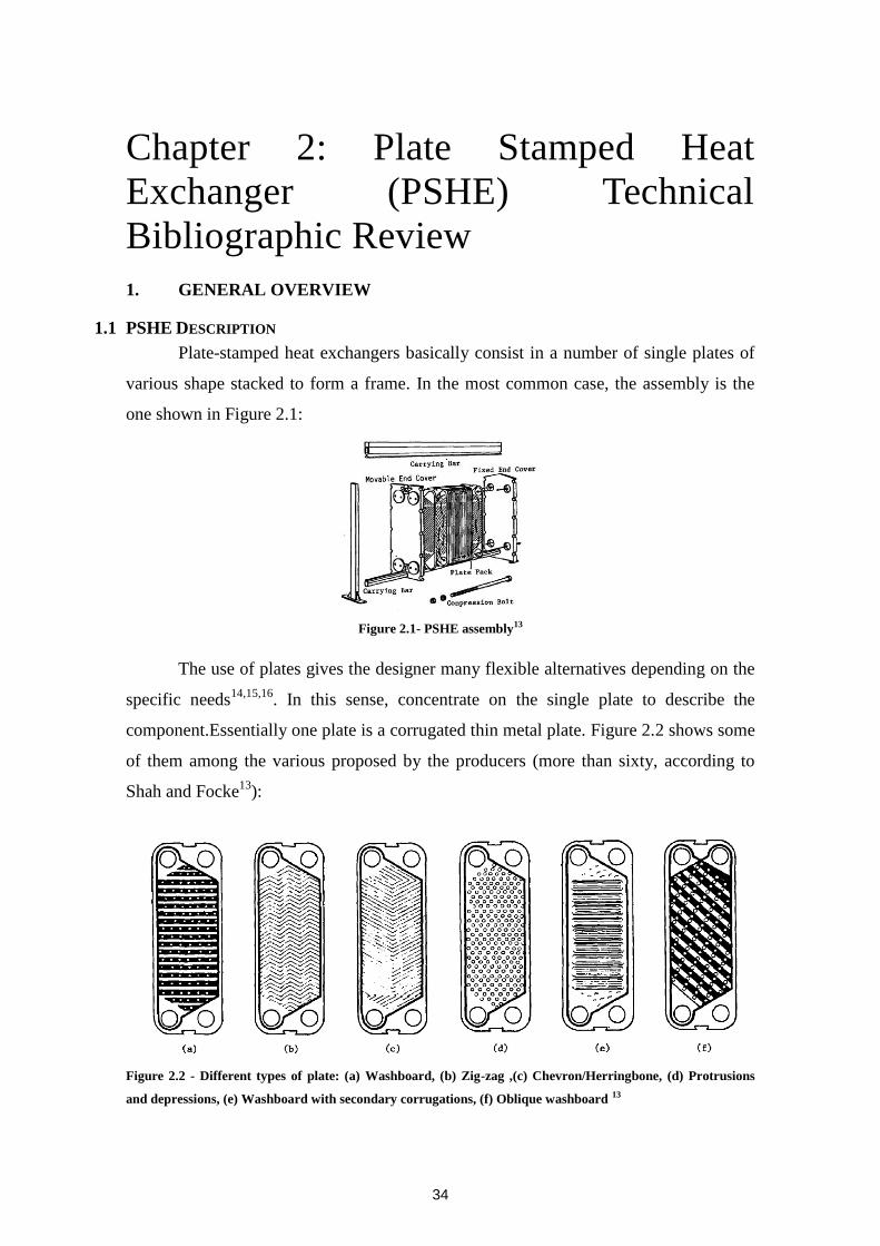
34
Chapter 2: Plate Stamped Heat
Exchanger (PSHE) Technical
Bibliographic Review
1. GENERAL OVERVIEW
1.1 PSHE DESCRIPTION
Plate-stamped heat exchangers basically consist in a number of single plates of
various shape stacked to form a frame. In the most common case, the assembly is the
one shown in Figure 2.1:
Figure 2.1- PSHE assembly13
The use of plates gives the designer many flexible alternatives depending on the
specific needs14,15,16
. In this sense, concentrate on the single plate to describe the
component.Essentially one plate is a corrugated thin metal plate. Figure 2.2 shows some
of them among the various proposed by the producers (more than sixty, according to
Shah and Focke13
):
Figure 2.2 - Different types of plate: (a) Washboard, (b) Zig-zag ,(c) Chevron/Herringbone, (d) Protrusions
and depressions, (e) Washboard with secondary corrugations, (f) Oblique washboard 13
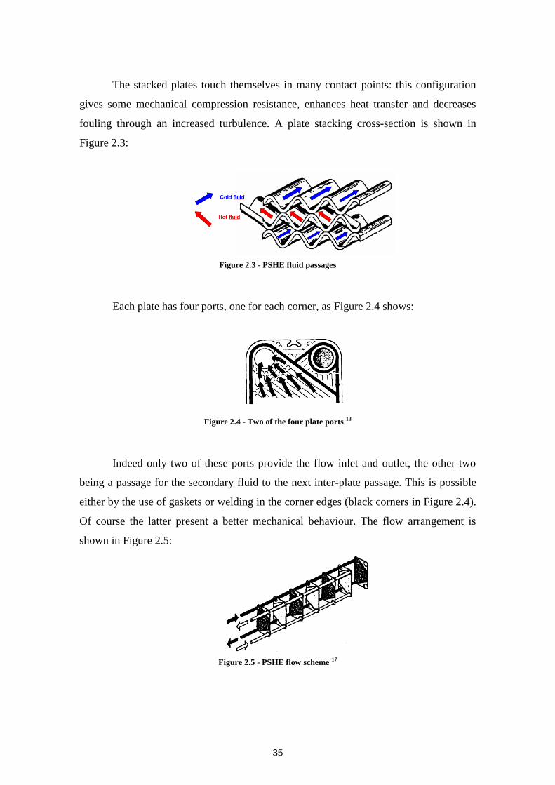
35
The stacked plates touch themselves in many contact points: this configuration
gives some mechanical compression resistance, enhances heat transfer and decreases
fouling through an increased turbulence. A plate stacking cross-section is shown in
Figure 2.3:
Figure 2.3 - PSHE fluid passages
Each plate has four ports, one for each corner, as Figure 2.4 shows:
Figure 2.4 - Two of the four plate ports 13
Indeed only two of these ports provide the flow inlet and outlet, the other two
being a passage for the secondary fluid to the next inter-plate passage. This is possible
either by the use of gaskets or welding in the corner edges (black corners in Figure 2.4).
Of course the latter present a better mechanical behaviour. The flow arrangement is
shown in Figure 2.5:
Figure 2.5 - PSHE flow scheme 17
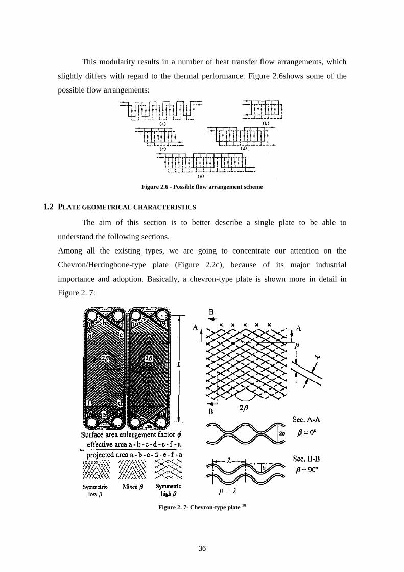
36
This modularity results in a number of heat transfer flow arrangements, which
slightly differs with regard to the thermal performance. Figure 2.6shows some of the
possible flow arrangements:
Figure 2.6 - Possible flow arrangement scheme
1.2 PLATE GEOMETRICAL CHARACTERISTICS
The aim of this section is to better describe a single plate to be able to
understand the following sections.
Among all the existing types, we are going to concentrate our attention on the
Chevron/Herringbone-type plate (Figure 2.2c), because of its major industrial
importance and adoption. Basically, a chevron-type plate is shown more in detail in
Figure 2. 7:
Figure 2. 7- Chevron-type plate 18
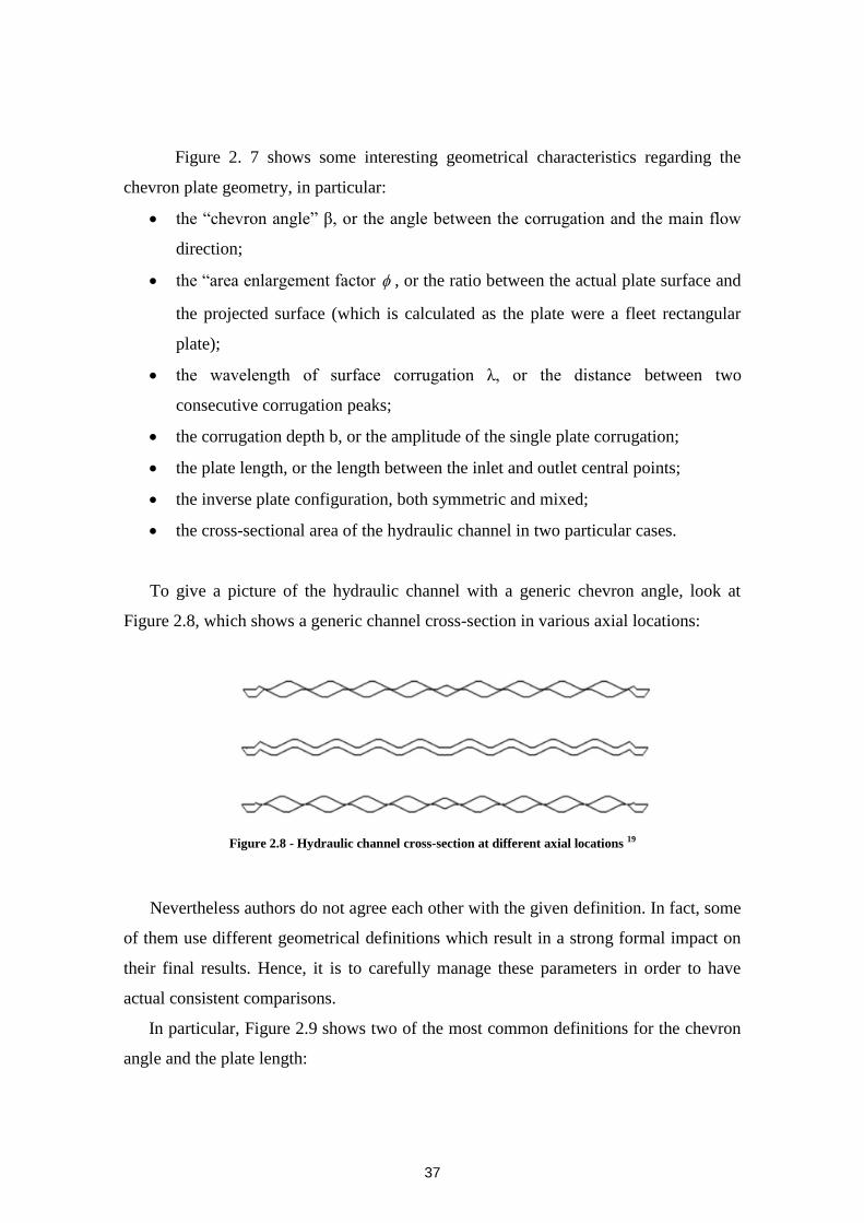
37
Figure 2. 7 shows some interesting geometrical characteristics regarding the
chevron plate geometry, in particular:
the “chevron angle” β, or the angle between the corrugation and the main flow
direction;
the “area enlargement factor , or the ratio between the actual plate surface and
the projected surface (which is calculated as the plate were a fleet rectangular
plate);
the wavelength of surface corrugation λ, or the distance between two
consecutive corrugation peaks;
the corrugation depth b, or the amplitude of the single plate corrugation;
the plate length, or the length between the inlet and outlet central points;
the inverse plate configuration, both symmetric and mixed;
the cross-sectional area of the hydraulic channel in two particular cases.
To give a picture of the hydraulic channel with a generic chevron angle, look at
Figure 2.8, which shows a generic channel cross-section in various axial locations:
Figure 2.8 - Hydraulic channel cross-section at different axial locations 19
Nevertheless authors do not agree each other with the given definition. In fact, some
of them use different geometrical definitions which result in a strong formal impact on
their final results. Hence, it is to carefully manage these parameters in order to have
actual consistent comparisons.
In particular, Figure 2.9 shows two of the most common definitions for the chevron
angle and the plate length:

38
Figure 2.9 - Alternative geometrical definitions 20
In particular, note that the chevron angle is the complementary angle to that
previously defined and that the plate length actually is the length of the heat transfer
active zone. With regard to the latest difference, note that this choice has likely been
done to exclude from the consideration the inlet and outlet flow ports, which behaviour
is completely different from that of the plate central zone.
Charre et al.21
provide a number of parameters which have an influence on PSHE
performance as high as eleven; they are listed as follows, even though some of them do
not refer to a single plate:
1. Number of plates ;
2. Corrugation inclination angle in the central part ;
3. Angle in the distribution zone ;
4. Central part pitch ;
5. Pitch of distribution zone ;
6. Maximum height of the plate profile (distance between the top and the bottom of the
profile, which is supposed to be sinusoidal);
7. Diameter of the collector ;
8. Width of the plate ;
9. Length of the chevron segment ;
10. Length of the central part zone ;
11. Length of the distribution zone.
All the previously listed parameters play a role in the global thermal-hydraulic
performance of the heat exchanger; nevertheless it is often hard to really have such data
since they are industrial property of the manufacturer.
39
1.3 HYDRAULIC DIAMETER DEFINITION
The aim of this section is to show the relationship between the two different
definitions of the hydraulic diameter and its influence on other thermal-hydraulic
variables.
Given the plate geometrical characteristics in Figure 2. 7, the theoretical definition
of hydraulic diameter Dh is:
)(2
4
_
_4
wb
bw
perimeterWetted
SectionChannelDh
Being w the plate width. Now, since b<<w, we obtain:
b
w
bwDh
2
)(2
4
Indeed some authors do not use this definition of hydraulic diameter. They use a
simpler definition, sometimes defined as “equivalent diameter” De, where:
bDe 2
The advantages of such an approach (based on the equivalent diameter De) are:
Easily comparing the performance of a PSHE with those of two parallel
plates;
Utilizing the plate projected area in the heat transfer calculations, which is
easier to use because it simply refers to the outer geometrical plate
dimensions. Indeed the area enlargement factor 𝜙 is not taken into account
anymore (as in the Dh definition), therefore the plate projected area is to be
used because it does not consider the area enlargement factor.
To convert a hydraulic diameter-defined correlation into an equivalent diameter-
defined any correlation should use the following correction factors, as calculated in
APPENDIX A:
40
Multiply the Nusselt number correlation by d1
IV;
Multiply the friction factor correlation byb1 V
1.4 FINAL DEFINITION OF THE PARAMETERS OF INTEREST
In the end, it is worth to give a final definition of the parameters of interest for the
following considerations. The choice is:
With regard to the geometrical parameters, the definitions are those shown in
Figure 2. 7:
the “chevron angle” β, or the angle between the corrugation and the
main flow direction;
the “area enlargement factor , or the ratio between the actual plate
surface and the projected surface (which is calculated as the plate
were a fleet rectangular plate);
the wavelength of surface corrugation λ, or the distance between two
consecutive corrugation peaks;
the corrugation depth b, or the amplitude of the single plate
corrugation;
With regard to the hydraulic diameter, the definition will be that one we
have previously defined as “equivalent diameter”:
bDe 2
Hence all the following sections will refer to this choice.
2. FLOW CHARACTERISTICS
2.1 FLOW PATTERN
Identifying the flow pattern in a plate is of primary importance to describe the fluid
flow and to understand why physical phenomena occur. Moreover, as it will be shown,
fluid flow description and heat transfer enhancement are strictly related: hence the aim
IV
Note that the superscript « d » corresponds to the superscript of the Reynolds number in the heat
transfer correlation VNote that the superscript « b » corresponds to the superscript of the Reynolds number in the friction
factor correlation
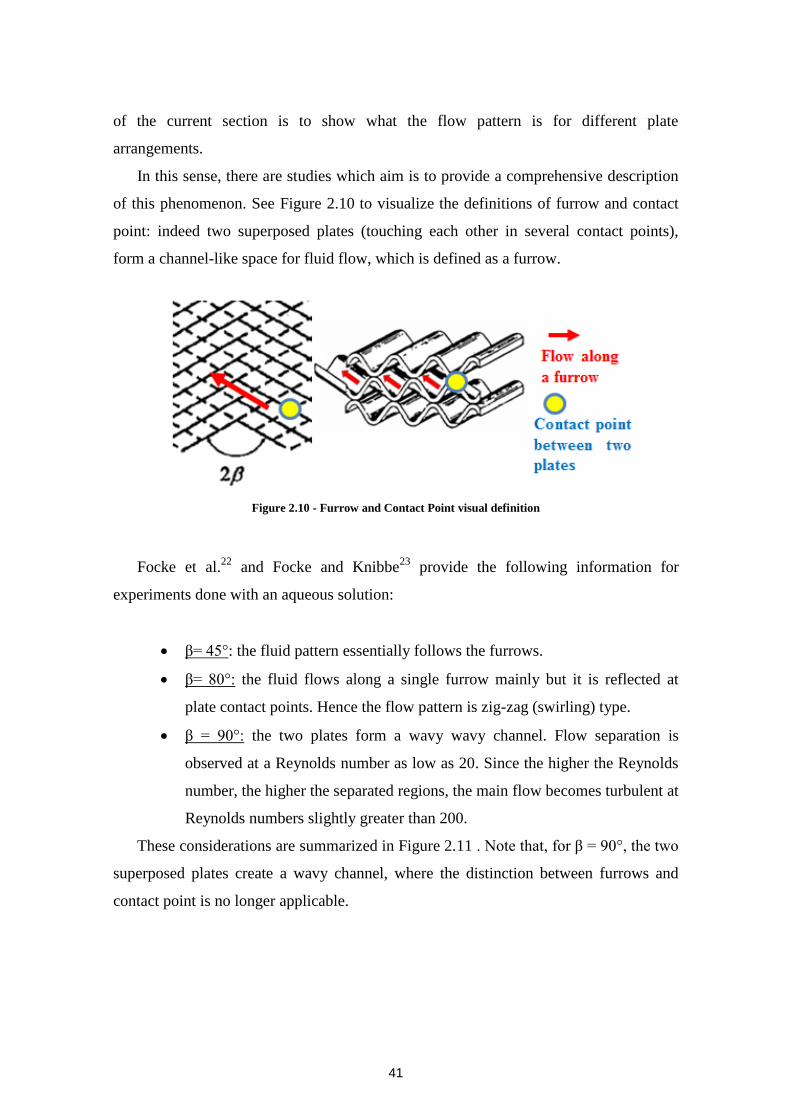
41
of the current section is to show what the flow pattern is for different plate
arrangements.
In this sense, there are studies which aim is to provide a comprehensive description
of this phenomenon. See Figure 2.10 to visualize the definitions of furrow and contact
point: indeed two superposed plates (touching each other in several contact points),
form a channel-like space for fluid flow, which is defined as a furrow.
Figure 2.10 - Furrow and Contact Point visual definition
Focke et al.22
and Focke and Knibbe23
provide the following information for
experiments done with an aqueous solution:
β= 45°: the fluid pattern essentially follows the furrows.
β= 80°: the fluid flows along a single furrow mainly but it is reflected at
plate contact points. Hence the flow pattern is zig-zag (swirling) type.
β = 90°: the two plates form a wavy wavy channel. Flow separation is
observed at a Reynolds number as low as 20. Since the higher the Reynolds
number, the higher the separated regions, the main flow becomes turbulent at
Reynolds numbers slightly greater than 200.
These considerations are summarized in Figure 2.11 . Note that, for β = 90°, the two
superposed plates create a wavy channel, where the distinction between furrows and
contact point is no longer applicable.
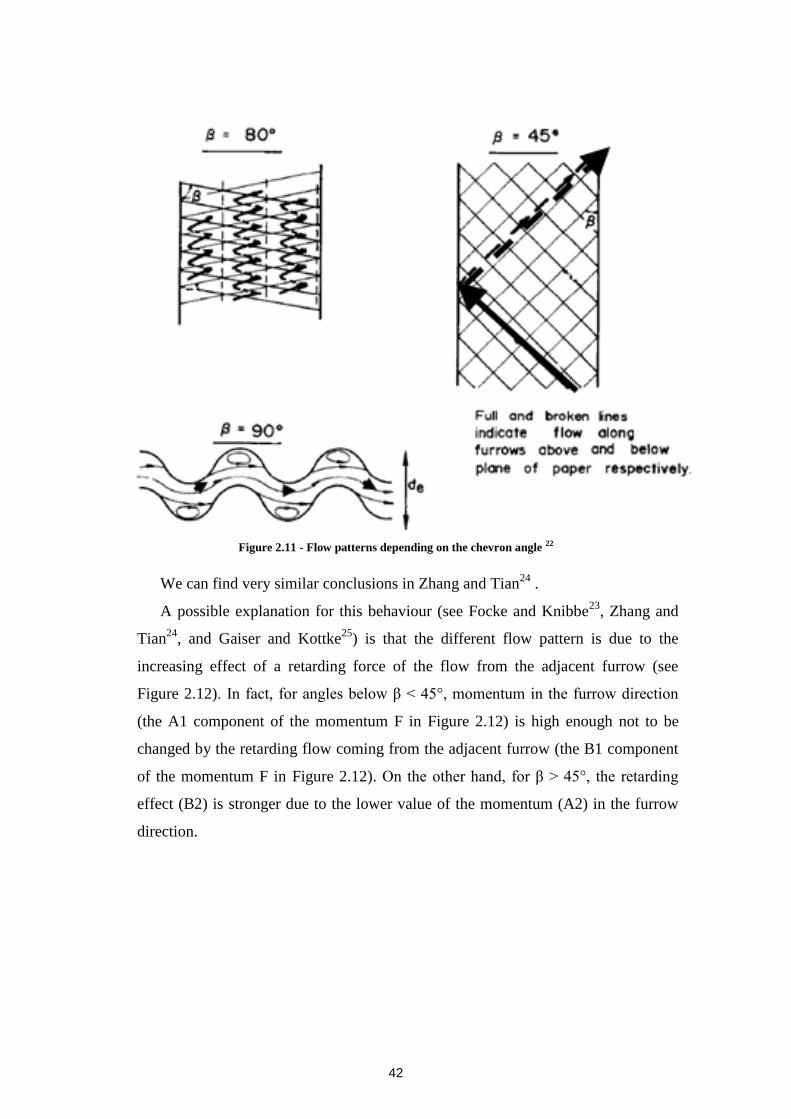
42
Figure 2.11 - Flow patterns depending on the chevron angle 22
We can find very similar conclusions in Zhang and Tian24
.
A possible explanation for this behaviour (see Focke and Knibbe23
, Zhang and
Tian24
, and Gaiser and Kottke25
) is that the different flow pattern is due to the
increasing effect of a retarding force of the flow from the adjacent furrow (see
Figure 2.12). In fact, for angles below β < 45°, momentum in the furrow direction
(the A1 component of the momentum F in Figure 2.12) is high enough not to be
changed by the retarding flow coming from the adjacent furrow (the B1 component
of the momentum F in Figure 2.12). On the other hand, for β > 45°, the retarding
effect (B2) is stronger due to the lower value of the momentum (A2) in the furrow
direction.
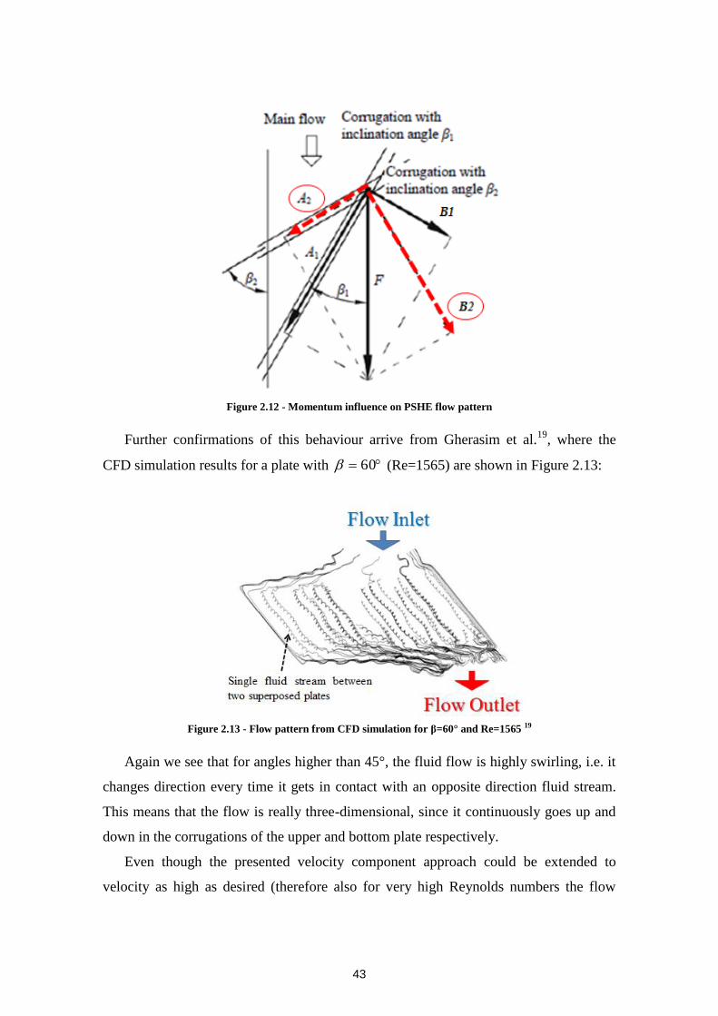
43
Figure 2.12 - Momentum influence on PSHE flow pattern
Further confirmations of this behaviour arrive from Gherasim et al.19
, where the
CFD simulation results for a plate with 60 (Re=1565) are shown in Figure 2.13:
Figure 2.13 - Flow pattern from CFD simulation for β=60° and Re=1565 19
Again we see that for angles higher than 45°, the fluid flow is highly swirling, i.e. it
changes direction every time it gets in contact with an opposite direction fluid stream.
This means that the flow is really three-dimensional, since it continuously goes up and
down in the corrugations of the upper and bottom plate respectively.
Even though the presented velocity component approach could be extended to
velocity as high as desired (therefore also for very high Reynolds numbers the flow
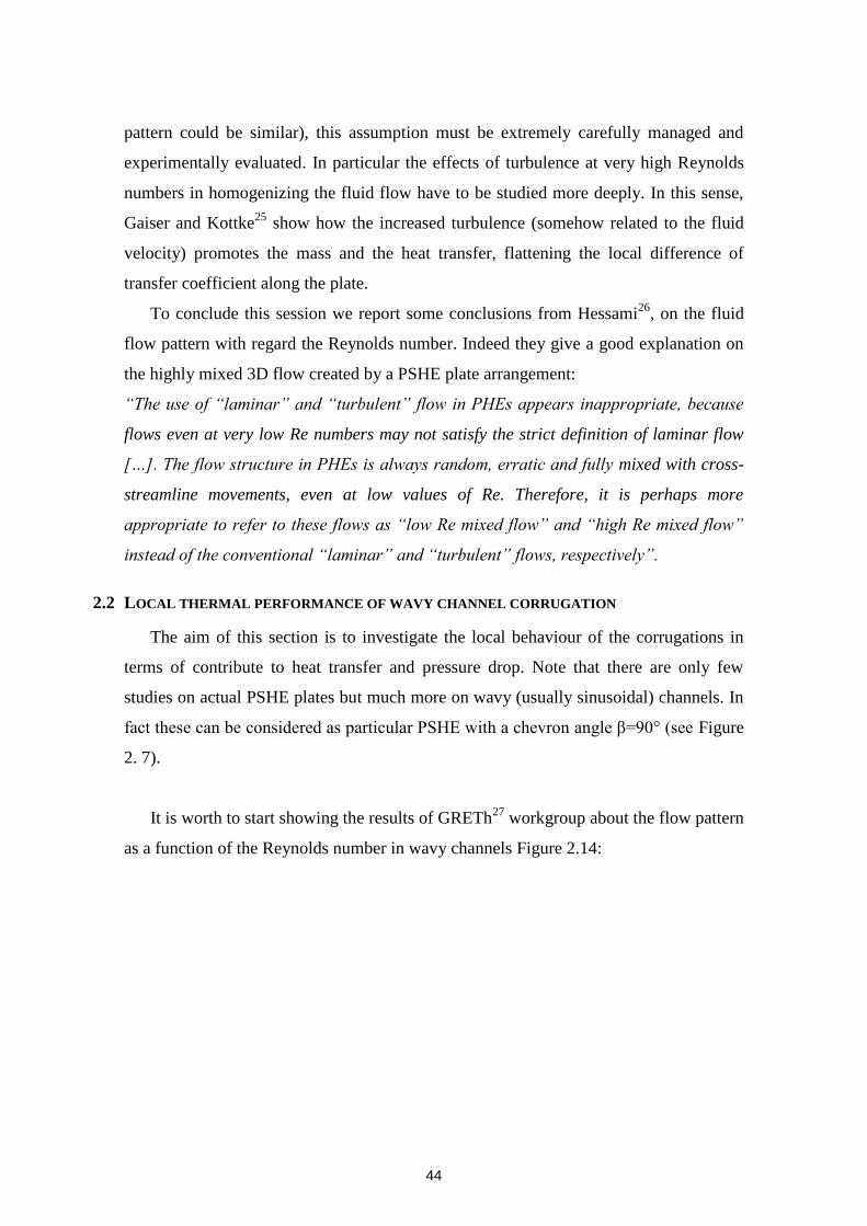
44
pattern could be similar), this assumption must be extremely carefully managed and
experimentally evaluated. In particular the effects of turbulence at very high Reynolds
numbers in homogenizing the fluid flow have to be studied more deeply. In this sense,
Gaiser and Kottke25
show how the increased turbulence (somehow related to the fluid
velocity) promotes the mass and the heat transfer, flattening the local difference of
transfer coefficient along the plate.
To conclude this session we report some conclusions from Hessami26
, on the fluid
flow pattern with regard the Reynolds number. Indeed they give a good explanation on
the highly mixed 3D flow created by a PSHE plate arrangement:
“The use of “laminar” and “turbulent” flow in PHEs appears inappropriate, because
flows even at very low Re numbers may not satisfy the strict definition of laminar flow
[…]. The flow structure in PHEs is always random, erratic and fully mixed with cross-
streamline movements, even at low values of Re. Therefore, it is perhaps more
appropriate to refer to these flows as “low Re mixed flow” and “high Re mixed flow”
instead of the conventional “laminar” and “turbulent” flows, respectively”.
2.2 LOCAL THERMAL PERFORMANCE OF WAVY CHANNEL CORRUGATION
The aim of this section is to investigate the local behaviour of the corrugations in
terms of contribute to heat transfer and pressure drop. Note that there are only few
studies on actual PSHE plates but much more on wavy (usually sinusoidal) channels. In
fact these can be considered as particular PSHE with a chevron angle β=90° (see Figure
2. 7).
It is worth to start showing the results of GRETh27
workgroup about the flow pattern
as a function of the Reynolds number in wavy channels Figure 2.14:
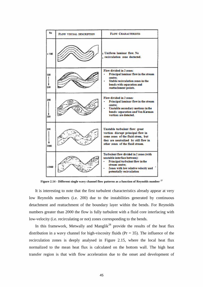
45
Figure 2.14 - Different single wavy channel flow patterns as a function of Reynolds number 27
It is interesting to note that the first turbulent characteristics already appear at very
low Reynolds numbers (i.e. 200) due to the instabilities generated by continuous
detachment and reattachment of the boundary layer within the bends. For Reynolds
numbers greater than 2000 the flow is fully turbulent with a fluid core interfacing with
low-velocity (i.e. recirculating or not) zones corresponding to the bends.
In this framework, Metwally and Manglik28
provide the results of the heat flux
distribution in a wavy channel for high-viscosity fluids (Pr = 35). The influence of the
recirculation zones is deeply analysed in Figure 2.15, where the local heat flux
normalized to the mean heat flux is calculated on the bottom wall. The high heat
transfer region is that with flow acceleration due to the onset and development of
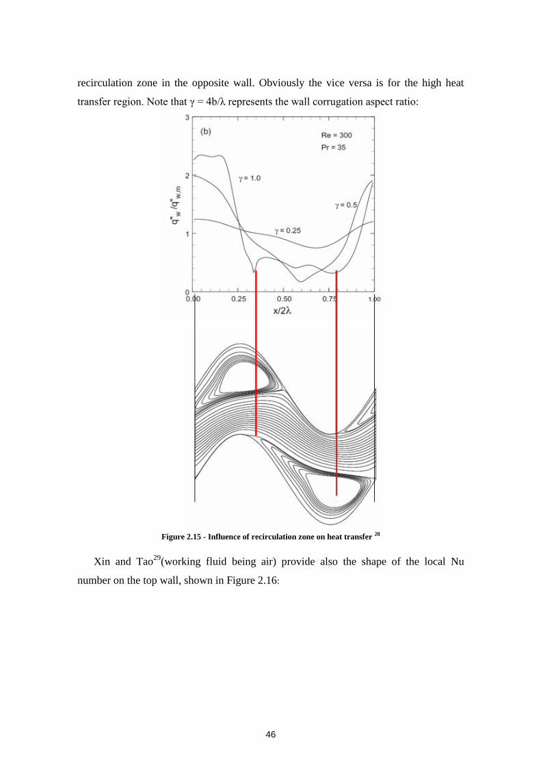
46
recirculation zone in the opposite wall. Obviously the vice versa is for the high heat
transfer region. Note that γ = 4b/λ represents the wall corrugation aspect ratio:
Figure 2.15 - Influence of recirculation zone on heat transfer 28
Xin and Tao29
(working fluid being air) provide also the shape of the local Nu
number on the top wall, shown in Figure 2.16:
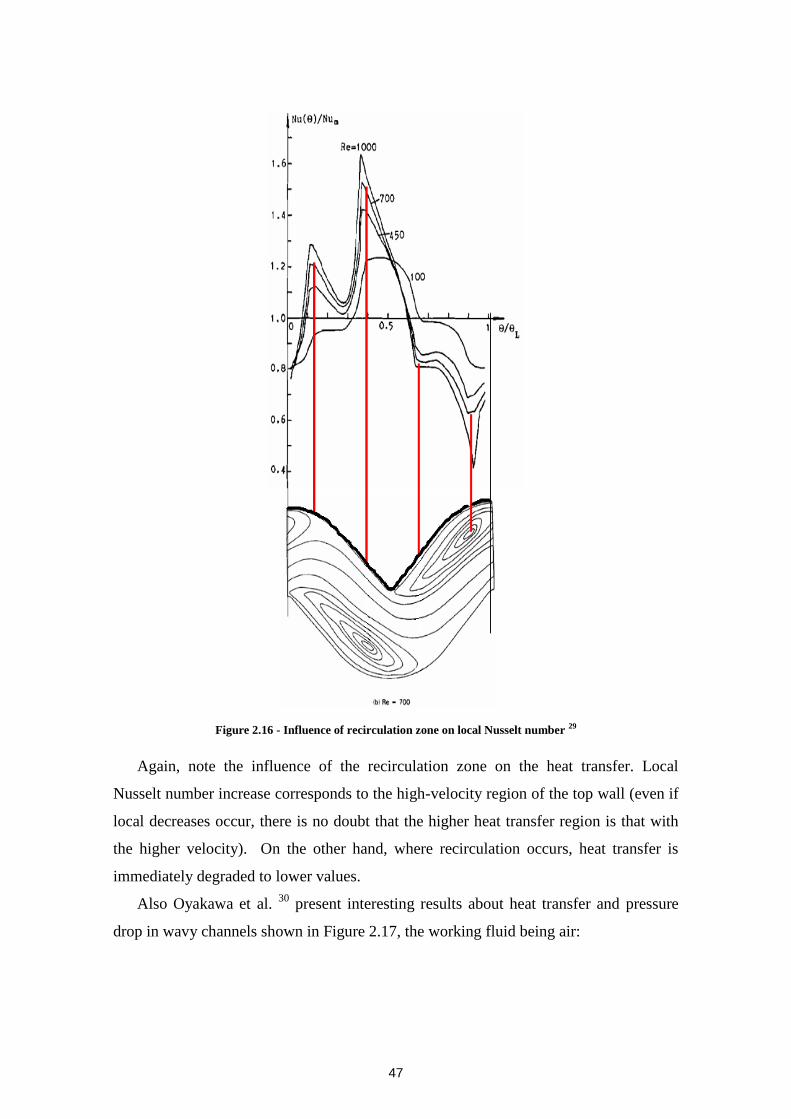
47
Figure 2.16 - Influence of recirculation zone on local Nusselt number 29
Again, note the influence of the recirculation zone on the heat transfer. Local
Nusselt number increase corresponds to the high-velocity region of the top wall (even if
local decreases occur, there is no doubt that the higher heat transfer region is that with
the higher velocity). On the other hand, where recirculation occurs, heat transfer is
immediately degraded to lower values.
Also Oyakawa et al. 30
present interesting results about heat transfer and pressure
drop in wavy channels shown in Figure 2.17, the working fluid being air:
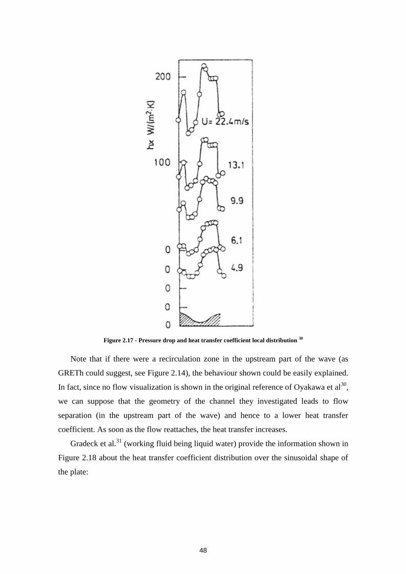
48
Figure 2.17 - Pressure drop and heat transfer coefficient local distribution 30
Note that if there were a recirculation zone in the upstream part of the wave (as
GRETh could suggest, see Figure 2.14), the behaviour shown could be easily explained.
In fact, since no flow visualization is shown in the original reference of Oyakawa et al30
,
we can suppose that the geometry of the channel they investigated leads to flow
separation (in the upstream part of the wave) and hence to a lower heat transfer
coefficient. As soon as the flow reattaches, the heat transfer increases.
Gradeck et al.31
(working fluid being liquid water) provide the information shown in
Figure 2.18 about the heat transfer coefficient distribution over the sinusoidal shape of
the plate:
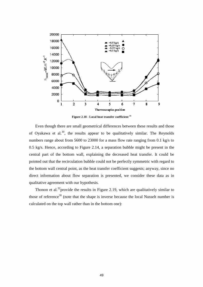
49
Figure 2.18 - Local heat transfer coefficient 31
Even though there are small geometrical differences between these results and those
of Oyakawa et al.30
, the results appear to be qualitatively similar. The Reynolds
numbers range about from 5600 to 23000 for a mass flow rate ranging from 0.1 kg/s to
0.5 kg/s. Hence, according to Figure 2.14, a separation bubble might be present in the
central part of the bottom wall, explaining the decreased heat transfer. It could be
pointed out that the recirculation bubble could not be perfectly symmetric with regard to
the bottom wall central point, as the heat transfer coefficient suggests; anyway, since no
direct information about flow separation is presented, we consider these data as in
qualitative agreement with our hypothesis.
Thonon et al.32
provide the results in Figure 2.19, which are qualitatively similar to
those of reference30
(note that the shape is inverse because the local Nusselt number is
calculated on the top wall rather than in the bottom one):
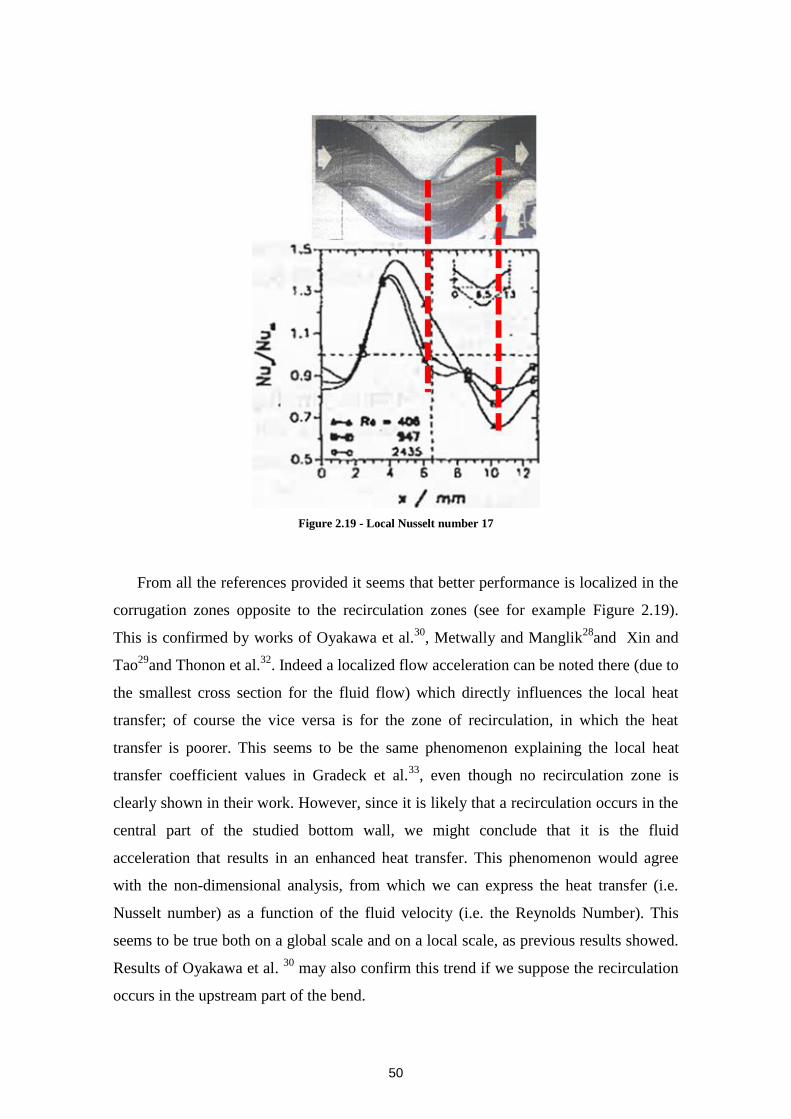
50
Figure 2.19 - Local Nusselt number 17
From all the references provided it seems that better performance is localized in the
corrugation zones opposite to the recirculation zones (see for example Figure 2.19).
This is confirmed by works of Oyakawa et al.30
, Metwally and Manglik28
and Xin and
Tao29
and Thonon et al.32
. Indeed a localized flow acceleration can be noted there (due to
the smallest cross section for the fluid flow) which directly influences the local heat
transfer; of course the vice versa is for the zone of recirculation, in which the heat
transfer is poorer. This seems to be the same phenomenon explaining the local heat
transfer coefficient values in Gradeck et al.33
, even though no recirculation zone is
clearly shown in their work. However, since it is likely that a recirculation occurs in the
central part of the studied bottom wall, we might conclude that it is the fluid
acceleration that results in an enhanced heat transfer. This phenomenon would agree
with the non-dimensional analysis, from which we can express the heat transfer (i.e.
Nusselt number) as a function of the fluid velocity (i.e. the Reynolds Number). This
seems to be true both on a global scale and on a local scale, as previous results showed.
Results of Oyakawa et al. 30
may also confirm this trend if we suppose the recirculation
occurs in the upstream part of the bend.
51
Anyway, since the geometries (hence the occurrence of recirculation) are different
in presented works, we can say with Snyder et al.34
that:
“It seems clear from these separate investigations that different flow mechanisms
may play starring roles in promoting heat transfer, depending crucially on operating
regime and local details of the surface geometry.”
In conclusion what can be inferred is that in wavy channels, recirculation zones
indirectly enhance the heat transfer (i.e. creating local accelerating regions on the
opposite wall). This means that such recirculation zones are desired for an enhancing
heat transfer technology. Moreover, what is not necessarily described by investigations
on wavy channel is that the three-dimensional flow (that we can observe for PSHEs)
continuously attaches and detaches the flow thermal boundary layer, i.e. the high
temperature region of the fluid. This is easily understandable considering that a wavy
channel is a two-dimensional flow whereas a 3D flow inherently has one more direction
for boundary layer attachment and detachment. Finally, this process does increase the
heat transfer, being the hotter fluid somehow mixed with colder one, hence
homogenising the global fluid temperature. This is very favourable and desirable for a
technology aiming to increase thermal performance of a heat exchanger.
3. CORRELATIONS
As previously exposed, thermal-hydraulic performances essentially depend on the
geometrical characteristics of the plate. Nevertheless many of the available correlations
do not take into account these dependences but only fit experimental or simulation data.
Indeed a few authors tried to theoretically investigate the problem in order to obtain
generally applicable correlations: actually they have to introduce some semi-empirical
factors to close the model: in this sense refer to them as semi-theoretical correlations.
The aim of this section is to provide a comparison of the existing correlations. We
are going to explicitly show only a few correlations, both semi-theoretical and
experimental. For the other ones, refer to the original references.
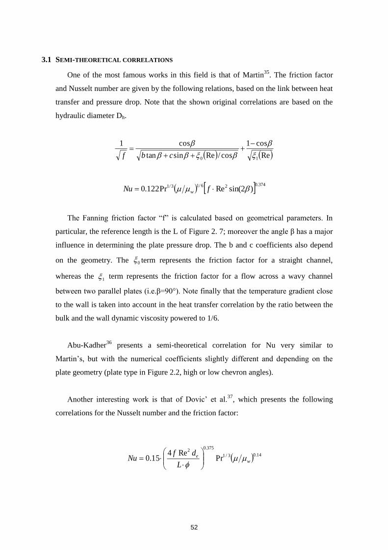
52
3.1 SEMI-THEORETICAL CORRELATIONS
One of the most famous works in this field is that of Martin35
. The friction factor
and Nusselt number are given by the following relations, based on the link between heat
transfer and pressure drop. Note that the shown original correlations are based on the
hydraulic diameter Dh.
Re
cos1
cos/Resintan
cos1
10
cbf
374.026/13/1 )2sin(RePr122.0 fNu w
The Fanning friction factor “f” is calculated based on geometrical parameters. In
particular, the reference length is the L of Figure 2. 7; moreover the angle β has a major
influence in determining the plate pressure drop. The b and c coefficients also depend
on the geometry. The 0 term represents the friction factor for a straight channel,
whereas the 1 term represents the friction factor for a flow across a wavy channel
between two parallel plates (i.e.β=90°). Note finally that the temperature gradient close
to the wall is taken into account in the heat transfer correlation by the ratio between the
bulk and the wall dynamic viscosity powered to 1/6.
Abu-Kadher36
presents a semi-theoretical correlation for Nu very similar to
Martin’s, but with the numerical coefficients slightly different and depending on the
plate geometry (plate type in Figure 2.2, high or low chevron angles).
Another interesting work is that of Dovic’ et al.37
, which presents the following
correlations for the Nusselt number and the friction factor:
14.03/1
375.02
PrRe4
15.0 we
L
dfNu
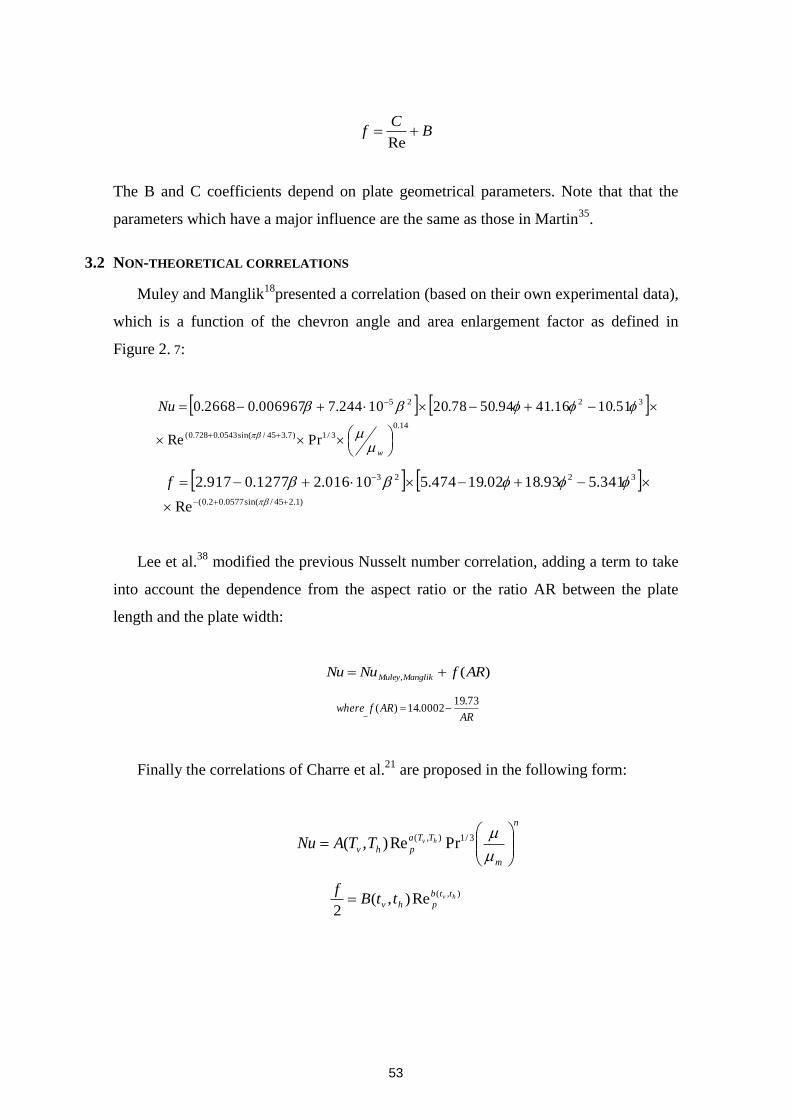
53
BC
f Re
The B and C coefficients depend on plate geometrical parameters. Note that that the
parameters which have a major influence are the same as those in Martin35
.
3.2 NON-THEORETICAL CORRELATIONS
Muley and Manglik18
presented a correlation (based on their own experimental data),
which is a function of the chevron angle and area enlargement factor as defined in
Figure 2. 7:
14.0
3/1)7.345/sin(0543.0728.0(
3225
PrRe
51.1016.4194.5078.2010244.7006967.02668.0
w
Nu
)1.245/sin(0577.02.0(
3223
Re
341.593.1802.19474.510016.21277.0917.2
f
Lee et al.38
modified the previous Nusselt number correlation, adding a term to take
into account the dependence from the aspect ratio or the ratio AR between the plate
length and the plate width:
)(, ARfNuNu ManglikMuley
ARARfwhere
73.190002.14)(
Finally the correlations of Charre et al.21
are proposed in the following form:
n
m
TTa
phvhvTTANu
3/1),(PrRe),(
),(Re),(
2hv ttb
phv ttBf
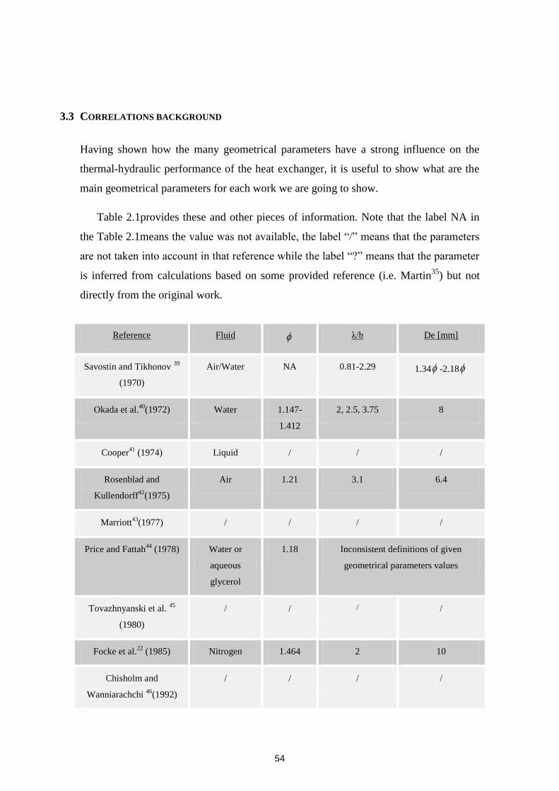
54
3.3 CORRELATIONS BACKGROUND
Having shown how the many geometrical parameters have a strong influence on the
thermal-hydraulic performance of the heat exchanger, it is useful to show what are the
main geometrical parameters for each work we are going to show.
Table 2.1provides these and other pieces of information. Note that the label NA in
the Table 2.1means the value was not available, the label “/” means that the parameters
are not taken into account in that reference while the label “?” means that the parameter
is inferred from calculations based on some provided reference (i.e. Martin35
) but not
directly from the original work.
Reference Fluid λ/b De [mm]
Savostin and Tikhonov 39
(1970)
Air/Water NA 0.81-2.29 1.34 -2.18
Okada et al.40
(1972) Water 1.147-
1.412
2, 2.5, 3.75 8
Cooper41
(1974) Liquid / / /
Rosenblad and
Kullendorff42
(1975)
Air 1.21 3.1 6.4
Marriott43
(1977) / / / /
Price and Fattah44
(1978) Water or
aqueous
glycerol
1.18 Inconsistent definitions of given
geometrical parameters values
Tovazhnyanski et al. 45
(1980)
/ / / /
Focke et al.22
(1985) Nitrogen 1.464 2 10
Chisholm and
Wanniarachchi 46
(1992)
/ / / /
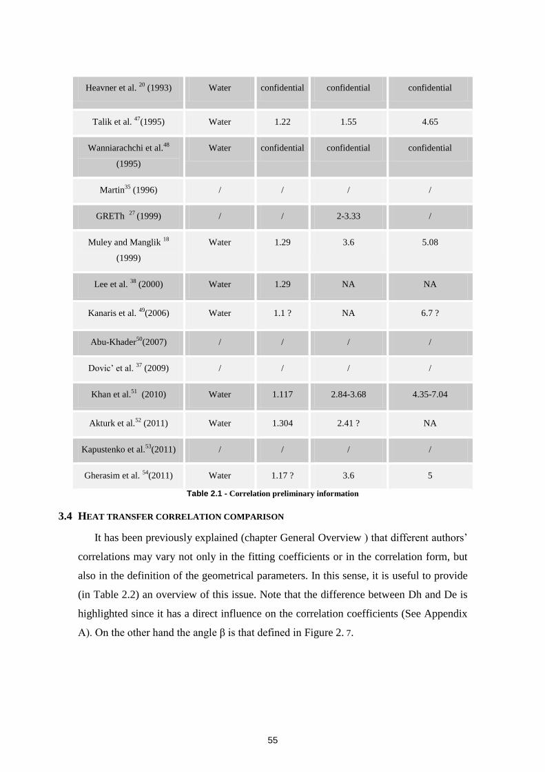
55
Heavner et al. 20
(1993) Water confidential confidential confidential
Talik et al. 47
(1995) Water 1.22 1.55 4.65
Wanniarachchi et al.48
(1995)
Water confidential confidential confidential
Martin35
(1996) / / / /
GRETh 27
(1999) / / 2-3.33 /
Muley and Manglik 18
(1999)
Water 1.29 3.6 5.08
Lee et al. 38
(2000) Water 1.29 NA NA
Kanaris et al. 49
(2006) Water 1.1 ? NA 6.7 ?
Abu-Khader50
(2007) / / / /
Dovic’ et al. 37
(2009) / / / /
Khan et al.51
(2010) Water 1.117 2.84-3.68 4.35-7.04
Akturk et al.52
(2011) Water 1.304 2.41 ? NA
Kapustenko et al.53
(2011) / / / /
Gherasim et al. 54
(2011) Water 1.17 ? 3.6 5
Table 2.1 - Correlation preliminary information
3.4 HEAT TRANSFER CORRELATION COMPARISON
It has been previously explained (chapter General Overview ) that different authors’
correlations may vary not only in the fitting coefficients or in the correlation form, but
also in the definition of the geometrical parameters. In this sense, it is useful to provide
(in Table 2.2) an overview of this issue. Note that the difference between Dh and De is
highlighted since it has a direct influence on the correlation coefficients (See Appendix
A). On the other hand the angle β is that defined in Figure 2. 7.
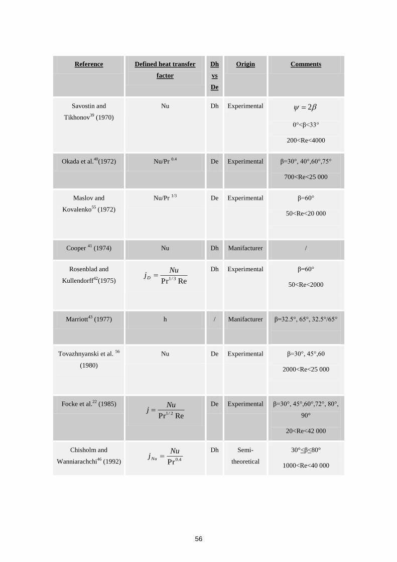
56
Reference Defined heat transfer
factor
Dh
vs
De
Origin Comments
Savostin and
Tikhonov39
(1970)
Nu Dh Experimental 2
0°<β<33°
200<Re<4000
Okada et al.40
(1972) Nu/Pr 0.4
De Experimental β=30°, 40°,60°,75°
700<Re<25 000
Maslov and
Kovalenko55
(1972)
Nu/Pr 1/3
De Experimental β=60°
50<Re<20 000
Cooper 41
(1974) Nu Dh Manifacturer /
Rosenblad and
Kullendorff42
(1975) RePr 3/1
NujD
Dh Experimental β=60°
50<Re<2000
Marriott43
(1977) h / Manifacturer β=32.5°, 65°, 32.5°/65°
Tovazhnyanski et al. 56
(1980)
Nu De Experimental β=30°, 45°,60
2000<Re<25 000
Focke et al.22
(1985)
RePr 2/1
Nuj
De Experimental β=30°, 45°,60°,72°, 80°,
90°
20<Re<42 000
Chisholm and
Wanniarachchi46
(1992) 4.0Pr
NujNu
Dh Semi-
theoretical
30°<β<80°
1000<Re<40 000
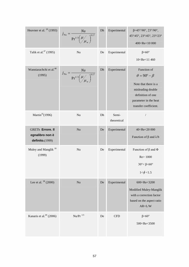
57
Heavner et al. 20
(1993)
17.0
3/1Pr
w
Nu
Nuj
Dh Experimental β=45°/90°, 23°/90°,
45°/45°, 23°/45°, 23°/23°
400<Re<10 000
Talik et al.47
(1995) Nu De Experimental β=60°
10<Re<11 460
Wanniarachchi et al.48
(1995) 17.0
3/1Pr
w
Nu
Nuj
Dh Experimental Function of
90
Note that there is a
misleading double
definition of one
parameter in the heat
transfer coefficient.
Martin35
(1996) Nu Dh Semi-
theoretical
/
GRETh Errore. Il
egnalibro non è
definito.(1999)
Nu De Experimental 40<Re<20 000
Function of β and λ/b
Muley and Manglik 18
(1999)
Nu De Experimental Function of β and Φ
Re> 1000
30°< β<60°
1< <1.5
Lee et al. 38
(2000) Nu De Experimental 600<Re<3200
Modified Muley-Manglik
with a correction factor
based on the aspect ratio
AR=L/W
Kanaris et al.49
(2006) Nu/Pr 1/3
De CFD β=60°
500<Re<3500
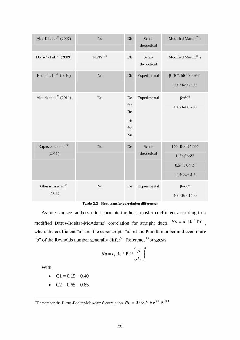
58
Abu-Khader50
(2007) Nu Dh Semi-
theoretical
Modified Martin35
’s
Dovic’ et al. 37
(2009) Nu/Pr 1/3
Dh Semi-
theoretical
Modified Martin35
’s
Khan et al. 51
(2010) Nu Dh Experimental β=30°, 60°, 30°/60°
500<Re<2500
Akturk et al.52
(2011) Nu De
for
Re
Dh
for
Nu
Experimental β=60°
450<Re<5250
Kapustenko et al.53
(2011)
Nu De Semi-
theoretical
100<Re< 25 000
14°< β<65°
0.5<b/λ<1.5
1.14< Φ <1.5
Gherasim et al.54
(2011)
Nu De Experimental β=60°
400<Re<1400
Table 2.2 - Heat transfer correlation differences
As one can see, authors often correlate the heat transfer coefficient according to a
modified Dittus-Boelter-McAdams’ correlation for straight ducts PrRebaNu ,
where the coefficient “a” and the superscripts “α” of the Prandtl number and even more
“b” of the Reynolds number generally differVI
. Reference13
suggests:
n
w
cccNu
32 PrRe1
With:
C1 = 0.15 – 0.40
C2 = 0.65 – 0.85
VI
Remember the Dittus-Boelter-McAdams’ correlation 4.08.0 PrRe022.0 Nu
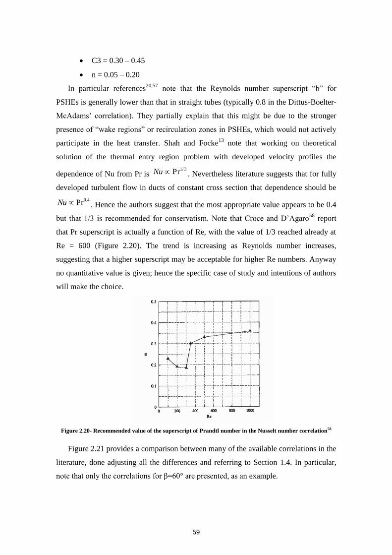
59
C3 = 0.30 – 0.45
n = 0.05 – 0.20
In particular references20,57
note that the Reynolds number superscript “b” for
PSHEs is generally lower than that in straight tubes (typically 0.8 in the Dittus-Boelter-
McAdams’ correlation). They partially explain that this might be due to the stronger
presence of “wake regions” or recirculation zones in PSHEs, which would not actively
participate in the heat transfer. Shah and Focke13
note that working on theoretical
solution of the thermal entry region problem with developed velocity profiles the
dependence of Nu from Pr is 3/1PrNu . Nevertheless literature suggests that for fully
developed turbulent flow in ducts of constant cross section that dependence should be
4.0PrNu . Hence the authors suggest that the most appropriate value appears to be 0.4
but that 1/3 is recommended for conservatism. Note that Croce and D’Agaro58
report
that Pr superscript is actually a function of Re, with the value of 1/3 reached already at
Re = 600 (Figure 2.20). The trend is increasing as Reynolds number increases,
suggesting that a higher superscript may be acceptable for higher Re numbers. Anyway
no quantitative value is given; hence the specific case of study and intentions of authors
will make the choice.
Figure 2.20- Recommended value of the superscript of Prandtl number in the Nusselt number correlation58
Figure 2.21 provides a comparison between many of the available correlations in the
literature, done adjusting all the differences and referring to Section 1.4. In particular,
note that only the correlations for β=60° are presented, as an example.
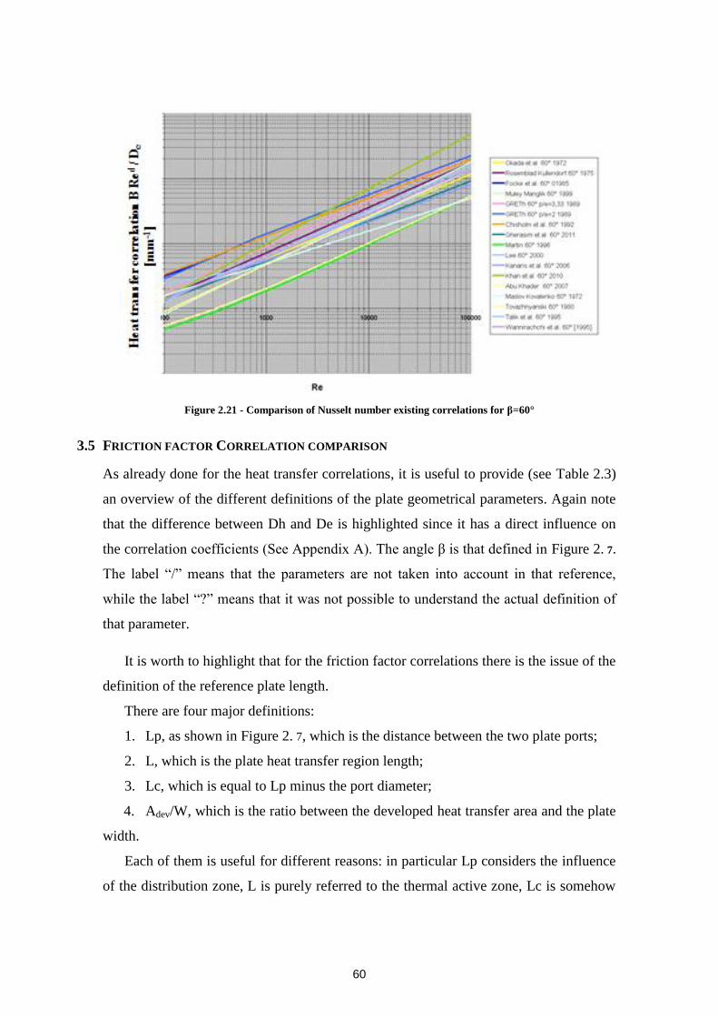
60
Figure 2.21 - Comparison of Nusselt number existing correlations for β=60°
3.5 FRICTION FACTOR CORRELATION COMPARISON
As already done for the heat transfer correlations, it is useful to provide (see Table 2.3)
an overview of the different definitions of the plate geometrical parameters. Again note
that the difference between Dh and De is highlighted since it has a direct influence on
the correlation coefficients (See Appendix A). The angle β is that defined in Figure 2. 7.
The label “/” means that the parameters are not taken into account in that reference,
while the label “?” means that it was not possible to understand the actual definition of
that parameter.
It is worth to highlight that for the friction factor correlations there is the issue of the
definition of the reference plate length.
There are four major definitions:
1. Lp, as shown in Figure 2. 7, which is the distance between the two plate ports;
2. L, which is the plate heat transfer region length;
3. Lc, which is equal to Lp minus the port diameter;
4. Adev/W, which is the ratio between the developed heat transfer area and the plate
width.
Each of them is useful for different reasons: in particular Lp considers the influence
of the distribution zone, L is purely referred to the thermal active zone, Lc is somehow
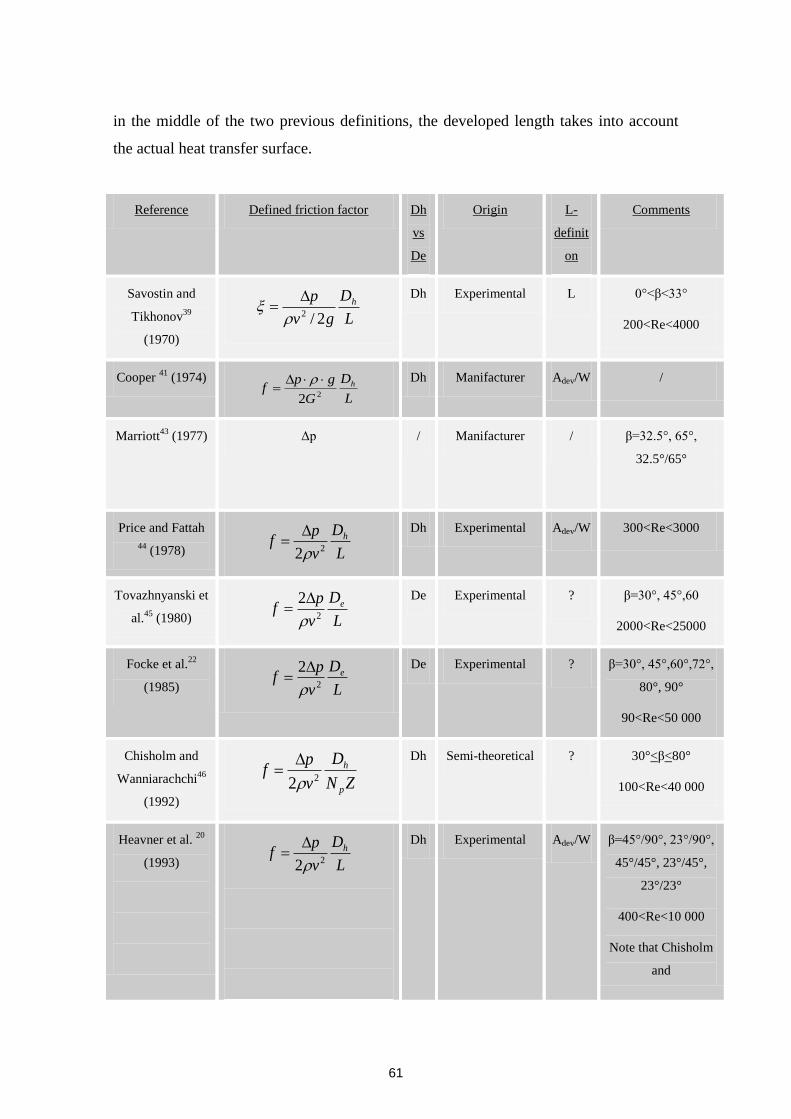
61
in the middle of the two previous definitions, the developed length takes into account
the actual heat transfer surface.
Reference Defined friction factor Dh
vs
De
Origin L-
definit
on
Comments
Savostin and
Tikhonov39
(1970)
L
D
gv
p h
2/2
Dh Experimental L 0°<β<33°
200<Re<4000
Cooper 41
(1974)
L
D
G
gpf h
22
Dh Manifacturer Adev/W /
Marriott43
(1977) Δp / Manifacturer / β=32.5°, 65°,
32.5°/65°
Price and Fattah
44 (1978) L
D
v
pf h
22
Dh Experimental Adev/W 300<Re<3000
Tovazhnyanski et
al.45
(1980) L
D
v
pf e
2
2
De Experimental ? β=30°, 45°,60
2000<Re<25000
Focke et al.22
(1985) L
D
v
pf e
2
2
De Experimental ? β=30°, 45°,60°,72°,
80°, 90°
90<Re<50 000
Chisholm and
Wanniarachchi46
(1992)
ZN
D
v
pf
p
h
22
Dh Semi-theoretical ? 30°<β<80°
100<Re<40 000
Heavner et al. 20
(1993)
L
D
v
pf h
22
Dh Experimental Adev/W β=45°/90°, 23°/90°,
45°/45°, 23°/45°,
23°/23°
400<Re<10 000
Note that Chisholm
and
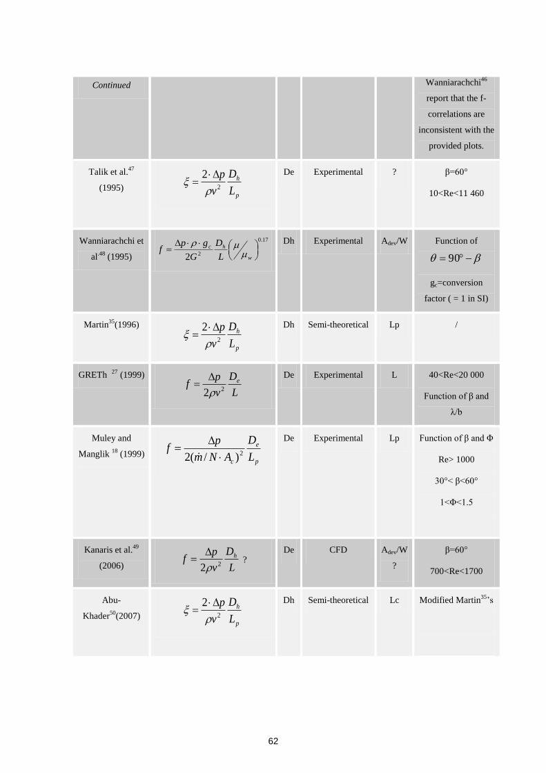
62
Continued Wanniarachchi46
report that the f-
correlations are
inconsistent with the
provided plots.
Talik et al.47
(1995) p
h
L
D
v
p2
2
De Experimental ? β=60°
10<Re<11 460
Wanniarachchi et
al.48
(1995)
17.0
22
w
hc
L
D
G
gpf
Dh Experimental Adev/W Function of
90
gc=conversion
factor ( = 1 in SI)
Martin35
(1996)
p
h
L
D
v
p2
2
Dh Semi-theoretical Lp /
GRETh 27 (1999)
L
D
v
pf e
22
De Experimental L 40<Re<20 000
Function of β and
λ/b
Muley and
Manglik 18
(1999) p
e
c L
D
ANm
pf
2)/(2
De Experimental Lp Function of β and Φ
Re> 1000
30°< β<60°
1<Φ<1.5
Kanaris et al.49
(2006) L
D
v
pf h
22
?
De CFD Adev/W
?
β=60°
700<Re<1700
Abu-
Khader50
(2007) p
h
L
D
v
p2
2
Dh Semi-theoretical Lc Modified Martin35
’s
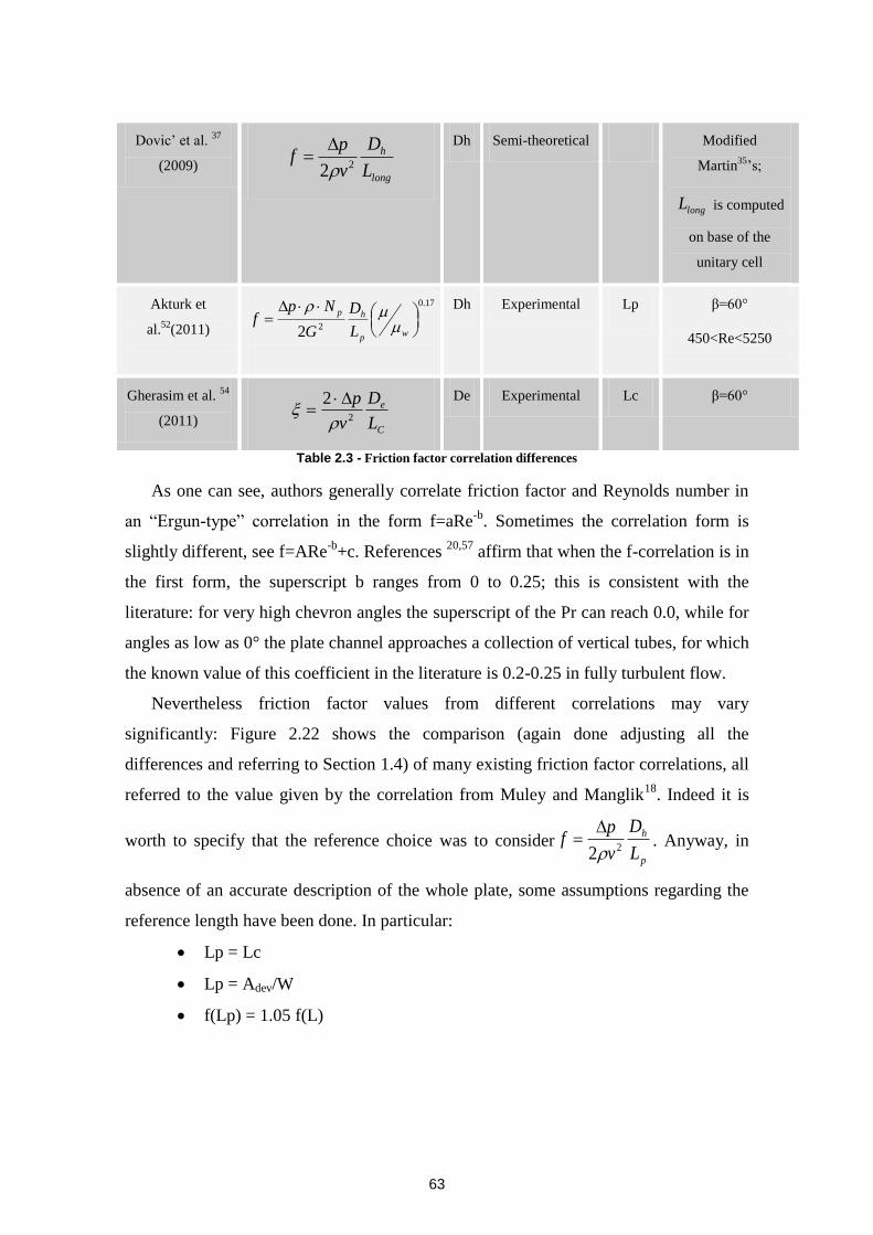
63
Dovic’ et al. 37
(2009) long
h
L
D
v
pf
22
Dh Semi-theoretical Modified
Martin35
’s;
longL is computed
on base of the
unitary cell
Akturk et
al.52
(2011)
17.0
22
wp
hp
L
D
G
Npf
Dh Experimental Lp β=60°
450<Re<5250
Gherasim et al. 54
(2011) C
e
L
D
v
p2
2
De Experimental Lc β=60°
Table 2.3 - Friction factor correlation differences
As one can see, authors generally correlate friction factor and Reynolds number in
an “Ergun-type” correlation in the form f=aRe-b
. Sometimes the correlation form is
slightly different, see f=ARe-b
+c. References 20,57
affirm that when the f-correlation is in
the first form, the superscript b ranges from 0 to 0.25; this is consistent with the
literature: for very high chevron angles the superscript of the Pr can reach 0.0, while for
angles as low as 0° the plate channel approaches a collection of vertical tubes, for which
the known value of this coefficient in the literature is 0.2-0.25 in fully turbulent flow.
Nevertheless friction factor values from different correlations may vary
significantly: Figure 2.22 shows the comparison (again done adjusting all the
differences and referring to Section 1.4) of many existing friction factor correlations, all
referred to the value given by the correlation from Muley and Manglik18
. Indeed it is
worth to specify that the reference choice was to considerp
h
L
D
v
pf
22
. Anyway, in
absence of an accurate description of the whole plate, some assumptions regarding the
reference length have been done. In particular:
Lp = Lc
Lp = Adev/W
f(Lp) = 1.05 f(L)
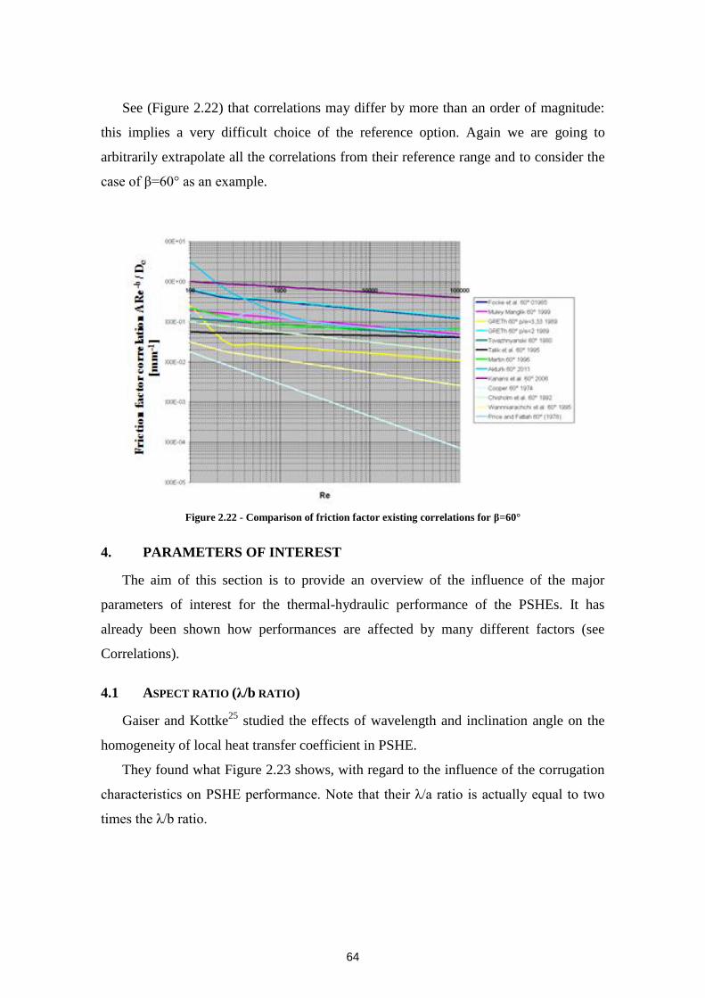
64
See (Figure 2.22) that correlations may differ by more than an order of magnitude:
this implies a very difficult choice of the reference option. Again we are going to
arbitrarily extrapolate all the correlations from their reference range and to consider the
case of β=60° as an example.
Figure 2.22 - Comparison of friction factor existing correlations for β=60°
4. PARAMETERS OF INTEREST
The aim of this section is to provide an overview of the influence of the major
parameters of interest for the thermal-hydraulic performance of the PSHEs. It has
already been shown how performances are affected by many different factors (see
Correlations).
4.1 ASPECT RATIO (λ/b RATIO)
Gaiser and Kottke25
studied the effects of wavelength and inclination angle on the
homogeneity of local heat transfer coefficient in PSHE.
They found what Figure 2.23 shows, with regard to the influence of the corrugation
characteristics on PSHE performance. Note that their λ/a ratio is actually equal to two
times the λ/b ratio.
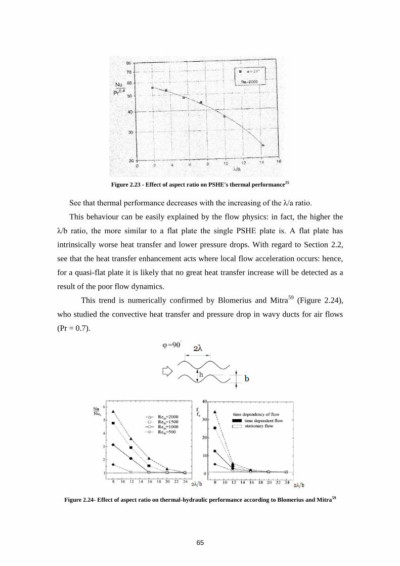
65
Figure 2.23 - Effect of aspect ratio on PSHE's thermal performance25
See that thermal performance decreases with the increasing of the λ/a ratio.
This behaviour can be easily explained by the flow physics: in fact, the higher the
λ/b ratio, the more similar to a flat plate the single PSHE plate is. A flat plate has
intrinsically worse heat transfer and lower pressure drops. With regard to Section 2.2,
see that the heat transfer enhancement acts where local flow acceleration occurs: hence,
for a quasi-flat plate it is likely that no great heat transfer increase will be detected as a
result of the poor flow dynamics.
This trend is numerically confirmed by Blomerius and Mitra59
(Figure 2.24),
who studied the convective heat transfer and pressure drop in wavy ducts for air flows
(Pr = 0.7).
Figure 2.24- Effect of aspect ratio on thermal-hydraulic performance according to Blomerius and Mitra59
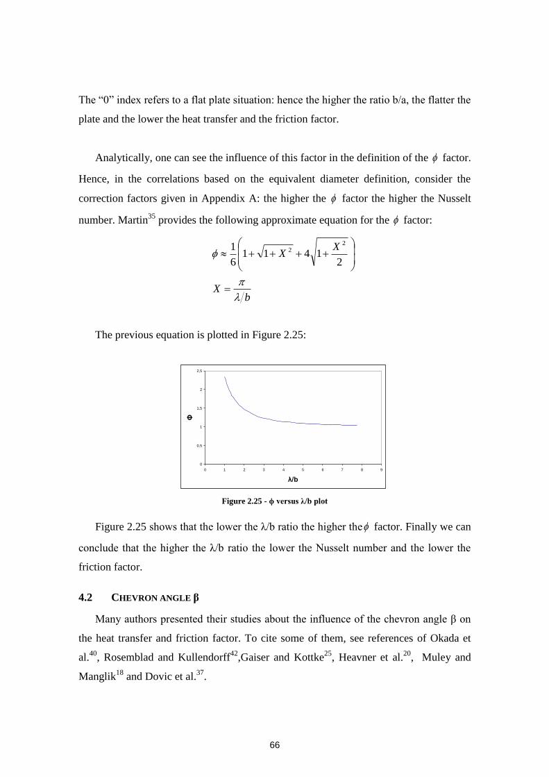
66
The “0” index refers to a flat plate situation: hence the higher the ratio b/a, the flatter the
plate and the lower the heat transfer and the friction factor.
Analytically, one can see the influence of this factor in the definition of the factor.
Hence, in the correlations based on the equivalent diameter definition, consider the
correction factors given in Appendix A: the higher the factor the higher the Nusselt
number. Martin35
provides the following approximate equation for the factor:
bX
XX
21411
6
1 22
The previous equation is plotted in Figure 2.25:
Figure 2.25 - ϕ versus λ/b plot
Figure 2.25 shows that the lower the λ/b ratio the higher the factor. Finally we can
conclude that the higher the λ/b ratio the lower the Nusselt number and the lower the
friction factor.
4.2 CHEVRON ANGLE β
Many authors presented their studies about the influence of the chevron angle β on
the heat transfer and friction factor. To cite some of them, see references of Okada et
al.40
, Rosemblad and Kullendorff42
,Gaiser and Kottke25
, Heavner et al.20
, Muley and
Manglik18
and Dovic et al.37
.
0
0,5
1
1,5
2
2,5
0 1 2 3 4 5 6 7 8 9
λ/b
Φ
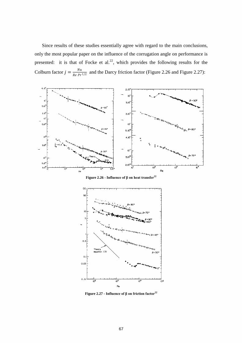
67
Since results of these studies essentially agree with regard to the main conclusions,
only the most popular paper on the influence of the corrugation angle on performance is
presented: it is that of Focke et al.22
, which provides the following results for the
Colburn factor 𝑗 =𝑁𝑢
𝑅𝑒 𝑃𝑟1/2 and the Darcy friction factor (Figure 2.26 and Figure 2.27):
Figure 2.26 - Influence of β on heat transfer22
Figure 2.27 - Influence of β on friction factor22

68
Increasing β (at constant Reynolds number) from 0° to 80° leads to pressure drop
increases of over 2.5 orders of magnitude, although heat transfer increases by a factor of
only 4 to10 times. Note that, while the heat transfer increases monotonically with the
chevron angle β, this is not the case for the friction factor, which is lower at β=90° than
80°. This is possibly explained by the fact that for β=90° a wavy channel is formed,
where no contact points and stream crossing occur. Indeed this are potentially the
phenomena that provide such a high friction factor value for β=80°. Anyway it is worth
to say that there is no general agreement whether this local maximum friction factor
value has to occur or not. However there is no doubt about the fact that an increased
chevron angle β provides, in the general case, higher heat transfer and pressure drops.
4.3 AREA ENLARGEMENT FACTOR
Muley and Manglik 18
highlight the influence of the area enlargement factor on the
heat transfer, as Figure 2.28 shows:
Figure 2.28 - Influence of the area enlargement factor 𝝓 on heat transfer18
It is straightforward to understand that the larger the area enlargement factor 𝜙, the
larger the heat transfer area (projected area being fixed). Hence the heat transfer is
improved, but also pressure drop will be higher. However, note that the area
enlargement factor is strictly related to the plate geometrical characteristics: hence it
somehow includes all the effects typically due to these plate geometrical parameters.
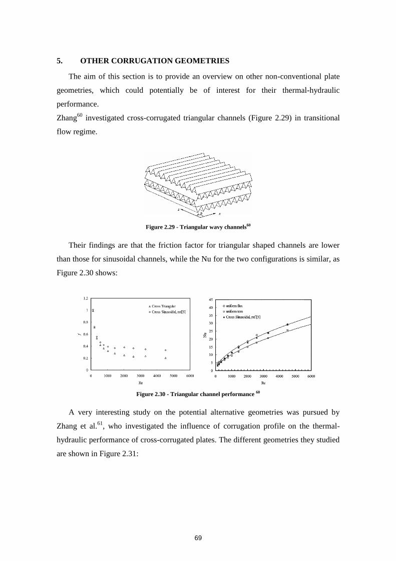
69
5. OTHER CORRUGATION GEOMETRIES
The aim of this section is to provide an overview on other non-conventional plate
geometries, which could potentially be of interest for their thermal-hydraulic
performance.
Zhang60
investigated cross-corrugated triangular channels (Figure 2.29) in transitional
flow regime.
Figure 2.29 - Triangular wavy channels60
Their findings are that the friction factor for triangular shaped channels are lower
than those for sinusoidal channels, while the Nu for the two configurations is similar, as
Figure 2.30 shows:
Figure 2.30 - Triangular channel performance 60
A very interesting study on the potential alternative geometries was pursued by
Zhang et al.61
, who investigated the influence of corrugation profile on the thermal-
hydraulic performance of cross-corrugated plates. The different geometries they studied
are shown in Figure 2.31:
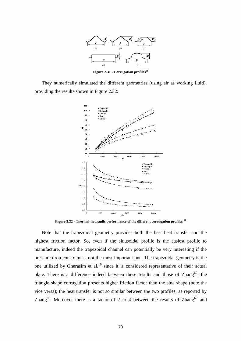
70
Figure 2.31 - Corrugation profiles61
They numerically simulated the different geometries (using air as working fluid),
providing the results shown in Figure 2.32:
Figure 2.32 - Thermal-hydraulic performance of the different corrugation profiles 61
Note that the trapezoidal geometry provides both the best heat transfer and the
highest friction factor. So, even if the sinusoidal profile is the easiest profile to
manufacture, indeed the trapezoidal channel can potentially be very interesting if the
pressure drop constraint is not the most important one. The trapezoidal geometry is the
one utilized by Gherasim et al.19
since it is considered representative of their actual
plate. There is a difference indeed between these results and those of Zhang60
: the
triangle shape corrugation presents higher friction factor than the sine shape (note the
vice versa); the heat transfer is not so similar between the two profiles, as reported by
Zhang60
. Moreover there is a factor of 2 to 4 between the results of Zhang60
and
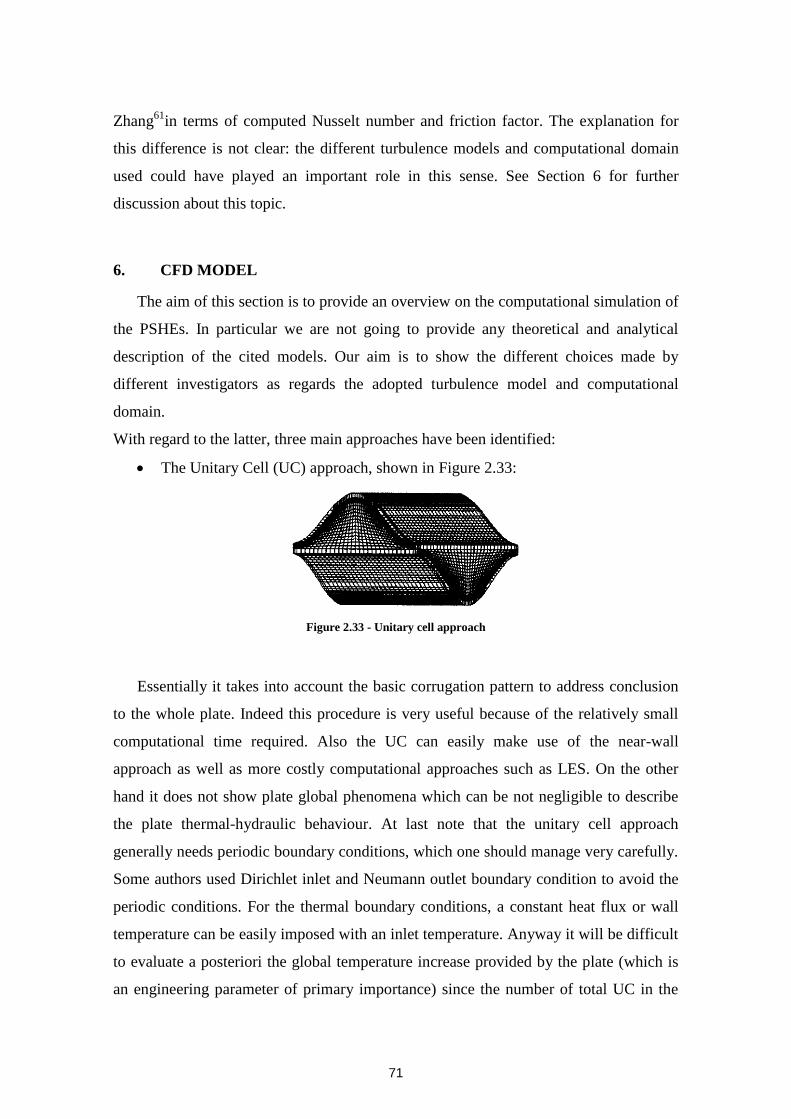
71
Zhang61
in terms of computed Nusselt number and friction factor. The explanation for
this difference is not clear: the different turbulence models and computational domain
used could have played an important role in this sense. See Section 6 for further
discussion about this topic.
6. CFD MODEL
The aim of this section is to provide an overview on the computational simulation of
the PSHEs. In particular we are not going to provide any theoretical and analytical
description of the cited models. Our aim is to show the different choices made by
different investigators as regards the adopted turbulence model and computational
domain.
With regard to the latter, three main approaches have been identified:
The Unitary Cell (UC) approach, shown in Figure 2.33:
Figure 2.33 - Unitary cell approach
Essentially it takes into account the basic corrugation pattern to address conclusion
to the whole plate. Indeed this procedure is very useful because of the relatively small
computational time required. Also the UC can easily make use of the near-wall
approach as well as more costly computational approaches such as LES. On the other
hand it does not show plate global phenomena which can be not negligible to describe
the plate thermal-hydraulic behaviour. At last note that the unitary cell approach
generally needs periodic boundary conditions, which one should manage very carefully.
Some authors used Dirichlet inlet and Neumann outlet boundary condition to avoid the
periodic conditions. For the thermal boundary conditions, a constant heat flux or wall
temperature can be easily imposed with an inlet temperature. Anyway it will be difficult
to evaluate a posteriori the global temperature increase provided by the plate (which is
an engineering parameter of primary importance) since the number of total UC in the
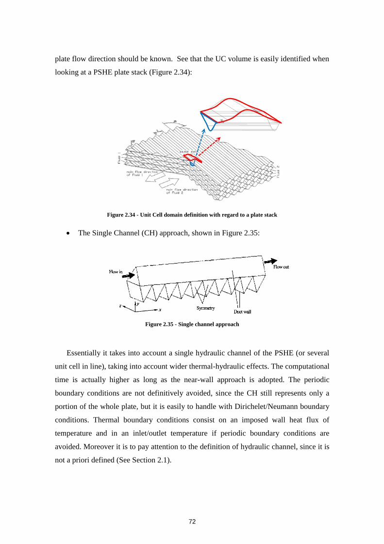
72
plate flow direction should be known. See that the UC volume is easily identified when
looking at a PSHE plate stack (Figure 2.34):
Figure 2.34 - Unit Cell domain definition with regard to a plate stack
The Single Channel (CH) approach, shown in Figure 2.35:
Figure 2.35 - Single channel approach
Essentially it takes into account a single hydraulic channel of the PSHE (or several
unit cell in line), taking into account wider thermal-hydraulic effects. The computational
time is actually higher as long as the near-wall approach is adopted. The periodic
boundary conditions are not definitively avoided, since the CH still represents only a
portion of the whole plate, but it is easily to handle with Dirichelet/Neumann boundary
conditions. Thermal boundary conditions consist on an imposed wall heat flux of
temperature and in an inlet/outlet temperature if periodic boundary conditions are
avoided. Moreover it is to pay attention to the definition of hydraulic channel, since it is
not a priori defined (See Section 2.1).

73
The whole plate (PL) approach, shown in Figure 2.36:
Figure 2.36 - Whole plate approach
Essentially it models the whole plate not using any sub-domain. Of course this is the
more realistic type of simulation; nevertheless its needed computational time can be
extremely high and the wall-function approach is necessary. On the other hand the
thermal-hydraulic boundary conditions can be as precise as desired.
Table 2.4 provides an overview of the various references on this topic.
Reference Domain Turbulence
Model
Used/Suggested
Fluid Corrug.
Type
Re #
range
Near-wall
Treatment
Ciofalo et
al.62
(1996)
UC Smagorinsky-
Lily LES
Lam-Bremhorst
Low Re k-ε
Air Sinusoidal 500-
7000
Low-Re with
damping
function for
the k- ε model
Smagorinsky-
Lily subgrid
model
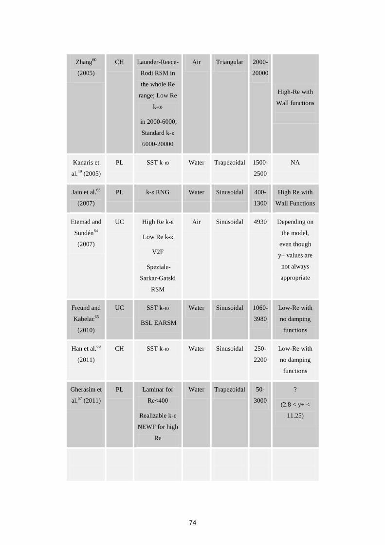
74
Zhang60
(2005)
CH Launder-Reece-
Rodi RSM in
the whole Re
range; Low Re
k-ω
in 2000-6000;
Standard k-ε
6000-20000
Air Triangular 2000-
20000
High-Re with
Wall functions
Kanaris et
al.49
(2005)
PL SST k-ω Water Trapezoidal 1500-
2500
NA
Jain et al.63
(2007)
PL k-ε RNG Water Sinusoidal 400-
1300
High Re with
Wall Functions
Etemad and
Sundén64
(2007)
UC High Re k-ε
Low Re k-ε
V2F
Speziale-
Sarkar-Gatski
RSM
Air Sinusoidal 4930 Depending on
the model,
even though
y+ values are
not always
appropriate
Freund and
Kabelac65
(2010)
UC SST k-ω
BSL EARSM
Water Sinusoidal 1060-
3980
Low-Re with
no damping
functions
Han et al.66
(2011)
CH SST k-ω Water Sinusoidal 250-
2200
Low-Re with
no damping
functions
Gherasim et
al.67
(2011)
PL Laminar for
Re<400
Realizable k-ε
NEWF for high
Re
Water Trapezoidal 50-
3000
?
(2.8 < y+ <
11.25)
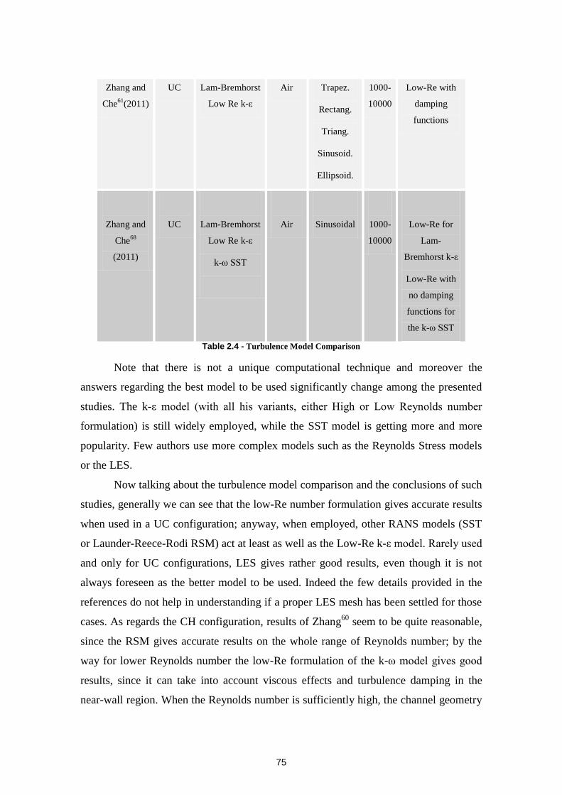
75
Zhang and
Che61
(2011)
UC Lam-Bremhorst
Low Re k-ε
Air Trapez.
Rectang.
Triang.
Sinusoid.
Ellipsoid.
1000-
10000
Low-Re with
damping
functions
Zhang and
Che68
(2011)
UC
Lam-Bremhorst
Low Re k-ε
k-ω SST
Air
Sinusoidal
1000-
10000
Low-Re for
Lam-
Bremhorst k-ε
Low-Re with
no damping
functions for
the k-ω SST
Table 2.4 - Turbulence Model Comparison
Note that there is not a unique computational technique and moreover the
answers regarding the best model to be used significantly change among the presented
studies. The k-ε model (with all his variants, either High or Low Reynolds number
formulation) is still widely employed, while the SST model is getting more and more
popularity. Few authors use more complex models such as the Reynolds Stress models
or the LES.
Now talking about the turbulence model comparison and the conclusions of such
studies, generally we can see that the low-Re number formulation gives accurate results
when used in a UC configuration; anyway, when employed, other RANS models (SST
or Launder-Reece-Rodi RSM) act at least as well as the Low-Re k-ε model. Rarely used
and only for UC configurations, LES gives rather good results, even though it is not
always foreseen as the better model to be used. Indeed the few details provided in the
references do not help in understanding if a proper LES mesh has been settled for those
cases. As regards the CH configuration, results of Zhang60
seem to be quite reasonable,
since the RSM gives accurate results on the whole range of Reynolds number; by the
way for lower Reynolds number the low-Re formulation of the k-ω model gives good
results, since it can take into account viscous effects and turbulence damping in the
near-wall region. When the Reynolds number is sufficiently high, the channel geometry
76
configuration can model macroscopic effects when viscous contribution becomes small:
hence a High-Re k-ε model predicts the good trends. Note that the k-ε model has been
developed as a High-Re model, therefore it is not surprising that it can work pretty well
in situations where wall viscous effects are significantly smaller than the core-fluid
region phenomena.
A similar conclusion can be deduced looking at the suggestions of Gherasim et
al.67
for a PL geometry: in this case the wall effects are so negligible that a simple High-
Re k-ε model gives sufficiently accurate results. Note that, due to the complexity of the
in-plate flow, a non-traditional wall function approach (i.e. the Non-Equilibrium Wall
Functions - NEWF) are suggested, trying to better describe the wall effects than the
Standard Wall Functions. In fact, the latter have been developed for a uniform pressure
gradient flow, which is not the case for the flow inside a PSHE, where continuous
boundary layer separation and reattachment occur, as clearly shown in Section 2.1.
However, is should be pointed out that the plate mesh for PL geometries seems to be
excessively coarse, especially in the work of Jain et al.69
: the number of total cells in
their study is around 880.000 for a plate of L=357 mm. For a similar plate length
(L=352 mm), Kanaris et al.49
use 2.6 million cells, which seem to be a more reasonable
value, also considering the use of wall functionsVII
.
VII
RANS modelling is actually the only doable way to model a whole plate. Consider that, for a Wall-
modelled LES calculation of the whole plate (i.e. L=0.352 m, W=0.123 m (plate width) and 2b=0.024 m
as in Kanaris et al.49
), a total number of cells of about 35 billion would be necessary! In fact, for a
reference𝑅𝑒𝐷𝑒 = 50000, 𝑅𝑒𝐿 = 𝑅𝑒𝐷𝑒 ∙𝐿
𝐷𝑒= 50 000 ∙
0.352
0.024= 733 000. Choi and Moin (“Grid-point
requirements for large eddy simulation: Chapman’s estimates revisited”, Center for Turbulence Research
- Annual Research Briefs 2011, pp.31-36) propose the following expression to determine the number of
grid points for a wall-modelled LES calculation:
𝑁 = 54.7𝐿𝑧
𝐿𝑥
𝑛𝑥𝑛𝑦𝑛𝑧𝑅𝑒𝐿2/7
𝑅𝑒𝐿
𝑅𝑒𝑥0
5/7
− 1
Where 𝑅𝑒𝑥0 is the Reynolds number based on the boundary layer development length. If we assume x0<<
L and hence 𝑅𝑒𝑥0≪ 𝑅𝑒𝐿 we obtain:
𝑁 ≈ 54.7𝐿𝑧
𝐿𝑥
𝑛𝑥𝑛𝑦𝑛𝑧𝑅𝑒𝐿
According to Chapman (“Computational aerodynamics development and outlook”, AIAA J. 17 (12),
1293–1313, 1979), the cell dimension ΔxΔyΔz should satisfy the following relations:
∆𝑥 =𝛿
𝑛𝑥
, ∆𝑦 =𝛿
𝑛𝑦
, ∆𝑧 =𝛿
𝑛𝑧
With nx= 10, ny= 25, nz = 10. Hence we can find the already mention total number of cell of around 35
billion cells as:
𝑁 ≈ 54.7𝐿𝑧
𝐿𝑥
𝑛𝑥𝑛𝑦𝑛𝑧𝑅𝑒𝐿 = 54.7 ∙0.123
0.352∙ 10 ∙ 25 ∙ 10 ∙ 733 000 ≈ 35 𝑏𝑖𝑙𝑙𝑖𝑜𝑛 𝑐𝑒𝑙𝑙𝑠!
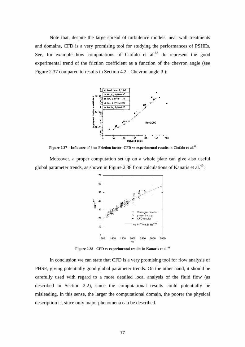
77
Note that, despite the large spread of turbulence models, near wall treatments
and domains, CFD is a very promising tool for studying the performances of PSHEs.
See, for example how computations of Ciofalo et al.62
do represent the good
experimental trend of the friction coefficient as a function of the chevron angle (see
Figure 2.37 compared to results in Section 4.2 - Chevron angle β ):
Figure 2.37 – Influence of β on Friction factor: CFD vs experimental results in Ciofalo et al.62
Moreover, a proper computation set up on a whole plate can give also useful
global parameter trends, as shown in Figure 2.38 from calculations of Kanaris et al.49
:
Figure 2.38 - CFD vs experimental results in Kanaris et al.49
In conclusion we can state that CFD is a very promising tool for flow analysis of
PHSE, giving potentially good global parameter trends. On the other hand, it should be
carefully used with regard to a more detailed local analysis of the fluid flow (as
described in Section 2.2), since the computational results could potentially be
misleading. In this sense, the larger the computational domain, the poorer the physical
description is, since only major phenomena can be described.
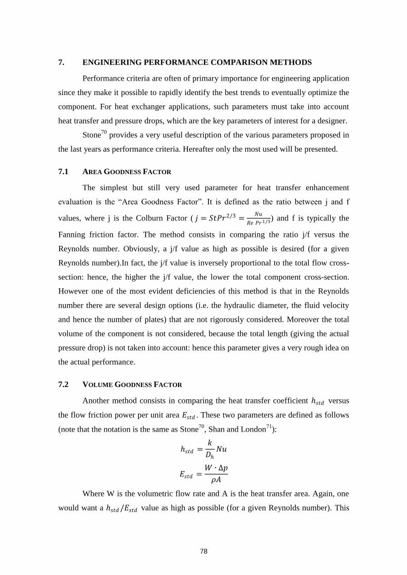
78
7. ENGINEERING PERFORMANCE COMPARISON METHODS
Performance criteria are often of primary importance for engineering application
since they make it possible to rapidly identify the best trends to eventually optimize the
component. For heat exchanger applications, such parameters must take into account
heat transfer and pressure drops, which are the key parameters of interest for a designer.
Stone70
provides a very useful description of the various parameters proposed in
the last years as performance criteria. Hereafter only the most used will be presented.
7.1 AREA GOODNESS FACTOR
The simplest but still very used parameter for heat transfer enhancement
evaluation is the “Area Goodness Factor”. It is defined as the ratio between j and f
values, where j is the Colburn Factor ( 𝑗 = 𝑆𝑡𝑃𝑟2/3 =𝑁𝑢
𝑅𝑒 𝑃𝑟1/3) and f is typically the
Fanning friction factor. The method consists in comparing the ratio j/f versus the
Reynolds number. Obviously, a j/f value as high as possible is desired (for a given
Reynolds number).In fact, the j/f value is inversely proportional to the total flow cross-
section: hence, the higher the j/f value, the lower the total component cross-section.
However one of the most evident deficiencies of this method is that in the Reynolds
number there are several design options (i.e. the hydraulic diameter, the fluid velocity
and hence the number of plates) that are not rigorously considered. Moreover the total
volume of the component is not considered, because the total length (giving the actual
pressure drop) is not taken into account: hence this parameter gives a very rough idea on
the actual performance.
7.2 VOLUME GOODNESS FACTOR
Another method consists in comparing the heat transfer coefficient 𝑠𝑡𝑑 versus
the flow friction power per unit area 𝐸𝑠𝑡𝑑 . These two parameters are defined as follows
(note that the notation is the same as Stone70
, Shan and London71
):
𝑠𝑡𝑑 =𝑘
𝐷𝑁𝑢
𝐸𝑠𝑡𝑑 =𝑊 ∙ ∆𝑝
𝜌𝐴
Where W is the volumetric flow rate and A is the heat transfer area. Again, one
would want a 𝑠𝑡𝑑 /𝐸𝑠𝑡𝑑 value as high as possible (for a given Reynolds number). This
79
would mean, for example, that for a given pressure drop and heat transfer coefficient the
heat transfer area for the better geometryis higher. Note that there is a direct link
between heat transfer area and volume of one side of a heat exchanger, i.e. through the
generalized hydraulic diameter definition 𝐷 =4𝑉
𝐴 and hence 𝐴 ∝
𝑉
𝐷. A higher heat
transfer area does not directly result in a smaller volume: a higher heat transfer surface
could be given either by a smaller Dh for the same volume or by a higher volume, that is
not desirable for compactness. Therefore even though the presence of the pumping
power somehow makes this method more interesting than the Area Goodness factor,
still their lacks are evident when dealing with the actual volume and compactness of the
component.
7.3 PERFORMANCE PARAMETERS
Soland and al.72
proposed methods consisting in comparing two performance
parameters, defined as follows:
Heat Transfer Performance Factor 𝐽 = 𝑗𝑅𝑒;
Pumping power factor 𝐹 = 𝑓𝑅𝑒3.
This method prevents to depend anymore on the Reynolds number of the actual design
application. In fact it will be shown that these two parameters are strictly related to heat
transfer coefficient times the surface to volume ratio and to the pumping power per unit
volume respectively. Nevertheless, it will also be shown that the method is still strictly
valid for two applications with the same hydraulic diameter.
In fact, Soland and al.72
propose another method, which is based on the
comparison of the following parameters:
Heat transfer coefficient times surface to volume ratio:
𝑠𝑡𝑑
𝐴
𝑉≈
𝑘
𝐷𝑁𝑢
𝐷2
𝐷3 ≈
𝑘
𝐷𝑗𝑅𝑒𝑃𝑟1/3
𝐷2
𝐷3 ∝
𝑗𝑅𝑒
𝐷2 ≈
𝐽
𝐷2
Pumping power per unit volume:
𝑊∆𝑝
𝜌𝑉≈
𝑆 ∙ 𝑉 ∙ 0.5 ∙ 𝑉2 ∗ 𝐿 ∗ 𝑓
𝐷 ∙ 𝐷3 ∝
𝑓𝑅𝑒3
𝐷4 ≈
𝐹
𝐷4
As already mentioned, this method prevents any problem due to the hydraulic
diameter selection, because it is identical to the previous one if the Dh is the same for

80
the different geometries to compare. A priori, this method could be the best prediction
regarding the comparison of different heat transfer geometries. Nevertheless see that
the use of the approximation 𝑉 = 𝐷3 does not correspond to the actual component
geometry. In particular, it seems not to be correct the use of the hydraulic diameter for
the main flow direction, which is the dimension influencing pressure drops. Hence the
formulation of the volume of the component should be better modified to properly take
into account geometry of the heat exchanger.
8. CONCLUSIONS
A technical bibliographic review on compact plate heat exchangers has been
presented.
Among the various types of compact heat exchangers (i.e. the Printed Circuit
Heat Exchangers - PCHE, the Plate-Fin Heat Exchangers-PFHE and the Plate Stamped
Heat Exchangers-PSHE), an extensive bibliographic research has been done on the
PSHEs in order to better understand the thermal-hydraulic behaviour of such
components.
The Plate Stamped Heat Exchangers PSHEs basically consist in a number of
single plates of various shape stacked to form a frame. Using plates let the designer
have many flexible alternatives depending on the specific needs. The stacked plates
touch themselves in many contact points: this configuration gives some mechanical
compression resistance, enhances heat transfer and decreases fouling through an
increased turbulence.
The most important geometrical characteristics regarding the PSHE chevron-
type plate geometry have been identified (see Section 1), in particular:
the “chevron angle” β, or the angle between the corrugation and the main flow
direction;
the “area enlargement factor Φ, or the ratio between the actual plate surface and
the projected surface (which is calculated as the plate were a fleet rectangular
plate);
the wavelength of surface corrugation λ, or the distance between two
consecutive corrugation peaks;
the corrugation depth b, or the amplitude of the single plate corrugation;
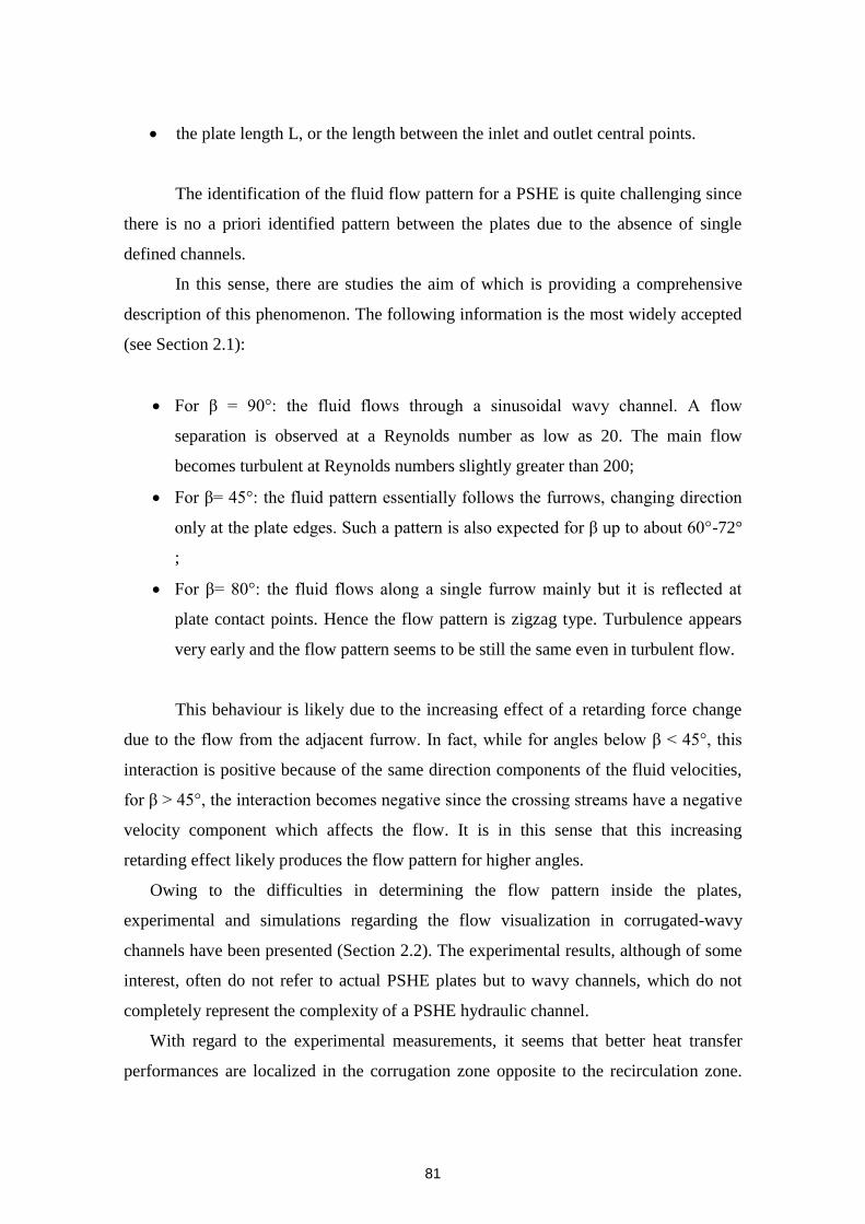
81
the plate length L, or the length between the inlet and outlet central points.
The identification of the fluid flow pattern for a PSHE is quite challenging since
there is no a priori identified pattern between the plates due to the absence of single
defined channels.
In this sense, there are studies the aim of which is providing a comprehensive
description of this phenomenon. The following information is the most widely accepted
(see Section 2.1):
For β = 90°: the fluid flows through a sinusoidal wavy channel. A flow
separation is observed at a Reynolds number as low as 20. The main flow
becomes turbulent at Reynolds numbers slightly greater than 200;
For β= 45°: the fluid pattern essentially follows the furrows, changing direction
only at the plate edges. Such a pattern is also expected for β up to about 60°-72°
;
For β= 80°: the fluid flows along a single furrow mainly but it is reflected at
plate contact points. Hence the flow pattern is zigzag type. Turbulence appears
very early and the flow pattern seems to be still the same even in turbulent flow.
This behaviour is likely due to the increasing effect of a retarding force change
due to the flow from the adjacent furrow. In fact, while for angles below β < 45°, this
interaction is positive because of the same direction components of the fluid velocities,
for β > 45°, the interaction becomes negative since the crossing streams have a negative
velocity component which affects the flow. It is in this sense that this increasing
retarding effect likely produces the flow pattern for higher angles.
Owing to the difficulties in determining the flow pattern inside the plates,
experimental and simulations regarding the flow visualization in corrugated-wavy
channels have been presented (Section 2.2). The experimental results, although of some
interest, often do not refer to actual PSHE plates but to wavy channels, which do not
completely represent the complexity of a PSHE hydraulic channel.
With regard to the experimental measurements, it seems that better heat transfer
performances are localized in the corrugation zone opposite to the recirculation zone.
82
Indeed one can note a localized flow acceleration, which directly influences the local
heat transfer; of course vice versa for the zone of recirculation in which the heat transfer
is poorer. Moreover it has been underlined that a 3-dimensional flow such as that of a
PSHE can enhance even more the heat transfer since there is no preferential direction
for the fluid flow, since the boundary layer is continuously attached and detached in all
directions. Pressure drops seem to be less sensitive to these flow characteristics,
depending much more on wall friction due to possible larger wetted surfaces in wavy
channels.
Then, a wide set of correlations for heat transfer and pressure drop has been
presented (see Section 3 - Correlations) based on semi-theoretical considerations or
experimental measurements. A large spread of data has been shown, which is likely due
to the very large range of Reynolds numbers and plate geometrical parameters of every
single case.
To better study these geometrical effects, an overview of the influence of plate
geometry on heat transfer and pressure drops has been presented (see Section 4),
showing that the aspect ratio as well as the chevron angle are major parameters of
interest for the designer.
Also various plate corrugations have been studied, (see Section 5) to verify if some
other corrugation presents better performances than the traditional ones (i.e. sinusoidal
corrugations).
Together with the experimental measurements, several computational studies have
been done to investigate the fluid flow inside the plates. Results depend both on the
computational domain and on the adopted model (see Section 6).
With regard to the computational domain, three main approaches have been identified:
1. The Unitary Cell approach;
2. The Single Channel approach;
3. The whole plate approach.
It is clear that the best turbulence model depends on the aim of the simulation and
on the computation capabilities of the available machines.
Finally, some engineering performance evaluation criteria have been presented,
trying to assess which one is potentially more useful to evaluate the compactness of
different geometries. This will be of primary importance to determine whether the final

83
goal of this PhD work (the heat transfer enhancement with pressure drop constraints in
compact plate heat exchanger) is accomplished or not.
9. ADOPTED STRATEGY FOR THE PRESENT WORK
9.1 INNOVATIVE GEOMETRY DESCRIPTION AND MOTIVATION
The conclusion of the bibliographic review led us to understand that the complex 3-D
flow of the PSHEs makes it possible to significantly increase the heat transfer
performances of the component (see Section 2.2). On the other hand, the low
mechanical resistance of this technology is often seen as too limiting for a wider
industrial application for high-pressure flow such as that of a nuclear reactor loop. In
fact, if PSHEs provide a relatively high heat transfer coefficient, on the other hand, they
do not seem to be able to provide sufficiently good mechanical resistance to withstand
working conditions (temperature and pressure) foreseen for ASTRID. Remember from
Chapter 1 Section 3 that the secondary sodium loop is supposed to be pressurized only
of a few bars while the tertiary nitrogen loop is supposed to reach up to 180 bar, with
the nitrogen reaching temperatures as high as 530°C. PSHE cannot provide sufficient
mechanical resistance due to the periphery welding (see Section 1.1)73
, 74
. Hence the
plate stack acts “as an accordion”, with mechanical deformation not assuring the proper
behavior during operations. This obviously means that a strong mechanical resistance
has to be provided by the sodium/gas heat exchanger to meet the design goals in terms
of performance and safety criteria. One of the PSHE vendors proposes his most
performing heat exchanger reaching 40 bar and 350°C. In this sense it does exist a
compact heat exchanger technology that can potentially stand this pressure difference:
the Printed Circuit Heat Exchanger (PCHE) technology, using diffusion bonding as
welding process. This results in a final unique block composed by all the plates welded
together at molecular level. See Figure 2.39 to visualize a PCHE plate and stack.
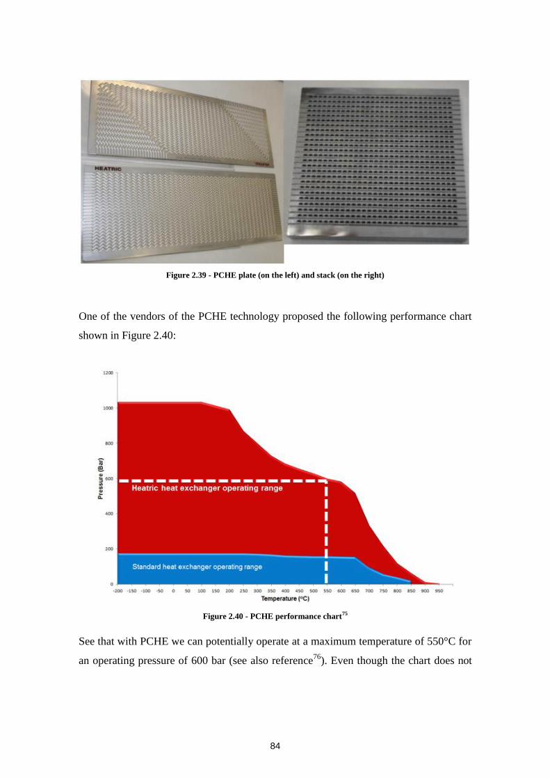
84
Figure 2.39 - PCHE plate (on the left) and stack (on the right)
One of the vendors of the PCHE technology proposed the following performance chart
shown in Figure 2.40:
Figure 2.40 - PCHE performance chart75
See that with PCHE we can potentially operate at a maximum temperature of 550°C for
an operating pressure of 600 bar (see also reference76
). Even though the chart does not
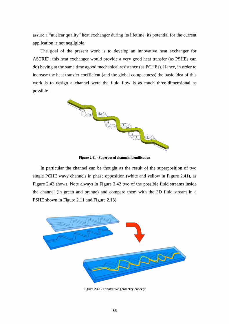
85
assure a “nuclear quality” heat exchanger during its lifetime, its potential for the current
application is not negligible.
The goal of the present work is to develop an innovative heat exchanger for
ASTRID: this heat exchanger would provide a very good heat transfer (as PSHEs can
do) having at the same time agood mechanical resistance (as PCHEs). Hence, in order to
increase the heat transfer coefficient (and the global compactness) the basic idea of this
work is to design a channel were the fluid flow is as much three-dimensional as
possible.
Figure 2.41 - Superposed channels identification
In particular the channel can be thought as the result of the superposition of two
single PCHE wavy channels in phase opposition (white and yellow in Figure 2.41), as
Figure 2.42 shows. Note always in Figure 2.42 two of the possible fluid streams inside
the channel (in green and orange) and compare them with the 3D fluid stream in a
PSHE shown in Figure 2.11 and Figure 2.13)
Figure 2.42 - Innovative geometry concept
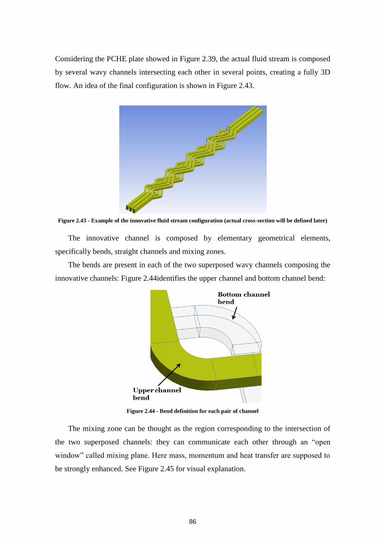
86
Considering the PCHE plate showed in Figure 2.39, the actual fluid stream is composed
by several wavy channels intersecting each other in several points, creating a fully 3D
flow. An idea of the final configuration is shown in Figure 2.43.
Figure 2.43 - Example of the innovative fluid stream configuration (actual cross-section will be defined later)
The innovative channel is composed by elementary geometrical elements,
specifically bends, straight channels and mixing zones.
The bends are present in each of the two superposed wavy channels composing the
innovative channels: Figure 2.44identifies the upper channel and bottom channel bend:
Figure 2.44 - Bend definition for each pair of channel
The mixing zone can be thought as the region corresponding to the intersection of
the two superposed channels: they can communicate each other through an “open
window” called mixing plane. Here mass, momentum and heat transfer are supposed to
be strongly enhanced. See Figure 2.45 for visual explanation.
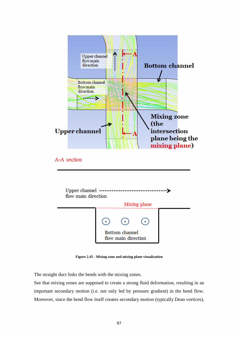
87
Figure 2.45 - Mixing zone and mixing plane visualization
The straight duct links the bends with the mixing zones.
See that mixing zones are supposed to create a strong fluid deformation, resulting in an
important secondary motion (i.e. not only led by pressure gradient) in the bend flow.
Moreover, since the bend flow itself creates secondary motion (typically Dean vortices),
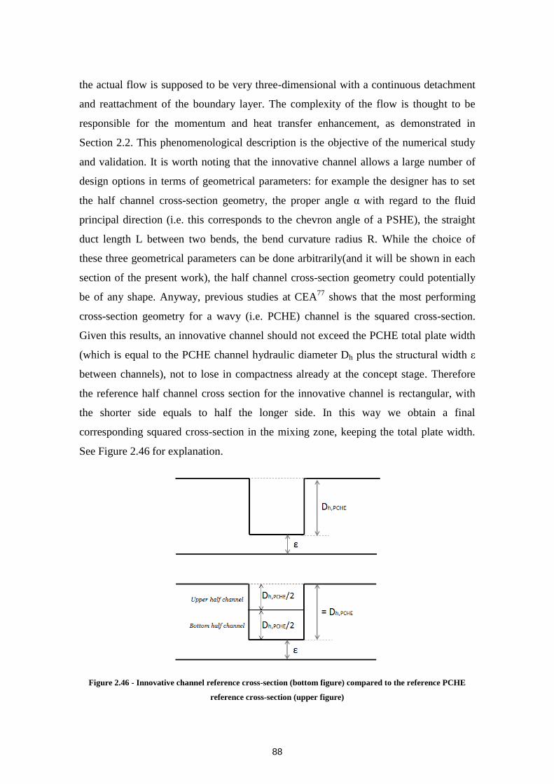
88
the actual flow is supposed to be very three-dimensional with a continuous detachment
and reattachment of the boundary layer. The complexity of the flow is thought to be
responsible for the momentum and heat transfer enhancement, as demonstrated in
Section 2.2. This phenomenological description is the objective of the numerical study
and validation. It is worth noting that the innovative channel allows a large number of
design options in terms of geometrical parameters: for example the designer has to set
the half channel cross-section geometry, the proper angle α with regard to the fluid
principal direction (i.e. this corresponds to the chevron angle of a PSHE), the straight
duct length L between two bends, the bend curvature radius R. While the choice of
these three geometrical parameters can be done arbitrarily(and it will be shown in each
section of the present work), the half channel cross-section geometry could potentially
be of any shape. Anyway, previous studies at CEA77
shows that the most performing
cross-section geometry for a wavy (i.e. PCHE) channel is the squared cross-section.
Given this results, an innovative channel should not exceed the PCHE total plate width
(which is equal to the PCHE channel hydraulic diameter Dh plus the structural width ε
between channels), not to lose in compactness already at the concept stage. Therefore
the reference half channel cross section for the innovative channel is rectangular, with
the shorter side equals to half the longer side. In this way we obtain a final
corresponding squared cross-section in the mixing zone, keeping the total plate width.
See Figure 2.46 for explanation.
Figure 2.46 - Innovative channel reference cross-section (bottom figure) compared to the reference PCHE
reference cross-section (upper figure)
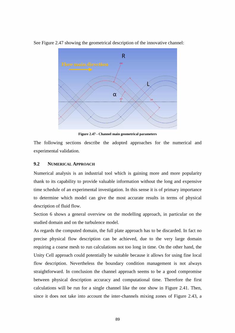
89
See Figure 2.47 showing the geometrical description of the innovative channel:
Figure 2.47 - Channel main geometrical parameters
The following sections describe the adopted approaches for the numerical and
experimental validation.
9.2 NUMERICAL APPROACH
Numerical analysis is an industrial tool which is gaining more and more popularity
thank to its capability to provide valuable information without the long and expensive
time schedule of an experimental investigation. In this sense it is of primary importance
to determine which model can give the most accurate results in terms of physical
description of fluid flow.
Section 6 shows a general overview on the modelling approach, in particular on the
studied domain and on the turbulence model.
As regards the computed domain, the full plate approach has to be discarded. In fact no
precise physical flow description can be achieved, due to the very large domain
requiring a coarse mesh to run calculations not too long in time. On the other hand, the
Unity Cell approach could potentially be suitable because it allows for using fine local
flow description. Nevertheless the boundary condition management is not always
straightforward. In conclusion the channel approach seems to be a good compromise
between physical description accuracy and computational time. Therefore the first
calculations will be run for a single channel like the one show in Figure 2.41. Then,
since it does not take into account the inter-channels mixing zones of Figure 2.43, a

90
wider calculation with a validated model will be run for a multiple channel
configuration.
As regards the turbulence model (and remembering that deeper information and
motivation will be given in Chapter 3), LES approach is discarded because the needed
computational resources would be very costly; in fact, the final goal of our numerical
analysis is to have an industrial model able to provide fast and accurate information
enough. Hence Reynolds-Averaged Navier-Stokes (RANS) approach is selected.
Conclusions of the bibliographic review show that a RANS low-Reynolds number
approach (i.e. computation of the fluid flow all the way down to the wall) theoretically
provides the most correct information about the fluid flow. In this sense, and
considering also the channel geometry, the most adapted turbulence model seems to be
a RANS model, specifically an ω-based model: in fact it has been extensively shown78
that this class of models provide better description of flow with adverse pressure
gradients (as it could be imagined for the in-bend flow of the innovative channel) with
no need of a specific low-Reynolds number modifications as for the ε-based models.
Moreover it has been also shown in reference79
that the ω-based models better account
for near-wall thermal compressibility, i.e. strong temperature gradients in the near wall
region and for wall roughness. Therefore, for the present application, the ω-based
modelling approach will be adopted: Chapter 3 will deeply study the numerical model
definition.
9.3 EXPERIMENTAL APPROACH
To validate the numerical model and to prove the design basis for the innovative
channel, an experimental database is of primary importance. Literature does not really
provide test-cases similar to the innovative channel. In fact, some classical validation
test-cases have been identified, but all of them lack in at least one important feature of
the innovative channel flow. Chapter 3 will show the list of the identified test-cases with
their similarities and differences with the current geometry of interest. Anyway, since
no exact validation case is available in literature, an experimental database on the actual
geometry is necessary. Measurements of velocities and Reynolds stresses will provide
the information needed to a full investigation of the fluid flow phenomena and
validation of the adopted numerical model. Chapter 4 will discuss in detail the
experimental techniques and facilities employed to meet this fundamental goal.
91
Chapitre 3: Définition du modèle
numérique
Dans le Chapitre 2, les avantages du modèle RANS basé sur ω pour simuler
l'écoulement à l'intérieur du canal innovant sont expliqués. En effet, l'intérêt est basé sur
le comportement de l'équation de transport de ω dans la région de proche paroi. le
modèle k-ω- standard est donc censé donner de meilleurs résultats dans la région de la
couche limite, (même pour les écoulements à gradient de pression négatif), ne
nécessitant pas de traitement spécifique proche de la paroi. Par conséquent, nous serions
amenés à choisir entre un modèle k-ω à deux équations standard ou bien un modèle de
transport des tensions de Reynolds plus sophistiqué. Dans le solveur disponible au
laboratoire (ANSYS Fluent ®) il n'y a pas d'autre choix possible si l'on veut effectuer un
calcul avec les équations de transport des contraintes de Reynolds basé sur une équation
de transport en ω. D'autre part, pour les modèles à deux équations on peut choisir entre
le modèle k-ω standard et le modèle SST. Ce dernier gagne de plus en plus de
popularité dans les applications industrielles en raison de ses améliorations potentielles
par rapport au modèle k-ω- standard. En fait, l'un des inconvénients connus du modèle
k-ω standard est sa dépendance vis-à-vis des valeurs loin de la paroi des variables
transportées, ce qui peut détériorer la solution dans certains cas. En ce sens, un modèle
k-ε est beaucoup plus stable que le k-ω, en fournissant des résultats très robustes, peu
importe les valeurs loin de la paroi. Sur la base de ces considérations macroscopiques,
le modèle SST associe un modèle k-ε standard dans la veine fluide avec un modèle k-ω
standard dans la couche limite, en utilisant uniquement avantages des deux modèles
originaux sans leurs inconvénients. En outre, il peut tenir compte de la relation de
Bradshaw dans la couche limite et fournit une solution en limitant la production de
l'énergie cinétique de la turbulence. Le choix final est d'utiliser le SST plutôt que le
modèle k-ω standard en raison de ses propriétés bénéfiques potentielles pour résoudre
les manques du modèle k-ω standard.
Le but de cette section est d'étudier le comportement de trois modèles de turbulence
basés sur l’équation de transport de ω, en utilisant trois approches de modélisation
différentes: le modèle à viscosité turbulente isotrope (SST), le modèle Stress Omega de

92
transport du tenseur de Reynolds et un nouveau modèle à viscosité turbulente non-
linéaire nommé ASST. Le modèle ASST, développé sur la base d’hypothèses
théoriques, présente la caractéristique avantageuse d'être un modèle pleinement
« réalisable», ce qui signifie que les caractéristiques turbulentes parasites et non-
physiques sont évitées grâce à des considérations mathématiques et physiques. Le
modèle a d'abord été développé pour fonctionner correctement dans la couche limite
d'un écoulement cisaillé, il a été mis en œuvre dans le solveur via des fonctions définies
par l'utilisateur. Enfin, il a été validé par des données expérimentales, avec une
comparaison au modèle SST et Stress Omega. Les trois modèles ont des performances
identiques pour l'écoulement de canal droit (ayant essentiellement été développés pour
un tel écoulement), ne différant que par la capacité à reproduire la turbulence
anisotrope. Cela se traduit macroscopiquement par une reproduction correcte des
tourbillons de coin dans un conduit droit à section de passage carrée et dans un coude à
90° des modèles ASST et Stress Omega . Des doutes vis-à-vis d’une application plus
large du modèle Stress Omega naissent par des résultats inattendus sur les cas tests de la
marche descendante et du faisceau de tubes: dans le premier, le modèle stress Omega
prédit une longueur de rattachement plus courte que prévue (ce qui est en contradiction
avec les résultats de son développeur); dans le second, le modèle Stress Omega échoue
dans la région où la vitesse de déformation est élevée, fournissant une forte diminution
de la contrainte de cisaillement de paroi par rapport aux mesures expérimentales. Ceci
n’est pas cohérent avec sa capacité potentielle à produire des résultats précis pour des
écoulements relativement simples. En ce sens, le modèle ASST peut fournir une
alternative intéressante, donnant des résultats globaux qui sont au moins aussi bonnes
que ceux du modèle Stress Omega. En outre, il conserve un temps de calcul très court,
ce qui le positionne pour être une très bon outil industriel pour décrire potentiellement
l’écoulement dans le canal innovant.
Aucun des cas tests indiqués ne représentent vraiment la complexité de l'écoulement du
canal innovant, qui peut être considéré comme leur combinaison. Par conséquent, cette
section identifie clairement la nécessité d'une base de données expérimentale pour
l'écoulement dans le canal innovant pour valider le modèle numérique et la performance
du motif. L'acquisition de cette base de données est l'objet du chapitre suivant.
93
Chapter 3: Numerical Model Definition
1. INTRODUCTION
1.1 SECTION GOALS AND MOTIVATION
Chapter 2 Section 9.2 stated and explained the interest to use a RANSVIII
ω-based model
to simulate the flow inside the innovative channel. Indeed the interest is based on the ω-
transport equation behavior in the near-wall region. Hence we would be led to choose
between a two-equation standard k-ω-model (i.e. that of Wilcox80
) and a more
sophisticated Reynolds stress transport model (i.e. Wilcox’s Stress Omega model80
). In
the available solver (ANSYS Fluent ®) there is no other possible choice if one wants to
perform a Reynolds stress transport calculation based on a ω-transport equation. On the
other hand, for the two equation models the possible choice is between the cited
standard k-ω-model and the Shear Stress Transport (SST) model81
. The latter has been
gaining more and more popularity in industrial application in the last years due to its
potential improvements with regard to the standard k-ω-model. In fact, one of the most
known negative features of the standard k-ω-model is its dependence on the freestream
values, which might deteriorate the solution for some cases. In this sense, the standard
k-ε model82
is much more stable than the k-ω-model, providing very robust results, no
matter the freestream values. On the other hand, the standard k-ω-model is supposed to
perform better in the boundary layer region, (even for adverse pressure gradient flows),
not needing any specific near-wall treatment. Based on these macroscopic
considerations, the SST model blends a standard k-ε model in the fluid bulk with a
standard k-ω-model in the boundary layer, using only the positive features of the two
original models. Moreover it can take into account the Bradshaw’s relation in duct
boundary layer and provides a pseudo-realizability condition by limiting the turbulence
kinetic energy production. The final choice is to use the SST rather than the standard k-
ω-model because of its potential beneficial features resolving the lacks of the standard
k-ω-model. Therefore its mentioned characteristics will be discussed further in the next
section.
VIII
Remember that the RANS models uses the Reynolds decomposition of the velocity field i.e. the
velocity U is decomposed as U= U + 𝑢′, with U being the average velocity and u’ being the fluctuating
velocity.
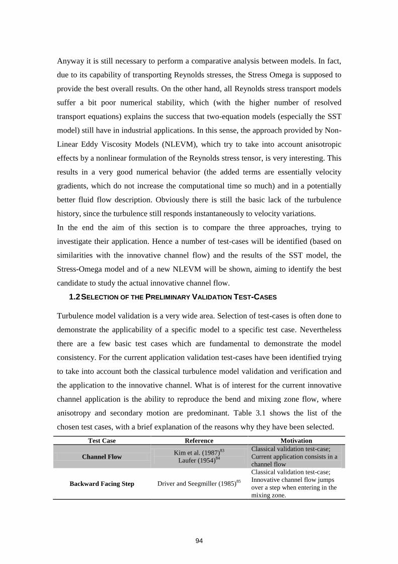
94
Anyway it is still necessary to perform a comparative analysis between models. In fact,
due to its capability of transporting Reynolds stresses, the Stress Omega is supposed to
provide the best overall results. On the other hand, all Reynolds stress transport models
suffer a bit poor numerical stability, which (with the higher number of resolved
transport equations) explains the success that two-equation models (especially the SST
model) still have in industrial applications. In this sense, the approach provided by Non-
Linear Eddy Viscosity Models (NLEVM), which try to take into account anisotropic
effects by a nonlinear formulation of the Reynolds stress tensor, is very interesting. This
results in a very good numerical behavior (the added terms are essentially velocity
gradients, which do not increase the computational time so much) and in a potentially
better fluid flow description. Obviously there is still the basic lack of the turbulence
history, since the turbulence still responds instantaneously to velocity variations.
In the end the aim of this section is to compare the three approaches, trying to
investigate their application. Hence a number of test-cases will be identified (based on
similarities with the innovative channel flow) and the results of the SST model, the
Stress-Omega model and of a new NLEVM will be shown, aiming to identify the best
candidate to study the actual innovative channel flow.
1.2 SELECTION OF THE PRELIMINARY VALIDATION TEST-CASES
Turbulence model validation is a very wide area. Selection of test-cases is often done to
demonstrate the applicability of a specific model to a specific test case. Nevertheless
there are a few basic test cases which are fundamental to demonstrate the model
consistency. For the current application validation test-cases have been identified trying
to take into account both the classical turbulence model validation and verification and
the application to the innovative channel. What is of interest for the current innovative
channel application is the ability to reproduce the bend and mixing zone flow, where
anisotropy and secondary motion are predominant. Table 3.1 shows the list of the
chosen test cases, with a brief explanation of the reasons why they have been selected.
Test Case Reference Motivation
Channel Flow Kim et al. (1987)
83
Laufer (1954)84
Classical validation test-case;
Current application consists in a
channel flow
Backward Facing Step Driver and Seegmiller (1985)85
Classical validation test-case;
Innovative channel flow jumps
over a step when entering in the
mixing zone.
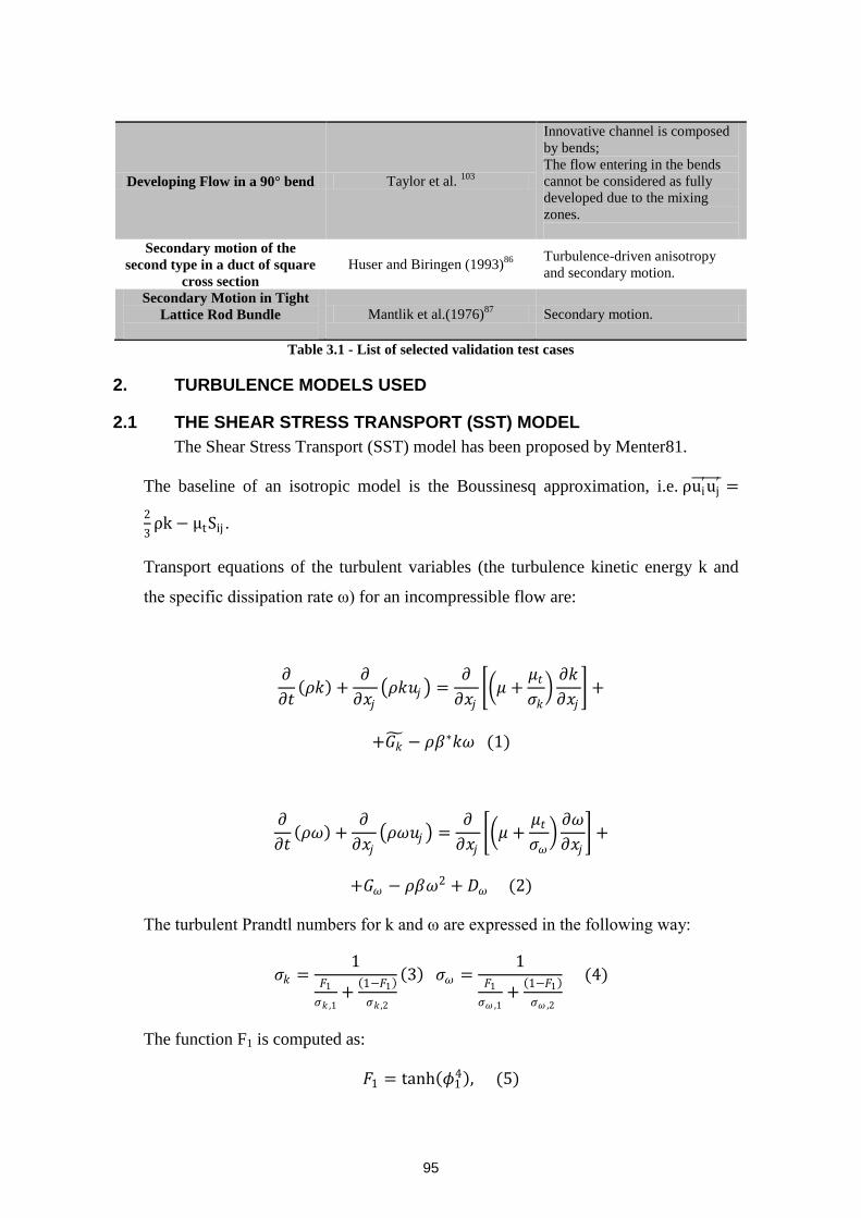
95
Developing Flow in a 90° bend Taylor et al. 103
Innovative channel is composed
by bends;
The flow entering in the bends
cannot be considered as fully
developed due to the mixing
zones.
Secondary motion of the
second type in a duct of square
cross section
Huser and Biringen (1993)86
Turbulence-driven anisotropy
and secondary motion.
Secondary Motion in Tight
Lattice Rod Bundle
Mantlik et al.(1976)87
Secondary motion.
Table 3.1 - List of selected validation test cases
2. TURBULENCE MODELS USED
2.1 THE SHEAR STRESS TRANSPORT (SST) MODEL
The Shear Stress Transport (SST) model has been proposed by Menter81.
The baseline of an isotropic model is the Boussinesq approximation, i.e. ρui′uj
′ =
2
3ρk − μtSij .
Transport equations of the turbulent variables (the turbulence kinetic energy k and
the specific dissipation rate ω) for an incompressible flow are:
𝜕
𝜕𝑡 𝜌𝑘 +
𝜕
𝜕𝑥𝑗 𝜌𝑘𝑢𝑗 =
𝜕
𝜕𝑥𝑗 𝜇 +
𝜇𝑡
𝜎𝑘 𝜕𝑘
𝜕𝑥𝑗 +
+𝐺𝑘 − 𝜌𝛽∗𝑘𝜔 (1)
𝜕
𝜕𝑡 𝜌𝜔 +
𝜕
𝜕𝑥𝑗 𝜌𝜔𝑢𝑗 =
𝜕
𝜕𝑥𝑗 𝜇 +
𝜇𝑡
𝜎𝜔 𝜕𝜔
𝜕𝑥𝑗 +
+𝐺𝜔 − 𝜌𝛽𝜔2 + 𝐷𝜔 (2)
The turbulent Prandtl numbers for k and ω are expressed in the following way:
𝜎𝑘 =1
𝐹1
𝜎𝑘 ,1+
1−𝐹1
𝜎𝑘 ,2
3 𝜎𝜔 =1
𝐹1
𝜎𝜔 ,1+
1−𝐹1
𝜎𝜔 ,2
(4)
The function F1 is computed as:
𝐹1 = tanh 𝜙14 , (5)
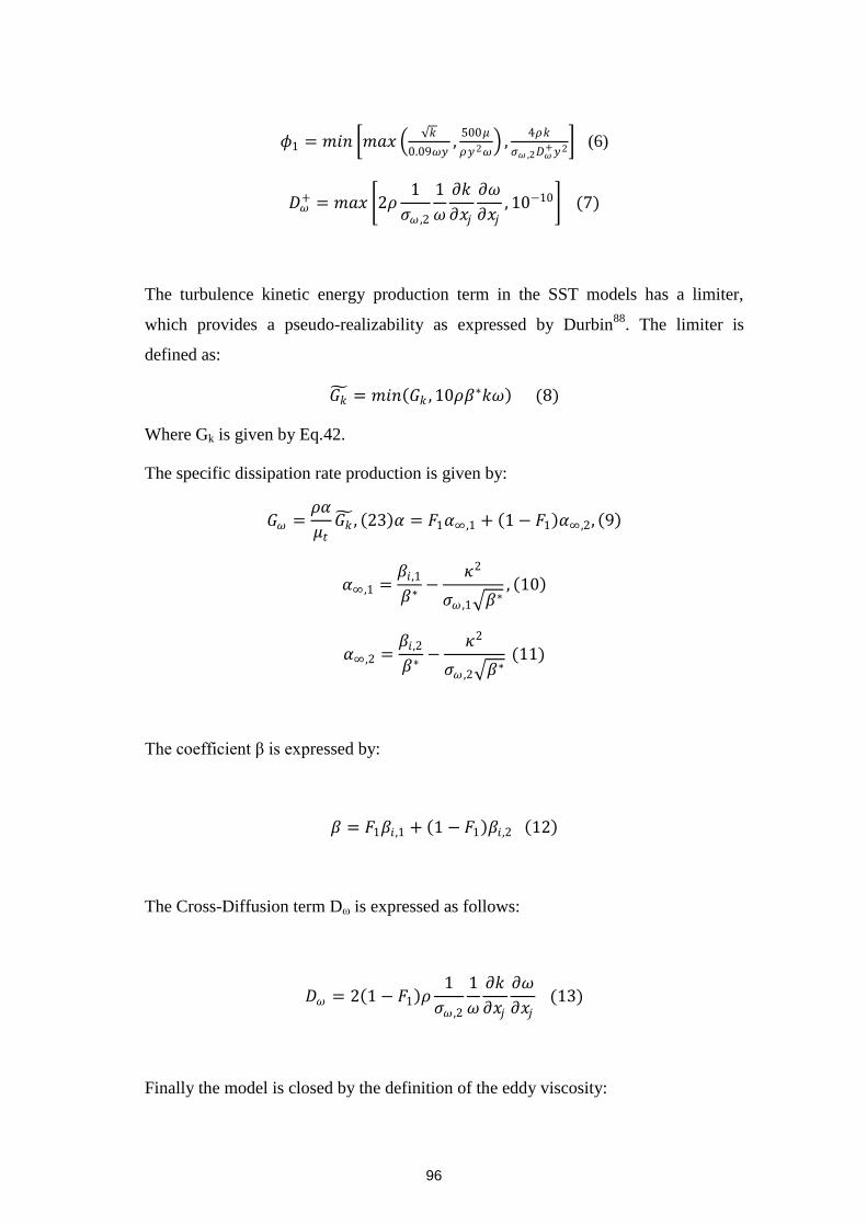
96
𝜙1 = 𝑚𝑖𝑛 𝑚𝑎𝑥 𝑘
0.09𝜔𝑦,
500𝜇
𝜌𝑦2𝜔 ,
4𝜌𝑘
𝜎𝜔 ,2𝐷𝜔+𝑦2
(6)
𝐷𝜔+ = 𝑚𝑎𝑥 2𝜌
1
𝜎𝜔 ,2
1
𝜔
𝜕𝑘
𝜕𝑥𝑗
𝜕𝜔
𝜕𝑥𝑗, 10−10 (7)
The turbulence kinetic energy production term in the SST models has a limiter,
which provides a pseudo-realizability as expressed by Durbin88
. The limiter is
defined as:
𝐺𝑘 = 𝑚𝑖𝑛 𝐺𝑘 , 10𝜌𝛽∗𝑘𝜔 (8)
Where Gk is given by Eq.42.
The specific dissipation rate production is given by:
𝐺𝜔 =𝜌𝛼
𝜇𝑡𝐺𝑘 , 23 𝛼 = 𝐹1𝛼∞ ,1 + 1 − 𝐹1 𝛼∞ ,2, 9
𝛼∞ ,1 =𝛽𝑖 ,1
𝛽∗−
𝜅2
𝜎𝜔 ,1 𝛽∗, 10
𝛼∞ ,2 =𝛽𝑖,2
𝛽∗−
𝜅2
𝜎𝜔 ,2 𝛽∗ (11)
The coefficient β is expressed by:
𝛽 = 𝐹1𝛽𝑖 ,1 + 1 − 𝐹1 𝛽𝑖 ,2 12
The Cross-Diffusion term Dω is expressed as follows:
𝐷𝜔 = 2 1 − 𝐹1 𝜌1
𝜎𝜔 ,2
1
𝜔
𝜕𝑘
𝜕𝑥𝑗
𝜕𝜔
𝜕𝑥𝑗 (13)
Finally the model is closed by the definition of the eddy viscosity:
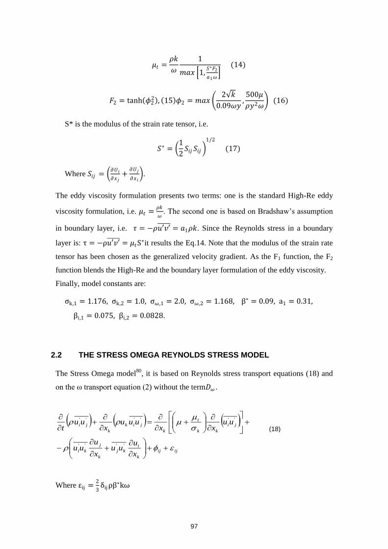
97
𝜇𝑡 =𝜌𝑘
𝜔
1
𝑚𝑎𝑥 1,𝑆∗𝐹2
𝑎1𝜔
(14)
𝐹2 = tanh 𝜙22 , 15 𝜙2 = 𝑚𝑎𝑥
2 𝑘
0.09𝜔𝑦,500𝜇
𝜌𝑦2𝜔 (16)
S* is the modulus of the strain rate tensor, i.e.
𝑆∗ = 1
2𝑆𝑖𝑗 𝑆𝑖𝑗
1/2
(17)
Where 𝑆𝑖𝑗 = 𝜕𝑈𝑖
𝜕𝑥𝑗+
𝜕𝑈𝑗
𝜕𝑥𝑖 .
The eddy viscosity formulation presents two terms: one is the standard High-Re eddy
viscosity formulation, i.e. 𝜇𝑡 =𝜌𝑘
𝜔. The second one is based on Bradshaw’s assumption
in boundary layer, i.e. 𝜏 = −𝜌𝑢′𝑣′ = 𝑎1𝜌𝑘. Since the Reynolds stress in a boundary
layer is: τ = −ρ𝑢′𝑣′ = 𝜇𝑡S∗it results the Eq.14. Note that the modulus of the strain rate
tensor has been chosen as the generalized velocity gradient. As the F1 function, the F2
function blends the High-Re and the boundary layer formulation of the eddy viscosity.
Finally, model constants are:
σk,1 = 1.176, σk,2 = 1.0, σω ,1 = 2.0, σω ,2 = 1.168, β∗ = 0.09, a1 = 0.31,
βi,1 = 0.075, βi,2 = 0.0828.
2.2 THE STRESS OMEGA REYNOLDS STRESS MODEL
The Stress Omega model80
, it is based on Reynolds stress transport equations (18) and
on the ω transport equation (2) without the term𝐷𝜔 .
ijij
k
ikj
k
j
ki
ji
kk
t
k
jik
k
ji
x
uuu
x
uuu
uuxx
uuux
uut
''''
''''''
Where εij =2
3δijρβ
∗kω
(18)
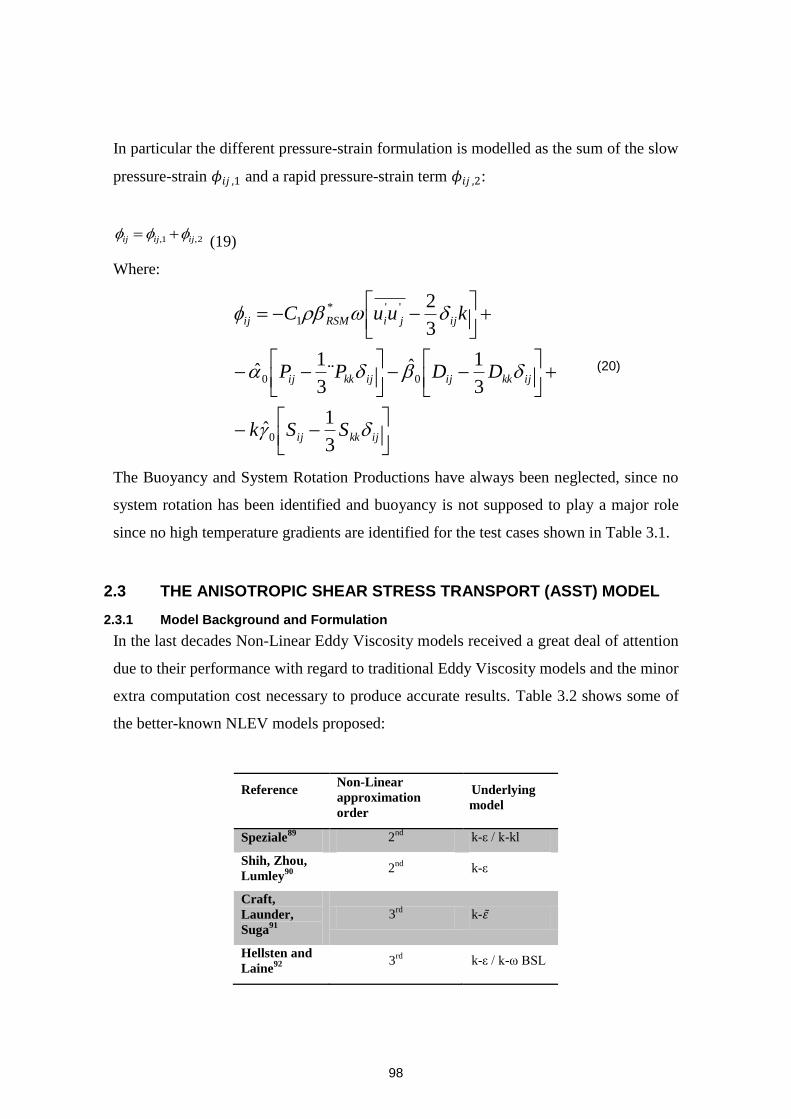
98
In particular the different pressure-strain formulation is modelled as the sum of the slow
pressure-strain 𝜙𝑖𝑗 ,1 and a rapid pressure-strain term 𝜙𝑖𝑗 ,2:
2,1, ijijij (19)
Where:
ijkkij
ijkkijijkkij
ijjiRSMij
SSk
DDPP
kuuC
3
1ˆ
3
1ˆ¨3
1ˆ
3
2
0
00
''*
1
The Buoyancy and System Rotation Productions have always been neglected, since no
system rotation has been identified and buoyancy is not supposed to play a major role
since no high temperature gradients are identified for the test cases shown in Table 3.1.
2.3 THE ANISOTROPIC SHEAR STRESS TRANSPORT (ASST) MODEL
2.3.1 Model Background and Formulation
In the last decades Non-Linear Eddy Viscosity models received a great deal of attention
due to their performance with regard to traditional Eddy Viscosity models and the minor
extra computation cost necessary to produce accurate results. Table 3.2 shows some of
the better-known NLEV models proposed:
Reference
Non-Linear
approximation
order
Underlying
model
Speziale89
2nd
k-ε / k-kl
Shih, Zhou,
Lumley90
2
nd k-ε
Craft,
Launder,
Suga91
3rd
k-휀
Hellsten and
Laine92
3
rd k-ε / k-ω BSL
(20)
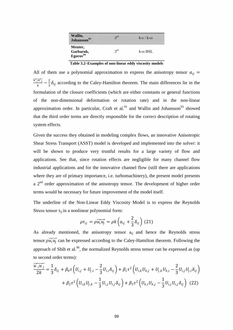
99
Wallin,
Johansson93
3
rd k-ε / k-ω
Menter,
Garbaruk,
Egorov94
3rd
k-ω BSL
Table 3.2–Examples of non-linear eddy viscosity models
All of them use a polynomial approximation to express the anisotropy tensor 𝑎𝑖𝑗 =
𝑢′ 𝑖𝑢′ 𝑗
𝑘−
2
3𝛿𝑖𝑗 according to the Caley-Hamilton theorem. The main differences lie in the
formulation of the closure coefficients (which are either constants or general functions
of the non-dimensional deformation or rotation rate) and in the non-linear
approximation order. In particular, Craft et al.91
and Wallin and Johansson93
showed
that the third order terms are directly responsible for the correct description of rotating
system effects.
Given the success they obtained in modeling complex flows, an innovative Anisotropic
Shear Stress Transport (ASST) model is developed and implemented into the solver: it
will be shown to produce very trustful results for a large variety of flow and
applications. See that, since rotation effects are negligible for many channel flow
industrial applications and for the innovative channel flow (still there are applications
where they are of primary importance, i.e. turbomachinery), the present model presents
a 2nd
order approximation of the anisotropy tensor. The development of higher order
terms would be necessary for future improvement of the model itself.
The underline of the Non-Linear Eddy Viscosity Model is to express the Reynolds
Stress tensor ηij in a nonlinear polynomial form:
𝜌𝜏𝑖𝑗 = 𝜌𝑢𝑖′𝑢𝑗
′ = 𝜌𝑘 𝑎𝑖𝑗 +2
3𝛿𝑖𝑗 (21)
As already mentioned, the anisotropy tensor aij and hence the Reynolds stress
tensor 𝜌𝑢𝑖′𝑢𝑗
′ can be expressed according to the Caley-Hamilton theorem. Following the
approach of Shih et al.90
, the normalized Reynolds stress tensor can be expressed as (up
to second order terms):
𝑢′𝑖𝑢′
𝑗
2𝑘=
1
3𝛿𝑖𝑗 + 𝛽0𝜏 𝑈𝑖 ,𝑗 + 𝑈𝑗 ,𝑖 −
2
3𝑈𝑖 ,𝑖𝛿𝑖𝑗 + 𝛽1𝜏
2 𝑈𝑖 ,𝑘𝑈𝑘 ,𝑗 + 𝑈𝑗 ,𝑘𝑈𝑘 ,𝑖 −2
3𝑈𝑖 ,𝑗𝑈𝑗 ,𝑖𝛿𝑖𝑗
+ 𝛽2𝜏2 𝑈𝑖 ,𝑘𝑈𝑗 ,𝑘 −
1
3𝑈𝑖 ,𝑗𝑈𝑖 ,𝑗𝛿𝑖𝑗 + 𝛽3𝜏
2 𝑈𝑘 ,𝑖𝑈𝑘 ,𝑗 −1
3𝑈𝑖 ,𝑗𝑈𝑖 ,𝑗𝛿𝑖𝑗 (22)
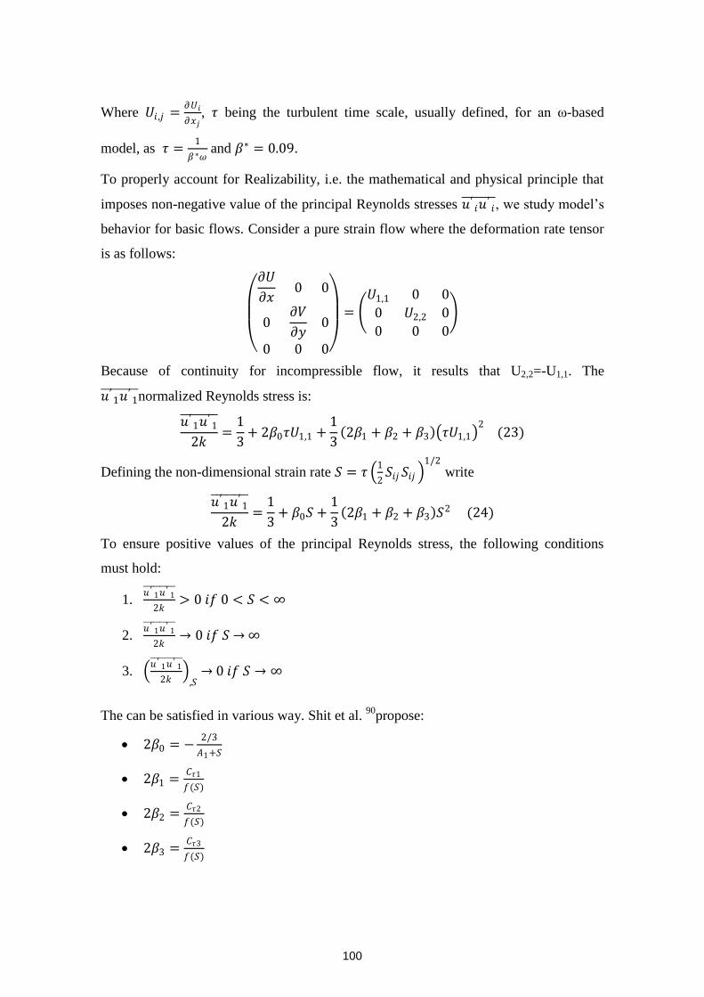
100
Where 𝑈𝑖 ,𝑗 =𝜕𝑈𝑖
𝜕𝑥𝑗, 𝜏 being the turbulent time scale, usually defined, for an ω-based
model, as 𝜏 =1
𝛽∗𝜔 and 𝛽∗ = 0.09.
To properly account for Realizability, i.e. the mathematical and physical principle that
imposes non-negative value of the principal Reynolds stresses 𝑢′𝑖𝑢′
𝑖 , we study model’s
behavior for basic flows. Consider a pure strain flow where the deformation rate tensor
is as follows:
𝜕𝑈
𝜕𝑥0 0
0𝜕𝑉
𝜕𝑦0
0 0 0
= 𝑈1,1 0 0
0 𝑈2,2 0
0 0 0
Because of continuity for incompressible flow, it results that U2,2=-U1,1. The
𝑢′1𝑢′
1 normalized Reynolds stress is:
𝑢′1𝑢′
1
2𝑘=
1
3+ 2𝛽0𝜏𝑈1,1 +
1
3 2𝛽1 + 𝛽2 + 𝛽3 𝜏𝑈1,1
2 (23)
Defining the non-dimensional strain rate 𝑆 = 𝜏 1
2𝑆𝑖𝑗𝑆𝑖𝑗
1/2
write
𝑢′1𝑢′
1
2𝑘=
1
3+ 𝛽0𝑆 +
1
3 2𝛽1 + 𝛽2 + 𝛽3 𝑆
2 (24)
To ensure positive values of the principal Reynolds stress, the following conditions
must hold:
1. 𝑢 ′
1𝑢 ′1
2𝑘> 0 𝑖𝑓 0 < 𝑆 < ∞
2. 𝑢 ′
1𝑢 ′1
2𝑘→ 0 𝑖𝑓 𝑆 → ∞
3. 𝑢 ′
1𝑢 ′1
2𝑘
,𝑆→ 0 𝑖𝑓 𝑆 → ∞
The can be satisfied in various way. Shit et al. 90
propose:
2𝛽0 = −2/3
𝐴1+𝑆
2𝛽1 =𝐶𝜏1
𝑓(𝑆)
2𝛽2 =𝐶𝜏2
𝑓(𝑆)
2𝛽3 =𝐶𝜏3
𝑓(𝑆)
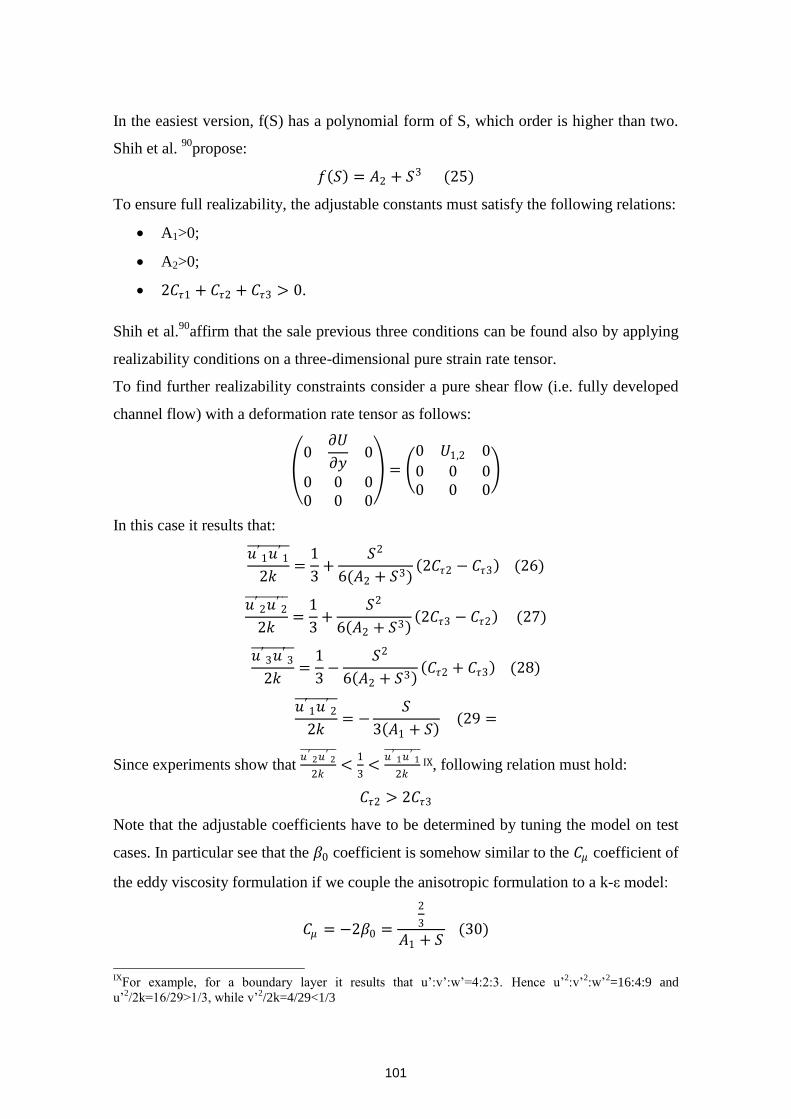
101
In the easiest version, f(S) has a polynomial form of S, which order is higher than two.
Shih et al. 90
propose:
𝑓 𝑆 = 𝐴2 + 𝑆3 (25)
To ensure full realizability, the adjustable constants must satisfy the following relations:
A1>0;
A2>0;
2𝐶𝜏1 + 𝐶𝜏2 + 𝐶𝜏3 > 0.
Shih et al.90
affirm that the sale previous three conditions can be found also by applying
realizability conditions on a three-dimensional pure strain rate tensor.
To find further realizability constraints consider a pure shear flow (i.e. fully developed
channel flow) with a deformation rate tensor as follows:
0
𝜕𝑈
𝜕𝑦0
0 0 00 0 0
= 0 𝑈1,2 0
0 0 00 0 0
In this case it results that:
𝑢′1𝑢′
1
2𝑘=
1
3+
𝑆2
6(𝐴2 + 𝑆3) 2𝐶𝜏2 − 𝐶𝜏3 (26)
𝑢′2𝑢′
2
2𝑘=
1
3+
𝑆2
6 𝐴2 + 𝑆3 2𝐶𝜏3 − 𝐶𝜏2 (27)
𝑢′3𝑢′
3
2𝑘=
1
3−
𝑆2
6 𝐴2 + 𝑆3 𝐶𝜏2 + 𝐶𝜏3 (28)
𝑢′1𝑢′
2
2𝑘= −
𝑆
3 𝐴1 + 𝑆 (29 =
Since experiments show that 𝑢 ′
2𝑢 ′2
2𝑘<
1
3<
𝑢 ′1𝑢 ′
1
2𝑘IX, following relation must hold:
𝐶𝜏2 > 2𝐶𝜏3
Note that the adjustable coefficients have to be determined by tuning the model on test
cases. In particular see that the 𝛽0 coefficient is somehow similar to the 𝐶𝜇 coefficient of
the eddy viscosity formulation if we couple the anisotropic formulation to a k-ε model:
𝐶𝜇 = −2𝛽0 =
2
3
𝐴1 + 𝑆 (30)
IX
For example, for a boundary layer it results that u’:v’:w’=4:2:3. Hence u’2:v’
2:w’
2=16:4:9 and
u’2/2k=16/29>1/3, while v’
2/2k=4/29<1/3
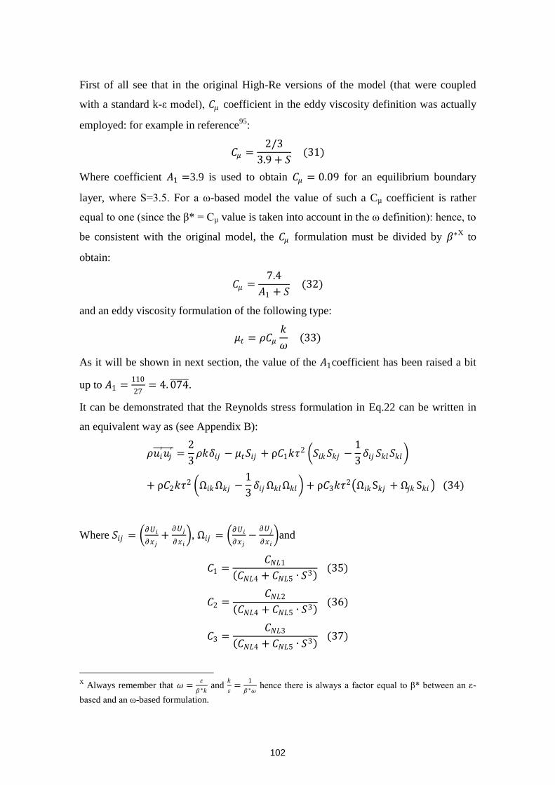
102
First of all see that in the original High-Re versions of the model (that were coupled
with a standard k-ε model), 𝐶𝜇 coefficient in the eddy viscosity definition was actually
employed: for example in reference95
:
𝐶𝜇 =2/3
3.9 + 𝑆 (31)
Where coefficient 𝐴1 =3.9 is used to obtain 𝐶𝜇 = 0.09 for an equilibrium boundary
layer, where S=3.5. For a ω-based model the value of such a Cµ coefficient is rather
equal to one (since the β* = Cµ value is taken into account in the ω definition): hence, to
be consistent with the original model, the 𝐶𝜇 formulation must be divided by 𝛽∗X to
obtain:
𝐶𝜇 =7.4
𝐴1 + 𝑆 (32)
and an eddy viscosity formulation of the following type:
𝜇𝑡 = 𝜌𝐶𝜇
𝑘
𝜔 (33)
As it will be shown in next section, the value of the 𝐴1coefficient has been raised a bit
up to 𝐴1 =110
27= 4. 074 .
It can be demonstrated that the Reynolds stress formulation in Eq.22 can be written in
an equivalent way as (see Appendix B):
𝜌𝑢𝑖′𝑢𝑗
′ =2
3𝜌𝑘𝛿𝑖𝑗 − 𝜇𝑡𝑆𝑖𝑗 + ρ𝐶1𝑘𝜏
2 𝑆𝑖𝑘𝑆𝑘𝑗 −1
3𝛿𝑖𝑗 𝑆𝑘𝑙𝑆𝑘𝑙
+ ρ𝐶2𝑘𝜏2 Ω𝑖𝑘Ω𝑘𝑗 −
1
3𝛿𝑖𝑗Ω𝑘𝑙Ω𝑘𝑙 + ρ𝐶3𝑘𝜏
2 Ω𝑖𝑘S𝑘𝑗 + Ω𝑗𝑘 S𝑘𝑖 (34)
Where 𝑆𝑖𝑗 = 𝜕𝑈𝑖
𝜕𝑥𝑗+
𝜕𝑈𝑗
𝜕𝑥𝑖 , Ω𝑖𝑗 =
𝜕𝑈𝑖
𝜕𝑥𝑗−
𝜕𝑈𝑗
𝜕𝑥𝑖 and
𝐶1 =𝐶𝑁𝐿1
𝐶𝑁𝐿4 + 𝐶𝑁𝐿5 ∙ 𝑆3 (35)
𝐶2 =𝐶𝑁𝐿2
𝐶𝑁𝐿4 + 𝐶𝑁𝐿5 ∙ 𝑆3 (36)
𝐶3 =𝐶𝑁𝐿3
𝐶𝑁𝐿4 + 𝐶𝑁𝐿5 ∙ 𝑆3 (37)
X Always remember that 𝜔 =
휀
𝛽∗𝑘 and
𝑘
휀=
1
𝛽∗𝜔 hence there is always a factor equal to β* between an ε-
based and an ω-based formulation.
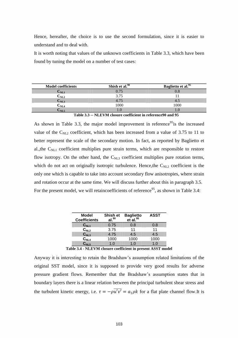
103
Hence, hereafter, the choice is to use the second formulation, since it is easier to
understand and to deal with.
It is worth noting that values of the unknown coefficients in Table 3.3, which have been
found by tuning the model on a number of test cases:
Model coefficients Shish et al.90
Baglietto et al.95
CNL1 0.75 0.8
CNL2 3.75 11
CNL3 4.75 4.5
CNL4 1000 1000
CNL5 1.0 1.0
Table 3.3 -- NLEVM closure coefficient in reference90 and 95
As shown in Table 3.3, the major model improvement in reference95
is the increased
value of the CNL2 coefficient, which has been increased from a value of 3.75 to 11 to
better represent the scale of the secondary motion. In fact, as reported by Baglietto et
al.,the CNL1 coefficient multiplies pure strain terms, which are responsible to restore
flow isotropy. On the other hand, the CNL3 coefficient multiplies pure rotation terms,
which do not act on originally isotropic turbulence. Hence,the CNL2 coefficient is the
only one which is capable to take into account secondary flow anisotropies, where strain
and rotation occur at the same time. We will discuss further about this in paragraph 3.5.
For the present model, we will retaincoefficients of reference95
, as shown in Table 3.4:
Model Coefficients
Shish et al.
90
Baglietto et al.
95
ASST
CNL1 0.75 0.8 0.8 CNL2 3.75 11 11 CNL3 4.75 4.5 4.5 CNL4 1000 1000 1000 CNL5 1.0 1.0 1.0
Table 3.4 - NLEVM closure coefficient in present ASST model
Anyway it is interesting to retain the Bradshaw’s assumption related limitations of the
original SST model, since it is supposed to provide very good results for adverse
pressure gradient flows. Remember that the Bradshaw’s assumption states that in
boundary layers there is a linear relation between the principal turbulent shear stress and
the turbulent kinetic energy, i.e. 𝜏 = −𝜌𝑢′𝑣′ = 𝑎1𝜌𝑘 for a flat plate channel flow.It is
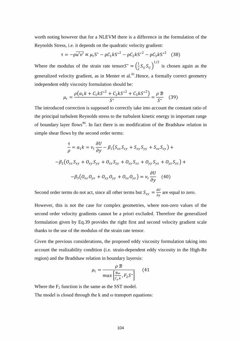
104
worth noting however that for a NLEVM there is a difference in the formulation of the
Reynolds Stress, i.e. it depends on the quadratic velocity gradient:
τ = −ρ𝑢′𝑣′ ∝ 𝜇𝑡S∗ − ρ𝐶1𝑘S∗2 − ρ𝐶2𝑘S∗2 − ρ𝐶3𝑘S∗2 (38)
Where the modulus of the strain rate tensor𝑆∗ = 1
2𝑆𝑖𝑗 𝑆𝑖𝑗
1/2
is chosen again as the
generalized velocity gradient, as in Menter et al.81
.Hence, a formally correct geometry
independent eddy viscosity formulation should be:
𝜇𝑡 =𝜌 𝑎1𝑘 + 𝐶1𝑘𝑆
∗2 + 𝐶2𝑘𝑆∗2 + 𝐶3𝑘𝑆
∗2
𝑆∗=
𝜌 ℬ
𝑆∗ (39)
The introduced correction is supposed to correctly take into account the constant ratio of
the principal turbulent Reynolds stress to the turbulent kinetic energy in important range
of boundary layer flows96
. In fact there is no modification of the Bradshaw relation in
simple shear flows by the second order terms:
τ
𝜌= 𝑎1𝑘 = 𝜈𝑡
𝜕𝑈
𝜕𝑦− 𝛽1 𝑆𝑥𝑥𝑆𝑥𝑦 + 𝑆𝑥𝑦𝑆𝑦𝑦 + 𝑆𝑥𝑧𝑆𝑧𝑦 +
−𝛽2 𝑂𝑥𝑥𝑆𝑥𝑦 + 𝑂𝑥𝑦𝑆𝑦𝑦 + 𝑂𝑥𝑧𝑆𝑧𝑦 + 𝑂𝑥𝑦𝑆𝑥𝑥 + 𝑂𝑦𝑦 𝑆𝑦𝑥 + 𝑂𝑦𝑧𝑆𝑧𝑥 +
−𝛽3 𝑂𝑥𝑥𝑂𝑦𝑥 + 𝑂𝑥𝑦𝑂𝑦𝑦 + 𝑂𝑥𝑧𝑂𝑦𝑧 = 𝜈𝑡
𝜕𝑈
𝜕𝑦 (40)
Second order terms do not act, since all other terms but 𝑆𝑥𝑦 =𝜕𝑈
𝜕𝑦 are equal to zero.
However, this is not the case for complex geometries, where non-zero values of the
second order velocity gradients cannot be a priori excluded. Therefore the generalized
formulation given by Eq.39 provides the right first and second velocity gradient scale
thanks to the use of the modulus of the strain rate tensor.
Given the previous considerations, the proposed eddy viscosity formulation taking into
account the realizability condition (i.e. strain-dependent eddy viscosity in the High-Re
region) and the Bradshaw relation in boundary layersis:
𝜇𝑡 =𝜌 ℬ
𝑚𝑎𝑥 ℬ𝜔
𝐶𝜇 𝑘, 𝐹2𝑆∗
(41
Where the F2 function is the same as the SST model.
The model is closed through the k and ω transport equations:
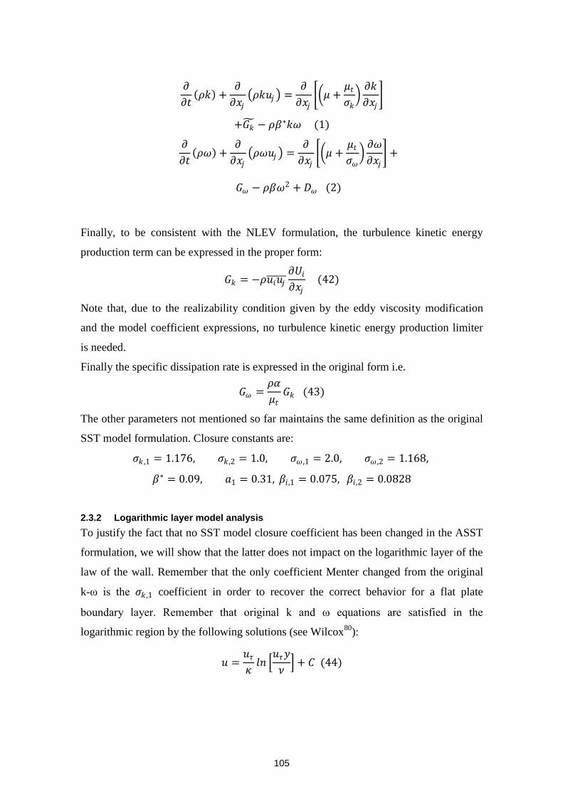
105
𝜕
𝜕𝑡 𝜌𝑘 +
𝜕
𝜕𝑥𝑗 𝜌𝑘𝑢𝑗 =
𝜕
𝜕𝑥𝑗 𝜇 +
𝜇𝑡
𝜎𝑘 𝜕𝑘
𝜕𝑥𝑗
+𝐺𝑘 − 𝜌𝛽∗𝑘𝜔 (1)
𝜕
𝜕𝑡 𝜌𝜔 +
𝜕
𝜕𝑥𝑗 𝜌𝜔𝑢𝑗 =
𝜕
𝜕𝑥𝑗 𝜇 +
𝜇𝑡
𝜎𝜔 𝜕𝜔
𝜕𝑥𝑗 +
𝐺𝜔 − 𝜌𝛽𝜔2 + 𝐷𝜔 (2)
Finally, to be consistent with the NLEV formulation, the turbulence kinetic energy
production term can be expressed in the proper form:
𝐺𝑘 = −𝜌𝑢𝑖𝑢𝑗 𝜕𝑈𝑖
𝜕𝑥𝑗 (42)
Note that, due to the realizability condition given by the eddy viscosity modification
and the model coefficient expressions, no turbulence kinetic energy production limiter
is needed.
Finally the specific dissipation rate is expressed in the original form i.e.
𝐺𝜔 =𝜌𝛼
𝜇𝑡𝐺𝑘 (43)
The other parameters not mentioned so far maintains the same definition as the original
SST model formulation. Closure constants are:
𝜎𝑘 ,1 = 1.176, 𝜎𝑘 ,2 = 1.0, 𝜎𝜔 ,1 = 2.0, 𝜎𝜔 ,2 = 1.168,
𝛽∗ = 0.09, 𝑎1 = 0.31, 𝛽𝑖,1 = 0.075, 𝛽𝑖,2 = 0.0828
2.3.2 Logarithmic layer model analysis
To justify the fact that no SST model closure coefficient has been changed in the ASST
formulation, we will show that the latter does not impact on the logarithmic layer of the
law of the wall. Remember that the only coefficient Menter changed from the original
k-ω is the 𝜎𝑘 ,1 coefficient in order to recover the correct behavior for a flat plate
boundary layer. Remember that original k and ω equations are satisfied in the
logarithmic region by the following solutions (see Wilcox80
):
𝑢 =𝑢𝜏
𝜅𝑙𝑛
𝑢𝜏𝑦
𝜈 + 𝐶 (44)
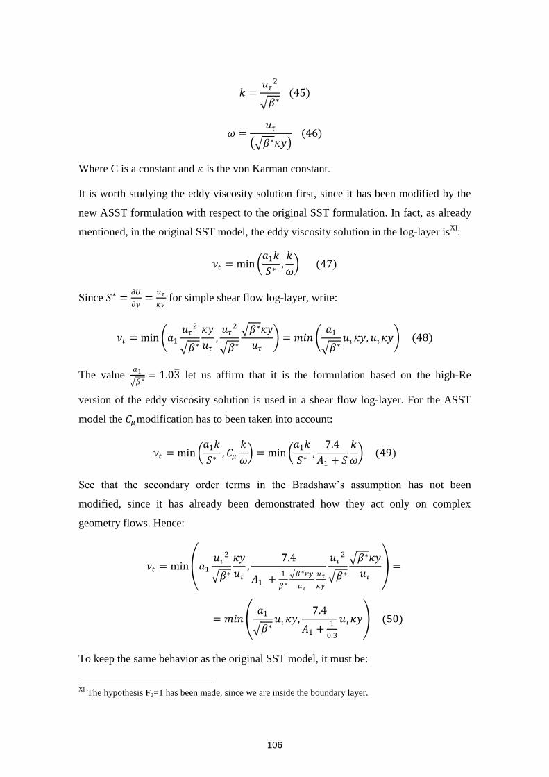
106
𝑘 =𝑢𝜏
2
𝛽∗ (45)
𝜔 =𝑢𝜏
𝛽∗𝜅𝑦 (46)
Where C is a constant and 𝜅 is the von Karman constant.
It is worth studying the eddy viscosity solution first, since it has been modified by the
new ASST formulation with respect to the original SST formulation. In fact, as already
mentioned, in the original SST model, the eddy viscosity solution in the log-layer isXI
:
𝜈𝑡 = min 𝑎1𝑘
𝑆∗,𝑘
𝜔 (47)
Since 𝑆∗ =𝜕𝑈
𝜕𝑦=
𝑢𝜏
𝜅𝑦 for simple shear flow log-layer, write:
𝜈𝑡 = min 𝑎1
𝑢𝜏2
𝛽∗
𝜅𝑦
𝑢𝜏,𝑢𝜏
2
𝛽∗
𝛽∗𝜅𝑦
𝑢𝜏 = 𝑚𝑖𝑛
𝑎1
𝛽∗𝑢𝜏𝜅𝑦, 𝑢𝜏𝜅𝑦 (48)
The value 𝑎1
𝛽∗= 1.03 let us affirm that it is the formulation based on the high-Re
version of the eddy viscosity solution is used in a shear flow log-layer. For the ASST
model the 𝐶𝜇modification has to been taken into account:
𝜈𝑡 = min 𝑎1𝑘
𝑆∗, 𝐶𝜇
𝑘
𝜔 = min
𝑎1𝑘
𝑆∗,
7.4
𝐴1 + 𝑆
𝑘
𝜔 (49)
See that the secondary order terms in the Bradshaw’s assumption has not been
modified, since it has already been demonstrated how they act only on complex
geometry flows. Hence:
𝜈𝑡 = min 𝑎1
𝑢𝜏2
𝛽∗
𝜅𝑦
𝑢𝜏,
7.4
𝐴1 +1
𝛽∗
𝛽∗𝜅𝑦
𝑢𝜏
𝑢𝜏
𝜅𝑦
𝑢𝜏2
𝛽∗
𝛽∗𝜅𝑦
𝑢𝜏 =
= 𝑚𝑖𝑛 𝑎1
𝛽∗𝑢𝜏𝜅𝑦,
7.4
𝐴1 +1
0.3
𝑢𝜏𝜅𝑦 (50)
To keep the same behavior as the original SST model, it must be:
XI
The hypothesis F2=1 has been made, since we are inside the boundary layer.
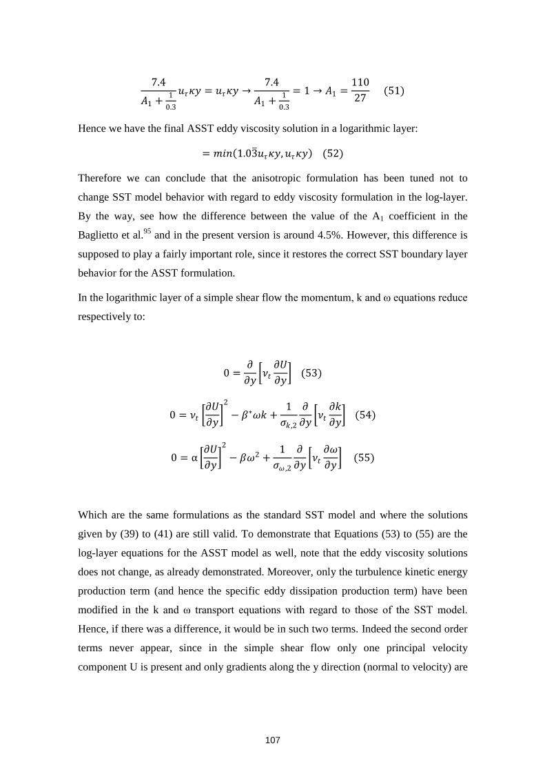
107
7.4
𝐴1 +1
0.3
𝑢𝜏𝜅𝑦 = 𝑢𝜏𝜅𝑦 →7.4
𝐴1 +1
0.3
= 1 → 𝐴1 =110
27 (51)
Hence we have the final ASST eddy viscosity solution in a logarithmic layer:
= 𝑚𝑖𝑛 1.03 𝑢𝜏𝜅𝑦, 𝑢𝜏𝜅𝑦 (52)
Therefore we can conclude that the anisotropic formulation has been tuned not to
change SST model behavior with regard to eddy viscosity formulation in the log-layer.
By the way, see how the difference between the value of the A1 coefficient in the
Baglietto et al.95
and in the present version is around 4.5%. However, this difference is
supposed to play a fairly important role, since it restores the correct SST boundary layer
behavior for the ASST formulation.
In the logarithmic layer of a simple shear flow the momentum, k and ω equations reduce
respectively to:
0 =𝜕
𝜕𝑦 𝜈𝑡
𝜕𝑈
𝜕𝑦 (53)
0 = 𝜈𝑡 𝜕𝑈
𝜕𝑦
2
− 𝛽∗𝜔𝑘 +1
𝜎𝑘 ,2
𝜕
𝜕𝑦 𝜈𝑡
𝜕𝑘
𝜕𝑦 (54)
0 = α 𝜕𝑈
𝜕𝑦
2
− 𝛽𝜔2 +1
𝜎𝜔 ,2
𝜕
𝜕𝑦 𝜈𝑡
𝜕𝜔
𝜕𝑦 (55)
Which are the same formulations as the standard SST model and where the solutions
given by (39) to (41) are still valid. To demonstrate that Equations (53) to (55) are the
log-layer equations for the ASST model as well, note that the eddy viscosity solutions
does not change, as already demonstrated. Moreover, only the turbulence kinetic energy
production term (and hence the specific eddy dissipation production term) have been
modified in the k and ω transport equations with regard to those of the SST model.
Hence, if there was a difference, it would be in such two terms. Indeed the second order
terms never appear, since in the simple shear flow only one principal velocity
component U is present and only gradients along the y direction (normal to velocity) are
108
allowed. Therefore, in the logarithmic layer the turbulent kinetic energy production
terms is:
𝐺𝑘
𝜌= −𝑢𝑖𝑢𝑗
𝜕𝑈𝑖
𝜕𝑥𝑗= −𝑢𝑣
𝜕𝑈
𝜕𝑦= − −𝜈𝑡
𝜕𝑈
𝜕𝑦+ 𝛽1 𝑆𝑥𝑥𝑆𝑥𝑦 + 𝑆𝑥𝑦𝑆𝑦𝑦 + 𝑆𝑥𝑧𝑆𝑧𝑦 +
+𝛽2 𝑂𝑥𝑥𝑆𝑥𝑦 + 𝑂𝑥𝑦𝑆𝑦𝑦 + 𝑂𝑥𝑧𝑆𝑧𝑦 + 𝑂𝑥𝑦𝑆𝑥𝑥 + 𝑂𝑦𝑦 𝑆𝑦𝑥 + 𝑂𝑦𝑧𝑆𝑧𝑥 +
+𝛽3 𝑂𝑥𝑥𝑂𝑦𝑥 + 𝑂𝑥𝑦𝑂𝑦𝑦 + 𝑂𝑥𝑧𝑂𝑦𝑧 𝜕𝑈
𝜕𝑦= 𝜈𝑡
𝜕𝑈
𝜕𝑦
2
(56)
Again, second order terms do not appear in the final formulation, since all other terms
but 𝑆𝑥𝑦 =𝜕𝑈
𝜕𝑦 are equal to zero.
If the Gk term does not change, so it does the Gω, since the two are related by
multiplying coefficient. Hence it is easily verified that no added term is present and that
the ASST acts exactly like the SST model in the logarithmic boundary layer. This is
consistent with the fact that the non-linear terms are not supposed to influence the flow
main characteristics for simple shear flow cases, but only to act on flow anisotropy.
This will be further shown in the next section, where the analysis of a channel flow
boundary layer is presented.
2.4 THERMAL MODELLING APPROACH
Aiming to build a solid numerical model to study the innovative channel thermal-
hydraulic performance, the thermal modelling approach has to be faced. In fact, if the
pure aerodynamic model can already improve the flow thermal description, still there is
the problem of how to model the turbulent heat flux for a complex flow.
In this context, the simplest modelling approach is to use a Simple Gradient Diffusion
Hypothesis (SGDH) model. It consists of modelling the turbulent heat flux 𝑢′𝑖𝜃 with the
same approach as the linear eddy viscosity models, i.e. with a formal dependence on the
temperature gradient.
𝑢′𝑖𝜃′ = −𝜈𝑡
𝜎𝑡
𝜕Θ
𝜕𝑥𝑖 (57)
The temperature T is decomposed as for the Reynolds decomposition 𝑇 = Θ + 𝜃′, with
Θ being the average temperature and θ’ being the fluctuating temperature.The 𝜎𝑡 is the
109
turbulent Prandtl numberXII
, which is assumed to be constant and equal to 0.85 in the
fluid bulk. In the near-wall region (laminar and logarithmic layer) its value is a bit
higher (around 1.197
).
A finer modelling strategy uses the Generalized Gradient Diffusion Hypothesis
(GGDH) proposed by Daly and Harlow98
. They propose the following expression to
evaluate turbulent scalar fluxes:
𝑢′𝑖𝜃′ = −𝐶1
𝛽∗𝜔𝑢′
𝑖𝑢′𝑗
𝜕Θ
𝜕𝑥𝑗 (58)
Where C is a constant usually equal to 0.15.
The used solver ANSYS Fluent ® only provides a default SSGH model for the turbulent
heat flux evaluation. Still the GGDH model can be implemented into the solver through
User Defined Functions. See that this approach could potentially be beneficial for the
Stress Omega model and for the ASST model, since they are supposed to provide better
results in terms of Reynolds stresses 𝑢′𝑖𝑢′𝑗 . However, since the use of such a GGDH
model resulted to be numerically unstable even for the simplest test cases (remember
the goal to build a solid industrial numerical model), we will use the available SGDH
model with 𝜎𝑡 = 0.85 already implemented into the solver. It could be stated that the
SGDH model is a too simple model to be used in a complex flow such as that of the
innovative channel. Nevertheless a constant turbulent Prandtl number can give some
good results for near-wall heat transfer, which is a major phenomenon occurring in the
innovative channel. On the other hand, the choice of a proper turbulence model, aiming
to improve the aerodynamic model, can be seen as a mean to increase the computational
accuracy of the global heat transfer.
3. MODEL VERIFICATION AND VALIDATION
3.1 CHANNEL FLOW
3.1.1 Motivation
The test case of fully developed channel flow has been studied extensively to increase
the understanding of the mechanics of wall-bounded turbulent flows. Its geometric
XII
The name follows the similarity between the viscous and turbulent heat flux formulation, with the total
heat flux being 𝜑𝑘 = 𝜈
𝑃𝑟+
𝜈𝑡𝜎𝑡
𝜕Θ
𝜕𝑥𝑘
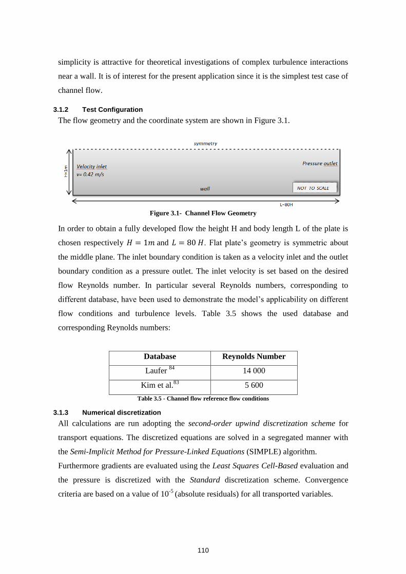
110
simplicity is attractive for theoretical investigations of complex turbulence interactions
near a wall. It is of interest for the present application since it is the simplest test case of
channel flow.
3.1.2 Test Configuration
The flow geometry and the coordinate system are shown in Figure 3.1.
Figure 3.1- Channel Flow Geometry
In order to obtain a fully developed flow the height H and body length L of the plate is
chosen respectively 𝐻 = 1𝑚 and 𝐿 = 80 𝐻. Flat plate’s geometry is symmetric about
the middle plane. The inlet boundary condition is taken as a velocity inlet and the outlet
boundary condition as a pressure outlet. The inlet velocity is set based on the desired
flow Reynolds number. In particular several Reynolds numbers, corresponding to
different database, have been used to demonstrate the model’s applicability on different
flow conditions and turbulence levels. Table 3.5 shows the used database and
corresponding Reynolds numbers:
Database Reynolds Number
Laufer 84
14 000
Kim et al.83
5 600
Table 3.5 - Channel flow reference flow conditions
3.1.3 Numerical discretization
All calculations are run adopting the second-order upwind discretization scheme for
transport equations. The discretized equations are solved in a segregated manner with
the Semi-Implicit Method for Pressure-Linked Equations (SIMPLE) algorithm.
Furthermore gradients are evaluated using the Least Squares Cell-Based evaluation and
the pressure is discretized with the Standard discretization scheme. Convergence
criteria are based on a value of 10-5
(absolute residuals) for all transported variables.

111
3.1.4 Mesh convergence evaluation
To determine a mesh-independent model, calculations have been run using three
increasingly refined meshes. Figure 3.2 provides an example of the channel flow mesh:
Figure 3.2 - Channel Flow Mesh
These different configurations give following values of y+ (Table 3.6):
Coarse Grid (Mesh A) y+ = 2.242
Fine Grid (Mesh B) y+ = 1.487
Refined Grid (Mesh C) y+ = 0.743
Table 3.6 - Channel flow used grids
To establish mesh convergence, the average wall shear stress ηw is evaluated: Table 3.7
shows the results:
Y+ Mesh A Mesh B Mesh C
τw 5.790𝑒−04 𝑃𝑎 5.801𝑒−04 𝑃𝑎 5.864𝑒−04 𝑃𝑎
Table 3.7 - Channel flow grid convergence evaluation
The comparison shows that there is almost no difference between the two finer grids
(difference of 0.2% between the fine and refined grids). Therefore we will adopt the
finest calculation grid to capture the finest turbulence phenomena occurring.
3.1.5 Results
In this section we will show several velocity and Reynolds Stress profiles to compare
and verify the correct implementation of the three turbulence models described in
Section 2.
3.1.5.1 Law of the Wall
The law of the wall is one of the most famous empirically-determined relationships in
turbulent flow near solid boundaries. Measurements show that, for both internal and
112
external flows, the streamwise velocity in the flow near the wall varies logarithmically
with distance from the surface.
The form of this law, valid for flows at high Reynolds numbers under constant
favorable pressure gradient and far enough from the wall for viscous effects to be
negligible (𝑦+ >30), is the mean velocity profile normalized in variables given by:
𝑢+ =1
𝑘ln 𝑦+ + 𝐶 (59)
where𝑢+ =𝑢
𝑢𝜏 and 𝑦+ =
𝑦∗𝑢𝜏
𝜈 where 𝑢𝜏 =
𝜏𝑊
𝜌 .
𝑢is the mean velocity, 𝑦 is the distance from the wall, 𝜈 is kinematic viscosity and 𝑢𝜏 is
the friction velocity defined from the wall shear stress 𝜏𝑊 . The Von Karman constant,
k, and the additive constant C is widely thought to be universal constants. From
experiments, the Von Kármán constant is found to be 𝑘 ≈0.41 and C+≈5.5 for a smooth
wall. Due to the functional form of the law of the wall, this region is also called the
logarithmic sublayer.
Near the wall, where turbulent fluctuations are strongly suppressed due to the
requirement that all fluctuations be zero at the wall, the flow is controlled by viscous
effects and the variation of u+ to y+ is approximately 1:1.
𝑢+ = 𝑦+ (60)
This region, approximately located when 𝑦+ < 5, is also known as viscous sublayer.
In the transition region (5<𝑦+ <30), viscous turbulent momentum transport are of
comparable magnitude. The transition region, where there isn’t an applicable law for
variation of u+ to y+, is also known as the buffer or transition zone.
So computational results based on the previously described turbulence models have
been compared with the law of the wall. Results are obtained considering velocity
at 𝑥 = 75𝐻 location, where the flow can be considered as fully developed.
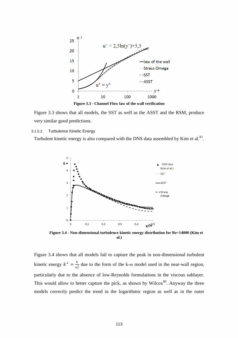
113
Figure 3.3 - Channel Flow law of the wall verification
Figure 3.3 shows that all models, the SST as well as the ASST and the RSM, produce
very similar good predictions.
3.1.5.2 Turbulence Kinetic Energy
Turbulent kinetic energy is also compared with the DNS data assembled by Kim et al.83
.
Figure 3.4 - Non-dimensional turbulence kinetic energy distribution for Re=14000 (Kim et
al.)
Figure 3.4 shows that all models fail to capture the peak in non-dimensional turbulent
kinetic energy 𝑘+ =𝑘
𝑢𝜏2 due to the form of the k-ω model used in the near-wall region,
particularly due to the absence of low-Reynolds formulations in the viscous sublayer.
This would allow to better capture the pick, as shown by Wilcox80
. Anyway the three
models correctly predict the trend in the logarithmic region as well as in the outer
DNS data
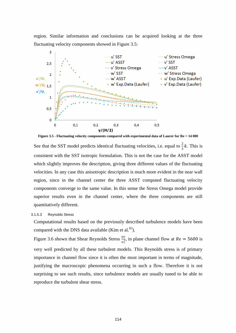
114
region. Similar information and conclusions can be acquired looking at the three
fluctuating velocity components showed in Figure 3.5:
Figure 3.5 - Fluctuating velocity components compared with experimental data of Laurer for Re = 14 000
See that the SST model predicts identical fluctuating velocities, i.e. equal to 2
3𝑘. This is
consistent with the SST isotropic formulation. This is not the case for the ASST model
which slightly improves the description, giving three different values of the fluctuating
velocities. In any case this anisotropic description is much more evident in the near wall
region, since in the channel center the three ASST computed fluctuating velocity
components converge to the same value. In this sense the Stress Omega model provide
superior results even in the channel center, where the three components are still
quantitatively different.
3.1.5.3 Reynolds Stress
Computational results based on the previously described turbulence models have been
compared with the DNS data available (Kim et al.83
).
Figure 3.6 shown that Shear Reynolds Stress 𝑢𝑣
𝑢𝜏2 , in plane channel flow at 𝑅𝑒 = 5600 is
very well predicted by all these turbulent models. This Reynolds stress is of primary
importance in channel flow since it is often the most important in terms of magnitude,
justifying the macroscopic phenomena occurring in such a flow. Therefore it is not
surprising to see such results, since turbulence models are usually tuned to be able to
reproduce the turbulent shear stress.
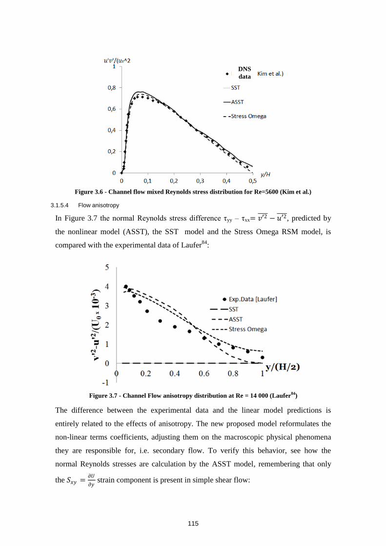
115
Figure 3.6 - Channel flow mixed Reynolds stress distribution for Re=5600 (Kim et al.)
3.1.5.4 Flow anisotropy
In Figure 3.7 the normal Reynolds stress difference ηyy – ηxx= 𝑣′2 − 𝑢′2 , predicted by
the nonlinear model (ASST), the SST model and the Stress Omega RSM model, is
compared with the experimental data of Laufer84
:
Figure 3.7 - Channel Flow anisotropy distribution at Re = 14 000 (Laufer84
)
The difference between the experimental data and the linear model predictions is
entirely related to the effects of anisotropy. The new proposed model reformulates the
non-linear terms coefficients, adjusting them on the macroscopic physical phenomena
they are responsible for, i.e. secondary flow. To verify this behavior, see how the
normal Reynolds stresses are calculation by the ASST model, remembering that only
the 𝑆𝑥𝑦 =𝜕𝑈
𝜕𝑦 strain component is present in simple shear flow:
DNS
data
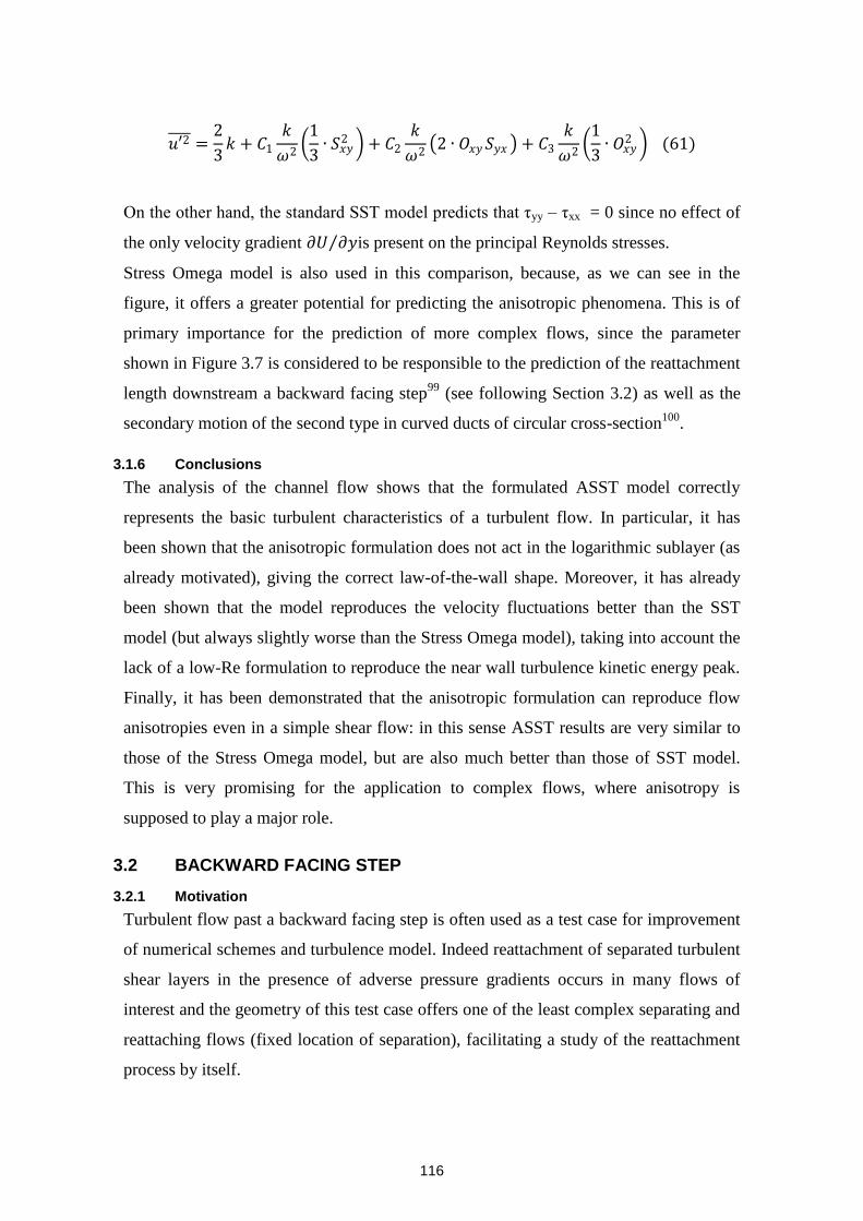
116
𝑢′2 =2
3𝑘 + 𝐶1
𝑘
𝜔2
1
3∙ 𝑆𝑥𝑦
2 + 𝐶2
𝑘
𝜔2 2 ∙ 𝑂𝑥𝑦𝑆𝑦𝑥 + 𝐶3
𝑘
𝜔2
1
3∙ 𝑂𝑥𝑦
2 (61)
On the other hand, the standard SST model predicts that ηyy – ηxx = 0 since no effect of
the only velocity gradient 𝜕𝑈 𝜕𝑦 is present on the principal Reynolds stresses.
Stress Omega model is also used in this comparison, because, as we can see in the
figure, it offers a greater potential for predicting the anisotropic phenomena. This is of
primary importance for the prediction of more complex flows, since the parameter
shown in Figure 3.7 is considered to be responsible to the prediction of the reattachment
length downstream a backward facing step99
(see following Section 3.2) as well as the
secondary motion of the second type in curved ducts of circular cross-section100
.
3.1.6 Conclusions
The analysis of the channel flow shows that the formulated ASST model correctly
represents the basic turbulent characteristics of a turbulent flow. In particular, it has
been shown that the anisotropic formulation does not act in the logarithmic sublayer (as
already motivated), giving the correct law-of-the-wall shape. Moreover, it has already
been shown that the model reproduces the velocity fluctuations better than the SST
model (but always slightly worse than the Stress Omega model), taking into account the
lack of a low-Re formulation to reproduce the near wall turbulence kinetic energy peak.
Finally, it has been demonstrated that the anisotropic formulation can reproduce flow
anisotropies even in a simple shear flow: in this sense ASST results are very similar to
those of the Stress Omega model, but are also much better than those of SST model.
This is very promising for the application to complex flows, where anisotropy is
supposed to play a major role.
3.2 BACKWARD FACING STEP
3.2.1 Motivation
Turbulent flow past a backward facing step is often used as a test case for improvement
of numerical schemes and turbulence model. Indeed reattachment of separated turbulent
shear layers in the presence of adverse pressure gradients occurs in many flows of
interest and the geometry of this test case offers one of the least complex separating and
reattaching flows (fixed location of separation), facilitating a study of the reattachment
process by itself.
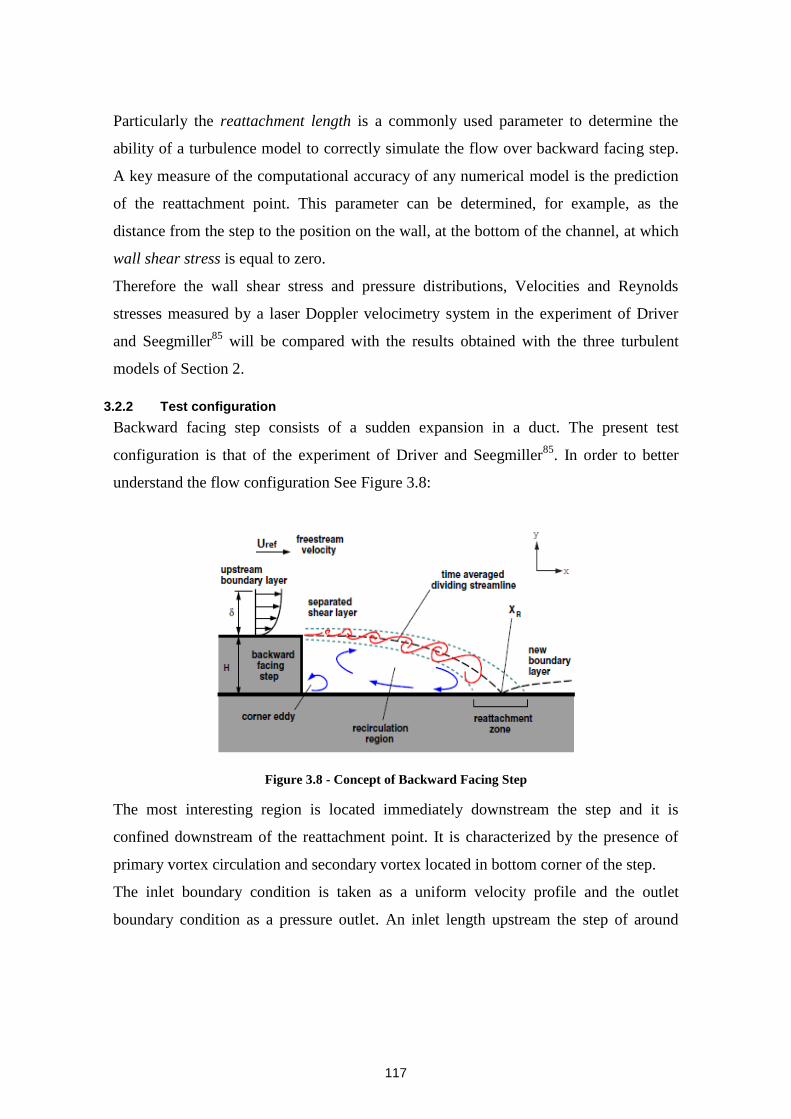
117
Particularly the reattachment length is a commonly used parameter to determine the
ability of a turbulence model to correctly simulate the flow over backward facing step.
A key measure of the computational accuracy of any numerical model is the prediction
of the reattachment point. This parameter can be determined, for example, as the
distance from the step to the position on the wall, at the bottom of the channel, at which
wall shear stress is equal to zero.
Therefore the wall shear stress and pressure distributions, Velocities and Reynolds
stresses measured by a laser Doppler velocimetry system in the experiment of Driver
and Seegmiller85
will be compared with the results obtained with the three turbulent
models of Section 2.
3.2.2 Test configuration
Backward facing step consists of a sudden expansion in a duct. The present test
configuration is that of the experiment of Driver and Seegmiller85
. In order to better
understand the flow configuration See Figure 3.8:
Figure 3.8 - Concept of Backward Facing Step
The most interesting region is located immediately downstream the step and it is
confined downstream of the reattachment point. It is characterized by the presence of
primary vortex circulation and secondary vortex located in bottom corner of the step.
The inlet boundary condition is taken as a uniform velocity profile and the outlet
boundary condition as a pressure outlet. An inlet length upstream the step of around
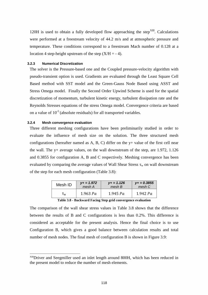
118
120H is used to obtain a fully developed flow approaching the stepXIII
. Calculations
were performed at a freestream velocity of 44.2 m/s and at atmospheric pressure and
temperature. These conditions correspond to a freestream Mach number of 0.128 at a
location 4 step-height upstream of the step (X/H = - 4).
3.2.3 Numerical Discretization
The solver is the Pressure-based one and the Coupled pressure-velocity algorithm with
pseudo-transient option is used. Gradients are evaluated through the Least Square Cell
Based method with SST model and the Green-Gauss Node Based using ASST and
Stress Omega model. Finally the Second Order Upwind Scheme is used for the spatial
discretization of momentum, turbulent kinetic energy, turbulent dissipation rate and the
Reynolds Stresses equations of the stress Omega model. Convergence criteria are based
on a value of 10-5
(absolute residuals) for all transported variables.
3.2.4 Mesh convergence evaluation
Three different meshing configurations have been preliminarily studied in order to
evaluate the influence of mesh size on the solution. The three structured mesh
configurations (hereafter named as A, B, C) differ on the y+ value of the first cell near
the wall. The y+ average values, on the wall downstream of the step, are 1.972, 1.126
and 0.3855 for configuration A, B and C respectively. Meshing convergence has been
evaluated by comparing the average values of Wall Shear Stress ηw on wall downstream
of the step for each mesh configuration (Table 3.8):
Mesh ID y+ = 1.972
mesh A y+ = 1.126
mesh B y+ = 0.3855
mesh C
τw 1.963 𝑃𝑎 1.945 𝑃𝑎 1.942 𝑃𝑎
Table 3.8 - Backward Facing Step grid convergence evaluation
The comparison of the wall shear stress values in Table 3.8 shows that the difference
between the results of B and C configurations is less than 0.2%. This difference is
considered as acceptable for the present analysis. Hence the final choice is to use
Configuration B, which gives a good balance between calculation results and total
number of mesh nodes. The final mesh of configuration B is shown in Figure 3.9:
XIIIDriver and Seegmiller used an inlet length around 800H, which has been reduced in
the present model to reduce the number of mesh elements.

119
Figure 3.9 - Backward Facing Step mesh B
3.2.5 Results
3.2.5.1 Step upstream conditions at X/H = -4
Streamwise velocity and Reynolds stress measurements are shown in Figure 3.10 and
Figure 3.11 and they are compared with computed profiles obtained using the three
different turbulent models of Section 2.
All results show a correct prediction of streamwise velocity and turbulent Reynolds
stress.
Figure 3.10 - Backward Facing Step velocity upstream the step at X/H = -4
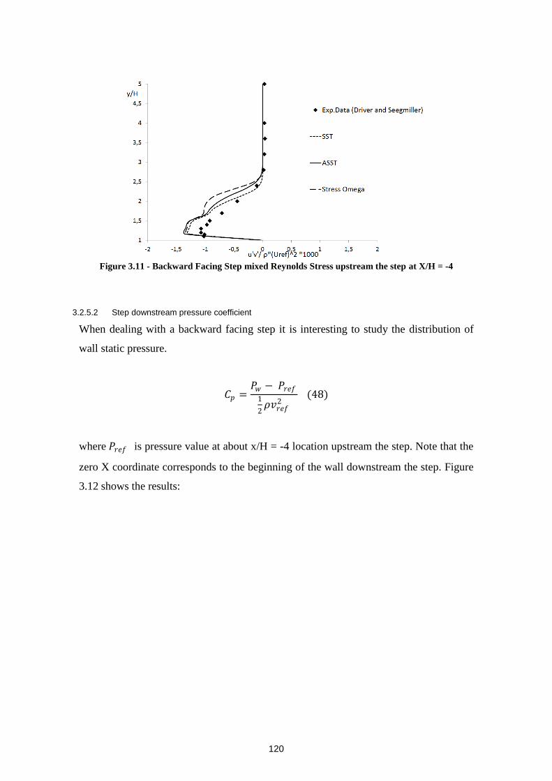
120
Figure 3.11 - Backward Facing Step mixed Reynolds Stress upstream the step at X/H = -4
3.2.5.2 Step downstream pressure coefficient
When dealing with a backward facing step it is interesting to study the distribution of
wall static pressure.
𝐶𝑝 =𝑃𝑤 − 𝑃𝑟𝑒𝑓
1
2𝜌𝑣𝑟𝑒𝑓
2 (48)
where 𝑃𝑟𝑒𝑓 is pressure value at about x/H = -4 location upstream the step. Note that the
zero X coordinate corresponds to the beginning of the wall downstream the step. Figure
3.12 shows the results:
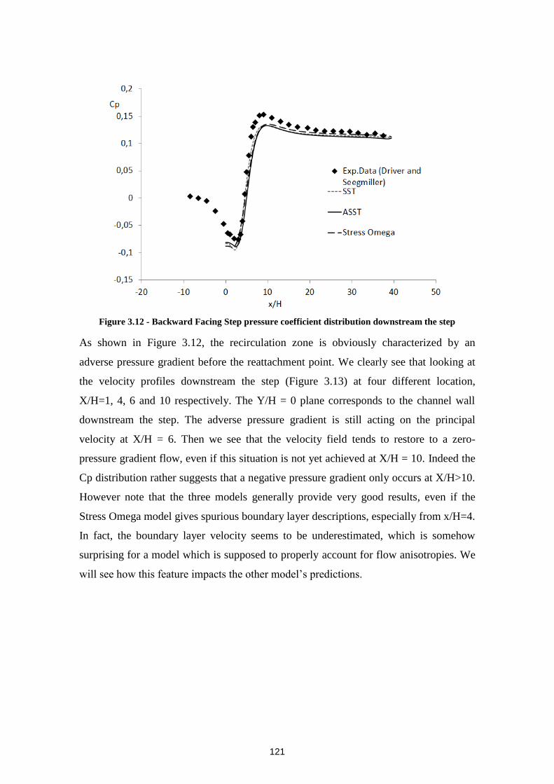
121
Figure 3.12 - Backward Facing Step pressure coefficient distribution downstream the step
As shown in Figure 3.12, the recirculation zone is obviously characterized by an
adverse pressure gradient before the reattachment point. We clearly see that looking at
the velocity profiles downstream the step (Figure 3.13) at four different location,
X/H=1, 4, 6 and 10 respectively. The Y/H = 0 plane corresponds to the channel wall
downstream the step. The adverse pressure gradient is still acting on the principal
velocity at X/H = 6. Then we see that the velocity field tends to restore to a zero-
pressure gradient flow, even if this situation is not yet achieved at X/H = 10. Indeed the
Cp distribution rather suggests that a negative pressure gradient only occurs at X/H>10.
However note that the three models generally provide very good results, even if the
Stress Omega model gives spurious boundary layer descriptions, especially from x/H=4.
In fact, the boundary layer velocity seems to be underestimated, which is somehow
surprising for a model which is supposed to properly account for flow anisotropies. We
will see how this feature impacts the other model’s predictions.
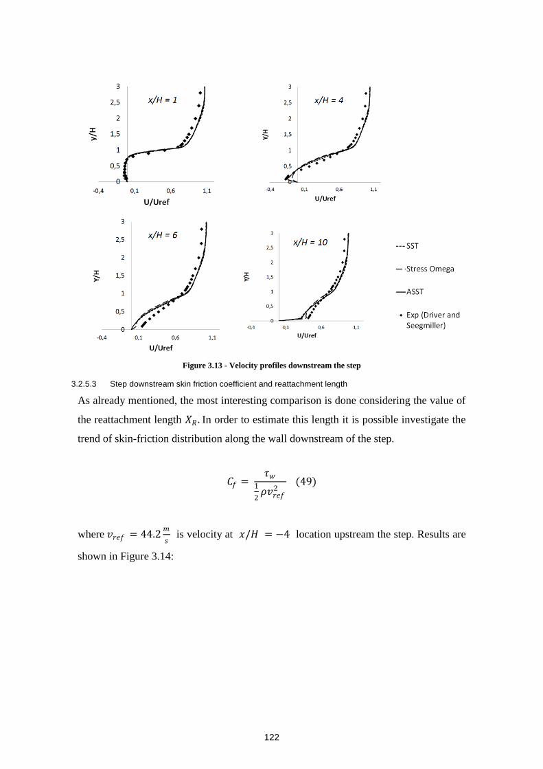
122
Figure 3.13 - Velocity profiles downstream the step
3.2.5.3 Step downstream skin friction coefficient and reattachment length
As already mentioned, the most interesting comparison is done considering the value of
the reattachment length 𝑋𝑅 . In order to estimate this length it is possible investigate the
trend of skin-friction distribution along the wall downstream of the step.
𝐶𝑓 = 𝜏𝑤
1
2𝜌𝑣𝑟𝑒𝑓
2 (49)
where 𝑣𝑟𝑒𝑓 = 44.2𝑚
𝑠 is velocity at 𝑥/𝐻 = −4 location upstream the step. Results are
shown in Figure 3.14:
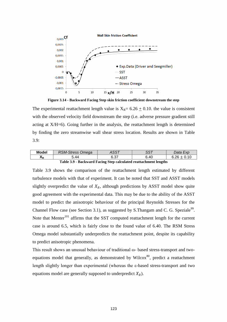
123
Figure 3.14 - Backward Facing Step skin friction coefficient downstream the step
The experimental reattachment length value is XR= 6.26 + 0.10. the value is consistent
with the observed velocity field downstream the step (i.e. adverse pressure gradient still
acting at X/H=6). Going further in the analysis, the reattachment length is determined
by finding the zero streamwise wall shear stress location. Results are shown in Table
3.9:
Model RSM-Stress Omega ASST SST Data Exp
XR 5.44 6.37 6.40 6.26 ± 0.10
Table 3.9 - Backward Facing Step calculated reattachment lengths
Table 3.9 shows the comparison of the reattachment length estimated by different
turbulence models with that of experiment. It can be noted that SST and ASST models
slightly overpredict the value of 𝑋𝑅, although predictions by ASST model show quite
good agreement with the experimental data. This may be due to the ability of the ASST
model to predict the anisotropic behaviour of the principal Reynolds Stresses for the
Channel Flow case (see Section 3.1), as suggested by S.Thangam and C. G. Speziale99
.
Note that Menter101
affirms that the SST computed reattachment length for the current
case is around 6.5, which is fairly close to the found value of 6.40. The RSM Stress
Omega model substantially underpredicts the reattachment point, despite its capability
to predict anisotropic phenomena.
This result shows an unusual behaviour of traditional ω- based stress-transport and two-
equations model that generally, as demonstrated by Wilcox80
, predict a reattachment
length slightly longer than experimental (whereas the ε-based stress-transport and two
equations model are generally supposed to underpredict 𝑋𝑅).
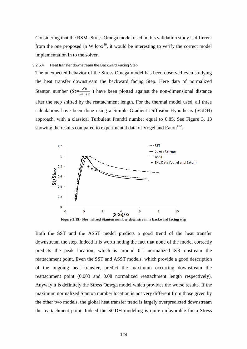
124
Considering that the RSM- Stress Omega model used in this validation study is different
from the one proposed in Wilcox80
, it would be interesting to verify the correct model
implementation in to the solver.
3.2.5.4 Heat transfer downstream the Backward Facing Step
The unexpected behavior of the Stress Omega model has been observed even studying
the heat transfer downstream the backward facing Step. Here data of normalized
Stanton number (𝑆𝑡=𝑁𝑢
𝑅𝑒𝐻𝑃𝑟 ) have been plotted against the non-dimensional distance
after the step shifted by the reattachment length. For the thermal model used, all three
calculations have been done using a Simple Gradient Diffusion Hypothesis (SGDH)
approach, with a classical Turbulent Prandtl number equal to 0.85. See Figure 3. 13
showing the results compared to experimental data of Vogel and Eaton102
.
Figure 3.15 - Normalized Stanton number downstream a backward facing step
Both the SST and the ASST model predicts a good trend of the heat transfer
downstream the step. Indeed it is worth noting the fact that none of the model correctly
predicts the peak location, which is around 0.1 normalized XR upstream the
reattachment point. Even the SST and ASST models, which provide a good description
of the ongoing heat transfer, predict the maximum occurring downstream the
reattachment point (0.003 and 0.08 normalized reattachment length respectively).
Anyway it is definitely the Stress Omega model which provides the worse results. If the
maximum normalized Stanton number location is not very different from those given by
the other two models, the global heat transfer trend is largely overpredicted downstream
the reattachment point. Indeed the SGDH modeling is quite unfavorable for a Stress
125
Model application, since the potential better description of the Reynolds Stresses could
be usefully used with a more sophisticated General Gradient Diffusion Hypothesis
(GGDH), which is not an available option in ANSYS Fluent ®.
3.2.6 Conclusions
The present analysis of backward facing step flow case shows that each of three
turbulent models does a good qualitative job of predicting the flow, moreover the ASST
model shows a good improvement over the other models. In fact it provides the best
reattachment length in a pure aerodynamic calculation and very good description of the
heat transfer downstream the step, when modelled. The SST model also provides
valuable results both for reattachment length and heat transfer. On the other hand,
unexpected behaviour of the Stress Omega model has been detected both for the
reattachment length and the heat transfer. This somehow questions the applicability of
such a model in more complex flows. Anyway it can be concluded that also this
validation test case assures the correct formulation and applicability of the ASST model.
3.3 TURBULENT DEVELOPING FLOW IN A 90° BEND
3.3.1 Motivation
Fluid flow in a bend is a baseline flow studied for several applications in applied
sciences. Configurations of interest are, for instance, centrifugal pumps, heat exchanger
tube-side and industrial pipelines. It is of particular interest for the present application
since the in-bend flow coming from mixing zones cannot be considered as fully
developed flow: therefore it is interesting to verify the model capabilities to correctly
describe this flow configuration.
A characteristic which distinguishes such flows from those in straight ducts is the
generation of streamwise vorticity, or "secondary motion," within the duct, resulting in
a pressure loss, the spatial redistribution of streamwise velocity and increased heat
transfer at the duct wall.
Hence, the aim of this work is to numerically investigate the turbulent flow inside a 90
degree bend of squared cross-section, and determine the appropriate turbulence
modelling level required to describe this flow.
3.3.2 Test Configuration
The present work will study the bend geometry proposed by Taylor and al.103
(Figure
3.16):
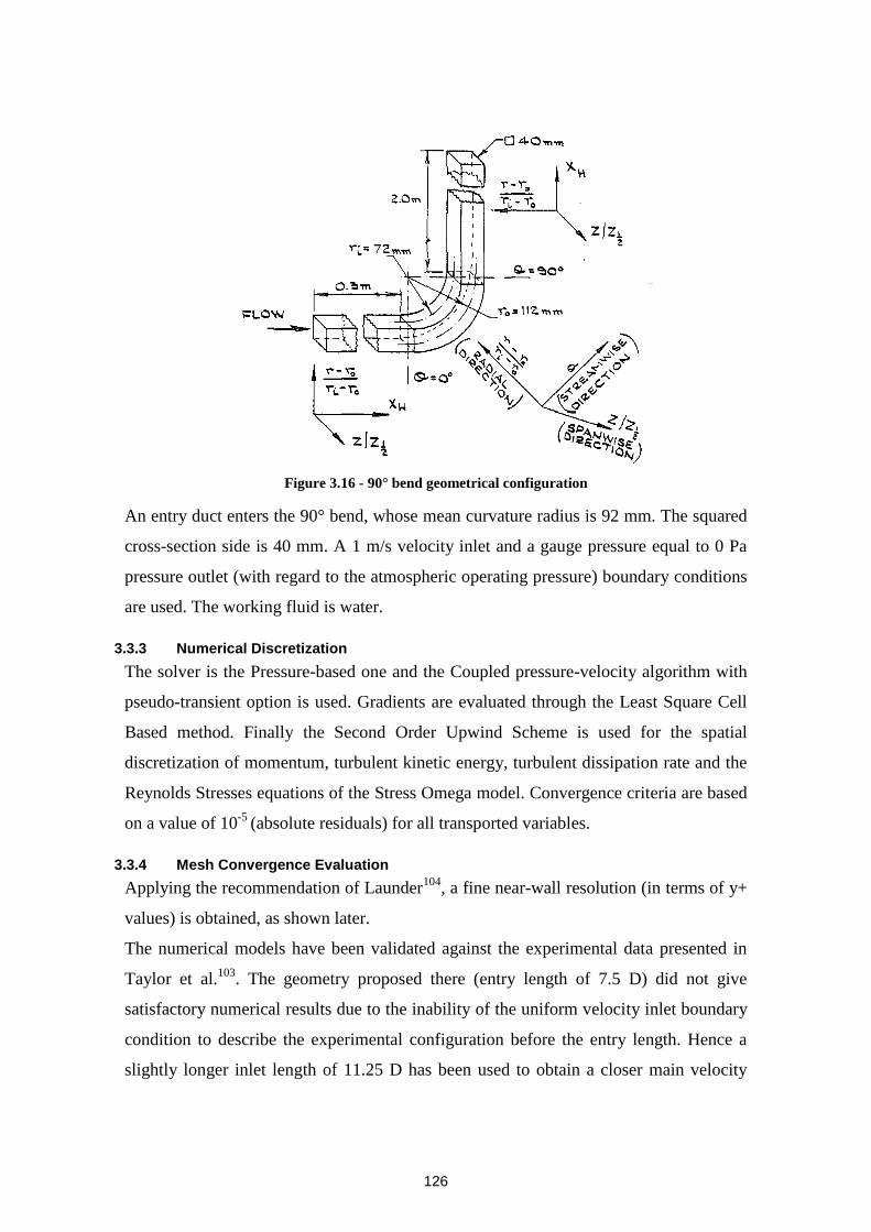
126
Figure 3.16 - 90° bend geometrical configuration
An entry duct enters the 90° bend, whose mean curvature radius is 92 mm. The squared
cross-section side is 40 mm. A 1 m/s velocity inlet and a gauge pressure equal to 0 Pa
pressure outlet (with regard to the atmospheric operating pressure) boundary conditions
are used. The working fluid is water.
3.3.3 Numerical Discretization
The solver is the Pressure-based one and the Coupled pressure-velocity algorithm with
pseudo-transient option is used. Gradients are evaluated through the Least Square Cell
Based method. Finally the Second Order Upwind Scheme is used for the spatial
discretization of momentum, turbulent kinetic energy, turbulent dissipation rate and the
Reynolds Stresses equations of the Stress Omega model. Convergence criteria are based
on a value of 10-5
(absolute residuals) for all transported variables.
3.3.4 Mesh Convergence Evaluation
Applying the recommendation of Launder104
, a fine near-wall resolution (in terms of y+
values) is obtained, as shown later.
The numerical models have been validated against the experimental data presented in
Taylor et al.103
. The geometry proposed there (entry length of 7.5 D) did not give
satisfactory numerical results due to the inability of the uniform velocity inlet boundary
condition to describe the experimental configuration before the entry length. Hence a
slightly longer inlet length of 11.25 D has been used to obtain a closer main velocity

127
profile in the inlet section but not changing the paper base idea of developing flow into
a bend. The original 50 D exit length has been retained.
Using the described geometry, three different meshing configurations have been
preliminarily studied in order to evaluate the influence of mesh size on the solution. The
three structured mesh configurations (hereafter named as A, B, C) differ by a factor of
around 2 on the mesh size in the first layer thickness (Table 3.10):
Mesh Configuration
Y+
A 0.27
B 0.15
C 0.12
Table 3.10 - 90° bend used grids
The y+ average values are 0.27 and 0.14 and 0.12 for configuration A, B and C whereas
the maximum y+ are 0.78, 0.40 and 0.21 respectively.
An example of the final mesh for the B configuration in the inlet channel cross-section
is shown in Figure 3.17:
Figure 3.17 - 90° bend mesh example
Meshing convergence has been evaluated by comparing wall average wall shear stress.
The mesh convergence evaluation is shown in Table 3.11:
Mesh Configuration
τw[Pa]
A 2.61
B 2.70
C 2.72
Table 3.11 - 90° bend mesh convergence evaluation
The comparison of the wall shear stress values shows a good agreement for the B and C
configurations (difference in the wall shear stress less than 1%). The final choice is to
use Configuration B, which gives a good balance between calculation results and total
number of mesh nodes.
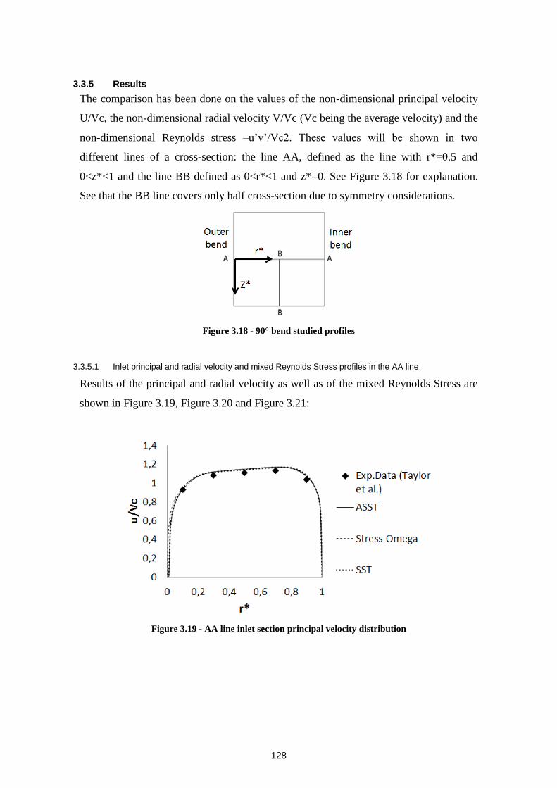
128
3.3.5 Results
The comparison has been done on the values of the non-dimensional principal velocity
U/Vc, the non-dimensional radial velocity V/Vc (Vc being the average velocity) and the
non-dimensional Reynolds stress –u’v’/Vc2. These values will be shown in two
different lines of a cross-section: the line AA, defined as the line with r*=0.5 and
0<z*<1 and the line BB defined as 0<r*<1 and z*=0. See Figure 3.18 for explanation.
See that the BB line covers only half cross-section due to symmetry considerations.
Figure 3.18 - 90° bend studied profiles
3.3.5.1 Inlet principal and radial velocity and mixed Reynolds Stress profiles in the AA line
Results of the principal and radial velocity as well as of the mixed Reynolds Stress are
shown in Figure 3.19, Figure 3.20 and Figure 3.21:
Figure 3.19 - AA line inlet section principal velocity distribution
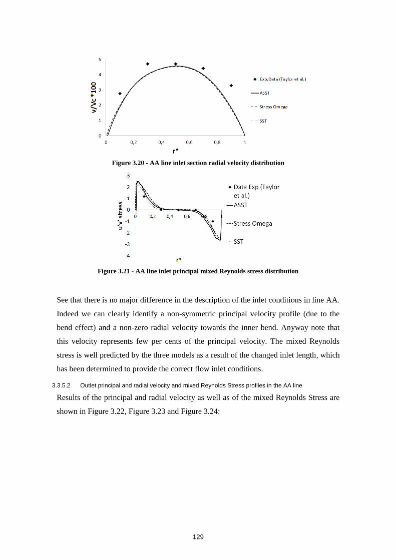
129
Figure 3.20 - AA line inlet section radial velocity distribution
Figure 3.21 - AA line inlet principal mixed Reynolds stress distribution
See that there is no major difference in the description of the inlet conditions in line AA.
Indeed we can clearly identify a non-symmetric principal velocity profile (due to the
bend effect) and a non-zero radial velocity towards the inner bend. Anyway note that
this velocity represents few per cents of the principal velocity. The mixed Reynolds
stress is well predicted by the three models as a result of the changed inlet length, which
has been determined to provide the correct flow inlet conditions.
3.3.5.2 Outlet principal and radial velocity and mixed Reynolds Stress profiles in the AA line
Results of the principal and radial velocity as well as of the mixed Reynolds Stress are
shown in Figure 3.22, Figure 3.23 and Figure 3.24:
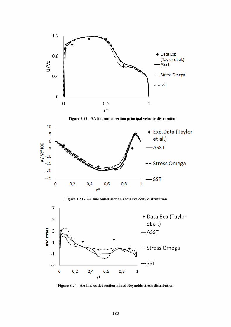
130
Figure 3.22 - AA line outlet section principal velocity distribution
Figure 3.23 - AA line outlet section radial velocity distribution
Figure 3.24 - AA line outlet section mixed Reynolds stress distribution
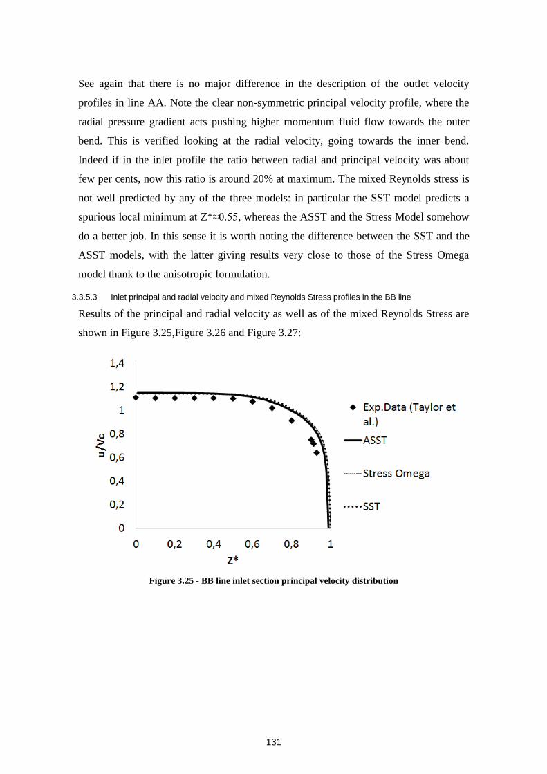
131
See again that there is no major difference in the description of the outlet velocity
profiles in line AA. Note the clear non-symmetric principal velocity profile, where the
radial pressure gradient acts pushing higher momentum fluid flow towards the outer
bend. This is verified looking at the radial velocity, going towards the inner bend.
Indeed if in the inlet profile the ratio between radial and principal velocity was about
few per cents, now this ratio is around 20% at maximum. The mixed Reynolds stress is
not well predicted by any of the three models: in particular the SST model predicts a
spurious local minimum at Z*≈0.55, whereas the ASST and the Stress Model somehow
do a better job. In this sense it is worth noting the difference between the SST and the
ASST models, with the latter giving results very close to those of the Stress Omega
model thank to the anisotropic formulation.
3.3.5.3 Inlet principal and radial velocity and mixed Reynolds Stress profiles in the BB line
Results of the principal and radial velocity as well as of the mixed Reynolds Stress are
shown in Figure 3.25,Figure 3.26 and Figure 3.27:
Figure 3.25 - BB line inlet section principal velocity distribution
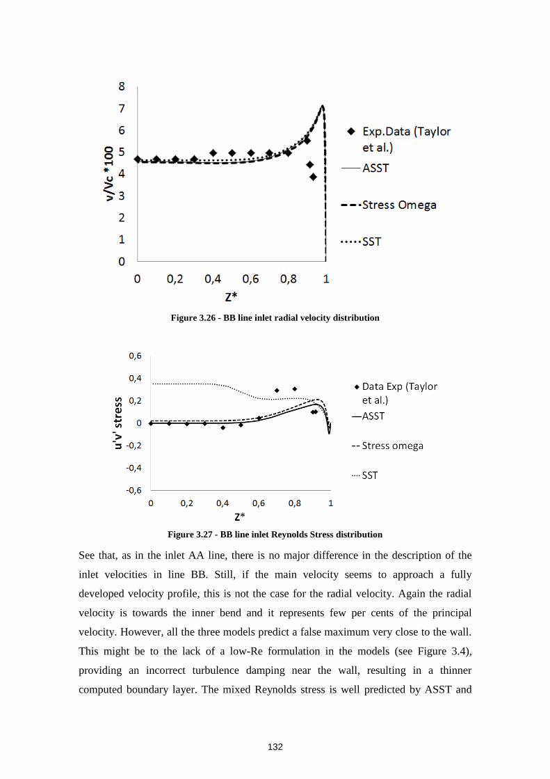
132
Figure 3.26 - BB line inlet radial velocity distribution
Figure 3.27 - BB line inlet Reynolds Stress distribution
See that, as in the inlet AA line, there is no major difference in the description of the
inlet velocities in line BB. Still, if the main velocity seems to approach a fully
developed velocity profile, this is not the case for the radial velocity. Again the radial
velocity is towards the inner bend and it represents few per cents of the principal
velocity. However, all the three models predict a false maximum very close to the wall.
This might be to the lack of a low-Re formulation in the models (see Figure 3.4),
providing an incorrect turbulence damping near the wall, resulting in a thinner
computed boundary layer. The mixed Reynolds stress is well predicted by ASST and
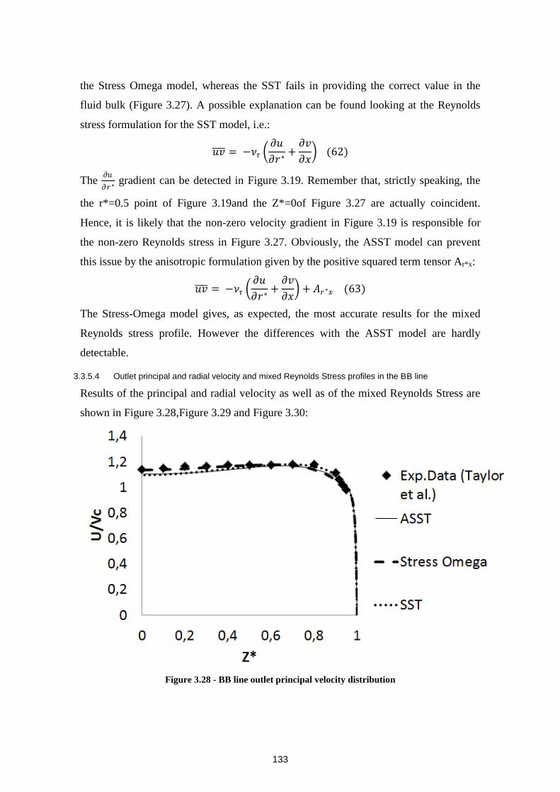
133
the Stress Omega model, whereas the SST fails in providing the correct value in the
fluid bulk (Figure 3.27). A possible explanation can be found looking at the Reynolds
stress formulation for the SST model, i.e.:
𝑢𝑣 = −𝜈𝜏 𝜕𝑢
𝜕𝑟∗+
𝜕𝑣
𝜕𝑥 (62)
The 𝜕𝑢
𝜕𝑟∗ gradient can be detected in Figure 3.19. Remember that, strictly speaking, the
the r*=0.5 point of Figure 3.19and the Z*=0of Figure 3.27 are actually coincident.
Hence, it is likely that the non-zero velocity gradient in Figure 3.19 is responsible for
the non-zero Reynolds stress in Figure 3.27. Obviously, the ASST model can prevent
this issue by the anisotropic formulation given by the positive squared term tensor Ar*x:
𝑢𝑣 = −𝜈𝜏 𝜕𝑢
𝜕𝑟∗+
𝜕𝑣
𝜕𝑥 + 𝐴𝑟∗𝑥 (63)
The Stress-Omega model gives, as expected, the most accurate results for the mixed
Reynolds stress profile. However the differences with the ASST model are hardly
detectable.
3.3.5.4 Outlet principal and radial velocity and mixed Reynolds Stress profiles in the BB line
Results of the principal and radial velocity as well as of the mixed Reynolds Stress are
shown in Figure 3.28,Figure 3.29 and Figure 3.30:
Figure 3.28 - BB line outlet principal velocity distribution
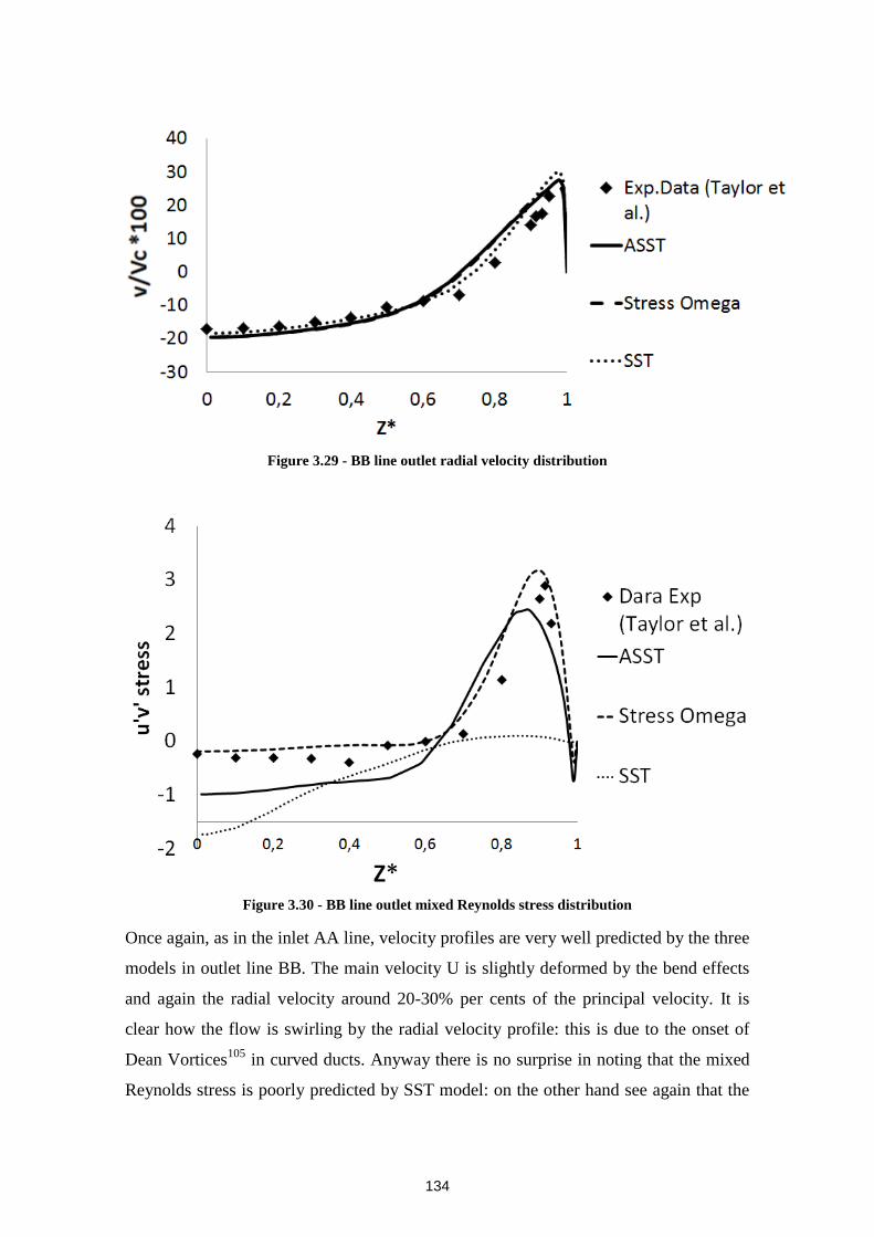
134
Figure 3.29 - BB line outlet radial velocity distribution
Figure 3.30 - BB line outlet mixed Reynolds stress distribution
Once again, as in the inlet AA line, velocity profiles are very well predicted by the three
models in outlet line BB. The main velocity U is slightly deformed by the bend effects
and again the radial velocity around 20-30% per cents of the principal velocity. It is
clear how the flow is swirling by the radial velocity profile: this is due to the onset of
Dean Vortices105
in curved ducts. Anyway there is no surprise in noting that the mixed
Reynolds stress is poorly predicted by SST model: on the other hand see again that the
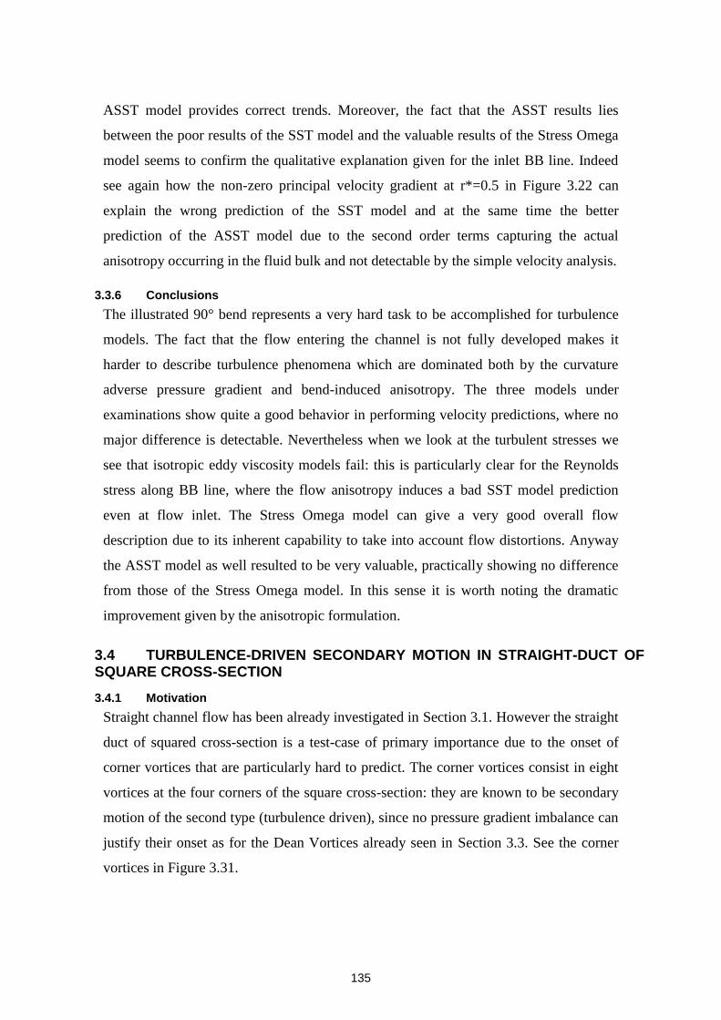
135
ASST model provides correct trends. Moreover, the fact that the ASST results lies
between the poor results of the SST model and the valuable results of the Stress Omega
model seems to confirm the qualitative explanation given for the inlet BB line. Indeed
see again how the non-zero principal velocity gradient at r*=0.5 in Figure 3.22 can
explain the wrong prediction of the SST model and at the same time the better
prediction of the ASST model due to the second order terms capturing the actual
anisotropy occurring in the fluid bulk and not detectable by the simple velocity analysis.
3.3.6 Conclusions
The illustrated 90° bend represents a very hard task to be accomplished for turbulence
models. The fact that the flow entering the channel is not fully developed makes it
harder to describe turbulence phenomena which are dominated both by the curvature
adverse pressure gradient and bend-induced anisotropy. The three models under
examinations show quite a good behavior in performing velocity predictions, where no
major difference is detectable. Nevertheless when we look at the turbulent stresses we
see that isotropic eddy viscosity models fail: this is particularly clear for the Reynolds
stress along BB line, where the flow anisotropy induces a bad SST model prediction
even at flow inlet. The Stress Omega model can give a very good overall flow
description due to its inherent capability to take into account flow distortions. Anyway
the ASST model as well resulted to be very valuable, practically showing no difference
from those of the Stress Omega model. In this sense it is worth noting the dramatic
improvement given by the anisotropic formulation.
3.4 TURBULENCE-DRIVEN SECONDARY MOTION IN STRAIGHT-DUCT OF SQUARE CROSS-SECTION
3.4.1 Motivation
Straight channel flow has been already investigated in Section 3.1. However the straight
duct of squared cross-section is a test-case of primary importance due to the onset of
corner vortices that are particularly hard to predict. The corner vortices consist in eight
vortices at the four corners of the square cross-section: they are known to be secondary
motion of the second type (turbulence driven), since no pressure gradient imbalance can
justify their onset as for the Dean Vortices already seen in Section 3.3. See the corner
vortices in Figure 3.31.
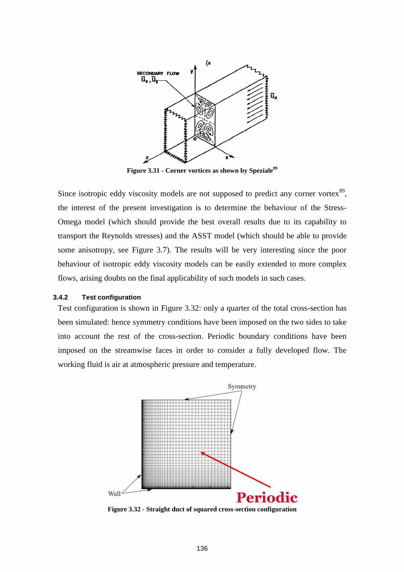
136
Figure 3.31 - Corner vortices as shown by Speziale
89
Since isotropic eddy viscosity models are not supposed to predict any corner vortex89
,
the interest of the present investigation is to determine the behaviour of the Stress-
Omega model (which should provide the best overall results due to its capability to
transport the Reynolds stresses) and the ASST model (which should be able to provide
some anisotropy, see Figure 3.7). The results will be very interesting since the poor
behaviour of isotropic eddy viscosity models can be easily extended to more complex
flows, arising doubts on the final applicability of such models in such cases.
3.4.2 Test configuration
Test configuration is shown in Figure 3.32: only a quarter of the total cross-section has
been simulated: hence symmetry conditions have been imposed on the two sides to take
into account the rest of the cross-section. Periodic boundary conditions have been
imposed on the streamwise faces in order to consider a fully developed flow. The
working fluid is air at atmospheric pressure and temperature.
Figure 3.32 - Straight duct of squared cross-section configuration

137
3.4.3 Numerical discretization
The solver is the Pressure-based one and the SIMPLE pressure-velocity algorithm with
pseudo-transient option is used. Gradients are evaluated through the Least Square Cell
Based method. Finally the Second Order Upwind Scheme is used for the spatial
discretization of momentum, turbulent kinetic energy, turbulent dissipation rate and the
Reynolds Stresses equations of the RSM model. Convergence criteria are based on a
value of 10-5
(absolute residuals) for all transported variables.
3.4.4 Mesh convergence evaluation
Three meshes differing by around two in the y+ value have been used to test grid
convergence; results of this study are shown in Table 3.12:
Mesh ID Y+ τw
A 0.81 4.82 mPa B 0.35 4.73 mPa C 0.13 4.71 mPa
Table 3.12 - Straight duct of squared cross-section grid independence evaluation
Note that there is practically no difference between mesh B and C. Therefore mesh C is
chosen, such a finest mesh not considering a major problem with regard to
computational time.
3.4.5 Results
Results of the analysis are shown in Figure 3.33, where the comparison between the
vertical velocities V (with respect to the mean velocity U0) is plotted. The difference
between the SST and the ASST models is dramatic: as expected, the isotropic SST
model cannot account for flow anisotropies resulting in the corner vortices, giving a
vertical velocity identically equal to 0. On the other hand, the anisotropic formulation of
the ASST model provides results that approach those of the Stress Omega model, which
is the only one that correctly takes into account anisotropy and turbulence history. In
this sense, the Stress Omega model provides the best approximation of the velocity
maximum value, even though the profile is somehow smoother than expected. ASST
model provides a lower maximum value but seems to reproduce better the global trend.
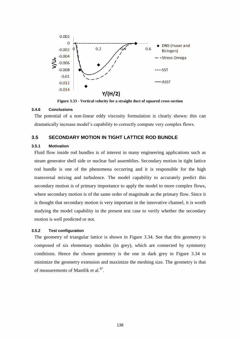
138
Figure 3.33 - Vertical velocity for a straight duct of squared cross-section
3.4.6 Conclusions
The potential of a non-linear eddy viscosity formulation is clearly shown: this can
dramatically increase model’s capability to correctly compute very complex flows.
3.5 SECONDARY MOTION IN TIGHT LATTICE ROD BUNDLE
3.5.1 Motivation
Fluid flow inside rod bundles is of interest in many engineering applications such as
steam generator shell side or nuclear fuel assemblies. Secondary motion in tight lattice
rod bundle is one of the phenomena occurring and it is responsible for the high
transversal mixing and turbulence. The model capability to accurately predict this
secondary motion is of primary importance to apply the model to more complex flows,
where secondary motion is of the same order of magnitude as the primary flow. Since it
is thought that secondary motion is very important in the innovative channel, it is worth
studying the model capability in the present test case to verify whether the secondary
motion is well predicted or not.
3.5.2 Test configuration
The geometry of triangular lattice is shown in Figure 3.34. See that this geometry is
composed of six elementary modules (in grey), which are connected by symmetry
conditions. Hence the chosen geometry is the one in dark grey in Figure 3.34 to
minimize the geometry extension and maximize the meshing size. The geometry is that
of measurements of Mantlik et al.87
.
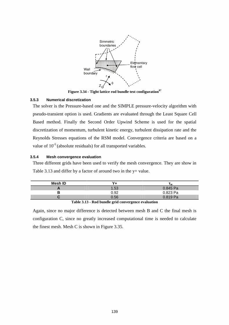
139
Figure 3.34 - Tight lattice rod bundle test configuration
87
3.5.3 Numerical discretization
The solver is the Pressure-based one and the SIMPLE pressure-velocity algorithm with
pseudo-transient option is used. Gradients are evaluated through the Least Square Cell
Based method. Finally the Second Order Upwind Scheme is used for the spatial
discretization of momentum, turbulent kinetic energy, turbulent dissipation rate and the
Reynolds Stresses equations of the RSM model. Convergence criteria are based on a
value of 10-5
(absolute residuals) for all transported variables.
3.5.4 Mesh convergence evaluation
Three different grids have been used to verify the mesh convergence. They are show in
Table 3.13 and differ by a factor of around two in the y+ value.
Mesh ID Y+ τw
A 1.53 0.845 Pa B 0.92 0.823 Pa C 0.56 0.819 Pa
Table 3.13 - Rod bundle grid convergence evaluation
Again, since no major difference is detected between mesh B and C the final mesh is
configuration C, since no greatly increased computational time is needed to calculate
the finest mesh. Mesh C is shown in Figure 3.35.
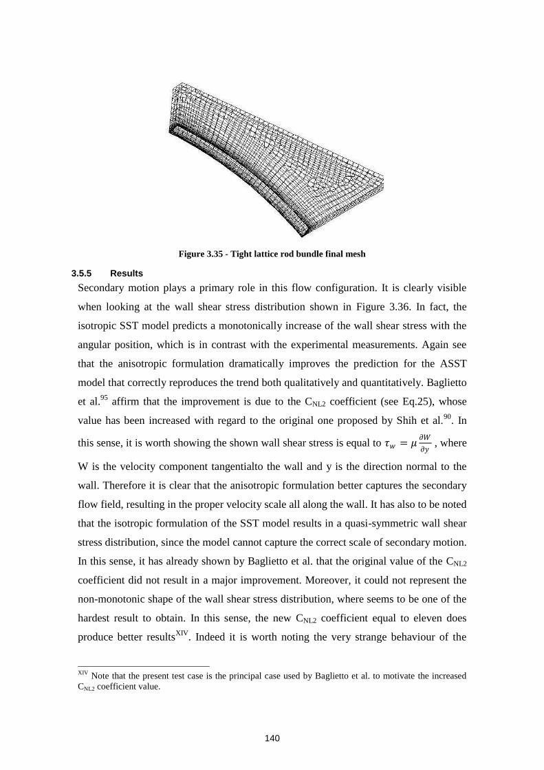
140
Figure 3.35 - Tight lattice rod bundle final mesh
3.5.5 Results
Secondary motion plays a primary role in this flow configuration. It is clearly visible
when looking at the wall shear stress distribution shown in Figure 3.36. In fact, the
isotropic SST model predicts a monotonically increase of the wall shear stress with the
angular position, which is in contrast with the experimental measurements. Again see
that the anisotropic formulation dramatically improves the prediction for the ASST
model that correctly reproduces the trend both qualitatively and quantitatively. Baglietto
et al.95
affirm that the improvement is due to the CNL2 coefficient (see Eq.25), whose
value has been increased with regard to the original one proposed by Shih et al.90
. In
this sense, it is worth showing the shown wall shear stress is equal to 𝜏𝑤 = 𝜇𝜕𝑊
𝜕𝑦 , where
W is the velocity component tangentialto the wall and y is the direction normal to the
wall. Therefore it is clear that the anisotropic formulation better captures the secondary
flow field, resulting in the proper velocity scale all along the wall. It has also to be noted
that the isotropic formulation of the SST model results in a quasi-symmetric wall shear
stress distribution, since the model cannot capture the correct scale of secondary motion.
In this sense, it has already shown by Baglietto et al. that the original value of the CNL2
coefficient did not result in a major improvement. Moreover, it could not represent the
non-monotonic shape of the wall shear stress distribution, where seems to be one of the
hardest result to obtain. In this sense, the new CNL2 coefficient equal to eleven does
produce better resultsXIV
. Indeed it is worth noting the very strange behaviour of the
XIV
Note that the present test case is the principal case used by Baglietto et al. to motivate the increased
CNL2 coefficient value.
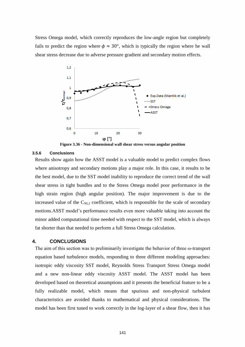
141
Stress Omega model, which correctly reproduces the low-angle region but completely
fails to predict the region where 𝜙 ≈ 30°, which is typically the region where he wall
shear stress decrease due to adverse pressure gradient and secondary motion effects.
Figure 3.36 - Non-dimensional wall shear stress versus angular position
3.5.6 Conclusions
Results show again how the ASST model is a valuable model to predict complex flows
where anisotropy and secondary motions play a major role. In this case, it results to be
the best model, due to the SST model inability to reproduce the correct trend of the wall
shear stress in tight bundles and to the Stress Omega model poor performance in the
high strain region (high angular position). The major improvement is due to the
increased value of the CNL2 coefficient, which is responsible for the scale of secondary
motions.ASST model’s performance results even more valuable taking into account the
minor added computational time needed with respect to the SST model, which is always
fat shorter than that needed to perform a full Stress Omega calculation.
4. CONCLUSIONS
The aim of this section was to preliminarily investigate the behavior of three ω-transport
equation based turbulence models, responding to three different modeling approaches:
isotropic eddy viscosity SST model, Reynolds Stress Transport Stress Omega model
and a new non-linear eddy viscosity ASST model. The ASST model has been
developed based on theoretical assumptions and it presents the beneficial feature to be a
fully realizable model, which means that spurious and non-physical turbulent
characteristics are avoided thanks to mathematical and physical considerations. The
model has been first tuned to work correctly in the log-layer of a shear flow, then it has
142
been implemented into the solver via User Defined Functions. Finally it has been
validated against experimental data, together with the SST and the Stress Omega
models. The three models have identical performances for straight channel flow
(basically having been developed for such a flow), differing only in the ability to
reproduce turbulence driven anisotropies. This macroscopically results in a good
behavior of the ASST and Stress Omega model to reproduce corner vortices in a
straight duct a squared cross-section and turbulence characteristics in a 90° bend.
Anyway the confidence towards a broader applicability of the Stress Omega model is
questioned by two unexpected results found in the Backward Facing Step and Tight
Lattice Rod Bundle cases: in the former, the Stress Omega predicts a shorter
reattachment length than expected (which is in contrast with its developer’s guideline);
in the latter, the Stress Omega model fails in the high strain rate region, providing a
dramatic decrease of the wall shear stress compared to experimental measurements.
This is in contrast with its potential ability to provide very truthful results for such
relatively simple flows. In this sense, it seems that the ASST model can provide a
valuable alternative, giving global results that are at least as good as those of the Stress
Omega model. Moreover, it keeps a very shorter computational time than the Stress
Omega model, resulting to be a very good option for the desired industrial tool to
potentially describe the innovative channel flow. See however that none of the shown
test cases really represents the complexity of the innovative channel flow, which can be
considered as a sum of all these test cases. Therefore this section clearly identifies the
need of an experimental database for the innovative channel flow to validate the
numerical model and the channel performance. The acquisition of this database is the
object of the following Chapter.
As a final comment, it had been stated that non-linear eddy viscosity models result in a
low additional computational effort compared to linear eddy viscosity models. In this
sense, see that, for the case discussed in Section 3.1 – Channel flow, the computational
time for the three tested models is about 2 minutes for the SST and ASST model (the
difference was hardly detectable) and around 4.5 minutes for the Stress Omega model.
This computational times are based on a 30 000 element meshing and have been
evaluated on a single processor Intel Xenon E5440 machine at 2.83 GHz and 24 Gb
RAM.
143
Chapitre 4: Acquisition de la base de
données expérimentales
Les chapitres 2 et 3 ont souligné le besoin d’une base de données expérimentale pour
valider le modèle numérique et pour étudier l’écoulement dans le canal innovant. Dans
le cas d’un canal pour un échangeur de chaleur, les besoins de validation concernent à la
fois la description purement aérauliques et la description thermique. Pour la partie
aéraulique deux bancs d’essai de vélocimétrie laser ont été mis en place : un banc de
vélocimétrie laser à franges (LDV) et un banc de vélocimétrie laser par images de
particules (PIV).
La campagne de LDV a permis d'acquérir une très grande base de données sur les
vitesses d'écoulement et sur les fluctuations de vitesse dans plusieurs régions du motif
innovant. Ces données sont très utiles pour la validation du modèle numérique, car ils
permettent un accès géographique aussi bien dans le fluide que dans la couche limite.
Par contre d’un point de vue physique, la vitesse verticale dans les profils orthogonaux à
la zone de mélange, responsable du mélange, n’a pas pu être mesurée. Cette information
peut être néanmoins retrouvée par la modélisation, une fois cette dernière validée. Les
données acquises confirment l'hypothèse de conception en termes de développement de
l’écoulement (qui est réalisé après quatre coudes) et la symétrie de l’écoulement, qui ont
été démontrés. Par contre la campagne expérimentale LDV ne permet pas d’avoir une
vue d'ensemble de l'écoulement du canal, qui est difficile de déduire des données
acquises sur les profils locaux. Pour cela, la campagne PIV, moins précise en proche
paroi, a permis l’acquisition de ces champs globaux sur le plan de mesure.
La base de données PIV a été acquise avec un nombre d'images par mesure trop faible
pour la convergence statistique de chaque mesure en raison de contraintes de temps.
Cependant, la convergence statistique non-parfaite a été prise en compte dans
l'évaluation des incertitudes, en permettant une analyse correcte des données acquises.
Ces données permettront de vérifier le comportement du modèle numérique tout en
révélant les caractéristiques globales d'écoulement qui n'ont pas été observées au cours
de la campagne LDV et qui seront discutées dans le Chapitre 5. La vérification du
développement et de la symétrie de l’écoulement est importante pour valider l'hypothèse
de conception. En ce qui concerne la validation thermique, un banc d’essai VHEGAS a

144
été conçu et mis en place pour mesurer le coefficient d’échange global du motif
innovant. Deux essais ont été menés avec des densités de flux de chaleur différentes,
pour analyser les effets potentiels de compressibilité thermique.
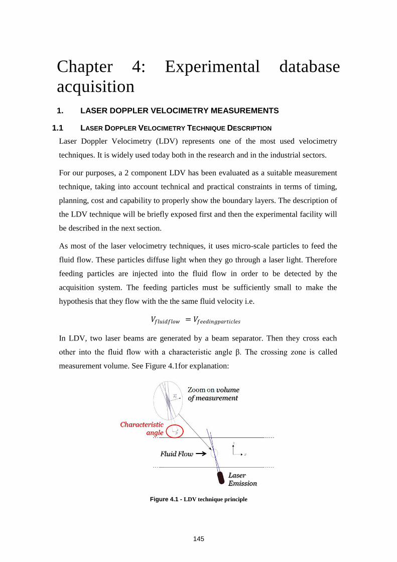
145
Chapter 4: Experimental database
acquisition
1. LASER DOPPLER VELOCIMETRY MEASUREMENTS
1.1 LASER DOPPLER VELOCIMETRY TECHNIQUE DESCRIPTION
Laser Doppler Velocimetry (LDV) represents one of the most used velocimetry
techniques. It is widely used today both in the research and in the industrial sectors.
For our purposes, a 2 component LDV has been evaluated as a suitable measurement
technique, taking into account technical and practical constraints in terms of timing,
planning, cost and capability to properly show the boundary layers. The description of
the LDV technique will be briefly exposed first and then the experimental facility will
be described in the next section.
As most of the laser velocimetry techniques, it uses micro-scale particles to feed the
fluid flow. These particles diffuse light when they go through a laser light. Therefore
feeding particles are injected into the fluid flow in order to be detected by the
acquisition system. The feeding particles must be sufficiently small to make the
hypothesis that they flow with the the same fluid velocity i.e.
𝑉𝑓𝑙𝑢𝑖𝑑𝑓𝑙𝑜𝑤 = 𝑉𝑓𝑒𝑒𝑑𝑖𝑛𝑔𝑝𝑎𝑟𝑡𝑖𝑐𝑙𝑒𝑠
In LDV, two laser beams are generated by a beam separator. Then they cross each
other into the fluid flow with a characteristic angle β. The crossing zone is called
measurement volume. See Figure 4.1for explanation:
Figure 4.1 - LDV technique principle
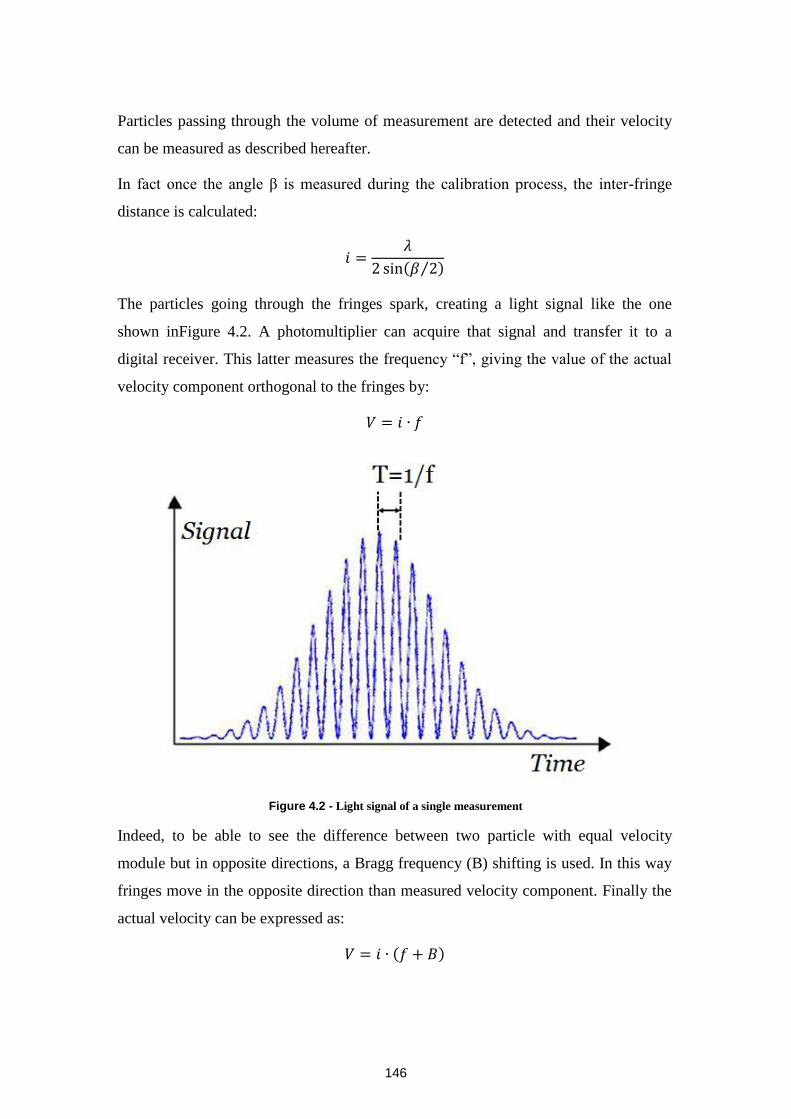
146
Particles passing through the volume of measurement are detected and their velocity
can be measured as described hereafter.
In fact once the angle β is measured during the calibration process, the inter-fringe
distance is calculated:
𝑖 =𝜆
2 sin 𝛽 2
The particles going through the fringes spark, creating a light signal like the one
shown inFigure 4.2. A photomultiplier can acquire that signal and transfer it to a
digital receiver. This latter measures the frequency “f”, giving the value of the actual
velocity component orthogonal to the fringes by:
𝑉 = 𝑖 ∙ 𝑓
Figure 4.2 - Light signal of a single measurement
Indeed, to be able to see the difference between two particle with equal velocity
module but in opposite directions, a Bragg frequency (B) shifting is used. In this way
fringes move in the opposite direction than measured velocity component. Finally the
actual velocity can be expressed as:
𝑉 = 𝑖 ∙ 𝑓 + 𝐵
147
1.2 EXPERIMENTAL FACILITY AND CALIBRATION
1.2.1 Experimental facility description
First of all the test section is presented. To simulate the innovative channel fluid flow,
only a pair of superposing wavy channels is used, to form a single channel (like the
one shown in Figure 4.3)XV
.
Preliminary calculations showed that the inlet straight length does not really change
the complete flow development, which seems to be reached after four bends. Hence,
we decided to use a six bend channel to measure a fully developed flow in the last
bend and mixing zone. The LDV technique needs two optical accesses (for laser
emission and reception) to the test section (see Figure 4.2), which are typically on
parallel planes. Hence two optical quality glass windows are put in the measurement
test section. In the other parts of the test section aluminum is used as structural
material whereas PMMA is used to constantly visualize the state of the wall (i.e. if
there were DEHS spots, see Section 1.2.1). The channel is designed in terms of
Reynolds similarity (inlet hydraulic diameter of 60mm, corresponding to an inlet
Reynolds number of 47 600) with actual heat exchanger conditions, to provide trustful
results to the aerodynamic validation. The two half channels have a rectangular cross-
section of 60mm x 30mm. Measurements are done with air at atmospheric pressure
and temperature.
The test section is shown in Figure 4.3 and Figure 4.4, while its geometrical
characteristics are shown in Table 4.1:
XV
Therefore we will hereafter use the term « bend » to indicate both the pair of opposite bends
representing portion of the channel between two mixing zones and the single bend where measurements
are done (see Section 1.3).
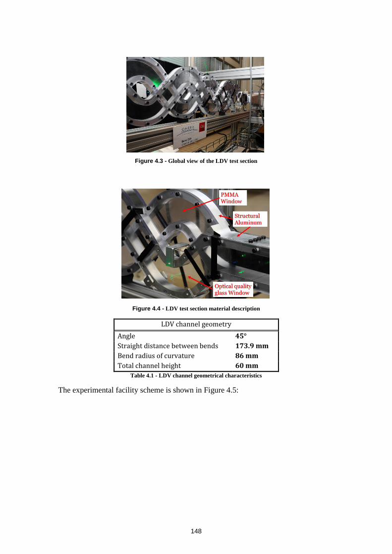
148
Figure 4.3 - Global view of the LDV test section
Figure 4.4 - LDV test section material description
LDV channel geometry
Angle 45°
Straight distance between bends 173.9 mm
Bend radius of curvature 86 mm
Total channel height 60 mm
Table 4.1 - LDV channel geometrical characteristics
The experimental facility scheme is shown in Figure 4.5:
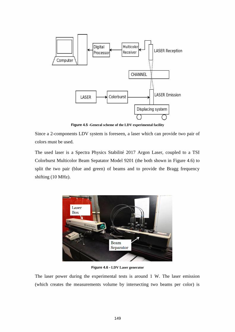
149
Figure 4.5 -General scheme of the LDV experimental facility
Since a 2-components LDV system is foreseen, a laser which can provide two pair of
colors must be used.
The used laser is a Spectra Physics Stabilité 2017 Argon Laser, coupled to a TSI
Colorburst Multicolor Beam Sepatator Model 9201 (the both shown in Figure 4.6) to
split the two pair (blue and green) of beams and to provide the Bragg frequency
shifting (10 MHz).
Figure 4.6 - LDV Laser generator
The laser power during the experimental tests is around 1 W. The laser emission
(which creates the measurements volume by intersecting two beams per color) is
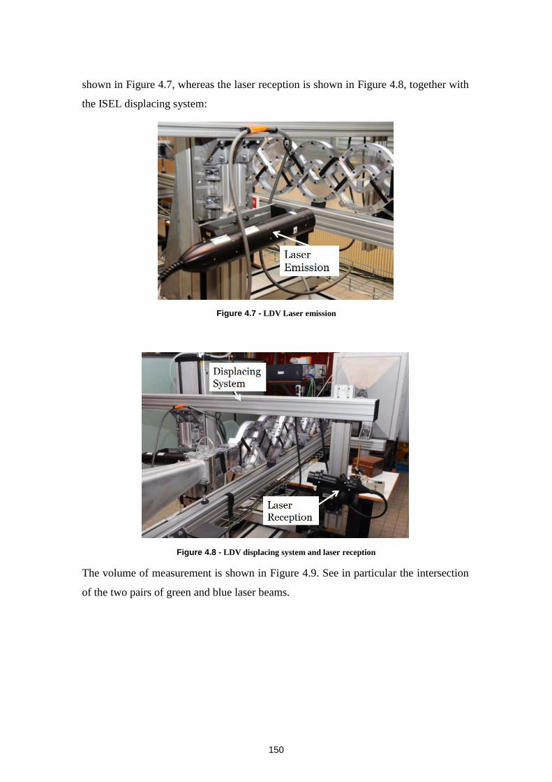
150
shown in Figure 4.7, whereas the laser reception is shown in Figure 4.8, together with
the ISEL displacing system:
Figure 4.7 - LDV Laser emission
Figure 4.8 - LDV displacing system and laser reception
The volume of measurement is shown in Figure 4.9. See in particular the intersection
of the two pairs of green and blue laser beams.
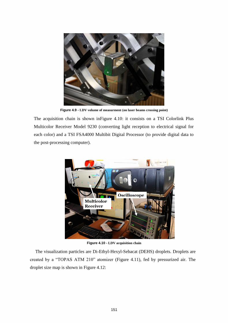
151
Figure 4.9 - LDV volume of measurment (on laser beams crossing point)
The acquisition chain is shown inFigure 4.10: it consists on a TSI Colorlink Plus
Multicolor Receiver Model 9230 (converting light reception to electrical signal for
each color) and a TSI FSA4000 Multibit Digital Processor (to provide digital data to
the post-processing computer).
Figure 4.10 - LDV acquisition chain
The visualization particles are Di-Ethyl-Hexyl-Sebacat (DEHS) droplets. Droplets are
created by a “TOPAS ATM 210” atomizer (Figure 4.11), fed by pressurized air. The
droplet size map is shown in Figure 4.12:
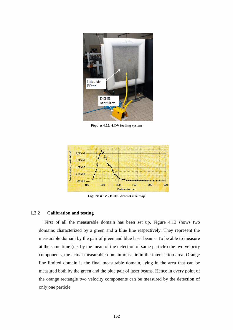
152
Figure 4.11 -LDV feeding system
Figure 4.12 - DEHS droplet size map
1.2.2 Calibration and testing
First of all the measurable domain has been set up. Figure 4.13 shows two
domains characterized by a green and a blue line respectively. They represent the
measurable domain by the pair of green and blue laser beams. To be able to measure
at the same time (i.e. by the mean of the detection of same particle) the two velocity
components, the actual measurable domain must lie in the intersection area. Orange
line limited domain is the final measurable domain, lying in the area that can be
measured both by the green and the blue pair of laser beams. Hence in every point of
the orange rectangle two velocity components can be measured by the detection of
only one particle.
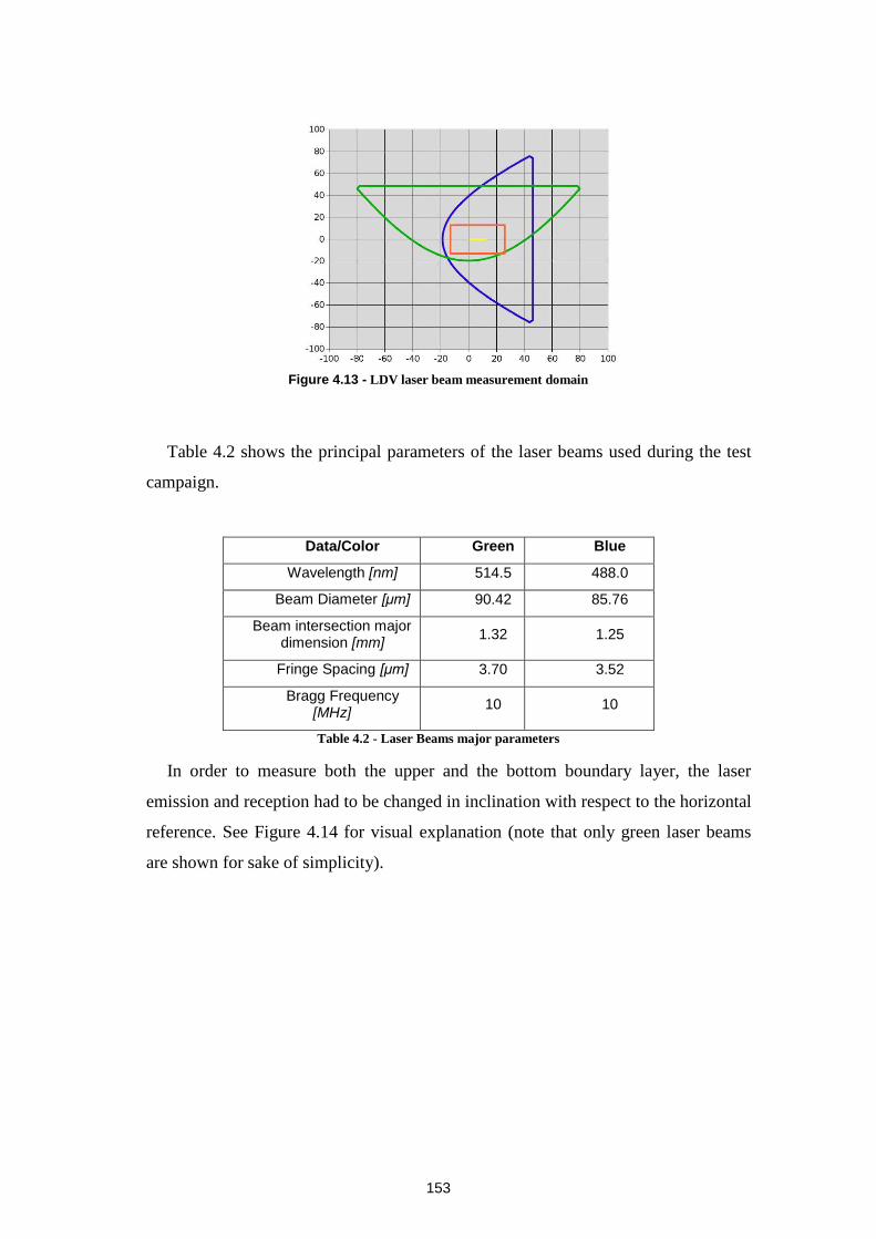
153
Figure 4.13 - LDV laser beam measurement domain
Table 4.2 shows the principal parameters of the laser beams used during the test
campaign.
Data/Color Green Blue
Wavelength [nm] 514.5 488.0
Beam Diameter [μm] 90.42 85.76
Beam intersection major dimension [mm]
1.32 1.25
Fringe Spacing [μm] 3.70 3.52
Bragg Frequency [MHz]
10 10
Table 4.2 - Laser Beams major parameters
In order to measure both the upper and the bottom boundary layer, the laser
emission and reception had to be changed in inclination with respect to the horizontal
reference. See Figure 4.14 for visual explanation (note that only green laser beams
are shown for sake of simplicity).
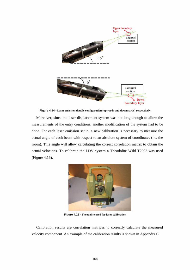
154
Figure 4.14 - Laser emission double configuration (upwards and downwards) respectively
Moreover, since the laser displacement system was not long enough to allow the
measurements of the entry conditions, another modification of the system had to be
done. For each laser emission setup, a new calibration is necessary to measure the
actual angle of each beam with respect to an absolute system of coordinates (i.e. the
room). This angle will allow calculating the correct correlation matrix to obtain the
actual velocities. To calibrate the LDV system a Theodolite Wild T2002 was used
(Figure 4.15).
Figure 4.15 - Theodolite used for laser calibration
Calibration results are correlation matrices to correctly calculate the measured
velocity component. An example of the calibration results is shown in Appendix C.
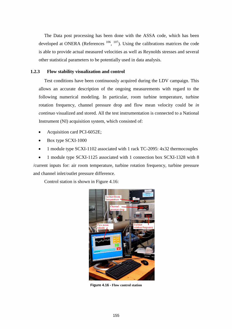
155
The Data post processing has been done with the ASSA code, which has been
developed at ONERA (References 106
, 107
). Using the calibrations matrices the code
is able to provide actual measured velocities as well as Reynolds stresses and several
other statistical parameters to be potentially used in data analysis.
1.2.3 Flow stability visualization and control
Test conditions have been continuously acquired during the LDV campaign. This
allows an accurate description of the ongoing measurements with regard to the
following numerical modeling. In particular, room turbine temperature, turbine
rotation frequency, channel pressure drop and flow mean velocity could be in
continuo visualized and stored. All the test instrumentation is connected to a National
Instrument (NI) acquisition system, which consisted of:
Acquisition card PCI-6052E;
Box type SCXI-1000
1 module type SCXI-1102 associated with 1 rack TC-2095: 4x32 thermocouples
1 module type SCXI-1125 associated with 1 connection box SCXI-1328 with 8
/current inputs for: air room temperature, turbine rotation frequency, turbine pressure
and channel inlet/outlet pressure difference.
Control station is shown in Figure 4.16:
Figure 4.16 - Flow control station
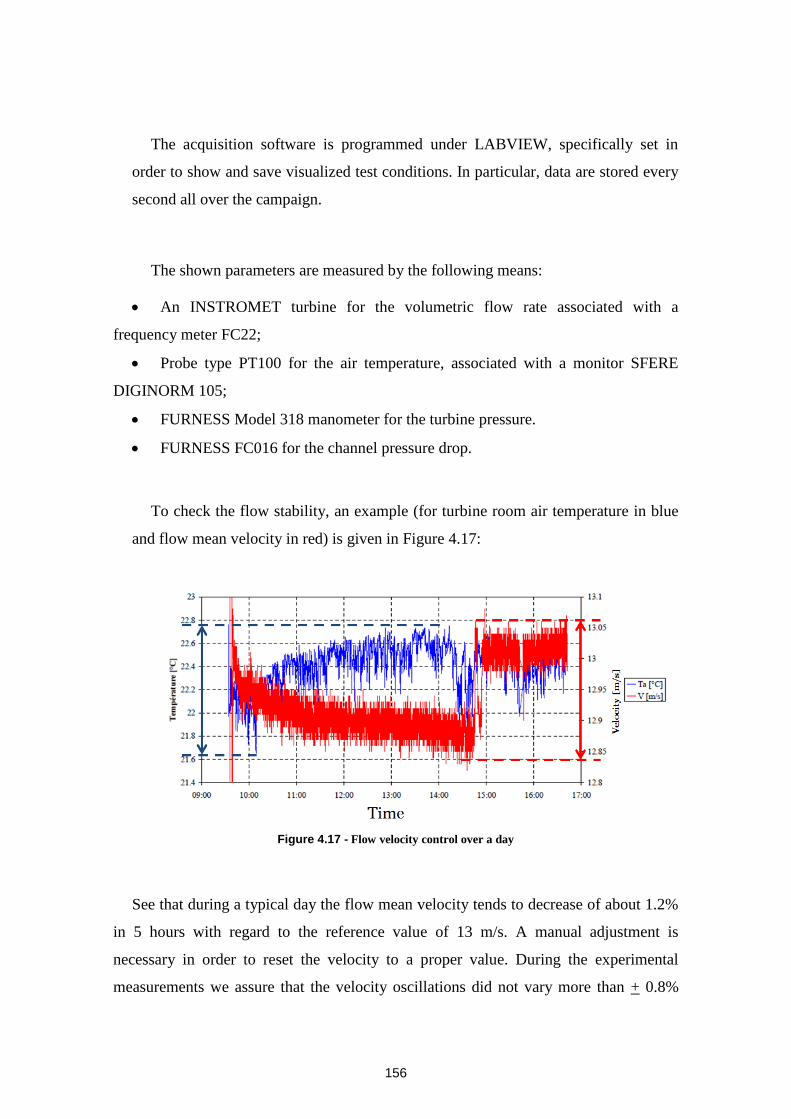
156
The acquisition software is programmed under LABVIEW, specifically set in
order to show and save visualized test conditions. In particular, data are stored every
second all over the campaign.
The shown parameters are measured by the following means:
An INSTROMET turbine for the volumetric flow rate associated with a
frequency meter FC22;
Probe type PT100 for the air temperature, associated with a monitor SFERE
DIGINORM 105;
FURNESS Model 318 manometer for the turbine pressure.
FURNESS FC016 for the channel pressure drop.
To check the flow stability, an example (for turbine room air temperature in blue
and flow mean velocity in red) is given in Figure 4.17:
Figure 4.17 - Flow velocity control over a day
See that during a typical day the flow mean velocity tends to decrease of about 1.2%
in 5 hours with regard to the reference value of 13 m/s. A manual adjustment is
necessary in order to reset the velocity to a proper value. During the experimental
measurements we assure that the velocity oscillations did not vary more than + 0.8%

157
(i.e. + 0.1 m/s) all over the campaign. Anyway the flow test clearly shows that the flow
is stable and the no macroscopic oscillatory phenomenon is detectable. Therefore the
LDV averages do make sense for the subsequent analysis.
On the other hand, temperature oscillations varied no more than 1.2°C during that
day. In general we can assure that temperature did not vary significantly during the
experimental campaign. Hence air properties will be always considered constant at
atmospheric pressure and temperature (specifically 𝑇𝑎𝑡𝑚 = 23°𝐶and 𝑝𝑎𝑡𝑚 =
101325 𝑃𝑎).
1.3 EXPERIMENTAL CAMPAIGN DESCRIPTION
1.3.1 Experimental measurement program definition
The experimental campaign has been defined in the following way: first of all, critical
zones of interest have been identified, to be able to have a good overview of the fluid
flow with regard to the numerical validation. Hence the inlet section (Figure 4.19), the
last mixing zone as well as the last bend (Figure 4.20) are chosen as reference regions
to investigate channel flow. Moreover, to verify flow development (hence the design
hypothesis) the fourth and fifth bends are studied as well. Since measuring a whole
cross-sections was impossible with regard to the set time schedule, only a few profiles
on different cross-sections have been identified to be studied. In particular the strategy
has been to always measure the two centerlines along plane main axis (i.e. Y and Z for
all the planes but the mixing plane where X and Z axis are used). Moreover, two
equally spaced profiles which are parallel to the main ones are used, in order to gather
as much information as possible and considering that investigating the whole plane
was unrealistic.
Prior to describe the experimental campaign it is worth showing the general test
section system of coordinates inFigure 4.18.
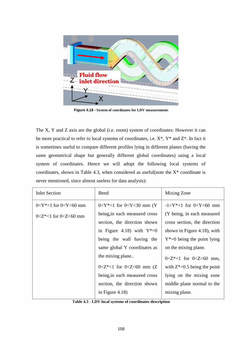
158
Figure 4.18 - System of coordinates for LDV measurements
The X, Y and Z axis are the global (i.e. room) system of coordinates: However it can
be more practical to refer to local systems of coordinates, i.e. X*, Y* and Z*. In fact it
is sometimes useful to compare different profiles lying in different planes (having the
same geometrical shape but generally different global coordinates) using a local
system of coordinates. Hence we will adopt the following local systems of
coordinates, shown in Table 4.3, when considered as useful(note the X* coordinate is
never mentioned, since almost useless for data analysis):
Inlet Section Bend Mixing Zone
0<Y*<1 for 0<Y<60 mm
0<Z*<1 for 0<Z<60 mm
0<Y*<1 for 0<Y<30 mm (Y
being,in each measured cross
section, the direction shown
in Figure 4.18) with Y*=0
being the wall having the
same global Y coordinates as
the mixing plane..
0<Z*<1 for 0<Z<60 mm (Z
being,in each measured cross
section, the direction shown
in Figure 4.18)
-1<Y*<1 for 0<Y<60 mm
(Y being, in each measured
cross section, the direction
shown in Figure 4.18), with
Y*=0 being the point lying
on the mixing plane.
0<Z*<1 for 0<Z<60 mm,
with Z*=0.5 being the point
lying on the mixing zone
middle plane normal to the
mixing plane.
Table 4.3 - LDV local systems of coordinates description
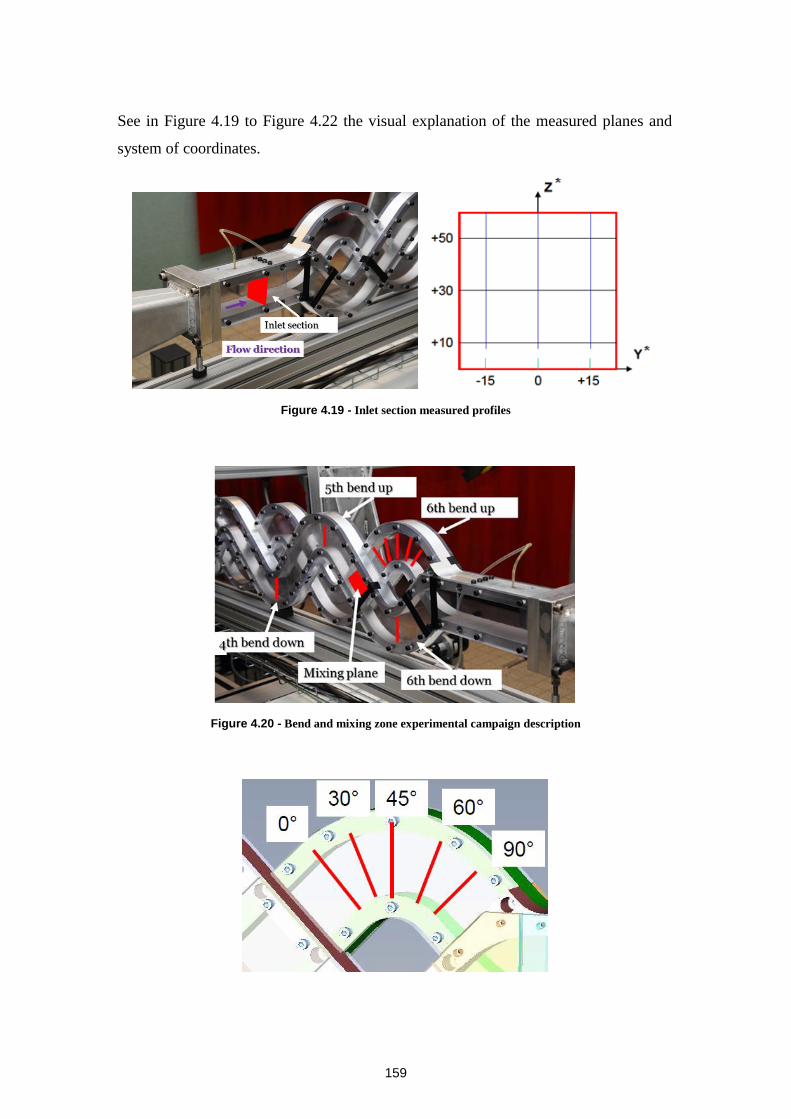
159
See in Figure 4.19 to Figure 4.22 the visual explanation of the measured planes and
system of coordinates.
Figure 4.19 - Inlet section measured profiles
Figure 4.20 - Bend and mixing zone experimental campaign description
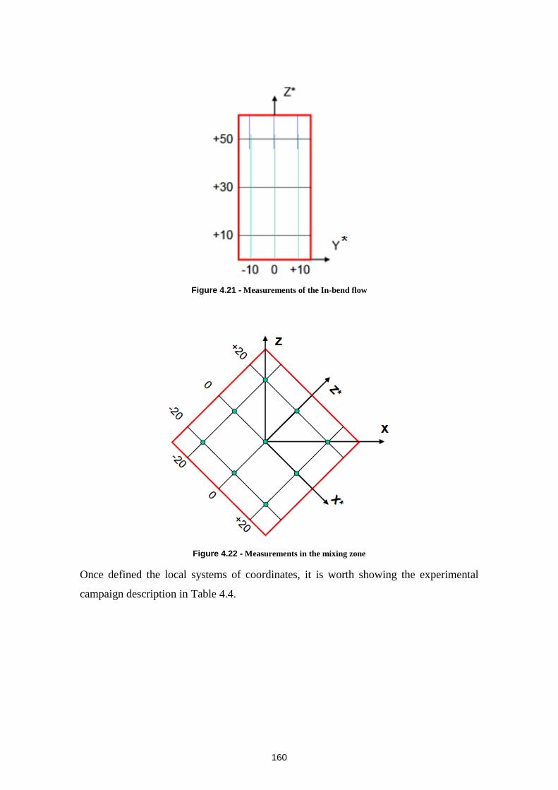
160
Figure 4.21 - Measurements of the In-bend flow
Figure 4.22 - Measurements in the mixing zone
Once defined the local systems of coordinates, it is worth showing the experimental
campaign description in Table 4.4.
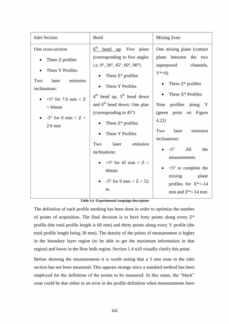
161
Inlet Section Bend Mixing Zone
One cross-section
Three Z profiles
Three Y Profiles
Two laser emission
inclinations:
+5° for 7.6 mm < Z
< 60mm
-5° for 0 mm < Z <
2.6 mm
6th
bend up: Five plans
(corresponding to five angles
i.e. 0°, 30°, 45°, 60°, 90°)
Three Z* profiles
Three Y Profiles
4th
bend up, 5th
bend down
and 6th
bend down: One plan
(corresponding to 45°)
Three Z* profiles
Three Y Profiles
Two laser emission
inclinations:
+5° for 45 mm < Z <
60mm
-5° for 0 mm < Z < 52
m
One mixing plane (contact
plane between the two
superposed channels,
Y*=0)
Three Z* profiles
Three X* Profiles
Nine profiles along Y
(green point on Figure
4.22)
Two laser emission
inclinations:
-5° All the
measurements
+5° to complete the
mixing plane
profiles for X*<-14
mm and Z*<-14 mm
Table 4.4 -Experimental campaign description
The definition of each profile meshing has been done in order to optimize the number
of points of acquisition. The final decision is to have forty points along every Z*
profile (the total profile length is 60 mm) and thirty points along every Y profile (the
total profile length being 30 mm). The density of the points of measurement is higher
in the boundary layer region (to be able to get the maximum information in that
region) and lower in the flow bulk region. Section 1.4 will visually clarify this point.
Before showing the measurements it is worth noting that a 5 mm zone in the inlet
section has not been measured. This appears strange since a standard method has been
employed for the definition of the points to be measured. In this sense, the “black”
zone could be due either to an error in the profile definition when measurements have
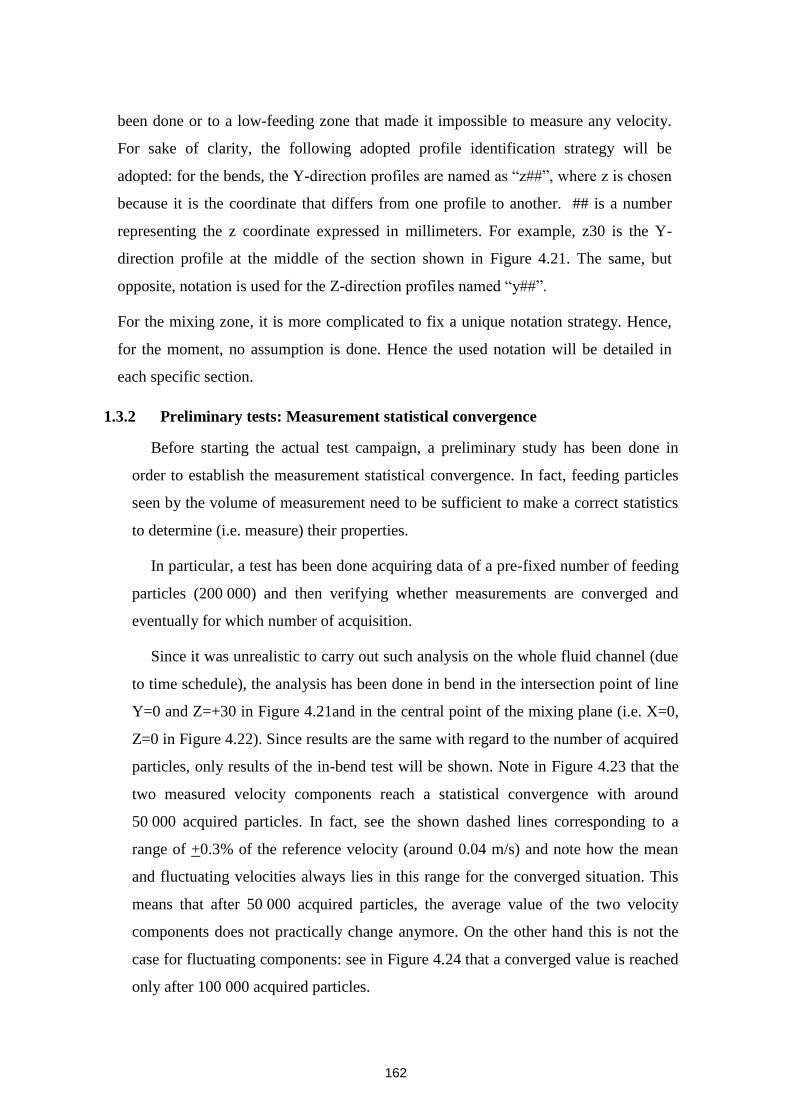
162
been done or to a low-feeding zone that made it impossible to measure any velocity.
For sake of clarity, the following adopted profile identification strategy will be
adopted: for the bends, the Y-direction profiles are named as “z##”, where z is chosen
because it is the coordinate that differs from one profile to another. ## is a number
representing the z coordinate expressed in millimeters. For example, z30 is the Y-
direction profile at the middle of the section shown in Figure 4.21. The same, but
opposite, notation is used for the Z-direction profiles named “y##”.
For the mixing zone, it is more complicated to fix a unique notation strategy. Hence,
for the moment, no assumption is done. Hence the used notation will be detailed in
each specific section.
1.3.2 Preliminary tests: Measurement statistical convergence
Before starting the actual test campaign, a preliminary study has been done in
order to establish the measurement statistical convergence. In fact, feeding particles
seen by the volume of measurement need to be sufficient to make a correct statistics
to determine (i.e. measure) their properties.
In particular, a test has been done acquiring data of a pre-fixed number of feeding
particles (200 000) and then verifying whether measurements are converged and
eventually for which number of acquisition.
Since it was unrealistic to carry out such analysis on the whole fluid channel (due
to time schedule), the analysis has been done in bend in the intersection point of line
Y=0 and Z=+30 in Figure 4.21and in the central point of the mixing plane (i.e. X=0,
Z=0 in Figure 4.22). Since results are the same with regard to the number of acquired
particles, only results of the in-bend test will be shown. Note in Figure 4.23 that the
two measured velocity components reach a statistical convergence with around
50 000 acquired particles. In fact, see the shown dashed lines corresponding to a
range of +0.3% of the reference velocity (around 0.04 m/s) and note how the mean
and fluctuating velocities always lies in this range for the converged situation. This
means that after 50 000 acquired particles, the average value of the two velocity
components does not practically change anymore. On the other hand this is not the
case for fluctuating components: see in Figure 4.24 that a converged value is reached
only after 100 000 acquired particles.
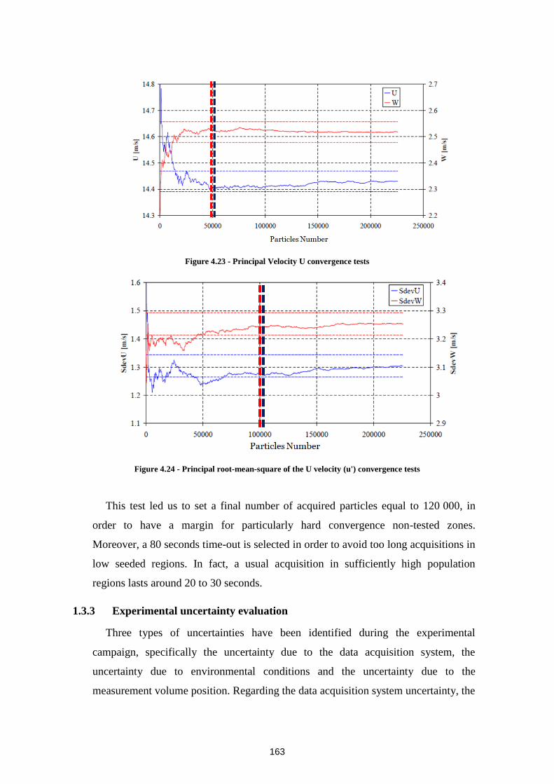
163
Figure 4.23 - Principal Velocity U convergence tests
Figure 4.24 - Principal root-mean-square of the U velocity (u') convergence tests
This test led us to set a final number of acquired particles equal to 120 000, in
order to have a margin for particularly hard convergence non-tested zones.
Moreover, a 80 seconds time-out is selected in order to avoid too long acquisitions in
low seeded regions. In fact, a usual acquisition in sufficiently high population
regions lasts around 20 to 30 seconds.
1.3.3 Experimental uncertainty evaluation
Three types of uncertainties have been identified during the experimental
campaign, specifically the uncertainty due to the data acquisition system, the
uncertainty due to environmental conditions and the uncertainty due to the
measurement volume position. Regarding the data acquisition system uncertainty, the
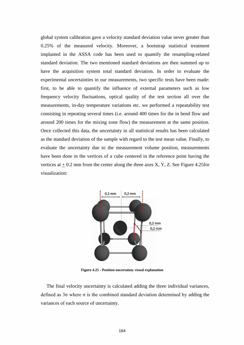
164
global system calibration gave a velocity standard deviation value never greater than
0.25% of the measured velocity. Moreover, a bootstrap statistical treatment
implanted in the ASSA code has been used to quantify the resampling-related
standard deviation. The two mentioned standard deviations are then summed up to
have the acquisition system total standard deviation. In order to evaluate the
experimental uncertainties in our measurements, two specific tests have been made:
first, to be able to quantify the influence of external parameters such as low
frequency velocity fluctuations, optical quality of the test section all over the
measurements, in-day temperature variations etc. we performed a repeatability test
consisting in repeating several times (i.e. around 400 times for the in bend flow and
around 200 times for the mixing zone flow) the measurement at the same position.
Once collected this data, the uncertainty in all statistical results has been calculated
as the standard deviation of the sample with regard to the test mean value. Finally, to
evaluate the uncertainty due to the measurement volume position, measurements
have been done in the vertices of a cube centered in the reference point having the
vertices at + 0.2 mm from the center along the three axes X, Y, Z. See Figure 4.25for
visualization:
Figure 4.25 - Position uncertainty visual explanation
The final velocity uncertainty is calculated adding the three individual variances,
defined as 3ζ where ζ is the combined standard deviation determined by adding the
variances of each source of uncertainty.

165
The final uncertainty analysis is shown in Table 4.5 toTable 4.8. Note that the
evaluation is strictly valid only for the points where the repeatability and the position
uncertainty tests have been performed (in fact, the measured values are also
presented); nevertheless it gives a good evaluation of the global uncertainties for the
actual flow.
ζ
System
Chain
ζ
Repeatability
ζ
Position
Average U
+Total 3ζ
Uncertainty
Inlet
Section 0.032 m/s 0.015 m/s
0.012
m/s
13.18+0.11
m/s
In-bend 0.1 m/s 0.025 m/s 0.014
m/s
14.02+0.31
m/s
In-
mixing zone 0.03
m/s 0.05 m/s
0.07
m/s
4.62+0.27
m/s
Table 4.5 - Velocity U Uncertainty Analysis
ζ
System
Chain
ζ
Repeatability
ζ
Position
Total 3ζ
Uncertainty
Inlet
Section 0.001
m/s 0.003 m/s
0.009
m/s
-0.03+0.03
m/s
In-bend 0.02
m/s 0.045 m/s
0. 014
m/s
1.41+0.15
m/s
In-
mixing
zone
0.03
m/s 0.05 m/s 0.07 m/s
4.75+0.27
m/s
Table 4.6 - Velocity W Uncertainty Analysis
ζ
System
Chain
ζ
Repeatability
ζ
Position
Total 3ζ
Uncertainty
Inlet
Section 0.015m
/s 0.003m/s
0.003m/
s
0.13+0.05
m/s
In-bend 0.01m/
s 0.013m/s
0.018
m/s
2.23+0.07
m/s
In-
mixing
zone
0.03m/
s 0.03m/s 0.03m/s
3.69+0.16
m/s
Table 4.7–u’ Reynolds Stress Uncertainty Analysis
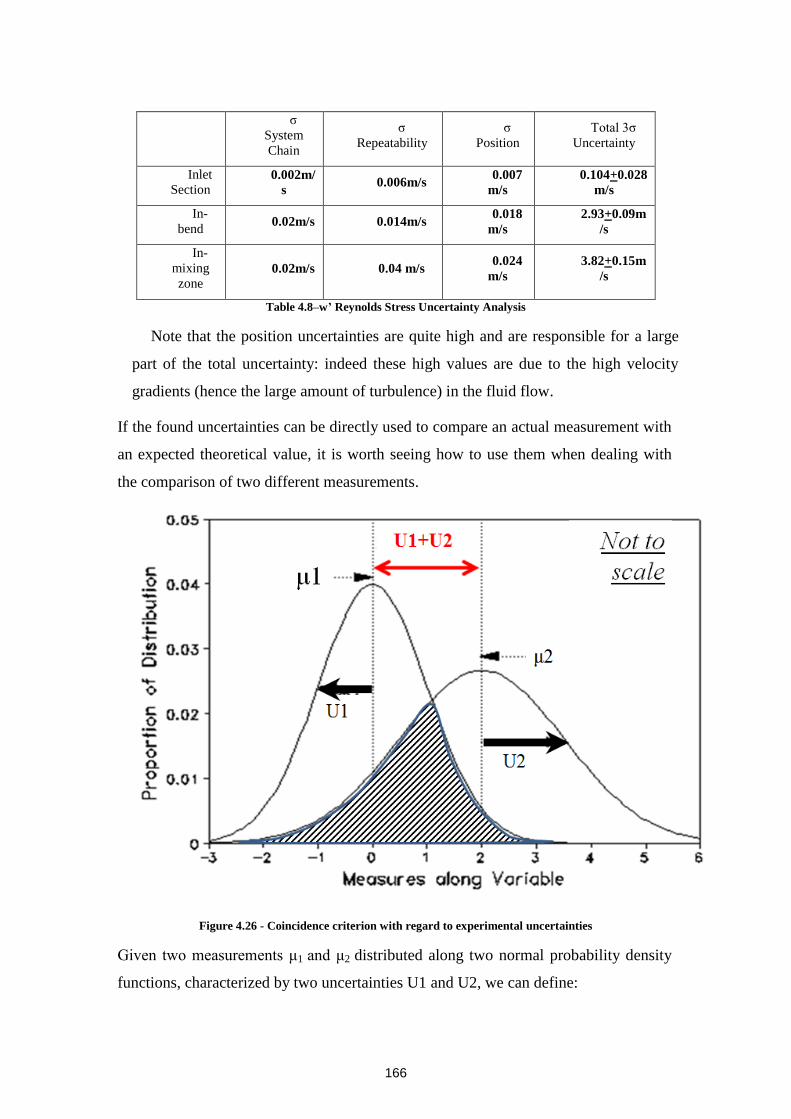
166
ζ
System
Chain
ζ
Repeatability
ζ
Position
Total 3ζ
Uncertainty
Inlet
Section 0.002m/
s 0.006m/s
0.007
m/s
0.104+0.028
m/s
In-
bend 0.02m/s 0.014m/s
0.018
m/s
2.93+0.09m
/s
In-
mixing
zone 0.02m/s 0.04 m/s
0.024
m/s
3.82+0.15m
/s
Table 4.8–w’ Reynolds Stress Uncertainty Analysis
Note that the position uncertainties are quite high and are responsible for a large
part of the total uncertainty: indeed these high values are due to the high velocity
gradients (hence the large amount of turbulence) in the fluid flow.
If the found uncertainties can be directly used to compare an actual measurement with
an expected theoretical value, it is worth seeing how to use them when dealing with
the comparison of two different measurements.
Figure 4.26 - Coincidence criterion with regard to experimental uncertainties
Given two measurements μ1 and μ2 distributed along two normal probability density
functions, characterized by two uncertainties U1 and U2, we can define:
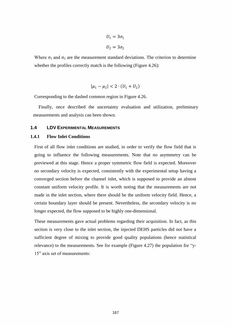
167
𝑈1 = 3𝜎1
𝑈2 = 3𝜎2
Where ζ1 and ζ2 are the measurement standard deviations. The criterion to determine
whether the profiles correctly match is the following (Figure 4.26):
𝜇1 − 𝜇2 < 2 ∙ 𝑈1 + 𝑈2
Corresponding to the dashed common region in Figure 4.26.
Finally, once described the uncertainty evaluation and utilization, preliminary
measurements and analysis can been shown.
1.4 LDV EXPERIMENTAL MEASUREMENTS
1.4.1 Flow Inlet Conditions
First of all flow inlet conditions are studied, in order to verify the flow field that is
going to influence the following measurements. Note that no asymmetry can be
previewed at this stage. Hence a proper symmetric flow field is expected. Moreover
no secondary velocity is expected, consistently with the experimental setup having a
converged section before the channel inlet, which is supposed to provide an almost
constant uniform velocity profile. It is worth noting that the measurements are not
made in the inlet section, where there should be the uniform velocity field. Hence, a
certain boundary layer should be present. Nevertheless, the secondary velocity is no
longer expected, the flow supposed to be highly one-dimensional.
These measurements gave actual problems regarding their acquisition. In fact, as this
section is very close to the inlet section, the injected DEHS particles did not have a
sufficient degree of mixing to provide good quality populations (hence statistical
relevance) to the measurements. See for example (Figure 4.27) the population for “y-
15” axis set of measurements:
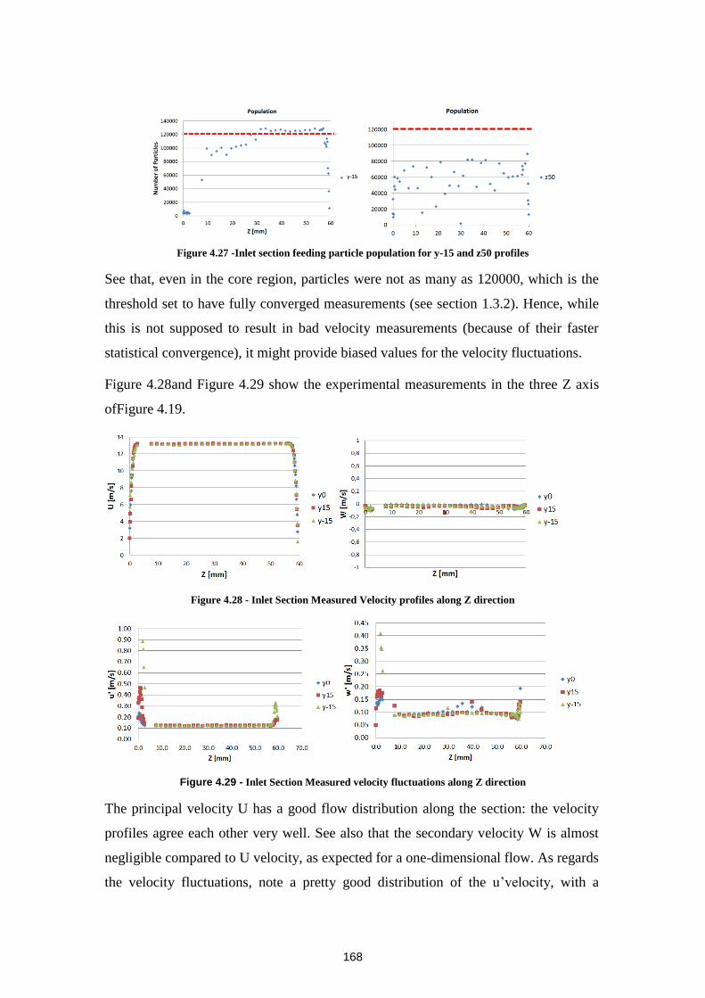
168
Figure 4.27 -Inlet section feeding particle population for y-15 and z50 profiles
See that, even in the core region, particles were not as many as 120000, which is the
threshold set to have fully converged measurements (see section 1.3.2). Hence, while
this is not supposed to result in bad velocity measurements (because of their faster
statistical convergence), it might provide biased values for the velocity fluctuations.
Figure 4.28and Figure 4.29 show the experimental measurements in the three Z axis
ofFigure 4.19.
Figure 4.28 - Inlet Section Measured Velocity profiles along Z direction
Figure 4.29 - Inlet Section Measured velocity fluctuations along Z direction
The principal velocity U has a good flow distribution along the section: the velocity
profiles agree each other very well. See also that the secondary velocity W is almost
negligible compared to U velocity, as expected for a one-dimensional flow. As regards
the velocity fluctuations, note a pretty good distribution of the u’velocity, with a
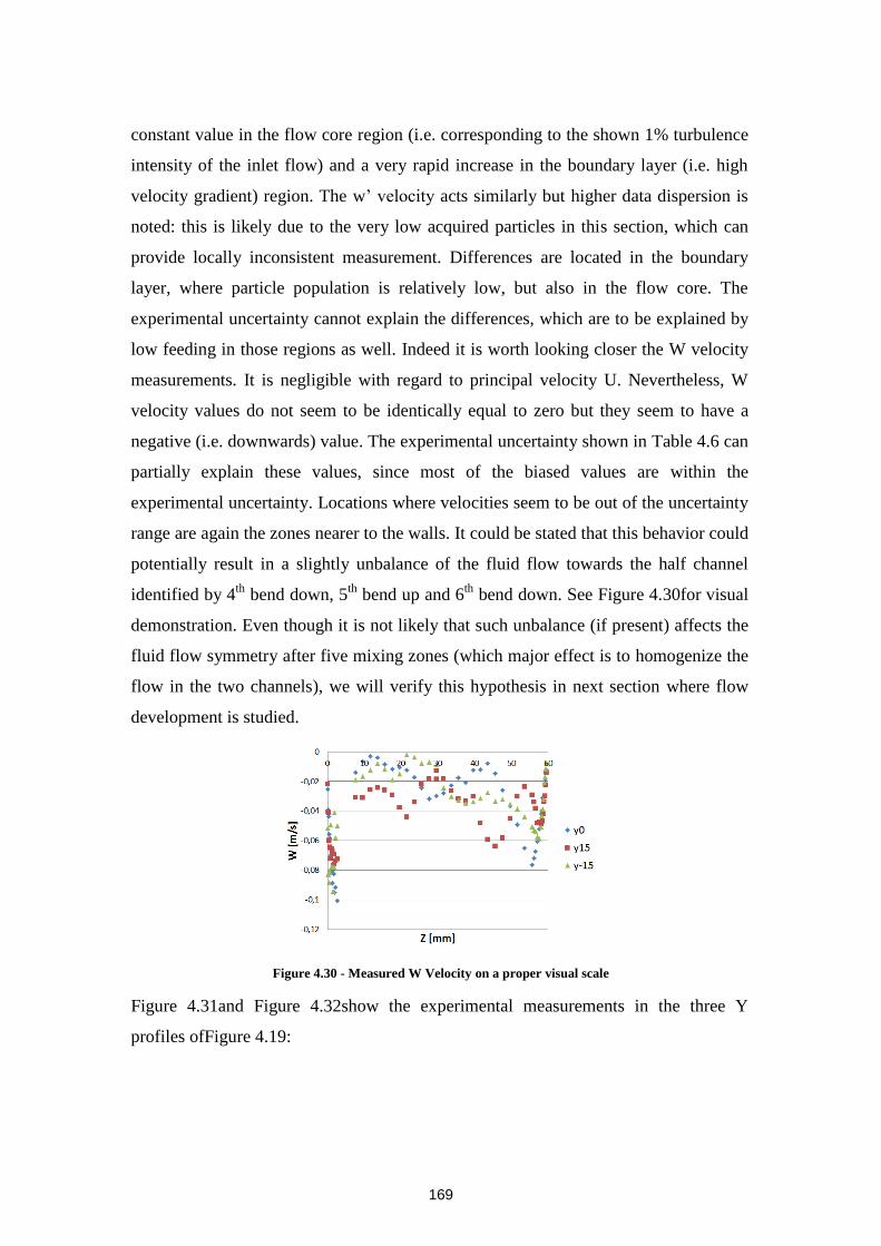
169
constant value in the flow core region (i.e. corresponding to the shown 1% turbulence
intensity of the inlet flow) and a very rapid increase in the boundary layer (i.e. high
velocity gradient) region. The w’ velocity acts similarly but higher data dispersion is
noted: this is likely due to the very low acquired particles in this section, which can
provide locally inconsistent measurement. Differences are located in the boundary
layer, where particle population is relatively low, but also in the flow core. The
experimental uncertainty cannot explain the differences, which are to be explained by
low feeding in those regions as well. Indeed it is worth looking closer the W velocity
measurements. It is negligible with regard to principal velocity U. Nevertheless, W
velocity values do not seem to be identically equal to zero but they seem to have a
negative (i.e. downwards) value. The experimental uncertainty shown in Table 4.6 can
partially explain these values, since most of the biased values are within the
experimental uncertainty. Locations where velocities seem to be out of the uncertainty
range are again the zones nearer to the walls. It could be stated that this behavior could
potentially result in a slightly unbalance of the fluid flow towards the half channel
identified by 4th
bend down, 5th
bend up and 6th
bend down. See Figure 4.30for visual
demonstration. Even though it is not likely that such unbalance (if present) affects the
fluid flow symmetry after five mixing zones (which major effect is to homogenize the
flow in the two channels), we will verify this hypothesis in next section where flow
development is studied.
Figure 4.30 - Measured W Velocity on a proper visual scale
Figure 4.31and Figure 4.32show the experimental measurements in the three Y
profiles ofFigure 4.19:
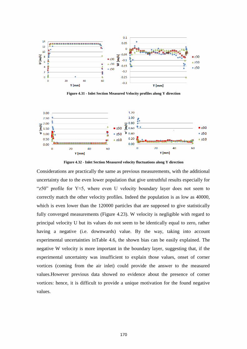
170
Figure 4.31 - Inlet Section Measured Velocity profiles along Y direction
Figure 4.32 - Inlet Section Measured velocity fluctuations along Y direction
Considerations are practically the same as previous measurements, with the additional
uncertainty due to the even lower population that give untruthful results especially for
“z50” profile for Y≈5, where even U velocity boundary layer does not seem to
correctly match the other velocity profiles. Indeed the population is as low as 40000,
which is even lower than the 120000 particles that are supposed to give statistically
fully converged measurements (Figure 4.23). W velocity is negligible with regard to
principal velocity U but its values do not seem to be identically equal to zero, rather
having a negative (i.e. downwards) value. By the way, taking into account
experimental uncertainties inTable 4.6, the shown bias can be easily explained. The
negative W velocity is more important in the boundary layer, suggesting that, if the
experimental uncertainty was insufficient to explain those values, onset of corner
vortices (coming from the air inlet) could provide the answer to the measured
values.However previous data showed no evidence about the presence of corner
vortices: hence, it is difficult to provide a unique motivation for the found negative
values.
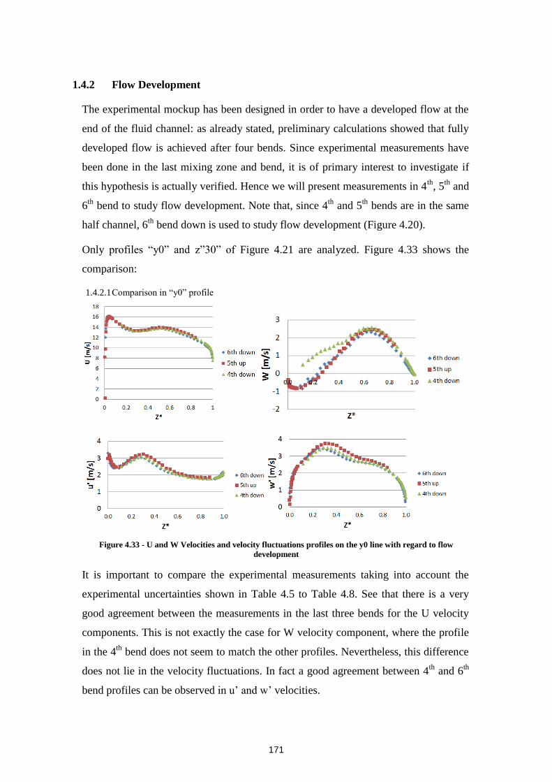
171
1.4.2 Flow Development
The experimental mockup has been designed in order to have a developed flow at the
end of the fluid channel: as already stated, preliminary calculations showed that fully
developed flow is achieved after four bends. Since experimental measurements have
been done in the last mixing zone and bend, it is of primary interest to investigate if
this hypothesis is actually verified. Hence we will present measurements in 4th
, 5th
and
6th
bend to study flow development. Note that, since 4th
and 5th
bends are in the same
half channel, 6th
bend down is used to study flow development (Figure 4.20).
Only profiles “y0” and z”30” of Figure 4.21 are analyzed. Figure 4.33 shows the
comparison:
1.4.2.1 Comparison in “y0” profile
Figure 4.33 - U and W Velocities and velocity fluctuations profiles on the y0 line with regard to flow
development
It is important to compare the experimental measurements taking into account the
experimental uncertainties shown in Table 4.5 to Table 4.8. See that there is a very
good agreement between the measurements in the last three bends for the U velocity
components. This is not exactly the case for W velocity component, where the profile
in the 4th
bend does not seem to match the other profiles. Nevertheless, this difference
does not lie in the velocity fluctuations. In fact a good agreement between 4th
and 6th
bend profiles can be observed in u’ and w’ velocities.
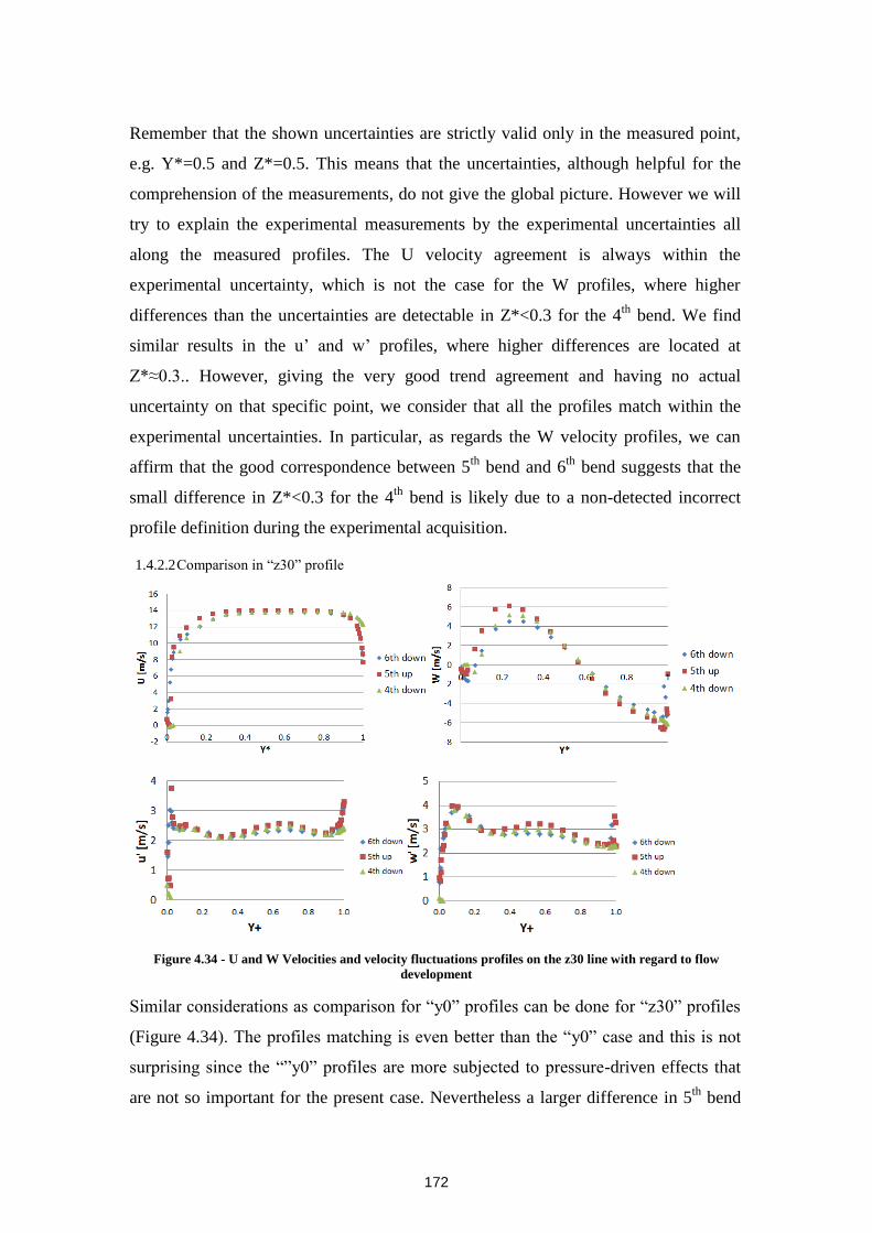
172
Remember that the shown uncertainties are strictly valid only in the measured point,
e.g. Y*=0.5 and Z*=0.5. This means that the uncertainties, although helpful for the
comprehension of the measurements, do not give the global picture. However we will
try to explain the experimental measurements by the experimental uncertainties all
along the measured profiles. The U velocity agreement is always within the
experimental uncertainty, which is not the case for the W profiles, where higher
differences than the uncertainties are detectable in Z*<0.3 for the 4th
bend. We find
similar results in the u’ and w’ profiles, where higher differences are located at
Z*≈0.3.. However, giving the very good trend agreement and having no actual
uncertainty on that specific point, we consider that all the profiles match within the
experimental uncertainties. In particular, as regards the W velocity profiles, we can
affirm that the good correspondence between 5th
bend and 6th
bend suggests that the
small difference in Z*<0.3 for the 4th
bend is likely due to a non-detected incorrect
profile definition during the experimental acquisition.
1.4.2.2 Comparison in “z30” profile
Figure 4.34 - U and W Velocities and velocity fluctuations profiles on the z30 line with regard to flow
development
Similar considerations as comparison for “y0” profiles can be done for “z30” profiles
(Figure 4.34). The profiles matching is even better than the “y0” case and this is not
surprising since the “”y0” profiles are more subjected to pressure-driven effects that
are not so important for the present case. Nevertheless a larger difference in 5th
bend
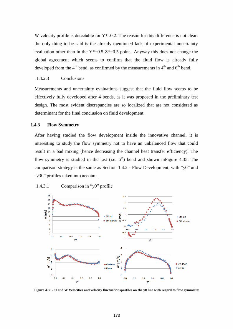
173
W velocity profile is detectable for Y*≈0.2. The reason for this difference is not clear:
the only thing to be said is the already mentioned lack of experimental uncertainty
evaluation other than in the Y*=0.5 Z*=0.5 point.. Anyway this does not change the
global agreement which seems to confirm that the fluid flow is already fully
developed from the 4th
bend, as confirmed by the measurements in 4th
and 6th
bend.
1.4.2.3 Conclusions
Measurements and uncertainty evaluations suggest that the fluid flow seems to be
effectively fully developed after 4 bends, as it was proposed in the preliminary test
design. The most evident discrepancies are so localized that are not considered as
determinant for the final conclusion on fluid development.
1.4.3 Flow Symmetry
After having studied the flow development inside the innovative channel, it is
interesting to study the flow symmetry not to have an unbalanced flow that could
result in a bad mixing (hence decreasing the channel heat transfer efficiency). The
flow symmetry is studied in the last (i.e. 6th
) bend and shown inFigure 4.35. The
comparison strategy is the same as Section 1.4.2 - Flow Development, with “y0” and
“z30” profiles taken into account.
1.4.3.1 Comparison in “y0” profile
Figure 4.35 - U and W Velocities and velocity fluctuationsprofiles on the y0 line with regard to flow symmetry
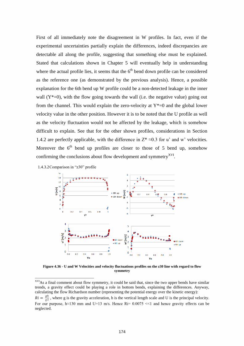
174
First of all immediately note the disagreement in W profiles. In fact, even if the
experimental uncertainties partially explain the differences, indeed discrepancies are
detectable all along the profile, suggesting that something else must be explained.
Stated that calculations shown in Chapter 5 will eventually help in understanding
where the actual profile lies, it seems that the 6th
bend down profile can be considered
as the reference one (as demonstrated by the previous analysis). Hence, a possible
explanation for the 6th bend up W profile could be a non-detected leakage in the inner
wall (Y*=0), with the flow going towards the wall (i.e. the negative value) going out
from the channel. This would explain the zero-velocity at Y*=0 and the global lower
velocity value in the other position. However it is to be noted that the U profile as well
as the velocity fluctuation would not be affected by the leakage, which is somehow
difficult to explain. See that for the other shown profiles, considerations in Section
1.4.2 are perfectly applicable, with the difference in Z* ≈0.3 for u’ and w’ velocities.
Moreover the 6th
bend up profiles are closer to those of 5 bend up, somehow
confirming the conclusions about flow development and symmetryXVI
.
1.4.3.2 Comparison in “z30” profile
Figure 4.36 - U and W Velocities and velocity fluctuations profiles on the z30 line with regard to flow
symmetry
XVI
As a final comment about flow symmetry, it could be said that, since the two upper bends have similar
trends, a gravity effect could be playing a role in bottom bends, explaining the differences. Anyway,
calculating the flow Richardson number (representing the potential energy over the kinetic energy):
𝑅𝑖 = 𝑔
𝑈2 , where g is the gravity acceleration, h is the vertical length scale and U is the principal velocity.
For our purpose, h≈130 mm and U=13 m/s. Hence Ri= 0.0075 <<1 and hence gravity effects can be
neglected.
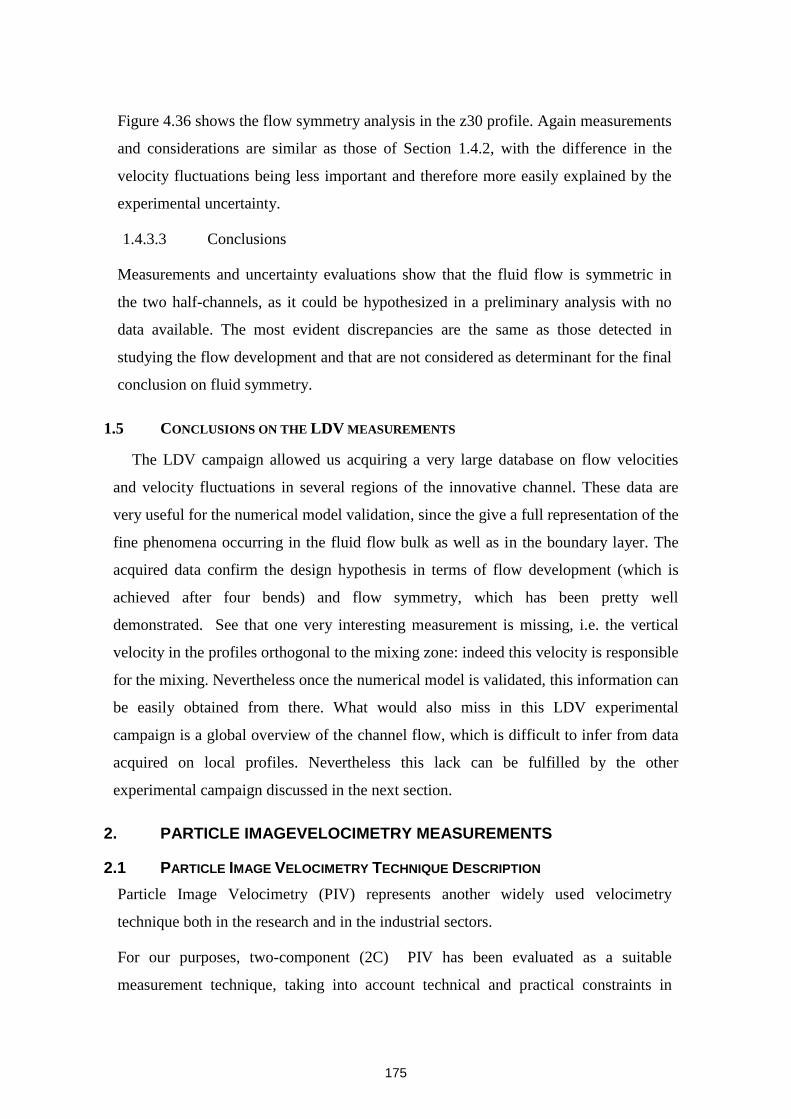
175
Figure 4.36 shows the flow symmetry analysis in the z30 profile. Again measurements
and considerations are similar as those of Section 1.4.2, with the difference in the
velocity fluctuations being less important and therefore more easily explained by the
experimental uncertainty.
1.4.3.3 Conclusions
Measurements and uncertainty evaluations show that the fluid flow is symmetric in
the two half-channels, as it could be hypothesized in a preliminary analysis with no
data available. The most evident discrepancies are the same as those detected in
studying the flow development and that are not considered as determinant for the final
conclusion on fluid symmetry.
1.5 CONCLUSIONS ON THE LDV MEASUREMENTS
The LDV campaign allowed us acquiring a very large database on flow velocities
and velocity fluctuations in several regions of the innovative channel. These data are
very useful for the numerical model validation, since the give a full representation of the
fine phenomena occurring in the fluid flow bulk as well as in the boundary layer. The
acquired data confirm the design hypothesis in terms of flow development (which is
achieved after four bends) and flow symmetry, which has been pretty well
demonstrated. See that one very interesting measurement is missing, i.e. the vertical
velocity in the profiles orthogonal to the mixing zone: indeed this velocity is responsible
for the mixing. Nevertheless once the numerical model is validated, this information can
be easily obtained from there. What would also miss in this LDV experimental
campaign is a global overview of the channel flow, which is difficult to infer from data
acquired on local profiles. Nevertheless this lack can be fulfilled by the other
experimental campaign discussed in the next section.
2. PARTICLE IMAGEVELOCIMETRY MEASUREMENTS
2.1 PARTICLE IMAGE VELOCIMETRY TECHNIQUE DESCRIPTION
Particle Image Velocimetry (PIV) represents another widely used velocimetry
technique both in the research and in the industrial sectors.
For our purposes, two-component (2C) PIV has been evaluated as a suitable
measurement technique, taking into account technical and practical constraints in
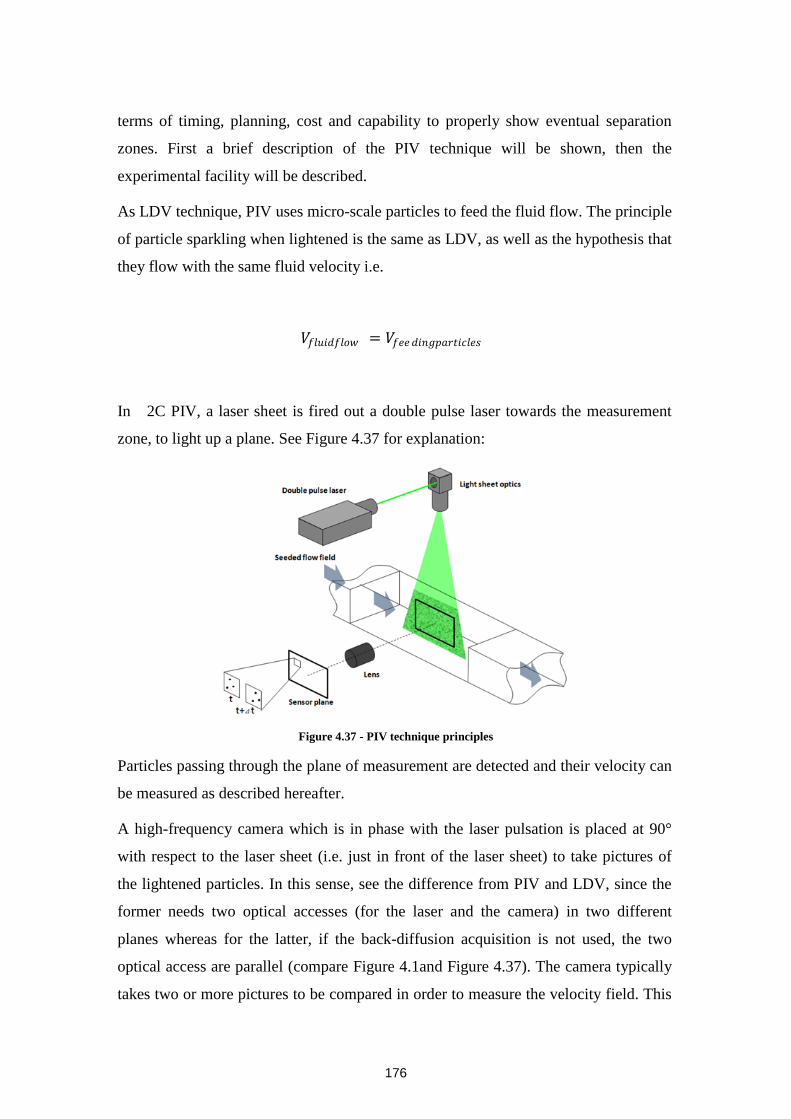
176
terms of timing, planning, cost and capability to properly show eventual separation
zones. First a brief description of the PIV technique will be shown, then the
experimental facility will be described.
As LDV technique, PIV uses micro-scale particles to feed the fluid flow. The principle
of particle sparkling when lightened is the same as LDV, as well as the hypothesis that
they flow with the same fluid velocity i.e.
𝑉𝑓𝑙𝑢𝑖𝑑𝑓𝑙𝑜𝑤 = 𝑉𝑓𝑒𝑒𝑑𝑖𝑛𝑔𝑝𝑎𝑟𝑡𝑖𝑐𝑙𝑒𝑠
In 2C PIV, a laser sheet is fired out a double pulse laser towards the measurement
zone, to light up a plane. See Figure 4.37 for explanation:
Figure 4.37 - PIV technique principles
Particles passing through the plane of measurement are detected and their velocity can
be measured as described hereafter.
A high-frequency camera which is in phase with the laser pulsation is placed at 90°
with respect to the laser sheet (i.e. just in front of the laser sheet) to take pictures of
the lightened particles. In this sense, see the difference from PIV and LDV, since the
former needs two optical accesses (for the laser and the camera) in two different
planes whereas for the latter, if the back-diffusion acquisition is not used, the two
optical access are parallel (compare Figure 4.1and Figure 4.37). The camera typically
takes two or more pictures to be compared in order to measure the velocity field. This
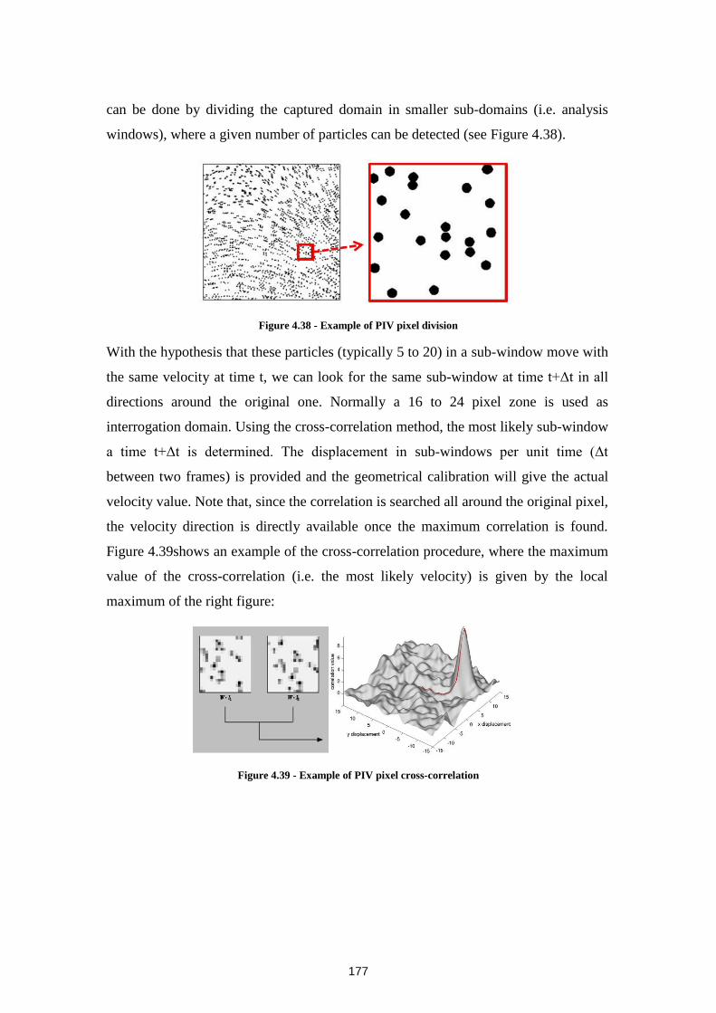
177
can be done by dividing the captured domain in smaller sub-domains (i.e. analysis
windows), where a given number of particles can be detected (see Figure 4.38).
Figure 4.38 - Example of PIV pixel division
With the hypothesis that these particles (typically 5 to 20) in a sub-window move with
the same velocity at time t, we can look for the same sub-window at time t+Δt in all
directions around the original one. Normally a 16 to 24 pixel zone is used as
interrogation domain. Using the cross-correlation method, the most likely sub-window
a time t+Δt is determined. The displacement in sub-windows per unit time (Δt
between two frames) is provided and the geometrical calibration will give the actual
velocity value. Note that, since the correlation is searched all around the original pixel,
the velocity direction is directly available once the maximum correlation is found.
Figure 4.39shows an example of the cross-correlation procedure, where the maximum
value of the cross-correlation (i.e. the most likely velocity) is given by the local
maximum of the right figure:
Figure 4.39 - Example of PIV pixel cross-correlation
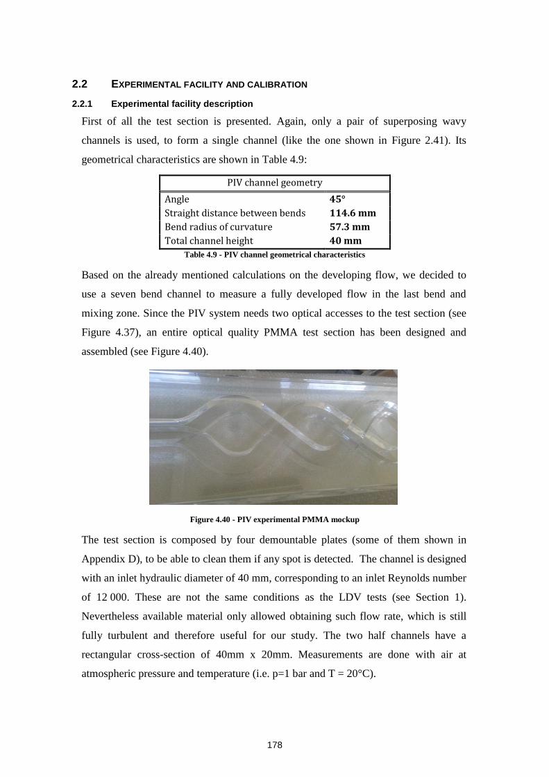
178
2.2 EXPERIMENTAL FACILITY AND CALIBRATION
2.2.1 Experimental facility description
First of all the test section is presented. Again, only a pair of superposing wavy
channels is used, to form a single channel (like the one shown in Figure 2.41). Its
geometrical characteristics are shown in Table 4.9:
PIV channel geometry
Angle 45°
Straight distance between bends 114.6 mm
Bend radius of curvature 57.3 mm
Total channel height 40 mm
Table 4.9 - PIV channel geometrical characteristics
Based on the already mentioned calculations on the developing flow, we decided to
use a seven bend channel to measure a fully developed flow in the last bend and
mixing zone. Since the PIV system needs two optical accesses to the test section (see
Figure 4.37), an entire optical quality PMMA test section has been designed and
assembled (see Figure 4.40).
Figure 4.40 - PIV experimental PMMA mockup
The test section is composed by four demountable plates (some of them shown in
Appendix D), to be able to clean them if any spot is detected. The channel is designed
with an inlet hydraulic diameter of 40 mm, corresponding to an inlet Reynolds number
of 12 000. These are not the same conditions as the LDV tests (see Section 1).
Nevertheless available material only allowed obtaining such flow rate, which is still
fully turbulent and therefore useful for our study. The two half channels have a
rectangular cross-section of 40mm x 20mm. Measurements are done with air at
atmospheric pressure and temperature (i.e. p=1 bar and T = 20°C).
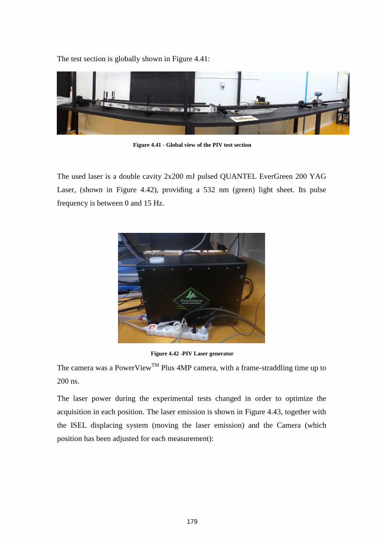
179
The test section is globally shown in Figure 4.41:
Figure 4.41 - Global view of the PIV test section
The used laser is a double cavity 2x200 mJ pulsed QUANTEL EverGreen 200 YAG
Laser, (shown in Figure 4.42), providing a 532 nm (green) light sheet. Its pulse
frequency is between 0 and 15 Hz.
Figure 4.42 -PIV Laser generator
The camera was a PowerViewTM
Plus 4MP camera, with a frame-straddling time up to
200 ns.
The laser power during the experimental tests changed in order to optimize the
acquisition in each position. The laser emission is shown in Figure 4.43, together with
the ISEL displacing system (moving the laser emission) and the Camera (which
position has been adjusted for each measurement):
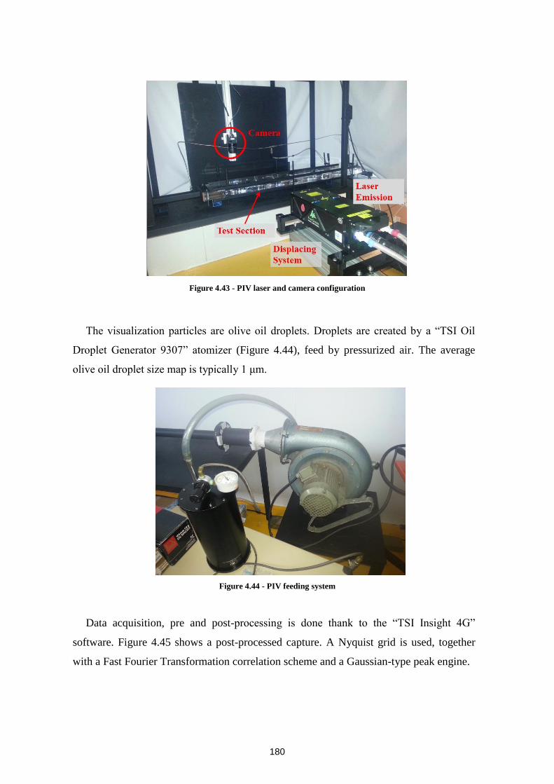
180
Figure 4.43 - PIV laser and camera configuration
The visualization particles are olive oil droplets. Droplets are created by a “TSI Oil
Droplet Generator 9307” atomizer (Figure 4.44), feed by pressurized air. The average
olive oil droplet size map is typically 1 μm.
Figure 4.44 - PIV feeding system
Data acquisition, pre and post-processing is done thank to the “TSI Insight 4G”
software. Figure 4.45 shows a post-processed capture. A Nyquist grid is used, together
with a Fast Fourier Transformation correlation scheme and a Gaussian-type peak engine.
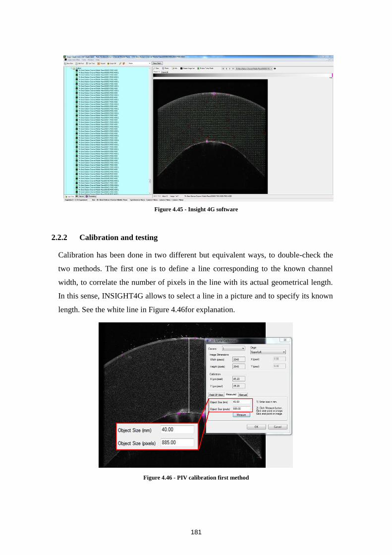
181
Figure 4.45 - Insight 4G software
2.2.2 Calibration and testing
Calibration has been done in two different but equivalent ways, to double-check the
two methods. The first one is to define a line corresponding to the known channel
width, to correlate the number of pixels in the line with its actual geometrical length.
In this sense, INSIGHT4G allows to select a line in a picture and to specify its known
length. See the white line in Figure 4.46for explanation.
Figure 4.46 - PIV calibration first method
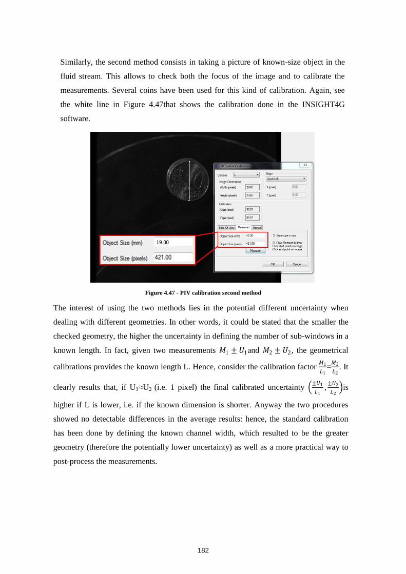
182
Similarly, the second method consists in taking a picture of known-size object in the
fluid stream. This allows to check both the focus of the image and to calibrate the
measurements. Several coins have been used for this kind of calibration. Again, see
the white line in Figure 4.47that shows the calibration done in the INSIGHT4G
software.
Figure 4.47 - PIV calibration second method
The interest of using the two methods lies in the potential different uncertainty when
dealing with different geometries. In other words, it could be stated that the smaller the
checked geometry, the higher the uncertainty in defining the number of sub-windows in a
known length. In fact, given two measurements 𝑀1 ± 𝑈1and 𝑀2 ± 𝑈2, the geometrical
calibrations provides the known length L. Hence, consider the calibration factor 𝑀1
𝐿1=𝑀2
𝐿2. It
clearly results that, if U1≈U2 (i.e. 1 pixel) the final calibrated uncertainty ±𝑈1
𝐿1,
±𝑈2
𝐿2 is
higher if L is lower, i.e. if the known dimension is shorter. Anyway the two procedures
showed no detectable differences in the average results: hence, the standard calibration
has been done by defining the known channel width, which resulted to be the greater
geometry (therefore the potentially lower uncertainty) as well as a more practical way to
post-process the measurements.

183
2.3 EXPERIMENTAL CAMPAIGN DESCRIPTION
2.3.1 Experimental measurement program definition
The experimental campaign has been defined in a similar way as the LDV one: in
particular, the inlet section, the last mixing zone as well as the last bend are chosen as
reference regions to investigate channel flow. Moreover, to verify flow development
(hence the design hypothesis) the fifth and sixth bend are studied as well.
Note that the test section system of coordinates is shown in Figure 4.48.
Figure 4.48 - System of coordinates for PIV measurements
It is worth mentioning immediately that the mixing plane could not be measured, since
it correspond to the physical interface between two plates (see Appendix E). Hence, it
could not be properly illuminated by the laser sheet, diffraction phenomena being
predominant. The used notation is provided in Table 4.10. Figure 4.49, Figure 4.50
and Figure 4.51 show then the planes that have been studied.
Inlet Section Bend Mixing Zone
The planes are named as
a function of their
distance in millimeters
from the bottom plane,
defined as the Z=0 plane
(Z=40 mm being the top
plane). As an example,
see Bottom plane + 16
mm.
For each half channel, the
middle plane (i.e. the
Z=20 mm for the bottom
haldf channel and the
Z=30 of the top half
channel) are used as
reference. Hence, the
notation is a function of
the distance from these
middle-planes for each
channel (i.e. top channel
middle-plane + 4
millimeters).
Same as bend
Table 4.10 - PIV measured plane used notation
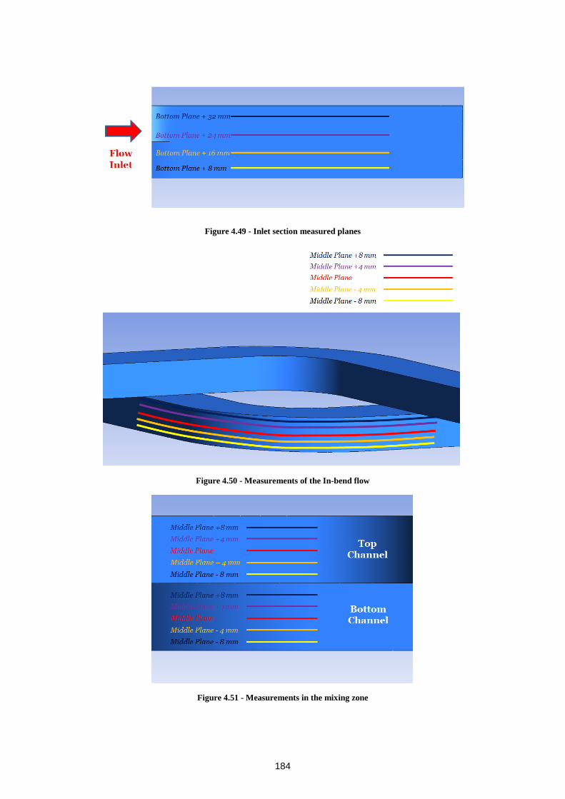
184
Figure 4.49 - Inlet section measured planes
Figure 4.50 - Measurements of the In-bend flow
Figure 4.51 - Measurements in the mixing zone
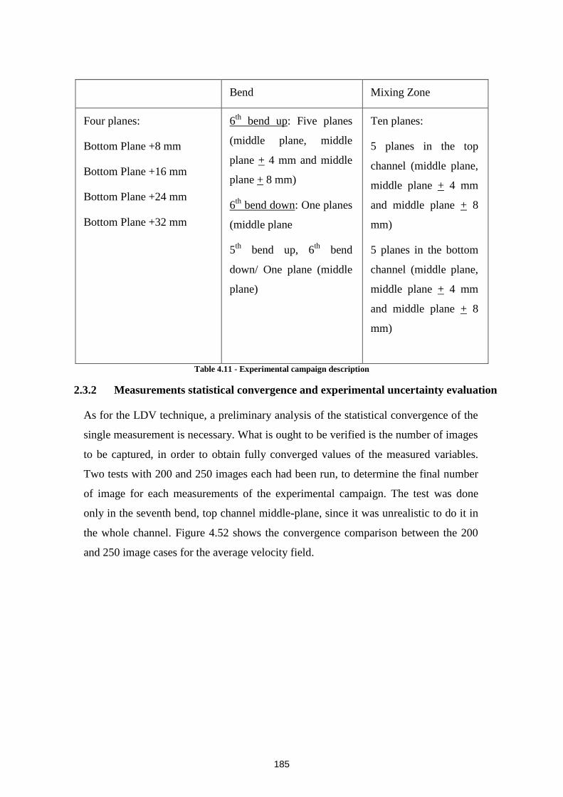
185
Inlet Section Bend Mixing Zone
Four planes:
Bottom Plane +8 mm
Bottom Plane +16 mm
Bottom Plane +24 mm
Bottom Plane +32 mm
6th
bend up: Five planes
(middle plane, middle
plane + 4 mm and middle
plane + 8 mm)
6th
bend down: One planes
(middle plane
5th
bend up, 6th
bend
down/ One plane (middle
plane)
Ten planes:
5 planes in the top
channel (middle plane,
middle plane + 4 mm
and middle plane + 8
mm)
5 planes in the bottom
channel (middle plane,
middle plane + 4 mm
and middle plane + 8
mm)
Table 4.11 - Experimental campaign description
2.3.2 Measurements statistical convergence and experimental uncertainty evaluation
As for the LDV technique, a preliminary analysis of the statistical convergence of the
single measurement is necessary. What is ought to be verified is the number of images
to be captured, in order to obtain fully converged values of the measured variables.
Two tests with 200 and 250 images each had been run, to determine the final number
of image for each measurements of the experimental campaign. The test was done
only in the seventh bend, top channel middle-plane, since it was unrealistic to do it in
the whole channel. Figure 4.52 shows the convergence comparison between the 200
and 250 image cases for the average velocity field.
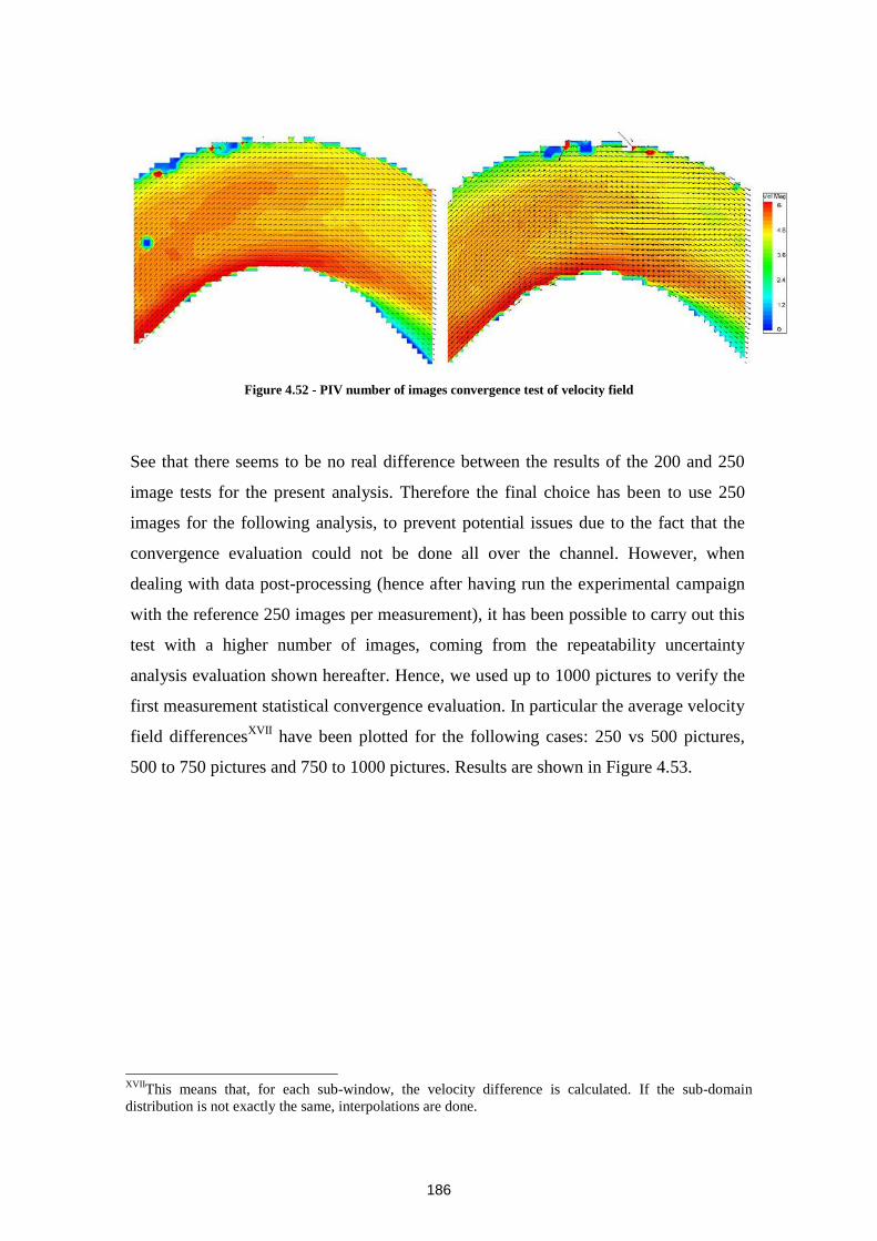
186
Figure 4.52 - PIV number of images convergence test of velocity field
See that there seems to be no real difference between the results of the 200 and 250
image tests for the present analysis. Therefore the final choice has been to use 250
images for the following analysis, to prevent potential issues due to the fact that the
convergence evaluation could not be done all over the channel. However, when
dealing with data post-processing (hence after having run the experimental campaign
with the reference 250 images per measurement), it has been possible to carry out this
test with a higher number of images, coming from the repeatability uncertainty
analysis evaluation shown hereafter. Hence, we used up to 1000 pictures to verify the
first measurement statistical convergence evaluation. In particular the average velocity
field differencesXVII
have been plotted for the following cases: 250 vs 500 pictures,
500 to 750 pictures and 750 to 1000 pictures. Results are shown in Figure 4.53.
XVII
This means that, for each sub-window, the velocity difference is calculated. If the sub-domain
distribution is not exactly the same, interpolations are done.
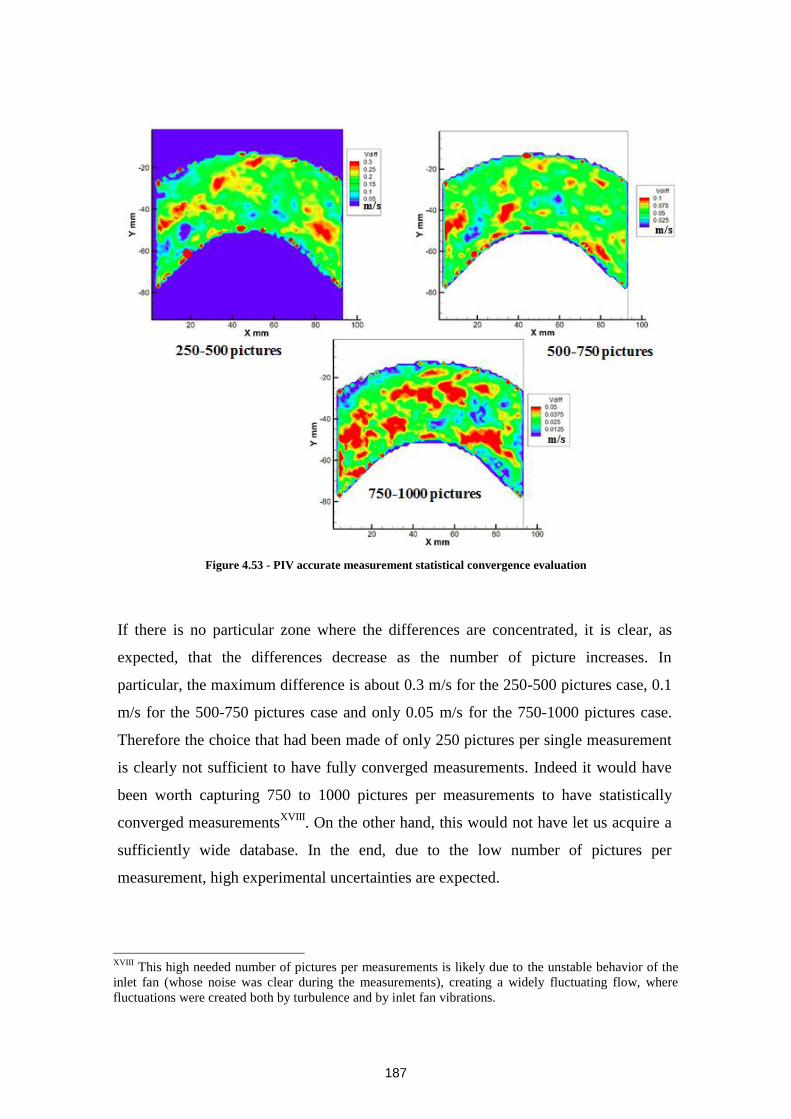
187
Figure 4.53 - PIV accurate measurement statistical convergence evaluation
If there is no particular zone where the differences are concentrated, it is clear, as
expected, that the differences decrease as the number of picture increases. In
particular, the maximum difference is about 0.3 m/s for the 250-500 pictures case, 0.1
m/s for the 500-750 pictures case and only 0.05 m/s for the 750-1000 pictures case.
Therefore the choice that had been made of only 250 pictures per single measurement
is clearly not sufficient to have fully converged measurements. Indeed it would have
been worth capturing 750 to 1000 pictures per measurements to have statistically
converged measurementsXVIII
. On the other hand, this would not have let us acquire a
sufficiently wide database. In the end, due to the low number of pictures per
measurement, high experimental uncertainties are expected.
XVIII
This high needed number of pictures per measurements is likely due to the unstable behavior of the
inlet fan (whose noise was clear during the measurements), creating a widely fluctuating flow, where
fluctuations were created both by turbulence and by inlet fan vibrations.
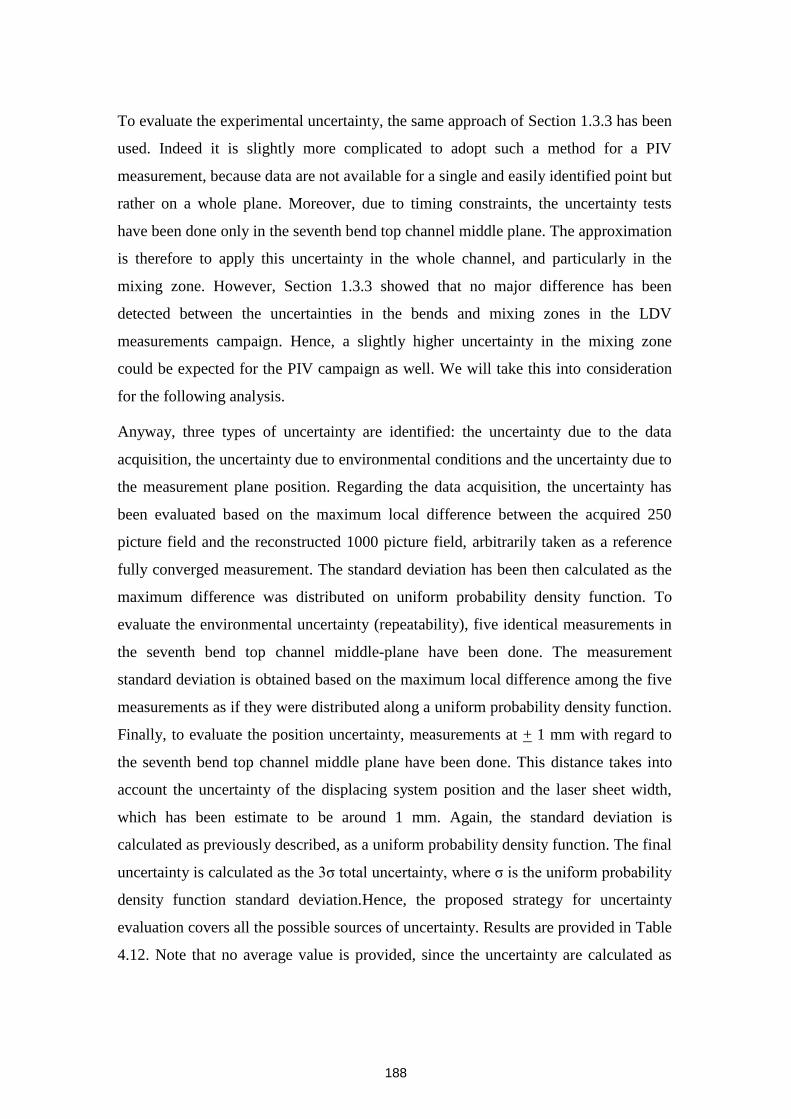
188
To evaluate the experimental uncertainty, the same approach of Section 1.3.3 has been
used. Indeed it is slightly more complicated to adopt such a method for a PIV
measurement, because data are not available for a single and easily identified point but
rather on a whole plane. Moreover, due to timing constraints, the uncertainty tests
have been done only in the seventh bend top channel middle plane. The approximation
is therefore to apply this uncertainty in the whole channel, and particularly in the
mixing zone. However, Section 1.3.3 showed that no major difference has been
detected between the uncertainties in the bends and mixing zones in the LDV
measurements campaign. Hence, a slightly higher uncertainty in the mixing zone
could be expected for the PIV campaign as well. We will take this into consideration
for the following analysis.
Anyway, three types of uncertainty are identified: the uncertainty due to the data
acquisition, the uncertainty due to environmental conditions and the uncertainty due to
the measurement plane position. Regarding the data acquisition, the uncertainty has
been evaluated based on the maximum local difference between the acquired 250
picture field and the reconstructed 1000 picture field, arbitrarily taken as a reference
fully converged measurement. The standard deviation has been then calculated as the
maximum difference was distributed on uniform probability density function. To
evaluate the environmental uncertainty (repeatability), five identical measurements in
the seventh bend top channel middle-plane have been done. The measurement
standard deviation is obtained based on the maximum local difference among the five
measurements as if they were distributed along a uniform probability density function.
Finally, to evaluate the position uncertainty, measurements at + 1 mm with regard to
the seventh bend top channel middle plane have been done. This distance takes into
account the uncertainty of the displacing system position and the laser sheet width,
which has been estimate to be around 1 mm. Again, the standard deviation is
calculated as previously described, as a uniform probability density function. The final
uncertainty is calculated as the 3ζ total uncertainty, where ζ is the uniform probability
density function standard deviation.Hence, the proposed strategy for uncertainty
evaluation covers all the possible sources of uncertainty. Results are provided in Table
4.12. Note that no average value is provided, since the uncertainty are calculated as

189
the maximum local uncertainty on an entire field, not referred to any specific average
value.
Data
acquisition
Uncertainty
Environmental
conditions
Uncertainty
Position
Uncertainty
Total 3ζ
Uncertainty
Velocity
Magnitude
0.17 m/s 0.12 m/s 0.24 m/s 0.80 m/s
u’ Magnitude 0.07 m/s 0.09m/s 0. 09 m/s 0.38m/s
v’ Magnitude
Uncertainty
0.07 m/s 0. 09 m/s 0. 09 m/s 0.38m/s
Table 4.12 - PIV experimental uncertainty evaluation
Position uncertainty is still very high as for the LDV campaign. Here the
environmental conditions are important to the same extent; anyway this is easily
explained by the fact that the uncertainty evaluation procedure is different, as already
explained: for LDV that has been done in a single point of measurements, whereas for
PIV the local maximum difference has been used as the basis to calculate the total
uncertainty. This means that the relative importance of position uncertainty and
environmental conditions changes as a function of the local point of measurements
(i.e. of the local flow conditions, gradients, etc.).
2.4 PIV EXPERIMENTAL MEASUREMENTS
2.4.1 Flow Inlet Conditions
First of all the flow inlet conditions are studied. Again no asymmetry is expected,
since the inlet flow comes from several straight tubes. By the way, the flow is not
almost uniform in the inlet section because of the same reason. Hence we expect to
have clear turbulent developed flow profiles. Figure 4.54 shows the velocity profiles
in the four measured planes:
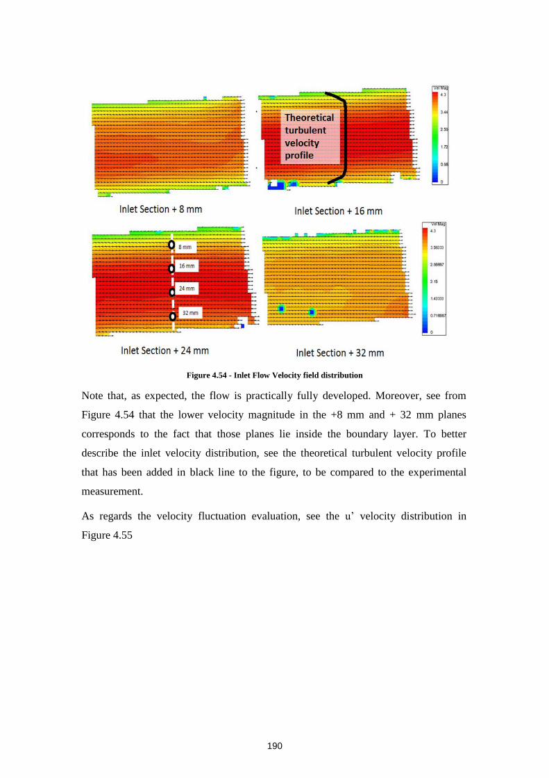
190
Figure 4.54 - Inlet Flow Velocity field distribution
Note that, as expected, the flow is practically fully developed. Moreover, see from
Figure 4.54 that the lower velocity magnitude in the +8 mm and + 32 mm planes
corresponds to the fact that those planes lie inside the boundary layer. To better
describe the inlet velocity distribution, see the theoretical turbulent velocity profile
that has been added in black line to the figure, to be compared to the experimental
measurement.
As regards the velocity fluctuation evaluation, see the u’ velocity distribution in
Figure 4.55
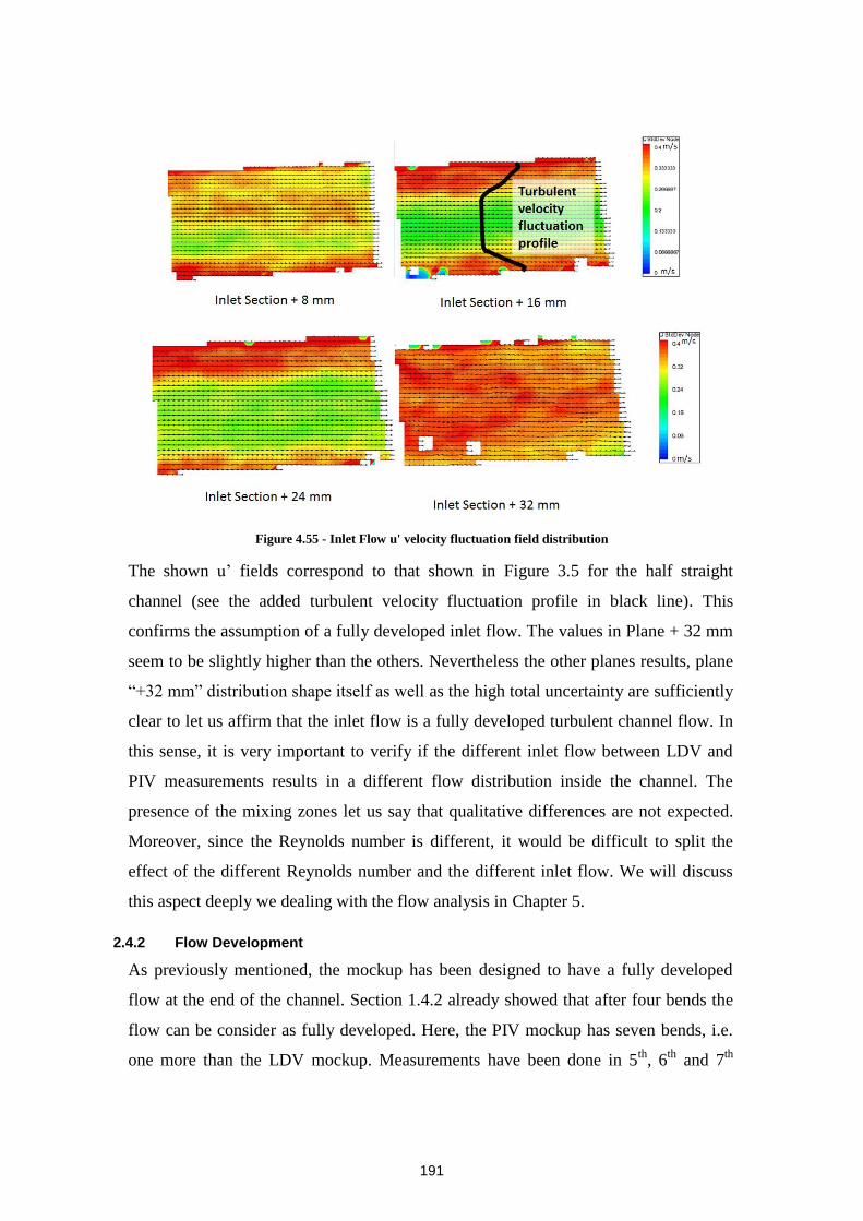
191
Figure 4.55 - Inlet Flow u' velocity fluctuation field distribution
The shown u’ fields correspond to that shown in Figure 3.5 for the half straight
channel (see the added turbulent velocity fluctuation profile in black line). This
confirms the assumption of a fully developed inlet flow. The values in Plane + 32 mm
seem to be slightly higher than the others. Nevertheless the other planes results, plane
“+32 mm” distribution shape itself as well as the high total uncertainty are sufficiently
clear to let us affirm that the inlet flow is a fully developed turbulent channel flow. In
this sense, it is very important to verify if the different inlet flow between LDV and
PIV measurements results in a different flow distribution inside the channel. The
presence of the mixing zones let us say that qualitative differences are not expected.
Moreover, since the Reynolds number is different, it would be difficult to split the
effect of the different Reynolds number and the different inlet flow. We will discuss
this aspect deeply we dealing with the flow analysis in Chapter 5.
2.4.2 Flow Development
As previously mentioned, the mockup has been designed to have a fully developed
flow at the end of the channel. Section 1.4.2 already showed that after four bends the
flow can be consider as fully developed. Here, the PIV mockup has seven bends, i.e.
one more than the LDV mockup. Measurements have been done in 5th
, 6th
and 7th
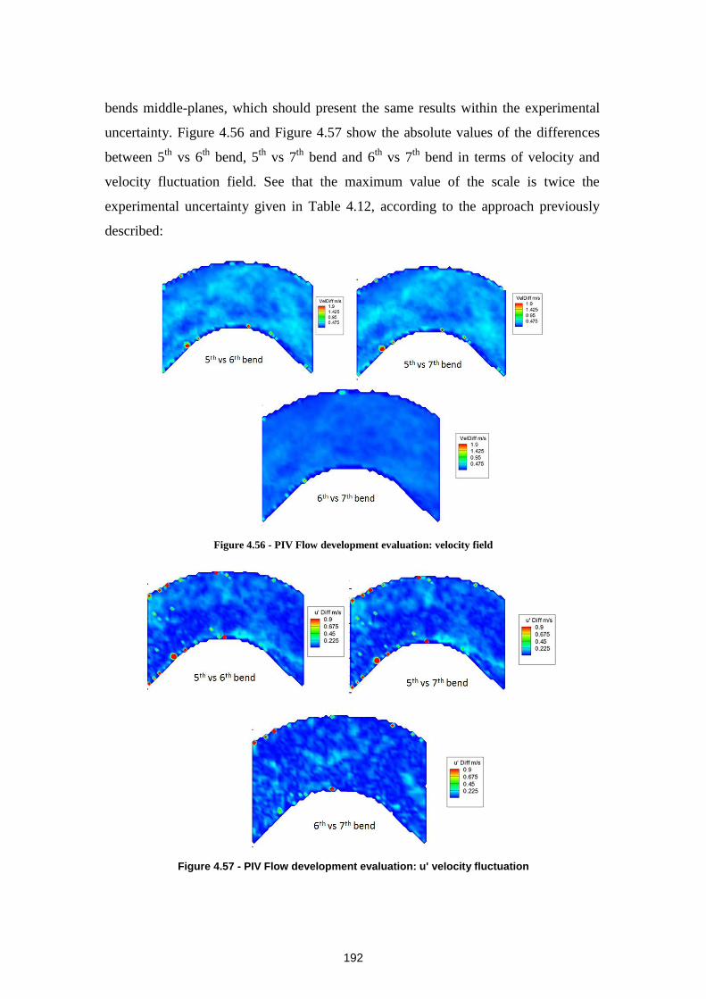
192
bends middle-planes, which should present the same results within the experimental
uncertainty. Figure 4.56 and Figure 4.57 show the absolute values of the differences
between 5th
vs 6th
bend, 5th
vs 7th
bend and 6th
vs 7th
bend in terms of velocity and
velocity fluctuation field. See that the maximum value of the scale is twice the
experimental uncertainty given in Table 4.12, according to the approach previously
described:
Figure 4.56 - PIV Flow development evaluation: velocity field
Figure 4.57 - PIV Flow development evaluation: u' velocity fluctuation
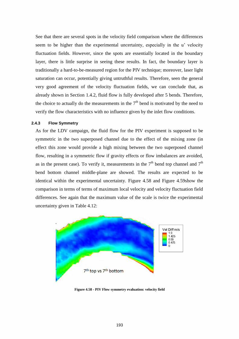
193
See that there are several spots in the velocity field comparison where the differences
seem to be higher than the experimental uncertainty, especially in the u’ velocity
fluctuation fields. However, since the spots are essentially located in the boundary
layer, there is little surprise in seeing these results. In fact, the boundary layer is
traditionally a hard-to-be-measured region for the PIV technique; moreover, laser light
saturation can occur, potentially giving untruthful results. Therefore, seen the general
very good agreement of the velocity fluctuation fields, we can conclude that, as
already shown in Section 1.4.2, fluid flow is fully developed after 5 bends. Therefore,
the choice to actually do the measurements in the 7th
bend is motivated by the need to
verify the flow characteristics with no influence given by the inlet flow conditions.
2.4.3 Flow Symmetry
As for the LDV campaign, the fluid flow for the PIV experiment is supposed to be
symmetric in the two superposed channel due to the effect of the mixing zone (in
effect this zone would provide a high mixing between the two superposed channel
flow, resulting in a symmetric flow if gravity effects or flow imbalances are avoided,
as in the present case). To verify it, measurements in the 7th
bend top channel and 7th
bend bottom channel middle-plane are showed. The results are expected to be
identical within the experimental uncertainty. Figure 4.58 and Figure 4.59show the
comparison in terms of terms of maximum local velocity and velocity fluctuation field
differences. See again that the maximum value of the scale is twice the experimental
uncertainty given in Table 4.12:
Figure 4.58 - PIV Flow symmetry evaluation: velocity field
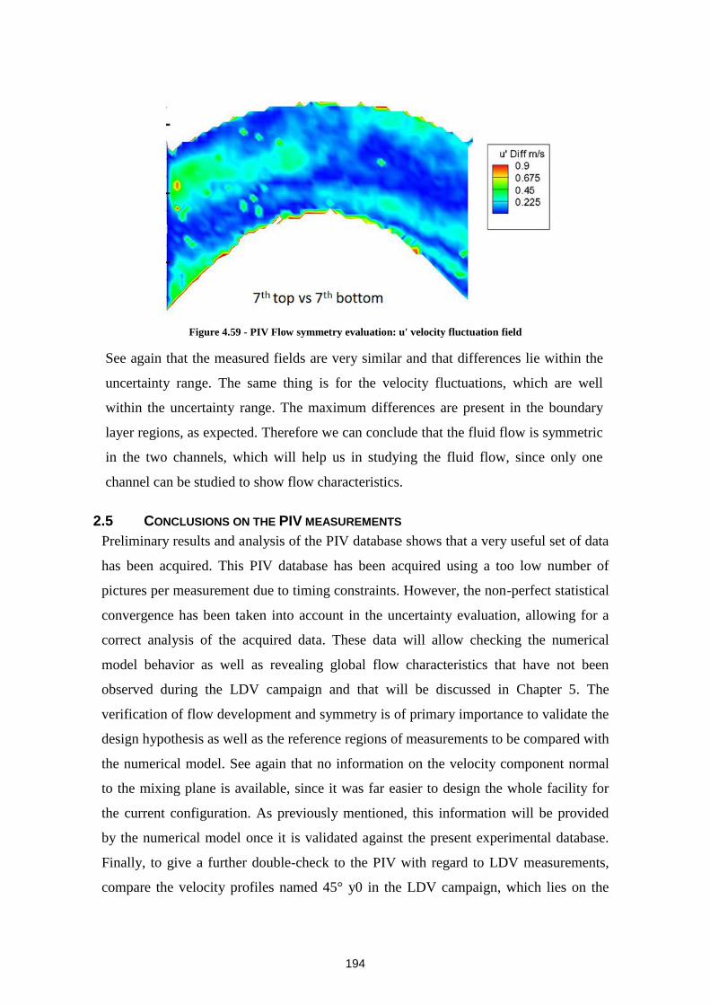
194
Figure 4.59 - PIV Flow symmetry evaluation: u' velocity fluctuation field
See again that the measured fields are very similar and that differences lie within the
uncertainty range. The same thing is for the velocity fluctuations, which are well
within the uncertainty range. The maximum differences are present in the boundary
layer regions, as expected. Therefore we can conclude that the fluid flow is symmetric
in the two channels, which will help us in studying the fluid flow, since only one
channel can be studied to show flow characteristics.
2.5 CONCLUSIONS ON THE PIV MEASUREMENTS
Preliminary results and analysis of the PIV database shows that a very useful set of data
has been acquired. This PIV database has been acquired using a too low number of
pictures per measurement due to timing constraints. However, the non-perfect statistical
convergence has been taken into account in the uncertainty evaluation, allowing for a
correct analysis of the acquired data. These data will allow checking the numerical
model behavior as well as revealing global flow characteristics that have not been
observed during the LDV campaign and that will be discussed in Chapter 5. The
verification of flow development and symmetry is of primary importance to validate the
design hypothesis as well as the reference regions of measurements to be compared with
the numerical model. See again that no information on the velocity component normal
to the mixing plane is available, since it was far easier to design the whole facility for
the current configuration. As previously mentioned, this information will be provided
by the numerical model once it is validated against the present experimental database.
Finally, to give a further double-check to the PIV with regard to LDV measurements,
compare the velocity profiles named 45° y0 in the LDV campaign, which lies on the
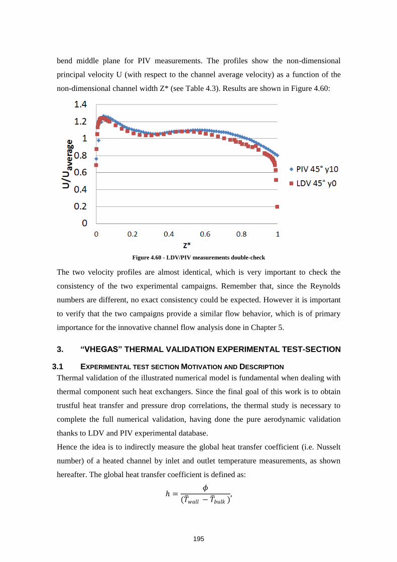
195
bend middle plane for PIV measurements. The profiles show the non-dimensional
principal velocity U (with respect to the channel average velocity) as a function of the
non-dimensional channel width Z* (see Table 4.3). Results are shown in Figure 4.60:
Figure 4.60 - LDV/PIV measurements double-check
The two velocity profiles are almost identical, which is very important to check the
consistency of the two experimental campaigns. Remember that, since the Reynolds
numbers are different, no exact consistency could be expected. However it is important
to verify that the two campaigns provide a similar flow behavior, which is of primary
importance for the innovative channel flow analysis done in Chapter 5.
3. “VHEGAS” THERMAL VALIDATION EXPERIMENTAL TEST-SECTION
3.1 EXPERIMENTAL TEST SECTION MOTIVATION AND DESCRIPTION
Thermal validation of the illustrated numerical model is fundamental when dealing with
thermal component such heat exchangers. Since the final goal of this work is to obtain
trustful heat transfer and pressure drop correlations, the thermal study is necessary to
complete the full numerical validation, having done the pure aerodynamic validation
thanks to LDV and PIV experimental database.
Hence the idea is to indirectly measure the global heat transfer coefficient (i.e. Nusselt
number) of a heated channel by inlet and outlet temperature measurements, as shown
hereafter. The global heat transfer coefficient is defined as:
=𝜙
(𝑇 𝑤𝑎𝑙𝑙 − 𝑇 𝑏𝑢𝑙𝑘 ),
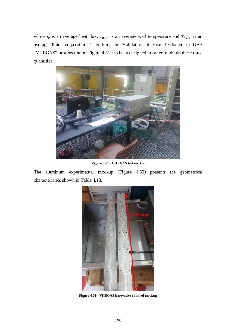
196
where 𝜙 is an average heat flux, 𝑇 𝑤𝑎𝑙𝑙 is an average wall temperature and 𝑇 𝑏𝑢𝑙𝑘 is an
average fluid temperature. Therefore, the Validation of Heat Exchange in GAS
“VHEGAS” test-section of Figure 4.61 has been designed in order to obtain these three
quantities.
Figure 4.61 - VHEGAS test section
The aluminum experimental mockup (Figure 4.62) presents the geometrical
characteristics shown in Table 4.13.
Figure 4.62 - VHEGAS innovative channel mockup
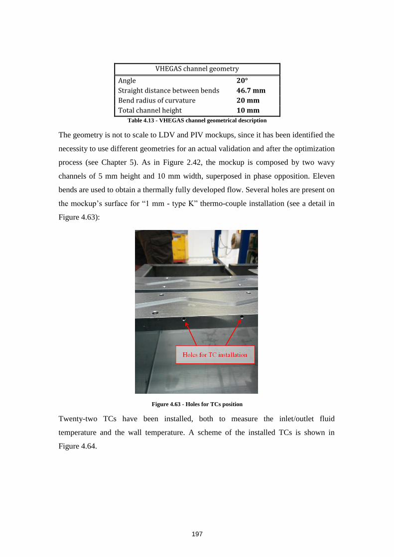
197
VHEGAS channel geometry
Angle 20°
Straight distance between bends 46.7 mm
Bend radius of curvature 20 mm
Total channel height 10 mm
Table 4.13 - VHEGAS channel geometrical description
The geometry is not to scale to LDV and PIV mockups, since it has been identified the
necessity to use different geometries for an actual validation and after the optimization
process (see Chapter 5). As in Figure 2.42, the mockup is composed by two wavy
channels of 5 mm height and 10 mm width, superposed in phase opposition. Eleven
bends are used to obtain a thermally fully developed flow. Several holes are present on
the mockup’s surface for “1 mm - type K” thermo-couple installation (see a detail in
Figure 4.63):
Figure 4.63 - Holes for TCs position
Twenty-two TCs have been installed, both to measure the inlet/outlet fluid
temperature and the wall temperature. A scheme of the installed TCs is shown in
Figure 4.64.
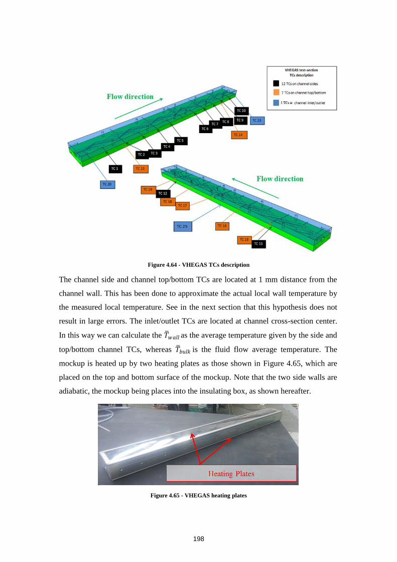
198
Figure 4.64 - VHEGAS TCs description
The channel side and channel top/bottom TCs are located at 1 mm distance from the
channel wall. This has been done to approximate the actual local wall temperature by
the measured local temperature. See in the next section that this hypothesis does not
result in large errors. The inlet/outlet TCs are located at channel cross-section center.
In this way we can calculate the 𝑇 𝑤𝑎𝑙𝑙 as the average temperature given by the side and
top/bottom channel TCs, whereas 𝑇 𝑏𝑢𝑙𝑘 is the fluid flow average temperature. The
mockup is heated up by two heating plates as those shown in Figure 4.65, which are
placed on the top and bottom surface of the mockup. Note that the two side walls are
adiabatic, the mockup being places into the insulating box, as shown hereafter.
Figure 4.65 - VHEGAS heating plates
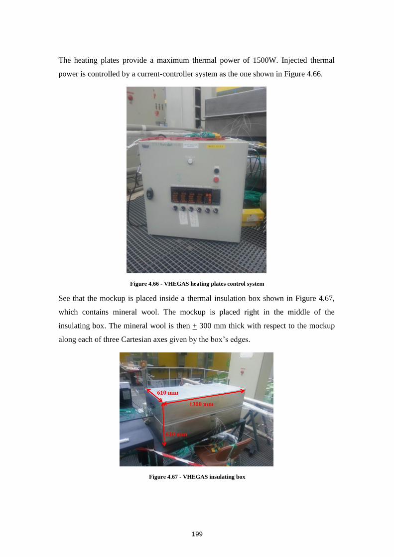
199
The heating plates provide a maximum thermal power of 1500W. Injected thermal
power is controlled by a current-controller system as the one shown in Figure 4.66.
Figure 4.66 - VHEGAS heating plates control system
See that the mockup is placed inside a thermal insulation box shown in Figure 4.67,
which contains mineral wool. The mockup is placed right in the middle of the
insulating box. The mineral wool is then + 300 mm thick with respect to the mockup
along each of three Cartesian axes given by the box’s edges.
Figure 4.67 - VHEGAS insulating box
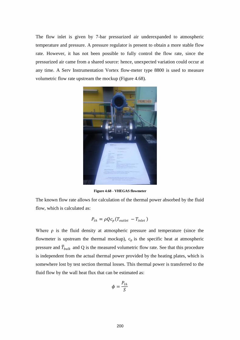
200
The flow inlet is given by 7-bar pressurized air underexpanded to atmospheric
temperature and pressure. A pressure regulator is present to obtain a more stable flow
rate. However, it has not been possible to fully control the flow rate, since the
pressurized air came from a shared source: hence, unexpected variation could occur at
any time. A Serv Instrumentation Vortex flow-meter type 8800 is used to measure
volumetric flow rate upstream the mockup (Figure 4.68).
Figure 4.68 - VHEGAS flowmeter
The known flow rate allows for calculation of the thermal power absorbed by the fluid
flow, which is calculated as:
𝑃𝑡 = 𝜌𝑄𝑐𝑝 𝑇𝑜𝑢𝑡𝑙𝑒𝑡 − 𝑇𝑖𝑛𝑙𝑒𝑡
Where ρ is the fluid density at atmospheric pressure and temperature (since the
flowmeter is upstream the thermal mockup), cp is the specific heat at atmospheric
pressure and 𝑇 𝑏𝑢𝑙𝑘 and Q is the measured volumetric flow rate. See that this procedure
is independent from the actual thermal power provided by the heating plates, which is
somewhere lost by test section thermal losses. This thermal power is transferred to the
fluid flow by the wall heat flux that can be estimated as:
𝜙 =𝑃𝑡
𝑆
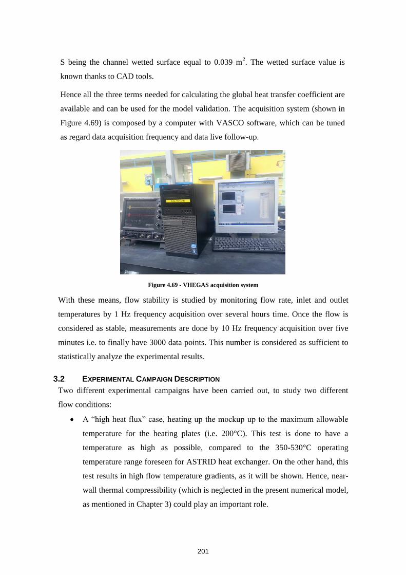
201
S being the channel wetted surface equal to 0.039 m2. The wetted surface value is
known thanks to CAD tools.
Hence all the three terms needed for calculating the global heat transfer coefficient are
available and can be used for the model validation. The acquisition system (shown in
Figure 4.69) is composed by a computer with VASCO software, which can be tuned
as regard data acquisition frequency and data live follow-up.
Figure 4.69 - VHEGAS acquisition system
With these means, flow stability is studied by monitoring flow rate, inlet and outlet
temperatures by 1 Hz frequency acquisition over several hours time. Once the flow is
considered as stable, measurements are done by 10 Hz frequency acquisition over five
minutes i.e. to finally have 3000 data points. This number is considered as sufficient to
statistically analyze the experimental results.
3.2 EXPERIMENTAL CAMPAIGN DESCRIPTION
Two different experimental campaigns have been carried out, to study two different
flow conditions:
A “high heat flux” case, heating up the mockup up to the maximum allowable
temperature for the heating plates (i.e. 200°C). This test is done to have a
temperature as high as possible, compared to the 350-530°C operating
temperature range foreseen for ASTRID heat exchanger. On the other hand, this
test results in high flow temperature gradients, as it will be shown. Hence, near-
wall thermal compressibility (which is neglected in the present numerical model,
as mentioned in Chapter 3) could play an important role.
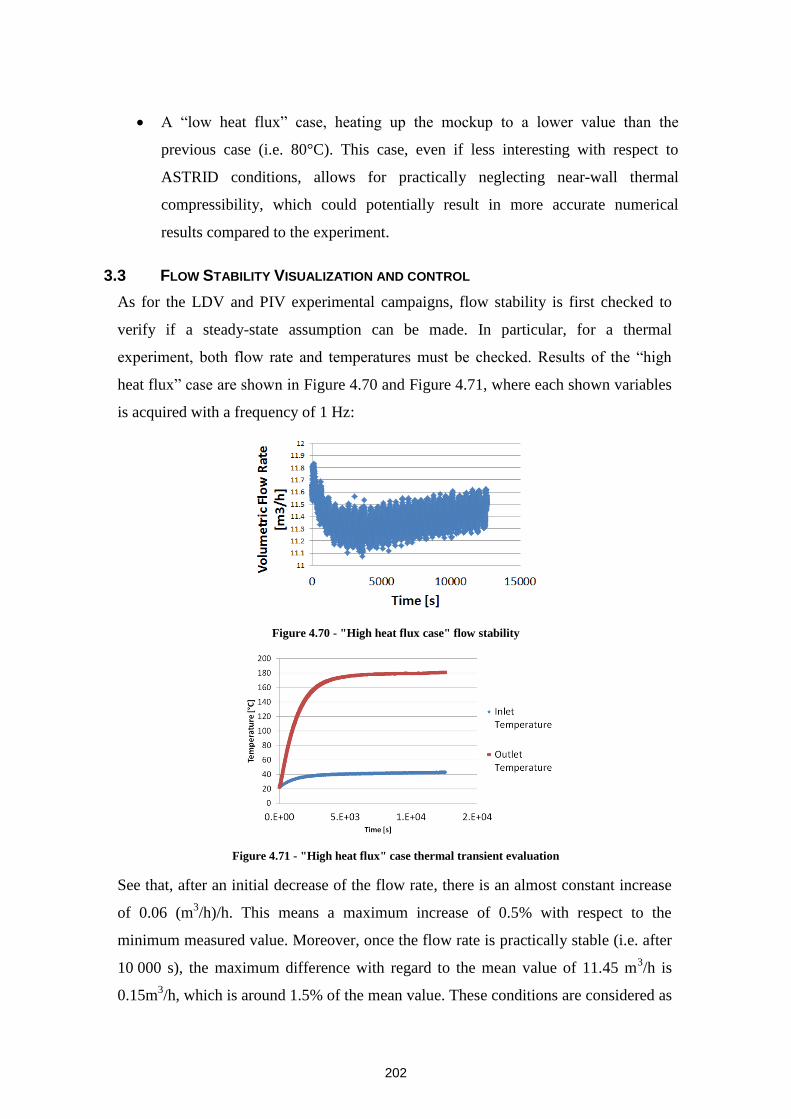
202
A “low heat flux” case, heating up the mockup to a lower value than the
previous case (i.e. 80°C). This case, even if less interesting with respect to
ASTRID conditions, allows for practically neglecting near-wall thermal
compressibility, which could potentially result in more accurate numerical
results compared to the experiment.
3.3 FLOW STABILITY VISUALIZATION AND CONTROL
As for the LDV and PIV experimental campaigns, flow stability is first checked to
verify if a steady-state assumption can be made. In particular, for a thermal
experiment, both flow rate and temperatures must be checked. Results of the “high
heat flux” case are shown in Figure 4.70 and Figure 4.71, where each shown variables
is acquired with a frequency of 1 Hz:
Figure 4.70 - "High heat flux case" flow stability
Figure 4.71 - "High heat flux" case thermal transient evaluation
See that, after an initial decrease of the flow rate, there is an almost constant increase
of 0.06 (m3/h)/h. This means a maximum increase of 0.5% with respect to the
minimum measured value. Moreover, once the flow rate is practically stable (i.e. after
10 000 s), the maximum difference with regard to the mean value of 11.45 m3/h is
0.15m3/h, which is around 1.5% of the mean value. These conditions are considered as
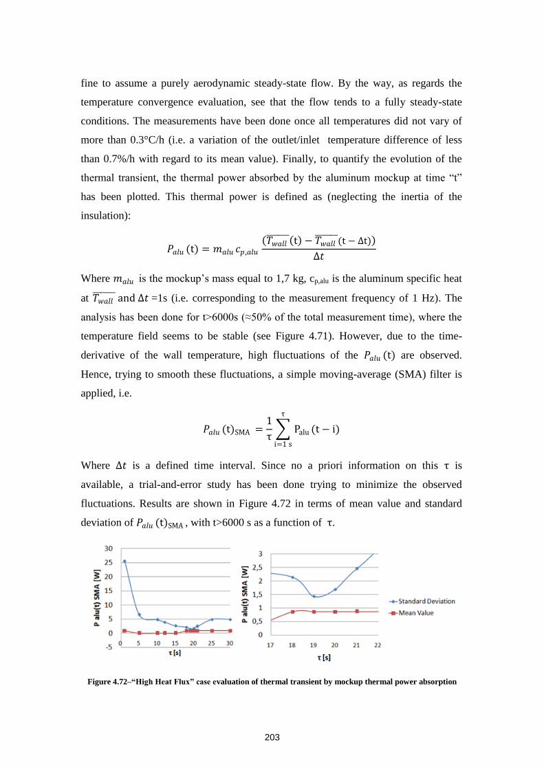
203
fine to assume a purely aerodynamic steady-state flow. By the way, as regards the
temperature convergence evaluation, see that the flow tends to a fully steady-state
conditions. The measurements have been done once all temperatures did not vary of
more than 0.3°C/h (i.e. a variation of the outlet/inlet temperature difference of less
than 0.7%/h with regard to its mean value). Finally, to quantify the evolution of the
thermal transient, the thermal power absorbed by the aluminum mockup at time “t”
has been plotted. This thermal power is defined as (neglecting the inertia of the
insulation):
𝑃𝑎𝑙𝑢 (t) = 𝑚𝑎𝑙𝑢 𝑐𝑝 ,𝑎𝑙𝑢
𝑇𝑤𝑎𝑙𝑙 t − 𝑇𝑤𝑎𝑙𝑙
(t − ∆t)
∆𝑡
Where 𝑚𝑎𝑙𝑢 is the mockup’s mass equal to 1,7 kg, cp,alu is the aluminum specific heat
at 𝑇𝑤𝑎𝑙𝑙 and ∆𝑡 =1s (i.e. corresponding to the measurement frequency of 1 Hz). The
analysis has been done for t>6000s (≈50% of the total measurement time), where the
temperature field seems to be stable (see Figure 4.71). However, due to the time-
derivative of the wall temperature, high fluctuations of the 𝑃𝑎𝑙𝑢 (t) are observed.
Hence, trying to smooth these fluctuations, a simple moving-average (SMA) filter is
applied, i.e.
𝑃𝑎𝑙𝑢 (t)SMA =1
τ Palu (t − i)
τ
i=1 s
Where ∆𝑡 is a defined time interval. Since no a priori information on this τ is
available, a trial-and-error study has been done trying to minimize the observed
fluctuations. Results are shown in Figure 4.72 in terms of mean value and standard
deviation of 𝑃𝑎𝑙𝑢 (t)SMA , with t>6000 s as a function of τ.
Figure 4.72–“High Heat Flux” case evaluation of thermal transient by mockup thermal power absorption
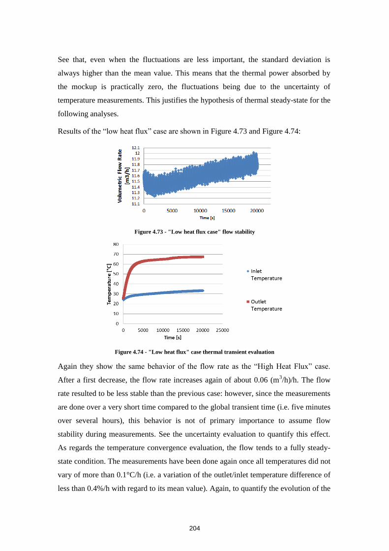
204
See that, even when the fluctuations are less important, the standard deviation is
always higher than the mean value. This means that the thermal power absorbed by
the mockup is practically zero, the fluctuations being due to the uncertainty of
temperature measurements. This justifies the hypothesis of thermal steady-state for the
following analyses.
Results of the “low heat flux” case are shown in Figure 4.73 and Figure 4.74:
Figure 4.73 - "Low heat flux case" flow stability
Figure 4.74 - "Low heat flux" case thermal transient evaluation
Again they show the same behavior of the flow rate as the “High Heat Flux” case.
After a first decrease, the flow rate increases again of about 0.06 (m3/h)/h. The flow
rate resulted to be less stable than the previous case: however, since the measurements
are done over a very short time compared to the global transient time (i.e. five minutes
over several hours), this behavior is not of primary importance to assume flow
stability during measurements. See the uncertainty evaluation to quantify this effect.
As regards the temperature convergence evaluation, the flow tends to a fully steady-
state condition. The measurements have been done again once all temperatures did not
vary of more than 0.1°C/h (i.e. a variation of the outlet/inlet temperature difference of
less than 0.4%/h with regard to its mean value). Again, to quantify the evolution of the
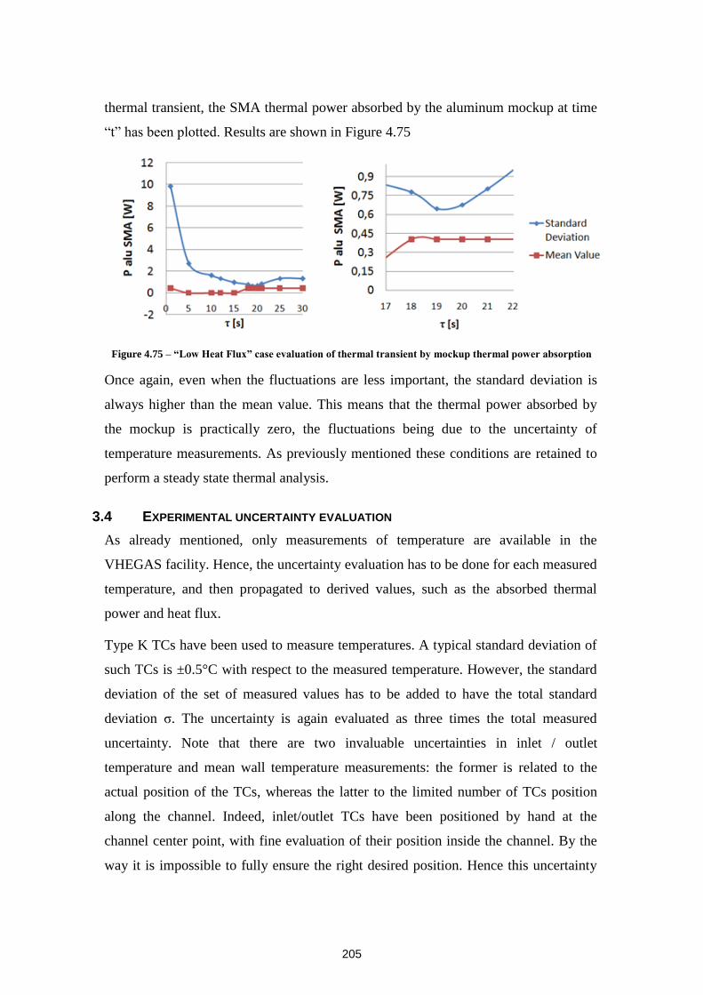
205
thermal transient, the SMA thermal power absorbed by the aluminum mockup at time
“t” has been plotted. Results are shown in Figure 4.75
Figure 4.75 – “Low Heat Flux” case evaluation of thermal transient by mockup thermal power absorption
Once again, even when the fluctuations are less important, the standard deviation is
always higher than the mean value. This means that the thermal power absorbed by
the mockup is practically zero, the fluctuations being due to the uncertainty of
temperature measurements. As previously mentioned these conditions are retained to
perform a steady state thermal analysis.
3.4 EXPERIMENTAL UNCERTAINTY EVALUATION
As already mentioned, only measurements of temperature are available in the
VHEGAS facility. Hence, the uncertainty evaluation has to be done for each measured
temperature, and then propagated to derived values, such as the absorbed thermal
power and heat flux.
Type K TCs have been used to measure temperatures. A typical standard deviation of
such TCs is ±0.5°C with respect to the measured temperature. However, the standard
deviation of the set of measured values has to be added to have the total standard
deviation ζ. The uncertainty is again evaluated as three times the total measured
uncertainty. Note that there are two invaluable uncertainties in inlet / outlet
temperature and mean wall temperature measurements: the former is related to the
actual position of the TCs, whereas the latter to the limited number of TCs position
along the channel. Indeed, inlet/outlet TCs have been positioned by hand at the
channel center point, with fine evaluation of their position inside the channel. By the
way it is impossible to fully ensure the right desired position. Hence this uncertainty
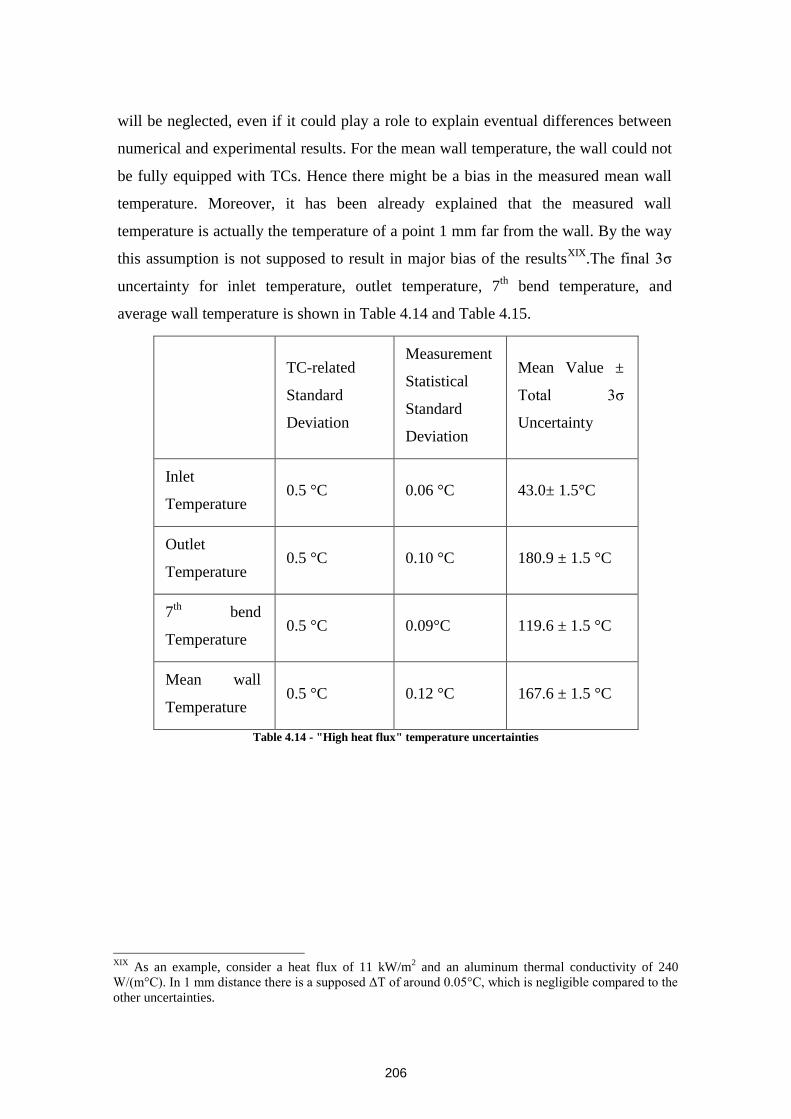
206
will be neglected, even if it could play a role to explain eventual differences between
numerical and experimental results. For the mean wall temperature, the wall could not
be fully equipped with TCs. Hence there might be a bias in the measured mean wall
temperature. Moreover, it has been already explained that the measured wall
temperature is actually the temperature of a point 1 mm far from the wall. By the way
this assumption is not supposed to result in major bias of the resultsXIX
.The final 3ζ
uncertainty for inlet temperature, outlet temperature, 7th
bend temperature, and
average wall temperature is shown in Table 4.14 and Table 4.15.
TC-related
Standard
Deviation
Measurement
Statistical
Standard
Deviation
Mean Value ±
Total 3ζ
Uncertainty
Inlet
Temperature 0.5 °C 0.06 °C 43.0± 1.5°C
Outlet
Temperature 0.5 °C 0.10 °C 180.9 ± 1.5 °C
7th
bend
Temperature 0.5 °C 0.09°C 119.6 ± 1.5 °C
Mean wall
Temperature 0.5 °C 0.12 °C 167.6 ± 1.5 °C
Table 4.14 - "High heat flux" temperature uncertainties
XIX
As an example, consider a heat flux of 11 kW/m2 and an aluminum thermal conductivity of 240
W/(m°C). In 1 mm distance there is a supposed ΔT of around 0.05°C, which is negligible compared to the
other uncertainties.
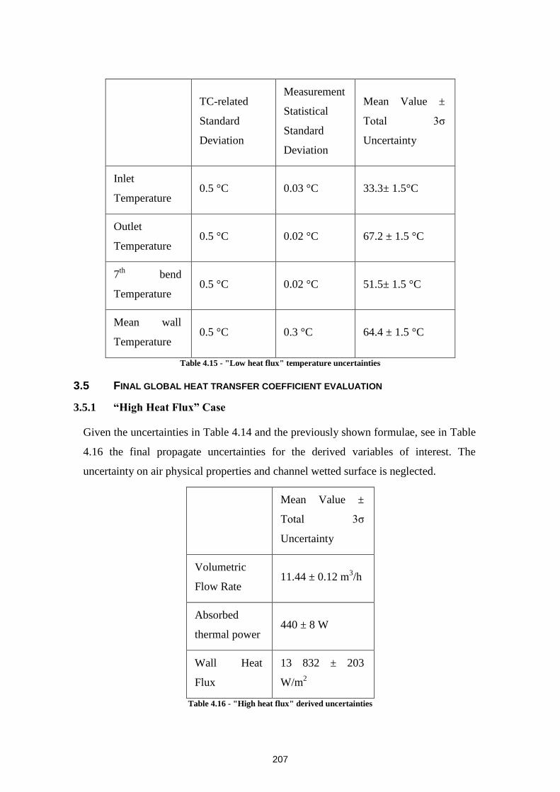
207
TC-related
Standard
Deviation
Measurement
Statistical
Standard
Deviation
Mean Value ±
Total 3ζ
Uncertainty
Inlet
Temperature 0.5 °C 0.03 °C 33.3± 1.5°C
Outlet
Temperature 0.5 °C 0.02 °C 67.2 ± 1.5 °C
7th
bend
Temperature 0.5 °C 0.02 °C 51.5± 1.5 °C
Mean wall
Temperature 0.5 °C 0.3 °C 64.4 ± 1.5 °C
Table 4.15 - "Low heat flux" temperature uncertainties
3.5 FINAL GLOBAL HEAT TRANSFER COEFFICIENT EVALUATION
3.5.1 “High Heat Flux” Case
Given the uncertainties in Table 4.14 and the previously shown formulae, see in Table
4.16 the final propagate uncertainties for the derived variables of interest. The
uncertainty on air physical properties and channel wetted surface is neglected.
Mean Value ±
Total 3ζ
Uncertainty
Volumetric
Flow Rate 11.44 ± 0.12 m
3/h
Absorbed
thermal power 440 ± 8 W
Wall Heat
Flux
13 832 ± 203
W/m2
Table 4.16 - "High heat flux" derived uncertainties
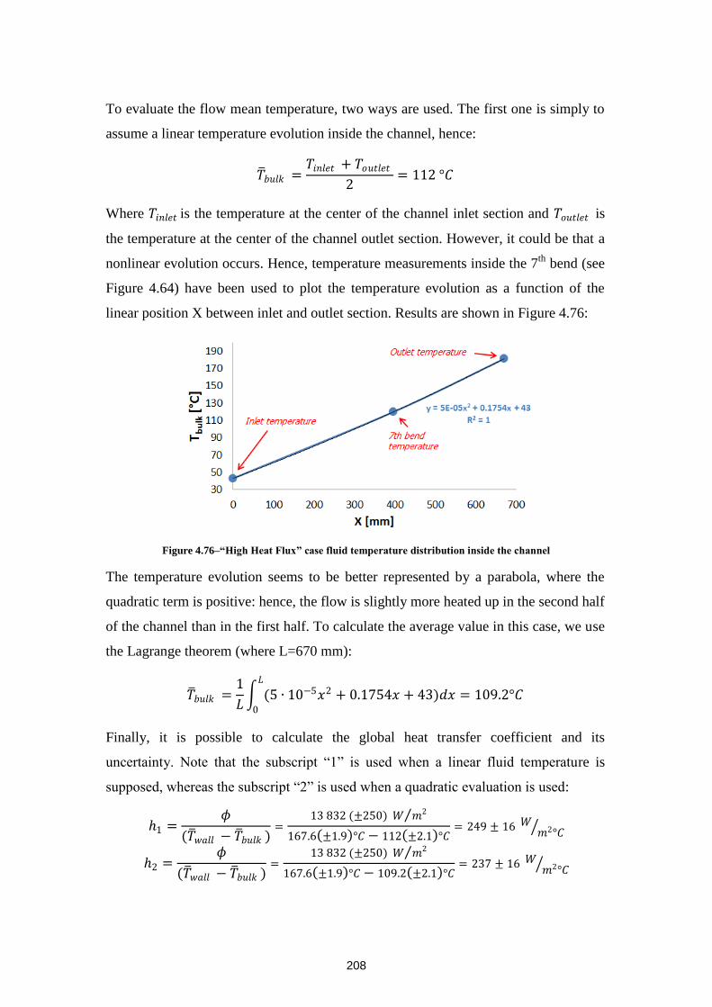
208
To evaluate the flow mean temperature, two ways are used. The first one is simply to
assume a linear temperature evolution inside the channel, hence:
𝑇 𝑏𝑢𝑙𝑘 =𝑇𝑖𝑛𝑙𝑒𝑡 + 𝑇𝑜𝑢𝑡𝑙𝑒𝑡
2= 112 °𝐶
Where 𝑇𝑖𝑛𝑙𝑒𝑡 is the temperature at the center of the channel inlet section and 𝑇𝑜𝑢𝑡𝑙𝑒𝑡 is
the temperature at the center of the channel outlet section. However, it could be that a
nonlinear evolution occurs. Hence, temperature measurements inside the 7th
bend (see
Figure 4.64) have been used to plot the temperature evolution as a function of the
linear position X between inlet and outlet section. Results are shown in Figure 4.76:
Figure 4.76–“High Heat Flux” case fluid temperature distribution inside the channel
The temperature evolution seems to be better represented by a parabola, where the
quadratic term is positive: hence, the flow is slightly more heated up in the second half
of the channel than in the first half. To calculate the average value in this case, we use
the Lagrange theorem (where L=670 mm):
𝑇 𝑏𝑢𝑙𝑘 =1
𝐿 (5 ∙ 10−5𝑥2 + 0.1754𝑥 + 43)𝑑𝑥
𝐿
0
= 109.2°𝐶
Finally, it is possible to calculate the global heat transfer coefficient and its
uncertainty. Note that the subscript “1” is used when a linear fluid temperature is
supposed, whereas the subscript “2” is used when a quadratic evaluation is used:
1 =𝜙
(𝑇 𝑤𝑎𝑙𝑙 − 𝑇 𝑏𝑢𝑙𝑘 )=
13 832 (±250) 𝑊 𝑚2
167.6 ±1.9 °𝐶 − 112 ±2.1 °𝐶= 249 ± 16 𝑊
𝑚2°𝐶
2 =𝜙
(𝑇 𝑤𝑎𝑙𝑙 − 𝑇 𝑏𝑢𝑙𝑘 )=
13 832 (±250) 𝑊 𝑚2
167.6 ±1.9 °𝐶 − 109.2 ±2.1 °𝐶= 237 ± 16 𝑊
𝑚2°𝐶
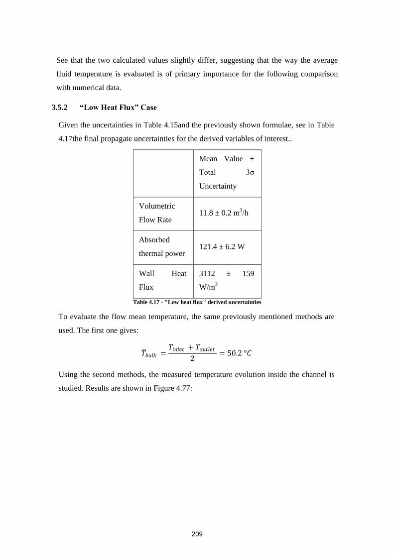
209
See that the two calculated values slightly differ, suggesting that the way the average
fluid temperature is evaluated is of primary importance for the following comparison
with numerical data.
3.5.2 “Low Heat Flux” Case
Given the uncertainties in Table 4.15and the previously shown formulae, see in Table
4.17the final propagate uncertainties for the derived variables of interest..
Mean Value ±
Total 3ζ
Uncertainty
Volumetric
Flow Rate 11.8 ± 0.2 m
3/h
Absorbed
thermal power 121.4 ± 6.2 W
Wall Heat
Flux
3112 ± 159
W/m2
Table 4.17 - "Low heat flux" derived uncertainties
To evaluate the flow mean temperature, the same previously mentioned methods are
used. The first one gives:
𝑇 𝑏𝑢𝑙𝑘 =𝑇𝑖𝑛𝑙𝑒𝑡 + 𝑇𝑜𝑢𝑡𝑙𝑒𝑡
2= 50.2 °𝐶
Using the second methods, the measured temperature evolution inside the channel is
studied. Results are shown in Figure 4.77:
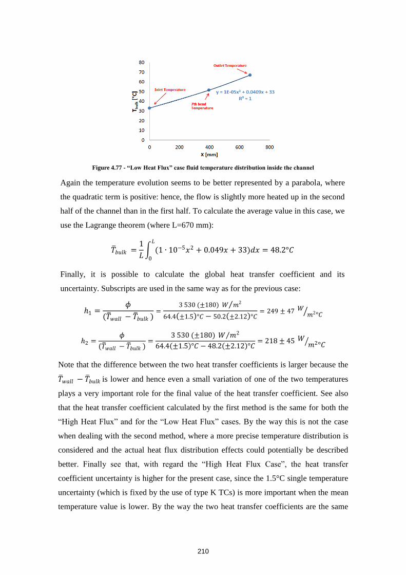
210
Figure 4.77 - “Low Heat Flux” case fluid temperature distribution inside the channel
Again the temperature evolution seems to be better represented by a parabola, where
the quadratic term is positive: hence, the flow is slightly more heated up in the second
half of the channel than in the first half. To calculate the average value in this case, we
use the Lagrange theorem (where L=670 mm):
𝑇 𝑏𝑢𝑙𝑘 =1
𝐿 (1 ∙ 10−5𝑥2 + 0.049𝑥 + 33)𝑑𝑥
𝐿
0
= 48.2°𝐶
Finally, it is possible to calculate the global heat transfer coefficient and its
uncertainty. Subscripts are used in the same way as for the previous case:
1 =𝜙
(𝑇 𝑤𝑎𝑙𝑙 − 𝑇 𝑏𝑢𝑙𝑘 )=
3 530 (±180) 𝑊 𝑚2
64.4 ±1.5 °𝐶 − 50.2 ±2.12 °𝐶= 249 ± 47 𝑊
𝑚2°𝐶
2 =𝜙
(𝑇 𝑤𝑎𝑙𝑙 − 𝑇 𝑏𝑢𝑙𝑘 )=
3 530 (±180) 𝑊 𝑚2
64.4 ±1.5 °𝐶 − 48.2 ±2.12 °𝐶= 218 ± 45 𝑊
𝑚2°𝐶
Note that the difference between the two heat transfer coefficients is larger because the
𝑇 𝑤𝑎𝑙𝑙 − 𝑇 𝑏𝑢𝑙𝑘 is lower and hence even a small variation of one of the two temperatures
plays a very important role for the final value of the heat transfer coefficient. See also
that the heat transfer coefficient calculated by the first method is the same for both the
“High Heat Flux” and for the “Low Heat Flux” cases. By the way this is not the case
when dealing with the second method, where a more precise temperature distribution is
considered and the actual heat flux distribution effects could potentially be described
better. Finally see that, with regard the “High Heat Flux Case”, the heat transfer
coefficient uncertainty is higher for the present case, since the 1.5°C single temperature
uncertainty (which is fixed by the use of type K TCs) is more important when the mean
temperature value is lower. By the way the two heat transfer coefficients are the same
211
(within the experimental uncertainty): in fact the difference between the heat transfer
coefficient mean value is lower than twice the sum of the experimental uncertainties
(see Figure 4.26), which is the criterion used so far to determine whether two
experimental values can be considered the same or not.
3.6 CONCLUSIONS ON VHEGAS MEASUREMENTS
The VHEGAS test section has been built to obtained experimental data to evaluate the
global heat transfer coefficient of the innovative channel as well as of other channel
geometries. Regarding the innovative channel geometry, two tests (high and low heat
flux) have been carried out in order to determine the influence of near-wall thermal
compressibility effects on the measured heat transfer coefficient. Measurements have
been done after a careful evaluation of the thermal transient to ensure the stability of the
thermal field. Experimental value of the heat transfer coefficient have been obtained in
two different ways, trying to properly take into account the temperature evolution inside
the innovative channel. The acquired database will be used to validate the numerical
model in the next Chapter.
4. CONCLUSIONS
The aim of the present chapter was to built a wide experimental database on the
innovative channel to be used both for flow analysis and for the numerical model
validation. Such an experimental necessity has been motivated in Chapter 2 and 3,
where no real test case has been found in the literature. Hence, an aerodynamic database
has been acquired by the LDV and PIV experiments. In particular, LDV experiment
provided precise local measurements, whereas PIV experiment provided global pictures
of the fluid stream. Design hypotheses have been carefully verified, to justify the
measurement campaign strategies. Together with these data, thermal data have been
obtained by the VHEGAS facility. These data are of primary importance since they can
be used to verify the correctness of the thermal model and of the innovative channel
performances.
Therefore, what it is still to be done is the flow analysis, to describe the phenomena
occurring the innovative channel (especially with regard to the effect of the mixing
zones) and to obtain design correlations to show whether the innovative geometry is
competitive with already existing compact heat exchanger technologies. This will be the
goal of the next Chapter.
212
Chapitre 5: Analyse de l’écoulement
Dans le chapitre 3, trois modèles de turbulence (SST, Stress Omega et ASST) ont été
testés sur un certain nombre de cas test de base qui décrivent certains phénomènes
potentiellement présents dans le canal innovant. En ce sens, la nécessité d'une base de
données expérimentale spécifique a été soulignée. Les moyens nécessaires à
l’établissement de cette base de données expérimentale ont été décrits dans le Chapitre
4, où les sections d'essais et une analyse préliminaire ont été détaillées.
L'objectif de ce chapitre est d'étudier l'écoulement de canal innovant et de donner un
aperçu de la performance potentielle qui peut être obtenue. Plus précisément, la
répartition de l’écoulement principal, ainsi que le mouvement secondaire présentent
un intérêt pour l'écoulement dans un coude, ainsi que dans la zone de mélange. Avec
la campagne expérimentale il n’était pas envisageable d’obtenir une description
exhaustive de l’écoulement, et l’objectif était d’avoir suffisamment de données
pertinentes pour valider le modèle numérique. Une fois validé, ce dernier nous a
permis de décrire en détails l’écoulement dans le canal innovant.. Pour mettre en
évidence cette approche, les résultats expérimentaux et numériques seront toujours
affichés ensemble, sauf pour les variables qui n'ont pas été mesurées. Par conséquent,
le choix est de sélectionner l'un des trois modèles décrits dans le chapitre 3 comme
référence, en se basant sur les résultats présentés dans le chapitre 3 et sur une brève
évaluation dans le premier paragraphe de ce chapitre.
Au final l’écoulement principal et secondaire sont analysés, avec les données
expérimentales LDV et PIV et les résultats numériques du modèle ASST. Pour
l’écoulement dans un coude, une région inhabituelle à vitesse élevée dans l’intérieur
du coude est montrée alors que, pour l’écoulement secondaire dans le coude un
tourbillon initial évoluant dans une structure à trois tourbillons est identifiée. Ce
comportement est essentiellement dû à l'écoulement en entrée du coude provenant de
la sortie de la zone de mélange. Dans la zone de mélange, le mélange est mis en
évidence, du fait du champ de vitesse secondaire, de l’effet du coude et de
l'entraînement visqueux de la vitesse d'écoulement secondaire du canal opposé.

213
Une fois le modèle aéraulique validé, la validation thermique a été faite en comparant
le coefficient d’échange thermique calculé et expérimental, pour avoir un modèle
numérique globalement fiable. Les résultats montrent que la valeur calculée du
coefficient d’échange peut être comprise dans l’incertitude expérimentale.
Une fois expliqués les phénomènes d'écoulement à l'état stationnaire, le comportement
thermo-hydraulique du canal innovant est étudié.
L'objectif final de ce travail étant de proposer un motif d’échange thermique innovant,
des corrélations d’échange thermique et de pertes de charge sont fournies.
Avec les corrélations, une stratégie de comparaison de compacité est proposée: elle
prend en compte les contraintes de dimensionnement, notamment le fait que les
différentes technologies comparées ont la même puissance thermique échangée et les
mêmes pertes de charge. Avec cette approche, il est montré que le motif innovant est
le plus compact parmi les technologies d’'échangeur de chaleur compact existantes
dans le domaine industriel.
Une conception finale de l'échangeur de chaleur sodium-gaz d’ASTRID est proposée,
démontrant qu’un gain d’environ 25% de compacité peut être acquis lors de l'adoption
de la géométrie du canal innovant si on la compare à une technologie d'échangeur de
chaleur compact à base de canaux droits traditionnels. De même une compacité
supérieure peut être atteinte si le concepteur a des contraintes mécaniques et / ou de
pertes de charge moins importantes.
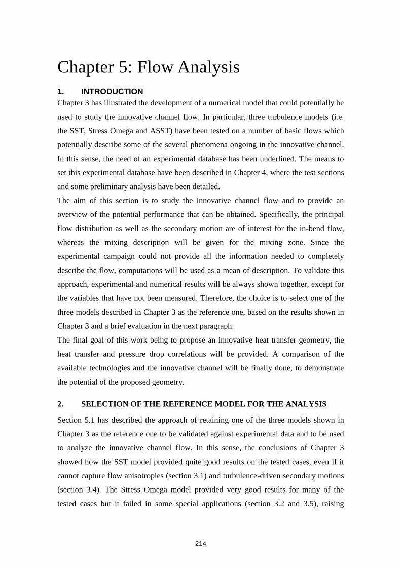
214
Chapter 5: Flow Analysis
1. INTRODUCTION
Chapter 3 has illustrated the development of a numerical model that could potentially be
used to study the innovative channel flow. In particular, three turbulence models (i.e.
the SST, Stress Omega and ASST) have been tested on a number of basic flows which
potentially describe some of the several phenomena ongoing in the innovative channel.
In this sense, the need of an experimental database has been underlined. The means to
set this experimental database have been described in Chapter 4, where the test sections
and some preliminary analysis have been detailed.
The aim of this section is to study the innovative channel flow and to provide an
overview of the potential performance that can be obtained. Specifically, the principal
flow distribution as well as the secondary motion are of interest for the in-bend flow,
whereas the mixing description will be given for the mixing zone. Since the
experimental campaign could not provide all the information needed to completely
describe the flow, computations will be used as a mean of description. To validate this
approach, experimental and numerical results will be always shown together, except for
the variables that have not been measured. Therefore, the choice is to select one of the
three models described in Chapter 3 as the reference one, based on the results shown in
Chapter 3 and a brief evaluation in the next paragraph.
The final goal of this work being to propose an innovative heat transfer geometry, the
heat transfer and pressure drop correlations will be provided. A comparison of the
available technologies and the innovative channel will be finally done, to demonstrate
the potential of the proposed geometry.
2. SELECTION OF THE REFERENCE MODEL FOR THE ANALYSIS
Section 5.1 has described the approach of retaining one of the three models shown in
Chapter 3 as the reference one to be validated against experimental data and to be used
to analyze the innovative channel flow. In this sense, the conclusions of Chapter 3
showed how the SST model provided quite good results on the tested cases, even if it
cannot capture flow anisotropies (section 3.1) and turbulence-driven secondary motions
(section 3.4). The Stress Omega model provided very good results for many of the
tested cases but it failed in some special applications (section 3.2 and 3.5), raising
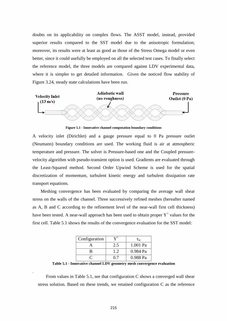
215
doubts on its applicability on complex flows. The ASST model, instead, provided
superior results compared to the SST model due to the anisotropic formulation;
moreover, its results were at least as good as those of the Stress Omega model or even
better, since it could usefully be employed on all the selected test cases. To finally select
the reference model, the three models are compared against LDV experimental data,
where it is simpler to get detailed information. Given the noticed flow stability of
Figure 3.24, steady state calculations have been run.
Figure 5.1 - Innovative channel compotation boundary conditions
A velocity inlet (Dirichlet) and a gauge pressure equal to 0 Pa pressure outlet
(Neumann) boundary conditions are used. The working fluid is air at atmospheric
temperature and pressure. The solver is Pressure-based one and the Coupled pressure-
velocity algorithm with pseudo-transient option is used. Gradients are evaluated through
the Least-Squared method. Second Order Upwind Scheme is used for the spatial
discretization of momentum, turbulent kinetic energy and turbulent dissipation rate
transport equations.
Meshing convergence has been evaluated by comparing the average wall shear
stress on the walls of the channel. Three successively refined meshes (hereafter named
as A, B and C according to the refinement level of the near-wall first cell thickness)
have been tested. A near-wall approach has been used to obtain proper Y+ values for the
first cell. Table 5.1 shows the results of the convergence evaluation for the SST model:
Configuration Y+ ηw
A 2.5 1.001 Pa
B 1.2 0.984 Pa
C 0.7 0.988 Pa
Table 5.1 - Innovative channel LDV geometry mesh convergence evaluation
.
From values in Table 5.1, see that configuration C shows a converged wall shear
stress solution. Based on these trends, we retained configuration C as the reference
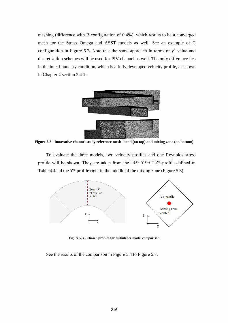
216
meshing (difference with B configuration of 0.4%), which results to be a converged
mesh for the Stress Omega and ASST models as well. See an example of C
configuration in Figure 5.2. Note that the same approach in terms of y+ value and
discretization schemes will be used for PIV channel as well. The only difference lies
in the inlet boundary condition, which is a fully developed velocity profile, as shown
in Chapter 4 section 2.4.1.
Figure 5.2 - Innovative channel study reference mesh: bend (on top) and mixing zone (on bottom)
To evaluate the three models, two velocity profiles and one Reynolds stress
profile will be shown. They are taken from the “45° Y*=0” Z* profile defined in
Table 4.4and the Y* profile right in the middle of the mixing zone (Figure 5.3).
Figure 5.3 - Chosen profiles for turbulence model comparison
See the results of the comparison in Figure 5.4 to Figure 5.7.
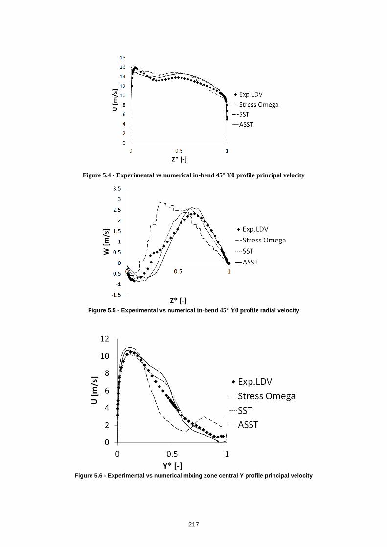
217
Figure 5.4 - Experimental vs numerical in-bend 45° Y0 profile principal velocity
Figure 5.5 - Experimental vs numerical in-bend 45° Y0 profile radial velocity
Figure 5.6 - Experimental vs numerical mixing zone central Y profile principal velocity
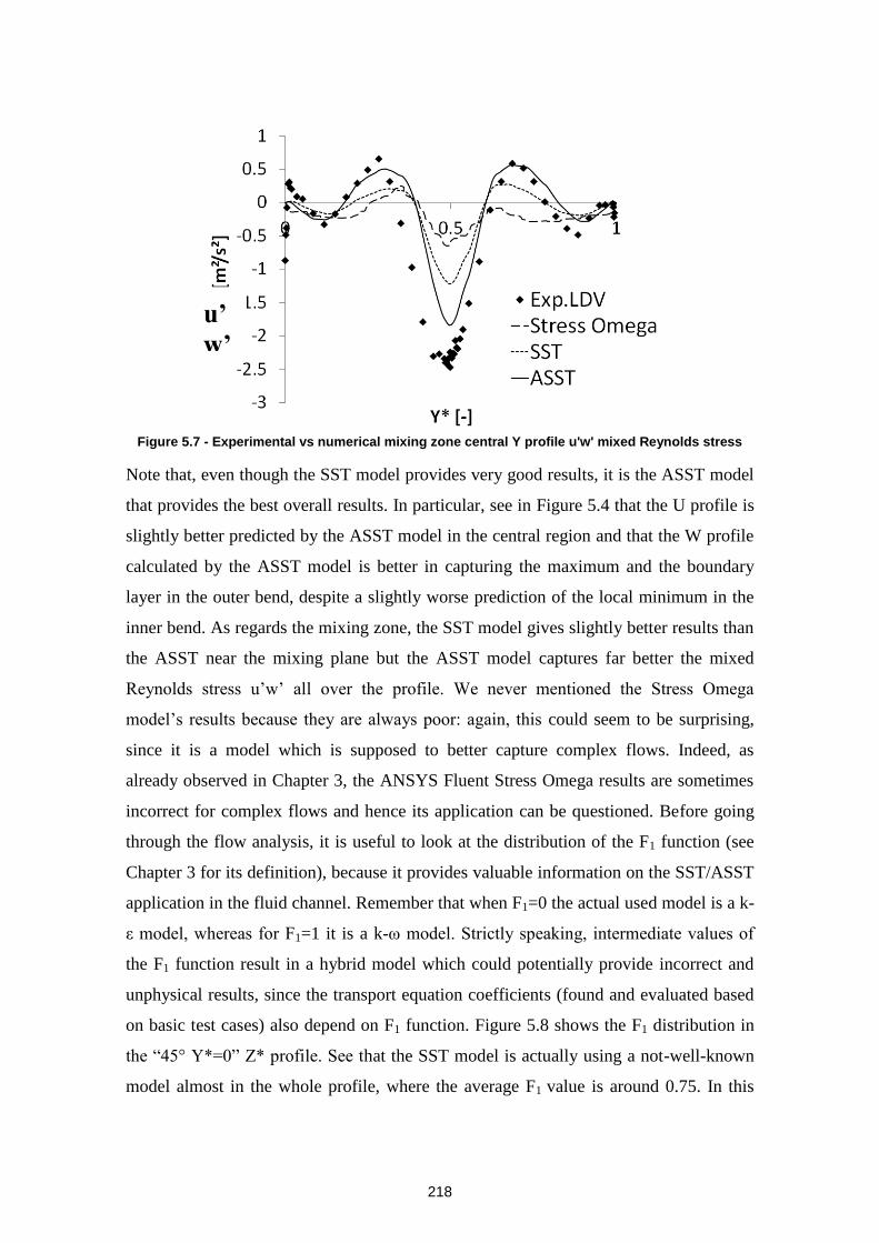
218
Figure 5.7 - Experimental vs numerical mixing zone central Y profile u'w' mixed Reynolds stress
Note that, even though the SST model provides very good results, it is the ASST model
that provides the best overall results. In particular, see in Figure 5.4 that the U profile is
slightly better predicted by the ASST model in the central region and that the W profile
calculated by the ASST model is better in capturing the maximum and the boundary
layer in the outer bend, despite a slightly worse prediction of the local minimum in the
inner bend. As regards the mixing zone, the SST model gives slightly better results than
the ASST near the mixing plane but the ASST model captures far better the mixed
Reynolds stress u’w’ all over the profile. We never mentioned the Stress Omega
model’s results because they are always poor: again, this could seem to be surprising,
since it is a model which is supposed to better capture complex flows. Indeed, as
already observed in Chapter 3, the ANSYS Fluent Stress Omega results are sometimes
incorrect for complex flows and hence its application can be questioned. Before going
through the flow analysis, it is useful to look at the distribution of the F1 function (see
Chapter 3 for its definition), because it provides valuable information on the SST/ASST
application in the fluid channel. Remember that when F1=0 the actual used model is a k-
ε model, whereas for F1=1 it is a k-ω model. Strictly speaking, intermediate values of
the F1 function result in a hybrid model which could potentially provide incorrect and
unphysical results, since the transport equation coefficients (found and evaluated based
on basic test cases) also depend on F1 function. Figure 5.8 shows the F1 distribution in
the “45° Y*=0” Z* profile. See that the SST model is actually using a not-well-known
model almost in the whole profile, where the average F1 value is around 0.75. In this
u’
w’
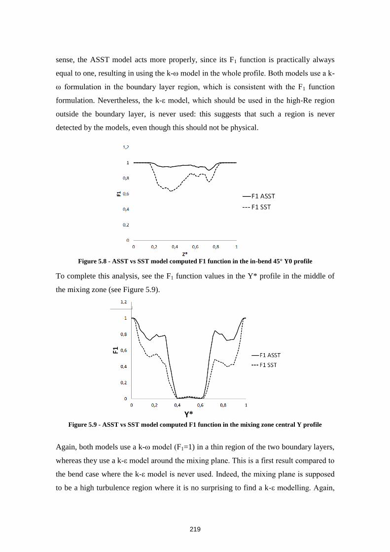
219
sense, the ASST model acts more properly, since its F1 function is practically always
equal to one, resulting in using the k-ω model in the whole profile. Both models use a k-
ω formulation in the boundary layer region, which is consistent with the F1 function
formulation. Nevertheless, the k-ε model, which should be used in the high-Re region
outside the boundary layer, is never used: this suggests that such a region is never
detected by the models, even though this should not be physical.
Figure 5.8 - ASST vs SST model computed F1 function in the in-bend 45° Y0 profile
To complete this analysis, see the F1 function values in the Y* profile in the middle of
the mixing zone (see Figure 5.9).
Figure 5.9 - ASST vs SST model computed F1 function in the mixing zone central Y profile
Again, both models use a k-ω model (F1=1) in a thin region of the two boundary layers,
whereas they use a k-ε model around the mixing plane. This is a first result compared to
the bend case where the k-ε model is never used. Indeed, the mixing plane is supposed
to be a high turbulence region where it is no surprising to find a k-ε modelling. Again,
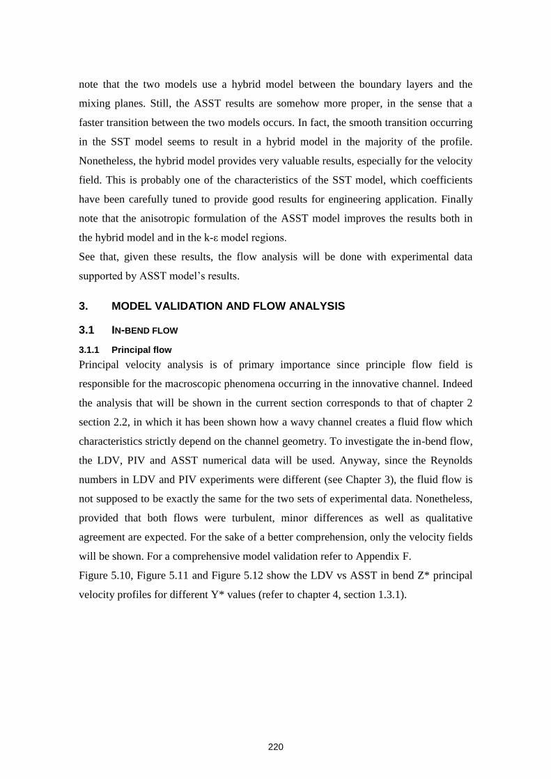
220
note that the two models use a hybrid model between the boundary layers and the
mixing planes. Still, the ASST results are somehow more proper, in the sense that a
faster transition between the two models occurs. In fact, the smooth transition occurring
in the SST model seems to result in a hybrid model in the majority of the profile.
Nonetheless, the hybrid model provides very valuable results, especially for the velocity
field. This is probably one of the characteristics of the SST model, which coefficients
have been carefully tuned to provide good results for engineering application. Finally
note that the anisotropic formulation of the ASST model improves the results both in
the hybrid model and in the k-ε model regions.
See that, given these results, the flow analysis will be done with experimental data
supported by ASST model’s results.
3. MODEL VALIDATION AND FLOW ANALYSIS
3.1 IN-BEND FLOW
3.1.1 Principal flow
Principal velocity analysis is of primary importance since principle flow field is
responsible for the macroscopic phenomena occurring in the innovative channel. Indeed
the analysis that will be shown in the current section corresponds to that of chapter 2
section 2.2, in which it has been shown how a wavy channel creates a fluid flow which
characteristics strictly depend on the channel geometry. To investigate the in-bend flow,
the LDV, PIV and ASST numerical data will be used. Anyway, since the Reynolds
numbers in LDV and PIV experiments were different (see Chapter 3), the fluid flow is
not supposed to be exactly the same for the two sets of experimental data. Nonetheless,
provided that both flows were turbulent, minor differences as well as qualitative
agreement are expected. For the sake of a better comprehension, only the velocity fields
will be shown. For a comprehensive model validation refer to Appendix F.
Figure 5.10, Figure 5.11 and Figure 5.12 show the LDV vs ASST in bend Z* principal
velocity profiles for different Y* values (refer to chapter 4, section 1.3.1).
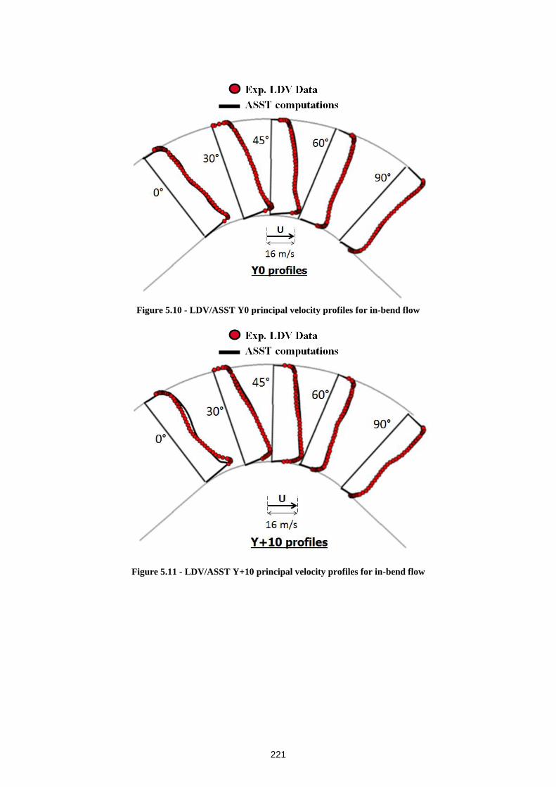
221
Figure 5.10 - LDV/ASST Y0 principal velocity profiles for in-bend flow
Figure 5.11 - LDV/ASST Y+10 principal velocity profiles for in-bend flow
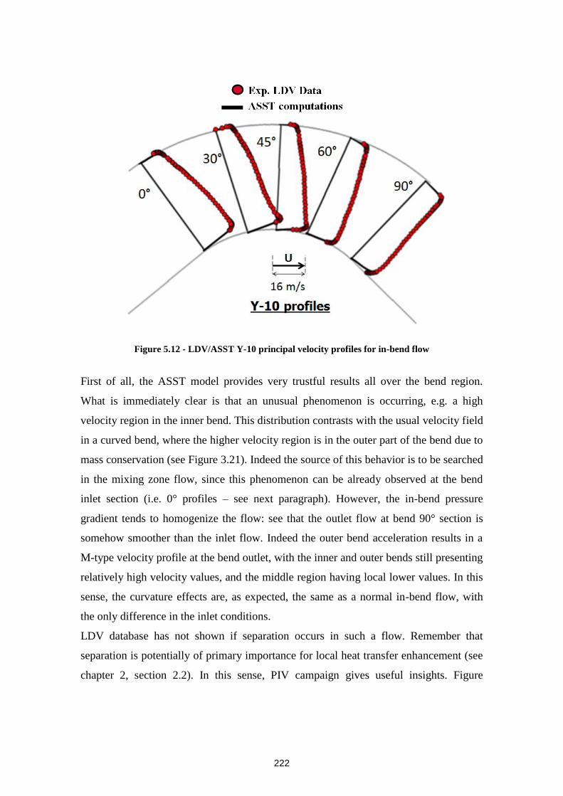
222
Figure 5.12 - LDV/ASST Y-10 principal velocity profiles for in-bend flow
First of all, the ASST model provides very trustful results all over the bend region.
What is immediately clear is that an unusual phenomenon is occurring, e.g. a high
velocity region in the inner bend. This distribution contrasts with the usual velocity field
in a curved bend, where the higher velocity region is in the outer part of the bend due to
mass conservation (see Figure 3.21). Indeed the source of this behavior is to be searched
in the mixing zone flow, since this phenomenon can be already observed at the bend
inlet section (i.e. 0° profiles – see next paragraph). However, the in-bend pressure
gradient tends to homogenize the flow: see that the outlet flow at bend 90° section is
somehow smoother than the inlet flow. Indeed the outer bend acceleration results in a
M-type velocity profile at the bend outlet, with the inner and outer bends still presenting
relatively high velocity values, and the middle region having local lower values. In this
sense, the curvature effects are, as expected, the same as a normal in-bend flow, with
the only difference in the inlet conditions.
LDV database has not shown if separation occurs in such a flow. Remember that
separation is potentially of primary importance for local heat transfer enhancement (see
chapter 2, section 2.2). In this sense, PIV campaign gives useful insights. Figure
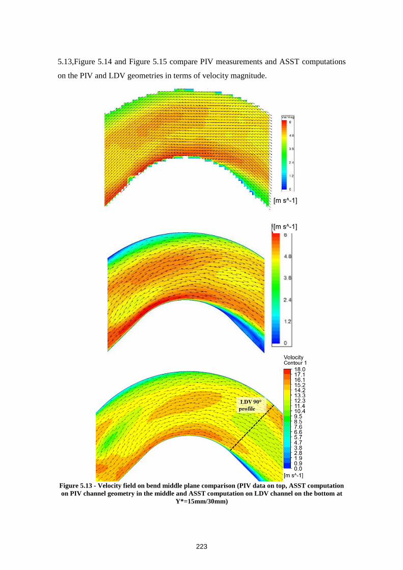
223
5.13,Figure 5.14 and Figure 5.15 compare PIV measurements and ASST computations
on the PIV and LDV geometries in terms of velocity magnitude.
Figure 5.13 - Velocity field on bend middle plane comparison (PIV data on top, ASST computation
on PIV channel geometry in the middle and ASST computation on LDV channel on the bottom at
Y*=15mm/30mm)
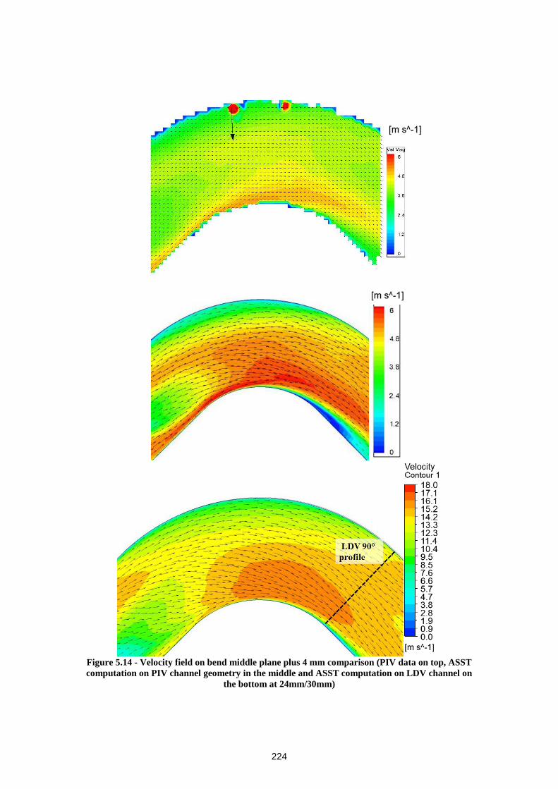
224
Figure 5.14 - Velocity field on bend middle plane plus 4 mm comparison (PIV data on top, ASST
computation on PIV channel geometry in the middle and ASST computation on LDV channel on
the bottom at 24mm/30mm)
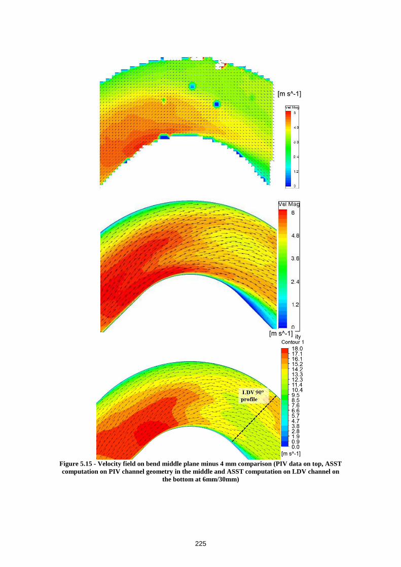
225
Figure 5.15 - Velocity field on bend middle plane minus 4 mm comparison (PIV data on top, ASST
computation on PIV channel geometry in the middle and ASST computation on LDV channel on
the bottom at 6mm/30mm)
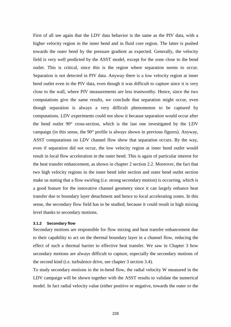
226
First of all see again that the LDV data behavior is the same as the PIV data, with a
higher velocity region in the inner bend and in fluid core region. The latter is pushed
towards the outer bend by the pressure gradient as expected. Generally, the velocity
field is very well predicted by the ASST model, except for the zone close to the bend
outlet. This is critical, since this is the region where separation seems to occur.
Separation is not detected in PIV data. Anyway there is a low velocity region at inner
bend outlet even in the PIV data, even though it was difficult to capture since it is very
close to the wall, where PIV measurements are less trustworthy. Hence, since the two
computations give the same results, we conclude that separation might occur, even
though separation is always a very difficult phenomenon to be captured by
computations. LDV experiments could not show it because separation would occur after
the bend outlet 90° cross-section, which is the last one investigated by the LDV
campaign (in this sense, the 90° profile is always shown in previous figures). Anyway,
ASST computations on LDV channel flow show that separation occurs. By the way,
even if separation did not occur, the low velocity region at inner bend outlet would
result in local flow acceleration in the outer bend. This is again of particular interest for
the heat transfer enhancement, as shown in chapter 2 section 2.2. Moreover, the fact that
two high velocity regions in the inner bend inlet section and outer bend outlet section
make us stating that a flow swirling (i.e. strong secondary motion) is occurring, which is
a good feature for the innovative channel geometry since it can largely enhance heat
transfer due to boundary layer detachment and hence to local accelerating zones. In this
sense, the secondary flow field has to be studied, because it could result in high mixing
level thanks to secondary motions.
3.1.2 Secondary flow
Secondary motions are responsible for flow mixing and heat transfer enhancement due
to their capability to act on the thermal boundary layer in a channel flow, reducing the
effect of such a thermal barrier to effective heat transfer. We saw in Chapter 3 how
secondary motions are always difficult to capture, especially the secondary motions of
the second kind (i.e. turbulence drive, see chapter 3 section 3.4).
To study secondary motions in the in-bend flow, the radial velocity W measured in the
LDV campaign will be shown together with the ASST results to validate the numerical
model. In fact radial velocity value (either positive or negative, towards the outer or the
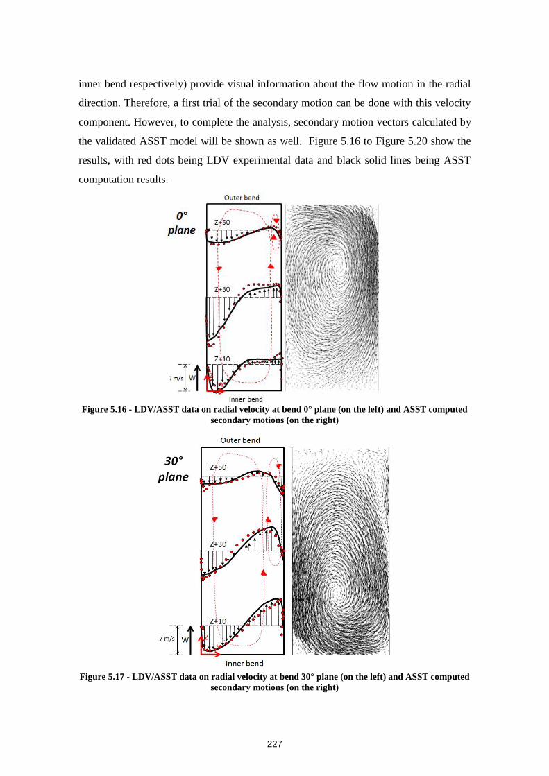
227
inner bend respectively) provide visual information about the flow motion in the radial
direction. Therefore, a first trial of the secondary motion can be done with this velocity
component. However, to complete the analysis, secondary motion vectors calculated by
the validated ASST model will be shown as well. Figure 5.16 to Figure 5.20 show the
results, with red dots being LDV experimental data and black solid lines being ASST
computation results.
Figure 5.16 - LDV/ASST data on radial velocity at bend 0° plane (on the left) and ASST computed
secondary motions (on the right)
Figure 5.17 - LDV/ASST data on radial velocity at bend 30° plane (on the left) and ASST computed
secondary motions (on the right)
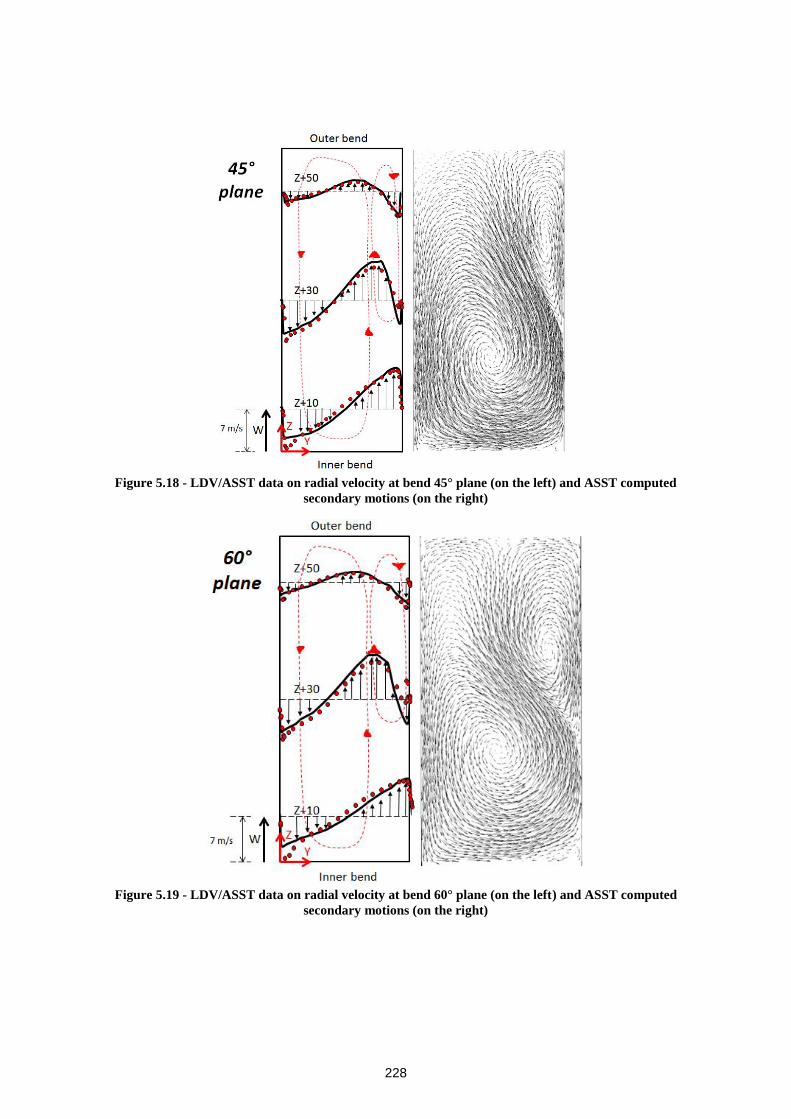
228
Figure 5.18 - LDV/ASST data on radial velocity at bend 45° plane (on the left) and ASST computed
secondary motions (on the right)
Figure 5.19 - LDV/ASST data on radial velocity at bend 60° plane (on the left) and ASST computed
secondary motions (on the right)
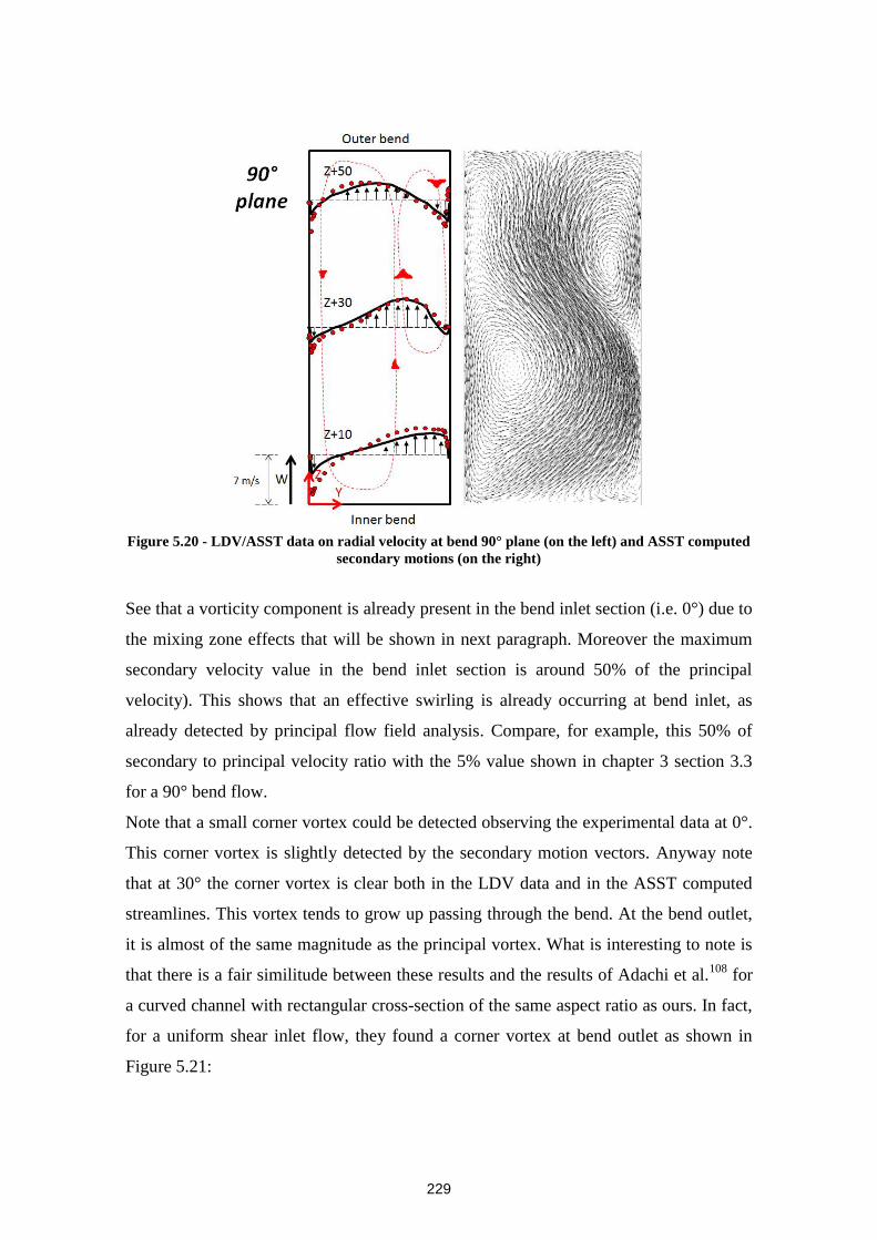
229
Figure 5.20 - LDV/ASST data on radial velocity at bend 90° plane (on the left) and ASST computed
secondary motions (on the right)
See that a vorticity component is already present in the bend inlet section (i.e. 0°) due to
the mixing zone effects that will be shown in next paragraph. Moreover the maximum
secondary velocity value in the bend inlet section is around 50% of the principal
velocity). This shows that an effective swirling is already occurring at bend inlet, as
already detected by principal flow field analysis. Compare, for example, this 50% of
secondary to principal velocity ratio with the 5% value shown in chapter 3 section 3.3
for a 90° bend flow.
Note that a small corner vortex could be detected observing the experimental data at 0°.
This corner vortex is slightly detected by the secondary motion vectors. Anyway note
that at 30° the corner vortex is clear both in the LDV data and in the ASST computed
streamlines. This vortex tends to grow up passing through the bend. At the bend outlet,
it is almost of the same magnitude as the principal vortex. What is interesting to note is
that there is a fair similitude between these results and the results of Adachi et al.108
for
a curved channel with rectangular cross-section of the same aspect ratio as ours. In fact,
for a uniform shear inlet flow, they found a corner vortex at bend outlet as shown in
Figure 5.21:
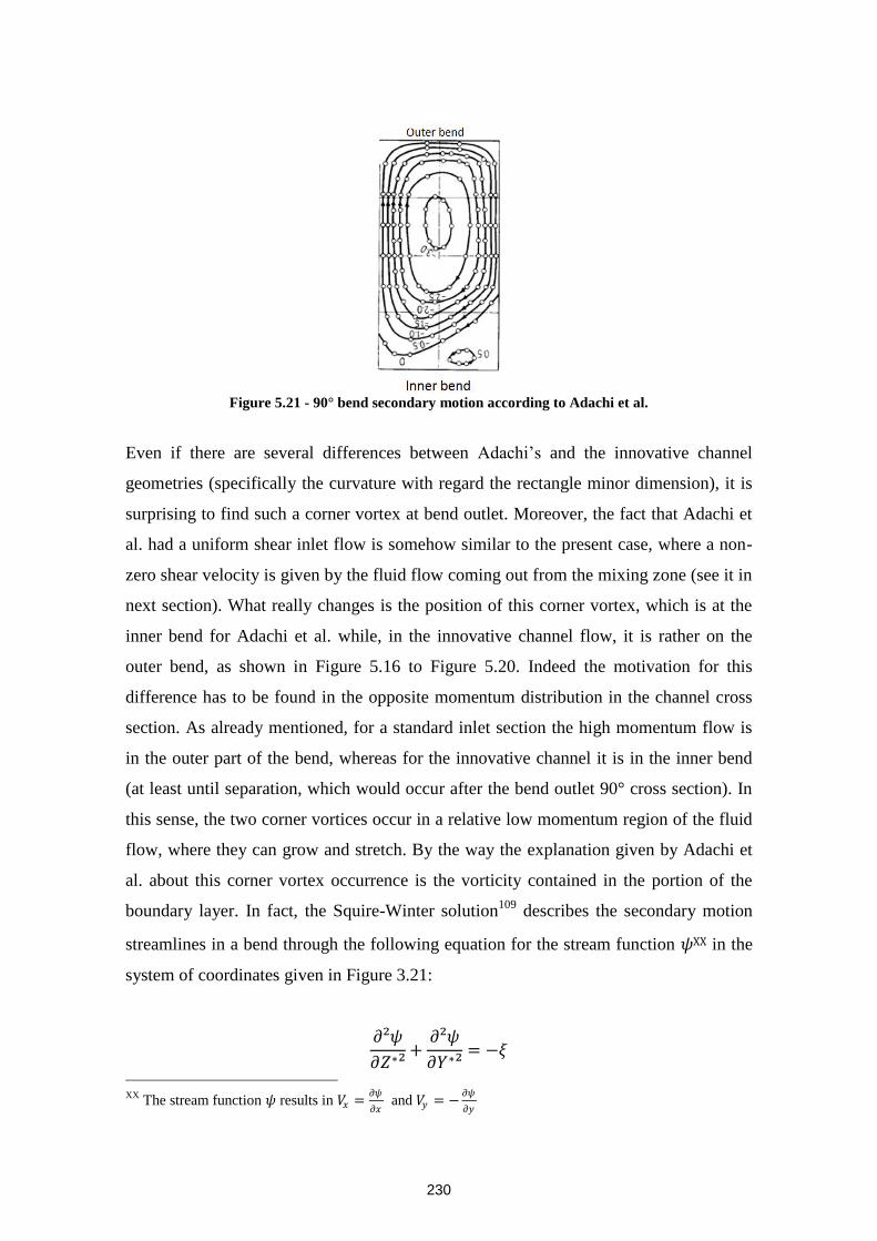
230
Figure 5.21 - 90° bend secondary motion according to Adachi et al.
Even if there are several differences between Adachi’s and the innovative channel
geometries (specifically the curvature with regard the rectangle minor dimension), it is
surprising to find such a corner vortex at bend outlet. Moreover, the fact that Adachi et
al. had a uniform shear inlet flow is somehow similar to the present case, where a non-
zero shear velocity is given by the fluid flow coming out from the mixing zone (see it in
next section). What really changes is the position of this corner vortex, which is at the
inner bend for Adachi et al. while, in the innovative channel flow, it is rather on the
outer bend, as shown in Figure 5.16 to Figure 5.20. Indeed the motivation for this
difference has to be found in the opposite momentum distribution in the channel cross
section. As already mentioned, for a standard inlet section the high momentum flow is
in the outer part of the bend, whereas for the innovative channel it is in the inner bend
(at least until separation, which would occur after the bend outlet 90° cross section). In
this sense, the two corner vortices occur in a relative low momentum region of the fluid
flow, where they can grow and stretch. By the way the explanation given by Adachi et
al. about this corner vortex occurrence is the vorticity contained in the portion of the
boundary layer. In fact, the Squire-Winter solution109
describes the secondary motion
streamlines in a bend through the following equation for the stream function 𝜓XX in the
system of coordinates given in Figure 3.21:
𝜕²𝜓
𝜕𝑍∗²+
𝜕²𝜓
𝜕𝑌∗²= −𝜉
XX
The stream function 𝜓 results in 𝑉𝑥 =𝜕𝜓
𝜕𝑥 and 𝑉𝑦 = −
𝜕𝜓
𝜕𝑦
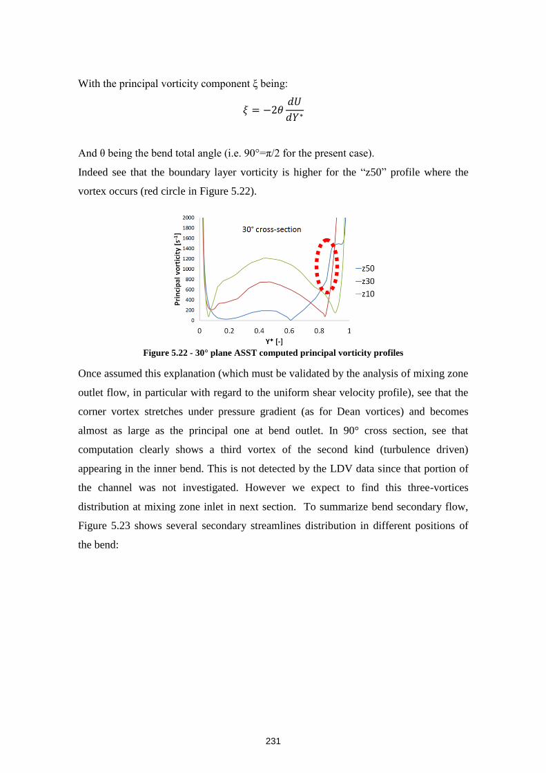
231
With the principal vorticity component ξ being:
𝜉 = −2𝜃𝑑𝑈
𝑑𝑌∗
And θ being the bend total angle (i.e. 90°=π/2 for the present case).
Indeed see that the boundary layer vorticity is higher for the “z50” profile where the
vortex occurs (red circle in Figure 5.22).
Figure 5.22 - 30° plane ASST computed principal vorticity profiles
Once assumed this explanation (which must be validated by the analysis of mixing zone
outlet flow, in particular with regard to the uniform shear velocity profile), see that the
corner vortex stretches under pressure gradient (as for Dean vortices) and becomes
almost as large as the principal one at bend outlet. In 90° cross section, see that
computation clearly shows a third vortex of the second kind (turbulence driven)
appearing in the inner bend. This is not detected by the LDV data since that portion of
the channel was not investigated. However we expect to find this three-vortices
distribution at mixing zone inlet in next section. To summarize bend secondary flow,
Figure 5.23 shows several secondary streamlines distribution in different positions of
the bend:
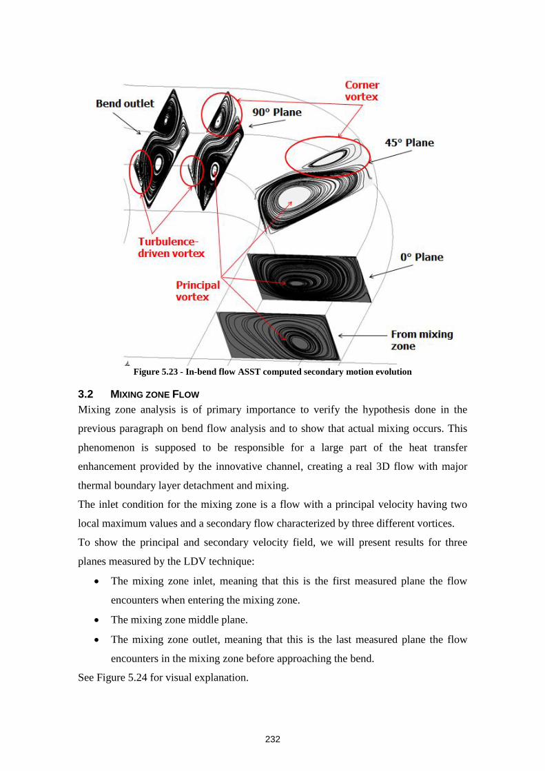
232
Figure 5.23 - In-bend flow ASST computed secondary motion evolution
3.2 MIXING ZONE FLOW
Mixing zone analysis is of primary importance to verify the hypothesis done in the
previous paragraph on bend flow analysis and to show that actual mixing occurs. This
phenomenon is supposed to be responsible for a large part of the heat transfer
enhancement provided by the innovative channel, creating a real 3D flow with major
thermal boundary layer detachment and mixing.
The inlet condition for the mixing zone is a flow with a principal velocity having two
local maximum values and a secondary flow characterized by three different vortices.
To show the principal and secondary velocity field, we will present results for three
planes measured by the LDV technique:
The mixing zone inlet, meaning that this is the first measured plane the flow
encounters when entering the mixing zone.
The mixing zone middle plane.
The mixing zone outlet, meaning that this is the last measured plane the flow
encounters in the mixing zone before approaching the bend.
See Figure 5.24 for visual explanation.
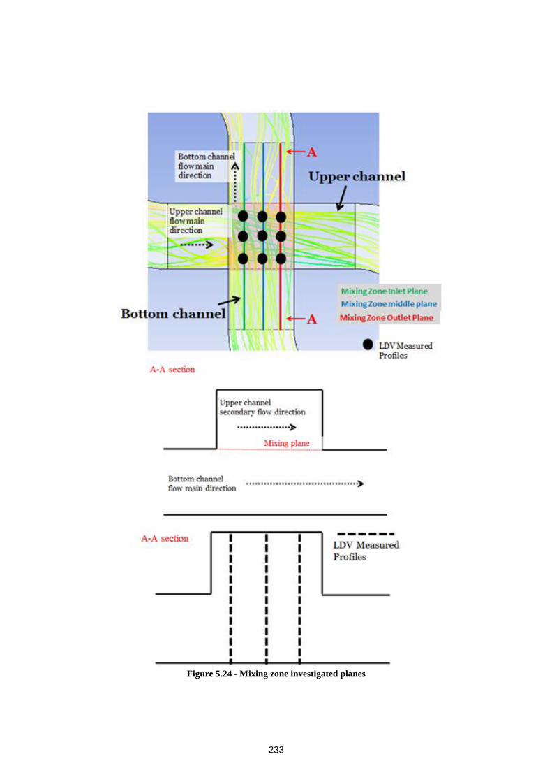
233
Figure 5.24 - Mixing zone investigated planes
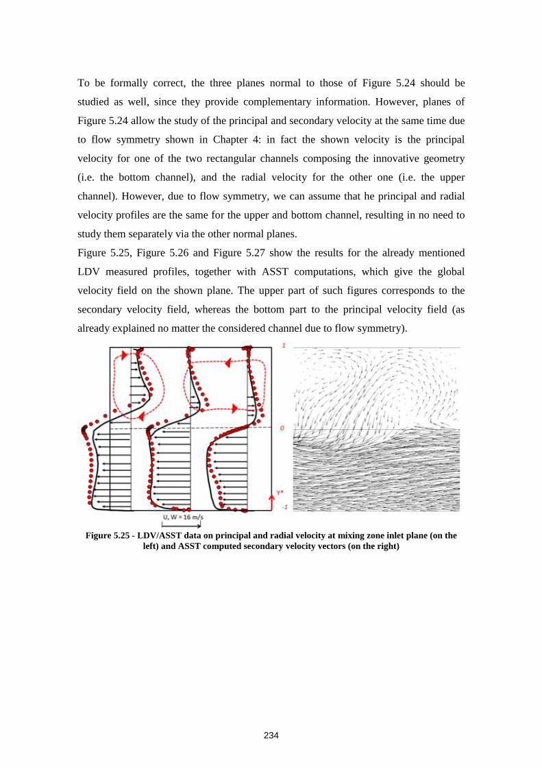
234
To be formally correct, the three planes normal to those of Figure 5.24 should be
studied as well, since they provide complementary information. However, planes of
Figure 5.24 allow the study of the principal and secondary velocity at the same time due
to flow symmetry shown in Chapter 4: in fact the shown velocity is the principal
velocity for one of the two rectangular channels composing the innovative geometry
(i.e. the bottom channel), and the radial velocity for the other one (i.e. the upper
channel). However, due to flow symmetry, we can assume that he principal and radial
velocity profiles are the same for the upper and bottom channel, resulting in no need to
study them separately via the other normal planes.
Figure 5.25, Figure 5.26 and Figure 5.27 show the results for the already mentioned
LDV measured profiles, together with ASST computations, which give the global
velocity field on the shown plane. The upper part of such figures corresponds to the
secondary velocity field, whereas the bottom part to the principal velocity field (as
already explained no matter the considered channel due to flow symmetry).
Figure 5.25 - LDV/ASST data on principal and radial velocity at mixing zone inlet plane (on the
left) and ASST computed secondary velocity vectors (on the right)
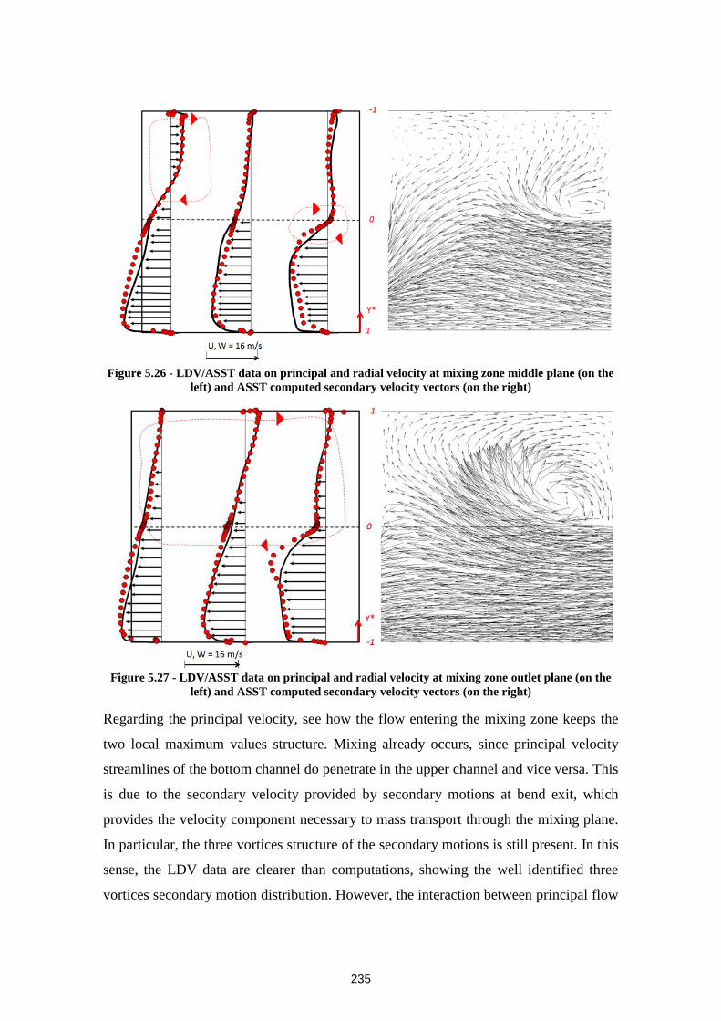
235
Figure 5.26 - LDV/ASST data on principal and radial velocity at mixing zone middle plane (on the
left) and ASST computed secondary velocity vectors (on the right)
Figure 5.27 - LDV/ASST data on principal and radial velocity at mixing zone outlet plane (on the
left) and ASST computed secondary velocity vectors (on the right)
Regarding the principal velocity, see how the flow entering the mixing zone keeps the
two local maximum values structure. Mixing already occurs, since principal velocity
streamlines of the bottom channel do penetrate in the upper channel and vice versa. This
is due to the secondary velocity provided by secondary motions at bend exit, which
provides the velocity component necessary to mass transport through the mixing plane.
In particular, the three vortices structure of the secondary motions is still present. In this
sense, the LDV data are clearer than computations, showing the well identified three
vortices secondary motion distribution. However, the interaction between principal flow
236
in the bottom channel with secondary vortices of the upper channel results in a
smoother principal velocity distribution in the mixing zone mixing plane and a
corresponding destruction of the secondary motion structure. In this sense, penetration
of bottom channel principal streamlines in the upper channel is more effective,
demonstrating how effective mixing is occurring. This behavior is essentially due to two
phenomena:
principal flow inertia: the principal flow tends to pass through the mixing plane
because of secondary velocity component (i.e. at least one velocity component is
normal to the mixing plane), as already mentioned for flow in the inlet plane;
flow viscous entrainment of the bottom channel principal flow by the upper
channel secondary motion.
It is worth noting that this is a steady state analysis on the average velocity components
measured by LDV technique and calculated by the ASST model. In fact, it has to be
noted that velocity fluctuations are definitely higher around the mixing zone. This
means that turbulence created by mass transfer through the mixing plane enhances even
more the flow mixing and has to be added to the flow inertia and viscous entrainment to
explain flow mixing. Velocity fluctuations (which are up to 50% of average principal
velocity near the mixing plane) are shown in Appendix FXXI
.
Regarding the principal flow at outlet plane, note the uniform shear velocity
distribution, which is consistent with the hypothesis done in the previous paragraph to
explain the corner vortex generation in the outer region of the bend. Secondary motion
at mixing zone outlet plane clearly shows a difference from the precedent two planes: a
corner vortex appears. To understand this phenomenon, it is useful to look at ASST
computation results on mixing plane. Since no direct information on velocity field in
mixing plane is available in the experimental database, we will first show PIV/ASST
results to validate the analysis that will be done hereafter only with ASST numerical
results (Figure 5.28 to Figure 5.32).
XXI
In this sense questions rise on the applicability of a RANS approach to such turbulence level. Indeed
the computed velocity field will contain some information about the flow characteristics; however, it has
to be expected that the steady-state approach is definitely more limiting than the RANS approach itself, a
transient approach (which is out of the scope of the present work, as already motivated in Chapter 2)
could better account for such unsteadiness.
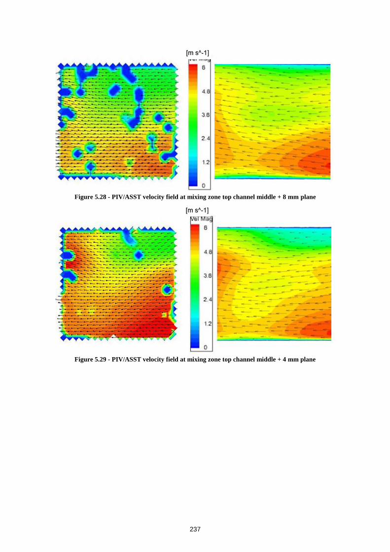
237
Figure 5.28 - PIV/ASST velocity field at mixing zone top channel middle + 8 mm plane
Figure 5.29 - PIV/ASST velocity field at mixing zone top channel middle + 4 mm plane
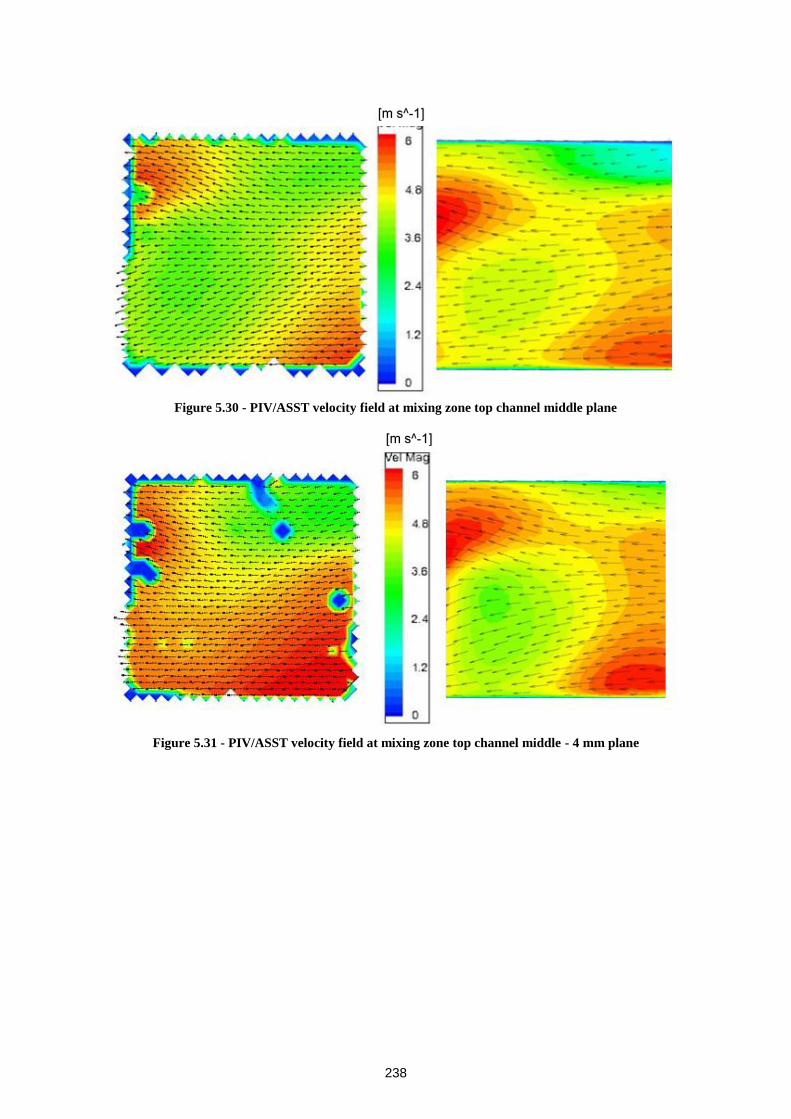
238
Figure 5.30 - PIV/ASST velocity field at mixing zone top channel middle plane
Figure 5.31 - PIV/ASST velocity field at mixing zone top channel middle - 4 mm plane
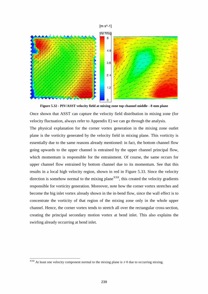
239
Figure 5.32 - PIV/ASST velocity field at mixing zone top channel middle - 8 mm plane
Once shown that ASST can capture the velocity field distribution in mixing zone (for
velocity fluctuation, always refer to Appendix E) we can go through the analysis.
The physical explanation for the corner vortex generation in the mixing zone outlet
plane is the vorticity generated by the velocity field in mixing plane. This vorticity is
essentially due to the same reasons already mentioned: in fact, the bottom channel flow
going upwards to the upper channel is entrained by the upper channel principal flow,
which momentum is responsible for the entrainment. Of course, the same occurs for
upper channel flow entrained by bottom channel due to its momentum. See that this
results in a local high velocity region, shown in red in Figure 5.33. Since the velocity
direction is somehow normal to the mixing planeXXII
, this created the velocity gradients
responsible for vorticity generation. Moreover, note how the corner vortex stretches and
become the big inlet vortex already shown in the in-bend flow, since the wall effect is to
concentrate the vorticity of that region of the mixing zone only in the whole upper
channel. Hence, the corner vortex tends to stretch all over the rectangular cross-section,
creating the principal secondary motion vortex at bend inlet. This also explains the
swirling already occurring at bend inlet.
XXII
At least one velocity component normal to the mixing plane is ≠ 0 due to occurring mixing.
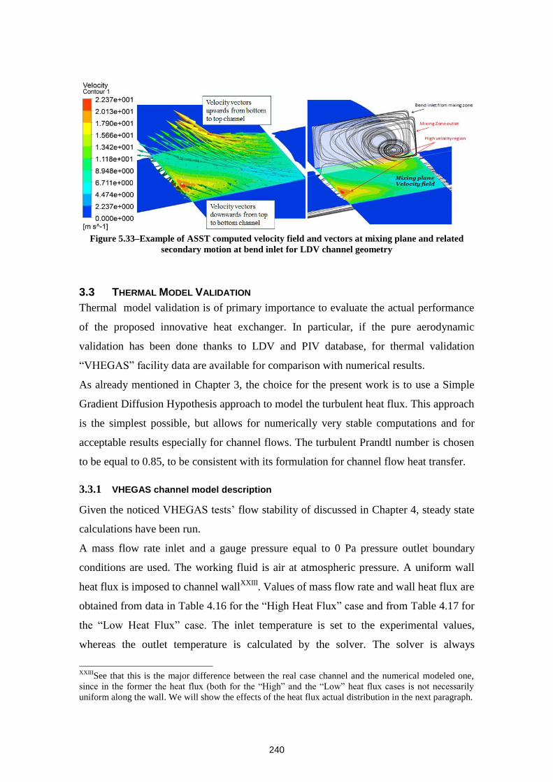
240
Figure 5.33–Example of ASST computed velocity field and vectors at mixing plane and related
secondary motion at bend inlet for LDV channel geometry
3.3 THERMAL MODEL VALIDATION
Thermal model validation is of primary importance to evaluate the actual performance
of the proposed innovative heat exchanger. In particular, if the pure aerodynamic
validation has been done thanks to LDV and PIV database, for thermal validation
“VHEGAS” facility data are available for comparison with numerical results.
As already mentioned in Chapter 3, the choice for the present work is to use a Simple
Gradient Diffusion Hypothesis approach to model the turbulent heat flux. This approach
is the simplest possible, but allows for numerically very stable computations and for
acceptable results especially for channel flows. The turbulent Prandtl number is chosen
to be equal to 0.85, to be consistent with its formulation for channel flow heat transfer.
3.3.1 VHEGAS channel model description
Given the noticed VHEGAS tests’ flow stability of discussed in Chapter 4, steady state
calculations have been run.
A mass flow rate inlet and a gauge pressure equal to 0 Pa pressure outlet boundary
conditions are used. The working fluid is air at atmospheric pressure. A uniform wall
heat flux is imposed to channel wallXXIII
. Values of mass flow rate and wall heat flux are
obtained from data in Table 4.16 for the “High Heat Flux” case and from Table 4.17 for
the “Low Heat Flux” case. The inlet temperature is set to the experimental values,
whereas the outlet temperature is calculated by the solver. The solver is always
XXIII
See that this is the major difference between the real case channel and the numerical modeled one,
since in the former the heat flux (both for the “High” and the “Low” heat flux cases is not necessarily
uniform along the wall. We will show the effects of the heat flux actual distribution in the next paragraph.
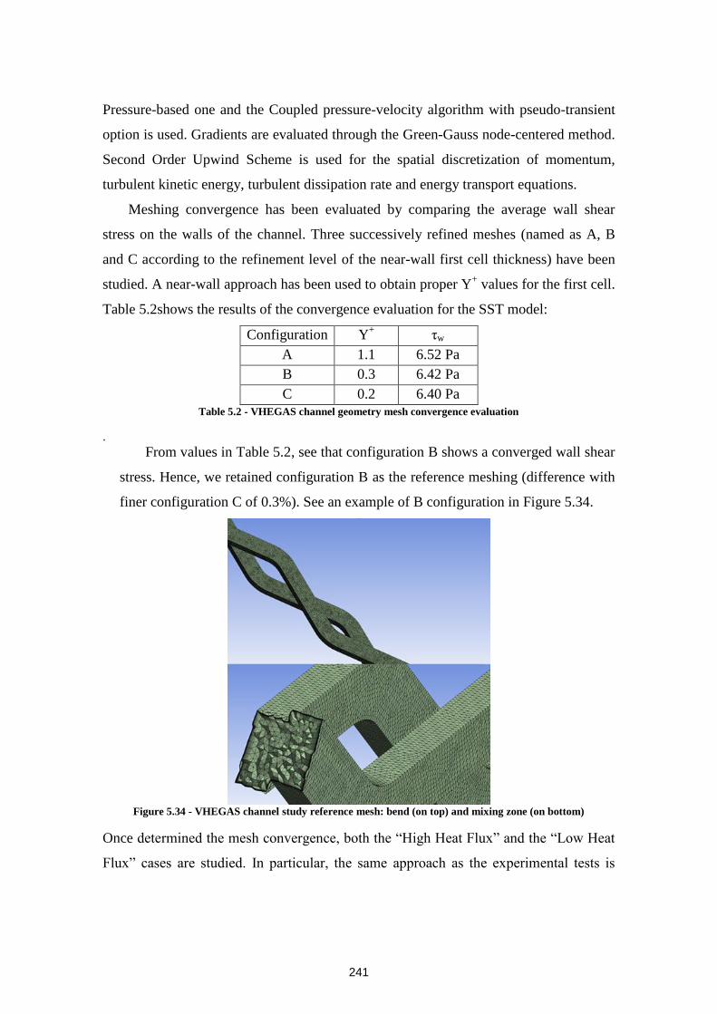
241
Pressure-based one and the Coupled pressure-velocity algorithm with pseudo-transient
option is used. Gradients are evaluated through the Green-Gauss node-centered method.
Second Order Upwind Scheme is used for the spatial discretization of momentum,
turbulent kinetic energy, turbulent dissipation rate and energy transport equations.
Meshing convergence has been evaluated by comparing the average wall shear
stress on the walls of the channel. Three successively refined meshes (named as A, B
and C according to the refinement level of the near-wall first cell thickness) have been
studied. A near-wall approach has been used to obtain proper Y+ values for the first cell.
Table 5.2shows the results of the convergence evaluation for the SST model:
Configuration Y+ ηw
A 1.1 6.52 Pa
B 0.3 6.42 Pa
C 0.2 6.40 Pa
Table 5.2 - VHEGAS channel geometry mesh convergence evaluation
.
From values in Table 5.2, see that configuration B shows a converged wall shear
stress. Hence, we retained configuration B as the reference meshing (difference with
finer configuration C of 0.3%). See an example of B configuration in Figure 5.34.
Figure 5.34 - VHEGAS channel study reference mesh: bend (on top) and mixing zone (on bottom)
Once determined the mesh convergence, both the “High Heat Flux” and the “Low Heat
Flux” cases are studied. In particular, the same approach as the experimental tests is
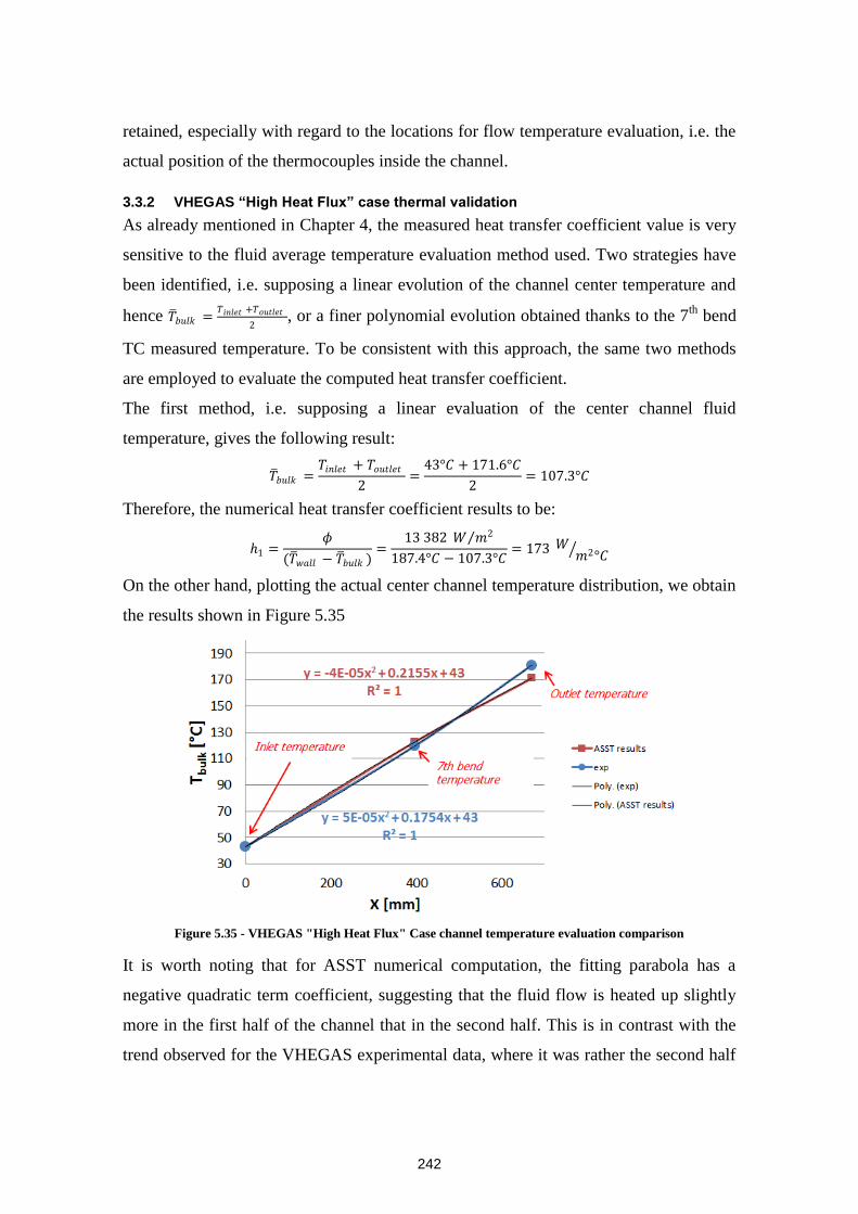
242
retained, especially with regard to the locations for flow temperature evaluation, i.e. the
actual position of the thermocouples inside the channel.
3.3.2 VHEGAS “High Heat Flux” case thermal validation
As already mentioned in Chapter 4, the measured heat transfer coefficient value is very
sensitive to the fluid average temperature evaluation method used. Two strategies have
been identified, i.e. supposing a linear evolution of the channel center temperature and
hence 𝑇 𝑏𝑢𝑙𝑘 =𝑇𝑖𝑛𝑙𝑒𝑡 +𝑇𝑜𝑢𝑡𝑙𝑒𝑡
2, or a finer polynomial evolution obtained thanks to the 7
th bend
TC measured temperature. To be consistent with this approach, the same two methods
are employed to evaluate the computed heat transfer coefficient.
The first method, i.e. supposing a linear evaluation of the center channel fluid
temperature, gives the following result:
𝑇 𝑏𝑢𝑙𝑘 =𝑇𝑖𝑛𝑙𝑒𝑡 + 𝑇𝑜𝑢𝑡𝑙𝑒𝑡
2=
43°𝐶 + 171.6°𝐶
2= 107.3°𝐶
Therefore, the numerical heat transfer coefficient results to be:
1 =𝜙
(𝑇 𝑤𝑎𝑙𝑙 − 𝑇 𝑏𝑢𝑙𝑘 )=
13 382 𝑊 𝑚2
187.4°𝐶 − 107.3°𝐶= 173 𝑊 𝑚2°𝐶
On the other hand, plotting the actual center channel temperature distribution, we obtain
the results shown in Figure 5.35
Figure 5.35 - VHEGAS "High Heat Flux" Case channel temperature evaluation comparison
It is worth noting that for ASST numerical computation, the fitting parabola has a
negative quadratic term coefficient, suggesting that the fluid flow is heated up slightly
more in the first half of the channel that in the second half. This is in contrast with the
trend observed for the VHEGAS experimental data, where it was rather the second half
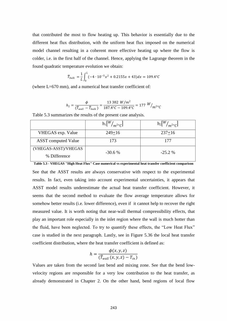
243
that contributed the most to flow heating up. This behavior is essentially due to the
different heat flux distribution, with the uniform heat flux imposed on the numerical
model channel resulting in a coherent more effective heating up where the flow is
colder, i.e. in the first half of the channel. Hence, applying the Lagrange theorem in the
found quadratic temperature evolution we obtain:
𝑇 𝑏𝑢𝑙𝑘 =1
𝐿 (−4 ∙ 10−5𝑥2 + 0.2155𝑥 + 43)𝑑𝑥
𝐿
0
= 109.4°𝐶
(where L=670 mm), and a numerical heat transfer coefficient of:
2 =𝜙
(𝑇 𝑤𝑎𝑙𝑙 − 𝑇 𝑏𝑢𝑙𝑘 )=
13 382 𝑊 𝑚2
187.4°𝐶 − 109.4°𝐶= 177 𝑊 𝑚2°𝐶
Table 5.3 summarizes the results of the present case analysis.
h1 𝑊 𝑚2°𝐶 h2 𝑊 𝑚2°𝐶
VHEGAS exp. Value 249+16 237+16
ASST computed Value 173 177
(VHEGAS-ASST)/VHEGAS
% Difference -30.6 % -25.2 %
Table 5.3 - VHEGAS "High Heat Flux" Case numerical vs experimental heat transfer coefficient comparison
See that the ASST results are always conservative with respect to the experimental
results. In fact, even taking into account experimental uncertainties, it appears that
ASST model results underestimate the actual heat transfer coefficient. However, it
seems that the second method to evaluate the flow average temperature allows for
somehow better results (i.e. lower difference), even if it cannot help to recover the right
measured value. It is worth noting that near-wall thermal compressibility effects, that
play an important role especially in the inlet region where the wall is much hotter than
the fluid, have been neglected. To try to quantify these effects, the “Low Heat Flux”
case is studied in the next paragraph. Lastly, see in Figure 5.36 the local heat transfer
coefficient distribution, where the heat transfer coefficient is defined as:
=𝜙(𝑥, 𝑦, 𝑧)
(𝑇 𝑤𝑎𝑙𝑙 (𝑥, 𝑦, 𝑧) − 𝑇𝑖𝑛 )
Values are taken from the second last bend and mixing zone. See that the bend low-
velocity regions are responsible for a very low contribution to the heat transfer, as
already demonstrated in Chapter 2. On the other hand, bend regions of local flow
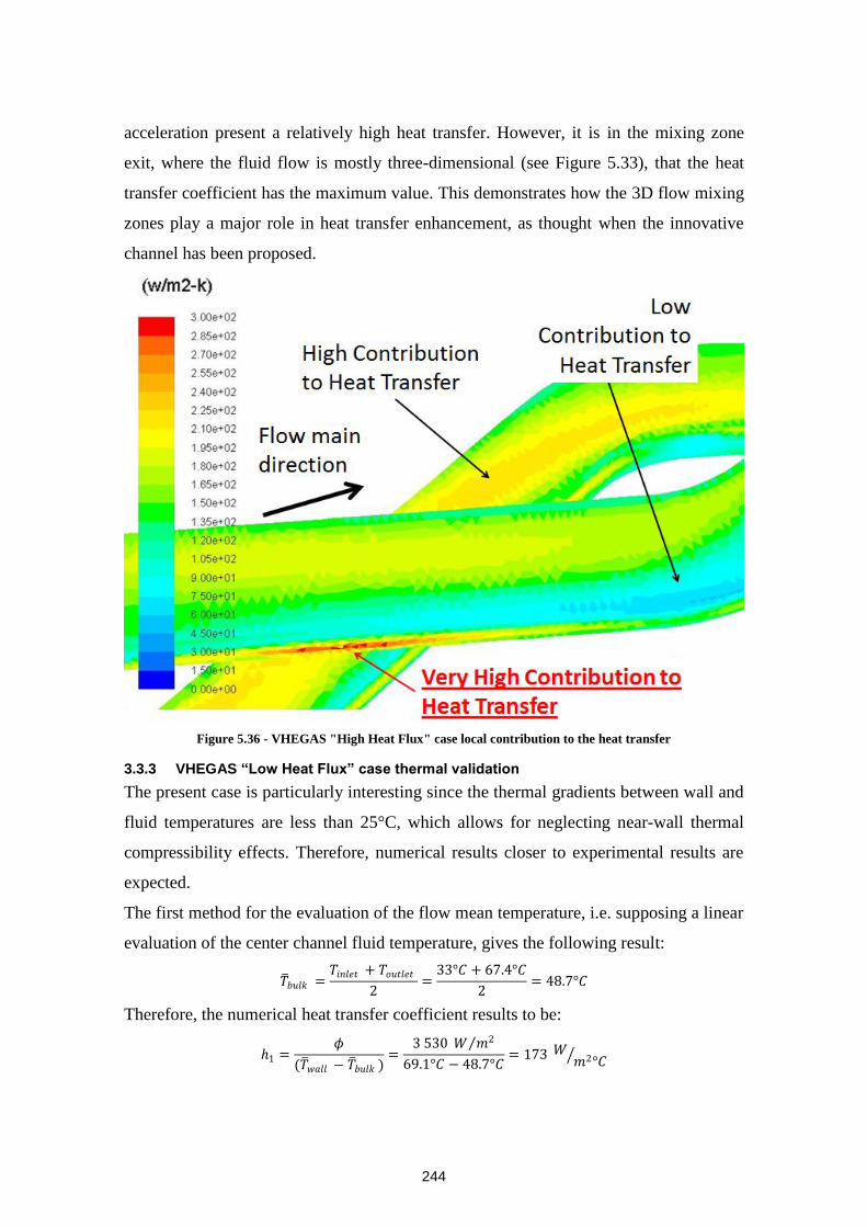
244
acceleration present a relatively high heat transfer. However, it is in the mixing zone
exit, where the fluid flow is mostly three-dimensional (see Figure 5.33), that the heat
transfer coefficient has the maximum value. This demonstrates how the 3D flow mixing
zones play a major role in heat transfer enhancement, as thought when the innovative
channel has been proposed.
Figure 5.36 - VHEGAS "High Heat Flux" case local contribution to the heat transfer
3.3.3 VHEGAS “Low Heat Flux” case thermal validation
The present case is particularly interesting since the thermal gradients between wall and
fluid temperatures are less than 25°C, which allows for neglecting near-wall thermal
compressibility effects. Therefore, numerical results closer to experimental results are
expected.
The first method for the evaluation of the flow mean temperature, i.e. supposing a linear
evaluation of the center channel fluid temperature, gives the following result:
𝑇 𝑏𝑢𝑙𝑘 =𝑇𝑖𝑛𝑙𝑒𝑡 + 𝑇𝑜𝑢𝑡𝑙𝑒𝑡
2=
33°𝐶 + 67.4°𝐶
2= 48.7°𝐶
Therefore, the numerical heat transfer coefficient results to be:
1 =𝜙
(𝑇 𝑤𝑎𝑙𝑙 − 𝑇 𝑏𝑢𝑙𝑘 )=
3 530 𝑊 𝑚2
69.1°𝐶 − 48.7°𝐶= 173 𝑊 𝑚2°𝐶
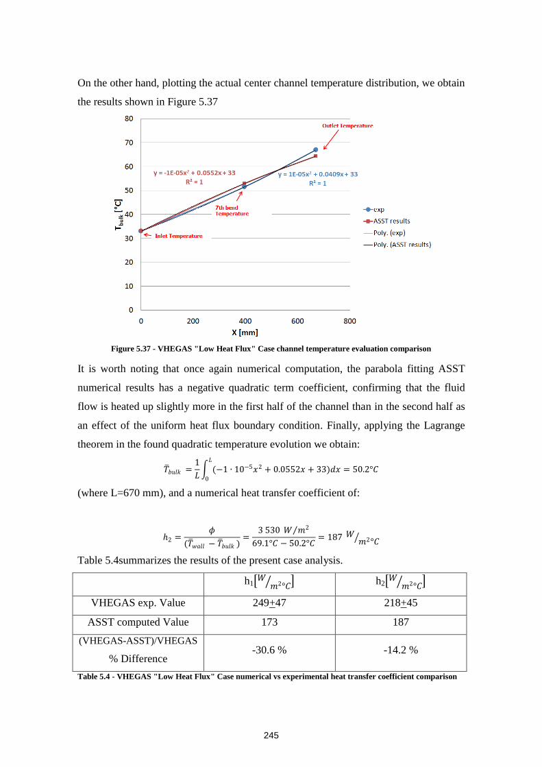
245
On the other hand, plotting the actual center channel temperature distribution, we obtain
the results shown in Figure 5.37
Figure 5.37 - VHEGAS "Low Heat Flux" Case channel temperature evaluation comparison
It is worth noting that once again numerical computation, the parabola fitting ASST
numerical results has a negative quadratic term coefficient, confirming that the fluid
flow is heated up slightly more in the first half of the channel than in the second half as
an effect of the uniform heat flux boundary condition. Finally, applying the Lagrange
theorem in the found quadratic temperature evolution we obtain:
𝑇 𝑏𝑢𝑙𝑘 =1
𝐿 (−1 ∙ 10−5𝑥2 + 0.0552𝑥 + 33)𝑑𝑥
𝐿
0
= 50.2°𝐶
(where L=670 mm), and a numerical heat transfer coefficient of:
2 =𝜙
(𝑇 𝑤𝑎𝑙𝑙 − 𝑇 𝑏𝑢𝑙𝑘 )=
3 530 𝑊 𝑚2
69.1°𝐶 − 50.2°𝐶= 187 𝑊 𝑚2°𝐶
Table 5.4summarizes the results of the present case analysis.
h1 𝑊 𝑚2°𝐶 h2 𝑊 𝑚2°𝐶
VHEGAS exp. Value 249+47 218+45
ASST computed Value 173 187
(VHEGAS-ASST)/VHEGAS
% Difference -30.6 % -14.2 %
Table 5.4 - VHEGAS "Low Heat Flux" Case numerical vs experimental heat transfer coefficient comparison
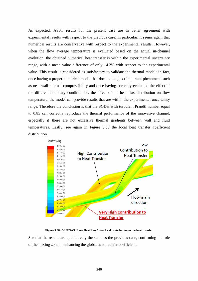
246
As expected, ASST results for the present case are in better agreement with
experimental results with respect to the previous case. In particular, it seems again that
numerical results are conservative with respect to the experimental results. However,
when the flow average temperature is evaluated based on the actual in-channel
evolution, the obtained numerical heat transfer is within the experimental uncertainty
range, with a mean value difference of only 14.2% with respect to the experimental
value. This result is considered as satisfactory to validate the thermal model: in fact,
once having a proper numerical model that does not neglect important phenomena such
as near-wall thermal compressibility and once having correctly evaluated the effect of
the different boundary condition i.e. the effect of the heat flux distribution on flow
temperature, the model can provide results that are within the experimental uncertainty
range. Therefore the conclusion is that the SGDH with turbulent Prandtl number equal
to 0.85 can correctly reproduce the thermal performance of the innovative channel,
especially if there are not excessive thermal gradients between wall and fluid
temperatures. Lastly, see again in Figure 5.38 the local heat transfer coefficient
distribution.
Figure 5.38 - VHEGAS "Low Heat Flux" case local contribution to the heat transfer
See that the results are qualitatively the same as the previous case, confirming the role
of the mixing zone in enhancing the global heat transfer coefficient.
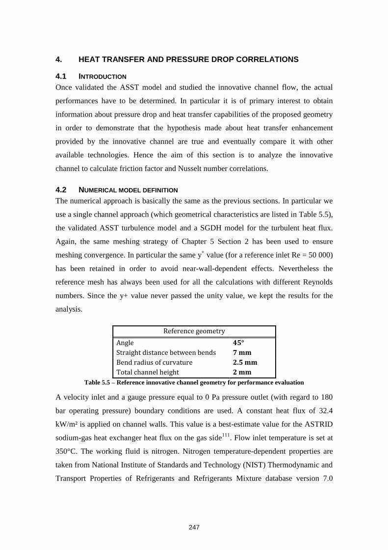
247
4. HEAT TRANSFER AND PRESSURE DROP CORRELATIONS
4.1 INTRODUCTION
Once validated the ASST model and studied the innovative channel flow, the actual
performances have to be determined. In particular it is of primary interest to obtain
information about pressure drop and heat transfer capabilities of the proposed geometry
in order to demonstrate that the hypothesis made about heat transfer enhancement
provided by the innovative channel are true and eventually compare it with other
available technologies. Hence the aim of this section is to analyze the innovative
channel to calculate friction factor and Nusselt number correlations.
4.2 NUMERICAL MODEL DEFINITION
The numerical approach is basically the same as the previous sections. In particular we
use a single channel approach (which geometrical characteristics are listed in Table 5.5),
the validated ASST turbulence model and a SGDH model for the turbulent heat flux.
Again, the same meshing strategy of Chapter 5 Section 2 has been used to ensure
meshing convergence. In particular the same y+ value (for a reference inlet Re = 50 000)
has been retained in order to avoid near-wall-dependent effects. Nevertheless the
reference mesh has always been used for all the calculations with different Reynolds
numbers. Since the y+ value never passed the unity value, we kept the results for the
analysis.
Reference geometry
Angle 45°
Straight distance between bends 7 mm
Bend radius of curvature 2.5 mm
Total channel height 2 mm
Table 5.5 – Reference innovative channel geometry for performance evaluation
A velocity inlet and a gauge pressure equal to 0 Pa pressure outlet (with regard to 180
bar operating pressure) boundary conditions are used. A constant heat flux of 32.4
kW/m² is applied on channel walls. This value is a best-estimate value for the ASTRID
sodium-gas heat exchanger heat flux on the gas side111
. Flow inlet temperature is set at
350°C. The working fluid is nitrogen. Nitrogen temperature-dependent properties are
taken from National Institute of Standards and Technology (NIST) Thermodynamic and
Transport Properties of Refrigerants and Refrigerants Mixture database version 7.0
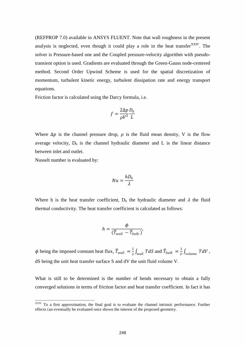
248
(REFPROP 7.0) available in ANSYS FLUENT. Note that wall roughness in the present
analysis is neglected, even though it could play a role in the heat transferXXIV
. The
solver is Pressure-based one and the Coupled pressure-velocity algorithm with pseudo-
transient option is used. Gradients are evaluated through the Green-Gauss node-centered
method. Second Order Upwind Scheme is used for the spatial discretization of
momentum, turbulent kinetic energy, turbulent dissipation rate and energy transport
equations.
Friction factor is calculated using the Darcy formula, i.e.
𝑓 =2∆𝑝
𝜌𝑉²
𝐷
𝐿
Where ∆𝑝 is the channel pressure drop, 𝜌 is the fluid mean density, V is the flow
average velocity, Dh is the channel hydraulic diameter and L is the linear distance
between inlet and outlet.
Nusselt number is evaluated by:
𝑁𝑢 =𝐷
𝜆
Where h is the heat transfer coefficient, Dh the hydraulic diameter and 𝜆 the fluid
thermal conductivity. The heat transfer coefficient is calculated as follows:
=𝜙
(𝑇 𝑤𝑎𝑙𝑙 − 𝑇 𝑏𝑢𝑙𝑘 ),
𝜙 being the imposed constant heat flux, 𝑇 𝑤𝑎𝑙𝑙 =1
𝑆 𝑇𝑑𝑆 𝑤𝑎𝑙𝑙
and 𝑇 𝑏𝑢𝑙𝑘 =1
𝑉 𝑇𝑑𝑉 𝑣𝑜𝑙𝑢𝑚𝑒
,
dS being the unit heat transfer surface S and dV the unit fluid volume V.
What is still to be determined is the number of bends necessary to obtain a fully
converged solutions in terms of friction factor and heat transfer coefficient. In fact it has
XXIV
To a first approximation, the final goal is to evaluate the channel intrinsic performance. Further
effects can eventually be evaluated once shown the interest of the proposed geometry.
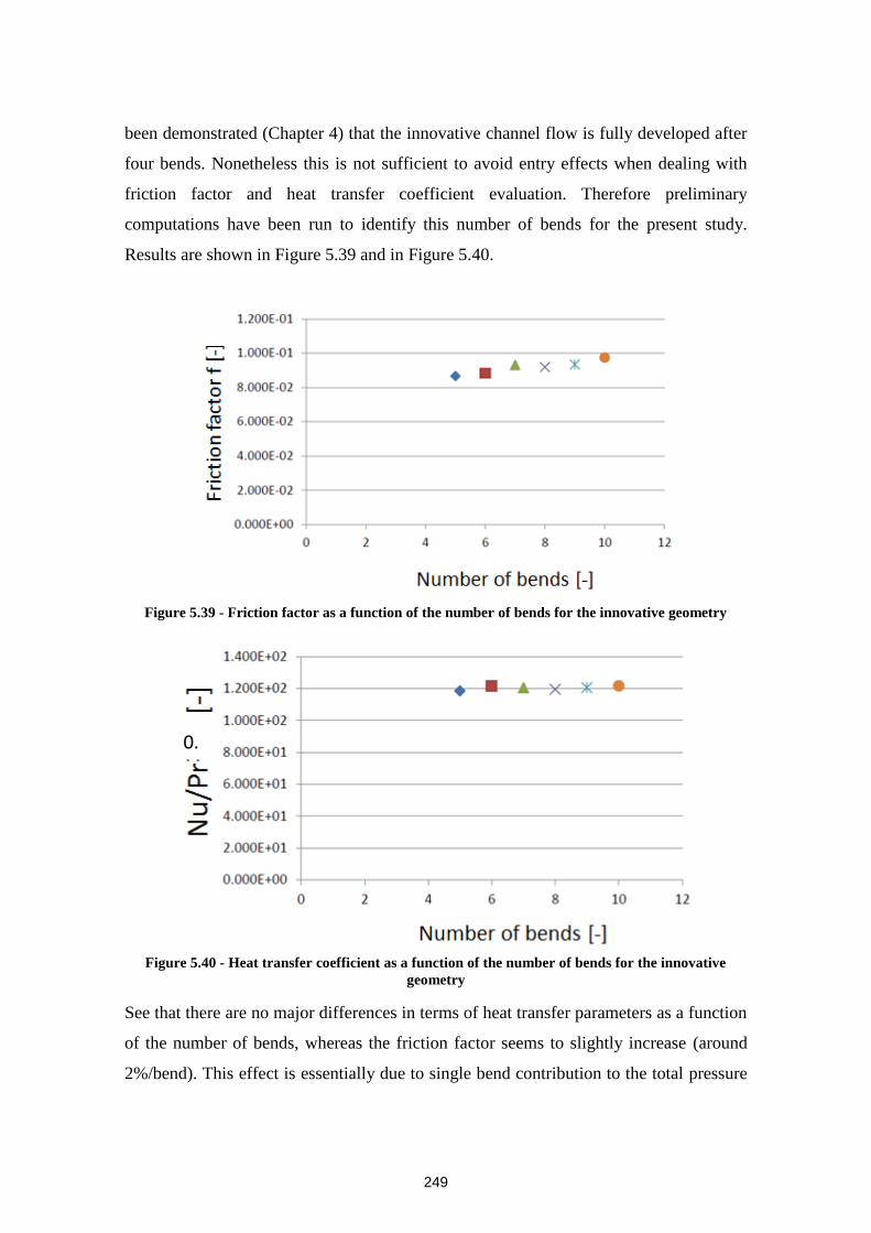
249
been demonstrated (Chapter 4) that the innovative channel flow is fully developed after
four bends. Nonetheless this is not sufficient to avoid entry effects when dealing with
friction factor and heat transfer coefficient evaluation. Therefore preliminary
computations have been run to identify this number of bends for the present study.
Results are shown in Figure 5.39 and in Figure 5.40.
Figure 5.39 - Friction factor as a function of the number of bends for the innovative geometry
Figure 5.40 - Heat transfer coefficient as a function of the number of bends for the innovative
geometry
See that there are no major differences in terms of heat transfer parameters as a function
of the number of bends, whereas the friction factor seems to slightly increase (around
2%/bend). This effect is essentially due to single bend contribution to the total pressure
0.4

250
drop. In fact, if the fluid flow is fully developed after 4 bends, the single bend pressure
drop from the 4th
bend on will be the same. However, when the number of bends
presenting a periodic flow is comparable to the number of bends necessary to flow
development, entry effects provide a bias in the final pressure drop value, which is no
longer linearly proportional to the number of bends. Therefore it would be necessary a
number of bends much higher than 4 to be able to neglect these entry effects, i.e. to have
a negligible increase of the friction factor value with regard to the number of bends. By
the way, this would result in a too much big computational domain for the purpose of
the present work. Therefore the final choice is to use eight bends for the analysis, trying
to obtain a converged friction factor and heat transfer variables without resulting in
excessive time-consuming calculations.
4.3 HYDRAULIC DIAMETER DEFINITION
It is worth defining properly the hydraulic diameter, since it determines the non-
dimensional numbers and the parameters of interest for the following analysis. In fact, if
there is no issue in defining the hydraulic diameter for wavy channels, we already
underlined how it is more difficult to do it for a complex flow (see Chapter 2 Section
1.3).
In the present case, there are two different regions, where the hydraulic diameter could
be defined differently:
The bend region, where the hydraulic diameter should be defined based on the
rectangular cross-section;
The mixing zones, where the hydraulic diameter might be defined based on the
squared cross-section, even if the definition of cross-section and wetted
perimeter would not be clear due to occurring mixing.
The innovative channel hydraulic diameter definition should possibly include both the
previous definitions.
Remember the classical hydraulic diameter definition for a channel flow:
𝐷 =4𝐴
𝑝
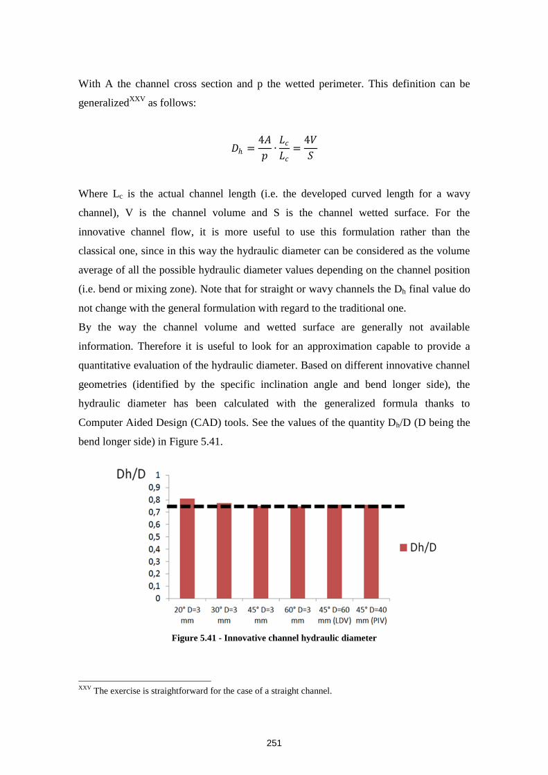
251
With A the channel cross section and p the wetted perimeter. This definition can be
generalizedXXV
as follows:
𝐷 =4𝐴
𝑝∙𝐿𝑐
𝐿𝑐=
4𝑉
𝑆
Where Lc is the actual channel length (i.e. the developed curved length for a wavy
channel), V is the channel volume and S is the channel wetted surface. For the
innovative channel flow, it is more useful to use this formulation rather than the
classical one, since in this way the hydraulic diameter can be considered as the volume
average of all the possible hydraulic diameter values depending on the channel position
(i.e. bend or mixing zone). Note that for straight or wavy channels the Dh final value do
not change with the general formulation with regard to the traditional one.
By the way the channel volume and wetted surface are generally not available
information. Therefore it is useful to look for an approximation capable to provide a
quantitative evaluation of the hydraulic diameter. Based on different innovative channel
geometries (identified by the specific inclination angle and bend longer side), the
hydraulic diameter has been calculated with the generalized formula thanks to
Computer Aided Design (CAD) tools. See the values of the quantity Dh/D (D being the
bend longer side) in Figure 5.41.
Figure 5.41 - Innovative channel hydraulic diameter
XXV
The exercise is straightforward for the case of a straight channel.
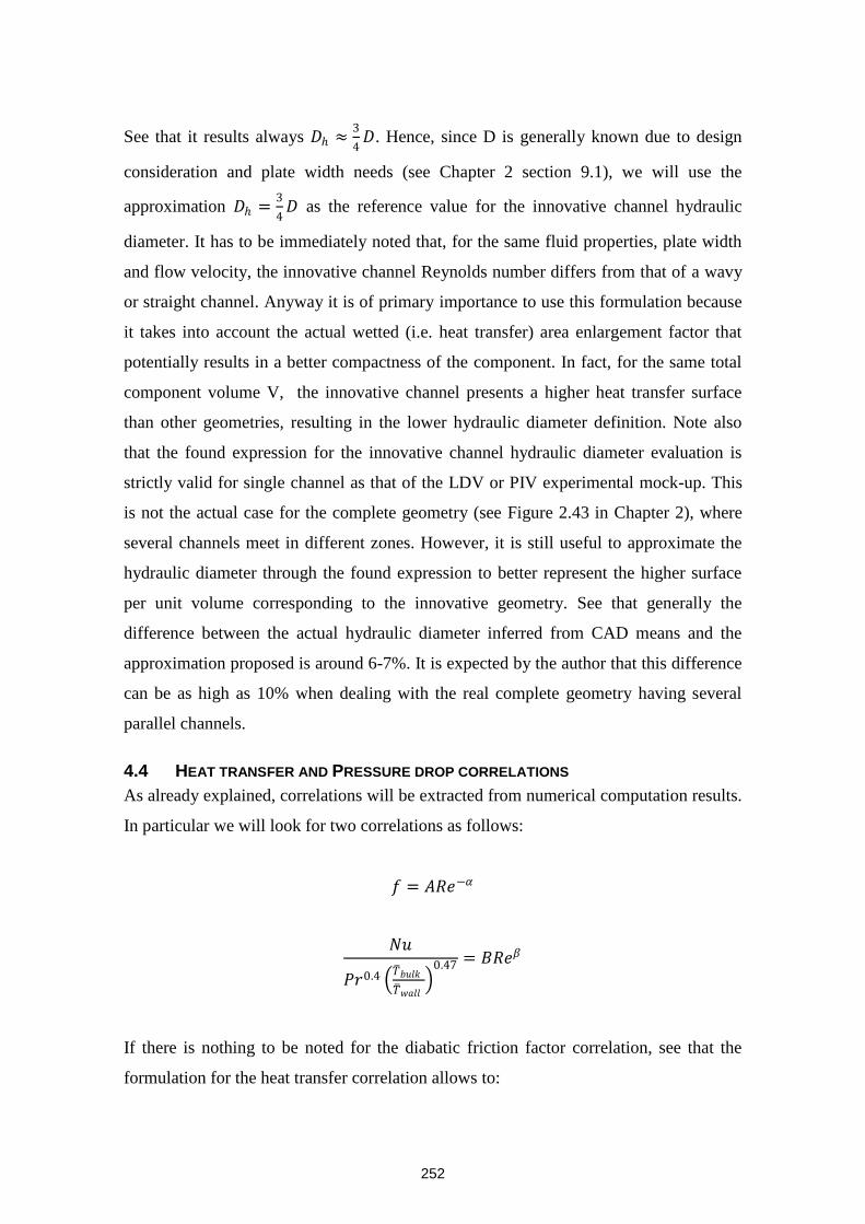
252
See that it results always 𝐷 ≈3
4𝐷. Hence, since D is generally known due to design
consideration and plate width needs (see Chapter 2 section 9.1), we will use the
approximation 𝐷 =3
4𝐷 as the reference value for the innovative channel hydraulic
diameter. It has to be immediately noted that, for the same fluid properties, plate width
and flow velocity, the innovative channel Reynolds number differs from that of a wavy
or straight channel. Anyway it is of primary importance to use this formulation because
it takes into account the actual wetted (i.e. heat transfer) area enlargement factor that
potentially results in a better compactness of the component. In fact, for the same total
component volume V, the innovative channel presents a higher heat transfer surface
than other geometries, resulting in the lower hydraulic diameter definition. Note also
that the found expression for the innovative channel hydraulic diameter evaluation is
strictly valid for single channel as that of the LDV or PIV experimental mock-up. This
is not the actual case for the complete geometry (see Figure 2.43 in Chapter 2), where
several channels meet in different zones. However, it is still useful to approximate the
hydraulic diameter through the found expression to better represent the higher surface
per unit volume corresponding to the innovative geometry. See that generally the
difference between the actual hydraulic diameter inferred from CAD means and the
approximation proposed is around 6-7%. It is expected by the author that this difference
can be as high as 10% when dealing with the real complete geometry having several
parallel channels.
4.4 HEAT TRANSFER AND PRESSURE DROP CORRELATIONS
As already explained, correlations will be extracted from numerical computation results.
In particular we will look for two correlations as follows:
𝑓 = 𝐴𝑅𝑒−𝛼
𝑁𝑢
𝑃𝑟0.4 𝑇 𝑏𝑢𝑙𝑘
𝑇 𝑤𝑎𝑙𝑙
0.47 = 𝐵𝑅𝑒𝛽
If there is nothing to be noted for the diabatic friction factor correlation, see that the
formulation for the heat transfer correlation allows to:
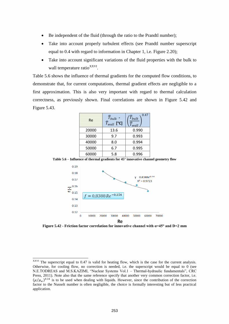
253
Be independent of the fluid (through the ratio to the Prandtl number);
Take into account properly turbulent effects (see Prandtl number superscript
equal to 0.4 with regard to information in Chapter 1, i.e. Figure 2.20);
Take into account significant variations of the fluid properties with the bulk to
wall temperature ratioXXVI
.
Table 5.6 shows the influence of thermal gradients for the computed flow conditions, to
demonstrate that, for current computations, thermal gradient effects are negligible to a
first approximation. This is also very important with regard to thermal calculation
correctness, as previously shown. Final correlations are shown in Figure 5.42 and
Figure 5.43.
Re 𝑇 𝑏𝑢𝑙𝑘 -
𝑇 𝑤𝑎𝑙𝑙 [°C] 𝑇 𝑏𝑢𝑙𝑘
𝑇 𝑤𝑎𝑙𝑙
0.47
20000 13.6 0.990
30000 9.7 0.993
40000 8.0 0.994
50000 6.7 0.995
60000 5.8 0.996 Table 5.6 – Influence of thermal gradients for 45° innovative channel geometry flow
Figure 5.42 - Friction factor correlation for innovative channel with α=45° and D=2 mm
XXVI
The superscript equal to 0.47 is valid for heating flow, which is the case for the current analysis.
Otherwise, for cooling flow, no correction is needed, i.e. the superscript would be equal to 0 (see
N.E.TODREAS and M.S.KAZIMI, “Nuclear Systems Vol.1 – Thermal-hydraulic fundamentals”, CRC
Press, 2011). Note also that the same reference specify that another very common correction factor, i.e.
𝜇 𝜇𝑤 0.14 is to be used when dealing with liquids. However, since the contribution of the correction
factor to the Nusselt number is often negligible, the choice is formally interesting but of less practical
application.
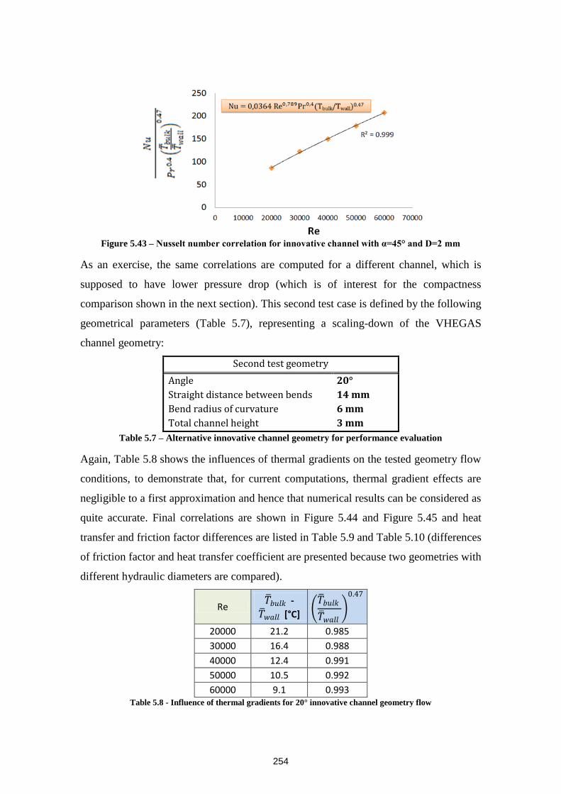
254
Figure 5.43 – Nusselt number correlation for innovative channel with α=45° and D=2 mm
As an exercise, the same correlations are computed for a different channel, which is
supposed to have lower pressure drop (which is of interest for the compactness
comparison shown in the next section). This second test case is defined by the following
geometrical parameters (Table 5.7), representing a scaling-down of the VHEGAS
channel geometry:
Second test geometry
Angle 20°
Straight distance between bends 14 mm
Bend radius of curvature 6 mm
Total channel height 3 mm
Table 5.7 – Alternative innovative channel geometry for performance evaluation
Again, Table 5.8 shows the influences of thermal gradients on the tested geometry flow
conditions, to demonstrate that, for current computations, thermal gradient effects are
negligible to a first approximation and hence that numerical results can be considered as
quite accurate. Final correlations are shown in Figure 5.44 and Figure 5.45 and heat
transfer and friction factor differences are listed in Table 5.9 and Table 5.10 (differences
of friction factor and heat transfer coefficient are presented because two geometries with
different hydraulic diameters are compared).
Re 𝑇 𝑏𝑢𝑙𝑘 -
𝑇 𝑤𝑎𝑙𝑙 [°C] 𝑇 𝑏𝑢𝑙𝑘
𝑇 𝑤𝑎𝑙𝑙
0.47
20000 21.2 0.985
30000 16.4 0.988
40000 12.4 0.991
50000 10.5 0.992
60000 9.1 0.993 Table 5.8 - Influence of thermal gradients for 20° innovative channel geometry flow
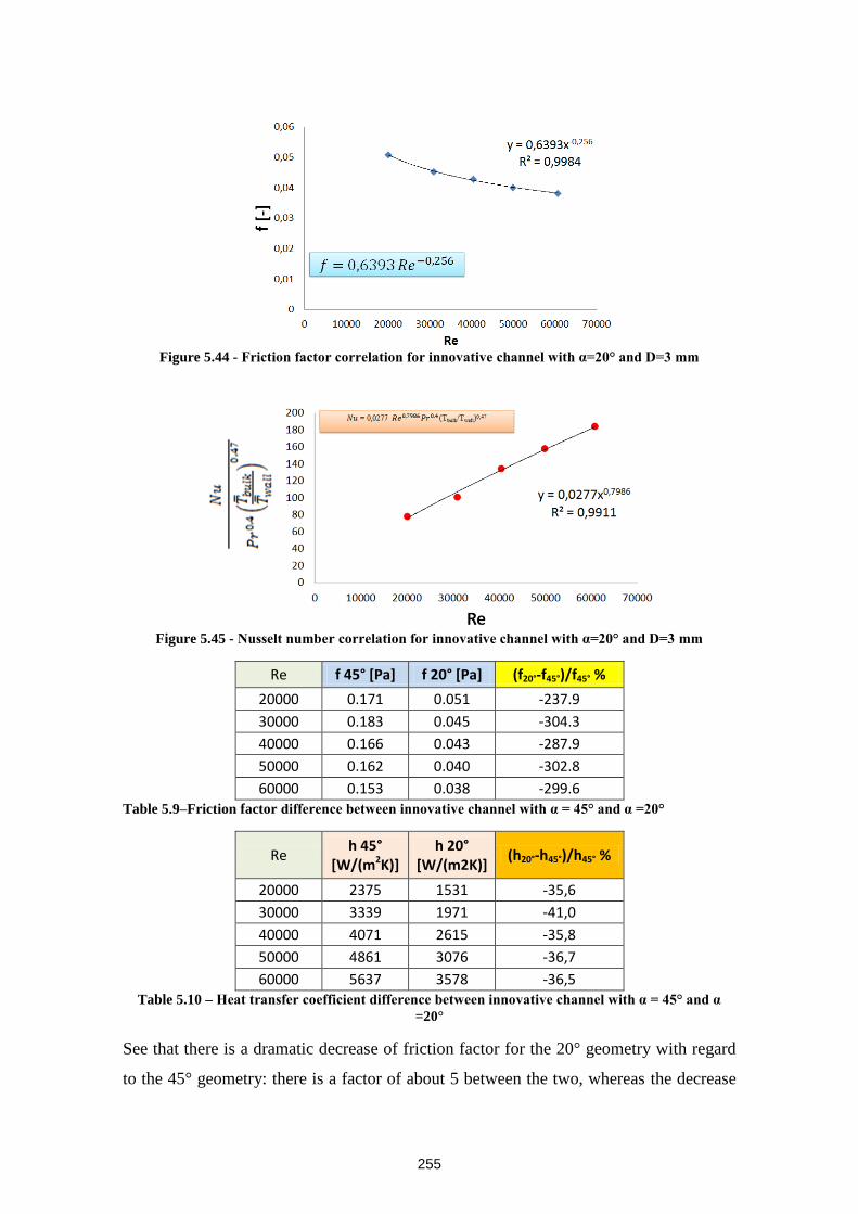
255
Figure 5.44 - Friction factor correlation for innovative channel with α=20° and D=3 mm
Figure 5.45 - Nusselt number correlation for innovative channel with α=20° and D=3 mm
Re f 45° [Pa] f 20° [Pa] (f20°-f45°)/f45° %
20000 0.171 0.051 -237.9
30000 0.183 0.045 -304.3
40000 0.166 0.043 -287.9
50000 0.162 0.040 -302.8
60000 0.153 0.038 -299.6 Table 5.9–Friction factor difference between innovative channel with α = 45° and α =20°
Re h 45°
[W/(m2K)] h 20°
[W/(m2K)] (h20°-h45°)/h45° %
20000 2375 1531 -35,6
30000 3339 1971 -41,0
40000 4071 2615 -35,8
50000 4861 3076 -36,7
60000 5637 3578 -36,5 Table 5.10 – Heat transfer coefficient difference between innovative channel with α = 45° and α
=20°
See that there is a dramatic decrease of friction factor for the 20° geometry with regard
to the 45° geometry: there is a factor of about 5 between the two, whereas the decrease
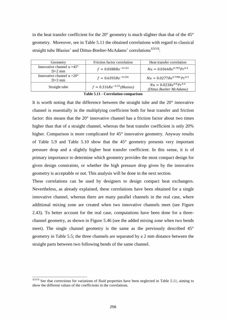
256
in the heat transfer coefficient for the 20° geometry is much slighter than that of the 45°
geometry. Moreover, see in Table 5.11 the obtained correlations with regard to classical
straight tube Blasius’ and Dittus-Boelter-McAdams’ correlationsXXVII
:
Geometry Friction factor correlation Heat transfer correlation
Innovative channel α =45°
D=2 mm 𝑓 = 0.8388𝑅𝑒−0.154 𝑁𝑢 = 0.0364𝑅𝑒0.789𝑃𝑟0.4
Innovative channel α =20°
D=3 mm 𝑓 = 0.6393𝑅𝑒−0.256 𝑁𝑢 = 0.0277𝑅𝑒0.7986𝑃𝑟0.4
Straight tube 𝑓 = 0.316𝑅𝑒−0.25(Blasius) 𝑁𝑢 = 0.023𝑅𝑒0.8𝑃𝑟0.4
(Dittus Boelter McAdams)
Table 5.11 - Correlation comparison
It is worth noting that the difference between the straight tube and the 20° innovative
channel is essentially in the multiplying coefficient both for heat transfer and friction
factor: this means that the 20° innovative channel has a friction factor about two times
higher than that of a straight channel, whereas the heat transfer coefficient is only 20%
higher. Comparison is more complicated for 45° innovative geometry. Anyway results
of Table 5.9 and Table 5.10 show that the 45° geometry presents very important
pressure drop and a slightly higher heat transfer coefficient. In this sense, it is of
primary importance to determine which geometry provides the most compact design for
given design constraints, or whether the high pressure drop given by the innovative
geometry is acceptable or not. This analysis will be done in the next section.
These correlations can be used by designers to design compact heat exchangers.
Nevertheless, as already explained, these correlations have been obtained for a single
innovative channel, whereas there are many parallel channels in the real case, where
additional mixing zone are created when two innovative channels meet (see Figure
2.43). To better account for the real case, computations have been done for a three-
channel geometry, as shown in Figure 5.46 (see the added mixing zone when two bends
meet). The single channel geometry is the same as the previously described 45°
geometry in Table 5.5; the three channels are separated by a 2 mm distance between the
straight parts between two following bends of the same channel.
XXVII
See that corrections for variations of fluid properties have been neglected in Table 5.11, aiming to
show the different values of the coefficients in the correlations.
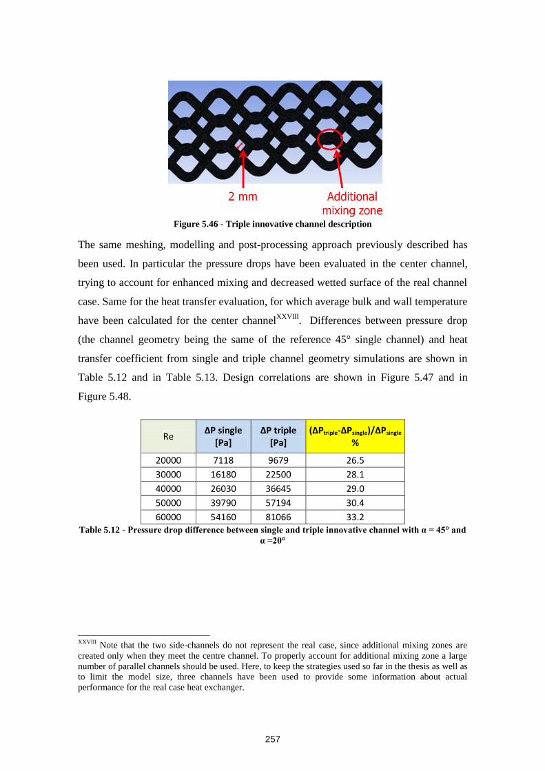
257
Figure 5.46 - Triple innovative channel description
The same meshing, modelling and post-processing approach previously described has
been used. In particular the pressure drops have been evaluated in the center channel,
trying to account for enhanced mixing and decreased wetted surface of the real channel
case. Same for the heat transfer evaluation, for which average bulk and wall temperature
have been calculated for the center channelXXVIII
. Differences between pressure drop
(the channel geometry being the same of the reference 45° single channel) and heat
transfer coefficient from single and triple channel geometry simulations are shown in
Table 5.12 and in Table 5.13. Design correlations are shown in Figure 5.47 and in
Figure 5.48.
Re ΔP single
[Pa] ΔP triple
[Pa] (ΔPtriple-ΔPsingle)/ΔPsingle
%
20000 7118 9679 26.5
30000 16180 22500 28.1
40000 26030 36645 29.0
50000 39790 57194 30.4
60000 54160 81066 33.2 Table 5.12 - Pressure drop difference between single and triple innovative channel with α = 45° and
α =20°
XXVIII
Note that the two side-channels do not represent the real case, since additional mixing zones are
created only when they meet the centre channel. To properly account for additional mixing zone a large
number of parallel channels should be used. Here, to keep the strategies used so far in the thesis as well as
to limit the model size, three channels have been used to provide some information about actual
performance for the real case heat exchanger.
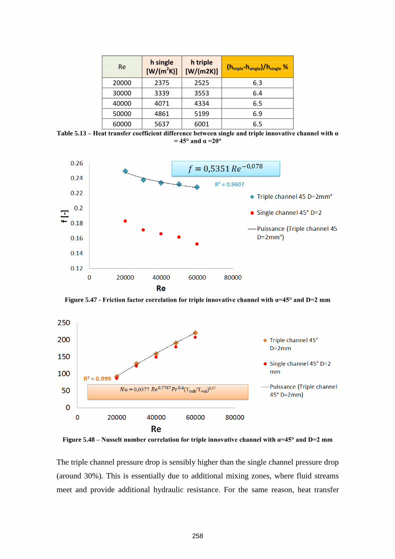
258
Re h single
[W/(m2K)] h triple
[W/(m2K)] (htriple-hsingle)/hsingle %
20000 2375 2525 6.3
30000 3339 3553 6.4
40000 4071 4334 6.5
50000 4861 5199 6.9
60000 5637 6001 6.5 Table 5.13 – Heat transfer coefficient difference between single and triple innovative channel with α
= 45° and α =20°
Figure 5.47 - Friction factor correlation for triple innovative channel with α=45° and D=2 mm
Figure 5.48 – Nusselt number correlation for triple innovative channel with α=45° and D=2 mm
The triple channel pressure drop is sensibly higher than the single channel pressure drop
(around 30%). This is essentially due to additional mixing zones, where fluid streams
meet and provide additional hydraulic resistance. For the same reason, heat transfer
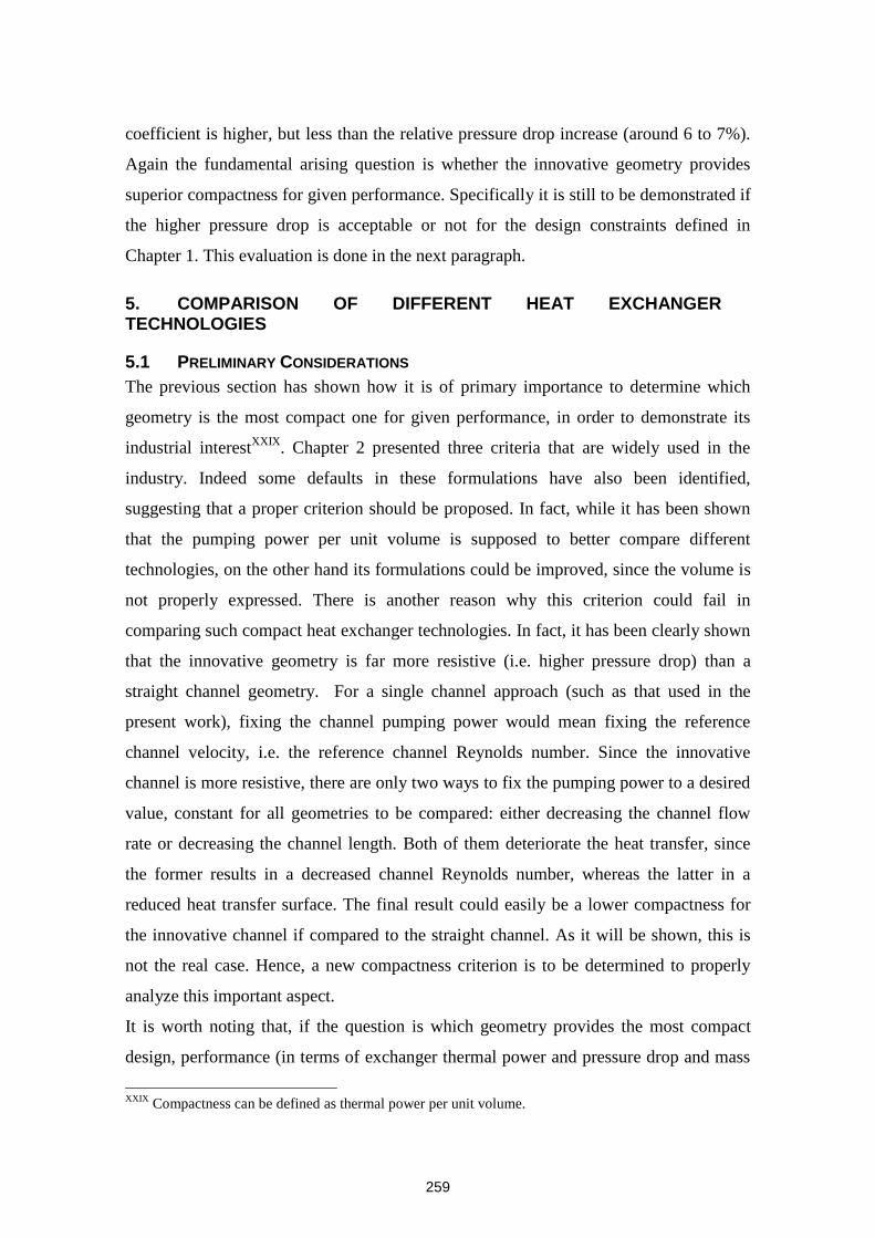
259
coefficient is higher, but less than the relative pressure drop increase (around 6 to 7%).
Again the fundamental arising question is whether the innovative geometry provides
superior compactness for given performance. Specifically it is still to be demonstrated if
the higher pressure drop is acceptable or not for the design constraints defined in
Chapter 1. This evaluation is done in the next paragraph.
5. COMPARISON OF DIFFERENT HEAT EXCHANGER TECHNOLOGIES
5.1 PRELIMINARY CONSIDERATIONS
The previous section has shown how it is of primary importance to determine which
geometry is the most compact one for given performance, in order to demonstrate its
industrial interestXXIX
. Chapter 2 presented three criteria that are widely used in the
industry. Indeed some defaults in these formulations have also been identified,
suggesting that a proper criterion should be proposed. In fact, while it has been shown
that the pumping power per unit volume is supposed to better compare different
technologies, on the other hand its formulations could be improved, since the volume is
not properly expressed. There is another reason why this criterion could fail in
comparing such compact heat exchanger technologies. In fact, it has been clearly shown
that the innovative geometry is far more resistive (i.e. higher pressure drop) than a
straight channel geometry. For a single channel approach (such as that used in the
present work), fixing the channel pumping power would mean fixing the reference
channel velocity, i.e. the reference channel Reynolds number. Since the innovative
channel is more resistive, there are only two ways to fix the pumping power to a desired
value, constant for all geometries to be compared: either decreasing the channel flow
rate or decreasing the channel length. Both of them deteriorate the heat transfer, since
the former results in a decreased channel Reynolds number, whereas the latter in a
reduced heat transfer surface. The final result could easily be a lower compactness for
the innovative channel if compared to the straight channel. As it will be shown, this is
not the real case. Hence, a new compactness criterion is to be determined to properly
analyze this important aspect.
It is worth noting that, if the question is which geometry provides the most compact
design, performance (in terms of exchanger thermal power and pressure drop and mass
XXIX
Compactness can be defined as thermal power per unit volume.
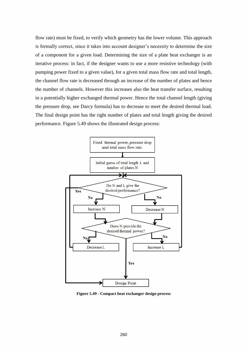
260
flow rate) must be fixed, to verify which geometry has the lower volume. This approach
is formally correct, since it takes into account designer’s necessity to determine the size
of a component for a given load. Determining the size of a plate heat exchanger is an
iterative process: in fact, if the designer wants to use a more resistive technology (with
pumping power fixed to a given value), for a given total mass flow rate and total length,
the channel flow rate is decreased through an increase of the number of plates and hence
the number of channels. However this increases also the heat transfer surface, resulting
in a potentially higher exchanged thermal power. Hence the total channel length (giving
the pressure drop, see Darcy formula) has to decrease to meet the desired thermal load.
The final design point has the right number of plates and total length giving the desired
performance. Figure 5.49 shows the illustrated design process:
Figure 5.49 - Compact heat exchanger design process
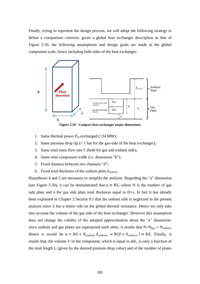
261
Finally, trying to represent the design process, we will adopt the following strategy to
define a comparison criterion: given a global heat exchanger description as that of
Figure 5.50, the following assumptions and design goals are made at the global
component scale, hence including both sides of the heat exchanger:
Figure 5.50 - Compact heat exchanger major dimensions
1. Same thermal power Pth exchanged (=24 MW);
2. Same pressure drop Δp (= 1 bar for the gas-side of the heat exchanger);
3. Same total mass flow rate Γ (both for gas and sodium side);
4. Same total component width (i.e. dimension “b”);
5. Fixed distance between two channels “d”;
6. Fixed total thickness of the sodium plate δsodium.
Hypotheses 4 and 5 are necessary to simplify the analysis. Regarding the “a” dimension
(see Figure 5.50), it can be demonstrated that 𝑎 ∝ 𝑁𝛿, where N is the number of gas
side plate and δ the gas side plate total thickness equal to D+ε. In fact it has already
been explained in Chapter 2 Section 9.1 that the sodium side is neglected in the present
analysis since it has a minor role on the global thermal resistance. Hence we only take
into account the volume of the gas side of the heat exchanger. However this assumption
does not change the validity of the adopted approximation about the “a” dimension:
since sodium and gas plates are superposed each other, it results that N=Ngas ≈ Nsodium.
Hence it would be 𝑎 = 𝑁𝛿 + 𝑁𝑠𝑜𝑑𝑖𝑢𝑚 𝛿𝑠𝑜𝑑𝑖𝑢𝑚 ≈ 𝑁 𝛿 + 𝛿𝑠𝑜𝑑𝑖𝑢𝑚 ∝ 𝑁𝛿. Finally, it
results that, the volume V of the component, which is equal to abL, is only a function of
the total length L (given by the desired pressure drop value) and of the number of plates
262
of the heat exchanger gas side N, since the gas side plate total thickness δ is constant
due to considerations in Chapter 2 Section 9.1 and hypothesis 5. Together with these
two parameters, the total channel height D (remember that D=Dh for a straight or PCHE
channel but D∝Dh for the innovative channel) is the third parameter to take into account
since it gives the total channel thickness (i.e.) δ=D+ε, the number of channel per plate
(i.e. Nc=b/(D+d, see hypothesis 5), the channel cross section A0 (i.e. A0=D² for a
squared cross section) as well as the Reynolds number values to be considered into
friction factor and heat transfer correlations. Next section will demonstrate that,
knowing N, L and D it is possible to correctly compare different geometries.
5.2 COMPACTNESS COMPARISON STRATEGY
Figure 5.49 showed the iterative design process of a compact heat exchanger to meet a
fixed performance in terms of exchanged thermal power Pth and pressure drop Δp. It
essentially consists of varying the total length and number of plates of the component,
for a fixed total channel height D, to meet the design goals.
As it will be shown, writing the pressure drop and thermal power equations, we can
express these two equations in terms of three unknowns, specifically N, L and D. One
unknown is of particular interest: in fact D can be fixed by the designer in order to have
a certain plate thickness (see Chapter 2). To confirm that, remember that this strategy
has already been adopted when determining the innovative channel rectangular shape in
Chapter 2. In fact, the rectangular cross-section of the single wavy channel was chosen
to keep the total plate width (see also hypothesis 4) and cross-section with regard to a
reference PCHE or straight channel with squared cross-section. Therefore we can fix a
given D value and finally have two equations (pressure drop and exchanged thermal
power) and two unknown to be determined (N and L). The problem has always a
physical solution, since the exchanged thermal power and pressure drop always assume
non-zero values. Therefore the comparison strategy will consist of writing L as a
function of the pressure drop and number of plates i.e. 𝐿 = 𝐿 ∆𝑝, 𝑁 and as a function
of the exchanged thermal power and number of plates i.e. 𝐿 = 𝐿 𝑃𝑡 , 𝑁 . Since the two
design constraints must me respected at the same time, there must be a design point
corresponding to the intersection point (L,N) such as 𝐿 ∆𝑝, 𝑁 = 𝐿 𝑃𝑡 , 𝑁 , Pth ,Δp and
D being fixed.
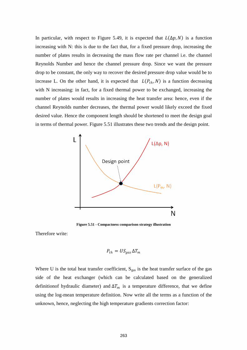
263
In particular, with respect to Figure 5.49, it is expected that 𝐿 ∆𝑝, 𝑁 is a function
increasing with N: this is due to the fact that, for a fixed pressure drop, increasing the
number of plates results in decreasing the mass flow rate per channel i.e. the channel
Reynolds Number and hence the channel pressure drop. Since we want the pressure
drop to be constant, the only way to recover the desired pressure drop value would be to
increase L. On the other hand, it is expected that 𝐿 𝑃𝑡 , 𝑁 is a function decreasing
with N increasing: in fact, for a fixed thermal power to be exchanged, increasing the
number of plates would results in increasing the heat transfer area: hence, even if the
channel Reynolds number decreases, the thermal power would likely exceed the fixed
desired value. Hence the component length should be shortened to meet the design goal
in terms of thermal power. Figure 5.51 illustrates these two trends and the design point.
Figure 5.51 - Compactness comparison strategy illustration
Therefore write:
𝑃𝑡 = 𝑈𝑆𝑔𝑎𝑠∆𝑇𝑚
Where U is the total heat transfer coefficient, Sgas is the heat transfer surface of the gas
side of the heat exchanger (which can be calculated based on the generalized
definitionof hydraulic diameter) and ∆𝑇𝑚 is a temperature difference, that we define
using the log-mean temperature definition. Now write all the terms as a function of the
unknown, hence, neglecting the high temperature gradients correction factor:
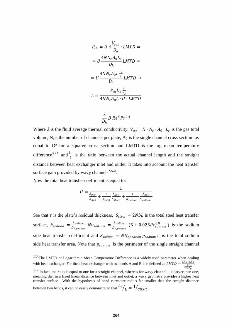
264
𝑃𝑡 = 𝑈 4𝑉𝑔𝑎𝑠
𝐷∙ 𝐿𝑀𝑇𝐷 =
= 𝑈4𝑁𝑁𝑐𝐴0𝐿𝑐
𝐷𝐿𝑀𝑇𝐷 =
= 𝑈4𝑁𝑁𝑐𝐴0𝐿
𝐿𝑐
𝐿
𝐷𝐿𝑀𝑇𝐷 →
𝐿 =𝑃𝑡𝐷
𝐿
𝐿𝑐=
4𝑁𝑁𝑐𝐴0𝐿 ∙ 𝑈 ∙ 𝐿𝑀𝑇𝐷
𝜆
𝐷𝐵 𝑅𝑒𝛽𝑃𝑟0.4
Where 𝜆 is the fluid average thermal conductivity, Vgas= 𝑁 ∙ 𝑁𝑐 ∙ 𝐴0 ∙ 𝐿𝑐 is the gas total
volume, Ncis the number of channels per plate, A0 is the single channel cross section i.e.
equal to D² for a squared cross section and LMTD is the log mean temperature
differenceXXX
and 𝐿𝑐
𝐿 is the ratio between the actual channel length and the straight
distance between heat exchanger inlet and outlet. It takes into account the heat transfer
surface gain provided by wavy channelsXXXI
.
Now the total heat transfer coefficient is equal to:
𝑈 =1
𝑆𝑔𝑎𝑠
𝑔𝑎𝑠+
휀
𝜆𝑠𝑡𝑒𝑒𝑙
𝑆𝑔𝑎𝑠
𝑆𝑠𝑡𝑒𝑒𝑙+
1
𝑠𝑜𝑑𝑖𝑢𝑚
𝑆𝑔𝑎𝑠
𝑆𝑠𝑜𝑑𝑖𝑢𝑚
See that 휀 is the plate’s residual thickness, 𝑆𝑠𝑡𝑒𝑒𝑙 = 2𝑁𝑏𝐿 is the total steel heat transfer
surface, 𝑠𝑜𝑑𝑖𝑢𝑚 =𝜆𝑠𝑜𝑑𝑖𝑢𝑚
𝐷 ,𝑠𝑜𝑑𝑖𝑢𝑚𝑁𝑢𝑠𝑜𝑑𝑖𝑢𝑚 =
𝜆𝑠𝑜𝑑𝑖𝑢𝑚
𝐷 ,𝑠𝑜𝑑𝑖𝑢𝑚(5 + 0.025𝑃𝑒𝑠𝑜𝑑𝑖𝑢𝑚
0.8 ) is the sodium
side heat transfer coefficient and 𝑆𝑠𝑜𝑑𝑖𝑢𝑚 = 𝑁𝑁𝑐 ,𝑠𝑜𝑑𝑖𝑢𝑚 𝑝𝑠𝑜𝑑𝑖𝑢𝑚 𝐿 is the total sodium
side heat transfer area. Note that 𝑝𝑠𝑜𝑑𝑖𝑢𝑚 is the perimeter of the single straight channel
XXX
The LMTD or Logarithmic Mean Temperature Difference is a widely used parameter when dealing
with heat exchanger. For the a heat exchanger with two ends A and B it is defined as 𝐿𝑀𝑇𝐷 =∆𝑇𝐴−∆𝑇𝐵
𝑙𝑛∆𝑇𝐴∆𝑇𝐵
.
XXXIIn fact, the ratio is equal to one for a straight channel, whereas for wavy channel it is larger than one,
meaning that in a fixed linear distance between inlet and outlet, a wavy geometry provides a higher heat
transfer surface. With the hypothesis of bend curvature radius far smaller than the straight distance
between two bends, it can be easily demonstrated that 𝐿𝑐
𝐿 = 1𝑐𝑜𝑠𝛼 .
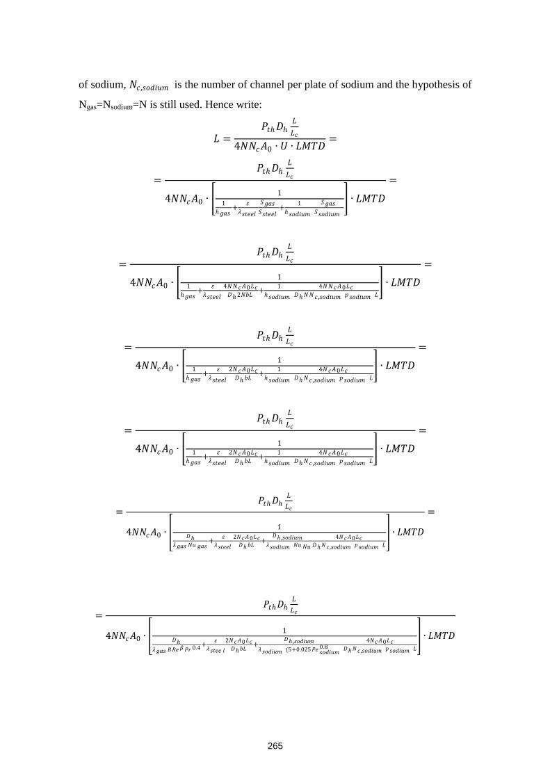
265
of sodium, 𝑁𝑐 ,𝑠𝑜𝑑𝑖𝑢𝑚 is the number of channel per plate of sodium and the hypothesis of
Ngas=Nsodium=N is still used. Hence write:
𝐿 =𝑃𝑡𝐷
𝐿
𝐿𝑐
4𝑁𝑁𝑐𝐴0 ∙ 𝑈 ∙ 𝐿𝑀𝑇𝐷=
=𝑃𝑡𝐷
𝐿
𝐿𝑐
4𝑁𝑁𝑐𝐴0 ∙ 1
1
𝑔𝑎𝑠+
휀
𝜆𝑠𝑡𝑒𝑒𝑙
𝑆𝑔𝑎𝑠
𝑆𝑠𝑡𝑒𝑒𝑙+
1
𝑠𝑜𝑑𝑖𝑢𝑚
𝑆𝑔𝑎𝑠
𝑆𝑠𝑜𝑑𝑖𝑢𝑚
∙ 𝐿𝑀𝑇𝐷
=
=𝑃𝑡𝐷
𝐿
𝐿𝑐
4𝑁𝑁𝑐𝐴0 ∙ 1
1
𝑔𝑎𝑠+
휀
𝜆𝑠𝑡𝑒𝑒𝑙
4𝑁𝑁𝑐𝐴0𝐿𝑐𝐷2𝑁𝑏𝐿
+1
𝑠𝑜𝑑𝑖𝑢𝑚
4𝑁𝑁𝑐𝐴0𝐿𝑐𝐷𝑁𝑁𝑐 ,𝑠𝑜𝑑𝑖𝑢𝑚 𝑝𝑠𝑜𝑑𝑖𝑢𝑚 𝐿
∙ 𝐿𝑀𝑇𝐷
=
=𝑃𝑡𝐷
𝐿
𝐿𝑐
4𝑁𝑁𝑐𝐴0 ∙ 1
1
𝑔𝑎𝑠+
휀
𝜆𝑠𝑡𝑒𝑒𝑙
2𝑁𝑐𝐴0𝐿𝑐𝐷𝑏𝐿
+1
𝑠𝑜𝑑𝑖𝑢𝑚
4𝑁𝑐𝐴0𝐿𝑐𝐷𝑁𝑐 ,𝑠𝑜𝑑𝑖𝑢𝑚 𝑝𝑠𝑜𝑑𝑖𝑢𝑚 𝐿
∙ 𝐿𝑀𝑇𝐷
=
=𝑃𝑡𝐷
𝐿
𝐿𝑐
4𝑁𝑁𝑐𝐴0 ∙ 1
1
𝑔𝑎𝑠+
휀
𝜆𝑠𝑡𝑒𝑒𝑙
2𝑁𝑐𝐴0𝐿𝑐𝐷𝑏𝐿
+1
𝑠𝑜𝑑𝑖𝑢𝑚
4𝑁𝑐𝐴0𝐿𝑐𝐷𝑁𝑐 ,𝑠𝑜𝑑𝑖𝑢𝑚 𝑝𝑠𝑜𝑑𝑖𝑢𝑚 𝐿
∙ 𝐿𝑀𝑇𝐷
=
=𝑃𝑡𝐷
𝐿
𝐿𝑐
4𝑁𝑁𝑐𝐴0 ∙ 1
𝐷𝜆𝑔𝑎𝑠 𝑁𝑢 𝑔𝑎𝑠
+휀
𝜆𝑠𝑡𝑒𝑒𝑙
2𝑁𝑐𝐴0𝐿𝑐𝐷𝑏𝐿
+𝐷 ,𝑠𝑜𝑑𝑖𝑢𝑚
𝜆𝑠𝑜𝑑𝑖𝑢𝑚 𝑁𝑢 𝑁𝑢
4𝑁𝑐𝐴0𝐿𝑐𝐷𝑁𝑐 ,𝑠𝑜𝑑𝑖𝑢𝑚 𝑝𝑠𝑜𝑑𝑖𝑢𝑚 𝐿
∙ 𝐿𝑀𝑇𝐷
=
=𝑃𝑡𝐷
𝐿
𝐿𝑐
4𝑁𝑁𝑐𝐴0 ∙ 1
𝐷
𝜆𝑔𝑎𝑠 𝐵𝑅𝑒 𝛽 𝑃𝑟 0.4+휀
𝜆𝑠𝑡𝑒𝑒 𝑙
2𝑁𝑐𝐴0𝐿𝑐𝐷𝑏𝐿
+𝐷 ,𝑠𝑜𝑑𝑖𝑢𝑚
𝜆𝑠𝑜𝑑𝑖𝑢𝑚 (5+0.025𝑃𝑒 𝑠𝑜𝑑𝑖𝑢𝑚0.8
4𝑁𝑐𝐴0𝐿𝑐𝐷𝑁𝑐 ,𝑠𝑜𝑑𝑖𝑢𝑚 𝑝𝑠𝑜𝑑𝑖𝑢𝑚 𝐿
∙ 𝐿𝑀𝑇𝐷
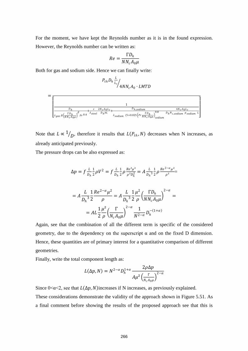
266
For the moment, we have kept the Reynolds number as it is in the found expression.
However, the Reynolds number can be written as:
𝑅𝑒 =Γ𝐷
𝑁𝑁𝑐𝐴0𝜇
Both for gas and sodium side. Hence we can finally write:
=
𝑃𝑡𝐷𝐿
𝐿𝑐
4𝑁𝑁𝑐𝐴0 ∙ 𝐿𝑀𝑇𝐷
1𝐷
𝜆𝑔𝑎𝑠 𝐵 Γ𝐷
𝑁𝑁𝑐𝐴0𝜇 𝛽𝑃𝑟 0.4
+휀
𝜆𝑠𝑡𝑒𝑒𝑙
2𝑁𝑐𝐴0𝐿𝑐𝐷𝑏𝐿
+𝐷 ,𝑠𝑜𝑑𝑖𝑢𝑚
𝜆𝑠𝑜𝑑𝑖𝑢𝑚 (5+0.025 𝑃𝑟Γ𝐷
𝑁𝑁𝑐𝐴0𝜇 𝑠𝑜𝑑𝑖𝑢𝑚
0.84𝑁𝑐𝐴0𝐿𝑐
𝐷𝑁𝑐 ,𝑠𝑜𝑑𝑖𝑢𝑚 𝑝𝑠𝑜𝑑𝑖𝑢𝑚 𝐿
Note that 𝐿 ∝ 1𝐷 , therefore it results that 𝐿 𝑃𝑡 , 𝑁 decreases when N increases, as
already anticipated previously.
The pressure drops can be also expressed as:
∆𝑝 = 𝑓𝐿
𝐷
1
2𝜌𝑉2 = 𝑓
𝐿
𝐷
1
2𝜌
𝑅𝑒²𝜇²
𝜌²𝐷2 = 𝐴
𝐿
𝐷3
1
2𝜌
𝑅𝑒 2−𝛼𝜇²
𝜌²=
= 𝐴𝐿
𝐷3
1
2
𝑅𝑒2−𝛼𝜇2
𝜌= 𝐴
𝐿
𝐷3
1
2
𝜇2
𝜌
Γ𝐷
𝑁𝑁𝑐𝐴0𝜇
2−𝛼
=
= 𝐴𝐿1
2
𝜇²
𝜌
Γ
𝑁𝑐𝐴0𝜇
2−𝛼 1
𝑁2−𝛼𝐷
− 1+𝛼
Again, see that the combination of all the different term is specific of the considered
geometry, due to the dependency on the superscript α and on the fixed D dimension.
Hence, these quantities are of primary interest for a quantitative comparison of different
geometries.
Finally, write the total component length as:
𝐿 ∆𝑝, 𝑁 = 𝑁2−𝛼𝐷1+𝛼
2𝜌∆𝑝
𝐴𝜇² Γ
𝑁𝑐𝐴0𝜇
2−𝛼
Since 0<α<2, see that 𝐿 ∆𝑝, 𝑁 increases if N increases, as previously explained.
These considerations demonstrate the validity of the approach shown in Figure 5.51. As
a final comment before showing the results of the proposed approach see that this is
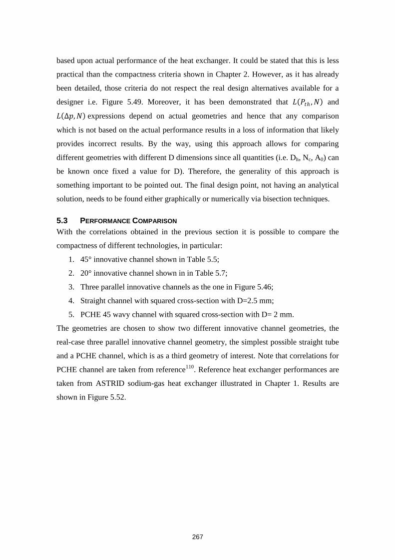
267
based upon actual performance of the heat exchanger. It could be stated that this is less
practical than the compactness criteria shown in Chapter 2. However, as it has already
been detailed, those criteria do not respect the real design alternatives available for a
designer i.e. Figure 5.49. Moreover, it has been demonstrated that 𝐿 𝑃𝑡 , 𝑁 and
𝐿 ∆𝑝, 𝑁 expressions depend on actual geometries and hence that any comparison
which is not based on the actual performance results in a loss of information that likely
provides incorrect results. By the way, using this approach allows for comparing
different geometries with different D dimensions since all quantities (i.e. Dh, Nc, A0) can
be known once fixed a value for D). Therefore, the generality of this approach is
something important to be pointed out. The final design point, not having an analytical
solution, needs to be found either graphically or numerically via bisection techniques.
5.3 PERFORMANCE COMPARISON
With the correlations obtained in the previous section it is possible to compare the
compactness of different technologies, in particular:
1. 45° innovative channel shown in Table 5.5;
2. 20° innovative channel shown in in Table 5.7;
3. Three parallel innovative channels as the one in Figure 5.46;
4. Straight channel with squared cross-section with D=2.5 mm;
5. PCHE 45 wavy channel with squared cross-section with D= 2 mm.
The geometries are chosen to show two different innovative channel geometries, the
real-case three parallel innovative channel geometry, the simplest possible straight tube
and a PCHE channel, which is as a third geometry of interest. Note that correlations for
PCHE channel are taken from reference110
. Reference heat exchanger performances are
taken from ASTRID sodium-gas heat exchanger illustrated in Chapter 1. Results are
shown in Figure 5.52.
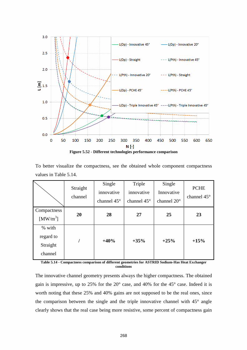
268
Figure 5.52 - Different technologies performance comparison
To better visualize the compactness, see the obtained whole component compactness
values in Table 5.14.
Straight
channel
Single
innovative
channel 45°
Triple
innovative
channel 45°
Single
Innovative
channel 20°
PCHE
channel 45°
Compactness
[MW/m3]
20 28 27 25 23
% with
regard to
Straight
channel
/ +40% +35% +25% +15%
Table 5.14 - Compactness comparison of different geometries for ASTRID Sodium-Has Heat Exchanger
conditions
The innovative channel geometry presents always the higher compactness. The obtained
gain is impressive, up to 25% for the 20° case, and 40% for the 45° case. Indeed it is
worth noting that these 25% and 40% gains are not supposed to be the real ones, since
the comparison between the single and the triple innovative channel with 45° angle
clearly shows that the real case being more resistive, some percent of compactness gain

269
could be lost. Hence, even if a value of 35% for the 45° innovative channel geometry
and 20% (author’s best estimate) for the 20° geometry are foreseen as the more real
ones, anyway it represents an important result. Note that the drawback of additional
pressure drop created by the additional mixing zones for the real channel case (see
Figure 5.46) could be eliminated if the distance between innovative channels is large
enough to allow for having separated channel not intersecting each other on their bends.
However, this presumably high distance would deteriorate the global component
compactness. In any way, the innovative channel compactness improvement is even
more impressive when looking at the PCHE, which is an existing technology more and
more used in the industry when dealing with heat exchangers. PCHE at 45° seems to
provide a smaller gain, compared to the innovative channel geometry. See that it could
be considered as illogical that the innovative geometry, which is the most resistive
among the studied geometries, is always the most compact one. Indeed this is not
surprising at all: in fact, a more resistive geometry leads the designer to reduce the heat
exchanger length (as shown) to meet the pressure drop value goal. This is obviously
favorable if the heat exchanger can deal, in that lower volume, the same thermal load.
The major parameter of interest for a compact heat exchanger is therefore the heat
transfer surface to volume ratio, which is higher for the innovative channel, as shown in
Chapter 5 section 4.3. Hence it is clear that the interest given by the innovative
geometry is due to the fact that the global length has to be reduced to meet the pressure
drop value, reducing the total volume of the component keeping the right heat transfer
surface. Even if additional plates are to be added (see Figure 5.49) the final design point
is always more compact than any other known industrial technology. This is obviously
more true if the number of plates to be added is not excessive: in fact in that case, too
short plates would be designed, which could be a potential drawback for other design
constraints such as thermal-mechanical resistance. As a final comment see that, based
on purely thermal-hydraulic considerations, the most compact geometry is that of 45°
D=2mm.
6. PROPOSED DESIGN FOR ASTRID Na/N2 HEAT EXHANGER
The previous section showed some correlations and the different geometry comparison
for innovative channel-, PCHE- and straight tube-based compact heat exchangers. It has
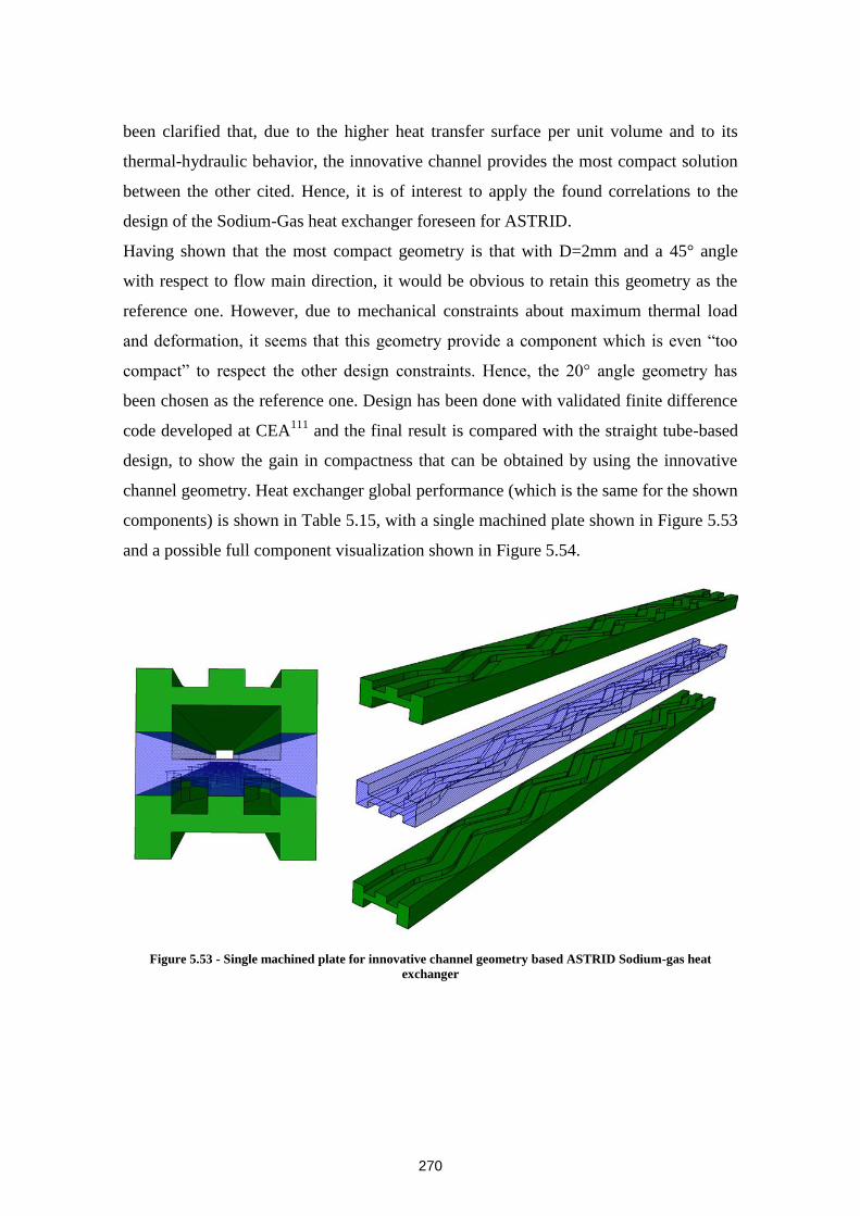
270
been clarified that, due to the higher heat transfer surface per unit volume and to its
thermal-hydraulic behavior, the innovative channel provides the most compact solution
between the other cited. Hence, it is of interest to apply the found correlations to the
design of the Sodium-Gas heat exchanger foreseen for ASTRID.
Having shown that the most compact geometry is that with D=2mm and a 45° angle
with respect to flow main direction, it would be obvious to retain this geometry as the
reference one. However, due to mechanical constraints about maximum thermal load
and deformation, it seems that this geometry provide a component which is even “too
compact” to respect the other design constraints. Hence, the 20° angle geometry has
been chosen as the reference one. Design has been done with validated finite difference
code developed at CEA111
and the final result is compared with the straight tube-based
design, to show the gain in compactness that can be obtained by using the innovative
channel geometry. Heat exchanger global performance (which is the same for the shown
components) is shown in Table 5.15, with a single machined plate shown in Figure 5.53
and a possible full component visualization shown in Figure 5.54.
Figure 5.53 - Single machined plate for innovative channel geometry based ASTRID Sodium-gas heat
exchanger
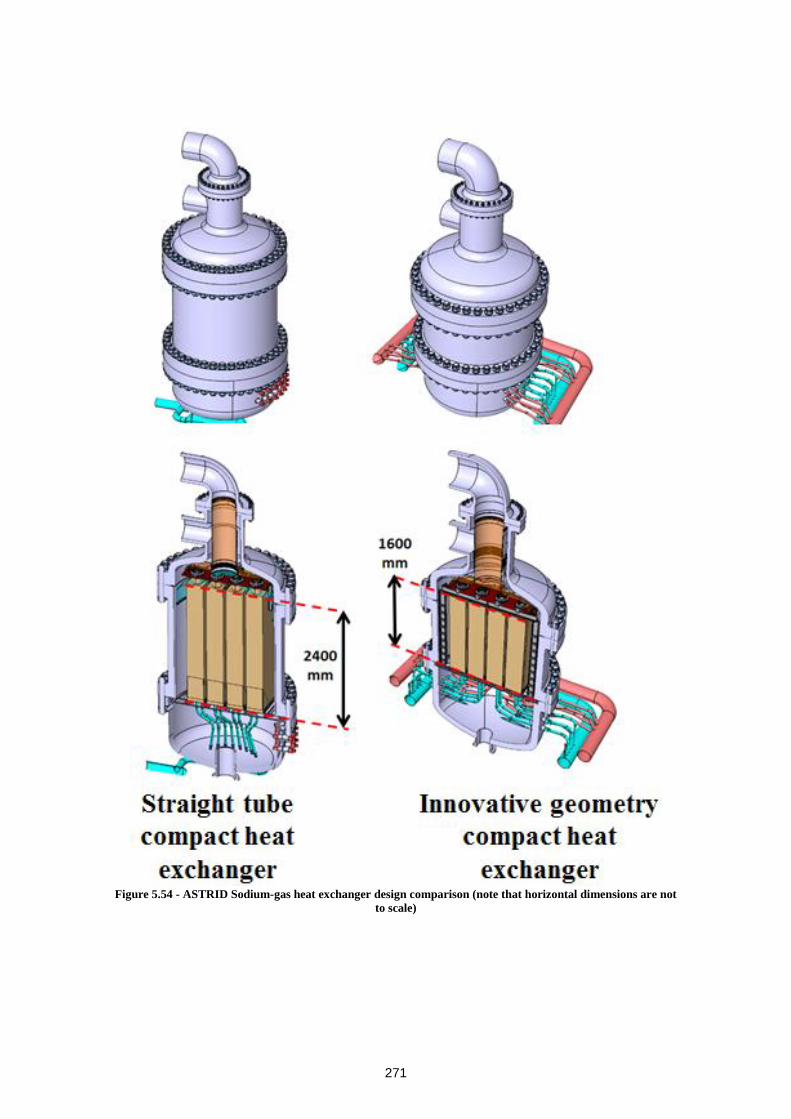
271
Figure 5.54 - ASTRID Sodium-gas heat exchanger design comparison (note that horizontal dimensions are not
to scale)
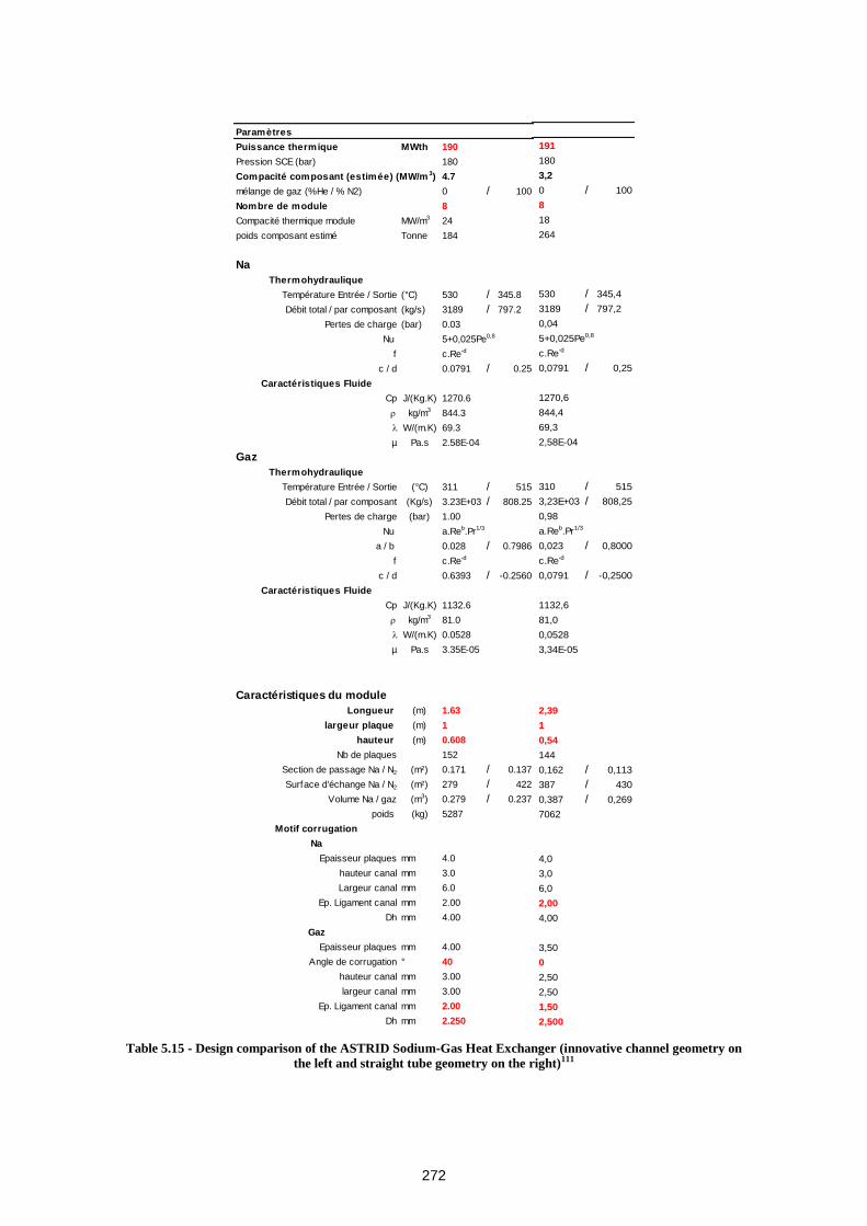
272
Table 5.15 - Design comparison of the ASTRID Sodium-Gas Heat Exchanger (innovative channel geometry on
the left and straight tube geometry on the right)111
Paramètres
Puissance thermique MWth 190
Pression SCE (bar) 180
Compacité composant (estimée) (MW/m 3) 4.7
mélange de gaz (%He / % N2) 0 / 100
Nombre de module 8
Compacité thermique module MW/m3 24
poids composant estimé Tonne 184
Na
Thermohydraulique
Température Entrée / Sortie (°C) 530 / 345.8
Débit total / par composant (kg/s) 3189 / 797.2
Pertes de charge (bar) 0.03
Nu 5+0,025Pe0,8
f c.Re-d
c / d 0.0791 / 0.25
Caractéristiques Fluide
Cp J/(Kg.K) 1270.6
kg/m3 844.3
W/(m.K) 69.3
µ Pa.s 2.58E-04
Gaz
Thermohydraulique
Température Entrée / Sortie (°C) 311 / 515
Débit total / par composant (Kg/s) 3.23E+03 / 808.25
Pertes de charge (bar) 1.00
Nu a.Reb.Pr1/3
a / b 0.028 / 0.7986
f c.Re-d
c / d 0.6393 / -0.2560
Caractéristiques Fluide
Cp J/(Kg.K) 1132.6
kg/m3 81.0
W/(m.K) 0.0528
µ Pa.s 3.35E-05
Caractéristiques du module
Longueur (m) 1.63
largeur plaque (m) 1
hauteur (m) 0.608
Nb de plaques 152
Section de passage Na / N2 (m²) 0.171 / 0.137
Surface d'échange Na / N2 (m²) 279 / 422
Volume Na / gaz (m3) 0.279 / 0.237
poids (kg) 5287
Motif corrugation
Na
Epaisseur plaques mm 4.0
hauteur canal mm 3.0
Largeur canal mm 6.0
Ep. Ligament canal mm 2.00
Dh mm 4.00
Gaz
Epaisseur plaques mm 4.00
Angle de corrugation ° 40
hauteur canal mm 3.00
largeur canal mm 3.00
Ep. Ligament canal mm 2.00
Dh mm 2.250
Paramètres
Puissance thermique MWth 191
Pression SCE (bar) 180
Compacité composant (estimée) (MW/m 3) 3,2
mélange de gaz (%He / % N2) 0 / 100
Nombre de module 8
Compacité thermique module MW/m3 18
poids composant estimé Tonne 264
Na
Thermohydraulique
Température Entrée / Sortie (°C) 530 / 345,4
Débit total / par composant (kg/s) 3189 / 797,2
Pertes de charge (bar) 0,04
Nu 5+0,025Pe0,8
f c.Re-d
c / d 0,0791 / 0,25
Caractéristiques Fluide
Cp J/(Kg.K) 1270,6
kg/m3 844,4
W/(m.K) 69,3
µ Pa.s 2,58E-04
Gaz
Thermohydraulique
Température Entrée / Sortie (°C) 310 / 515
Débit total / par composant (Kg/s) 3,23E+03 / 808,25
Pertes de charge (bar) 0,98
Nu a.Reb.Pr1/3
a / b 0,023 / 0,8000
f c.Re-d
c / d 0,0791 / -0,2500
Caractéristiques Fluide
Cp J/(Kg.K) 1132,6
kg/m3 81,0
W/(m.K) 0,0528
µ Pa.s 3,34E-05
Caractéristiques du module
Longueur (m) 2,39
largeur plaque (m) 1
hauteur (m) 0,54
Nb de plaques 144
Section de passage Na / N2 (m²) 0,162 / 0,113
Surface d'échange Na / N2 (m²) 387 / 430
Volume Na / gaz (m3) 0,387 / 0,269
poids (kg) 7062
Motif corrugation
Na
Epaisseur plaques mm 4,0
hauteur canal mm 3,0
Largeur canal mm 6,0
Ep. Ligament canal mm 2,00
Dh mm 4,00
Gaz
Epaisseur plaques mm 3,50
Angle de corrugation ° 0
hauteur canal mm 2,50
largeur canal mm 2,50
Ep. Ligament canal mm 1,50
Dh mm 2,500
273
The design is based on an eight-module heat exchanger. Actual dimensions show the
gain in compactness shown in Table 5.15. In particular, note how the proposed
comparison approach, even if employs several simplifying assumptions, can give a very
good prediction of the final design point in terms of number of plates and total
component length. In fact, see in Figure 5.52 that both the component length and
number of gas plates (i.e. half of the total number of plates in Table 5.15) are very well
predicted by the proposed approach for the 20° innovative channel case, whereas
slightly higher differences are found for the straight channel case due to the different
heat transfer and pressure drop correlations used for data in Table 5.15 (i.e. Pethukov-
Gnielinski correlations instead of Blausius and Dittus-Boelter-McAdams)111
.In any
case, always remember that the used correlations for the design of the innovative
channel geometry with α=20° are those shown in Table 5.11, which do not take into
account the actual geometry with several parallel channels. Since it has demonstrated
that the innovative real geometry (i.e. several innovative single channels intersecting
each other on their bends) is slightly less compact than the innovative single channel
geometry (see Table 5.15), it can be stated that the proposed design is slightly optimistic
and that a lower gain would be achieved. However, as a last comment, remember that
the 20° geometry has been chosen due to the nuclear-related mechanical constraints.
This means that, for an application which requires less strict mechanical performance or
pressure drop constraints, a dramatic gain in compactness could be obtain by more
compact geometries, i.e. the previously mentioned D=2mm 45° one.
7. CONCLUSIONS
In the present Chapter the analysis of the innovative channel flow has been done, to
identify the physical phenomena ongoing in the channel as well as its thermal-hydraulic
performance.
Principal and secondary flow has been analyzed, with LDV and PIV experimental data
and ASST numerical results. For the bend flow, an unusual high velocity region in the
inner bend has been shown, whereas for the secondary flow an initial vortex evolving in
a three vortices structure has been identified. This behavior is essentially due to the inlet
bend flow coming from the mixing zone outlet. In the mixing zone, actual occurring
mixing has been demonstrated, due to secondary velocity field from the bend outlet and
to viscous entrainment of the opposite channel secondary flow velocity.
274
Once explained the steady-state flow phenomena, thermal hydraulic behavior of the
innovative channel has been studied. Correlations for friction factor and Nusselt number
for various geometries have been obtained. With the correlations, a new compactness
comparison has been proposed: it takes into account design constraints, in particular the
fact that different compared technologies have the same exchanger thermal power and
pressure drop. With this approach, it has been shown that the innovative channel is the
most compact one among the most important existing industrial compact heat exchanger
technologies.
A final ASTRID Sodium-gas heat exchanger design has been proposed, which
demonstrates that 25% compactness can be gained when adopting the innovative
channel geometry if compared to a traditional straight-tube-based compact heat
exchanger technology. Even higher compactness can be achieved if the designer has
less important mechanical and/or pressure drop constraints.
275
Chapitre 6: Conclusions et Perspectives
Dans le cadre du programme CEA R&D pour développer un prototype industriel de
RNR-Na, nommé ASTRID, une technologie d'échangeur de chaleur compact
innovante est en cours de développement pour l'utilisation d'un système de conversion
de l'énergie à cycle Brayton. L’objectif de ce travail de thèse a consisté à mettre en
place un travail de recherche visant à évaluer le potentiel, en termes d’efficacité
thermique et de résistance aéraulique, de motifs d’échange innovant.
Parmi les technologies existantes d'échangeurs de chaleur compacts, l'échangeur de
chaleur à tôles embouties (PSHE), a été identifié car il offre potentiellement la
solution la plus compacte. La conclusion de l'étude bibliographique nous a permis de
comprendre qu'un écoulement complexe 3-D des PSHEs permet d'augmenter de
manière significative les performances de transfert de chaleur. D'autre part, la faible
résistance mécanique de cette technologie est souvent considérée comme trop
limitative pour une application industrielle plus large pour des écoulements à haute
pression. Dans ce cadre, il existe une technologie d'échangeur de chaleur compact qui
peut potentiellement supporter cette différence de pression: la technologie d'échangeur
de chaleurs à circuit imprimé (PCHE). Par conséquent, afin d'augmenter la compacité
globale du composant un canal innovant est proposé. Le canal peut être considéré
comme le résultat de la superposition de deux canaux ondulés type PCHE en
opposition de phase.
Afin de fournir un modèle numérique physiquement cohérent, et industriellement
utilisable, un nouveau modèle de turbulence à viscosité turbulente non linéaire nommé
"Anisotropic Shear Stress Transport" model (ASST) a été développé et implémenté
dans le solveur ANSYS FLUENT ®. Il a été démontré que le modèle ASST peut
fournir une alternative intéressante aux modèles plus complexes (par exemple les
modèles type transport des tensions de Reynolds) pour une variété d'écoulements,
donnant des résultats globaux qui sont au moins aussi bons que ceux du modèle Stress
Omega, beaucoup plus couteux en temps de calcul.
Compte tenu de l'innovation de la géométrie actuelle, aucun cas-test de validation n'a
été trouvé dans la littérature pour être pleinement applicable à la géométrie innovante.
276
Ainsi, deux sections expérimentales ont été utilisées pour obtenir une base de données
aérodynamique fiable. La campagne de Vélocimétrie Laser à franges (LDV) nous a
permis d'acquérir une très grande base de données sur les vitesses d'écoulement et les
fluctuations de vitesse dans plusieurs régions du canal innovant. D'autre part, un banc
d'essai de Vélocimétrie Laser par images de particules (PIV) a été utilisé pour étudier
les phénomènes globaux qui se produisent dans le canal innovant qui n'ont pas été
observés au cours de la campagne LDV.
Ensuite, l'analyse numérique de l'écoulement avec le modèle développé ASST dans le
canal innovant a été faite avec les données d’entrées des expérimentations afin
d’évaluer la performance du modèle. Une fois validée, la modélisation a permis
d’étudier en détails le comportement aéraulique du canal innovant.
Pour la partie thermique, l'installation "VHEGAS" a été construite pour mesurer le
coefficient de transfert de chaleur global dans le canal innovant. Le modèle ASST est
utilisé avec un modèle thermique SGDH; ils ont été validés avec les données
expérimentales de "VHEGAS", en montrant que le coefficient de transfert de chaleur
calculé se situe dans la plage d'incertitude expérimentale (+ 20%).
Le modèle ASST est donc validé d’un point de vue thermo-hydraulique. Par
conséquent, les corrélations pour le coefficient de frottement et le nombre de Nusselt
pour différentes géométries peuvent être calculées. En comparant différentes
géométries, il a été montré que la géométrie innovante est la plus compacte parmi les
autres technologies d'échangeur de chaleurs compactes.
Enfin, une conception de l'échangeur de chaleur sodium-gaz d'ASTRID a été
proposée, démontrant qu'un gain de compacité de 25% peut être acquis lors de
l'adoption de la géométrie du canal innovant par rapport à une technologie d'échangeur
de chaleur compact à base de canaux droits plus classiques.
Ce travail constitue une première étape pour l'évaluation d'une géométrie de transfert
de chaleur innovant qui peut fournir à la fois une très grande compacité et une
résistance mécanique élevée. Même si le travail accompli jusqu'à présent a fourni des
informations précieuses, de nombreux points restent encore à être approfondis.
Le nouveau modèle ASST de turbulence proposé couple le modèle SST avec une
formulation non-linéaire d'ordre deux des tensions de Reynolds. Cependant, comme il
277
a été mentionné dans le Chapitre 3, une formulation d'ordre trois saurait mieux rendre
compte du swirling, qui est un phénomène survenant dans le canal innovant, comme
on l'a souligné dans le chapitre 5.
L'approche de modélisation de ce travail a été basée sur des modèles de turbulence
RANS. Cependant, d'autres modèles plus fins peuvent être utilisés pour étudier les
caractéristiques d'écoulement des canaux innovants. Si la LES pourrait être une
solution difficile à cause du temps de calcul très élevée, le modèle SAS pourrait
fournir une solution très intéressante, car l'approche URANS permettrait d'étudier
l'écoulement des fluides dans la décomposition du spectre des fréquences. Cette
décomposition pourrait montrer les contributions instationnaires au transfert de
chaleur, notamment au niveau des zones de mélange.
Dans le cadre d'une étude locale, il serait intéressant d'améliorer l'approche de
modélisation thermique. En raison de contraintes de temps, seule une validation
globale a pu être faite dans ce travail de thèse. Toutefois, afin de mieux mettre en
évidence les contributions locales au transfert thermique, un banc d’essai spécifique
doit être conçu et construit, probablement à grande échelle pour être en mesure
d'utiliser un grand nombre de thermocouples sans perturber l'écoulement du fluide.
Cette analyse locale peut être numériquement étudiée par un modèle à flux de chaleur
turbulent algébrique (EAHFM), ce qui pourrait mieux expliquer le transfert de
chaleur, en particulier dans un écoulement très turbulent tel que celui des canaux
innovants grâce aux fluctuations du flux de chaleur turbulent dans les trois
dimensions.
Pour effectuer une optimisation de la géométrie, une étude paramétrique approfondie
sur le paramètre géométrique du canal innovant devrait être faite. Une première étude
paramétrique a été effectuée en utilisant le modèle SST et le modèle de SGDH.
Cependant, les corrélations d’échange thermique et de pertes de charge calculées
doivent être mises à jour en utilisant au moins le modèle ASST couplé au modèle
SDGH en fonction des résultats de la validation thermique.
« Last but not least », il sera très intéressant de comparer différentes sections de
canaux innovants pour vérifier si une section de passage du fluide rectangulaire
donnant une section transversale totale carrée est la meilleure possible en termes de

278
performance. En fait, le motif innovant pourrait se décliner en différentes sections de
canal ondulé, soit triangulaire, semi-circulaire, trapézoïdale, carrée, etc. Le
comportement thermo-hydraulique de ces canaux innovants mérite d'être étudié pour
déterminer le meilleur candidat. Même si certaines sections transversales peuvent être
considérés comme «exotiques» et industriellement irréalisables, la section semi-
circulaire ou semi-éliptique semble être très intéressante en raison de sa possible
fabrication par usinage électrochimique.
279
Chapter 6: Conclusions and
Perspectives
1. CONCLUSIONS
In the framework of CEA R&D program to develop an industrial prototype of Sodium-
cooled Fast Reactor, the present thesis aimed to propose an innovative compact heat
exchanger technology to provide solid technological basis for the utilization of a
Brayton Gas-power conversion system, in order to avoid the energetic sodium-water
interaction if a traditional Rankine cycle was used. The design of the gas-side (which
determines the heat transfer resistance of the heat exchanger) of the Sodium-gas heat
exchanger has been the object of the present work. Compact technologies are necessary
for the present application because of the low heat transfer capacity of the gas foreseen,
i.e. nitrogen. Among the compact heat exchanger existing technologies, Plate Stamped
Heat Exchanger (PSHE), has been identified since it potentially provides the most
compact solution. Therefore the present work started studying the PSHE technology, to
investigate its thermal-hydraulic behavior and to understand the physical phenomena
providing the efficient heat transfer.
The conclusion of the bibliographic review led us to understand that the complex 3-D
flow of the PSHEs makes it possible to significantly increase the heat transfer
performances of the component (see Section 2.2). On the other hand, the low
mechanical resistance of this technology is often seen as too limiting for a wider
industrial application for high-pressure flow such as that of a nuclear reactor loop. In
fact, if PSHEs provide a relatively high heat transfer coefficient, on the other hand, they
do not seem to be able to provide sufficiently good mechanical resistance to withstand
working conditions (temperature and pressure) foreseen for ASTRID. In this sense it
does exist a compact heat exchanger technology that can potentially stand this pressure
difference: the Printed Circuit Heat Exchanger (PCHE) technology, using diffusion
bonding as welding process.
Hence, in order to increase the heat transfer coefficient (and the global
compactness) the basic idea of this work is to design a channel were the fluid flow is as
much three-dimensional as possible.
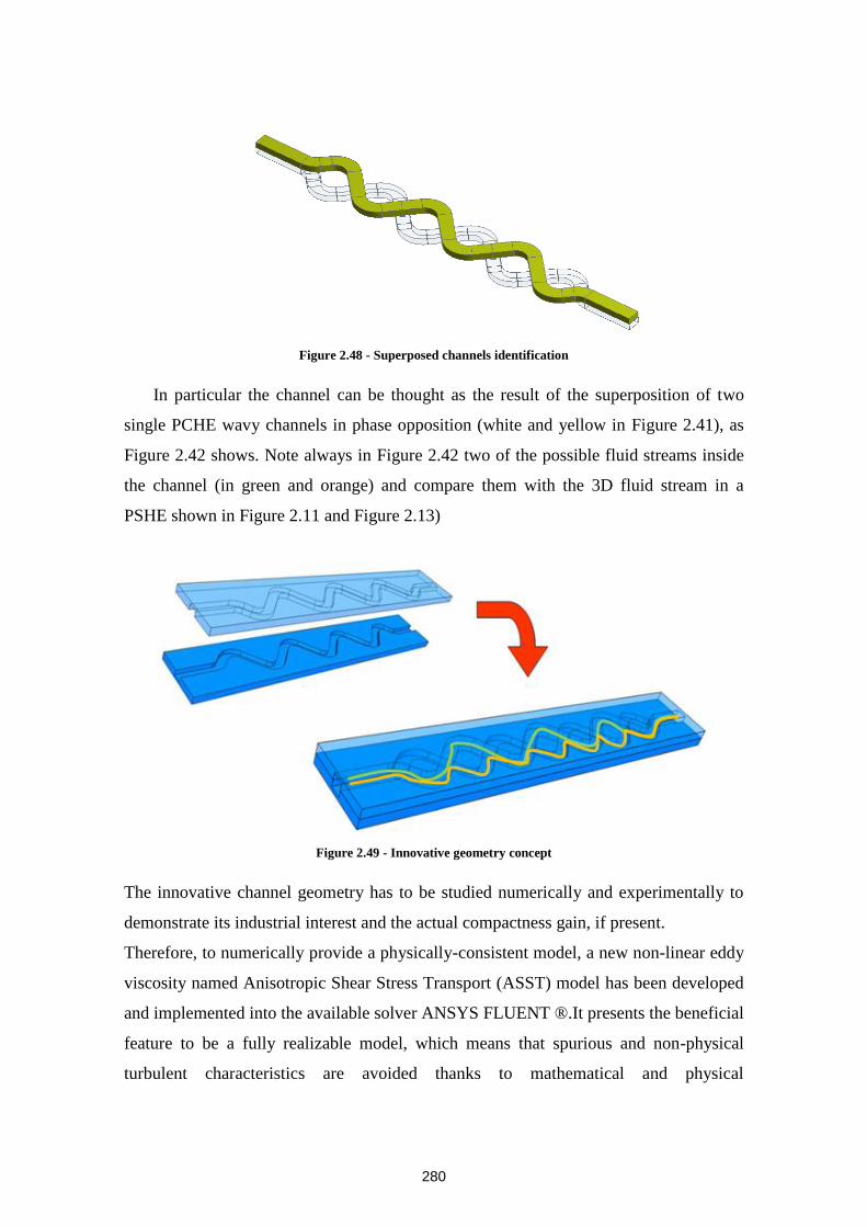
280
Figure 2.48 - Superposed channels identification
In particular the channel can be thought as the result of the superposition of two
single PCHE wavy channels in phase opposition (white and yellow in Figure 2.41), as
Figure 2.42 shows. Note always in Figure 2.42 two of the possible fluid streams inside
the channel (in green and orange) and compare them with the 3D fluid stream in a
PSHE shown in Figure 2.11 and Figure 2.13)
Figure 2.49 - Innovative geometry concept
The innovative channel geometry has to be studied numerically and experimentally to
demonstrate its industrial interest and the actual compactness gain, if present.
Therefore, to numerically provide a physically-consistent model, a new non-linear eddy
viscosity named Anisotropic Shear Stress Transport (ASST) model has been developed
and implemented into the available solver ANSYS FLUENT ®.It presents the beneficial
feature to be a fully realizable model, which means that spurious and non-physical
turbulent characteristics are avoided thanks to mathematical and physical
281
considerations. It has been demonstrated that the ASST model can provide a valuable
alternative to more complex models (i.e. Reynolds Stress Transport models) for a
variety of flows, giving global results that are at least as good as those of the Stress
Omega model. Moreover, it keeps a very shorter computational time than the Stress
Omega model, resulting to be a very good option for the desired industrial tool to
potentially describe the innovative channel flow.
Given the innovation of the present geometry, no actual test case has been found in the
literature to be fully applicable to the present study. So, two experimental sections have
been used to acquire an extensive aerodynamic database. The Laser Doppler
Velocimetry (LDV) campaign allowed us acquiring a very large database on flow
velocities and velocity fluctuations in several regions of the innovative channel. These
data are helpful for the numerical model validation, since they give a full representation
of the fine phenomena occurring in the fluid flow bulk as well as in the boundary layer.
On the other hand, a Particle Image Velocimetry (PIV) technique has been used to study
global phenomena occurring in the innovative channel flow that have not been observed
during the LDV campaign and that have been discussed. To give a further double-check
to the PIV with regard to LDV measurements, a comparison of velocity profiles in
equivalent geometrical places has been shown, demonstrating thatthe two velocity
profiles are almost identical, even though Reynolds numbers were different and hence
no exact consistency could be expected.
Then, the analysis of the innovative channel flow has been done, to identify the physical
phenomena ongoing in the channel as well as its thermal-hydraulic performance.
Principal and secondary flow has been analyzed, with LDV and PIV experimental data
and ASST numerical results. For the bend flow, an unusual high velocity region in the
inner bend has been shown, whereas for the secondary flow an initial vortex evolving in
a three vortices structure has been identified, and it has been shown that this behavior is
due to the inlet bend condition from the mixing zone. Here, high mixing has been
demonstrated, due to secondary velocity field from the bend outlet and to viscous
entrainment of the opposite channel secondary flow velocity.
Once explained the steady-state flow phenomena, thermal hydraulic behavior of the
innovative channel has been studied.
282
To do that, the VHEGAS facility has been built to investigate the innovative channel
global heat transfer coefficient. The ASST model used with a SGDH thermal model has
been validated against VHEGAS experimental data, showing that, under proper
conditions, the computed heat transfer coefficient lies within the experimental
uncertainty range. Hence, once having done the validation of the pure aerodynamic and
the coupled thermal-hydraulic model, correlations for friction factor and Nusselt
number for various geometries could be obtained. With the correlations, a compactness
comparison strategy has been developed: it takes into account design constraints, in
particular the fact that different compared technologies have the same exchanger
thermal power and pressure drop. With this strategy, it has been shown that the
innovative channel is the most compact one among the most important existing
industrial compact heat exchanger technologies.
A final ASTRID Sodium-gas heat exchanger design has been proposed, which
demonstrates that a 25% compactness can be gained when adopting the innovative
channel geometry if compared to a traditional straight-tube-based compact heat
exchanger technology. Even higher compactness can be achieved if the designer has
less important mechanical and/or pressure drop constraints.
2. PERSPECTIVES
The present work represents a first step for the assessment of an innovative heat transfer
geometry which can provide both a very high compactness and high mechanical
resistance to pressure gradients between the two sides of the heat exchanger. Even
though the work done so far has provided valuable information, many points are still to
be investigated further.
1. The new proposed ASST turbulence model coupled the linear SST model with a 2nd
order non-linear Reynolds stress formulation. However, as it has been mentioned in
Chapter 3, a 3rd
order formulation would better account for flow swirling, which is
an occurring phenomenon in the innovative channel, as highlighted in Chapter 5.
For example, Baglietto et al. proposed the following 3rd
order formulation, which
could be a starting point for ASST model improving:
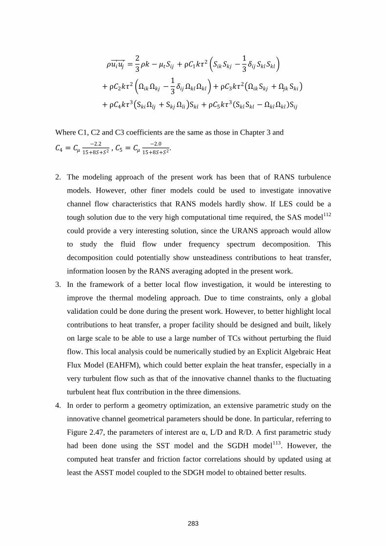
283
𝜌𝑢𝑖′𝑢𝑗
′ =2
3𝜌𝑘 − 𝜇𝑡𝑆𝑖𝑗 + ρ𝐶1𝑘𝜏
2 𝑆𝑖𝑘𝑆𝑘𝑗 −1
3𝛿𝑖𝑗 𝑆𝑘𝑙𝑆𝑘𝑙
+ ρ𝐶2𝑘𝜏2 Ω𝑖𝑘Ω𝑘𝑗 −
1
3𝛿𝑖𝑗Ω𝑘𝑙Ω𝑘𝑙 + ρ𝐶3𝑘𝜏
2 Ω𝑖𝑘S𝑘𝑗 + Ω𝑗𝑘 S𝑘𝑖
+ ρ𝐶4𝑘𝜏3 S𝑘𝑖Ω𝑙𝑗 + S𝑘𝑗 Ω𝑙𝑖 S𝑘𝑙 + ρ𝐶5𝑘𝜏
3 S𝑘𝑙S𝑘𝑙 − Ω𝑘𝑙Ω𝑘𝑙 S𝑖𝑗
Where C1, C2 and C3 coefficients are the same as those in Chapter 3 and
𝐶4 = 𝐶𝜇−2.2
15+8𝑆+𝑆2 , 𝐶5 = 𝐶𝜇
−2.0
15+8𝑆+𝑆2.
2. The modeling approach of the present work has been that of RANS turbulence
models. However, other finer models could be used to investigate innovative
channel flow characteristics that RANS models hardly show. If LES could be a
tough solution due to the very high computational time required, the SAS model112
could provide a very interesting solution, since the URANS approach would allow
to study the fluid flow under frequency spectrum decomposition. This
decomposition could potentially show unsteadiness contributions to heat transfer,
information loosen by the RANS averaging adopted in the present work.
3. In the framework of a better local flow investigation, it would be interesting to
improve the thermal modeling approach. Due to time constraints, only a global
validation could be done during the present work. However, to better highlight local
contributions to heat transfer, a proper facility should be designed and built, likely
on large scale to be able to use a large number of TCs without perturbing the fluid
flow. This local analysis could be numerically studied by an Explicit Algebraic Heat
Flux Model (EAHFM), which could better explain the heat transfer, especially in a
very turbulent flow such as that of the innovative channel thanks to the fluctuating
turbulent heat flux contribution in the three dimensions.
4. In order to perform a geometry optimization, an extensive parametric study on the
innovative channel geometrical parameters should be done. In particular, referring to
Figure 2.47, the parameters of interest are α, L/D and R/D. A first parametric study
had been done using the SST model and the SGDH model113
. However, the
computed heat transfer and friction factor correlations should by updated using at
least the ASST model coupled to the SDGH model to obtained better results.

284
5. Last but not least, it will be very interesting to compare different innovative channel
geometries to verify if the assumption done in Chapter 2 of a rectangular cross
section giving a total squared cross section is the best possible. In fact, the
innovative channel can be thought as the superposition of very different single
channel cross sections, i.e. triangular, hemi-circular, trapezoidal, squared, etc (see
Figure 6.1). Thermal-hydraulic behavior of such innovative channels is worth being
studied to determine the best candidate. Even if some cross-sections might be
considered as “exotic” and industrially unfeasible, the hemi-circular cross-section
appears to be very interesting due to its possible fabrication via chemical machining.
Figure 6.1 - Possible innovative channel cross-section geometries to be studied

285
APPENDIX A – DIFFERENTLY DEFINED PSHE CORRELATION CONVERSION FACTORS
It is important to show the correlation between the definition of Nusselt number and
friction factor, using the hydraulic diameter or the equivalent diameter.
It is straightforward that
eh
DD ; therefore there will be the same relation for the
two differently defined Reynolds and Nusselt numbers: in particular it will be
e
h
eRRe and
e
h
NuNu , with obvious meaning of the subscripts “h” and “e”. The
opposite is for the definition of the friction factor, which depends on the inverse of the
hydraulic/equivalent diameter. Hence:
he
e
e
h
h ffD
fD
f 1
,1
Now consider the general type of correlation for Nusselt number and friction factor
(See Correlations):
b
dc
Af
BNu
Re
RePr
Since we want:
b
hhh
b
eee
d
h
c
hh
d
e
c
ee
AfAf
BNuNu
Re,Re
RePr,RePrB
Write:
h
d
e
d
e
c
h
d
b
d
ec
h
d
h
c
he
d
h
c
hh
BB
BBBNuBNu
1
1 RePrRe
PrRePrRePr
And
h
b
e
b
eh
b
b
b
eh
b
hhe
b
hhh
AA
AAAfAf
1
1 ReRe
ReRe
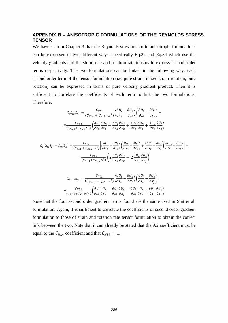
286
APPENDIX B – ANISOTROPIC FORMULATIONS OF THE REYNOLDS STRESS TENSOR
We have seen in Chapter 3 that the Reynolds stress tensor in anisotropic formulations
can be expressed in two different ways, specifically Eq.22 and Eq.34 which use the
velocity gradients and the strain rate and rotation rate tensors to express second order
terms respectively. The two formulations can be linked in the following way: each
second order term of the tensor formulation (i.e. pure strain, mixed strain-rotation, pure
rotation) can be expressed in terms of pure velocity gradient product. Then it is
sufficient to correlate the coefficients of each term to link the two formulations.
Therefore:
𝐶1𝑆𝑖𝑘𝑆𝑘𝑗 =𝐶𝑁𝐿1
𝐶𝑁𝐿4 + 𝐶𝑁𝐿5 ∙ 𝑆3 𝜕𝑈𝑖
𝜕𝑥𝑘
+𝜕𝑈𝑘
𝜕𝑥𝑖
𝜕𝑈𝑘
𝜕𝑥𝑗+
𝜕𝑈𝑗
𝜕𝑥𝑘
=
=𝐶𝑁𝐿 1
𝐶𝑁𝐿 4+𝐶𝑁𝐿 5 ∙𝑆3 𝜕𝑈𝑖
𝜕𝑥𝑘
𝜕𝑈𝑘
𝜕𝑥𝑗+
𝜕𝑈𝑖
𝜕𝑥𝑘
𝜕𝑈𝑗
𝜕𝑥𝑘+
𝜕𝑈𝑘
𝜕𝑥𝑖
𝜕𝑈𝑘
𝜕𝑥𝑗+
𝜕𝑈𝑘
𝜕𝑥𝑖
𝜕𝑈𝑗
𝜕𝑥𝑘
𝐶2 Ω𝑖𝑘𝑆𝑘𝑗 + Ω𝑗𝑘 𝑆𝑘𝑖 =𝐶𝑁𝐿2
𝐶𝑁𝐿4 + 𝐶𝑁𝐿5 ∙ 𝑆3
𝜕𝑈𝑖
𝜕𝑥𝑘−
𝜕𝑈𝑘
𝜕𝑥𝑖
𝜕𝑈𝑘
𝜕𝑥𝑗+
𝜕𝑈𝑗
𝜕𝑥𝑘 +
𝜕𝑈𝑗
𝜕𝑥𝑘−
𝜕𝑈𝑘
𝜕𝑥𝑗
𝜕𝑈𝑘
𝜕𝑥𝑖+
𝜕𝑈𝑖
𝜕𝑥𝑘 =
=𝐶𝑁𝐿 2
𝐶𝑁𝐿 4+𝐶𝑁𝐿 5 ∙𝑆3 2
𝜕𝑈𝑖
𝜕𝑥𝑘
𝜕𝑈𝑗
𝜕𝑥𝑘− 2
𝜕𝑈𝑘
𝜕𝑥𝑖
𝜕𝑈𝑘
𝜕𝑥𝑗
𝐶3Ω𝑖𝑘Ω𝑗𝑘 =𝐶𝑁𝐿3
𝐶𝑁𝐿4 + 𝐶𝑁𝐿5 ∙ 𝑆3 𝜕𝑈𝑖
𝜕𝑥𝑘
−𝜕𝑈𝑘
𝜕𝑥𝑖
𝜕𝑈𝑗
𝜕𝑥𝑘
−𝜕𝑈𝑘
𝜕𝑥𝑗 =
=𝐶𝑁𝐿 3
𝐶𝑁𝐿 4+𝐶𝑁𝐿 5 ∙𝑆3 𝜕𝑈𝑖
𝜕𝑥𝑘
𝜕𝑈𝑗
𝜕𝑥𝑘−
𝜕𝑈𝑖
𝜕𝑥𝑘
𝜕𝑈𝑘
𝜕𝑥𝑗−
𝜕𝑈𝑘
𝜕𝑥𝑖
𝜕𝑈𝑗
𝜕𝑥𝑘+
𝜕𝑈𝑘
𝜕𝑥𝑖
𝜕𝑈𝑘
𝜕𝑥𝑗
Note that the four second order gradient terms found are the same used in Shit et al.
formulation. Again, it is sufficient to correlate the coefficients of second order gradient
formulation to those of strain and rotation rate tensor formulation to obtain the correct
link between the two. Note that it can already be stated that the A2 coefficient must be
equal to the 𝐶𝑁𝐿4 coefficient and that 𝐶𝑁𝐿5 = 1.
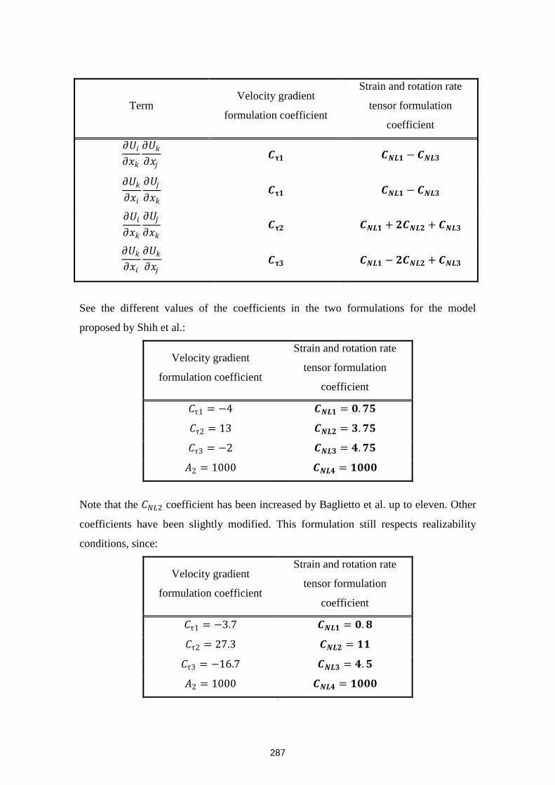
287
Term Velocity gradient
formulation coefficient
Strain and rotation rate
tensor formulation
coefficient
𝜕𝑈𝑖
𝜕𝑥𝑘
𝜕𝑈𝑘
𝜕𝑥𝑗 𝑪𝛕𝟏 𝑪𝑵𝑳𝟏 − 𝑪𝑵𝑳𝟑
𝜕𝑈𝑘
𝜕𝑥𝑖
𝜕𝑈𝑗
𝜕𝑥𝑘 𝑪𝛕𝟏 𝑪𝑵𝑳𝟏 − 𝑪𝑵𝑳𝟑
𝜕𝑈𝑖
𝜕𝑥𝑘
𝜕𝑈𝑗
𝜕𝑥𝑘 𝑪𝛕𝟐 𝑪𝑵𝑳𝟏 + 𝟐𝑪𝑵𝑳𝟐 + 𝑪𝑵𝑳𝟑
𝜕𝑈𝑘
𝜕𝑥𝑖
𝜕𝑈𝑘
𝜕𝑥𝑗 𝑪𝛕𝟑 𝑪𝑵𝑳𝟏 − 𝟐𝑪𝑵𝑳𝟐 + 𝑪𝑵𝑳𝟑
See the different values of the coefficients in the two formulations for the model
proposed by Shih et al.:
Velocity gradient
formulation coefficient
Strain and rotation rate
tensor formulation
coefficient
𝐶τ1 = −4 𝑪𝑵𝑳𝟏 = 𝟎. 𝟕𝟓
𝐶τ2 = 13 𝑪𝑵𝑳𝟐 = 𝟑. 𝟕𝟓
𝐶τ3 = −2 𝑪𝑵𝑳𝟑 = 𝟒. 𝟕𝟓
𝐴2 = 1000 𝑪𝑵𝑳𝟒 = 𝟏𝟎𝟎𝟎
Note that the 𝐶𝑁𝐿2 coefficient has been increased by Baglietto et al. up to eleven. Other
coefficients have been slightly modified. This formulation still respects realizability
conditions, since:
Velocity gradient
formulation coefficient
Strain and rotation rate
tensor formulation
coefficient
𝐶τ1 = −3.7 𝑪𝑵𝑳𝟏 = 𝟎. 𝟖
𝐶τ2 = 27.3 𝑪𝑵𝑳𝟐 = 𝟏𝟏
𝐶τ3 = −16.7 𝑪𝑵𝑳𝟑 = 𝟒. 𝟓
𝐴2 = 1000 𝑪𝑵𝑳𝟒 = 𝟏𝟎𝟎𝟎

288
With the new coefficients it results that realizability conditions are respcted:
2𝐶𝜏1 + 𝐶𝜏2 + 𝐶𝜏3 = 2 ∙ −3.7 + 27.3 − 16.7 = 3.2 > 0
𝐶τ2 = 27.3 > 2 ∙ −16.7 = −33.4
𝐶τ4 = 𝐴2 = 1000 > 0
Hence the model of Baglietto et al.(with modified coefficients) is fully realizable as
well, providing physical positive principal Reynolds stresses values, which can
potentially improve complex flow modelling and description.

289
APPENDIX C – EXAMPLE OF LDV CALIBRATION FILE
# application/x-assa
# calibration file
[Etalonnage]
Numéro=44
Date=2013-10-28
NbCanaux=2
Canaux=514,488,0
Interfranges=3.70047e-06,3.5326e-06,0
sdInterfranges=9.63382e-09,8.97233e-09,0
MatriceL1=0.00524428,0.999998,0
MatriceL2=0,0,1
MatriceL3=1.00417,-0.00548003,0
sdMatriceL1=0.00389577,2.2714e-05,0
sdMatriceL2=0,0,0
sdMatriceL3=3.42137e-05,0.00357572,0
Bragg=10 MHz,10 MHz,10 MHz
sdBragg=0.001 MHz,0.001 MHz,0.001 MHz
# "Comment" peut comporter plusieurs lignes.
Comment=RAS
[DataLink]
nCWord=0
[DataLink0]
Nom=HP
Type=OFF
A0=0.0
A1=1.0
A2=0.000000
A3=0.000000
A4=0.000000
Unité=V
Précision=3
[DataLink1]
Nom=Mic1
Type=OFF
A0=0.0
A1=1.0
A2=0.000000
A3=0.000000
A4=0.000000
Unité=V
Précision=3
[DataLink2]
Nom=Mic2
Type=OFF
A0=0.0

290
A1=1.0
A2=0.000000
A3=0.000000
A4=0.000000
Unité=V
Précision=3
[DataLink3]
Nom=Compteur
Type=OFF
A0=0.0
A1=1.0
A2=0.000000
A3=0.000000
A4=0.000000
Unité=#
Précision=0
[Banc]
# Changement d'unités de la position du volume de mesure
# selon new_xi = ai * old_xi + bi
# sachant que old_xi est toujours en mètre.
# Les bi sont réservés à des décalages fortuits.
A=1000.,1000.,1000.
B=0.,0.,0.
Unité=mm
# Passage entre le repère Vélocimètre et le repère Maquette
# Translation d'origine entre repère vélocimètre et repère
maquette
# Coordonnées du zéro maquette dans le repère vélocimètre
OvOm=0.,0.,0.
# Matrice de passage entre les repères Déplacement
# V(Rv) = MD V(Rd)
MatriceDL1=-1.0,0.0,0.0
MatriceDL2=0.0,1.0,0.0
MatriceDL3=0.0,0.0,-1.0
# Matrice de passage entre les repères Vitesse
# V(Rm) = MV V(Rv)
MatriceVL1=1.0,0.0,0.0
MatriceVL2=0.0,1.0,0.0
MatriceVL3=0.0,0.0,1.0
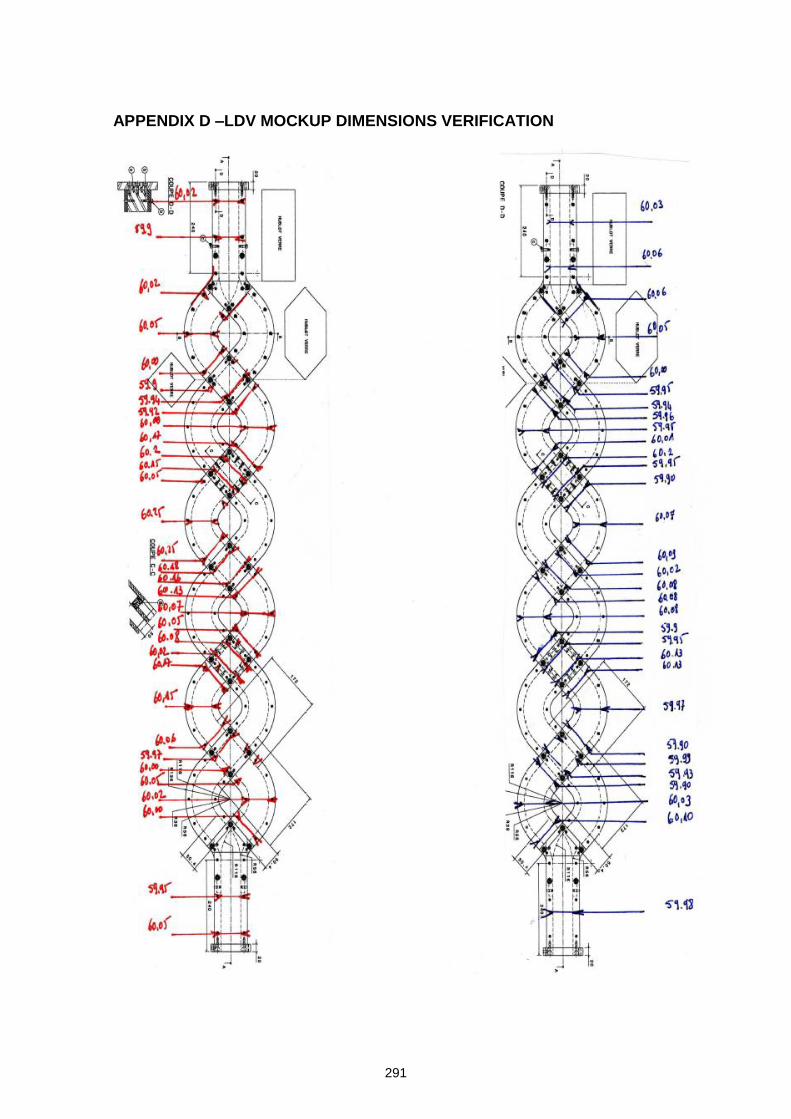
291
APPENDIX D –LDV MOCKUP DIMENSIONS VERIFICATION

292
APPENDIX E – PIV MOCKUP PLATE
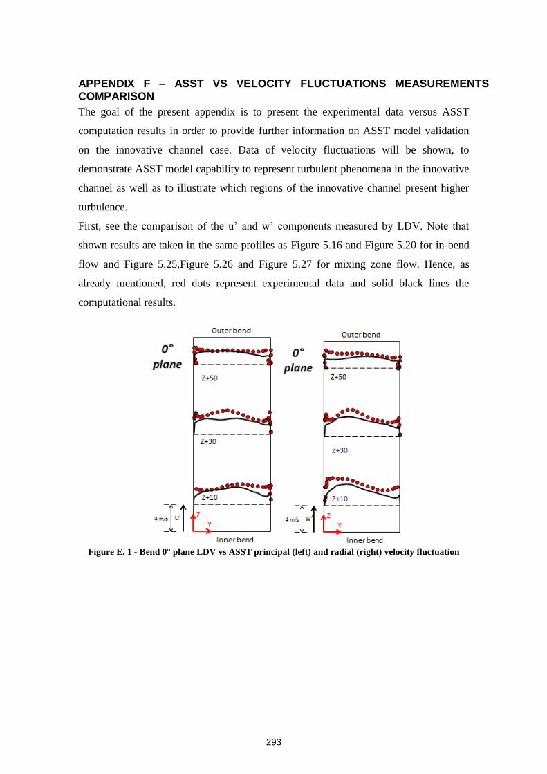
293
APPENDIX F – ASST VS VELOCITY FLUCTUATIONS MEASUREMENTS COMPARISON
The goal of the present appendix is to present the experimental data versus ASST
computation results in order to provide further information on ASST model validation
on the innovative channel case. Data of velocity fluctuations will be shown, to
demonstrate ASST model capability to represent turbulent phenomena in the innovative
channel as well as to illustrate which regions of the innovative channel present higher
turbulence.
First, see the comparison of the u’ and w’ components measured by LDV. Note that
shown results are taken in the same profiles as Figure 5.16 and Figure 5.20 for in-bend
flow and Figure 5.25,Figure 5.26 and Figure 5.27 for mixing zone flow. Hence, as
already mentioned, red dots represent experimental data and solid black lines the
computational results.
Figure E. 1 - Bend 0° plane LDV vs ASST principal (left) and radial (right) velocity fluctuation
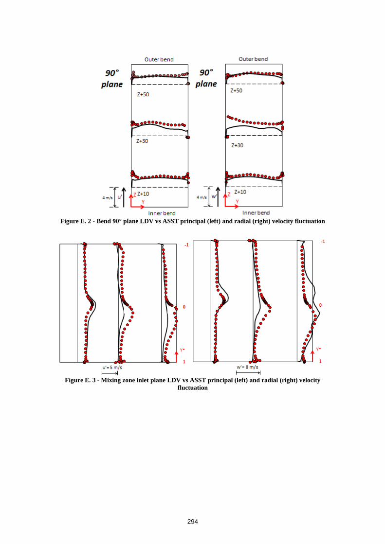
294
Figure E. 2 - Bend 90° plane LDV vs ASST principal (left) and radial (right) velocity fluctuation
Figure E. 3 - Mixing zone inlet plane LDV vs ASST principal (left) and radial (right) velocity
fluctuation
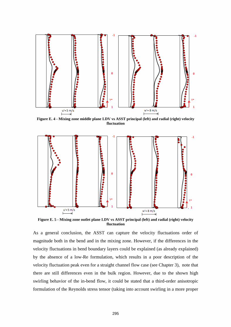
295
Figure E. 4 - Mixing zone middle plane LDV vs ASST principal (left) and radial (right) velocity
fluctuation
Figure E. 5 - Mixing zone outlet plane LDV vs ASST principal (left) and radial (right) velocity
fluctuation
As a general conclusion, the ASST can capture the velocity fluctuations order of
magnitude both in the bend and in the mixing zone. However, if the differences in the
velocity fluctuations in bend boundary layers could be explained (as already explained)
by the absence of a low-Re formulation, which results in a poor description of the
velocity fluctuation peak even for a straight channel flow case (see Chapter 3), note that
there are still differences even in the bulk region. However, due to the shown high
swirling behavior of the in-bend flow, it could be stated that a third-order anisotropic
formulation of the Reynolds stress tensor (taking into account swirling in a more proper
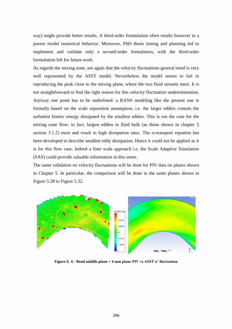
296
way) might provide better results. A third-order formulation often results however in a
poorer model numerical behavior. Moreover, PhD thesis timing and planning led to
implement and validate only a second-order formulation, with the third-order
formulation left for future work.
As regards the mixing zone, see again that the velocity fluctuations general trend is very
well represented by the ASST model. Nevertheless the model seems to fail in
reproducing the peak close to the mixing plane, where the two fluid streams meet. It is
not straightforward to find the right reason for this velocity fluctuation underestimation.
Anyway one point has to be underlined: a RANS modeling like the present one is
formally based on the scale separation assumption, i.e. the larger eddies contain the
turbulent kinetic energy dissipated by the smallest eddies. This is not the case for the
mixing zone flow: in fact, largest eddies in fluid bulk (as those shown in chapter 5
section 3.1.2) meet and result in high dissipation rates. The ω-transport equation has
been developed to describe smallest eddy dissipation. Hence it could not be applied as it
is for this flow case. Indeed a finer scale approach i.e. the Scale Adaptive Simulation
(SAS) could provide valuable information in this sense.
The same validation on velocity fluctuations will be done for PIV data on planes shown
in Chapter 5. In particular, the comparison will be done in the same planes shown in
Figure 5.28 to Figure 5.32.
Figure E. 6 - Bend middle plane + 4 mm plane PIV vs ASST u’ fluctuation
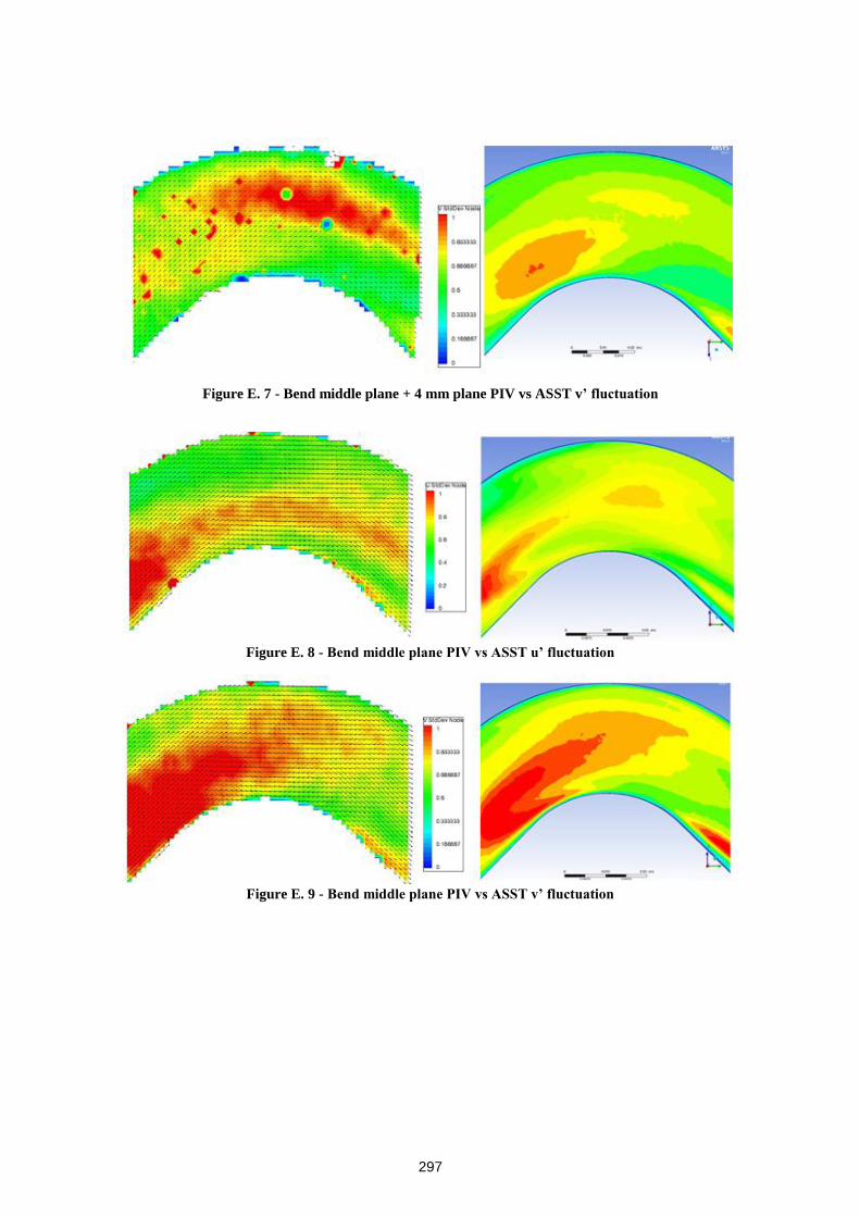
297
Figure E. 7 - Bend middle plane + 4 mm plane PIV vs ASST v’ fluctuation
Figure E. 8 - Bend middle plane PIV vs ASST u’ fluctuation
Figure E. 9 - Bend middle plane PIV vs ASST v’ fluctuation
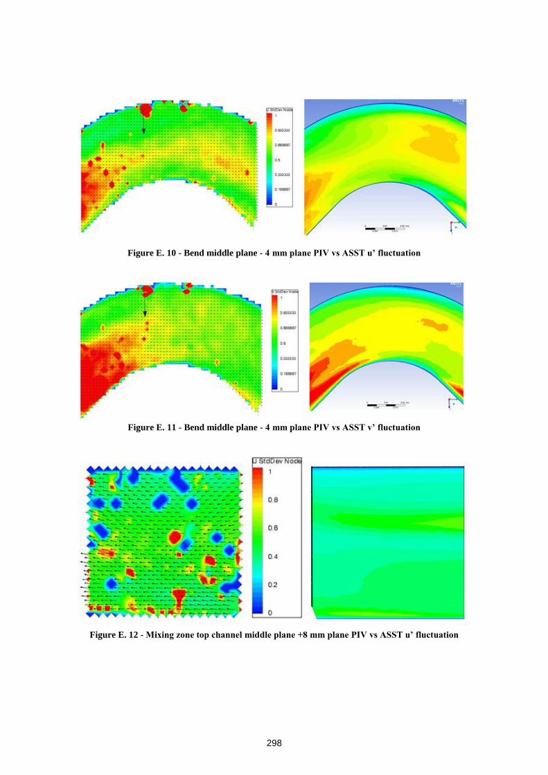
298
Figure E. 10 - Bend middle plane - 4 mm plane PIV vs ASST u’ fluctuation
Figure E. 11 - Bend middle plane - 4 mm plane PIV vs ASST v’ fluctuation
Figure E. 12 - Mixing zone top channel middle plane +8 mm plane PIV vs ASST u’ fluctuation
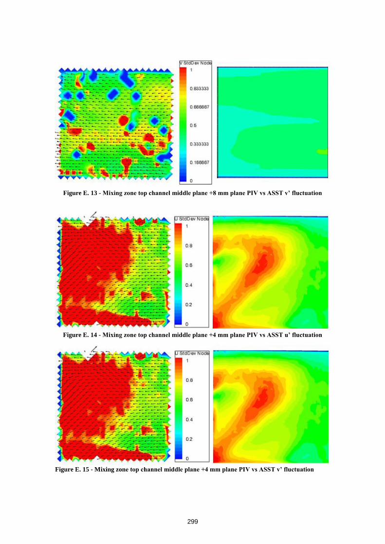
299
Figure E. 13 - Mixing zone top channel middle plane +8 mm plane PIV vs ASST v’ fluctuation
Figure E. 14 - Mixing zone top channel middle plane +4 mm plane PIV vs ASST u’ fluctuation
Figure E. 15 - Mixing zone top channel middle plane +4 mm plane PIV vs ASST v’ fluctuation
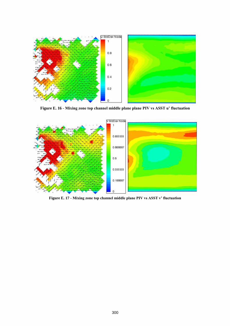
300
Figure E. 16 - Mixing zone top channel middle plane plane PIV vs ASST u’ fluctuation
Figure E. 17 - Mixing zone top channel middle plane PIV vs ASST v’ fluctuation
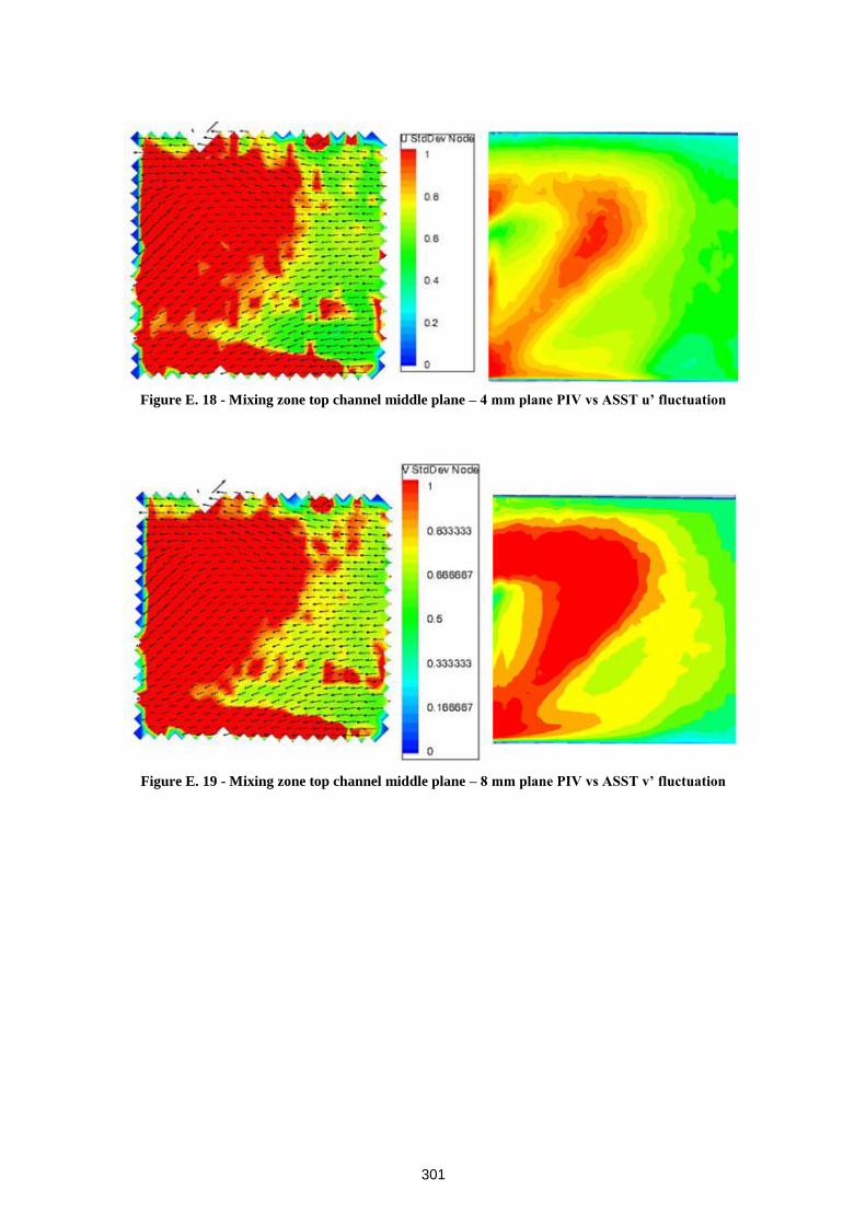
301
Figure E. 18 - Mixing zone top channel middle plane – 4 mm plane PIV vs ASST u’ fluctuation
Figure E. 19 - Mixing zone top channel middle plane – 8 mm plane PIV vs ASST v’ fluctuation
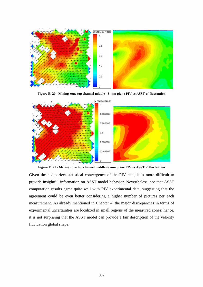
302
Figure E. 20 - Mixing zone top channel middle - 8 mm plane PIV vs ASST u’ fluctuation
Figure E. 21 - Mixing zone top channel middle -8 mm plane PIV vs ASST v’ fluctuation
Given the not perfect statistical convergence of the PIV data, it is more difficult to
provide insightful information on ASST model behavior. Nevertheless, see that ASST
computation results agree quite well with PIV experimental data, suggesting that the
agreement could be even better considering a higher number of pictures per each
measurement. As already mentioned in Chapter 4, the major discrepancies in terms of
experimental uncertainties are localized in small regions of the measured zones: hence,
it is not surprising that the ASST model can provide a fair description of the velocity
fluctuation global shape.

303
REFERENCES
1Key World Energy Statistics 2012, International Energy Agency, 2012
2 World Nuclear Power Reactors 2007-08 and Uranium Requirements, World Nuclear Association, 2008-
06-09.
3 Nuclear Energy Agency, Nuclear Energy Data, Nuclear Development 2013
4Nuclear Energy Agency, Nuclear Energy Today 2
nd Edition, Nuclear Development 2012
5 CEA – ELECNUC, Nuclear power plants in the world, 2012
6 P.Le Coz, J.F.Sauvage and J.P.Serpantie, « Sodium-cooled Fast Reactors : the ASTRID plant project »,
Proceedings of ICAPP 2011 – Nice, France, May 2-5, 2011, paper 11249, pp.419-425
7 P.Sciora et al., « Low Void Effect Core Design Applied on 2400 MWth SFR reactor », Proceedings of
ICAPP 2011 – Nice, France, May 2-5, 2011, paper 11048, pp.487-495
8 F.Varaine et al., « Pre-conceptual design study of ASTRID core », Proceedings of ICAPP’12, Chicago,
USA, June 24-28, 2012, paper 12173, pp.572-579
9 M.Saez et al., « The use of gas based energy conversion cycles for sodium fast reactors », Proceedings
of ICAPP’08, Anaheim, USA, June 8-12, 2008, paper 8037, pp.565-573
10 S.Carnevali, C.Proust, M.Soucille, « Unsteady aspects of sodium-water-air reaction », Chemical
Engineering Research and Design 91, pp.633-639, 2013
11 S.Carnevali, « Unsteady aspects of sodium-water reaction », PhD thesis, Université de Technologie de
Compiegne, France, October 2012
12 L.Cachon, A.Morcillo, « ASTRID : faisabilité des échangeurs du SCE gaz et programme R&D
associé », NT DEN/CAD/DTN/STPA/LCIT/2010-041, Novembre 2010
13 Shah R.K. and Focke W.W., “Plate Heat Exchangers and their design theory”, Heat transfer-Seattle -
American Institute of Chemical Engineers (AIChE) Symposium Series 225, Vol.79, pp.227-254, 1983
14 Kakaç S., Liu H., “Heat Exchangers: Selection, Rating, and Thermal Design”, Chap. 10, CRC Press,
1992
15 Kumar, “The plate heat exchanger: construction and design”, First UK National Conference in Heat
Transfer, Vol.2, pp.1275-1288, 1984
16 Bond M.P., “Plate Heat Exchangers for Effective Heat Transfer”, Chem.Eng., pp.162-167, 1981
17 B.Thonon, “Design method for plate evaporators and condensers”, 1st International Conference on
Process Intensification for the Chemical Industry, Vol.18, pp.37-47, BHR Group Conference Series
Publication, 1995
18 Muley A., Manglik R.M., “Experimental study of turbulent flow heat transfer and pressure drop in a
plate heat exchanger with chevron plates”, Journal of heat transfer, Vol.121, pp. 110-117; 1999
19 I. Gherasim, N. Galanis, C.T. Nguyen, “ Effects of smooth longitudinal passages and port
configuration on the flow and thermal fields in a plate heat exchanger”, Applied Thermal Engineering 31
(2011) 4113-4124
20 R.L. Heavner, H. Kumar, A.S.Wanniarachchi, “Performance of an industrial heat exchanger: effect of
chevron angle”, AlChE Symposium, Vol.89, n.295, pp. 262-267, 1993

304
21 Charre et al., “General model for plate heat exchanger performance prediction”, Journal of enhanced
heat transfer, Vol. 9, pp. 181-186, 2002
22 W.W.Focke, J.Zachariades, I.Olivier., “The effect of the corrugation inclination angle on the
thermohydraulic performance of plate heat exchangers”, Int. J. Hear Mass Transfer. Vol. 28, No. 8, pp.
1469-1479, 1985
23W.W.Focke, P.G.Knibbe, “Flow visualization in parallel-plate ducts with corrugated walls”,
J.Fluid.Mech. (1986) vol. 165, pp. 73-77
24 Zhang, Tian, “Simulation and analysis of flow pattern in cross-corrugated plate heat exchangers”,
Journal of Hydrodynamics, Ser.B, 2006,18(5): 547-551
25 Gaiser, Kottke, “Effects of wavelength and inclination angle on the homogeneity of local heat transfer
coefficients in plate heat exchangers”, Heat Transfer 1998, Proceedings of the 11th IHTC, Vol.6, August
23-28, 1998, Kyongju, Korea
26 Hessami, “An experimental investigation of the performance of cross-corrugated plate heat
exchangers”, Journal of enhanced heat transfer, Vol.10 N°4, pp.379-393, 2003
27 GRETh, TM11 – Perte de pression et transfert de chaleur dans les échangeurs à plaques en simple
phase, Manuel technique, 24 juin 1999
28 Metwally, Manglik, “Enhanced heat transfer due to curvature-induced lateral vortices in laminar flows
in sinusoidal corrugated-plate channels”, International Journal of Heat and Mass Transfer 47 (2004)
2283–2292
29 Xin, Tao (1988): “Numerical prediction of laminar flow and heat transfer in wavy channel of uniform
cross-sectional area”, Numerical Heat Transfer, 14:4, 465-481
30 Oyakawa et al., “The effect of the channel width on heat transfer augmentation in a sinusoidal wavy
channel”, JSME International Journal, Series II, Vol.32, n°3, pp.403-410, 1989
31 Gradeck, Hoareau, Lebouche, « Local analysis of heat transfer inside corrugated channel”,
International Journal of Heat and Mass Transfer 48 (2005) 1909–1915
32Thonon, Vidil, Marvillet, “Recent Research and developments in plate heat exchangers”, Journal of
enhanced heat transfer, Vol.2, n°1-2, pp. 149-155, 1995
33 Gradeck, Hoareau, Lebouche, « Local analysis of heat transfer inside corrugated channel”,
International Journal of Heat and Mass Transfer 48 (2005) 1909–1915
34Snyder et al., « Heat transfer enhancement in a serpentine channel » , International Journal of Heat and
Mass Transfer, Vol.36, n°12, pp.2965-2976, 1993
35 Martin, “ A theoretical approach to predict the performance of chevron-type heat exchangers”,
Chemical Engineering and Processing 35 (1996) 301-310
36 Mazen M. Abu-Khader, « Better thermal calculations using modified generalized Leveque equations
for chevron plate heat excha,gers », International Journal of Green energy, Vol.4, pp. 351-366, 2007
37 Dovic et al., “Generalized correlations for predicting heat transfer and pressure drop in plate heat
exchanger channels of arbitrary geometry”, International Journal of Heat and Mass Transfer 52 (2009)
4553–4563
38 Lee et al. “The effect of aspect ratio on turbulent flow heat transfer and pressure drop in a plate heat
exchanger”, International Journal of Heat Exchangers, Vol.I, pp.113-124, 200, ISSN 1524-5608
39 Savostin, A. F., and Tikhonov, A. M., “Investigation of the Characteristics of Plate-Type Heating
Surfaces”, Teploenergetika, Vol.17, n.9, pp. 75-78, 1970
40 Okada et al., “Design and heat transfer characteristics of new plate heat exchanger”, Heat transfer-
Japanese research, Vol.1, pp.90-95, 1972

305
41 A. Cooper, “Recover More Heat with Plate Heat Exchangers”, Chemical Engineer, Vol. 285, pp.280-
285, May 1974
42 G. Rosenblad and A. Kullendorff, “Estimating Heat Transfer Rates from Mass Transfer Studies on
Plate Heat Exchanger Surfaces”, Wärme-und- Stofffübertragung 8 (1975) 187-191
43 Marriott, J. “Performance of an Alfaflex plate heat exchanger”, Chemical Engineering Progress,
Vol.73, n.2, pp.73-78, 1977
44 Price, Fattah, “Hydrodynamic characteristics of a Plate Heat Exchanger Channel”, Trans. Inst. of
Chem. Eng., Vol.56, pp.217-228, 1978
45 Tovazhnyanski L.L. et al., « Heat Transfer and Hydraulic Resistance in Channels of Plate Heat
Exchangers », Energetika, Vol.9, pp.123-125, 1980
46 Chisholm D., Wanniarachchi A.S., « Maldistribution in Single-Pass Mixed-Channel Plate Heat
Exchanger », Compact Heat Exchangers for Power and Process Industries, HTD- Vol.201, ASME, New
York, pp.95-99, 1992
47 Talik A.C. et al., « Heat Tranfer and Pressure Drop Characteristics of a Plate Heat Exchangers », Proc.
ASME/JSME Thermal Engineering Joint Conference, Maui, Hawaii, 1995
48 Wanniarachchi et al., “Approximate correlations for chevron-type plate heat exchangers », HTD Vol.
314, 1995 National Heat Transfer Conference, Vol. 12, ASME 1995
49 Kanaris et al., “Flow and Heat Transfer Prediction in a Corrugated Plate Heat Exchanger using a CFD
Code », Chem. Eng. Technol. 2006, 29, No. 8, 923–930
50 Abu-Khader; “Better Thermal Calculations Using Modified Generalized Leveque Equations for
Chevron Plate Heat Exchangers”, International Journal of Green Energy, 4:4, 351-366 (2007)
51 Khan et al., “Experimental investigation of single phase convective heat transfer coefficient in a
corrugated plate heat exchanger for multiple plate configurations”, Applied Thermal Engineering 30
(2010) 1058–1065
52 Akturk et al., “Experimental investigation of the characteristics of a chevron-type gasketed plate heat
exchanger”, 6th International Advanced Technologies Symposium (IATS’11), 16-18 May 2011, Elazığ,
Turkey
53 Kapustenko et al., “The Heat and Momentum Transfers Relation in Channels of Plate Heat
Exchangers”, 14th International Conference on Process Integration, Modelling and Optimisation for
Energy Saving and Pollution Reduction 8-11 May 2011 - Florence, Italy, paper 89
54 Gherasim et al., “Heat transfer and fluid flow in a plate heat exchanger part I. Experimental
investigation », International Journal of Thermal Sciences 50 (2011) 1492-1498
55 Maslov A.M., Kovalenko L.M., « Hydraulic Resistance and Heat Transfer in Plate Heat Exchangers »,
Molochnaya Promyshlenost, N.10, pp.20-22, 1972
56 Tovazhnyanski L.L. et al., « Heat Transfer and Hydraulic Resistance in Channels of Plate Heat
Exchangers », Energetika, Vol.9, pp.123-125, 1980
57 O’Brien and Sparrow; “Corrugated-Duct heat transfer, pressure drop and flow visualization”, Journal
of heat transfer, vol.104, pp.410-416, 1982
58Croce, D’Agaro, “Numerical analysis of forced convection in plate and frame heat exchangers”,
International Journal of numerical methods for heat and fluid flow, Vol.12, n°6, pp.756-771
59 H. Blomerius, N. K. Mitra (2000): Numerical investigation of convective heat transfer and pressure
drop in wavy ducts, Numerical Heat Transfer, Part A: Applications, 37:1, 37-54
60 Zhang, “Numerical study of periodically fully developed flow and heat transfer in cross-corrugated
triangular channels in transitional flow regime”, Numerical Heat Transfer, Part A, 48: 387–405, 2005
61 Lei Zhang & Defu Che (2011): Influence of Corrugation Profile on the Thermalhydraulic Performance
of Cross-Corrugated Plates, Numerical Heat Transfer, Part A: Applications, 59:4, 267-296

306
62 Ciofalo, Stasiek, Collins, Investigation of flow and heat transfer in corrugated passages-II Numerical
simulations, In1 J Heai UO\J Trmfer. Vol. 39.No. 1.pp. 165 192. 1996
63 Jain et al., “A New Approach to Numerical Simulation of Small Sized Plate Heat Exchangers With
Chevron
Plates”, Journal of Heat Transfer March 2007, Vol. 129, pp. 291-297
64 Etemad and Sundén, “CFD-analysis of fully developed turbulent flow and heat transfer in a unitary
cell of a cross corrugated plate pattern heat exchanger”, Proceedings of HT2007, 2007 ASME-JSME
Engineering Summer heat transfer conference, pp. 531-540, July 8-12 2007, Vancouver, British
Columbia, Canada
65 S. Freund, S. Kabelac, “Investigation of local heat transfer coefficients in plate heat exchangers with
temperature oscillation IR thermography and CFD”, International Journal of Heat and Mass Transfer 53
(2010) 3764–3781
66 Weizhe Han, Khaled Saleh, Vikrant Aute, Guoliang Ding, Yunho Hwang, Reinhard Radermacher,
“Numerical simulation and optimization of single-phase turbulent flow in chevron-type plate heat
exchanger with sinusoidal corrugations”, HVAC&R Research, Vol.17, N° 2, pp.186-197, 2011
67 Gherasim et al., “Heat transfer and fluid flow in a plate heat exchanger. Part III: Assesment of laminar
and two-equation turbulent models”, International Journal of Thermal Sciences 50 (2011) 1499-1511
68 Lei Zhang and Defu Che, “Turbulence models for fluid flow and heat transfer between cross-
corrugated plates”, Numerical Heat Transfer, Part A, 60: 410–440, 2011
69 Jain et al., “A New Approach to Numerical Simulation of Small Sized Plate Heat Exchangers With
Chevron
Plates”, Journal of Heat Transfer March 2007, Vol. 129, pp. 291-297
70 K.M.Stone, “Review of literature on heat transfer enhancement in compact heat exchangers”, ACRC
TR-105, August 1996
71 R.K.Shah and A.L.London, “Laminar Flow Forced Convection in Ducts”, Advances in Heat Transfer,
J.Thomas, F.Irvine and P.Hartnett ed. Academic Press, 1978
72 J. G. Soland, J. W. M. Mack and W. M. Rohsenow, Performance Ranking of Plate-Fin Heat
Exchanger Surfaces, Transactions of the ASME Journal of Heat Transfer, Vol. 100,
pp. 514-519, 1978.
73 L.Cachon, “Avant Projet Sommaire des échangeurs de chaleur du SCE gaz d’ASTRID”, NT
DEN/CAD/DTN/STPA/LCIT/2011-056, Fevrier 2012
74 S.Christin, « ASTRID – Etude de tenue thermoméchanique des PSHE sodium/gaz », NT
DEN/CAD/DTN/STPA/LCIT 2012-039, October 2012
75HEATRIC Inc. http://www.heatric.com/superior_performance.html
76
K.Gezelius, “Design of Compact Intermediate Heat Exchangers for Gas Cooled Fast Reactors”, MSc
Thesis, Massachusetts Institute of Technology, Cambridge USA, June 2004
77 Thomas Schmerber, “Calculs CFD sur des échangeurs thermiques Sodium/Gaz pour ASTRID”,
Rapport de stage ST50 – Printemps 2011, UTBM – Université de Technologie de Belfort-Montbéliard
78D.C.Wilcox, “Turbulence Modeling for CFD”, DCW Industries, 2006
79 S.Castris, B.Aupoix, « Density corrections for turbulence models », Aerospace Science and
Technology, Vol.4, pp.1-11, 2000 81
D.C.Wilcox, “Turbulence Modeling for CFD”, DCW Industries, 1998

307
81
F.R.MENTER, M.Kuntz, R.Langtry, “Ten years of industrial experience with the SST Turbulence
model”, Turbulence, Heat and Mass Transfer 4, Begell House, Inc., 2003
82B.E.Launder and D.B.Spalding, “Lectures in Matematical Models of Turbulence”, Academic Press,
1972
83J.Kim, P.Moin, R.Moser, “Turbulence Statistics in fully developed channel flow at low Reynolds
number”, J.Flud Mech. Vol.56, pp.337-351, 1987
84J.Laufer, “The structure of turbulence in fully developed pipe flow”, NACA report 1174
85D.M.Driver and H.L.Seegmiller, “Features of a reattaching turbulent shear layer in divergent channel
flow”, AIAA Journal Vol.23, N° 2, pp.163-171, 1985
86 A.Huser, S.Biringen, “Direct numerical simulation of turbulent flow in a square duct”, J.Fluid Mech.,
v. 257, pp. 65-95, 1993
87F.Mantlik, J.Heina, J.Chervenka, “Results of local measurements of hydraulic characteristic in
triangular pin bundle”, UJV-3778-R, Rzez, Czech Republic, 1976.
88P.A.Durbin, “Limiters and wall treatments in applied turbulence modeling”, Fluid Dyn. Res. Vol. 41,
pp.1-18, 2009
89C.G.Speziale, “On Nonlinear k-ℓ and k-ε Models of Turbulence”, J.Fluid Mech., Vol.178, pp.459-475,
1987
90 T.H.SHIH, J.ZHU and J.L.LUMLEY, “A Realizable Reynolds Stress Algebraic Equation Model”,
NASA TM 105993
91T.J.CRAFT, B.E.Launder and K.Suga, “Prediction of turbulent transitional phenomena with a
nonlinear eddy-viscosity model”, Int. J. Heat and Fluid Flow 18: 15-28, 1997
92A.Hellsten and S.Laine, “Explicit Algebraic Reynolds-Stress Modelling in Decelerating and Separating
Flows”, AIAA Paper 2000-2313, 2000
93S.WALLIN and A.V.JOHANSSON, “An explicit algebraic Reynolds stress model for incompressible
and compressible turbulent flows”, J.Fluid Mech (2000), vol.43, pp.89-132
94F.R.Menter, A.V.Gabaruk, Y.Egorov, “Explicit Algebraic Reynolds Stress Models for Anisotropic
Wall-Bounded Flows”, EUCASS – 3rd European Conference for Aero-Space Sciences, Versailles
(France), July 6-9 2009
95 E.Baglietto, H.Ninokata, T.Misawa, “CFD and DNS methodologies development for fuel bundle
simulations”, Nuclear Engineering and Design, Vol. 236, pp.1503-1510, 2006
96 P.Bradshaw, D.H.Ferris, N.P.Atwell, “Calculation of Boundary Layer development using the turbulent
energy equation”, Journal of Fluid Mechanics, Vol.28, No 3, pp.593-616, 1967
97 J.Kim and P.Moin, “Transport of passive scalars in a turbulent channel flow”, Turbulent Shear flows,
edited by J.C.André et al., Vol.6, pp.85-96, 1989
98 B.J.Daly, F.H.Harlow, “Transport Equations in turbulence”, Physics of Fluids, Vol.13, pp.2634-2649,
1970
99S.Thangam and C.G.Speziale, “Turbulent flow past a backward facing step: a critical evaluation of
two-equation models”, AIAA Journal, Vol.30, No 5, pp.1314-1320, 1992

308
100
Y.G.Lai, R.M.C.So and H.S.Zhang, “Turbulence-Driven Secondary Flows in a Curved Pipe”,
Theoret.Comput. Fluid Dynamics, Vol.3, pp.163-180, 1991
101F.R.Menter, “Two-equation eddy viscosity turbulence models for engineering applications”, AIAA
Journal Vol.32, No 8, August 1994
102J.C.Vogel and J.K. Eaton. “Combined Heat Transfer and Fluid Dynamic Measurements Downstream of
a Backward-Facing Step”. J. Heat Transfer. Vol. 107.922-929. 1985.
103 A.M.K.P.Taylor, J.H.Whitelaw and M.Yianneskis, “Measurements of laminar and turbulent flow in a
curved duct with thin inlet boundary layer”, NASA Contractor Report 3367, 1981
104B.E.Launder, “Numerical computation of convective heat transfer in complex turbulent flows: time to
abandon wall functions?”, Int.J.Heat Mass Transfer, Vol.27, N.9, pp. 1485-1491, 1984
105W .R.Dean, “Note on the motion of fluid in a curved pipe”, Proc.Roy.Soc. A, Vol. 85, pp.208-223,
1911
106F. Micheli, "Étalonnage d'un Vélocimètre Laser à Franges", ONERA RT 1/15062 DMAE, 2013
107
F. Micheli, M. Lavieille, P. Millan. "ASSA, un outil de référence pour le traitement du signal en
vélocimétrie laser", Congrès Francophone de Techniques Laser, CFTL 2006, Toulouse, 19- 22 septembre,
2006. hathor.onera.fr/dmae/velocimetrie-laser-assa
108T. ADACHI et al., “Secondary flows in curved ducts of rectangular cross-section”, Bulletin of the
JSME, Vol.20, N° 143, May 1977
109 H.B.SQUIRE and K.G.WINTER, « The secondary flow in a cascade of aerofoils in a non-uniform
stream », Royal Aircraft Establishment, Report N° AERO 2317, March 1949
110C.GALATI, intern at CEA/DEN/CAD/DTN/STCP/LCIT, Personal Communication
111L.CAHON, R&D Engineer at CEA/DEN/CAD/DTN/STCP/LCIT and Head of Power conversion
system R&D within the TECNA project, Personal Communication
112Y.EGOROV, F.Menter, « Development and Application of SST-SAS Turbulence Model in the
DESIDER Project », Advances in Hybrid RANS-LES Modelling, Notes on Numerical Fluid Mechanics
and Multidisciplinary Design, Vol.97, pp. 261-270, 2008
113 J.NAVE, « Modélisation CFD d’un motif d’échange innovant pour l’ECSG d’ASTRID »,
CEA/DEN/CAD/DTN/STPA/LCIT/NT/2013-026-INDICE A, Diffusion Restreinte, 2013
Contribution Expérimentale et numérique à l’amélioration de l’échange
thermique des échangeurs de chaleur compacts à plaques
Résumé : Dans le cadre du programme CEA R&D pour développer un prototype industriel de
Réacteur à Neutrons Rapides refroidi au Sodium (RNR-Na), cette thèse vise à proposer une
technologie d'échangeur de chaleur compact innovant. Afin d'augmenter la compacité globale du
composant la conception est réalisée d’un canal: il peut être considéré comme le résultat de la
superposition de deux canaux ondulés en opposition de phase. Afin de fournir un modèle numérique
physiquement cohérent, un nouveau modèle de turbulence à viscosité turbulente non linéaire
nommé modele ASST a été développé et implémenté dans le solveur ANSYS FLUENT ®. Il a été
démontré que le modèle ASST peut fournir une alternative intéressante aux modèles plus
complexes. Pour valider le modèle ASST, deux montages expérimentaux ont été réalisés, dont un
utilisant la Vélocimétrie Laser à franges et l'autre la Vélocimétrie Laser par images de particules.
Pour la validation thermique, l'installation "VHEGAS" a été construite. Une fois le modèle ASST
validé, les performances pour différentes géométries peuvent être étudiées. Enfin, il a été montré
que la géométrie innovante est la plus compacte parmi les autres technologies d'échangeurs de
chaleur compacts type PCHE.
Mots clés : Motif d’échange innovant, CFD, modèle ASST, LDV, PIV, transfer thermique,
échangeurs thermiques à plaques
______________________________________________________________________
Experimental and numerical contribution to heat transfer enhancement in
compact plate heat exchangers
Abstract : In the framework of CEA R&D program to develop an industrial prototype of Sodium-
cooled Fast Reactor, the present thesis aimed to propose an innovative compact heat exchanger
technology. In order to increase the global compactness the basic idea of this work is to design a
channel were the fluid flow is as much three-dimensional as possible. In particular the channel can
be thought as the result of the superposition of two undulated channels in phase opposition. To
numerically provide a physically-consistent model, a new non-linear eddy viscosity named
Anisotropic Shear Stress Transport (ASST) model has been developed and implemented into the
available solver ANSYS FLUENT. To validate the numerical model, two experimental sections
have been used to acquire an extensive aerodynamic database, whereas, to validate the thermal
modeling approach, the VHEGAS facility has been built. Once having validated the ASST model,
correlations for friction factor and Nusselt number for various geometries could be obtained.
Finally, it has been shown that the innovative channel is the most compact one among the most
important existing industrial compact heat exchanger technologies.
Keywords: Innovative heat exchanger, CFD, ASST model, LDV, PIV, heat transfer, plate heat
exchanger