


Langages
Pages
Légal


Modélisation de la détérioration basée sur les
données de surveillance conditionnelle et
estimation de la durée de vie résiduelle
T. T. Le , C. Bérenguer, F. Chatelain
Univ. Grenoble Alpes, GIPSA-lab, F-38000 Grenoble, France
CNRS, GIPSA-lab, F-38000 Grenoble, France
Journées de l’Automatique GdR MACS

Context
FP7 European project:
• “SUstainable PREdictive Maintenance for manufacturing Equipment”
• Purpose: Development of new tools for predictive maintenance to improve
productivity, reduce machine downtimes and increase energy efficiency.
⇒ Application case: Paper machine
⇒ Main objectives:
� Deterioration modeling
� Remaining Useful Life (RUL)
estimation
11/12/2015 Journées de l’Automatique GdR MACS 2
Predictive maintenanceSUPREME partners

Journées de l’Automatique GdR MACS
Problem statement
Deterioration models
• Represent temporal evolution of defects, i.e. of health indicators.
• Health indicators: unobservable
• Observations: noisy condition monitoring data
=> State-space representation
• Two type of states
– Continuous
– Discrete
11/12/2015 3
1 ) : Hidden state( ,
( , ) : Observati
s
onst
t
t t
t t
xx f
y g x
ων
−= =
Discrete-state modelingContinuous-state modeling
Problem statement
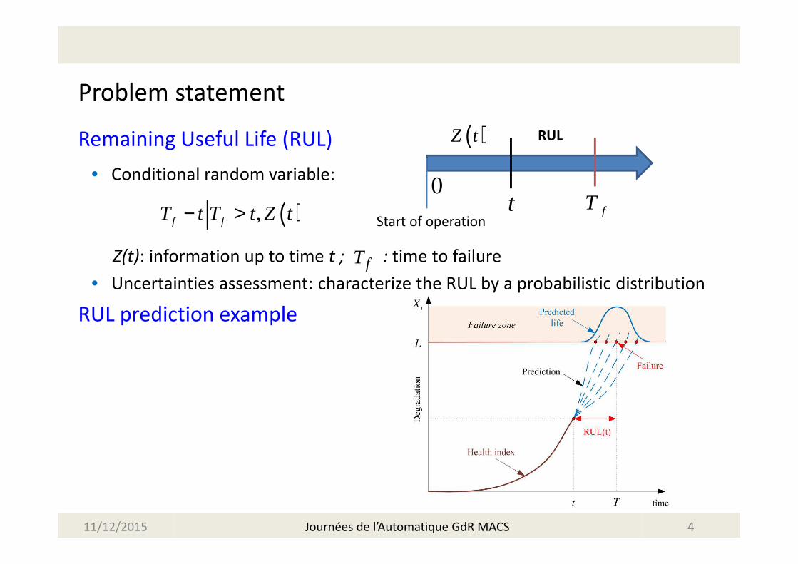
Remaining Useful Life (RUL)
• Conditional random variable:
Z(t): information up to time t ; : time to failure
• Uncertainties assessment: characterize the RUL by a probabilistic distribution
RUL prediction example
11/12/2015 4
fTtStart of operation
0
( )Z t RUL
( ),f fT t T t Z t− >
Journées de l’Automatique GdR MACS
fT
Problem statement
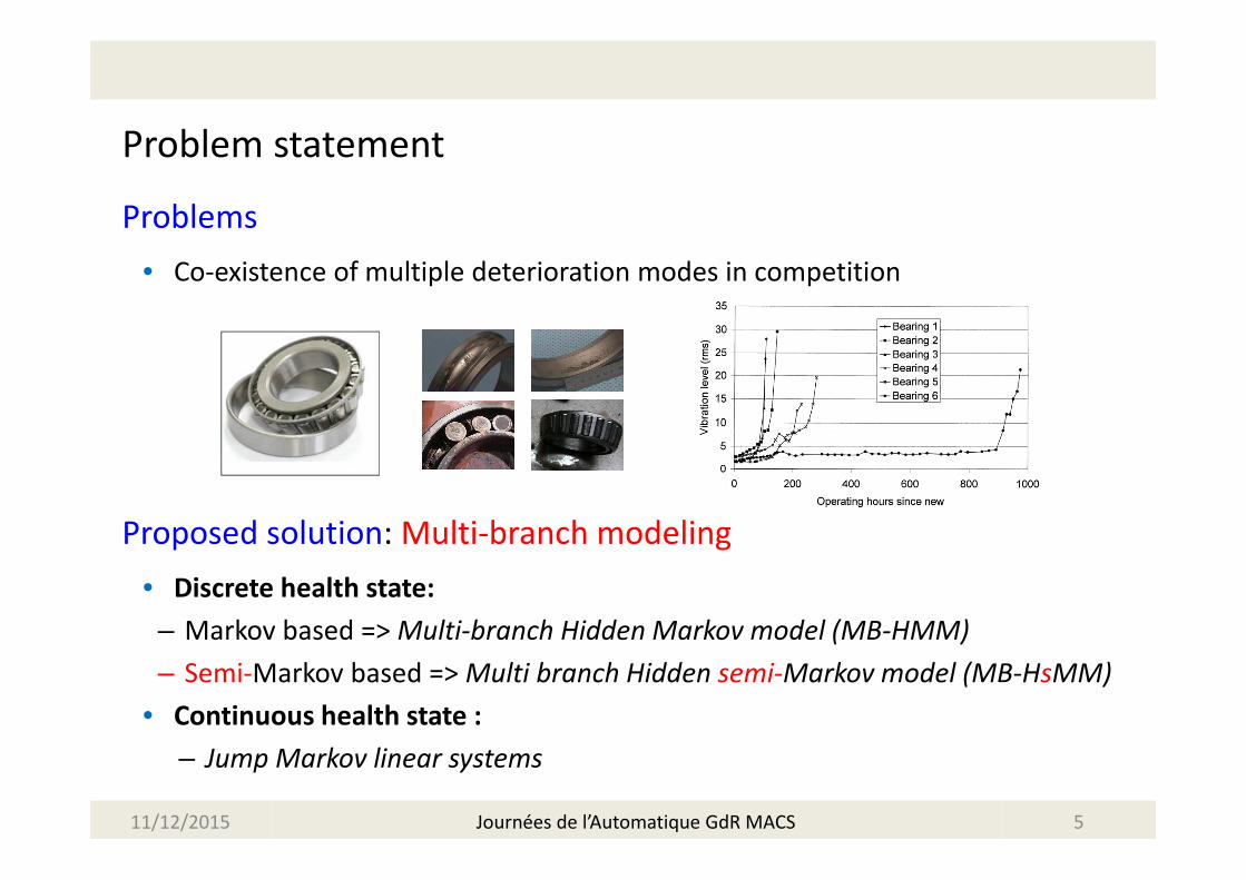
Problems
• Co-existence of multiple deterioration modes in competition
Proposed solution: Multi-branch modeling
• Discrete health state:
– Markov based => Multi-branch Hidden Markov model (MB-HMM)
– Semi-Markov based => Multi branch Hidden semi-Markov model (MB-HsMM)
• Continuous health state :
– Jump Markov linear systems
11/12/2015 5Journées de l’Automatique GdR MACS

Outline
� Multi-branch discrete-state model
� Diagnostics and Prognostics framework
� Numerical studies
� Jump Markov linear systems
� Parameters learning
� Health assessment and RUL estimation
� Numerical study
� Conclusion & Perspectives
11/12/2015 6Journées de l’Automatique GdR MACS

Multi-branch discrete-state models
11/12/2015 7Journées de l’Automatique GdR MACS
Multi-branch discrete-state modeling
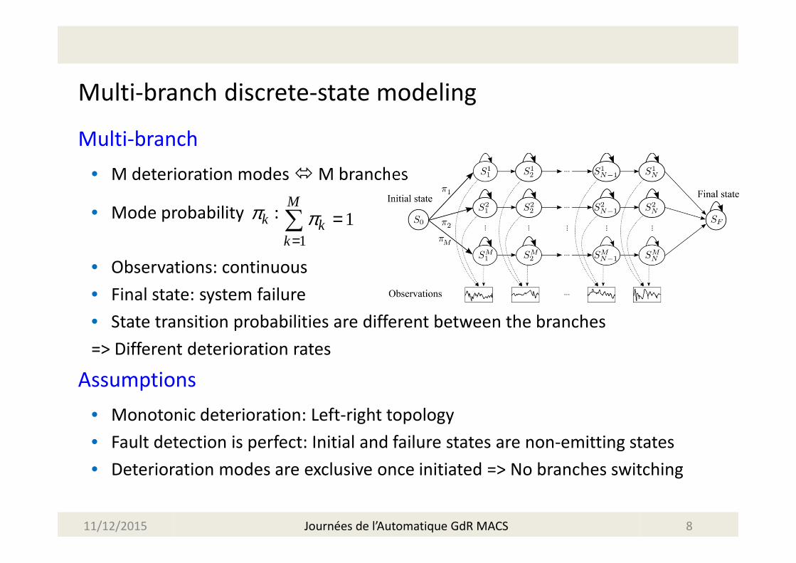
Multi-branch
• M deterioration modes � M branches
• Mode probability :
• Observations: continuous
• Final state: system failure
• State transition probabilities are different between the branches
=> Different deterioration rates
Assumptions
• Monotonic deterioration: Left-right topology
• Fault detection is perfect: Initial and failure states are non-emitting states
• Deterioration modes are exclusive once initiated => No branches switching
11/12/2015 8
1
1M
kk
π=
=∑kπ
Journées de l’Automatique GdR MACS

Multi-branch discrete-state modeling
Multi-branch Hidden Markov Model
• Each branch ~ left-right Markov chain
• Markovian property
⇒State sojourn time: Exponential
or geometrical distributed
⇒May not be true in practice
Multi-branch Hidden semi-Markov Model
• Each branch ~ left-right semi-Markov chain
• Semi-Markov property: relax the Markovian assumption
=> allow arbitrary distributions for sojourn time: Gaussian, Weibull, …
11/12/2015 9Journées de l’Automatique GdR MACS

Diagnostics and prognostics framework
Two-phase implementation: offline & online
11/12/2015 10Journées de l’Automatique GdR MACS
Off-line phase
Model training
• Training data: High-level features extracted from condition monitoring data
• Topology selection: BIC criterion
• Data classification => M groups
• Each group is used to train a constituent branch:
– MB-HMM: Adaption of the Baum-Welch algorithm
– MB-HsMM: Adaption of the Forward-Backward procedure [Yu 2006]
• A priori mode probabilities
is the number of training sequences corresponding to the mode k
11/12/2015 11
( ) / , 1k k kP K K k Mπ λ= = = K
kK*[Yu06]: Practical implementation of an efficient forward-backward algorithm for an explicit-duration hidden Markov model. IEEE Transactions
on Signal Processing, 54(5), 1947-1951.
Journées de l’Automatique GdR MACS
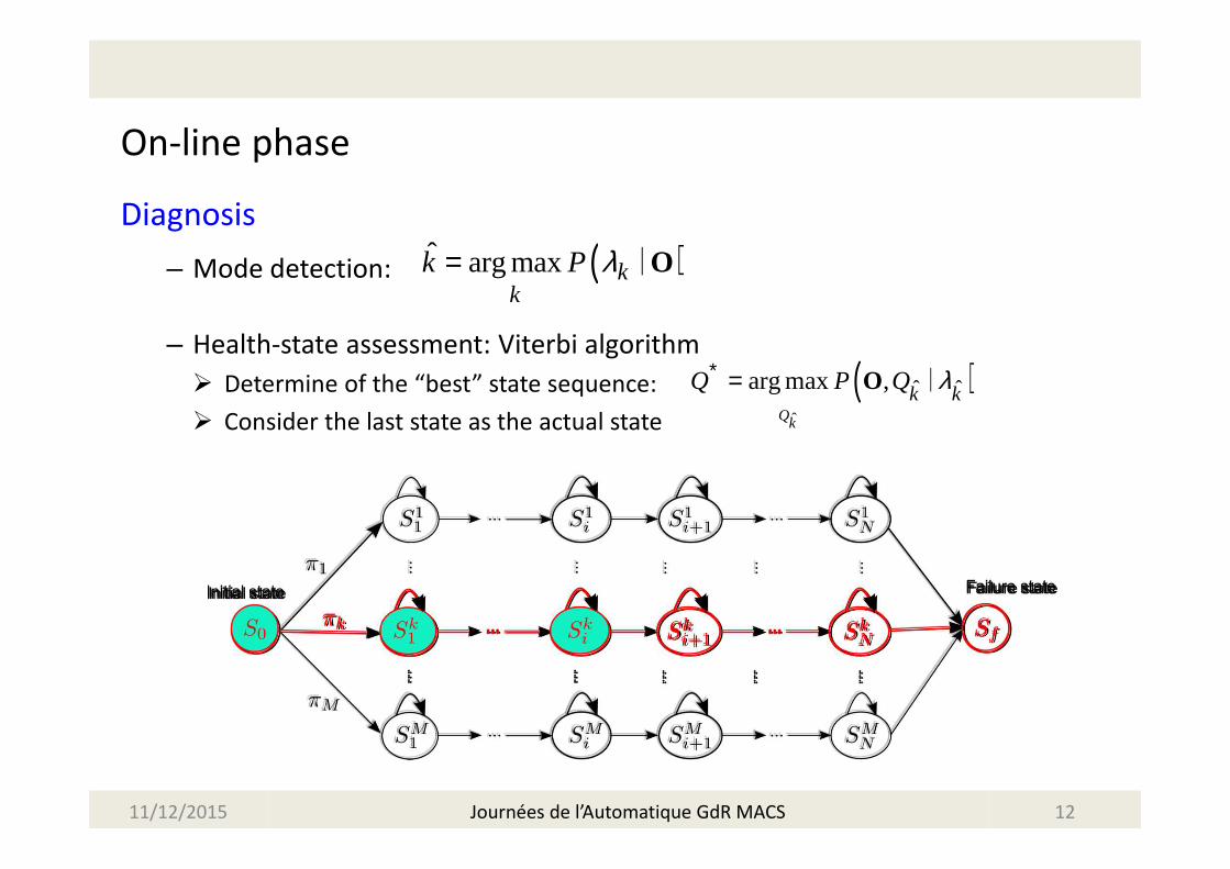
On-line phase
Diagnosis
– Mode detection:
– Health-state assessment: Viterbi algorithm
� Determine of the “best” state sequence:
� Consider the last state as the actual state
( )ˆ arg max kk
k P λ= O∣
( )ˆ
ˆ ˆarg max ,Qk
k kQ P Q λ∗ = O ∣
11/12/2015 12Journées de l’Automatique GdR MACS

RUL estimation
One branch (HMM case)
• Suppose that the system is following the mode k
• RUL : discrete time assumption => number of transition steps to reach for the
1st time the failure state:
• Left-right HMM: Given the current state, the system can either stay in the
same state or jump to the next one
⇒ Recursive computation
( ) ( )( )1 1, , ,l
t i t l N t l N t N t iiRUL P RUL l q S P q S q S q S q S+ + − += = = ≠ …= = ≠ =∣ ∣
11/12/2015 13Journées de l’Automatique GdR MACS
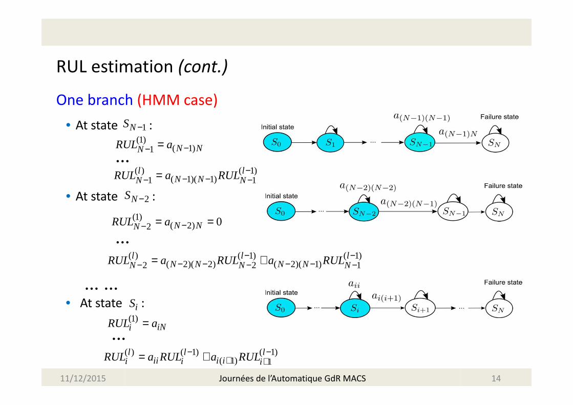
RUL estimation (cont.)
One branch (HMM case)
• At state :
• At state :
• At state :(1)i iNRUL a=
( ) ( 1) ( 1)( 1) 1
l l liii ii iiRUL RUL RULa a− −
+ += +
2NS −
(1)( 2)2 0N NNRUL a −− = =
iS
( ) ( 1) ( 1)( 2)( 2) ( 2)( 1)2 2 1
l l lN N N NN N NRUL LR a Ra UUL − −
− − − −− − −+=
...
...
... ...
1NS −(1)
( 1)1 N NNRUL a −− =
( ) ( 1)( 1)( 1)1 1
l lN NN NRRUL a UL −
− −− −=...
11/12/2015 14Journées de l’Automatique GdR MACS
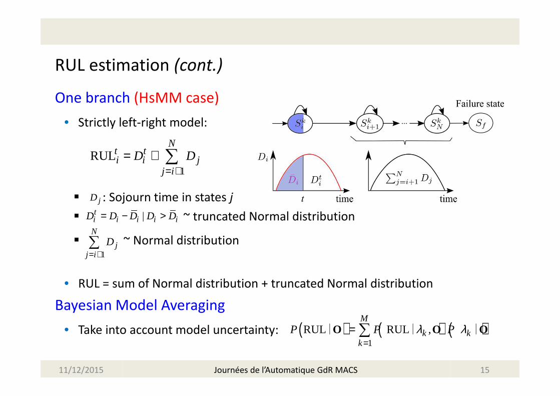
RUL estimation (cont.)
One branch (HsMM case)
• Strictly left-right model:
� : Sojourn time in states j
� ~ truncated Normal distribution
� ~ Normal distribution
• RUL = sum of Normal distribution + truncated Normal distribution
Bayesian Model Averaging
• Take into account model uncertainty: ( ) ( ) ( )1
RUL RUL ,M
k kk
P P Pλ λ=
= ∑O O O∣ ∣ ∣
1
RULN
t ti i j
j i
D D= +
= + ∑
|ti i i i iD D D D D= − >
jD
1
N
jj i
D= +∑
11/12/2015 15Journées de l’Automatique GdR MACS

Numerical examples
Simulated deterioration data
• Fatigue Crack Growth (FCG) model to represent the evolution of a crack depth
• Observation model:
• Multi-mode: Two propagation rates
– Crack depth is proportional with
( )1 1
tii i i
enw
t t b tx x e C e x tγβ− −
= + ∆
i i it t ty x ξ= +
0.005, 1.3, 1.7wC n σ= = =
Two-mode training data
eγ
1 22 , 100, 010 .5Lξ π πσ = == =
[ ]0 0.75Teγ =
11/12/2015 16Journées de l’Automatique GdR MACS

Numerical examples
Online RUL estimation (MB-HsMM model)
11/12/2015 17Journées de l’Automatique GdR MACS
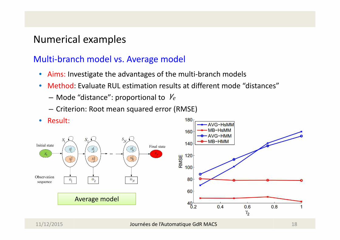
Numerical examples
Multi-branch model vs. Average model
• Aims: Investigate the advantages of the multi-branch models
• Method: Evaluate RUL estimation results at different mode “distances”
– Mode “distance”: proportional to
– Criterion: Root mean squared error (RMSE)
• Result:
Average model
eγ
11/12/2015 18Journées de l’Automatique GdR MACS

Case study (MB-HsMM model):
PHM08 competition
• C-MAPSS: Modeling a large realistic commercial turbofan engine
• 2 data set for training and test
• 218 identical and independent units
• Objective:
– Construct a prognostic method basing on training data set
– Use it to estimate the RUL of each unit in test data set
• Evaluation criterion:
Where is penalty score for unit i:
where
*C-MAPSS: Commercial Modular Aero-Propulsion System Simulation
218
1i
i
S S=
= ∑
iS
/13
/10
1, 0
1, 0
i
i
di
i di
e dS
e d
− − ≤= − >
i ii est reald RUL RUL= −
Simplified diagram of engine
simulated in C-MAPSS
11/12/2015 19Journées de l’Automatique GdR MACS
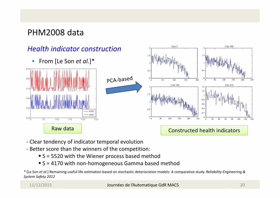
PHM2008 data
Health indicator construction
• From [Le Son et al.]*
* [Le Son et al.] Remaining useful life estimation based on stochastic deterioration models: A comparative study. Reliability Engineering &
System Safety 2012
11/12/2015 20
Raw data Constructed health indicators
- Clear tendency of indicator temporal evolution
- Better score than the winners of the competition:
� S = 5520 with the Wiener process based method
� S = 4170 with non-homogeneous Gamma based method
Journées de l’Automatique GdR MACS
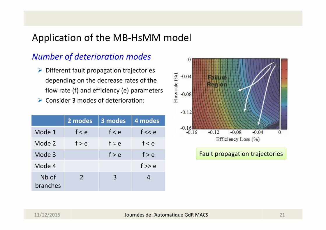
Application of the MB-HsMM model
Number of deterioration modes
� Different fault propagation trajectories
depending on the decrease rates of the
flow rate (f) and efficiency (e) parameters
� Consider 3 modes of deterioration:
11/12/2015 21
Fault propagation trajectories
2 modes 3 modes 4 modes
Mode 1 f < e f < e f << e
Mode 2 f > e f ≈ e f < e
Mode 3 f > e f > e
Mode 4 f >> e
Nb of
branches
2 3 4
Journées de l’Automatique GdR MACS
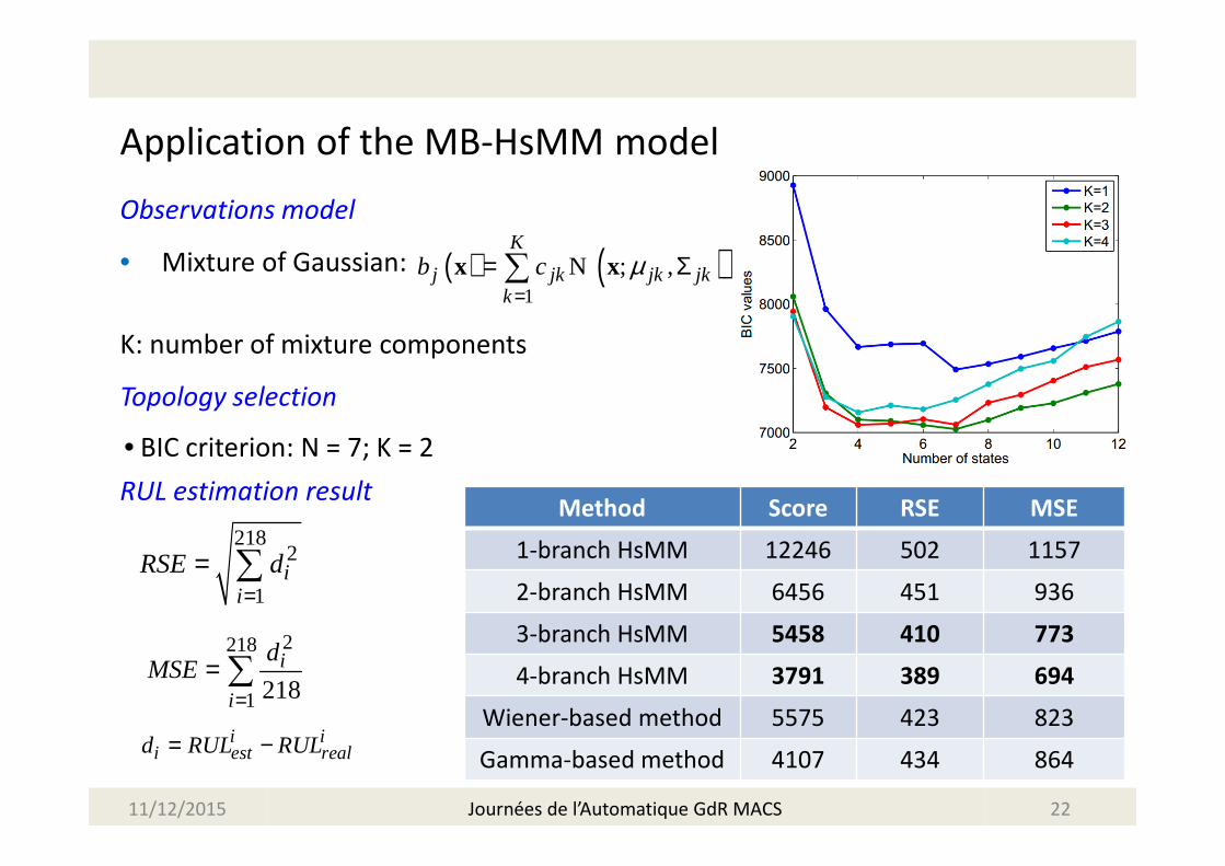
Application of the MB-HsMM model
Observations model
• Mixture of Gaussian:
K: number of mixture components
Topology selection
• BIC criterion: N = 7; K = 2
RUL estimation result
11/12/2015 22
Method Score RSE MSE
1-branch HsMM 12246 502 1157
2-branch HsMM 6456 451 936
3-branch HsMM 5458 410 773
4-branch HsMM 3791 389 694
Wiener-based method 5575 423 823
Gamma-based method 4107 434 864
Journées de l’Automatique GdR MACS
( ) ( )1
; ,K
j jk jk jkk
b c µ=
= Σ∑x xN
2182
1i
i
RSE d=
= ∑
2218
1 218i
i
dMSE
== ∑
i ii est reald RUL RUL= −

Multi-branch continuous-state models
11/12/2015 23Journées de l’Automatique GdR MACS
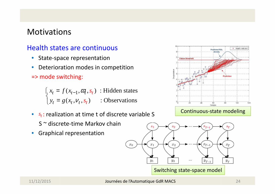
Motivations
Health states are continuous
• State-space representation
• Deterioration modes in competition
=> mode switching:
• : realization at time t of discrete variable S
S ~ discrete-time Markov chain
• Graphical representation
11/12/2015 24Journées de l’Automatique GdR MACS
1 , ) : Hidden states( ,
( , , ) : Observationst
t
t
tt
t
t
t sxf
y s
x
g x
ων
−= =
ts
Switching state-space model
Continuous-state modeling
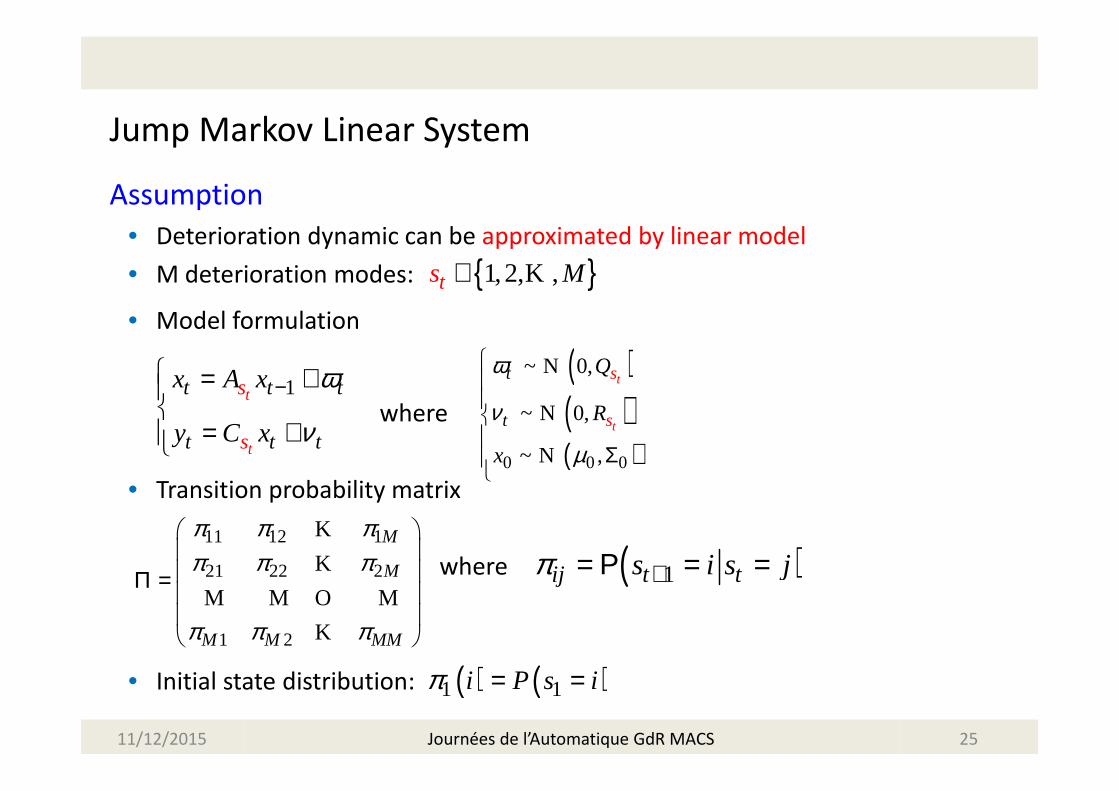
Jump Markov Linear System
Assumption
• Deterioration dynamic can be approximated by linear model
• M deterioration modes:
• Model formulation
where
• Transition probability matrix
where
• Initial state distribution:
11/12/2015 25
1t
t
t
t
s
s
t t
t t
x
y
A x
C x
ω
ν
−=
+=
+
( )( )( )0 0 0
~ 0,
~ 0,
~ ,
t
t
st
t s
Q
R
x
ω
ν
µ
Σ
N
N
N
Journées de l’Automatique GdR MACS
{ }1,2, ,ts M∈ K
11 12 1
21 22 2
1 2
M
M
M M MM
π π ππ π π
π π π
Π =
K
K
M M O M
K
( )1ij t ts i s jπ += Ρ = =
( ) ( )1 1i P s iπ = =
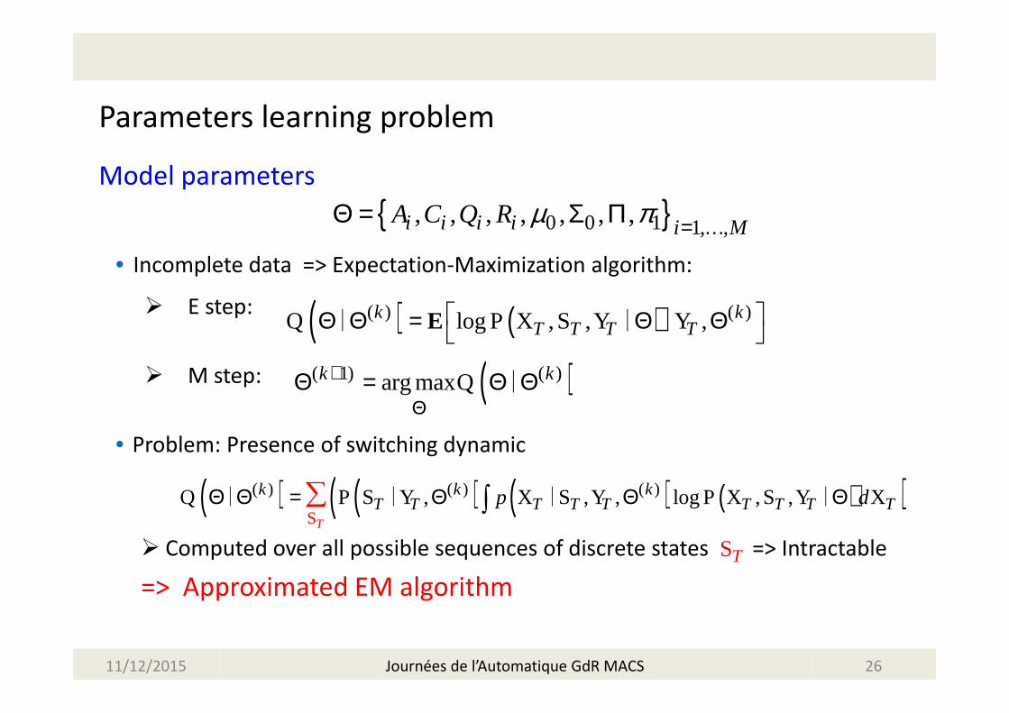
Parameters learning problem
Model parameters
• Incomplete data => Expectation-Maximization algorithm:
� E step:
� M step:
• Problem: Presence of switching dynamic
� Computed over all possible sequences of discrete states => Intractable
=> Approximated EM algorithm
11/12/2015 26
{ }0 0 1 1, ,, , , , , , ,i i i i i M
A C Q R µ π = …Θ = Σ Π
( ) ( )( ) ( )log , , ,k kT T T T
Θ Θ = Θ Θ
E PQ X S Y Y∣ ∣ ∣
( )( 1) ( )arg maxk k+
ΘΘ = Θ ΘQ ∣
( ) ( ) ( ) ( )( )( ) ( ) ( ), , , log , ,T
k k kT T T T T T T T Tp dΘ Θ = Θ Θ Θ∑ ∫P P
SQ S Y X S Y X S Y X∣ ∣ ∣ ∣
TS
Journées de l’Automatique GdR MACS

Approximated EM algorithm
Pruning technique
• Approximation: Calculate the sum over the most “likely” state sequence
• Adaption of the Viterbi algorithm
• Do not guarantee the convergence, but still sufficient in several practical cases
• Most important: the algorithm is linear in number of time steps.
From the traditional Viterbi algorithm…
• Define the best “partial cost” at time t:
• Then, for each state transition j -> i, assign an “innovation cost”:
11/12/2015 27
( )1
1,
( ) max log , , ,t t
t t t t tJ i s i−
−= =PS X
X Y S
( ) ( ) ( )( )
1,1 , , 1 , , 1 , ,, 1
1 , ,
1
21
log log ,2
j it i i i i t it t j i t t j i t t j it t
i i it t j i
J y C x C C R y C x
C C R j i
′ −+ + ++
+
′= − − Σ + −
′− Σ + + Π
∣ ∣ ∣
∣
Journées de l’Automatique GdR MACS
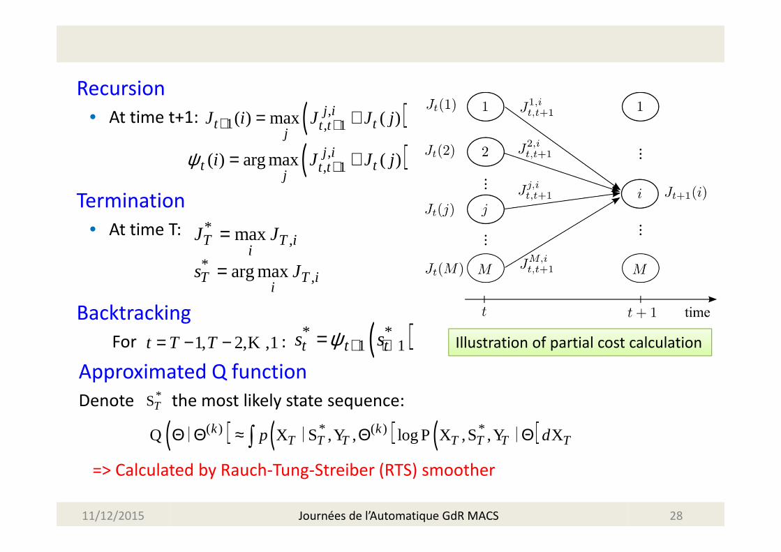
Recursion
• At time t+1:
Termination
• At time T:
Backtracking
For :
Approximated Q function
Denote the most likely state sequence:
=> Calculated by Rauch-Tung-Streiber (RTS) smoother
11/12/2015 28
*,maxT T i
iJ J=
( ),1 , 1( ) max ( )j i
t tt tj
J i J J j+ += +
1, 2, ,1t T T= − − K
( ),, 1( ) arg max ( )j i
t tt tj
i J J jψ += +
*,arg maxT T i
is J=
( )* *1 1t t ts sψ + +=
( ) ( ) ( )( ) * ( ) *, , log , ,k kT T T T T T Tp dΘ Θ ≈ Θ Θ∫ PQ X S Y X S Y X∣ ∣ ∣
*TS
Illustration of partial cost calculation
Journées de l’Automatique GdR MACS
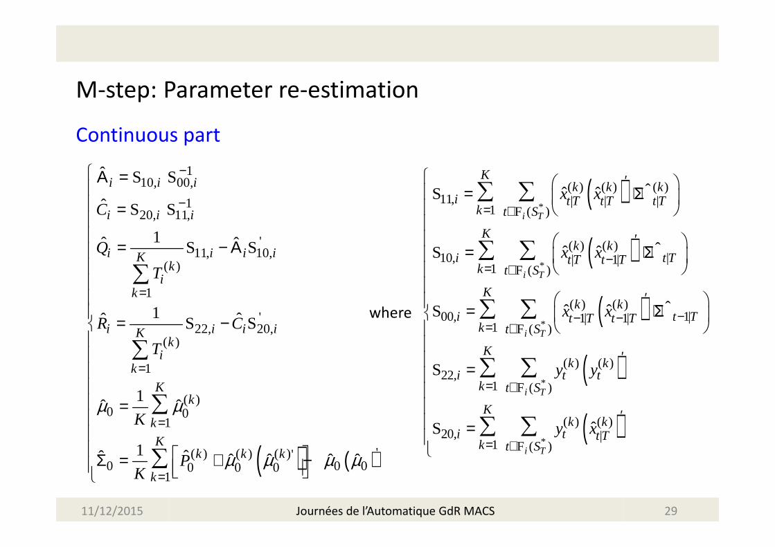
M-step: Parameter re-estimation
Continuous part
11/12/2015 29
( ) ( )
110, 00,
120, 11,
11, 10,( )
1
22, 20,( )
1
( )0 0
1
'( ) ( ) ( )0 0 00 0 0
1
'
'
'
ˆ
1ˆ ˆ
1 ˆˆ
1ˆ ˆ
1 ˆˆ ˆ ˆ ˆ ˆ
ˆi i i
i i i
i i i iKk
ik
i i i iKk
ik
Kk
k
Kk k k
k
C
Q
T
R C
T
K
PK
µ µ
µ µ µ µ
−
−
=
=
=
=
=
=
= − Α
= −
=
Σ = + −
Α
∑
∑
∑
∑
S S
S S
S S
S S
( )
( )
( )
( )
*
*
*
*
( ) ( ) ( )11, | | |
1 ( )
( ) ( )10, || 1|
1 ( )
( ) ( )00, 1|1| 1|
1 ( )
( ) ( )22,
1 ( )
20
ˆˆ ˆ
ˆˆ ˆ
ˆˆ ˆ
i T
i T
i T
i T
Kk k k
i t T t T t Tk t S
Kk k
i t Tt T t Tk t S
Kk k
i t Tt T t Tk t S
Kk k
i t tk t S
x x
x x
x x
y y
′
= ∈
′−
= ∈
′−− −
= ∈
′
= ∈
= + Σ
= + Σ
= + Σ
=
∑ ∑
∑ ∑
∑ ∑
∑ ∑
F
F
F
F
S
S
S
S
S ( )*
( ) ( ), |
1 ( )ˆ
i T
Kk k
i t t Tk t S
y x′
= ∈
=
∑ ∑F
where
Journées de l’Automatique GdR MACS
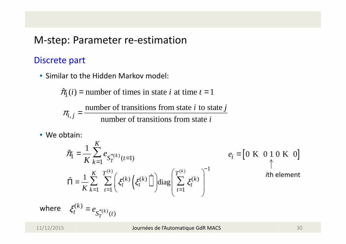
M-step: Parameter re-estimation
Discrete part
• Similar to the Hidden Markov model:
• We obtain:
where
11/12/2015 30
1ˆ ( ) number of times in state at time 1i i tπ = =
,number of transitions from state to state
number of transitions from state i ji j
iπ =
*( )1 ( 1)1
1ˆ k
T
K
S tk
eK
π === ∑
( )( ) ( ) 1
'( ) ( ) ( )
1 1 1
1ˆ diag
k kK T Tk k k
t t tk t tK
ξ ξ ξ
−
= = =
Π =
∑ ∑ ∑
*( )( )
( )kT
kt S t
eξ =
[ ]0 0 1 0 0ie = K K
ith element
Journées de l’Automatique GdR MACS
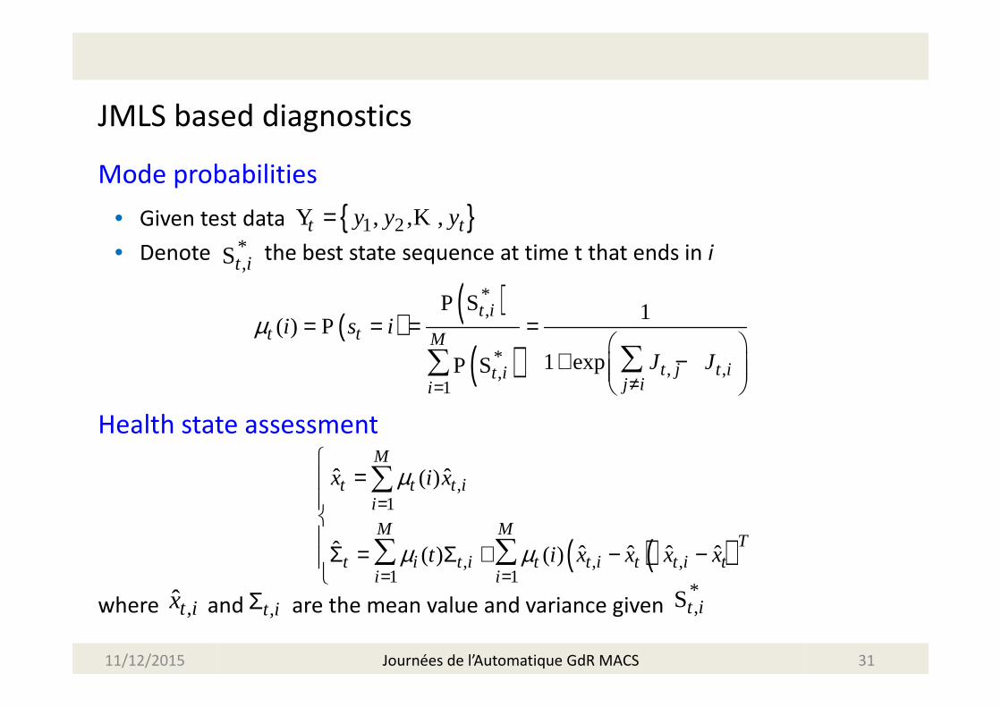
JMLS based diagnostics
Mode probabilities
• Given test data
• Denote the best state sequence at time t that ends in i
Health state assessment
where and are the mean value and variance given
11/12/2015 31
*,t iS
{ }1 2, , ,t ty y y= KY
( )( )
( )
*,
*, ,,
1
1( )
1 exp
t it t M
t j t it ij ii
i s i
J J
µ
≠=
= = = =
+ − ∑∑
PP
P
S
S
( )( )
,1
, , ,1 1
ˆ ˆ( )
ˆ ˆ ˆ ˆ ˆ( ) ( )
M
t t t ii
M MT
t i t i t t i t t i ti i
x i x
t i x x x x
µ
µ µ
=
= =
=
Σ = Σ +
− −
∑
∑ ∑
,ˆt ix ,t iΣ *,t iS
Journées de l’Automatique GdR MACS

RUL estimation
• Discrete time:
• If future mode changes are deterministic => can be estimated by multi-
step ahead Kalman prediction
• In JMLS case: M fold increase in number of Gaussian distributions to consider
⇒ Intractable computation
⇒ Approximation: merge all one-step predicted Gaussian distributions into one
Gaussian distribution
• Mode probability update
11/12/2015 32
( )min 1: t k tRUL k x L x L+= ≥ ≥ <∣
( ) ( )11 1 , 1 ,1
( ) ,M
tt t t t i t t ii
p x i xµ ++ + +=
≈ Σ∑ N∣ ∣ ∣
,11
( ) ( )j i
M
t tj
i jπµ µ+=
= ⋅∑
Journées de l’Automatique GdR MACS
t kx +

Numerical results
Mode training
• Two deterioration modes: quick-rate (mode 1) and normal-rate (mode 2)
• Real parameters
• Estimated parameters
11/12/2015 33
1 1 1 1
2 2 2 2
0 0
1.01 C 1 Q 0.015 R 2.5
1.002 C 1 Q 0.005 R 0.25
2 0.2
A
A
µ
= = = == = = == Σ =
10.3
0.7π
=
0.99 0.01
0.02 0.98
Π =
Convergence of the EM algorithm
1 1 1 1
2 2 2 2
0 0
ˆ ˆ ˆ ˆ1.01 C 1.01 Q 0.02 R 2.59
ˆ ˆ ˆ ˆ1.002 C 1 Q 0.01 R 0.25
ˆˆ 2.19 0.285
A
A
µ
= = = =
= = = =
= Σ =
10.3
ˆ0.7
π =
0.994 0.006ˆ0.011 0.989
Π =
Journées de l’Automatique GdR MACS
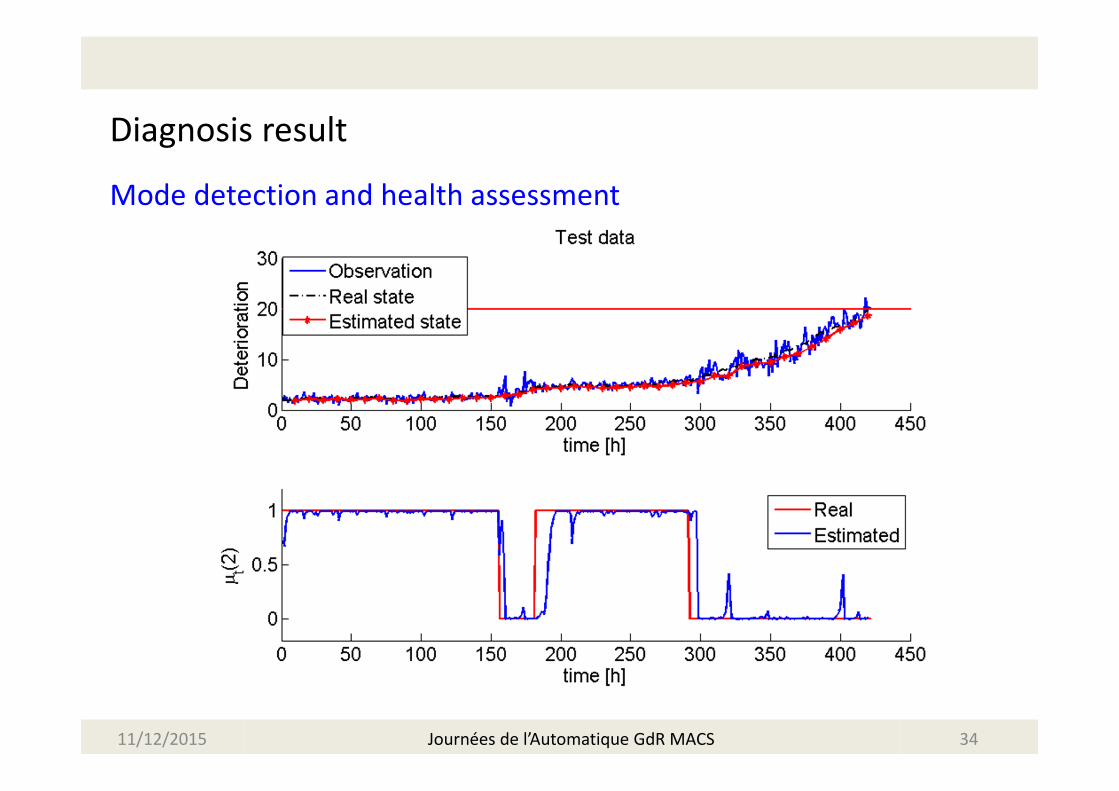
Diagnosis result
Mode detection and health assessment
11/12/2015 34Journées de l’Automatique GdR MACS
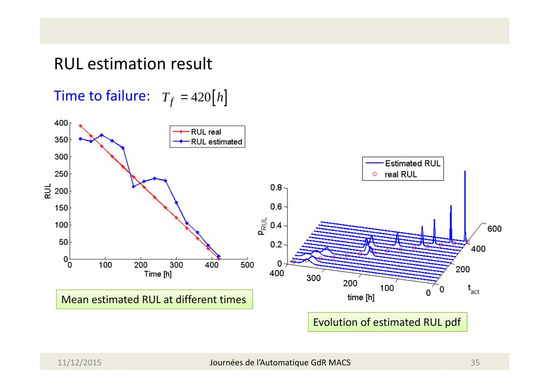
RUL estimation result
Time to failure:
11/12/2015 35
Mean estimated RUL at different times
Evolution of estimated RUL pdf
[ ]420fT h=
Journées de l’Automatique GdR MACS
Conclusion & Perspectives
Conclusion
• Development of multi-branch models to deal with the co-existence problem of
multiple deterioration modes
– Discrete health states: MB-HMM & MB-HsMM
– Continuous health states: JMLS
• Proposition of multi-branch models based framework for diagnostics &
prognostics
– Detection of actual deterioration mode
– Assessment of current health status
– Estimation of the RUL
Perspectives
• Extension of the JMLS model to the non-linear case
• Application with real-life data
11/12/2015 36Journées de l’Automatique GdR MACS

Thank you for your attention!
LE Thanh Trung
PhD student
GIPSA-lab, Grenoble Insititut of Technology
11 rue des Mathématiques – 38402 Saint Martin d’Hères cedex
Phone: +33 4 76 82 71 59 - Fax: +33 4 76 82 63 88
Email: [email protected]
Top Related