Modélisation de la détérioration basée sur les données...

Modélisation de la détérioration basée sur les

données de surveillance conditionnelle et

estimation de la durée de vie résiduelle

T. T. Le , C. Bérenguer, F. Chatelain

Univ. Grenoble Alpes, GIPSA-lab, F-38000 Grenoble, France

CNRS, GIPSA-lab, F-38000 Grenoble, France

Journées de l’Automatique GdR MACS

Context

FP7 European project:

• “SUstainable PREdictive Maintenance for manufacturing Equipment”

• Purpose: Development of new tools for predictive maintenance to improve

productivity, reduce machine downtimes and increase energy efficiency.

⇒ Application case: Paper machine

⇒ Main objectives:

� Deterioration modeling

� Remaining Useful Life (RUL)

estimation

11/12/2015 Journées de l’Automatique GdR MACS 2

Predictive maintenanceSUPREME partners


Problem statement

Deterioration models

• Represent temporal evolution of defects, i.e. of health indicators.

• Health indicators: unobservable

• Observations: noisy condition monitoring data

=> State-space representation

• Two type of states

– Continuous

– Discrete

11/12/2015 3

1 ) : Hidden state( ,

( , ) : Observati

s

onst

t

t t

t t

xx f

y g x

ων

−= =

Discrete-state modelingContinuous-state modeling

Problem statement

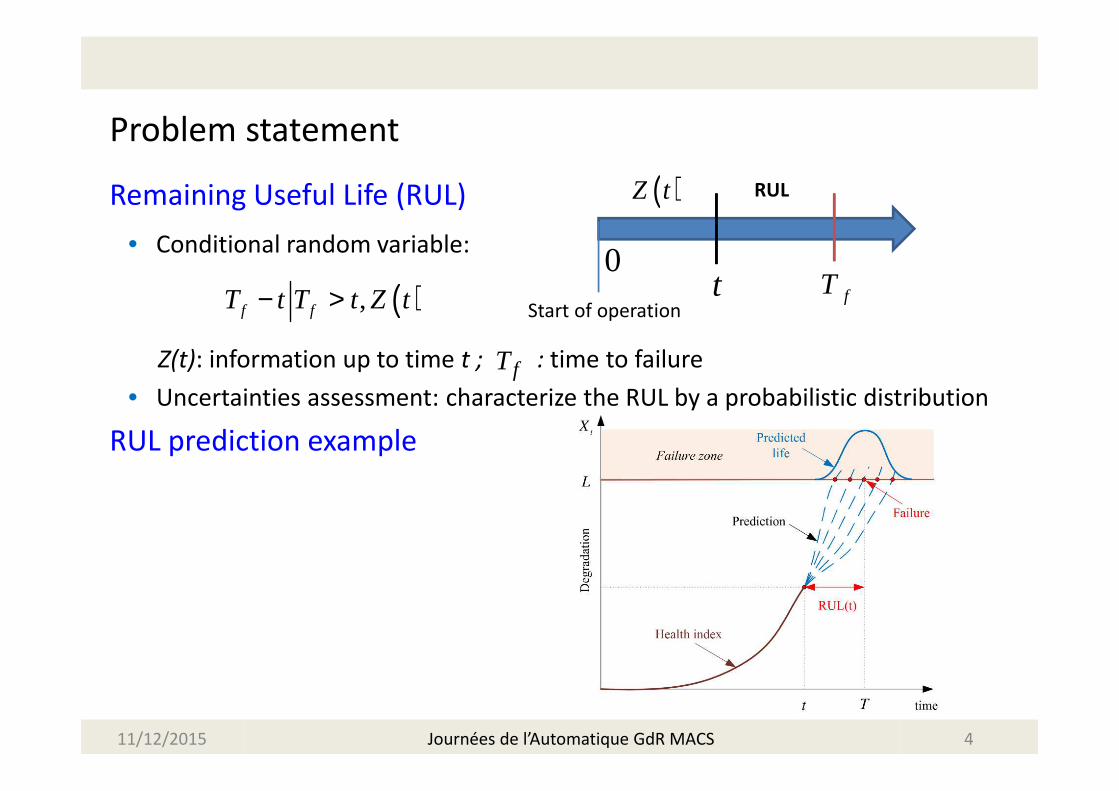
Remaining Useful Life (RUL)

• Conditional random variable:

Z(t): information up to time t ; : time to failure

• Uncertainties assessment: characterize the RUL by a probabilistic distribution

RUL prediction example

11/12/2015 4

fTtStart of operation

0

( )Z t RUL

( ),f fT t T t Z t− >


fT

Problem statement

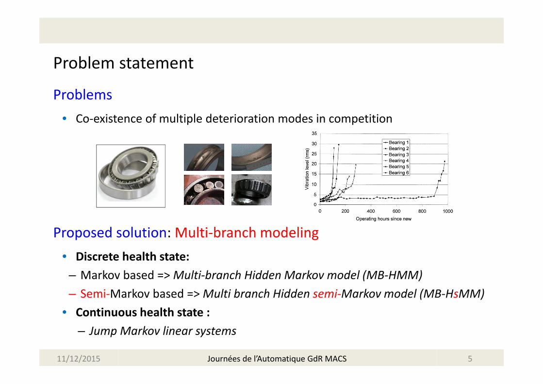
Problems

• Co-existence of multiple deterioration modes in competition

Proposed solution: Multi-branch modeling

• Discrete health state:

– Markov based => Multi-branch Hidden Markov model (MB-HMM)

– Semi-Markov based => Multi branch Hidden semi-Markov model (MB-HsMM)

• Continuous health state :

– Jump Markov linear systems

11/12/2015 5Journées de l’Automatique GdR MACS

Outline

� Multi-branch discrete-state model

� Diagnostics and Prognostics framework

� Numerical studies

� Jump Markov linear systems

� Parameters learning

� Health assessment and RUL estimation

� Numerical study

� Conclusion & Perspectives


Multi-branch discrete-state models


Multi-branch discrete-state modeling

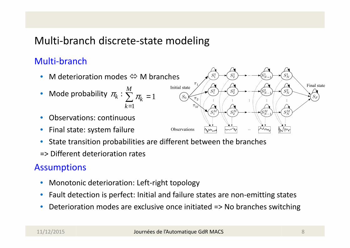
Multi-branch

• M deterioration modes � M branches

• Mode probability :

• Observations: continuous

• Final state: system failure

• State transition probabilities are different between the branches

=> Different deterioration rates

Assumptions

• Monotonic deterioration: Left-right topology

• Fault detection is perfect: Initial and failure states are non-emitting states

• Deterioration modes are exclusive once initiated => No branches switching

11/12/2015 8

1

1M

kk

π=

=∑kπ


Multi-branch discrete-state modeling

Multi-branch Hidden Markov Model

• Each branch ~ left-right Markov chain

• Markovian property

⇒State sojourn time: Exponential

or geometrical distributed

⇒May not be true in practice

Multi-branch Hidden semi-Markov Model

• Each branch ~ left-right semi-Markov chain

• Semi-Markov property: relax the Markovian assumption

=> allow arbitrary distributions for sojourn time: Gaussian, Weibull, …


Diagnostics and prognostics framework

Two-phase implementation: offline & online


Off-line phase

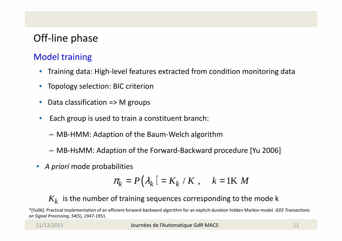
Model training

• Training data: High-level features extracted from condition monitoring data

• Topology selection: BIC criterion

• Data classification => M groups

• Each group is used to train a constituent branch:

– MB-HMM: Adaption of the Baum-Welch algorithm

– MB-HsMM: Adaption of the Forward-Backward procedure [Yu 2006]

• A priori mode probabilities

is the number of training sequences corresponding to the mode k

11/12/2015 11

( ) / , 1k k kP K K k Mπ λ= = = K

kK*[Yu06]: Practical implementation of an efficient forward-backward algorithm for an explicit-duration hidden Markov model. IEEE Transactions

on Signal Processing, 54(5), 1947-1951.


On-line phase

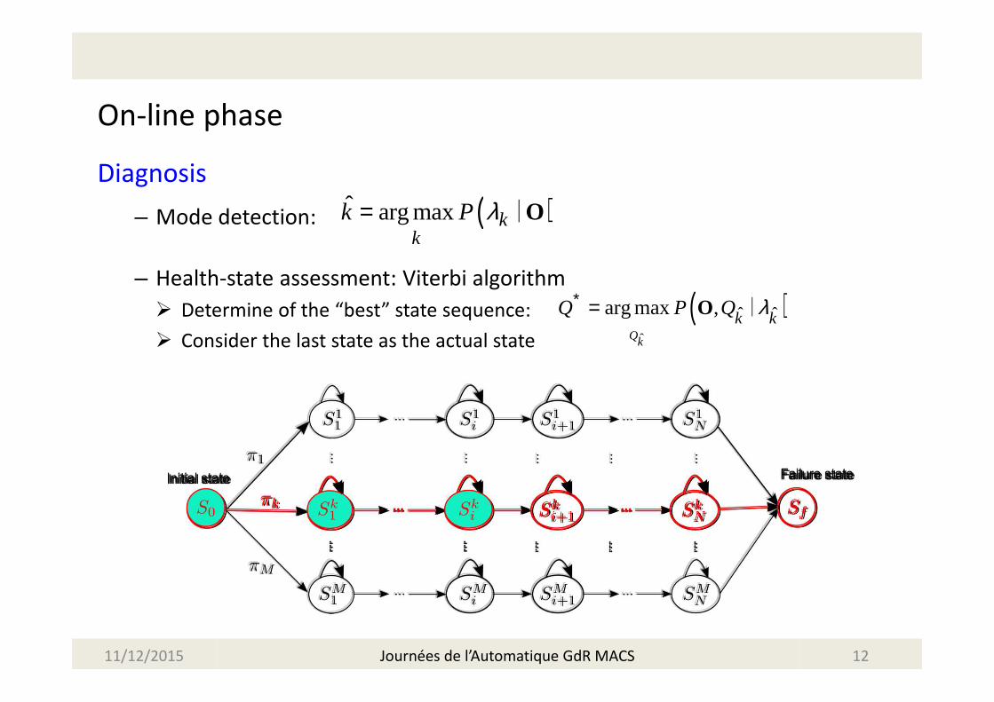
Diagnosis

– Mode detection:

– Health-state assessment: Viterbi algorithm

� Determine of the “best” state sequence:

� Consider the last state as the actual state

( )ˆ arg max kk

k P λ= O∣

( )ˆ

ˆ ˆarg max ,Qk

k kQ P Q λ∗ = O ∣


RUL estimation

One branch (HMM case)

• Suppose that the system is following the mode k

• RUL : discrete time assumption => number of transition steps to reach for the

1st time the failure state:

• Left-right HMM: Given the current state, the system can either stay in the

same state or jump to the next one

⇒ Recursive computation

( ) ( )( )1 1, , ,l

t i t l N t l N t N t iiRUL P RUL l q S P q S q S q S q S+ + − += = = ≠ …= = ≠ =∣ ∣


RUL estimation (cont.)

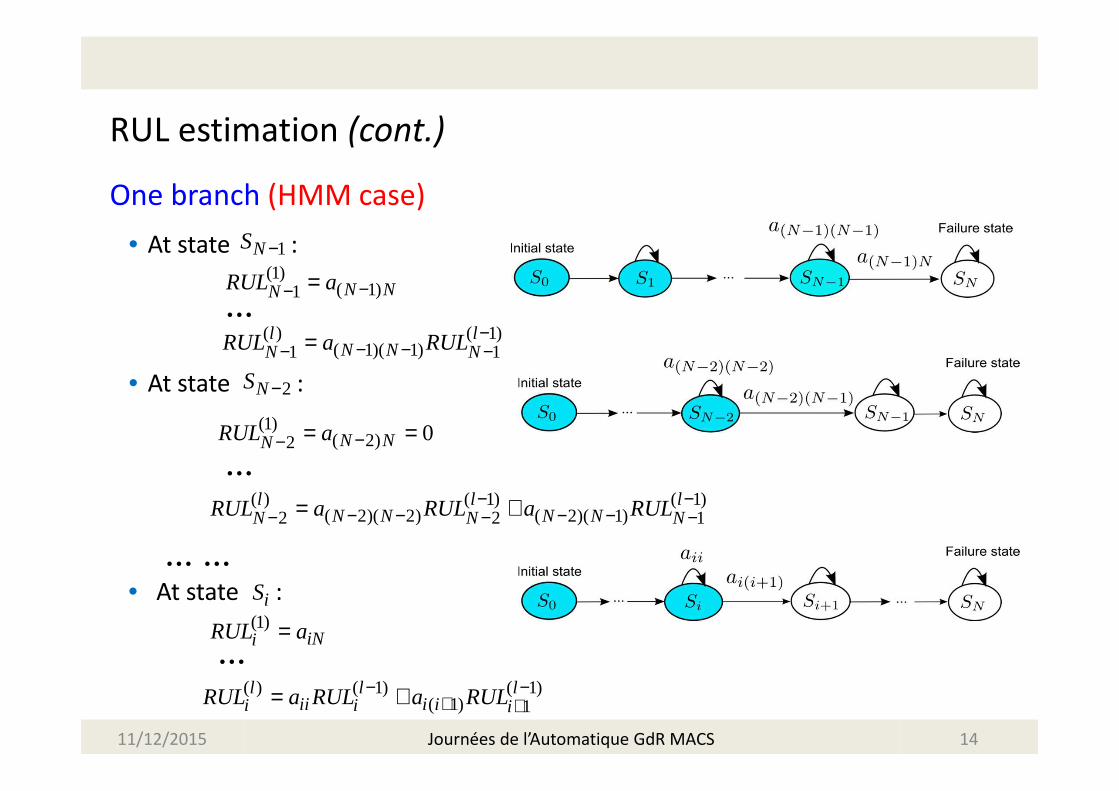
One branch (HMM case)

• At state :

• At state :

• At state :(1)i iNRUL a=

( ) ( 1) ( 1)( 1) 1

l l liii ii iiRUL RUL RULa a− −

+ += +

2NS −

(1)( 2)2 0N NNRUL a −− = =

iS

( ) ( 1) ( 1)( 2)( 2) ( 2)( 1)2 2 1

l l lN N N NN N NRUL LR a Ra UUL − −

− − − −− − −+=

...

...

... ...

1NS −(1)

( 1)1 N NNRUL a −− =

( ) ( 1)( 1)( 1)1 1

l lN NN NRRUL a UL −

− −− −=...


RUL estimation (cont.)

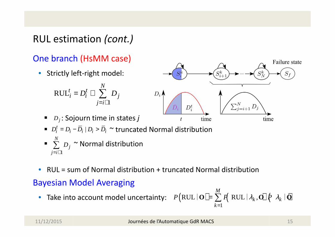
One branch (HsMM case)

• Strictly left-right model:

� : Sojourn time in states j

� ~ truncated Normal distribution

� ~ Normal distribution

• RUL = sum of Normal distribution + truncated Normal distribution

Bayesian Model Averaging

• Take into account model uncertainty: ( ) ( ) ( )1

RUL RUL ,M

k kk

P P Pλ λ=

= ∑O O O∣ ∣ ∣

1

RULN

t ti i j

j i

D D= +

= + ∑

|ti i i i iD D D D D= − >

jD

1

N

jj i

D= +∑


Numerical examples

Simulated deterioration data

• Fatigue Crack Growth (FCG) model to represent the evolution of a crack depth

• Observation model:

• Multi-mode: Two propagation rates

– Crack depth is proportional with

( )1 1

tii i i

enw

t t b tx x e C e x tγβ− −

= + ∆

i i it t ty x ξ= +

0.005, 1.3, 1.7wC n σ= = =

Two-mode training data

eγ

1 22 , 100, 010 .5Lξ π πσ = == =

[ ]0 0.75Teγ =


Numerical examples

Online RUL estimation (MB-HsMM model)


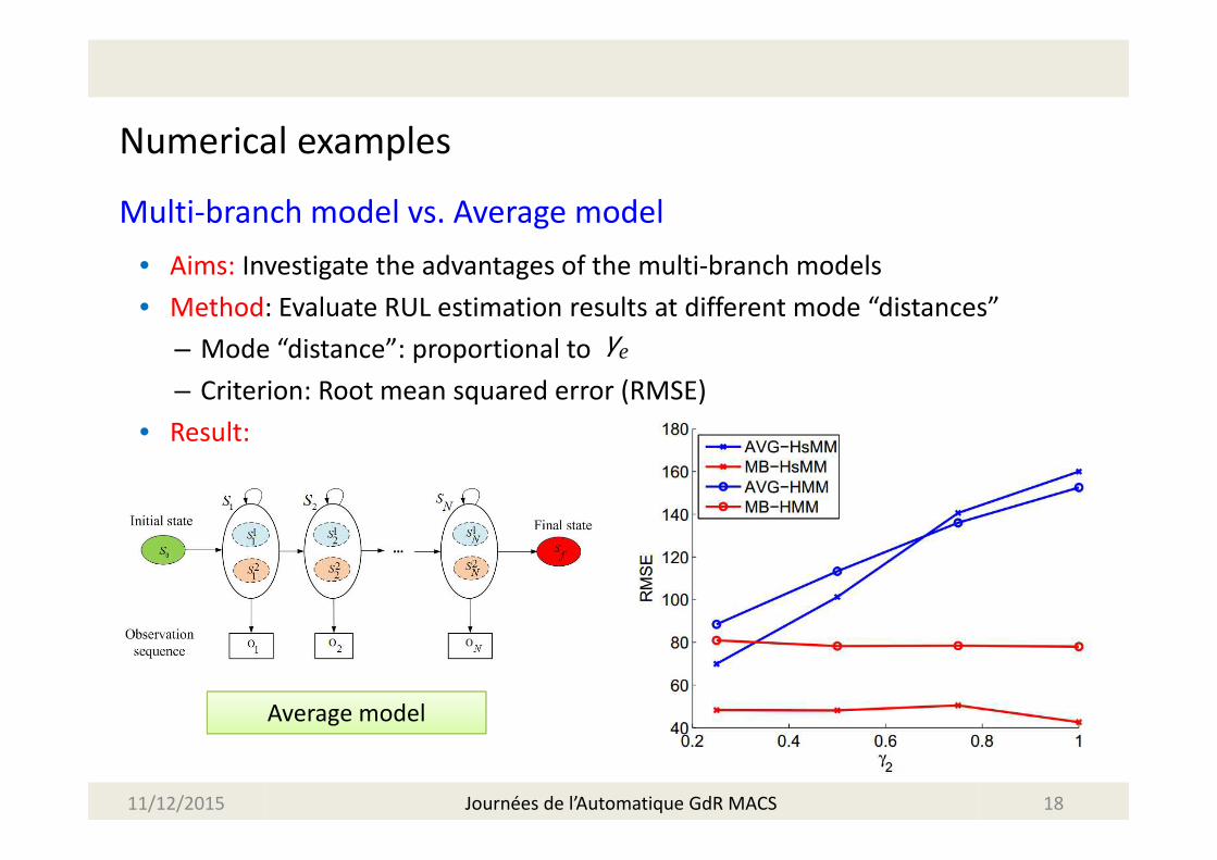
Numerical examples

Multi-branch model vs. Average model

• Aims: Investigate the advantages of the multi-branch models

• Method: Evaluate RUL estimation results at different mode “distances”

– Mode “distance”: proportional to

– Criterion: Root mean squared error (RMSE)

• Result:

Average model

eγ


Case study (MB-HsMM model):

PHM08 competition

• C-MAPSS: Modeling a large realistic commercial turbofan engine

• 2 data set for training and test

• 218 identical and independent units

• Objective:

– Construct a prognostic method basing on training data set

– Use it to estimate the RUL of each unit in test data set

• Evaluation criterion:

Where is penalty score for unit i:

where

*C-MAPSS: Commercial Modular Aero-Propulsion System Simulation

218

1i

i

S S=

= ∑

iS

/13

/10

1, 0

1, 0

i

i

di

i di

e dS

e d

− − ≤= − >

i ii est reald RUL RUL= −

Simplified diagram of engine

simulated in C-MAPSS


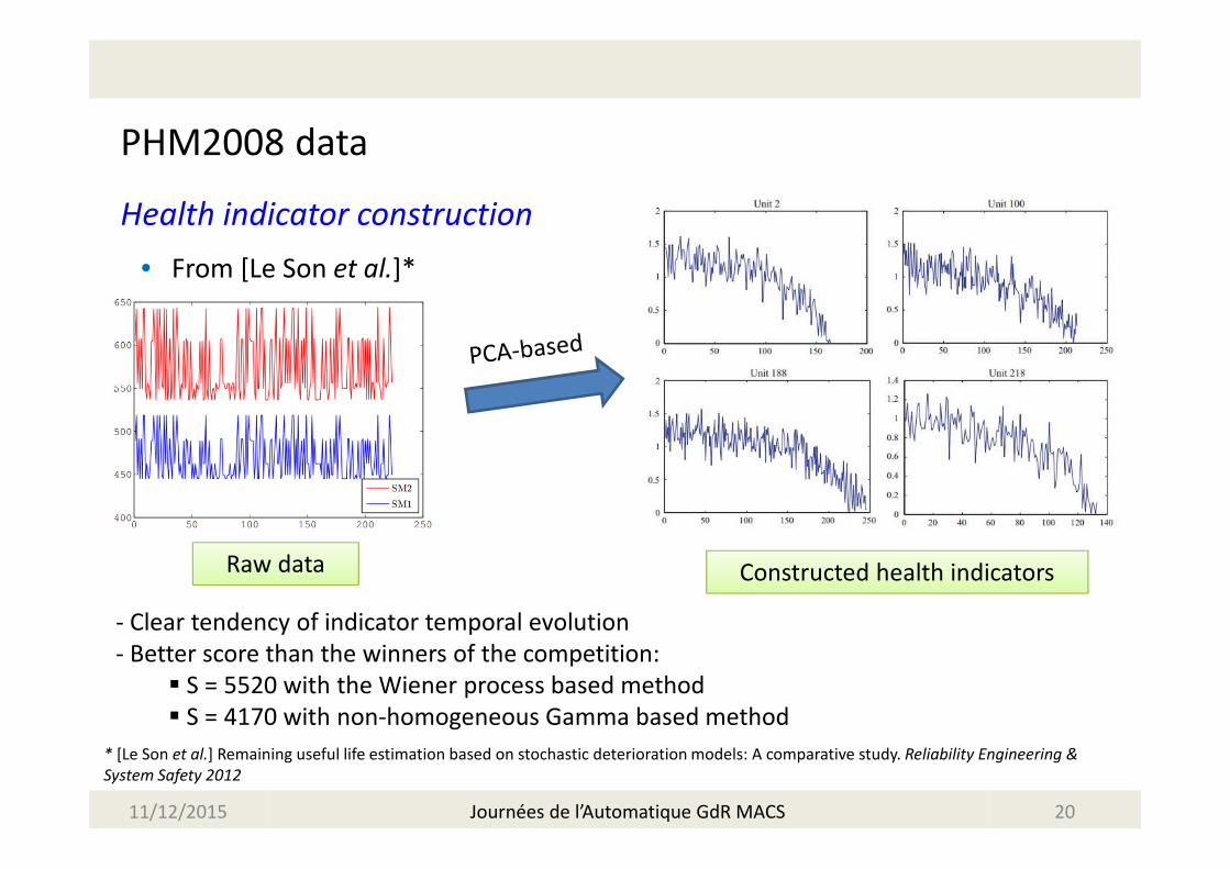
PHM2008 data

Health indicator construction

• From [Le Son et al.]*

* [Le Son et al.] Remaining useful life estimation based on stochastic deterioration models: A comparative study. Reliability Engineering &

System Safety 2012

11/12/2015 20

Raw data Constructed health indicators

- Clear tendency of indicator temporal evolution

- Better score than the winners of the competition:

� S = 5520 with the Wiener process based method

� S = 4170 with non-homogeneous Gamma based method


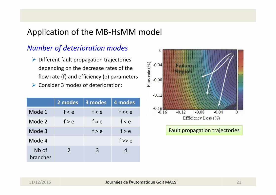
Application of the MB-HsMM model

Number of deterioration modes

� Different fault propagation trajectories

depending on the decrease rates of the

flow rate (f) and efficiency (e) parameters

� Consider 3 modes of deterioration:

11/12/2015 21

Fault propagation trajectories

2 modes 3 modes 4 modes

Mode 1 f < e f < e f << e

Mode 2 f > e f ≈ e f < e

Mode 3 f > e f > e

Mode 4 f >> e

Nb of

branches

2 3 4


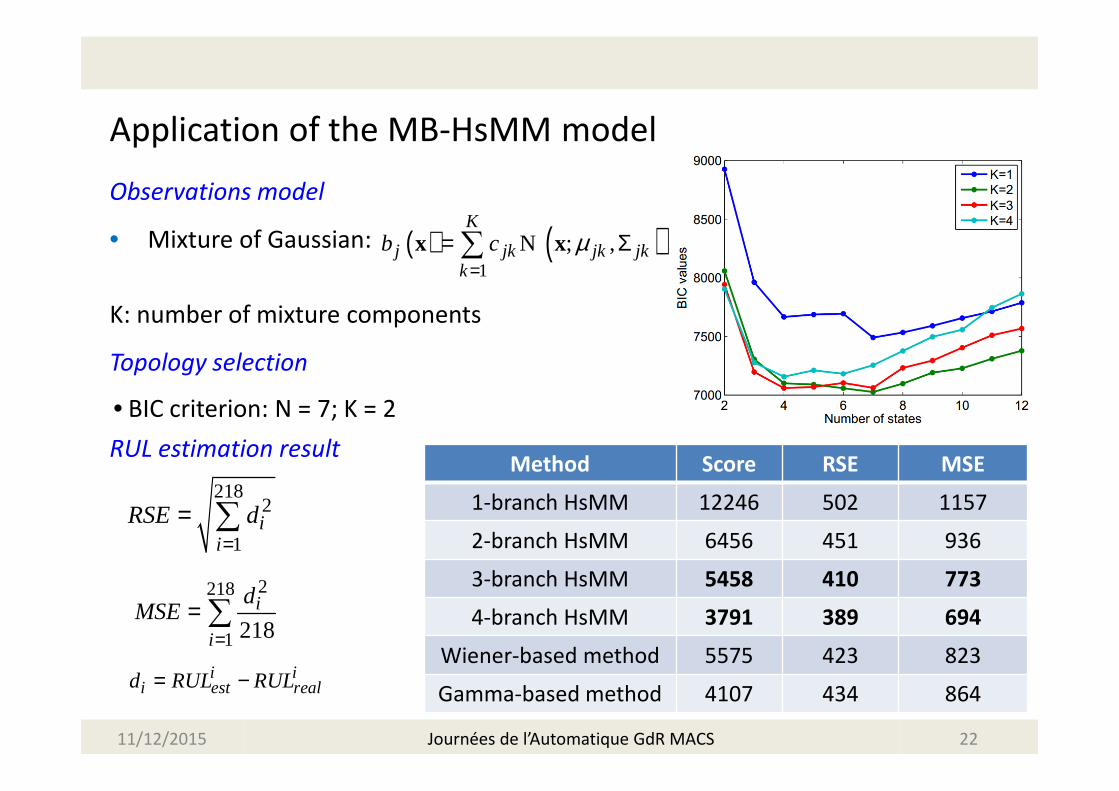
Application of the MB-HsMM model

Observations model

• Mixture of Gaussian:

K: number of mixture components

Topology selection

• BIC criterion: N = 7; K = 2

RUL estimation result

11/12/2015 22

Method Score RSE MSE

1-branch HsMM 12246 502 1157

2-branch HsMM 6456 451 936

3-branch HsMM 5458 410 773

4-branch HsMM 3791 389 694

Wiener-based method 5575 423 823

Gamma-based method 4107 434 864


( ) ( )1

; ,K

j jk jk jkk

b c µ=

= Σ∑x xN

2182

1i

i

RSE d=

= ∑

2218

1 218i

i

dMSE

== ∑

i ii est reald RUL RUL= −

Multi-branch continuous-state models


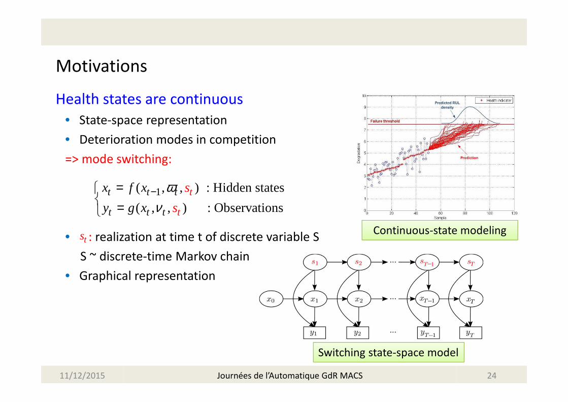
Motivations

Health states are continuous

• State-space representation

• Deterioration modes in competition

=> mode switching:

• : realization at time t of discrete variable S

S ~ discrete-time Markov chain

• Graphical representation


1 , ) : Hidden states( ,

( , , ) : Observationst

t

t

tt

t

t

t sxf

y s

x

g x

ων

−= =

ts

Switching state-space model

Continuous-state modeling

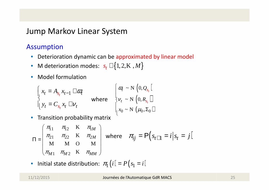
Jump Markov Linear System

Assumption

• Deterioration dynamic can be approximated by linear model

• M deterioration modes:

• Model formulation

where

• Transition probability matrix

where

• Initial state distribution:

11/12/2015 25

1t

t

t

t

s

s

t t

t t

x

y

A x

C x

ω

ν

−=

+=

+

( )( )( )0 0 0

~ 0,

~ 0,

~ ,

t

t

st

t s

Q

R

x

ω

ν

µ

Σ

N

N

N


{ }1,2, ,ts M∈ K

11 12 1

21 22 2

1 2

M

M

M M MM

π π ππ π π

π π π

Π =

K

K

M M O M

K

( )1ij t ts i s jπ += Ρ = =

( ) ( )1 1i P s iπ = =

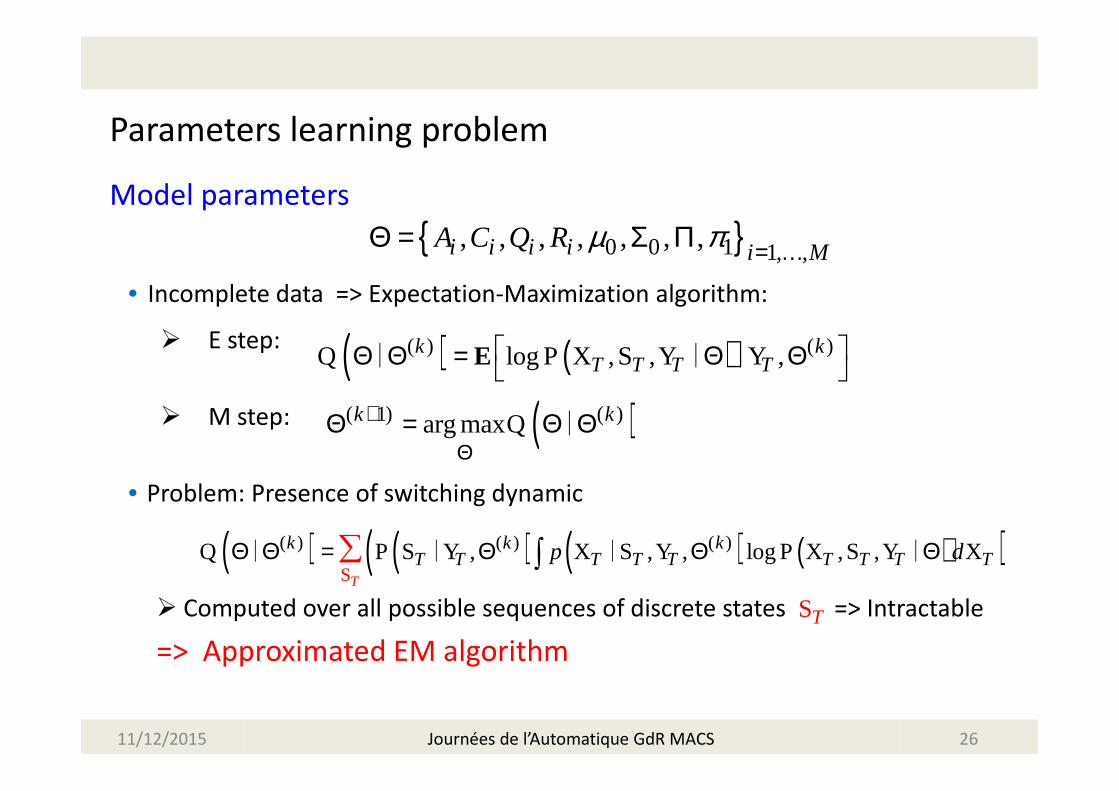
Parameters learning problem

Model parameters

• Incomplete data => Expectation-Maximization algorithm:

� E step:

� M step:

• Problem: Presence of switching dynamic

� Computed over all possible sequences of discrete states => Intractable

=> Approximated EM algorithm

11/12/2015 26

{ }0 0 1 1, ,, , , , , , ,i i i i i M

A C Q R µ π = …Θ = Σ Π

( ) ( )( ) ( )log , , ,k kT T T T

Θ Θ = Θ Θ

E PQ X S Y Y∣ ∣ ∣

( )( 1) ( )arg maxk k+

ΘΘ = Θ ΘQ ∣

( ) ( ) ( ) ( )( )( ) ( ) ( ), , , log , ,T

k k kT T T T T T T T Tp dΘ Θ = Θ Θ Θ∑ ∫P P

SQ S Y X S Y X S Y X∣ ∣ ∣ ∣

TS


Approximated EM algorithm

Pruning technique

• Approximation: Calculate the sum over the most “likely” state sequence

• Adaption of the Viterbi algorithm

• Do not guarantee the convergence, but still sufficient in several practical cases

• Most important: the algorithm is linear in number of time steps.

From the traditional Viterbi algorithm…

• Define the best “partial cost” at time t:

• Then, for each state transition j -> i, assign an “innovation cost”:

11/12/2015 27

( )1

1,

( ) max log , , ,t t

t t t t tJ i s i−

−= =PS X

X Y S

( ) ( ) ( )( )

1,1 , , 1 , , 1 , ,, 1

1 , ,

1

21

log log ,2

j it i i i i t it t j i t t j i t t j it t

i i it t j i

J y C x C C R y C x

C C R j i

′ −+ + ++

+

′= − − Σ + −

′− Σ + + Π

∣ ∣ ∣

∣


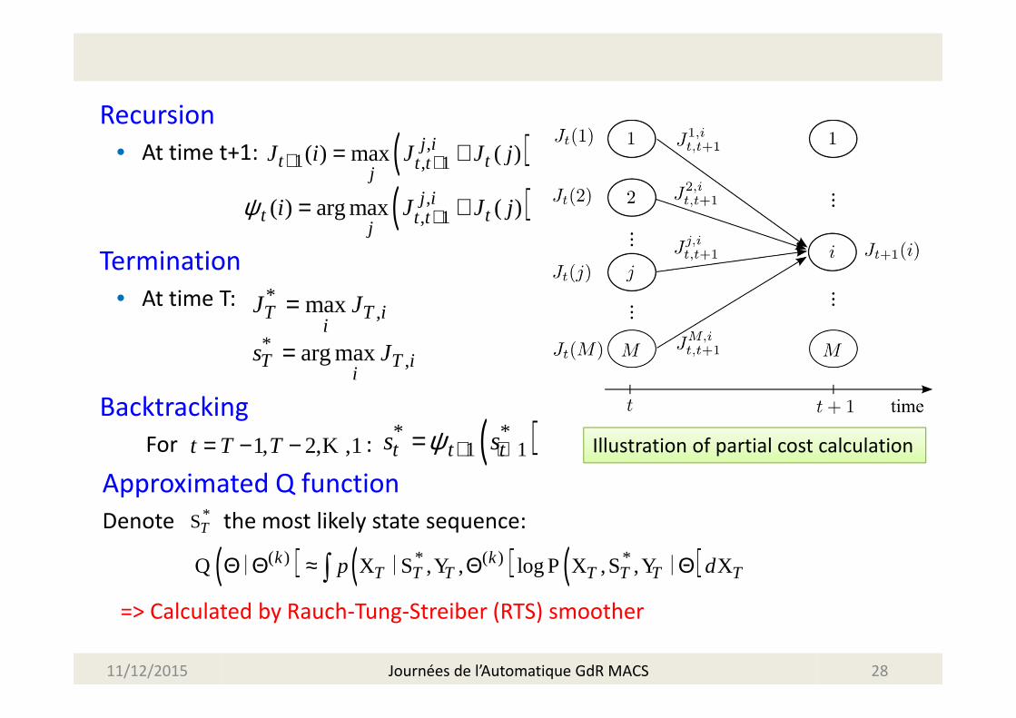
Recursion

• At time t+1:

Termination

• At time T:

Backtracking

For :

Approximated Q function

Denote the most likely state sequence:

=> Calculated by Rauch-Tung-Streiber (RTS) smoother

11/12/2015 28

*,maxT T i

iJ J=

( ),1 , 1( ) max ( )j i

t tt tj

J i J J j+ += +

1, 2, ,1t T T= − − K

( ),, 1( ) arg max ( )j i

t tt tj

i J J jψ += +

*,arg maxT T i

is J=

( )* *1 1t t ts sψ + +=

( ) ( ) ( )( ) * ( ) *, , log , ,k kT T T T T T Tp dΘ Θ ≈ Θ Θ∫ PQ X S Y X S Y X∣ ∣ ∣

*TS

Illustration of partial cost calculation


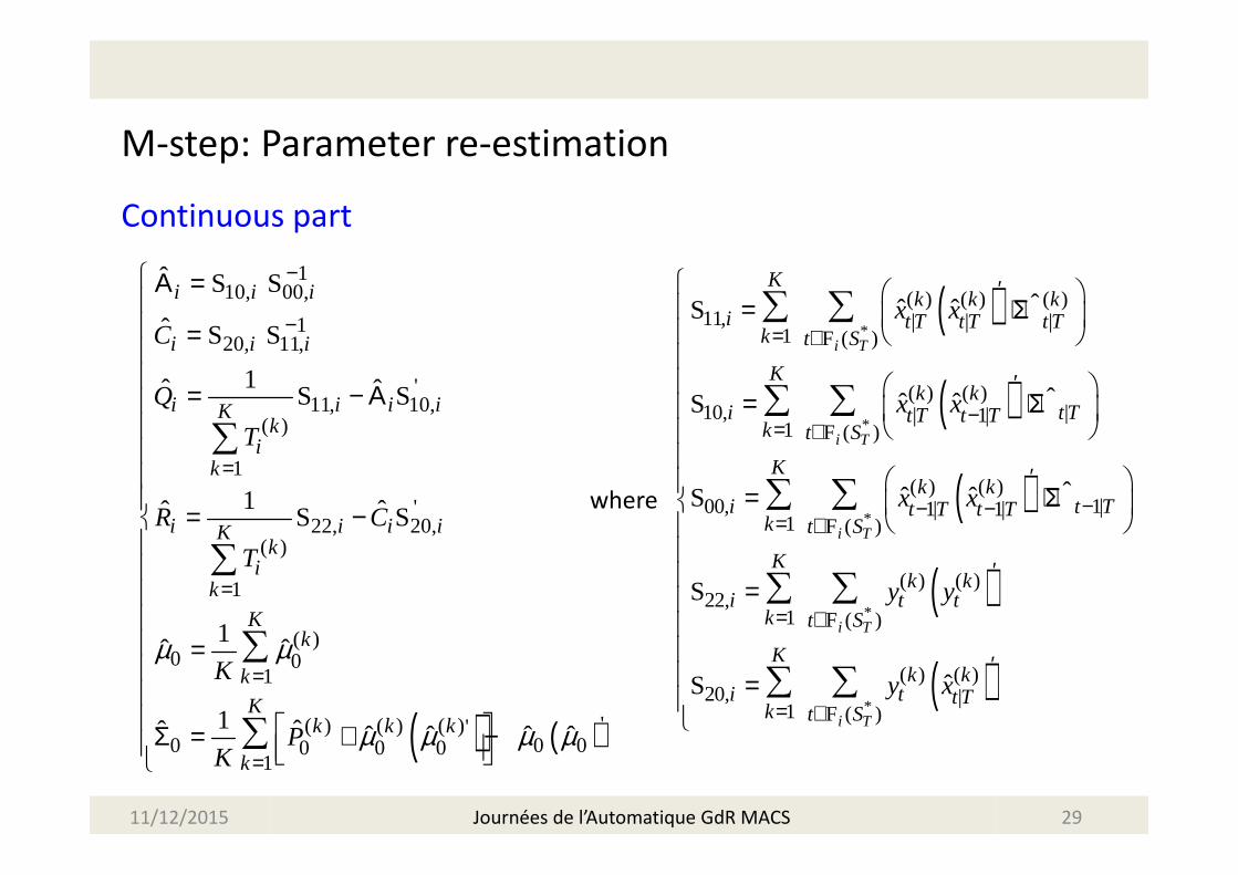
M-step: Parameter re-estimation

Continuous part

11/12/2015 29

( ) ( )

110, 00,

120, 11,

11, 10,( )

1

22, 20,( )

1

( )0 0

1

'( ) ( ) ( )0 0 00 0 0

1

'

'

'

ˆ

1ˆ ˆ

1 ˆˆ

1ˆ ˆ

1 ˆˆ ˆ ˆ ˆ ˆ

ˆi i i

i i i

i i i iKk

ik

i i i iKk

ik

Kk

k

Kk k k

k

C

Q

T

R C

T

K

PK

µ µ

µ µ µ µ

−

−

=

=

=

=

=

=

= − Α

= −

=

Σ = + −

Α

∑

∑

∑

∑

S S

S S

S S

S S

( )

( )

( )

( )

*

*

*

*

( ) ( ) ( )11, | | |

1 ( )

( ) ( )10, || 1|

1 ( )

( ) ( )00, 1|1| 1|

1 ( )

( ) ( )22,

1 ( )

20

ˆˆ ˆ

ˆˆ ˆ

ˆˆ ˆ

i T

i T

i T

i T

Kk k k

i t T t T t Tk t S

Kk k

i t Tt T t Tk t S

Kk k

i t Tt T t Tk t S

Kk k

i t tk t S

x x

x x

x x

y y

′

= ∈

′−

= ∈

′−− −

= ∈

′

= ∈

= + Σ

= + Σ

= + Σ

=

∑ ∑

∑ ∑

∑ ∑

∑ ∑

F

F

F

F

S

S

S

S

S ( )*

( ) ( ), |

1 ( )ˆ

i T

Kk k

i t t Tk t S

y x′

= ∈

=

∑ ∑F

where


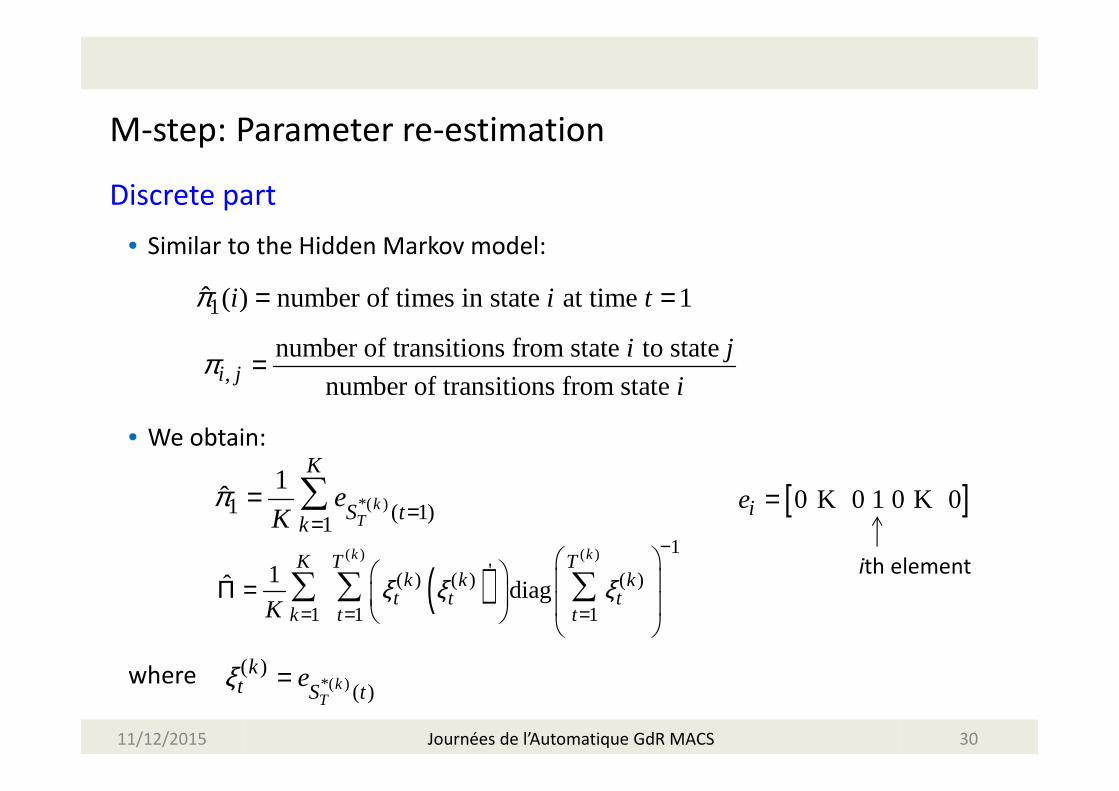
M-step: Parameter re-estimation

Discrete part

• Similar to the Hidden Markov model:

• We obtain:

where

11/12/2015 30

1ˆ ( ) number of times in state at time 1i i tπ = =

,number of transitions from state to state

number of transitions from state i ji j

iπ =

*( )1 ( 1)1

1ˆ k

T

K

S tk

eK

π === ∑

( )( ) ( ) 1

'( ) ( ) ( )

1 1 1

1ˆ diag

k kK T Tk k k

t t tk t tK

ξ ξ ξ

−

= = =

Π =

∑ ∑ ∑

*( )( )

( )kT

kt S t

eξ =

[ ]0 0 1 0 0ie = K K

ith element


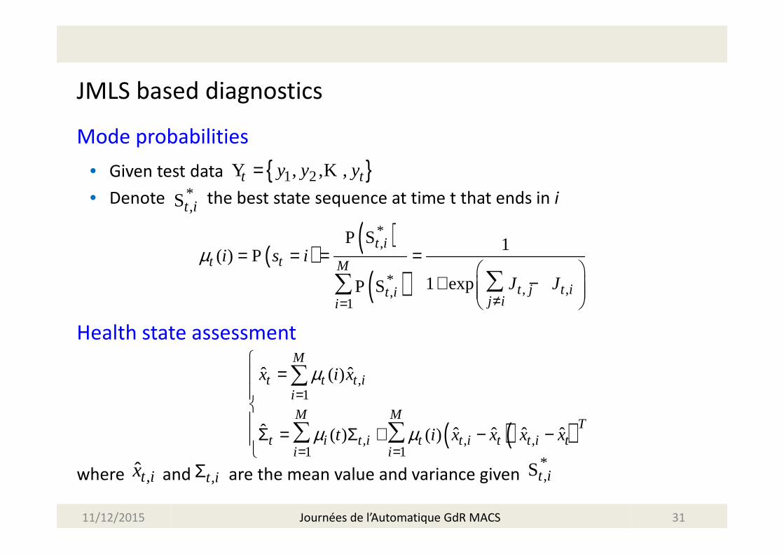
JMLS based diagnostics

Mode probabilities

• Given test data

• Denote the best state sequence at time t that ends in i

Health state assessment

where and are the mean value and variance given

11/12/2015 31

*,t iS

{ }1 2, , ,t ty y y= KY

( )( )

( )

*,

*, ,,

1

1( )

1 exp

t it t M

t j t it ij ii

i s i

J J

µ

≠=

= = = =

+ − ∑∑

PP

P

S

S

( )( )

,1

, , ,1 1

ˆ ˆ( )

ˆ ˆ ˆ ˆ ˆ( ) ( )

M

t t t ii

M MT

t i t i t t i t t i ti i

x i x

t i x x x x

µ

µ µ

=

= =

=

Σ = Σ +

− −

∑

∑ ∑

,ˆt ix ,t iΣ *,t iS


RUL estimation

• Discrete time:

• If future mode changes are deterministic => can be estimated by multi-

step ahead Kalman prediction

• In JMLS case: M fold increase in number of Gaussian distributions to consider

⇒ Intractable computation

⇒ Approximation: merge all one-step predicted Gaussian distributions into one

Gaussian distribution

• Mode probability update

11/12/2015 32

( )min 1: t k tRUL k x L x L+= ≥ ≥ <∣

( ) ( )11 1 , 1 ,1

( ) ,M

tt t t t i t t ii

p x i xµ ++ + +=

≈ Σ∑ N∣ ∣ ∣

,11

( ) ( )j i

M

t tj

i jπµ µ+=

= ⋅∑


t kx +

Numerical results

Mode training

• Two deterioration modes: quick-rate (mode 1) and normal-rate (mode 2)

• Real parameters

• Estimated parameters

11/12/2015 33

1 1 1 1

2 2 2 2

0 0

1.01 C 1 Q 0.015 R 2.5

1.002 C 1 Q 0.005 R 0.25

2 0.2

A

A

µ

= = = == = = == Σ =

10.3

0.7π

=

0.99 0.01

0.02 0.98

Π =

Convergence of the EM algorithm

1 1 1 1

2 2 2 2

0 0

ˆ ˆ ˆ ˆ1.01 C 1.01 Q 0.02 R 2.59

ˆ ˆ ˆ ˆ1.002 C 1 Q 0.01 R 0.25

ˆˆ 2.19 0.285

A

A

µ

= = = =

= = = =

= Σ =

10.3

ˆ0.7

π =

0.994 0.006ˆ0.011 0.989

Π =


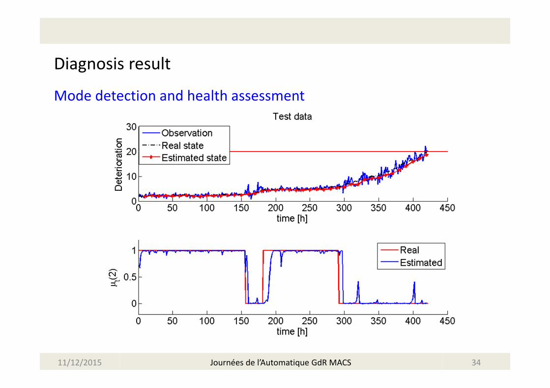
Diagnosis result

Mode detection and health assessment


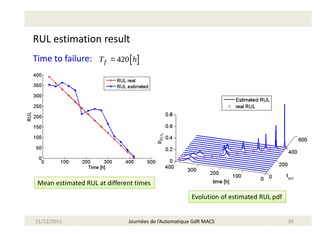
RUL estimation result

Time to failure:

11/12/2015 35

Mean estimated RUL at different times

Evolution of estimated RUL pdf

[ ]420fT h=


Conclusion & Perspectives

Conclusion

• Development of multi-branch models to deal with the co-existence problem of

multiple deterioration modes

– Discrete health states: MB-HMM & MB-HsMM

– Continuous health states: JMLS

• Proposition of multi-branch models based framework for diagnostics &

prognostics

– Detection of actual deterioration mode

– Assessment of current health status

– Estimation of the RUL

Perspectives

• Extension of the JMLS model to the non-linear case

• Application with real-life data


Thank you for your attention!

LE Thanh Trung

PhD student

GIPSA-lab, Grenoble Insititut of Technology

11 rue des Mathématiques – 38402 Saint Martin d’Hères cedex

Phone: +33 4 76 82 71 59 - Fax: +33 4 76 82 63 88

Email: [email protected]

Modélisation de la détérioration basée sur les données...

Documents

Transcript of Modélisation de la détérioration basée sur les données...