Water-vapour measurements by Raman lidar: Calibration and
31
Water vapor measurements by Raman lidar: calibration and accuracy F. Congeduti , D. Dionisi, G. Liberti (Istituto di Scienze dell’Atmosfera ed il Clima ISAC – CNR, Rome-Tor Vergata) LINDENBERG 21-23.5.2008
Transcript of Water-vapour measurements by Raman lidar: Calibration and

Water vapor measurements by Raman lidar: calibration
and accuracy
F. Congeduti, D. Dionisi, G. Liberti(Istituto di Scienze dell’Atmosfera ed il
ClimaISAC – CNR, Rome-Tor Vergata)
LINDENBERG 21-23.5.2008
Overview
• System description• Calibration & Systematic errors• Random errors• Example of products• Conclusions
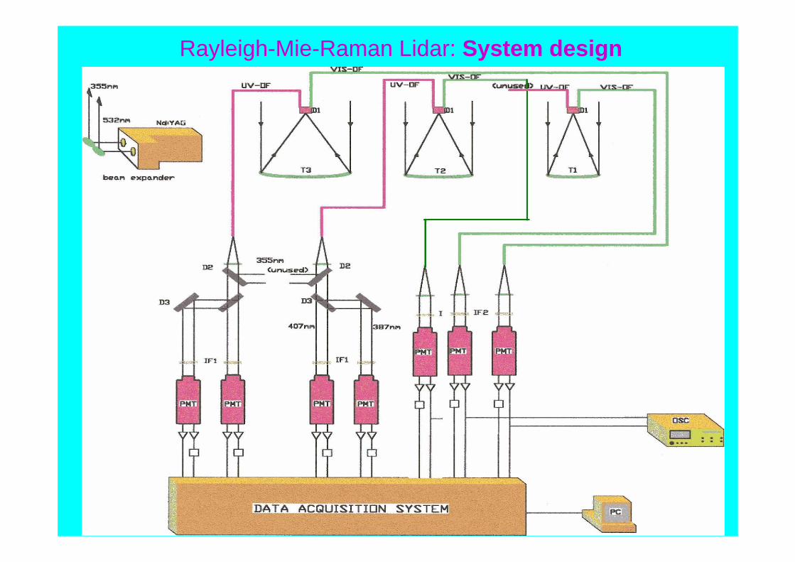
Rayleigh-Mie-Raman Lidar: System design
Rayleigh-Mie-Raman Lidar: System design
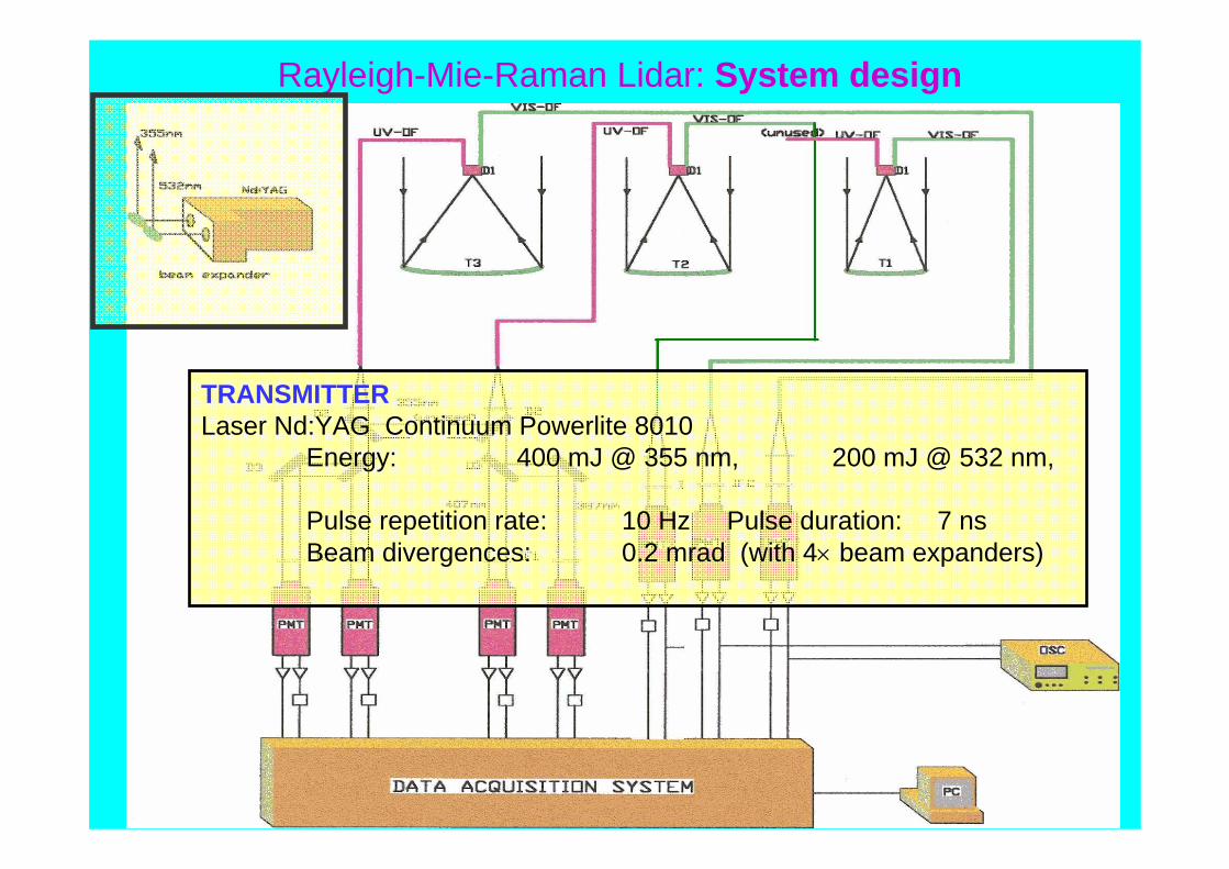
TRANSMITTERLaser Nd:YAG Continuum Powerlite 8010
Energy: 400 mJ @ 355 nm, 200 mJ @ 532 nm,
Pulse repetition rate: 10 Hz Pulse duration: 7 nsBeam divergences: 0.2 mrad (with 4× beam expanders)
Rayleigh-Mie-Raman Lidar: System design
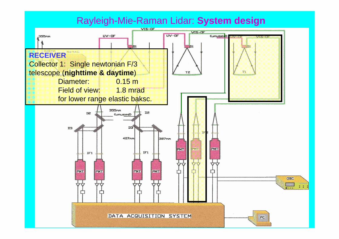
RECEIVERCollector 1: Single newtonian F/3 telescope (nighttime & daytime)
Diameter: 0.15 m Field of view: 1.8 mradfor lower range elastic baksc.

Rayleigh-Mie-Raman Lidar: System design
RECEIVERCollector 2: Single newtonian F/3 telescope
Diameter: 0.3 m Field of view: 0.9 mrad (nighttime), 0.45 mrad (daytime)for lower range Raman backsc. and middle range elastic backsc.

Rayleigh-Mie-Raman Lidar: System design
RECEIVERCollector 3: Array of 9 newtonian F/3 telescopes (nighttime)
Diameter: 0.5 m each (total collecting area ∼1.75 m2)Field of view: 0.6 mrad
for upper range Raman backsc. and upper range elastic backsc.
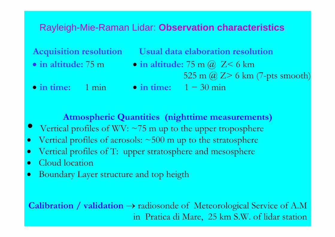
Acquisition resolution Usual data elaboration resolution• in altitude: 75 m • in altitude: 75 m @ Z< 6 km
525 m @ Z> 6 km (7-pts smooth)• in time: 1 min • in time: 1 − 30 min
Rayleigh-Mie-Raman Lidar: Observation characteristics
Atmospheric Quantities (nighttime measurements)• Vertical profiles of WV: ~75 m up to the upper troposphere • Vertical profiles of aerosols: ~500 m up to the stratosphere • Vertical profiles of T: upper stratosphere and mesosphere • Cloud location• Boundary Layer structure and top heigth
Calibration / validation → radiosonde of Meteorological Service of A.Min Pratica di Mare, 25 km S.W. of lidar station
Overview• System description• Calibration & Systematic errors• Random errors• Example of products• Conclusions
Calibration
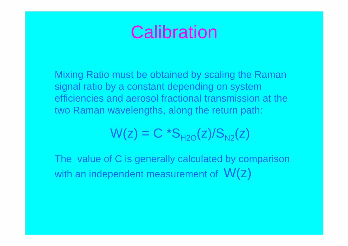
Mixing Ratio must be obtained by scaling the Raman signal ratio by a constant depending on system efficiencies and aerosol fractional transmission at the two Raman wavelengths, along the return path:
W(z) = C *SH2O(z)/SN2(z)
The value of C is generally calculated by comparison with an independent measurement of W(z)
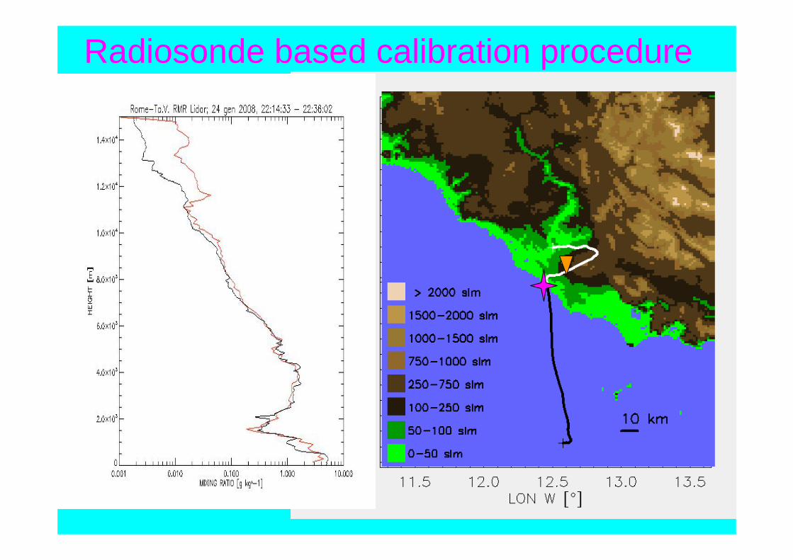
Radiosonde based calibration procedure
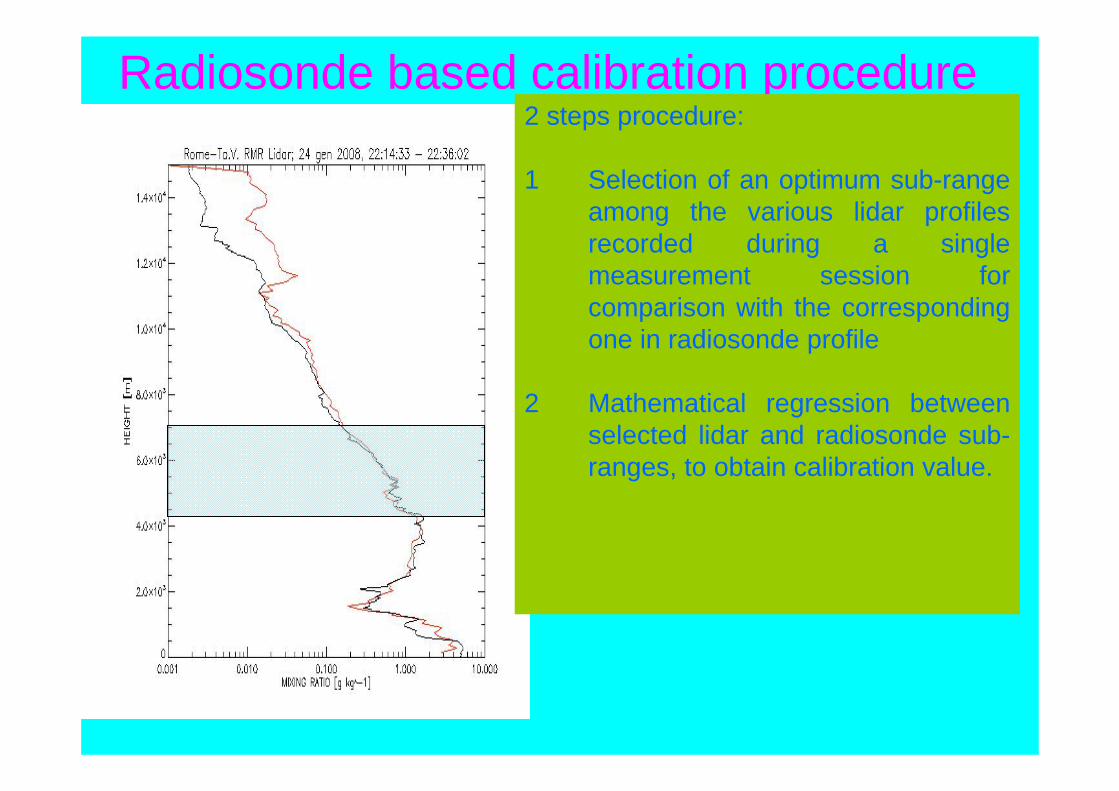
Radiosonde based calibration procedure2 steps procedure:
1 Selection of an optimum sub-range among the various lidar profiles recorded during a single measurement session for comparison with the corresponding one in radiosonde profile
2 Mathematical regression between selected lidar and radiosonde sub-ranges, to obtain calibration value.
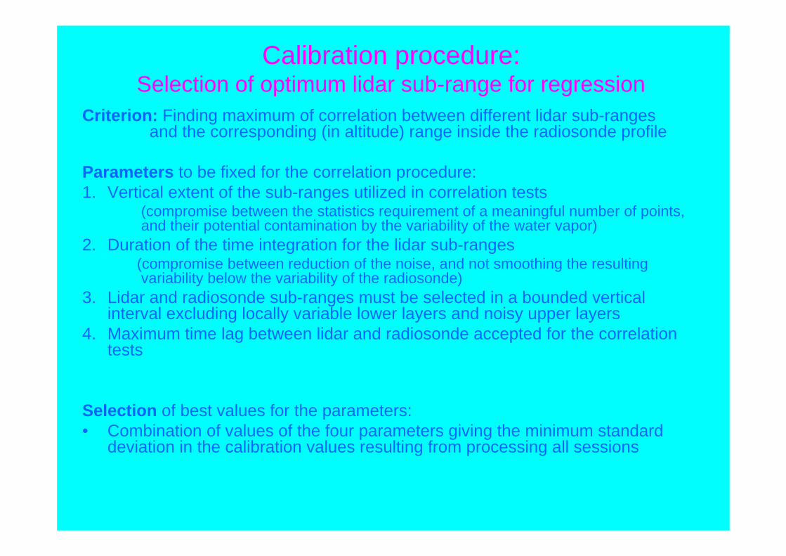
Calibration procedure:Selection of optimum lidar sub-range for regression
Criterion: Finding maximum of correlation between different lidar sub-ranges and the corresponding (in altitude) range inside the radiosonde profile
Parameters to be fixed for the correlation procedure:1. Vertical extent of the sub-ranges utilized in correlation tests
(compromise between the statistics requirement of a meaningful number of points, and their potential contamination by the variability of the water vapor)
2. Duration of the time integration for the lidar sub-ranges(compromise between reduction of the noise, and not smoothing the resulting variability below the variability of the radiosonde)
3. Lidar and radiosonde sub-ranges must be selected in a bounded vertical interval excluding locally variable lower layers and noisy upper layers
4. Maximum time lag between lidar and radiosonde accepted for the correlation tests
Selection of best values for the parameters:• Combination of values of the four parameters giving the minimum standard
deviation in the calibration values resulting from processing all sessions
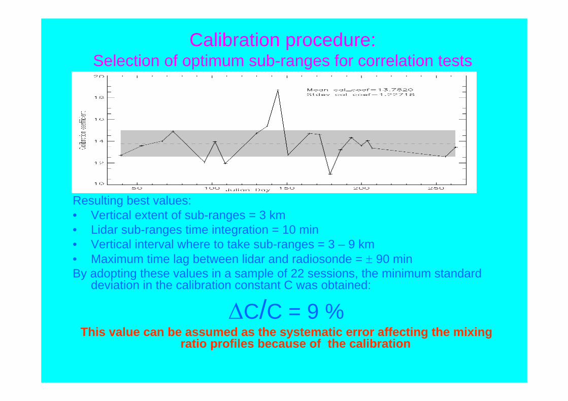
Calibration procedure:Selection of optimum sub-ranges for correlation tests
Resulting best values:• Vertical extent of sub-ranges = 3 km• Lidar sub-ranges time integration = 10 min• Vertical interval where to take sub-ranges = 3 – 9 km• Maximum time lag between lidar and radiosonde = ± 90 minBy adopting these values in a sample of 22 sessions, the minimum standard
deviation in the calibration constant C was obtained:
ΔC/C = 9 %This value can be assumed as the systematic error affecting the mixing
ratio profiles because of the calibration

Calibration procedure: example
Lidar profileLidar best correlation sub-rangeRDS of Pratica di Mare (23:00 UT)
Overview• System description• Calibration & Systematic errors• Random errors• Example of products• Conclusions
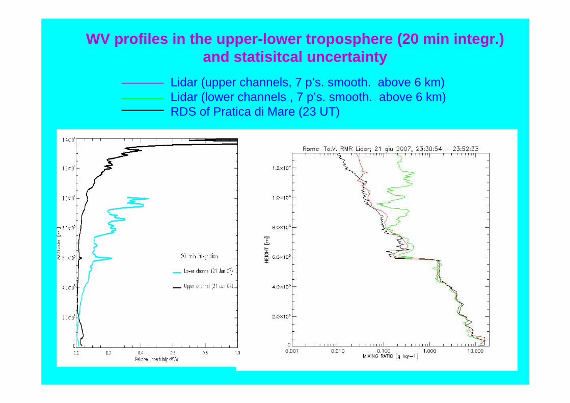
WV profiles in the upper-lower troposphere (20 min integr.)and statisitcal uncertainty
Lidar (upper channels, 7 p’s. smooth. above 6 km) Lidar (lower channels , 7 p’s. smooth. above 6 km)RDS of Pratica di Mare (23 UT)
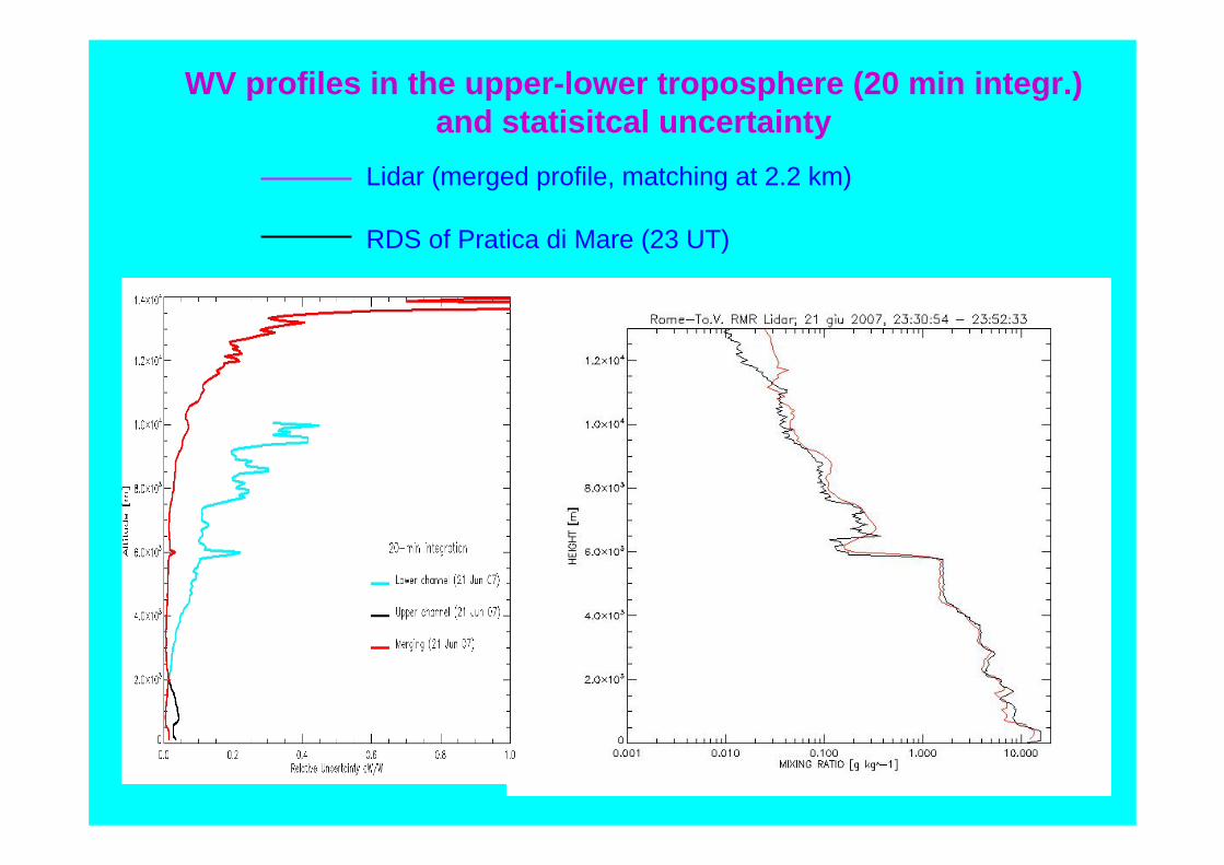
WV profiles in the upper-lower troposphere (20 min integr.) and statisitcal uncertainty
Lidar (merged profile, matching at 2.2 km)
RDS of Pratica di Mare (23 UT)
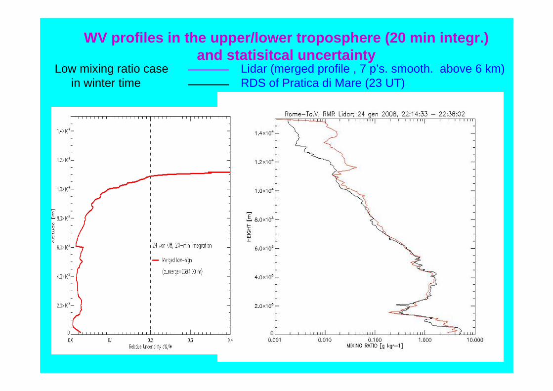
WV profiles in the upper/lower troposphere (20 min integr.) and statisitcal uncertainty
Low mixing ratio case Lidar (merged profile , 7 p’s. smooth. above 6 km) in winter time RDS of Pratica di Mare (23 UT)
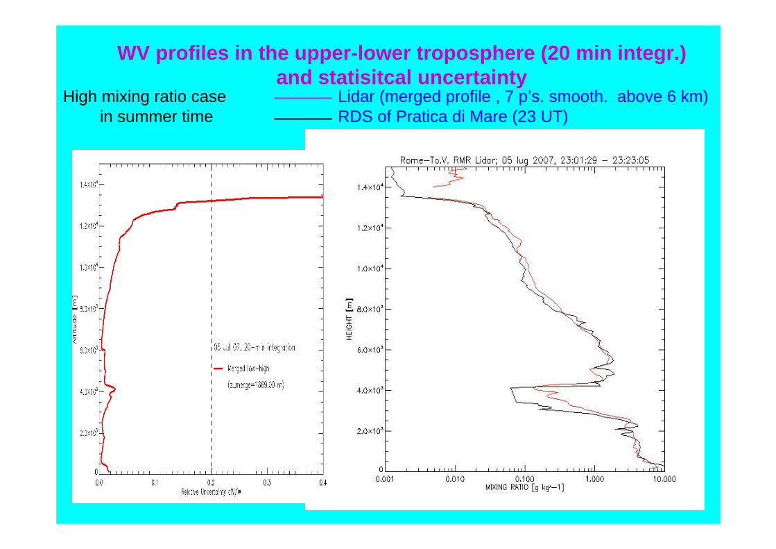
WV profiles in the upper-lower troposphere (20 min integr.) and statisitcal uncertainty
High mixing ratio case Lidar (merged profile , 7 p’s. smooth. above 6 km) in summer time RDS of Pratica di Mare (23 UT)
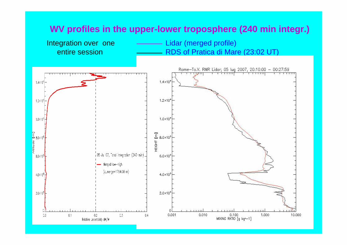
WV profiles in the upper-lower troposphere (240 min integr.)Integration over one Lidar (merged profile)
entire session RDS of Pratica di Mare (23:02 UT)

Overview• System description• Calibration & Systematic errors• Random errors• Example of products• Conclusions
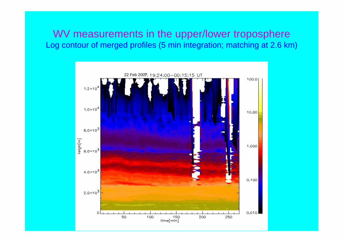
WV measurements in the upper/lower troposphereLog contour of merged profiles (5 min integration; matching at 2.6 km)
22 Feb 2007;
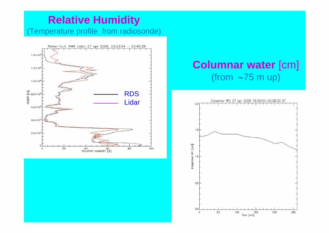
Relative Humidity(Temperature profile from radiosonde)
RDS Lidar
Columnar water [cm](from ∼75 m up)
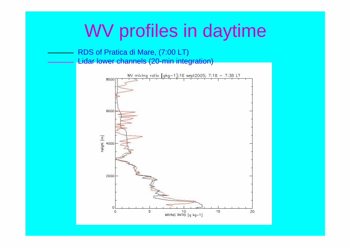
WV profiles in daytimeRDS of Pratica di Mare, (7:00 LT) Lidar lower channels (20-min integration)
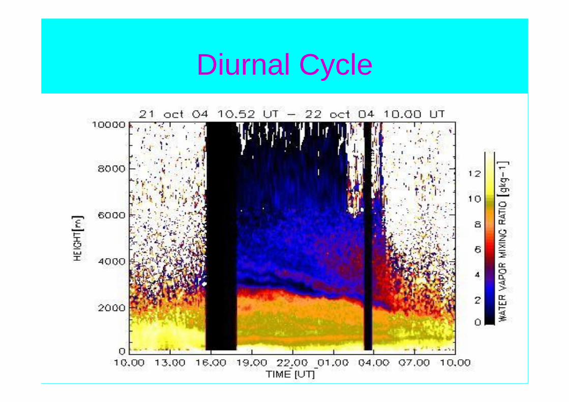
Diurnal Cycle
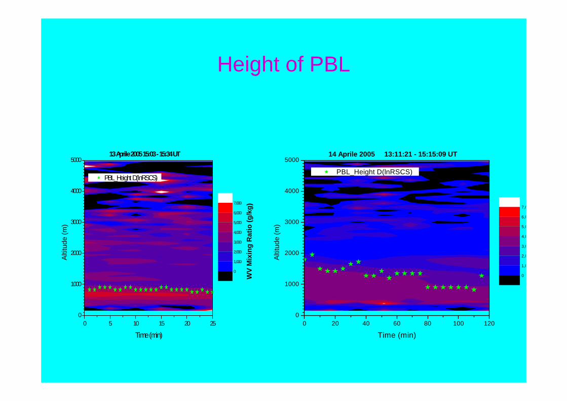
Height of PBL
0 5 10 15 20 250
1000
2000
3000
4000
5000
PBL_Height D(lnRSCS)
Time (min)
Altit
ude
(m)
0
1,000
2,000
3,000
4,000
5,000
6,000
7,000
WV
Mix
ing
Rat
io (g
/kg)
13 Aprile 2005 15:03 - 15:34 UT
0 20 40 60 80 100 1200
1000
2000
3000
4000
5000
PBL_Height D(lnRSCS)
Time (min)
Altit
ude
(m)
0
1,0
2,0
3,0
4,0
5,0
6,0
7,0
14 Aprile 2005 13:11:21 - 15:15:09 UT
ITALIAN GROUPSUniversity of Rome(WV & aerosol Raman Lidar,Sodar,MFRSR)
CNR-ISAC(WV & aerosol Raman Lidar, Sodar)
University of L’Aquila(weather forecast,lidar assimilation)University of L’Aquila
(WV & aerosol Raman Lidar, soundings)CNR-IMAA(WV & aerosol Raman Lidar,soundings)
University of Basilicata(WV & T & aerosol Raman Lidar)
University of Napoli(WV & aerosol Raman Lidar)
Univeristy of Lecce(WV & aerosol Raman Lidar, soundings)
Enea –Lampedusa(soundings, aereosol Lidar)
ISAC
UNIRM
UNIAQ
UNINA
DIFA
UNIBAS
UNILC
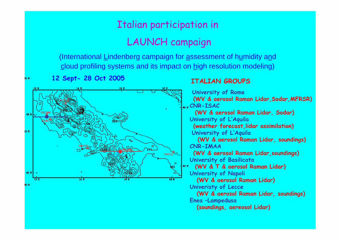
Italian participation in
LAUNCH campaign(International Lindenberg campaign for assessment of humidity and cloud profiling systems and its impact on high resolution modeling)
12 Sept- 28 Oct 2005
ITALIAN GROUPSUniversity of Rome(WV & aerosol Raman Lidar,Sodar,MFRSR)
CNR-ISAC(WV & aerosol Raman Lidar, Sodar)
University of L’Aquila(weather forecast,lidar assimilation)University of L’Aquila
(WV & aerosol Raman Lidar, soundings)CNR-IMAA(WV & aerosol Raman Lidar,soundings)
University of Basilicata(WV & T & aerosol Raman Lidar)
University of Napoli(WV & aerosol Raman Lidar)
Univeristy of Lecce(WV & aerosol Raman Lidar, soundings)
Enea –Lampedusa(soundings, aereosol Lidar)
ISAC
UNIRM
UNIAQ
UNINA
DIFA
UNIBAS
UNILC
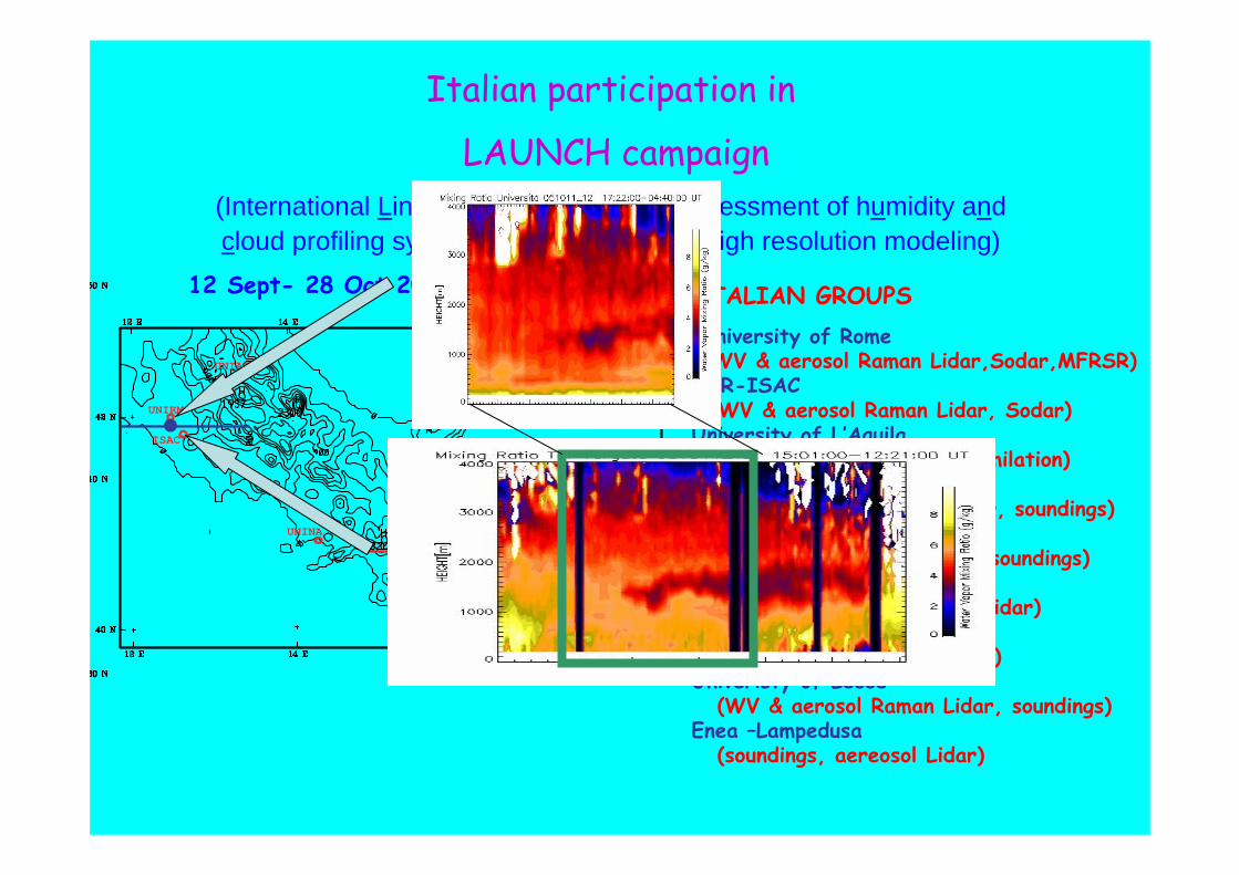
Italian participation in
LAUNCH campaign(International Lindenberg campaign for assessment of humidity and cloud profiling systems and its impact on high resolution modeling)
12 Sept- 28 Oct 2005

Overview• System description• Calibration & Systematic errors• Random errors• Example of products• Conclusions
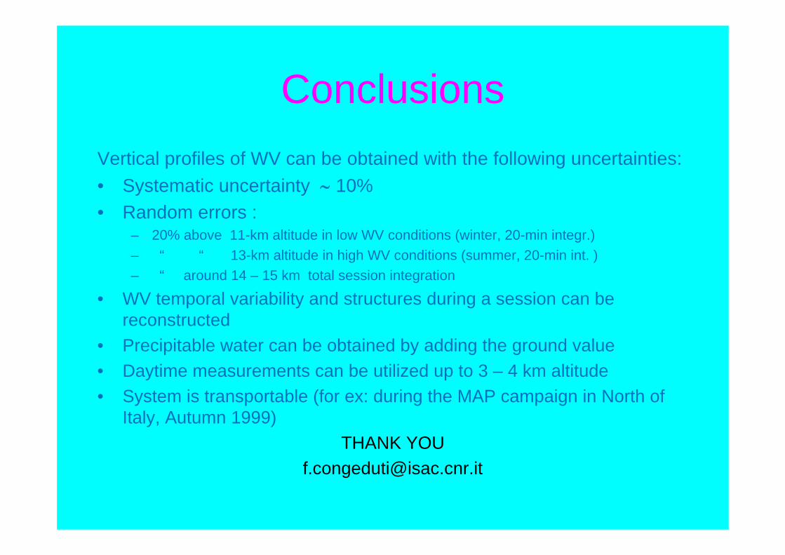
ConclusionsVertical profiles of WV can be obtained with the following uncertainties:• Systematic uncertainty ∼ 10%• Random errors :
– 20% above 11-km altitude in low WV conditions (winter, 20-min integr.)– “ “ 13-km altitude in high WV conditions (summer, 20-min int. )– “ around 14 – 15 km total session integration
• WV temporal variability and structures during a session can be reconstructed
• Precipitable water can be obtained by adding the ground value• Daytime measurements can be utilized up to 3 – 4 km altitude• System is transportable (for ex: during the MAP campaign in North of
Italy, Autumn 1999)THANK YOU