UNIVERSITÉ DE MONTRÉAL

A COMPARISON BETWEEN LINEAR PROGRAMMING AND SIMULATION

MODELS FOR A DISPACTHING SYSTEM IN OPEN PIT MINES

RAZIEH FARAJI

DÉPARTEMENT DE MATHÉMATIQUES ET DE GÉNIE INDUSTRIEL

ÉCOLE POLYTECHNIQUE DE MONTRÉAL

MÉMOIRE PRÉSENTÉ EN VUE DE L’OBTENTION

DU DIPLÔME DE MAÎTRISE ÈS SCIENCES APPLIQUÉES

(GÉNIE INDUSTRIEL)

AOÛT 2013

© Razieh Faraji, 2013.

UNIVERSITÉ DE MONTRÉAL

ÉCOLE POLYTECHNIQUE DE MONTRÉAL

Ce mémoire intitulé :

A COMPARISON BETWEEN LINEAR PROGRAMMING AND SIMULATION

MODELS FOR A DISPACTHING SYSTEM IN OPEN PIT MINES

présenté par : FARAJI Razieh

en vue de l’obtention du diplôme de : Maîtrise ès sciences appliquées

a été dûment accepté par le jury d’examen constitué de :

M. BASSETTO Samuel-Jean, Doct., président

M. GAMACHE Michel, Ph.D., membre et directeur de recherche

M. BAPTISTE Pierre, Doct., membre et codirecteur

Mme AUGER Geneviève, M.Sc.A., membre

iii

DEDICATION

To my best friend,

and my eternal love, my fiancé Mohammad

iv

ACKNOWLEDGMENTS

I would like to thank my supervisor, Dr. Michel Gamache for his support and guidance, useful

comments, remarks throughout my studies and research.

I would also like to thank my co-supervisor, Dr. Pierre Baptiste, for giving me the opportunity to

pursue this research and for all of the confidence, guidance, and support provided along the way.

Last but not least, I would like to thank my parents for being helpful and present during my

studies and this research. Furthermore, my deepest thanks to my sisters for always being there for

me. I will be thankful forever for your love.

v

RÉSUMÉ

Cette recherche est principalement axée sur la planification de la production à très court terme et

de l’affectation des camions aux pelles dans une mine à ciel ouvert. Les principales lacunes des

modèles existants dans la littérature sont: a) la non considération du temps d'attente et de la file

d'attente aux serveurs (pelles et concasseurs), b) la simplification des modèles et la considération

d'une quantité limitée de détails dans les modèles, c) la négligence de la nature stochastique du

système d’affectation des camions aux pelles, d) le développement des modèles est basé sur

l'hypothèse d'une flotte identique (camions et pelles).

Les objectifs de cette recherche sont le développement et l'utilisation d'un modèle de simulation

de base pour valider la solution du modèle de programmation linéaire (PL) et le développement

d'un second modèle de simulation qui représente le système de contrôle en temps réel. L'objectif

du second modèle de simulation est la maximisation de la production de minerai tout en prenant

en compte les contraintes du modèle de PL. Les deux modèles de simulation sont considérés dans

les situations déterministes et stochastiques.

Les modèles proposés sont appliqués dans une mine de charbon. Les résultats obtenus à partir de

l’exemplaire de base démontrent que le concasseur est le goulot d'étranglement de l'installation.

Afin de valider et vérifier les modèles proposés, l’exemplaire de base est modifié pour que les

camions et les pelles deviennent à tour de rôle les goulots d'étranglement du système

d'exploitation.

Lorsqu’on diminue le nombre de camions pour que ceux-ci deviennent le goulot d'étranglement,

le résultat du modèle PL est très optimiste et diffère de la réalité. Le modèle de PL ne considère

pas le temps d'attente aux serveurs, mais le modèle de simulation de base tient compte de la file

d'attente aux concasseurs et aux pelles. En conséquence, dès qu'on a un temps d'attente dans le

modèle de simulation, il y a perte de temps ce qui réduit la production de minerai. Le modèle de

simulation en temps réel obtient un meilleur résultat que le modèle de simulation de base. La

raison de cette différence est due au fait que dans le deuxième modèle de simulation, la

destination pour laquelle on estime qu’il y aura un temps d'attente aux pelles sera pénalisée. La

quantité de minerai produite est donc plus grande que dans le modèle de simulation de base.

Quand le temps de chargement de la pelle est considéré comme un goulot d'étranglement, le

résultat du second modèle de simulation produit plus de stérile que la solution du modèle de PL.

vi

Étant donné que dans le modèle de PL, l'objectif est de maximiser la production de minerai, il

existe plusieurs solutions de même valeur (i.e. même quantité de minerai) mais dont la

production de stérile peut fortement varier.

vii

ABSTRACT

This research deals with very short term production plan and truck-shovel hauling system in open

pit mines. The main shortcomings of the existing models reviewed in the literature are: a) not

considering the waiting time and queue at servers (shovels and crushers), b) simplifying the

models and considering a limited amount of details in the models, c) ignoring the stochastic

nature of the truck and shovel hauling system, d) developing model based on an homogeneous

fleet (trucks and shovels).

The objectives of this research are: 1- to develop and apply a basic simulation model considering

the queue and waiting time of trucks at shovels and crushers in both deterministic and stochastic

situations based on the linear programming (LP) model result. This model validates the result of

the LP model and provides the detailed and applicable dispatching plan for an open pit mine, 2-

To develop, apply and verify the second simulation model which is the real time control system.

This simulation model maximizes the ore production while taking into account the LP

constraints. This model imitates the truck shovel haulage system in both deterministic and

stochastic situations.

The proposed models are applied in a coal open pit mine. The obtained results from the LP and

simulation models in our case study demonstrate the fact that the crusher is the bottleneck of the

system. Then, in order to validate and verify the proposed models, we created two other scenarios

where the fleet of trucks and the shovel’s service time are considered respectively as bottleneck

of the operational system.

When the fleet of trucks is the bottleneck, the result of the LP model is too optimistic and differs

from the reality. The LP model does not consider the waiting time at servers while the basic

simulation model takes into account the queue at crushers and shovels. As a result, as soon as the

waiting time occurs in the simulation model, system is losing time thus the production of ore is

lower than the expected. The real time simulation model has better results than the basic

simulation model. The reason is that in the second simulation model, the waiting time at shovels

will be penalized therefore; this model has a better production level than the basic simulation

model.

When the shovel loading time is considered as the bottleneck of the system, the result of the

second simulation model produces more waste in comparison with LP model solution. Since in

viii

the LP model, the objective is to maximize the ore production only, there are an infinite number

of solutions which have the same level of ore production but different amounts of extracted

waste.

ix

TABLE OF CONTENTS

DEDICATION…………………………………………………………………………………… iii

ACKNOWLEDGMENTS………………………………………………………………………...iv

RÉSUMÉ…………………………………………………………………………………………..v

ABSTRACT……………………………………………………………………………………...vii

TABLE OF CONTENTS………………………………………………………………………....ix

LISTOF TABLES………………………………………………………………………………..xii

LIST OF FIGURES……………………………………………………………………………..xiv

LIST OF ABBREVIATIONS…………………………………………………………………....xv

CHAPTER 1: INTRODUCTION………………………………………………………………….1

1.1 PROBLEM DEFINITION………………………………………………………………… 1

1.2 RESEARCH OBJECTIVES………………………………………………………………...3

1.3 THESIS STRUCTURE……………………………………………………………………...5

CHAPTER 2: LITERATURE REVIEW…………………………………………………………..6

2.1 LINEAR PROGRAMMING………………………………………………………………..7

2.2 SIMULATION……………………………………………………………………………..11

2.3 COMBINATION OF LINEAR PROGRAMMING AND SIMULATION MODELS……14

2.4 METHODOLOGY………………………………………………………………………...15

2.5 SUMMARY AND REMARKS……………………………………………………………17

CHAPTER 3: THEORITICAL MODELS……………………………………………………….18

3.1 LINEAR PROGRAMMING (LP) MODEL ………………………………………….19

3.1.1 NOTAIONS…………………………………………………………………………...19

3.1.2 OBJECTIVE FUNCTION…………………………………………………………….20

3.1.3 CONSTRAINTS………………………………………………………………………20

x

3.2 GENERAL CONCEPTS AND DEFINITION OF SIMULATION MODELS……….28

3.2.1 ASSUMPTIONS ……………………………………………………………………...29

3.2.2 DEFINITIONS………………………………………………………………………...29

3.2.3 NOTATIONS………………………………………………………………………….30

3.2.4 INPUT DATA…………………………………………………………………………34

3.3 DETERMINISTIC SIMULATION MODELS………………………………………..34

3.3.1 DETERMINISTIC BASIC SIMUALTION (DBS) MODEL………………………...34

3.3.2 DETERMINISTIC REAL TIME SIMUALTION (DRTS) MODEL…………………39

3.3.3 STOCHASTIC MODELS…………………………………………………………….44

CHAPTER 4: TESTS, RESULTS AND ANALYSIS…………………………………………...45

4.1 INSTANCES………………………………………………………………………………45

4.2 COMPARING THE DETERMINISTIC MODELS RESULT FOR DBS AND DRTS

WITH LP MODEL…………………………………………………………………………….49

4.2.1 THE OPTIMAL SOLUTION OF THE LP MODEL…………………………………49

4.2.2 COMPARING THE RESULTS OF THE LP MODEL WITH DBS MODEL……….52

4.2.3 COMPARING THE RESULTS OF THE LP MODEL WITH DRTS MODEL……...55

4.3 COMPARING THE RESULTS OF STOCHASTIC BASIC SIMULATION (SBS)

AND STOCHASTIC REAL TIME SIMULATION (SRTS) MODEL WITH LP MODEL….56

4.3.1 COMPARING THE RESULTS OF THE LP, DBS AND SBS MODELS…………..58

4.3.2 COMPARING THE RESULTS OF THE LP, DRTS AND SRTS MODELS……….59

4.4 DIFFERENT SCENARIOS…………………………………………………………...62

4.4.1 TRUCKS AS A BOTTLENEK……………………………………………………….62

4.4.2 SHOVELS AS A BOTTLENECK …………………………………………………...67

4.5 SUMMARY AND REMARKS ……………………………………………………….71

CHAPTER 5: CONCLUSION AND RECOMMENDATIONS…………………………………72

xi

5.1 CONCLUSIONS………………………………………………………………………72

5.2 RECOMMENDATIONS FOR FUTURE RESEARCH………………………………73

REFRENCES…………………………………………………………………………………….74

xii

LIST OF TABLES

Table 4.1: Available material in front of each shovel in mining areas .......................................... 46

Table 4.2: Ore characteristics in each mining area ........................................................................ 46

Table 4.3: Upper and lower bounds on some ore characteristics ................................................... 47

Table 4.4: Shovel loading time in mining areas ............................................................................. 47

Table 4.5: Unloading time in dumping sites .................................................................................. 47

Table 4.6: Number and capacity of each type of truck .................................................................. 48

Table 4.7: Distance between mining areas and dumping sites ....................................................... 48

Table 4.8: Velocity of each type of truck ....................................................................................... 49

Table 4.9: Tonnage of extracted ore and waste per shift ............................................................... 50

Table 4.10: Number of empty trucks type A – in the LP solution ................................................. 50

Table 4.11: Number of empty trucks of type B – in the LP solution ............................................. 50

Table 4.12: Number of full trucks of type A– in the LP solution .................................................. 51

Table 4.13: Number of full trucks type B– in the LP solution ....................................................... 51

Table 4.14: ................................................................................................... 52

Table 4.15: Results of the LP and DBS models ............................................................................. 53

Table 4.16: Number of empty trucks type A- in the DBS model solution ..................................... 53

Table 4.17: Number of empty trucks type B- in the DBS model solution ..................................... 54

Table 4.18: Results of the LP and DRTS models .......................................................................... 55

Table 4.19: Number of empty trucks type A- in the DRTS model solution .................................. 55

Table 4.20: Number of empty trucks type B- in the DRTS model solution .................................. 56

Table 4.21: Coefficients for triangular distribution ....................................................................... 57

Table 4.22: Random variables and their probability density functions .......................................... 57

Table 4.23: Result of the LP, DBS and SBS models ..................................................................... 58

xiii

Table 4.24: Waiting time at servers in the SBS model .................................................................. 59

Table 4.25: Utilization of servers in the SBS model ...................................................................... 59

Table 4.26: Results of the LP, the DRTS and the SRTS models ................................................... 60

Table 4.27: Waiting time at servers in the SRTS model ................................................................ 60

Table 4.28: Utilization of servers in SRTS model ......................................................................... 61

Table 4.29: Tonnage of extracted ore and waste in modified LP model ....................................... 63

Table 4.30: Number of required trucks .......................................................................................... 64

Table 4.31: Result of the LP and SBS models-truck as a bottleneck ............................................. 64

Table 4.32: Waiting time at servers in SBS model-truck as a bottleneck ...................................... 65

Table 4.33: Utilization of the servers in SBS model-truck as bottleneck ...................................... 65

Table 4.34: Result of the LP and SRTS models-truck as a bottleneck .......................................... 66

Table 4.35: Waiting time at servers in SRTS model-truck as a bottleneck ................................... 66

Table 4.36: Utilization of servers in SRTS model-truck as bottleneck .......................................... 67

Table 4.37: Tonnage of extracted ore and waste in LP model-shovel as a bottleneck .................. 67

Table 4.38: the result of the LP and SBS models- shovel as a bottleneck ..................................... 68

Table 4.39: the waiting time at servers in SBS model-shovel as a bottleneck ............................... 68

Table 4.40: the utilization of servers in SBS model-shovel as bottleneck ..................................... 69

Table 4.41: Result of the LP and SRTS models- shovel as a bottleneck ....................................... 69

Table 4.42: Waiting time at servers in SRTS model-shovel as a bottleneck ................................. 70

Table 4.43: Utilization of servers in SRTS model-shovel as bottleneck ....................................... 71

xiv

LIST OF FIGURES

Figure 1- 1: Isometric view of a block model in open pit mine ....................................................... 2

Figure 3- 1: Schematic picture of the mining area in simulation models ...................................... 29

Figure 3- 2: Schematic picture of the entities creation in simulation models ................................ 35

Figure 3- 3: Schematic picture of the crusher area in simulation models ...................................... 36

Figure 3- 4: Schematic picture of the mining areas in simulation models ..................................... 38

Figure 3- 5: Schematic picture of the dumping site in simulation models ..................................... 39

xv

LIST OF ABBREVIATIONS

LP Linear Programing

MIP Mixed Integer Programing

NPV Net Present Value

LOM Life Of Mine

NN Neural Network

MR Multiple Regression

VSTPP Very Short Term Production Planning

DBS Deterministic Basic Simulation

SBS Stochastic Basic Simulation

DRTS Deterministic Real Time Simulation

SRTS Stochastic Real Time Simulation

1

CHAPTER 1: INTRODUCTION

1.1 Problem definition

Open pit mining is a surface mining method of excavating rock or minerals from the ground by

removing them from an open pit. This method is used when deposits of valuable minerals or rock

are found near the surface. This valuable mineral is called ore which is a natural combination of

one or more solid minerals that can be mined, processed and sold at a profit. Also, the non-

valuable material is called waste which removing of them in order to reach the ore in an open pit

mine is inevitable.

The ore body is excavated from the upper down in sequences of horizontal layers of identical

thickness called benches. Mining starts with the highest bench and after an appropriate floor area

has been exposed; mining of the next layer begins. The process carries on until the bottom bench

height is reached and the final pit out line is achieved. In order to access the different benches, a

road or ramp must be prepared (Hustrulid and Kuchta, 1995).

There is a set of operations which will repeat for extracting ore and waste during the life of the

mine (LOM). These activities include drilling, blasting, loading and hauling the extracted

material to the specific destination. The width and steepness of the ramps and benches in the

mine depends upon these operations equipment (Hustrulid and Kuchta, 1995).

2

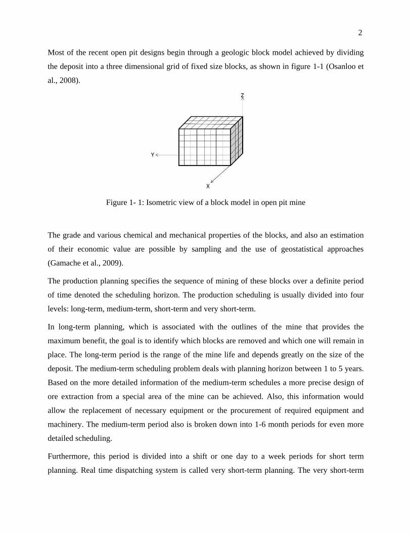
Most of the recent open pit designs begin through a geologic block model achieved by dividing

the deposit into a three dimensional grid of fixed size blocks, as shown in figure 1-1 (Osanloo et

al., 2008).

Figure 1- 1: Isometric view of a block model in open pit mine

The grade and various chemical and mechanical properties of the blocks, and also an estimation

of their economic value are possible by sampling and the use of geostatistical approaches

(Gamache et al., 2009).

The production planning specifies the sequence of mining of these blocks over a definite period

of time denoted the scheduling horizon. The production scheduling is usually divided into four

levels: long-term, medium-term, short-term and very short-term.

In long-term planning, which is associated with the outlines of the mine that provides the

maximum benefit, the goal is to identify which blocks are removed and which one will remain in

place. The long-term period is the range of the mine life and depends greatly on the size of the

deposit. The medium-term scheduling problem deals with planning horizon between 1 to 5 years.

Based on the more detailed information of the medium-term schedules a more precise design of

ore extraction from a special area of the mine can be achieved. Also, this information would

allow the replacement of necessary equipment or the procurement of required equipment and

machinery. The medium-term period also is broken down into 1-6 month periods for even more

detailed scheduling.

Furthermore, this period is divided into a shift or one day to a week periods for short term

planning. Real time dispatching system is called very short-term planning. The very short-term

3

production planning is a two phases system, that consists in presenting a production plan for a

very short-term period that permits better design of the operations and a guide line for

dispatching trucks to shovels located in the mining areas.

This thesis will focus on the Very Short-Term Production Planning (VSTPP) in open pit mines.

VSTPP determines the number of each type of trucks traveling between each pair of shovel and

crusher (or waste dump) for one shift. The model that we will use is the linear programming (LP)

model proposed by Gamache et al. (2009). This model provides a production plan for a work

shift indicating the number of trucks to be allocated to the different mining areas and the amount

of ore and waste extracted by shovels and transported to the crusher or to each waste dump.

The LP model optimizes the ore production considering several constraints. It does not take into

account the waiting time and queues at servers such as shovels and crushers. Also, the LP model

does not present the operational dispatching plan for trucks in the mine. It only presents the

number of truck that has to be sent send to a specific area not the time or their type. Additionally,

this is a deterministic model since it considers constant service times at shovels and crushers and

constant velocity of the trucks that affect the trucks traveling time.

The first purpose of this research is to apply a discrete event simulation model to open pit mine in

order to validate the optimal result of the LP model. In this simulation model, the optimal

solution of the LP model is used as a target for the simulator to send the right number of trucks to

the mining area whilst providing the operational dispatching plan of trucks in mine. This

operational plan presents which truck and when has to be allocated to shovel.

The second purpose of this research is to examine the possibility of developing a simulation

model to maximize ore production and determine the number of trips between mining areas and

dumping sites that can be used instead of the LP model for a very short-term planning period in

an open pit mine.

In the next section the objectives of this research will be presented in more details.

1.2 Research objectives

The performance of the truck and shovel haulage system has been studied in the literature in

regard to optimize the objective function through linear programming, simulation models and

4

combination of these methods. In these researches it has been tried to maximize material

production or minimize the number of trucks for a specific production plan for a short term.

In this study, a discrete event simulation model is developed to validate the LP model by

considering the queue and the waiting time at servers which are ignored by the LP model. The

basic simulation model deals with the result of the LP model as a predefined target for

dispatching the number of trucks to the shovels and dumping sites. Moreover, another simulation

model, that we call a real time simulation model, is developed in order to find a production plan

for an open pit mine by considering the LP model constraints through simulation software. So,

the general objectives of this research are, to validate the result of the LP model by developing

the simulation model, to provide an operational dispatching plan, and to find another way to do

the very short-term production planning in open pit mines.

Since the main problem of VSTPP is the uncertainty related to the operations of trucks and

shovels in open pit mines, the suggested simulation models deal with the uncertainties consisting

of truck velocity, loading time at shovels, unloading time in either crushers or waste dumps.

We can summarize the objectives of this work as:

To develop and apply a basic simulation model considering the queue and waiting time of

trucks at shovels and crushers in both deterministic and stochastic situations based on the

LP model result. This model validates the result of the LP model and provides the detailed

and applicable dispatching plan for an open pit mine.

To develop, apply and verify the second simulation model which is the real time control

system. This simulation model maximizes the ore production while taking into account

the LP constraints. This model imitates the truck shovel haulage system in both

deterministic and stochastic situations.

To compare the result of the LP model and simulation models by considering different

scenarios where the main operational components will be in turn the bottleneck of the

system.

The next section presents the overall view of this thesis based.

5

1.3 Thesis structure

In this chapter, an overview of the problem in hand and the research objectives are presented. In

chapter 2, the literature review provides an overview of common methodologies and approaches

used in studying truck and shovel systems including linear programming, simulation, and

combination of these methods. Chapter 3 includes the theoretical framework for the linear

programming formulation to optimize the allocation of trucks and shovels as well as describing

the simulation models. Chapter 4 is dedicated to the presentation and a discussion of

computational results achieved. In chapter 5, some conclusions are drawn and directions for

future work are proposed.

6

CHAPTER 2: LITERATURE REVIEW

This chapter presents the review of studies about the production planning and truck and shovel

hauling system. Different approaches have studied this kind of problems in literature. The

following classifications are discussed in this chapter.

1. Linear programming

2. Simulation

3. Combination of linear programming and simulation

The planning issues in mining can be represented by mathematical models for distribution of the

flow of material on the mine’s transportation network. Mathematics programs can be grouped

into two classes: linear and nonlinear programming. Soumis et al. (1986) obtained excellent

results using a nonlinear programming. Since this research applies the linear programming so, in

this thesis only the literature related to the linear programming is presented.

Also, over the last recent decades, simulation has been one of the most respected operational

researches tool. The reason for the popularity of the simulation models can be seen in ability and

flexibility of this type of method in handling the complex problems. Moreover, simulation

models are powerful and also cost effective (Kelton et al., 2007).

This chapter consists of the following sections. In section 2.1, linear programming models used

for optimizing the different objective in haulage system for a short-term and very short-term

period in an open pit mine are discussed. Section 2.2 focuses on simulation models. Section 2.3

describes the models that combine linear programming and simulation for short term production

scheduling in an open pit mine. Section 2.4 presents the methodology of this research and the

final section is allocated to the summary of this chapter.

7

2.1 Linear programming

The first application of the linear programming in truck- shovel hauling system in an open pit

mine returns to 1970s (Torkamani and Askari-Nasab, (2012).

Wilke and Reiner (1977) studied the production planning in an open pit mine. They used a linear

program whose objective function was to maximize the productivity of the shovel. For each

shovel, the authors added a weight in the objective function describing the priority of the shovel.

The set of constraints includes blending constraints, capacity constraints of the sources and sinks.

The advantages of using a scheme of arbitrary priorities in the objective function make it possible

for the objective function to be divided into different technical goals, and it is possible to stop and

take into account the major deviations from the long-term production plan. The main

disadvantage of this method lies in the fact that it is essential to adjust the weights in the

objective blindly to respect the production plan.

Zhang et al. (1990) discussed the optimal allocation of the flow of trucks in an open pit. To make

the distribution of trucks to the shovels, the authors use a linear program. The objective function

is to minimize the number of trucks required to meet mine production in a short-term horizon.

Although the set of constraints is broad and includes the flow conservation, shovels capacity, a

minimum level of production, blending constraints, ore and waste ratio, minimum and maximum

capacity of the dumping sites, the model ignores other constraints such as those on the capacity

of the fleet of trucks.

Gershon et al. (1993) were interested particularly in the problem of finding the appropriate

blending of ore in a coal mine. To solve this problem, the authors used a linear program. The

objective function of the problem is to minimize the operation costs. In addition to blending

constraints, the model makes sure that a minimum level of ore production is achieved. The final

mixture of ore must not contain more than a certain maximum amount of sulfur and impurities,

and a minimum level of BTU. This kind of problems is easily solvable with the simplex method.

The proposed formulation provides an optimal solution to the established scheduling of small and

medium complexity problem.

Temeng (1997) proposed to make the production planning using a linear program in an open pit

mine by the optimal allocation of the trucks to the shovels. The author used an objective function

that has two levels which simultaneously maximize ore production of the shovels and maintain

8

the quality of the ore mixture within acceptable limits defined by the mine. In addition, the author

considered several groups of constraints to arrive at a more realistic level of production such as

capacity of the shovels, crushers and waste dumps, flow conservation constraint, blending

constraint, stripping ratio, and the number of trucks. However, this model does not consider the

truck cycle time in the mine.

Temeng et al. (1997) combined goal programming model with the transportation algorithm as a

real time dispatcher in order to maximize production and minimize the total waiting time of

shovels and trucks. The objective function of the goal programming model includes production

rate and ore grade, to present the importance of both production and ore quality in company’s

goals. This model optimizes the total production by considering routes between mining areas and

their destinations. In order to optimize the production, routes having the shortest cycle time are

selected. Then, according to the transportation models the trucks are allocated to the shovels

which minimize the cumulative deviations of the optimal production target. The transportation

model attempts to minimize total waiting time of shovels and trucks. Moreover, the effect of the

shovels and trucks breakdowns on quality of dispatching model is tested in this paper.

The work of Burt et al. (2005) focused on the optimal allocation of trucks to the shovels. To do

this allocation, they use a linear programming model where the objective function is to minimize

the cost of operation of the trucks and shovels fleet. The set of constraints of the model includes

the productivity of trucks and shovels and the minimum production. The major difference of this

article is the desire of the authors to obtain a production plan reflecting high productivity of the

equipment. In this regard, they use a match factor that is a measure of the productivity of the

fleet. The match factor is the ratio of the productivity of the trucks and shovels for a

homogeneous fleet of trucks. The article does not consider the waiting time at shovels, but they

propose a method for modeling the waiting time which would depend on the inter arrival time of

the trucks at shovels. Unfortunately, this model uses average cost of equipment that is not

realistic and does not consider the global optimization for mine.

The paper by Rubito (2007) concentrated on the optimal allocation of trucks to the crushers in the

mine. The author uses a linear program where the objective function is to maximize profits of

sending the trucks to the various crushers. The only constraints of this model include capacity

9

constraints of shovels which make the proposed model as a simple model that cannot be useful

for the more complex problems.

Ercelebi and Bascetin (2009) studied a truck and shovel system of a coal mine in Turkey. This

work has two stages. In the first stage: the optimal numbers of trucks are determined by the

closed queuing network model. In the second stage, LP model aids how to dispatch the trucks to

shovels. The LP model minimizes the number of trucks on the road, number of trucks at shovels

and number of trucks at dump site which assumes no truck queuing under ideal conditions.

Although this model guarantees maximum shovel utilization, it cannot be functional in the

complex models with other desirable constraints.

Gamache et al. (2009) developed a generic linear programming model to optimize an open pit

mine production plan. The proposed model presents a production plan for a work shift

considering several constraints such as blending constraint, capacity of equipment, stripping

ratio, the amount of available material infront of each shovel, etc. After developing the basic

model, authors tried to lineraize a set of constraints that calculates the waiting time of trucks at

shovels and crushers. For this thesis the basic model does not consider the waiting time at sevice

points. The experiments and the results of this paper present a more realistic production plan for a

working shift. It is worth mentioning that the basic model of the above paper will be used in

order to accomplish the reaserch.

Topal and Ramazan (2010) minimized the truck maintenance costs developing a Mixed Integer

Programming (MIP) model for a large scale gold mine in Western Australia. The MIP model in

order to create an optimal truck schedule uses the total hours of truck usage (truck age),

maintenance cost and essential operational hours. Although the presented MIP model optimizes

the utilization of truck over the life of mine, this model is developed for a long time period and

has to be simplified to be applicable for a short-term and very short-term period.

Another multi stage approaches for hauling system in mine was made by Gurgur et al. (2011).

They used LP model to optimize allocation of trucks using interactively and simultaneously of

MIP model for short-term and long-term mine production planning. The MIP model maximizes

the NPV by optimizing the material movement with respect to the ore quality and also

precedence constraints. LP model minimizes the deviation of actual movement of material from

the predefined target. Availability of fleet including the number and size of the trucks and road

10

profile are the LP model constraints. The proposed LP model can be efficient only using the

developed MIP model.

Considering the reviewed literature, there are several ways to model a production plan in a mine

by a linear program. The choice of objective function is extensive and can greatly influence the

behavior of the model. Several techniques exist to incorporate groups of constraints in the

mathematical program, which depend on the problem. Although linear programming methods

have applied in the literature since 1970s for truck shovel dispatching, they have some

limitations. The most significant shortcomings of these models are:

1- Simplifying the models and considering a limited amount of details in the model. For

example, considering the limited constraints and providing the simple model which does

not include the whole aspects of the haulage system. Also, using the identical equipment

in terms of the capacity and speed of trucks and shovels.

2- Not considering the waiting time at servers (shovels and crushers)

3- Not taking into account the stochastic nature of the hauling systems (truck and shovel

transporting system) which are the uncertainties of the loading, unloading, traveling times

and ore grades (Gurgur, Dagdelen, & Artittong, 2011).

Also, most of the researches have been studied the long-term period which emphasizes the

necessity of more studies for the short-term and very short-term period.

11

2.2 Simulation

Simulation has been used in both open pit and underground mines in material handling and truck

and shovel hauling systems, mining operations, production scheduling and mine planning (Yuriy

& Vayenas, 2008).

Castillo and Cochran (1987) studied a truck dispatching system in a copper mine. In their study,

the fleet size is known and the fixed dispatch strategy is used to allocate trucks to shovels. This

means that trucks must travel between the same destinations during the shift. A microcomputer

simulation model is developed using SLAM II, to compare the suggested dispatching procedure

to the current one. This algorithm gives the priority to the shovels in ore areas to maximize ore

production and maximizes utilization of the truck. The presented simulation model follows the

fixed assignment strategy which is the main disadvantage of the system because, this strategy

reduces the efficiency of the truck and shovel capacity in the mine.

Sturgul and Eharrison (1987) simulated three different dispatching systems of three open pit

mines in Australia. The first dispatching system is applied in a coal mine. This system increases

the production; however it causes an extra cost. In the second example, the accurate number of

trucks is estimated to optimize the production of uranium mine. In this case study, each truck is

allocated to a specific shovel for the shift. The third case study is again in a coal mine using a

truck and shovel hauling system. Simulation model tries to estimate the correct number of trucks.

A hauling system using conveyor belt is also considered as an alternative. This work also follows

the fixed dispatch and assignment strategy.

Bonates and Lizotte (1988) developed a computer simulation model for an open pit mine based

on FORTRAN programming language. They propose different dispatching strategies such as

maximizing trucks and shovels utilization and fixed dispatch. This simulation model attempts to

respect the long term production objectives. Each of these policies has its own advantages and

disadvantages. Maximizing truck utilization causes higher production but it is not always the best

policy all the time. For example, when the difference between traveling time of truck among

shovels is significant or system has to also consider the grade quality of ore. Since, the objective

is to maximize truck utilization so trucks will be allocated to the nearest shovels and then the

further shovel will be idle for longer time that causes the unbalances in the system. On the other

hand maximizing shovel utilization results on the same operating rate for all of the shovels that is

12

more desirable. The efficiency of these policies depends on the available number of trucks.

Moreover, the developed simulation model follows the fixed dispatch strategy.

Peng et al. (1988) proposed a simulation model for an iron mine in northeast China. This semi

continuous open pit mine has a discontinuous truck and shovel hauling system and a continuous

belt elevator system. The proposed simulation model used to define the optimal number and the

size of the shovels to work with crushers, the number of trucks, the size of the crusher and the

size of the storage for a specific crusher and conveyor system. In summary they try to study the

effect of the various type of the equipment on the production rate. This model does not consider

the uncertainties of the operational system in the proposed simulation model.

Forsman et al. (1993) applied a simulation model into an open pit copper mine in northern

Sweden. This model is similar to one proposed in Bonates and Lizotte (1988) work, but in this

model a graphical animation is also presented. By maximizing the shovel utilization, the total

tonnage of production will decrease. Maximizing the truck utilization results in the same total

tonnages as fixed dispatching model, but the tonnage of ore is lower. The developed model also

makes decisions about setting up a crusher in the pit, purchasing new trucks, and planning a route

for effective material carrying.

Karami et al. (1996) developed a simulation model to study truck and shovel hauling systems in

an open pit mine using SLAM II. They consider the fix assignment of trucks to the shovels in the

transportation system. The model is applied to understand the behavior of the hauling system

under different configurations and to evaluate the operating performance.

Ataeepour and Baafi (1999) studied the impact of dispatching rule on system productivity using

the simulation model. They considered the dispatching and non-dispatching mode in the research.

In a non-dispatching mode, each truck keeps its shovel allocation, for example a mine with five

shovels is similar to five mines with one shovel each except that there is a shared dumpsite.

These procedures attempts to maximize using of shovels or trucks in the system that actually

minimize the waiting time of trucks at shovels. In this regard, the arrival time of a truck at each

shovel and the time the shovel starts loading the truck have been calculated. Therefore, the

dispatcher sends a truck to a shovel, which results in the least delay time for the truck. Their

model assumes that all trucks in the mine are the same in terms of capacity; engine power, speed,

etc.

13

Awuah-Offei et al. (2003) used simulation to predict the truck and shovel requirements of a gold

mine for a four years period which was important for the mining contractor to know the

equipment needs in advance. Trucks are considered as entities and processes include the arrival

of entities, loading, and movement of entities, unloading and queuing. The historical data for

loading and unloading time, traveling time and failure of the shovels are collected and the

appropriate functions are fitted. Average queue length of trucks at the shovel, average shovel

utilization per shift and number of trucks loaded per shift is the specific results of this program

but, this model was developed for a long term period.

Yuriy and Vayenas (2008), are an instance of the researchers who combine the mathematical

programming model with a simulation model. They use a genetic algorithm to develop a reliable

model for providing the times between failures in order to combine it by arena simulation model

for maintenance analysis of mining equipment. They estimate the time between failures for each

fleet as input for the arena simulation model. The simulation model imitates the operations in the

mine to evaluate the effect of failures on production rate, and to estimate fleet availability and

utilization. This simulation models does not take into account the failure of the equipment. They

also do not consider which equipment has the critical role on production quantity.

Comparisons between the application of simulation models and other operation research methods

are also stated in the literature. For example, Chanda and Gardiner (2010) use computer

simulation, neural networks (NNs) and multiple regressions (MRs) to estimate the truck cycle

time in a large gold mine in Western Australia. They only study the travel time of empty and

loaded truck as a cycle time. The deviations from the actual cycle time of trucks used to compare

the above methods. Authors show that although the simulation is the most common method in

this field but it usually overrates or miscalculates the cycle time. Also, the developed model for

forecasting the cycle time applies to a specific mine site and it cannot be directly apply to other

operations.

14

2.3 Combination of linear programming and simulation models

Combination of the linear programming model and a simulation model also exist in the literature.

In these problems, mathematical models are used for solving the allocation problem and

simulation for the real time dispatching problem.

Fioroni et al. (2008) used an optimization model and a simulation model to generate short-term

planning plans. They create monthly schedule of an open pit mine using Arena simulation

software and Lingo optimization software. The objective of the LP model using Lingo software is

to find the initial allocation of the loader and transportation equipment. The objective of the

simulation model using Arena is to identify the number of trips of trucks in each area respecting

the grade of ore during the simulation period. At first, the initial number of trucks and shovels are

calculated using the optimization model. Then, using the result of the optimizer, simulation

model will run until a failure occurs in the system therefore, the optimizer will calculate the new

plan and this procedure will continue for the period of one month. They use simulation model to

allow the feasibility of the mining plan proposed by optimizer, giving utilization and production.

This work is based on the optimizer model and relies on the result of that.

Torkamani and Askari-Nasab (2012) developed and implemented a simulation model to analyze

the truck and shovel haulage system in a copper mine. The developed approach assures the

optimum Net Present Value (NPV) in long-term scheduling and short-term scheduling periods

objectives. The developed model considers the optimal short-term schedule in simulation model

while considering the uncertainties related with the manoeuvre of trucks and shovels, loading and

dumping time. In the proposed model an entity is a mining-cut portion removed at each period

and sent to a certain destination. Trucks, shovels, and loaders are resources in the simulation

model. This approach has two stages which short-term scheduling plans are the basis for building

the model. These two stages are as follows.

In the first stage using the MIP model, several scenarios are created with a different number of

trucks and shovels and they are examined to define the essential number of each resource. In the

second stage, using the result of the first stage, the system is simulated in Arena and the

developed model is evaluated. One of the main advantages of this model is in founding the

required number of trucks and shovels based on the short-term mine plan not only based on the

15

shovel’s requirements. But, the proposed simulation model assumes that all trucks and all shovels

are identical.

2.4 Methodology

As it can be seen form the literature, the proposed models in the literature have limitations and

shortcomings to solve the production planning in an open pit mine which are:

1- Ignoring the waiting time at servers (shovels and crushers)

2- Simplifying the models and considering a limited amount of details in the models

3- Ignoring the stochastic nature of the truck and shovel hauling system

4- Developing model based on the identical fleet (trucks and shovels)

Discrete event simulation model will be applied in this thesis to overcome the presented

limitations and shortcomings. The current research will overcome these limitations by

considering the LP model proposed by Gamache et al. (2009) for a very short-term production

plan. Their model is a complete linear programming that is used to maximize the ore production

respecting several constraints. This model approximate waiting time at service points in an open

pit mine but, we use the basic linear model of their model which does not consider the waiting

time at servers. The basic simulation model will apply to validate the result of the LP model

considering the waiting time and queue of trucks at servers during the time period. Besides, in

order to find a new way of very short-term production planning the second simulation model

which is the real time control system developed. The real time simulation model presents the

truck and shovel hauling system with more details in order to provide a new model with enough

details to overcome the shortcomings of the literature.

In order to consider the uncertainties of the hauling systems, randomness variables are added to

the deterministic simulation models. These models take into account the uncertainties of loading

time, unloading time and traveling times. One of the main contributions of this work is that the

proposed simulation model can work when a heterogeneous fleet of trucks and shovels is used,

which is something that we haven’t seen in the literature.

16

Based on these observations, we propose the following procedure for the development of a new

dispatching system in an open pit mine:

Develop and solve a linear programming model to allocate trucks to the shovels. The

optimal solution of this model will indicate the amount of ore and waste to be transported

during the shift between shovels and crushers or waste dumps. The objective of LP model

is to maximize the ore production with respect to the blending constraints, strip ratio, flow

conservations constraints, mining capacity, cycle time constraints, etc.

Implement two different simulation models (a basic simulation model and a real time

simulation model) that will use different types of trucks as entities and the shovels as

resource of the simulation.

Use the basic simulation model to test the accuracy of the LP model. To achieve that the

simulation model will use the optimal solution of the LP model (more precisely the

number of trips of the different type of trucks at each shovel) as input.

Use the real time simulation model to imitate the real system considering the LP

constraints. This model is developed in order to find the new way of very short-term

production planning.

Create different bottleneck situations of the shovel truck haulage system in order to

evaluate different configurations to better evaluate the new dispatching system.

17

2.5 Summary and Remarks

In this chapter the related literature of two different approaches in regard to evaluating the truck

and shovel systems were presented. Obviously, the ability of accurately assessing a transporting

performance of system is vital for mining companies. Any improvement in the performance of

system would save a considerable quantity of money. Because of the complexity of the hauling

system in mine, this assessment is not an easy task. This complexity is coming from stochastic

features of the system. In the next chapter the theoretical models which are developed in this

thesis will be presented.

18

CHAPTER 3: THEORITICAL MODELS

The objective of this chapter is to present the theoretical models which are developed in order to

reach the objective of this thesis. First in this chapter the LP model that maximizes the total ore

production during the shift will be presented. The result of the LP model is a very short-term

production plan which is used as a guide line for the dispatching system. The LP model does not

take into account the waiting time at servers and does not present the operational dispatching

plan. To validate the result of the LP model we will develop a simulation model named the basic

simulation model. The basic simulation model takes into account the waiting time at servers and

provides the operational dispatching plan for an open pit mine considering the optimal solution of

LP model as target for allocating the trucks to the shovels in mining areas.

The second simulation model is a real time simulation model, which imitates the real problem to

determine the required number of trucks to allocate to shovels. This model takes into account the

characteristics of the mine’s material content in mining areas and considers the ratio between

sterile material and the production of total material. With this model, the possibility of presenting

a new way of VSTPP will be tested.

Furthermore, since LP model and also simulation models are based on the deterministic input

data, so; at the end of this chapter, both simulation models are considered in the stochastic

situations. The stochastic simulation models involve uncertainties associated with the trucks,

shovels and crusher operations into the model.

Details of each proposed model are explained in the following sections. Section 3.1 introduces

the LP model formulation for VSTPP generated by Gamache et al. (2009). Section 3.2 describes

the simulation models (the basic and real time simulation models) as deterministic models and

stochastic models. Finally Section 3.3 presents the summary and remarks. The next section

introduces the linear programming model for very short-term production planning (VSTPP) in an

open pit mine.

19

3.1 Linear Programing (LP) model

We first present a linear programming (LP) model which creates an open pit mine’s production

plan for a shift. This model, based on Gamache et al. (2009), maximizes ore production during

the shift by considering the blending constraints, stripping ratio, flow conservation constraints,

mining capacity constraints, etc.

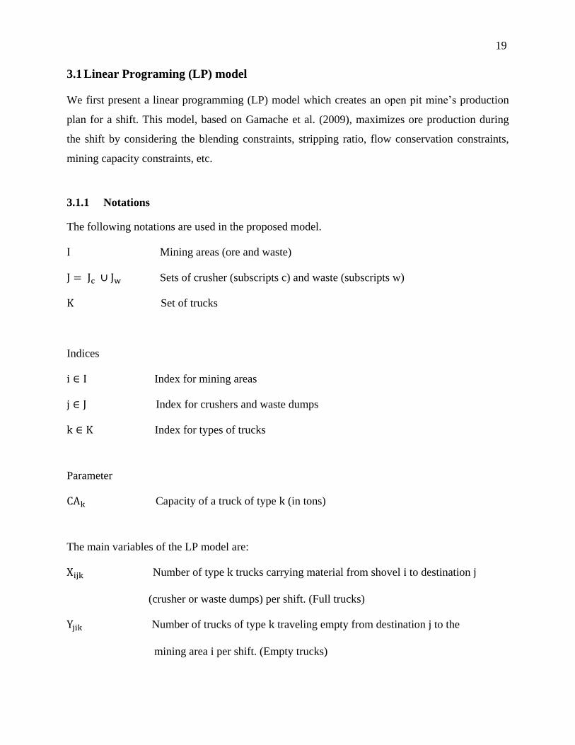
3.1.1 Notations

The following notations are used in the proposed model.

Mining areas (ore and waste)

Sets of crusher (subscripts c) and waste (subscripts w)

Set of trucks

Indices

Index for mining areas

Index for crushers and waste dumps

Index for types of trucks

Parameter

Capacity of a truck of type (in tons)

The main variables of the LP model are:

Number of type trucks carrying material from shovel to destination

(crusher or waste dumps) per shift. (Full trucks)

Number of trucks of type traveling empty from destination to the

mining area per shift. (Empty trucks)

20

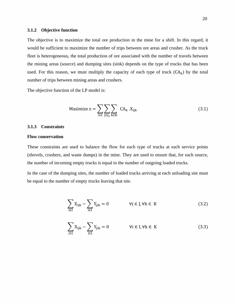
3.1.2 Objective function

The objective is to maximize the total ore production in the mine for a shift. In this regard, it

would be sufficient to maximize the number of trips between ore areas and crusher. As the truck

fleet is heterogeneous, the total production of ore associated with the number of travels between

the mining areas (source) and dumping sites (sink) depends on the type of trucks that has been

used. For this reason, we must multiply the capacity of each type of truck ( ) by the total

number of trips between mining areas and crushers.

The objective function of the LP model is:

∑∑∑ .

3.1.3 Constraints

Flow conservation

These constraints are used to balance the flow for each type of trucks at each service points

(shovels, crushers, and waste dumps) in the mine. They are used to ensure that, for each source,

the number of incoming empty trucks is equal to the number of outgoing loaded trucks.

In the case of the dumping sites, the number of loaded trucks arriving at each unloading site must

be equal to the number of empty trucks leaving that site.

∑

∑

∑

∑

21

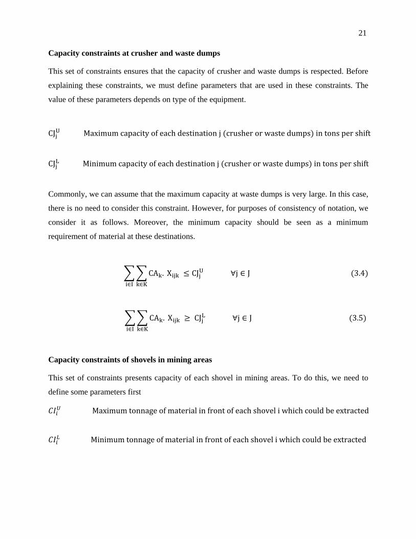
Capacity constraints at crusher and waste dumps

This set of constraints ensures that the capacity of crusher and waste dumps is respected. Before

explaining these constraints, we must define parameters that are used in these constraints. The

value of these parameters depends on type of the equipment.

Commonly, we can assume that the maximum capacity at waste dumps is very large. In this case,

there is no need to consider this constraint. However, for purposes of consistency of notation, we

consider it as follows. Moreover, the minimum capacity should be seen as a minimum

requirement of material at these destinations.

∑∑

∑∑

Capacity constraints of shovels in mining areas

This set of constraints presents capacity of each shovel in mining areas. To do this, we need to

define some parameters first

22

The maximum tonnage of material in front of each shovel which could be extracted depends on

two parameters, (tonnage of material available at shovel ) and (capacity of shovel in tons

per shift). In fact is the minimum of and .

{ }

Thus, the capacity constraints at each shovel in mining areas are:

∑∑

∑∑

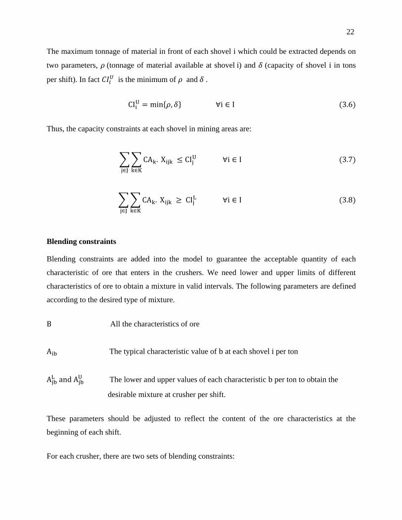
Blending constraints

Blending constraints are added into the model to guarantee the acceptable quantity of each

characteristic of ore that enters in the crushers. We need lower and upper limits of different

characteristics of ore to obtain a mixture in valid intervals. The following parameters are defined

according to the desired type of mixture.

All the characteristics of ore

The typical characteristic value of at each shovel per ton

The lower and upper values of each characteristic per ton to obtain the

desirable mixture at crusher per shift.

These parameters should be adjusted to reflect the content of the ore characteristics at the

beginning of each shift.

For each crusher, there are two sets of blending constraints:

23

∑∑( )

∑∑( )

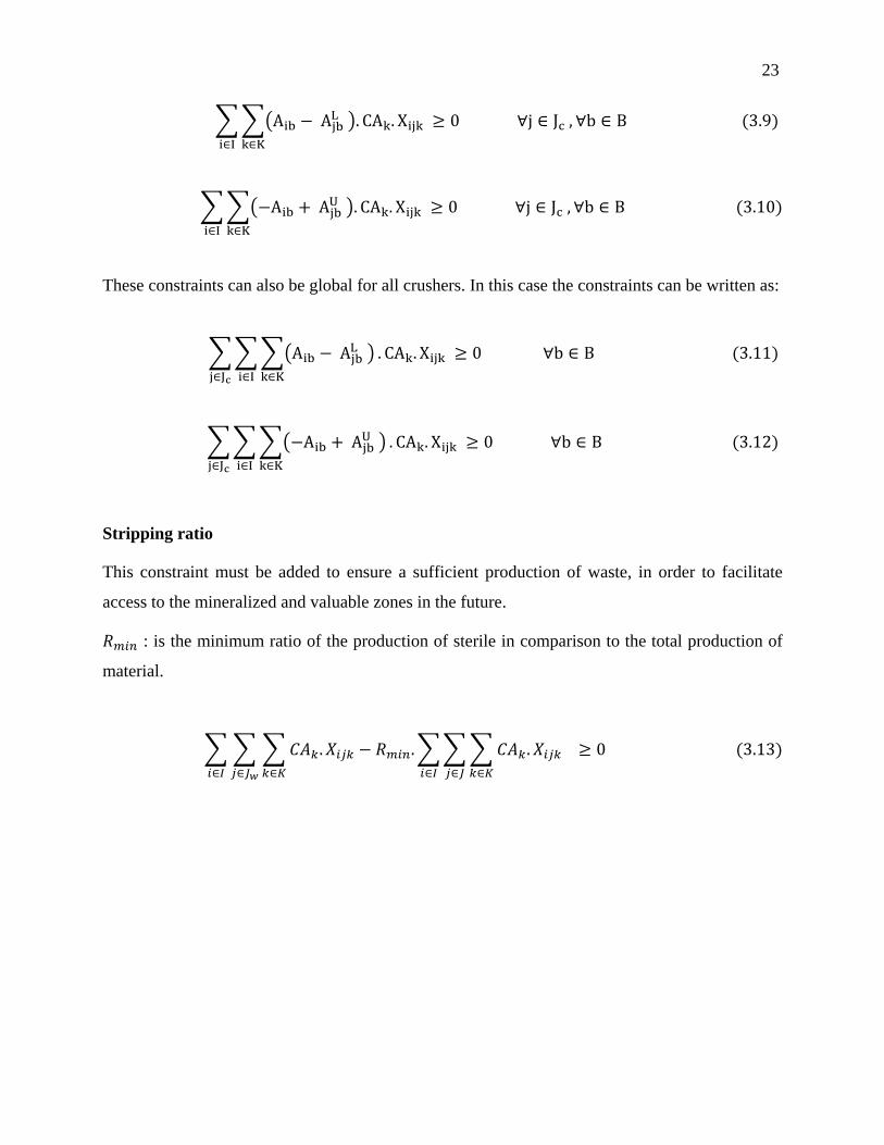
These constraints can also be global for all crushers. In this case the constraints can be written as:

∑∑∑( )

∑∑∑( )

Stripping ratio

This constraint must be added to ensure a sufficient production of waste, in order to facilitate

access to the mineralized and valuable zones in the future.

: is the minimum ratio of the production of sterile in comparison to the total production of

material.

∑ ∑ ∑

∑∑ ∑

24

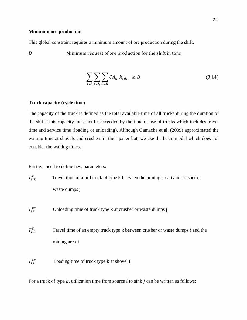
Minimum ore production

This global constraint requires a minimum amount of ore production during the shift.

∑ ∑ ∑

Truck capacity (cycle time)

The capacity of the truck is defined as the total available time of all trucks during the duration of

the shift. This capacity must not be exceeded by the time of use of trucks which includes travel

time and service time (loading or unloading). Although Gamache et al. (2009) approximated the

waiting time at shovels and crushers in their paper but, we use the basic model which does not

consider the waiting times.

First we need to define new parameters:

Travel time of a full truck of type between the mining area and crusher or

waste dumps

Unloading time of truck type at crusher or waste dumps

Travel time of an empty truck type between crusher or waste dumps and the

mining area

Loading time of truck type at shovel

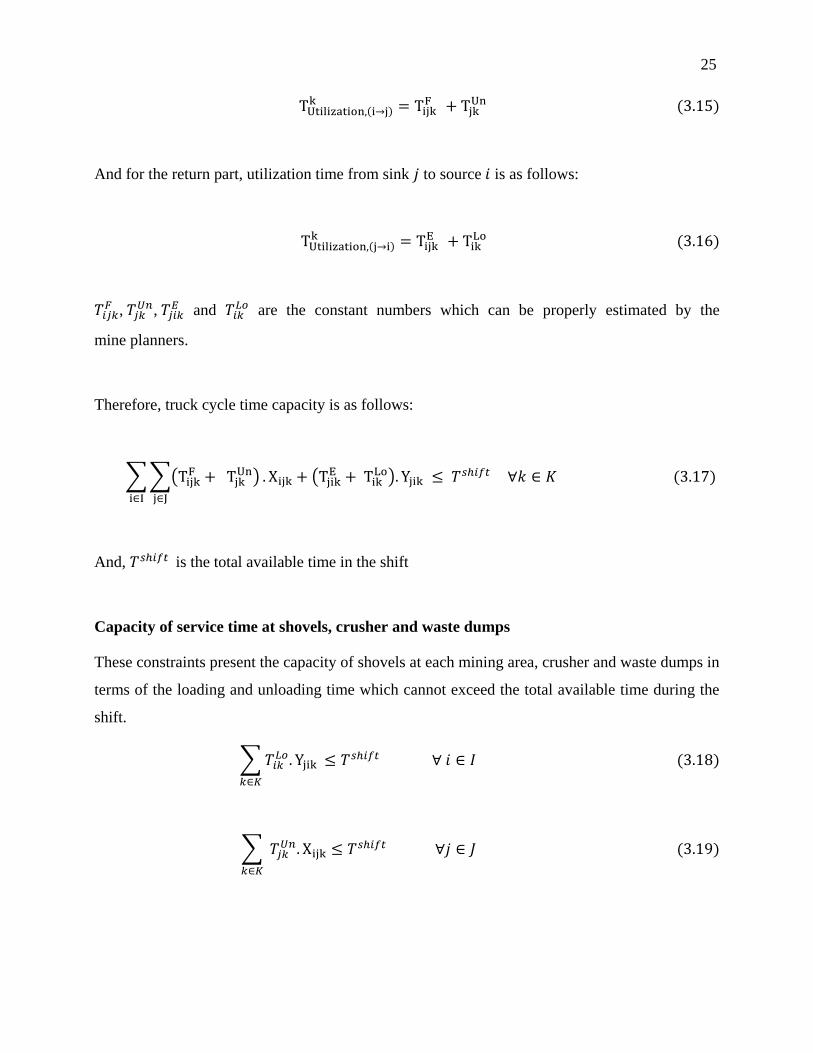
For a truck of type , utilization time from source to sink can be written as follows:

25

And for the return part, utilization time from sink to source is as follows:

,

, and

are the constant numbers which can be properly estimated by the

mine planners.

Therefore, truck cycle time capacity is as follows:

∑∑(

)

(

)

And, is the total available time in the shift

Capacity of service time at shovels, crusher and waste dumps

These constraints present the capacity of shovels at each mining area, crusher and waste dumps in

terms of the loading and unloading time which cannot exceed the total available time during the

shift.

∑

∑

26

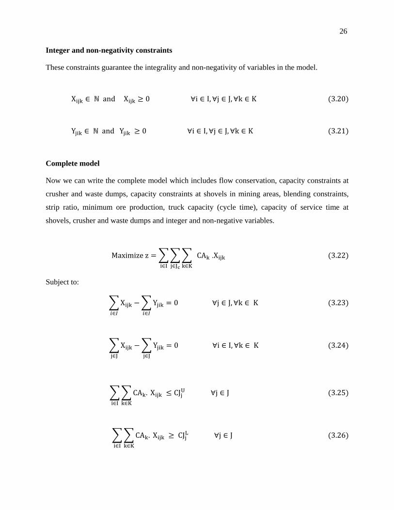
Integer and non-negativity constraints

These constraints guarantee the integrality and non-negativity of variables in the model.

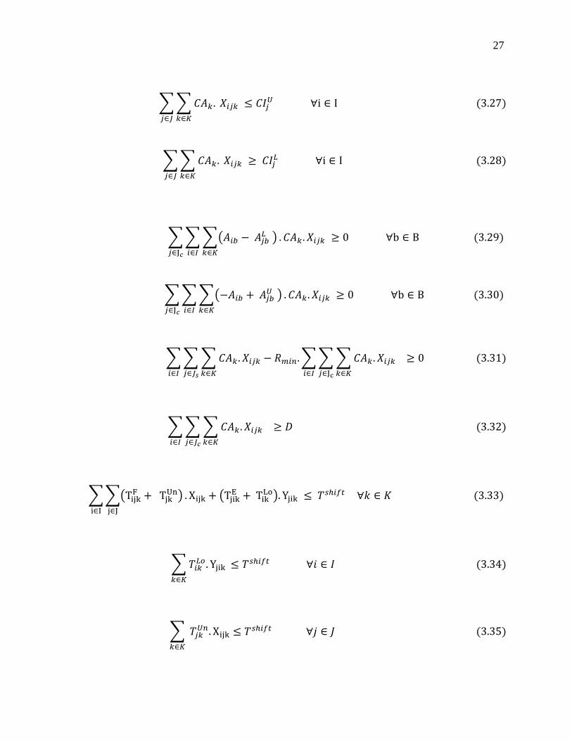
Complete model

Now we can write the complete model which includes flow conservation, capacity constraints at

crusher and waste dumps, capacity constraints at shovels in mining areas, blending constraints,

strip ratio, minimum ore production, truck capacity (cycle time), capacity of service time at

shovels, crusher and waste dumps and integer and non-negative variables.

∑∑∑ .

Subject to:

∑

∑

∑

∑

∑∑

∑∑

27

∑ ∑

∑ ∑

∑∑ ∑( )

∑∑ ∑( )

∑ ∑ ∑

∑∑ ∑

∑ ∑ ∑

∑∑(

)

(

)

∑

∑

28

This section presented the linear programming model for a VSTPP in an open pit mine, which

maximizes ore production during a shift according to the required constraints. The LP model

doesn’t take into account the waiting time at shovels and crushers. In the following section, the

simulation models are presented in order to validate the optimal result of the LP model and to

find a new way for VSTPP.

3.2 General concepts and definition of simulation models

In this thesis, we present two simulation models. The first model, called basic simulation model,

considers the queue and waiting times at shovels in mining areas and crushers in dumping sites.

This simulation model is used to validate the optimal result of the LP model which is related to

truck and shovel hauling system. The LP solution indicates the number of trips between sources

and sinks in terms of the number of empty and full trucks that should be traveling between

dumping sites and mining areas. The basic simulation model uses the optimal result of the LP

model as a target for allocating trucks to the mining areas.

To assess the possibility of finding and proposing a new way for production planning for a very

short-term period, a second simulation model, called the real time simulation model, is

developed. This simulation model imitates the real hauling system of the mine and takes into

account all constrains of the VSTPP. Its objective is to maximize ore production.

The suggested simulation models are developed in Arena (Rockwell Automation, 2012)

simulation software. Arena is one of the common simulation modeling tools, because it has a

powerful and operational user base (Rossetti, 2009).

In the next section the general assumptions of simulation models are presented.

29

3.2.1 Assumptions

To develop simulation models, some basic assumptions which are considered in this work are as

follows:

All shovels and crushers can serve only one truck at a time and trucks might be in the

queue at mining areas or in the crusher to be served

The crusher is considered as the parking lot at the beginning and at the end of the shift

During the running of the simulation models, the truck and shovels system are operating

without following any schedule.

The necessary definitions applied in simulation models are introduced in the following section.

3.2.2 Definitions

In this thesis, the Entities of the simulation models are the trucks; for example if we have two

types of trucks, we will have two different entities.

In these simulation models, loading and unloading the trucks are considered as Process and the

essential Resources for these processes are shovels in mining areas, crushers and waste dumps in

dumping sites.

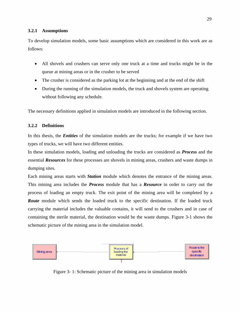
Each mining areas starts with Station module which denotes the entrance of the mining areas.

This mining area includes the Process module that has a Resource in order to carry out the

process of loading an empty truck. The exit point of the mining area will be completed by a

Route module which sends the loaded truck to the specific destination. If the loaded truck

carrying the material includes the valuable contains, it will send to the crushers and in case of

containing the sterile material, the destination would be the waste dumps. Figure 3-1 shows the

schematic picture of the mining area in the simulation model.

Figure 3- 1: Schematic picture of the mining area in simulation models

Mining areadestination

specific

Route to the

materialloading theProcess of

0

30

Each unloading area such as crusher or waste dumps starts with Station module. This unloading

area includes the Process module that must utilize a Resource in order to complete the process of

unloading a full truck. There are different kinds of logic for Resources in the Process at dumping

sites. In crusher area, a crusher is added as a Resource which is based on seize, delay and release

logic. In the waste dumps, the logic is only delay the Resource which is equal to the unloading

time of each truck at these dumping sites. For example in this research, two trucks can unload in

parallel in this area but crusher can only unload one truck at a time. This Process module will

connect to the Decide module to choose the mining area where the empty truck will be sent based

on the decision criterion which will be explained in the basic simulation model section. An

Assign module is added after the decision part to allocate the desirable variables in this segment

such as a counter to keep track of the number of sending trucks to the mining areas. The exit

point of this area will be completed by a Route which sends the unloaded truck to the decided

destination.

In this section, the general definition which we used in the simulation models was presented.

Section 3.2.3 presents notations that are applied in simulation models.

3.2.3 Notations

The essential notations in the simulation models are presented.

Let first denote

Number of mining areas

Number of dumping sites

There are two different kinds of notations in this section such as Variable data and Attribute

notations. Most of these notations are created in the Variable data module which is

“measurement information” and subject to change and others is as Attribute data which stores

entities information (Kelton et al., 2007).

31

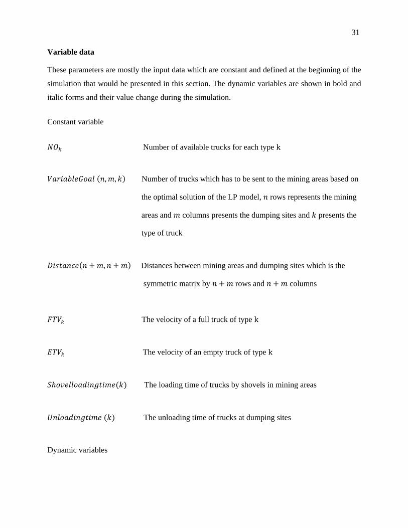
Variable data

These parameters are mostly the input data which are constant and defined at the beginning of the

simulation that would be presented in this section. The dynamic variables are shown in bold and

italic forms and their value change during the simulation.

Constant variable

Number of available trucks for each type

Number of trucks which has to be sent to the mining areas based on

the optimal solution of the LP model, rows represents the mining

areas and columns presents the dumping sites and presents the

type of truck

Distances between mining areas and dumping sites which is the

symmetric matrix by rows and columns

The velocity of a full truck of type

The velocity of an empty truck of type

The loading time of trucks by shovels in mining areas

The unloading time of trucks at dumping sites

Dynamic variables

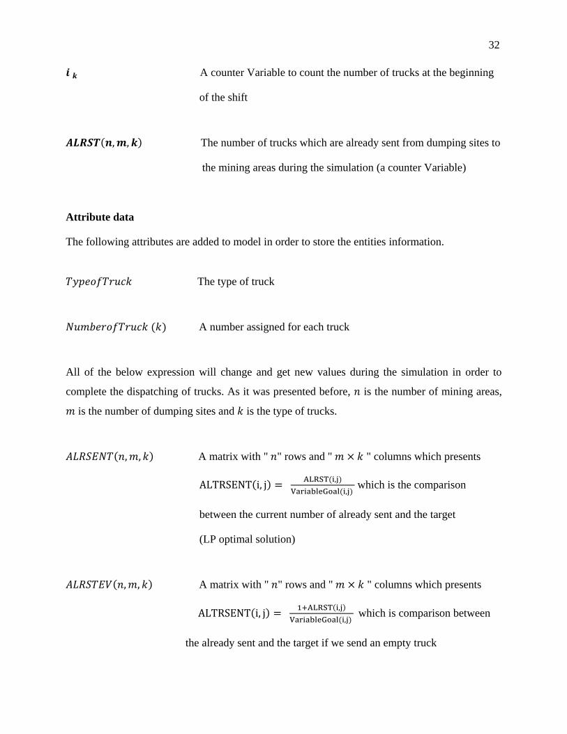
32

A counter Variable to count the number of trucks at the beginning

of the shift

The number of trucks which are already sent from dumping sites to

the mining areas during the simulation (a counter Variable)

Attribute data

The following attributes are added to model in order to store the entities information.

The type of truck

A number assigned for each truck

All of the below expression will change and get new values during the simulation in order to

complete the dispatching of trucks. As it was presented before, is the number of mining areas,

is the number of dumping sites and is the type of trucks.

A matrix with " " rows and " " columns which presents

which is the comparison

between the current number of already sent and the target

(LP optimal solution)

A matrix with " " rows and " " columns which presents

which is comparison between

the already sent and the target if we send an empty truck

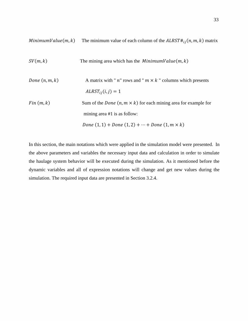
33

The minimum value of each column of the matrix

The mining area which has the

A matrix with " " rows and " " columns which presents

Sum of the for each mining area for example for

mining area #1 is as follow:

In this section, the main notations which were applied in the simulation model were presented. In

the above parameters and variables the necessary input data and calculation in order to simulate

the haulage system behavior will be executed during the simulation. As it mentioned before the

dynamic variables and all of expression notations will change and get new values during the

simulation. The required input data are presented in Section 3.2.4.

34

3.2.4 Input data

The following information is the essential data that must be provided as inputs to run the LP and

simulation models. These input data are the real data of an open pit mine which enter to models

by the parameters which were explained in the previous sections.

Tonnage of available material in front of each shovel

Ore characteristics at each mining area

Upper and lower bound of ore characteristics, needed for mixture of material in the

crushers

Loading time of shovels

Unloading time at crushers and waste dumps

Capacity and number of each type of truck

Distances between mining areas and dumping sites

The velocity of the full and empty for each type of truck

Stripping ratio for waste removal in comparison to the total extracted material

3.3 Deterministic simulation models

This section presents two simulation models based on the deterministic input data. In the next

subsection, we present the first model, called the basic simulation model, which is used to

validate the result of the LP model.

3.3.1 Deterministic Basic simulation (DBS) model

The DBS model is developed to validate the optimal result of the LP model. In this regard, we

developed the DBS model in Arena which takes into account the queue and waiting time at

shovels and crushers and tries to send the similar number of trucks to different destinations based

on the LP model result. The optimal solution of the LP model is considered as the target of this

35

simulation model and defined at the beginning of the shift in the DBS model. In the DBS model,

every time that an empty truck becomes available at dumping sites, a module checks the number

of already sent of trucks (based on their type). The already sent number of trucks that is 2D

variable will be compared with the target value. The mining area which has the minimum ratio of

comparison is the area that we need to send the empty truck. This process will continue during

the simulation in order to send as much as number of possible trucks to each mining area

according to the predefined target.

This model has four main sections: Creation of entities, Crushers as parking lot and dumping

sites, Mining areas (ore and waste), and Waste dumps as other options of dumping sites. These

four parts are described below.

Creation of entities (initialization of model)

The creation of entities is done during steps 1 to 3 of the model at the beginning of the shift.

Step 1: Create different types of trucks “constantly” using the Create module.

Step 2: Connect the Create module to the Assign module. Add an attribute for ,

Truck A and Truck B. Assign variable and increase this variable by one unit. This counter

variable will be increased until it reaches the number of available trucks ( ) for each type .

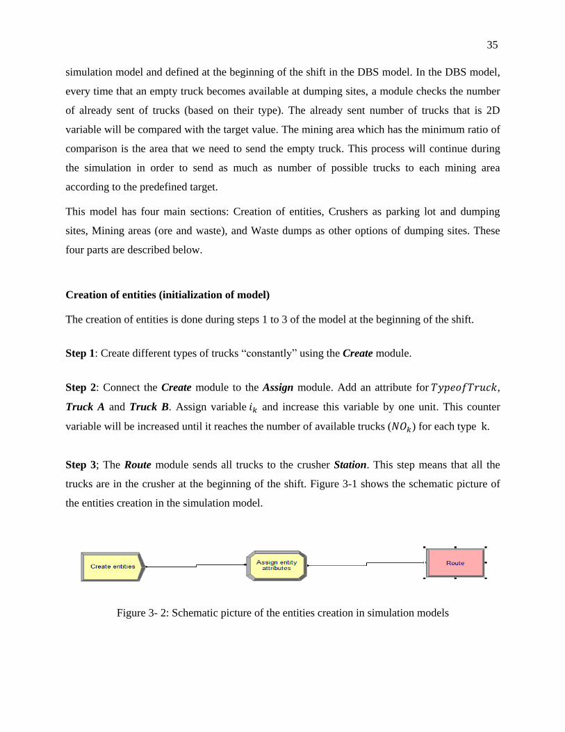
Step 3; The Route module sends all trucks to the crusher Station. This step means that all the

trucks are in the crusher at the beginning of the shift. Figure 3-1 shows the schematic picture of

the entities creation in the simulation model.

Figure 3- 2: Schematic picture of the entities creation in simulation models

36

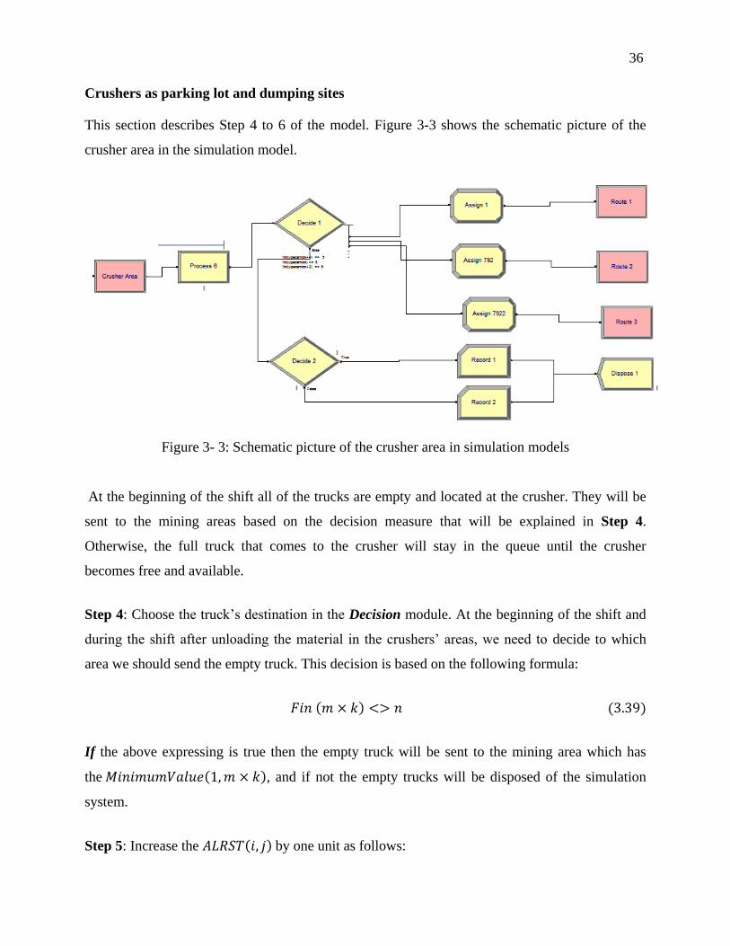
Crushers as parking lot and dumping sites

This section describes Step 4 to 6 of the model. Figure 3-3 shows the schematic picture of the

crusher area in the simulation model.

Figure 3- 3: Schematic picture of the crusher area in simulation models

At the beginning of the shift all of the trucks are empty and located at the crusher. They will be

sent to the mining areas based on the decision measure that will be explained in Step 4.

Otherwise, the full truck that comes to the crusher will stay in the queue until the crusher

becomes free and available.

Step 4: Choose the truck’s destination in the Decision module. At the beginning of the shift and

during the shift after unloading the material in the crushers’ areas, we need to decide to which

area we should send the empty truck. This decision is based on the following formula:

If the above expressing is true then the empty truck will be sent to the mining area which has

the , and if not the empty trucks will be disposed of the simulation

system.

Step 5: Increase the by one unit as follows:

37

Step 6: Send back the empty truck to the selected mining area. The required time is equal to the

following formula:

Mining areas (ore and waste)

This section describes the mining areas in an open pit mine where shovels are distributed to

extract the material and load the empty trucks. This section starts at Step 7 and terminates at Step

8. An empty truck waits in the mining area until to be served by shovel. The required time to load

an empty truck is equal to the loading time at each shovel.

Step 7: If the truck is full of ore, send it to the crusher; otherwise send it to the waste dumps.

Step 8: Calculate the time taken for a full truck to reach the dumping destination using the

following formula:

38

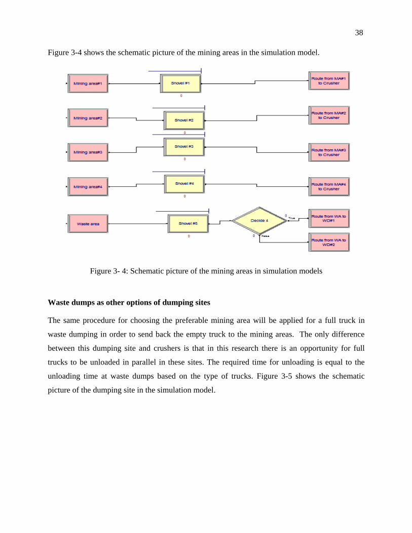
Figure 3-4 shows the schematic picture of the mining areas in the simulation model.

Figure 3- 4: Schematic picture of the mining areas in simulation models

Waste dumps as other options of dumping sites

The same procedure for choosing the preferable mining area will be applied for a full truck in

waste dumping in order to send back the empty truck to the mining areas. The only difference

between this dumping site and crushers is that in this research there is an opportunity for full

trucks to be unloaded in parallel in these sites. The required time for unloading is equal to the

unloading time at waste dumps based on the type of trucks. Figure 3-5 shows the schematic

picture of the dumping site in the simulation model.

39

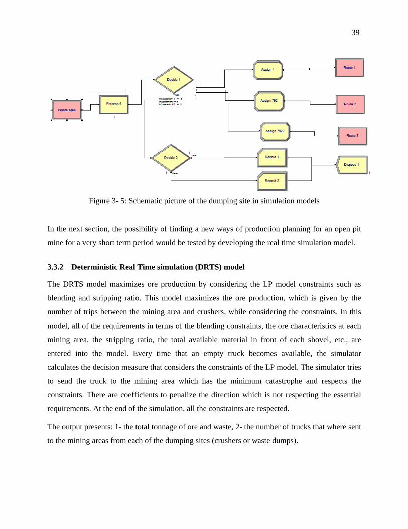
Figure 3- 5: Schematic picture of the dumping site in simulation models

In the next section, the possibility of finding a new ways of production planning for an open pit

mine for a very short term period would be tested by developing the real time simulation model.

3.3.2 Deterministic Real Time simulation (DRTS) model

The DRTS model maximizes ore production by considering the LP model constraints such as

blending and stripping ratio. This model maximizes the ore production, which is given by the

number of trips between the mining area and crushers, while considering the constraints. In this

model, all of the requirements in terms of the blending constraints, the ore characteristics at each

mining area, the stripping ratio, the total available material in front of each shovel, etc., are

entered into the model. Every time that an empty truck becomes available, the simulator

calculates the decision measure that considers the constraints of the LP model. The simulator tries

to send the truck to the mining area which has the minimum catastrophe and respects the

constraints. There are coefficients to penalize the direction which is not respecting the essential

requirements. At the end of the simulation, all the constraints are respected.

The output presents: 1- the total tonnage of ore and waste, 2- the number of trucks that where sent

to the mining areas from each of the dumping sites (crushers or waste dumps).

40

In order to develop the DRTS model, we require new definitions in dumping sites and also new

notations. In this model, we have the similar definitions for creation of Entities and mining areas

but there is a different definition for dumping sites after the Process module.

The Process module will connect to the Assign module at each dumping site to allocate different

variables which are defined below. All decisions to select to which mining area we are sending

the empty truck are taken by the Expression module in Advanced Process panel. After decision

is taken a Route module sends the unloaded truck to the decided destination.

Let define:

Number of ore characteristic

Number of constraints

These parameters are also the input data which are constant and defined at the beginning of the

simulation. There are dynamic variables which are assigned in the Assign module during the

simulation run. These variables are shown in bold and italic format in the following part. The rest

of the notations are the parameter which remains constant during the simulation.

Constant parameters

The ore characteristics in mining areas

The minimum or maximum required quantity of the ore

characteristics in ore at the end of the shift in crusher

The total material which is available in front of each shovel

This parameter presents the number of truck waiting at shovel

and traveling to shovel multiply by loading time at shovel has

41

to be less than route time from dumping site to shovel and if not

it will be waiting time at shovels.

This parameter is equal to

Dynamic variables

The total quantity of ore and waste extracted and transported

by trucks to their destinations

The quantity of material already extracted by shovels in

mining areas during the simulation

The cumulative variable that shows the amount of ore extracted

during the simulation

The amount of the in the

The penalty for not respecting the constraints at the mining area

The number of trucks sent to the mining areas from crushers

or waste dumps (a 2D counter Variable)

A matrix with " " rows and " " columns that presents

the decision measure that is presented in (3.41)

The minimum value of

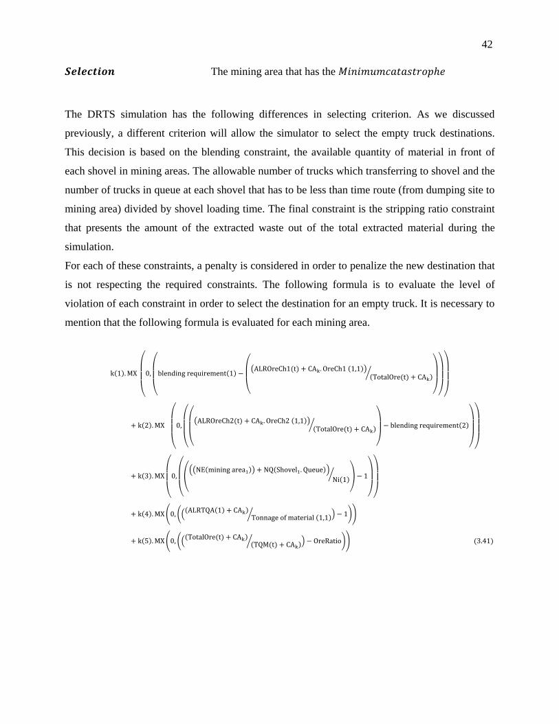
42

The mining area that has the

The DRTS simulation has the following differences in selecting criterion. As we discussed

previously, a different criterion will allow the simulator to select the empty truck destinations.

This decision is based on the blending constraint, the available quantity of material in front of

each shovel in mining areas. The allowable number of trucks which transferring to shovel and the

number of trucks in queue at each shovel that has to be less than time route (from dumping site to

mining area) divided by shovel loading time. The final constraint is the stripping ratio constraint

that presents the amount of the extracted waste out of the total extracted material during the

simulation.

For each of these constraints, a penalty is considered in order to penalize the new destination that

is not respecting the required constraints. The following formula is to evaluate the level of

violation of each constraint in order to select the destination for an empty truck. It is necessary to

mention that the following formula is evaluated for each mining area.

(

(

(

( )

⁄

)

)

)

(

(

(

( )

⁄

)

)

)

(

(

((( ) )

⁄ )

)

)

( ((

⁄ ) ))

( ((

⁄ ) ))

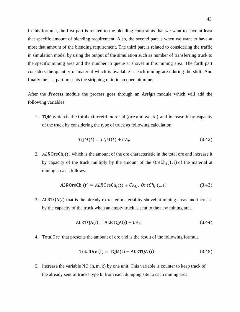
43

In this formula, the first part is related to the blending constraints that we want to have at least

that specific amount of blending requirement. Also, the second part is when we want to have at

most that amount of the blending requirement. The third part is related to considering the traffic

in simulation model by using the output of the simulation such as number of transferring truck to

the specific mining area and the number in queue at shovel in this mining area. The forth part

considers the quantity of material which is available at each mining area during the shift. And

finally the last part presents the stripping ratio in an open pit mine.

After the Process module the process goes through an Assign module which will add the

following variables:

1. and increase it by capacity

of the truck by considering the type of truck as following calculation

2. which is the amount of the ore characteristic in the total ore and increase it

by capacity of the truck multiply by the amount of the of the material at

mining area as follows:

3. that is the already extracted material by shovel at mining areas and increase

by the capacity of the truck when an empty truck is sent to the new mining area

4. that presents the amount of ore and is the result of the following formula

5. Increase the variable by one unit. This variable is counter to keep track of

the already sent of trucks type from each dumping site to each mining area

44

The next section presents the essential modification in both simulation models in order to develop

the stochastic model which is more accurate and reflects the reality of the problem in an open pit

mine.

3.3.3 Stochastic models

Since deterministic models do not consider the uncertainties in the simulation models, they

cannot be the best choice to validate and analyze the result, in this subsection, simulation models

are improved by accumulating the uncertainties to the simulation models.

These uncertainties are related to the following areas:

a. Loading time by shovels at each mining area. This loading time is the required time to

load the truck by shovels which are located in the mining areas.

b. Velocity of the full and empty trucks during transporting material from mining areas to

the destinations and returning from the unloading areas to the mining areas.

c. Unloading time at crushers and waste dumps. This time is the required time to unload the

truck in the crushers or waste dumps.

3.4 summary

In this chapter we have described the LP and simulation models, and then in the next chapter we

will test these models in order to evaluate their strength and weakness in an open pit mine.

45

CHAPTER 4: TESTS, RESULTS AND ANALYSIS

The LP model and the simulation models that have been developed in Chapter 3 are applied on a

real mine using Excel Solver (Microsoft office, 2010) and Arena simulation software (Rockwell

Automation, 2012) respectively.

The LP model that is to maximize the total ore production during the shift uses Solver to find the

number of trips between mining areas and waste dumps. Then, the final result of the LP model is

considered as the target of the DBS model while considering the waiting times at servers. The

objective of this model as explained in the previous chapters is to validate the result of the LP

model and to provide an operational dispatching plan for the open pit mine. In this regard, the

result of the DBS model will be compared to the result of the LP model. Moreover, a new method

of VSTPP is developed in chapter 3 which is called DRTS model and employs Arena simulator.

In addition, the solution of this model will be compared to the solution of the LP model with the

purpose of verifying the developed simulation model and validating the LP model. At the end of

this chapter, the performance of the LP model and simulation models considering the different

states as the bottleneck of operational system will be discussed.

The next section presents all of the required input data of the mine studied in this work.

4.1 Instances

The open pit mine under study is a coal mine with five mining areas where shovels are

distributed in these areas. Four of these mining areas are located in the valuable mineral (ore)

area (shovel #1 to shovel#4 are distributed in these areas) and the other one is in the waste area

(shovel #5). There are two types of trucks with different capacities and velocities. Loaded trucks

will be traveled to transfer the extracted material to the destinations including one crusher and

two waste dumps. The following sections, presents the essential input data which are constant at

the beginning and during the simulation:

Tonnage of available material in front of each shovel

Ore characteristics in mining areas

The essential upper and lower bounds of ore characteristics in crusher

Loading and unloading time of trucks

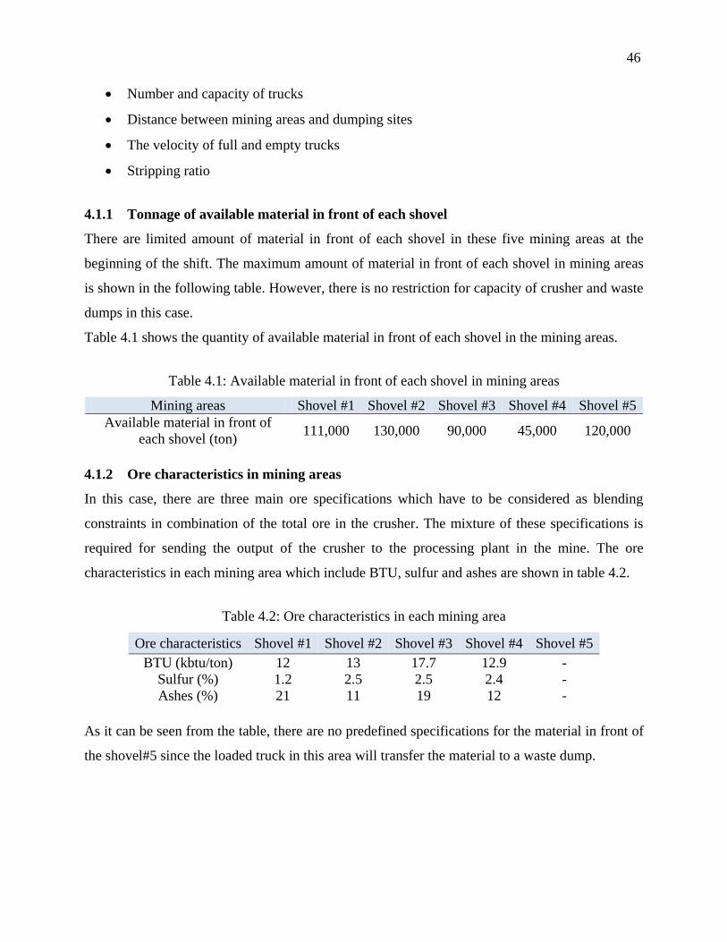
46

Number and capacity of trucks

Distance between mining areas and dumping sites

The velocity of full and empty trucks

Stripping ratio

4.1.1 Tonnage of available material in front of each shovel

There are limited amount of material in front of each shovel in these five mining areas at the

beginning of the shift. The maximum amount of material in front of each shovel in mining areas

is shown in the following table. However, there is no restriction for capacity of crusher and waste

dumps in this case.

Table 4.1 shows the quantity of available material in front of each shovel in the mining areas.

Table 4.1: Available material in front of each shovel in mining areas

Mining areas Shovel #1 Shovel #2 Shovel #3 Shovel #4 Shovel #5

Available material in front of

each shovel (ton) 111,000 130,000 90,000 45,000 120,000

4.1.2 Ore characteristics in mining areas

In this case, there are three main ore specifications which have to be considered as blending

constraints in combination of the total ore in the crusher. The mixture of these specifications is

required for sending the output of the crusher to the processing plant in the mine. The ore

characteristics in each mining area which include BTU, sulfur and ashes are shown in table 4.2.

Table 4.2: Ore characteristics in each mining area

Ore characteristics Shovel #1 Shovel #2 Shovel #3 Shovel #4 Shovel #5

BTU (kbtu/ton) 12 13 17.7 12.9 -

Sulfur (%) 1.2 2.5 2.5 2.4 -

Ashes (%) 21 11 19 12 -

As it can be seen from the table, there are no predefined specifications for the material in front of

the shovel#5 since the loaded truck in this area will transfer the material to a waste dump.

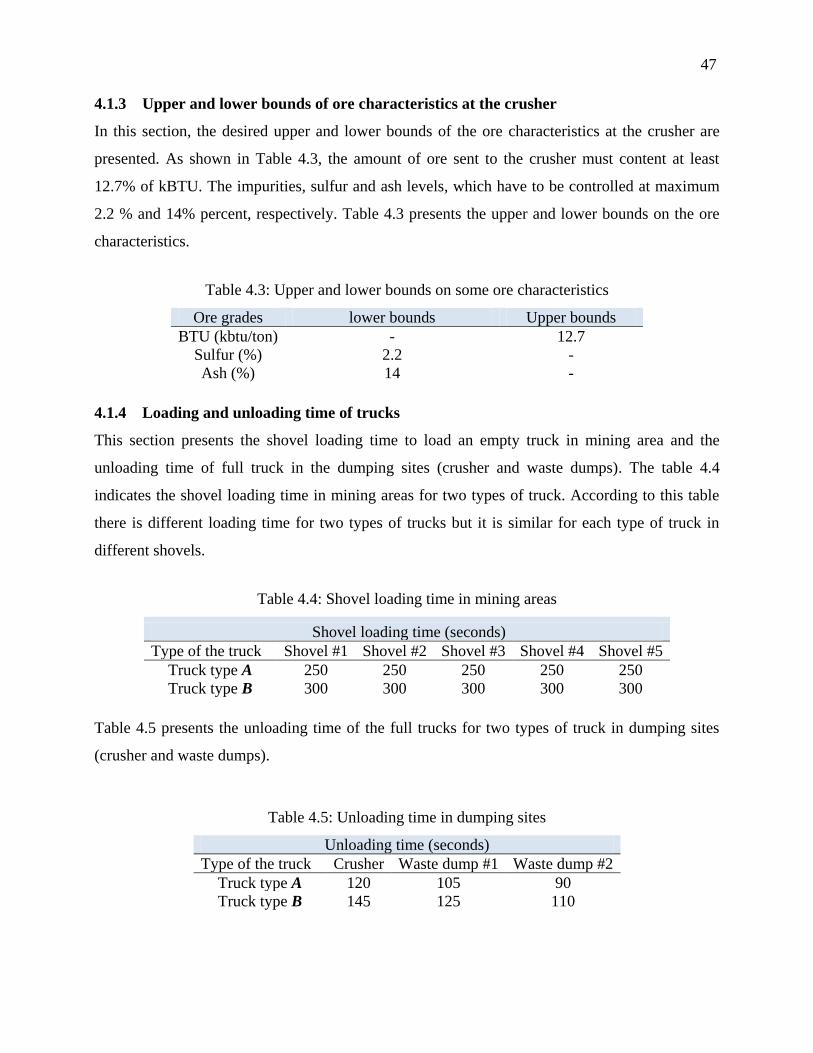
47

4.1.3 Upper and lower bounds of ore characteristics at the crusher

In this section, the desired upper and lower bounds of the ore characteristics at the crusher are

presented. As shown in Table 4.3, the amount of ore sent to the crusher must content at least

12.7% of kBTU. The impurities, sulfur and ash levels, which have to be controlled at maximum

2.2 % and 14% percent, respectively. Table 4.3 presents the upper and lower bounds on the ore

characteristics.

Table 4.3: Upper and lower bounds on some ore characteristics

Ore grades lower bounds Upper bounds

BTU (kbtu/ton) - 12.7

Sulfur (%) 2.2 -

Ash (%) 14 -

4.1.4 Loading and unloading time of trucks

This section presents the shovel loading time to load an empty truck in mining area and the

unloading time of full truck in the dumping sites (crusher and waste dumps). The table 4.4

indicates the shovel loading time in mining areas for two types of truck. According to this table

there is different loading time for two types of trucks but it is similar for each type of truck in

different shovels.

Table 4.4: Shovel loading time in mining areas

Shovel loading time (seconds)

Type of the truck Shovel #1 Shovel #2 Shovel #3 Shovel #4 Shovel #5

Truck type A 250 250 250 250 250

Truck type B 300 300 300 300 300

Table 4.5 presents the unloading time of the full trucks for two types of truck in dumping sites

(crusher and waste dumps).

Table 4.5: Unloading time in dumping sites

Unloading time (seconds)

Type of the truck Crusher Waste dump #1 Waste dump #2

Truck type A 120 105 90

Truck type B 145 125 110

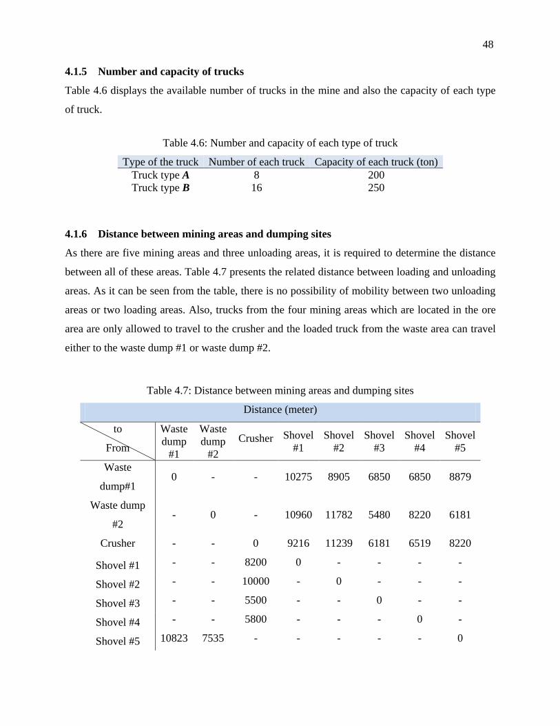
48

4.1.5 Number and capacity of trucks

Table 4.6 displays the available number of trucks in the mine and also the capacity of each type

of truck.

Table 4.6: Number and capacity of each type of truck

Type of the truck Number of each truck Capacity of each truck (ton)

Truck type A 8 200

Truck type B 16 250

4.1.6 Distance between mining areas and dumping sites

As there are five mining areas and three unloading areas, it is required to determine the distance

between all of these areas. Table 4.7 presents the related distance between loading and unloading

areas. As it can be seen from the table, there is no possibility of mobility between two unloading

areas or two loading areas. Also, trucks from the four mining areas which are located in the ore

area are only allowed to travel to the crusher and the loaded truck from the waste area can travel

either to the waste dump #1 or waste dump #2.

Table 4.7: Distance between mining areas and dumping sites

Distance (meter)

to

From

Waste

dump

#1

Waste

dump

#2

Crusher Shovel

#1

Shovel

#2

Shovel

#3

Shovel

#4

Shovel

#5

Waste

dump#1 0 - - 10275 8905 6850 6850 8879

Waste dump

#2 - 0 - 10960 11782 5480 8220 6181

Crusher - - 0 9216 11239 6181 6519 8220

Shovel #1 - - 8200 0 - - - -

Shovel #2 - - 10000 - 0 - - -

Shovel #3 - - 5500 - - 0 - -

Shovel #4 - - 5800 - - - 0 -

Shovel #5 10823 7535 - - - - - 0

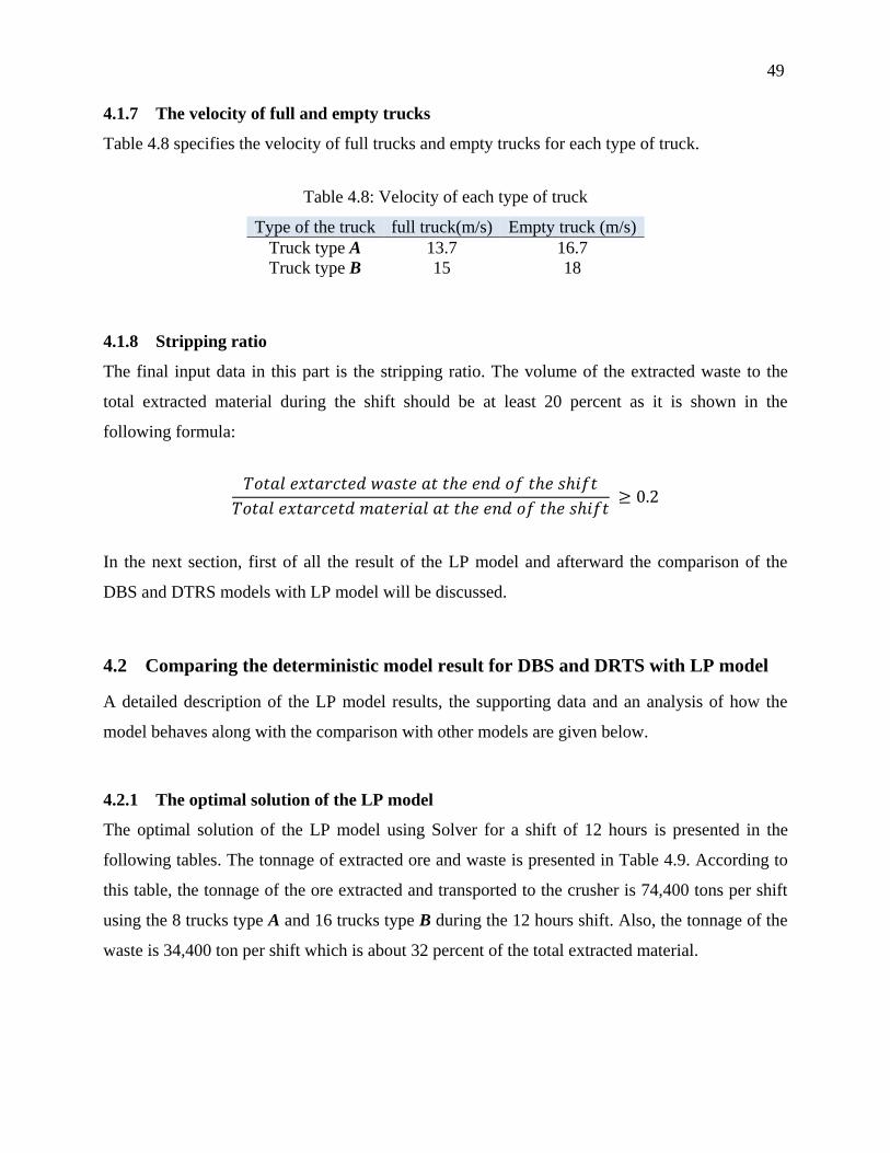
49

4.1.7 The velocity of full and empty trucks

Table 4.8 specifies the velocity of full trucks and empty trucks for each type of truck.

Table 4.8: Velocity of each type of truck

Type of the truck full truck(m/s) Empty truck (m/s)

Truck type A 13.7 16.7

Truck type B 15 18

4.1.8 Stripping ratio

The final input data in this part is the stripping ratio. The volume of the extracted waste to the

total extracted material during the shift should be at least 20 percent as it is shown in the

following formula:

In the next section, first of all the result of the LP model and afterward the comparison of the

DBS and DTRS models with LP model will be discussed.

4.2 Comparing the deterministic model result for DBS and DRTS with LP model

A detailed description of the LP model results, the supporting data and an analysis of how the

model behaves along with the comparison with other models are given below.

4.2.1 The optimal solution of the LP model

The optimal solution of the LP model using Solver for a shift of 12 hours is presented in the

following tables. The tonnage of extracted ore and waste is presented in Table 4.9. According to

this table, the tonnage of the ore extracted and transported to the crusher is 74,400 tons per shift

using the 8 trucks type A and 16 trucks type B during the 12 hours shift. Also, the tonnage of the

waste is 34,400 ton per shift which is about 32 percent of the total extracted material.

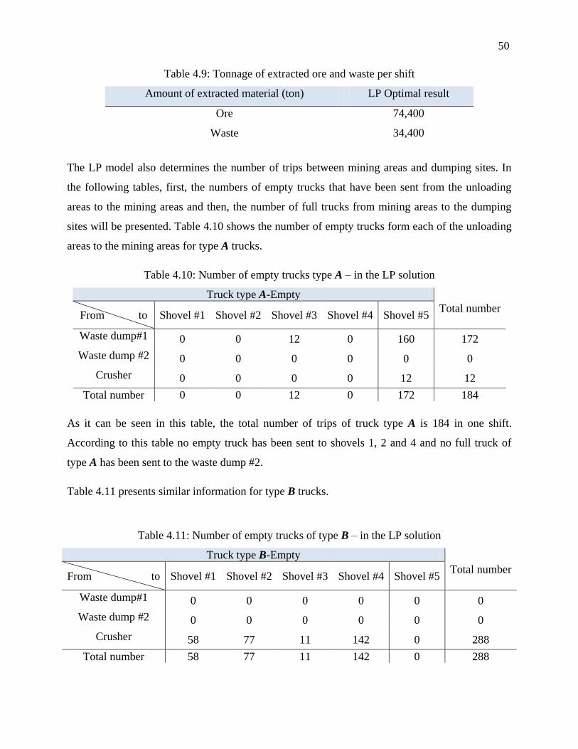
50

Table 4.9: Tonnage of extracted ore and waste per shift

Amount of extracted material (ton) LP Optimal result

Ore 74,400

Waste 34,400

The LP model also determines the number of trips between mining areas and dumping sites. In

the following tables, first, the numbers of empty trucks that have been sent from the unloading

areas to the mining areas and then, the number of full trucks from mining areas to the dumping

sites will be presented. Table 4.10 shows the number of empty trucks form each of the unloading

areas to the mining areas for type A trucks.

Table 4.10: Number of empty trucks type A – in the LP solution

Truck type A-Empty

Total number From to Shovel #1 Shovel #2 Shovel #3 Shovel #4 Shovel #5

Waste dump#1 0 0 12 0 160 172

Waste dump #2 0 0 0 0 0 0

Crusher 0 0 0 0 12 12

Total number 0 0 12 0 172 184

As it can be seen in this table, the total number of trips of truck type A is 184 in one shift.

According to this table no empty truck has been sent to shovels 1, 2 and 4 and no full truck of

type A has been sent to the waste dump #2.

Table 4.11 presents similar information for type B trucks.

Table 4.11: Number of empty trucks of type B – in the LP solution

Truck type B-Empty

Total number From to Shovel #1 Shovel #2 Shovel #3 Shovel #4 Shovel #5

Waste dump#1 0 0 0 0 0 0

Waste dump #2 0 0 0 0 0 0

Crusher 58 77 11 142 0 288

Total number 58 77 11 142 0 288

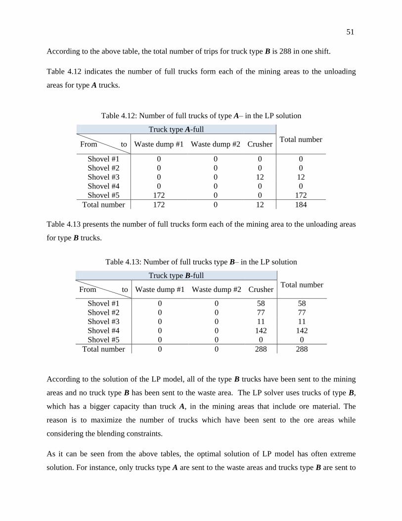
51

According to the above table, the total number of trips for truck type B is 288 in one shift.

Table 4.12 indicates the number of full trucks form each of the mining areas to the unloading

areas for type A trucks.

Table 4.12: Number of full trucks of type A– in the LP solution

Truck type A-full

Total number From to Waste dump #1 Waste dump #2 Crusher

Shovel #1 0 0 0 0

Shovel #2 0 0 0 0

Shovel #3 0 0 12 12

Shovel #4 0 0 0 0

Shovel #5 172 0 0 172

Total number 172 0 12 184

Table 4.13 presents the number of full trucks form each of the mining area to the unloading areas

for type B trucks.

Table 4.13: Number of full trucks type B– in the LP solution

Truck type B-full

Total number From to Waste dump #1 Waste dump #2 Crusher

Shovel #1 0 0 58 58

Shovel #2 0 0 77 77

Shovel #3 0 0 11 11

Shovel #4 0 0 142 142

Shovel #5 0 0 0 0

Total number 0 0 288 288

According to the solution of the LP model, all of the type B trucks have been sent to the mining

areas and no truck type B has been sent to the waste area. The LP solver uses trucks of type B,

which has a bigger capacity than truck A, in the mining areas that include ore material. The

reason is to maximize the number of trucks which have been sent to the ore areas while

considering the blending constraints.

As it can be seen from the above tables, the optimal solution of LP model has often extreme

solution. For instance, only trucks type A are sent to the waste areas and trucks type B are sent to

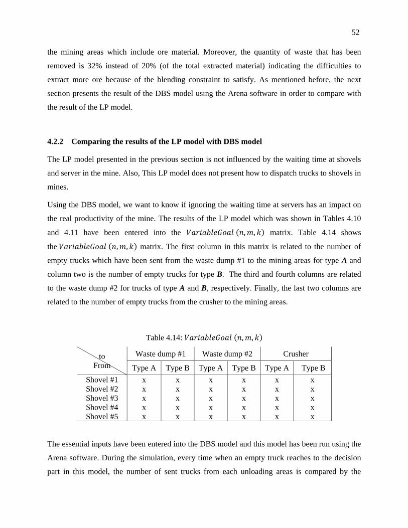
52

the mining areas which include ore material. Moreover, the quantity of waste that has been

removed is 32% instead of 20% (of the total extracted material) indicating the difficulties to

extract more ore because of the blending constraint to satisfy. As mentioned before, the next

section presents the result of the DBS model using the Arena software in order to compare with

the result of the LP model.

4.2.2 Comparing the results of the LP model with DBS model

The LP model presented in the previous section is not influenced by the waiting time at shovels

and server in the mine. Also, This LP model does not present how to dispatch trucks to shovels in

mines.

Using the DBS model, we want to know if ignoring the waiting time at servers has an impact on

the real productivity of the mine. The results of the LP model which was shown in Tables 4.10

and 4.11 have been entered into the matrix. Table 4.14 shows

the matrix. The first column in this matrix is related to the number of

empty trucks which have been sent from the waste dump #1 to the mining areas for type A and

column two is the number of empty trucks for type B. The third and fourth columns are related

to the waste dump #2 for trucks of type A and B, respectively. Finally, the last two columns are

related to the number of empty trucks from the crusher to the mining areas.

Table 4.14:

The essential inputs have been entered into the DBS model and this model has been run using the

Arena software. During the simulation, every time when an empty truck reaches to the decision

part in this model, the number of sent trucks from each unloading areas is compared by the

to

From

Waste dump #1 Waste dump #2 Crusher

Type A Type B Type A Type B Type A Type B

Shovel #1 x x x x x x

Shovel #2 x x x x x x

Shovel #3 x x x x x x

Shovel #4 x x x x x x

Shovel #5 x x x x x x

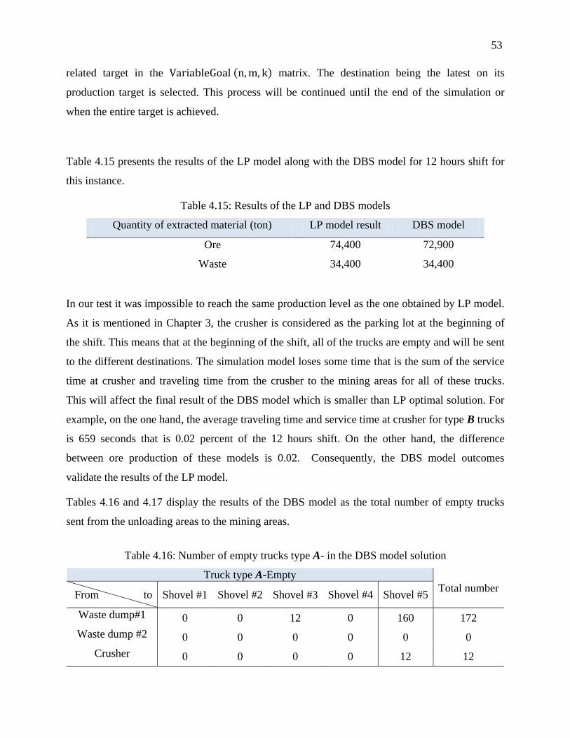
53

related target in the matrix. The destination being the latest on its

production target is selected. This process will be continued until the end of the simulation or

when the entire target is achieved.

Table 4.15 presents the results of the LP model along with the DBS model for 12 hours shift for

this instance.

Table 4.15: Results of the LP and DBS models

Quantity of extracted material (ton) LP model result DBS model

Ore 74,400 72,900

Waste 34,400 34,400

In our test it was impossible to reach the same production level as the one obtained by LP model.

As it is mentioned in Chapter 3, the crusher is considered as the parking lot at the beginning of

the shift. This means that at the beginning of the shift, all of the trucks are empty and will be sent

to the different destinations. The simulation model loses some time that is the sum of the service

time at crusher and traveling time from the crusher to the mining areas for all of these trucks.

This will affect the final result of the DBS model which is smaller than LP optimal solution. For

example, on the one hand, the average traveling time and service time at crusher for type B trucks

is 659 seconds that is 0.02 percent of the 12 hours shift. On the other hand, the difference

between ore production of these models is 0.02. Consequently, the DBS model outcomes

validate the results of the LP model.

Tables 4.16 and 4.17 display the results of the DBS model as the total number of empty trucks

sent from the unloading areas to the mining areas.

Table 4.16: Number of empty trucks type A- in the DBS model solution

Truck type A-Empty

Total number From to Shovel #1 Shovel #2 Shovel #3 Shovel #4 Shovel #5

Waste dump#1 0 0 12 0 160 172

Waste dump #2 0 0 0 0 0 0

Crusher 0 0 0 0 12 12

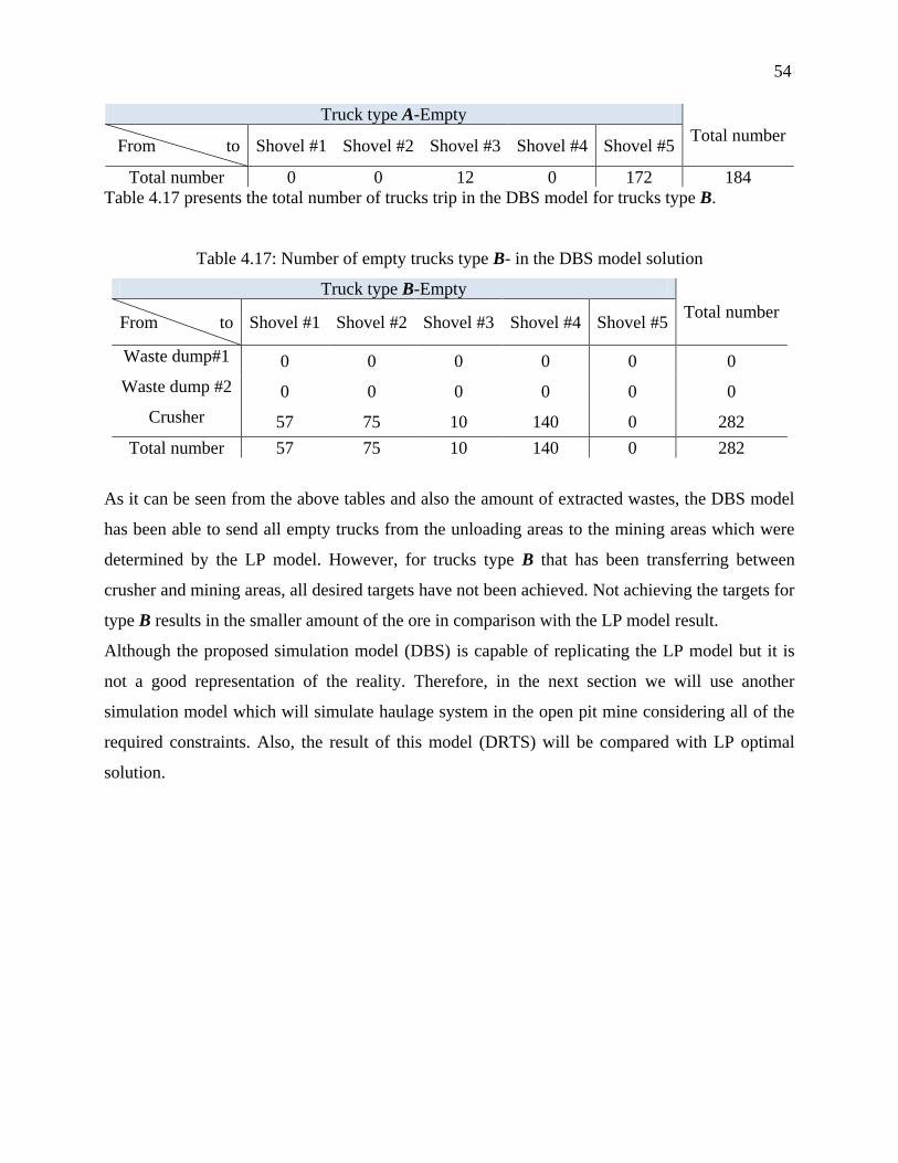
54

Truck type A-Empty

Total number From to Shovel #1 Shovel #2 Shovel #3 Shovel #4 Shovel #5

Total number 0 0 12 0 172 184

Table 4.17 presents the total number of trucks trip in the DBS model for trucks type B.

Table 4.17: Number of empty trucks type B- in the DBS model solution

Truck type B-Empty

Total number From to Shovel #1 Shovel #2 Shovel #3 Shovel #4 Shovel #5

Waste dump#1 0 0 0 0 0 0

Waste dump #2 0 0 0 0 0 0

Crusher 57 75 10 140 0 282

Total number 57 75 10 140 0 282

As it can be seen from the above tables and also the amount of extracted wastes, the DBS model

has been able to send all empty trucks from the unloading areas to the mining areas which were

determined by the LP model. However, for trucks type B that has been transferring between

crusher and mining areas, all desired targets have not been achieved. Not achieving the targets for

type B results in the smaller amount of the ore in comparison with the LP model result.

Although the proposed simulation model (DBS) is capable of replicating the LP model but it is

not a good representation of the reality. Therefore, in the next section we will use another

simulation model which will simulate haulage system in the open pit mine considering all of the

required constraints. Also, the result of this model (DRTS) will be compared with LP optimal

solution.

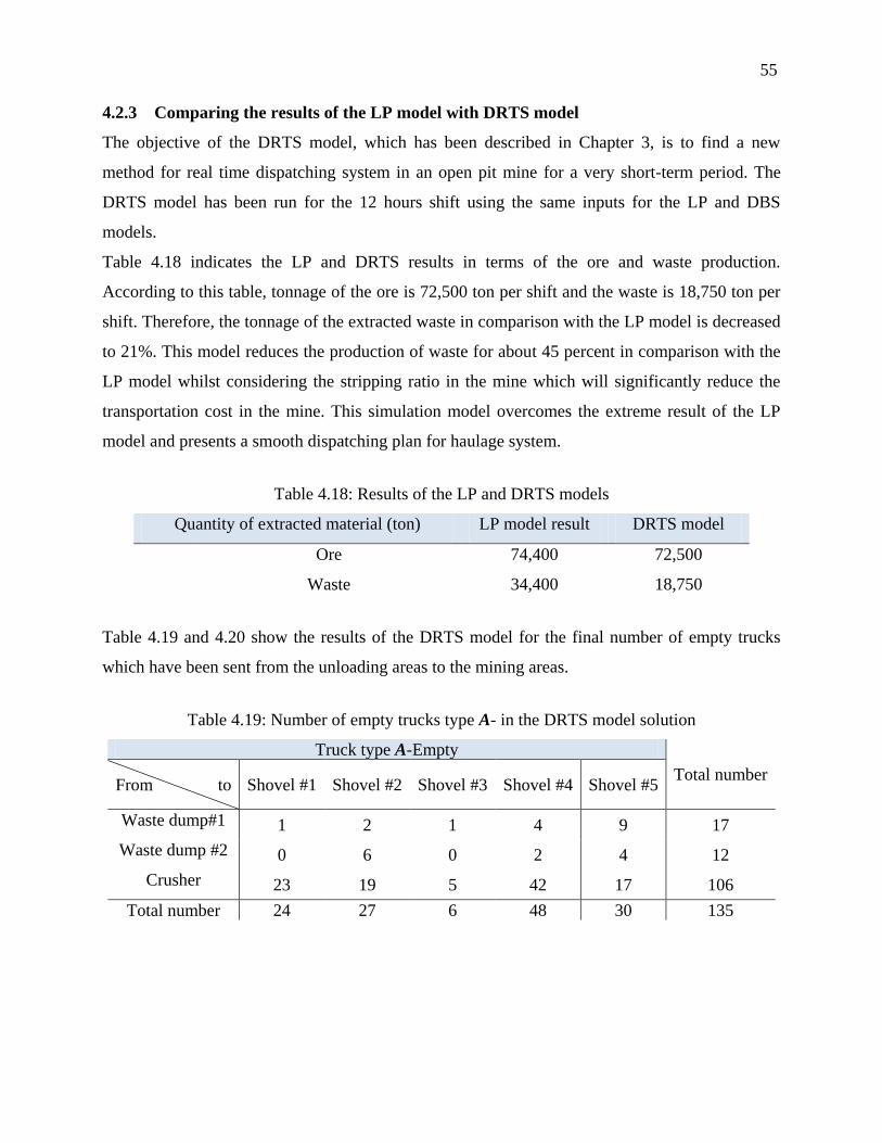
55

4.2.3 Comparing the results of the LP model with DRTS model

The objective of the DRTS model, which has been described in Chapter 3, is to find a new

method for real time dispatching system in an open pit mine for a very short-term period. The

DRTS model has been run for the 12 hours shift using the same inputs for the LP and DBS

models.

Table 4.18 indicates the LP and DRTS results in terms of the ore and waste production.

According to this table, tonnage of the ore is 72,500 ton per shift and the waste is 18,750 ton per

shift. Therefore, the tonnage of the extracted waste in comparison with the LP model is decreased

to 21%. This model reduces the production of waste for about 45 percent in comparison with the

LP model whilst considering the stripping ratio in the mine which will significantly reduce the

transportation cost in the mine. This simulation model overcomes the extreme result of the LP

model and presents a smooth dispatching plan for haulage system.

Table 4.18: Results of the LP and DRTS models

Quantity of extracted material (ton) LP model result DRTS model

Ore 74,400 72,500

Waste 34,400 18,750

Table 4.19 and 4.20 show the results of the DRTS model for the final number of empty trucks

which have been sent from the unloading areas to the mining areas.

Table 4.19: Number of empty trucks type A- in the DRTS model solution

Truck type A-Empty

Total number From to Shovel #1 Shovel #2 Shovel #3 Shovel #4 Shovel #5

Waste dump#1 1 2 1 4 9 17

Waste dump #2 0 6 0 2 4 12

Crusher 23 19 5 42 17 106

Total number 24 27 6 48 30 135

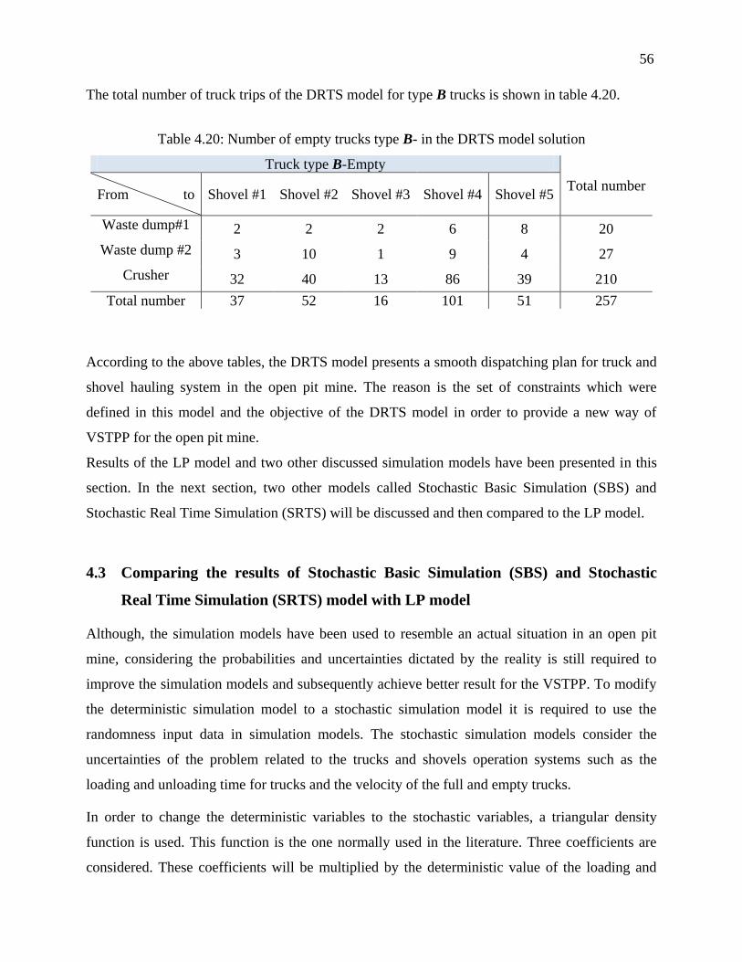
56

The total number of truck trips of the DRTS model for type B trucks is shown in table 4.20.

Table 4.20: Number of empty trucks type B- in the DRTS model solution

Truck type B-Empty

Total number From to Shovel #1 Shovel #2 Shovel #3 Shovel #4 Shovel #5

Waste dump#1 2 2 2 6 8 20

Waste dump #2 3 10 1 9 4 27

Crusher 32 40 13 86 39 210

Total number 37 52 16 101 51 257

According to the above tables, the DRTS model presents a smooth dispatching plan for truck and

shovel hauling system in the open pit mine. The reason is the set of constraints which were

defined in this model and the objective of the DRTS model in order to provide a new way of

VSTPP for the open pit mine.

Results of the LP model and two other discussed simulation models have been presented in this

section. In the next section, two other models called Stochastic Basic Simulation (SBS) and

Stochastic Real Time Simulation (SRTS) will be discussed and then compared to the LP model.

4.3 Comparing the results of Stochastic Basic Simulation (SBS) and Stochastic

Real Time Simulation (SRTS) model with LP model

Although, the simulation models have been used to resemble an actual situation in an open pit

mine, considering the probabilities and uncertainties dictated by the reality is still required to

improve the simulation models and subsequently achieve better result for the VSTPP. To modify

the deterministic simulation model to a stochastic simulation model it is required to use the

randomness input data in simulation models. The stochastic simulation models consider the

uncertainties of the problem related to the trucks and shovels operation systems such as the

loading and unloading time for trucks and the velocity of the full and empty trucks.

In order to change the deterministic variables to the stochastic variables, a triangular density

function is used. This function is the one normally used in the literature. Three coefficients are

considered. These coefficients will be multiplied by the deterministic value of the loading and

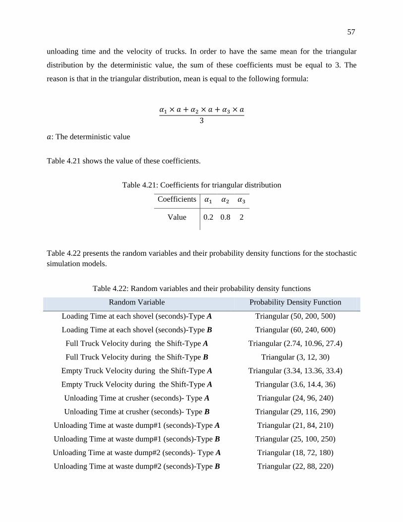
57

unloading time and the velocity of trucks. In order to have the same mean for the triangular

distribution by the deterministic value, the sum of these coefficients must be equal to 3. The

reason is that in the triangular distribution, mean is equal to the following formula:

: The deterministic value

Table 4.21 shows the value of these coefficients.

Table 4.21: Coefficients for triangular distribution

Coefficients

Value 0.2 0.8 2

Table 4.22 presents the random variables and their probability density functions for the stochastic

simulation models.

Table 4.22: Random variables and their probability density functions

Random Variable Probability Density Function

Loading Time at each shovel (seconds)-Type A Triangular (50, 200, 500)

Loading Time at each shovel (seconds)-Type B Triangular (60, 240, 600)

Full Truck Velocity during the Shift-Type A Triangular (2.74, 10.96, 27.4)

Full Truck Velocity during the Shift-Type B Triangular (3, 12, 30)

Empty Truck Velocity during the Shift-Type A Triangular (3.34, 13.36, 33.4)

Empty Truck Velocity during the Shift-Type A Triangular (3.6, 14.4, 36)

Unloading Time at crusher (seconds)- Type A Triangular (24, 96, 240)

Unloading Time at crusher (seconds)- Type B Triangular (29, 116, 290)

Unloading Time at waste dump#1 (seconds)-Type A Triangular (21, 84, 210)

Unloading Time at waste dump#1 (seconds)-Type B Triangular (25, 100, 250)

Unloading Time at waste dump#2 (seconds)- Type A Triangular (18, 72, 180)

Unloading Time at waste dump#2 (seconds)-Type B Triangular (22, 88, 220)

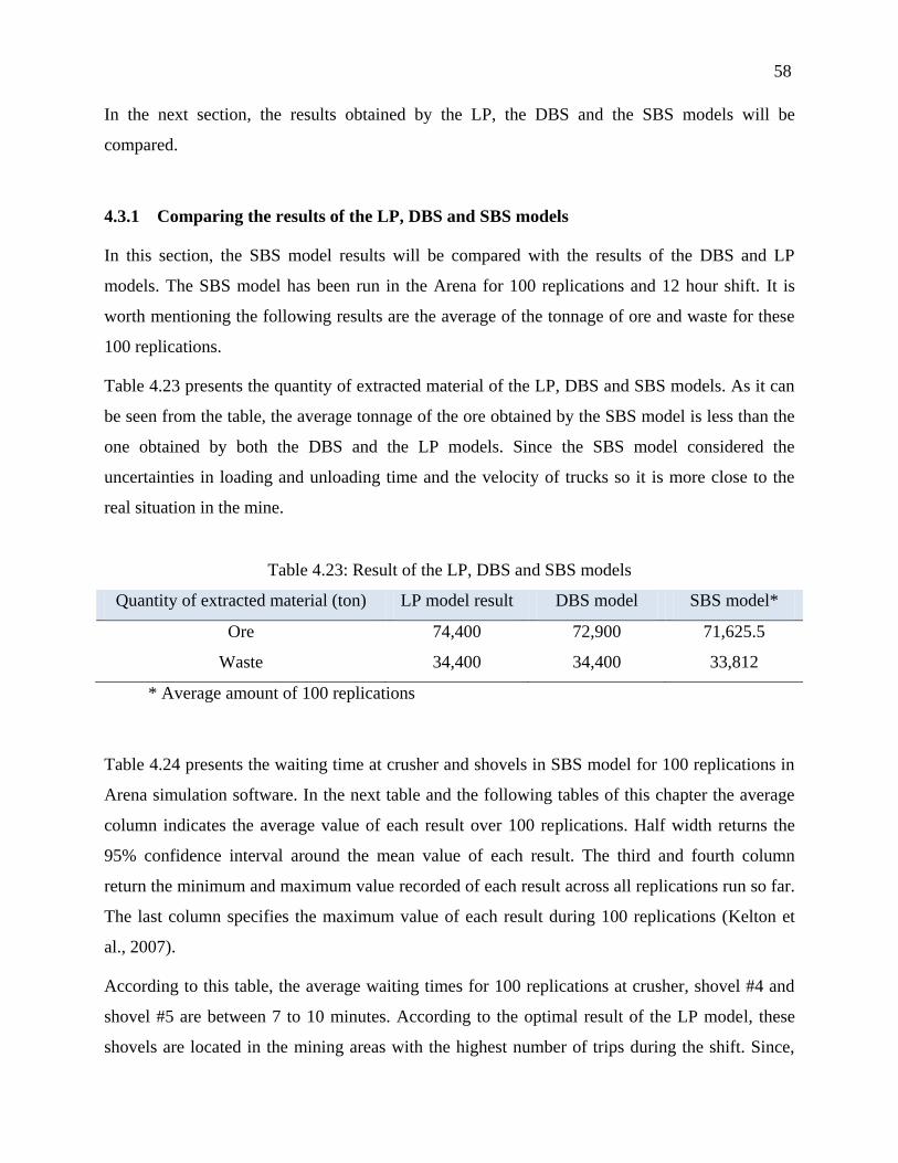
58

In the next section, the results obtained by the LP, the DBS and the SBS models will be

compared.

4.3.1 Comparing the results of the LP, DBS and SBS models

In this section, the SBS model results will be compared with the results of the DBS and LP

models. The SBS model has been run in the Arena for 100 replications and 12 hour shift. It is

worth mentioning the following results are the average of the tonnage of ore and waste for these

100 replications.

Table 4.23 presents the quantity of extracted material of the LP, DBS and SBS models. As it can

be seen from the table, the average tonnage of the ore obtained by the SBS model is less than the

one obtained by both the DBS and the LP models. Since the SBS model considered the

uncertainties in loading and unloading time and the velocity of trucks so it is more close to the

real situation in the mine.

Table 4.23: Result of the LP, DBS and SBS models

Quantity of extracted material (ton) LP model result DBS model SBS model*

Ore 74,400 72,900 71,625.5

Waste 34,400 34,400 33,812

* Average amount of 100 replications

Table 4.24 presents the waiting time at crusher and shovels in SBS model for 100 replications in

Arena simulation software. In the next table and the following tables of this chapter the average

column indicates the average value of each result over 100 replications. Half width returns the

95% confidence interval around the mean value of each result. The third and fourth column

return the minimum and maximum value recorded of each result across all replications run so far.

The last column specifies the maximum value of each result during 100 replications (Kelton et

al., 2007).

According to this table, the average waiting times for 100 replications at crusher, shovel #4 and

shovel #5 are between 7 to 10 minutes. According to the optimal result of the LP model, these

shovels are located in the mining areas with the highest number of trips during the shift. Since,

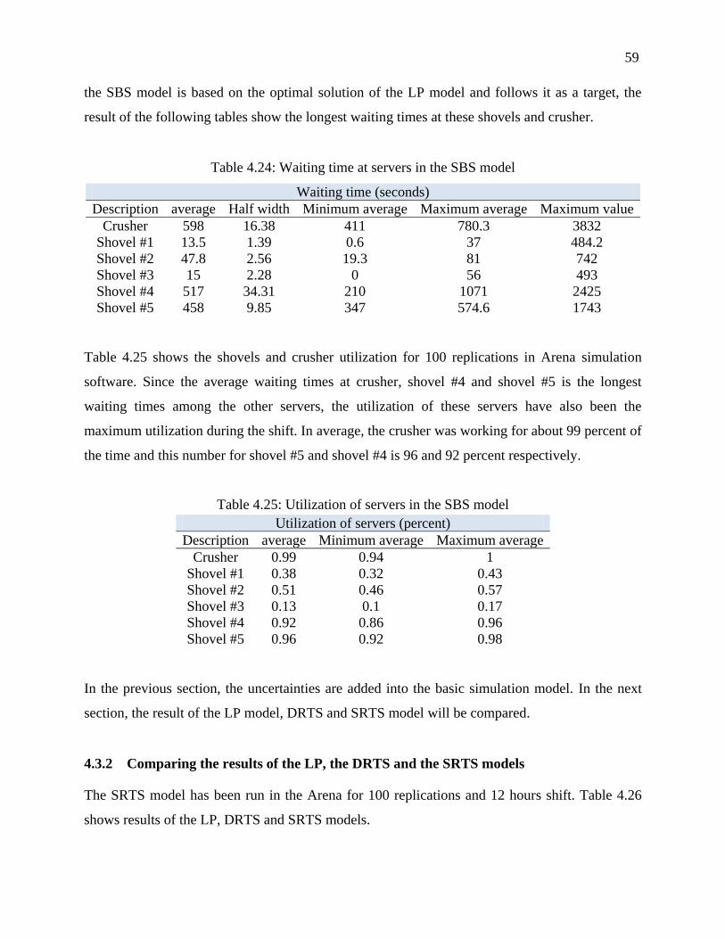
59

the SBS model is based on the optimal solution of the LP model and follows it as a target, the

result of the following tables show the longest waiting times at these shovels and crusher.

Table 4.24: Waiting time at servers in the SBS model

Waiting time (seconds)

Description average Half width Minimum average Maximum average Maximum value

Crusher 598 16.38 411 780.3 3832

Shovel #1 13.5 1.39 0.6 37 484.2

Shovel #2 47.8 2.56 19.3 81 742

Shovel #3 15 2.28 0 56 493

Shovel #4 517 34.31 210 1071 2425

Shovel #5 458 9.85 347 574.6 1743

Table 4.25 shows the shovels and crusher utilization for 100 replications in Arena simulation

software. Since the average waiting times at crusher, shovel #4 and shovel #5 is the longest

waiting times among the other servers, the utilization of these servers have also been the

maximum utilization during the shift. In average, the crusher was working for about 99 percent of

the time and this number for shovel #5 and shovel #4 is 96 and 92 percent respectively.

Table 4.25: Utilization of servers in the SBS model

Utilization of servers (percent)

Description average Minimum average Maximum average

Crusher 0.99 0.94 1

Shovel #1 0.38 0.32 0.43

Shovel #2 0.51 0.46 0.57

Shovel #3 0.13 0.1 0.17

Shovel #4 0.92 0.86 0.96

Shovel #5 0.96 0.92 0.98

In the previous section, the uncertainties are added into the basic simulation model. In the next

section, the result of the LP model, DRTS and SRTS model will be compared.

4.3.2 Comparing the results of the LP, the DRTS and the SRTS models

The SRTS model has been run in the Arena for 100 replications and 12 hours shift. Table 4.26

shows results of the LP, DRTS and SRTS models.

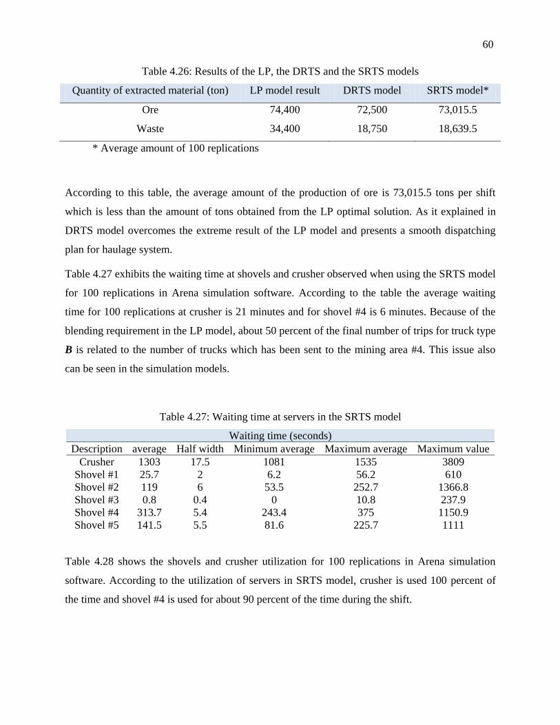
60

Table 4.26: Results of the LP, the DRTS and the SRTS models

Quantity of extracted material (ton) LP model result DRTS model SRTS model*

Ore 74,400 72,500 73,015.5

Waste 34,400 18,750 18,639.5

* Average amount of 100 replications

According to this table, the average amount of the production of ore is 73,015.5 tons per shift

which is less than the amount of tons obtained from the LP optimal solution. As it explained in

DRTS model overcomes the extreme result of the LP model and presents a smooth dispatching

plan for haulage system.

Table 4.27 exhibits the waiting time at shovels and crusher observed when using the SRTS model

for 100 replications in Arena simulation software. According to the table the average waiting

time for 100 replications at crusher is 21 minutes and for shovel #4 is 6 minutes. Because of the

blending requirement in the LP model, about 50 percent of the final number of trips for truck type

B is related to the number of trucks which has been sent to the mining area #4. This issue also

can be seen in the simulation models.

Table 4.27: Waiting time at servers in the SRTS model

Waiting time (seconds)

Description average Half width Minimum average Maximum average Maximum value

Crusher 1303 17.5 1081 1535 3809

Shovel #1 25.7 2 6.2 56.2 610

Shovel #2 119 6 53.5 252.7 1366.8

Shovel #3 0.8 0.4 0 10.8 237.9

Shovel #4 313.7 5.4 243.4 375 1150.9

Shovel #5 141.5 5.5 81.6 225.7 1111

Table 4.28 shows the shovels and crusher utilization for 100 replications in Arena simulation

software. According to the utilization of servers in SRTS model, crusher is used 100 percent of

the time and shovel #4 is used for about 90 percent of the time during the shift.

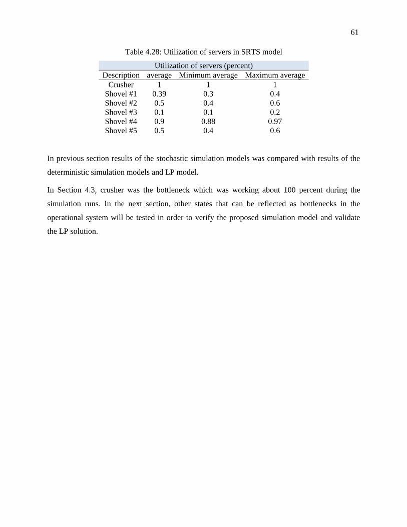
61

Table 4.28: Utilization of servers in SRTS model

Utilization of servers (percent)

Description average Minimum average Maximum average

Crusher 1 1 1

Shovel #1 0.39 0.3 0.4

Shovel #2 0.5 0.4 0.6

Shovel #3 0.1 0.1 0.2

Shovel #4 0.9 0.88 0.97

Shovel #5 0.5 0.4 0.6

In previous section results of the stochastic simulation models was compared with results of the

deterministic simulation models and LP model.

In Section 4.3, crusher was the bottleneck which was working about 100 percent during the

simulation runs. In the next section, other states that can be reflected as bottlenecks in the

operational system will be tested in order to verify the proposed simulation model and validate

the LP solution.

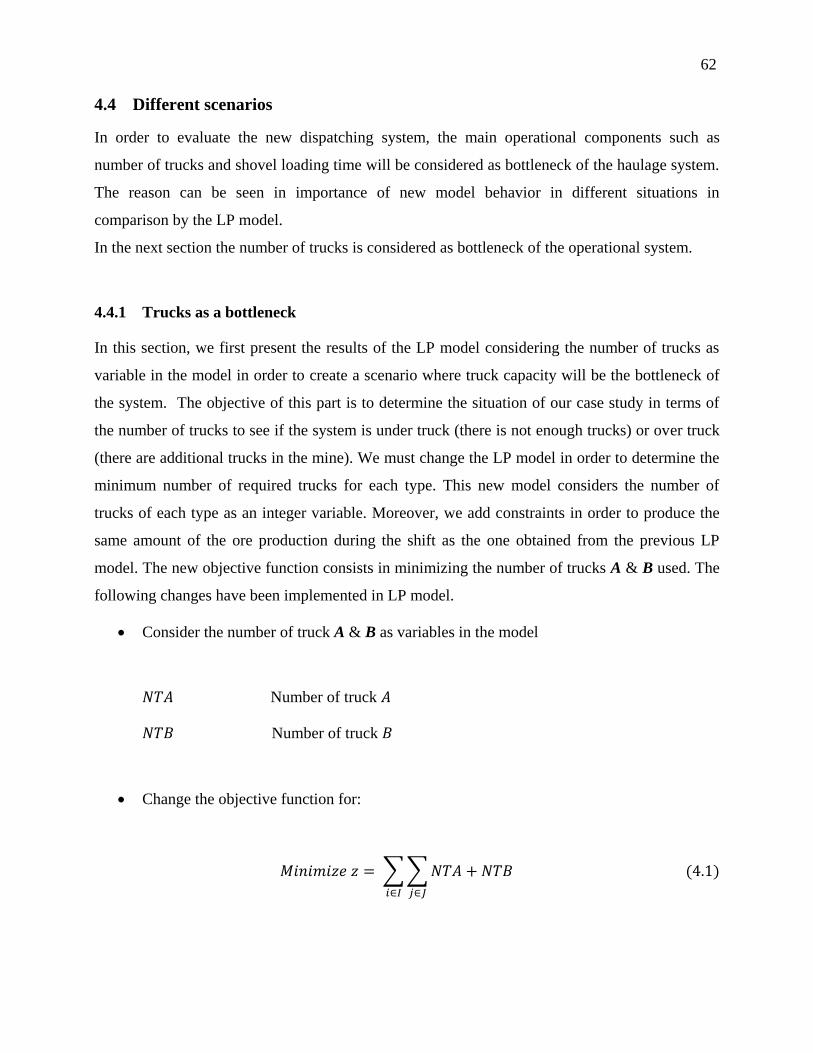
62

4.4 Different scenarios

In order to evaluate the new dispatching system, the main operational components such as

number of trucks and shovel loading time will be considered as bottleneck of the haulage system.

The reason can be seen in importance of new model behavior in different situations in

comparison by the LP model.

In the next section the number of trucks is considered as bottleneck of the operational system.

4.4.1 Trucks as a bottleneck

In this section, we first present the results of the LP model considering the number of trucks as

variable in the model in order to create a scenario where truck capacity will be the bottleneck of

the system. The objective of this part is to determine the situation of our case study in terms of

the number of trucks to see if the system is under truck (there is not enough trucks) or over truck

(there are additional trucks in the mine). We must change the LP model in order to determine the

minimum number of required trucks for each type. This new model considers the number of

trucks of each type as an integer variable. Moreover, we add constraints in order to produce the

same amount of the ore production during the shift as the one obtained from the previous LP

model. The new objective function consists in minimizing the number of trucks A & B used. The

following changes have been implemented in LP model.

Consider the number of truck A & B as variables in the model

Number of truck

Number of truck

Change the objective function for:

∑∑

63

Add the following constraints to the LP model

∑∑∑ .

Constraints 4.2 presents the minimum amount of the ore production according to the result of the

SRTS model because, results from the SRTS model are more reliable and accurate. Constraints

(4.3) and (4.4) guarantee the integrality and non-negativity of the number of trucks in the model.

According to the above changes the following result presents the tonnage of the extracted

material and also the optimal number of essential trucks in order to transport the mentioned

extracted material. Table 4.29 shows the result of the modified LP model.

Table 4.29: Tonnage of extracted ore and waste in modified LP model

Amount of extracted material (ton) LP Optimal result

Ore 73250

Waste 18350

The number of tons of ore remains the same, but the number of tons of waste is reduced to 18350

tons which corresponds to the minimal amount of waste necessary to respect the stripping ratio.

64

Table 4.30 shows the minimum number of required trucks in this case study.

Table 4.30: Number of required trucks

Type of the truck Number of each truck

Truck type A 1

Truck type B 13

Comparing the results of the LP model and SBS model – truck as a bottleneck

In this section the SBS model has run using the 1 truck type A and 13 trucks type B. Table 4.31

presents the result of the SBS model and LP model solution. This table emphasizes the fact that

the LP model is too optimistic and produces large amount of ore in comparison with the SBS

model using the same number of trucks during the simulation. The reason is that the LP model

does not consider waiting time at service points such as shovels and crusher and assumes trucks

are working continuously during the shift. While SBS model takes into account the waiting time

at service points. In this model, when a truck waits to be served by crusher or shovel during the

simulation, system losses time and then produces small amount of ore in comparison with the LP

solution.

Table 4.31: Result of the LP and SBS models-truck as a bottleneck

Quantity of extracted material (ton) LP model result SBS model*

Ore 73250 64227.5

Waste 18350 16355.5

* Average amount of 100 replications

Table 4.32 shows the waiting time at shovels and crusher in SBS model-trucks as bottleneck for

100 replications in Arena simulation software. According to the table, the average waiting time

for 100 replications at crusher and shovel #4 is about 4 minutes. According to the LP optimal

solution, the maximum numbers of trucks are sent to shovel #4 during the shift. Since, the SBS

model is based on the result of the LP model and follows it as a target, then the result of the

following tables show the longest waiting times in this shovel. In the LP model about 49 percent

of the final number of trips for truck type B is related to the number of truck which has sent to the

mining area #4. This issue also can be seen in the SBS model.

65

Table 4.32: Waiting time at servers in SBS model-truck as a bottleneck

Waiting time (seconds)

Description average Half width Minimum average Maximum average Maximum value

Crusher 217.7 4.3 172.5 281 2534

Shovel #1 11.1 1.26 0.37 33.5 569.3

Shovel #2 53.2 3 27.2 93.5 864.6

Shovel #3 0 0 0 0 0

Shovel #4 207.8 7.6 125.5 313.9 1212

Shovel #5 37.7 1.9 19.7 63.7 628

Table 4.33 indicates the utilization of the servers in SBS model when truck is considered as

bottleneck. As it can be seen from the following table the utilization of crusher is reduced from

99 percent to 87 percent during the shift. The reason is reduction in the number of trucks in the

system which will decrease the number of trips between crusher and mining areas.

Table 4.33: Utilization of the servers in SBS model-truck as bottleneck

Utilization of servers (percent)

Description average Minimum average Maximum average

Crusher 0.87 0.83 0.92

Shovel #1 0.34 0.3 0.38

Shovel #2 0.4 0.38 0.49

Shovel #3 0.12 0.09 0.14

Shovel #4 0.86 0.81 0.91

Shovel #5 0.5 0.4 0.5

In the next section, the result of the SRTS model while considering trucks as bottleneck of

system will be presented.

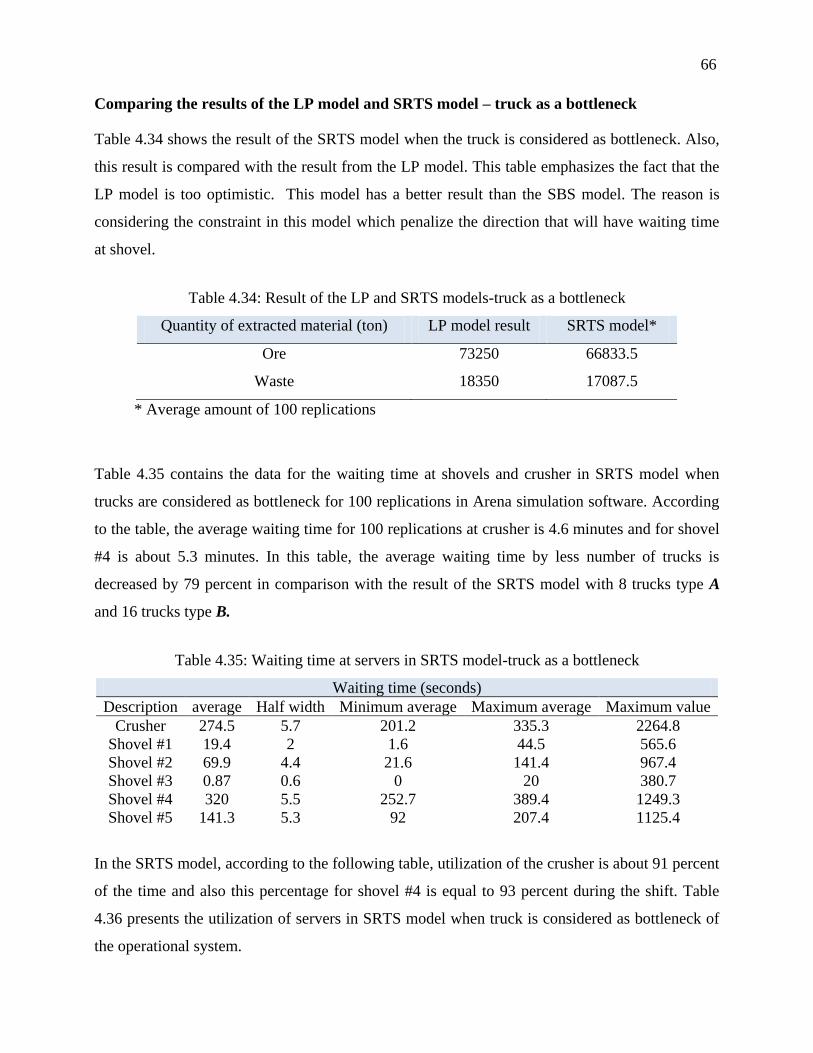
66

Comparing the results of the LP model and SRTS model – truck as a bottleneck

Table 4.34 shows the result of the SRTS model when the truck is considered as bottleneck. Also,

this result is compared with the result from the LP model. This table emphasizes the fact that the

LP model is too optimistic. This model has a better result than the SBS model. The reason is

considering the constraint in this model which penalize the direction that will have waiting time

at shovel.

Table 4.34: Result of the LP and SRTS models-truck as a bottleneck

Quantity of extracted material (ton) LP model result SRTS model*

Ore 73250 66833.5

Waste 18350 17087.5

* Average amount of 100 replications

Table 4.35 contains the data for the waiting time at shovels and crusher in SRTS model when

trucks are considered as bottleneck for 100 replications in Arena simulation software. According

to the table, the average waiting time for 100 replications at crusher is 4.6 minutes and for shovel

#4 is about 5.3 minutes. In this table, the average waiting time by less number of trucks is

decreased by 79 percent in comparison with the result of the SRTS model with 8 trucks type A

and 16 trucks type B.

Table 4.35: Waiting time at servers in SRTS model-truck as a bottleneck

Waiting time (seconds)

Description average Half width Minimum average Maximum average Maximum value

Crusher 274.5 5.7 201.2 335.3 2264.8

Shovel #1 19.4 2 1.6 44.5 565.6

Shovel #2 69.9 4.4 21.6 141.4 967.4

Shovel #3 0.87 0.6 0 20 380.7

Shovel #4 320 5.5 252.7 389.4 1249.3

Shovel #5 141.3 5.3 92 207.4 1125.4

In the SRTS model, according to the following table, utilization of the crusher is about 91 percent

of the time and also this percentage for shovel #4 is equal to 93 percent during the shift. Table

4.36 presents the utilization of servers in SRTS model when truck is considered as bottleneck of

the operational system.

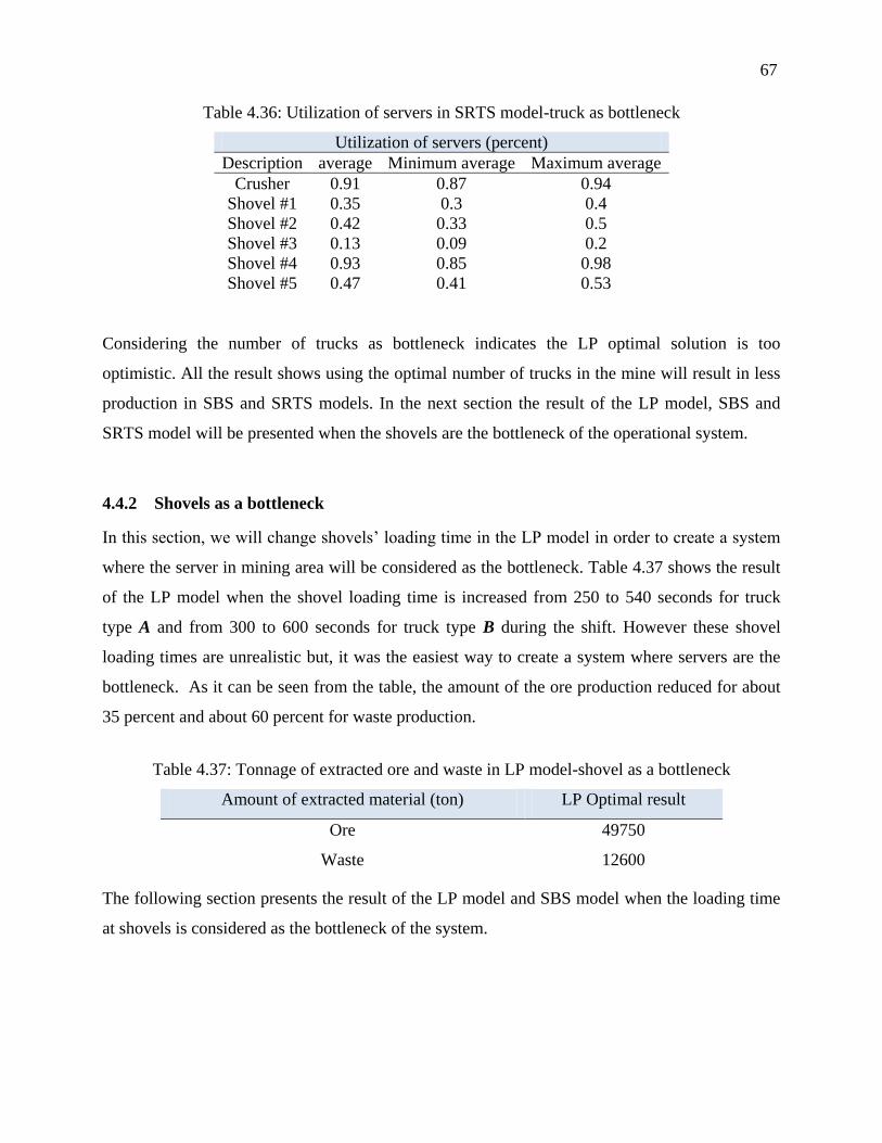
67

Table 4.36: Utilization of servers in SRTS model-truck as bottleneck

Utilization of servers (percent)

Description average Minimum average Maximum average

Crusher 0.91 0.87 0.94

Shovel #1 0.35 0.3 0.4

Shovel #2 0.42 0.33 0.5

Shovel #3 0.13 0.09 0.2

Shovel #4 0.93 0.85 0.98

Shovel #5 0.47 0.41 0.53

Considering the number of trucks as bottleneck indicates the LP optimal solution is too

optimistic. All the result shows using the optimal number of trucks in the mine will result in less

production in SBS and SRTS models. In the next section the result of the LP model, SBS and

SRTS model will be presented when the shovels are the bottleneck of the operational system.

4.4.2 Shovels as a bottleneck

In this section, we will change shovels’ loading time in the LP model in order to create a system

where the server in mining area will be considered as the bottleneck. Table 4.37 shows the result

of the LP model when the shovel loading time is increased from 250 to 540 seconds for truck

type A and from 300 to 600 seconds for truck type B during the shift. However these shovel

loading times are unrealistic but, it was the easiest way to create a system where servers are the

bottleneck. As it can be seen from the table, the amount of the ore production reduced for about

35 percent and about 60 percent for waste production.

Table 4.37: Tonnage of extracted ore and waste in LP model-shovel as a bottleneck

Amount of extracted material (ton) LP Optimal result

Ore 49750

Waste 12600

The following section presents the result of the LP model and SBS model when the loading time

at shovels is considered as the bottleneck of the system.

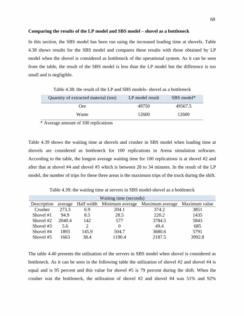
68

Comparing the results of the LP model and SBS model – shovel as a bottleneck

In this section, the SBS model has been run using the increased loading time at shovels. Table

4.38 shows results for the SBS model and compares these results with those obtained by LP

model when the shovel is considered as bottleneck of the operational system. As it can be seen

from the table, the result of the SBS model is less than the LP model but the difference is too

small and is negligible.

Table 4.38: the result of the LP and SBS models- shovel as a bottleneck

Quantity of extracted material (ton) LP model result SBS model*

Ore 49750 49567.5

Waste 12600 12600

* Average amount of 100 replications

Table 4.39 shows the waiting time at shovels and crusher in SBS model when loading time at

shovels are considered as bottleneck for 100 replications in Arena simulation software.

According to the table, the longest average waiting time for 100 replications is at shovel #2 and

after that at shovel #4 and shovel #5 which is between 28 to 34 minutes. In the result of the LP

model, the number of trips for these three areas is the maximum trips of the truck during the shift.

Table 4.39: the waiting time at servers in SBS model-shovel as a bottleneck

Waiting time (seconds)

Description average Half width Minimum average Maximum average Maximum value

Crusher 273.3 6.9 204.1 374.2 3851

Shovel #1 94.9 8.5 28.5 220.2 1435

Shovel #2 2040.4 142 577 3784.5 5843

Shovel #3 5.6 2 0 49.4 685

Shovel #4 1893 145.9 504.7 3680.6 5791

Shovel #5 1663 38.4 1190.4 2187.5 3992.8

The table 4.40 presents the utilization of the servers in SBS model when shovel is considered as

bottleneck. As it can be seen in the following table the utilization of shovel #2 and shovel #4 is

equal and is 95 percent and this value for shovel #5 is 79 percent during the shift. When the

crusher was the bottleneck, the utilization of shovel #2 and shovel #4 was 51% and 92%

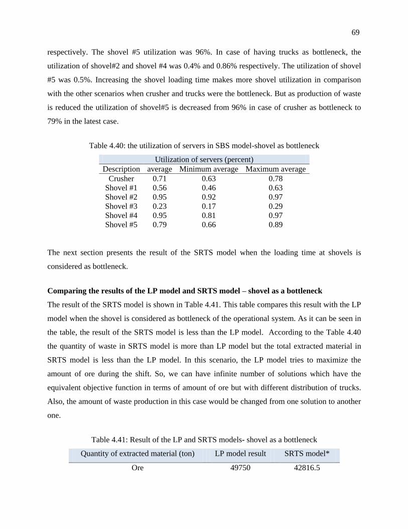
69

respectively. The shovel #5 utilization was 96%. In case of having trucks as bottleneck, the

utilization of shovel#2 and shovel #4 was 0.4% and 0.86% respectively. The utilization of shovel

#5 was 0.5%. Increasing the shovel loading time makes more shovel utilization in comparison

with the other scenarios when crusher and trucks were the bottleneck. But as production of waste

is reduced the utilization of shovel#5 is decreased from 96% in case of crusher as bottleneck to

79% in the latest case.

Table 4.40: the utilization of servers in SBS model-shovel as bottleneck

Utilization of servers (percent)

Description average Minimum average Maximum average

Crusher 0.71 0.63 0.78

Shovel #1 0.56 0.46 0.63

Shovel #2 0.95 0.92 0.97

Shovel #3 0.23 0.17 0.29

Shovel #4 0.95 0.81 0.97

Shovel #5 0.79 0.66 0.89

The next section presents the result of the SRTS model when the loading time at shovels is

considered as bottleneck.

Comparing the results of the LP model and SRTS model – shovel as a bottleneck

The result of the SRTS model is shown in Table 4.41. This table compares this result with the LP

model when the shovel is considered as bottleneck of the operational system. As it can be seen in

the table, the result of the SRTS model is less than the LP model. According to the Table 4.40

the quantity of waste in SRTS model is more than LP model but the total extracted material in

SRTS model is less than the LP model. In this scenario, the LP model tries to maximize the

amount of ore during the shift. So, we can have infinite number of solutions which have the

equivalent objective function in terms of amount of ore but with different distribution of trucks.

Also, the amount of waste production in this case would be changed from one solution to another

one.

Table 4.41: Result of the LP and SRTS models- shovel as a bottleneck

Quantity of extracted material (ton) LP model result SRTS model*

Ore 49750 42816.5

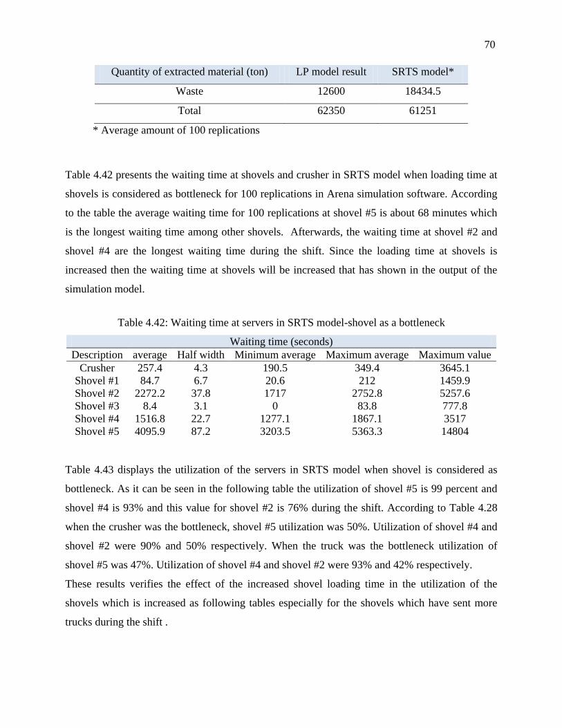
70

Quantity of extracted material (ton) LP model result SRTS model*

Waste 12600 18434.5

Total 62350 61251

* Average amount of 100 replications

Table 4.42 presents the waiting time at shovels and crusher in SRTS model when loading time at

shovels is considered as bottleneck for 100 replications in Arena simulation software. According

to the table the average waiting time for 100 replications at shovel #5 is about 68 minutes which

is the longest waiting time among other shovels. Afterwards, the waiting time at shovel #2 and

shovel #4 are the longest waiting time during the shift. Since the loading time at shovels is

increased then the waiting time at shovels will be increased that has shown in the output of the

simulation model.

Table 4.42: Waiting time at servers in SRTS model-shovel as a bottleneck

Waiting time (seconds)

Description average Half width Minimum average Maximum average Maximum value

Crusher 257.4 4.3 190.5 349.4 3645.1

Shovel #1 84.7 6.7 20.6 212 1459.9

Shovel #2 2272.2 37.8 1717 2752.8 5257.6

Shovel #3 8.4 3.1 0 83.8 777.8

Shovel #4 1516.8 22.7 1277.1 1867.1 3517

Shovel #5 4095.9 87.2 3203.5 5363.3 14804

Table 4.43 displays the utilization of the servers in SRTS model when shovel is considered as

bottleneck. As it can be seen in the following table the utilization of shovel #5 is 99 percent and

shovel #4 is 93% and this value for shovel #2 is 76% during the shift. According to Table 4.28

when the crusher was the bottleneck, shovel #5 utilization was 50%. Utilization of shovel #4 and

shovel #2 were 90% and 50% respectively. When the truck was the bottleneck utilization of

shovel #5 was 47%. Utilization of shovel #4 and shovel #2 were 93% and 42% respectively.

These results verifies the effect of the increased shovel loading time in the utilization of the

shovels which is increased as following tables especially for the shovels which have sent more

trucks during the shift .

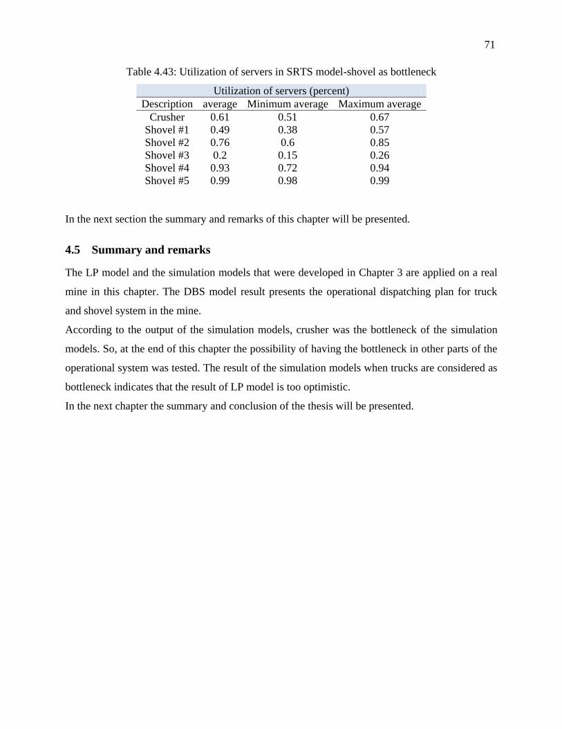
71

Table 4.43: Utilization of servers in SRTS model-shovel as bottleneck

Utilization of servers (percent)

Description average Minimum average Maximum average

Crusher 0.61 0.51 0.67

Shovel #1 0.49 0.38 0.57

Shovel #2 0.76 0.6 0.85

Shovel #3 0.2 0.15 0.26

Shovel #4 0.93 0.72 0.94

Shovel #5 0.99 0.98 0.99

In the next section the summary and remarks of this chapter will be presented.

4.5 Summary and remarks

The LP model and the simulation models that were developed in Chapter 3 are applied on a real

mine in this chapter. The DBS model result presents the operational dispatching plan for truck

and shovel system in the mine.

According to the output of the simulation models, crusher was the bottleneck of the simulation

models. So, at the end of this chapter the possibility of having the bottleneck in other parts of the

operational system was tested. The result of the simulation models when trucks are considered as

bottleneck indicates that the result of LP model is too optimistic.

In the next chapter the summary and conclusion of the thesis will be presented.

72

CHAPTER 5: CONCLUSION AND

RECOMMENDATIONS

This chapter contains conclusion of the thesis, as well as recommendations for future work in

studying truck and shovel hauling systems in an open pit mine for a very short-term-term period.

5.1 Conclusions

The LP model was developed by Gamache et al. (2009) with the suitable level of detail, and

many different aspects of truck and shovel operations has run using Solver. This model does not

take into account the waiting time at servers.

After running the basic simulation model which considers the waiting time at shovels and

crusher, and also the real time simulation model crusher discovered as a bottleneck of the

operational system.

Considering truck as a bottleneck of the system presents that the LP model is too optimistic and

not taking into account the waiting time will cause reduction in the ore production in the SBS

model. The result of the SRTS model confirms the above fact and also produces more ore in

comparison with the SBS model. The reason is using the constraint in this simulation model

which penalizes the direction that will have the waiting time.

The shovel loading time is the other bottleneck of the system. In this situation also the LP model

and simulation models have run for 12 hours shift. In this scenario, the SBS model has the same

amount of waste production as LP model but less ore production that is negligible. In the SRTS

model we have much less ore production but the more amount of waste production. The reason

can be seen in the fact that the LP model tries to maximize the ore production. The LP model has

different solutions with the same amount of ore but different solutions in terms of trucks

distribution and waste production.

In the next section recommendation for future research will be presented.

73

5.2 Recommendations for future research

The following recommendations could improve the truck and shovel hauling system and

researches in this area.

Apply Opt Quest tool in Arena in order to maximize ore production according to the LP

model constraints

Scheduled and unexpected failures of trucks, shovels, and crushers and repairing

processes could be added to the model to create a more precise valuation of the system.

A time study with probability analysis to determine the cycle time more accurately.

A sensitivity study of input parameter to understand how the system reacts to the different

scenarios.

74

REFRENCES

1. Ataeepour, N., & Baafi, E. Y. (1999). Arena simulation model for truck-shovel operation in

despatching and non-despatching modes. International Journal of Surface Mining,

Reclamation and Environment, 13(3), 125-129.

2. Awuah-Offei, K., Temeng, V. A., & Al-Hassan, S. (2003). Predicting equipment

requirements using SIMAN simulation - a case study. Mining Technology, 112(3), 180-184.

3. Bonates, E., & Lizotte, Y. (1988). A computer simulation model to evaluate the effect of

dispatching. International Journal of Surface Mining, Reclamation and Environment, 2(2),

99-104.

4. Burt, C., Caccetta, L., Hill, S., & Welgama, P. (2005). Models for mining equipment

selection. Paper presented at the MODSIM 2005 International congress on modelling and

simulation, Canberra, Australia.

5. Castillo, D., & Cochran, J. K. (1987). A microcomputer approach for simulating truck

haulage systems in open pit mining. Computers in Industry, 8(1), 37-47.

6. Chanda, E. K., & Gardiner, S. (2010). A comparative study of truck cycle time prediction

methods in open-pit mining. Engineering, Construction and Architectural Management,

17(5), 446-460.

75

7. Ercelebi, S. G., & Bascetin, A. (2009). Optimization of shovel-truck system for surface

mining. SIAMM - Journal of The South African Institute of Mining and Metallurgy, 109(7),

433-439.

8. Fioroni, M. M., Franzese, L. A. G., Bianchi, T. J., Ezawa, L., Pinto, L. R., & Gilberto de

Miranda, J. (2008). Concurrent simulation and optimization models for mining planning.

Paper presented at the Proceedings of the 40th Conference on Winter Simulation, Miami,

Florida.

9. Forsman, B., Rönnkvist, E., & Vagenas, N. (1993). Truck dispatch computer simulation in

Aitik open pit mine. International Journal of Surface Mining, Reclamation and Environment,

7(3), 117-120.

10. Gamache, M., Hebert-Desgroseilliers, L., & Desaulniers, G. (2009). A generic linear

program for an optimal mine production plan. Paper presented at the MPES, Mining Planning

and Equipment Selection Conference.

11. Gershon, M., Davala, R., & Mudragega, M. (1993). LP decomposition applied to blending

minerals. Paper presented at the 24th APCOM proceedings.

12. Gurgur, C. Z., Dagdelen, K., & Artittong, S. (2011). Optimisation of a real-time multi-period

truck dispatching system in mining operations. International Journal of Applied Decision

Sciences, 4(1), 57-79.

76

13. Hustrulid, W. A., & Kuchta, M. (1995). Open Pit Mine Planning And Design (Vol. 1).

Rotterdam, Netherlands: Taylor & Francis.

14. Karami, A., Szymanski, J., & Planeta, S. (1996). A simulation analysis model of the ore

truck haulage system in open pit mining. Prace Naukowe Instytutu Gornictwa Politechniki

Wroclawskiej, 79, 164-171.

15. Kelton, W. D., Sadowski, R. P., & Sturrock, D. T. (2007). Simulation with Arena. New

York: McGraw-Hill.

16. Osanloo, M., Gholamnejad, J., & Karimi, B. (2008). Long-term open pit mine production

planning: a review of models and algorithms. International Journal of Mining, Reclamation

and Environment, 22(1), 3-35.

17. Peng, S., Zhang, D., & Xi, Y. (1988). Computer simulation of a semi-continuous open-pit

mine haulage system. International Journal of Mining and Geological Engineering, 6(3), 267-

271.

18. Rubito, E. (2007). Mill feed optimization for multiple processing facilities using integer

linear programming. Paper presented at the Proceedings of the fifteen international

symposium on mine planning and equipement selection, Turin, Italie.

77

19. oumis, ., thier, ., McInnis, D., Université de Montréal. . Une méthode

d optimisation pour le contrôle en temps-réel des camions dans une mine ciel ouvert.

Montréal Université de Montréal, Centre de recherche sur les transports.

20. Soumis, F., Ethier, J., McInnis, D., Elbrond, J., (1986), "A new method of automatic truck

dispatching in open pit mines", Proceedings of the computer applications in mineral industry,

Quebec, p.393-401.

21. Sturgul, J. R., & Eharrison, J. (1987). Simulation models for surface mines. International

Journal of Surface Mining, Reclamation and Environment, 1(3), 187-189.

22. Temeng, V. A. (1997). A computerized model for truck dispatching in open pit mines.

(Master degree), Michigan Technological University, Houghton.

23. Temeng, V. A., Otuonye, F. O., & Frendewey, J. O. (1997). Real-time truck dispatching

using a transportation algorithm. International Journal of Surface Mining, Reclamation and

Environment, 11(4), 203-207.

24. Topal, E., & Ramazan, S. (2010). A new MIP model for mine equipment scheduling by

minimizing maintenance cost. European Journal of Operational Research, 207(2), 1065-1071.

25. Torkamani, E., & Askari-Nasab, H. (2012). Verifying Short-Term Production Schedules

using Truck-Shovel Simulation (pp. 190-205): Mining Optimization Laboratory (MOL).

78

26. Wilke, F. L., & Reiner, T. (1977). Optimizing the short-term production schedule for an

open-pit iron ore mining operation. Computer methods for the 0’s in the mineral industry,

642-646.

27. Yuriy, G., & Vayenas, N. (2008). Discrete-event simulation of mine equipment systems

combined with a reliability assessment model based on genetic algorithms. International

Journal of Mining, Reclamation and Environment, 22(1), 70-83.

28. Zhang, Y., Li, S., & Cai, Q. (1990). Optimization criteria for computer-controlled truck

dispatching system. Computer and operations research in the mineral industries, 295-306.