Atmos. Chem. Phys., 16, 8963–8981, 2016www.atmos-chem-phys.net/16/8963/2016/doi:10.5194/acp-16-8963-2016© Author(s) 2016. CC Attribution 3.0 License.

HCOOH distributions from IASI for 2008–2014: comparison withground-based FTIR measurements and a globalchemistry-transport modelMatthieu Pommier1,a, Cathy Clerbaux1,2, Pierre-François Coheur2, Emmanuel Mahieu3, Jean-François Müller4,Clare Paton-Walsh5, Trissevgeni Stavrakou4, and Corinne Vigouroux4

1LATMOS/IPSL, UVSQ Université Paris-Saclay, UPMC, CNRS, Guyancourt, France2Spectroscopie de l’Atmosphère, Chimie Quantique et Photophysique, Université Libre de Bruxelles (ULB),Brussels, Belgium3Institute of Astrophysics and Geophysics of the University of Liège, Liège, Belgium4Royal Belgian Institute for Space Aeronomy (BIRA-IASB), Avenue Circulaire 3, 1180 Brussels, Belgium5School of Chemistry, University of Wollongong, Wollongong, Australiaanow at: Norwegian Meteorological Institute, Oslo, Norway

Correspondence to: Matthieu Pommier (matthieup@met.no)

Received: 27 January 2016 – Published in Atmos. Chem. Phys. Discuss.: 1 March 2016Revised: 6 June 2016 – Accepted: 24 June 2016 – Published: 21 July 2016

Abstract. Formic acid (HCOOH) is one of the most abun-dant volatile organic compounds in the atmosphere. It isa major contributor to rain acidity in remote areas. Thereare, however, large uncertainties on the sources and sinks ofHCOOH and therefore HCOOH is misrepresented by globalchemistry-transport models. This work presents global dis-tributions from 2008 to 2014 as derived from the measure-ments of the Infrared Atmospheric Sounding Interferom-eter (IASI), based on conversion factors between bright-ness temperature differences and representative retrieved to-tal columns over seven regions: Northern Africa, southernAfrica, Amazonia, Atlantic, Australia, Pacific, and Russia.The dependence of the measured HCOOH signal on the ther-mal contrast is taken into account in the conversion method.This conversion presents errors lower than 20 % for totalcolumns ranging between 0.5 and 1× 1016 molec cm−2 butreaches higher values, up to 78 %, for columns that are lowerthan 0.3× 1016 molec cm−2. Signatures from biomass burn-ing events are highlighted, such as in the Southern Hemi-sphere and in Russia, as well as biogenic emission sources,e.g., over the eastern USA. A comparison between 2008and 2014 with ground-based Fourier transform infrared spec-troscopy (FTIR) measurements obtained at four locations(Maido and Saint-Denis at La Réunion, Jungfraujoch, and

Wollongong) is shown. Although IASI columns are foundto correlate well with FTIR data, a large bias (> 100 %) isfound over the two sites at La Réunion. A better agreementis found at Wollongong with a negligible bias. The compar-ison also highlights the difficulty of retrieving total columnsfrom IASI measurements over mountainous regions such asJungfraujoch. A comparison of the retrieved columns withthe global chemistry-transport model IMAGESv2 is also pre-sented, showing good representation of the seasonal and in-terannual cycles over America, Australia, Asia, and Siberia.A global model underestimation of the distribution and amisrepresentation of the seasonal cycle over India are alsofound. A small positive trend in the IASI columns is ob-served over Australia, Amazonia, and India over the 2008–2014 period (from 0.7 to 1.5 % year−1), while a decrease of∼ 0.8 % year−1 is measured over Siberia.

1 Introduction

Formic acid (HCOOH) is among the most abundant volatileorganic compounds (VOCs) present in the atmosphere.Along with acetic acid it is a major contributor to the acid-ity of precipitation, especially in remote regions (Keene and

Published by Copernicus Publications on behalf of the European Geosciences Union.

8964 M. Pommier et al.: HCOOH distributions from IASI for 2008–2014

Galloway, 1988; Andreae et al., 1988). HCOOH has small di-rect emissions from vegetation (Keene and Galloway, 1984,1988), ants (Graedel and Eisner, 1988), biomass burning(e.g., Goode et al., 2000), soils (Sanhueza and Andreae,1991), agriculture (e.g., Ngwabie et al., 2008), and motorvehicles (Kawamura et al., 1985; Grosjean, 1989) but ismainly a secondary product from other organic precursors.The largest global chemical sources of HCOOH include iso-prene, monoterpenes, other terminal alkenes (e.g., Neeb etal., 1997; Lee et al., 2006; Paulot et al., 2011), alkynes(Hatakeyama et al., 1986; Bohn et al., 1996), and acetalde-hyde (Andrews et al., 2012; Clubb et al., 2012). HCOOH ismainly removed from the troposphere through wet and drydeposition and to a lesser extent through oxidation by theOH radical.

HCOOH is a short-lived species and its lifetime is mainlydetermined by the precipitation rate. The lifetime ranges be-tween 2 days during the rainy season and 6 days in the dryseason in the boundary layer (Sanhueza et al., 1996). Theglobal lifetime in the troposphere is 3–4 days (Paulot et al.,2011; Stavrakou et al., 2012). Photochemical loss is rela-tively slow (τ ∼ 25 days), so that any HCOOH formed orvented outside of the boundary layer can be transported overlong distances in the free troposphere (Paulot et al., 2011).

Our knowledge about sources and sinks of HCOOH is stillincomplete despite the numerous studies that have been pub-lished during the last decade. In current emissions inven-tories, such as the biogenic emission inventory MEGAN-MACC (Sindelarova et al., 2014), the main source regionsare located in tropical regions as presented in Fig. 1 for theperiod between 2008 and 2010. A recent work shows a pos-sible source of HCOOH over the Arctic Ocean (Jones etal., 2014). The study by Stavrakou et al. (2012) highlightsa misrepresentation of emissions from tropical and borealforests in models compared to total columns retrieved fromInfrared Atmospheric Sounding Interferometer (IASI) obser-vations by Razavi et al. (2011). Millet et al. (2015), Paulot etal. (2011), and Stavrakou et al. (2012) point to the existenceof one or more large missing sources. These studies suggestan important gap in our current understanding of hydrocar-bon oxidation and/or the existence of unknown direct fluxesof HCOOH.

Nadir-looking atmospheric sensors allow us to deriveglobal distributions for trace gases, with a limited verticalsensitivity as compared to airborne or ground-based mea-surements. Their extended spatial coverage allows the ob-serving of remote regions which are sparsely studied byfield campaigns. Only a few satellites provide troposphericHCOOH observations, such as the nadir-viewing instrumentIASI (e.g., Razavi et al., 2011) and the Tropospheric Emis-sion Spectrometer (TES) (e.g., Cady-Pereira et al., 2014).The Michelson Interferometer for Passive AtmosphericSounding (MIPAS) limb instrument provided monthly globaldistributions of HCOOH around 10 km (Grutter et al., 2010),and the solar-occultation Atmospheric Chemistry Experi-

Figure 1. MEGAN-MACC HCOOH emissions for the period be-tween 2008 and 2010 on a 0.5◦× 0.5◦ grid. The green stars corre-spond to the location of the FTIR measurements, the seven selectedregions used for the retrievals and described in Table 1 are high-lighted in blue, and the black boxes are the regions used for thecomparison with IMAGESv2.

ment (ACE) provides seasonal global distribution in the up-per troposphere (e.g., González Abad et al., 2009).

The data used in this study are provided by IASI. This in-strument has two important advantages: a low radiometricnoise and a high spatial coverage. HCOOH is a weak ab-sorber, so it is a challenge to retrieve total columns fromthe IASI radiance. Global distributions of HCOOH overland were initially derived using a method based on bright-ness temperature difference and using forward simulations(Razavi et al., 2011). More recently, R’Honi et al. (2013)developed a specific method to study extreme events oc-curring during the large fires in Russia during the summer2010. These studies, however, highlighted discrepancies be-tween the retrieved distributions and especially within en-riched HCOOH air masses as, for instance, over large forestfires. Indeed, the total columns from R’Honi et al. (2013)were on average a factor of 2 lower than in Razavi etal. (2011) (around a factor of 1.5 for columns higher than5× 1016 molec cm−2 and 2.3 for columns lower than 5×1016 molec cm−2). In this paper, we present an update ofthe method used in Razavi et al. (2011), in order to deriveHCOOH distributions over both land and sea, suitable forboth enhanced and background concentrations over the pe-riod 2008–2014. Section 2 introduces the IASI mission andexplains the methodology used, based on an optimal esti-mation method (OEM) retrieval over selected areas, used todesign a fast retrieval methodology based on the brightnesstemperature difference and conversion factors. In Sect. 3,global distributions are shown; the products are compared

Atmos. Chem. Phys., 16, 8963–8981, 2016 www.atmos-chem-phys.net/16/8963/2016/

M. Pommier et al.: HCOOH distributions from IASI for 2008–2014 8965

Table 1. Selected regions used for the retrieval. The localization ofeach area and the number of spectra retrieved during the studiedperiod are provided. The numbers correspond to the total numberof successfully retrieved spectra and those given in parentheses tothe total number of spectra in each region.

Region Localization Number ofretrieved spectra

Northern Africa 6–7◦ N, 18–22◦ E 265 (358)Southern Africa 12–14◦ S, 20–24◦ E 788 (1083)Amazonia 6–10◦ S, 43–45◦ W 682 (739)Atlantic 22–24◦ N, 42–45◦ W 675 (737)Australia 14–15◦ S, 131–133◦ E 218 (271)Pacific 20–22◦ S, 140–142◦ E 472 (492)Russia 50–54◦ N, 60–62◦ E 538 (781)

to ground-based measurements and to the global chemistry-transport model (CTM) IMAGESv2, providing an analysis ofthe seasonal and interannual variability of HCOOH columns.The conclusions are given in Sect. 4.

2 IASI HCOOH columns

2.1 The IASI mission

IASI is a nadir-viewing Fourier transform spectrometer in-strument. Currently two instruments are in orbit. The firstmodel was launched on board the MetOp-A platform in Oc-tober 2006 providing now more than 8 years of observations.The second instrument was launched in September 2012.Owing to its wide swath, each instrument delivers near globalcoverage twice per day at around 09:30 and 21:30 local time.IASI measures in the thermal infrared part of the spectrum,between 645 and 2760 cm−1. It records radiance from theEarth’s surface and the atmosphere with an apodized spec-tral resolution of 0.5 cm−1, spectrally sampled at 0.25 cm−1.IASI has a good radiometric performance, around 0.15 K (oraround 2× 10−6 W cm−2 sr−1/ cm−1) in the HCOOH spec-tral range (∼ 1105 cm−1) for a reference blackbody at 280 K(Clerbaux et al., 2009).

Analysis of the mean of the normalized Jacobians (Fig. 2)over the spectral range used by IASI for the HCOOH re-trievals (1095–1114 cm−1), for a set of representative geo-graphical regions (see Fig. 1 and next section), shows thatIASI is sensitive to tropospheric HCOOH between 1 and6 km. These Jacobians represent the sensitivity of IASI andthe radiative transfer model to the abundance of HCOOH ina fixed atmosphere. This corresponds to the mean of the Ja-cobians simulated from the selected spectra over the studiedregions.

Figure 2. Mean normalized Jacobians of all retrieved spectra (overthe seven selected regions) as a function of altitude.

2.2 Retrieval approach

Processing 7 years (2008–2014) of IASI data using an iter-ative method such as the OEM (Rodgers, 2000) is computa-tionally demanding. Hence we have chosen a fast approachbased on brightness temperature differences (1Tb) betweenspectral channels with and without the signature of the tar-get gas to extract information without performing a full re-trieval. In a second step, the 1Tb were converted into totalcolumns of HCOOH using conversion factors derived froma set of data retrieved by OEM. This approach was adaptedfrom the previous works for other IASI weak absorbers, suchas methanol (Razavi et al., 2011), sulfur dioxide (Clarisse etal., 2008), and ammonia (Van Damme et al., 2014).

In the current work, the main difference with the previ-ous IASI HCOOH determination in Razavi et al. (2011) isthe use of retrieved total columns over selected regions todetermine conversion factors instead of the use of forwardsimulations. The OEM implemented in the line-by-line ra-diative transfer model Atmosphit (Coheur et al., 2005) hasbeen used as in Razavi et al. (2011). In Razavi et al. (2011),the reason invoked for performing only forward simulationsfor HCOOH was the unstable character of the retrievals.With the retrieval settings chosen here, we relied on the re-trieved columns since 82 % of the selected spectra were suc-cessfully retrieved (Table 1) and the mean root mean square(RMS) between the observed and fitted spectra is about2.5× 10−6 W cm−2 sr−1/ cm−1. This RMS value was closeto the IASI-estimated radiometric noise.

The conversion factors allowing the calculation of totalcolumns based on 1Tb values were determined by usingthe parameters from a linear regression, obtained by corre-lating 1Tb with HCOOH total columns based on the OEMretrieval. The spectroscopic parameters were from the HI-

www.atmos-chem-phys.net/16/8963/2016/ Atmos. Chem. Phys., 16, 8963–8981, 2016

8966 M. Pommier et al.: HCOOH distributions from IASI for 2008–2014

Table 2. Retrieval parameters used in this work.

Parameters Layers A priori Variability

H2O 0–10 km: five 2 km thick layers EUMETSAT operational 20 %10–20 km: two 5 km thick layers level 2

O3 total column standard atmosphere 20 %NH3 ditto standard atmosphere 20 %HCOOH ditto Razavi et al. (2011) 350 %CFC-12 ditto Coheur et al. (2003) 20 %

TRAN 2008 database (Rothman et al., 2009), using the setof HCOOH spectroscopic line parameters of Vander Auweraet al. (2007). The retrievals have been done with the samea priori profile as in Razavi et al. (2011) but with a looseconstraint (350 %). The reference channels used for the cal-culation of 1Tb were chosen on both sides of the HCOOHchannel (1105 cm−1), i.e., at 1103.0 and 1109.0 cm−1.

In the OEM-based retrieval, only cloud-free scenes (whenthe cloud coverage for the pixel is below 2 %) have beenused. The total columns of interfering species in the studiedspectral range, such as ozone, ammonia, and CFC-12, in ad-dition to the partial columns of water vapor, were retrievedsimultaneously. The details of the retrieval parameters aregiven in Table 2. The EUMETSAT L2 operational data wereused, and daytime and nighttime data with a positive thermalcontrast (TC) were taken into account. The TC was definedas the temperature difference between the surface and the airjust above. Negative TC data were excluded as these werefound to deteriorate the correlation 1Tb-total column.

The OEM-based retrieval has been performed over sevengeographical regions shown as blue boxes in Fig. 1. These in-clude five source areas (in southern Africa, Northern Africa,Amazonia, Australia, Russia) and two remote areas (over theAtlantic and Pacific oceans). These seven regions are repre-sentative of different conditions: emission sources, remoteareas, areas influenced by long-range transport, over land,and over sea. We have retrieved the 5 first days of each monthin 2009 over the seven regions, allowing the characterizationof the seasonal variation. The localization of each area andthe number of retrieved spectra are given in Table 1.

From these retrievals, we derived a linear regression be-tween the retrieved total columns and the 1Tb, illustratedby Fig. 3a. A good correlation was found (r = 0.74) be-tween both parameters. The density of the distribution isalso given (Fig. 3b), showing a larger density of data be-tween 0.3 and 0.6 K on the 1Tb axis and between 0.4 and0.6× 1016 molec cm−2 for the total column. As in Razavi etal. (2011), this relationship was found to depend on the localTC conditions. This dependence is characterized by the colorcode showing the TC values in Fig. 3a. For example, a 1Tbequal to 0.5 K generally corresponds to a total column closeto 0 at high TC, or around 2× 1016 molec cm−2 at very lowTC.

2.3 Development of an updated IASI HCOOH data set

2.3.1 Reduction of the TC dependence

To account for the TC dependence in the 1Tb-total columnrelationship as shown in Fig. 3a, we have performed forwardsimulations with different TCs, using the observation madein the regions and periods listed in Table 1. We artificiallymodified the surface temperature for each atmospheric pro-file by ±5 K. In total, three TC conditions were simulated:TCref, TCref+ 5 K, and TCref− 5 K. These simulations wereperformed with the a priori as initial total column. In total,13 155 spectra were simulated. The linear regression betweenTC and 1Tb is illustrated in Fig. 4a. A fair correlation wasfound, with r equal to 0.6. Based on this linear regression, acorrected 1Tb (1TbTC) was defined using Eq. (1):

1TbTC =1Tb− (TC× a1+ a2) , (1)

with a1 = 0.0138 and a2 = 0.3502. These 1TbTC still pre-sented a high correlation with the OEM-based total columns(r = 0.75) and the TC dependence disappeared, as shown inFig. 4b. We then deduced a relationship between the totalcolumn and the measured 1Tb:

x = b1×1TbTC+ b2, (2)

where x is the total column in 1016 molec cm−2, b1 =

1.5713, and b2 = 0.6792.Note that this conversion could lead to negative total

columns. If we eliminated all the negative values and keptonly all the positive values, we would introduce an artificialbias in the average. For comparisons with zonal or temporalaverages, the negative total columns were included in the av-erage. However, when the average was found to be negative,it was filtered out.

2.3.2 Error estimation

This technique has a low computational cost but the draw-backs of the method are the difficulty to characterize the re-trieval in terms of vertical sensitivity (averaging kernels notavailable) and the lack of an error budget.

The total error of the 1Tb approach can be described bythree terms: (1) the instrumental error, (2) the error caused

Atmos. Chem. Phys., 16, 8963–8981, 2016 www.atmos-chem-phys.net/16/8963/2016/

M. Pommier et al.: HCOOH distributions from IASI for 2008–2014 8967

Figure 3. (a) Scatter plot of all the retrieved total columns using the optimal estimation method and the corresponding HCOOH 1Tb. Theblack line corresponds to the linear regression. Each data point is colored based on its thermal contrast value. (b) Distribution of pointsdensity from the scatter plot. The number of points is highlighted with the color scale. The linear regression is also reported by a white line.

Figure 4. (a) Scatter plot of the simulated 1Tb and the TC for one fixed HCOOH total column (0.6× 1016 molec cm−2). (b) Scatter plotbetween the HCOOH retrieved total columns using the optimal estimation method and the corrected HCOOH 1TbTC. 1TbTC correspondsto the HCOOH 1Tb taking account the TC dependence, given by the equation in panel (a). Each data point is colored based on its thermalcontrast value as in Fig. 3a.

by the conversion from 1Tb to total column, and (3) the er-ror originating in the OEM-based retrieval. To provide anestimate of the algorithm error, simulations were performedfor the data set over the seven regions, using six initial totalcolumns, i.e., by perturbing the a priori (−50 %, the referencea priori, +50, +100, +200, +350 %). In total, 26 310 for-ward simulations were used. In the simulations, the tempera-ture profile used was from EUMETSAT operational level 2.

A Gaussian distributed random noise (with σ = 0.15 K,corresponding to the noise in the studied spectral range) wasadded to the Tb channels used for the 1Tb calculation fromthe simulated spectra. Then the conversion formula (Eq. 2)was applied to the calculated 1Tb.

Figure 5 shows the histogram of the relative difference(RD) between the calculated total columns and the true to-tal columns used as input in the forward simulations. TheRD was defined as the difference between the calculated to-

tal columns and the true total columns, divided by the lat-ter. Positive RDs imply that the calculated total column ishigher than the true column. This histogram presents a meanof ∼ 1.6 % and a standard deviation around 69 %. Note thatthese results agree with those from Razavi et al. (2011), whofound a mean RD equal to −0.8 % and a standard deviationof 60 %. The RD was not impacted by the TC or the H2O pro-file but it depended on the HCOOH total column. Figure 6ashows the dependence of the mean RD on the HCOOH to-tal column used as input to the forward simulation. Largepositive RDs (up to 78 %) were found for low total columnswhereas negative RDs prevailed for large HCOOH columns(lower than 35 %). In other words, the retrieval based onbrightness temperature differences tends to overestimate thelow values of the true columns and to underestimate the highvalues.

www.atmos-chem-phys.net/16/8963/2016/ Atmos. Chem. Phys., 16, 8963–8981, 2016

8968 M. Pommier et al.: HCOOH distributions from IASI for 2008–2014

Figure 5. Histogram of the relative differences between the calcu-lated total columns (derived from the 1Tb conversion) and the apriori total columns (used as input in the forward simulations). Thea priori total columns are defined as the reference.

Considering the detection threshold defined as 2σ onthe 1Tb (= 0.30 K), an indicative total column detectionthreshold was calculated using our conversion factors. To doso, forward simulations were performed for different totalcolumns and TC. The result is illustrated in Fig. 6b and thisshows that for the less favorable TC condition (TC= 0 K) thedetection limit of HCOOH is close to 0.6×1016 molec cm−2

(0.4× 1016 molec cm−2 for σ ). This detection limit is im-proved with higher TC.

3 Analysis of the data set

3.1 Global distributions

Mean HCOOH global distributions (averaged on a0.5◦×0.5◦ grid) from IASI for the 2008–2014 periodare presented in Fig. 7 and compared with columns obtainedusing the retrieval method of Razavi et al. (2011). Notethat Razavi et al. (2011) retrieved only total columns overland. Except over Indonesia, lower values are observed overthe source regions with the updated data set. The previoussection shows that large positive RDs are expected for verylow true columns. Even if the columns from Razavi etal. (2011) are not the true columns, this could explain whythe total columns for this study are higher over remote areas(e.g., deserts) than those obtained using the methodologydescribed by Razavi et al. (2011). It is also important tonote that in Razavi et al. (2011) only averaged data in a0.5◦× 0.5◦ grid with TC higher than 5 K were considered.This implies that only data with a strong signal were used,probably overestimating the threshold of the 1Tb and thusalso the retrieved columns.

Yearly global distributions between 2008 and 2014 withthe updated data set are also presented in Fig. 8 (on a 1◦× 1◦

grid).These distributions highlight well the recurring source re-

gions detected by IASI such as equatorial Africa, north-ern Australia, Amazonia, and India, as well as the long-range transport such as over the Atlantic Ocean from Africa.The long-range transport over oceans (Atlantic, Indian, andPacific) was not investigated in Razavi et al. (2011). Theretrieved columns over the Atlantic Ocean are consistentwith the Fourier transform infrared spectroscopy (FTIR)data from ship cruises reported in the study of Paulot etal. (2011). They showed a gradient of columns from thepoles to the Equator, with the highest values between 0and 10◦ N, but with large variability, as the maximum was3.5× 1016 molec cm−2 but the monthly mean in this regionwas only 0.5× 1016 molec cm−2.

Several hotspots and distributions are detected and arenumbered from (1) to (10) in Fig. 8.

A particularly striking feature is the large hotspot overRussia (close to Moscow) in 2010 as documented by R’Honiet al. (2013) due to intense forest fires during the sum-mer and also in 2012 over Siberia (see label 1). The cur-rent data set presents a mean total column twice lower(2.0×1016 molec cm−2) than the mean derived using the con-version from Razavi et al. (2011) (4.2× 1016 molec cm−2),within the emission area (50–55◦ N, 30–70◦ E), on 27 July–27 August 2010, in agreement with the conclusions fromR’Honi et al. (2013). Over Russia, other large columns werealso found over Sakha Republic and over Khabarovsk Krai in2008 and 2012 (see label 2). It is also worth noting that theNorth American boreal emissions around the Hudson Baywere larger between 2008 and 2010 compared to other years(see label 3). Over North America, and especially the USA,we observe lower columns over Louisiana and Texas in 2008and in 2014 compared to the other years (see label 4); whilelarger total columns were measured over northern Australiabetween 2012 and 2014, in comparison to the period from2008 to 2010 (see label 5).

The monthly means over the 7 years are also presentedwith an animation (Fig. S1) in the Supplement. As alreadyobserved over eastern Russia with label (2), in June 2010 and2012, there were large concentrations, close to KhabarovskKrai, compared to the other years in this region. Whereas in-tense fires were detected in June 2012 in this region, this wasnot the case in June 2010 (see maps on http://lance-modis.eosdis.nasa.gov/cgi-bin/imagery/firemaps.cgi). The absenceof forest fires and the lack of hotspots in the biogenic emis-sion inventory (Fig. 1) in this region points to the presence ofan unidentified source, possibly of biogenic origin.

Large columns were similarly retrieved over a large regionencompassing Laos, Thailand, and Myanmar in April 2010,2012, 2013, and 2014 (see label 6). It matches well with thelocations of fire hotspots detected by MODIS.

Atmos. Chem. Phys., 16, 8963–8981, 2016 www.atmos-chem-phys.net/16/8963/2016/

M. Pommier et al.: HCOOH distributions from IASI for 2008–2014 8969

Figure 6. (a) Variation of the mean relative difference between the total columns derived from the 1Tb conversion and the a priori totalcolumns (used as input in the forward simulations) according to the a priori used. The black solid line corresponds to a relative differenceequal to 0 and the dashed black lines to ±40 %. (b) Variation of the simulated 1Tb for different HCOOH total columns and TC. The dashedblack lines correspond to a 1Tb equal to 0.15, 0.30, and 0.45 K; 0.15 K corresponds to the IASI radiometric noise in the HCOOH spectralrange (see Sect. 2.1).

Figure 7. Mean HCOOH global distribution between 2008 and 2014, derived using the IASI radiance observations on a 0.5◦× 0.5◦ gridwith the retrieval from this work (a), using the methodology described by Razavi et al. (2011) (b), and the relative difference between bothdistributions in percent (c). The relative difference is defined as (HCOOHthis work – HCOOHRazavi et al. (2011)) /HCOOHRazavi et al. (2011).

www.atmos-chem-phys.net/16/8963/2016/ Atmos. Chem. Phys., 16, 8963–8981, 2016

8970 M. Pommier et al.: HCOOH distributions from IASI for 2008–2014

Figure 8. Annual HCOOH global distribution from 2008 to 2014, derived using the IASI radiance observations on a 1◦× 1◦ grid. Differentsources or distributions described in the text are numbered in blue on the bottom-right map.

Atmos. Chem. Phys., 16, 8963–8981, 2016 www.atmos-chem-phys.net/16/8963/2016/

M. Pommier et al.: HCOOH distributions from IASI for 2008–2014 8971

Over India, the largest total columns are observed fromMarch to June probably due to biomass burning (see label 7).Indeed, those emissions present a marked seasonal variationwith a maximum in March–May according to the GFED3 in-ventory (van der Werf et al., 2010), with 50, 22, and 11 %of annual emissions occurring in March, April, and May, re-spectively.

Larger total columns were retrieved in August 2010 alongthe Euphrates River compared to the other years (see label 8).

The monthly distributions also highlight hotspots over theUSA, besides those shown in the annual distributions (see la-bel 9). In summer 2011, large signatures over the USA werenot confined to coastal regions; high total columns were alsodetected in the Midwestern USA such as over Kansas, Mis-sissippi, Missouri, or Oklahoma. These states are flagged asbiogenic emission regions of VOCs by Millet et al. (2015),acting as secondary source of HCOOH. In July 2012, theemissions over the USA were mostly confined to the easternpart.

The Asian HCOOH outflow is well captured over thewestern Pacific (see label 10). The range of values of theIASI total columns, from 2008 to 2014, broadly agreeswith our estimation of total columns using the measure-ments from the aircraft PEM-West-B campaign conductedin February–March 1994 (Talbot et al., 1997a, b) over alarge region covering the latitudes 0–60◦ N and the longi-tudes 110–180◦ E. Indeed, measured HCOOH mixing ratioprofiles during the campaign mostly ranged around 100–150 pptv from the boundary layer to about 12 km altitude,with peak values of up to 4 ppbv in fresh (< 2 days) plumesoriginating in China. Using these profiles, we estimated thatthis corresponded approximately to columns ranging from0.2 to 0.9× 1016 molec cm−2 while the IASI mean columnis around 0.55× 1016 molec cm−2. Over the remote Pacific,the IASI total columns, for the studied period, are largerthan measured during the aircraft PEM-Tropics-A cam-paign in August–December 1996 (e.g., Talbot et al., 1999).They measured mixing ratios of the order of 20–40 ppbvin the boundary layer and 50–100 pptv in the free tropo-sphere, corresponding to estimated total columns of 0.1–0.2× 1016 molec cm−2. This overestimation is in agreementwith the error budget from Fig. 6.

Overall, these monthly means highlight the seasonal vari-ation of the HCOOH distribution around the world. The an-imation reveals clear variations in the HCOOH distributiondue to the seasonality of biomass burning and vegetationgrowth. This is shown well with the large total columns ob-served during September and October 2008, 2012, and 2014in the Southern Hemisphere (over Amazonia, Africa, andAustralia). In 2010, the same features were noted except forAustralia.

3.2 Comparison with ground-based FTIRmeasurements

The IASI HCOOH retrieved columns in this work havebeen compared with ground-based FTIR measurements. Thiscomparison was done without smoothing the data since theaveraging kernels (AKs) were not provided by our retrievalmethod. This comparison is presented at four sites: Jungfrau-joch (46.55◦ N, 7.98◦ E) in Switzerland, Wollongong inAustralia (34.41◦ S, 150.88◦ E), and Saint-Denis (20.88◦ S,55.45◦ E) and Maido (21.07◦ S, 55.39◦ E) at La Réunion(Fig. 9). The current retrieved columns have also been eval-uated with those using the methodology from Razavi etal. (2011) over the same sites (Fig. 10).

A complete description of the FTIR instruments and theretrieved HCOOH data can be found in Zander et al. (2010),Paton-Walsh et al. (2005), and Vigouroux et al. (2012) for theJungfraujoch, Wollongong, and Saint-Denis stations, respec-tively. For the Jungfraujoch, spectra were typically recordedat spectral resolutions of 0.004 and 0.006 cm−1. For thepresent subset, a mean signal-to-noise ratio (SNR) of 895was computed, with 10th and 90th percentiles of 525 and1525, respectively. A uniform scaling of the HCOOH a pri-ori was performed, and no information was available regard-ing the sensitivity of the retrieval with altitude. For Wollon-gong, the spectral resolution was 0.004 cm−1 and the SNRwas around 1000–2000. Over La Réunion, the HCOOH re-trieval parameters were the same for Saint-Denis and for themore recent data at the Maïdo station. The spectral resolutionof La Réunion spectra was 0.007 or 0.011 cm−1, dependingon the time of the measurement. The SNR was about 1000–2000 depending on the spectra.

The current IASI retrieved columns were also comparedwith a set of columns retrieved by OEM around the sites. Foreach OEM-based retrieved column, the corresponding col-umn using the conversion factors was calculated, showingthat the current data set and the OEM-based retrieval are inagreement (correlation ranging from 0.7 to 0.8, with an un-derestimation of the columns calculated with the conversionfactors between 6 and 15 %) (Fig. S2). It is also worth not-ing that similar biases were found between the columns re-trieved by OEM around the ground-based locations and theFTIR columns as between the columns retrieved in this workand the FTIR ones (Table S1).

Averaging kernels were also unavailable for the FTIRmeasurements performed at Jungfraujoch (extended fromZander et al., 2010) and at Wollongong (Paton-Walsh et al.,2005). The measurements at Saint-Denis and Maido reacheda maximum sensitivity between about 3 and 12 km as de-scribed in Vigouroux et al. (2012) and shown in Fig. 11. TheAKs indicate the vertical sensitivity of the retrieval. The Ja-cobians express the sensitivity of the radiative transfer modeland the IASI instrument (through its instrumental function)to the variation of HCOOH in the atmosphere. Both func-tions then give a good indication of the vertical sensitivity

www.atmos-chem-phys.net/16/8963/2016/ Atmos. Chem. Phys., 16, 8963–8981, 2016

8972 M. Pommier et al.: HCOOH distributions from IASI for 2008–2014

Figure 9. Time series of HCOOH daily means over Jungfraujoch (a), Wollongong (b), Saint-Denis (c), and Maido (d) between 2008 and2014 for IASI (blue) and the ground-based FTIR (red) measurements. The IASI data are collocated at ±0.5◦ around the site location. Thecorrelation coefficient, the mean bias, and the normalized mean bias for all years are given in blue font on each plot. The blue shade error barcorresponds to the standard deviation on the IASI daily means. The altitude of the stations is 3.6 km for Jungfraujoch, 20 m for Wollongong,50 m for Saint-Denis, and 2.2 km for Maido.

for each data set. These AKs and the Jacobians show thatFTIR and IASI were both mostly sensitive to the free tropo-sphere but that the FTIR measurements presented a broadervertical sensitivity, reaching higher altitudes than IASI.

A difficulty in comparisons of satellite columns withground-based measurements over mountain sites likeJungfraujoch over the Swiss Alps (3.6 km altitude) or Maidoat La Réunion (2.2 km altitude) is the difference of altitudebetween the FTIR sites and the co-located IASI ground pixelheight. To account for the altitude dependence, both the IASIand the FTIR total columns were normalized to the sea levelaltitude using

Ccorrected = C× exp(H/7.4), (3)

where H represents the ground measurement height (in km)and C is the total column (in 1016 molec cm−2). This simpli-fied formula is a variation of the hypsometric equation (Wal-lace and Hobbs, 1977). This normalization relies on the as-sumption that the HCOOH mixing ratio is constant as a func-tion of altitude. Although crude, this procedure improved thecomparisons.

The time series of the IASI and FTIR columns over theselected sites are shown in Fig. 9. The comparison used IASIdata collocated within 0.5◦ of the site location in both latitudeand longitude. To keep enough IASI data to compare, dailyaverages were used. A more stringent criterion of ±2 h wastested but provided similar results, except over Maido wherethe correlation increased to 0.6 without improvement of thebias. The advantage of this daily average is the possibility toderive the seasonal variation over each site. Over all sites, thebroad patterns of seasonal and interannual variations weresimilarly captured by IASI and the ground-based FTIR.

The comparison between the ground-based measurementsand the total column derived from the IASI spectra maybe affected by sampling differences associated, e.g., withcloudiness. IASI may be able to measure through clear skiesin the vicinity of the station when the FTIR data are notavailable due to localized cloud. Moreover, despite the useof strict co-location criteria (spatial and temporal), most mis-matches in peak values could be a result of mismatches inthe spatial and temporal scales of the measurements beingcompared.

Atmos. Chem. Phys., 16, 8963–8981, 2016 www.atmos-chem-phys.net/16/8963/2016/

M. Pommier et al.: HCOOH distributions from IASI for 2008–2014 8973

Figure 10. Box and whisker plots showing mean (red central circle), median (red central line), and 25th and 75th percentile (blue boxedges) of the relative difference between the HCOOH derived using the IASI radiance observations from this work or using the conversionfrom Razavi et al. (2011) and the FTIR measurements for each station: Jungfraujoch, Wollongong, Saint-Denis, and Maido. The whiskersencompass values from 25th−1.5×(75th−25th) to the 75th+1.5×(75th−25th). This range covers more than 99 % of a normally distributeddata set. The outliers are represented individually by black crosses. For this comparison, the IASI data are collocated at ±4◦ around the sitelocation. The mean bias, the normalized mean bias (in parentheses), and the correlation coefficient are given for both methods.

Figure 11. Mean total column AK for the FTIR ground-based mea-surements over Maido (black) and Saint-Denis (red) at La Réunion.Both stations are shown by green stars in Fig. 1. Both FTIR stationshave a degree of freedom for signal close to 1. As reminder, themean normalized Jacobian from Fig. 2 is plotted in blue.

The correlation coefficients and the biases between FTIRand IASI are also provided for each year in Table 3. OverJungfraujoch (Fig. 9), large total columns were measured bythe ground-based instrument during the spring and the sum-mer for each year. These large values were not captured byIASI data, causing a large bias of 1.14×1016 molec cm−2 onaverage. The comparison at Jungfraujoch presents the lowestcorrelation coefficient among the four stations. This mightbe caused to some extent by the error associated with thenormalization to the sea level, which is largest at the highaltitude of the Jungfraujoch.

The seasonal cycle obtained from IASI agrees well withFTIR data over both sites at La Réunion (correlation co-efficient r = 0.77 at St-Denis, up to 0.85 in 2011; see Ta-ble 3) but the columns from the IASI retrieval show a largepositive bias at both sites (> 100 %). The overestimation byIASI is especially large for background columns, i.e., be-tween February and July, when FTIR columns are of the or-der of 0.15× 1016 molec cm−2. This increase of the bias forlower values of the true column is qualitatively consistentwith the dependence of the error associated with the con-

www.atmos-chem-phys.net/16/8963/2016/ Atmos. Chem. Phys., 16, 8963–8981, 2016

8974 M. Pommier et al.: HCOOH distributions from IASI for 2008–2014

Table 3. Correlation coefficient (in italics), mean bias in 1016 molec cm−2, and normalized mean bias (square brackets) in percent betweenthe daily FTIR measurements and the IASI co-located data. The IASI data were chosen at ±0.5◦ around the site location. The number ofcoincidence days is given in parentheses.

FTIR station 2008 2009 2010 2011 2012 2013 2014

Jungfraujoch 0.33−1.10 0.06−1.21 0.23−1.26 0.49−0.99 0.47−1.15 0.54−1.24 0.43−1.06[−71.8] (57) [−72.9] (53) [−73.7] (69) [−69.0](91) [−72.4] (97) [−71.4] (106) [−71.1] (78)

Wollongong 0.77−0.07 0.16 0.01 0.56 0.03 0.60−0.02 0.63−0.01 0.69−0.03 0.57 0[−11.2] (50) [2.9] (79) [6.1] (44) [−3.5] (96) [−1.1] (124) [−5.1] (106) [0.6] (56)

Saint-Denis – 0.69 0.28 0.75 0.24 0.85 0.27 – – –(La Réunion) [110.1] (82) [100.1] (72) [100.6] (97)Maïdo – – – – – 0.35 0.28 0.53 0.28(La Réunion) [131.2] (60) [117.7] (49)

version from brightness temperatures on the magnitude ofthe true column and especially for lower TC (Fig. 6): theexpected error is lower than 20 % for columns ranging be-tween 0.5 and 1× 1016 molec cm−2 and close to 80 % forcolumns lower than 0.3× 1016 molec cm−2. In addition, thedifference in the altitude range of the vertical sensitivity be-tween IASI and the FTIR could also contribute to the biasesat Saint-Denis and Maido. Regarding the time series at LaRéunion, it is worth noting that large columns measured inOctober 2010 and 2011 over Saint-Denis, corresponding toenriched plumes from Africa, are seen in the spatial distribu-tions (Fig. S1).

At Wollongong, IASI and ground-based FTIR backgroundlevels are in broad agreement. The correlation is highest in2008. The peaks in the HCOOH columns in October 2012,2013 and in November 2014 observed by both instrumentsare also seen in the distributions in Fig. S1. As in the caseof La Réunion data, a larger positive bias is found when theFTIR total columns are low (< 0.5× 1016 molec cm−2).

The FTIR measurements were also used to evaluate thecurrent HCOOH columns with those using the conversionfrom Razavi et al. (2011) (Fig. 10). The colocation criteriahave been enlarged to±4◦ as used in the evaluation shown inStavrakou et al. (2012). The criterion was enlarged since thenumber of available data from Razavi et al. (2011) aroundthe sites was less important than for the current data set.Figure 10 shows the distribution of the RDs with the FTIRmeasurements for both methodologies. It provides informa-tion about the bias, the normalized bias, and the correlationcoefficient. At all sites, the distribution is more spread outwith the conversion from Razavi et al. (2011). The correla-tion coefficient is largely improved with the updated data set,except over Saint-Denis where it is similar. The bias is alsosignificantly reduced with the updated data set except overJungfraujoch. This difference over Jungfraujoch is coherentwith the previous comparison (Fig. 9) since the updated dataset is underestimated compared to the FTIR measurements.

Overall, the current data set presents higher correlationand lower bias than the columns from Razavi et al. (2011).

3.3 Comparison with IMAGESv2

The IMAGESv2 global CTM runs at 2◦ resolution in latitudeand 2.5◦ resolution in longitude. The model is resolved at40 vertical levels, from the surface up to 44 hPa (Stavrakouet al., 2011). The biogenic emissions of isoprene (believed tobe the most important precursor of HCOOH) were obtainedfrom MEGAN-MOHYCAN (Stavrakou et al., 2014). Thevegetation fire emissions were from GFEDv3 (van derWerf et al., 2010). This data set distinguished emissionsfrom savanna, woodland, forest fires, agricultural wasteburning, peatlands, deforestation, and degradation fires.Anthropogenic emissions were constructed from a mixof inventories: REASv2 in Asia (Kurokawa et al., 2013),NEI in USA (from www.epa.gov/ttnchie1/trends/), EMEP(obtained from www.ceip.at/webdab-emission-database/emissions-as-used-in-emep-models/) in Europe, and theRETRO database (Schultz et al., 2007) for the rest of theworld.

3.3.1 Seasonal variation

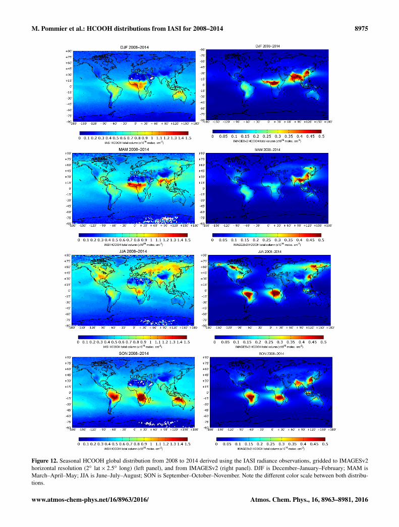
For the sake of comparison, the IASI HCOOH total columnshave been averaged to the horizontal model grid resolution.The IASI and the model total columns have also been av-eraged by season, defined as December–January–February(DJF), March–April–May (MAM), June–July–August (JJA),and September–October–November (SON) over the 7 years,between 2008 and 2014. Figure 12 presents these global dis-tributions for IASI and the model. For each season, we findthat the IASI total columns are higher than those from IM-AGESv2 simulations. This highlights the difficulty to predictthe measured concentrations by models as found in previousmodeling studies such as Stavrakou et al. (2012) and Paulotet al. (2011).

During winter (DJF), the model shows large total columnsover equatorial Africa and Asia while IASI only detects largevalues over Africa.

In spring (MAM), the CTM largely underestimates the dis-tributions over Africa compared to IASI.

Atmos. Chem. Phys., 16, 8963–8981, 2016 www.atmos-chem-phys.net/16/8963/2016/

M. Pommier et al.: HCOOH distributions from IASI for 2008–2014 8975

Figure 12. Seasonal HCOOH global distribution from 2008 to 2014 derived using the IASI radiance observations, gridded to IMAGESv2horizontal resolution (2◦ lat× 2.5◦ long) (left panel), and from IMAGESv2 (right panel). DJF is December–January–February; MAM isMarch–April–May; JJA is June–July–August; SON is September–October–November. Note the different color scale between both distribu-tions.

www.atmos-chem-phys.net/16/8963/2016/ Atmos. Chem. Phys., 16, 8963–8981, 2016

8976 M. Pommier et al.: HCOOH distributions from IASI for 2008–2014

In summer (JJA), the emissions from fires seem to be theprimary cause for the strong HCOOH enhancements in theCTM (Africa, Amazonia, boreal regions of Canada and east-ern Siberia) although biogenic emissions (southeastern USA)and anthropogenic activities (eastern China) also producevisible enhancements. In the IASI distributions, enhance-ments associated with fires are less prominent over Northand South America. IASI reveals larger total columns overAfrica in JJA than over South America while the CTM showsroughly the same values over both regions. Compared withthe CTM, IASI also shows larger HCOOH columns over theMidwestern USA, India, and semiarid regions in southwest-ern Russia and Kazakhstan.

During fall (SON), the columns from IASI over the south-ern hemispheric biomass burning emission regions (SouthAmerica, Africa, and Australia) are larger than over Asia (In-dia and China) and over Indonesia, while those simulated bythe model are quite similar for these regions.

3.3.2 Interannual variation

The global and seasonal distributions from IASI suggest anunderestimation of the modeled columns and a misrepresen-tation of some emission sources. Figure 13 presents the timeseries over the areas identified by black boxes in Fig. 1. Theseregions are AMER (North America), AMAZ (Amazonia),AFRI (Africa), SIBE (Central Siberia), INDI (India), ASIA(Asia), and AUST (Australia).

Over all regions, these time series confirm a large biasof IASI in comparison to the simulations. The seasonalvariation is, however, well represented, except over India,where the seasonal cycle is out of phase. This phase dif-ference is coherent with the cycle shown on the globaldistribution (Fig. 12). The model underestimation over In-dia suggests that either the emission factors of HCOOH(or its precursors) are underestimated in the model or thebiomass burnt estimated by GFEDv3 is too low for this re-gion. The underestimation for forest fire emissions is a se-vere issue as shown by Chaliyakunnel et al. (2016) overthe tropical forests. The calculated linear trend is also pro-vided, based on the annual IASI mean (blue dots in Fig. 13).Over three regions (North America, Africa, and Asia), thetrend is negligible (0.2–0.4 % year−1) but a small increaseis noted over Australia, Amazonia, and India (1.5± 0.5,0.9± 0.7, and 0.7± 0.1 % year−1, respectively). A decreaseof 0.8± 0.9 % year−1 is also observed over Siberia.

Over Amazonia, the large peak in 2010 due to large forestfire emissions (e.g., Hooghiemstra et al., 2012) is well repre-sented in the model and captured by IASI; however, the peakin the IASI data occurs 1 month later than in the CTM. A sim-ilar shift was already observed between the CO and NH3 ob-servations from IASI (Withburn et al., 2015). This HCOOHshift could be partly due to the difference of altitude in theHCOOH vertical distributions. IASI detects the plumes inthe free troposphere, whereas the IMAGES columns reflect

more directly the surface emissions. The mean altitude of themaximum in the HCOOH vertical profile from the modelis located around 2.8 km for this region and close to 2 kmin August 2010, while the maximum of vertical sensitivityfrom IASI is located at higher altitudes. This assumes thattransport time could be close to 1 month but it is longer thanthe known mean transport time between the boundary layerand the upper troposphere. Over Siberia, the summer 2010and to a lesser extent the summer 2012 were exceptional interms of large HCOOH emissions, as evident in the globaldistributions shown in Fig. 8. As revealed by the correlationcoefficients, the seasonal cycle is very well captured overAsia (r = 0.75), Australia (r = 0.92), Siberia (r = 0.94), andNorth America (r = 0.94).

The double peaks (∼ March and September) over Africaare explained by the shift of emission seasons on either sideof the Equator. Over Africa, the correlation is lower, dueto two factors: there is a shift of 1 month between IASIand the CTM in the maximum of columns and the highercolumns from IASI remain longer in time than those simu-lated (especially between the peak around January with theCTM and the one around February–March for IASI). A dif-ference of altitude in the detection of HCOOH between theCTM and IASI could not explain IASI detected higher to-tal columns during more than 1 month in the tropospherein March. Around March–April, the mean altitude of max-imum in the simulated columns is around 4 km, close to thealtitude of maximum vertical sensitivity from IASI, show-ing that the CTM and IASI should detect the same enrichedHCOOH plume.

4 Conclusions

Global distributions of HCOOH were derived from IASI ra-diance spectra, using conversion factors between represen-tative retrieved total columns and selected radiance chan-nels (1Tb). This paper presents 7 years of HCOOH mea-surements recorded by IASI. A limitation of this data set isits lack of characterization for vertical sensitivity due to theconversion technique used, even though the maximum sensi-tivity is shown to be in the mid-troposphere. This approachhas the significant advantage of reducing the computing timenecessary to analyze large amounts of data and to providea global representation of the HCOOH distribution aroundthe world, including ocean and land scenes, and emissionsources as well as remote areas.

IASI provides global distributions of HCOOH, highlight-ing the long-range transport of tropospheric HCOOH overthe Atlantic Ocean and the detection of source regions, e.g.,biomass burning areas over Amazonia, Africa, Australia, andSiberia. Other source regions are detected such as the mid-eastern USA in 2011 or over India.

The comparison with an atmospheric model and, to alesser extent, with ground-based FTIR observations remains

Atmos. Chem. Phys., 16, 8963–8981, 2016 www.atmos-chem-phys.net/16/8963/2016/

M. Pommier et al.: HCOOH distributions from IASI for 2008–2014 8977

Figure 13. Time series of the monthly HCOOH column means for IASI (blue) and IMAGESv2 (red) over different regions highlighted byblack boxes in Fig. 1, between 2008 and 2014. The coordinates of each box (latitude and longitude) are written on the top of each plot. Thered and blue shaded areas correspond to the monthly standard deviation. The correlation coefficient, the mean bias, and the normalized meanbias (in parentheses) for the full period are given on each plot. The blue dots correspond to the annual IASI mean. The linear regressionon the annual IASI mean and the calculated linear trend are also provided. On the bottom panel, the mean altitude of the maximum in theHCOOH vertical distribution from IMAGESv2 is plotted in black with the corresponding standard deviation represented by the black shadeareas.

www.atmos-chem-phys.net/16/8963/2016/ Atmos. Chem. Phys., 16, 8963–8981, 2016

8978 M. Pommier et al.: HCOOH distributions from IASI for 2008–2014

challenging. Despite large biases in many cases, we showthat the interannual and the seasonal variations are well cap-tured by IASI when compared with ground-based FTIR mea-surements and the IMAGESv2 CTM. The best overall cor-relation with the FTIR is obtained at Saint-Denis over LaRéunion (r = 0.77) but both sites at La Réunion presentthe larger biases (> 100 % lower than IASI). High correla-tions are obtained with the CTM, in particularly over Amer-ica, Australia, Siberia, and Asia, with correlation coefficientsranging from 0.75 to 0.94. This comparison also points outa misrepresentation of the distribution between IASI and theCTM over India and Africa and a global underestimation ofthe distribution by the CTM. A small decreasing trend dur-ing the 7-year period is observed over Siberia, while a smallincrease is noted over India, Amazonia, and Australia (0.7,0.9, and 1.5 % year−1, respectively).

The HCOOH columns from IASI will require further eval-uation and probably improvements to narrow down the bi-ases but the data set available now spans 7 years and it willlikely contribute to a better understanding of the troposphericHCOOH budget. The data set will be made available throughthe Ether database (http://ether.ipsl.jussieu.fr) for further sci-entific studies. This 7-year record will be completed by thedata provided by IASI/MetOp-B, launched at the end of2012, and IASI/MetOp-C, to be launched in 2018. The IASIprogram will be followed up (after 2022) by the IASI-NGmission aboard the MetOp-SG satellite series (Clerbaux andCrevoisier, 2013; Crevoisier et al., 2014). This new instru-ment will be characterized by improved spectral resolutionand lower radiometric noise. It will lead to a better verti-cal resolution, along with improved accuracy and detectionthreshold.

5 Data availability

The IASI data are not available yet but as described in theconclusion, the data set will be made available through theEther database (http://ether.ipsl.jussieu.fr; CNES and INSU,2016).

The Supplement related to this article is available onlineat doi:10.5194/acp-16-8963-2016-supplement.

Acknowledgements. IASI was developed and built under theresponsibility of Centre National des Etudes Spatiales (CNES)and flies onboard the MetOp satellite as part of the EUMET-SAT Polar system. We thank the Aeris data infrastructure(http://www.aeris-data.fr/) for providing access to the IASIL1C data and to the ECCAD emission inventories used in thisstudy. The French scientists are grateful to CNES for financialsupport. We also gratefully acknowledge Yasmina R’Honi and

Lieven Clarisse (ULB) for their help with the HCOOH retrieval.The authors would like to thank the other researchers involved inthe ground-based solar remote sensing program at Wollongong(including Nicholas B. Jones, David Griffith, Nicholas Deutscher,and Voltaire Velazco) and the Australian Research Council for itssupport for the NDACC site at Wollongong, most recently as partof project DP110101948. Acknowledgements are addressed tothe Université de La Réunion and CNRS (LACy-UMR8105 andUMS3365) for their support of the OPAR station (Observatoire dePhysique de l’Atmosphère de la Réunion). The authors gratefullyacknowledge C. Hermans, F. Scolas, and B. Langerock fromBIRA-IASB, and J.-M. Metzger from Université de La Réunionfor the Réunion Island measurements. The University of Liègecontribution to the present work has been supported by the F.R.S.– FNRS, the Belgian Science Policy Office (BELSPO), Brussels,the Fédération Wallonie-Bruxelles, and MeteoSwiss (GAW-CHprogram). We thank the International Foundation High AltitudeResearch Stations Jungfraujoch and Gornergrat (HFSJG, Bern).We are grateful to all Belgian colleagues who contributed to theacquisition of the FTIR data at Jungfraujoch. The Réunion Islandmeasurements have mainly been supported by the A3C project(PRODEX Program of BELSPO). The research was supportedby BELSPO and ESA through the IASI.Flow project (Prodexarrangement 4000111403).

Edited by: T. von ClarmannReviewed by: two anonymous referees

References

Andreae, M. O., Andreae, T. W., Talbot, R. W., and Harriss,R. C.: Formic and acetic acid over the central Amazon re-gion, Brazil. I. Dry season, J. Geophys. Res., 93, 1616–1624,doi:10.1029/JD093iD02p01616, 1988.

Andrews, D. U., Heazlewood, B. R., Maccarone, A. T., Conroy,T., Payne, R. J., Jordan, M. J. T., and Kable, S. H.: Photo-tautomerization of acetaldehyde to vinyl alcohol: a potentialroute to tropospheric acids, Science, 337, 1203–1206, 2012.

Bohn, B., Siese, M., and Zetzschn, C.: Kinetics of the OH+C2H2reaction in the presence of O2, J. Chem. Soc. Faraday T., 92,1459–1466, 1996.

Cady-Pereira, K. E., Chaliyakunnel, S., Shephard, M. W., Mil-let, D. B., Luo, M., and Wells, K. C.: HCOOH measurementsfrom space: TES retrieval algorithm and observed global distri-bution, Atmos. Meas. Tech., 7, 2297–2311, doi:10.5194/amt-7-2297-2014, 2014.

Chaliyakunnel, S., Millet, D. B., Wells, K. C., Cady-Pereira,K. E., and Shephard, M. W.: A Large Underestimate ofFormic Acid from Tropical Fires: Constraints from Space-Borne Measurements, Environ. Sci. Technol., 50, 5631–5640,doi:10.1021/acs.est.5b06385, 2016.

Clarisse, L., Coheur, P. F., Prata, A. J., Hurtmans, D., Razavi,A., Phulpin, T., Hadji-Lazaro, J., and Clerbaux, C.: Trackingand quantifying volcanic SO2 with IASI, the September 2007eruption at Jebel at Tair, Atmos. Chem. Phys., 8, 7723–7734,doi:10.5194/acp-8-7723-2008, 2008.

Atmos. Chem. Phys., 16, 8963–8981, 2016 www.atmos-chem-phys.net/16/8963/2016/

M. Pommier et al.: HCOOH distributions from IASI for 2008–2014 8979

Clerbaux, C. and Crevoisier, C.: New Directions: Infrared remotesensing of the troposphere from satellite: Less, but better, Atmos.Environ., 72, 24–26, doi:10.1016/j.atmosenv.2013.01.057, 2013.

Clerbaux, C., Boynard, A., Clarisse, L., George, M., Hadji-Lazaro,J., Herbin, H., Hurtmans, D., Pommier, M., Razavi, A., Turquety,S., Wespes, C., and Coheur, P.-F.: Monitoring of atmosphericcomposition using the thermal infrared IASI/MetOp sounder, At-mos. Chem. Phys., 9, 6041–6054, doi:10.5194/acp-9-6041-2009,2009.

Clubb, A. E., Jordan, M. J. T., Kable, S. H., and Osborn, D. L.:Phototautomerization of Acetaldehyde to vinyl alcohol: a pri-mary process in UV-irradiated acetaldehyde from 295 to 335 nm,J. Phys. Chem. Lett., 3, 3522–3526, 2012.

CNES (Centre National dEtudes Spatiales) and INSU (Institut Na-tional des Sciences de l’Univers): Ether database, available at:http://ether.ipsl.jussieu.fr, last access: 15 July 2016.

Coheur, P. F., Clerbaux, C., and Colin, R. : Spectroscopicmeasurements of halocarbons and hydrohalocarbons bysatellite-borne remote sensors, J. Geophys. Res., 108, 4130,doi:10.1029/2002JD002649, 2003.

Coheur, P.-F., Barret, B., Turquety, S., Hurtmans, D., Hadji-Lazaro,J., and Clerbaux, C.: Retrieval and characterization of ozone ver-tical profiles from a thermal infrared nadir sounder, J. Geophys.Res., 110, D24303, doi:10.1029/2005JD005845, 2005.

Crevoisier, C., Clerbaux, C., Guidard, V., Phulpin, T., Armante,R., Barret, B., Camy-Peyret, C., Chaboureau, J.-P., Coheur, P.-F., Crépeau, L., Dufour, G., Labonnote, L., Lavanant, L., Hadji-Lazaro, J., Herbin, H., Jacquinet-Husson, N., Payan, S., Péquig-not, E., Pierangelo, C., Sellitto, P., and Stubenrauch, C.: TowardsIASI-New Generation (IASI-NG): impact of improved spectralresolution and radiometric noise on the retrieval of thermody-namic, chemistry and climate variables, Atmos. Meas. Tech., 7,4367–4385, doi:10.5194/amt-7-4367-2014, 2014.

González Abad, G., Bernath, P. F., Boone, C. D., McLeod, S. D.,Manney, G. L., and Toon, G. C.: Global distribution of upper tro-pospheric formic acid from the ACE-FTS, Atmos. Chem. Phys.,9, 8039–8047, doi:10.5194/acp-9-8039-2009, 2009.

Goode, J., Yokelson, R., Ward, D., Susott, R., Babbitt, R., Davies,M., and Hao, W.: Measurements of excess O3, CO2, CO, CH4,C2H4, C2H2, HCN, NO, NH3, HCOOH, CH3COOH, HCHO,and CH3OH in 1997 Alaskan biomass burning plumes by air-borne Fourier transform infrared spectroscopy (AFTIR), J. Geo-phys. Res., 105, 22147, doi:10.1029/2000JD900287, 2000.

Graedel, T. and Eisner, T.: Atmospheric formic acid from formicineants: a preliminary assessment, Tellus B, 40, 335–339, 1988.

Grosjean, D.: Organic acids in southern California air: ambient con-centrations, mobile source emissions, in situ formation and re-moval processes, Environ. Sci. Technol., 23, 1506–1514, 1989.

Grutter, M., Glatthor, N., Stiller, G. P., Fischer, H., Grabowski,U., Höpfner, M., Kellmann, S., Linden, A., and von Clarmann,T.: Global distribution and variability of formic acid as ob-served by MIPAS-ENVISAT, J. Geophys. Res., 115, D10303,doi:10.1029/2009JD012980, 2010.

Hatakeyama, S., Washida, N., and Akimoto, H.: Rate constantsand mechanisms for the reaction of hydroxyl (OD) radicals withacetylene, propyne, and 2-butyne in air at 297± 2 K, J. Phys.Chem., 6, 173–178, 1986.

Hooghiemstra, P. B., Krol, M. C., van Leeuwen, T. T., van der Werf,G. R., Novelli, P. C., Deeter, M. N., Aben, I., and Röckmann, T.:Interannual variability of carbon monoxide emission estimatesover South America from 2006 to 2010, J. Geophys. Res., 117,D15308, doi:10.1029/2012JD017758, 2012.

Jones, B. T., Muller, J. B. A., O’Shea, S. J., Bacak, A., Le Bre-ton, M., Bannan, T. J., Leather, K. E., Murray Booth, A., Illing-worth, S., Bower, K., Gallagher, M. W., Allen, G., Dudley Shall-cross, E., Bauguitte, S. J.-B., Pyle, J. A., and Percival, C. J.:Airborne measurements of HC(O)OH in the European Arctic:A winter summer comparison, Atmos. Environ., 99, 556–567,doi:10.1016/j.atmosenv.2014.10.030, 2014.

Kawamura, K., Ng, L., and Kaplan, I.: Determination of organicacids (C1-C10) in the atmosphere, motor exhausts, and engineoils, Environ. Sci. Technol., 19, 1082–1086, 1985.

Keene, W. and Galloway, J.: Organic acidity in precipitation ofNorth America, Atmos. Environ., 18, 2491–2497, 1984.

Keene, W. C. and Galloway, J. N.: The biogeochemical cycling offormic and acetic acids through the troposphere: An overview ofcurrent understanding, Tellus B, 40, 322–334, 1988.

Kurokawa, J., Ohara, T., Morikawa, T., Hanayama, S., Janssens-Maenhout, G., Fukui, T., Kawashima, K., and Akimoto, H.:Emissions of air pollutants and greenhouse gases over Asian re-gions during 2000–2008: Regional Emission inventory in ASia(REAS) version 2, Atmos. Chem. Phys., 13, 11019–11058,doi:10.5194/acp-13-11019-2013, 2013.

Lee, A., Goldstein, A. H., Kroll, J. H., Ng, N. L., Varut-bangkul, V., Flagan, R. C., and Seinfeld, J. H.: Gas-phaseproducts and secondary aerosol yields from the photooxida-tion of 16 different terpenes, J. Geophys. Res., 111, D17305,doi:10.1029/2006JD007050, 2006.

Millet, D. B., Baasandorj, M., Farmer, D. K., Thornton, J. A., Bau-mann, K., Brophy, P., Chaliyakunnel, S., de Gouw, J. A., Graus,M., Hu, L., Koss, A., Lee, B. H., Lopez-Hilfiker, F. D., Neu-man, J. A., Paulot, F., Peischl, J., Pollack, I. B., Ryerson, T. B.,Warneke, C., Williams, B. J., and Xu, J.: A large and ubiqui-tous source of atmospheric formic acid, Atmos. Chem. Phys., 15,6283–6304, doi:10.5194/acp-15-6283-2015, 2015.

Neeb, P., Sauer, F., Horie, O., and Moortgat, G. K.: Formation ofhydroxymethyl hydroperoxide and formic acid in alkene ozonol-ysis in the presence of water vapour, Atmos. Environ., 31, 1417–1423, 1997.

Ngwabie, N. M., Schade, G. W., Custer, T. G., Linke, S., and Hinz,T.: Abundances and flux estimates of volatile organic compoundsfrom a dairy cowshed in Germany, J. Environ. Qual., 37, 565–573, 2008.

Paton-Walsh, C., Jones, N. B., Wilson, S. R., Haverd, V., Meier, A.,Griffith, D. W. T., and Rinsland, C. P.: Measurements of tracegas emissions from Australian forest fires and correlations withcoincident measurements of aerosol optical depth, J. Geophys.Res.-Atmos., 110, D24305, doi:10.1029/2005JD006202, 2005.

Paulot, F., Wunch, D., Crounse, J. D., Toon, G. C., Millet, D.B., DeCarlo, P. F., Vigouroux, C., Deutscher, N. M., GonzálezAbad, G., Notholt, J., Warneke, T., Hannigan, J. W., Warneke,C., de Gouw, J. A., Dunlea, E. J., De Mazière, M., Griffith, D.W. T., Bernath, P., Jimenez, J. L., and Wennberg, P. O.: Im-portance of secondary sources in the atmospheric budgets offormic and acetic acids, Atmos. Chem. Phys., 11, 1989–2013,doi:10.5194/acp-11-1989-2011, 2011.

www.atmos-chem-phys.net/16/8963/2016/ Atmos. Chem. Phys., 16, 8963–8981, 2016

8980 M. Pommier et al.: HCOOH distributions from IASI for 2008–2014

Razavi, A., Karagulian, F., Clarisse, L., Hurtmans, D., Coheur, P.F., Clerbaux, C., Müller, J. F., and Stavrakou, T.: Global distribu-tions of methanol and formic acid retrieved for the first time fromthe IASI/MetOp thermal infrared sounder, Atmos. Chem. Phys.,11, 857–872, doi:10.5194/acp-11-857-2011, 2011.

R’Honi, Y., Clarisse, L., Clerbaux, C., Hurtmans, D., Duflot, V.,Turquety, S., Ngadi, Y., and Coheur, P.-F.: Exceptional emis-sions of NH3 and HCOOH in the 2010 Russian wildfires, At-mos. Chem. Phys., 13, 4171–4181, doi:10.5194/acp-13-4171-2013, 2013.

Rodgers, C. D.: Inverse methods for atmospheric sounding: theoryand practice, Ser. Atmos. Ocean. Planet. Phys. 2, World Sci.,Hackensack, NJ, USA, 2000.

Rothman, L. S., Gordon, I. E., Barbe, A., Benner, D. C., Bernath, P.F., Birk, M., Boudon, V., Brown, L. R., Campargue, A., Cham-pion, J., Chance, K., Coudert, L. H., Dana, V., Devi, V. M., Fally,S., Flaud, J., Gamache, R. R., Goldman, A., Jacquemart, D.,Kleiner, I., Lacome, N., Lafferty, W. J., Mandin, J., Massie, S.T., Mikhailenko, S. N., Miller, C. E., Moazzen-Ahmadi, N., Nau-menko, O. V., Nikitin, A. V., Orphal, J., Perevalov, V. I., Perrin,A., Predoi-Cross, A., Rinsland, C. P., Rotger, M., Simeckova, M.,Smith, M. A. H., Sung, K., Tashkun, S. A., Tennyson, J., Toth, R.A., Vandaele, A. C., and Vander Auwera, J.: The HITRAN 2008molecular spectroscopic database, J. Quant. Spectrosc. Ra., 110,533–572, doi:10.1016/j.jqsrt.2009.02.013, 2009.

Sanhueza, E. and Andreae, M.: Emission of formic and acetic acidsfrom tropical savanna soils, Geophys. Res. Lett., 18, 1707–1710,1991.

Sanhueza, E., Figueroa, L., and Santana, M.: Atmospheric formicand acetic acids in Venezuela, Atmos. Environ., 30, 1861–1873,1996.

Schultz, M. G., Backman, L., Balkanski, Y., Bjoerndalsaeter, S.,Brand, R., Burrows, J. P., Dalsoeren, S., de Vasconcelos, M.,Grodtmann, B., Hauglustaine, D. A., Heil, A., Hoelzemann,J. J., Isaksen, I. S. A., Kaurola, J., Knorr, W., Ladstaetter-Weißenmayer, A., Mota, B., Oom, D., Pacyna, J., Panasiuk, D.,Pereira, J. M. C., Pulles, T., Pyle, J., Rast, S., Richter, A., Savage,N., Schnadt, C., Schulz, M., Spessa, A., Staehelin, J., Sundet, J.K., Szopa, S., Thonicke, K., van het Bolscher, M., van Noije,T., van Velthoven, P., Vik, A. F., and Wittrock, F.: REanalysis ofthe TROpospheric chemical composition over the past 40 years(RETRO): A long-term global modeling study of troposphericchemistry, Jülich/Hamburg, Germany, 48/2007 report on EarthSystem Science of the Max Planck Institute for Meteorology,Hamburg, ISSN 1614-1199, available at: http://retro-archive.iek.fz-juelich.de/data/documents/ (last access: 13 July 2016), 2007.

Sindelarova, K., Granier, C., Bouarar, I., Guenther, A., Tilmes, S.,Stavrakou, T., Müller, J.-F., Kuhn, U., Stefani, P., and Knorr, W.:Global data set of biogenic VOC emissions calculated by theMEGAN model over the last 30 years, Atmos. Chem. Phys., 14,9317–9341, doi:10.5194/acp-14-9317-2014, 2014.

Stavrakou, T., Guenther, A., Razavi, A., Clarisse, L., Clerbaux,C., Coheur, P.-F., Hurtmans, D., Karagulian, F., De Maz-ière, M., Vigouroux, C., Amelynck, C., Schoon, N., Laffineur,Q., Heinesch, B., Aubinet, M., Rinsland, C., and Müller,J.-F.: First space-based derivation of the global atmosphericmethanol emission fluxes, Atmos. Chem. Phys., 11, 4873–4898,doi:10.5194/acp-11-4873-2011, 2011.

Stavrakou, T., Müller, J-F., Peeters, J., Razavi, A., Clarisse, L., Cler-baux, C., Coheur, P.-F., Hurtmans, D., and De Mazière, M.: Satel-lite evidence for a large source of formic acid from boreal andtropical forests, Nat. Geosci., 5, 26–30, doi:10.1038/ngeo1354,2012.

Stavrakou, T., Müller, J.-F., Bauwens, M., De Smedt, I., VanRoozendael, M., Guenther, A., Wild, M., and Xia, X.: Isopreneemissions over Asia 1979–2012: impact of climate and land-usechanges, Atmos. Chem. Phys., 14, 4587–4605, doi:10.5194/acp-14-4587-2014, 2014.

Talbot, R. W., Dibb, J. E., Lefer, B. L., Scheuer, E. M., Bradshaw,J. D., Sandholm, S. T., Smyth, S., Blake, D. R., Blake, N. J.,Sachse, G. W., Collins, J. E., and Gregory, G. L.: Large-scaledistributions of tropospheric nitric, formic, and acetic acids overthe western Pacific basin during wintertime, J. Geophys. Res.,102, 28303–28313, doi:10.1029/96JD02975, 1997a.

Talbot, R. W., Dibb, J. E., Lefer, B. L., Bradshaw, J. D., Sandholm,S. T., Blake, D. R., Blake, N. J., Sachse, G. W., Collins, J. E.,Heikes, B. G., Merrill, J. T., Gregory, G. L., Anderson, B. E.,Singh, H. B., Thornton, D. C., Bandy, A. R., and Pueschel, R.F.: Chemical characteristics of continental outflow from Asia tothe troposphere over the western Pacific Ocean during February-March 1994: Results from PEM-West B, J. Geophys. Res., 102,28255–28274, doi:10.1029/96JD02340, 1997b.

Talbot, R. W., Dibb, J. E., Scheuer, E. M., Blake, D. R., Blake, N.J., Gregory, G. L., Sachse, G. W., Bradshaw, J. D., Sandholm, S.T., and Singh, H. B.: Influence of biomass combustion emissionson the distribution of acidic trace gases over the Southern Pacificbasin during austral springtime, J. Geophys. Res., 104, 5623–5634, 1999.

Van Damme, M., Clarisse, L., Heald, C. L., Hurtmans, D., Ngadi,Y., Clerbaux, C., Dolman, A. J., Erisman, J. W., and Coheur, P.F.: Global distributions, time series and error characterization ofatmospheric ammonia (NH3) from IASI satellite observations,Atmos. Chem. Phys., 14, 2905–2922, doi:10.5194/acp-14-2905-2014, 2014.

Vander Auwera, J., Didriche, K., Perrin, A., and Keller, F.: Abso-lute line intensities for formic acid and dissociation constant ofthe dimer, J. Chem. Phys., 126, 124311, doi:10.1063/1.2712439,2007.

van der Werf, G. R., Randerson, J. T., Giglio, L., Collatz, G. J., Mu,M., Kasibhatla, P. S., Morton, D. C., DeFries, R. S., Jin, Y., andvan Leeuwen, T. T.: Global fire emissions and the contribution ofdeforestation, savanna, forest, agricultural, and peat fires (1997–2009), Atmos. Chem. Phys., 10, 11707–11735, doi:10.5194/acp-10-11707-2010, 2010.

Vigouroux, C., Stavrakou, T., Whaley, C., Dils, B., Duflot, V., Her-mans, C., Kumps, N., Metzger, J.-M., Scolas, F., Vanhaelewyn,G., Müller, J.-F., Jones, D. B. A., Li, Q., and De Mazière, M.:FTIR time-series of biomass burning products (HCN, C2H6,C2H2, CH3OH, and HCOOH) at Reunion Island (21◦ S, 55◦ E)and comparisons with model data, Atmos. Chem. Phys., 12,10367–10385, doi:10.5194/acp-12-10367-2012, 2012.

Wallace, J. M. and Hobbs, P. V.: Atmospheric Science: An Introduc-tory Survey, ISBN-13: 978-0127329512, Academic Press, NewYork, USA, 1977.

Atmos. Chem. Phys., 16, 8963–8981, 2016 www.atmos-chem-phys.net/16/8963/2016/

M. Pommier et al.: HCOOH distributions from IASI for 2008–2014 8981

Whitburn, S., Van Damme, M., Kaiser, J. W., van der Werf, G.R., Turquety, S., Hurtmans, D., Clarisse, L., Clerbaux, C., andCoheur, P.-F.: Ammonia emissions in tropical biomass burn-ing regions: Comparison between satellite-derived emissionsand bottom-up fire inventories, Atmos. Environ, 121, 42–54,doi:10.1016/j.atmosenv.2015.03.015, 2015.

Zander, R., Duchatelet, P., Mahieu, E., Demoulin, P., Roland,G., Servais, C., Auwera, J. V., Perrin, A., Rinsland, C. P.,and Crutzen, P. J.: Formic acid above the Jungfraujoch during1985–2007: observed variability, seasonality, but no long-termbackground evolution, Atmos. Chem. Phys., 10, 10047–10065,doi:10.5194/acp-10-10047-2010, 2010.

www.atmos-chem-phys.net/16/8963/2016/ Atmos. Chem. Phys., 16, 8963–8981, 2016