THE STOCHASTISATION HYPOTHESIS AND THE SPACING OF...

THE STOCHASTISATION HYPOTHESIS AND THE SPACING OF

PLANETARY SYSTEMS

by

Jacky Cresson1,2

1 Laboratoire de Mathématiques Appliquées de Pau, Université de Pau et des Pays de l'Adour,

avenue de l'Université, BP 1155, 64013 Pau Cedex, France

2 Institut de Mécanique Céleste et de Calcul des Éphémérides, Observatoire de Paris,

77 avenue Denfert-Rochereau, 75014 Paris, France

Il était générallement admis que les probabilités n'étaient que l'expression de notre ignorance.Pour les systèmes instables, il n'en est pas ainsi.

Les probabilités acquièrent une signication dynamique intrinsèque.Peu à peu se dessine dès lors une nouvelle rationalité

dans laquelle probabilité n'est pas ignoranceet science ne se confond pas avec certitude.

C'est à ce prix que la notion d'évolution et avec elle les notions d'événement et de créativitéfont leur entrée dans les lois fondamentales de la nature.

Ilya Progogine, Les lois du Chaos, Ed. Flammarion, 1994

Abstract. We introduce the stochastisation hypothesis which aims to provide a frameworkto deal with physical systems in random environment. We apply the stochastisation hypothesisin two dierent cases : in the study of the dynamics of a protoplanetary nebula and in theChaotic long term behaviour of a generic planetary system using previous works of S. Albeverioand al., L. Nottale and J. Laskar. These results give both a particular law for the distributionof planetary orbits.

Contents

1. Introduction.. . . . . . . . . . . . . . . . . . . . . . . . . . . . . . . . . . . . . . . . . . . . . . . . . . . . . . . . . . . . . . . . . . . . . . . . . . . . . . . . . . . . . . . . . . . . . . . . . . . . . . . . . 22. Reminder about stochastic embedding.. . . . . . . . . . . . . . . . . . . . . . . . . . . . . . . . . . . . . . . . . . . . . . . . . . . . . . . . . . . . . . . . . . . . . . . . . . . 3

2.1. Notations.. . . . . . . . . . . . . . . . . . . . . . . . . . . . . . . . . . . . . . . . . . . . . . . . . . . . . . . . . . . . . . . . . . . . . . . . . . . . . . . . . . . . . . . . . . . . . . . . . . . . . . 32.2. Stochastic derivatives. . . . . . . . . . . . . . . . . . . . . . . . . . . . . . . . . . . . . . . . . . . . . . . . . . . . . . . . . . . . . . . . . . . . . . . . . . . . . . . . . . . . . . . . . 42.3. Stochastic embedding.. . . . . . . . . . . . . . . . . . . . . . . . . . . . . . . . . . . . . . . . . . . . . . . . . . . . . . . . . . . . . . . . . . . . . . . . . . . . . . . . . . . . . . . . 6

2.3.1. Stochastic dierential embedding.. . . . . . . . . . . . . . . . . . . . . . . . . . . . . . . . . . . . . . . . . . . . . . . . . . . . . . . . . . . . . . . . . . . . . 62.3.2. Stochastic analogue of dynamical quantities : speed and acceleration. . . . . . . . . . . . . . . . . . . . . . . . . . . . 82.3.3. Stochastic variational embedding.. . . . . . . . . . . . . . . . . . . . . . . . . . . . . . . . . . . . . . . . . . . . . . . . . . . . . . . . . . . . . . . . . . . . . 9

2.4. Coherence of stochastic embedding.. . . . . . . . . . . . . . . . . . . . . . . . . . . . . . . . . . . . . . . . . . . . . . . . . . . . . . . . . . . . . . . . . . . . . . . . . 102.5. Lifting of symmetries and a stochastic Noether theorem.. . . . . . . . . . . . . . . . . . . . . . . . . . . . . . . . . . . . . . . . . . . . . . . . 10

2.5.1. First integrals of stochastic dynamical systems.. . . . . . . . . . . . . . . . . . . . . . . . . . . . . . . . . . . . . . . . . . . . . . . . . . . . . 112.5.2. Stochastic lifting of symmetries. . . . . . . . . . . . . . . . . . . . . . . . . . . . . . . . . . . . . . . . . . . . . . . . . . . . . . . . . . . . . . . . . . . . . . . . 112.5.3. Stochastic invariance.. . . . . . . . . . . . . . . . . . . . . . . . . . . . . . . . . . . . . . . . . . . . . . . . . . . . . . . . . . . . . . . . . . . . . . . . . . . . . . . . . . . 112.5.4. Stochastic Noether's theorem... . . . . . . . . . . . . . . . . . . . . . . . . . . . . . . . . . . . . . . . . . . . . . . . . . . . . . . . . . . . . . . . . . . . . . . . 132.5.5. An example : rotations and stochastisation.. . . . . . . . . . . . . . . . . . . . . . . . . . . . . . . . . . . . . . . . . . . . . . . . . . . . . . . . . 13

3. The Stochastisation hypothesis. . . . . . . . . . . . . . . . . . . . . . . . . . . . . . . . . . . . . . . . . . . . . . . . . . . . . . . . . . . . . . . . . . . . . . . . . . . . . . . . . . . . 133.1. The stochastisation hypothesis. . . . . . . . . . . . . . . . . . . . . . . . . . . . . . . . . . . . . . . . . . . . . . . . . . . . . . . . . . . . . . . . . . . . . . . . . . . . . . . 143.2. Discussion of the stochastisation hypothesis. . . . . . . . . . . . . . . . . . . . . . . . . . . . . . . . . . . . . . . . . . . . . . . . . . . . . . . . . . . . . . . 153.3. Stochastic processes and stochastisation : diusion processes ?. . . . . . . . . . . . . . . . . . . . . . . . . . . . . . . . . . . . . . . . . 15

2 JACKY CRESSON1,2

4. The stochastisation hypothesis and the Newton's equation.. . . . . . . . . . . . . . . . . . . . . . . . . . . . . . . . . . . . . . . . . . . . . . . . . . . . 164.1. The stochastic Newton equation.. . . . . . . . . . . . . . . . . . . . . . . . . . . . . . . . . . . . . . . . . . . . . . . . . . . . . . . . . . . . . . . . . . . . . . . . . . . . 164.2. The reversible stochastic Newton's equation.. . . . . . . . . . . . . . . . . . . . . . . . . . . . . . . . . . . . . . . . . . . . . . . . . . . . . . . . . . . . . . 18

5. Application : organisation of planetary systems.. . . . . . . . . . . . . . . . . . . . . . . . . . . . . . . . . . . . . . . . . . . . . . . . . . . . . . . . . . . . . . . . 205.1. Dynamics of a protoplanetary nebula.. . . . . . . . . . . . . . . . . . . . . . . . . . . . . . . . . . . . . . . . . . . . . . . . . . . . . . . . . . . . . . . . . . . . . . 20

5.1.1. Model for the dynamics in a protoplanetary nebula.. . . . . . . . . . . . . . . . . . . . . . . . . . . . . . . . . . . . . . . . . . . . . . . . 205.1.2. On the nature of collisions. . . . . . . . . . . . . . . . . . . . . . . . . . . . . . . . . . . . . . . . . . . . . . . . . . . . . . . . . . . . . . . . . . . . . . . . . . . . . 205.1.3. Mechanisms for connements. . . . . . . . . . . . . . . . . . . . . . . . . . . . . . . . . . . . . . . . . . . . . . . . . . . . . . . . . . . . . . . . . . . . . . . . . . 215.1.4. Law of repartition for planetary orbits. . . . . . . . . . . . . . . . . . . . . . . . . . . . . . . . . . . . . . . . . . . . . . . . . . . . . . . . . . . . . . . . 22

5.2. Long term behaviour of the solar system... . . . . . . . . . . . . . . . . . . . . . . . . . . . . . . . . . . . . . . . . . . . . . . . . . . . . . . . . . . . . . . . . 225.2.1. Chaos and Stochastic processes. . . . . . . . . . . . . . . . . . . . . . . . . . . . . . . . . . . . . . . . . . . . . . . . . . . . . . . . . . . . . . . . . . . . . . . . 235.2.2. Hierarchical structures. . . . . . . . . . . . . . . . . . . . . . . . . . . . . . . . . . . . . . . . . . . . . . . . . . . . . . . . . . . . . . . . . . . . . . . . . . . . . . . . . . 235.2.3. Is the Solar system stable ?.. . . . . . . . . . . . . . . . . . . . . . . . . . . . . . . . . . . . . . . . . . . . . . . . . . . . . . . . . . . . . . . . . . . . . . . . . . . 24

6. Conclusion.. . . . . . . . . . . . . . . . . . . . . . . . . . . . . . . . . . . . . . . . . . . . . . . . . . . . . . . . . . . . . . . . . . . . . . . . . . . . . . . . . . . . . . . . . . . . . . . . . . . . . . . . . . . 256.1. Summary.. . . . . . . . . . . . . . . . . . . . . . . . . . . . . . . . . . . . . . . . . . . . . . . . . . . . . . . . . . . . . . . . . . . . . . . . . . . . . . . . . . . . . . . . . . . . . . . . . . . . . . 256.2. Perspectives. . . . . . . . . . . . . . . . . . . . . . . . . . . . . . . . . . . . . . . . . . . . . . . . . . . . . . . . . . . . . . . . . . . . . . . . . . . . . . . . . . . . . . . . . . . . . . . . . . . . 26

6.2.1. Coalescent processes. . . . . . . . . . . . . . . . . . . . . . . . . . . . . . . . . . . . . . . . . . . . . . . . . . . . . . . . . . . . . . . . . . . . . . . . . . . . . . . . . . . . 266.2.2. Statistics and gravitational structuration constant.. . . . . . . . . . . . . . . . . . . . . . . . . . . . . . . . . . . . . . . . . . . . . . . . . 266.2.3. Stability of the solar system... . . . . . . . . . . . . . . . . . . . . . . . . . . . . . . . . . . . . . . . . . . . . . . . . . . . . . . . . . . . . . . . . . . . . . . . . . 26

References.. . . . . . . . . . . . . . . . . . . . . . . . . . . . . . . . . . . . . . . . . . . . . . . . . . . . . . . . . . . . . . . . . . . . . . . . . . . . . . . . . . . . . . . . . . . . . . . . . . . . . . . . . . . . . . 27

1. Introduction

The aim of this paper is to describe a new way to take into account the bath of a given

physical experiment on the dynamical equations which model it. As a typical example, we

think to the Davidov's model of energy transfer in proteins where there exists a phonon bath

or the classical problem of the Brownian motion. From the mathematical point of view,

our approach is based on the recent stochastic embedding formalism of Lagrangian systems

developed by S. Darses and the author in [10].

Our main concern is the following stochastisation problem :

i - Let xt be a dynamical variable governed by a physical constraint. We assume in the

following that the dynamics of xt is controlled by a Lagrangian equation, i.e. there exists a

Lagrangian L such that xt satises the classical Euler-Lagrange equations. From the physical

point of view, it means that we look for Physical systems coming from a least action principle.

ii - We assume that the underlying bath, which is assumed to model the particular condi-

tions under which the experiment is done, induces random behaviours, i.e. that xt is now no

longer deterministic but a stochastic process Xt.

What is the dynamics of Xt ?

In this paper, we will use the following notion of stochastisation, which is in fact an hy-

pothesis of a physical nature on the underlying dynamics:

STOCHASTIC DYNAMICS 3

Stochastization hypothesis : The dynamics of Xt is obtain by the stochastic embedding

in the sense of [10] of the initial Lagrangian system.

The previous framework can be used in a wild variety of problems. We have an analogous

situation when one studies the long term behaviour of chaotic dynamical systems or the

dynamics of a protoplanetary nebula. In this case we have no longer a bath but the long term

dynamics can be described using stochastic processes ([28],[29]). Using the stochastisation

hypothesis, we prove that the law for the distribution of planetary orbits follows a simple

rule. This work is related to L. Nottale's approach to chaotic dynamical systems [41] and its

application to the Titius-Bode law [42].

The plane of our paper is as follow : In Section 2 we remind the stochastic embedding of

dynamical systems developed in [10]. In Section 3 we dene the stochastisation hypothesis and

discuss some issues related to it. In Section 4, we give a characterisation of Lagrangian systems

under the stochastisation hypothesis using PDEs of the Schrödinger type. Section 5 describes

two applications of this formalism : In Section 5.1 we apply the stochastisation hypothesis in

the study of the dynamics of a protoplanetary nebula. This work is related to the approach

of S. Albeverio, Ph. Blanchard and R. Hoegh-Krohn ([3],[4]), L. Nottale ([41],[42],[45]) and

J. Laskar ([28],[29]) to the Titius-Bode law. We then apply the stochastisation hypothesis

to the long term behaviour of the solar systems using the work of J. Laskar ([28]) in Section

5.2. Both of these applications give an analogue of the Titius-Bode law for the repartition of

planetary distances around a star although the domain of application is dierent.

2. Reminder about stochastic embedding

We refer to [10] for a complete introduction to the stochastic embedding formalism for

ordinary dierential equations and to [9] for an overview. The formalism of embedding is

described in ([12],[13]) in full generality.

2.1. Notations. Let T > 0, ν > 0 and d ∈ N∗. Let L be the set of all measurable

functions f : [0,T ] × Rd → Rd satisfying the following hypothesis: There exists K > 0 such

that for all x, y ∈ Rd : supt |f(t, x)− f(t, y)| ≤ K |x− y| and supt |f(t, x)| ≤ K(1 + |x|).

We are given a probability space (Ω,A,P) on which a family (W (b,σ))(b,σ)∈L×L of Brownian

motions indexed by L × L is dened. If b, σ ∈ L, we denote by P(b,σ) the natural ltration

associated to W (b,σ). Let P be the ltration generated by the ltrations P(b,σ) where (b, σ) ∈

4 JACKY CRESSON1,2

L× L, and we set: For t ∈ [0,T ],

Pt =∨

(b,σ)∈L×L

P(b,σ)t .

Let F ([0, T ] × Rd) be the space of measurable functions dened on [0, T ] × Rd and let

F ([0, T ]× Ω) be the space of measurable stochastic processes dened on [0, T ]× Ω.

Let us dene the involution φ : F ([0, T ]×Rd)→ F ([0, T ]×Rd) such that for all t ∈ [0, T ] and

x ∈ Rd, (φu)(t, x) = −u(T − t, x). We also dene the time-reversal involution on stochastic

processes: r : F ([0, T ]× Ω)→ F ([0, T ]× Ω), r(X)t(ω) = XT−t(ω).

It is convenient to use the bar symbol to denote these two involutions. We now agree to

denote deterministic functions by small letters and stochastic processes by capital letters. So

there will not be any confusion when using the bar symbol: u := φu and X := r(X).

2.2. Stochastic derivatives.

Denition 1. We denote by Λ1 the space of all diusions X satisfying the following con-

ditions:

(i) X is a solution on [0,T ] of the SDE: dXt = b(t,Xt)dt+ σ(t,Xt)dW(b,σ)t , X0 = X0

where X0 ∈ L2(Ω) and (b, σ) ∈ L× L,

(ii) For all t ∈ (0, T ), Xt admits a density pt(·),(iii) Setting aij = (σσ∗)ij, for all i ∈ 1, · · · , n, t0 > 0,∫ T

t0

∫Rd

∣∣∂j(aij(t, x)pt(x))∣∣ dxdt < +∞,

(iv) For all i, j, t,

∂j(aij(t, ·)pt(·))pt(·)

∈ L.

A diusion verifying (i) will be called a (b, σ)-diusion and we denote it by X(b,σ).

We denote by Λ1v the closure of Vect(Λ1) in L1(Ω × [0, T ]) endowed with the usual norm

‖ · ‖ = E∫| · |.

We know that the reversed process of any element Λ1 is still a Brownian diusion driven

by a Brownian motion W (b,σ) (cf [34]). We denote by P(b,σ) the natural ltration associated

to W (b,σ). Let P be the ltration dened by: For all t ∈ [0,T ],

Pt =∨

(b,σ)∈L×L

P(b,σ)t .

We nally consider the ltration F such that Ft = PT−t for all t ∈ [0,T ].

Proposition 1 (Denition of Nelson Stochastic derivatives)


Let X = Xb,σ ∈ Λ1 with aij = (σσ∗)ij and aj = (a1j , · · · , adj). For almost all t ∈ (0, T ),

the Nelson stochastic derivatives exist in L2(Ω) :

DXt : = limh→0+

E

[Xt+h −Xt

h| Pt]

= b(t,Xt)(1)

D∗Xt : = limh→0+

E

[Xt −Xt−h

h| Ft

]= b(t,Xt)−

1

pt(Xt)

∑j

∂j(aj(t,Xt)pt(Xt)).(2)

Therefore, for Xb,σ ∈ Λ1, there exists a measurable function b∗ such that D∗Xt = b∗(t,Xt).

We call it the left velocity eld of X. It turns out to be an important objet for the sequel.

Also, this eld is related to the drift of the time reversed process X through the following

identity:

(3) DX = −b∗.

We denote by Λ2 = X ∈ Λ1;DX, D∗X ∈ Λ1 and Λ2v the closure of Vect(Λ2) in L1(Ω ×

[0, T ]). We then dene Λkv in an obvious way.

We denote by Dµ the stochastic derivative introduced in ([9] Lemme 1.2) and dened by

(4) Dµ =D +D∗

2+ µ

D −D∗2

, µ ∈ 0,±1,±i.

We can extend D by C-linearity to complex processes Λ1C := Λ1

v ⊕ iΛ1v.

Remark 1. We denote by π : C0 → Λ0 the mapping dened by π(x)t(ω) = x(t) for all

ω ∈ Ω and t ∈ R. If x ∈ C1, we have

(5) Dµπ(x)t = π

(dx

dt

).

In this sense, the stochastic derivative is an extension of the classical derivative as it reduces

to the classical one on π(C1).

Theorem 1. Let X(b,σ) ∈ Λ1, a = σσ∗ and f ∈ C1,2(I × Rd) such that ∂tf , ∇f and ∂ijf

are bounded. We get:

(6) Dµf(t,X(b,σ)t ) =

∂tf +DX(b,σ)t · ∇f +

µ

2

∑k,j

akj∂kjf

(t,X(b,σ)t ).

Moreover, we can generalize for the operator Dµ the "product rule" given by Nelson in [38]

p.80, which is a fundamental tool to develop a stochastic calculus of variation:

Lemma 1. Let X,Y ∈ Λ1C. Then E[DµXt · Yt +Xt · D−µYt] = d

dtE[Xt · Yt].

The proof is an immediate consequence of the form of the operator D and the fact that Λ1

is a subspace of the class S(F ,G) ([62] p.226) for which W. Zheng and P-A. Meyer show the

product rule of Nelson (cf [62] Th. I.2 p.227).

6 JACKY CRESSON1,2

We denote by Σσ the set of all Brownian diusions in Λ1 such that X0 ∈ L2(Ω), σ is a

constant. We set

Σ =⋃σ∈R

Σσ.

We nally denote by Σ∇σ (resp. Σ∇) the subspace of Σσ (resp. Σ) of all Brownian diusions

with a gradient drift.

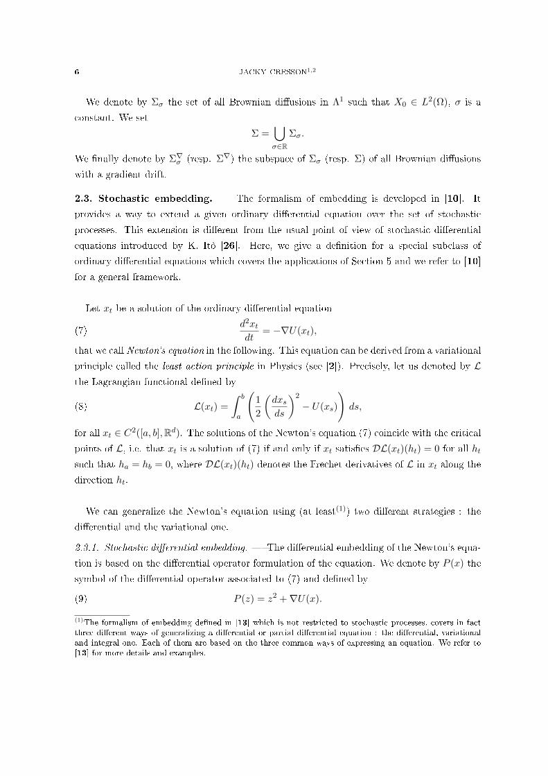
2.3. Stochastic embedding. The formalism of embedding is developed in [10]. It

provides a way to extend a given ordinary dierential equation over the set of stochastic

processes. This extension is dierent from the usual point of view of stochastic dierential

equations introduced by K. Itô [26]. Here, we give a denition for a special subclass of

ordinary dierential equations which covers the applications of Section 5 and we refer to [10]

for a general framework.

Let xt be a solution of the ordinary dierential equation

(7)d2xtdt

= −∇U(xt),

that we call Newton's equation in the following. This equation can be derived from a variational

principle called the least action principle in Physics (see [2]). Precisely, let us denoted by Lthe Lagrangian functional dened by

(8) L(xt) =

∫ b

a

(1

2

(dxsds

)2

− U(xs)

)ds,

for all xt ∈ C2([a, b],Rd). The solutions of the Newton's equation (7) coincide with the critical

points of L, i.e. that xt is a solution of (7) if and only if xt satises DL(xt)(ht) = 0 for all ht

such that ha = hb = 0, where DL(xt)(ht) denotes the Frechet derivatives of L in xt along the

direction ht.

We can generalize the Newton's equation using (at least(1)) two dierent strategies : the

dierential and the variational one.

2.3.1. Stochastic dierential embedding. The dierential embedding of the Newton's equa-

tion is based on the dierential operator formulation of the equation. We denote by P (x) the

symbol of the dierential operator associated to (7) and dened by

(9) P (z) = z2 +∇U(x).

(1)The formalism of embedding dened in [13] which is not restricted to stochastic processes, covers in factthree dierent ways of generalizing a dierential or partial dierential equation : the dierential, variationaland integral one. Each of them are based on the three common ways of expressing an equation. We refer to[13] for more details and examples.


The Newton's equation is then given by

(10) P

(d

dt

).xt = 0.

We can dened the dierential operator on the set of stochastic processes as long as we have

a notion of derivative and functional.

Let a : Rd → Rm be a function. A natural extension of a over stochastic processes is given

by

(11) a(Xt)(ω) = a(Xt(ω)),

for all ω ∈ Ω. Using this denition, we can dene the following stochastic version of the

Newton's equation :

Denition 2. The stochastic dierential embedding of equation (10) is dened by for all

Xt ∈ Λ3 by

(12) P (Dµ) .Xt = 0.

The previous construction can be generalized to arbitrary dierential operators. We refer

to [10] for more details.

Remark 2. The principle of taking the symbol of a dierential operator and replacing the

classical derivative by a new one is a well-known procedure in PDEs when dealing with PDEs

in the sense of Schwartz's distribution theory (see [56]). In this sense, the generalization of

a classical PDE to Schwartz's distributions is a particular example of a dierential embedding

(see [12] and [13]).

Remark 3. A main property of this stochastic extension of a dierential equation is that

it reduces to the classical equation over the set π(Cn) where n is the order of the dierential

operator. This remark justies also the terminology of embedding : the initial equation is

contained in the extended one. In particular, this stochastic extension does not coincide with

the classical theory of stochastic dierential equations due to K. Ito. This comes from the

fact that Ito's strategy does not use the dierential formulation of a dierential equation as a

starting point but the integral formulation thus providing a dierent theory.

As a consequence, the embedded Newton's equation is given by

(13) D2µXt = −∇U(Xt).

Particular cases of this equation have been studied by E. Nelson [38] and Thieullen-Zambrini

[52] for the case µ = i (see [52], Prop.2.7). It must be noted that we have just dened the

stochastic analogue of the classical derivative in order to generalize our dierential equation,

8 JACKY CRESSON1,2

i.e. when dealing with a given stochastic process, only a stochastic notion of speed is given. In

particular, no denition of a stochastic acceleration is needed in order to derive this equation

as its form is xed by the stochastic dierential embedding.

2.3.2. Stochastic analogue of dynamical quantities : speed and acceleration. The two ba-

sic quantities allowing to write the fundamental law of dynamics for forces deriving from a

potential U

(14) a = −∇U(x),

is the notion of speed v and acceleration a for a particle. If x(t) denotes the motion of the

particle, we have by denition

(15) v =dx

dta =

d2x

dt2.

For a stochastic process X the natural analogues are given by

(16) V = DX, A = D2X.

As the denition of the stochastic speed is xed, i.e. when the real number µ is given, then

the notion of stochastic acceleration is also xed by substitution of D instead of d/dt. This

denition for a stochastic acceleration follows then from the dierential stochastic embedding

procedure, i.e. by a pure algebraic procedure.

Remark 4. In ([38], p.81-82) E. Nelson introduces a denition of a stochastic accelera-

tion which does not follows from the denition of a stochastic speed as in our case using the

stochastic dierential embedding. Indeed, Nelson looks for expressions involving both the back-

ward anf forward Nelson's derivatives which are quadratic. He then makes some assumptions

in order to select a denition of acceleration which is in agreement with what we are waiting

for in specic stochastic systems. We refer to ([10], Remark 1.4, p.13-14) for more details.

Denition 16 is interesting for two reasons :

This choice keeps the coherence between a direct stochastic analogue of the fundamental

law of dynamics which can be written

(17) A = −∇U(X),

and the dierential stochastic embedding dened in the previous Section. As a conse-

quence, we can formulate a direct stochastic analogue of the laws of dynamics.

We can easily compute

(18) D2i =

DD∗ +D∗D

2+ i

D2 −D2∗

2.


The real part of D2 coincides with the notion of mean acceleration introduced by Nelson

[38] in his dynamical theory of the Brownian motion, for which he had conjectured that

it is the more relevant quantity describing an acceleration on Brownian diusions.

Remark 5. The previous remark answers the objection of L. Nottale [45], p. 385 about

the work of S. Albeverio and al. [3]. They have used the theory of Nelson about stochastic

mechanics [38] to write the equations of motion of a particle in a protoplanetary nebula (see

also Section 5.1). E. Nelson [38] as well as S. Albeverio and al. ([3], p. 367) have to postulate

the form of the mean acceleration. This is not the case in the present framework as the

analogue of the acceleration is xed by the stochastic embedding to be D2.

2.3.3. Stochastic variational embedding. Another point of view is to dene the stochastic

analogue of equation (7) using the variational characterization. The Lagrangian functional

L can be extended to stochastic processes easily. Indeed, we rst remark that the quantity1

2

(dxsds

)2

−U(xs) keep sense over stochastic processes replacingd

dtby the stochastic derivative

Dµ. We then dene the following stochastic analogue of the Lagrangian functional (8) :

Denition 3. The stochastic embedded version of the Lagrangian functional L dened by

(8) denoted by Lstoc is given for all Xt ∈ Λ3 by

(19) Lstoc(Xt) = E

[∫ b

a

(1

2D2µXs − U(Xs)

)ds

].

Remark 6. More generally, if L(t, x, v) denotes a Lagrangian function over R× Rd × Rd

and

(20) L(x) =

∫ b

aL(s, x(s), dx/dt)(s) ds,

the associated Lagrangian functional, the stochastic analogue is given by

(21) Lstoc(Xt) = E

[∫ b

aL(s,Xs,DµXs) ds

].

The form of the functional is then xed by the formalism of stochastic embedding.

It is natural to look for the Frechet derivative of Lstoc in a direction Ht ∈ V ⊂ Λ1 denoted

by DLstoc(Xt)(Ht). The set V is the set of variations. We use the following terminology :

Denition 4. A process Xt ∈ Λ3 is a V -critical process of the functional Lstoc if

DLstoc(Xt)(Ht) = 0 for all Ht ∈ V .

Using ([10], Thm.3.1 p.33) we have the following theorem :

10 JACKY CRESSON1,2

Theorem 2. A necessary and sucient condition for a process X ∈ Λ3 to be a Λ1-critical

process of the functional Lstoc is that it satises

D−µDµXt = −∇U(Xt)(22)

The stochastic embedded Newton's equation coincides with (22) only when µ = 0.

However, if we change the set of variations using the space of Nelson dierentiable processes:

(23) N1 = X ∈ Λ1, DX = D∗X.

We obtain the following partial result (see [10], Lemma 3.4 p.34) :

Proposition 2. A solution of the equation

D2µXt = −∇U(Xt),(24)

is a N1-critical process for the functional Lstoc

We have not been able to prove the converse of this lemma for N1-variations.

2.4. Coherence of stochastic embedding. The two previous approaches to deal with

an extension of a given ordinary dierential equation over stochastic processes are natural.

However, as the least-action principle is a rst principle of Physics, it is certainly preferable

to keep track of this structure in the stochastic case. The coherence problem introduced in

[10] is to determine when the dierential and variational stochastic embedding coincide. The

previous results can be summarized in the following Theorem :

Theorem 3. The dierential and variational embedding of the Newton's equation coincide

if and only if µ = 0.

If µ 6= 0 we have only a partial result, as the stochastic Newton's equation does not char-

acterize the critical point of the stochastic functional Lstoc over N 1.

2.5. Lifting of symmetries and a stochastic Noether theorem. In the two previous

Sections, we have discussed two distinct generalizations, dierential and variational, of a given

classical dierential equation and in which case they provide the same extension to stochastic

processes. The "natural" character of the generalized equation is based on the preservation

of a given specic property : the algebro-dierential structure in the case of the dierential

embedding and the fact to be a critical point of a functional in the variational case. Of course,

many other properties of a given equation are important and suitable to be preserved. For

instance, symmetries play an important role in the dynamics as they induce the existence

of rst integrals by the classical Noether theorem (see for example [2], p.88). First integrals


constrain the behaviour of the solutions of the equation. A natural demand is then to preserve

as far as possible the symmetries of the initial system under an embedding.

This problem was discussed in ([10] and [11]) in the context of the stochastic embedding

of Lagrangian systems. A related but dierent approach is given by Thieullen and Zambrini

in [53]. We give here a short account of these results.

2.5.1. First integrals of stochastic dynamical systems. A denition of rst integrals for

stochastic dynamical systems obtained by the stochastic embedding is the following (see [11],

Denition 4.4, p. 263) :

Denition 5. Let X ∈ Λ1 be a solution of the stochastic Newton's equation. The map

I : Λ1 → C0(R,C) is a rst integral for X ifd

dtI(X)t = 0.

Other denitions of rst integrals can be given. We refer to ([11], p.262-263 and [10], §.7,p. 39-40) for a discussion, in particular a comparison with Thieullen-Zambrini [53].

2.5.2. Stochastic lifting of symmetries. A stochastic embedding provided a natural stochas-

tic counter part to classical functions. As a consequence, we obtain the following stochastic

lifted notion of one parameter group of dieomorphisms.

Denition 6. Let φ : Rd → Rd be a dieomorphism. The stochastic suspension of φ is

the mapping φstoc : Λ0 → Λ0 dened for all X ∈ Λ0 by φstoc(X)t(ω) = φ(Xt(ω)). We denote

by Φ = φss∈R a one parameter group of dieomorphisms φs : Rd −→ Rd. The associated

stochastic lifted group of dieomorphisms Φstoc is dened byφstocs

s∈R.

A one parameter group of dieomorphisms Φ = φss∈R is said to be admissible if for all

s ∈ R, φs ∈ C2, (s, x)→ ∂xφs(x) ∈ C3 and formula (6) is valid for all f = φs, s ∈ R.

2.5.3. Stochastic invariance. A stochastic Lagrangian functional is said to be invariant

under a stochastic lifted one parameter group of dieomorphisms Φstoc if for all X ∈ Λ1, we

have L(φstocs (X),D

(φstocs (X)

)) = L(X,D).

The notion of invariance introduced in Thieullen-Zambrini (see [53], p.313) can be formu-

lated using our notion of stochastic lifted group of dieomorphisms. The stochastic invariance

dened by Yasue (see [60], p.332, formula (3.1)) is dierent. We refer to ([10], Remark 3.3,

p.37) for more details.

A natural question in the embedding formalism is to know whether or not a group of

symmetries is preserved under the stochastic embedding :

12 JACKY CRESSON1,2

Problem 1 (Persistence of invariance). Assume that a Lagrangian L is invariant un-

der a group of symmetries φss∈R. Do we have the stochastic invariance of the Lagrangian

L under the stochastic lifted one parameter group of dieomorphisms φstocs s∈R?

A general solution of this problem is out of reach for the moment. In the following, we give

a partial solution to this problem following our previous approach to the non-dierentiable

case [14].

Denition 7 (Strong invariance). Let Φ = φss∈R be a one parameter group of dif-

feomorphisms. An admissible Lagrangian L is said to be strongly invariant under the action

of Φ if

L(t, x, v) = L(t, φs(x), φs(v)), ∀s ∈ R, ∀t ∈ I, ∀x ∈ Rd, ∀v ∈ Rd.

As an example we can consider the following Lagrangian L, given by:

L(t, x, v) =1

2‖v‖2 − 1

‖x‖2.

If φs is a rotation, φs(x) := eisθx, then the Lagrangian L is strongly invariant.

The main property that the stochastic lifted group of dieomorphisms must satisfy is the

following commutation property :

Denition 8 (D-commutation). Let Φ = φss∈R be a one parameter group of dieo-

morphisms. We say that the associated stochastic lifted group satises the D-commutationproperty, if

(25) D(φstocs (X)t) = φstoc

s

(D(X)t

), ∀s ∈ R, ∀t ∈ R.

Using these two notions, we have the following sucient condition for persistence of invari-

ance under stochastisation :

Theorem 4. Let L be an admissible Lagrangian system, strongly invariant under a one

parameter group of dieomorphisms Φ = φss∈R satisfying the commutation property. Then,

L is invariant under the stochastic lifted group of dieomorphisms φstocs s∈R.

Proof of Theorem 4. - Using the commutation property given by equation 25, we have

(26) L(φstocs X,D(φstoc

s X)) = L(φstocs X,φstoc

s (DX)).

By the strong invariance property, we obtain

(27) L(φs(Xt(ω)), φs ((DX)t(ω))) = L(Xt(ω), (DX)t(ω)), ∀ t ∈ I, ω ∈ Ω.

This concludes the proof. 2


The commutation property is satised by linear maps whose matrix coecients do not

depend on the time variable t, as for example rotations or translations.

2.5.4. Stochastic Noether's theorem. In [10] we prove the following version of a stochastic

Noether's theorem :

Theorem 5. Let L be an admissible lagrangian with all second derivatives bounded, and

invariant under a stochastic lifted one-parameter group of dieomorphisms Φstoc = φstocs

s∈R.

Let L be the associated functional dened by (21) on Ξ ∩ Λ1. Let X ∈ Ξ ∩ Λ1 be a Λ1-critical

point of L. Then, we haved

dtE

[∂vL ·

∂Y

∂s

∣∣∣∣s=0

]= 0,

where

(28) Ys = Φs(X).

We refer to ([10],p.38) for the proof.

2.5.5. An example : rotations and stochastisation. The previous theorem can be applied

in the following situation : We consider the Lagrangian system dened by

L(t, x, v) =1

2‖v‖2 − 1

‖x‖2.

We have already seen that L is strongly invariant under the group φs of rotations, φs(x) :=

eisθx. As the φs are linear maps whose matrix coecients do not depend on t, the commutation

property is easily satised for this group. As a consequence, the invariance of the initial

Lagrangian system under rotations is preserved under stochastisation.

The rst integrals associated to rotations in this system correspond to the components of

the angular momentum. The previous result implies that such quantities are also preserved

by stochastisation.

3. The Stochastisation hypothesis

In this Section using the previous stochastic embedding formalism, we state the stochasti-

sation hypothesis for a physical system. The strategy of the stochastic embedding can be

extended over arbitrary stochastic processes. However, our rst attempt in Section 2 deals

with diusion processes. In Section 3.3 we discuss this assumption. We prove in particular

that under general regularity assumptions the set of stochastic processes is the set of diusion

processes.

14 JACKY CRESSON1,2

3.1. The stochastisation hypothesis. The stochastisation hypothesis is a way to dene

a stochastic extension of a given ordinary dierential equation. The previous section has given

two natural extensions of ordinary dierential equations : the dierential and the variational

one.

The stochastic dierential embedding of an equation keeps the algebraic structure of the

equation in term of operators. As the dierential operator codes the dierent dynamical

eects, the conservation of this structure is by itself suitable.

The stochastic variational embedding is based on a rst principle of Physics : the least-

action principle. A main property of this characterization is that it does not depend on

the coordinates system on the contrary to the form of the dierential operator.

As a consequence, a stochastic extension of a given ordinary dierential equation must be

coherent in order to preserve both the dynamical and physical background of the equation.

The two results of Section 2.4 give a strong support to the µ = 0 case. In any cases, Proposition

2 ensures that the stochastic dierential embedding preserves in a weak sense the least-action

principle. The main principle of our extension can be summarized in the following diagram :

(29) L

L.A.P.

Stochastisation // Lstoc

S.L.A.P.

d2x

dt2= −∇U(x)

Stochastisation// D2Xt = −∇U(Xt),

where the acronyms L.A.P. and S.L.A.P. are for Least Action Principle and Stochastic Least

Action Principle in the sense of Proposition 2. The word stochastisation means that we apply

the stochastic embedding.

The Stochastisation hypothesis can now be formulated :

Stochastisation Hypothesis : Let xt be a physical process governed by a given ordinary

dierential equation. The stochastic extension of this equation is given by the dierential

stochastic embedding of the equation.

There exist already many ways of generalizing dierential equations over stochastic pro-

cesses, the most common one being to add a noise to the equation in integral form and to

interpret the corresponding object using K. Itô theory [26] of stochastic dierential equa-

tions. However, no analogue of the coherence between the stochastic dynamical/variational

formulations of a given equation has been formulated in this case.


3.2. Discussion of the stochastisation hypothesis. In this Section, I would like

to make only few comments on the physical background underlying the stochastisation

hypothesis. This discussion is informal. However, it oers some ideas explaining the choice

we have made in the formulation of the stochastisation hypothesis.

In the stochastisation hypothesis a specic role is given to the underlying classical dieren-

tial equation representing the motion or behaviour of a quantity under the law of Physics. The

formulation of a physical law is made using a given mathematical framework. The mathemat-

ical framework by itself possesses constrains. For example, classical mechanics is formulated

using the classical dierential calculus. However, the underlying law applies by denition to

the real world. In the real world the limitations imposed by the mathematical framework

do not need to be satised. However, even if the law applies to (a priori) very complicated

(at least suciently in order to describe the underlying motion) quantities (in our setting for

example : the motion of a particle must be described by a stochastic process and not by a

smooth function), the only way to have access to this law is to rst check the formulation in

very particular cases where the behaviour is very regular. The classical behaviours are then

understood as good conditions under which the form of the laws of Nature can be found, or

in other words, the form of the fundamental equations associated to these laws.

The fact that the form of the equation is meaningful can be seen as a consequence of an

extended form of the relativity principle in Physics which can be roughly formulated as follows

: equations of physics must keep the same forms under admissible family of transformations.

This is for example explicitly used by Nottale ([40], p.195-196) in his approach to quantum

mechanics via the scale relativity theory. The characterisation of the admissible set of trans-

formations is of course not always easy. We refer to the classical work of Levy-Leblond [32]

for the classical case of special relativity and to [8] for the scale relativity case following the

idea of Nottale [40].

Naturally, all these points and arguments can be discussed and improved. However, I

believe that they can be useful to construct a meaningful formalism for the laws of physics

over stochastic processes. The previous point of view is also related to Prigogine approach to

chaotic dynamical systems as exposed for example in his book "The laws of Chaos" [47].

3.3. Stochastic processes and stochastisation : diusion processes ? In this Sec-

tion, we prove that natural regularity conditions on the process X that we must characterize

to model a given system yield to the structure of diusion.

16 JACKY CRESSON1,2

The hypothesis that X has continuous paths and is a Markov process are relevant for many

physical systems. To go further, one can add a rst order regularity condition for the averages

of suitable functionals of X: Namely the quantity

(30)Exf(Xt)− f(x)

t

converges for all x ∈ Rd and all f ∈ C∞0 (Rd) when t ↓ 0. As pointed out in [25] e.g., one

obtains the existence of a drift coecient b and a covariance matrix a:

limt↓0

Ex[Xt − x]

t= b(x)(31)

limt↓0

Ex[(Xt − x)t(Xt − x)]

t= a(x).(32)

These equalities are the starting point of diusion theory. See Denition 1.1 p.282 in [25] or

Denition 1.2 p.110 in [55]. A precise theorem is given in [38] p.77 concerning the structure

of X when assuming the conditions (31) and (32) for a Markov process. Then X has to solve a

stochastic dierential equation. The relationship between diusions and solutions of stochastic

dierential equations is one of the crucial points of Ito's Theory. We refer to Chap.V in [25]

or Chap.5 in [55] regarding the involved results.

In our framework, we have to point out that the hypothesis of choosing Brownian diu-

sions arises from regularity conditions on the process. These conditions can be seen as a rst

requirement to write an embedded equation; Particularly, the condition (31) ensures the ex-

istence of the rst order stochastic derivative of X with respect to its present. Moreover, the

drift b will be unknown in an embedded equation.

4. The stochastisation hypothesis and the Newton's equation

We discuss the application of the stochastisation hypothesis for the Newton's equation. In

this case, depending on the assumption about the underlying set of stochastic processes, we

provide a characterisation of the solutions of the associated stochastic Lagrangian systems

using PDEs of the Schrödinger type.

4.1. The stochastic Newton equation. In [10] we have proved that the solutions of

the stochastic Newton's equation (13) possess a density pt satisfying the linear Schrödinger

equation as long as we restrict our attention on diusions with gradient drift. Using the

characterization of gradient drift diusions obtained by S. Darses and I. Nourdin [17], we can

cancel this restriction.


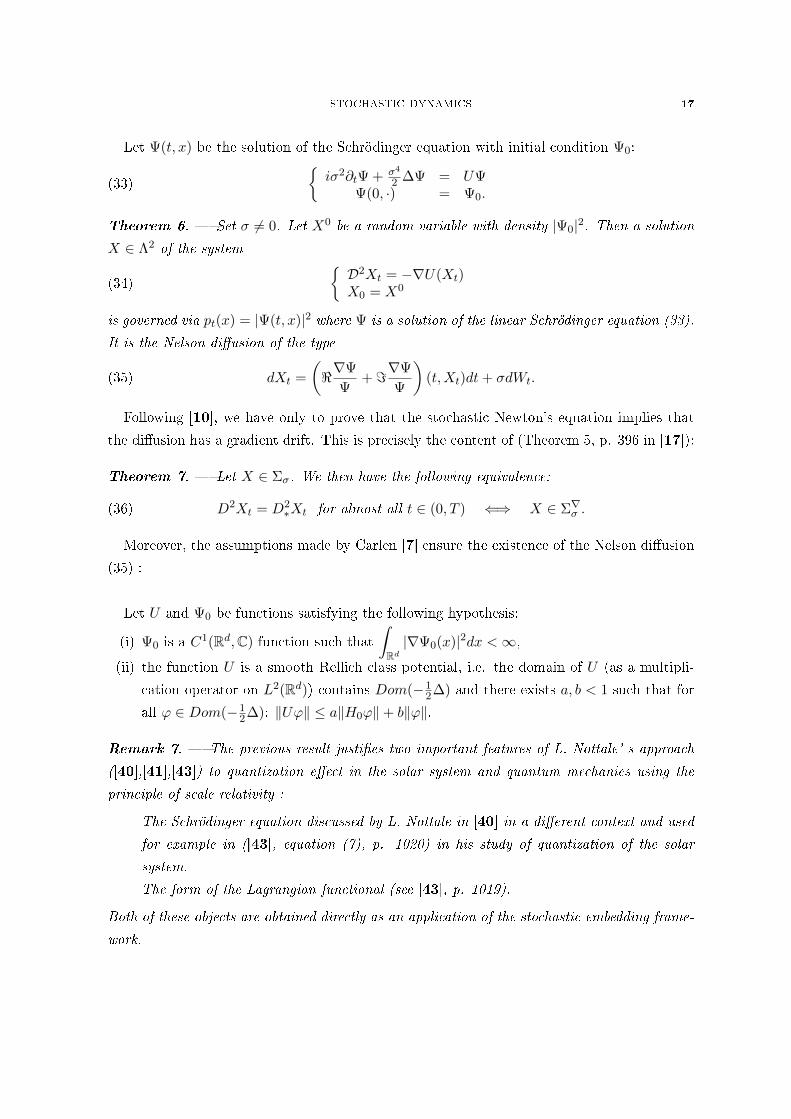
Let Ψ(t, x) be the solution of the Schrödinger equation with initial condition Ψ0:

(33)

iσ2∂tΨ + σ4

2 ∆Ψ = UΨΨ(0, ·) = Ψ0.

Theorem 6. Set σ 6= 0. Let X0 be a random variable with density |Ψ0|2. Then a solution

X ∈ Λ2 of the system

(34)

D2Xt = −∇U(Xt)X0 = X0

is governed via pt(x) = |Ψ(t, x)|2 where Ψ is a solution of the linear Schrödinger equation (33).

It is the Nelson diusion of the type

(35) dXt =

(<∇Ψ

Ψ+ =∇Ψ

Ψ

)(t,Xt)dt+ σdWt.

Following [10], we have only to prove that the stochastic Newton's equation implies that

the diusion has a gradient drift. This is precisely the content of (Theorem 5, p. 396 in [17]):

Theorem 7. Let X ∈ Σσ. We then have the following equivalence:

(36) D2Xt = D2∗Xt for almost all t ∈ (0, T ) ⇐⇒ X ∈ Σ∇σ .

Moreover, the assumptions made by Carlen [7] ensure the existence of the Nelson diusion

(35) :

Let U and Ψ0 be functions satisfying the following hypothesis:

(i) Ψ0 is a C1(Rd,C) function such that

∫Rd|∇Ψ0(x)|2dx <∞,

(ii) the function U is a smooth Rellich class potential, i.e. the domain of U (as a multipli-

cation operator on L2(Rd)) contains Dom(−12∆) and there exists a, b < 1 such that for

all ϕ ∈ Dom(−12∆): ‖Uϕ‖ ≤ a‖H0ϕ‖+ b‖ϕ‖.

Remark 7. The previous result justies two important features of L. Nottale' s approach

([40],[41],[43]) to quantization eect in the solar system and quantum mechanics using the

principle of scale relativity :

The Schrödinger equation discussed by L. Nottale in [40] in a dierent context and used

for example in ([43], equation (7), p. 1020) in his study of quantization of the solar

system.

The form of the Lagrangian functional (see [43], p. 1019).

Both of these objects are obtained directly as an application of the stochastic embedding frame-

work.

18 JACKY CRESSON1,2

Remark 8. In order to derive the previous equation in the context of the dynamics of a

protoplanetary nebula, S. Albeverio and al. ([3], p.367) make an assumption of time symmetry

in a stochastic sense which is

(37) −DXt = D∗Xt.

This assumption is dicult to justify as collisions usually lead to irreversible systems via

dissipation of energy. However, they noted that this equation can also be obtained under the

assumption that the diusions have gradient drift (see [3], Remark p. 368). In our setting,

no assumption is made on the set of diusion processes except that they satisfy the stochastic

embedded Newton's equation. This equation induces a gradient drift structure on the diusion

processes which are solutions.

The previous derivation without the time symmetry assumption answers an objection made

by L. Nottale (see [43] p.385) on the approach of S. Albeverio and al. [3]. In [43] the breaking

of time reversibility is of fundamental importance.

4.2. The reversible stochastic Newton's equation. Many physical problems possess

a fundamental property called reversibility, i.e. that if xt is a solution of the equation then x−t

is a solution of the same equation. This is for example the case of the Newton's equation. A

natural demand is then to extend the equation over the set of stochastic processes conserving

this property. Of course, the notion of reverse solution is not always easy to dene and

we prefer to use an algebraic characterization, saying that the operator is invariant under

the substitution ofd

dtby − d

dt. In the framework of the stochastic derivatives introduced in

Section 2.2, this substitution is the analogue of replacing Dµ by −D−µ. Using the denition

of Dµ it is easy to see that we preserve the reversibility property of the equation if and only

if µ = 0.

We now consider the following equation

(38) D20Xt = −∇U(Xt).

We want to characterize particular diusion solutions of (38). We are interested in solutions

having a gradient drift and belonging to Σσ. By making the same Nelson change of variables,

we obtain that Ψ has to solve a non-linear Schrodinger equation. We have to note that

Misawa and Yasue [35] have already introduced the operator D0 when they want to put

Nelson's stochastic mechanics into a lagrangian setting using D0. To this end, they modied

the Newtonian potential by an "adequate" term. Here we can relate the equation (38) to a

singular non linear Schrodinger equation:


Theorem 8. Let X ∈ Σ∇σ be a gradient diusion solution of (38). The density of this

solution is governed via pt(x) = |Ψ(t, x)|2 where Ψ is a solution of the nonlinear Schrödinger

equation:

(39) iσ2∂tΨ + σ2 Ψ

|Ψ|∆|Ψ|+ σ4

2∆Ψ = UΨ.

Proof. Let us make again the change of variable Ψ = eR+iS

σ2 where

∇R =σ2

2

∇pp,(40)

∇S = b− σ2

2

∇pp

= D0Xt.(41)

So D20Xt = ∂t∇S + (∂x∇S)∇S. We have:

(42) σ4 ∆Ψ

Ψ= σ2(∆R+ i∆S) + 2i∇R · ∇S + |∇R|2 − |∇S|2.

Since ∇|∇S|2 = 2(∂x∇S)∇S and ∇S = σ2=∇ΨΨ , we can write

(43) D20Xt = −σ2<

(i∂t∇Ψ

Ψ+σ2

2∇∆Ψ

Ψ−∇∆R−∇|∇R|

2

σ2

)But

∇∆R+∇|∇R|2

σ2=σ2

2

(∆∇pp

+

(∂x∇pp

)∇pp

)

∇∆R+∇|∇R|2

σ2=

σ2

2

(∆∇pp

+

(∂x∇pp

)∇pp

)=

σ2

2

(∆∇|Ψ|2

|Ψ|2+

(∂x∇|Ψ|2

|Ψ|2

)∇|Ψ|2

|Ψ|2

)= σ2

(∆∇|Ψ||Ψ|

+ 2

(∂x∇|Ψ||Ψ|

)∇|Ψ||Ψ|

)= σ2∇∆|Ψ|

|Ψ|.

Since b is a gradient, we can again use the formula

D2Xt = iσ2∇

(∂tΨ

Ψ− iσ

2

2

∆Ψ

Ψ

)(t,Xt)

which is real, that is

=(iσ2∇

(∂tΨ

Ψ− iσ

2

2

∆Ψ

Ψ

))= 0.

Therefore

(44) D20Xt = −σ2

(i∂t∇Ψ

Ψ+σ2

2∇∆Ψ

Ψ− σ2∇∆|Ψ|

|Ψ|

).

Since D20Xt = −∇U(Xt), we then obtain by a suitable integration the desired nonlinear

Schrödinger equation.

20 JACKY CRESSON1,2

5. Application : organisation of planetary systems

In order to apply the stochastisation hypothesis, we must nd physical systems for which

something about the underlying set of stochastic processes can be said. Of course, using

dierent operators we can enlarge the class of stochastic processes which can be considered.

However, two examples related to the dynamics of planetary systems can be studied : the pro-

toplanetary nebula dynamics and the long term behaviour of the solar system. The following

Sections give details for these two cases.

5.1. Dynamics of a protoplanetary nebula. We follow the work of S. Albeverio and

al. [3] as well as J. Laskar [29] and L. Nottale [42]. In both of these models the main goal

is to derive the general features of the organization of planetary systems without a precise

mechanism for accretion. Our main problem in order to apply the stochastisation hypothesis is

to characterize the underlying set of stochastic processes for the dynamics of a protoplanetary

nebula. In the next Section, we discuss this problem following S. Albeverio and al. [3], J.

Laskar [29] and L. Nottale [42].

5.1.1. Model for the dynamics in a protoplanetary nebula. We rst make our basic as-

sumptions on the structure of the protoplanetary nebula :

Structural assumptions : A protoplanetary nebula is made of :

A central body of mass M acting by some potential U .

A gas of some particles called grains around the central body.

We also make some assumptions on the dynamics of grains :

Dynamical assumptions : The motion of a given grain is governed by :

The potential U .

Collisions between grains.

The main point is of course to precise the nature of the collisions between grains. This is

the subject of the next Section.

5.1.2. On the nature of collisions. In the following, we make a simple assumption on

the nature of collisions which enables us to use the results of Section 4. However, the same

framework can be used under more general assumptions.


Assumptions on collisions : We assume that the collisions are :

Randomly distributed

Isotropic

Homogeneous

As a consequence of isotropy and homogeneity, we can model the randomness by a white

noise (see [3], p. 366). Hence, the typical motion of a grain can be modelled by a diu-

sion process with a constant diusion coecient (due to isotropy and homogeneity). These

assumptions then induce that we work with diusion processes in Σσ, σ ∈ R.

5.1.3. Mechanisms for connements. The previous Section allows us to use the reasoning

made by S. Albeverio and al. [3] and used also by L. Nottale [41] in order to prove that the

dynamics of a protoplanetary nebula naturally leads to formation of structures which follow

a simple rule. We give a short reminder of the results described in details in Albeverio and

al. ([4],§.2, p. 193-197) concerning the formation of impenetrable barriers.

We denote by

(45) Bψ =x ∈ R3 , ψ(x) = 0

.

Let Xt be a process starting in x 6∈ Bψ. Then under general assumptions on U , one can

prove that Xt never reaches Bψ. We can then dene disjoint connected regions Λn such that

(46) R3 = Bψ ∪

(⋃n

Λn

).

The previous result on Bψ leads to the following connement property :

Connement property : If Xt is a process starting in x ∈ Λn, then Xt ∈ Λn for all t.

This mechanism is already used in quantum mechanics.

Remark 9. In the paper of J. Laskar [29] the organisation of the system is related to the

conservation of the angular momentum decit (AMD) for the averaged equations, the main

remark being that the erratic wandering of orbits are still constrained by the conservation of

energy and angular momentum. As noticed by J. Laskar ([28],p.I.11 and [29], p.3243) this

provides a kind of connement property using the fact that the motion of the large planets is

very regular. Indeed, a large excursion of the inner planets would induce a big variation of the

angular momentum for the outer planets, which is more or less constant.

22 JACKY CRESSON1,2

Remark 10. As proved in Section 2.5.5, the stochastic embedding preserved the invariance

of the Lagrangian under rotations and as a consequence, using the stochastic Noether's theorem,

the components of the angular momentum are also rst integrals for the stochastic Lagrangian

system. The previous reasoning of J. Laskar can then be applied in our stochastic setting.

5.1.4. Law of repartition for planetary orbits. We do not reproduce here the computations

and remarks which lead the law of repartition for planetary orbits using the Schrödinger

equation. These arguments can be found in L. Nottale [42] and S. Albeverio and al. [4]. The

distribution of the distances of planets takes the form

(47)√a = n

(1 +

1

2n

)1/2√a0,

or

(48)√a = n

2σ√gM

,

where

(49)√a0 =

4σ2

gM,

depending on the fact that one considers the mean distance or the peak of probability density.

For homogeneity reasons the constant σ must have the dimension of a mass. However, the

expected form of this constant is not given in our setting. L. Nottale ([43], p.1021), using

arguments related to the principle of equivalence, propose to look for this constant in the

following form :

(50) σ =gM

2ω0,

where ω0 has the dimension of a velocity.

5.2. Long term behaviour of the solar system. The main problem here is to give

some prediction about the long term behaviour of the solar system. As noticed by J. Laskar

([28], p. L9) as the motion of the solar system is chaotic with a Lyapounov time of about 5 Myr

a numerical integration must be only "considered as an indication of its possible behaviour,

and cannot pretend to be the description of its actual motion.". As a consequence, one must

perform many numerical integrations in order to obtain a global view of the dynamics of the

solar system. In this Section, using the numerical results of J. Laskar on the chaotic behaviour

of the solar system, we bypass this problem by including the randomness induced by chaos

using the stochastisation hypothesis. Doing so, we must divide the solar system in two parts

: the large planets and the inner planets due to their dierent dynamical behaviour. We then


obtain again a law of repartition for the semimajor axes of the planets of the solar system

which follow a n2 power law for the outer and inner planetary system.

5.2.1. Chaos and Stochastic processes. The long term behaviour of the solar system is

chaotic. Following J. Laskar ([29]) it has the following consequence : Since the characteristic

time scale for the divergence of nearby orbits in the Solar system is approximately 5 Myr,

the orbital evolution of the planets becomes practically unpredictable after 100 Myr. Thus in

the long term, the motion of the solar system may be described by a random process, where

orbits wander erratically in a chaotic zone.". It is well known that in some cases, the long

term dynamics can be associated to diusion processes like for example in the Lorenz gas [61]

or some problems of instability of Hamiltonian systems [49]. In the following, we make the

assumption that the set of stochastic processes is a subset of diusion processes.

For more general assumptions, we refer to the work of G. Zaslavsky [61] on Hamiltonian

Chaos and Fractional dynamics which describes the possible characteristics of these stochastic

processes. For a work in the spirit of the stochastisation hypothesis about Hamiltonian Chaos,

we refer to [15].

Remark 11. In ([43], Section 2., p.1019) L. Nottale describes an heuristic method to

associate stochastic processes to a chaotic dynamical system. These heuristic arguments lead

to diusion processes. Indeed, the idea is to look for trajectories of the dynamical system over

a time which is far larger than the Lyapounov time. As a consequence, the resulting trajectory

"become" Markovian. General assumptions on the nature of the "uctuation" term lead then

to diusion processes.

5.2.2. Hierarchical structures. The main consequences of the numerical simulations made

by J. Laskar (see for example [28]) is a fundamental dierence between the dynamical

behaviour of the large planets and the inner planets (see [28], Fig. 1a, p.I.10). The motion

of the large planets is always (up to 200 Myr) very regular. On the other hand, the motion

of the inner planets is highly chaotic. As a consequence, the stochastisation hypothesis can

be applied using dierent diusion coecients σin and σout leading to two n2 power law for

the law of repartition for the semimajor axes of planets.

As remind by J. Laskar ([29], p. 3243), "it is well known that, if the Solar system is split

into sets of inner and outer planets, the seminmajor axes in each set follow a n2 power law

to a high degree of approximation" (see also [46],[50]). However, the previous splitting is

not assumed here, but follows from the stochastisation hypothesis as the underlying set of

stochastic processes have not the same diusion coecient.

24 JACKY CRESSON1,2

Remark 12. The theory developed by L. Nottale predicts a simple relation between these

two coecients :

(51) σout = 5σin.

This result can not follow from our formalism or the one used by J. Laskar and S. Albeverio

and al.

5.2.3. Is the Solar system stable ? Following the formulation of Moser [36], the problem of

the stability of the solar system is "the question of deciding whether the planetary system in

the distant future will keep the same form as it now has or whether after a long time perhaps

one or another of the planets might leave the solar system or whether collisions might even

lead to a catastrophic change."

From a mathematical point of view, the problem remains open. The Arnold's theorem

on the stability of n-body problem [1] does not give a signicant result as it applies under

unrealistic assumptions [24]. We refer to [19] for a complete proof of Arnold's theorem

following Herman's approach and in particular Section 8, p.61-62 for comments about the

stability of the solar system.

However, as pointed out by D. Mumford in ([37], §.6) the classical study of the n-body

problem is not sucient in order to have a more realistic model for the dynamics of planetary

motion. He says that Newton's laws of motion "... predicted wonderfully planetary motion

and, with perturbation, models the full set of planets for moderate period of time (e.g.,

maybe 108 years). But going out further (maybe to 109 years), the unmodeled eects begin

to add up and the approximation is not useful. So where does this leave the mathematical

study of the 3-body problem ? It makes the classical deterministic analysis of the 3-body

gravitational equations about as relevant to the world as the continuum hypothesis! A major

step in making the equation more relevant is to add a small stochastic term.".A study of a

stochastically perturbed two-body problem is done in [57].

Remark 13. To add a small stochastic term is not trivial and the signicance of this

adding is far from being well understood. In particular, the word "perturbation" seems to

be an abuse of language because the relation between the perturbed equation and the initial

deterministic equation is not so easy and far from intuition (I refer to the classical phenomenon

described by Wong and Zakai [59]) and also because the perturbed object and the initial one

do not belong to the same class of objects. A main problem also is in which sense we must

consider the perturbation (Itô or Stratonovich or something else intermediary). This problem

is fundamental in many applied problems, in particular in biology. It must be noted that in


the stochastic embedding framework, the classical equation and then the classical motion is

contained in the stochastic version.

From the numerical point of view Laskar [30] has proved that collisions can occur between

Mercury, Mars, Venus and the Earth. A review of several results of Laskar and others can be

found in Marmi [33] and Laskar [31]. The remark of Mumford applies again as no stochastic

perturbations of the equations have been taken into account for the numerical simulation of

the planetary motion. However, several other physical eects, in particular relativistic eects,

are integrated. In general, due to the Chaotic evolution of the solar system, we can only,

taking a set of initial conditions, provide some possible evolutions of the behaviour of the

planets. The probability of, for example, collisions between the Earth and Venus or Mercury

is not known. We can only say that such a collision is possible.

Our result provides a stability result in a probabilistic sense : regarding the solar system

over stochastic processes we loose a precise location of the planets. However, we obtain in

expectation the fact that the structure of this system remains the same. This does not prevent

the system to experience catastrophic behaviour as found by Laskar. Of course, our result

is only a rst step in a complete stochastic approach to the stability problem of the solar

system. We have to assume that the dynamical eect induced by the others planets, i.e.

mutual gravitational interaction, on the dynamical motion of a single planet can be modeled

by a particular class of stochastic processes at least over a sucient large amount of time.

A more realistic approach is certainly to consider the complete n-body problem, to make a

stochastic embedding and then a stochastic perturbation. We discuss in more details this

perspective in Section 6.2.3.

6. Conclusion

6.1. Summary. The previous approach to the organisation of planetary systems based on

the stochastisation hypothesis and the formalism of stochastic embedding provides a unied

treatment of several approaches, in particular the work of S. Albeverio and al. [3] and L.

Nottale [42]. As discussed in this paper, it allows us also to either simplify or reduce the

number of assumptions or to give complete proofs for partially justied results. We can list

the following points :

The form of the stochastic equation is xed by embedding and preserves the form as well

as the variational structure of the initial equation. This last result is not assumed but

proved.

26 JACKY CRESSON1,2

The form of the stochastic acceleration is xed by the theory and not assumed as in S.

Albeverio and al. [3].

The density probability of the stochastic processes which are solutions of the stochastic

Newton's equation is proved to satisfy the Schrödinger equation.

The same formalism can be applied to the long term behaviour of the Solar system

providing a stability result for planetary orbits contrary to all others known approaches.

Finally, only one assumption is used : the stochastisation hypothesis which is heuristically

used in many arguments but mathematically formalized in our framework using the

stochastic embedding formalism.

6.2. Perspectives.

6.2.1. Coalescent processes. This framework can be developed in several directions. The

main one is certainly to study the stochastic Newton's equation over more general stochastic

processes than diusion processes. In particular, with respect to the simple assumption made

in Section 5.1.2 and related to the accretion mechanisms, we can for example assume as in

J. Laskar ([29], p.3240) that when two small bodies of mass m1 and m2 collide, they form a

new one of mass m1 + m2. A natural choice for the underlying stochastic processes is then

given by coalescent processes (see for example [6]).

6.2.2. Statistics and gravitational structuration constant. Another important point is to

compute the constant of structure ω0 in the law (50) and the integers n for every Planet

of extrasolar planetary systems and to perform a statistical analysis in details. The main

point is to give a denitive conrmation for the existence of a universal constant governing

the organisation of gravitational structures predict by L. Nottale ([42],[44]). This result is

not predicted or discussed in the other approaches to the formation of planetary systems.

However, the statistical analysis of this problem is not simple and leads to many diculties.

For an example of the typical diculties related to this problem, we refer to B. Efron [18],

I.J. Good [22] and W. Hayes-S. Tremaine [23].

6.2.3. Stability of the solar system. As already discussed, the previous result on the ex-

istence of a law of repartition of planetary orbits gives a hint that the solar system is stable

in a probabilistic sense. Due to the Chaotic behaviour of the solar system, we can not hope

more that this result. Of course, as pointed out, many assumptions are not mathematically

proved, in particular the existence and properties of the stochastic processes associated to

the chaotic behaviour of the solar system are far from being characterized. In this paper, we

have only made assumptions which are satised by chaotic Hamiltonian systems under general


hypothesis. However, even if we manage to describe such class of processes, this result is by

itself not sucient. Indeed, we must also make a perturbation of the stochastic system which

is then described, as the underlying model is not complete. As a consequence, the problem is

to develop the stochastic theory of perturbations for stochastic dynamical systems obtained

by stochastic embedding.

References

[1] V.I. Arnold. Petits dénominateurs et problèmes de stabilité du mouvement en mécanique classiqueet céleste (en russe). Usp. Mat. Nauk. 18 (1963), 91192 (trad. anglaise, Russ. Math. Surv. 18(1963), 85193).

[2] Arnold V.I., Mathematical Methods of Classical Mechanics, 2d edition, Springer, 1989.

[3] Albeverio S., Blanchard Ph., Hoegh-Krohn R., A stochastic model for the orbits of planets andsatellites: an interpretation of Titius-Bode law, Expositiones Mathematicae 4, 363-373 (1983).

[4] Albeverio S., Blanchard Ph., Hoegh-Krohn R., Newtonian diusions and planets, with a remarkon non-standard Dirichlet forms and polymers,

[5] Arnold, Ludwig . Random dynamical systems. Springer Monographs in Mathematics. Springer-Verlag, Berlin, 1998. 586 pp.

[6] Bertoin J. J-F. Le Gall, Stochastic ows associated to coalescent processes, Probab. Th. Rel.Fields 126 (2003), 261-288.

[7] Eric A. Carlen. (1984) Conservative diusions. Comm. Math. Phys. 94, no 3, 293315.

[8] J. Cresson, Non-dierentiable deformations of Rn, International Journal of Geometric Methodsin Modern Physics, Vol. 3, no. 7 (2006) 1395-1415.

[9] J. Cresson and S. Darses (2006), Plongement stochastique des systèmes lagrangiens, C.R. Acad.Sci. Paris Ser. I 342 (5), 333-336.

[10] J. Cresson and S. Darses, Stochastic embedding of dynamical systems. J. Math. Phys.,48(7):072703, 54, 2007.

[11] J. Cresson, S. Darses, Théorème de Noether Stochastique, C.R. Acad. Sci. Paris, Ser. I 344 (2007)259-264

[12] J. Cresson, Introduction to embedding of Lagrangian systems, International Journal of Biomath-ematics and Biostatistics, Vol. 1, no. 1, 23-31, 2010

[13] J. Cresson, Introduction to embedding formalisms and Lagrangian PDEs, Lecture Notes TUMünchen, 2011.

[14] J. Cresson, I. Gre, A non-dierentiable Noether's theorem, J. Math. Phys. 52, 023513 (2011);doi:10.1063/1.3552936 (10 pages).

[15] J. Cresson and P. Inizan. About fractional Hamiltonian systems. Physica Scripta, T136:014007,2009.

[16] S. Darses and I. Nourdin (2006): Stochastic derivatives for fractional diusions. To appear inAnn. Probab.

[17] S. Darses and I. Nourdin, Dynamical properties and characterization of gradient drift diusions.Electron. Comm. Probab. 12 (2007) 390-400

[18] Efron B., Does an observed sequence of numbers follow a simple rule ? (another look at Bode'slaw), J. Am. Statist. Assoc. 66 (335), 552-559, 1971.

[19] Féjoz J., Démonstration du "théorème d'Arnold" sur la stabilité du système planétaire (d'aprèsM.Herman), Ergod. Th. and Dynam. Sys. (2004), 24, 1-62.

28 JACKY CRESSON1,2

[20] H. Föllmer (1984): Time reversal on Wiener space. Stochastic processes - mathematics andphysics (Bielefeld). Lecture Notes in Math. 1158, 119-129.

[21] E. Fournié, J.-M. Lasry, J. Lebuchoux, P.-L. Lions and N. Touzi (1999): Applications of Malliavincalculus to Monte Carlo methods in nance. Finance Stochast. 3, 391-412.

[22] Good I.J., A subjective evaluation of Bode's law and an objective" test for approximate numericalrationality, J. Am. Statis. Assoc. 64, 23-66, 1969.

[23] W. Hayes, S. Tremaine, Fitting selected random planetary systems to Titius-Bode laws, Icarus135, 549-557 (1998).

[24] M. Hénon. Exploration numérique du problème restreint IV. Masses égales, orbites non péri-odiques. Bull. Astronom. 3(1 :2) (1966), 49-66.

[25] I. Karatzas and S.E. Shreve (1991): Brownian Motion and Stochastic Calculus. Springer-Verlag,New York Second Edition.

[26] K. Itô, On stochastic dierential equations, Mem. Amer. Math. Soc. 4 (1951), 1-51.[27] A.N. Kolmogorov (1937): Zur Umkehrbarkeit der statistischen Naturgesetze. Math. Ann 113,

766-772.[28] Laskar J., Large-scale chaos in the solar system, Astron. Astrophys. 287, L9-L12 (1994).[29] Laskar J., On the spacing of planetary systems, Phys. Rev. Lett. 84? no. 15, 3240-3243, 2000.[30] J. Laskar, M. Gastineau, Existence of collisional trajectories of Mercury, Mars and Venus with

the Earth, Nature Vol. 459, 2009.[31] Jacques Laskar, Le Système solaire est-il stable ?, Séminaire Poincaré XIV (2010) 221-246.[32] Levy-Leblond J-M, One more derivation of the Lorentz transformation, Am. J. Phys. Vol. 44, No.

3, 1976, pp. 271-277.[33] Marmi, S., Chaotic behaviour in the solar system following J. Laskar, Séminaire Bourbaki, 51ème

année, 1998-1999, Paper No. 854.[34] A. Millet, D. Nualart and M. Sanz (1989): Integration by parts and time reversal for diusion

processes. Ann. Probab. 17, no. 1, 208238.[35] Misawa T., Yasue K., Canonical dynamical systems. J. Math. Phys. 28(11), 1987, 2569-2573.[36] Moser, J., Is the solar system stable?, Math. Intell. 1, 6571, 1978.[37] Mumford D., The dawning of the age of stochasticity, in Mathematics: Frontiers and perspectives,

V. Arnold, M. Atiyah, P. Lax, B. Mazur editors, AMS, 2000, 197-218.[38] E. Nelson (2001): Dynamical theory of Brownian motion. Princeton University Press. Second

edition. Available online at http://www.math.princeton.edu/∼nelson/books/bmotion.pdf.[39] Nelson E., Derivation of the Schrödinger equation from Newtonian mechanics, Physical Review,

Vol. 150, No. 4, 1079-1084 (1966).[40] Nottale L., Fractal Space-Time and Microphysics : towards a theory of Scale relativity, World

Scientic, 1993.[41] Nottale L, New formulation of stochastic mechanics. Application to chaos, in Chaos and diusion

in Hamiltonian systems", Proceedings of the fourth workshop in Astronomy and Astrophysics ofChamonix (France), 7-12 February 1994, Eds. D. Benest and C. Froeschlé (Editions Frontières),pp. 173-198 (1995).

[42] Nottale L., The quantization of the solar system, Astron. Astrophys. 315, L9, 1996.[43] Nottale L., Scale relativity and quantization of the solar system, Astronomy and Astrophysics.

322, 1018-1025 (1997).[44] Nottale L., Scale-relativity, Fractal space-time and gravitational structures, in "Fractals and

Beyond : complexity in the sciences", Ed. M.M. Novak, pp. 149-160, World Scientic, 1998.[45] Nottale L., La relativité dans tous ses états, Hachette littérature, 2000.[46] J.C. Pecker, E. Schatzman, Astrophysique générale, Masson, Paris, 1959.


[47] I. Prigogine, Les lois du chaos, Champs Flammarion, 1994.[48] S. Roelly and M. Thieullen (2005): Duality formula for the bridges of a Brownian diusion:

application to gradient drifts. Stochastic Process. Appl. 115, no. 10, 16771700.[49] Sauzin D., Exemples de diusion d'Arnold avec convergence vers un mouvement brownien,

Journées scientiques 2006 de l'Institut de Mécanique Céleste et de Calcul des éphémérides,Notes scientiques et techniques de l'Institut de Mécanique Céleste.

[50] O. Schmidt, in The origin of the Solar system : Soviet Research, 1925-1991, Edited by A.E. Levinand al., AIP, New York, 1995.

[51] Stroock, Daniel W. ; Varadhan, S. R. Srinivasa . Multidimensional diusion processes. Reprint ofthe 1997 edition. Classics in Mathematics. Springer-Verlag, Berlin, 2006. xii+338 pp.

[52] Thieullen, M. and Zambrini, J. C. (1997): Symmetries in the stochastic calculus of variations.Probab. Theory and Rel. Fields 107, no 3, 401427.

[53] Thieullen M. and Zambrini J.C, Probability and quantum symmetries I. The theorem of Noetherin Schrödinger's euclidean mechanics, Ann. Inst. Henri Poincaré, Physique Théorique, Vol. 67, 3,p. 297-338 (1997).

[54] Wu, Liming. Uniqueness of Nelson's diusions (1999). Probab. Theory Related Fields, 114, no.4, 549585.

[55] L.C.G. Rogers and D. Williams (1987). Diusions, Markov processes, and martingales. Vol. 2. Itôcalculus. Wiley Series in Probability and Mathematical Statistics: Probability and MathematicalStatistics. John Wiley and Sons, Inc., New York. 475 pp.

[56] L. Schwartz, Théorie des distributions, Publications de l'Institut de Mathématique de l'Universitéde Strasbourg, No. IX-X. Nouvelle édition, entiérement corrigée, refondue et augmentée, Her-mann, Paris, 1966.

[57] N Sharma and H Parthasarathy, Dynamics of a stochastically perturbed two-body problem, Proc.R. Soc. A 2007 463, 979-1003.

[58] J-C. Zambrini. Variational processes and stochastic versions of mechanics. J. Math. Phys. 27(1986), no. 9, 23072330.

[59] Wong E., Zakaï M., On the relationship between ordinary and stochastic dierential equations,Internat. J. Engin. Sci. 3, 213-229, 1965.

[60] K. Yassue, Stochastic calculus of variations, Journal of functional analysis 41, 327-340 (1981).[61] G.M. Zaslavsky. Hamiltonian Chaos & Fractional Dynamics. Oxford University Press, Oxford,

2005.[62] Zheng W.A., Meyer P.A., Quelques résultats de mécanique stochastique. Séminaire de Probabilités

XVIII, 223-243

Jacky Cresson1,2, 1 Laboratoire de Mathématiques Appliquées de Pau, Université de Pau et des Pays de

l'Adour, avenue de l'Université, BP 1155, 64013 Pau Cedex, France • 2 Institut de Mécanique Célesteet de Calcul des Éphémérides, Observatoire de Paris, 77 avenue Denfert-Rochereau, 75014 Paris, France

THE STOCHASTISATION HYPOTHESIS AND THE SPACING OF...

Documents

Transcript of THE STOCHASTISATION HYPOTHESIS AND THE SPACING OF...