
Statistical Mechanics Master de Physique fondamentale et ...
103
Statistical Mechanics Master de Physique fondamentale et appliquée – Spécialité : Champs, particules et matière Leticia F. Cugliandolo Laboratoire de Physique Théorique et Hautes Energies de Jussieu Laboratoire de Physique Théorique de l’Ecole Normale Supérieure Membre de l’Institut Universitaire de France [email protected] 20 November 2005 Abstract Ce cours présente une introduction à quelques problèmes d’intérêt actuel en mé- canique statistique. Chaque chapitre est focalisé sur un sujet. On expliqera ces sujet en s’appuyant sur les résultats d’expériences. On présentera leur modélisation ainsi qu’une sélection de méthodes théoriques utilisées pour leur étude. This document includes: (1) A detailed schedule of the lectures, TDs and exam. (2) A draft of the Lecture notes on Statistical Mechanics. It presents a summary of the material that will be described during the semester. They are certainly incom- plete and may contain errors. Hopefully, we shall improve it with the help of the students. (3) The TDs. 1
Transcript of Statistical Mechanics Master de Physique fondamentale et ...

Statistical Mechanics
Master de Physique fondamentale et appliquée –
Spécialité : Champs, particules et matière
Leticia F. Cugliandolo
Laboratoire de Physique Théorique et Hautes Energies de Jussieu
Laboratoire de Physique Théorique de l’Ecole Normale Supérieure
Membre de l’Institut Universitaire de France
20 November 2005
Abstract
Ce cours présente une introduction à quelques problèmes d’intérêt actuel en mé-canique statistique. Chaque chapitre est focalisé sur un sujet. On expliqera ces sujeten s’appuyant sur les résultats d’expériences. On présentera leur modélisation ainsiqu’une sélection de méthodes théoriques utilisées pour leur étude.
This document includes: (1) A detailed schedule of the lectures, TDs and exam.(2) A draft of the Lecture notes on Statistical Mechanics. It presents a summary ofthe material that will be described during the semester. They are certainly incom-plete and may contain errors. Hopefully, we shall improve it with the help of thestudents. (3) The TDs.
1
1 PROGRAMME
1 Programme
Les TDs sont conçus pour être faits à la maison après une aide donnée en cours. Leurssolutions devront être rendus et cela fera parti de la note finale.
1. Introduction Rappel des notions de probabilités et statistique [1, 2, 3, 4].
Quelques applications : l’expérience de Luria-Delbrück [5]; statistiques d’extrêmes [6,7]; un paradigme, le modèle d’Ising et ses applications interdisciplinaires [8, 9, 10,11, 12].
TD 1 : exercises simples de rappel.
Lecture : l’article de Luria-Delbrück [5]; structures dans l’univers [14].
2. Transitions de phase [8, 9, 10, 11, 12]
Exemples : vapeur-liquide, paramagnétique-ferromagnétique, DNA. Classificationdes transitions.
Approche de champ moyen.
Phénomènes critiques, invariance d’échelle, introduction au groupe de renormalisa-tion [10, 11, 13].
TD 2 : modèle d’Ising ferromagnétique complètement connecté avec des interactionsà p spins, (p = 2) transition de second ordre, (p > 2) transition de premier ordre.
Lecture : Transitions de phase, un exemple mécanique [15].
3. Désordre [16, 17, 18, 19, 20]
Définition de désordre recuit et désordre gelé (exemples). Leur traitement statis-tique.
Désordre gelé : effets de la frustration, auto-moyennage de l’énergie libre, introduc-tion à la méthode des repliques.
Exemples : verres de spin, potentiels aléatoires, réseau de neurones.
TD 3: La chaîne de spins avec des interactions désordonnées.
Lecture : Le problème de la rupture [21]
4. Processus stochastiques [22, 23]
Mouvement Brownien. L’équation maîtresse, l’approche de Langevin et Fokker-Planck.
TD 4 : Ratchets, application à l’electrophorèse.
5. Croissance de surfaces et d’interfaces [24]
Exemples. Rugosité. Lois d’échelle dynamiques.
Le ‘random deposition model’ : solution, limite continue et présentation des équa-tions de Edwards-Wilkinson et de Kardar-Parisi-Zhang.
TD 5 : Étude de l’équation d’Edwards-Wilkinson.
2

2 INTRODUCTION
2 Introduction
2.1 Background
Equilibrium Statistical Mechanics is a very well-established branch of theoretical physicsTogether with Quantum Mechanics, they form the basis of Modern Physics.
The goal of equilibrium statistical mechanics is to derive the thermodynamic functionsof state of a macroscopic system from the microscopic laws that determine the behaviourof its constituents. In particular, it explains the origin of thermodynamic – and intuitive– concepts like presure, temperature, heat, etc.
In Table 1 we recall the typical length, time and energy scales appearing in the micro-scopic and macroscopic World.
Micro Macro
dist (ℓ)Solid Gaz
10−10m 10−8m10−3m
# part (N) 1Solid Gaz
(
10−3
10−10
)d=3= 1021
(
10−3
10−8
)d=3= 1015
energy (E) 1 eV 1J ≈ 6 1018eV
time (t)Solid Gaz
h/1eV ≈ 6 10−14 s 10−9 s1 s
Table 1: Typical length, energy and time scales in the microscopic and macroscopic World.
A reference number is the number of Avogadro, NA = 6.02 1023; it counts the numberof atoms in a mol, i.e. 12gr of 12C, and it yields the order of magnitude of the number ofmolecules at a macroscopic level. The ionization energy of the Hydrogen atom is 13.6 eVand sets the energy scale in Table 1.
It is clear from the figures in Table 1 that, from a practical point of view, it would beimpossible to solve the equations of motion for each one of the N ≈ NA particles – let uskeep the discussion classical, including quantum mechanical effects would not change themain conclusions to be drawn henceforth – and derive from their solution the macroscopicbehaviour of the system. Moreover, the deterministic equations of motion may presenta very high sensitivity to the choice of the initial conditions – deterministic chaos – andthus the precise prediction of the evolution of the ensemble of microscopic constituentsbecomes unfeasible even from a more fundamental point of view.
The passage from the microscopic to the macroscopic is then done with the help ofStatistical methods, Probability Theory and, in particular, the Law of Large Numbers. Itassumes – and it has been quite well confirmed – that there are no big changes in thefundamental Laws of Nature when going through all these orders of magntide. However, anumber of new and interesting phenomena arise due to the unexpected collective behaviourof these many degrees of freedom. For example, phase transitions when varying an externalparameter occur; these are not due to a change in the form of the microscopic interactionsbut, rather, to the locking of the full system in special configurations.
Equilibrium statistical mechanics also makes another very important assumption that
3
2.2 This course 2 INTRODUCTION
we shall explain in more detail below: that of the equilibration of the macroscopic system.Some very interesting systems do not match this hypothesis. Still, one would like touse Probabilistic arguments to characterize their macroscopic behavior. This is possiblein a number of cases and we shall discuss some of them. Indeed, deriving a theoreticalframework to describe the behavior of macroscopic systems out of equilibrium is one thepresent major challenges in theoretical physics.
2.2 This course
In this set of lecture we shall discuss same problems in equilibrium and dynamic statisticalmechanics that either are not fully understood or receive the attention of researchers atpresent due to their application to problems of interest in physics and other areas ofscience. The plan of the set of lectures is the following:
In the first Chapter we recall some aspects of Probability Theory and Statistical Me-chanics. In Appendix A we recall the definition of a probability, its main properties, andthe main probability functions encountered in hard Science. In the main part of the textwe show the utility of Probability arguments by discussing the experiment of Luria andDelbrück – considered the founder of Molecular Biology, the authors received the NobelPrize in 1969 – and some aspects of the laws of large numbers and extreme value statistics.Basic features of the foundations of Statistical Mechanics are recalled next. Finally, wedefine the Ising model and list some of its more important properties that render it sucha standard model.
In the second Chapter we describe the theory of phase transitions: first we explain themean-field approach, and then we introduce fluctuations and show how the importanceof these led to the development of the renormalization group.
The third Chapter is devoted to the discussion of disorder and its effects in phasetransitions and low-temperature behavior. We briefly describe the three main routes todescribe these systems analytically: scaling, the replica method and functional renormal-ization group ideas.
In the last two Chapters we introduce time into the discussion. First, in Chapter 4we define stochastic processes, the Langevin and Fokker-Planck formalism and we brieflydiscuss the dynamics of macroscopic systems close to thermal equilibrium. Next, inChapter 5 we treat the problem of the random growth of a surface. We introduce somephysical examples and two simple models, we discuss the behavior in terms of scaling lawsand we also solve one of these models analytically while describing what fails in the otherand the need to use improved renormalization group ideas out of equilibrium.
It is clear that the correct explanation of all of these problems and alytical methodwould need many more hours of teaching. We shall only give the main ingredients of eachof them and provide the interested students with references to deepen their knowledge ofthese subjects. The cours is intimately related to the one of J-M di Meglio (first semester)and O. Martin (second semester).
4

3 BASIC NOTIONS
3 Basic notions
3.1 Applications of probability theory
3.1.1 The Luria-Delbrück experiment
This is a very cute example of the use of probability concepts – and more generality, of atraining in Physics! – in varied problems in Science.
This experiment provided the first proof of genetic mutation in bacteria. It works asfollows. Colonies of bacteria, typically including 109 members, are exposed to a virus thatkills most of them. However, after some time, some new bacteria appear showing thateither(i) some bacteria acquire resistance to the virus (adaptation, Lamarckian hypothesis), or(ii) their ancestors already possessed resistance via mutation,when they were exposed to the virus.
����
����
����
����
��������
����
����
����
����
�������������������������������������������������������������������������������������������������������������������������
�������������������������������������������������������������������������������������������������������������������������
�������������������������������������������������������������������������������������������������������������������������
�������������������������������������������������������������������������������������������������������������������������
������������������������������������������������������������������������
������������������������������������������������������������������������
�������������������������������������������������������������������������������������������
�������������������������������������������������������������������������������������������
������������������������������������������������������������������
������������������������������������������������������������������
������������������������������������������������������������������
������������������������������������������������������������������
��������������������������������������������
��������������������������������������������
��������������������������������������������
��������������������������������������������
���������������������������������
���������������������������������
���������������������������������
���������������������������������
���������������������������������
���������������������������������
������������������������������������
������������������������������������
��������������������������������������������
��������������������������������������������
��������������������������������������������
��������������������������������������������
���������������������������������
���������������������������������
���������������������������������
���������������������������������
���������������������������������
���������������������������������
���������������������������������
��������������������������������� ����
����������������������������������������
��������������������������������������������
��������������������������������������������
��������������������������������������������
��������������������������������������������
��������������������������������������������
������������������������������������������������
������������������������������������������������
���������������������������������
���������������������������������
���������������������������������
���������������������������������
���������������������������������
���������������������������������
���������������������������������
���������������������������������
������������������������������������
������������������������������������
���������������������������������
���������������������������������
���������������������������������
���������������������������������
���������������������������������
���������������������������������
x
x
Figure 1: A tree representing the growth of a colony of bacteria under the mutation hy-pothesis. Each level in the tree corresponds to a generation. Time grows going down alongthe vertical direction. The nodes represent individuals in the colonies. The individualsshown with a cross are the mutant ones. The individuals painted white are sensitive tothe virus while the ones painted black are resistant.
How can one distinguish between the two scenarii? It is clear that if the adaptivehypothesis held true, the spatial distribution of the resistant bacteria in the sample wouldbe uniform and, moreover, the number of resistant bacteria would not increase with theage of the sample. If, in contrast, the mutation hypothesis held true, then, the number ofresistant bacteria should be larger for an older sample and, they should appear in groupsof individuals related by inheritage. Luria developed an experimental analysis, based onthe smart use of Statistical analysis (see Appendix A) that allowed him to determine thatthe mutation hypothesis is correct.
Luria’s idea was to study finite-size sample-to-sample fluctuations to distinguish be-tween adaptation and mutation. Take a colony of bacteria of a given age, say it containsN individuals, and divide it in M samples with ≈ N/M individuals each. Expose noweach sample to virus and count how many resistant bacteria, nk with k = 1, . . . ,M , arein each of them. If the adaptation hypothesis is correct, all sample react in roughly the
5

3.1 Applications of probability theory 3 BASIC NOTIONS
same way, and n should be described by a Poisson distribution characterized by an av-erage that coincides with the mean-square deviation, 〈n 〉 = 〈 (n − 〈n 〉)2 〉 = µ, with µthe parameter of the Poisson distribution. If, instead, the mutation hypothesis is correctsome samples should have many more resistant bacteria than others. Thus, the mean-square-displacement should be much larger than the average.
Let us discuss the theory behind Luria’s argument in a bit more detail. Rememberthe usual calculation of the density fluctuations in a gas. Let N and V be the number ofparticles and volume of a gas and n be the number of particles in a very small volume vwithin the bulk, v ≪ V . Since the gas is uniform, the probability that any given particleis in v is just v/V and the probability that n given particles are in v is just (v/V )n.Similarly, the probability that a particle is not in v is 1 − v/V and the probability thatN − n particles are not in v is (1 − v/V )N−n. The probability of having any n particlesin v is given by the binomial formula:
P (n, v;N, V ) =N !
n!(N − n)!
(
v
V
)n (
1− v
V
)N−n
. (3.1)
The prefactor gives the number of ways of choosing n particles from the total number N .Now, this expression can be simplified, and becomes Poisson’s law, in the limits v ≪ V ,n≪ N :
P (n) =〈n〉ne−〈n〉
n!. (3.2)
(In the third factor one replaces the exponent N−n ∼ N ; the first factor is approximatedby using Stirling formula for the factorials, see Appendix [?]; and then 〈n〉 ≡ Nv/V asone can also verify by computing the average directly from this expression.) Note thatn can be very different from its mean value, 〈n〉 but it is still much smaller than N thathas been taken to infinity in this calculation. From this expression one can compute theaverage 〈n2〉 and the mean-square fluctuations of the number of particles
σ2 ≡ 〈n2〉 − 〈n〉2 = 〈n〉 . (3.3)
This is the main characteristics of the Poisson law exploited by Luria.Luria carried out these experiments and he found the desired result, the sample-to-
sample fluctuations were much larger than predicted from a Poisson distribution andhence he concluded that the mutation hypothesis was correct. In collaboration withDelbrück they refined the analysis and even found a way to estimate the mutation ratefrom their experimental observations. They got the Nobel Prize in Medicine in 1969.
3.1.2 Statistics of extremes
The statistics of extreme values is currently appearing in a number of interesting problemsin hard and applied Sciences. In all sorts of applications, accurate risk assessment relieson the effective evaluation of the extremal behavior of the process under study. Unlikemost of Statistics which tries to say something about typical behavior, Extreme ValueStatistics attempts to characterize unlikely behavior, or at least to say how unlikely thebehavior is. Applications include: flood risk assessment; financial risk management; in-surance assessment; setting industrial safety standards; the prediction of extreme weather
6
3.1 Applications of probability theory 3 BASIC NOTIONS
conditions. In the context of our lectures, we shall see Statistics of extremes appearing inPhase transitions and diffusion processes.
The mathematical question is the following. Let us study a sequence sN ≡ x1, . . . , xNof realizations of a random variable x with a probability distribution function p(x). Eachentry xi is an independent identically distributed random number. A natural question toask is what is the maximum value taken by x, i.e. what is xmax ≡ max(x1, x2, . . . , xN)?it is clear that xmax is itself a random variable (since if we drew different sequences sN wewould obtain different values of xmax). We then need to characterize xmax in probabilityand the quantity we need to determine is its probability distribution function, q(xmax).
This kind of question was raised in the context of studies funded by insurance compa-nies in the Netherlands... it was useful to know how high could it be a raise in the sealevel... Emil Gumbel developed part of the theory of extreme value statistics. Quotinghim "It seems that the rivers know the theory. It only remains to convince the engineers ofthe validity of this analysis." or also "Il est impossible que l’improbable n’arrive jamais."With the computational advances and software developed in recent years, the applicationof the statistical theory of extreme values to weather and climate has become relativelystraightforward. Annual and diurnal cycles, trends (e.g., reflecting climate change), andphysically-based covariates (e.g., El Niño events) all can be incorporated in a straightfor-ward manner.
Let us call f(Λ) the cumulative probability,
f(Λ) =∫ Λ
−∞dx p(x) , (3.4)
i.e. the probability of x being smaller than Λ and g(Λ) the cumulative probability ofxmax:
g(Λ) =∫ Λ
−∞dxmax q(xmax) . (3.5)
Now, in order to have xmax < Λ one needs to have all x’s smaller than Λ. Thus,
g(Λ) = [f(Λ)]N (3.6)
Let us call h(Λ) the probability that x is larger than Λ,
h(Λ) = 1− f(Λ) (3.7)
If Λ is a large number, h(Λ) is expected to be small, and
g(Λ) = [1− h(Λ)]N ∼ 1−Nh(Λ) ∼ e−Nh(Λ) (3.8)
One needs to evaluate this expression for different functions h(Λ). It turns out that forall p(x) that are not bounded and that fall off to zero faster than exponentially one hasthe Gumbel distribution of the maximum
q(xmax) = be−b(xmax−s)−e−b(xmax−s))
. (3.9)
The two parameters b and s fix the mean and the variance of q and depend on the onesof x. Note that a better representation is obtained using the reduced variable b(qmax− s)and a logarithmic scale.
7

3.2 Elements in statistical mechanics 3 BASIC NOTIONS
Actually one can also derive the pdf of the a-th value in the sequence a = 1 being themaximum, a = 2 the next one, and so on and so forth, to find
q(xa) = N e−ab(xa−s)−e−b(xa−s))
(3.10)
with N the normalization constant that depends on a, b and s.Other p(x) with different decaying forms at infinity (slower than exponential) fall into
different classes of extreme value statistics (Fréchet, Weibull).We shall see extreme value statistics play a role in the context of critical phenomena
(Chapter 2) and surface growth (Chapter 5).
3.2 Elements in statistical mechanics
Let us here recall some important features of Statistical Mechanics [1, 2, 3, 4].The state of a classical system made of i = 1, . . . , N particles living in d-dimensional
space is fully characterized by a point in the 2dN dimensional phase space Γ made of thecoordinates, ~q, and momenta, ~p, of the particles (~q, ~p) ≡ (q11, q
21, q
31,q
12, q
22, q
32,. . . , q
1N , q
2N , q
3N ,
p11, p21, p
31,p
12, p
22, p
32,. . . , p
1N , p
2N , p
3N). The Hamiltonian of the system is H(~q, ~p) and the
time evolution is determined by Hamilton’s equation of motion (equivalent to Newtoniandynamics, of course). As time passes the representative point (~q(t), ~p(t)) traces a pathin Γ. Energy, E, is conserved if the Hamiltonian does not depend on time explicitly andthus all points in any trajectory lie on a constant energy surface, H = E.
Liouville’s theorem states that a volume element in phase space does not change in thecourse of time if each point in it follows the microscopic Hamilton laws of motion. It ispretty easy to show just by computing the Jacobian of a change of variables correspondingto the infinitesimal evolution of a little volume dΓ dictated by the equations of motion.
If the macroscopic state of the system is characterized by the number of particles N ,the volume V and the energy E that, say, lies between E and E + dE, all microstates,i.e. all configurations on the constant energy surface, are equivalent. We can think aboutall these microstates as being (many) independent copies of the original system. This isGibbs’ point of view, he introduced the notion of ensemble as the collection of mentalcopies of a system in identical macroscopic conditions. Different ensembles, correspondto different choices of the parameters characterizing the macroscopic state, (N, V,E) inthe microcanonical, (N, V, T ) in the canonical and (µ, V, T ) in the macrocanonical, withT temperature and µ the chemical potential.
But, how can one describe the evolution of the system in phase space? In practice,given a macroscopic system with N ≫ 1, one cannot determine the position and momentaof all particles with great precision – uncertainty in the initial conditions, deterministicchaos, etc. A probabilistic element enters into play since what one can do is estimate theprobability that the representative point of the system is in a given region of Γ. Indeed,one introduces a time-dependent probability density ρ(~q, ~p; t) such that ρ(~q, ~p; t)dΓ is theprobability that the representative point is in a region of volume dΓ around the point(~q, ~p) at time t. Probability behaves like an incompressible fluid in phase space. Thedeterminist equations of motion for (~q, ~p) allow us to derive the Liouville deterministicequation for the evolution of ρ:
∂ρ
∂t= −i
(
∂H
∂paj
∂
∂qaj− ∂H
∂qaj
∂
∂paj
)
, (3.11)
8
3.2 Elements in statistical mechanics 3 BASIC NOTIONS
with the summation convention over repeated indices (i labels particles and a labelscoordinates).
Note that if initially one knows the state of the system with great precision, the initial ρwill be concentrated in some region of phase space. At later times, ρ can still be localized– perhaps in a different region of phase – or it can spread. This depends on the system.Following Gibbs, the probability density ρ is interpreted as the one obtained within the(microcanonical) ensemble.
It is important to note that Liouville’s equation remains invariant under time-reversal,t → −t and ~p → −~p. Thus, for generic initial conditions its solutions oscillate in timeand do not approach a single asymptotic stationary solution that could be identified withequilibrium. The problem of how to obtain irreversible decay from Liouville’s equationis a fundamental one in Statistical Mechanics. We shall come back to this problem inChapter 4. Now, let us mention an attempt to understand the origin of irreversibility interms of flows in phase space, namely, ergodic theory, founded by Boltzmann by the endof the XIXth century [3].
In the absence of a good way to determine the evolution of ρ and its approach to astationary state, we can simply look for stationary solutions of eq. (3.11), i.e. ρ such thatthe right-hand-side vanishes. The simplest such solution is given by a ρ that dependson the energy E only, ρ(E). Even if it is very difficult to show, this solution is verysmooth as a function of (~q, ~p) and it is then the best candidate to describe the equilibriumstate – understood as the one that corresponds to the intuitive knowledge of equilibriumin thermodynamics. In short, one postulates that all points in the energy surface E areequally likely – there is a priori no reason why some should be more probable than others!– and one proposes the microcanonical measure:
ρ(E) =
{
ρ0 if H ∈ (E,E + dE) ,0 otherwise ,
(3.12)
and then constructs all the Statistical Mechanics machinery on it, constructing the otherensembles, showing that thermodynamics is recovered and so on and so forth.
Finally, let us discuss Boltzmann’s and Gibb’s interpretation of averages and the ergodichypothesis. Boltzmann interpreted macroscopic observations as time averages of the form
A ≡ limτ→∞
1
2τ
∫ τ
−τdt A(~q(t), ~p(t)) . (3.13)
However, in practice, these averages are impossible to calculate. With the introductionof the concept of ensembles Gibbs gave a different interpretation (and an actual way ofcomputing) macroscopic observations. For Gibbs, these are averages are statistical onesover all elements of the statistical ensemble,
〈A 〉 = c∫ N∏
i=1
d∏
a=1
dqai dpai ρ(~q, ~p)A(~q, ~p) , (3.14)
with ρ the measure. In the microcanonical ensemble this is an average over microstateson the constant energy surface taken with the microcanonical distribution (3.12):
〈A 〉 = c∫ N∏
i=1
d∏
a=1
dqai dpai δ(H(~q, ~p)− E)A(~q, ~p) , (3.15)
9

3.3 The Ising model 3 BASIC NOTIONS
and the normalization constant c−1 =∫∏Ni=1
∏da=1 δ(H(~q, ~p) − E). In the canonical en-
semble the is computed with the Gibbs-Boltzmann weight:
〈A 〉 = Z−1∫ N∏
i=1
d∏
a=1
dqai dpai e
−βH(~q,~p)A(~q, ~p) . (3.16)
Z is the partition function Z =∫∏Ni=1
∏da=1 dq
ai dp
ai e
−βH(~q,~p).The (weak) ergodic hypothesis states that under the dynamic evolution the representa-
tive point in phase space of a classical system governed by Newton laws can get as closeas desired to any point on the constant energy surface.
The ergodic hypothesis states that time and ensemble averages, (3.13) and (3.14) co-incide in equilibrium for all reasonable observables. This hypothesis cannot be proven ingeneral but it has been verified in a large number of cases. In general, the great successof Statistical Mechanics in predicting quantitative results has given enough evidence toaccess this hypothesis.
An important activity in modern Statistical Mechanics is devoted to the study ofmacroscopic systems that do not satisfy the ergodic hypothesis. A well-understood caseis the one of phase transitions and we shall discuss it in the next section. Other casesare related to the breakdown of the equilibration. This can occur either because they areexternally driven or because they start from an initial condition that is far from equilib-rium and their interactions are such that they do not manage to equilibrate. One maywonder whether certain concepts of thermodynamics and equilibrium statistical mechan-ics can still be applied to the latter problems. At least for cases in which the macroscopicdynamics is slow one can hope to derive an extension of equilibrium statistical mechanicsconcepts to describe their behavior.
Finally, let us remark that it is usually much easier to work in the canonical ensembleboth experimentally and analytically. Thus, in all our future applications we assume thatthe system is in contact with a heat reservoir with which it can exchange energy and thatkeeps temperature fixed.
3.3 The Ising model
The Ising model is a mathematical representation of a magnetic system. It describesmagnetic moments as classical spins, si, taking value ±1, lying on the vertices of a cubiclattice in d dimensional space, and interacting via nearest-neighbor couplings, J > 0. Theenergy is then
E = −J∑
〈ij〉
sisj − h∑
i
si (3.17)
where h is an external magnetic field.The Ising model is specially attractive for a number of reasons:
(i) It is probably the simple example of modeling to which a student is confronted.(ii) It can be solved in some cases: d = 1 (Chapter 2), d = 2, d → ∞ (Chapter 2). Thesolutions have been the source of new and powerful techniques later applied to a varietyof different problems in physics and interdisciplinary fields.(iii) It has not been solved analytically in the most natural case, d = 3!(iv) It has a phase transition, a interesting collective phenomenon, separating two phases
10

3.3 The Ising model 3 BASIC NOTIONS
that are well-understood and behave, at least qualitatively, as real magnets with a para-magnetic and a ferromagnetic phase (Chapter 2).(v) There is an upper, du, and lower, dl, critical dimension. Above du mean-field theorycorrectly describes the critical phenomenon. Below dl there is no finite T phase transition.Below du mean-field theory fails (Chapter 2).(vi) One can see at work generic tools to describe the critical phenomenon like scaling(Chapter 2, 5) and the renormalization group (Chapter 2).(vii) Generalizations in which the interactions and/or the fields are random variables takenfrom a probability distribution are typical examples of problems with quenched disorder(Chapter 3).(viii) Generalizations in which spins are not just Ising variables but vectors with n com-ponents are also interesting: n = 1 (Ising), n = 2 (XY), n = 3 (Heisenberg), ... , n → ∞(O(n)).(ix) One can add a dynamic rule to update the spins and we are confronted to the newWorld of stochastic processes (Chapter 4).(x) Last but not least, it has been a paradigmatic model extended to describe manyproblems going beyond physics like neural networks, social ensembles, etc.
In the rest of this set of Lectures we shall discuss the physics of this model and weshall study its statics and dynamics with a number of analytic techniques.
11

4 PHASE TRANSITIONS
4 Phase transitions
Take a piece of material in contact with an external reservoir. The material will be char-acterized by certain observables, energy, magnetization, etc.. To characterize macroscopicsystems it is convenient to consider densities of energy, magnetization, etc, by diving themacroscopic value by the number of particles (or the volume) of the system. The externalenvironment will be characterized by some parameters, like the temperature, magneticfield, pressure, etc. In principle, one is able to tune the latter and the former will be afunction of them.
Sharp changes in the behavior of macroscopic systems at critical point (lines) in pa-rameter space have been observed experimentally. These correspond to phase transitions,a non-trivial collective phenomenon appearing in the thermodynamic limit. In this Sec-tion we shall review the main features of, and analytic approaches used to study, phasetransitions.
4.1 Order and disorder
When one cools down a magnetic sample it undergoes a sharp change in structure, asshown by a sharp change in its macroscopic properties, at a well-defined value of thetemperature which is called the critical temperature or the Curie temperature. Assumingthat this annealing process is done in equilibrium, that is to say, that at each tempera-ture step the system manages to equilibrate with its environment after a relatively shorttransient – an assumption that is far from being true in glassy systems but that can besafely assumed in this context – the two states above and below Tc are equilibrium statesthat can be studied with the standard Statistical Mechanics tools.
More precisely, at Tc the equilibrium magnetization density changes from 0 above Tc toa finite value below Tc, see Fig. 2. The high temperature state is a disordered paramagnetwhile the low temperature state is an ordered ferromagnet.
One identifies the magnetization density as the order parameter of the phase transition.It is a macroscopic observable that vanishes above the transition and takes a continuouslyvarying value below Tc. The transition is said to be continuous since the order parametergrows continuously from zero at Tc.
If one looks in more detail into the behavior of the variation of the magnetizationdensity close Tc one would realize that the magnetic susceptibility,
∂mh
∂h
∣
∣
∣
∣
∣
h=0
=∂
∂h
(
− ∂
∂hfh
)∣
∣
∣
∣
∣
h=0
(4.1)
i.e. the linear variation of the magnetization density with respect to its conjugate magneticfield h diverges when approaching the transition from both sides. As the second identityshows, the susceptibility is just a second derivative of the free-energy density. Thus,a divergence of the susceptibility indicates a non-analyticity of the free-energy density.This can occur only in the infinite volume or thermodynamic limit, N → ∞. Otherwisethe free-energy density is just the logarithm of the partition function, a finite number ofterms that are exponentials of analytic functions of the parameters, and thus an analyticfunction of the external parameters itself.
12

4.2 Discussion 4 PHASE TRANSITIONSFigure 1 http://www.biomagres.com/content/2/1/4/figure/F1?highres=y
1 of 1 10/18/05 14:30
Figure 1 Resolution: standard / high
Magnetization and magnetic phase transition (Curie temperature) of the as-produced, sand grinded and ball-milled copper-nickel alloy (29% wt. copper, 71% wt nickel), from top to bottom, respectively.
Figure 2: The magnetization as a function of temperature for three magnetic compounds.
What is observed near such a critical temperature are called critical phenomena. Sincethe pioneering work of Curie, Langevin and others, the two phases, paramagnetic andferromagnetic are well-understood. Qualitative arguments (see Sect. 4.3) as well as themean-field approach (see Sect. 4.6) captures the two phases and their main characteris-tics. However, what happens close to the critical point has remained difficult to describequantitatively until the development of scaling and the renormalization group (Sect. 4.8).
4.2 Discussion
Let su discuss some important concepts, pinning fields, broken ergodicity and brokensymmetry, with the help of a concrete example, the Ising model (3.17). The dicuss ion ishowever much more general and introduces the concepts mentioned above.
4.2.1 Pinning field
In the absence of a magnetic field for pair interactions the energy is an even function of thespins, E(~s) = E(−~s) and, consequently, the equilibrium magnetization density computedas an average over all spin configurations with their canonical weight, e−βH , vanishes atall temperatures.
At high temperatures, m = 0 characterizes completely the equilibrium properties of thesystem since there is a unique paramagnetic state with vanishing magnetization density.At low temperatures instead if we perform an experiment we do observe a net magnetiza-tion density. In practice, what happens is that when the experimenter takes the systemthrough the transition one cannot avoid the application of tiny external fields – the ex-perimental set-up, the Earth... – and there is always a small pinning field that actuallyselects one of the two possible equilibrium states, with positive of negative magnetizationdensity, allowed by symmetry. In the course of time, the experimentalist should see thefull magnetization density reverse, however, this is not see in practice since astronomi-cal time-scales would be needed. We shall see this phenomenon at work when solving
13

4.3 Energy vs entropy 4 PHASE TRANSITIONS
mean-field models exactly below.
4.2.2 Broken ergodicity
Introducing dynamics into the problem 1, ergodicity breaking can be stated as the factthat the temporal average over a long (but finite) time window is different from the staticalone, with the sum running over all configurations with their associated Gibbs-Boltzmannweight:
A 6= 〈A 〉 . (4.2)
In practice the temporal average is done in a long but finite interval τ <∞. During thistime, the system is positively or negatively magnetized depending on whether it is in “oneor the other degenerate equilibrium states”. Thus, the temporal average of the orientationof the spins, for instance, yields a non-vanishing result A = m 6= 0. If, instead, onecomputes the statistical average summing over all configurations of the spins, the result iszero, as one can see using just symmetry arguments. The reason for the discrepancy is thatwith the time average we are actually summing over half of the available configurationsof the system. If time τ is not as large as a function of N , the trajectory does nothave enough time to visit all configurations in phase space. One can reconcile the tworesults by, in the statistical average, summing only over the configurations with positive(or negative) magnetization density. We shall see this at work in a concrete calculationbelow.
4.2.3 Spontaneous broken symmetry
In the absence of an external field the Hamiltonian is symmetric with respect to thesimultaneous reveral of all spins, si → −si for all i. The phase transition corresponds to aspontaneous symmetry breaking between the states of positive and negative magnetization.One can determine the one that is chosen when going through Tc either by applying a smallpinning field that is taken to zero only after the thermodynamic limit, or by imposingadequate boundary conditions like, for instance, all spins pointing up on the borders ofthe sample. Once a system sets into one of the equilibrium states this is completely stablein the N → ∞ limit.
Ergodicity breaking necessarily accompanies spontaneous symmetry breaking but thereverse is not true; see [9] for an example and the discussion in Sect. 5 on disorderedsystems. Indeed, spontaneous symmetry breaking generates disjoint ergodic regions inphase space, related by the broken symmetry, but one cannot prove that these are theonly ergodic components in total generality. Mean-field spin-glass models provide a coun-terexample of this implication.
4.3 Energy vs entropy
Let us first use a thermodynamic argument to describe the high and low temperaturephases.
1Note that Ising model does not have a natural dynamics associated to it. We shall see in Section 6how a dynamic rule is attributed to the evolution of the spins.
14

4.3 Energy vs entropy 4 PHASE TRANSITIONS
The free energy of a system is given by F = U − kBTS where U is the internal energy,U = 〈H〉, and S is the entropy. In the following we measure temperature in units ofkB, kBT → T . The equilibrium state may depend on temperature and it is such that itminimizes its free-energy F . A competition between the energetic contribution and theentropic one may then lead to a change in phase at a definite temperature, i.e. a differentgroup of microconfigurations, constituting a state, with different macroscopic propertiesdominate the thermodynamics at one side and another of the transition.
At zero temperature the free-energy is identical to the internal energy U . In a systemwith ferromagnetic couplings between magnetic moments, the magnetic interaction is suchthat the energy is minimized when neighboring moments are parallel. Thus the preferredconfiguration is such that all moments are parallel and the system is fully ordered.
Switching on temperature thermal agitation provokes the reorientation of the momentsand, consequently, misalignments. Let us then investigate the opposite, infinite temper-ature case, in which the entropic term dominates and the chosen configurations are suchthat entropy is maximized. This is achieved by the magnetic moments pointing in ran-dom independent directions. For example, for a model with N Ising spins, the entropy atinfinite temperature is S ∼ N ln 2.
Decreasing temperature disorder becomes less favorable. The existence or not of afinite temperature phase transitions depends on whether long-range order, as the oneobserved in the low-temperature phase, can remain stable with respect to fluctuations, orthe reversal of some moments, induced by temperature. Up to this point, the discussionhas been general and independent of the dimension d.
The competition argument made more precise allows one to conclude that there isno finite temperature phase transition in d = 1 while it suggests there is one in d > 1.Take a one dimensional ferromagnetic Ising model with closed boundary conditions (thecase of open boundary conditions can be treated in a similar way), H = −J∑N
i=1 sisi+1,sN+1 = s1. At zero temperature it is ordered and its internal energy is just
Uo = −JN (4.3)
with N the number of links and spins. Since there are two degenerate ordered configura-tions the entropy is
So = ln 2 (4.4)
The internal energy is extensive while the entropy is just a finite number. At temperatureT the free-energy of the ordered state is then
Fo = Uo − TSo = −JN − T ln 2 . (4.5)
Adding a domain of the opposite order in the system, i.e. reversing n spins, two bondsare unsatisfied and the internal energy becomes
U2 = −J(N − 2) + 2J = −J(N − 4) , (4.6)
for all n. Since one can place the misaligned spins anywhere in the lattice, there are Nequivalent configurations with this internal energy. The entropy of this state is then
S2 = ln(2N) . (4.7)
15
4.4 Stiffness 4 PHASE TRANSITIONS
The factor of 2 inside the logarithm arises due to the fact that we consider a reverseddomain in each one of the two ordered states. At temperature T the free-energy of a statewith one reversed spin and two domain walls is
F2 = U2 − TS2 = −J(N − 4)− T ln(2N) . (4.8)
The variation in free-energy between the ordered state and the one with one domain is
∆F = F2 − Fo = 4J − T lnN . (4.9)
Thus, even if the internal energy increases due to the presence of the domain wall, theincrease in entropy is such that the free-energy of the state with a droplet in it is muchmore favorable at any finite temperature T . We conclude that spin flips are favorable andorder is destroyed at any finite temperature. The ferromagnetic Ising chain does not havea finite temperature phase transition.
A similar argument in d > 1 suggests that one can have, as indeed happens, a finitetemperature transition in these cases (see, e.g. [9]).
At low temperatures, the structure of droplets, meaning patches in which the spinspoint in the direction of the opposite state, have been studied in detail with numericalsimulations. Their knowledge has been used to derive phenomenological theories, thedroplet model for systems with quenched disorder. At criticality one observes ordereddomains of the two equilibrium states at all length scales – with fractal properties – andthese have also been studied in detail. Right above Tc finite patches of the system areindeed ordered but these do not include a finite fraction of the spins in the sample andthe magnetic density vanishes. However, these patches are enough to generate non-trivialthermodynamic properties very close to Tc and the richness of the critical phenomena.
4.4 Stiffness
A fundamental difference between an ordered and a disordered phase is their stiffness (orrigidity). In an ordered phase the free-energy cost of changing one part of the system withrespect to the other part far away is of the order kBT and usually diverges as a powerlaw of the system size. In a disordered phase the information about the reversed partpropagates only a finite distance (of the order of the correlation length, see below) andthe stiffness vanishes.
The calculation of the stiffness is usually done as follows. Antiparallel configurations(or more generally the two ground states) are imposed at the opposite boundaries of thesample. A domain wall is then generated somewhere in the bulk. Its energy (or free-energy) cost, i.e. the difference between the modified configuration and the equilibriumone, is then measured.
4.5 Classification
Phase transitions are commonly classified by their order. The more common ones arethose of first and second order.
In first order phase transition the order parameter jumps at the critical point from avanishing value in the disordered side to a finite value right on the ordered side of the
16

4.6 Mean-field theory 4 PHASE TRANSITIONS
critical point. This is accompanied by discontinuities in various thermodynamic quantitiesand it is related to the fact that a first derivative of the free-energy density diverges. Insuch a transition the high and low temperature phases coexist at the critical point. Well-known examples are the melting of three dimensional solids and the condensation of agas into a liquid. These transitions often exhibit hysteresis or memory effects since thesystem can remain in the metastable phase when the external parameters go beyond thecritical point.
In second order phase transition the order parameter is continuous at the transition,i.e. it smoothly departs from zero at the critical point, but its variation with respect tothe conjugate field in the zero field limit, or linear susceptibility, diverges. This is a secondderivative of the free-energy density. At the critical point there is no phase coexitence,the system is in one critical state; the two phases on either side of the transition becomeidentical at the critical point.
Higher order phase transitions appear when higher derivatives of the free-energy densitydiverge, i.e. when ∂nf/∂yn is discontinuous the transition is of n-th order, where y is anyargument of f .
In disordered systems (see Sect. 5) a mixed case occurs in which the order parameteris discontinuous at the transition but all first derivatives of the free-energy density arefinite. This is called a random first order transition and it provides a scenario for theglassy arrest [26].
4.6 Mean-field theory
In spite of their apparent simplicity, the statics of ferromagnetic Ising models has beensolved analytically only in one and two dimensions. The mean-field approximation allowsone to solve the Ising model in any spatial dimensionality. Even if the qualitative resultsobtained are correct, the quantitative comparison to experimental and numerical datashows that the approximation fails below an upper critical dimension du. It is howeververy instructive to see the mean-field approximation at work.
4.6.1 The naive mean-field approximation
The naive mean-field approximation consists in assuming that the probability density ofthe system’s spin configuration is factorizable in independent factors
P ({si}) =N∏
i=1
Pi(si) with Pi(si) =1 +mi
2δsi,1 +
1−mi
2δsi,−1 (4.10)
and mi = 〈 si 〉, where the thermal average has to be interpreted in the restricted sensedescribed in the previous sections, i.e. taken over one ergodic component, in a way thatmi 6= 0. Note that one introduces an order-parameter dependence in the probabilities.Using this assumption one can compute the total free-energy
F = U − TS (4.11)
where the average is taken with the factorized probability distribution (4.10) and theentropy S is given by
S = −∑
{si}
P ({si}) lnP ({si}) . (4.12)
17
4.6 Mean-field theory 4 PHASE TRANSITIONS
One can use this approximation to treat finite dimensional models. Applied to the d-dimensional pure ferromagnetic Ising model with nearest-neighbor interactions on a cubiclattice Jij = J/2 for nearest-neighbors and zero otherwise. One finds the internal energy
U = −J2
∑
〈ij〉
〈sisj〉 − h∑
i
〈si〉 = −J2
∑
〈ij〉
mimj − h∑
i
mi , (4.13)
and the entropy
S = −∑
si=±1
N∏
k=1
Pk(sk) lnN∏
l=1
Pl(sl)
= −N∑
l=1
∑
sl=±1
Pl(sl) lnPl(sl)
= −∑
i
1 +mi
2ln
1 +mi
2+
1−mi
2ln
1−mi
2. (4.14)
For a uniformly applied magnetic field, all local magnetization equal the total densityone, mi = m, and one has the ‘order-parameter dependent’ free-energy density:
f(m) = −dJm2 − hm+ T[
1 +m
2ln
1 +m
2+
1−m
2ln
1−m
2
]
. (4.15)
The extrema, df(m)/dm = 0, are given by
m = tanh (β2dJm+ βh) , (4.16)
with the factor 2d coming from the connectivity of the cubic lattice. This equation predictsa second order phase transition at Tc = 2dJ when h = 0. This result is qualitativelycorrect in the sense that Tc increases with increasing d but the actual value is incorrectat all finite dimensions. In particular, this treatment predicts a finite Tc in d = 1 whichis clearly wrong. The critical behavior is also incorrect in all finite d, with exponents(see Sect. 4.7) that do not depend on dimensionality and take the mean-field values.Still, the nature of the qualitative paramagnetic-ferromagnetic transition in d > 1 iscorrectly captured. We postpone the study of the solutions to eq. (4.16) to the nextSubsection where we shall treat a similar, and in some respects, more general case. Havingan expression for the free-energy density as a function of the order parameter, that isdetermined by eq. (4.16), one an compute all observables and, in particular, their criticalbehavior. We shall discuss it below.
4.6.2 The fully-connected Ising ferromagnet
Let us now solve exactly the fully-connected Ising ferromagnet with interactions betweenall p uplets of spins in an external field:
H = −∑
i1 6=... 6=ip
Ji1...ipsi1 . . . sip −∑
i
hisi , (4.17)
18

4.6 Mean-field theory 4 PHASE TRANSITIONS
si = ±1, i = 1, . . . , N . For the sake of generality – and to include the disordered modelsto be discussed in Sect. 5 – we use a generic interaction strength Ji1...ip . The ferromagneticmodel corresponds to
Ji1...ip =J
p!Np−1(4.18)
with 0 < J = O(1), i.e. finite, and p is a fixed integer parameter, p = 2 or p = 3 or ..., thatdefines the model. The normalization with Np−1 of the first term ensures an extensiveenergy in the ferromagnetic state at low temperatures, and thus a sensible thermodynamiclimit. The factor p! is chosen for later convenience. This model is a source of inspirationfor more elaborate ones with dilution and/or disorder (see Sect. 5). Using the factorizationof the joint probability density that defines the mean-field approximation, one finds
F ({mi}) = −∑
i1 6=...6=ip
Ji1...ipmi1 . . . mip −∑
i
himi
+TN∑
i=1
[
1 +mi
2ln
1 +mi
2+
1−mi
2ln
1−mi
2
]
. (4.19)
The local magnetizations, mi, are then determined by requiring that they minimize thefree-energy density, ∂f({mj})/∂mi = 0 and a positive definite Hessian, ∂2f({mj})/∂mi∂mj
(i.e. with all eigenvalues being positive at the extremal value). This yields
mi = tanh
pβ∑
i2 6=... 6=ip
Jii2...ipmi2 . . .mip + βhi
(4.20)
If Ji1...ip = J/(p!Np−1) for all p uplets and the applied field is uniform, hi = h, one can takemi = m for all i and these expressions become (4.22) and (4.24) below, respectively. Themean-field approximation is exact for the fully-connected pure Ising ferromagnet. [Notethat the fully-connected limit of the model with pair interactions (p = 2) is correctlyattained by taking J → J/N and 2d→ N in (4.16) leading to Tc = J .]
Let us solve the ferromagnetic model exactly. The sum over spin configurations in thepartition function can be traded for a sum over the a variable, x = N−1∑N
i=1 si, that takesvalues x = −1,−1 + 2/N,−1 + 4/N, . . . , 1 − 4/N, 1 − 2/N, 1. Neglecting subdominantterms in N , one then writes
Z =∑
x
e−Nβf(x) (4.21)
with the order-parameter dependent free-energy density
f(x) = − J
p!xp − hx+ T
[
1 + x
2ln
1 + x
2+
1− x
2ln
1− x
2
]
. (4.22)
The first two terms are the energetic contribution while the third one is of entropic originsince N !/(N(1 + x)/2)!(N(1 − x)/2)! spin configurations have the same magnetizationdensity.
In the large N limit, the partition function can be evaluated using the saddle-pointmethod (see Appendix 3)
Z ≈∑
α
e−Nβf(mαsp) , (4.23)
19

4.6 Mean-field theory 4 PHASE TRANSITIONS
p = 2
m
f(m
)
1.50.5-0.5-1.5
-0.8
-1.2
-1.6
p = 3
m
1.50.5-0.5-1.5
0.25
0
-0.25
-0.5
p = 4
m
1.50.5-0.5-1.5
-0.25
-0.3
-0.35
Figure 3: The free-energy density f(m) of the p = 2 (left), p = 3 (center) and p = 4(right) models at three values of the temperature T < Tc (light dashed line), T = Tc(dark dashed line) and T > Tc (solid line) and with no applied field.
where mαsp are the absolute minima of f(x) given by the solutions to ∂f(x)/∂x|msp = 0,
msp = tanh
(
βJ
(p− 1)!mp−1sp + βh
)
, (4.24)
together with the conditions d2f(x)/dx2|mαsp> 0.
High temperature
In a finite magnetic field, eqn. (4.24) has a unique positive – negative – solution forpositive – negative – h at all temperatures. The model is ferromagnetic at all temperaturesand there is no phase transition in this parameter.
2nd order transition for p = 2
In the absence of a magnetic field this model has a paramagnetic-ferromagnetic phasetransition at a finite Tc. The order of the phase transition depends on the value of p. Thiscan be seen from the temperature dependence of the free-energy density (4.22). Figure 3displays f(x) in the absence of a magnetic field at three values of T for the p = 2 (left),p = 3 (center) and p = 4 (right) models (we call the independent variable m since thestationary points of f(x) are located at the magnetization density of the equilibrium andmetastable states, see below). At high temperature the unique minimum is m = 0 in allcases. For p = 2, when one reaches Tc, the m = 0 minimum splits in two that slowlyseparate and move towards higher values of |m| when T decreases until reaching |m| = 1at T = 0 (see Fig. 3-left). The transition occurs at Tc = J as can be easily seen from agraphical solution to eqn. (4.24), see Fig. 4-left. Close but below Tc, the magnetizationincreases as m ∼ (Tc − T )
12 . The linear magnetic susceptibility has the usual Curie
behavior at very high temperature, χ ≈ β, and it diverges as χ ∼ |T − Tc|−1 on bothsides of the critical point. The order parameter is continuous at Tc and the transition isof second-order thermodynamically.
1st order transition for p > 2
For p > 2 the situation changes. For even values of p, at T ∗ two minima (and twomaxima) at |m| 6= 0 appear. These coexist as metastable states with the stable minimum
20

4.6 Mean-field theory 4 PHASE TRANSITIONS
p = 2
m
eq(m
)
1.50.5-0.5-1.5
1.5
0.5
-0.5
-1.5
p = 3
m
1.510.50
1.2
0.8
0.4
0
p = 4
m
1.510.50
1.2
0.8
0.4
0
Figure 4: Graphical solution to the equation fixing the order parameter x for p = 2 (left),p = 3 (center) and p = 4 (right) ferromagnetic models at three values of the temperatureT < T ∗, T = T ∗ and T > T ∗ and with no applied field. Note that the rhs of this equationis antisymmetric with respect to m→ −m for odd values of p while it is symmetric underthe same transformation for even values of p. We show the positive quadrant only toenlarge the figure. T ∗ is the temperature at which a second minimum appears in thecases p = 3 and p = 4.
at m = 0 until a temperature Tc at which the three free-energy densities coincide, seeFig. 3-right. Below Tc the m = 0 minimum continues to exist but the |m| 6= 0 ones arefavored since they have a lower free-energy density. For odd values of p the free-energydensity is not symmetric with respect to m = 0. A single minimum at m∗ > 0 appears atT ∗ and at Tc it reaches the free-energy density of the paramagnetic one, f(m∗) = f(0),see Fig. 3-center. Below Tc the equilibrium state is the ferromagnetic minimum. For allp > 2 the order parameter is discontinuous at Tc, it jumps from zero at T+
c to a finitevalue at T−
c . The linear magnetic susceptibility also jumps at Tc. While it diverges as(T −Tc)
−1 on the paramagnetic side, it takes a finite value given by eqn. (4.26) evaluatedat m∗ on the ferromagnetic one. In consequence, the transition is of first-order.
Pinning field, broken ergodicity and spontaneous broken symmetry
The saddle-point equation (4.24) for p = 2 [or the mean-field equation (4.16)] admit twoequivalent solutions in no field. What do they correspond to? They are the magnetizationdensity of the equilibrium ferromagnetic states with positive and negative value. Indeed,if we computed the averaged magnetization density with the partition sum restricted tothe configurations with positive (or negative) value of x we find m = msp. For T < Tc ifone computed this result from m = N−1∑N
i=1〈 si 〉 =∑
x e−βNf(x)x summing over the two
minima of the free-energy density one finds m = 0 as expected by symmetry.In practice, the restricted sum is performed by applying a small magnetic field, com-
puting the statistical properties in the N → ∞ limit, and then setting the field to zero.In other words,
m± ≡ 1
N
N∑
i=1
〈si〉± =
(
1
βN
∂ lnZ
∂h
)∣
∣
∣
∣
∣
h→0±
=∂f(msp)
∂h
∣
∣
∣
∣
∣
h→0±
= ±|msp| . (4.25)
The limit N → ∞ taken in a field selects the positive (or negatively) magnetized states.
21

4.6 Mean-field theory 4 PHASE TRANSITIONS
The magnetic linear susceptibility is given by
χ ≡ ∂m
∂h
∣
∣
∣
∣
∣
h→0±
=∂msp
∂h
∣
∣
∣
∣
∣
h→0±
=β
cosh2( βJ(p−1)!
mp−1sp )− βJ
. (4.26)
For even p the two magnetized states have the same divergent susceptibility at Tc.For odd values of p there is only one non-degerate minimum of the free-energy density
at low temperatures and the application of a pinning field is then superfluous.The existence of two degenerate minima of the free-energy density, that correspond to
the two equilibrium ferromagnetic states at low temperatures, implies that ergodicity isbroken in these models. In pure static terms this means that one can separate the sumover all spin configurations into independent sums over different sectors of phase spacethat correspond to each equilibrium state. In dynamic terms it means that temporal andstatistical averages (taken over all configurations) do not coincide.
For any even value of p and at all temperatures the free-energy density in the absenceof the field is symmetric with respect to m→ −m , see the left and right panels in Fig. 3.The phase transition corresponds to a spontaneous symmetry breaking between the statesof positive and negative magnetization. One can determine the one that is chosen whengoing through Tc either by applying a small pinning field that is taken to zero only afterthe thermodynamic limit, or by imposing adequate boundary conditions. Once a systemsets into one of the equilibrium states this is completely stable in the N → ∞ limit.
For all odd values of p the phase transition is not associated to symmetry breaking, sincethere is only one non-degenerate minimum of the free-energy density that corresponds tothe equilibrium state at low temperature.
4.6.3 Landau theory
The exercise that we solved in the last subsection corresponds to a fully solvable modelfor which mean-field theory is exact. Now, can one get an idea of the limit of validity ofmean-field theory and when it is expected to fail?
Landau proposed an extension of Weiss mean-field theory for ferromagnets (Sect. 4.6)that has a much wider range of application, includes space, allows to predict when itapplies and when it fails. In a few words – we shall not develop Landau theory here – itconsists in proposing a field theory for coarse-grained fields that represent the averagedrelevant variable. In the case of an Ising spin system, the field in each coarse-grainingvolume v = ℓd within the sample is defined as:
φ(~x) ≡ 1
ℓd∑
j∈v~x
sj , (4.27)
and the effective free-energy of the interacting system is proposed to be
F (φ) =∫
ddx
[
c(∇φ(~x))2 + λ
4!φ4(~x) +
T − TcTc
φ2(~x)
]
. (4.28)
The first term mimics an elastic energy related to the ferromagnetic interactions. Thesecond term is an expansion of the entropic contribution in powers of T − Tc that isexpected to be valid only close to Tc. One keeps the leading terms in the Taylor expansion.
22

4.7 Critical exponents 4 PHASE TRANSITIONS
Note that this ‘order-parameter dependent’ free-energy is not quadratic due to the termφ4. If one then integrates over all φ configurations – to compute the partition function –and then evaluates this integral with a saddle-point approximation one can also includethe fluctuations (see Appendix 3) and see when these ones become too important andthus make the saddle-point evaluation invalid. This analysis is called Ginzburg criterionand tells us that there is an upper critical dimension,
du = 4 (4.29)
above which mean-field theory is exact! and below which it fails. However, it does not faileverywhere in parameter space. It just fails when one gets very close to the critical point.How close, it depends on the system, and this is called the critical region. The behaviorof is then well-described by the Landau-Ginzburg theory away from the critical region.Inside the critical region the approach fails. In particular, it predicts the mean-fieldexponents in (4.34) for all d.
Landau and Ginzburg got Nobel Prizes in Physics that were strongly associated totheir work along these lines.
4.7 Critical exponents
The rest of the discussion will focus on second order phase transitions for which the orderparameter departs from zero smootly when entering the ordered phase.
When studying the observables close to the critical point one realizes that they dependon the distance from the critical point in the form of power laws. For instance, in zerofield the order parameter increases as
m ∼ (Tc − T )β (4.30)
while at Tc and as a function of the conjugate field it behaves as
m ∼ h1/δ . (4.31)
The divergence of the linear susceptibility at Tc is characterized by two exponents
χ ∼{
(T − Tc)−γ T > Tc ,
(Tc − T )−γ′
T < Tc .(4.32)
The specif heat also diverges at Tc:
CV ∼{
(T − Tc)−α T > Tc ,
(Tc − T )−α′
T < Tc .(4.33)
While the values of Tc are material dependent, all ferromagnetic transitions of systemsin d = 3 that with an order parameter of the same dimensionality can be described bythe same – within error bars – critical exponent! This feature indicates the existenceof universality classes, i.e. groups of systems for which the details of the microscopicinteractions do not matter and whose macroscopic critical behavior is identical.
23
4.8 Towards an understanding of critical phenomena 4 PHASE TRANSITIONS
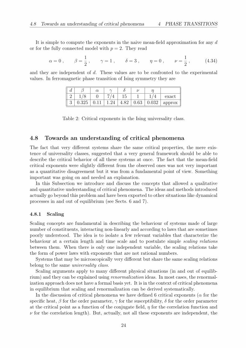
It is simple to compute the exponents in the naive mean-field approximation for any dor for the fully connected model with p = 2. They read
α = 0 , β =1
2, γ = 1 , δ = 3 , η = 0 , ν =
1
2, (4.34)
and they are independent of d. These values are to be confronted to the experimentalvalues. In ferromagnetic phase transition of Ising symmetry they are
d β α γ δ ν η2 1/8 0 7/4 15 1 1/4 exact3 0.325 0.11 1.24 4.82 0.63 0.032 approx
Table 2: Critical exponents in the Ising universality class.
4.8 Towards an understanding of critical phenomena
The fact that very different systems share the same critical properties, the mere exis-tence of universality classes, suggested that a very general framework should be able todescribe the critical behavior of all these systems at once. The fact that the mean-fieldcritical exponents were slightly different from the observed ones was not very importantas a quantitative disagreement but it was from a fundamental point of view. Somethingimportant was going on and needed an explanation.
In this Subsection we introduce and discuss the concepts that allowed a qualitativeand quantitative understanding of critical phenomena. The ideas and methods introducedactually go beyond this problem and have been exported to other situations like dynamicalprocesses in and out of equilibrium (see Sects. 6 and 7).
4.8.1 Scaling
Scaling concepts are fundamental in describing the behaviour of systems made of largenumber of constituents, interacting non-linearly and according to laws that are sometimespoorly understood. The idea is to isolate a few relevant variables that characterize thebehaviour at a certain length and time scale and to postulate simple scaling relationsbetween them. When there is only one independent variable, the scaling relations takethe form of power laws with exponents that are not rational numbers.
Systems that may be microscopically very different but share the same scaling relationsbelong to the same universality class.
Scaling arguments apply to many different physical situations (in and out of equilib-rium) and they can be explained using renormalization ideas. In most cases, the renormal-ization approach does not have a formal basis yet. It is in the context of critical phenomenain equilibrium that scaling and renormalization can be derived systematically.
In the discussion of critical phenomena we have defined 6 critical exponents (α for thespecific heat, β for the order parameter, γ for the susceptibility, δ for the order parameterat the critical point as a function of the conjugate field, η for the correlation function andν for the correlation length). But, actually, not all these exponents are independent, the
24

4.8 Towards an understanding of critical phenomena 4 PHASE TRANSITIONS
scaling hypothesis allows one to show that only two of them are. One example of theserelations is the one called Rushbrooke scaling law
α + 2β + γ = 2 . (4.35)
These relations follow from the fact that all observables can be computed from the free-energy density and, if one assumes a scaling form for it, one is forced to have relationsbetween the exponents characterizing the thermodynamic observables and correlationfunctions. We shall not discuss these relations here, the interested student can find themin any book on critical phenomena, see e.g. [9].
Let us take a simple viewpoint and discuss a way to collapse data close to a criticalpoint, a property closely related to scaling. The power law expressions (4.30) and (4.31)suggest Widom scaling for the order parameter:
m(t, h) ∼ |t|βΦ±
(
h
|t|βδ)
t ≡ |T − Tc|Tc
, (4.36)
with Φ±(0) = 1 and Φ±(x → ∞) ∼ x1/δ. With these limits, (4.31) is recovered on thecritical isotherm and (4.30) follows at strictly zero field and for |t| ≪ 1. An example ofdata collapse is given in Fig. 5.
Surprisingly enough, all systems undergoing a ferromagnetic transition can be scaledin this way using the same functions Φ± above and below the critical temperature, re-spectively! The way of checking this hypothesis is by plotting m/|t|β against |h|/|t|βδ fordifferent systems and looking for data collapse. Of course, we do not know the values ofthe universal exponents β and δ and the material dependent critical temperature Tc apriori, so we need to manipulate a bit the data before obtaining collapse. Note that thescaling law (4.36) is independent of the dimension d.
One can also write the scaling hypothesis for the free-energy density and derive theone for the magnetization by differentiation.
Scaling relations that involve the dimension are called hyperscaling. The correlationfunction satisfies
G(~r; t, h) =1
rd−2+ηg
(
r|t|ν , h
|t|βδ)
(4.37)
Kadanoff proposed that this quite incredible feature could be explained assuming thatnear a critical point a system looks the same at all length scales. This is called scaleinvariance.
4.8.2 The correlation length
A very important concept in critical phenomena is that of a correlation length usuallydenoted by ξ.
The correlation length is the distnce over which the fluctuations of the microscopicdegrees of freedom are significantly correlated. A simple way to understand its meaningis the following. Take a macroscopic sample and measure some macroscopic observableunder some external conditions, i.e. temperature T and pressure P . Now, repeat themeasurement after cutting the sample in two pieces and keeping the external conditions
25

4.8 Towards an understanding of critical phenomena 4 PHASE TRANSITIONS
Figure 5: Critical scaling in gas-liquid transitions at constant pressure. At very lowdensity and low temperature, at the left of the curve the system is a gas, at very largedensity and still low temperature, at the right of the curve the system is a liquid. In theregion below the curve there is coexistence of gas and liquid. Above the curve the systemgoes continuously from a gas to a liquid when increasing the density. The critical linebehaves as |ρl − ρg| ∼ |T − Tc|β with β ∼ 0.327 close to the maximum. Note that scalingholds as far as T/Tc ∼ 0.55!
unchanged. The result for the macroscopic observable is the same. Repeating this proce-dure, one finds the same result until the system size reaches the correlation length of thematerial.
At finite temperature, one can have droplets of the wrong phase within the correct one,due to thermal agitation. The size of these droplets will be a function of temperature andat a given instant, a snapshot of the system reveals the existence of a number of themwith different sizes. One expects though that they have a well-defined average (taken,for instance, over different snapshots taken at different times). This average size can betaken as a qualitative indication of the value of the correlation length (we shall give amore precise definition below).
In first order phase transition the correlation length is finite for all values of the pa-rameters. In second order phase transitions, the correlation length is usually very short,of the order of a few lattice spacing, at low temperature. It increases when approachingTc, it diverges at Tc, and then decreases again in the high temperature phase when gettingaway from the critical point. See Fig. 6.
26

4.8 Towards an understanding of critical phenomena 4 PHASE TRANSITIONS
Figure 6: Two snapshots of the spin configuration in a 2d Ising model. Left: below Tc;right: at Tc.
The fact that one finds coherent structures at all lengths at the critical point means thatthere is no spatial scale left in the problem and then all scales participate in the criticalbehaviour. The system becomes scale invariant and, if one looks at it with differentmicroscopes one essentially sees the same.
The actual definition of the correlation length is based on the use of the static sucep-tibility sum rule. Let us define the two-point connected correlation function
G(~ri, ~rj) ≡ 〈sisj〉 − 〈si〉〈sj〉 (4.38)
where ~ri is the spatial position of the spin si. A simple calculation allows one to showthat the linear susceptibility reads
χ ≡ ∂mh
∂h= − ∂2f
∂h2
∣
∣
∣
∣
∣
h=0
=β
N
∑
ij
G(~ri − ~rj) . (4.39)
Let us prove this statement. Nothing indicates that spatial translational invariance shouldbe violated, thus, the correlation should be a function of the distance between the points~ri and ~rj only:
G(~ri, ~rj) = G(~ri − ~rj) . (4.40)
One then has
χ ≡ ∂m
∂h= β
∑
i
G(~ri) =β
ad
∫
Vddr G(~r) . (4.41)
This means that the divergence of the susceptibility at the critical point must be accom-panied by a special behavior of the correlation function. Indeed, one finds that
G(~r) ∼ e−r/ξ
rd−1ξ(d−3)/2, for r ≫ ξ . (4.42)
27

4.8 Towards an understanding of critical phenomena 4 PHASE TRANSITIONS
This expression is integrable over the full volume unless the exponential factor disappears.This is indeed what happens at Tc where the correlation length diverges, again as a powerlaw of the distance to the critical point
ξ ∼ |T − Tc|−ν . (4.43)
Finally, one observes that the correlation function right at the critical point also divergesas a power law:
G(~r) ∼ r−(d−2+η) , (4.44)
with η another critical exponent.Let us discuss the correlation length in a simple solvable case, the Ising model in d = 1
with, say, open boundary conditions. In this case, the finite temperature correlationfunction is
Gkl = 〈sksl〉 − 〈sk〉〈sl〉 = 〈sksl〉 (4.45)
since 〈sk〉 = 0 at any T > 0. Introducing, for convenience, different coupling constantsKi = βJi on the links, Gkl reads
Gkl = Z−1∑
{si=±1}
e∑
iKisisi+1sksl = Z−1 ∂
∂Kk
∂
∂Kk+1
. . .∂
∂Kl−1
Z . (4.46)
At the end of the calculation one takes Ki = K = βJ for all i. Thus, at finite temperaturethe connected correlation between any two spins can be computed as a number of deriva-tives (depending on the distance between the spins) of the partition function convenientlynormalized. Using the change of variables ηi = sisi+1, one finds
Z =∑
{ηi=1}
e∑
iKiηi = 2
N−1∏
i=1
2 cosh(Ki) → 2(2 cosh βJ)N−1 . (4.47)
Taking the distance between the chosen spins sk and sl to be k − l = r the correlationfunction is then given by
G(r) = [tanh(βJ)]r = er ln[tanh(βJ)] = e−r/ξ (4.48)
with
ξ =1
ln coth(βJ)∼ e4J/(T−Tc) , T ∼ 0 . (4.49)
In this one dimensional example we found a essential singularity, an exponential diver-gence, of the correlation length when approaching Tc = 0. In general, in higher d, one hasa power law divergence of the form (4.44).
4.8.3 Finite size effects
A real system is large but finite, 1 ≪ NA ∼ 1023 <∞. Finite size effects will then play arole in the phase transition that is rounded by the fact that NA < ∞. Finite size effectsbecome important when ξ ∼ L, the linear size of the system, say L ∼ 1cm for an actualsample. A rough estimation of how close to Tc one needs to get to see deviations from
28

4.8 Towards an understanding of critical phenomena 4 PHASE TRANSITIONS
critical scaling shows that finite size effects are quite negligible in experiments but arecertainly not in numerical simulations and have to be taken into account very carefullywhen trying to compare numerical data to analytical predictions.
Finite size effects are taken into account by introducing correcting functions in thescaling laws, for example,
χL ∼ |t|−γg(
L
ξ
)
(4.50)
with g(x→ ∞) → 1 and g(x→ 0) → xγ/ν , and
m ∼ Lβ/ν . (4.51)
4.8.4 The renormalization group
The development of the renormalization group by K. Wilson in the early 70s gave atotally new way of understanding condensed-matter and particle physics phenomena.He transformed the picture of phase transitions that developed in the 60s – with theunderstanding of concepts like scaling, universality and correlations – into a calculationaltool and got the Nobel Prize in Physics in 1982.
Let us describe how the RG works on one example, again the one dimensional Isingmodel with N (even) spins in the absence of an applied field. The partition function reads
Z(N, J) =∑
si=±1
eβJ∑N−1
i=1sisi+1 (4.52)
We shall call K ≡ βJ . The sum in the exponential is
s1s2 + s2s3 + s3s4 + s4s5 + . . . (4.53)
It is clear that s2 enters only in the first two terms, s4 enters only on the third and forthterm and so on and so forth. One can then sum over all configurations of the spins withan even label. For example, the sum over s2 = ±1 yields
eK(s1+s3) + e−K(s1+s3) . (4.54)
One then obtains:
Z(N,K) =∑
si=±1;i odd
N−1∏
i=1
[eK(si+si+2) + e−K(si+si+2)] (4.55)
If we find a function κ(K) and a new coupling constant K ′ such that each of these termscan be written as
eK(si+si+2) + e−K(si+si+2) = κ(K)eK′sisi+2 , (4.56)
the right-hand-side in eq. (4.55) would be proportional to the partition function of anotherone dimensional Ising model with N/2 spins and a different coupling constant K ′:
Z(N,K) = κ(K)N/2Z(N/2, K ′) . (4.57)
29
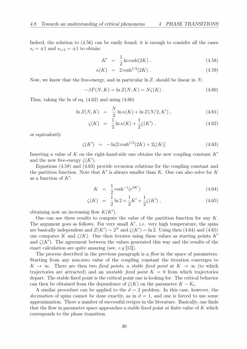
4.8 Towards an understanding of critical phenomena 4 PHASE TRANSITIONS
Indeed, the solution to (4.56) can be easily found; it is enough to consider all the casessi = ±1 and si+2 = ±1 to obtain:
K ′ =1
2ln cosh(2K) , (4.58)
κ(K) = 2 cosh1/2(2K) . (4.59)
Now, we know that the free-energy, and in particular lnZ, should be linear in N ;
−βF (N,K) = lnZ(N,K) = Nζ(K) . (4.60)
Thus, taking the ln of eq. (4.62) and using (4.60)
lnZ(N,K) =N
2lnκ(K) + lnZ(N/2, K ′) , (4.61)
ζ(K) =1
2lnκ(K) +
1
2ζ(K ′) . (4.62)
or equivalently
ζ(K ′) = − ln[2 cosh1/2(2K) + 2ζ(K)] (4.63)
Inserting a value of K on the right-hand-side one obtains the new coupling constant K ′
and the new free-energy ζ(K ′).Equations (4.58) and (4.63) provide recursion relations for the coupling constant and
the partition function. Note that K ′ is always smaller than K. One can also solve for Kas a function of K ′:
K =1
2cosh−1(e2K
′
) (4.64)
ζ(K) =1
2ln 2 +
1
2K ′ +
1
2ζ(K ′) , (4.65)
obtaining now an increasing flow K(K ′).One can use these results to compute the value of the partition function for any K.
The argument goes as follows. For very small K ′, i.e. very high temperature, the spinsare basically independent and Z(K ′) ∼ 2N and ζ(K ′) = ln 2. Using then (4.64) and (4.65)one computes K and ζ(K). One then iterates using these values as starting points K ′
and ζ(K ′). The agreement between the values generated this way and the results of theexact calculation are quite amazing (see, e.g [13]).
The process described in the previous paragraph is a flow in the space of parameters.Starting from any non-zero value of the coupling constant the iteration converges toK → ∞. There are then two fixed points, a stable fixed point at K → ∞ (to whichtrajectories are attracted) and an unstable fixed point K = 0 from which trajectoriesdepart. The stable fixed point is the critical point one is looking for. The critical behaviorcan then be obtained from the dependence of ζ(K) on the parameter K −Kc.
A similar procedure can be applied to the d = 2 problem. In this case, however, thedecimation of spins cannot be done exactly, as in d = 1, and one is forced to use someapproximation. There a number of successful recipes in the literature. Basically, one findsthat the flow in parameter space approaches a stable fixed point at finite value of K whichcorresponds to the phase transition.
30

4.8 Towards an understanding of critical phenomena 4 PHASE TRANSITIONS
4.8.5 Fluctuations of macroscopic observables
A direct consequence of having a diverging correlations length is that the critical measure-to-measure fluctuations global observables like, for instance, the magnetization density,are not Gaussian. The reason is simple, if L < ξ, a global measurement is not the resultof an average over many uncorrelated regions and, thus, one can not use the central limittheorem to argue for a normal distribution of fluctuations. Recently, the study of criticalfluctuations of macroscopic observables received much attention. The best adapted modelfor this analysis is the 2d XY model, that is critical on a finite interval of temperatures(and not only at a single precise value of Tc) [27]. This model, in an approximation, ismapped onto an interface model, the Edwards-Wilkinson one, that we shall discuss inSect. 7.
In the limit we are now interested in L is finite with respect to ξ and finite size effectsare important. Finite size scaling implies
pL(M) = Lβ/ν Π
(
MLβ/ν ,ξ
L
)
. (4.66)
The calculation of this probability function in the so-called spin-wave approximation ofthe 2d XY model showed that it has the form of Gumbel distributions found in the staudyof extreme value statistics that we discussed in Sect. 3.1.2. The role payed by extreme Wevalues in this context remains, however, not clear. shall give more details on the analysisof these non-Gaussian fluctuations in the language of interfaces.
31

5 DISORDERED SYSTEMS
5 Disordered systems
No material is perfectly homogeneous: impurities of different kinds are distributed ran-domly throughout the samples.
A natural effect of disorder should be to lower the critical temperature. Much atten-tion has been payed to the effect of weak disorder on phase transitions, that is to say,situations in which the nature of the ordered and disordered phases is not modified bythe impurities but the critical phenomenon is. On the one hand, the critical exponents ofsecond order phase transitions might be modified by disorder, on the other hand, disordermay smooth out the discontinuities of first order phase transitions rendering them of sec-ond order. Strong disorder instead changes the nature of the low-temperature phase andbefore discussing the critical phenomenon one needs to understand how to characterizethe new ordered ‘glassy’ phase.
In this Chapter we shall discuss several types of quenched disorder and models thataccount for it. We shall also overview some of the theoretical methods used to deal withthe static properties of models with quenched disorder.
5.1 Quenched and annealed disorder
First, one has to distinguish between quenched and annealed disorder. Imagine that onemixes some random impurities in a melt and then very slowly cools it down in such a waythat the impurities and the host remain in thermal equilibrium. If one wants to studythe statistical properties of the full system one then has to compute the full partitionfunction in which one sums over all configurations of original components and impurities.This is called annealed disorder. In the opposite case in which upon cooling the hostand impurities do not equilibrate but the impurities remain blocked in random fixedpositions, one talks about quenched disorder. Basically, the relaxation time associatedwith the diffusion of the impurities in the sample is so long that these remain trapped.The former case is easier to treat analytically but is less physically relevant. The latteris the one that leads to new phenomena and ideas that we shall discuss next.
5.2 Bond disorder: the case of spin-glasses
Spin-glasses are alloys in which magnetic impurities substitute the original atoms in posi-tions randomly selected during the chemical preparation of the sample. The interactionsbetween the impurities are of RKKY type:
Vrkky = −J cos(2kF rij)
r3ijsisj (5.1)
with rij = |~ri− ~rj| the distance between them and si a spin variable that represents theirmagnetic moment. Clearly, the initial location of the impurities varies from sample tosample. The time-scale for diffusion of the magnetic impurities is much longer than thetime-scale for spin flips. Thus, for all practical purposes the positions ~ri can be associatedto quenched random variables distributed according to a uniform probability distributionthat in turn implies a probability distribution of the exchanges. This is called quencheddisorder.
32

5.2 Bond disorder: the case of spin-glasses 5 DISORDERED SYSTEMS
+ + + +
+
++
−
Figure 7: A frustrated (left) and an unfrustrated (center) square plaquette. A frustratedtriangular plaquette (right).
5.2.1 Frustration
Depending on the value of the distance rij the numerator in eqn. (5.1) can be positive ornegative implying that both ferromagnetic and antiferromagnetic interactions exist. Thisleads to frustration, which means that some two-body interactions cannot be satisfied byany spin configuration. An example with four sites and four links is shown in Fig. 7-left,where we took three positive exchanges and one negative one all, for simplicity, with thesame absolute value, J . Four configurations minimize the energy, Ef = −2J , but noneof them satisfies the lower link. One can easily check that any closed loop such that theproduct of the interactions takes a negative sign is frustrated. Frustration naturally leadsto a higher energy and a large degeneracy of the number of ground states. This is againeasy to grasp by comparing the number of ground states of the frustrated plaquette inFig. 7-left to its unfrustrated counterpart shown on the central panel. Indeed, the energyand degeracy of the ground state of the unfrustrated plaquette is Eu = −4J and nu = 2,respectively.
Frustration may be due to pure geometrical constraints. The canonical example is anantiferromagnet on a triangular lattice in which each plaquette is frustrated, see Fig. 7.
5.2.2 Self-averageness
If each sample is characterized by its own realization of the exchanges, should one expecta totally different behavior from sample to sample? Fortunately, many generic static anddynamic properties of spin-glasses (and other systems with quenched disorder) do notdepend on the specific realization of the random couplings and are self-averaging. Thismeans that the typical value is equal to the average over the disorder:
AtypJ = [AJ ]av . (5.2)
In particular, the free-energy of models with short-ranged interactions is expected to beself-averaging.
The meaning of this property can grasped from the solution of the random bond Isingchain defined by the energy function E = −∑i Jisisi+1 with spin variables si = ±, fori = 1, . . . , N and random bonds Ji independently taken from a probability distributionP (Ji). For simplicity, we consider periodic boundary conditions. The disorder-dependentpartition function reads
ZJ =∑
{si=±1}
eβ∑
iJisisi+1 (5.3)
33

5.3 Models 5 DISORDERED SYSTEMS
and this can be readily computed introducing the change of variables σi ≡ sisi+1. Onefinds.
ZJ =∏
i
2 cosh(βJi) ⇒ −βFJ =∑
i
ln cosh(βJi) +N ln 2 . (5.4)
The partition function is a product of i.i.d. random variables and it is itself a randomvariable with a log-normal distribution. The free-energy instead is sum of i.i.d. and, usingthe central limit theorem, it becomes a Gaussian random variable that is narrowly peakedabout its maximum in the large N limit. The typical value, determined by the maximumin the distribution coincides with the average.
A simple argument that justifies the self-averageness of the free-energy in generic finitedimensional systems with short-range interactions is the following. Let us divide thesystem of volume V in n subsystems of volume v with V = nv. If the interactions areshort-ranged, the total energy is the sum of two terms, a contribution from the bulk ofthe subsystems and a contribution from the interfaces between the subsystems. In thethermodynamic limit, the latter is negligible with respect to the former. The disorderdependent free-energy density is then a of random numbers, each one being the disorderdependent free-energy of the bulk of each subsystem. In the limit of a very large numberof subsystems (V ≫ v) the central limit theorem implies that the total free-energy isGaussian distributed with the maximum reached at a value F ∗
J that coincides with theaverage of all realizations of the randomness [FJ ]. Thus, the typical FJ is identical to theaveraged [FJ ]av. One can then compute the latter to understand the static properties ofthe typical system.
Once one has [FJ ], one derives all disordered average thermal averages by taking deriva-tives of the disordered averaged free-energy with respect to sources introduced in thepartition function. For example,
[ 〈 si 〉 ]av = − ∂[FJ ]av∂hi
∣
∣
∣
∣
∣
hi=0
, (5.5)
[ 〈 sisj 〉 − 〈 si 〉〈 sj 〉 ]av = T∂[FJ ]av∂hihj
∣
∣
∣
∣
∣
hi=0
, (5.6)
with E → E −∑
i hisi.
5.3 Models
In early 70s Edwards and Anderson proposed a rather simple model that should capturethe main features of spin-glasses. The interactions (5.1) decay with a cubic power of thedistance and hence they are relatively short-ranged. This suggests to put the spins ona regular cubic lattice model and to trade the randomness in the positions into randomnearest neighbor exchanges taken from a Gaussian (or bimodal) probability distribution:
Eea = −∑
〈ij〉
Jijsisj with P (Jij) = (2πσ2)−12 e−
J2ij
2σ2 . (5.7)
A natural extension of the EA model in which all spins interact has been proposed bySherrington and Kirkpatrick
E = −∑
i1 6=j
Jijsisj −∑
i
hisi (5.8)
34

5.3 Models 5 DISORDERED SYSTEMS
and it is called the SK model. The interaction strengths Jij are taken from a Gaussianpdf and they scale with N in such a way that the thermodynamic is non-trivial:
P (Jij) = (2πσ2N)
− 12 e
−J2ij
2σ2N σ2
N = σ2N . (5.9)
This is a case for which a mean-field approximation is expected to be exact.A further extension of the EA model is called the p spin model
E = −∑
i1 6=... 6=ip
Ji1...ipsi1 . . . sip −∑
i
hisi (5.10)
with p ≥ 3. The exchanges are now taken from a Gaussian probability distribution with
[Ji1...ip ]av = 0 , [J2i1...ip
]av =J2
2Np−1. (5.11)
Indeed, an interesting thermodynamic limit is achieved by scaling Ji1...ip with N−(p−1)/2.This scaling is justified as follows. The “force” Fi ≡
∑
ii2 6=ip Jii2...ipmi2 . . .mip should be oforder one. At low temperatures the mi’s take plus and minus sign. In particular, we canestimate the order of magnitude of this term working at T = 0 and taking mi = ± withprobability 1
2. In order to make the discussion simple, let us take p = 2. In this case,
if the strengths are of order one, Fi is a sum of N independent, identically distributedrandom variables, with zero mean and variance equal to 1. Thus, Fi has zero mean andvariance equal to N . Thus, one can argue that Fi is of order
√N . To make it finite we
then chose Jij to be of order 1/√N or, in other words, we impose [J2
ij ]av = J2/(2N). Thegeneralization to p ≥ 2 is straightforward.
Cases that find an application in computer science are defined on random graphs withfixed or fluctuating finite connectivity. In the latter case one places the spins on thevertices of a graph with links between couples or groups of p spins chosen with a probabilityc. These are called dilute spin-glasses.
Let us now discuss some, a priori simpler cases. An example is the Mattis randommagnet in which the interaction strengths are given by
Ji1...ip = ξi1 . . . ξip with ξj = ± with p = 1/2 . (5.12)
In this case a simple gauge transformation, ηi ≡ ξisi, allows one to transform the disor-dered model in a ferromagnet, showing that there was no true frustration in the system.
Random ferromagnets are systems in which the strengths of the intearctions are notall identical but their sign is. Thus, there is no frustration in this systems either.
Link randomness is not the only type of disorder encountered experimentally. Randomfields, that couple linearly to the magnetic moments, are also quite common; the classicalmodel is the ferromagnetic random field Ising model:
Erfim = −J∑
〈ij〉
sisj −∑
i
sihi with P (hi) = (2πσ2)−12 e−
h2i
2σ2 . (5.13)
Models with site or link dilution are also interesting:
Esite dil = −J∑〈ij〉 sisjǫiǫj , Elink dil = −J∑〈ij〉 sisjǫij , . (5.14)
35

5.4 The Griffiths phase 5 DISORDERED SYSTEMS
with P (ǫi = 0, 1) = p, 1 − p in the first case and P (ǫij = 0, 1) = p, 1 − p in the second.The dilute antiferromagnet in a uniform magnetic field is believed to behave similarly tothe ferromagnetic random field Ising model. Experimental realizations of the former arecommon and measurements have been performed in samples like Rb2Co0.7Mg0.3F4.
Once again, disorder is not only present in magnetic systems. An example that hasreceived much attention is the case of a d dimensional directed manifold moving in anembedding N+d dimensional space under the effect of a quenched random potential. Thesimplest case with d = 0 corresponds to a particle moving in an embedding space withN dimensions. If, for instance N = 1, the particle moves on a line, if N = 2 it moves ona plane and so on and so forth. If d = 1 one has a line that can represent a polymer, avortex line, etc. The fact that the line is directed means that it does not have overhangs.If the line moves in a plane, the embedding space has (N = 1)+ (d = 1) dimensions. Thequenched random potential is, say, V (~x), with ~x the coordinate on the embedding spaceand one characterises it with its probability distribution function P (V ).
5.4 The Griffiths phase
The effects of quenched disorder shows up already in the paramagnetic phase of a finitedimensional model, as the ones introduced above. Below the critical point of the purecase (no disorder) one sees finite regions of the system that order due to fluctuations inthe couplings that can make certain parts of the sample more ferromagnetic than others.These properties manifest in non-analyticities of the free-energy that appear in a fullinterval of temperatures above the critical temperature of the disordered model, as shownby Griffiths. We shall not discuss these features in detail here.
5.5 The random field Ising model
The random fields give rise to many metastable states that modify the equilibrium andnon-equilibrium behaviour of the RFIM. In one dimension the RFIM does not order at all,in d = 2 there is strong evidence that the model is disordered even at zero temperature, ind = 3 it there is a finite temperature transition towards a ferromagnetic state. Whetherthere is a glassy phase near zero temperture and close to the critical point is still andopen problem.
The RFIM at zero temperature has been proposed to yield a generic description ofmaterial cracking through a series of avalaches. In this problem one cracking domaintriggers others, of which size, depends on the quenched disorder in the samples. In arandom magnetic systems this phenomenon corresponds to the variation of the magneti-zation in discrete steps as the external field is adiabatically increased (the time scale foran avalanche to take place is much shorter than the time-scale to modify the field) andit is accessed using Barkhausen noise experiments. Disorder is responsible for the jerkymotion of the domain walls. The distribution of sizes and duration of the avalanches isfound to decay with a power law tail cut-off at a given size. The value of the cut-off sizedepends on the strength of the random field and it moves to infinity at the critical point.
36

5.6 The spin-glass transition 5 DISORDERED SYSTEMS
5.6 The spin-glass transition
Let us now discuss a problem in which disorder is so strong as to modify the nature of thelow temperature phase. If this is so, one needs to define a new order parameter, capableof identifying order in this phase.
5.6.1 The order parameter
The spin-glass equilibrium phase is one in which spins “freeze” in randomly-looking con-figurations. In finite dimensions these configurations are spatially irregular. A snapshotlooks statistical identical to a high temperature paramagnetic configuration in which spinspoint in both directions. However, while at high temperatures the spins flip rapidly andanother snapshot taken immediately after would look completely different from the pre-vious one, at low temperatures two snapshots taken at close times are highly correlated.
In a spin-glass state the local magnetization is expected to take a non-zero value,mi = 〈 si 〉 6= 0, where the average is interpreted in the restricted sense discussed above,i.e. within a pure state. Instead, the global magnetization density, m = N−1∑N
i=1mi,vanishes since one expects to have as many spins pointing up as spins pointing downwith each possible value of |mi|. Thus, the total magnetization, m = N−1∑N
i=1mi, of aspin-glass vanishes at all temperatures and it is not a good order parameter.
The spin-glass transition is characterized by a finite peak in the linear magnetic sus-ceptibility and a diverging non-linear magnetic susceptibility. Let us discuss the formerfirst and show how it yields evidence for the freezing of the local magnetic moments. Fora generic magnetic model such that the magnetic field couples linearly to the Ising spin,E → E −∑
i hisi, the linear susceptibility is related, via the static fluctuation-dissipationtheorem to the correlations of the fluctuations of the magnetization:
χij ≡∂〈si〉h∂hj
∣
∣
∣
∣
∣
h=0
= β 〈 (si − 〈si〉)(sj − 〈sj〉) 〉 . (5.15)
This relation is proven by using the definition of 〈si〉 and simply computing the derivativewith respect to hj. In particular,
χii = β(
1−m2i
)
≥ 0 , (5.16)
with mi = 〈si〉. The total susceptibility measured experimentally is χ ≡ 1N
∑
ij χij. Onthe experimental side we do not expect to see order one sample-to-sample fluctuations inthis global quantity. On the analytical side one can use a similar argument to the onepresented in Sect. 5.2.2 to argue that χ should be self-averaging. Thus, the experimentallyobserved susceptibility should be given by
[χ ]av = N−1∑
ij
[χij ]av ≈ N−1∑
i
[χii ]av = N−1∑
i
β(
1− [m2i ]av
)
, (5.17)
since we can expect that cross-terms cancel under the disorder average. The fall of χ at lowtemperatures with respect to its value at Tc signals the freezing of the local magnetizations,mi, in non-zero values. Note that this argument is based on the assumption that themeasurement is done in equilibrium.
37

5.6 The spin-glass transition 5 DISORDERED SYSTEMS
Thus, the natural global order parameter that characterizes the spin-glass transition is
qea ≡ N−1∑
i
[m2i ]av (5.18)
as proposed in the seminal Edwards-Anderson paper. qea vanishes in the high tempera-ture phase since all mi are zero but it does not in the low temperature phase since thesquare power takes care of the different signs. Averaging over disorder eliminates the sitedependence. Thus, qea is also given by
qea = [m2i ]av . (5.19)
In all this discussion the statistical average has to be interpreted in the same restrictedsense as the one discussed in the paramagnetic - ferromagnetic transition of the usualIsing model (see Sect. 4). Whether there are two equilibrium states (as in the usualferromagnetic phase) or many more (as we shall see appear in fully-connected spin-glassmodels) the average is taken in one of them. Since in the latter case it is found that evenif the individual mi take different values in different states, qea is ‘state-independent’, thisdefinition does not allow to distinguish between the two scenarios.
We shall see below a more pertinent definition of an order parameter that allows one todistinguish between the simple, two-state, and the many state scenarios. In practice it isrelated to the definition of the overlap – or correlation – between two spin configurations,say {si} and {σi}, defined as
qsσ = N−1∑
i
siσi . (5.20)
qsσ takes values between O and 1. It equals one if {si} and {σi} differ in a number ofspins that is smaller than O(N), is equals −1 when the two configurations are totallyanticorrelated – with the same proviso concerning a number of spins that is not O(N)– and it equals zero when {si} and {σi} are completely uncorrelated. Note that theself-overlap of a configuration with itself is identically one for Ising spins.
5.6.2 Divergent susceptibility
In a pure magnetic system with a second-order phase transition, see the discussion inSect. 4, the susceptibility of the order parameter to a field that couples linearly to itdiverges at the transition. In a spin system, in particular a ferromagnet, one induces alocal magnetization with a local field
〈si〉 =N∑
j=1
χijhj (5.21)
with χij the linear susceptibilities. Using this expression, the Edwards-Anderson param-eter becomes
qea =1
N
N∑
i=1
[〈si〉2]av =1
N
N∑
i=1
N∑
j=1
N∑
k=1
[χijχikhjhk]av (5.22)
If the applied fields are random and taken from a probability distribution such thathjhk = σ2δjk one obtains
qea =1
N
N∑
i=1
[〈si〉2]av =1
N
N∑
i=1
N∑
j=1
N∑
k=1
[χ2ij]avσ
2 = χSGσ2 (5.23)
38

5.7 Statics of models with strong disorder 5 DISORDERED SYSTEMS
σ2 acts then as a field conjugated to the order parameter qea. (One can also argue that auniform field looks random to a spin-glass sample and thus the same result holds.) Thespin-glass susceptibility is then defined as
χSG ≡ 1
N
∑
ij
[χ2ij]av =
1
N
∑
ij
[ (〈sisj〉 − 〈si〉〈sj〉)2 ]av (5.24)
and one can check whether it diverges at Tc as expected in a second-order phase transition.One can show that the divergence of χSG is related to the divergence of the non-linearusual magnetic susceptibility
χ(3) ≡ 1
N
∑
i=1
∂3〈si〉∂h3
∣
∣
∣
∣
∣
h=0
(5.25)
that can be accessed experimentally. A careful experimental measurement of χ(3), χ(5)
and χ(7) demonstrated that all these susceptibilities diverge at Tc.
5.7 Statics of models with strong disorder
Let us discuss in this part the statics of spin-glass models and the two main competingdescriptions of it. Similar arguments can be used to study other models with strongdisorder, as a manifold in a random potential.
5.7.1 Scaling arguments and the droplet theory
The droplet theory is a phenomenological model that assumes that the low temperaturephase of a spin-glass model has only two equilibrium states related by an overall spin flip.It is then rather similar to a ferromagnet, only that the nature of the order in the twoequilibrium states is not easy to see, it is not just most spins pointing up or most spinspointing down with some thermal fluctuations within. At a glance, one sees a disorderedparamagnetic like configuration and a more elaborate order parameter has to be measuredto observe the order. The spin-glass phase is then called a disguised ferromagnet and ausual spontaneous symmetry breaking (between the two equilibrium states related spinreversal symmetry) leading to usual ergodicity breaking is supposed to take place at Tc.
Once this assumption has been done, renormalization group arguments are used todescribe the scaling behavior of several thermodynamic quantities. The results found arethen quantitatively different from the ones for a ferromagnet but no novelties appear.
Let us now just discuss one simple argument that is at the basis of what is neededto derive the results of the droplet theory without entering into the complications of thecalculations.
The Imry-Ma argument
Take a ferromagnetic Ising model in a random field, defined in eq. (5.13). In zeroapplied field and low enough temperature, if d > 1 there is phase transition between aparamagnetic and a ferromagnetic phase. If one considers the effect of a random fieldwith very strong typical strength, the the spins will align with the local external fieldsand the system will be paramagnetic. However, It is, however, non-trivial to determine
39

5.7 Statics of models with strong disorder 5 DISORDERED SYSTEMS
the effect of a relatively weak random field on the ferromagnetic phase at sufficiently lowtemperature. The long-range ferromagnetic order could be preserved or else the field couldbe enough to break up the system into large but finite domains of the two ferromagneticphases.
A qualitative argument to estimate whether the ferromagnetic phase survives or notin presence of the external random field is called the Imry-Ma argument in this contextand it is a simple extension of the discussion in Sect. 4.3. Let us fix T = 0 and switch ona random field. If a domain D of a the opposite order (say down) is created within thebulk of the ordered state (say up) the system pays an energy due to the unsatisfied linkslying on the boundary that is
∆Eborder ∼ 2JLd−1 (5.26)
where L is the linear length of the border and d − 1 is the dimension of the border ofa domain embedded in d a dimensional volume, assuming it is compact. Typically themagnetic energy in the interior of the domain due to the external field is
∆Erf ∼ −hLd/2 (5.27)
since there are N = Ld spins inside the domain of linear length L and, using the centrallimit theorem, −h∑j∈D si ∼ −h
√N = −hLd/2. The comparison between these two
energy scales yields
JLd−1 ∼ −hLd/2(
J
h
)
22−d
∼ L (5.28)
This indicates that the creation of domains at zero temperature is favorable in d < 2 andit is not favorable in d > 2. (The marginal case d = 2 is more subtle and we do notdiscuss it here.) The size of the domain is given by the expression above.
A very similar reasoning is used to argue that there cannot be spin-glass order in anEdwards-Anderson model in an external field. The only difference is that the domain wallenergy is here assumed to be proportional to Ly with an a priori unknown d-dependentexponent y that is related to the geometry of the domains.
5.7.2 The naive mean-field approximation
Disordered models have quenched random interactions. Due to the fluctuating values ofthe exchanges, one expects that the equilibrium configurations be such that the spinsfreeze in different directions. The local averaged magnetizations need not be identical. Atlow-temperatures, and quite surprisingly a priori the naive mean-field equations (4.20)have an exponential in N number of minima. These can be identified as different equilib-rium states that could be accessed by applying the corresponding site-dependent pinningfields.
Even if it has been shown by Thouless-Anderson-Palmer [16, 17] that these equationsare not correct in the fully-connected disordered case, a term which is called the Onsagerreaction term is missing, the fact that the number of equilibrium states diverges as anexponential of N in the thermodynamic limit remains true for these models. We shallnot derive the correct TAP equations here but we shall describe the main features theypredict.
40

5.7 Statics of models with strong disorder 5 DISORDERED SYSTEMS
The free-energy density as a function of the local magnetizations mi defines what isusually called the free-energy landscape. Note that this function depends on N ≫ 1variables, mi, that are not all identical in the disordered case in which the interactionsbetween different groups of spins are different.
For all models, at high temperatures f(mi) it is characterized by a single minimum inwhich all local magnetizations vanish, as expected; this is the paramagnetic state.
At very low temperature there are many equilibrium states (and not just two as in anIsing ferromagnetic model) and they are not related by a symmetry (as spin reversal inthe Ising ferromagnet or a rotational symmetry in the Heisenberg ferromagnet). Theseare characterized by non-zero values of the local magnetizations mi that are different indifferent states.
On can also access the saddle-points of the free-energy landscape by looking for sta-tionary points of f(mi) that are not the absolute minima or have unstable directions. Thenumber and structure of saddle-points is particularly interesting in the p ≥ 3 cases andit is indeed the reason why these models, with a random first order transition, have beenproposed to mimic the structural glass arrest.
The derivation and understanding of these results is quite subtle and goes beyond thescope of these Lectures. Still, we shall briefly present the phenomenology of these modelshere, jus to give a flavor of their complexity. Below a temperature Tc, an exponential(in N) number of metastable states contribute to the thermodynamics in such a non-trivial way that their combined contribution to the observables makes them those of aparamagnet. Even if each of these states is non-trivial (the mi’s are different from zero)the statistical average over all of them yields results that are identical to those of aparamagnet. At a lower temperature Ts (Ts < Tc) there is an entropy crisis, less than anexponential number of metastable states survive, and there is a static phase transition toa glassy state.
5.7.3 The replica method
A picture that is consistent with the one arising from the naive mean-field approximationbut contradicts the initial assumption of the droplet model arises from the exact solutionof fully-connected spin-glass models. These results are obtained using a method which iscalled the replica trick and that we shall briefly present below.
In Sect. 5.2.2 we argued that the typical properties of a disordered system can becomputed from the disorder averaged free-energy
[FJ ]av ≡∫
dJP (J)FJ . (5.29)
The replica method allows one to compute [FJ ]av for fully-connected models. It is basedon the smart use of the identity
lnZ = limn→0
Zn − 1
n. (5.30)
Thus,
−β[FJ ]av = −∫
dJP (J) lnZJ = − limn→0
1
n
(∫
dJP (J)ZnJ − 1
)
, (5.31)
41

5.7 Statics of models with strong disorder 5 DISORDERED SYSTEMS
where we have exchanged the limit n → 0 with the integration over the exchanges. Forinteger n the replicated partition function, Zn
J , reads
ZnJ =
∑
{sai}
e−β[EJ ({s1i })+...+EJ ({s
ni }] . (5.32)
Here∑
{sa} ≡ ∑
{s1=±1} . . .∑
{sn=±1}. ZnJ corresponds to n identical copies of the original
system, that is to say, all of them with the same realization of the disorder. Each copyis characterized by an ensemble of n spins, {sai }, that we label with a replica indexa = 1, . . . , n.
With this method one can study p spin disordered spin models. for which ZnJ takes the
form
ZnJ =
∑
{sai}
eβ∑n
a=1
[
∑
i1 6=... 6=ipJi1...ips
ai1...saip+
∑
ihis
ai
]
. (5.33)
The average over disorder amounts to computing a Gaussian integral for each set of spinindices i1, . . . ip. One finds
[ZnJ ]av =
∑
{sai}
eβ2J2
2Np−1
∑
i1 6=... 6=ip(∑
asai1
...saip )2+β
∑
a
∑
ihis
ai
≡∑
{sai}
e−βF ({sai }) . (5.34)
The function βF ({sai }) is not random. It depends on the spin variables only but it includesterms that couple different replica indices:
F ({sai }) = − β2J2
2Np−1
∑
i1 6=... 6=ip
∑
ab
sai1 . . . saips
bi1. . . sbip − β
∑
a
∑
i
hisai
≈ −Nβ2J2
2
∑
a 6=b
(
1
N
∑
i
sai sbi
)p
+ n
− β∑
a
∑
i
hisai . (5.35)
In writing the last expression we have dropped terms that are subleading inN (in completeanalogy with what we have done for the pure p spin ferromagnet). The constant term−Nnβ2J2/2 originates in the terms with a = b, for which (sai )
2 = 1.To summarize, we started with an interacting spin model. Next, we enlarged the num-
ber of variables from N spins to N × n replicated spins by introducing n non-interactingcopies of the system. By integrating out the disorder we decoupled the sites but we payedthe price of coupling the replicas. Hitherto the replica indices act as a formal tool in-troduced to compute the average over the bond distribution. Nothing distinguishes onereplica from another and, in consequence, the “free-energy” F ({sai }) is invariant underpermutations of the replica indices.
The next step to follow is to identify the order parameters and transform the free-energy into an order-parameter dependent expression to be rendered extremal at theirequilibrium values. In a spin-glass problem we already know that the order parameter isnot the global magnetization as in a pure magnetic system but the parameter q – or moregenerally the overlap between states. Within the replica calculation an overlap betweenreplicas
qab ≡ N−1∑
i
sai sbi (5.36)
42

5.7 Statics of models with strong disorder 5 DISORDERED SYSTEMS
naturally appeared in eq. (5.35). It can be shown that this expression plays the role of anoverlap between states labeled, say, by α and β
qαβ ≡ N−1∑
i
〈si〉α〈si〉β (5.37)
The statistics of possible overlaps is then characterized by a probability function
P (q) ≡∑
αβ
δ(q − qαβ) (5.38)
and it is the function that extends the concept of the order parameter and allows one todistinguish between the droplet picture prediction that corresponds to
P (q) =1
2(δ(q − qea) + δ(q + qea)) (5.39)
and a more complicated situation in which P (q) has the two delta functions at ±qeq plusa non-zero value on a continuous support in between.
The idea is to write a free-energy density as a function of the order parameter qab andthen look for the extreme that minimizes it, in complete analogy with what has beendone for the fully-connected ferromagnet. This is, of course, a tricky business, since theorder parameter is here a matrix with number of elements n going to zero! A recipe foridentifying the form of order parameter (or the correct saddle-point solution) has beenproposed by G. Parisi in the late 70s and early 80s. This solution has been recently provento be exact for mean-field models by two mathematical physics, Guerra and Talagrand.Whether the very rich physical structure that derives from this rather formal solutionsurvives in finite dimensional systems remains a subject of debate.
Symmetry and ergodicity breaking
Let us summarize some of the main features of the solution to the SK model obtainedwith replicas. There is a phase transition at a finite Tc at which the replica symmetry isbroken. This is a rather abstract symmetry. This symmetry breaking is accompanied byergodicity breaking as in the usual case.
Right below Tc an exponential in N number of equilibrium states appear. The transi-tion is continuous, the order parameter approaches zero right below Tc. Lowering furtherthe temperature each ergodic component breaks in many other ones. In this sense, thefull spin-glass phase, T < Tc, is ‘critical’ and not only the single point Tc.
43

6 STOCHASTIC PROCESSES
6 Stochastic processes
Simultaneously to the development of equilibrium statistical mechanics, which assumesthat systems can be described in terms of Boltzmann-Gibbs probability distributions, thequestion of how this equilibrium is reached was raised (in fact by Boltzmann himself),and led to the well known debate about irreversibility and the arrow of time. Althoughthe conceptual issues are formidable, one can take a phenomenological point of view andpostulate the nature of the coupling between a given system and a thermal bath suchthat equilibrium is, at least in principle, reached at long times. This is known as theLangevin approach, which provides a consistent description of the dynamics of systemssubject to thermal noise, such that the stationary solution reproduces the Boltzmann-Gibbs distribution.
On can be interested in situations such that the dynamics should lead at long timesto equilibrium, but the time needed to do so is either infinite or very large comparedto experimental time scales.2 These systems are usually referred to as ‘glassy’. In thesecases, equilibrium concepts are a priori useless; the description of the system is inherentlyof dynamical nature. The theoretical framework available to describe the dynamics of asystem subject to thermal noise is good for both cases.
Almost any physical system is subject to fluctuations that have an unknown originand/or can only be characterized only statistically. This noise is one of the manifes-tations of the exchange of energy between the system and its environment; the otheraccompanying feature is, as we will see in more detail below, dissipation. The time evolu-tion of a system coupled to its environment can be described in two equivalent ways. Oneis the Langevin approach that consists in studying Newton’s equations with the additionof two terms representing friction and thermal noise. The other description is probabilisticand is concerned with the evolution of the probability distribution of the relevant degreesof freedom of the system. Both approaches turn out to be very useful to understand thedynamics of model systems.
The environment is often assumed to be a heat bath in equilibrium at a given temper-ature. In these conditions, many systems do equilibrate with such an environment aftera short transient. The dynamics of equilibrated systems has several special features thatwe also review in this Chapter. How these properties are modified in systems that neverreach equilibrium is a problem of current interest in research but we shall not develop ithere.
6.1 The Langevin equation
The Langevin equation is a stochastic differential equation that describes phenomenolog-ically a large variety of problems. It describes the time evolution of a set of slow variablescoupled to a much larger set of fast variables that are usually (but not necessarily) as-sumed to be in thermal equilibrium at a given temperature. We first introduce it in thecontext of Brownian motion and later derive it in more generality.
2There might of course be systems that never reach thermal equilibrium, such as driven dissipativesystems for example.
44

6.1 The Langevin equation 6 STOCHASTIC PROCESSES
6.1.1 Brownian motion
The Brownian motion is the erratic motion of a mesoscopic colloidal particle (in themicrometer range) immersed in an equilibrated fluid made up of much lighter molecules.The jerky motion of the colloidal particle is due to the collisions with the molecules inthe liquid. Knowing that each individual collision deflects the trajectory of the particleby a tiny amount, Langevin proposed to collect the effect of all molecules in the fluid ina time-dependent random force. If the particle moves in d dimensions, has mass m, itscenter of mass position at time t is represented by ~x = (x1, . . . , xd) and its velocity is~v = ~x, Newton’s equation reads
m~v(t) = ~F (~x, t) + ~f(t) . (6.1)
The force ~F designates all external deterministic forces, and depends in general alsoon the position of the particle ~x, while ~f represents the net force exerted by all theindividual molecules in the fluid on the massive particle. The latter depends on the time-dependent positions of all the molecules and is a rapidly fluctuating function of time. Thecharacteristic time for the variation of this force is related to the time interval betweensuccessive collisions, that we call τc, and can be estimated to be of the order of thepico-second or even shorter for a typical liquid. 3
Due to its rapid fluctuations, the time-dependence of the force ~f cannot be specified.One can, instead, make reasonable assumptions about its average over a large number ofidentical macroscopic situations and characterize it in statistical terms. More precisely,one considers an ensemble of n systems made of one tracer particle moving in a fluid andthat are prepared in identical conditions, and defines ensemble-average quantities
〈O(t) 〉 = 1
n
n∑
k=1
O(k)~f(t) , (6.2)
with the label k identifying the copy in the ensemble and O is an observable that dependson the force ~f . (Equivalently, one can consider a single experiment in which one uses nidentical non-interacting tracer particles moving in the medium.) Equation (6.1) impliesthat the position and velocity of the particle are both fluctuating quantities that dependon ~f . The aim is then to predict the average result (and the fluctuations) over a largenumber of experiments performed in identical conditions, or equivalently over a largenumber of particles provided these are non interacting.
In the absence of external forces, the problem is fully isotropic and the ensemble-averaged velocity can only vanish. If however the particle acquires a non-vanishing velocity~v, then the environment will react and induce a non zero force which, by symmetry, mustbe in the direction of ~v. Thus, one can propose the following decomposition:
~f = f1(v)~v + ξ , (6.3)
where f1 is some function of the modulus of ~v, and ξ is an isotropic random force, thethermal noise, that keeps the agitation of the particle (this name has its origin in the
3This does not mean, however, that the correlation function of this random force is short range intime. Because of momentum conservation in the surrounding fluid, there appears a now well known ‘longtime tail’ in the force correlation function, only decaying as t−3/2 in three dimensions.
45

6.1 The Langevin equation 6 STOCHASTIC PROCESSES
random noise that one can actually hear in electric circuits). ξ has vanishing ensemble-average at each instant t: 〈 ~ξi(t) 〉 = 0, for all i and all times. The average over differentrealizations of the history of the system introduced in eqn (6.2) corresponds now to anaverage over histories of the time-dependent random force, ~ξ. Thus, henceforth the angularbrackets represent:
〈O(t) 〉 =∫ ∞
∞
Nt∏
j=0
d∏
i=1
dξi(tj)P [ξi(tj)] O~ξ(tj) ≡∫
Dξ P (~ξ) O~ξ(t) ,
where P [ξi(tj)] is the probability of occurrence of ξi at time tj = jδ, with j = 1, . . . ,Nt,and δ an infinitesimal time-interval. In the second term above we wrote it explicitly, andin the third term we used a short-hand notation that we adopt hereafter. The subindex~ξ in O indicates that it is evaluated in the solution to the Langevin equation and hencedepends on the thermal noise realization.
The simplest assumption for f1(v) is that it tends to a constant for small velocities,leading to the familiar friction force:
f1(v → 0)~v = −γ~v γ > 0 , (6.4)
that opposes the motion of the particle. The friction coefficient, γ, is proportional to theshear viscosity η of the medium4, γ = cη > 0, with c a constant of geometric origin thatdepends on the size and shape of the colloidal particle. When the medium is a normalfluid, and the particle is a sphere of radius a that is much larger than the mean free-pathof the molecules one has c = 6πa and one recovers the Stokes law for a spherical particlein a viscous fluid. The friction coefficient γ is of the order of npℓτcT with np the densityof particles in the fluid, ℓ the mean free path, τc the average time between collisions, thetemperature T is measured in units of the Boltzmann’s constant kB. For a typical liquid,like water in normal conditions, the viscosity is of the order of 0.01 Poise.5 With thechoice (6.4) eqn (6.1) becomes
m~v(t) = −γ~v(t) + ~F (~x, t) + ~ξ(t) . (6.5)
So far we have characterized the random force exerted by the fluid by giving its averagevalue, the friction force. In order characterize more completely the motion of the particle,one also needs to know how the random force fluctuates in time. This information is (inpart) contained in its correlation function, defined by comparing the thermal noise at twosubsequent times t and t′, with t = t′ + τ . Since collisions are very irregular, one canassume that the forces at two different times are statistically independent for long enoughtime-separations period (but see footnote 3), i.e.
〈 ξi(t)ξj(t′) 〉 = 〈 ξi(t) 〉〈 ξj(t′) 〉 = 0 if τ ≡ t− t′ ≫ τc ∀ i, j,= 1, . . . , d .
4The shear viscosity of a system measures its resistance to flow. A flow field can be established byplacing the system between two plates and pulling them apart in opposite directions creating a shear
force. The rate at which the plates are pulled apart is called the shear rate. Other geometries are alsopossible.
5The friction coefficient and the viscosity are measured in units of [mass]/[time] and Poise≡[energy×time]/[volume] in the cgs system, respectively.
46

6.1 The Langevin equation 6 STOCHASTIC PROCESSES
The correlation between the same component of the random force evaluated at differenttimes is, by definition, a symmetric function of times, 〈 ξi(t)ξi(t′) 〉 = 〈 ξi(t′)ξi(t) 〉. Inaddition, one assumes that the correlation between the same component of the force attwo different times is stationary, that is to say, that it only depends on the time-differenceτ . This is a property of the reservoir (the fluid in our case) in thermal equilibrium. Finally,since we assume that all directions of space are equivalent, the components of the randomforce in different directions are uncorrelated (even at time-differences that are shorterthan τc):
〈 ξi(t)ξj(t′) 〉 = δij g(|τ |) , ∀ i, j = 1, . . . , d . (6.6)
This comes from the fact that δij is the only rotationally invariant tensor. In the aboveequation, 〈ξ2i (t′)〉 = g(0) > 0 and g(|τ |) sharply peaked around τ = 0 with a support ofthe order of τc. At macroscopic time-scales, τ is actually much longer than τc, and onecan approximate g(|τ |) by a delta function of weight 2A
〈 ξi(t)ξj(t′) 〉 = 2Aδij δ(τ) , ∀ i, j = 1, . . . , d . (6.7)
The Fourier transform of the stationary correlation of the noise defines its spectral density,S(ω). In this case, S(ω) is independent of the frequency ω, defining a white noise.
Two-time correlations do not characterize time-dependent random variables completely.This is achieved either by giving all higher-order correlations or, equivalently, by specifyingits full multivariate probability distribution function. The simplest choice is a multivariateGaussian distribution compatible with the above two-time correlation. In discrete time,we write:
P (~ξ) =1
N exp
− 1
4A
Nt∑
j=0
d∑
i=1
ξ2i (tj)
, (6.8)
with N the normalization constant. The Gaussian hypothesis is based on the central limittheorem. Indeed, if one observes the thermal force acting on a sufficiently large particle,with a time-grid that is much larger that τc, ~ξ is the result of a large number of randomforces with finite average and variance, all sharing the same distribution law. However,one could imagine ‘sporadic’ thermal baths that would lead to deviations from a Gaussiandistribution of random forces, in particular in the tails.
The Gaussian hypothesis implies that all higher-order correlations can be expressed asfunctions of the two-time correlation (6.6). This is the content of Wick’s theorem, whichstates that:
〈 ξi2n(t2n) . . . ξi1(t1) 〉 =∑
pairs
〈 ξi2n(t2n)ξi2n−1(t2n−1) 〉 . . . 〈 ξi2(t2)ξi1(t1) 〉 ,
with the sum running over all the different ways of separating the product of 2n variablesinto n pairs. The average of a product of an odd number of noise factors vanishes identi-cally since the thermal noise has zero-average (remember that the average of the randomforce, namely the friction force, has been subtracted off). So far the variance, 2A, is a freeparameter. We shall see later on that if the environment is assumed to be in equilibriumat a temperature T , then A must in fact relate to γ and T .
Irreversibility and dissipation.
47

6.1 The Langevin equation 6 STOCHASTIC PROCESSES
The friction force −γ~v in the Langevin equation (6.5) explicitly breaks the time-reversal(t→ −t) invariance, a property that has to be respected by any set of microscopic dynamicequations. This is the well known paradox raised by the irreversibility of thermodynamics.However, the Langevin equation is an effective equation that only describes the particleand not the individual motion of the molecules of the surrounding fluid. Of course,Newton’s equation describing the whole system, the particle and all the molecules of thefluid, must be time reversal invariant. However, time-reversal can be broken in the reducedequation, where the ability of the thermal bath to reach equilibrium is assumed from thestart. The Langevin approach is a clever way to hide the irreversibility problem under therug (by transferring the conceptual difficulties to the reservoir) and allows to investigatein a phenomelogical way the dynamics of the particle alone. In Sect. ?? we shall studya simple model where the assumptions behind Langevin’s equation can be made moretransparent.
Note that the energy of the particle is not conserved and, in general, flows to the bathleading to dissipation. At very long times however, the particle may reach a stationaryregime in which the exchange of energy becomes symmetric on average: the particle givesand receives energy from the bath at equal rate.
Generation of memory.
The Langevin equation (6.5) is a first order differential equation on the velocity. Thefull dynamics of the particle is determined by this equation together with ~v(t) = ~x(t)which is also a first-order differential equation.
These features imply that the pair velocity-position of the particle at time t+ δ, withδ an infinitesimal time-step, depends on the pair velocity-position at time t and the valueof the noise at time t. Thus, the full set of equations defines a Markov process, that isa stochastic process that depends on its history only through its very last step. Notice,however, that the pair of first order differential equations could also be described by asingle second-order differential equation:
m~x(t) + γ~x(t) = ~F (~x, t) + ~ξ(t) . (6.9)
Having replaced the velocity by its definition in terms of the position the Markov characterof the process is lost. This is a very general feature: by integrating away some degrees offreedom one generates memory in the evolution. Generalizations of the Langevin equation,such as the one that we present in Sect. 6.1, and the ones that will be generated to describethe slow evolution of super-cooled liquids and glasses, do have memory.
Fluctuation – dissipation relation of the second kind.
In the heuristic derivation of the Langevin equation that we presented above the con-stant A is not fixed. The simplest way of fixing the value of this parameter is to studythe velocity fluctuations of a Brownian particle in a constant external force. The time-dependent velocity follows from the integration over time of eqn (6.5)
~v(t) = ~v0e− γ
mt +
1
m
∫ t
0dt′ e−
γm(t−t′) [ ~F + ~ξ(t′) ] ,
with ~v0 the initial velocity at t = 0. Using the fact that the noise has zero average one
48

6.1 The Langevin equation 6 STOCHASTIC PROCESSES
finds
〈~v(t) 〉 = ~v0e− γ
mt +
~F
γ
(
1− e−γmt)
→~F
γwhen t≫ tvc ≡
m
γ.
Using the noise-noise auto-correlation in eqn (6.7), and setting ~v0 = ~0 for simplicity, onereadily calculates the mean-square displacement of the velocity in each direction of space,σ2vi(t) ≡ 〈 (vi(t)− 〈vi(t)〉)2 〉,
σ2vi(t) =
1
m2
∫ t
0dt′∫ t
0dt′′ e−
γm(2t−t′−t′′) 〈 ξi(t′)ξi(t′′) 〉 =
A
γm
(
1− e−2γmt)
.
Since the Langevin equation is a phenomenological description of the approach to thermalequilibrium, we must impose for consistency that the above quantity saturates to theexpected value calculated with the canonical distribution at temperature T . Thus,
limt≫tvc
σ2vi(t) =
A
γm= 〈 (vi − 〈vi 〉)2〉eq =
T
m,
where 〈 〉eq denotes an average taken with Maxwell’s velocity distribution. For thisequality to hold one enforces that:
A = γT . (6.10)
This relation is known under the name of fluctuation–dissipation theorem (fdt) of the‘second kind’ in Kubo’s nomenclature. (The ‘first kind’ will be discussed below; thesenames are here a little unfortunate).
It is important to note that this fdt characterizes the surrounding fluid and not theparticle, since it relates the noise-noise correlation to the friction coefficient. In the caseof the Brownian particle this relation ensures that after a transient of the order of tc,the bath maintains the mean kinetic energy of the particle constant and equal to itsequilibrium value. The Gaussian distribution of the noise and the linear relation linkingit to the velocity imply that the velocity of the particle is indeed distributed accordingto Maxwell’s distribution. We shall see later that even when the environment satisfies afluctuation – dissipation relation (fdr) the system in contact with it does not necessarilyfollow and satisfy an fdr itself. This is one of the main characteristics of non-equilibriumsystems in contact with equilibrated environments.
Diffusion in velocity space.
For the sake of simplicity let us focus in this section on a one dimensional problem.The two-time velocity-velocity ‘variogram’, defined as: ∆vv(t, t
′) ≡ 〈 (v(t) − v(t′))2 〉 =Cvv(t, t) + Cvv(t
′, t′) − 2Cvv(t, t′) is a simple function of the two-time correlation of the
velocity Cvv(t, t′) = 〈 v(t)v(t′) 〉 that itself is easily calculated to be:
Cvv(t, t′) = v20 e
− γm
(t+t′) +T
m
(
e−γm
|t−t′| − e−γm
(t+t′))
. (6.11)
The first term comes from the initial condition and the second term sometimes goes underthe name of Dirichlet correlator. When t + t′ ≫ tc the initial condition is forgotten, thelast term vanishes, and the correlation and displacement become functions of |t− t′| only,
49
6.1 The Langevin equation 6 STOCHASTIC PROCESSES
as expected in equilibrium (see Sect. 6.3.1). The variogram crosses over from a diffusiveregime to saturation at the characteristic time tvc :
∆vv(t, t′) ∼
2Dv|t− t′| when |t− t′| ≪ tvc with Dv ≡Tγ
m2,
4T
mwhen |t− t′| ≫ tvc .
The coefficient Dv of the linear regime is called the velocity diffusion coefficient.
Diffusion in position space.
The position-position variogram is similarly defined as ∆xx(t, t′) ≡ 〈 (x(t) − x(t′))2 〉
and measures the square of the typical displacement of the particle between t and t′.Choosing x0 = v0 = 0 one finds:
∆xx(t, t′) =
2Dvm2
γ2
[
|t− t′|+ 2m
γ
(
e−γm|t−t′| − 1
)
− m
2γ
(
e−2γm
|t−t′| − 1)
]
,
and there is also a change in behavior at time-differences of the order of tvc :
∆xx(t, t′) ∼
2Dv
3|t− t′|3 when |t− t′| ≪ tvc ,
2Dx|t− t′| when |t− t′| ≫ tvc with Dx ≡T
γ.
At small times, the particle is subject to a random acceleration; its velocity is thus of theorder of
√
|t− t′|, leading to a typical displacement of the order of |t − t′|3/2. For timeslarger than tvc , the velocity saturates under the effect of friction, and normal diffusion sets
in, with a typical displacement given by√
Dx|t− t′|.Einstein relation.
The mobility of the particle is defined as
µ ≡ limF→0
limt→∞
〈 v(t) 〉F
. (6.12)
Using the above result on Dx, we find:
µ =1
γ≡ Dx
Twhen |t− t′| ≫ tvc , (6.13)
This identity between µ and Dx is known as the Einstein relation between the transportproperties of the particle, its diffusion in real space, and the temperature of the surround-ings. It expresses the fluctuation–dissipation theorem of the first kind, to be distinguishedfrom the one of the second kind by the fact that it now describes a dynamic property ofthe particle induced by those of the bath.
Stokes-Einstein relation.
We have mentioned that in a normal fluid the viscosity and friction coefficient of thefrictional force exerted on an spherical particle of radious a are related by the Stokes lawγ = 6πaη. This relation, combined with (6.13) implies the Stokes-Einstein relation
6πaη =T
Dx
50

6.1 The Langevin equation 6 STOCHASTIC PROCESSES
linking the viscosity to the temperature and spatial diffusion constant. This predictionfirst obtained by Einstein and then confirmed by Langevin was experimentally verifiedby Perrin. Much more recently, though, it has been noticed that in liquids that aresuper-cooled this relation ceases to be valid.
Smoluchowski (strong overdamped) limit.
In many situations in which friction is very strong the inertial term m~v can be droppedfrom eqn (6.5):
γ~x(t) = ~F (~x, t) + ~ξ(t) . (6.14)
This limit is acceptable when the observation times are much longer than the characteristictime for relaxation tvc = m/γ, such that the mean-squared displacement of the velocitysaturates and the position diffuses. The range of validity of this approximation can beeasily put to test in the example of a particle moving in a harmonic potential.
In the white-noise case the friction coefficient can be eliminated from the Langevinequation in the Smoluchowski limit and the noise-noise correlation with the rescaling oftime: τ ≡ tγ−1, x(τ) ≡ x(tγ−1).
6.1.2 Generalized Langevin equations
Langevin-like equations are used to describe the dynamics of a much more general mi-croscopic or macroscopic systems coupled to environments. The applications in physics,chemistry and engineering are numerous. One can cite, for instance, the description of thedynamics of macromolecules in solution, with the analysis of the electrophoresis techniqueas a particular case. The time required to dissociate molecules or the transition rate be-tween molecular configurations are subjects of great interest in chemistry that have beenattacked with the Langevin approach. Stochastic equations with damping and white noiseare also used to describe noisy electric circuits. To treat glassy problems that are typ-ically macroscopic systems constituted by particles (colloids, atoms, molecules, spins...)in contact with an environment (the solution, phonons...) that is described statisticallywe need to justify them beyond the simple Brownian motion problem.
Langevin equations with multiplicative noise.
So far the random force appeared as a separate term in the Langevin equation. Exten-sions of the Langevin approach with multiplicative noise lead to the so-called non-linearLangevin equations [?] in which the usually delta-correlated Gaussian noise ~ξ multiplies acertain function e(~x, t) of the stochastic variable ~x itself:
m~x+ γ~x = −~F (~x, t) + e(~x, t)~ξ(t) . (6.15)
However, as written, this equation is at best ambiguous. A proper prescription in a dis-crete time setting must be specified. This is a very important point that we shall notdiscuss here. It leads to what is called Ito and Stratonovich calculus, basically differ-ent prescriptions as to how to interpret the continuous differential equation and how todiscretize the time-derivative.
Langevin equations with memory.
51

6.1 The Langevin equation 6 STOCHASTIC PROCESSES
A derivation of a generalized linear Langevin equation with memory is very simple. Ingeneral, one studies the coupled (closed) system made by the actual system of interestin interaction with an environment. The description of the bath and of its interactionwith the system depends on the problem at hand. The simplest choice is that of anindependent ensemble of harmonic oscillators that couple linearly to each coordinate-likedegree of freedom in the system. This choice allows one to solve the dynamic equations forthe bath variables analytically. After introducing their solution in the dynamic equationsfor the system, one thus obtains the dynamics of the reduced system. Until this point thedynamics of the system remains deterministic and is completely determined by its initialconditions as well as those of the reservoir variables. The statistical element comes in whenone proposes that the initial coordinates and momenta of the oscillators in the bath aredistributed according to an equilibrium measure. This induces randomness and frictionin the dynamics of the reduced system. After performing explicitly these calculations oneends up with the generalized Langevin equation:
m~v(t) = ~F (~x, t) + ~ξ(t)−∫ t
0dt′ γ(t− t′)~x(t′) . (6.16)
with the Gaussian thermal noise characterized by
〈ξi(t)〉 = 0 , ∀ i and ∀ t , (6.17)
〈ξi(t)ξj(t′)〉 = T δijγ(t− t′) , (6.18)
and γ(t − t′) a retarded friction. A multiplicative retarded noise arises from a model inwhich one couples the coordinates of the oscillators to a generic function of the coordinatesof the system.
Different oscillator reservoirs are characterized by different kernels γ(t− t′). The spec-tral function of the colored bath is usually assumed to have the form
S(ω) = T γ(ω) = 2Tγ
(
|ω|ω
)δ−1
fc
(
|ω|Λ
)
. (6.19)
The function fc(x) is a high-frequency cut-off of typical width Λ and is usually chosento be an exponential. The frequency ω ≪ Λ is a reference frequency that allows one tohave a coupling strength γ with the dimensions of a viscosity. If δ = 1, the friction issaid to be Ohmic, S(ω) is constant when |ω| ≪ Λ and one recovers a white noise. Whenδ > 1 (δ < 1) the bath is superOhmic (subOhmic). The exponent δ is taken to vary inthe interval [0, 2] to avoid divergencies.
Time-dependent, ~f(t), and constant non-potential forces, ~fnp, as the ones applied togranular matter and in rheological measurements, respectively, are simply included in theright-hand-side (rhs) as part of the deterministic force. When the force derives from apotential, Fi(t) = −∂xiV (~x(t)).
In so far we have discussed systems with position and momentum degrees of freedom.Other variables might be of interest to describe the dynamics of different kind of systems.In particular, a continuous Langevin equation for classical spins can also be used if onereplaces the hard Ising constraint, si = ±1, by a soft one implemented with a potentialterm of the form V (si) = u(s2i − 1)2 with u a coupling strength (that one eventuallytakes to infinity to recover a hard constraint). The soft spins are continuous unbounded
52

6.2 Averages, correlations and responses 6 STOCHASTIC PROCESSES
variables, si ∈ (−∞,∞), but the potential energy favors the configurations with si closeto ±1. Even simpler models are constructed with spherical spins, that are also continuousunbounded variables globally constrained to satisfy
∑Ni=1 s
2i = N .
6.2 Averages, correlations and responses
In Sect. 6.1 we analyzed several averaged properties of Brownian motion. In this Sectionwe introduce the averaged observables on which we shall focus in the rest of the book.We use a vector ~x to encode all dynamic degrees of freedom in the system. These can beposition and momenta for a particle system, spins for a magnetic sample, or even a fieldsuch as the local and time-dependent density.
6.2.1 One-time functions
The simplest dynamic observables depend only on one time and are defined by
〈A(~x, t) 〉 =∫
D~ξ P (~ξ)A(~xξ, t) , (6.20)
where ~ξ symbolically denotes the noise at all times. The integral indicates a sum overall possible noise history realizations, each counted with its weight P (ξ). This is a path-integral and we shall not discuss it here. Even if A can in principle be any complicatedfunctional of the system’s degrees of freedom, in most cases of interest it is a simplescalar function of these variables. Typical examples we shall examine later are the energydensity, the magnetization density in a magnetic system, the particle density in a liquidor a glass, etc.
6.2.2 The correlation functions
Given any two functionals of ~x, say A(~x, t) and B(~x, t), one defines the correlation functionbetween A and B at two subsequent times t and t′ as
CAB(t, t′) ≡ 〈A(~x, t)B(~x, t′) 〉 =
∫
D~ξ P (~ξ)A(~xξ, t)B(~xξ, t′) .
Note that the auto-correlations are, by definition, symmetric under exchanges of t and t′,CAA(t, t
′) = CAA(t′, t).
In a generic situation CAB(t, t′) is a function of both times t and t′. We shall see
that when the system reaches a steady state, and in particular the equilibrium measure,CAB(t, t
′) becomes stationary and a function of time-differences only CAB(t, t′) = CstAB(t−
t′) = CstAB(τ) with τ ≡ t− t′. In complete generality we write the two-time correlator as
CAB(t, t′) = CAB(τ, t′) and we define Fourier transforms with respect to the time difference
τ :CAB(ω, t′) ≡
∫ ∞
−∞dτ CAB(τ, t′) eiωτ
with the inverse Fourier transform given by
CAB(τ, t′) =∫ dω
2πCAB(ω, t′) e−iωτ .
53

6.2 Averages, correlations and responses 6 STOCHASTIC PROCESSES
Æ
t
h
t
3
t
2
t
1
t
0
t
h
t
3
t
2
t
1
t
0
Figure 8: Sketch of perturbations of strength h; a kick (left) and a step (right).
In the stationary limit these become the usual expressions
CAB(ω) ≡∫ ∞
−∞dτ Cst
AB(τ) eiωτ , Cst
AB(τ) ≡∫ ∞
−∞
dω
2πCAB(ω) e−iωτ ,
and CAA(ω) is the spectral density of A.Sometimes it is useful to calculate the connected correlation functions in which one
correlates the fluctuations of A and B about their averages:
CcAB(t, t
′) ≡ 〈 (A(~x, t)− 〈A(~x, t)〉) (B(~x, t′)− 〈B(~x, t′)〉) 〉 .
Other important two-time quantities in the analysis of dynamical problems with diffu-sion are the displacement between observables:
∆(1)AB(t, t
′) ≡⟨
(A(~x, t)− B(~x, t′))2⟩
= CAB(t, t) + CAB(t′, t′)− 2CAB(t, t
′) ,
and the displacement between the fluctuations of these observables,
∆(2)AB(t, t
′) ≡⟨
(A(~x, t)− 〈A(~x, t)〉 −B(~x, t′) + 〈B(~x, t′)〉)2⟩
= CcAB(t, t) + Cc
AB(t′, t′)− 2Cc
AB(t, t′) .
6.2.3 The linear response
The application of an infinitesimal external force of strength h, possibly time-dependent,that couples linearly to a generic function B of the system’s degrees of freedom, modifiesthe Hamiltonian according to
H → H − h(t)B(~x, t) .
We represent the instantaneous infinitesimal perturbation h(t) as the kick between t2−δ/2and t2 + δ/2 in Fig. 8-left and a step-like perturbation that is continuously applied aftertime t2 in the right panel of the same figure.
The variation of the average of another generic function A evaluated at time t, due tothe applied force is
δ〈A(~x, t) 〉 =∫ ∞
0dt′ RAB(t, t
′) δh(t′) . (6.21)
This relation defines the instantaneous linear response RAB(t, t′).
It is important to notice that the perturbation can modify the particle’s position onlyat future times. This is the reason why the integration in (6.21) can only span the timeinterval going from the initial time t′ = 0 to the measuring time t′ = t. Otherwise stated,
54

6.2 Averages, correlations and responses 6 STOCHASTIC PROCESSES
the instantaneous linear response is causal and hence proportional to the Heavide thetafunction:
RAB(t, t′) ≡ δ〈A(t)〉
δh(t′)
∣
∣
∣
∣
∣
h=0
= rAB(t, t′) θ(τ) τ ≡ t− t′ . (6.22)
Equation (6.21) then means that the change in the averaged function A due to the couplingof B to the force h exerted during a finite time-interval is a linear superposition of thechanges due to spike-like perturbations applied at each instant in the same time-interval.
A very useful expression for the linear response of a Langevin process with additivenoise is a consequence of Novikov’s formula, which applies to general functions of Gaussianrandom variables with zero mean and states that
〈 x(t)ξ(t′) 〉 =∫ ∞
0dt′′ 〈 ξ(t′′)ξ(t′) 〉
⟨
δx(t)
δξ(t′′)
⟩
. (6.23)
Using the noise-noise correlation (6.18) and the fact that the second factor in the integrandequals the linear response one finds
〈 x(t)ξ(t′) 〉 = T∫ ∞
0dt′′ γ(t′, t′′)R(t, t′′) . (6.24)
For a white noise γ(t′, t′′) = 2γδ(t′−t′′) and the relation becomes: 2γTR(t, t′) =〈 x(t)ξ(t′) 〉.The Itô convention assumes that the noise term ξ(t) has a strictly zero correlation timeand is always slightly posterior to (and therefore independent of) any function G(x, t),possibly determined by all previous values of ξ(t′), t′ < t. Therefore, 〈 ξ(t)x(t) 〉 vanishes.The Stratonovich rule, on the other hand, assumes that the noise term ξ(t) has a verysmall, but non zero correlation time, which is taken to zero after the continuous time limitof the Langevin equation has been taken. This implies that the linear responses take theboundary values:
Stratonovich R(t, t) = 1/2γ , R(t, t−) = 1/γ ,Itô R(t, t) = 0 , R(t, t−) = 1/γ .
A function that we shall explore in great detail in future chapters is the integratedlinear response
χAB(t, tw) ≡∫ t
twdt′′RAB(t, t
′′) . (6.25)
It represents the influence on the observable A of a perturbation applied at the waiting-time tw and held constant until the measuring time t, as the one sketch in Fig. 8-right,normalized by the strength of the applied field.
The Fourier transform with respect to the time-difference τ of the response functionat fixed time t′ reads
χAB(ω, t′) ≡
∫ ∞
−∞dτ rAB(t
′ + τ, t′) θ(τ) eiωτ , (6.26)
and defines a generalized ac-susceptibility. The real and imaginary parts of χAB, arecalled χ′
AB and χ′′AB, respectively. The generalized ac-susceptibility satisfies χ∗
AB(ω, t′) =
−χAB(−ω, t′) and χ′AB and χ′′
AB are, respectively, even and odd functions of ω:
χ′AB(ω, t
′) = χ′AB(−ω, t′) , χ′′
AB(ω, t′) = −χ′′
AB(−ω, t′) .In equilibrium χAB(ω, t
′) → χAB(ω) since χAB(t, t′) → χstAB(τ) for all observables A andB.
55
6.2 Averages, correlations and responses 6 STOCHASTIC PROCESSES
6.2.4 Multi correlations and responses
More general correlations and linear responses involve many time and possibly many pointfunctions. More precisely, one defines
CAnAn−1...A1(tn, . . . , t1) = 〈An(~x, tn) . . . A1(~x, t1) 〉 , (6.27)
and the reaction of many observables to several fields linearly coupled to the system atdifferent times; i.e. if H → H − h(tk)Ak(tk) or H → H − h(tk)Ak(tk)− h(tk−1)Ak(tk−1),
RAn...A1;Ak(tn, . . . , t1; tk) =
δ〈An(tn) . . . A1(t1)〉δhk(tk)
∣
∣
∣
∣
∣
h=0
(6.28)
RAn...A1;Ak,Ak−1(tn, . . . , t1; tk, tk−1) =
δ2〈An(tn) . . . A1(t1)〉δhk(tk)δhk−1(tk−1)
∣
∣
∣
∣
∣
h=0
(6.29)
6.2.5 Absorption and dissipation
The power absorbed by a system is just the work done by a force applied on it measuredby unit of time. More precisely, the differential work done on the system by a force ~Fthat is coupled to an observable ~O when the latter changes by an amount d ~O is
dW = −~F · d ~O ,
and the absorbed power at time t is
P (t) =dW (t)
dt= −~F (t) · ~O(t) = −Fi(t)
d
dt
∫ ∞
0dt′ROiOj
(t, t′)Fj(t′) .
In Fourier representation, this formula becomes
P (t) =∫ ∞
−∞
dω
2π
∫ ∞
−∞
dω′
2π
∫ ∞
−∞
dω′′
2π(−iω) Fi(ω′′)Fj(ω
′)e−i(ω+ω′′)t
×∫ ∞
0dt′ ei(ω−ω
′)t′Rij(ω, t′) ,
where we have shorten the notation Rij ≡ ROiOj. In a steady state where Rij(ω, t
′) doesnot depend anymore on t′,
P (t) = −i(
1
2π
)2 ∫ ∞
−∞dω
∫ ∞
−∞dω′′ ω Fi(ω
′′)Rij(ω)Fj(ω) e−i(ω+ω′′)t . (6.30)
Dissipation represents the transfer of energy from the system to the incoherent degreesof freedom that form its environment. The sign of the friction term in the Langevin equa-tion sets the direction of energy transfer from the system to the bath until equilibrationsets in. Then, the averaged energy stabilizes and its fluctuations are only determined bythe equilibrium measure. In this limit, using eqn (6.30) for the power and setting againthe “initial time” to −∞, one finds that the total energy dissipated is
E∞ =∫ t
−∞dt′P (t′) = FiFj
∫ ∞
−∞
dω
2πωχ′′
ij(ω) ,
56

6.2 Averages, correlations and responses 6 STOCHASTIC PROCESSES
when the applied force is a percussion, Fi(t) = Fiδ(t) for all i, and
E∞ =ω0t
2Fi χ
′′ij(ω0)Fj ,
for an oscillatory force Fi(t) = Fi cos(ω0t) that is applied from time t = 0 to time t. Inthese two typical cases the total energy dissipated depends only on the imaginary part ofthe Fourier transform of the response function, χ′′
ij. This is the reason why χ′′ is usuallycalled the dissipative part of the response.
6.2.6 The Kramers-Krönig relations.
The Kramers-Krönig relations connect the real and imaginary parts of the frequencydependent linear response χAB. Usually they are derived in a stationary regime in whichthe response is invariant under translations of time. More general relations connectingthe time dependent a.c. susceptibilities χ′(ω, t′) and χ′′(ω, t′) can also be derived. Theproof that we present below generalizes the one in Ref. [?] to the non-stationary case.The waiting time t′ in the definition (6.26) will in fact be a dummy variable that plays norôle in the derivation. The Fourier transform convolution theorem implies
χAB(ω, t′) =
∫ ∞
−∞
dω′
2πrAB(ω − ω′, t′) θ(ω′) ,
rAB(ω − ω′, t′) =∫ ∞
−∞dτ ei(ω−ω
′)τ rAB(t′ + τ, t′) ,
and the Fourier transform of the Heaviside theta-function is
θ(ω′) =∫ ∞
−∞dτ eiω
′τ θ(τ) = limǫ→0+
i
ω′ + iǫ= P
i
ω′+ πδ(ω′) ,
with P indicating the principal part of the integral. Hence,
χAB(ω, t′) =
1
2πP∫ ∞
−∞dω′ irAB(ω
′, t′)
w − w′+rAB(ω, t
′)
2. (6.31)
Due to causality, the function rAB(τ + t′, t′) is not determined for τ < 0 (since itgets multiplied by θ(τ) = 0). One can take advantage of this freedom and choose itat convenience. Indeed, if one chooses rAB to be symmetric in τ , rAB(−τ + t′, t′) =rAB(τ + t′, t′), then rAB(ω
′, t′) is real and eqn (6.31) implies rAB(ω′, t′) =2Re RAB(ω, t′)
that inserted back in eqn (6.31) yields
χ′′AB(ω, t
′) = − 1
πP∫
dω′ χ′AB(ω
′, t′)
ω′ − ω. (6.32)
Instead, if one chooses rAB to be antisymmetric in τ : rAB(−τ + t′, t′) = −rAB(τ +t′, t′), rAB(ω′, t′) is imaginary and eqn (6.31) implies irAB(ω′, t′) = −2 Im RAB(ω, t
′) thatsubstituted in eqn (6.31) yields
χ′AB(ω, t
′) =1
πP∫
dω′ χ′′AB(ω
′, t′)
ω′ − ω. (6.33)
Equations (6.32) and (6.33) are the Kramers-Krönig relations, generalized to a non-stationary situation. Clearly, ifRAB reaches a stationary regime, the explicit t′ dependencedisappears and the usual relations are recovered.
57

6.3 Probabilistic formalism 6 STOCHASTIC PROCESSES
6.3 Probabilistic formalism
In this Section we recall some features of the alternative approach to stochastic processesthat consists in studying the evolution of the time-dependent probability distribution ofthe system’s degrees of freedom, instead of writing a stochastic evolution equation fortheir dynamics.
6.3.1 Time-dependent probabilities
Let us consider a stochastic processes characterized by a dynamic variable ~x. For sim-plicity we use a notation in which we encode all dynamic variables in a single vectorialdegree of freedom ~x = (x1, x2, . . . , xd). Later we shall make explicit the case in whichone has position-like and momentum-like variables. The time-dependence of ~x can bedictated by a Langevin equation of the kind discussed in the previous Sections or it canbe determined by other stochastic dynamic rules. Since its evolution is not deterministic,it can be known only in probabilistic sense. The knowledge of the joint time-dependentprobability density
P (~xn, tn; ~xn−1, tn−1; . . . ; ~x0, t0) ,
characterizes the process completely (we use a discretized description of all times, t0 ≤t1 ≤ . . . ≤ tn, tn being the total time). In ?? we shall use a short-hand notation denoting~X the complete trajectory of the process, ~X ≡ (~xn, tn; . . . ; ~x0, t0).
The conditional probability density
P (~xn, tn; ~xn−1, tn−1; . . . ; ~xk+1, tk+1|~xk, tk; ~xk−1, tk−1; . . . ~x0, t0)
=P (~xn, tn; ~xn−1, tn−1; . . . ; ~xk+1, tk+1)
P (~xk, tk; ~xk−1, tk−1; . . . ; ~x0, t0)(6.1)
allows one to know the probability of finding future configurations given that the processtook some specified previous values.
One can distinguish between processes for which their full history is needed to predicttheir future (in a probabilistic sense) and processes for which the knowledge of the presentis enough to do so. The former are called non-Markov while the latter are Markov. Thestandard example of a Markov chain is a random walk on a d-dimensional square lattice: ateach time-step the walker can jump to any of its 2d neighboring sites with equal probability1/(2d) that is totally independent of how the walker got to its present position. A self-avoiding random walk on the same lattice is instead a non-Markovian stochastic process:since the chain cannot cross on the lattice one needs to know the positions the walkeroccupied at all previous times.6 In more technical terms, a Markov process is such that
P (~xn, tn; . . . ; ~xk+1, tk+1|~xk, tk; . . . ~x0, t0) = P (~xn, tn; . . . ; ~xk+1, tk+1|~xk, tk) .
This property implies that any joint probability density can be expressed in terms ofconditional probabilities that depend only on the present and immediately subsequentconfigurations, called transition probabilities,
T (~xk, tk|~xk−1, tk−1) ≡ P (~xk, tk|~xk−1, tk−1) .
6Note however that we refer here to dynamically generated self-avoiding walks, which does not definethe same statistical ensemble as that relevant for polymers in thermal equilibrium. On this point, see [?].
58

6.3 Probabilistic formalism 6 STOCHASTIC PROCESSES
Hence,
P (~xn, tn; . . . ; ~x0, t0) = T (~xn, tn|~xn−1, tn−1) . . . T (~x1, t1|~x0, t0)P (~x0, t0) .
Clearly, the transition probabilities satisfy∫
d~xk T (~xk, tk|~xk−1, tk−1) = 1 , T (~xk, tk|~xk−1, tk−1) ≥ 0 .
Chapman-Kolmogorov integral equations.
The probability density P of a generic (and not necessarily Markov) stochastic processevaluated at t2 is related to the one at t1 by the integral equation
P (~x2, t2) =∫
d~x1 P (~x2, t2; ~x1, t1) =∫
d~x1 P (~x2, t2|~x1, t1)P (~x1, t1)
where the integration runs over all possible values of ~x1. Note that t1 and t2 are notnecessarily infinitesimally close to each other.
The conditional probabilities satisfy a similar integral equation. Indeed,
P (~x3, t3; ~x1, t1) = P (~x3, t3|~x1, t1)P (~x1, t1) =∫
d~x2 P (~x3, t3; ~x2, t2; ~x1, t1)
=∫
d~x2 P (~x3, t3|~x2, t2; ~x1, t1)P (~x2, t2; ~x1, t1)
=∫
d~x2 P (~x3, t3|~x2, t2; ~x1, t1)P (~x2, t2|~x1, t1)P (~x1, t1) , (6.2)
from where we get
T (~x3, t3|~x1, t1) =∫
d~x2 T (~x3, t3|~x2, t2)T (~x2, t2|~x1, t1) , (6.3)
if the process is Markov. This is the Chapman-Kolmogorov equation that links the tran-sition probabilities.
Generation and elimination of memory.
Two points about the differences between Markov and non-Markov processes are worthdiscussing before going on.
First, the minimum time-separation, δ = tk+1 − tk, that is physically observable mayplay a role in the classification of a process as Markov or non-Markov. In most realisticsituations, if one investigated the dynamics with a sufficiently fine time grid, non-Markoveffects would be observable. However, for many practical purposes one can assume thatthese fine details are overlooked by a sparse time-grid that is longer than the characteristicmemory time. Thus, the processes can be considered to be effectively Markov, in the sameway as the noise-noise correlations in the Langevin approach can usually be taken to bedelta functions (in time).
Besides, as we have already noticed when we rewrote the Langevin equation for theBrownian particle as a function of the coordinate only, the elimination of some degreesof freedom in the system, by integrating their dynamic equations and replacing the resultin the remaining ones, may transform a Markov process into a non-Markov one. The
59
6.4 Master equation 6 STOCHASTIC PROCESSES
same can occur at the level of the probabilistic description that we are discussing in thisSection.
Thus, we conclude that the Markov or non-Markov character of a process may dependon the level of description we want to obtain and on the approach we adopt.
Stationarity and ergodicity.
A stochastic process is stationary when the joint-probability distribution is invariantunder translations of time (tti):
P (~xn, tn; . . . ; ~x0, t0) = P (~xn, tn +∆; . . . ; ~x0, t0 +∆) . (6.4)
In particular, this implies that the one-time probability is independent of time, P (~x, t) =Pst(~x), and the two-time joint probability depends on the time-difference only, P (~x1, t1; ~x2, t2) =Pst(~x1, t1 − t2; ~x2, 0). This immediately implies that the conditional probabilities are alsofunctions of the time-difference only: P (~x1, t1|~x2, t2) = Pst(~x1, t1− t2|~x2, 0). For a Markovprocess the latter properties are sufficient to determine the stationary character of theprocess since all joint probabilities can be expressed in terms of one-time and transitionprobabilities only.
Property (6.4) immediately implies that in a stationary process the the correlationbetween any number of observables, A1, . . . , An, evaluated at different times t1 ≤ . . . ≤ tn,is invariant under translations of time, irrespective of the values of the time differencest2 − t1, . . . , tn − tn−1,
CAnAn−1...A1(tn +∆, . . . , t1 +∆) = CAnAn−1...A1(tn, . . . , t1) .
In particular, one has CAB(t, t′) = CstAB(t− t′). Similarly, one proves that the multi-time
linear responses are also stationary when (6.4) holds.An ergodic Markov chain is such that all possible configuration, i.e. all possible values
of ~x, are accessible from any initial condition.
6.4 Master equation
Let us now focus on a Markov chain. The evolution of the conditional probability densityP (~x, tk|~x′, t0) on the time sequence t0, . . . , tn, is determined by the master equation
P (~x, tk+1|~x′′, t0)− P (~x, tk|~x′′, t0) = −∑
~x′
T (~x′, tk+1|~x, tk)P (~x, tk|~x′′, t0)
+∑
~x′
T (~x, tk+1|~x′, tk)P (~x′, tk|~x′′, t0) . (6.5)
Sometimes, one simplifies the notation and writes P (~x, t) for the unknown in this equation,with the initial condition P (~x, t0) kept implicit. The lhs is the definition of the changein the probability dentisty between the subsequent times tk and tk+1. The rhs has twocontributions: the first (negative) term represents the process of leaving the configuration~x, the second (positive) term represents the process of reaching the configuration ~x.
The master equation (6.5) can be written in a matricial form. Indeed, one recasts it as
P (~x, tk+1|~x′′, t0) =∑
~x′
W (~x, tk+1|~x′, tk)P (~x′, tk|~x′′, t0) (6.6)
60

6.4 Master equation 6 STOCHASTIC PROCESSES
with the matrix W written in terms of the transition probabilities, T .
Balance and detailed balance.
Any stationary solution to the master equation satisfies∑
~x′
T (~x′, tk+1|~x, tk)Pst(~x) =∑
~x′
T (~x, tk+1|~x′, tk)Pst(~x′) ∀ ~x. (6.7)
This equation is called balance and it is a necessary condition to allow for a steady state.The balance condition may admit many solutions. Detailed balance is a restatement ofthe invariance of the dynamics under time-reversal in a probabilistic sense. It states that,in the steady state, any transition is balanced by its time-reversed,
T (~x′, δ|~x, 0)Pst(~x) = T (~xR, δ|~x′R, 0)Pst(~x′R) , (6.8)
and the stationary measure is also invariant under time-reversal,
Pst(~x) = Pst(~xR) . (6.9)
We classified the stochastic variables of a system depending on their parity propertiesunder time-reversal
xRi (t) ≡ xi(−t) = ǫixi(t) with ǫi = ±1 ,
for even and odd variables, respectively. One can check that detailed balance impliesbalance.
When the number of possible ‘microstates’ ~x is finite, detailed balance is sufficient(though not necessary) to ensure that the stochastic process approaches its stationarydistribution function for long times.
As an example let us consider a particle system characterized by the positions andmomenta of each particle. A transition corresponds to modifying the position and mo-mentum of one particle from (~r,~v) to (~r′, ~v′). Since the backwards motion from ~r′ to ~roccurs in the opposite direction, the reversed transition corresponds to modifying (~r′,−~v′)into (~r,−~v). Detailed balance requires that these two processes be equiprobable when thesystem attained its stationary state, i.e.
Pst(~r′, ~v′, δ;~r,~v, 0) = Pst(~r,−~v, δ;~r′,−~v′, 0)
T (~r′, ~v′, δ|~r,~v, 0)Pst(~r,~v) = T (~r,−~v, δ|~r′,−~v′, 0)Pst(~r′,−~v′) . (6.10)
Note that these conditions ensure that the master equation admits a stationary solu-tion. We still do not know if this solution is the only one or whether the process converges,asymptotically, to it. We shall discuss these two questions in Sect. 6.5. Furthermore, wehave to determine, in as much generality as possible, when the stationary solution coin-cides with the equilibrium measure Pst(~x) = Peq(~x). We shall come back to these veryimportant issues later. Finally, we have not discussed here the effect of external fields onthe time-reversal properties of a stochastic process. As we discuss in ??. the externalfields should also be time-reversed in the rhs of the generalized (6.8).
61
6.5 Fokker-Planck equations 6 STOCHASTIC PROCESSES
6.5 Fokker-Planck equations
The integral Chapman-Kolmogorov equation can be transformed into a differential equa-tion under certain assumptions. Several textbooks describe this derivation [22]. Here wesummarize some of the forms that this equation can take.
Kramers-Moyal expansion.
Starting from the Chapman-Kolmogorov equation, Kramers and Moyal derived a gen-eral differential equation for the conditional probabilities. This equation involves a seriesin which the coefficients are related to the momenta of the conditional probability. Fornon-Markov systems these coefficients depend on the full history of the process. ForMarkov processes the differential equation is local in time but it might involve an infinitenumber of terms. When the Kramers-Moyal expansion stops after the second term, ashappens for Langevin processes with additive noise, we are left with a Fokker-Planck equa-tion (see also below). In the case where the process does not ‘jump’, i.e. all displacementsbecome small in the limit δ → 0, one can write [22]:
∂P (~x, t|~x′, t′)∂t
= − ∂
∂xi
[
D(1)i (~x, t)P (~x, t|~x′, t′)
]
+∂2
∂xi∂xj
[
D(2)ij (~x, t)P (~x, t|~x′, t′)
]
(6.11)
The drift D(1)i (~x, t) and the diffusion constants D
(2)ij (~x, t) are given by:
D(1)i (~x, t) = lim
δ→0
1
δ
∫
d~x′ (x′ − x)iT (~x′, tk+1|~x, tk)
D(2)ij (~x, t) = lim
δ→0
1
2!δ
∫
d~x′ (x′ − x)i(x′ − x)jT (~x
′, tk+1|~x, tk). (6.12)
The names given to these coefficients reflect their underlying physical nature, as will beclear below. The above Fokker-Planck equation describes a Brownian motion process witha local and time dependent drift and diffusion constants. There are however a much widerclass of processes that admit a continuous time limit, although they lose the property ofbeing continuous (in ~x). Suppose that the process can make jumps of non vanishingamplitude, but more and more as δ → 0, such that the contribution to the transitionprobabilities T (~x′, tk+1|~x, tk) corresponding to these jumps are proportional to δ. In thiscase, the Kramers-Moyal expansion must contain non local spatial terms, correspondingto these jumps, and reads
∂P (~x, t|~x′, t′)∂t
= − ∂
∂xi
[
D(1)i (~x, t)P (~x, t|~x′, t′)
]
+∂2
∂xi∂xj
[
D(2)ij (~x, t)P (~x, t|~x′, t′)
]
+∫
d~x′′[
T (~x, t+ δ|~x′′, t)δ
P (~x′′, t|~x′, t′)− T (~x′′, t+ δ|~x, t)δ
P (~x, t|~x′, t′)]
,
(6.13)
where the last term describes the jumps in the trajectories of the stochastic process,and T the corresponding transition probabilities. That the above decomposition betweena (continuous) Brownian diffusion component and a jump component is unique in thecontinuous time limit is the content of the work of P. Lévy on infinitely divisible processes,
62

6.5 Fokker-Planck equations 6 STOCHASTIC PROCESSES
and is called the Lévy decomposition. In some cases, the jump component admits afractional derivative representation, generalizing the second order diffusion term. Thiscorresponds to what is known as Lévy flight processes [25].
When the jump processes vanish, the Fokker-Planck equation can be recast in the formof a local conservation law. Indeed, defining the probability current
Ji(~x, t|~x′, t′) ≡ D(1)i (~x, t)P (~x, t|~x′, t′)−
∑
j
∂
∂xjD
(2)ij (~x, t)P (~x, t|~x′, t′) ,
it becomes∂P (~x, t|~x′, t′)
∂t= −
∑
i
∂Ji(~x, t|~x′, t′)∂xi
.
Two special cases: Kramers and Smoluchowski.
The Kramers and Smoluchowski equations are particular cases that hold exactly fora linear Langevin process with white additive noise. The probability distribution of thethermal noise, P (ξ), induces a time-dependent probability distribution of the dynamicvariables ~x and ~v:
P (~x,~v, t) ≡∫
Dξ P (ξ) δ (~x− ~xξ(t)) δ (~v − ~vξ(t)) , (6.14)
where we adopted the short-hand notation P (~x,~v, t) for the conditional probabilityP (~x,~v, t|~x′, ~v′, t′).
In the overdamped limit, the velocity ~v is slaved to the local force and P (~x,~v, t) isreplaced by an exclusive function of ~x:
P (~x, t) ≡∫
Dξ P (ξ) δ (~x− ~xξ(t)) (6.15)
that is determined by the following Fokker-Planck equation (also called Smoluchowskiequation in this context):
γ∂P (~x, t)
∂t=
∂
∂xi
[
P (~x, t)∂V (~x)
∂xi
]
+ T∂2
∂x2iP (~x, t) , (6.16)
with the initial condition P (~x0, t0). [Note that this equation actually applies to the con-ditional probability P (~x, t|~x0, t0).] See 4 for a rather rigurous proof of this equation.
In the case where inertia cannot be neglected, and noise is additive, one can establishthat the probability density P (~x,~v, t) satisfies a first order differential Kramers equation:
∂P (~x,~v, t)
∂t= − ∂
∂xi(viP (~x,~v, t))
+1
m
∂
∂vi
[(
γvi +∂V (x)
∂xi+γT
m
∂
∂vi
)
P (~x,~v, t)
]
(6.17)
with the initial condition P (~x0, ~v0, t0).It is very important to note that the balancing of factors on the rhs of the Kramers
and Smoluchowski equations is a direct consequence of the equilibration of the noise (see
63

6.5 Fokker-Planck equations 6 STOCHASTIC PROCESSES
Sect. 6.1.2) when the equations derive from a Langevin process. It is totally equivalent tothe relation (6.10) between the strength of the noise-noise correlator and the friction coef-ficient. More generally, it is a particular case of the detailed-balance condition (6.8), thatcalling Hfp(~x) the operator acting on P (~x, t) in the rhs of the Fokker-Planck equation,reads
Hfp(~x)Pst(~x) = Pst({ǫixi})H†fp({ǫixi}) . (6.18)
The Fokker-Planck equation for a stochastic field.
A Fokker-Planck equation can also be deduced for a stochastic variable that is actuallya d-dimensional field, ~φ(~x, t) = (φ1(~x, t), . . . , φd(~x, t). It the natural generalization of theequations presented in the previous section. In the Smoluchowski limit, and for additivenoise it reads
∂P (~φ, t)
∂t=
δ
δφa(~x, t)
[
P (~φ, t)δV [φ]
δφa(~x, t)
]
+ Tδ
δφ2a
P (~φ, t) .
Approach to stationarity.
Under rather mild conditions one can prove that if a stochastic process governed bya generic master equation admits a stationary state asymptotically, this one is unique.We present a proof of this statement below. A very simple exception to this rule is givenby “decomposable” systems made of two or more non-interacting systems in which caseone can construct several stationary asymptotic solutions given by linear superpositionswith arbitrary coefficients of the stationary solution for each subsystem. Another case ofexceptions is given by certain problems with a continuous set of possible states. We shallnot discuss these special cases here but focus on the more generic situation.
Possibly, the simplest way to test under which conditions the time-dependent solutionto the Fokker-Planck equation approaches a stationary form asymptotically is to use the“H-theorem” that we discuss, with other purposes, in Comp. ?? [?, ?, ?]. The H-functionalor Lyapunov-functional
HP1,P2(t) ≡∫
d~x C
(
P1(~x, t)
P2(~x, t)
)
P2(~x, t) , (6.19)
measures a “distance” between the (normalised) pdfs, P1 and P2. C(y) is any strictlyconvex function, i.e., it satisfies
∑
iC(ωiyi) >∑
iC(yi)ωi for∑
i ωi = 1 and ωi ≥ 0.Customarily one uses C(x) = x ln x which suggests to relate H to a non-equilibriumextension of the entropy concept via S(t) = So−H(t) with So the thermodynamic entropy.
Now, HP1,P2(t) is bounded from below and it is a monotonic decreasing function oftime when (a) the diffusion matrix D
(2)ij is positive definite7, (b) the drift matrix does
not have singularities (that correspond to infinite high barriers that render the problemdecomposable) and (c) P1 and P2 are different from zero away from infinity. Thus, thedistance between any two normalized solutions vanishes asymptotically.
When the drift and diffusion matrices do not depend on time, the Fokker-Planck equa-tion may admit a stationary solution. Based on the above argument, any other normalized
7The argument needs to be slightly modified for the Kramers equation given that its diffusion matrixis not positive definite; still, one also proves that the asymptotic solution is unique in this case [?].
64

6.5 Fokker-Planck equations 6 STOCHASTIC PROCESSES
solution necessarily approaches the stationary one in the long-time limit. Two types ofstationary solution can be identified. The simpler ones have constant current Ji(~x) = Jifixed by the boundary conditions. Natural boundary conditions demand Ji = 0, whenxj → ∞ for all j, thus, Ji = 0 everywhere in space, in which case the stationary solutiontakes the potential form
Pst(~x) ∝ e−φ(~x) , φ(~x) = −∫
~xdx′k
D(2)ki
−1(~x′)
D(1)i (~x′)− ∂D
(2)ij (~x
′)
∂xj ′
where a sum over repeated indices is assumed. In the simple case D(1)i (~x) = −∂xiV (~x)
and D(2)ij (~x) = Tδij one easily checks that this expression becomes the Boltzmann factor.
The question then arises as to whether an explicit solution is possible when the drift termis not of a potential form.
Another family of solution correspond to non-equilibrium steady states (ness) with adivergenceless, time-independent current that is not necessarily constant in space. Whenthe drift term itself is divergenceless and D(2) is constant – corresponding for exampleto tracer particles advected by a incompressible convection flow and subject to moleculardiffusion – then the ness is trivial and is given by Pst(~x) = 1/V , where V is the totalvolume accessible to the particle. The local current is then given by Ji = D
(1)i (~x)/V and is
by construction divergenceless. Another case that can be solved in full generality is whenthe drift term is the sum of a potential part and a divergenceless part that are everywhereorthogonal to each other. Then, the divergenless part simply advects the particles alongequi-potential lines and does not modify the standard equilibrium Boltzmann factor. Inthe completely general case of an arbitrary drift and diffusion structure, there are ingeneral no explicit construction of the ness (for examples where this construction ispossible, see Haake, Derrida et al., Jona Lasinio).
Approach to equilibrium.
Whether a stochastic process approaches equilibrium asymptotically depends on thenature of the forces applied, the boundary conditions, etc. In the following we shallfocus on Fokker-Planck processes with no jumps. Among these, a subclass admit a spec-tral representation of the Fokker-Plank operator with generic complex eigenvalues. Theasymptotic analysis has to be performed on a case-by-case basis.
A more restrictive class of systems are represented by self-adjoint fp operators. Thepotential case, D(2)
ij = Tδij and D(1)i = −∂xiV , is a special problem in this class and one
proves that the process does indeed approach a stationary solution that is given by thecanonical equilibrium measure.
An easy and elegant proof of this statement, for a Smoluchowski potential problem relieson a mapping of the Fokker-Planck equation to the Schrödinger equation [?]. Introducing
P (~x, t) ≡ c e−β2V (~x) p(~x, t) (6.20)
with c a positive constant the Fokker-Planck equation becomes
∂p(~x, t)
∂t=
T∂2
∂x2i−
−1
2
∂2V (~x)
∂x2i+β
4
(
∂V (~x)
∂xi
)2
p(~x, t)
= −Lsp(~x, t) . (6.21)
65
6.5 Fokker-Planck equations 6 STOCHASTIC PROCESSES
This is a Schrödinger equation in imaginary time. The potential energy term, say Vs, is afunction of the original potential V . p(~x, t) is related to the probability density and playsthe role of a wave function, while in true quantum mechanics it is the modulus squaredof the wave function which has a probability interpretation. The operator Ls admits aspectral representation in terms of its eigenvalues λn and its eigenvectors ψn. Since thepotential Vs is independent of time, the eigenvectors, ψn, are time-independent, ψn(~x). Ifthe potential Vs grows to infinity sufficiently fast when xi → ±∞, for all i, the spectrum isdiscrete and there is gap between the lowest eigenvalue, λ0, and the first excited state, λ1.The ground state wavevector is everywhere positive and can hence describe a probability.One can also show that the operator Ls can be written as the square of a certain operator,and is thus positive semi-definite in a Hilbert space8 and the eigenvalues, λn, are real andsatisfy λn ≤ 0.
The solution to eqn (6.21) can be expressed as the series
p(~x, t) =∑
n
cnψn(~x)e−λnt , (6.22)
with cn arbitrary numerical constants. When a stationary solution exists, the operatorhas a vanishing eigenvalue, λ0 = 0, that, if the conditions mentioned in the previoussubsection are satisfied, is not degenerate. One has pst(~x) = c0ψ0(~x). The eigenstatesassociated to non-zero eigenvalue can be degenerate in which case one needs a morerefined notation to distinguish their associated eigenvectors. We skip this detail andwe continue to use the simplified notation above. If there is a gap in the spectrum,λ1 > 0, in the long-time limit only the contribution of the zero eigenvalue survives andp(~x, t) → pst(~x) = c0ψ0(~x). The constant c0 is fixed to one by the normalization of theprobability. Indeed, c0 =
∫
d~xψ0(~x)p(~x, 0) =∫
d~xP (~x, 0) = 1.Going back to the original pdf, P (~x, t), one has
limt→∞
P (~x, t) = ψ20(~x) = c2e−βV (~x) =
e−βV (~x)
∫
d~x e−βV (~x)
where we used the conservation of probability to compute c−2. Thus Peq is indeed theasymptotic solution to the Fokker-Planck equation.
Note that this argument assumes that a sufficiently long t (t > teq) is reached such thatonly the λ0 = 0 term survives in the sum. This hypothesis does not hold in the asymptoticanalysis for the relaxing models we analyze in the next Sections. If the next eigenvalue λ1does not vanish, its inverse is the time-scale needed to equilibrate the model. If however,there is no gap in the spectrum, one does not have a simple argument to estimate howlong one should wait until the asymptotic limit is reached. This is a question that willbe raised regularly in the treatment of glassy dynamics. Moreover, when non-potential ortime-dependent forces are exerted on the system the transformation (6.20) is not sufficientto deal with their effect and equilibrium cannot be established.
Since the eigenvectors corresponding to excited states are not everywhere positive, onecannot interpret ψ0ψn directly as a probability. Interestingly however, one can constructlinear combination of these that can be interpreted as metastable states, that can bedefined as states with lifetimes longer than a certain fixed but long time-scale.
8This space is defined via the scalar product (f, g) ≡∫
d~xf(~x)g(~x)/Pst(~x) and an operator L isself-adjoint if (f,Lg) = (Lf, g).
66

6.6 Quantum mechanical formulation 6 STOCHASTIC PROCESSES
6.6 Quantum mechanical formulation
Kadanoff and Swift proposed to use a quantum mechanical notation to represent Fokker-Planck equations. Note that this is not identical to the above mapping to a Schrödingerequation since the Fokker-Planck Hamiltonian is non-Hermitian. This notation is veryuseful to prove simple properties of stochastic processes as the ones holding near equilib-rium that we discuss in Sect. ??. Indeed, identifying −i∂/∂xi with the operator pi theusual commutation relations between momenta and coordinates are recovered:
−i ∂∂xi
→ pi [pi, xj ] = −iδij ,
while [xi, xj ] = 0 and [pi, pj] = 0, for all i, j. The probability distributions P (~x, t) is thenidentified with a quantum time-dependent “state” |P (t)〉 and the Fokker-Planck equationreads
∂|P (t)〉∂t
= Hfp|P (t)〉 ,
where Hfp is written in terms of the canonically conjugated operators ~x and ~p, and thetransition probability is
T (~x, t+ τ |~x′, t) = 〈~x|e−Hfpτ |~x′〉 .The detailed balance property (6.18) implies that
eβH({ǫixi})Hfp(~x)e−βH(~x) = H†
fp({ǫixi}) , (6.23)
The form of the Fokker-Planck operator depends on the stochastic processes considered.In the case of a stochastic processes of Kramers’ type, describing a one dimensional systemwith position x and momentum p, one works with two “position operators”, (x, p), andtwo “momentum operators”, (px, pp), and the Hamiltonian reads
Hk = −ipxv +1
mipv V
′(x) + ipv
(
γ
mv +
γT
m2ipv
)
.
For the Smoluchowski equation one has one pair of conjugated variables, (x, p), and
Hs =1
γp(
iV ′(x)− T p)
.
6.7 The fluctuation – dissipation theorem
The fluctuation-dissipation theorem (fdt) relates the correlations of spontaneous equilib-rium fluctuations to the response induced by an external field. It is a model independentrelation between the linear response and its associated correlation function that takessomewhat different forms for classical and quantum system. The latter reduces to theformer when quantum fluctuations become irrelevant. In this Section we present severalproofs of the fdt. When the system is out of equilibrium hypothesis, on the other hand,this relation in general does not hold, although a generalized version of the fdt can insome cases be established.
67
6.7 The fluctuation – dissipation theorem 6 STOCHASTIC PROCESSES
6.7.1 Static fdt
Many relations between correlations of fluctuations and susceptibilities are known in sta-tistical mechanics. All these are different statements of the static fdt.
Take for instance a perfect gas. The fluctuations in the density ρ = n/V where n isthe number of particles within a sub-volume V of a system with N particles and volumeV , are defined as: σ2
ρ ≡ 〈(ρ− 〈ρ〉)2〉. In the thermodynamic limit N → ∞, V → ∞ withN/V = ρ fixed, these are related to the isothermal compressibility χT = −V −1∂V/∂P |Tvia σ2
ρ = Tρ2χT/V . This relation is a form of fdt.For a system in equilibrium with a thermal reservoir at temperature T one has
χ ≡ δ〈A〉hδh
∣
∣
∣
∣
∣
h=0
= β〈(A− 〈A〉)2〉 (6.24)
for any observable A. The average 〈 〉h is calculated with the partition function of the sys-tem in the presence of a small field coupled to A in such a way that the Hamiltonian readsH = H0−hA. For a magnetic system this equation relates the magnetic susceptibility tothe magnetization fluctuations.
When the order parameter is a field, for instance a scalar one, described by a Hamilto-nian or a Landau-type free-energy that is linearly modified by an external perturbation,F [φ] → F [φ]− ∫
ddx h(~x)φ(~x), the static fdt (6.24) gets generalized to
χ(~x, ~x′) ≡ δ〈φ(~x)〉δh(~x′)
∣
∣
∣
∣
∣
h=0
= β〈φ(~x)φ(~x′) 〉c ≡ βC(~x, ~x′) .
6.7.2 Dynamic fdt
There are several proofs of this theorem. We present two of them that are particularlyinstructive since they use, very explicitely, the two necessary hypothesis which are i.detailed balance, and ii. equilibration.
FDT from the master equation.
For the sake of simplicity, let us consider a system with a single dynamical variablex that evolves according to a Markov process on a discrete time-grid tk = kδ. In whatfollows we simplify the notation and we eliminate the time-dependence from the transi-tion probabilities, Th(xk|xk−1) ≡ Th(xk, tk|xk−1, tk−1). The subindex h indicates that theperturbation is present during the time-step tk−1 → tk. If the system reached equilibriumat time tk−1 one has
∑
xl;1≤l≤k−1
∏
T (xl|xl−1)P (x0, t0) = Peq(xk−1) . (6.25)
We will use a superscript h whenever equilibration has been achieved in the presence ofa field, P h
eq(xk−1).The correlation between two observables A(x) and B(x) in the absence of any pertur-
bation is given by
〈A(xj)B(xk)〉 =∑
xl
A(xj)T (xj|xj−1) . . . T (xk+1|xk)B(xk)T (xk|xk−1)Peq(xk−1) .
68

6.7 The fluctuation – dissipation theorem 6 STOCHASTIC PROCESSES
The variation with respect to h of the mean value of A(x) evaluated at time tj after astep-like perturbation of strength h that modified the energy as H → H−hB(x) betweentk−1 and tk is
δ〈A(xj)〉hδhk
=∑
xl
A(xj)T (xj|xj−1) . . . T (xk+1|xk)δTh(xk|xk−1)
δh
∣
∣
∣
∣
∣
h=0
Peq(xk−1)
Let us assume that the variable x is even with respect to time-reversal. In this case, andif detailed balance holds, Th(xk|xk−1)P
heq(xk−1) = Th(xk−1|xk)P h
eq(xk), and
δTh(xk|xk−1)
δh=
δ
δh
(
P heq(xk)
P heq(xk−1)
)
Th(xk−1|xk) +P heq(xk)
P heq(xk−1)
δTh(xk−1|xk)δh
(6.26)
that has to be evaluated at h = 0. The first term is easily calculated by replacingP heq(xk) = exp (−βV (xk) + βhB(xk)) /Zhand yields
β(B(xk)−B(xk−1))Peq(xk)
Peq(xk−1)T (xk−1|xk) . (6.27)
The second term in eqn (6.26) vanishes identically; indeed, after simplification, xk−1 isseen to appear only in the derivative of the transition probability. Using the h independentnormalisation condition,
∑
xk−1Th(xk−1|xk) = 1 one finally finds that this term is zero.
Thusδ〈A(xj)〉h
δhk
∣
∣
∣
∣
∣
h=0
= β 〈A(xj) (B(xk)−B(xk−1)) 〉 , j ≥ k . (6.28)
This relation expresses the fdt in discrete time. Interestingly enough, we did not needto specify the h dependence of the transition probabilities T , provided this dependence iscompatible with detailed balance.
Note that since in equilibrium the averages of one-time quantities are constant one canreplace 〈A(xj)B(xk)〉 by the connected correlation 〈A(xj)B(xk)〉 − 〈A(xj)〉〈B(xk)〉 andthe fdt also reads
δ〈A(xj)〉hδhk
∣
∣
∣
∣
∣
h=0
= β 〈A(xj) (B(xk)− 〈B(xk)〉 −B(xk−1) + 〈B(xk−1)〉) 〉 , j ≥ k .
In its integrated form
χjl ≡j∑
k=l
δ〈A(xj)〉hδhk
∣
∣
∣
∣
∣
h=0
= β (〈A(xj)B(xj) 〉 − 〈A(xj)B(xl) 〉) . (6.29)
The rhs can also be written in terms of connected correlations.The lhs in eqn (6.28) is just the linear response, RAB(tj, tk), while the rhs is a dis-
cretized time-derivative of the correlation, CAB(tj, tk), with respect to the earlier timetk. We have already assumed that the system is equilibrated at time tk−1. Thus, allcorrelations and responses are stationary and we have:
RstAB(tj − tk) = β (Cst
AB(tj − tk)− CstAB(tj − tk−1) ) , j ≥ k .
69

6.7 The fluctuation – dissipation theorem 6 STOCHASTIC PROCESSES
that in the continuous limit tk − tk−1 → 0 becomes
RstAB(t− t′) = β ∂t′C
stAB(t− t′) , t ≥ t′ . (6.30)
One can also express the fdt in an equivalent form in which the correlation is replacedby the displacement:
RstAB(t− t′) = −β
2∂t′∆
stAB(t− t′) .
In a problem that undergoes normal diffusion this expression implies the Einstein rela-tion (6.13).
If one deals with a more complicated Markov chain with several degrees of freedom, andwith both even and odd components of the transition rates with respect to time-reveral,the proof carries through in the same way iff the perturbation applied does not breaktime-reversal. In other words, perturbations that modify the Hamiltonian as
H → H − hB({xi}) with B({xi}(−t)) = B({xi}(t))
admit an fdt of the form given above. For instance, if we deal with a particle characterisedby its position and velocity, the function B can have any depence on the position but itmust be an even function of the velocity. An example would be to perturb the kineticenergy of the particle.
A fluctuation-dissipation relation for the velocities takes the form:
TRvx(t, t′) = T
δ〈 v(t) 〉δh(t′)
= 〈 v(t)v(t′) 〉 = Cvv(t, t′) , (6.31)
when the field h perturbs the system by being coupled to the coordinate at time t′. Thisproperty is a version of a Kubo formula and it can be useful in problems in which it iseasy to measure a current. Being very sloppy, one can “derive” it from (??) by taking aderivative with respect to t on both sides and exchanging the average over the noise andthe time-derivatives (a highly non-trivial operation).
fdt in the frequency domain.
Experimental devices often measure the correlation and response function in the fre-quency domain. The Fourier transform of the fdt relation (6.30) reads:
χAB(ω) = β(
CstAB(0) + iω
∫ ∞
0dτ eiωτCst
AB(τ))
. (6.32)
The imaginary part of this expression leads to the fdt in the frequency domain:
χ′′(ω)
ω= β Re
∫ ∞
0dτ eiωτCst
AB(τ)
There is no extra information in the real part, since it is related to χ′′(ω) by the Kramers-Krönig relations (6.32) or (6.33).
When the fdt is written in the above form we see the justification of its name. Asdiscussed in Sect. 6.2 χ′′(ω) quantifies the dissipation and the rhs is related to the powerspectrum of the spontaneous fluctuations in the system.
70
6.8 Dynamics of discrete variables 6 STOCHASTIC PROCESSES
6.8 Dynamics of discrete variables
6.8.1 Glauber dynamics
In Sect. ?? we presented the Langevin stochastic differential equation that describes thetime evolution of continuous variables in contact with a heat bath. The question remainsas to how to describe the time evolution of discrete, e.g. Ising spin variables, in con-tact with a reservoir. One way of doing it is to use the Langevin equation extendingthe discrete variables to become soft spins and, at the end of the calculation, imposingthe hard constraint, s = ±1. Another way is to propose updates of the trully discretespins that satisfy detailed balance and include the stochastic effect of the coupling to theenvironment.
Glauber proposed such a dynamic rule; his proposal is now known as Glauber dynamics.Let us first consider the simplest possible problem of a single Ising variable, s = ±1, andupdate it randomly. If there is no magnetic field, none of the two states s = ±1 isfavoured. If the rate per unit time at which the spin makes a transition to its oppositestate is α/2,
s(t+ dt) =
{
−s(t) with probability α2dt
s(t) with probability 1− α2dt
, (6.33)
then the probability that the spin s takes the value σ at time t+ dt satisfies the equation
p(s, t+ dt) = p(s, t)×(
1− α
2dt)
+ p(−s, t)× α
2dt . (6.34)
Taking the limit dt→ 0 one has
dp(s, t)
dt= p(−s, t)α
2− p(s, t)
α
2. (6.35)
This is the master equation that determines the evolution of the probability distributionfrom an initial state characterized in probability. Randomly chosen initial conditionsshould satify
p(s, 0) + p(−s, 0) = 1 . (6.36)
One can easily check, by writing the evolution equation for p(s, t) and p(−s, t), thateq. (6.35) conserves the probability, i.e. given (6.36), p(s, t)+p(−s, t) = 1 for all t follows.p(s, t) can be computed by noting that 〈s〉(t) = p(1, t)−p(−1, t) = [p(1, 0)−p(−1, 0)]e−αt
and p(s, t) = 12{1 + s[p(1, t)− p(−1, t)]}.
Let us now consider an Ising model made of N spins si = ±1, for i = 1, . . . , N ininteraction. At each instant the system is characterized, in probability, by the jointprobability function P (s1 = σ1, . . . , sN = σN ; t). Taking a sufficiently short time intervaldt such that only one spin among the N in the system can attempt a flip, and callingTj(sj)dt the probability that spin j changes its sign in dt, in analogy with (6.37) one has
(s1, . . . , sN)(t+ dt) =
{
(s1, . . . ,−sj , . . . , sN)(t) with prob Tj(−sj) dt for all j(s1, . . . , sj , . . . , sN)(t) with prob 1−∑N
j=1 Tj(sj) dt.(6.37)
71

6.8 Dynamics of discrete variables 6 STOCHASTIC PROCESSES
Proceeding as above, the joint probability distribution is given by
p(s1, . . . , sN ; t+ dt) = p(s1, . . . , sN ; t)×
1−N∑
j=1
Tj(sj) dt
+N∑
j=1
p(s1, . . . ,−sj , . . . , sN ; t)× Tj(−sj) dt . (6.38)
Taking the limit dt→ 0 one has
dp(s1, . . . , sN ; t)
dt= −p(s1, . . . , sN ; t)
N∑
j=1
Tj(sj) +N∑
j=1
p(s1, . . . ,−sj, . . . , sN ; t)Tj(−sj) .
(6.39)There is now quite a big freedom to chose the transition probabilities Tj(sj). They can,in particular, depend on the configuration of the neighbouring spins to sj and not onlyon sj. The constraint
Peq(s1, . . . , sN)N∑
j=1
Tj(sj) =N∑
j=1
Peq(s1, . . . ,−sj, . . . , sN)Tj(−sj) , (6.40)
on the transition probabilities, with Peq the Boltzmann weight, ensures that this expressionis a stationary solution of the dynamics. This condition is satisfied if, in particular, oneasks the stronger detailed balance condition
Peq(s1, . . . , sN)Tj(sj) = Peq(s1, . . . ,−sj , . . . , sN)Tj(−sj) for allj . (6.41)
For the Ising model with generic two-body interactions one can simplify these equationusing
Peq(s1, . . . , sj, . . . , sN)
Peq(s1, . . . ,−sj , . . . , sN)=e−sj
∑
i(j)Jijsi
esj∑
i(j)Jijsi
=Tj(−sj)Tj(sj)
(6.42)
where i(j) means that the sum runs only over spins connected to the j-th spin: nearestneighbours on the lattice for finite dimensional systems, all other spins in the systemfor fully connecetd models, something in between for models defined on random lattices.∑
i(j) Jijsj is the local field acting on sj. Now, one can check by simple enumeration of allthe possible configurations that the choice
Tj(sj) =1
2
1− sj tanh(β∑
i(j)
Jijsi)
(6.43)
satisfies eq. (6.42).
6.8.2 Montecarlo dynamics
This is a numerical technique to simulate the temporal evolution of a system includingthe stochastic effect of its coupling to a heat bath. One uses a master equation with
72

6.8 Dynamics of discrete variables 6 STOCHASTIC PROCESSES
transition probabilities that satisfy detail balance. At each step a spin in the sample, saysi, is chosen at random. It is then turned with probability
Wi =
{
e−∆Ei/T ∆Ei ≥ 0 ,1 ∆Ei < 0 ,
(6.44)
where ∆Ei = E(−si)−E(si) where E is the energy of the system and −si is the reversedvalue of the spin si. The spin flips whether Wi exceeds a random number taken froma uniform distribution between 0 and 1. This rule implies that all updates that arefavourable in energy (∆Ei < 0) are accepted while some updates that increase the energyof the system are also acceped [with probability (6.44)]. These a priori unfavourablemoves might help the system get out of metastable configurations and reach equilibrium.The unit of time is defined as a Montecarlo sweep, that is to say, N attemps to flip aspin (note that due to the random choice of spins, some will appear more than once andothers will not appear within the N chosen ones).
73

7 INTERFACE AND SURFACE GROWTH
7 Interface and surface growth
An interface is a frontier separatiing two regions of space with two phases. It could be theborder between water and oil in a liquid mixture, the border between regions with positiveand negative magnetization in a magnet, the limit of a fluid invading porous media, etc.As a physicist one would like to characterize the static and dynamic properties of such asurface.
7.1 Generic
The morphology of an interface depends on the length scale of observation: the Alps lookrough on Earth but thy look smooth seen from the Moon.
7.2 Domain growth
Take a magnetic system, such as the ubiquitous Ising model, and quench it into thelow temperate phase starting from a random initial condition. In the course of timeneighbouring spins realize that their preferred configuration is an ordered one and domainsof the two ordered phases form and grow. At any finite time the configuration is suchthat both types of domains exist.
The domain growth kinetics in systems undergoing an ordering process after a quenchis an important problem for material science applications but also for our understandingof pattern formation in nonequilibrium systems. The late stage dynamics is believed to begoverned by a few properties of the systems whereas material details should be irrelevant.Among these relevant properties one may expect to find the number of degenerate goundstates, the nature of the conservation laws and the hardness or softness of the domainwalls. Thus, classes akin to the universality classes of critical phenomena have beenidentified.
If the ordering is governed by an order-parameter field φ(~,t) the physically relevantobservable is the order-parameter correlation function
〈φ(~r, t)φ(~r′, t′)〉 (7.1)
For simplicity, we consider a scalar field φ but cases in which vectorial or even tensorialorder parameters are also of experimental relevance. The times t and t′
The simplest way to determine the domain growth properties of pure models is to usecomputer simulations of lattice models. The average domain size is determined usingseveral criteria, the most common ones being:
• The ‘inverse perimeter density’
R(t) =1
U(t)− Ueq, (7.2)
where U(t) is the energy at time t and Ueq is the equilibrium energy.
• The pair correlation function C(~r, t) LOOK AT AMAR ET AL.
74

7.2 Domain growth 7 INTERFACE AND SURFACE GROWTH
•R(t) = 〈N−1(
N∑
i=1
si)2〉1/d (7.3)
In order to avoid finite-size effects, a rule-of-thumb states that the growth has to bestopped when R reaches 0.4 L, with L the linear size of the system. Another limitation isgiven by the fact that the true asymptotic behaviour may be veiled by crossover effects.
In pure and isotropic systems the domain growth is characterized by a power law
R(t) = Atφ (7.4)
with φ the growth exponent.The averaged radious of the magnetic domains in clean ferromagnetic models has been
determined using computer simulation studies of Ising (and Potts) models and with field-theoretical Langevin-like effective equations. One finds the so-called Lifshitz-Allen-Cahngrowth law
R(t) = At1/2 (7.5)
with A a weakly temperature dependent coefficient, independently of the number of equi-librium states (Ising or Potts models). The domain walls are sharp. The domains andtheir surface are compact (i.e. they have dimension d and d− 1, respectively).
For systems with continuous variables, such as rotors or XY models, and no conservedorder parameter, a number of computer simulations have shown that the growth law is
R(t) ∼ t1/4 . (7.6)
These models support the formation of wider domain walls. This result was hardly debatedduring some years, since several authors claimed that (7.6) was just a crossover towardsthe asymptotic regime (7.5), at least at non-zero temperature.
Another question one may would be interested in is characterizing the distribution ofthe sizes of these domains and its evolution. This is known in d = 1 but much less canbe said about the higher dimensional problem.
A different type of dynamics occurs in the case of phase separation (the water and oilmixture). In this case, the material is locally conserved, i.e. water does not transforminto oil but they just separate. Determining the growth and geometrical properties of thedomains is already much harder in this case. After some discussion, it was established, aslate as in the early 90s, that for systems with conserved order parameter as the exampleat hand, the growth is given by
R(t) ∼ t1/3 . (7.7)
In the late stages of the coarsening process the spherically averaged structure factorS(k, t) that can be measured experimentally with small-angle scattering of neutrons, x-rays or light, has been found to satisfy scaling:
S(k, t) = N−1〈∣
∣
∣
∣
∣
N∑
i=1
siei~k~r
∣
∣
∣
∣
∣
2
〉 ∼ Rd(t)F (kR(t)) (7.8)
and correspondingly the real space correlation function is expected to behave as
C(r, t) = F (r/R(t)) (7.9)
75

7.2 Domain growth 7 INTERFACE AND SURFACE GROWTH
m
eq
(T )�m
eq
(T )
f(m)
m
Figure 9: Time evolution of a spin configuration; two snapshots of a 2d slice in a 3d Isingmodel on a cubic lattice at tw = 1000, tw = 10000 MC steps in a simulation.
The situation becomes much less clear when there is quenched disorder in the form ofnon-magnetic impurities in a magnetic sample, lattice dislocations, residual stress, etc.Qualitatively, the dynamics is expected to be slower than in the pure cases. Indeed,disorder generates metastable states that trap the system in its evolution and thus renderits relaxation slower. Determining the precise growth law becomes a difficult task.
Already for the random ferromagnet, for example, there is no consensus about thegrowth law. *** RIEGER GREG ***
In the 3d RFIM the curvature-driven growth mechanism that leads to (7.5) is impededby the random field roughening of the domain walls. Indeeed, one observes that aftera quench to low temperature the spins rapidly coalesce and form small domains, thesedomains expand and compact at the expense of their smaller neighbours but their growthis partially stopped by the random fields that pin the interfaces. Much longer time scalesare needed to surmount the (free) energy barriers introduced by the local fluctuationsin the fields, and eventually reach the long-range order. Comparing to the pure Isingmodel one notices that the initial growth follows a very similar time-dependence in thetwo cases but the subsequent coarsening is much slower in the presence of random fields.The precise behaviour of the growth law depends on time, temperature and the strengthof the random field. In the early stages of growth, one expects the zero-field result to holdwith a reduction in the amplitude
R(t) ∼ (A−Bh2) t1/2 . (7.10)
The time-window over which this law is observed numerically is smaller, the larger the fieldstrength. In the late time regime, where pinning is effective Villain deduced a logarithmicgrowth
R(t) ∼ T
h2ln t (7.11)
by estimating the maximum barrier height encountered by the domain wall and using theArrhenius law to derive the associated time-scale.
In the case of spin-glasses, if the mean-field picture with a large number of equilibriumstates is realized in finite dimensional models, the dynamics would be one in which allthese states grow in competition. If, instead, the droplet model applies, there would betwo types of domains growing and this phenomenological theory predicts that these willhave an average radious growing as
R(t) = (ln t)1/ψ , (7.12)
76
7.3 Phase space dynamics 7 INTERFACE AND SURFACE GROWTH
with the exponent ψ satisfying 0 ≤ ψ ≤ d− 1. Some refined arguments that we shall notdiscuss here indicate that the dimension of the bulk of these domains should be compactbut their surface should be a rough with fractal dimension ds > d− 1.
Note that if one starts such a dynamics in a very large (L≫ a) system with no biasingmagnetic field the system will never magnetize in finite times with respect to L. Moreexplicitly, if the growth law is the power law (7.5) one needs times of the order of L2 togrow a domain of the size of the system. For any shorter time, domains of the two typesexist and the system is out of equilibrium. This systems constitutes a first example ofa problem with slow dynamics. Whether all systems with slow dynamics, in particularstructural and spin glasses, undergo some kind of sumple though slow domain growth isan open question.
7.2.1 Damage spreading
A useful method to isolate the effect of initial conditions on the subsequent evolution of asystem, in paticular one undergoing coarsening dynamics, is damage spreading. The ideais simple. Take two copies of a system and at, say, time t∗, introducing damage into oneof them, both systems are then evolved using idential dynamic rules (same thermal noise,same random numbers in a Montecarlo simulation). Any subsequent difference betweenthe two copies is due to the difference in the configuration at t∗. A measure of damagespreading is the Hamming distance between the two configurations.
7.3 Phase space dynamics
It is commonly done in the study of disordered systems or, better said, in the applicationsof disordered systems and ideas in other areas as biology, economy, etc. to discuss thedynamics in phase space. Adopting a mean-field-like viewpoint in which disordered sys-tems are characterized by many metastable states of all types, one pictures the dynamicsof the system as the wandering of a representative point in a phase space characterizedby a rough (free)-energy landscape. This viewpoint can be very useful if correctly usedbut it can also be misleading.
Indeed, phase space if a highly dimensional (2N in a spin system) space and one can onlygrasp three dimensional geomtries. To show this problem, let us come back to a magneticsystems that is quenched to its low temperature phase. The initial, high temperatureconfiguration, is not magnetized. It corresponds to the unstable maximum of the free-energy density f(m). Naively, one would imagine that in time the point that sits on topof this barrier very quickly falls to one of the two mimima corresponding to ±m, theequilibrium values. Instead, we know that this happens in a rather slow time scale andfor all times t < L2 the system is not magnetized and just sits on top of the maximum.
Moreover, in more complicated systems, as mean-field spin-glass models, the relevantfree-energy density is not a function of just one parameter but N of them, the N localmagnetizations. The dynamics is not just given by jumps from one minimum to anotherand saddle-points take an unexpected importance that might go beyond these solvablebut unrealistic models.
77

7.4 Surface growth 7 INTERFACE AND SURFACE GROWTH
7.4 Surface growth
Another interesting problem consists in characterizing the growth of a surface on a sub-strate due to material deposition combined (or not) with transverse diffusion of the ma-terial that reaches the surface.
7.4.1 Solid-on-solid models
These models are microscopic; they represent a trully experimental situation, such as atomdeposition as in film growth by molecular beam epitaxy, and they are also advantageousto do numerical simulations.
A substrate d dimensional surface of size L2 is divided into cells that can be occupiedby columns of falling particles. Particles fall on this substrate and stick to it according todifferent rules that define different models.
In ballistic deposition particles are released from a randomly chosen position abovethe surface, and they follow a vertical trajectory and they simply stick to the nearestneighbour encountered.
In random deposition the particles fall vertically until they reach the top of their col-umn.
In random deposition with surface relaxation, after reaching the top of its column theparticle can further diffuse along the surface until it finds the position with the lowestheight.
*** Depositing a particle at site ~r increases the height by one unity. In a time-step fewparticles reach the surface and they can then move to nearest neighbours sites subjectto the condition that its new height is not higher than the original one. One translatesthe numerical time-scale into an experimental time-scale in which d = 2 as follows: thedeposition of L2 particles per Montecarlo time unit corresponds to the growth of one layerper second for a system with a lattice constant os 10øA and a flux of 1014cm2 s. ***
7.4.2 Continuous models
Continuous models often describe the surfaces at larger length-scales. A coarsening pro-cess is employed in such a way that the surface can be described by a continuous function.
The simplest model for the growth and rearrangement of a surface is due to Edwardsand Wilkinson who showed that the continuum limit of the process of sedimentation ofgranular particles under gravity on an initial flat substrate and their further diffusion onthe surface leads to
∂h(~x, t)
∂t= ν∇2h(~x, t) + ξ(~x, t) , (7.13)
where ~x is a d-dimensional spatial vector denoting position on the substrate, t is timeand h is a scalar function taking real values and measuring the height with respect toits average value. The last term is a thermal noise, typically chosen to have a Gaussianprobability distribution a zero average and correlations
〈 ξ(~x, t)ξ(~x′, t′) 〉 = 2Tδ(~x− ~x′)δ(t− t′) . (7.14)
Equation (7.13) is a stochastic field equation. The first term on the rhs of eqn (7.13)penalizes rapid variations of the surface in space and ν is then a measure of the surface
78

7.5 Scaling 7 INTERFACE AND SURFACE GROWTH
tension. The noise term describes the randomness in the deposition process. Note that theEdwards-Wilkinson equation can in fact be seen as describing the equilibrium fluctuationsof an interface (for example liquid vapor), with the noise term describing the thermalfluctuations. The stochastic equation (7.13) is linear and can be easily solved using aFourier transform of the space coordinate ~x.
When the interface is driven out-of-equilibrium by an external force (for example anon zero average flux of particles impinging on the surface, or a difference in chemicalpotential between the two sides of the interface), then a new, non linear term of the form[∇h(~x, t)]2 should be added. This leads to the well-studied Kardar-Parisi-Zhang equationwith many applications in various fields.
7.5 Scaling
The kinetics of a surface is characterised by the width of the surface that is defined as themean-squared displacement of the total height and depends on time and the linear size ofthe substrate, L. Asymptotically, this quantity has a scaling limit given by:
W (L, t) ≡ 〈 (h(~x, t)− 〈h(~x, t) 〉)2 〉1/2 = LαF(tLz) , (7.15)
where the roughness exponent α, the dynamical exponent z and the scaling function Fare defined by the above equation in the large L limit. The average denotes either anaverage over thermal histories or an average over space, 〈 · 〉 = A−1
L
∑
~x · with the area ofthe substracte of linear dimension L indicated by AL. The scaling function F is such that
W (L, t) ∼
t1/2 , for short timestα/z , for intermediate timesLα , for very long times
(7.16)
The exponents α and z characterize the universality class of the growth problem.FIGURERecently, there has been growing interest in characterising the complete dynamic prob-
ability distribution PL(W 2, t) since it has been suggested that it might be used to defineuniversality classes for non-equilibrium steady states via the scaling function:
〈W 2〉L→∞PL(W2, t) = Φ
(
W 2
〈W 2〉L→∞
)
.
Note the similarity between this problem and the one of the fluctuations of the globalmagnetization in the critical 2d XY model that we discussed in Sect. 4.8.5. Indeed, thetwo problems are intimately connected since the dynamics of the 2d XY model in thespin-wave approximation is given by eq. (7.13).
The above definition leads to what can be called a “global” characterisation of theroughness of the interface, averaged over the whole surface. Another, more local, charac-terisation of the roughness of the surface, is defined as
∆(~x, ~x′, t, t′) ≡ 〈 (h(~x, t)− h(~x′, t′) )2〉 = |~x− ~x′|α F (|t− t′||~x− ~x′|z) , (7.17)
where we are now looking at the limit Λ−1 ≪ |~x − ~x′| ≪ L. Often, the exponents andthe scaling function defined globally over the whole surface [as in eq. (7.15)] coincide withtheir local counterpart, but this is not always the case. Note that in (7.17) one measuresat two different times t and t′.
79

A PROBABILITY AND STATISTICS
A Probability and statistics
We are used to reading the word “statistics” in many contexts of science but also everydaylife. The word statistics has its origin in the Latin “status” as well as the word “state”,suggesting that governments used statistical concepts since long ago. In a few words,statistics is the theory that allows one to make sense out of a list of numbers; it is thebranch of mathematics that deals with the analysis of data. One identifies two sub-branches:
1. Descriptive statistics. The goal is to obtain useful information from a series ofraw data that is typically too large to deal with directly. For instance, presentexperiments in molecular biology present the “difficulty” of yielding too much rawdata that need processing before becoming useful. Descriptive statistics is a set oftools, or mathematical manipulations of the raw data, that convert them into a fewnumbers and plots that are easy to understand.
2. Inferential statistics. The goal is to obtain useful information about a very largepopulation being able to test only a sample, that is to say, a small portion of thetotal population. The typical example of the application of inferential statistics areelection polls. Clearly, one is not able to ask every citizen for which candidate he orshe is going to vote. However, one can ask a sample of the population and infer fromthe result which is going to be the global one. One of the main difficulties in thiscase is related to the choice of the sample. Clearly, if the sample is taken exclusivelyfrom a posh neighbourhood the result will be different from the one obtained from apoor one. Similarly, if only aged people are consulted, the result might be differentfrom the one obtained using a sample of young people.
Probability Theory is at the basis of Statistics. It allows to identify generic behaviourof random events. The mathematical theory of Statistics developed mostly in England,during the beginning of the XXth century. It was also the time when it became clearthat a purely deterministic description of physics was not feasible with the developmentof Statistical Mechanics and Quantum Mechanics. [Interestingly enough, many develop-ments in the Theory of Statistics were the consequence of research in Agriculture (theanalysis of the effect of fertilizers!) by Sir R. Fisher.]
Let us here recall the definition and main properties of probabilities. If one tosses acoin it is practically impossible to predict if it will fall heads or tails (try to solve Newton’sequations for the coin and air...) However, repeating the experiment many times one canpredict general patterns of the head-tail sequence. This is a general feature of randomevents: one is unable to predict the outcome of a single experiment but one can predictsome general features of a sequence of them. The same feature applies to determine theposition and velocity of a particle in a gaz, and so many other physical systems involvingmany agents in interaction.
1.1 Frequency and probability
If we toss an unbiased coin we expect all sequences of heads (H) and tails (T) to be equallylikely. Why? This is a very important assumption! How can we justify it?
80
1.2 “Ideal experimental’ definition of probabilityA PROBABILITY AND STATISTICS
Imagine that we toss the same coin a very large number of times, n → ∞, we countthe number of H and Ts that we obtain, and we construct the probability or large N limitfrequency:
P (H) ≡ limn→∞
fn(#H) = limn→∞
#Hsn
. (1.1)
P (T ) ≡ limn→∞
fn(#T) = limn→∞
(
n−#Hsn
)
= 1− P (H) . (1.2)
This definition quantifies the subjective idea ‘what do we expect to get after tossing acoin?’ If the coin is not biased, if n is sufficiently large, we should get one half of Hs andone half of Ts. Thus, for n→ ∞:
p ≡ P (H) =1
2= 1− P (T ) q ≡ P (T ) =
1
2. (1.3)
If, instead, the coin is biased, H (or T) will appear more frequently. Then p > 12
andq < 1
2or viceversa.
1.2 “Ideal experimental’ definition of probability
Based on the toin coss example it is natural to define in general the probability of an eventas the value taken by the frequency in the limit n→ ∞:
P (E) ≡ limn→∞
fn(E) (1.4)
where E denotes the event we are interested in, e.g. getting 3Hs after tossing n → ∞coins.
Let us mention that one is used to listen to weather reports in which people talk aboutthe “probability of having rain tomorrow”. In this case, the definition of probability asa limiting procedure is much less clear and becomes much more subjective. We stick toobjective cases here where the above definition can be safely applied.
But, it is actually not necessary to go to such extreme example to realize that sometimesthe definition above may be ambiguous. This problem has been discussed in the past.Kolmogorov gave a rigurous definition of probability that we shall not discuss here. Weshall simply say that it is based on using the list of properties that we discuss below as adefinition of probability.
1.3 Properties
We now list a series of properties of probabilities. Some of them are obvious and followsimply from the frequency-based definition given above. Some other are not and constitutenew definitions.
Semi-positive definite. It is clear that the probability of an event is a quantity that cantake only positive or zero values:
P (E) ≥ 0 . (1.5)
81

1.3 Properties A PROBABILITY AND STATISTICS
Bound. It is also clear from its definition that the probability of an event is bounded byone:
P (E) ≤ 1 . (1.6)
Normalization. Note that the sum of the number of occurrences of each event is equal tothe total number of possible event. Thus, the sum of the frequencies over the events isnormalised to one, and the sum of probabilities is also normalised to one:
∑
E
P (E) =∑
E
limn→∞
fn(E) = 1 (1.7)
(assuming that one can exchange sum and limit).
Probability of the complementary event. If the probability of occurrence of an event, E , isP (E), the probability of non-occurrence of the same event (its complementary event, E)is
P (E) = 1− P (E) . (1.8)
This is just a consequence of the normalization of the probabilities.For example, when we introduced the coin toss problem before we said that when
tossing a normal coin one finds H one half of the times and T the other half of the times.In toher words, we assumed that the probability of getting H in a toss is 1/2 and theprobability of finding the complemetary event T is 1− 1/2 = 1/2 too.
Addition principle. For any pair of events E1 and E2,
P (E1∨
E2) = P (E1) + P (E2)− P (E1∧
E2) . (1.9)
The symbol∨
represents the logical (not exclusive) “or” while the symbol∧
representsthe logical “and”. The meaning of the logical or is that the event E1
∨ E2 is true wheneverE1 is true, E2 is true or both E1 and E2 are true. The meaning of the logical and is thatthe event E1
∧ E2 is true only if E1 and E2 are true.Let us illustrate this property with an example. Imagine that one is playing with two
dices, a red and a blue one (to make them distinguishable). What is the probability forgetting 1 with the red one or 2 with blue one?
This problem is represented mathematically as follows. The event E1 is getting 1 withthe red dice. The event E2 is getting 2 with the blue dice. There are 6×6 = 36 possible out-comes of throwing the two dices, i.e. getting the pairs (1, 1); (1, 2); . . . ; (2, 1); (2, 2); . . . ; (6, 6)where the first element in each pair is the result of the red dice and the second one is the re-sult of the blue dice. The event E1
∨ E2 is true in the cases (1, 1);(1, 2);(1, 3);(1, 4);(1, 5);(1, 6);(2, 2);(3, 2);(4, 2);(5, 2);(6, 2), so there are 11 true realizations and, since the dices are notbiased, after n→ ∞ repetitions of the experiment “throwing the two dices” we expact tofind 11/36 successful tries. Thus, the probability of this event is P (E1
∨ E2) = 11/36.Now, the number of positive outcomes for the event E1 is just 6. The same applies
to the event E2. The sum of these two numbers is 12 and it does not coincide withresult above. The reason why is that the event (1, 2), that solves the problem, is countedtwice. Once in the number of positive outcomes for E1 and once in the number of positiveoutcomes for E2. One needs to correct this double counting and this is why there is thelast term in (1.9). Taking this into account, one finds that the right-hand-side of thisequation predicts P (E1
∨ E2) = (6 + 6− 1)/36 = 11/36 which is the correct result.
82

1.4 Discrete and continuous random variables A PROBABILITY AND STATISTICS
Particular case: mutually exclusive events. When the events E1 and E2 are mutually ex-clusive, E1
∧ E2 = 0 and the formula (1.9) simplifies to
P (E1∨
E2) = P (E1) + P (E2) . (1.10)
Working again with dices, mutually exclusive events are ‘getting 1 and 2 with one diceafter one throw. There are plenty of other examples of this sort.
Joint probability. One calls in this way the probability of simultaneous occurrence of anumber of events,
P (E1, E2, . . . , En) . (1.11)
The comma means here the same as the symbol∧
in (1.9).
Independence principle. If two events can occur independently of the realisation of theother, the probability of the simultaneous occurrence of them is simply the product of theindividual probabilities:
P (E1, E2) = P (E1)P (E2) . (1.12)
The generalisation to n independent events is straightforward:
P (E1, E2, . . . , En) = P (E1)P (E2) . . . P (En) . (1.13)
As an example one can imagine playing with dice and cards and asking about eventsthat are associated to the dice and to the cards, independently.
Conditional probability. The probability of the occurrence of an event event E1 conditionedto the occurrence of another event E2 is
P (E1|E2) =P (E1, E2)P (E2)
. (1.14)
Clearly, if E1 and E2 are independent events, P (E1|E2) = P (E1)In the TDs we shall see plenty of examples that illustrate these properties.
1.4 Discrete and continuous random variables
A careful experimentalist performs a measurement many times in identical conditions,then calculates the frequency of each result and from them, in the limit of a very largenumber of measurements (that in real life are never infinite!) estimates the probability ofeach result. We call random variable the result of the experiment.
For instance, in the coin toss problem the random variable, let us call it x, takesonly two possible values, H and T. We can associate these two exclusive results with thenumbers 0 and 1 and then call the random variable x bimodal. Bimodal random variablesare discrete since they can only take values on a discrete set (0, 1 in this case).
Other random variables can take values on continuous sets, as the real numbers, andare hence called continuous random variables. Imagine that we look at the absolute valueof the velocity v of a particle moving within a gas. In principle, this value can be any realnumber (most probably bounded...) and hence v is a continuous random variable.
When dealing with continuous random variables we have to be more precise about whatwe mean by the probability of an event. In this case, the quantity that is well defined is the
83

1.4 Discrete and continuous random variables A PROBABILITY AND STATISTICS
probability for the event to take values within a given interval. In the case of the velocityof a particle in the gas, we ask what is the probability that the particle has an absolutevelocity comprised between v1 and v1 + ∆v. In the limit in which ∆v is infinitesimallysmall (∆v → dv) this allows us to define the probability density as the probability for therandom variable to take values within the infinitesimal interval of length dv starting atv1:
p(v)dv (1.15)
We use lower cases to denote probability densities and upper cases to indicate probabilities.Next we define quantities that characterise the behaviour of random variables.
Probability distribution. The set of probabilities associated to a random variable is calleda probability distribution. The probability distributions may be represented by tables butit is far more convenient to represent them with formulæor diagrams that generalize thefrequency plot in Fig. ??-right. These are just plots with P (x) in the y-axis and x in thex-axis.
Cumulative probability. With the probability distribution of a discrete random variableone constructs a cumulative probability that is simply the probability for the randomvariable to take a value that is larger than some chosen one:
F (x1) =∑
x≥x1
P (x) . (1.16)
Similarly, for a continuous random variable,
F (x1) =∫ ∞
x1dx p(x) . (1.17)
Expected value, mean or average9 The expected values of a discrete and a continuous ran-dom variable are
E(x) =∑
x
xP (x) , E(x) =∫
dx p(x)x , (1.18)
respectively.
Median. It is the “middle” value:
xmedian ≡∫ xmedian
−∞dx p(x) =
∫ ∞
xmedian
dx p(x) (1.19)
The word median originates in the Latin medius.
Mode. It is the most probable value:
xmode :{
dp(x)dx
∣
∣
∣
xmode
= 0 , d2p(x)dx2
∣
∣
∣
xmode
> 0 . (1.20)
The mode is not necessarily unique.
Variance. The variance of a discrete and a continuous random variable are defined as
σ2x ≡
∑
x
(x− E(x))2P (x) σ2x ≡
∫
dx p(x)(x− E(x))2 , (1.21)
84

1.4 Discrete and continuous random variables A PROBABILITY AND STATISTICS
respectively. It measures the spreading of the pdf, i.e. the variance is small if all data areconcentrated around the mean and it is large otherwise.
The variance is well-suited to distinguish rare events.
Standard deviation. It is just given by
σx ≡√
σ2x ; (1.22)
since it is measured in the same units as the average it is hence directly comparable to it.
Relative variability. It is a (adimensional) comparison between the standard deviation andthe average:
rvx ≡σxµx
. (1.23)
It is relevant to compare the spread to the average of the data.
Momenta The k-th momentum of a random variable is defined as
µ(k) ≡∑
x
xkP (x) µ(k) ≡∫
dx xk p(x) . (1.24)
Indeed, knowing all momenta one can reconstruct the functional form of P or p.
Correlation. The correlation quantifies the similarity between two (or more) random vari-ables. There are many possible definitions of correlation and each may be better adaptedto some problem.
Let us take two random variables x and y described by the jopint probability distrobu-tion p(x, y). For example, x and y may represent two different observables of a physicalsystem.
The correlation between the two sets X and Y is then defined as
Cxy =1
σxσy
∫
dx∫
dyp(x, y)(x− µx)(y − µy) (1.25)
with the averages µx and µy, and the standard deviations, σx and σy defined above. Cxytakes values between −1 (complete decorrelation) and 1 (complete correlation).
Another example can be drawn from physics: a magnetic system modelled by what iscalled the Ising model. Within this model the magnetic system is represented by spins(see the Quantum Mechanics course!) on a lattice. Each spin is a little vector that canonly point up and down and is hence represented by a variable s that takes values ±1 (forup and down, respectively). Each spin is labelled by an index i that represents the site itoccupies on the lattice. If the lattice is cubic and d dimensional and one then has n = Ld
spins in the system, with L the linear length of the d dimensional cube. the set we wantto study is then X = {s1, . . . , sn}. The magnetized state is represented by a configurationsuch that the magnetization density, m = n−1∑n
i=1 si, takes a non-zero value while theparamagnetic state is such that m = 0. Note that the magnetization density m is justthe average of the set X, m = µx. Now, one can imagine that the configuration evolvesin time, meaning that each spin changes its configuration as time evolves. And one maybe interested in comparing the configurations of the total system at different times. Thisis achieved by computing the correlation (1.25) where the X is the set of n spin values at
85

1.5 Probability distributions A PROBABILITY AND STATISTICS
one time, say t1, and the Y is the set of n spin values at another time, say t2. In otherwords, X = {s1(t1), s2(t1), . . . , sn(t1)}, Y = {s1(t2), s2(t2), . . . , sn(t2)} and
Cxy =1
σ(t1)σ(t2)
n∑
i=1
(si(t1)−m(t1))(si(t2)−m(t2)) . (1.26)
Covariance. The numerator in (1.25) is called the covariance of x and y.
1.5 Probability distributions
In this Section we present some probability distributions that appear recurrently in thestudy of physical, biological, and sociological systems among others.
The binomial
A simple question one can pose now is: how many Hs do we expect after a finite numbern of tosses? The binomial (or Bernoulli) distribution gives an asnwer to this question.The probability of getting h Hs after n tosses of the coin is
Pn(h) =
(
nh
)
ph(1− p)n−h ,
with p the probability of getting an H is one toss, 1− p the probability of getting a T inone toss, and the combinatorial number defined as
(
nh
)
≡ n!
(n− h)!h!n! = n(n− 1) . . . 1 .
A simply way of understanding this result is the following.The form of the bimodal distribution and its evolution with n is shown in Figs. 10
(p = q = 1/2) and 13(p 6= q). Note that when n incrases the figures look more andmore peaked about their maximum that occurs at ≈ n/2. This statement can be provenrigorously.
With a simple calculation one proves
E(h) = np , σ2h = np(1− p) (1.27)
(see Problem Set 1). Note that rvh = σh/E(h) ∝ 1/√n and this tends to 0 when
n→ ∞. This means that the distributions look more and more smooth and peaked whenn increases.
The bimodal distribution is a ‘two-parameter’ one. n and p are the parameters con-trolling its form.
To summarize, we have just studied a problem, the tossing of a coin and we havederived an equation that gives us the probability of occurrence of an event (h Hs) in aseries of n experiments. This formula is valid, obviously, only for this problem (and othersthat can be mapped onto it). Even if it is just an example, it is illuminating and it allowsus to define the concept of probability.
A typical physical realization of the toss coin problem is the random walk problem.Take a one dimensional lattice with spacing a and a drunken walker that can occupy the
86

1.5 Probability distributions A PROBABILITY AND STATISTICS
0
0.125
0.25
0.375
0 1 2 3
p(x
)
x
n=3
0
0.0625
0.125
0.1875
0.25
0 1 2 3 4 5 6 7 8 9
p(x
)
x
n=9
0
0.0625
0.125
0.1875
0.25
1 3 5 7 9 11 13 15
p(x
)
x
n=15 0
0.0625
0.125
0.1875
4 9 14 19 24 29
p(x
)
x
n=30
0
0.0625
0 25 50 75 100
p(x
)
x
n=100
Figure 10: Evolution with n of the binomial distribution function. Note how the form ismore and more continuous as n increases. One sees from these plots that the location ofthe maximum is at ≈ n/2 while the width of the curve at half height is ≈ 2σh ≈
√n.
sites on this lattice. One knows that in each time step the walker moves right one halfof the times and it moves left the other half. After n time steps, the walker might havetaken h steps to the right and n − h steps to the left. Pn(h) represents the probabilityof this composed event. This rather simple problem has many application in physics andbiology and it is at the basis of the theory of diffusion.
In general, the bimodal disctribution applies to problems that can be cast in the formof a yes or no answer. For example, given a population of n patients one can wonder whatis the probability that h among them have asthma if one knows that the probability ofeach patient having asthma is p. This is given by Pn(h) with parameters n and p.
The Poisson distribution
The distribution
P (x) =µx
x!e−µ , (1.28)
87

1.5 Probability distributions A PROBABILITY AND STATISTICS
with µ a parameter and x a discrete random variable, taking values x = 0, 1, 2, . . ., iscalled Poisson probability distribution function (pdf). See Fig. 11.
With a simple calculation one proves that the parameter µ is the expected value of therandom variable, E(x) = µ and σ2
x = µ.Poisson pdf can be obtained as the limit of the binomial distribution when n is very
large, p is small and np is kept fixed.Two examples of random variables described by the Poisson distribution are the fol-
lowing.Take a gas confined to a volume V with average density ρ. If one divides the total
volume into small boxes with equal volume v, the local density fluctuations from box tobox. The number of particles in each little volume v is described by a Poisson distribution.
Another example is the one of the local connectivity in the so-called Erdos-Renyirandom graph with average connectivity c. The number of links reaching a vertex fluctuateaccording to a Poisson distribution with parameter µ = c.
The normal or Gaussian distribution
p(x) =1√2πσ2
e−(x−µ)2
2σ2 , (1.29)
where x takes all values on the real axis and µ and σ2 are two parameters, represents theGaussian probability density. One easily checks, by direct integration, that the expectedvalue of x, E(x), equals µ and its variance, σ2
x, equals σ2. See Fig. 12.The Gaussian probability density can also be viewed as a limit of the binomial distri-
bution. In this case one keeps p finite and takes n to infinity.The Gaussian distribution in its normal form has zero mean and unit variance. Given
a generic Gaussian distribution, the normal form is achieved by defining y = (x − µ)/σand transforming p(x) into p(y):
p(y) =1√2π
e−y2
2 . (1.30)
The cumulative probability of a random variable with a Gaussian distribution aretabulated or can be computed numerically. They are of great use in Inferential Statistics.
Approximating the binomial
The calculation of the Poisson and Gaussian distributions is much simpler than thecalculation of the binomial. Of course, these distributions are not identical.
A rule of thumb tells that the Poissonian approximation to the binomial is ratheraccurate when
n ≥ 20 p ≤ 0.05 . (1.31)
Let us check this statement with an example. Take a binomial distribution with n = 70and p = 0.02. The probability of three successes is
P (h = 3, n = 70) =70!
67! 3!0.023(0.98)67 = 0.1151 . (1.32)
while the Poissonian approximation is
P (µ = np = 1.4, x = 3) =1.43
3!e−1.4 = 0.1128 , (1.33)
88

1.5 Probability distributions A PROBABILITY AND STATISTICS
0
0.2
0.4
0.6
0.8
1
0 3 6 9 12 15
P(x
)x
0.526
Figure 11: Poisson distribution for three values of µ given in the key.
0
0.1
0.2
0.3
0.4
0.5
-3 0 3 6 9 12 15
p(x
)
x
0.526
0
0.1
0.2
0.3
0.4
0.5
-12 -9 -6 -3 0 3 6 9 12
p(x
)
x
123
Figure 12: Gaussian probability density. Left: fixed σ2 = 1 and three values of µ givenin the key. Right: fixed µ = 0 and three values of σ given in the key.
a very good result.The binomial distribution is discrete while the Gaussian is continuous. To approximate
the former by the latter one has to be precise what one really means. Thus, the binomialprobability of having h will be approaximated by the Gaussian cumulative probability offinding the continuous variable x within the interval [h− 0.5, h+ 0.5]:
P (h, n) ≈∫ h+0.5
h−0.6dx p(x) . (1.34)
Let us test this hypothesis with an example. Suppose that 15% of the cars coming out ofan assembly plant have some defect. In a delivery of 40 cars what is the probability thatexactly five cars hace defects? The actual answer is given by the binomial formula
40!
35!5!0.1550.8535 = 0.1692 . (1.35)
But the calculation of the factorials is quite complicated. What about the Gaussianapproximation to this result? The mean and average are of the binomial µ = np =
40 × 0.15 = 6 and σ =√
np(1− p) =√40× 0.15× 0.85 = 2258. Thus, the Gaussian
approximation is∫ 5.5
4.5dx
1√2π2258
e−−(x−6)2
2×22582 = 0.1583 (1.36)
and, again, this result is quite close to the exact one. Note that in this case, p = 0.15 is not
89

1.6 The law of large numbers A PROBABILITY AND STATISTICS
0
0.0625
0.125
0.1875
4 9 14 19 24 29
p(x
)
x
n=30Gauss
Figure 13: The binomial compared to the Gaussian.
small (it is not smaller than 0.05 as in the above example where we used the Poissonianapproximation).
Lévy distribution
Lévy distributions play an important rôl ein the description of a number of statisticalproblems of current interest (finance, anomalous diffusion, etc). They are pdf’s that fallsoff at infinity as a power law:
Lµ(x) ∼µA±
|x|1+µ , |x| → ∞ . (1.37)
µ is a positve parameter (to ensure the normalization to one of the pdf). The n-th momentdiverges as soon as n ≥ µ. In particular, if 0 < µ ≤ 2 then the variance diverges.
1.6 The law of large numbers
We have already mentioned that if we toss a coin a large number of times, the number ofHs found will be close to n/2. This result is a particular form of the law of large numbers.
Take a random variable x and measure it n times, i.e. draw the numbers x1, x2, . . . , xn.Construct the average of these numbers, as done in Sect. 3:
µx =1
n
n∑
i=1
xi . (1.38)
The law of large numbers tell us that the probability for this value to be different fromthe expected value of x, E(x), tends to zero when n→ ∞:
P (|x− µx|) > ǫ) →n→∞ 0 . (1.39)
This statement can be rigorously proven. We shall not discuss the proof here. It canbe found in the literature.
90

1.7 The central limit theorem A PROBABILITY AND STATISTICS
1.7 The central limit theorem
The central limit theorem states that in the large n limit the random variable constructedwith the sum of independent, identically distributed random variables,
y ≡ 1
n
n∑
i=1
xi , (1.40)
has a Gaussian distribution with expectation value equal to the expectation value ofthe original random variable, E(x), and variance given by σ2
x/n. In other words, y isa continuous random variable (even if x might have been a discrete one) distributedaccording to
p(y) =1
√
2πσ2y
e− (y−E(y))2
2σ2y =
√
n
2πσ2x
e−n(y−E(x))2
2σ2x . (1.41)
Since y is a sum over n random variables, divided by n, its expectation value is
E(y) = E
(
1
n
n∑
i=1
xi
)
=1
n
∑
i=1
E(x) = E(x) , (1.42)
i.e. it is equal to the expectation value of the variables xi that are supposed to be equallydistributed.
What about the variance of the random variable y? We have shown that the varianceof a random variable z built with the sum of two random variables, x and y, is equal tothe sum of the variances, σ2
z = σ2x + σ2
y , z = x + y. Now, in our case, each element inthe sum is equal to x/n. And we also showed that the variance of x/n, σ2
x/n, equals thevariance of x divided by n2: σ2
x/n = σ2x/n
2. Hence,
σ2y = (σ2
x/n + . . .+ σ2x/n) = nσ2
x/n = nσ2x/n
2 = σ2x/n (1.43)
Note the importance of this theorem for developing experiments. An experiment con-sists of the measurement of an observable. A single measurement does not make sensesince the result found will be subject to many sources of noise. The result of an experi-ment only has a statistical sense. If one repeats the measurement n times and constructsthe average of the results, x1, . . . , xn, the central limit theorem ensures that the y willbe a normal distributed random variable with expected value E(x) and variance σ2
x/n.Incresing the number n one then reduces the width of the Gaussian and for sufficientlylarge n one is sure to approach the actual expected value of the observable x with theaverage of the data, y. We shall come back to this issue below.
Generalization in which the variables xi are not equally distributed (but have finiteexpectation value and variance) are possible but we shall not discuss them here.
In the case in which the variables to be added are still iid but have a probabilitydistribution with a tail that falls as a power law with µ < 2, as in the Lévy case withAµ±, the limit law is a symmetric Lévy law (if the right and left tails of p(x) have differentamplitudes one obtains an asymmetric limit law with amplitude that are a combinationof the original ones).
91
4 THE FOKKER-PLANCK EQUATION
2 Some useful formulæ
Stirling formula for the factorial of a large number reads:
lnN ! ∼ N lnN − lnN , for N ≫ 1 . (2.1)
3 The saddle-point method
Imagine one has to compute the following integral
I ≡∫ b
adx e−Nf(x) , (3.1)
with f(x) a positive definite function in the interval [a, b], in the limit N → ∞. It is clearthat due to the rapid exponential decay of the integrand, the integral will be dominatedby the minimum of the function f in the interval. Assuming there is only one absoluteminimum, x0, one then Taylor expands f(x) upto second order
f(x) ∼ f(x0) +1
2f ′′(x0)(x− x0)
2 (3.2)
and obtains
I ∼ e−Nf(x0)∫ b
adx e−N
12f ′′(x0)(x−x0)2 = e−Nf(x0)[Nf ′′(x0)]
−1/2∫ yb
yady e−
12(y−y0)2 , (3.3)
with y0 ≡√
Nf ′′(x0)x0 and similarly for ya and yb. The Gaussian integral is just an errorfunction that one can find in Tables.
This argument can be extended to multidimensional integrals, cases in which there isno absolute minimum within the integration interval, cases in which the function f is notpositive definite, etc.
4 the Fokker-Planck equation
Let us show how to obtain the above Fokker-Planck equation from the Langevin equation.The following derivation encompasses the multiplicative noise case; this allows one to seehow the difference between the Itô convention and the Stratonovich convention, discussedin Sect. ??, translates onto the evolution of the probability density. For simplicity, wewill only consider here the one dimensional Smoluchowski case.
Suppose first that one works with the Itô convention. Then, an arbitrary function G(x)of the random variable x, and that does not depend explicitly on time, evolves accordingto
dG =∂G
∂xdx+ e2(x)
T
γ
∂2G
∂x2dt
=∂G
∂x
1
γ[F (x) + e(x)ξ(t)]dt+ e2(x)
T
γ
∂2G
∂x2dt , (4.4)
92

4 THE FOKKER-PLANCK EQUATION
where e(x) is the function multiplying the noise term ξ in the Langevin equation (cfr.eqn ??). Averaging the above equation over the thermal noise leads to
〈G(x(t+ dt))−G(x(t))〉 = 1
γ
⟨
∂G
∂xF (x)
⟩
+T
γ
⟨
e2(x)∂2G
∂x2
⟩
, (4.5)
where we have used the fact that x(t) and ξ(t) are independent in the Itô convention.Now, as an identity, any average 〈O(x)〉 of a function O(x) can be written in terms of theprobability density P (x, t) as
〈O(x)〉 =∫
O(x)P (x, t) dx . (4.6)
Hence, eqn (4.5) is equivalent to∫
dxG(x)∂P (x, t)
∂t=
1
γ
∫
dx∂G
∂xF (x)P (x, t) +
T
γ
∫
dx e2(x)∂2G
∂x2P (x, t) .
After integrating by parts and noticing that the resulting equation holds for an arbitraryfunction G(x), one finally finds:
γ∂P (x, t)
∂t= − ∂
∂x[F (x)P (x, t) ] + T
∂2
∂x2[ e2(x)P (x, t) ] , (4.7)
which is identical to the Smoluchowski equation (6.16) with the identification F (x) =−dV/dx and e(x) = 1.
If we now consider the Stratonovich prescription, the starting point is simply
dG =∂G
∂xdx =
∂G
∂x
1
γ[F (x) + e(x)ξ(t)]dt , (4.8)
but now one cannot assume that 〈O(x(t))ξ(t)〉 = 0 when averaging the above equationover the noise ξ. Rather, one has, using Novikov’s formula in a discrete time setting:
〈O(x(t))ξ(t)〉 =∑
l≤k
⟨
∂O(xk)
∂ξl
⟩
〈ξkξl〉
=∑
l≤k
⟨
O′(xk)1
2γ[e(xk)δk,l + e(xk−1)δk−1,l]
⟩
2γTδk,l . (4.9)
Therefore, taking O(x) = e(x)∂G/∂x, one finally obtains⟨
e(x)∂G
∂xξ(t)
⟩
= T
⟨
e(x)∂
∂x
[
e(x)∂G
∂x
]⟩
. (4.10)
A manipulation to the above allows then one to establish the following evolution equationfor the probability density:
γ∂P (x, t)
∂t= − ∂
∂x[F (x)P (x, t) ] + T
∂
∂x
{
e(x)∂
∂x[e(x)P (x, t)]
}
. (4.11)
Note the difference with the above equation established in the Itô framework: the functione(x) appears differently in the diffusion term. It can easily be checked that this equationis equivalent to the Itô case provided the true force F (x) is replaced by an effective forcegiven by F (x)− Te(x)e′(x). Hence, the different conventions lead in general to differentresults, because they describe different microscopic processes. The two Fokker-Planckequations become the same in the additive noise case e(x) = 1.
93

2 2
Mécanique Statistique TD 1 :Notions de base
Le but de ce TD est de faire un rappel des notions de base en probabilité of mécaniquestatistique.
1 Probabilité
Soit la fonction f(x) = axe−αx, définie pour des valeurs de x réels et positifs.
1. Que sont les conditions que les paramètres a et α doivent satisfaire pour que cettefonction soit une densité de probabilité ?
2. Calculer sa moyenne – en introduisant une source – et l’emplacement de son maxi-mum. Sont ces deux valeurs les mêmes ?
3. Que peut-on dire sur les propriètés de symétrie de cette densité de probabilité ?
4. Calculer l’écart-type, σ.
5. Relier la valeur d’expectation de x et de x+ λ avec λ une constante.
6. Relier la valeur d’expectation de x et de λx avec λ une constante.
2 Paramagnetisme
Soit un ensemble de N spins, s1 = 1, . . . , N , en présence d’un champ magnétique externe.L’énergie de l’ensemble est donnée par
E = −h∑
i=1
si . (1)
L’ensemble est en contact avec un reservoir à température T .
1. Calculer la fonction de partition et l’énergie libre par spin.
2. Calculer la densité d’aimantation du système.
3. Calcule la susceptibilité magnétique.
4. Identifier un paramètre naturel pour ce système. Tracer la densité d’énergie libre,la densité d’aimantation du système, et sa susceptibilité magnétique en fonction dece paramètre. Discuter.
94
4 4
3 Théorème de fluctuation - dissipation
Prenons un système caractérisé par une énergie E en équilibre thermique avec un reservoirà température T .
1. Montrer le théorème de fluctuation – dissipation
∂〈A〉h∂h
∣
∣
∣
∣
∣
h=0
= β〈(A− 〈A〉)2〉 , (2)
où h est un champs qui se couple linéairement à A:
E → E − hA . (3)
Ce résultat ne dépend pas du système consideré.
4 Modèle d’Ising en une dimension
On étudiera le modèle d’Ising où les spins, s = ±1 sont placés sur un anneau de longueurL (i.e. avec des conditions au bord periodiques), sans champ magnétique externe.
1. Calculer l’énergie libre. Aide: définir les variables de lien, ηi = sisi+1.
2. Calculer la fonction de corrélation G(~ri − ~rj) ≡ 〈sisj〉 − 〈si〉〈sj〉. Aide: calculer lafonction de corrélation G(~ri−~ri+1) comme la variation de l’énergie libre par rapportà la contante de couplage Ji entre les spins si et si+1 (on fixera tous les Ji = J à lafin du calcul).
95
1 LE MODÈLE D’ISING
Mécanique Statistique TD 2 :Modèles avec des interactions à portée infinie
1 Le modèle d’Ising
On considère le modèle d’Ising avec des interactions ferromagnétiques de portée infinieentre p spins : la constante de couplage Ji1...ip vaut Ji1...ip = J0 pour touts les groupes dep spins :
H = −J0∑
i1...ip
si1 . . . sip − h∑
i
si. (1)
1. Comment doivent se comporter J0 et h en fonction de N pour que le modèle soitbien défini dans la limite thermodynamique ?
2. Calculer l’énergie et l’entropie moyennes pour le cas cas h = 0 dans les limites T = 0et T → ∞. Que peut-on remarquer ?
3. Écrire la fonction de partition du système comme une somme sur les différentesvaleurs de l’aimantation par spin m. Définir une densité énergie libre à m fixée.
4. En utilisant la méthode du col, trouver une équation pour l’aimantation par spin,m.
5. Dans le cas p = 2 comparer avec l’équation obtenue par l’approximation de Weiss(champ moyen) pour le modèle d’Ising avec interactions entre plus proche voisinssur un réseau carré de dimension d. Que peut-on alors conclure sur l’approximationde champ moyen pour le modèle d’Ising avec des interactions de portée infinie ?
6. Étudier graphiquement l’équation pour l’aimantation par spinm avec ou sans champmagnétique. Distinguer les cas p = 2 et p > 2.
7. Idem pour l’énergie libre par spin f(m).
8. Dans le cas p = 2, étudier l’aimantation près de la transition et déterminer lesexposants critiques β, γ et δ.
96

3 3
Mécanique Statistique TD 3 :Systèmes désordonnés
1 Frustration
1. Considerer trois spins, s1, s2 et s3, avec fonction d’énergie
E = −s1s2 − s1s3 − s2s3 . (1)
Calculer la fonction de partition, Z, l’aimantation moyenne de chaque spin, mi =〈 si 〉, avec i = 1, 2, 3, ainsi que la valeur moyenne de l’énergie, 〈E 〉. Calculerl’énergie et l’entropie moyennes à température nulle.
2. Repeter ces calculs pour l’énergie
E = −s1s2 − s1s3 + s2s3 . (2)
3. Que constatez-vous ?
2 Désordre
1. Considerer deux spins s1 et s2 couplés selon
E = −Js1s2 . (3)
Calculer la fonction de partition, l’aimanation moyenne de chaque spin ainsi quel’énergie moyenne en fonction de J .
2. Prenons maintenant J aléatoire distribué selon une densité de probabilité continue,p(J) = 1/(J+−J−) pour J− ≤ J ≤ J+ et p(J) = 0 autrement. Calculer la moyennesur le désordre des aimantations: [m1] = [〈 s1 〉] et [m2] = [〈 s2 〉] et de l’énergie,[〈E 〉]. Quel est la valeur de l’énegie moyenne de l’état fondamental ?
3 Propriété d’auto-moyennement
1. Considerez une chaine de spins avec des couplages aléatoires :
E = −N∑
i=1
Jisisi+1 . (4)
2. Calculer la fonction de partition ZJ .
3. Calculer l’aimantation locale moyenne mi = 〈 si 〉 pour une réalisation donnée dudésordre. Est-elle invariante par rapport aux traslations ?
97

4 4
4. Calculer l’énergie libre FJ . Quelle est la distribution de probabilité de FJ ?
5. Montrer que FJ est une quantité auto-moyennante.
6. Est ZJ auto-moyennante ?
7. Calculer la fonction de corrélation 〈sisj 〉 et discuter ses propriétés.
4 Le magnet de Mattis
Montrer que le modèle de Mattis n’est pas vraiment frustré.
98

2 2
Mécanique Statistique TD 4 :Dynamique stochastique
Nous allons travailler, par souci de simplicité, en dimension d = 1. La généralisationau cas d dimensionnel est immédiate. Dans cette section nous étudierons quelques équa-tions de Langevin pour le mouvement d’une particule sur un axe sous l’effet d’un bainthermique.
1 Transformation de l’équation de Langevin
La forme générique de l’équation de Langevin est
γdx
dt= F + ξ , (1)
où ξ répresente un bruit thermique qu’on prend, typiquement, Gaussien et blanc :
〈 ξ(t) 〉 = 0 , 〈 ξ(t)ξ(t′) 〉 = 2kBTγ δ(t− t′) , (2)
pout tous les temps t et t′. F est la force totale appliquée sur la particule.Montrer qu’avec une transformation du temps, τ ≡ g(t), l’équation dévient
dx
dt= F + η , (3)
avec η un bruit blanc Gaussienne avec moyenne et corrélation :
〈 η(τ) 〉 = 0 , 〈 η(τ)η(τ ′) 〉 = 2kBT δ(τ − τ ′) . (4)
Trouver g(t) et η.
2 Le mouvement Brownien forcé
Dans plusieurs application d’intérêt on ‘tire’ de la particule avec un force constante; unexemple est l’électrophorèse où on fait avancer les particules chargées (typiquement delignes) sous l’effet d’un champ électrique.
1. Trouver la solution de l’équation stochastique
dx
dt= ξ + f (5)
ou ξ est un bruit blanc et f est une force qu’on prendra constante, f(t) = f . Onprend comme condition initielle x(0) = x0.
2. Calculer la position moyenne de la particule 〈 x(t) 〉. Discuter la perte de mémoirede la condition initielle.
99

2.1 1.2 2 2
3. Calculer le déplacement moyen quadratique ∆2(t, t′) ≡ 〈 (x(t)− x(t′))2 〉.Avez vous trouvé un résulat stationnaire ? Dans quelle limite ?
Comparer le résultat à la forme diffusive normale. Peut-on identifier une constantede diffusion ?
4. Calculer la fonction de corrélation connexe 〈 (x(t)− 〈 x(t) 〉)(x(t′)− 〈 x(t′) 〉) 〉.
5. Calculer la réponse linéaire à une force infinitesimel h(t′), δ〈x(t) 〉/δh(t′)|h=0.
6. Comparer les deux résultats.
2.1 L’oscillateur harmonique
On considère une particule en contacte avec un bruit blanc et sous l’effet d’une forceharmonique:
dx
dt= −kx+ ξ (6)
1. Calculer la position moyenne 〈 x(t) 〉.
2. Calculer la fonction de corrélation connexe 〈 (x(t)− 〈 x(t) 〉)(x(t′)− 〈 x(t′) 〉) 〉.
3. Calculer le déplacement moyen quadratique ∆2(t, t′) ≡ 〈 (x(t)− x(t′))2 〉.Avez vous trouvé un résulat stationnaire ?
Comparer le résultat à la forme diffusive normale. Peut-on identifier une constantede diffusion ? Discuter la limite k → 0.
4. Calculer la réponse linéaire à une force infinitesimel h(t′), δ〈x(t) 〉/δh(t′)|h=0.
5. Comparer la réponse linéaire à la derivée temporelle de la fonction de corrélation.Sont-elles réliées par le théorème de fluctuation-dissipation ?
Que se passe-t-il dans la limite k → 0. Discuter.
100

2.1 1.2 2 2
Mécanique Statistique TD 5 :Phénomènes de croissance de surfaces
101

REFERENCES REFERENCES
References
[1] F. Reif, Fundamentals of Statistical and Thermal Physics (McGraw-Hill Series inFundamentals of Physics).
[2] K. Huang, Statistical mechanics, (J. Wiley & sons, 2nd ed., 1987).
[3] L. E. Reichl, A modern course in statistical physics (E. Arnold publ., 1980).
[4] W. Pauli, Pauli lectures on physics, Volume 4 Statistical Mechanics (MIT Press,1973).
[5] S. E. Luria, M. Delbrück, Mutations of bacteria from virus sensitivity to virus resis-tance, Genetics 28, 491 (1943). This article is available online at www.esp.org
[6] W. Feller, An introduction to probability theory and its applications, Wiley, 1971.
[7] J-P Bouchaud, M. Potters Theory of financial risk and Derivative Pricing : FromStatistical Physics to Risk Management.
[8] H. E. Stanley, Introduction to phase transitions and critical phenomena (Oxford Uni-versity Press, New York, 1971).
[9] N. Goldenfeld, Lectures on phase transitions and the renormalization group (Addison-Wesley, 1992).
[10] J. Cardy, Scaling and renormalization in Statistical Physics, Cambridge Lecture notesin physics (Cambridge University Press, 1996).
[11] D. J. Amit, Field theory, the renormalization group and critical phenomena(WorldScientific, Singapore, 1984).
[12] G. Parisi, Statistical field theory (Addison-Wesley, 1988).
[13] H. J. Maris, L. P. Kadanoff, Teaching the renormalization group, Am. J. Phys. 46,652 (1978).
[14] A. Gabrielli, F. Sylos-Labini, M. Joyce, L. Pietronero Statistical physics for cosmistructures (Springer Verlag, 2004).
[15] G. Fletcher, A mechanical analog of first- and second-order phase transitions, Am. J.Phys. 65, 74 (1997). E. Guyon, Second-order phase transitions: Models and analogies,Am. J. Phys. 43, 877 (1975). R. V. Mancuso, A working mechanical model for first-and second-order phase transitions and the cusp catastrophe, Am. J. Phys. 68, 271(2000).
[16] M. Mézard, G. Parisi, M. A. Virasoro, Spin-glass theory and beyond (Springer-Verlag,1987).
[17] Spin Glasses (Cambridge Studies in Magnetism, 1993).
102

REFERENCES REFERENCES
[18] O. Martin, R. Monasson, R. Zecchina, Statistical mechanics methods and phase tran-sitions in optimization problems, http://xxx.lanl.gov/cond-mat/0104428.
[19] Vik. Dotsenko, Introduction to the Replica Theory of Disordered Statistical Systems(Cambridge University Press)
[20] Vik. Dotsenko, Introduction to the Theory of Spin Glasses and Neural Networks(World Scientific, 1995).
[21] R. da Silveira, An introduction to breakdown phenomena in disordered systems,http://xxx.lanl.gov/cond-mat/0008174. Am. J. Phys.
[22] C. W. Gardiner, Handbook of Stochastic Methods.
[23] N.G. Van Kampen Stochastic Processes in Physics and Chemistry (North-HollandPersonal Library).
[24] A-L Barabasi, H. E. Stanley, Fractal concepts in surface growth, (Cambridge Univer-sity Press, 1995).
[25] J-P Bouchaud and A. Georges, Phys. Rep. 195, 127 (1990).
[26] L. F. Cugliandolo, Dynamics of glassy systems Lecture notes in “Slow Relaxation andnon equilibrium dynamics in condensed matter”, Les Houches Session 77 July 2002,J-L Barrat, J Dalibard, J Kurchan, M V Feigel’man eds., cond-mat/0210312
[27] F. Portelli, FLuctuations des grandeurs globales dans les systèmes corrélés, ENS-Lyonthesis under the advise of P. W. Holdsworth.
103