••

•

SPACE SWEEP SOLVES INTERSECTION OF TWO CONVEX POLYHEDRA ELEGAtHL Y

• Stefan He rtel • Kurt Meh lho rn •• Ma rtti MantyUi ••• Jurg Nievergelt

Fachbereich 10

Universitat des Saarlande s

6600 Saarbrucken

West Germany

A 84 / 02

March 1984

Fachbereich 10, Universitat des Saarlandes,

0-6600 Saarbriicken, Wes t Germany

Lab. of In£. Proe . Science, Helsinki Univers ity of Technology

Otakaari I, SF-02I S0, Espoo 15 , Finland

•• * Institut fUr Informatik, ETH-Zentrum,

CH-8092 . ZUrich, Switzerland

SPACE SWEEP SOLVES INTERSECTION OF TWO CONVEX

POLYHEDRA ELEGANTLY

Stefan Hertel , Kurt Mehlhorn , Universitat des Saarlandes , SaarbrUcken

Martti Mantyla , Helsinki University of Technology , Helsinki

Jurg Nievergelt , Ei dgen6ssische Technische Hochschule, ZUrich

Plane- svle ep algorithms form a f airly general approach to two­

dimensional probl ems o f compu t ational geometry . No corresponding

three- d imensional s pace- sweep algorithms for geometric problems

in 3-s pace are known , hOHever . We derive concepts for such

s pace - sweep algorithms t hat yield an elegant solution to the

problem of solving any set operation (union , intersection , .. . )

of t wo convex po l yhedra . Moreover , o u r solution matches the best

known time bound of O(n log n ) where n ist the combined number

of corners of the two polyhedra .

Index terms : Computational geometry, s weep algorithms , i nter­

s ection problems , convex polyhedra .

I. I NTRODUCT ION

In r e cent y e ars plane-s weep a l gorithms have become prominent

i n 2- dimensiona l computationa l geome t ry , beginning wi th the

influe ntial pape r of Sha~os and Hoey [ SH 7 6 ]. Bieri and Nef

[BN 82] trace tile i dea b ack to Hadwiger [Il a 55 ] who considered

the so - called "Konvexring ", the class of all finite unions of

convex and compact subs ets of md . He gave an induc~ive existence

proof for Euler's characteristic of t he "Konvexring" - a mea ­

sure is assigne d to an eleme n t S of thi s ri ng by advancing a

(d-l) - dimensional hyperplane H orthogonal to t he x-axis from

left to r igh t , and by considering th e measure of S f") H in d- l m which o nly changes at finitely ma ny x-va lues . Much l ater

[H a 68] Hadwige r e xt end ed this approach and defined th e prin ­

ci pl e (which h e called "Schnittrekursion " ) i n a syste mati c

way .

The na~e o f the se algori t hms comes from their character ist ic

property that a figure i n t he plane is processed by a dva n c in g

a "brush " (often a straig ht l i ne) from left t o r ight acro ss

the figure. ProceSSing is strictly local: No backing up ever

occurs , and the lookahead r eaches to the next "transit ion

point" o nly .

Plane - sweep algorithms promise to be ef fic ient for many appli­

cations of prilctica l inte r e st in comput e r - a i d e d design (e. g.

for VLSI), computer graphics (for instance , scan conver sion) ,

and geographic d a ta processing (cons i s tency checking of ma p

da ta ) . Due t o this motivating factor, the scope of problems that

c a n b e ha nd l ed by plane - s weep algorithms has been extended in

various pape rs, such as [BO 79] and [NP 82].

Let us first r ev i e w th e conce pts needed to unde rstand plane­

s weep a l gori thms and in troduce the motivation and terminology

used i n t he r est of this pape r (see also Nieverge lt and P re ­

parata [NP 82]).

Consider a conf iguration of g e ometriC fig ur es given by a

co ll ec tion o f straight line segments , as s hown in fig ure 1-1.

- 2 -

Figure I-I. and "spiral". tersections.

o 0 0 f 4 fO "Ion 11 !t'rIOang le", "rec tangle", A configuration conslstmg 0 19ures: Ie, The fiO'ure has a t otal o f n ::: 16 line segments and s = 6 unl< nown in-

o

Intere sting topological a nd g eometr i c questions r egard i ng the

figure include containment (the rectangle contains th e l ine bu t

is not conta ined by the spiral) I int ersection ( t he triang le

intersects th e r e ctangle and th e

(the shaded region of t he plane

and me as urement (area or

spiral) , r egion identifi c a t ion

is c o vered by the triangle

length of perimeter of t he only ) ,

s haded region ) . Solutions by plane -sweep algorithms working

i n time O«n+ s) loqn) are known where n i s the number of l ine

s e gments, and 5 the number of (initia lly unknown) intersec­

tions. Thus n measures the size of the in put data, and s the

complexity of the data (and often the size of the output) .

Some of th e pr o blems above can be solved by obvious exhau stive

s e arch algorithms that work in time o (n2 ) by checking every

pair of line segments for an intersec tion. Since s = O(n 2 ) ,

plane- sweep algorithms have a worst case time behavior of

0(n 2 log n) which at first sight seems to make them unattrac ­

tive . However , such "dense " configurati o n s characte riz e d by

5 = 0(n2 ) rarely occur in practic~~ realistic configurations

- 3 -

tend to have s = O(n). For these applications plane-sweeps

are very useful as they - surprisingly - solve many seemingly

complex problems at the asymptotic cost O(n loq n) of sorting.

Plane - sweep algorithms superimpose an x-y coordinate system

on the geometriC configuration to be processed. This arbitrary

choice of a sweep direction for problems that are independent

of coordinate systems is anesthetic blemish, but for some

applications, such as raster scan conversion or drum plotters,

it mirrors in a natural way the constraints imposed by the

mode of operation of devices.

The x-y coordinate system is represented by two data struc­

tures common to all plane-sweep algorithms: The x - structure

X and the y-structure Y. I n addition, there are one or more

problem- dependent data structures. X is a queue representing

the tasks still to be accomplished . At any time, it contains

the known transition pOints to the right of the brush, sorted

according to x - coordinate. As the next transition point is

processed it gets deleted from X, and newly discovered transi ­

tions "get inserted. The y - structure which is usually implemen­

ted by a balanced tree represents the state of the current

cross section of the configuration , a t the position of the

brush. The information contained in Y remains unchanged for

a slice between two transition pOints; it must be updated as

the brush passes a transition pOint. Figure 1-2 illustrates

these concepts .

- 4 -

y-table

c :',U _---

B _ .... :---: ........ r

Transitions already processed and discarded

H

x-queue

Figure 1-2. The data structures common to all plane-sweep algorithm s. A through H ar e the transition points known before the sweep starts; U, V, W arc discovered during the sweep. A, B, C, U have been processed and discarded; D, E, V, F, G, H arc known at this time and wait to be processed. W is not yet in th e queue, as it will be discove red only at transition D.

Plane-sweep algorithms work according to the following schema;

proc SWEEP;

x ~ all transition pOints known initially, sorted by x-coordinate;

y ~ Ill; Initialize problem-dependent data structures;

while X to III do

od

P +-- MIN (X);

TRANSITION(P)

- 5 -

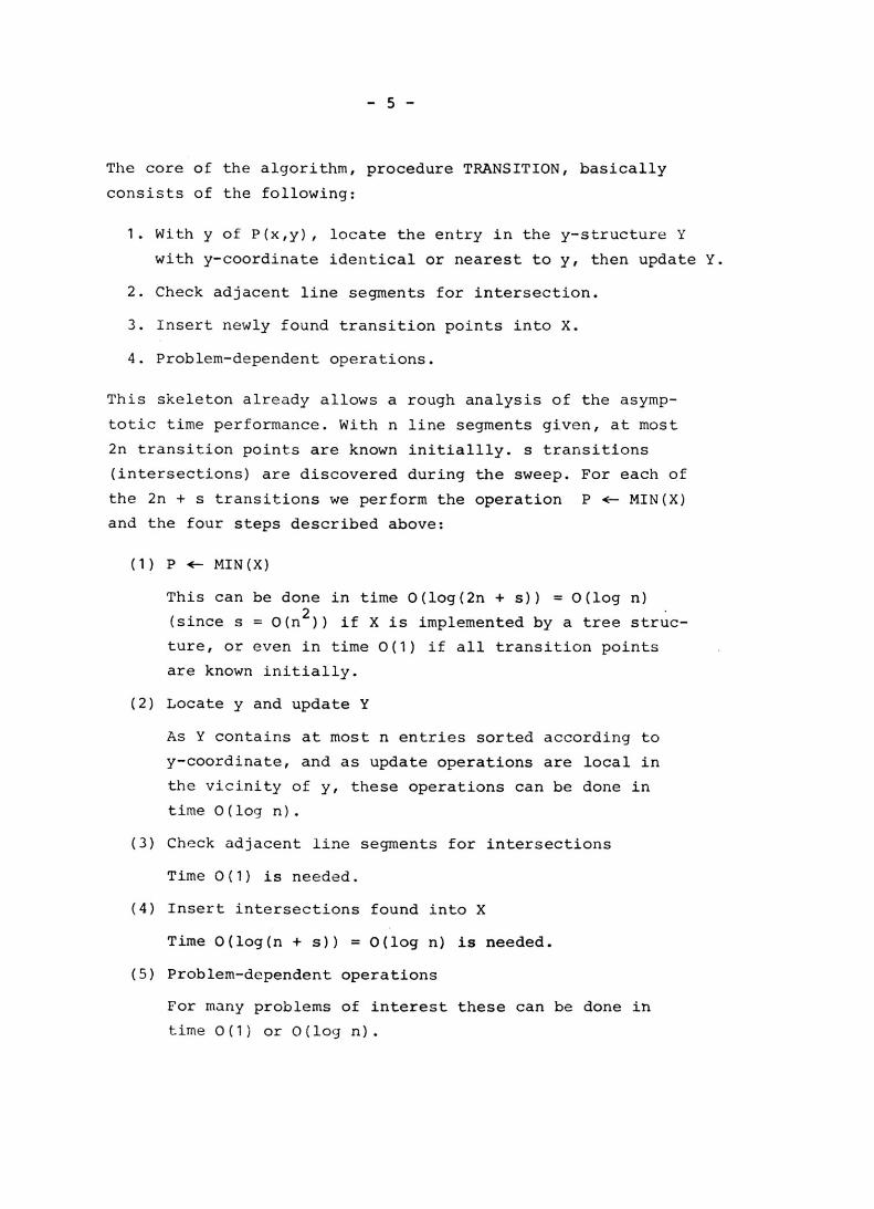
The core of the algorithm, procedure TRANSITION, basically

consis t s of the following:

1. With Y of P(x,y), locate the entry in the y-structure Y

with y-coordinate identical or nearest to y , then update Y.

2. Check adjacent line segments for intersec tion.

3. Insert newly found transition pOints into X.

4. Problem-dependent operations.

This skeleton already allows a rough analysis of the asymp­

totic time performance . With n line segments given, at most

2n transition pOints are known initiailly. 5 transitions

(intersections) are discovered during the sweep. For each of

the 2n + s transitions we perform the operation P +- MIN(X)

and the four steps described above:

(1) P +- MIN (X)

This can be done in time 0( 10g (2n + s)) = O(log n)

(since s = 0(n 2 )) if X is implemented by a tree struc­

ture, or even in time O(1} if al l transition pOints

are known initially.

(2) Locate y and update Y

As Y contains at most n entries sorted according to

y-coordinate , and as update operations are local in

th e vicinity of y, these operations can be done in

time 0 (log n).

( 3 ) Check adjacent line segments for intersections

Time 0(1) is needed.

(4 ) Insert intersections found into X

Time O(log(n + s)) = O(log n) is needed.

(5) Problem-dependent operations

For m3ny problems of interest these can be done in

time 0(1) or O(log n).

- 6 -

This sums up to O«n + s) log n) as mentioned earlier. In

special circumstances a time performance of O(n log n + s)

can be achieved (e.g. (MS 83). As we are interested in the

generality of plane-sweep algorithms, we do not discuss

these cases.

As a summary of this brief review of plane-sweep algorithms:

they are well understood, very general in their applicability

to different problems, and efficient for the large class of

applications where data "spread evenly across the working

plane", characterized by s = O(n).

In contrast to the two-dimensional ~ase, it is not yet clear

whether efficient multi-dimensional space - sweep algorithms

exist for problems of practical interest. As examples of

initial investigations into this question, let us mention

the use of plane-sweep techniques for hidden-surface elimi­

nation (Schmitt [Sch 81), and of space-sweep algorithms for

computing the subdivision of the space given by a finite

number of hyperplanes by Bieri and Nef [BN 82). The former

could well be called a "two-and-a-half-dimensional " problem

(superposi tion of several two-din\ensional problems), a nd thus

it is not clear whether its results generalize to k ~ 3 d i ­

mens ions. The latter is a truly k-dirnensional problem, and

provides a n interesting example worth extending.

In this paper, we present in an intuitive but systematic way

a space-sweep algorithm that completes the intersection of

two convex polyhedra in time O(n log n). This upper bound

has previously been a chieved by Muller and Preparata [MP 78).

We find it interesting to show how a sweep algorithm achieves

the same r esult by an entirely different technique.

- 7 -

2. SIMPLIFICA·rrON OF THE PROBLEM

In this paper we study the problem

rep (Intersection of two Convex Polyhedra): "Given two convex

polyhed ra in the form of a boundary representation, calculate

their intersection. 'I

This problem has previously b een studied by Muller and Prepa­

rata [ M? 78] who established an upper bound of O (n log n) for

po lyhedra having a total of n vertices. Later, attention has

shifted to t esting the intersection of two preprocessed poly­

hedra; Dobkin and Kirkpatrick [DK 82] are able to do this in

time O((log n)2) after 0(n2 ) preprocessing. More recently,

the same authors [DK 83] have presented a linear time algo ­

rithm that allows to detect whether two convex polyhedra in­

tersect. We return to the harder problem of calculating the

intersection, rather than merely testing for intersection ,

and achieve the same time bound as Muller and Preparata by an

entirely different and Simpler technique.

Our algorithm works by first determining some pOints in the

intersection of the surfaces of the two polyhedra Po and P"

using space-sweep. Starting from there it constructs all

edges of Po n P, and thus the resulting convex polyhedron by

graph exploration methods. Minor modifications in the graph

exploration phase allow to construct Po U P, or Po ' P, in­

stead of Po n Pl.

Throughout this paper we assume that no two corners of one

of the polyhedra have identical x-coordinates. This can al­

ways be achieved by a slight rotation of the coordinate

system, requiring linear time in addition to the initial

sorting of the corners. We also assume that all faces of

the polyhedra Po and P1 are triangulated from their respective

pO.int of minimal x-coordinate by improper edges . The "boun­

dary representation" mentioned above i s basically the doubly

connected edge list introduced by Muller and Preparata [MP 78),

- 8 -

enriched by the improper edges and by pOinters between fa ces

and the i mproper edges contained therein .

In the fo llowing t he word f a c e (bou nding trj ~lngle) always

refers to a bounding face of one of the polyhedra without

(with) consideration of improper edges. Thus a face may con­

sist of several co- planar bounding triangles.

Problem rep i s reduced to a simpler problem . The edge set E

of

o f

of

of

the re sulting convex polyhedroll p n P 1 consists o f a set 0

line segments o n the surf ace of both polyhedra, and a se t

line s egments that are edges or part of edges o f only one

the polyhedra. Figure 2-1 gives an examp l e.

I

J..-------/ ~~

/ /

/

Figure 2-1 Two bricks penetra t ing e a ch othe r. Hea v y l ines

are edges in E1 , dotted lines edges in E2 "

E1 is naturally composed of connected components; the examp le

E1 E 2

in figure 2- 1 has only one component . I t will be shown (l emma 1)

that Po n Pl can be systema tica lly c ons t r ucted in time O( n ) if

at leas t one pO i n t (on an edge ) of each c omponent of E , i s

known. With thi s in mind, we def ine the following prob lem that

lends itself more directly to the sp~ce -swe ep approach:

- 9 -

Problem rep': "Given two convex polyhedra Po and P, with a

"total of n corners , compute a set of intersection pOints of

proper edges of P. with bounding triangles of P 1 . , i = 0 or 1 -1

i = 1 . This set must contain at least one point of each con-

nected component of E 1 cPo n P 1 ...

Lemma 1: a solution to problem ICP' allows to compute

a) Po n

in time P 1 ' o (n) •

b)Po

UP1

, c)Po .... P1

Proof: We argue about part a) only. Parts b) and c) solely

differ in the definition of E 2 , and thus in a modified deter­

mination of the edges in E 2 .

The basic idea is to consider the solution set to lep' as part

of the se t of vertices of a graph, and, starting from these

vertices, to explore the graph by a systematic method . To have

a sensible stopping criterion we want to know E1 completely

before we start exploring E2 .

Let S be the solution set to lep'. As shown in section 4, we

can get x € S as intersection of e, the proper edge separating

the bounding triangles F' and F' I of P. , with the bounding 1

triangle F of P1 . . We process all points xES as follows: -1

We construct all edges of E l incident to x. On the proper

edges of P1 (Po) extending from x into the interior of Po (P 1 )

(observe that there may be more than one of these if x is

vertex of Po or P1), the candidates tor E2

, we mark X, and

store these edges in a set. If such an edge is marked already,

it penetrates one of the two polyhedra; in this case we add

the segment between the two markings to the set E2 . Compare

figure 2- 2.

We have to distinguish three cases concerning the respective

position of x, namely

(case 1) x is no polyhedron vertex, and lies in the interior

of bounding triangle F of P1 . , -1

- 10 -

/I _II L~' -- I y

x \ __ ---

Figure 2-2 Marking of candidates for E2'

e is edge of p , and intersects 1

e penetrates P'-i from x on to

P 1 . in x, -1

the right; this

part of e becomes a candidate for E2 , and x is

marked on e, If e is later explored starting

from y (y may belong to a different component

of E1 ), the mark x is detected; we then add xy

to the set E2'

(case 2) x is the intersection of two edges but no polyhedron

vertex , and

(case 3) x is vertex of Pi or/and of P1-i '

Case 1 - as illustrated in figure 2-3 - is the standard case,

In case 2 let x be the intersection of edge e with edge f se­

parating bounding triangles F and F'" of P1-i ' Ordinarily

(and analoguously to case 1), we can compute the structure

around x in time 0(1) by intersecting F and F' I I with pi and

FI '. A problem arises, however, if F or pI I I is co-planar with

F' or F", Say, F is co-planar with F', F' is part of face Gi

,

F is part of face G1_ i , To avoi~ getting irrelevant and unde­

sired intersections in the interior of Gi

n G'_i' we treat the

faces as a whole and compute Gi

n G1

_i

in time

o (deg. (G.) + deg 1 . (G 1 .», using the known method due to ~ ). -~-1

, , , , I , ,v

- 11 -

f

Figure 2-3 Edge e intersects bounding triangle F in x,

Edges F n F' and F n F" belong to E" The

part of e extending into the interior of the

other polyhedron is candidate for E 2 ; x is

marked on e.

Shamos [Sh 75J, deg. (G) denotes the number of vertices of ~

convex polygon G in Pi" We mark the two faces as "done", and

then process t he vertices of the intersection polygon ,

Case 3 can be divided into three subcases. Let x be a vertex

of Po Then x can lie in the interior of a bounding triangle

F of P" or on an edge f of P" or it can even be a vertex

of P, as

bounding

well. In the first case we intersect F with all

triangles of P inc iden t to x, and thus get all o

edges i n E, (and candidates for E2 ) incident to x in time

O(dego(x», Here degi( x) denotes the degree of x in poly­

hedron Pi' improper edges included, In addition, we might

have to treat co-planar faces a s described i n case 2 above.

In general, we will get two edges in E" and some candidates

for E2' as shown in figure 2-4.

- '2 -

F

Figure 2-4 Vertex x of Pi lies in bounding triangle F

of P, .. -~

The second subcase is analoguous; time O(dego(x» suffices,

apart from the time for treating co-planar faces.

If x is vertex of both polyhedra, however, the situation is

considerably more subtle . The naive approach might result in

quadratic running time. Therefore we transform the problem

in a suitable manner to a two-dimensional problem. Basically,

we find a plane D intersecting all edges of Po incident to x

in time O(dego(x». Po n D is a convex polygon, P, n D a con­

vex polygonal region. We intersect these two plane figures in

time O(dego(x) + deg, (x», using Shamos' method. The s t r uc­

ture around x can be inferred fro~ the resulting polygon in

a straightforward manner. Again, co-planar faces might have

to be handled in addition.

In all three subcases we afterwards mark x in the polyhedron

it belongs to.

This way we have constructed all edges in E, (and candidates

for E2 ) incident to a pOint xES in total time O(n). Total

time O(n) is also sufficient for the treatment of co-planar

faces since the computation described in case 2 is performed

at most once for each face.

- '3 -

Starting from these edges we fi rst want to explore E1 comple­

tely . This is done by working with two sets W, (W Z), that

initially contain all the known members of E1 (candidates for

E Z) ' A,S long as W, contains any element an edge e = (x,y) is

removed from W, and processed. Processing all. edge means

checking whether its endpoints were processed already; all.

endpoint that was not is processed according to the pertinent

case as described above, thereby possibly adding new edges to

W" E" w2 ' E2" The time for the whole procedure sums up to

O(n) by arguments above if one c an decide fast (i.e., in con­

stant time) whether an edge endpoint was processed already.

This is indeed possible if we mark pOints that are not cor­

ners of Po or P, all. the edges they lie on in a sensible way,

such that no edge eventually bears more than two markings.

The only question as to where one should mark arises in

case Z above (x = e, n e, .) if e , lies (partly) in a face .... -l. l.

of P, ,. We mark x on e 1 ' if this edge does not lie in a -l. -l.

face of p,: otherwise (two co-planar faces), e, and e, , 1. 1. -1.

will be proper edges (the algorithm in section 4 will deli-

ver no intersection with an improper edge in this case), and

we can safely mark x on both of them (details left to the

reader) .

By now we have explored all of E1 in

dates for EZ can be added to set EZ' terior endpoints of these candidates

remaining edges that belong to E2 in

time O(n), and candi­

Starting from the in­

it is easy to find the

time 0 (n) . o

More details of the proof above, especially of the corner­

in-corner subcase, can be found in [He 84).

- 14 -

3. BASIC CONCEPTS

By analogy to p l ane-sweep algorithms, a space-sweep algorithm

operates by advancing a plane through space. The x-structure

is a queue X containing (for our problem) all n corners o f the

two polyhedra. The yz-structure that replaces the y-structure

represents the state o f the cross section. The latter has ( for

each one of the two polyhedra) the f orm of a convex polygon .

The set of edges (of one polyhedron ) intersec ted by the sweep

plane forms a cycle whose neighbor edges bound the same boun­

ding triangle of the polyhedron. This leads us to

Defini tion 1: Let P., i = 0,1, be one of t he polyhedra . Let 1

ej

, 0 S j < n i , be the cyclically o r dered sequence o f edge s

intersected by the sweeping plane. A prong is the portion of

a bounding triangle bounded by t wo consecutive edges ej

and

e(j+1) mod ni

' and, to the left, b y the sweeping plane. The

cyclically ordered set o f prongs forms the c rown Ci

"

Obs e rve that, because of t he triangulation chosen, the par t

o f a face o f Pi to the right of the sweeping plane is eith er

completely or not at all part of the crown C . . 1

Obv iously all prongs are either triangles or quadrila terals ,

and we can classify crown edges as follows:

De fi nition 2: Let P. and 1

o f the polygon formed b y

e . be a s in Definition 1 . The edge s J

connecting the intersection pOi n t s

in a circular fas h ion are called base edge s , their x-c oor d i ­

nate is the base; the edges e. of the original polyhedron J

are called Eo r Wdxd edges, and all other edges of the crow n

are called prong edges (they connect tips of p r ongs).

These definitions are pictured in figure 3-1.

Thus we can represent a cross section in a way analoguou~ t o

the one-dimensional cross section o f plane-sweep algor iti~~s :

- 15 -

Figure 3-1 Edge classification of a crown.

b,f,p denote the three edge t ypes .

Point q is the polyhedron corner just processed.

Forward edges starting left o f q are shown dashed

to the left of the s weeping plane.

here the linearly ordered y-structure is r e? laced by a circu­

larly ordered yz-crown. Due to this circular ordering, the

crown can be searched in logarithmic time by binary searc h

for angular arguments, to dete r mine the relative position of

a new transition point w.r.t. the crown edges.

To s tore crown c. in a balanced tree we select an axis line L., 1 1

e.g. the line connecting the vertices of Pi having the minimum

and maximum x-coordinate, respectively. This axis alvlays inter­

se~t: tIle s weeping pl ane , and we can represent p E ffi 3 w.r.t. L . 1

- '6 -

by the cylindrical coordinates ( XI alfa, radius). Here x is

pIS x-coordinate, and (alfa, radius) are piS polar coordinates

in the yz-plane through p, with pole on L . and alfa's measured l.

against, say, the positive y-axis.

ted by the cylindrical coordinates

A forward edge is represen-

w.r.t. L . of its endpoints, l.

i.e., by (xo ' alfao ' r o ' x" alfa" r,). Note that for every p on such a forward edge with x-coordinate x, Xo $ x S x" we

can calculate (alfa, r) in constant time. The radial . represen­

tation is depicted in figure 3-2; in figure 3-3 formulae are

given that help for the calculation of (alfa, r) - for sim­

plification , the axis is assumed to be the x-axis.

I I /

f

" "

f

"' " .....

)

- . -----

Figure 3-2 Radial representation of a crown, viewed parallel

to the axis. Qi'S are angles of left, ails

angles of right endpoints of forward edges.

Note that although a lfas and radii change with X, the r elative

ordering of crown edges r emains invariant between transitions.

- 17 -

':I.

x y

x, (,-- 'J" ~o A-I ~-z,

x = x.

'J = 'j.

Z =. 2.

Figure 3-3

~,

+ k(x,-x.) to." "Z

'" = 'j

+ kt~,-'jo ) "-k ( .. , - z.)

r - oS,:", 0( +

(a.) (b)

Coordinate transformation for a forward edge

f = (po 'p, ) if the axis is the x-axis.

(a) Projection into the xy-plane.

(b) Projections into the yz - plane at x Xo and

atx=x,.

This allows us to store the crown as a balanced binary tree,

organized with respect to alfas.

Before we can process (see next section) a new polyhedron vertex

p = (x,y,z) (with cylindrica l coordinates (x, alfa, r», we have

to know where it is located in the respective crown. Therefore

we use angular binary search to find a crown edge the right end­

point of which is p. If the intersection of any forward edge of

the crown wi th the yz-plane through p has cylindrical coordina­

tes (x, alfa* , r*), we have to search until we find an edge

such that al fa' = alfa.

- '8 -

4. THE ALGORITHM

Our algorithm will construct two crowns, one for each poly­

hedron, and will find their intersections (as specified in

problem rep' I i .e ., at least one per connected component of

E,). Thereby, if edge e lies completely in a face of the

other polyhedron, "intersection" is defined to be an end­

point of e. Advancing in the x-queue (that initially con­

tains all n corners) from vertex to vertex of the two poly­

hedra, we perform one transition per vertex . We will first

present procedure TRANSITION, the core of our algorithm, and

then show that the algorithm is correct and stays within the

desired time limit of O(n log n ) .

Processing vertex p of polyhedron Pi we assume that at l eas t

one point was found already of every component of E, comple ­

tely left of p (and possibly including p); we only look for

intersections to the right of p . One execution of TRANSITION

will deliver zero, one , or several intersection pOints of

"the two polyhdra on an edge or in a face of Pi starting at

p. To achieve this, we first intersect all proper edges of

Pi starting at p with the opposite crown C'_i. If none of the two edges bounding a face F of P . starting at p inter-

1 sects the opposite crown, a part of P'-i could nevertheless penetrate face F, as shown in figure 4-'.

Figure 4-' No bounding edge of face F of Pi intersects C'_i;

however, forward edges of C'_i penetrate F.

- '9 -

To detect some of these intersections, we intersect, in this

case ,

Lemma

an arbitrary proper forward edge of crown C, . with F. -1

2 below asserts that thi s is sufficient to find at

leas t one point of each component of E, .

Specif ically , a transition is performed as follows (S is an

initially empty set of intersections):

(') proc TRANSITION (p , i) :

( 2)

(3)

( 4 )

( 5 )

(6 )

( 7 )

(8)

( 9 )

( 10)

( " )

update crown C . of po lyhedron P . ; 1 1

if exact ly one edge e of P. starts a t p -- 1

fi

the n intersect e with the crown C'_i of P, . and -1

add all intersections to s e t S

else for all faces F of P. starting at p 1

(possibly consisting of several prongs)

do intersect the starting proper edges of F

with the crown C ,and add all inter­'-i

od

sections to S;

if no intersection is found

fi

then choose a proper forward edge of crown

C, . and intersect it with F; add -1

intersection, if any , (in the pertain-

ing bounding triangle) to S

('2) corp.

Lemma 2: Performing TRANSITION once for each of the vertices

of the two polyhedra sorted into a common queue correctly

solves problem ICP'.

Proof: It is clear that a set of inters e ctions is computed.

Thus we only need to show that at least one point of each

component of E, will be r epor ted .

Le t K be a component of E" and let v be a vertex o f K with

minimal x-coordinat _e. Clearly v is the intersection of an

- 20 -

edge e of polyhedron P. with a face F of polyh e dron ~

I f v is not reported then e must start before F (in

P, .. -~

the

swe ep orde r). Consider the state of the space-sweep imme ­

diately after the start ver tex p of F is encountered. At

this pOint e is a forward edge of the crown Ci of Pi.

Conceptually t race K in fa ce F and crown Ci ' starting a t v .

Two cases may arise:

£a~e_1~ We are not able t o trace K completely, i.e., we

first hit either a bounding edge e' of F (s ub case a»,

or a prong edge e" of C . (subcase b ». Because o f ~

the minirnality of V i S x-coordinate we do not leave

Ci by way of a base edge.

a) e' intersects a prong G of Ci . Then e' n G either

was detected at processing p, or it will be d e ­

tected when the starting point of e t is processed ,

since G is still a prong of Ci

at that time . Com­

pare fig ure 4-2.

b) Because of the triangulation chose n for faces, e 1 I

i s a proper edge. Also, F still is part of crown

C, . whe n the starting pOint of ell is process e d. - ~

Therefore e" n F is detected at that time.

fa~e_2-,- We are able to trace K completely in F and Ci .

Since e starts before F and s ince it does not inte r ­

sec t a bound ing edge of F, e does not lie in fa ce F

but intersects t he interior of F. The intersection

with F of the two prongs of Ci neighboring e i s c om­

ple t e ly contained in F, and the forward edges (other

than e) of these prongs again intersect the inte rior

of F. The argume nt propagates around the crown Ci

.

Thus K is a closed curve in F running through all

prongs of Ci ' and i ntersecting all forward edges of

Ci . Hence a point of F is found in line (8) of TRAN­

SITION. Figure 4-' helps for understanding this case ;

we may, in line (8) of TRANSITION, select forward

edge f of Ci and intersect it with F. D

- 21 -

p ~::::.:::------l

e'

G

Figure 4-2 Case 1 a) of the proof of lemma 2. Shown are

a part of the crown C1

_i

, and prong G of

crown Cio W = e l n G is detected when the

starting pOint of e' is processed.

Let us now examine the time required for the different actions

of TRANSITION.

Lemma 3: The updating of crown Co (C 1 , res p.) can be done

in total time O(n log n).

Proof:

vertex

Consider updating crown Ci

(i = 0,1) at a transition

v = (x,y ,z). Let c be the maximum of the number of

forward edges of Ci

before the transition, and the number of

such edges after the transition, and let d = d1

+ d2

, with

d 1 (d 2 ) being the number of edges of Pi ending (starting) at

v. We have to localize the edges ending at v in th e balanced

tree r e present:i ng c. for updating c. subsequently . 'rhis can 1 1

be d one by angular binary search as described in the previous

- 22 -

sectiun. Because of the cyclic ordering of the crown this

yields a subtree Tv' as pictured in figure 4-3.

- - -

~ C·

.~\ L

~.­

c.d. 3 e.li. .... ~ tL. ~......11' • .:_t v

Figure 4-3 The two outermost search paths (bounding Tv)

for edges with endpoint v.

Now we split C. along the two outermost search paths, drop

.Tv ' and merge ~he tree T~ew formed from the d 2 edges s tart­

ing in v (that are given in cyclic order) with the remainder

of Ci . This can be done in time O(log c + d 2) , namely time

O(log c) for the search with the subsequent splitting of the

tree Ci ' time 0(d 2 ) for the construction of the tree T~ew,

and time O(log c) for the merging of T~ew with the remainder

of Ci " The operations necessary are those of a "concate nable

queue II ([AHU 74], p. 155ff.) - observe that the remainder of

Ci

is a forest of trees with known relative orde ring, and

with height differences between two neighbors summing up to

O(log c). Since c < n, and since the sum of d's over all po-

lyhedron vertices is O(n), the lemma follows . c

Lemma 4: Let g be a straight line , and let C be a crown with

c forward edges. C n g can be computed in time O(log c) .

Proo f: Similarly to the idea o f Dobki n and Kirkpatrick (DK 82,

- 23 -

OK 83] we let the bala nced tree d e fine a hierarchical repre­

sentation of the crown. It will help us for f inding an inter­

section if we do not use the crown directly but an extens ion

of it to a convex polyhe dron. Specifically, l et v 1 ' . . . , Vc

be the vertices of the base polygon , and let w1 ' . . . , Wc be

the right endpoints of the c forward edges. Neighboring v's

or neighboring WIS may coincide . Le t V := (v1

, . . . , ve),

W : = (w 1 ' . . . • wc)' and let t be the right e nd point of t he

axis of C, i.e., the rightmost vertex of the respective po ly­

he dron . Cons ide r the convex hull of the points V U W U (t).

The bounding faces of the convex hull are the base polygon

whi ch we will no t consider in the sequel (intersections with

g there are not interesting). the prongs of crown C and the

terminal triangles (tt's) extending from two neighboring but

no t identical w's each to t . Thus each tt has exactly one

partner prong (pp); the reverse relation does not hold neces­

sarily. Figure 4- 4 presents such a solid object and illustra­

tes the new terms .

Figure 4- 4 Convex hull of a crown with 8 forward edges

joining in 5 different right endpoints , to­

gether with t , the rightmost polyhedron ve rtex .

Partner of tt w7w,t is prong v,w,wsva; prong v 7vawS has no partner .

- 24 -

We will r e present such a special polyhedron hierarchically

by a balanced tree. To be specific, let us choose a (2,3)­

tree (compare [AHU 74]). Observe that the crown resp. the

special polyhedron is ~i nd of a two-and-a-half-dimensional

solid for which the two-dimensional hierarchical representa­

tion of [DK 82] is basically sufficient. Let C(i), i = 1, ..

.. , k = O(log c), be the forward edges of the crown store d

in depth i of the tree. C(k) is C, and p(i), the convex hull

of C(i) and pOint t, is an inner approximation of the spe cial

polyhedron. C(i) is shrunk to C(i-1 ) by transforming two (or

three) prongs of C(i) each into one - this, in turn, i s done

by removing the forward edgers) separating them. Compare fi­

gure 4-5.

Figure 4-5 a Two sUbsequent approximations of the crown of

a polyhedron, seen from the direction of the

positive axis. C(i) (cons isting of prongs

with at least one forward edge shown dashe d)

is made coarser and thus changed into C(i-1)

(solid edges) .

0

____ 0

.\ eO

-0 0-

Figure 4-5 b

- 25 -

)

_0

0-

.\' , eO (co-planar prongs)

" " , ____ 0

0 0 0

or ) .\\ eO

\ 0 0...., ,,'

or '0 '-0_ ,.. \ -0 ,..

0 .... \

.\ \ \ e O \

0 0

0 0---0-

or I

e \ eO

Refinement

transition

of the representation ( i-I) (i) from C t o C .

° ,0

0 _ _ 0'

of a crown;

Forms of the IIpartitioninglf of a prong into

two by adding an additional forward e dge

(dashed; between two neighboring f orward

edges , e and e O, of C(i-l». If two addi­

tional edges are inserted even more forms

of refining a prong are pos s ible.

- 26 -

Figure 4-6 (a) Part of crown C (k) with the corresponding

part of C(k-') (solid lines).

(b) Hierarchical representation of (a) in the

(2,3)-tree; shown is only the hierarchy in­

formation in the internal nodes. From the

upper node marked bye, one can find the

corresponding prong w,w6v7v6 of C(k-2)

that is not explicitly drawn in (a).

., _/

- 27 -

Il ~ ter:lal nodes of the balanced tree contain a hierarchy in­

formation, apart from the usual order info rmation (fo r pre­

serving t he order during r ebalancing). The former is chosen

t o insure that , in each depth i t i = 1, ... , k , two neigh­

boring nodes each correspond to a prong of the crown c(i).

To ach ieve this, it is sufficient to let leaves of the tree

represent forward edges of the crown C = c(k), and every in­

ternal node the (cyc lically) minimal edge of the subtree the

root of which it is. Via neighbor pointers on every l evel one

can find the prong corresponding to a node in constant time.

Figure 4- 6 illustrates the correspondence between a connected

section of the crown c(k ) a nd the pertinent tree r epr esenta­

tion.

The r e finement of the representation, i.e., the transition

from p(i) to p(i+l) , may be understood as a convex extension

of p(i). We will present related terms and investigations be­

fore we explain the algorithm for determining eng .

Let P = (V,E ) be an arbitrary convex polyhedron. Let Z =

= (v 1 , . . . , v s ' vs+l = v) be a closed simple path of edge s

on P, i.e., vi € V, (vi,V i +,) E E for i = 1, ... , Sl and

v . f v. for if j, i,j E [1 :s1 . Z d ivides the surface of p ~ J

into two segments. Let S be a segment. A convex extension of S

is an expansion of P in the region of 5 (by adding new nodes

and edges , and by possibly r emov ing nodes in the interior of

5, i. e. , in 5 but not on the path of edges bounding 5) that

preserves convexity. The roof o ver S is t~e maximal convex

extension of S. Roofs may be c losed or open (i.e., infinite);

for instance, the faces of a tetrahedron have open r oofs,

those of a d odekahedron have closed roofs.

Relevant for our algorithm is the following fact (proved in

[He 841, p. 85):

Fact : Let 5 ~ (5" . . . , Sk) be a parti t ion of the surface of

conve x po l yhed r on P into segments. A line 9 t.nat does not

- 28 -

intersect P can inters ect the roofs of at most two of these

segments.

Now we are going to compute eng, guided by Dobkin and Kirk­

patrick's algorithm for determining the intersection of a

straight line with a convex polygon. In the following, segments

will always be tt-pp-pairs, and prongs without partner; com­

pare figure 4-4.

We start with p(1), a (possib l y degenerated) convex poly­

hedron with few segments, and determine the part of p( 1) where

an intersection could occur if it exists. There we local ly

proceed to p(2) and determine a - smaller - section for a

possible intersection . We locally expand the polyhedron up

to p(k) to find an intersection if any. If g intersects p(k)

in a prong of C(k) this point is reported; intersections with

tt's are neglected.

Depending on whether we already have found an intersection

9 n C or no t, we have to distinguish two case s.

A prope r inte rsection (i.e., not only touching point) found

in depth i is processed by refining the respective segment to

the next depth. One of the (at most six) new bounding faces

must again have an intersection with 9i we proceed analog uous­

ly at depth i + 1.

If no intersection was found so far, the following invariant

is maintained before t he start of the i-th iteration (i.e.,

c omputat ion at depth i) I i = 2, ... , k:

(INV. 1): (i -1 )

51' 52 are two segments of p . with the foll ow-

ing property: If g intersects p(J) with j ~ i, then

g intersects one or both of the roofs over 51,52 ,

51 = 52 is allowed.

For the second iteration t he invariant is established as

fo llo'''s:

- 29 -

l!ltc l~sect 9 with al l bou llding faces of p(l). I f no sue],

intersection is found intersect 9 with the roofs of all (1)

segments of P . Observe t nat such an intersection is com-

putab l e in constant ti rr:e. Get at most two segmen ts S l' 52

the roofs of which are intersected by g. Stop if no such

segment exists.

The transition from the i-th to the (i+l)st iteration, i ~ 2,

is performed as follows:

Refine segments S 1 I 52 to depth i + 1 • Get at most six new

segments. If no intersect i on of 9 with one of the maximally

12 new bounding faces is found, intersect g with the roofs

of the new segments. Get at most two new segments 5" 52 the

roofs of which are intersected by g. Observe that, if seg­

ment S is refined into two or three new segments, the roofs

of the new segments are contained in the roof of S, and, that

roofs of segments not considered never grow either. Stop if

g does not intersect any roof.

Let us briefly mention two special cases that require some

modification of our procedure in the i-th iteration. If g

touches p(i) in exactly one point on a forward or "terminal"

edge, we refine the two incident segments; if a part of g

lies in a prong of C(i) we refine, per iteration, the outer­

most two segments concerned, in order to avoid reporting an

intersection of 9 with an improper edge.

Details of such special cases are left to the reader. It

suffices to realize that only constant work is necessary

per iteration. Since, due to the convexity of p(i), not more

than two search paths are folloHed through in the tree, the

time bound follows. a

Corollary: Let C be a crot,om with c forward edges, and let e

be an edge the left endpOint of which does not lie left of

the base of C. C n e can be computed in time 0(10g c) •

- 30 -

By combining lemmata 2 - 4 we obtain

Lemma 5: The space-sweep. algorithm using procedure TRANSITION

described above solves problem Iep' defined in section 2 in

time O(n log n).

Proof: The total cost for line (2) of TRANSITION is O(n log n)

according to lemma 3, as is, according to lemma 4 including

its corollary, the total cost for lines (4) and (6). Line (8)

needs O(degi(F)) per execution, that is, total time O(n)

since it is executed at most once per face F. For all other

lines linear time suffices in total. o

Together with lemma 1 we finally get our main result

Theorem : The intersection of two convex polyhedra with a

total of n corners can be computed by space-sweep in time

O(n log n).

- 31 -

5. CONCLvSIO" S

We h a ve s e C ll t hat the space-swe ep approach y ields an effi­

cient algorithm for intersection of convex polyhedra that

ma t ches the performance of the best known algorithm to this

pro b l em. Moreover, the method is mOre universal than the

pre vious solution by Muller and Preparata [MP 78J; we further

believe it to be easier to understand.

Th us t here are effective space-sweep algorithms for selected

problems. Howe ver, space-sweep does not seem to offer as

general an approach to solving geometric problems in 3 di­

men s ions as plane-sweep does for 2 dimensions. It is an

open question whether space-sweep can be effectively applied

to more general problems, such as those involving non-convex

solids.

ACKNOWLEDGEMENT

We are grateful to Klaus Hinrichs, Herbert Edelsbrunner, and

Athanasios Tsakalidis for helpful comments.

[AHU 74]

[BN 82]

[BO 79]

[DK 82 ]

[DK 83]

[Ha 55]

[Ha 68 J

[He 84 J

IMp 78]

[MS 83]

[NP 82]

- 32 -

REFERENCES

A.V.Aho/J.E.Hopcroft/J.D.Ullman: "The Design and Analysis of Computer Algorithms" Addison-Wesley Publ. Comp., Reading, Mass., 1974

H.Bieri and W.Nef: "A Recursive Sweep-Plane Algorithm, getermining All Cells of a Finite Division of E. II

Computing 28 (1982), 189-198

J . L.Bentley and T .A.Ottman: "Algorithms for Reporting and Counting Geometric

Intersections" IEEE Trans. on Comp., Vol . C-28 ( 19 79) , 643-647

D.P.Dobkin and D. G.Kirkpatrick : "Past Detection of Polyhedral Intersections" Proc. 9th ICALP, Springer LNCS 140 (1982), 154-165

D. P.Dobkin and D.G.Kirkpatrick: "A Linear Algorithm for Determining the Separation of Convex Polyhedra"

Manuscript, 1983

H.Hadwiger: "Eulers Charakteristik und kombinatorische Geometrie"

J. reine und angew. Math. 194 (1955), 101-110

H.Hadwlger, "Eine Schnittrekurslon fUr die Eulersche Charakte­ristlk euklidischer Polyeder mit Anwendungen innerhalb der kombinatorischen Geometrie"

Elemente der Mathematik 23 (1968), 121-132

S.Hertel: "Sweep-Algorithmen fUr Polygone und Polyeder" Univ. des Saarlandes, Saarbrlicken, Di ss . 1984

D.E.Muller and F.P.Preparata: "Finding the Intersection of Two Convex Polyhedra" Theoret. Compo Sci. 7 (1978), 217-236

Mairson and Stolfi, personal communication, 1983

J.Nieverqelt and F.P.Preparata: "Plane-Sweep Algorithms for Intersecting Geometric Figures"

Corran. ACM 25, 10 (Oct. 1982), 739-747

[Sch 81 ]

[Sh 75]

[SH 76]

- 33 -

A.Schmitt: "Time and Space Bounds for Hidden Line and Hidden Surface Algorithms"

Proc. EUROGRAPHICS '81, North-Holland, Amsterdam, 1981, pp. 43-56

M.I.Shamos: "Geometric Cornpexity" Proc. 7th ACM STOC (1975), 224-233

M.I.Shamos and D.Hoey: "Geometric Intersection Problems" Proc. 17th IEEE FOCS Symp. (1976), 208-215