Préparation à Solvabilité II Traduction partielle du ... · 1/77 Préparation à Solvabilité II...

1/77

Préparation à Solvabilité II Traduction partielle du document de l’EIOPA sur les hypothèses sous-jacentes à la formule standard pour le calcul du SCR

6 août 2014 – Version 1.0

2/77

Table of Contents Avertissement ............................................................................................ 4 Introduction............................................................................................... 4 1. Structure générale de la formule standard ................................................. 6

1.1 Corrélations dans la formule standard ................................................... 8

1.2 Sélection des paramètres de corrélation pour les risques indépendants ..... 9

1.3 Risques non explicitement inclus dans le calcul de la formule standard ... 10

2. Risque de marché ............................................................................. 13 2.1. Risque de taux d’intérêt .............................................................. 14

2.2. Risque sur actions ...................................................................... 16

Standard equity capital charge ................................................................ 18

Symmetric adjustment mechanism .......................................................... 19

Duration-based approach ....................................................................... 20

2.3. Risque de change ....................................................................... 20

2.4. Risque sur actif immobilier........................................................... 22

2.5. Risque lié à la marge ou risque de spread ...................................... 23

Spread risk on bonds and loans other than residential mortgage loans ......... 24

Spread risk on securitisation positions ...................................................... 25

Spread risk on credit derivatives ............................................................. 26

2.6. Risque marché de concentration ................................................... 26

3. Risque de souscription en vie .............................................................. 29 3.1. Risque de mortalité..................................................................... 31

3.2. Risque de longévité .................................................................... 32

3.3. Risque d’incapacité/invalidité – de morbidité .................................. 33

Inception and recovery rates ................................................................... 34

3.4. Risque de dépenses .................................................................... 35

3.5. Risque de révision ...................................................................... 36

3.6. Risque de cessation .................................................................... 37

Increase and decrease of lapse rate ......................................................... 38

Mass lapse event ................................................................................... 38

3.7. Risque de catastrophe en vie ....................................................... 39

4. Risque de souscription en non-vie ....................................................... 41 4.1 Risque de primes et de réserve en non-vie ...................................... 41

4.1.1 The combined approach for setting premium and reserve risk factors .. 44 4.1.2 Premium risk ................................................................................ 46 4.1.3 Reserve risk ................................................................................. 47

3/77

4.2 Risque de cessation en non-vie ....................................................... 49

4.3 Risque de catastrophe en non-vie .................................................... 50

4.3.1 Risque de catastrophe naturelle ........................................................ 50 4.3.2 Risque de catastrophe d’origine humaine ........................................... 52

Calibration for man-made catastrophe risk ............................................... 53

5. Risque de souscription en santé .......................................................... 56 5.1. Risque de souscription en santé SLT ............................................. 57

5.1.1. SLT Health Mortality risk ............................................................. 58 5.1.2. SLT Health Longevity risk ............................................................ 58 5.1.3. Risque d’incapacité/invalidité – de morbidité en santé SLT relevant de l’assurance frais médicaux ......................................................................... 59 5.1.4. SLT Health Disability-Morbidity risk for income protection insurance . 61 5.1.5. SLT Health Expenses................................................................... 61 5.1.6. SLT Health Revision risk .............................................................. 62 5.1.7. Risque de cessationen santé SLT .................................................. 63

5.2. Risque de souscription en santé non-SLT ....................................... 64

5.2.1 Non-SLT Health Premium and reserve risk ........................................ 64 5.2.2 Non-SLT Health lapse risk ............................................................. 65

5.3 Risque de catastrophe en santé ...................................................... 65

Calibration of the proportion of people affected (rs) .................................... 68

6. Risque opérationnel ........................................................................... 71 7. Risque de contrepartie ....................................................................... 72

Capital requirement for type 1 exposures ................................................. 74

Capital requirement for type 2 exposures ................................................. 76

4/77

Avertissement

L’Autorité de contrôle prudentiel et de résolution (ACPR) propose ci-dessous une

traduction des éléments principaux des hypothèses sous-jacentes à la formule standard

publiées par l’Autorité européenne des assurances et des pensions professionnelles

(EIOPA en anglais). Elle vise à faciliter l’appropriation de ce document par le marché

français dans le cadre des exercices de préparation et ne présente pas de caractère

officiel.

Introduction

1.1 Ce document présente les hypothèses sous-jacentes à la formule standard

utilisées pour le calcul du capital de solvabilité requis (SCR). Il doit être lu en

complément des orientations sur l’évaluation prospective des risques propres de

l’entreprise (basées sur les principes de l’ORSA) et à partir de 2016, en

complément des orientations sur l’ORSA.

1.2 L’évaluation du degré avec lequel le profil de risque d’un organisme d’assurance

ou de réassurance ou d’un groupe s’écarte des hypothèses qui sous-tendent le

calcul du SCR et un processus important que les organismes et groupes sont

tenus de réaliser à partir de 2015. Elle doit permettre de s’assurer que les

organismes et groupes comprennent les hypothèses sous-jacentes au calcul du

SCR et procèdent à leur évaluation afin de juger si elles sont appropriées pour

l’organisme ou le groupe. Pour ce faire, l’organisme ou le groupe devra comparer

ces hypothèses avec son profil de risque. L’objectif de l’évaluation n’est cependant

pas de revoir la pertinence de la calibration de la formule standard en elle-même.

1.3 La formule standard pour le calcul du capital de solvabilité requis (SCR) vise à

prendre en compte les risques importants et quantifiables auxquels la plupart des

organismes sont exposés. La formule standard peut cependant ne pas couvrir tous

les risques importants auxquels serait soumis un organisme en particulier. Une

formule de ce type, par nature et par construction, n’est pas personnalisée pour le

profil de risque de chaque organisme.

1.4 Ce document couvre tous les modules de risque de la formule standard: il traite

des hypothèses relatives aux risques couverts par les modules ainsi que des

hypothèses relatives à la corrélation entre les modules. Il n’explique pas pourquoi

certains risques ne sont pas explicitement couverts par la formule standard.

Néanmoins, cela ne signifie pas que ces risques ne doivent pas être pris en

considération lors de l’évaluation de la mesure de la déviation.

1.5 Les hypothèses en elles-mêmes sont résumées dans les parties encadrées1 en

début de chapitre et sont accompagnées d’informations plus détaillées2. Le texte

encadré comprend les informations que l’organe d’administration, de gestion ou

de contrôle devrait connaitre d’après l’EIOPA pour piloter le processus de l’ORSA.

1 NDT : et traduites

2 Les informations détaillées n’ont par contre pas été traduites

5/77

Les informations plus détaillées doivent servir aux personnes qui vont

effectivement réaliser l’évaluation de la mesure de la déviation.

1.6 L’évaluation de la mesure de la déviation étant à l’appréciation de l’organisme ou

du groupe lui-même, le document ne prescrit pas quelles sont les hypothèses à

considérer en priorité ni la méthode pour mener l’évaluation de la déviation du

profil de risque. Le document ne fait que donner des informations nécessaires

pour la mener. De plus, le document décrit les hypothèses principales mais ne

cherche pas à décrire exhaustivement toutes les hypothèses sous-jacentes ni à

recenser tous les risques qui ne sont pas explicitement pris en compte dans la

formule standard. Lorsque des méthodes simplifiées sont disponibles, elles ont

été développées sur la base des mêmes hypothèses que la méthode standard.

Dans la plupart des cas cependant, des hypothèses supplémentaires ont été

avancées pour en déduire les simplifications. Lorsque cela est possible, les

hypothèses additionnelles de simplification sont également décrites dans ce

document.

1.7 Conformément à l’article 45 alinéa 6 de la Directive 2009/138/EC, les organismes

devront donner des informations concernant la mesure de la déviation du profil de

risque par rapport aux hypothèses qui sous-tendent le calcul du SCR à leur

autorité de contrôle dans leur rapport ORSA au contrôle. Cela nécessitera de

justifier la significativité de la déviation ou de la non significativité de toute les

déviations individuellement ou prises ensemble. Comme cela est expliqué dans le

texte explicatif de l’orientation 16 des orientations préparatoires (respectivement

orientation 12 des orientations mises en consultation en juin 2014), l’organisme

devra aussi considérer les conséquences possibles d’une déviation significative et

comment il a l’intention de traiter celle-ci.

1.8 Ce document a fait l’objet d’une consultation informelle avec les parties prenantes

durant le printemps 2014 et d’une révision suite aux commentaires reçus. Il

pourra à nouveau être amendé au fur et à mesure que les autorités de contrôle

acquièrent de l’expérience concernant l’usage de la formule standard et sur la

façon dont les groupes et les organismes évaluent la mesure de la déviation du

profil de risque par rapport aux hypothèses sous-jacentes à la formule standard.

6/77

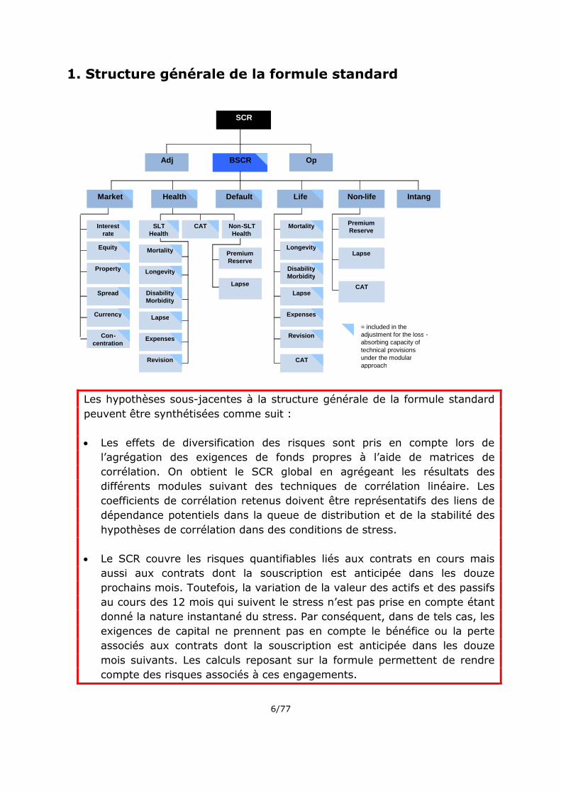
1. Structure générale de la formule standard

Les hypothèses sous-jacentes à la structure générale de la formule standard

peuvent être synthétisées comme suit :

Les effets de diversification des risques sont pris en compte lors de

l’agrégation des exigences de fonds propres à l’aide de matrices de

corrélation. On obtient le SCR global en agrégeant les résultats des

différents modules suivant des techniques de corrélation linéaire. Les

coefficients de corrélation retenus doivent être représentatifs des liens de

dépendance potentiels dans la queue de distribution et de la stabilité des

hypothèses de corrélation dans des conditions de stress.

Le SCR couvre les risques quantifiables liés aux contrats en cours mais

aussi aux contrats dont la souscription est anticipée dans les douze

prochains mois. Toutefois, la variation de la valeur des actifs et des passifs

au cours des 12 mois qui suivent le stress n’est pas prise en compte étant

donné la nature instantané du stress. Par conséquent, dans de tels cas, les

exigences de capital ne prennent pas en compte le bénéfice ou la perte

associés aux contrats dont la souscription est anticipée dans les douze

mois suivants. Les calculs reposant sur la formule permettent de rendre

compte des risques associés à ces engagements.

Mortality

CAT

BSCR Adj

Health

SLT Health

CAT Non - SLT Health

Default Life

Mortality

Longevity

Disability Morbidity

Lapse

Expenses

Revision

Non - life

Premium Reserve

Lapse

Market

SCR

Op

Intang

= included in the adjustment for the loss - absorbing capacity of technical provisions under the modular approach

CAT

Interest rate

Equity

Property

Spread

Currency

Con - centration

Premium Reserve

Lapse

Longevity

Disability Morbidity

Lapse

Expenses

Revision

7/77

Le SCR est calibré avec la valeur à risque (Value-at-Risk– VaR) des fonds

propres de base d’une entreprise d’assurance ou de réassurance, avec un

niveau de confiance de 99,5 % à l’horizon d’un an. Cet objectif de

calibrage est appliqué à chaque module ou sous-module de risque.

The SCR standard formula follows a modular approach where the overall risk

which the insurance or reinsurance undertaking (hereby undertaking) is exposed

to, is divided into sub-risks and in some risk modules also into sub- sub risks.

For each sub-risk (or sub-sub risk) a capital requirement is determined. The

capital requirement on sub-risk or sub-sub risk level is aggregated with the use

of correlation matrices in order to derive the capital requirement for the overall

risk.

To ensure that the overall SCR is calibrated using the Value-at-Risk of the basic

own funds of an undertaking subject to a confidence level of 99.5% over a one-

year period this calibration objective applies to each individual risk module in a

consistent manner.

Formula-based calculations are used for sub-modules where a scenario-based

approach was not considered as the most appropriate. Formula-based

calculations allow capturing risks associated with new business expected to be

written in the following 12 months. However, the effects of risk-mitigation

techniques are more difficult to take account when using a formula-based

calculation.

8/77

1.1 Corrélations dans la formule standard

Les hypothèses sous-jacentes aux corrélations dans la formule standard


La dépendance entre les risques peut être pleinement prise en compte par

l’utilisation d’une méthode reposant sur un coefficient de corrélation

linéaire.

En raison des problèmes que pose cette formule d’agrégation (liens de

dépendance dans la queue de distribution ou distributions asymétriques),

les paramètres de corrélation sont choisis de sorte à parvenir à la

meilleure approximation de la VaR à 99,5 % pour l’exigence globale de

capital agrégée.

The selection of the correlation parameters has a significant influence on the final

SCR, since the choice of correlation parameters has an impact on the level of

diversification recognised within the standard formula.

The aggregation formula in the standard formula is based on the assumption that

the dependence between the distributions can be fully captured by linear

correlations. In the mathematical literature a number of examples can be found

where linear correlations are insufficient to fully reflect the dependence between

distributions and where the use of linear correlations could lead to incorrect

aggregated results, i.e. producing either an under-estimation or an over-

estimation of the capital requirements at the aggregated level.

Two main reasons can be identified for this aggregation issue:

The dependence between the distributions is not linear; for example there

are tail dependencies.

The shape of the marginal distributions is significantly different from the

normal distribution; for example cases where marginal distributions are

skewed.

Unfortunately, both characteristics appear in many risks which an insurance or

reinsurance undertaking is exposed to. Tail dependence can exist in underwriting

risks (e.g. low-frequency and high-severity catastrophe events) market and

credit risks. As to the second characteristic, it is generally known that the

underlying distributions of the relevant risks of an insurance or reinsurance

undertaking are not normal distributions. They are usually skewed and some of

them are truncated by reinsurance or hedging effects.

Because of these shortfalls of correlation technique and the relevance of such

shortfalls for the risks covered in the standard formula, the choice of the

9/77

correlation factors should avoid a mis-estimation of the aggregated risk. In

particular, linear correlations are not an appropriate choice for the aggregation of

risks in many circumstances.

In the standard formula, correlation parameters should be chosen in such a way

as to achieve the best approximation of the 99.5% VaR for the aggregated

capital requirement. In mathematical terms, this approach can be described as

follows:

For two risks X and Y with E(X)=E(Y)=0, the correlation parameter ρ should

minimize the following aggregation error:

|VaR(X Y )2 VaR(X )2 VaR(Y )2 2VaR(X ) VaR(Y )|

1.2 Sélection des paramètres de corrélation pour les risques

indépendants

Plusieurs risques couverts dans la formule standard sont considérés comme

indépendants. On considère souvent qu’un paramètre de corrélation de 0

constitue le meilleur choix pour l’agrégation des risques indépendants. Or ce

n’est pas toujours le cas.

Several risks covered in the standard formula are intended to be independent.

For the aggregation of independent risks, a correlation parameter set at 0 is

considered.

However, the choice of the correlation parameter for independent risks is not

straightforward. If the underlying distributions are not normal, setting a

correlation parameter of 0 can lead to an mis-estimation of the aggregated risk,

hence to an mis-estimation of the required capital at the aggregated level.

Where the shape or the type of the marginal distributions is known, sometimes it

is possible to determine a correlation parameter which more closely reflects the

aggregated risks. However, in practice, this often proves to be difficult. The

shape of the underlying distributions is often not known or it differs across

undertakings and over time. For example, even if the distribution of an

underlying risk driver is known, hedging and reinsurance effects can modify the

net risk in an undertaking-specific way. Hence where a standard formula

correlation parameter between two risks assumed to be independent has to be

specified, it appears to be acceptable to choose a low correlation parameter,

reflecting that model risk might lead to an over- or under-estimation of the

combined risk.

10/77

1.3 Risques non explicitement inclus dans le calcul de la formule

standard

Les hypothèses sous-jacentes concernant les risques qui ne sont pas

explicitement inclus dans le calcul selon la formule standard peuvent être

synthétisées comme suit :

Tous les risques quantifiables ne sont pas explicitement inclus dans la

formule standard. En conséquence, certains risques qui ne sont pas

explicitement inclus dans la formule standard peuvent être pertinents pour

une entreprise donnée. Certains risques dont la nature et le calibrage

dépendent fortement des spécificités de l’entreprise n’ont pas non plus été

pris en compte dans la formule standard.

La formule standard a été élaborée pour une entreprise considérée sur une

base individuelle et appliquée mutatis mutandis à des groupes. Par

conséquent, il se peut que certains risques spécifiques aux des entités

appartenant à un groupe ne soient pas couverts dans la formule standard.

Certains risques sont traités implicitement dans un module ou sous-

module de risque, voire dans plusieurs modules ou sous-modules de

risques. Ces risques sont donc considérés comme implicitement inclus

dans la conception et le calibrage de la formule standard.

For some risks (mostly sub-risks or parts of risks covered already in the standard

formula) it can generally be assumed that the exposure is not always material

enough to justify a separate and more granular SCR quantification within the

context of the standard formula. These (sub-) risks are not explicitly formulated

in the standard formula calculation.

The SCR calibration objective, corresponding to the VaR of basic own funds

subject to a confidence level of 99.5 % over a one-year period, is applied to each

individual risk sub-module. However, for certain risks data availability is very

scarce and therefore no reliable calibration that is representative for the whole

market can be obtained. Therefore these types of risks are also not explicitly

formulated in the standard formula calculation.

Finally, it would be inappropriate to cover some risks through pillar 1 capital

requirements but these should be covered instead through pillar 2 requirements,

in particular through risk management requirements for an appropriate

monitoring and disclosing of the risk profile of an undertaking.

For illustration purposes, the following risks can be identified as being not

explicitly formulated in the standard formula calculation (note that this is not

intended to be an exhaustive list of excluded risks):

11/77

Inflation risk:

The sensitivity of the values of assets, liabilities and financial instruments to

changes in the term structure of inflation rates, or in the volatility of inflation

rates is not explicitly taken up as a separate risk sub-module in the standard

formula. However, for the Life expense and SLT Health expense risk sub-

modules as well as for the SLT Health disability-morbidity risk sub-module for

medical expense (the capital requirement for the increase or decrease of

medical expense payments), undertakings shall apply a 1 percentage point

annual increase in expense inflation rates used for the calculation of technical

provisions . For the health revision risk sub-modules the increase in annuity

benefits is assumed to be related to changes in for example, inflation. Other

sources of inflation risk are assumed implicitly in the calibration of the upward

and downward interest rate shocks in the interest rate sub-module. However,

the modelling of the Life and SLT Health underwriting risk modules should be

based on the assumption that the risk relating to the dependence of insurance

and reinsurance benefits on inflation is not material.

Reputation risk:

The risk related to the trustworthiness of an undertaking resulting in loss of

revenues or destruction of shareholders value is not explicitly covered in the

standard formula. The operational risk module explicitly excludes reputation

risk and risks arising from strategic decisions. Given the limited amount of

data or relevant information on past events of reputation risks, no reliable

calibration of a capital requirement for reputation risk would be appropriate

for the whole market. Therefore it is assumed inappropriate to cover

reputation risk within the context of a standard formula approach.

Liquidity risk:

The risk that insurance and reinsurance undertakings are unable to realize

investments and other assets in order to settle their financial obligations

when they fall due is not explicitly covered in the standard formula SCR

calculation. It is assumed that a capital requirement to cover liquidity risk

would be ineffective and that it is appropriate to cover such risk by an explicit

liquidity risk management policy within the overall risk management system.

Undertakings are supposed to publicly disclose qualitative and quantitative

information regarding their risk profile, including exposures to liquidity risk

where these are material or in case of material changes in the liquidity risk

profile.

Contagion risk:

An insurance or reinsurance undertaking could be exposed to the risk that an

adverse event or situation will spread from one undertaking to another. For

example an insurance undertaking could be exposed to the financial weakness

of other group entities affected by for instance market, reputation or

12/77

operational risk. Conversely, some risks crystallizing at entity level can have

knock-on or ripple effects on the wider group level. Such exposures to

contagion risk are not explicitly covered in the standard formula, as the

sources of contagion effects and the financial losses in case of contagion

events are very specific to the business profile of individual undertakings and

to the context of the group structure within which undertakings operate.

Undertakings are anyway supposed to publicly disclose qualitative and

quantitative information regarding their risk profile, including exposures to

contagion risk and concentration risk where these are material or in case of

material changes in the concentration risk profile.

Legal environment risk:

This is the risk that insurance and reinsurance undertakings are unable to

adapt their risk profile in response to sudden or unexpected changes in the

legal environment, such as an unforeseen change in the legal retirement age.

This is supposed to be understood as being different from legal risk directly

affecting an undertaking, which is covered by a SCR for operational risk.

13/77

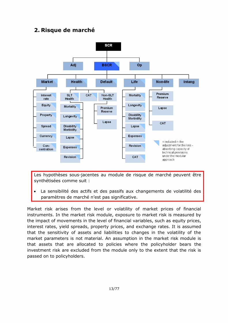
2. Risque de marché

Les hypothèses sous-jacentes au module de risque de marché peuvent être


La sensibilité des actifs et des passifs aux changements de volatilité des

paramètres de marché n’est pas significative.

Market risk arises from the level or volatility of market prices of financial

instruments. In the market risk module, exposure to market risk is measured by

the impact of movements in the level of financial variables, such as equity prices,

interest rates, yield spreads, property prices, and exchange rates. It is assumed

that the sensitivity of assets and liabilities to changes in the volatility of the

market parameters is not material. An assumption in the market risk module is

that assets that are allocated to policies where the policyholder bears the

investment risk are excluded from the module only to the extent that the risk is

passed on to policyholders.

14/77

© EIOPA 2014

2.1. Risque de taux d’intérêt

Les hypothèses sous-jacentes au sous-module risque de taux d’intérêt peuvent

être synthétisées comme suit :

Seul le risque de taux d’intérêt qui résulte de changements au niveau de la

courbe de base des taux d’intérêt sans risque est pris en compte.

La volatilité et les variations de la forme de la courbe des taux ne sont pas

explicitement couvertes par le sous-module relatif aux taux d’intérêt.

L’entreprise n’est pas exposée à un risque d’inflation ou de déflation significatif.

Dans le cadre de l’utilisation d’un calcul simplifié des exigences de capital

relatives au risque de taux d’intérêt pour les entreprises captives, on suppose

que les actifs et passifs sensibles aux mouvements des taux d’intérêt de

l’entreprise captive peuvent être considérés comme nettement moins diversifiés

en termes de duration des intervalles d’échéances et de lignes d’activités que le

portefeuille utilisé pour le calibrage de la formule standard.

The interest rate risk sub-module should capture interest rate risk in relation to all

interest rate sensitive assets and liabilities. The upward and downward shocked term

structures are derived by multiplying the current interest rate curve by an upward and

downward stress factor. It is important to note that the stress should only be applied

to the basic risk-free interest rates. The assumption underlying the design of the

interest rate risk sub- module is that in times of lower interest rates also the absolute

shocks are lower, and vice versa. The interest risk module does not fully capture the

risk of inflation or deflation. The undertaking should take into account any risk arising

from inflation or deflation as part of their own risk and solvency assessment.

The interest risk sub- module only captures interest rate risk that arises from changes

in the level of the basic risk-free interest rates. Volatility and changes in the shape of

the yield curve are not covered in the standard formula. The volatility of forward rates

plays a vital role in the determination of the slope and convexity of the underlying

yield curve. This particular volatility can be implied from market prices for swaptions,

which render the right to the holders to enter into a swap agreement for a specified

term at the maturity of the option. In particular, any increase in the implied volatility

surface can have subsequent "spill over" effects onto the shape and convexity of the

underlying term structure. As a result, shocks in the volatility of the term structure

are usually only relevant where insurer's asset portfolio and/or their insurance

obligations are sensitive to changes in interest rate volatility, for example where

liabilities contain embedded options and guarantees. Insurers can also be exposed to

volatility if they hold derivatives in their asset portfolios for interest rate hedging

purposes.

15/77

The calibration of the interest rate shocks in the standard formula are based on the

relative changes of the term structure of interest rates using the following 4 datasets:

EUR government zero coupon term structures (1997 to 2009)3, GBP government zero

coupon term structures (1979 to 2009)4, and both Euro and GBP LIBOR/swap rates

(1997 to 2009)5.

For each of the four individual datasets, stress factors were assessed through a

Principal Component Analysis6 (PCA), according to their maturity. PCA is a tractable

and easy- to- implement method for extracting market risk factors. For each maturity,

the mean of the results in the four datasets was taken as a single stress factor7.

The datasets chosen for calibrating the interest risk sub- module represent the

deepest and most liquid markets for interest rate sensitive instruments in the

European area. Moreover, the use of all four datasets together introduces a control

against the uncertainties that could result from using just one dataset in isolation. For

example, using the longer data period available for the GBP government bond data

introduces additional balance and a greater depth of information to the economic cycle

than the other three datasets. There are several technical idiosyncrasies in each of the

other data sets generating uncertainties that can be balanced out by combining the

results from all four datasets appropriately.

The analysis is based on time series of EUR and GPB interest rates and therefore

reflects the European economic experience over the last 30 years. However, financial

parameters can develop differently from what has been observed in the past in

Europe. For instance, there can be deflationary scenarios like in Japan in the 1990s.

A simplified calculation of the capital requirement for interest risk is also available to

captive insurance and reinsurance undertakings as it is considered to be proportionate

to the nature, scale and complexity of the risks they face. The underlying assumption

for the use of a simplified calculation of the capital requirement for interest rate risk

for captives is that all assets and liabilities sensitive to interest rate movements held

by captives can be considered materially less diversified in terms of maturity intervals

and of lines of business compared to the portfolio used in the calibration of the

standard formula.

3 Rates for maturities from 1 year to 15 years. 4 Rates for maturities of 6 months, 12 month, 18 months up until 25 years. 5 Rates for maturities 3-month, 6-month, 1 year until 10 years, 15 years, 20 years and 30 years.

6 PCA is mathematically defined as an orthogonal linear transformation that transforms the data to a new coordinate system such that the greatest variance by any projection of the data comes to lie on the first coordinate (called the first principal component), the second greatest variance on the second coordinate, and so on. PCA is theoretically the optimum transform for given data in least square terms. For further details, please refer to Jolliffe I.T, (2002), Principal Component Analysis, Springer Series in Statistics, 2nd ed., Springer-Verlag. 7 In addition to the calibration of the relative stress factor, a floor of 1 percentage point for the absolute change of interest rate in the downward scenario is defined.

16/77

2.2. Risque sur actions

Les hypothèses sous-jacentes au sous-module risque sur actions peuvent être


Les actifs et les passifs exposés au risque sur actions ne sont exposés qu’à une

baisse des prix des actions et non à une hausse.

La valeur des investissements en actions ne peut tomber en-dessous de zéro.

Pour différencier les actions de type 1 et de type 2, on suppose que les actions

de type 2 sont des actions plus risquées que celles de type 1. Pour cette raison,

le facteur de choc pour les actions de type 2 est plus élevé que pour celles de

type 1.

L’entreprise possède un portefeuille d’actions de type 1 qui est bien diversifié en

termes de géographie (pays développés), de taille des titres (grosses,

moyennes, petites et micro capitalisations), de secteurs et de styles

d’investissement (croissance, valeur, revenu, etc.).

L’entreprise détient un portefeuille de titres de capital-investissement, qui fait

partie de son portefeuille d’actions de type 2, composé principalement de

grandes sociétés de capital-investissement. Le portefeuille est supposé bien

diversifié en termes de géographie, de taille des titres, de styles

d’investissement et de financement, ainsi qu’en termes d’années d’émission.

Le portefeuille d’actions de type 2 de l’entreprise inclut un portefeuille de titres

liquides du secteur des matières premières. Ce portefeuille est supposé bien

diversifié en termes de composition (proportion par rapport à la production

mondiale).

L’entreprise possède un portefeuille de hedge funds composé de titres de taille

moyenne à grande qui s’échangent sur une base transparente. Ce portefeuille

est supposé bien diversifié en termes de stratégies des fonds et de situation

géographique.

L’entreprise possède un portefeuille d’actions sur les marchés émergents qui est

bien diversifié en termes de géographie, de taille des titres (grosses,

moyennes, petites et micro capitalisations), de secteurs et de styles

d’investissement (croissance, valeur, revenu, etc.).

Concernant le mécanisme d'ajustement symétrique dans la méthode standard

pour le sous-module relatif au risque sur actions, on suppose que le prix des

actions a un comportement de retour à la moyenne. Par conséquent, le

mécanisme d'ajustement symétrique augmentera le chargement en capital en

période de hausse des marchés actions et le réduira en période de baisse. Il

s’agit d’une hypothèse qui est faite sur le comportement des marchés action.

Pour l’approche par la duration dans le sous-module risque sur actions, on

suppose que l’on peut appliquer un choc moins important si l’entreprise est

17/77

exposée à une moindre volatilité des actions sur le long terme que sur le court

terme, conformément à l’hypothèse d’un comportement de retour à la moyenne

pour les marchés boursiers. On suppose que, pour l’entreprise pour laquelle on

utilise l’approche par la duration, la période typique de détention des

investissements en actions est cohérente avec la duration moyenne de ces

engagements.

Le chargement pour risque sur actions s’applique à tous les investissements en

actions, y compris ceux dans des entreprises liées, et à toutes les participations

détenues dans des établissements financiers et des établissements de crédit,

pour la valeur qui n’a pas été déduite des fonds propres en vertu de [Article 71

POF1]. Si les investissements en actions dans des entreprises liées sont

également classés en expositions de type 1 ou de type 2, un chargement pour

risque réduit de 22 % s’applique aux deux types d’expositions lorsque les

investissements sont de nature stratégique comme défini dans [Article 152

ER4].

Equity risk arises from the level or volatility of market prices for equities. Exposure to

equity risk arises in respect of all assets and liabilities whose value is sensitive to

changes in equity prices. In the standard formula, the equity risk sub-module only

captures changes in the level of equity prices, and the module only covers a

downward equity stress scenario.

Many insurers are sensitive to changes in equity volatility either through the

investments they hold (equities and equity derivatives) or through equity- linked

options and guarantees embedded in their liability portfolio. As a result, equity

volatility has an impact particularly on insurers writing traditional participating

business, investment-linked business and other investment contracts. However,

volatility is not explicitly covered in the equity risk sub-module.

An underlying assumption in respect of an equity investment is that its value cannot

fall below zero where the undertaking remains exposed to loss in basic own funds not

captured in the counterparty default risk module (especially referred to in [Article 174

CDR1 (2) (e) of the draft Delegated Acts]). This is particularly relevant in the case of

investments in related undertakings valued with the adjusted equity method in

accordance with [Article 9 V5]. For instance, the valuation of an investment in a non-

regulated related undertaking based on Solvency II principles might lead to a negative

value in the Solvency II balance sheet notwithstanding the fact that the related

undertaking is not in a stressed financial position under local accounting rules.

For the purpose of the standard formula the application of the equity risk sub-module

in respect of related undertakings only arises in the case that the participating

undertaking holds an equity investment in its related undertaking. For clarification, a

related undertaking can also be identified by reference to the nature of the

relationship and extent of influence exercised by the participating undertaking.

Therefore, the holding of an equity investment at all or of a specified percentage is

18/77

not a pre-requisite for the identification of a related undertaking. In the light of the

aforementioned the participating undertaking’s equity investment in the related

undertaking may not be fully representative of its equity exposure to the related

undertaking notwithstanding other exposures dealt with elsewhere in the standard

formula in respect of bonds, receivables and legal commitments made.

There are two possible methods to calculate the equity risk capital charge: the

"standard" approach and the "duration based" approach. For the "standard" approach

there is also a symmetric adjustment mechanism, which is always in force, to be

applied to the standard capital stress. This symmetric adjustment mechanism allows

the equity shock to move within a band of 10% on either side of the underlying

standard equity stress. The calibration of the "standard" approach therefore firstly

looks at the underlying standard equity stress, which is calibrated to the 99, 5% VaR

level for both "type 1" and "type 2" equities. The symmetric adjustment mechanism

then overlays the standard charge to arrive at the full standard approach.

Standard equity capital charge

The equity risk sub- module consists of two "sub-sub" modules for type 1 and type 2

equities. The underlying assumption for this split is that type 2 equities are more risky

than the equities that are covered in the type 1 category. The category of type 2

equities also covers alternative investments. For this reason, the stress factor for type

2 equities is higher than for type 1 equities.

The category of "type 1" equities covers equities listed in regulated markets which are

members of the EEA or the OECD. “Type 1” equities also include:

exposures to European Long-term Investment funds;

exposures to collective investment undertakings qualifying as social

entrepreneurship funds;

exposures to collective investment undertakings qualifying as venture capital

funds; and

exposures to close-ended and unleveraged alternative investment funds where

those alternative investment funds are established in the Union or, if they are

not established in the Union, they are marketed in the Union.

The calibration of the stress is based on data from the MSCI World Developed Price

Equity Index (1979 to end 2009, i.e. data from stressed markets are included). This

index consists of equities listed in developed countries located across America, Europe

and the Pacific Basin8. An underlying assumption in respect of type 1 equities is that

the undertaking owns a diversified equity portfolio.

8 Further information on the MSCI Barra International Equity Indices can be found at http://www.mscibarra.com/products/indices/equity/index.jsp

http://www.mscibarra.com/products/indices/equity/index.jsp

19/77

Simplified observations about the distribution of equity and other financial returns

tend to confirm that at longer horizons equity returns appear to be normally

distributed. The exact distribution of financial returns is an open question; however, at

weekly, daily and higher frequencies the equity return distribution displays definite

non-normal properties. In the calibration exercise, a huge amount of equity return

data was studied, and higher densities (known as “fat tails”) than that predicted under

the assumption of normality were observed.

The category "type 2" equities comprises equities listed in countries other than EEA

and OECD countries, non-listed and private equities, hedge funds, commodities and

other alternative investments. In the calibration exercise the following indices were

used: LPX50 Total Return (Private Equity), S&P GSCI Total Return Index

(Commodities), HFRX Global Hedge Fund Index (Hedge Funds) and MSCI Emerging

Markets BRIC (Emerging Markets). An underlying assumption in the calibration of the

equity type 2 shock is that the underlying portfolio of type 2 equities are diversified

and that this portfolio is representative for an average European insurance or

reinsurance undertaking.

The results of the calibration exercise demonstrated a rather wide variation between

the different classes of "type 2" equities.

The equity risk charge applies to all equity investments including those in related

undertakings and participations in financial and credit institutions in respect of the

value not deducted from own funds in accordance with Article 71 POF1. While equity

investments in related undertakings are also categorised as type 1 or type 2

exposures, a reduced risk charge of 22% applies to both types where the investments

are of a strategic nature as set out in [Article 152 ER4].

Symmetric adjustment mechanism

For the "standard" approach a symmetric adjustment mechanism is introduced, which

is always in force, to be applied to the standard capital stress. This symmetric

adjustment mechanism allows the equity shock to move within a band of 10% on

either side of the underlying standard equity stress.

The justification of such an adjustment, in the context of a 99.5% percentile

approach, is based on the underlying assumption that equity prices have a mean

reverting behaviour.

The symmetric adjustment is included due to the following objectives:

To avoid that insurance and reinsurance undertakings are unduly forced to raise

additional capital or sell their investments as a result of adverse movements in

financial markets;

To discourage or avoid fire sales which would further negatively impact the

equity prices – i.e. prevent a pro-cyclical effect of the capital requirements

20/77

which would in times of stress lead to an increase of capital requirements and

hence have a potential de- stabilising effect on the economy.

Therefore, in times of rising equity markets the dampener will increase the capital

charge, and in times of falling equity indices the dampener will reduce the capital

charge.

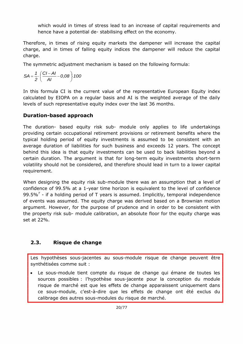
The symmetric adjustment mechanism is based on the following formula:

1000,08AI

AICI

2

1SA

In this formula CI is the current value of the representative European Equity index

calculated by EIOPA on a regular basis and AI is the weighted average of the daily

levels of such representative equity index over the last 36 months.

Duration-based approach

The duration- based equity risk sub- module only applies to life undertakings

providing certain occupational retirement provisions or retirement benefits where the

typical holding period of equity investments is assumed to be consistent with an

average duration of liabilities for such business and exceeds 12 years. The concept

behind this idea is that equity investments can be used to back liabilities beyond a

certain duration. The argument is that for long-term equity investments short-term

volatility should not be considered, and therefore should lead in turn to a lower capital

requirement.

When designing the equity risk sub-module there was an assumption that a level of

confidence of 99.5% at a 1-year time horizon is equivalent to the level of confidence

99.5%T - if a holding period of T years is assumed. Implicitly, temporal independence

of events was assumed. The equity charge was derived based on a Brownian motion

argument. However, for the purpose of prudence and in order to be consistent with

the property risk sub- module calibration, an absolute floor for the equity charge was

set at 22%.

2.3. Risque de change

Les hypothèses sous-jacentes au sous-module risque de change peuvent être


Le sous-module tient compte du risque de change qui émane de toutes les

sources possibles : l’hypothèse sous-jacente pour la conception du module

risque de marché est que les effets de change apparaissent uniquement dans

ce sous-module, c’est-à-dire que les effets de change ont été exclus du

calibrage des autres sous-modules du risque de marché.

21/77

Pour les monnaies rattachées à l’euro, qui font soit partie du mécanisme de

change européen, ou pour lesquelles une décision du Conseil européen

reconnaît un rattachement à l’euro ou encore pour lesquelles un accord de

rattachement est établi par la loi qui définit la monnaie du pays, on utilise un

facteur de choc réduit dans le sous-module risque de change. L’hypothèse

sous-jacente est que pour ces monnaies, le taux de change face à l’euro

fluctuera dans une fourchette limitée. Par conséquent, les chocs dus au risque

de change face à l’euro devraient également être limités. Les mêmes facteurs

de choc réduits s’appliqueront entre des paires de monnaies rattachées à l’euro,

sur la base de cette même hypothèse sous-jacente.

Currency risk arises from changes in the level or volatility of currency exchange rates.

Undertakings can be exposed to currency risk arising from various sources, including

their investment portfolios, as well as assets, liabilities and investments in related

undertakings located in a different currency area. The design of the currency risk sub-

module is intended to take into account currency risk arising from all possible sources,

and the underlying assumption of the market risk module design is that currency

effects appear only in this sub-module, i.e. currency effects have been stripped out in

the calibration of the other market risk sub modules.

In the calibration of the currency stress factor, daily data to study the distribution of

holding period rate of returns derived from EUR and GBP currency pairs were used.

The data sample, sourced from Bloomberg, covers a daily period from January 1971

to June 2009, a total of circa 10,000 observations across 14 currency pairs against

GBP. In addition, the sample consisted of 14 currency pairs expressed against the

EUR. For most pairs, the sample covered a daily period spanning a period of 10 years

starting in 1999 to 2009. Annual holding period returns were computed for the

Japanese Yen (JPY), the Brazilian Real (BRL), the Lithuanian Litas (LTL), the Indian

Rupee (INR), the Chinese Yuan (CNY) the US, Hong Kong (HKD), the Australian (AUD)

and the New Zealand (NZD) Dollars, the Norwegian (NOK), Swedish (SEK) and Danish

(DKK) Krone, the Swiss Franc (CHF) and the British Pound (GBP).

This is a currency basket expressed against the EUR, and is equally distributed across

CNY, INR, HKD, AUD, BRL and ARS. It was preferred to extend the definition of the

emerging market to include developed economies, whilst including the dominant Latin

American countries, Brazil and Argentina excluding Mexico. The presence of the

Australian and Hong Kong economy to the mix balances out the level of the stress as

it was believed that insurance groups are more exposed to these economies across

the Pacific basin region.

In the calibration of the currency risk stress factor, a visual inspection of different

standardised distributions, which were plotted against the normal distribution, showed

that the data did not adhere to the laws of normal distribution. Most distributions were

skewed and exhibited excess kurtosis ("fat tails").

22/77

For currencies pegged to the Euro, either by way of currencies participating in the

European Exchange Rate Mechanism, or where a decision from the Council recognizes

pegging arrangements to the Euro or where a pegging arrangement is established by

law of the country establishing the country's currency, a reduced shock factor in the

currency risk sub-module is used. The underlying assumption is that for these

currencies the rate against the Euro will fluctuate within a limited band, and therefore

the currency risk shocks against the Euro should be limited as well. The same reduced

shock factors will apply between pairs of currencies pegged to the Euro, based on the

same underlying assumption.

2.4. Risque sur actif immobilier

Les hypothèses sous-jacentes au sous-module risque sur actifs immobiliers


Le profil de risque de toutes les expositions de l’entreprise au risque sur actifs

immobiliers situés dans des pays tiers ne diffère pas significativement de celui

des marchés immobiliers européens.

La distribution des rendements immobiliers se caractérise par des queues de

distribution épaisses à gauche et par un excès de kurtosis (signe d’un écart par

rapport à la distribution normale).

The property shock is the immediate effect expected in the event of a fall in real

estate benchmarks, where all direct and indirect exposures of the insurer to property

prices are taken into account. It is assumed that the volatility of property prices is

implicitly covered in the calibration of the property shock. The property shock was

calibrated using UK data extracted from the Investment Property Databank (IPD)

indices. The IPD indices are based on survey data collected from institutional

investors, property companies and open-ended investment funds, and are the most

widely used commercial property indices. Indices for most European markets and

some countries outside Europe are produced, but for most European markets long

time series are lacking. The indices consist of time series of income (rental yield) and

capital growth for the main property market sectors – retail, office, industrial and

residential.

The calibration was based on monthly IPD total return9 indices for the UK market

(1987 to 2008), because this dataset provides the greatest and most detailed pool of

information. Total return indices are based on appraised market values rather than

actual sales transactions, so by using them smoothed data were to some degree used

(because appraisers tend to be “backward-looking”, the current appraisal values

9 Calibrating based on total return indices is based on the inherent assumption that the rental yield earned on a property portfolio is re-invested back into the same pool.

23/77

mirror also previous valuation prices). Even though the calibration of the property

shock is based on UK data, it is implicitly assumed that the UK property market can

be used as a good proxy for the average European property market. Undertakings not

exposed to the UK property market can rely on this assumption underlying the

property risk module. It should also be assumed that the risk-profile of any exposures

to property located in third countries is not materially different from the risk-profile

European property markets.

The lower percentiles of the distribution of the “smoothed” property returns – i.e., the

unadjusted index data –were derived by using non-parametric methods. The

distributions of property returns are generally characterised by long left fat-tails and

excess kurtosis (signifying disparity from normal distribution). Different methods were

applied to de-smooth the annual returns, but this resulted in even heavier left tails.

As the historical values at risk for the different property classes did not diverge too

much, no breakdown in different property classes was proposed.

2.5. Risque lié à la marge ou risque de spread

Les hypothèses sous-jacentes au sous-module risque lié à la marge peuvent être


On suppose une augmentation de la marge (ou de spread) d’un montant

correspondant à une augmentation bi centennale. On suppose donc également

qu’il n’y aura pas de diversification entre les différents sous-sous-modules du

sous-module risque lié à la marge.

Le risque de dégradation et le risque de défaut ne sont pas explicitement

couverts. En revanche, ces risques sont traités de manière implicite dans le

calibrage des facteurs des mouvements des marges de crédit. Les facteurs

traitent en outre de façon implicite non seulement la variation du niveau des

marges de crédit, mais aussi du niveau des marges en fonction de la maturité.

Pour les obligations et les prêts autres que les prêts hypothécaires résidentiels,

on suppose que les marges augmentent sur tous les instruments, car les

entreprises ne sont exposées qu’au risque de hausse des marges de crédit.

Les expositions d’une entreprise sous la forme d’obligations sécurisées

correspondant à une catégorie de crédit élevée (0 ou 1) et d’une duration

courte ou moyenne (inférieure ou égale à 10 ans) sont couvertes par le panier

d'actifs diversifiés qui garantissent l’essentiel de la valeur du titre en cas de

défaut de l’émetteur. La marge du titre dépend donc également de ce panier

d'actifs diversifié qui est supposé présenter une faible volatilité sur la duration

de l’obligation. Si les obligations sécurisées ne peuvent pas être classées dans

la catégorie de crédit élevée (0 ou 1) ou si leur duration est longue, on

supposera qu’un facteur de risque plus faible n’est pas approprié.

24/77

Un calcul simplifié des exigences de capital pour le risque lié à la marge sur les

obligations et les prêts est possible pour l’entreprise si l’on considère qu’il est

proportionné à la nature, à l’ampleur et à la complexité des risques auxquels

une entreprise est exposée. L’hypothèse sous-jacente est que le portefeuille

d’actifs est significativement moins diversifié en termes de qualité du crédit et

de duration que le portefeuille utilisé pour le calibrage de la formule standard.

Par conséquent, le produit de la duration et d’un facteur de risque dépendant

de la qualité du crédit est considéré comme une approximation prudente du

risque lié à la marge.

L’hypothèse sous-jacente pour le classement de tous les actifs détenus par des

entreprises captives au niveau 3 de la catégorie de crédit aux fins du calcul

simplifié du risque lié à la marge est que les portefeuilles d’actifs des

entreprises captives sont significativement moins diversifiés en termes de

qualité du crédit que le portefeuille utilisé pour le calibrage de la formule

standard.

The spread risk module is designed to reflect the change in the value of assets and

liabilities caused by changes in the level or the volatility of credit spreads over the risk

free term structure. It applies to bonds and loans other than residential mortgage

loans (residential mortgage loans are covered in the counterparty default risk module

as type 2 exposures, as it is assumed that this is a well-diversified portfolio of small

single name exposures without a rating), structured credit products (such as asset-

backed securities and collateralised debt obligations) and credit derivatives (such as

credit default swaps, total return swaps and credit linked notes). The capital charges

are assessed for each class of instruments and then added to get the capital charge

for spread risk:

SCRspread = SCRbonds&loans + SCRsecuritisation + SCRcd

Perfect positive correlation between the different sub-sub-modules in the spread risk

sub-module is assumed, so no diversification effect is allowed for. Empirically, spreads

tend to move in the same direction in a stressed scenario, and therefore the

assumption is made that spreads on all instruments increase at the same time.

Spread risk on bonds and loans other than residential mortgage loans

The spread risk capital charge on bonds and loans other than residential mortgage

loans is assessed through a factor-based calculation (starting from the market value

of the instrument and taking into account its credit quality step and duration). The

assumption is made that the spreads on all instruments increase, leading to an

instantaneous reduction in the value of bonds. The undertaking should multiply the

market value of the instrument with a risk factor stressi that depends on the credit

quality step of the instrument, and the modified duration of the bond or loan

denominated in years. For variable interest rate bonds or loans, the duration is

equivalent to the modified duration of a fixed interest rate bond or loan of the same

25/77

maturity and with coupon payments equal to the forward interest rate. The shock in

spread risk for bonds and loans other than residential mortgage loans is designed as a

concave function of duration ("kinking"). The reason for this is to ensure righti

ncentives that long-term liabilities are backed by long term assets.

The calibration of the risk factor stressi was based on the factors on Corporate Bond

Indices from Merrill Lynch. Monthly re-balanced sub-indices for EMU Corporates, for

different maturity buckets and rating classes10 between 1999 and February 2010 were

used. Each maturity bucket and rating class was split into new maturity buckets in

order to be able to calibrate on more granular buckets.

There are lower capital requirements for covered bonds. The underlying assumption is

that a pool of assets of high credit quality covers the bond and therefore the shock

factors for covered bonds should be somewhat aligned with the shocks for bond

exposures of credit quality steps 0 or 1.

A simplified calculation of the capital requirement for spread risk on bonds and loans

is available if it is considered to be proportionate to the nature, scale and complexity

of the risks an undertaking faces. The underlying assumption is that the asset

portfolio is materially less diversified in terms of credit quality and duration compared

to the portfolio used in the calibration of the standard formula.

The simplified calculation of the capital requirement for spread risk on bonds and

loans is assumed to apply to captives. The underlying assumption is that assets held

by captives can be assigned to credit quality step 3 for the purpose of the simplified

calculation for spread risk as these are materially less diversified in terms of credit

quality compared to the portfolio used in the calibration of the standard formula.

Spread risk on securitisation positions

The spread risk capital charge on securitisations positions is determined by a method

comparable to the method for bonds and loans other than residential mortgage loans,

i.e. by multiplying the market value of the instrument with its modified duration and a

risk factor stressi that depends on the credit quality step of the instrument. The

spread risk sub-module differentiates between securitisations positions of Type I and

Type II other than resecuritisation exposures. Type I securitisations have to meet

quality criteria regarding structural features, asset class eligibility and related

collateral characteristics, listing and transparency features and underwriting

processes. It is noted that since the beginning of the crisis (2007) the indices of

structured credit products have exhibited highly diverging performance patterns, as

not only the ratings11 of tranches determines the price but also the type and quality of

the assets in the securitised asset pool are important. Therefore, the calibration was

not based solely on the ratings of securitisations.

10 Data for rating classes AAA, AA, A, BBB, BB and B were used. 11 The tranche ratings are considered to be one of the reasons for the financial crisis.

26/77

The risk factor stressi for securitisation positions other than resecuritisations was

calibrated using spread data of US and European indices from Bank of America Merrill

Lynch and Markit between January 2007 and September 2013. The indices consisted

either of Type I or Type II securitisations positions12. To derive the spread risk charge

from this data it was assumed that investments are made mainly in European

securitisations.

The data justified a lower spread risk charge for Type I securitisations.

As the observed credit spread of resecuritisations was considerably higher than for

Type II securitisations a different set of capital requirements for the former was

introduced in the spread risk sub-module.

Spread risk on credit derivatives

The capital charge for credit derivatives is determined as the change in the value of

the derivative (i.e. as the decrease in the asset or the increase in the liability after

netting with offsetting corporate bond exposures) that would occur following (a) a

widening of credit spreads if overall this was more onerous, or (b) a narrowing of

credit spreads by 75% if this was more onerous.

2.6. Risque marché de concentration

Les hypothèses sous-jacentes au sous-module concentration des risques de

marché peuvent être synthétisées comme suit :

L’exposition des entreprises au risque de concentration ne concerne que

l’accumulation d’expositions à la même contrepartie. Le sous-module risque de

concentration n’inclut pas d’autres types de risques de concentration, tels que

la concentration géographique ou sectorielle des actifs détenus.

Les entreprises sont exposées au risque lorsque l’accumulation des expositions

à une contrepartie unique dépasse les seuils spécifiés, et l’on détermine alors

un capital requis à cette fin. Lorsque l’accumulation des expositions à une

contrepartie unique reste inférieure aux seuils spécifiés, les entreprises ne sont

pas exposées au risque, et il n’est pas nécessaire de déterminer de capital

requis pour les risques de concentration.

Le risque (volatilité, VaR) est plus élevé avec un portefeuille peu diversifié

qu’avec un panier d’investissements bien diversifié. On suppose que les

entreprises disposent d’un portefeuille dont le mix de placements ne s’écarte

pas considérablement du portefeuille d’investissements moyen d’une entreprise

12 Some of the Bank of America Merrill Lynch indices contain a number of subsectors. Separate subsector time series were calculated where necessary.

27/77

de l’Union européenne, c’est-à-dire qu’il est constitué de nettement plus

d’obligations que d’actions.

Les expositions d’une entreprise qui revêtent la forme d’obligations sécurisées

présentant une catégorie de qualité du crédit élevée (0 ou 1) sont couvertes

par un ensemble d’actifs diversifié garantissant la majeure partie de la valeur

obligataire en cas de défaut de l’émetteur. Lorsqu’une catégorie élevée (0 ou 1)

ne peut être assignée aux obligations sécurisées, on part du principe que le

relèvement du seuil de concentration n’est pas approprié.

Un seuil de concentration limite plus élevé est jugé approprié pour les

entreprises captives dans le sous-module risque de concentration, parce que

pour les entreprises captives, les entités assurées font également partie du

groupe qui détient l’entreprise captive. Le risque de concentration se référant

aux montants compris entre les deux seuils (à savoir 3 % ou 1,5 % contre

15 %) est entièrement atténué par l’existence de mécanismes de compensation

intragroupe, explicites ou implicites. Même en l’absence de mécanisme de

compensation formel, le groupe (le propriétaire et la partie assurée

simultanément) a intérêt à soutenir l’entreprise captive si cette dernière

rencontre des problèmes financiers ou autres.

The scope of the market risk concentration risk sub-module covers assets considered

in the equity, interest rate, spread and property risk sub-modules within the market

risk module, but excludes assets covered by the counterparty default risk module in

order to avoid any overlap between both elements of the standard calculation of the

SCR.

The risk dealt with in the market risk concentration risk sub-module is restricted to

the risk regarding the accumulation of exposure with the same counterparty i

(denoted with Ei). It does not include other types of concentration risk, such as

geographical or sector concentrations of the assets held. The calculation is performed

in three steps: (a) determination of excess exposure XSi, (b) calculation of risk

concentration capital charge per ‘name’, (c) aggregation across single names.

The underlying assumption in the market risk concentration risk sub-module is that

when the undertaking is above the specified excess exposure thresholds, the

undertaking is at risk in case a single name counterparty defaults and a capital

requirement is determined, and when the undertaking is below the specified

thresholds, the undertaking is not at risk, and no capital requirement for

concentration risk is determined.

The calibration of the market risk concentration risk sub-module is based on simple

evidence: the risk (volatility- VaR) of an undiversified portfolio is higher than for a

well- diversified basket of investments. The calibration process for concentration risk

was based on the comparison of the historical VaR of a well-diversified portfolio with

the VaR of a set of portfolios where one single concrete exposure was increased step

28/77

by step by 1 per cent, i.e. an initially well-diversified portfolio was progressively

transformed into a badly diversified portfolio.

In each step the initial VaR of the well-diversified portfolio was compared to the VaR

of the progressively more concentrated portfolio. The increase of VaR was mapped as

a function of the level of the concentration in the portfolio. For each exposure (‘name’

i) a regression line was fitted through the data points. The parameters that were

estimated from the fitted functions, delivered the calibration parameters gi, per ‘name’

i.

The starting portfolio was designed as a portfolio with an investment mix that is

assumed to be representative of an EU average undertakings’ portfolio of

investments. The mix proposed was 80% of bonds - 20% of equities. Undertakings

should rely on the assumption that the mix is representative of an EU average

portfolio of investments.

Within each of these two groups, a sector-distribution of investments was built,

according to an EU expected average: 25 % of total portfolio was deemed to be

invested in bonds issued by central governments of Member States, and 55% in

corporate bonds of different sectors and ratings.13 To obtain a sufficiently numerous

and well-diversified portfolio, additional names were added.

Simplified calculations that are specifically available to captive insurance and

reinsurance undertakings are considered to be proportionate to the nature, scale and

complexity of the risks they face. For market risk concentration the underlying

assumption of the higher excess exposure threshold for captives is that, due to the

fact that for captives the insured entities are part of the same group owning the

captive, the concentration risk referring to the amounts between the two thresholds

(i.e. 1% or 3% versus 15%) is entirely mitigated by the existence of explicit or

implicit intragroup compensation mechanisms. Even without formal compensation

mechanisms, the group entity has an economic interest in supporting the captive in

case of financial or other difficulties of the latter.

13 Equity portfolio: To the extent that this exercise assumes as starting point a well-diversified portfolio, consequently it should be based on a sufficiently representative and well-known equity index. In a first instance the selected names were those belonging to the Eurostoxx 50 index, and the period used to record data of prices, ranged from 1993 until 2009. However, the assessment of the historical vector of prices for each equity revealed that for a number of elements of the index the records of price data are only available for a significantly shorter period than that mentioned or are not homogeneous. Bond portfolio: Bonds used in the computation were notional bonds, all of them issued at a 5% rate and pending 5 years to maturity. Throughout the simulation each bond maintained these features.

29/77

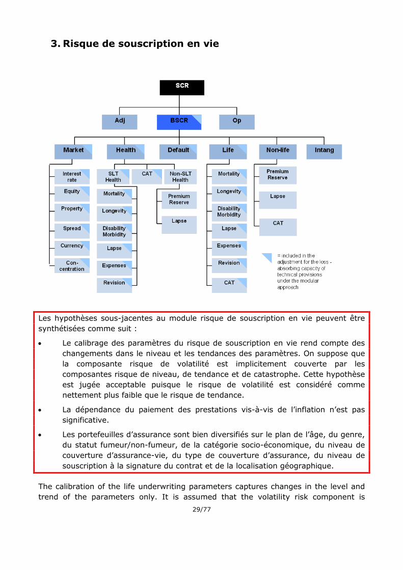
3. Risque de souscription en vie

Les hypothèses sous-jacentes au module risque de souscription en vie peuvent être


Le calibrage des paramètres du risque de souscription en vie rend compte des

changements dans le niveau et les tendances des paramètres. On suppose que

la composante risque de volatilité est implicitement couverte par les

composantes risque de niveau, de tendance et de catastrophe. Cette hypothèse

est jugée acceptable puisque le risque de volatilité est considéré comme

nettement plus faible que le risque de tendance.

La dépendance du paiement des prestations vis-à-vis de l’inflation n’est pas

significative.

Les portefeuilles d’assurance sont bien diversifiés sur le plan de l’âge, du genre,

du statut fumeur/non-fumeur, de la catégorie socio-économique, du niveau de

couverture d’assurance-vie, du type de couverture d’assurance, du niveau de

souscription à la signature du contrat et de la localisation géographique.

The calibration of the life underwriting parameters captures changes in the level and

trend of the parameters only. It is assumed that the volatility risk component is

30/77

implicitly covered by the level, trend and catastrophe risk components. This is

considered to be acceptable, since volatility risk is thought to be considerably lower

than the trend risk.

For the life underwriting risk module it should be assumed that the dependence of

benefit payments on inflation is not material.

An underlying assumption in the life underwriting risk module is the diversification in

the insurance portfolios. The reference population underlying all calibration work is an

insured population that is well diversified with respect to:

age

gender

smoker status

socio- economic class

level of life insurance cover

type of insurance cover

degree of underwriting applied at inception of the cover

geographic location

Therefore, one example of deviations from the assumptions underlying the standard

formula calculation would be an insurance portfolio with a higher than average level of

concentration in on or more risk factors (e.g. death protections are sold to a high

number of impaired lives, for instance due to poor underwriting or adverse selection).

Also a niche player is likely to have a materially different risk exposure than the one

reflected in the calibration of the standard formula.

Underwriting risk can affect undertakings liabilities as well as its assets. The scope of

the life underwriting risk module is therefore not confined to the liabilities.

Undertakings can have indirect underwriting exposures, like exposure to catastrophe

bonds and longevity bonds.

It is important to point out that the calibration of the life underwriting risk stress

factors are considered to be in line with the 99,5% VaR and a one-year time horizon.

For mortality, longevity, disability-morbidity, expenses and revision risk, the

calibration regarded of great importance a study by Watson Wyatt, published in 2004.

14 The study analysed the 99.5% assumptions over a 12 month time horizon that firms

were proposing to make for their Individual Capital Assessments (ICAS) submissions

in the UK.

14 For more information about the Watson Wyatt study see https://eiopa.europa.eu/fileadmin/tx_dam/files/consultations/QIS/QIS3/QIS3CalibrationPapers.pdf under life underwriting risk.

https://eiopa.europa.eu/fileadmin/tx_dam/files/consultations/QIS/QIS3/QIS3CalibrationPapers.pdf

31/77

3.1. Risque de mortalité

Le facteur de stress pour le risque de mortalité reflète l’incertitude dans les

paramètres de mortalité résultant d’une mauvaise estimation et/ou de

changements dans le niveau, la tendance et la volatilité des taux de mortalité et

rend compte du risque que davantage de souscripteurs qu’anticipé meurent avant

l’échéance du contrat.

Les hypothèses sous-jacentes au sous-module risque de mortalité peuvent être


L’entreprise a mis en place un système visant à réduire la sélection adverse.

La distribution de la probabilité de la mortalité est asymétrique, la tendance

actuelle étant à l’amélioration de la mortalité.

Pour le calcul simplifié des exigences de fonds propres pour le risque de

mortalité, on suppose qu’il n’y a pas de diminution importante du montant du

capital sous risque y afférent durant les n prochaines années, où n est la

duration modifiée (en années) du capital payable au décès inclus dans la

meilleure estimation de la projection. On suppose en outre que le taux de

mortalité moyen des assurés (pondéré du montant assuré) n’augmentera pas

significativement sur les n prochaines années.

The capital charge for mortality risk is intended to reflect the uncertainty in mortality

parameters, stemming from:

changes in the level, trend and volatility of mortality rates;

possible mis-estimation of the mortality rates used when calculation technical

provisions

and therefore to capture the risk that more policyholders than anticipated die during

the policy term.

The mortality risk sub- module is applicable for (re)insurance obligations contingent

on mortality risk i.e. where the amount currently payable on death exceeds the

technical provisions held and, as a result, an increase in mortality rates leads to an

increase in the technical provisions. The risk is normally captured by increasing the

mortality rates either by a fixed amount or by a proportion of the base mortality rates.

An underlying assumption in the mortality risk sub- module is that the probability

distribution for mortality is skewed, with a current trend towards improving mortality.

A simplified calculation for mortality risk is available for undertakings, where it is

proportionate to the nature, scale and complexity of the risks faced and where the

standard calculation would lead to an undue burden for the undertaking. The

32/77

underlying assumption for the simplified calculation of the capital requirement for

mortality risk is that there is no material decrease in the respective sum of capital at

risk in the next n years, where n is the modified duration (in years) of payments

payable on death included in the best estimate projection. It is furthermore assumed,

that the average mortality rate of the insured persons (weighted by sum insured) will

not increase materially over the next n years.

3.2. Risque de longévité

Le facteur de choc pour le risque de longévité vise à refléter l’incertitude dans les

paramètres de mortalité résultant d’une mauvaise estimation et/ou d’un

changement dans le niveau, la tendance et la volatilité des taux de mortalité et

rend compte du risque que les souscripteurs vivent plus longtemps qu’anticipé.

Les hypothèses sous-jacentes au sous-module risque de longévité peuvent être


Les améliorations de la mortalité annuelle suivent une distribution normale.

Pour le calcul simplifié du capital requis pour le risque de longévité, on suppose

que l’âge moyen des souscripteurs dans le portefeuille est de 60 ans ou plus.

On suppose en outre que le taux de mortalité moyen des assurés concernés

n’augmente pas de plus de 10 % par an.

The capital charge for longevity risk is intended to reflect the uncertainty in mortality

parameters as a result of mis-estimation and/or changes in the level, trend and

volatility of mortality rates and to capture the risk of policyholders living longer than

anticipated. It is applicable for (re)insurance obligations contingent on longevity risk

i.e. where there is no death benefit or the amount currently payable on death is less

than the technical provisions held and, as a result, a decrease in mortality rates is

likely to lead to an increase in the technical provisions.

The Watson Wyatt study indicated a single uniform permanent decrease in mortality

rates between 5% and 35%, with an average decrease around 18%. Feedback from

internal model firms indicated that the median stress for the decrease in mortality

rates used was 25%.

Furthermore, a calibration exercise was performed, where the mortality data for nine

countries15 was analysed; both historic data and stochastically projected16 future

mortality improvements of the mortality rates were considered.

15 Data is available at www.mortality.org. 16 The model was similar to the stochastic model presented by Towers Perrin to the UNESPA: UNESPA Longevity Risk Investigation, Towers Perrin, 21 January 2009.

http://www.mortality.org/

33/77

From the historical data the mean and the standard deviation of annual unisex

mortality improvements were assessed separately for each age group for the years

1992-2006. The improvements in mortality rates over this past 15 years can be seen

to be higher than 25% for almost all age groups.

Based on the assumption that the annual mortality improvements follow a normal

distribution17, stochastically simulated future mortality rates were produced. Instead

of assuming an improvement of x% per annum, the shock was calibrated as an

equivalent one-off shock (a permanent change in mortality rates for each age).

However, the result of the stochastic model of future mortality improvements implied

a lower stress than the 25 % as derived from historical data.

A simplified calculation for longevity risk is available for undertakings, where such

simplified calculation is proportionate to the nature, scale and complexity of the risks

faced and where the standard calculation would lead to an undue burden for the

undertaking. The underlying assumption for the simplified calculation of the capital

requirement for longevity risk is that the average age of policyholders within the

portfolio is 60 years or more. It is furthermore assumed, that the average mortality

rate of the respective insured persons does not increase by more than 10% each year.

3.3. Risque d’incapacité/invalidité – de morbidité

Les facteurs de choc pour le risque d’incapacité/invalidité – de morbidité reflètent

le risque que davantage de souscripteurs qu’anticipé développent une

incapacité/invalidité ou tombent malades avant l’échéance du contrat (risque

d’incidence), et que les personnes souffrant d’une incapacité/invalidité se

rétablissent moins qu’attendu (risque lié au niveau de rétablissement).

Les hypothèses sous-jacentes au sous-module de risque d’incapacité/invalidité –

de morbidité peuvent être synthétisées comme suit :

Le portefeuille d’assurance est bien diversifié en termes de probabilité

d’incapacité/invalidité ou de maladie (taux d’incidence) ou d’évolution de la

gravité de l’incapacité ou de la maladie (taux lié au niveau de rétablissement).

Pour le calcul simplifié des exigences de fonds propres pour le risque

d’incapacité/invalidité – de morbidité, on suppose qu’il n’y a pas de baisse

importante dans les montantsrespectifs du capital sous risque sur les n-

1 années après l’année suivante, où n est la duration modifiée (en années) du

capital payable sur l’invalidité-la morbidité inclus dans la projection de meilleure

estimation. On suppose en outre que le taux moyen anticipé

d’incapacité/invalidité – de morbidité des assurés (pondéré par le montant

assuré) n’augmentera pas considérablement durant cette période. Enfin, on

17 This assumption was verified in the Towers Perrin paper.

34/77

suppose aussi que le taux moyen anticipé d’incapacité/invalidité – de morbidité

et le taux de sortie attendu n’augmente pas de plus de 10 % par an.

The capital requirement for disability-morbidity risk is intended to capture the risk

that more policyholders than anticipated become disabled or sick during the policy

term (inception risk), and that disabled people recover less than expected (recovery

risk). An underlying assumption in the disability- morbidity risk sub-module is that the

insurance portfolio is well diversified in terms of likelihood of disability or sickness

(inception rates) or change in the severity of disability or sickness (recovery rate).

A simplified calculation for disability-morbidity risk is available for undertakings, where

such simplified calculation is proportionate to the nature, scale and complexity of the

risks faced and where the standard calculation would lead to an undue burden for the


requirement for disability-morbidity risk is that there is no material decrease in the

respective sum of capital at risk in the next n-1 years after the following year, where

n is the modified duration (in years) of payments payable on disability-morbidity

included in the best estimate projection. It is furthermore assumed, that the expected

average disability-morbidity rate of insured persons (weighted by the sum insured)

will not increase materially during that period. Finally, it is also assumed that the

expected average disability-morbidity rate and the expected termination rates do not

increase by more than 10% each year. The design of the disability-morbidity risk sub-

module is a combination of the approaches for mortality and longevity risks. The

assumptions regarding disability-morbidity parameters are therefore also a

combination of the assumptions for the other two sub-modules.

Inception and recovery rates

The stress factors for the inception rates were based on several studies. The Watson

Wyatt study indicated an increase of disability/morbidity inception rates between 10%

and 60%, with an average increase of around 40%.

In addition an investigation by the Swedish Financial Supervisory Authority was

performed. This study indicated that an increase of 50% in morbidity/disability

inception rates for the first year would be appropriate. The results also suggested that

the appropriate calibration of the decrease in morbidity/disability recovery rates would

be 20%.

The total recovery rate has been estimated from the proportion of provisions released

as a result of recovery for a number of companies over 6 years (2002-2007). Based

on these estimates, it was prescribed that the recovery rate stress should be a 20%

decrease.

35/77

3.4. Risque de dépenses

Les hypothèses sous-jacentes pour le sous-module risque de dépenses peuvent


Les entreprises sont exposées au risque d’évolution des dépenses découlant

essentiellement des frais de personnel, des frais de commission aux

intermédiaires de vente (sur la base des conditions contractuelles), du coût de

l’infrastructure informatique, du coût du terrain et des bâtiments occupés.

L’entreprise opère dans un environnement macroéconomique où l’inflation,

quoique affichant des fluctuations, est globalement maîtrisée (ciblage de

l’inflation).


dépenses, on suppose qu’il n’y a pas de hausse significative ayant d’autre

origine que l’inflation concernant les dépenses supportées pour honorer les

engagements d’assurance vie, et lorsque les flux de trésorerie prévus suivent

un certain profil.

Expense risk arises from the variation in the expenses incurred in servicing insurance

or reinsurance contracts. It is likely to be applicable for all insurance obligations.

The model undertakings underlying the calibration are subject to expenses arising

predominantly from:

staff costs

cost of commissions to sales intermediaries (on the basis of the contractual

terms of the arrangements)

cost of IT infrastructure

cost of land and buildings occupied

The Watson Wyatt study from 2004 indicated a potential increase in the level of

expenses between 5% and 50%, with an average increase of around 26%.

Later ICAS submissions in the UK showed an increase of around 10% in the level of

expenses in the following year, together with an increase of between 1% and 2 % per

annum in the rate of future expense inflation.

The expense inflation assumption is based on a macro economy in which inflation,

though subject to fluctuations, is broadly under control (i.e. inflation targeting).

Based on these studies, it was decided that the stresses should be based on an

increase of 10% in future expenses compared to the best estimate anticipations and

an increase of 1% per annum of the expense inflation rate compared to anticipations.

36/77

A simplified calculation for expense risk is available for undertakings, where such




requirement for expense risk is that there is no material increase due to other sources

than inflation in the expenses incurred in servicing life insurance obligations other

than health insurance in the next n years, where n is the modified duration (in years)

of expenses included in the best estimate projection. Moreover, the simplified

calculation is applicable only insofar as the future expenses follow a certain pattern.

3.5. Risque de révision

Les hypothèses sous-jacentes pour le sous-module risque de révision peuvent être


Toutes les annuités sont indépendantes et leur montant annuel est supposé

constant.

Le portefeuille de taille moyenne comprenant des annuités à différents stades

prend en compte les proportions « moyennes ».

Revision risk is intended to capture the risk of adverse variation of an annuity's

amount, as a result of an unanticipated revision of the claim process. This risk should

only be applied to annuities and to those benefits that can be approximated by a life

annuity arising from non-life claims, including accident insurance, but excluding

workers compensation that are allocated to the life underwriting risk module.

The calibration for revision risk was based on historical data for pensions in payment

for the workers’ compensation line of business in Portugal.

In the analysis a binomial compound distribution was fitted to the historical data,

assuming a binomial distribution for the frequency process and a lognormal

distribution to model the severity of revision. The aggregate loss distribution was

derived using Monte Carlo simulation for different portfolio sizes. All annuities were

assumed to be independent and their annual amount was assumed to be constant.

Different assumptions were considered for annuities homologated and annuities not

yet defined; the latter with higher frequency and severity volatilities.

Revision risk is calculated assuming an increase of 3% in the annual amount payable

for annuities exposed to revision risk. The 3% scenario corresponds to the 99.5%

quantile of the aggregate loss distribution for an average sized portfolio comprising

annuities at different legal stages in ‘average’ proportions.

37/77

3.6. Risque de cessation

Le sous-module risque de cessation reflète l’évolution négative de la valeur des

engagements d’assurance, découlant d’évolutions dans le niveau ou la volatilité

des taux de cessation, d’échéance, de reconduction et de rachats des polices.

Les hypothèses sous-jacentes au sous-module risque de cessation peuvent être


L’augmentation et la diminution du taux de cessation constituent un choc

symétrique pour les scénarios d’augmentation et de diminution du risque de

cessation (pas d’événement de cessation massive).

Le risque associé aux options que l’entreprise d’assurance ou de réassurance

cédante peut exercer n’est pas significatif.

Une distinction entre les polices d’assurance rentrant ou non dans le cadre de la

gestion de fonds de pension de groupes est jugée appropriée concernant le

choc d’événement de cessation massive. Cela est dû au fait que pour la gestion

de fonds de pension de groupes, le risque de cessation massive est jugé

nettement plus élevé du fait qu’il n’y a généralement pas de pénalité pour

rachat, et que les investisseurs institutionnels sont généralement mieux

informés et donc retireraient rapidement leurs fonds s’ils avaient le moindre

doute quant à la solvabilité d’une entreprise.

Pour le calcul simplifié des exigences de fonds propres concernant le risque de

cessation vie, on suppose ce qui suit : le calcul simplifié est effectué à un degré

de granularité approprié, de telle sorte que le groupe de polices auquel la

méthode est appliquée est homogène en termes de taux de cessation ; les taux

de cessation ne sont pas significativement sensibles aux tendances des

variables économiques, les taux de cessation ne varient pas significativement

en fonction de l’âge du souscripteur ; et le capital requis pour le risque de

cessation en vie calculé à partir de la formule simplifiée n’est pas significatif au

regard du capital requis global.

The lapse risk sub- module should capture the adverse change in the value of

insurance liabilities, resulting from changes in the level or volatility of the rates of

policy lapses, terminations, renewals, and surrenders. The capital requirement for

lapse risk is the maximum of the capital requirement in one of the following scenarios:

a permanent increase of lapse rates, a permanent decrease of lapse rates, and the

mass lapse event.

38/77

Increase and decrease of lapse rate

The calibration of the shock of the decrease of lapse rates was based on a study of the

UK with-profit life insurance market in 2003 performed by order of the British FSA18.

The study does not cover the risk of a permanent increase of lapse rates; however, it

was deemed appropriate to assume a symmetrical stress for both scenarios.

In addition to the above mentioned study, further evidence was studied from other

markets. An analysis of the Polish supervisors on their national life insurance market

shows that the 99.5% quantile of annual lapse rates deviates from the long-term

mean by 60% to 100% for increases and by -60% to -90% for decreases. As these

values are based on an annual deviation, they over-estimate the shock of a

permanent change.

A simplified calculation for lapse risk is available for undertakings, where such



undertaking. The underlying assumptions for the simplified calculation of the capital

requirement for lapse risk are the following: the simplified calculation is done at an

appropriate granularity, such that the group of policies to which the method is applied

is homogeneous in terms of lapse rate; the lapse rates are not significantly sensitive

to trends in economic variables; the lapse rates do not vary significantly with the age

of the policyholder; the capital requirement for life lapse risk determined with the

simplification is not material compared to the overall capital requirement.

Mass lapse event

The empirical basis to calibrate the mass lapse event is scarce. It can be assumed

that different types of life insurance policies are affected differently by mass lapse

events: products with significant guarantees, like with-profit products, can show a

higher persistency than products with low guarantees like many unit-linked policies.

However, it was decided to discriminate only between insurance policies falling or not

within the scope of management of group pension funds.

The underlying assumption behind this split is due to the fact that for management of

group pension funds19, the risk of a mass lapse is deemed to be substantially greater

because there are generally no surrender penalties, and institutional investors tend to

be better informed and therefore would be quick to withdraw funds if there was any

question over the solvency of a firm.

18 Financial Services Authority "Calibration of the Enhanced Capital Requirement for with-profits life insurers" 2004, http://www.fsa.gov.uk/pubs/policy/04_16/ww_report.pdf 19 As referred in article 2(3)(b)(iii) and (iv) of Directive 2009/138/EC.

http://www.fsa.gov.uk/pubs/policy/04_16/ww_report.pdf

39/77

3.7. Risque de catastrophe en vie

Le sous-module risque de catastrophe en vie reflète le risque associé à des

événements induisant une extrême mortalité qui n’est pas suffisamment pris en

compte dans le sous-module risque de mortalité.

Les hypothèses sous-jacentes au sous-module risque de catastrophe en vie


Le risque de catastrophe en vie est limité aux engagements qui sont

subordonnés à la mortalité, c’est-à-dire lorsqu’une augmentation de la mortalité

conduit à une augmentation des provisions techniques.

On suppose que le sous-module n’est pas applicable aux engagements, tels que

les annuités, lorsque la hausse de la mortalité conduit à une réduction des

provisions techniques.


catastrophe en vie, on suppose que le capital sous risque constitue une mesure

indirecte appropriée des pertes instantanées causées par le décès de la

personne assurée par le contrat correspondant.

The life catastrophe risk stems from extreme death events that are not sufficiently

captured by the mortality risk sub- module. Life catastrophe risks are one- time

shocks from the extreme, adverse tail of the probability distribution that are not

adequately represented by extrapolation from more common events and for which it is

usually difficult to specify a loss value, and thus an amount of capital to hold. For

example, a contagious disease process or a pandemic can affect many persons

simultaneously, nullifying the usual assumption of independence among persons.

The capital requirement for the life catastrophe risk sub-module should be calculated

as an absolute increase in the rate of policyholders dying over the following year. The

life catastrophe risk stress factor is restricted to obligations which are contingent on

mortality i.e. where an increase in mortality leads to an increase in technical

provisions.

The life catastrophe risk sub- module is assumed not to be applicable to obligations,

such as annuities, where the increase in mortality leads to a reduction in technical

provisions. Although this seems to reflect the economic substance of insurance -

allowing for the diversification between different lines of business –enough evidence

suggests that this diversification benefit might not exist in reality. (In particular,

historic data indicates that it is primarily young and healthy people that die as a result

of influenza pandemics.)

The calibration of the mortality catastrophe stress is based on a study carried out by

Swiss Re in 2007, which estimated that the 1 in 200 year pandemic stress for most

developed countries is between 1.0 and 1.5 per mille within insured lives. This study

was based on a sophisticated epidemiological model, but had a number of weaknesses

40/77

(such as not adequately allowing for the probability of flu jumping across species, not

allowing for non-influenza pandemics as AIDS, drug resistant TB and the Ebola virus,

not allowing for catastrophe due to terrorism or earthquakes, and so on). If these

weaknesses were addressed, it is likely that the estimated stress would increase.

In light of this, a mortality catastrophe stress of 1.5 per mille was proposed.

A simplified calculation for catastrophe risk is available for undertakings, where such




requirement for catastrophe risk is that the capital at risk is an appropriate proxy for

the instantaneous loss caused by the death of the person insured by the respective

contract.

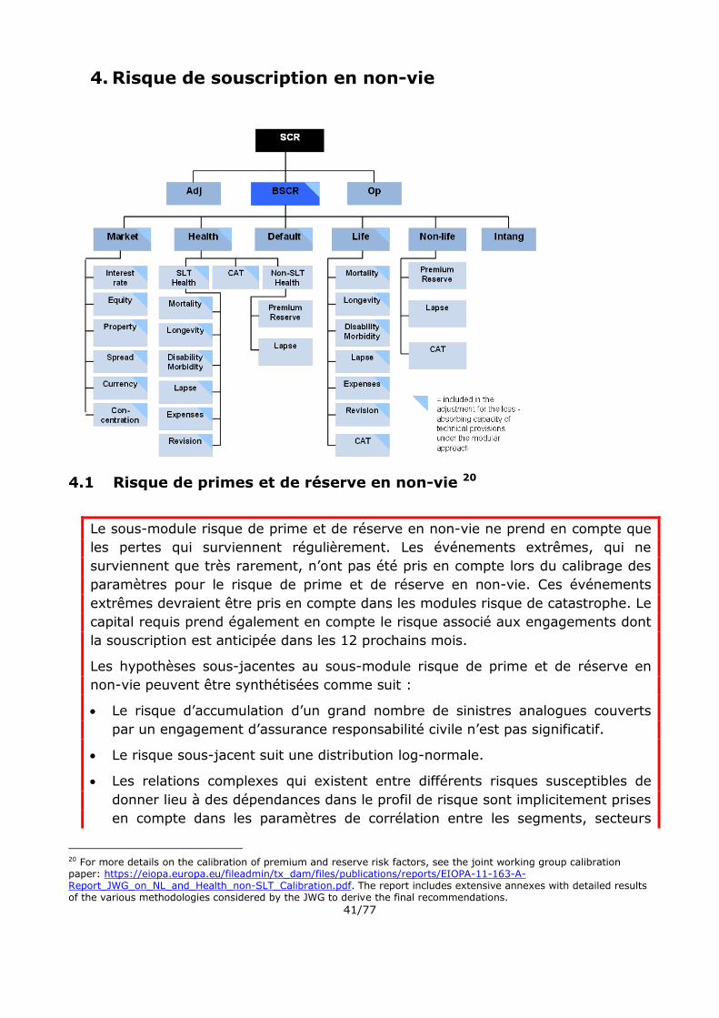
41/77

4. Risque de souscription en non-vie

4.1 Risque de primes et de réserve en non-vie 20

Le sous-module risque de prime et de réserve en non-vie ne prend en compte que

les pertes qui surviennent régulièrement. Les événements extrêmes, qui ne

surviennent que très rarement, n’ont pas été pris en compte lors du calibrage des

paramètres pour le risque de prime et de réserve en non-vie. Ces événements

extrêmes devraient être pris en compte dans les modules risque de catastrophe. Le

capital requis prend également en compte le risque associé aux engagements dont

la souscription est anticipée dans les 12 prochains mois.

Les hypothèses sous-jacentes au sous-module risque de prime et de réserve en

non-vie peuvent être synthétisées comme suit :

Le risque d’accumulation d’un grand nombre de sinistres analogues couverts

par un engagement d’assurance responsabilité civile n’est pas significatif.

Le risque sous-jacent suit une distribution log-normale.

Les relations complexes qui existent entre différents risques susceptibles de

donner lieu à des dépendances dans le profil de risque sont implicitement prises

en compte dans les paramètres de corrélation entre les segments, secteurs

20 For more details on the calibration of premium and reserve risk factors, see the joint working group calibration paper: https://eiopa.europa.eu/fileadmin/tx_dam/files/publications/reports/EIOPA-11-163-A-Report_JWG_on_NL_and_Health_non-SLT_Calibration.pdf. The report includes extensive annexes with detailed results of the various methodologies considered by the JWG to derive the final recommendations.

https://eiopa.europa.eu/fileadmin/tx_dam/files/publications/reports/EIOPA-11-163-A-Report_JWG_on_NL_and_Health_non-SLT_Calibration.pdf


42/77

d’activité et entre les risques de prime et de réserve de chaque secteur

d’activité.

Les facteurs finaux sont représentatifs de la taille et des performances

moyennes des portefeuilles des assureurs sur le marché européen.

La prime acquise nette peut être utilisée comme une approximation de

l’exposition au risque de primes.

Les provisions nettes pour sinistres à payer peuvent être utilisées comme une

approximation de l’exposition au risque de réserve.

La valeur attendue du ratio combiné du portefeuille reste relativement stable

dans le temps.

La valeur attendue du ratio de liquidation du portefeuille reste relativement

stable dans le temps.

Les frais n’évoluent ni de manière indépendante ni de manière inverse au risque

sous-jacent.

La réassurance non proportionnelle réduit la volatilité du risque de primes de

20 % sur les segments 1, 4 et 5. Aucune réduction n’est permise sur les autres

segments dans le cas de non-utilisation de paramètres spécifiques à

l’entreprise.

Aux fins d’un calcul simplifié des exigences de fonds propres pour risque de

prime et de réserve en non-vie pour les entreprises captives, on suppose que la

segmentation des engagements d’assurance par les entreprises captives peut

être considérée comme substantiellement moins diversifiée en termes de lignes

d’activité que le portefeuille utilisé pour le calibrage de la formule standard.

Dans le calcul du coefficient de diversification géographique qui permet

d’ajuster la mesure du volume pour le risque de prime et de réserve en non-

vie, on suppose que des portefeuilles géographiquement diversifiés sont

diversifiés en termes de taille et de moment des pertes qu’une entreprise

d’assurance supporte.

Premium risk is understood to relate to future claims arising during and after the

period for the solvency assessment. The risk is that the expenses plus the volume of

(covered but not incurred) losses for these claims (comprising both amounts paid

during the period and (incurred but not settled) claim provisions made at its end) are

higher than the premiums received. Premium risk is present at the time the policy is

issued, before any events occur. Premium risk also arises because of uncertainties

prior to issues of policies during the time horizon.

Reserve risk stems from two sources: on the one hand, the absolute level of the

claims provisions could be mis-estimated. On the other hand the actual claims will

fluctuate around their statistical mean value because of the stochastic nature of future

claims payouts.

43/77

The premium and reserve risk sub-module only takes into account losses that occur at

a regular frequency. Extreme events, which occur very rarely, have not been taken

into account when calibrating the premium and reserve risk factors. Such extreme

events should be taken into account in the catastrophe risk sub-modules.

As a matter of mathematical convenience the underlying risk can be viewed to follow

a normal or lognormal distribution. This applies to premium as well as reserve risk.

It is important to note that some undertakings have specific risk characteristics of

assets and liabilities, and the factor based approach to premium and reserve risk in

non- life insurance only partially reflects the undertaking- specific profile of its non-

life business (which is impacted e.g. by the specific type of products sold, or the sales

policy of the undertaking).

The expected value of the combined ratio of the portfolio does not change

substantially over time.

The expected value of run-off ratios of the portfolio does not change substantially over

time.

The premium and reserve risk capital requirement is calculated based on a factor-

based approach. Formula-based calculations are used for sub- modules where a

scenario-based approach was not considered as the most appropriate. The formula

based calculations allow capturing risks associated with new business expected to be

written in the following 12 months. However, to take the effect of risk mitigation

techniques into account is more difficult with a formula based calculation.

Complex relationships between different risks could also give rise to dependencies in

the risk profile. The most obvious of these is the relationship between non-life

underwriting risk and contingent credit risk. The circumstances that cause increased

insurance losses, and therefore an increase in reinsurance recoveries, could in turn

have a negative effect on the creditworthiness of the reinsurer. However, such

complex relationships between premium and reserve risk and counterparty default

risk or market risks have not been considered in the premium and reserve risk

module. They are implicitly taken up in the correlation parameters between the risk

modules.

3∙σ V

σ denotes the combined standard deviation for premium and reserve risk and V

denotes the total volume measure for premium and reserve risk. The volume measure

V is equal to the sum of all volume measures for the different segments the

undertaking is exposed to. Originally in the design of the SCR for non-life insurance

underwriting risk, the lognormal probability distribution acted prominently as a vehicle

to model a skew bell-shaped probability distribution. This implied a function of that

should amount more or less to the value 3. Later on it was decided just to focus on

44/77

this simple factor and downsizing the explicit assumption of an exact lognormal

probability distribution.

The combined standard deviation is equal to the following:

ts

ttssts VVCorrSV ,

),(

1

To calculate this combined standard deviation, the undertaking needs estimates for

premium and reserve risk standard deviations for the particular LoBs the undertaking

is exposed to and calculate the volume measures for each segment. For calculating

the standard deviations for each LoB, the following formula applies:

),(),(

2

),(

2

),(),(),(),(),(

2

),(

2

),(

sressprem

sressressressresspremspremspremsprem

sVV

VVVV

In order to estimate the capital charge for the premium and reserve risk sub module,

the following calibrated factors for the following inputs are needed:

Standard deviations for premium risk σ (prem, LoB)

Standard deviations for reserve risk σ (res, LoB)

Correlation factors between lines of business

In the design of the geographical diversification coefficient adjusting the volume

measures for non-life premium and reserve risk, it is also assumed that the regions

represent an appropriate geographical division of the undertaking’s insurance portfolio

in each line of business; i.e. it is assumed that an insurance portfolio of an

undertaking with contracts across regions does not contain sub-portfolios split per

region that in fact generate positively correlated losses. This situation can occur when

the portfolios are located in few similar (in respect of type and time of losses)

countries but assigned to different regions or when portfolios are locally concentrated

around both sides of the border between two regions

4.1.1 The combined approach for setting premium and reserve risk

factors

An underlying assumption in the premium and reserve risk module is that the final

factors are reflective of the average size of the portfolios of insurers in the European

markets.

In the calibration exercise two broad options emerged for setting premium and

reserve risk factors:

45/77

a pan- European approach; and an

averaging approach

Under the pan- European approach, the factors are set on the basis of the pooled

European data set. Under the averaging approach, in a first step factors are set at a

regional (country) level. The final Europe- wide factor is then determined by averaging

across the regional factors.

Based on these two approaches a combined approach was developed and used for

calibrating premium and reserve risk factors. Under this combined approach the

modeling focused on the efficient estimator of a pan- European volatility parameter.

However, in order to more fully address the issue of heterogeneity between different

markets, the methodology was applied at the level of an individual country. The

intermediate output by country was then grouped by taking a weighted average also

resulting in a single pan- European volatility. One could regard this as a kind of voting

procedure where voting power is proportional with market share. This combined

approach therefore offers the advantage of taking into account the heterogeneity of

the non-life risks in the individual markets for the setting of the European factors. At

the same time, it ensures that the final factors are reflective of the average size of the

portfolios of insurers in the European markets to which they are applied.

For the calculation of a pan- European weighted average, this presented the difficulty

that the standard portfolio sizes would typically differ between different countries. An

approach which would average across unbiased estimates in individual countries

based on such different portfolio sizes would lead to inconsistencies. To overcome this

difficulty, the following two-step method was applied:

In a first step, unbiased estimates per member state for a common European

portfolio size- selected as the average portfolio size of all the undertakings in

the sample across the countries- were calculated.

The pan- European factor was then derived in a second step as a weighted

average of these unbiased sigmas per individual country.

The following sections will provide a summary description of the methods that were

applied in order to derive estimates of the premium and reserve risk factors. A more

detailed description of these methods including the underlying statistical framework is

contained in Annex 3 of the calibration report on premium and reserve risk factors.21

This summary excludes the calibration of the factors for credit and suretyship reserve

risk, assistance reserve risk and the non-proportional lines of business for which too

few observations were available to draw statistically founded conclusions.

21 See annex 3 in the calibration report: https://eiopa.europa.eu/fileadmin/tx_dam/files/publications/reports/EIOPA-11-163-A-Report_JWG_on_NL_and_Health_non-SLT_Calibration.pdf.



46/77

4.1.2 Premium risk

For premium risk undertakings submitted the following data split by LoB and accident

year:

Volume of earned premium for the accident year gross of acquisition costs

Acquisition costs/ earned commission

Expense information, if available, comprising relevant Unallocated Loss Adjustment

Expenses (ULAE) as well as other relevant paid expenses

Information on the current estimate of ultimate loss22 (henceforth referred to as CE

ultimate loss data), comprising;

o Paid claims up until 2009 for that accident year

o QIS5 best estimate claims provisions (including IBNR) as at year end 2009

Information on the ultimate loss as at the end of the first development year

(henceforth referred to as YE ultimate loss data), comprising;

o Paid claims in the first development year for that accident year

o Best estimate claims provisions (including IBNR) posted at the end of the first

development year

The undertakings were also asked to submit this set of data items separately for:

raw data gross of reinsurance;

adjusted data gross of reinsurance, excluding catastrophe loss; and

adjusted data net of reinsurance, excluding catastrophe loss.

To obtain estimates of ultimate losses, two different concepts were considered: the

year-end estimate (YE) and the current estimate of the ultimate losses (CE). In the

end, a combined approach that maximizes the use of both loss concepts was used in

the calibration exercise. This approach was seen to be in line with the observation that

in most cases, the results obtained from the two different concepts were found to be

comparable.

The calibration of the premium risk factors needed to be based on data gross of

reinsurance (excluding catastrophe events). Although adjusted gross data was

collected, its quality and quantity was insufficient compared to non- adjusted gross

data. Therefore, a pragmatic approach was followed in order to quantify a "potential"

catastrophe effect. The approach followed was to view the premium risk analysis

results at the initial stage and examine the time series of loss ratios for each

undertaking separately. When such time series showed a smooth flat or somewhat

cyclic pattern this was viewed as evidence of a catastrophe-free experience for this

22 Here "ultimate loss" denotes the estimated aggregate claims expenditure that will have to be paid to finally settle the claims for the accident year considered.

47/77

undertaking. If on the other hand such a smooth pattern was distorted by a sudden

upward outlying loss ratio (typically exceeding twice the neighboring level), this was

viewed as an observation where the occurrence of a catastrophe was a real possibility.

Removing such observations created in the end a new dataset for analysis in the

standard way. Finally, by comparing the results arising from the cleaned data (which

was the result of this pragmatic approach) and the risk factors arising from the

original gross (raw) database, it was possible to estimate a factor to adjust the gross

volatility factors for catastrophe events. In the end, the final capital charge for

premium risk needs to be on a net basis. Therefore, a gross to net adjustment is

introduced a posteriori within the design of the standard formula of this capital

charge. Thus, the calibration process did not take into account such adjustments.

In the calibration of premium risk gross earned premium adjusted for catastrophe

events was used as a proxy for exposure. The mean of the aggregate year loss was

modeled as being proportional to the volume of gross earned premiums where the

proportionality factor was an undertaking-specific loss ratio parameter subject to

statistical parameter estimation.

For the variance of the aggregate year loss a general quadratic expression in gross

earned premiums was used. This formulation contains as special cases both the case

where the variance is proportional to gross earned premiums and also the case where

the variance is proportional to its square.

After the specification of the mean and variance, this was embedded into both a

normal probability model as well as into a lognormal probability model. Therefore, two

models were obtained to fit the data and to compare them as regards their goodness

of fit. For more details about the parameter estimation, see annex 3 in the calibration

report published by the Joint working group23.

4.1.3 Reserve risk

For reserve risk undertakings submitted the following data split by LoB and accident

year:

triangles of paid claims;

triangles of best estimate claims provisions; and

reported triangles, if available

Undertakings were asked to submit this set of data items separately for:

23 https://eiopa.europa.eu/fileadmin/tx_dam/files/publications/reports/EIOPA-11-163-A-Report_JWG_on_NL_and_Health_non-SLT_Calibration.pdf.



48/77

raw data gross of reinsurance;

adjusted data gross of reinsurance, excluding catastrophe loss; and

adjusted data net of reinsurance, excluding catastrophe loss.

When it comes to the selection of data for reserve risk, factors net of reinsurance

needed to be calibrated. However, it was found that much fewer data net than gross

of reinsurance was available in the individual lines of business, To achieve a more

representative analysis, it was therefore decided to base the calibration on gross of

reinsurance data, and to apply a separate "gross-to-net" factor to derive an estimate

of the standard deviation net of reinsurance.24 This gross to net adjustment is

introduced a posteriori within the design of the standard formula of this capital

charge. Thus, the calibration process does not take into account such adjustment.

For reserve risk two different model approaches were considered:

A model approach based on financial year end data under which the premium

risk methodology was applied in an analogous way to reserve risk (hereafter

referred to as premium risk type methods); and

A model approach based on runoff triangle accident year data (will not be

described in this report since this model approach was not used for the final

calibration).

Premium risk type methods applied for reserve risk

Based on financial year-end data, reserve risk was modeled completely analogous to

the methods described for premium risk. This is possible by using claims provisions

instead of premiums as volume measure, and by considering aggregate loss as the

run-off losses incurred in a financial year t for accidents years less than t. Such an

approach enables the application of a single and consistent methodology across both

premium and reserve risk.

After a preliminary analysis, it was decided that where the premium risk tool was

used, the undertaking- specific runoff ratio parameters should be assumed to be

subject to parameter estimation. It was found that such an assumption would better

fit the data than an assumption under which these were fixed at the value of 1.

Probability distribution assumptions

For the premium risk analysis as well as for the reserve risk analysis based on

premium risk type methods, models based on the assumption of a normal probability

distribution for the underlying data (normal models) and also models based on the

assumption of a lognormal probability distribution for the underlying data (lognormal

models) were used. It is difficult to discriminate on theoretical grounds between the

24

See also section 6.5 in the final calibration report for a more detailed exploration of this issue.

49/77

normal and log-normal probability distribution. The findings on this issue- for

example, with regards to the various goodness-of-fit diagnostics and PP-plots- were

also inconclusive.

Recognition of size variations in recommended factors

The volatility factors for premium and reserve risks are typically impacted by the size

of the portfolio (in the sense that with increasing size the volatility will typically

decrease). In the analysis, a curvature parameter modeling the decrease of volatility

with size was estimated and the calibration process was then pursued using the

average portfolio size of undertakings in the sample. If no adjustment were

introduced in order to correct a potential mismatch between the average size or

portfolios in the sample and the average size of the portfolios in the market, the

volatility factors produced would likely be underestimated if the average size of the

sample is above the average market size, or overestimated in the opposite situation.

This issue was solved by applying a corrective factor to obtain a calibration

appropriate for the median portfolio size at market level.

4.2 Risque de cessation en non-vie

Pour le risque de cessation en non-vie, on suppose que soit les taux d’exercice des

options ne sont pas utilisés dans le calcul des provisions techniques pour les

engagements en non-vie, soit, lorsqu’ils sont utilisés, que les modifications du taux

d’exercice des options utilisé dans ce calcul n’auraient pas d’impact significatif sur

le calcul des provisions techniques.

For non-life lapse risk it is assumed that either relevant option exercise rates are not

used in the calculation of technical provisions for non-life obligations or, where they

are used in the calculation, changes of the relevant option exercise rates used in the

calculation of technical provisions would not have a material impact on the value of

technical provisions. The design of this module is therefore different from the design

for life lapse Risk. The module does not cover a change of lapse rates used in the

calculation of technical provisions like the lapse-up and lapse-down scenario in life

underwriting risk. The capital charge for non-life lapse risk is instead calculated in a

way that it would cover a loss in basic own funds that would result from a

discontinuance of 40% of the policies where the discontinuance would result in an

increase in technical provisions without risk margin. Undertakings that write

furthermore reinsurance have to calculate a capital charge for policies that cover

business to be written in the future in a way that the capital charge would cover a loss

in basic own funds that would result from a decrease of 40% in the number of those

future contracts used in the calculation of technical provisions.

50/77

4.3 Risque de catastrophe en non-vie

The non-life catastrophe risk sub-module is essentially split into three separate and

independent sub-sub-modules that cover catastrophe risk related to natural perils,

risk related to man-made events and other catastrophe events.

4.3.1 Risque de catastrophe naturelle

Les hypothèses sous-jacentes au sous-module risque de catastrophe naturelle

peuvent être synthétisées comme suit : Le calibrage du sous-module risque de

catastrophe naturelle s’appuie sur les conditions « moyennes » pour toute

combinaison donnée pays-péril. On suppose que le portefeuille d’assurance

non-vie de l’entreprise n’est focalisé ni sur le résidentiel, ni sur le commercial,

ni sur l’industriel, ni sur l’agricole.

On prend l’hypothèse sous-jacente d’une vulnérabilité moyenne par

combinaison pays-péril, d’une franchise moyenne et d’une répartition des

assurés identique à celle des valeurs assurées.

L’approche par scénario appliquée au sous-module risque de catastrophe

naturelle suppose que le portefeuille à la date des états financiers est

représentatif de l’ensemble de l’année. Dans le calcul du coefficient de

diversification géographique qui permet d’ajuster la mesure du volume pour le

risque de primes et de provisions en non-vie, on suppose que des portefeuilles

géographiquement diversifiés sont diversifiés en termes de type et de moment

des pertes qu’une entreprise d’assurance supporte.


d’ajuster la mesure du volume pour le risque de catastrophe naturelle

(tempête, séisme, inondation, grêle et réassurance non proportionnelle

dommages aux biens immobiliers), on suppose que des portefeuilles

géographiquement diversifiés sont diversifiés en termes de de type et de

moment des pertes qu’une entreprise d’assurance supporte.


d’ajuster la mesure du volume pour le risque de catastrophe naturelle

(tempête, séisme, inondation, grêle et réassurance non proportionnelle

dommages aux biens immobiliers), on suppose en outre que les régions

représentent une division géographique appropriée du portefeuille des

entreprises d’assurance dans chaque ligne d’activité ; autrement dit, on

suppose que le portefeuille d’assurance d’une entreprise ayant des contrats

dans plusieurs régions n’est pas scindé en sous-portefeuilles par région pouvant

générer des pertes positivement corrélées. Cette situation peut se produire

lorsque les portefeuilles sont situés dans un petit nombre de pays analogues en

termes de type et de moment des pertes, mais assignés à différentes régions,

51/77

ou lorsque les portefeuilles sont concentrés de part et d’autre de la frontière

entre deux régions.

The natural catastrophe risk sub-module is based on a consistent, comprehensive, risk

commensurate and fair approach to account for all possible natural perils. This had

to apply across all countries and perils, as well as for all types of insurers. All member

states of the European Economic Area (the European Union, Iceland, Lichtenstein and

Norway) plus Switzerland were in scope.

Every significant natural peril should be covered; earthquake, flood, hail, subsidence,

and windstorm (winter storm). Exposures and perils outside the European Economic

Area and Switzerland were not in scope, apart from the French Dom Toms. The

calibration is based on known geographic distributions of natural hazard risk, and that

accounts for variability in building stock and damageability, rather than one which

relies on “what-if” scenarios – e.g. what if a major windstorm strikes Paris, which

would not capture the risk that exists in others parts of the country.

Probabilistic cat models are the most widely used tool to perform the calibration.

However, probabilistic catastrophe risk models are not available for all the perils and

countries in scope. In addition, several decades of scarce loss experience are not

sufficient to calibrate a one in two hundred year loss level for any natural peril. Hence,

in an attempt to ensure consistency and risk adequacy much of the calibration

assumptions were based on expert judgment and scenario-based approaches were

chosen. These do not take into account insurance written in the following 12 months.

Country Factors

The country factors represent the per-occurrence 99.5% loss for that peril in the

country under consideration, as a ratio of the total sums insured in the country. This

can be represented as the one in two hundred years per occurrence PML (Probable

Maximum Loss) percentage. For each peril best estimates of each country’s 1/200

year per occurrence PML were provided. Expert judgment was used to identify outliers

and obtain consensus on the outcome. It was assumed that a peril is not significant

for a given country, if its estimated country factor was less than 1/15 of the largest

peril-specific factor for that country.

Country & Peril Correlations

The matrices for the correlations between perils and between countries were also

derived using an iterative discussion process using expert judgment.

Annual Aggregate vs. per Occurrence

The same procedure was used as for the country factors. Estimates of the ratio of the

1 in 200 year annual aggregate loss to the 1/200 year per occurrence loss for each

52/77

peril were provided. A consensus on how to distribute the 1/200 year aggregate loss

between two occurrences for each peril was based on expert judgment.

Zonal Relativities and Correlations

The zonal relativities are proportional to the 1 in 200 year loss of each zone, and the

aggregation matrices reflect the correlation between zones at the 1 in 200 year loss

level. The calculation and calibration of these relativities were derived using several

underlying, stochastic event-based catastrophe risk models and an assumption about

the relative distribution between the zones of the total sums insured within the

country. While the methodology was consistent, not all countries and perils benefitted

from the same level of detailed model treatment. It should be noted that the zonal

relativities and correlations only become relevant to the extent that the geographic

distribution of an undertaking’s exposures deviate from the industry average

distribution assumed in the calibration.

4.3.2 Risque de catastrophe d’origine humaine

Les hypothèses sous-jacentes au sous-module risque de catastrophe d’origine

humaine peuvent être synthétisées comme suit :

Les facteurs de calibrage du risque de catastrophe d’origine humaine sont

susceptibles d’être sous-évalués par rapport au risque d’une entreprise

considérée sur une base individuelle. À l’inverse, les données utilisées pour le

calibrage représentent un mix-produit qui induit un risque plus élevé (risques

de plus grande ampleur et plus forte exposition intrinsèque à des pertes) que

dans le cas d’une entreprise type située dans l’UE. Il se pourrait donc que les

facteurs calculés surévaluent les pertes 1/200 pour les entreprises qui ne

proposent qu’une couverture très limitée et/ou la couverture d’une faible

exposition inhérente à des pertes sur le passif. On suppose que la surestimation

et la sous-estimation des facteurs s’annulent mutuellement.

Pour la responsabilité civile des véhicules à moteur, l’hypothèse fondamentale

retenue est que le nombre de véhicules assurés constitue la meilleure mesure

de l’exposition. Sur la base des limites des polices habituelles dans certains

pays, et en supposant que la sinistralité suit une loi de Pareto, le quantile a été

extrapolé à 99,5 % de la perte annuelle. La principale hypothèse implicite est

que le nombre de véhicules assurés constitue une bonne mesure de la

fréquence d’une perte extrême, c’est-à-dire que tous les véhicules ont une

probabilité égale de causer une perte majeure, ou que toutes les entreprises

ont un mix de véhicules analogue.

Pour le risque incendie (incendie, explosion ou acte de terrorisme), même si

une explosion ou un acte de terrorisme peut entraîner des pertes de couverture

au titre de l’assurance responsabilité générale, on suppose que la ligne

53/77

d’activité constituée par l’assurance responsabilité générale n’est pas prise en

compte dans le sous-module incendie.

Pour l’assurance responsabilité civile, on suppose que le risque d’accumulation

d’un grand nombre de sinistres analogues est faible.

For man-made catastrophe risk an event scenario based approach is assumed to

be less appropriate for the following reasons:

to cover the range of insurances falling into the liability category, a lengthy list

of scenarios would need to be specified;

liability scenarios are more varied and less predictable in their nature than

natural catastrophe losses, so specifying a list of scenarios that represent

current and potential concerns at a particular moment in time runs the risk of

missing out the scenario behind the next actual major event; and

an undertaking with material potential liability catastrophe risk, but not in an

area picked up by any of the listed scenarios would not be subject to a capital

charge.

Instead the chosen approach is to derive a factor to apply to premiums that

represents the additional loss from a 1 in 200 liability catastrophe.

Calibration for man-made catastrophe risk

The calibration for man-made catastrophe risk was based on industry data. It was

assumed that the 1 in 200 year factor would vary between different types of liability

cover, and therefore a split of the liability category into a small number of subsets of a

less heterogeneous nature is appropriate. The industry data allows an estimation of a

factor for each subset. The factor was calculated as the 1 in 200 year loss for the

subset less the expected loss for that subset based on the industry data, expressed as

a percentage of the corresponding insurance premiums for that subset.

As the industry data covered a large and geographically diverse market the resulting 1

in 200 factors were felt to already incorporate geographical diversification, so no

country level aggregation matrices would be required. However, the factors are likely

to be understated, compared to the risk for an individual undertaking.

Countering this, the market represented by the data is likely to have a mix of business

that is likely to be higher risk (larger sized risks and risks that are inherently more

exposed to risk of loss) than the typical EU undertaking. Hence the factors calculated

could overstate the 1 in 200 loss for undertakings writing only small limits and/or

risks with low inherent exposure to liability losses. It was assumed that the

overestimation/underestimation of the factors cancel each other out.

For motor third party liability coverage the scenario works on the principle of

allocating a pan-Europe extreme market loss assumption across undertakings. With

the concern being primarily a large loss from an individual risk, as opposed to

54/77

accumulation loss of many individual risks in the same event, the ‘allocation’ is based

not on severity but on frequency. The fundamental assumption used here was that,

within the constraints of a standardized scenario harmonized across Europe, the

number of vehicles insured is the best measure of exposure. The resulting loss is

extrapolated down to a 1-in-200 year level using a Pareto assumption and allowance

is made for policy limits common in some countries. The main implicit assumption is

that the number of vehicles insured is a good measure of frequency of extreme loss. –

i.e. all vehicles are equally likely to cause a major loss, or all undertakings have a

similar mix of vehicle types.

Relevant exaples where the assumptions may not be made are–

Vehicles operating “air-side” at airports are much more likely to cause a major

loss than other vehicles.

Younger & less experience drivers (especially male) are generally higher risk

than other drivers.

Fleet vehicles (where the driver of the car is not the owner) are usually higher

risk

Commercial vehicles are often driven for long hours and might carry

inflammable cargo. This is a particular concern in some of the situations this

scenario is intended to cover (tunnel fire and football team coach)

Mopeds are generally driven slower and over much shorter distances than cars.

Although they can exhibit a high frequency of loss, these tend to be smaller

than average.

To the extent that an undertaking’s portfolio varies from the average mix implicit in

the assumptions, the standardized scenario can deviate either way from the intended

1-in-200 year loss.

The approach to account for fire risk (fire, explosion and acts of terror) under the

catastrophe risk sub-module in the standard formula draws upon the measure of a

maximum probable loss (100% damage ratio) for the total sum insured of the largest

known concentration of exposures under the Fire and Other Damage line of business

in a 200 meter radius.

The concentration is intended to cover, for example, damage in the vicinity of

industrial facilities (which could also impact residential, commercial or other industrial

risks).

While other methods have been considered (e.g. damage ratios on the overall

undertaking portfolio), the current methodology is the only one that provides a sense

for risk concentration, which is a key element for fire, explosion and acts of terror risk

factors.

55/77

The scope of the fire sub-module is relevant for all exposures from the Fire and other

damage to Property insurance line of business present in the undertaking's portfolio

(not limited to EEA countries). While fire, explosion or acts of terrorism can trigger

general liability insurance coverage losses, the general liability LoB is assumed not to

be considered in the fire sub-module.

The fire risk concentration scenario loss considers 100% damage on the total sum

insured of all buildings located partly or fully within a 200m radius.

No distinction for risk types or coverage type is being made: residential, commercial

and industrial risks covering building, contents and time elements are being

considered similarly both for exposure accumulation and damage ratio.

The scenario applies to insurance as well as to proportional and non-proportional

reinsurance coverage. While the relative weighting of coverage will vary from policy to

policy, the damage ratio factor of 100% is to be applied to the total exposure in the

200 meters radius. The choice of the 200 m radius as a measure for concentration is

the result of loss statistics and expert judgment.

56/77

5. Risque de souscription en santé

Les hypothèses sous-jacentes au risque de souscription en santé peuvent être


On suppose que la composante risque de volatilité est implicitement couverte

par les composantes risque de niveau, de tendance et de catastrophe. Cette

hypothèse est jugée acceptable étant donné que le risque de volatilité est

considéré comme nettement plus faible que le risque de tendance.

On a conçu de manière simple le module risque de souscription santé en n’y

incluant que les composantes risque de niveau, tendance et risque de

catastrophe en santé.

On suppose que les hypothèses sous-jacentes pour les calculs simplifiés ou non

du module risque de souscription en santé SLT sont les mêmes que pour le

module risque de souscription en vie, exception faite du risque

d’incapacité/invalidité relevant de l’assurance frais médicaux, du risque de

cessation en santé SLT, du risque de révision en santé SLT et du module de

risque de catastrophe en santé.

Les hypothèses sous-jacentes pour le module risque de souscription en santé

non-SLT sont les mêmes que pour le module risque de souscription en non-vie,

à l’exception du module de risque de catastrophe en santé.

The health underwriting risk sub-module is split into 3 sub-modules, according to the

technical basis of the health insurance obligations:

57/77

Health (re)insurance obligations pursued on a similar technical basis to that of

life insurance (SLT Health)

Health (re)insurance obligations pursued on a similar technical basis to that of

non-life insurance (Non-SLT Health).

Health (re)insurance obligations exposed to catastrophe risk (Health CAT)

The calibration of the health underwriting risk parameters should capture changes in

the level, trend and volatility of the parameter. However for the sake of simplicity it

has been decided to keep the design of the health underwriting risk module simple by

including only the level, trend and catastrophe risk components. It is assumed that

the volatility risk component is implicitly covered by the level, trend and catastrophe

risk components. This is considered to be acceptable, since volatility risk is thought to

be considerably lower than the trend risk.

5.1. Risque de souscription en santé SLT

On suppose que les hypothèses sous-jacentes au module risque de souscription

en santé SLT sont les mêmes que pour le module risque de souscription en vie,

exception faite du risque d’incapacité/invalidité relevant de l’assurance frais

médicaux, du risque de résiliation en santé SLT, du risque de révision en santé

SLT et du risque de catastrophe en santé.

Un calcul simplifié pour les sous-modules risques de souscription en santé

(risque de mortalité, risque de longévité, risque d’incapacité/invalidité, risque

de dépenses, risque de résiliation) est possible pour les entreprises lorsqu’il est

proportionné à la nature, à l’ampleur et à la complexité des risques et lorsque

le calcul standard induirait une charge indue pour l’entreprise. Les hypothèses

sous-jacentes pour le calcul simplifié sont les mêmes que pour les sous-

modules du risque de souscription en vie, exception faite du risque

d’incapacité/invalidité – de morbidité relevant de l’assurance frais médicaux.

The calibration of the SLT Health underwriting parameters captures changes in the

level and trend of the parameters only.

An underlying assumption in the SLT Health underwriting risk module is the

substantial degree of diversification in the insurance portfolios. The reference

population underlying all calibration work is identical to the life underwriting risk

module and refers to an insured population that is well diversified with respect to:

age

gender

smoker status

socio- economic class

level of health insurance cover

type of health insurance cover

58/77

degree of underwriting applied at inception of the cover

geographic location

Therefore, one example of deviations from the assumptions underlying the standard

formula calculation would be an insurance portfolio with a higher than average level of

concentration in one or more risk factors (e.g. death protections are sold to a high

number of impaired lives, for instance due to poor underwriting or adverse selection).

Also a niche player is likely to have a materially different risk exposure than the one

reflected in the calibration of the standard formula.

Underwriting risk can affect undertakings liabilities as well as its assets. The scope of

the SLT Health underwriting module is therefore not confined to the liabilities.

Undertakings can have indirect underwriting exposures, like exposure to catastrophe

bonds and longevity bonds.

It is important to point out that for most of the SLT Health underwriting risk sub-

modules (except for disability risk for medical expense insurance, lapse risk and

catastrophe risk) there was no specific calibration analysis carried out for the stress

factors, as the SLT health insurance obligations are pursued on a similar technical

basis to that of life insurance.

For mortality, longevity, disability-morbidity for income protection insurance,

expenses and revision risk, the calibration was based on the corresponding Life

underwriting risk sub-modules.

5.1.1. SLT Health Mortality risk

No health-specific analysis for the calibration of health mortality risk was made. As

there are no indications that the mortality risk of health obligations differs

substantially from the mortality risk of life obligations, the same shock is assumed as

for the life underwriting risk module (a permanent increase of 15% in mortality rates

for each age and each policy where the payment of benefits is contingent on mortality

risk).

A simplified calculation for health mortality risk is available for undertakings, where



undertaking. The underlying assumptions for the simplified calculation are the same

as for life mortality risk.

5.1.2. SLT Health Longevity risk

No health-specific analysis for the calibration of health longevity risk was made. As

there are no indications that the longevity risk of health obligations differs

substantially from the longevity risk of life obligations, the same shock is assumed as

for the life underwriting risk module. Based on the analysis of historic mortality

improvements the longevity risk shock should be based on a revised permanent 20%

decrease in the mortality rates.

59/77

A simplified calculation for health longevity risk is available for undertakings, where




as for life longevity risk.

5.1.3. Risque d’incapacité/invalidité – de morbidité en santé SLT

relevant de l’assurance frais médicaux

Les hypothèses sous-jacentes au sous-module risque d’incapacité/invalidité – de

morbidité en santé SLT peuvent être synthétisées comme suit :

On suppose que les mêmes hypothèses paramétriques s’appliquent à la

tendance des sinistres en santé (risque d’inflation) et au sous-module risque de

dépenses en vie. En effet, aucun élément n’indique que la variabilité de la

sinistralité estsignificativement différente de celle des engagements d’assurance

vie.

Pour le risque d’estimation qui découle des hypothèses de sinistralité reposant

sur les observations antérieures, on suppose que les entreprises estiment la

sinistralité sur la base des observations des cinq dernières années. On suppose

que le résultat estimé est approprié pour un portefeuille d’assurance ou de

réassurance santé type en Europe.

Un calcul simplifié du risque d’incapacité/invalidité – de morbidité relevant de

l’assurance des frais médicaux est disponible pour les entreprises lorsqu’il est

proportionné à la nature, à l’ampleur et à la complexité des risques et lorsque

le calcul standard induirait une charge indue pour l’entreprise. Les hypothèses

sous-jacentes pour le calcul simplifié sont les suivantes : nonobstant le facteur

d’inflation, les montants des sinistres pris en compte dans le calcul de la

meilleure estimation des engagements au titre des frais médicaux restent

constants dans le temps, jusqu’à la fin de la période de paiement ; l’effet de

l’actualisation sur l’évolution de la valeur de la meilleure estimation avant et

après le choc est négligeable ; la réassurance des engagements au titre des

frais médicaux est proportionnelle et le choc n’a pas d’incidence sur la capacité

du réassureur à payer sa quote-part des pertes ; la projection du taux

d’inflation moyen donne une valeur proche de zéro (dans la pratique, ce taux

ne doit pas dépasser pas 3 %) ; la duration modifiée des flux de trésorerie

inclus dans la meilleure estimation des engagements considérés est égale (ou

très proche) de la durée totale de la période de règlement des sinistres.

For medical insurance, disability-morbidity risk can be split into three components:

The assumption on the trend of health claims needs to be revised

(inflation risk).

60/77

The assumptions on the level of claims need to be revised because the

level estimated from past observations deviates from the underlying

claims level of more recent observations (estimation risk).

The assumptions on the level of claims need to be revised for any other

reason than estimation risk (e.g. model risk, risk of change, random

error).

There is no reliable database to estimate the volatility of medical claims inflation on a

99.5% VaR level. For the calculation of the medical claims inflation risk sub-module an

increase of inflation rate by 1% per annum (in absolute terms) is assumed. Although

the level of medical claims inflation might deviate from the level of general expense

inflation, there are no indications that the variability of the level is significantly

different. Therefore, the same inflation shock is assumed as for life expense risk. For

estimation risk it is assumed that undertakings estimate the level of claims from the

last five years observations, i.e. the annual inflation-adjusted claims for the last five

years. If the distribution of annual claims is assumed to be approximately normal, the

estimation error on a 99.5%-VaR level can be calculated as follows:

estimation error = N-1(0.995)

1.15

where N is the cumulative distribution function of the standard normal distribution and

σ the standard deviation of annual claims. From data of the German health insurance

market the standard deviation of annual claims was estimated for 37 health insurance

undertakings. In order to allow for inflation and portfolio changes the annual claims

were standardised with the expected annual claims as taken into account in the

premium calculation. The standard deviations varied from 2% to 10% of the expected

annual claims; the average value was 4.4%. Using the formula above the estimation

error is 5% of the expected annual claims. Therefore the resulting shock for

estimation risk is a permanent increase of the claims level of 5%.

A simplified calculation for health medical expense disability-morbidity risk is available

for undertakings, where such simplified calculation is proportionate to the nature,

scale and complexity of the risks faced and where the standard calculation would lead

to an undue burden for the undertaking. The underlying assumptions for the simplified

calculation are the following:

1. Notwithstanding the inflation factor, the amounts of claims taken into account

in the calculation of the best estimate for medical expense obligations are

constant over time, until the end of the payment period. Expressed differently,

it is possible to approximate the amount of claims paid in year t by the

following formula:

{ } ( )

where:

61/77

- is the amount of claims paid during the last year with respect to medical

expense obligations, net of reinsurance

- is the length (in years) of the payment period considered in the calculation of

the best estimate

- denotes the weighted average inflation rate included in the calculation of the

best estimate of those obligations, weighted by the present value of expenses

included in the calculation of the best estimate for servicing existing life

obligations.

2. The effect of discounting on the change in value of the best estimate before and

after shock can be neglected.

3. The reinsurance applied to medical expense obligations is proportional, and the

application of the shock has no impact on the ability of the reinsurer to pay its

quota-share of losses.

4. The average projected inflation rate is close to zero (in practice, no more than

3%).

5. The modified duration of the cash-flows included in the best estimate of the

obligations considered is equal (or very close) to the total length of the claims

settlement period.

5.1.4. SLT Health Disability-Morbidity risk for income protection

insurance

No health-specific analysis for the calibration of health disability-morbidity risk was

made. As there are no indications that the disability risk of health obligations differs

substantially from the disability risk of life obligations, the same shock is assumed as

for the life underwriting risk module. It was proposed to calculate the

morbidity/disability capital charge from a combined scenario, where the

morbidity/disability inception rates for the first year are increased by 35% and for all

subsequent years by 25%, the morbidity/disability recovery rates are permanently

decreased by 20%, the morbidity/disability rates are permanently decreased by 20%.

A simplified calculation for health income protection disability-morbidity risk is

available for undertakings, where such simplified calculation is proportionate to the

nature, scale and complexity of the risks faced and where the standard calculation

would lead to an undue burden for the undertaking. The underlying assumptions for

the simplified calculation are the same as for life disability-morbidity risk.

5.1.5. SLT Health Expenses

No health-specific analysis for the calibration of health expense risk was made. As

there are no indications that the expense risk of health obligations differs substantially

from the expense risk of life obligations, the same shock is assumed as for the life

62/77

underwriting risk module. It is proposed to maintain the QIS4 calibration of the

expense risk stress i.e. the stress is based on an increase of 10% in future expenses

compared to best estimate anticipations and an increase of 1% per annum of the

expense inflation rate compared to anticipations.

A simplified calculation for health expense risk is available for undertakings, where




as for life expense risk.

5.1.6. SLT Health Revision risk

No health-specific analysis for the calibration of health revision risk was made. As

there are no indications that the revision risk of health obligations differs substantially

from the revision risk of life obligations, a similar approach is used as for the life

underwriting risk module. For SLT Health revision risk a permanent increase of 4% in

the amount of annuity benefits is assumed, which corresponds to the 99.5% quantile

of the aggregate loss distribution for an average sized portfolio comprising pensions at

different legal stages in ‘average’ proportions.

63/77

5.1.7. Risque de cessation en santé SLT

Les hypothèses sous-jacentes au risque de résiliation en santé SLT peuvent être


Les taux d’exercice de l’option de cessation suivent une distribution normale.

Ces taux ne dépendent pas de l’âge, et un choc moyen sur l’ensemble des

classes d’âge produit un calibrage approprié en ce qui concerne le montant

minimal requis pour les taux de cessation hypothétiques.

Les taux d’exercice des options sont supposés plus élevés que le montant

minimal requis en cas de choc.

Pour le risque de cessation de masse en santé, les hypothèses sous-jacentes

sont les mêmes que pour le sous-module risque de cessation en vie, mais ne

tiennent pas compte de la distinction entre les activités retail et les autres

activités au niveau du comportement des souscripteurs.

A statistical study was carried out on the basis of comprehensive data in the German

Health insurance market. The raw data comprised lapse take-up rates from each

insurance undertaking in the German market writing Health SLT business in the time

period 2001 to 2008, differentiated per individual ages of the insured. In the statistical

analysis, the data on the lapse take-up rates for individual ages was grouped into

over-lapping age bands comprising each 10 years of age, beginning with the age band

of 21 years. For each age band, the mean value and standard deviation of the

observed lapse take-up rates for the time period 2001 to 2008 was determined.

Assuming a normal distribution this then allowed computation of a lapse shock for

each age band corresponding to the VaR 99.5% confidence level. To determine which

age-independent lapse risk shock would be appropriate on the basis of these results,

it was considered that the absolute take-up rates for lapse risks from age 70 on-wards

are very small, and so for the calibration purpose the ages 60 to 100 were

disregarded. A medium lapse shock can appropriately be determined as an average

across the age bands with mid-points between 25 and 55. Overall, this resulted in a

medium lapse take-up rate of 20%, which is proposed as a minimum floor in the

scenario of a decrease of lapse rates. The lapse shock scenarios correspond to a 50%

instantaneous permanent increase/decrease of the lapse exercise rates for those

contracts where technical provisions would increase under the scenarios, assuming a

higher option take-up rate by policyholders under stressed situations.

A simplified calculation for health lapse risk is available for undertakings, where such




as for life lapse risk.

64/77

5.2. Risque de souscription en santé non-SLT

On suppose que toutes les hypothèses sous-jacentes au module risque de

souscription en non-vie, exception faite du sous-module risque de catastrophe

naturelle en non-vie, sont aussi valides pour le module risque de souscription

en santé non-SLT.

The calibration of the Non-SLT Health underwriting risk module follows the same

approach as the non-life underwriting risk module, with the exception of the non-life

natural catastrophe risk sub-module, but was specifically performed on the Medical

expense, Income protection, Workers compensation and Non-proportional health

reinsurance lines of business.

5.2.1 Non-SLT Health Premium and reserve risk25

The premium and reserve risk module for Non-SLT Health is similar to the non-life risk

premium and reserve risk sub-module and only takes into account losses that occur at

a regular frequency. Extreme events, which occur very rarely, have not been taken

into account when calibrating the premium and reserve risk factors. Such extreme

events should be taken into account in the catastrophe risk modules.

In order to estimate the capital charge for the Non-SLT premium and reserve risk sub

module, there was a need to provide calibrated factors for the following inputs:

Standard deviation for premium risk σ (prem, LoB)

Standard deviation for reserve risk σ (res, LoB)

Correlation factors between lines of business

The calibration factors were derived for the LoBs Medical expense, Income protection,

Workers compensation and Non-Proportional health reinsurance. EIOPA launched a

European wide statistical data request to carry out this calibration exercise as part of

the Joint Working Group on Non-Life and Health NSLT calibration work. This full

calibration exercise was meant to be a refinement of previous CEIOPS calibration

results, including the calibration results as used in QIS5 which were based on German

data only for premium risk, some UK and German data for reserve risk and French

data for the health segments. The estimation methods used and calibration

assumptions made follow the same combined approach as described for the non-life

premium and reserve risk calibration assumptions.

25 For a more detailed calibration report regarding premium and reserve risk, see: https://eiopa.europa.eu/fileadmin/tx_dam/files/publications/reports/EIOPA-11-163-A-Report_JWG_on_NL_and_Health_non-SLT_Calibration.pdf.



65/77

5.2.2 Non-SLT Health lapse risk 26

The Non-SLT Health lapse sub-module was included in QIS5, assuming both a

decrease and an increase of 50% in the option take-up rates in all future years for all

policies where this would lead to an increase in technical provisions. There is currently

no information available about the calibration of the Non-SLT Health lapse shocks

used in QIS5. The currently proposed lapse shocks assume a combined stress of a

discontinuance rate of 40% of insurance policies where this would lead to an increase

in technical provisions and a decrease of 40% of the number of reinsurance contracts

or insurance contracts to be written in the future where these are covered by

reinsurance contracts. There is no information available about the calibration of these

factors.

5.3 Risque de catastrophe en santé 27

Les hypothèses sous-jacentes au sous-module risque de catastrophe en santé peuvent


On suppose que les trois scénarios du risque de catastrophe en santé (accident

de masse, concentration d’accidents et pandémie) sont indépendants.

Les scénarios élaborés pour le sous-module risque de catastrophe en santé

supposent que le portefeuille tel que présenté dans les états financiers est

représentatif de l’ensemble de l’exercice.

The health catastrophe risk module is based on standardized scenarios as a method

for the estimation of the catastrophe risk charge to apply across all countries for

medical expense plus accident and sickness products. The final calibration aims to

provide a catastrophe risk charge at the 99.5 % VaR for undertakings that are

exposed to extreme or exceptional events relevant for health insurance obligations. It

is assumed that all events are independent (arena scenario for mass accident risk for

health insurance obligations other than workers compensation, concentration scenario

for accident concentration risk for workers compensation and group income protection

insurance obligations, pandemic scenario for pandemic risk for health insurance

obligations other than workers compensation).

The three health catastrophe risk scenarios (mass accident, accident concentration

and pandemic) are based on standardized scenarios as these risks are unlikely to be

appropriately captured by a formula based approach. It is important to highlight that

the standardized scenarios in the catastrophe risk modules is a tradeoff between

accuracy and ease of use. There could be many circumstances where the standardized

scenarios will be inadequate because the risk profile of the (re)insurance undertaking

26 For a more detailed calibration report regarding premium and reserve risk, see: https://eiopa.europa.eu/fileadmin/tx_dam/files/publications/reports/EIOPA-11-163-A-Report_JWG_on_NL_and_Health_non-SLT_Calibration.pdf. 27 For a detailed report on the calibration of the standardized scenarios for the catastrophe risk module in the standard formula see: https://eiopa.europa.eu/fileadmin/tx_dam/files/publications/submissionstotheec/CEIOPS-DOC-79-10-CAT-TF-Report.pdf. Please note that this report was updated in June 2011 with some amendments.



https://eiopa.europa.eu/fileadmin/tx_dam/files/publications/submissionstotheec/CEIOPS-DOC-79-10-CAT-TF-Report.pdf

https://eiopa.europa.eu/fileadmin/tx_dam/files/publications/submissionstotheec/CEIOPS-DOC-79-10-CAT-TF-Report.pdf

66/77

deviates from the assumptions underlying the standard formula calculations.

Moreover, it is impossible to allow for all undertakings and risk profile particularities

within the standard formula. It is recommended that undertakings consider alternative

measures, in particular partial internal models, before choosing to use the

standardized scenarios. This particularly applies to undertakings with significant

exposure to health catastrophe events where close proximity to the source of the

event requires a more sophisticated approach to resolve the geographical distribution

of the risk, or those with a need to distinguish between vulnerability of different lines

of business, rather than the aggregate approach provided by the scenarios.

Circumstances, in which the standardised scenarios for health catastrophe risk

presented in this document might be inadequate because of the risk profile of the

(re)insurance undertaking, include among others situations

where undertakings are not able to recognize geographical boundaries.

where undertakings write non-proportional reinsurance business.

where undertakings have exposures that are not captured by the standardised

scenario.

If an undertaking writes for example a material amount of travel insurance with

durations of few weeks or days and the financial statement date falls into a period

when less people travel its risk will not be appropriately captured in the health risk

catastrophe scenario.

It is important to note that the above list is not complete.

5.3.1 Calibrage du scénario standardisé d’une catastrophe en

santé résultant d’un accident de masse

Le scénario d’un accident de masse rend compte du risque de concentration d’un

grand nombre de personnes en un même lieu au même moment, entraînant de

nombreux décès accidentels, cas d’incapacité/invalidité et traumatismes, avec un

impact important sur le coût des traitements médicaux nécessaires.

Les hypothèses sous-jacentes pour le sous-module risque de catastrophe en santé

résultant d’un accident de masse peuvent être synthétisées comme suit :

On suppose que la couverture d’assurance est répartie entre un grand nombre

d’entreprises d’assurance (ce qui diffère du scénario de concentration

d’accidents en santé).

On suppose que le périmètre des produits d’assurance concernés par le scénario

se limite aux produits couvrant le décès accidentel, l’incapacité/invalidité

permanente totale, l’incapacité/invalidité de longue durée (10 ans),

l’incapacité/invalidité de courte durée (12 mois) et le traitement

médical/traitement des traumatismes. On suppose également que le risque

67/77

d’accident de masse couvert par l’assurance accidents du travail n’est pas

significatif.

On suppose que l’entreprise est peu exposée au risque d’accident de masse

survenant dans des pays tiers autres que certains pays européens. C’est

pourquoi le calibrage de la proportion de personnes affectées par un accident de

masse n’est réalisé que pour des pays européens.

Dans le scénario de l’accident de masse, la proportion de personnes qui

recevront des prestations est calibrée sur la base de la distribution des

traumatismes par type de produit d’assurance, et elle est supposée fixe et

identique pour chaque pays.

The assumption underlying the choice of the Health Mass Accident Catastrophe

scenario is that the event captures the risk of having many people in one location at

the same time, causing mass accidental deaths, disabilities and injuries with a high

impact on the cost of medical treatment sought. It is assumed that the insurance

cover is shared amongst a large number of insurance undertakings, but that not all

people affected are insured. The calibration of the Health Mass Accident Catastrophe

standardised scenarios (Arena scenarios) is based on a 99.5% confidence level and

assumes the following parameters and volume measures:

The choice of the scenario was based on a footprint for a 10-ton truck bomb,

the largest bomb modelled, causing fatalities and serious injuries within the

largest arena in each country.

The maximum capacity of the largest arena in each country to derive the

number of persons affected by the scenario in each country (S). It is assumed

that 50% of the arena capacity is affected by the scenario;

The proportion of people affected (accidental deaths/disabilities and injuries)

(rs) has been calibrated by product type P and are assumed to be fixed and the

same for each country. The scope of insurance products affected by the

scenario (P) are assumed to be limited to Accidental Deaths, Permanent Total

Disability, Long Term Disability (lasting 10 years), Short Term Disability (lasting

12 months), Medical/Injuries treatment;

As the standardized scenario is based on a market share approach each

undertaking has to apply their own market share factor per product type (xe

based on written premiums) to the insurance penetration rate per product type.

xe can be considered as a share of the total loss to ascertain the loss that will

be claimed from the insurance industry in case of a catastrophe, and was

estimated for some countries based on health care coverage data;

The volume measure is assumed to be total sum insured per person (Es) by

product type and by country

68/77

Calibration of the proportion of people affected (rs)

The calibration of injury distributions per product type P were derived from the

frequency distributions of WTC Worker's compensation claims and the proportion of

workforce affected for the different types of products. The same parameters would

also apply to group income protection insurance.

5.3.2. Calibrage du scénario standardisé d’une catastrophe en

santé résultant d’une concentration d’accidents

Le scénario d’une concentration d’accidents rend compte du risque de concentration

des expositions dans des lieux densément peuplés, entraînant une concentration de

décès accidentels, de cas d’incapacité/invalidité et de traumatismes comme dans le

scénario relatif au risque de catastrophe résultant d’un accident de masse.

Les hypothèses sous-jacentes au sous-module risque de catastrophe en santé

résultant d’une concentration d’accidents peuvent être synthétisées comme suit :

On suppose que la couverture d’assurance est répartie entre un nombre limité

d’entreprises d’assurance (ce qui diffère du scénario d’un accident de masse en

santé).


se limite aux produits couvrant le décès accidentel, l’incapacité/invalidité

permanente totale, l’incapacité/invalidité de longue durée (10 ans),

l’incapacité/invalidité de courte durée (12 mois) et le traitement

médical/traitement des traumatismes. Le calibrage est le même que pour le

risque de catastrophe résultant d’un accident de masse. On suppose également

que l’entreprise est peu exposée au risque de concentration d’accidents relevant

de l’assurance frais médicaux et de l’assurance protection du revenu, hors

contrats de groupe.

Les scénarios de concentration d’accidents sont applicables aux expositions

partout dans le monde. On suppose que les entreprises disposent

d’informations sur la valeur de concentration du risque d’accident la plus élevée

et sur la valeur moyenne des prestations à payer pour la plus forte

concentration du risque d’accident dans les pays auxquels elles sont exposées.

Dans le scénario, la proportion de personnes qui recevront des prestations a été

calibrée sur la base de la distribution des traumatismes par type de produit

d’assurance, et elle est supposée fixe et identique pour chaque pays.

The assumption underlying the choice of the Health Accident Concentration

Catastrophe scenario is that the event captures the risk of having concentrated

exposures due to densely populated locations, causing concentrations of deaths

caused by accident, disabilities and injuries in the event of the scenario as applies also

69/77

to mass accident catastrophe risk. It is assumed that the insurance cover is shared

amongst only a limited number of insurance undertakings. The calibration of the

Health Accident Concentration Catastrophe standardized scenarios are based on

99.5% confidence level and assume the following parameters and volume measures:

The choice of scenario was based on a footprint for a 10-ton truck bomb, the

largest bomb modelled, causing fatalities and serious injuries to extend in

measurable quantities up to 300m in low-rise buildings and 200m in high-rise

engineered buildings commonly found in central business districts. The scenario

assumes that people are affected within densely populated office blocks in a

financial district.

Number of persons insured in the largest known concentration of persons

working in a single building, including number of people covered and working

within a 300m radius;

The proportion of people affected (accidental deaths/disabilities and injuries)

(xP) has been calibrated by product type P and are assumed to be fixed and the

same for each country. The scope of insurance products affected by the

scenario (P) is assumed to be limited to products that cover Deaths caused by

Accidents, Permanent Total Disability, Long Term Disability (lasting 10 years),

Short Term Disability (lasting 12 months), and Medical/Injuries treatment. The

same calibration is used as for mass accident catastrophe risk;

The volume measure is assumed to be total sum insured per person (Ep) by

product type p

5.3.3. Calibrage du scénario standardisé d’une catastrophe en

santé résultant d’une pandémie

Le scénario d’une pandémie rend compte du risque de recevoir un grand nombre de

demandes d’indemnisation pour une incapacité/invalidité non létale ou de protection

du revenu à la suite d’une pandémie dont les victimes ne se rétabliront probablement

pas. Ce scénario diffère du scénario d’une catastrophe en vie, qui suppose une

mortalité de masse.

Les hypothèses sous-jacentes pour le sous-module risque de catastrophe en santé

résultant d’une pandémie peuvent être synthétisées comme suit :

On suppose que la couverture d’assurance est répartie entre un nombre limité

d’entreprises d’assurance.


se limite aux produits couvrant l’incapacité/invalidité de longue durée (10 ans).

La proportion de cas d’incapacité/invalidité résultant d’une pandémie, la

proportion de personnes affectées qui survivent et, parmi ces personnes, la

proportion de celles souffrant d’une incapacité/invalidité chronique dans le cas

d’un événement susceptible de se produire avec une probabilité annuelle de

70/77

1/200 ne sont pas plus élevées que pour la pandémie d’encéphalite léthargique

(maladie du sommeil).

Les scénarios de catastrophe pandémique sont applicables aux expositions

partout dans le monde. On suppose que les entreprises disposent

d’informations sur le nombre d’assurés couverts par l’assurance frais médicaux,

autre que l’assurance des travailleurs, qui couvre les frais médicaux liés à une

maladie infectieuse, ainsi que d’informations sur la valeur moyenne attendue

des prestations à payer en cas de pandémie dans les pays auxquels les

entreprises sont exposées.

Dans le scénario d’une pandémie, la proportion de personnes présentant des

symptômes cliniques qui recourront à un certain type de soins de santé a été

calibrée sur la base de la distribution des cas d’incapacité/invalidité par type de

produit d’assurance, et elle est supposée fixe et identique pour chaque pays.

The assumption underlying the choice of the Health Pandemic Catastrophe scenario is

that the event captures the risk of having a large number of disability and income

protection claims and where victims are unlikely to die or recover as a result of a

pandemic infection. The scenario is different from the Life Catastrophe scenario where

mass mortality is assumed to occur. The calibration of the Health Pandemic

Catastrophe standardized scenarios are based on 99.5% confidence level and assume

the following parameters and volume measures:

The choice of scenario is driven by a pandemic event that causes only health

claims but no death claims as in the life catastrophe risk module. The choice of

the Encephalitis Lethagica (EL) was retained.

The proportion of people affected (disabilities) (R) has been calibrated and are

assumed to be fixed and the same for each product P. Based on empirical

estimations of the incidence rate of EL, the proportion of affected people that

survive, and the proportion of people thereof that become chronically disabled

(the R factor) was calibrated at 0.075‰;

As the underlying data suggests that people affected by the EL were mostly

young and likely to live more than 10 years, it is assumed that only Long Term

Disability (lasting 10 years) products are impacted;

The volume measure is assumed to be total sum insured per person by product

type p.

71/77

6. Risque opérationnel

Le risque opérationnel augmente avec la taille de l’activité, puisqu’il résulte de

procédures internes inadaptées ou défaillantes, du personnel ou des systèmes, ou

d’événements extérieurs, sauf si l’entreprise est suffisamment diversifiée et bien

gérée, auquel cas le SCR de base (BSCR) est faible.

Les hypothèses sous-jacentes au module risque opérationnel peuvent être


L’hypothèse générale retenue pour le module risque opérationnel est qu’il existe

un niveau standardisé de gestion du risque.

Pour les produits en unités de compte, les caractéristiques sont analogues à

celles des autres produits vie. Par conséquent, les paramètres évolueront

comme les paramètres vie.

Concernant le volume des dépenses relatives aux produits en unités de compte,

on suppose que les frais d’acquisition sont exclusivement liés aux

intermédiaires d’assurance, ce qui n’induit pas de risque opérationnel.

The overall assumption in the operational risk module is that a standardised level of

risk management is present. The operational risk module is based on a linear formula,

and is therefore not risk sensitive.

The calibrations of the operational risk factors have been a particular challenging task

due to the lack of information available. The underlying assumption of the operational

risk module is that the capital charge for operational risk can be set at a level of 99, 5

% VaR. As there is no explicit way of measuring operational risk at the tail of the

distribution, indications from internal model users on operational risk charges were

used as a benchmark for where firms believe their 99.5% VaR for operational risk lies.

In the standard formula, factors should be chosen so that the standard formula

operational risk charge is broadly in line with the undiversified operational risk from a

firm's internal model. This is due to the fact that there is no allowance for

diversification within the standard formula.

Several analyses were carried out and reference to external information for validation

and benchmarking purposes was used.28 One of these analyses was the basis for the

factors set in the operational risk charge of the standard formula. This analysis was

based on 5 EU countries and 32 entities in total, including both data on the pre-

diversification and post-diversification charges. The sample of undertakings providing

post- diversification charges was different from the sample providing pre-

diversification charges.

28 These analysis can be found in QIS5 Calibration document under operational risk: http://ec.europa.eu/9D814DC5-CAAE-4EF7-86B6-DC3BB89737B4/FinalDownload/DownloadId-D44D9ED693D85AE849BEC81E6236A338/9D814DC5-CAAE-4EF7-86B6-DC3BB89737B4/internal_market/insurance/docs/solvency/qis5/ceiops-calibration-paper_en.pdf

http://ec.europa.eu/9D814DC5-CAAE-4EF7-86B6-DC3BB89737B4/FinalDownload/DownloadId-D44D9ED693D85AE849BEC81E6236A338/9D814DC5-CAAE-4EF7-86B6-DC3BB89737B4/internal_market/insurance/docs/solvency/qis5/ceiops-calibration-paper_en.pdf



72/77

The following data was used in for setting the factors:

Internal models operational pre-diversification charge in relation to non-life

technical provisions.

Internal models operational pre-diversification charge in relation to non-life

earned premiums.

Internal models operational pre- diversification charge in relation to life

technical provisions excluding unit-linked business.

Internal models operational pre-diversification charge in relation to life earned

premiums excluding unit- linked business.

In the calibration summary statistics for each of the data subsets above were

produced, and a charge was selected based on the median of the pre- diversification

charge of the internal models.

For unit-linked businesses it was assumed that the characteristics were similar to

those of other life products. Therefore, the parameters will evolve in line with the life

parameter.

In relation to the expense volume measure for unit-linked business it is assumed that

administrative expenses exclude acquisition expenses as these are primarily related to

insurance intermediaries. Acquisition expenses are excluded from operational risk.

7. Risque de contrepartie

Différents traitements des expositions à une contrepartie unique sont jugés

appropriés, selon le degré de diversification du portefeuille, la qualité de crédit de

la contrepartie et la notation ou l’absence de notation de la contrepartie. La perte

en cas de défaut prend en compte les recouvrements potentiels, la valeur corrigée

du risque de la garantie en présence de tensions liées au risque de marché, ainsi

que l’impact de l’inefficacité des mesures d’atténuation du risque sur le risque de

souscription et sur le risque de marché dans un scénario de défaut.

Les hypothèses sous-jacentes au sous-module risque de contrepartie peuvent être


Pour les expositions de type 1, les pertes en cas de défaut de contreparties qui

n’appartiennent pas au même groupe sont indépendantes tandis que les pertes

en cas de défaut de contreparties qui appartiennent au même groupe ne sont

pas indépendantes.

Les expositions qui ne sont ni incluses au titre des expositions de type 1 dans le

sous-module risque de contrepartie ni dans le sous-module risque lié à la

73/77

marge devraient être incluses au titre des expositions de type 2 dans le module

risque de contrepartie.

Les probabilités de défaut reposent sur un un composant ayant subi un choc et

sur une corrélation de queue entre les défauts des contreparties supposés

atteindre un quantile de distribution des pertes de 99,5 %. Cette méthode

suppose que la probabilité de défaut d’une contrepartie donnée peut varier

significativement dans le temps et qu’il peut exister une dépendance

significative entre les défauts à certains moments.

On suppose que les taux de recouvrement associés aux techniques

d’atténuation du risque (montants recouvrables au titre de la réassurance,

produits dérivés et crédit hypothécaire résidentiel) reflètent les meilleures

pratiques.

Pour le calcul simplifié de l’effet d’atténuation du risque, on suppose qu’il

n’existe pas d’autre relation financière entre la contrepartie et l’entreprise

d’assurance que celle découlant de la technique d’atténuation du risque. En

particulier, l’entreprise n’est exposée à aucune source de pertes autre que la

perte de l’effet d’atténuation du risque consécutive au défaut de la contrepartie

(pas d’utilisation des passifs éventuels par exemple).

Pour le calcul simplifié de l’effet d’atténuation du risque au titre des contrats de

réassurance ou de la titrisation, on suppose qu’il n’existe pas de relation

financière entre la contrepartie et l’entreprise d’assurance autre que celle

associée à la technique d’atténuation du risque. En particulier, l’entreprise n’est

exposée à aucune source de pertes autre que la perte de l’effet d’atténuation

du risque consécutive au défaut de la contrepartie (pas d’utilisation des passifs

éventuels par exemple).

Pour le calcul simplifié de l’effet d’atténuation du risque au titre des contrats de

réassurance proportionnelle, on suppose que les programmes de réassurance

offerts à l’entreprise par différentes contreparties sont similaires en termes de

couverture, de limite et de nature. On suppose également qu’il n’existe pas de

relation financière entre la contrepartie et l’entreprise d’assurance autre que

celle associée à la technique d’atténuation du risque. En particulier, en dehors

de la perte de l’effet d’atténuation du risque sur le SCR, l’entreprise n’est

exposée à aucune autre source additionnelle de pertes , consécutive au défaut

de la contrepartie (pas d’utilisation des passifs éventuels par exemple).

Pour le calcul simplifié de la valeur du collatéral ajusté du risque pour prendre

en compte l’impact économique du collatéral, on suppose que la collatéral n’est

pas réutilisé comme collatéral et qu’il n’est pas non plus prévu de le réutiliser

pour d’autres fins. De plus, l’ajustement de la valeur du collatéral en raison du

risque de marché est supposé inférieur à 15% de sa valeur de marché et le

collatéral est supposé appartenir à une classe d’actifs suffisamment diversifiée

au regard du portefeuille d’actifs de l’entreprise.

74/77

The counterparty default risk module is designed to reflect the change in the value of

assets and liabilities caused by unexpected default or deterioration in the credit

standing of independent counterparties and debtors. It applies to reinsurance

arrangements, securitisations, derivatives (excluding credit derivatives which are

already treated under the spread risk module), deposits with ceding and credit

institutions, which are classified as type 1 exposures and are assumed not to be

diversified but likely to be rated. Exposures to receivables from intermediaries and

policyholder debtors are classified as type 2 exposures, which are assumed to be well

diversified but unlikely to be rated. The capital charges are assessed for exposures to

each and every independent counterparty and are then summed into either type 1 or

type 2 exposures. Exposures to multiple counterparties that belong to the same group

are assumed to count as one single independent counterparty. The aggregated capital

charge for counterparty default risk assumes a correlation of 0.75 between both types

of exposures.

The capital charges for type 1 or type 2 exposures are calculated in a very different

way, as the behaviour of default probabilities and the loss in the event of default are

assumed to be inherently very different.

Capital requirement for type 1 exposures

For type 1 exposures the design of counterparty default risk is driven by the loss

given default (LGD) and the probability of default (PD) for a given single name

counterparty. The PD is driven by the rating of the counterparty (for rated exposures).

For unrated (re-) insurance undertakings subject to Solvency II the PD is determined

on the basis of the SCR ratio.

The calibration of pi is based on a model that scales up a baseline default probability

in order to take account of a shock-induced default probability and allowing for tail

correlation between default probabilities of different counterparties. This method

assumes that the default probability of a given counterparty can vary significantly

over time and there can be significant dependence between defaults at certain points

in time.

In order to define the appropriate quantile of the loss distribution of the exposures,

the PD and LGD parameters are used to derive the variance of the loss distribution of

type 1 exposures V, which is then scaled up with a quantile factor q to derive the

99.5% quantile. It is assumed that the portfolio of counterparties is sufficiently

diversified and that the credit quality is reasonably high. On this basis it would seem

appropriate to assume a skewed lognormal distribution of q, which produces a value

of q= 3. In case of a less diversified portfolio or lower credit quality (assumed to be

lower than BBB rating) a higher quantile factor of q= 5 is used when the standard

deviation of the loss distribution exceeds 7% of the single name LGD. The final capital

charge for type 1 exposures then becomes:

,5.1 2

2,2,1,

2

1, defdefdefdefdef SCRSCRSCRSCRSCR

75/77

VLGD

LGDVLGD

LGDV

if

if

if

LGD

V

V

SCR

i

i

i

i

i

i

i

i

i

i

def

%20

%20%7

%7

,

,5

,3

1,

In case of default of a given counterparty, typically a part of the exposure can still be

recovered. The LGD is therefore adjusted for the share of the exposure that can be

recovered (recoverables in case of reinsurance arrangements or market value in case

of derivatives), net of the risk-adjusted value of existing collateral or mortgage and

taking into account the additional loss of risk mitigation effect (RM) in the

underwriting risk (in case of reinsurance and insurance securitisation) or market risk

(in case of financial derivatives or mortgage loans) resulting from the default of the

counterparty. The resulting LGD then becomes:

[ ( ) ]

for non-heavily collateralised reinsurance counterparties (less than 60% of the assets)

[ ( ) ]

for heavily collateralised reinsurance counterparties (at least 60% of the assets)

[ ( ) ]

for derivatives and

[ ]

for outstanding amounts of mortgage loans.

The recovery rate of 50% on reinsurance counterparties is assumed to reflect best

practices. Based on the 2008 Lehman Brothers default experience a 9.3% recovery

rate was observed. Therefore for credit derivatives a 10% recovery rate is assumed.

A simplified calculation of the risk mitigation effect RM is available, where it is

assumed that there is no financial relationship between the counterparty and the

insurance undertaking other than the risk mitigation technique. In particular, no net

additional loss to the undertaking (in addition to the loss of the risk mitigation on the

SCR per se) would occur following the default of the counterparty (e.g. no triggering

of contingent liabilities).

In particular, for the simplified calculation of the risk mitigation effect for reinsurance

arrangements or securitisation it is assumed that there is no financial relationship

76/77

between the counterparty and the insurance undertaking other than the risk

mitigation technique. In particular, no net additional loss to the undertaking (in

addition to the loss of the risk mitigation on the SCR per se) would occur following the

default of the counterparty (e.g. no triggering of contingent liabilities).

Specifically for the simplified calculation of the risk mitigation effect for proportional

reinsurance arrangements, it is assumed that reinsurance programs provided to the

undertaking by different counterparties are similar in term of covers and limits and

nature. It is also assumed that there is no financial relationship between the

counterparty and the insurance undertaking other than the risk mitigation technique.

In particular, no net additional loss to the undertaking (in addition to the loss of the

risk mitigation on the SCR per se) would occur following the default of the

counterparty (e.g. no triggering of contingent liabilities).

Specifically for the simplified calculation of the risk adjusted value of collateral to take

into account the economic effect of the collateral, it is assumed that the collateral

instrument is neither a re-utilised collateral nor foreseen to be re-utilised for other

purposes. In addition, the market risk adjustment for the collateral is assumed lower

than 15% of the market value and the collateral is assumed to be of an asset class

that is sufficiently diversified with regards to the asset portfolio of the undertaking.

Capital requirement for type 2 exposures

The capital charge for type 2 exposures is based on scenario of a fall in the value of

type 2 exposures. The scenario assumes a 15% fall of the market value of the

exposure assuming a well-diversified portfolio and a credit quality between BBB and

BB rating. For exposures to 3 month past-due receivables from intermediaries a

higher fall of 90% of the value is assumed, given the higher probability of default and

the limited recovery rate in the event of default. The combined scenario is therefore

given by:

∑

Préparation à Solvabilité II Traduction partielle du ... · 1/77 Préparation à Solvabilité II...

Documents

Transcript of Préparation à Solvabilité II Traduction partielle du ... · 1/77 Préparation à Solvabilité II...