Mémoire de maîtrise - Polytechnique Montréal · l'évaluation des nouveaux mécanismes de...
128
UNIVERSITÉ DE MONTRÉAL A PRACTICAL APPROACH TO MODEL PREDICTIVE CONTROL (MPC) FOR SOLAR COMMUNITIES HUMBERTO QUINTANA DÉPARTEMENT DE GÉNIE MÉCANIQUE ÉCOLE POLYTECHNIQUE DE MONTRÉAL MÉMOIRE PRÉSENTÉ EN VUE DE L’OBTENTION DU DIPLÔME DE MAÎTRISE ÈS SCIENCES APPLIQUÉES (GÉNIE MÉCANIQUE) JUIN 2013 © Humberto Quintana, 2013.
Transcript of Mémoire de maîtrise - Polytechnique Montréal · l'évaluation des nouveaux mécanismes de...
UNIVERSITÉ DE MONTRÉAL
A PRACTICAL APPROACH TO MODEL PREDICTIVE CONTROL (MPC) FOR SOLAR
COMMUNITIES
HUMBERTO QUINTANA
DÉPARTEMENT DE GÉNIE MÉCANIQUE
ÉCOLE POLYTECHNIQUE DE MONTRÉAL
MÉMOIRE PRÉSENTÉ EN VUE DE L’OBTENTION
DU DIPLÔME DE MAÎTRISE ÈS SCIENCES APPLIQUÉES
(GÉNIE MÉCANIQUE)
JUIN 2013
© Humberto Quintana, 2013.
UNIVERSITÉ DE MONTRÉAL
ÉCOLE POLYTECHNIQUE DE MONTRÉAL
Ce mémoire intitulé:
A PRACTICAL APPROACH TO MODEL PREDICTIVE CONTROL (MPC) FOR SOLAR
COMMUNITIES
présenté par : QUINTANA Humberto
en vue de l’obtention du diplôme de : Maîtrise ès sciences appliquées
a été dûment accepté par le jury d’examen constitué de :
M. BERNIER Michel, Ph.D, président
M. KUMMERT Michaël, Ph.D., membre et directeur de recherche
M. SIBBITT Bruce, M.A.Sc., membre

iii
To my mother and mis abuelitos

iv
ACKNOWLEDGEMENTS
It is curious that this page is the first one with prose when in the actual chronological order it is
the last one. This is the personal touch that takes the mind away from the technical facts and
allows remembering the path that has been followed and the people who were there for guiding,
sharing, cheering or just observing. Please grant me the licence to be a bit informal on this page.
First of all, a Big Thank You to my supervisor Michaël Kummert for the opportunity to work
with him, his knowledge and positive attitude are inspiring (and his feedback very much needed).
Same Big gratitude goes for Professor Michel Bernier; it has been an honor to be part of his
group on Mécanique de Bâtiments (MecBat) at Polytechnique-Montréal. I also want to thank to
Professor Alberto Teyssedou, Professor Oumarou Savadogo and Jean-François Desgroseillers,
also from Polytechnique, for their advice and teachings.
Thanks to the SNEBRN research network for the funding for this research, and to John Kokko
(Enermodal) and Bill Wong (SAIC-Canada) for making available all the needed documentation.
At Natural Resources Canada, my appreciation goes to Doug McClenahan and Bruce Sibbitt for
the interest on the development of this work; without the data, documents and feedback they
provided, this research would have been impossible to carry out. I’m also grateful to Angela,
David, Matt, Tim and Jeff from TESS for looking after me during my internship at their
headquarters.
A special recognition to my hard-working colleagues in the MecBat team for their openness,
cooperation and professionalism: Ali, Antoine, Aurélie, Benoit, Chiara, Katherine, Marilyne,
Massimo, Mathieu(s), Mathilde, Roman, Parham, Yannick, and Vivien. Thanks to my brother,
the family artist, for his help with certain figures. Special hugs travel the distance to reach my
mother, my sisters, and my cousins, aunts and uncles; your love is very important in my life.
Anna, Denise, Emmanuelle, Lidia, Maria Elena, Milena, Mónica, Verónica, Daniel, Edwin,
Enrique, Harold, Juan Carlos, Ricardo, Sebastian and Thibaut; your support was also part of me
achieving this goal.
Finally, a thankful smile to all those persons that may be never read this document but that
directly or indirectly influenced my decisions, my thoughts and my motivation. In the same way,
I hope this work will eventually have a positive influence in society.
v
RÉSUMÉ
Les réseaux de chaleur solaire (SDH pour Solar District Heating) font partie des solutions pour
réduire la consommation d'énergie et les émissions de Gaz à Effet de Serre (GES) dues aux
besoins de chauffage. Ce type d'installation permet de profiter des effets d’économie d’échelle et
des avantages d'avoir un système centralisé qui facilite l’intégration de l'énergie solaire pour
réduire la dépendance aux carburants fossiles. Un système SDH est un concept éprouvé qui peut
être complémenté avec l'ajout de stockage à long terme de l'énergie thermique pour compenser le
décalage dans le temps entre l'offre d'énergie solaire et la demande de la charge de chauffage. Ces
systèmes sont surtout déployés en Europe; au Canada, la seule installation de SDH est la
communauté solaire Drake Landing (DLSC pour Drake Landing Solar Community). Ce projet,
qui comprend du stockage saisonnier (BTES pour Borehole Thermal Energy Storage), a été un
grand succès, il a atteint 95% de fraction solaire à la cinquième année d'opération.
Un système SDH ne peut être complet sans un système de commande qui coordonne le
fonctionnement et l'interaction des composants de l’installation. Le contrôle est basé sur un
ensemble de règles qui prennent en considération l’état interne du système et les conditions
extérieures pour garantir le confort des occupants avec un minimum de consommation de
combustibles fossiles. Ce projet de recherche se concentre principalement sur la conception et
l'évaluation des nouveaux mécanismes de commande visant à l'augmentation de l'efficacité
énergétique globale des systèmes SDH. L'étude de cas est le projet DLSC, et les stratégies de
commande proposées sont basées sur l'application pratique des concepts de la Commande
Prédictive basée sur des Modèles (MPC pour Model Predictive Control).
Un modèle calibré de DLSC qui inclut les stratégies de commande a été développé dans
TRNSYS, en s'appuyant sur le modèle utilisé pour les études de conception. Le modèle a été
amélioré et de nouveaux composants ont été créés. Le processus de calibration a montré un très
bon accord pour les indices annuels de performance énergétique (2% pour la consommation de
gaz et pour la partie solaire de l’énergie thermique livrée au réseau de chaleur et, 5% pour la
consommation d'électricité).
Les stratégies de commande proposées ont été conçues pour modifier quatre aspects du système
du commande actuel: les paramètres qui définissent l'interaction entre le stockage de court terme
vi
(STTS pour Short-Term Thermal Storage) et le BTES ont été optimisés pour faire en sorte que le
STTS maintient un niveau plus élevé de charge lorsque le système est en mode hiver; une
deuxième stratégie de contrôle oblige la décharge du BTES lorsque les conditions
météorologiques prévues indiquent une forte charge de chauffage et/ou un rayonnement solaire
réduit; les deux dernières stratégies ciblent la consommation d'électricité dans la boucle solaire et
la boucle BTES en modulant la vitesse des pompes. Les résultats montrent que l'efficacité
énergétique peut être améliorée d'environ 5% lorsque ces stratégies de commande sont utilisées
avec des prévisions météorologiques parfaites.
vii
ABSTRACT
Solar district heating (SDH) systems are part of the solution to reduce energy consumption and
GHG emissions required for space heating. This kind of installation takes advantage of the
convenience of a centralized system and of solar energy to reduce dependency on fossil-fuels. An
SDH system is a proven concept that can be enhanced with the addition of long-term thermal
energy storage to compensate the seasonal disparity between solar energy supply and heating
load demand. These systems are especially deployed in Europe. In Canada, the only SDH
installation is the Drake Landing Solar Community (DLSC). This project, which includes
seasonal storage (Borehole Thermal Energy Storage-BTES), has been a remarkable success,
reaching a solar fraction of 97% by the fifth year of operation.
An SDH system cannot be complete without an appropriate supervisory control that coordinates
the operation and interaction of system components. The control is based on a set of rules that
must consider the system’s internal status and external conditions to guarantee occupant comfort
with minimal fossil-fuels consumption. This research project is mainly focused on conceiving
and assessing new control mechanisms aiming towards an increase of SDH systems' overall
energy efficiency. The case study is the DLSC plant, and the proposed control strategies are
based on the practical application of Model Predictive Control (MPC) theory.
A calibrated model of DLSC including the supervisory control strategies was developed in
TRNSYS, building upon the model used for design studies. The model was improved and new
components were created when needed. The calibration process delivered a very good agreement
for the most important yearly energy performance indices (2 % for solar heat input to the district
and for gas consumption, and 5 % for electricity use).
Proposed control strategies were conceived for modifying four aspects of the current control: the
parameters that define the interaction between the Short-Term Thermal Storage (STTS) and the
BTES have been optimized so the STTS keeps a higher level of charge in winter-mode operation;
a second control strategy forces the BTES discharge when anticipated weather conditions
indicate a high heating load and/or reduced solar irradiation; the last two strategies target
electricity consumption in the solar loop and the BTES loop by modulating the pumps speeds.
Results show that energy efficiency when these control strategies are applied altogether can be
improved by about 5% when using perfect forecasts as model’s input.
viii
CONTENTS
ACKNOWLEDGEMENTS .......................................................................................................... IV
RÉSUMÉ ........................................................................................................................................ V
ABSTRACT .................................................................................................................................VII
CONTENTS ............................................................................................................................... VIII
LIST OF TABLES ..................................................................................................................... XIV
LIST OF FIGURES .................................................................................................................... XVI
LIST OF APPENDICES ......................................................................................................... XVIII
NOMENCLATURE AND ABBREVIATIONS ........................................................................ XIX
CONTROL STRATEGIES TERMINOLOGY .......................................................................... XXI
INTRODUCTION ........................................................................................................................... 1
Problem definition ........................................................................................................................ 2
Objectives and scope .................................................................................................................... 2
Methodology ................................................................................................................................ 3
Thesis outline ............................................................................................................................... 4
CHAPTER 1 LITERATURE REVIEW .................................................................................... 5
1.1 Solar Communities / Solar District Heating Systems ...................................................... 5
1.1.1 Solar Fraction ............................................................................................................... 7
1.1.2 SDH in Europe ............................................................................................................. 8
1.1.3 SDH Worldwide ........................................................................................................... 9
1.2 Seasonal Thermal Energy Storage (STES) ...................................................................... 9
1.2.1 Borehole Thermal Energy Storage (BTES) ............................................................... 11
1.2.1.1 Models ................................................................................................................ 13
1.2.1.2 BTES installations .............................................................................................. 15
ix
1.3 Supervisory Control ....................................................................................................... 15
1.3.1 Control for Solar District Heating .............................................................................. 16
1.4 Model Predictive Control (MPC) ................................................................................... 17
1.4.1 Online and offline MPC ............................................................................................. 19
1.4.1.1 Online MPC ........................................................................................................ 19
1.4.1.2 Offline MPC ....................................................................................................... 20
1.4.2 MPC research and applications .................................................................................. 21
1.4.3 Software ..................................................................................................................... 22
CHAPTER 2 CASE STUDY: DRAKE LANDING SOLAR COMMUNITY (DLSC) ......... 24
2.1 Description ..................................................................................................................... 24
2.2 Components .................................................................................................................... 24
2.3 Operation and Control (STD) ......................................................................................... 28
2.3.1 General concepts ........................................................................................................ 29
2.3.1.1 Operation modes ................................................................................................ 29
2.3.1.2 District Loop Set Point (DLSP) ......................................................................... 29
2.3.1.3 STTS percentage of charge (STTS % charge) ................................................... 30
2.3.2 Solar collector loop control ........................................................................................ 31
2.3.3 District loop control ................................................................................................... 31
2.3.4 BTES loop control ...................................................................................................... 32
2.3.4.1 Winter mode operation ....................................................................................... 33
2.4 Summary ........................................................................................................................ 34
CHAPTER 3 METHODOLOGY ............................................................................................ 35
3.1 Model calibration ........................................................................................................... 35
3.1.1 Model ......................................................................................................................... 35
x
3.1.2 Disturbances and predictions ..................................................................................... 36
3.2 Inception and design of control strategies ...................................................................... 37
3.2.1 Online or offline MPC? .............................................................................................. 37
3.2.2 Introduction of control strategies ............................................................................... 38
3.2.3 Rationale behind the selected approach ..................................................................... 39
3.2.3.1 Winter BTES charge .......................................................................................... 39
3.2.3.2 (Forced) Winter BTES discharge ....................................................................... 39
3.2.3.3 Solar loop ........................................................................................................... 40
3.2.3.4 BTES loop pump control .................................................................................... 40
3.2.4 STTS Absolute Charge Level (STTS ACL) .............................................................. 40
3.2.5 Disturbances forecast ................................................................................................. 41
3.3 Implementation ............................................................................................................... 42
3.3.1 Software ..................................................................................................................... 42
3.3.1.1 TRNSYS ............................................................................................................. 43
3.3.1.2 GenOpt ............................................................................................................... 43
3.3.1.3 Integration .......................................................................................................... 44
3.3.2 MPC implementation details ...................................................................................... 45
3.4 Control strategies assessment ......................................................................................... 46
3.4.1.1 Weighted Solar Fraction (WSF) definition ........................................................ 46
3.5 Summary ........................................................................................................................ 48
CHAPTER 4 SIMULATION MODEL ................................................................................... 49
4.1 Existing TRNSYS Model ............................................................................................... 50
4.1.1 Solar loop ................................................................................................................... 50
4.1.2 District loop ................................................................................................................ 51
xi
4.1.3 BTES loop .................................................................................................................. 52
4.1.4 Model Inputs .............................................................................................................. 52
4.1.5 Model Outputs ............................................................................................................ 53
4.2 Model changes and new TRNSYS components ............................................................ 54
4.2.1 BTES controller .......................................................................................................... 54
4.2.2 Degree-hour counter ................................................................................................... 56
4.3 Model calibration ........................................................................................................... 56
4.3.1 Using measured data .................................................................................................. 57
4.3.1.1 Processing of monitored variables ..................................................................... 57
4.3.2 Calibration details ...................................................................................................... 58
4.4 Improving computational speed ..................................................................................... 59
4.4.1 BTES preheating ........................................................................................................ 59
4.5 Summary ........................................................................................................................ 62
CHAPTER 5 CONTROL STRATEGIES FOR BTES OPERATION .................................... 63
5.1 Standard improved (STD+) ............................................................................................ 63
5.1.1 Optimization results ................................................................................................... 63
5.2 Force BTES discharge coupled with STD (FRC) .......................................................... 64
5.2.1 Description ................................................................................................................. 64
5.2.2 Operating scenarios for the FRC strategy .................................................................. 65
5.3 FRC+: Force BTES discharge with STD+ ..................................................................... 66
5.3.1 Cost function and optimization cases ......................................................................... 67
5.4 Continuous Time Block Optimization (CTBO) ............................................................. 68
5.5 Results discussion .......................................................................................................... 69
5.5.1 Optimal parameters and thresholds ............................................................................ 69
xii
5.5.1.1 FRC/FRC+ thresholds ........................................................................................ 69
5.5.2 Dynamic/Short-term behaviour .................................................................................. 71
5.5.3 Long-term analysis ..................................................................................................... 73
5.6 Summary ........................................................................................................................ 75
CHAPTER 6 MPC FOR INTEGRATED CONTROL STRATEGIES .................................. 76
6.1 Control strategy for collector loop ................................................................................. 76
6.2 Control strategy for BTES loop ..................................................................................... 77
6.3 Optimization and MPC ................................................................................................... 78
6.3.1 Proof of concept ......................................................................................................... 78
6.3.2 CTBO and CLO introduction ..................................................................................... 79
6.3.3 Incremental Continuous Time Block Optimization (CTBO) ..................................... 80
6.3.4 Incremental Closed-Loop Optimization (CLO) ......................................................... 81
6.4 Results discussion .......................................................................................................... 82
6.4.1 Optimized parameters ................................................................................................ 83
6.4.2 Pumps dynamic behaviour ......................................................................................... 84
6.4.3 Weighted Solar Fraction ............................................................................................. 85
6.4.4 BTES behaviour ......................................................................................................... 86
6.4.5 Energy savings ........................................................................................................... 89
6.5 MPC strategies for operation: Review ........................................................................... 89
CONCLUSION ............................................................................................................................. 91
Discussion .................................................................................................................................. 91
Contributions .............................................................................................................................. 92
Recommendations for practical implementation ........................................................................ 92
Recommendations for future work ............................................................................................. 93

xiii
REFERENCES .............................................................................................................................. 94
APPENDICES ............................................................................................................................. 101
xiv
LIST OF TABLES
Table 0.1: Control strategies terminology ..................................................................................... xxi
Table 1.1: BTES comparison for different SDH systems .............................................................. 15
Table 3.1 : Summary of modified control elements ....................................................................... 38
Table 3.2: STTS Relative and Absolute Charge Level .................................................................. 41
Table 3.3 : Control and disturbances .............................................................................................. 41
Table 3.4: SF vs. WSF ................................................................................................................... 47
Table 4.1: Model’s output items .................................................................................................... 53
Table 4.2: BTES controller’s configuration parameters ................................................................ 55
Table 4.3: BTES controller’s inputs and outputs ........................................................................... 55
Table 4.4: Degree-Hour Counter’s inputs and outputs .................................................................. 56
Table 4.5: Reports vs. Calibrated model ........................................................................................ 59
Table 4.6: BTES pre-heating parameters ....................................................................................... 60
Table 5.1: Strategies comparison ................................................................................................... 63
Table 5.2: FRC strategy scenarios/lookup table ............................................................................. 66
Table 5.3: Test cases ...................................................................................................................... 67
Table 5.4: Energy transfer (MWh) for the 4-day period ................................................................ 73
Table 6.1: Summary of pump control strategies ............................................................................ 79
Table 6.2: Weather data for simulations ........................................................................................ 80
Table 6.3: Measured weather features ............................................................................................ 82
Table 6.4: SF vs. WSF over the 11-year period ............................................................................. 86
Table A2.1: Results for reference case* ....................................................................................... 105
Table A2.2: Control parameters for reference case* .................................................................... 105
Table A2.3: Results for CTBO optimization ............................................................................... 106

xv
Table A2.4: Control parameters for CTBO optimization ............................................................ 106
Table A2.5: Results for CLO optimization .................................................................................. 107
Table A2.6: Control parameters for CLO optimization ............................................................... 107
xvi
LIST OF FIGURES
Figure 1-1: SDH system components ............................................................................................... 6
Figure 1-2: Underground thermal energy storage types (Schmidt et al., 2004. With permission
from Elsevier) ......................................................................................................................... 11
Figure 1-3: Vertical section of borehole heat exchangers (left) and common types (right) .......... 12
Figure 1-4: BTES flow and boreholes connection ......................................................................... 12
Figure 1-5: BTES with double U-Pipe (Adapted from Verstraete, 2013) ..................................... 13
Figure 1-6: Model Predictive Control by Martin Behrendt (2009). Made available under Creative
Commons Licence. ................................................................................................................. 19
Figure 1-7: Online MPC ................................................................................................................. 19
Figure 1-8: CTBO and CLO ........................................................................................................... 20
Figure 1-9: Offline MPC ................................................................................................................ 21
Figure 2-1: Drake Landing Main Components .............................................................................. 25
Figure 2-2: Drake Landing layout (Source: http://www.dlsc.ca, retrieved May 15, 2013) ........... 26
Figure 2-3: BTES distribution (Source: http://www.dlsc.ca, retrieved March 22, 2013) .............. 27
Figure 2-4: DLSP vs. Air Temperature .......................................................................................... 30
Figure 2-5: STTS % Charge required schedule ............................................................................. 33
Figure 2-6: Standard Control Strategy (STD) ................................................................................ 34
Figure 3-1: Online (left) and Offline MPC (right) ......................................................................... 37
Figure 3-2: Running optimizations in GenOpt ............................................................................... 44
Figure 3-3: TRNSYS - GenOpt integration ................................................................................... 45
Figure 3-4: Receding horizon ......................................................................................................... 46
Figure 4-1: TRNSYS model calibration process ............................................................................ 49
Figure 4-2: Solar Loop ................................................................................................................... 50
xvii
Figure 4-3: District Loop ................................................................................................................ 51
Figure 4-4: BTES Loop .................................................................................................................. 52
Figure 4-5: Monitored variables (Source: Sibbitt et al., 2012) ...................................................... 57
Figure 4-6: BTES pre-heating ........................................................................................................ 60
Figure 4-7: BTES average temperature for short- and long- run models ....................................... 61
Figure 5-1: BTES temperatures ...................................................................................................... 66
Figure 5-2: CTBO implementation ................................................................................................ 68
Figure 5-3: Minimum Usable Solar Energy threshold (MinUE) ................................................... 70
Figure 5-4: Maximum District Load threshold (MaxLoad) ........................................................... 70
Figure 5-5: Controller comparison for cold winter days ................................................................ 71
Figure 5-6: STD, FRC+ and CTBO ............................................................................................... 72
Figure 5-7: Average energy savings ............................................................................................... 74
Figure 5-8: BTES average temperature .......................................................................................... 74
Figure 6-1: Flow rate vs. STTS ACL ............................................................................................. 77
Figure 6-2: % Heating load vs. % Collected solar energy ............................................................. 80
Figure 6-3: Incremental CTBO optimization ................................................................................. 80
Figure 6-4: Incremental CLO optimization over 6 years ............................................................... 82
Figure 6-5: External conditions and pumps flow rate for STD and CLO cases ............................. 84
Figure 6-6: Weighted Solar Fraction .............................................................................................. 85
Figure 6-7: BTES average thermal energy ..................................................................................... 87
Figure 6-8: BTES Volume average temperature ............................................................................ 88
Figure 6-9: BTES losses over the 11-year period .......................................................................... 88
Figure 6-10: Average energy consumption and % of total energy savings ................................... 89
Figure A1-1: Example of Day of minimum storage temperature (N) .......................................... 102

xviii
LIST OF APPENDICES
APPENDIX 1 BTES PRE-HEATING PARAMETERS OPTIMIZATION ............................... 101
APPENDIX 2 SUMMARY OF RESULTS AND OPTIMAL PARAMETERS ........................ 105
xix
NOMENCLATURE AND ABBREVIATIONS
ACL See STTS ACL
ATES Aquifer Thermal Energy Storage
BTES Borehole Thermal Energy Storage
CLO Closed-Loop Optimization
CSHP Central Solar Heating Plant
CSHPDS Central Solar Heating Plant with Diurnal Storage
CSHPSS Central Solar Heating Plant with Seasonal Storage
CSHPxS Central Solar Heating Plant with no Storage
CTBO Continuous Time Block Optimization
CWEC Canadian Weather for Energy Calculations
Delta T (∆T) Temperature difference between collectors’ inlet and outlet
DLSC Drake Landing Solar Community
DLSP District Loop Set Point
DST Duct Ground Heat Storage model
FLL Future Load Limit
FRC Force BTES discharge
GenOpt Generic Optimization software
GHX Ground Heat Exchanger
HVAC Heating, Ventilation, Air Conditioning
MaxLoad Maximum (District) Load threshold
MinUE Minimum Usable (Solar) Energy threshold
MPC Model Predictive Control
SF Solar Fraction
xx
SDH Solar District Heating
SDHW Solar Domestic Heat Water
STD Current control strategy for DLSC
STES Seasonal Thermal Energy Storage
STTS Short-Term Thermal Storage
STTS ACL Short-Term Thermal Storage Absolute Charge Level
TRNSYS TRaNsient SYStems software
WGTES Water-Gravel Thermal Energy Storage
WSF Weighted Solar Fraction
WTES Water Thermal Energy Storage
xxi
CONTROL STRATEGIES TERMINOLOGY
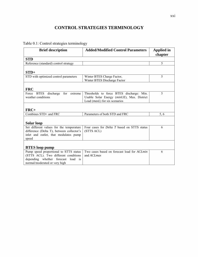
Table 0.1: Control strategies terminology
Brief description Added/Modified Control Parameters Applied in
chapter
STD Reference (standard) control strategy 5
STD+ STD with optimized control parameters Winter BTES Charge Factor,
Winter BTES Discharge Factor 5
FRC Force BTES discharge for extreme weather conditions
Thresholds to force BTES discharge: Min. Usable Solar Energy (minUE), Max. District Load (maxL) for six scenarios
5
FRC+ Combines STD+ and FRC Parameters of both STD and FRC 5, 6
Solar loop Set different values for the temperature difference (Delta T), between collector’s inlet and outlet, that modulates pump speed
Four cases for Delta T based on STTS status (STTS ACL)
6
BTES loop pump Pump speed proportional to STTS status (STTS ACL). Two different conditions depending whether forecast load is normal/moderated or very high
Two cases based on forecast load for ACLmin and ACLmax
6
1
INTRODUCTION
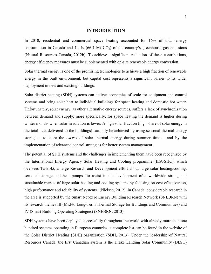
In 2010, residential and commercial space heating accounted for 16% of total energy
consumption in Canada and 14 % (66.4 Mt CO2) of the country’s greenhouse gas emissions
(Natural Resources Canada, 2012b). To achieve a significant reduction of these contributions,
energy efficiency measures must be supplemented with on-site renewable energy conversion.
Solar thermal energy is one of the promising technologies to achieve a high fraction of renewable
energy in the built environment, but capital cost represents a significant barrier to its wider
deployment in new and existing buildings.
Solar district heating (SDH) systems can deliver economies of scale for equipment and control
systems and bring solar heat to individual buildings for space heating and domestic hot water.
Unfortunately, solar energy, as other alternative energy sources, suffers a lack of synchronization
between demand and supply; more specifically, for space heating the demand is higher during
winter months when solar irradiation is lower. A high solar fraction (high share of solar energy in
the total heat delivered to the buildings) can only be achieved by using seasonal thermal energy
storage – to store the excess of solar thermal energy during summer time – and by the
implementation of advanced control strategies for better system management.
The potential of SDH systems and the challenges in implementing them have been recognized by
the International Energy Agency Solar Heating and Cooling programme (IEA-SHC), which
oversees Task 45, a large Research and Development effort about large solar heating/cooling,
seasonal storage and heat pumps “to assist in the development of a worldwide strong and
sustainable market of large solar heating and cooling systems by focusing on cost effectiveness,
high performance and reliability of systems” (Nielsen, 2012). In Canada, considerable research in
the area is supported by the Smart Net-zero Energy Building Research Network (SNEBRN) with
its research themes III (Mid-to Long-Term Thermal Storage for Buildings and Communities) and
IV (Smart Building Operating Strategies) (SNEBRN, 2013).
SDH systems have been deployed successfully throughout the world with already more than one
hundred systems operating in European countries; a complete list can be found in the website of
the Solar District Heating (SDH) organization (SDH, 2013). Under the leadership of Natural
Resources Canada, the first Canadian system is the Drake Landing Solar Community (DLSC)

2
located in Okotoks, Alberta (Wong et al., 2007). The DLSC plant is the case study for this
research.
Problem definition
Besides selecting the appropriate component sizes, improving energy performance relies to some
extent on an effective supervisory control system designed to manage, among others, the
interactions between the Short-Term Thermal Storage (STTS) and the long-term seasonal storage
(Borehole Thermal Energy Storage, BTES). In the case of the DLSC control strategy, STTS-
BTES control follows an indirect approach for estimating current and near-future heating needs
based on current temperature and time of day. Nevertheless, very low ambient temperatures (or a
rapid temperature drop), low solar irradiation periods, and low BTES temperatures can lead to
cases when the STTS is unable to supply all the needed heat to the district loop.
Another characteristic of the current control is the priority given to solar fraction which basically
translates to a diminution of gas consumption. Under some circumstances – related to energy
prices and/or CO2 emissions reduction – priority could be shifted to reduce electricity
consumption rather than gas usage.
The paragraphs above lead to the following research questions:
Can the long-term system performance be improved if the STTS-BTES control strategy is
able to anticipate extreme weather events and to adapt the charge/discharge operation
accordingly?
Is it possible for the control strategy to take into account the electricity consumption in
addition to the (heat-based) solar fraction so that operating costs (or CO2 emissions if that
is desired) can be optimized?
Can MPC principles be integrated at different levels in SDH systems (supervisory control,
local pump speed control)?
Objectives and scope
The objectives of the project are:
Develop a calibrated model of DSLC suitable for MPC studies
3
Develop new control strategies based on Model Predictive Control (MPC) to increase the
energy performance of solar communities and reduce their operating costs.
Assess the potential of MPC to optimize the supervisory control strategy managing the
short-term and long-term thermal storage.
Assess the potential of MPC to further reduce operating costs by controlling variable
speed pumps.
The supervisory control system consists of rules, parameters and set-points for the different
system components and fluid circuits. The introduction of new control strategies was limited to
the components and circuits being perceived as the ones having a direct impact on reaching the
aforementioned objectives.
Methodology
Initial steps consisted of gathering and understanding all possible information about the case
study (DLSC); this included articles, reports, schemas, internal documents and most importantly:
monitored data for five year of operation and an out-dated – but very useful and instructive –
system model implemented in TRNSYS.
The collected documents and data allowed to calibrate the community’s TRNSYS model and to
provide the measured weather and heating load to simulations. After this process, potential
improvements to the control strategy were identified and alternative controls with predictive
features were devised. The method used to build on the existing controller rules and take into
account the predicted system behaviour is explained in Chapter 3.
The conceived control strategies were first tested by trial and error to validate their relevance and
to identify the control parameters suitable for optimization. In a second step, optimization and
tune up of the predictive strategies was performed using measured data as perfect forecasts for
weather and heating load. The generic optimization tool GenOpt was employed to evaluate the
control strategies parameters that minimize the combined consumption of gas and electricity for
different periods of simulated system operation. In the last step, two different MPC approaches
were implemented to optimize the control strategies altogether.
4
Thesis outline
There are six chapters in this thesis. The first one is a literature review oriented to covering the
topics of solar district heating, seasonal storage and control methods, especially Model Predictive
Control. The second chapter presents the system used as case study, the Drake Landing Solar
Community (DLSC). The third chapter presents the methodology and briefly introduces the
proposed control strategies and the concepts applied during the different phases of the project.
Chapter four details the process followed to obtain a calibrated TRNSYS DLSC model starting
from the original model; this included the development of two new TRNSYS components. Next
two chapters introduce and discuss the results of using Model Predictive Control (MPC) for the
new control strategies intended to increase overall energy performance during system operation;
chapter five describes a control add-on (FRC) that forces the discharge of the seasonal storage in
order to have thermal energy more readily available for heating needs; chapter six shows the
integration of this add-on with control strategies aimed to reduce pump electricity consumption.

5
CHAPTER 1 LITERATURE REVIEW
This chapter describes the concept of solar communities, also known as solar heating districts,
and explores the developments for seasonal storage and supervisory control for such systems.
Model Predictive Control theory and applications are also especially reviewed to illustrate its
potential and limitations.
1.1 Solar Communities / Solar District Heating Systems
A district heating system provides heat from a centralized point to residential or commercial
areas to satisfy the demands for space heating and/or hot water. The heat production can be from
different sources: gas, biomass, solar, geothermal, co-generation or any combination of them.
District heating systems have some advantages over individual heating systems, especially for
high density areas or buildings. When using co-generation the energy efficiency of the overall
plant is increased due to the utilization of the waste heat for the district (District Heating, 2013).
The oldest systems for heat distribution can be traced to the ancient Romans; they used
underground tunnels called hypocausts to circulate hot air to heat homes. In modern times, it was
in 1877 that the engineer Birdsill Holly conceived the first heating district for Lockport (New
York); the system drew a lot of attention and it was soon followed with more plants in the U.S. In
Europe, the development of heating districts started as early as 1921 in Hamburg; the system was
so successful that by 1938 it was expanded to provide 30 times the initial heat. Similar growth
was observed in other countries (Turping, 1966). Nowadays, there are district heating systems in
Asian, European and North-American cities, such as the one in downtown Montreal (operating
since 1947), which serves 20 large buildings including commercial, residential and institutional
customers (Dalkia, 2010).
In the case of solar communities, also known as Solar District Heating (SDH) systems or Central
Solar Heating Plants (CSHP), one if the heat sources is obviously the sun’s radiation. The Solar
District Heating organization (http://www.solar-district-heating.eu) lists in its European database
only the larger plants consisting of more than 500 m2 of solar collectors’ area.
The first SDH projects emerged at the end of the 70’s in Sweden, The Netherlands and Denmark.
Some of the systems were intended for research purposes so to set the foundations for further
projects. In the 90’s, Germany and Austria grew more interested in these kinds of systems and
6
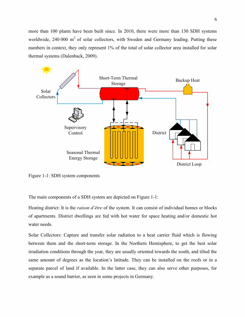
more than 100 plants have been built since. In 2010, there were more than 130 SDH systems
worldwide, 240 000 m2 of solar collectors, with Sweden and Germany leading. Putting these
numbers in context, they only represent 1% of the total of solar collector area installed for solar
thermal systems (Dalenback, 2009).
Seasonal Thermal Energy Storage
Short-Term Thermal Storage
Backup Heat
District Loop
Supervisory Control
Solar Collectors
District
Figure 1-1: SDH system components
The main components of a SDH system are depicted on Figure 1-1:
Heating district: It is the raison d’être of the system. It can consist of individual homes or blocks
of apartments. District dwellings are fed with hot water for space heating and/or domestic hot
water needs.
Solar Collectors: Capture and transfer solar radiation to a heat carrier fluid which is flowing
between them and the short-term storage. In the Northern Hemisphere, to get the best solar
irradiation conditions through the year, they are usually oriented towards the south, and tilted the
same amount of degrees as the location’s latitude. They can be installed on the roofs or in a
separate parcel of land if available. In the latter case, they can also serve other purposes, for
example as a sound barrier, as seen in some projects in Germany.

7
Short-Term Thermal Storage (STTS): It is a temporary storage of thermal energy coming from
the collectors on the way to the users and/or to long-term storage (if available). When heating
needs arise in the district, the STTS retrieves thermal energy from the long-term storage when its
own state of charge in not enough. The STTS is an optional thermal buffer typically used when
the long-term storage exhibits low heat transfer rate or when there is no long-term storage (e.g.
systems with a low solar fraction).
Seasonal (long-term) Thermal Energy Storage (STES): It is an optional component that allows
increasing solar energy performance by storing the excess of solar energy during the summer and
shoulder months to make it available through the winter time. Solar Heating Districts including
this component are called Central Solar Heating Plants with Seasonal Storage (CSHPSS). More
details about seasonal thermal energy storage will be presented in section 1.2.
Backup heat: It is activated when the temperature of the water going to the district is not enough
to fulfill the heating needs. In Figure 1-1 a centralized gas boiler is depicted.
District Loop: It is the heat distribution network that carries hot water to the homes and brings
back the colder water to the plant. In some installations it is used as an alternative means of
diurnal storage.
Supervisory Control: It is the brain of the plant. It controls the operation by adjusting pumps and
valves to transfer thermal energy among the components according to system status and heating
needs. Further description and review of the Control component is available in section 0.
1.1.1 Solar Fraction
To quantify solar energy performance in solar districts, the most common measure is the Solar
Fraction (SF), usually defined as the ratio between the amount of solar energy delivered to the
district and the total energy consumption for district needs. When SDH systems do not have
seasonal storage (CSHPxS), or only have diurnal storage (CSHPDS), the SF is usually low
(between 10% - 20%), because collected solar thermal energy in winter cannot cope with the
increased heat consumption. On the other hand, CSHPSS plants can attain 70% of solar fraction
the cases where they are built to provide space heating and domestic hot water (Fisch, Guigas, &
Dalenbäck, 1998). Solar fraction can be even higher (more than 90%) for CSHPSS’s designed for
8
space heating only (Sibbitt et al., 2012). It is important to mention that initial costs also increase
when seasonal storage is considered for the plant.
1.1.2 SDH in Europe
Most solar district heating systems are found in Europe. A complete list is available at the Solar
District Heating organization database (SDH, 2013). From that list, a few plants in Denmark,
Germany and Sweden will be described shortly. Here, the focus is on those having what is known
as Borehole Thermal Energy Storage (BTES), the same type of seasonal storage as used in the
case study. BTES details of two of these systems are listed along with the case study in Table 1.1.
A review of existing projects in Denmark can be found in Heller (2000). The following
comparison shows the evolution of these systems:
Saltum (operates since 1988): With 1 000 m2 of solar collectors, it is the oldest plant installed in
Denmark (and one of the oldest in Europe) still operating. Its solar fraction is very low (4%) in
part due to the lack of seasonal storage.
Marstal I (since 1996): 18 300 m2 of solar collectors and diurnal storage. The system reached
12% of solar fraction before being upgraded.
Marstal II (upgrade in 1998): Includes a Water Thermal Energy Storage (WTES) as seasonal
storage. Solar fraction is increased to 25%.
Brædstrup (since 2007, upgraded in 2012): Its collectors area of 18 600 m2 is the largest in
Europe. The expected share of heat load is 20% (Brædstrup SolPark, 2012); with a projected
BTES storage the target is a long-term solar fraction of 50% (PlanEnergi, 2010).
Information for most of Denmark’s plants, including current status, operational and economic
data can be found online at http://solvarmedata.dk.
In the case of Germany, Bauer et al. (2010) compare the most important plants with seasonal heat
storage. The installations with BTES storage are:
Neckarsulm (since 1977): 5 570 m2 of solar collectors and a solar fraction (SF) close to 40%.
Crailsheim (since 2003): 7 300 m2 of solar collectors. SF is planned to be 50% in the long-term,
currently it is 36% (Nussbicker & Druck, 2012).
9
In Sweden, the district of Anneberg is operating since 2002. The collector array’s area is 2 400
m2 and seasonal storage is of BTES-type. Solar fraction was projected to be 70% in 5 years
(Lundh & Dalenbäck, 2008); however, it has stayed around 40% (Heier et al., 2011).
1.1.3 SDH Worldwide
The case study, Drake Landing Solar Community (DLSC) in Okotoks (Alberta, Canada), with a
collector array of 2 300 m2 and BTES storage, reached more than 95% SF in its 5th year of
operation (Sibbitt et al., 2012). Chapter 1 gives more details about the case study, its operation
and modelling.
Solar heating district projects are not limited to Europe and Canada. In South Korea, a feasibility
study for a CSHPSS project in Cheju Island was conducted by Chung, Park & Yoon (1998);
more recently, in 2011, a 1 000 m2 array plant started operations, providing hot water to a
hospital (http://www.solarthermalworld.org/content/south-korea-hospital-receives-1040-m2-
large-scale-collectors).
In China, some cities, including Beijing, are passing laws mandating Solar Domestic Heat Water
(SDHW) systems for new residential blocks (of up 12 floors) where no waste heat is employed
for heating water (http://www.solarthermalworld.org/content/china-beijing-mandates-solar-hot-
water-systems).
In 2012, Saudi Arabia inaugurated what is the biggest solar plant as of March 2013: 36 000 m2 of
collectors (almost double as much as Brædstrup) for providing domestic hot water to 40 000
students in the Princess Noura Bint Abdul Rahman University campus in Riyadh
(http://www.solarthermalworld.org/content/saudi-arabia-worlds-biggest-solar-thermal-plant-
operation).
1.2 Seasonal Thermal Energy Storage (STES)
For solar district heating in countries north or south of tropical latitudes, STES is fundamental to
overcome the seasonal imbalance between heating needs and amount of solar radiation. With
seasonal thermal storage, it is possible to provide in winter some of the heat stored during the
summer. In Europe, 21 out of 86 solar heating districts have seasonal storage (SDH, 2013).
10
Hadorn (1988) is considered as a seminal reference for seasonal storage; he presents heat storage
principles and types along with analytical and numerical methods for modelling and design. The
heat storage categories are:
Sensible heat storage: There is no phase change in the substance used for storage, e.g. hot water.
It is the simplest and most common way to store heat. All the European plants with seasonal
storage listed in the Solar District Heating organization database (SDH, 2013) have some variant
of this category.
Latent heat storage: There is a phase change when heat is stored or recovered. They have much
higher energy density than the sensible heat type (100-200 times), but their implementation is
more difficult due to hysteresis in the phase change cycle and slower thermal energy transfer. A
study about using ice slurry as latent storage material can be found in Tamasauskas et al. (2012)
Chemical heat storage: Uses reversible chemical reactions where there are virtually no heat
losses. The energy density is even higher, – about 10 times that of latent heat storage. There has
been some research in the field but no practical applications at district level were found.
The most commonly employed technologies for solar seasonal storage are underground systems
based on the principle of sensible heat, using water and/or earth. Pavlov & Olesen (2011)
compare and summarize the results from different European CSHPSS systems, with focus in the
seasonal storage role. Schmidt et al. (2004) present and define the following types identified in
Figure 1-2:
“Hot-water heat storage (also known as Water Thermal Energy Storage-WTES, or simply
Water Tank Storage): The water-filled tank construction of usually reinforced concrete is
totally or partly embedded into the ground.
Gravel-water heat storage (also known as Water-Gravel Thermal Energy Storage-WGTES
or Water Gravel Pit Storage): A pit with a watertight plastic liner is filled with a gravel–
water mixture forming the storage material.
Aquifer heat storage (also known as Aquifer Thermal Energy Storage-ATES): Aquifers
are below-ground widely distributed sand, gravel, sandstone or limestone layers with high
hydraulic conductivity which are filled with groundwater.
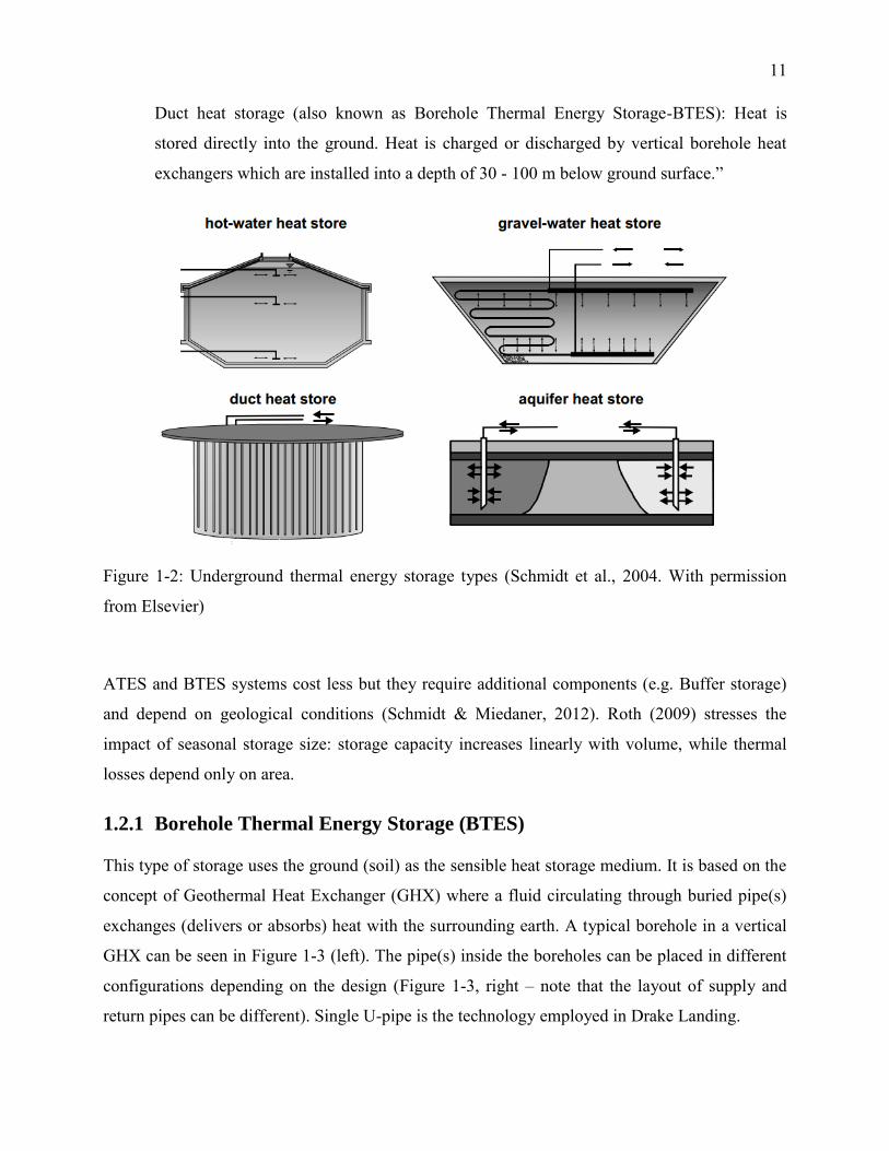
11
Duct heat storage (also known as Borehole Thermal Energy Storage-BTES): Heat is
stored directly into the ground. Heat is charged or discharged by vertical borehole heat
exchangers which are installed into a depth of 30 - 100 m below ground surface.”
Figure 1-2: Underground thermal energy storage types (Schmidt et al., 2004. With permission
from Elsevier)
ATES and BTES systems cost less but they require additional components (e.g. Buffer storage)
and depend on geological conditions (Schmidt & Miedaner, 2012). Roth (2009) stresses the
impact of seasonal storage size: storage capacity increases linearly with volume, while thermal
losses depend only on area.
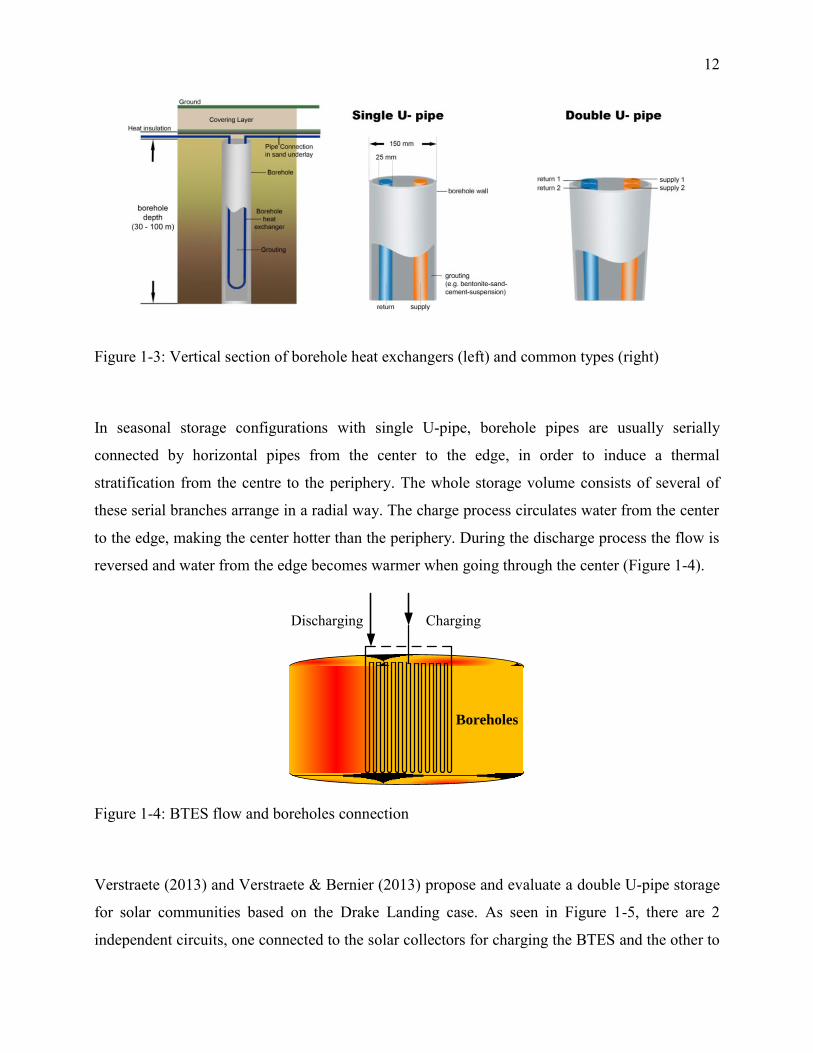
1.2.1 Borehole Thermal Energy Storage (BTES)
This type of storage uses the ground (soil) as the sensible heat storage medium. It is based on the
concept of Geothermal Heat Exchanger (GHX) where a fluid circulating through buried pipe(s)
exchanges (delivers or absorbs) heat with the surrounding earth. A typical borehole in a vertical
GHX can be seen in Figure 1-3 (left). The pipe(s) inside the boreholes can be placed in different
configurations depending on the design (Figure 1-3, right – note that the layout of supply and
return pipes can be different). Single U-pipe is the technology employed in Drake Landing.
12
Figure 1-3: Vertical section of borehole heat exchangers (left) and common types (right)
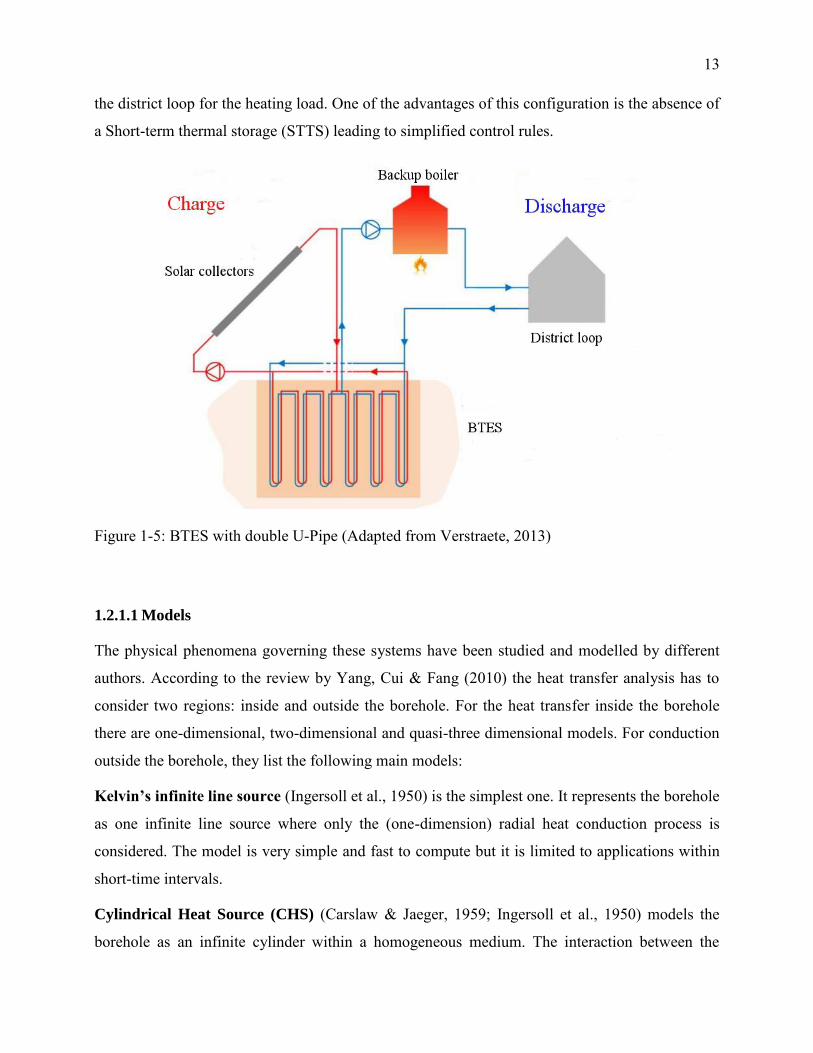
In seasonal storage configurations with single U-pipe, borehole pipes are usually serially
connected by horizontal pipes from the center to the edge, in order to induce a thermal
stratification from the centre to the periphery. The whole storage volume consists of several of
these serial branches arrange in a radial way. The charge process circulates water from the center
to the edge, making the center hotter than the periphery. During the discharge process the flow is
reversed and water from the edge becomes warmer when going through the center (Figure 1-4).
Boreholes
Discharging Charging
Figure 1-4: BTES flow and boreholes connection
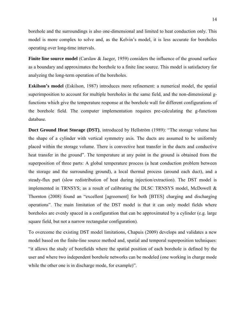
Verstraete (2013) and Verstraete & Bernier (2013) propose and evaluate a double U-pipe storage
for solar communities based on the Drake Landing case. As seen in Figure 1-5, there are 2
independent circuits, one connected to the solar collectors for charging the BTES and the other to
13
the district loop for the heating load. One of the advantages of this configuration is the absence of
a Short-term thermal storage (STTS) leading to simplified control rules.
Figure 1-5: BTES with double U-Pipe (Adapted from Verstraete, 2013)
1.2.1.1 Models
The physical phenomena governing these systems have been studied and modelled by different
authors. According to the review by Yang, Cui & Fang (2010) the heat transfer analysis has to
consider two regions: inside and outside the borehole. For the heat transfer inside the borehole
there are one-dimensional, two-dimensional and quasi-three dimensional models. For conduction
outside the borehole, they list the following main models:
Kelvin’s infinite line source (Ingersoll et al., 1950) is the simplest one. It represents the borehole
as one infinite line source where only the (one-dimension) radial heat conduction process is
considered. The model is very simple and fast to compute but it is limited to applications within
short-time intervals.
Cylindrical Heat Source (CHS) (Carslaw & Jaeger, 1959; Ingersoll et al., 1950) models the
borehole as an infinite cylinder within a homogeneous medium. The interaction between the
14
borehole and the surroundings is also one-dimensional and limited to heat conduction only. This
model is more complex to solve and, as the Kelvin’s model, it is less accurate for boreholes
operating over long-time intervals.
Finite line source model (Carslaw & Jaeger, 1959) considers the influence of the ground surface
as a boundary and approximates the borehole to a finite line source. This model is satisfactory for
analyzing the long-term operation of the boreholes.
Eskilson’s model (Eskilson, 1987) introduces more refinement: a numerical model, the spatial
superimposition to account for multiple boreholes in the same field, and the non-dimensional g-
functions which give the temperature response at the borehole wall for different configurations of
the borehole field. The computer implementation requires pre-calculating the g-functions
database.
Duct Ground Heat Storage (DST), introduced by Hellström (1989): “The storage volume has
the shape of a cylinder with vertical symmetry axis. The ducts are assumed to be uniformly
placed within the storage volume. There is convective heat transfer in the ducts and conductive
heat transfer in the ground”. The temperature at any point in the ground is obtained from the
superposition of three parts: A global temperature process (a heat conduction problem between
the storage and the surrounding ground), a local thermal process (around each duct), and a
steady-flux part (slow redistribution of heat during injection/extraction). The DST model is
implemented in TRNSYS; as a result of calibrating the DLSC TRNSYS model, McDowell &
Thornton (2008) found an “excellent [agreement] for both [BTES] charging and discharging
operations”. The main limitation of the DST model is that it can only model fields where
boreholes are evenly spaced in a configuration that can be approximated by a cylinder (e.g. large
square field, but not a narrow rectangular configuration).
To overcome the existing DST model limitations, Chapuis (2009) develops and validates a new
model based on the finite-line source method and, spatial and temporal superposition techniques:
“it allows the study of borefields where the spatial position of each borehole is defined by the
user and where two independent borehole networks can be modeled (one working in charge mode
while the other one is in discharge mode, for example)”.
15
Bernier, Kummert & Bertagnolio (2007) define and execute a set of test cases to compare CHS,
DST, the Eskilson’s model and the Multiple Load Aggregation Algorithm (MLAA) (Bernier et
al., 2004) –a technique of temporal superposition based on CHS.
1.2.1.2 BTES installations
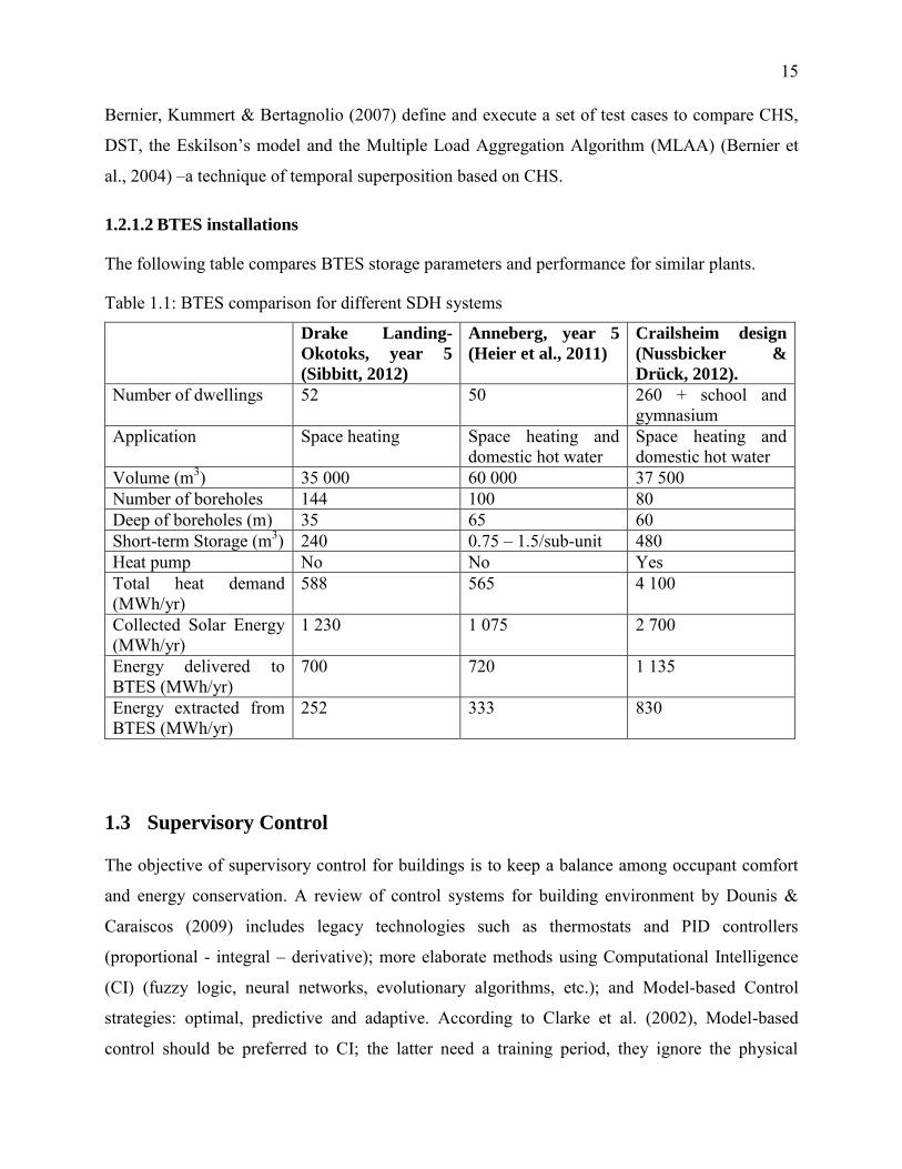
The following table compares BTES storage parameters and performance for similar plants.
Table 1.1: BTES comparison for different SDH systems
Drake Landing-
Okotoks, year 5
(Sibbitt, 2012)
Anneberg, year 5
(Heier et al., 2011)
Crailsheim design
(Nussbicker &
Drück, 2012).
Number of dwellings 52 50 260 + school and gymnasium
Application Space heating Space heating and domestic hot water
Space heating and domestic hot water
Volume (m3) 35 000 60 000 37 500 Number of boreholes 144 100 80 Deep of boreholes (m) 35 65 60 Short-term Storage (m3) 240 0.75 – 1.5/sub-unit 480 Heat pump No No Yes Total heat demand (MWh/yr)
588 565 4 100
Collected Solar Energy (MWh/yr)
1 230 1 075 2 700
Energy delivered to BTES (MWh/yr)
700 720 1 135
Energy extracted from BTES (MWh/yr)
252 333 830
1.3 Supervisory Control
The objective of supervisory control for buildings is to keep a balance among occupant comfort
and energy conservation. A review of control systems for building environment by Dounis &
Caraiscos (2009) includes legacy technologies such as thermostats and PID controllers
(proportional - integral – derivative); more elaborate methods using Computational Intelligence
(CI) (fuzzy logic, neural networks, evolutionary algorithms, etc.); and Model-based Control
strategies: optimal, predictive and adaptive. According to Clarke et al. (2002), Model-based
control should be preferred to CI; the latter need a training period, they ignore the physical
16
underlying system phenomena and their control decisions are not tractable. Another advantage of
Model-based control is that it is better suited to be considered during the early stages of building
design as it is proposed by Petersen & Svendsen (2010).
Henze, Dodier & Krarti (1997) present three conventional thermal storage control strategies for
cooling applications in buildings: chiller-priority, constant-proportion and storage-priority. They
state that some of these can also be applied for other types of thermal storage. The first 2 methods
are mainly based in current system and weather conditions, but storage-priority implies some
level of load prediction. More advanced methods, such as optimal control, allow taking
advantage of the passive building thermal storage to time-shift peak electrical load and reduce
electricity costs (Braun, J., 1990). De Ridder et al. (2011) describe a dynamic programming
algorithm for a long term storage coupled to a heating, ventilation and cooling (HVAC) system.
For the general case of district heating systems, Saarinen (2008) explains how the common
method for controlling supply temperature, called Feed-Forward Control, can be improved by
using a dynamic algorithm for load prediction.
1.3.1 Control for Solar District Heating
The design of the control system for a SDH plant always meets “conflicting targets” as
enumerated by Schubert & Trier (2012): “Avoidance of stagnation of the solar system, optimal
use of heat storages, minimization of heat losses in collectors, pipes and storages; minimal
electricity consumption of pumps, minimum requirement of human intervention, optimal use of
other heat sources like heat pumps, boilers, waste heat”
This is confirmed by Wong et al. (2007) regarding Drake Landing: “Optimizing the control
strategy was a significant challenge, developing into a balancing act between the two primary
goals of assuring occupant comfort and maximizing the solar fraction.”
In a SDH plant with no seasonal storage, there are mainly two circuits to control: the charge
circuit which includes the collectors and the short-term storage, and the discharge circuit (of the
short-term storage) for supplying heat to the district. In the charge segment, the concept of
variable flow rate is applied to the circuit pump whether using collector temperature
measurement or collector irradiation measurement (Schubert et al., 2012). The Marstal plant
employs the temperature measurement method (Heller, 2000). Another alternative consists in
17
modulating the pump speed to maintain a predefined temperature difference between the solar
collectors’ inlet and outlet ports (Wong et al., 2007).
The short-term thermal storage (STTS) discharge circuit is activated when the district demands
thermal energy from the plant. According to Wong et al. (2007), “the biggest challenge with the
District (discharge) Loop was to ensure the greatest temperature drop through the system”, this
ensures “efficient operation of the STTS by maintaining stratification” and increases the
“efficiency in the solar collectors by maintaining the lowest inlet water temperature.”
When there is a seasonal storage, two additional circuits, for its charge and discharge, need to be
controlled. The seasonal storage is mainly charged from the STTS during summer, besides
building the thermal energy reserve, another objective is to make sure that the short-term storage
is able to collect the daily solar radiation. The discharge is essentially started for winter periods
where the buffer storage has not enough charge to conveniently feed the district loop. No detailed
information was found about how these processes are controlled in plants other than Drake
Landing; this case will be described in Chapter 2.
1.4 Model Predictive Control (MPC)
As its name states, this control method is based on a model of the actual physical system and
predictions of external conditions (or disturbances). With these two elements, MPC is able to
determine the best control input to the system so its output is the closest as possible to the
expected output.
The following MPC theory is based on the book by Rossiter (2003). The initial concept is that a
system model can be represented using the concept of transfer function or state-space matrices.
The latter representation is preferred because it is more convenient and less complicated than the
former one for the cases of multiple-input, multiple-output (MIMO) systems. In the case of a
Linear Time Invariant (LTI) system the state-space matrices (A, B, C, D and F) are constant –
because there is no time dependency– and the model is given by
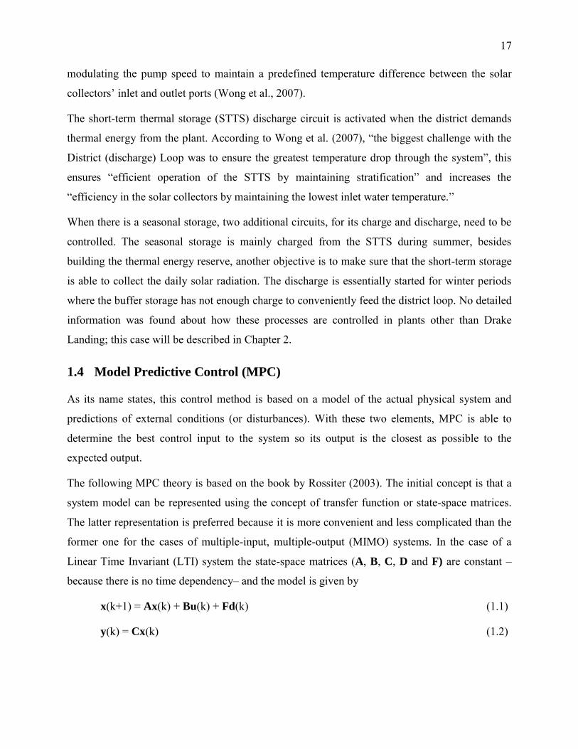
x(k+1) = Ax(k) + Bu(k) + Fd(k) (1.1)
y(k) = Cx(k) (1.2)
18
where, x is the state vector, y is the system’s outputs vector, u vector is the controller input to the
system, d is the disturbances vector, and (k, k+i) indicate consecutive discrete time samples –
commonly used in MPC applications. Future system status and outputs can be predicted for each
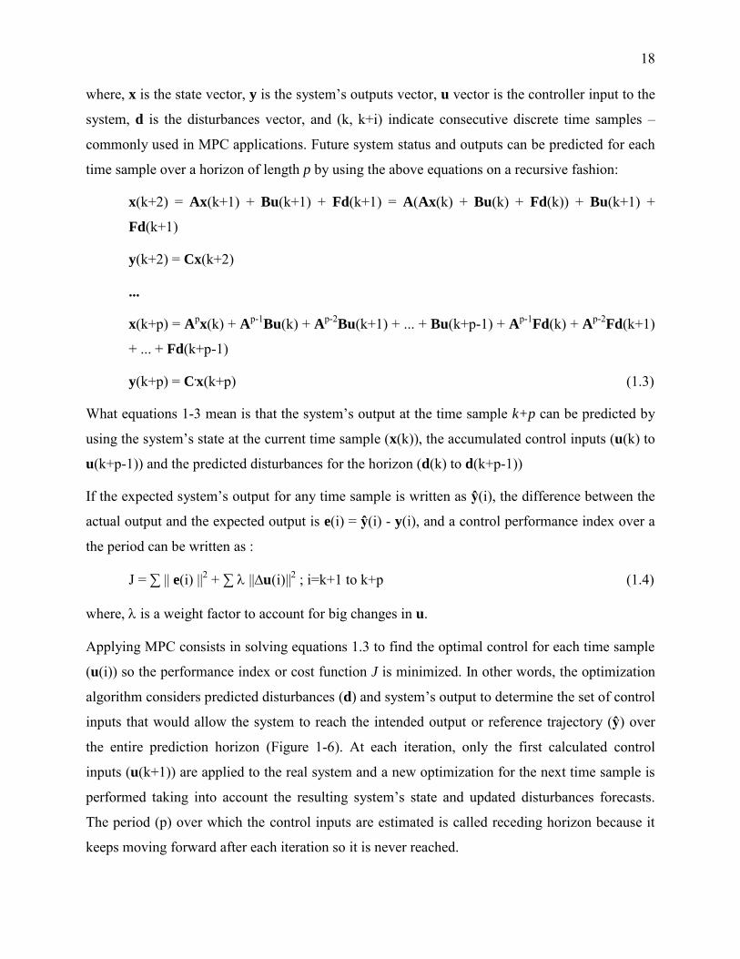
time sample over a horizon of length p by using the above equations on a recursive fashion:
x(k+2) = Ax(k+1) + Bu(k+1) + Fd(k+1) = A(Ax(k) + Bu(k) + Fd(k)) + Bu(k+1) +
Fd(k+1)
y(k+2) = Cx(k+2)
...
x(k+p) = Apx(k) + Ap-1
Bu(k) + Ap-2Bu(k+1) + ... + Bu(k+p-1) + Ap-1
Fd(k) + Ap-2Fd(k+1)
+ ... + Fd(k+p-1)
y(k+p) = C•x(k+p) (1.3)
What equations 1-3 mean is that the system’s output at the time sample k+p can be predicted by
using the system’s state at the current time sample (x(k)), the accumulated control inputs (u(k) to
u(k+p-1)) and the predicted disturbances for the horizon (d(k) to d(k+p-1))
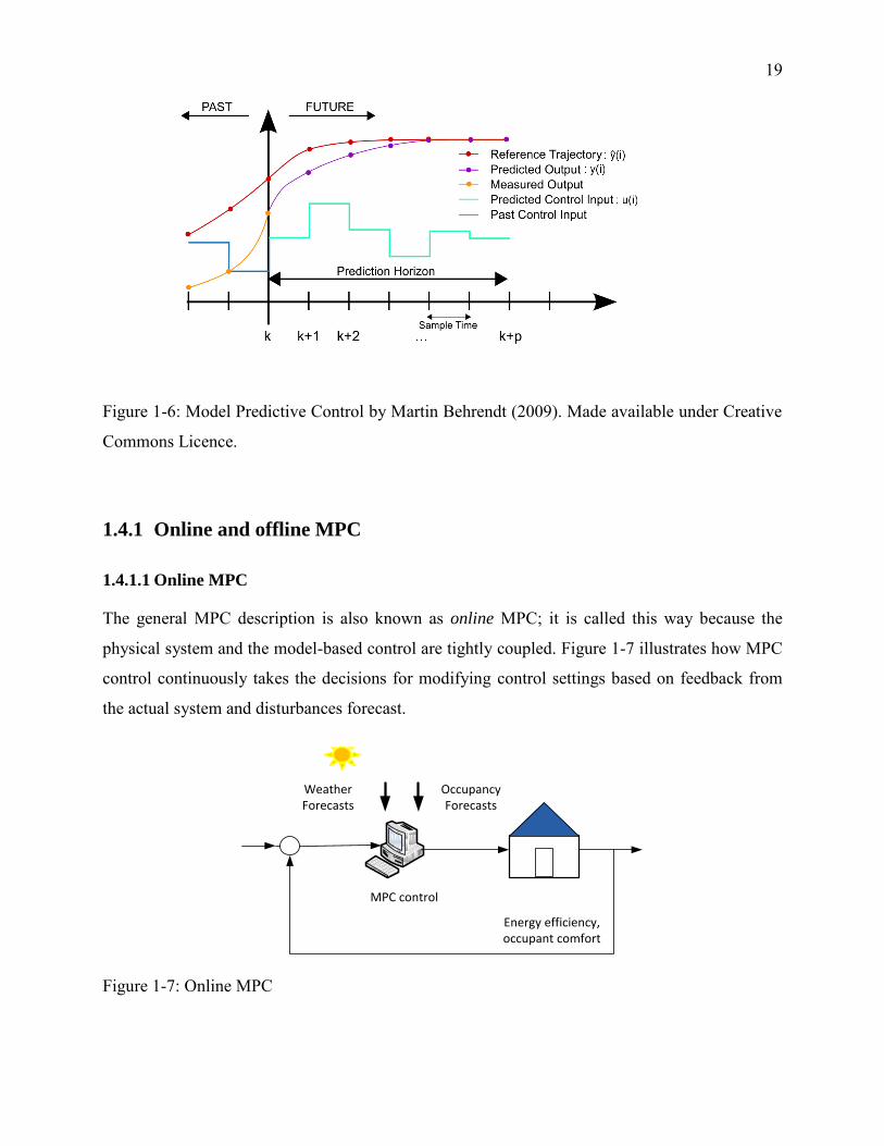
If the expected system’s output for any time sample is written as ŷ(i), the difference between the
actual output and the expected output is e(i) = ŷ(i) - y(i), and a control performance index over a
the period can be written as :
J = ∑ || e(i) ||2 + ∑ ||∆u(i)||2 ; i=k+1 to k+p (1.4)
where, is a weight factor to account for big changes in u.
Applying MPC consists in solving equations 1.3 to find the optimal control for each time sample
(u(i)) so the performance index or cost function J is minimized. In other words, the optimization
algorithm considers predicted disturbances (d) and system’s output to determine the set of control
inputs that would allow the system to reach the intended output or reference trajectory (ŷ) over
the entire prediction horizon (Figure 1-6). At each iteration, only the first calculated control
inputs (u(k+1)) are applied to the real system and a new optimization for the next time sample is
performed taking into account the resulting system’s state and updated disturbances forecasts.
The period (p) over which the control inputs are estimated is called receding horizon because it
keeps moving forward after each iteration so it is never reached.
19
Figure 1-6: Model Predictive Control by Martin Behrendt (2009). Made available under Creative
Commons Licence.
1.4.1 Online and offline MPC
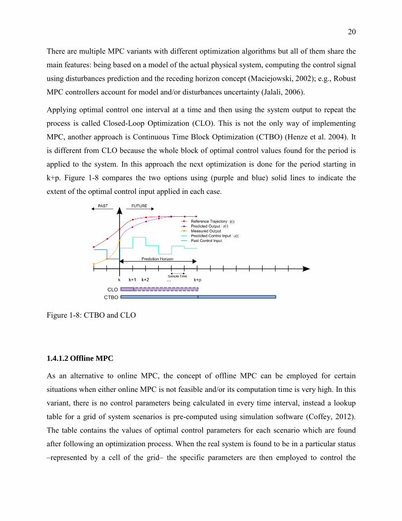
1.4.1.1 Online MPC
The general MPC description is also known as online MPC; it is called this way because the
physical system and the model-based control are tightly coupled. Figure 1-7 illustrates how MPC
control continuously takes the decisions for modifying control settings based on feedback from
the actual system and disturbances forecast.
Weather Forecasts
Occupancy Forecasts
Energy efficiency, occupant comfort
MPC control
Figure 1-7: Online MPC
20
There are multiple MPC variants with different optimization algorithms but all of them share the
main features: being based on a model of the actual physical system, computing the control signal
using disturbances prediction and the receding horizon concept (Maciejowski, 2002); e.g., Robust
MPC controllers account for model and/or disturbances uncertainty (Jalali, 2006).
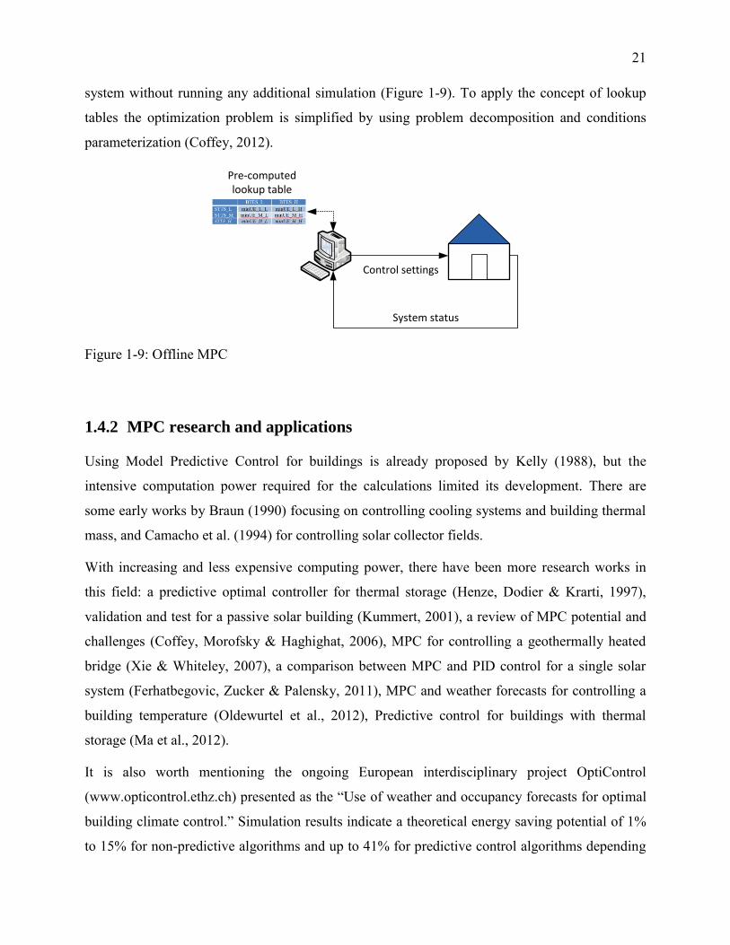
Applying optimal control one interval at a time and then using the system output to repeat the
process is called Closed-Loop Optimization (CLO). This is not the only way of implementing
MPC, another approach is Continuous Time Block Optimization (CTBO) (Henze et al. 2004). It
is different from CLO because the whole block of optimal control values found for the period is
applied to the system. In this approach the next optimization is done for the period starting in
k+p. Figure 1-8 compares the two options using (purple and blue) solid lines to indicate the
extent of the optimal control input applied in each case.
CLO
CTBO
Figure 1-8: CTBO and CLO
1.4.1.2 Offline MPC
As an alternative to online MPC, the concept of offline MPC can be employed for certain
situations when either online MPC is not feasible and/or its computation time is very high. In this
variant, there is no control parameters being calculated in every time interval, instead a lookup
table for a grid of system scenarios is pre-computed using simulation software (Coffey, 2012).
The table contains the values of optimal control parameters for each scenario which are found
after following an optimization process. When the real system is found to be in a particular status
–represented by a cell of the grid– the specific parameters are then employed to control the
21
system without running any additional simulation (Figure 1-9). To apply the concept of lookup
tables the optimization problem is simplified by using problem decomposition and conditions
parameterization (Coffey, 2012).
Pre-computed lookup table
System status
Control settings
Figure 1-9: Offline MPC
1.4.2 MPC research and applications
Using Model Predictive Control for buildings is already proposed by Kelly (1988), but the
intensive computation power required for the calculations limited its development. There are
some early works by Braun (1990) focusing on controlling cooling systems and building thermal
mass, and Camacho et al. (1994) for controlling solar collector fields.
With increasing and less expensive computing power, there have been more research works in
this field: a predictive optimal controller for thermal storage (Henze, Dodier & Krarti, 1997),
validation and test for a passive solar building (Kummert, 2001), a review of MPC potential and
challenges (Coffey, Morofsky & Haghighat, 2006), MPC for controlling a geothermally heated
bridge (Xie & Whiteley, 2007), a comparison between MPC and PID control for a single solar
system (Ferhatbegovic, Zucker & Palensky, 2011), MPC and weather forecasts for controlling a
building temperature (Oldewurtel et al., 2012), Predictive control for buildings with thermal
storage (Ma et al., 2012).
It is also worth mentioning the ongoing European interdisciplinary project OptiControl
(www.opticontrol.ethz.ch) presented as the “Use of weather and occupancy forecasts for optimal
building climate control.” Simulation results indicate a theoretical energy saving potential of 1%
to 15% for non-predictive algorithms and up to 41% for predictive control algorithms depending
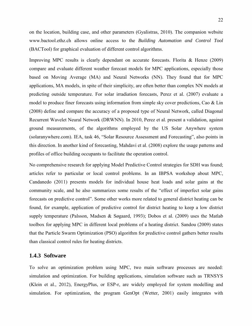
22
on the location, building case, and other parameters (Gyalistras, 2010). The companion website
www.bactool.ethz.ch allows online access to the Building Automation and Control Tool
(BACTool) for graphical evaluation of different control algorithms.
Improving MPC results is clearly dependant on accurate forecasts. Florita & Henze (2009)
compare and evaluate different weather forecast models for MPC applications, especially those
based on Moving Average (MA) and Neural Networks (NN). They found that for MPC
applications, MA models, in spite of their simplicity, are often better than complex NN models at
predicting outside temperature. For solar irradiation forecasts, Perez et al. (2007) evaluate a
model to produce finer forecasts using information from simple sky cover predictions, Cao & Lin
(2008) define and compare the accuracy of a proposed type of Neural Network, called Diagonal
Recurrent Wavelet Neural Network (DRWNN). In 2010, Perez et al. present a validation, against
ground measurements, of the algorithms employed by the US Solar Anywhere system
(solaranywhere.com). IEA, task 46, “Solar Resource Assessment and Forecasting”, also points in
this direction. In another kind of forecasting, Mahdavi et al. (2008) explore the usage patterns and
profiles of office building occupants to facilitate the operation control.
No comprehensive research for applying Model Predictive Control strategies for SDH was found;
articles refer to particular or local control problems. In an IBPSA workshop about MPC,
Candanedo (2011) presents models for individual house heat loads and solar gains at the
community scale, and he also summarizes some results of the “effect of imperfect solar gains
forecasts on predictive control”. Some other works more related to general district heating can be
found, for example, application of predictive control for district heating to keep a low district
supply temperature (Palsson, Madsen & Søgaard, 1993); Dobos et al. (2009) uses the Matlab
toolbox for applying MPC in different local problems of a heating district. Sandou (2009) states
that the Particle Swarm Optimization (PSO) algorithm for predictive control gathers better results
than classical control rules for heating districts.
1.4.3 Software
To solve an optimization problem using MPC, two main software processes are needed:
simulation and optimization. For building applications, simulation software such as TRNSYS
(Klein et al., 2012), EnergyPlus, or ESP-r, are widely employed for system modelling and
simulation. For optimization, the program GenOpt (Wetter, 2001) easily integrates with

23
simulation software through input and output text-files. Matlab also provides an MPC toolbox but
it requires the system to be defined in terms of the transfer function or a state-space model
(www.mathworks.com/products/mpc/). The optimization program evaluates the simulation’s
output and applies special algorithms to find the control parameters values that minimize a
defined cost function, which should corresponds to the best point of system operation.
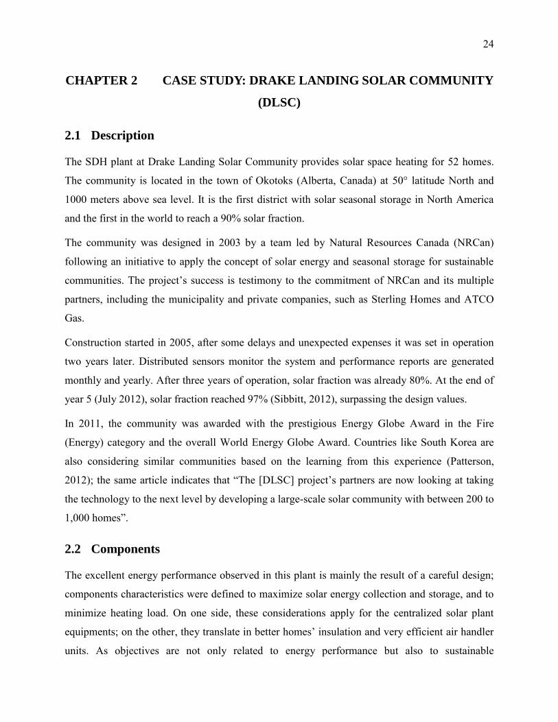
24
CHAPTER 2 CASE STUDY: DRAKE LANDING SOLAR COMMUNITY
(DLSC)
2.1 Description
The SDH plant at Drake Landing Solar Community provides solar space heating for 52 homes.
The community is located in the town of Okotoks (Alberta, Canada) at 50° latitude North and
1000 meters above sea level. It is the first district with solar seasonal storage in North America
and the first in the world to reach a 90% solar fraction.
The community was designed in 2003 by a team led by Natural Resources Canada (NRCan)
following an initiative to apply the concept of solar energy and seasonal storage for sustainable
communities. The project’s success is testimony to the commitment of NRCan and its multiple
partners, including the municipality and private companies, such as Sterling Homes and ATCO
Gas.
Construction started in 2005, after some delays and unexpected expenses it was set in operation
two years later. Distributed sensors monitor the system and performance reports are generated
monthly and yearly. After three years of operation, solar fraction was already 80%. At the end of
year 5 (July 2012), solar fraction reached 97% (Sibbitt, 2012), surpassing the design values.
In 2011, the community was awarded with the prestigious Energy Globe Award in the Fire
(Energy) category and the overall World Energy Globe Award. Countries like South Korea are
also considering similar communities based on the learning from this experience (Patterson,
2012); the same article indicates that “The [DLSC] project’s partners are now looking at taking
the technology to the next level by developing a large-scale solar community with between 200 to
1,000 homes”.
2.2 Components
The excellent energy performance observed in this plant is mainly the result of a careful design;
components characteristics were defined to maximize solar energy collection and storage, and to
minimize heating load. On one side, these considerations apply for the centralized solar plant
equipments; on the other, they translate in better homes’ insulation and very efficient air handler
units. As objectives are not only related to energy performance but also to sustainable
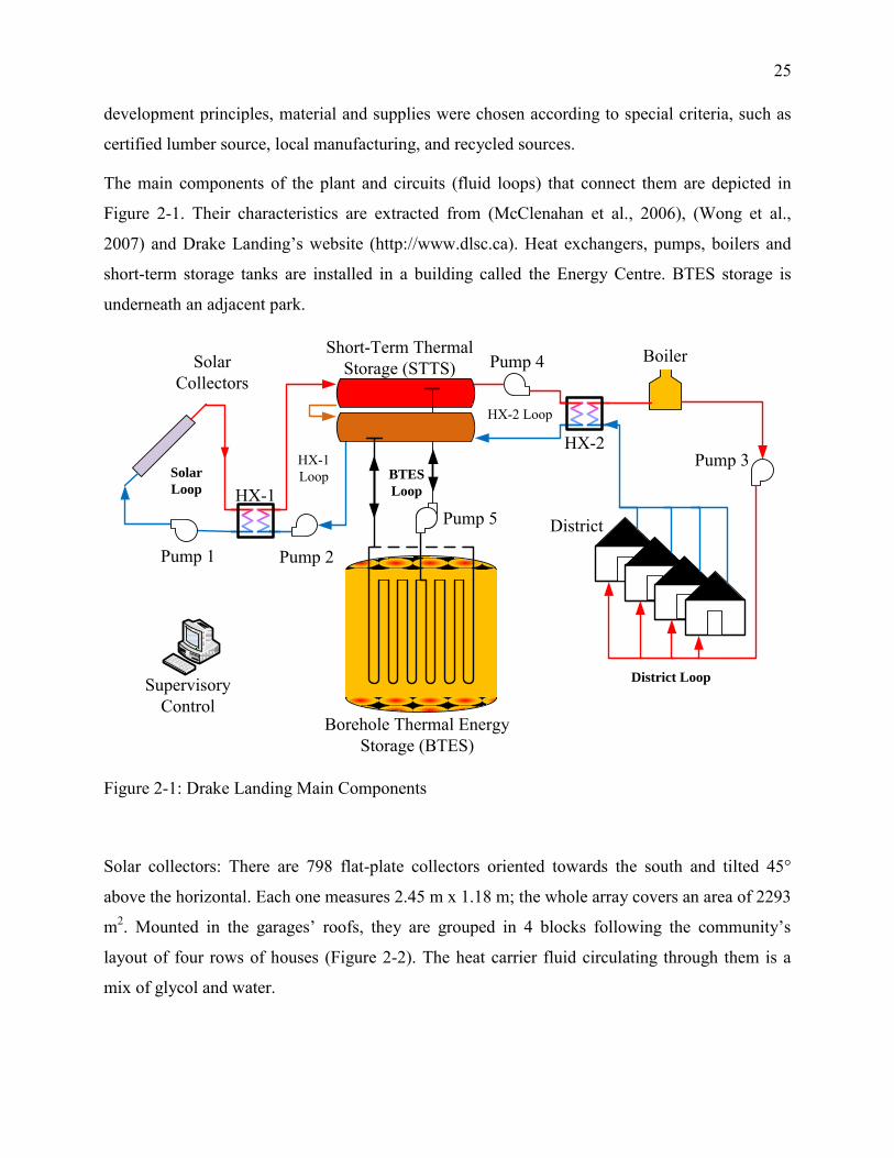
25
development principles, material and supplies were chosen according to special criteria, such as
certified lumber source, local manufacturing, and recycled sources.
The main components of the plant and circuits (fluid loops) that connect them are depicted in
Figure 2-1. Their characteristics are extracted from (McClenahan et al., 2006), (Wong et al.,
2007) and Drake Landing’s website (http://www.dlsc.ca). Heat exchangers, pumps, boilers and
short-term storage tanks are installed in a building called the Energy Centre. BTES storage is
underneath an adjacent park.
Borehole Thermal Energy Storage (BTES)
Short-Term Thermal Storage (STTS)
Boiler
District LoopSupervisory Control
Pump 1 Pump 2
Pump 5
Pump 4
Pump 3HX-2
HX-1
Solar Collectors
District
Solar
Loop
HX-1 Loop
HX-2 Loop
BTES
Loop
Figure 2-1: Drake Landing Main Components
Solar collectors: There are 798 flat-plate collectors oriented towards the south and tilted 45°
above the horizontal. Each one measures 2.45 m x 1.18 m; the whole array covers an area of 2293
m2. Mounted in the garages’ roofs, they are grouped in 4 blocks following the community’s
layout of four rows of houses (Figure 2-2). The heat carrier fluid circulating through them is a
mix of glycol and water.
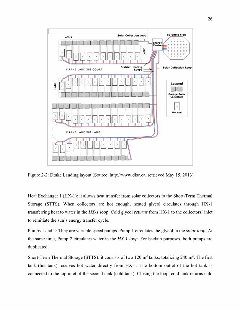
26
Figure 2-2: Drake Landing layout (Source: http://www.dlsc.ca, retrieved May 15, 2013)
Heat Exchanger 1 (HX-1): it allows heat transfer from solar collectors to the Short-Term Thermal
Storage (STTS). When collectors are hot enough, heated glycol circulates through HX-1
transferring heat to water in the HX-1 loop. Cold glycol returns from HX-1 to the collectors’ inlet
to reinitiate the sun’s energy transfer cycle.
Pumps 1 and 2: They are variable speed pumps. Pump 1 circulates the glycol in the solar loop. At
the same time, Pump 2 circulates water in the HX-1 loop. For backup purposes, both pumps are
duplicated.
Short-Term Thermal Storage (STTS): it consists of two 120 m3 tanks, totalizing 240 m3. The first
tank (hot tank) receives hot water directly from HX-1. The bottom outlet of the hot tank is
connected to the top inlet of the second tank (cold tank). Closing the loop, cold tank returns cold
27
water to HX-1. For improved stratification, each tank has an internal division by means of a
special baffle.
Figure 2-3: BTES distribution (Source: http://www.dlsc.ca, retrieved March 22, 2013)
Borehole Thermal Energy Storage (BTES): It is composed of 144 boreholes of 15 cm diameter
and 35 m deep, separated 2.25 m from center-to-center. Each borehole contains a single U-tube.
These pipes are serially connected in strings of 6 from the center to the edge for better radial
stratification. Four circuits made up of non-adjacent strings increase reliability of water supply
and return (Figure 2-3). The total earth volume is 35 000 m3, and the equivalent water thermal
capacity is 15 800 m3.
Pump 5: It is the pump for BTES charge and discharge operations. The pump is actually
unidirectional, with the flow direction dependant on the position of the BTES loop valves
determined by the control platform. Two constant speed pumps in standby-backup configuration
were initially installed for this operation, but a variable speed pump was retrofitted in 2012.
Heat Exchanger 2 (HX-2): Transfers heat from STTS’ hot tank to the district loop when heat
demand exists. The HX-2’s outlet in the small HX-2 loop is the return path for cold water to
STTS’s cold tank.
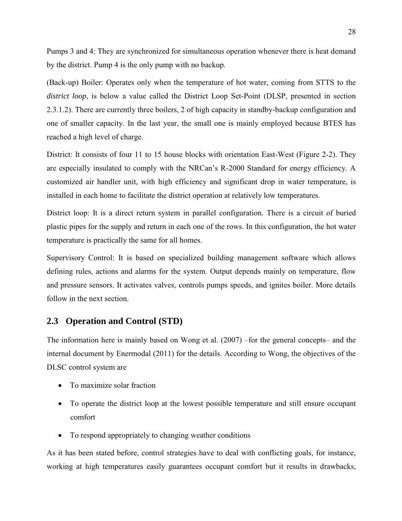
28
Pumps 3 and 4: They are synchronized for simultaneous operation whenever there is heat demand
by the district. Pump 4 is the only pump with no backup.
(Back-up) Boiler: Operates only when the temperature of hot water, coming from STTS to the
district loop, is below a value called the District Loop Set-Point (DLSP, presented in section
2.3.1.2). There are currently three boilers, 2 of high capacity in standby-backup configuration and
one of smaller capacity. In the last year, the small one is mainly employed because BTES has
reached a high level of charge.
District: It consists of four 11 to 15 house blocks with orientation East-West (Figure 2-2). They
are especially insulated to comply with the NRCan’s R-2000 Standard for energy efficiency. A
customized air handler unit, with high efficiency and significant drop in water temperature, is
installed in each home to facilitate the district operation at relatively low temperatures.
District loop: It is a direct return system in parallel configuration. There is a circuit of buried
plastic pipes for the supply and return in each one of the rows. In this configuration, the hot water
temperature is practically the same for all homes.
Supervisory Control: It is based on specialized building management software which allows
defining rules, actions and alarms for the system. Output depends mainly on temperature, flow
and pressure sensors. It activates valves, controls pumps speeds, and ignites boiler. More details
follow in the next section.
2.3 Operation and Control (STD)
The information here is mainly based on Wong et al. (2007) –for the general concepts– and the
internal document by Enermodal (2011) for the details. According to Wong, the objectives of the
DLSC control system are
To maximize solar fraction
To operate the district loop at the lowest possible temperature and still ensure occupant
comfort
To respond appropriately to changing weather conditions
As it has been stated before, control strategies have to deal with conflicting goals, for instance,
working at high temperatures easily guarantees occupant comfort but it results in drawbacks,
29
such as the increase in thermal losses through the system and the reduction of solar collector
efficiency.
It is important to mention that control rules and parameters, defined during the design phase,
have been changing through time due to control system improvements or physical upgrades, e.g.,
the replacement of the constant speed BTES pump –with a variable speed pump– implied
extending the pump control beyond the original on/off switch.
2.3.1 General concepts
2.3.1.1 Operation modes
To provide the district with the maximum possible of solar thermal energy under different
seasonal weather conditions, two modes of operation, winter and summer are defined. There is a
fixed winter mode between September 1st and April 30th, but a “temporary” summer mode from
May to August. During these months, summer mode can be switched back and forth to winter
mode depending on the number of cumulative degree hours (DH) below or above 17 °C: if the
number of degree hours below the reference reaches 5, winter mode is imposed; summer mode is
set again when the DH-above condition is 15 or more. As a control measure, the cooling DH
counter is reset (to 0) when the number of heating DH is higher than 15; in an analog way,
heating DH counter is reset when cooling DH is more than 20. This mechanism is especially
useful during the shoulder months when days are still warm but nights are cold.
District and BTES loops operate differently in each mode: district loop is only active in winter
mode, BTES loop is active during both operation modes but the control strategy parameters are
different. Solar loop is not affected by the operation mode; it works always in the same way and
the control parameters are not changed.
2.3.1.2 District Loop Set Point (DLSP)
This is another important concept in the system control strategy. It defines the set-point of the
minimum water temperature that must be supplied to the district depending on the external air
temperature. If the temperature of hot water coming from STTS does not reach DLSP, then the
boiler is set in operation. Figure 2-4 shows how DLSP is between 37°C and 55°C depending on
three air temperature ranges delimited by -40°C and -2.5°C.
30
30354045505560
-45 -40 -35 -30 -25 -20 -15 -10 -5 0 5 10 15
DLS
P (
C)
Air temperature ( C)
Figure 2-4: DLSP vs. Air Temperature
2.3.1.3 STTS percentage of charge (STTS % charge)
Finally, it is worth highlighting the central role the STTS has. As it is involved in all the heat
transfers through the heating district, the control system looks to keep an adequate STTS
stratification to maximize thermal energy transfers: control rules for the three main loops always
take in consideration STTS’ internal temperatures or parameters that indicate its status.
The main parameter to measure STTS status is STTS % charge; it is calculated from DLSP and
from the temperatures of two nodes in each of the STTS tanks. Each node temperature is only
taken into account for the total % of charge if it is higher than a certain limit called Minimum
Usable Temperature, which depends on DLSP. In other words, the philosophy of the defined
STTS % charge is to assess “how warm” the STTS is when compared to the DLSP.
STTS % charge is obtained from the following formulas:
dT Base = 0.5*DLSP - 10 ( in °C) (2.1)
Minimum Usable Temperature = (DLSP +4) – dT Base ( in °C)
For each node’s temperature, Ti (i=1,..,4):
If (Ti - Minimum Usable Temperature) > 0,
Then Usable dTi = Ti - Minimum Usable Temperature
Else Usable dTi = 0
% Charge Ti =100* (Usable dTi) / dT Base;
STTS %Charge = ∑ % Charge Ti; i=1,..,4
31
2.3.2 Solar collector loop control
From the existing options for solar collector control, the DLSC Design Team selected the
alternative of pumps speed modulation because it provides increased solar collector efficiency
and offers the possibility of electricity savings compared to other methods using constant speed.
In normal operation mode, Pump 1 and Pump 2 speeds are controlled to keep a 15°C difference
between the HX-1’s input and output in the collectors side. The process stops whenever the
average collector temperature is very close to the cold tank’s outlet.
Other operating modes are also needed for the loop:
HX-1 bypass: This operation mode is applied in the mornings when the collectors start getting
warmer and the fluid temperature in collectors and pipes needs to be stabilized. Only Pump 1
starts working in an on-off cycle, and glycol is diverted away from going to HX-1. Normal
operation resumes once the temperature of returning glycol is higher than the cold tank
temperature.
Fluid cooler bypass: This mode is enabled if temperature in STTS is too high to accept more
energy. In that situation, glycol temperature in HX-1’s return outlet is too high and glycol must
be diverted to the fluid coolers.
2.3.3 District loop control
The special air handler unit installed in each house contributes to the district loop efficiency. It
has a two position valve (on/off) that allows full water flow when opened. The internal fan-coil,
for water to air heat exchange, is designed to provide up to 25 °C drop in water temperature. This
is very important because the colder return water allows achieving a better STTS stratification.
To guarantee that the last house in each row is able to receive an adequate flow rate, the district
loop has a constant pressure condition (75 kPa). For doing so, Pump 3 has its speed adjusted to
compensate the pressure losses dues to heat demands when the valve in the air handler units is
on. If heat is not demanded, hot water keeps flowing at the minimum rate to ensure heat
availability at all times.
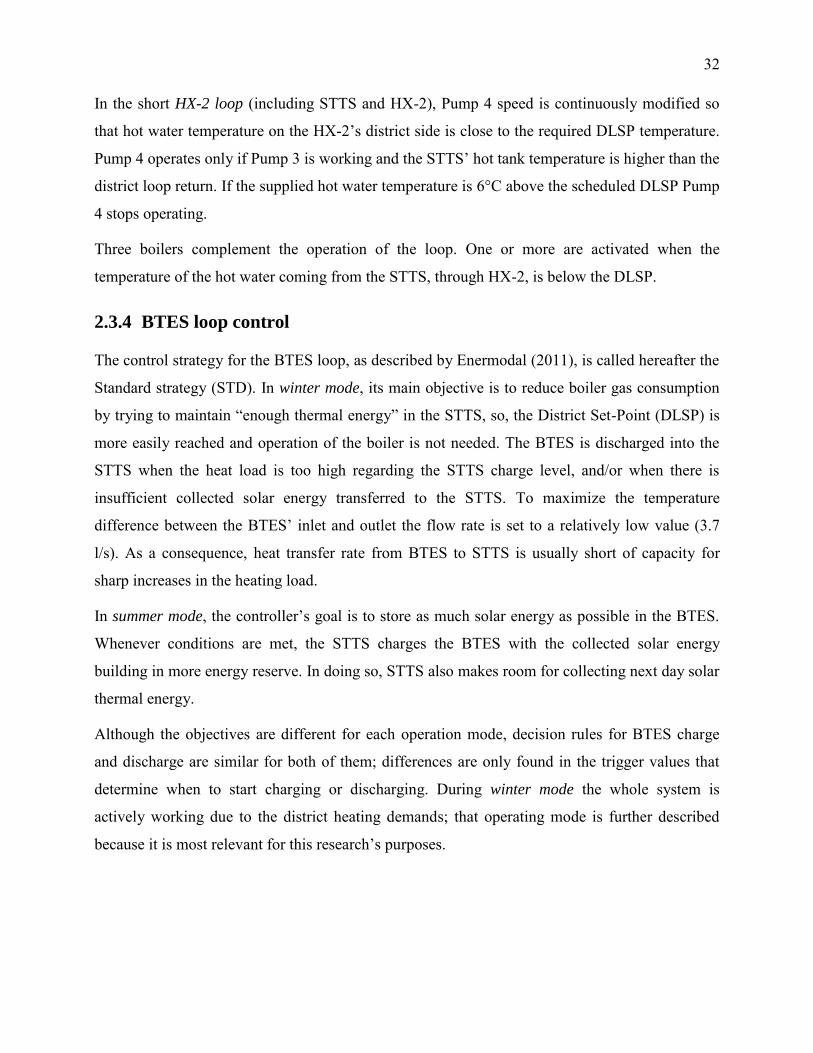
32
In the short HX-2 loop (including STTS and HX-2), Pump 4 speed is continuously modified so
that hot water temperature on the HX-2’s district side is close to the required DLSP temperature.
Pump 4 operates only if Pump 3 is working and the STTS’ hot tank temperature is higher than the
district loop return. If the supplied hot water temperature is 6°C above the scheduled DLSP Pump
4 stops operating.
Three boilers complement the operation of the loop. One or more are activated when the
temperature of the hot water coming from the STTS, through HX-2, is below the DLSP.
2.3.4 BTES loop control
The control strategy for the BTES loop, as described by Enermodal (2011), is called hereafter the
Standard strategy (STD). In winter mode, its main objective is to reduce boiler gas consumption
by trying to maintain “enough thermal energy” in the STTS, so, the District Set-Point (DLSP) is
more easily reached and operation of the boiler is not needed. The BTES is discharged into the
STTS when the heat load is too high regarding the STTS charge level, and/or when there is
insufficient collected solar energy transferred to the STTS. To maximize the temperature
difference between the BTES’ inlet and outlet the flow rate is set to a relatively low value (3.7
l/s). As a consequence, heat transfer rate from BTES to STTS is usually short of capacity for
sharp increases in the heating load.
In summer mode, the controller’s goal is to store as much solar energy as possible in the BTES.
Whenever conditions are met, the STTS charges the BTES with the collected solar energy
building in more energy reserve. In doing so, STTS also makes room for collecting next day solar
thermal energy.
Although the objectives are different for each operation mode, decision rules for BTES charge
and discharge are similar for both of them; differences are only found in the trigger values that
determine when to start charging or discharging. During winter mode the whole system is
actively working due to the district heating demands; that operating mode is further described
because it is most relevant for this research’s purposes.
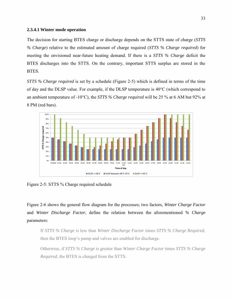
33
2.3.4.1 Winter mode operation
The decision for starting BTES charge or discharge depends on the STTS state of charge (STTS
% Charge) relative to the estimated amount of charge required (STTS % Charge required) for
meeting the envisioned near-future heating demand. If there is a STTS % Charge deficit the
BTES discharges into the STTS. On the contrary, important STTS surplus are stored in the
BTES.
STTS % Charge required is set by a schedule (Figure 2-5) which is defined in terms of the time
of day and the DLSP value. For example, if the DLSP temperature is 40°C (which correspond to
an ambient temperature of -10°C), the STTS % Charge required will be 25 % at 6 AM but 92% at
8 PM (red bars).
0%
10%
20%
30%
40%
50%
60%
70%
80%
90%
100%
0:00AM 01:00 02:00 03:00 04:00 05:00 06:00 07:00 08:00 09:00 10:00 11:00 12:00 PM
13:00 14:00 15:00 16:00 17:00 18:00 19:00 20:00 21:00 22:00 23:00
STTS
% C
har
ge r
eq
uir
ed
Time of day
DLSP <=38°C DLSP between 38°C-45°C DLSP >=45°C
Figure 2-5: STTS % Charge required schedule
Figure 2-6 shows the general flow diagram for the processes; two factors, Winter Charge Factor
and Winter Discharge Factor, define the relation between the aforementioned % Charge
parameters:
If STTS % Charge is less than Winter Discharge Factor times STTS % Charge Required,
then the BTES loop’s pump and valves are enabled for discharge.
Otherwise, if STTS % Charge is greater than Winter Charge Factor times STTS % Charge
Required, the BTES is charged from the STTS.
34
STTS_%_CHARGE < Discharge_Factor x %_CHARGE
REQUIRED
STTS_%_CHARGE > Charge_Factor x %_CHARGE
REQUIRED
BTES Discharge: Flow is from BTES’ edge to center
BTES Charge: Flow is from BTES’ center to edge
Figure 2-6: Standard Control Strategy (STD)
To be more accurate, additive factors –not shown– are also taken into account for fine tuning the
relationship between % Charge amounts. Moreover, if the rule condition that enabled the
operation is no longer true, the operation is not stopped immediately, the charge or discharge can
continue until a threshold (or tolerance) is reached. This is helpful to avoid switching off the
process-in-execution during temporary situations that may change the ratio between the %
Charge variables. An absolute condition for stopping the processes-in-execution is when BTES
input and output temperatures cause a change in the direction of the net heat transfer rate, e.g.
BTES discharge is actually removing energy from the STTS.
2.4 Summary
This concludes the general description of the case study and more importantly the control details
for each of the three main loops of the system. Some control aspects were especially highlighted
as they are directly involved when applying Model Predictive Control (MPC) methods.
The control strategy described above will be used as a reference in the following chapters, and it
will be referred to as the STD (standard) control strategy. That strategy was established by the
DLSC Design Team and refined over time using engineering judgement. The concept of “charge
required” (see section 2.3.4.1) shows that the STD control strategy does, in fact, include a simple
predictive element; it works by assuming that the temperature changes are smooth and that more
or less charge is required depending on the time of day. However, STD control has no rules
regarding the current solar irradiation or its estimated amount in the near-future.
35
CHAPTER 3 METHODOLOGY
The main steps followed during this study are presented together with the concepts that help to
explain the elements found in each phase. The discussed general steps are model calibration,
inception and design of control strategies, implementation, and evaluation of control strategies.
3.1 Model calibration
According to Rossiter (2003), “philosophically MPC reflects human behaviour whereby we
select control actions which we think will lead to the best predicted outcome (or output) over
some limited horizon. To make this selection we use an internal model of the process in question.
We constantly update our decisions as new observations become available.” In that line of
thought, a practical approach (see section 3.2.1) was followed to implement MPC while keeping
its two characteristic elements, a system model and observed disturbances.
3.1.1 Model
Traditional MPC research includes mathematical models expressed either in terms of state-space
matrixes or transfer functions; in both cases, they can be optimally solved using a broad range of
advanced algorithms to find the optimal control settings. They are the settings applied to the
system to obtain the desired response under the predicted external conditions (disturbances). In
this study, the system representation is a TRNSYS model that is not solved but rather executed;
multiple executions are needed to find the optimal control parameters that minimize a given cost
function that represents the system’s output. Working with a TRNSYS model was an advantage
given the existing in-house TRNSYS expertise and the software’s modular approach. No other
model or software was considered for simulating DLSC.
Accuracy is the most critical requirement for models employed in MPC implementations: the
better the model represents the physical system and its response to disturbances, the more reliable
will be the results. There is some terminology regularly applied to the process of achieving
desired model accuracy: calibration, validation, verification, tuning, etc. In general, calibration of
component parameters is considered as being part of a validation process where the simulation
outputs are compared with actual operation data. In the context of this dissertation, a full
validation with the meaning of demonstrating that the parameters and equations of all model
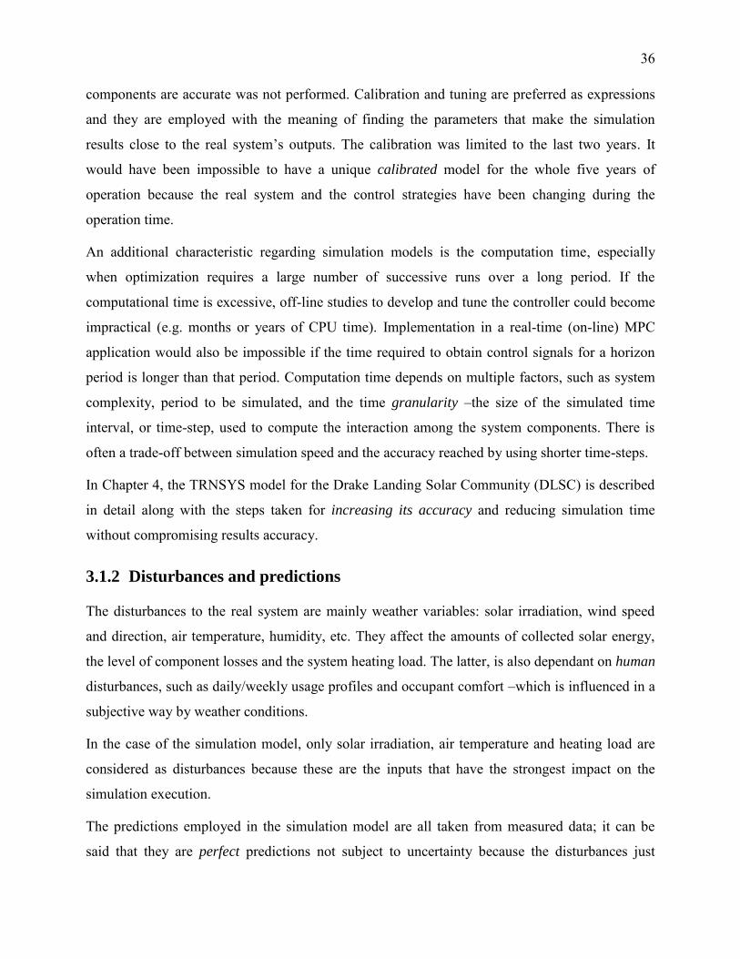
36
components are accurate was not performed. Calibration and tuning are preferred as expressions
and they are employed with the meaning of finding the parameters that make the simulation
results close to the real system’s outputs. The calibration was limited to the last two years. It
would have been impossible to have a unique calibrated model for the whole five years of
operation because the real system and the control strategies have been changing during the
operation time.
An additional characteristic regarding simulation models is the computation time, especially
when optimization requires a large number of successive runs over a long period. If the
computational time is excessive, off-line studies to develop and tune the controller could become
impractical (e.g. months or years of CPU time). Implementation in a real-time (on-line) MPC
application would also be impossible if the time required to obtain control signals for a horizon
period is longer than that period. Computation time depends on multiple factors, such as system
complexity, period to be simulated, and the time granularity –the size of the simulated time
interval, or time-step, used to compute the interaction among the system components. There is
often a trade-off between simulation speed and the accuracy reached by using shorter time-steps.
In Chapter 4, the TRNSYS model for the Drake Landing Solar Community (DLSC) is described
in detail along with the steps taken for increasing its accuracy and reducing simulation time
without compromising results accuracy.
3.1.2 Disturbances and predictions
The disturbances to the real system are mainly weather variables: solar irradiation, wind speed
and direction, air temperature, humidity, etc. They affect the amounts of collected solar energy,
the level of component losses and the system heating load. The latter, is also dependant on human
disturbances, such as daily/weekly usage profiles and occupant comfort –which is influenced in a
subjective way by weather conditions.
In the case of the simulation model, only solar irradiation, air temperature and heating load are
considered as disturbances because these are the inputs that have the strongest impact on the
simulation execution.
The predictions employed in the simulation model are all taken from measured data; it can be
said that they are perfect predictions not subject to uncertainty because the disturbances just
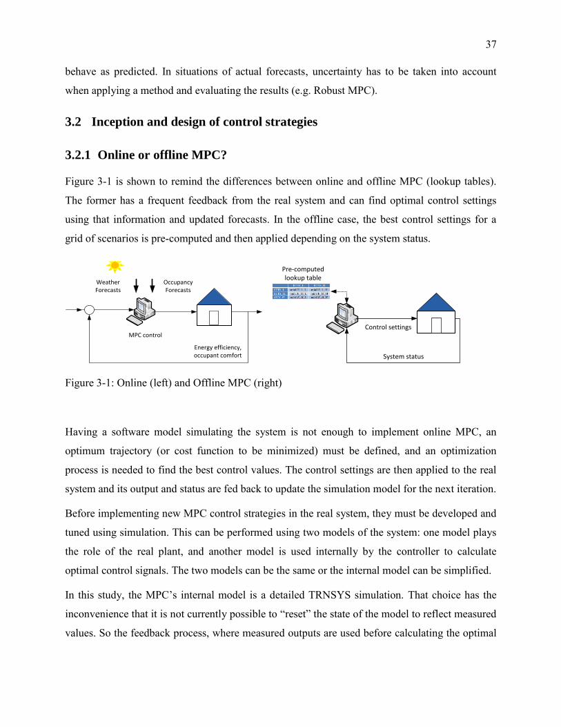
37
behave as predicted. In situations of actual forecasts, uncertainty has to be taken into account
when applying a method and evaluating the results (e.g. Robust MPC).
3.2 Inception and design of control strategies
3.2.1 Online or offline MPC?
Figure 3-1 is shown to remind the differences between online and offline MPC (lookup tables).
The former has a frequent feedback from the real system and can find optimal control settings
using that information and updated forecasts. In the offline case, the best control settings for a
grid of scenarios is pre-computed and then applied depending on the system status.
Weather Forecasts
Occupancy Forecasts
Energy efficiency, occupant comfort
MPC control
Pre-computed lookup table
System status
Control settings
Figure 3-1: Online (left) and Offline MPC (right)
Having a software model simulating the system is not enough to implement online MPC, an
optimum trajectory (or cost function to be minimized) must be defined, and an optimization
process is needed to find the best control values. The control settings are then applied to the real
system and its output and status are fed back to update the simulation model for the next iteration.
Before implementing new MPC control strategies in the real system, they must be developed and
tuned using simulation. This can be performed using two models of the system: one model plays
the role of the real plant, and another model is used internally by the controller to calculate
optimal control signals. The two models can be the same or the internal model can be simplified.
In this study, the MPC’s internal model is a detailed TRNSYS simulation. That choice has the
inconvenience that it is not currently possible to “reset” the state of the model to reflect measured
values. So the feedback process, where measured outputs are used before calculating the optimal
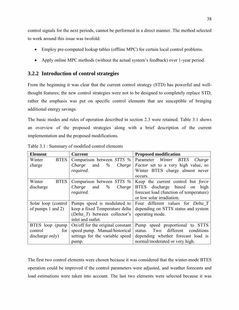
38
control signals for the next periods, cannot be performed in a direct manner. The method selected
to work around this issue was twofold:
Employ pre-computed lookup tables (offline MPC) for certain local control problems.
Apply online MPC methods (without the actual system’s feedback) over 1-year period.
3.2.2 Introduction of control strategies
From the beginning it was clear that the current control strategy (STD) has powerful and well-
thought features; the new control strategies were not to be designed to completely replace STD,
rather the emphasis was put on specific control elements that are susceptible of bringing
additional energy savings.
The basic modes and rules of operation described in section 2.3 were retained. Table 3.1 shows
an overview of the proposed strategies along with a brief description of the current
implementation and the proposed modifications.
Table 3.1 : Summary of modified control elements
Element Current Proposed modification
Winter BTES charge
Comparison between STTS %
Charge and % Charge
required.
Parameter Winter BTES Charge
Factor set to a very high value, so Winter BTES charge almost never occurs.
Winter BTES discharge
Comparison between STTS %
Charge and % Charge
required.
Keep the current control but force BTES discharge based on high forecast load (function of temperature) or low solar irradiation.
Solar loop (control of pumps 1 and 2)
Pumps speed is modulated to keep a fixed Temperature delta (Delta_T) between collector’s inlet and outlet.
Four different values for Delta_T depending on STTS status and system operating mode.
BTES loop (pump control for discharge only)
On/off for the original constant speed pump. Manual/historical settings for the variable speed pump.
Pump speed proportional to STTS status. Two different conditions depending whether forecast load is normal/moderated or very high.
The first two control elements were chosen because it was considered that the winter-mode BTES
operation could be improved if the control parameters were adjusted, and weather forecasts and
load estimations were taken into account. The last two elements were selected because it was
39
suggested by NRCan that they offered an interesting possibility of reducing electricity
consumption. The district loop control and summer-mode BTES operation were not considered in
order to limit the scope of this study, but they could also be optimized in a global approach.
Changing the district loop control parameters (e.g. supply temperature) would have implications
on the occupants comfort and would require to carefully assess these with a detailed house
model, which was not used in this study.
3.2.3 Rationale behind the selected approach
As explained before, the objective was not to replace the existing control strategy with an MPC
controller, but rather to modify the existing rule-based controller to take into account the
information provided by a detailed model and a forecast of future system behaviour. The reasons
for selecting specific control elements and the basic idea behind of each proposed control strategy
are described in the following sub-sections. Detailed implementation and results of these
alternative control strategies are presented in Chapters 5 and 6.
3.2.3.1 Winter BTES charge
This control element is included in the set of modifications because it was observed in simulation
results and the actual measured data that sometimes the BTES was unwisely charged –thus
discharging the STTS– just hours before a critical weather condition appeared: sharp temperature
changes and/or scarce solar irradiation. The ideal system response would have been leaving the
STTS accumulate more thermal energy instead of transferring it to the BTES. The proposed
solution is logical: allowing BTES charge only when a very high ratio (Winter BTES Charge
Factor) between the current STTS charge and the required charge exists. An indirect advantage
of this approach is the decrease in the pump operation with the resulting electricity savings.
3.2.3.2 (Forced) Winter BTES discharge
In this case, the motivation was similar to the BTES charge process: to keep more thermal energy
in the STTS to better cope with difficult weather conditions. The proposed solution could not be
limited to modifying the Winter BTES Discharge Factor. Frequent BTES discharges –into the
STTS– could be useless or counterproductive under mild weather conditions, because they would
use more electricity for pumping and they could lead to the STTS being unnecessarily warm,
40
therefore lowering the solar collector efficiency. The selected approach is to force the BTES
discharge whenever weather forecasts announce extreme conditions that could significantly
lessen the collected thermal energy and/or sharply increase the heating load. This decision is then
based on the predicted imbalance between the heat added to the STTS (solar energy collected)
and the heat removed from the STTS (heating load).
3.2.3.3 Solar loop
The Temperature difference parameter (Delta T), set in the loop control rules, plays an important
role in the amount of collected solar energy: low values translate into more solar energy being
collected, because the solar collector operates at a lower average temperature. But lower Delta T
values also result in higher flow rates, hence more electricity being consumed. The main reason
behind including this loop in the proposed control was to achieve electricity savings without
compromising the solar performance. As collected solar energy also depends on the STTS
stratification, it was decided to define four Delta_T values that would be selected taking into
account the STTS level of charge.
3.2.3.4 BTES loop pump control
This last element required a different control strategy due to the change of the existing BTES
pump for a variable speed pump; achieving some level of electricity savings was also in the list
of priorities. For the new control strategy, the speed of the BTES pump in discharge mode (i.e.
when transferring heat from the BTES to the STTS) was varied depending on the STTS level of
charge and the forecast load. Lower pump speeds will charge the STTS slowly, with lower
electricity consumption, and will induce a better thermal stratification in the STTS. On the other
hand, if the forecast load is high and the current energy stored in the STTS is insufficient to meet
that load, the STTS must be charged quickly to avoid using gas boilers –in that case the BTES
pump must operate at a higher speed.
3.2.4 STTS Absolute Charge Level (STTS ACL)
The discussion above shows that many control decisions are based on the STTS level of charge.
The current parameter STTS % Charge is defined in a relative way, depending on the desired
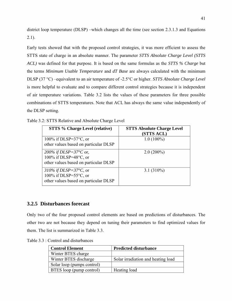
41
district loop temperature (DLSP) –which changes all the time (see section 2.3.1.3 and Equations
2.1).
Early tests showed that with the proposed control strategies, it was more efficient to assess the
STTS state of charge in an absolute manner. The parameter STTS Absolute Charge Level (STTS
ACL) was defined for that purpose. It is based on the same formulas as the STTS % Charge but
the terms Minimum Usable Temperature and dT Base are always calculated with the minimum
DLSP (37 °C) –equivalent to an air temperature of -2.5°C or higher. STTS Absolute Charge Level
is more helpful to evaluate and to compare different control strategies because it is independent
of air temperature variations. Table 3.2 lists the values of these parameters for three possible
combinations of STTS temperatures. Note that ACL has always the same value independently of
the DLSP setting.
Table 3.2: STTS Relative and Absolute Charge Level
STTS % Charge Level (relative) STTS Absolute Charge Level
(STTS ACL)
100% if DLSP=37°C, or other values based on particular DLSP
1.0 (100%)
200% if DLSP=37°C or, 100% if DLSP=48°C, or other values based on particular DLSP
2.0 (200%)
310% if DLSP=37°C, or 100% if DLSP=55°C, or other values based on particular DLSP
3.1 (310%)
3.2.5 Disturbances forecast
Only two of the four proposed control elements are based on predictions of disturbances. The
other two are not because they depend on tuning their parameters to find optimized values for
them. The list is summarized in Table 3.3.
Table 3.3 : Control and disturbances
Control Element Predicted disturbance
Winter BTES charge Winter BTES discharge Solar irradiation and heating load Solar loop (pumps control) BTES loop (pump control) Heating load
42
It can be noticed that the heating load is listed while the air temperature is not. In this study, they
are in fact equivalent because measured values at DLSC have shown that there is a very good
correlation between the heating load and the ambient temperature averaged over a certain number
of hours. A linear regression with 6-hour average is used in the original model (see Equation 4.1).
In a real implementation, both the ambient temperature and human occupancy impacts (e.g.
heating thermostat settings) would need to be anticipated. Although this work does not address
this issue, the adopted formulation would make it easier to include both aspects in one estimated
disturbance.
3.3 Implementation
The main elements for the implementation were the initial TRNSYS model and the 5-year
monitored data. In the same way TRNSYS model needed calibration, the measured data had to be
processed to eliminate inconsistencies (section 4.3.1).
Once the calibrated simulation model with the measured data was ready, it was used to test
different control strategies and to optimize system operation based on a desired output. It has
been told that the desired system’s output is equivalent to minimizing a given cost function. The
name does not necessarily imply that actual monetary costs have to be considered in the function.
For all the optimization experiences carried out in the scope of this research, cost function is
always related, but not limited, to energy consumption.
As it has been suggested, the optimization process means running multiple simulations and
comparing their results to find the combination of control parameters producing the desired
output. For each proposed control strategy, the cost function and associated optimization
conditions are described in detail in the corresponding chapter. Table 0.1 can also be consulted to
quickly identify the naming and the control parameters in each case.
3.3.1 Software
For carrying out the simulation and the optimization processes, the two main software tools
TRNSYS and GenOpt were selected. They are briefly described in the next sections.
43
3.3.1.1 TRNSYS
TRNSYS (a TRaNsient SYStems Simulation program) was designed as a generic simulation tool
for transient systems, but it is most often used to analyze buildings and energy systems in the
built environment. It belongs to the type of software known as Building energy Performance
Simulation (BPS) tools. In a TRNSYS model the various pieces of equipment, or system
components, are represented by encapsulated models known as “types”. These units can represent
physical components (solar collectors, pipes, tanks, etc.) or perform some accessory functions,
such as reading files, displaying and integrating outputs, making intermediate calculations, etc.
Each type’s outputs depend on their configuration parameters, inputs coming from other types
and internal logic representing either a physical phenomena or an intended utility for the type.
TRNSYS’ modular architecture allows to add new models, or types, to model new equipment or
to add other functionalities. Examples of TRNSYS projects, showing how components are
arranged in the visual interface (called the Simulation Studio) are shown in Chapter 4.
TRNSYS models are run to simulate the operation of a system during a specific number of hours.
Type outputs are computed every certain period of time (timestep) depending on simulated
phenomena and required level of accuracy. For each simulation timestep, multiple iterations may
be needed before reaching convergence between the calculated inputs and outputs.
3.3.1.2 GenOpt
GenOpt is a specialized optimization tool that can be integrated with any software using text files
for configuration and output results. GenOpt has built-in algorithms for dealing with different
cases of parameters optimization; the default one is a hybrid implementation that consists of two
parts: Generalized Pattern Search (GPS) method and Particle Swarm Optimization (PSO)
(Wetter, 2011). This hybrid algorithm can be applied to problems dealing with discontinuous cost
functions and continuous and discrete variables, as is the case for this research.
GenOpt tests different values for the parameters to be optimized and searches for those that
minimize the cost function. Figure 3-2 is a screenshot of GenOpt execution, for each new
simulation the values of control parameters are modified according to some initial set of
possibilities (all lines except the red one); the cost function value (red line) smoothly decreases as
the GenOpt algorithms get more accurate values for the parameters. Depending on the selected
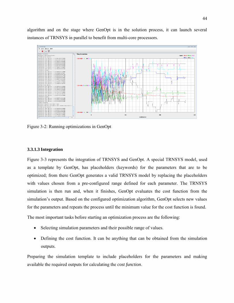
44
algorithm and on the stage where GenOpt is in the solution process, it can launch several
instances of TRNSYS in parallel to benefit from multi-core processors.
Figure 3-2: Running optimizations in GenOpt
3.3.1.3 Integration
Figure 3-3 represents the integration of TRNSYS and GenOpt. A special TRNSYS model, used
as a template by GenOpt, has placeholders (keywords) for the parameters that are to be
optimized; from there GenOpt generates a valid TRNSYS model by replacing the placeholders
with values chosen from a pre-configured range defined for each parameter. The TRNSYS
simulation is then run and, when it finishes, GenOpt evaluates the cost function from the
simulation’s output. Based on the configured optimization algorithm, GenOpt selects new values
for the parameters and repeats the process until the minimum value for the cost function is found.
The most important tasks before starting an optimization process are the following:
Selecting simulation parameters and their possible range of values.
Defining the cost function. It can be anything that can be obtained from the simulation
outputs.
Preparing the simulation template to include placeholders for the parameters and making
available the required outputs for calculating the cost function.
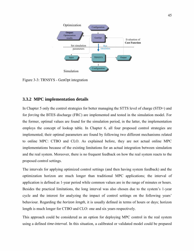
45
Output:
Optimization results
TRNSYS
GenOpt
Configuration
Configuration
Input Output
Optimization
Simulation
Run simulation
Evaluation of Cost Function
Set simulation parameters
Figure 3-3: TRNSYS - GenOpt integration
3.3.2 MPC implementation details
In Chapter 5 only the control strategies for better managing the STTS level of charge (STD+) and
for forcing the BTES discharge (FRC) are implemented and tested in the simulation model. For
the former, optimal values are found for the simulation period, in the latter, the implementation
employs the concept of lookup table. In Chapter 6, all four proposed control strategies are
implemented; their optimal parameters are found by following two different mechanisms related
to online MPC: CTBO and CLO. As explained before, they are not actual online MPC
implementations because of the existing limitations for an actual integration between simulation
and the real system. Moreover, there is no frequent feedback on how the real system reacts to the
proposed control settings.
The intervals for applying optimized control settings (and then having system feedback) and the
optimization horizon are much longer than traditional MPC applications; the interval of
application is defined as 1-year period while common values are in the range of minutes or hours.
Besides the practical limitations, the long interval was also chosen due to the system’s 1-year
cycle and the interest for analyzing the impact of control settings on the following years’
behaviour. Regarding the horizon length, it is usually defined in terms of hours or days; horizon
length is much longer for CTBO and CLO: one and six years respectively.
This approach could be considered as an option for deploying MPC control in the real system
using a defined time-interval. In this situation, a calibrated or validated model could be prepared
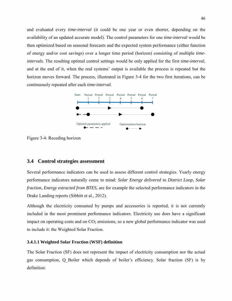
46
and evaluated every time-interval (it could be one year or even shorter, depending on the
availability of an updated accurate model). The control parameters for one time-interval would be
then optimized based on seasonal forecasts and the expected system performance (either function
of energy and/or cost savings) over a longer time period (horizon) consisting of multiple time-
intervals. The resulting optimal control settings would be only applied for the first time-interval,
and at the end of it, when the real systems’ output is available the process is repeated but the
horizon moves forward. The process, illustrated in Figure 3-4 for the two first iterations, can be
continuously repeated after each time-interval.
Start Period1
Period2
Period3
Period4
Period5
Period 6
Period 7
Optimal parameters applied Optimization horizon
Figure 3-4: Receding horizon
3.4 Control strategies assessment
Several performance indicators can be used to assess different control strategies. Yearly energy
performance indicators naturally come to mind: Solar Energy delivered to District Loop, Solar
fraction, Energy extracted from BTES, are for example the selected performance indicators in the
Drake Landing reports (Sibbitt et al., 2012).
Although the electricity consumed by pumps and accessories is reported, it is not currently
included in the most prominent performance indicators. Electricity use does have a significant
impact on operating costs and on CO2 emissions, so a new global performance indicator was used
to include it: the Weighted Solar Fraction.
3.4.1.1 Weighted Solar Fraction (WSF) definition
The Solar Fraction (SF) does not represent the impact of electricity consumption nor the actual
gas consumption, Q_Boiler which depends of boiler’s efficiency. Solar fraction (SF) is by
definition:
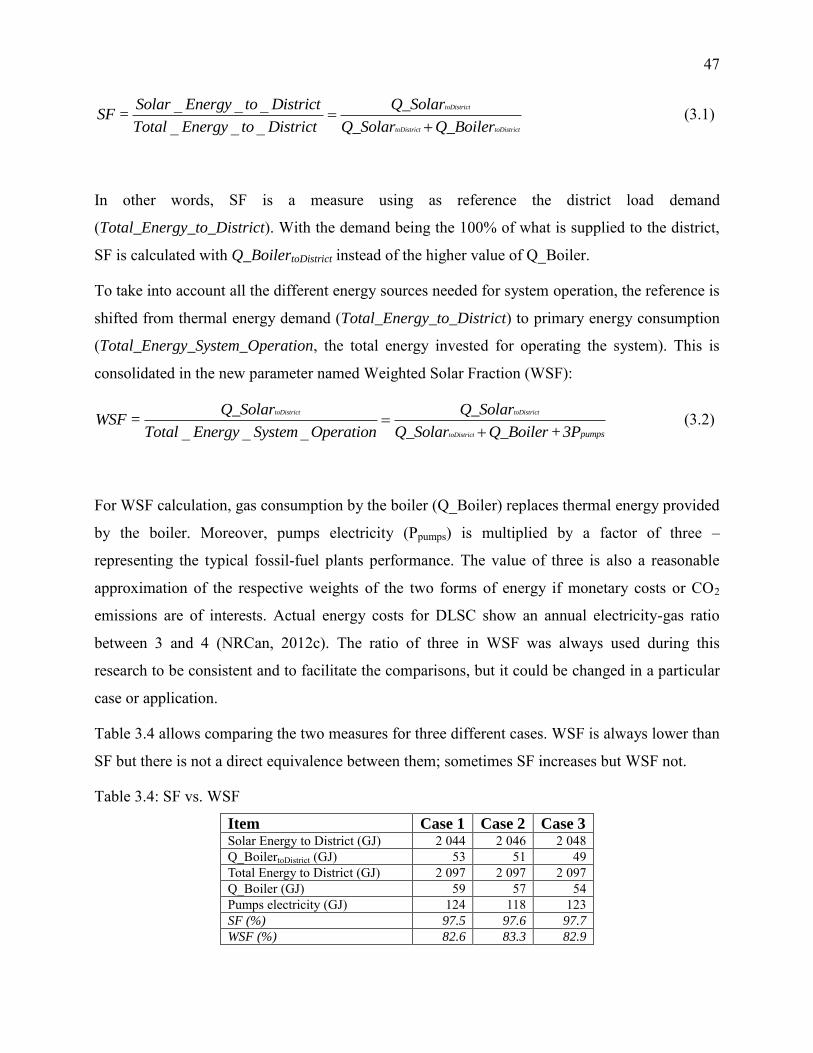
47
_ _ __ _ _
toDistrict
toDistrict toDistrict
Solar Energy to District Q_SolarSF =
Total Energy to District Q_Solar Q_Boiler
(3.1)
In other words, SF is a measure using as reference the district load demand
(Total_Energy_to_District). With the demand being the 100% of what is supplied to the district,
SF is calculated with Q_BoilertoDistrict instead of the higher value of Q_Boiler.
To take into account all the different energy sources needed for system operation, the reference is
shifted from thermal energy demand (Total_Energy_to_District) to primary energy consumption
(Total_Energy_System_Operation, the total energy invested for operating the system). This is
consolidated in the new parameter named Weighted Solar Fraction (WSF):
_ _ _toDistrict toDistrict
toDistrict pumps
Q_Solar Q_SolarWSF =
Total Energy System Operation Q_Solar Q_Boiler +3P
(3.2)
For WSF calculation, gas consumption by the boiler (Q_Boiler) replaces thermal energy provided
by the boiler. Moreover, pumps electricity (Ppumps) is multiplied by a factor of three –
representing the typical fossil-fuel plants performance. The value of three is also a reasonable
approximation of the respective weights of the two forms of energy if monetary costs or CO2
emissions are of interests. Actual energy costs for DLSC show an annual electricity-gas ratio
between 3 and 4 (NRCan, 2012c). The ratio of three in WSF was always used during this
research to be consistent and to facilitate the comparisons, but it could be changed in a particular
case or application.
Table 3.4 allows comparing the two measures for three different cases. WSF is always lower than
SF but there is not a direct equivalence between them; sometimes SF increases but WSF not.
Table 3.4: SF vs. WSF
Item Case 1 Case 2 Case 3 Solar Energy to District (GJ) 2 044 2 046 2 048 Q_BoilertoDistrict (GJ) 53 51 49 Total Energy to District (GJ) 2 097 2 097 2 097 Q_Boiler (GJ) 59 57 54 Pumps electricity (GJ) 124 118 123 SF (%) 97.5 97.6 97.7
WSF (%) 82.6 83.3 82.9
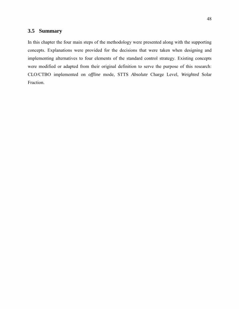
48
3.5 Summary
In this chapter the four main steps of the methodology were presented along with the supporting
concepts. Explanations were provided for the decisions that were taken when designing and
implementing alternatives to four elements of the standard control strategy. Existing concepts
were modified or adapted from their original definition to serve the purpose of this research:
CLO/CTBO implemented on offline mode, STTS Absolute Charge Level, Weighted Solar
Fraction.
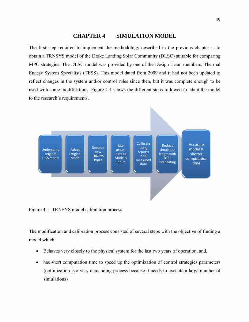
49
CHAPTER 4 SIMULATION MODEL
The first step required to implement the methodology described in the previous chapter is to
obtain a TRNSYS model of the Drake Landing Solar Community (DLSC) suitable for comparing
MPC strategies. The DLSC model was provided by one of the Design Team members, Thermal
Energy System Specialists (TESS). This model dated from 2009 and it had not been updated to
reflect changes in the system and/or control rules since then, but it was complete enough to be
used with some modifications. Figure 4-1 shows the different steps followed to adapt the model
to the research’s requirements.
Understand original
TESS model
Adapt Original Model
Develop new
TRNSYS types
Use actual data as Model’s
input
Calibrate using
reports and
measured data
Reduce simulation length with
BTES Preheating
Accurate model & shorter
computation time
Figure 4-1: TRNSYS model calibration process
The modification and calibration process consisted of several steps with the objective of finding a
model which:
Behaves very closely to the physical system for the last two years of operation, and,
has short computation time to speed up the optimization of control strategies parameters
(optimization is a very demanding process because it needs to execute a large number of
simulations)
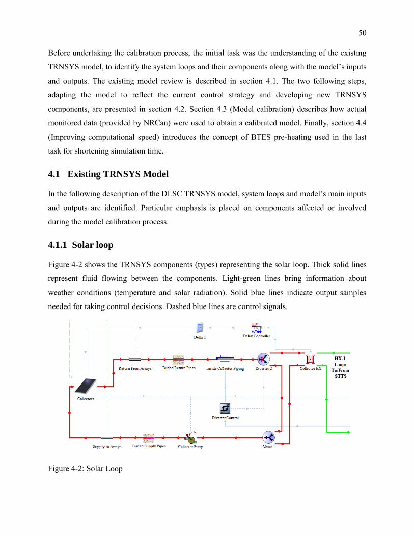
50
Before undertaking the calibration process, the initial task was the understanding of the existing
TRNSYS model, to identify the system loops and their components along with the model’s inputs
and outputs. The existing model review is described in section 4.1. The two following steps,
adapting the model to reflect the current control strategy and developing new TRNSYS
components, are presented in section 4.2. Section 4.3 (Model calibration) describes how actual
monitored data (provided by NRCan) were used to obtain a calibrated model. Finally, section 4.4
(Improving computational speed) introduces the concept of BTES pre-heating used in the last
task for shortening simulation time.
4.1 Existing TRNSYS Model
In the following description of the DLSC TRNSYS model, system loops and model’s main inputs
and outputs are identified. Particular emphasis is placed on components affected or involved
during the model calibration process.
4.1.1 Solar loop
Figure 4-2 shows the TRNSYS components (types) representing the solar loop. Thick solid lines
represent fluid flowing between the components. Light-green lines bring information about
weather conditions (temperature and solar radiation). Solid blue lines indicate output samples
needed for taking control decisions. Dashed blue lines are control signals.
Figure 4-2: Solar Loop
51
Pipes surrounded by air and buried pipes are represented by the appropriate models. Mixer,
Diverter, and Diverter Control allow switching between normal and bypass modes. The Solar
Collectors’ desired output temperature is set by a formula (Calculator icon) named Delta T; it is
the HX-1’s output temperature (solar loop side) plus the desired temperature rise (15°C in the
current control strategy). The Collectors type models the energy performance of solar collectors
but also includes the control logic for the Collector pump speed in order to maintain the desired
temperature rise. The Delay Controller prevents convergence issues by using the HX-1 outlet
temperature from the previous time step.
Last, but not least, the Heat Exchanger type links this loop with the complementary HX-1 loop
which involves the STTS.
4.1.2 District loop
As it can be seen in Figure 4-3, there are some new types in this model section: Auxiliary Boiler,
HX-2 (Heat Exchanger 2) and Imposed Heating Loads. As in the real system, the Boiler here is
only enabled when the temperature of hot water coming from STTS through HX-2 is below the
district loop set-point (DLSP). HX-2 is a type that combines the functionality of bypass and pump
speed control (Pump 4) for keeping its output at the required set-point (DLSP).
Detailed DLSC models included the four branches of homes with their pipes and individual
homes heat load (Thermal Energy Systems Specialists-TESS, 2007). The selected model is
simpler and employs the Imposed Heating Loads type to replace all the houses with an estimated
load (linear regression based on the ambient 6-hour moving average of the temperature). The
different piping loops are aggregate within a single one.
Figure 4-3: District Loop
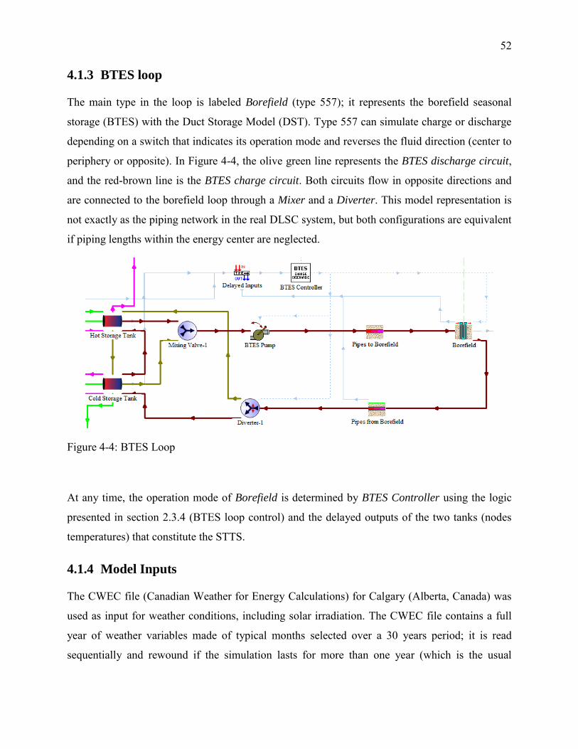
52
4.1.3 BTES loop
The main type in the loop is labeled Borefield (type 557); it represents the borefield seasonal
storage (BTES) with the Duct Storage Model (DST). Type 557 can simulate charge or discharge
depending on a switch that indicates its operation mode and reverses the fluid direction (center to
periphery or opposite). In Figure 4-4, the olive green line represents the BTES discharge circuit,
and the red-brown line is the BTES charge circuit. Both circuits flow in opposite directions and
are connected to the borefield loop through a Mixer and a Diverter. This model representation is
not exactly as the piping network in the real DLSC system, but both configurations are equivalent
if piping lengths within the energy center are neglected.
Figure 4-4: BTES Loop
At any time, the operation mode of Borefield is determined by BTES Controller using the logic
presented in section 2.3.4 (BTES loop control) and the delayed outputs of the two tanks (nodes
temperatures) that constitute the STTS.
4.1.4 Model Inputs
The CWEC file (Canadian Weather for Energy Calculations) for Calgary (Alberta, Canada) was
used as input for weather conditions, including solar irradiation. The CWEC file contains a full
year of weather variables made of typical months selected over a 30 years period; it is read
sequentially and rewound if the simulation lasts for more than one year (which is the usual
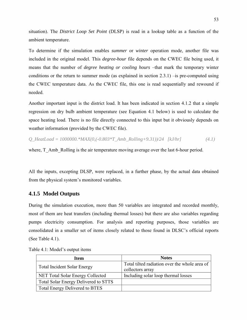
53
situation). The District Loop Set Point (DLSP) is read in a lookup table as a function of the
ambient temperature.
To determine if the simulation enables summer or winter operation mode, another file was
included in the original model. This degree-hour file depends on the CWEC file being used, it
means that the number of degree heating or cooling hours –that mark the temporary winter
conditions or the return to summer mode (as explained in section 2.3.1) –is pre-computed using
the CWEC temperature data. As the CWEC file, this one is read sequentially and rewound if
needed.
Another important input is the district load. It has been indicated in section 4.1.2 that a simple
regression on dry bulb ambient temperature (see Equation 4.1 below) is used to calculate the
space heating load. There is no file directly connected to this input but it obviously depends on
weather information (provided by the CWEC file).
Q_HeatLoad = 1000000.*MAX(0,(-0.803*T_Amb_Rolling+9.31))/24 [kJ/hr] (4.1)
where, T_Amb_Rolling is the air temperature moving average over the last 6-hour period.
All the inputs, excepting DLSP, were replaced, in a further phase, by the actual data obtained
from the physical system’s monitored variables.
4.1.5 Model Outputs
During the simulation execution, more than 50 variables are integrated and recorded monthly,
most of them are heat transfers (including thermal losses) but there are also variables regarding
pumps electricity consumption. For analysis and reporting purposes, those variables are
consolidated in a smaller set of items closely related to those found in DLSC’s official reports
(See Table 4.1).
Table 4.1: Model’s output items
Item Notes
Total Incident Solar Energy Total tilted radiation over the whole area of collectors array
NET Total Solar Energy Collected Including solar loop thermal losses Total Solar Energy Delivered to STTS Total Energy Delivered to BTES
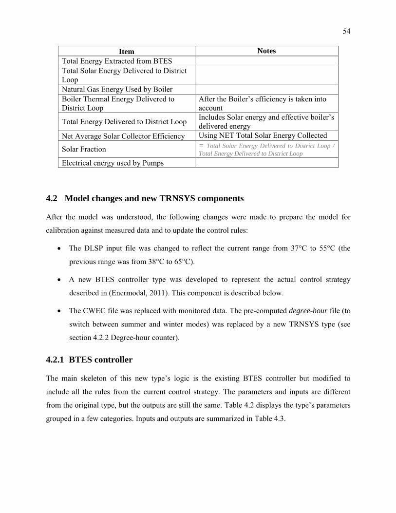
54
Item Notes
Total Energy Extracted from BTES Total Solar Energy Delivered to District Loop
Natural Gas Energy Used by Boiler Boiler Thermal Energy Delivered to District Loop
After the Boiler’s efficiency is taken into account
Total Energy Delivered to District Loop Includes Solar energy and effective boiler’s delivered energy
Net Average Solar Collector Efficiency Using NET Total Solar Energy Collected
Solar Fraction = Total Solar Energy Delivered to District Loop /
Total Energy Delivered to District Loop
Electrical energy used by Pumps
4.2 Model changes and new TRNSYS components
After the model was understood, the following changes were made to prepare the model for
calibration against measured data and to update the control rules:
The DLSP input file was changed to reflect the current range from 37°C to 55°C (the
previous range was from 38°C to 65°C).
A new BTES controller type was developed to represent the actual control strategy
described in (Enermodal, 2011). This component is described below.
The CWEC file was replaced with monitored data. The pre-computed degree-hour file (to
switch between summer and winter modes) was replaced by a new TRNSYS type (see
section 4.2.2 Degree-hour counter).
4.2.1 BTES controller
The main skeleton of this new type’s logic is the existing BTES controller but modified to
include all the rules from the current control strategy. The parameters and inputs are different
from the original type, but the outputs are still the same. Table 4.2 displays the type’s parameters
grouped in a few categories. Inputs and outputs are summarized in Table 4.3.
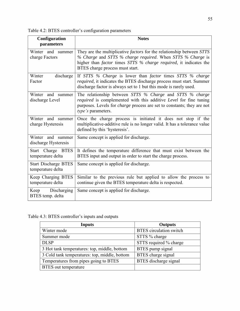
55
Table 4.2: BTES controller’s configuration parameters
Configuration
parameters
Notes
Winter and summer charge Factors
They are the multiplicative factors for the relationship between STTS
% Charge and STTS % charge required. When STTS % Charge is higher than factor times STTS % charge required, it indicates the BTES charge process must start.
Winter discharge Factor
If STTS % Charge is lower than factor times STTS % charge
required, it indicates the BTES discharge process must start. Summer discharge factor is always set to 1 but this mode is rarely used.
Winter and summer discharge Level
The relationship between STTS % Charge and STTS % charge
required is complemented with this additive Level for fine tuning purposes. Levels for charge process are set to constants; they are not type’s parameters.
Winter and summer charge Hysteresis
Once the charge process is initiated it does not stop if the multiplicative-additive rule is no longer valid. It has a tolerance value defined by this ‘hysteresis’.
Winter and summer discharge Hysteresis
Same concept is applied for discharge.
Start Charge BTES temperature delta
It defines the temperature difference that must exist between the BTES input and output in order to start the charge process.
Start Discharge BTES temperature delta
Same concept is applied for discharge.
Keep Charging BTES temperature delta
Similar to the previous rule but applied to allow the process to continue given the BTES temperature delta is respected.
Keep Discharging BTES temp. delta
Same concept is applied for discharge.
Table 4.3: BTES controller’s inputs and outputs
Inputs Outputs
Winter mode BTES circulation switch Summer mode STTS % charge DLSP STTS required % charge 3 Hot tank temperatures: top, middle, bottom BTES pump signal 3 Cold tank temperatures: top, middle, bottom BTES charge signal Temperatures from pipes going to BTES BTES discharge signal BTES out temperature
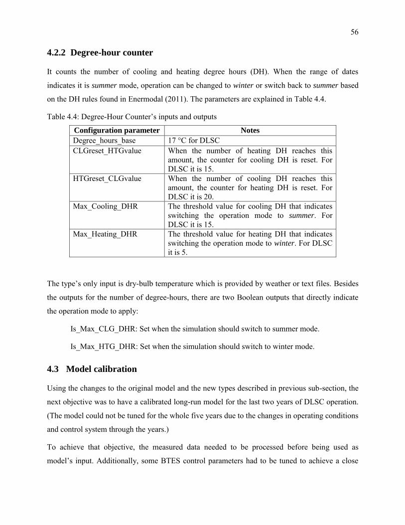
56
4.2.2 Degree-hour counter
It counts the number of cooling and heating degree hours (DH). When the range of dates
indicates it is summer mode, operation can be changed to winter or switch back to summer based
on the DH rules found in Enermodal (2011). The parameters are explained in Table 4.4.
Table 4.4: Degree-Hour Counter’s inputs and outputs
Configuration parameter Notes
Degree_hours_base 17 °C for DLSC CLGreset_HTGvalue When the number of heating DH reaches this
amount, the counter for cooling DH is reset. For DLSC it is 15.
HTGreset_CLGvalue When the number of cooling DH reaches this amount, the counter for heating DH is reset. For DLSC it is 20.
Max_Cooling_DHR The threshold value for cooling DH that indicates switching the operation mode to summer. For DLSC it is 15.
Max_Heating_DHR The threshold value for heating DH that indicates switching the operation mode to winter. For DLSC it is 5.
The type’s only input is dry-bulb temperature which is provided by weather or text files. Besides
the outputs for the number of degree-hours, there are two Boolean outputs that directly indicate
the operation mode to apply:
Is_Max_CLG_DHR: Set when the simulation should switch to summer mode.
Is_Max_HTG_DHR: Set when the simulation should switch to winter mode.
4.3 Model calibration
Using the changes to the original model and the new types described in previous sub-section, the
next objective was to have a calibrated long-run model for the last two years of DLSC operation.
(The model could not be tuned for the whole five years due to the changes in operating conditions
and control system through the years.)
To achieve that objective, the measured data needed to be processed before being used as
model’s input. Additionally, some BTES control parameters had to be tuned to achieve a close
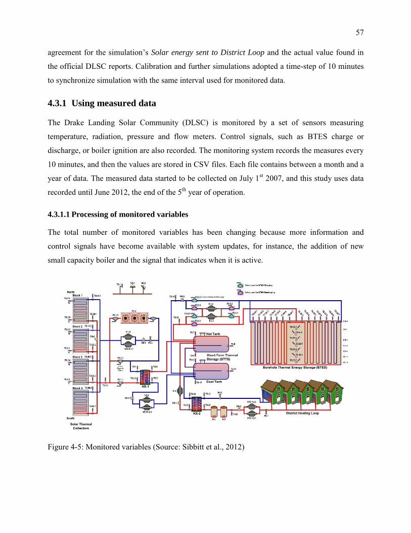
57
agreement for the simulation’s Solar energy sent to District Loop and the actual value found in
the official DLSC reports. Calibration and further simulations adopted a time-step of 10 minutes
to synchronize simulation with the same interval used for monitored data.
4.3.1 Using measured data
The Drake Landing Solar Community (DLSC) is monitored by a set of sensors measuring
temperature, radiation, pressure and flow meters. Control signals, such as BTES charge or
discharge, or boiler ignition are also recorded. The monitoring system records the measures every
10 minutes, and then the values are stored in CSV files. Each file contains between a month and a
year of data. The measured data started to be collected on July 1st 2007, and this study uses data
recorded until June 2012, the end of the 5th year of operation.
4.3.1.1 Processing of monitored variables
The total number of monitored variables has been changing because more information and
control signals have become available with system updates, for instance, the addition of new
small capacity boiler and the signal that indicates when it is active.
Figure 4-5: Monitored variables (Source: Sibbitt et al., 2012)
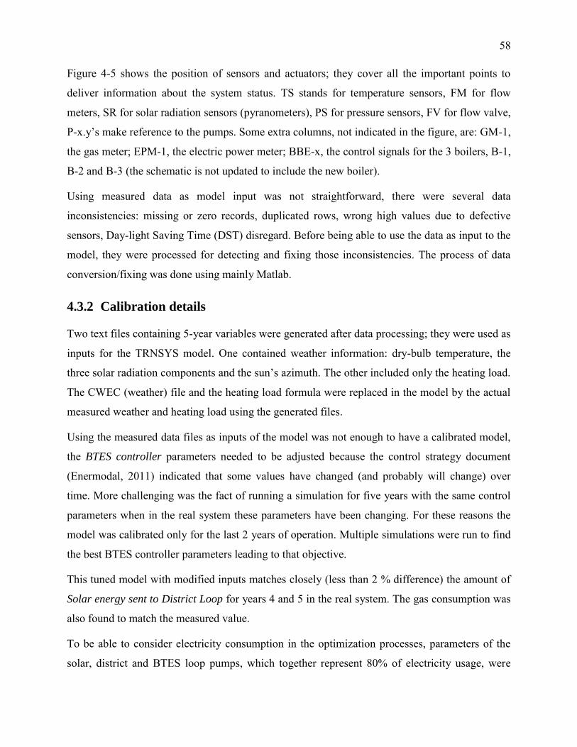
58
Figure 4-5 shows the position of sensors and actuators; they cover all the important points to
deliver information about the system status. TS stands for temperature sensors, FM for flow
meters, SR for solar radiation sensors (pyranometers), PS for pressure sensors, FV for flow valve,
P-x.y’s make reference to the pumps. Some extra columns, not indicated in the figure, are: GM-1,
the gas meter; EPM-1, the electric power meter; BBE-x, the control signals for the 3 boilers, B-1,
B-2 and B-3 (the schematic is not updated to include the new boiler).
Using measured data as model input was not straightforward, there were several data
inconsistencies: missing or zero records, duplicated rows, wrong high values due to defective
sensors, Day-light Saving Time (DST) disregard. Before being able to use the data as input to the
model, they were processed for detecting and fixing those inconsistencies. The process of data
conversion/fixing was done using mainly Matlab.
4.3.2 Calibration details
Two text files containing 5-year variables were generated after data processing; they were used as
inputs for the TRNSYS model. One contained weather information: dry-bulb temperature, the
three solar radiation components and the sun’s azimuth. The other included only the heating load.
The CWEC (weather) file and the heating load formula were replaced in the model by the actual
measured weather and heating load using the generated files.
Using the measured data files as inputs of the model was not enough to have a calibrated model,
the BTES controller parameters needed to be adjusted because the control strategy document
(Enermodal, 2011) indicated that some values have changed (and probably will change) over
time. More challenging was the fact of running a simulation for five years with the same control
parameters when in the real system these parameters have been changing. For these reasons the
model was calibrated only for the last 2 years of operation. Multiple simulations were run to find
the best BTES controller parameters leading to that objective.
This tuned model with modified inputs matches closely (less than 2 % difference) the amount of
Solar energy sent to District Loop for years 4 and 5 in the real system. The gas consumption was
also found to match the measured value.
To be able to consider electricity consumption in the optimization processes, parameters of the
solar, district and BTES loop pumps, which together represent 80% of electricity usage, were
59
also adapted. Regression curves and electricity consumption reported by NRCan (Natural
Resources Canada-NRCan, 2012a) allowed to closely match (within 5% difference) electricity
consumption.
The resulting model out of this process is called the reference long-run model because it runs
from year 1 (July 2007) until year 5 (June 2012); DLSC operating years start on July 1st and end
on next year’s June 30. Table 4.5 summarizes the variables considered for model calibration and
compares the values from official reports and those obtained after running the calibrated model.
Table 4.5: Reports vs. Calibrated model
Energy parameter (GJ)
Year 4 (July 2010-
June 2011)
Year 5 (July 2011-
June 2012)
Report Model Report Model
Solar energy delivered to District 2 456 2 489 2 048 2 028 Gas consumption 436 429 76 76 Electricity consumption 145 142 130 123 Heating load 2 859 2 875 2 120 2 097
4.4 Improving computational speed
To achieve shorter computation time a reference short-run model was needed. The concept
behind it was to start the simulation at a later time than the long-run model but still be able to
have the same output for years 4 and 5. The “pre-heating period” feature of Type 577 was used
for that purpose. When simulation starts and the pre-heating parameters are configured, the type
acts as if there were already some level of stored heat in the ground so there is no need to run the
simulation from year 1. Since the interest is in the results for years 4 and 5, the objective was to
find a pre-heating strategy that would account for the first three years of operation.
4.4.1 BTES preheating
Figure 4-6 depicts the three periods involved in BTES preheating implementation:
Skipped period. As the short-run simulation starts on January 2010, the period from July
2007 to January 2010 is not simulated (that period is indicated by the dashed line).
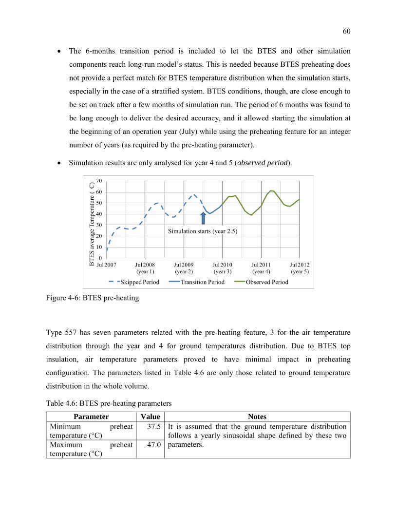
60
The 6-months transition period is included to let the BTES and other simulation
components reach long-run model’s status. This is needed because BTES preheating does
not provide a perfect match for BTES temperature distribution when the simulation starts,
especially in the case of a stratified system. BTES conditions, though, are close enough to
be set on track after a few months of simulation run. The period of 6 months was found to
be long enough to deliver the desired accuracy, and it allowed starting the simulation at
the beginning of an operation year (July) while using the preheating feature for an integer
number of years (as required by the pre-heating parameter).
Simulation results are only analysed for year 4 and 5 (observed period).
0
10
20
30
40
50
60
70
Jul 2007 Jul 2008 (year 1)
Jul 2009 (year 2)
Jul 2010 (year 3)
Jul 2011 (year 4)
Jul 2012 (year 5)
BTE
S av
erag
e Te
mpe
ratu
re (
C)
Skipped Period Transition Period Observed Period
Simulation starts (year 2.5)
Figure 4-6: BTES pre-heating
Type 557 has seven parameters related with the pre-heating feature, 3 for the air temperature
distribution through the year and 4 for ground temperatures distribution. Due to BTES top
insulation, air temperature parameters proved to have minimal impact in preheating
configuration. The parameters listed in Table 4.6 are only those related to ground temperature
distribution in the whole volume.
Table 4.6: BTES pre-heating parameters
Parameter Value Notes
Minimum preheat temperature (°C)
37.5 It is assumed that the ground temperature distribution follows a yearly sinusoidal shape defined by these two parameters. Maximum preheat
temperature (°C) 47.0
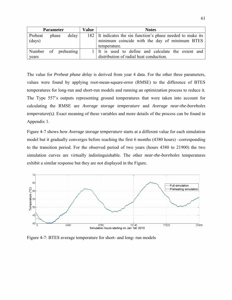
61
Parameter Value Notes
Preheat phase delay (days)
182 It indicates the sin function’s phase needed to make its minimum coincide with the day of minimum BTES temperature.
Number of preheating years
1 It is used to define and calculate the extent and distribution of radial heat conduction.
The value for Preheat phase delay is derived from year 4 data. For the other three parameters,
values were found by applying root-mean-square-error (RMSE) to the difference of BTES
temperatures for long-run and short-run models and running an optimization process to reduce it.
The Type 557’s outputs representing ground temperatures that were taken into account for
calculating the RMSE are Average storage temperature and Average near-the-boreholes
temperature(s). Exact meaning of these variables and more details of the process can be found in
Appendix 1.
Figure 4-7 shows how Average storage temperature starts at a different value for each simulation
model but it gradually converges before reaching the first 6 months (4380 hours) –corresponding
to the transition period. For the observed period of two years (hours 4380 to 21900) the two
simulation curves are virtually indistinguishable. The other near-the-boreholes temperatures
exhibit a similar response but they are not displayed in the Figure.
Figure 4-7: BTES average temperature for short- and long- run models

62
4.5 Summary
This chapter presented the modifications applied to an existing TRNSYS model to meet the
requirements of outputs accuracy and short computation time. The main four activities were
developing new types, processing actual data, calibrating the model and improving the execution
time (BTES preheating).
A calibrated model was obtained; it matches the measured energy performance at DLSC within
2% for the parameters Solar energy sent to District Loop and Gas consumption, and 5% for
electricity consumption.
A procedure was established to use Type 557 preheating feature and shorten the required
simulation length. The BTES is pre-conditioned by a (not simulated) preheating and a 6-month
(simulated) transition period. The simulation length to obtain realistic values for years 4 and 5 is
reduced from 5 years to 2.5 years, thereby saving 50% of the computational time.
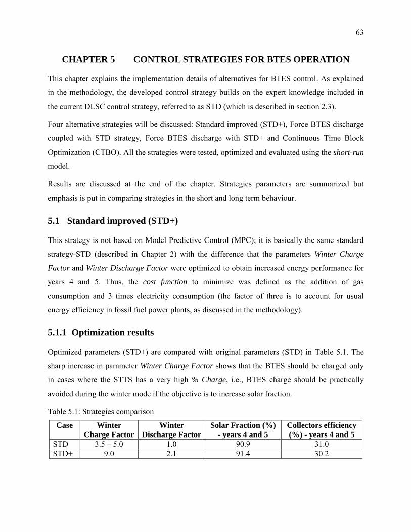
63
CHAPTER 5 CONTROL STRATEGIES FOR BTES OPERATION
This chapter explains the implementation details of alternatives for BTES control. As explained
in the methodology, the developed control strategy builds on the expert knowledge included in
the current DLSC control strategy, referred to as STD (which is described in section 2.3).
Four alternative strategies will be discussed: Standard improved (STD+), Force BTES discharge
coupled with STD strategy, Force BTES discharge with STD+ and Continuous Time Block
Optimization (CTBO). All the strategies were tested, optimized and evaluated using the short-run
model.
Results are discussed at the end of the chapter. Strategies parameters are summarized but
emphasis is put in comparing strategies in the short and long term behaviour.
5.1 Standard improved (STD+)
This strategy is not based on Model Predictive Control (MPC); it is basically the same standard
strategy-STD (described in Chapter 2) with the difference that the parameters Winter Charge
Factor and Winter Discharge Factor were optimized to obtain increased energy performance for
years 4 and 5. Thus, the cost function to minimize was defined as the addition of gas
consumption and 3 times electricity consumption (the factor of three is to account for usual
energy efficiency in fossil fuel power plants, as discussed in the methodology).
5.1.1 Optimization results
Optimized parameters (STD+) are compared with original parameters (STD) in Table 5.1. The
sharp increase in parameter Winter Charge Factor shows that the BTES should be charged only
in cases where the STTS has a very high % Charge, i.e., BTES charge should be practically
avoided during the winter mode if the objective is to increase solar fraction.
Table 5.1: Strategies comparison
Case Winter
Charge Factor
Winter
Discharge Factor
Solar Fraction (%)
- years 4 and 5
Collectors efficiency
(%) - years 4 and 5
STD 3.5 – 5.0 1.0 90.9 31.0 STD+ 9.0 2.1 91.4 30.2
64
The other parameter, Winter Discharge Factor, is more than doubled in value for STD+. What it
means is that the BTES discharge process should be started before the STTS had discharged
beyond the minimum acceptable to fulfil the expected district load (% Charge required). It is
important to highlight that the change in the factors has the indirect effect of reducing collectors’
efficiency as seen in the last column of the Table.
The STD+ parameters’ net effect is to maintain a higher STTS level of charge compared to the
STD strategy: a charge reserve is imposed for difficult weather conditions. A consequence due to
fewer charge/discharge cycles is the reduction of BTES pump electricity consumption.
5.2 Force BTES discharge coupled with STD (FRC)
5.2.1 Description
This control strategy is actually an add-on to the STD strategy; it means that STD is working all
the time except for some intervals when the FRC strategy takes over to force the BTES discharge
in anticipation of difficult weather conditions.
The mechanism is derived from manual trials that proved that, in the case of important heat load
increases, starting the BTES discharge some time ahead of the moment determined by STD
provided the STTS with higher level of charge. FRC will overwrite STD’s output when forecast
weather for the near future indicates:
Very low air temperatures, leading to an increase of the district heating load, or,
Low solar irradiation, meaning a reduction of collected thermal energy sent to the STTS.
To determine how low these values can go before forcing the discharge, representative threshold
levels are established for them. Using the thresholds, FRC strategy can be summarized as:
IF (District Load > Maximum District Load Threshold)
OR (Usable Solar Energy < Minimum Usable Solar Energy Threshold)
THEN Force BTES discharge
Usable Solar Energy is a fraction (20% in this study) of the total incident solar energy on the
collectors over the next 24-hour period. That fraction represents the reduction due to the average
65
collector performance (30%) and approximated heat losses. District Load could be estimated
using forecast temperatures.
This rule is evaluated every hour over the 24-hour forecast horizon. The value was chosen after
that manual tests with longer periods did not indicate a clear advantage in the STTS level of
charge for days of extreme weather. Shorter periods were considered in the first automatic tests;
the implementation was complicated because extra rules were needed to deal with night periods
when no sun energy is available.
The controller has a built-in check to avoid the special situation whereby forcing the BTES
discharge could provoke the reverse of heat transfer flow and mistakenly remove thermal energy
from the STTS.
The thresholds used in the rules above are the most important parameters. They are set according
to different scenarios corresponding to given sets of operating conditions, as explained in the next
section.
5.2.2 Operating scenarios for the FRC strategy
The implementation of FRC is based on the Model Predictive Control (MPC) concept of pre-
computing lookup tables for a grid of possible scenarios. It has been pointed out that to
implement this MPC method, the problem has to be decomposed into simpler problems, and the
varying conditions should be parameterized to reduce the range of values to consider. The first
requirement is considered by limiting the problem to winter mode BTES discharge only. Charge
process is much less important for increasing energy performance. External weather conditions
are parameterized using terms that convey more information: District Load and Usable Solar
Energy (both over 24 hours).
An additional parameterization is done to define the grid of scenarios in terms of STTS status
and BTES status. Using STTS Absolute Charge Level (STTS ACL), defined in section 3.2.4, three
STTS charge-related scenarios are defined:
STTS_L (low) corresponds to STTS ACL < 1
STTS_M (medium) corresponds to, 1 <= STTS ACL < 2
STTS_H (high) corresponds to STTS ACL >= 2
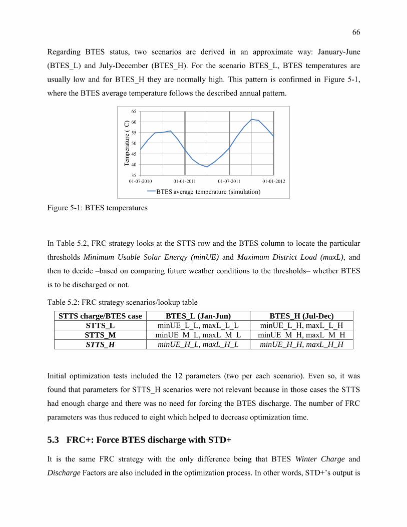
66
Regarding BTES status, two scenarios are derived in an approximate way: January-June
(BTES_L) and July-December (BTES_H). For the scenario BTES_L, BTES temperatures are
usually low and for BTES_H they are normally high. This pattern is confirmed in Figure 5-1,
where the BTES average temperature follows the described annual pattern.
35
40
45
50
55
60
65
01-07-2010 01-01-2011 01-07-2011 01-01-2012
Tem
pera
ture
( C
)
BTES average temperature (simulation)
Figure 5-1: BTES temperatures
In Table 5.2, FRC strategy looks at the STTS row and the BTES column to locate the particular
thresholds Minimum Usable Solar Energy (minUE) and Maximum District Load (maxL), and
then to decide –based on comparing future weather conditions to the thresholds– whether BTES
is to be discharged or not.
Table 5.2: FRC strategy scenarios/lookup table
STTS charge/BTES case BTES_L (Jan-Jun) BTES_H (Jul-Dec)
STTS_L minUE_L_L, maxL_L_L minUE_L_H, maxL_L_H STTS_M minUE_M_L, maxL_M_L minUE_M_H, maxL_M_H STTS_H minUE_H_L, maxL_H_L minUE_H_H, maxL_H_H
Initial optimization tests included the 12 parameters (two per each scenario). Even so, it was
found that parameters for STTS_H scenarios were not relevant because in those cases the STTS
had enough charge and there was no need for forcing the BTES discharge. The number of FRC
parameters was thus reduced to eight which helped to decrease optimization time.
5.3 FRC+: Force BTES discharge with STD+
It is the same FRC strategy with the only difference being that BTES Winter Charge and
Discharge Factors are also included in the optimization process. In other words, STD+’s output is
67
overwritten by FRC strategy’s output to discharge the BTES when conditions apply. In this way,
their best characteristics are combined, energy reserve provided by STD+ and FRC’s anticipated
BTES discharge.
5.3.1 Cost function and optimization cases
When long-term storage is considered for optimization, the period over which the cost function is
evaluated can change the results. Optimizing control parameters for a short period of time could
affect the system performance in the long-term. E.g. if the BTES is deeply discharged to reduce
the gas consumption during a short period, it would surely cause an increase in gas consumption
later on. This constraint implies that the cost function optimization period has to cover at least
one entire heating season, and possibly several years. To assess the long-term impact of FRC+,
the cost function is calculated over a three-year period –equivalent to years 4, 5 and 6 of DLSC
operation. FRC+ strategy is only applied for the first two years and in year 6 (July 2012 to July
2013) the control is switched back to the standard control strategy. As the actual year six data
were not available, two options were tried: year 6 is warm as year 5, or it is cold as year 4
(“warm” and “cold” translate into heating loads respectively lower and higher than average).
Cost function definition is the addition of gas and weighted electricity consumption for the 3-year
period. Two weight factors (W) were evaluated:
W=3, to take into account the average performance of fossil-fuel plants. This is also close
to DLSC average electricity to gas cost ratio for 2008-2010 (NRCan, 2012c)
W=8, to account for a possible (but extreme) cost ratio between electricity and gas in
Alberta.
Four optimization cases (Table 5.3) result from combining the two options for year 6 and the two
weight factors for electricity.
Table 5.3: Test cases
Electricity weight = 3 Electricity weight = 8
Year 6 is Warm 3E_W 8E_W Year 6 is Cold 3E_C 8E_C
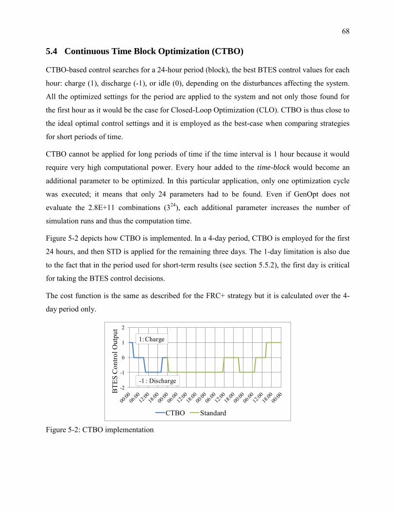
68
5.4 Continuous Time Block Optimization (CTBO)
CTBO-based control searches for a 24-hour period (block), the best BTES control values for each
hour: charge (1), discharge (-1), or idle (0), depending on the disturbances affecting the system.
All the optimized settings for the period are applied to the system and not only those found for
the first hour as it would be the case for Closed-Loop Optimization (CLO). CTBO is thus close to
the ideal optimal control settings and it is employed as the best-case when comparing strategies
for short periods of time.
CTBO cannot be applied for long periods of time if the time interval is 1 hour because it would
require very high computational power. Every hour added to the time-block would become an
additional parameter to be optimized. In this particular application, only one optimization cycle
was executed; it means that only 24 parameters had to be found. Even if GenOpt does not
evaluate the 2.8E+11 combinations (324), each additional parameter increases the number of
simulation runs and thus the computation time.
Figure 5-2 depicts how CTBO is implemented. In a 4-day period, CTBO is employed for the first
24 hours, and then STD is applied for the remaining three days. The 1-day limitation is also due
to the fact that in the period used for short-term results (see section 5.5.2), the first day is critical
for taking the BTES control decisions.
The cost function is the same as described for the FRC+ strategy but it is calculated over the 4-
day period only.
-2
-1
0
1
2
BTE
S C
ontro
l Out
put
CTBO Standard
1: Charge
-1 : Discharge
Figure 5-2: CTBO implementation
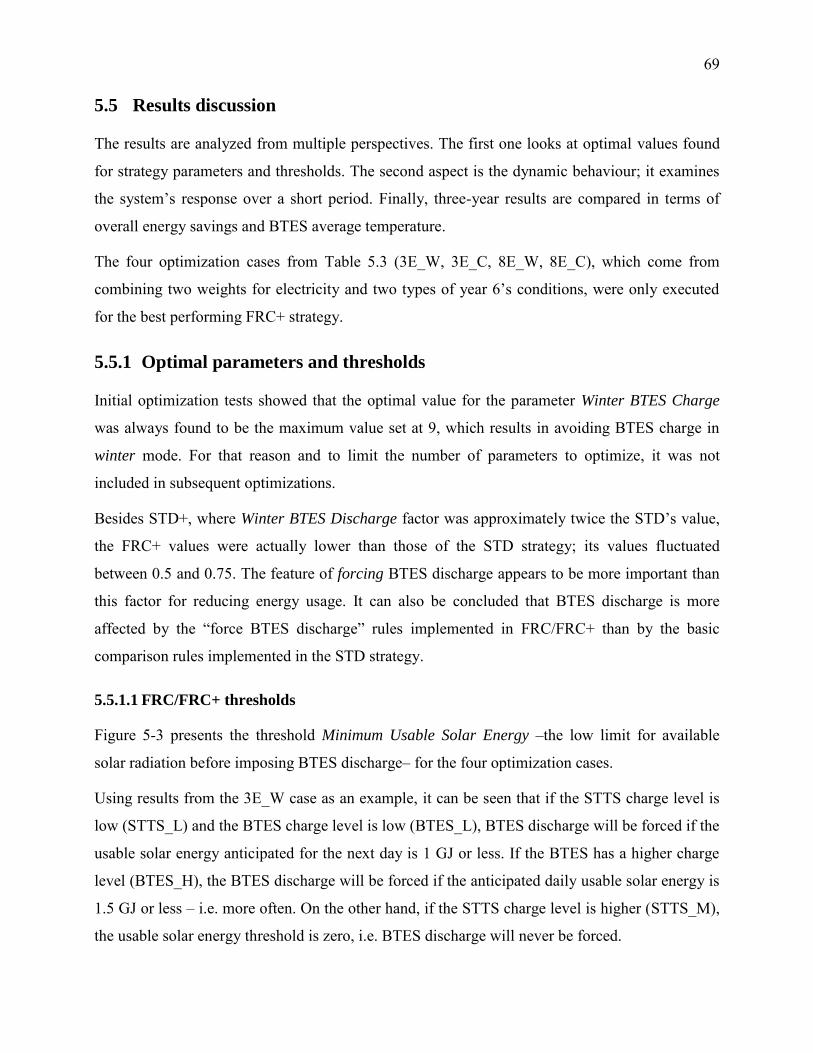
69
5.5 Results discussion
The results are analyzed from multiple perspectives. The first one looks at optimal values found
for strategy parameters and thresholds. The second aspect is the dynamic behaviour; it examines
the system’s response over a short period. Finally, three-year results are compared in terms of
overall energy savings and BTES average temperature.
The four optimization cases from Table 5.3 (3E_W, 3E_C, 8E_W, 8E_C), which come from
combining two weights for electricity and two types of year 6’s conditions, were only executed
for the best performing FRC+ strategy.
5.5.1 Optimal parameters and thresholds
Initial optimization tests showed that the optimal value for the parameter Winter BTES Charge
was always found to be the maximum value set at 9, which results in avoiding BTES charge in
winter mode. For that reason and to limit the number of parameters to optimize, it was not
included in subsequent optimizations.
Besides STD+, where Winter BTES Discharge factor was approximately twice the STD’s value,
the FRC+ values were actually lower than those of the STD strategy; its values fluctuated
between 0.5 and 0.75. The feature of forcing BTES discharge appears to be more important than
this factor for reducing energy usage. It can also be concluded that BTES discharge is more
affected by the “force BTES discharge” rules implemented in FRC/FRC+ than by the basic
comparison rules implemented in the STD strategy.
5.5.1.1 FRC/FRC+ thresholds
Figure 5-3 presents the threshold Minimum Usable Solar Energy –the low limit for available
solar radiation before imposing BTES discharge– for the four optimization cases.
Using results from the 3E_W case as an example, it can be seen that if the STTS charge level is
low (STTS_L) and the BTES charge level is low (BTES_L), BTES discharge will be forced if the
usable solar energy anticipated for the next day is 1 GJ or less. If the BTES has a higher charge
level (BTES_H), the BTES discharge will be forced if the anticipated daily usable solar energy is
1.5 GJ or less – i.e. more often. On the other hand, if the STTS charge level is higher (STTS_M),
the usable solar energy threshold is zero, i.e. BTES discharge will never be forced.
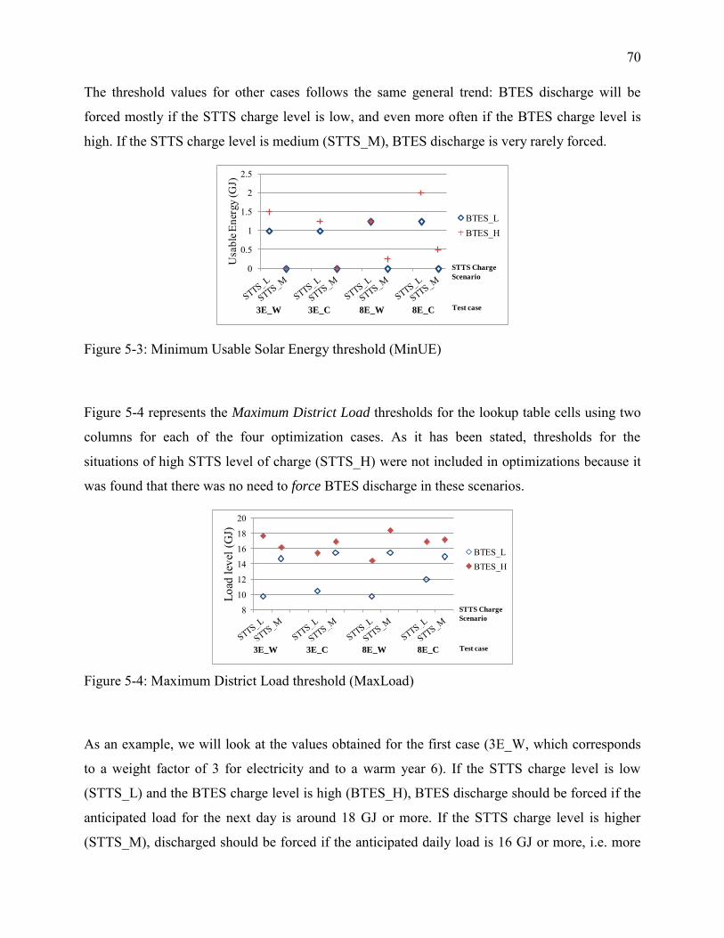
70
The threshold values for other cases follows the same general trend: BTES discharge will be
forced mostly if the STTS charge level is low, and even more often if the BTES charge level is
high. If the STTS charge level is medium (STTS_M), BTES discharge is very rarely forced.
0
0.5
1
1.5
2
2.5
Usa
ble E
nerg
y (G
J)
h
BTES_LBTES_H
3E_W 3E_C 8E_W 8E_C
STTS Charge
Scenario
Test case
Figure 5-3: Minimum Usable Solar Energy threshold (MinUE)
Figure 5-4 represents the Maximum District Load thresholds for the lookup table cells using two
columns for each of the four optimization cases. As it has been stated, thresholds for the
situations of high STTS level of charge (STTS_H) were not included in optimizations because it
was found that there was no need to force BTES discharge in these scenarios.
8
10
12
14
16
18
20
Load
leve
l (G
J)
h
BTES_LBTES_H
3E_W 3E_C 8E_W 8E_C
STTS Charge
Scenario
Test case
Figure 5-4: Maximum District Load threshold (MaxLoad)
As an example, we will look at the values obtained for the first case (3E_W, which corresponds
to a weight factor of 3 for electricity and to a warm year 6). If the STTS charge level is low
(STTS_L) and the BTES charge level is high (BTES_H), BTES discharge should be forced if the
anticipated load for the next day is around 18 GJ or more. If the STTS charge level is higher
(STTS_M), discharged should be forced if the anticipated daily load is 16 GJ or more, i.e. more
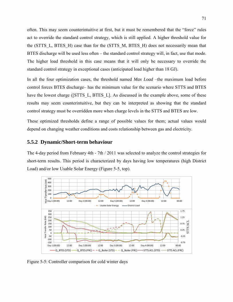
71
often. This may seem counterintuitive at first, but it must be remembered that the “force” rules
act to override the standard control strategy, which is still applied. A higher threshold value for
the (STTS_L, BTES_H) case than for the (STTS_M, BTES_H) does not necessarily mean that
BTES discharge will be used less often – the standard control strategy will, in fact, use that mode.
The higher load threshold in this case means that it will only be necessary to override the
standard control strategy in exceptional cases (anticipated load higher than 18 GJ).
In all the four optimization cases, the threshold named Max Load –the maximum load before
control forces BTES discharge– has the minimum value for the scenario where STTS and BTES
have the lowest charge ([STTS_L, BTES_L]. As discussed in the example above, some of these
results may seem counterintuitive, but they can be interpreted as showing that the standard
control strategy must be overridden more when charge levels in the STTS and BTES are low.
These optimized thresholds define a range of possible values for them; actual values would
depend on changing weather conditions and costs relationship between gas and electricity.
5.5.2 Dynamic/Short-term behaviour
The 4-day period from February 4th - 7th / 2011 was selected to analyze the control strategies for
short-term results. This period is characterized by days having low temperatures (high District
Load) and/or low Usable Solar Energy (Figure 5-5, top).
0
100
200
300
400
500
0
100
200
300
400
500
Day 1 (00:00) 12:00 Day 2 (00:00) 12:00 Day 3 (00:00) 12:00 Day 4 (00:00) 12:00 00:00
Load
He
at T
ran
sfer
Rat
e (k
W)
Usable Solar Energy District Load
-0.75
-0.25
0.25
0.75
1.25
1.75
-150
-100
-50
0
50
100
150
200
250
300
350
Day 1 (00:00) 12:00 Day 2 (00:00) 12:00 Day 3 (00:00) 12:00 Day 4 (00:00) 12:00 00:00
STTS
AC
L
Hea
t Tra
nsfe
r R
ate
(kW
)
Q_BTES (STD) Q_BTES (FRC) Q_Boiler (STD) Q_Boiler (FRC) STTS ACL (STD) STTS ACL (FRC)
Figure 5-5: Controller comparison for cold winter days
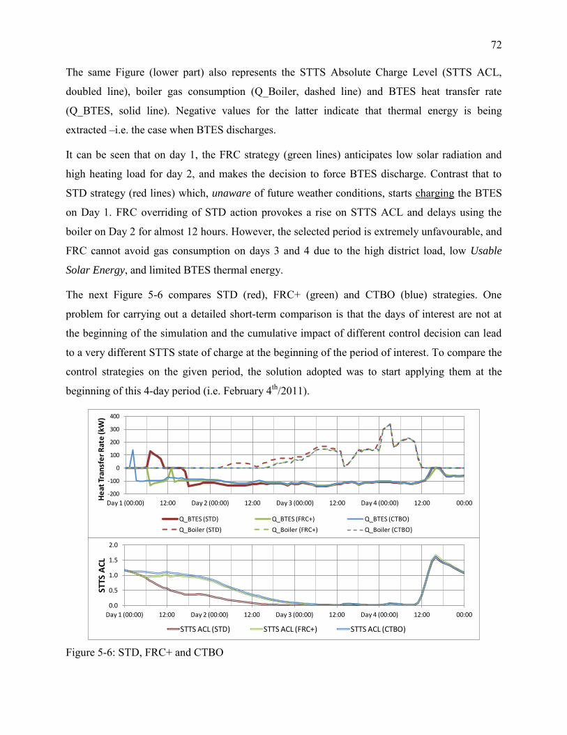
72
The same Figure (lower part) also represents the STTS Absolute Charge Level (STTS ACL,
doubled line), boiler gas consumption (Q_Boiler, dashed line) and BTES heat transfer rate
(Q_BTES, solid line). Negative values for the latter indicate that thermal energy is being
extracted –i.e. the case when BTES discharges.
It can be seen that on day 1, the FRC strategy (green lines) anticipates low solar radiation and
high heating load for day 2, and makes the decision to force BTES discharge. Contrast that to
STD strategy (red lines) which, unaware of future weather conditions, starts charging the BTES
on Day 1. FRC overriding of STD action provokes a rise on STTS ACL and delays using the
boiler on Day 2 for almost 12 hours. However, the selected period is extremely unfavourable, and
FRC cannot avoid gas consumption on days 3 and 4 due to the high district load, low Usable
Solar Energy, and limited BTES thermal energy.
The next Figure 5-6 compares STD (red), FRC+ (green) and CTBO (blue) strategies. One
problem for carrying out a detailed short-term comparison is that the days of interest are not at
the beginning of the simulation and the cumulative impact of different control decision can lead
to a very different STTS state of charge at the beginning of the period of interest. To compare the
control strategies on the given period, the solution adopted was to start applying them at the
beginning of this 4-day period (i.e. February 4th/2011).
0.0
0.5
1.0
1.5
2.0
Day 1 (00:00) 12:00 Day 2 (00:00) 12:00 Day 3 (00:00) 12:00 Day 4 (00:00) 12:00 00:00
STTS
AC
L
STTS ACL (STD) STTS ACL (FRC+) STTS ACL (CTBO)
-200
-100
0
100
200
300
400
Day 1 (00:00) 12:00 Day 2 (00:00) 12:00 Day 3 (00:00) 12:00 Day 4 (00:00) 12:00 00:00
He
at T
ran
sfe
r R
ate
(kW
)
Q_BTES (STD) Q_BTES (FRC+) Q_BTES (CTBO)
Q_Boiler (STD) Q_Boiler (FRC+) Q_Boiler (CTBO)
Figure 5-6: STD, FRC+ and CTBO
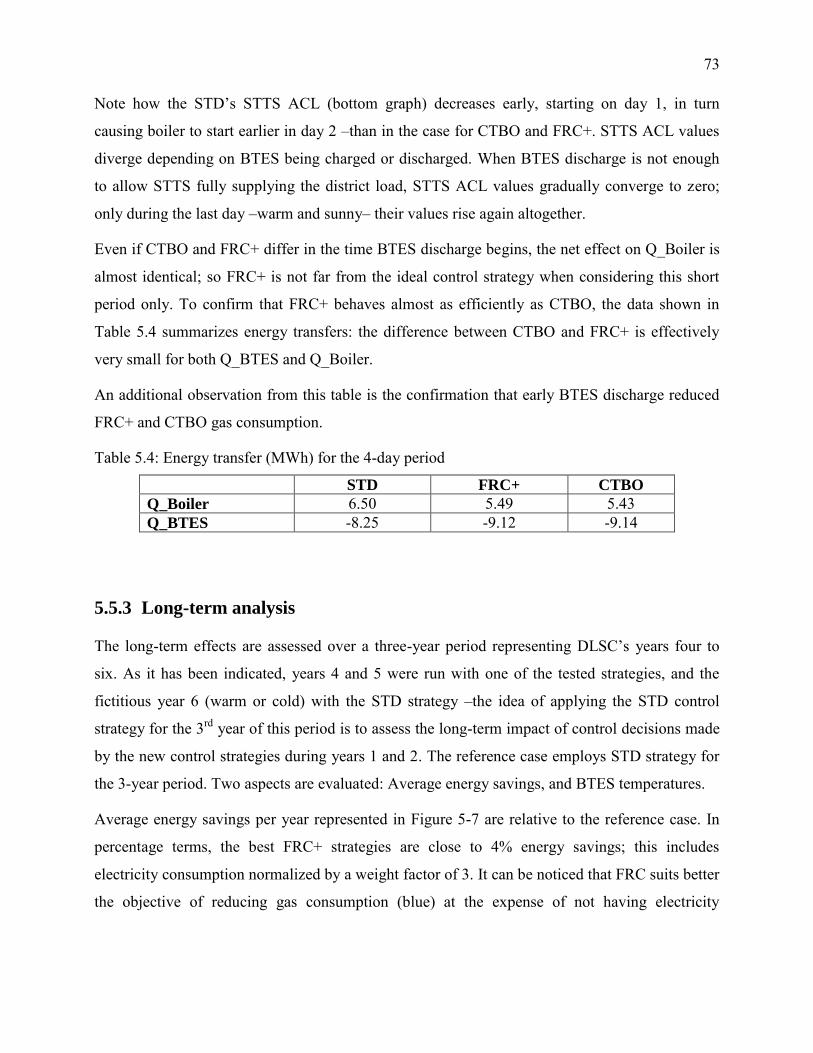
73
Note how the STD’s STTS ACL (bottom graph) decreases early, starting on day 1, in turn
causing boiler to start earlier in day 2 –than in the case for CTBO and FRC+. STTS ACL values
diverge depending on BTES being charged or discharged. When BTES discharge is not enough
to allow STTS fully supplying the district load, STTS ACL values gradually converge to zero;
only during the last day –warm and sunny– their values rise again altogether.
Even if CTBO and FRC+ differ in the time BTES discharge begins, the net effect on Q_Boiler is
almost identical; so FRC+ is not far from the ideal control strategy when considering this short
period only. To confirm that FRC+ behaves almost as efficiently as CTBO, the data shown in
Table 5.4 summarizes energy transfers: the difference between CTBO and FRC+ is effectively
very small for both Q_BTES and Q_Boiler.
An additional observation from this table is the confirmation that early BTES discharge reduced
FRC+ and CTBO gas consumption.
Table 5.4: Energy transfer (MWh) for the 4-day period
STD FRC+ CTBO
Q_Boiler 6.50 5.49 5.43 Q_BTES -8.25 -9.12 -9.14
5.5.3 Long-term analysis
The long-term effects are assessed over a three-year period representing DLSC’s years four to
six. As it has been indicated, years 4 and 5 were run with one of the tested strategies, and the
fictitious year 6 (warm or cold) with the STD strategy –the idea of applying the STD control
strategy for the 3rd year of this period is to assess the long-term impact of control decisions made
by the new control strategies during years 1 and 2. The reference case employs STD strategy for
the 3-year period. Two aspects are evaluated: Average energy savings, and BTES temperatures.
Average energy savings per year represented in Figure 5-7 are relative to the reference case. In
percentage terms, the best FRC+ strategies are close to 4% energy savings; this includes
electricity consumption normalized by a weight factor of 3. It can be noticed that FRC suits better
the objective of reducing gas consumption (blue) at the expense of not having electricity
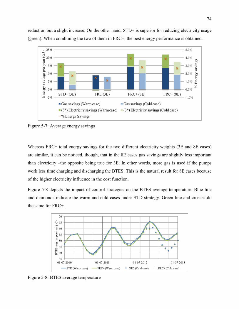
74
reduction but a slight increase. On the other hand, STD+ is superior for reducing electricity usage
(green). When combining the two of them in FRC+, the best energy performance is obtained.
-1.0%
0.0%
1.0%
2.0%
3.0%
4.0%
5.0%
-5.0
0.0
5.0
10.0
15.0
20.0
25.0
STD+ (3E) FRC (3E) FRC+ (3E) FRC+ (8E)
% E
nerg
y sa
ving
s
Ene
rgy
savi
ngs p
er y
ear (
GJ)
Gas savings (Warm case) Gas savings (Cold case)(3*) Electricity savings (Warm case) (3*) Electricity savings (Cold case)% Energy Savings
Figure 5-7: Average energy savings
Whereas FRC+ total energy savings for the two different electricity weights (3E and 8E cases)
are similar, it can be noticed, though, that in the 8E cases gas savings are slightly less important
than electricity –the opposite being true for 3E. In other words, more gas is used if the pumps
work less time charging and discharging the BTES. This is the natural result for 8E cases because
of the higher electricity influence in the cost function.
Figure 5-8 depicts the impact of control strategies on the BTES average temperature. Blue line
and diamonds indicate the warm and cold cases under STD strategy. Green line and crosses do
the same for FRC+.
35
40
45
50
55
60
65
70
01-07-2010 01-07-2011 01-07-2012 01-07-2013
BTE
S av
g te
mpe
ratu
re (
C)
STD (Warm case) FRC+ (Warm case) STD (Cold case) FRC+ (Cold case)
Figure 5-8: BTES average temperature
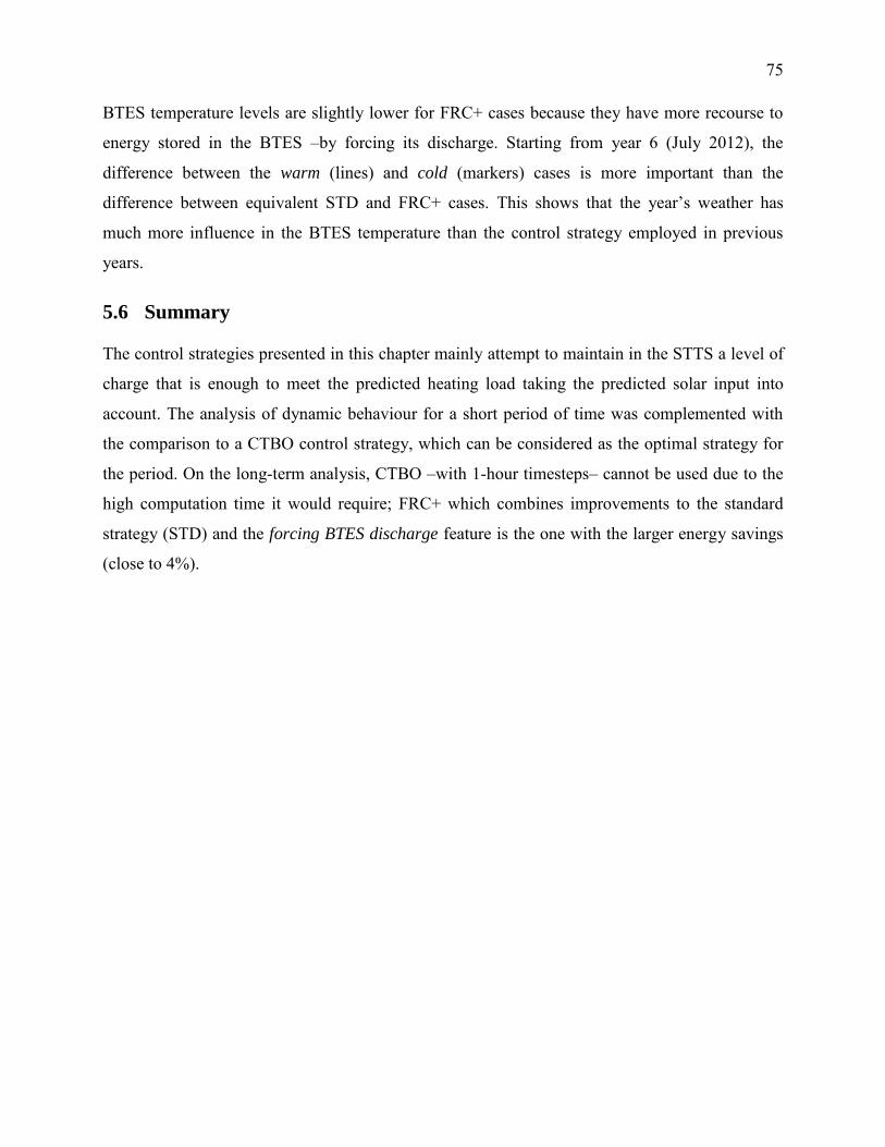
75
BTES temperature levels are slightly lower for FRC+ cases because they have more recourse to
energy stored in the BTES –by forcing its discharge. Starting from year 6 (July 2012), the
difference between the warm (lines) and cold (markers) cases is more important than the
difference between equivalent STD and FRC+ cases. This shows that the year’s weather has
much more influence in the BTES temperature than the control strategy employed in previous
years.
5.6 Summary
The control strategies presented in this chapter mainly attempt to maintain in the STTS a level of
charge that is enough to meet the predicted heating load taking the predicted solar input into
account. The analysis of dynamic behaviour for a short period of time was complemented with
the comparison to a CTBO control strategy, which can be considered as the optimal strategy for
the period. On the long-term analysis, CTBO –with 1-hour timesteps– cannot be used due to the
high computation time it would require; FRC+ which combines improvements to the standard
strategy (STD) and the forcing BTES discharge feature is the one with the larger energy savings
(close to 4%).
76
CHAPTER 6 MPC FOR INTEGRATED CONTROL STRATEGIES
This chapter presents the process and the outcome of testing and optimizing the four control
alternatives together using two MPC schemas. In the first part, the solar and the BTES loop
control are presented in detail. Next sections describe how the two MPC mechanisms, CTBO and
CLO, were applied using incremental 1-year periods. Finally, results are presented and reviewed.
6.1 Control strategy for collector loop
In the reference control strategy (Enermodal, 2011), the principal parameter for controlling this
loop is the temperature difference between the collector outlet and inlet. The pump speed is
modulated to keep the temperature difference (∆T) as close as possible to a fixed value of 15 C
for all weather conditions and STTS/BTES status. It is worth to bring again the fact that if ∆T
were above 15°C, less solar energy would be collected, because the collectors would operate at a
higher average temperature. The usability of that energy might be higher (higher temperature)
and the induced stratification in the STTS could also be improved, but the main positive impact
of a higher ∆T would be reduced electricity consumption. A ∆T value below 15°C would result
in more solar energy being collected at the cost of higher pump electricity consumption.
The proposed control strategy is based on the idea that ∆T may depend on certain system
conditions (STTS status, BTES status) and/or weather forecasts. Nevertheless, only STTS status
–by means of the parameter STTS Absolute Charge Level (STTS ACL) – was chosen due to the
inverse but clear relation between the collected solar energy and the STTS charge level: More
solar energy can be gathered when STTS is low in charge, and vice versa. If this control were to
be implemented in the real system, it would be more intuitive and easier to tune-up by system
operators than other rules depending on forecasts. So, even though a detailed model was used to
develop this control strategy, it is not an MPC strategy. It is included in this dissertation because
it is part of the overall effort to develop a practical implementation of MPC for solar
communities.
As a reminder, FRC/FRC+ strategies have three scenarios defined in terms of STTS Absolute
Charge Level: STTS_L, STTS_M and STTS_H (for low, medium and high values). For solar
collector loop control, the same three scenarios were kept but one more was added to consider the
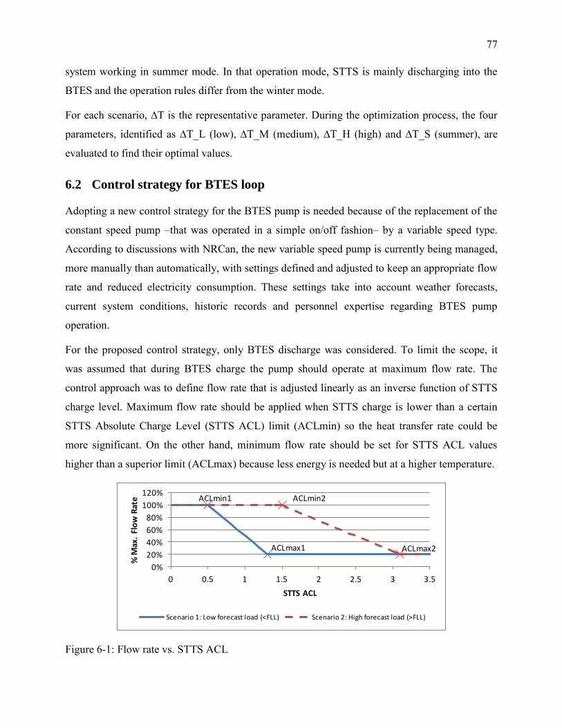
77
system working in summer mode. In that operation mode, STTS is mainly discharging into the
BTES and the operation rules differ from the winter mode.
For each scenario, ∆T is the representative parameter. During the optimization process, the four
parameters, identified as ∆T_L (low), ∆T_M (medium), ∆T_H (high) and ∆T_S (summer), are
evaluated to find their optimal values.
6.2 Control strategy for BTES loop
Adopting a new control strategy for the BTES pump is needed because of the replacement of the
constant speed pump –that was operated in a simple on/off fashion– by a variable speed type.
According to discussions with NRCan, the new variable speed pump is currently being managed,
more manually than automatically, with settings defined and adjusted to keep an appropriate flow
rate and reduced electricity consumption. These settings take into account weather forecasts,
current system conditions, historic records and personnel expertise regarding BTES pump
operation.
For the proposed control strategy, only BTES discharge was considered. To limit the scope, it
was assumed that during BTES charge the pump should operate at maximum flow rate. The
control approach was to define flow rate that is adjusted linearly as an inverse function of STTS
charge level. Maximum flow rate should be applied when STTS charge is lower than a certain
STTS Absolute Charge Level (STTS ACL) limit (ACLmin) so the heat transfer rate could be
more significant. On the other hand, minimum flow rate should be set for STTS ACL values
higher than a superior limit (ACLmax) because less energy is needed but at a higher temperature.
ACLmax1
ACLmin1 ACLmin2
ACLmax2
0%
20%
40%
60%
80%
100%
120%
0 0.5 1 1.5 2 2.5 3 3.5
% M
ax.
Flo
w R
ate
STTS ACL
Scenario 1: Low forecast load (<FLL) Scenario 2: High forecast load (>FLL)
Figure 6-1: Flow rate vs. STTS ACL

78
The predictive aspect of this strategy resides in the estimated future district load. The two
scenarios in Figure 6-1 illustrate the concept: when forecast district load over a 24-hour period is
lower than a certain amount (scenario 1), ACLmax and ACLmin are rather small because there is
no need for fast discharge; on the other hand, scenario 2 is more sensitive to high load, so it must
start increasing the flow rate even if STTS absolute level of charge (STTS ACL) is not too low.
To differentiate between the two scenarios another limit called Future Load Limit (FLL) was
defined; it indicates whether the predicted load is low or high. Depending on the optimization
process, some of the five limits (parameters) introduced for this strategy are evaluated for finding
their best values while others are just set to constant values.
6.3 Optimization and MPC
Three optimization cases are presented in the following sub-sections. The first one analyzes the
individual effect of new pump control strategies over a period including years four and five. The
second (CTBO) and third (CLO) cases combine the two pump strategies (collectors and BTES)
and FRC+ to perform incremental optimizations (year to year) in a different way.
6.3.1 Proof of concept
These optimization processes are intended to assess the impact on energy performance of pump
control strategies and validate their relevance. Besides energy considerations, the idea was also to
identify control parameters having less impact in the cost function so they could be set to
constant values and be removed from future optimizations.
To assess the two new pump control strategies separately, optimizations were run by enabling the
new control in one loop while the other loop was working with the original control strategy. The
cost function was used as always, as the sum of the gas and 3 times the electricity consumption.
Table 6.1 compiles the results. Delta T (solar loop) control exhibited reduced solar energy
collection and increased gas consumption –and thus lowered the Solar Fraction (SF) when
compared to the others; however, its overall energy performance (Weighted Solar Fraction, WSF)
is improved due to the reduction in electricity usage. On the other hand, BTES pump strategy had
an interesting behaviour: It is not as effective as STD for collecting solar energy nor does it have
a large reduction in electricity consumption as Delta T but it provided the district with the
maximum amount of solar energy of the three cases –which means higher SF and minimized gas
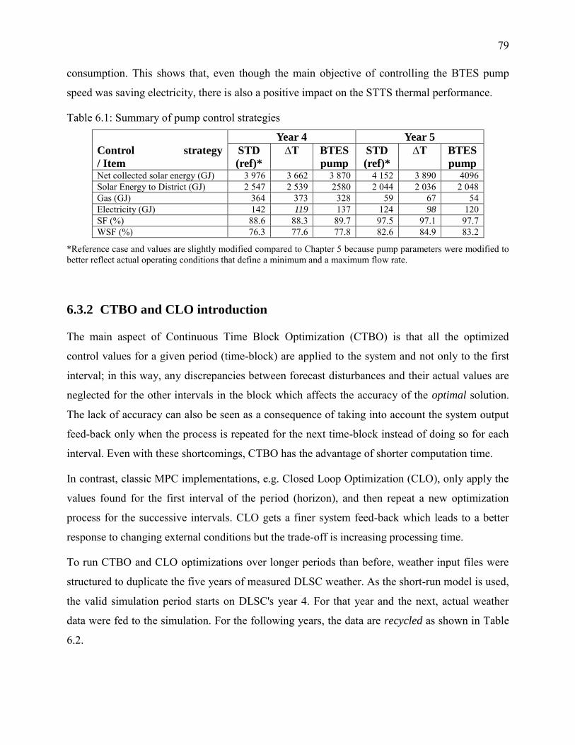
79
consumption. This shows that, even though the main objective of controlling the BTES pump
speed was saving electricity, there is also a positive impact on the STTS thermal performance.
Table 6.1: Summary of pump control strategies
Control strategy
/ Item
Year 4 Year 5
STD
(ref)*
∆T BTES
pump
STD
(ref)*
∆T BTES
pump Net collected solar energy (GJ) 3 976 3 662 3 870 4 152 3 890 4096 Solar Energy to District (GJ) 2 547 2 539 2580 2 044 2 036 2 048 Gas (GJ) 364 373 328 59 67 54 Electricity (GJ) 142 119 137 124 98 120 SF (%) 88.6 88.3 89.7 97.5 97.1 97.7 WSF (%) 76.3 77.6 77.8 82.6 84.9 83.2
*Reference case and values are slightly modified compared to Chapter 5 because pump parameters were modified to better reflect actual operating conditions that define a minimum and a maximum flow rate.
6.3.2 CTBO and CLO introduction
The main aspect of Continuous Time Block Optimization (CTBO) is that all the optimized
control values for a given period (time-block) are applied to the system and not only to the first
interval; in this way, any discrepancies between forecast disturbances and their actual values are
neglected for the other intervals in the block which affects the accuracy of the optimal solution.
The lack of accuracy can also be seen as a consequence of taking into account the system output
feed-back only when the process is repeated for the next time-block instead of doing so for each
interval. Even with these shortcomings, CTBO has the advantage of shorter computation time.
In contrast, classic MPC implementations, e.g. Closed Loop Optimization (CLO), only apply the
values found for the first interval of the period (horizon), and then repeat a new optimization
process for the successive intervals. CLO gets a finer system feed-back which leads to a better
response to changing external conditions but the trade-off is increasing processing time.
To run CTBO and CLO optimizations over longer periods than before, weather input files were
structured to duplicate the five years of measured DLSC weather. As the short-run model is used,
the valid simulation period starts on DLSC's year 4. For that year and the next, actual weather
data were fed to the simulation. For the following years, the data are recycled as shown in Table
6.2.
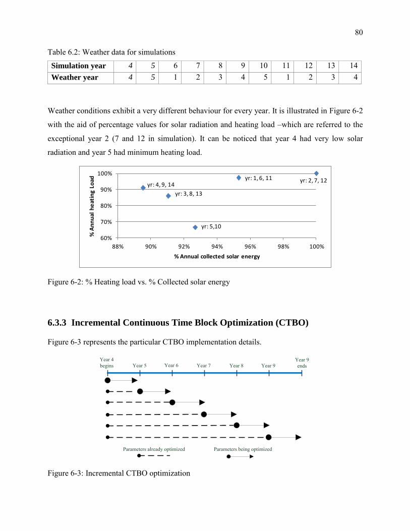
80
Table 6.2: Weather data for simulations
Simulation year 4 5 6 7 8 9 10 11 12 13 14 Weather year 4 5 1 2 3 4 5 1 2 3 4
Weather conditions exhibit a very different behaviour for every year. It is illustrated in Figure 6-2
with the aid of percentage values for solar radiation and heating load –which are referred to the
exceptional year 2 (7 and 12 in simulation). It can be noticed that year 4 had very low solar
radiation and year 5 had minimum heating load.
yr: 4, 9, 14
yr: 5,10
yr: 1, 6, 11 yr: 2, 7, 12
yr: 3, 8, 13
60%
70%
80%
90%
100%
88% 90% 92% 94% 96% 98% 100%
% A
nn
ual
he
atin
g Lo
ad
% Annual collected solar energy
Figure 6-2: % Heating load vs. % Collected solar energy
6.3.3 Incremental Continuous Time Block Optimization (CTBO)
Figure 6-3 represents the particular CTBO implementation details.
Year 4 begins Year 5 Year 6 Year 7 Year 8 Year 9
Year 9 ends
Parameters already optimized Parameters being optimized
Figure 6-3: Incremental CTBO optimization
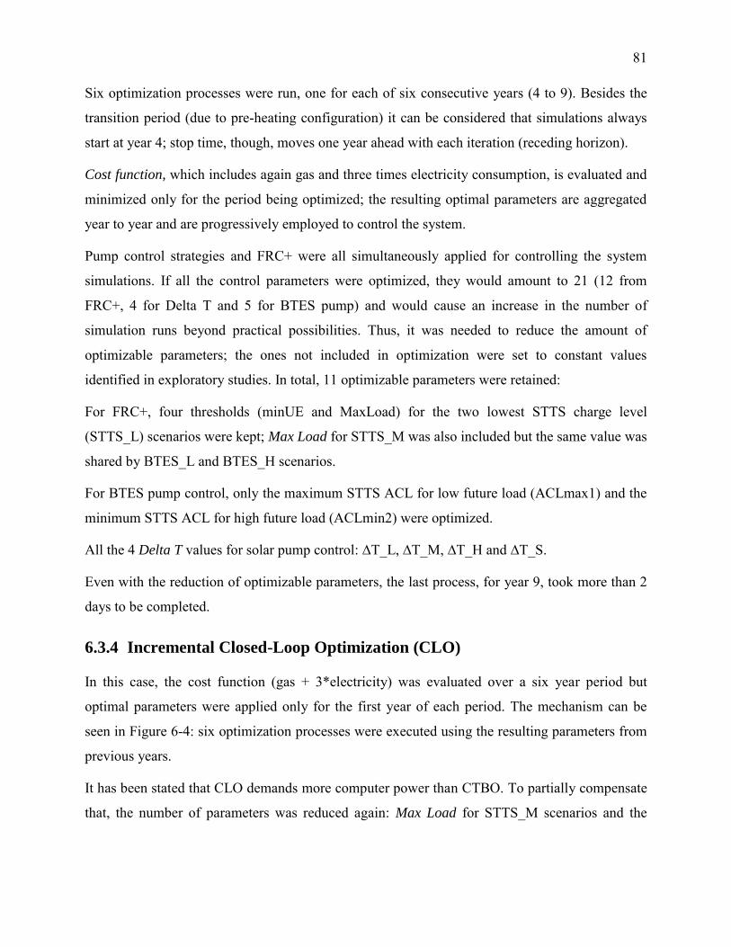
81
Six optimization processes were run, one for each of six consecutive years (4 to 9). Besides the
transition period (due to pre-heating configuration) it can be considered that simulations always
start at year 4; stop time, though, moves one year ahead with each iteration (receding horizon).
Cost function, which includes again gas and three times electricity consumption, is evaluated and
minimized only for the period being optimized; the resulting optimal parameters are aggregated
year to year and are progressively employed to control the system.
Pump control strategies and FRC+ were all simultaneously applied for controlling the system
simulations. If all the control parameters were optimized, they would amount to 21 (12 from
FRC+, 4 for Delta T and 5 for BTES pump) and would cause an increase in the number of
simulation runs beyond practical possibilities. Thus, it was needed to reduce the amount of
optimizable parameters; the ones not included in optimization were set to constant values
identified in exploratory studies. In total, 11 optimizable parameters were retained:
For FRC+, four thresholds (minUE and MaxLoad) for the two lowest STTS charge level
(STTS_L) scenarios were kept; Max Load for STTS_M was also included but the same value was
shared by BTES_L and BTES_H scenarios.
For BTES pump control, only the maximum STTS ACL for low future load (ACLmax1) and the
minimum STTS ACL for high future load (ACLmin2) were optimized.
All the 4 Delta T values for solar pump control: ∆T_L, ∆T_M, ∆T_H and ∆T_S.
Even with the reduction of optimizable parameters, the last process, for year 9, took more than 2
days to be completed.
6.3.4 Incremental Closed-Loop Optimization (CLO)
In this case, the cost function (gas + 3*electricity) was evaluated over a six year period but
optimal parameters were applied only for the first year of each period. The mechanism can be
seen in Figure 6-4: six optimization processes were executed using the resulting parameters from
previous years.
It has been stated that CLO demands more computer power than CTBO. To partially compensate
that, the number of parameters was reduced again: Max Load for STTS_M scenarios and the
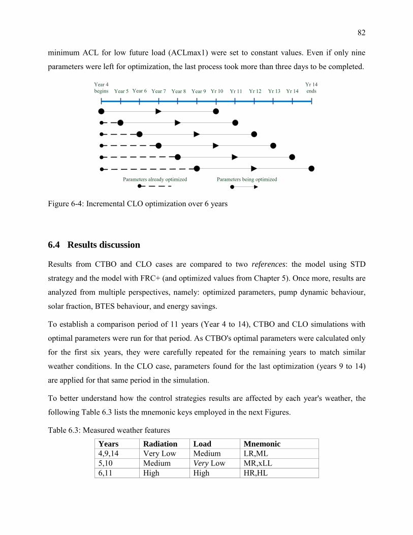
82
minimum ACL for low future load (ACLmax1) were set to constant values. Even if only nine
parameters were left for optimization, the last process took more than three days to be completed.
Year 4 begins Year 5 Year 6 Year 7 Year 8 Year 9 Yr 10 Yr 11 Yr 12 Yr 13 Yr 14
Parameters already optimized Parameters being optimized
Yr 14 ends
Figure 6-4: Incremental CLO optimization over 6 years
6.4 Results discussion
Results from CTBO and CLO cases are compared to two references: the model using STD
strategy and the model with FRC+ (and optimized values from Chapter 5). Once more, results are
analyzed from multiple perspectives, namely: optimized parameters, pump dynamic behaviour,
solar fraction, BTES behaviour, and energy savings.
To establish a comparison period of 11 years (Year 4 to 14), CTBO and CLO simulations with
optimal parameters were run for that period. As CTBO's optimal parameters were calculated only
for the first six years, they were carefully repeated for the remaining years to match similar
weather conditions. In the CLO case, parameters found for the last optimization (years 9 to 14)
are applied for that same period in the simulation.
To better understand how the control strategies results are affected by each year's weather, the
following Table 6.3 lists the mnemonic keys employed in the next Figures.
Table 6.3: Measured weather features
Years Radiation Load Mnemonic
4,9,14 Very Low Medium LR,ML 5,10 Medium Very Low MR,xLL 6,11 High High HR,HL
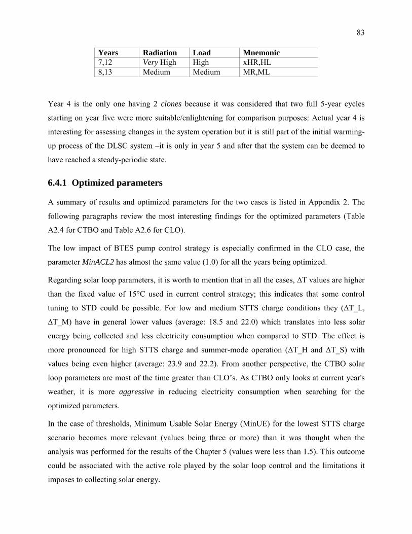
83
Years Radiation Load Mnemonic
7,12 Very High High xHR,HL 8,13 Medium Medium MR,ML
Year 4 is the only one having 2 clones because it was considered that two full 5-year cycles
starting on year five were more suitable/enlightening for comparison purposes: Actual year 4 is
interesting for assessing changes in the system operation but it is still part of the initial warming-
up process of the DLSC system –it is only in year 5 and after that the system can be deemed to
have reached a steady-periodic state.
6.4.1 Optimized parameters
A summary of results and optimized parameters for the two cases is listed in Appendix 2. The
following paragraphs review the most interesting findings for the optimized parameters (Table
A2.4 for CTBO and Table A2.6 for CLO).
The low impact of BTES pump control strategy is especially confirmed in the CLO case, the
parameter MinACL2 has almost the same value (1.0) for all the years being optimized.
Regarding solar loop parameters, it is worth to mention that in all the cases, ∆T values are higher
than the fixed value of 15°C used in current control strategy; this indicates that some control
tuning to STD could be possible. For low and medium STTS charge conditions they (∆T_L,
∆T_M) have in general lower values (average: 18.5 and 22.0) which translates into less solar
energy being collected and less electricity consumption when compared to STD. The effect is
more pronounced for high STTS charge and summer-mode operation (∆T_H and ∆T_S) with
values being even higher (average: 23.9 and 22.2). From another perspective, the CTBO solar
loop parameters are most of the time greater than CLO’s. As CTBO only looks at current year's
weather, it is more aggressive in reducing electricity consumption when searching for the
optimized parameters.
In the case of thresholds, Minimum Usable Solar Energy (MinUE) for the lowest STTS charge
scenario becomes more relevant (values being three or more) than it was thought when the
analysis was performed for the results of the Chapter 5 (values were less than 1.5). This outcome
could be associated with the active role played by the solar loop control and the limitations it
imposes to collecting solar energy.
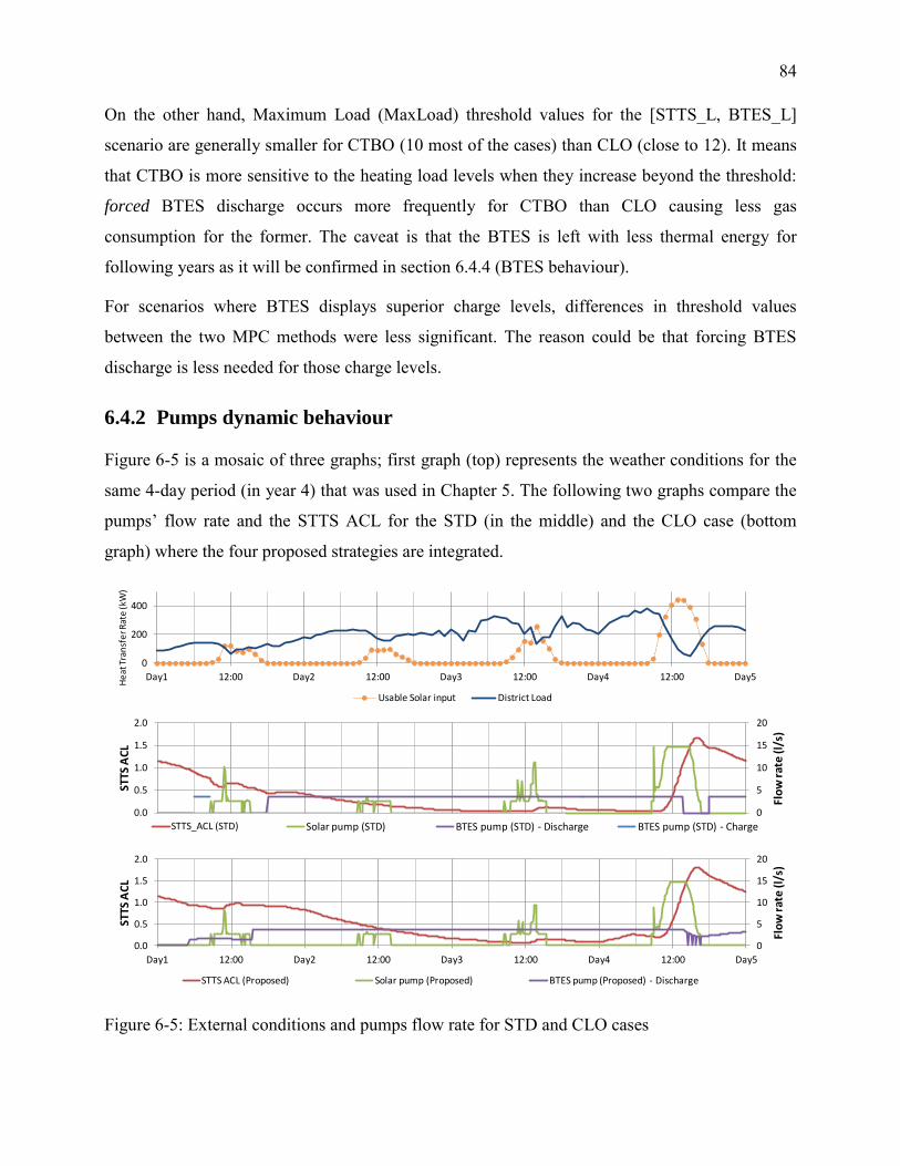
84
On the other hand, Maximum Load (MaxLoad) threshold values for the [STTS_L, BTES_L]
scenario are generally smaller for CTBO (10 most of the cases) than CLO (close to 12). It means
that CTBO is more sensitive to the heating load levels when they increase beyond the threshold:
forced BTES discharge occurs more frequently for CTBO than CLO causing less gas
consumption for the former. The caveat is that the BTES is left with less thermal energy for
following years as it will be confirmed in section 6.4.4 (BTES behaviour).
For scenarios where BTES displays superior charge levels, differences in threshold values
between the two MPC methods were less significant. The reason could be that forcing BTES
discharge is less needed for those charge levels.
6.4.2 Pumps dynamic behaviour
Figure 6-5 is a mosaic of three graphs; first graph (top) represents the weather conditions for the
same 4-day period (in year 4) that was used in Chapter 5. The following two graphs compare the
pumps’ flow rate and the STTS ACL for the STD (in the middle) and the CLO case (bottom
graph) where the four proposed strategies are integrated.
0
5
10
15
20
0.0
0.5
1.0
1.5
2.0
Flo
w r
ate
(l/s
)
STTS
AC
L
STTS_ACL (STD) Solar pump (STD) BTES pump (STD) - Discharge BTES pump (STD) - Charge
0
100
200
300
400
500
0
200
400
Day1 12:00 Day2 12:00 Day3 12:00 Day4 12:00 Day5
Load
He
at T
ran
sfe
r Rat
e (k
W)
Usable Solar input District Load
0
5
10
15
20
0.0
0.5
1.0
1.5
2.0
Day1 12:00 Day2 12:00 Day3 12:00 Day4 12:00 Day5
Flo
w r
ate
(l/s
)
STTS
AC
L
STTS ACL (Proposed) Solar pump (Proposed) BTES pump (Proposed) - Discharge
Figure 6-5: External conditions and pumps flow rate for STD and CLO cases
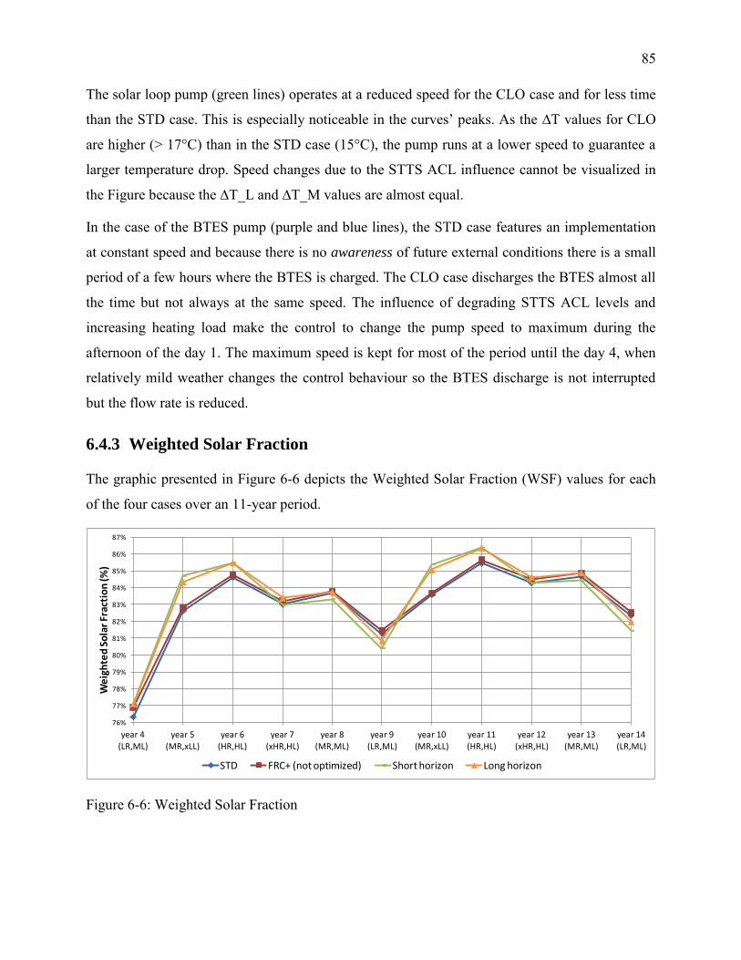
85
The solar loop pump (green lines) operates at a reduced speed for the CLO case and for less time
than the STD case. This is especially noticeable in the curves’ peaks. As the ∆T values for CLO
are higher (> 17°C) than in the STD case (15°C), the pump runs at a lower speed to guarantee a
larger temperature drop. Speed changes due to the STTS ACL influence cannot be visualized in
the Figure because the ∆T_L and ∆T_M values are almost equal.
In the case of the BTES pump (purple and blue lines), the STD case features an implementation
at constant speed and because there is no awareness of future external conditions there is a small
period of a few hours where the BTES is charged. The CLO case discharges the BTES almost all
the time but not always at the same speed. The influence of degrading STTS ACL levels and
increasing heating load make the control to change the pump speed to maximum during the
afternoon of the day 1. The maximum speed is kept for most of the period until the day 4, when
relatively mild weather changes the control behaviour so the BTES discharge is not interrupted
but the flow rate is reduced.
6.4.3 Weighted Solar Fraction
The graphic presented in Figure 6-6 depicts the Weighted Solar Fraction (WSF) values for each
of the four cases over an 11-year period.
76%
77%
78%
79%
80%
81%
82%
83%
84%
85%
86%
87%
year 4 (LR,ML)
year 5 (MR,xLL)
year 6 (HR,HL)
year 7 (xHR,HL)
year 8 (MR,ML)
year 9 (LR,ML)
year 10 (MR,xLL)
year 11 (HR,HL)
year 12 (xHR,HL)
year 13 (MR,ML)
year 14 (LR,ML)
We
igh
ted
So
lar
Frac
tio
n (%
)
STD FRC+ (not optimized) Short horizon Long horizon
Figure 6-6: Weighted Solar Fraction
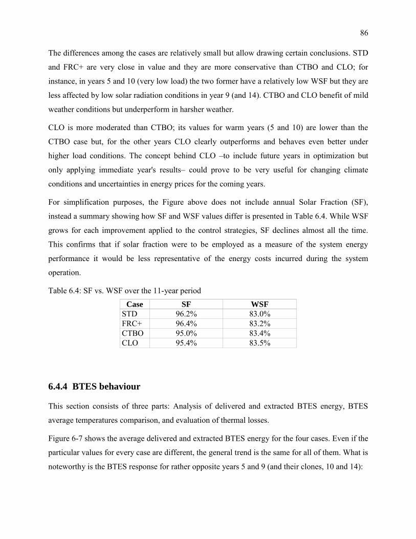
86
The differences among the cases are relatively small but allow drawing certain conclusions. STD
and FRC+ are very close in value and they are more conservative than CTBO and CLO; for
instance, in years 5 and 10 (very low load) the two former have a relatively low WSF but they are
less affected by low solar radiation conditions in year 9 (and 14). CTBO and CLO benefit of mild
weather conditions but underperform in harsher weather.
CLO is more moderated than CTBO; its values for warm years (5 and 10) are lower than the
CTBO case but, for the other years CLO clearly outperforms and behaves even better under
higher load conditions. The concept behind CLO –to include future years in optimization but
only applying immediate year's results– could prove to be very useful for changing climate
conditions and uncertainties in energy prices for the coming years.
For simplification purposes, the Figure above does not include annual Solar Fraction (SF),
instead a summary showing how SF and WSF values differ is presented in Table 6.4. While WSF
grows for each improvement applied to the control strategies, SF declines almost all the time.
This confirms that if solar fraction were to be employed as a measure of the system energy
performance it would be less representative of the energy costs incurred during the system
operation.
Table 6.4: SF vs. WSF over the 11-year period
Case SF WSF
STD 96.2% 83.0% FRC+ 96.4% 83.2% CTBO 95.0% 83.4% CLO 95.4% 83.5%
6.4.4 BTES behaviour
This section consists of three parts: Analysis of delivered and extracted BTES energy, BTES
average temperatures comparison, and evaluation of thermal losses.
Figure 6-7 shows the average delivered and extracted BTES energy for the four cases. Even if the
particular values for every case are different, the general trend is the same for all of them. What is
noteworthy is the BTES response for rather opposite years 5 and 9 (and their clones, 10 and 14):
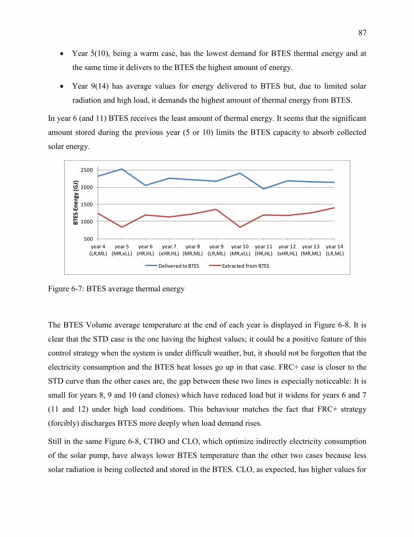
87
Year 5(10), being a warm case, has the lowest demand for BTES thermal energy and at
the same time it delivers to the BTES the highest amount of energy.
Year 9(14) has average values for energy delivered to BTES but, due to limited solar
radiation and high load, it demands the highest amount of thermal energy from BTES.
In year 6 (and 11) BTES receives the least amount of thermal energy. It seems that the significant
amount stored during the previous year (5 or 10) limits the BTES capacity to absorb collected
solar energy.
500
1000
1500
2000
2500
year 4 (LR,ML)
year 5 (MR,xLL)
year 6 (HR,HL)
year 7 (xHR,HL)
year 8 (MR,ML)
year 9 (LR,ML)
year 10 (MR,xLL)
year 11 (HR,HL)
year 12 (xHR,HL)
year 13 (MR,ML)
year 14 (LR,ML)
BTE
S En
erg
y (G
J)
Delivered to BTES Extracted from BTES
Figure 6-7: BTES average thermal energy
The BTES Volume average temperature at the end of each year is displayed in Figure 6-8. It is
clear that the STD case is the one having the highest values; it could be a positive feature of this
control strategy when the system is under difficult weather, but, it should not be forgotten that the
electricity consumption and the BTES heat losses go up in that case. FRC+ case is closer to the
STD curve than the other cases are, the gap between these two lines is especially noticeable: It is
small for years 8, 9 and 10 (and clones) which have reduced load but it widens for years 6 and 7
(11 and 12) under high load conditions. This behaviour matches the fact that FRC+ strategy
(forcibly) discharges BTES more deeply when load demand rises.
Still in the same Figure 6-8, CTBO and CLO, which optimize indirectly electricity consumption
of the solar pump, have always lower BTES temperature than the other two cases because less
solar radiation is being collected and stored in the BTES. CLO, as expected, has higher values for
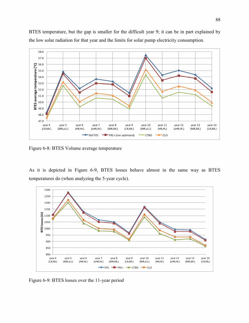
88
BTES temperature, but the gap is smaller for the difficult year 9; it can be in part explained by
the low solar radiation for that year and the limits for solar pump electricity consumption.
47.0
48.0
49.0
50.0
51.0
52.0
53.0
54.0
55.0
56.0
57.0
58.0
year 4 (LR,ML)
year 5 (MR,xLL)
year 6 (HR,HL)
year 7 (xHR,HL)
year 8 (MR,ML)
year 9 (LR,ML)
year 10 (MR,xLL)
year 11 (HR,HL)
year 12 (xHR,HL)
year 13 (MR,ML)
year 14 (LR,ML)
BT
ES
av
era
ge
te
mp
era
ture
(°C
)
Ref STD FRC+ (not optimized) CTBO CLO
Figure 6-8: BTES Volume average temperature
As it is depicted in Figure 6-9, BTES losses behave almost in the same way as BTES
temperatures do (when analyzing the 5-year cycle).
800
850
900
950
1000
1050
1100
1150
1200
1250
1300
year 4 (LR,ML)
year 5 (MR,xLL)
year 6 (HR,HL)
year 7 (xHR,HL)
year 8 (MR,ML)
year 9 (LR,ML)
year 10 (MR,xLL)
year 11 (HR,HL)
year 12 (xHR,HL)
year 13 (MR,ML)
year 14 (LR,ML)
BTE
S lo
sse
s (G
J)
STD FRC+ CTBO CLO
Figure 6-9: BTES losses over the 11-year period
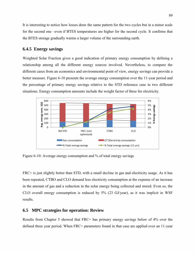
89
It is interesting to notice how losses draw the same pattern for the two cycles but in a minor scale
for the second one –even if BTES temperatures are higher for the second cycle. It confirms that
the BTES storage gradually warms a larger volume of the surrounding earth.
6.4.5 Energy savings
Weighted Solar Fraction gives a good indication of primary energy consumption by defining a
relationship among all the different energy sources involved. Nevertheless, to compare the
different cases from an economics and environmental point of view, energy savings can provide a
better measure. Figure 6-10 presents the average energy consumption over the 11-year period and
the percentage of primary energy savings relative to the STD reference case in two different
situations. Energy consumption amounts include the weight factor of three for electricity.
0%
1%
2%
3%
4%
5%
6%
0
100
200
300
400
500
600
Ref STD FRC+ (not optimized)
CTBO CLO
% E
ne
rgy
savi
ngs
Avg
. e
ne
rgy
con
s. (
GJ)
Gas consumption (3*)Electricity consumption
% Total energy savings % Total energy savings (11 yrs)
Figure 6-10: Average energy consumption and % of total energy savings
FRC+ is just slightly better than STD, with a small decline in gas and electricity usage. As it has
been repeated, CTBO and CLO demand less electricity consumption at the expense of an increase
in the amount of gas and a reduction in the solar energy being collected and stored. Even so, the
CLO overall energy consumption is reduced by 5% (23 GJ/year), as it was implicit in WSF
results.
6.5 MPC strategies for operation: Review
Results from Chapter 5 showed that FRC+ has primary energy savings below of 4% over the
defined three year period. When FRC+ parameters found in that case are applied over an 11-year

90
period (with different weather conditions) the savings drop to 1%. With the changes introduced
in the current chapter, especially those regarding the solar loop control and the MPC optimization
mechanisms, primary energy savings in the CLO case are close to 5% for 10 years average; when
the difficult year 14 (LR, ML – i.e. low radiation and medium load) is taken into account in an
11-year average the value is just above 4%.
CLO has a limited increase in primary energy savings (less than 1%) in respect to CTBO. But it
should be remembered that the results were obtained using perfect forecasts; in a real
environment the divergence between CTBO and CLO could be higher. Considering the system
seasonal behaviour and the impact on control settings of the solar energy stored in the BTES, it
seems less risky to apply the CLO approach because of the regular system feed-back.
Regarding an actual deployment of proposed solar loop control, the temperature difference
between collectors’ inlet and outlet (Delta T) could be adjusted depending on STTS charge status
and on energy prices.
91
CONCLUSION
The calibrated TRNSYS model featuring shorter computation time is accurate enough to test and
analyze the impact of the proposed control strategies. Even if only perfect forecasts were
employed, the applied MPC methods illustrate the possibility of including not only weather
forecasts but also energy costs forecasts.
When analyzing the system dynamic behaviour, it was found that the most significant energy
savings are possible during short periods of extreme weather. In long-term analysis, the Weighted
Solar Fraction (WSF) was shown to be a useful measure to account for the fact that electricity
costs more than natural gas, or to consider the primary energy relationship.
The impact of control strategies is influenced by the trade-offs between collected solar energy
and STTS charge level, BTES temperatures and BTES losses, electricity vs. gas consumption.
The latter is mainly manifested in the amount of collected and stored solar energy, and in a less
proportion in the amount of thermal energy extracted from the BTES.
Long-term improvements of energy performance (and/or operating costs) are possible but
relatively small. The predictive strategy FRC+ delivered a maximum of 3.9 % on primary energy
savings using pre-computed lookup tables. FRC+, solar and BTES loops control yield 5% on the
same primary energy savings when applying the CLO mechanism –with year-to-year
optimization.
Discussion
The overall energy and cost savings are modest, in the order of a few percent. But these savings
were achieved without any hardware changes, just by modifying control algorithms –so the cost
to implement the new control strategies could be low. The modest performance increases are a
testimony to the very high level of expert knowledge that is already included in the standard
control strategy. That control strategy was developed by members of the Design Team having a
very good knowledge of the system and its operation, and it was further refined during the first
years of operation. The application of MPC-based strategies would have the added advantage of
expressing mathematically the compromise to be reached between the Solar Fraction, based only
on the solar energy delivered to the district loop, and the operating costs (or CO2 emissions for
92
example). It would also provide a framework to adapt this compromise to varying energy prices
or related conditions.
Contributions
The main contributions of this work are:
Obtaining a calibrated TRNSYS model of DLSC adapted to MPC studies. The model
includes new TRNSYS components: the BTES controller which implements the standard
control strategy (dated on 2011), and the Degree-hours counter which helps to identify
heating or cooling trends from air temperatures.
Introduction of a methodology for applying Model Predictive Control that can be
employed when there are limits to the traditional implementation. The method uses
predictions based on a system model to tune existing rules and to define new rules for the
supervisory control strategy, and to dynamically adjust the set-point of local pump speed
controllers.
Definition of new concepts for control implementation and evaluation: STTS absolute
charge level (STTS ACL) and Weighted Solar Fraction (WSF).
Inception and evaluation of four control alternatives for different parts of the current
control strategy: winter-mode BTES charge enable, winter-mode BTES discharge enable,
solar loop and BTES loop.
Recommendations for practical implementation
The results of this work could be partially or fully implemented in the real DLSC supervisory
controller –which is based on specialized software for facilities management and control. The
main limitation could be the software’s inability to read weather forecasts.
Since most of the alternative control strategies use elements already present on the existing rules
or derived from them, they can be explained to the engineers managing the system and their
behaviour can be followed and understood. Before implementing those rules in a definitive way,
the MPC-based rules and parameters can be separately or simultaneously applied within a period
of a few days or weeks to assess their impact on the real system.
93
Recommendations for future work
The proposed MPC methodology could be employed to test new control strategies for other parts
of the current control, for example, the BTES charge when in summer operation mode.
FRC+ strategy could be refined to include more scenarios for the lookup tables and assess if this
could lead to increased energy performance. These additional scenarios would consist of finer
levels when STTS charge is low. Additionally, they could include a more accurate way to
determine the levels of BTES charge status used to define the grid of scenarios.
If computation power is available, Closed-Loop Optimization (CLO) should always be
considered. The interval for applying optimal control settings should be reduced as much as
possible (e.g. one month) but the horizon should not be less than two years –to include the impact
of control settings in the next year. In that context, actual forecasts and the feedback of the real
system would be regularly updated. The most important requirement to achieve this
implementation is a simplified way to calibrate the DLSC model at the end of each interval.
The next step in assessing the potential of MPC for solar communities would be to explore the
possibility of applying the MPC methodology and proposed control strategies during the design
phase of solar communities. Designers aiming to reduce the size of the system components could
assess the impact of MPC control in achieving that target. As mentioned above, the very
ambitious solar fraction target at DLSC and the large amount of expert knowledge included in the
current control strategy resulted in relatively modest performance improvements. It would be
interesting to evaluate the benefits of MPC when designing new solar communities with lower
solar fraction targets; that would present more latitude in selecting configurations, components
and control strategies in an integrated approach.
Our work also showed that the lack of possibility to impose a given (non-uniform) initial state for
most existing TRNSYS components requires workarounds that can be very complex to
implement and costly in terms of computing time. To make TRNSYS really suitable to be
deployed for online MPC applications, a mechanism should be implemented to set the current
state of TRNSYS components based on feedback from a real system.
94
REFERENCES
Bauer, D., Marx, R., Nußbicker-Lux, J., Ochs, F., Heidemann, W., & Müller-Steinhagen, H.
(2010). German central solar heating plants with seasonal heat storage. Solar energy, 84(4),
612-623.
Bernier, M. A., Pinel, P., Labib, R., & Paillot, R. (2004). A multiple load aggregation algorithm
for annual hourly simulations of GCHP systems. HVAC&R Research, 10(4), 471-487.
Bernier, M., Kummert, M., & Bertagnolio, S. (2007). Development and application of test cases
for comparing vertical ground heat exchangers models. In Proceedings of the 10th International
IBPSA Conference, Beijing, China.
Brædstrup SolPark. (2012). Brochure. Retrieved April 30, 2013, from http://www.e-
pages.dk/nordad/1810/
Braun, J., (1990). Reducing energy costs and peak electrical demand through optimal control of
building thermal storage. ASHRAE Transactions, 96 (2), 264-273.
Camacho, E. F., Berenguel, M., & Bordons, C. (1994). Adaptive generalized predictive control of
a distributed collector field. Control Systems Technology, IEEE Transactions on, 2(4), 462-467.
Candanedo, J.A., Bucking S., Allard A., & Athienitis A. (2011). Model-Based Predictive Control
Applications for Solar Homes and Communities. Presentation at Model Predictive Control in
Buildings Workshop, Montreal. Retrieved March 9, 2013, from:
http://www.ibpsa.us/pub/mpc2011/presentations/Fri06_Candanedo.pdf
Cao, J., & Lin, X. (2008). Study of hourly and daily solar irradiation forecast using diagonal
recurrent wavelet neural networks. Energy Conversion and Management, 49(6), 1396-1406.
Carslaw, H.S., & Jaeger, J.C. (1959). Conduction of heat in solids, Oxford.
Chapuis, S. (2009). Stockage thermique saisonnier dans un champ de puits géothermiques
verticaux en boucle fermée (Doctoral dissertation, École Polytechnique de Montréal, Montréal).
Chung, M., Park, J. U., & Yoon, H. K. (1998). Simulation of a central solar heating system with
seasonal storage in Korea. Solar energy, 64(4), 163-178.
95
Clarke, J.A. & Cockroft, J. & Conner, S., Hand, J., Kelly, N.J., Moore, R., O'Brien, T. &
Strachan, P.A. (2002). Simulation-assisted control in building energy management systems.
Energy and Buildings, 34 (9), 933-940.
Coffey, B., Morofsky, E., & Haghighat, F. (2006). Model-based control of responsive building
systems: a summary of its potential and challenges. Proceedings of eSim 2006 Building
Performance Simulation Conference, Toronto, 2006, (pp. 157-164).
Coffey, B. (2012). Using Building Simulation and Optimization to Calculate Lookup Tables for
Control. ((Doctoral dissertation, University of California, Berkeley: Center for the Built
Environment).
Dalenbäck, J. O. (2009). Large-Scale Solar Heating and Cooling Systems in Europe. In
Proceedings of ISES World Congress 2007 (Vol. I–Vol. V) (pp. 799-803). Springer Berlin
Heidelberg.
Dalkia. (2010). Montréal, Québec, Canada, District Energy System. Retrieved March 9, 2013,
from http://www.dalkia.ca/link/dl?site=canada-energie.en&objectId=15186&src=kit_veolia
De Ridder F., Diehl M., Mulder G., Desmedt J., Van Bael J. (2011). An optimal control
algorithm for borehole thermal energy storage systems. Energy and Buildings, 43 (10), 2918-
2925.
District Heating. (n.d.). In Wikipedia. Retrieved March 9, 2013, from
http://en.wikipedia.org/wiki/District_heating
Dobos, L., Jäschke, J., Abonyi, J., & Skogestad, S. (2009). Dynamic model and control of heat
exchanger networks for district heating. Hungarian Journal of Industrial Chemistry, 37(1), 37-49.
Dounis, A. I., & Caraiscos, C. (2009). Advanced control systems engineering for energy and
comfort management in a building environment-A review. Renewable and Sustainable Energy
Reviews, 13 (6-7), 1246-1261.
Enermodal Engineering Ltd. (2011). Okotoks sequence of Control V5. Internal NRCan document.
Eskilson, P. (1987). Thermal analysis of heat extraction boreholes. Department of Mathematical
Physics, University of Lund.
96
Ferhatbegovic, T., Zucker, G., Palensky, P. (2011). Model based predictive control for a solar-
thermal system. IEEE AFRICON, 2011, (pp. 1-6).
Fisch, M. N., Guigas, M., & Dalenbäck, J. O. (1998). A review of large-scale solar heating
systems in Europe. Solar energy, 63(6), 355-366.
Florita, A. R., & Henze, G. P. (2009). Comparison of short-term weather forecasting models for
model predictive control. HVAC&R Research, 15(5), 835-853.
Gyalistras, D. (2010). Final report: Use of weather and occupancy forecasts for optimal building
climate control (OptiControl). ETH Zürich, Switzerland.
Hadorn, J.-C., & Chuard, D. (1988). Guide du stockage saisonnier de chaleur. Société suisse des
ingénieurs et des architects, Zürich, Swiss.
Heier, J., Bales, C., Sotnikov, A., & Ponomarova, G. (2011). Evaluation of a high temperature
solar thermal seasonal borehole storage. In ISES Solar World Congress 2011.
Heller, A. (2000). 15 Years of R&D in central solar heating in Denmark. Solar energy, 69(6),
437-447.
Hellström, G. (1989). Duct Ground Heat Storage Model,Manual for Computer Code. Department
of Mathematical Physics, University of Lund, Sweden.
Henze, G. P., Dodier, R. H., Krarti, M. (1997). Development of a Predictive Optimal Controller
for Thermal Energy Storage Systems. HVAC&R Research, 3 (3), 233-264.
Henze, G. P., Felsmann, C., & Knabe, G. (2004). Evaluation of optimal control for active and
passive building thermal storage. International Journal of Thermal Sciences, 43(2), 173-183.
Ingersoll, L. R., Adler, F. T., Plass, H. J., & Ingersoll, A. C. (1950). Theory of earth heat
exchangers for the heat pump. ASHVE Trans, 56, 167-188.
Jalali, A. A., & Nadimi, V. (2006). A survey on robust model predictive control from 1999-2006.
Computational Intelligence for Modelling, Control and Automation, 2006 and International
Conference on Intelligent Agents, Web Technologies and Internet Commerce, International
Conference on, 207-207).
Kelly, G. (1988). Control system simulation in North America. Energy and Buildings, 10 (3),
193-202.
97
Klein, S. A., Beckman, W. A., Mitchell, J. W., Duffie, J. A., Duffie, N. A., Freeman, T. L.,
Mitchell, J. C., et al. (2012). TRNSYS 17 – A TRaNsient SYstem Simulation program, User
manual. Madison, WI: University of Wisconsin -Madison, USA.
Kummert, M. (2001). Contribution to the application of modern control to solar buildings -
Simulation-based approach and experimental validation. (Doctoral dissertation, Fondation
Universitaire Luxembourgeoise, Belgique).
Lundh, M., & Dalenbäck, J. O. (2008). Swedish solar heated residential area with seasonal
storage in rock: Initial evaluation. Renewable energy, 33(4), 703-711.
Ma, Y., Kelman, A., Daly, A., & Borrelli, F. (2012). Predictive control for energy efficient
buildings with thermal storage: Modeling, stimulation, and experiments. Control Systems, IEEE,
32(1), 44-64.
Maciejowski, J. M. Predictive Control with Constraints. 2002. Harlow, England: Pearson
Education
Mahdavi, A., Mohammadi, A., Kabir, E., & Lambeva, L. (2008). Occupants' operation of
lighting and shading systems in office buildings. Journal of building performance simulation,
1(1), 57-65.
McDowell, T. P., & Thornton, J. W. (2008). Simulation and model calibration of a large-scale
solar seasonal storage system. In 3rd National conference of IBPSA, USA, Berkeley
(California), USA.
Natural Resources Canada (NRCan). (2012). DLSC pump power consumption v2. Internal
document.
Natural Resources Canada (NRCan). (2012). Energy Use Data Handbook Tables. Retrieved
April 27, 2013, from
http://oee.nrcan.gc.ca/corporate/statistics/neud/dpa/handbook_totalsectors_ca.cfm
Natural Resources Canada (NRCan). (2012). Utility Cost Summary.xls. Internal document.
Nielsen, J. E. (2012). IEA-SHC Task 45: Large Solar Heating/Cooling Systems, Seasonal
Storage, Heat Pumps. Energy Procedia, 30, 849-855.
98
Nussbicker-Lux, J., & Drück, H. (2012). Solare Nahwärmeversorgung in Crailsheim mit 7500 m²
Kollektorfläche. Symposium Thermische Solarenergie 2012. Kloster Banz.
Oldewurtel, F. , Parisio, A. , Jones, C.N. , Gyalistras, D. , Gwerder, M. , Stauch, V. , Lehmann,
B. , Morari, M. (2012). Use of model predictive control and weather forecasts for energy efficient
building climate control. Energy and Buildings, 45, 15-27.
Palsson, O. P., Madsen, H., & Søgaard, H. T. (1993). Application of predictive control in district
heating systems. Proceedings of the Institution of Mechanical Engineers, Part A: Journal of
Power and Energy, 207(3), 157-163.
Patterson, D. (2012, April 25). Korean researchers learn from Drake Landing. Okotoks Western
Wheel. Retrieved from http://www.westernwheel.com/article/20120425/WHE0801/304259996/-
1/whe/korean-researchers-learn-from-drake-landing
Pavlov, G. K., & Olesen, B. W. (2011). Seasonal ground solar thermal energy storage-review of
systems and applications. In Proceedings of ISES Solar World Congress, Kassel (DE), ISSN (pp.
1583-1078).
Perez, R., Moore, K., Wilcox, S., Renné, D., & Zelenka, A. (2007). Forecasting solar radiation –
Preliminary evaluation of an approach based upon the national forecast database. Solar energy,
81(6), 809-812.
Perez, R., Kivalov, S., Schlemmer, J., Hemker, K., Renné, D., & Hoff, T. E. (2010). Validation of
short and medium term operational solar radiation forecasts in the US. Solar Energy, 84(12),
2161-2172.
Petersen, S., & Svendsen, S. (2010). Method and simulation program informed decisions in the
early stages of building design. Energy and Buildings, 42(7), 1113-1119.
PlanEnergi. (2010). Solar Heating and Seasonal Heat Storage. Retrieved March 9, 2013, from
http://www.planenergi.eu/solar-heating-and-seasonal-heat-storage.html
Rossiter, J. A. (2003). Model-based predictive control: a practical approach (Vol. 4). CRC press.
Roth, K. (2009). Seasonal Energy Storage. ASHRAE journal, (January), 41-43.
Saarinen, L. (2008). Modelling and control of a district heating system (Doctoral dissertation,
Uppsala University, Sweden).
99
Sandou, G., & Sorin O. (2009). Particle swarm optimization based nmpc: An application to
district heating networks. Nonlinear Model Predictive Control (2009): 551-559.
Schmidt, T., Mangold, D., & Müller-Steinhagen, H. (2004). Central solar heating plants with
seasonal storage in Germany. Solar energy, 76(1), 165-174.
Schmidt, T., Miedaner, O. (2012). Solar district heating guidelines-Storage. Retrieved March 9,
2013 from http://www.solar-district-heating.eu/Portals/0/Factsheets/SDH-WP3-D31-
D32_August2012.pdf
Schubert, M., Trier, D. (2012). Solar district heating guidelines-Control Strategies. Retrieved
March 9, 2013 from http://www.solar-district-heating.eu/Portals/0/Factsheets/SDH-WP3-D31-
D32_August2012.pdf
Sibbitt, B., McClenahan, D., Djebbar, R., Thornton, J., Wong, B., Carriere, J., & Kokko, J.
(2012). The Performance of a High Solar Fraction Seasonal Storage District Heating System–
Five Years of Operation. Energy Procedia, 30, 856-865.
Smart Net-zero Energy Building Research Network (SNEBRN). (2013). Consulted March 9,
2013, from http://www.solarbuildings.ca/index.php/en/themes
Solar District Heating organization (SDH). (2013). Ranking List of European Large Scale Solar
Heating Plants. Retrieved March 9, 2013, from http://www.solar-district-
heating.eu/SDH/LargeScaleSolarHeatingPlants.aspx
Tamasauskas, J., Poirier, M., Zmeureanu, R., & Sunyé, R. (2012). Modeling and optimization of
a solar assisted heat pump using ice slurry as a latent storage material. Solar Energy, 86(11),
3316-3325.
Thermal Energy Systems Specialists (TESS). (2007). Drake Landing Solar Community, Okotoks,
Alberta, Canada. Retrieved November 19, 2012 from http://www.tess-inc.com/site-
com/assets/filedownloads/Okotoks%20Project%20Summary%20-%20New.pdf
Turpin, F.B. District Heating. 1996. London, Heywood Books.
Wetter, M. (2001). GenOpt®,Generic Optimization Program. Seventh International IBPSA
Conference. 601-608.
100
Wetter, M. (2011). GenOpt®,Generic Optimization Program, User Manual Version 3.1.0.
Retrieved May 30, 2013, from http://simulationresearch.lbl.gov/GO/download/manual-3-1-0.pdf
Wong, W.P., McClung J.L., Kokko, J.P., & Snijders, A.L. (2007). First Large-Scale Solar
Seasonal Borehole Thermal Energy Storage in Canada. Ecostock 2006 Conference Proceedings.
Verstraete, A. (2013). Étude d'une communauté solaire avec stockage thermique saisonnier par
puits géothermiques (Doctoral dissertation, École Polytechnique de Montréal).
Verstraete, A., Bernier, M. (2013). Étude d’une communauté solaire utilisant un réseau de
distribution à un seul tuyau. XIe Colloque Inter-universitaire Franco-Québécois, Reims, France,
289-294
Xie, F., & Whiteley, J. R. (2007). Model Predictive Control of a Geothermally Heated Bridge
Deck. In American Control Conference, 2007. ACC'07 (pp. 2214-2219). IEEE.
Yang, H., Cui, P., & Fang, Z. (2010). Vertical-borehole ground-coupled heat pumps: A review of
models and systems. Applied Energy, 87(1), 16-27.
101
APPENDIX 1 BTES PRE-HEATING PARAMETERS OPTIMIZATION
The process started with a general review of the Type 557 source code to have a basic idea of the
software implementation of the Duct Ground Heat Storage (DST) model and the impact of pre-
heating parameters in the storage temperature. After identifying the most relevant pre-heating
parameters, they were optimized to find their best values so the pre-heating simulation produced
the same results as the long-run simulation. A complete description of the source code can be
found in Hellström (1989) and Chapuis (2009).
Preheating parameters
The BTES Preheating parameters can be classified in two groups:
Those affecting only the storage's top layer, related with air temperature
Those affecting the whole storage volume, related with storage's earth temperature
After inspecting the source code it was validated that air temperature parameters could be
ignored, the documentation confirms that “the variation of the boundary conditions at the ground
surface during the year can be neglected, except for very shallow ground heat stores” (Hellström,
1989).
The storage's earth temperature parameters are the following: Maximum preheat temperature
(TCMAX), Minimum preheat temperature (TCMIN), Preheat phase delay (TCPH) and Number
of preheating years (IPRE). When IPRE is set to a value different from zero, the Initial storage’s
temperature (TST0) is calculated from TCMAX, TCMIN and TCPH. At simulation start time,
TST0 is the value given to the storage's output; it is also used to set the initial value for most of
the arrays' cells representing the sub-regions.
For calculating TST0, it is assumed that it follows an annual sinusoidal behaviour, according to
the equation:
TST0=TCM+TCA*Sin(ACK*(TT+TCPH)) (A1.1)
where, TCM is the mean between TCMAX and the TCMIN. TCA is the amplitude of the Sin
function, TCA=TCMAX-TCM. TT is the initial simulation time in seconds, it is set to zero.
TCPH is the parameter Preheat phase delay expressed in seconds. ACK is the normalized
argument for the Sine function, so 1 year is a full sinusoidal cycle:
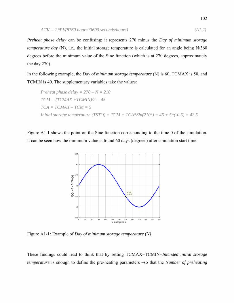
102
ACK = 2*PI/(8760 hours*3600 seconds/hours) (A1.2)
Preheat phase delay can be confusing; it represents 270 minus the Day of minimum storage
temperature day (N), i.e., the initial storage temperature is calculated for an angle being N/360
degrees before the minimum value of the Sine function (which is at 270 degrees, approximately
the day 270).
In the following example, the Day of minimum storage temperature (N) is 60, TCMAX is 50, and
TCMIN is 40. The supplementary variables take the values:
Preheat phase delay = 270 – N = 210
TCM = (TCMAX +TCMIN)/2 = 45
TCA = TCMAX – TCM = 5
Initial storage temperature (TSTO) = TCM + TCA*Sin(210°) = 45 + 5*(-0.5) = 42.5
Figure A1.1 shows the point on the Sine function corresponding to the time 0 of the simulation.
It can be seen how the minimum value is found 60 days (degrees) after simulation start time.
0 30 60 90 120 150 180 210 240 270 300 330 36037.5
40
42.5
45
47.5
50
52.5
X: 210
Y: 42.5
x in degrees
f(x)=
45
+ 5
*S
in(x
)
Figure A1-1: Example of Day of minimum storage temperature (N)
These findings could lead to think that by setting TCMAX=TCMIN=Intended initial storage
temperature is enough to define the pre-heating parameters –so that the Number of preheating
103
years (IPRE) is not important. However, it was found that IPRE and TCMIN are also used in
other equations that set the temperature for certain storage’s sub-regions.
IPRE, TCMAX and TCMIN were the only parameters to be considered when finding the
optimum settings for preheating. Preheat phase delay (TCPH) was not included because it was
found in preliminary optimizations that its impact was low if the value was properly selected. It
was set to 182 because in the year 4 the minimum BTES average temperature occurs on day 88
(270 – 88 = 182).
Pre-heating parameters calibration
The idea is to compare selected outputs between a long-run simulation and one running with the
pre-heating settings. As this process is on the domain of the optimization, GenOpt was employed
with the objective of finding the optimal pre-heating settings that minimize the root-mean-square-
error (RMSE) of selected simulation outputs. These outputs are mainly BTES temperatures but
there is also the STTS % of charge. Even if the latter is not directly related to the BTES, it is
included to assess the behaviour of other simulation components when executing the short-run
simulation with preheating parameters.
Type 557 provides an output for the storage average temperature and temperature outputs for
each radial region (six for the DLSC case) close to the boreholes (temperature-near-the-
boreholes). The default type 557's proforma was modified to include all the 6 regions'
temperatures because in the original TRNSYS distribution only the one for the central region is
available. TRNSYS Visual Studio –the TRNSYS graphic user interface that facilitates the
configuration and interconnection of types– needs the proformas to let know the user the inputs,
outputs and parameters that are available for each type.
In total, the compared outputs are eight: The average BTES temperature, the six temperature-
near-the-boreholes and the STTS % of charge. A reference file was prepared with the outputs of
the long-term simulation for years 4 and 5. The optimization process is commanded by GenOpt
and supported by TRNSYS and Matlab, the latter runs TRNSYS and calculates the RMSE. At the
end of each TRNSYS simulation the resulting outputs and the long-run reference data are loaded
in Matlab, then, it calculates and writes the RMSE to a file that is read by GenOpt. According to
an optimization algorithm, GenOpt repeats the process for a new set of pre-heating parameters
until the minimum RMSE is found.

104
The range of possible values for the preheating parameters was based on the maximum and
minimum value of BTES average temperature. The maximum is approximately 57°C and the
minimum 40°C.
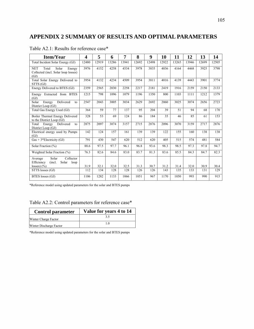
105
APPENDIX 2 SUMMARY OF RESULTS AND OPTIMAL PARAMETERS
Table A2.1: Results for reference case*
Item/Year 4 5 6 7 8 9 10 11 12 13 14 Total Incident Solar Energy (GJ) 12480 12919 13286 13941 12692 12498 12922 13265 13946 12699 12505
NET Total Solar Energy Collected (incl. Solar loop losses) (GJ)
3976 4152 4258 4534 3978 3835 4036 4164 4468 3925 3798
Total Solar Energy Delivered to STTS (GJ)
3954 4132 4234 4509 3954 3811 4016 4139 4443 3901 3774
Energy Delivered to BTES (GJ) 2359 2565 2030 2258 2217 2181 2419 1916 2159 2150 2133
Energy Extracted from BTES (GJ)
1215 798 1096 1079 1196 1350 800 1103 1111 1212 1379
Solar Energy Delivered to District Loop (GJ)
2547 2043 3005 3034 2629 2692 2060 3025 3074 2656 2723
Total Gas Energy Used (GJ) 364 59 77 137 95 204 39 51 94 68 170
Boiler Thermal Energy Delivered to the District Loop (GJ)
328 53 69 124 86 184 35 46 85 61 153
Total Energy Delivered to District Loop (GJ)
2875 2097 3074 3157 2715 2876 2096 3070 3159 2717 2876
Electrical energy used by Pumps (GJ)
142 124 157 161 139 139 122 155 160 138 138
Gas + 3*Electricity (GJ) 791 430 547 620 512 620 405 515 574 481 584
Solar Fraction (%) 88.6 97.5 97.7 96.1 96.8 93.6 98.3 98.5 97.3 97.8 94.7
Weighted Solar Fraction (%) 76.3 82.6 84.6 83.0 83.7 81.3 83.6 85.5 84.3 84.7 82.3
Average Solar Collector Efficiency (incl. Solar loop losses) (%) 31.9 32.1 32.0 32.5 31.3 30.7 31.2 31.4 32.0 30.9 30.4 STTS losses (GJ) 112 134 128 128 126 126 143 135 133 131 129
BTES losses (GJ) 1106 1282 1133 1066 1051 967 1170 1050 993 990 915
*Reference model using updated parameters for the solar and BTES pumps
Table A2.2: Control parameters for reference case*
Control parameter Value for years 4 to 14
Winter Charge Factor 3.5
Winter Discharge Factor 1.0
*Reference model using updated parameters for the solar and BTES pumps
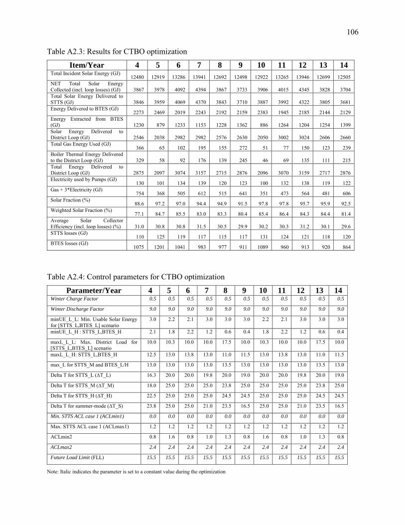
106
Table A2.3: Results for CTBO optimization
Item/Year 4 5 6 7 8 9 10 11 12 13 14 Total Incident Solar Energy (GJ)
12480 12919 13286 13941 12692 12498 12922 13265 13946 12699 12505 NET Total Solar Energy Collected (incl. loop losses) (GJ) 3867 3978 4092 4394 3867 3733 3906 4015 4345 3828 3704 Total Solar Energy Delivered to STTS (GJ) 3846 3959 4069 4370 3843 3710 3887 3992 4322 3805 3681 Energy Delivered to BTES (GJ)
2273 2469 2019 2243 2192 2159 2383 1945 2185 2144 2129 Energy Extracted from BTES (GJ) 1230 879 1233 1153 1228 1362 886 1264 1204 1254 1399 Solar Energy Delivered to District Loop (GJ) 2546 2038 2982 2982 2576 2630 2050 3002 3024 2606 2660 Total Gas Energy Used (GJ)
366 65 102 195 155 272 51 77 150 123 239 Boiler Thermal Energy Delivered to the District Loop (GJ) 329 58 92 176 139 245 46 69 135 111 215 Total Energy Delivered to District Loop (GJ) 2875 2097 3074 3157 2715 2876 2096 3070 3159 2717 2876 Electricity used by Pumps (GJ)
130 101 134 139 120 123 100 132 138 119 122 Gas + 3*Electricity (GJ)
754 368 505 612 515 641 351 473 564 481 606 Solar Fraction (%)
88.6 97.2 97.0 94.4 94.9 91.5 97.8 97.8 95.7 95.9 92.5 Weighted Solar Fraction (%)
77.1 84.7 85.5 83.0 83.3 80.4 85.4 86.4 84.3 84.4 81.4 Average Solar Collector Efficiency (incl. loop losses) (%) 31.0 30.8 30.8 31.5 30.5 29.9 30.2 30.3 31.2 30.1 29.6 STTS losses (GJ)
110 125 119 117 115 117 131 124 121 118 120 BTES losses (GJ)
1075 1201 1041 983 977 911 1089 960 913 920 864
Table A2.4: Control parameters for CTBO optimization
Parameter/Year 4 5 6 7 8 9 10 11 12 13 14 Winter Charge Factor 0.5 0.5 0.5 0.5 0.5 0.5 0.5 0.5 0.5 0.5 0.5
Winter Discharge Factor 9.0 9.0 9.0 9.0 9.0 9.0 9.0 9.0 9.0 9.0 9.0
minUE_L_L: Min. Usable Solar Energy for [STTS_L,BTES_L] scenario
3.0 2.2 2.1 3.0 3.0 3.0 2.2 2.1 3.0 3.0 3.0
minUE_L_H : STTS_L,BTES_H 2.1 1.8 2.2 1.2 0.6 0.4 1.8 2.2 1.2 0.6 0.4
maxL_L_L: Max. District Load for [STTS_L,BTES_L] scenario
10.0 10.3 10.0 10.0 17.5 10.0 10.3 10.0 10.0 17.5 10.0
maxL_L_H: STTS_L,BTES_H 12.5 13.0 13.8 13.0 11.0 11.5 13.0 13.8 13.0 11.0 11.5
max_L for STTS_M and BTES_L/H 13.0 13.0 13.0 13.0 13.5 13.0 13.0 13.0 13.0 13.5 13.0
Delta T for STTS_L (∆T_L) 16.3 20.0 20.0 19.8 20.0 19.0 20.0 20.0 19.8 20.0 19.0
Delta T for STTS_M (∆T_M) 18.0 25.0 25.0 25.0 23.8 25.0 25.0 25.0 25.0 23.8 25.0
Delta T for STTS_H (∆T_H) 22.5 25.0 25.0 25.0 24.5 24.5 25.0 25.0 25.0 24.5 24.5
Delta T for summer-mode (∆T_S) 23.8 25.0 25.0 21.0 23.5 16.5 25.0 25.0 21.0 23.5 16.5
Min. STTS ACL case 1 (ACLmin1) 0.0 0.0 0.0 0.0 0.0 0.0 0.0 0.0 0.0 0.0 0.0
Max. STTS ACL case 1 (ACLmax1) 1.2 1.2 1.2 1.2 1.2 1.2 1.2 1.2 1.2 1.2 1.2
ACLmin2 0.8 1.6 0.8 1.0 1.3 0.8 1.6 0.8 1.0 1.3 0.8
ACLmax2 2.4 2.4 2.4 2.4 2.4 2.4 2.4 2.4 2.4 2.4 2.4
Future Load Limit (FLL) 15.5 15.5 15.5 15.5 15.5 15.5 15.5 15.5 15.5 15.5 15.5
Note: Italic indicates the parameter is set to a constant value during the optimization

107
Table A2.5: Results for CLO optimization
Item/Year 4 5 6 7 8 9 10 11 12 13 14 Total Incident Solar Energy (GJ) 12480 12919 13286 13941 12692 12498 12922 13265 13946 12699 12505
NET Total Solar Energy Collected (incl. loop losses) (GJ)
3884 4032 4150 4424 3888 3747 3952 4072 4385 3848 3717
Total Solar Energy Delivered to STTS (GJ)
3862 4013 4126 4401 3864 3725 3933 4048 4360 3824 3693
Energy Delivered to BTES (GJ) 2287 2488 1994 2209 2191 2146 2385 1913 2142 2139 2105
Energy Extracted from BTES (GJ)
1229 842 1163 1107 1227 1349 845 1188 1143 1249 1384
Solar Energy Delivered to District Loop (GJ)
2547 2040 2993 3002 2594 2647 2053 3013 3045 2626 2680
Total Gas Energy Used (GJ) 364 63 91 172 135 253 48 64 127 102 218
Boiler Thermal Energy Delivered to the District Loop (GJ)
328 57 81 155 121 228 43 57 114 92 196
Total Energy Delivered to District Loop (GJ)
2875 2097 3074 3157 2715 2876 2096 3070 3159 2717 2876
Electricity used by Pumps (GJ) 131 105 139 142 123 125 104 137 142 122 124
Gas + 3*Electricity (GJ) 758 379 508 598 503 627 361 475 553 468 589
Solar Fraction (%) 88.6 97.3 97.3 95.1 95.5 92.1 97.9 98.1 96.4 96.6 93.2
Weighted Solar Fraction (%) 77.1 84.3 85.5 83.4 83.8 80.8 85.1 86.4 84.6 84.9 82.0
Average Solar Collector Efficiency (incl. loop losses) (%)
31.1 31.2 31.2 31.7 30.6 30.0 30.6 30.7 31.4 30.3 29.7
STTS losses (GJ) 111 127 122 120 118 118 134 128 124 122 121
BTES losses (GJ) 1079 1222 1067 1001 991 918 1109 987 935 935 870
Table A2.6: Control parameters for CLO optimization
Parameter/Year 4 5 6 7 8 9 10 11 12 13 14 Winter Charge Factor 0.5 0.5 0.5 0.5 0.5 0.5 0.5 0.5 0.5 0.5 0.5
Winter Discharge Factor 9.0 9.0 9.0 9.0 9.0 9.0 9.0 9.0 9.0 9.0 9.0
minUE_L_L: Min. Usable Solar Energy for [STTS_L,BTES_L] scenario
3.7 3.1 3.7 3.2 3.2 3.2 3.2 3.2 3.2 3.2 3.2
minUE_L_H : STTS_L,BTES_H 2.1 1.0 1.7 1.8 1.8 1.1 1.1 1.1 1.1 1.1 1.1
maxL_L_L: Max. District Load for [STTS_L,BTES_L] scenario
12.5 12.0 12.5 12.0 12.3 12.3 12.3 12.3 12.3 12.3 12.3
maxL_L_H: STTS_L,BTES_H 13.5 13.0 13.8 13.8 14.0 13.5 13.5 13.5 13.5 13.5 13.5
max_L for STTS_M and BTES_L/H 13.5 13.5 13.5 13.5 13.5 13.5 13.5 13.5 13.5 13.5 13.5
Delta T for STTS_L (∆T_L) 17.5 18.0 18.0 18.0 17.8 17.8 17.8 17.8 17.8 17.8 17.8
Delta T for STTS_M (∆T_M) 17.0 20.5 21.0 22.3 21.5 20.5 20.5 20.5 20.5 20.5 20.5
Delta T for STTS_H (∆T_H) 23.0 23.5 23.5 23.5 23.5 23.3 23.3 23.3 23.3 23.3 23.3
Delta T for summer-mode (∆T_S) 16.0 23.5 23.0 23.0 22.5 23.3 23.3 23.3 23.3 23.3 23.3
Min. STTS ACL case 1 (ACLmin1) 0.0 0.0 0.0 0.0 0.0 0.0 0.0 0.0 0.0 0.0 0.0
Max. STTS ACL case 1 (ACLmax1) 1.3 1.3 1.3 1.3 1.3 1.3 1.3 1.3 1.3 1.3 1.3
ACLmin2 1.0 1.1 1.0 1.0 1.2 1.0 1.0 1.0 1.0 1.0 1.0
ACLmax2 2.4 2.4 2.4 2.4 2.4 2.4 2.4 2.4 2.4 2.4 2.4
Future Load Limit (FLL) 15.5 15.5 15.5 15.5 15.5 15.5 15.5 15.5 15.5 15.5 15.5
Note: Italic indicates the parameter is set to a constant value during the optimization