
Master Recherche IAC TC2: Apprentissage Statistique ...sebag/Slides/M2R_TC2_2_cours.pdf · Master...
93
Master Recherche IAC TC2: Apprentissage Statistique & Optimisation Alexandre Allauzen - Anne Auger - Mich` ele Sebag LIMSI - LRI Oct. 21st, 2013
Transcript of Master Recherche IAC TC2: Apprentissage Statistique ...sebag/Slides/M2R_TC2_2_cours.pdf · Master...

Master Recherche IACTC2: Apprentissage Statistique & Optimisation
Alexandre Allauzen − Anne Auger − Michele SebagLIMSI − LRI
Oct. 21st, 2013
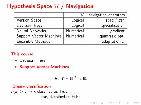
Hypothesis Space H / Navigation
H navigation operators
Version Space Logical spec / genDecision Trees Logical specialisation
Neural Networks Numerical gradientSupport Vector Machines Numerical quadratic opt.
Ensemble Methods − adaptation E
This course
I Decision Trees
I Support Vector Machines
h : X = IRD 7→ IR
Binary classificationh(x) > 0 → x classified as True
else, classified as False
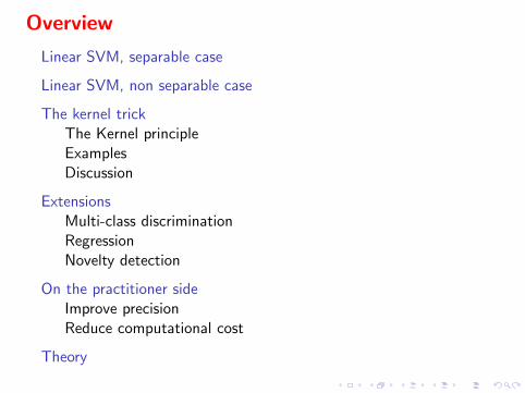
Overview
Linear SVM, separable case
Linear SVM, non separable case
The kernel trickThe Kernel principleExamplesDiscussion
ExtensionsMulti-class discriminationRegressionNovelty detection
On the practitioner sideImprove precisionReduce computational cost
Theory
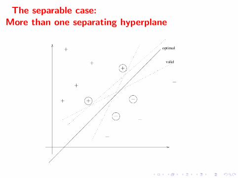
The separable case:More than one separating hyperplane
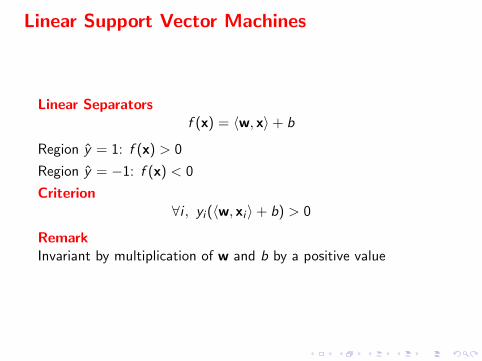
Linear Support Vector Machines
Linear Separatorsf (x) = 〈w, x〉+ b
Region y = 1: f (x) > 0
Region y = −1: f (x) < 0
Criterion∀i , yi (〈w, xi 〉+ b) > 0
RemarkInvariant by multiplication of w and b by a positive value
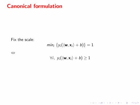
Canonical formulation
Fix the scale:mini {yi (〈w, xi 〉+ b)} = 1
⇔∀i , yi (〈w, xi 〉+ b) ≥ 1
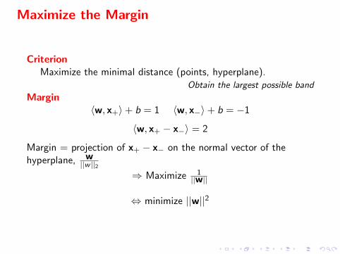
Maximize the Margin
CriterionMaximize the minimal distance (points, hyperplane).
Obtain the largest possible band
Margin〈w, x+〉+ b = 1 〈w, x−〉+ b = −1
〈w, x+ − x−〉 = 2
Margin = projection of x+ − x− on the normal vector of thehyperplane, w
||w ||2⇒ Maximize 1
||w||
⇔ minimize ||w||2
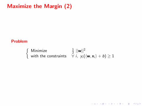
Maximize the Margin (2)
Problem{Minimize 1
2 ||w||2
with the constraints ∀ i , yi (〈w, xi 〉+ b) ≥ 1

Maximal Margin Hyperplane
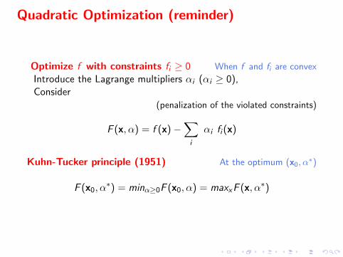
Quadratic Optimization (reminder)
Optimize f with constraints fi ≥ 0 When f and fi are convex
Introduce the Lagrange multipliers αi (αi ≥ 0),Consider
(penalization of the violated constraints)
F (x, α) = f (x)−∑i
αi fi (x)
Kuhn-Tucker principle (1951) At the optimum (x0, α∗)
F (x0, α∗) = minα≥0F (x0, α) = maxxF (x, α∗)
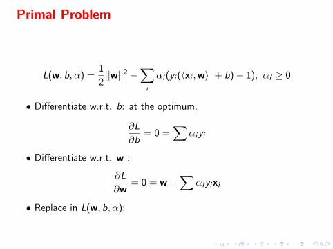
Primal Problem
L(w, b, α) =1
2||w||2 −
∑i
αi (yi (〈xi ,w〉 + b)− 1), αi ≥ 0
• Differentiate w.r.t. b: at the optimum,
∂L
∂b= 0 =
∑αiyi
• Differentiate w.r.t. w :
∂L
∂w= 0 = w−
∑αiyixi
• Replace in L(w, b, α):
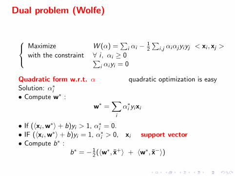
Dual problem (Wolfe)
Maximize W (α) =
∑i αi − 1
2
∑i ,j αiαjyiyj < xi , xj >
with the constraint ∀ i , αi ≥ 0∑i αiyi = 0
Quadratic form w.r.t. α quadratic optimization is easySolution: α∗i• Compute w∗ :
w∗ =∑i
α∗i yixi
• If (〈xi ,w∗〉+ b)yi > 1, α∗i = 0.• IF (〈xi ,w∗〉+ b)yi = 1, α∗i > 0, xi support vector• Compute b∗ :
b∗ = −12 (〈w∗, x+〉 + 〈w∗, x−〉)
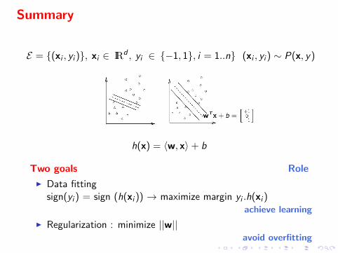
Summary
E = {(xi , yi )}, xi ∈ IRd , yi ∈ {−1, 1}, i = 1..n} (xi , yi ) ∼ P(x, y)
h(x) = 〈w, x〉+ b
Two goals Role
I Data fittingsign(yi ) = sign (h(xi )) → maximize margin yi .h(xi )
achieve learning
I Regularization : minimize ||w||avoid overfitting
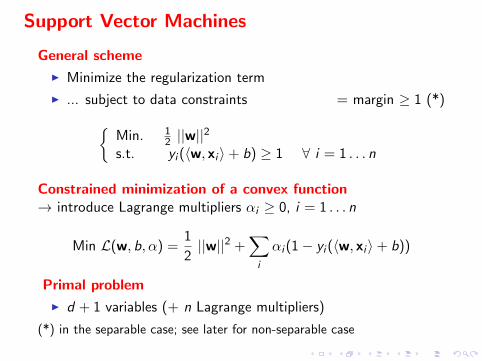
Support Vector Machines
General scheme
I Minimize the regularization term
I ... subject to data constraints = margin ≥ 1 (*){Min. 1
2 ||w||2
s.t. yi (〈w, xi 〉+ b) ≥ 1 ∀ i = 1 . . . n
Constrained minimization of a convex function→ introduce Lagrange multipliers αi ≥ 0, i = 1 . . . n
Min L(w, b, α) =1
2||w||2 +
∑i
αi (1− yi (〈w, xi 〉+ b))
Primal problem
I d + 1 variables (+ n Lagrange multipliers)
(*) in the separable case; see later for non-separable case
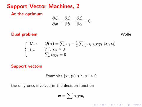
Support Vector Machines, 2At the optimum
∂L∂w
=∂L∂b
=∂L∂α
= 0
Dual problem WolfeMax. Q(α) =
∑i αi − 1
2
∑i ,j αiαjyiyj 〈xi , xj〉
s.t. ∀ i , αi ≥ 0∑i αiyi = 0
Support vectors
Examples (xi , yi ) s.t. αi > 0
the only ones involved in the decision function
w =∑
αiyixi
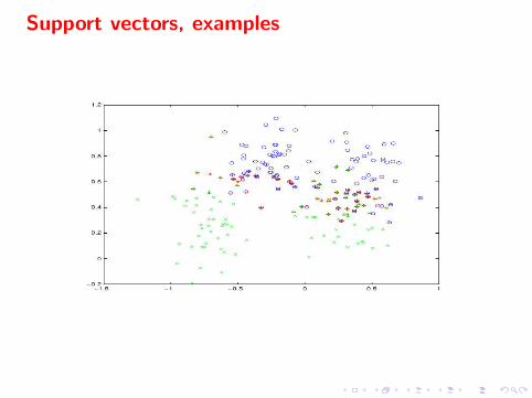
Support vectors, examples
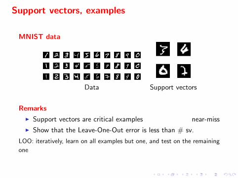
Support vectors, examples
MNIST data
Data Support vectors
Remarks
I Support vectors are critical examples near-miss
I Show that the Leave-One-Out error is less than # sv.
LOO: iteratively, learn on all examples but one, and test on the remaining
one
Overview
Linear SVM, separable case
Linear SVM, non separable case
The kernel trickThe Kernel principleExamplesDiscussion
ExtensionsMulti-class discriminationRegressionNovelty detection
On the practitioner sideImprove precisionReduce computational cost
Theory
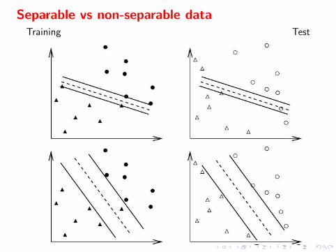
Separable vs non-separable dataTraining Test
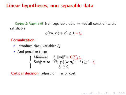
Linear hypotheses, non separable data
Cortes & Vapnik 95 Non-separable data ⇒ not all constraints aresatisfiable
yi (〈w, xi 〉+ b) ≥ 1− ξi
Formalization
I Introduce slack variables ξiI And penalize them
Minimize 12 ||w||
2+ C∑
i ξi
Subject to ∀i , yi (〈w, xi 〉+ b) ≥ 1−ξi
ξi ≥ 0
Critical decision: adjust C = error cost.
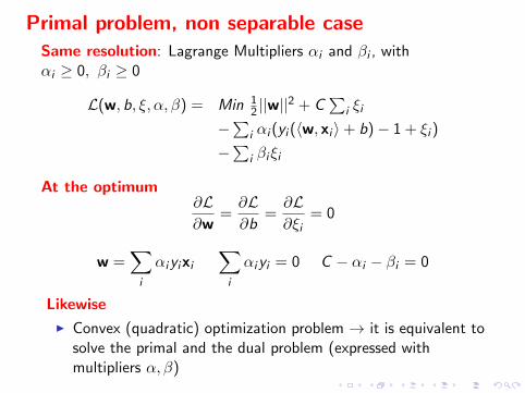
Primal problem, non separable caseSame resolution: Lagrange Multipliers αi and βi , withαi ≥ 0, βi ≥ 0
L(w, b, ξ, α, β) = Min 12 ||w||
2 + C∑
i ξi
−∑
i αi (yi (〈w, xi 〉+ b)− 1 + ξi )
−∑
i βiξi
At the optimum∂L∂w
=∂L∂b
=∂L∂ξi
= 0
w =∑i
αiyixi∑i
αiyi = 0 C − αi − βi = 0
Likewise
I Convex (quadratic) optimization problem → it is equivalent tosolve the primal and the dual problem (expressed withmultipliers α, β)
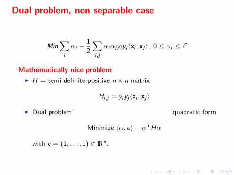
Dual problem, non separable case
Min∑i
αi −1
2
∑i ,j
αiαjyiyj〈xi , xj〉, 0 ≤ αi ≤ C
Mathematically nice problem
I H = semi-definite positive n × n matrix
Hi ,j = yiyj〈xi , xj〉
I Dual problem quadratic form
Minimize 〈α, e〉 − αTHα
with e = (1, . . . , 1) ∈ IRn.
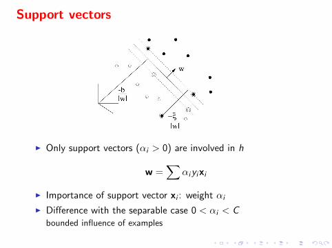
Support vectors
I Only support vectors (αi > 0) are involved in h
w =∑
αiyixi
I Importance of support vector xi : weight αi
I Difference with the separable case 0 < αi < Cbounded influence of examples
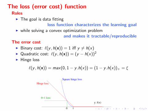
The loss (error cost) functionRoles
I The goal is data fittingloss function characterizes the learning goal
I while solving a convex optimization problemand makes it tractable/reproducible
The error costI Binary cost: `(y , h(x)) = 1 iff y 6= h(x)I Quadratic cost: `(y , h(x)) = (y − h(x))2
I Hinge loss
`(y , h(x)) = max(0, 1− y .h(x)) = (1− y .h(x))+ = ξ
y. f(x)
1
Square hinge loss
0
Hinge loss
0−1 loss
Complexity
Learning complexity
I Worst case: O(n3)
I Empirical complexity: depends on C
I O(n2nsv ) where nsv is the number of s.v.
Usage complexity
I O(nsv )
Overview
Linear SVM, separable case
Linear SVM, non separable case
The kernel trickThe Kernel principleExamplesDiscussion
ExtensionsMulti-class discriminationRegressionNovelty detection
On the practitioner sideImprove precisionReduce computational cost
Theory
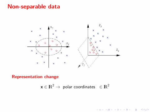
Non-separable data
Representation change
x ∈ IR2 → polar coordinates ∈ IR2
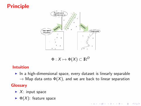
Principle
Φ : X 7→ Φ(X ) ⊂ IRD
Intuition
I In a high-dimensional space, every dataset is linearly separable→ Map data onto Φ(X ), and we are back to linear separation
Glossary
I X : input space
I Φ(X ): feature space
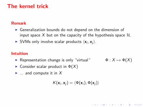
The kernel trick
Remark
I Generalization bounds do not depend on the dimension ofinput space X but on the capacity of the hypothesis space H.
I SVMs only involve scalar products 〈xi , xj〉.
Intuition
I Representation change is only “virtual“ Φ : X 7→ Φ(X )
I Consider scalar product in Φ(X )
I ... and compute it in X
K (xi , xj) = 〈Φ(xi ),Φ(xj)〉
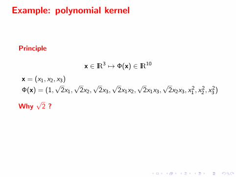
Example: polynomial kernel
Principle
x ∈ IR3 7→ Φ(x) ∈ IR10
x = (x1, x2, x3)
Φ(x) = (1,√
2x1,√
2x2,√
2x3,√
2x1x2,√
2x1x3,√
2x2x3, x21 , x
22 , x
23 )
Why√
2 ?
because
〈Φ(x),Φ(x′)〉 = (1 + 〈x, x′〉)2 = K (x, x′)
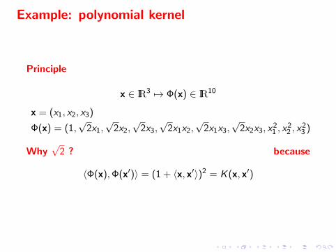
Example: polynomial kernel
Principle
x ∈ IR3 7→ Φ(x) ∈ IR10
x = (x1, x2, x3)
Φ(x) = (1,√
2x1,√
2x2,√
2x3,√
2x1x2,√
2x1x3,√
2x2x3, x21 , x
22 , x
23 )
Why√
2 ? because
〈Φ(x),Φ(x′)〉 = (1 + 〈x, x′〉)2 = K (x, x′)
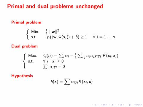
Primal and dual problems unchanged
Primal problem{Min. 1
2 ||w||2
s.t. yi (〈w,Φ(xi )〉+ b) ≥ 1 ∀ i = 1 . . . n
Dual problemMax. Q(α) =
∑i αi − 1
2
∑i ,j αiαjyiyj K (xi , xj)
s.t. ∀ i , αi ≥ 0∑i αiyi = 0
Hypothesis
h(x) =∑i
αiyiK (xi , x)
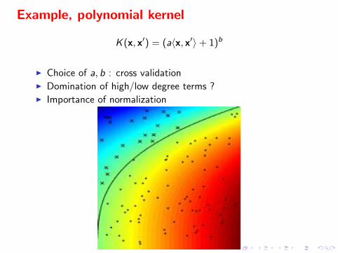
Example, polynomial kernel
K (x, x′) = (a〈x, x′〉+ 1)b
I Choice of a, b : cross validationI Domination of high/low degree terms ?I Importance of normalization

Example, Radius-Based Function kernel (RBF)
K (x, x′) = exp(−γ||x− x′||2
)I No closed form ΦI Φ(X ) of infinite dimension
For x in IR
Φ(x) = exp(−γx2)
) [1,
√2γ
1!x ,
√(2γ)2
2!x2,
√(2γ)3
3!x3, . . .
]I Choice of γ ? (intuition: think of H, Hi ,j = yiyjK (xi , xj))
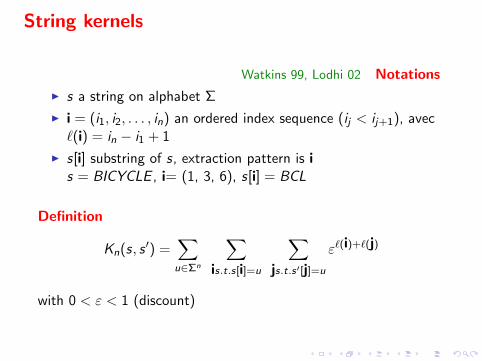
String kernels
Watkins 99, Lodhi 02 Notations
I s a string on alphabet Σ
I i = (i1, i2, . . . , in) an ordered index sequence (ij < ij+1), avec`(i) = in − i1 + 1
I s[i] substring of s, extraction pattern is is = BICYCLE , i= (1, 3, 6), s[i] = BCL
Definition
Kn(s, s ′) =∑u∈Σn
∑is.t.s[i]=u
∑js.t.s′[j]=u
ε`(i)+`(j)
with 0 < ε < 1 (discount)
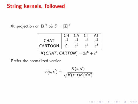
String kernels, followed
Φ: projection on IRD ou D = |Σ|n
CH CA CT ATCHAT ε2 ε3 ε4 ε2
CARTOON 0 ε2 ε4 ε3
K (CHAT ,CARTON) = 2ε5 + ε8
Prefer the normalized version
κ(s, s′) =
K (s, s ′)√K (s, s)K (s ′s ′)
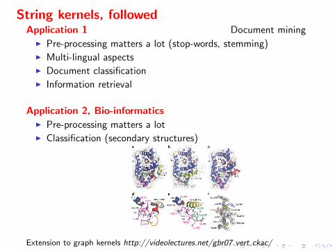
String kernels, followedApplication 1 Document mining
I Pre-processing matters a lot (stop-words, stemming)I Multi-lingual aspectsI Document classificationI Information retrieval
Application 2, Bio-informaticsI Pre-processing matters a lotI Classification (secondary structures)
Extension to graph kernels http://videolectures.net/gbr07 vert ckac/
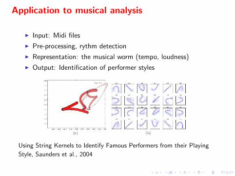
Application to musical analysis
I Input: Midi files
I Pre-processing, rythm detection
I Representation: the musical worm (tempo, loudness)
I Output: Identification of performer styles
Using String Kernels to Identify Famous Performers from their Playing
Style, Saunders et al., 2004
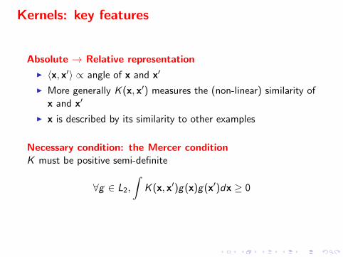
Kernels: key features
Absolute → Relative representation
I 〈x, x′〉 ∝ angle of x and x′
I More generally K (x, x′) measures the (non-linear) similarity ofx and x′
I x is described by its similarity to other examples
Necessary condition: the Mercer conditionK must be positive semi-definite
∀g ∈ L2,
∫K (x, x′)g(x)g(x′)dx ≥ 0
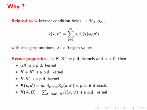
Why ?
Related to Φ Mercer condition holds → ∃φ1, φ2, ..
k(x, x′) =∞∑i=1
λiφi (x)φi (x′)
with φi eigen functions, λi > 0 eigen values
Kernel properties: let K ,K ′ be p.d. kernels and α > 0, then
I αK is a p.d. kernel
I K + K ′ is a p.d. kernel
I K .K ′ is a p.d. kernel
I K (x, x′) = limitp→∞Kp(x, x′) is p.d. if it exists
I K (A,B) =∑
x∈A,x′∈B K (x , x ′) is a p.d. kernel
Overview
Linear SVM, separable case
Linear SVM, non separable case
The kernel trickThe Kernel principleExamplesDiscussion
ExtensionsMulti-class discriminationRegressionNovelty detection
On the practitioner sideImprove precisionReduce computational cost
Theory
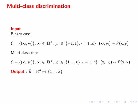
Multi-class discrimination
InputBinary case
E = {(xi , yi )}, xi ∈ IRd , yi ∈ {−1, 1}, i = 1..n} (xi , yi ) ∼ P(x, y)
Multi-class case
E = {(xi , yi )}, xi ∈ IRd , yi ∈ {1 . . . k}, i = 1..n} (xi , yi ) ∼ P(x, y)
Output : h : IRd 7→ {1 . . . k}.
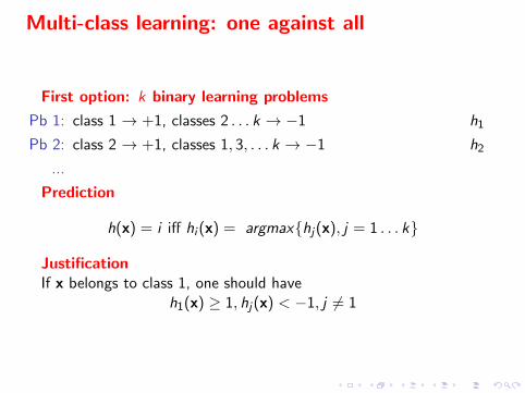
Multi-class learning: one against all
First option: k binary learning problems
Pb 1: class 1 → +1, classes 2 . . . k → −1 h1
Pb 2: class 2 → +1, classes 1, 3, . . . k → −1 h2
...
Prediction
h(x) = i iff hi (x) = argmax{hj(x), j = 1 . . . k}
JustificationIf x belongs to class 1, one should have
h1(x) ≥ 1, hj(x) < −1, j 6= 1
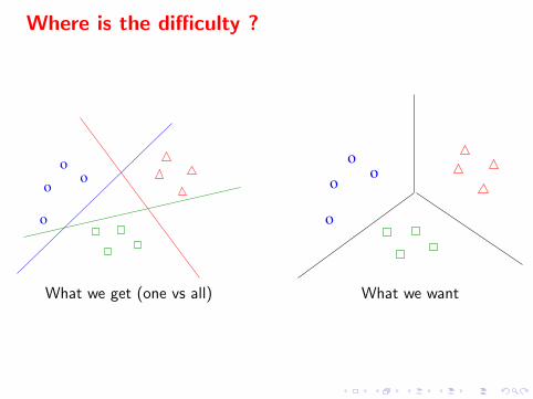
Where is the difficulty ?
o
o
o
o
o
o
o
o
What we get (one vs all) What we want
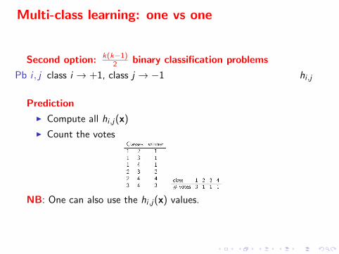
Multi-class learning: one vs one
Second option: k(k−1)2 binary classification problems
Pb i , j class i → +1, class j → −1 hi ,j
Prediction
I Compute all hi ,j(x)
I Count the votes
NB: One can also use the hi ,j(x) values.
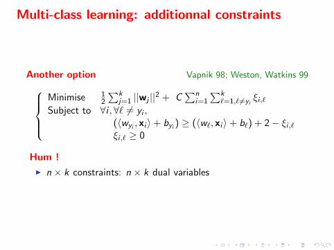
Multi-class learning: additionnal constraints
Another option Vapnik 98; Weston, Watkins 99Minimise 1
2
∑kj=1 ||wj ||2 + C
∑ni=1
∑k`=1,`6=yi
ξi ,`Subject to ∀i ,∀` 6= yi ,
(〈wyi , xi 〉+ byi ) ≥ (〈w`, xi 〉+ b`) + 2− ξi ,`ξi ,` ≥ 0
Hum !
I n × k constraints: n × k dual variables
Recommendations
In practice
I Results are in general (but not always !) similar
I 1-vs-1 is the fastest option

Overview
Linear SVM, separable case
Linear SVM, non separable case
The kernel trickThe Kernel principleExamplesDiscussion
ExtensionsMulti-class discriminationRegressionNovelty detection
On the practitioner sideImprove precisionReduce computational cost
Theory
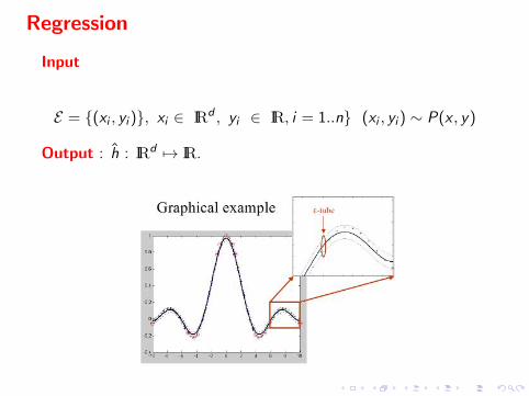
Regression
Input
E = {(xi , yi )}, xi ∈ IRd , yi ∈ IR, i = 1..n} (xi , yi ) ∼ P(x , y)
Output : h : IRd 7→ IR.
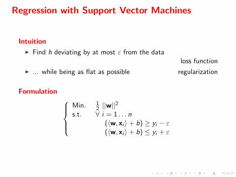
Regression with Support Vector Machines
Intuition
I Find h deviating by at most ε from the dataloss function
I ... while being as flat as possible regularization
Formulation Min. 1
2 ||w||2
s.t. ∀ i = 1 . . . n(〈w, xi 〉+ b) ≥ yi − ε(〈w, xi 〉+ b) ≤ yi + ε
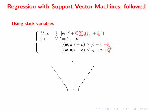
Regression with Support Vector Machines, followed
Using slack variablesMin. 1
2 ||w||2 + C
∑i(ξ
+i + ξ−i )
s.t. ∀ i = 1 . . . n(〈w, xi 〉+ b) ≥ yi − ε −ξ−i(〈w, xi 〉+ b) ≤ yi + ε +ξ+
i
Regression with Support Vector Machines, followed
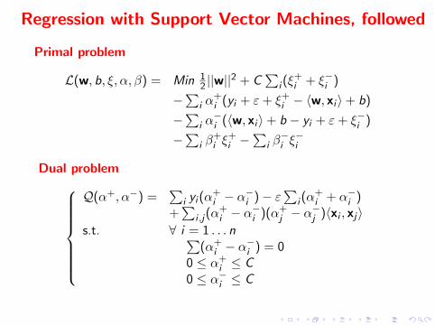
Primal problem
L(w, b, ξ, α, β) = Min 12 ||w||
2 + C∑
i (ξ+i + ξ−i )
−∑
i α+i (yi + ε+ ξ+
i − 〈w, xi 〉+ b)
−∑
i α−i (〈w, xi 〉+ b − yi + ε+ ξ−i )
−∑
i β+i ξ
+i −
∑i β−i ξ−i
Dual problem
Q(α+, α−) =∑
i yi (α+i − α
−i )− ε
∑i (α
+i + α−i )
+∑
i ,j(α+i − α
−i )(α+
j − α−j )〈xi , xj〉
s.t. ∀ i = 1 . . . n∑(α+
i − α−i ) = 0
0 ≤ α+i ≤ C
0 ≤ α−i ≤ C
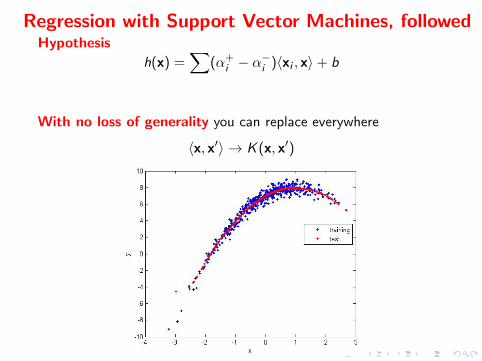
Regression with Support Vector Machines, followedHypothesis
h(x) =∑
(α+i − α
−i )〈xi , x〉+ b
With no loss of generality you can replace everywhere
〈x, x′〉 → K (x, x′)
Beware
High-dimensional regression
E = {(xi , yi )}, xi ∈ IRD , yi ∈ IR, i = 1..n} (xi , yi ) ∼ P(x, y)
A very slippery game if D >> n curse of dimensionality
Dimensionality reduction mandatory
I Map x onto IRd
I Central subspace:π : X 7→ S ⊂ IRd
with S minimal such that y and x are independentconditionally to π(x).
Find h,w : y = h(w, x)
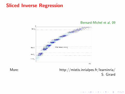
Sliced Inverse Regression
Bernard-Michel et al, 09
More: http://mistis.inrialpes.fr/learninria/S. Girard

Overview
Linear SVM, separable case
Linear SVM, non separable case
The kernel trickThe Kernel principleExamplesDiscussion
ExtensionsMulti-class discriminationRegressionNovelty detection
On the practitioner sideImprove precisionReduce computational cost
Theory
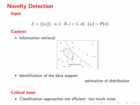
Novelty DetectionInput
E = {(xi )}, xi ∈ X , i = 1..n} (xi ) ∼ P(x)
Context
I Information retrieval
I Identification of the data supportestimation of distribution
Critical issue
I Classification approaches not efficient: too much noise
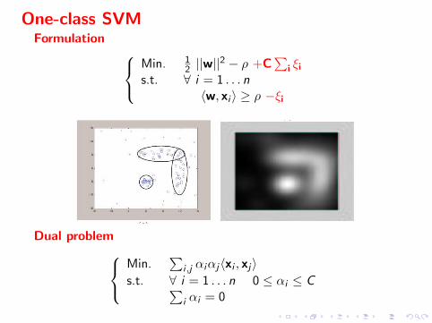
One-class SVMFormulation
Min. 12 ||w||
2 − ρ +C∑
i ξi
s.t. ∀ i = 1 . . . n〈w, xi 〉 ≥ ρ −ξi
Dual problemMin.
∑i ,j αiαj〈xi , xj〉
s.t. ∀ i = 1 . . . n 0 ≤ αi ≤ C∑i αi = 0
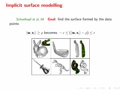
Implicit surface modelling
Schoelkopf et al, 04 Goal: find the surface formed by the datapoints
〈w, xi 〉 ≥ ρ becomes − ε ≤ (〈w, xi 〉 − ρ) ≤ ε

Overview
Linear SVM, separable case
Linear SVM, non separable case
The kernel trickThe Kernel principleExamplesDiscussion
ExtensionsMulti-class discriminationRegressionNovelty detection
On the practitioner sideImprove precisionReduce computational cost
Theory
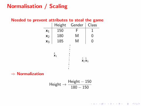
Normalisation / Scaling
Needed to prevent attributes to steal the gameHeight Gender Class
x1 150 F 1x2 180 M 0x3 185 M 0
⇒ Normalization
Height→ Height− 150
180− 150
Beware
Usual practice
I Normalize the whole dataset
I Learn on the training set
I Test on the test set
NO!Good practice
I Normalize the training set (Scaletrain)
I Learn from the normalized training set
I Scale the test set according to Scaletrain and test
Beware
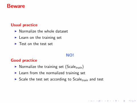
Usual practice
I Normalize the whole dataset
I Learn on the training set
I Test on the test set
NO!Good practice
I Normalize the training set (Scaletrain)
I Learn from the normalized training set
I Scale the test set according to Scaletrain and test
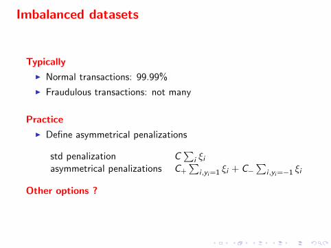
Imbalanced datasets
Typically
I Normal transactions: 99.99%
I Fraudulous transactions: not many
Practice
I Define asymmetrical penalizations
std penalization C∑
i ξiasymmetrical penalizations C+
∑i ,yi=1 ξi + C−
∑i ,yi=−1 ξi
Other options ?
Overview
Linear SVM, separable case
Linear SVM, non separable case
The kernel trickThe Kernel principleExamplesDiscussion
ExtensionsMulti-class discriminationRegressionNovelty detection
On the practitioner sideImprove precisionReduce computational cost
Theory
Data sampling
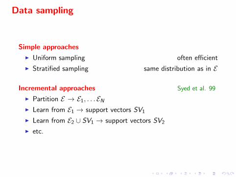
Simple approaches
I Uniform sampling often efficient
I Stratified sampling same distribution as in E
Incremental approaches Syed et al. 99
I Partition E → E1, . . . ENI Learn from E1 → support vectors SV1
I Learn from E2 ∪ SV1 → support vectors SV2
I etc.
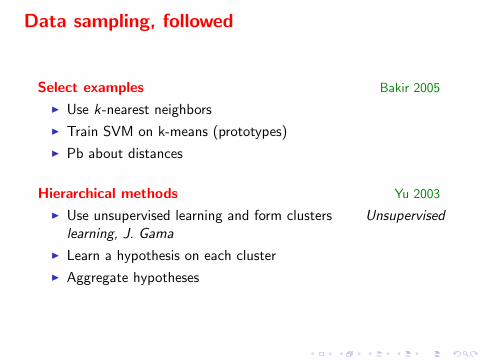
Data sampling, followed
Select examples Bakir 2005
I Use k-nearest neighbors
I Train SVM on k-means (prototypes)
I Pb about distances
Hierarchical methods Yu 2003
I Use unsupervised learning and form clusters Unsupervisedlearning, J. Gama
I Learn a hypothesis on each cluster
I Aggregate hypotheses
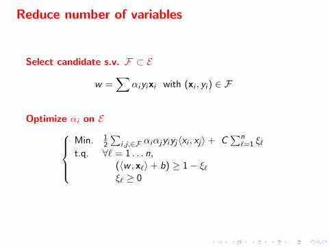
Reduce number of variables
Select candidate s.v. F ⊂ E
w =∑
αiyixi with (xi , yi ) ∈ F
Optimize αi on EMin. 1
2
∑i ,j ,∈F αiαjyiyj〈xi , xj〉+ C
∑n`=1 ξ`
t.q. ∀` = 1 . . . n,(〈w , x`〉+ b) ≥ 1− ξ`ξ` ≥ 0
Sources
I Vapnik, The nature of statistical learning, Springer Verlag1995; Statistical Learning Theory, Wiley 1998
I Cristianini & Shawe Taylor, An introduction to SupportVector Machines, Cambridge University Press, 2000.
I http://www.kernel-machines.org/tutorials
I Videolectures + ML Summer Schools
I Large scale Machine Learning challenge,ICML 2008 wshop:http://largescale.ml.tu-berlin.de/workshop/
Overview
Linear SVM, separable case
Linear SVM, non separable case
The kernel trickThe Kernel principleExamplesDiscussion
ExtensionsMulti-class discriminationRegressionNovelty detection
On the practitioner sideImprove precisionReduce computational cost
Theory
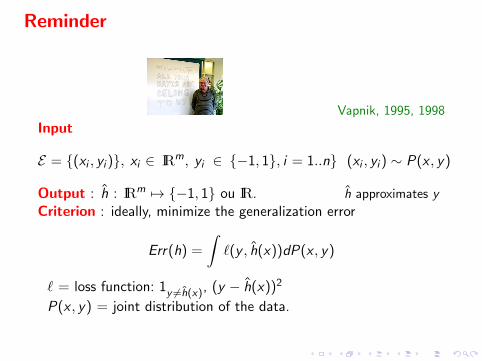
Reminder
Vapnik, 1995, 1998
Input
E = {(xi , yi )}, xi ∈ IRm, yi ∈ {−1, 1}, i = 1..n} (xi , yi ) ∼ P(x , y)
Output : h : IRm 7→ {−1, 1} ou IR. h approximates y
Criterion : ideally, minimize the generalization error
Err(h) =
∫`(y , h(x))dP(x , y)
` = loss function: 1y 6=h(x), (y − h(x))2
P(x , y) = joint distribution of the data.
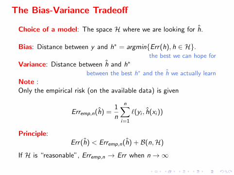
The Bias-Variance Tradeoff
Choice of a model: The space H where we are looking for h.
Bias: Distance between y and h∗ = argmin{Err(h), h ∈ H}.the best we can hope for
Variance: Distance between h and h∗
between the best h∗ and the h we actually learn
Note :Only the empirical risk (on the available data) is given
Erremp,n(h) =1
n
n∑i=1
`(yi , h(xi ))
Principle:Err(h) < Erremp,n(h) + B(n,H)
If H is “reasonable”, Erremp,n → Err when n→∞
Statistical Learning
Statistical Learning TheoryLearning from a statistical perspective.
Goal of the theory in generalModel a real / artificial phenomenon, in order to:* understand* predict* exploit
General
A theory: hypotheses → predictions
I Hypotheses on the phenomenon here, Learning
I Predictions about its behavior errors
Theory → algorithm
I Optimize the quantities allowing prediction
I Nothing practical like a good theory! Vapnik
Strength/Weaknesses
+ Stronger Hypotheses → more precise predictions
BUT if the hypotheses are wrong, nothing will work
What Theory do we need?
Approach in expectation one example
I A set of data breast cancer
I x+: average of positive examples
I x−: average of negative examples
I h(x) = +1 iff d(x , x+) < d(x , x−)
Estimate the generalization error
I Data → Training set, test set
I Learn x+ et x− on the training set, measure the errors on thetest set
Classical Statistics vs Statistical Learning
Classical Statistics
I Mean error
We want guarantees
I PAC Model Probably Approximately Correct
I What is the probability that the error is greater than a giventhreshold?
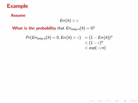
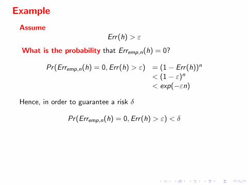
Example
AssumeErr(h) > ε
What is the probability that Erremp,n(h) = 0?
Pr(Erremp,n(h) = 0,Err(h) > ε) = (1− Err(h))n
< (1− ε)n
< exp(−εn)
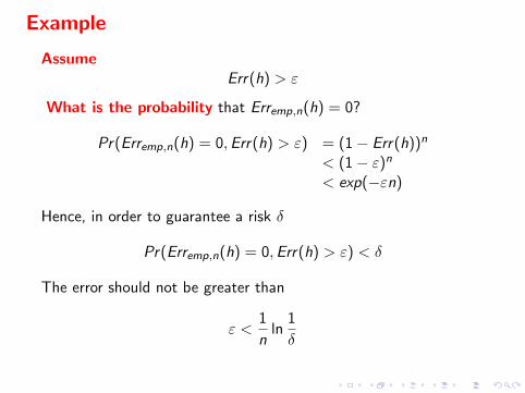
Hence, in order to guarantee a risk δ
Pr(Erremp,n(h) = 0,Err(h) > ε) < δ
The error should not be greater than
ε <1
nln
1
δ
Example
AssumeErr(h) > ε
What is the probability that Erremp,n(h) = 0?
Pr(Erremp,n(h) = 0,Err(h) > ε) = (1− Err(h))n
< (1− ε)n
< exp(−εn)
Hence, in order to guarantee a risk δ
Pr(Erremp,n(h) = 0,Err(h) > ε) < δ
The error should not be greater than
ε <1
nln
1
δ
Example
AssumeErr(h) > ε
What is the probability that Erremp,n(h) = 0?
Pr(Erremp,n(h) = 0,Err(h) > ε) = (1− Err(h))n
< (1− ε)n
< exp(−εn)
Hence, in order to guarantee a risk δ
Pr(Erremp,n(h) = 0,Err(h) > ε) < δ
The error should not be greater than
ε <1
nln
1
δ
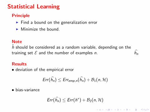
Statistical Learning
Principle
I Find a bound on the generalization error
I Minimize the bound.
Noteh should be considered as a random variable, depending on thetraining set E and the number of examples n. hn
Results• deviation of the empirical error
Err(hn) ≤ Erremp,n(hn) + B1(n,H)
• bias-variance
Err(hn) ≤ Err(h∗) + B2(n,H)
Approaches
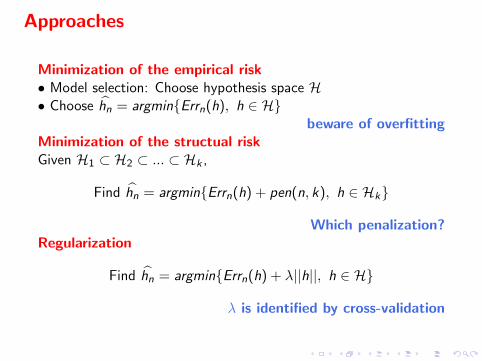
Minimization of the empirical risk• Model selection: Choose hypothesis space H• Choose hn = argmin{Errn(h), h ∈ H}
beware of overfittingMinimization of the structual riskGiven H1 ⊂ H2 ⊂ ... ⊂ Hk ,
Find hn = argmin{Errn(h) + pen(n, k), h ∈ Hk}
Which penalization?Regularization
Find hn = argmin{Errn(h) + λ||h||, h ∈ H}
λ is identified by cross-validation
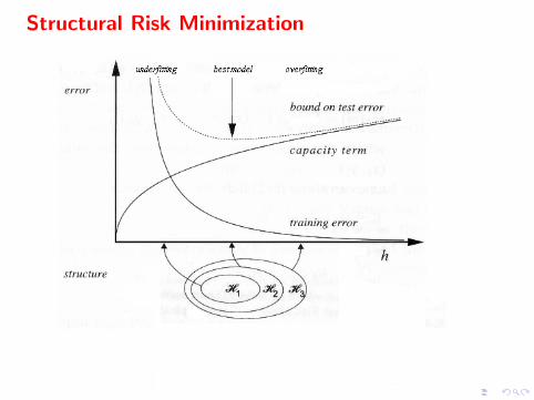
Structural Risk Minimization
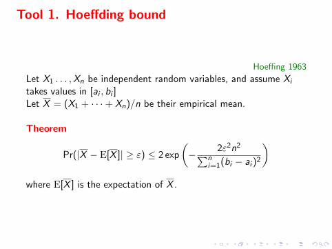
Tool 1. Hoeffding bound
Hoeffing 1963
Let X1 . . . ,Xn be independent random variables, and assume Xi
takes values in [ai , bi ]Let X = (X1 + · · ·+ Xn)/n be their empirical mean.
Theorem
Pr(|X − E[X ]| ≥ ε) ≤ 2 exp
(− 2ε2n2∑n
i=1(bi − ai )2
)where E[X ] is the expectation of X .
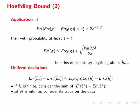
Hoeffding Bound (2)
Application: if
Pr(|Err(g)− Errn(g)| > ε) < 2e−2nε2
then with probability at least 1− δ
Err(g) ≤ Errn(g) +
√log 2/δ
2n
but this does not say anything about hn...Uniform deviations
|Err(hn)− Errn(hn)| ≤ suph∈H |Err(h)− Errn(h)|
• if H is finite, consider the sum of |Err(h)− Errn(h)|• sif H is infinite, consider its trace on the data
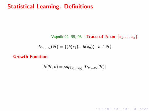
Statistical Learning. Definitions
Vapnik 92, 95, 98 Trace of H on {x1, . . . xn}
Trx1,..xn(H) = {(h(x1), ..h(xn)), h ∈ H}
Growth Function
S(H, n) = sup(x1,..xn)|Trx1,..xn(H)|
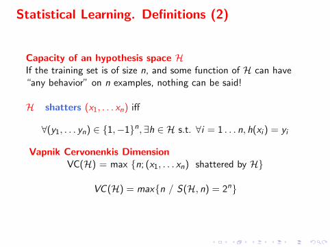
Statistical Learning. Definitions (2)
Capacity of an hypothesis space HIf the training set is of size n, and some function of H can have“any behavior” on n examples, nothing can be said!
H shatters (x1, . . . xn) iff
∀(y1, . . . yn) ∈ {1,−1}n,∃h ∈ H s.t. ∀i = 1 . . . n, h(xi ) = yi
Vapnik Cervonenkis DimensionVC(H) = max {n; (x1, . . . xn) shattered by H}
VC (H) = max{n / S(H, n) = 2n}
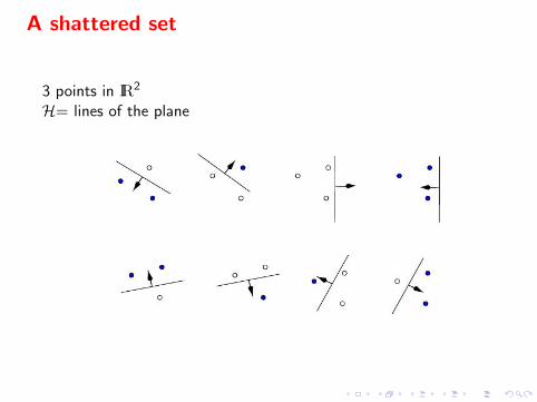
A shattered set
3 points in IR2
H= lines of the plane
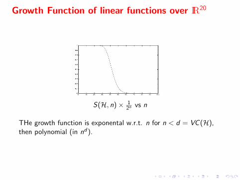
Growth Function of linear functions over IR20
S(H, n)× 12n vs n
THe growth function is exponental w.r.t. n for n < d = VC (H),then polynomial (in nd).
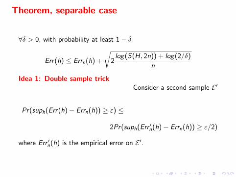
Theorem, separable case
∀δ > 0, with probability at least 1− δ
Err(h) ≤ Errn(h) +
√2log(S(H, 2n)) + log(2/δ)
n
Idea 1: Double sample trickConsider a second sample E ′
Pr(suph(Err(h)− Errn(h)) ≥ ε) ≤
2Pr(suph(Err ′n(h)− Errn(h)) ≥ ε/2)
where Err ′n(h) is the empirical error on E ′.
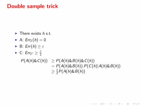
Double sample trick
I There exists h s.t.
I A: ErrE(h) = 0
I B: Err(h) ≥ εI C: ErrE ′ ≥ ε
2
P(A(h)&C (h)) ≥ P(A(h)&B(h)&C (h))= P(A(h)&B(h)).P(C (h)|A(h)&B(h))≥ 1
2P(A(h)&B(h))
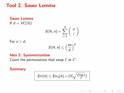
Tool 2. Sauer Lemma
Sauer LemmaIf d = VC (H)
S(H, n) =d∑
i=1
(ni
)For n > d ,
S(H, n) ≤(end
)dIdea 2: SymmetrizationCount the permutations that swap E et E ′.
Summary
Err(h) ≤ Errn(h) +O(√
d log nn )