Marc Desmet, Pr. Université de Tours · Marc Desmet, Pr. Université de Tours ... control of...
74
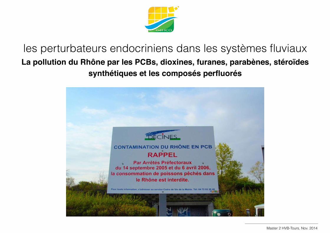
les perturbateurs endocriniens dans les systèmes fluviaux La pollution du Rhône par les PCBs, dioxines, furanes, parabènes, stéroïdes synthétiques et les composés perfluorés Marc Desmet, Pr. Université de Tours Master 2 HVB-Tours, Nov. 2014
Transcript of Marc Desmet, Pr. Université de Tours · Marc Desmet, Pr. Université de Tours ... control of...
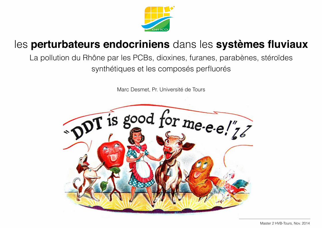
les perturbateurs endocriniens dans les systèmes fluviauxLa pollution du Rhône par les PCBs, dioxines, furanes, parabènes, stéroïdes
synthétiques et les composés perfluorés
Marc Desmet, Pr. Université de Tours
Master 2 HVB-Tours, Nov. 2014
1. Un perturbateur endocrinien potentiel est une substance ou un mélange exogène, possédant des propriétés susceptibles d’induire une perturbation endocrinienne dans un organisme intact, chez ses descendants ou au sein de (sous)- populations.
3. ces substances peuvent altérer différents processus tels que la production, l’utilisation et le stockage de l’énergie et plus largement la régulation du métabolisme et le développement. Certaines de ces substances peuvent par ailleurs avoir d’autres effets toxiques, notamment sur la reproduction, et nuire à la fertilité ou perturber le développement du foetus
Endocrine Society 2012/OMS 2012:
Définitions
Master 2 HVB-Tours, Nov. 2014
1. Reproduction 2. Métabolisme 3. systèmes nerveux, immunitaire, cardio-vasculaire 4. fonction thyroïdienne 5. Pathologies auxquelles l'organisme humain peut être exposé par différentes voies (orale, respiratoire, cutanée).
Endocrine Society 2012/OMS 2012:
Conséquences sanitaires détaillées
Master 2 HVB-Tours, Nov. 2014

Effets mimétiques, de blocage ou perturbant d’une hormone
Master 2 HVB-Tours, Nov. 2014
State of the Science of Endocrine Disrupting Chemicals - 2012
4
HypothalamusProduction ofantidiuretic hormone (ADH),oxytocin and regulatoryhormones
Pituitary GlandAdenohypophysis (anterior lobe):Adrenocorticotropic hormone,Thyroid stimulating hormone,Growth hormone, Prolactin,Follicle stimulating hormone,Luteinizing hormone,Melanocyte stimulatinghormone,Neurohypophysis(posterior lobe):Release of oxytocinand ADH
Thyroid GlandThyroxineTriiodothyronineCalcitonin
Thymus(Undergoes atrophyduring childhood)Thymosins
Adrenal GlandsEach suprarenal gland issubdivided into:Suprarenal medulla;
EpinephrineNorepinephrine
Suprarenal cortex:Cortisol, corticosterone,aldosterone, androgens
Parathyroid Glands(on posterior surface ofthyroid gland)Parathyroid hormone
HeartAtrial natriureticpeptide
KidneyErythropoietinCalcitriolRenin
Gastrointestinal TractGhrelin, cholecystokinin,glucagon-like peptide,peptide YY
Pancreatic IsletsInsulin, glucagon
GonadsTestes (male):
Androgens (especiallytestosterone), inhibin
Ovaries (female):Estrogens, progestins,inhibin
Ovary
Testis
Pineal GlandMelatonin
Adipose TissueLeptin, adiponectin,others
Figure1.1. What are hormones? Hormones are molecules produced by specialized cells in a large variety of glands and tissues. These molecules travel through the blood to produce effects at sometimes distant target tissues.
1.2.1 Hormones control major physiological processesHormones are important to both vertebrates and invertebrates. They are essential for controlling a large number of processes in the body from early processes such as cell differentiation during embryonic development and organ formation, to the control of tissue and organ function in adulthood (Melmed & Williams, 2011). A well-known example is that of insulin, a small protein hormone produced by specialized cells in the pancreas called “beta cells”. These cells are stimulated
to secrete insulin into the blood by the direct action of the sugar, glucose. As blood levels of glucose rise during and after a meal, it enters the beta cells through a specific protein transporter on the cell membrane and is converted inside the cell to the high-energy compound ATP. This process directly causes changes inside the beta cells, resulting in the secretion of insulin that was already produced and stored in anticipation of these events. Insulin then travels through the blood to many different tissues and cells, causing glucose to be taken up into those tissues via specific membrane receptors linked to transport systems.
What is endocrine disruption all about?
7
ATP
cAMP
1
2
3
41
2
3
4
5
6
Steroidhormone
Hormone-receptorcomplex
Receptorprotein
Receptorprotein
Newprotein
Nucleus
DNA
mRNA
Plasmamembraneof target cell
Plasmamembraneof target cellCytoplasm
Cytoplasm
Secondmessenger
Activatedenzyme
Effect on cellular function,such as glycogenbreakdown
Nonsteroidhormone(first messenger)
intracellular proteinswith enzymatic
activity
receptor withintrinsic enzymatic
activity
enzyme-associatedreceptor
(recruiter receptor)
Cytosol
7-helix transmembranereceptor
ion-channelreceptor
ions
Extracellular
Figure1.2. Hormones produce effects in the body exclusively by acting on receptors. There are different classes of receptors. A (Upper left): Nuclear receptors bind to steroid and thyroid hormones and act directly to regulate gene expression. B (Upper right): Membrane receptors bind to protein and amine hormones and produce effects inside the cell by a second messenger system. C (lower): Membrane receptors can be linked to a variety of second messenger systems. In addition, there are “co-regulator” proteins that link the hormone receptor to the transcriptional apparatus, and these co-regulators can differ between cells, which can affect the way a nuclear hormone receptor can function. These are important considerations because we know that environmental chemicals can interact directly with some nuclear receptors in ways that change their ability to interact with gene regulatory processes, thereby producing effects that are unexpected. These effects need to be identified and considered when we think about endocrine disruption.
transporter in other tissues, which directly stimulates glucose uptake. This occurs because the insulin receptor is linked to different kinds of cellular machinery in different cells. All protein and peptide hormones act in a similar fashion; there are specialized receptors on the outside of cells that “transduce” the effect of hormone binding to the inside of the cell. These
receptors are linked to different sets of proteins in different cells, which cause the cells to respond differently to the same hormone. Interestingly, there are also membrane receptors for some steroid hormones that also act via nuclear receptors. Estrogens and progestins both act through nuclear and membrane receptors. In these cases the membrane receptor is
WHO/HSE, 2013
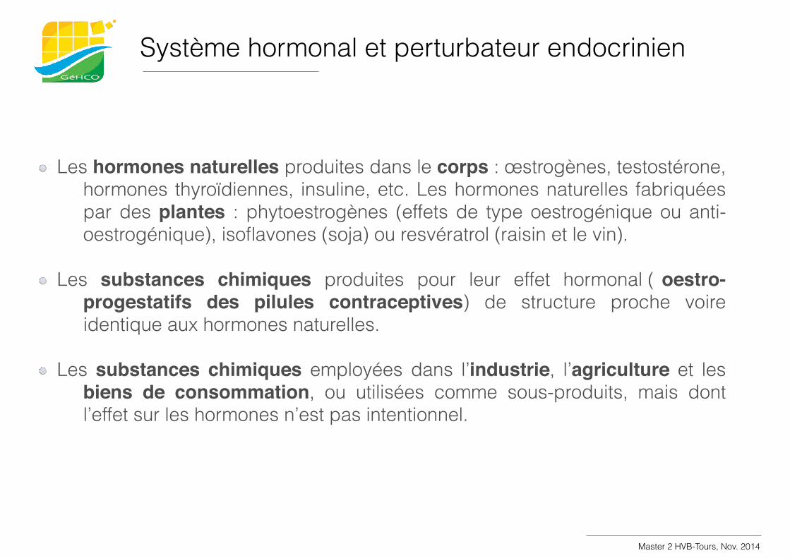
Les hormones naturelles produites dans le corps : œstrogènes, testostérone, hormones thyroïdiennes, insuline, etc. Les hormones naturelles fabriquées par des plantes : phytoestrogènes (effets de type oestrogénique ou anti-oestrogénique), isoflavones (soja) ou resvératrol (raisin et le vin).
Les substances chimiques produites pour leur effet hormonal ( oestro-progestatifs des pilules contraceptives) de structure proche voire identique aux hormones naturelles.
Les substances chimiques employées dans l’industrie, l’agriculture et les biens de consommation, ou utilisées comme sous-produits, mais dont l’effet sur les hormones n’est pas intentionnel.
Système hormonal et perturbateur endocrinien
Master 2 HVB-Tours, Nov. 2014
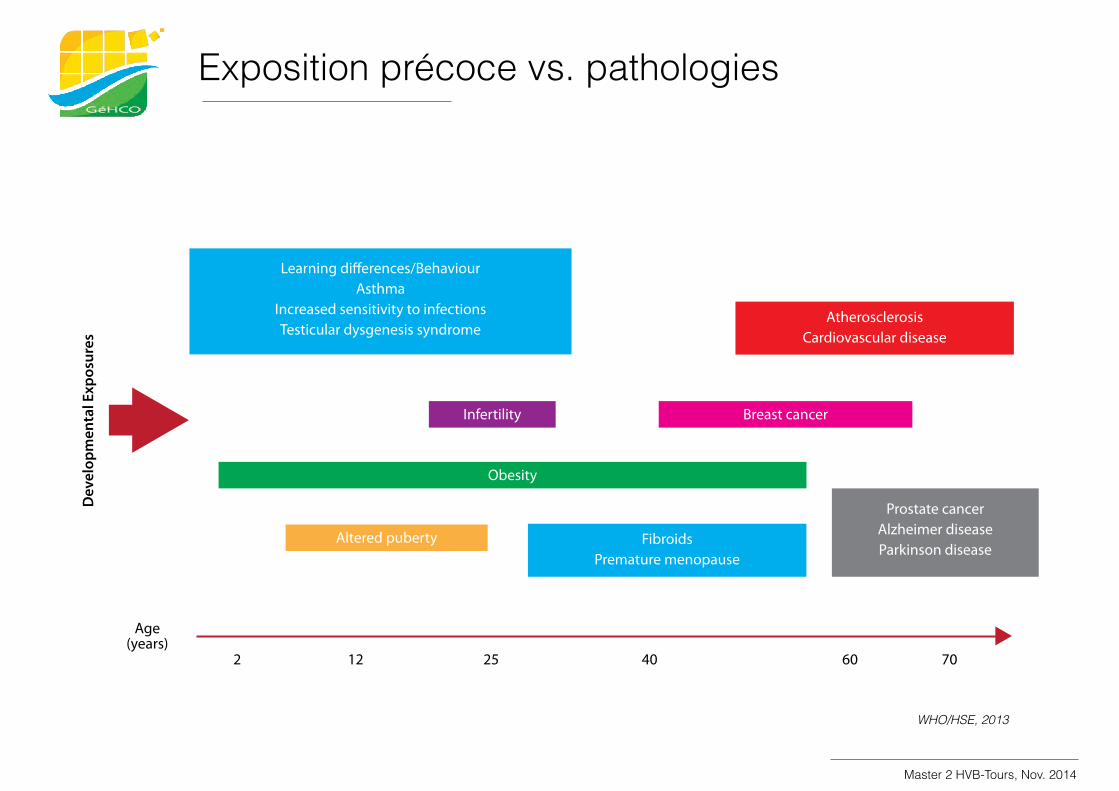
Exposition précoce vs. pathologies
13
Figure 15. Examples of potential diseases and dysfunctions originating from early exposures to EDCs.
are not likely to be evident at birth, but may show up only later in life, from a few months to decades later (Figures 14 and 15). These developmental effects emphasize that babies and children are not just little adults!
Some EDCs produce effects that can cross generations (transgenerational effects), such that exposure of a pregnant woman or wild
animal may affect not only the development of her offspring but also their offspring over several generations. This means that the increase in disease rates we are seeing today could in part be due to exposures of our grandparents to EDCs, and these effects could increase over each generation due to both transgenerational transmission of the altered programming and continued exposure across generations.
Dev
elop
men
tal E
xpos
ures
Age(years)
2 12 25 40 60 70
Presentation of Disease over the Lifespan
Learning differences/BehaviourAsthma
Increased sensitivity to infectionsTesticular dysgenesis syndrome
AtherosclerosisCardiovascular disease
Infertility Breast cancer
Obesity
Altered puberty FibroidsPremature menopause
Prostate cancerAlzheimer diseaseParkinson disease
WHO/HSE, 2013
Master 2 HVB-Tours, Nov. 2014
Quels sont les perturbateurs ?
Master 2 HVB-Tours, Nov. 2014
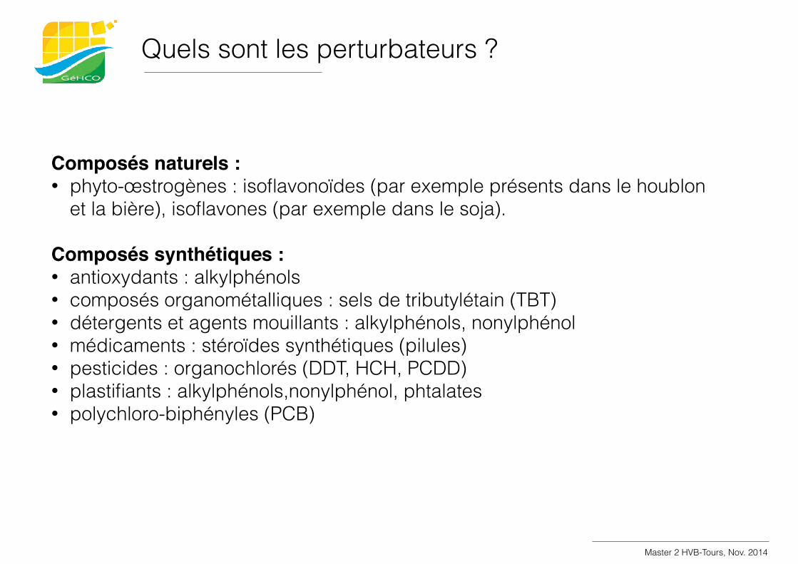
Composés naturels : • phyto-œstrogènes : isoflavonoïdes (par exemple présents dans le houblon
et la bière), isoflavones (par exemple dans le soja).
Composés synthétiques : • antioxydants : alkylphénols • composés organométalliques : sels de tributylétain (TBT) • détergents et agents mouillants : alkylphénols, nonylphénol • médicaments : stéroïdes synthétiques (pilules) • pesticides : organochlorés (DDT, HCH, PCDD) • plastifiants : alkylphénols,nonylphénol, phtalates • polychloro-biphényles (PCB)
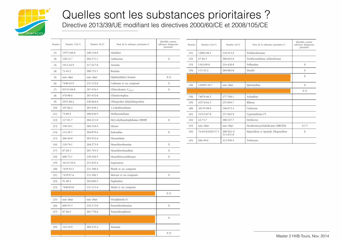
Quelles sont les substances prioritaires ? Directive 2013/39/UE modifiant les directives 2000/60/CE et 2008/105/CE
Master 2 HVB-Tours, Nov. 2014
Numéro Numéro CAS ( 1 ) Numéro UE ( 2 ) Nom de la substance prioritaire ( 3 ) Identifiée comme
substance dangereuse prioritaire
(1) 15972-60-8 240-110-8 Alachlore
(2) 120-12-7 204-371-1 Anthracène X
(3) 1912-24-9 217-617-8 Atrazine
(4) 71-43-2 200-753-7 Benzène
(5) sans objet sans objet Diphényléthers bromés X ( 4 )
(6) 7440-43-9 231-152-8 Cadmium et ses composés X
(7) 85535-84-8 287-476-5 Chloroalcanes, C 10-13 X
(8) 470-90-6 207-432-0 Chlorfenvinphos
(9) 2921-88-2 220-864-4 Chlorpyrifos (éthylchlorpyrifos)
(10) 107-06-2 203-458-1 1,2-dichloroéthane
(11) 75-09-2 200-838-9 Dichlorométhane
(12) 117-81-7 204-211-0 Di(2-ethylhexyle)phthalate (DEHP) X
(13) 330-54-1 206-354-4 Diuron
(14) 115-29-7 204-079-4 Endosulfan X
(15) 206-44-0 205-912-4 Fluoranthène
(16) 118-74-1 204-273-9 Hexachlorobenzène X
(17) 87-68-3 201-765-5 Hexachlorobutadiène X
(18) 608-73-1 210-168-9 Hexachlorocyclohexane X
(19) 34123-59-6 251-835-4 Isoproturon
(20) 7439-92-1 231-100-4 Plomb et ses composés
(21) 7439-97-6 231-106-7 Mercure et ses composés X
(22) 91-20-3 202-049-5 Naphtalène
(23) 7440-02-0 231-111-4 Nickel et ses composés
(24) sans objet sans objet Nonylphénols X ( 5 )
(25) sans objet sans objet Octylphénols ( 6 )
(26) 608-93-5 210-172-0 Pentachlorobenzène X
(27) 87-86-5 201-778-6 Pentachlorophénol
(28) sans objet sans objet Hydrocarbures aromatiques polycycliques (HAP) ( 7 )
X
(29) 122-34-9 204-535-2 Simazine
(30) sans objet sans objet Composés du tributylétain X ( 8 )
Numéro Numéro CAS ( 1 ) Numéro UE ( 2 ) Nom de la substance prioritaire ( 3 ) Identifiée comme
substance dangereuse prioritaire
(31) 12002-48-1 234-413-4 Trichlorobenzène
(32) 67-66-3 200-663-8 Trichlorométhane (chloroforme)
(33) 1582-09-8 216-428-8 Trifluraline X
(34) 115-32-2 204-082-0 Dicofol X
(35) 1763-23-1 217-179-8 Acide perfluorooctanesulfonique et ses dérivés (perfluoro-octanesulfonate PFOS)
X
(36) 124495-18-7 sans objet Quinoxyfène X
(37) sans objet sans objet Dioxines et composés de type dioxine X ( 9 )
(38) 74070-46-5 277-704-1 Aclonifène
(39) 42576-02-3 255-894-7 Bifénox
(40) 28159-98-0 248-872-3 Cybutryne
(41) 52315-07-8 257-842-9 Cypermethrine ( 10 )
(42) 62-73-7 200-547-7 Dichlorvos
(43) sans objet sans objet Hexabromocyclododécanes (HBCDD) X ( 11 )
(44) 76-44-8/1024-57-3 200-962-3/ 213-831-0
Heptachlore et époxyde d’heptachlore X
(45) 886-50-0 212-950-5 Terbutryne
(1 ) CAS: Chemical Abstracts Service.
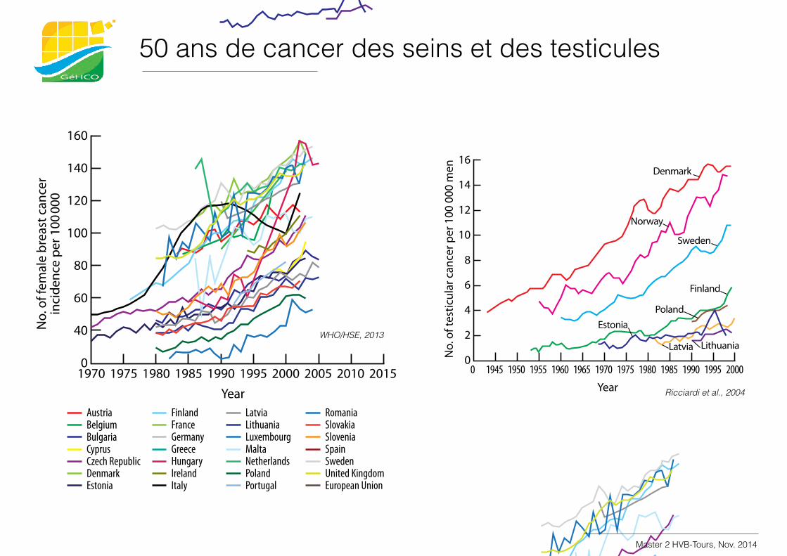
50 ans de cancer des seins et des testicules
WHO/HSE, 2013
8 State of the Science of Endocrine Disrupting Chemicals – 2012
Figure 8. Female breast cancer incidence across Europe (data from http://data.euro.who.int/hfadb/).
Figure 7.rates across northern Europe
used with permission of the publisher).
♦ A significant increase in reproductive problems in some regions of the world over the last few decades points to a strong role for unidentified environmental factors in disease etiology.
♦ Incidences of endocrine cancers, illustrated by country or region in Figures 7 and 8 for testicular cancer and breast cancer, respectively, have also increased during the same period.
♦ In certain parts of the world, there has been a significant decrease in human fertility rates, which occurred during one generation. There is also a notable rise in the use of assisted reproductive services.
♦ An increasing number of chemicals to which all humans in industrialized areas are exposed have been shown to interfere with hormone synthesis, action or metabolism.
♦ Experimental animal studies or studies with cells grown in culture have shown that many of these chemicals can also interfere with the development and function of mammalian endocrine systems.
In adults, EDC exposures have recently been linked with obesity (Figure 9), cardiovascular disease, diabetes and metabolic syndrome. Many of these diseases and disorders are increasing in incidence, some globally. The global health expenditure on diabetes alone was expected to a total of at least 376 billion USD in 2010 and rise to US$ 490 billion in 2030—reaching 12% of all per capita health-care
20001945 1950 1955 1960 1965 1970 1975 1980 1985 1990 1995
14
16
12
10
8
6
4
2
00
No.
of t
estic
ular
can
cer p
er 1
00 0
00 m
en Denmark
Norway
Sweden
Finland
PolandEstonia
Latvia Lithuania
Year
160
140
120
100
20152000 20102005
80
60
40
01970 1975 1980 1990 19951985
AustriaBelgiumBulgariaCyprusCzech RepublicDenmarkEstonia
FinlandLithuania
Malta
SlovakiaSlovenia
Sweden
GermanyFrance
GreeceHungaryIrelandItaly
Latvia
Luxembourg
NetherlandsPolandPortugal
Romania
Spain
United KingdomEuropean Union
No.
of f
emal
e br
east
can
cer
inci
denc
e pe
r 100
000
Year
5. Why should we be concerned?—Human disease trends
Master 2 HVB-Tours, Nov. 2014
Ricciardi et al., 2004
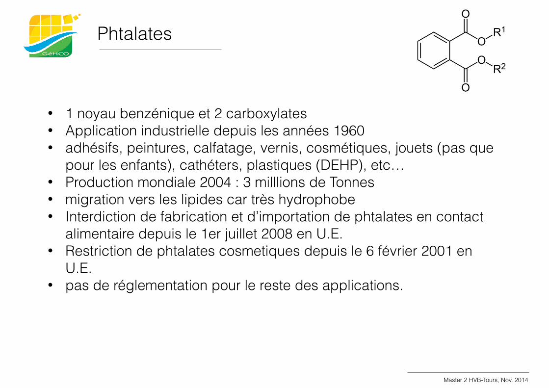
Phtalates
Master 2 HVB-Tours, Nov. 2014
• 1 noyau benzénique et 2 carboxylates • Application industrielle depuis les années 1960 • adhésifs, peintures, calfatage, vernis, cosmétiques, jouets (pas que
pour les enfants), cathéters, plastiques (DEHP), etc… • Production mondiale 2004 : 3 milllions de Tonnes • migration vers les lipides car très hydrophobe • Interdiction de fabrication et d’importation de phtalates en contact
alimentaire depuis le 1er juillet 2008 en U.E. • Restriction de phtalates cosmetiques depuis le 6 février 2001 en
U.E. • pas de réglementation pour le reste des applications.
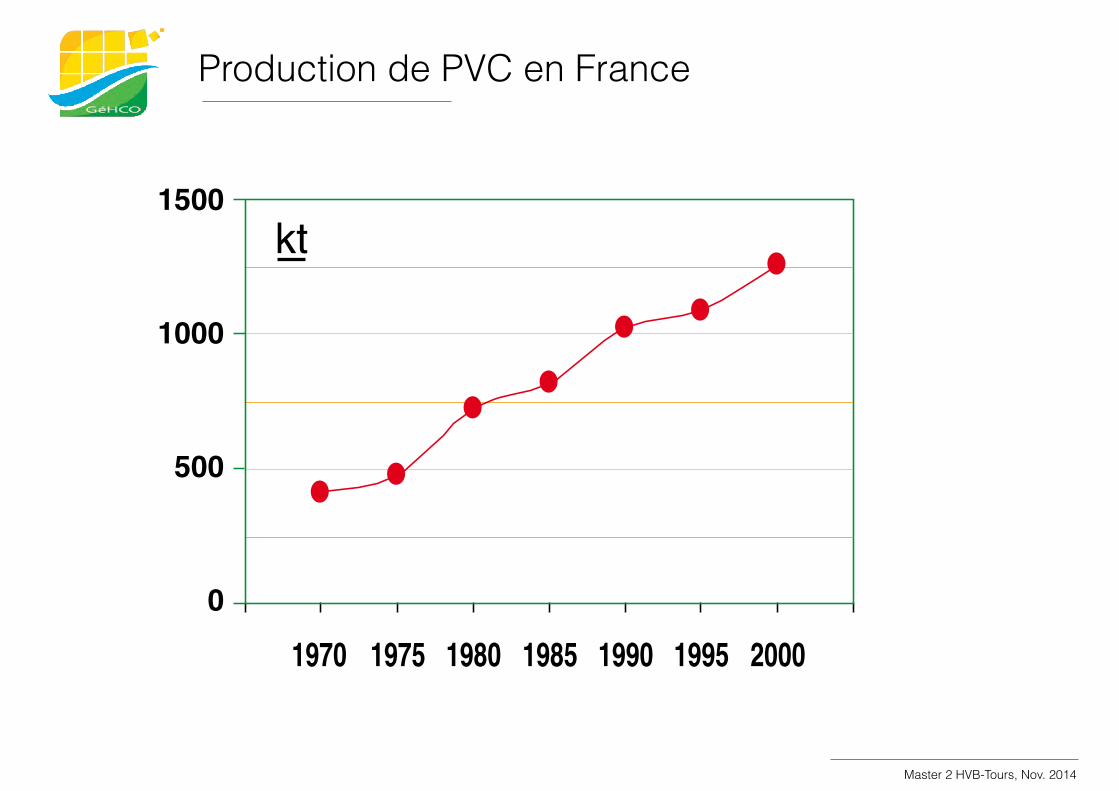
Production de PVC en France
Master 2 HVB-Tours, Nov. 2014
29
Figure 17 : Evolution de la production de PVC en France au cours des 30 dernières années.
Des contaminants longtemps ignorés
Les phatalates sont des molécules organiques (diesters de l’acide ortho-phtalique) synthétisées volontairement pour leurs propriétés plastifiantes depuis les années 1930.
La production mondiale de phtalates est passée de 1,8 million de tonnes en 1975 à 4,3 millions de tonnes en 2006 (Peijnenburg et Struijs, 2006), le quart étant représenté par le di-(2-éthylhexyl) phtalate (DEHP) qui entre dans la composition finale du chlorure de polyvinyle (PVC) (Hervé-Bazin et al., 2001). En France, ce composé est produit à raison de 60 000 tonnes par an à Chauny dans l’Aisne, soit 10 % de la production européenne (INERIS). L’exposition humaine à ce composé est importante du fait de l’augmentation de la fabrication au cours des 30 dernières années (figure 17).
Alors que les HAP et PCB ont été suivis depuis les années 70, la prise en considération des phtalates est beaucoup plus récente et date des années 90. Seules quelques rares données de phtalates totaux, difficilement exploitables, sont disponibles pour les années antérieures.
Certains phtalates peuvent avoir des effets néfastes sur la santé tels que des perturbations endocriniennes (poissons, mammifères) ou des effets carcinogènes* et mutagènes (rongeurs).
Ainsi, le DEHP est inscrit par la Communauté Européenne sur la liste des 33 substances dangereuses à surveiller dans les rivières.
L’interdiction d’emploi du DEHP dans les films alimentaires à usage unique a été précisée par la directive européenne 2007/19/CE. Cependant, le di-butyl et le butylbenzyl phtalate y sont autorisés dans les objets à usage unique en contact avec des aliments non gras. Par ailleurs, le DEHP (directive 2004/93/CE) ainsi que les n-pentyl, di-n-pentyl, l’iso-pentyl, le di iso-pentyl et le butylbenzyl phtalates (directive 2005/80/CE) ont été interdits dans les cosmétiques. Pour les eaux de consommation, une valeur limite pour le DEHP de 8 µg/L a été édictée par l’Organisation Mondiale de la Santé (OMS) et de 6 µg/L par l’Environmental Protection Agency américaine (EPA, 2002).
De plus, dans le cadre de la nouvelle réglementation chimique européenne REACH, le DnBP, le BBP et le DEHP figurent actuellement sur une première liste de substances classées comme extrêmement préoccupantes pour l’Homme et l’environnement et seront inscrits dans l’annexe XV du programme. Les substances figurant sur cette liste devront être abandonnées et remplacées par d’autres plus appropriées et plus sûres.
1500
1970 1975 1980 1985 1990 1995 2000
1000
500
0
kt
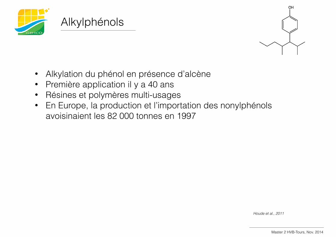
Alkylphénols
Houde et al., 2011
Master 2 HVB-Tours, Nov. 2014
• Alkylation du phénol en présence d’alcène • Première application il y a 40 ans • Résines et polymères multi-usages • En Europe, la production et l’importation des nonylphénols
avoisinaient les 82 000 tonnes en 1997
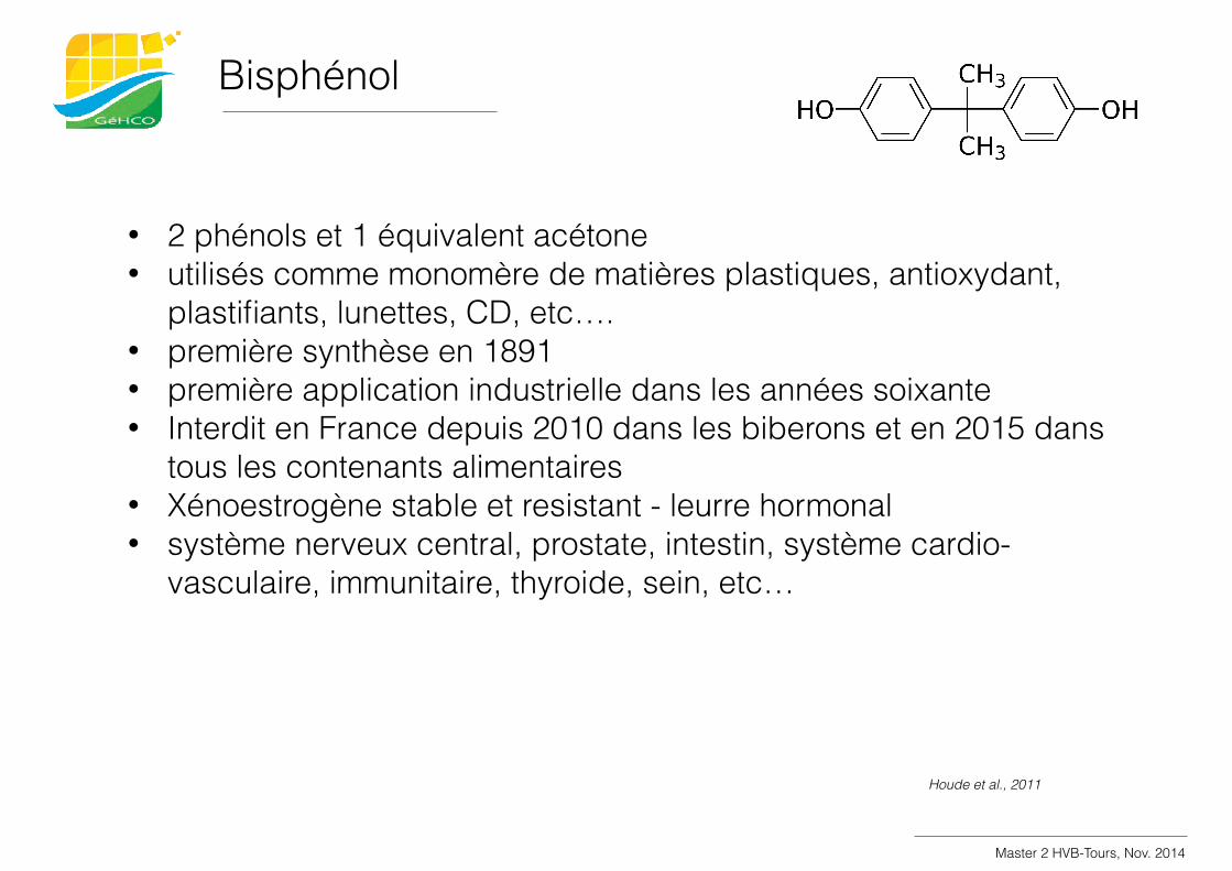
Bisphénol
Houde et al., 2011
Master 2 HVB-Tours, Nov. 2014
• 2 phénols et 1 équivalent acétone • utilisés comme monomère de matières plastiques, antioxydant,
plastifiants, lunettes, CD, etc…. • première synthèse en 1891 • première application industrielle dans les années soixante • Interdit en France depuis 2010 dans les biberons et en 2015 dans
tous les contenants alimentaires • Xénoestrogène stable et resistant - leurre hormonal • système nerveux central, prostate, intestin, système cardio-
vasculaire, immunitaire, thyroide, sein, etc…
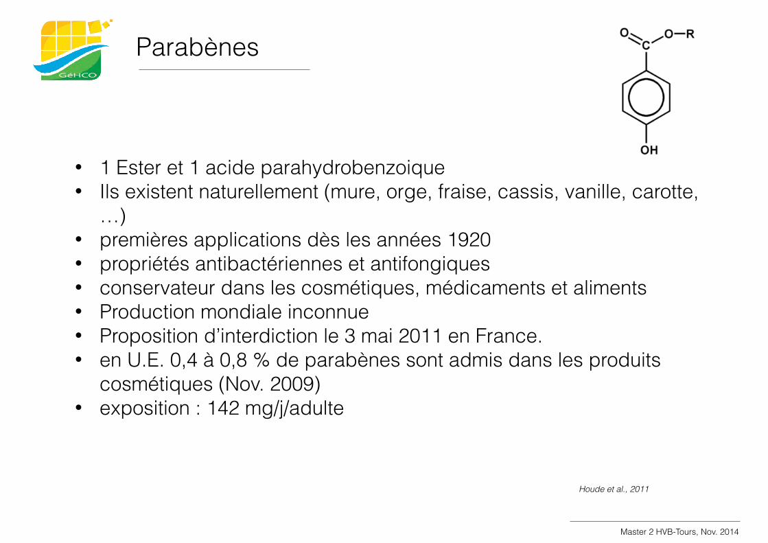
Parabènes
Houde et al., 2011
Master 2 HVB-Tours, Nov. 2014
• 1 Ester et 1 acide parahydrobenzoique • Ils existent naturellement (mure, orge, fraise, cassis, vanille, carotte,
…) • premières applications dès les années 1920 • propriétés antibactériennes et antifongiques • conservateur dans les cosmétiques, médicaments et aliments • Production mondiale inconnue • Proposition d’interdiction le 3 mai 2011 en France. • en U.E. 0,4 à 0,8 % de parabènes sont admis dans les produits
cosmétiques (Nov. 2009) • exposition : 142 mg/j/adulte
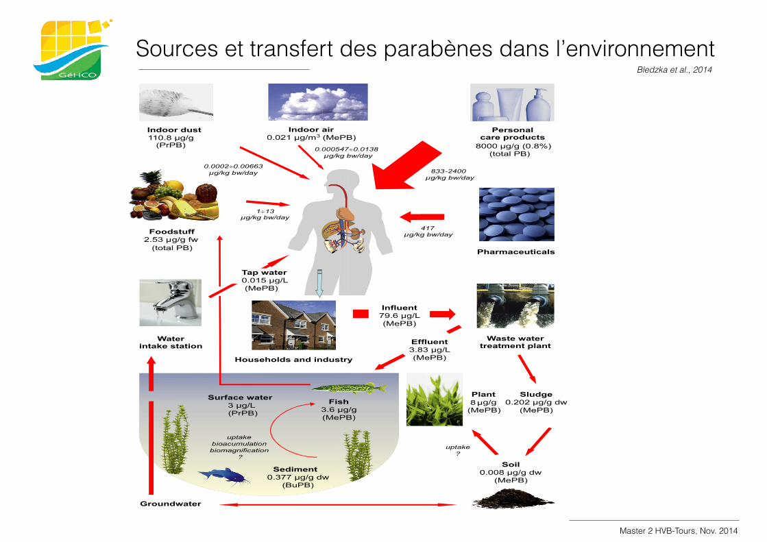
Sources et transfert des parabènes dans l’environnement Bledzka et al., 2014
Master 2 HVB-Tours, Nov. 2014
is considerably more complex. It also includes influencing the productionand break-down of endogenous steroids and receptor synthesis (Waringand Harris, 2011; Whitehead and Rice, 2006).
The reproductive system is vulnerable and therefore it is highlyaffected by EDCs. Additionally, EDCs can also influence various steroidsensitive tissues, thereby disturbing the functioning of the central
Fig. 1. Sources and pathways of human exposure and fate of parabens in environment (maximum concentration values are shown; based on data discussed inparagraphs 1.4, 2, 3.1;bw — body weight, dw— dry weight, fw — fresh weight).
32 D. Błędzka et al. / Environment International 67 (2014) 27–42
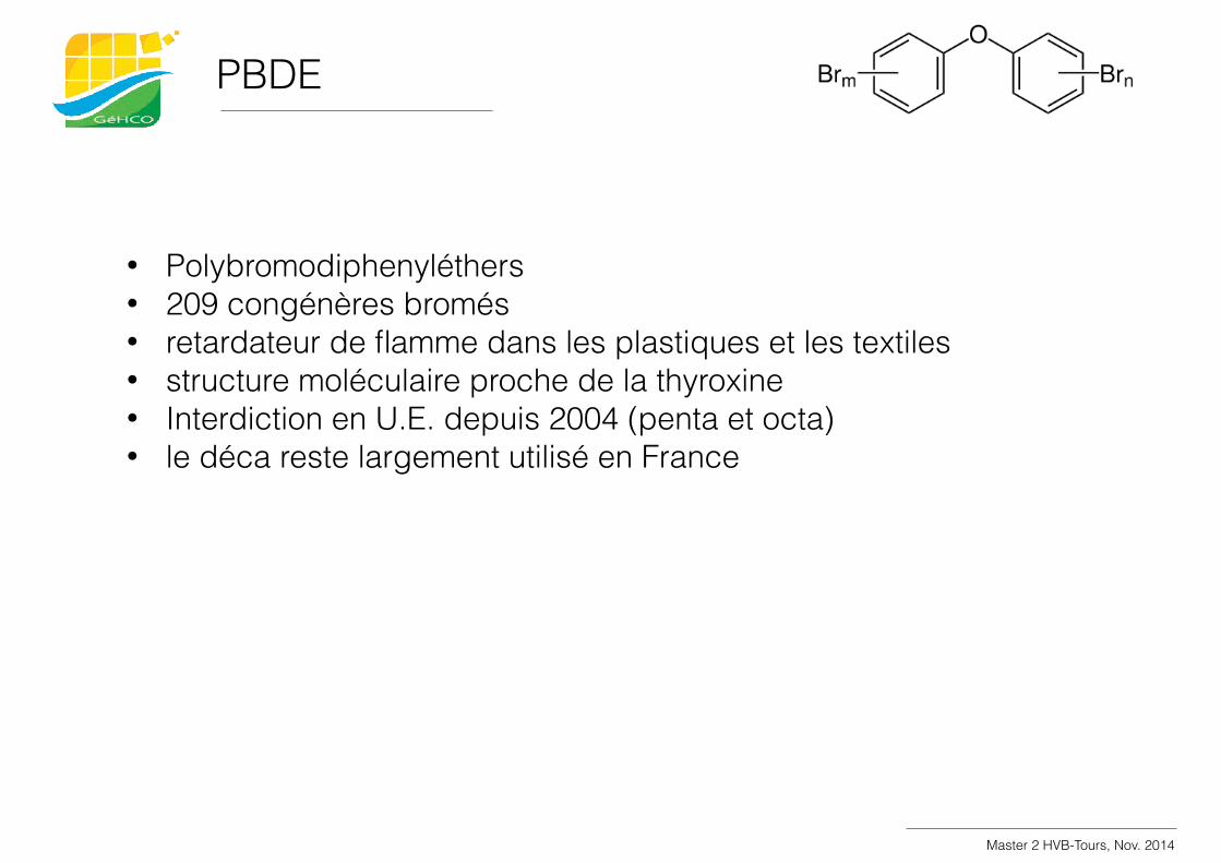
PBDE
Master 2 HVB-Tours, Nov. 2014
• Polybromodiphenyléthers • 209 congénères bromés • retardateur de flamme dans les plastiques et les textiles • structure moléculaire proche de la thyroxine • Interdiction en U.E. depuis 2004 (penta et octa) • le déca reste largement utilisé en France
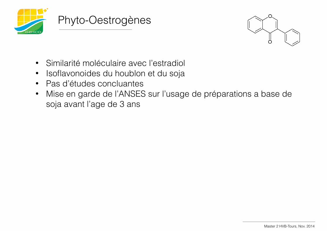
Phyto-Oestrogènes
Master 2 HVB-Tours, Nov. 2014
• Similarité moléculaire avec l’estradiol • Isoflavonoides du houblon et du soja • Pas d’études concluantes • Mise en garde de l’ANSES sur l’usage de préparations a base de
soja avant l’age de 3 ans
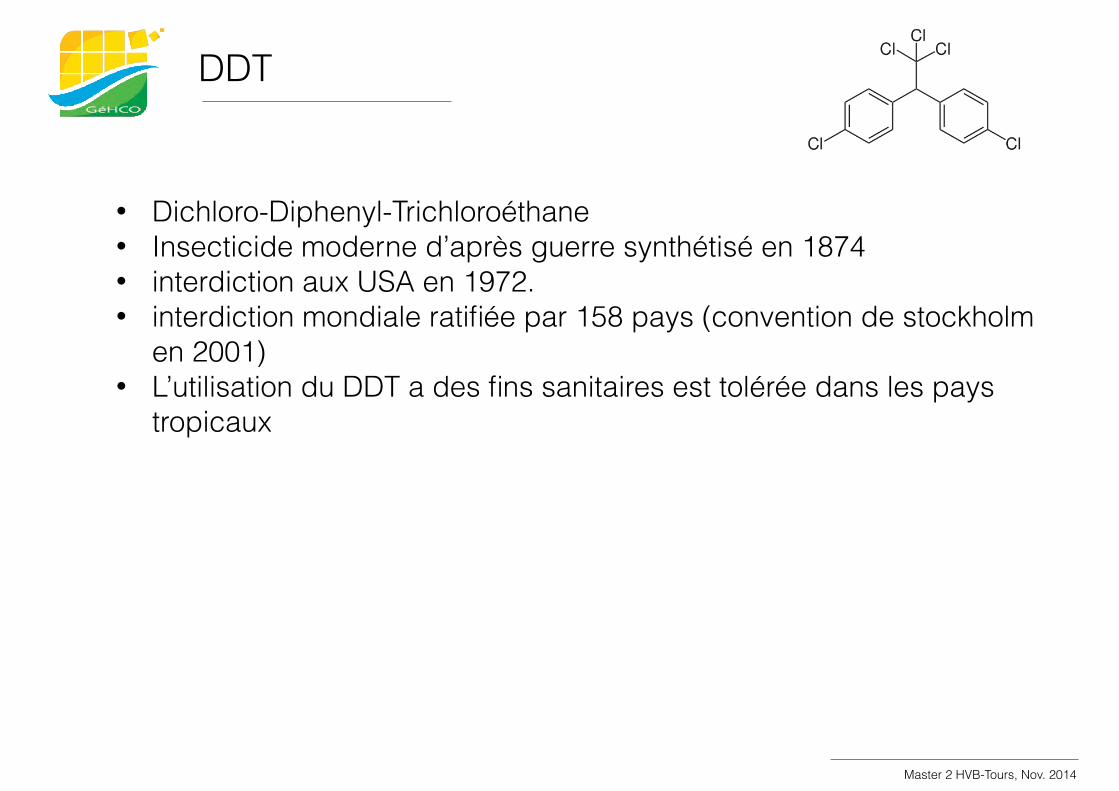
DDT
Master 2 HVB-Tours, Nov. 2014
• Dichloro-Diphenyl-Trichloroéthane • Insecticide moderne d’après guerre synthétisé en 1874 • interdiction aux USA en 1972. • interdiction mondiale ratifiée par 158 pays (convention de stockholm
en 2001) • L’utilisation du DDT a des fins sanitaires est tolérée dans les pays
tropicaux
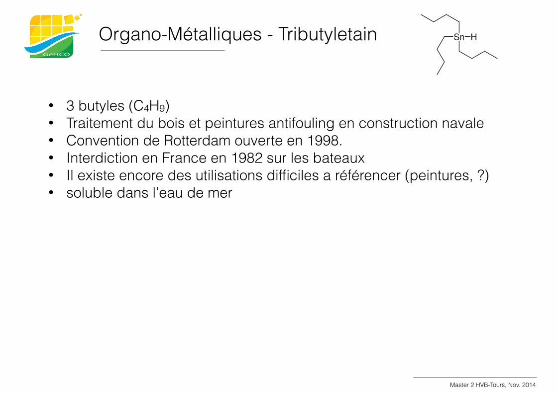
Organo-Métalliques - Tributyletain
Master 2 HVB-Tours, Nov. 2014
• 3 butyles (C4H9) • Traitement du bois et peintures antifouling en construction navale • Convention de Rotterdam ouverte en 1998. • Interdiction en France en 1982 sur les bateaux • Il existe encore des utilisations difficiles a référencer (peintures, ?) • soluble dans l’eau de mer
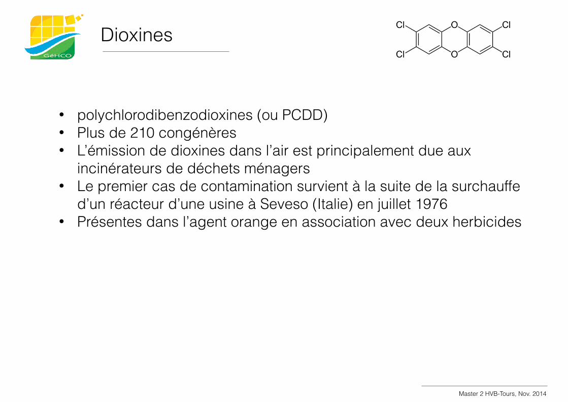
Dioxines
Master 2 HVB-Tours, Nov. 2014
• polychlorodibenzodioxines (ou PCDD) • Plus de 210 congénères • L’émission de dioxines dans l’air est principalement due aux
incinérateurs de déchets ménagers • Le premier cas de contamination survient à la suite de la surchauffe
d’un réacteur d’une usine à Seveso (Italie) en juillet 1976 • Présentes dans l’agent orange en association avec deux herbicides
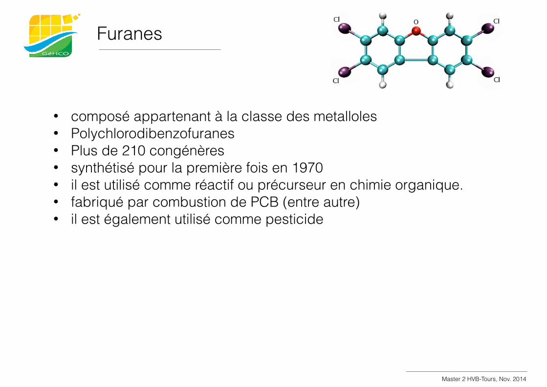
Furanes
Master 2 HVB-Tours, Nov. 2014
• composé appartenant à la classe des metalloles • Polychlorodibenzofuranes • Plus de 210 congénères • synthétisé pour la première fois en 1970 • il est utilisé comme réactif ou précurseur en chimie organique. • fabriqué par combustion de PCB (entre autre) • il est également utilisé comme pesticide
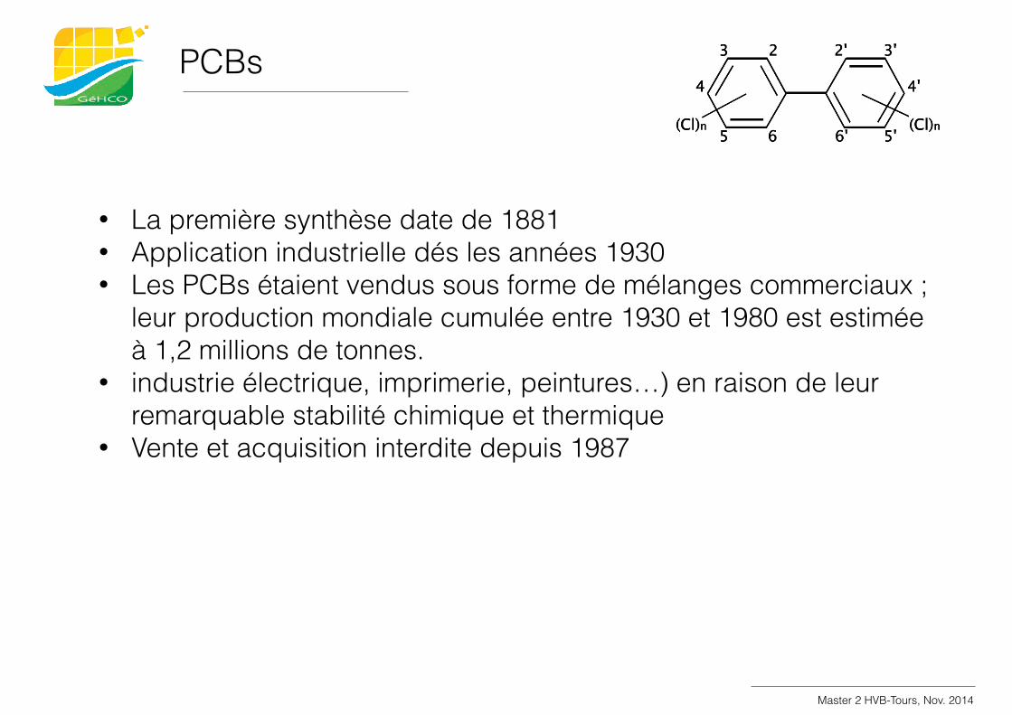
PCBs
Master 2 HVB-Tours, Nov. 2014
• La première synthèse date de 1881 • Application industrielle dés les années 1930 • Les PCBs étaient vendus sous forme de mélanges commerciaux ;
leur production mondiale cumulée entre 1930 et 1980 est estimée à 1,2 millions de tonnes.
• industrie électrique, imprimerie, peintures…) en raison de leur remarquable stabilité chimique et thermique
• Vente et acquisition interdite depuis 1987
Transfert des PCBs dans l’environnement
Chevreuil et al., 2012
Master 2 HVB-Tours, Nov. 2014
14
Les poLychLorobiphényLes (pcb)
Figure 2 : Modes de dépôt atmosphérique.
transfrontières. Cette convention a donné naissance au programme de suivi EMEP (European Monitoring and Evaluation Programme). Bien que motivés au départ par la question des pluies acides, les travaux induits par cette convention s’ouvriront à d’autres composés, notamment les POP, ce qui sera acté par le protocole d’Aarhus en 1998. Ainsi, des séries de données de retombée atmosphérique ou de concentrations dans l’air dans des stations positionnées pour être «exemptes de sources de contamination proches» sont disponibles à partir de 1995, soit bien après la période de contamination supposée la plus élevée.
De fait, peu de tendances temporelles peuvent être mises en évidence. Dans une station donnée, les
concentrations dans la pluie ont diminué, en teneur de fond, de 0,5 à 0,3 ng/L de 7-PCB en 10 ans (1996-2006). Mais dans une autre, la retombée de PCB est particulièrement intense au cours de quelques courtes périodes de quelques mois réparties aléatoirement au cours des 10 années de suivi (source : banque de données EMEP). Quelle que soit l’échelle, planétaire ou réduite au nord de l’Europe, à laquelle on observe l’évolution, il est difficile aujourd’hui de tirer des tendances complètement généralisables.
On note que toutes les stations EMEP produisant régulièrement des données de PCB sont situées en Europe du nord. Il n’existe aucune station active en France ou en Europe du sud.
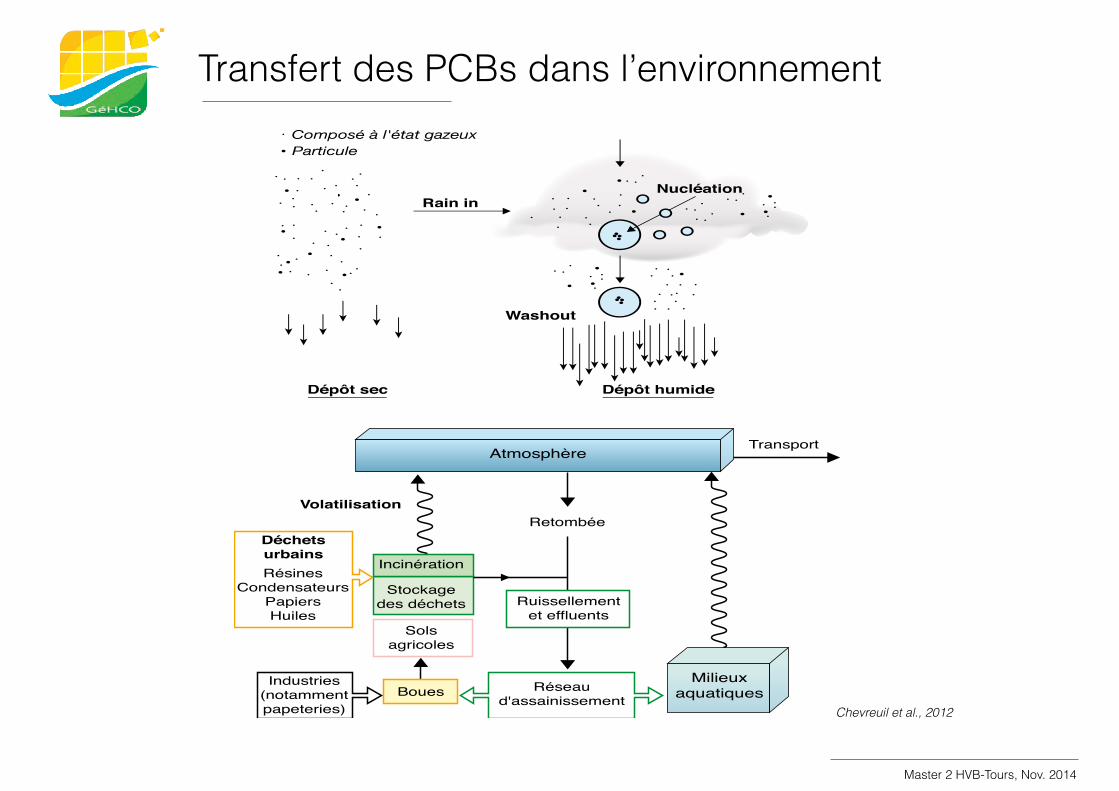
Composé à l'état gazeuxParticule
Rain inNucléation
Washout
Dépôt sec Dépôt humide
Atmosphère
Volatilisation
Déchetsurbains
Boues
Retombée
RésinesCondensateurs
PapiersHuiles
Industries(notammentpapeteries)
Réseaud'assainissement
Milieuxaquatiques
Incinération
Stockagedes déchets
Solsagricoles
Ruissellementet effluents
Transport
Figure 3 : Cycle des PCB dans l’environnement.
Composés perfluorés
Master 2 HVB-Tours, Nov. 2014
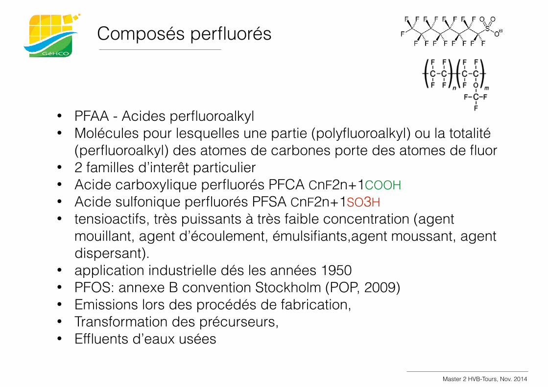
• PFAA - Acides perfluoroalkyl • Molécules pour lesquelles une partie (polyfluoroalkyl) ou la totalité
(perfluoroalkyl) des atomes de carbones porte des atomes de fluor • 2 familles d’interêt particulier • Acide carboxylique perfluorés PFCA CnF2n+1COOH • Acide sulfonique perfluorés PFSA CnF2n+1SO3H • tensioactifs, très puissants à très faible concentration (agent
mouillant, agent d’écoulement, émulsifiants,agent moussant, agent dispersant).
• application industrielle dés les années 1950 • PFOS: annexe B convention Stockholm (POP, 2009) • Emissions lors des procédés de fabrication, • Transformation des précurseurs, • Effluents d’eaux usées
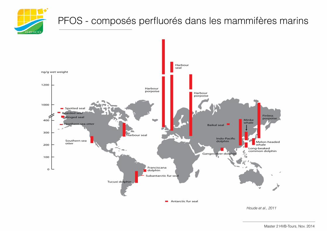
PFOS - composés perfluorés dans les mammifères marins
Houde et al., 2011
Master 2 HVB-Tours, Nov. 2014
16 State of the Science of Endocrine Disrupting Chemicals – 2012
Figure 18. EDCs are found in wildlife worldwide. This figure shows concentrations (in ng/g wet weight) of per-fluorooctane sulfonate, also known as PFOS, in liver of marine mammals (modified from Houde et al., 2011).
transport by air and ocean currents and food web accumulation. A few examples of exposure of wildlife around the world are shown in Figures 18 and 19. There are no longer any pristine areas without environmental pollutants. In addition, levels of chemicals in the body are tightly linked to trends in their use. There are good examples where bans or reductions in chemical use have resulted in reduced levels in humans and wildlife. Indeed, human and animal tissue concentrations of many POPs have declined because the chemicals are being phased out following global bans on their use. In contrast, EDCs that are being used more now are found at higher levels in humans and wildlife. It is notable how well production and exposure mirror each other, as exemplified in Figure 20.
Hundreds of chemicals in commerce are known to have endocrine disrupting effects. However, thousands of other chemicals with potential endocrine effects have not been looked for or tested. It is likely that these chemicals are contributing to wildlife and human exposures to EDCs. The situation is illustrated in Figure 21. Since only a very limited number of all chemicals in commerce have been tested for their endocrine disrupting properties, there may be many more with such properties. Also, the EDC metabolites or environmental transformation products and the by-products and products formed upon waste treatment are not included in these estimates, and their endocrine disrupting effects are mainly unknown.
1200
1000
400
300
200
100
0
ng/g wet weight
Spotted seal
Bearded sealRinged seal
Northern sea otter
Southern seaotter
Antarctic fur seal
Harbour seal
Harbourporpoise
Harbourseal
Harbourporpoise
Finlessporpoise
Baikal seal
Indo-Pacificdolphin
Minkewhale
Melon-headedwhale
Long-beakedcommon dolphin
Ganges river dolphin
Franciscanadolphin
Subantarctic fur seal
Tucuxi dolphin
les perturbateurs endocriniens dans les systèmes fluviauxLa pollution du Rhône par les PCBs, dioxines, furanes, parabènes, stéroïdes
synthétiques et les composés perfluorés
Master 2 HVB-Tours, Nov. 2014
La pollution du Rhône
Master 2 HVB-Tours, Nov. 2014
• S’agit-il -aussi- d’une pollution historique et diffuse ? • Y a t-il un gradient amont-aval de la contamination ? • Peut-on identifier les sources ? • En quoi le fonctionnement hydrosédimentaire du fleuve modifie l’état de
pollution ? • Qu’en est-il de la capacité de résilience du fleuve ? • Quelles sont les modalités de transfert du sédiment au biote ?
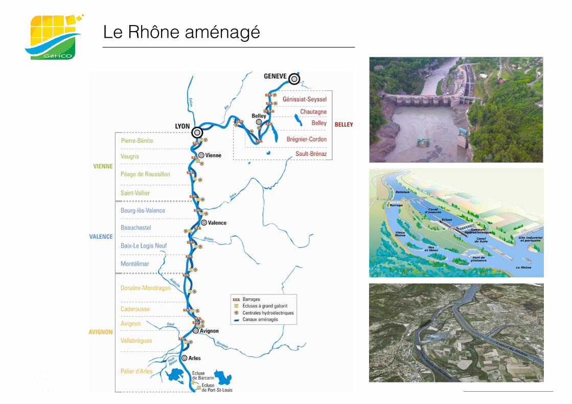
Le Rhône aménagé
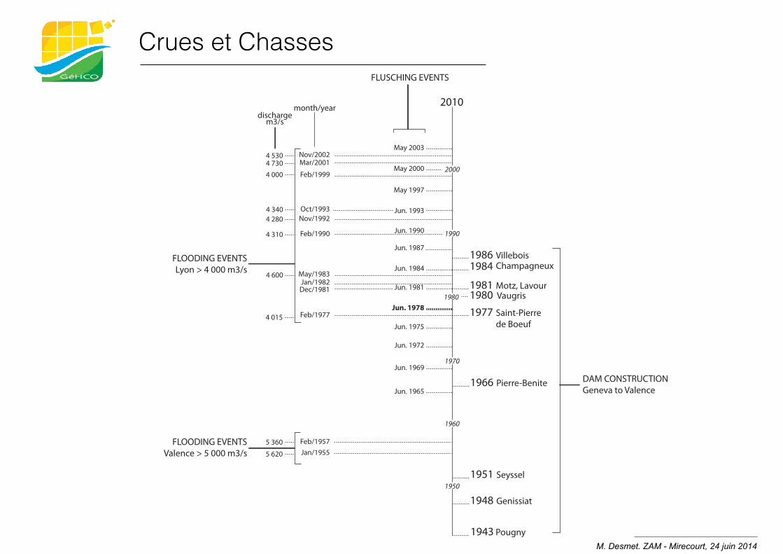
Crues et Chasses
1948
2010
Genissiat
1951 Seyssel
1981 Motz, Lavour
1984 Champagneux1986 Villebois
1966 Pierre-Benite
1980 Vaugris
1977 Saint-Pierre de Boeuf
May/1983
Feb/1990
Oct/1993
Feb/1999
Mar/2001Nov/2002
Nov/1992
1950
1960
1970
1980
1990
2000
May 2003
May 2000
May 1997
Jun. 1993
Jun. 1990
Jun. 1987
Jun. 1984
Jun. 1981
Jun. 1978
Jun. 1975
Jun. 1972
Jun. 1969
Jun. 1965
FLOODING EVENTSLyon > 4 000 m3/s
FLUSCHING EVENTS
DAM CONSTRUCTIONGeneva to Valence
1943 Pougny
4 5304 7304 000
4 3404 280
4 310
4 600Jan/1982
Dec/1981
Feb/19774 015
Feb/1957Jan/1955
FLOODING EVENTSValence > 5 000 m3/s
5 3605 620
month/yeardischarge
m3/s
M. Desmet. ZAM - Mirecourt, 24 juin 2014
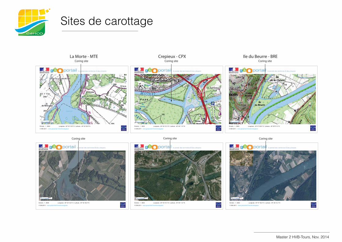
Sites de carottage
Master 2 HVB-Tours, Nov. 2014
© IGN 2011 - www.geoportail.fr/mentionslegales/
Longitude : 05º 33' 18.5'' E / Latitude : 45º 42' 00.8'' NÉchelle : 1 : 8000
© IGN 2011 - www.geoportail.fr/mentionslegales/
Longitude : 05º 33' 18.5'' E / Latitude : 45º 42' 00.8'' NÉchelle : 1 : 8000
© IGN 2011 - www.geoportail.fr/mentionslegales/
Longitude : 04º 55' 07.0'' E / Latitude : 45º 48' 11.9'' NÉchelle : 1 : 8000
© IGN 2011 - www.geoportail.fr/mentionslegales/
Longitude : 04º 55' 07.0'' E / Latitude : 45º 48' 11.9'' NÉchelle : 1 : 8000
© IGN 2011 - www.geoportail.fr/mentionslegales/
Longitude : 04º 47' 08.5'' E / Latitude : 45º 28' 31.0'' NÉchelle : 1 : 8000
© IGN 2011 - www.geoportail.fr/mentionslegales/
Longitude : 04º 47' 08.5'' E / Latitude : 45º 28' 31.0'' NÉchelle : 1 : 8000
La Morte - MTE Crepieux - CPX Ile du Beurre - BRECoring site
Coring site Coring site Coring site
Coring site Coring site
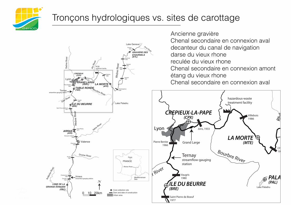
Tronçons hydrologiques vs. sites de carottage
used at sites CPX and BRE to help correlate the primary and radionuclidecores so that dates could be assigned to the primary core.
Dry bulk density was determined as the difference between wet anddrymass divided by the volume of the container. Grain-size distributionswere determined by sonicating and then analyzing each sample with aMastersizer 2000® laser mounted with a hydro SM small-volume dis-persion unit (Malvern Instruments, Worcestershire, UK). Grain-sizemean, mode, sorting, and skewness were computed using the Gradistatprogram (Blott and Pye, 2001). Cumulative volumetric percentages ofsand (N63 μm), silt (4–63 μm), and clay (b4 μm) were determined for
each depth interval (b63 μm, i.e. silt and clay together, hereinafter finefraction).
2.3. Analytical methods
Sediment sampleswere analyzed for radionuclides at the Laboratoiredes sciences du climat et de l'environnement (LSCE), Gif sur Yvette,France. Following drying, sub-samples from each core were analyzedfor radionuclides by counting for at least 24 h using low-noise gammaspectrometry. Gamma emissions were detected with a germanium
LA MORTE(MTE)
Bourbre River
Core collection siteDam and date of constructionUrban area
Ain
Riv
er
Saô
ne R
iver
Arve River
CREPIEUX(CPX)
ILE DU BEURRE(BRE)
PCBtreatment facility
Gier River
Seyssel1951
Lavours1981
Champagneux1984
Villebois1986
Genissiat1948
Pougny1943
Vaugris1980
Pierre Benite1966
Saint Pierre de Boeuf1977
Arras-Rhône1971
Jons1933
Ternaystreamflow-gauging station
Lyon
Bourg les Valence1968
Motz1980
GRAVIERE DES ETOURNELS(ETL)
GRAND LARGE(GDL)
TABLE RONDE(TBR)
ARRAS(ARS)
LONE DE LA GRANGE ECRASEE
(GEC)
Valence
Viviersstreamflow-gauging station
Drome River
Isère R
iver
Ardè
che
Riv
er
Charmes1964
Pouzin1961
Chateauneuf1958
Donzère1952
Paris
0 2010 km
Lake Paladru
Rhône River
Lake Geneva
Rhô
ne R
iver
MediterraneanSea
FRANCE
Rhô
ne R
iver
Fig. 1.Map of the study area (Rhône River basin, France) and locations of sediment core collection.
570 B. Mourier et al. / Science of the Total Environment 476–477 (2014) 568–576
Sediment core collection siteDam and date of constructionUrban area
Lyon
Grenoble
Geneva
Ain
Rive
r
Fier River
Saôn
e Ri
ver
Arve River
LA MORTE(MTE)
CREPIEUX-LA-PAPE(CPX)
ILE DU BEURRE(BRE)
10 km
hazardous-wastetreatment facility
Gier RiverChambéry
Seyssel1951
Belley1981
Champagneux1984
Villebois1986
Genissiat1948
Pougny1943
Vaugris1980
Pierre Benite1966
Saint Pierre de Boeuf1977
Arras-Rhône1971
Jons, 1933
Bourbre River
PALADRU(PAL)
Rhôn
e Ri
ver
Rhôn
e Ri
ver
Annecy Lake Annecy
Lake Geneva
Lake Bourget
Lake Paladru
France Rhône River
Paris
Ternaystreamflow-gaugingstation
Grand Large
N
Figure 1. Map of the study area, Rhône basin, France.
Mediterranean Sea
AtlanticOcean
Ancienne gravière Chenal secondaire en connexion aval decanteur du canal de navigation darse du vieux rhone reculée du vieux rhone Chenal secondaire en connexion amont étang du vieux rhone Chenal secondaire en connexion aval
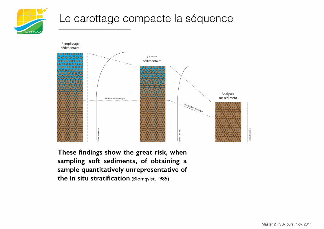
Tene
ur e
n ea
u
Tene
ur e
n ea
u
Profondeur massique
Profondeur massique
Remplissagesédimentaire
Carottesédimentaire
Analysessur sédiment
Tene
ur e
n ea
u
Le carottage compacte la séquence
These findings show the great risk, when sampling soft sediments, of obtaining a sample quantitatively unrepresentative of the in situ stratification (Blomqvist, 1985)
Master 2 HVB-Tours, Nov. 2014
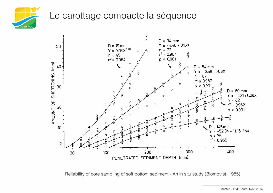
Reliability of core sampling of soft bottom sediment - An in situ study (Blomqvist, 1985)
Core sampling of soft bottom sediment
50 -
609
8 D = 3 4 m m
D 19mm Y 0.03X'.L0 A)
Y -4.48 + 0.15X n = 72
n = 45 r 2 = 0.964 r2= 0.964 p < 0.001
I i f i ~ = 5 4 m m 0 //( ; ; $58+0.08X
/" r2 0.957 .
20 100 200 300 400 PENETRATED SEDIMENT DEPTH (mm)
Fig. 4. Amount of sediment core shortening in relation to ambient sediment surface as a function of the depth of penetrating tubes, of different diameter (D) (cf. Table 2). Five replicates of each tube size. Data obtained by a SCUBA diver who gently pushed the Plexiglas cylinders into the sediment. The presented equations have been selected between eight given functions [ y = a x ; y=a+bx ; y=&; y = l/(a+bx); y=a+b/x; y=a+b.lnx; y=nxb; y = x / ( a + b x ) ] . The best fits have been chosen on the basis of revealed maximum r-square; in all cases also accordant with minimum residual error (i.e. standard error of the estimate) and smallest maximum absolute deviation. During calculations, carried out with a Tektronix 4050-Series Graphic System, each of the non-linear equations have been transformed to an intrinsically linear form (sensu Draper & Smith, 1966), least-square fitted, and transformed back to the original equations.
tube size. By excluding the lowest and highest quarter of the primary values in the graphs of Fig. 4 and then fitting the remaining central 50% of the data points by linear regression (Table 3), the relationship of the slope of these regressions versus inner cylinder diameter is revealed (Fig. 5). As shown by this figure the intensity of core shortening (measured as slope value) decreases markedly and asymptotically with increasing inner tube diameter.
If the computed intercepts on the abscissa of the curves in Fig. 4 are plotted versus inner cylinder diameter a linear relationship results (Fig. 6), which shows that the depth at which core shortening commences increases with the diameter of the cylin- der. The regression line in Fig. 6 intercepts close to the origin, as might be expected. In the present investigation, core shortening started nearer the
sediment surface (about 0.014.1 1 m depth) than reported earlier; i.e. about 0.3 m in haff (lagoonal) sediments (Pratje, 1934, p. 143), 0.38-0.64 m in soils (Hvorslev, 1949, pp. 100-1 19), 0.5-0,6 m in subsurface
Table 3. Linear regression equations derived by extracting the central 50% of the primary values around the medians of the graphs in Fig. 4. y is the amount of core shortening, and xis the depth of sediment penetration by the sample tube
Cylinder Regression line r2 n P diameter
(mm) ~~
19 y=-5 '69+0'25~ 0.91 30 <0.001 34 ~ = - 3 . 1 7 + 0 . 1 4 ~ 0.89 35 <0.001 54 y = -3.31+0.08~ 0.89 50 <0.001 80 y = -4.70+0.07~ 0.94 45 <0.001
145 y=-3.09+0.05~ 0.83 40 <0.001
Le carottage compacte la séquence
Master 2 HVB-Tours, Nov. 2014
Sém
inai
re P
CB
-Rhô
ne, 1
2 fé
vrie
r 200
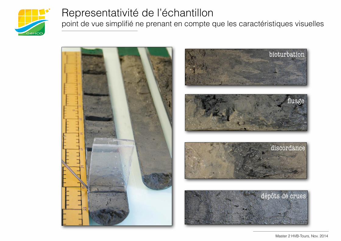
9Representativité de l’échantillon point de vue simplifié ne prenant en compte que les caractéristiques visuelles
bioturbation
fluage
discordance
dépôts de crues
Master 2 HVB-Tours, Nov. 2014
Sém
inai
re P
CB
-Rhô
ne, 1
2 fé
vrie
r 200
9
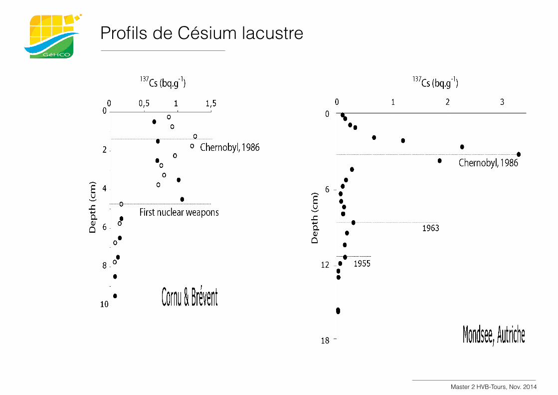
Profils de Césium lacustre
Master 2 HVB-Tours, Nov. 2014
Sém
inai
re P
CB
-Rhô
ne, 1
2 fé
vrie
r 200
9
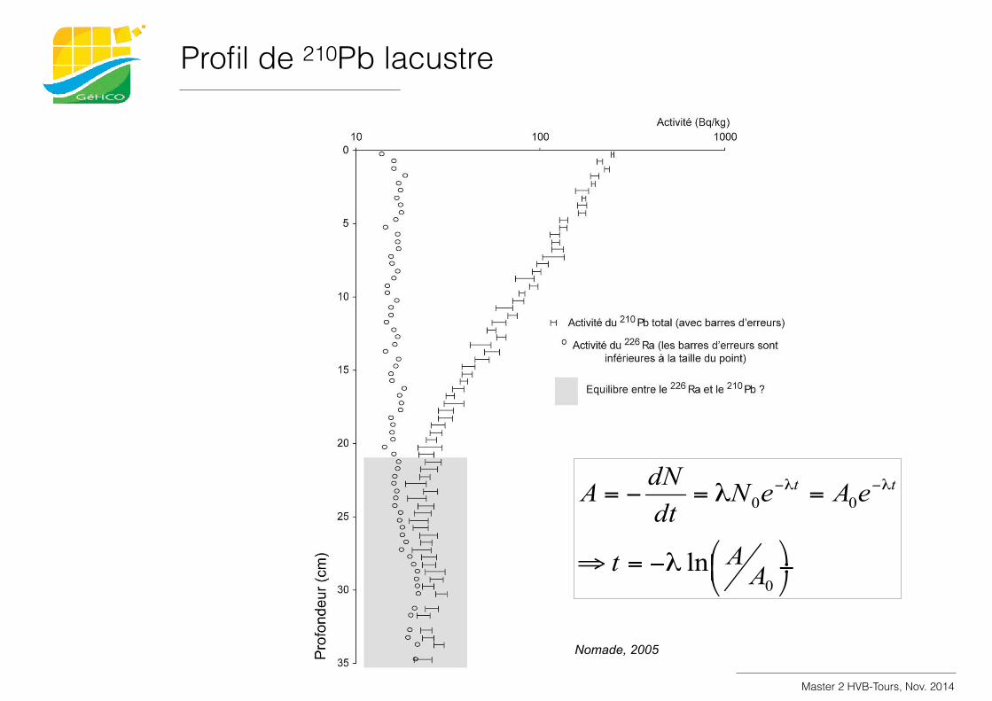
Nomade, 2005
Profil de 210Pb lacustre
Master 2 HVB-Tours, Nov. 2014
Sém
inai
re P
CB
-Rhô
ne, 1
2 fé
vrie
r 200
9
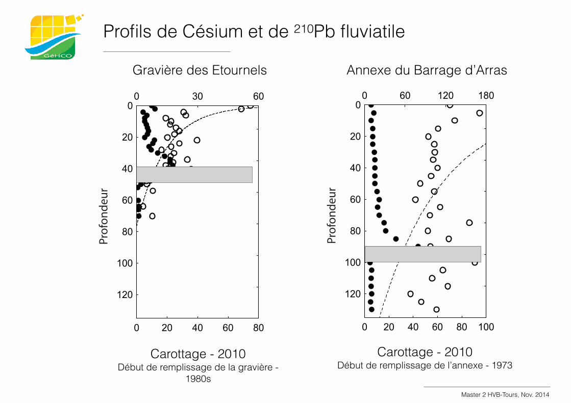
0 20 40 60 80
0 30 600
20
40
60
80
100
120
Prof
onde
ur
0 20 40 60 80 100
0 60 120 1800
20
40
60
80
100
120
Prof
onde
ur
Gravière des Etournels Annexe du Barrage d’Arras
Carottage - 2010 Début de remplissage de la gravière -
1980s
Carottage - 2010 Début de remplissage de l’annexe - 1973
Profils de Césium et de 210Pb fluviatile
Master 2 HVB-Tours, Nov. 2014
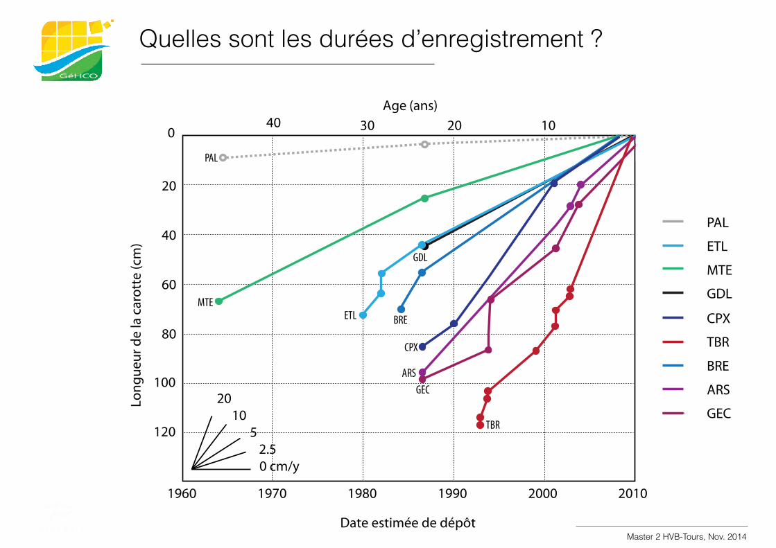
Quelles sont les durées d’enregistrement ?
1960 1970 1980 1990 2000 2010
PAL
ETL
MTE
GDL
CPX
TBR
BRE
ARS
GEC
0
20
40
60
80
100
120
10 20 30 40
Age (ans)
Date estimée de dépôt
Long
ueur
de
la c
arot
te (c
m)
20 10 5 2.5 0 cm/y
MTE
GDL
CPX
TBR
BRE
ARSGEC
PAL
ETL
Master 2 HVB-Tours, Nov. 2014
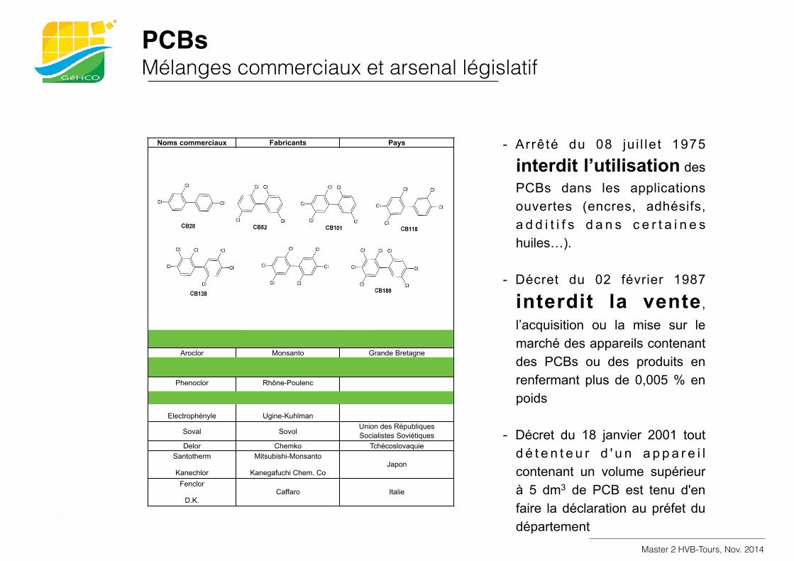
Noms commerciaux Fabricants Pays
Asbetol
Chlorextol
Diaclor
Dykanol
Elemex
Hyvol
Inerteen
No-Flamol
Pyranol
Sat-T-Kuhl
Therminol
Aroclor
American Corporation
Allis Chlamers
Sangamo Electric
Cornell Dubilier
Mac Graw Edison
Aerovox
Westinghouse Electric
Wagner Electric
General Electric
Kuhlman Electric
Monsanto
Monsanto Etats-Unis
Aroclor Monsanto Grande Bretagne
Clophen Farbenfabriken Bayer République Fédérale d’Allemagne
Phenoclor
Pyralène
Electrophényle
Rhône-Poulenc
Prodélec
Ugine-Kuhlman
France
Soval SovolUnion des Républiques Socialistes Soviétiques
Delor Chemko TchécoslovaquieSantotherm
Kanechlor
Mitsubishi-Monsanto
Kanegafuchi Chem. CoJapon
Fenclor
D.K.Caffaro Italie
PCBsMélanges commerciaux et arsenal législatif
- Arrêté du 08 ju i l le t 1975
interdit l’utilisation des PCBs dans les applications ouvertes (encres, adhésifs, a d d i t i f s d a n s c e r t a i n e s huiles…).
- Décret du 02 février 1987
interdit la vente , l’acquisition ou la mise sur le marché des appareils contenant des PCBs ou des produits en renfermant plus de 0,005 % en poids
- Décret du 18 janvier 2001 tout d é t e n t e u r d ' u n a p p a r e i l contenant un volume supérieur à 5 dm3 de PCB est tenu d'en faire la déclaration au préfet du département
Master 2 HVB-Tours, Nov. 2014
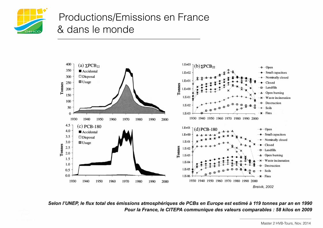
Productions/Emissions en France & dans le monde
Selon l’UNEP, le flux total des émissions atmosphériques de PCBs en Europe est estimé à 119 tonnes par an en 1990 Pour la France, le CITEPA communique des valeurs comparables : 58 kilos en 2009
Breivik, 2002
Master 2 HVB-Tours, Nov. 2014
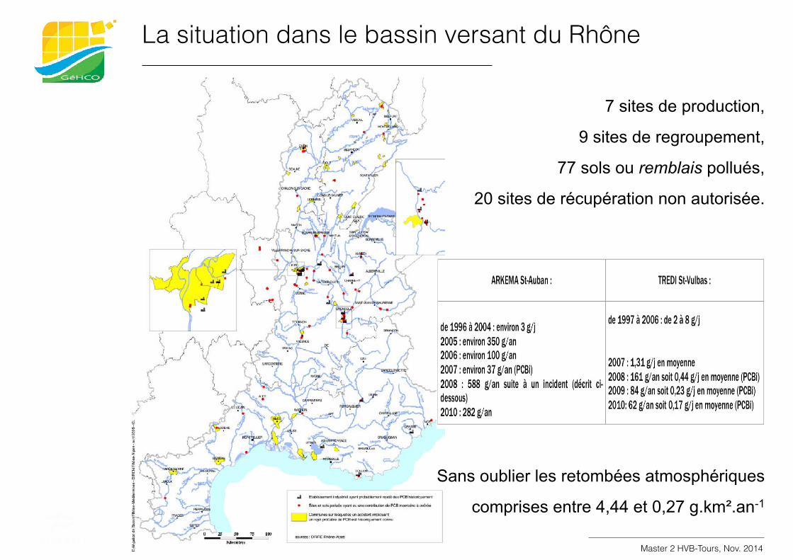
La situation dans le bassin versant du Rhône
7 sites de production,
9 sites de regroupement,
77 sols ou remblais pollués,
20 sites de récupération non autorisée.
Sans oublier les retombées atmosphériques
comprises entre 4,44 et 0,27 g.km².an-1
Master 2 HVB-Tours, Nov. 2014
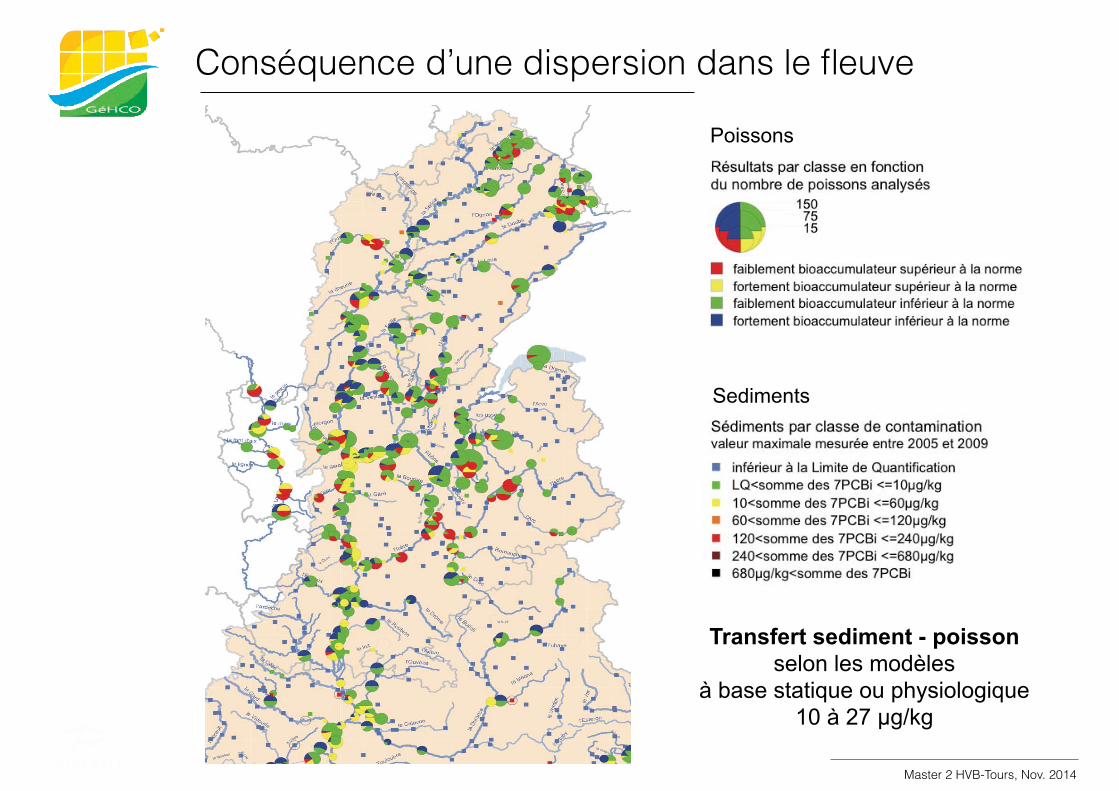
Conséquence d’une dispersion dans le fleuve
Poissons
Sediments
Transfert sediment - poisson selon les modèles
à base statique ou physiologique 10 à 27 µg/kg
Master 2 HVB-Tours, Nov. 2014
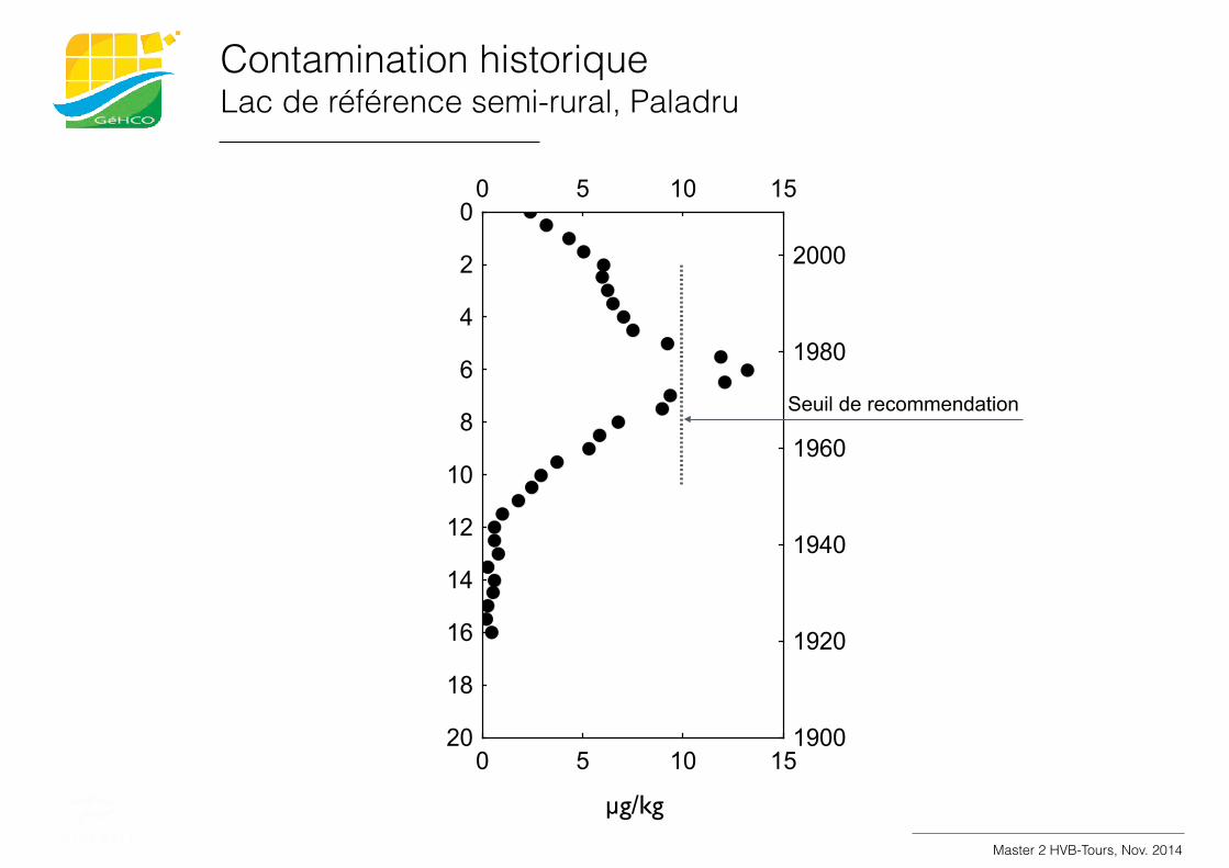
Contamination historique Lac de référence semi-rural, Paladru
0 5 10 15
0 5 10 150
2
4
6
8
10
12
14
16
18
20 1900
1920
1940
1960
1980
2000
µg/kg
Seuil de recommendation
Master 2 HVB-Tours, Nov. 2014
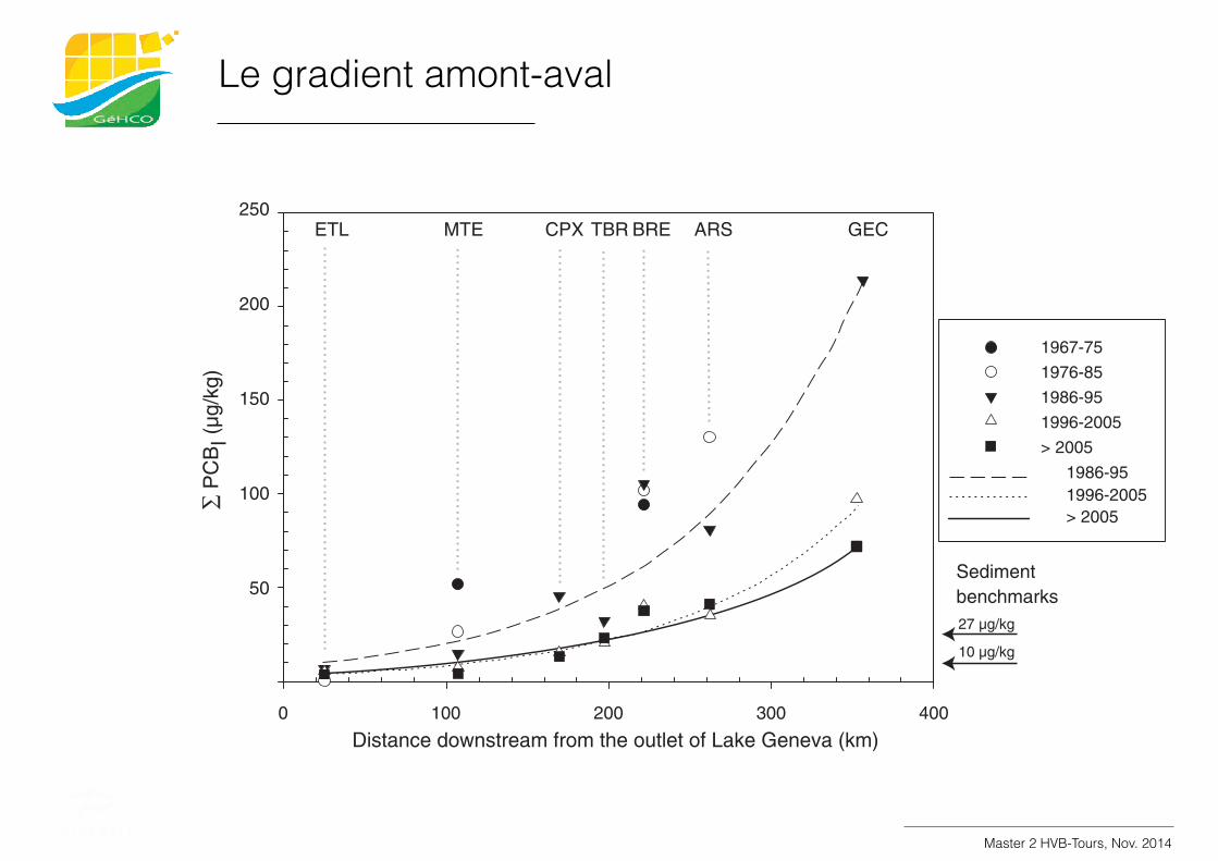
Le gradient amont-aval
since 1986 and up to 940 μg/kg in the 1970s) (Babut et al., 2011) and insediment from the Isère River (EauFrance, 2011). The hypothesis ofother PCB inputs from the Isère River is consistent with a difference incongener mixture at site GEC (relatively low chlorinated congeners,cluster 1) relative to those upstream (Fig. 3). In the Rhône River delta,PCB concentrations are lower than in sediments collected at site GECfor themost recent period (post-2005)— themeanΣPCBI for suspendedsediments collected since 2008 near the mouth of the Rhône River is24.1 μg/kg (n = 122) (EauFrance, 2011; SORA Station).
4.2. Time and system recovery
Results from this study and that of Desmet et al. (2012) provideempirical evidence that environmental regulation of point sourcesenacted since 1975 and 1986 reduced the PCB burden recorded insediments. They also provide an indication of the time required forPCB levels to decrease, particularly at downstream sites. Regulation ofpoint sources, however, has not prevented exceedances of the fish-consumption regulatory threshold set in 2008 and revised in 2011 to6.5 pg toxic equivalency factor (TEQ)/g wet weight (ww) for all speciesbut eel, forwhich the thresholdwas set at 10 pg TEQ/gww (data for fish
available at http://www.rhone-mediterranee.eaufrance.fr/usages-et-pressions/pollution_PCB/basepcb/index.php) (European Commission,2011). The question thus arises: How much more time is requireduntil PCB concentrations in surface sediment are consistentwith regula-tions for fish consumption? The ΣPCBI concentration in sediment thatcorresponds to the fish regulatory limit depends on the approach usedand the data involved. Using biota–sediment accumulation factors(BSAFs) over a large spatial scale, the sediment benchmark for ΣPCBI
was determined to be 27 μg/kg (Babut et al., 2012). At ΣPCBI of10 μg/kg, 75% of fish from 3 cyprinid species from 3 sites in theRhône River along a contamination gradient wouldmatch the regulato-ry threshold when applying the statistical model developed by Lopeset al. (2011). We therefore consider ΣPCBI of 10 and 27 μg/kg as poten-tial targets (Fig. 4a).
At some sites theΣPCBI concentration in themost recently depositedsediments are less than the lower target of 10 μg/kg, at others theΣPCBIconcentration is between the two targets, and at some sites ΣPCBI
concentration exceeds the upper target of 27 μg/kg (Supplementaryinformation Table S1). At sites ETL and MTE, ΣPCBI concentrations atthe sediment surface (top of the core) already are below the lowertarget value and are still decreasing (Desmet et al., 2012). At site CPX
∑ P
CB
I (µg
/kg)
Distance downstream from the outlet of Lake Geneva (km)
27 µg/kg
10 µg/kg
1967-751976-851986-951996-2005> 2005
1986-951996-2005> 2005
Pop
ulat
ion,
in th
ousa
nds
of in
habi
tant
s
Sedimentbenchmarks
1990 census1999 census2010 census
ETL MTE CPX TBR BRE ARS GEC
ETL MTE CPX TBR BRE ARS GEC
A
B
250
200
150
100
50
10,000
8,000
6,000
4,000
2,000
00 100 200 300 400
Fig. 4. (A) Median ΣPCBI concentrations in sediment core samples for decadal time windows. Site GDL is excluded because sediment at this site was disturbed by reservoir managementactivities. Two-parameter exponential models were fit to the 1986–95, 1996–2005, and post-2005 time windows (adjusted r2 of 0.92, 0.96, and 0.94, respectively). Data for the 1967–75and 1976–85 time windows were not modeled as insufficient data were available for many of the sites. Arrows indicate sediment benchmarks calculated from BSAFs models that corre-spond to PCB thresholds infish (Lopes et al., 2011; Babut et al., 2012). (B) Cumulative population in the catchment upstreamof each sampling site. Census data fromL'Institut national de lastatistique et des études économiques (INSEE) (http://www.insee.fr/fr/themes/detail.asp?reg_id=99&ref_id=base-cc-evol-struct-pop-2010).
574 B. Mourier et al. / Science of the Total Environment 476–477 (2014) 568–576
Master 2 HVB-Tours, Nov. 2014
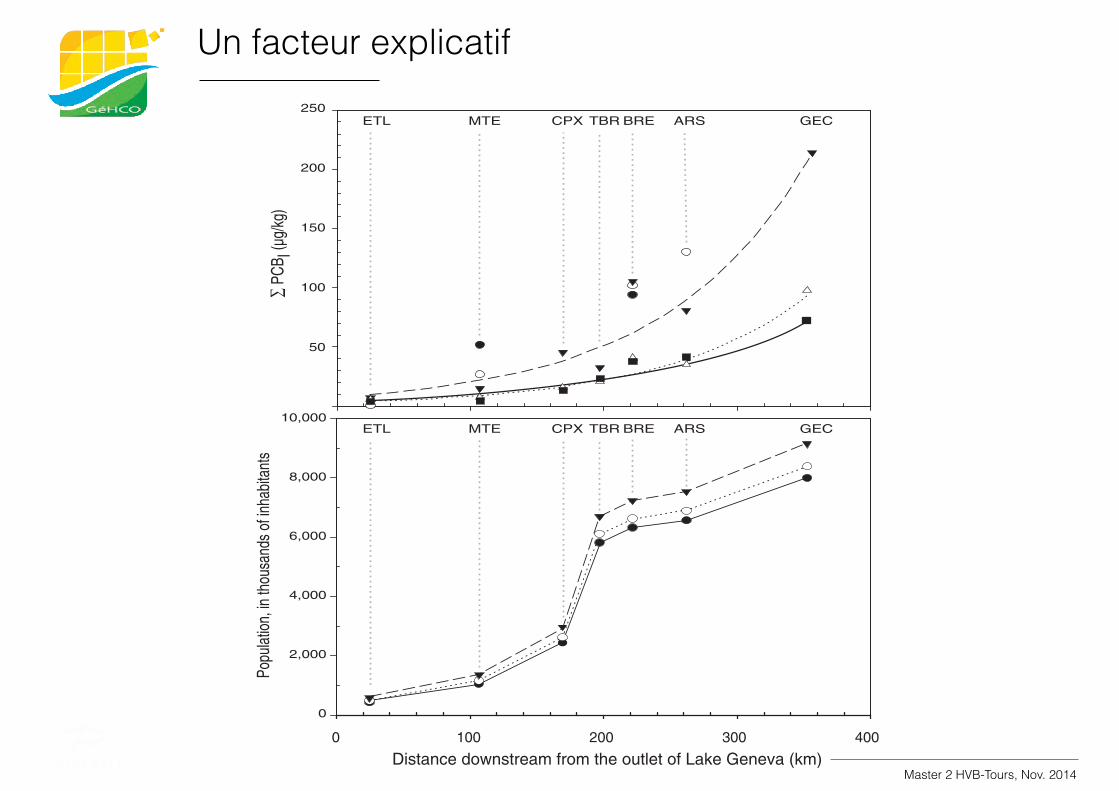
Un facteur explicatif
since 1986 and up to 940 μg/kg in the 1970s) (Babut et al., 2011) and insediment from the Isère River (EauFrance, 2011). The hypothesis ofother PCB inputs from the Isère River is consistent with a difference incongener mixture at site GEC (relatively low chlorinated congeners,cluster 1) relative to those upstream (Fig. 3). In the Rhône River delta,PCB concentrations are lower than in sediments collected at site GECfor themost recent period (post-2005)— themeanΣPCBI for suspendedsediments collected since 2008 near the mouth of the Rhône River is24.1 μg/kg (n = 122) (EauFrance, 2011; SORA Station).
4.2. Time and system recovery
Results from this study and that of Desmet et al. (2012) provideempirical evidence that environmental regulation of point sourcesenacted since 1975 and 1986 reduced the PCB burden recorded insediments. They also provide an indication of the time required forPCB levels to decrease, particularly at downstream sites. Regulation ofpoint sources, however, has not prevented exceedances of the fish-consumption regulatory threshold set in 2008 and revised in 2011 to6.5 pg toxic equivalency factor (TEQ)/g wet weight (ww) for all speciesbut eel, forwhich the thresholdwas set at 10 pg TEQ/gww (data for fish
available at http://www.rhone-mediterranee.eaufrance.fr/usages-et-pressions/pollution_PCB/basepcb/index.php) (European Commission,2011). The question thus arises: How much more time is requireduntil PCB concentrations in surface sediment are consistentwith regula-tions for fish consumption? The ΣPCBI concentration in sediment thatcorresponds to the fish regulatory limit depends on the approach usedand the data involved. Using biota–sediment accumulation factors(BSAFs) over a large spatial scale, the sediment benchmark for ΣPCBI
was determined to be 27 μg/kg (Babut et al., 2012). At ΣPCBI of10 μg/kg, 75% of fish from 3 cyprinid species from 3 sites in theRhône River along a contamination gradient wouldmatch the regulato-ry threshold when applying the statistical model developed by Lopeset al. (2011). We therefore consider ΣPCBI of 10 and 27 μg/kg as poten-tial targets (Fig. 4a).
At some sites theΣPCBI concentration in themost recently depositedsediments are less than the lower target of 10 μg/kg, at others theΣPCBIconcentration is between the two targets, and at some sites ΣPCBI
concentration exceeds the upper target of 27 μg/kg (Supplementaryinformation Table S1). At sites ETL and MTE, ΣPCBI concentrations atthe sediment surface (top of the core) already are below the lowertarget value and are still decreasing (Desmet et al., 2012). At site CPX
∑ PC
B I (µg/
kg)
Distance downstream from the outlet of Lake Geneva (km)
27 µg/kg
10 µg/kg
1967-751976-851986-951996-2005> 2005
1986-951996-2005> 2005
Popu
lation
, in th
ousa
nds o
f inha
bitan
ts
Sedimentbenchmarks
1990 census1999 census2010 census
ETL MTE CPX TBR BRE ARS GEC
ETL MTE CPX TBR BRE ARS GEC
A
B
250
200
150
100
50
10,000
8,000
6,000
4,000
2,000
00 100 200 300 400
Fig. 4. (A) Median ΣPCBI concentrations in sediment core samples for decadal time windows. Site GDL is excluded because sediment at this site was disturbed by reservoir managementactivities. Two-parameter exponential models were fit to the 1986–95, 1996–2005, and post-2005 time windows (adjusted r2 of 0.92, 0.96, and 0.94, respectively). Data for the 1967–75and 1976–85 time windows were not modeled as insufficient data were available for many of the sites. Arrows indicate sediment benchmarks calculated from BSAFs models that corre-spond to PCB thresholds infish (Lopes et al., 2011; Babut et al., 2012). (B) Cumulative population in the catchment upstreamof each sampling site. Census data fromL'Institut national de lastatistique et des études économiques (INSEE) (http://www.insee.fr/fr/themes/detail.asp?reg_id=99&ref_id=base-cc-evol-struct-pop-2010).
574 B. Mourier et al. / Science of the Total Environment 476–477 (2014) 568–576
since 1986 and up to 940 μg/kg in the 1970s) (Babut et al., 2011) and insediment from the Isère River (EauFrance, 2011). The hypothesis ofother PCB inputs from the Isère River is consistent with a difference incongener mixture at site GEC (relatively low chlorinated congeners,cluster 1) relative to those upstream (Fig. 3). In the Rhône River delta,PCB concentrations are lower than in sediments collected at site GECfor themost recent period (post-2005)— themeanΣPCBI for suspendedsediments collected since 2008 near the mouth of the Rhône River is24.1 μg/kg (n = 122) (EauFrance, 2011; SORA Station).
4.2. Time and system recovery
Results from this study and that of Desmet et al. (2012) provideempirical evidence that environmental regulation of point sourcesenacted since 1975 and 1986 reduced the PCB burden recorded insediments. They also provide an indication of the time required forPCB levels to decrease, particularly at downstream sites. Regulation ofpoint sources, however, has not prevented exceedances of the fish-consumption regulatory threshold set in 2008 and revised in 2011 to6.5 pg toxic equivalency factor (TEQ)/g wet weight (ww) for all speciesbut eel, forwhich the thresholdwas set at 10 pg TEQ/gww (data for fish
available at http://www.rhone-mediterranee.eaufrance.fr/usages-et-pressions/pollution_PCB/basepcb/index.php) (European Commission,2011). The question thus arises: How much more time is requireduntil PCB concentrations in surface sediment are consistentwith regula-tions for fish consumption? The ΣPCBI concentration in sediment thatcorresponds to the fish regulatory limit depends on the approach usedand the data involved. Using biota–sediment accumulation factors(BSAFs) over a large spatial scale, the sediment benchmark for ΣPCBI
was determined to be 27 μg/kg (Babut et al., 2012). At ΣPCBI of10 μg/kg, 75% of fish from 3 cyprinid species from 3 sites in theRhône River along a contamination gradient wouldmatch the regulato-ry threshold when applying the statistical model developed by Lopeset al. (2011). We therefore consider ΣPCBI of 10 and 27 μg/kg as poten-tial targets (Fig. 4a).
At some sites theΣPCBI concentration in themost recently depositedsediments are less than the lower target of 10 μg/kg, at others theΣPCBIconcentration is between the two targets, and at some sites ΣPCBI
concentration exceeds the upper target of 27 μg/kg (Supplementaryinformation Table S1). At sites ETL and MTE, ΣPCBI concentrations atthe sediment surface (top of the core) already are below the lowertarget value and are still decreasing (Desmet et al., 2012). At site CPX
∑ P
CB
I (µg
/kg)
Distance downstream from the outlet of Lake Geneva (km)
27 µg/kg
10 µg/kg
1967-751976-851986-951996-2005> 2005
1986-951996-2005> 2005
Pop
ulat
ion,
in th
ousa
nds
of in
habi
tant
s
Sedimentbenchmarks
1990 census1999 census2010 census
ETL MTE CPX TBR BRE ARS GEC
ETL MTE CPX TBR BRE ARS GEC
A
B
250
200
150
100
50
10,000
8,000
6,000
4,000
2,000
00 100 200 300 400
Fig. 4. (A) Median ΣPCBI concentrations in sediment core samples for decadal time windows. Site GDL is excluded because sediment at this site was disturbed by reservoir managementactivities. Two-parameter exponential models were fit to the 1986–95, 1996–2005, and post-2005 time windows (adjusted r2 of 0.92, 0.96, and 0.94, respectively). Data for the 1967–75and 1976–85 time windows were not modeled as insufficient data were available for many of the sites. Arrows indicate sediment benchmarks calculated from BSAFs models that corre-spond to PCB thresholds infish (Lopes et al., 2011; Babut et al., 2012). (B) Cumulative population in the catchment upstreamof each sampling site. Census data fromL'Institut national de lastatistique et des études économiques (INSEE) (http://www.insee.fr/fr/themes/detail.asp?reg_id=99&ref_id=base-cc-evol-struct-pop-2010).
574 B. Mourier et al. / Science of the Total Environment 476–477 (2014) 568–576
Master 2 HVB-Tours, Nov. 2014
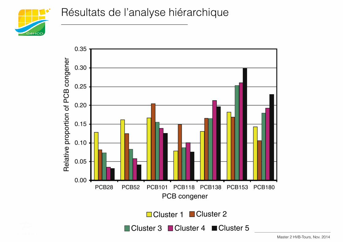
Résultats de l’analyse hiérarchique
information Fig. S7). The age model was refined on the basis of a slightdecrease in percentage of silt and clay in the upper part of the corethat matched well with floods in the early 2000s.
3.2. Indicator PCB (PCBI) concentrations
PCBI weremeasured in 248 sediment samples. Three ormore conge-ners with concentrations below the detection limit were measured infour samples; those samples therefore were excluded from the datasetfor statistical analysis. For two samples, the concentration of an unde-tected congener (PCB 101) was estimated by multiplying the medianproportion of the congener in the adjacent layers by the sum of sevencongeners in the layer with the non-detection. Sediment samplesdeeper than 51 cm at site ETL (11 samples) were excluded from statis-tical analysis because the deposits were interpreted as having beenremobilized (Supplementary information Fig. S1). Samples with an ab-solute standardized residual greater than 2 (outliers) were evaluated:two were excluded (one collected from site BRE and the other fromsite ARS) from subsequent statistical analysis because the total PCB con-centrationwas atypically high relative to that in adjacent layers, and be-cause the PCB profile (in both cases, a presumed positive bias of PCB 52)was not consistent with that of most of the other measurements.
PCBI concentrations and profiles varied considerably within and be-tween the sites sampled for this study, both in timing andmagnitude ofpeak concentrations (Figs. 2 and 3).MaximumPCBI concentrationswerelowest upstream (e.g., maximum ΣPCBI concentration of 11.50 μg/kg atETL) and increased downstream to a concentration of 417.1 μg/kg atGEC (Fig. 3). Maximum concentrations measured for this studyexceeded those measured in sediment in several other European rivers,such as the Sava River (the largest tributary to the Danube) (b4 μg/kg)(Heath et al., 2010), the Vistula River, Poland (64 μg/kg) (Dmitruket al., 2008), and the Po River, Italy (4.1 μg/kg) (Viganò et al., 2008).
Temporal patterns of ΣPCBI concentrations vary from upstream todownstream. Concentrations at site MTE are highest in the 1970s anddecrease monotonically to the top of the core; concentrations at siteARS generally decrease from the mid-1980s onward. Concentrationsin PCB concentrations at the other six sites are more variable. At ETL,CPX, BRE, and GEC, concentrations of PCBs were elevated and variablein the late 1980s and mid-1990s, decreased in the late 1990s, andhave remained relatively stable since. At GDL and TBR, maximumconcentrations occurred in the 2000s (ΣPCBI of159.8 μg/kg in 2003 atGDL and 131.5 μg/kg at TBR in 2007). At GDL, a progressive increase
occurred in the early 1980s until 2005, but the ΣPCBI maximum atTBR was brief, occurring only during 2007–08.
3.3. Spatial trends in PCBs at the scale of the Rhône River and changesthrough time
Exponential regression models used to evaluate changes in PCBconcentrations in a downstream direction for three time windows(1986–1995, 1996–2005, and post 2005) provided a good fit to thedata (r2 = 0.92, r2 = 0.96, r2 = 0.94, respectively; p = 0.03). SiteGDL was excluded from this regression because its age model was notconsistent with those from the other sites (Supplementary dataFig. S3). Linear and piecewise linear regression models had acceptablebut lower r2 (0.71–0.96), and residuals were substantially higher thanthose from the exponential models.
The exponentialmodels illustrate spatial and temporal trends in PCBconcentrations in Rhône River sediment (Fig. 4). PCB concentrationsgenerally increase from upstream to downstream, regardless of theperiod considered. Concentrations decreased substantially from about1986–95 to 1996–2005 and to a much lesser extent from 1996–2005to post 2005–top of core. The decreases are more marked at down-stream sites than at upstream sites. The apparent slowing of the rateat which PCBs are decreasing indicates that PCB inputs to the RhôneRiver might be continuing, particularly downstream from the greaterLyon area.
Median ΣPCBI values for downstream sites TBR and BRE for the1986–95 time window diverge from the exponential model for thisperiod (Fig. 4). The median for TBR is less than that predicted by theregression model for this period, whereas the median for BRE is greaterthan that predicted (and greater than that predicted by the exponentialmodels, to a lesser extent, for the 1996–2005 and post-2005 time win-dows). The watershed of the Rhône River downstream from the city ofLyon is much larger than it is upstream, because it also includes thewatershed of the Saône River, whose confluence with the Rhone Riveris at the downstream end of Lyon (Fig. 1). A mean ΣPCBI concentrationof 18.7 μg/kg (n = 6, ±16.6) was measured in sediments samplescollected from the downstream end of the Saône River after 2007(Eaufrance, 2011). The change in watershed sizemight explain the con-siderable dilution of PCB concentrations observed at TBR. Conversely, atBRE and downstream, local PCB sources might be superimposed on thegeneral contamination pattern.
3.4. PCB congener profiles
Cluster analysis provides some insights into patterns of PCB conge-ners. On the basis of the dendrogram distances (Supplementary infor-mation Fig. S10), all samples were assigned to one of five clusters.Clusters 4 and 5 contained the most samples (n = 97 and 70, respec-tively), and clusters 1, 2 and 3 contained far fewer (n = 21, 18, and25, respectively). In the DA, two factors were sufficient to describe97% of the variance; the separation of the PCB congeners in the two-dimensional factor space indicated that samples were distinguished toa large extent by degree of biphenyl chlorination (Supplementary infor-mation Figs. S10 and S11a). The confusion matrix confirmed theintegrity of the clustering: less than 10% of the cluster analysis classifica-tionswere reclassified into a different cluster by theDA (Supplementaryinformation Fig. S11b and c).
Despite variability within and between sites, some patterns amongPCB profiles can be identified (Fig. 3). Cluster 1 is characterized bylow-chlorinated biphenyls (PCBs 28, 52, and 101), and samples incluster 1 mostly are from GEC, the most downstream site. In the GECcore, the dominance of cluster 1 extends from about 1990 to the topof the core. Cluster 2 is composed mainly of tetra–penta-chlorinatedbiphenyls (PCB-52, PCB-101, and PCB-118). This assemblage, character-ized by relatively low-chlorinated biphenyls, was common for GDLsamples deposited from the 1980s to 2005. Congener profiles at sites
0.00
0.05
0.10
0.15
0.20
0.25
0.30
0.35
PCB28 PCB52 PCB101 PCB118 PCB138 PCB153 PCB180
Rel
ativ
e pr
opor
tion
of P
CB
con
gene
r
Cluster 1 Cluster 2
Cluster 3 Cluster 4 Cluster 5
PCB congener
Fig. 2. Proportions of the seven indicator PCB congeners for centroids of five clusters.
572 B. Mourier et al. / Science of the Total Environment 476–477 (2014) 568–576
Master 2 HVB-Tours, Nov. 2014
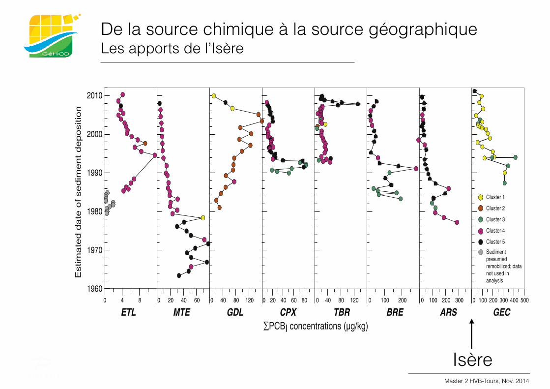
De la source chimique à la source géographique Les apports de l’Isère
GEC and GDL differ from those at other sites, indicating that PCBcontamination at these sites might be affected by local sources. Samplesin cluster 3 are primarily samples from the lower parts of cores collectedfrom sites CPX andBRE, and, to a lesser extent, from cores collected fromsites TBR and GEC. These sediment intervals correspond to flood de-posits in the early 1990s and 2000s at sites CPX, TBR, and GEC (Supple-mentary information Figs. S3, S5, and S8) and to removal of debris in1984 at site BRE (Supplementary information Fig. S6). Cluster 4 is dom-inated by penta–hexa–hepta-chlorinated biphenyls (PCB-118, PCB-138,PCB-153, and PCB-180), and more samples are in cluster 4 than in anyother cluster. Samples in cluster 4 are abundant at upstream sites ETL,MTE, and CPX, and at downstream site TBR (sediment deposited priorto 2007). Cluster 5 is characterized by high proportions of hexa- andhepta-chlorinated biphenyls (PCB-153 and PCB-180). Upstream sitesamples in cluster 5 consist of deeper sediments collected at site MTEand the most recently deposited sediment collected at site CPX. Down-stream site samples in cluster 5 include recently deposited sedimentsrepresented by TBR, BRE, and ARS cores. Recently deposited sedimentsin the TBR core, which include the PCB maximum, are in cluster 5whereas older sediments are in cluster 4.
4. Discussion
4.1. Implication for sources
A general upstream–downstream pattern of increasing PCB con-centrations indicates a relation between PCB contamination anddrivers, such as the catchment area and the cumulative upstreampopulation (Fig. 4B). Cumulative area and upstream population arecorrelated (r2 = 0.985, p b 0.0001), and we hypothesize that theyare proxies for emissions, as suggested by others (e.g., Breiviket al., 2002). However, population is neither the only nor the maindriver of trends in historical PCB concentrations along the up-stream–downstream gradient. Regardless of the decade, consider-able variations are observed between the median concentrations,the models, and the cumulative population.
Trends in PCBs at sites MTE and ARS are consistent with widelyreported patterns in PCB contamination (e.g., Eisenreich et al., 1989;Van Metre et al., 1997) in which the highest concentrations coincidewith maximum use and environmental release in the 1960s and1970s andmarked decreases since. At other Rhône River sites, however,relatively high concentrations persist into the 1990s, inconsistent withthis pattern, indicating that PCB inputs might have continued to occur
in the basin following regulation. The PCB peak at TBR during 2007–08is an example of this (Fig. 3). We hypothesize that local PCB releases(in addition to those from the PCB treatment facility upstream fromLyon) have occurred upstream from this site in the past decade.
PCB distribution and trends also are affected by sediment flushingevents and floods. Floods can cause bank erosion, resulting in inputs ofless-contaminated sediment in some cases, or in inputs of more-contaminated sediment in others (e.g., Lecce and Pavlowsky, 1997;Rozan and Hunter, 2001). Floods also can mobilize upstream PCBsources, and major hydro-sedimentary events therefore can affect con-gener compositions. At sites CPX, TBR, and GEC, the data indicate amixed congener assemblage (cluster 3) that corresponds to flooddeposits.
A potential PCB point source to sediments deposited at sites GDL,CPX, and downstream is the PCB treatment facility upstream fromLyon (Fig. 1), which is authorized to release small amounts of PCBsinto the Rhône River (Eaufrance, 2011). Because PCBs are treated anddisposed of at this facility, its regulation differs from that of PCB use inFrance. The magnitude and timing of PCB discharges at the facility areconsistent with temporal trends in PCBs at site CPX (Desmet et al.,2012), but they are more difficult to interpret at site GDL. At site GDL,PCB concentrations increased until 2005 and the congener mixture(cluster 2, higher proportions of low-chlorinated biphenyls) is distinctfrom that at the other sites. The trend at site GDL might be attributableto PCB inputs from upstream tributaries (e.g., the Bourbre River) and(or) management operations in the Grand Large (e.g., dredging). MeanΣPCBI concentrations measured in surficial sediment of the BourbreRiver range between 201.3 μg/kg (1986–1995) and 25.9 μg/kg (post-2005) (Eaufrance, 2011).
Overall, PCBI concentrations are higher at sites downstream fromLyon (TBR, BRE, ARS, and GEC) than at sites upstream from Lyon (ETL,MTE, GDL, and CPX). This pattern indicates that, although the PCB treat-ment facility is a source, it is neither the only source nor themost impor-tant. The substantial increase in PCBI concentrations in the downstreamdirection can be explained only by other PCB sources in the greater Lyonmetropolitan area and from tributaries to the Rhône River downstreamfrom Lyon. Potential sources include the City of Lyon, the industrial cor-ridor downstream from Lyon, the Gier River (a tributary that flows intothe Rhône River between TBR and BRE), the Isère River (a tributary thatflows into the Rhône River at Valence, between ARS and GEC), and per-haps other tributarywatersheds (Fig. 1), consistentwith sources evokedby Santiago et al. (1994). High concentrations of PCBsweremeasured ina sediment core collected from the Gier River (ΣPCBI of 115–160 μg/kg
1960
1970
1980
1990
2000
2010
0 4 8 0 40 80 120 0 40 80 120 0 100 2000 20 40 60 800 20 40 60 0 100 200 300 400 500
GECETL GDL BREMTE CPX TBR
Estim
ate
d d
ate
of
se
dim
en
t d
ep
ositio
n
∑PCBI concentrations (µg/kg)
Cluster 1
Cluster 2
Cluster 3
Cluster 5
Sediment presumed remobilized; data not used in analysis
Cluster 4
0 100 200 300
ARS
Fig. 3. Profiles of the sumof the concentrations of the seven indicator PCBs (ΣPCBI) in sediment cores collected from the Rhône River basin, France. The color of each symbol corresponds toits PCB congener assemblage cluster (Fig. 2).
573B. Mourier et al. / Science of the Total Environment 476–477 (2014) 568–576
IsèreMaster 2 HVB-Tours, Nov. 2014
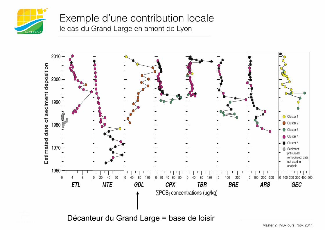
Exemple d’une contribution locale le cas du Grand Large en amont de Lyon
GEC and GDL differ from those at other sites, indicating that PCBcontamination at these sites might be affected by local sources. Samplesin cluster 3 are primarily samples from the lower parts of cores collectedfrom sites CPX andBRE, and, to a lesser extent, from cores collected fromsites TBR and GEC. These sediment intervals correspond to flood de-posits in the early 1990s and 2000s at sites CPX, TBR, and GEC (Supple-mentary information Figs. S3, S5, and S8) and to removal of debris in1984 at site BRE (Supplementary information Fig. S6). Cluster 4 is dom-inated by penta–hexa–hepta-chlorinated biphenyls (PCB-118, PCB-138,PCB-153, and PCB-180), and more samples are in cluster 4 than in anyother cluster. Samples in cluster 4 are abundant at upstream sites ETL,MTE, and CPX, and at downstream site TBR (sediment deposited priorto 2007). Cluster 5 is characterized by high proportions of hexa- andhepta-chlorinated biphenyls (PCB-153 and PCB-180). Upstream sitesamples in cluster 5 consist of deeper sediments collected at site MTEand the most recently deposited sediment collected at site CPX. Down-stream site samples in cluster 5 include recently deposited sedimentsrepresented by TBR, BRE, and ARS cores. Recently deposited sedimentsin the TBR core, which include the PCB maximum, are in cluster 5whereas older sediments are in cluster 4.
4. Discussion
4.1. Implication for sources
A general upstream–downstream pattern of increasing PCB con-centrations indicates a relation between PCB contamination anddrivers, such as the catchment area and the cumulative upstreampopulation (Fig. 4B). Cumulative area and upstream population arecorrelated (r2 = 0.985, p b 0.0001), and we hypothesize that theyare proxies for emissions, as suggested by others (e.g., Breiviket al., 2002). However, population is neither the only nor the maindriver of trends in historical PCB concentrations along the up-stream–downstream gradient. Regardless of the decade, consider-able variations are observed between the median concentrations,the models, and the cumulative population.
Trends in PCBs at sites MTE and ARS are consistent with widelyreported patterns in PCB contamination (e.g., Eisenreich et al., 1989;Van Metre et al., 1997) in which the highest concentrations coincidewith maximum use and environmental release in the 1960s and1970s andmarked decreases since. At other Rhône River sites, however,relatively high concentrations persist into the 1990s, inconsistent withthis pattern, indicating that PCB inputs might have continued to occur
in the basin following regulation. The PCB peak at TBR during 2007–08is an example of this (Fig. 3). We hypothesize that local PCB releases(in addition to those from the PCB treatment facility upstream fromLyon) have occurred upstream from this site in the past decade.
PCB distribution and trends also are affected by sediment flushingevents and floods. Floods can cause bank erosion, resulting in inputs ofless-contaminated sediment in some cases, or in inputs of more-contaminated sediment in others (e.g., Lecce and Pavlowsky, 1997;Rozan and Hunter, 2001). Floods also can mobilize upstream PCBsources, and major hydro-sedimentary events therefore can affect con-gener compositions. At sites CPX, TBR, and GEC, the data indicate amixed congener assemblage (cluster 3) that corresponds to flooddeposits.
A potential PCB point source to sediments deposited at sites GDL,CPX, and downstream is the PCB treatment facility upstream fromLyon (Fig. 1), which is authorized to release small amounts of PCBsinto the Rhône River (Eaufrance, 2011). Because PCBs are treated anddisposed of at this facility, its regulation differs from that of PCB use inFrance. The magnitude and timing of PCB discharges at the facility areconsistent with temporal trends in PCBs at site CPX (Desmet et al.,2012), but they are more difficult to interpret at site GDL. At site GDL,PCB concentrations increased until 2005 and the congener mixture(cluster 2, higher proportions of low-chlorinated biphenyls) is distinctfrom that at the other sites. The trend at site GDL might be attributableto PCB inputs from upstream tributaries (e.g., the Bourbre River) and(or) management operations in the Grand Large (e.g., dredging). MeanΣPCBI concentrations measured in surficial sediment of the BourbreRiver range between 201.3 μg/kg (1986–1995) and 25.9 μg/kg (post-2005) (Eaufrance, 2011).
Overall, PCBI concentrations are higher at sites downstream fromLyon (TBR, BRE, ARS, and GEC) than at sites upstream from Lyon (ETL,MTE, GDL, and CPX). This pattern indicates that, although the PCB treat-ment facility is a source, it is neither the only source nor themost impor-tant. The substantial increase in PCBI concentrations in the downstreamdirection can be explained only by other PCB sources in the greater Lyonmetropolitan area and from tributaries to the Rhône River downstreamfrom Lyon. Potential sources include the City of Lyon, the industrial cor-ridor downstream from Lyon, the Gier River (a tributary that flows intothe Rhône River between TBR and BRE), the Isère River (a tributary thatflows into the Rhône River at Valence, between ARS and GEC), and per-haps other tributarywatersheds (Fig. 1), consistentwith sources evokedby Santiago et al. (1994). High concentrations of PCBsweremeasured ina sediment core collected from the Gier River (ΣPCBI of 115–160 μg/kg
1960
1970
1980
1990
2000
2010
0 4 8 0 40 80 120 0 40 80 120 0 100 2000 20 40 60 800 20 40 60 0 100 200 300 400 500
GECETL GDL BREMTE CPX TBR
Estim
ate
d d
ate
of
se
dim
en
t d
ep
ositio
n
∑PCBI concentrations (µg/kg)
Cluster 1
Cluster 2
Cluster 3
Cluster 5
Sediment presumed remobilized; data not used in analysis
Cluster 4
0 100 200 300
ARS
Fig. 3. Profiles of the sumof the concentrations of the seven indicator PCBs (ΣPCBI) in sediment cores collected from the Rhône River basin, France. The color of each symbol corresponds toits PCB congener assemblage cluster (Fig. 2).
573B. Mourier et al. / Science of the Total Environment 476–477 (2014) 568–576
Décanteur du Grand Large = base de loisir Master 2 HVB-Tours, Nov. 2014
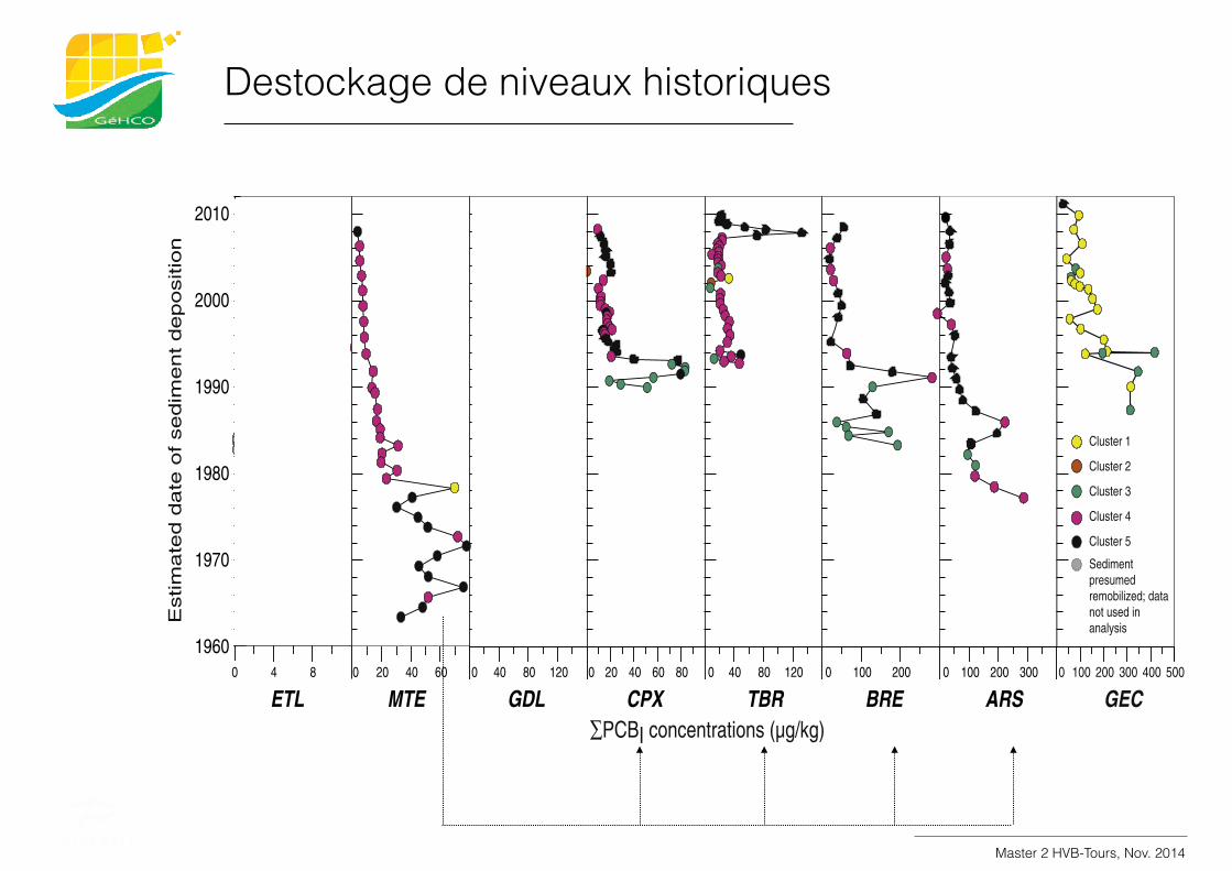
Destockage de niveaux historiques
GEC and GDL differ from those at other sites, indicating that PCBcontamination at these sites might be affected by local sources. Samplesin cluster 3 are primarily samples from the lower parts of cores collectedfrom sites CPX andBRE, and, to a lesser extent, from cores collected fromsites TBR and GEC. These sediment intervals correspond to flood de-posits in the early 1990s and 2000s at sites CPX, TBR, and GEC (Supple-mentary information Figs. S3, S5, and S8) and to removal of debris in1984 at site BRE (Supplementary information Fig. S6). Cluster 4 is dom-inated by penta–hexa–hepta-chlorinated biphenyls (PCB-118, PCB-138,PCB-153, and PCB-180), and more samples are in cluster 4 than in anyother cluster. Samples in cluster 4 are abundant at upstream sites ETL,MTE, and CPX, and at downstream site TBR (sediment deposited priorto 2007). Cluster 5 is characterized by high proportions of hexa- andhepta-chlorinated biphenyls (PCB-153 and PCB-180). Upstream sitesamples in cluster 5 consist of deeper sediments collected at site MTEand the most recently deposited sediment collected at site CPX. Down-stream site samples in cluster 5 include recently deposited sedimentsrepresented by TBR, BRE, and ARS cores. Recently deposited sedimentsin the TBR core, which include the PCB maximum, are in cluster 5whereas older sediments are in cluster 4.
4. Discussion
4.1. Implication for sources
A general upstream–downstream pattern of increasing PCB con-centrations indicates a relation between PCB contamination anddrivers, such as the catchment area and the cumulative upstreampopulation (Fig. 4B). Cumulative area and upstream population arecorrelated (r2 = 0.985, p b 0.0001), and we hypothesize that theyare proxies for emissions, as suggested by others (e.g., Breiviket al., 2002). However, population is neither the only nor the maindriver of trends in historical PCB concentrations along the up-stream–downstream gradient. Regardless of the decade, consider-able variations are observed between the median concentrations,the models, and the cumulative population.
Trends in PCBs at sites MTE and ARS are consistent with widelyreported patterns in PCB contamination (e.g., Eisenreich et al., 1989;Van Metre et al., 1997) in which the highest concentrations coincidewith maximum use and environmental release in the 1960s and1970s andmarked decreases since. At other Rhône River sites, however,relatively high concentrations persist into the 1990s, inconsistent withthis pattern, indicating that PCB inputs might have continued to occur
in the basin following regulation. The PCB peak at TBR during 2007–08is an example of this (Fig. 3). We hypothesize that local PCB releases(in addition to those from the PCB treatment facility upstream fromLyon) have occurred upstream from this site in the past decade.
PCB distribution and trends also are affected by sediment flushingevents and floods. Floods can cause bank erosion, resulting in inputs ofless-contaminated sediment in some cases, or in inputs of more-contaminated sediment in others (e.g., Lecce and Pavlowsky, 1997;Rozan and Hunter, 2001). Floods also can mobilize upstream PCBsources, and major hydro-sedimentary events therefore can affect con-gener compositions. At sites CPX, TBR, and GEC, the data indicate amixed congener assemblage (cluster 3) that corresponds to flooddeposits.
A potential PCB point source to sediments deposited at sites GDL,CPX, and downstream is the PCB treatment facility upstream fromLyon (Fig. 1), which is authorized to release small amounts of PCBsinto the Rhône River (Eaufrance, 2011). Because PCBs are treated anddisposed of at this facility, its regulation differs from that of PCB use inFrance. The magnitude and timing of PCB discharges at the facility areconsistent with temporal trends in PCBs at site CPX (Desmet et al.,2012), but they are more difficult to interpret at site GDL. At site GDL,PCB concentrations increased until 2005 and the congener mixture(cluster 2, higher proportions of low-chlorinated biphenyls) is distinctfrom that at the other sites. The trend at site GDL might be attributableto PCB inputs from upstream tributaries (e.g., the Bourbre River) and(or) management operations in the Grand Large (e.g., dredging). MeanΣPCBI concentrations measured in surficial sediment of the BourbreRiver range between 201.3 μg/kg (1986–1995) and 25.9 μg/kg (post-2005) (Eaufrance, 2011).
Overall, PCBI concentrations are higher at sites downstream fromLyon (TBR, BRE, ARS, and GEC) than at sites upstream from Lyon (ETL,MTE, GDL, and CPX). This pattern indicates that, although the PCB treat-ment facility is a source, it is neither the only source nor themost impor-tant. The substantial increase in PCBI concentrations in the downstreamdirection can be explained only by other PCB sources in the greater Lyonmetropolitan area and from tributaries to the Rhône River downstreamfrom Lyon. Potential sources include the City of Lyon, the industrial cor-ridor downstream from Lyon, the Gier River (a tributary that flows intothe Rhône River between TBR and BRE), the Isère River (a tributary thatflows into the Rhône River at Valence, between ARS and GEC), and per-haps other tributarywatersheds (Fig. 1), consistentwith sources evokedby Santiago et al. (1994). High concentrations of PCBsweremeasured ina sediment core collected from the Gier River (ΣPCBI of 115–160 μg/kg
1960
1970
1980
1990
2000
2010
0 4 8 0 40 80 120 0 40 80 120 0 100 2000 20 40 60 800 20 40 60 0 100 200 300 400 500
GECETL GDL BREMTE CPX TBR
Estim
ate
d d
ate
of
se
dim
en
t d
ep
ositio
n
∑PCBI concentrations (µg/kg)
Cluster 1
Cluster 2
Cluster 3
Cluster 5
Sediment presumed remobilized; data not used in analysis
Cluster 4
0 100 200 300
ARS
Fig. 3. Profiles of the sumof the concentrations of the seven indicator PCBs (ΣPCBI) in sediment cores collected from the Rhône River basin, France. The color of each symbol corresponds toits PCB congener assemblage cluster (Fig. 2).
573B. Mourier et al. / Science of the Total Environment 476–477 (2014) 568–576
Master 2 HVB-Tours, Nov. 2014
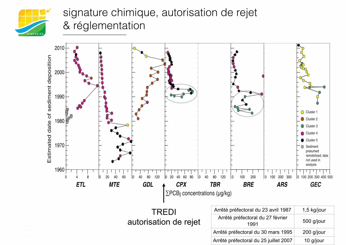
signature chimique, autorisation de rejet & réglementation
GEC and GDL differ from those at other sites, indicating that PCBcontamination at these sites might be affected by local sources. Samplesin cluster 3 are primarily samples from the lower parts of cores collectedfrom sites CPX andBRE, and, to a lesser extent, from cores collected fromsites TBR and GEC. These sediment intervals correspond to flood de-posits in the early 1990s and 2000s at sites CPX, TBR, and GEC (Supple-mentary information Figs. S3, S5, and S8) and to removal of debris in1984 at site BRE (Supplementary information Fig. S6). Cluster 4 is dom-inated by penta–hexa–hepta-chlorinated biphenyls (PCB-118, PCB-138,PCB-153, and PCB-180), and more samples are in cluster 4 than in anyother cluster. Samples in cluster 4 are abundant at upstream sites ETL,MTE, and CPX, and at downstream site TBR (sediment deposited priorto 2007). Cluster 5 is characterized by high proportions of hexa- andhepta-chlorinated biphenyls (PCB-153 and PCB-180). Upstream sitesamples in cluster 5 consist of deeper sediments collected at site MTEand the most recently deposited sediment collected at site CPX. Down-stream site samples in cluster 5 include recently deposited sedimentsrepresented by TBR, BRE, and ARS cores. Recently deposited sedimentsin the TBR core, which include the PCB maximum, are in cluster 5whereas older sediments are in cluster 4.
4. Discussion
4.1. Implication for sources
A general upstream–downstream pattern of increasing PCB con-centrations indicates a relation between PCB contamination anddrivers, such as the catchment area and the cumulative upstreampopulation (Fig. 4B). Cumulative area and upstream population arecorrelated (r2 = 0.985, p b 0.0001), and we hypothesize that theyare proxies for emissions, as suggested by others (e.g., Breiviket al., 2002). However, population is neither the only nor the maindriver of trends in historical PCB concentrations along the up-stream–downstream gradient. Regardless of the decade, consider-able variations are observed between the median concentrations,the models, and the cumulative population.
Trends in PCBs at sites MTE and ARS are consistent with widelyreported patterns in PCB contamination (e.g., Eisenreich et al., 1989;Van Metre et al., 1997) in which the highest concentrations coincidewith maximum use and environmental release in the 1960s and1970s andmarked decreases since. At other Rhône River sites, however,relatively high concentrations persist into the 1990s, inconsistent withthis pattern, indicating that PCB inputs might have continued to occur
in the basin following regulation. The PCB peak at TBR during 2007–08is an example of this (Fig. 3). We hypothesize that local PCB releases(in addition to those from the PCB treatment facility upstream fromLyon) have occurred upstream from this site in the past decade.
PCB distribution and trends also are affected by sediment flushingevents and floods. Floods can cause bank erosion, resulting in inputs ofless-contaminated sediment in some cases, or in inputs of more-contaminated sediment in others (e.g., Lecce and Pavlowsky, 1997;Rozan and Hunter, 2001). Floods also can mobilize upstream PCBsources, and major hydro-sedimentary events therefore can affect con-gener compositions. At sites CPX, TBR, and GEC, the data indicate amixed congener assemblage (cluster 3) that corresponds to flooddeposits.
A potential PCB point source to sediments deposited at sites GDL,CPX, and downstream is the PCB treatment facility upstream fromLyon (Fig. 1), which is authorized to release small amounts of PCBsinto the Rhône River (Eaufrance, 2011). Because PCBs are treated anddisposed of at this facility, its regulation differs from that of PCB use inFrance. The magnitude and timing of PCB discharges at the facility areconsistent with temporal trends in PCBs at site CPX (Desmet et al.,2012), but they are more difficult to interpret at site GDL. At site GDL,PCB concentrations increased until 2005 and the congener mixture(cluster 2, higher proportions of low-chlorinated biphenyls) is distinctfrom that at the other sites. The trend at site GDL might be attributableto PCB inputs from upstream tributaries (e.g., the Bourbre River) and(or) management operations in the Grand Large (e.g., dredging). MeanΣPCBI concentrations measured in surficial sediment of the BourbreRiver range between 201.3 μg/kg (1986–1995) and 25.9 μg/kg (post-2005) (Eaufrance, 2011).
Overall, PCBI concentrations are higher at sites downstream fromLyon (TBR, BRE, ARS, and GEC) than at sites upstream from Lyon (ETL,MTE, GDL, and CPX). This pattern indicates that, although the PCB treat-ment facility is a source, it is neither the only source nor themost impor-tant. The substantial increase in PCBI concentrations in the downstreamdirection can be explained only by other PCB sources in the greater Lyonmetropolitan area and from tributaries to the Rhône River downstreamfrom Lyon. Potential sources include the City of Lyon, the industrial cor-ridor downstream from Lyon, the Gier River (a tributary that flows intothe Rhône River between TBR and BRE), the Isère River (a tributary thatflows into the Rhône River at Valence, between ARS and GEC), and per-haps other tributarywatersheds (Fig. 1), consistentwith sources evokedby Santiago et al. (1994). High concentrations of PCBsweremeasured ina sediment core collected from the Gier River (ΣPCBI of 115–160 μg/kg
1960
1970
1980
1990
2000
2010
0 4 8 0 40 80 120 0 40 80 120 0 100 2000 20 40 60 800 20 40 60 0 100 200 300 400 500
GECETL GDL BREMTE CPX TBR
Estim
ate
d d
ate
of
se
dim
en
t d
ep
ositio
n
∑PCBI concentrations (µg/kg)
Cluster 1
Cluster 2
Cluster 3
Cluster 5
Sediment presumed remobilized; data not used in analysis
Cluster 4
0 100 200 300
ARS
Fig. 3. Profiles of the sumof the concentrations of the seven indicator PCBs (ΣPCBI) in sediment cores collected from the Rhône River basin, France. The color of each symbol corresponds toits PCB congener assemblage cluster (Fig. 2).
573B. Mourier et al. / Science of the Total Environment 476–477 (2014) 568–576
Arrêté préfectoral du 23 avril 1987 1,5 kg/jourArrêté préfectoral du 27 février
1991 500 g/jour
Arrêté préfectoral du 30 mars 1995 200 g/jourArrêté préfectoral du 25 juillet 2007 10 g/jour
TREDI autorisation de rejet
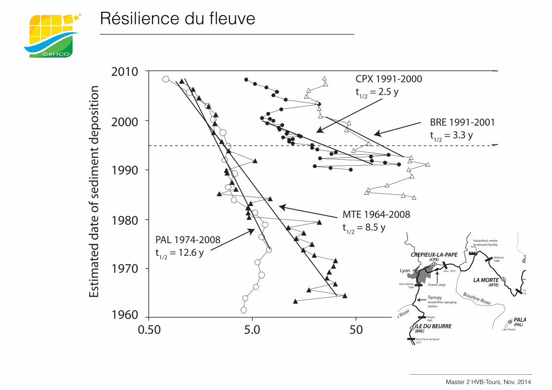
Résilience du fleuve
BRE 1991-2001t1/2 = 3.3 y
CPX 1991-2000t1/2 = 2.5 y
MTE 1964-2008t1/2 = 8.5 y
PAL 1974-2008t1/2 = 12.6 y
PALMTECPXBRE
2000
2010
1990
1980
1970
19600.50 5.0 50 500
PCBI concentration (micrograms per kilogram) normalized by total organic carbon content (percent)
Estim
ated
dat
e of
sed
imen
t dep
ositi
on
2010
2005
2000
19950.5 5.0 50
PAL 1998-2009t1/2 = 6.2 y
MTE 2001-08t1/2 = 6.4 y
CPX 2003-08t1/2 =2.4 y
BRE 2001-08no change
Sediment core collection siteDam and date of constructionUrban area
Lyon
Grenoble
Geneva
Ain
Rive
r
Fier River
Saôn
e Ri
ver
Arve River
LA MORTE(MTE)
CREPIEUX-LA-PAPE(CPX)
ILE DU BEURRE(BRE)
10 km
hazardous-wastetreatment facility
Gier RiverChambéry
Seyssel1951
Belley1981
Champagneux1984
Villebois1986
Genissiat1948
Pougny1943
Vaugris1980
Pierre Benite1966
Saint Pierre de Boeuf1977
Arras-Rhône1971
Jons, 1933
Bourbre River
PALADRU(PAL)
Rhôn
e Ri
ver
Rhôn
e Ri
ver
Annecy Lake Annecy
Lake Geneva
Lake Bourget
Lake Paladru
France Rhône River
Paris
Ternaystreamflow-gaugingstation
Grand Large
N
Figure 1. Map of the study area, Rhône basin, France.
Mediterranean Sea
AtlanticOcean
Master 2 HVB-Tours, Nov. 2014
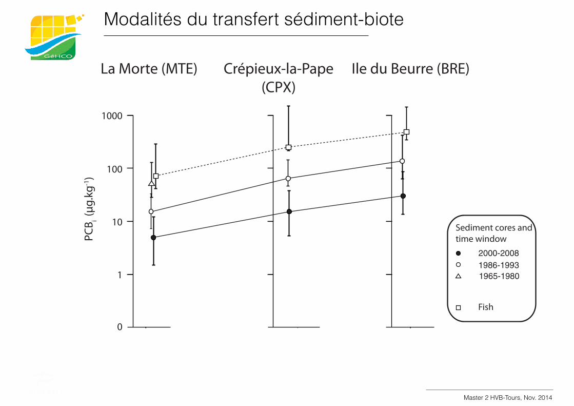
Modalités du transfert sédiment-biote
ARVERiver FIER
River
LakeBOURGET AIN
River
SAONERiver
BOURBRERiver GIER
River
Productionfactory
Hazardous-wastetreatment site
Contaminatedsoils
LYON URBAN AREA
Productionfactory
Contaminatedsoils
Contaminatedsoils
Contaminatedsoils
CHAMBERYURBAN AREA
Paladru (PAL) La Morte (MTE) Crépieux-la-Pape(CPX)
Ile du Beurre (BRE)
0
1
10
1000
100
PCB i (µ
g.kg
-1)
0
1
10
1000
100
2000-20081986-19931965-1980
Fish
Figure 5. Mean and range of PCBI concentrations in sediment cores from the Rhône River for three time windows and concentrations measured in fish (bream) in 2008 (Babut et al., 2011). Also shown are locations of two urban areas relative to the main stem of the Rhône and confluences with major tributaries (fig. 1), and locations of known or suspected PCB sources (Robin des Bois, 2011).
Downstreamdirection
Sediment cores andtime window
Master 2 HVB-Tours, Nov. 2014
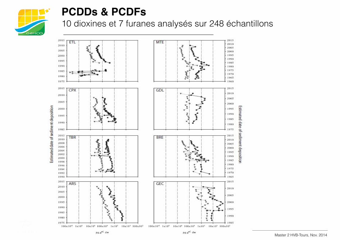
PCDDs & PCDFs10 dioxines et 7 furanes analysés sur 248 échantillons
Master 2 HVB-Tours, Nov. 2014
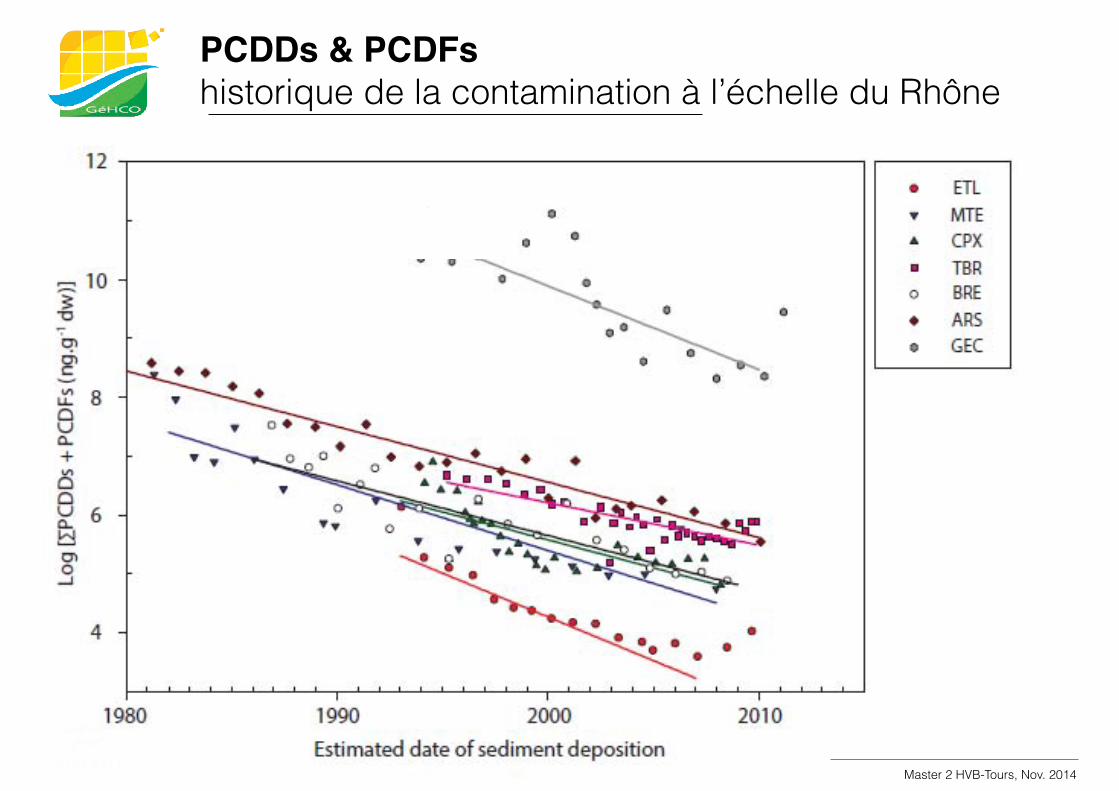
PCDDs & PCDFshistorique de la contamination à l’échelle du Rhône
Master 2 HVB-Tours, Nov. 2014
Quelques conclusions récapitulatives
Master 2 HVB-Tours, Nov. 2014
• Des demi-vies comprises entre 5 et 10 ans • Les interdictions sont donc efficaces • Le fonctionnement hydrosédimentaire du Rhône l’est aussi • Le gradient amont-aval est moins significatif que celui des PCBs • le site aval est fortement influencé par les apports de l’Isère • la sidérurgie de la vallée de romanche et les procédés de
transformation par four électrique à arc ont conduit à des rejets
importants de dioxines et furanes
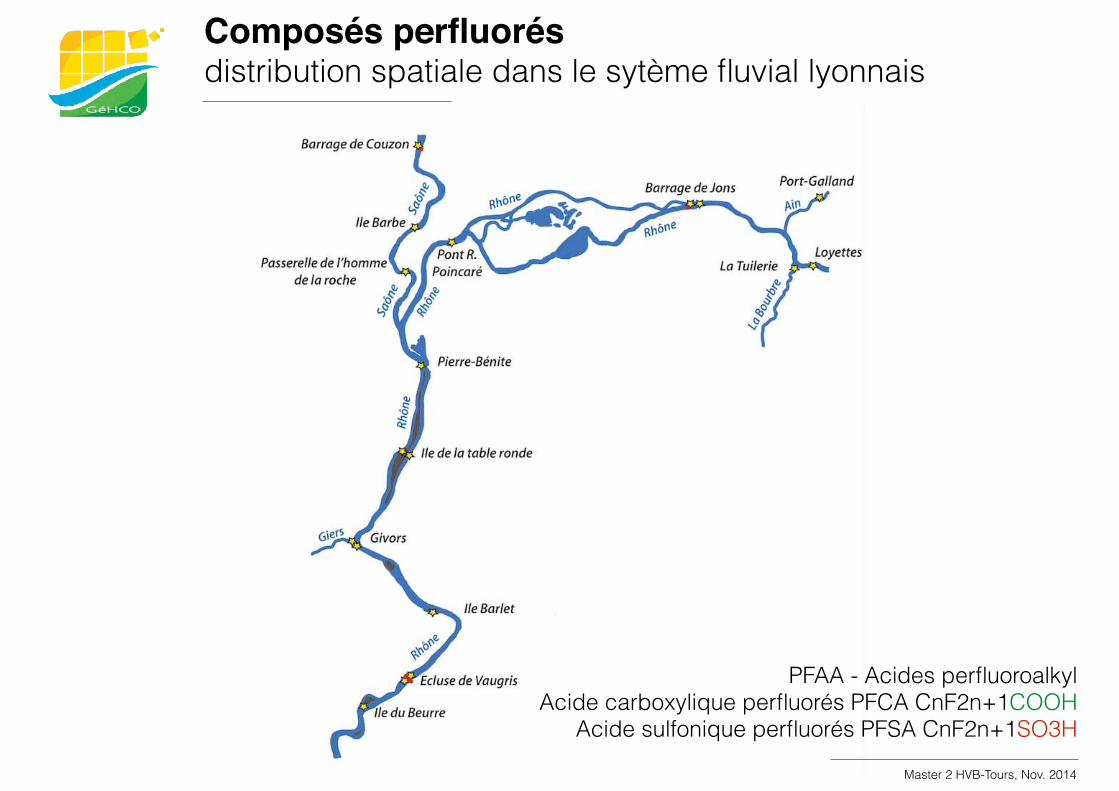
Master 2 HVB-Tours, Nov. 2014
Composés perfluorésdistribution spatiale dans le sytème fluvial lyonnais
PFAA - Acides perfluoroalkyl Acide carboxylique perfluorés PFCA CnF2n+1COOH
Acide sulfonique perfluorés PFSA CnF2n+1SO3H
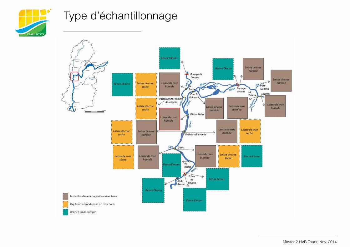
Master 2 HVB-Tours, Nov. 2014
Type d’échantillonnage
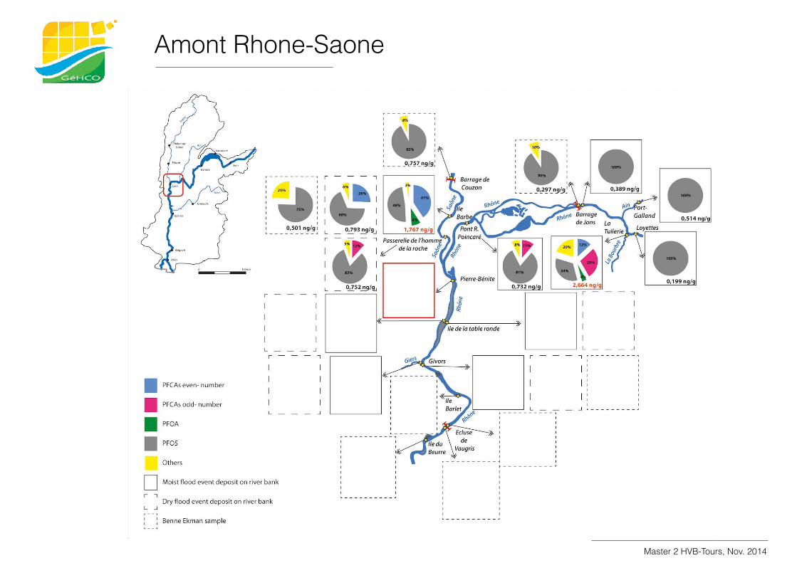
Master 2 HVB-Tours, Nov. 2014
Amont Rhone-Saone
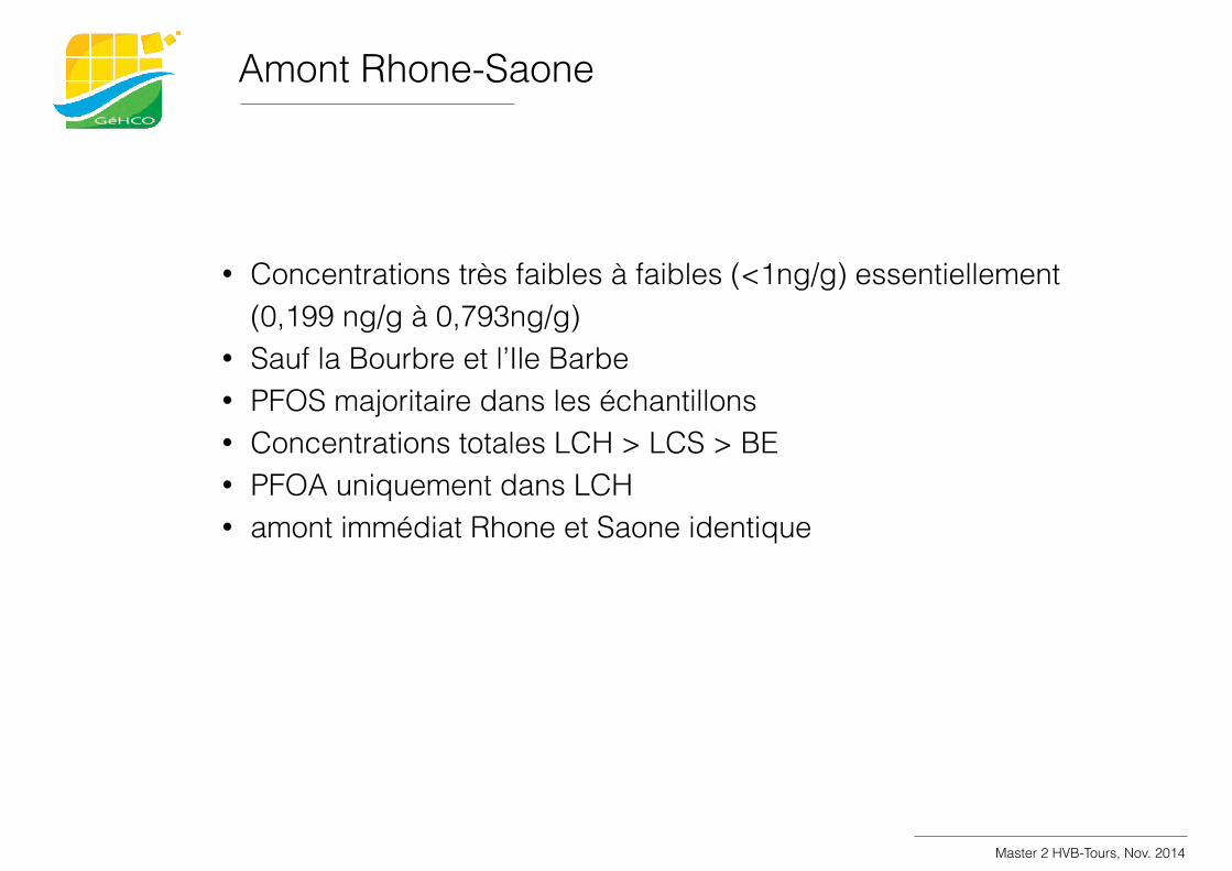
Master 2 HVB-Tours, Nov. 2014
Amont Rhone-Saone
• Concentrations très faibles à faibles (<1ng/g) essentiellement (0,199 ng/g à 0,793ng/g)
• Sauf la Bourbre et l’Ile Barbe • PFOS majoritaire dans les échantillons • Concentrations totales LCH > LCS > BE • PFOA uniquement dans LCH • amont immédiat Rhone et Saone identique
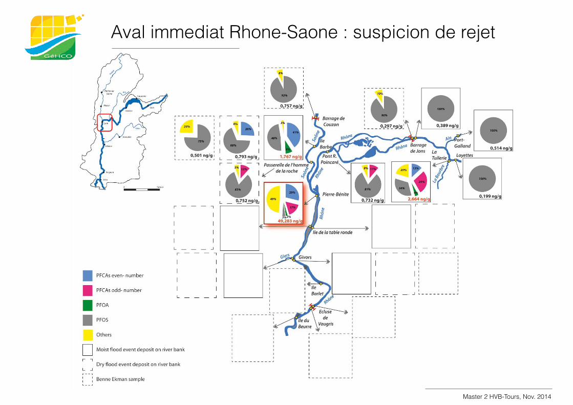
Master 2 HVB-Tours, Nov. 2014
Aval immediat Rhone-Saone : suspicion de rejet
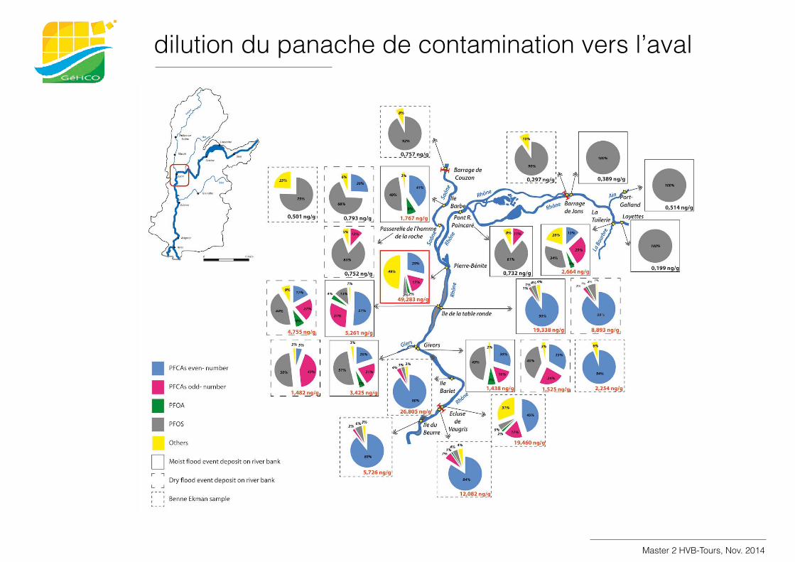
Master 2 HVB-Tours, Nov. 2014
dilution du panache de contamination vers l’aval

Master 2 HVB-Tours, Nov. 2014
dilution du panache de contamination vers l’aval
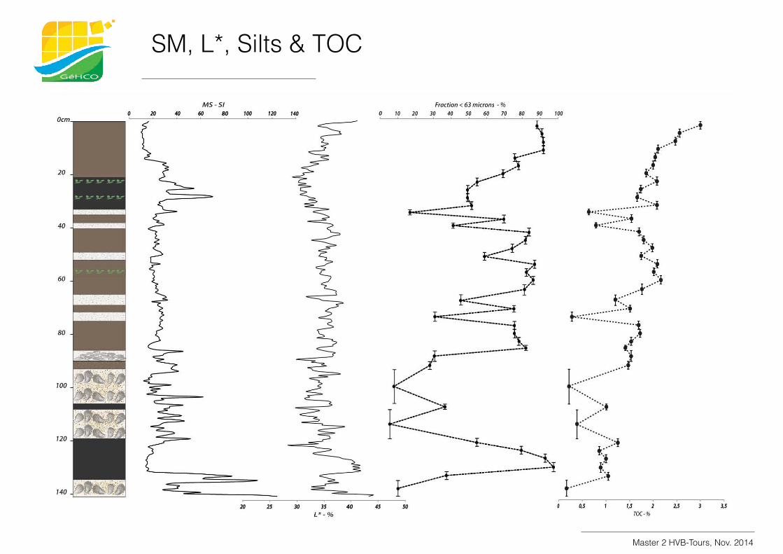
Master 2 HVB-Tours, Nov. 2014
SM, L*, Silts & TOC
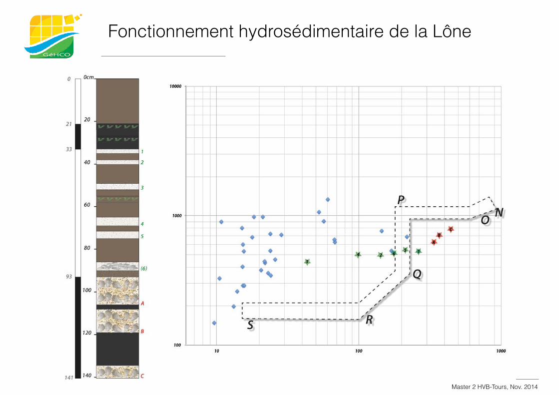
Master 2 HVB-Tours, Nov. 2014
Fonctionnement hydrosédimentaire de la Lône
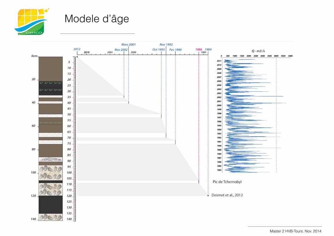
Master 2 HVB-Tours, Nov. 2014
Modele d’âge
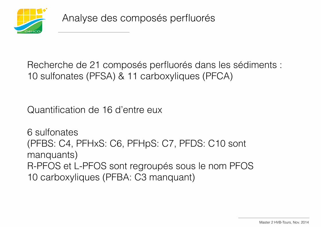
Master 2 HVB-Tours, Nov. 2014
Recherche de 21 composés perfluorés dans les sédiments : 10 sulfonates (PFSA) & 11 carboxyliques (PFCA)
Quantification de 16 d’entre eux
6 sulfonates (PFBS: C4, PFHxS: C6, PFHpS: C7, PFDS: C10 sont manquants) R-PFOS et L-PFOS sont regroupés sous le nom PFOS 10 carboxyliques (PFBA: C3 manquant)
Analyse des composés perfluorés
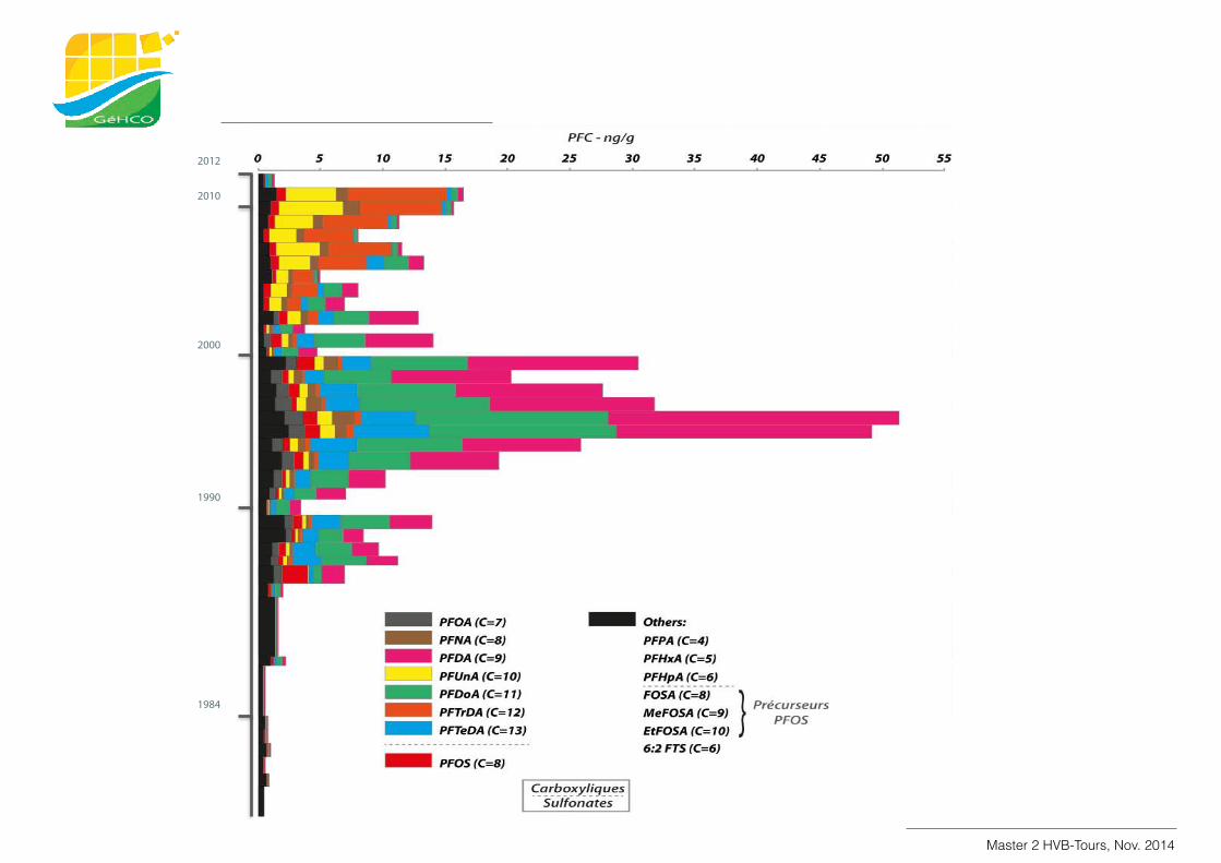
Master 2 HVB-Tours, Nov. 2014
2010
2000
1990
1984
2012
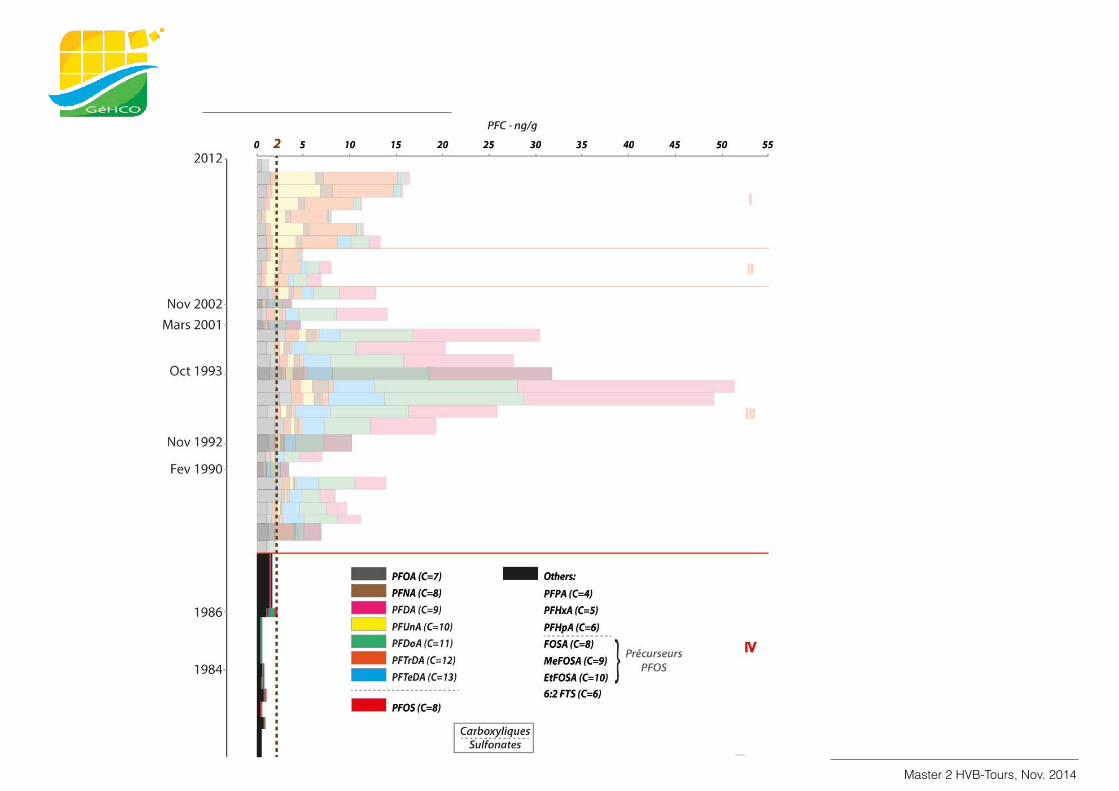
Master 2 HVB-Tours, Nov. 2014
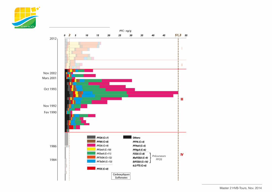
Master 2 HVB-Tours, Nov. 2014
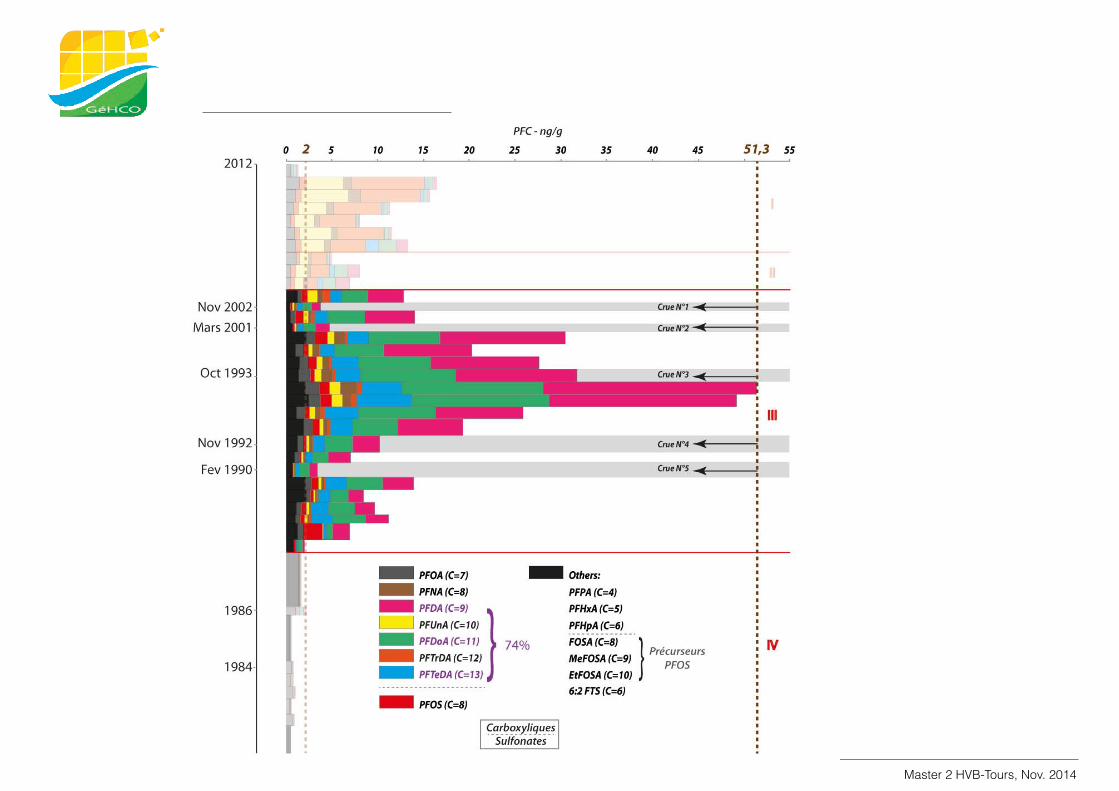
Master 2 HVB-Tours, Nov. 2014
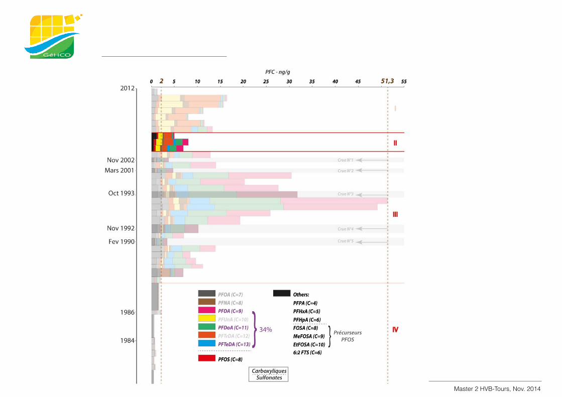
Master 2 HVB-Tours, Nov. 2014
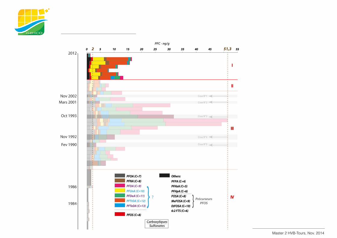
Master 2 HVB-Tours, Nov. 2014
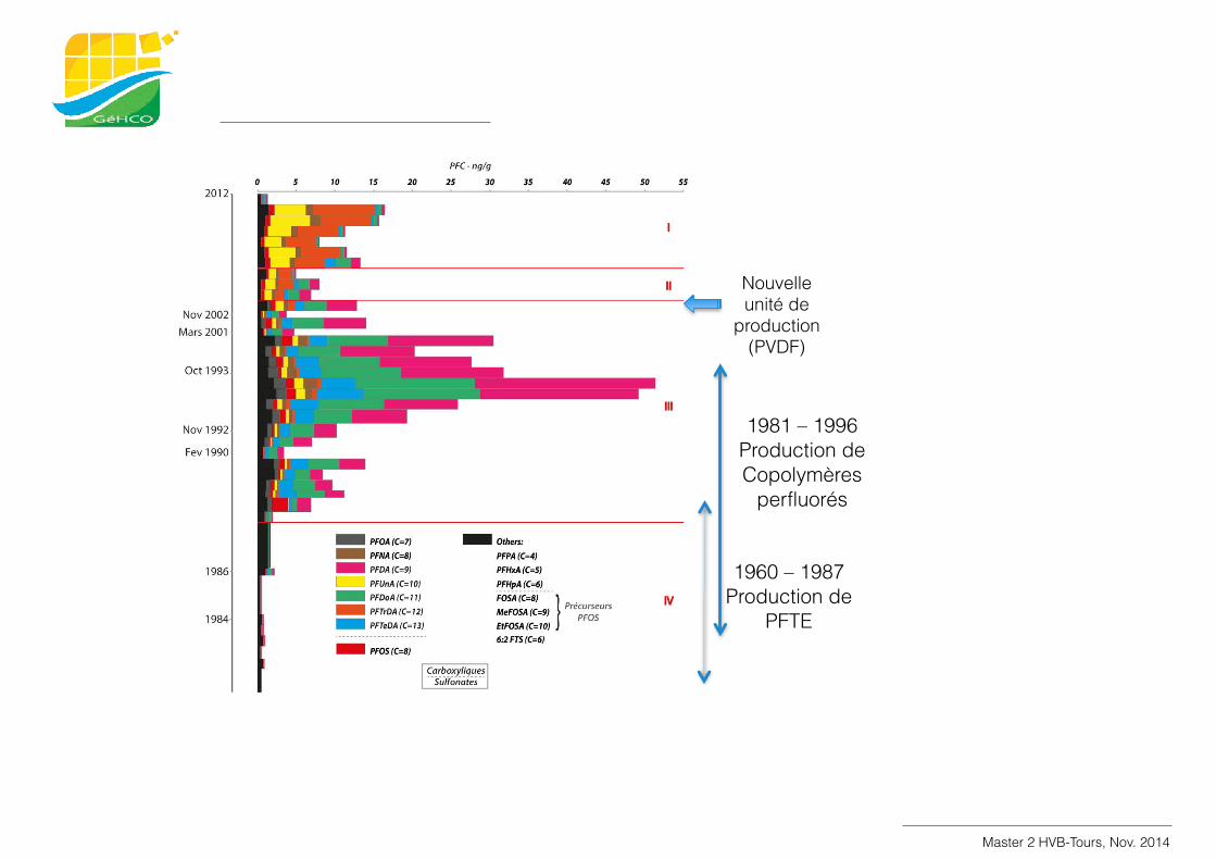
Master 2 HVB-Tours, Nov. 2014
Nouvelle unité de
production (PVDF)
1960 – 1987 Production de
PFTE
1981 – 1996 Production de Copolymères
perfluorés
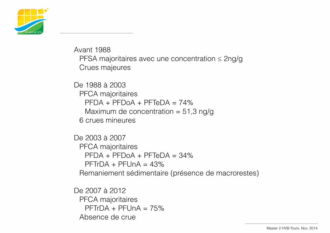
Master 2 HVB-Tours, Nov. 2014
Avant 1988 PFSA majoritaires avec une concentration ≤ 2ng/g Crues majeures
De 1988 à 2003 PFCA majoritaires
PFDA + PFDoA + PFTeDA = 74% Maximum de concentration = 51,3 ng/g
6 crues mineures
De 2003 à 2007 PFCA majoritaires
PFDA + PFDoA + PFTeDA = 34% PFTrDA + PFUnA = 43%
Remaniement sédimentaire (présence de macrorestes)
De 2007 à 2012 PFCA majoritaires
PFTrDA + PFUnA = 75% Absence de crue