DOCUMENT

DE TRAVAIL

N° 588

DIRECTION GÉNÉRALE DES ÉTUDES ET DES RELATIONS INTERNATIONALES

THE ROLE OF PRODUCTION FACTOR QUALITY AND TECHNOLOGY

DIFFUSION IN 20TH CENTURY PRODUCTIVITY GROWTH

Antonin Bergeaud, Gilbert Cette and Rémy Lecat

April 2016

DIRECTION GÉNÉRALE DES ÉTUDES ET DES RELATIONS INTERNATIONALES

THE ROLE OF PRODUCTION FACTOR QUALITY AND TECHNOLOGY

DIFFUSION IN 20TH CENTURY PRODUCTIVITY GROWTH

Antonin Bergeaud, Gilbert Cette and Rémy Lecat

April 2016

Les Documents de travail reflètent les idées personnelles de leurs auteurs et n'expriment pas nécessairement la position de la Banque de France. Ce document est disponible sur le site internet de la Banque de France « www.banque-france.fr ». Working Papers reflect the opinions of the authors and do not necessarily express the views of the Banque de France. This document is available on the Banque de France Website “www.banque-france.fr”.

1

The role of production factor quality and technology diffusion in

20th

century productivity growth1

Antonin Bergeaud Gilbert Cette Rémy Lecat Banque de France Banque de France and Université

Aix-Marseille (Aix-Marseille School of Economics), CNRS et EHESS

Banque de France

1 The views expressed herein are those of the authors and do not necessarily reflect the views of the

institutions they belong to. We wish to thank, without implicating, Thierry Mayer for valuable advice concerning the construction of the instruments, Bas Van Leeuwen for advice on education data, Nicholas Craft and John Fernald for comments.

2

Abstract:

20th century growth has been an exceptional period in the history of mankind, relying mostly on increase in total factor productivity (TFP). Using a 1890-2013 17-OECD country database, this paper improves the measurement of TFP by taking into account production factor quality, i.e. the education level of the working-age population for labor and the age of equipment for the capital stock. However, our main contribution is to assess the role of technology diffusion to TFP growth through two emblematic general purpose technologies, electricity and information and communication technologies (ICT). Using both growth decomposition methodology and instrumental variables estimates, this paper finds that, among factor quality, education levels have posted the largest contribution to growth, while the age of capital has a significant, although limited, contribution. Quality-adjusted production factors explain less than half of labor productivity growth in the largest countries but Japan, where capital deepening posted a very large contribution. As a consequence, the “one big wave” of productivity growth (Gordon, 1999), as well as the ICT productivity wave for the countries which experienced it, remains only partially explained by quality-adjusted factors, although education and technology diffusion contribute to explain the US earlier wave in the 1930s-1940s. Finally, technology diffusion, as captured through our two general purpose technologies, leaves between 0.6 and 1 point of yearly growth, as well as a large share of the two 20

th century technology waves,

unexplained. These results support both a significant lag in the diffusion of general purpose technologies and a wider view on growth factors, encompassing changes in the production process, management techniques or financing practices.

JEL classifications: N10, O47, E20

Keywords: Productivity, Total factor productivity, Education, Technological Change, Technology diffusion, Global History Résumé:

La croissance au 20ème siècle a été une période exceptionnelle dans l’histoire de l’humanité, reposant principalement sur la croissance de la productivité globale des facteurs (PGF). Utilisant une base de données couvrant la période 1890-2013 pour 17 pays de l’OCDE, ce papier améliore la mesure de la PGF en prenant en compte la qualité des facteurs de production, c'est-à-dire le niveau d’éducation de la population en âge de travailler pour l’emploi et l’âge des équipements pour le stock de capital. Cependant, notre contribution principale est l’évaluation du rôle de la diffusion des nouvelles technologies à la croissance de la PGF au travers de deux technologies généralistes (General purpose technologies) emblématiques, l’électricité et les technologies de l’information et de la communication (TIC). En utilisant à la fois une décomposition comptable de la croissance et des estimations en variables instrumentales, ce papier montre que, parmi la qualité des facteurs, les niveaux d’éducation ont apporté la contribution la plus forte à la croissance, tandis que l’âge du capital a eu une contribution significative mais limitée. Les facteurs de production ajustés par la qualité expliquent moins de la moitié de la croissance de la productivité du travail dans les pays les plus grands sauf le Japon, où l’intensité capitalistique a apporté une forte contribution. En conséquence, la « grande vague » de productivité (Gordon, 1999), ainsi que la vague TIC pour les pays qui l’ont connue n’est que partiellement expliquée par la qualité des facteurs. Enfin, la diffusion des technologies, telle qu’estimée par nos deux technologies généralistes, laisse inexpliquée entre 0,6 et 1 point de croissance annuelle, ainsi qu’une large part des deux vagues technologiques du 20

ème siècle. La qualité

des facteurs, tout comme la diffusion des technologies, contribuent néanmoins à expliquer l’avance des États-Unis au milieu du 20

ème siècle. Ces résultats confortent un retard significatif de diffusion des technologies et la

nécessité d’une vision plus large des facteurs de croissance, prenant en compte les modifications du processus de production, des techniques de management ou des pratiques de financement.

Classifications JEL: N10, O47, E20

Mots-clés: Productivité, productivité globale des facteurs, éducation, changement technologique, diffusion technologique, histoire mondiale

3

Non technical summary

Growth in the 20th century has been characterized by three stylized facts, which the growth literature has tried to explain over the recent decades. First, the period starting with the second industrial revolution has been a period of exceptional growth compared to the past history of mankind or even to the first industrial revolution. World GDP per capita growth has averaged 1.5% per year from 1870 to 2000, as compared to less than 0.1% during the pre-industrial era and 0.3% during the first industrial revolution (Maddison, 2001). Second, this take-off has been uneven across countries, leading to a “Great divergence” (Galor, 2005) between emerging and advanced economies, and has been staggered across advanced countries. Finally, GDP per capita has slowed markedly in advanced countries since the 1970s, leading to question the durability of the 20th century pace of growth (Gordon, 2012, 2013 and 2014). These stylized facts come down to three questions: why such a take-off at this stage of human history? Why such heterogeneity in this take-off? Will this take-off last? These questions have already been extensively addressed by the growth literature, which focused both on the factors of growth and on the convergence process. One crucial factor to answer these questions is to quantify the contribution of traditional factors of growth (capital, labor) taking into account their quality but, beyond this growth accounting exercise, to explore more deeply the role of General Purpose Technologies (GPT) in long-term growth. Growth accounting (Solow, 1957) was a first attempt to analyze the respective roles of production factors, failing however to explain the bulk of 20th century growth, which was attributed to total factor productivity (TFP), the residual of this decomposition. TFP improvements are attributed to technical change, which however remains largely a “black box” notion. This is partly related to the difficulty to capture the role of General Purpose technologies, due to their pervasiveness and their technological dynamism (Bresnahan and Trajtenberg, 1995). Indeed, General Purpose technologies’ contribution goes beyond factors included in growth accounting approach such as capital deepening in GPT-related equipment and TFP improvement in GPT producing sectors. First, GPTs lead to fundamental changes in the production process of GPT-using industries. These changes may be badly accounted for in growth accounting exercises, for example if they require the accumulation of complementary organizational capital (Basu and Fernald, 2007). Second, GPT may generate spillovers to seemingly far-away sectors (Helpman and Trajtenberg, 1998). Third, GPT may have a long diffusion lag (cf. for instance David, 1990). This paper estimates the role of quality-adjusted production factors and technology diffusion in the GDP per capita growth of 17 OECD countries over the period 1890-2013. First, we have built a long-run dataset over a large number of countries, with data reconstituted in purchasing power parity and on the basis of, as much as possible, consistent assumptions. Second, we have adjusted production factors for quality, taking into account education levels and the age of the capital stock. Third, our main contribution is to estimate the contribution of technology diffusion to TFP growth, focusing on two general purpose technologies, electricity and ICT, often considered as characteristic of different technology diffusion periods across the 20th century. Our results are manifold, and the three main contributions to the literature are the following ones: (i) Among factor quality, education levels have posted the largest contribution to growth, while the age of capital has a significant, although limited, contribution; (ii) Quality-adjusted production factors explain less than half of labor productivity growth in the largest countries, but Japan, where capital deepening posted a very large contribution. As a consequence, the “one big wave” of productivity growth (Gordon, 1999), as well as of the ICT productivity wave for the countries which experienced it, remain unexplained by quality-adjusted factors, although the early access of the masses to higher education partly explains the US advance over the other countries before World War II; (iii) Our main contribution is however the estimation of the contribution of General Purpose Technologies to long-term growth. Technology diffusion, as captured through our two general purpose technologies, also

4

contributes to explain the US advance in the 1930s-1940s and ICT productivity waves but leaves unexplained between 0.6 and 1 point yearly growth, as well as a large share of the two 20th century technology waves. These results support both a significant lag in the diffusion of general purpose technologies and a wider view on growth factors, encompassing changes in the production process, financing techniques, management practices… as emphasized by Ferguson and Wascher (2004).

5

1. Introduction

Growth in the 20th century has been characterized by three stylized facts, which the growth literature has tried to explain over the recent decades. First, the period starting with the second industrial revolution has been a period of exceptional growth compared to the past history of mankind or even to the first industrial revolution. World GDP per capita growth has averaged 1.5% per year from 1870 to 2000, as compared to less than 0.1% during the pre-industrial era and 0.3% during the first industrial revolution (Maddison, 2001). Second, this take-off has been uneven across countries, leading to a “Great divergence” (Galor, 2005) between emerging and advanced economies, and has been staggered across advanced countries (see for example Baumol, 1986, Barro, 1991 and Bergeaud et al., 2015a). Finally, GDP per capita has slowed markedly in advanced countries since the 1970s, except during the 1995-2005 period in the US and the UK, where productivity has accelerated thanks to the ICT technology revolution (e.g. Maddison, 2007, Bergeaud et al., 2015b), leading to question the durability of the 20th century pace of growth (Gordon, 2012, 2013 and 2014). These stylized facts come down to three questions: why such a take-off at this stage of human history? Why such heterogeneity in this take-off? Will this take-off last? These questions have already been extensively addressed by the growth literature, which focused both on the factors of growth and on the convergence process. This paper provides some elements of answers to these questions, from estimates of the role of quality-adjusted production factors and of the contribution of technology diffusion, through two emblematic General purpose technologies (GPT), to the GDP per capita growth in the main developed countries. Indeed, one crucial factor to answer these questions is to quantify the contribution of traditional factors of growth (capital, labor) taking into account their quality but, beyond this growth accounting exercise, to explore more deeply the role of General Purpose Technologies in long-term growth. Growth accounting (Solow, 1957) was a first attempt to analyze the respective roles of production factors, failing however to explain the bulk of 20th century growth, which was attributed to total factor productivity (TFP), the residual of this decomposition. TFP improvements are attributed to technical change, which however remains largely a “black box” notion. This is partly related to the difficulty to capture the role of General Purpose technologies, due to their pervasiveness and their technological dynamism (Bresnahan and Trajtenberg, 1995). Indeed, General Purpose technologies’ contribution goes beyond factors included in growth accounting approach such as capital deepening in GPT-related equipment and TFP improvement in GPT producing sectors. First, GPTs lead to fundamental changes in the production process of GPT-using industries. These changes may be badly accounted for in growth accounting exercises, for example if they require the accumulation of complementary organizational capital (Basu and Fernald, 2007). Second, GPT may generate spillovers to seemingly far-away sectors (Helpman and Trajtenberg, 1998). The literature dedicated to growth factors and to convergence have both emphasized the role of innovation and innovation diffusion, in interaction with education and institutions. For countries at the technological frontier, growth relies on improved human capital through education (see Krueger and Lindahl, 2001, for a survey) and increasing TFP through innovation. The innovation process hinges on education level and adapted institutions (labor and product market regulations, juridical system quality, political system…) as well as relative factor endowment and market size (“Directed technical change”, see Acemoglu 1998, 2002) 2. For countries below the frontier, even those conducting a significant R&D activity such as France, Germany and the United Kingdom, adoption of

2 Basu and Fernald (2002) show that imperfections and frictions in output and factor markets matter in the

relation from aggregate technology to aggregate productivity. For example, with heterogeneous firm mark-ups, the same resources may be valued differently in different uses. Then “reallocating resources towards

more socially valued uses raises aggregate productivity, without necessarily reflecting changes in

technology.” (p. 964). Edquist (2001) raises the role of innovation policy concerning technology diffusion.

6

new technologies from abroad is the main source of technological progress (Eaton and Kortum, 1999). Heterogeneity in the adoption and the diffusion of new technologies is large and explains a significant share of the “Great divergence” (Comin and Mestieri, 2013). Comin and Hobijn (2010) provide evidence that those countries that caught up the most with the U.S. in the postwar period are those that also saw an acceleration in the adoption of new technologies. But adoption of new technologies requires both a “social capability”, relying on a minimum education level within the population and on adapted institutions, and “technological congruence” making it cost effective to adopt leader’s technology (Abramovitz and David, 1995). These conditions to benefit as much as possible from new innovations could play a growing role in the future if the rate of innovation accelerates, as evoked for example by Fernald and Jones (2014, citation from p. 48), which suggest that such an acceleration could happen within the next decade, from “… the rise of China, India and

other emerging economies countries, which likely implies rapid growth in world researchers for at

least several decades.”. Although the empirical literature has achieved major progress in understanding growth dynamics, much remains to be done to assess the respective contributions of these different factors. In particular, the contribution of general purpose technologies is hard to account for due to their diffusion lag (cf. for instance David, 1990), their pervasiveness and dynamic technological effects (Bresnahan and Trajtenberg, 1995). Moreover, many articles focused on one specific factor, leading to over-explain growth when adding these different contributions. Collinearity between growth factors and causality directions has hence to be properly sorted out in order to make an acute diagnosis on growth factors. Several papers have attempted to part growth factors over the long run on a large panel of countries (see Crafts and O’Rourke, 2013, for a survey). In particular, Madsen has developed a long-term database on OECD countries and has examined the respective role of capital deepening and TFP (Madsen, 2010a), the role of production factors and TFP determinants (Madsen, 2010b) and the role of human capital (Madsen, 2014). He has emphasized the major role of TFP in growth dynamics, showing that capital deepening has been strongly driven by TFP: in the OECD countries, since 1870, TFP has contributed to annual per capital GDP growth for 1.81 point over 1.87%, as the contribution of education (0.48 point) has been offset by the reduction in hours worked per employee (-0.49 point). Among the vast convergence literature, Barro (2015) emphasizes the role of education and

democracy in conditioning β-convergence on a country panel starting in 1870; Bergeaud et al.

(2015b) show that the bulk of 20th century σ-convergence hinges on TFP and capital deepening. Derived from unified growth theory (Galor, 2005), which provides microfunded and macrodynamic models trying to highlight the causal relationship between human capital, technology and growth, Cervellati et al. (2013) assess a microfounded macrodynamic model in a panel of countries since 1880 and find that income gaps between rich and poor countries relate to the health environment, war occurrence and geographical remoteness. Numerous papers have also attempted to characterize the role of technology diffusion on productivity growth through growth accounting approaches. Among others, Jorgenson and Stiroh (2000), Oliner and Sichel (2000) or Oliner, Sichel and Stiroh (2007) have focused on the contribution of ICTs in the US at the end of the 20th Century. And regarding industrial revolution comparisons, among others, Crafts (2002) has compared the contributions of steam engines in the UK during 1780-1860, electricity and ICTs in the US during 1899-1929 and 1974-2000 respectively, or Jalava and Pohjola (2008) have compared the contributions of electricity during 1920-1938 and ICTs during 1990-2004 in Finland. The goal of most of these approaches was however not, as it is the case in this paper, to explore the contributions to TFP growth, as the growth accounting method cannot really characterize spillovers which is one of the channels of technology diffusion impact on productivity for general purpose technologies.

7

This paper estimates the role of quality-adjusted production factors and technology diffusion in the GDP per capita growth of 17 OECD countries over the period 1890-2013. First, we have built a long-run dataset over a large number of countries, with data reconstituted in purchasing power parity and on the basis of, as much as possible, consistent assumptions. Second, we have adjusted production factors for quality, taking into account education levels and the age of the capital stock. Third, our main contribution is to estimate the contribution of technology diffusion to TFP growth, focusing on two general purpose technologies, electricity and ICT, often considered as characteristic of different technology diffusion periods across the 20th century (see among others Comin et al., 2006a and 2006b). Our dataset is composed of 17 advanced countries: the G7 countries (the United States, Japan, Germany, France, the United Kingdom, Italy and Canada), the other three biggest countries of the Euro Area (Spain, the Netherlands and Belgium), two other countries of this Area (Portugal and Finland) and five other OECD countries highly relevant for productivity analysis because of their specificities, such as a high productivity level at the beginning of the period for Australia, a specific industry structure for Norway and Switzerland and the role of structural policies for Sweden and Denmark at some point of their history. In addition, a Euro Area has been reconstituted, aggregating Germany, France, Italy, Spain, the Netherlands, Belgium, Portugal and Finland. This approximation seems acceptable as these eight countries represent together, in 2010, 93.2% of the Euro Area GDP (16 countries in 2010). The analysis is carried out over the period 1890-2013 on annual data. The starting database was the one built by Cette, Kocoglu and Mairesse (2009), updated and considerably enlarged in Bergeaud et

al. (2015a and b), and once more in this study. We have tried to make the best use of national accounting data for the last decades and of the estimates of long aggregate historical data series by economists and historians, in particular Maddison (2001), updated by Bolt and van Zanden (2014). The data are built under the hypothesis of constant borders, in their last state. Series for GDP and capital are given in 2010 constant national currencies and converted to 2010 US dollars at purchasing power parity (ppp) with a conversion rate from the Penn World Tables. Strong assumptions are required to reconstitute some countries and series. We may nevertheless consider that the orders of magnitude of our estimates and the ensuing dynamics in GDP per capita and production factors are fairly reliable and meaningful. GDP growth has been decomposed between the contribution of production factors, capital and labor, to obtain TFP as a residual. In a second step, the quality of production factors, education and the age of capital, has been introduced through an estimation of their contribution to this gross TFP, taking into account their potential endogeneity through instrumental variables regressions. In a third step, the contribution of technology diffusion through the contribution of two emblematic general purpose technologies has been estimated, endogeneity being addressed by a similar estimation procedure. Our results are manifold, and the three main contributions to the literature are the following ones: (i) Among factor quality, education levels have posted the largest contribution to growth, while the age of capital has a significant, although limited, contribution; (ii) Quality-adjusted production factors explain less than half of labor productivity growth in the largest countries, but Japan, where capital deepening posted a very large contribution. As a consequence, the “one big wave” of productivity growth (Gordon, 1999), as well as of the ICT productivity wave for the countries which experienced it, remain unexplained by quality-adjusted factors, although the early access of the masses to higher education partly explains the US advance before World War II; (iii) Our main contribution is however the estimation of the contribution of General Purpose Technologies to long-term growth. Technology diffusion, as captured through our two general purpose technologies, also contributes to explain the US advance in the 1930s-1940s and ICT productivity waves but leaves unexplained between 0.6 and 1

8

point yearly growth, as well as a large share of the two 20th century technology waves. These results support both a significant lag in the diffusion of general purpose technologies and a wider view on growth factors, encompassing changes in the production process, financing techniques… as emphasized by Ferguson and Wascher (2004). Section 2 presents the data sources and construction methods. Section 3 focuses on the contribution of factor quality. Section 4 addresses the impact of the spread of technologies. Section 5 concludes. 2. Data: sources, method and construction

The original dataset used in this study comes from Bergeaud et al. (2015a), updated and enlarged to more countries (2.1.). We have completed this dataset with education level (2.2.), age of capital (2.3.) and spread of some generic technologies (2.4.) data. 2.1. The original dataset

Our main dataset is the one used in Bergeaud et al. (2015a) and based on the works of Cette et al. (2009) and Bergeaud et al. (2015b) gathering data for 17 OECD countries over the period 1890-2013. These countries have been chosen for their economic relevance: the G7 (The United States, Japan, Germany, France, the United Kingdom, Italy and Canada), five other euro area countries (Spain, Netherlands, Belgium, Portugal and Finland) and five other countries, which represent a significant share of world GDP at some point during our time frame or which represent a specific interest in terms of productivity (Australia, Switzerland, Denmark, Sweden and Norway). In addition, a Euro Area has been reconstituted, aggregating Germany, France, Italy, Spain, the Netherlands, Belgium, Portugal and Finland. This approximation seems acceptable as these eight countries represent together, in 2010, 93.2% of the Euro Area GDP (16 countries in 2010). The starting date, 1890, has been chosen so as to have sufficiently long time series to initialize our capital stock. A detailed description of the construction of this dataset is given in Bergeaud et al. (2015b), in particular its appendix A which presents the source of the data. To compute GDP over this long 1890-2013 period, we have relied mostly on Maddison (2001) whose series have been updated by Bolt and Van Zanden (2014). Maddison provides data for GDP (Y) and population (P), most of the time from 1820. We have supplemented these data with national accounts data. For other series and in particular to compute the capital intensity and labor productivity, three basic series are needed for each country: employment (N), average hours worked per worker (H) and capital (K). The capital indicator is constructed by the perpetual inventory method (PIM) applied to each of the two components (equipment KE and buildings KB) thanks to the corresponding investment data (IE and IB). The yearly depreciation rates used to build the capital series by the PIM are 10.0% for equipment and 2.5% for buildings following Cette et al. (2009) and are assumed to be constant across time and space. Finally, damages happening during World Wars, earthquakes in Japan and the civil war for Spain are, as much as information is available for this, taken into account to build the capital series. For long aggregate historical data, we have used series built by economists and historians on consistent assumptions. Many of these data are subject to uncertainty and inaccuracy, not only for the most distant periods but also for recent ones. The data are built at the country level under the hypothesis of constant borders, in their last state. It should be noted that, however talented economists and historians are, strong assumptions are required to reconstitute some countries, in addition retropolating series in different year basis may bias the estimated growth rates (Prados de la Escosura, 2015). We may nevertheless consider that the orders of magnitude of our estimates and the ensuing large differentials in productivity levels and growth rates are fairly reliable and

9

meaningful. Series for GDP and capital are given in 2010 constant national currencies and converted to US dollars at 2010 purchasing power parity (ppp) with a conversion rate from the Penn World Tables. For this study, we have improved the Bergeaud et al. (2015a) database, including or building series for education, age of capital and the spread of technology as described below. 2.2. The education level

Since the development of new growth accounting frameworks based on the addition of the stock of human capital in production function, many attempts have been made to compute series of education. First, figures of school and universities enrollment have been used. For example, Mankiw et al. (1992) proxied the rate of human capital accumulation by the share of total population that is currently attending secondary school, while Barro (1991) used the same measure to proxy for the stock of human capital. However, comparing different education systems can be cumbersome and macroeconomic studies have struggled to find convincing experimental results that match theories. In addition, these approaches have been largely criticized because they focus on a flow which only makes sense if we are at the steady state. Since these first developments, many studies have chosen to focus on education attainment as defined by the average time spent studying in total population above 15 or 25 years old3, taking advantage of newly improved datasets. Kyriacou (1991) was one of the first to compute and share such data. Since then, further improvement have been made and education attainment is available every five years and for a large set of countries from 1950 to 2010 in the Barro and Lee (1993, 2010) dataset, or alternatively every 10 years from 1960 to 2020 in Cohen and Soto (2007). These series can be extended until 1870 with one observation every decade, using data from Morrisson and Murtin (2009). Once again, this measure is not flawless. First, several economists (e.g. De la Fuente, 2011; Krueger and Lindahl, 2000, and Soto, 2002) suggest that albeit being regularly improved, these data suffer from measurement errors due to difference in education law across countries, which could lead to a bias in growth regression. Others (see in particular Pritchet, 2001) argue that average year of education is not expected to be correlated with economic growth if the quality of education is not taken into account. For this reason, some studies have used literacy rates or tests results to capture the quality of education (see Hanushek and Ludger, 2012, for an example), although such data are available for a very limited time period. Because we wanted to take benefit from our long time dimension, and to rely as much as possible on yearly data, we have updated our dataset with new series of education attainment provided by van Leeuwen and van Leeuwen-Li (2014) and available from 1870 to 2010, except for Denmark for which before 1900, only 1890, 1880 and 1870 are given (we have linearly interpolated these data). In the beginning of the 20th century, Canada, France, Germany and Switzerland were the countries with the highest level of education attainment with over 6 years, while Finland, Portugal and Japan counted less than 2 years of education attainment. At the end of our dataset, in 2010, Portugal is by far the country with the lowest level of education in its population, with an average duration of 7.8 years, far below Australia, Canada and USA with around 13 years. Other countries stand around 12 years, except for Spain (9.9) and Italy (11) and Belgium (11.1) as seen in Chart 1.

3 The count starts with primary school and does not include kindergarten or any other type of education

received before 6.

10

Chart 1 Education attainment in 1900, 1950 and 2010.

Average duration of schooling for the population over 15 (in years)

Source: van Leeuwen and van Leeuwen-Li (2014).

2.3. The age of Capital

We have calculated the average age of the equipment capital stock which is an indicator of the quality of this factor and should therefore be incorporated in the production function. This simply translates the intuitive idea of vintage effect: older capital should be less productive than newer one, as suggested by Solow (1959, 1962) and developed after in numerous papers, as for example Nelson (1964) and more recently Gittleman et al. (2003). With our yearly series on investment in volume, it is possible to compute an estimate of the average age of the capital stock. To do so, we have relied on the fact that capital stock is computed by the Permanent Inventory Method (PIM) and therefore:

�� � �����1 � � �� �� ���1 � ����

���� ���1 � �

Where Kt and It stand respectively for the capital stock installed at the end of year t and the investment realized during year t, and δ is a depreciation rate.4 The average age of the capital installed at the end of year t, At, is computed using the relation:

�� ��1 � �����1 � ����

��� �1 � ��

���1 � ���� (1)

4 In our model, depreciation of each element of capital follows a geometric distribution where the probability

of depreciation is . This distribution is memoryless, that is, the probability of depreciation is independent

of the age of capital, and the average life expectancy of capital is then equal to ��.

11

To use the relation (1), we need the value of A0, the average age of capital at the starting year of our investment series. Assuming that before this starting year investment grew at a constant rate G then A0 is computed by the relation:5

�� � 1 � � � (2)

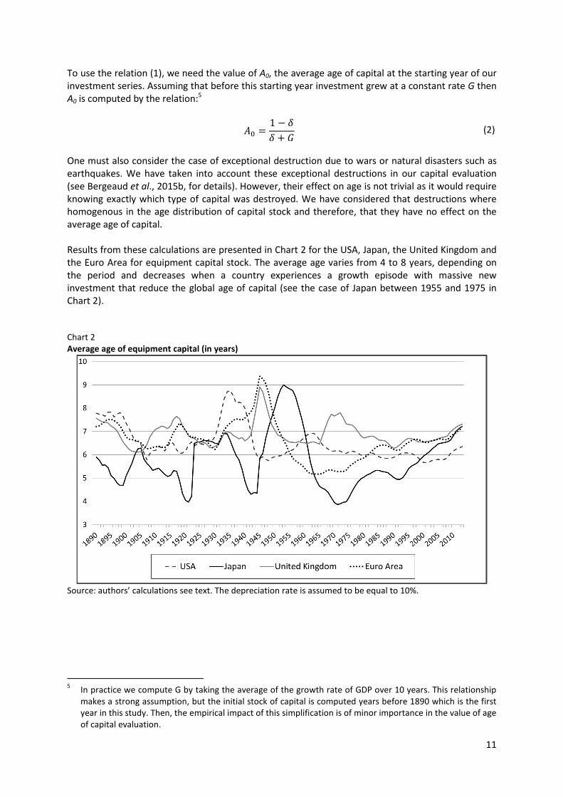
One must also consider the case of exceptional destruction due to wars or natural disasters such as earthquakes. We have taken into account these exceptional destructions in our capital evaluation (see Bergeaud et al., 2015b, for details). However, their effect on age is not trivial as it would require knowing exactly which type of capital was destroyed. We have considered that destructions where homogenous in the age distribution of capital stock and therefore, that they have no effect on the average age of capital. Results from these calculations are presented in Chart 2 for the USA, Japan, the United Kingdom and the Euro Area for equipment capital stock. The average age varies from 4 to 8 years, depending on the period and decreases when a country experiences a growth episode with massive new investment that reduce the global age of capital (see the case of Japan between 1955 and 1975 in Chart 2). Chart 2 Average age of equipment capital (in years)

Source: authors’ calculations see text. The depreciation rate is assumed to be equal to 10%.

5 In practice we compute G by taking the average of the growth rate of GDP over 10 years. This relationship

makes a strong assumption, but the initial stock of capital is computed years before 1890 which is the first year in this study. Then, the empirical impact of this simplification is of minor importance in the value of age of capital evaluation.

12

2.4. Spread of technology

To measure diffusion of technology over the whole period, we have relied on the CHAT database constructed by Comin and Hobijn (2009). This database provides annual estimates of the diffusion of more than 100 technologies for a large set of countries. We have selected one technology which is often considered as representative of the development of technologies during the 20th century, the production of electricity in kWh (see Comin et al., 2006a and 2006b). Data have been completed with series using the World Development Indicators of the World Bank up to 2013 and have been standardized by total population. To measure the diffusion of technology in the more recent time period, we have relied on the work of Cette et al. (2015) which provides estimates of the stock of capital of three ICTs from 1950 to 2012 for most of our countries. More details on data construction will be given in section 4. An alternative measure of innovation would have relied on patents stock, both domestic and foreign. However, as shown in Sanchis et al., 2015, patents stock have a heterogeneous impact on TFP from one country to another, which may rely on differences in education level and domestic knowledge accumulation. By using electricity and ICT capital measures, we are directly measuring technology diffusion, at the closest to what actually impact TFP. 3. Education and age of capital in a growth accounting framework

The purpose of this section is to evaluate the contributions of the changes in education and age of capital on TFP growth. To do that, we successively specify how the productivity impact of education (3.1.) and age of capital (3.2.) can be empirically taken into account and what the main results of the literature are on these aspects. Then we propose some estimates of these impacts (3.3.) and an evaluation of them on productivity growth over the long period of our analysis, using for this purpose a growth accounting approach (3.4.). 3.1. Education and productivity

We have relied on the endogenous growth model of Lucas (1988) formalized, among other, in Hall and Jones (1999) to expand the approach we adopted in Bergeaud et al. (2015a, 2015b). Lucas updated the neoclassical growth model by considering the stock of human capital (denoted C) as an input in a Cobb-Douglas production function. This stock accumulates according to the equation:

���� � ��1 � ��

Where u is the fraction of time spent working and �is a parameter representing the maximum reachable human capital, for someone who would spend his life studying (that is when u = 0), also sometime called the productivity of schooling (the productivity level of an individual who spends his whole life studying). The stock of physical capital K increases following a permanent inventory method and, from a Cobb-Douglas constant return to scale relation, the production function becomes:

� � ���.����. �. ��� Where L is the number of hours worked, with L = N.H, N being the number of workers and H the average working hours per worker. The idea is that individuals invest in education through the choice of a fraction 1 - u of life spent studying and accumulating knowledge in order to increase their productivity. This model is a microfoundation of the way education can enter the production function.

13

In Bergeaud et al. (2015a, 2015b), we used a classical Solow Model in which the production function was a Cobb-Douglas constant return to scale relation: � � ���.�� . ��� . Here we aim at understanding which part of TFP can be attributed to human capital and we therefore consider: � � ���′. �� . � ���� where C is the human capital stock. To calculate the stock C of human capital, we have followed a Mincerian approach (Mincer, 1974) and assume that:

� � "#�$ (3) With S representing the number of years spent studying and g is an increasing function verifying g(0) = 0. When g = 0, we are back to the Solow model and human capital is no longer an input. Otherwise, the derivative of g is called the return to education. Usually, g is assumed linear, or at least piecewise linear (see Psacharopoulos, 1994, for a review), but more complex formula have also been tested, namely by Temple (2001). In this study, we suppose that %�& � '. & where ' is a constant and homogenous term.

Many studies have focused on estimating the returns to education, using micro or macro approaches. In the former, the return to one year of education is defined as the average increase in wage associated with an additional year of schooling. Even if a large number of individual dataset are available for a large range of countries, estimating the private return to education is not straightforward because the effect of schooling on wage is highly endogenous (Klein and Vella, 2009; Card, 1999; Bills and Klenow 2000). Indeed, the choice of schooling duration is likely to be correlated with unobserved ability that would also be positively correlated with wage (self-selection effect). The OLS coefficient should then be biased upwards. Most studies use different strategies to address this issue: for example, some use natural experiments, among which reforms raising of the minimum school leaving age, generate somehow exogenous discontinuities in education attainment (Devereux and Wen, 2011; Dickson and Smith, 2011). Angrist and Krueger (1991) use a different school age start policy for individuals born at the beginning of the year to instrument education by the quarter of birth. Other studies look at parents or spouse education as an instrument (Trostel et al., 2002). There is a large empirical consensus in most micro studies for a private return to education between 6% and 8% of additional wage for one more year of study in developed countries. For example, Dickson and Smith (2011) find a value of 8% for male in the UK, exploiting the reform raising the minimum leaving age from 15 to 16, in 1972. Trostel et al. (2002) looked at 28 countries and find similar values when family education is taken as an instrument. Finally, Psacharopoulos (1994) has surveyed many studies and concludes that the average private return to education in the literature in OECD countries is 6.8%.6 In macro analyses, the return to education is defined by taking the national mean of every variable from the Mincer wage equation to obtain the “Macro-Mincer” equation. It is thus the productivity gains associated with an average increase of one year in education attainment. Due to social externalities, the productivity impact of education should be higher at macro than at micro level. But contrary to the relative consensus in the micro literature, results are subject to more uncertainty in macro and economists find contradictory results. Some studies like Benhabib and Spiegel (1994) and Pritchett (2001) have found a non-significant coefficient on education when physical capital stock is also included in the regressions. This result led Pritchett to develop the idea that the absence of correlation between education and growth is the result of low quality education in developing

6 As raised in Psacharopoulos (1994), this return can be higher in other regions of the world (12.4% in Latin

America, 13.4% for South Saharian Africa and 9.6% for Asia).

14

countries in line with the idea that human capital should take into account quality as well as years of education. Krueger and Lindahl (2000) suggest that measurement errors in education data is the main reason for these negative results and show that when capital stock in not included as a regressor, human capital becomes significantly positive. Since then, other studies have tried to solve this puzzle by using updated and improved figures of education attainment (Soto, 2002; Cohen and Soto, 2007 and Barro and Lee, 2010). In Barro and Lee (2010), a very similar framework as the one presented in this study is used and the return to education is estimated around 4% for developed countries, using the twenty year lag in education series as an instrument to proxy parental educational background. Similarly, Soto (2002) uses data from Cohen and Soto (2007) and finds values from 6.7 to 10% using a GMM estimator and after dealing with collinearity by changing the growth accounting framework. Finally, Topel (1999) finds a return of 6% with the Barro Lee dataset but chose to set the coefficient of capital intensity. All in all, results from the macro literature suggest that the value of ' should stand between 4 and 15%. However, every study cited above focuses on a large range of countries (the Barro-Lee database contains 146 countries) and on a short time dimension. Our dataset enables us to extend the time period from 1890 with yearly data on GDP, human capital and physical capital but in turns limits the number of countries to 17 developed countries, which may implies different estimates of return to education. Finally, it is important to understand what a given value of ' implies for productivity. From the neoclassical framework, we indeed have:

� � ���′. �� . ���"����(.$ (4) Which yields:

� � ���′. )� *

�. "����(.$

But another transformation can also yields:

� � ���′ )��*

���� "(.$

Hence, conditionally on the fact that +, is constant, an increase of one year in education attainment

implies an increase of productivity by �1 � -' points and conditionnally on the fact that +. remains

constant, a similar increase in education implies an increase in productivity of ' points. According to Soto (2002), �1 � -' is the “short-time” return to education while ' is the “long-time” return to education.7 3.2. Age of capital and productivity

It is very intuitive that older investment is less productive than newer one, as technical progress is partly embodied in capital.8 Constant-quality price indexes attempt to take into account productive performance improvement of the investment. For a stable value of investment spending over two

7 Over the long-run, the ratio of capital to output is very stable as seen in Madsen (2010).

8 A reverse impact could come from a learning by doing effect, if firms manage to use better a capital vintage

as it ages. Our estimates encompass this effect, which appears not to be predominant.

15

years, an embodied productive performance improvement would correspond to an increase in the investment volume and to a decrease in the investment price index. The embodied technical change is, in this view, a determinant of the price of investment (see on this debate the survey from Gordon, 1990). From a more wide-open point of view, and as raised by different papers, for example Jorgenson and Griliches (1967), if the production function is perfectly specified, if all productive factors are well measured and taken into account, the TFP measurement through the Solow residual approach would be small and would correspond mainly to the impact of externalities. Nevertheless, the measurement of investment price indexes takes only partly into account the improvements in the investment productive performances for several reasons, and at least the two following ones: (i) these improvements are taken into account only for some products, mainly automobiles and, within ICTs, hardware, prepackaged and partly custom software, and some communication equipment. For other investment products, there is almost no impact of an investment quality change on investment prices measurement. This partial approach is explained by the cost of the methods (hedonic or matching approaches, mainly) used to take into account quality change in investment price indexes; (ii) Whatever the efforts of national accountants and their sophistication degree, these methods remain imperfect and take only partially into account the embodied technical progress in investment price indexes. For these reasons, an unknown part of the embodied technical progress is not included in investment volume increase and investment price decrease. From this, the vintage composition of capital should influence the productivity level. A large amount of literature takes into account the vintage composition of capital in production functions through a synthetic capital age variable. In this approach, a negative impact of the capital age on productivity is expected. To take this idea into account, we define effective productive capital stock (KP) as the productive capital stock (K) times an exponentially decreasing function of the average age of capital (A):

��� � ��"�/.01 Where ε is the elasticity of the age of capital. This representation was suggested by Solow (1959, 1962) and developed after in numerous papers, as for example Nelson (1964). So far, we have considered two types of assets to construct our series of capital: equipment and buildings. The vintage effect of capital is not necessary relevant for this latter type, or at least, it is negligible when compared to the vintage effect of equipment. An older piece of machinery is likely to be less productive than a newer one, either because of technological obsolescence, or because of physical depreciation. This is not necessarily the case for a building. For this reason, in what follows, we have only considered the average year of equipment capital stock. Numerous papers have estimated an empirical impact of the capital vintage structure on productivity, both on macro and micro data. On industry level data, Gittleman et al. (2003) give a literature survey and show empirically that the capital vintage productivity impact can vary a lot across industries. On macroeconomic data, some papers assume a vintage effect without estimates. For example, Jorgenson (1966, p. 14) assumes, for the US, a value of the capital average age elasticity on productive capital (which correspond to our parameter ε) of -0.13, which would mean, if we suppose a value of the capital elasticity α of 0.3 (α = 0.3), an impact of the age on productivity of nearly 0.04 (α.ε = -0.039). Clark (1979) assumes directly on US macro data an impact of the capital average age on productivity of 1% (α.ε = -0.01) which corresponds to a low value compared to estimates. For example, Wolf (1991, 1996) proposes some estimates of the impact of the average capital age on productivity (our parameter product (α.ε) on a country level dataset panel composed by the G7

16

countries over the 1950-1989 period. Estimates’ results are within a range of -3% to -6.5% (-0.065 ≤

α.ε ≤ -0.03), and for his growth account computing, Wolf assumes a value of -4.1% (α.ε = -0.041).

Some analyses have proposed estimates of the capital average age impact on productivity on firm level data, mainly, to our knowledge, on French firm datasets. On panel samples of 124 to 195 manufacturing firms over the period 1966 to 1975 or on a dataset of 16 885 manufacturing firms in 1962 or 275 manufacturing firms in 1972, Mairesse (1977, 1978) and Mairesse and Pescheux (1980) estimate a capital age productivity impact of about -4% (α.ε = -0.04). On a panel of 3 200 French manufacturing firms over the period 1972-1984, Cette and Szpiro (1989) estimate also a capital age productivity impact of about -4% (α.ε = -0.04).

3.3. Estimation strategy and results

Taking into account these considerations, we have included education and age of capital into the production function:

� � ���′. ��. "�/.0�� "(.$��� (5) Where TFP’ is the new measurement of the total factor productivity (taken as a Solow residual), from which the effects of embodied technical progress and of human capital (education) are removed. Dividing by L, the total number of hours worked, yields the following breakdown:

� � ���′. )� *

�. "�/.�.0. "����(.$ (6)

Finally, taking the logarithm:

23 � tfp7 � α. 9: � ε. -. � � �1 � -'. & (7)

Where lp and ik are the logarithms of labor productivity and capital intensity (�� � +,), and tfp’ is the

logarithm of total factor productivity excluding the effects of the age of physical capital and of human capital. With our data, we want to estimate the values of ' and ε from the previous equation. To do so, we first assume that the value of α is 0.3 which is equivalent to set the left hand side variable to

23<,� � 0.3. 9:<,� For a country i, 1 ≤ 9 ≤ 17 and a year t. In the right hand side part of the equation, we use the average year of education &<,� and the average age of equipment capital stock Ai,t as regressors. The induced values of ' and ε can then be obtained after division of the estimated coefficients of these two explaining variables by, respectively, 1 - α (0.7) and α (0.3). In a second step, we estimate jointly α, ' and ε by including capital intensity in the right hand side, the dependent variable being now only the logarithm of labor productivity.

17

Results from these two OLS regressions are presented in Table 19, column (1) and (2).10 We find a coefficient of education highly significant and positive in both cases, equal to 0.037 and 0.031, and a negative coefficient for the age of capital equal to -0.010. When coefficient α is estimated, its value can be directly read from the coefficient on the log of capital intensity which is respectively 0.323 in column (2). These results in turns imply a value of ε around -3% while ' is around 5% which are both lower than expected (in absolute value), although still acceptable for the macro returns to education. Remarkably, at odds with results from Barro and Lee (2013), Soto (2002) or Krueger and Lindahl (2000), we found a convincing and standard value for α. In the previously mentioned studies, when physical capital intensity is included in the regression, the implicit value of its elasticity is always larger than expected. This led Soto (2002) to argue in favor of an endogeneity issue stemming both from measurement errors in education and capital stock11 and simultaneity between education and growth: when people anticipate future growth, they are likely to spend more time studying. Bils and Klenow (2000) also suggest that better enforcement of property rights may explain both a higher level of schooling and an increase in productivity and is therefore a potential omitted variable. To better compare our results with those already mentioned in the literature, we have restricted the time period to 1950-2010 and run the same regressions. Results are presented in columns (3) and (4) of Table 1 from which we see that when α has been set to 0.3, the value of ' is 9.14% which is within the expected range, whereas ε is still lower than expected but higher than previously (-7.67%). From column (4), however, the estimated value of α is very large (0.638) and the education coefficient loses its significance, the same results as, among others, Barro and Lee (2013). This result could be due to the high correlation between capital intensity and education in this 1950-2010 period over our set of countries, the correlation being lower on the longer 1890-2010 period as increase in education was mostly driven by compulsory attendance in the primary and secondary levels at the beginning of the period. Finally, going back to our whole 1890-2010 period, we have followed Barro and Lee (2013) and instrumented school attainment by its 20 year lagged value to proxy for parental education, which is likely to be less endogenous. In addition, physical capital intensity is instrumented by its 1 year lag value to correct for correlation in measurement error with the current value of the left hand side variable. These results are presented in columns (5) and (6) and imply a value for ' around 7%, suggesting that our OLS estimators were biased downward, possibly by measurement errors. We then reproduce the exact same regressions, but after having deleted average working time per worker (H), that is by defining labor productivity as the ratio of GDP over employment, and capital intensity as the ratio of physical capital over employment. Removing average working time per worker is a way to reduce the inaccuracy in our measures as it is by far the most delicate series to measure. In addition, this would enable us to derive the elasticity of education with regards to labor productivity per employee. As seen in Table 2, the value of ' remains stable and around its expected value. Coefficient on the capital intensity is still too high between 1950 and 2010, but this time, education has a positive and significant effect on productivity. The other changes are for ε which is now higher and much closer to its 10 to 13% expected value.

9 The dependent variable shows very strong autocorrelation of degree one which disappears when looking at

longer lags. We thus control that our results are still valid when autocorrelation and heteroskedasticity robust standard errors using the Newey-West variance estimator are implemented (of course this won’t affect the coefficients).

10 For these columns and for all others, we include time and country fixed effects and remove war periods.

11 Capital stock is constructed with investment which is included in GDP, so any measurement error in

investment would impact both labor productivity and capital intensity.

18

All in all, these results suggest that over the whole period, and for the set of 17 countries under study, the coefficient of education in the Macro-Mincer equation ' is roughly equal to 8%, which implies a short-term return to education of 5.6% (assuming the elasticity of capital to be equal to 0.3). Note that, in this study, we have followed the growth literature on relatively long period and measure the elasticity of the average year of education in the population over 15 on TFP. For this reason, the results presented in Table 3 might differ from other estimates on the most recent period. For example, the Bureau of Labor Statistics uses a more detailed and sophisticated measure of human capital by estimating a Mincer equation from microdata, taking into account many parameters like gender, type of education… Of course, over such a long period as the one considered in this study, it is impossible to conduct a similar detailed analysis. 3.4. The impact of education and age of capital on TFP growth

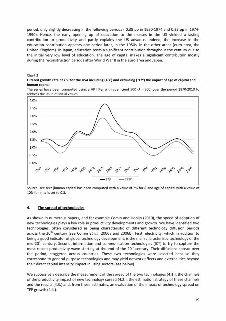
We can now evaluate TFP’ excluding the impact of education and age of capital and compare its evolution to that of TFP not excluding these two factors. We have used for this the growth accounting approach corresponding to previous relations and the following values for the parameters: α = 0.3 for the share of capital, ' = 7% for the impact of education and ε = 10% for the impact of the age of capital. Although we can see from Table 312 that changes in human capital and age of capital significantly contribute to TFP growth, it appears that the amplitude of TFP’ growth, the residual TFP growth excluding the impact of these two factors, does not differ a lot from the one which includes this impact.13 In particular, the one-big wave happening during the 20th Century is still persistent as shown in Chart 3 concerning the US and this is also the case for the ICT wave. The same result is obtained for different values of 'andEwithin the ranges which seem reasonable from previous developments (5% < ' < 10%and5% < E < 15%. Our results for the contribution of education closely compares to Madsen (2010)’s, but as his methodological approach tries to identify TFP-induced capital deepening and attributes its contribution to TFP, the contribution of capital stock growth is smaller than in our estimates, the bulk of growth being attributed to TFP. Hence, Madsen’s results leave even a greater share of productivity waves unexplained through his growth accounting estimates. For the United States, between 1913 and 1950, technology, computed as a residual of a growth accounting equation, explains 2.2 percentage points (pp) of GDP per capita annual growth, while the contribution of education (0.6 pp) offsets the negative contribution of annual hours worked (-0.7); the capital-output ratio posts a negative -0,4 pp contribution. These results are important: they indicate that even if education (mainly) and the age of capital have a strong influence on productivity level and growth, they do not explain the productivity waves observed during the 20th Century.14 Other contributions have to be found and among numerous candidates. We try, in the following section, to evaluate the impact of some generic technologies on TFP growth. Nevertheless, we see from Table 3 that education significantly contributed to the first productivity wave in the United States, with a contribution of 0.42 percentage point (pp) during the 1913-1950

12

Periods in Table 3 are based on productivity breaks from Bergeaud et al. (2015b). 13

Over the whole period, human capital and age of physical capital accounts for 21% for the US, 17% for the Euro Area, 25% for the UK and 26% for Japan.

14 Interestingly, the one big wave is the most affected by the exclusion of education and age of capital: for the

US, the pick is reduced by 25%. This is not surprising as this wave is associated with an acceleration in education attainment. In the US, average duration of schooling increased by more than 2 years between 1935 and 1955.

19

period, only slightly decreasing in the following periods ( 0.38 pp in 1950-1974 and 0.32 pp in 1974-1990). Hence, the early opening up of education to the masses in the US yielded a lasting contribution to productivity and partly explains the US advance. Indeed, the increase in the education contribution appears one period later, in the 1950s, in the other areas (euro area, the United Kingdom). In Japan, education posts a significant contribution throughout the century due to the initial very low level of education. The age of capital makes a significant contribution mostly during the reconstruction periods after World War II in the euro area and Japan. Chart 3 Filtered growth rate of TFP for the USA including (TFP) and excluding (TFP’) the impact of age of capital and

human capital

The series have been computed using a HP filter with coefficient 500 (λ = 500) over the period 1870-2010 to address the issue of initial values.

Source: see text (human capital has been computed with a value of 7% for ' and age of capital with a value of 10% for ε). α is set to 0.3.

4. The spread of technologies

As shown in numerous papers, and for example Comin and Hobijn (2010), the speed of adoption of new technologies plays a key role in productivity developments and growth. We have identified two technologies, often considered as being characteristic of different technology diffusion periods across the 20th century (see Comin et al., 2006a and 2006b). First, electricity, which in addition to being a good indicator of global technology development, is the main characteristic technology of the mid-20th century. Second, information and communication technologies (ICT) to try to capture the most recent productivity wave starting at the end of the 20th century. Their diffusions spread over the period, staggered across countries. These two technologies were selected because they correspond to general-purpose technologies and may yield network effects and externalities beyond their direct capital intensity impact in using sectors (see below). We successively describe the measurement of the spread of the two technologies (4.1.), the channels of the productivity impact of new technology spread (4.2.), the estimation strategy of these channels and the results (4.3.) and, from these estimates, an evaluation of the impact of technology spread on TFP growth (4.4.).

20

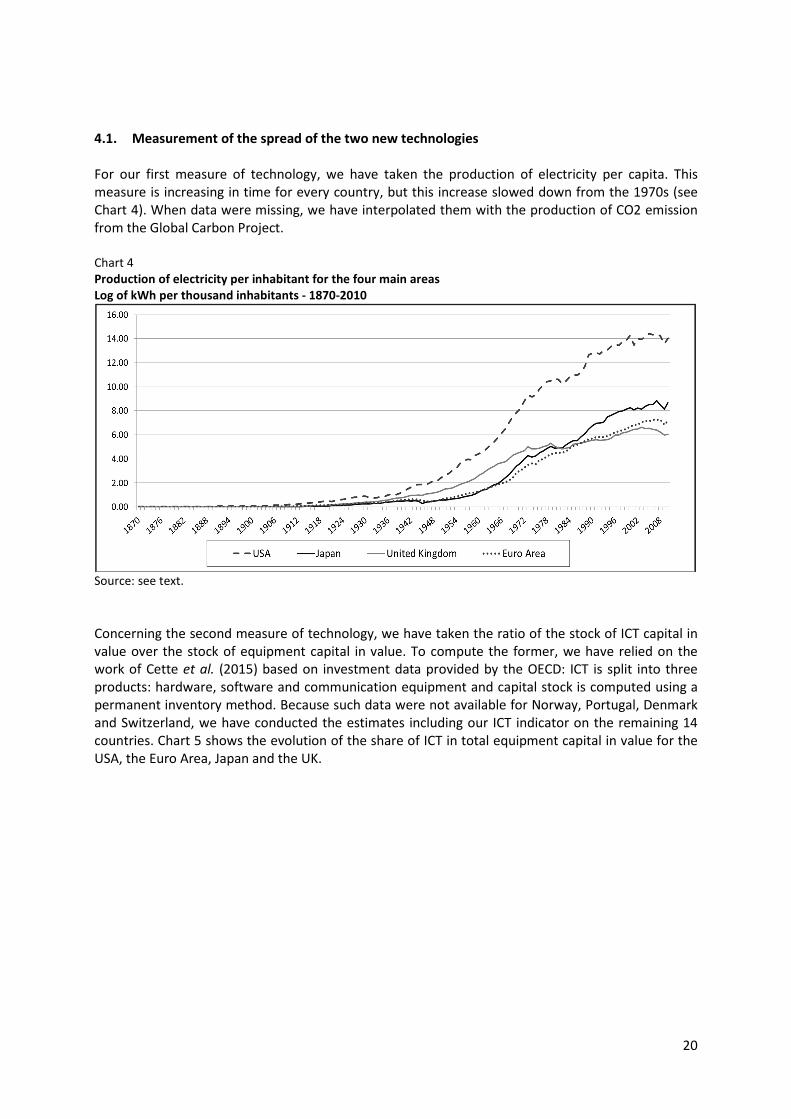
4.1. Measurement of the spread of the two new technologies

For our first measure of technology, we have taken the production of electricity per capita. This measure is increasing in time for every country, but this increase slowed down from the 1970s (see Chart 4). When data were missing, we have interpolated them with the production of CO2 emission from the Global Carbon Project. Chart 4 Production of electricity per inhabitant for the four main areas

Log of kWh per thousand inhabitants - 1870-2010

Source: see text.

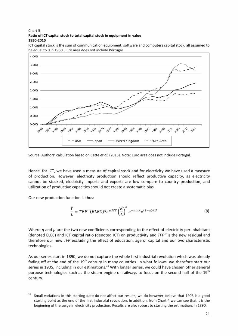
Concerning the second measure of technology, we have taken the ratio of the stock of ICT capital in value over the stock of equipment capital in value. To compute the former, we have relied on the work of Cette et al. (2015) based on investment data provided by the OECD: ICT is split into three products: hardware, software and communication equipment and capital stock is computed using a permanent inventory method. Because such data were not available for Norway, Portugal, Denmark and Switzerland, we have conducted the estimates including our ICT indicator on the remaining 14 countries. Chart 5 shows the evolution of the share of ICT in total equipment capital in value for the USA, the Euro Area, Japan and the UK.

21

Chart 5 Ratio of ICT capital stock to total capital stock in equipment in value

1950-2010

ICT capital stock is the sum of communication equipment, software and computers capital stock, all assumed to be equal to 0 in 1950. Euro area does not include Portugal

Source: Authors’ calculation based on Cette et al. (2015). Note: Euro area does not include Portugal.

Hence, for ICT, we have used a measure of capital stock and for electricity we have used a measure of production. However, electricity production should reflect productive capacity, as electricity cannot be stocked, electricity imports and exports are low compare to country production, and utilization of productive capacities should not create a systematic bias. Our new production function is thus:

� � ���77�I I�J"K.LMN )� *

�"�/.�.0"����(.$ (8)

Where η and µ are the two new coefficients corresponding to the effect of electricity per inhabitant (denoted ELEC) and ICT capital ratio (denoted ICT) on productivity and TFP’’ is the new residual and therefore our new TFP excluding the effect of education, age of capital and our two characteristic technologies. As our series start in 1890, we do not capture the whole first industrial revolution which was already fading off at the end of the 19th century in many countries. In what follows, we therefore start our series in 1905, including in our estimations.15 With longer series, we could have chosen other general purpose technologies such as the steam engine or railways to focus on the second half of the 19th century.

15

Small variations in this starting date do not affect our results; we do however believe that 1905 is a good starting point as the end of the first industrial revolution. In addition, from Chart 4 we can see that it is the beginning of the surge in electricity production. Results are also robust to starting the estimations in 1890.

22

Finally, equation (8) makes the assumption that electricity enters log linearly in the production function which in turn implies the underlying assumption that the elasticity of electricity was constant over time. An alternative would be to allow non-linearity in the effect of technology on growth, for example by fitting a logistic function with three parameters, the first one determining the speed of diffusion, the second one the maximal possible effect and the third one the date at which the marginal effect of electricity is the largest. However, the fitting of this function would be necessarily arbitrary. The constant elasticity assumption, as it has been chosen for the education productivity impact and although it is a strong one, appears preferable to an ad hoc rule (we come back to this issue below). 4.2. Channels of the productivity impact of new technology spread

New technologies may have three distinct types of effects on productivity (see Jorgenson, 2001; Cette et al., 2005 or Cette, 2014, for more details): - First, sectors producing new technologies benefit from a fast pace of technological progress,

leading to a rapid increase in their TFP: for example, in ICT-producing sectors, according to Moore’s law, the number of transistors in a dense integrated circuit has doubled approximately every two years, leading to a fast decrease in ICT production deflator and a fast increase in ICT production volume.

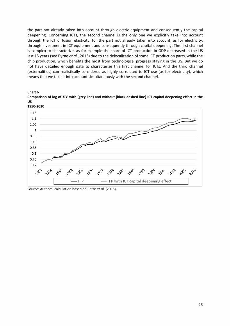
- Second, due to the price decrease of investment including the new technology, this technological progress can accelerate the capital deepening process in the new technology-using industries, leading to an increase in capital intensity and hence in labor productivity - but not necessarily in TFP. The methodology adopted to evaluate this capital deepening effect is described for ICT in Box 1. Chart 6 represents TFP in the US, taking into account or not ICT capital deepening; it appears that a part of the TFP apparent increase when ICT capital deepening is not taken into account corresponds to an increase in the capital intensity from ICT capital deepening. It also appears that the new estimation of TFP is more volatile, but this does not affect the shape of the ICT wave.

- Finally, the two selected technologies can be considered as general purpose technologies (see Jovanovic and Rousseau, 2005 for a comparison between ICT and electricity) and their joint utilization across firms may leads to TFP gains through spillovers, which means externalities or network effects at the macroeconomic level, this impact being “Manna from the heaven”, to use the expression from Hulten (2000).

Usual growth accounting approaches are able to characterize empirically the role of the first two channels but not of the third one. Concerning these studies, among numerous others, Jorgenson and Stiroh (2000), Oliner and Sichel (2000) or Oliner et al. (2007) evaluate the contribution of ICTs in the US at the end of the 20th Century. For industrial revolution comparisons, among others also, Crafts (2002) compares the contributions of steam engines in the UK during 1780-1860, electricity and ICTs in the US during 1899-1929 and 1974-2000 respectively, and Jalava and Pohjola (2008) compare the contributions of electricity during 1920-1938 and ICTs during 1990-2004 in Finland. In our approach, concerning electricity, the three channels are empirically taken into account simultaneously in the next section through the electricity production elasticity. As said before, production and use of electricity are, at the country level, very similar (there is no electricity storage and electricity imports and exports are low compare to production), and spillovers can realistically be considered as highly correlated to production and use. The second channel is characterized only for

23

the part not already taken into account through electric equipment and consequently the capital deepening. Concerning ICTs, the second channel is the only one we explicitly take into account through the ICT diffusion elasticity, for the part not already taken into account, as for electricity, through investment in ICT equipment and consequently through capital deepening. The first channel is complex to characterize, as for example the share of ICT production in GDP decreased in the US last 15 years (see Byrne et al., 2013) due to the delocalization of some ICT production parts, while the chip production, which benefits the most from technological progress staying in the US. But we do not have detailed enough data to characterize this first channel for ICTs. And the third channel (externalities) can realistically considered as highly correlated to ICT use (as for electricity), which means that we take it into account simultaneously with the second channel. Chart 6 Comparison of log of TFP with (grey line) and without (black dashed line) ICT capital deepening effect in the

US

1950-2010

Source: Authors’ calculation based on Cette et al. (2015).

24

4.3. Estimation strategy and results

The TFP effects are included in our TFP and TFP’ measures. To evaluate them for each of the two

technologies, we have regressed �O3′ on the spread measure of each technology, being assumed to correspond to the spread of a specific general purpose technology.

�P�LMN � -�LMN�∆:���LMN � ∆R� � ∆ℎ�

-�,TLMN � 12 �-�LMN � -���LMN

-�LMN ���LMN����LMN

�.1 . ��

��LMN � ��LMN �9� � LMN � ∆3�LMN

Box 1 Methodology of the Evaluation of the contribution of ICT to labor productivity growth through capital

deepening The evaluation of the contribution of ICT to hourly labor productivity growth, through capital deepening, is calculated by applying the growth accounting methodology evoked by Solow (1956, 1957). This

contribution in year t, noted as �P�LMN, is evaluated through the following relation:

Where ����LMN corresponds to the ICT capital installed at the end of year t-1, V� refers to total employment in year t, and W� designates the average annual hours worked per person per year t. The notation of the variables in lowercase corresponds to their natural log �X � 2R�Y, and the growth rate of a variable is approximated by the variation of its logarithm. The ∆ symbol refers to the variation of a variable �∆Y� � Y� � Y���.

The coefficient -�,TLMN is the Törnquist index of the coefficient -�:

The coefficient -�LMN corresponds to the share of the capital remuneration in the GDP:

Where ��LMN corresponds to the user cost of capital, �.1 corresponds to the GDP deflator, and �� refers to

GDP in volume. The user cost of ICT capital � is calculated employing the relation proposed by Jorgenson (1963):

Where �LMN corresponds to the investment price of ICT, 9 refers to the nominal interest rate, and LMNdesignates the assumed invariant depreciation rate of the ICT.

We have considered two alternative options for the nominal interest rate: 10 year government bond interest rates and a fixed rate of 10%. The evaluation of both approaches is close to one another in the growth contribution calculation. In this study, we have retained the 10 year government bond interest rates taken from the OECD main economic indicators. The global share of capital, α, is assumed to be invariant and the same for all countries with α = 0.3. It

means that to evaluate the global capital deepening effect, we have assumed that -�ZLMN , the non ICT capital share, is obtained, for each year t and country i observation, from the relation: -� � -�LMN � -�ZLMN �0.3 and then -�ZLMN � 0.3 � -�LMN

25

Table 4 columns (1), (2) and (3) display the result from OLS regressions when the logarithm of the production of electricity per capita (column (1)), when the ratio of ICT capital stock over GDP in value (column (2), over 1950-2010) or the two together (column (3)) are used as regressors. Coefficients for the two technologies are positive and significant in each case. We may however suffer from endogeneity and reserve causality effects for these technologies. Indeed, the demand for new technologies increases with standards of living; other TFP-improving changes in areas such as management, financing or production process (Ferguson and Wascher, 2004) have taken place alongside with the diffusion of the three technologies. In columns (4), (5) and (6), we have hence instrumented these technologies with the sum of the other countries’ technological diffusion measures, weighted by the logarithm of the distance. Indeed, trade is one vector of technological diffusion and is closely related to distance. Of course, reflection effect may lead our instruments to reflect themselves the improvement in the country technological diffusion. To limit that effect, we have lagged our indicator. In the IV regressions, the coefficients of the two technologies are positive. ICT is highly significant with a coefficient of 1.59 while electricity is no longer significant with a coefficient of 0.039. However, when estimated together, the coefficients are both significant. This regression presented in column (6) is our preferred one and we therefore use the corresponding coefficients. A 1% increase in electricity production would lead to a 7.9% increase in TFP’. A 1-point increase in the ratio of ICT capital stock to total equipment capital stock would lead to a multiplication by 1.016 of TFP’. Instrumentation is reducing the electricity coefficient, which may be the most prone to endogeneity as it is a production measure. As explained above, technology, and in particular electricity could enter differently in the production function and the measured effect is probably a lower bound of the elasticity of electricity during some periods. For example, if we assume that a technological shock makes the use of electricity more efficient, then this quality improvement will not be captured in our regression and from this effect, we will underestimate the impact of electricity over TFP. The effect of electricity is possibly not constant over time and to take this into account, one could look at the effect of electricity using different sub-periods. To consider this formally, we have estimated this TFP - electricity elasticity on different periods, changing the starting date of the regression. We have found that the elasticity is remarkably stable in the IV specification: when starting in 1905, 1925, or 1950, the estimated coefficient is equal to, respectively, 0.079, 0.089 and 0.061 and remains significant. From that, it has seemed to us reasonable to use, for the TFP decomposition, the elasticity estimated over the 1905-2010 period (0.079, see Table 4, column 6) and to consider it as stable. One can question the choice of population to standardize the production of electricity. The production of electricity per capita could be considered as a demand variable inserted in the production function (the average consumption of electricity). Our instrumentation strategy is designed to address this potential endogeneity problem. However, ideally, we would like to proceed as in some country-specific articles (see for example Jalava and Pohjola, 2008) and to measure the capital deepening from highly electricity intensive sectors. Since such data are unfortunately not available is our set of countries and for the whole 20th century, an alternative would be to standardize the production of electricity by GDP. But doing so would lead to a specification problem as the log of GDP intervenes in the left hand side variable of the equation, leading to a negative coefficient on electricity per unit of output. All in all, the coefficient of electricity is very stable across different specifications. In Table 5, we have chosen an elasticity of 0.079 to be consistent with the results presented in Table 4.

26

4.4. The impact of technology diffusion on TFP growth

From our previous estimation, we can now look at the shape of our new estimate of TFP (denoted TFP’’). Chart 7 plots the three waves from 1905 to 2010 for the USA for TFP, TFP’ and TFP’’ growth rates. We can see that the general evolution is still persistent, especially as far as the one big-wave is concerned. However, the amplitude of this one big-wave has been reduced and is almost 40% lower for TFP’’ than for TFP’. This result seems comparable to the one of David (1990) who estimates for example that “… approximately half of the 5 percentage point acceleration recorded in the aggregate

TFP growth rate of the U.S. manufacturing sector during 1919-29 (compared with 1909-19) is

accounted for … by the growth in manufacturing secondary electric motor capacity during that

decade.” The ICT wave has also been significantly explained. However, the impact of ICT diffusion may seem low as only about 35% of the corresponding productivity wave has been explained by education, age of capital and the inclusion of ICT diffusion in our regressions. Table 5 gives more details about the share of TFP growth that is attributed to electricity and ICT. Because of data restriction, we have started this decomposition in 1913: the period 1905-1913 would be of poor statistical interest with only 9 years. However, we mention the whole 1905-2010 period. In addition, because we have removed four countries from our dataset, we do not plot results for the « World ». Looking for example at the Euro Area, we can see that electricity explains a large share of TFP evolution. ICT appears especially important for the US and the UK. Although the difference in contribution is not very large across areas, electricity diffusion contributed significantly to the US advance on the euro area, as its contribution peaked in the 1913-1950, while it increased in the 1950-1974 period in the euro area. The UK appears not to lag in terms of electricity diffusion, with a very large contribution in the 1913-1950 period. Broadberry and Crafts (1990) trace the productivity lead that the US took over the UK during this period rather to barriers to competition allowing high cost producers to remain in business. The contribution of ICTs to TFP growth appears in all areas smaller than the one of electricity. This result seems to contradict the ones from Crafts (2002) or Jalava and Pohjola (2008) mentioned above, which find that in the US and in Finland ICT contribution to growth is higher than the electricity one. But this difference comes from difference in the approaches. These growth accounting approaches characterize two channels of the growth impact of technology shocks: TFP gains in the producing sectors and capital deepening in using sectors. Our approach characterizes partly the capital deepening channel, more exactly the part not already taken into account in our capital measurement and consequently in the explicit capital deepening channel, and the spillover channel which cannot be measured through growth accounting approaches. For these reasons, our results cannot be compared to these previous ones. One reason for the low contribution of ICT diffusion to explain the second productivity wave could come from the fact that ICT investment data compiled by national accountants (and taken into account here as ICT investment) underestimate productive ICT expenditure. Indeed, spending on ICT is regarded as investment only when the corresponding products are physically isolated. Therefore, generally speaking, ICT that is included in productive investment (for example machine tools or robots) is not counted as ICT investment but as intermediate consumption of companies producing these capital goods. Beretti and Cette (2009) have tried to correct French ICT investment data in 2000, by considering intermediate consumption ICT components integrated in non-ICT productive investment as ICT investment. Their main result is that the amount of ‘indirect ICT investment’ appears to be small, compared with ‘direct ICT investment’, and that considering them as ICT investment changes numbers only slightly. But we cannot exclude that this result could differ for other countries and on more recent periods.

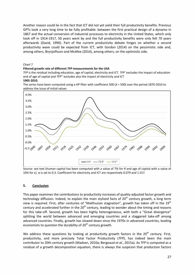
27

Another reason could lie in the fact that ICT did not yet yield their full productivity benefits. Previous GPTs took a very long time to be fully profitable: between the first practical design of a dynamo in 1867 and the actual conversion of industrial processes to electricity in the United States, which only took off in 1914-1917, 50 years went by and the full productivity benefits were only felt 70 years afterwards (David, 1990). Part of the current productivity debate hinges on whether a second productivity wave could be expected from ICT, with Gordon (2014) on the pessimistic side and, among others, Brynjolfsson and McAfee (2014), among others, on the optimistic side. Chart 7 Filtered growth rate of different TFP measurements for the USA

TFP is the residual including education, age of capital, electricity and ICT. TFP’ excludes the impact of education and of age of capital and TFP’’ excludes also the impact of electricity and ICT 1905-2010.

The series have been computed using a HP filter with coefficient 500 (λ = 500) over the period 1870-2010 to address the issue of initial values

Source: see text (human capital has been computed with a value of 7% for ' and age of capital with a value of 10% for ε). α is set to 0.3. Coefficient for electricity and ICT are respectively 0.079 and 1.557.

5. Conclusion

This paper examines the contributions to productivity increases of quality-adjusted factor growth and technology diffusion. Indeed, to explain the main stylized facts of 20th century growth, a long term view is required. First, after centuries of “Malthusian stagnation”, growth has taken off in the 19th century and accelerated further in the 20th century, leading to wonder about the timing and reasons for this take-off. Second, growth has been highly heterogeneous, with both a “Great divergence” splitting the world between advanced and emerging countries and a staggered take-off among advanced countries. Finally, growth has slowed down since the 1970s in advanced countries, leading economists to question the durability of 20th century growth. We address these questions by looking at productivity growth factors in the 20th century. First, productivity, and more precisely Total Factor Productivity (TFP), has indeed been the main contributor to 20th century growth (Madsen, 2010a; Bergeaud et al., 2015a). As TFP is computed as a residual of a growth decomposition equation, there is always the suspicion that production factors

28

have been improperly measured, which contributes to ascribe too much weight to TFP in growth dynamics. In this paper, production factors are adjusted for quality and in particular for the age of capital. Second, technology diffusion appears as a large contributor to TFP growth (Comin and Mestieri, 2013), even in innovating countries such as France, Germany and the United Kingdom (Eaton and Kortum, 1999). This paper assesses the contribution of technology diffusion through two 20th century general purpose technologies, electricity and information and communication technologies (ICT). To do so, we rely on an original capital, labor and GDP database built over 1890-2013 for seventeen advanced countries. We completed this database with data on education, age of capital and technology so that we were able to decompose GDP growth. GDP growth has then been decomposed between the contribution of production factors, capital and labor, to obtain TFP as a residual. In a second step, the quality of production factors, education and the age of capital, has been introduced through an estimate of their contribution to this gross TFP, taking into account their potential endogeneity through instrumental variables regressions. In a third step, the contribution of technology diffusion has been estimated, endogeneity being treated by a similar estimation procedure. The main results are the following: (i) Among factor quality, education levels have posted the largest contribution to growth, while the age of capital has a significant, although limited, contribution; (ii) Quality-adjusted production factors explain less than half of labor productivity growth in the largest countries, but Japan, where capital deepening posted a very large contribution. Although the US “one

big wave” of productivity growth, which took place some two decades before other advanced countries (Gordon, 1999) is partially explained by an earlier access to higher education of the masses, this wave as well as the ICT productivity wave for the countries which experienced it, remains partly unexplained by quality-adjusted factors; (iii) Technology diffusion, as captured through our two general purpose technologies, also constitutes a partial explanation of the earlier US “one big wave” and for the ICT productivity wave but leaves between 0.6 and 1 point yearly growth, as well as a large share of the two 20th century technology waves, unaccounted for. These results are consistent with previous ones on the role of education and TFP in standard growth accounting approach. Education posted a very significant contribution to productivity growth throughout the period, explaining part of the US lead in the first productivity wave, but not the extent of the wave itself. Our analysis goes further by taking into account the quality of the capital stock through the age of capital, which posts a significant contribution mostly in the post World War II reconstruction period. But our main contribution consists in trying to estimate the role of general purpose technologies beyond their capital-deepening impact and TFP growth in GPT-producing sectors. While the ICT contribution remains limited at this point, both in duration and extent, the diffusion of electricity explains a significant share of 20th century growth and part of the US advance in the first productivity wave. However, it still cannot account for the whole bulk of productivity waves, which point to a major role of factors beyond technology diffusion and production factors to the 20th century growth. Candidates are numerous: among them, improvement in the production process such as assembly lines in large manufacturing firms (implemented for example for the Ford Model T in the Ford Motor Company in 1913), enhanced management practices (Bloom et al., 2014) or new financing techniques (Ferguson and Wascher, 2004). Interactions between these different growth factors are large and further research appears necessary to disentangle their respective roles. Another limit of our analysis is that we have supposed a linear (in log) impact of education, capital age, electricity or ICT capital on TFP. We cannot exclude that in reality, these impact could be non-linear. But more detailed data would be necessary to go further in these directions.

29

This study has empirically given some partial explanations concerning the sources of TFP contribution to growth over the 20th century. That is its main contribution. But a large part of this contribution remains unexplained, and, as a consequence, stays a “Manna from the heaven”…

30

References

Abramovitz, Moses and Paul A. David (1995): “Convergence and Deferred Catch-up Productivity Leadership and the Waning of American Exceptionalism” in “Growth and Development: The Economics of the 21st Century”, edited by Ralph Landau, Timothy Taylor, and Gavin Wright, Stanford CA: Stanford University Press.

Acemoglu, Daron (1998): "Why Do New Technologies Complement Skills? Directed Technical Change And Wage Inequality," The Quarterly Journal of Economics, MIT Press, vol. 113(4), pages 1055-1089, November.

Acemoglu, Daron (2002): "Directed Technical Change," Review of Economic Studies, Wiley Blackwell, vol. 69(4), pages 781-809, October.

Aghion, Philippe and Howitt, Peter, (1992): "A Model of Growth through Creative Destruction," Econometrica, Econometric Society, vol. 60(2), pages 323-51, March.

Angrist, Joshua and Alan Krueger (1991): "Does Compulsory School Attendance Affect Schooling and Earnings?," The Quarterly Journal of Economics, MIT Press, vol. 106(4), pages 979-1014, November.

Barro, Robert (1991): “Economic Growth in a Cross Section of Counties,” The Quarterly Journal of

Economics, 106(2):407-43. Barro, Robert (2015): “Convergence and Modernisation”, The Economic Journal, 125 (June), pp. 911–942. Barro, Robert and Jong-Wha Lee (1993): “International comparisons of educational attainment,"

Journal of Monetary Economics, Elsevier, vol. 32(3), pages 363-394, December.

Barro, Robert and Jong-Wha Lee (2010): “A new data set of educational attainment in the world, 1950-2010,” NBER Working Papers 15902, National Bureau of Economic Research, Inc.

Basu, Susanto and John G. Fernald (2002): “Aggregate productivity and aggregate technology”, European Economic Review, vol. 46, pp. 963-991.

Basu, Susanto and John G. Fernald (2007): "Information and Communications Technology as a General-Purpose Technology: Evidence from US Industry Data," German Economic Review, Verein für Socialpolitik, vol. 8, pages 146-173, 05.

Baumol, William (1986): “Productivity growth, convergence and welfare: What the long-run data show?”, American Economic Review, 76, pp. 1072-1085.

Benhabib, Jess and Mark M. Spiegel (1994): “The role of human capital in economic development evidence from aggregate cross-country data,” Journal of Monetary Economics, 34(2):143-173

Beretti, Paul-Antoine and Gilbert Cette (2009): “Indirect ICT investment”, Applied Economics Letters, Vol. 16, pp. 1713–1716.

Bergeaud, Antonin, Gilbert Cette and Remy Lecat (2015a): "GDP per capita over the 20th century in advanced countries," Working papers N° 549, Banque de France.

31

Bergeaud, Antonin, Gilbert Cette and Remy Lecat (2015b): "Productivity trends from 1890 to 2012 in advanced countries," Forthcoming in the Review of Income and Wealth

Bils, Mark and Peter, Klenow (2000): "Does Schooling Cause Growth?," American Economic Review, American Economic Association, vol. 90(5), pages 1160-1183, December.

Bloom Nicholas, Renata Lemos, Raffaella Sadun, Daniela Scur and John Reenen (2014): "Jeea-Fbbva Lecture 2013: The New Empirical Economics Of Management," Journal of the European Economic Association, European Economic Association, vol. 12(4), pages 835-876, 08.

Bolt, Jutta and Jan Luiten van Zanden (2014): “The Maddison Project: collaborative research on historical national accounts,” The Economic History Review, 67(3): 627-651.

Bresnahan, Timothy F. and Manuel Trajtenberg (1995): "General purpose technologies 'Engines of growth'?," Journal of Econometrics, Elsevier, vol. 65(1), pages 83-108, January.

Broadberry, Stephen and Nicholas Crafts (1990): “Explaining Anglo-American Productivity Differences in the Mid-Twentieth Century”, Oxford Bulletin of Economics and Statistics, Department of Economics, University of Oxford, vol. 52(4), Special I, pp. 375-402. Brynjolfsson, Erik and Andrew McAfee (2014): “The Second Machine Age: Work, Progress, and Prosperity in a Time of Brilliant Technologies”, Ed. WW Norton and company, New York.

Card, David (1999): "The causal effect of education on earnings,” in: Ashenfelter, Orley and David Card (ed.), Handbook of Labor Economics, edition 1, volume 3, chapter 30, pages 1801-1863. Elsevier.

Cervellati, Matteo, Fabrice Murtin and Uwe Sunde (2013): “Unified Growth Empirics: 1880-2000”, mimeo.

Cette, Gilbert (2014): “Does ICT remain a powerful engine of growth?” Revue d’Economie Politique, 124 (4), juillet-août, pp. 473-492.

Cette, Gilbert and Daniel Szpiro (1989): „Une interprétation du ralentissement de la productivité industrielle au moment du second choc pétrolier“, Economie et Prévision, N° 87, 1989-1, pp. 33-42.

Cette, Gilbert, Yusuf Kocoglu and Jacques Mairesse (2009): “Productivity growth and levels in France, Japan, the United Kingdom and the United States in the Twenthieth Century,” NBER Working Paper, N° 15577. Cette, Gilbert, Christian Clerc and Lea Bresson (2015): “Contribution of ICT Diffusion to Labour Productivity Growth: The United States, Canada, the Eurozone, and the United Kingdom, 1970-2013”, International productivity monitor, n°28, Spring.

Cette Gilbert, Jacques Mairesse and Yusuf Kokoglu (2005): « ICT and potential output growth », Economics Letters, vol. 87, Issue 2, p. 231-234.

Clark, Peter (1979): “Issues in the Analysis of Capital Formation and Productivity Growth”, Brookings Papers on Economic Activity, 2, pp. 423-431.

Cohen, Daniel and Marcelo Soto (2007): “Growth and Human Capital: Good Data, Good Results,” Journal of Economic Growth, 12(1):51-76.

32

Comin, Diego and Bart Hobijn (2009): "The CHAT Dataset," Harvard Business School Working Papers 10-035, Harvard Business School. Comin, Diego and Bart Hobijn (2010): "Technology diffusion and postwar growth”, Harvard Business school, Working Paper, n° 11-027, January 1. Comin, Diego, Bart Hobijn and Emilie Rovito (2006a): “Five facts you need to know about technology diffusion”, NBER working papers series, n° 11928, January. Comin, Diego, Bart Hobijn and Emilie Rovito (2006b): “World technology usage lags”, NBER working papers series, n° 12677, November. Comin, Diego and Mestieri, Marti (2013): "If Technology Has Arrived Everywhere, Why Has Income Diverged?," TSE Working Papers 13-409, Toulouse School of Economics (TSE).

Crafts, Nicholas (2002): “The Solow Productivity Paradox in Historical Perspective”, CEPR, Discussion Paper Series, n° 3142, January.

Crafts, Nicholas and Kevin O’Rourke (2013): “Twentieth Century Growth,” Oxford University Economic and Social History Series _117, Economics Group, Nuffield College, University of Oxford. de la Fuente, Angel (2011): “Human Capital and Productivity,” UFAE and IAE Working Papers 860.11, Unitat de Fonaments de l’Analisi Economica (UAB) and Institut d’Analisi Economica (CSIC). David, Paul A. (1990): “The Dynamo and the Computer: An Historical Perspective on the Modern Productivity Paradox,” American Economic Review: Papers and Proceedings, 80, 355-361. Devereux, Paul and Wen Fan (2011): "Earnings returns to the British education expansion," Economics of Education Review, Elsevier, vol. 30(6), pages 1153-1166. Dickson, Matt and Sarah Smith, (2011): "What determines the return to education: An extra year or hurdle cleared?," The Centre for Market and Public Organisation 11/256, Department of Economics, University of Bristol, UK. Eaton, Jonathan, and Samuel Kortum (1999): «International Technology Diffusion: Theory and Measurement». International Economic Review 40, pp. 537-570.

Edquist, Charles (2001): “Innovation Policy in the Systems of Innovation Approach: Some Basic Principles”, Chap. 3 in “Knowledge, Complexity and Innovation Systems”, Manfred Fischher and Josef Fröhlich eds, Springer Berlin Heidelberg Publisher, pp. 46-57.

Ferguson, Roger and William Wascher (2004): “Distinguished lecture on economics in Government: lessons from past productivity booms”, The Journal of Economic Perspectives, vol. 18, n° 2, Spring, pp. 3-28.

Fernald, John and Charles Jones (2014): “The future of US productivity growth”, American Economic Review, Papers and Proceedings, 104(5), pp. 44-49.

Galor, Oded (2005): "From Stagnation to Growth: Unified Growth Theory," Handbook of Economic Growth, in: Philippe Aghion & Steven Durlauf (ed.), Handbook of Economic Growth, edition 1, volume 1, chapter 4, pages 171-293 Elsevier.

33

Gittleman, Maury, Thijs Ten Raa and Edward Wolff (2003): "The Vintage Effect in TFP Growth: An Analysis of the Age Structure of Capital," NBER Working Papers 9768, National Bureau of Economic Research, Inc.

Gordon, Robert (1990): “The Measurement of Durable Goods Prices”, University of Chicago Press.

Gordon, Robert (1999): “US Economic Growth since 1970: One Big Wave?”, American Economic Review, Vol. 89, No. 2, pp.123-128.

Gordon, Robert (2012): “Is U.S. Economic Growth Over? Faltering Innovation Confronts the Six Headwinds,” National Bureau of Economic Research, Inc, NBER Working Papers 18315, 2012. Gordon, Robert (2013): “US productivity Growth: The Slowdown has returned after a temporary revival,” International Productivity Monitor, Centre for the Study of Living Standards, vol. 25, Spring, pp. 13-19.

Gordon, Robert (2014): “The demise of US Economic Growth: Restatement, rebuttal, and reflexions”, National Bureau of Economic Research, Inc, NBER Working Papers, N° 19895, February.

Hall, Robert and Charles Jones (1999): “Why Do Some Countries Produce So Much More Output Per Worker Than Others?,” The Quarterly Journal of Economics, 114(1):83-116.

Hanushek, Eric and Wößmann Ludger (2012): "Do better schools lead to more growth? Cognitive skills, economic outcomes, and causation," Munich Reprints in Economics 20400, University of Munich, Department of Economics.

Helpman, Elhanan and Manuel Trajtenberg (1998): “Diffusion of General Purpose Technologies.” In General Purpose Technologies and Economic Growth, ed. E. Helpman. Cambridge, MA: MIT Press. Hulten, Charles, R. (2000): « Total factor productivity: a short biography », NBER Working Paper, n° 7471.

Jalava, Jukka and Matti Pohjola (2008): “The roles of electricity and ICT in economic growth: Case Finland”, Explorations in Economic history, 45, pp. 270-287.

Jones, Charles (2002): “Sources of U.S. Economic Growth in a World of Ideas," American Economic

Review, American Economic Association, vol. 92(1), pages 220-239, March.

Jorgenson, Dale (1963): “Capital theory and investment behavior.” The American Economic Review 53 (2): 247-259.

Jorgenson, Dale (1966): “The embodiment hypothesis”, The Journal of Political Economy, Vol. LXXIV, n° 1, February, pp. 1-17.

Jorgenson, Dale (2001): “Information technology and the US economy”, The American Economic

Review, Vol. 91, March, N°1.

Jorgenson, Dale and Zvi Griliches (1967): The Explanation of Productivity Change”, Review of Economic Studies, 34, July, pp. 349-383.

Jorgenson, Dale and Kevin Stiroh (2000): “Raising the Speed Limit: US Economic Growth in the Information Age”, Brookings Papers on Economic Activity, 1:2000, pp. 125-211.

34

Jovanovic, Boyan and Peter L. Rousseau (2005): “GENERAL PURPOSE TECHNOLOGIES”, Handbook of Economic Growth, Volume 1B, chapter 18, edited by Philippe Aghion and Steven N. Durlauf.

Klein, Roger and Francis Vella (2009): "Estimating the Return to Endogenous Schooling Decisions via Conditional Second Moments," Journal of Human Resources, University of Wisconsin Press, vol. 44(4).

Kyriacou, George (1991): "Level and Growth Effects of Human Capital: A Cross-Country Study of the Convergence Hypothesis," Working Papers 91-26, C.V. Starr Center for Applied Economics, New York University.

Krueger, Alan and Mikael Lindahl (2001): "Education for Growth: Why and For Whom?," Journal of Economic Literature, American Economic Association, vol. 39(4), pages 1101-1136, December.

Lucas, Robert (1988): “On the mechanics of economic development,” Journal of Monetary

Economics, 22(1):3-42.

Maddison, Angus (2001): “The World Economy: A Millennium Perspective,” Development Centre

Studies. Development Centre of the Organization for Economic Co-operation and Development. Maddison, Angus (2007): “Fluctuations in the momentum of growth within the capitalist epoch”, Cliometrica (2007) 1:145–175.

Madsen, Jakob (2010a): “Growth and capital deepening since 1870: is it all technological progress?”, Journal of Macroeconomics, 32, pp. 641-656.

Madsen, Jakob (2010b): "The anatomy of growth in the OECD since 1870," Journal of Monetary Economics, Elsevier, vol. 57(6), pages 753-767, September.

Madsen, Jakob (2014): "Human Capital and the World Technology Frontier," The Review of Economics and Statistics, MIT Press, vol. 96(3), pages 676-692, October. Mairesse, Jacques (1977): “Deux essais d’estimation du taux moyen de progrès technique incorporé au capital”, Annales de l’INSEE, N° 28, October-December, pp. 41-76.

Mairesse, Jacques (1978): “New Estimates of Embodied and Disembodied Technical Progress”, Annales de l’INSEE, N° 30-31, April-September, pp. 681-720.

Mairesse, Jacques and Jean-Michel Pescheux (1980): “Fonction de production et mesure du capital : La robustesse des estimations », Annales de l’INSEE, N° 38-39, April-September, pp. 63-75.

Mankiw, Gregory, David Romer and David Weil (1992): “A contribution to the Empirics of Economic Growth. The Quarterly Journal of Economics, 107(2):407-37.

Mayer, Thierry and Soledad Zignago (2011): "Notes on CEPII’s distances measures: The GeoDist database," Working Papers 2011-25, CEPII research center.

Nelson, Richard (1964): “Aggregate Production Function and Medium-Range Growth Projections”, The American Economic Review, Vol. 54, n° 5, Sept, pp. 575-606.

35

Oliner, Stephen and Daniel Sichel (2000): “The Resurgence of Growth in the Late 1990s: Is Information Technology the Story?“, Journal of Economic Perspectives, 14(4), pp. 3-22.

Oliner, Stephen, Daniel Sichel and Kevin Stiroh (2007): “Explaining a Productive Decade“, Brookings Papers on Economic Activity, 1:2007, pp. 81-152.

Prados de la Escosura, Leandro (2015) : “Mismeasuring long-run growth: the bias from splicing national accounts—the case of Spain”, Cliometrica, forthcoming.

Pritchett, Lant (1996): “Where has all the education gone?,” Policy Research Working Paper Series 1581, The World Bank.

Psacharopoulos, George (1994): “Return to investment in education: A global update,” World

Development, 22(9):1325-1343.

Sanchis, Teresa, Juan A. Sanchis-Llopis, Vicente Esteve and Antonio Cubel (2015): “Total factor productivity, domestic knowledge accumulation, and international knowledge spillovers in the second half of the twentieth century”, Cliometrica 9:209–233.

Solow, Robert (1956): “A contribution to the theory of growth.” Quarterly Journal of economics 70 (1): 65-94. Solow, Robert (1957): “Technical change and aggregate production function.” Review of Economics

and Statistics 39 (3): 312-320.

Solow, Robert (1959): “Investment and Technical Change”, in Mathematical Methods in the Social Sciences, Stanford.

Solow, Robert (1962): “Technical Progress, Capital Formation, and Economic Growth”, The American Economic Review, Proceedings, May, pp. 76-86.

Soto, Marcelo (2002): "Rediscovering Education in Growth Regressions," OECD Development Centre Working Papers 202, OECD Publishing.

Temple, Jonathan (2001): "Generalizations that aren't? Evidence on education and growth," European Economic Review, Elsevier, vol. 45(4-6), pages 905-918, May.

Topel, Robert (1999): “Labor markets and economic growth,” in: Ashenfelter, Orley and David Card (ed.), Handbook of Labor Economics, edition 1, volume 3, chapter 44, pages 2943-2984. Elsevier.

Trostel, Philip, Ian Walker and Paul Wooley (2002): "Estimates of the economic return to schooling for 28 countries," Labour Economics, Elsevier, vol. 9(1), pages 1-16, February.

van Leeuwen, Bas and Jieli van Leeuwen-Li (2014): "Education since 1820", In: J.L. van Zanden et al. (eds.), How Was Life?: Global Well-being since 1820, OECD Publishing, pp. 88-101.

Wolff, Edward (1991): “Capital Formation and Productivity Convergence Over the Long Term”, The American Economic Review, Vol. 81, N° 3, June, pp. 565-579.

Wolff, Edward (1991): “The Productivity Slowdown: The Culprit at Last? Follow-Up on Hulten and Wolff”, The American Economic Review, Vol. 86, N° 5, December, pp. 1239-1252.

36

Table 1

Results from estimates of labor productivity (lp) or tfp’ (lp – 0.3.ik) in log, on school attainment and age of

equipment capital stock. Labor input is measured by total hours worked.

Time and country fixed effects included. Heteroskedasticity robust standard errors are under brackets. Estimations start in 1895 because GDP is highly volatile during the first five years.

(1) (2) (3) (4) (5) (6)

Dependent variable: [\ � ]. ^. _` [\ [\ � ]. ^. _` [\ [\ � ]. ^. _` [\

Estimator OLS OLS OLS OLS IV IV

School 0.037*** (0.005)

0.031*** (0.006)

0.064*** (0.009)

0.007 (0.009)

0.050*** (0.006)

0.047*** (0.008)

Age of equipment -0.010** (0.005)

-0.010** (0.005)

-0.023*** (0.007)

-0.022*** (0.005)

-0.012** (0.005)

-0.011** (0.005)

Log of capital

intensity -

0.323*** (0.011)

- 0.638*** (0.016)

- 0.315*** (0.012)

Implicit θ 5.29% 4.58% 9.14% 1.93% 7.14% 6.86%

Implicit ε -3.33% -3.10% -7.67% -3.45% -4.00% -3.49%

Implicit α Set to 0.3 0.323 Set to 0.3 0.638 Set to 0.3 0.315

Time period 1895-2010 1895-2010 1950-2010 1950-2010 1895-2010 1895-2010

Number of Obs. 1,714 1,714 1,037 1,037 1,714 1,714

Adjusted ab 0.961 0.983 0.920 0.981 0.983 0.982

*** p value < 1%, ** p value < 5%, * p value < 10%

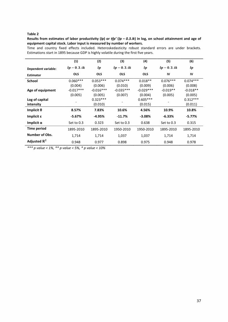
37

Table 2

Results from estimates of labor productivity (lp) or tfp’ (lp – 0.3.ik) in log, on school attainment and age of

equipment capital stock. Labor input is measured by number of workers.

Time and country fixed effects included. Heteroskedasticity robust standard errors are under brackets. Estimations start in 1895 because GDP is highly volatile during the first five years.

(1) (2) (3) (4) (5) (6)

Dependent variable: [\ � ]. ^. _` [\ [\ � ]. ^. _` [\ [\ � ]. ^. _` [\

Estimator OLS OLS OLS OLS IV IV

School 0.060*** (0.004)

0.053*** (0.006)

0.074*** (0.010)

0.018** (0.009)

0.076*** (0.006)

0.074*** (0.008)

Age of equipment -0.017*** (0.005)

-0.016*** (0.005)

-0.035*** (0.007)

-0.029*** (0.004)

-0.019** (0.005)

-0.018** (0.005)

Log of capital

intensity -

0.323*** (0.010)

- 0.605*** (0.015)

- 0.312*** (0.011)

Implicit θ 8.57% 7.83% 10.6% 4.56% 10.9% 10.8%

Implicit ε -5.67% -4.95% -11.7% -3.08% -6.33% -5.77%

Implicit α Set to 0.3 0.323 Set to 0.3 0.638 Set to 0.3 0.315

Time period 1895-2010 1895-2010 1950-2010 1950-2010 1895-2010 1895-2010

Number of Obs. 1,714 1,714 1,037 1,037 1,714 1,714

Adjusted ab 0.948 0.977 0.898 0.975 0.948 0.978

*** p value < 1%, ** p value < 5%, * p value < 10%

38

Table 3 Average growth rates for various subperiods for labor productivity (col. 1) and some of its contributors:

capital intensity (col. 2), TFP (col 3= col 1 - col 2), education (col 4), age of capital (col 5) and TFP’ (col 6 = col 3

- col 4 - col 5)

(1) (2) (3) (4) (5) (6)

Subperiods Δlp α.Δik Δtfp (1-α).θ.ΔS -αεA Δtfp’

The United States

1890-1913 1.76% 0.57% 1.19% 0.14% 0.19% 0.86%

1913-1950 2.85% 0.45% 2.41% 0.42% 0.03% 1.96%

1950-1974 2.25% 0.57% 1.68% 0.38% -0.02% 1.32%

1974-1990 1.27% 0.29% 0.98% 0.34% 0.04% 0.60%

1990-2010 1.83% 0.58% 1.25% 0.17% -0.03% 1.11%

1890-2010 2.21% 0.51% 1.70% 0.31% 0.04% 1.34%

Euro Area

1890-1913 1.82% 0.49% 1.34% 0.23% 0.12% 1.22%

1913-1950 1.49% 0.39% 1.10% 0.15% -0.13% 1.08%

1950-1974 5.19% 1.58% 3.62% 0.48% 0.33% 2.81%

1974-1990 2.77% 1.02% 1.74% 0.34% -0.18% 1.58%

1990-2010 1.28% 0.59% 0.69% 0.26% -0.07% 0.50%

1890-2010 2.52% 0.80% 1.72% 0.29% 0.01% 1.43%

United Kingdom

1891-1913 0.72% 0.17% 0.54% 0.22% 0.04% 0.28%

1913-1950 1.51% 0.36% 1.15% 0.19% 0.00% 0.97%

1950-1974 2.97% 1.15% 1.83% 0.62% -0.03% 1.25%

1974-1990 2.22% 0.83% 1.39% 0.49% 0.21% 0.68%

1990-2010 2.18% 0.73% 1.45% 0.07% -0.09% 1.47%

1890-2013 1.93% 0.63% 1.30% 0.31% 0.01% 0.97%

Japan

1890-1913 2.35% 1.59% 0.76% 0.53% 0.08% 0.15%

1913-1950 1.78% 1.08% 0.70% 0.47% -0.18% 0.42%

1950-1974 6.58% 2.20% 4.38% 0.50% 0.44% 3.44%

1974-1990 3.61% 1.62% 1.99% 0.31% -0.21% 1.88%

1990-2010 1.70% 1.06% 0.64% 0.29% -0.21% 0.56%

1890-2010 3.20% 1.52% 1.67% 0.45% -0.02% 1.24%

World

1890-1913 1.84% 0.64% 1.20% 0.25% 0.15% 0.80%

1913-1950 2.15% 0.48% 1.68% 0.28% -0.03% 1.43%

1950-1974 3.75% 1.09% 2.66% 0.48% 0.13% 2.05%

1974-1990 2.24% 0.79% 1.45% 0.36% -0.05% 1.14%

1990-2010 1.68% 0.65% 1.03% 0.22% -0.09% 0.90%

1890-2010 2.42% 0.73% 1.70% 0.32% 0.02% 1.35%

Source: See text. World includes all the 17 countries: Australia, Belgium, Canada, Denmark, Germany, Finland, France, Italy, Japan, the Netherlands, Norway, Portugal, Spain, Sweden, Switzerland, the United Kingdom and the United States of America.

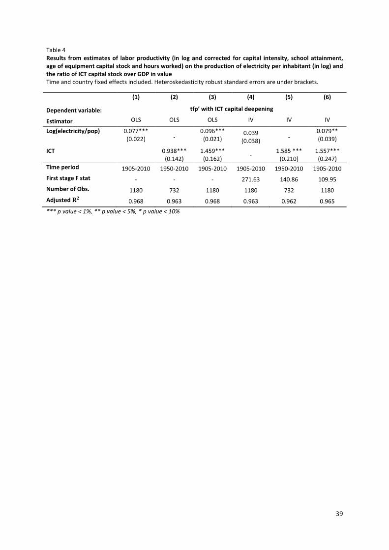
39

Table 4 Results from estimates of labor productivity (in log and corrected for capital intensity, school attainment,

age of equipment capital stock and hours worked) on the production of electricity per inhabitant (in log) and

the ratio of ICT capital stock over GDP in value

Time and country fixed effects included. Heteroskedasticity robust standard errors are under brackets.

(1) (2) (3) (4) (5) (6)

Dependent variable: tfp’ with ICT capital deepening

Estimator OLS OLS OLS IV IV IV

Log(electricity/pop) 0.077*** (0.022) -

0.096*** (0.021)

0.039 (0.038)

- 0.079** (0.039)

ICT

0.938***

(0.142) 1.459***

(0.162) -

1.585 ***

(0.210) 1.557***

(0.247)

Time period 1905-2010 1950-2010 1905-2010 1905-2010 1950-2010 1905-2010

First stage F stat - - - 271.63 140.86 109.95

Number of Obs. 1180 732 1180 1180 732 1180

Adjusted ab 0.968 0.963 0.968 0.963 0.962 0.965

*** p value < 1%, ** p value < 5%, * p value < 10%

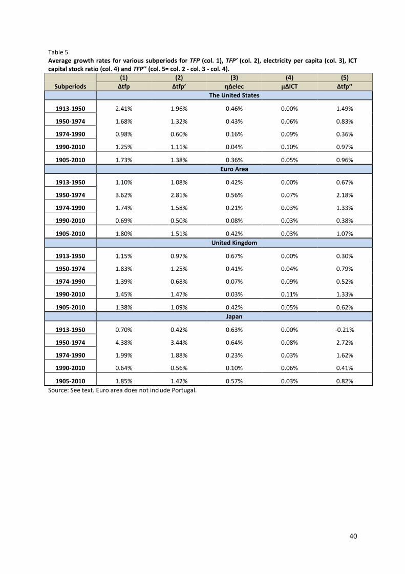
40

Table 5 Average growth rates for various subperiods for TFP (col. 1), TFP’ (col. 2), electricity per capita (col. 3), ICT

capital stock ratio (col. 4) and TFP’’ (col. 5= col. 2 - col. 3 - col. 4).

(1) (2) (3) (4) (5)

Subperiods Δtfp Δtfp’ ηΔelec µΔICT Δtfp’’

The United States

1913-1950 2.41% 1.96% 0.46% 0.00% 1.49%

1950-1974 1.68% 1.32% 0.43% 0.06% 0.83%

1974-1990 0.98% 0.60% 0.16% 0.09% 0.36%

1990-2010 1.25% 1.11% 0.04% 0.10% 0.97%

1905-2010 1.73% 1.38% 0.36% 0.05% 0.96%

Euro Area

1913-1950 1.10% 1.08% 0.42% 0.00% 0.67%

1950-1974 3.62% 2.81% 0.56% 0.07% 2.18%

1974-1990 1.74% 1.58% 0.21% 0.03% 1.33%

1990-2010 0.69% 0.50% 0.08% 0.03% 0.38%

1905-2010 1.80% 1.51% 0.42% 0.03% 1.07%

United Kingdom

1913-1950 1.15% 0.97% 0.67% 0.00% 0.30%

1950-1974 1.83% 1.25% 0.41% 0.04% 0.79%

1974-1990 1.39% 0.68% 0.07% 0.09% 0.52%

1990-2010 1.45% 1.47% 0.03% 0.11% 1.33%

1905-2010 1.38% 1.09% 0.42% 0.05% 0.62%

Japan

1913-1950 0.70% 0.42% 0.63% 0.00% -0.21%

1950-1974 4.38% 3.44% 0.64% 0.08% 2.72%

1974-1990 1.99% 1.88% 0.23% 0.03% 1.62%

1990-2010 0.64% 0.56% 0.10% 0.06% 0.41%

1905-2010 1.85% 1.42% 0.57% 0.03% 0.82%

Source: See text. Euro area does not include Portugal.

Documents de Travail

570. G. Verdugo, “Real Wage Cyclicality in the Eurozone before and during the Great Recession: Evidence from micro data” September 2015

571. M. Bussière, L. Ferrara and J. Milovich, “Explaining the Recent Slump in Investment: the Role of Expected

Demand and Uncertainty” September 2015

572. M. Albert, C. Jude and C. Rebillard, “The Long Landing Scenario: Rebalancing from Overinvestment and Excessive Credit Growth. Implications for Potential Growth in China” October 2015

573. P. Andrade, G. Gaballo, E. Mengus and B. Mojon, “Forward Guidance and Heterogeneous Beliefs” October 2015

574. C. Jadeau, E. Jousselin, S. Roux and G. Verdugo, “The behaviour of French Firms during the Crisis: Evidence from

the Wage Dynamics Network Survey” October 2015

575. C. Berson and N. Ferrari, “Financial incentives and labor market duality” October 2015

576. K. Istrefi and B. Vonnak, “Delayed Overshooting Puzzle in Structural Vector Autoregression Models” October 2015

577. S. Avouyi-Dovi and J-G. Sahuc, “On the sources of macroeconomic stability in the euro area” November 2015

578. F. Canova, F. Ferroni and C. Matthes, “Approximating time varying structural models with time invariant

structures” December 2015

579. R. Cezar and O. R. Escobar, “Institutional distance and foreign direct investment” December 2015

580. J. Carluccio, A. Cuñat, H. Fadinger and C. Fons-Rosen, “Offshoring and Skill-upgrading in French Manufacturing: A Heckscher-Ohlin-Melitz View” December 2015

581. G. Cette, R. Lecat et A. Ould Ahmed Jiddou, “Margin rate and the cycle: the role of trade openness” February 2016

582. G. Horny, S. Manganelli and B. Mojon, “Measuring Financial Fragmentation in the Euro Area Corporate Bond

Market” February 2016

583. S. Osotimehin and F. Pappadà, “Credit frictions and the cleansing effect of recessions” March 2016

584. F. Langot and A. Pizzo, “Accounting for Labor Gaps” March 2016

585. P. Fève and J.-G. Sahuc, “In Search of the Transmission Mechanism of Fiscal Policy in the Euro Area” March 2016

586. G. Cette, J. Fernald and B. Mojon, “The Pre-Great Recession Slowdown in Productivity” March 2016

587. E. Gautier, D. Fougère and S. Roux, “The Impact of the National Minimum Wage on Industry-Level Wage Bargaining in France” March 2016

588. A. Bergeaud, G. Cette and R. Lecat, “The role of production factor quality and technology diffusion in 20th

century productivity growth” April 2016

Pour accéder à la liste complète des Documents de Travail publiés par la Banque de France veuillez consulter le site : www.banque-france.fr For a complete list of Working Papers published by the Banque de France, please visit the website: www.banque-france.fr Pour tous commentaires ou demandes sur les Documents de Travail, contacter la bibliothèque de la Direction Générale des Études et des Relations Internationales à l'adresse suivante : For any comment or enquiries on the Working Papers, contact the library of the Directorate General Economics and International Relations at the following address : BANQUE DE FRANCE 49- 1404 Labolog 75049 Paris Cedex 01 tél : 0033 (0)1 42 97 77 24 ou 01 42 92 63 40 ou 48 90 ou 69 81 email : HU1404-ut@banque-france.fr