ED 139 Connaissances, Langages, Modélisation

T H È S E

pour obtenir le grade de

Docteur de

Université Paris Ouest Nanterre La Défense

Spécialité "Mécanique et Génie Mécanique"

présentée et soutenue publiquement le 12 Décembre 2014

par

Jefri Semuel BALE

THE DAMAGE OBSERVATION OF COMPOSITE

USING NON DESTRUCTIVE TESTING (NDT) METHOD

M. Dedi PRIADI University of Indonesia Président

M. Jacques RENARD Ecole des Mines de Paris Raporteur

Mme Anne Zulfia SYAHRIAL University of Indonesia Raporteur

M. Claude BATHIAS Université Paris Ouest Nanterre La Défense Co-directeur

Mme Martine MONIN PSA Peugeot Citroen Examinateur

M. Olivier POLIT Université Paris Ouest Nanterre La Défense Directeur

M. Tresna SOEMARDI University of Indonesia Co-directeur

M. Emmanuel VALOT Université Paris Ouest Nanterre La Défense Examinateur

Co-tutelle internationale de thèse entre :

Université Paris Ouest Nanterre La Défense

Laboratoire Energétique Mécanique Electromagnétisme 50 rue de Sèvres – 92410 Ville d’Avray – FRANCE

Universitas Indonesia

UI Campus Depok 16424 – INDONESIA

i

CONTENTS

Contents i

Abstract iv

Résumé v

List of Figures vi

List of Tables xii

Acknowledgement xiii

Nomenclatures xiv

CHAPTER 1 : INTRODUCTION 1

1.1. Background 1

1.2. Objective Research 6

1.3. Research Contribution 7

1.4. Content of thesis 8

CHAPTER II : LITERATURE REVIEW 10

2.1. Introduction 10

2.2. Composite material 12

2.3. Damage behaviour of composite material 15

2.3.1 Damage behaviour of composite under fatigue loading 17

2.3.2 Effect of loading type on fatigue of fiber composite 21

2.3.3 Stress concentration of composite with the open hole condition 23

2.4. Thermography on composite material 29

2.4.1 Thermography study on composite material 32

2.4.2 Thermography approach to determine high cycle fatigue strength 35

2.5. Acoustic emission on composite material 37

2.6. Tomography on composite material 40

2.7. Discontinuous carbon fiber composite 47

CHAPTER III : EXPERIMENTAL METHOD 52

3.1. Research Method 52

3.2. Material 52

ii

3.2.1 Unidirectional glass fiber composite 52

3.2.2 Discontinuous carbon fiber composite 53

3.3. Experimental 55

3.3.1 Tensile (static and fatigue) testing 55

3.3.2 NDT thermography 57

3.3.3 NDT acoustic emission 57

3.3.4 NDT tomography 58

3.4. Analysis 59

3.5. Experimental flowchart 62

CHAPTER IV : TENSILE (STATIC AND FATIGUE) TESTING AND 63

DAMAGE OBSERVATION OF UNIDIRECTIONAL

GLASS FIBER COMPOSITE (GFRP) BY

THERMOGRAPHY

4.1. Tensile static testing and damage observation of GFRP by thermography 63

4.1.1 Tensile static testing of GFRP 90o without hole and damage 63

observation by thermography

4.1.2 Tensile static testing of GFRP 90o with hole and damage 68

observation by thermography

4.1.3 Tensile static testing of GFRP 0o with hole and damage 72

observation by thermography

4.2. Tensile fatigue testing and damage observation of GFRP by 79

thermography

4.3. Rapid analysis of fatigue strength based on thermography and energy 87

dissipation of GFRP

CHAPTER V : TENSILE (STATIC AND FATIGUE) TESTING AND 93

DAMAGE OBSERVATION OF DISCONTINUOUS

CARBON FIBER COMPOSITE (DCFC) BY

THERMOGRAPHY

5.1. Tensile static testing and damage observation of DCFC by 93

thermography

iii

5.1.1 Tensile static testing of DCFC without hole and damage 93

observation by thermography

5.1.2 Tensile static testing of DCFC with hole and damage 100

observation by thermography

5.2. Tensile fatigue testing and damage observation of DCFC by 112

thermography

5.3. Rapid analysis of fatigue strength based on thermography and 117

energy dissipation of DCFC

CHAPTER VI : SUPPORTING ANALYSIS BY DIFFERENT 121

NDT METHOD 119

6.1. Coupling between thermography and acoustic emission for damage 121

observation under tensile static test

6.2. Post failure analysis of tomography for damage observation under 124

tensile fatigue test

6.2.1 Tomography observation of DCFC with hole 125

6.2.2 Tomography observation of GFRP with hole 130

CHAPTER VII : CONCLUSION AND FUTURE WORK 134

7.1 Conclusion 134

7.2 Future work 135

REFERENCES 137

APPENDIX

iv

ABSTRACT

The aim of this study is to investigate the damage behavior of composite

material in static and fatigue condition with non destructive testing (NDT)

thermography method and supported by acoustic emission and also computed

tomography (CT) scan. Thermography and acoustic emission are used in real-time

monitoring techniques during the test. On the other hand, NDT observation of

tomography is used for a post-failure analysis. In order to achive this, continuous

glass fiber composite (GFRP) and discontinuous carbon fiber composite (DCFC)

have been used as the test specimens which supplied by PSA Company, France.

A series of mechanical testing was carried out to determine the damage

behavior under static and fatigue loading. During all the mechanical testing,

thermography was used in real-time observation to follow the temperature change

on specimen surface and supported by acoustic emission in certain condition.

This study used rectangular shape and consist of specimen with and without

circular notches (hole) at the center. The constant displacement rate is applied to

observe the effect on damage behavior under tensile static loading. Under fatigue

testing, the constant parameter of frequency and amplitude of stress was explored

for each load level to have the fatigue properties and damage evolution of

specimen. The tomography was used to confirm the appearance of damage and

material condition after fatigue testing.

The analysis from the experiment results and NDT observation shown the

good agreement between mechnical results and NDT thermography with

supported by acoustic emission observation in detect the appearance and

propagation of damage for GFRP and DCFC under static loading. Fatigue testing

shows that thermal dissipation is related to the damage evolution and also

thermography and can be successfully used to determine high cycle fatigue

strength (HCFS) and S-N curve of fiber composite material. From post failure

analysis, CT scan analysis successfully measured and evaluated damage and

material condition after fatigue test for fiber composite material.

v

RÉSUMÉ

L'objectif de ce travail de thèse est d'étudier le comportement de

l'endommagement des matériaux composites sous chargement statique et fatigue

par contrôle non destructif (C.N.D) thermographie et soutenu par émission

acoustique et la tomographie (CT scan). Pour cela, ce unidirectionnels composite

à fibres de verre (GFRP) et discontinue composite à fibres de carbone (DCFC)

ont été utilisés comme les éprouvettes qui ont fourni par PSA peugeot citröen,

France.

Une série d'essais mécaniques a été réalisée pour déterminer le

comportement de l'endommagement sous chargement statique et fatigue. Pendant

tout des essais mécanique, la thermographie a été utilisé pour l'observation en

temps réel pour suivre l'évolution des températures sur la surface de l'éprouvette et

supporté par émission acoustique dans certaines conditions. Cette étude a utilisé

une forme rectangulaire et se compose d'éprouvettes trouées et non trouées au

centre de l'éprouvette. La vitesse de déplacement constante est appliquée pour

observer l'effet sur le comportement de l'endommagement sous chargement de

traction statique. Sous les essais de fatigue, le paramètre constant de la fréquence

et de l'amplitude de stress a été étudiée pour chaque niveau de charge pour avoir

les propriétés de fatigue et l'évolution de l'endommagement de l'éprouvette. La

tomographie a été utilisée pour confirmer l'apparition de l'endommagement et

l'etat du matériau après l'essai de fatigue.

L'analyse des résultats de l'expérimentation et de l'observation NDT montré

le bon accord entre les résultats mechnical et NDT thermographie avec prise en

charge par l'observation de l'émission acoustique en détecter l'apparition et la

propagation de l'endommagement de GFRP PRV et DCFC sous chargement de

statique en traction. Les essais en fatigue montrent que la dissipation thermique

est liée à l'évolution de l'endommagement et également thermographie et peut être

utilisé avec succès pour déterminer la limite d'endurance (HCFS) et la courbe de

Wöhler du matériau composite. Les résultats par CT scan ont mesurée avec succès

les endommagements et l'état du matériau après essai de fatigue du matériau

composite.

vi

LIST OF FIGURES

Page

Figure 1.1 Framework of research background 6

Figure 2.1 Ilustration of the state of the art 11

Figure 2.2 Classification of composite 14

Figure 2.3 The “big picture” of composite products 15

Figure 2.4 Stiffness degradation of fiber reinforced composite 17

materials

Figure 2.5 Development of damage in composite under fatigue 19

Figure 2.6 Damage type of Fiber reinforced plastic 20

Figure 2.7 Illustration of sinusoidal loading 21

Figure 2.8 Illustration of different loading R-ratios normalized to 21

a maximum absolute value stress of 1.0

Figure 2.9 Failure mode at different scales 24

Figure 2.10 Tension at an angle to a principal elastic axis 1 of an 25

isotropic plate with a hole

Figure 2.11 Tangensial stress distribtuion around a hole 25

Figure 2.12 Failure hypothesis 26

Figure 2.13 Stress concentration factor as a function of hole size 27

Figure 2.14 Stress concentration factor versus ϴ for glass-epoxy 28

composite

Figure 2.15 Stress concentration versus for various elasticity 28

modulus ratio

Figure 2.16 Thermography ilustration 30

Figure 2.17 Case ilustration of unidirectional composite with 31

off-axis direction

Figure 2.18 Temperature distribution on the surface of the 33

specimen during extension

Figure 2.19 Thermography images of damage mechanism on 34

composite

vii

Page

Figure 2.20 Comparison between the change of temperature and 34

the damage evolution: (a) 70% level of loading,

(b) 67.5% level of loading, (c) 60% level of loading

Figure 2.21 Temperature changes as increase of stress around the hole 35

on CFC under tension compression fatigue loading

Figure 2.22 Damage observation by Thermography on carbon fiber 35

composite

Figure 2.23 (a) Stabilisation temperature during fatigue test 36

(b) Determine the fatigue limit for composite material

.Figure 2.24 Acoustic Emission Ilustration 38

Figure 2.25 Frequency domain of acoustic emission of composite 38

damage

Figure 2.26 Amplitude distribution according to damage in composite 39

material

Figure 2.27 AE signal of damage mode under tensile static loading 39

Figure 2.28 AE signal of damage mode under tensile cyclic loading 40

Figure 2.29 Amplitude distribution in tensile loading of glass fiber 41

composite

Figure 2.30 Overview of CT scan and measurement process 42

Figure 2.31 An X-ray beam passing through an object with different 43

four linear attenuation coefficients

Figure 2.32 3D internal microstructure of a testing sample is 44

reconstructed from series of x-ray tomography images

Figure 2.33 Tomography 3D visualization of damage on composite 44

material

Figure 2.34 CT images of typical carbon reinforced composite 45

Figure 2.35 Grey value along the yellow line parameter with fibers 45

are shown white and voids black

viii

Page

Figure 2.36 Micro-voids percentage in the entire samples as a function 46

of the fatigue life (number of cycles)

Figure 2.37 2D images of tomography result (material is depicted in 46

grey and void is depicted in blue)

Figure 2.38 DFC product for windows frame of Boeing 787 47

Figure 2.39 Failure and insensitive of DCFC 48

Figure 2.40 UTS of DFC for different static condition 49

Figure 2.41 Failure of DCFC 50

Figure 2.42 Failure of DCFC in gross section 50

Figure 2.43 Damage observation of DCFC 51

Figure 3.1 GFRP specimen 53

Figure 3.2 DCFC specimen 54

Figure 3.3 INSTRON Machine and IR camera 56

Figure 3.4 Acoustic Emission set up 58

Figure 3.5 CT-scan machine 59

Figure 3.6 Flowchart of research method 62

Figure 4.1 Stress-strain curve of GFRP 90o without hole 63

Figure 4.2 Macroscopic of catastrophic damage form of GFRP 90° 64

without hole

Figure 4.3 Thermography images of GFRP 90° without hole 65

Figure 4.4 Temperature evolution of GFRP 90o without hole 66

Figure 4.5 Strain and temperature evolution of GFRP 90o without hole 67

Figure 4.6 Stress-strain curve of GFRP 90o with hole 68

Figure 4.7 Microscopic observation on damage of GFRP 90o with hole 69

Figure 4.8 Thermography images of GFRP 90o with hole 69

Figure 4.9 Temperature evolution of GFRP 90o with hole 71

Figure 4.10 Macro damage detection by strain gage and thermography 71

Figure 4.11 Tensile curves of GFRP 0o with hole 72

Figure 4.12 Tensile test of GFRP 0o with strain gage 74

Figure 4.13 Ilustration of stress distribution and final failure of GFRP 0o 75

Figure 4.14 Damage types of GFRP 0o with hole 76

ix

Page

Figure 4.15 Thermography images of GFRP 0o with hole 77

Figure 4.16 Temperature evolution of GFRP 0o with hole 78

Figure 4.17 S-N curve for GFRP 90o with hole 80

Figure 4.18 Strain propagation of GFRP 90o during the test 81

Figure 4.19 Normalized Stiffness degradation at 65% UTS tests of 82

GFRP 90o

Figure 4.20 Damage evolution of GFRP 90o with 65% of UTS 83

Figure 4.21 Final failure of GFRP 90O wiht hole under fatigue loading 84

Figure 4.22 Evolution of surface temperature of GFRP 90o 85

Figure 4.23 Temperature and damage evolution of GFRP 90o with 85

60% of UTS

Figure 4.24 Temperature profile of GFRP 90o for each load level 87

Figure 4.25 HCFS of GFRP 90o by thermography method 88

Figure 4.26 Ilustration of energy dissipation under 55% of UTS fatigue 89

loading for GFRP 90o

Figure 4.27 HCFS of GFRP 90o by energy dissipation 90

Figure 4.28 Energy dissipation versus ΔTstable of GFRP 90o for 91

different load level

Figure 4.29 S-N curve based on thermography approach using 92

Ф parameter

Figure 5.1 Stress-strain curve of DCFC without hole 93

Figure 5.2 Tensile curve of DCFC without hole 94

Figure 5.3 Catastrophic damage form of DCFC under tensile loading 95

Figure 5.4 Stress-strain curve of DCFC specimen 95

Figure 5.5 Change of modulus measurement of DCFC 96

Figure 5.6 Thermography images of DCFC without hole 97

Figure 5.7 Delta-T spots on DCFC specimen during tensile loading 97

Figure 5.8 Stress and temperature evolution of micro damage 98

Figure 5.9 Stress and temperature evolution of DCFC 99

Figure 5.10 Temperature at final failure period 99

Figure 5.11 Tensile curve of DCFC with hole 101

Figure 5.12 Stress - strain curve of DCFC specimen 101

x

Page

Figure 5.13 Damage tipe of DCFC under tensile loading 102

Figure 5.14 Delta-T spots location on the surface of DCFC 103

Figure 5.15 Micro defects at the edge of the specimen of DCFC 103

Figure 5.16 Critical area of DCFC 104

Figure 5.17 Rupture of DCFC with D/W ratio of 0.4 105

Figure 5.18 Tensile curve of DCFC with hole 106

Figure 5.19 Damage form of DCFC with an open hole 106

Figure 5.20 Stress-strain curve of DCFC specimen with an open hole 107

Figure 5.21 Thermography images of DCFC specimen with open hole 109

Figure 5.22 Delta-T spots on DCFC with an open hole during tensile 110

loading

Figure 5.23 Area profile on specimen surface 110

Figure 5.24 Temperature evolution on specimen surface until final 111

failure

Figure 5.25 Temperature and stress-strain evolution during the test 112

Figure 5.26 S-N curve of DCFC 113

Figure 5.27 Damage evolution of DCFC 114

Figure 5.28 Temperature profile during fatigue test for each different 114

load level

Figure 5.29 Thermography images of DCFC under fatigue test with 115

80% of UTS

Figure 5.30 Rupture of DCFC specimen under fatigue loading 116

Figure 5.31 Comparison between the temperature and the damage 116

evolution

Figure 5.32 Temperature profile of DCFC for each load level 117

Figure 5.33 HCFS of DCFC by thermography method 118

Figure 5.34 Energy dissipation under 40% of UTS fatigue loading 118

for DCFC material

Figure 5.35 HCFS of DCFC by energy dissipation 119

Figure 5.36 Energy dissipation versus ΔTstable of GFRP 90o for different 119

load level

xi

Page

Figure 5.37 S-N curve of DCFC based on thermography approach 120

using Ф parameter

Figure 6.1 Thermography images of GFRP 0o 121

Figure 6.2 Thermography and AE results of first damage under tensile 122

test of GFRP 0o

Figure 6.3 Fiber matrix debonding recorded by thermography and 123

AE of GFRP 0o

Figure 6.4 Observation results of fiber breakage and fiber pull out of 124

GFRP 0o

Figure 6.5 Ilustration of CT scanning proces 125

Figure 6.6 Example of slice image of DCFC resulting by CT-Scan 125

around the hole

Figure 6.7 Example of slice image before and after colour treatment 126

of DCFC

Figure 6.8 Cut out of gray value process of DCFC 126

Figure 6.9 3D reconstruction of DCFC 127

Figure 6.10 Gray level parameter of line profile for DCFC 127

Figure 6.11 Gray value parameter of line profile for DCFC 128

Figure 6.12 Gray value parameter of line profile for micro cracking 128

on DCFC

Figure 6.13 Histogram of slice image for DCFC 129

Figure 6.14 Example of slice image of GFRP 0o around the hole 130

Figure 6.15 3D reconstruction of GFRP 0o 130

Figure 6.16 Gray value parameter of line profile for GFRP 0o 132

Figure 6.17 Wavy fiber laminate of GFRP 0o 132

Figure 6.19 Histogram of slice image fro GFRP 0o 133

xii

LIST OF TABLES

Page

Table 2.1 Type of failure mechanism of fiber composite 16

Table 2.2 Summary table for CT scan on FRP composite material 43

Table 2.3 The effect of microstructural on tensile modulus of DFC 49

Table 3.1 Properties and fabrication data of GFRP 52

Table 6.1 Description of Histogram for GFRP 0o 133

xiii

ACKNOWLEDGEMENTS

First and foremost, I thank Jesus Christ for his blessing to accomplish this

chapter in my life. I would like to offer my sincere appreciation to my magnificent

supervisor committes, Prof. Claude Bathias, Prof. Tresna Soemardi, Prof. Olivier

Polit, and also Dr. Emmanuel Valot for their continued support, guidance,

encouragement, patience and valuable advice. This thesis would not have been

completed without their involvement. I wish to thank Phillipe Niogret for his help

in many ways in the laboratory.

I am thankful to the PSA Peugeot Citröen for trusting and giving me the

opportunity to work together as a team, providing financial assistance as well as

materials and equipment, without which this research would not have been

possible, special thanks to Mrs. Martine Monin, Mrs Amelie Houdbert, Mrs

Peggy Laloue, Mr. Olivier Ponte-Felgueiras and Mr. Christian Duparque. In my

daily work I have been blessed with a friendly group of fellow students in LEME

laboratory; who supported me in any respect during the completion of this thesis.

I wish to thank my family members for providing a loving and caring

environment. Special thanks to my lovely wife Astrid and our boys Rava, Nino,

Lionel, my parents in Law, all the family in Jakarta, my sisters Diana and Dewi,

and all the family in Kupang for helping me get through the diffcult times and for

all the emotional support, entertainment and care they provided. I am also grateful

for my friends in Paris, Jakarta, Kupang for their concern and most of all just

being there for me when I needed them.

Lastly, and most importantly, I wish to thank my parents. They raised me,

supported me, taught me, and loved me. To them I dedicate this thesis.

Thanks everyone.

xiv

NOMENCLATURES

e Elastic strain

p Plastic strain

Stress concentration factor

ao small fixed distance ahead of the hole boundary used in the average stress

criterion

do Characteristic distance ahead of the hole boundary used in the point stress

criterion

E1 Modulus of elasticity of single ply in axis-1 direction or modulus of

elasticity of anisotropic plate in axis-1 direction

E2 Modulus of elasticity of single ply in axis-2 direction or modulus of

elasticity of anisotropic plate in axis-2 direction

Eα Modulus sof elasticity of anisotropic plate in α direction

EL Modulus of elasticity of single ply in fiber direction

ET Modulus of elasticity of single ply transverse to fiber direction

G12 Shear modulus of single ply associated with {1,2} system

Kᴨ/2 Stress concentration factor at α = ᴨ/2

k

R Radius of circular hole

x,y rectangular cartesian coordinates

{1,2} Rectangular coordinate system

α angular coordinate

12 poisson's ratios

1 R/(R+do)

2 R/(R+ao)

1 Principal stress

2 Principal stress

x Elastic strain

xv

y Elastic strain

xy Shear strain in-plane

xy Poisson’s ratio in-plane

Ex Longitudinal Young’s modulus (fibre direction)

Ey Transverse Young’s modulus

Gxy Shear modulus in-plane

Y Yield strength

α1,α2 Coefficient of thermal expansion

Cp Spesific heat at constant pressure

ρ Density

Δσ Change in stress

S Detector signal

Δϕ Change of infrared emmitance

ΔT Temperature changes at the surface of the loaded component, as follows :

K1 -3Bfeα1T3/ρCp

K2 Material coefficient = α2 / α1

Q Stiffness

T Transformation matrix relating the local material (1,2) and principal stress

axes (x,y)

Δ Change of the plane strain in the principal stress axes

Ed Energy dissipation

εmax Strain maximum in hysteristic loading

εmin Strain minimum in hysteristic loading

Ф Energy parameter

I Intensity

b Fatigue sensitivity coeffisient

Nf Number of cycles

D Damage evolution

E Residual modulus

Eo Initial modulus

Wf Weight fraction

Vf Volume fraction

Chapter I INTRODUCTION

1.1 BACKGROUND

According to recent studies, the weight of an automobile largely effect on its

energy consumption and weight saving technology in automobiles is crucial to

reduce both the energy / fuel consumption and emissions substantially [1].

From the material use point of view, there is a need for developing new

material that can be used to replace conventional material in automotive and

aeronautic industry according to the weight reduction issues and environmental

aspect. In this regard, there are six main issues that are driving material

development in the automotive and aeronautic industry. The first four issues are

the development and use of lighter weight material which correlates with the issue

of fuel efficiency, reduce CO2 emissions and save non renewable resources. Two

other issues driving the automotive and aeronautic industry to seek new materials

are cost effectiveness and the capability of material.

As a combination material that can be varied with respect to size, shape,

orientation and content in order to obtain optimum properties for specific

engineering applications, to date, the use of composite materials has increased

progressively to substitute traditional materials, such as steel, aluminium or

wood, due to its specific properties. The excellent stiffness to weight and strength

ratios of polymeric matrix composite materials, particularly those reinforced with

fiber, make it very attractive for certain manufacturing sectors. The properties of

fiber reinforced composites depend on a number of parameters such as material

parameters : volume fraction of the fibers, fiber matrix adhesion, orientation of

fiber, etc and experimental parameters : specimen shape, the use of tabs for

testing, the test velocity, and the loading conditions.

Glass fiber and carbon fiber are the most fiber-reinforced plastic composite

materials are ideal for many engineering and structural applications owing to their

attractive physical properties. Product developments for demanding applications

have been achieved in different engineering sectors to take full advantage of the

benefits of composite materials such as design versatility and parts consolidation.

Fiber reinforcement material is popular because it is easily drawn into high

2

strength fibers, it is readily available and may be fabricated into fiber reinforced

plastic economically, using a wide variety of composite manufacturing

techniques. Fiber reinforced plastic composites have been widely used in many

engineering structures due to their excellent mechanical properties especially in

automotive industry that require high strength to weight ratios. Generally, in all

application of composite, the CAGR (Compound Annual Growth Rate) value of

global composite materials shipment market is estimated to increase about 7.4%

of CAGR from 2011 – 2017. In automotive industry especially, global automotive

composite material market is also estimated to grow about 7% of CAGR from 2.8

$ Billion in 2011 to 4.3 $ Billion in 2017 [2].

Unlike steel, the fabrication process of fiber reinforced plastic composite

have multiple options with many variables, making it widely more challenging to

select the most cost effective. Recent composite technology research and

development efforts have focused on new low-cost material product forms, and

automated processes that can markedly increase production efficiencies. In

comparison with commercial systems and in application where the state of stress

is known to be approximately equal in all directions, discontinuous fiber

thermoplastics composite can significantly reduce cost and weight for medium or

large volume production [3]. Discontinuous fiber thermoplastics are still

predominantly used in non-structural and cosmetic elements, but over the last

decade there has been significant progress for structural applications. Hexcel

corporation has developed a high performance form of discontinuous fiber

compounds that has been used for structural applications in industrial and

recreational markets for about 12 years [4].

With the increasing use of composite materials comes an increasing need to

understand their behaviour. Mechanical testing such as tensile static testing, can

give many of important characteristic of material such as yield strength, tensile

strength, elongation, etc which describe the global mechanical behaviour of

material.

Regardless of how well an automotive component is maintained or how

favorable the operation conditions are, many of the component will eventually fail

from fatigue caused by the repeated flexing of loading and not be able to fulfill the

3

function as it should and it can cause damage. Hence, an understanding of fatigue

and damage behaviour of is paramount importance for predicting the service (or

fatigue) life of composite materials subjected to long-term cyclic loads to prevent

the occurrence of failure and proving its capability to replace conventional steel

component.

Composite materials exhibit very complex failure mechanisms under

fatigue loading because of anisotropic characteristics in their strength and

stiffness. There are four basic failure mechanisms in composite materials as a

result of fatigue: matrix cracking, delamination, fiber breakage and interfacial

debonding. In the practical use of the composite structure as an automotive

component, Some geometrical discontinuities like cutouts and holes are an

important machining operations to facilitate the assembly of composite

component such as joining of riveted and bolted joints because composites cannot

be welded directly like metal materials to ascertain the structural integrity of

complex composite products. From mechanical point of view, the hole tends to

cause stress concentration in areas adjacent to the hole’s boundary, and reduce the

load-carryring capacities of the products. Therefore, it is important to take note of

this notch sensitivity when designing for bolt holes, joints or cut-out.

Many method have been applicated to monitoring and observed the damage

mechanisms in composite materials which is compounded by the fact that damage

is not visible to the naked eye and can occur in many different forms. Regarding

to the exploitation safety of structures of composite made parts, the most

important are the characteristics, describing the appearance and growth of the

cracks under the impact of the static and dynamic loads. In general, the fatigue

damage of polymer matrix composites occurs within the composite, without

cracking macroscopic, with the exception of the final fracture. At the microscopic

level, the fatigue damage of composites occurs invariably by microcracking of the

resin, followed by microcracking interfaces and finally damage of the reinforcing

fibers. Consequently, monitoring and diagnosis of the early detection of these

different forms of damage growth requires the application of a contactless method

in real-time operation,i.e non destructive method.

4

NDT (Non Destructive Testing) is a monitoring and observing method that

widely used in composite field to understand how the damage initiate and grow

until failure occurs. It is advantageous that the inspection is performed while the

material is being tested as opposed to periodic removal of the material from a test

fixture. This is more time efficient and removes the potential for handling induced

damage.

Thermography is an experimental technique of non destructive testing that

allows for the monitoring of surface while the equipment is online and running

under full load. This contactless method is an excellent condition monitoring tool

to assist in the reduction of maintenance costs on mechanical equipment and only

need minimal surface preparation (i.e. coatings is not needed). This method based

on infra-red thermography, basically includes a camera, equipped with a series of

changeable optics, and a computer interface. The core of the camera is a high

sensitive infrared focal plane array detector, which absorbs the infra red energy

emitted by the object/surface temperature and converts it into electrical voltage or

current then represented in the form of thermographic images. It is well known

that when a material is subjected to a loading, heat transfer will occurs both in

elastic and plastic regime under adiabatic conditions. Thermography investigation

on composite material were conducted by several previous studies showed that

thermography can indicate the zones of stress and strain on entire surface of the

tested subject and succesfully detect the damage propagation based on the

temperature changes because the inspection is nonintrusive. The benefit of

infrared thermography is the viscosity of the matrix which is heated more than the

metal. It helps find the first microscopic damage early, it should help to identify

more individual degradation mechanisms; transverse cracks, interface cracks,

fiber cracks, etc.

The other real-time NDT method of acoustic emission has the ability to

detect and locate damage continuously in a non-destructive behaviour [4]. Failure

mechanisms in composite material namely debonding, delamination, fiber

cracking and/or matrix cracking also succeeded detectable by acoustic emission

[5].

5

Post failure analysis of NDT method to inspect the inner structure of an

object is computed tomography. X-ray computed tomography is a radiographic

based inspection technique that produces cross-sectional and 3D volumetric

images of the linear attenuation coefficient of a scanned object. These attenuation

coefficients directly relate to the material densities present within the object under

inspection. Due to its ability of exact three-dimensional cross sectional imaging of

the entire part, x-ray computed tomography (CT) is the ideal technology to have

complete material characteristic. Several previous studies of tomography

observation on composite material conclude that x-ray computed tomography can

be very well adapted to the non destructive evaluation of defect detection and

characterisation for composite material.

From the previous combination background of damage behaviour and non

destructive method on composite material, there is a demand of the ability to

apply the combination of mechanical testing and NDT analysis of thermography

that supported by acoustic emission and tomography in order to understand the

damage behaviour of specific type of fiber composite material. Consequently, a

further study is mandatory to investigate the damage observation of fiber

composite material by NDT method.

Under this study, unidirectional glass fiber composite (GFRP) and

discontinuous carbon fiber composite (DCFC) will be used as the specimen test.

The use of these types of fiber composite and is driven by the fact that relatively

low cost compared to others. Later, especially for discontinuous carbon fiber

composite, analysis of discontinuous carbon fiber composite parts is a challenge

since the material has limited information and different behaviour than traditional

composites nor isotropic materials. The list of problem research that leads to the

new challenges for this study are listed below:

1. Mechanical characteristic and damage behaviour of GFRP and DCFC

2. Develop a description of NDT method on damage characteristic of GFRP

and DCFC materials

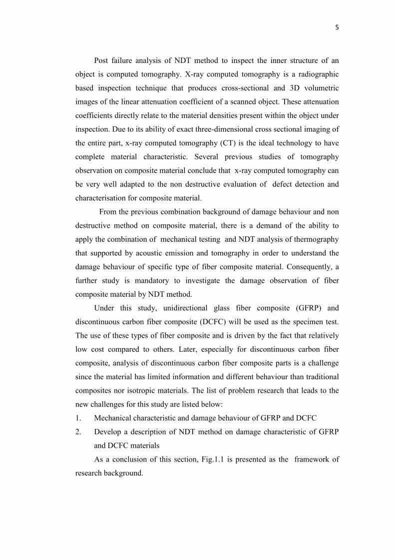
As a conclusion of this section, Fig.1.1 is presented as the framework of

research background.

6

Figure 1.1 Framework of research background

1.2 OBJECTIVE RESEARCH

This research is part of collaboration project of PSA Peugeot Citroën in

France with LEME laboratory of University of Paris Ouest Nanterre-La Défense.

This project is a jointly funded industrial and academic research initiative to

apply the NDT method on observe the damage behaviour of GFRP and DCFC.

To achieve this aim, a series of experiments are conducted to examine the damage

behaviour (appearance, type, location, evolution) of GFRP and DCFC under

tensile (static and fatigue) loading. Generally, damage behaviour of fiber

composite under static condition can be in the form of fiber fracture, fiber

splitting, fiber pull out, fiber/matrix debonding, matrix cracking and

7

delaminations between layers of the laminate. Under fatigue loading, The damage

evolution can be determined directly by using stiffness reduction that consists of

the development of transverse matrix cracks dominates the stiffness reduction

ascertained in this first stage, Predominant damage mechanisms that develope in

delaminations and cracks propagation in intermediate stage, and as final stage,

the occurance of fiber fractures lead to significant stiffness reduction and

specimen completely failed [16].

Additionally, during all the tests, specimen surface was observed with NDT

thermography supported by acoustic emission (AE) and post failure observation

of tomography (CT scan) in order to characterize the damage behaviour through

NDT observation.

As a result, this research studies have the objectives are as follows:

1. To obtain the NDT thermography characteristic and provide a combination

with mechanical testing results of tensile static loading on damage

behaviour and mechanical properties of GFRP and DCFC

2. To obtain the NDT thermography characteristic and provide a combination

with mechanical testing results of tensile fatigue loading on damage

behaviour and mechanical properties of GFRP and DCFC

3. To determine the NDT characteristics of the results support by acoustic

emission (AE) under tensile static loading and tomography (CT-scan) on

damage behaviour of GFRP and DCFC where produced by tensile fatigue

loading.

1.3 RESEARCH CONTRIBUTION

After conducting a thorough literature review, it is evident that studies of the

NDT method for damage analysis of fiber composite are limited. There is no prior

work on NDT thermography and post failure observation of tomography on

discontinuous carbon fiber composite (DCFC) material. Most studies are limited

to continuous composite. It is also notable that in many cases of damage

observation on unidirectional fiber composite (GFRP), a combination of NDT

thermography and acoustic emission, fatigue strength analysis by thermography

and tomography observation have not been fully conducted.

8

The work presented in this thesis concentrates on the application of NDT

method of thermography supported by acoustic emission and tomography as

observation tools on damage behaviour of DCFC and GFRP specimen under

tensile (static and fatigue) loading condition. This approach aims to correlate all

the results in order to obtain a more reliable and accurate representation of the

damage behaviour of fiber composite. Moreover, determination of high cycle

fatigue strength and the prediction of S-N curve based on thermography and

energy dissipation approach also described in this study. To the knowledge of the

author, all the results are significant contribution on damage characteristics of

DCFC and GFRP composite material that used in this study.

Beside the gap or future work based on the previous studies and the research

background, this research will open the opportunity to accomodate the interest in

supporting maritime industry in Indonesia where generally using composite as a

material for shipping industry due to an excellent corrosion resistance. This

opportunity is directly related to the declaration of Indonesia as a maritime pivot

by Indonesian President Joko Widodo in Summit East Asian Nations 2014 where

the shipping industry to be one of the priority pillar.

For the future, through this research, the application of NDT observation in

understanding the damage behaviour of composite component in shipping

industry or others is highly expected and reliable for predicting the service (or

fatigue) life of composite materials subjected to long-term cyclic loads to prevent

the occurrence of failure.

1.4 CONTENT OF THESIS

Chapter 1 describes an introduction of this research. A clear description of

background, problem statement, objective of the research and novelty are

elaborated as a guideline in conducting this research.

Chapter 2, following the introduction, provides an overview of the state of

the art in NDT study and damage analysis on composite material. The review

comprehends of the composite, damage behaviour, and NDT method is provided.

The observation results on each NDT method of thermography, acoustic emission

and tomography associate with damage observation are highlighted in this

9

chapter. The justification of this work also described along with require further

investigation as the novel results.

Chapter 3 explains on experimental method of mechanical testing and

NDT observation. The specimen type, procedure of mechanical tensile loading

under static and fatigue condition and NDT method of Thermography, acoustic

emission, tomography are well documented based on experimental measurements.

Sequentially, Chapter 4 and Chapter 5 outlines the analysis of mechanical

testing and NDT thermography observation on GFRP and DCFC. Analysis of

static tensile loading along with thermography observation of GFRP and DCFC

for specimen with and without hole, analysis of fatigue tensile loading along with

thermography observation on GFRP and DCFC for specimen with hole, and rapid

strength analysis of GFRP and DCFC under fatigue loading are presented.

Support analysis by acoustic emission and tomography on damage

behaviour of fiber composite are given in chapter 6. The coupling between

thermography and acoustic emission for damage observation of GFRP and post

failure analysis of tomography are focused in this chapter. The correlation of

damage behaviour and observation analysis is discussed based on temperature

intensity from thermography, the energy - amplitude of acoustic emission signals,

and gray value from tomography.

Chapter 7 contains overall conclusion and future work derived from this

research work.

10

Chapter II LITERATURE REVIEW

2.1 INTRODUCTION

The damage behaviour of composite materials has been widely investigated

in recent years with a lot of works on damage mechanisms (section 2.3) and

damage observation (section 2.4 - section 2.8)

This literature review is started by a general discussion on composite

material (Section 2.2) and the damage behaviour of composite material in general

(Section 2.3). Some aspects of the effect of loading type in composites are then

briefly introduced (page 21-23). Following this, the composite with an open hole

condition are also discussed (page 23-29).

Although they are not strictly speaking as a new type of reinforcement form

in composite material, Discontinuous carbon fiber composite have only less

coverage in the literature associates with NDT investigation. A limited number of

works already exist regarding their mechanical properties and damage behaviour

(page 47-51). However, glass fiber composites does not need a brief discussion

and their behaviour is well documented.

NDT techniques of thermography, acoustic emission and tomography and

details of these procedures for monitoring damage in composites are available in

the literature ( page 29-46). The application of these NDT method for damage

observation in composite material are also described.

From the new focus from industrial point of view shown by background

research and limited information on NDT method of thermography, acoustic

emission and tomography for damage observation on fiber composite material

thorough literature review, there is a need to conduct a research that concentrates

on the application of NDT method as an observation tools of damage behaviour

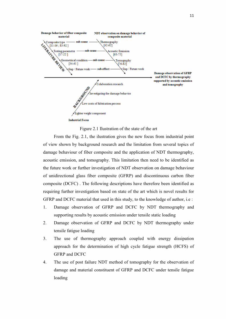
for composite material, as seen in Fig 2.1 as an ilustration of the state of the art of

new research.

11

Figure 2.1 Ilustration of the state of the art

From the Fig. 2.1, the ilustration gives the new focus from industrial point

of view shown by background research and the limitation from several topics of

damage behaviour of fiber composite and the application of NDT thermography,

acoustic emission, and tomography. This limitation then need to be identified as

the future work or further investigation of NDT observation on damage behaviour

of unidirectional glass fiber composite (GFRP) and discontinuous carbon fiber

composite (DCFC) . The following descriptions have therefore been identified as

requiring further investigation based on state of the art which is novel results for

GFRP and DCFC material that used in this study, to the knowledge of author, i.e :

1. Damage observation of GFRP and DCFC by NDT thermography and

supporting results by acoustic emission under tensile static loading

2. Damage observation of GFRP and DCFC by NDT thermography under

tensile fatigue loading

3. The use of thermography approach coupled with energy dissipation

approach for the determination of high cycle fatigue strength (HCFS) of

GFRP and DCFC

4. The use of post failure NDT method of tomography for the observation of

damage and material constituent of GFRP and DCFC under tensile fatigue

loading

12

2.2 COMPOSITE MATERIAL

Composite materials are created by combining two material to achieve

desired properties that usually processed separately and the bonded, resulting

properties that are different from those of either of the component materials

namely reinforcement and matrix.

Mohanty et.al. [6] very clearly that the composites should not be regarded

simple as a combination of two materials. In the broader significance; the

combination has its own distinctive properties. In terms of strength to resistance to

heat or some other desirable quality, it is better than either of the components

alone or radically different from either of them. Uzamani et.al. [7] defines as “The

composites are compound materials which differ from alloys by the fact that the

individual components retain their characteristics but are so incorporated into the

composite as to take advantage only of their attributes and not of their short

comings”, in order to obtain improved materials. Bilba et.al. [8] explains

composite materials as heterogeneous materials consisting of two or more solid

phases, which are in intimate contact with each other on a microscopic scale. They

can be also considered as homogeneous materials on a microscopic scale in the

sense that any portion of it will have the same physical property.

Some advantages of composite materials over conventional ones are as

follows [9]:

Tensile strength of composites is four to six times greater than that of steel

or aluminium (depending on the reinforcements).

Higher fatigue endurance limit (up to 60% of ultimate tensile strength).

30% - 40% lighter for example any particular aluminium structures designed

to the same functional requirements.

Composites are more versatile than metals and can be tailored to meet

performance needs and complex design requirements.

Composites enjoy reduced life cycle cost compared to metals.

Composites exhibit excellent corrosion resistance and fire retardancy.

Composite parts can eliminate joints / fasteners, providing part

simplification and integrated design compared to conventional metallic

parts.

13

The reinforcement presents the strength and stiffness that more harder,

stronger, and stiffer compared to the matrix. Fiber reinforced composites is one of

reinforcement type besides particulate and structural that are available in three

basic form :

Continuous fibers are long, straight and layed-up parallel to each other.

Chopped /Discontinuous fibers are short and randomly distributed

Woven Fibers

Glass fiber and carbon fiber are the most common fiber reinforcement that

typically used within the automotive industry for applications such as body

panels, suspension, steering, brakes, and other accessories. Glass fibers are

manufactured by drawing molten glass into very fine threads and then

immediately protecting them from contact with the atmosphere or with hard

surfaces in order to preserve the defect free structure that is created by the

drawing process, known as E-glass [7]. The advantages of glass fiber are

inexpensive, easy to manufacture and possess high strength and stiffness. Carbon

fiber produced by oxidising and pyrolysing a highly drawn textile fiber such as

polyacrylonitrile (PAN), preventing it from shrinking in the early stages of the

degradation process, and subsequently hot-stretching it [7].

Matrix is the continuous phase and can be clasified into : polymer–matrix

composites (PMC), metal–matrix composites (MMC), and ceramic–matrix

composites (CMC). Polymer-matrix is the most commonly used matrix materials,

because compared to metal and ceramic matrix composites, polymer composites

are less costly to manufacture. In a composite material, the matrix material have

the following critical functions [10]:

Holds the fibers together

Protects the fibers from environment

Distributes the loads evenly between fibers so that all fibers are subjected to

the same amount of strain.

Enhances transverse properties of a laminate

Helps to avoid propagation of crack growth through the fibers by providing

alternate failure path along the interface between the fibers and the matrix.

Carry interlaminar shear.

14

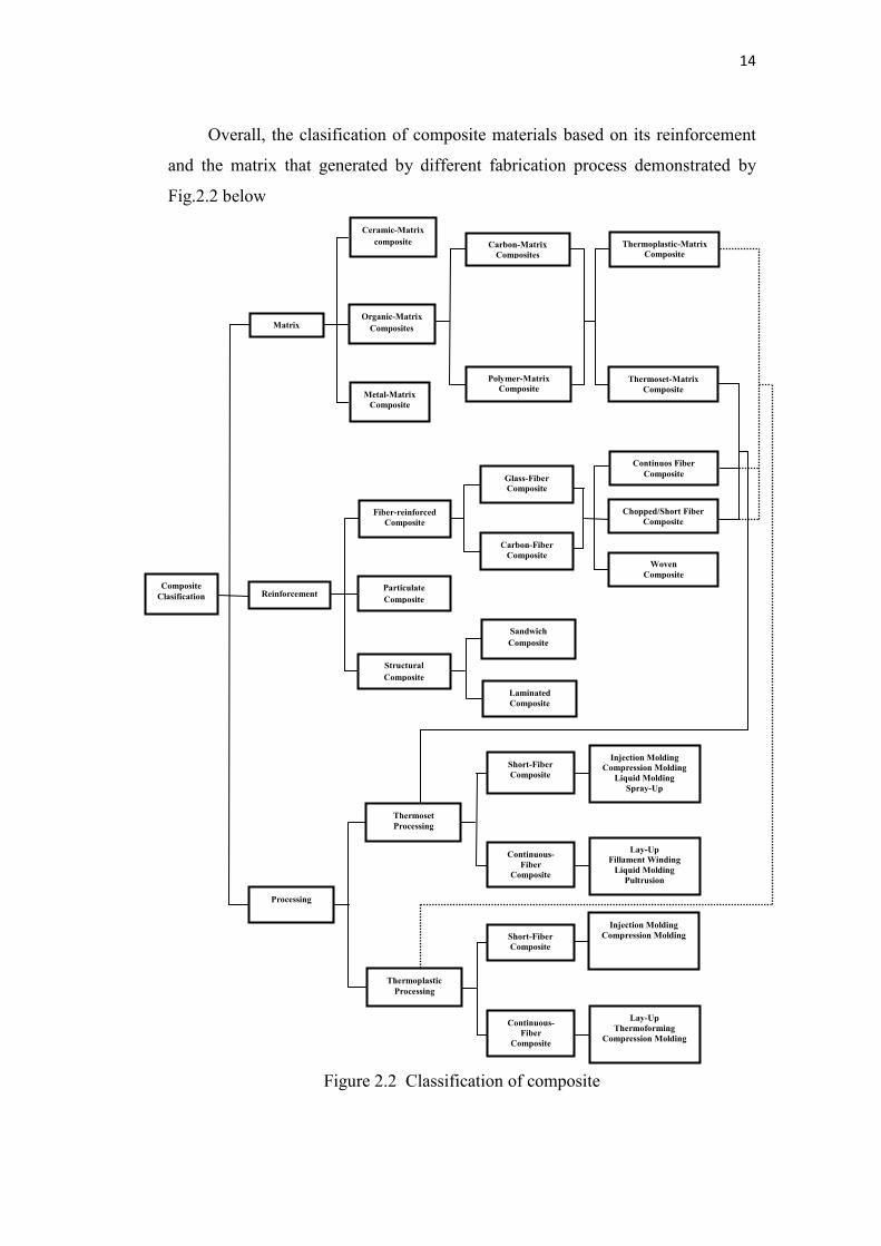
Overall, the clasification of composite materials based on its reinforcement

and the matrix that generated by different fabrication process demonstrated by

Fig.2.2 below

Figure 2.2 Classification of composite

Composite Clasification

Matrix

Ceramic-Matrix composite

Organic-Matrix Composites

Metal-Matrix Composite

Polymer-Matrix Composite

Carbon-Matrix Composites

Thermoplastic-Matrix Composite

Thermoset-Matrix Composite

Injection Molding Compression Molding

Liquid Molding Spray-Up

Processing

Thermoset Processing

Short-Fiber Composite

Thermoplastic Processing

Continuous-Fiber

Composite

Short-Fiber Composite

Continuous-Fiber

Composite

Lay-Up Fillament Winding

Liquid Molding Pultrusion

Injection Molding Compression Molding

Lay-Up Thermoforming

Compression Molding

Particulate Composite

Reinforcement

Structural Composite

Sandwich Composite

Laminated Composite

Fiber-reinforced Composite

Glass-Fiber Composite

Carbon-Fiber Composite

Continuos Fiber Composite

Chopped/Short Fiber Composite

Woven Composite

15

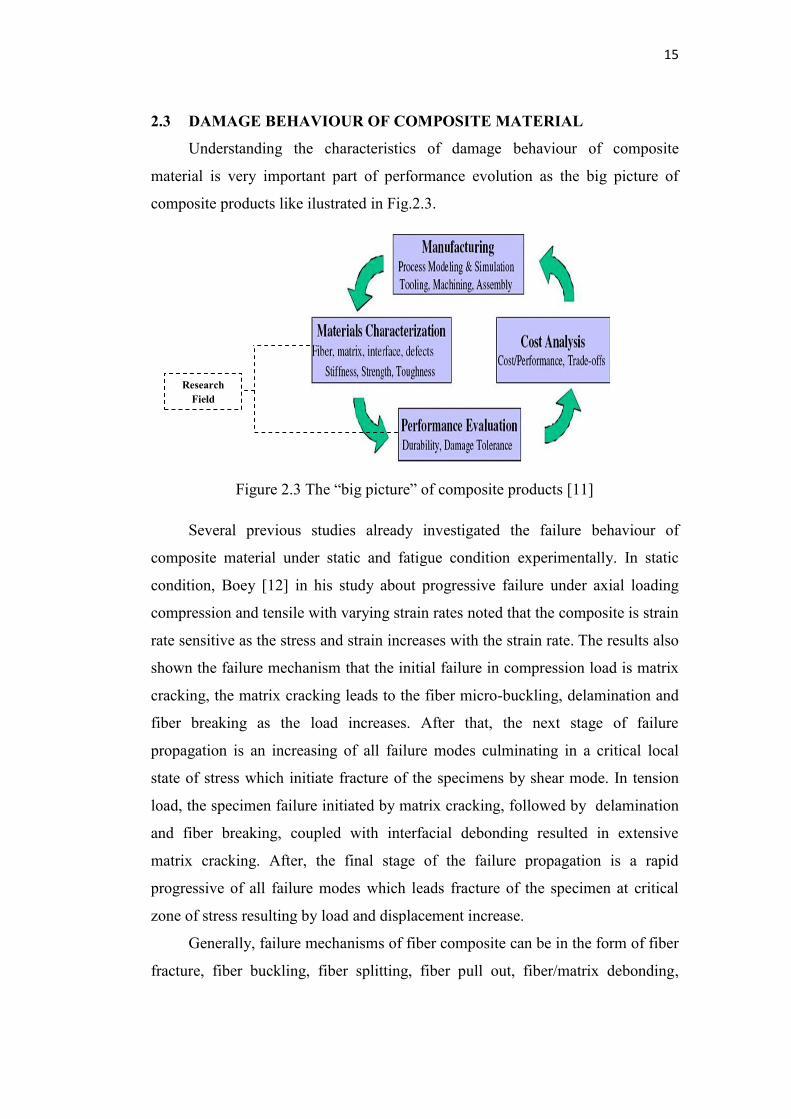
2.3 DAMAGE BEHAVIOUR OF COMPOSITE MATERIAL

Understanding the characteristics of damage behaviour of composite

material is very important part of performance evolution as the big picture of

composite products like ilustrated in Fig.2.3.

Figure 2.3 The “big picture” of composite products [11]

Several previous studies already investigated the failure behaviour of

composite material under static and fatigue condition experimentally. In static

condition, Boey [12] in his study about progressive failure under axial loading

compression and tensile with varying strain rates noted that the composite is strain

rate sensitive as the stress and strain increases with the strain rate. The results also

shown the failure mechanism that the initial failure in compression load is matrix

cracking, the matrix cracking leads to the fiber micro-buckling, delamination and

fiber breaking as the load increases. After that, the next stage of failure

propagation is an increasing of all failure modes culminating in a critical local

state of stress which initiate fracture of the specimens by shear mode. In tension

load, the specimen failure initiated by matrix cracking, followed by delamination

and fiber breaking, coupled with interfacial debonding resulted in extensive

matrix cracking. After, the final stage of the failure propagation is a rapid

progressive of all failure modes which leads fracture of the specimen at critical

zone of stress resulting by load and displacement increase.

Generally, failure mechanisms of fiber composite can be in the form of fiber

fracture, fiber buckling, fiber splitting, fiber pull out, fiber/matrix debonding,

Research Field

16

matrix cracking and delaminations between layers of the laminate that introduced

by severe loading conditions, environmental attacks and defect within fiber and

matrix. Table 2.1 below gives the type of failure mechanism of fiber composite.

Table 2.1 Type of failure mechanism of fiber composite [13]

Type of Failure Mechanism Fiber breakage Damage usually occurs when the composite is subjected to

tensile load. Maximum allowable axial tensile stress (or strain) of the fiber is exceeded.

Fiber pull out Fiber fracture accompanied by fiber/matrix debonding or fiber/matrix separation

Matrix cracking Strength of matrix is exceeded

Fiber buckling Axial compressive stress causes fiber to buckle

Fiber splitting Transverse in the fiber or interphase region between the fiber and the matrix reaches its ultimate value

Delamination Interlaminar damage in fiber composite that cause considerable reduction in structural stiffness and leads to growth of the damage and final damage

Despite their excellent characteristics, composite are susceptible to the

fatigue and damage phenomena when subjected to certain cyclic loads (static or

dynamic) and/or environmental conditions. Failure processes may actually begin

during fabrication or at a low applied stress level. Furthermore, failure may be

catastrophic and unpredictable. Unlike metals, composite exhibit a peculiar

behaviour in fatigue. The experience with the metal fatigue cannot be directly

used for composite materials due to its inhomogeneous and anisotropic properties.

For example, after initiation, the propagation of the crack is responsible for

final fatigue failure in metals, while accumulation of cracks leads to failure in

composite material [14]. Even for unidirectional reinforced composite under the

simple loading case, such as tension loading along the direction of fibers, fatigue

cracks may initiate at different locations and in different directions [15]. Further

more, the composite material experience relatively significant material

degradation under fatigue loading. All these differences make it difficult to apply

the same fatigue analysis methodology of metals to the composite materials.

Hence, an understanding and prediction of further propagation of such

defects is importance for predicting the service (or fatigue) life of composite

materials subjected to long-term cyclic loads.

17

2.3.1 Damage behaviour of fiber composite under fatigue loading

Early study about fatigue failure development of fiber reinforced plastic

was conduct by Schulte [16] by analyze the stiffness reduction. The stiffness

reduction can be used directly to monitor failure development by grouping into

three distinctive stages of damage development [16] :

The initial region (stage I) with a rapid stiffness reduction of 2-5%. The

development of transverse matrix cracks dominates the stiffness reduction

ascertained in this first stage,

An intermediate region (stage II), in which an additional 1–5% stiffness

reduction occurs in an approximately linear fashion with respect to the

number of cycles. Predominant damage mechanisms are the development of

edge delaminations and additional longitudinal cracks along the 0° fibers,

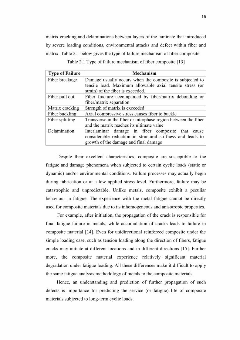
and a final region (stage III), in which stiffness reduction occurs in abrupt

steps ending in specimen fracture. In stage III, a transfer to local damage

progression occurs, when the first initial fiber fractures lead to strand

failures. These damages evolution as seen in Fig.2.4 below.

Figure 2.4 Stiffness degradation of fiber reinforced composite materials [13]

In relation with fatigue life of composite, Talreja [11] also divided into three

region of composite failure by fatigue. Based on his explanation, First region is

the composite failure strain in tension, represents the non-progressive fiber

breakage regime in which random fiber failure mechanism governs, Second

region is the regime of progressive fiber-bridged matrix cracking in which

interfacial debonding plays a role and the final region is the region of matrix

cracking, which is effectively arrested by fibers, assisted possibly by interfacial

debonding, such that composite failure is not reached within specified large

18

number of cycles. The boundary between Region II and Region III is the so-called

fatigue limit.

Other differences of fatigue damage behaviour between composite and

metals was explained by Bathias [17]. In composite, fatigue damage is not related

to plasticity, which is very different behaviour compared to metals that its fatigue

damage is strongly related to the cyclic plasticity. Due to complex behaviour of

composite, further studies has been undertaken to gain more understanding of

fatigue failure behaviour in glass fiber reinforced plastics (GFRP) experimentally.

Dyer and Isaac [15] studied about the fatigue behaviour of continuous glass

fiber reinforced plastics to evaluate the micromechanisms that occurred during

fatigue and how damage accumulated throughout the sample lifetime. It was

found that damage accumulation during fatigue has a patern characterised by

matrix cracking, delamination and fiber failure. These cracks were seen to have

penetrated the fiber bundles before failure, and propagated by debonding of the

fiber/matrix interfaces. The observation using SEM shown that both the fibers and

the resins failed in a brittle manner.

Fatigue mechanisms in unidirectional glass fiber reinforced plastic was

investigated by Gamstedt et.al [18]. The fatigue life performance, stifness

degradation and micro mechanisms have been investigated for glass fiber

reinforced polypropylene. From microscopic observations, it could be concluded

that the better fatigue resistance of glass fiber reinforced plastic can be attributed

to the greater interfacial strength and the resistance to debond propagation.

In [19-22],. The effect of lay-up design and the rise of the temperature of

the specimens on fatigue perfomance were investigated. The results shows that

the fatigue strength is strongly influenced by the layer design and the temperature

rise on the surface of the specimens reaches a maximum value at failure or the

damage parameter E present a nearly linear relationship with te rise of

temperature.

Fatigue crack propagation of GFRP was investigated by Pegoretti and Ricco

[23]. The aim of the study is to investigate how the fatigue-crack propagation is

affected by the test frequency and the amount of reinforcing fibers. It was found

that, at a fixed stress intensity factor amplitude (ΔK), the fatigue crack

19

propagation (FCP) rate per cycle (da/dN) is reduced when the fiber content is

increased. When the effects of the loading frequency were investigated, it was

found that the higher the frequency the lower the FCP rate at any fixed ΔK value.

Gagel et.al [24] investigated the relation between crack densities, stiffness

degradation, and surface temperature distribution of fatigue behaviour of glass

fiber reinforced epoxy. The results shows that in the case of cyclic loading, the

stiffness decreases with an increase in Crack Density (CD) until the end of the

steady stage of fatigue life. Then, the loss in stiffness turns to be progressive until

failure that contrast to the CD development, which continues to grow

degressively. It was observed that the location of final failure coincides with the

region of the highest surface temperature and cannot be related to the local CD.

In order to avoid large safety factors being applied, failure accumulation

during the component lifetime must be monitored. So, it is possible to replace

components before final failure. Undergoing different failure types, such as

matrix cracking, fiber–matrix debonding, delamination, fiber breakage, quite

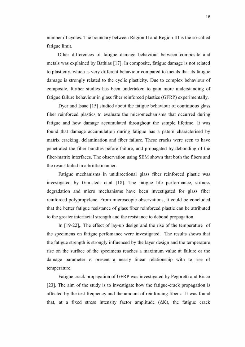
evenly distributed within the entire material volume [11,17]. The failure

behaviour composite under fatigue is ilustrated by the damage progression-time

diagram in Fig.2.5.

Figure 2.5 Development of damage in composite under fatigue [11]

There are several types of failure stage behaviour in the failure diagram. In

the initial stage matrix crack will form and increase with the number of load

cycles and will eventually form macroscopic cracks. These macroscopic cracks

will show a classical crack propagation patern. The matrix cracks will generally

run through the ply thickness and also ply width. These cracks will initiate

20

microcracks in adjacent plies. In the plies interfaces close to the macroscopic and

microscopic cracks strong interlaminar stresses develop which lead to separation

between the plies locally. At this state the rate of damage progression increase

rapidly and will soon lead to an area where the local stresses reaches a level above

the critical and a fracture is initiated. Two dominating stages can be clearly

identified : the formation of local, independent matrix micro cracks and a second

stage where various types and orientations of cracks interact with increasing rates

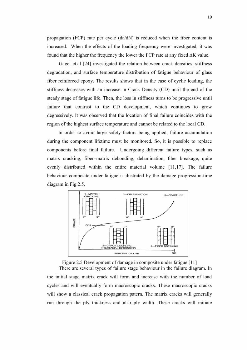
which finally lead to failure. Wang and Chung [25] also studied about the

evolution of fiber breakage of glass fiber composite. It was found that fiber

breakage to occur involves 1000 fibers or more and started at about half of the

fatigue life during fatigue testing and at least 18% of the fibers were broken

before fatigue failure. This Fig.2.6 below also shows the damage type of

composite from several investigated by previous authors.

Figure 2.6 Damage type of fiber reinforced plastic [27]

Between the macroscopic and microscopic levels, there exists a very

important middle domain, typical of composite materials, which is treated at the

mesoscopic level: that of transverse cracking, distribution of the reinforcements

and of porosity, that is, the domain of sequential cells [28]. At the mesoscopic

level, the fatigue damage is multidirectional and the damage zone, much larger

than the plastic zone, is related to the complex morphology of the fracture as

reported by Bathias [17].

21

2.3.2 Effect of loading type on fatigue of fiber composite

Fatigue in materials is caused by repeated loading and unloading cycles to

maximum stresses below the ultimate strength of a material. This cyclic loading

causes a progressive degradation of the material properties and eventual failure. In

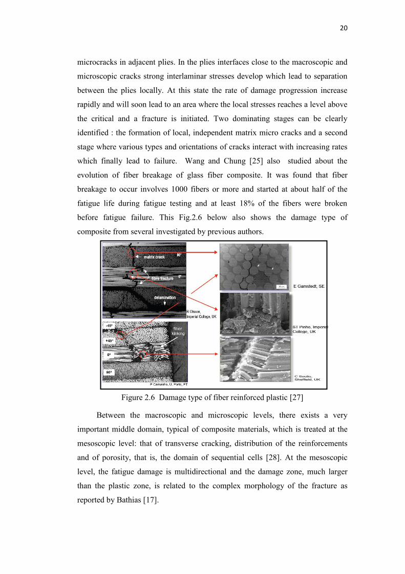
many constant amplitude load controlled fatigue experiments, a specimen is

loaded sinusoidally in time with the stress: (1)

Common parameters for describing cycling loading are shown in Fig.2.7.

Figure 2.7 Illustration of sinusoidal loading

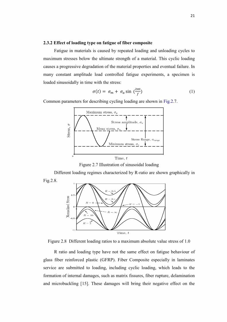
Different loading regimes characterized by R-ratio are shown graphically in

Fig.2.8.

Figure 2.8 Different loading ratios to a maximum absolute value stress of 1.0

R ratio and loading type have not the same effect on fatigue behaviour of

glass fiber reinforced plastic (GFRP). Fiber Composite especially in laminates

service are submitted to loading, including cyclic loading, which leads to the

formation of internal damages, such as matrix fissures, fiber rupture, delamination

and microbuckling [15]. These damages will bring their negative effect on the

22

mechanical performance of laminates, which reduces the useful life of the

material. Many previous study has been undertaken to investigated the effect of

loading on fatigue of GFRP.

Bathias [17] in his point of view about damage in composite reported that

under monotonic loading all composite materials present a compressive strength

inferior to the ultimate tensile strength and decreasing as a function of the

reinforcement type (boron, carbon, glass, and kevlar). Under cyclic loading the

fatigue behaviour is the same. At the limit, when the fatigue cycle is entirely in

compression, fracture can occur. For practical applications, it is very important to

notice that in compression loading the ratio SD/UTS can be as low as 0.3 for

certain composites.

Fatigue Damage, mechanism and failure prevention in fiberglass reinforced

composite under different stress ratio were researched by Freire and Aquino [26].

The tests were performed under stress ratios, R (= σmin/σmax), of 0.1, -1 and 10.

The results shows that for R = 0.1 laminates experienced fatigue damage

according to: formation and saturation of transversal cracks, formation and

propagation of delamination, fiber rupture and ultimate composite fracture. For R

= -1 the order of the events leading to fracture of both laminates slightly changed

to: transversal cracking, formation and propagation of delamination, saturation of

transversal cracks, continued formation and propagation of delamination, fiber

rupture and ultimate composite fracture. For R = 10 fracture was restricted to

delamination, fiber rupture and ultimate composite fracture.

Investigation about the effect of stress ratio on the fatigue of unidirectional

fiber glass epoxy composite has been done by Kadi and Ellin [29]. The test was

performed under tension-tension and tension-compression loading and variation

of stress ratio ( R = 0.5 , 0, and -1). The experiment data were obtained for several

fiber orientation. It is shown that, in general, tensile and compressive parts of the

stress do not contribute equally to the damage.

About the type of loading, Bathias [17] also said that each type has the

specific effect on composite materials. The analysis of bending behaviour is more

difficult compared to tension or compression because several types of damage

could occur in bending such as tension, shear and compression simultaneously.

23

And for the compression loading, impact damage is plays important role to predict

fatigue endurance because of the involved of low energy impacts on the initiation

of fatigue fracture which has the same role with machining grooved on the surface

of metals. This behaviour be a concern because the low energy could instigates

delamination which can propagate under cyclic loading. One of the previous study

about fatigue behaviour of behaviour of glass fiber reinforced plastic under

bending with different fiber orientation on cantilever beam specimens was studied

by Paepegem and Degrieck [18]. Experiments show that these two specimen types

based on fiber orientation (0o and 45o) have a quite different damage behaviour

and that the stiffness degradation follows a different path. The results show that

the outermost layers which have been subjected to the largest tensile stresses, are

severely damaged, ,while the outer layer on the compression side showed no signs

of damage were observed. This brings about an important result: due to the growth

of damage and the degradation of the bending stiffness, there is a continuous

redistribution of the stresses in the cross-section, especially near the fixation

where damage growth is dominant. The position of the ‘neutral fiber’ (according

to its definition in the classical beam theory) does not remain in the middle of the

cross-section, but tends to move towards the compression side and transfers the

load to that zone.

2.3.3 Stress concentration of composite with the open hole condition

The stress concentration effect that caused by the open hole on mechanical

properties of component is an important issue in failure reliability evaluation for

example the component life of joining application in automotive industry

especially with composite material. Joining structure that containing the hole in

mechanical fastener joints such as pinned joints are very useful and inevitable in

complex structure because of their low cost, simplicity for assemble and

facilitation of disassembly for repair [34]. The natural behaviour of anisotropic

and heterogeneous makes composite material is more complicate and to analyze

than isotropic material in the joint application which contains the hole. In the

presence of a hole, crack, or other discontinuity, the strength reduction of a

24

composite from is often the critical design driver and therefore failure prediction

is of significant practical importtance [35].

Previous studies about the effect of the hole on the stress concentration and

failure mechanism of composite material under static and fatigue loading will be

defined below. Awerbuch and Madhukar [36] noted that local damage on the

microscopic level in the highly stressed region with cutouts occurs in the form of

fiber pull-out, matrix micro-cracking, fiber-matrix interfacial failure, matrix

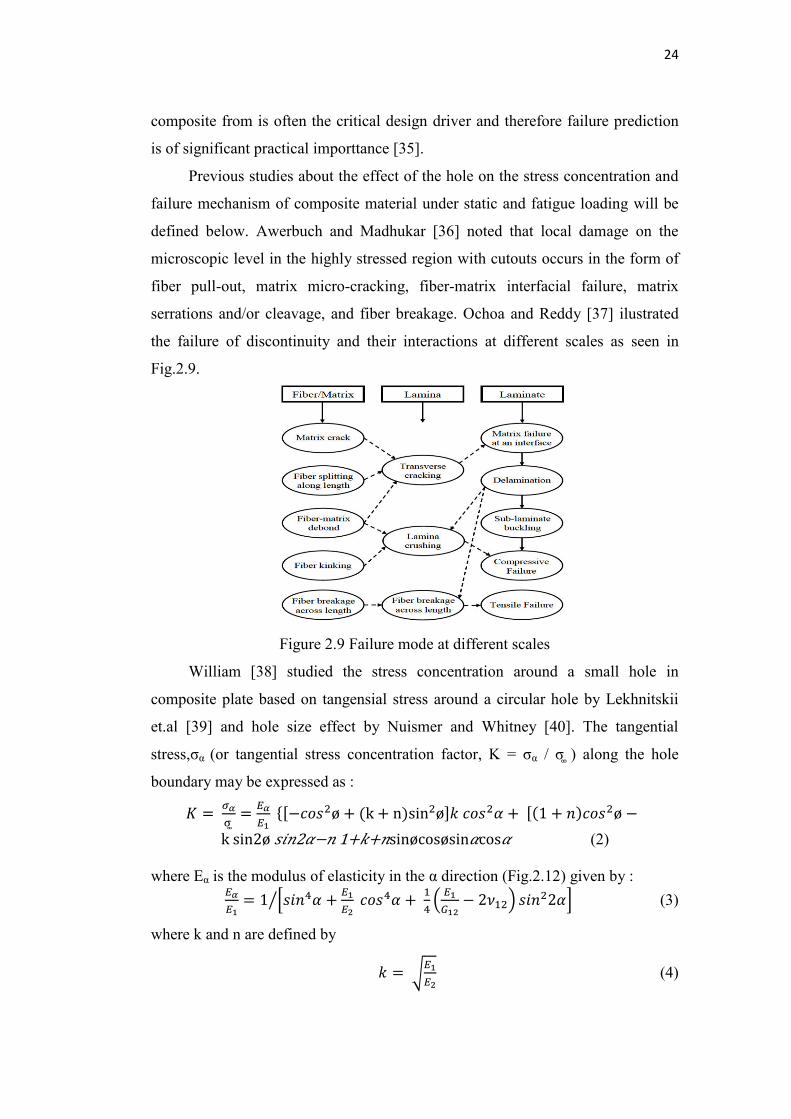
serrations and/or cleavage, and fiber breakage. Ochoa and Reddy [37] ilustrated

the failure of discontinuity and their interactions at different scales as seen in

Fig.2.9.

Figure 2.9 Failure mode at different scales

William [38] studied the stress concentration around a small hole in

composite plate based on tangensial stress around a circular hole by Lekhnitskii

et.al [39] and hole size effect by Nuismer and Whitney [40]. The tangential

stress,σα (or tangential stress concentration factor, K = σα / σ ) along the hole

boundary may be expressed as : k sin2ø 2 1+ + sinøcosøsin cos (2) where Eα is the modulus of elasticity in the α direction (Fig.2.12) given by μ

(3)

where k and n are defined by (4)

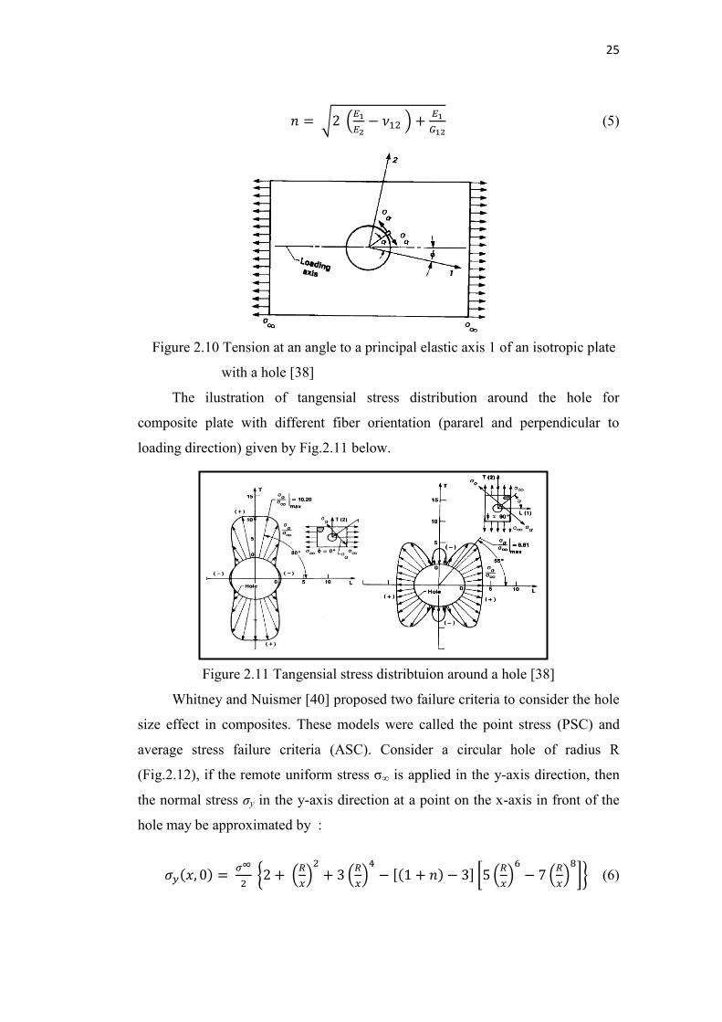
25

(5)

Figure 2.10 Tension at an angle to a principal elastic axis 1 of an isotropic plate

with a hole [38]

The ilustration of tangensial stress distribution around the hole for

composite plate with different fiber orientation (pararel and perpendicular to

loading direction) given by Fig.2.11 below.

Figure 2.11 Tangensial stress distribtuion around a hole [38]

Whitney and Nuismer [40] proposed two failure criteria to consider the hole

size effect in composites. These models were called the point stress (PSC) and

average stress failure criteria (ASC). Consider a circular hole of radius R

(Fig.2.12), if the remote uniform stress σ∞ is applied in the y-axis direction, then

the normal stress σy in the y-axis direction at a point on the x-axis in front of the

hole may be approximated by :

(6)

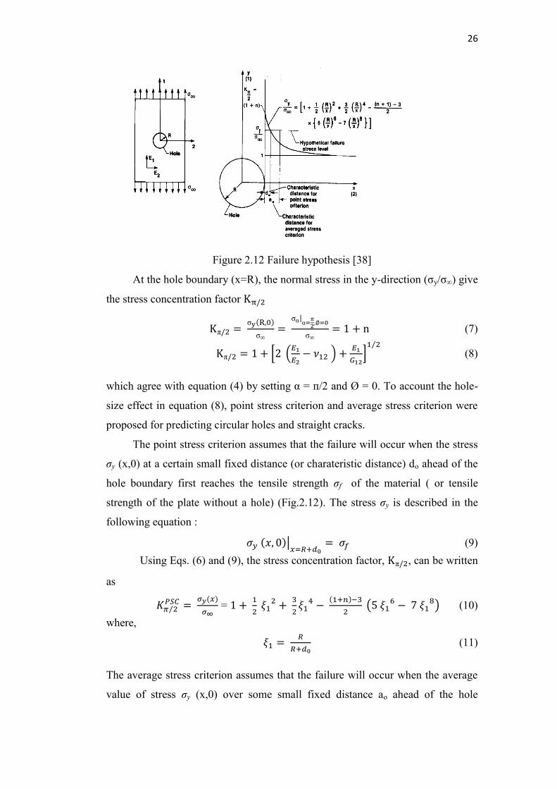
26

Figure 2.12 Failure hypothesis [38]

At the hole boundary (x=R), the normal stress in the y-direction (σy/σ∞) give

the stress concentration factor σ σ∞

σα α σ∞

(7) (8)

which agree with equation (4) by setting α = п/2 and Ø = 0. To account the hole-

size effect in equation (8), point stress criterion and average stress criterion were

proposed for predicting circular holes and straight cracks.

The point stress criterion assumes that the failure will occur when the stress

σy (x,0) at a certain small fixed distance (or charateristic distance) do ahead of the

hole boundary first reaches the tensile strength σf of the material ( or tensile

strength of the plate without a hole) (Fig.2.12). The stress σy is described in the

following equation : (9)

Using Eqs. (6) and (9), the stress concentration factor, , can be written

as = (10)

where, (11)

The average stress criterion assumes that the failure will occur when the average

value of stress σy (x,0) over some small fixed distance ao ahead of the hole

27

boundary first reaches the tensile strength σf of the material ( or tensile strength of

the plate without a hole) (Fig.2.12). It is described in the following equation : (12)

Using Eqs. (6) and (12), the stress concentration factor, , can be written as (13)

where, (14)

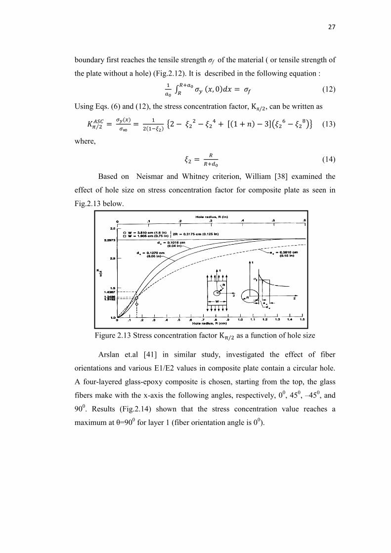
Based on Neismar and Whitney criterion, William [38] examined the

effect of hole size on stress concentration factor for composite plate as seen in

Fig.2.13 below.

Figure 2.13 Stress concentration factor as a function of hole size

Arslan et.al [41] in similar study, investigated the effect of fiber

orientations and various E1/E2 values in composite plate contain a circular hole.

A four-layered glass-epoxy composite is chosen, starting from the top, the glass

fibers make with the x-axis the following angles, respectively, 00, 450, –450, and

900. Results (Fig.2.14) shown that the stress concentration value reaches a

maximum at θ=900 for layer 1 (fiber orientation angle is 00).

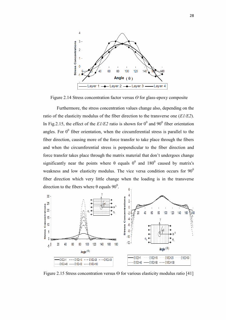
28

Figure 2.14 Stress concentration factor versus ϴ for glass-epoxy composite

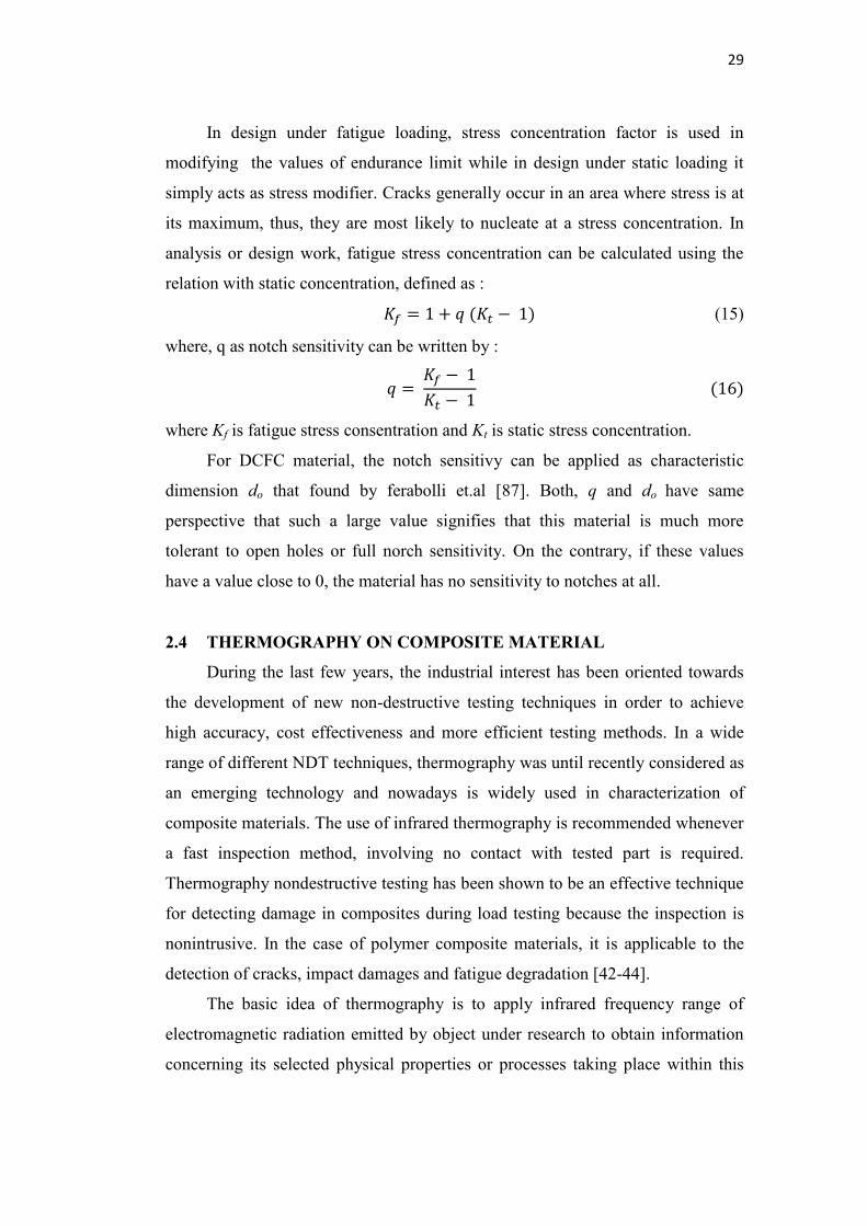
Furthermore, the stress concentration values change also, depending on the

ratio of the elasticity modulus of the fiber direction to the transverse one (E1/E2).

In Fig.2.15, the effect of the E1/E2 ratio is shown for 00 and 900 fiber orientation

angles. For 00 fiber orientation, when the circumferential stress is parallel to the

fiber direction, causing more of the force transfer to take place through the fibers

and when the circumferential stress is perpendicular to the fiber direction and

force transfer takes place through the matrix material that don’t undergoes change

significantly near the points where θ equals 00 and 1800 caused by matrix's

weakness and low elasticity modulus. The vice versa condition occurs for 900

fiber direction which very little change when the loading is in the transverse

direction to the fibers where θ equals 900.

Figure 2.15 Stress concentration versus for various elasticity modulus ratio [41]

29

In design under fatigue loading, stress concentration factor is used in

modifying the values of endurance limit while in design under static loading it

simply acts as stress modifier. Cracks generally occur in an area where stress is at

its maximum, thus, they are most likely to nucleate at a stress concentration. In

analysis or design work, fatigue stress concentration can be calculated using the

relation with static concentration, defined as : (15)

where, q as notch sensitivity can be written by : where Kf is fatigue stress consentration and Kt is static stress concentration.

For DCFC material, the notch sensitivy can be applied as characteristic

dimension do that found by ferabolli et.al [87]. Both, q and do have same

perspective that such a large value signifies that this material is much more

tolerant to open holes or full norch sensitivity. On the contrary, if these values

have a value close to 0, the material has no sensitivity to notches at all.

2.4 THERMOGRAPHY ON COMPOSITE MATERIAL

During the last few years, the industrial interest has been oriented towards

the development of new non-destructive testing techniques in order to achieve

high accuracy, cost effectiveness and more efficient testing methods. In a wide

range of different NDT techniques, thermography was until recently considered as

an emerging technology and nowadays is widely used in characterization of

composite materials. The use of infrared thermography is recommended whenever

a fast inspection method, involving no contact with tested part is required.

Thermography nondestructive testing has been shown to be an effective technique

for detecting damage in composites during load testing because the inspection is

nonintrusive. In the case of polymer composite materials, it is applicable to the

detection of cracks, impact damages and fatigue degradation [42-44].

The basic idea of thermography is to apply infrared frequency range of

electromagnetic radiation emitted by object under research to obtain information

concerning its selected physical properties or processes taking place within this

30

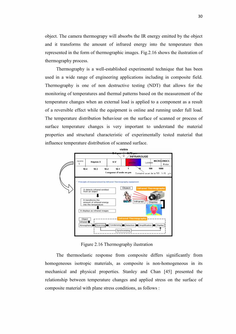
object. The camera thermograpy will absorbs the IR energy emitted by the object

and it transforms the amount of infrared energy into the temperature then

represented in the form of thermographic images. Fig.2.16 shows the ilustration of

thermography process.

Thermography is a well-established experimental technique that has been

used in a wide range of engineering applications including in composite field.

Thermography is one of non destructive testing (NDT) that allows for the

monitoring of temperatures and thermal patterns based on the measurement of the

temperature changes when an external load is applied to a component as a result

of a reversible effect while the equipment is online and running under full load.

The temperature distribution behaviour on the surface of scanned or process of

surface temperature changes is very important to understand the material

properties and structural characteristic of experimentally tested material that

influence temperature distribution of scanned surface.

Figure 2.16 Thermography ilustration

The thermoelastic response from composite differs significantly from

homogeneous isotropic materials, as composite is non-homogeneous in its

mechanical and physical properties. Stanley and Chan [45] presented the

relationship between temperature changes and applied stress on the surface of

composite material with plane stress conditions, as follows :

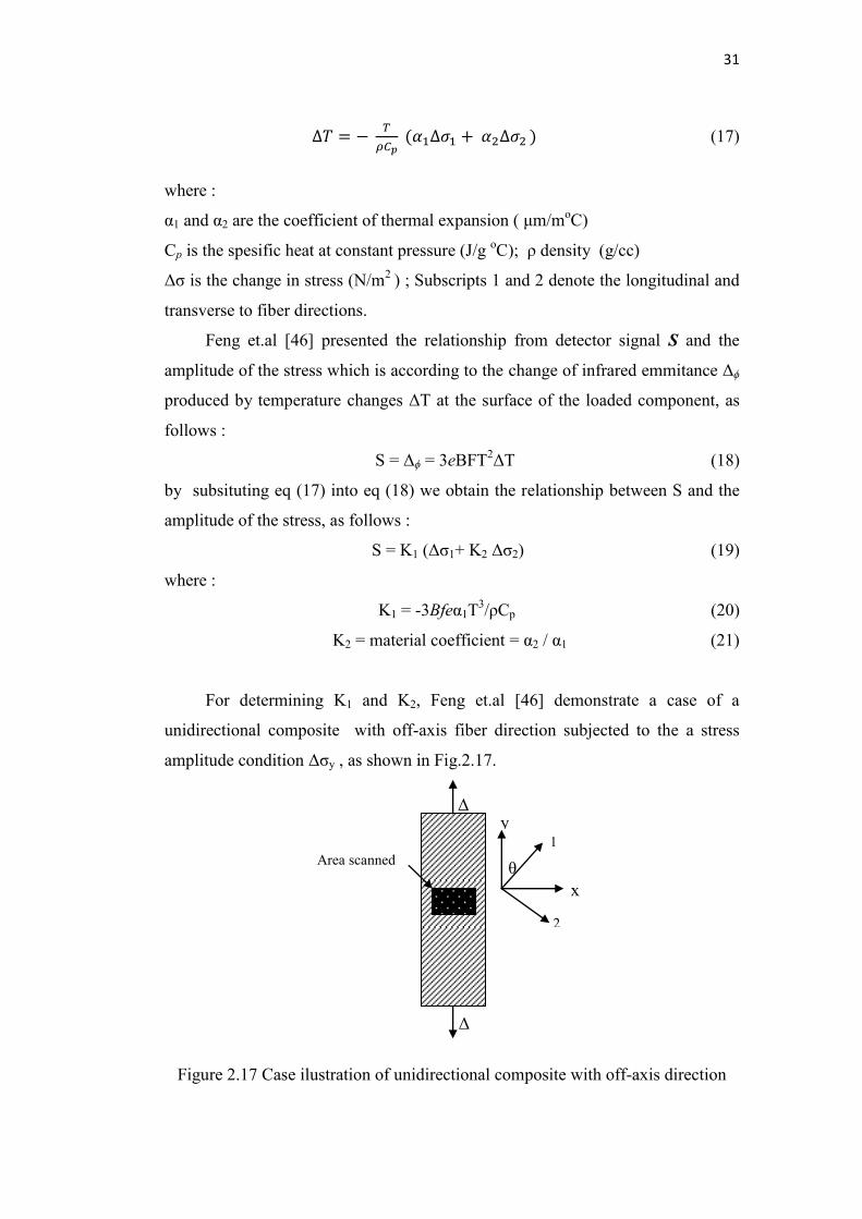
31

(17)

where :

α1 and α2 are the coefficient of thermal expansion ( m/moC)

Cp is the spesific heat at constant pressure (J/g oC)ν ρ density (g/cc)

Δσ is the change in stress (N/m2 ) ; Subscripts 1 and 2 denote the longitudinal and

transverse to fiber directions.

Feng et.al [46] presented the relationship from detector signal S and the

amplitude of the stress which is according to the change of infrared emmitance Δϕ

produced by temperature changes ΔT at the surface of the loaded component, as

follows :

S = Δϕ = 3eBFT2ΔT (18)

by subsituting eq (17) into eq (18) we obtain the relationship between S and the

amplitude of the stress, as follows :

S = K1 (Δσ1+ K2 Δσ2) (19)

where :

K1 = -3Bfeα1T3/ρCp (20)

K2 = material coefficient = α2 / α1 (21)

For determining K1 and K2, Feng et.al [46] demonstrate a case of a

unidirectional composite with off-axis fiber direction subjected to the a stress

amplitude condition Δσy , as shown in Fig.2.17.

Figure 2.17 Case ilustration of unidirectional composite with off-axis direction

Δσ

Δσ

2

x

y

θ

1

Area scanned

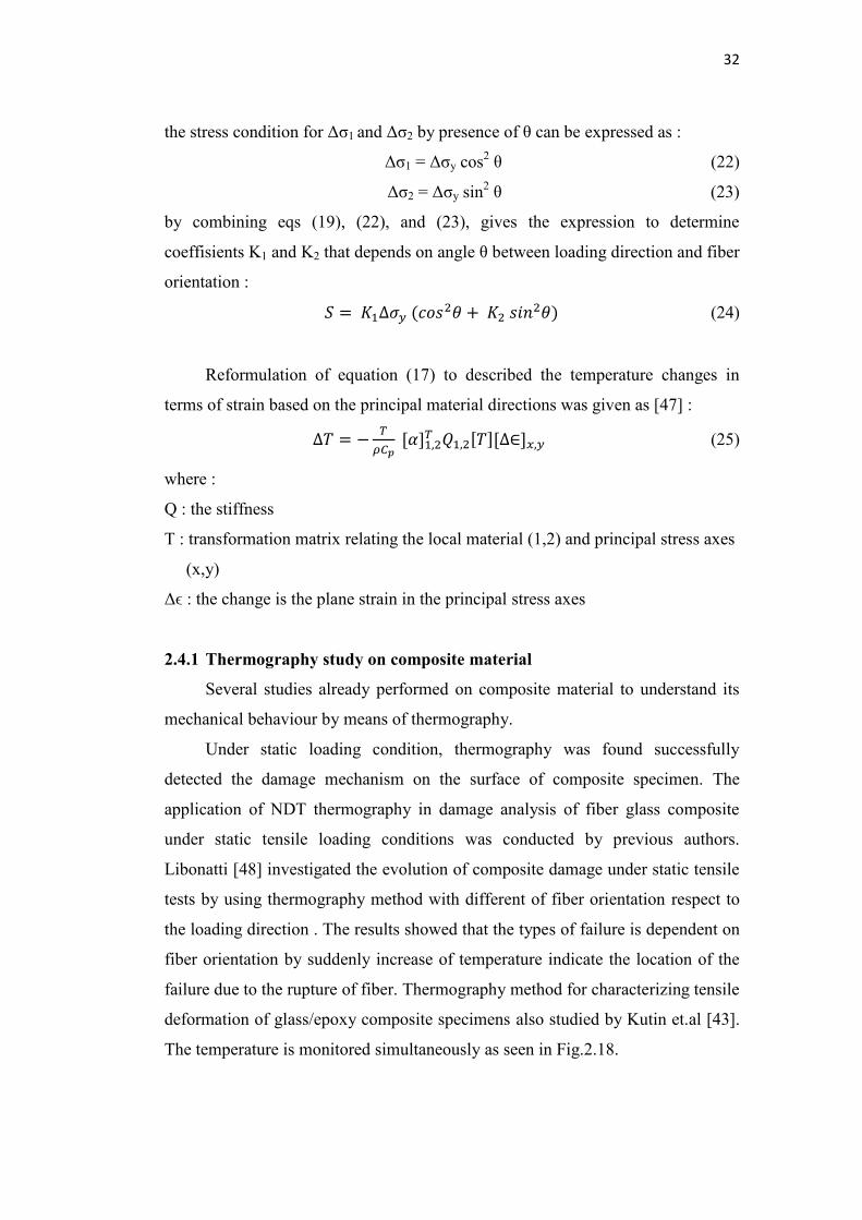
32

the stress condition for Δσ1 and Δσ2 by presence of θ can be expressed as :

Δσ1 = Δσy cos2 θ (22)

Δσ2 = Δσy sin2 θ (23)

by combining eqs (19), (22), and (23), gives the expression to determine

coeffisients K1 and K2 that depends on angle θ between loading direction and fiber

orientation : (24)

Reformulation of equation (17) to described the temperature changes in

terms of strain based on the principal material directions was given as [47] : (25)

where :

Q : the stiffness

T : transformation matrix relating the local material (1,2) and principal stress axes

(x,y)

Δ : the change is the plane strain in the principal stress axes

2.4.1 Thermography study on composite material

Several studies already performed on composite material to understand its

mechanical behaviour by means of thermography.

Under static loading condition, thermography was found successfully

detected the damage mechanism on the surface of composite specimen. The

application of NDT thermography in damage analysis of fiber glass composite

under static tensile loading conditions was conducted by previous authors.

Libonatti [48] investigated the evolution of composite damage under static tensile

tests by using thermography method with different of fiber orientation respect to

the loading direction . The results showed that the types of failure is dependent on

fiber orientation by suddenly increase of temperature indicate the location of the

failure due to the rupture of fiber. Thermography method for characterizing tensile

deformation of glass/epoxy composite specimens also studied by Kutin et.al [43].

The temperature is monitored simultaneously as seen in Fig.2.18.

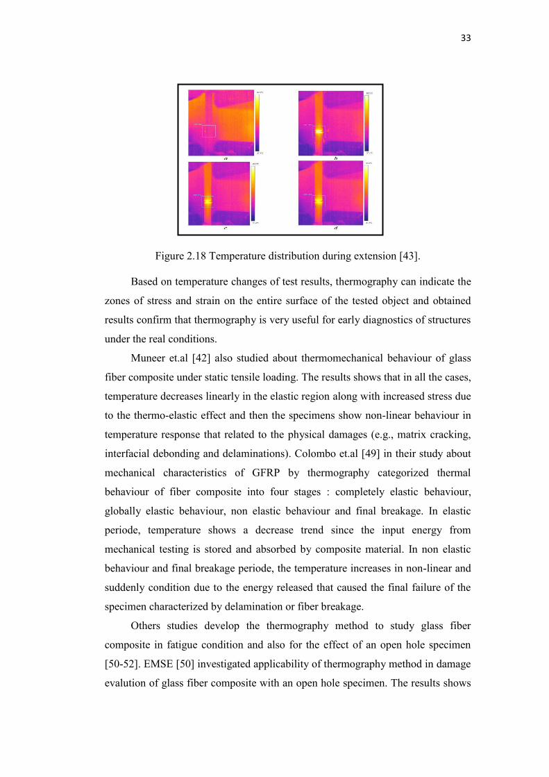
33

Figure 2.18 Temperature distribution during extension [43].

Based on temperature changes of test results, thermography can indicate the

zones of stress and strain on the entire surface of the tested object and obtained

results confirm that thermography is very useful for early diagnostics of structures

under the real conditions.

Muneer et.al [42] also studied about thermomechanical behaviour of glass

fiber composite under static tensile loading. The results shows that in all the cases,

temperature decreases linearly in the elastic region along with increased stress due

to the thermo-elastic effect and then the specimens show non-linear behaviour in

temperature response that related to the physical damages (e.g., matrix cracking,

interfacial debonding and delaminations). Colombo et.al [49] in their study about

mechanical characteristics of GFRP by thermography categorized thermal

behaviour of fiber composite into four stages : completely elastic behaviour,

globally elastic behaviour, non elastic behaviour and final breakage. In elastic

periode, temperature shows a decrease trend since the input energy from

mechanical testing is stored and absorbed by composite material. In non elastic

behaviour and final breakage periode, the temperature increases in non-linear and

suddenly condition due to the energy released that caused the final failure of the

specimen characterized by delamination or fiber breakage.

Others studies develop the thermography method to study glass fiber

composite in fatigue condition and also for the effect of an open hole specimen

[50-52]. EMSE [50] investigated applicability of thermography method in damage

evalution of glass fiber composite with an open hole specimen. The results shows

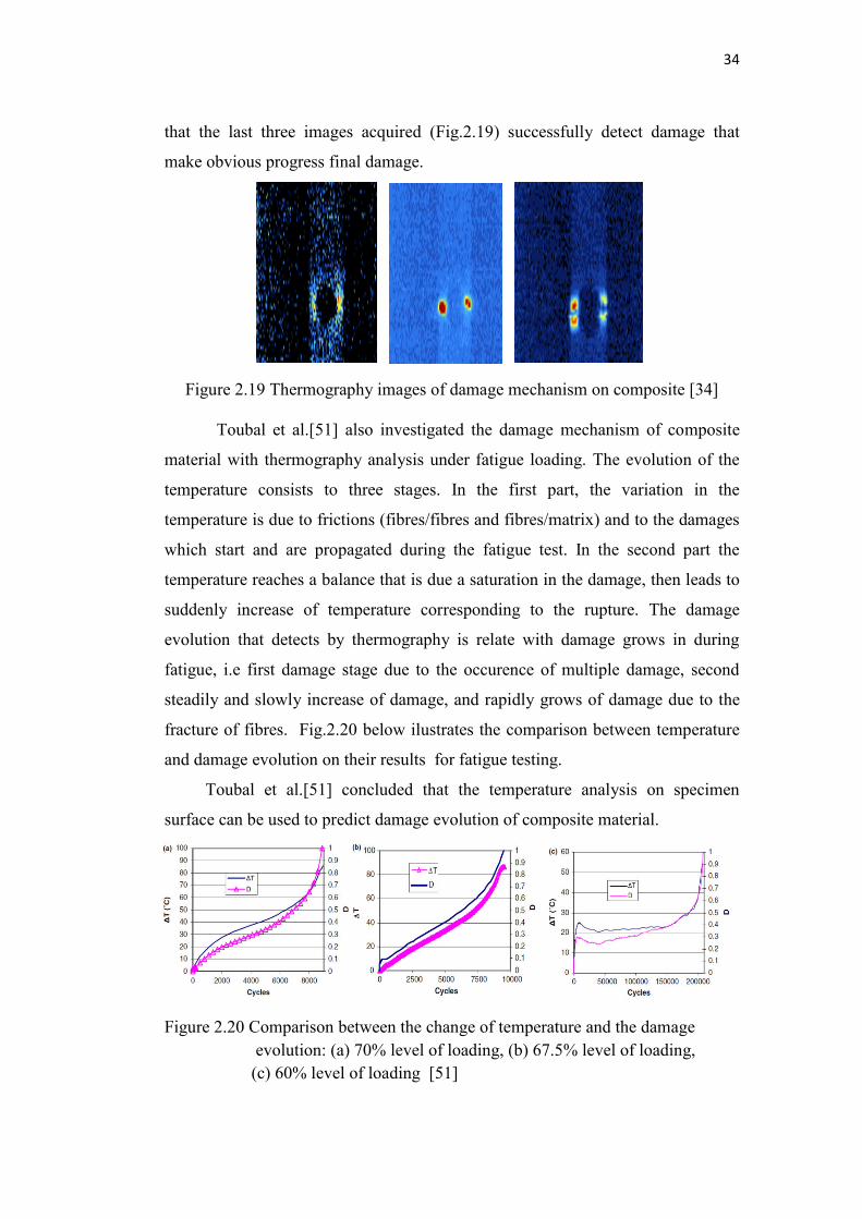
34

that the last three images acquired (Fig.2.19) successfully detect damage that

make obvious progress final damage.

Figure 2.19 Thermography images of damage mechanism on composite [34]

Toubal et al.[51] also investigated the damage mechanism of composite

material with thermography analysis under fatigue loading. The evolution of the

temperature consists to three stages. In the first part, the variation in the

temperature is due to frictions (fibres/fibres and fibres/matrix) and to the damages

which start and are propagated during the fatigue test. In the second part the

temperature reaches a balance that is due a saturation in the damage, then leads to

suddenly increase of temperature corresponding to the rupture. The damage

evolution that detects by thermography is relate with damage grows in during

fatigue, i.e first damage stage due to the occurence of multiple damage, second

steadily and slowly increase of damage, and rapidly grows of damage due to the

fracture of fibres. Fig.2.20 below ilustrates the comparison between temperature

and damage evolution on their results for fatigue testing.

Toubal et al.[51] concluded that the temperature analysis on specimen

surface can be used to predict damage evolution of composite material.

.

Figure 2.20 Comparison between the change of temperature and the damage

evolution: (a) 70% level of loading, (b) 67.5% level of loading,

(c) 60% level of loading [51]

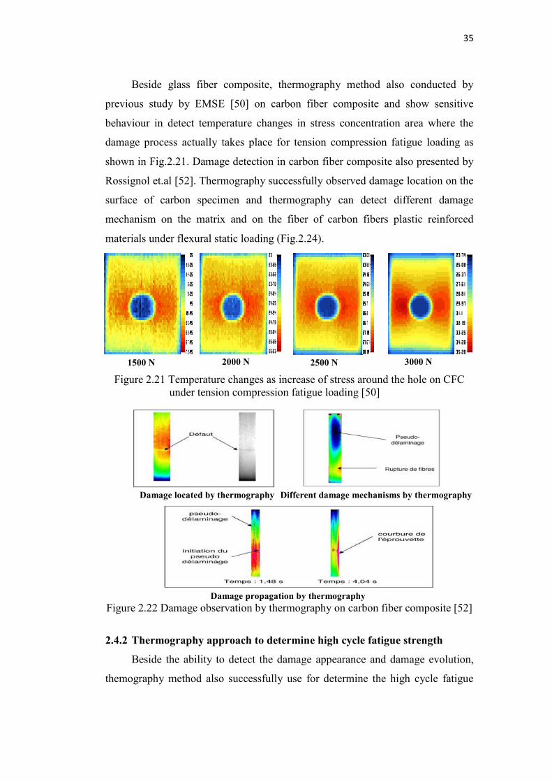
35

Beside glass fiber composite, thermography method also conducted by

previous study by EMSE [50] on carbon fiber composite and show sensitive

behaviour in detect temperature changes in stress concentration area where the

damage process actually takes place for tension compression fatigue loading as

shown in Fig.2.21. Damage detection in carbon fiber composite also presented by

Rossignol et.al [52]. Thermography successfully observed damage location on the

surface of carbon specimen and thermography can detect different damage

mechanism on the matrix and on the fiber of carbon fibers plastic reinforced

materials under flexural static loading (Fig.2.24).

Figure 2.21 Temperature changes as increase of stress around the hole on CFC under tension compression fatigue loading [50]

Figure 2.22 Damage observation by thermography on carbon fiber composite [52]

2.4.2 Thermography approach to determine high cycle fatigue strength

Beside the ability to detect the damage appearance and damage evolution,

themography method also successfully use for determine the high cycle fatigue

Damage located by thermography Different damage mechanisms by thermography

Damage propagation by thermography

1500 N 2000 N 2500 N 3000 N

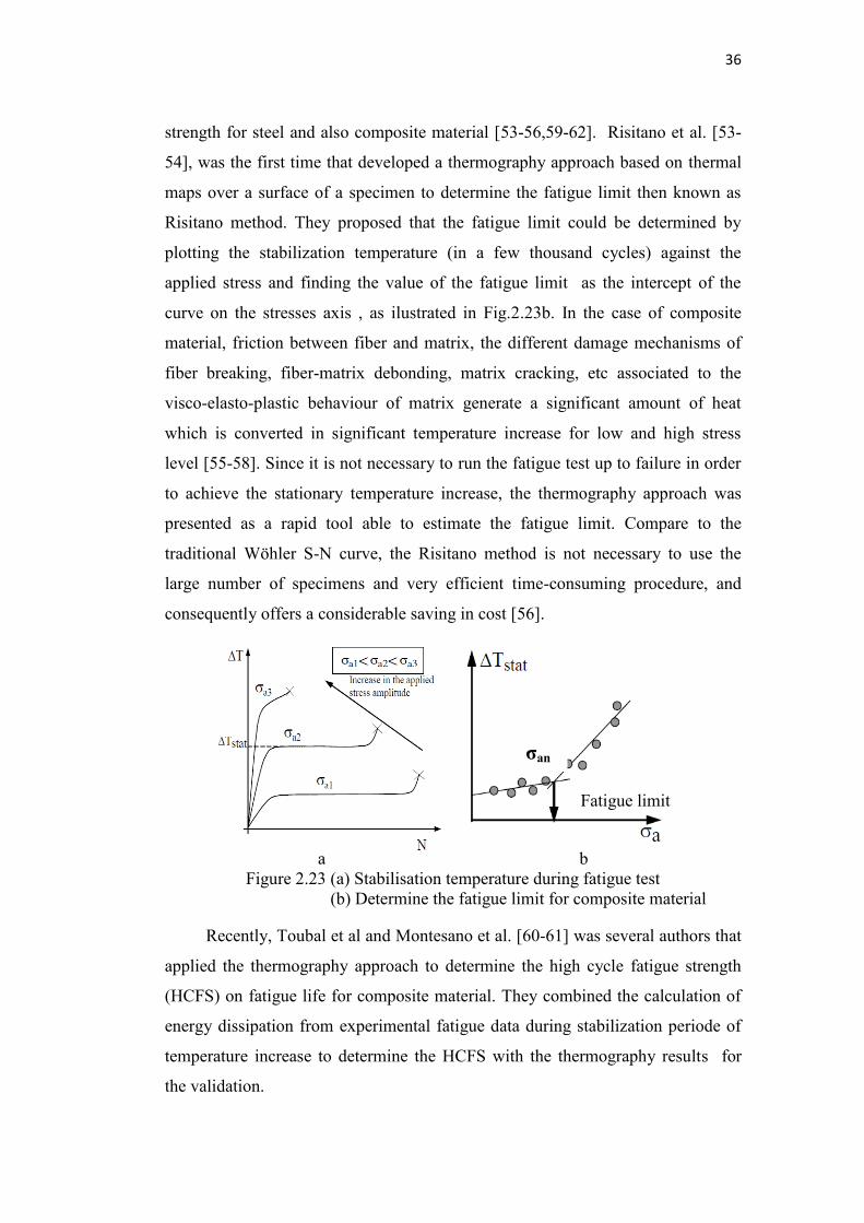
36

strength for steel and also composite material [53-56,59-62]. Risitano et al. [53-

54], was the first time that developed a thermography approach based on thermal

maps over a surface of a specimen to determine the fatigue limit then known as

Risitano method. They proposed that the fatigue limit could be determined by

plotting the stabilization temperature (in a few thousand cycles) against the

applied stress and finding the value of the fatigue limit as the intercept of the

curve on the stresses axis , as ilustrated in Fig.2.23b. In the case of composite

material, friction between fiber and matrix, the different damage mechanisms of

fiber breaking, fiber-matrix debonding, matrix cracking, etc associated to the

visco-elasto-plastic behaviour of matrix generate a significant amount of heat

which is converted in significant temperature increase for low and high stress

level [55-58]. Since it is not necessary to run the fatigue test up to failure in order

to achieve the stationary temperature increase, the thermography approach was

presented as a rapid tool able to estimate the fatigue limit. Compare to the

traditional Wöhler S-N curve, the Risitano method is not necessary to use the

large number of specimens and very efficient time-consuming procedure, and

consequently offers a considerable saving in cost [56].

a b

Figure 2.23 (a) Stabilisation temperature during fatigue test (b) Determine the fatigue limit for composite material

Recently, Toubal et al and Montesano et al. [60-61] was several authors that

applied the thermography approach to determine the high cycle fatigue strength

(HCFS) on fatigue life for composite material. They combined the calculation of

energy dissipation from experimental fatigue data during stabilization periode of

temperature increase to determine the HCFS with the thermography results for

the validation.

Fatigue limit

σan

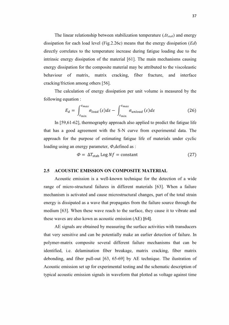
37

The linear relationship between stabilization temperature (Δtstab) and energy

dissipation for each load level (Fig.2.26c) means that the energy dissipation (Ed)

directly correlates to the temperature increase during fatigue loading due to the

intrinsic energy dissipation of the material [61]. The main mechanisms causing

energy dissipation for the composite material may be attributed to the viscoleastic

behaviour of matrix, matrix cracking, fiber fracture, and interface

cracking/friction among others [56].

The calculation of energy dissipation per unit volume is measured by the

following equation : In [59,61-62], thermography approach also applied to predict the fatigue life

that has a good agreement with the S-N curve from experimental data. The

approach for the purpose of estimating fatigue life of materials under cyclic

loading using an energy parameter, Ф,defined as :

Ф

2.5 ACOUSTIC EMISSION ON COMPOSITE MATERIAL

Acoustic emission is a well-known technique for the detection of a wide

range of micro-structural failures in different materials [63]. When a failure

mechanism is activated and cause microstructural changes, part of the total strain

energy is dissipated as a wave that propagates from the failure source through the

medium [63]. When these wave reach to the surface, they cause it to vibrate and

these waves are also kown as acoustic emission (AE) [64].

AE signals are obtained by measuring the surface activities with transducers

that very sensitive and can be potentially make an earlier detection of failure. In

polymer-matrix composite several different failure mechanisms that can be

identified, i.e. delamination fiber breakage, matrix cracking, fiber matrix

debonding, and fiber pull-out [63, 65-69] by AE technique. The ilustration of

Acoustic emission set up for experimental testing and the schematic description of

typical acoustic emission signals in waveform that plotted as voltage against time

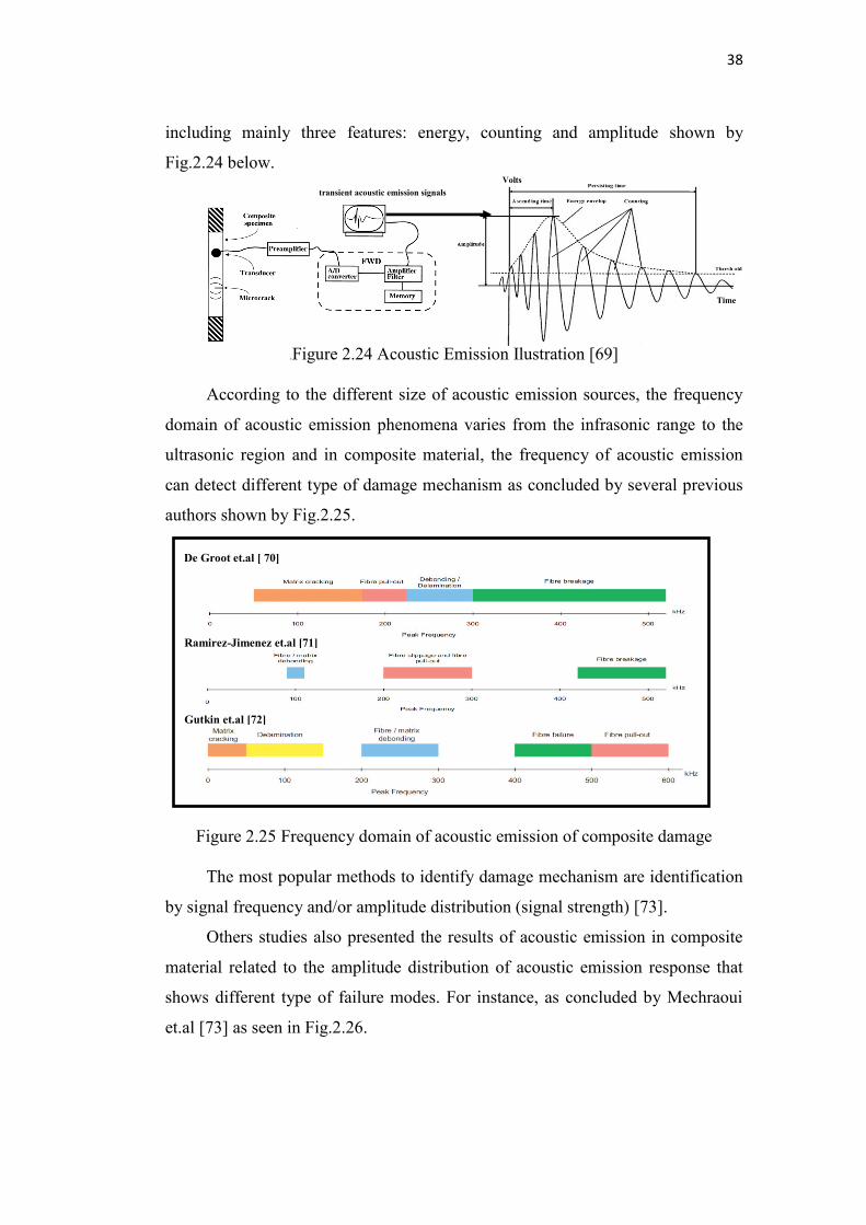
38

including mainly three features: energy, counting and amplitude shown by

Fig.2.24 below.

.Figure 2.24 Acoustic Emission Ilustration [69]

According to the different size of acoustic emission sources, the frequency

domain of acoustic emission phenomena varies from the infrasonic range to the

ultrasonic region and in composite material, the frequency of acoustic emission

can detect different type of damage mechanism as concluded by several previous

authors shown by Fig.2.25.

Figure 2.25 Frequency domain of acoustic emission of composite damage

The most popular methods to identify damage mechanism are identification

by signal frequency and/or amplitude distribution (signal strength) [73].

Others studies also presented the results of acoustic emission in composite

material related to the amplitude distribution of acoustic emission response that

shows different type of failure modes. For instance, as concluded by Mechraoui

et.al [73] as seen in Fig.2.26.

transient acoustic emission signals

De Groot et.al [ 70]

Ramirez-Jimenez et.al [71]

Gutkin et.al [72]

Volts

Time

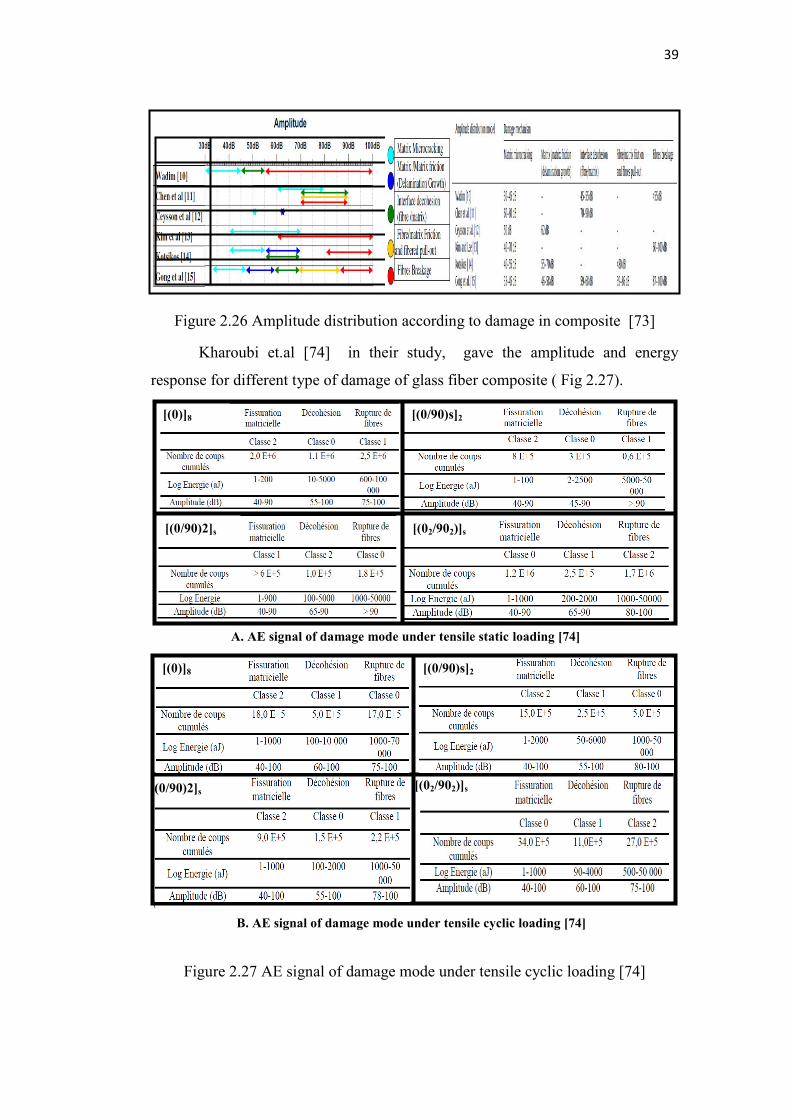
39

Figure 2.26 Amplitude distribution according to damage in composite [73]

Kharoubi et.al [74] in their study, gave the amplitude and energy

response for different type of damage of glass fiber composite ( Fig 2.27).

\

Figure 2.27 AE signal of damage mode under tensile cyclic loading [74]

[(0)]8 [(0/90)s]2

[(0/90)2]s [(02/902)]s

[(0)]8 [(0/90)s]2

[(0/90)2]s [(02/902)]s

B. AE signal of damage mode under tensile cyclic loading [74]

A. AE signal of damage mode under tensile static loading [74]

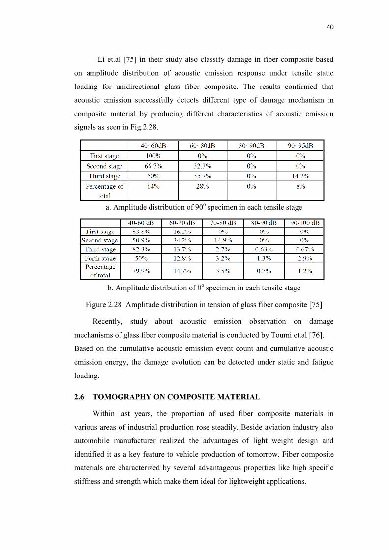
40

Li et.al [75] in their study also classify damage in fiber composite based

on amplitude distribution of acoustic emission response under tensile static

loading for unidirectional glass fiber composite. The results confirmed that

acoustic emission successfully detects different type of damage mechanism in

composite material by producing different characteristics of acoustic emission

signals as seen in Fig.2.28.

a. Amplitude distribution of 90o specimen in each tensile stage

b. Amplitude distribution of 0o specimen in each tensile stage

Figure 2.28 Amplitude distribution in tension of glass fiber composite [75]

Recently, study about acoustic emission observation on damage

mechanisms of glass fiber composite material is conducted by Toumi et.al [76].

Based on the cumulative acoustic emission event count and cumulative acoustic

emission energy, the damage evolution can be detected under static and fatigue

loading.

2.6 TOMOGRAPHY ON COMPOSITE MATERIAL

Within last years, the proportion of used fiber composite materials in

various areas of industrial production rose steadily. Beside aviation industry also

automobile manufacturer realized the advantages of light weight design and

identified it as a key feature to vehicle production of tomorrow. Fiber composite

materials are characterized by several advantageous properties like high specific

stiffness and strength which make them ideal for lightweight applications.

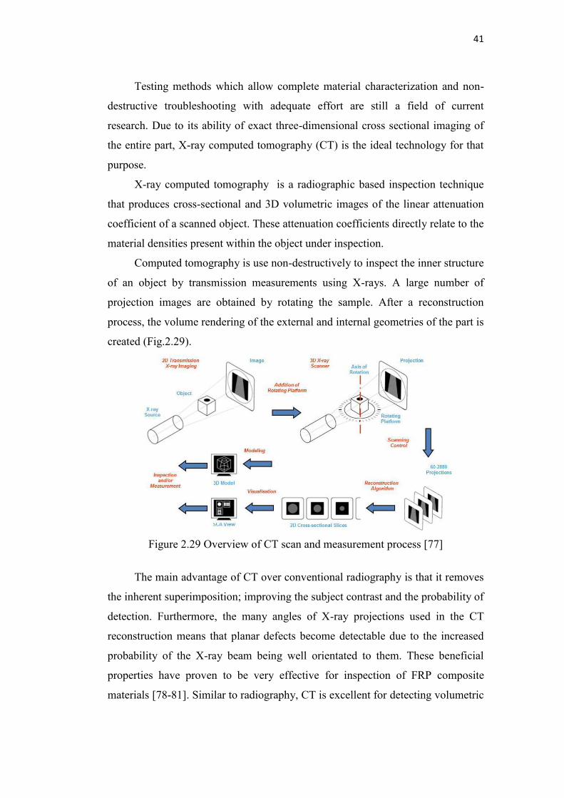
41

Testing methods which allow complete material characterization and non-

destructive troubleshooting with adequate effort are still a field of current

research. Due to its ability of exact three-dimensional cross sectional imaging of

the entire part, X-ray computed tomography (CT) is the ideal technology for that

purpose.

X-ray computed tomography is a radiographic based inspection technique

that produces cross-sectional and 3D volumetric images of the linear attenuation

coefficient of a scanned object. These attenuation coefficients directly relate to the

material densities present within the object under inspection.

Computed tomography is use non-destructively to inspect the inner structure

of an object by transmission measurements using X-rays. A large number of

projection images are obtained by rotating the sample. After a reconstruction

process, the volume rendering of the external and internal geometries of the part is

created (Fig.2.29).

Figure 2.29 Overview of CT scan and measurement process [77]

The main advantage of CT over conventional radiography is that it removes

the inherent superimposition; improving the subject contrast and the probability of

detection. Furthermore, the many angles of X-ray projections used in the CT

reconstruction means that planar defects become detectable due to the increased

probability of the X-ray beam being well orientated to them. These beneficial

properties have proven to be very effective for inspection of FRP composite

materials [78-81]. Similar to radiography, CT is excellent for detecting volumetric

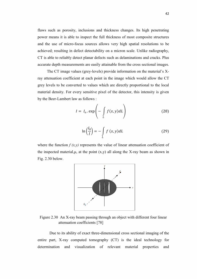
42

flaws such as porosity, inclusions and thickness changes. Its high penetrating

power means it is able to inspect the full thickness of most composite structures

and the use of micro-focus sources allows very high spatial resolutions to be

achieved; resulting in defect detectability on a micron scale. Unlike radiography,

CT is able to reliably detect planar defects such as delaminations and cracks. Plus

accurate depth measurements are easily attainable from the cross sectional images.

The CT image values (grey-levels) provide information on the material’s X-

ray attenuation coefficient at each point in the image which would allow the CT

grey levels to be converted to values which are directly proportional to the local

material density. For every sensitive pixel of the detector, this intensity is given

by the Beer-Lambert law as follows :

where the function f (x,y) represents the value of linear attenuation coefficient of

the inspected material, , at the point (x,y) all along the X-ray beam as shown in

Fig. 2.30 below.

Figure 2.30 An X-ray beam passing through an object with different four linear

attenuation coefficients [78]

Due to its ability of exact three-dimensional cross sectional imaging of the

entire part, X-ray computed tomography (CT) is the ideal technology for

determination and visualization of relevant material properties and

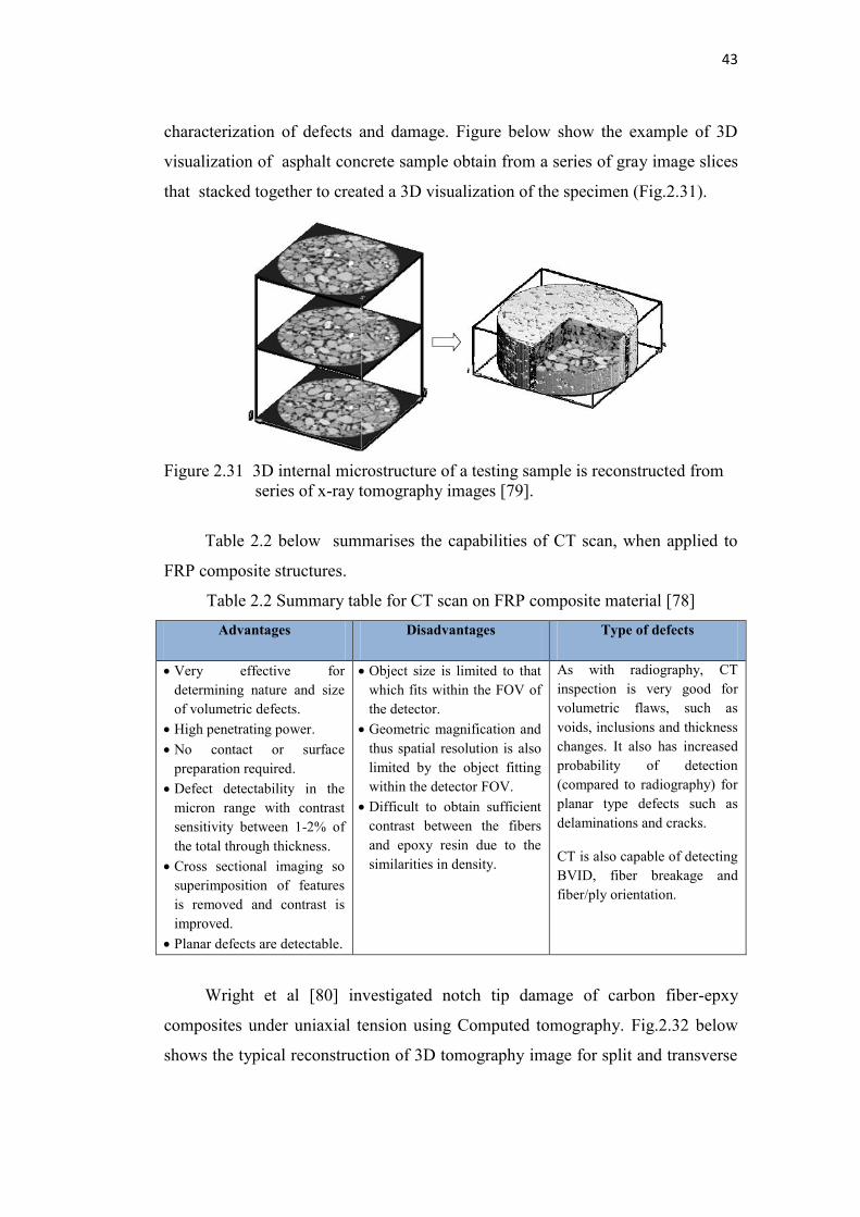
43

characterization of defects and damage. Figure below show the example of 3D

visualization of asphalt concrete sample obtain from a series of gray image slices

that stacked together to created a 3D visualization of the specimen (Fig.2.31).

Figure 2.31 3D internal microstructure of a testing sample is reconstructed from series of x-ray tomography images [79].

Table 2.2 below summarises the capabilities of CT scan, when applied to

FRP composite structures.

Table 2.2 Summary table for CT scan on FRP composite material [78]

Advantages Disadvantages Type of defects

Very effective for

determining nature and size

of volumetric defects.

High penetrating power.

No contact or surface

preparation required.

Defect detectability in the

micron range with contrast

sensitivity between 1-2% of

the total through thickness.

Cross sectional imaging so

superimposition of features

is removed and contrast is

improved.

Planar defects are detectable.

Object size is limited to that

which fits within the FOV of

the detector.

Geometric magnification and

thus spatial resolution is also

limited by the object fitting

within the detector FOV.

Difficult to obtain sufficient

contrast between the fibers

and epoxy resin due to the

similarities in density.

As with radiography, CT

inspection is very good for

volumetric flaws, such as

voids, inclusions and thickness

changes. It also has increased

probability of detection

(compared to radiography) for

planar type defects such as

delaminations and cracks.

CT is also capable of detecting

BVID, fiber breakage and

fiber/ply orientation.

Wright et al [80] investigated notch tip damage of carbon fiber-epxy

composites under uniaxial tension using Computed tomography. Fig.2.32 below

shows the typical reconstruction of 3D tomography image for split and transverse

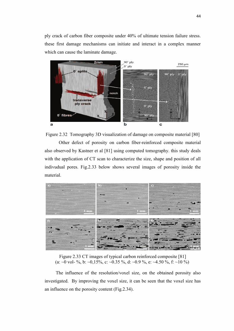
44

ply crack of carbon fiber composite under 40% of ultimate tension failure stress.

these first damage mechanisms can initiate and interact in a complex manner

which can cause the laminate damage.

Figure 2.32 Tomography 3D visualization of damage on composite material [80]

Other defect of porosity on carbon fiber-reinforced composite material

also observed by Kastner et al [81] using computed tomography. this study deals

with the application of CT scan to characterize the size, shape and position of all

indivudual pores. Fig.2.33 below shows several images of porosity inside the

material.

Figure 2.33 CT images of typical carbon reinforced composite [81] (a: ~0 vol- %, b: ~0,15%, c: ~0.35 %, d: ~0.9 %, e: ~4.50 %, f: ~10 %) The influence of the resolution/voxel size, on the obtained porosity also

investigated. By improving the voxel size, it can be seen that the voxel size has

an influence on the porosity content (Fig.2.34).

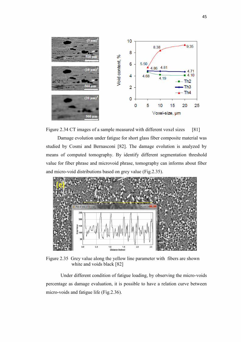
45

Figure 2.34 CT images of a sample measured with different voxel sizes [81]

Damage evolution under fatigue for short glass fiber composite material was

studied by Cosmi and Bernasconi [82]. The damage evolution is analyzed by

means of computed tomography. By identify different segmentation threshold

value for fiber phrase and microvoid phrase, tomography can informs about fiber

and micro-void distributions based on grey value (Fig.2.35).

Figure 2.35 Grey value along the yellow line parameter with fibers are shown white and voids black [82] Under different condition of fatigue loading, by observing the micro-voids

percentage as damage evaluation, it is possible to have a relation curve between

micro-voids and fatigue life (Fig.2.36).

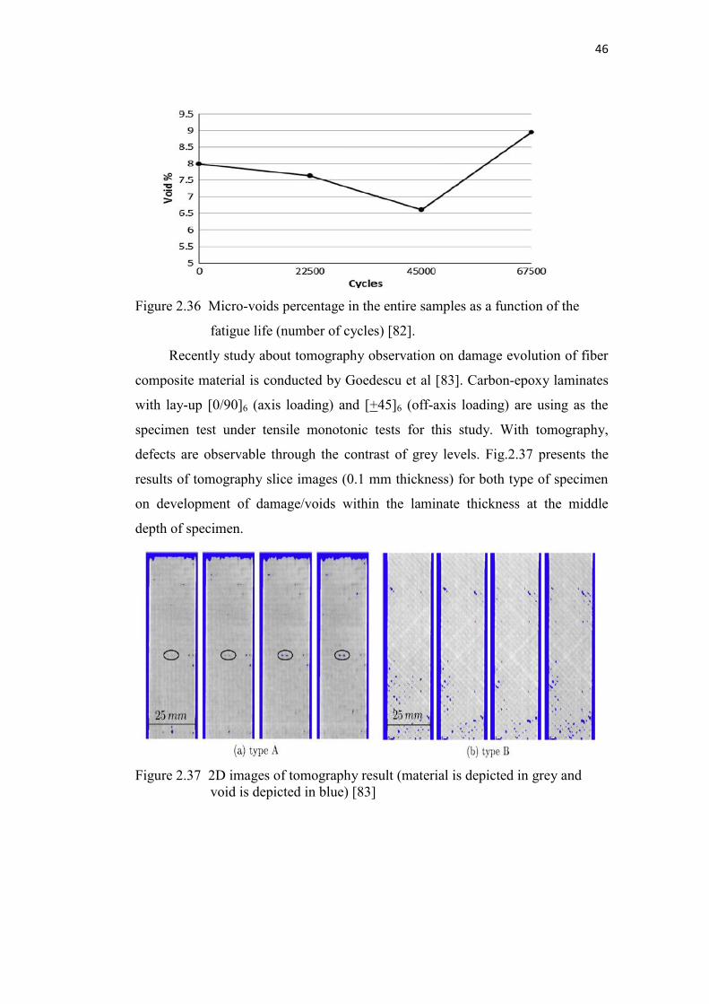
46

Figure 2.36 Micro-voids percentage in the entire samples as a function of the

fatigue life (number of cycles) [82].

Recently study about tomography observation on damage evolution of fiber

composite material is conducted by Goedescu et al [83]. Carbon-epoxy laminates

with lay-up [0/90]6 (axis loading) and [+45]6 (off-axis loading) are using as the

specimen test under tensile monotonic tests for this study. With tomography,

defects are observable through the contrast of grey levels. Fig.2.37 presents the

results of tomography slice images (0.1 mm thickness) for both type of specimen

on development of damage/voids within the laminate thickness at the middle

depth of specimen.

Figure 2.37 2D images of tomography result (material is depicted in grey and void is depicted in blue) [83]

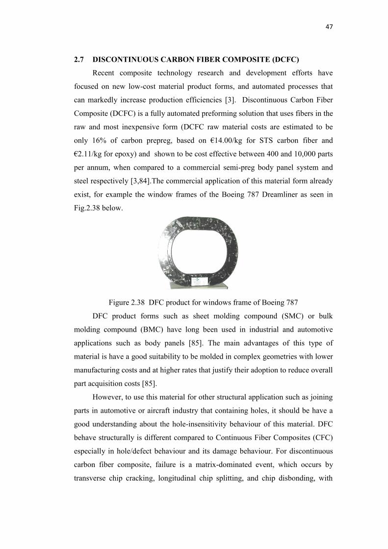
47

2.7 DISCONTINUOUS CARBON FIBER COMPOSITE (DCFC)

Recent composite technology research and development efforts have

focused on new low-cost material product forms, and automated processes that

can markedly increase production efficiencies [3]. Discontinuous Carbon Fiber

Composite (DCFC) is a fully automated preforming solution that uses fibers in the

raw and most inexpensive form (DCFC raw material costs are estimated to be

only 16% of carbon prepreg, based on €14.00/kg for STS carbon fiber and

€2.11/kg for epoxy) and shown to be cost effective between 400 and 10,000 parts

per annum, when compared to a commercial semi-preg body panel system and

steel respectively [3,84].The commercial application of this material form already

exist, for example the window frames of the Boeing 787 Dreamliner as seen in

Fig.2.38 below.

Figure 2.38 DFC product for windows frame of Boeing 787

DFC product forms such as sheet molding compound (SMC) or bulk

molding compound (BMC) have long been used in industrial and automotive

applications such as body panels [85]. The main advantages of this type of

material is have a good suitability to be molded in complex geometries with lower

manufacturing costs and at higher rates that justify their adoption to reduce overall

part acquisition costs [85].

However, to use this material for other structural application such as joining

parts in automotive or aircraft industry that containing holes, it should be have a

good understanding about the hole-insensitivity behaviour of this material. DFC

behave structurally is different compared to Continuous Fiber Composites (CFC)

especially in hole/defect behaviour and its damage behaviour. For discontinuous

carbon fiber composite, failure is a matrix-dominated event, which occurs by

transverse chip cracking, longitudinal chip splitting, and chip disbonding, with

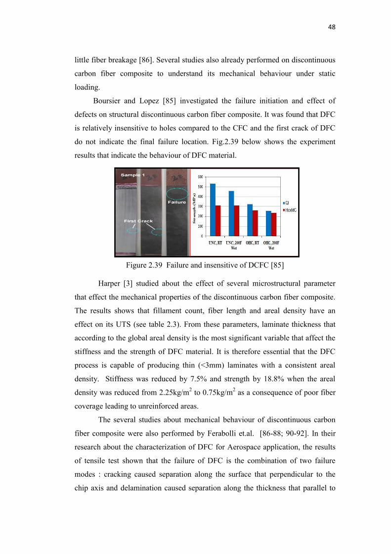
48

little fiber breakage [86]. Several studies also already performed on discontinuous

carbon fiber composite to understand its mechanical behaviour under static

loading.

Boursier and Lopez [85] investigated the failure initiation and effect of

defects on structural discontinuous carbon fiber composite. It was found that DFC

is relatively insensitive to holes compared to the CFC and the first crack of DFC

do not indicate the final failure location. Fig.2.39 below shows the experiment

results that indicate the behaviour of DFC material.

Figure 2.39 Failure and insensitive of DCFC [85]

Harper [3] studied about the effect of several microstructural parameter

that effect the mechanical properties of the discontinuous carbon fiber composite.

The results shows that fillament count, fiber length and areal density have an

effect on its UTS (see table 2.3). From these parameters, laminate thickness that

according to the global areal density is the most significant variable that affect the

stiffness and the strength of DFC material. It is therefore essential that the DFC

process is capable of producing thin (<3mm) laminates with a consistent areal

density. Stiffness was reduced by 7.5% and strength by 18.8% when the areal

density was reduced from 2.25kg/m2 to 0.75kg/m2 as a consequence of poor fiber

coverage leading to unreinforced areas.

The several studies about mechanical behaviour of discontinuous carbon

fiber composite were also performed by Ferabolli et.al. [86-88; 90-92]. In their

research about the characterization of DFC for Aerospace application, the results

of tensile test shown that the failure of DFC is the combination of two failure

modes : cracking caused separation along the surface that perpendicular to the

chip axis and delamination caused separation along the thickness that parallel to

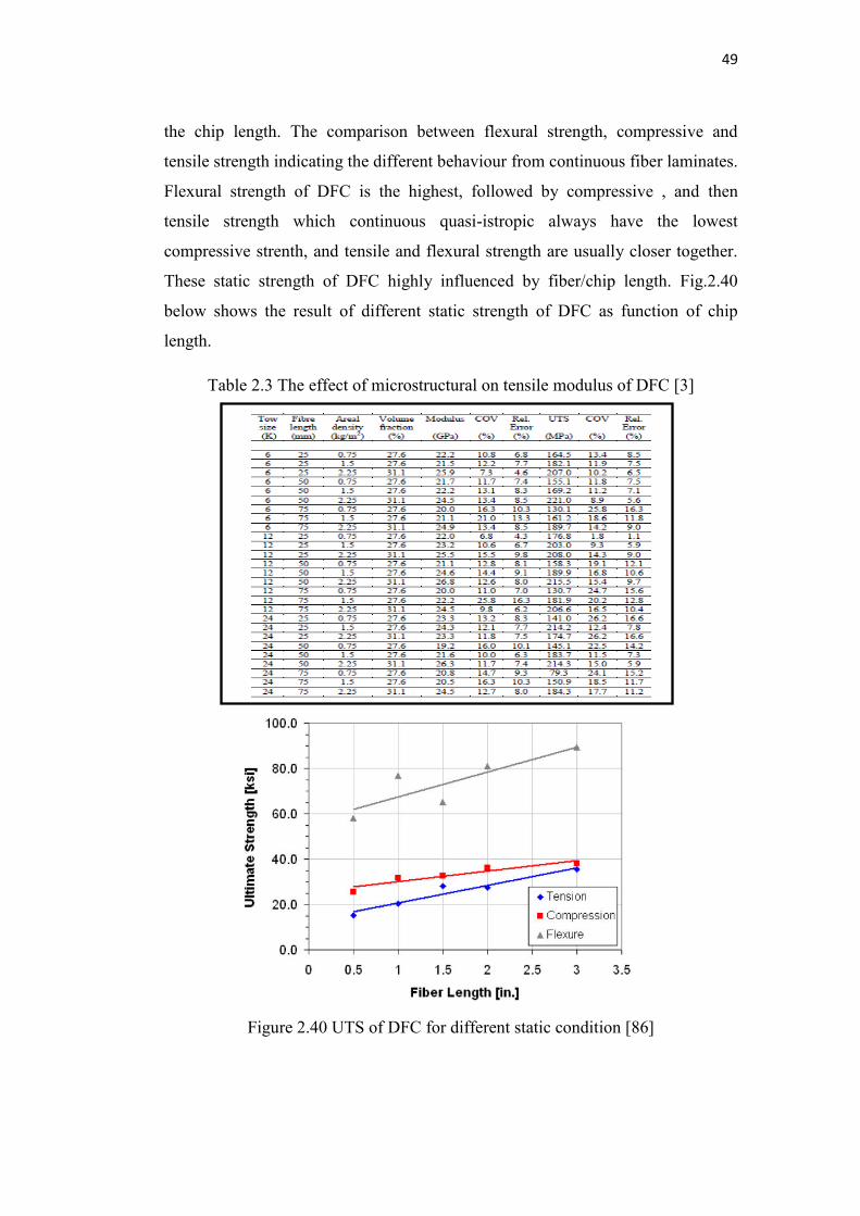
49

the chip length. The comparison between flexural strength, compressive and

tensile strength indicating the different behaviour from continuous fiber laminates.

Flexural strength of DFC is the highest, followed by compressive , and then

tensile strength which continuous quasi-istropic always have the lowest

compressive strenth, and tensile and flexural strength are usually closer together.

These static strength of DFC highly influenced by fiber/chip length. Fig.2.40

below shows the result of different static strength of DFC as function of chip

length.

Table 2.3 The effect of microstructural on tensile modulus of DFC [3]

Figure 2.40 UTS of DFC for different static condition [86]

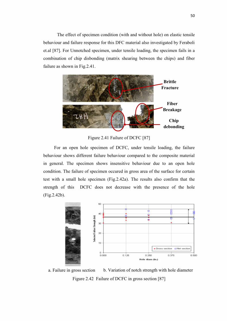
50

The effect of specimen condition (with and without hole) on elastic tensile

behaviour and failure response for this DFC material also investigated by Feraboli

et.al [87]. For Unnotched specimen, under tensile loading, the specimen fails in a

combination of chip disbonding (matrix shearing between the chips) and fiber

failure as shown in Fig.2.41.

Figure 2.41 Failure of DCFC [87]

For an open hole specimen of DCFC, under tensile loading, the failure

behaviour shows different failure behaviour compared to the composite material

in general. The specimen shows insensitive behaviour due to an open hole

condition. The failure of specimen occured in gross area of the surface for certain

test with a small hole specimen (Fig.2.42a). The results also confirm that the

strength of this DCFC does not decrease with the presence of the hole

(Fig.2.42b).

Figure 2.42 Failure of DCFC in gross section [87]

Brittle Fracture

Fiber Breakage

Chip debonding

a. Failure in gross section b. Variation of notch strength with hole diameter

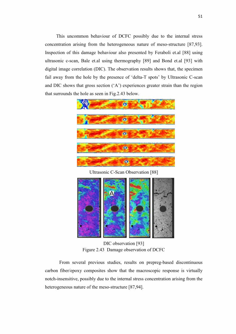
51

This uncommon behaviour of DCFC possibly due to the internal stress

concentration arising from the heterogeneous nature of meso-structure [87,93].

Inspection of this damage behaviour also presented by Feraboli et.al [88] using

ultrasonic c-scan, Bale et.al using thermography [89] and Bond et.al [93] with

digital image correlation (DIC). The observation results shows that, the specimen

fail away from the hole by the presence of ‘delta-T spots’ by Ultrasonic C-scan

and DIC shows that gross section (‘A’) experiences greater strain than the region

that surrounds the hole as seen in Fig.2.43 below.

Ultrasonic C-Scan Observation [88]

DIC observation [93]

Figure 2.43 Damage observation of DCFC

From several previous studies, results on prepreg-based discontinuous

carbon fiber/epoxy composites show that the macroscopic response is virtually

notch-insensitive, possibly due to the internal stress concentration arising from the

heterogeneous nature of the meso-structure [87,94].

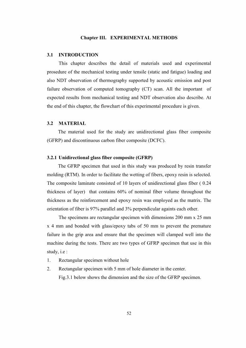
52

Chapter III. EXPERIMENTAL METHODS

3.1 INTRODUCTION

This chapter describes the detail of materials used and experimental

prosedure of the mechanical testing under tensile (static and fatigue) loading and

also NDT observation of thermography supported by acoustic emission and post

failure observation of computed tomography (CT) scan. All the important of

expected results from mechanical testing and NDT observation also describe. At

the end of this chapter, the flowchart of this experimental procedure is given.

3.2 MATERIAL

The material used for the study are unidirectional glass fiber composite

(GFRP) and discontinuous carbon fiber composite (DCFC).

3.2.1 Unidirectional glass fiber composite (GFRP)

The GFRP specimen that used in this study was produced by resin transfer

molding (RTM). In order to facilitate the wetting of fibers, epoxy resin is selected.

The composite laminate consisted of 10 layers of unidirectional glass fiber ( 0.24

thickness of layer) that contains 60% of nominal fiber volume throughout the

thickness as the reinforcement and epoxy resin was employed as the matrix. The

orientation of fiber is 97% parallel and 3% perpendicular againts each other.

The specimens are rectangular specimen with dimensions 200 mm x 25 mm

x 4 mm and bonded with glass/epoxy tabs of 50 mm to prevent the premature

failure in the grip area and ensure that the specimen will clamped well into the

machine during the tests. There are two types of GFRP specimen that use in this

study, i.e :

1. Rectangular specimen without hole

2. Rectangular specimen with 5 mm of hole diameter in the center.

Fig.3.1 below shows the dimension and the size of the GFRP specimen.

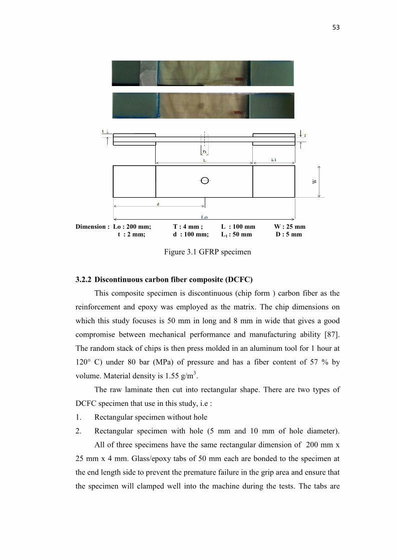
53

Dimension : Lo : 200 mm; T : 4 mm ; L : 100 mm W : 25 mm t : 2 mm; d : 100 mm; L1 : 50 mm D : 5 mm

Figure 3.1 GFRP specimen

3.2.2 Discontinuous carbon fiber composite (DCFC)

This composite specimen is discontinuous (chip form ) carbon fiber as the

reinforcement and epoxy was employed as the matrix. The chip dimensions on

which this study focuses is 50 mm in long and 8 mm in wide that gives a good

compromise between mechanical performance and manufacturing ability [87].

The random stack of chips is then press molded in an aluminum tool for 1 hour at

120° C) under 80 bar (MPa) of pressure and has a fiber content of 57 % by

volume. Material density is 1.55 g/m3.

The raw laminate then cut into rectangular shape. There are two types of

DCFC specimen that use in this study, i.e :

1. Rectangular specimen without hole

2. Rectangular specimen with hole (5 mm and 10 mm of hole diameter).

All of three specimens have the same rectangular dimension of 200 mm x

25 mm x 4 mm. Glass/epoxy tabs of 50 mm each are bonded to the specimen at

the end length side to prevent the premature failure in the grip area and ensure that

the specimen will clamped well into the machine during the tests. The tabs are

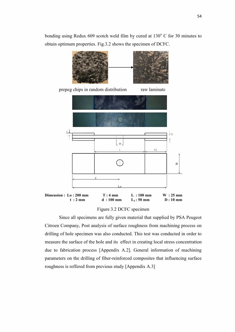
54

bonding using Redux 609 scotch weld film by cured at 130o C for 30 minutes to

obtain optimum properties. Fig.3.2 shows the specimen of DCFC.

Dimension : Lo : 200 mm T : 4 mm L : 100 mm W : 25 mm t : 2 mm d : 100 mm L1 : 50 mm D : 10 mm

Figure 3.2 DCFC specimen

Since all specimens are fully given material that supplied by PSA Peugeot

Citroen Company, Post analysis of surface roughness from machining process on

drilling of hole specimen was also conducted. This test was conducted in order to

measure the surface of the hole and its effect in creating local stress concentration

due to fabrication process [Appendix A.2]. General information of machining

parameters on the drilling of fiber-reinforced composites that influencing surface

roughness is reffered from previous study [Appendix A.3]

prepeg chips in random distribution raw laminate

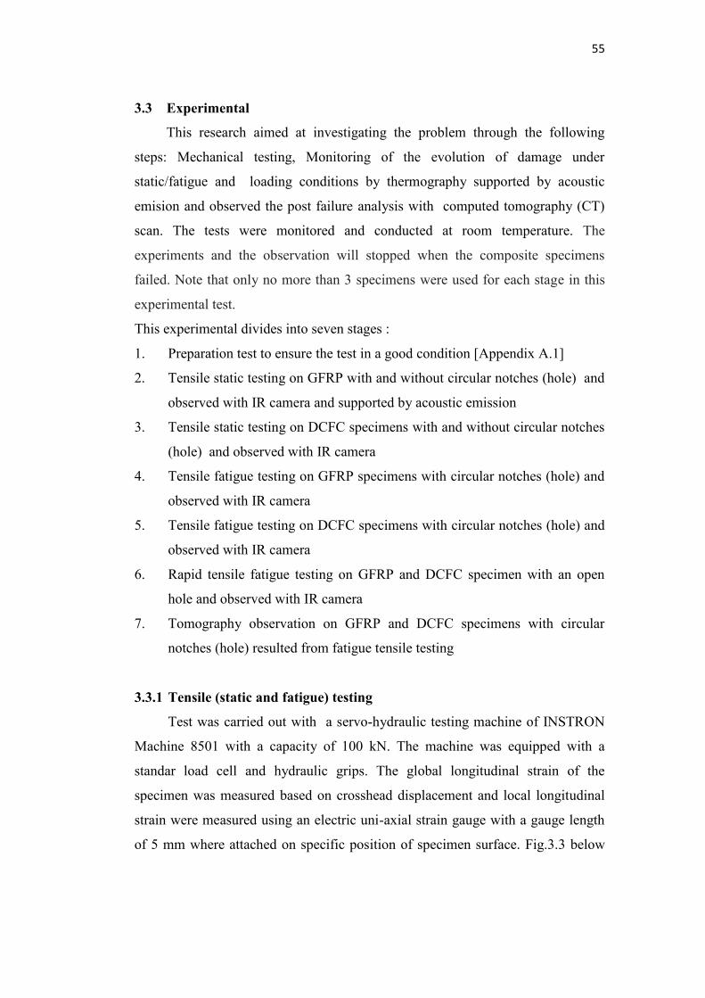
55

3.3 Experimental

This research aimed at investigating the problem through the following

steps: Mechanical testing, Monitoring of the evolution of damage under

static/fatigue and loading conditions by thermography supported by acoustic

emision and observed the post failure analysis with computed tomography (CT)

scan. The tests were monitored and conducted at room temperature. The

experiments and the observation will stopped when the composite specimens

failed. Note that only no more than 3 specimens were used for each stage in this

experimental test.

This experimental divides into seven stages :

1. Preparation test to ensure the test in a good condition [Appendix A.1]

2. Tensile static testing on GFRP with and without circular notches (hole) and

observed with IR camera and supported by acoustic emission

3. Tensile static testing on DCFC specimens with and without circular notches

(hole) and observed with IR camera

4. Tensile fatigue testing on GFRP specimens with circular notches (hole) and

observed with IR camera

5. Tensile fatigue testing on DCFC specimens with circular notches (hole) and

observed with IR camera

6. Rapid tensile fatigue testing on GFRP and DCFC specimen with an open

hole and observed with IR camera

7. Tomography observation on GFRP and DCFC specimens with circular

notches (hole) resulted from fatigue tensile testing

3.3.1 Tensile (static and fatigue) testing

Test was carried out with a servo-hydraulic testing machine of INSTRON

Machine 8501 with a capacity of 100 kN. The machine was equipped with a

standar load cell and hydraulic grips. The global longitudinal strain of the

specimen was measured based on crosshead displacement and local longitudinal

strain were measured using an electric uni-axial strain gauge with a gauge length

of 5 mm where attached on specific position of specimen surface. Fig.3.3 below

56

shows the experiment condition. All tests were done following the ASTM D 5766

standard test method.

Figure 3.3 INSTRON Machine and IR camera

Either static or fatigue, specimens were aligned and mounted first in the

lower and afterwards in the upper grips of the test station. Previously, strain gauge

already installed on the surface of the specimen. After mounting the specimens,

any loading due to the gripping was minimized through Instron controller panel.

A unit of computer with an external data acquisition (Labview software) was used

to record all the test results such as load, strain and displacement. During the

recording, all the data stored in a computer hard disk. Then, the tests was

considered to begin. Static tensile tests were performed under a constant cross-

head speed of 1 mm/min. Fatigue tests were performed under load control, at a

stress ratio, R, equal to 0.1, i.e., tension tension loading and constant 3 Hz of

frequency (ASTM D3479). Various maximum stresses were used for the fatigue

tests. The test specimens were allowed to cycle until failure occurred or until a

predetermined number of cycles was reached. Moreover, rapid test of fatigue

loading with same parameter also conducted to determine the high cycle fatigue

strength and fatigue life utilizing IR camera that referred to the Risitano's method.

This rapid fatigue test was used one specimen for each test of maximum stress

until certain cycle of 10000 cycles. Once this 10000 cycles are reached, the test

was stopped, then continue with the next maximum stress.

Specimen

Hydraulic Grip

IR Camera

57

3.3.2 NDT Thermography

For follow the temperature changes on the specimen surface, an infra-red

camera of FLIR A325sc was used for the tests. Control of the camera and data

recording are done with the FLIR R&D software. The FLIR R&D software is able

to measure temperature change in various shape and dimensions such as spots,

lines, and area as well as of using several various palette of colours and shades.

The camera resolution is 320 x 240 pixels with detector type of uncooled

microbolometer. Camera spectral range is 7.5 to 13 µm, whereas the temperature

range is from -20°C to +120°C with accuracy + 2°C or + 2% of reading. The

camera is provided with the automatic correction of emissivity and atmospheric

transmission based on distance, atmospheric and relative humidity. IR camera was

placed approximately 30 cm of fix distance in front of the specimen surface;

therefore, it was possible to obtain full-field thermal maps of the specimens during

the tests. This thermography observation did not use an externally applied heat

source. In this case, the thermal images acquisition were set at 30 Hz.

3.3.3 NDT Acoustic Emission

During the tensile tests, Acoustic emission was continuously monitored by

using a Mistras monitoring system. AE measurements were achieved by using two

transducers which coupled on the surface of the samples with silicon grease. The

transducers were held in place with a clamp mechanical device. The amplitude

distribution covers the range 0–100 dB. The nominal distance between the sensors

was around 60 mm. After the installation of the transducers, a pencil lead break

procedure was used to simulate AE signals in the calibration of each test.

Furthermore each waveform was digitized and stored. After storage and before

processing the signals were subjected to a linear location procedure to determine

the location of AE signal source. In the analysis of AE results, only events located

between the sensors were used. The acoustic emission analysis is performed by

the NOESIS software in particular to have the parameter value of energy and

amplitude associated with damage appearance. The illustration of the

experimental condition using acoustic emission system as seen in Fig.3.4 below.

58

Figure 3.4 Acoustic Emission set up

3.3.4 NDT Tomography

After certain cycles of tensile fatigue loading, the tests were stopped and

observed the specimen under CT-Scan. This observation using two condition, i.e :

1. GFRP 0o specimen under tensile fatigue condition with σmax : 150 MPa until

500 cycles without macro damage.

2. GFRP 0o specimen under tensile fatigue condition with σmax : 150 MPa until

1500 cycles without macro damage.

3. DCFC specimen under tensile fatigue condition with σmax : 250 MPa until

3100 cycles without macro damage.

4. DCFC specimen under tensile fatigue condition with σmax : 250 MPa until

200 cycles without macro damage.

The specimen for each condition mounted facing each other. CT-scan

machine is connected to a computer using a software for visualization the rotating

observation and also a software of image post processing to have images

sequences during the test. The turn table will rotating 360o for around 1 hour. All

images of CT-scan then analyze based on image pixel and grey value using

Image-J software. Fig.3.5 shows the CT-scan machine and the experimental

description.

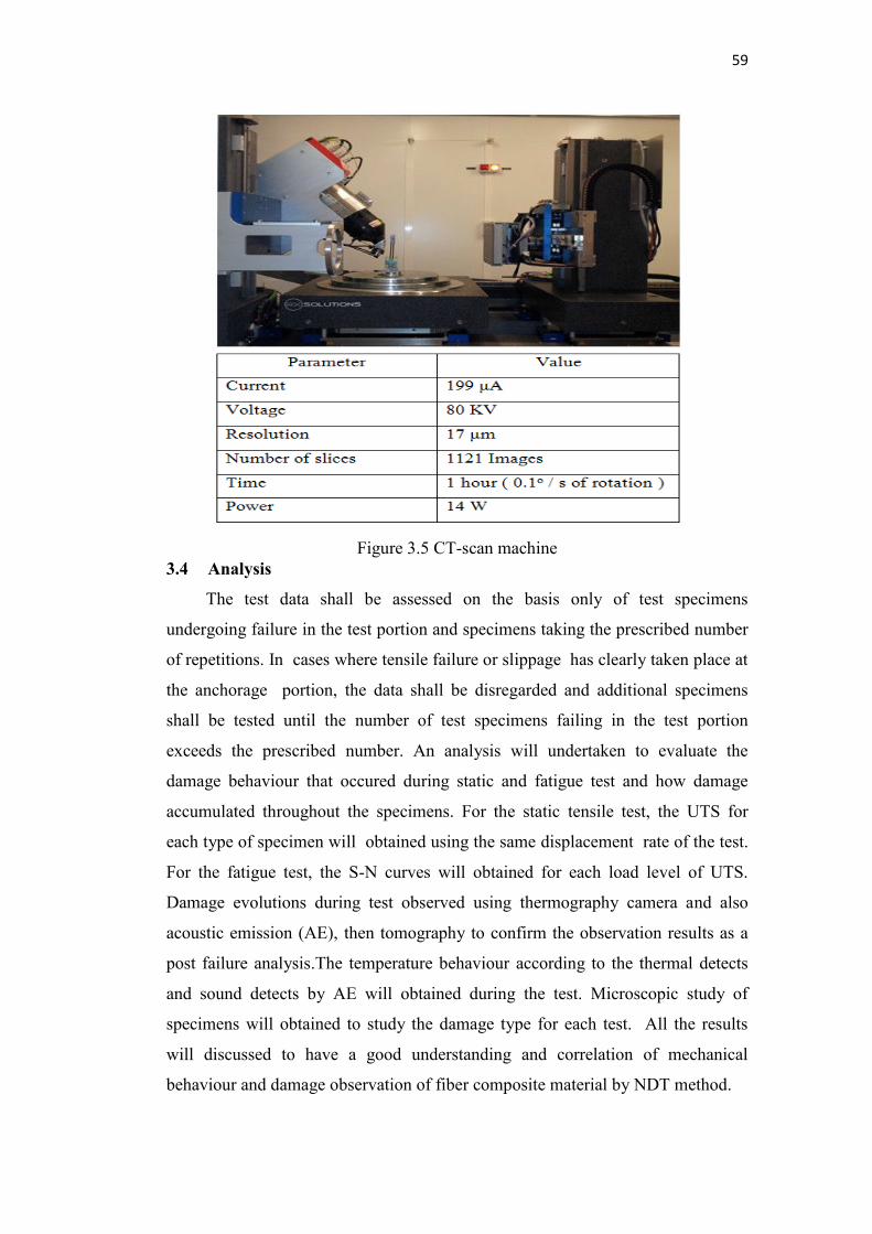
59

Figure 3.5 CT-scan machine

3.4 Analysis

The test data shall be assessed on the basis only of test specimens

undergoing failure in the test portion and specimens taking the prescribed number

of repetitions. In cases where tensile failure or slippage has clearly taken place at

the anchorage portion, the data shall be disregarded and additional specimens

shall be tested until the number of test specimens failing in the test portion

exceeds the prescribed number. An analysis will undertaken to evaluate the

damage behaviour that occured during static and fatigue test and how damage

accumulated throughout the specimens. For the static tensile test, the UTS for

each type of specimen will obtained using the same displacement rate of the test.

For the fatigue test, the S-N curves will obtained for each load level of UTS.

Damage evolutions during test observed using thermography camera and also

acoustic emission (AE), then tomography to confirm the observation results as a

post failure analysis.The temperature behaviour according to the thermal detects

and sound detects by AE will obtained during the test. Microscopic study of

specimens will obtained to study the damage type for each test. All the results

will discussed to have a good understanding and correlation of mechanical

behaviour and damage observation of fiber composite material by NDT method.

60

Some expected results are :

1. Mechanical testing of tensile (static and fatigue) loading :

Tensile Curve.

Tensile curve shows the relationship between the load and the cross head

displacement. The Stress-strain curve also can be obtained fom tensile tests

by dividing the measured load by average cross section of the specimens

and the cross-head displacement by nominal gage length of the specimens.

Elastic Modulus, E will determined by linear interpolation of the stress-

strain curves. The same curve also can be obtained using the local strain

results from strain gages

S-N Curve.

The S-N curve shows the relationship between the maximum repeated

stress, the stress range or the stress amplitude and the number of repetitions.

When some test results come at the same point in the S-N diagram, the

number of data shall be noted. Right-facing arrows shall be used to indicate

that the test specimen did not fracture at that number of repetitions

E/Eo - n/Nf curve.

The E/Eo - n/Nf curve shows the stiffness degradation during the test until

failure. This curve is used to create damage evolution curve during the

fatigue test (D - n/Nf curve)

Ed - load level curve

The Ed - load level curve shows the energy dissipation for a cycle in

stabilization periode for each maximum stress of rapid fatigue test. This

curve is created to determine the high cycle fatigue strength (HCFS) based

on tensile fatigue test

2. NDT thermography observation :

ΔT - Time curve.

This curve shows the variation of temperature profile on obervation area of

specimen surface during the tensile static test until catastrophic failure or

rupture. This temperature variation is resulted by ΔT = T - To , swith T is the

temperature surface at t time and To the initial temperature surface at t = 0.

This curve also compared with strain result from tensile static test results to

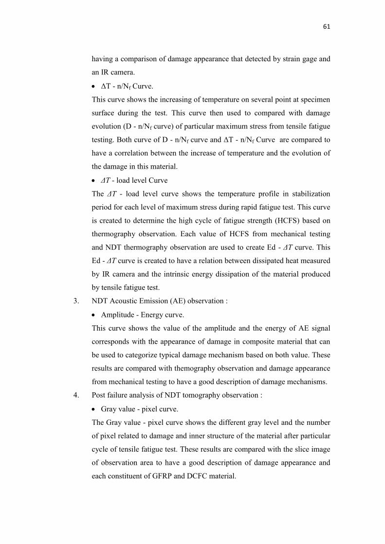
61

having a comparison of damage appearance that detected by strain gage and

an IR camera.

ΔT - n/Nf Curve.

This curve shows the increasing of temperature on several point at specimen

surface during the test. This curve then used to compared with damage

evolution (D - n/Nf curve) of particular maximum stress from tensile fatigue

testing. Both curve of D - n/Nf curve and ΔT - n/Nf Curve are compared to

have a correlation between the increase of temperature and the evolution of

the damage in this material.

ΔT - load level Curve

The ΔT - load level curve shows the temperature profile in stabilization

period for each level of maximum stress during rapid fatigue test. This curve

is created to determine the high cycle of fatigue strength (HCFS) based on

thermography observation. Each value of HCFS from mechanical testing

and NDT thermography observation are used to create Ed - ΔT curve. This

Ed - ΔT curve is created to have a relation between dissipated heat measured

by IR camera and the intrinsic energy dissipation of the material produced

by tensile fatigue test.

3. NDT Acoustic Emission (AE) observation :

Amplitude - Energy curve.

This curve shows the value of the amplitude and the energy of AE signal

corresponds with the appearance of damage in composite material that can

be used to categorize typical damage mechanism based on both value. These

results are compared with themography observation and damage appearance

from mechanical testing to have a good description of damage mechanisms.

4. Post failure analysis of NDT tomography observation :

Gray value - pixel curve.

The Gray value - pixel curve shows the different gray level and the number

of pixel related to damage and inner structure of the material after particular

cycle of tensile fatigue test. These results are compared with the slice image

of observation area to have a good description of damage appearance and

each constituent of GFRP and DCFC material.

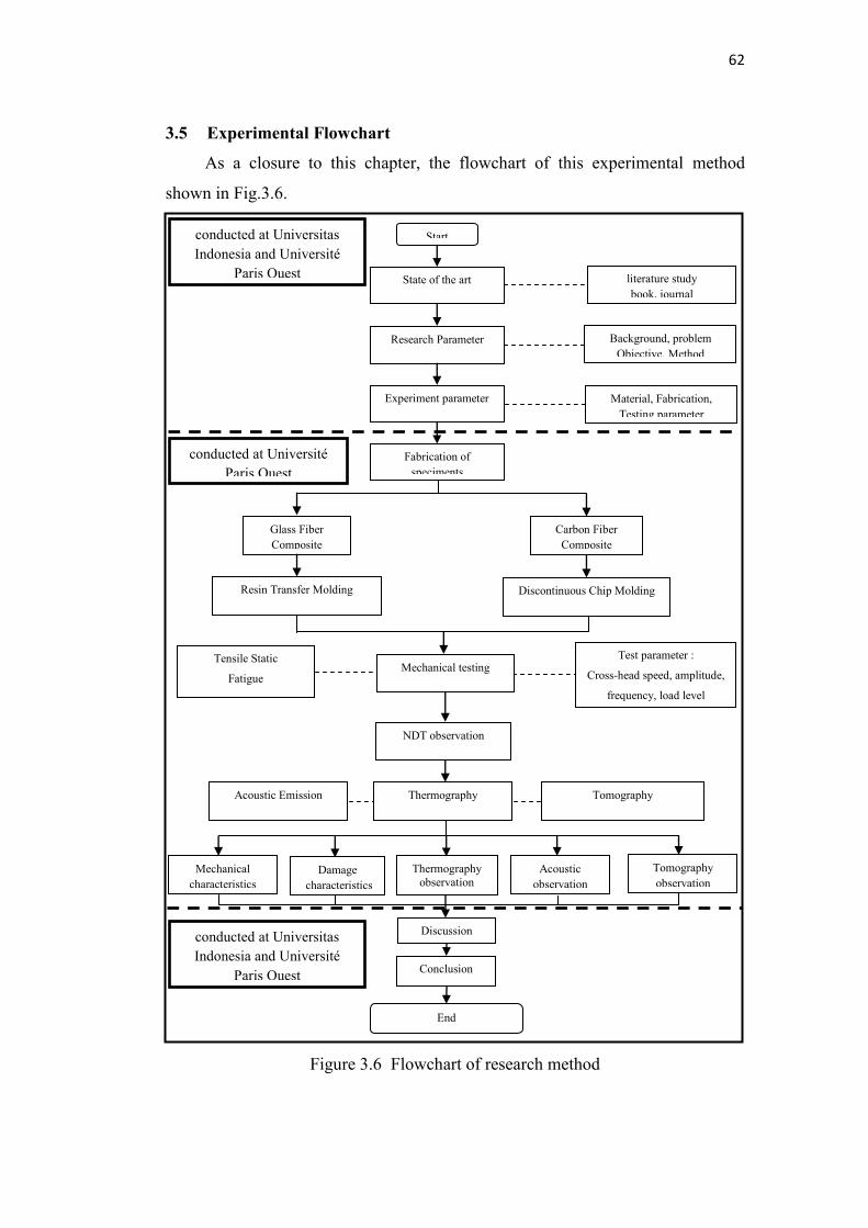
62

3.5 Experimental Flowchart

As a closure to this chapter, the flowchart of this experimental method

shown in Fig.3.6.

Figure 3.6 Flowchart of research method

Discontinuous Chip Molding

Carbon Fiber

Composite

Glass Fiber

Composite

Resin Transfer Molding

Tensile Static

Fatigue

Test parameter :

Cross-head speed, amplitude,

frequency, load level

Mechanical testing

Thermography Acoustic Emission

NDT observation

Tomography

Acoustic

observation

Thermography observation

Mechanical

characteristics

Damage

characteristics

Tomography

observation

Discussion

Conclusion

End

Fabrication of

speciments

Start

State of the art literature study

book, journal

Research Parameter

Experiment parameter Material, Fabrication,

Testing parameter

Background, problem

Objective, Method

conducted at Universitas

Indonesia and Université

Paris Ouest

conducted at Université

Paris Ouest

conducted at Universitas

Indonesia and Université

Paris Ouest

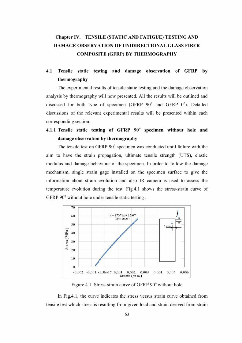
63

Chapter IV. TENSILE (STATIC AND FATIGUE) TESTING AND

DAMAGE OBSERVATION OF UNIDIRECTIONAL GLASS FIBER

COMPOSITE (GFRP) BY THERMOGRAPHY

4.1 Tensile static testing and damage observation of GFRP by

thermography

The experimental results of tensile static testing and the damage observation

analysis by thermography will now presented. All the results will be outlined and

discussed for both type of specimen (GFRP 90o and GFRP 0o). Detailed

discussions of the relevant experimental results will be presented within each

corresponding section.

4.1.1 Tensile static testing of GFRP 90o specimen without hole and

damage observation by thermography

The tensile test on GFRP 90o specimen was conducted until failure with the

aim to have the strain propagation, ultimate tensile strength (UTS), elastic

modulus and damage behaviour of the specimen. In order to follow the damage

mechanism, single strain gage installed on the specimen surface to give the

information about strain evolution and also IR camera is used to assess the

temperature evolution during the test. Fig.4.1 shows the stress-strain curve of

GFRP 90o without hole under tensile static testing .

Figure 4.1 Stress-strain curve of GFRP 90o without hole

In Fig.4.1, the curve indicates the stress versus strain curve obtained from

tensile test which stress is resulting from given load and strain derived from strain

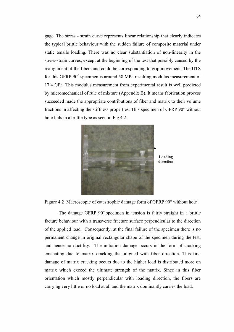
64

gage. The stress - strain curve represents linear relationship that clearly indicates

the typical brittle behaviour with the sudden failure of composite material under

static tensile loading. There was no clear substantiation of non-linearity in the

stress-strain curves, except at the beginning of the test that possibly caused by the

realignment of the fibers and could be corresponding to grip movement. The UTS

for this GFRP 90o specimen is around 58 MPa resulting modulus measurement of

17.4 GPa. This modulus measurement from experimental result is well predicted

by micromechanical of rule of mixture (Appendix B). It means fabrication process

succeeded made the appropriate contributions of fiber and matrix to their volume

fractions in affecting the stiffness properties. This specimen of GFRP 90° without

hole fails in a brittle type as seen in Fig.4.2.

Figure 4.2 Macroscopic of catastrophic damage form of GFRP 90° without hole The damage GFRP 90o specimen in tension is fairly straight in a brittle

facture behaviour with a transverse fracture surface perpendicular to the direction

of the applied load. Consequently, at the final failure of the specimen there is no

permanent change in original rectangular shape of the specimen during the test,

and hence no ductility. The initiation damage occurs in the form of cracking

emanating due to matrix cracking that aligned with fiber direction. This first

damage of matrix cracking occurs due to the higher load is distributed more on

matrix which exceed the ultimate strength of the matrix. Since in this fiber

orientation which mostly perpendicular with loading direction, the fibers are

carrying very little or no load at all and the matrix dominantly carries the load.

Loading direction

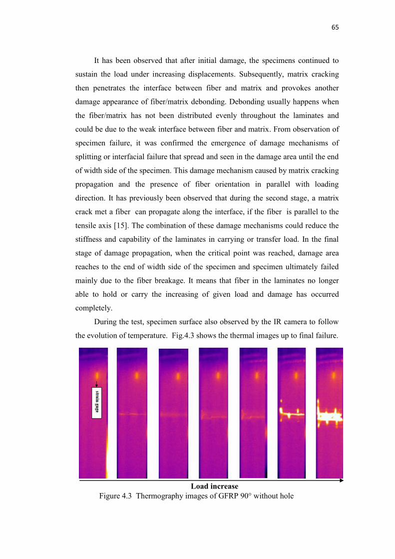
65

It has been observed that after initial damage, the specimens continued to

sustain the load under increasing displacements. Subsequently, matrix cracking

then penetrates the interface between fiber and matrix and provokes another

damage appearance of fiber/matrix debonding. Debonding usually happens when

the fiber/matrix has not been distributed evenly throughout the laminates and

could be due to the weak interface between fiber and matrix. From observation of

specimen failure, it was confirmed the emergence of damage mechanisms of

splitting or interfacial failure that spread and seen in the damage area until the end

of width side of the specimen. This damage mechanism caused by matrix cracking

propagation and the presence of fiber orientation in parallel with loading

direction. It has previously been observed that during the second stage, a matrix

crack met a fiber can propagate along the interface, if the fiber is parallel to the

tensile axis [15]. The combination of these damage mechanisms could reduce the

stiffness and capability of the laminates in carrying or transfer load. In the final

stage of damage propagation, when the critical point was reached, damage area

reaches to the end of width side of the specimen and specimen ultimately failed

mainly due to the fiber breakage. It means that fiber in the laminates no longer

able to hold or carry the increasing of given load and damage has occurred

completely.

During the test, specimen surface also observed by the IR camera to follow

the evolution of temperature. Fig.4.3 shows the thermal images up to final failure.

Figure 4.3 Thermography images of GFRP 90° without hole

Load increase

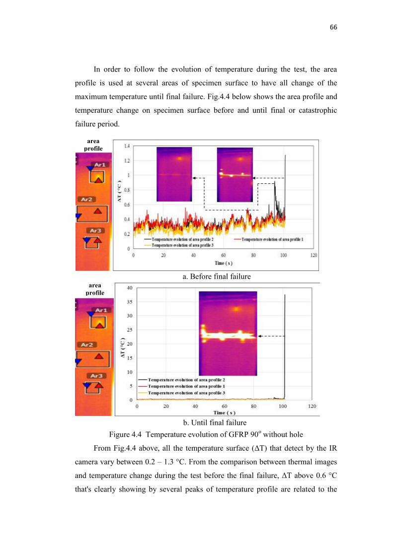
66

In order to follow the evolution of temperature during the test, the area

profile is used at several areas of specimen surface to have all change of the

maximum temperature until final failure. Fig.4.4 below shows the area profile and

temperature change on specimen surface before and until final or catastrophic

failure period.

Figure 4.4 Temperature evolution of GFRP 90o without hole

From Fig.4.4 above, all the temperature surface (ΔT) that detect by the IR

camera vary between 0.2 – 1.3 °C. From the comparison between thermal images

and temperature change during the test before the final failure, ΔT above 0.6 °C

that's clearly showing by several peaks of temperature profile are related to the

area profile

area profile

a. Before final failure

b. Until final failure

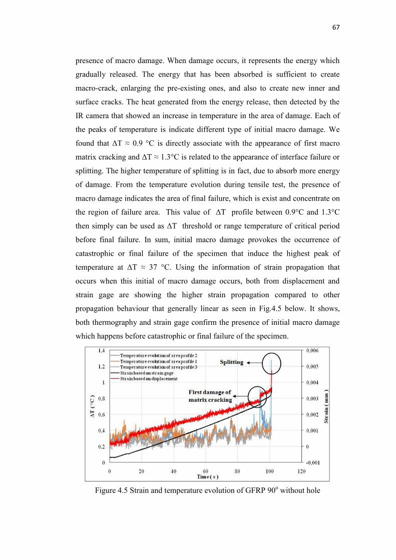
67

presence of macro damage. When damage occurs, it represents the energy which

gradually released. The energy that has been absorbed is sufficient to create

macro-crack, enlarging the pre-existing ones, and also to create new inner and

surface cracks. The heat generated from the energy release, then detected by the

IR camera that showed an increase in temperature in the area of damage. Each of

the peaks of temperature is indicate different type of initial macro damage. We

found that ΔT ≈ 0.9 °C is directly associate with the appearance of first macro

matrix cracking and ΔT ≈ 1.3°C is related to the appearance of interface failure or

splitting. The higher temperature of splitting is in fact, due to absorb more energy

of damage. From the temperature evolution during tensile test, the presence of

macro damage indicates the area of final failure, which is exist and concentrate on

the region of failure area. This value of ΔT profile between 0.9°C and 1.3°C

then simply can be used as ΔT threshold or range temperature of critical period

before final failure. In sum, initial macro damage provokes the occurrence of

catastrophic or final failure of the specimen that induce the highest peak of

temperature at ΔT ≈ 37 °C. Using the information of strain propagation that

occurs when this initial of macro damage occurs, both from displacement and

strain gage are showing the higher strain propagation compared to other

propagation behaviour that generally linear as seen in Fig.4.5 below. It shows,

both thermography and strain gage confirm the presence of initial macro damage

which happens before catastrophic or final failure of the specimen.

Figure 4.5 Strain and temperature evolution of GFRP 90o without hole

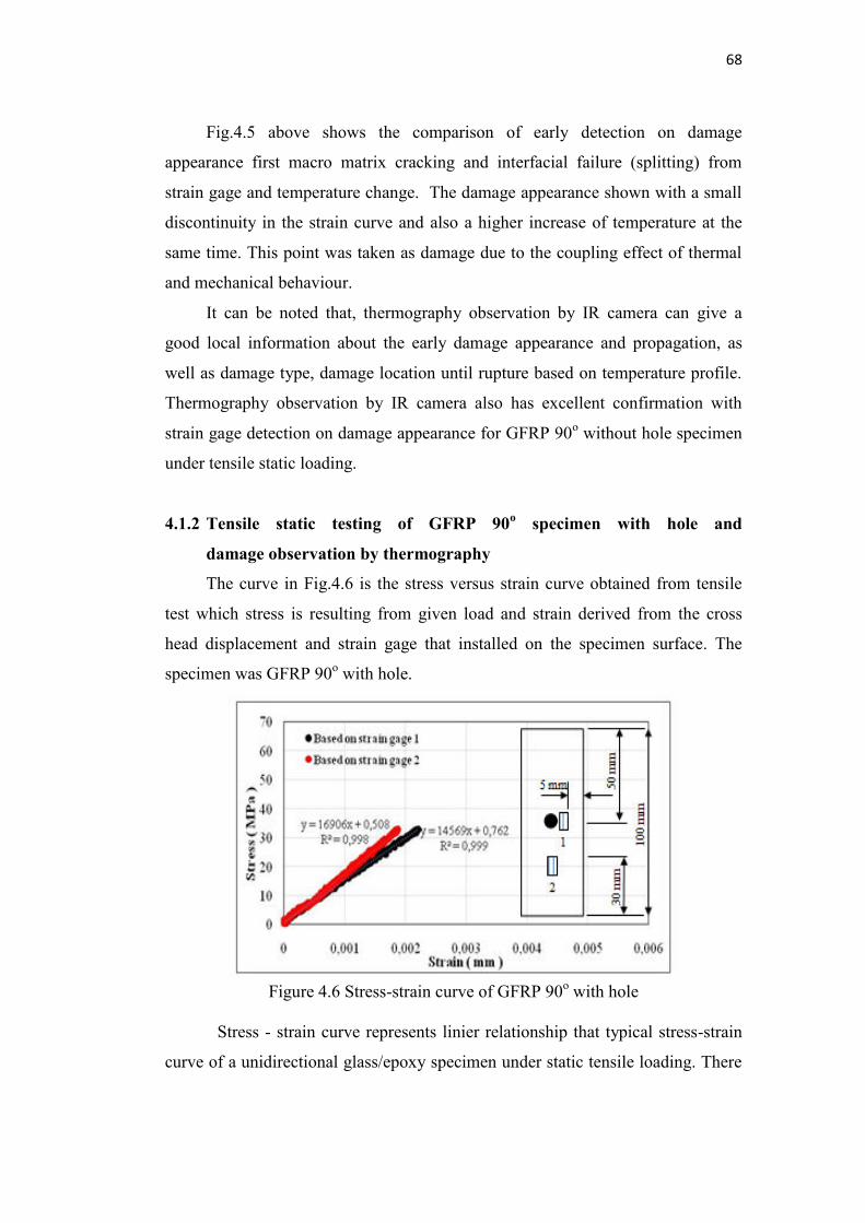
68

Fig.4.5 above shows the comparison of early detection on damage

appearance first macro matrix cracking and interfacial failure (splitting) from

strain gage and temperature change. The damage appearance shown with a small

discontinuity in the strain curve and also a higher increase of temperature at the

same time. This point was taken as damage due to the coupling effect of thermal

and mechanical behaviour.

It can be noted that, thermography observation by IR camera can give a

good local information about the early damage appearance and propagation, as

well as damage type, damage location until rupture based on temperature profile.

Thermography observation by IR camera also has excellent confirmation with

strain gage detection on damage appearance for GFRP 90o without hole specimen

under tensile static loading.

4.1.2 Tensile static testing of GFRP 90o specimen with hole and

damage observation by thermography

The curve in Fig.4.6 is the stress versus strain curve obtained from tensile

test which stress is resulting from given load and strain derived from the cross

head displacement and strain gage that installed on the specimen surface. The

specimen was GFRP 90o with hole.

Figure 4.6 Stress-strain curve of GFRP 90o with hole

Stress - strain curve represents linier relationship that typical stress-strain

curve of a unidirectional glass/epoxy specimen under static tensile loading. There

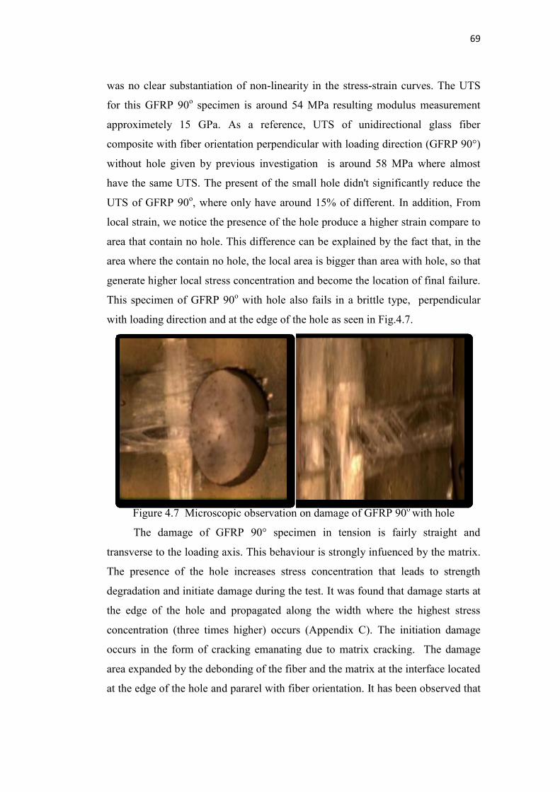
69

was no clear substantiation of non-linearity in the stress-strain curves. The UTS

for this GFRP 90o specimen is around 54 MPa resulting modulus measurement

approximetely 15 GPa. As a reference, UTS of unidirectional glass fiber

composite with fiber orientation perpendicular with loading direction (GFRP 90°)

without hole given by previous investigation is around 58 MPa where almost

have the same UTS. The present of the small hole didn't significantly reduce the

UTS of GFRP 90o, where only have around 15% of different. In addition, From

local strain, we notice the presence of the hole produce a higher strain compare to

area that contain no hole. This difference can be explained by the fact that, in the

area where the contain no hole, the local area is bigger than area with hole, so that

generate higher local stress concentration and become the location of final failure.

This specimen of GFRP 90o with hole also fails in a brittle type, perpendicular

with loading direction and at the edge of the hole as seen in Fig.4.7.

Figure 4.7 Microscopic observation on damage of GFRP 90o with hole

The damage of GFRP 90° specimen in tension is fairly straight and

transverse to the loading axis. This behaviour is strongly infuenced by the matrix.

The presence of the hole increases stress concentration that leads to strength

degradation and initiate damage during the test. It was found that damage starts at

the edge of the hole and propagated along the width where the highest stress

concentration (three times higher) occurs (Appendix C). The initiation damage

occurs in the form of cracking emanating due to matrix cracking. The damage

area expanded by the debonding of the fiber and the matrix at the interface located

at the edge of the hole and pararel with fiber orientation. It has been observed that

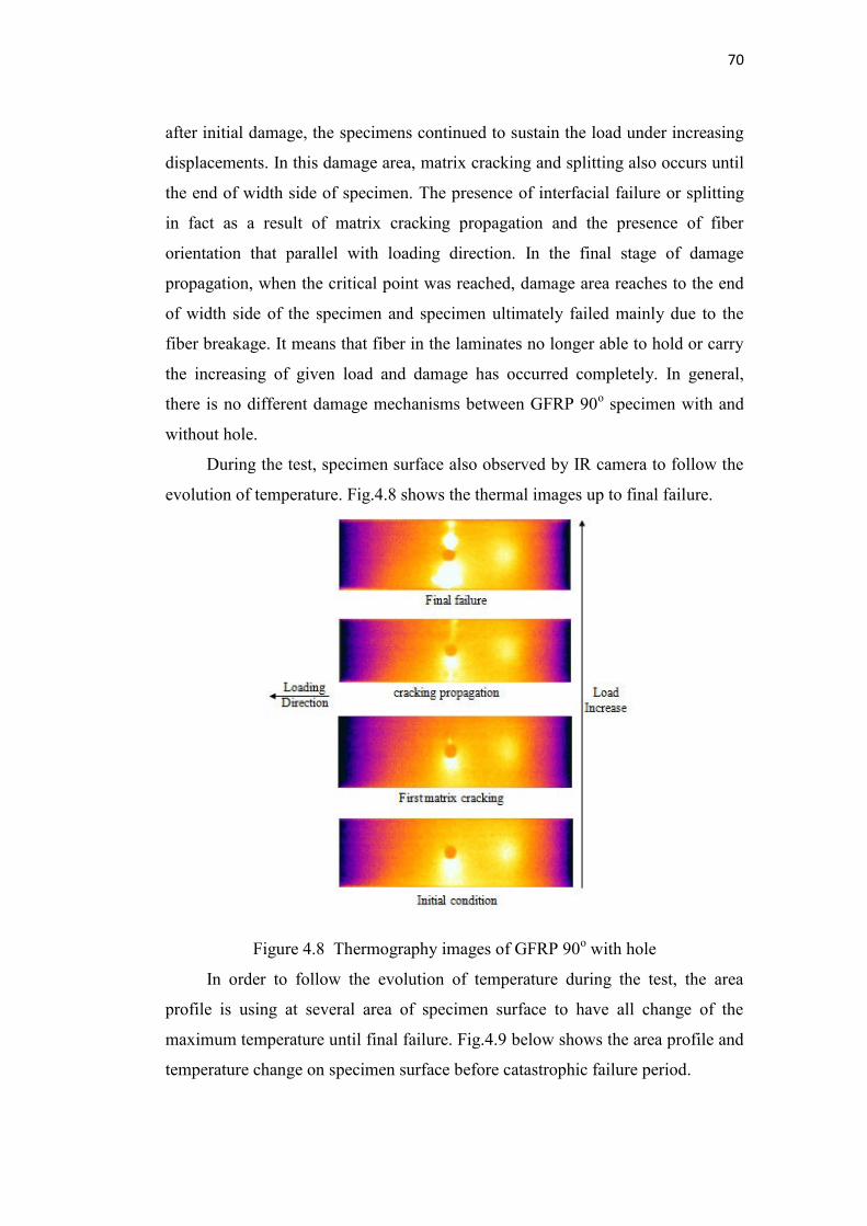
70

after initial damage, the specimens continued to sustain the load under increasing

displacements. In this damage area, matrix cracking and splitting also occurs until

the end of width side of specimen. The presence of interfacial failure or splitting

in fact as a result of matrix cracking propagation and the presence of fiber

orientation that parallel with loading direction. In the final stage of damage

propagation, when the critical point was reached, damage area reaches to the end

of width side of the specimen and specimen ultimately failed mainly due to the

fiber breakage. It means that fiber in the laminates no longer able to hold or carry

the increasing of given load and damage has occurred completely. In general,

there is no different damage mechanisms between GFRP 90o specimen with and

without hole.

During the test, specimen surface also observed by IR camera to follow the

evolution of temperature. Fig.4.8 shows the thermal images up to final failure.

Figure 4.8 Thermography images of GFRP 90o with hole

In order to follow the evolution of temperature during the test, the area

profile is using at several area of specimen surface to have all change of the

maximum temperature until final failure. Fig.4.9 below shows the area profile and

temperature change on specimen surface before catastrophic failure period.

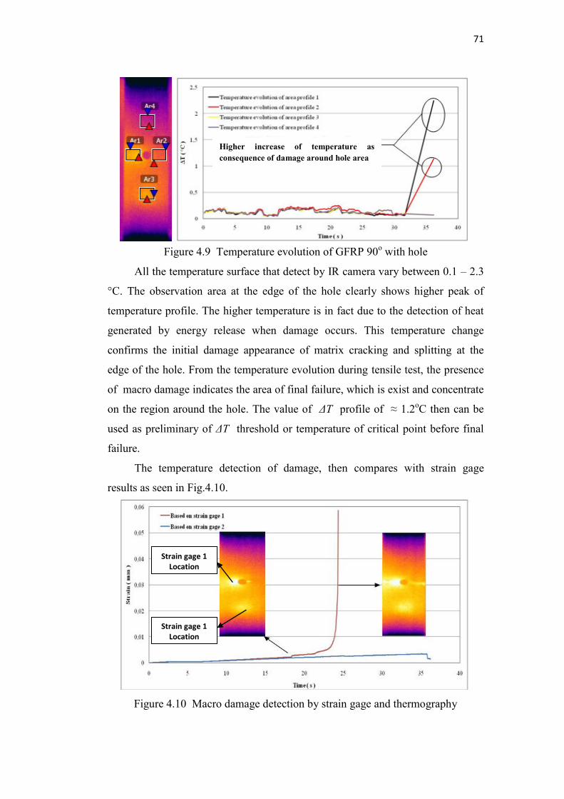
71

Figure 4.9 Temperature evolution of GFRP 90o with hole

All the temperature surface that detect by IR camera vary between 0.1 – 2.3

°C. The observation area at the edge of the hole clearly shows higher peak of

temperature profile. The higher temperature is in fact due to the detection of heat

generated by energy release when damage occurs. This temperature change

confirms the initial damage appearance of matrix cracking and splitting at the

edge of the hole. From the temperature evolution during tensile test, the presence

of macro damage indicates the area of final failure, which is exist and concentrate

on the region around the hole. The value of ΔT profile of ≈ 1.2oC then can be

used as preliminary of ΔT threshold or temperature of critical point before final

failure.

The temperature detection of damage, then compares with strain gage

results as seen in Fig.4.10.

Figure 4.10 Macro damage detection by strain gage and thermography

Higher increase of temperature as consequence of damage around hole area

Strain gage 1

Location

Strain gage 1

Location

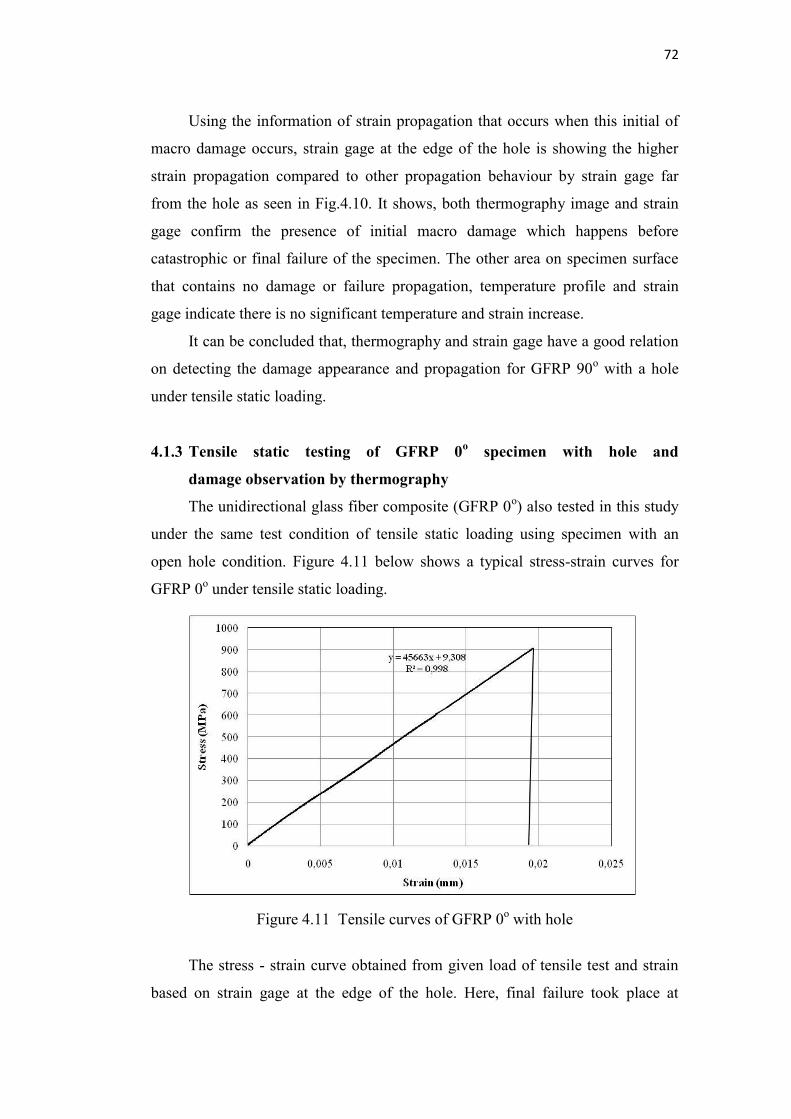
72

Using the information of strain propagation that occurs when this initial of

macro damage occurs, strain gage at the edge of the hole is showing the higher

strain propagation compared to other propagation behaviour by strain gage far

from the hole as seen in Fig.4.10. It shows, both thermography image and strain

gage confirm the presence of initial macro damage which happens before

catastrophic or final failure of the specimen. The other area on specimen surface

that contains no damage or failure propagation, temperature profile and strain

gage indicate there is no significant temperature and strain increase.

It can be concluded that, thermography and strain gage have a good relation

on detecting the damage appearance and propagation for GFRP 90o with a hole

under tensile static loading.

4.1.3 Tensile static testing of GFRP 0o specimen with hole and

damage observation by thermography

The unidirectional glass fiber composite (GFRP 0o) also tested in this study

under the same test condition of tensile static loading using specimen with an

open hole condition. Figure 4.11 below shows a typical stress-strain curves for

GFRP 0o under tensile static loading.

Figure 4.11 Tensile curves of GFRP 0o with hole

The stress - strain curve obtained from given load of tensile test and strain

based on strain gage at the edge of the hole. Here, final failure took place at

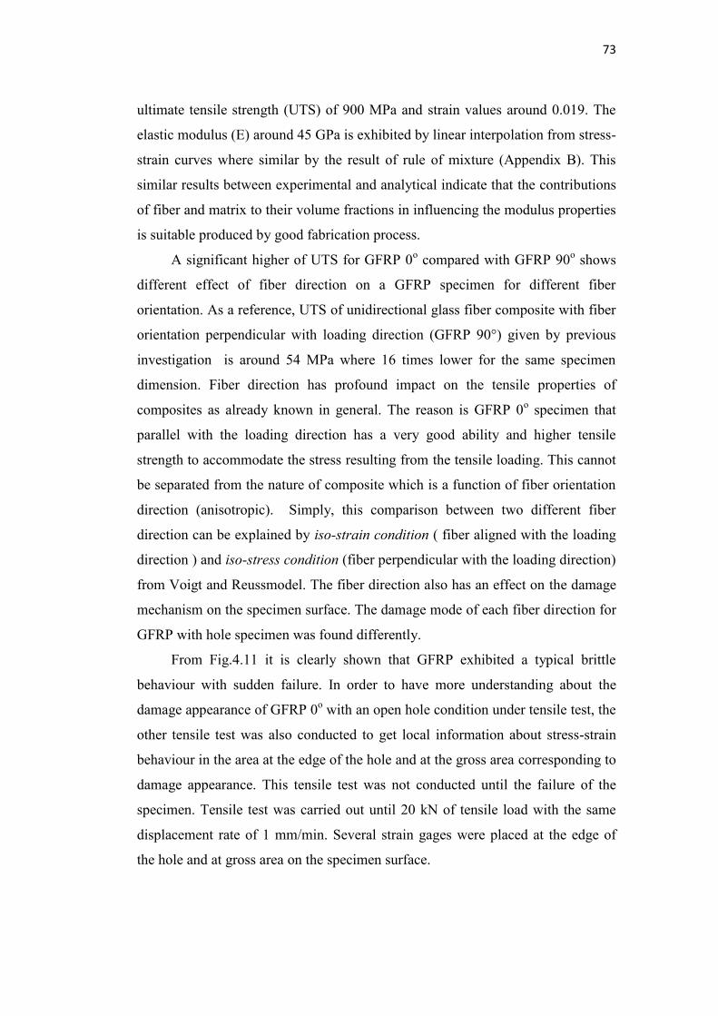
73

ultimate tensile strength (UTS) of 900 MPa and strain values around 0.019. The

elastic modulus (E) around 45 GPa is exhibited by linear interpolation from stress-

strain curves where similar by the result of rule of mixture (Appendix B). This

similar results between experimental and analytical indicate that the contributions

of fiber and matrix to their volume fractions in influencing the modulus properties

is suitable produced by good fabrication process.

A significant higher of UTS for GFRP 0o compared with GFRP 90o shows

different effect of fiber direction on a GFRP specimen for different fiber

orientation. As a reference, UTS of unidirectional glass fiber composite with fiber

orientation perpendicular with loading direction (GFRP 90°) given by previous

investigation is around 54 MPa where 16 times lower for the same specimen

dimension. Fiber direction has profound impact on the tensile properties of

composites as already known in general. The reason is GFRP 0o specimen that

parallel with the loading direction has a very good ability and higher tensile

strength to accommodate the stress resulting from the tensile loading. This cannot

be separated from the nature of composite which is a function of fiber orientation

direction (anisotropic). Simply, this comparison between two different fiber

direction can be explained by iso-strain condition ( fiber aligned with the loading

direction ) and iso-stress condition (fiber perpendicular with the loading direction)

from Voigt and Reussmodel. The fiber direction also has an effect on the damage

mechanism on the specimen surface. The damage mode of each fiber direction for

GFRP with hole specimen was found differently.

From Fig.4.11 it is clearly shown that GFRP exhibited a typical brittle

behaviour with sudden failure. In order to have more understanding about the

damage appearance of GFRP 0o with an open hole condition under tensile test, the

other tensile test was also conducted to get local information about stress-strain

behaviour in the area at the edge of the hole and at the gross area corresponding to

damage appearance. This tensile test was not conducted until the failure of the

specimen. Tensile test was carried out until 20 kN of tensile load with the same

displacement rate of 1 mm/min. Several strain gages were placed at the edge of

the hole and at gross area on the specimen surface.

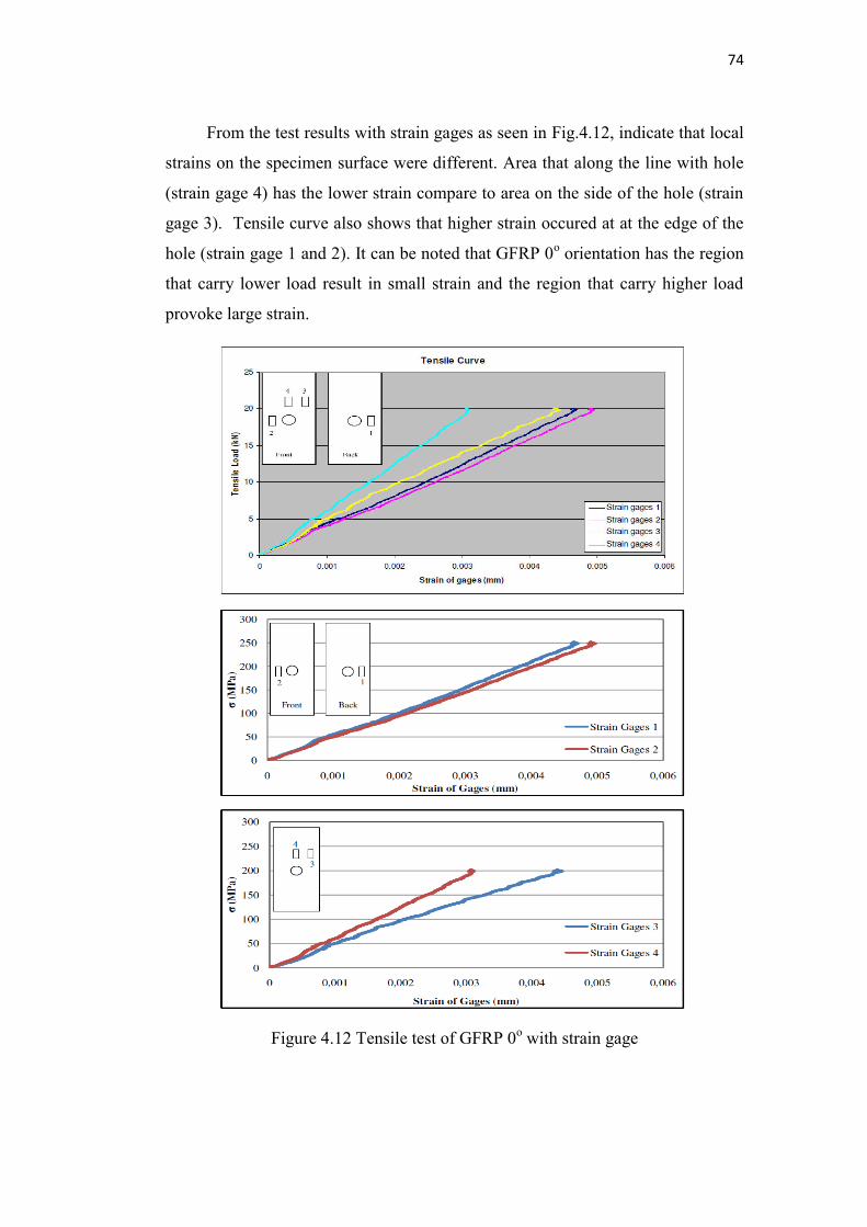
74

From the test results with strain gages as seen in Fig.4.12, indicate that local

strains on the specimen surface were different. Area that along the line with hole

(strain gage 4) has the lower strain compare to area on the side of the hole (strain

gage 3). Tensile curve also shows that higher strain occured at at the edge of the

hole (strain gage 1 and 2). It can be noted that GFRP 0o orientation has the region

that carry lower load result in small strain and the region that carry higher load

provoke large strain.

Figure 4.12 Tensile test of GFRP 0o with strain gage

75

From this condition, we can assume that area at the edge of the hole and

side area of the hole will experience higher stress concentration and can be a

catastrophic failure area. These results then will be compared with specimen that

have been damaged due to the tensile load to prove the earlier assumptions based

on results obtained from strain gage.

From previous study [41], the investigation on the stress concentration

around the hole for glass epoxy found that the stress distribution resulting lowest

stress concentration at the area along the hole for tensile loading testing pararell

with fiber direction on composite. For this GFRP 0o with hole specimen, the

presence of an open hole will be redistributing also the force at the edge of the

hole resulting the highest stress concentration around four times higher at this area

(Appendix D). There is no stress pass through the hole and result in the lowest

stress at the area along the hole location,as seen the ilustration in Fig.4.13.

Figure 4.13 Ilustration of stress distribution and final failure of GFRP 0o

The damage mechanism of GFRP 0o with hole specimen may be attributed

to the combination of matrix damage, fiber-matrix debonding and fiber breakage

(Fig.4.14). From the observation results, the first damage of matrix macro-

cracking is in splitting form and also indicates by cracking sound. After the first

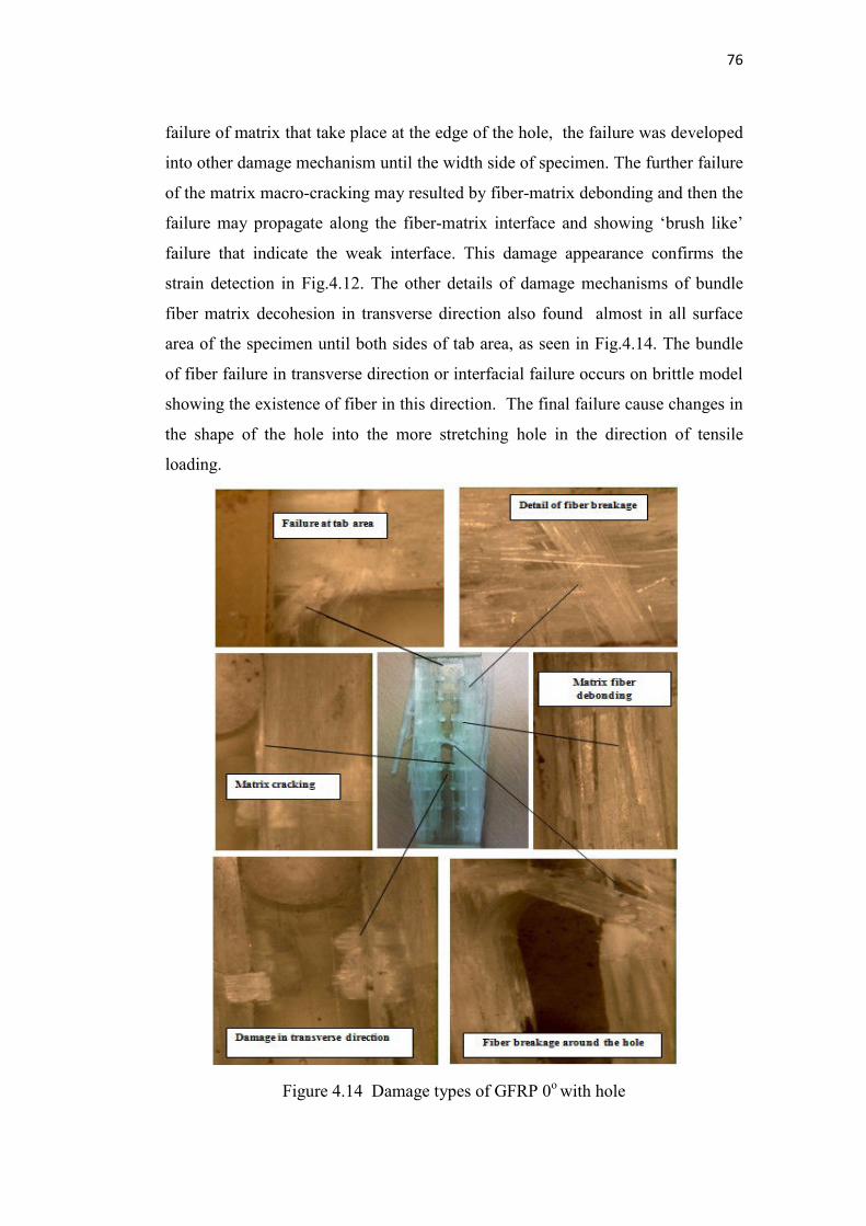
76

failure of matrix that take place at the edge of the hole, the failure was developed

into other damage mechanism until the width side of specimen. The further failure

of the matrix macro-cracking may resulted by fiber-matrix debonding and then the

failure may propagate along the fiber-matrix interface and showing ‘brush like’

failure that indicate the weak interface. This damage appearance confirms the

strain detection in Fig.4.12. The other details of damage mechanisms of bundle

fiber matrix decohesion in transverse direction also found almost in all surface

area of the specimen until both sides of tab area, as seen in Fig.4.14. The bundle

of fiber failure in transverse direction or interfacial failure occurs on brittle model

showing the existence of fiber in this direction. The final failure cause changes in

the shape of the hole into the more stretching hole in the direction of tensile

loading.

Figure 4.14 Damage types of GFRP 0o with hole

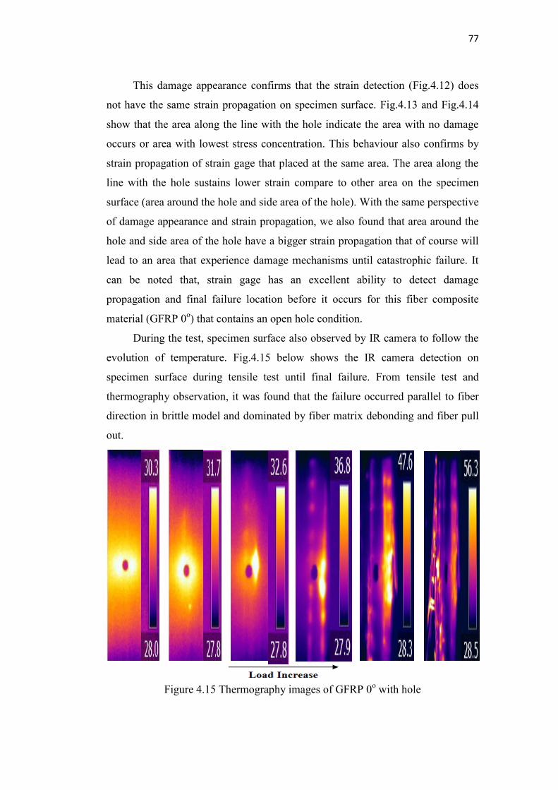
77

This damage appearance confirms that the strain detection (Fig.4.12) does

not have the same strain propagation on specimen surface. Fig.4.13 and Fig.4.14

show that the area along the line with the hole indicate the area with no damage

occurs or area with lowest stress concentration. This behaviour also confirms by

strain propagation of strain gage that placed at the same area. The area along the

line with the hole sustains lower strain compare to other area on the specimen

surface (area around the hole and side area of the hole). With the same perspective

of damage appearance and strain propagation, we also found that area around the

hole and side area of the hole have a bigger strain propagation that of course will

lead to an area that experience damage mechanisms until catastrophic failure. It

can be noted that, strain gage has an excellent ability to detect damage

propagation and final failure location before it occurs for this fiber composite

material (GFRP 0o) that contains an open hole condition.

During the test, specimen surface also observed by IR camera to follow the

evolution of temperature. Fig.4.15 below shows the IR camera detection on

specimen surface during tensile test until final failure. From tensile test and

thermography observation, it was found that the failure occurred parallel to fiber

direction in brittle model and dominated by fiber matrix debonding and fiber pull

out.

Figure 4.15 Thermography images of GFRP 0o with hole

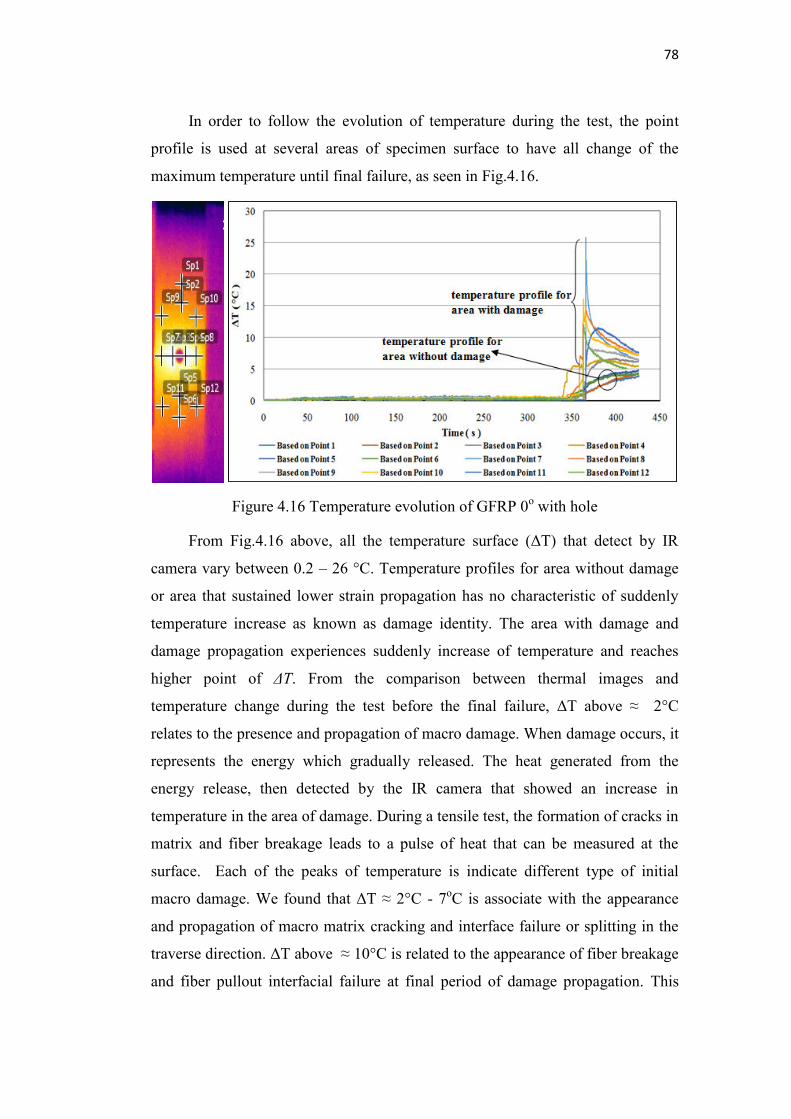
78

In order to follow the evolution of temperature during the test, the point

profile is used at several areas of specimen surface to have all change of the

maximum temperature until final failure, as seen in Fig.4.16.

Figure 4.16 Temperature evolution of GFRP 0o with hole

From Fig.4.16 above, all the temperature surface (ΔT) that detect by IR

camera vary between 0.2 – 26 °C. Temperature profiles for area without damage

or area that sustained lower strain propagation has no characteristic of suddenly

temperature increase as known as damage identity. The area with damage and

damage propagation experiences suddenly increase of temperature and reaches

higher point of ΔT. From the comparison between thermal images and

temperature change during the test before the final failure, ΔT above ≈ 2°C

relates to the presence and propagation of macro damage. When damage occurs, it

represents the energy which gradually released. The heat generated from the

energy release, then detected by the IR camera that showed an increase in

temperature in the area of damage. During a tensile test, the formation of cracks in

matrix and fiber breakage leads to a pulse of heat that can be measured at the

surface. Each of the peaks of temperature is indicate different type of initial

macro damage. We found that ΔT ≈ 2°C - 7oC is associate with the appearance

and propagation of macro matrix cracking and interface failure or splitting in the

traverse direction. ΔT above ≈ 10°C is related to the appearance of fiber breakage

and fiber pullout interfacial failure at final period of damage propagation. This

79

value of ΔT profile between 2°C and 10°C then simply can be used as ΔT

threshold or range temperature of critical period in terms of macro damage

appearance before final failure. It can be concluded that, thermography

successfully follows the damage propagation for GFRP 0o with hole under tensile

static loading.

4.2 Tensile fatigue testing and damage observation by thermography of

GFRP

This section describes the experimental investigation on the fatigue

behaviour of GFRP 90o with hole. Thermography observation applies to detect

temperature distribution on specimen surface during the tests. The aim is to

determine the damage evolution with respect to the number of cycles by varying

the stress level applied. In practice, damages are observed by two systems. The

first consists in a damage evolution during the test by strain gage and/or

displacement to follow the stiffness degradation by controlling the continuous

decay of the elastic properties. The second system consists in an analysis under

thermography observation. The change of temperature will be monitoring to have

temperature profile according to damage appearance and propagation. In this way

it is possible to determine the relationship of damage evolution between

experimental results and thermography analysis.

The constant amplitude load controlled tension-tension fatigue tests were

performed with other fatigue test parameters selected were sinusoidal waveform, 3

Hz frequency, and the stress ratio of 0.1. Fatigue loads were applied as

percentages of ultimate tensile strength (UTS). The fatigue load, where specimens

survived 1 million cycles is referred as a high cycle fatigue strength (HCFS) in

this report.

Fatigue tests were conducted for several stress levels based on UTS with

the range of 40%-65% of UTS. The initial maximum stress level was taken as

about 65% of the UTS. Maximum stress levels were then chosen to give a range

of lifetimes (Nf) between 103 and 106 cycles. The S-N curve of GFRP 90o based

on normalized stress (maximum fatigue tensile stress divided by ultimate static

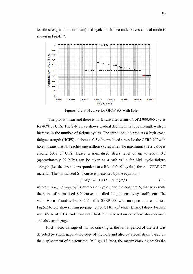
80

tensile strength as the ordinate) and cycles to failure under stress control mode is

shown in Fig.4.17.

Figure 4.17 S-N curve for GFRP 90o with hole

The plot is linear and there is no failure after a run-off of 2.900.000 cycles

for 40% of UTS. The S-N curve shows gradual decline in fatigue strength with an

increase in the number of fatigue cycles. The trendline line predicts a high cycle

fatigue strength (HCFS) of about ≈ 0.5 of normalized stress for the GFRP 90o with

hole, means that Nf reaches one million cycles when the maximum stress value is

around 50% of UTS. Hence a normalised stress level of up to about 0.5

(approximately 29 MPa) can be taken as a safe value for high cycle fatigue

strength (i.e. the stress correspondent to a life of 5·106 cycles) for this GFRP 90o

material. The normalized S-N curve is presented by the equation : (30)

where y is σmax / σUTS, Nf is number of cycles, and the constant b, that represents

the slope of normalised S-N curve, is called fatigue sensitivity coefficient. The

value b was found to be 0.02 for this GFRP 90o with an open hole condition.

Fig.5.2 below shows strain propagation of GFRP 90o under tensile fatigue loading

with 65 % of UTS load level until first failure based on crosshead displacement

and also strain gages.

First macro damage of matrix cracking at the initial period of the test was

detected by strain gage at the edge of the hole and also by global strain based on

the displacement of the actuator. In Fig.4.18 (top), the matrix cracking breaks the

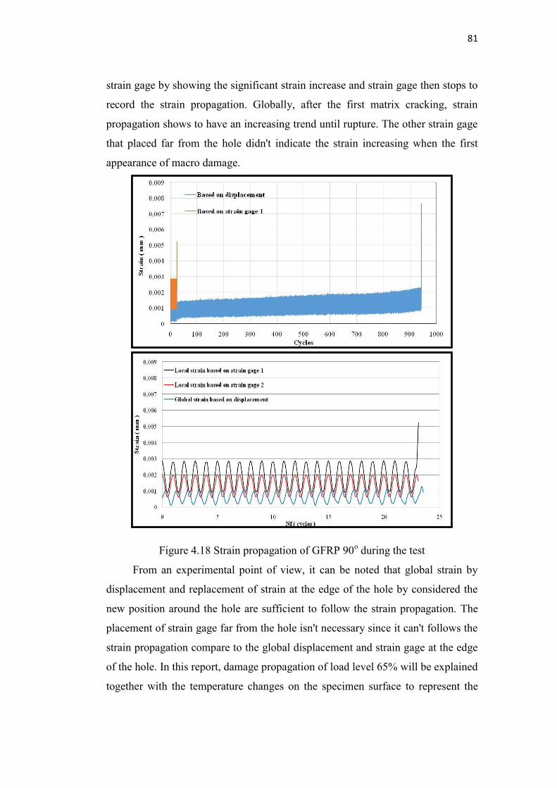
81

strain gage by showing the significant strain increase and strain gage then stops to

record the strain propagation. Globally, after the first matrix cracking, strain

propagation shows to have an increasing trend until rupture. The other strain gage

that placed far from the hole didn't indicate the strain increasing when the first

appearance of macro damage.

Figure 4.18 Strain propagation of GFRP 90o during the test

From an experimental point of view, it can be noted that global strain by

displacement and replacement of strain at the edge of the hole by considered the

new position around the hole are sufficient to follow the strain propagation. The

placement of strain gage far from the hole isn't necessary since it can't follows the

strain propagation compare to the global displacement and strain gage at the edge

of the hole. In this report, damage propagation of load level 65% will be explained

together with the temperature changes on the specimen surface to represent the

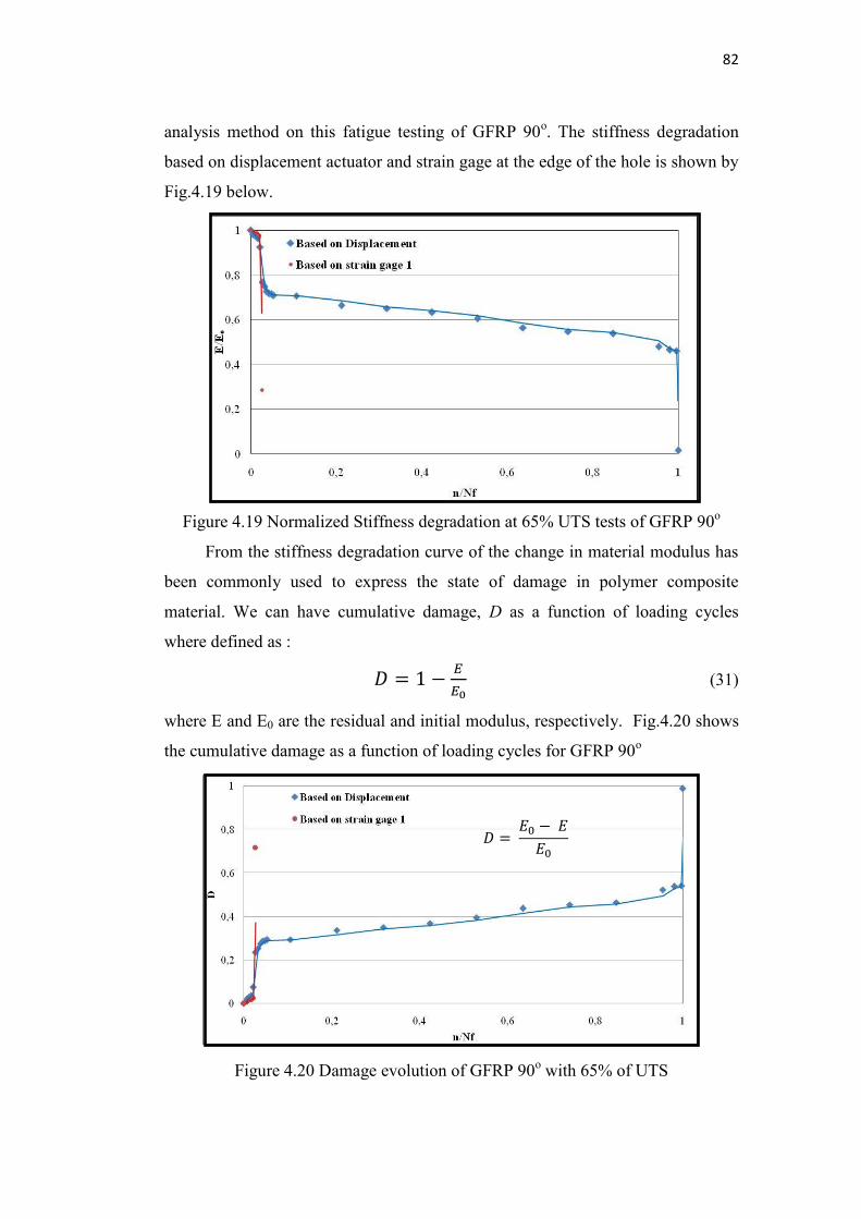
82

analysis method on this fatigue testing of GFRP 90o. The stiffness degradation

based on displacement actuator and strain gage at the edge of the hole is shown by

Fig.4.19 below.

Figure 4.19 Normalized Stiffness degradation at 65% UTS tests of GFRP 90o

From the stiffness degradation curve of the change in material modulus has

been commonly used to express the state of damage in polymer composite

material. We can have cumulative damage, D as a function of loading cycles

where defined as : (31)

where E and E0 are the residual and initial modulus, respectively. Fig.4.20 shows

the cumulative damage as a function of loading cycles for GFRP 90o

Figure 4.20 Damage evolution of GFRP 90o with 65% of UTS

III

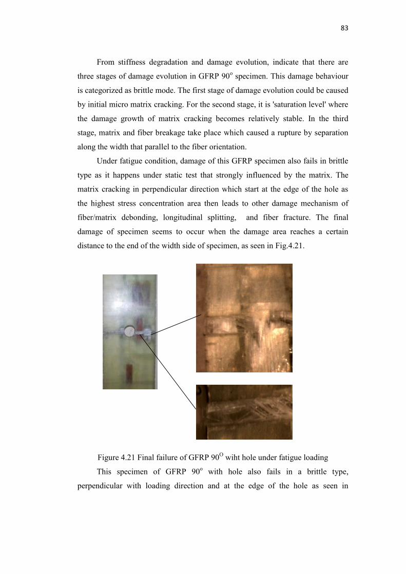
83

From stiffness degradation and damage evolution, indicate that there are

three stages of damage evolution in GFRP 90o specimen. This damage behaviour

is categorized as brittle mode. The first stage of damage evolution could be caused

by initial micro matrix cracking. For the second stage, it is 'saturation level' where

the damage growth of matrix cracking becomes relatively stable. In the third

stage, matrix and fiber breakage take place which caused a rupture by separation

along the width that parallel to the fiber orientation.

Under fatigue condition, damage of this GFRP specimen also fails in brittle

type as it happens under static test that strongly influenced by the matrix. The

matrix cracking in perpendicular direction which start at the edge of the hole as

the highest stress concentration area then leads to other damage mechanism of

fiber/matrix debonding, longitudinal splitting, and fiber fracture. The final

damage of specimen seems to occur when the damage area reaches a certain

distance to the end of the width side of specimen, as seen in Fig.4.21.

Figure 4.21 Final failure of GFRP 90O wiht hole under fatigue loading

This specimen of GFRP 90o with hole also fails in a brittle type,

perpendicular with loading direction and at the edge of the hole as seen in

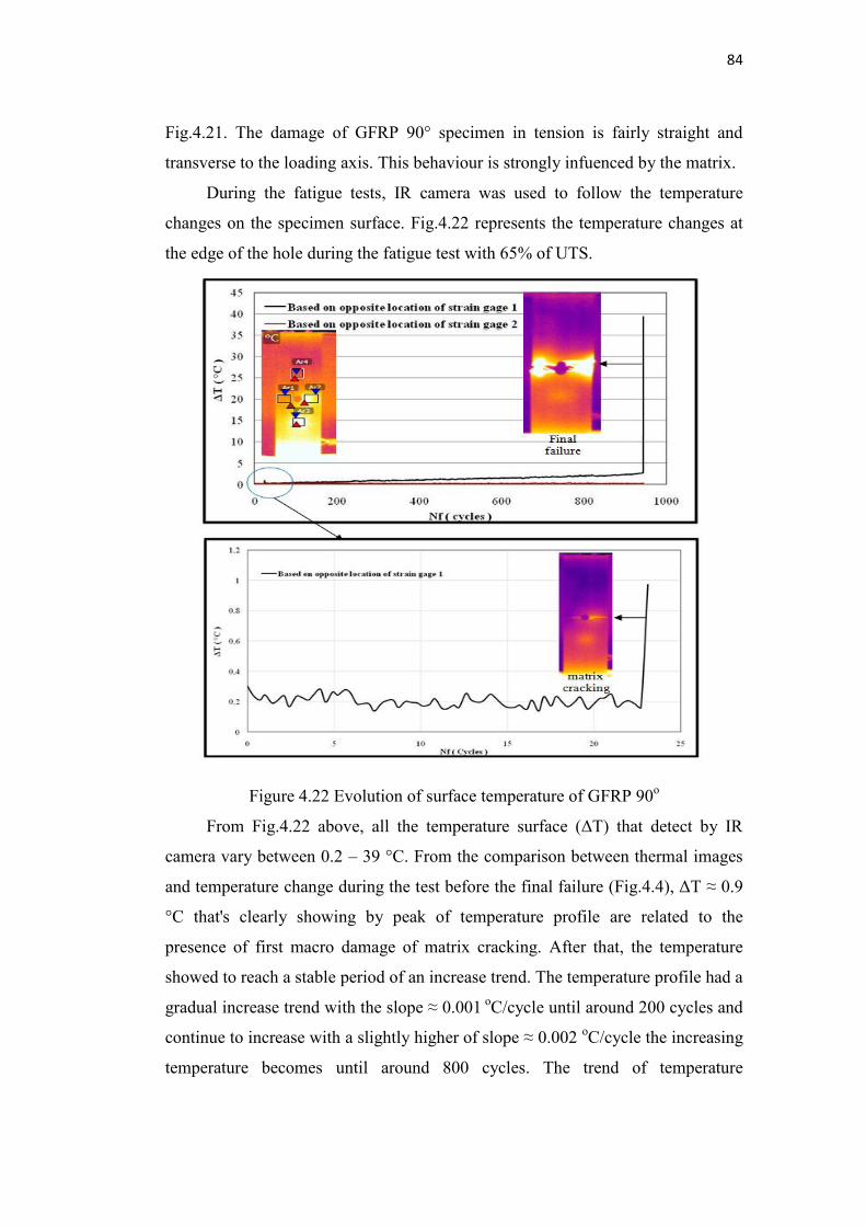
84

Fig.4.21. The damage of GFRP 90° specimen in tension is fairly straight and

transverse to the loading axis. This behaviour is strongly infuenced by the matrix.

During the fatigue tests, IR camera was used to follow the temperature

changes on the specimen surface. Fig.4.22 represents the temperature changes at

the edge of the hole during the fatigue test with 65% of UTS.

Figure 4.22 Evolution of surface temperature of GFRP 90o

From Fig.4.22 above, all the temperature surface (ΔT) that detect by IR

camera vary between 0.2 – 39 °C. From the comparison between thermal images

and temperature change during the test before the final failure (Fig.4.4), ΔT ≈ 0.9

°C that's clearly showing by peak of temperature profile are related to the

presence of first macro damage of matrix cracking. After that, the temperature

showed to reach a stable period of an increase trend. The temperature profile had a

gradual increase trend with the slope ≈ 0.001 oC/cycle until around 200 cycles and

continue to increase with a slightly higher of slope ≈ 0.002 oC/cycle the increasing

temperature becomes until around 800 cycles. The trend of temperature

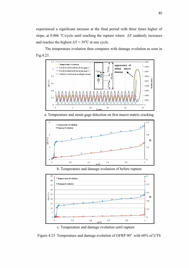
85

experienced a significant increase at the final period with three times higher of

slope, at 0.006 oC/cycle until reaching the rupture where ΔT suddenly increases

and reaches the highest ΔT ≈ 39oC at one cycle.

The temperature evolution then compares with damage evolution as seen in

Fig.4.23.

a. Temperature and strain gage detection on first macro matrix cracking

Figure 4.23 Temperature and damage evolution of GFRP 90o with 60% of UTS

D

D

appearance of initial macro damage

b. Temperature and damage evolution of before rupture

c. Temperature and damage evolution until rupture

86

From the temperature and damage evolution during tensile fatigue test

(Fig.4.22 and 4.23), the presence of damage was indicated by temperature change

on specimen surface during the test that exist and concentrate at the hole.

Meanwhile, the temperature evolution at another area of specimen surface that far

from the hole didn't show an increase of temperature or relatively to have the

same temperature from the beginning of the test until rupture of the specimen.

When damage occurs, it represents the energy which gradually released. The heat

generated from the energy release then detected by the IR camera that showed an

increase in temperature in the area of damage. The evolution of the temperature

can be categorized in four stages. In the first part, the initial increase of

temperature is possibly due to the micro cracking in matrix. In the second part, a

sudden increase in temperature caused by first appearance of macro matrix

cracking. After that, the temperature reaches a slowly increasing trend due to the

stable growth of matrix cracking as part of the third stage. The final part, a

significant trend increase of temperature could be due to fiber/matrix debonding

as the interfacial failure in splitting form and finally provokes the occurrence of

fiber fracture which dealing with the rupture of the specimen.

It can be noted that, thermography observation by IR camera gives a good

confirmation with strain gage detection on damage appearance and evolution for

GFRP 90o with hole specimen under tensile fatigue loading.

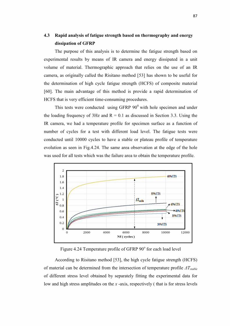
87

4.3 Rapid analysis of fatigue strength based on thermography and energy

dissipation of GFRP

The purpose of this analysis is to determine the fatigue strength based on

experimental results by means of IR camera and energy dissipated in a unit

volume of material. Thermographic approach that relies on the use of an IR

camera, as originally called the Risitano method [53] has shown to be useful for

the determination of high cycle fatigue strength (HCFS) of composite material

[60]. The main advantage of this method is provide a rapid determination of

HCFS that is very efficient time-consuming procedures.

This tests were conducted using GFRP 900 with hole specimen and under

the loading frequency of 3Hz and R = 0.1 as discussed in Section 3.3. Using the

IR camera, we had a temperature profile for specimen surface as a function of

number of cycles for a test with different load level. The fatigue tests were

conducted until 10000 cycles to have a stable or plateau profile of temperature

evolution as seen in Fig.4.24. The same area observation at the edge of the hole

was used for all tests which was the failure area to obtain the temperature profile.

Figure 4.24 Temperature profile of GFRP 90o for each load level

According to Risitano method [53], the high cycle fatigue strength (HCFS)

of material can be determined from the intersection of temperature profile ΔTstable

of different stress level obtained by separately fitting the experimental data for

low and high stress amplitudes on the x -axis, respectively ( that is for stress levels

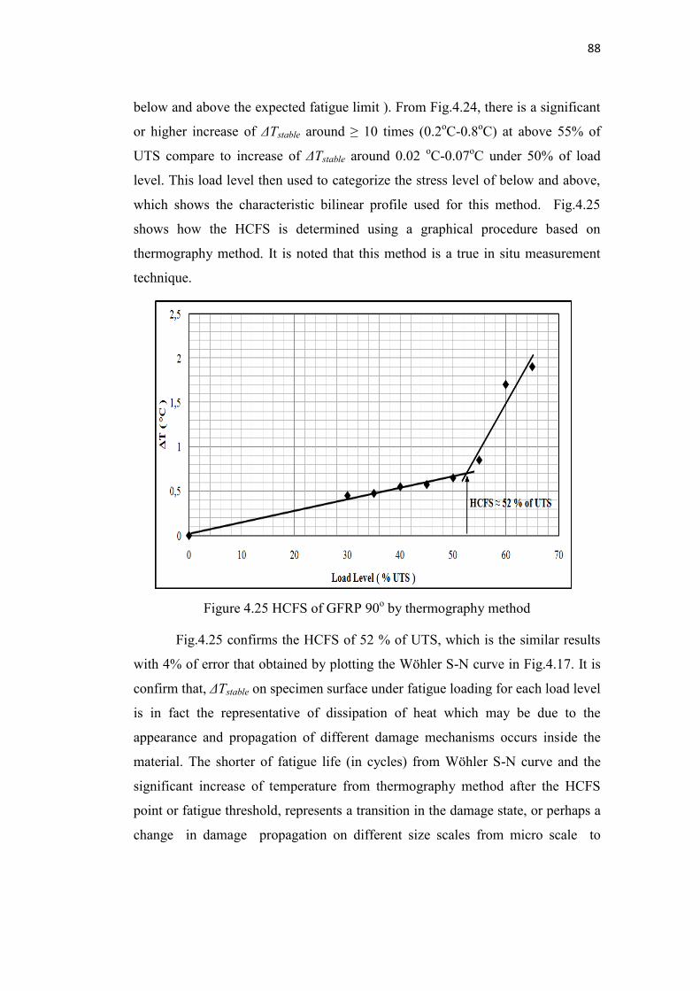
88

below and above the expected fatigue limit ). From Fig.4.24, there is a significant

or higher increase of ΔTstable around ≥ 10 times (0.2oC-0.8oC) at above 55% of

UTS compare to increase of ΔTstable around 0.02 oC-0.07oC under 50% of load

level. This load level then used to categorize the stress level of below and above,

which shows the characteristic bilinear profile used for this method. Fig.4.25

shows how the HCFS is determined using a graphical procedure based on

thermography method. It is noted that this method is a true in situ measurement

technique.

Figure 4.25 HCFS of GFRP 90o by thermography method

Fig.4.25 confirms the HCFS of 52 % of UTS, which is the similar results

with 4% of error that obtained by plotting the Wöhler S-N curve in Fig.4.17. It is

confirm that, ΔTstable on specimen surface under fatigue loading for each load level

is in fact the representative of dissipation of heat which may be due to the

appearance and propagation of different damage mechanisms occurs inside the

material. The shorter of fatigue life (in cycles) from Wöhler S-N curve and the

significant increase of temperature from thermography method after the HCFS

point or fatigue threshold, represents a transition in the damage state, or perhaps a

change in damage propagation on different size scales from micro scale to

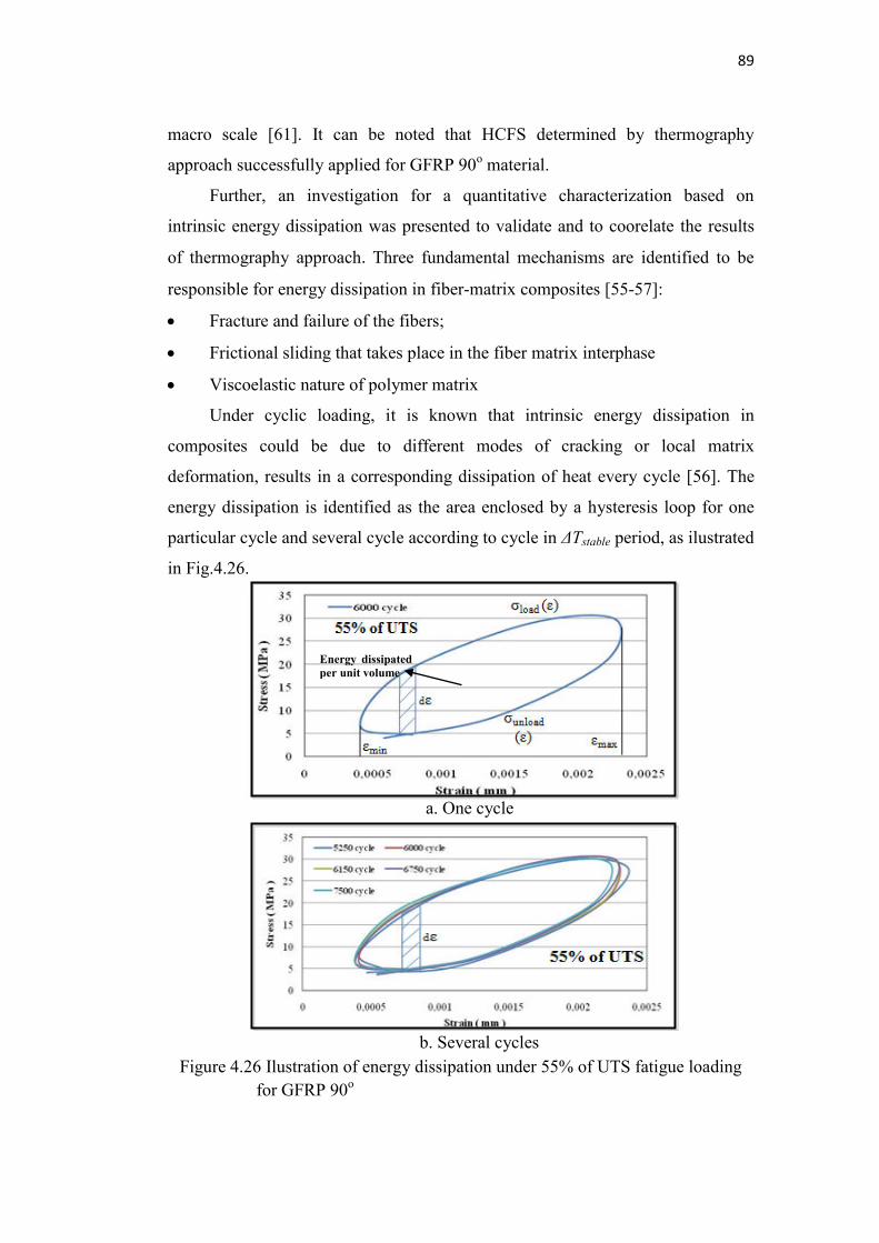
89

macro scale [61]. It can be noted that HCFS determined by thermography

approach successfully applied for GFRP 90o material.

Further, an investigation for a quantitative characterization based on

intrinsic energy dissipation was presented to validate and to coorelate the results

of thermography approach. Three fundamental mechanisms are identified to be

responsible for energy dissipation in fiber-matrix composites [55-57]:

Fracture and failure of the fibers;

Frictional sliding that takes place in the fiber matrix interphase

Viscoelastic nature of polymer matrix

Under cyclic loading, it is known that intrinsic energy dissipation in

composites could be due to different modes of cracking or local matrix

deformation, results in a corresponding dissipation of heat every cycle [56]. The

energy dissipation is identified as the area enclosed by a hysteresis loop for one

particular cycle and several cycle according to cycle in ΔTstable period, as ilustrated

in Fig.4.26.

Figure 4.26 Ilustration of energy dissipation under 55% of UTS fatigue loading

for GFRP 90o

Energy dissipated per unit volume

a. One cycle

b. Several cycles

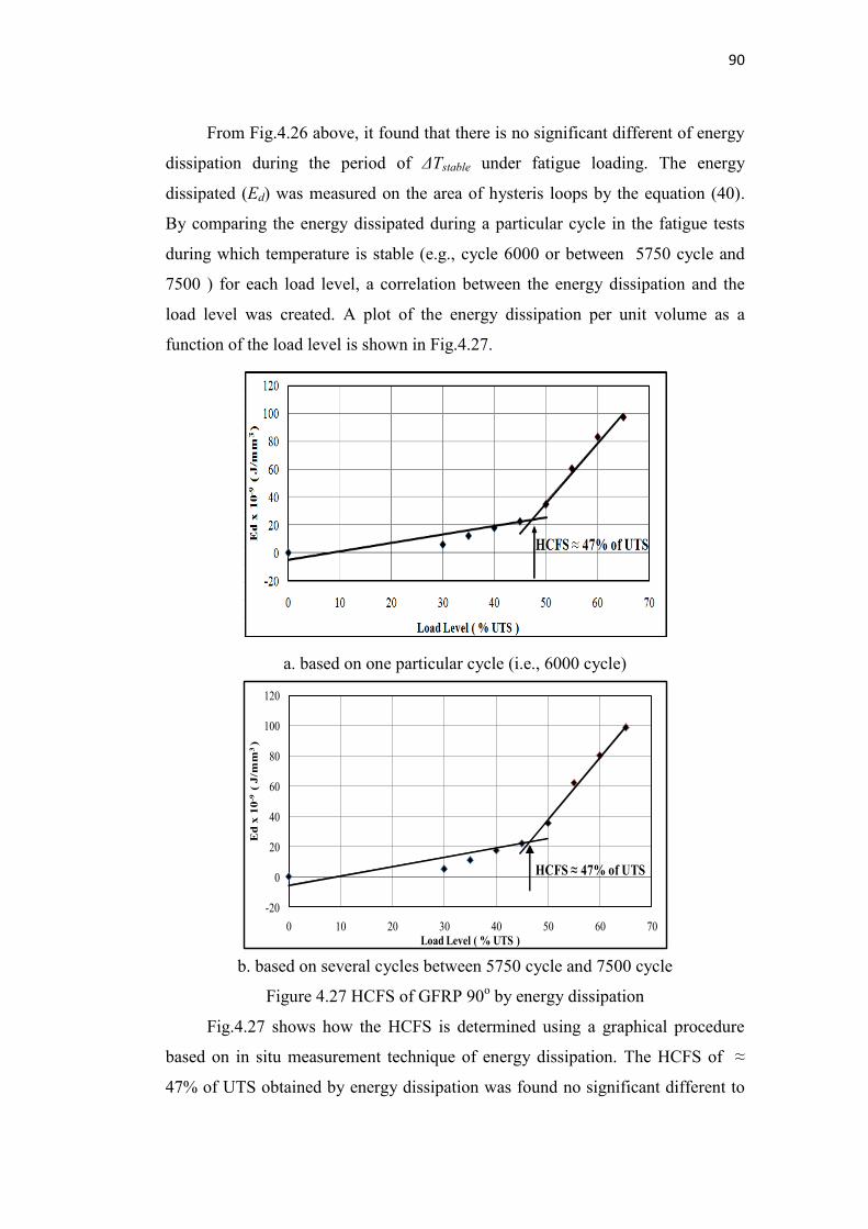
90

From Fig.4.26 above, it found that there is no significant different of energy

dissipation during the period of ΔTstable under fatigue loading. The energy

dissipated (Ed) was measured on the area of hysteris loops by the equation (40).

By comparing the energy dissipated during a particular cycle in the fatigue tests

during which temperature is stable (e.g., cycle 6000 or between 5750 cycle and

7500 ) for each load level, a correlation between the energy dissipation and the

load level was created. A plot of the energy dissipation per unit volume as a

function of the load level is shown in Fig.4.27.

a. based on one particular cycle (i.e., 6000 cycle)

b. based on several cycles between 5750 cycle and 7500 cycle

Figure 4.27 HCFS of GFRP 90o by energy dissipation

Fig.4.27 shows how the HCFS is determined using a graphical procedure

based on in situ measurement technique of energy dissipation. The HCFS of ≈

47% of UTS obtained by energy dissipation was found no significant different to

-20

0

20

40

60

80

100

120

0 10 20 30 40 50 60 70

Ed

x 1

0-9

( J/m

m3

)

Load Level ( % UTS )

HCFS ≈ 47% of UTS

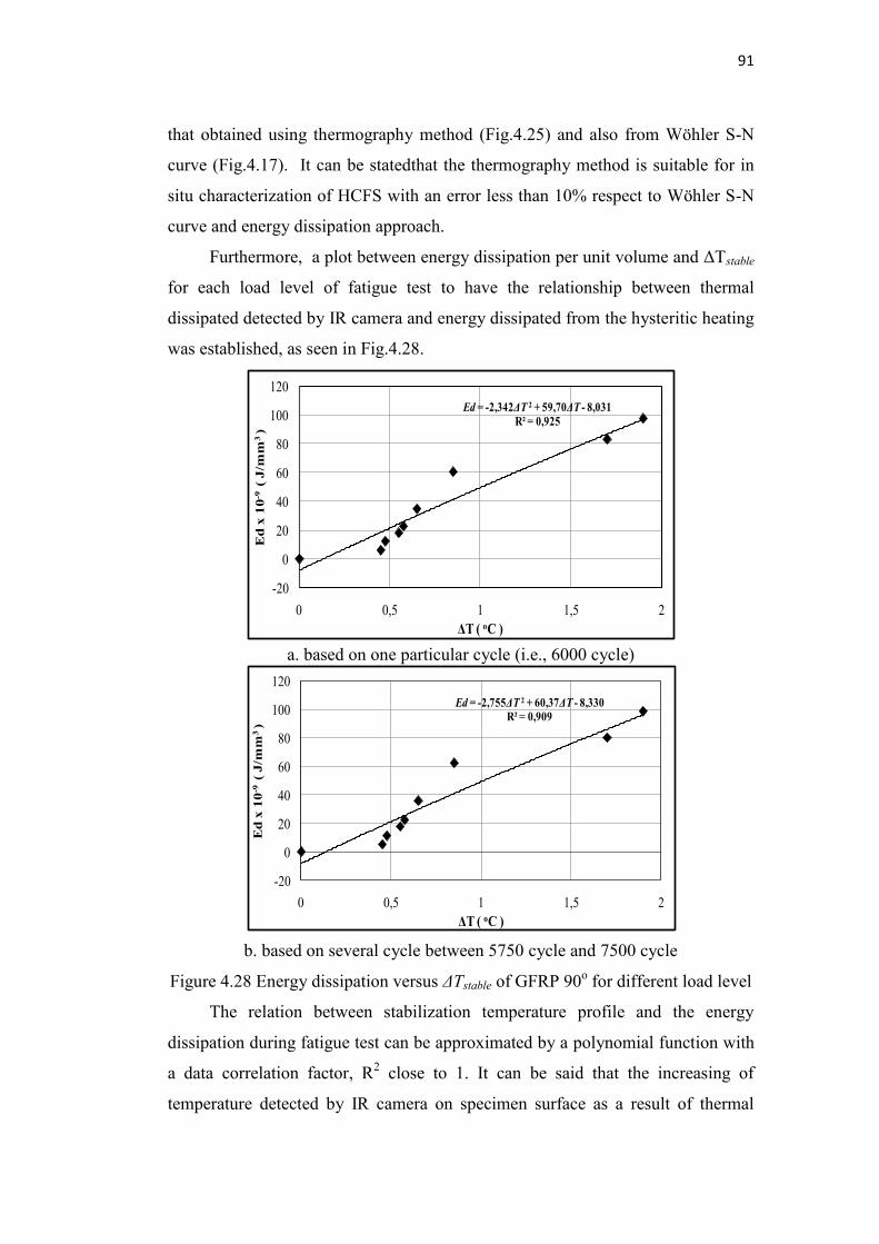
91

that obtained using thermography method (Fig.4.25) and also from Wöhler S-N

curve (Fig.4.17). It can be statedthat the thermography method is suitable for in

situ characterization of HCFS with an error less than 10% respect to Wöhler S-N

curve and energy dissipation approach.

Furthermore, a plot between energy dissipation per unit volume and ΔTstable

for each load level of fatigue test to have the relationship between thermal

dissipated detected by IR camera and energy dissipated from the hysteritic heating

was established, as seen in Fig.4.28.

a. based on one particular cycle (i.e., 6000 cycle)

b. based on several cycle between 5750 cycle and 7500 cycle

Figure 4.28 Energy dissipation versus ΔTstable of GFRP 90o for different load level

The relation between stabilization temperature profile and the energy

dissipation during fatigue test can be approximated by a polynomial function with

a data correlation factor, R2 close to 1. It can be said that the increasing of

temperature detected by IR camera on specimen surface as a result of thermal

Ed = -2,342ΔT 2 + 59,70ΔT - 8,031R² = 0,925

-20

0

20

40

60

80

100

120

0 0,5 1 1,5 2

Ed

x 1

0-9

( J

/mm

3 )

ΔT ( oC )

Ed = -2,755ΔT 2 + 60,37ΔT - 8,330R² = 0,909

-20

0

20

40

60

80

100

120

0 0,5 1 1,5 2

Ed

x 1

0-9

( J/m

m3

)

ΔT ( oC )

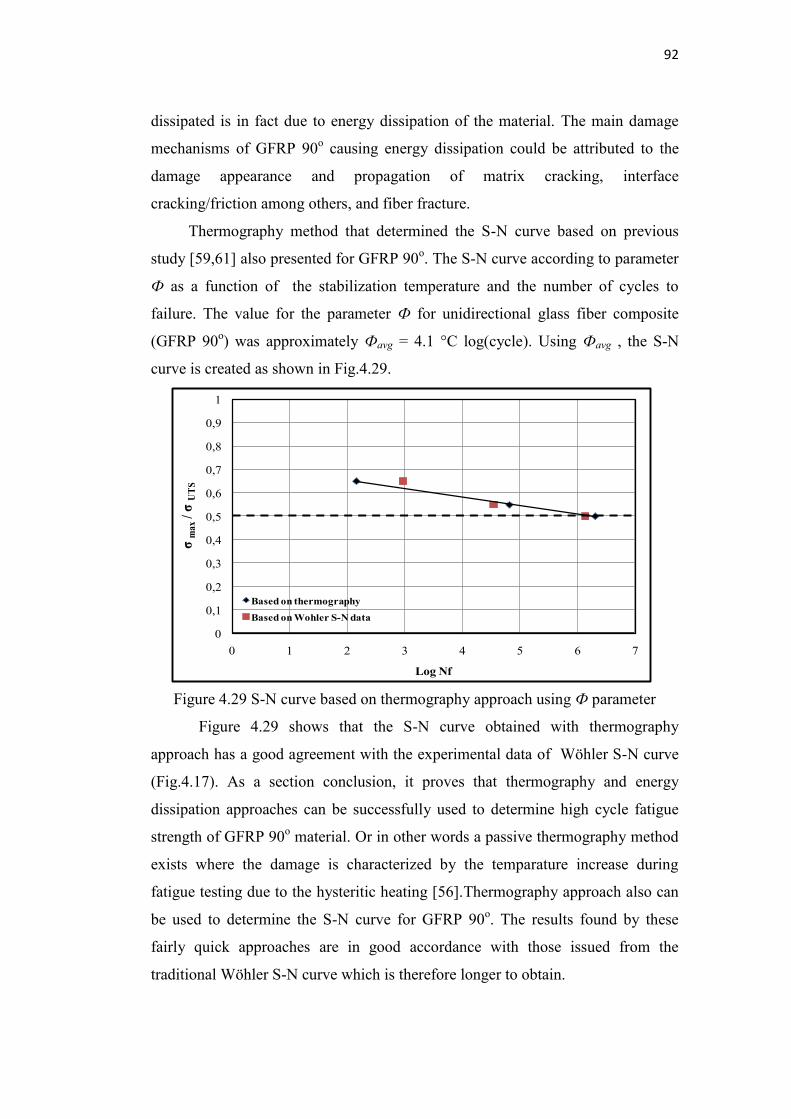
92

dissipated is in fact due to energy dissipation of the material. The main damage

mechanisms of GFRP 90o causing energy dissipation could be attributed to the

damage appearance and propagation of matrix cracking, interface

cracking/friction among others, and fiber fracture.

Thermography method that determined the S-N curve based on previous

study [59,61] also presented for GFRP 90o. The S-N curve according to parameter

Ф as a function of the stabilization temperature and the number of cycles to

failure. The value for the parameter Ф for unidirectional glass fiber composite

(GFRP 90o) was approximately Фavg = 4.1 °C log(cycle). Using Фavg , the S-N

curve is created as shown in Fig.4.29.

Figure 4.29 S-N curve based on thermography approach using Ф parameter

Figure 4.29 shows that the S-N curve obtained with thermography

approach has a good agreement with the experimental data of Wöhler S-N curve

(Fig.4.17). As a section conclusion, it proves that thermography and energy

dissipation approaches can be successfully used to determine high cycle fatigue

strength of GFRP 90o material. Or in other words a passive thermography method

exists where the damage is characterized by the temparature increase during

fatigue testing due to the hysteritic heating [56].Thermography approach also can

be used to determine the S-N curve for GFRP 90o. The results found by these

fairly quick approaches are in good accordance with those issued from the

traditional Wöhler S-N curve which is therefore longer to obtain.

0

0,1

0,2

0,3

0,4

0,5

0,6

0,7

0,8

0,9

1

0 1 2 3 4 5 6 7

σm

ax/ σ

UT

S

Log Nf

Based on thermography

Based on Wohler S-N data

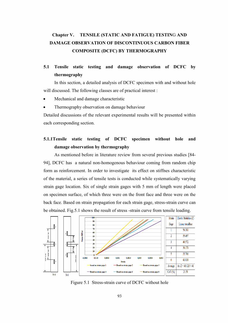
93

Chapter V. TENSILE (STATIC AND FATIGUE) TESTING AND

DAMAGE OBSERVATION OF DISCONTINUOUS CARBON FIBER

COMPOSITE (DCFC) BY THERMOGRAPHY

5.1 Tensile static testing and damage observation of DCFC by

thermography

In this section, a detailed analysis of DCFC specimen with and without hole

will discussed. The following classes are of practical interest :

Mechanical and damage characteristic

Thermography observation on damage behaviour

Detailed discussions of the relevant experimental results will be presented within

each corresponding section.

5.1.1Tensile static testing of DCFC specimen without hole and

damage observation by thermography

As mentioned before in literature review from several previous studies [84-

94], DCFC has a natural non-homogenous behaviour coming from random chip

form as reinforcement. In order to investigate its effect on stiffnes characteristic

of the material, a series of tensile tests is conducted while systematically varying

strain gage location. Six of single strain gages with 5 mm of length were placed

on specimen surface, of which three were on the front face and three were on the

back face. Based on strain propagation for each strain gage, stress-strain curve can

be obtained. Fig.5.1 shows the result of stress -strain curve from tensile loading.

Figure 5.1 Stress-strain curve of DCFC without hole

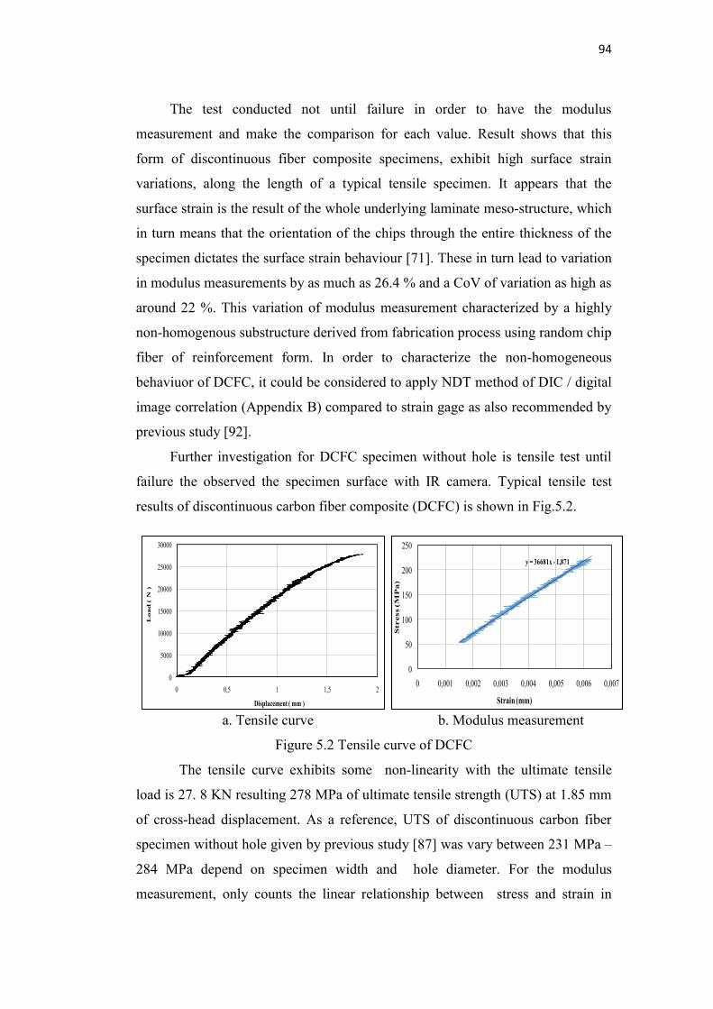
94

The test conducted not until failure in order to have the modulus

measurement and make the comparison for each value. Result shows that this

form of discontinuous fiber composite specimens, exhibit high surface strain

variations, along the length of a typical tensile specimen. It appears that the

surface strain is the result of the whole underlying laminate meso-structure, which

in turn means that the orientation of the chips through the entire thickness of the

specimen dictates the surface strain behaviour [71]. These in turn lead to variation

in modulus measurements by as much as 26.4 % and a CoV of variation as high as

around 22 %. This variation of modulus measurement characterized by a highly

non-homogenous substructure derived from fabrication process using random chip

fiber of reinforcement form. In order to characterize the non-homogeneous

behaviuor of DCFC, it could be considered to apply NDT method of DIC / digital

image correlation (Appendix B) compared to strain gage as also recommended by

previous study [92].

Further investigation for DCFC specimen without hole is tensile test until

failure the observed the specimen surface with IR camera. Typical tensile test

results of discontinuous carbon fiber composite (DCFC) is shown in Fig.5.2.

a. Tensile curve b. Modulus measurement

Figure 5.2 Tensile curve of DCFC

The tensile curve exhibits some non-linearity with the ultimate tensile

load is 27. 8 KN resulting 278 MPa of ultimate tensile strength (UTS) at 1.85 mm

of cross-head displacement. As a reference, UTS of discontinuous carbon fiber

specimen without hole given by previous study [87] was vary between 231 MPa –

284 MPa depend on specimen width and hole diameter. For the modulus

measurement, only counts the linear relationship between stress and strain in

0

5000

10000

15000

20000

25000

30000

0 0,5 1 1,5 2

Load

( N

)

Displacement ( mm )

y = 36681x - 1,871

0

50

100

150

200

250

0 0,001 0,002 0,003 0,004 0,005 0,006 0,007

Str

ess (M

Pa)

Strain (mm)

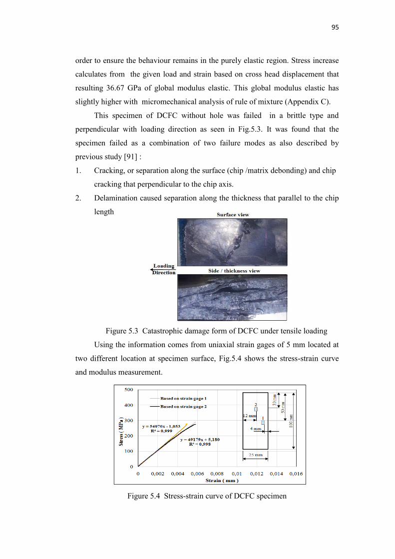
95

order to ensure the behaviour remains in the purely elastic region. Stress increase

calculates from the given load and strain based on cross head displacement that

resulting 36.67 GPa of global modulus elastic. This global modulus elastic has

slightly higher with micromechanical analysis of rule of mixture (Appendix C).

This specimen of DCFC without hole was failed in a brittle type and

perpendicular with loading direction as seen in Fig.5.3. It was found that the

specimen failed as a combination of two failure modes as also described by

previous study [91] :

1. Cracking, or separation along the surface (chip /matrix debonding) and chip

cracking that perpendicular to the chip axis.

2. Delamination caused separation along the thickness that parallel to the chip

length

Figure 5.3 Catastrophic damage form of DCFC under tensile loading

Using the information comes from uniaxial strain gages of 5 mm located at

two different location at specimen surface, Fig.5.4 shows the stress-strain curve

and modulus measurement.

Figure 5.4 Stress-strain curve of DCFC specimen

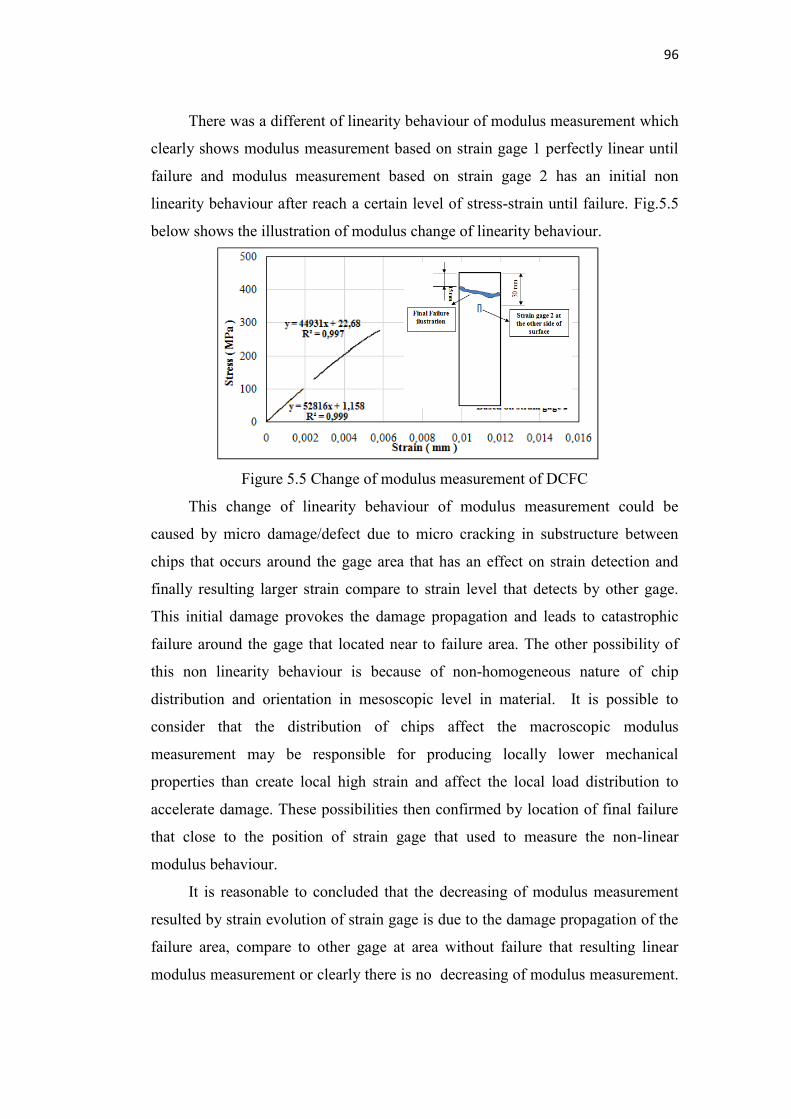
96

There was a different of linearity behaviour of modulus measurement which

clearly shows modulus measurement based on strain gage 1 perfectly linear until

failure and modulus measurement based on strain gage 2 has an initial non

linearity behaviour after reach a certain level of stress-strain until failure. Fig.5.5

below shows the illustration of modulus change of linearity behaviour.

Figure 5.5 Change of modulus measurement of DCFC

This change of linearity behaviour of modulus measurement could be

caused by micro damage/defect due to micro cracking in substructure between

chips that occurs around the gage area that has an effect on strain detection and

finally resulting larger strain compare to strain level that detects by other gage.

This initial damage provokes the damage propagation and leads to catastrophic

failure around the gage that located near to failure area. The other possibility of

this non linearity behaviour is because of non-homogeneous nature of chip

distribution and orientation in mesoscopic level in material. It is possible to

consider that the distribution of chips affect the macroscopic modulus

measurement may be responsible for producing locally lower mechanical

properties than create local high strain and affect the local load distribution to

accelerate damage. These possibilities then confirmed by location of final failure

that close to the position of strain gage that used to measure the non-linear

modulus behaviour.

It is reasonable to concluded that the decreasing of modulus measurement

resulted by strain evolution of strain gage is due to the damage propagation of the

failure area, compare to other gage at area without failure that resulting linear

modulus measurement or clearly there is no decreasing of modulus measurement.

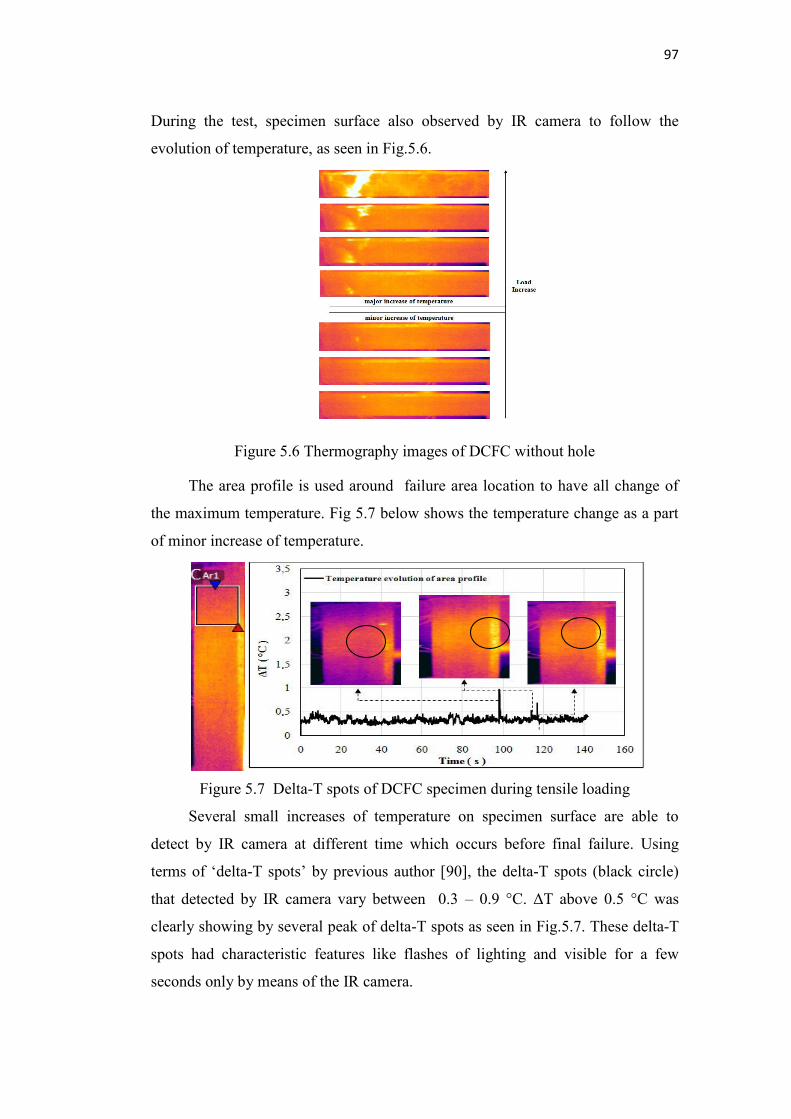
97

During the test, specimen surface also observed by IR camera to follow the

evolution of temperature, as seen in Fig.5.6.

Figure 5.6 Thermography images of DCFC without hole

The area profile is used around failure area location to have all change of

the maximum temperature. Fig 5.7 below shows the temperature change as a part

of minor increase of temperature.

Figure 5.7 Delta-T spots of DCFC specimen during tensile loading

Several small increases of temperature on specimen surface are able to

detect by IR camera at different time which occurs before final failure. Using

terms of ‘delta-T spots’ by previous author [90], the delta-T spots (black circle)

that detected by IR camera vary between 0.3 – 0.9 °C. ΔT above 0.5 °C was

clearly showing by several peak of delta-T spots as seen in Fig.5.7. These delta-T

spots had characteristic features like flashes of lighting and visible for a few

seconds only by means of the IR camera.

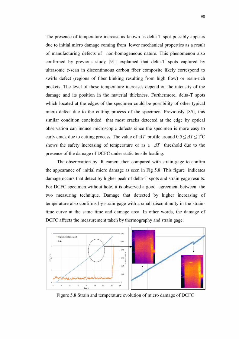
98

The presence of temperature increase as known as delta-T spot possibly appears

due to initial micro damage coming from lower mechanical properties as a result

of manufacturing defects of non-homogeneous nature. This phenomenon also

confirmed by previous study [91] explained that delta-T spots captured by

ultrasonic c-scan in discontinuous carbon fiber composite likely correspond to

swirls defect (regions of fiber kinking resulting from high flow) or resin-rich

pockets. The level of these temperature increases depend on the intensity of the

damage and its position in the material thickness. Furthermore, delta-T spots

which located at the edges of the specimen could be possibility of other typical

micro defect due to the cutting process of the specimen. Previously [85], this

similar condition concluded that most cracks detected at the edge by optical

observation can induce microscopic defects since the specimen is more easy to

early crack due to cutting process. The value of ΔT profile around 0.5 ≤ ΔT ≤ 1oC

shows the safety increasing of temperature or as a ΔT threshold due to the

presence of the damage of DCFC under static tensile loading.

The obserevation by IR camera then compared with strain gage to confim

the appearance of initial micro damage as seen in Fig 5.8. This figure indicates

damage occurs that detect by higher peak of delta-T spots and strain gage results.

For DCFC specimen without hole, it is observed a good agreement between the

two measuring technique. Damage that detected by higher increasing of

temperature also confirms by strain gage with a small discontinuity in the strain-

time curve at the same time and damage area. In other words, the damage of

DCFC affects the measurement taken by thermography and strain gage.

Figure 5.8 Strain and temperature evolution of micro damage of DCFC

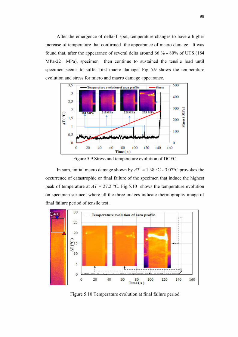
99

After the emergence of delta-T spot, temperature changes to have a higher

increase of temperature that confirmed the appearance of macro damage. It was

found that, after the appearance of several delta around 66 % - 80% of UTS (184

MPa-221 MPa), specimen then continue to sustained the tensile load until

specimen seems to suffer first macro damage. Fig 5.9 shows the temperature

evolution and stress for micro and macro damage appearance.

Figure 5.9 Stress and temperature evolution of DCFC

In sum, initial macro damage shown by ΔT ≈ 1.38 °C - 3.07°C provokes the

occurrence of catastrophic or final failure of the specimen that induce the highest

peak of temperature at ΔT = 27.2 °C. Fig.5.10 shows the temperature evolution

on specimen surface where all the three images indicate thermography image of

final failure period of tensile test .

Figure 5.10 Temperature evolution at final failure period

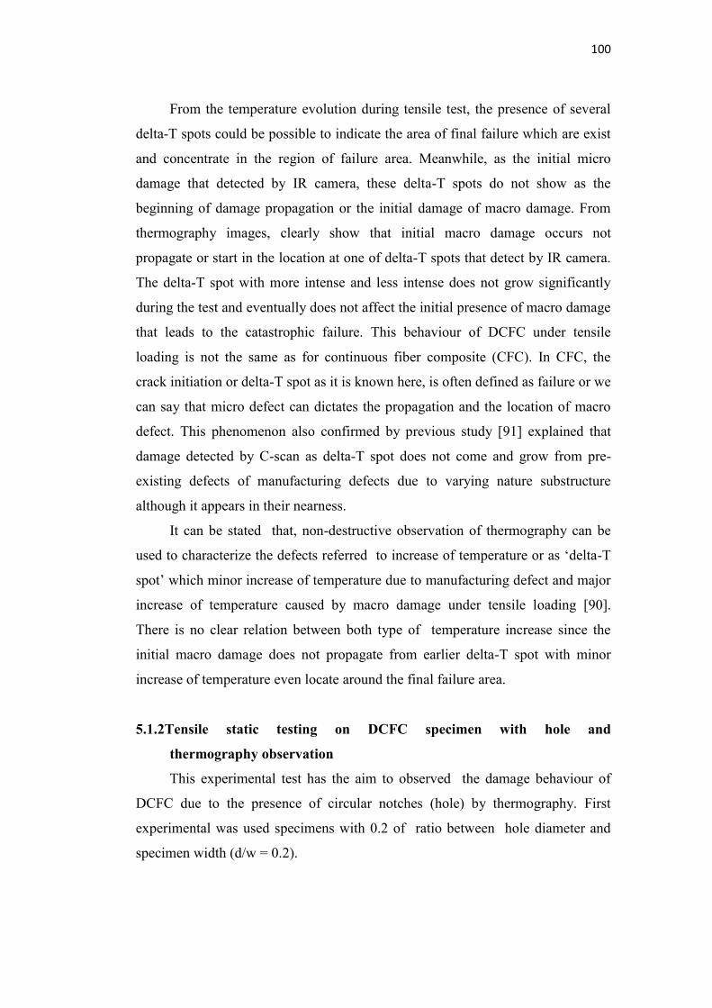
100

From the temperature evolution during tensile test, the presence of several

delta-T spots could be possible to indicate the area of final failure which are exist

and concentrate in the region of failure area. Meanwhile, as the initial micro

damage that detected by IR camera, these delta-T spots do not show as the

beginning of damage propagation or the initial damage of macro damage. From

thermography images, clearly show that initial macro damage occurs not

propagate or start in the location at one of delta-T spots that detect by IR camera.

The delta-T spot with more intense and less intense does not grow significantly

during the test and eventually does not affect the initial presence of macro damage

that leads to the catastrophic failure. This behaviour of DCFC under tensile

loading is not the same as for continuous fiber composite (CFC). In CFC, the

crack initiation or delta-T spot as it is known here, is often defined as failure or we

can say that micro defect can dictates the propagation and the location of macro

defect. This phenomenon also confirmed by previous study [91] explained that

damage detected by C-scan as delta-T spot does not come and grow from pre-

existing defects of manufacturing defects due to varying nature substructure

although it appears in their nearness.

It can be stated that, non-destructive observation of thermography can be

used to characterize the defects referred to increase of temperature or as ‘delta-T

spot’ which minor increase of temperature due to manufacturing defect and major

increase of temperature caused by macro damage under tensile loading [90].

There is no clear relation between both type of temperature increase since the

initial macro damage does not propagate from earlier delta-T spot with minor

increase of temperature even locate around the final failure area.

5.1.2Tensile static testing on DCFC specimen with hole and

thermography observation

This experimental test has the aim to observed the damage behaviour of

DCFC due to the presence of circular notches (hole) by thermography. First

experimental was used specimens with 0.2 of ratio between hole diameter and

specimen width (d/w = 0.2).

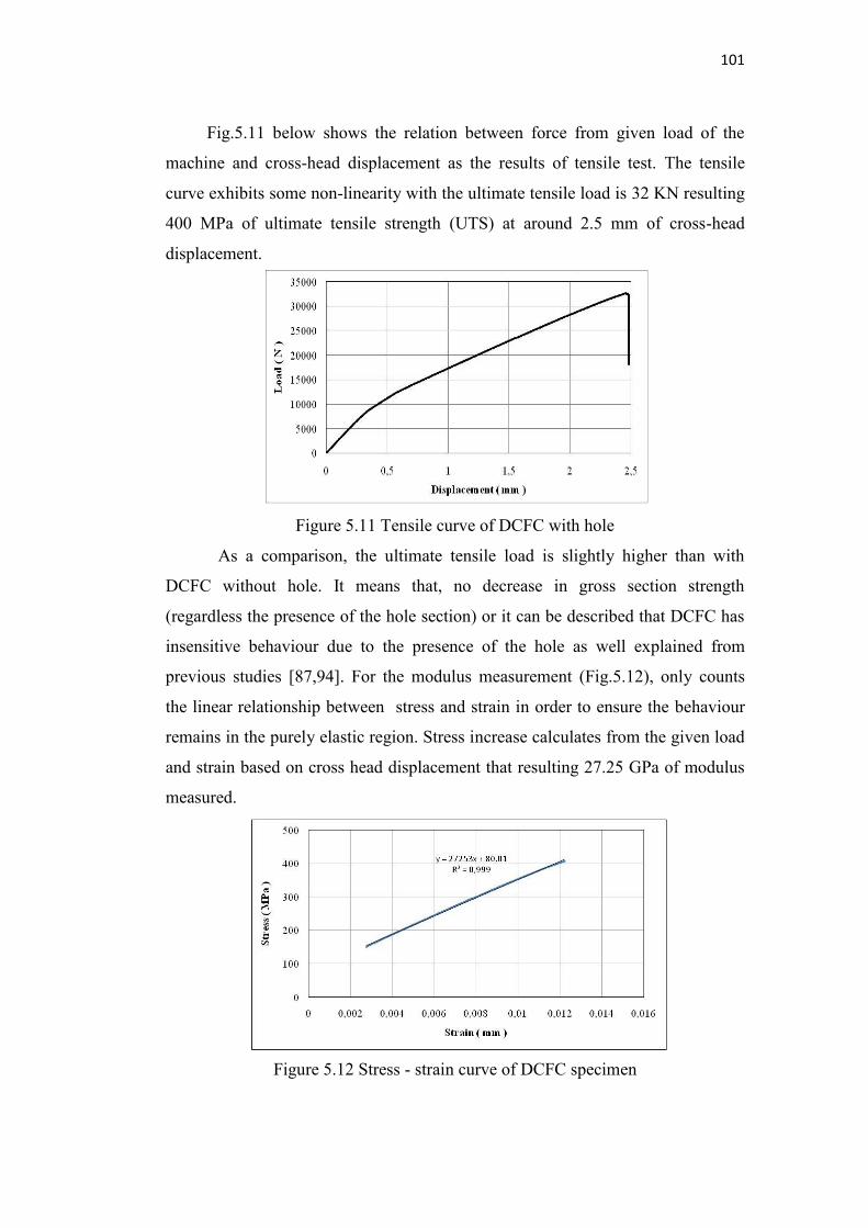
101

Fig.5.11 below shows the relation between force from given load of the

machine and cross-head displacement as the results of tensile test. The tensile

curve exhibits some non-linearity with the ultimate tensile load is 32 KN resulting

400 MPa of ultimate tensile strength (UTS) at around 2.5 mm of cross-head

displacement.

Figure 5.11 Tensile curve of DCFC with hole

As a comparison, the ultimate tensile load is slightly higher than with

DCFC without hole. It means that, no decrease in gross section strength

(regardless the presence of the hole section) or it can be described that DCFC has

insensitive behaviour due to the presence of the hole as well explained from

previous studies [87,94]. For the modulus measurement (Fig.5.12), only counts

the linear relationship between stress and strain in order to ensure the behaviour

remains in the purely elastic region. Stress increase calculates from the given load

and strain based on cross head displacement that resulting 27.25 GPa of modulus

measured.

Figure 5.12 Stress - strain curve of DCFC specimen

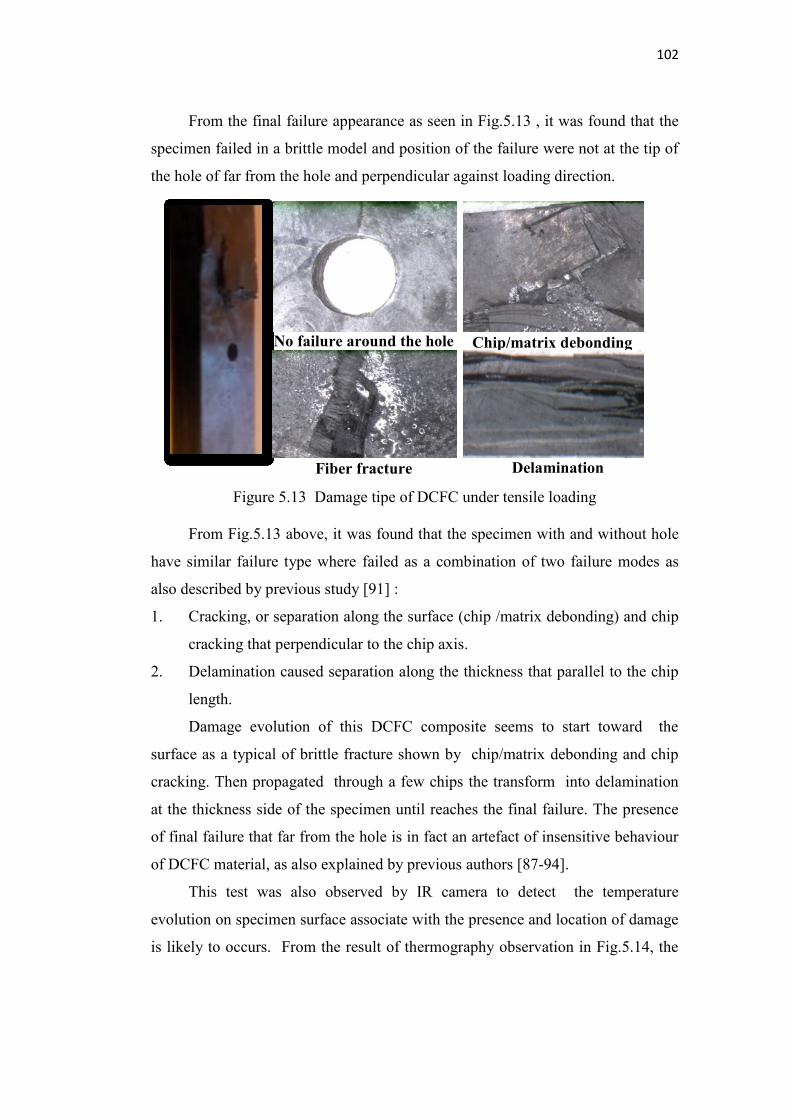
102

From the final failure appearance as seen in Fig.5.13 , it was found that the

specimen failed in a brittle model and position of the failure were not at the tip of

the hole of far from the hole and perpendicular against loading direction.

Figure 5.13 Damage tipe of DCFC under tensile loading

From Fig.5.13 above, it was found that the specimen with and without hole

have similar failure type where failed as a combination of two failure modes as

also described by previous study [91] :

1. Cracking, or separation along the surface (chip /matrix debonding) and chip

cracking that perpendicular to the chip axis.

2. Delamination caused separation along the thickness that parallel to the chip

length.

Damage evolution of this DCFC composite seems to start toward the

surface as a typical of brittle fracture shown by chip/matrix debonding and chip

cracking. Then propagated through a few chips the transform into delamination

at the thickness side of the specimen until reaches the final failure. The presence

of final failure that far from the hole is in fact an artefact of insensitive behaviour

of DCFC material, as also explained by previous authors [87-94].

This test was also observed by IR camera to detect the temperature

evolution on specimen surface associate with the presence and location of damage

is likely to occurs. From the result of thermography observation in Fig.5.14, the

No failure around the hole Chip/matrix debonding

Fiber fracture Delamination

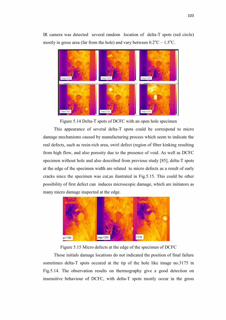
103

IR camera was detected several random location of delta-T spots (red circle)

mostly in gross area (far from the hole) and vary between 0.2oC – 1.5oC.

Figure 5.14 Delta-T spots of DCFC with an open hole specimen

This appearance of several delta-T spots could be correspond to micro

damage mechanisms caused by manufacturing process which seem to indicate the

real defects, such as resin-rich area, swirl defect (region of fiber kinking resulting

from high flow, and also porosity due to the presence of void. As well as DCFC

specimen without hole and also described from previous study [85], delta-T spots

at the edge of the specimen width are related to micro defects as a result of early

cracks since the specimen was cut,as ilustrated in Fig.5.15. This could be other

possibility of first defect can induces microscopic damage, which are initiators as

many micro damage inspected at the edge.

Figure 5.15 Micro defects at the edge of the specimen of DCFC

Those initials damage locations do not indicated the position of final failure

sometimes delta-T spots occured at the tip of the hole like image no.3175 in

Fig.5.14. The observation results on thermography give a good detection on

insensitive behaviour of DCFC, with delta-T spots mostly occur in the gross

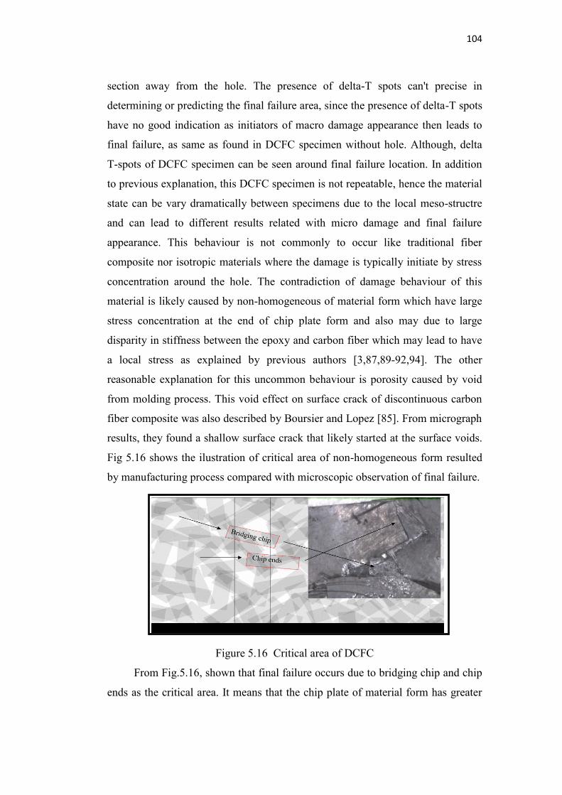
104

section away from the hole. The presence of delta-T spots can't precise in

determining or predicting the final failure area, since the presence of delta-T spots

have no good indication as initiators of macro damage appearance then leads to

final failure, as same as found in DCFC specimen without hole. Although, delta

T-spots of DCFC specimen can be seen around final failure location. In addition

to previous explanation, this DCFC specimen is not repeatable, hence the material

state can be vary dramatically between specimens due to the local meso-structre

and can lead to different results related with micro damage and final failure

appearance. This behaviour is not commonly to occur like traditional fiber

composite nor isotropic materials where the damage is typically initiate by stress

concentration around the hole. The contradiction of damage behaviour of this

material is likely caused by non-homogeneous of material form which have large

stress concentration at the end of chip plate form and also may due to large

disparity in stiffness between the epoxy and carbon fiber which may lead to have

a local stress as explained by previous authors [3,87,89-92,94]. The other

reasonable explanation for this uncommon behaviour is porosity caused by void

from molding process. This void effect on surface crack of discontinuous carbon

fiber composite was also described by Boursier and Lopez [85]. From micrograph

results, they found a shallow surface crack that likely started at the surface voids.

Fig 5.16 shows the ilustration of critical area of non-homogeneous form resulted

by manufacturing process compared with microscopic observation of final failure.

Figure 5.16 Critical area of DCFC

From Fig.5.16, shown that final failure occurs due to bridging chip and chip

ends as the critical area. It means that the chip plate of material form has greater

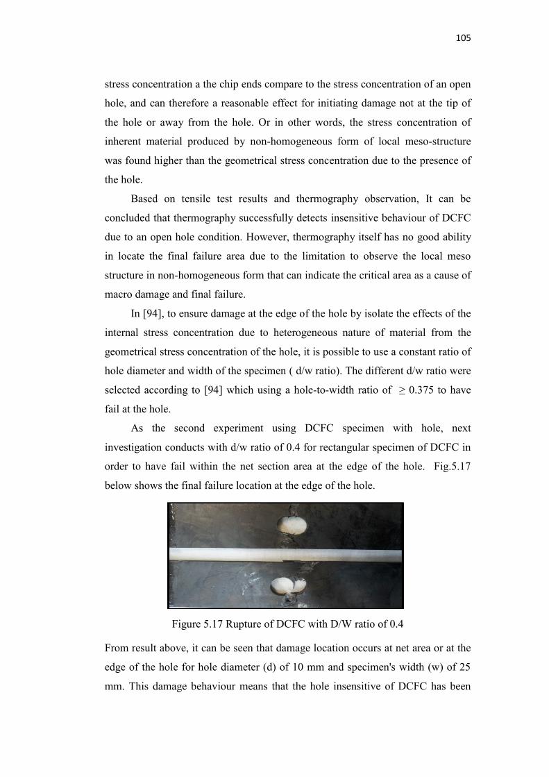
105

stress concentration a the chip ends compare to the stress concentration of an open

hole, and can therefore a reasonable effect for initiating damage not at the tip of

the hole or away from the hole. Or in other words, the stress concentration of

inherent material produced by non-homogeneous form of local meso-structure

was found higher than the geometrical stress concentration due to the presence of

the hole.

Based on tensile test results and thermography observation, It can be

concluded that thermography successfully detects insensitive behaviour of DCFC

due to an open hole condition. However, thermography itself has no good ability

in locate the final failure area due to the limitation to observe the local meso

structure in non-homogeneous form that can indicate the critical area as a cause of

macro damage and final failure.

In [94], to ensure damage at the edge of the hole by isolate the effects of the

internal stress concentration due to heterogeneous nature of material from the

geometrical stress concentration of the hole, it is possible to use a constant ratio of

hole diameter and width of the specimen ( d/w ratio). The different d/w ratio were

selected according to [94] which using a hole-to-width ratio of ≥ 0.375 to have

fail at the hole.

As the second experiment using DCFC specimen with hole, next

investigation conducts with d/w ratio of 0.4 for rectangular specimen of DCFC in

order to have fail within the net section area at the edge of the hole. Fig.5.17

below shows the final failure location at the edge of the hole.

Figure 5.17 Rupture of DCFC with D/W ratio of 0.4

From result above, it can be seen that damage location occurs at net area or at the

edge of the hole for hole diameter (d) of 10 mm and specimen's width (w) of 25

mm. This damage behaviour means that the hole insensitive of DCFC has been

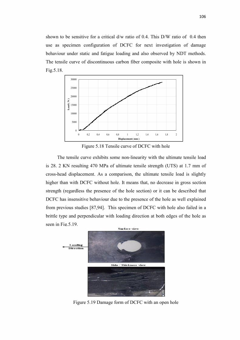
106

shown to be sensitive for a critical d/w ratio of 0.4. This D/W ratio of 0.4 then

use as specimen configuration of DCFC for next investigation of damage

behaviour under static and fatigue loading and also observed by NDT methods.

The tensile curve of discontinuous carbon fiber composite with hole is shown in

Fig.5.18.

Figure 5.18 Tensile curve of DCFC with hole

The tensile curve exhibits some non-linearity with the ultimate tensile load

is 28. 2 KN resulting 470 MPa of ultimate tensile strength (UTS) at 1.7 mm of

cross-head displacement. As a comparison, the ultimate tensile load is slightly

higher than with DCFC without hole. It means that, no decrease in gross section

strength (regardless the presence of the hole section) or it can be described that

DCFC has insensitive behaviour due to the presence of the hole as well explained

from previous studies [87,94]. This specimen of DCFC with hole also failed in a

brittle type and perpendicular with loading direction at both edges of the hole as

seen in Fig.5.19.

Figure 5.19 Damage form of DCFC with an open hole

0

5000

10000

15000

20000

25000

30000

0 0,2 0,4 0,6 0,8 1 1,2 1,4 1,6 1,8 2

Lo

ad

( N

)

Displacement ( mm )

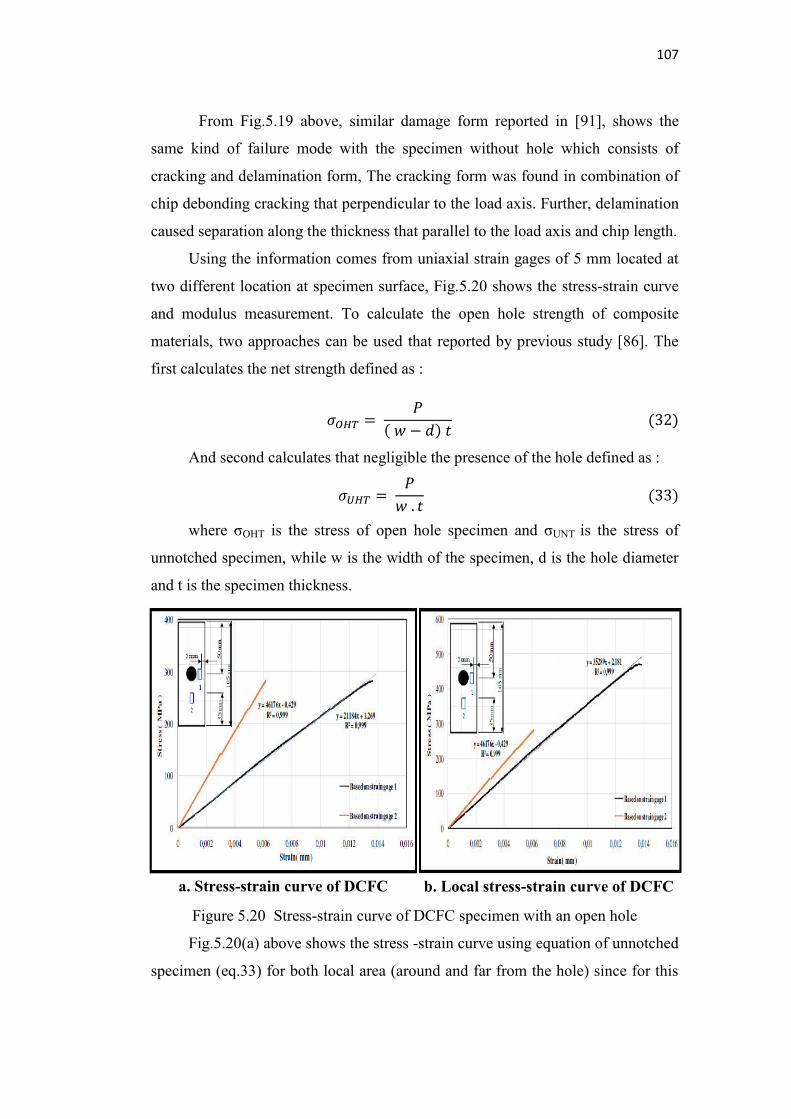
107

From Fig.5.19 above, similar damage form reported in [91], shows the

same kind of failure mode with the specimen without hole which consists of

cracking and delamination form, The cracking form was found in combination of

chip debonding cracking that perpendicular to the load axis. Further, delamination

caused separation along the thickness that parallel to the load axis and chip length.

Using the information comes from uniaxial strain gages of 5 mm located at

two different location at specimen surface, Fig.5.20 shows the stress-strain curve

and modulus measurement. To calculate the open hole strength of composite

materials, two approaches can be used that reported by previous study [86]. The

first calculates the net strength defined as :

And second calculates that negligible the presence of the hole defined as :

where σOHT is the stress of open hole specimen and σUNT is the stress of

unnotched specimen, while w is the width of the specimen, d is the hole diameter

and t is the specimen thickness.

Figure 5.20 Stress-strain curve of DCFC specimen with an open hole

Fig.5.20(a) above shows the stress -strain curve using equation of unnotched

specimen (eq.33) for both local area (around and far from the hole) since for this

a. Stress-strain curve of DCFC b. Local stress-strain curve of DCFC

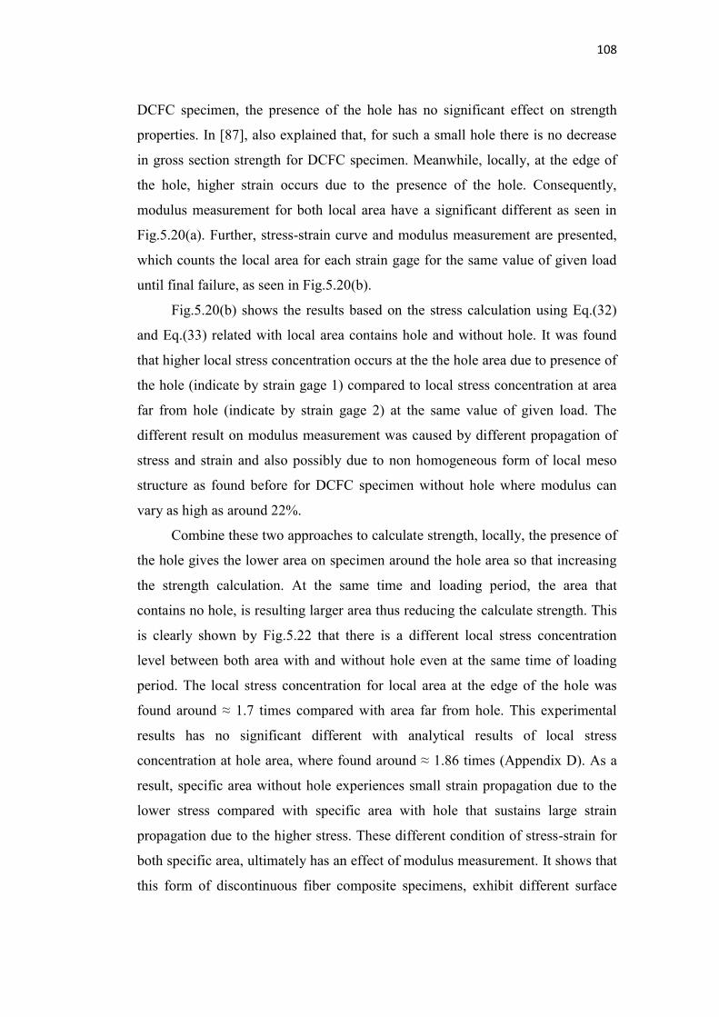
108

DCFC specimen, the presence of the hole has no significant effect on strength

properties. In [87], also explained that, for such a small hole there is no decrease

in gross section strength for DCFC specimen. Meanwhile, locally, at the edge of

the hole, higher strain occurs due to the presence of the hole. Consequently,

modulus measurement for both local area have a significant different as seen in

Fig.5.20(a). Further, stress-strain curve and modulus measurement are presented,

which counts the local area for each strain gage for the same value of given load

until final failure, as seen in Fig.5.20(b).

Fig.5.20(b) shows the results based on the stress calculation using Eq.(32)

and Eq.(33) related with local area contains hole and without hole. It was found

that higher local stress concentration occurs at the the hole area due to presence of

the hole (indicate by strain gage 1) compared to local stress concentration at area

far from hole (indicate by strain gage 2) at the same value of given load. The

different result on modulus measurement was caused by different propagation of

stress and strain and also possibly due to non homogeneous form of local meso

structure as found before for DCFC specimen without hole where modulus can

vary as high as around 22%.

Combine these two approaches to calculate strength, locally, the presence of

the hole gives the lower area on specimen around the hole area so that increasing

the strength calculation. At the same time and loading period, the area that

contains no hole, is resulting larger area thus reducing the calculate strength. This

is clearly shown by Fig.5.22 that there is a different local stress concentration

level between both area with and without hole even at the same time of loading

period. The local stress concentration for local area at the edge of the hole was

found around ≈ 1.7 times compared with area far from hole. This experimental

results has no significant different with analytical results of local stress

concentration at hole area, where found around ≈ 1.86 times (Appendix D). As a

result, specific area without hole experiences small strain propagation due to the

lower stress compared with specific area with hole that sustains large strain

propagation due to the higher stress. These different condition of stress-strain for

both specific area, ultimately has an effect of modulus measurement. It shows that

this form of discontinuous fiber composite specimens, exhibit different surface

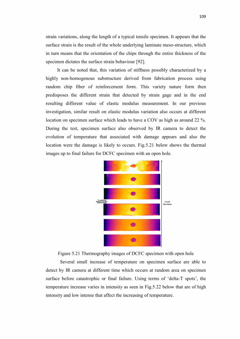
109

strain variations, along the length of a typical tensile specimen. It appears that the

surface strain is the result of the whole underlying laminate meso-structure, which

in turn means that the orientation of the chips through the entire thickness of the

specimen dictates the surface strain behaviour [92].

It can be noted that, this variation of stiffness possibly characterized by a

highly non-homogenous substructure derived from fabrication process using

random chip fiber of reinforcement form. This variety nature form then

predisposes the different strain that detected by strain gage and in the end

resulting different value of elastic modulus measurement. In our previous

investigation, similar result on elastic modulus variation also occurs at different

location on specimen surface which leads to have a COV as high as around 22 %.

During the test, specimen surface also observed by IR camera to detect the

evolution of temperature that associated with damage appears and also the

location were the damage is likely to occurs. Fig.5.21 below shows the thermal

images up to final failure for DCFC specimen with an open hole.

Figure 5.21 Thermography images of DCFC specimen with open hole

Several small increase of temperature on specimen surface are able to

detect by IR camera at different time which occurs at random area on specimen

surface before catastrophic or final failure. Using terms of ‘delta-T spots’, the

temperature increase varies in intensity as seen in Fig.5.22 below that are of high

intensity and low intense that affect the increasing of temperature.

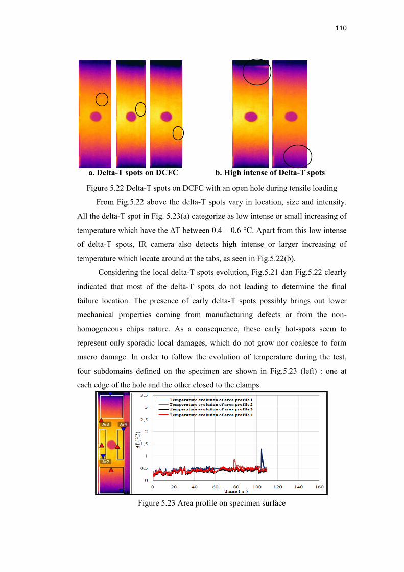
110

Figure 5.22 Delta-T spots on DCFC with an open hole during tensile loading

From Fig.5.22 above the delta-T spots vary in location, size and intensity.

All the delta-T spot in Fig. 5.23(a) categorize as low intense or small increasing of

temperature which have the ΔT between 0.4 – 0.6 °C. Apart from this low intense

of delta-T spots, IR camera also detects high intense or larger increasing of

temperature which locate around at the tabs, as seen in Fig.5.22(b).

Considering the local delta-T spots evolution, Fig.5.21 dan Fig.5.22 clearly

indicated that most of the delta-T spots do not leading to determine the final

failure location. The presence of early delta-T spots possibly brings out lower

mechanical properties coming from manufacturing defects or from the non-

homogeneous chips nature. As a consequence, these early hot-spots seem to

represent only sporadic local damages, which do not grow nor coalesce to form

macro damage. In order to follow the evolution of temperature during the test,

four subdomains defined on the specimen are shown in Fig.5.23 (left) : one at

each edge of the hole and the other closed to the clamps.

Figure 5.23 Area profile on specimen surface

a. Delta-T spots on DCFC b. High intense of Delta-T spots

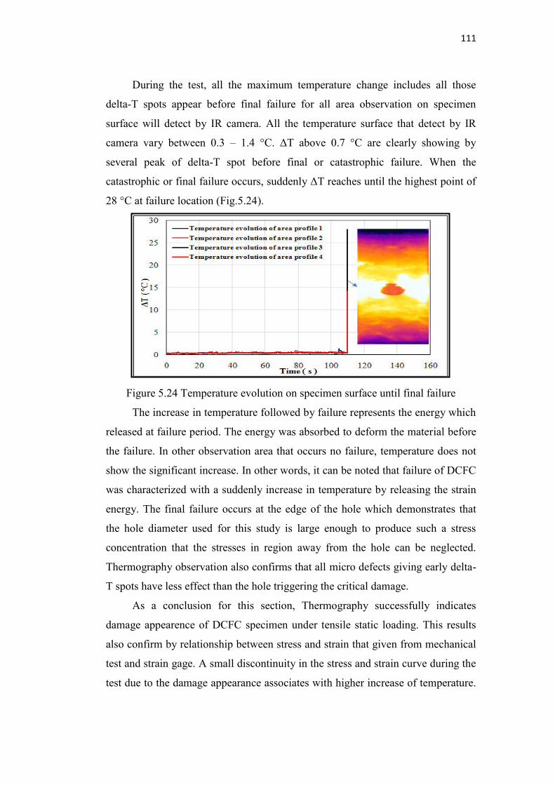
111

During the test, all the maximum temperature change includes all those

delta-T spots appear before final failure for all area observation on specimen

surface will detect by IR camera. All the temperature surface that detect by IR

camera vary between 0.3 – 1.4 °C. ΔT above 0.7 °C are clearly showing by

several peak of delta-T spot before final or catastrophic failure. When the

catastrophic or final failure occurs, suddenly ΔT reaches until the highest point of

28 °C at failure location (Fig.5.24).

Figure 5.24 Temperature evolution on specimen surface until final failure

The increase in temperature followed by failure represents the energy which

released at failure period. The energy was absorbed to deform the material before

the failure. In other observation area that occurs no failure, temperature does not

show the significant increase. In other words, it can be noted that failure of DCFC

was characterized with a suddenly increase in temperature by releasing the strain

energy. The final failure occurs at the edge of the hole which demonstrates that

the hole diameter used for this study is large enough to produce such a stress

concentration that the stresses in region away from the hole can be neglected.

Thermography observation also confirms that all micro defects giving early delta-

T spots have less effect than the hole triggering the critical damage.

As a conclusion for this section, Thermography successfully indicates

damage appearence of DCFC specimen under tensile static loading. This results

also confirm by relationship between stress and strain that given from mechanical

test and strain gage. A small discontinuity in the stress and strain curve during the

test due to the damage appearance associates with higher increase of temperature.

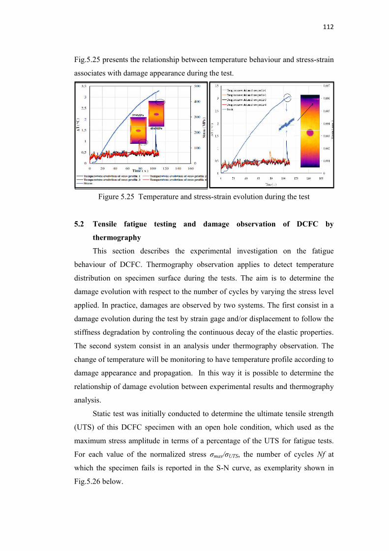
112

Fig.5.25 presents the relationship between temperature behaviour and stress-strain

associates with damage appearance during the test.

Figure 5.25 Temperature and stress-strain evolution during the test

5.2 Tensile fatigue testing and damage observation of DCFC by

thermography

This section describes the experimental investigation on the fatigue

behaviour of DCFC. Thermography observation applies to detect temperature

distribution on specimen surface during the tests. The aim is to determine the

damage evolution with respect to the number of cycles by varying the stress level

applied. In practice, damages are observed by two systems. The first consist in a

damage evolution during the test by strain gage and/or displacement to follow the

stiffness degradation by controling the continuous decay of the elastic properties.

The second system consist in an analysis under thermography observation. The

change of temperature will be monitoring to have temperature profile according to

damage appearance and propagation. In this way it is possible to determine the

relationship of damage evolution between experimental results and thermography

analysis.

Static test was initially conducted to determine the ultimate tensile strength

(UTS) of this DCFC specimen with an open hole condition, which used as the

maximum stress amplitude in terms of a percentage of the UTS for fatigue tests.

For each value of the normalized stress σmax/σUTS, the number of cycles Nf at

which the specimen fails is reported in the S-N curve, as exemplarity shown in

Fig.5.26 below.

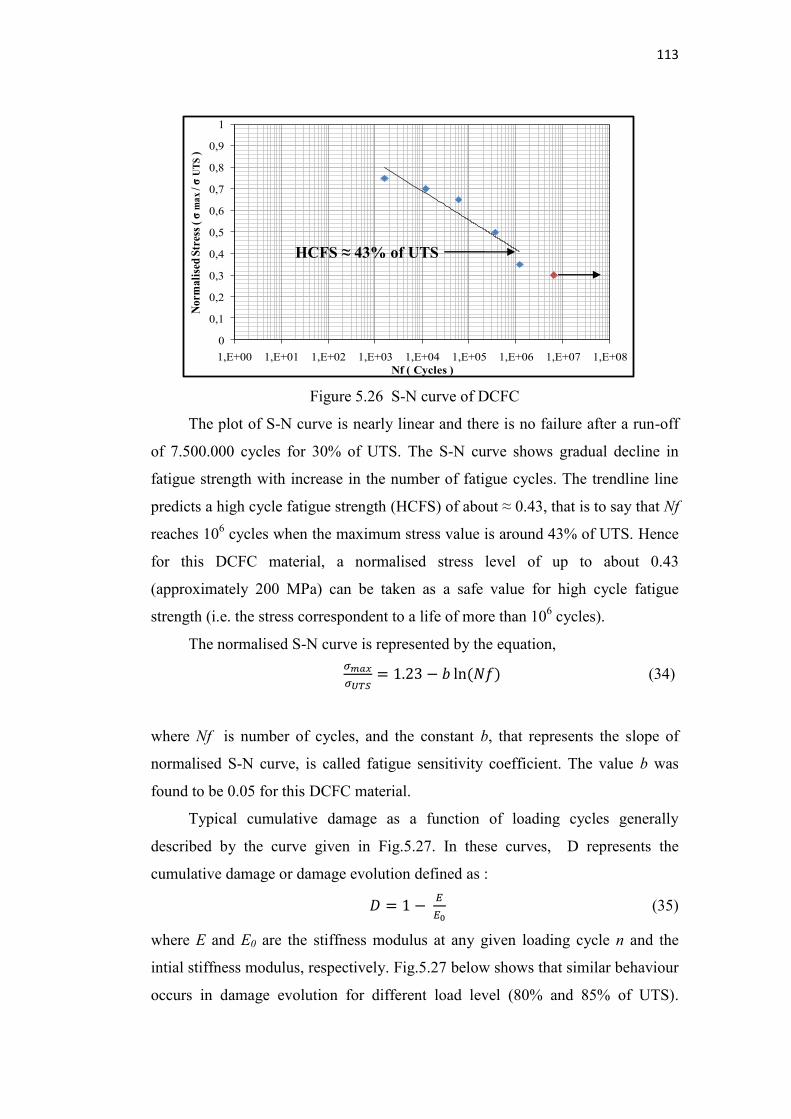
113

Figure 5.26 S-N curve of DCFC

The plot of S-N curve is nearly linear and there is no failure after a run-off

of 7.500.000 cycles for 30% of UTS. The S-N curve shows gradual decline in

fatigue strength with increase in the number of fatigue cycles. The trendline line

predicts a high cycle fatigue strength (HCFS) of about ≈ 0.43, that is to say that Nf

reaches 106 cycles when the maximum stress value is around 43% of UTS. Hence

for this DCFC material, a normalised stress level of up to about 0.43

(approximately 200 MPa) can be taken as a safe value for high cycle fatigue

strength (i.e. the stress correspondent to a life of more than 106 cycles).

The normalised S-N curve is represented by the equation, (34)

where Nf is number of cycles, and the constant b, that represents the slope of

normalised S-N curve, is called fatigue sensitivity coefficient. The value b was

found to be 0.05 for this DCFC material.

Typical cumulative damage as a function of loading cycles generally

described by the curve given in Fig.5.27. In these curves, D represents the

cumulative damage or damage evolution defined as : (35)

where E and E0 are the stiffness modulus at any given loading cycle n and the

intial stiffness modulus, respectively. Fig.5.27 below shows that similar behaviour

occurs in damage evolution for different load level (80% and 85% of UTS).

0

0,1

0,2

0,3

0,4

0,5

0,6

0,7

0,8

0,9

1

1,E+00 1,E+01 1,E+02 1,E+03 1,E+04 1,E+05 1,E+06 1,E+07 1,E+08

Nor

mal

ised

Str

ess

( σm

ax /

σU

TS

)

Nf ( Cycles )

HCFS ≈ 43% of UTS

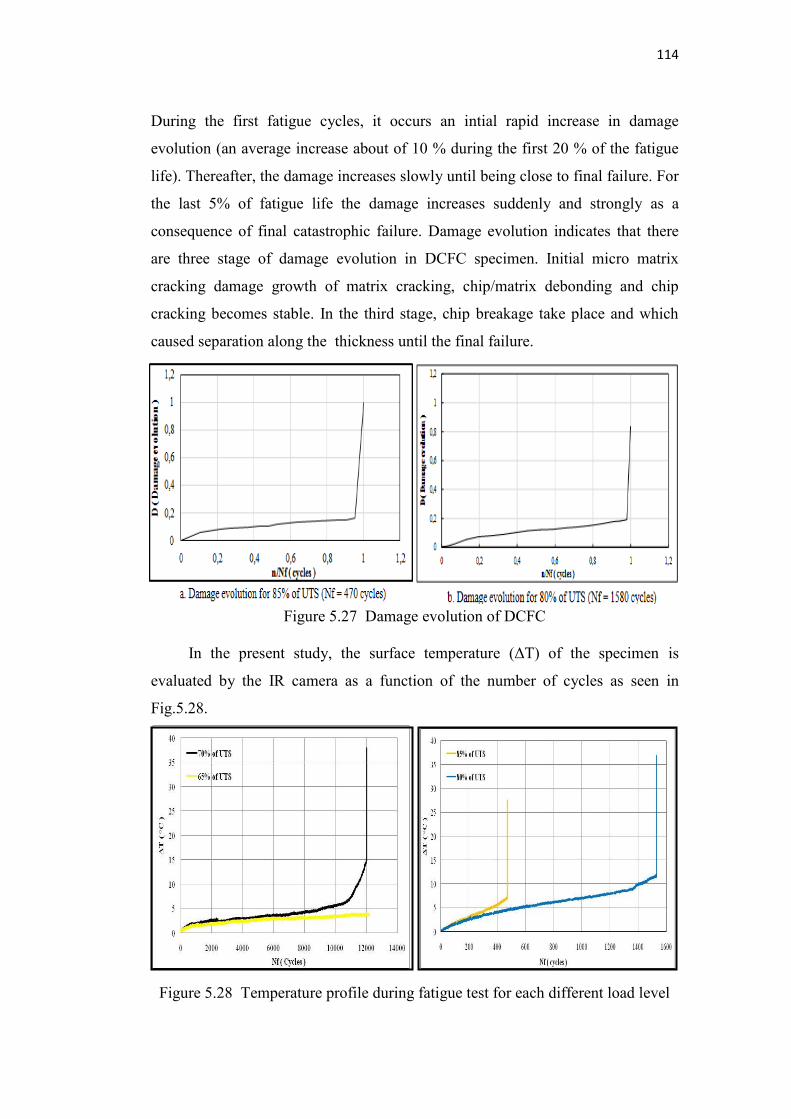
114

During the first fatigue cycles, it occurs an intial rapid increase in damage

evolution (an average increase about of 10 % during the first 20 % of the fatigue

life). Thereafter, the damage increases slowly until being close to final failure. For

the last 5% of fatigue life the damage increases suddenly and strongly as a

consequence of final catastrophic failure. Damage evolution indicates that there

are three stage of damage evolution in DCFC specimen. Initial micro matrix

cracking damage growth of matrix cracking, chip/matrix debonding and chip

cracking becomes stable. In the third stage, chip breakage take place and which

caused separation along the thickness until the final failure.

Figure 5.27 Damage evolution of DCFC

In the present study, the surface temperature (ΔT) of the specimen is

evaluated by the IR camera as a function of the number of cycles as seen in

Fig.5.28.

Figure 5.28 Temperature profile during fatigue test for each different load level

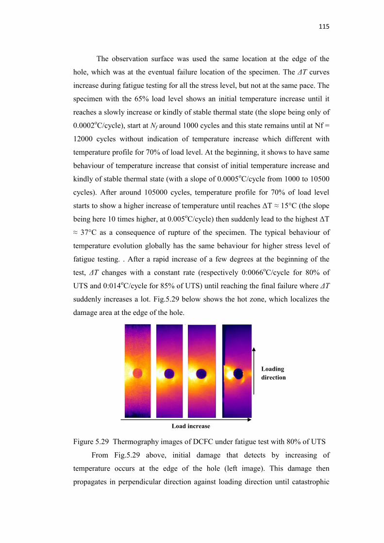
115

The observation surface was used the same location at the edge of the

hole, which was at the eventual failure location of the specimen. The ΔT curves

increase during fatigue testing for all the stress level, but not at the same pace. The

specimen with the 65% load level shows an initial temperature increase until it

reaches a slowly increase or kindly of stable thermal state (the slope being only of

0.0002oC/cycle), start at Nf around 1000 cycles and this state remains until at Nf =

12000 cycles without indication of temperature increase which different with

temperature profile for 70% of load level. At the beginning, it shows to have same

behaviour of temperature increase that consist of initial temperature increase and

kindly of stable thermal state (with a slope of 0.0005oC/cycle from 1000 to 10500

cycles). After around 105000 cycles, temperature profile for 70% of load level

starts to show a higher increase of temperature until reaches ΔT ≈ 15°C (the slope

being here 10 times higher, at 0.005oC/cycle) then suddenly lead to the highest ΔT

≈ 37°C as a consequence of rupture of the specimen. The typical behaviour of

temperature evolution globally has the same behaviour for higher stress level of

fatigue testing. . After a rapid increase of a few degrees at the beginning of the

test, ΔT changes with a constant rate (respectively 0:0066oC/cycle for 80% of

UTS and 0:014oC/cycle for 85% of UTS) until reaching the final failure where ΔT

suddenly increases a lot. Fig.5.29 below shows the hot zone, which localizes the

damage area at the edge of the hole.

Figure 5.29 Thermography images of DCFC under fatigue test with 80% of UTS

From Fig.5.29 above, initial damage that detects by increasing of

temperature occurs at the edge of the hole (left image). This damage then

propagates in perpendicular direction against loading direction until catastrophic

Load increase

Loading direction

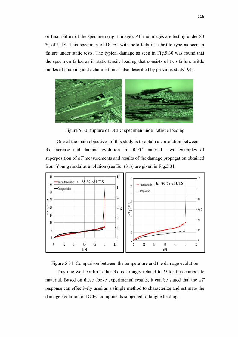
116

or final failure of the specimen (right image). All the images are testing under 80

% of UTS. This specimen of DCFC with hole fails in a brittle type as seen in

failure under static tests. The typical damage as seen in Fig.5.30 was found that

the specimen failed as in static tensile loading that consists of two failure brittle

modes of cracking and delamination as also described by previous study [91].

Figure 5.30 Rupture of DCFC specimen under fatigue loading

One of the main objectives of this study is to obtain a correlation between

ΔT increase and damage evolution in DCFC material. Two examples of

superposition of ΔT measurements and results of the damage propagation obtained

from Young modulus evolution (see Eq. (31)) are given in Fig.5.31.

Figure 5.31 Comparison between the temperature and the damage evolution

This one well confirms that ΔT is strongly related to D for this composite

material. Based on these above experimental results, it can be stated that the ΔT

response can effectively used as a simple method to characterize and estimate the

damage evolution of DCFC components subjected to fatigue loading.

a. 85 % of UTS b. 80 % of UTS

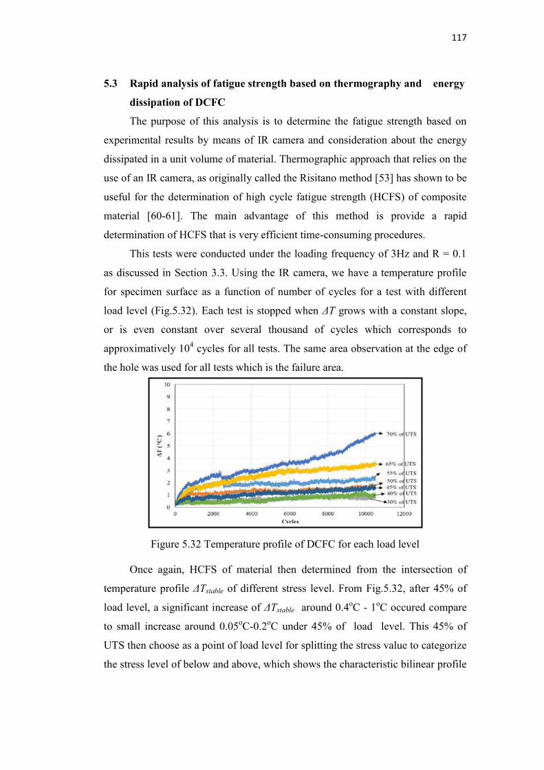
117

5.3 Rapid analysis of fatigue strength based on thermography and energy

dissipation of DCFC

The purpose of this analysis is to determine the fatigue strength based on

experimental results by means of IR camera and consideration about the energy

dissipated in a unit volume of material. Thermographic approach that relies on the

use of an IR camera, as originally called the Risitano method [53] has shown to be

useful for the determination of high cycle fatigue strength (HCFS) of composite

material [60-61]. The main advantage of this method is provide a rapid

determination of HCFS that is very efficient time-consuming procedures.

This tests were conducted under the loading frequency of 3Hz and R = 0.1

as discussed in Section 3.3. Using the IR camera, we have a temperature profile

for specimen surface as a function of number of cycles for a test with different

load level (Fig.5.32). Each test is stopped when ΔT grows with a constant slope,

or is even constant over several thousand of cycles which corresponds to

approximatively 104 cycles for all tests. The same area observation at the edge of

the hole was used for all tests which is the failure area.

Figure 5.32 Temperature profile of DCFC for each load level

Once again, HCFS of material then determined from the intersection of

temperature profile ΔTstable of different stress level. From Fig.5.32, after 45% of

load level, a significant increase of ΔTstable around 0.4oC - 1oC occured compare

to small increase around 0.05oC-0.2oC under 45% of load level. This 45% of

UTS then choose as a point of load level for splitting the stress value to categorize

the stress level of below and above, which shows the characteristic bilinear profile

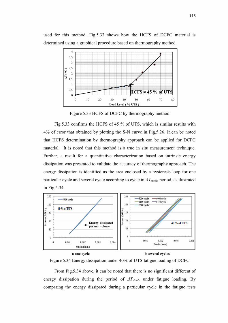
118

used for this method. Fig.5.33 shows how the HCFS of DCFC material is

determined using a graphical procedure based on thermography method.

Figure 5.33 HCFS of DCFC by thermography method

Fig.5.33 confirms the HCFS of 45 % of UTS, which is similar results with

4% of error that obtained by plotting the S-N curve in Fig.5.26. It can be noted

that HCFS determination by thermography approach can be applied for DCFC

material. It is noted that this method is a true in situ measurement technique.

Further, a result for a quantitative characterization based on intrinsic energy

dissipation was presented to validate the accuracy of thermography approach. The

energy dissipation is identified as the area enclosed by a hysteresis loop for one

particular cycle and several cycle according to cycle in ΔTstable period, as ilustrated

in Fig.5.34.

Figure 5.34 Energy dissipation under 40% of UTS fatigue loading of DCFC

From Fig.5.34 above, it can be noted that there is no significant different of

energy dissipation during the period of ΔTstable under fatigue loading. By

comparing the energy dissipated during a particular cycle in the fatigue tests

Energy dissipated per unit volume

a one cycle b several cycles

0

0,5

1

1,5

2

2,5

3

3,5

4

0 10 20 30 40 50 60 70 80

ΔT (

o C )

Load Level ( % UTS )

HCFS ≈ 45 % of UTS

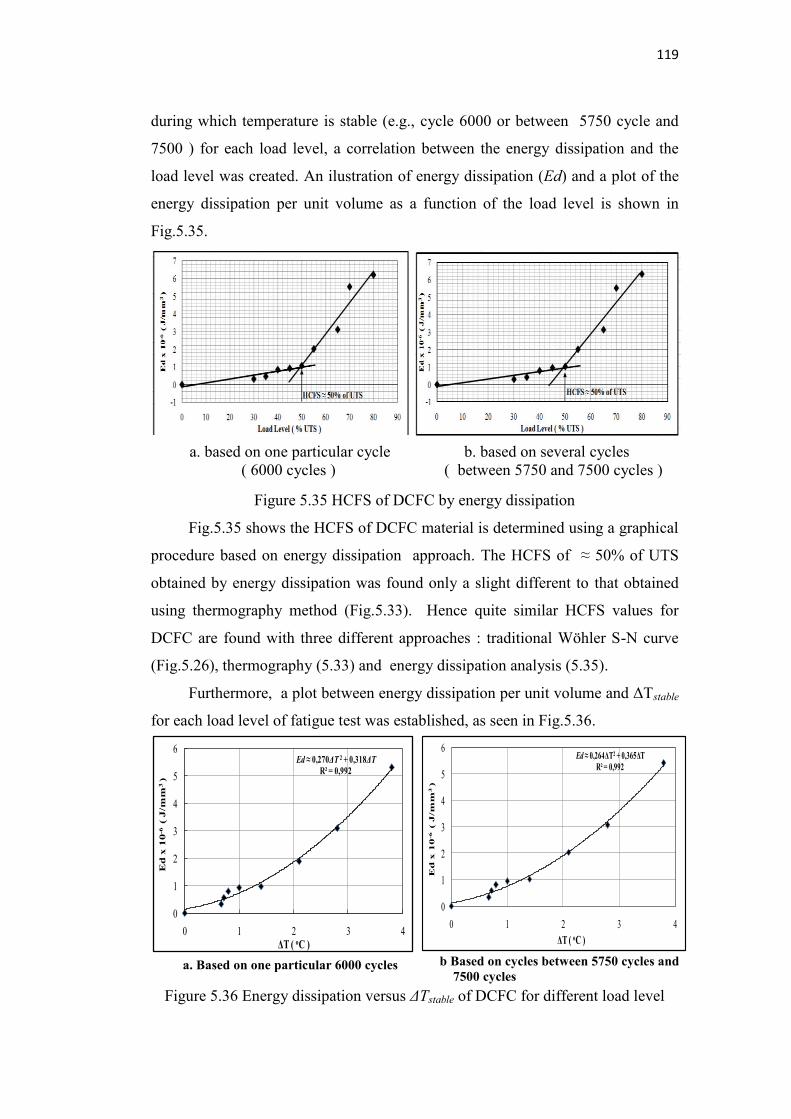
119

during which temperature is stable (e.g., cycle 6000 or between 5750 cycle and

7500 ) for each load level, a correlation between the energy dissipation and the

load level was created. An ilustration of energy dissipation (Ed) and a plot of the

energy dissipation per unit volume as a function of the load level is shown in

Fig.5.35.

Figure 5.35 HCFS of DCFC by energy dissipation

Fig.5.35 shows the HCFS of DCFC material is determined using a graphical

procedure based on energy dissipation approach. The HCFS of ≈ 50% of UTS

obtained by energy dissipation was found only a slight different to that obtained

using thermography method (Fig.5.33). Hence quite similar HCFS values for

DCFC are found with three different approaches : traditional Wöhler S-N curve

(Fig.5.26), thermography (5.33) and energy dissipation analysis (5.35).

Furthermore, a plot between energy dissipation per unit volume and ΔTstable

for each load level of fatigue test was established, as seen in Fig.5.36.

Figure 5.36 Energy dissipation versus ΔTstable of DCFC for different load level

a. based on one particular cycle ( 6000 cycles )

b. based on several cycles ( between 5750 and 7500 cycles ) ( 6000 cycles )

b Based on cycles between 5750 cycles and 7500 cycles

a. Based on one particular 6000 cycles

Ed ≈ 0,264ΔT2 + 0,365ΔTR² = 0,992

0

1

2

3

4

5

6

0 1 2 3 4

Ed

x 1

0-6

( J/m

m3

)

ΔT ( oC )

Ed ≈ 0,270ΔT 2 + 0,318ΔT

R² = 0,992

0

1

2

3

4

5

6

0 1 2 3 4

Ed

x 1

0-6

( J

/mm

3 )

ΔT ( oC )

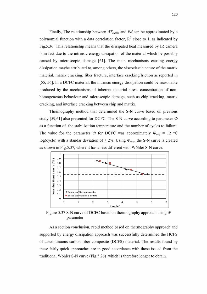
120

Finally, The relationship between ΔTstable and Ed can be approximated by a

polynomial function with a data correlation factor, R2 close to 1, as indicated by

Fig.5.36. This relationship means that the dissipated heat measured by IR camera

is in fact due to the intrinsic energy dissipation of the material which be possibly

caused by microscopic damage [61]. The main mechanisms causing energy

dissipation maybe attributed to, among others, the viscoelastic nature of the matrix

material, matrix cracking, fiber fracture, interface cracking/friction as reported in

[55, 56]. In a DCFC material, the intrinsic energy dissipation could be reasonable

produced by the mechanisms of inherent material stress concentration of non-

homogeneous behaviour and microscopic damage, such as chip cracking, matrix

cracking, and interface cracking between chip and matrix.

Thermography method that determined the S-N curve based on previous

study [59,61] also presented for DCFC. The S-N curve according to parameter Ф

as a function of the stabilization temperature and the number of cycles to failure.

The value for the parameter Ф for DCFC was approximately Фavg ≈ 12 °C

log(cycle) with a standar deviation of + 2%. Using Фavg, the S-N curve is created

as shown in Fig.5.37, where it has a less different with Wöhler S-N curve.

Figure 5.37 S-N curve of DCFC based on thermography approach using Ф parameter As a section conclusion, rapid method based on thermography approach and

supported by energy dissipation approach was successfully determined the HCFS

of discontinuous carbon fiber composite (DCFS) material. The results found by

these fairly quick approaches are in good accordance with those issued from the

traditional Wöhler S-N curve (Fig.5.26) which is therefore longer to obtain.

0

0,1

0,2

0,3

0,4

0,5

0,6

0,7

0,8

0,9

1

0 1 2 3 4 5 6 7

Norm

alise

d Str

ess (

σm

ax /

σUTS

)

Log Nf

Based on Thermography

Based on Wohler S-N data

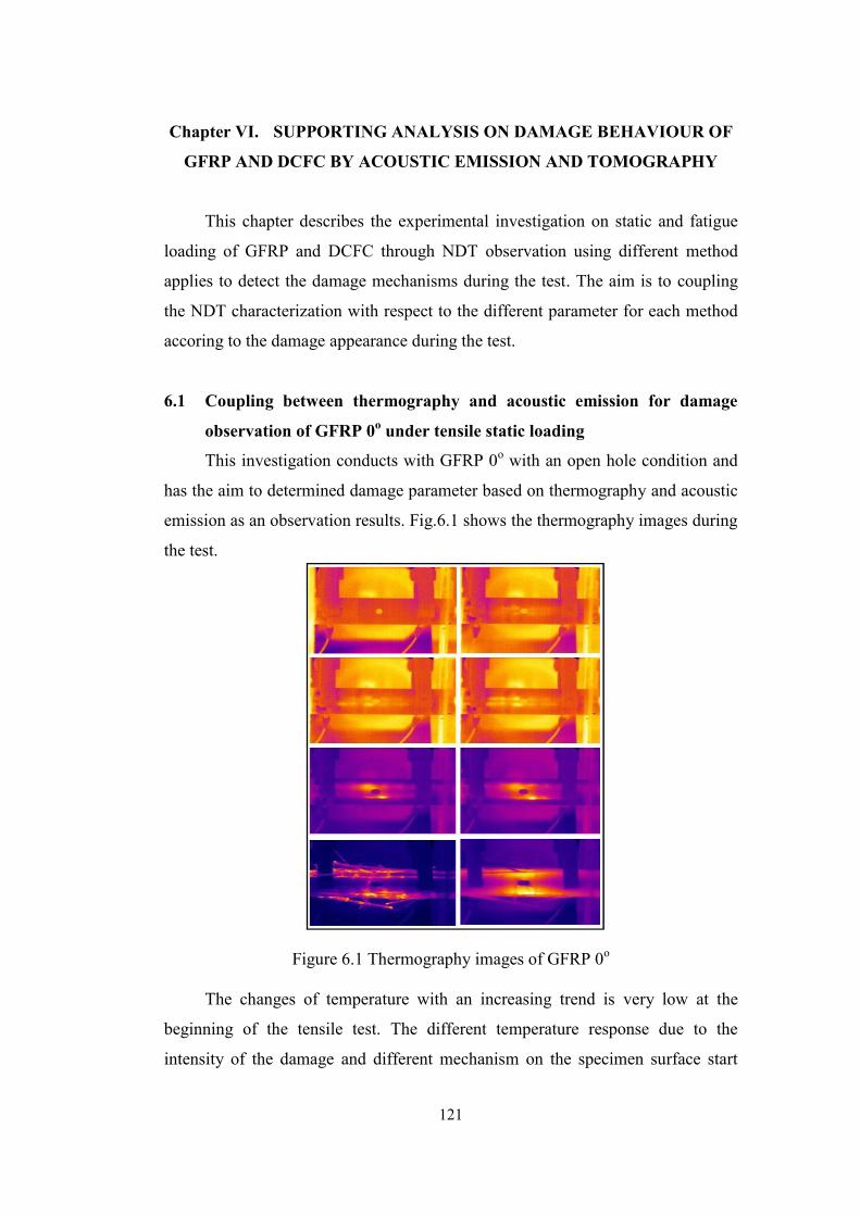
121

Chapter VI. SUPPORTING ANALYSIS ON DAMAGE BEHAVIOUR OF

GFRP AND DCFC BY ACOUSTIC EMISSION AND TOMOGRAPHY

This chapter describes the experimental investigation on static and fatigue

loading of GFRP and DCFC through NDT observation using different method

applies to detect the damage mechanisms during the test. The aim is to coupling

the NDT characterization with respect to the different parameter for each method

accoring to the damage appearance during the test.

6.1 Coupling between thermography and acoustic emission for damage

observation of GFRP 0o under tensile static loading

This investigation conducts with GFRP 0o with an open hole condition and

has the aim to determined damage parameter based on thermography and acoustic

emission as an observation results. Fig.6.1 shows the thermography images during

the test.

Figure 6.1 Thermography images of GFRP 0o

The changes of temperature with an increasing trend is very low at the

beginning of the tensile test. The different temperature response due to the

intensity of the damage and different mechanism on the specimen surface start

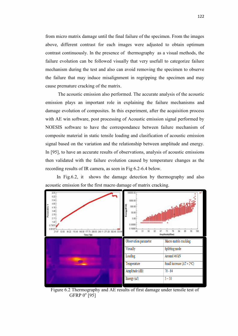
122

from micro matrix damage until the final failure of the specimen. From the images

above, different contrast for each images were adjusted to obtain optimum

contrast continuously. In the presence of thermography as a visual methods, the

failure evolution can be followed visually that very usefull to categorize failure

mechanism during the test and also can avoid removing the specimen to observe

the failure that may induce misalignment in regripping the specimen and may

cause premature cracking of the matrix.

The acoustic emission also performed. The accurate analysis of the acoustic

emission plays an important role in explaining the failure mechanisms and

damage evolution of composites. In this experiment, after the acquisition process

with AE win software, post processing of Acoustic emission signal performed by

NOESIS software to have the correspondance between failure mechanism of

composite material in static tensile loading and clasification of acoustic emission

signal based on the variation and the relationship between amplitude and energy.

In [95], to have an accurate results of observations, analysis of acoustic emissions

then validated with the failure evolution caused by temperature changes as the

recording results of IR camera, as seen in Fig 6.2-6.4 below.

In Fig.6.2, it shows the damage detection by thermography and also

acoustic emission for the first macro damage of matrix cracking.

Figure 6.2 Thermography and AE results of first damage under tensile test of GFRP 0o [95]

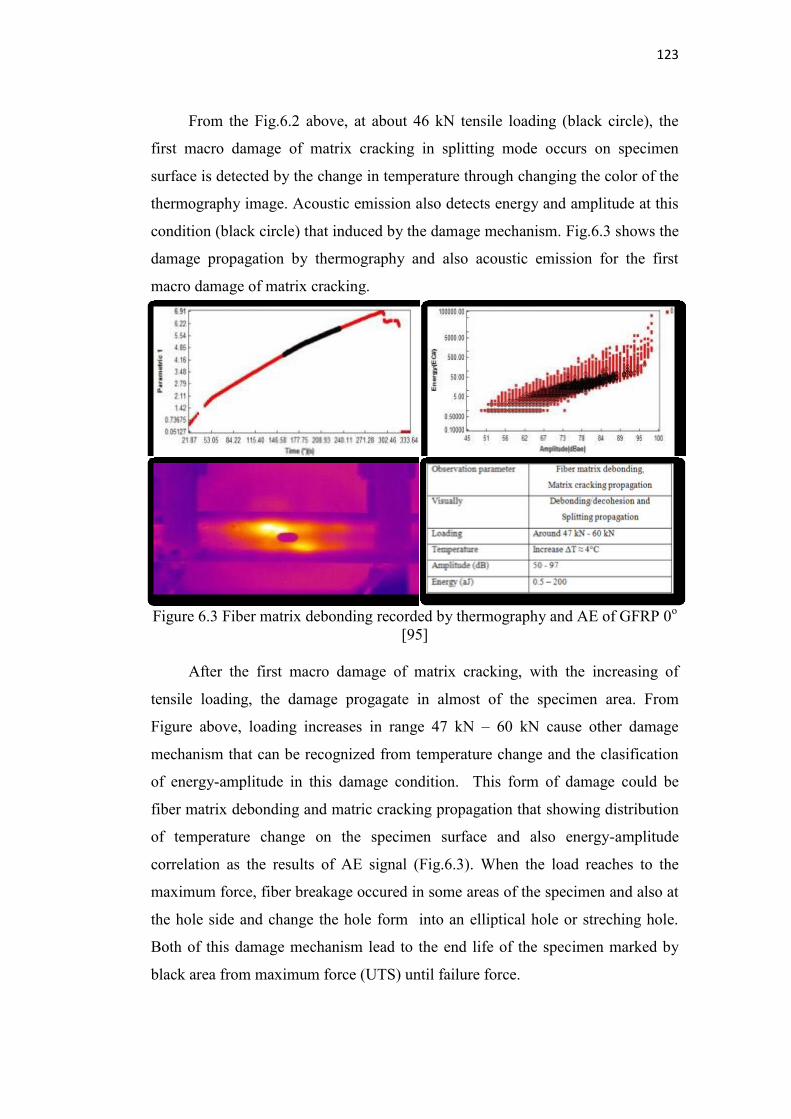
123

From the Fig.6.2 above, at about 46 kN tensile loading (black circle), the

first macro damage of matrix cracking in splitting mode occurs on specimen

surface is detected by the change in temperature through changing the color of the

thermography image. Acoustic emission also detects energy and amplitude at this

condition (black circle) that induced by the damage mechanism. Fig.6.3 shows the

damage propagation by thermography and also acoustic emission for the first

macro damage of matrix cracking.

Figure 6.3 Fiber matrix debonding recorded by thermography and AE of GFRP 0o [95]

After the first macro damage of matrix cracking, with the increasing of

tensile loading, the damage progagate in almost of the specimen area. From

Figure above, loading increases in range 47 kN – 60 kN cause other damage

mechanism that can be recognized from temperature change and the clasification

of energy-amplitude in this damage condition. This form of damage could be

fiber matrix debonding and matric cracking propagation that showing distribution

of temperature change on the specimen surface and also energy-amplitude

correlation as the results of AE signal (Fig.6.3). When the load reaches to the

maximum force, fiber breakage occured in some areas of the specimen and also at

the hole side and change the hole form into an elliptical hole or streching hole.

Both of this damage mechanism lead to the end life of the specimen marked by

black area from maximum force (UTS) until failure force.

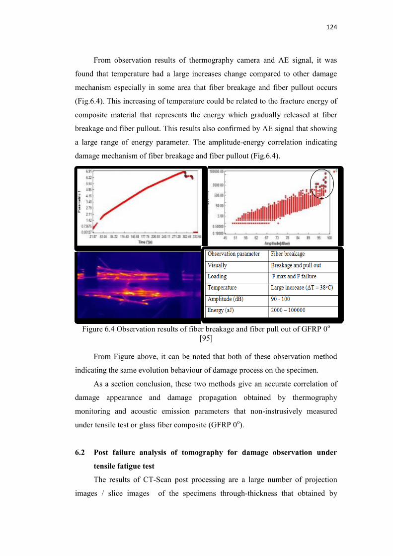
124

From observation results of thermography camera and AE signal, it was

found that temperature had a large increases change compared to other damage

mechanism especially in some area that fiber breakage and fiber pullout occurs

(Fig.6.4). This increasing of temperature could be related to the fracture energy of

composite material that represents the energy which gradually released at fiber

breakage and fiber pullout. This results also confirmed by AE signal that showing

a large range of energy parameter. The amplitude-energy correlation indicating

damage mechanism of fiber breakage and fiber pullout (Fig.6.4).

Figure 6.4 Observation results of fiber breakage and fiber pull out of GFRP 0o

[95]

From Figure above, it can be noted that both of these observation method

indicating the same evolution behaviour of damage process on the specimen.

As a section conclusion, these two methods give an accurate correlation of

damage appearance and damage propagation obtained by thermography

monitoring and acoustic emission parameters that non-instrusively measured

under tensile test or glass fiber composite (GFRP 0o).

6.2 Post failure analysis of tomography for damage observation under

tensile fatigue test

The results of CT-Scan post processing are a large number of projection

images / slice images of the specimens through-thickness that obtained by

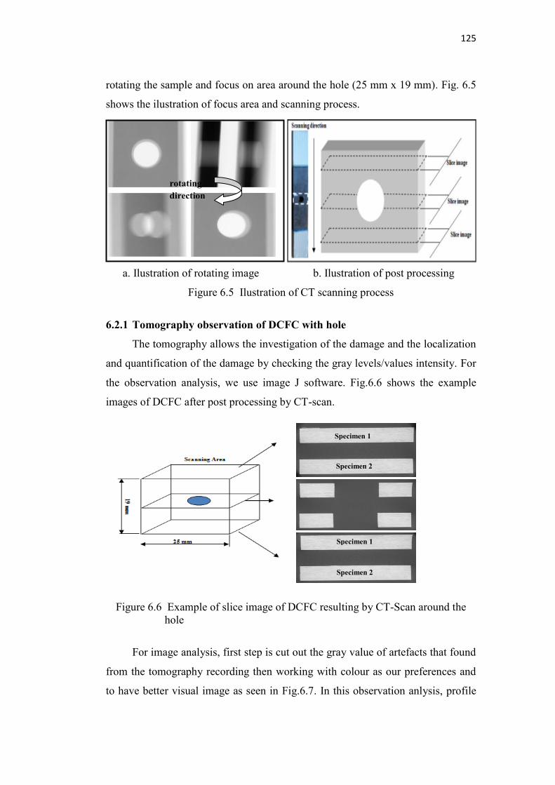
125

rotating the sample and focus on area around the hole (25 mm x 19 mm). Fig. 6.5

shows the ilustration of focus area and scanning process.

a. Ilustration of rotating image b. Ilustration of post processing

Figure 6.5 Ilustration of CT scanning process

6.2.1 Tomography observation of DCFC with hole

The tomography allows the investigation of the damage and the localization

and quantification of the damage by checking the gray levels/values intensity. For

the observation analysis, we use image J software. Fig.6.6 shows the example

images of DCFC after post processing by CT-scan.

Figure 6.6 Example of slice image of DCFC resulting by CT-Scan around the hole

For image analysis, first step is cut out the gray value of artefacts that found

from the tomography recording then working with colour as our preferences and

to have better visual image as seen in Fig.6.7. In this observation anlysis, profile

Specimen 1

Specimen 2

Specimen 1

Specimen 2

rotating direction

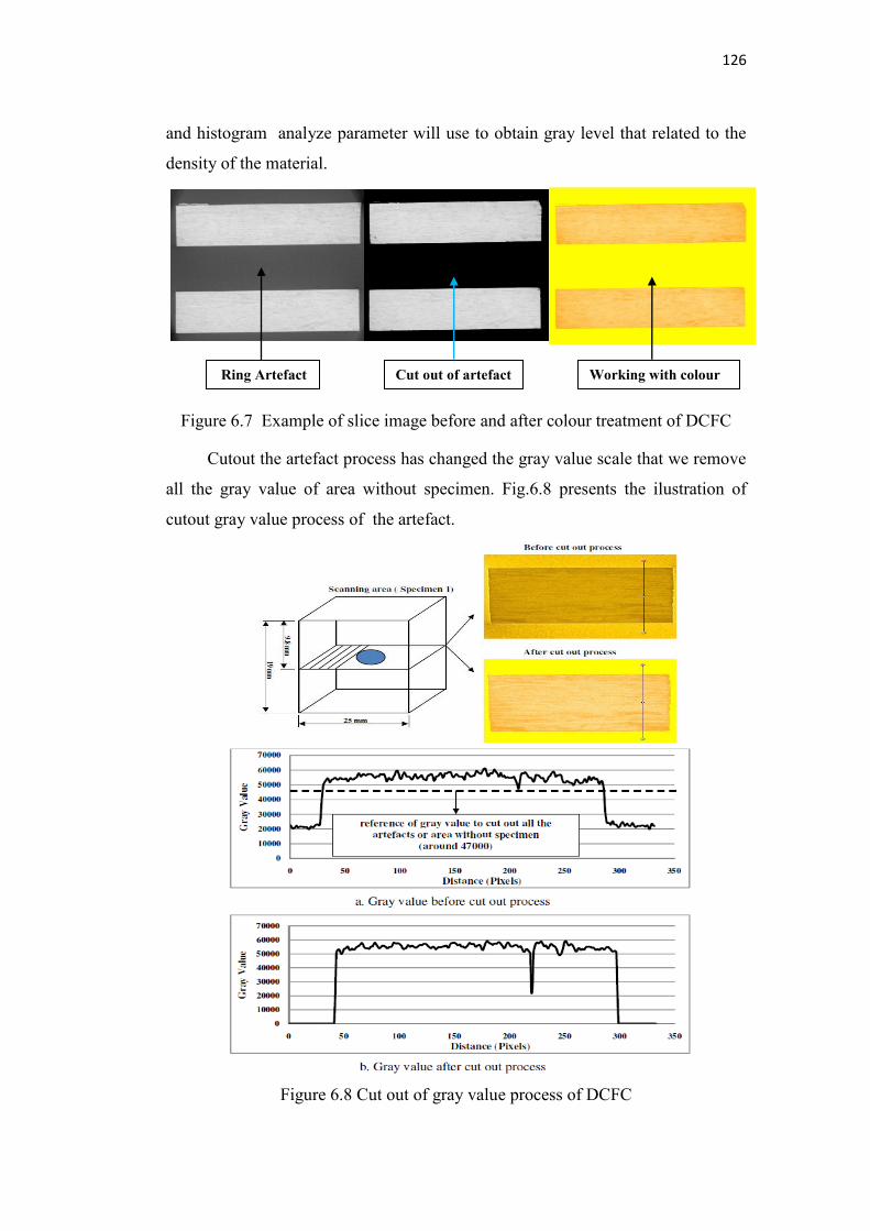
126

and histogram analyze parameter will use to obtain gray level that related to the

density of the material.

Figure 6.7 Example of slice image before and after colour treatment of DCFC

Cutout the artefact process has changed the gray value scale that we remove

all the gray value of area without specimen. Fig.6.8 presents the ilustration of

cutout gray value process of the artefact.

Figure 6.8 Cut out of gray value process of DCFC

Ring Artefact Cut out of artefact Working with colour

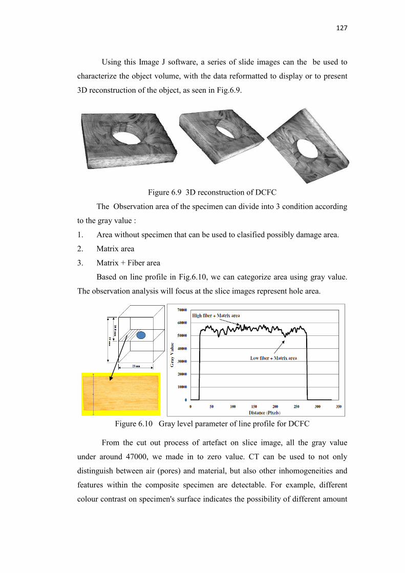
127

Using this Image J software, a series of slide images can the be used to

characterize the object volume, with the data reformatted to display or to present

3D reconstruction of the object, as seen in Fig.6.9.

Figure 6.9 3D reconstruction of DCFC

The Observation area of the specimen can divide into 3 condition according

to the gray value :

1. Area without specimen that can be used to clasified possibly damage area.

2. Matrix area

3. Matrix + Fiber area

Based on line profile in Fig.6.10, we can categorize area using gray value.

The observation analysis will focus at the slice images represent hole area.

Figure 6.10 Gray level parameter of line profile for DCFC

From the cut out process of artefact on slice image, all the gray value

under around 47000, we made in to zero value. CT can be used to not only

distinguish between air (pores) and material, but also other inhomogeneities and

features within the composite specimen are detectable. For example, different

colour contrast on specimen's surface indicates the possibility of different amount

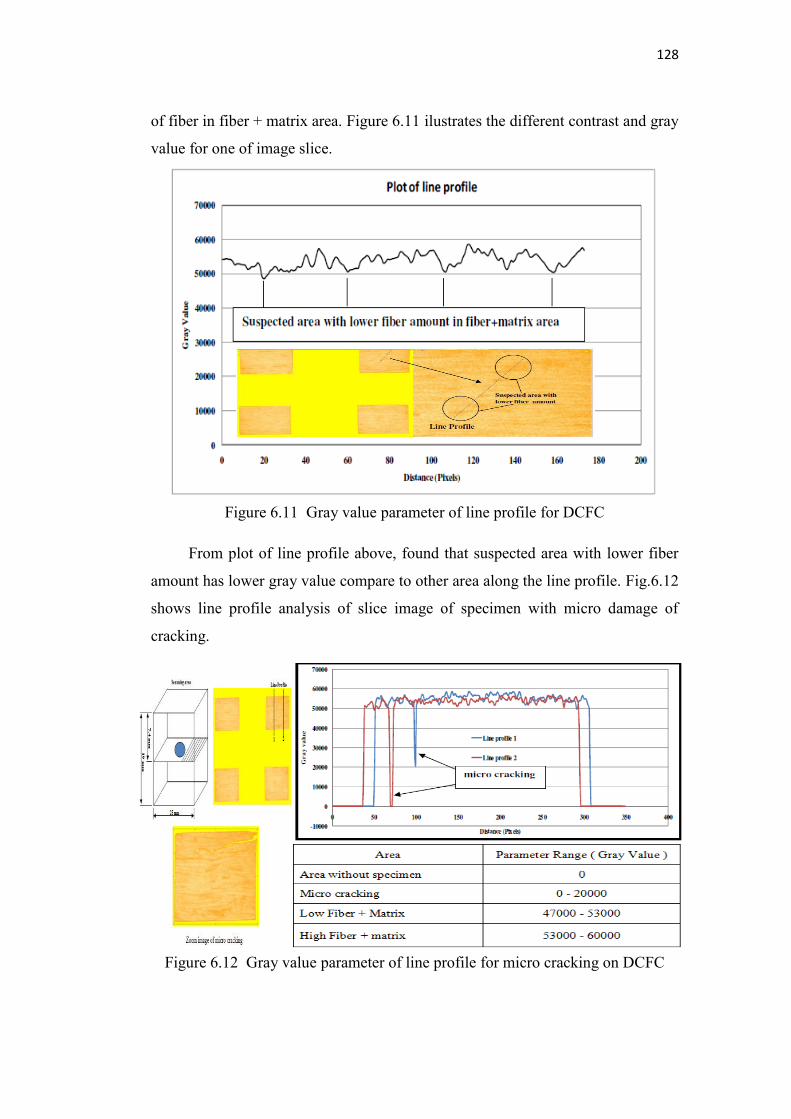
128

of fiber in fiber + matrix area. Figure 6.11 ilustrates the different contrast and gray

value for one of image slice.

Figure 6.11 Gray value parameter of line profile for DCFC

From plot of line profile above, found that suspected area with lower fiber

amount has lower gray value compare to other area along the line profile. Fig.6.12

shows line profile analysis of slice image of specimen with micro damage of

cracking.

Figure 6.12 Gray value parameter of line profile for micro cracking on DCFC

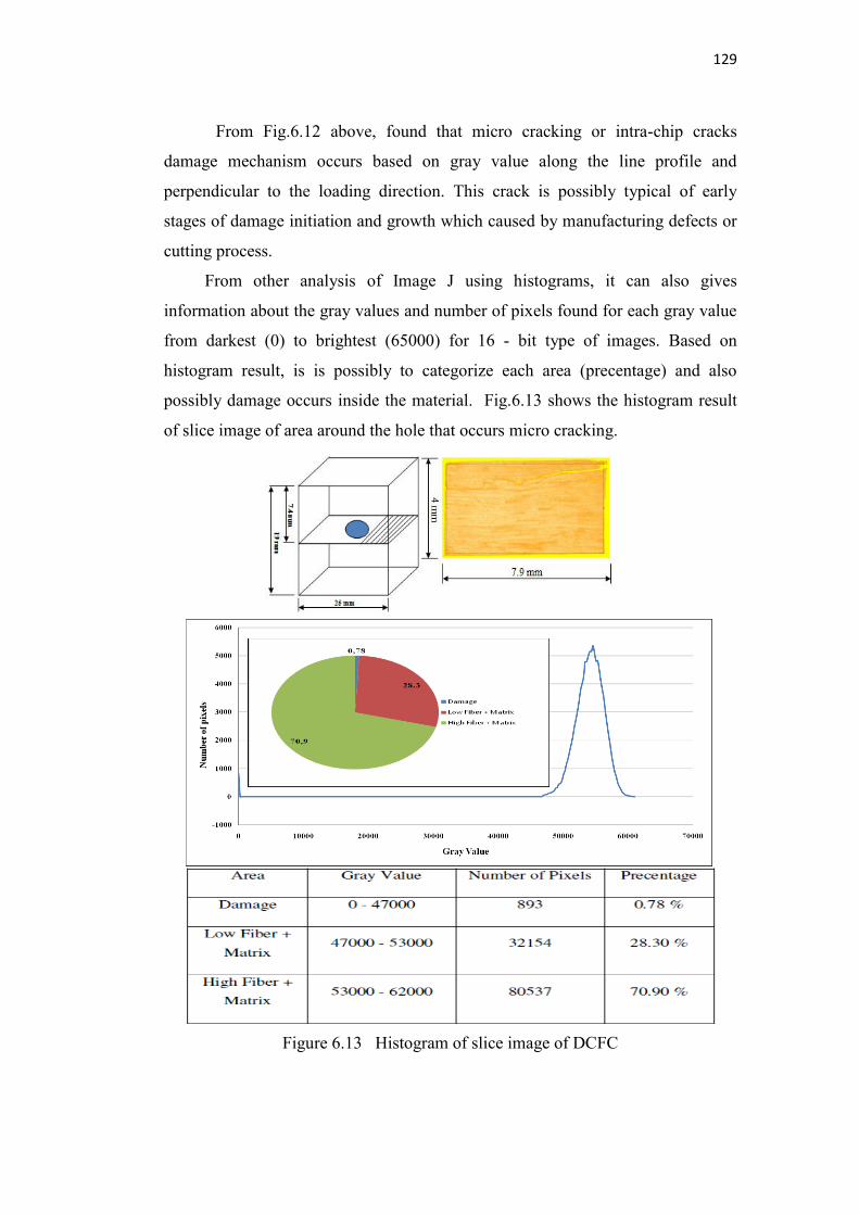
129

From Fig.6.12 above, found that micro cracking or intra-chip cracks

damage mechanism occurs based on gray value along the line profile and

perpendicular to the loading direction. This crack is possibly typical of early

stages of damage initiation and growth which caused by manufacturing defects or

cutting process.

From other analysis of Image J using histograms, it can also gives

information about the gray values and number of pixels found for each gray value

from darkest (0) to brightest (65000) for 16 - bit type of images. Based on

histogram result, is is possibly to categorize each area (precentage) and also

possibly damage occurs inside the material. Fig.6.13 shows the histogram result

of slice image of area around the hole that occurs micro cracking.

Figure 6.13 Histogram of slice image of DCFC

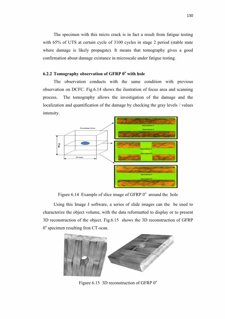
130

The specimen with this micro crack is in fact a result from fatigue testing

with 65% of UTS at certain cycle of 3100 cycles in stage 2 period (stable state

where damage is likely propagate). It means that tomography gives a good

confirmation about damage existance in microscale under fatigue testing.

6.2.2 Tomography observation of GFRP 0o with hole

The observation conducts with the same condition with previous

observation on DCFC. Fig.6.14 shows the ilustration of focus area and scanning

process. The tomography allows the investigation of the damage and the

localization and quantification of the damage by checking the gray levels / values

intensity.

Figure 6.14 Example of slice image of GFRP 0o around the hole

Using this Image J software, a series of slide images can the be used to

characterize the object volume, with the data reformatted to display or to present

3D reconstruction of the object. Fig.6.15 shows the 3D reconstruction of GFRP

0o specimen resulting fron CT-scan.

Figure 6.15 3D reconstruction of GFRP 0o

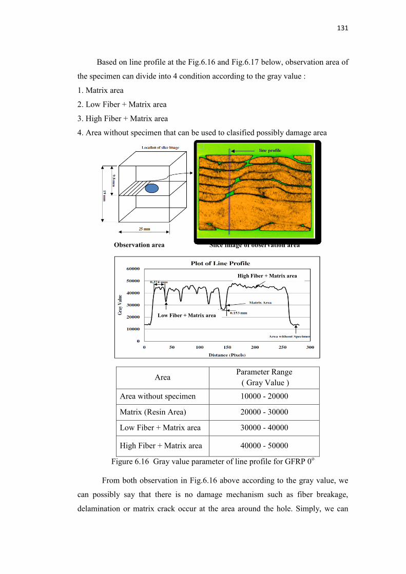
131

Based on line profile at the Fig.6.16 and Fig.6.17 below, observation area of

the specimen can divide into 4 condition according to the gray value :

1. Matrix area

2. Low Fiber + Matrix area

3. High Fiber + Matrix area

4. Area without specimen that can be used to clasified possibly damage area

Area Parameter Range

( Gray Value )

Area without specimen 10000 - 20000

Matrix (Resin Area) 20000 - 30000

Low Fiber + Matrix area 30000 - 40000

High Fiber + Matrix area 40000 - 50000

Figure 6.16 Gray value parameter of line profile for GFRP 0o

From both observation in Fig.6.16 above according to the gray value, we

can possibly say that there is no damage mechanism such as fiber breakage,

delamination or matrix crack occur at the area around the hole. Simply, we can

Low Fiber + Matrix area

High Fiber + Matrix area

Observation area Slice image of observation area

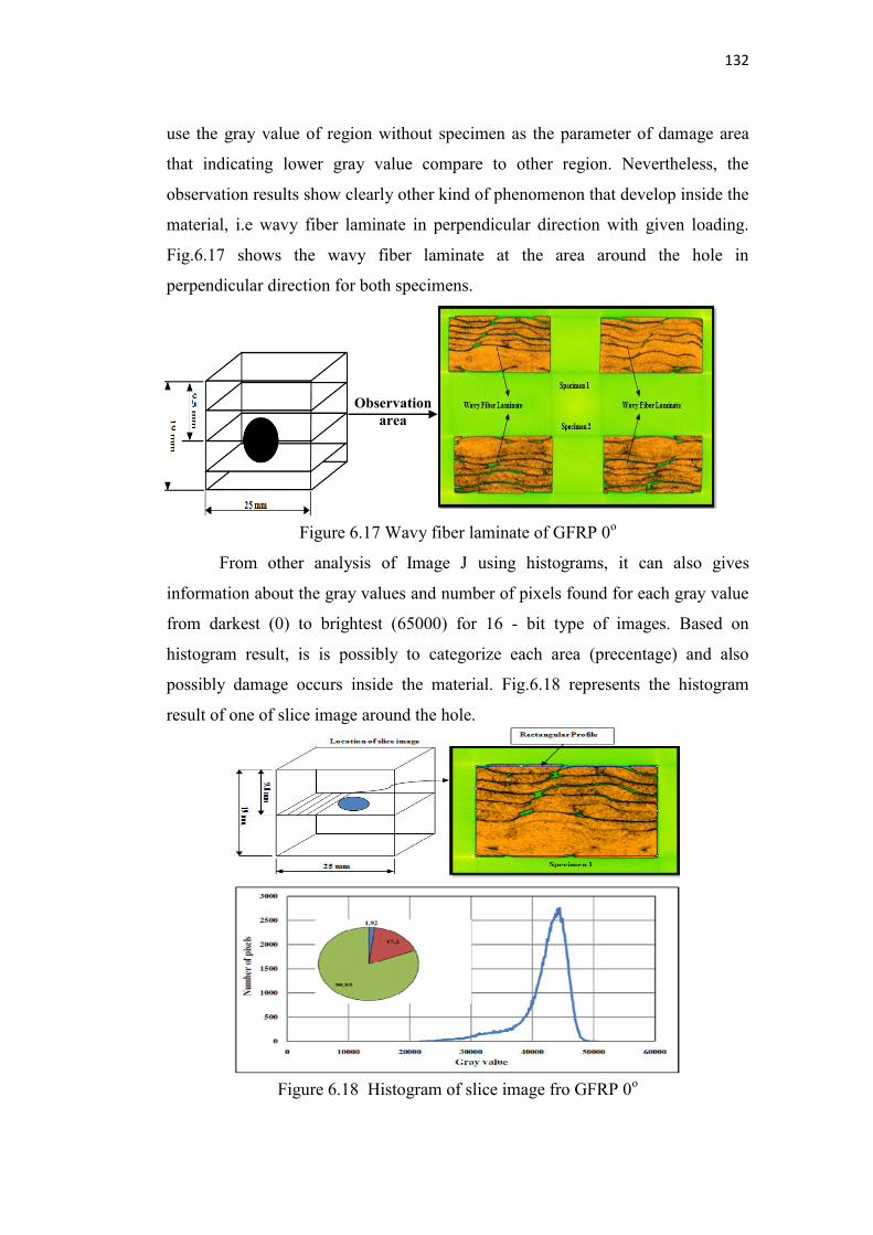
132

use the gray value of region without specimen as the parameter of damage area

that indicating lower gray value compare to other region. Nevertheless, the

observation results show clearly other kind of phenomenon that develop inside the

material, i.e wavy fiber laminate in perpendicular direction with given loading.

Fig.6.17 shows the wavy fiber laminate at the area around the hole in

perpendicular direction for both specimens.

Figure 6.17 Wavy fiber laminate of GFRP 0o

From other analysis of Image J using histograms, it can also gives

information about the gray values and number of pixels found for each gray value

from darkest (0) to brightest (65000) for 16 - bit type of images. Based on

histogram result, is is possibly to categorize each area (precentage) and also

possibly damage occurs inside the material. Fig.6.18 represents the histogram

result of one of slice image around the hole.

Figure 6.18 Histogram of slice image fro GFRP 0o

Observation area

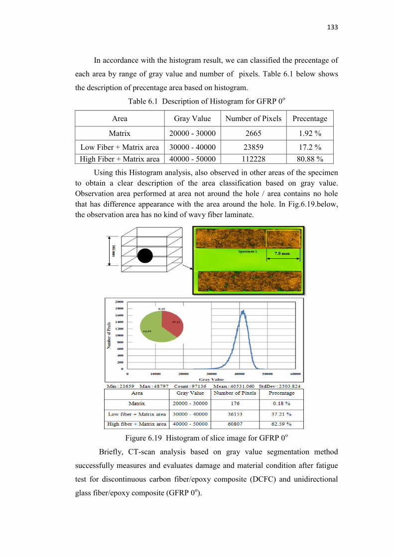
133

In accordance with the histogram result, we can classified the precentage of

each area by range of gray value and number of pixels. Table 6.1 below shows

the description of precentage area based on histogram.

Table 6.1 Description of Histogram for GFRP 0o

Area Gray Value Number of Pixels Precentage

Matrix 20000 - 30000 2665 1.92 %

Low Fiber + Matrix area 30000 - 40000 23859 17.2 %

High Fiber + Matrix area 40000 - 50000 112228 80.88 %

Using this Histogram analysis, also observed in other areas of the specimen

to obtain a clear description of the area classification based on gray value.

Observation area performed at area not around the hole / area contains no hole

that has difference appearance with the area around the hole. In Fig.6.19.below,

the observation area has no kind of wavy fiber laminate.

Figure 6.19 Histogram of slice image for GFRP 0o

Briefly, CT-scan analysis based on gray value segmentation method

successfully measures and evaluates damage and material condition after fatigue

test for discontinuous carbon fiber/epoxy composite (DCFC) and unidirectional

glass fiber/epoxy composite (GFRP 0o).

134

Chapter VII. CONCLUSION AND FUTURE WORK

7.1 Conclusion

In the following section, several conclusions based on damage observation

of GFRP and DCFC by NDT method are described below. The important finding

in this chapter are:

1. NDT thermography characteristic on damage behaviour under tensile

static loading :

Thermography observation by IR camera can give a good local information

about the early damage appearance and propagation, as well as damage

type, critical point, damage location until rupture based on temperature

profile.

Thermography can be used to characterize the damage growth on DCFC

specimen. The early detect by thermography on micro defect shows a flash

lighting form of delta-T spot that has minor or small increase in temperature

possibly due to manufacturing defect. Final failure or rupture of the DCFC

specimen represents by suddenly increase of temperature that has major or

the highest increase of temperature.

The delta-T spots on DCFC material that possibly due to manufacturing

defecr do not grow significantly during the test and eventually do not affect

the initial presence of macro damage that leads to the catastrophic failure.

2. NDT thermography characteristic on damage behaviour under tensile

fatigue loading :

The evolution of the temperature of GFRP can be categorized in four stages.

In the first part, the initial increase of temperature is possibly due to the

micro cracking in matrix. In the second part, a sudden increase in

temperature caused by first appearance of macro matrix cracking. After that,

the temperature reaches a slowly increasing trend due to the stable growth of

matrix cracking as part of the third stage. The final part, a significant trend

increase of temperature could be due to fiber/matrix debonding as the

135

interfacial failure in splitting form and finally provokes the occurrence of

fiber fracture which dealing with the rupture of the specimen represents by

the highest increase of temperature.

The typical behaviour of temperature evolution of DCFC has three stages of

initial increase due to initial micro matrix cracking damage growth of matrix

cracking, slowly increase due to stable propagation of chip/matrix

debonding and chip cracking and suddenly increase caused by chip breakage

and delamination until reaches the highest increase of temperature as a

consequence of final failure.

Thermography can be efficiently used as a simple method to characterize

and estimate the damage evolution of GFRP and DCFC subjected to fatigue

loading.

Thermography can use accurately to predict the high cycle fatigue strength

(HCFS) with 4% of error for GFRP and DCFC material

Thermography method also can be used to determine the S-N curve for

GFRP and DCFC material

3. Supporting analysis of Acoustic emission and tomography :

The Acoustic emission can be used to determine damage propagation of

GFRP under tensile static loading. Coupling with thermography, these two

methods is satisfactory for giving information about damage propagation of

matrix cracking, fiber matrix debonding, fiber breakage and fiber pullout for

GFRP material.

Tomography analysis based on gray value segmentation method

successfully measures and evaluates damage and material condition after

fatigue test for discontinuous carbon fiber/epoxy composite (DCFC) and

unidirectional glass fiber/epoxy composite (GFRP).

7.2 Future work

Although several important finding were made in this study, additional work

can be performed to further understanding based on this study. The following is a

list of recommendations for future work :

136

Develop an investigation on the effect of frequency on thermal response and

energy dissipation for composite material.

An experimental test for each constituent material (matrix, fiber) to

understand the effect on the thermal response and energy dissipation

associated with the thermal source of damage mechanisms.

Further investigation on post failure analysis using tomography and also

micro optic observation to understand the damage mechanisms of fiber

composite material.

A similar experimental test program can be conducted and developed with

different fiber and matrix material

Develop an analysis and simulation study to determine the damage

constitutive model associate with temperature profile from NDT

thermography.

137

REFERENCES

[1] Y. Yang, R. Boom, B. Irion, D.J van Heerden, P.Kuiper, H.deWit,

Recycling of composite material, Chem. Eng. Process, 2011.

[2] C. Kazmierski, Global composite market analysis–ACMA 2012 -

EducationalSession.http://www.lucintel.com/LucintelGlobalCompositeMa

rketAnalysis-ACMA2012-EducationalSession.pdf

[3] L.T. Harper, Discontinuous carbon fiber composite for automotive

applications. Thesis submitted to the University of Nottingham for the

degree of Doctor of Philosophy. 2006.

[4] P. Marin-Francha, T. Martin, D.C. Tunnicliffe, DK Das-Gupta,

PTCa/PEKK piezo-composites for acoustic emission detection. Sensors

and Actuators A 99. 2002. pp.236–243

[5] Y. Yeun-Ho, C. Jin-Ho, K. Jin-Hwe, K. Dong-Hyun, A study on the

failure detection of composite materials using an acoustic emission.

Composite Structures 75. 2006. pp. 163–169

[6] A. K. Mohanty, M.A. Khan, G. Hinrichsen, Surface modification of jute

and its influence on performance of biodegradable jute-fabric/Biopol

composites. Compos Sci Technol, Volume 60. 2000. pp. 1115–1124.

[7] M.A. Usamani, O.I. Salyer, L.G. Ball, L.J. Schwendeman, Bagasse-fiber-

reinforced composites. Journal of Elastomers and Plastics, Volume 13,

No. 1. 1981. pp. 46-73.

[8] K. Bilba, M.A. Arsene, A. Quensanga, Sugar cane bagasse fiber

reinforced cement composites. Part I. Influence of the botanical

components of bagasse on the setting of bagasse/cement composite.

Cement and concrete composites, Volume 25. 2003. pp. 91-96.

[9] P. Tudu, Processing and characterization of natural Fiber reinforced

polymer composites. Thesis. Department of Mechanical Engineering

National Institute of Technology Rourkela. 2009.

[10] F.C. Campbell, Structural composite material. ASM International. 2010.

www. asminternational.org

138

[11] R. Talreja, Damage and fatigue in composites – A personal account

Composites Science and Technology 68. 2008. pp. 2585–2591.

[12] Y.K. Boey, Study of progressive failure of composites under axial loading

with varying strain rates. Thesis. Naval Postgraduate School. 2011.

[13] A. Yudhanto, Effects of micromechanical factors in the strain in variant

failure theory for composites. Thesis. National University of Singapura.

2005.

[14] B. Harris, Fatigue in composites: Science and technology of the fatigue

response of fiber-reinforced plastics. Published by Woodhead

Publishing Limited. 2003.

[15] K.P. Dyer, D.H. Isaac, Fatigue behaviour of continuous glass fiber

reinforced composites. Composites Part B 29B. 1998. pp.725–733.

[16] K. Schulte, Damage monitoring in polymer matrix structures, Journal de

Physique IV, Vol.3. 1993. pp. 1629– 1636.

[17] C. Bathias. An engineering point of view about fatigue of polymer matrix

composite materials. International Journal Fatigue 28. 2006. pp. 1094-

1099.

[18] E.K. Gamstedt, A. Lars, L.A. Berglund, T. Peijs, Fatigue mechanisms in

unidirectional glass-fiber-reinforced polypropylene Composites

Science and Technology 59. 1999. pp. 759-768.

[19] J.A.M. Ferreira, J.D.M. Costa, P.N.B. Reis, M.O.W. Richardson,

Analysis of fatigue and damage in glass-fiber-reinforced polypropylene

composite materials. Composites Science and Technology 59. 1999. pp.

1461-1467.

[20] P.T. Curtis, A review of the fatigue of composite materials. Royal

Aircraft Establishment, Technical Report 87031. 1987.

[21] B. Harris, H. Reiter, T. Adam, R.F. Dickson, G. Fernando, Fatigue

behaviour of carbon fiber reinforced plastics. Composites 21. 1990. pp.

232-242.

[22] A. Rotem, H.G. Nelson, Fatigue behaviour of graphite-epoxy laminates

at elevated temperatures. Fatigue of Fibrous Composite Materials, ASTM

STP 723. 1981. pp. 152-73.

139

[23] A. Pegoretti, T. Ricco, Fatigue crack propagation in polypropylene

reinforced with short glass fibers. Composites Science and Technology

59. 1999. pp.1055-1062.

[24] A. Gagel, D. Lange, K. Schulte, On the relation between crack

densities, stiffness degradation and surface temperature distribution of

tensile fatigue loaded glass-fiber reinforced epoxy. Composites: Part

A 37. 2006. pp. 222–228.

[25] X. Wang and D.D.L. Chung, Fiber breakage in polymer matrix composite

during static and fatigue loading. Journal Material 14 no 11. 1999. pp.

4224-4229.

[26] R. C. S. Freire Jr and E.M.Freire de Aquino, Fatigue damage mechanism

and failure prevention in fiberglass reinforced plastic. Material

Research, Vol. 8, No. 1. 2005. pp. 45-49.

[27] C.G. Davila and C.A. Rose, Progressive damage analysis of composite,

Aircraft Aging and Durability Project. www.eng.morgan.edu.

[28] E. Bayraktar, S.D. Antolovich, C. Bathias, New developments in non-

destructive controls of the composite materials and applications in

manufacturing engineering. Journal of materials processing technology

206. 2008. pp. 30–44.

[29] H.E. Kadi and F.Ellyin Reddy. Effect of stress ratio on the fatigue of

unidirectional glass/fiber epoxy composite laminae, Composite, Vol 25,

No.10.1994. pp. 917-924.

[30] A. Puck and W. Schneider, On failure mechanisms and failure criteria of

filament wound glass-fibre/resin composites, Plastics and Polymers. 1969.

pp. 33–44.

[31] L. Guangyan, Damage progression in open-hole tension composite

laminates by the element-failure method. A thesis submitted for the

degree of doctor of philosophy department of mechanical engineering

National University of Singapore. 2007.

[32] Z. Hashin, Failure criteria for unidirectional fiber composites, Journal

of Applied Mechanics, vol. 47. 1980. pp. 329–334.

140

[33] R. M. Christensen, The comparison and evaluation of three fiber

composite failure criteria, Annual Conference & Exposition on

Experimental & Applied Mechanics. 2005.

[34] B. Okutan, Stress and failure analysis of laminated composite pinned

joints, A Thesis Submitted to the Graduate School of Natural and

Applied Sciences of Dokuz Eylul University In Partial Fulfillment of the

Requirements for the Degree of Doctor of Philosophy in Mechanical

Engineering, 2001.

[35] ESP. Brian, Stress distribution and strength prediction of composite

laminates with multiple holes, Presented to the Faculty of the Graduate

School of The University of Texas at Arlington in Partial Fulfillment of

the Requirements for the Degree of Doctor of Philosophy the

University of Texas at Arlington. 2007.

[36] J. Awerbuch and M.S. Madhukar, Notched strength of composite

laminates; predictions and experiments – A review, Journal of

Reinforced Plastic Composites. 4. 1985. pp. 3-159.

[37] O.O. Ochoa and J.N. Reddy, Finite element analysis of composite

laminates, Kluwer Academic Publishers. Norwell. 1992.

[38] L.K. William, Stress concentration around a small circular hole in the

HIMAT composite plate, NASA. 1985.

[39] S.G. Lekhnitskii, S.W. Tsai, T. Cheron, Anisotropic plates, Gordon and

Breach Science Publishers. New York. 1968.

[40] R.J. Nuismer and J.M. Whitney, Uniaxial failure of composite laminates

containing stress concentrations, Fracture Mechanics of Composites,

ASTM STP 593, American Society for Testing and Materials. 1975. pp.

117-142.

[41] H.M. Arslan, M.Y. Kaltakci, H.R. Yerli, Effect of circular holes on

cross- ply laminated composite plates, The Arabian Journal for Science

and Engineering, Vol 34, Number 2. 2009. pp. 301-315.

[42] K.M.M. Muneer, R.V. Prakash, K. Balasubramaniam, Thermomechanical

studies in glass/epoxy composite specimen during tensile loading. World

141

Academy of Science, Engineering and Technology 56. 2009. pp. 865-

872.

[43] M. Kutin, S. Ristic, M. Puharic, M. Vilotijevic, M. Krmar, Thermographic

testing of epoxy-glass composite tensile properties. Contemporary

Materials II. 2011. pp. 88-93.

[44] C. Colombo, F. Libonati, F. Pezzani, A. Salerno L. Vergani, Fatigue

Behaviour of a GFRP Laminate by thermographic measurements.

Procedia Engineering 10. 2011. pp. 3518–3527.

[45] P. Stanley and W.K. Chan, Quantitative analysis by means of

thermoelastic effect, J. Strain Analysis 20. 1985. pp. 129-134.

[46] Z. Feng, D. Zhang, R.E. Rowlands, B.I. Sandor, Thermoelastic

determination of individual stress components in loaded composites,

Experiment Mechanics. 1990. pp. 89-95.

[47] S. Sambasivam, Thermoelastic stress analysis of laminated composite

materials, Ph.D thesis, Faculty of Engineering, Science and Mathematics

School of Engineering Sciences, UNIVERSITY OF SOUTHAMPTON.

2009.

[48] F. Libonati, Damage analysis of composite by means of thermography.

Symphosium on Experiment Solid Mechanics ISBN 978-88-95940-30-4.

2010.

[49] C. Colombo, F. Libonati, L. Vergani, Study of the mechanical

characteristics of GFRP by thermography, ICCS 16. 2011.

[50] Ecole Des Mines de Saint Etienne (EMSE), Suivi par thetmographie

infrarouge sur composites carbon-epoxy. 1996

http://www.carlosantulli.net/stetstage96.pdf

[51] L. Toubal, M. Karama, and B. Lorrain, Damage evoution and infrared

thermography in woven composite laminates under fatigue loading.

hermoelastic Stress Analysis of damage mechanisms in composite

materials, International Journal of fatigue 28 Composites. 2006.pp.1867–

1872

142

[52] J. Rossignola, M.L .Pastor, A.Thionnet, Détection d’endommagement

dans les composites à l’aide d’une technologie utilisant des micro-ondes et

par thermographie infrarouge, Matériaux. 2010.

[53] G. Curti, G. La Rosa, M. Orlando, and A Risitano, Analisi tramite

infrarosso termico della 'temperatura limite' in prove di fatica (in Italian),

14th AIAS Italian National Conference, Catania, Italy. 1986:211-20.

[54] G. La Rosa and A. Risitano, Thermographic methodology for rapid

determination of the fatigue limit of materials and mechanical

components, International Journal of Fatigue 22. 2000. pp. 65-73.

[55] G. Meneghetti, M. Quaresimin, M. De Monte, fatigue strength

assessment of a short fibre-reinforced plastic based on the energy

dissipation , 16th international conference on composite materials, 2007.

[56] R. Steinberger , T.I. Valadas Leitaão , E. Ladstätter, G. Pinter, W.

Bilinger, and R.W. Lang, Infrared thermographic techniques for non-

destructive damage characterization of carbon fibre reinforced

polymersduring tensile fatigue testing, International Journal of Fatigue

28. 2006. pp. 1340-1347.

[57] T.P. Soemardi, Etude du comportement mecanique et de

l'endommagement de tube en composites verre/epoxy soumis a des

sollicitations axiales et biaxees en statique et en fatigue, Ph.D thesis,

Formation Doctorale Mécanique et Matériaux, Ecole Centrale Paris. 1990.

[58] T.P. Soemardi, D. Lai, C. Bathias, Static and fatigue biaxial testing of

fiber composite using thin walled tubular specimens, IUTAM Symposium.

New York-USA in Dvorak (ed). Springer Verlag, Germany. 1991.

[59] G. Fargione *, A. Geraci, G. La Rosa, A. Risitano, Rapid

determination of the fatigue curve by the thermographic, International

Journal of Fatigue 24. 2002. pp. 11-19.

[60] L Toubal, B. Lorrain, F. Peyruseigt, and M. Karama, Détermination de la

limite d'endurance d'un carbone/époxy par analyse thermographique ( in

French ), 17ème Congrès Français de Mécanique, Troyes, France,

Septembre 2005.

143

[61] J. Montesano, Z. Fawaz, and H. Bougherara, Use of infrared

thermography to investigate the fatigue behaviour of a carbon fiber

reinforced polymer composite , Composite Structure 97. 2013. pp. 76-83.

[62] A. Risitano and G. Risitano, Cumulative damage evaluation in multiple

cycle fatigue tests taking into account energy parameters, International

Journal of Fatigue 48. 2013. pp.214-222.

[63] M. Giordano, A. Calabro ,C. Esposito, A. D'Amore, L. Nicolais, An

acoustic-emission characterization of the failure modes in polymer-

composite materials, Composites Science and Technology 58. 1998.

pp.1923-1928.

[64] N. C. Shippen, D. F. Adams, Acoustic emission monitoring of damage

progression in graphite/epoxy laminates, Journal of Reinforced Plastics

and Composites, Vol. 4. July 1985. pp. 242-261.

[65] J. M. Berthelot, Relation between amplitudes and rupture mechanisms in

composite materials, Proceedings of Acoustic Emission from Composite

Materials II, Montreal. 1986. pp. 126-133.

[66] H. Otsuka, H. A. Scarton, variations in acoustic emission between

graphite- and glass-epoxy composites, J. Composite Materials, Vol. 5.

Nov.1981. pp. 591-597.

[67] J. P. Favre, J. C. Laizet, amplitude and counts per event analysis of

acoustic emission generated by transverse cracking of cross-ply CFRP,

Composites Science and Technology, Vol. 36. 1989. pp. 27-43.

[68] Favre, J. P., and J. C. Laizet, Acoustic analysis of the accumulation of

cracks in CFRP cross-ply composites under tensile loading, Journal of

Acoustic Emission, Vol 9. 1990. pp. 97-102.

[69] M. Johnson, Classification of AE transients based on numerical

simulations of composite laminates, NDT&E International 36. 2003.

pp.319–329

[70] P.J. de Groot, P.A.M.Wijnen, R.B.F. Janssen, Real-time frequency

determination of acoustic emission for different fracture mechanisms in

carbon/epoxy composites, Composites Science and Technology 55. 1995.

pp.405–412.

144

[71] C.R. Ramirez-Jimenez, N. Papadakis, N. Reynolds, T.H. Gan, P. Purnell,

M. Pharaoh, Identification of failure modes in glass/polypropylene

composites by means of the primary frequency content of the acoustic

emission event, Composites Science and Technology 64. 2004. pp.1819–

1827.

[72] R. Gutkin, C.J.Green, S. Vangrattanachai, S.T. Pinho, P. Robinson, P.T.

Curtis, On acoustic emission for failure investigation in DCFC: Pattern

recognition and peak frequency, Mechanical Systems and Signal

Processing 25. 2011. pp.1393–1407.

[73] Mechraoui S.E, Laksimi A, and Benmedakhene S. Reliability of damage

mechanism localisation by acoustic emission on glass/epoxy composite

material plate. Composite Structures 94. 2012. pp. 1483-1494.

[74] M. Kharoubi, L. Fatmi, A. El Mahi, R. EL Guerjouma, R. Berbaoui,

Identification du dommage par EA de stratifiés composites chargés en

statique et cyclique, 10ème Congrès Français d'Acoustique, Lyon, 12-16

Avril 2010.

[75] W. Li, G. Dai, F. Long, P. Jiang, Y. Wang, Study on FRP composite

material damage based on the acoustic emission testing technology, 18th

World Conference on Non-destructive Testing. 2012.

[76] R.B. Toumi. J. Renard, M. Monin, P. Nimdum, Fatigue damage modelling

of continuous E-glass fibre/epoxy composite, Procedia Engineering 66.

2013. pp. 723-736.

[77] A.A. Malcolm and T. Liu, Case Studies in the use of computed

tomography for non-destructive testing, failure analysis and

performance evaluation , Singapore International NDT Conference &

Exhibition. 2011.

[78] M. Amos, Advanced industrial x-ray computed tomography for defect

detection and characterisation of composite structures, A thesis

submitted to The University of Manchester for the degree of Doctor of

Engineering in the Faculty of Engineering and Physical Sciences. 2010.

[79] B. Zhang, Digital test of composite material using x-ray tomography

and finite element simulation, Dissertation submitted to the faculty of

145

Virginia Polytechnic Institute and State University in partial fulfillment of

the requirements for the degree of Doctor of Philosophy. 2007.

[80] P. Wright, A. Moffat, I. Sinclair, S.M. Spearing, High resolution

tomographic imaging and modelling of notch tip damage in a

laminated composite, Composites Science and Technology 70. 2010.

pp.1444–1452.

[81] J. Kastner, B. Plank, D. Salaberger, J. Sekelja, ASTNER*, Defect and

Porosity Determination of Fibre Reinforced Polymers by X-ray Computed

Tomography, 2nd International Symposium on NDT in Aerospace. 2010.

[82] F. Cosmi and A. Bernasconi, Micro-CT investigation on fatigue

damage evolution in short fibre reinforced polymers, Composites Science

and Technology 79. 2013. pp.70–76.

[83] C. Goidescu, H. Welemane, C. Garnier, M. Fazzini, R. Brault, E.

Péronnet, S. Mistou, Damage investigation in CFRP composites using

full field measurement techniques: Combination of digital image

stereo-correlation, infrared thermography and X-ray tomography,

Composites: Part B 48. 2013. pp. 95–105.

[84] M. Turtle, T. Shifman and B. Boursier, Simplifying certification of

discontinuous composite material forms primary aircraft structures,

Hexcel Research and Technology. http://www.hexcel.com

[85] B. Boursier and A. Lopez, Failure initiation and effect of defects in

structural discontinuous fiber composites, Hexcel Research and

Technology. 2010. http://www.hexcel.com

[86] P. Feraboli, E. Peitso, F. Deleo, T. Cleveland, M. Graves, P. Stickler,

Characterization of discontinuous carbon fiber/epoxy systems for

aerospaceapplications.http://www.aa.washington.edu/research/structures/

pubs/208.pdf

[87] P. Feraboli, E. Peitso, T. Cleveland, P. Stickler B, C.J. Halpin, Notched

behaviour of prepeg-based discontinuous carbon fiber/epoxy systems.

Composites : Part A 40. 2009. pp. 289-299.

146

[88] P. Feraboli, T. Cleveland, P. Stickler, J. Halpin, Stochastic laminate

analogy for simulating the variability in modulus of discontinuous

composite materials, Composites : Part A 41. 2010. pp. 557-570.

[89] J. Bale, E. Valot, M. Monin, P. Laloue, O. Polit, C. Bathias, T.P.

Soemardi, Thermography observation on damage behaviour of

discontinuous carbon fiber composite, The 13th Japanese-European

Symposium on Composite Materials, Bougenais, France. 2013.

[90] P. Feraboli, T. Cleveland, M. Ciccu, P. Stickler, L. DeOto, Defect and

damage analysis of advanced discontinuous carbon/epoxy composite

materials, Composites : Part A 41. 2010. pp. 888-901.

http://www.aa.washington.edu/research/structures/pubs/208.pdf

[91] P. Feraboli, E. Peitso, F. Deleo, T. Cleveland, M. Graves, P. Stickler,

Characterization of discontinuous carbon fiber/epoxy systems for

aerospace applications.

[92] P. Feraboli, E. Peitso and T. Cleveland, Modulus measurement for prepeg-

based discontinuous carbon fiber/epoxy systems, Journal of composite

materials Vol 43 No.19. 2009. pp. 1947-1965.

[93] M.D. Bond, L.T. Harper, T.A. Turner, N.A. Warrior, Full - field strain

measurement of notched discontinuous carbon fiber composites, ICCM 17

Proceeding. http://www.iccm-central.org

[94] C. Qian, L.T. Harper, T.A. Turner, N.A. Warrior, Notched behaviour of

discontinuous carbon fiber composites: Comparison with quasi-isotropic

non-crimp fabric, Composites: Part A 42. 2011. pp. 293–302.

[95] J. Bale, E. Valot, M. Monin, P. Laloue, O. Polit, C. Bathias, T.P.

Soemardi, Damage observation of glass fiber epoxy composites using

thermography and supported by acoustic emission, Applied Mechanics

and Materials Journal Vol. 627. 2014. pp.187-190.

[96] S.H. Najem, Methodology for Assessment of factors influencing surface

roughness on the drilling of carbon-reinforced composite, Journal of

Babylon University/ENgineering Science 2 Vol.21. 2013. pp.604-615.

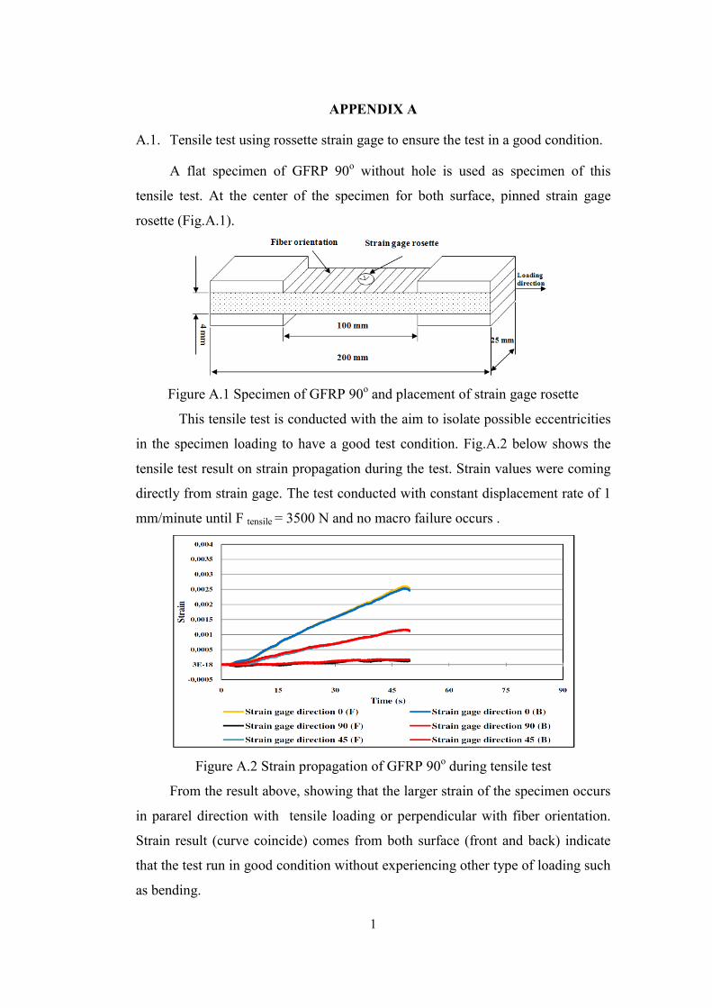
1

APPENDIX A

A.1. Tensile test using rossette strain gage to ensure the test in a good condition.

A flat specimen of GFRP 90o without hole is used as specimen of this

tensile test. At the center of the specimen for both surface, pinned strain gage

rosette (Fig.A.1).

Figure A.1 Specimen of GFRP 90o and placement of strain gage rosette

This tensile test is conducted with the aim to isolate possible eccentricities

in the specimen loading to have a good test condition. Fig.A.2 below shows the

tensile test result on strain propagation during the test. Strain values were coming

directly from strain gage. The test conducted with constant displacement rate of 1

mm/minute until F tensile = 3500 N and no macro failure occurs .

Figure A.2 Strain propagation of GFRP 90o during tensile test

From the result above, showing that the larger strain of the specimen occurs

in pararel direction with tensile loading or perpendicular with fiber orientation.

Strain result (curve coincide) comes from both surface (front and back) indicate

that the test run in good condition without experiencing other type of loading such

as bending.

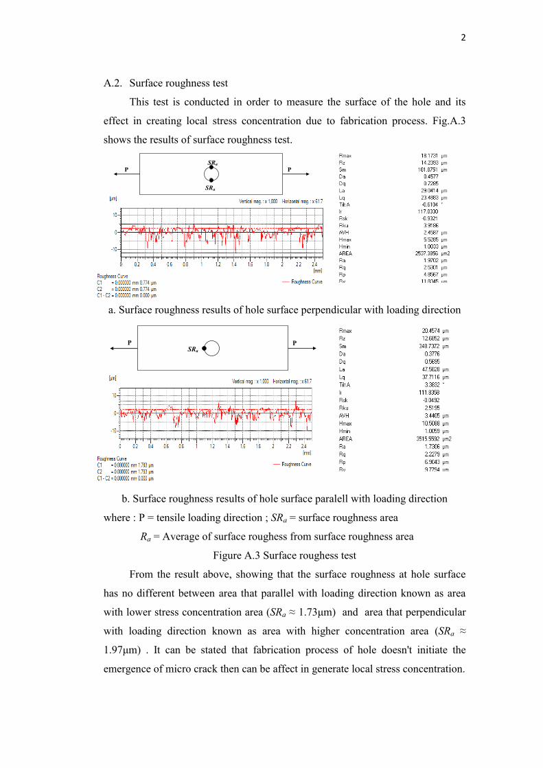
2

A.2. Surface roughness test

This test is conducted in order to measure the surface of the hole and its

effect in creating local stress concentration due to fabrication process. Fig.A.3

shows the results of surface roughness test.

a. Surface roughness results of hole surface perpendicular with loading direction

b. Surface roughness results of hole surface paralell with loading direction

where : P = tensile loading direction ; SRa = surface roughness area

Ra = Average of surface roughess from surface roughness area

Figure A.3 Surface roughess test

From the result above, showing that the surface roughness at hole surface

has no different between area that parallel with loading direction known as area

with lower stress concentration area (SRa ≈ 1.73 m) and area that perpendicular

with loading direction known as area with higher concentration area (SRa ≈

1.97 m) . It can be stated that fabrication process of hole doesn't initiate the

emergence of micro crack then can be affect in generate local stress concentration.

P P SRa

SRa

P P SRa

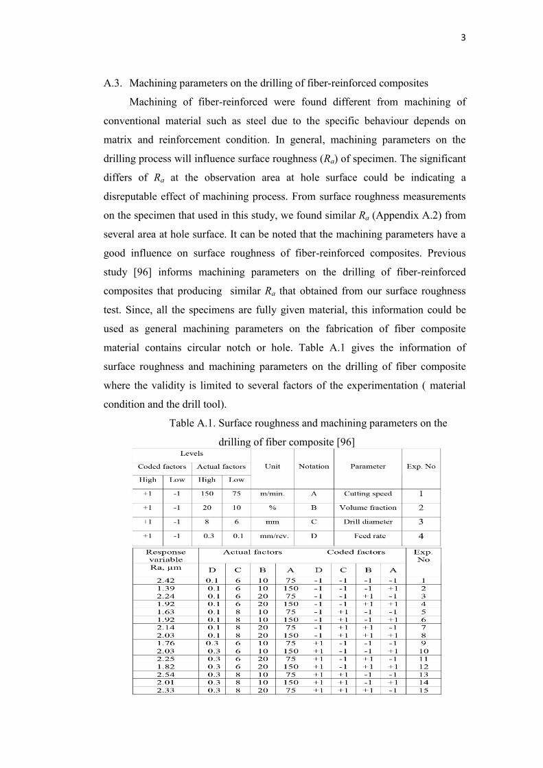
3

A.3. Machining parameters on the drilling of fiber-reinforced composites

Machining of fiber-reinforced were found different from machining of

conventional material such as steel due to the specific behaviour depends on

matrix and reinforcement condition. In general, machining parameters on the

drilling process will influence surface roughness (Ra) of specimen. The significant

differs of Ra at the observation area at hole surface could be indicating a

disreputable effect of machining process. From surface roughness measurements

on the specimen that used in this study, we found similar Ra (Appendix A.2) from

several area at hole surface. It can be noted that the machining parameters have a

good influence on surface roughness of fiber-reinforced composites. Previous

study [96] informs machining parameters on the drilling of fiber-reinforced

composites that producing similar Ra that obtained from our surface roughness

test. Since, all the specimens are fully given material, this information could be

used as general machining parameters on the fabrication of fiber composite

material contains circular notch or hole. Table A.1 gives the information of

surface roughness and machining parameters on the drilling of fiber composite

where the validity is limited to several factors of the experimentation ( material

condition and the drill tool).

Table A.1. Surface roughness and machining parameters on the

drilling of fiber composite [96]

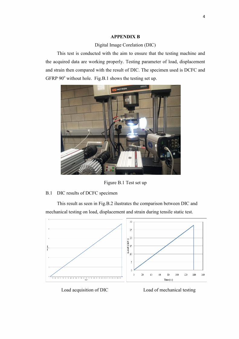
4

APPENDIX B

Digital Image Corelation (DIC)

This test is conducted with the aim to ensure that the testing machine and

the acquired data are working properly. Testing parameter of load, displacement

and strain then compared with the result of DIC. The specimen used is DCFC and

GFRP 90o without hole. Fig.B.1 shows the testing set up.

Figure B.1 Test set up

B.1 DIC results of DCFC specimen

This result as seen in Fig.B.2 ilustrates the comparison between DIC and

mechanical testing on load, displacement and strain during tensile static test.

Load acquisition of DIC Load of mechanical testing

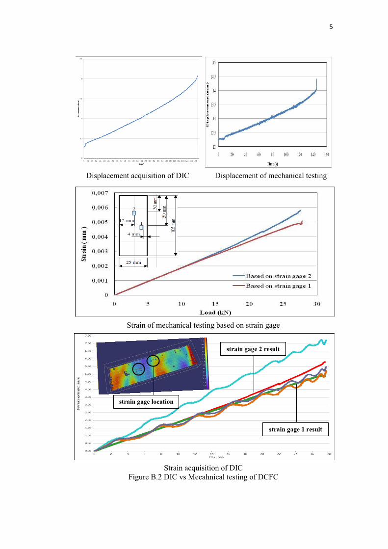
5

Displacement acquisition of DIC Displacement of mechanical testing

Strain of mechanical testing based on strain gage

Strain acquisition of DIC Figure B.2 DIC vs Mecahnical testing of DCFC

strain gage location

strain gage 2 result

strain gage 1 result

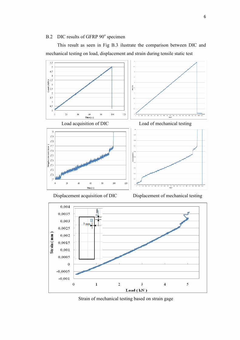
6

B.2 DIC results of GFRP 90o specimen

This result as seen in Fig B.3 ilustrate the comparison between DIC and

mechanical testing on load, displacement and strain during tensile static test

Load acquisition of DIC Load of mechanical testing

Displacement acquisition of DIC Displacement of mechanical testing

Strain of mechanical testing based on strain gage

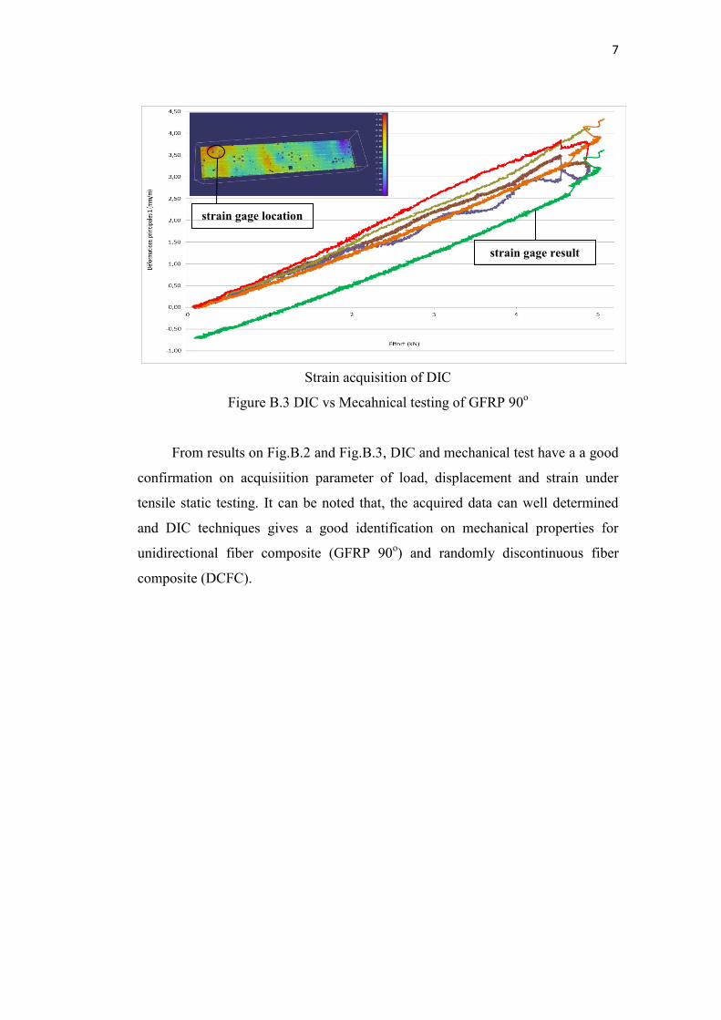
7

Strain acquisition of DIC

Figure B.3 DIC vs Mecahnical testing of GFRP 90o

From results on Fig.B.2 and Fig.B.3, DIC and mechanical test have a a good

confirmation on acquisiition parameter of load, displacement and strain under

tensile static testing. It can be noted that, the acquired data can well determined

and DIC techniques gives a good identification on mechanical properties for

unidirectional fiber composite (GFRP 90o) and randomly discontinuous fiber

composite (DCFC).

strain gage location

strain gage result

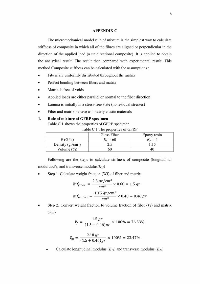
8

APPENDIX C The micromechanical model rule of mixture is the simplest way to calculate

stiffness of composite in which all of the fibres are aligned or perpendicular in the

direction of the applied load (a unidirectional composite). It is applied to obtain

the analytical result. The result then compared with experimental result. This

method Composite stiffness can be calculated with the assumptions :

Fibers are uniformly distributed throughout the matrix

Perfect bonding between fibers and matrix

Matrix is free of voids

Applied loads are either parallel or normal to the fiber direction

Lamina is initially in a stress-free state (no residual stresses)

Fiber and matrix behave as linearly elastic materials

1. Rule of mixture of GFRP specimen Table C.1 shows the properties of GFRP specimen

Table C.1 The properties of GFRP

Glass Fiber Epoxy resin

E (GPa) Ef ≈ 60 Em ≈ 4

Density (gr/cm3) 2.5 1.15

Volume (%) 60 40

Following are the steps to calculate stiffness of composite (longitudinal

modulus/E11 and transverse modulus/E22)

Step 1. Calculate weight fraction (Wf) of fiber and matrix

Step 2. Convert weight fraction to volume fraction of fiber (Vf) and matrix

(Vm)

Calculate longitudinal modulus (E11) and transverse modulus (E22)

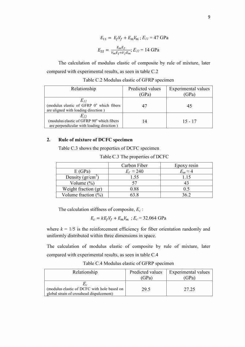
9

; E11 = 47 GPa ; E22 = 14 GPa

The calculation of modulus elastic of composite by rule of mixture, later

compared with experimental results, as seen in table C.2

Table C.2 Modulus elastic of GFRP specimen

Relationship Predicted values (GPa)

Experimental values (GPa)

E11

(modulus elastic of GFRP 0o which fibers are aligned with loading direction )

47

45

E22

(modulus elastic of GFRP 90o which fibers are perpendicular with loading direction )

14

15 - 17

2. Rule of mixture of DCFC specimen

Table C.3 shows the properties of DCFC specimen

Table C.3 The properties of DCFC

Carbon Fiber Epoxy resin

E (GPa) Ef ≈ 240 Em ≈ 4

Density (gr/cm3) 1.55 1.15

Volume (%) 57 43

Weight fraction (gr) 0.88 0.5

Volume fraction (%) 63.8 36.2

The calculation stiffness of composite, Ec : ; Ec = 32.064 GPa

where k = 1/5 is the reinforcement efficiency for fiber orientation randomly and

uniformly distributed within three dimensions in space.

The calculation of modulus elastic of composite by rule of mixture, later

compared with experimental results, as seen in table C.4

Table C.4 Modulus elastic of GFRP specimen

Relationship Predicted values (GPa)

Experimental values (GPa)

Ec

(modulus elastic of DCFC with hole based on global strain of crosshead dispalcement)

29.5

27.25

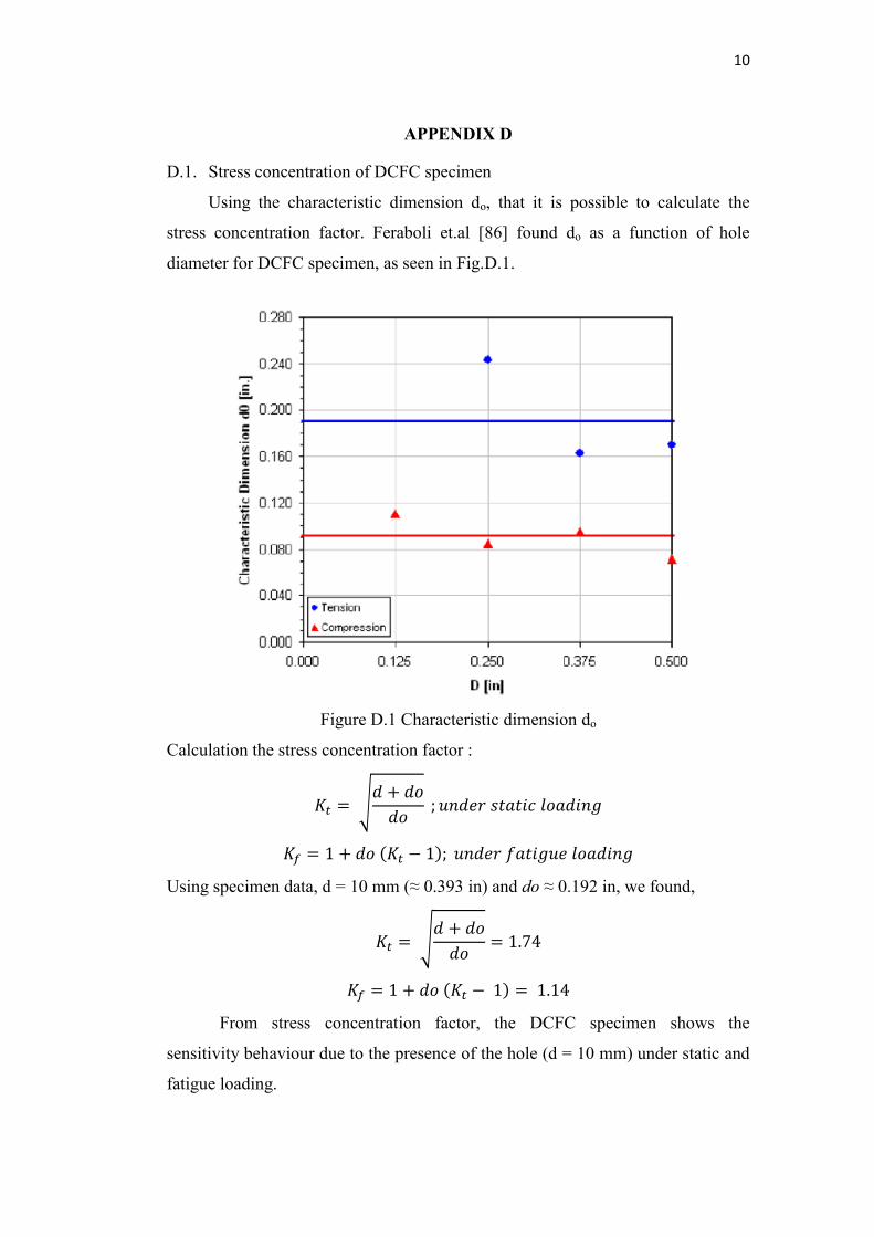
10

APPENDIX D

D.1. Stress concentration of DCFC specimen

Using the characteristic dimension do, that it is possible to calculate the

stress concentration factor. Feraboli et.al [86] found do as a function of hole

diameter for DCFC specimen, as seen in Fig.D.1.

Figure D.1 Characteristic dimension do

Calculation the stress concentration factor :

Using specimen data, d = 10 mm (≈ 0.393 in) and do ≈ 0.192 in, we found,

From stress concentration factor, the DCFC specimen shows the

sensitivity behaviour due to the presence of the hole (d = 10 mm) under static and

fatigue loading.

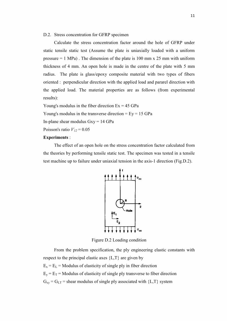
11

D.2. Stress concentration for GFRP specimen

Calculate the stress concentration factor around the hole of GFRP under

static tensile static test (Assume the plate is uniaxially loaded with a uniform

pressure = 1 MPa) . The dimension of the plate is 100 mm x 25 mm with uniform

thickness of 4 mm. An open hole is made in the centre of the plate with 5 mm

radius. The plate is glass/epoxy composite material with two types of fibers

oriented : perpendicular direction with the applied load and pararel direction with

the applied load. The material properties are as follows (from experimental

results):

Young's modulus in the fiber direction Ex = 45 GPa

Young's modulus in the transverse direction = Ey = 15 GPa

In-plane shear modulus Gxy = 14 GPa

Poisson's ratio Ѵ12 = 0.05

Experiments :

The effect of an open hole on the stress concentration factor calculated from

the theories by performing tensile static test. The specimen was tested in a tensile

test machine up to failure under uniaxial tension in the axis-1 direction (Fig.D.2).

Figure D.2 Loading condition

From the problem specification, the ply engineering elastic constants with

respect to the principal elastic axes {L,T} are given by

Ex = EL = Modulus of elasticity of single ply in fiber direction

Ey = ET = Modulus of elasticity of single ply transverse to fiber direction

Gxy = GLT = shear modulus of single ply associated with {L,T} system

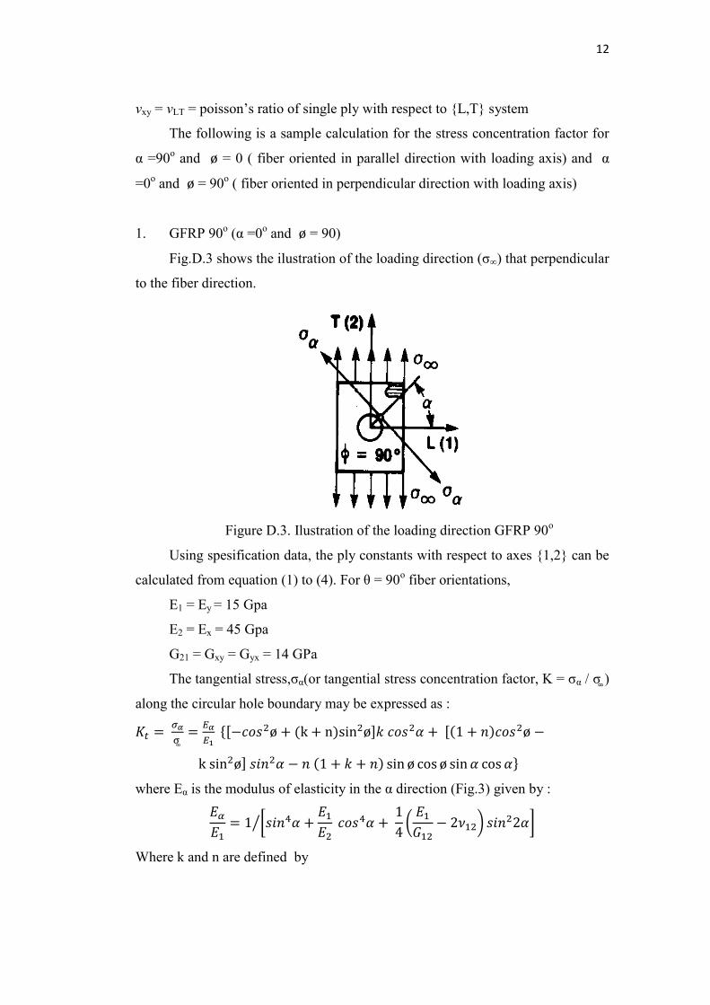
12

νxy = vLT = poisson’s ratio of single ply with respect to {L,T} system

The following is a sample calculation for the stress concentration factor for

α =90o and = 0 ( fiber oriented in parallel direction with loading axis) and α

=0o and = 90o ( fiber oriented in perpendicular direction with loading axis)

1. GFRP 90o (α =0o and = 90)

Fig.D.3 shows the ilustration of the loading direction (σ∞) that perpendicular

to the fiber direction.

Figure D.3. Ilustration of the loading direction GFRP 90o

Using spesification data, the ply constants with respect to axes {1,2} can be

calculated from equation (1) to (4). For θ = 90o fiber orientations,

E1 = Ey = 15 Gpa

E2 = Ex = 45 Gpa

G21 = Gxy = Gyx = 14 GPa

The tangential stress,σα(or tangential stress concentration factor, K = σα / σ )

along the circular hole boundary may be expressed as : where Eα is the modulus of elasticity in the α direction (Fig.3) given by μ

Where k and n are defined by

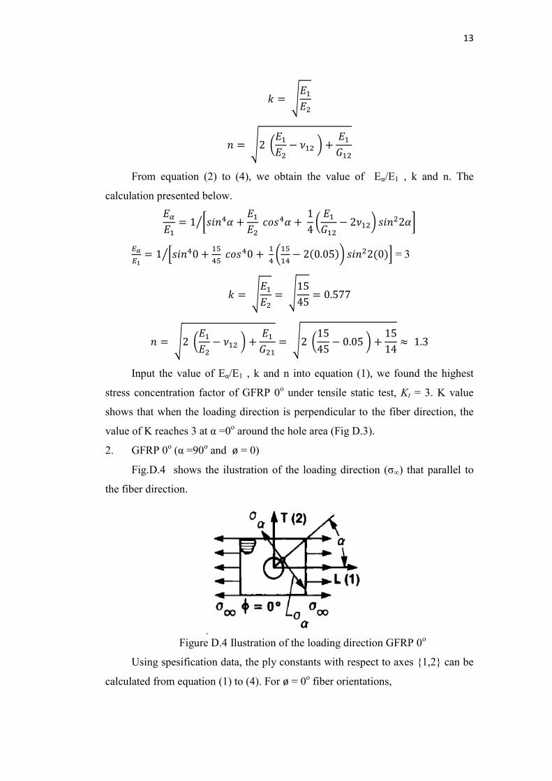
13

From equation (2) to (4), we obtain the value of Eα/E1 , k and n. The

calculation presented below.

= 3

Input the value of Eα/E1 , k and n into equation (1), we found the highest

stress concentration factor of GFRP 0o under tensile static test, Kt = 3. K value

shows that when the loading direction is perpendicular to the fiber direction, the

value of K reaches 3 at α =0o around the hole area (Fig D.3).

2. GFRP 0o (α =90o and = 0)

Fig.D.4 shows the ilustration of the loading direction (σ∞) that parallel to

the fiber direction.

Figure D.4 Ilustration of the loading direction GFRP 0o

Using spesification data, the ply constants with respect to axes {1,2} can be

calculated from equation (1) to (4). For = 0o fiber orientations,

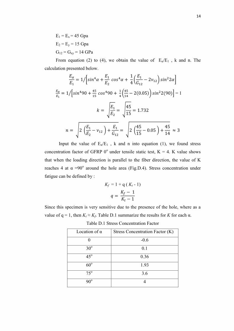
14

E1 = Ex = 45 Gpa

E2 = Ey = 15 Gpa

G12 = Gxy = 14 GPa

From equation (2) to (4), we obtain the value of Eα/E1 , k and n. The

calculation presented below.

= 1

Input the value of Eα/E1 , k and n into equation (1), we found stress

concentration factor of GFRP 0o under tensile static test, K = 4. K value shows

that when the loading direction is parallel to the fiber direction, the value of K

reaches 4 at α =90o around the hole area (Fig.D.4). Stress concentration under

fatigue can be defined by :

Kf = 1 + q ( Kt - 1)

Since this specimen is very sensitive due to the presence of the hole, where as a

value of q = 1, then Kt ≈ Kf. Table D.1 summarize the results for K for each α.

Table D.1 Stress Concentration Factor

Location of α Stress Concentration Factor (K)

0 -0.6

30o 0.1

45o 0.36

60o 1.93

75o 3.6

90o 4

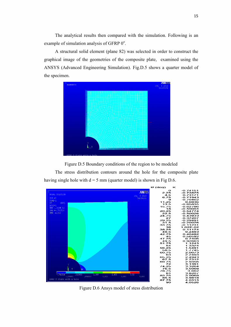
15

The analytical results then compared with the simulation. Following is an

example of simulation analysis of GFRP 0o.

A structural solid element (plane 82) was selected in order to construct the

graphical image of the geometries of the composite plate, examined using the

ANSYS (Advanced Engineering Simulation). Fig.D.5 shows a quarter model of

the specimen.

Figure D.5 Boundary conditions of the region to be modeled

The stress distribution contours around the hole for the composite plate

having single hole with d = 5 mm (quarter model) is shown in Fig D.6.

Figure D.6 Ansys model of stess distribution

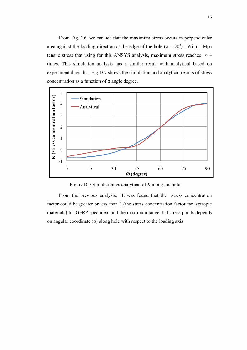
16

From Fig.D.6, we can see that the maximum stress occurs in perpendicular

area against the loading direction at the edge of the hole ( = 90o) . With 1 Mpa

tensile stress that using for this ANSYS analysis, maximum stress reaches ≈ 4

times. This simulation analysis has a similar result with analytical based on

experimental results. Fig.D.7 shows the simulation and analytical results of stress

concentration as a function of angle degree.

Figure D.7 Simulation vs analytical of K along the hole

From the previous analysis, It was found that the stress concentration

factor could be greater or less than 3 (the stress concentration factor for isotropic

materials) for GFRP specimen, and the maximum tangential stress points depends

on angular coordinate (α) along hole with respect to the loading axis.

-1

0

1

2

3

4

5

0 15 30 45 60 75 90

K (

stre

ss c

once

ntr

atio

n fa

ctor

)

Ø (degree)

Simulation

Analytical