Cahier 15-2018

The Impact of Uncertainty in Agriculture

Raphael Godefroy & Joshua Lewis

Le Centre interuniversitaire de recherche en économie quantitative (CIREQ) regroupe des chercheurs dans les domaines de l'économétrie, la théorie de la décision, la macroéconomie et les marchés financiers, la microéconomie appliquée ainsi que l'économie de l'environnement et des ressources naturelles. Ils proviennent principalement des universités de Montréal, McGill et Concordia. Le CIREQ offre un milieu dynamique de recherche en économie quantitative grâce au grand nombre d'activités qu'il organise (séminaires, ateliers, colloques) et de collaborateurs qu'il reçoit chaque année. The Center for Interuniversity Research in Quantitative Economics (CIREQ) regroups researchers in the fields of econometrics, decision theory, macroeconomics and financial markets, applied microeconomics as well as environmental and natural resources economics. They come mainly from the Université de Montréal, McGill University and Concordia University. CIREQ offers a dynamic environment of research in quantitative economics thanks to the large number of activities that it organizes (seminars, workshops, conferences) and to the visitors it receives every year.

Cahier 15-2018

The Impact of Uncertainty in Agriculture

Raphael Godefroy Joshua Lewis

CIREQ, Université de Montréal C.P. 6128, succursale Centre-ville Montréal (Québec) H3C 3J7 Canada Téléphone : (514) 343-6557 Télécopieur : (514) 343-7221 cireq@umontreal.ca http://www.cireqmontreal.com

Ce cahier a également été publié par le Département de sciences économiques de l’Université de Montréal sous le numéro «No_du_cahier_conjoint».

This working paper was also published by the Department of Economics of the University of Montreal under number «No_du_cahier_conjoint». Dépôt légal - Bibliothèque nationale du Canada, 2018, ISSN 0821-4441 Dépôt légal - Bibliothèque et Archives nationales du Québec, 2018 ISBN-13 : «No_ISBN13»

The Impact of Uncertainty in Agriculture∗

Raphael Godefroy (University of Montreal)Joshua Lewis (University of Montreal)

February 2018

Abstract

Income uncertainty in the rural economy is widely considered an important impediment togrowth in poor countries. This paper uses a rich dataset on productivity, land use, and outputfor 17 different crops across 500,000 plots of land in 87 countries to study the impact of uncer-tainty in the agricultural sector. The analysis relies on historical variability in crop productivitydriven by local climatic conditions to estimate the impact of of uncertainty on farmers’ landallocation. Applying a standard portfolio framework, we estimate that the incentive to diversifyled to large losses in agricultural revenue. We adopt a spatial regression discontinuity approachthat compares how national institutions affected agricultural outcomes near the borders of for-mer British and French colonies in Africa. We find that farmers in former British colonies,which tended to adopt pro-private sector policies, adopted more advanced input technologiesand achieved higher crop-specific returns. In contrast, farmers in former French colonies, whichtended to devote more public resources to the agricultural sector, tolerated higher levels ofuncertainty and adopted more specialized crop portfolios. These offsetting effects suggest thatboth a well-functioning market system along with public investments that reduce risk may benecessary to foster rural economic development.

∗Contact: Raphael Godefroy: raphael.godefroy@umontreal.ca. Joshua Lewis: joshua.lewis@umontreal.ca.

1 Introduction

Households in many rural areas are subject to substantial economic uncertainty. Recurrent

droughts and fluctuations in output prices lead to volatile agricultural earnings (e.g., Carter,

1997; Shanahan et al., 2009), and rural producers often lack access to credit or insurance markets

(Binswanger and Rosenzweig, 1986).1 Despite a growing literature, there is little consensus on

the impact of uncertainty on the rural economy, and estimated effects have varied widely across

different locations.

This paper combines a detailed micro-dataset on agricultural productivity, land use, and

output to study the economic impact of agricultural income uncertainty at a global scale. Our

analysis builds on the simple idea that risk-averse farmers facing ex ante uncertainty over future

revenue may sacrifice additional earnings in order to reduce exposure to income volatility. If

climate shocks and output price shocks affect all crops similarly, there would be no scope for

crop portfolio adjustments to lower income uncertainty. However, to the extent that output

price shocks and climatic conditions are crop specific, farmers may divert land to crops that

generate lower expected returns but help smooth against annual income fluctuations.

Our empirical analysis is based on detailed geospatial data assembled by the Global Agro-

Ecological Zones (GAEZ) project of the Food and Agriculture Organization (FAO). The GAEZ

project provides agronomic modelling with high-resolution data to provide information on po-

tential yields, harvested land, and actual yields by crop for 1.7 million plots of land that span

the earth’s surface.2 Potential crop yields are constructed by combining agronomic models

of specific crop requirements with high-resolution data on geographic and climatic conditions.

Crucially, the GAEZ data provides information potential crop yields by year, allowing us to

construct measures of mean and variability in yields by crop for each grid cell, whether or not

the crop is actually grown.

1For example, Kazianga and Udry (1996) find that the standard deviation of rainfall-induced income variationis more than half of average rural household income in Burkina Faso.

2Land plots are available at the 5-arc-minute level, which corresponds to roughly 10 km by 10 km at theequator.

1

To estimate the impact of uncertainty on rural producers decision-making, we combine the

GAEZ crop data with a standard mean-variable portfolio framework (Markowitz, 1952). Farm-

ers are assumed to trade-off higher expected crop returns against increased variance on their

plot. We combine this simple framework with plot-level data on the observed land allocation,

expected returns by crop, and the historical covariance in crop yields to calculate the mean-

variance efficient (MVE) frontier for each plot of land: the maximum attainable return given

a specific level of output risk. The empirical analysis compares farm earnings under full spe-

cialization, the MVE allocation, and the actual allocation to calculate the fraction of revenue

losses attributable to diversification incentives across each plot of agricultural land. Farmers

may divert land from the highest yield crop for a variety of motives unrelated to output risk.

Our identification, which relies on the specific structure of the covariance matrix in crop returns,

allows us to the effect of uncertainty from other sources of land misallocation.

We have three main findings. First, ‘crop misallocation’ – the fact that farmers did not

specialize in revenue maximizing crops – is associated with large losses in agricultural revenue.

We estimate that revenue on the typical plot could have been doubled under full specialization.

These losses exceeded those attributable to within-crop distortions, and they were particularly

large in lower income countries. Crop misallocation cannot be explained by the selection of

workers into the agricultural sector (Lagakos and Waugh, 2013), distortions affecting the scale

of production units in agriculture (e.g., Adamopoulos and Restuccia, 2014), or farmers’ choices

of input technologies (e.g., Donovan, 2016), since each of these factors will have similar effects

on agricultural productivity irrespective of the particular crop that is grown.

Second, we find that the incentive to diversify land against annual income uncertainty

was the primary source of crop misallocation. Comparing the MVE efficient allocation to

the observed land allocation and the allocation under full specialization, we calculate that

80 percent of the losses from crop misallocation are attributable to diversification incentives.

Farmers in richer and poorer countries faced similar level of income uncertainty. Nevertheless,

their response was markedly different. Farmers in below-median income countries planted more

2

different crops and devoted 20 percent less agricultural land to the dominant crop. Comparing

the sources of crop misallocation across countries, we estimate that the losses attributable to

income uncertainty were 50 percent larger in countries with below-median income. Together,

these findings suggest that rural income uncertainty is a major source of revenue losses in

poorer countries, and that limited access to insurance and incomplete credit markets may be

an important reason why agricultural productivity is so low in poor countries.

Third, using a regression discontinuity design, we find no significant difference in overall

agricultural output across African farmers operating at the borders of former British and French

colonies. These small overall effects mask two offsetting forces. On the one hand, farmers in

former British colonies used more advanced input technologies and achieved higher crop-specific

returns. On the other hand, these farmers were more likely to diversify their crop portfolio

given a particular level of economic uncertainty. We argue that these findings are consistent

with the institutional arrangements of the two sets of countries. In particular, former British

colonies were more likely to adopt pro-private sector policies, and better functioning credit

markets, which may have faciliated investment in the agricultural sector. In contrast, former

French colonies had larger public sectors that devoted more resources to the agricultural sector,

potentially shielding rural producers from the consequences of income volatility. Together, the

findings suggest that both a well-functioning market systems along with some form of non-

market interventions that reduce individual exposure to uncertainty may be necessary to foster

rural economic development.

The paper contributes to the large literature on the role of uncertainty in agriculture. Re-

searchers have identified a number of channels through which individual households cope with

income uncertainty in the face of credit constraints, including precautionary savings (Deaton,

1990, 1991; Fafchamps et al., 1998), remittances from urban family members (Rapoport and

Docquier, 2006; Gonzalez-Velosa, 2012, Yang and Choi, 2007), delayed technological adoption

(Antle and Crissman, 1990, Dercon and Christiaensen, 2011, Donovan, 2014), and crop diver-

sification (Kurosaki, and Fafchamps, 2002; Di Falco, and Chavas, 2009, Nicola, 2015). Despite

3

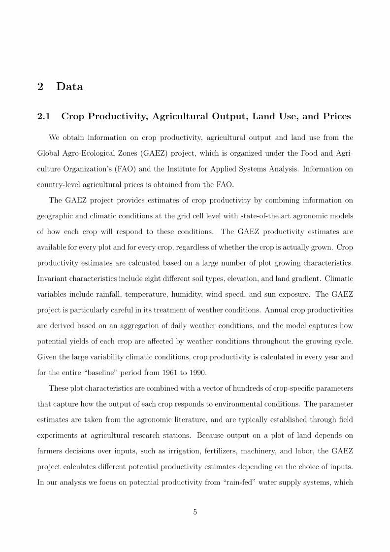
this research, there is ongoing debate of the effectiveness of these strategies (Udry, 2016). The

lack of consensus is, in part, a result of the fact that the populations studied differ widely in

both the risks posed by climatic shocks and the institutional framework in which rural produc-

ers operate. By studying the consequences of income uncertainty across virtually all cultivated

land, we are able to examine the impact of income uncertainty in agriculture at a much broader

scale, allowing us to explore the extent to which different levels of producer risk and different

income levels impact decision-making in rural areas.

This paper also contributes to the literature that studies agricultural productivity gaps and

their role in explaining cross-country income differences. A number of studies have documented

the role of sector specific distortions for agricultural productivity (Adamopoulos and Restuccia,

2011; Restuccia, Yang, and Zhu, 2008; Tombe, 2014; Adamopoulos, 2011). Researchers have

also examined role of self-selection across sectors in explaining these large gaps (Lagakos and

Waugh, 2013). Our results complement recent work by Donovan (2014) that shows how id-

iosyncratic risk can lead to underinvestment in the agricultural sector. Most closely related to

our work is Adamopoulos and Restuccia (2015), who use the GAEZ data to explore the extent

to which agricultural productivity gaps are driven by production inefficiencies, crop misalloca-

tion, and production inefficiencies across cultivated and cultivatable plots. Consistent with our

results, they find that the majority of cross-country differences in output can be attributed to

economic decision-making rather than differences in land quality.

Our analysis also contributes to a growing literature that uses the historical partition of

African countries to study the impact of national institutions on economic outcomes. Previous

research has found mixed evidence on the importance of institutions (e.g., Michalopoulos and

Papiaoannou, 2013, 2014).3 Our results show that the limited overall impact on rural eco-

nomic activity was partly a reflection of offsetting institutional arrangements. In particular,

the benefits the pro-market institutions that promoted rural investment were counteracted by

the redistributive policies that developed in former French colonies.

3Other research that exploits border discontinuities to identify the role of particular national policies includeMiguel (2004), Cogneau and Moradi (2011), Bubb (2012), and Cogneau, Mesple-Somps, adn Spielvogel (2012).

4

2 Data

2.1 Crop Productivity, Agricultural Output, Land Use, and Prices

We obtain information on crop productivity, agricultural output and land use from the

Global Agro-Ecological Zones (GAEZ) project, which is organized under the Food and Agri-

culture Organization’s (FAO) and the Institute for Applied Systems Analysis. Information on

country-level agricultural prices is obtained from the FAO.

The GAEZ project provides estimates of crop productivity by combining information on

geographic and climatic conditions at the grid cell level with state-of-the art agronomic models

of how each crop will respond to these conditions. The GAEZ productivity estimates are

available for every plot and for every crop, regardless of whether the crop is actually grown. Crop

productivity estimates are calcuated based on a large number of plot growing characteristics.

Invariant characteristics include eight different soil types, elevation, and land gradient. Climatic

variables include rainfall, temperature, humidity, wind speed, and sun exposure. The GAEZ

project is particularly careful in its treatment of weather conditions. Annual crop productivities

are derived based on an aggregation of daily weather conditions, and the model captures how

potential yields of each crop are affected by weather conditions throughout the growing cycle.

Given the large variability climatic conditions, crop productivity is calculated in every year and

for the entire “baseline” period from 1961 to 1990.

These plot characteristics are combined with a vector of hundreds of crop-specific parameters

that capture how the output of each crop responds to environmental conditions. The parameter

estimates are taken from the agronomic literature, and are typically established through field

experiments at agricultural research stations. Because output on a plot of land depends on

farmers decisions over inputs, such as irrigation, fertilizers, machinery, and labor, the GAEZ

project calculates different potential productivity estimates depending on the choice of inputs.

In our analysis we focus on potential productivity from “rain-fed” water supply systems, which

5

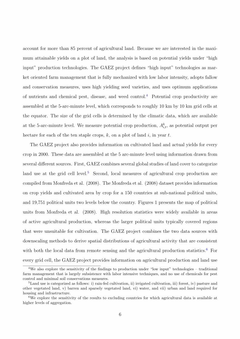
account for more than 85 percent of agricultural land. Because we are interested in the maxi-

mum attainable yields on a plot of land, the analysis is based on potential yields under “high

input” production technologies. The GAEZ project defines “high input” technologies as mar-

ket oriented farm management that is fully mechanized with low labor intensity, adopts fallow

and conservation measures, uses high yielding seed varieties, and uses optimum applications

of nutrients and chemical pest, disease, and weed control.4 Potential crop productivity are

assembled at the 5-arc-minute level, which corresponds to roughly 10 km by 10 km grid cells at

the equator. The size of the grid cells is determined by the climatic data, which are available

at the 5-arc-minute level. We measure potential crop production, Aki,t, as potential output per

hectare for each of the ten staple crops, k, on a plot of land i, in year t.

The GAEZ project also provides information on cultivated land and actual yields for every

crop in 2000. These data are assembled at the 5 arc-minute level using information drawn from

several different sources. First, GAEZ combines several global studies of land cover to categorize

land use at the grid cell level.5 Second, local measures of agricultural crop production are

compiled from Monfreda et al. (2008). The Monfreda et al. (2008) dataset provides information

on crop yields and cultivated area by crop for a 150 countries at sub-national political units,

and 19,751 political units two levels below the country. Figures 1 presents the map of political

units from Monfreda et al. (2008). High resolution statistics were widely available in areas

of active agricultural production, whereas the larger political units typically covered regions

that were unsuitable for cultivation. The GAEZ project combines the two data sources with

downscaling methods to derive spatial distributions of agricultural activity that are consistent

with both the local data from remote sensing and the agricultural production statistics.6 For

every grid cell, the GAEZ project provides information on agricultural production and land use

4We also explore the sensitivity of the findings to production under “low input” technologies – traditionalfarm management that is largely subsistence with labor intensive techniques, and no use of chemicals for pestcontrol and minimal soil conservations measures.

5Land use is categorized as follows: i) rain-fed cultivation, ii) irrigated cultivation, iii) forest, iv) pasture andother vegetated land, v) barren and sparsely vegetated land, vi) water, and vii) urban and land required forhousing and infrastructure.

6We explore the sensitivity of the results to excluding countries for which agricultural data is available athigher levels of aggregation.

6

for each crop. Specifically, Qki,2000 measures total output (measured in dry-weight tons) of crop

k on plot i for each of the 10 crops used in the analysis. We denote Li,2000 as the total hectares

of cultivated land on plot i, and ski,2000 the fraction of land devoted to crop k.

Data on agricultural producer prices are obtained from the FAOSTAT program at the FAO

(available at http://faostat3.fao.org/home/E). We assemble data on real output prices, pkc,t,

for each crop, k, in a country, c, in year t.7 Each grid cell observation is matched to relevant

country prices based on the country in which it falls using the country boundaries file available

from the World Borders Dataset (Thematic Mapping).8

The analysis is based on roughly 500,000 grid cells that had positive land used in agriculture

in 2000.9 Table 1 reports the crops and countries used in the analysis. We consider 17 staple

crops that comprise almost two-thirds of arable land worldwide.10 Our primary sample accounts

for almost two thirds of global land devoted to these crops, and spans 87 countries.11

2.2 Variable Construction

We combine the GAEZ data to assemble various measures of agricultural activity at the

plot level. These variables are used to compare observed farm earnings to potential earnings,

given land and climatic conditions.

We calculate total agricultural revenue per plot in 2000 (M4). For each grid cell, we use

information on output per hectare for each crop, Qki,2000, total cultivated land, Lk

i,2000, the share

of land devoted to each crop, ski,2000, and crop output prices, pkc,2000 to calculate actual plot

7All prices are inflation-adjusted (DISCUSS).8For the small number of observations that span multiple country boundaries, we assign the country based

on the grid cell centroid.9The full GAEZ dataset consists of 2.2 million grid cells. We omit roughly 1.5 million plots that had zero

agricultural production. A further 200,000 plots are excluded because of missing information on crop outputprices.

10Virtually all remaining arable land is devoted to fodder and vegetable production.11China and Russia account for roughly half of the remaining arable land. These two countries are excluded

from the main analysis because of missing information on historical crop output prices, although we explore therobustness of the results to their inclusion.

7

revenue in 2000 as follows:

M4i,2000 = Li,2000 ·∑k

pkc,2000 ·Qki,2000 · ski,2000.

The second variable of interest is potential revenue, M3i,t. This variable is constructed by

holding total agricultural land and crop land shares fixed at their 2000 values, and assuming

that farmers achieved maximum attainable yields per hectare for every crop, k grown, Akit, in

year t. The gap between actual revenue and potential revenue reflects the losses in agricultural

revenue attributable to farmers not maximizing output on a particular plot of land.12 We

calculate potential revenue in every year from 1990 to 2000. Potential revenue may vary from

one year to the next because of both fluctuations in output prices, and changes in potential

crop productivity due to local variation weather and climatic conditions. We calculate potential

revenue (M3) in every year from 1990 to 2000 as

M3i,t = Li,2000 ·∑k

pkc,t · Aki,t · ski,2000.

The third variable of interest is maximum potential revenue, M1i,2000, which is calculate in

2000.13 This variable is constructed by holding total agricultural land fixed at its 2000 value,

and assuming that farmers both produce maximum attainable yields for every crop and grow

the optimal portfolio. In particular, the vector of optimal crop shares is determined as follows:

s∗i,2000 = Argmaxski,2000∈[0,1]Li,2000

∑k

pkc,2000 · Aki,2000s

ki,2000.

The solution to this problem is full specialization, in which all agricultural land is devoted to

the revenue maximizing crop, k∗, and all other crop shares are set equal to zero. The maximum

12We discuss the possible reasons for these two variables to differ, and note that differences between actualand potential revenue may still be fully consistent with farm optimization in the following section.

13We discuss the construction of the final variable of interest, M2, in the following section.

8

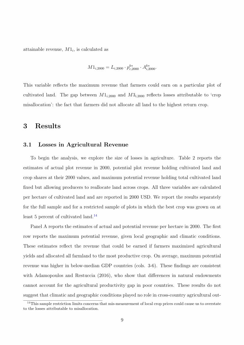
attainable revenue, M1i, is calculated as

M1i,2000 = Li,2000 · pk∗c,2000 · Ak∗i,2000.

This variable reflects the maximum revenue that farmers could earn on a particular plot of

cultivated land. The gap between M1i,2000 and M3i,2000 reflects losses attributable to ‘crop

misallocation’: the fact that farmers did not allocate all land to the highest return crop.

3 Results

3.1 Losses in Agricultural Revenue

To begin the analysis, we explore the size of losses in agriculture. Table 2 reports the

estimates of actual plot revenue in 2000, potential plot revenue holding cultivated land and

crop shares at their 2000 values, and maximum potential revenue holding total cultivated land

fixed but allowing producers to reallocate land across crops. All three variables are calculated

per hectare of cultivated land and are reported in 2000 USD. We report the results separately

for the full sample and for a restricted sample of plots in which the best crop was grown on at

least 5 percent of cultivated land.14

Panel A reports the estimates of actual and potential revenue per hectare in 2000. The first

row reports the maximum potential revenue, given local geographic and climatic conditions.

These estimates reflect the revenue that could be earned if farmers maximized agricultural

yields and allocated all farmland to the most productive crop. On average, maximum potential

revenue was higher in below-median GDP countries (cols. 3-6). These findings are consistent

with Adamopoulos and Restuccia (2016), who show that differences in natural endowments

cannot account for the agricultural productivity gap in poor countries. These results do not

suggest that climatic and geographic conditions played no role in cross-country agricultural out-

14This sample restriction limits concerns that mis-measurement of local crop prices could cause us to overstateto the losses attributable to misallocation.

9

put differences. In particular, farmers in low income countries may have been more vulnerable

to volatile output yields caused by climatic and weather shocks, despite having higher average

potential yields. The second row reports potential revenue per plot, based on observed culti-

vated land shares in 2000, assuming that farmers achieved maximum crop yields given land and

climatic constraints. These estimates reflect the revenue that could be if farmers adopted state-

of-the-art production technologies, but did not alter the composition of land fixed. Finally, the

third row reports actual revenue per hectare.

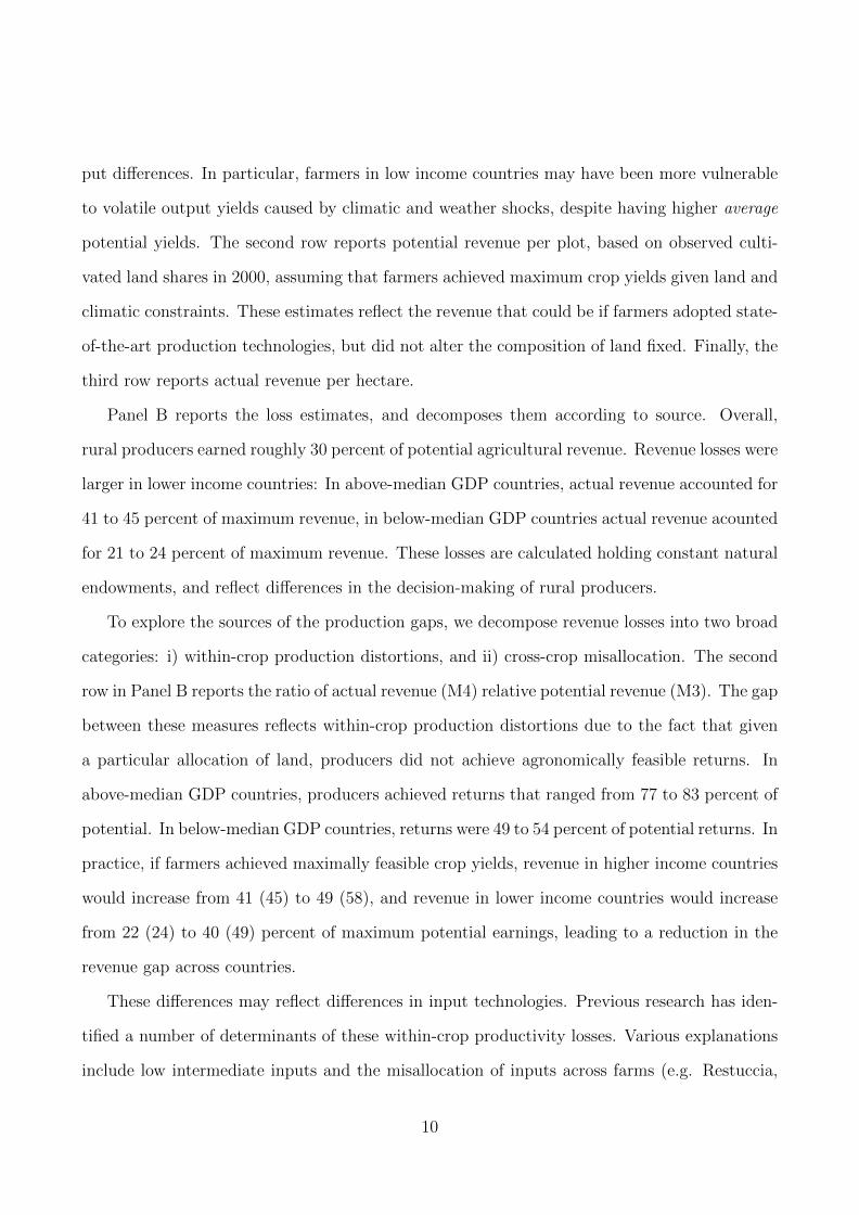
Panel B reports the loss estimates, and decomposes them according to source. Overall,

rural producers earned roughly 30 percent of potential agricultural revenue. Revenue losses were

larger in lower income countries: In above-median GDP countries, actual revenue accounted for

41 to 45 percent of maximum revenue, in below-median GDP countries actual revenue acounted

for 21 to 24 percent of maximum revenue. These losses are calculated holding constant natural

endowments, and reflect differences in the decision-making of rural producers.

To explore the sources of the production gaps, we decompose revenue losses into two broad

categories: i) within-crop production distortions, and ii) cross-crop misallocation. The second

row in Panel B reports the ratio of actual revenue (M4) relative potential revenue (M3). The gap

between these measures reflects within-crop production distortions due to the fact that given

a particular allocation of land, producers did not achieve agronomically feasible returns. In

above-median GDP countries, producers achieved returns that ranged from 77 to 83 percent of

potential. In below-median GDP countries, returns were 49 to 54 percent of potential returns. In

practice, if farmers achieved maximally feasible crop yields, revenue in higher income countries

would increase from 41 (45) to 49 (58), and revenue in lower income countries would increase

from 22 (24) to 40 (49) percent of maximum potential earnings, leading to a reduction in the

revenue gap across countries.

These differences may reflect differences in input technologies. Previous research has iden-

tified a number of determinants of these within-crop productivity losses. Various explanations

include low intermediate inputs and the misallocation of inputs across farms (e.g. Restuccia,

10

Yang, and Zhu, 2008; Adamopoulos and Restuccia, 2011), the selection of less productive work-

ers into the agricultural sector (e.g. Lagakos and Waugh, 2013), and underinvestment in farm

technology due to rural producers’ inability to insure against idiosyncratic risks (e.g. Donovan,

2014). It may also be the case that these revenue losses reflect optimal response to cross-country

differences in input prices. For example, if farmers in low income countries chose to adopt lower

production technologies.15

The third row in Panel B reports potential revenue as a percentage of maximum potential

revenue under full specialization. These estimates reflect losses due to the fact that land was

devoted to crops that did not maximize farm revenue. We estimate that cross-crop distortions

were associated large losses in revenue, particularly in lower income countries. These results

suggest that understanding the sources of crop-misallocation are critical for the understanding

agricultural productivity gap.

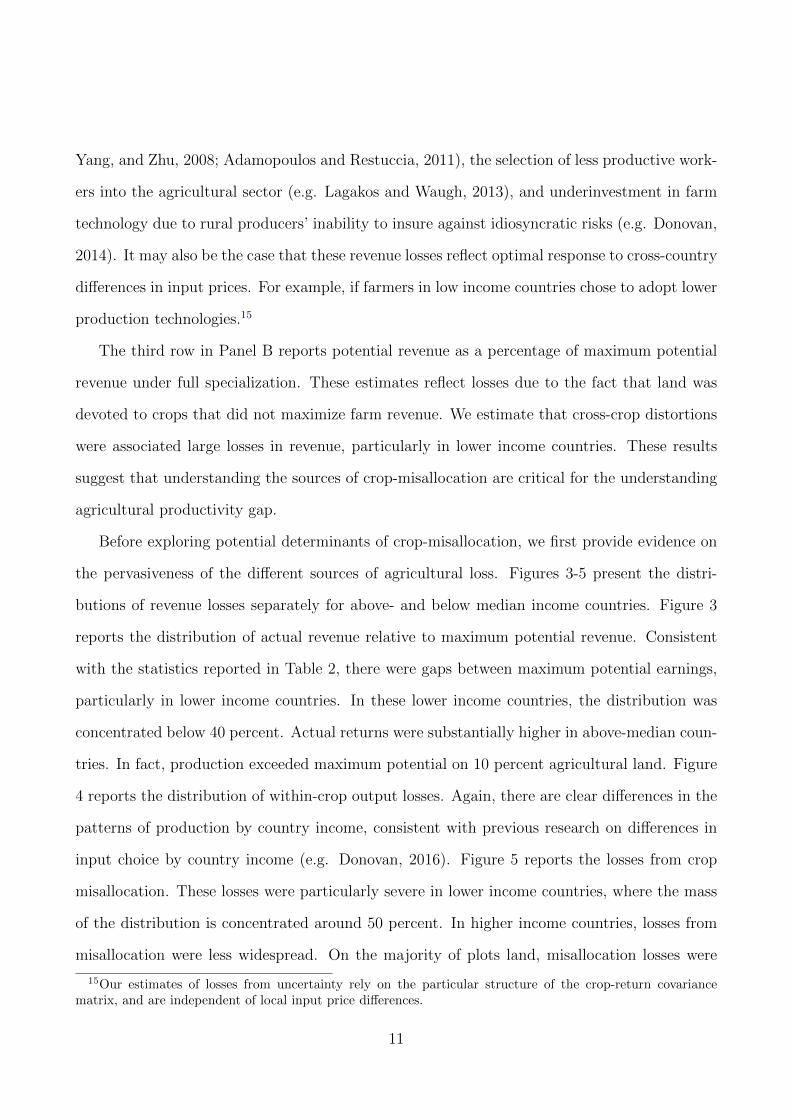
Before exploring potential determinants of crop-misallocation, we first provide evidence on

the pervasiveness of the different sources of agricultural loss. Figures 3-5 present the distri-

butions of revenue losses separately for above- and below median income countries. Figure 3

reports the distribution of actual revenue relative to maximum potential revenue. Consistent

with the statistics reported in Table 2, there were gaps between maximum potential earnings,

particularly in lower income countries. In these lower income countries, the distribution was

concentrated below 40 percent. Actual returns were substantially higher in above-median coun-

tries. In fact, production exceeded maximum potential on 10 percent agricultural land. Figure

4 reports the distribution of within-crop output losses. Again, there are clear differences in the

patterns of production by country income, consistent with previous research on differences in

input choice by country income (e.g. Donovan, 2016). Figure 5 reports the losses from crop

misallocation. These losses were particularly severe in lower income countries, where the mass

of the distribution is concentrated around 50 percent. In higher income countries, losses from

misallocation were less widespread. On the majority of plots land, misallocation losses were

15Our estimates of losses from uncertainty rely on the particular structure of the crop-return covariancematrix, and are independent of local input price differences.

11

less than 25 percent.

3.2 Determinants of Crop Misallocation

The large losses attributable to cross-crop distortions suggests that, in many areas, land was

not allocated to its most productive use. There are two potential explanations for this result.

First, crop misallocation may have been caused by farmers having specialized in crops that did

not maximize revenue. This situation could reflect differences between local producer prices

and national-level crop prices. High transportation costs and poor market access could cause

within-country variation in agricultural prices, implying that the optimal crop allocation under

national prices may have differed from the optimal allocation under local prices. Differences in

input costs across crops could also lead the revenue maximizing allocation to differ from the

profit maximizing optimal crop allocation. Government agricultural policies, such as quotas or

crop-specific subsidies, could also distort the observed crop allocation away from optimum. Any

of these price distortions could lead to crop misallocation and cause farmers should allocate land

to crops that do not maximize observed revenue. Because these distortions do not influence the

incentive to produce multiple crops, however, this scenario should still be associated with high

level of specialization within-plots.

A second possibility is that land was allocated across multiple different crops in ways that did

not maximize plot revenue. Differences in production decisions across farms could be the result

of information problems which could cause decision-making of some rural producers to differ

from optimum. Heterogeneous access to credit could also limit the ability of some farmers to

allocate land optimally. It is also possible that highly localized differences in land productivity

could lead the optimal local crop allocation to diverge from the average plot-level optimum.

Similarly, rural producers may have adopted outdated crop-cycling practices, rotating land

between higher and lower productivity crops in an effort to preserve soil nutrients.16 Finally, the

16The agronomic model used by the FAO to construct potential yields accounts for optimal fallow periodsand fertilizer usage to best preserve long-run soil quality.

12

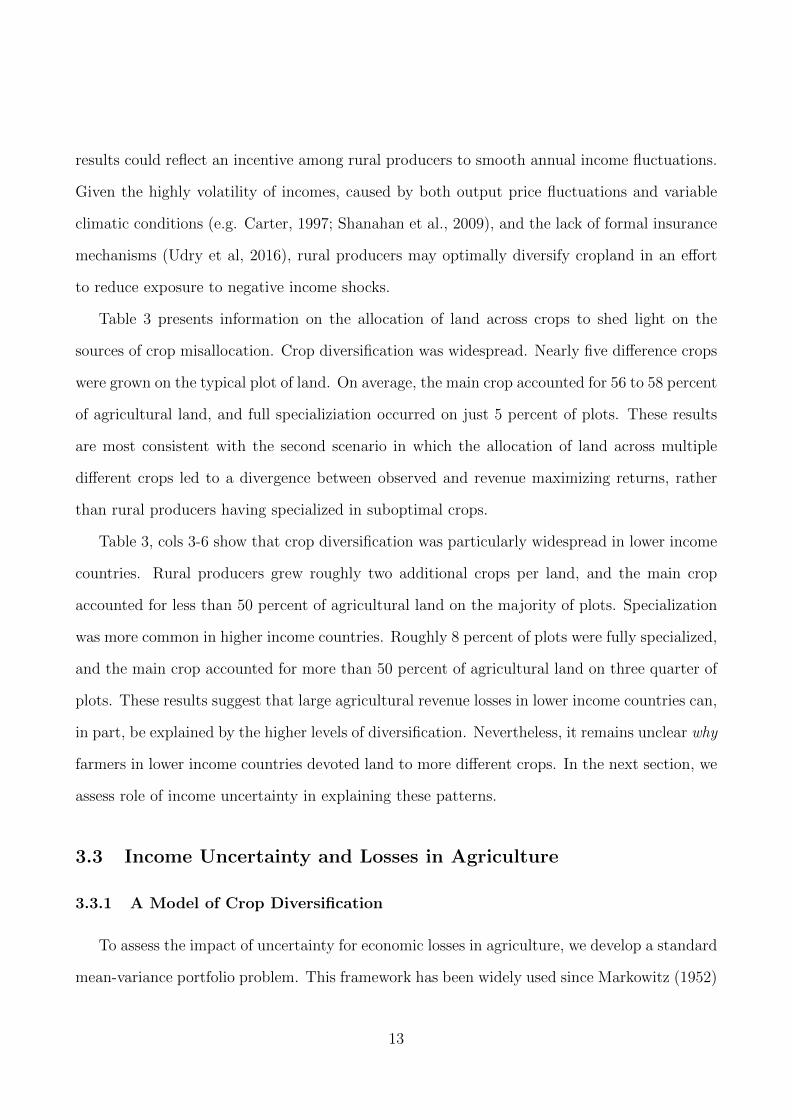
results could reflect an incentive among rural producers to smooth annual income fluctuations.

Given the highly volatility of incomes, caused by both output price fluctuations and variable

climatic conditions (e.g. Carter, 1997; Shanahan et al., 2009), and the lack of formal insurance

mechanisms (Udry et al, 2016), rural producers may optimally diversify cropland in an effort

to reduce exposure to negative income shocks.

Table 3 presents information on the allocation of land across crops to shed light on the

sources of crop misallocation. Crop diversification was widespread. Nearly five difference crops

were grown on the typical plot of land. On average, the main crop accounted for 56 to 58 percent

of agricultural land, and full specializiation occurred on just 5 percent of plots. These results

are most consistent with the second scenario in which the allocation of land across multiple

different crops led to a divergence between observed and revenue maximizing returns, rather

than rural producers having specialized in suboptimal crops.

Table 3, cols 3-6 show that crop diversification was particularly widespread in lower income

countries. Rural producers grew roughly two additional crops per land, and the main crop

accounted for less than 50 percent of agricultural land on the majority of plots. Specialization

was more common in higher income countries. Roughly 8 percent of plots were fully specialized,

and the main crop accounted for more than 50 percent of agricultural land on three quarter of

plots. These results suggest that large agricultural revenue losses in lower income countries can,

in part, be explained by the higher levels of diversification. Nevertheless, it remains unclear why

farmers in lower income countries devoted land to more different crops. In the next section, we

assess role of income uncertainty in explaining these patterns.

3.3 Income Uncertainty and Losses in Agriculture

3.3.1 A Model of Crop Diversification

To assess the impact of uncertainty for economic losses in agriculture, we develop a standard

mean-variance portfolio problem. This framework has been widely used since Markowitz (1952)

13

to study investor decision-making in the presence of risk. The model, which was originally

developed to study the portfolio decisions of investors, applies natural to the decision-making

problem of rural producers, who must decide how to allocate land across a variety of crops

that have different expected returns and carry different levels of risk. The results provide a

benchmark against which we can compare the actual crop choices of farmers.

We consider a rural economy with one unit of agricultural land.17 Let s be a k-vector

where each element sk denotes the fraction of land devoted to crop k and∑

k sk = 1. Farmers

are assumed to face uncertainty in the realization of individual crop returns, which may be

correlated across crops. Let r denote the k-vector of mean crop returns with typical element

rk, and V as a k×k covariance matrix with typical element σij denoting the covariance between

the returns for crops i and j.18 According to this setup, any portfolio of crops chosen by the

farmer, s, can be characterized by an expected return, Rp, and variance, σ2p:

Rp = sTr =∑k

skrk, σ2p = sTV s =

∑i

∑j

xixjσij.

The farmer is assumed to trade-off higher returns against increased risk in the portfolio

according to the following formulation:

maximize Rp = sTr (1)

subject to σ2p = sTV s, sT1 = 1, s ≥ 0.

The farmer’s problem is to maximize the portfolio return subject to three constraints. First,

the variance of the portfolio cannot exceed a desired level, σ2p. Second, the amount of land used

for agricultural production cannot exceed the total amount available. Third, the amount of

land devoted to each crop must be non-negative.19

17This normalization abstracts from decisions over how much land to devote to agriculture.18To ensure that V is nonsingular and positive definite, we assume that no two crops have perfectly correlated

returns and that all crops have strictly positive variances.19This constraint is equivalent to a short-selling restriction in the standard portfolio asset allocation problem.

14

The solution to the problem is an optimal set of weights, s∗, that achieves the highest

expected return given an particular level of portfolio volatility.20 Solving for the optimal weights

for different values of σ2p, we can trace out the mean-variance efficient (MVE) locus, the portfolio

mean-variance pairs (Rp, σ2p) that provide the highest return for a given variances.21 Figure 1

displays the upward-sloping MVE locus. Intuitively, as the tolerance for risk increases, the

farmer is able to achieve greater expected returns. All combinations of (Rp, σ2p) that fall below

this locus are suboptimal, since the farmer could achieve higher expected returns without

increasing risk. We denote RMaxi as the highest possible return the farmer could obtain on a

plot of land, i. Meanwhile, let denote RGi as the return associated with the global minimum

variance portfolio – the crop choice with the lowest variability.

This simple framework can be applied to assess the impact of uncertainty on agricultural

losses. Figure 2 provides intuition for the analysis. Consider a farmer operating on a plot of

land, i, who chooses a vector of crops, si that yields a return-variance combination (Ri, σ2i ).

Given the particular characteristics of the plot, RMaxi represents the maximum revenue that

could be generated on the plot under full specialization. Meanwhile, R∗i represents the return

from the efficient crop portfolio based on the observed plot variance, σ2i . This value reflects the

highest agricultural earnings that could be earned without increasing the farmer’s level of risk

exposure.

Total revenue losses on plot i, RMaxi − Ri, can be decomposed into two sources: 1) losses

attributable to uncertainty, RMaxi − R∗i , and 2) residual losses from ‘crop misallocation’, R∗i −

Ri. The first term reflects losses caused by the fact that farmers may diversify their crop

portfolio to reduce income volatility. This gap reflects that fact that crop diversification lowers

expected returns, and given a particular risk tolerance, σ2i , it is impossible for farmers to achieve

maximum returns. The second term reflects the residual losses from ‘crop misallocation’ that

20The farmer’s specific utility function does not enter the problem, although portfolio optimization has beenshown to be consistent with expected utility maximization with quadratic utility (see Ingersoll, 1987, for adiscussion).

21An analytic solution to (1) does not exist, although the optimal weights can be calculated using numericalmethods

15

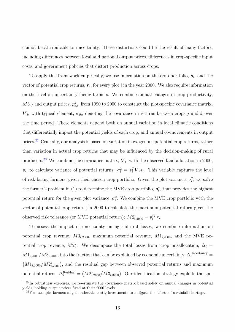
cannot be attributable to uncertainty. These distortions could be the result of many factors,

including differences between local and national output prices, differences in crop-specific input

costs, and government policies that distort production across crops.

To apply this framework empirically, we use information on the crop portfolio, si, and the

vector of potential crop returns, ri, for every plot i in the year 2000. We also require information

on the level on uncertainty facing farmers. We combine annual changes in crop productivity,

M3i,t and output prices, pkc,t, from 1990 to 2000 to construct the plot-specific covariance matrix,

V i, with typical element, σjk, denoting the covariance in returns between crops j and k over

the time period. These elements depend both on annual variation in local climatic conditions

that differentially impact the potential yields of each crop, and annual co-movements in output

prices.22 Crucially, our analysis is based on variation in exogenous potential crop returns, rather

than variation in actual crop returns that may be influenced by the decision-making of rural

producers.23 We combine the covariance matrix, V i, with the observed land allocation in 2000,

si, to calculate variance of potential returns: σ2i = sTi V isi. This variable captures the level

of risk facing farmers, given their chosen crop portfolio. Given the plot variance, σ2i , we solve

the farmer’s problem in (1) to determine the MVE crop portfolio, s∗i , that provides the highest

potential return for the given plot variance, σ2i . We combine the MVE crop portfolio with the

vector of potential crop returns in 2000 to calculate the maximum potential return given the

observed risk tolerance (or MVE potential return): M2∗i,2000 = s∗Ti ri.

To assess the impact of uncertainty on agricultural losses, we combine information on

potential crop revenue, M3i,2000, maximum potential revenue, M1i,2000, and the MVE po-

tential crop revenue, M2∗i . We decompose the total losses from ‘crop misallocation, ∆i =

M1i,2000

/M3i,2000, into the fraction that can be explained by economic uncertainty, ∆Uncertainty

i =(M1i,2000

/M2∗i,2000

), and the residual gap between observed potential returns and maximum

potential returns, ∆Residuali =

(M2∗i,2000

/M3i,2000

). Our identification strategy exploits the spe-

22In robustness exercises, we re-estimate the covariance matrix based solely on annual changes in potentialyields, holding output prices fixed at their 2000 levels.

23For example, farmers might undertake costly investments to mitigate the effects of a rainfall shortage.

16

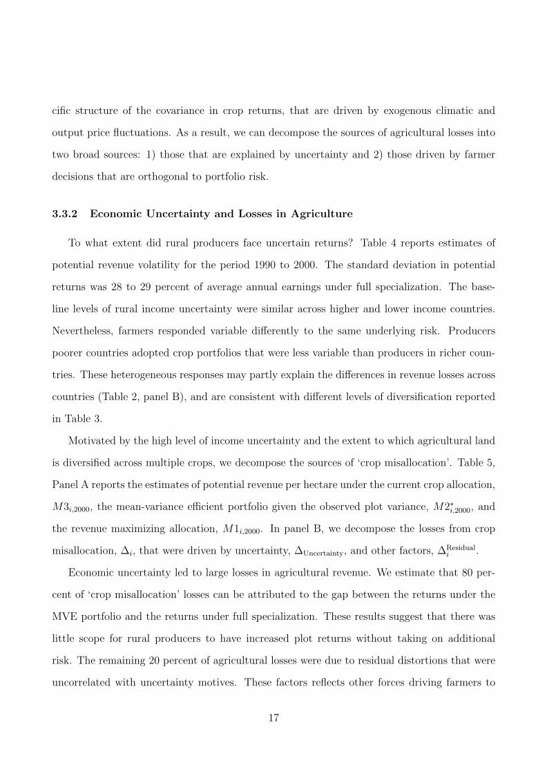
cific structure of the covariance in crop returns, that are driven by exogenous climatic and

output price fluctuations. As a result, we can decompose the sources of agricultural losses into

two broad sources: 1) those that are explained by uncertainty and 2) those driven by farmer

decisions that are orthogonal to portfolio risk.

3.3.2 Economic Uncertainty and Losses in Agriculture

To what extent did rural producers face uncertain returns? Table 4 reports estimates of

potential revenue volatility for the period 1990 to 2000. The standard deviation in potential

returns was 28 to 29 percent of average annual earnings under full specialization. The base-

line levels of rural income uncertainty were similar across higher and lower income countries.

Nevertheless, farmers responded variable differently to the same underlying risk. Producers

poorer countries adopted crop portfolios that were less variable than producers in richer coun-

tries. These heterogeneous responses may partly explain the differences in revenue losses across

countries (Table 2, panel B), and are consistent with different levels of diversification reported

in Table 3.

Motivated by the high level of income uncertainty and the extent to which agricultural land

is diversified across multiple crops, we decompose the sources of ‘crop misallocation’. Table 5,

Panel A reports the estimates of potential revenue per hectare under the current crop allocation,

M3i,2000, the mean-variance efficient portfolio given the observed plot variance, M2∗i,2000, and

the revenue maximizing allocation, M1i,2000. In panel B, we decompose the losses from crop

misallocation, ∆i, that were driven by uncertainty, ∆Uncertainty, and other factors, ∆Residuali .

Economic uncertainty led to large losses in agricultural revenue. We estimate that 80 per-

cent of ‘crop misallocation’ losses can be attributed to the gap between the returns under the

MVE portfolio and the returns under full specialization. These results suggest that there was

little scope for rural producers to have increased plot returns without taking on additional

risk. The remaining 20 percent of agricultural losses were due to residual distortions that were

uncorrelated with uncertainty motives. These factors reflects other forces driving farmers to

17

divert land from revenue maximizing crops, and might have included differences between local

and national level output prices or crop specific input costs, information problems among rural

producers, or outdated crop-cycling practices. The effects of income uncertainty were particu-

larly acute in lower income countries. We estimate that the losses from uncertainty were larger

in lower income countries (31= 100 − 69 to 37= 100 − 63) relative to higher income countries

(30=100 − 70 to 24= 100 − 76). Poorer farmers were also more likely to deviate from full

specialization for reasons unrelated to uncertainty.

In Table 6, we explore the robustness of the loss estimates. For reference, column (1)

reports the baseline estimates. In column (2), we explore the sources of revenue uncertainty,

re-estimating the potential revenue assuming that farmers faced fixed prices for the period

1990 to 2000, so that the incentive to diversify can be solely attributable to fluctuations in

climatic conditions. Estimated losses from crop misallocation are similar, suggesting that the

main results are not sensitive to current versus average output prices. When crop prices are

held constant, economic uncertainty is estimated to account for a smaller fraction of total crop

misallocation. Comparing the estimates in columns (1) and (2), we calculate that annual output

price variability can account for roughly one quarter of the losses from crop misallocation, while

the remaining three quarters can be attributed to climatic variability.

In column (3), we report results based on calorie-weighted output.24 This analysis addresses

the concern that in many rural areas that had limited access to national markets, calorie content

may provide a more accurate measure of output value. Calorie-weighted misallocation losses

are slightly smaller than the estimate losses based on country-level prices, perhaps because

many small scale subsistence farmers allocated farmland according to crop consumption value.

Nevertheless, the relative importance of income uncertainty is comparable to the estimates

found in column (2), in which output prices also did not vary from one year to the next.

In columns (4) to (6) we explore the sensitivity of the main findings to several alternative

sample restrictions. In column (4) we restrict the analysis to plots on which known crop

24Information on crop calorie content was obtained from the FAO (available at http://faostat3.fao.org)

18

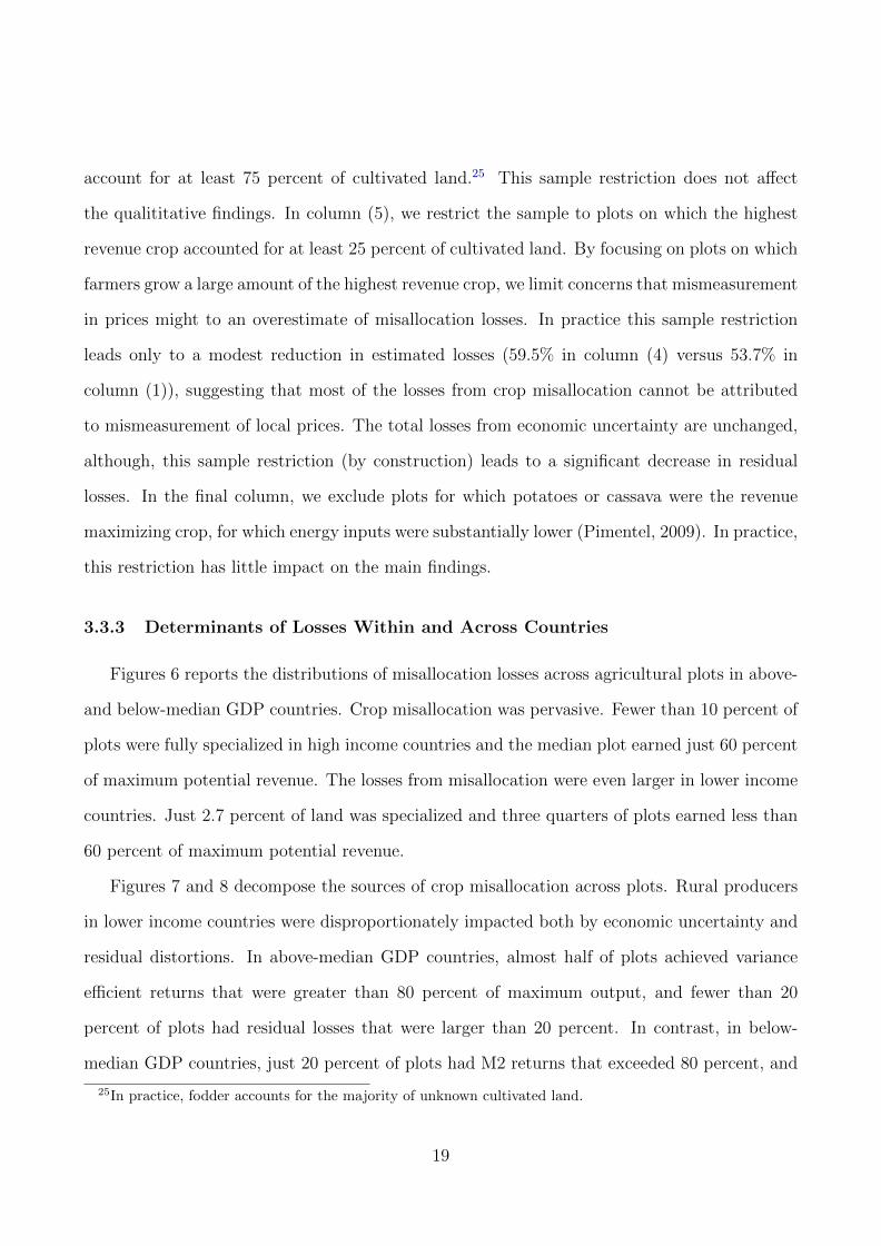
account for at least 75 percent of cultivated land.25 This sample restriction does not affect

the qualititative findings. In column (5), we restrict the sample to plots on which the highest

revenue crop accounted for at least 25 percent of cultivated land. By focusing on plots on which

farmers grow a large amount of the highest revenue crop, we limit concerns that mismeasurement

in prices might to an overestimate of misallocation losses. In practice this sample restriction

leads only to a modest reduction in estimated losses (59.5% in column (4) versus 53.7% in

column (1)), suggesting that most of the losses from crop misallocation cannot be attributed

to mismeasurement of local prices. The total losses from economic uncertainty are unchanged,

although, this sample restriction (by construction) leads to a significant decrease in residual

losses. In the final column, we exclude plots for which potatoes or cassava were the revenue

maximizing crop, for which energy inputs were substantially lower (Pimentel, 2009). In practice,

this restriction has little impact on the main findings.

3.3.3 Determinants of Losses Within and Across Countries

Figures 6 reports the distributions of misallocation losses across agricultural plots in above-

and below-median GDP countries. Crop misallocation was pervasive. Fewer than 10 percent of

plots were fully specialized in high income countries and the median plot earned just 60 percent

of maximum potential revenue. The losses from misallocation were even larger in lower income

countries. Just 2.7 percent of land was specialized and three quarters of plots earned less than

60 percent of maximum potential revenue.

Figures 7 and 8 decompose the sources of crop misallocation across plots. Rural producers

in lower income countries were disproportionately impacted both by economic uncertainty and

residual distortions. In above-median GDP countries, almost half of plots achieved variance

efficient returns that were greater than 80 percent of maximum output, and fewer than 20

percent of plots had residual losses that were larger than 20 percent. In contrast, in below-

median GDP countries, just 20 percent of plots had M2 returns that exceeded 80 percent, and

25In practice, fodder accounts for the majority of unknown cultivated land.

19

more than 40 percent of plots experienced residual losses that were greater than 20 percent.

The previous results show that crop misallocation was pervasive across much of the world’s

cultivated land, and that both economic uncertainty and residual distortions contributed to

losses on a majority of plots. What remains unclear is the extent to which these losses varied

across countries, and the relative importance of economic uncertainty and residual distortions in

explaining regional variation in crop misallocation. To examine these questions, we estimate the

impact of economic uncertainty and residual distortions on within- and across-country variation

in crop misallocation. To separately identify the causal impact of economic uncertainty and

residual distortions, we report the results after controlling for any remaining correlation for

each explanatory variable.26

The top panel of Table 7 decomposes the sources of crop misallocation into variation that

occurred within- and across-countries. We find that roughly one-third of the total variation was

driven by within-country variation while the remaining two-thirds was driven by cross-country

variation. Decomposing the source of this variation, we find that roughly three quarters of

within-country variation in crop misallocation can be attributed to differences in economic

uncertainty, while the remaining one quarter was the result of unexplained residual local losses.

Economic uncertainty was an even greater driver of crop misallocation across countries, and the

relative explanatory power is roughly twice as large in the cross-country analysis (see figures 9

and 10 for the residual plots).

3.3.4 Agricultural Losses in Africa: A Border Discontinuity Approach

The previous results show that economic uncertainty was the principal source of the geo-

graphic variation in crop misallocation, and that its impact was disproportinately large on losses

across countries. There are a number of potential explanations for this result. First, rural pro-

ducers in different countries may have been exposed to varying levels of underlying uncertainty

due to regional climatic shocks causing different levels of diversification across countries. Sec-

26By construction, this adjustment guarantees that all coefficient estimates are equal to one, although inpractice, controlling for correlation has little impact on the estimated effects.

20

ond, the results could simply reflect the wide differences in economic conditions across countries

that could influence agricultural activity through a variety of channels including credit market

access, input costs and technological adoption, and non-agricultural employment opportuni-

ties (e.g., Adamopoulos and Restuccia, 2011; Lagakos and Waugh, 2013; Donovan, 2014). A

third possibility is that the results capture differences in government policies aimed at reducing

uncertainty in the agricultural sector.

We study the sources of agricultural losses in Africa. The African context provides a par-

ticularly useful case study on the effects of economic uncertainty for three main reasons. First,

local variability in weather conditions are an important source of economic uncertainty (e.g.,

Bloom and Sachs, 1998; Sachs, 2001), and the vast majority of rural producers lack access to

formal insurance and credit markets. Second, modern day country borders were shaped by the

historical European colonization, through a process that generally did not consider local ethnic

or geographic features (Michalopoulos and Papaioannou, 2017). As a result of the historical

partition, farmers facing similar geographic and climatic conditions were exposed to widely dif-

ferent instutional environments. We focus on differences in the evolution of institutions across

former English and French colonies. Researchers have argued that the English common law

system supports market outcomes, including property rights enforcement, functioning credit

markets, and openness to trade (La Porta et al., 2008), all of which may have fostered agri-

cultural development and led to private solutions to rural economic uncertainty. On the other

hand, former French colonies typically had larger public sectors and devoted a disproportionate

share of public expenditure to the agricultural sector, which may have mitigated the impacts

of economic uncertainty.

We adopt a border regression discontinuity approach to study the determinants of crop

misallocation in Africa. We estimate the following specification:

yibc = α + βBritishc + f(distic) + γb + εibc, (2)

21

where yibc denotes agricultural outcome on plot i, located within 100 kilometers of border b,

in country c. The model includes a cubic control for plot distance to the border that we allow

to vary according to French versus British colonial origin, f(distic), and a border-specific fixed

effect, γb. The explanatory variable of interest, Britishc, is a dummy variable equal to one

for former British colonies.27 The coefficient β captures the combined impact of institutional

and economic changes that occurred in countries established under British colonization relative

to those that were established under French colonization. The analysis is based on a sample

of 8,623 plots of land spanning 14 countries and 10 border pairs. We report double-clustered

standard errors at the country and at the border level using the method of Cameron, Gelbach,

and Miller (2011) to account for spatial correlation and arbitrary residual correlation within

each dimension.

Before reporting the results, we first evaluate the validity of the research design. Table 8

reports the estimated effects of British colonization on potential crop productivity. Intuitively,

if country border were created for reasons unrelated to local land characteristics, we should

not observe systematic differences in land productivity across former British or French colonies.

We report the estimates for five staple crops: maize, pulses, cassava, palm oil, and sugarcane.

Panel A reports the coefficient estimates based on all border plots. There is no evidence that

agricultural productivity changed discontinously at the country border. The coefficient esti-

mates are all statistically insignificant and generally small in magnitude. These results broadly

support the identifying assumptions that the drawing of country borders under colonization

was largely made independently of considerations of localized geographic conditions. Panel B

reports the results for plots that had positive cultivated land. Again there are no significant

differences in crop productivity across countries, suggesting that different policies that devel-

oped following British colonization had little effect on extensive margin decisions over which

land was cultivated.

Table 9 reports the results for agricultural output. Columns (1) to (3) report the overall

27To avoid misassignment of the relevant country to agricultural land, we exclude plots located within 10kilometers from a border.

22

impact of the British system on revenue losses in agriculture (M4/M1). Observed agricultural

returns were somewhat higher in former British colonies, although none of the differences are

statistically significant. We decompose the sources of these revenue differences into crop mis-

allocation (cols. 4-6) and within-crop distortions (cols. 7-9). The results show that the small

overall impacts were the result of two offsetting forces. Farmers in former British colonies

appear to have adopted more advanced inputs, achieving higher crop-specific returns. At the

same time, producers in former British colonies displayed higher levels of crop misallocation.

Together these results show that despite having limited overall impact on overall agricultural

output, the economic and institutional systems that developed following British and French

colonization differentially affected the decision-making of rural producers.

Table 10 decomposes the sources of crop misallocation across former British and French

colonies. Roughly two thirds of the gap in crop misallocation can be explained by economic

uncertainty (cols. 7-9). In particular, despite having access to equally productive land and

facing similar climatic conditions, farmers in former French and British colonies responded

differently to output risk. Producers in former French colonies took on greater levels of risk,

and adopted a less diversified and higher yield crop portfolio. Consistent with this result, we

estimate significant cross-country differences in the number of crops grown, with farmers in

former British colonies growing an additional 1.3 crops per plot on average. The remaining one

third of the gap can be accounted for by residual factors that disproportionately affected the

allocation of land in former British colonies (cols. 4-6).

The results in Tables 9 and 10 show that farmers in former British colonies achieved higher

crop-specific yields, but adopted a more heavily diversified crop portfolio. These findings re-

flect the combined effects of the many differences in legal and institutional arrangements that

emerged post-colonization. The British common law system is thought to have fostered growth

and political stability by promoting a host of private sector reforms. Consistent with this view,

former British colonies had higher levels of GDP per capita, had a higher levels of trade. Former

British colonies also score higher on the polity IV index of democratization. Meanwhile, former

23

French colonies had higher levels of government expenditure as fraction of GDP and devoted a

disproportionate share of government spending to the agricultural sector. These different insti-

tutional arrangements and economic conditions appear to have impacted the decision-making

of rural producers. On the one hand, farmers in former British colonies adopted more intensive

agricultural techniques, and achieved higher crop-specific returns. This gap might have been

driven by the private sector expansion and improved credit markets that fostered investments

in agricultural inputs. On the other hand, these same farmers were more heavily influenced by

economic uncertainty, perhaps because they lacked access to the security provided the govern-

ment.28

4 Conclusion

Using FAO data on agriculture for cultivated areas that spans all arable land, this paper

estimates the revenue losses in agriculture. We identify a new source of misallocation associated

with the fact that agricultural land is often not allocated to the highest revenue crops. ‘Crop

misallocation’ was an important driver of losses in agriculture, and revenue could be increased

by almost 100 percent if currently cultivated land were allocated to its most productive use.

Applying a standard portfolio theory framework to historical data on annual potential crop

yields and agricultural prices, we find that uncertainty over annual income was the primary

reason why farmers did not specialize. The losses attributable to income uncertainty were

particularly large in lower income countries. Nevertheless, comparing agricultural outcomes

across the borders of African countries, we find that pro-private sector policies in former British

colonies led to greater investment in agricultural inputs, but did not mitigate the effects of

economic uncertainty. Instead, it appear that a combination of well-functioning private systems

along with non-market public interventions that reduce exposure to risk are needed to foster

28In fact, under the Comprehensive Africa Agriculture Development Programme (CAADP), a target was setfor African countries to allocate at least 10 percent of public expenditures to the agricultural sector. One of thefour pillars of this progam was “reducing the vulnerability of rural households and risk management”.

24

broad-based improvements in agricultural outcomes in developing countries.

This paper’s findings have relevance for policies aimed at rural economic development. Much

of the recent empirical literature has emphasized the importance of major infrastructure invest-

ments (e.g Adamopoulos, 2011; Tombe, 2014; Dinkelman, 2011) and rural production technolo-

gies (e.g. Donovan, 2014). Nevertheless, these projects require major upfront investments and

the benefits may only emerge after a period of several decades (Devine Jr, 1983; David, 1990;

Lewis and Severnini, 2017). This paper’s results suggest that policies aimed at risk reduction

may also promote rural economic development.

It is important to emphasize that our estimates likely do not reflect the full effects of agri-

cultural income uncertainty. In particular, rural residents may have engaged in a variety of

alternative strategies to mitigate local risks. These might have included precautionary sav-

ings (Deaton 1990; 1991), underinvestment in agricultural technologies (Donovan, 2014), or

cross-regional insurance. A comprehensive assessment of the economic costs of rural income

uncertainty must also account for the losses stemming from these other mitigation strategies.

Finally, it is important to emphasize that our partial equilibrium estimates are unlikely

to reflect the general equilibrium impacts of broad-based programs aimed at lowering rural

income uncertainty, which will ultimately depend on output price elasticities. Nevertheless,

there may still be wide scope for risk-mitigation policies to improve welfare, by lowering the

labor demands needed to meet subsistence consumption requirements, and promoting the rural-

transition. Further study of the general equilbrium consequences of these policies is a potentially

interesting avenue for future research.

25

References

Adamopoulos, T. (2011). Transportation costs, agricultural productivity, and cross-countryincome differences. International Economic Review, 52(2): 489-521.

Adamopoulos, T. and D. Restuccia. (2014). The size distribution of farms and internationalproductivity differences. American Economic Review, 104(6): 1667- 1697.

Adamopoulos, T. and D. Restuccia. (2015). Geography and Agricultural Productivity: Cross-Country Evidence from Micro Plot-Level Data. Mimeo.

Binswanger, H.P., and J. McIntire. Behavioral and Material Determinants of Production Re-lations in Land-Abundant Tropical Agriculture. Economic Development and Cultural Change,36(1), 73-99.

Binswanger, H.P., and M.R. Rosenzweig. Behavioral and Material Determinants of ProductionRelations in Agriculture. Journal of Development Studies, 22(3), 503-539.

Bloom, D.E., and J.D. Sachs. (1998). Geography, demography, and economic growth in Africa.Brookings Papers of Economic Activity, 2, 207-273.

Caselli, F. (2005). Accounting for cross-country income differences. Handbook of EconomicGrowth, Volume 1, P. Aghion and S. Durlauf (eds.), Elsevier, Ch.9, 679-741.

Carter, M.R. (1997). Technology, and the Social Articulation of Risk in West African Agricul-ture. Economic Development and Cultural Change, 45(3), 557-590.

Carter, M.R., and F.J. Zimmerman. (2003). Asset Smoothing, Consumption Smoothing and theReproduction of Inequality Under Risk and Subsistence Constraints. Journal of DevelopmentEconomics, 71, 233-260.

Carter, M.R., and T.J. Lybbert. Consumption Versus Asset Smoothing: Testing the Implica-tions of Poverty Trap Theory in Burkina Faso. Journal of Development Economics, 99, 255-264.

Deaton, A. (1990). On Risk, Insurance and Intra-Village Consumption Smoothing. ResearchProgram in Development Studies, Princeton University, N.J.

Deaton, A. (1991). Savings and Liquidity Constraints. Econometrica, 59(5), 1221-1248.

Dercon, S. 2004. Insurance Against Poverty, WIDER Studies in Development Economics. Ox-ford University Press, Oxford, U.K.

Di Falco, S., and J.P. Chavas. (2009). On crop biodiversity, risk exposure and food security inthe highlands of Ethiopia. American Journal of Agricultural Economics, 91, 599-611.

Donovan, K. (2014). Agricultural risk, intermediate inputs, and cross-country productivitydifferences. Mimeo.

Fafchamps, M. 1992. Cash crop production, food price volatility and rural market integrationin the third world, American Journal of Agricultural Economics, 74, 90-99.

26

Fafchamps, M., and S. Lund. (2003). Risk-Sharing Networks in Rural Philippines. Journal ofDevelopment Economics, 72(2), 261-287.

Fafchamps, M., C. Udry, and K. Czukas. (1998). Drought and Saving in West Africa: AreLivestock a Buffer Stock? Journal of Development Economics, 55(2), 273-305.

Ingersoll, J.E. (1987). Theory of Financial Decision Making. Rowman & Littlefield Publishers.

Kazianga, H. and C. Udry. (2006). Consumption Smoothing? Livestock, Insurance and Droughtin Rural Burkina Faso. Journal of Development Economics, 79, 413-446.

Lagakos, D. and M. E. Waugh. (2013). Selection, agriculture, and cross-country productivitydifferences. American Economic Review, 103(2): 948-980.

Lange, S. and M. Reimers. 2014. Livestock as an Imperfect Buffer Stock in Poorly IntegratedMarkets. Mimeo.

Markowitz, H. (1952). Portfolio Selection. Journal of Finance, 40, 561-572.

Michaloupouls., S., and E. Papaioannou. (2013). Pre-Colonial Ethnic Institutions and Contem-porary African Development. Econometrica, 81(1): 113-152.

Michaloupouls., S., and E. Papaioannou. (2014). National Institutions and Subnational Devel-opment in Africa. Quarterly Journal of Economics, 129(1): 151-213.

Morduch, J. (1995). Income Smoothing and Consumption Smoothing. Journal of EconomicPerspectives, 9, 103-114.

Park, A. (2006). Risk and Household Grain Management in Developing Countries. EconomicJournal, 116, 1088-1115.

Paxson, C.H. (1992). Using Weather Variability To Estimate the Response of Savings to Tran-sitory Income in Thailand. American Economic Review, 81(1), 15-33.

Restuccia, D., D.T. Yang, and X. Zhu. (2008). Agriculture and aggregate productivity: Aquantitative cross-country analysis. Journal of Monetary Economics, 55(2): 234-250.

Rosenzweig, M.R., and K.I. Wolpin. (1993). Credit Market Constraints, Consumption Smooth-ing, and the Accumulation of Durable Production Assets in Low-Income countries: Investmentsin Bullocks in India. Journal of Political Economy, 101(2), 223-244.

Sachs, J.D. (2001). Tropical Underdevelopment. NBER Working Paper #8119.

Schultz, T. W. (1953). The Economic Organization of Agriculture, New York: McGraw Hill.

Tombe, T. (2014). The missing food problem: Trade, agriculture, and international productivitydifferences. American Economic Journal: Macroeconomics, Forthcoming.

Udry, C. (1995). Risk and Saving in Northern Nigeria. American Economic Review, 85(5),1287-1300.

27

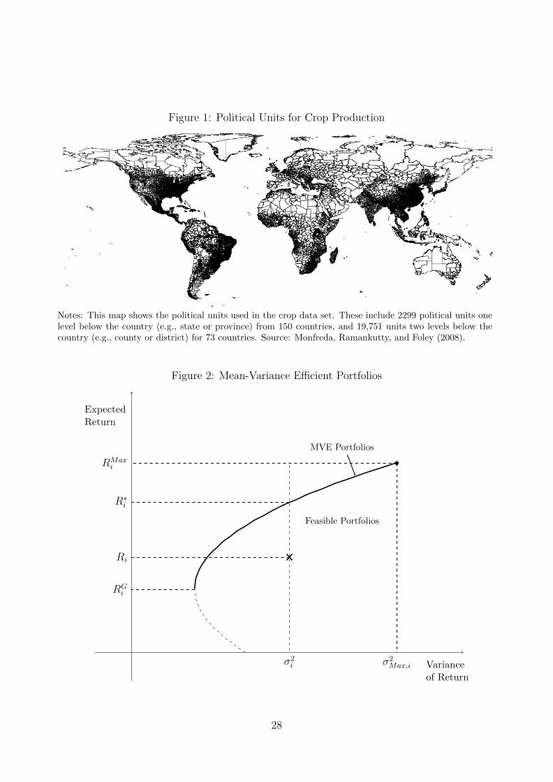
Figure 1: Political Units for Crop Production

Notes: This map shows the political units used in the crop data set. These include 2299 political units onelevel below the country (e.g., state or province) from 150 countries, and 19,751 units two levels below thecountry (e.g., county or district) for 73 countries. Source: Monfreda, Ramankutty, and Foley (2008).

Figure 2: Mean-Variance Efficient Portfolios

ExpectedReturn

Varianceof Return

Feasible Portfolios

MVE Portfolios

σ2Max,i

RMaxi

σ2i

Ri

R∗i

RGi

28

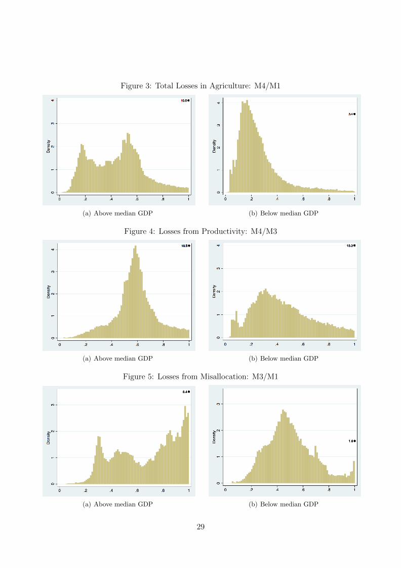
Figure 3: Total Losses in Agriculture: M4/M1

(a) Above median GDP (b) Below median GDP

Figure 4: Losses from Productivity: M4/M3

(a) Above median GDP (b) Below median GDP

Figure 5: Losses from Misallocation: M3/M1

(a) Above median GDP (b) Below median GDP

29

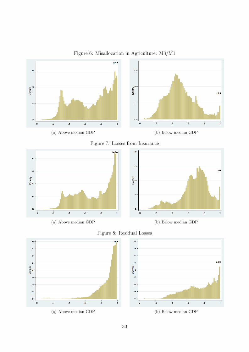
Figure 6: Misallocation in Agriculture: M3/M1

(a) Above median GDP (b) Below median GDP

Figure 7: Losses from Insurance

(a) Above median GDP (b) Below median GDP

Figure 8: Residual Losses

(a) Above median GDP (b) Below median GDP

30

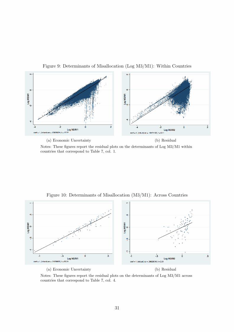
Figure 9: Determinants of Misallocation (Log M3/M1): Within Countries

(a) Economic Uncertainty (b) Residual

Notes: These figures report the residual plots on the determinants of Log M3/M1 withincountries that correspond to Table 7, col. 1.

Figure 10: Determinants of Misallocation (M3/M1): Across Countries

(a) Economic Uncertainty (b) Residual

Notes: These figures report the residual plots on the determinants of Log M3/M1 acrosscountries that correspond to Table 7, col. 4.

31

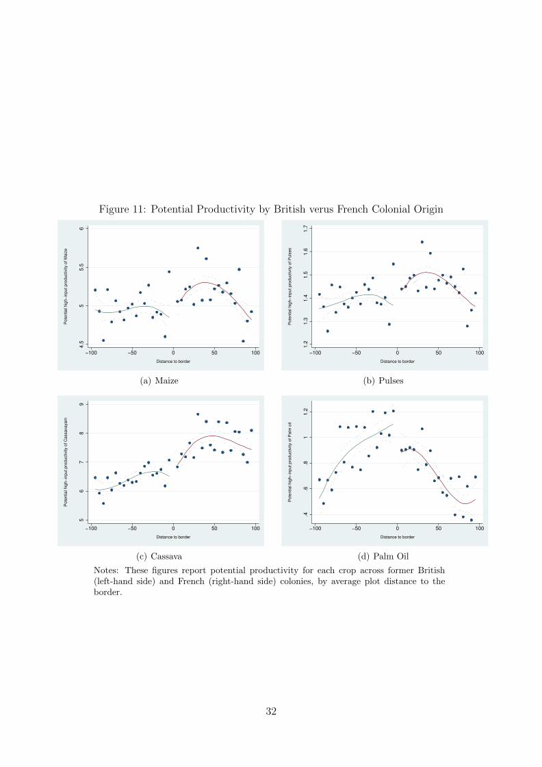
Figure 11: Potential Productivity by British verus French Colonial Origin

4.5

55.5

6

Pote

ntial hig

h−

input pro

ductivity o

f M

aiz

e

−100 −50 0 50 100

Distance to border

(a) Maize

1.2

1.3

1.4

1.5

1.6

1.7

Pote

ntial hig

h−

input pro

ductivity o

f P

uls

es

−100 −50 0 50 100

Distance to border

(b) Pulses

56

78

9

Pote

ntial hig

h−

input pro

ductivity o

f C

assavayam

−100 −50 0 50 100

Distance to border

(c) Cassava

.4.6

.81

1.2

Pote

ntial hig

h−

input pro

ductivity o

f P

alm

oil

−100 −50 0 50 100

Distance to border

(d) Palm Oil

Notes: These figures report potential productivity for each crop across former British(left-hand side) and French (right-hand side) colonies, by average plot distance to theborder.

32

Table 1: Agricultural Land, by Crop and by CountryPanel A: Agricultural land, by crop

Cultivated % World % % Land Allocated to CropLand Arable Cropland Below median Above median

Crop (Millions Ha) Land in sample GDP GDPAll 899 64.2 63.7Wheat 215 15.4 57.9 13.1 28.7Rice 154 11.0 39.3 24.7 4.6Maize 138 9.9 73.1 8.8 21.5Soybean 74 5.3 77.1 3.3 19.5Pulses 45 3.2 103.4 12.0 4.6Sorghum 41 2.9 57.1 8.3 2.4Millet 37 2.7 43.6 10.6 0.1Potato 30 2.1 59.7 1.0 1.2Cassava, Yam 25 1.8 101.6 4.2 1.3Cocoa, Coffee, Tea 25 1.8 106.9 3.5 2.8Rapeseed 26 1.8 73.9 2.0 3.5Groundnut 23 1.7 53.6 4.8 0.4Sunflower 21 1.5 45.0 0.5 2.5Sugarcane 19 1.4 78.9 2.0 2.5Oilpalm 10 0.7 63.3 0.9 1.5Olive 8 0.6 54.4 0.2 2.0Sugarbeet 6 0.4 84.6 0.0 0.9Panel B: Agricultural land, by Country

% Country’s % Country’s % Country’sArable Land Arable Land Arable Land

World 60.8 Germany 43.0 Niger 58.2Algeria 19.1 Ghana 113.1 Nigeria 83.0Argentina 82.3 Greece 68.6 Pakistan 15.1Australia 24.5 Guinea 72.2 Panama 42.6Austria 47.4 Honduras 80.9 Paraguay 73.0Bangladesh 143.3 Hungary 61.4 Peru 21.4Belize 83.4 India 87.9 Philippines 145.2Bhutan 88.0 Indonesia 105.3 Poland 33.8Bolivia 53.9 Iran 40.8 Portugal 56.8Botswana 16.0 Ireland 10.1 Rwanda 72.6Brazil 73.3 Israel 39.0 Senegal 55.8Brunei 36.6 Italy 64.1 South Africa 23.0Burkina Faso 86.6 Jamaica 43.1 Spain 29.7Burundi 64.7 Japan 44.9 Sri Lanka 119.3Cambodia 56.6 Jordan 37.8 Sudan 13.4Cameroon 38.5 Kenya 72.4 Suriname 84.1Canada 42.3 Laos 95.0 Sweden 0.7Chile 31.5 Lebanon 91.7 Switzerland 38.6Colombia 113.7 Madagascar 74.6 Tanzania 74.9Congo 34.8 Malaysia 394.7 Thailand 86.6Costa Rica 125.9 Mali 55.7 Togo 46.3Cotedivoire 173.9 Malta 51.4 Tunisia 66.5Cyprus 15.8 Mexico 53.0 Turkey 54.3Denmark 34.4 Morocco 31.8 United Kingdom 48.5Dominican Republic 68.0 Mozambique 64.9 Uruguay 29.1Ecuador 106.8 Namibia 29.0 United States 46.7El Salvador 104.4 Nepal 144.1 Venezuela 50.2Equatorial Guinea 42.2 Netherlands 47.2 Vietnam 158.3France 54.0 New Zealand 6.6Gambia 86.5 Nicaragua 40.1

33

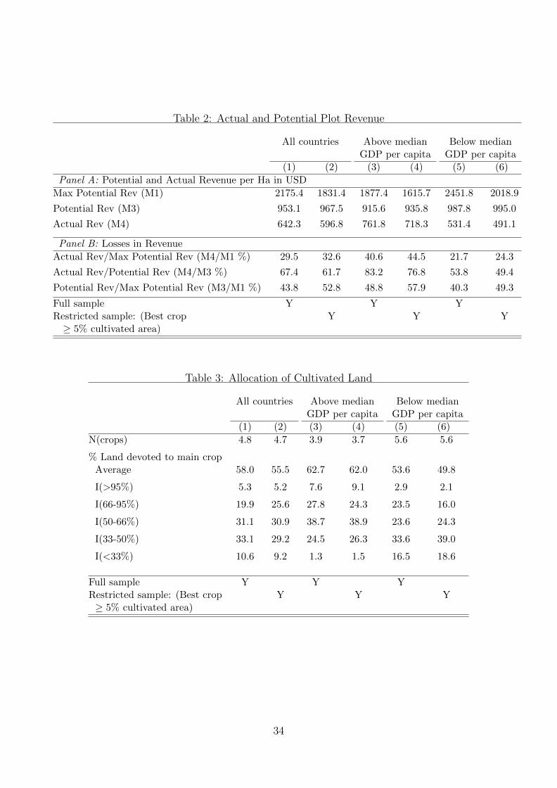
Table 2: Actual and Potential Plot Revenue

All countries Above median Below medianGDP per capita GDP per capita

(1) (2) (3) (4) (5) (6)

Panel A: Potential and Actual Revenue per Ha in USD

Max Potential Rev (M1) 2175.4 1831.4 1877.4 1615.7 2451.8 2018.9

Potential Rev (M3) 953.1 967.5 915.6 935.8 987.8 995.0

Actual Rev (M4) 642.3 596.8 761.8 718.3 531.4 491.1

Panel B: Losses in Revenue

Actual Rev/Max Potential Rev (M4/M1 %) 29.5 32.6 40.6 44.5 21.7 24.3

Actual Rev/Potential Rev (M4/M3 %) 67.4 61.7 83.2 76.8 53.8 49.4

Potential Rev/Max Potential Rev (M3/M1 %) 43.8 52.8 48.8 57.9 40.3 49.3

Full sample Y Y YRestricted sample: (Best crop Y Y Y≥ 5% cultivated area)

Table 3: Allocation of Cultivated Land

All countries Above median Below medianGDP per capita GDP per capita

(1) (2) (3) (4) (5) (6)

N(crops) 4.8 4.7 3.9 3.7 5.6 5.6

% Land devoted to main cropAverage 58.0 55.5 62.7 62.0 53.6 49.8

I(>95%) 5.3 5.2 7.6 9.1 2.9 2.1

I(66-95%) 19.9 25.6 27.8 24.3 23.5 16.0

I(50-66%) 31.1 30.9 38.7 38.9 23.6 24.3

I(33-50%) 33.1 29.2 24.5 26.3 33.6 39.0

I(<33%) 10.6 9.2 1.3 1.5 16.5 18.6

Full sample Y Y YRestricted sample: (Best crop Y Y Y≥ 5% cultivated area)

34

Table 4: Variability in Agricultural Revenue

All countries Above median Below medianGDP per capita GDP per capita

(1) (2) (3) (4) (5) (6)

Panel A: Variability in Plot Revenue

Standard deviationHighest yield crop 761.8 625.0 538.0 457.5 969.3 770.7Currently cultivated crops 310.7 320.0 214.3 219.4 400.1 407.3

Coeff. of variation (%)Highest yield crop 29.1 28.4 28.2 28.4 30.0 28.5Currently cultivated crops 13.9 15.5 15.0 17.2 12.8 14.0

Full sample Y Y YRestricted sample: (Best crop Y Y Y≥ 5% cultivated area)

Table 5: Uncertainty and Losses in Agricultural Revenue

All countries Above median Below medianGDP per capita GDP per capita

(1) (2) (3) (4) (5) (6)

Panel A: Potential Revenue Estimates

Max Potential Rev (M1) 2175.4 1831.0 1877.4 1615.7 2451.8 2018.9MVE Potential Rev (M2) 1180.2 1172.8 1092.1 1055.2 1262.0 1275.0Potential Rev (M3) 953.1 967.5 915.6 935.8 987.8 995.0

Panel B: Decomposing Revenue Losses

M3/M1 53.7 59.3 61.1 69.0 46.9 50.9M3/M2 81.4 82.5 86.9 90.8 76.2 75.2M2/M1 66.1 71.8 69.8 75.5 62.8 68.5

Full sample Y Y YRestricted sample: (Best crop Y Y Y≥ 5% cultivated area)

35

Table 6: Uncertainty and Losses in Agricultural Revenue

Restricted samplesBaseline Fixed Calorie Known crops Best crop Excludeestimates prices weighted >75% of >25% of plots with

output cultivated cultivated potato, pulsesland land best crop

(1) (2) (3) (4) (5) (6)

Panel A: Potential Revenue Estimates

Max Potential Rev (M1) 2175.4 2061.9 2987.5 1849 1541.6 1888.1MVE Potential Rev (M2) 1180.2 1395.5 2031.6 1100.4 1228.6 1097.4Potential Rev (M3) 953.1 958.3 1545.4 945.2 1120.6 885.5

Panel B: Decomposing Revenue Losses

M3/M1 53.7 54.7 59.3 59.5 78.7 55.4M3/M2 81.4 74.7 76.4 85.9 92.1 81.4M2/M1 66.1 74.9 79 59.5 85.0 68.2

Table 7: Determinants of Misallocation

Within countries Across countries(1) (2) (3) (4) (5) (6)

Dependent Variable: Log Crop Misallocation (Log M3/M1)

Fraction Variation (dep. var.) 0.33 0.49 0.34 0.67 0.51 0.64

Log(M2/M1)R-squared 0.765 0.734 0.725 0.908 0.814 0.943T-statistic 17.8 20.5 16.7 23.3 14.1 31.9Coeff 1 1 1 1 1 1SE [0.0563] [0.04879] [0.05982] [0.04290] [0.0708] [0.0313]

Log(M3/M2)R-squared 0.2503 0.3662 0.1781 0.1242 0.1357 0.1348T-statistic 5.4 6.0 5.4 2.5 3.3 2.2Coeff 1 1 1 1 1 1SE [0.1847] [0.1662] [0.1858] [0.3982] [0.2988] [0.4506]

Relative explanatory power: M3/M1 vs. M3/M2R-squared Ratio 3.1 2.0 4.1 7.3 6.0 7.0T-statistic Ratio 3.3 3.4 3.1 9.3 4.2 14.4

Observations 486,872 351,407 450,399 87 87 85Full Sample Y YBest crop ≥ 5% Y YTrimmed sample Y Y

Notes: This table reports the results for the impact of uncertainty (Log M2/M1) and residual factors (LogM3/M2) on crop misallocation (Log M3/M1). Each cell reports the results from a difference regression.All models are weighted by total cultivated area. Standard errors are clustered at the country level.

36

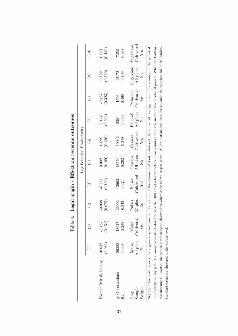
Tab

le8:

Legal

ori

gin

-E

ffect

on

revenue

outc

om

es

Log

Pote

nti

al

Pro

du

ctiv

ity

(1)

(2)

(3)

(4)

(5)

(6)

(7)

(8)

(9)

(10)

For

mer

Bri

tish

Col

ony

-0.0

32-0

.152

-0.0

38

-0.1

71

0.0

02

0.0

99

0.1

47

-0.1

87

0.1

22

0.0

81

(0.0

82)

(0.1

54)

(0.0

75)

(0.1

60)

(0.1

09)

(0.1

56)

(0.2

64)

(0.3

23)

(0.1

20)

(0.1

49)

#O

bse

rvat

ion

s26

222

1391

726

092

13903

18229

10042

2381

1596

12172

7256

R2

0.30

80.

285

0.34

30.3

76

0.2

62

0.3

78

0.4

60

0.4

68

0.1

96

0.3

38

Cro

pM

aize

Mai

zeP

uls

esP

uls

esC

ass

ava

Cass

ava

Palm

oil

Palm

oil

Su

garc

an

eS

ugarc

an

eS

amp

leA

llp

lots

Cu

ltiv

ated

All

plo

tsC

ult

ivate

dA

llp

lots

Cu

ltiv

ate

dA

llp

lots

Cu

ltiv

ate

dA

llp

lots

Cu

ltiv

ate

dW

eigh

tN

oY

esN

oY

esN

oY

esN

oY

esN

oY

es

NO

TE

S.

Th

ista

ble

rep

ort

s,fo

ra

giv

encr

op

ind

icate

dat

the

bott

om

of

the

colu

mn

,R

DD

esti

mati

on

sof

the

imp

act

of

the

legal

ori

gin

of

aco

untr

yon

the

pote

nti

al

pro

du

ctiv

ity

on

any

plo

t.T

he

sam

ple

con

sist

sof

ob

serv

ati

on

wit

hin

100

km

of

ab

ord

erb

etw

een

two

cou

ntr

ies

wh

ow

ere

un

der

diff

eren

tco

lon

ial

pow

ers.

Wh

enth

eb

ott

om

row

ind

icate

sC

ult

ivate

d,

the

sam

ple

isre

stri

cted

toob

serv

ati

on

sw

her

eso

me

kn

ow

ncr

op

isgro

wn

.A

lles

tim

ati

on

sin

clu

de

cub

icp

oly

nom

ials

on

eith

ersi

de

of

the

bord

er.

Sta

nd

ard

erro

rsare

clu

ster

edat

the

bord

erle

vel

.

37

Tab

le9:

Legal

ori

gin

-E

ffect

on

revenue

outc

om

es

Log

M4/M

1L

og

M3/M

1L

og

M4/M

3

(1)

(2)

(3)

(4)

(5)

(6)

(7)

(8)

(9)

For

mer

Bri

tish

Col

ony

0.01

20.

507

0.5

92

-0.2

52∗

∗-0

.404∗∗

-0.4

84∗

∗0.2

64

0.9

11∗∗

1.0

76∗∗

(0.3

33)

(0.3

74)

(0.3

78)

(0.1

00)

(0.1

64)

(0.1

55)

(0.3

19)

(0.3

63)

(0.3

90)

#O

bse

rvat

ion

s86

5286

52

6492

8652

8652

6492

8652

8652

6492

R2

0.26

10.

414

0.4

01

0.1

32

0.2

18

0.1

78

0.2

86

0.5

39

0.5

26

Wei

ghte

dN

oY

esY

esN

oY

esY

esN

oY

esY

esW

ith

out

25%

leas

tp

rod

uct

ive

lan

dN

oN

oY

esN

oN

oY

esN

oN

oY

es

NO

TE

S.

This

tab

lere

port

sR

DD

esti

mati

on

sof

the

imp

act

of

the

legal

ori

gin

of

aco

untr

yon

Log

of

M4/M

1,

M3/M

1an

dM

4/M

3.

Th

esa

mp

leof

ob

serv

ati

on

sco

nsi

sts

of

all

plo

tsw

her

eso

me

kn

ow

ncr

op

isgro

wn

,w

ith

in100

km

of

ab

ord

erb

etw

een

two

cou

ntr

ies

wh

ow

ere

un

der

diff

eren

tco

lon

ial

pow

ers.

All

esti

mati

on

sin

clu

de

bord

erfi

xed

effec

ts.

Th

eyals

oin

clu

de

cub

icp

oly

nom

ials

spec

ific

toei

ther

sid

eof

ab

ord

er.

Sta

nd

ard

erro

rsare

dou

bly

clust

ered

,at

the

cou

ntr

yan

dat

the

bord

erle

vel

.

38

Tab

le10

:L

egal

ori

gin

-E

ffect

on

revenue

outc

om

es

Log

M3/M

1L

og

M3/M

2L

og

M2/M

1

(1)

(2)

(3)

(4)

(5)

(6)

(7)

(8)

(9)

For

mer

Bri

tish

Col

ony

-0.2

52∗∗

-0.4

04∗∗

-0.4

84∗∗

-0.0

22

-0.1

48∗

-0.1

89∗

-0.2

30

-0.2

56

-0.2

95∗

(0.1

00)

(0.1

64)

(0.1

55)

(0.0

62)

(0.0

79)

(0.0

91)

(0.1

35)

(0.1

81)

(0.1

58)

#O

bse

rvat

ion

s86

528652

6492

8652

8652

6492

8652

8652

6492

R2

0.13

20.

218

0.1

78

0.1

63

0.3

43

0.3

54

0.1

79

0.1

84

0.1

45

Wei

ghte

dN

oY

esY

esN

oY

esY

esN

oY

esY

esW

ith

out

25%

leas

tp

rod

uct

ive

lan

dN

oN

oY

esN

oN

oY

esN

oN

oY

es

NO

TE

S.

This

tab

lere

port

sR

DD

esti

mati

on

sof

the

imp

act

of

the

legal

ori

gin

of

aco

untr

yon

Log

of

M3/M

1,

M3/M

2an

dM

2/M

3.

Th

esa

mp

leof

ob

serv

ati

on

sco

nsi

sts

of

all

plo

tsw

her

eso

me

kn

ow

ncr

op

isgro

wn

,w

ith

in100

km

of

ab

ord

erb

etw

een

two

cou

ntr

ies

wh

ow

ere

un

der

diff

eren

tco

lon

ial

pow

ers.

All

esti

mati

on

sin

clu

de

bord

erfi

xed

effec

ts.

Th

eyals

oin

clu

de

cub

icp

oly

nom

ials

spec

ific

toei

ther

sid

eof

ab

ord

er.

Sta

nd

ard

erro

rsare

dou

bly

clust

ered

,at

the

cou

ntr

yan

dat

the

bord

erle

vel

.

39

Récents cahiers de recherche du CIREQ Recent Working Papers of CIREQ

La liste complète des cahiers de recherche du CIREQ est disponible à l’adresse suivante : http://www.cireqmontreal.com/cahiers-de-recherche . The complete list of CIREQ’s working papers is available at the following address : http://www.cireqmontreal.com/cahiers-de-recherche .

08-2017 Alvarez-Mozos, M., L. Ehlers, "Externalities and the Nucleolus", septembre 2017, 13 pages

09-2017 Bouakez, H., R. Oikonomou, R. Priftis, "Optimal Debt Management in a Liquidity Trap", octobre 2017, 29 pages

01-2018 Riboni, A., F. Ruge-Murcia, "Deliberation in Committees : Theory and Evidence from the FOMC", mars 2018, 22 pages

02-2018 Ruge-Murcia, F., "Asset Prices in a Small Production Network", mars 2018, 43 pages

03-2018 Horan, S., M.J. Osborne, M.R. Sanver, "Positively Responsive Collective Choice Rules and Majority Rule : A Generalization of May’s Theorem to Many Alternatives", avril 2018, 26 pages

04-2018 Ehlers, L., J. Massó, "Robust Design in Monotonic Matching Markets : A Case for Firm-Proposing Deferred-Acceptance", mai 2018, 20 pages

05-2018 Bosković, B., U. Chakravorty, M. Pelli, A. Risch, "The Effect of Forest Access on the Market for Fuelwood in India", mai 2018, 45 pages

06-2018 Coulibaly, L., "Monetary Policy in Sudden Stop-Prone Economies", juin 2018, 42 pages

07-2018 Bengui, J., T. Phan, "Asset Pledgeability and Endogenously Leveraged Bubbles", juin 2018, 48 pages

08-2018 Andersson, T., L. Ehlers, L.-G. Svensson, R. Tierney, "Gale's Fixed Tax for Exchanging Houses", juin 2018, 22 pages

09-2018 Ramachandran, R., C. Rauh, "Discrimination Without Taste - How Discrimination Can Spillover and Persist", juin 2018, 38 pages

10-2018 Gonçalves, S., B. Perron, "Bootstrapping Factor Models With Cross Sectional Dependence", juillet 2018, 30 pages

11-2018 Andersson, T., Á. Cseh, L. Ehlers, A. Erlanson, “Organizing Time Banks : Lessons from Matching Markets”, juillet 2018, 24 pages

12-2018 Hoelzemann, J., N. Klein, “Bandits in the Lab”, août 2018, 52 pages.

13-2018 Klein, N., P. Wagner, “Strategic investment and learning with private information”, août 2018, 24 pages.

14-2018 Godefroy, R., “The Birth of the Congressional Clinic”, août 2018, 47 pages.