An Algorithmic Approach to Personalized Drug Concentration ...
148
POUR L'OBTENTION DU GRADE DE DOCTEUR ÈS SCIENCES acceptée sur proposition du jury: Prof. D. Atienza Alonso, président du jury Prof. G. De Micheli, directeur de thèse Prof. S. Goto, rapporteur Prof. C. Guiducci, rapporteur Dr Y. Thoma, rapporteur An Algorithmic Approach to Personalized Drug Concentration Predictions THÈSE N O 6039 (2014) ÉCOLE POLYTECHNIQUE FÉDÉRALE DE LAUSANNE PRÉSENTÉE LE 16 JANVIER 2014 À LA FACULTÉ INFORMATIQUE ET COMMUNICATIONS LABORATOIRE DES SYSTÈMES INTÉGRÉS (IC/STI) PROGRAMME DOCTORAL EN INFORMATIQUE, COMMUNICATIONS ET INFORMATION Suisse 2014 PAR Wenqi YOU DUBOUT
Transcript of An Algorithmic Approach to Personalized Drug Concentration ...

POUR L'OBTENTION DU GRADE DE DOCTEUR ÈS SCIENCES
acceptée sur proposition du jury:
Prof. D. Atienza Alonso, président du juryProf. G. De Micheli, directeur de thèse
Prof. S. Goto, rapporteur Prof. C. Guiducci, rapporteur
Dr Y. Thoma, rapporteur
An Algorithmic Approach to Personalized Drug Concentration Predictions
THÈSE NO 6039 (2014)
ÉCOLE POLYTECHNIQUE FÉDÉRALE DE LAUSANNE
PRÉSENTÉE LE 16 JANVIER 2014
À LA FACULTÉ INFORMATIQUE ET COMMUNICATIONSLABORATOIRE DES SYSTÈMES INTÉGRÉS (IC/STI)
PROGRAMME DOCTORAL EN INFORMATIQUE, COMMUNICATIONS ET INFORMATION
Suisse2014
PAR
Wenqi YOU DUBOUT

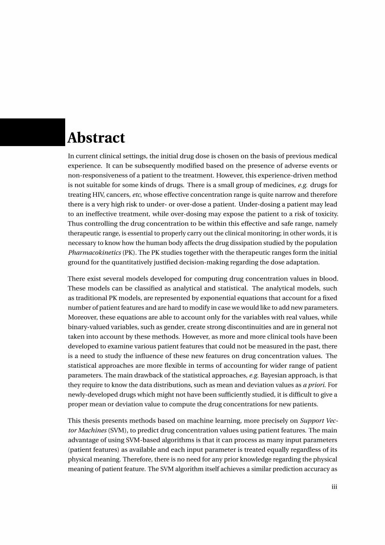
AbstractIn current clinical settings, the initial drug dose is chosen on the basis of previous medical
experience. It can be subsequently modified based on the presence of adverse events or
non-responsiveness of a patient to the treatment. However, this experience-driven method
is not suitable for some kinds of drugs. There is a small group of medicines, e.g. drugs for
treating HIV, cancers, etc, whose effective concentration range is quite narrow and therefore
there is a very high risk to under- or over-dose a patient. Under-dosing a patient may lead
to an ineffective treatment, while over-dosing may expose the patient to a risk of toxicity.
Thus controlling the drug concentration to be within this effective and safe range, namely
therapeutic range, is essential to properly carry out the clinical monitoring; in other words, it is
necessary to know how the human body affects the drug dissipation studied by the population
Pharmacokinetics (PK). The PK studies together with the therapeutic ranges form the initial
ground for the quantitatively justified decision-making regarding the dose adaptation.
There exist several models developed for computing drug concentration values in blood.
These models can be classified as analytical and statistical. The analytical models, such
as traditional PK models, are represented by exponential equations that account for a fixed
number of patient features and are hard to modify in case we would like to add new parameters.
Moreover, these equations are able to account only for the variables with real values, while
binary-valued variables, such as gender, create strong discontinuities and are in general not
taken into account by these methods. However, as more and more clinical tools have been
developed to examine various patient features that could not be measured in the past, there
is a need to study the influence of these new features on drug concentration values. The
statistical approaches are more flexible in terms of accounting for wider range of patient
parameters. The main drawback of the statistical approaches, e.g. Bayesian approach, is that
they require to know the data distributions, such as mean and deviation values as a priori. For
newly-developed drugs which might not have been sufficiently studied, it is difficult to give a
proper mean or deviation value to compute the drug concentrations for new patients.
This thesis presents methods based on machine learning, more precisely on Support Vec-
tor Machines (SVM), to predict drug concentration values using patient features. The main
advantage of using SVM-based algorithms is that it can process as many input parameters
(patient features) as available and each input parameter is treated equally regardless of its
physical meaning. Therefore, there is no need for any prior knowledge regarding the physical
meaning of patient feature. The SVM algorithm itself achieves a similar prediction accuracy as
iii
traditional PK models. The potential inaccuracy can be caused by the noise due to the mea-
surement errors, insufficient data samples and data attributes (patient features). Therefore,
the thesis employs an outlier-removal technique, RANSAC algorithm, that is used for initial
data library preprocessing to remove the outliers from the given data library. The use of the
RANSAC algorithm enhances the prediction accuracy compared to the PK methods.
The representation of the drug concentration curve is also important for better visual analysis.
The drug concentration predicted by the SVM algorithm is point-wise; thus the concentration
curve has to be constructed by interpolation through all the predicted points. Moreover, in
order to be able to study the effect of the residual drug concentration after previous intakes
or to adjust a patient-specific curve with a new drug concentration measurement, which
is essential for the a posteriori drug dose adaptation, the analytical representation of the
concentration curve becomes necessary. Therefore, this thesis also introduces a new hybrid
approach, namely parameterized SVM. It utilizes the SVM algorithm to predict the coefficients
for the set of pre-defined RANSAC basis functions that extracts the structural information of
the Drug Concentration to Time (DCT) curve. This allows to reconstruct an analytical drug
concentration curve, which can be adjusted with any new real measurement done for the
current patient. This way, by knowing only the parameters of all the basis functions, the DCT
curve can be modeled.
These algorithms are finally incorporated into a Drug Administration Decision Support System
(DADSS) for imatinib, a drug used to treat Chronic Myeloid Leukemia (CML) and Gastroin-
testinal Stromal Tumors (GST). The system provides the decision support in drug dose and
administration interval for medical doctors in accordance with the medical guidelines.
Keywords: Support Vector Machine, RANSAC, Drug Administration Decision Support System
iv

RésuméDans le contexte clinique actuel, le dosage initial d’un médicament est établi sur la base
de l’expérience médicale pré-existante. Il peut ensuite éventuellement être modifié suite à
l’apparition d’effets indésirables ou l’absence de résultats satisfaisants chez un patient. Cette
méthode de dosage basée sur l’expérience médicale ne convient cependant pas à toutes les
substances actives. Il existe en effet un groupe restreint de médicaments, notamment ceux
employés dans le traitement du VIH, de cancers, etc, dont la plage de concentration thérapeu-
tique est relativement étroite, ce qui implique un risque élevé de sous- ou sur-dosage pour
le patient. Alors qu’un sous-dosage peut rendre le traitement inefficace, un sur-dosage peut
exposer le patient à un risque d’intoxication. Par conséquent, un contrôle précis de la concen-
tration d’un tel médicament est essentiel pour garantir son efficacité ainsi que la sécurité du
patient, et donc un bon suivi médical. En d’autres termes, il est important de connaître le
devenir d’une substance active dans l’organisme, tel qu’étudié par la pharmacocinétique (PK).
Les études PK, associées aux plages de concentration thérapeutiques fournies par les études
pharmacodynamiques (PD) des effets du médicament, constituent la base d’une prise de
décision justifiée quantitativement quant à l’adaptation d’un dosage.
Il existe différents modèles permettant de calculer la concentration d’une substance active
dans le sang. Ces modèles peuvent être répartis en deux catégories, les modèles analytiques
et les modèles statistiques. Les premiers, comme les modèles PK traditionnels, comportent
un certain nombre d’équations exponentielles compliquées qui ne reproduisent qu’une frac-
tion restreinte des caractéristiques du patient, et sont difficilement modifiables lorsque l’on
souhaite ajouter des paramètres supplémentaires. En outre, ces équations ne permettent de
traiter que des variables à valeurs réelles. Les variables à valeurs binaires, telles que le sexe,
créant de fortes discontinuités, ne sont en général pas prises en compte par ces méthodes.
Cependant, l’augmentation constante des outils cliniques développés pour examiner diffé-
rentes caractéristiques du patient qui n’étaient jusque là pas accessibles, requiert l’étude
des corrélations entre ces caractéristiques et la concentration des substances actives. Les
approches statistiques sont plus flexibles quant à la prise en compte de nouveaux paramètres
liés au patient. Leur principal défaut, comme dans le cas de l’approche bayesienne, est qu’elles
requièrent une connaissance préliminaire des paramètres statistiques, comme la moyenne et
l’écart-type. Dans le cas de nouveaux médicaments qui n’ont pas été suffisamment étudiés, il
peut s’avérer difficile de fournir une valeur moyenne et un écart-type fiables permettant le
calcul des dosages adaptés à de nouveaux patients.
Cette thèse présente des méthodes basées sur des algorithmes d’Apprentissage Automatique,
v

et plus précisément sur les Machines à Vecteur de Support (SVM), pour prédire la concentra-
tion d’un médicament d’après les caractéristiques du patient. L’avantage principal de ce type
d’algorithmes est qu’ils peuvent prendre en compte tous les paramètres (les caractéristiques
du patient) disponibles, chaque paramètre étant, de plus, traité de manière égale quelle que
soit sa signification physique. Aucune connaissance n’est donc requise a priori quant à la
signification physique des caractéristiques du patient. L’algorithme SVM lui-même fournit
des prédictions dont la précision est comparable à celle des modèles PK traditionnels. Ce
manque de précision est en partie due au bruit lié aux erreurs de mesure, et à l’insuffisance
des échantillons statistiques et des attributs considérés (caractéristiques du patient). Pour
remédier à cela, cette thèse emploie une technique de suppression des données aberrantes,
l’algorithme RANSAC, en pré-traitement de la bibliothèque de données. L’utilisation de l’al-
gorithme RANSAC augmente la précision des prédictions d’environ 40% par rapport aux
méthodes PK.
La représentation de la concentration d’un médicament sous forme de courbe offre la pos-
sibilité d’analyser une situation de manière visuelle. L’algorithme SVM permet justement
une prédiction par point de la concentration. Une simple interpolation des valeurs calculées
permet de construire la courbe de concentration. En outre, pour être en mesure d’étudier
l’effet d’une concentration résiduelle après absorption, ou pour pouvoir ajuster une courbe
relative à un patient à une nouvelle mesure de concentration (ce qui est essentiel pour une
adaptation a posteriori du dosage d’un médicament), une représentation analytique de la
courbe de concentration est impérative. C’est la raison pour laquelle cette thèse introduit
aussi une nouvelle approche hybride, dite SVM paramétrée. Elle emploie l’algorithme SVM
pour prédire les coefficients pour l’ensemble des fonctions de base RANSAC qui extraient
l’information structurelle de la courbe de concentration en fonction du temps. Cela permet
de reconstruire une approximation analytique de la courbe, qui peut être ajustée à n’importe
quelle nouvelle mesure effectuée sur le patient. Ainsi, seule la connaissance des paramètres
de toutes les fonctions de base est requise pour modéliser la courbe de la concentration
du médicament en fonction du temps. Ces algorithmes sont finalement incorporés au sein
d’un Système d’Aide à la Décision d’Administration de Médicament (DADSS) pour l’imatinib,
une substance active utilisée dans le traitement de la Leucémie Myéloïde Chronique (CML).
Le système fournit aux médecins une aide à la décision quant au dosage et à la fréquence
d’administration d’un médicament en accord avec les directives médicales.
Keywords: Machines à Vecteur de Support, RANSAC, Système d’Aide à la Décision d’Administration
de Médicament
vi

AcknowledgementsPursuing the PhD degree in EPFL is definitely one of the most exciting, interesting and chal-
lenging things in the first 30 years of my life. Foremost, I would like to express my deepest
appreciation to my advisor Professor Giovanni De Micheli for providing me the opportunity
to do research under his supervision, for the continuous support of my work, for his trust,
motivation, enthusiasm and immense knowledge. His guidance helped me through all the
difficult time during my research and writing of this thesis.
I also would like to gratefully thank Dr. Alena Simalatsar, the post-doctoral assistant supervis-
ing me, following my work and helping me out of the difficulty, for her endless patience with
me. I have learned a lot from her. It is her who has inspired me to the area of clinical decision
support systems, to link my research work to the practical applications.
I would like to sincerely thank Dr. Nicolas Widmer, Dr. Thierry Buclin and Dr. Verena Gotta for
their helpful suggestions in the my research, especially in the clinical aspect.
I would like also to express my gratitude to my examination committee members Professor
David Atienza, Professor Carlotta Guiducci, Professor Satoshi Goto and Professor Yann Thoma,
for their time and patience in helping me improve this thesis.
I thank all my lovely colleagues Sandro, Federico, Anil, Cristina, Pierre-Emmanuel, Jaime,
Kyungsu, Davide, Nima, Luca, Camila, Giulia, Michele, Catherine, Hassan, Julien, Sara, Zhen-
dong, Gozen, Jacopo, Francesca, Somayyeh, Irene, Xifan, Ioulia, Jian, Elisabete, Andrea,
Ciprian, Hu, Shashi, and especially Mme. Christina Govoni who has helped me with all the
administrative work and also Mr. Rodolphe Buret for taking care of my working environment.
Last but not least, I want to thank my parents Xuemin You and Meijuan Sun for their uncondi-
tional support for my pursuit for a PhD degree, and also thank my husband Charles Dubout
who understands me and encourages me each time I feel depressed.
I could not have imagined that I would have finished my PhD study without those people
accompanied. Thank you to all of you!
In the end, I would like to thank the Project ‘Intelligent Integrated Systems for Personalized
Medicine’ (ISyPeM), Swiss NanoTera.ch initiative and the Swiss National Science Foundation
for supporting my research work in LSI.
Lausanne, October 2013 Wenqi You
vii


ContentsAbstract (English/Français/Deutsch) iii
Acknowledgements vii
List of figures x
List of tables xii
1 Introduction 1
1.1 Personalized Medicine . . . . . . . . . . . . . . . . . . . . . . . . . . . . . . . . . . 1
1.2 Therapeutic Drug Monitoring . . . . . . . . . . . . . . . . . . . . . . . . . . . . . . 4
1.3 Mathematical Modeling . . . . . . . . . . . . . . . . . . . . . . . . . . . . . . . . . 5
1.4 Machine Learning Approaches . . . . . . . . . . . . . . . . . . . . . . . . . . . . . 7
1.4.1 Applying Machine Learning Approaches to Drug Concentration Prediction 8
1.4.2 Challenges . . . . . . . . . . . . . . . . . . . . . . . . . . . . . . . . . . . . . 9
1.5 Thesis Contribution . . . . . . . . . . . . . . . . . . . . . . . . . . . . . . . . . . . 11
1.5.1 Assumptions and Limitations . . . . . . . . . . . . . . . . . . . . . . . . . . 12
1.6 Thesis Overview . . . . . . . . . . . . . . . . . . . . . . . . . . . . . . . . . . . . . . 13
2 Related Work 17
2.1 Clinical Decision Support System . . . . . . . . . . . . . . . . . . . . . . . . . . . 17
2.2 Pharmacokinetic Models for Drug Concentration Computations . . . . . . . . . 19
2.3 Support Vector Machines . . . . . . . . . . . . . . . . . . . . . . . . . . . . . . . . 21
3 Background 25
3.1 Pharmacokinetic Models . . . . . . . . . . . . . . . . . . . . . . . . . . . . . . . . 25
3.2 Support Vector Machines . . . . . . . . . . . . . . . . . . . . . . . . . . . . . . . . 27
3.2.1 Kernel Methods . . . . . . . . . . . . . . . . . . . . . . . . . . . . . . . . . . 28
3.2.2 Linear Support Vector Machine . . . . . . . . . . . . . . . . . . . . . . . . . 29
3.2.3 Non-linear Support Vector Machines . . . . . . . . . . . . . . . . . . . . . 33
3.2.4 Support Vector Machines for Regression . . . . . . . . . . . . . . . . . . . 34
3.2.5 Least Square Support Vector Machines . . . . . . . . . . . . . . . . . . . . 39
3.2.6 Cross Validation for Finding the Kernel Parameters . . . . . . . . . . . . . 42
3.3 RANSAC algorithm . . . . . . . . . . . . . . . . . . . . . . . . . . . . . . . . . . . . 43
3.3.1 Compare The Bagging Algorithm with RANSAC . . . . . . . . . . . . . . . 45
ix
Contents
3.4 Clinical Decision Support Systems . . . . . . . . . . . . . . . . . . . . . . . . . . . 50
3.5 Summary . . . . . . . . . . . . . . . . . . . . . . . . . . . . . . . . . . . . . . . . . . 52
4 SVM-based Drug Concentration Predictions 55
4.1 Applying SVM to Predict Drug Concentrations . . . . . . . . . . . . . . . . . . . . 55
4.2 Optimization Using Example-based SVM (E-SVM) . . . . . . . . . . . . . . . . . 58
4.3 Comparison Results . . . . . . . . . . . . . . . . . . . . . . . . . . . . . . . . . . . 61
4.4 Summary . . . . . . . . . . . . . . . . . . . . . . . . . . . . . . . . . . . . . . . . . . 64
5 RANSAC-based Improvement for Drug Concentration Predictions 65
5.1 RANSAC-SVM Approach for Improving the Prediction Accuracy . . . . . . . . . 65
5.1.1 Experimental Results . . . . . . . . . . . . . . . . . . . . . . . . . . . . . . . 67
5.2 RANSAC Basis Function Discovery . . . . . . . . . . . . . . . . . . . . . . . . . . . 70
5.3 Bagging Algorithm Estimations . . . . . . . . . . . . . . . . . . . . . . . . . . . . . 71
5.4 Parameterized SVM for Visualization . . . . . . . . . . . . . . . . . . . . . . . . . 79
5.4.1 Parameterized SVM (ParaSVM) . . . . . . . . . . . . . . . . . . . . . . . . . 87
5.5 Summary . . . . . . . . . . . . . . . . . . . . . . . . . . . . . . . . . . . . . . . . . . 88
6 Drug Administration Decision Support System 91
6.1 Statistics of Drug imatinib . . . . . . . . . . . . . . . . . . . . . . . . . . . . . . . . 91
6.2 Decision Support System . . . . . . . . . . . . . . . . . . . . . . . . . . . . . . . . 93
6.2.1 Preprocess Module . . . . . . . . . . . . . . . . . . . . . . . . . . . . . . . . 94
6.2.2 Prediction Core Module . . . . . . . . . . . . . . . . . . . . . . . . . . . . . 104
6.2.3 Selection Module . . . . . . . . . . . . . . . . . . . . . . . . . . . . . . . . . 109
6.2.4 Adaptation Module . . . . . . . . . . . . . . . . . . . . . . . . . . . . . . . . 112
6.3 Summary . . . . . . . . . . . . . . . . . . . . . . . . . . . . . . . . . . . . . . . . . . 116
7 Conclusions 117
7.1 Summary of the Thesis . . . . . . . . . . . . . . . . . . . . . . . . . . . . . . . . . . 117
7.2 Open Problems . . . . . . . . . . . . . . . . . . . . . . . . . . . . . . . . . . . . . . 119
7.3 Future Work . . . . . . . . . . . . . . . . . . . . . . . . . . . . . . . . . . . . . . . . 120
A An appendix 123
Bibliography 132
Curriculum Vitae 133
x

List of Figures4.1 Selections of the N % Close Examples from the Total Data Library . . . . . . . . 58
4.2 Concept Flow of Example-based SVM Approach . . . . . . . . . . . . . . . . . . . 59
4.3 Comparison between PK Modeling and LS-SVM Methods based on 100% Uti-
lization of the Patient Library, x-axis: Predicted Concentration Values, y-axis:
Measured Concentration Values. . . . . . . . . . . . . . . . . . . . . . . . . . . . . 62
4.4 Histogram of the Mean Absolute Difference in the Drug Concentration Predic-
tions Among the four Approaches: (a) PK Model, (b) LS-SVM, (c) E-SVM Uniform,
(d) E-SVM Discriminatory [bar unit = 200 mcg/L] . . . . . . . . . . . . . . . . . . 63
5.1 Drug Concentration to Time Curve analyzed using the RANSAC algorithm . . . 69
5.2 RANSAC Basis Function Analysis 1: {x0} . . . . . . . . . . . . . . . . . . . . . . . . 72
5.3 RANSAC Basis Function Analysis 2: {x1} . . . . . . . . . . . . . . . . . . . . . . . . 72
5.4 RANSAC Basis Function Analysis 3: {x2} . . . . . . . . . . . . . . . . . . . . . . . . 73
5.5 RANSAC Basis Function Analysis 4: {x3} . . . . . . . . . . . . . . . . . . . . . . . . 73
5.6 RANSAC Basis Function Analysis 5: {x−1} . . . . . . . . . . . . . . . . . . . . . . . 74
5.7 RANSAC Basis Function Analysis 6: {x−2} . . . . . . . . . . . . . . . . . . . . . . . 74
5.8 RANSAC Basis Function Analysis 7: {x−3} . . . . . . . . . . . . . . . . . . . . . . . 75
5.9 RANSAC Basis Function Analysis 8: {log(x)} . . . . . . . . . . . . . . . . . . . . . . 75
5.10 RANSAC Basis Function Analysis 9: {(1−exp(−x))} . . . . . . . . . . . . . . . . . 76
5.11 RANSAC Basis Function Analysis 10: {cos(x)} . . . . . . . . . . . . . . . . . . . . . 76
5.12 RANSAC Basis Function Analysis 11: {tan(x)} . . . . . . . . . . . . . . . . . . . . . 77
5.13 RANSAC Basis Function Analysis 12: {x0, x1} . . . . . . . . . . . . . . . . . . . . . 77
5.14 RANSAC Basis Function Analysis 13: {x0, x1, x2} . . . . . . . . . . . . . . . . . . . 78
5.15 RANSAC Basis Function Analysis 14: {x0, x1, x2, x3} . . . . . . . . . . . . . . . . . 78
5.16 RANSAC Basis Function Analysis 15: {x−2, log(x), (1−exp(x))} . . . . . . . . . . . 79
5.17 Bagging Algorithm for the Basis Function Analysis 1: {x0} . . . . . . . . . . . . . 80
5.18 Bagging Algorithm for the Basis Function Analysis 2: {x1} . . . . . . . . . . . . . 80
5.19 Bagging Algorithm for the Basis Function Analysis 3: {x2} . . . . . . . . . . . . . 81
5.20 Bagging Algorithm for the Basis Function Analysis 4: {x3} . . . . . . . . . . . . . 81
5.21 Bagging Algorithm for the Basis Function Analysis 5: {x−1} . . . . . . . . . . . . . 82
5.22 Bagging Algorithm for the Basis Function Analysis 6: {x−2} . . . . . . . . . . . . . 82
5.23 Bagging Algorithm for the Basis Function Analysis 7: {x−3} . . . . . . . . . . . . . 83
5.24 Bagging Algorithm for the Basis Function Analysis 8: {log(x)} . . . . . . . . . . . 83
xi
List of Figures
5.25 Bagging Algorithm for the Basis Function Analysis 9: {(1−exp(−x))} . . . . . . . 84
5.26 Bagging Algorithm for the Basis Function Analysis 10: {cos(x)} . . . . . . . . . . 84
5.27 Bagging Algorithm for the Basis Function Analysis 11: {tan(x)} . . . . . . . . . . 85
5.28 Bagging Algorithm for the Basis Function Analysis 12: {x0, x1} . . . . . . . . . . . 85
5.29 Bagging Algorithm for the Basis Function Analysis 13: {x0, x1, x2} . . . . . . . . . 86
5.30 Bagging Algorithm for the Basis Function Analysis 14: {x0, x1, x2, x3} . . . . . . . 86
5.31 Bagging Algorithm for the Basis Function Analysis 15: {x−2, log(x), (1−exp(x))} 87
6.1 Flowchart of the Drug Administration Decision Support System . . . . . . . . . 92
6.2 Flowchart of the integrated DADSS . . . . . . . . . . . . . . . . . . . . . . . . . . 94
6.3 List of three groups of potentially relevant patients’ features . . . . . . . . . . . 95
6.4 Drug concentration values in the dose group 100 [mg] . . . . . . . . . . . . . . . 96
6.5 Drug concentration values in the dose group 200 [mg] . . . . . . . . . . . . . . . 97
6.6 Drug concentration values in the dose group 300 [mg] . . . . . . . . . . . . . . . 98
6.7 Drug concentration values in the dose group 400 [mg] . . . . . . . . . . . . . . . 98
6.8 Drug concentration values in the dose group 600 [mg] . . . . . . . . . . . . . . . 99
6.9 Drug concentration values in the dose group 800 [mg] . . . . . . . . . . . . . . . 99
6.10 Drug concentration modeling on one sample patient over time and doses, with
patient information as weight = 60kg, age=50, gender=Male. . . . . . . . . . . . 100
6.11 Drug concentration modeling over different gender information with other
patient features fixed: weight=50kg, age=50, dose=400mg. . . . . . . . . . . . . 101
6.12 Drug concentration modeling over patients with different ages with other patient
features fixed: weight=50kg, gender=Male, dose=400mg . . . . . . . . . . . . . . 101
6.13 Drug concentration modeling over patients with different body weights with
other patient features fixed: age=50, dose=400mg, gender=Male . . . . . . . . . 102
6.14 The influence of prediction accuracy using different threshold values with re-
spect to different dose groups. . . . . . . . . . . . . . . . . . . . . . . . . . . . . . 103
6.15 Influence of hyper-parameter C (from 0 to 2000). . . . . . . . . . . . . . . . . . . 105
6.16 Influence of hyper-parameter σ (from 0.001 to 10). . . . . . . . . . . . . . . . . . 105
6.17 Example of Peak Concentration Range . . . . . . . . . . . . . . . . . . . . . . . . 109
6.18 Example of Trough Concentration Range . . . . . . . . . . . . . . . . . . . . . . . 110
6.19 Example 1 of Parametrically Refined DCT Curves over 3 days in a stead y state of
a same patient being sampled in different days with a same dose amount 400 [mg].113
6.20 Example 2 of Parametrically Refined DCT Curves over 3 days in a stead y state of
a same patient being sampled in different days with a same dose amount 400 [mg].113
6.21 Example 3 of Parametrically Refined DCT Curves over 3 days in a stead y state of
a same patient being sampled in different days with a same dose amount 400 [mg].114
6.22 Example 4 of Parametrically Refined DCT Curves over 3 days in a stead y state of
a same patient being sampled in different days with a same dose amount 400 [mg].114
6.23 Example of Multiple Dose Estimation for the DCT Curve Over 10 Days of Drug
imatinib. X-axis: time [h], Y-axis: concentration value [mcg/L] . . . . . . . . . . 116
xii

List of Tables4.1 Six patients’ data sample selected randomly from the training data library. . . . 56
4.2 Mean and STD values of the training data library. . . . . . . . . . . . . . . . . . . 56
4.3 Four patient data samples selected randomly from the testing data library. . . . 60
4.4 Orders of the close data samples in the training library with respect to each
testing sample. . . . . . . . . . . . . . . . . . . . . . . . . . . . . . . . . . . . . . . 60
4.5 Comparisons of the Mean Absolute Differences among LS-SVM (LS), E-SVM
Uniform (E1) and E-SVM Discriminatory (E2) (Features: A-Dose, B-Measuring
Time, C-Gender, D-Age, E-Body Weight) [unit: mcg / L] . . . . . . . . . . . . . . 61
5.1 RANSAC basis function analysis with respect to different thresholds. T: Threshold
with unit [mcg/L]. score 0 stands for ‘unused’ and score 1 for ‘in use’. . . . . . . 67
5.2 Comparisons of the drug concentration predictions using RANSAC-based per-
sonalization (RPER), RANSAC-SVM (RSVM), SVM, and Bayesian estimation
(BAYE). ‘ > 500′: Number of prediction samples that are greater than 500mcg/L. 68
5.3 Analysis of the Basis Functions used in the RANSAC algorithm with respect to
the prediction accuracy. Alpha values are the coefficients used to build the curve
for the drug concentration over time in the RANSAC algorithm. MAD stands for
the Mean Absolute Differences between the predicted drug concentration values
and the clinical measured ones. STD stands for the standard deviation of the
differences. . . . . . . . . . . . . . . . . . . . . . . . . . . . . . . . . . . . . . . . . . 70
5.4 Analysis of the Basis Functions used in the RANSAC algorithm with respect to
the number of inliers in both training and testing datasets. . . . . . . . . . . . . 70
6.1 Distribution of patient samples with respect to different doses in the training
and testing library. . . . . . . . . . . . . . . . . . . . . . . . . . . . . . . . . . . . . 92
6.2 Comparisons of the prediction accuracy over 5 methods and the PK method.
(MAD values with units [mcg/L]) . . . . . . . . . . . . . . . . . . . . . . . . . . . . 107
6.3 5 Sample Recommendations from DADSS. M: Male, F: Female. . . . . . . . . . . 111
A.1 List of acronym. . . . . . . . . . . . . . . . . . . . . . . . . . . . . . . . . . . . . . . 124
xiii


1 Introduction
Modern medicine embraces a vast variety of procedures, which can be logically associated
with one of three main phases: patient management, diagnosis and consequently medical
treatment. While each of these phases plays an essential role in patient’s recovery, for chronic
diseases the treatment phase eventually comes to the front line since it lasts for the rest of
patient’s life. This thesis is focused on improving patient recovery and survival rates during the
treatment phase. Prescribing correct treatment for a patient is not a trivial task. Traditionally,
the decision is evidence-based meaning that medical doctors choose the treatment that has
the highest probability of a positive outcome for an average patient over the population with
similar disease. Nevertheless, when referring to an individual patient, the traditional approach
may not be as effective as expected since in most cases patients have their specific health
conditions that are different from the average. Therefore, the traditional treatment process
entails frequent clinical interventions in order to adjust the therapy, especially for those
patients who are in an acute, rare, or critical medical condition. However, such interventions
are often troublesome and time-consuming both for the patients and medical personnel.
Hence, there is a need in development of a personalized approach that builds upon the
traditional medical treatment and enhances it by adjusting the treatment of each individual
patient.
1.1 Personalized Medicine
The concept of personalized medicine is an integral domain referring to medical decisions,
clinical practices, product developments for each patient with individual manner which
includes both new technologies in patient-specific measurements and new methodologies of
interpreting individualized model for each patient. The research in the area of personalized
medicine covers a big variety of subjects, including patients’ genetic testing, metabolic analysis,
clinical symptoms descriptions, medical data modeling, clinical decision support, and medical
device developments. In short, it is a patient-oriented design of medical care provisions,
treatments, and supports [21].
1

Chapter 1. Introduction
The need of personalized medicine comes naturally from the observations of different out-
comes for different patients after receiving the same medical treatment. For example, with
the same prescribed amount of a drug to different patients, some of the patients could be
cured within a certain period of time without observable side-effects, while others might have
no essential response to the treatment and might even suffer from strong side-effects. This
phenomenon is due to the difference between patients, which is called inter-patient difference.
Therefore, each patient needs to receive a specific treatment based on his/her health state.
Meanwhile, even the same patient may have changing conditions, therefore, his/her response
to the same medical treatment may vary with time. This is due to the variation happening
inside patient’s body, which we call intra-patient difference. Knowing the relation between the
inter-patient difference and the possible variation of the response to the treatment is essential
for choosing the most effective and thus personalized treatment for each individual patient,
while monitoring of the intra-patient difference helps to adjust the treatment with respect to
the changes. The domain of personalized medicine is targeting various research aspects areas,
such as personalized surgery strategy development, personalized health care equipment,
sensor-based body state monitor, as well as most clinical decision-support systems. All of
them are focused on evaluation of the patient state and the variation of the health condition
of an individual patient in order to choose the most suitable medical treatment for him or her.
Drug administration, being one of the most common clinical routines in hospitals, is highly
related to patients’ health and recovery process. The choices of a drug, its amount and the
frequency of oral intake period, all have an impact on the drug effect on a patient. There exist
several scientific approaches aiming to choose the best drug administration regimen for an
individual patient:
• Pharmacogenetics [5] is a study of genetic differences in metabolic pathways that can
affect individual patient’s response to drugs, both in terms of therapeutic effect as well
as adverse effects. It refers to variation in genes involved in drug metabolism with a
particular emphasis on improving drug safety. It is also a rising attention in clinical
oncology, because the therapeutic range, a range within which a drug effect is safe and
effective for a patient, of most anticancer drugs is narrow and patients with impaired
ability to detoxify drugs may have no response or undergo life-threatening toxicities.
• Pharmacogenomics [53] as well as Pharmacogenetics tends to be used interchangeably.
However, the latter is generally regarded as the study of genetic variation that gives rise
to differing responses to drugs, while the former is the broader application of genomic
technologies to new drug discovery and further characterization of older drugs.
• Proteogenomics [8] is an intersection of two research areas of proteomics and genomics
which are often referred to as studies that use proteomic information (e.g. protein struc-
tures and functions), derived from mass spectrometry, to improve gene annotations.
• Metabolomics [48] is a study of chemical processes involving metabolites, which have
various functions on enzymes such as fuel, structure, signaling, stimulatory and in-
2

1.1. Personalized Medicine
hibitory. The target of this study the body metabolic processes when receiving external
stimulations or genetic mutation, etc.
• Pharmacokinetics [20] is a study dedicated to the determination of the dynamical
changes of substances administered externally to a living organism. The substances
can include pharmaceutical agents, hormones, nutrients and toxins. The objective is to
discover the pathway of a drug from the moment that it is administered till the point at
which it is completely eliminated from the body by describing how the body affects the
drug through the mechanisms of absorption and distribution.
• Pharmacodynamics [88] is the study of the biochemical and physiological effects of
drugs on the body or microorganisms and the mechanisms of drug action and the
relationship between drug concentration and effect.
In practice, the drug concentration in blood is the main measure to analyze the drug effect
on a patient. Its value depends on various patient features determining both inter- and intra-
patient variability. Therapeutic range is a term that refers to the drug concentration range at
a desired measuring time that gives more effective influence than toxicity to a patient. The
desired time point is usually referred to the moment when the drug concentration in blood
reaches the peak or goes down to the trough (right before the next dose administration) value.
That is, the information of the therapeutic range of a drug for its peak and/or trough values of
the drug concentration is usually important. In turn, therapeutic window, or pharmaceutical
window, of a drug is the range of drug doses, which can treat diseases effectively while the
patients stay within the safety range, which corresponds to the drug therapeutic range.
For a drug to be effective and non-toxic to a patient its concentration values in blood must
lay within the effective therapeutic ranges. The over-dosing of a drug may provoke adverse
effects due to toxicity. It refers to the situation when a patient is given the amount of drug that
leads to the excess of the corresponding drug concentration value at the desired measuring
time with respect to the therapeutic range. On the other hand, the drug may have little or no
effect on the patient thus causing a delay in the treatment due to the situation opposite to
over-dosing, which is called under-dosing and refers to the case when a patient is given the
amount of drug that leads to a corresponding drug concentration below the therapeutic range.
The decision regarding the drug dose and intake time interval becomes even more critical
when the therapeutic range is narrow.
Pharmacokinetics (PK) is often studied in conjunction with Pharmacodynamics (PD) [20]. To
model the process of a drug after being administered to a patient, one needs to first apply a
model with a set of personalized parameters to describe the patient. There exist several com-
monly used models, i .e. mono-compartmental (or one-compartmental), two-compartmental
and multi-compartment models. The compartments that the multi-compartment model is
divided to are commonly referred to the ADME scheme [20]:
• Absorption: the process of a substance entering the blood circulation;
3
Chapter 1. Introduction
• Distribution: the dispersion or dissemination of substances throughout the fluids and
tissues of the body;
• Metabolization: the recognition by the organism that a foreign substance is present and
the irreversible transformation of parent compounds into daughter metabolites.
• Excretion: the removal of the substances from the body. In rare cases, some drugs are
irreversibly accumulated in body tissue.
The last two terms can also be grouped together into the term ‘Elimination’. Because of the
computational complexity of the multi-compartment models, the first two models (e.i. mono-
and two-compartmental) are the most frequently used in practice.
1.2 Therapeutic Drug Monitoring
Therapeutic Drug Monitoring (TDM) is the approach that utilizes the outcome of the studies
listed above to monitor intra-patient difference. It belongs to clinical chemistry and clinical
pharmacology that specializes in the measurement of drug concentrations in blood [87]. It is
mostly applied to study the effects of drugs with narrow therapeutic ranges in order to improve
patient care by adjusting the drug dose individually.
Decision-making process in TDM regarding the drug administration can be logically divided
into two phases: a priori and a posteriori. In the a priori phase an appropriate dose regimen
needs to be determined for a patient. This is usually done based on established population
pharmacokinetic-pharmacodynamic (PK/PD) relationships or information provided by the
previous pharmacogenetics, pharmacogenomics and proteogenomics studies that help to
identify sub-populations of patients with different dose amount. The a posteriori decision-
making regarding the change of the treatment is usually made based on TDM. The real
measurements of the drug concentration are obtained to make sure that drug concentration
is within the therapeutic range.
Current clinical trials rely on the a posteriori adaptation of the drug dose and intake frequency
based on a concentration measurement several hours after a patient has taken the drug. It is a
compensation of the inaccuracy prescription using traditional PK methods that examine a very
small number of patient features. Nevertheless, the cost of TDM is also non-negligible. It re-
quires the involvement of medical practitioners, clinical pharmacologists, clinical pharmacists,
medical laboratory scientists, and nurses to carry out the measurements, analysis of the results
and decision-making regarding the modification of the treatment. Apart from the workload
cost, these tests are performed by using machines for measuring the drug concentrations that
are usually expensive and the process takes a long time. Furthermore, to guarantee a close and
fast response to any variation happening to a patient, frequent blood tests are necessary, which
causes discomfort to a patient since the procedure is invasive. Moreover, measurement-based
drug prescription adaptation is a post-factum operation that reflects the situation which has
4

1.3. Mathematical Modeling
already happened. It is indeed preferable to develop a method able to foresee (predict) the
outcome of the current decision and/or even help to support the decision-making. In this
thesis, this term refers to the model-based prediction of the drug concentration in blood using
the previous lab measurements done for patients with a certain list of parameters.
1.3 Mathematical Modeling
A mathematical model is a description of a system or a process by means of formal abstractions.
Mathematical modeling aims at developing models based on certain instances and able to
explain the system or the process, examine the functional components, and make predictions
of future behaviors. It has been widely applied for centuries to model natural phenomena,
scientific discoveries and engineering behaviors, to help explain a system and to study the
effects of different components, and to be able to predict the system behavior [58]. The basic
elements of mathematical modeling are a set of variables and a set of equations which describe
the relations among these variables. A mathematical model can take many forms, such as
dynamic system, statistical model, differential equation, or game theory model. It may also
include logic models to be part of the system inputs [58].
There are several criteria to classify different mathematical models, i .e. linear or nonlinear
model, explicit or implicit model, deterministic or stochastic model. A linear explicit model is
the simplest among all. An easy example is the distance being equal to the velocity multiplied
by the time. Nowadays, especially in the modern engineering domain, more and more complex
models are required to describe the newly developed systems in such domains as information
transmission, financial analysis, human body systems [58].
Based on whether there is a priori information or not, the mathematical modeling can be again
classified into black box and white box models. Black box model refers to a system where there
is no a priori knowledge, while white box model gives all necessary a priori information [58].
Compared with white box, black box model has the advantages as the model learns by itself
the structure and relation of data samples, which reflects a better automatic understanding
of the data. In practice, most systems are in the place of between white box and black box
models [58].
A priori information helps to decrease the complexity of mathematical model and the white
box model is therefore preferred in many studies. However, newly-developed science and
technology do not guarantee to bear a sufficient amount of valuable a priori information that
could be applied successfully. In the example of modeling the drug distribution in human
body, traditional experience defines the drug concentration in the blood representing it by an
exponentially-decaying function in time. To approximate this function, several parameters, or
patient features, are required, i .e. the drug initial amount in the blood, the drug absorption
and elimination rates.
Black box model [60] requires algorithms to learn the data structures, functional form and
5
Chapter 1. Introduction
the relations among data without having any a priori information. It can be illustrated as a
box with several inputs and outputs, where a set of inputs and outputs are given as training
samples to help the box to construct a mathematical model with a certain algorithm. The
accuracy or reliability of the model is then evaluated with another set of inputs and outputs
called testing samples. Any model that is not purely white box requires a certain learning or
training step to estimate all the parameters. A typical black box algorithm example is given by
Artificial Neural Networks (ANN) in machine learning domain, inspired by biological neural
networks. The black box is represented as hidden layers composed of hidden neurons that
are connected with different weights to the inputs and outputs (in the case of single hidden
layer ANN) [60]. With the increase of the number of hidden layers, ANN becomes powerful
to analyze complicated relationships among data and gives appropriate prediction results to
the future behavior of a system. In most cases, it is an adaptive system changing its structure
during a learning phase. Often, it is applied to model complex relationships between inputs
and outputs or find patterns in data. However, ANN has several drawbacks such as: (i ) it is
difficult to control the over-fitting problem; (i i ) the structure of the hidden layer is not opaque;
(i i i ) it finds a local optimum.
Apart from ANN, there are many other famous machine learning algorithms that try to build
the relationship between inputs and outputs, i .e. Decision Trees (DT), Support Vector Machines
(SVM), etc. The DT algorithm is a decision support tool that uses a tree-like graph or model
of decisions and their possible consequences, including chance event outcomes, resource
costs, and utility. It has a flow-chart like structure where each internal node represents a test
or a question on an attribute, each branch represents outcome of the test and each leaf node
represents a class label. It is applied mostly to solve classification problems based on data
features. Though it has advantages as being easily understood and implemented, it suffers
some drawbacks of being difficult to control the overfiting with the data. SVMs have a good
mechanism to control the over-fitting problem and find a global optimum solution. It has
been widely applied both to classification and regression problems. In general, given a set
of data samples with inputs and corresponding outputs, SVM builds a mathematical model
extracting the data structures and predicting a new instance using this model.
In clinical practice, traditional PK methods are widely applied based on the population study (a
method studying a large number of recorded patients’ responses to a medicine and apply with
a certain criteria the obtained values to future patients). The traditional treatment is conducted
according to doctor’s empirical experience on an individual patient’s clinical signs, symptoms,
medical and co-medical history, and family illness, together with the patient’s laboratory data
and evaluations, i .e. prescription of a drug. Therefore, a PK model for a patient is nearly a
white box system in the sense that all the parameters are pre-analyzed based on recorded
clinical data, or doctors’ empirical experience, or post-analyzed laboratory values. However,
this box itself does not bear the ability to relate all these features together mathematically so
as to enable the system to be stable, quantitative, qualitative, and reproducible. Personalized
medicine, in the case of drug delivery domain, aims at designing a specific drug prescription
recipe for an individual patient regarding the patient’s specific features and also conforming
6
1.4. Machine Learning Approaches
the traditional models of drug concentration in blood. Therefore, grey box models are needed
to support the personalized medicine in drug delivery system.
1.4 Machine Learning Approaches
In recent decades, machine learning, or artificial intelligence, which builds up a learned
system from data, has gained a lot of attention on data processing. It has been widely applied
in various domains such as computer vision, pattern recognition, nature language processing,
bioinformatic data mining, etc. The principal idea of machine learning is to understand,
generalize and represent the given data samples so as to extract a structured mathematical
model that is able to estimate, analyze and predict future cases. Depending on given tasks,
these algorithms can be further grouped into two types [70]:
• The first type is to deal with classification problems, where the training data are labeled
with different class attributes. The classification algorithms have to build a classifier
according to the library data and predict the class label for a new sample.
• The other type deals with regression problems, where regression algorithms learn the
data structures from the library data, generate a certain function to fit these data and
make prediction for a new sample.
Depending on the selected algorithm types, machine learning methods can further be classi-
fied into mainly four groups:
• Supervised learning, where the training data are given with a set of inputs and associated
outputs and the model learns to predict the outcome of a future input.
• Unsupervised learning, where the data are provided with only a set of inputs, mainly in
clustering problem, and the model needs to make decisions to separate the data in a
proper way.
• Semi-supervised learning, where the data are a mix of inputs-outputs and only inputs
and the model generates an appropriate function or classifier from the given data.
• Reinforcement learning, where the model learns from an observation of the world and
at the same time receives a feedback rewards to guide its learning procedure.
Many famous machine learning algorithms, i .e. ANN, SVMs, DT, AdaBoost, etc, have been
studied, extended and improved to adapt to practical cases. However, in personalized medicine,
especially drug delivery domain, machine learning is still a relatively new approach to solve
related problems [70].
7
Chapter 1. Introduction
1.4.1 Applying Machine Learning Approaches to Drug Concentration Prediction
As discussed before, machine learning methods has been widely applied to various domains
but to the best of my knowledge they have not yet been applied for the drug concentration pre-
dictions. Current clinical practice still relies heavily on the traditional PK models to compute
the drug concentration values. However, there are several drawbacks with this approach.
First, the most significant drawback of the PK models is linked to the fact that they only
account for a limited number of patient features despite their complicated analytical models.
The extension of such model so that it can account for an additional feature would mean
a complete change of the model. Moreover, there is a rapidly-growing number of patient
features that are now testable or measurable in clinical practice that might influence the drug
concentration in blood and thus must be taken into account in modeling. In addition they
are not able to account for binary values since they create discontinuity in the model, while
such parameters as gender of a patient or smoking habits may have a great impact on the drug
concentrations. On the other hand, machine learning algorithms can process as many input
features as possible, find the relation between the sets of features and the target outputs, and
make inference on the output for a new input set of features. And they can process features
both with real values and with binary ones at the same time. In other words, as long as the
features are available to train the model, machine learning algorithms can apply all of them in
the prediction procedure.
Second, when applying machine learning approach, each data attribute is usually scaled
(or normalized) to have a value within 0 and 1, in order to guarantee an equal influence on
the modeling procedure. These scaled values are, therefore, not representing any physical
meaning, e.g . after being scaled, the gender of any patient is usually some values between 0
and 1 instead of being 0 or 1, if the data library contains both female and male patients. Thus,
together with the ability of considering as many data attributes as possible, machine learning
algorithms are able to take into account all patient data without biasing toward any single
feature.
Last but not least, in most cases patients are taking the cocktails of drugs while the traditional
PK models are modeling the concentration of a specific drug assuming that it is taken inde-
pendently of other drugs. However, the data analysis show that some drugs may inhibit or
activate the work of certain drugs and thus provoke changes in the pharmacokinetics of the
studied drug. The traditional PK models then are not able to account for these changes due to
the drug-drug interaction. The machine learning algorithms treat the data without knowing
any physical meaning of the data and therefore may account for drug-drug interaction as long
as there are corresponding training library available.
Therefore, the machine learning approach can considered as an appropriate trend in the drug
concentration prediction domain. Nevertheless, applying machine learning algorithms are
facing several challenges.
8
1.4. Machine Learning Approaches
There are several machine learning algorithms commonly applied to various other domains
as data analysis methods, such as neural networks, decision trees, support vector machines.
Among them, decision trees have the simplest algorithm scheme but difficult in achieving
good accuracy. Overfitting is also a problem with decision trees approach. Neural networks
are widely applied in various domains but it is a black-box model which makes it difficult to
command the model structure. Furthermore, it also suffers from the difficult in finding the
global optimum solution. Compared with them, support vector machines have an explicit
mechanism in controlling overfitting problem and it has a convex objective function which
guarantees a global optimum solution. Therefore, in the following chapters, I mainly focus
on our research in applying support vector machines to the domain of drug concentration
predictions.
1.4.2 Challenges
When analyzing clinical data, machine learning algorithms are faced with challenges such
as: (i ) inaccuracy of measurements in data library, (i i ) insufficiency of data samples, (i i i )
insufficiency of data attributes (specifically patient features in this thesis), (iv) inaccuracy of
the model. All of these challenges are critical to building a proper mathematical model.
Inaccuracy of Measurements in Data Library
Data library consists of previous patients’ data samples that have been recorded by clinicians.
It is used to build up, or to train, the mathematical model. In other words, the selected model
parameters are computed with respect to this data library. Therefore, it is highly important that
the data samples stored in the library have been accurately measured, recorded, and expressed.
A certain fraction of inaccurate data samples in this library can lead to a wrongly-estimated
model parameters, thus causing the model to be inaccurate in processing future incoming
data.
The inaccuracy of the data library could happen when there is a measurement error caused by
measurement tools or machines, or by an inaccurate readout of the measurement by different
clinical practitioners. To deal with the inaccuracy of data library, one could first practice
multiple measurements and average out the error, or perform data preprocessing before using
the library to estimate the model parameters.
Insufficiency of Data Samples
Apart from the requirement for the accuracy of data library, the number of data samples
is crucial to build up a mathematical model that is not biased toward some specific, more
common variables. If there are not enough data samples available, the resulting mathematical
models will only satisfy the property of the given data, which is highly probable to be not
general enough to describe the whole population.
9

Chapter 1. Introduction
The are two main causes of insufficiency of data samples:
• It is a newly-developed drug. Usually, the collection of sufficient clinical data for a new
drug is time-consuming, therefore having sufficient data for a new drug needs a certain
amount of time.
• There are only a few number of patients taking the drug and agreeing on donating their
records, thus it takes a long time to collect sufficient clinical data.
For some chronic diseases data-collecting procedure usually takes a long time, i .e. several
years, to examine the real effects of a treatment. Plus, due to different patients probably facing
(slightly) different treatments, the clinical data for a specific case study often contain a very
limited number of data samples. Therefore, models that are generally robust in dealing with
these difficulties are highly needed. The advantage of machine learning approaches is that it
is not only able to process as many features as available but also to update the data library and
re-train the model.
The results of this thesis are based on data library for drug called imatinib mesylate (Gleevec
or Glivec; Novartis Pharma AG, Basel, Switzerland). It is an anti-cancer drug which is designed
to treat chronic myeloid leukemia and gastrointestinal stromal tumors [86]. The therapeutic
range of this drug is narrow, while the drug concentration values vary significantly from
patient to patient. It may vary even for the same patient when his/her health condition
changes. Therefore, a large number of patients’ data is required in order to build a proper
model. In this research, there are 119 patients with altogether 461 samples available, among
which 54 patients with 252 samples are used as training data and the rest as testing data.
Insufficiency of data attributes
Data attributes, or patient features in this thesis, are also critical in analyzing the drug concen-
trations. Some of patient features directly affect the drug concentration values in blood.
With the development of new medical machineries, clinicians can easily obtain features that
were not considered in the past. The traditional PK methods examines the patients’ features
such as body weight and combines them with some other features values obtained from a
population study such as absorption and elimination rates of a drug in order to compute
the drug concentration values. By taking into account the covariates of patients’ features
based on the measurements, the computation of the drug concentration values can then be
adjusted. However, the traditional PK methods, which consider only a limited number of
patient features such as the patient’s body weight, drug absorption and elimination rates, are
not able to estimate the drug concentration values taking into account all the newly available
data attributes. In addition, some of these attributes require clinical analysis to compute their
values before using the models, such as the drug absorption and elimination rates.
Thus, the biggest drawback of the existing PK methods is that it is difficult to modify these
10

1.5. Thesis Contribution
methods such that they account for a larger number of parameters, because they are mostly
based on analytical models, which are hard to modify accordingly. On the other hand, most
machine learning approaches do not limit the number of attributes used to build the model.
Therefore, an increase in the number of data attributes corresponds only to different esti-
mation results for the model parameters, while the training method itself does not change.
Hence, given sufficient data attributes, machine learning approaches show more potentials to
achieve a better generalization taking into consideration all patient features.
However, currently available data library in our research is composed of a limited number of
data attributes, which are mainly utilized in the traditional PK methods. Thus, the research
is also facing the challenge of surpassing the traditional methods while keeping the same
insufficient number of data attributes, as used in traditional PK methods.
Inaccuracy of the model
Last but not least, the selection of a proper mathematical model is an important issue. It
directly affects the predicted concentration values, thus the accuracy of the prediction results.
The accuracy of the model here stands for the precision of the drug concentration prediction
results compared with the measured ones under the assumption that the measured values are
correct. Various machine learning algorithms are able to deal with prediction tasks. Therefore,
there is also the challenge to select a most appropriate one taking into account all the aspects
such as accuracy, complexity, and implementation.
1.5 Thesis Contribution
The main contribution of this thesis is the machine learning algorithms, namely the SVM and
the RANSAC methods, that are applied to the domain of drug concentration predictions. The
advantages of using these methods are described and the prediction accuracy is analyzed on
a specific drug imatinib. Based on these methods, a Drug Administration Decision Support
System (DADSS) is proposed to assist clinicians in dose and intake interval computations.
The system also follows the current medical guideline for this drug and can be part of other
Clinical Decision Support Systems (CDSS) as well.
Four main technical contributions of this thesis are listed here:
1. Machine learning approaches, namely the SVMs algorithm, have been applied to predict
the drug concentration values, which, to the best of my knowledge, are used in dose
computation for the first time. In contrast to the traditional PK methods, when using
machine learning algorithms there is no need to know the process of drug dissipation in
human body and physical meaning of patient parameters, such as how they affect the
drug distribution. These algorithms just need a reasonable amount of measurements
of drug concentration correlated with the set of parameters. Two example-based SVM
11

Chapter 1. Introduction
strategies are proposed and both show a good prediction accuracy when a subset of
the patient library is extracted for training. The thesis also analyzes the influence of
different patient features on prediction accuracy and emphasizes the importance of
extension of patient parameters.
2. An outlier-removal approach, RANdom SAmple Consensus (RANSAC) algorithm, has
been applied as one of the data preprocessing steps to remove the outliers from the
given data library. It is to address the challenges mentioned in Section 1.4.2 that the
patient library data may contain a certain proportion of noise due to the measurement
error, insufficient data samples and insufficient data attributes (patient features). After
applying the RANSAC algorithm, the prediction accuracy can be significantly improved.
Estimation of choosing a proper set of the basis functions required in the algorithm
is also presented. In addition, the thesis also analyzes the variations of prediction
accuracy when using different attributes in the RANSAC algorithm. On the other hand,
in real clinical settings, every sample should be viewed as an inlier if the samples are
obtained by a proper measuring procedure. Therefore, the fact that removing outliers
largely improves the prediction results reveals that currently-used patient features
are not be able to sufficiently explain the variations of the drug concentration values.
Hence, a larger and more sophisticated set of patient features is proposed to the clinical
doctors so as to analyze this variation and link it to the patient features to improve the
computational accuracy.
3. The thesis proposes a novel method in combining the SVM method and the analytical
one. This approach has the merits of both methods: (i ) it can deal with as many
patient features as available and relate them to the output as a traditional SVM approach
does; (i i ) it uses an explicit analytical function based on which the DCT curve can
be structurally constructed, modified, and extended to a multiple dose regime. The
extraction of the new training library for this method is estimated using the RANSAC
algorithm, which is also, to the best of my knowledge, the first case of applying it in this
aspect.
4. Last but not least, a DADSS system is presented in this thesis for the specific case
study of the drug imatinib [86]. The system aims at assisting medical doctors in the
drug prescription and monitoring phases. A feedback loop is designed to adjust the
prediction performance under certain constraints in order to be more personalized.
Compared with current clinical routines, the proposed system has the merits of being
fast, low-cost and easy-manipulated. It can be considered as a solid brick for any general
Decision Support System assisting medical doctors when applying TDM approaches.
1.5.1 Assumptions and Limitations
The thesis introduces the concepts of some machine learning algorithms and how they are
applied to the domain of drug concentration prediction. It is then demonstrated on a specific
12
1.6. Thesis Overview
drug imatinib as a clinical case study. The major assumptions made in this work are related to
the noise of the data library. There are two main reasons for the data to be noisy:
• Measurement noise: The data in the patient library is exposed to noise caused by
different measurement conditions. The noise is introduced when the measurements
are carried out by different clinical practitioners, different measuring machines or tools.
This kind of noise is difficult to avoid from the data library. Therefore, in this thesis we
assume that the data are correct.
• Noise introduced by insufficient patient features: I assume that the number of patient
features considered in the current clinical practice is not sufficient enough to reflect
the reasons of the variations of the drug concentration values. According to the current
patient data library in the specific case study of the drug imatinib, patients with a similar
set of patient attribute inputs can have different measured drug concentration values.
In some cases, even for a same patient, the drug concentration values can also have
a large difference when measured in different days. Therefore, I assume that some
patient features are not taken into account while they might be influential to the drug
concentration values. Under this assumption, a list of more patient features is proposed
in this thesis to be referenced by clinicians in their future clinical practice.
Besides the assumptions listed above, there are also several limitations encountered by the
methods proposed in the thesis. They are mainly coming from the database used in the
research:
• The work is based on the database of a specific drug imatinib. The application of the
presented methods to other drugs is potentially possible but yet requires modifications
according to different drug features. In addition, the proposed Drug Administration
Decision Support System is also specific to the guideline of this drug. Therefore, when
applying the system to assist clinicians in other drug prescription procedures, some
modifications are necessary such as the values of therapeutic range(s).
• The case study has a limited number of patient features. Though the machine learning
algorithms can deal with as many input attributes as possible, no test has been carried
out in the thesis to demonstrate the improvement in the performance when there are
more patient features due to the unavailability in the current clinical practice. Therefore,
a certain modification is expected to the methods in the future work when more features
are available, such as the selection of the most useful set of patient features.
1.6 Thesis Overview
The thesis consists of three parts: (i ) descriptions of fundemental algorithms that are applied
in the work; (i i ) extensions of the algorithms in the specific clinical case study of imatinib;
13

Chapter 1. Introduction
and (i i i ) combination and estimations of the algorithms into a Drug Administration Decision
Support System. The methods presented in this thesis were published in [93, 94, 89, 91, 73, 90,
92, 72].
Chapter 2 introduces the related work in the domain of Clinical Decision Support Systems and
the applications of SVMs. Various tools and programming languages are presented to model
of the CDSSs as well as to perform formalization of medical guidelines [72, 73]. The related
work of using PK models to predict clinical cases and using the SVM methods for different
pattern recognition domains is also introduced.
Chapter 3 introduces the mathematic part of all the algorithms referred to in the thesis, i .e.
PK models, SVMs, the RANSAC algorithm, as well as the background of the Clinical Decision
Support Systems. The PK models using different number of components are introduced
briefly and the Bayesian approach is also presented which takes into account the measured
concentration values. This chapter focuses mainly on the mathematical reasoning of the
SVM algorithms, including the introduction of the kernel methods, linear and nonlinear SVM
algorithms for solving both classification and regression problems, and a Least Square SVM
method. The influence of using different parameters is demonstrated using an open-source
software and the current technique of how to select the parameters is also discussed in this
chapter. The RANSAC algorithm is presented and compared with the Bagging approach which
can apply a similar idea of using basis functions. The difference between the two algorithms
lies in the fact that the Bagging algorithm computes an averaged output based on all the
rounds of its computation while the RANSAC algorithm selects the best output according to
certain criteria. The background of the Clinical Decision Support Systems is then introduced
at the end of this chapter including four challenges facing the current CDSS designs. This
chapter provides a solid background in both mathematics and clinical systems to readers to
continue the thesis.
Chapters 4 and 5 apply the SVM algorithm and the RANSAC approach to predict the drug
concentrations in the real clinical case study of the drug imatinib. Chapter 4 also presents two
strategies using example-based SVM [93] to extract a subset of the patient data library in order
to personalize the training data according to a new patient. This subset of library is namely
“close” examples. The extraction can be categorized based on whether it is a uniform strategy
or a discriminatory one. Experimental results show that the example-based approaches have
a better prediction accuracy when there is a reduced number of patient library. Chapter 4
shows some possibility to improve the prediction accuracy of drug concentration values, the
percentage of the improvement is not great.
In Chapter 5, the RANSAC algorithm is applied to remove the outliers in the patient data library
in order to increase the prediction accuracy [89]. It is also extended to personalize the data
library by using different patient features as the two RANSAC axes in selecting the inliers. Two
scenarios are analyzed according to whether a measured concentration value is considered
or not. Experiments show that both RANSAC algorithm and the proposed RANSAC-based
14

1.6. Thesis Overview
personalization approach can improve the prediction accuracy compared to the traditional PK
method. When there is a measured concentration value, both methods have a similar averaged
prediction accuracy compared to the Bayesian approach but surpass the Bayesian approach
in the sense of standard deviation results. A set of commonly used basis functions are also
analyzed in this chapter. The results are given in both the Mean Absolute Difference (MAD)
values, Standard Deviation (STD) values, number of selected training and testing inliers by
the algorithm, and their corresponding DCT curves. The Bagging algorithm is then applied
on the same sets of basis functions for comparison. In the end, the best combination of the
basis functions is obtained. Based on the selected basis functions, a novel approach, namely
Parameterized Support Vector Machines (ParaSVM), is presented [90].
Chapter 6 presents the DADSS system proposed in [91, 92]. Two strategies are given: (i )
one strategy uses the SVM algorithm as the core function and predicts the point-wise drug
concentration values with respect to a given time period, based on which the dose amount is
recommended as output for the decision-making by clinicians; (i i ) the other strategy uses the
ParaSVM algorithm to predict the drug concentration curve directly based on the input patient
features, which enables the convenience to adjust the curve once a measured concentration
value of a patient is available. The latter one also allows an easy construction for the multiple
dose regimes as well. In this chapter, the patient library is separated according to different
dose amount and the influence of different parameter values is analyzed on each dose group.
The recommendation strategy and the curve modification rules are introduced in details.
Chapter 7 draws the conclusion of the thesis work and presents the future work.
15

2 Related Work
In this section, I first introduce the background of Clinical Decision Support System. Then
the PK models used in current clinical practice will be discussed. In the end, I present some
popular machine learning algorithms and their applications in decision-support domains.
2.1 Clinical Decision Support System
In the literature, there exist many definitions of a Decision Support System according to various
purposes, within which Clinical DSSs form a special type of DSSs that provide clinicians with
medical guidelines (GLs) of best practices in patient care according to clinical knowledge.
Previous studies [37, 33, 68, 69] of comparing Clinical DSSs to the professional clinicians have
concluded that using a reliable Clinical DSS helps improve the patients’ treatment process
in effectiveness and safety. In [44], authors have also shown that some measurements of
blood plasma during treatments help to increase the accuracy of the blood concentration
analysis for one individual. In [23], authors have demonstrated that using Bayesian approach
other than empirical choice can reduce the number of hospital stay so as to save the cost.
When one develops a CDSS, the two main problems that need to be addressed are: (1) the
Medical Knowledge Acquisition, which is devoted to build a medical knowledge database in
a structural way and (2) Medical Knowledge Representation, which analyzes the data of the
medical databases in order to produce inferences helping medical decision-making.
A number of specific languages and tools [1, 71, 83, 32, 75, 49, 82, 17, 81, 26, 79, 29, 63], aimed
to perform formalization of medical GLs, has been developed in the past decades. Some of
these tools provide the recommendation for the structural representation of the GL in textual
format such as AGREE [1] and GME [71]. Others, such as GMT [83, 32], play the role of the text
markup tools. However, these tools only assist designers in representing medical protocols in
one of the flow-charts supported by executable engines [75, 49, 82, 17, 81, 26, 79] and [29, 63]
representing a big class of decision-support tools. the first step towards formalization of the
protocols. PRODIGY [49] introduced in 1996 was the first knowledge-based decision-support
system. Its model is organized as a network of patient scenarios, management decisions and
17
Chapter 2. Related Work
action steps, which produce further scenarios called a disease-state map. Its development
has been already discontinued, however, it has created a fruitful base for other knowledge-
based decision-support tools. EON [82] is a component-based suite for GLs modeling and
creation of guideline-based applications. The EON architecture is composed of Dharma and
RESUME problem-solving methods as well as a temporal query system called Chronus. The
Dharma model is divided into two parts the first of which determines the eligibility of a patient
for a treatment procedure (diagnosis phase), while the second one, called therapy planner,
represents the treatment procedure. Similar to PRODIGY, disease-state map approach of the
therapy planner is based on an abstract skeletal-plan. It is then gradually refined using patient
condition specific details provided by RESUME that are then assigned to the skeletal plan
elements as attributes. Chronus is a temporal query system that provides patient’s data stored
in electronic medical-record systems when the history of the disease progression is important.
The Guideline Interchange Format (GLIF) [17] was developed to support guideline modeling
as a flow-chart, showing the steps as boxes of various kinds, and their order by connecting
them with arrows. However, GLIF2 flowcharts attributes were represented in plain text, which
introduces a problem in translation of GLIF models into computable formalisms. similar to
GLIF2, however, a formal structure for the class attributes is also provided. It introduces a
hybrid approach by combining ontology classes that provide parameters, such as medication
name, dose and administration frequency, with a structured description of the medical actions.
GUIDE [26] is focused on providing an integrated medical knowledge management through a
unique central system and consists of three independent modules: Guideline Management
System (GlMS) (providing clinical decision support), Electronic Patient Record (EPR) and
Workflow Management System (WfMS) or Careflow Management System (CfMS) (providing
organizational support). The GUIDE graphical editor is a part of the whole environment used
to formally represent a general GL as flow-charts that involve medical terms and concepts.
This GL can then be instantiated by an end user for the management of an individual patient
by annotating it with patient data. From the point of view of the GL representation GUIDE
is similar to EON and GLIF by exploiting flow-charts to represent the sequence of actions
and ontologies for medical terminology and concept representation. However, it is more
focused on data centralization and distribution and thus goes further with formalizing the
data structure, using GEM [71], and data access representation. In our work we are more
interested in the part of the protocol modeling equivalent to the therapy planner of EON.
The GLARE [79] system is based on a modular architecture, which includes an acquisition and
an execution tool. Similar to other formalisms, GLARE separates the concerns of the protocol
representation (acquisition) and their execution or its application to a specific patient. The
representation formalism of GLARE is based on the concept of an action that can be atomic
or composite. Recently, GLARE was extended with a translation path into the PROMELA
language accepted by the SPIN model checker. In [15] the authors provide a wide variety
of the GL properties (examples) that can be verified. The idea of dividing the SPIN model
into several agents is similar to the use of cooperating TA, where each TA plays a role of an
agent. A GL described in Asbru [29, 63] is called a plan, and it consists of a name, a set of
18

2.2. Pharmacokinetic Models for Drug Concentration Computations
arguments, and five components types: preferences, intentions, conditions, effects, and a plan
body, which describes the actions to be executed. Intentions, conditions and world state are
represented with temporal patterns. The temporal dimension of Asbru is a main advantage
over other languages of this domain since it bridges the gap between the data delivered from
monitoring devices (e.g . blood tests, manual examination, etc .) and the treatment plan. Plans
of Asbru can be executed in parallel, sequentially, periodically or in a particular order. From
the semantical point of view an Asbru plan is a hierarchical composition of nondecomposable
subplans (actions) stored in a plan-specification library, which are executed by the user or by
an external call to a computer program. AsbruView [2] is a data and plan visualization tool that
has been developed specifically to support the understanding of Asbru guidelines. The formal
verification of GLARE and Asbru protocols requires an additional translation into a formal
model. For example, a translation path first from Asbru to the Karlsruhe Interactive Verifier
(KIV), and further, to the SMV formal model checker was developed [11]. TIMES [3] tool,
in turn, provides the GUI for TAT graphical representation as well as a CTL model checking
engine. This excludes the necessity of developing a translator from the GLs representation for-
malism into a language accepted by a model checking and trace back the results of properties
verification. TAT models introduce a very natural way of representing medical GL as shown
in [73, 72] and it can also be turned to a fully synthesizable deterministic model [7].
The tools presented above aim at combining knowledge acquisition and data representa-
tion. These tools form a class of knowledge-based decision-support systems, namely, PRO-
forma [75], Prodigy [49], EON [82], GLIF [17], SAGE [81], Guide [26], GLARE [79] and Asbru [29],
[63]. They approach the problem of generalization of medical guidelines (GLs) representation.
However, due to the big variety of the GLs and information sources as well as the continuous
growth of the medical knowledge database there has been no common standard for GLs repre-
sentation presented until now. The proposed integrated DADSS system in this thesis can be
applied as part of the computer-assisted medical GLs control flow to predict the concentration
values and therefore give the advice on dose amount and time interval for a patient. It can be
considered as a solid brick for a general decision support system aimed at assisting medical
doctors when applying the therapeutic drug monitoring approach. For instance, it can close
the verification loop of the TAT-based medical protocol representation [74] by bridging the
modeling gap between treatment and patient’s reaction to it.
2.2 Pharmacokinetic Models for Drug Concentration Computations
In the domain of drug concentration computation, PK models are commonly applied. The
pioneering work in modeling drug distribution was carried out in 1930s and authors of [77, 78]
have published their research on drug uptake, distribution and elimination. In current clinical
practice, clinical doctors use analytical model to estimate the patient response to certain
medical treatment. This section introduces two clinical cases using PK models to compute
drug concentration in blood.
19

Chapter 2. Related Work
• Pharmacokinetic models for the drug imatinib: Authors in [86] and [40] have presented
clinical studies on the drug imatinib to characterize the variability in imatinib pharma-
cokinetics and to explore the relationship between its disposition and various biological
covariates. In their work, a one-compartment model with first-order absorption was
applied to describe the data. The data used in the work were from 59 patients pro-
viding a total of 321 plasma samples, which have been collected for over 3 years for
the population PK model study. The dose ranged from 150 to 800 mg per day and the
medical history was not taken into account. The median patient age was 55 years old,
body weight 71 kg, height 172 cm and 26 out of 59 patients were female. Additional
measurements were carried out on five patients over one dose interval to obtain a de-
tailed concentration to time graph. Concomitant intake of other medications that might
affect the metabolism of imatinib was also examined. Studies showed that the oral
clearance was influenced by patient features such as body weight, age, sex and disease
diagnosis. But they have also confirmed that the disease diagnosis feature had only a
small influence on total and free clearance of the drug concentration in blood, which
indicated that the pharmacokinetics of imatinib was nearly unaffected by the two dis-
eases referred to in their work. The work also suggested a close relationship between the
clearance and the body weight. In addition, they have demonstrated a large proportion
of the inter-patient variability remained unexplained by these patient features using a
demographic covariate model. Therefore, the usefulness of therapeutic drug monitoring
as an aid to optimizing therapy in the case of imatinib should be further investigated.
• Pharmacokinetic models for volatile anesthesia: As to the cases of volatile anesthesia,
an in-depth analysis of the uptake of specific tissues and the effect of the partition
coefficient and physiological variables is presented in [50]. The work has later been ex-
tended by [59, 36, 55, 56] into a 14-compartment model and focused on physiologically
based PK modeling. Authors in [52] have recently presented a procedure to establish a
mathematical model for drug distribution, pharmacokinetics, and drug effect, pharma-
codynamics during volatile anesthesia. A pharmacokinetic part consisting of multiple
blood and tissue compartmental models were proposed, each adjusted to body weight,
height, gender and age of the patient. They also proposed a pharmacodynamic model
described by an effect site compartment and the Hill-Equation linking the hypnotic
effect to the arterial anesthetic concentration. The analysis of the uncertainty intro-
duced by pharmacodynamic variability has shown more significant than the uncertainty
due to pharmacokinetic variability. A case study was introduced for Isoflurane based
anesthesia. The authors claimed a good accordance between their simulated results
and the measured end-tidal concentration and proposed to focus on the individual
identification of the pharmacodynamic parameters in the future applications.
In the selected two clinical studies listed above, the PK models were applied to compute
the drug concentration in blood. The former case study used a one-compartment model
while the latter one used a multi-compartment model. Different patient features were also
20

2.3. Support Vector Machines
examined for discovering their influence to the drug concentrations. Both work relied on a
case-by-case feature analysis approach which was not automated to find this influence by the
proposed models. In this thesis, the presented methods are applied to analyze the clinical
case study of the drug imatinib with a different database accessible to the research work. The
relationship of different patient features to the drug concentration values is demonstrated
using the proposed algorithms which is also in accordance to the conclusion drawn in [86].
We also show the comparisons of applying machine learning algorithms and the PK models,
as well as the advantages and disadvantages of both approaches.
2.3 Support Vector Machines
Machine learning has been applied with some success to solve classification problems in
computer vision and pattern recognition in the past few decades [6].
Four of the most representative machine learning techniques are DT, ANN, SVM, AdaBoosting
(AB) [80]. With the extension to solve regression problems, these techniques became popular
in various domains such as image superresolution [65], object tracking [95], etc. Among the
four, DT is the simplest and thus the fastest approach, but it is not as precise as the other
three, especially for regression to give a prediction on continuous numbers [19]. NN is the
oldest technique of the four inspired from neurobiological knowledge, but it is often regarded
as a black box due to the high complexity of the model it builds [47]. SVM uses a nonlinear
mapping to transform the original training data into a higher dimensional space, within which
it searches for the linear optimal separating hyperplane, or ‘decision boundary’, to separate
the two classes [42]. It is convenient due to both its clear mathematic understanding and its
control of the overfitting problem. AB is a meta-algorithm used in conjunction with other
weak classifiers iteratively, but it is sensitive to outliers or noisy data [38].
Here we have chosen the SVM technique for our modeling system because of its appropriate
complexity, efficiency and strength in data regularization [9]. It was invented by Vapnik in 1979
and applied to classification and regression problems in 1995 [27]. It has been widely applied
to the areas such as object recognition, handwritten digit detection, etc. The linear SVM
algorithm was first successfully applied to robust visual object recognition in [28]. Human
detection in images has long been a challenging task due to the variable appearance and the
wide range of poses that human can show. The paper [28] detected the MIT pedestrian test set
[64, 67] using a simple linear SVM method and obtain nearly perfect results. In the mean time,
the used SVM detector was reasonably efficient in the sense of processing a 320x240 scale-
space image in less than a second. Inspired by the work in [28], an object detection system
was proposed based on mixtures of multi-scale deformable part models, or part-based models
[30]. The part-based models approach divides an object into different parts and detects these
parts by training several SVM detectors for each part. A pictorial structured framework [31, 35]
was adopted in the work which represents objects by a collection of different parts arranged
in a deformable configuration. The experiments showed the close to state-of-the-art results
21

Chapter 2. Related Work
by using SVM algorithm together with the deformable part-based models. One of the other
early successful applications of the SVM algorithm is handwritten digit recognition [22, 51, 54].
[22] trained an SVM model using the features extracted through the chordiogram method
which has been proposed for detection and segmentation of shapes in images. The paper has
demonstrated that the calculations of similar features based on a character skeleton which
was extracted using thinning method have outperformed the approach using boundary pixel
information. In [51], authors embedded the SVM algorithm into the Bagging or Boosting
approaches. When combined with the Bagging algorithm, each individual SVM was trained
independently on the digits using randomly selected training samples via bootstrap technique.
When adopted by the Boosting algorithm, each individual SVM was trained on the training
data samples selected based on the sample probability distribution and this distribution
is updated with respect to the degree of error of the sample. Simulation results showed
that the SVM ensemble with the Bagging and Boosting techniques has greatly improved the
classification accuracy achieved by a single SVM. [54] has presented a multiplication table
game to automatically detects and recognizes handwritten digits written on a white board
based on the SVM detectors. A gradient-based feature extraction from a segmented character
is adopted to select proper features. An SVM classifier is then trained based on MNIST training
set [4] and the experimental results show a robust recognition performance under the changes
of illumination.
Recent research work has also shown its ability to solve the prediction problems in economics,
clinical diagnosis, etc . Among them, [24] has first applied the SVM algorithm to financial time
series forecasting. The authors proposed an adaptive parameters methods which reduced
the number of support vectors and achieved higher generalization performance compared
to the standard SVM. Experiments also demonstrated that the SVM outperformed the back-
propagation neural network and had comparable generalization ability as the regularized
radial basis function neural network. In [46], the Least Square SVM method was proposed to
model the macroeconomic system together with a multi-scale chaotic optimization algorithm
combined with the genetic algorithm. In contrast to the ANN approach which minimize
the experience risk, the SVM method is based on the structural risk minimization principle.
Compared to the ANN method, SVM has a better generalization ability and can be extended
to a larger scale with a few support vectors. Therefore, it has been used extensively to solve
function regression and prediction problems. Similarly in the domain of clinical diagnosis,
the SVM algorithm is also widely applied. In [85], authors proposed to use SVM in clinical
diagnosis of cardiac disease which was based on an analysis of patients’ electrocardiogram
(ECG) examinations. 8-lead ECG given as input to the SVM algorithm in series and in parallel
were compared and the result showed that the latter approach was more reliable and accurate.
[57] has applied the SVM algorithm to the domain of diagnosis of fatty liver based on B-scan
ultrasound where clinicians usually obtained poor quality ultrasonic images thus making
difficulty in fatty liver diagnosis. Authors used SVM to transform the clinicians’ empirical diag-
nosis into a pattern recognition problem of liver ultrasound image features. The SVM classifier
was built according to different characteristics of fatty liver and healthy one, with extracted
22

2.3. Support Vector Machines
and selected important image features. Experimental results showed a great improvement on
the fatty liver diagnosis in terms of efficiency and accuracy.
The SVM approaches have also been applied in DSS where prediction-based decision making
is required. In [41], the authors used an SVM and an ANN as bases for their heart diseases
classification DSS. The SVM method was used to separate the disease data into two classes,
showing the presence or absence of heart diseases with 80.41% accuracy. In [43], the authors
proposed a Medical Diagnosis DSS with an extension to the SVM algorithm to classify four
types of acid-base disturbance. Apart from clinical cases, the SVM approaches have also been
used in DSSs for hard landing of civil aircrafts [84], electric power information systems [25],
etc.
While all these works rely on the classification ability of SVMs, in this thesis we present
a DSS for drug administration using the SVM algorithm for regression [10] to predict the
drug concentration in the blood and then use it to compute an appropriate dose and a dose
administration interval for a patient in our decision support system.
23

3 Background
This chapter introduces the mathematical foundations and the general algorithms that are
going to be applied in the later chapters of this thesis. In Section 3.1, the mathematical model
currently used in medical practice, the PK model, is presented. Section 3.2 discusses the
basic mathematics related to SVM, including SVM for both linear and non-linear classifica-
tion problems, regression problems, and cross-validation techniques for finding the optimal
parameters in SVM. Then, a further improvement to simplify the computation is achieved
using Least Squares SVM (LS-SVM) technique introduced in Section 3.2.5. Afterwards, another
technique, RANdom SAmple Consensus or RANSAC, is presented in Section 3.3 followed by a
brief introduction of Bootstrap Aggregation (Bagging) in Section 3.3.1. The RANSAC algorithm
is later applied together with SVM as a preprocessing method to remove the outliers from
the given database. Last but the least, Section 3.4 introduces the background information of
clinical DSS.
3.1 Pharmacokinetic Models
The pharmacokinetic models, PK models, are a set of analytical models that describe the drug
distribution in human body after each administration. These models can be classified based
on number of compartments taken into account in the model. Compartment models are
often used to describe transportation of material in a number of subsystems in the biological
systems. The models are named with respect to the number of compartments, e.g . one-
compartment model, multi-compartment model as shown in Figure 3.1. One assumption is
that within the same compartment, the drug concentration is uniformly distributed.
The simplest PK model is a one-compartment PK model that accounts for the drug concen-
tration after a single intravenous (IV) bolus dose, which has a quick and concentrated drug
effect to a patient [16]. In the one-compartment model, the human body is considered as
one unique chemical and biological system and the drug concentration is computed by a
25

Chapter 3. Background
!"#$%&'#()'*+)$,'* -,'$,'*
(a) An example of a one-compartment model.
!"#$%&'#()'*+*,)$-'* .-'$-'*
!"#$%&'#()'*/*
(b) An example of a two-compartment model.
Figure 3.1 – Examples of different compartment models.
first-order linear differential equation as shown in Equations 3.1, 3.2 and 3.3.
dC
d t=−kel ·C , (3.1)
Ci ni t = dose
V, at timet = 0, (3.2)
C = dose
V·e−kel ·t , (3.3)
where V denotes the body volume and kel stands for the elimination rate of the drug inside
the body, which generally depends on the liver metabolic capacity or of the renal function
(expressed by creatinine clearance), depending on the drug.
Furthermore, if we assume that the drug is taken orally, we need to consider one more compo-
nent, i .e. the mechanism of absorption from the gastrointestinal (GI) tract to the arteriovenous
system. This way after a single dose, the concentration of the drug is calculated using Equation
26

3.2. Support Vector Machines
3.4.
C = F ·dose ·ka
V · (ka −kel )· {e−kel ·t −e−ka ·t }, (3.4)
where ka is the absorption rate and F is an extent factor called bioavailability.
Practically, in real clinical scenarios, since drugs are usually given as series of shots, multiple
dose regimens are more interesting to clinicians. After m doses, the drug concentration can
be estimated as in Equation 3.5.
C = F ·dose ·ka
V · (ka −kel )· {[
1−e−m·kel ·τ
1−e−kel ·τ ] ·e−kel ·t − [1−e−m·ka ·τ
1−e−ka ·τ ] ·e−ka ·t }, (3.5)
where τ stands for the dose interval and t stands for the time corresponding to the computed
drug concentration.
When there is no real measurement of drug concentration in blood, the selection of a drug
dose regimen in the traditional clinical approach is based on the population PK parameters or
a priori. The patient’s PK parameters are estimated from the measured drug concentration in
blood without relying in any way on the population model.
The Bayesian approach incorporates the above two models [16]. It first uses the a priori
PK parameters of the population model as the starting estimate for a patient, and then it
adjusts these estimates based on the new measured drug concentration values, taking into
consideration the variability of the population parameters. This is known as a posteriori
adaptation as will be discussed in Section 5.4. Mathematically, it tries to minimize the following
objective function and at the same time looking for the proper set of patient’s PK parameters:
N1∑i=1
(Cobsi−Ccalci
)2
variancei+
N2∑j=1
(Ppop j−Pcalc j
)2
variance j, (3.6)
where Cobs and Ccalc stand for observed (or measured) drug concentration and calculated
drug concentration respectively, Ppop and Pcalc jare parameter values obtained from a
population study and the estimated parameter values respectively, and N1 is the number of
data points, while N2 denotes the number of patient parameters.
3.2 Support Vector Machines
Unlike the traditional PK approaches as presented above, Support Vector Machines do not
use a specific analytical model but train a model by using a data library which contains
previous patients’ information. SVMs have been widely applied to solve both classification
and regression problems. They are supervised learning models with associated learning
algorithms that analyze data and recognize patterns. They are also one of the most popular
application of kernel methods. Therefore, firstly, Section 3.2.1 introduces the basic idea of the
27

Chapter 3. Background
kernel methods. Then, SVMs for dealing with classification problems in linear and non-linear
cases are presented in Section 3.2.2 and 3.2.3, and Section 3.2.4 discusses the situations when
SVMs are applied in regression problems. Afterwards, the LS-SVM is introduced in Section
3.2.5 which reduces the computational difficulty and provides similar prediction accuracy.
In the end, a cross-validation technique is presented in Section 3.2.6 to find the optimal set
of SVM parameters. The algorithms introduced in this section are mainly referring to the
Machine Learning course book by Aude G. Billard [14].
3.2.1 Kernel Methods
In machine learning approaches, the relation among the data points is sometimes not easy to
be observed in the original data space. Kernel methods are the techniques that map the data
from the original space to another (usually a higher dimensional) space so that a linear relation
is wished to be discovered in this space. They first project the data through a transformation,
which can be either linear or non-linear, from the input feature space X to an inner product
space V throughφ as shown in Equation 3.30 and then perform the same type of computation,
e.g . classification or regression as in the original space to obtain a satisfactory result. [45, 14]
φ : X →V (3.7)
Finding the appropriate transformation φ is difficult in practice. Based on the observations
that most computations only depend on an inner product of the data⟨
xi , x j⟩
, this φ dose not
necessarily need to be known explicitly. It is sufficient to only have the kernel matrix, where
each of the entries is computed as:
K (xi , x j ) = ⟨φ(xi ),φ(x j )
⟩(3.8)
where xi , x j ∈ X .
Being a kernel matrix, it has to satisfy Mercer’s condition [62], which follows Mercer’s theorem as
a representation of a symmetric positive-definite function on a square as a sum of a convergent
sequence of product functions. The common choices of the kernel matrices can be:
• Linear kernel: K (xi , x j ) = ⟨xi , x j
⟩.
• Homogeneous Polynomial kernel: K (xi , x j ) = ⟨xi , x j
⟩p , p ∈N.
• Inhomogeneous Polynomial kernel: K (xi , x j ) = (⟨
xi , x j⟩+1)p , p ∈N.
• Radial-basis function (RBF) kernel: K (xi , x j ) = exp{−||xi−x j ||22
σ2 }, σ ∈R.
• Two-layer perception (TLP) kernel: K (xi , x j ) = tanh(⟨
xi , x j⟩+θ), θ ∈R.
Kernel methods are widely applied in machine learning algorithms such as SVMs, Principal
Component Analysis (PCA), Gaussian Process, etc. In this thesis, I used the RBF kernel and
28
3.2. Support Vector Machines
the comparisons of the influence of using different kernels on the algorithm performance will
also be provided.
3.2.2 Linear Support Vector Machine
Linear SVM is the simplest data classification case. Let us assume there are two classes of
objects and we need to define the class which a new object belongs to; that is, we map an
input data x into a binary output y =±1. The formal expression of this problem is defined as
follows [14].
Consider a training set composed of M input-output pairs where each input {xi }, i = 1, · · · , M , ∈Rd is associated with a label {yi }, i = 1, · · · , M . The label yi denotes the class of the pattern xi .
In original linear SVM, only binary classification problem is considered:
{xi , yi } ∈ X × {±1} (3.9)
Given this training set, we wish to build a model of the relationships across the input points
and their associated class labels. This model should be a good predictor of the class each
pattern belongs to and would allow doing inference. That is, given a new pattern x, we can
estimate the class this new pattern belongs to.
This way, for a given new pattern x, we would choose a corresponding y , so that the new pair
{x, y} is somehow similar to the training examples. Therefore, a notion of similarity analysis in
X with its corresponding classes is needed.
Characterizing the similarity of the outputs {±1} is easy. In binary classification, only two
situations occur: two labels can either be identical or different. For other non-linear cases, the
choice of the similarity measure for the inputs is more complex and is tightly related to the
idea of kernel as introduced in Section 3.2.1. When considering the simple linear classification
problem, we process the data with the linear kernel matrix:
K (xi , x j ) = ⟨xi , x j
⟩= M∑i=1, j=1
xi · x j . (3.10)
The geometrical interpretation of the canonical dot product is that it computes the cosine
of the angle between the vectors xi and x j , provided they are normalized with length 1. We
compute the class a point x belongs to by checking the angles of this point and the means of
the points in both classes. As shown in Equation 3.11 and 3.12, c+ and c− indicate the means
of two classes in the feature space respectively.
c+ = 1
m+
∑i |yi=+1
xi , (3.11)
29

Chapter 3. Background
c− = 1
m−
∑i |yi=−1
xi , (3.12)
where m+ and m− are the number of samples in each class. Let c = (c++c−)/2, the class of a
new point is assigned according to:
y = sgn(⟨x − c, w⟩)= sgn(⟨x − (c++ c−)/2,c++ c−⟩)= sgn(⟨x,c+⟩−⟨x,c−⟩+b),
(3.13)
where w = c+−c− defines a hyperplane separating the two classes and the offset b := 12 (||c+||2−
||c−||2).
When rewriting Equation 3.13 with respect to the input patterns x, we get the decision function:
y = sgn
(1
m+
∑i |yi=+1
⟨x, xi ⟩− 1
m−
∑i |yi=−1
⟨x, xi ⟩+b
)
= sgn
(1
m+
∑i |yi=+1
K (x, xi )− 1
m−
∑i |yi=−1
K (x, xi )+b
) (3.14)
In the case when b = 0, e.g . the means of two classes are equidistant to the origin, then
K (xi , x j ) can be viewed as a probability density when one of its arguments is fixed, which is
positive and satisfying:∫X
K (x, xi )d x = 1, ∀xi ∈ X (3.15)
In this situation, the class of a new point is decided by comparing the values of the two class
densities:
p+ := 1
m+
∑i |yi=+1
K (x, xi ), (3.16)
p− := 1
m−
∑i |yi=−1
K (x, xi ), (3.17)
where x ∈ X . Thus, the class label of the new point is computed by checking which of the two
values p+ or p− is larger.
Now that we have seen the decision function as shown in Equation 3.13 and 3.14, a learning al-
gorithm can be defined to separate two linearly-separable classes. Intuitively, the hyperplanes
that can separate two classes are not unique. However, among all hyperplanes, there exists a
30

3.2. Support Vector Machines
unique optimal hyperplane distinguished by the maximum margin of separation between any
training point and the hyperplane. This hyperplane is defined as:
maxw,b
min{||x −xi | |, x ∈ X ,⟨x, w⟩+b = 0, i = 1, · · · , M } (3.18)
To find the optimal hyperplane by maximizing the margin, let us first look at the example as
shown in Figure 3.2. The margin is defined to be the boundaries from the hyperplane towards
the first point they touch against in each class, e.g . the points x1 and x2 in Figure 3.2. These
two boundaries are parallel (having the same norm) and that no other points fall between
them. As the signs of x1 and x2 are y1 =+1 and y2 =−1 respectively, therefore we have:
⟨x1, w⟩+b =+1 (3.19)
⟨x2, w⟩+b =−1 (3.20)
where w is the norm of the hyperplane. Combining Equations 3.19 and 3.20, we have:
⟨(x1 −x2), w⟩ = 2
⇒⟨
(x1 −x2),w
||w ||⟩= 2
||w ||(3.21)
Therefore, to construct the optimal hyperplane, we want to maximize the term 2||w || , which
can be transformed to solve the convex objective function:
minw,b
Obj(w) = 1
2||w ||2 (3.22)
subject to the inequality constraints that ensures that the class label for a given xi will be +1 if
yi =+1 and −1 if yi =−1:
yi (⟨xi , w⟩+b) ≥ 1, ∀i = 1, · · · , M (3.23)
After rephrasing the minimization under constraints function given by Equation 3.22 and 3.23
in terms of the Lagrange multipliers αi , i = 1, · · · , l , we obtain:
Lp (w,b,α) = 1
2||w ||2 −
l∑i=1
αi yi (⟨xi , w⟩+b)+l∑
i=1αi . (3.24)
The problem now can be defined as the minimization of Lp with respect to w , b, which
simultaneously requires that the derivatives of Lp with respect to the αi vanish due to the
constraint αi ≥ 0. This is a convex quadratic programming problem, since the objective
function is itself convex and those points which satisfy the constraints also form a convex set.
31
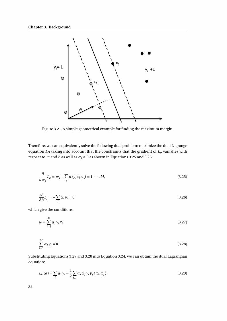
Chapter 3. Background
!
"#$%&' "#$(&')&'
)*'
Figure 3.2 – A simple geometrical example for finding the maximum margin.
Therefore, we can equivalently solve the following dual problem: maximize the dual Lagrange
equation LD taking into account that the constraints that the gradient of Lp vanishes with
respect to w and b as well as αi ≥ 0 as shown in Equations 3.25 and 3.26.
∂
∂w jLp = w j −
∑iαi yi xi j , j = 1, · · · , M , (3.25)
∂
∂bLp =−∑
iαi yi = 0, (3.26)
which give the conditions:
w =M∑
i=1αi yi xi (3.27)
M∑i=1
αi yi = 0 (3.28)
Substituting Equations 3.27 and 3.28 into Equation 3.24, we can obtain the dual Lagrangian
equation:
LD (α) =∑iαi yi − 1
2
∑i , jαiα j yi y j
⟨xi , x j
⟩(3.29)
32

3.2. Support Vector Machines
The solution can be found either by minimizing Lp or maximizing LD . Note that there is a
Lagrange multiplier αi for each training point and αi ≥ 0. In the solution, those points for
which αi > 0 are called Support Vectors and stay on one of the boundaries. All other training
points have αi = 0 and stay either on one of the boundaries or on the side of the boundaries
such that the strict inequality in Equation 3.23 is satisfied. In principle, the support vectors
are the critical elements of the training set. They are in the positions closest to the decision
boundaries. If all other training points were removed or moved around but not to cross the
boundaries, and the training was repeated, the same separating hyperplane would be found.
3.2.3 Non-linear Support Vector Machines
The extension of linear SVMs to non-linear ones is based on the application of kernel meth-
ods [14]. Considering that linear SVM uses a linear kernel as in Equation 3.10, non-linear SVM
first map the data to a feature space through φ to the Euclidean space H :
φ : X → H
x →φ(x)(3.30)
which indicates that in the space H , x is re-mapped as φ(x). As the training problem is in the
form of inner products⟨
xi , x j⟩ = xT
i x j , the training algorithm in the mapped space would
only depend on the data through inner products in H with a form⟨φ(xi ),φ(x j )
⟩. Therefore,
we can define the kernel function K such that:
K (xi , x j ) = ⟨φ(xi ),φ(x j )
⟩. (3.31)
Then, the training depends only on knowing K and would not require to know φ. The opti-
mization problem becomes:
maxα
L(α) =M∑
i=1αi − 1
2
M∑i , j=1
αiα j yi y j K (xi , x j )
subject to: αi ≥ 0, i = 1, · · · , M
M∑i=1
αi yi = 0
(3.32)
The decision function y in the feature space for a new point x is computed and classified by
comparing it to all the training points with non-zero weight as follows:
y = sgn
(M∑
i=1αi yi K (x, xi )+b
)(3.33)
33
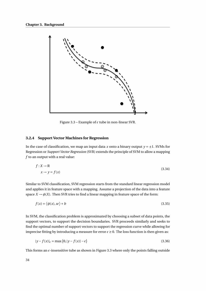
Chapter 3. Background
!!!!!!!
!!!!!!!Figure 3.3 – Example of ε tube in non-linear SVR.
3.2.4 Support Vector Machines for Regression
In the case of classification, we map an input data x onto a binary output y =±1. SVMs for
Regression or Support Vector Regression (SVR) extends the principle of SVM to allow a mapping
f to an output with a real value:
f : X →R
x → y = f (x)(3.34)
Similar to SVM classification, SVM regression starts from the standard linear regression model
and applies it in feature space with a mapping. Assume a projection of the data into a feature
space X →φ(X). Then SVR tries to find a linear mapping in feature space of the form:
f (x) = ⟨φ(x), w
⟩+b (3.35)
In SVM, the classification problem is approximated by choosing a subset of data points, the
support vectors, to support the decision boundaries. SVR proceeds similarly and seeks to
find the optimal number of support vectors to support the regression curve while allowing for
imprecise fitting by introducing a measure for error ε≥ 0. The loss function is then given as:
|y − f (x)|ε = max{0, |y − f (x)|−ε} (3.36)
This forms an ε-insensitive tube as shown in Figure 3.3 where only the points falling outside
34

3.2. Support Vector Machines
!"#
$"#
"#%&'()*#(a) Smaller margin corresponds to a steeper slope
!"#
$"#
"#%&'()*#
(b) Larger margin corresponds to a flatter slope
Figure 3.4 – Example of ε margin in linear SVR.
of the boundaries given by ε are considered in the loss function. Similarly to the margin in
SVM, the ε margin of SVR is defined as shown in Figures 3.4a and 3.4b, where a larger margin
corresponds to a flatter slope of the estimated regression curve while a smaller margin for a
steeper slope. Therefore, in order to have a smooth regression estimation which guarantees a
wider range in the x axis as shown in Figure 3.4, a larger ε-margin is wanted, which corresponds
to a smaller absolute value of the norm |w |. Hence, in SVR we also want to minimize |w | as in
35

Chapter 3. Background
SVM so as to find the optimal solution as shown in Equation 3.37:
minw
(1
2||w ||2 +C · 1
M
M∑i=1
∣∣yi − f (xi )∣∣ε
), (3.37)
where C is a constant which is a free parameter to be estimated during the training phase and
it decides a tradeoff between optimizing for the smoothness of the fit and minimizing the
increase in the training error. The right part of Equation 3.37 gives an averaged measure of the
error computed based on the choice of ε value.
The optimization problem given by Equation 3.37 can be also expressed as a constrained
problem in the form:
min1
2||w ||2
s.t .
⟨φ(xi ), w
⟩+b − yi ≤ εyi −
⟨φ(xi ), w
⟩−b ≤ ε∀i = 1, · · · , M
(3.38)
Minimizing for the norm of w ensures that the optimization problem is convex. However,
considering the difficulty of satisfying the conditions in Equation 3.38 towards an arbitrarily
small ε, a set of slack variables ξi and ξ∗i (i = 1, · · · , M) can be introduced for each data point. ξi
and ξ∗i denote whether the data point is on the left or right side of the function f respectively.
These slack variables measure by how much each data point is incorrectly fitted, which gives
the following optimization problem:
min1
2||w ||2 + C
M
M∑i=1
(ξi +ξ∗i )
s.t .
⟨φ(xi ), w
⟩+b − yi ≤ ε+ξi
yi −⟨φ(xi ), w
⟩−b ≤ ε+ξ∗iξi ≥ 0, ξ∗i ≥ 0
∀i = 1, · · · , M
(3.39)
Applying Lagrange solver to solve this quadratic problem, we first introduce a set of Lagrange
multipliers αi ,γi ≥ 0 for each of inequalities constraints:
L(w,ξ,ξ∗,b) = 1
2||w ||2 + C
M
M∑i=1
(ξi +ξ∗i )− C
M
M∑i=1
(γiξi +γ∗i ξ∗i )
−M∑
i=1αi (ε+ξi + yi −
⟨φ(xi ), w
⟩−b)
−M∑
i=1α∗
i (ε+ξ∗i − yi +⟨φ(xi ), w
⟩+b)
(3.40)
36

3.2. Support Vector Machines
The solutions are found through solving the partial derivatives:
∂L
∂b= 0
∂L
∂w= 0
∂L
∂ξ(∗)= 0
(3.41)
where ξ(∗) means that the notation can be applied both to ξ and ξ∗. Hence we get the equations:
∂L
∂b=
M∑i=1
(αi −α∗i ) = 0 (3.42)
∂L
∂w= w −
M∑i=1
(α∗i −αi )φ(xi ) = 0 (3.43)
∂L
∂ξ(∗)= C
M−α(∗)
i −γ(∗)i (3.44)
Substituting Equations 3.42, 3.43 and 3.44 into 3.40 gives the dual optimization under con-
straint problem as follows:
maxα,α∗
−12
∑Mi , j=1(α∗
i −αi )(α∗j −α j ) ·K (xi , x j )
−ε∑Mi=1(α∗
i +αi )+∑Mi=1 yi (α∗
i +αi )
s.t .
∑M
i=1(α∗i −αi ) = 0
α∗i ,αi ∈
[0, C
M
].
(3.45)
After obtaining the Lagrange multipliers α∗,α, the best projection vector w can be then
computed as:
w =M∑
i=1(α∗
i −αi )φ(xi ) (3.46)
The offset b can be determined by solving Equation 3.47 for the Karush-Kuhn-Tucher (KKT)
37

Chapter 3. Background
conditions:αi(ε+ξi + yi −
⟨φ(xi ), w
⟩−b)= 0
α∗i
(ε+ξ∗i − yi +
⟨φ(xi ), w
⟩+b)= 0
under the conditions( C
M −αi)ξi = 0( C
M −α∗i
)ξ∗i = 0
(3.47)
The second pair of equations in Equation 3.47 shows that:
• if the Lagrange multiplier takes the value α(∗)i = C
M , the corresponding slack variable
ξ(∗)i can take any arbitrary value and hence the corresponding points can be anywhere,
including outside of the ε tube.
• if the Lagrange multiplier takes the value α(∗)i ∈ (
0, CM
), then the corresponding ξ(∗)
i = 0
and these corresponding points become the support vectors.
Since we never have an explicit form of the projection φ(xi ), we therefore cannot compute w
in Equation 3.46. However, we can apply once more the kernel trick to compute f by:
⟨φ(x), w
⟩= M∑i=1
(α∗i −αi )φ(xi )φ(x)
=M∑
i=1(α∗
i −αi )K (xi , x).
(3.48)
Then the estimated regression function f can be obtained through:
f (x) =M∑
i=1(α∗
i −αi )K (xi , x)+b, (3.49)
where K (xi , x) stands for the kernel matrix. Observe that the computational cost for the
regression function grow linearly with the number of M data points. The computational cost
can be reduced if the number of data points for which the elements in the sum are non-zero
(support vectors) is reduced. In SVR, this is the case when (α∗i −αi ) = 0.
Figures 3.5a and 3.5b show the influence of the ε values in SVR with a linear kernel. The red
dots are the data points randomly drawn with the free software MLdemos [66]. Three lines
denote the estimated regression curve (middle one) and its ε tube (upper and lower ones).
These data points emphasized by a black circle around are the support vectors. Figures 3.6a,
3.6b and 3.6c also compare the influence of different ε values but on an RBF kernel as defined
in Section 3.2.1. Compared with the linear kernel, RBF kernel is demonstrated to fit more
closely to the given data points. Different ε values give different fitting curve and the smaller,
the more support vectors are used. On the other hand, a big kernel width reduces the fitting
38

3.2. Support Vector Machines
(a) SVR with linear kernel, kernel width = 0.1, ε= 0.01
(b) SVR with linear kernel, kernel width = 0.1, ε= 0.1
Figure 3.5 – Comparisons of different ε values in SVR with a linear kernel using MLdemos [66].
accuracy as indicated in Figure 3.7 and 3.6b. However, when the ε value becomes too small as
shown in Figure 3.6c, almost all the points are used as the support vectors, and if the kernel
width of RBF kernel is set to be small too, an overfitting will happen.
3.2.5 Least Square Support Vector Machines
There are many attractive aspects of SVM, for instance, the sparseness of the solution vector α,
the implicit redefining of the optimization in the input space [14]. However, it still remains
computationally heavy as its complexity increases with the size of the data points. LS-SVM is a
version of SVM that simplify the original formulation and, at the same time, retain the good
properties such as able to consider as many input features as possible, etc. [76, 18] Hence,
the solution is obtained by solving a system of linear equations and at the same time LS-SVM
shows comparable generalization performance compared to SVM.
39

Chapter 3. Background
(a) SVR with RBF kernel, kernel width = 0.01, ε= 0.1
(b) SVR with RBF kernel, kernel width = 0.01, ε= 0.01
(c) SVR with RBF kernel, kernel width = 0.01, ε= 0.001
Figure 3.6 – Comparisons of different ε values in SVR with a linear kernel using MLdemos [66].
Let us first consider the formulation of SVM:
minw,b,ξ
Lp = 1
2||w ||2 +C
1
2
M∑i=1
ξ2i , (3.50)
40

3.2. Support Vector Machines
Figure 3.7 – SVR with RBF kernel, kernel width = 0.1, ε= 0.01.
under the equality constraints (instead of the inequality constraints in SVM):
yi [⟨φ(xi ), w
⟩+b] = 1−ξi , i = 1, · · · , M , (3.51)
A slightly modified approach is presented here: an equality constraint is defined instead to
align the regression surface in the feature space exactly with the target surface with the use of
a slack variable ξi .
Then we have the Lagrangian:
Ld (w,b,ξ;α) = Lp −M∑
i=1αi [yi (
⟨φ(xi ), w
⟩+b)−1+ξi ], (3.52)
where αi are Lagrange multipliers, which can be either positive or negative now due to the
equality constraints as follows from the KKT conditions.
To find the optimal solution, we have to solve:
∂Lp
∂w= 0 → w =
M∑i=1
αi yiφ(xi ),
∂Lp
∂b= 0 →
M∑i=1
αi yi = 0,
∂Lp
∂ξi=→αi =Cξi , i = 1, · · · , M ,
∂Lp
∂αi= 0 → yi (
⟨φ(xi ), w
⟩+b)−1+ξi = 0, i = 1, · · · , M ,
(3.53)
41

Chapter 3. Background
which can be re-written in the form of the matrix of linear equations:I 0 0 −ZT
0 0 0 −YT
0 0 C · I −I
Z Y I 0
w
b
ξ
α
=
0
0
0
1
, (3.54)
where Z = [⟨φ(x1), yi
⟩; · · · ;⟨φ(xM ), yM
⟩], Y = [y1; · · · ; yM ], ξ= [ξ1; · · · ;ξM ], α= [α1; · · · ;αM ]. The
solution is given by:[0 −YT
Y ZZT +C−1I
][b
α
]=
[0
1
]. (3.55)
The so-called kernel trick can be applied in forming the matrix ZZT : K (xi , x j ) = ⟨φ(xi ),φ(x j )
⟩,
where
zizjT = yi y j
⟨φ(xi ),φ(x j )
⟩= yi y j K (xi , x j )
(3.56)
This implicitly transforms the linear system so that computation is performed in the input
space instead of the feature space. The linear set of Equation 3.55 is faster to solve than the
quadratic programming required in SVM. The kernel trick can be applied in Equation 3.56
and the parameters can be tuned via cross validation.
The resulting regression surface is:
y =M∑
i=1αi K (x, xi )+b (3.57)
The solution vector here is no longer sparse and the support values αi are proportional to the
errors at the data points, while in the case of SVM most values are equal to zero.
3.2.6 Cross Validation for Finding the Kernel Parameters
In machine learning or other areas such as statistics or data mining, learning a model from
available data points to accomplish either a regression task or a classification one is one typical
task [14]. The problem with evaluating such a model is that it may demonstrate adequate
performance on the training data but may fail to achieve a good prediction capability on the
future unseen testing data. Therefore, cross validation is introduced to simulate a similar
environment for the model with only the training data. Usually there are two goals in using
cross validation:
• Estimate the performance of a learned model and to optimize it on the data available.
• Compare the ability of generalization of the two algorithms on the same dataset to
42
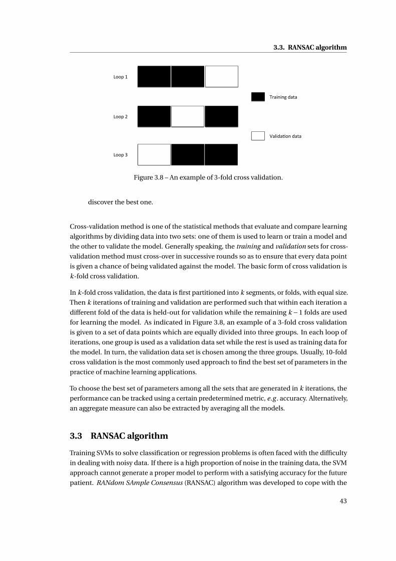
3.3. RANSAC algorithm
!""#$%$
!""#$&$
!""#$'$
()*+,+,-$.*/*$
0*1+.*2",$.*/*$
Figure 3.8 – An example of 3-fold cross validation.
discover the best one.
Cross-validation method is one of the statistical methods that evaluate and compare learning
algorithms by dividing data into two sets: one of them is used to learn or train a model and
the other to validate the model. Generally speaking, the training and validation sets for cross-
validation method must cross-over in successive rounds so as to ensure that every data point
is given a chance of being validated against the model. The basic form of cross validation is
k-fold cross validation.
In k-fold cross validation, the data is first partitioned into k segments, or folds, with equal size.
Then k iterations of training and validation are performed such that within each iteration a
different fold of the data is held-out for validation while the remaining k −1 folds are used
for learning the model. As indicated in Figure 3.8, an example of a 3-fold cross validation
is given to a set of data points which are equally divided into three groups. In each loop of
iterations, one group is used as a validation data set while the rest is used as training data for
the model. In turn, the validation data set is chosen among the three groups. Usually, 10-fold
cross validation is the most commonly used approach to find the best set of parameters in the
practice of machine learning applications.
To choose the best set of parameters among all the sets that are generated in k iterations, the
performance can be tracked using a certain predetermined metric, e.g . accuracy. Alternatively,
an aggregate measure can also be extracted by averaging all the models.
3.3 RANSAC algorithm
Training SVMs to solve classification or regression problems is often faced with the difficulty
in dealing with noisy data. If there is a high proportion of noise in the training data, the SVM
approach cannot generate a proper model to perform with a satisfying accuracy for the future
patient. RANdom SAmple Consensus (RANSAC) algorithm was developed to cope with the
43

Chapter 3. Background
noisy dataset problems. In this section, we will mainly introduce its mathematic base and the
algorithm.
Algorithm 1 RANSAC algorithm, where d at a is a set of observations, model is a modelthat can be fitted to data, K is the minimum number of data points required to fit the modelparameters, N is the number of trials performed by the algorithm, T is a threshold determiningif a data point fits a model, and bestmodel is the model fitting the highest number of datapoints.
Input: d at a,model ,K , N ,TOutput: bestmodel
best i nl i er s ←;for i = 1 → N do
possi bl ei nl i er s ← SampleUniformly(d at a,K )possi bl emodel ← Fit(model , possi bl ei nl i er s)i nl i er s ←;for all poi nt ∈ d at a do
if Distance(poi nt ,model ) < T theni nl i er s ← i nl i er s ∪ {poi nt }
end ifend forif |i nl i er s| > |besti nl i er s| then
best i nl i er s ← i nl i er send if
end forreturn bestmodel ← Fit(model ,best i nl i er s)
The RANSAC [34] algorithm works as described in Algorithm 1. The number of trials N is set
to be big enough to guarantee that at least one of the sets of possible inliers does not include
any outlier with a high probability p. Usually p is set to 0.99. Let us assume, that u is the
probability that any selected data point is an inlier, then v = 1−u is the probability of selecting
an outlier. N trials of sampling each K data points are required, where 1−p = (1−vK )N . This
way:
N = ln(1−p)
ln(1− (1−u)K ). (3.58)
The model of the RANSAC algorithm is a linear combination of several basis functions. The
number of basis functions corresponds directly to the minimum number of points K required
to fit the model. The parameters of the model are the weights of each basis function. In
this paper, the drug concentration prediction method enhanced with filtering of the training
dataset using RANSAC algorithm is called RANSAC-SVM method.
Figures 3.9, 3.10 and 3.11 present a simple line-fitting example of the flow of RANSAC algorithm.
Raw data points are given as shown in Figure 3.9 and the task is to fit a line to these observations.
In each loop out of a total of N iterations, two points are selected randomly as indicated with a
44

3.3. RANSAC algorithm
Figure 3.9 – An example of line fitting with RANSAC algorithm – raw data.
red color in the figures. Then the parameters are computed based on these two points. Given
a certain threshold value, presented as dash lines in the figures, we can separate the rest of
the data points into inliers (black points) and outliers (white points). Each time, only the
parameters that correspond to the largest number of inliers are kept until we finish all the
iterations.
The RANSAC algorithm has several merits such as to be easy to understand, fast to implement,
and both statistically and practically powerful. In this thesis, it is not only a method to remove
the outliers from the data library, but also applied to find the basis functions for the drug
concentration curve as presented in Section 5.4.
3.3.1 Compare The Bagging Algorithm with RANSAC
Bootstrap Aggregation (Bagging) is a machine learning algorithm designed to improve statis-
tically the stability and accuracy of solving classification and regression problems. It can be
embedded with any type of method. It has a similar nature as the RANSAC algorithm in the
sense of estimating the output based on random subsamples. It is also applied to the same
basis functions as used in RANSAC. In contrast to RANSAC, the Bagging algorithm is averaging
all the estimated outputs instead of choosing the best one according to certain criteria.
45

Chapter 3. Background
Figure 3.10 – An example of line fitting with RANSAC algorithm – one of the iterations offinding the best fitting by counting the number of inliers.
A traditional approach to estimate a model from a set of given data points would be to generate
a φ(x,G) from all the data samples, where x are the input data samples and G are the sets of x
and y pairs. The general algorithm of Bagging goes as follows:
1. Generate subsets of data points, each in the form:
G∗i = {(X ∗
1 ,Y ∗1 ), · · · , (X ∗
n ,Y ∗n )}(i ), (3.59)
where the star mark ∗ is used for the subset elements. And then it compute an estimator
φ̂(x,G∗i ) from these samples.
2. Repeat step 1 for Q times independently and identically yielding subsets:
G∗1 ,G∗
2 , · · · ,G∗Q (3.60)
with corresponding estimators: φ̂(x,G∗1 ), φ̂(x,G∗
2 ), · · · , φ̂(x,G∗Q ).
3. Aggregate (Average) all the estimates:
φ(x,G) = 1
Q
Q∑i=1
φ̂(x,G∗i ). (3.61)
46

3.3. RANSAC algorithm
Figure 3.11 – An example of line fitting with RANSAC algorithm – the best fitting model withthe largest number of inliers.
From the above description, the Bagging algorithm can be interpreted as an approximation:
φ(x,G) ≈ E∗[φ̂] (3.62)
When the value of Q increases,φ(x,G) is supposed to be statistically approaching the optimum.
Compared with the RANSAC algorithm, the Bagging method can be explained in details as
Figures 3.12 to 3.15. In Figure 3.12, two points are selected at random in the first round and a
corresponding curve (straight line) is generated as the red dotted line. Repeat this step for Q
times as shown in Figures 3.13 and 3.14, with a new curve is generated each time. In the end,
an averaged curve is computed based on all the Q generated curves.
The advantage of the Bagging algorithm is that there exists a proof of convergence under a
certain assumption, which the RANSAC algorithm does not have. The proof goes as follows:
• Given the assumption: φ̂1, φ̂2, · · · , φ̂Q are Independently and Identically Distributed (iid)
47

Chapter 3. Background
!"#"
Figure 3.12 – An example of line fitting with Bagging algorithm – first round generates one line.
and the expectation of Y is an unbiased estimator of the mean value y : E(φ̂) =φ.
• The expected error is in the form of E((φ̂−φ)2).
• While performing averaging in the Bagging algorithm, we have:
Z = 1
Q
Q∑i=1
φ̂i , (3.63)
which corresponds to the definition of covariance:
E((Z −φ)2) = 1
Q2
Q∑i=1
σ2(φ̂i ), (3.64)
which indicates that with the increase of the number of rounds Q, the error is approach-
ing to zero.
On the other hand, if there is no such assumption as E(φ̂) =φ, then the following transforma-
48

3.3. RANSAC algorithm
!"#"
Figure 3.13 – An example of line fitting with Bagging algorithm – second round generates asecond line.
tion is applied:
E((φ̂−φ)2) = E((φ̂−E(φ̂)+E(φ̂)−φ)2)
= E((φ̂−E(φ̂))2)+E((E(φ̂)−φ)2)+E(2(φ̂−e(φ̂))(E(φ̂)−φ))
= E((φ̂−E(φ̂))2)+E((E(φ̂)−φ)2)+E(φ̂−E(φ̂))E(2(E(φ̂)−φ))
(3.65)
where the first part which corresponds to the covariance of φ̂ is thus always non-negative, and
the third part goes to 0 since E(φ̂−E(φ̂)) = 0. Therefore the error is encapsulated by:
E((E(φ̂)−φ)2) ≤ E((φ̂−φ)2). (3.66)
Especially when E((φ̂−E(φ̂))2) has a large value, a smaller error is guaranteed.
However, the disadvantage of using the Bagging algorithm is that: as shown in Figures 3.14
and 3.15, if there are too many outliers in the data points, the final averaged output will be
influenced, especially when there is a large proportion of outliers.
49

Chapter 3. Background
!"#"
Figure 3.14 – An example of line fitting with Bagging algorithm – after Q rounds.
3.4 Clinical Decision Support Systems
Clinical Decision Support System is a computer-aided decision support system designed to
assist clinicians and other clinical practitioners with clinical decision making tasks, such as
determining the type of disease of a patient based on his/her clinical data. The system uses
the clinical knowledge to abstract the clinical advice for patient care based on some number of
patient data in the past. Furthermore, it can be combined with machine learning and artificial
intelligent algorithms to make the decision support more personalized to a specific patient.
Mainly two types of CDSS are listed in the literature [12, 13]:
• Knowledge-based CDSS: where three parts are often used, the knowledge base, inference
engine and mechanism to communicate. The system contains the clinical rules and
associations of compiled data. The inference engine refers to the rules from the knowl-
edge base with the patient data. The communication mechanism takes the functions of
taking inputs into the system and showing the results to the user.
• Non-knowledge-based CDSS: where CDSS use machine learning algorithms instead of
a knowledge base to learn the data patterns from the past experiences/patient data or
find patterns in clinical data for decision making. Most non-knowledge-based CDSS
50

3.4. Clinical Decision Support Systems
Figure 3.15 – An example of line fitting with Bagging algorithm – the final output line isobtained by averaging over all the generated lines.
use Artificial Neural Networks. This type of CDSS eliminates the need for writing rules
and for expert inputs. However, since there is no explicit explanations of how the system
deals with the data, most clinicians do not want to use them.
In this thesis, another machine learning approach, SVMs, is introduced to this area. Compared
with ANN and GA approaches, the SVM method has a clearer system expression. Furthermore,
instead of finding a local minimum, the SVM method outputs a result as a global optimum.
This thesis also introduces a way to combine both the machine learning algorithm and the
analytical method together to build up the base for a clinical decision support system.
CDSS are mainly faced with four challenges [13]:
• Clinical challenges: Clinical practice has its own complexity of the workflows. This
requires that the CDSS to be integrated fluidly as part of the workflow. Patient-oriented
CDSS have been found success but often limited to a certain scope. New systems are
required for different clinical routines.
• Technical challenges: There are different types of technical challenges facing CDSS
51

Chapter 3. Background
development. Mainly, CDSS need to consider as many patient features as possible. In
addition to a patient’s disease record, the patient’s symptoms, medical history, family
history, genetics, etc, have to be taken in to account for the medical decision making.
Besides, the data from other patients taking the same clinical practice are also valuable
and need to be considered in the system. Due to a large number of clinical records
from different resources, in some situation, to build up a CDSS also requires loading
paper-based records into computer.
• Maintenance: In current clinical practice, extensive quantity of clinical research can be
published over one year. However, each one of these studies must be manually read,
evaluated for scientific legitimacy, and integrated into CDSS in an accurate way. New
data can sometimes be difficult to quantify or incorporate into the existing decision
support schema, especially when different clinical papers are shown with conflicts. One
of the subjects is to properly resolving these types of discrepancies.s
• Evaluation: Different CDSS have their different purposes, therefore no generic metric
can be applied to evaluate all the systems. Most of the systems are evaluated based on
the consistency and accuracy of their output.
This thesis introduces a Drug Administration Decision Support System that integrates a self-
adaptation close-loop structure, so as to be able to update the system performance from time
to time with a given measurement. The algorithms used in the system are also easy to be
re-trained with the growth of the data library to take into account larger number and more
personalized data.
3.5 Summary
This chapter has introduced all the related algorithms applied in this thesis, including tra-
ditional PK models, various types of SVM algorithms, RANSAC and Bagging algorithm. In
short, the PK approaches are mainly based on a pre-defined analytical model, while the SVM
approaches are similar to a black box system, estimating the mathematical relation among
data points with respect to a pre-determined kernel function. The RANSAC and Bagging
algorithms are both used for generating a model from given data with several pre-set basis
functions, but Bagging computes an averaged model while RANSAC picks up the most rea-
sonable one according to certain criteria. Though there is a guaranteed convergence of the
Bagging algorithm, it is usually difficult to achieve a better modeling performance as the
RANSAC algorithm does.
The background knowledge of CDSS is also introduced. Two types of CDSS classify the
systems into knowledge-based and non-knowledge-based. This section also discusses about
the current challenges facing CDSS in the aspects of clinical, technical, maintenance and
evaluation.
52

3.5. Summary
In the next chapters, the ways of combining the RANSAC and SVM algorithms in the do-
main of personalized drug concentration predictions will be presented. A CDSS for assisting
drug administration will also be introduced based on these algorithms and the medical GLs
corresponding to the case study in this thesis.
53

4 SVM-based Drug Concentration Pre-dictions
This chapter presents how the SVM method is applied to perform the drug concentration
predictions. Two approaches are studied: the first one directly applies the Least Square SVM
method to predict the concentration values (Section 4.1) and the second one finds the set of
close examples in the patient data library to be used as new training data (Section 4.2). The
experimental and comparison results are shown in Section 4.3, and Section 4.4 draws a brief
conclusion. The methods presented here have been published in [93].
4.1 Applying SVM to Predict Drug Concentrations
Let us assume that there are N patients, each of whom has been examined ni times. The
number of total samples is∑N
i=1 ni . Each sample takes into account d features. Hence the
training data are given as
{(x11 , y1
1), (x12 , y1
2), · · · , (x1n1
, y1n1
), · · · , (xNnN
, y NnN
)}, (4.1)
where y denotes the output drug concentration and the subscript index of y jni
denotes ni -th
data sample value of the j -th patient in the library. Similarly, x is the space of input patterns
Rd , e.g . age, gender, body weight, dose amount, measuring time, etc, and the footnote of x jni
is the corresponding ni -th sample of the j -th patient.
19 sets of sample data from 6 patients in the library are randomly selected from the training
data library and shown in the Table 4.1. The ‘Drug Concentration’ denote the drug concentra-
tion values measured by clinical device. ‘Measuring Time’ corresponds to the point when the
‘Drug Concentration’ is measured. ‘Dose Amount’ indicates the quantity of the drug taken
by the patients. ‘Gender’ shows the patients’ sex information: ‘0’ for women and ‘1’ for men.
‘Age’ is the patients’ age when the measurement is carried out. ‘Body Weight’ is the patients’
weight at the time of measurement. The data in the training library are used to train the SVM
algorithm for computing the parameters based on which the model is built and tested on the
testing data library. The patients’ data in the testing data library have the same set of feature
55

Chapter 4. SVM-based Drug Concentration Predictions
Table 4.1 – Six patients’ data sample selected randomly from the training data library.
Y XSample j ni Drug Concentration Measuring Time Dose Amount Gender Age Body Weight
no. [mcg/L] [h] [mg] [kg]
1 1 1 2361.0 3.49 400 0 49.3 60.02 2 1225.1 17.5 400 0 49.6 59.03 3 1661.3 8.0 400 0 49.7 57.04 4 2191.1 4.25 400 0 50.0 58.05 5 1924.4 6.24 400 0 50.2 62.06 2 1 2095.4 9.49 400 1 74.7 67.07 2 1760.7 8.0 400 1 75.1 69.08 3 2218.4 9.0 400 1 75.3 68.09 4 3154.4 9.0 400 1 75.5 67.0
10 3 1 3083.4 7.74 300 0 66.9 47.011 2 3436.0 15.99 300 0 67.4 44.012 3 2797.6 4.74 300 0 67.6 46.013 4 1 4618.6 5.49 400 0 72.2 55.014 2 2898.0 5.49 300 0 72.3 52.015 3 2032.5 7.74 200 0 72.5 57.016 4 2049.0 5.75 200 0 72.7 52.017 5 1 446.9 25.74 400 1 26.9 110.018 2 1496.9 2.0 300 1 27.3 110.019 6 1 694.9 24.49 400 0 57.5 56.0
Table 4.2 – Mean and STD values of the training data library.
Measuring Time Dose Amount Gender Age Body Weight[h] [mg] [kg]
Mean 9.68 412.90 0.57 53.06 71.79STD 7.15 124.18 0.50 15.58 15.74
attributes. In the following part of the thesis, the comparison of different methods are based
on computing the MAD values between the predicted concentrations and the measured ones.
Then this MAD value is compared with the MAD value of the traditional PK method and the
measured concentrations.
Table 4.2 shows the Mean and STD values of the training data library which are used to
normalize both the training and the testing data libraries. This is reasonable since in real
clinical practice, the Mean and STD values of new patients are usually not available. Thus, to
normalize a new patient data before predicting, the values obtained from the training data
library are used.
The goal of the SVM method is to find a linear function:
f (x) = w ·φ(x)+b (4.2)
which approximates the relationship between the data points and can be used to estimate the
output y with respect to a new input patient data. In (4.2), φ(x) maps the input samples to a
higher-dimensional feature space by finding a non-linear function in the original space where
w stands for the weights of the feature space and b ∈R is an offset constant.
56

4.1. Applying SVM to Predict Drug Concentrations
Any regression problem uses a loss function L (y, f (x)) to describe how the predicted values
deviate from the target ones, among which the following quadratic loss function is one of the
most commonly used:
L (y, f (x)) = (y − f (x))2 (4.3)
In principle, Function 4.3 needs to be minimized and the optimal solution is found through
the procedure of minimization. Besides the task of minimizing the loss function, we also
need to make sure that the function f is as flat as possible in order to prevent overfitting the
problem. The flatness of the function f can be ensured by keeping the norm ‖w‖2 small. Thus
the regression problem can be rewritten as optimization of the following objective function:
minw,b
1
2‖w‖2 +C0
N∑j=1
n j∑i=1
[y ji −w ·φ(x j
i )−b]2 (4.4)
where the constant C0 determines the tradeoff between the flatness of f and the amount up
to which deviations between the predicted and measured values are tolerated. According to
Suykens et. al. [76] the optimal w can always be expressed by w =∑Nj=1
∑n j
i=1αji φ(x j
i ), where
α and b are found by solving the linear system:[K+ 1
C0I 1
1T 0
]︸ ︷︷ ︸
H
[α
b
]=
[y
0
](4.5)
where K is the kernel matrix and is defined as Kab = φ(x ja
ia)Tφ(x jb
ib). The use of the kernel
matrix greatly helps reducing the computational complexity without explicitly computing
φ(x), making use of the fact that the SVM algorithm depends only on dot products between
sample patterns. Hence, after defining the kernel function, the least-square optimization
problem can be solved simply by inverting the first term H in the left-hand side of (4.5).
Once theα and b have been obtained, the output can be estimated via the following prediction
function:
f (x) =N∑
j=1
n j∑i=1
αji K(x j
i , x)+b (4.6)
Till now, LS-SVM trains the inputs as a whole and applies the model to new patient indifferently.
Experiments show that this improves the prediction results but degrades greatly with the
decrease of input data samples.
57

Chapter 4. SVM-based Drug Concentration Predictions
!"#$%&#'$()()*&%(+'$',&
-.%./#.0&#'$()()*&%(+'$',&
!"#$%
&%'()*#+,
-%#
Figure 4.1 – Selections of the N % Close Examples from the Total Data Library
4.2 Optimization Using Example-based SVM (E-SVM)
Within the scenario described above, we introduce the idea of example-based SVM algorithm.
Although the SVM approach can estimate the drug concentration with a large number of input
features and also simplify the addition or removal of new features, it treats the input training
samples equally without selecting a subset of the training library containing more relevant
data to a new testing sample before running the algorithm. However, when comparing to
other fields such as computer vision or pattern recognition, clinical samples have much fewer
data. Therefore, inproper samples are going to greatly affect the model built by SVM, which
can cause inaccuracy in prediction. As shown in Figure 4.1, N % of the data in the training data
library are selected according to a certain strategy used to build up a selected training library.
Then, this selected training library is applied through a similar procedure as described in the
SVM approach in Section 4.1.
Therefore, Example-based SVM approach is proposed to optimize the prediction, which
carefully selects useful training patients in the library and builds the personalized model
specifically for a new patient. As illustrated in Figure 4.2, the system first takes all the features
fd from a new patient and extracts a subset of them fs to be the selection criteria for training
samples. The weights for each feature in fs are denoted by β. For each training patient in the
library, we assign a coefficient ε according to:
εji =
{0 ‖β · ( fs − f j )‖a > ts
1 ‖β · ( fs − f j )‖a ≤ ts(4.7)
where i , j stand for the i th sample of the j th patient in the library, ts is the threshold, and f j is
the corresponding criteria features. Both f j and fs are normalized in advance by subtracting
the mean and dividing the standard deviation. We indicate a as an la-norm having the form
‖x‖a = a√∑n
i=1 |xi |a .
58
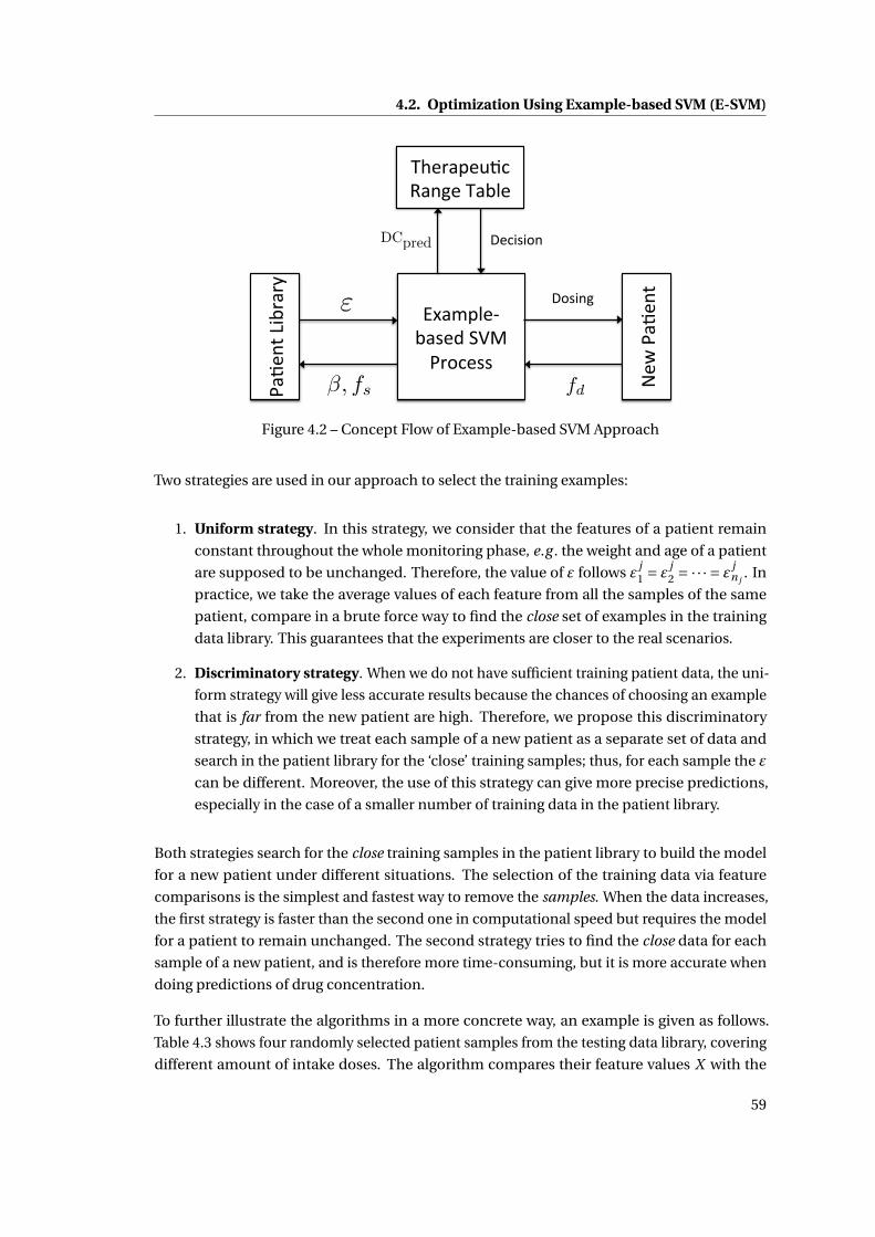
4.2. Optimization Using Example-based SVM (E-SVM)
!"#$
%&'()*+"+,'
-."/01$2*"3$4'567'!+89$33'
:$;
'!"#
$%&'
<83)%='
>?$+"0$@#9'A"%=$'>"*1$'
<$9)3)8%'
ε
DCpred
fdβ, fs
Figure 4.2 – Concept Flow of Example-based SVM Approach
Two strategies are used in our approach to select the training examples:
1. Uniform strategy. In this strategy, we consider that the features of a patient remain
constant throughout the whole monitoring phase, e.g . the weight and age of a patient
are supposed to be unchanged. Therefore, the value of ε follows ε j1 = ε
j2 = ·· · = ε j
n j. In
practice, we take the average values of each feature from all the samples of the same
patient, compare in a brute force way to find the close set of examples in the training
data library. This guarantees that the experiments are closer to the real scenarios.
2. Discriminatory strategy. When we do not have sufficient training patient data, the uni-
form strategy will give less accurate results because the chances of choosing an example
that is far from the new patient are high. Therefore, we propose this discriminatory
strategy, in which we treat each sample of a new patient as a separate set of data and
search in the patient library for the ‘close’ training samples; thus, for each sample the ε
can be different. Moreover, the use of this strategy can give more precise predictions,
especially in the case of a smaller number of training data in the patient library.
Both strategies search for the close training samples in the patient library to build the model
for a new patient under different situations. The selection of the training data via feature
comparisons is the simplest and fastest way to remove the samples. When the data increases,
the first strategy is faster than the second one in computational speed but requires the model
for a patient to remain unchanged. The second strategy tries to find the close data for each
sample of a new patient, and is therefore more time-consuming, but it is more accurate when
doing predictions of drug concentration.
To further illustrate the algorithms in a more concrete way, an example is given as follows.
Table 4.3 shows four randomly selected patient samples from the testing data library, covering
different amount of intake doses. The algorithm compares their feature values X with the
59

Chapter 4. SVM-based Drug Concentration Predictions
Table 4.3 – Four patient data samples selected randomly from the testing data library.
Y XTest Sample j ni Drug Concentration Measuring Time Dose Amount Gender Age Body Weight
no. [mcg/L] [h] [mg] [kg]
1 1 1 1481.0 1.0 400 1 87.5 64.02 2 1 1255.0 17.75 400 0 62.3 54.03 3 1 3272.0 6.75 300 0 23.4 56.04 4 1 747.0 25.25 600 1 58.5 105.0
Table 4.4 – Orders of the close data samples in the training library with respect to each testingsample.
Sample j ni Test sample Test sample Test sample Test sampleno. 1 2 3 4
1 1 1 9 2 3 172 2 7 19 5 193 3 8 11 4 64 4 6 3 1 85 5 13 13 10 76 2 1 1 5 14 97 2 14 4 12 188 3 4 10 15 29 4 5 1 13 5
10 3 1 12 14 2 211 2 3 12 16 412 3 15 15 11 113 4 1 16 16 19 1114 2 10 6 18 1315 3 2 9 7 1016 4 11 8 9 1417 5 1 19 7 6 1218 2 18 17 8 1519 6 1 17 18 17 16
training data library. Here, they are compared with the data in Table 4.1. Table 4.4 presents the
results by ordering the training data samples from 1 to 19, where the smaller the number is,
the closer this sample to the testing data. In this example, the weights for each feature β is 1
everywhere.
After obtaining ε for each patient, w can then be calculated by:
w =N∑
j=1
n j∑i=1
εji α
ji φ(x j
i ), (4.8)
where the equation still satisfies the ε ji α
ji ≥ 0. For those patient samples with ε
ji = 0, they
are regarded as faraway data in advance for a specified new patient in order not to affect the
personalized model. Hence equation (4.5) can be written as:[(K+ 1
C0I )ε 1
ε 0
][α
b
]=
[y
0
](4.9)
60

4.3. Comparison Results
Table 4.5 – Comparisons of the Mean Absolute Differences among LS-SVM (LS), E-SVM Uni-form (E1) and E-SVM Discriminatory (E2) (Features: A-Dose, B-Measuring Time, C-Gender,D-Age, E-Body Weight) [unit: mcg / L]
100% 70% 50% 30% 10%Features All LS E1 E2 LS E1 E2 LS E1 E2 LS E1 E2
A+B 822.3 850.4 830.6 836.3 858.2 832.4 832.7 857.0 843.5 849.9 971.9 957.0 938.9A+B+C 835.3 848.0 837.6 838.3 893.5 833.6 833.5 856.7 848.1 848.9 982.1 957.2 942.3
A+B+C+D 846.5 867.1 851.8 855.8 834.6 876.3 853.5 951.4 876.7 859.9 980.6 986.8 960.3A+B+D 853.0 878.2 853.4 852.8 890.1 853.3 851.5 904.0 853.1 868.1 973.4 953.5 945.6A+B+E 853.8 837.5 860.2 851.6 882.2 855.9 852.0 880.5 872.1 868.1 995.8 964.8 940.7
A+B+D+E 868.1 880.6 889.3 885.3 882.1 909.5 893.1 860.7 895.8 890.4 979.0 991.9 963.6A+B+C+D+E 903.6 882.7 879.1 875.2 867.8 915.1 884.9 855.5 891.3 885.7 984.2 991.9 963.6
A+B+C+E 849.1 865.6 851.9 855.8 854.0 876.3 853.5 926.4 876.7 859.9 975.9 986.8 960.3
The values of α and b can be computed similarly by adding ε to Equation (4.6). The accuracy
of the method has been shown experimentally in Section 4.3 to be more precise and stable
than the traditional PK modeling or LS-SVM method, where the .
Once the system gets the prediction of the drug concentration, it checks the value to be
effective or not according to the drug therapeutic range table. If it is above the range, the
dose has to be reduced. After considering the amount of reduction, the system will redo
the modeling step to give a new concentration prediction. The dose has to be increased
respectively for the case of under-dosing.
4.3 Comparison Results
I compare the prediction results of this system to the ones using a general population PK
model. As shown in equations (4.4), (4.6) and (4.7), several parameters both for LS-SVM and
the Example-based SVM method are determined as follows:
1. K: the effectiveness of the SVM method depends on the choice of the kernel function. A
common choice is to use a Gaussian Kernel which has a single parameter σ that has to
be estimated.
2. C0 and σ: after selecting the kernel, the performance of SVM highly depends on the
kernel parameters and the margin factor C0. The best combination of C0 and σ is found
by a grid-search with exponentially growing sequences via 10-fold cross validation. In
practice, our C0,σ ∈ {10−2,10−1, · · · ,103,104}. The 10-fold cross validation is done by
separating randomly the original training data into 10 subsample groups. In our experi-
ment, one of the subsamples is used as the set of validation data while the remaining 9
groups are used as training sets.
3. fs : determines the features used to find the close training examples. In the experiments,
the selected feature set is composed of {gender, age, weight}.
61
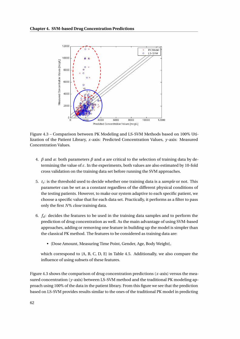
Chapter 4. SVM-based Drug Concentration Predictions
Figure 4.3 – Comparison between PK Modeling and LS-SVM Methods based on 100% Uti-lization of the Patient Library, x-axis: Predicted Concentration Values, y-axis: MeasuredConcentration Values.
4. β and a: both parameters β and a are critical to the selection of training data by de-
termining the value of ε. In the experiments, both values are also estimated by 10-fold
cross validation on the training data set before running the SVM approaches.
5. ts : is the threshold used to decide whether one training data is a sample or not. This
parameter can be set as a constant regardless of the different physical conditions of
the testing patients. However, to make our system adaptive to each specific patient, we
choose a specific value that for each data set. Practically, it performs as a filter to pass
only the first N % close training data.
6. fd : decides the features to be used in the training data samples and to perform the
prediction of drug concentration as well. As the main advantage of using SVM-based
approaches, adding or removing one feature in building up the model is simpler than
the classical PK method. The features to be considered as training data are:
• {Dose Amount, Measuring Time Point, Gender, Age, Body Weight},
which correspond to {A, B, C, D, E} in Table 4.5. Additionally, we also compare the
influence of using subsets of these features.
Figure 4.3 shows the comparison of drug concentration predictions (x-axis) versus the mea-
sured concentration (y-axis) between LS-SVM method and the traditional PK modeling ap-
proach using 100% of the data in the patient library. From this figure we see that the prediction
based on LS-SVM provides results similar to the ones of the traditional PK model in predicting
62

4.3. Comparison Results
!"#$
!%#$
!&#$
!'#$
Figure 4.4 – Histogram of the Mean Absolute Difference in the Drug Concentration PredictionsAmong the four Approaches: (a) PK Model, (b) LS-SVM, (c) E-SVM Uniform, (d) E-SVMDiscriminatory [bar unit = 200 mcg/L]
a high drug concentration values as shown in the red dash ellipse. However, as to the data
in the blue solid circle, the Figure 4.4 shows that the three SVM-based approaches are better
than the PK modeling method at predicting the drug concentration to be close to the mea-
sured value. The red dash rectangle highlights the number of the prediction difference within
[−200,200]mcg/L, in which the number of predictions for the PK modeling method is 78.1%
less than the LS-SVM method, and the number for LS-SVM method is 14.0% and 12.3% less
than the two example-based methods respectively.
Compared to the SVM methods, the traditional PK model is unable to consider Boolean inputs.
Neither can it be modified easily to analyze the importance of each feature. On the other hand,
the SVM-based approaches can deal with these issues. As shown in Table 4.5, we compare the
Mean Absolute Difference between the measured drug concentration values and the predicted
ones using LS-SVM (LS), E-SVM Uniform (E1), and E-SVM Discriminatory (E2) methods.
Feature A and B stand for dose and measuring time after one dose respectively, which are
thought to be the key features and are used through all the experiments. Using the PK model,
the mean value of the differences between the predicted concentrations and the real values is
842.1. Hence the three SVM-based methods provide predictions of similar accuracy.
Furthermore, the SVM-based methods analyze the importance of each listed feature. As Table
4.5 reveals, the best (lowest) differences for each subset of the data are the ones using only
Feature A and Feature B. Therefore, when applying the SVM method to build a model for a new
patient with 100% of the library, knowing only the dose and the measuring time is sufficient
to obtain comparable results, while the PK model depends on analyzing all the parameters
needed in Equation 3.4 and 3.5.
63

Chapter 4. SVM-based Drug Concentration Predictions
However, with a reduced library of patients, the two Example-SVM approaches surpass the
LS-SVM by searching for the close patients (or samples) to be the training data set instead of a
random selection. Table 4.5 also shows that as an overall, E2 method obtains better results
than E1 for 75% of all the experiments, while E1 is better than E2 if we consider the features
{Gender, Age, Body Weight} only during the selection phase of the training patients.
4.4 Summary
Assisting the predictions of drug concentration values in clinical situation with SVM has proved
to yield some similar results to the traditional PK model. It can build personalized model for
each patient in drug concentration analysis in order to give the guidance to the doctors in
the dose prescription. Despite its advantages, the limitation of this approach resides in the
high dependency of the results from the quality of the initial data obtained from patients.
Indeed, no assumption on the theoretical disposition of the drug in the body, according to the
classical pharmacokinetic behavior of drugs, is made. Under certain conditions, it improves
the predictions using fewer input features. Two example-based SVM strategies have been
analyzed in the paper and both are superior to the LS-SVM method when dealing with a
reduced library of patients. These approaches however deserve formal clinical validation
with more data sets from various drugs undergoing TDM. Future work has also shown that
SVM-based approached can build personalized model for each individual patient.
64

5 RANSAC-based Improvement for DrugConcentration Predictions
The results from the previous chapter show that the SVM approaches can improve a little bit
in the prediction accuracy for the drug concentration values based on the available patient
features. However, the improvement is still very small and new methods should be analyzed
to obtain a better accuracy result.
In this chapter, the RANSAC algorithm is applied to improve the accuracy of drug concentra-
tion predictions. It is used in Section 5.1 as one of the pre-processing methods to filter out the
outliers from the data library, which improves the prediction accuracy by about 40%. Different
sets of basis functions are analyzed using both the RANSAC (Section 5.2) and the Bagging algo-
rithms and the most proper set of basis functions is obtained based on certain criteria (Section
5.3). Section 5.4 proposes a Parameterized Support Vector Machine (ParaSVM) approach that,
instead of predicting the drug concentration values directly, predicts the parameters for each
basis function. ParaSVM combines both the merits of an analytical approach and a machine
learning algorithm. Section 5.5 draws a brief conclusion for this chapter.
5.1 RANSAC-SVM Approach for Improving the Prediction Accuracy
In Algorithm 1 described in Section 3.3, inliers and outliers are separated without considering
the information of a new patient. The SVM predictor for any new patient is estimated by
the same inliers chosen as the training data. The results of applying directly the RANSAC
algorithm will be analyzed in Section 5.1.1.
In some cases, however, it might happen that the set of inliers for one patient is actually a set
of outliers for another. Therefore, a predictor built out of the same set of inliers for a number
of new patients might not be applicable for some others. Hence, it is important to find an
individual set of inliers for each patient.
In this section, the RANSAC algorithm is modified to take into considerations each patient’s
features. A RANSAC-based personalization method is proposed to solve this task. Previously
in Chapter 4, a ‘close-example’ strategy has been used which, despite using a much fewer
65

Chapter 5. RANSAC-based Improvement for Drug Concentration Predictions
Algorithm 2 RANSAC-based personalized algorithm, where tr ai ni ng is a set of M trainingsamples, new pati ent s is an ordered set containing one sample per new patient , Y is theindex of a particular feature, model ,K , N ,T are parameters of the RANSAC algorithm, andbestmodel s is an ordered set containg the SVM model fitting the best each new patient.
Input: tr ai ni ng ,new pati ent s,F,model ,K , N ,TOutput: bestmodel s
bestmodel s ←;for all pati ent ∈ new pati ent s do
d at a ← {pati ent , . . . , pati ent } {|d at a| = M }d at a ← d at a ∪ tr ai ni ngi nl i er s ← RANSAC(d at a,model ,K , N ,T ) {predict Y }i nl i er s ← i nl i er s \ {pati ent }model ← SVM(i nl i er s)bestmodel s ← bestmodel s ∪model
end forreturn bestmodel s
number of training points (up to 30% of the total number), retains the initial performance of
the original SVM (<3% degradation). However, that strategy needs a set of predefined weights
for each feature in order to select the ‘close examples’.
Assume that we already have M samples from previous patients (the training dataset), for
each new patient we want to find a best subset of samples of M data to train the SVM. To do so
we treat them as if they were noisy samples of a new patient, and use RANSAC to remove the
outliers. The whole procedure is detailed in Algorithm 2. The new sample from each patient
is first replicated M times to make sure that it will always be considered as an inlier. Then
RANSAC is applied to those replicated samples plus to the original M training samples in order
to predict the feature Y as a linear combination of basis functions of the remaining features X .
The new patient sample is then removed from the inliers and finally an SVM is trained on the
remaining original training samples to predict the drug concentration of this new patient.
Two clinical scenarios can be applied by setting the target feature Y to be:
1. Any feature other than the concentration value;
2. The measured drug concentration.
For the scenario (1), no invasive blood test is required, while in (2) the drug concentration
value should be measured after the first-dosing.
66
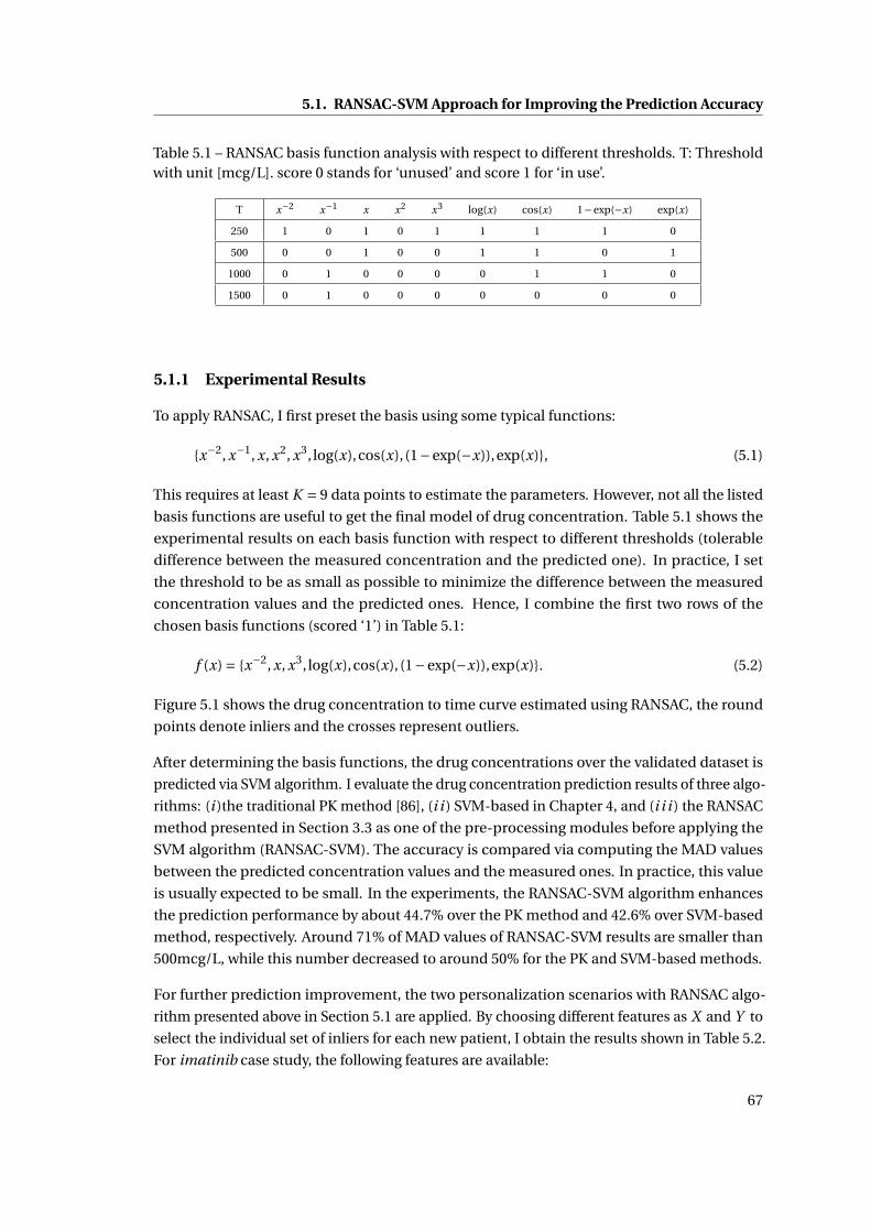
5.1. RANSAC-SVM Approach for Improving the Prediction Accuracy
Table 5.1 – RANSAC basis function analysis with respect to different thresholds. T: Thresholdwith unit [mcg/L]. score 0 stands for ‘unused’ and score 1 for ‘in use’.
T x−2 x−1 x x2 x3 log(x) cos(x) 1−exp(−x) exp(x)
250 1 0 1 0 1 1 1 1 0
500 0 0 1 0 0 1 1 0 1
1000 0 1 0 0 0 0 1 1 0
1500 0 1 0 0 0 0 0 0 0
5.1.1 Experimental Results
To apply RANSAC, I first preset the basis using some typical functions:
{x−2, x−1, x, x2, x3, log(x),cos(x), (1−exp(−x)),exp(x)}, (5.1)
This requires at least K = 9 data points to estimate the parameters. However, not all the listed
basis functions are useful to get the final model of drug concentration. Table 5.1 shows the
experimental results on each basis function with respect to different thresholds (tolerable
difference between the measured concentration and the predicted one). In practice, I set
the threshold to be as small as possible to minimize the difference between the measured
concentration values and the predicted ones. Hence, I combine the first two rows of the
chosen basis functions (scored ‘1’) in Table 5.1:
f (x) = {x−2, x, x3, log(x),cos(x), (1−exp(−x)),exp(x)}. (5.2)
Figure 5.1 shows the drug concentration to time curve estimated using RANSAC, the round
points denote inliers and the crosses represent outliers.
After determining the basis functions, the drug concentrations over the validated dataset is
predicted via SVM algorithm. I evaluate the drug concentration prediction results of three algo-
rithms: (i )the traditional PK method [86], (i i ) SVM-based in Chapter 4, and (i i i ) the RANSAC
method presented in Section 3.3 as one of the pre-processing modules before applying the
SVM algorithm (RANSAC-SVM). The accuracy is compared via computing the MAD values
between the predicted concentration values and the measured ones. In practice, this value
is usually expected to be small. In the experiments, the RANSAC-SVM algorithm enhances
the prediction performance by about 44.7% over the PK method and 42.6% over SVM-based
method, respectively. Around 71% of MAD values of RANSAC-SVM results are smaller than
500mcg/L, while this number decreased to around 50% for the PK and SVM-based methods.
For further prediction improvement, the two personalization scenarios with RANSAC algo-
rithm presented above in Section 5.1 are applied. By choosing different features as X and Y to
select the individual set of inliers for each new patient, I obtain the results shown in Table 5.2.
For imatinib case study, the following features are available:
67
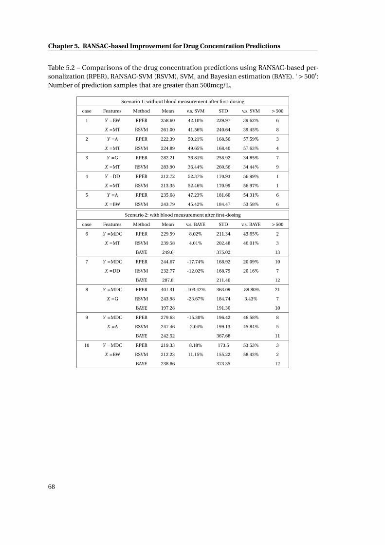
Chapter 5. RANSAC-based Improvement for Drug Concentration Predictions
Table 5.2 – Comparisons of the drug concentration predictions using RANSAC-based per-sonalization (RPER), RANSAC-SVM (RSVM), SVM, and Bayesian estimation (BAYE). ‘ > 500′:Number of prediction samples that are greater than 500mcg/L.
Scenario 1: without blood measurement after first-dosing
case Features Method Mean v.s. SVM STD v.s. SVM > 500
1 Y =BW RPER 258.60 42.10% 239.97 39.62% 6
X =MT RSVM 261.00 41.56% 240.64 39.45% 8
2 Y =A RPER 222.39 50.21% 168.56 57.59% 3
X =MT RSVM 224.89 49.65% 168.40 57.63% 4
3 Y =G RPER 282.21 36.81% 258.92 34.85% 7
X =MT RSVM 283.90 36.44% 260.56 34.44% 9
4 Y =DD RPER 212.72 52.37% 170.93 56.99% 1
X =MT RSVM 213.35 52.46% 170.99 56.97% 1
5 Y =A RPER 235.68 47.23% 181.60 54.31% 6
X =BW RSVM 243.79 45.42% 184.47 53.58% 6
Scenario 2: with blood measurement after first-dosing
case Features Method Mean v.s. BAYE STD v.s. BAYE > 500
6 Y =MDC RPER 229.59 8.02% 211.34 43.65% 2
X =MT RSVM 239.58 4.01% 202.48 46.01% 3
BAYE 249.6 375.02 13
7 Y =MDC RPER 244.67 -17.74% 168.92 20.09% 10
X =DD RSVM 232.77 -12.02% 168.79 20.16% 7
BAYE 207.8 211.40 12
8 Y =MDC RPER 401.31 -103.42% 363.09 -89.80% 21
X =G RSVM 243.98 -23.67% 184.74 3.43% 7
BAYE 197.28 191.30 10
9 Y =MDC RPER 279.63 -15.30% 196.42 46.58% 8
X =A RSVM 247.46 -2.04% 199.13 45.84% 5
BAYE 242.52 367.68 11
10 Y =MDC RPER 219.33 8.18% 173.5 53.53% 3
X =BW RSVM 212.23 11.15% 155.22 58.43% 2
BAYE 238.86 373.35 12
68

5.1. RANSAC-SVM Approach for Improving the Prediction Accuracy
Figure 5.1 – Drug Concentration to Time Curve analyzed using the RANSAC algorithm. Redpoints are inliers and blue points are outliers.
• {Measured Drug Concentration (MDC), Measuring Time (MT), Drug Dose (DD), Age (A),
Gender (G), Body weight (BW)}.
Scenario (1) uses any feature other than MDC values while scenario (2) uses only MDC to be
Y . I also compute the enhancement percentages with SVM (‘v.s. SVM’ in the Table 5.2) and
Bayesian algorithm [86] (‘v.s. BAYE’ in the table) in the Mean and STD results.
The table shows that the RANSAC-based personalization performs slightly better than the
RANSAC-SVM algorithm in the cases 1, 2, 3, 4, 5, 6, which results from a reduced number
of predictions whose MAD values are larger than 500mcg/L. Both algorithms improve the
prediction accuracy compared with SVM by around 40%. In scenario 2, the Bayesian algorithm
(BAYE) outperforms the other two in the average prediction values in the cases 7, 8, 9. However,
in most cases, BAYE gives a larger STD value in that it predicts the results with much less
accuracy for some patient points, while the other two algorithms estimate the concentration
values without a large deviation. Hence, it can be seen that the proposed algorithms are robust
to predict the concentrations more accurately for any individual patient, while Bayesian
algorithm only predicts well for some patients and less accurate for the others.
69

Chapter 5. RANSAC-based Improvement for Drug Concentration Predictions
5.2 RANSAC Basis Function Discovery
As has been presented in Section 3.3 and 5.1, the RANSAC algorithm functions based on a
certain set of pre-defined basis functions. These basis functions are crucial since they have to
directly reveal the shape and distribution of the data samples. In this section, different basis
functions are analyzed through all the data samples and compared through the mean absolute
differences and the standard deviation Value between the predicted drug concentrations by
the follow-up SVM algorithm and the measured ones. The choice of the basis functions are
widely enlarged than discussed in [92].
Table 5.3 – Analysis of the Basis Functions used in the RANSAC algorithm with respect tothe prediction accuracy. Alpha values are the coefficients used to build the curve for thedrug concentration over time in the RANSAC algorithm. MAD stands for the Mean AbsoluteDifferences between the predicted drug concentration values and the clinical measured ones.STD stands for the standard deviation of the differences.
index Basis Functions alpha MAD STD
1 {x0} [1355.1] 200.91 141.222 {x1} [36.76] 232.36 162.213 {x2} [1.5542] 208.76 139.054 {x3} [0.0661] 220.81 141.985 {x−1} [1541.7] 254.19 200.036 {x−2} [96276.0] 449.03 453.567 {x−3} [1005400] 731.09 550.108 {log(x)} [677.73] 230.33 167.329 {(1−exp(−x))} [1353.9] 245.45 185.93
10 {cos(x)} [2127.1] 585.69 448.7011 {tan(x)} [722.05] 774.40 715.2112 {x0, x1} [2239.6, -63.0] 201.28 122.7013 {x0, x1, x2} [2451.0, -94.3, 1.0] 198.78 125.3114 {x0, x1, x2, x3} [1540.6, 159.1, -16.4, 0.3] 302.90 260.9115 {x−2, log(x), (1−exp(−x))} [-4912.9, -946.8, 3820.3] 227.04 203.10
Table 5.4 – Analysis of the Basis Functions used in the RANSAC algorithm with respect to thenumber of inliers in both training and testing datasets.
index Basis Functions Training Inliers Testing Inliers Total Inliers
1 {x0} 70 77 1472 {x1} 34 57 913 {x2} 29 47 764 {x3} 28 42 705 {x−1} 80 82 1626 {x−2} 74 36 1107 {x−3} 57 21 788 {log(x)} 87 112 1999 {(1−exp(−x))} 69 76 145
10 {cos(x)} 32 41 7311 {tan(x)} 15 29 4412 {x0, x1} 89 105 19413 {x0, x1, x2} 88 110 19814 {x0, x1, x2, x3} 88 108 19615 {x−2, log(x), (1−exp(−x))} 88 112 200
70
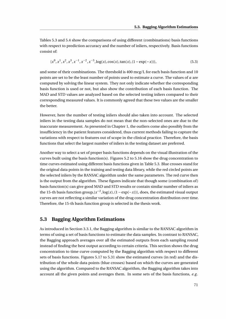
5.3. Bagging Algorithm Estimations
Tables 5.3 and 5.4 show the comparisons of using different (combinations) basis functions
with respect to prediction accuracy and the number of inliers, respectively. Basis functions
consist of:
{x0, x1, x2, x3, x−1, x−2, x−3, log(x),cos(x), tan(x), (1−exp(−x))}, (5.3)
and some of their combinations. The threshold is 400 mcg/L for each basis function and 10
points are set to be the least number of points used to estimate a curve. The values of α are
computed by solving the linear system. They not only indicate whether the corresponding
basis function is used or not, but also show the contribution of each basis function. The
MAD and STD values are analyzed based on the selected testing inliers compared to their
corresponding measured values. It is commonly agreed that these two values are the smaller
the better.
However, here the number of testing inliers should also taken into account. The selected
inliers in the testing data samples do not mean that the non-selected ones are due to the
inaccurate measurement. As presented in Chapter 1, the outliers come also possibly from the
insufficiency in the patient features considered, thus current methods failing to capture the
variations with respect to features out of scope in the clinical practice. Therefore, the basis
functions that select the largest number of inliers in the testing dataset are preferred.
Another way to select a set of proper basis functions depends on the visual illustration of the
curves built using the basis function(s). Figures 5.2 to 5.16 show the drug concentration to
time curves estimated using different basis functions given in Table 5.3. Blue crosses stand for
the original data points in the training and testing data library, while the red circled points are
the selected inliers by the RANSAC algorithm under the same parameters. The red curve then
is the output from the algorithm. These figures indicate that though some (combination of)
basis function(s) can give good MAD and STD results or contain similar number of inliers as
the 15-th basis function group,{x−2, log(x), (1−exp(−x))}, does, the estimated visual output
curves are not reflecting a similar variation of the drug concentration distribution over time.
Therefore, the 15-th basis function group is selected in the thesis work.
5.3 Bagging Algorithm Estimations
As introduced in Section 3.3.1, the Bagging algorithm is similar to the RANSAC algorithm in
terms of using a set of basis functions to estimate the data samples. In contrast to RANSAC,
the Bagging approach averages over all the estimated outputs from each sampling round
instead of finding the best output according to certain criteria. This section shows the drug
concentration to time curve computed by the Bagging algorithm with respect to different
sets of basis functions. Figures 5.17 to 5.31 show the estimated curves (in red) and the dis-
tribution of the whole data points (blue crosses) based on which the curves are generated
using the algorithm. Compared to the RANSAC algorithm, the Bagging algorithm takes into
account all the given points and averages them. In some sets of the basis functions, e.g .
71
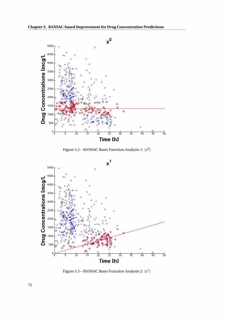
Chapter 5. RANSAC-based Improvement for Drug Concentration Predictions
Figure 5.2 – RANSAC Basis Function Analysis 1: {x0}
Figure 5.3 – RANSAC Basis Function Analysis 2: {x1}
72

5.3. Bagging Algorithm Estimations
Figure 5.4 – RANSAC Basis Function Analysis 3: {x2}
Figure 5.5 – RANSAC Basis Function Analysis 4: {x3}
73

Chapter 5. RANSAC-based Improvement for Drug Concentration Predictions
Figure 5.6 – RANSAC Basis Function Analysis 5: {x−1}
Figure 5.7 – RANSAC Basis Function Analysis 6: {x−2}
74

5.3. Bagging Algorithm Estimations
Figure 5.8 – RANSAC Basis Function Analysis 7: {x−3}
Figure 5.9 – RANSAC Basis Function Analysis 8: {log(x)}
75
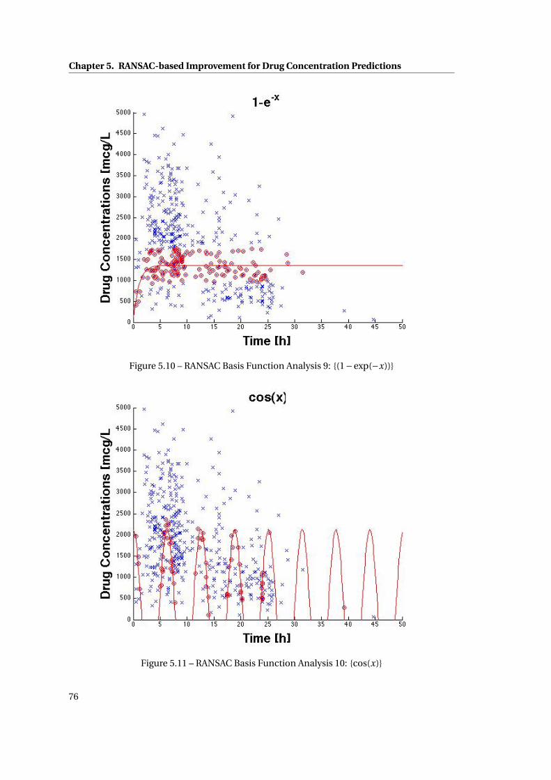
Chapter 5. RANSAC-based Improvement for Drug Concentration Predictions
Figure 5.10 – RANSAC Basis Function Analysis 9: {(1−exp(−x))}
Figure 5.11 – RANSAC Basis Function Analysis 10: {cos(x)}
76

5.3. Bagging Algorithm Estimations
Figure 5.12 – RANSAC Basis Function Analysis 11: {tan(x)}
Figure 5.13 – RANSAC Basis Function Analysis 12: {x0, x1}
77

Chapter 5. RANSAC-based Improvement for Drug Concentration Predictions
Figure 5.14 – RANSAC Basis Function Analysis 13: {x0, x1, x2}
Figure 5.15 – RANSAC Basis Function Analysis 14: {x0, x1, x2, x3}
78
5.4. Parameterized SVM for Visualization
Figure 5.16 – RANSAC Basis Function Analysis 15: {x−2, log(x), (1−exp(x))}
{x0}, {x1}, {x2}, {x3}, {x−1}, {x−2}, {x−3}, {log(x)}, {1− exp(−x)}, {x0, x1}, {x−2, log(x), (1− exp(−x)),
both Bagging and RANSAC obtain similar shapes of the DCT curve, while for other sets, e.g .
{cos(x)}, {tan(x)}, {x0, x1, x2}, {x0, x1, x2, x3}, RANSAC and Bagging algorithms give different es-
timated curve. Even within the sets of basis functions where the RANSAC and the Bagging
algorithms have a similar output, the position of the curves is not exactly the same, e.g .
different initial values, different descending rate, etc.
5.4 Parameterized SVM for Visualization
To apply the SVM algorithm, a set of data is needed to be the training library, which contains
both inputs (patient features) and outputs (parameters used to build the DCT curves). This
library is built using the RANSAC algorithm [34], which was originally used to separate inliers
and outliers from a set of (noisy) data with respect to given basis functions. As presented
in Sections 3.3 and 5.1, the algorithm is randomly selecting a very small subset of the given
input data, computes the parameters (or weights) of each basis function considering the
small subset, and then determines the inliers and outliers for the rest of the data with a given
distance value (threshold). The number of samples to build the subset is dependent on the
number of basis functions.
Here, instead of separating inliers and outliers, the RANSAC algorithm is applied to compute
79
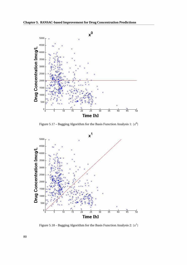
Chapter 5. RANSAC-based Improvement for Drug Concentration Predictions
Figure 5.17 – Bagging Algorithm for the Basis Function Analysis 1: {x0}
Figure 5.18 – Bagging Algorithm for the Basis Function Analysis 2: {x1}
80

5.4. Parameterized SVM for Visualization
Figure 5.19 – Bagging Algorithm for the Basis Function Analysis 3: {x2}
Figure 5.20 – Bagging Algorithm for the Basis Function Analysis 4: {x3}
81

Chapter 5. RANSAC-based Improvement for Drug Concentration Predictions
Figure 5.21 – Bagging Algorithm for the Basis Function Analysis 5: {x−1}
Figure 5.22 – Bagging Algorithm for the Basis Function Analysis 6: {x−2}
82

5.4. Parameterized SVM for Visualization
Figure 5.23 – Bagging Algorithm for the Basis Function Analysis 7: {x−3}
Figure 5.24 – Bagging Algorithm for the Basis Function Analysis 8: {log(x)}
83

Chapter 5. RANSAC-based Improvement for Drug Concentration Predictions
Figure 5.25 – Bagging Algorithm for the Basis Function Analysis 9: {(1−exp(−x))}
Figure 5.26 – Bagging Algorithm for the Basis Function Analysis 10: {cos(x)}
84
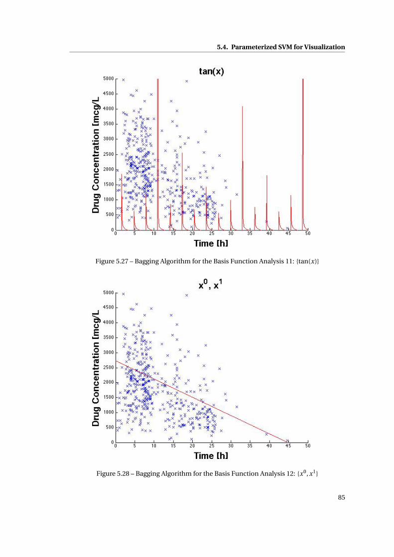
5.4. Parameterized SVM for Visualization
Figure 5.27 – Bagging Algorithm for the Basis Function Analysis 11: {tan(x)}
Figure 5.28 – Bagging Algorithm for the Basis Function Analysis 12: {x0, x1}
85

Chapter 5. RANSAC-based Improvement for Drug Concentration Predictions
Figure 5.29 – Bagging Algorithm for the Basis Function Analysis 13: {x0, x1, x2}
Figure 5.30 – Bagging Algorithm for the Basis Function Analysis 14: {x0, x1, x2, x3}
86
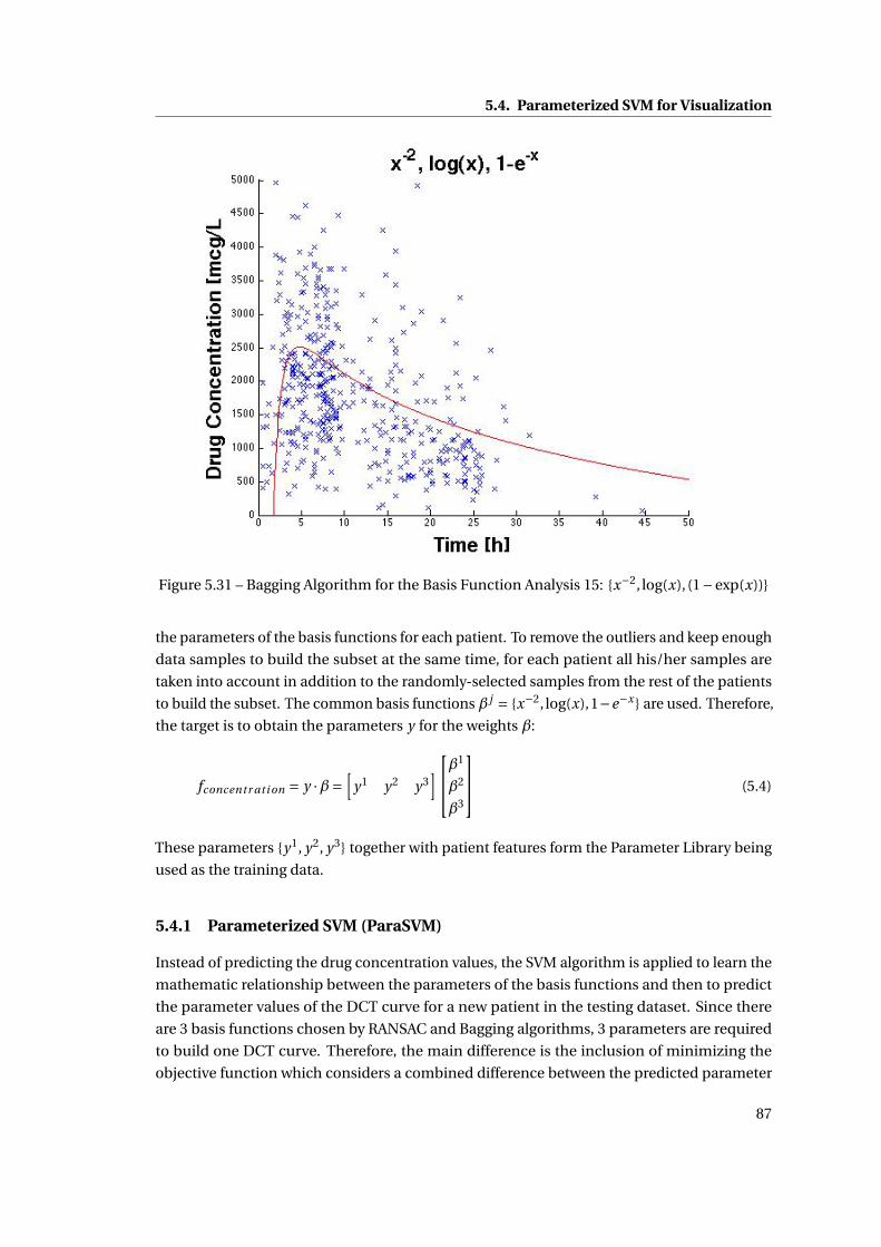
5.4. Parameterized SVM for Visualization
Figure 5.31 – Bagging Algorithm for the Basis Function Analysis 15: {x−2, log(x), (1−exp(x))}
the parameters of the basis functions for each patient. To remove the outliers and keep enough
data samples to build the subset at the same time, for each patient all his/her samples are
taken into account in addition to the randomly-selected samples from the rest of the patients
to build the subset. The common basis functions β j = {x−2, log(x),1−e−x } are used. Therefore,
the target is to obtain the parameters y for the weights β:
fconcentr ati on = y ·β=[
y1 y2 y3]β
1
β2
β3
(5.4)
These parameters {y1, y2, y3} together with patient features form the Parameter Library being
used as the training data.
5.4.1 Parameterized SVM (ParaSVM)
Instead of predicting the drug concentration values, the SVM algorithm is applied to learn the
mathematic relationship between the parameters of the basis functions and then to predict
the parameter values of the DCT curve for a new patient in the testing dataset. Since there
are 3 basis functions chosen by RANSAC and Bagging algorithms, 3 parameters are required
to build one DCT curve. Therefore, the main difference is the inclusion of minimizing the
objective function which considers a combined difference between the predicted parameter
87

Chapter 5. RANSAC-based Improvement for Drug Concentration Predictions
values and the ones in the parameter library (training dataset).
In the case of modeling N patient samples, the form of patient samples becomes:
(xi , y1i , · · · , y j
i , · · · , y NPi ), (5.5)
where i is the ID of a sample i ∈ {1,2 · · · , N }, xi represents the feature values of i -th patient,
y ji denotes the j -th parameter value of this patient, and NP is the number of parameters.
The goal is to find NP linear functions f j (x) = w j ·φ j (x)+b j to describe the relationship in
between the dataset points and to estimate the parameter value y ji according to a new input
dataset. Based on the methods presented in Chapter 3, we minimize the following modified
objective function:
minw,b
1
2||w ||2 +C0
NP∑j=1
N∑i=1
[y ji −w j ·φ j (xi )−b j ]2
︸ ︷︷ ︸H
, (5.6)
where H takes into account the combined difference of all three predicted values plus the ones
in the parameter library. Note that this objective function has Root of Sum of Square (RSS)
fitting error and a regularization term, which is also a standard procedure for the training of
Multi Layer Perceptron (MLP) and is related to ridge regression [39, 18]. Applying Lagrangian
analysis to solve the optimization problem of the objective function, this gives w as:
w j =N∑
i=1α
ji φ
j (xi ), (5.7)
Combining Equation (5.6) and (5.7), I obtain a linear system:[K j + 1
C0I 1
1T 0
][α j
b j
]=
[y j
0
], (5.8)
where each entry of the kernel matrix K j is defined to be K jab = φ j (xa)Tφ j (xb). A Gaussian
Kernel is applied here which has a single parameter σ that has to be determined. Both C0
and σ are selected from {10−2,10−1, · · · ,103,104} using 10-fold cross validation method in the
training step. Therefore, the prediction function for the DCT curve parameters becomes:
Par a j (x) =∑Ni=1αi K j (xi , x)+b j .
5.5 Summary
In this chapter, two RANSAC-based personalization approaches are presented. The accuracy
of drug concentration predictions is compared with the SVM method. From the results shown
in Table 5.2, both RANSAC-based personalization approaches have improved the prediction
results compared with the ones obtained from only applying the SVM method. The table also
shows that using RANSAC algorithm can achieve better STD results than using the Bayesian
88

5.5. Summary
approach.
In addition, the RANSAC algorithm is also applied to build the parameter library in the pro-
posed ParaSVM algorithm. The influence of using different basis functions has been analyzed
and a most proper set of basis functions is established. For comparison, the same sets of basis
functions are also analyzed via the Bagging algorithm, but the RANSAC algorithm shows more
reasonable results. ParaSVM predicts, instead of the drug concentration values directly, the
values of the parameters used to build the drug concentration to time curves. The ParaSVM
approach combines the merits of both the traditional analytical method and the machine
learning algorithms. It can analyze the drug concentration values based on various patient
features that are not considered in the traditional PK methods, and is able to be modified
while conserving a global structure in the mean time.
In the following chapter, a close-loop Drug Administration Decision Support System is going
to be presented by combining all the algorithms described till now.
89


6 Drug Administration Decision Sup-port System
So far, I have introduced the SVM-based algorithms and some improving approaches for drug
concentration predictions, as well as a RANSAC-SVM method for further increase of prediction
accuracy. This chapter introduces a decision support system embedding the above algorithms
and providing the clinicians with a dose suggestion and adaptation regarding each patient.
A Drug Administration Decision Support System (DADSS) is presented. Section 6.1 analyzes
the statistic information of the given data library for imatinib, where the number of samples
in each dose group from 100mg to 800mg is listed with respect to the training and testing data.
Section 6.2 describes the details in the DADSS system where each functional part is presented
and the influence of choosing different parameters is analyzed. The proposed system consists
of inputs and three main modules as shown in Figure 6.1: Preprocess, Prediction Core and
Selection parts. A more complete list of patient features is also proposed for the future clinical
practice to take them into consideration in the section. Section 6.3 draws a brief conclusion.
6.1 Statistics of Drug imatinib
Imatinib [86], a drug considered in our study, is used to treat chronic myeloid leukemia and
gastrointestinal stromal tumors. Until now, only a trough therapeutic range of this drug has
been proposed and is presently being validated in a randomized clinical study in leukemia
patients (I-COME; ISRCTN31181395). The trough range has a lower bound at 750mcg/L,
upper bound at 1500mcg/L and target value at 1000mcg/L [40]. The available training data in
our research are 251 collected from 54 patients and 209 testing data from 65 patients, which
distribute with respect to different doses as shown in Table 6.1. The set of input features of
patient profile data includes: {Gender, Age, and Body Weight}, which, together with the “dose
amount”, the “measuring time” and the “measured drug concentrations”, consist of the data
library for the work.
In Chapter 4, we have presented the SVM algorithm for drug concentration predictions able to
account for different feature parameters of a patient, where we have found that the feature
91

Chapter 6. Drug Administration Decision Support System
!"#$%&'"()$*+,-&-.$
%-"/-01"22$34&)&$105/6"'0(7$86)"-+(97$
(0-5&6+:&'0(;$
<0-"$3=>?@,&2"A$4-B9$
<0(1"()-&'0($%-"A+1'0(;$
="6"1'0($34-B9C2$A02&9"$&(A$'5"$
+()"-D&6;$
!"#$%&'()*"+,*#-.'
"+/$*'
0/,#(&'
Figure 6.1 – Flowchart of the Drug Administration Decision Support System
Table 6.1 – Distribution of patient samples with respect to different doses in the training andtesting library.
Dose unit: mg 100 200 300 400 500 600 700 800 TotalTraining Library 3 11 18 193 - 10 - 16 251Testing Library 1 1 7 176 1 13 - 10 209
“measuring time” is the most important feature to calculate the drug concentration values in
blood. However, the Mean Absolute Difference values between the predicted and the measured
concentrations were still large. We concluded that this large difference was possibly caused
by two factors the insufficient number of patient features, given the assumption that there
is no measurement error. In Chapter 5.1, we have applied the RANdom SAmple Consensus
(RANSAC) algorithm to remove the “outliers”, or noisy data, from all our data samples and
analyzed the influence of using different features to find the outliers, which has improved
the prediction accuracy. In this senction, the DADSS system is presented which uses all the
predicted drug concentration values from 1.0 to 24.0 hours after a patient has taken a dose
to compute the ideal dose amount and ideal time interval for this patient, namely a priori
adaptation, according to the therapeutic range. The section will also illustrate the potential
feature library to be considered in the future clinical practice. However, to collect sufficient
clinical data on newly proposed patient features is demanding in the sense of time, i.e. it will
probably take years. Therefore, one solution is to adjust the predicted concentrations with
92
6.2. Decision Support System
one or more measured values, in the phase of a posteriori adaptation. Nevertheless, the drug
concentration values predicted by the SVM algorithm are so-called “point-wise” interpolation
to build the DCT curve, hence difficult to adjust all the drug concentration values given one
measurement. Analytical model is an effective approach to overcome this problem thanks
to its explicit description of curve structure information. Current PK model [86] is one of
the commonly-used analytical models. However, the basis functions of this PK model rely,
exponentially, on several other parameters such as drug absorption rate and elimination rate,
which might also vary due to an intra-patient variation of the parameters. On the other hand,
explicit PK model makes it difficult to consider more patient features when they are available.
In Section 5.4, we presented a DCT curve approximation approach, Parameterized SVM, which
combines the SVM and analytical models. It keeps the merits of SVM, such as able to be
extended to a larger feature library in the future, and also adds the advantages of analytical
model being structurally adjustable.
The RANSAC algorithm has been applied to filter out the outliers in both training and testing
datasets, while in real clinical practice, it is hard to distinguish whether a newly-measured
concentration value is an outlier or it is due to a sudden intra-variation happening to the
patient. Under the condition that we do not have a sufficient number of features, we need to
search for a curve adaptation method to help the prediction to be more personalized for an
individual patient. In addition, all the analysis in the above work has considered the “dose
amount” as one of the input features for SVM to predict the drug concentrations. The results
in Table 6.1 show a large inequality distribution of the samples in different dose groups. Hence
in this chapter, we also investigate the influence of different dose groups on the prediction
accuracy.
6.2 Decision Support System
Input data are gathered in Library which stores the previous patient feature data and New
Patient features. Library is used to build a mathematical model which links the measured drug
concentration to patient features, while the new patient’s data estimate the drug concentration
that are used to generate the final decisions on dose computation. The Preprocess module
prepares the input data for the Prediction Core module. The Prediction Core module runs
an SVM-based drug concentration model using the preprocessed Library data and predicts
the concentration values for a new patient. The DADSS system uses the Least Square SVM
(LS-SVM) classifier to give a solution by solving a set of linear equations [76]. In Chapter 3, we
has given the details about this algorithm. The Selection module chooses the best dose and
dose intervals according to the given therapeutic ranges (possibly one for the peak and another
for the trough concentration). However, in practice, most drugs have only one therapeutic
range available, which usually refers to the trough concentration. DADSS proposes different
solutions accordingly.
The integrated DADSS takes, as input data, the patient features and, as output data, produces
93
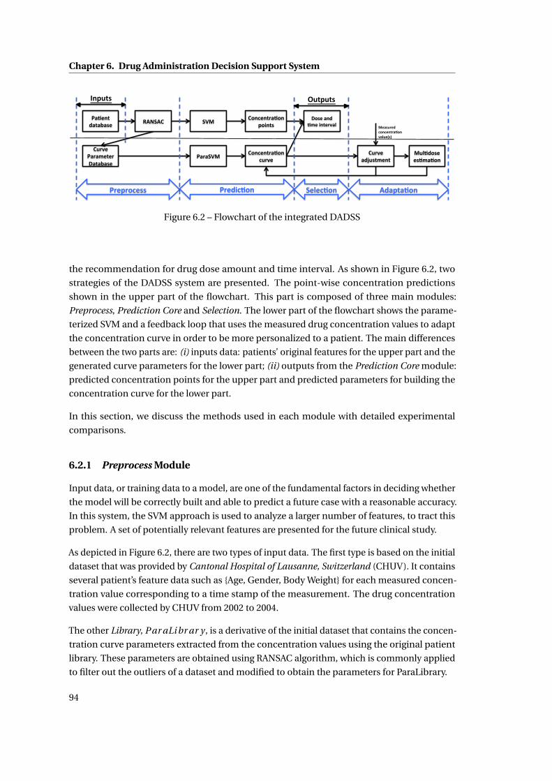
Chapter 6. Drug Administration Decision Support System
!"#$%&'("&")"*$' +,-.,/'
/012$'!"1"3$&$1'4"&")"*$'
.56'
!"1".56'
/7%8$%&1"#7%'97:%&*'
/7%8$%&1"#7%'8012$'
/012$'"(;0*&3$%&'
47*$'"%('#3$':%&$12"<'
60<#(7*$'$*#3"#7%'
!1$9178$**' !1$(:8#7%' .$<$8#7%' ,("9&"#7%'
6$"*01$('87%8$%&1"#7%'2"<0$=*>'
?%90&*' @0&90&*'
Figure 6.2 – Flowchart of the integrated DADSS
the recommendation for drug dose amount and time interval. As shown in Figure 6.2, two
strategies of the DADSS system are presented. The point-wise concentration predictions
shown in the upper part of the flowchart. This part is composed of three main modules:
Preprocess, Prediction Core and Selection. The lower part of the flowchart shows the parame-
terized SVM and a feedback loop that uses the measured drug concentration values to adapt
the concentration curve in order to be more personalized to a patient. The main differences
between the two parts are: (i) inputs data: patients’ original features for the upper part and the
generated curve parameters for the lower part; (ii) outputs from the Prediction Core module:
predicted concentration points for the upper part and predicted parameters for building the
concentration curve for the lower part.
In this section, we discuss the methods used in each module with detailed experimental
comparisons.
6.2.1 Preprocess Module
Input data, or training data to a model, are one of the fundamental factors in deciding whether
the model will be correctly built and able to predict a future case with a reasonable accuracy.
In this system, the SVM approach is used to analyze a larger number of features, to tract this
problem. A set of potentially relevant features are presented for the future clinical study.
As depicted in Figure 6.2, there are two types of input data. The first type is based on the initial
dataset that was provided by Cantonal Hospital of Lausanne, Switzerland (CHUV). It contains
several patient’s feature data such as {Age, Gender, Body Weight} for each measured concen-
tration value corresponding to a time stamp of the measurement. The drug concentration
values were collected by CHUV from 2002 to 2004.
The other Library, Par aLi br ar y , is a derivative of the initial dataset that contains the concen-
tration curve parameters extracted from the concentration values using the original patient
library. These parameters are obtained using RANSAC algorithm, which is commonly applied
to filter out the outliers of a dataset and modified to obtain the parameters for ParaLibrary.
94

6.2. Decision Support System
• !"#$%$#&'()*+',&-+.)• !"#$%"#&'#($%)#*"+,$%+#*"+,$%#,-.%
• /($"$0'()*+',&-+.)• /*01#,#2$%+34#(,#&2*5&$%+*"+%-+56#2,#(56$%+#0(,%'*2#02#$%-0&-#($%#,-.%
• 1+"23$0)4+',&-+.)• 708*63%'*2#02#%+*2,5(3$%"#&#%456385(4+*282.%
• 5637,23)*+',&-+.)• 958*:&"$%;#<#($%'*==*$%+#0'0-+#$%-5&<>62*5&$%258&56#&-#$%
2+5-?$%'(#082$%#,-.%• 8'9$,&'()*+',&-+.)
• !85>&,%5;%)0,#($%8*6?$%285?#$%06-5+56$%,#0$%-5@##$%245(,2$%#,-.%• :"%$-2"3+",'()*+',&-+.)
• A>8*'*,3$%,#84#(0,>(#$%4(#22>(#$%#,-.%
• ;'.0&('-)*+',&-+.)• B655'%2>"0($%4A%<06>#$%C+56#2,#(56%6#<#6$%#,-.%
• <=6.$0'()*+',&-+.)• B655'%4(#22>(#$%+#0(,%(0,#$%(#&06%;>&-:5&$%(#24*(0:5&%;(#D>#&-3$%
(#24*(0:5&%(+3,+8$%(#24*(0:5&%'##4$%#,-.%
E0:#&,%E(5F6#%
GH,#(&06%E0(08#,#(2%
E+32*-06%I#02>(#8#&,2%
Figure 6.3 – List of three groups of potentially relevant patients’ features
Extension of Patient Feature Data
I first present an extension of the feature database such that all kinds of patient features,
including both standard and non-standard, could be considered for future clinical practice.
The standard features are those that have already been considered in the clinical settings, such
as patient’s age, weight, etc. The non-standard features are referred to as the ones that have
not yet been taken into account in the traditional PK models. Figure 6.3 shows the potential
extension of the patient features with three classes: Patient Profile, Physical Measurements,
and External Parameters. Patient profile class is given by the user as semi-static data which
rarely change during the treatment. The physical measurements and the external parameters
can be collected by using clinical tools, questionnaires, etc. Though the features are not
considered explicitly in the current drug concentration prediction models, i.e. the PK method,
they are critical to help to determine whether a drug has been prescribed properly. If we take
Physical Features as an example, the abnormal responses of the patient might be a signal of
overdosing, i.e. during the period of patients’ taking the drug, a sudden and big increase in the
blood pressure.
While it is difficult to adjust the PK model such that it accounts for a bigger number of features,
the SVM approach is flexible in this term and is able to account for various patient features,
allowing one to study a large number (several dozens) of new parameters. Choosing new
valuable features is critical to enhance the accuracy of the drug concentration prediction as
well as can be potentially used to enhance the existing methods. Furthermore, the visualization
95

Chapter 6. Drug Administration Decision Support System
Figure 6.4 – Drug concentration values in the dose group 100 [mg]
of the DCT curve is important for clinicians to better examine the drug effect.
Figure 6.10 to Figure 6.13 show the ability of the SVM method in analyzing the DCT curve
with respect to different patient features. Due to the limitation of the database, four patient
features, {Dose amount, Gender, Age, Body Weight}, are examined separately in a 3D graph to
reveal their influences to the DCT curve. ‘Time’ parameter denotes the measuring time after
the previous dose has been taken, which is usually less than 24 hours, and ‘Dose Amount’ is
defined to be a single oral dose varying from 0 to 1000mg. ‘Gender’, ‘Age’ and ‘Body Weight’ are
personalized parameters and will be used to analyze the DCT curve given the other parameters
remain unchanged.
Figures 6.4 to 6.9 show the distribution of the drug concentration values with respect to
different dose groups where the blue points are the total training dataset and the red ones
are the concentration values in the corresponding dose group. From Figure 6.4 we can see
that given 100 mg dose amount to some patient, the resulting drug concentration values
are quite low and reach the lower boundary of the therapeutic range ([750, 1500] mcg/L) at
about 15 hours. Given a dose 200 mg, Figure 6.5 show a sudden increase in the concentration
values within 10 hours after a patient takes the drug. There are not too many samples showing
the drug concentration at a later stage of this dose group while the only one shows that
the drug concentration values are already falling out of the therapeutic range at about 16
hours. Samples in the dose group 300 mg (Figure 6.6) show a more distinct difference among
concentration values at a similar measuring time and no samples are taken after about 16
hours. Dose group 400 mg contains the most of the data sample in our training data. However,
96

6.2. Decision Support System
Figure 6.5 – Drug concentration values in the dose group 200 [mg]
from the Figure 6.7, it is difficult to observe a straightforward concentration curve since the
values can be either high or low at any time point measured after a patient takes the drug.
Different from the dose group 200 mg or 300 mg, dose group 600 mg (Figure 6.8) show that the
concentration values reach a highest point at about 20 hours. Figure 6.9 shows the dose group
800 mg which generally reaches a high concentration values at about 6 hours. Based on these
figures, the following feature examinations using SVM method is conducted.
From Figure 6.10 to Figure 6.13, the drug concentration to time curves are modeled over
different patient features such as dose amount, gender, age, and body weight, respectively.
Figure 6.10 plots the drug concentration predictions over different time and doses for an
individual patient. From this figure we can see that the larger the drug amount is, the higher
the peak value of the drug concentration will be. However, we can also observe that the
difference of the drug concentration curves with different dose amount dose not show a
proportional increments. This could be caused by the insufficient data points in the training
data samples and the relationship among the data in the training data samples do not provide
a proportional relationship among the data either.
Figure 6.11 shows the drug concentrations being affected by the gender information. The dose
is chosen to be 400mg. From this figure we could see that male patients will have a higher
peak concentration values than females.
Figure 6.12 describes how the patient’s age feature influences the drug concentration after
taking a dose of 400mg. The estimation from the training data samples reveals that the older
97

Chapter 6. Drug Administration Decision Support System
Figure 6.6 – Drug concentration values in the dose group 300 [mg]
Figure 6.7 – Drug concentration values in the dose group 400 [mg]
a patient is, the higher the drug concentration values will be. This could be explained as
the elder patients probably have a slower metabolic speed and thus the drug concentration
remains higher for a longer time than the young patients.
98

6.2. Decision Support System
Figure 6.8 – Drug concentration values in the dose group 600 [mg]
Figure 6.9 – Drug concentration values in the dose group 800 [mg]
Figure 6.13 shows the relationship between the drug concentrations and the values of body
weight of one random patient. The curves indicate that the heavier a patient is, the more dose
amount he/she needs to achieve a high drug concentration values at the trough time.
99

Chapter 6. Drug Administration Decision Support System
In short, the SVM method is able to find the relationship between the drug concentration
variations and each of the patient features. This character of SVM helps reveal the influential
ones among all the patient features. Nevertherless, the results shown in these figures might be
restricted by the training data samples’ distributions in each dose groups.
Figure 6.10 – Drug concentration modeling on one sample patient over time and doses, withpatient information as weight = 60kg, age=50, gender=Male.
RANSAC For Filtering Outliers
The Preprocess module prepares the input data for the Prediction Core. Apart from apply-
ing RANSAC to remove the outliers from all the dataset, first of all, the system checks the
completion of patient features. When the features of a new patient are available only par-
tially, it replaces the missing data by an average value of the corresponding feature in Library.
Moreover, since each feature considered in clinical scenarios has different absolute values
in different metrics, we normalize all the feature values using ‘zero mean, unit variance’
technique as:
norm(feature)i =featurei −mean(featurei )
std(featurei )(6.1)
RANSAC is applied between the above two steps.
The RANSAC [34] algorithm works as described in Algorithm 1 in Section 3.3. The number of
trials M is set to be big enough to guarantee that at least one of the sets of possible inliers does
100

6.2. Decision Support System
Figure 6.11 – Drug concentration modeling over different gender information with otherpatient features fixed: weight=50kg, age=50, dose=400mg.
Figure 6.12 – Drug concentration modeling over patients with different ages with other patientfeatures fixed: weight=50kg, gender=Male, dose=400mg
not include any outlier with a high probability p. Usually p is set to 0.99. Let us assume, that
101
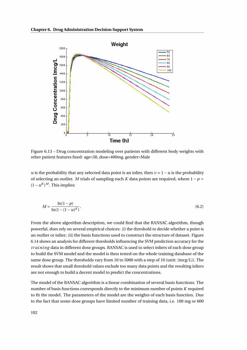
Chapter 6. Drug Administration Decision Support System
Figure 6.13 – Drug concentration modeling over patients with different body weights withother patient features fixed: age=50, dose=400mg, gender=Male
u is the probability that any selected data point is an inlier, then v = 1−u is the probability
of selecting an outlier. M trials of sampling each K data points are required, where 1−p =(1−uK )M . This implies:
M = ln(1−p)
ln(1− (1−u)K ). (6.2)
From the above algorithm description, we could find that the RANSAC algorithm, though
powerful, does rely on several empirical choices: (i) the threshold to decide whether a point is
an outlier or inlier; (ii) the basis functions used to construct the structure of dataset. Figure
6.14 shows an analysis for different thresholds influencing the SVM prediction accuracy for the
tr ai ni ng data in different dose groups. RANSAC is used to select inliers of each dose group
to build the SVM model and the model is then tested on the whole training database of the
same dose group. The thresholds vary from 10 to 5000 with a step of 10 (unit: [mcg/L]). The
result shows that small threshold values exclude too many data points and the resulting inliers
are not enough to build a decent model to predict the concentrations.
The model of the RANSAC algorithm is a linear combination of several basis functions. The
number of basis functions corresponds directly to the minimum number of points K required
to fit the model. The parameters of the model are the weights of each basis function. Due
to the fact that some dose groups have limited number of training data, i.e. 100 mg or 600
102
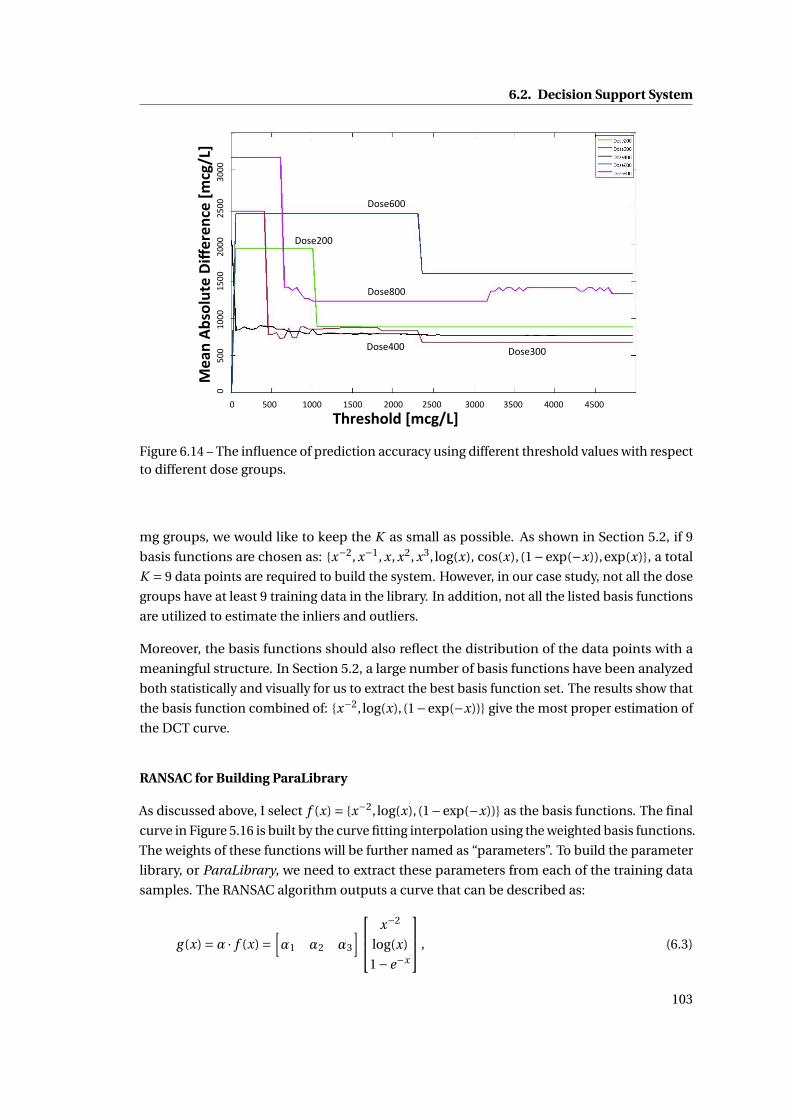
6.2. Decision Support System
!"#$%"&'()*+,-./0)
1$23)45
%&'67$)89:$#$3
,$)*+
,-./0)
!"#$%&&'
!"#$(&&'
!"#$)&&'
!"#$*&&'
!"#$+&&'
!"""""""""""""#!!""""""""""""$!!!""""""""""$#!!""""""""""%!!!"""""""""%#!!"""""""""""&!!!"""""""""&#!!""""""""""'!!!""""""""""'#!!"""""
!""""""""""""#!!"""""""""$!!!"""""""""$#!!"""""""%!!!"""""""""%#!!""""""""&!!!"
!"#$%&'
()*+,"%-./"0"$
1"%23
14567%
890"(9)*:%2314567%
Figure 6.14 – The influence of prediction accuracy using different threshold values with respectto different dose groups.
mg groups, we would like to keep the K as small as possible. As shown in Section 5.2, if 9
basis functions are chosen as: {x−2, x−1, x, x2, x3, log(x), cos(x), (1−exp(−x)),exp(x)}, a total
K = 9 data points are required to build the system. However, in our case study, not all the dose
groups have at least 9 training data in the library. In addition, not all the listed basis functions
are utilized to estimate the inliers and outliers.
Moreover, the basis functions should also reflect the distribution of the data points with a
meaningful structure. In Section 5.2, a large number of basis functions have been analyzed
both statistically and visually for us to extract the best basis function set. The results show that
the basis function combined of: {x−2, log(x), (1−exp(−x))} give the most proper estimation of
the DCT curve.
RANSAC for Building ParaLibrary
As discussed above, I select f (x) = {x−2, log(x), (1−exp(−x))} as the basis functions. The final
curve in Figure 5.16 is built by the curve fitting interpolation using the weighted basis functions.
The weights of these functions will be further named as “parameters”. To build the parameter
library, or ParaLibrary, we need to extract these parameters from each of the training data
samples. The RANSAC algorithm outputs a curve that can be described as:
g (x) =α · f (x) =[α1 α2 α3
] x−2
log(x)
1−e−x
, (6.3)
103

Chapter 6. Drug Administration Decision Support System
where, the set of αi composes our ParaLibrary. For each training sample Si , we first collect
all the other samples from the training library with the same dose amount (in the same dose
group). Then the RANSAC algorithm is applied M times. However, apart from selecting the
model by choosing the one with the biggest number of inliers, we also take into considerations
that the target sample Si has to be an inlier and also be as close to the estimated RANSAC
curve as possible.
6.2.2 Prediction Core Module
The Prediction Core module runs an SVM-based drug concentration prediction using the
preprocessed data, and predicts the concentration values for a new patient. Section 4.1
describes the mathematics of the LS-SVM algorithm used in the module. There the simulation
results of the influence of the SVM hyper-parameters are also discussed. This section modifies
the LS-SVM algorithm to predict three parameters, {α1,α2,α3} for each sample of the testing
library.
Least Square Support Vector Machine (LS-SVM)
In Section 4.1, the Least Square SVM method has been applied to our clinical case. It has
reduced the computational complexity into a convex QP problem and at the same time outputs
the results with a similar prediction accuracy to the traditional PK method. There are two
open parameters in the LS-SVM algorithm, as well as the SVM algorithm; that is the trade-off
control factor C and the Gaussian kernel width σ. To choose a best combination of C and σ,
an L-fold cross-validation technique is introduced and applied previously. Here, a more visual
comparison of the influence on the MAD value by using different C and σ is given in Figures
6.15 and 6.16.
The effectiveness and the accuracy of SVM highly depends on the choice of the kernel func-
tion. In our system, we select Gaussian distribution, a common choice with a single hyper-
parameter kernel width σ, as the kernel function of the SVM algorithm. Hence, there are two
parameters to be estimated, C and σ, the best combination of which is found by a grid-search
with exponentially growing sequences, e.g. C ∈ {10−2,10−1, · · · ,102,103} and σ ∈ {10−3, · · · ,10},
through cross validation. An L-fold cross validation is a commonly-used method to estimate
the parameters of a model over each observation value [61]. It randomly partitions the original
training sample into L subsamples, each of which is treated as the ‘validation data’ in the train-
ing phase and the remaining L−1 subsamples are used as training data. The cross-validation
process is then repeated L times, or folds, to compute the values of C and σ with each of the L
subsamples used exactly once as the validation data. As different dose groups have different
number of data points, and after preprocessed by RANSAC, the remaining number of training
data points, Nsi , are further reduced. Therefore, we choose L = min(10, Nsi ), where si denotes
the dose group i . We choose C and σ to be the one of the L results having the least MAD
between the predicted values and the ‘validation data’.
104

6.2. Decision Support System
!"#$%&&'
!"#$(&&'
!"#$)&&'
!"#$*&&'
!"#$+&&'
!"#$,&&'
&''''''''''''''',&&''''''''''''*&&'''''''''''''%&&'''''''''''')&&''''''''''+&&&'''''''''''+,&&''''''''''+*&&''''''''''+%&&''''''''''+)&&'
&''''''''''''''-&&''''''''''''+&&&''''''''''''+-&&'''''''''''',&&&''''''''''',-&&'''''''''''''''''''
!"#$%&'
()*+,"%-./"0"$
1"%23
14567%
8%
Figure 6.15 – Influence of hyper-parameter C (from 0 to 2000).
!"#$%&&'
!"#$(&&'
!"#$)&&'
!"#$*&&'
!"#$+&&'
!"#$,&&'
&''''''''''''''''+''''''''''''''''','''''''''''''''''('''''''''''''''''*''''''''''''''''-''''''''''''''''''%''''''''''''''''.''''''''''''''''')''''''''''''''''''/'
&''''''''''''-&&''''''''''+&&&'''''''''+-&&'''''''',&&&'''''''',-&&'''''''''(&&&''''''''''
!"#$%&
'(%)&*+
,-./0(&1"2(3()
4(&5$
4#678&
Figure 6.16 – Influence of hyper-parameter σ (from 0.001 to 10).
105

Chapter 6. Drug Administration Decision Support System
Figures 6.15 and 6.16 shows the influence of the hyper-parameters C and σ on the prediction
accuracy in different dose groups of the training data, when the RANSAC algorithm is not
applied. The results show that the MAD values decrease with the growth of the C value within
(10,200), and start to increase after C > 200 due to overfitting. On the other hand, smaller
kernel width σ< 1 decreases the MAD values.
Table 6.2 shows the accuracy results of the SVM and RANSAC algorithms over different dose
groups. From this table we can see that the number of patients in each dose group and in
training and testing library is largely biased. There are much more patient samples in the
dose group 400mg than the others. For some dose group, the number of training library is
even less than 5, i.e. dose group 100mg. An expected inaccuracy can be foreseen for those
groups having much less sample number when applying the data library as the training data.
As for the few samples in the testing dataset, there is also a possibility for these few testing
data to be actually outliers, thus causing inaccuracy in the prediction performance. However,
as mentioned before, this type of outlier is due to an insufficient types of patient features
considered in the current clinical study.
The predictions are made according to the following 5 methods as follows, where the first line
indicates the different dose groups in our dataset of the drug imatinib, the second line shows
the number of training data and testing data samples in each dose group respectively. The five
methods are compared via mean absolute difference between the predicted concentration
values and the measured ones, which are the smaller the better. The five methods are described
in details as:
• Method 1: training separately each dose group using the SVM approach without RANSAC.
This means all the patient features in the each training group (separated according to
their dose amount) are taken into account to build the SVM model.
• Method 2: training the whole library using the SVM approach without RANSAC. In this
method, all the patient data in the original training data library will be utilized. Due to
the fact that the original library is biased towards the 400mg dose, inaccuracy is expected
to happen to the prediction results, especially for 100mg, where we have just 3 samples.
• Method 3: training separately each dose group using the SVM approach together with
the RANSAC algorithm on training data. In this method, the SVM models are built
separated for each dose group taking into account only the inliers selected by the
RANSAC algorithm. For dose groups having only a few data samples, a full utilization
of the training samples is considered to set the SVM model, thus resulting a similar
prediction accuracy as shown in Method 1.
• Method 4: training the whole library using the SVM approach with the RANSAC algo-
rithm on the training data. This method considers the whole data library to be the
training dataset as in Method 2. The setting in this method is to examine whether the
RANSAC algorithm is able to reduce the influence caused by biased data or not.
106
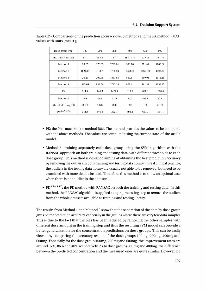
6.2. Decision Support System
Table 6.2 – Comparisons of the prediction accuracy over 5 methods and the PK method. (MADvalues with units [mcg/L])
Dose group [mg] 100 200 300 400 600 800
no. train / no. test 3 / 1 11 / 1 18 / 7 193 / 176 10 / 13 16 / 10
Method 1 26.25 178.05 1799.01 983.16 771.41 1868.66
Method 2 1024.47 1318.78 1785.94 1033.71 1274.10 1493.37
Method 3 26.25 209.95 1841.65 860.11 660.04 1011.15
Method 4 935.64 838.54 1732.18 827.41 461.31 1059.87
PK 311.4 446.3 1474.4 819.3 630.1 1200.4
Method 5 0.6 42.8 51.6 90.5 480.8 82.8
(threshold [mcg/L]) (210) (260) (20) (80) (120) (110)
PKR AN S AC 311.4 446.3 322.7 493.4 627.7 1831.1
• PK: the Pharmacokinetic method [86]. The method provides the values to be compared
with the above methods. The values are computed using the current state-of-the-art PK
model.
• Method 5: training separately each dose group using the SVM algorithm with the
RANSAC approach on both training and testing data, with different thresholds to each
dose group. This method is designed aiming at obtaining the best prediction accuracy
by removing the outliers in both training and testing data library. In real clinical practice,
the outliers in the testing data library are usually not able to be removed, but need to be
examined with more details instead. Therefore, this method is to show an optimal case
when there is not outlier in the datasets.
• PKR AN S AC : the PK method with RANSAC on both the training and testing data. In this
method, the RANSAC algorithm is applied as a preprocessing step to remove the outliers
from the whole datasets available as training and testing library.
The results from Method 1 and Method 2 show that the separation of the data by dose group
gives better prediction accuracy, especially in the groups where there are very few data samples.
This is due to the fact that the bias has been reduced by removing the other samples with
different dose amount in the training step and thus the resulting SVM model can provide a
better generalization for the concentration predictions on these groups. This can be easily
viewed by comparing the accuracy results of the dose groups 100mg, 200mg, 400mg and
600mg. Especially for the dose group 100mg, 200mg and 600mg, the improvement rates are
around 97%, 86% and 40% respectively. As to dose groups 300mg and 400mg, the difference
between the predicted concentration and the measured ones are quite similar. However, no
107

Chapter 6. Drug Administration Decision Support System
proper evidence has shown the reason why the dose group 800mg has a worse prediction
accuracy when using a separated training dataset.
The results from Methods 1 to 4 show that the RANSAC algorithm cannot improve the predic-
tion accuracy if the dose groups are not considered differently, but it has improved a lot when
all the dose groups are mixed. This is thanks to the RANSAC algorithm having removed outliers.
For some dose groups such as 400mg and 600mg, Method 4 gives the best accuracy result
which indicates that the RANSAC approach gives a good generalization for these dose groups
by removing the outliers from the other groups. Method 5 shows the great improvement in the
prediction performance if the outliers in the testing library have also been removed. Since in
this method, the aim to achieve an optimal performance in using the RANSAC algorithm, a
grid search is carried out to find the best threshold value for each dose group. As shown in the
table, the threshold values vary from one dose group to another but within a smaller range
20mcg/L to 260mcg/L compared to the predicted drug concentration differences listed in the
upper part of the table (Methods 1 to 4 and the PK method).
The results from PK and PKR AN S AC indicate that the RANSAC algorithm can further improve
the PK method in the prediction of the dose groups with a large number of samples, also
thanks to its outlier-removing technique. From this table we can observe that in most cases
the RANSAC algorithm has helped increase the prediction accuracy, while it still remains
unclear that the dose group 800mg are not in accordance with this regulation as the other dose
groups follow. One possible reason could be due to the fact that the dose amount of 800mg
has reached the limitation of human body’s ability to absorb and eliminate the quantity, thus
leading to some adverse events.
SVM-based Parametrization (ParaSVM)
Instead of directly computing the drug concentration at a given time, clinicians are more
interested in modeling the DCT curve, for each patient in order to visually check whether the
concentration drops within the therapeutic range at the trough value. There are two ways to
obtain the DCT curve:
• Compute the point-wise concentration values and build the DCT curve by linear inter-
polation;
• Compute the parameters used to construct the DCT curve (Equation 6.3), by curve
fitting interpolation.
The first method implicitly models the relationship of patient features and the drug concen-
trations. It relies on the point-wise prediction for the concentrations over time using the SVM
algorithm to take into account new patients’ features. However, it is difficult to capture a global
structure explicitly; especially when new measured concentration data is provided, it dose not
provide any means to adapt the global curve structure according to this given concentration
108

6.2. Decision Support System
value. The PK model provides an explicit structural information of the concentration curve.
However, it considers a limited number of patient features apart from the fact that some of
these features require several blood concentration measurements to be determined accurately,
i.e. the drug absorption/elimination rate. Hence, we combines the ‘implicit’ SVM method and
the ‘explicit’ analytical way to model the parameters of the basis functions used to construct
the DCT curve.
6.2.3 Selection Module
The Selection module chooses the best dose amount and dose interval according to the given
therapeutic ranges (possibly one for the peak and another for the trough concentration). How-
ever, in practice, some drugs have only one therapeutic range available, such as in imatinib
case study. For a general purpose, the DADSS system proposes both solutions accordingly.
!"#$
!%#$
!&#$
'()*+,$
'()*-./$
'()*0$
1203$
*4+5$6.7
83794:;.
7$
!""""""""""""""""""""""""""""""""""""#""""""""""""""""""""""""""""""""""""$!"""""""""""""""""""""""""""""""""$#"""""""""""""""""""""""
!""""""""""""""#!!"""""""""""""$!!!""""""""""""$#!!"""""""""""%!!!"""""""""""%#!!"
!"#$%&'(
)*(+",-'
(%./
)$012%
34/*%.52%
Figure 6.17 – Example of Peak Concentration Range
Two different therapeutic ranges are defined for a drug: one for the peak and another one for
the trough values of the drug concentration. Both Figures 6.17 and 6.18 depict three examples
of the drug concentration curves each, that are defined by PK studies. The therapeutic peak
range (PkBDl ow up to PkBDup ) and the ideal value (PkBDm) are defined in Figure 6.17 while the
trough range (TrBDlow up to TrBDup ) and the ideal value (TrBDm) are presented in Figure 6.18.
The ideal drug concentration curve is the one whose peak and trough values are as close as
possible to the corresponding ideal peak and trough values.
109
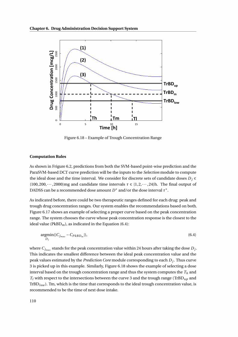
Chapter 6. Drug Administration Decision Support System
!"#$%&'
!"#$()*'
!"#$+'
!+'!,' !('
!-+.'
$"%/'0)1
2.13"45)
1'678'
698'
6:8'
!""""""""""""""""""""""""""""""""""""#""""""""""""""""""""""""""""""""""""$!"""""""""""""""""""""""""""""""""$#"""""""""""""""""""""""
!""""""""""""""#!!"""""""""""""$!!!""""""""""""$#!!"""""""""""%!!!"""""""""""%#!!"
!"#$%&'(
)*(+",-'
(%./
)$012%
34/*%.52%
Figure 6.18 – Example of Trough Concentration Range
Computation Rules
As shown in Frigure 6.2, predictions from both the SVM-based point-wise prediction and the
ParaSVM-based DCT curve prediction will be the inputs to the Selection module to compute
the ideal dose and the time interval. We consider for discrete sets of candidate doses D j ∈{100,200, · · · ,2000}mg and candidate time intervals τ ∈ {1,2, · · · ,24}h. The final output of
DADSS can be a recommended dose amount D∗ and/or the dose interval τ∗.
As indicated before, there could be two therapeutic ranges defined for each drug: peak and
trough drug concentration ranges. Our system enables the recommendations based on both.
Figure 6.17 shows an example of selecting a proper curve based on the peak concentration
range. The system chooses the curve whose peak concentration response is the closest to the
ideal value (PkBDm), as indicated in the Equation (6.4):
argminD j
(|C jmax −CPkBDm |), (6.4)
where C jmax stands for the peak concentration value within 24 hours after taking the dose D j .
This indicates the smallest difference between the ideal peak concentration value and the
peak values estimated by the Prediction Core module corresponding to each D j . Thus curve
3 is picked up in this example. Similarly, Figure 6.18 shows the example of selecting a dose
interval based on the trough concentration range and thus the system computes the Th and
Tl with respect to the intersections between the curve 3 and the trough range (TrBDup and
TrBDl ow ). Tm, which is the time that corresponds to the ideal trough concentration value, is
recommended to be the time of next dose intake.
110

6.2. Decision Support System
Table 6.3 – 5 Sample Recommendations from DADSS. M: Male, F: Female.
Patient Profile Features Recommendations
No. Gender Age Body Weight D∗ τh τl
1 M 82 56kg 400 mg 13h 24h
2 F 58 53kg 500 mg 15h 24h
3 F 62 54kg 700 mg 16h 24h
4 M 58 100kg 800 mg 18h 24h
5 M 47 73kg 500 mg 14h 24h
When only the trough concentration range is available, the system first selects the dose
amount whose corresponding concentration value at 24h is the closest to the ideal trough
concentration value, as shown in Equation (6.5).
argminD j
(|C j24 −CTr BDm |), (6.5)
where C j24 stands for the concentration values estimated at 24 hours after giving a dose D j .
Then it computes the dose interval τ∗ = (τh ,τl ) of this curve. Since we want to keep the
trough drug concentration value within the trough therapeutic range, τh and τl are computed
according to the higher and lower bounds of the trough therapeutic range respectively.
The imatinib Case Study
Table 6.3 describes some examples of how the decisions about imatinib dose and intake
interval are made for 5 randomly selected patients. For each pair of the cross product of
the dose Di and the dose interval τi for a new patient, the Prediction Core module com-
putes the corresponding drug concentration value. The Selection module first removes
the candidate doses whose predicted resulting drug concentration at time 24h (Ci24 ) are
higher than the upper bound of the trough therapeutic range as well as the ones whose
predicted peak concentration value is lower than the trough lower bound. Furthermore,
to choose the best dose, our system computes the absolute difference between each Ci24
value and the ideal value of the trough therapeutic range, and selects the dose with respect
to the smallest difference, as shown in Equation (6.5). For example, for patient 1, we ob-
tained the set of Ci24 = [890.6,1032.5,1152.5,1239.1] mcg/L that corresponds to the set of
Di = [200,400,600,800] mg. The ideal value is 1000mcg/L, therefore Ci24 = 1032.5mcg/L has
the smallest difference, and thus the curve whose D∗ = 400mg is chosen. Hereafter, the system
obtains the range of the dose interval (τ∗ = (τh ,τl )) according to the lower and upper bounds
of the trough therapeutic range. However, in the real clinical practice, doctors tend to give a
common dose amount (400 mg) and time interval (24 hours) to every adult patient at a prior
stage (at the start of treating a new patient). Following the clinical protocol in the later stages,
doctors update the dose amount and the time interval with respect to patients’ responses to
111

Chapter 6. Drug Administration Decision Support System
the treatment [74].
6.2.4 Adaptation Module
In the simplest clinical routine, once a new patient is admitted, a first dose is determined based
on a population value estimated from the library data. This method does not guarantee that
the new patient and the library datasets have similar conditions, SVM-based dose estimation
first uses these patient’s features and then predicts the drug concentrations at a specific time or
the DCT curves. This is called a priori adaptation. To further refine the predicted DCT curve to
be as close to the real measurement as possible, a blood test is sometimes taken to control the
drug concentration to be within the therapeutic range. This is known as a posteriori adaptation.
As presented in the previous sections, insufficient types of patient features and measurement
errors are two possible factors of current predicted concentration values being sometimes
largely deviated from the measured values. Here, we consider updating the predicted DCT
curve with a given measured concentration value to be efficient to personalize the prediction
results, as the feedback adaptation loop in Figure 6.2. We also show a way to build the DCT
curve for multiple doses after initial a priori adaptation taking into consideration the residual
drug concentrations in patient’s blood.
The a posteriori Adaptation
In a posteriori dose adaptation, we refine the predicted DCT curve computed by ParaSVM.
It is done by calibrating the current DCT curve using one or several measured data point
under certain constraints. This procedure is important in clinical routine to overcome an
inaccuracy caused by insufficient feature data collection for concentration prediction. Taking
into account that these measurements are done for the same patient, the calibration with
each new measurement makes the DCT curve more personalized. The same DCT curve ad-
justment approach is also applied to build the concentration curve for multiple dose regimens
using the computed trough concentration value from the previous cycle (computation) as a
measurement.
Once a new measurement is provided, we first predict the basis function parameters using
ParaSVM and then search within a certain radius ∆D around each parameter value with a step
δd to find the best set of parameters that satisfies the following conditions:
• The modified DCT curve has to pass through the given measured concentration value;
• After giving the dose, the concentration value should increase with time:
∂ fconcentr ati on
∂t|t=0 > 0; (6.6)
• After several hours, the concentration value reaches the peak value and starts to decrease:
112

6.2. Decision Support System
!"#$%&'()'*'+,'-"./0$'1,')23$'*'455.6'
!!! !!!"!!!!!!!!!!!!!!!!!!!#"!!!!!!!!!!!!!!!!!!$"!!!!!!!!!!!!!!!!!!%"!!!!!!!!!!!!!!!!!!&"!!!!!!!!!!!!!!!'"!!!!!!!!!!!!!!!!!!!!!("!!!!!!!!!!!!!!!!!!)"!
"!!!!!!!'""!!!!!#"""!!!!!#'""!!!!$"""!!!!!$'""!!!%"""!!!%'""!!!!&"""!!!&'""!
)786'92%
:$%&7"#2
%';.
:6<=>'
?@.$';A>'
Figure 6.19 – Example 1 of Parametrically Refined DCT Curves over 3 days in a stead y state ofa same patient being sampled in different days with a same dose amount 400 [mg].
!"#$%&'()'*'+,'-"./0$'+,')12$'*'344.5'
!!! !!!!!! !!!
!!! !!!
"!!!!!!!!!!!!!!!!!!!#"!!!!!!!!!!!!!!!!!!$"!!!!!!!!!!!!!!!!!!%"!!!!!!!!!!!!!!!!!!&"!!!!!!!!!!!!!!!'"!!!!!!!!!!!!!!!!!!!!!("!!!!!!!!!!!!!!!!!!)"!
"!!!!!!!'""!!!!!#"""!!!!!#'""!!!!$"""!!!!!$'""!!!%"""!!!%'""!!!!&"""!!!&'""!
)675'81%
9$%&6"#1
%':.
95;<='
>?.$':@='
Figure 6.20 – Example 2 of Parametrically Refined DCT Curves over 3 days in a stead y state ofa same patient being sampled in different days with a same dose amount 400 [mg].
113

Chapter 6. Drug Administration Decision Support System
!"#$%&'()'*'+,'-"./0$'1,')23$'*'455.6'
!!! !!!!!! !!!"!!!!!!!!!!!!!!!!!!!#"!!!!!!!!!!!!!!!!!!$"!!!!!!!!!!!!!!!!!!%"!!!!!!!!!!!!!!!!!!&"!!!!!!!!!!!!!!!'"!!!!!!!!!!!!!!!!!!!!!("!!!!!!!!!!!!!!!!!!)"!
"!!!!!!!'""!!!!!#"""!!!!!#'""!!!!$"""!!!!!$'""!!!%"""!!!%'""!!!!&"""!!!&'""!
)786'92%
:$%&7"#2
%';.
:6<=>'
?@.$';A>'
Figure 6.21 – Example 3 of Parametrically Refined DCT Curves over 3 days in a stead y state ofa same patient being sampled in different days with a same dose amount 400 [mg].
!"#$%&'()'*'+,'-"./0$'1,')23$'*'144.5'
!!! !!!!!! !!!"!!!!!!!!!!!!!!!!!!!#"!!!!!!!!!!!!!!!!!!$"!!!!!!!!!!!!!!!!!!%"!!!!!!!!!!!!!!!!!!&"!!!!!!!!!!!!!!!'"!!!!!!!!!!!!!!!!!!!!!("!!!!!!!!!!!!!!!!!!)"!
"!!!!!!!'""!!!!!#"""!!!!!#'""!!!!$"""!!!!!$'""!!!%"""!!!%'""!!!!&"""!!!&'""!
)675'82%
9$%&6"#2
%':.
95;<='
>?.$':@='
Figure 6.22 – Example 4 of Parametrically Refined DCT Curves over 3 days in a stead y state ofa same patient being sampled in different days with a same dose amount 400 [mg].
114

6.2. Decision Support System
∂ fconcentr ati on
∂t|t=Tp < 0, (6.7)
where Tp is a time point after the peak value, i.e. we set it as Tp = 24h.
• Considering the trough value or residual value, from the previous dose, the difference
between the starting value of DCT curve (t = 0) and the ending one (t = 24h, since
imatinib is usually administrated once a day), should be within a certain range (R), i.e.
< 50mcg/L:
| f t=0concentr ati on − f t=24
concentr ati on | < R, (6.8)
• The DCT curve whose shape is the closest to the curve previously predicted by ParaSVM
will be chosen:
mingr
∑j=0,··· ,Ns
(g t= jr − g t= j )2, (6.9)
where g t= j stands for the concentration value at time j and g t= jr is the one in the refined
curve. The set of parameters y corresponding to the best gr are selected.
Figures 6.19 to 6.22 show a posteriori adaptation for a sample patient with the same dose
amount D = 400mg, but in different dose periods (we assume that the patient has reached the
steady state). As the measured concentration values vary a lot even though the measuring time
is relatively similar between two days, it indicates a potential intra-variation has happened to
this patient. Based on the above adaptation rules, the DCT curves are adjusted accordingly.
Multidose Estimation
Knowing how the concentration value varies with time after multiple doses is important to
clinicians and patients in order to monitor a long term therapeutic procedure. In a priori
adaptation, the multi-dose DCT curve can be obtained simply by recomputing over days the
updated one-dose concentration curve taking into account the residual concentration value
of the previous day, since the drug sometimes takes several days, i.e. 5 to 7 days, to be clear
out from the human body.
Figure 6.23 shows an example of estimating the drug concentration over 10 days based on
ParaSVM taking into account the residual drug concentration from the previous day, while the
first period of the DCT curve is assumed to be the starting day. The DCT curve for multiple
doses makes it visually easy to obtain the peak and trough concentration values and to check
whether they are within the therapeutic ranges or not. As shown in Figure 6.23, the residual
concentration affects both the peak and the trough concentration values in the beginning of
the treatment and starts to be steady after several days (3 days in this example).
115

Chapter 6. Drug Administration Decision Support System
!""""""""""""""""""""""""""""""""""""#!""""""""""""""""""""""""""""""""""$!!"""""""""""""""""""""""""""""""""$#!""""""""""""""""""""""""""""""""%!!"
!"""""""#!!"""""$!!!""""$#!!"""%!!!""""%#!!""""&!!!""""&#!!""""""
!"#$%&'(
)*(+",-'
(%./
)$012%
34/*%.52%
Figure 6.23 – Example of Multiple Dose Estimation for the DCT Curve Over 10 Days of Drugimatinib. X-axis: time [h], Y-axis: concentration value [mcg/L]
6.3 Summary
In this chapter, a DADSS system has been presented. It employs a machine learning algorithm,
namely SVM, as its core function, which has several merits compared to the traditional PK
methods as listed in Chapter 1 and has never been applied to the domain of drug concentration
predictions before. The system also embeds the RANSAC algorithm as one of the preprocessing
methods to improve the prediction accuracy. However, as indicated in Section 6.2.1, the system
should consider all the patient data as inliers in the future work. This chapter has also proposed
a list of more complete patient features to be examined and recorded in the clinical practice. To
further help clinicians monitor the variation of the DCT curve, a Parameterized SVM algorithm
has been proposed. It has the advantages of both the analytical model and the SVM algorithm.
The rules to update a patient’s DCT curve once a measurement is available have been listed.
Patient data library has been classified into 6 groups according to the dose amount. The
dose group in which patients take 400mg dose per day has the largest number of samples,
about 80% of the training data samples and 85% of the testing one. This has shown to bias the
predictions for the other dose groups in the case when all the data samples have been used as
the training data indifferently. Experimental results have shown that prediction of the drug
concentration values by separating the patient samples according to their intake dose amount
can improve the accuracy. To further enhance the accuracy, we rely on the RANSAC algorithm
to remove the outliers from the data library. However, extension of the feature set may be a
potential possibility for accuracy improvement.
116
7 Conclusions
In this chapter, I give the summary of the work presented in this thesis. I also discuss the
existing open problems and the future work.
7.1 Summary of the Thesis
This thesis has presented the applications of the algorithmic approaches, namely the SVM and
RANSAC algorithms, to solve the problems in the domain of drug concentration predictions. I
have presented the fundamental mathematics of the SVM algorithms including the methods
for both classification and regression tasks. The difference of the algorithms in the aspects of
solving linear and nonlinear problems is described. The general method of choosing a proper
set of kernel parameters has also been presented and compared in the real clinical case study
for the drug imatinib.
In this thesis, I have presented the work published in journals and the proceedings of con-
ferences. I have introduced the DADSS system which is designed to assist clinical doctors
in the dose computation and adjustment for a patient. The DADSS system is based on the
SVM algorithm as the core function. In contrast to the traditional PK models, the system can
process as many patient features as available and build the mathematical model to analyze
their influence on the drug concentration values. The system is designed for the specific
drug imatinib and the output recommendations of the dose and time interval are based on
the drug therapeutic range. Therefore, the system settings have to be modified when it is
applied to another drug in the future. Two strategies have been presented in this thesis for
the DADSS system. One is the direct computations of the drug concentration values using
the SVM algorithm. The output of this approach is a set of point-wise concentration values
with respect to the sampling time steps and the obtained DCT curve is interpolated based
on these values. The other strategy computes the coefficients of the analytical model used
to build the DCT curve using the SVM algorithm. The analytical model is obtained through
the basis function analysis of the RANSAC algorithm. This approach combines both the SVM
algorithm and the analytical model. As a result, it enables the process of any number of patient
117

Chapter 7. Conclusions
features and has an analytical model to guarantee a structural modification of the curve as
well. This thesis has presented the rules for modifying the DCT curve when there is a new
measured concentration value available. In addition, the extension of the curve from one dose
regime to multiple doses has also been demonstrated. The experiments have been carried
out on different dose groups. The separation of the patient samples according to the dose
amount has shown an improvement in the prediction accuracy, especially for the dose group
with fewer samples than the others. This is due to the reduction of the bias caused by the
unbalanced number of data in the same patient feature, e.g . the dose group of patients taking
400mg per day is about 80% of the total number of patient samples.
Apart from the applications of the SVM and the RANSAC algorithms in the DADSS system, this
thesis has also presented our work in using these two algorithms for personalizing the drug
concentration predictions. Two example-based SVM approaches have been introduced by
selecting a ‘close’ set of patient data in the training library for a new patient. This subset of the
library is used as new training data. By reducing the number of the training data, we can both
reduce the training time and the required storage space for the data library. Experimental
results have also shown some gain of the prediction accuracy achieved in this way. The
RANSAC algorithm is an outlier-removal technique which has been used as one of the data
preprocessing steps in the DADSS system. It selects a subset of the data library to be the inliers
used as the training data. This thesis has also presented different criteria applied to select the
inliers using the RANSAC algorithm. All the available patient features of the drug imatinib have
been examined for extracting this subset, including body weight, age, gender, dose amount,
measuring time, and measured concentration values. Among these, when the measured
concentration values are used as a criterion, the corresponding comparisons of the prediction
accuracy have been carried out with the Bayesian method. Experimental results have shown
that both the RANSAC and personalized RANSAC algorithms have increased the prediction
accuracy compared to the traditional PK method, and the personalized RANSAC approach
has slightly better accuracy than the RANSAC one. Compared to the Bayesian approach, the
RANSAC and personalized RANSAC algorithms have similar performance in the prediction
accuracy in terms of mean absolute difference. But the latter two have a more than 20%
increase in the results of standard deviation values, which means that the overall prediction
difference from the measured concentration values are more uniform than the results given
by the Bayesian approach.
Furthermore, this thesis has also explained the extraction of the basis functions using the
RANSAC algorithm to be used for the parameterized SVM approach. Fifteen different sets of
basis functions have been analyzed with respect to their influence on the prediction accuracy
(mean absolute difference and standard deviation values) and the constructed DCT curve
as well. A similar machine learning algorithm, the Bagging approach, has been analyzed
and compared with the RANSAC algorithm. The results have shown that though the Bagging
algorithm tries to generalize the curve to fit as many data points as possible, the RANSAC
algorithm produces a more reasonable concentration curve, because the outliers in the dataset
have influenced the curve construction in the Bagging algorithm.
118
7.2. Open Problems
7.2 Open Problems
This thesis addresses some potential solutions to solve the problems in the current clinical
drug prescription and monitoring procedures. Meanwhile, there are still some open problems
remaining for future investigations.
• Patient features. What patient features should we consider to compute the drug con-
centration values? As more and more patient features are measurable and available to
the clinical study, they might not be all useful to the computation. Though the SVM
algorithm can take as many features as possible to be its inputs, unrelated features
might bias the prediction results. Therefore, new techniques might be required to select
proper feature set or reduce the dimension of features in the future work.
• Noise. There are two types of noise, the measurement error and the noise of inaccurate
predictions due to insufficient number of patient features. This thesis has assumed
that the former one is not considered in the work, while in practice measurement
error exists in all kinds of experiments requiring measurement. It remains a question
how to apply a noise model in the SVM approaches and what type of the model is
most proper. Especially when there are sufficient patient features, measurement errors
will dominate the performance of the predictions. In this thesis, together with the
RANSAC algorithm, the SVM has achieved a large improvement in the accuracy of
drug concentration predictions. Nevertheless, it remains a question whether the SVM
algorithm can improve without the RANSAC preprocessing when sufficient patient
features are available.
• Adaptation of the DADSS system to other drugs. The DADSS system is designed for the
specific case study of the drug imatinib in this thesis. The application of the system to
other drugs still needs to be investigated. The drug imatinib has so far the therapeutic
range for its trough concentration values. Thus, the system is subject to change when it
is applied to follow the guidelines of another drug, especially drugs with the therapeutic
ranges for both peak and trough concentrations. This thesis has selected the SVM and
the RANSAC algorithms as two major techniques to predict the drug concentration
values for the drug imatinib, because both algorithms have the merits of being mathe-
matically easy to understand, to program, and to modify. In addition, the SVM algorithm
has a global optimum solution and the RANSAC has a statistically robust solution for
outlier-removal tasks. Due to the fact that the work presented in this thesis is based on
the clinical data of the drug imatinib, there is still a question whether the SVM algorithm
can be successfully applied to analyze other drugs.
Therefore, there are still various types of research needed to carry out in the future work.
119
Chapter 7. Conclusions
7.3 Future Work
Many research topics in the area of personalized drug concentration predictions are not
covered by this thesis. In this section, I present some of the directions that can be pursued
based on the work described in this thesis.
• Design of the DADSS system with memory constraints. The DADSS system presented
in this thesis has been embedded with a feedback close-loop for updating the DCT
curve computed for a patient. The feedback here is a measured drug concentration
value and its corresponding measuring time. Currently, no memory constraint is taken
into account in the DADSS system. However, in the real clinical practice usually with
a large number of patient data, how to properly maintain the size of the data library
will become an issue. Therefore, one of the future work can be to design an efficient
data reduction algorithm that finds a set of most relevant data for a new patient. This
way, in several rounds of running the feedback loop, the total data remained in the
library will be personalized for this patient. Another future work in this area can be to
design a reliable data library maintenance algorithm that can keep the total size of the
original data library to be a constant by removing the noisy data. When a new patient is
admitted, the model of DCT for him/her is estimated through this original data library,
either with the total size or with a subset of the “close” data examples. Thus, removing
the noisy data in the original data library can also help reduce the influence of the noisy
data on modeling a new patient when the total data library is used.
• Smartphone application implementation. This thesis has introduced the detailed design
of the DADSS system. However, as to clinical doctors, an applicable device with the
designed system is preferred both for using and for evaluating the system. Therefore,
the future work can include a smartphone application implementation. In this case,
the memory storage issue mentioned above has to be taken into account both for the
local smartphone and for the server where the original data library is stored. Data
transmission for updating the library between the smartphone and the server also needs
to be designed.
• Automatic algorithm selection scheme in the DADSS system. The DADSS system in this
thesis uses mainly the SVM and the RANSAC algorithms. There are many other machine
learning algorithms that can be implemented into the DADSS system such as DT, ANN,
etc. The input and output required by these algorithms are similar as the ones needed
for the SVM algorithm. Therefore, a hybrid system can be designed by implementing
some other machine learning algorithms into the core function part of the DADSS
system. Furthermore, an automatic algorithm selection scheme can also be thought of
as one of the future work which chooses a most proper algorithm to use for a specific
drug to achieve the best prediction accuracy.
120

7.3. Future Work
Even though the proposed DADSS system in our research work has the ability to assist the
clinical doctors in the drug prescriptions, it is still restricted to the specific drug imatinib. The
SVM algorithm has many merits, but it is currently difficult to tell whether it surpasses the
traditional PK approach without using the RANSAC algorithm, because the available patient
features are limited to the ones used in the PK model. Therefore, further research needs to be
carried out to survey more patient features and build the SVM models based on these features
in order to compare with the PK model. Moreover, different machine learning approaches
should also be investigated. A future direction for the DADSS system will be the one with
flexibility and automation in both algorithm selection and patient library extraction.
121


A An appendix
123

Appendix A. An appendix
Table A.1 – List of acronym.
Abbreviation Full Name
AdaBoost Adaptive Boosting
ANN Artificial Neural Networks
Bagging Bootstrap Aggregating
CDSS Clinical Decision Support System
DADSS Drug Administration Decision Support System
DCT Drug Concentration to Time
DD Drug Dose
DSS Decision Support System
DT Decision Trees
GI Gastrointestinal
GL Guideline
LS-SVM Least Square Support Vector Machine
MAD Mean Absolute Value
MDC Measured Drug Concentration
MT Measuring Time
ParaSVM Parameterized SVM
PCA Principal Component Analysis
PD Pharmacodynamics
PK Pharmacokinetics
RANSAC RANdom SAmple Consensus
RBF Radial-Basis Function
RPER RANSAC-based personalization
RSVM RANSAC-SVM approach
STD Standard Deviation
SVM Support Vector Machine
SVR Support Vector Machine for Regression
TDM Therapeutic Drug Monitoring
TLP Two-Layer Perception
124

Bibliography
[1] AGREE instrument. http://www.agreetrust.org/.
[2] AsbruView. http://www.openclinical.org/dld_asbruview.html.
[3] TIMES. http://www.timestool.com/l.
[4] Minst data library. http://yann.lecun.com/exdb/mnist/.
[5] R. AD. Pharmacogenetics and the practic of medicine. In Nature, pages 857–65, 2000.
[6] E. Alpaydin. Introduction to Machine Learning (Adaptive Computation and Machine
Learning). MIT Press, 2004.
[7] T. Amnell, E. Fersman, P. Pettersson, H. Sun, and W. Yi. Code synthesis for timed automata.
Nord. J. Comput., 9(4):269–300, 2002.
[8] C. Ansong, S. O. Purvine, J. N. Adkins, M. S. Lipton, and R. D. Smith. Proteogenomics:
needs and roles to be filled by proteomics in genome annotation. In Brief. Funct. Ge-
nomics Proteomics, pages 50–62, 2008.
[9] L. Auria and R. A. Moro. Support vector machines (svm) as a technique for solvency
analysis. In DIW Berlin, page Discussion Papers, 2008.
[10] D. Basak, S. Pal, and D. C. Patranabis. Support Vector Regression. Neural Information
Processing, 11(10):203–224, 2007.
[11] S. Bäumler, M. Balser, A. Dunets, W. Reif, and J. Schmitt. A verification of medical
guidelines by model checking - a case study. In In Proc. Model Checking Software SPIN,
2006.
[12] e. Berner, Eta S. Clinical decision support systems. In Clinical Decision Support Systems.
Springer, 2007.
[13] E. S. Berner. Clinical decision support systems. In NY: Springer, 2007.
[14] A. G. Billard. Machine learning techniques. Course Notes., 2013.
125
Bibliography
[15] A. Bottrighi, L. Giordano, G. Molino, S. Montani, P. Terenziani, and M. Torchio. Adopting
model checking techniques for clinical guidelines verification. Artif. Intell. Med., 48:1–19,
January 2010.
[16] D. W. A. Bourne. Mathematical Modeling of Pharmacokinetic Data. Technomic Publishing
Company, Inc, second edition, 1995.
[17] A. Boxwala, M. Peleg, S. Tu, O. Ogunyemi, Q. Zeng, D. Wang, V. Patel, R. Greenes, and
E. Shortliffe. GLIF3: a representation format for sharable computer-interpretable clinical
practice guidelines. Journal of Biomedical Informatics, 37(3):147–161, June 2004.
[18] J. D. Brabanter. Ls-svm regression modelling and its applications. PhD thesis, pages
25–28, 2004.
[19] L. Breiman, J. H. Friedman, R. A. Olshen, and C. J. Stone. Classification and REgression
Trees. Monterey, CA: Wadsworth and Brooks/Cole Advanced Books and Software, 1984.
[20] R. F. Brown. Compartmental system analysis: State of the art. Biomedical Engineering,
IEEE Transactions on, BME-27(1):1–11, 1980.
[21] S. BS. Pharmacogenetics and the concept of individualized medicine. In Pharmacoge-
nomics J., pages 16–21, 2006.
[22] G. Bull and J. Gao. Classification of hand-written digits using chordiograms. In Digital
Image Computing Techniques and Applications (DICTA), 2011 International Conference
on, pages 358–363, 2011.
[23] M. Burton, C. Ash, D. J. Hill, T. Handy, M. Shepherd, and M. Vasko. A controlled trial of the
cost benefit of computerized bayesian aminoglycoside administration. Clin Pharmacol
Ther, 49(6):685–94, June 1991.
[24] L. J. Cao and F. Tay. Support vector machine with adaptive parameters in financial time
series forecasting. Neural Networks, IEEE Transactions on, 14(6):1506–1518, 2003.
[25] X. Cheng, Y. Wei, and X. Geng. A support vector machines security assessment method
based on group decision-marking for electric power information system. In Information
Assurance and Security, 2009, volume 2, pages 536–539, Aug. 2009.
[26] P. Ciccarese, I. E. Caff, L. Boiocchi, S. Quaglini, and M. Stefanelli. A guideline management
system. Stud Health Technol Inform, 107(Pt 1):28–32, 2004.
[27] C. Cortes and V. N. Vapnik. Support-vector networks. Machine Learning, 20(3):273–297,
1995.
[28] N. Dalal and B. Triggs. Histograms of oriented gradients for human detection. In Com-
puter Vision and Pattern Recognition, 2005. CVPR 2005. IEEE Computer Society Conference
on, volume 1, pages 886–893 vol. 1, 2005.
126

Bibliography
[29] G. Duftschmid, S. Miksch, Y. Shahar, and P. Johnson. Multi-level verification of clinical
protocols. In Proceedings of the Workshop on Validation Verification of Knowledge-Based
Systems, pages 1–4, 1998.
[30] P. Felzenszwalb, R. Girshick, D. McAllester, and D. Ramanan. Object detection with
discriminatively trained part-based models. Pattern Analysis and Machine Intelligence,
IEEE Transactions on, 32(9):1627–1645, 2010.
[31] P. Felzenszwalb and D. Huttenlocher. Efficient matching of pictorial structures. In Com-
puter Vision and Pattern Recognition, 2000. Proceedings. IEEE Conference on, volume 2,
pages 66–73 vol.2, 2000.
[32] M. Fieschi, P. Votruba, S. Miksch, and R. Kosara. Facilitating knowledge maintenance of
clinical guidelines and protocols, 2004.
[33] S. Fihn, M. McDonell, D. Vermes, J. Henikoff, D. Martin, C. Callahan, D. Kent, and R. White.
A computerized intervention to improve timing of outpatient follow-up: a multicenter
randomized trial in patients treated with warfarin. national consortium of anticoagula-
tion clinics. J Gen Intern Med, 9(3):131–9, mar 1994.
[34] M. Fischler and R. Bolles. Random sample consensus: A paradigm for model fitting with
applications to image analysis and automated cartography. Communications of the ACM,
24(6):381–395, 1981.
[35] M. A. Fischler and R. Elschlager. The representation and matching of pictorial structures.
Computers, IEEE Transactions on, C-22(1):67–92, 1973.
[36] V. Fiserova-Bergerova. Inhalation anesthesia using physiologically based pharmacoki-
netic models. In Drug Metab. Rev., volume 24, pages 531–557, 1992.
[37] D. A. Fitzmaurice, F. D. Hobbs, E. T. Murray, C. P. Bradley, and R. Holder. Evaluation of
computerized decision support for oral anticoagulation management based in primary
care. The British Journal of General Practice, 46(410):533–535, sept 1996.
[38] Y. Freund and R. E. Schapire. A short introduction to boosting. Journal of Japanese Society
for AI, 5(14):771–80, 1999.
[39] G. Golub and C. F. Van Loan. Matrix Computations. John Hopkins University Press, 1989.
[40] V. Gotta, N. Widmer, L. Decosterd, C. Csajka, M. Duchosal, Y. Chalandon, D. Heim,
M. Gregor, and T. Buclin. Therapeutic drug monitoring (TDM) of imatinib: Effectiveness
of bayesian dose adjustment for CML patients enrolled in the imatinib concentration
monitoring (I-COME) study. Swiss Medical Forum, page 285, 2010.
[41] M. Gudadhe, K. Wankhade, and S. Dongre. Decision support system for heart disease
based on support vector machine and artificial neural network. In Computer and Com-
munication Technology 2010, pages 741–745, Sept. 2010.
127

Bibliography
[42] S. R. Gunn. Support vector machines for classification and regression. Technical Report,
University of Southampton, pages 29–43, 1998.
[43] L. Guo, Y. Wu, W. Yan, X. Shen, and Y. Li. Research on medical diagnosis decision support
system for acid-base disturbance based on support vector machine. In Engineering in
Medicine and Biology Society, 2005. IEEE-EMBS 2005, pages 2413–2416, Jan. 2005.
[44] K. Hickling, E. Begg, and M. Moore. A prospective randomised trial comparing individu-
alised pharmacokinetic dosage prediction for aminoglycosides with prediction based on
estimated creatinine clearance in critically ill patients. Intensive Care Med, 15(4):233–7,
1989.
[45] M. Hofmann. Support vector machines – kernels and the kernel trick. Hauptseminar
report., 2006.
[46] X.-h. Huang. Economic forecasting based on chaotic optimized support vector machines.
In Computational Intelligence for Measurement Systems and Applications, 2009. CIMSA
’09. IEEE International Conference on, pages 124–128, 2009.
[47] P. Jeatrakul and K. W. Wong. Comparing the performance of differnt neural networks for
binary classification problems. In IEEE SNLP 2009, pages 111–5, 2009.
[48] N. JK and L. JC. Systems biology: Metabonomics. In Nature, pages 1054–6, 2008.
[49] P. Johnson, S. Tu, N. Booth, B. Sugden, and I. Purves. Using scenarios in chronic dis-
ease management guidelines for primary care. In in Proceedings of American Medical
Informatics Association(AMIA) Symposium, pages 389–93. PubMed Central PMCID, 2000.
[50] S. S. Kety. The theory and applications of the exchange of inert gases at the lungs and
tissues. In Pharmacol. Rev., volume 3, pages 1–41, 1951.
[51] H.-C. Kim, S. Pang, H.-M. Je, D. Kim, and S.-Y. Bang. Pattern classification using support
vector machine ensemble. In Pattern Recognition, 2002. Proceedings. 16th International
Conference on, volume 2, pages 160–163 vol.2, 2002.
[52] A. Krieger, N. Panoskaltsis, A. Mantalaris, M. Georgiadis, and E. Pistikopoulos. Modelling
and analysis of individualized pharmacokinetics and pharmacodynamics for volatile
anaesthesia, 2013.
[53] W. L. Pharmacogenomics: a systems approach. In Wiley Interdiscip Rev Syst Biol Med,
pages 3–22, 2010.
[54] D. Lee, H. Yoon, and M. A. Chung. Handwritten character recognition based on svms for
a multiplication table game. In Ubiquitous robots and ambient intelligence (URAI), 2012
9th International Conference on, pages 103–105, 2012.
[55] J. G. C. Lerou and et al. A system model for closed circuit inhalation anesthesia i. computer
study. In Anesthesiology, volume 75, pages 335–345, 1991.
128
Bibliography
[56] J. G. C. Lerou and et al. A system model for closed circuit inhalation anesthesia ii. clinical
validation. In Anesthesiology, volume 75, pages 230–237, 1991.
[57] G. Li, Y. Luo, W. Deng, X. Xu, A. Liu, and E. Song. Computer aided diagnosis of fatty liver
ultrasonic images based on support vector machine. In Engineering in Medicine and
Biology Society, 2008. EMBS 2008. 30th Annual International Conference of the IEEE, pages
4768–4771, 2008.
[58] D. MacKay. Information theory, inference, and learning algorithm. Cambridge, 2003-2004.
[59] W. W. Mapleson. An electric analogue for uptake and exchange of inert gases and other
agents. In J. App. Physiol., volume 18, pages 197–204, 1963.
[60] R. Mcfee. Determining the response of nonlinear systems to arbitrary inputs. American
Institute of Electrical Engineers, Part II: Applications and Industry, Transactions of the,
80(4):189–193, 1961.
[61] G. J. McLachlan, K. A. Do, and C. Ambroise. Analyzing micrarray gene expression data.
John Wiley and Sons, Inc., Hoboken, New Jersey, second edition, 2004.
[62] J. Mercer. Functions of positive and negative type and their connection with the theory of
integral equations. Philosophical Transactions of the Royal Society, pages 415–446, 1909.
[63] S. Miksch, Y. Shahar, and P. Johnson. Asbru: a task-specific, intention-based, and time-
oriented language for representing skeletal plans. In UK, OPEN UNIVERSITY, pages 1–9,
1997.
[64] A. Mohan, C. Papageorgiou, and T. Poggio. Example-based object detection in images by
components. Pattern Analysis and Machine Intelligence, IEEE Transactions on, 23(4):349–
361, 2001.
[65] K. S. Ni and T. Q. Nguyen. Image Superresolution Using Support Vector Regress. IEEE
Transaction on Image Processing, 16:1596–1610, jun 2007.
[66] B. Noris. Mldemos online sources.
[67] C. Papageorgiou and T. Poggio. Trainable pedestrian detection. In Image Processing, 1999.
ICIP 99. Proceedings. 1999 International Conference on, volume 4, pages 35–39 vol.4, 1999.
[68] L. Pller, D. Wright, and M. Rowlands. Prospective comparative study of computer pro-
grams used for management of warfarin. J Clin Pathol., 46(4):299–303, Apr. 1993.
[69] L. A. Ryff-de, H. Engler, E. Nutzi, M. Berger, and W. Berger. Clinical application of two
computerized diabetes management systems: comparison with the log-book method.
Diabetes Res., 19(3):97–105, Mar. 1992.
[70] A. L. Samuel. Some studies in machine learning using the game of checkers. IBM Journal
of Research and Development, 3(3):210–229, 1959.
129
Bibliography
[71] R. N. Shiffman, G. Michel, A. Essaihi, and E. Thornquist. Bridging the guideline imple-
mentation gap: a systematic, document-centered approach to guideline implementation.
J Am Med Inform Assoc, 11(5):418–26, Sep-Oct 2004.
[72] A. Simalatsar and G. De Micheli. Medical guidelines reconciling medical software and
electronic devices: Imatinib case-study. In Bioinformatics Bioengineering (BIBE), 2012
IEEE 12th International Conference on, pages 19–24, 2012.
[73] A. Simalatsar and G. De Micheli. Tat-based formal representation of medical guidelines:
Imatinib case-study. In Engineering in Medicine and Biology Society (EMBC), 2012 Annual
International Conference of the IEEE, pages 5078–5081, 2012.
[74] A. Simalatsar and G. De Micheli. Tat-based formal representation of medical guidelines:
Imatinib case-study. In proceedings of Engineering in Medicine and Biology Society
(EMBC), San Diego, USA, Aug. 28-Sept. 1 2012.
[75] D. R. Sutton, P. Taylor, and K. Earle. Evaluation of PROforma as a language for implement-
ing medical guidelines in a practical context. BMC Medical Informatics and Decision
Making, 6:20+, Apr. 2006.
[76] J. Suykens, T. Van Gestel, J. De Brabanter, B. De Moor, and J. Vandewalle. Least square
support vector machine. World Scientific Pub. Co., Singapore, 2002.
[77] T. Teorell. Kinetics of distribution of substances administered to the body, i. In Arch.
Intern. Pharmacodyn. Therap., volume 57, pages 205–225, 1937.
[78] T. Teorell. Kinetics of distribution of substances administered to the body, ii. In Arch.
Intern. Pharmacodyn. Therap., volume 57, pages 226–240, 1937.
[79] P. Terenziani, S. Montani, A. Bottrighi, M. Torchio, G. Molino, and G. Correndo. The
glare approach to clinical guidelines: main features. Studies in Health Technology and
Informatics, 101, 2004.
[80] S. Theodoridis and K. Koutroumbas. Pattern Recognition, Fourth Edition. Academic
Press, 4th edition, 2008.
[81] S. W. Tu, J. R. Campbell, J. Glasgow, M. A. Nyman, R. McClure, J. McClay, C. Parker, K. M.
Hrabak, D. Berg, T. Weida, J. G. Mansfield, M. A. Musen, and R. M. Abarbanel. The SAGE
Guideline Model: Achievements and Overview. J. of the American Medical Informatics
Association, 14(5):589–598, June 2007.
[82] S. W. Tu and M. A. Musen. Modeling data and knowledge in the EON guideline architec-
ture. Medinfo, 10(1):280–284, 2001.
[83] P. Votruba, S. Miksch, A. Seyfang, and R. Kosara. R.: Tracing the formalization steps of
textual guidelines. In in Computer-based Support for Clinical Guidelines and Protocols,
pages 172–176. Press, 2004.
130
Bibliography
[84] X. Wang, P. Shu, X. Rong, and L. Nie. A decision support system based on support
vector machine for hard landing of civil aircraft. In Computer Science-Technology and
Applications, 2009., volume 2, pages 66–70, Dec. 2009.
[85] G. Wei and W. Shoubin. Support vector machine for assistant clinical diagnosis of cardiac
disease. In Intelligent Systems, 2009. GCIS ’09. WRI Global Congress on, volume 3, pages
588–591, 2009.
[86] N. Widmer, L. Decosterd, C. Csajka, S. Leyvraz, M. A. Duchosal, A. Rosselet, B. Rochat,
C. B. Eap, H. Henry, J. Biollaz, and T. Buclin. Population pharmacokinetics of imatinib and
the role of α1-acid glycoprotein. British Journal of Clinical Pharmacology, 62(1):97–112,
2006.
[87] M. WJ and B. SK. Clinical Chemistry. Edinburgh, London: Mosby Elsevier, 6th edition,
2008.
[88] L. Xu, J. Eiseman, M. Egorin, and D. D’Argenio. Mechanistically-based pharmacodynam-
ics: molecular response to geldanamycin derivatives in human tumor xenographs. In
Engineering in Medicine and Biology, 2002. 24th Annual Conference and the Annual Fall
Meeting of the Biomedical Engineering Society EMBS/BMES Conference, 2002. Proceedings
of the Second Joint, volume 1, pages 511–512 vol.1, 2002.
[89] W. You, A. Simalatsar, and G. De Micheli. Ransac-based enhancement in drug concen-
tration prediction using support vector machine. In Proceedings of the International
Workshop on Innovative Simulation for Healthcare (IWISH), pages 21 – 5, September
2012.
[90] W. You, A. Simalatsar, and G. De Micheli. Parameterized svm for personalized drug
concentration prediction. In Engineering in Medicine and Biology Society,EMBC, 2013
Annual International Conference of the IEEE, July 2013.
[91] W. You, A. Simalatsar, N. Widmer, and G. De Micheli. A drug administration decision
support system. In Bioinformatics and Biomedicine Workshops, 2012 IEEE International
Conference, pages 122 – 9, October 2012.
[92] W. You, A. Simalatsar, N. Widmer, and G. De Micheli. Personalized drug administrations
using support vector machine. In Journal of BioNanoScience. Springer, 2013.
[93] W. You, N. Widmer, and G. De Micheli. Example-based support vector machine for
drug concentration analysis. In Engineering in Medicine and Biology Society,EMBC, 2011
Annual International Conference of the IEEE, pages 153 –157, Aug. 30-Sept. 3 2011.
[94] W. You, N. Widmer, and G. De Micheli. Personalized modeling for drug concentration
prediction using support vector machine. In Biomedical Engineering and Informatics
(BMEI), 2011 4th International Conference on, volume 3, pages 1505–1509, 2011.
131

Bibliography
[95] G. Zhu, D. Liang, Y. Liu, Q. Huang, and W. Gao. Improving particle filter with support
vector regression for efficient visual tracking. In IEEE ICIP2005, pages 422 –5, 2005.
132

Wenqi YOUCONTACTINFORMATION
INF 335, EPFL Date of Birth: 30.10.1983Lausanne, 1020, Switzerland Nationality: Chinese(+41) 21 693 72 14 [email protected]
Data Analysis, Data Mining, Statistics, Machine Learning, System Design.PROFILE
EPFL, Lausanne, Switzerland 09.2009 - 01.2014EDUCATION
PhD Candidate, Computer Science (Prof. Giovanni De Micheli)• Research work on applying machine learning algorithms to clinical data processing. A
clinical decision support system was designed and simulated using C and MATLAB.• Course projects: VHDL for circuits design, C++ for image processing.• First author of 5 international conference and 1 journal papers.
Waseda University, Tokyo, Japan 04.2007 - 03.2009M.E., System LSI Engineering (Prof. Satoshi Goto)• Research work on designing data mining algorithms in video processing and compres-
sion using C and C++.• Course project: using Verilog for pipeline design.• GPA: 4.0 on a scale of 4.0 (rank 1 out of 99).• First author of 2 international conference and 2 Japanese domestic conference papers.
Shanghai Jiao Tong University (SJTU), Shanghai, China 09.2002 - 07.2006B.E., Information Engineering• GPA: 86.5 on a scale of 100 (rank 5 out of 62).
Sophia Genetics, SwitzerlandPROFESSIONALEXPERIENCE Temporary External Consultant
• Genetic data analysis using R, C, Perl 11.2013 - 01.2014Integrated Systems Laboratory, EPFL
Teaching Assistant
• Course name: Design Technologies for Integrated Systems 09.2012 - 01.2013• Course name: Analysis IV 02.2012 - 06.2012
NEC Corporation, Tokyo, Japan
Student Intern 03.2008 - 04.2008• Algorithm design to enhance the data processing speed in the video decoder using C.
NEC Micro System (previous name), Yokohama, Japan
Trainee and employee 04.2009 - 08.2009• Software and hardware co-design training using Verilog and Perl.
HONORS ANDAWARDS
• Japanese Government Scholarship (Top 3 out of 99) 10.2007 - 03.2009• IPS Special Scholarship (Top 10%) 04.2007 - 09.2007• Tuition Fee Reduction Level A (Top 10%) 04.2007 - 09.2007• “Excellent League Member” of University (Top 3%) 09.2003 - 06.2006• “Scholarship Level A” of University (Top 1%) 09.2002 - 09.2003
133

MAINPUBLICATIONS • Alena Simalatsar, Wenqi You, Verena Gotta, Nicolas Widmer, Giovanni De Micheli,
“Representation of Medical Guidelines with a Computer Interpretable Model”, SpecialIssue on Intelligent Biomedical Systems, Intl.Jr. on Artificial Intelligence Tools (IJAIT),2013. (Accepted)
• Wenqi You, Alena Simalatsar, Nicolas Widmer, Giovanni De Micheli, “PersonalizedDrug Administrations Using Support Vector Machine”, in BioNanoScience, 2013.
• Wenqi You, Alena Simalatsar, Giovanni De Micheli, “Parameterized SVM for Person-alized Drug Concentration Prediction”, 35th Annual International EMBS Conference,July 2013.
• Wenqi You, Alena Simalatsar, Nicolas, Widmer, Giovanni De Micheli, “A Drug Ad-ministration Decision Support System”, IEEE International Conference on Bioinfor-matics and Biomedicine, Octorber 2012.
• Wenqi You, Alena Simalatsar, Giovanni De Micheli, “RANSAC-based Enhancement inDrug Concentration Prediction Using Support Vector Machine”, International Workshipon Innovative Simulation for Healthcare, September 2012.
• Wenqi You, Nicolas Widmer, Giovanni De Micheli, “Personalized Modeling for DrugConcentration Prediction Using Support Vector Machine”, 4th International Conferenceon Biomedical Engineering and Informatics, Octorber 2011.
• Wenqi You, Nicolas Widmer, Giovanni De Micheli, “Example-based Support VectorMachine for Drug Concentration Analysis”, 33rd Annual International EMBS Confer-ence, August 2011.
Earlier Publications• Wenqi You, Yang Song, Takeshi Ikenaga, Satoshi Goto, “A Video Quality Preserved
Fast Motion Estimation Algorithm for H.264/AVC”, Congress on Image and SignalProcessing (CISP 2008), May 2008.
• Wenqi You, Yao Ma, Yang Song, Yan Zhuang, Takeshi Ikenaga, Satoshi Goto, “VLSIOriented Group-Based Algorithm for Multiple Reference Frame Fractional Motion Es-timation in H.264/AVC”, Signal and Image Processing (SIP 2008), Aug. 2008.
• Xianghui Wei, Wenqi You, Gui-fen Tian, Yan Zhuang, Takeshi Ikenaga, Satoshi Goto,“Bandwidth Reduction Schemes for MPEG-2 to H.264 Transcoder Design”, 16th Euro-pean Signal Processing Conference (EUSIPCO 2008), Aug. 2008.
• Wenqi You, Yang Song, Guifen Tian, Takeshi Ikenaga, Satoshi Goto, “A Mode Reduc-tion Based Fast Integer Motion Estimation Algorithm for HDTV”, IEICE Symposium,March 2008.
• Wenqi You, Xianghui Wei, Yang Song, Takeshi Ikenaga, Satoshi Goto,“A Regular 3-Step Based Fast Integer Motion Estimation Algorithm for H.264/AVC”, IEICE Sympo-sium, Meiji University, September 2008.
• Wenqi You, Yang Song, Guifen Tian, Takeshi Ikenaga, Satoshi Goto, ”A Mode Reduc-tion Based Fast Integer Motion Estimation Algorithm for HDTV”, IEICE Symposium,March 2008.
• Wenqi You, Xianghui Wei, Yang Song, Takeshi Ikenaga, Satoshi Goto, ”A Regular3-Step Based Fast Integer Motion Estimation Algorithm for H.264/AVC”, IEICE Sym-posium, Meiji University, September 2008.
• Guifen Tian, Tianruo Zhang, Wenqi You, Takeshi Ikenaga, Satoshi Goto, ”A Fast ModeDecision Algorithm for H.264/AVC Intra Prediction”, IEICE Symposium, March 2008.
TECHNICALSKILLS
• 2 years’ experience in algorithm design for video encoding, video processing.• 3 years’ experience in data processing and data mining for personalized medicine.• Programming: Matlab, R, C, C++, Verilog HDL, VHDL...
LANGUAGES • Chinese: Native speaker English: Fluent• French: Intermediate (B1/B2) Japanese: Intermediate (JLPT-2)
STRESS RELIEF Badminton, Volleyball, Painting, Chinese chess, etc.
134


![Liposomes the potential drug carriers - IOSR-PHR · Liposomes – the potential drug carriers 28 1.3.1.2. Membrane Additives [Sterols] Cholesterol is the most commonly used sterol,](https://static.fdocuments.fr/doc/165x107/5ec63da195aa25320c743ecf/liposomes-the-potential-drug-carriers-iosr-liposomes-a-the-potential-drug-carriers.jpg)