5) 6) 7) 8) 9) INTRODUCTION TO - Courses · 2018-09-20 · BAYESIAN NETWORKS • A Bayesian network...

v=1v=–1 v=–1 v=–1

v=–1 v=1

v=–1

optimaalin

en peli

O O

O

XX

O O

O

XXX X

O O

OX

XX X

OO

O

X

XX X

O

O OX

XX

O

O

O

X

XXO

O

O

O

O

X

XX XO

XO

XO

OX

2) 3)

5) 6) 7) 8) 9)

12)

O

O O

OX

XX XO

11)

O O

O

OX

XXO

XO

13)

OO

I N T R O D U C T I O N T O A R T I F I C I A L I N T E L L I G E N C E

D A TA 1 5 0 0 1

E P I S O D E 6 : B A Y E S I A N N E T W O R K S

1. N E T W O R K S T R U C T U R E S

2. C A R E X A M P L E

3. I N F E R E N C E ( E X A C T A N D A P P R O X I M AT E )

T O D A Y ’ S M E N U

B AY E S I A N N E T W O R K S

• A Bayesian network is a representation of a probabilistic model

• The nodes of the network (X, Y, Z, Å) are random variables (r.v.) such as the result of a die, or a medical condition, ...

• The edges correspond to direct dependency: no edge ⇔ conditional independence (exact definition will be studied in DATA12002 Probabilistic Graphical Models)

• Each r.v. is given a conditional distribution of the form P(V = v | PaV = pav), where PaV are the parents of node V

ZX

Y

Å


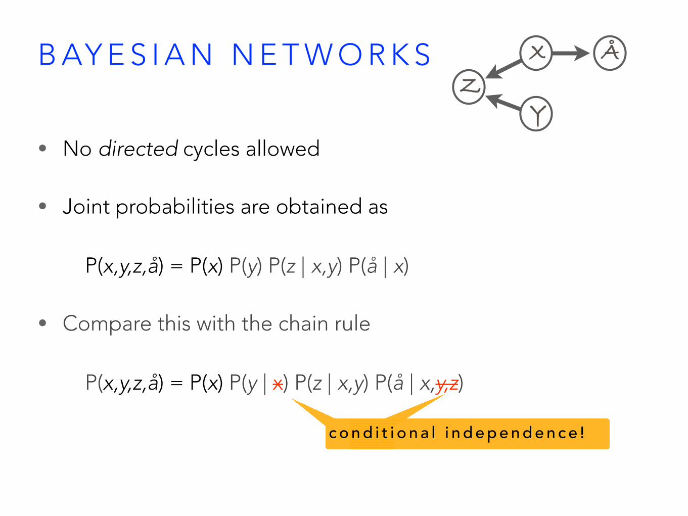
• No directed cycles allowed

• Joint probabilities are obtained as P(x,y,z,å) = P(x) P(y) P(z | x,y) P(å | x)

ZX

Y

Å

PARENTSZ


• The power of BNs: – easier to define conditional distributions, e.g.,

P(å | x) rather than P(å | x,y,z) – efficient inference procedures for computing posterior

probabilities

ZX

Y

Å

E X A M P L E : C A R P R O B L E M S ?

RADIO

BATTERY

IGNITION GAS

STARTS

MOVES



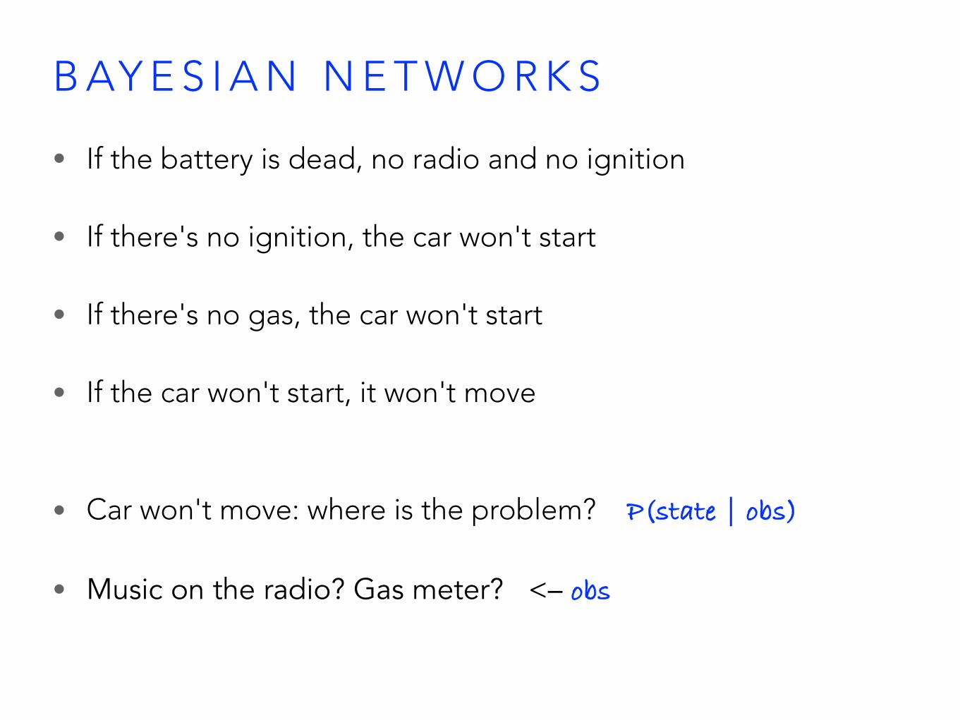
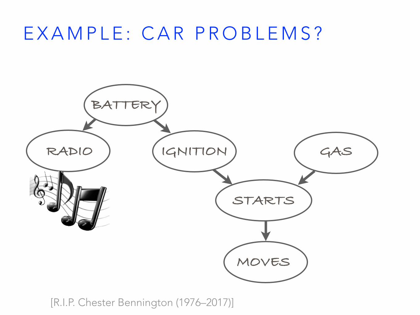
• If the battery is dead, no radio and no ignition

• If there's no ignition, the car won't start

• If there's no gas, the car won't start

• If the car won't start, it won't move

• Car won't move: where is the problem? P(state | obs)

• Music on the radio? Gas meter? <– obs

RADIO

BATTERY

IGNITION GAS

STARTS

MOVES

[R.I.P. Chester Bennington (1976–2017)]


RADIO

BATTERY

IGNITION GAS

STARTS

MOVES


q u i t e s u r e ?

RADIO

BATTERY

IGNITION GAS

STARTS

MOVES


9 5 % p r o b .

RADIO

BATTERY

IGNITION GAS

STARTS

MOVES


9 5 % p r o b .9 0 % p r o b . 9 9 % p r o b .

9 9 % p r o b .

9 0 % p r o b .

9 5 % p r o b .

• P(“battery alive” | ¬“starts” AND “radio ok” AND "gas") = ?

• Exact approach: P(B,¬S,R,G) P(B | ¬S,R,G) = ----------- P(¬S,R,G) P(B,¬S,R,G) = P(B,R,I,G,¬S,M) + P(B,R,I,G,¬S,¬M) + P(B,R,¬I,G,¬S,M) + P(B,R,¬I,G,¬S,¬M)

• Again, the probability of an event, (B,¬S,R,G), is a sum of atomic (elementary) event probabilities


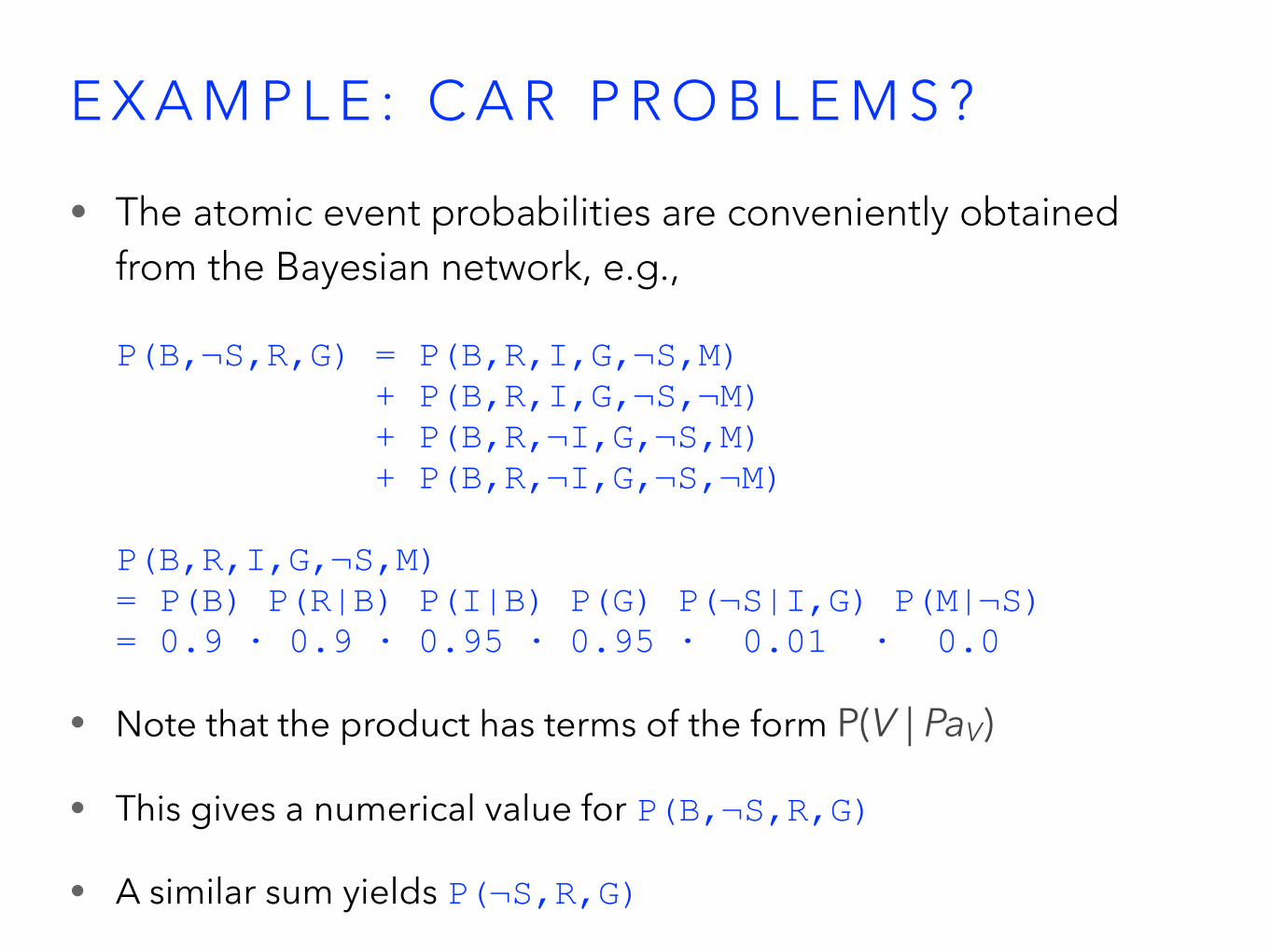
• The atomic event probabilities are conveniently obtained from the Bayesian network, e.g.,P(B,¬S,R,G) = P(B,R,I,G,¬S,M) + P(B,R,I,G,¬S,¬M) + P(B,R,¬I,G,¬S,M) + P(B,R,¬I,G,¬S,¬M) P(B,R,I,G,¬S,M) = P(B) P(R|B) P(I|B) P(G) P(¬S|I,G) P(M|¬S) = 0.9 · 0.9 · 0.95 · 0.95 · 0.01 · 0.0

• Note that the product has terms of the form P(V | PaV)

• This gives a numerical value for P(B,¬S,R,G)

• A similar sum yields P(¬S,R,G)


• This direct approach always gives the exact solution

• However, the sums can quickly become very large (no. of terms is exponential in the size of the network)

• More clever inference algorithms exploit the structure of the network

• For example, in tree-shaped networks (any two nodes are connected by at most one path), belief propagation runs in linear time wrt. number of nodes

• These algorithms are not discussed on this course


• Instead of exact inference algorithms, we take a "hackers approach" to probability

• The probability of any event can be approximated by the Monte Carlo method / sampling: repeat the trial many times and calculate the relative frequency of the event

• E.g., toss a coin 106 times: P(heads) ≈ #heads / #tosses

• To approximate conditional probability P(A | B):

1. generate N tuples (A, B)

2. discard all but those where B occurs

3. among the remaining tuples, calculate the portion where A occurs

A P P R O X I M AT E I N F E R E N C E

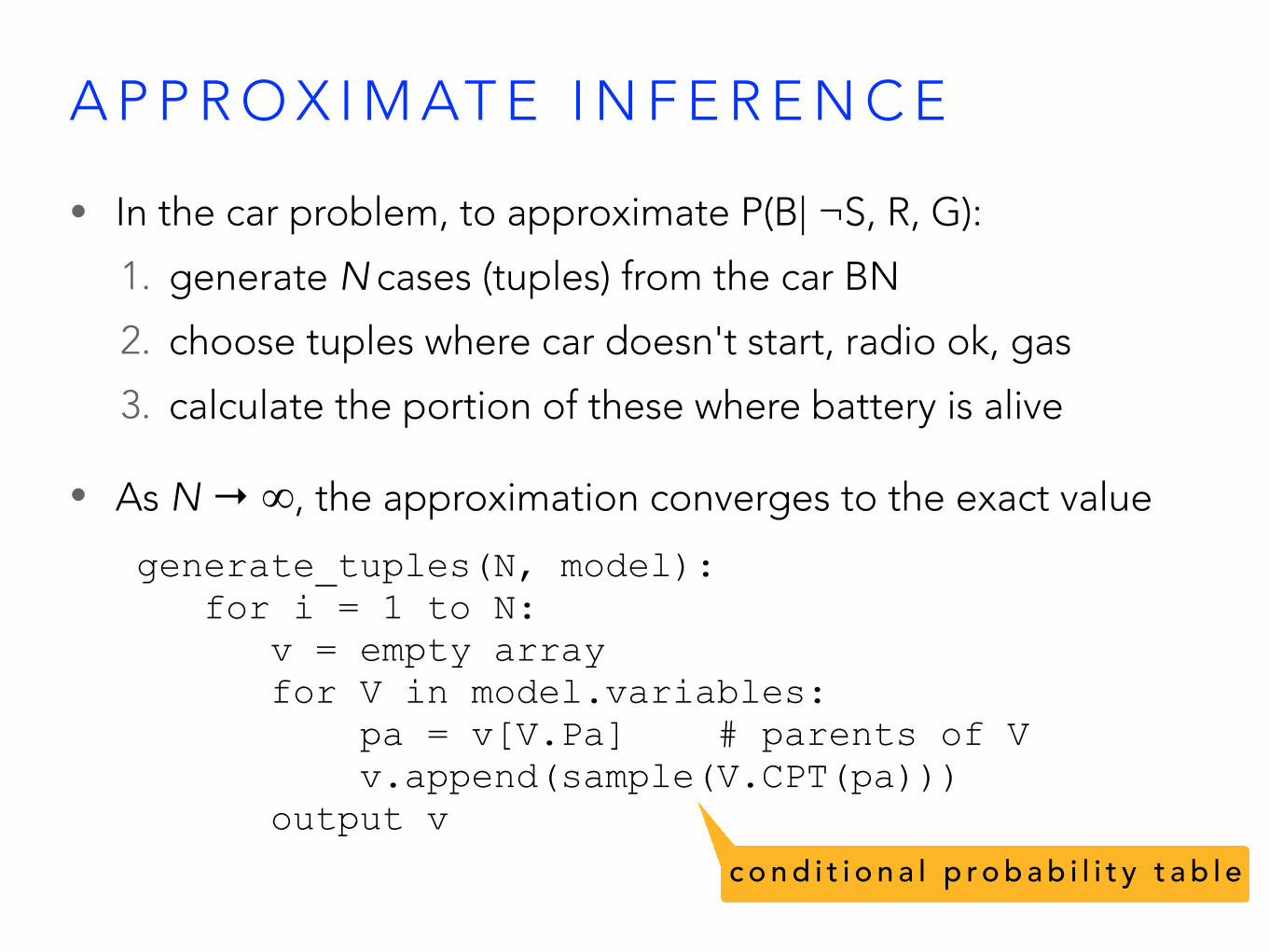
• In the car problem, to approximate P(B| ¬S, R, G):

1. generate N cases (tuples) from the car BN

2. choose tuples where car doesn't start, radio ok, gas

3. calculate the portion of these where battery is alive

• As N → ∞, the approximation converges to the exact value

generate_tuples(N, model): for i = 1 to N: v = empty array for V in model.variables: pa = v[V.Pa] # parents of V v.append(sample(V.CPT(pa))) output v


c o n d i t i o n a l p r o b a b i l i t y t a b l e


• generate N cases (tuples) from the car BN

• choose tuples where car doesn't start, radio ok, gas

• calculate the portion of these where battery is alive





R

B

I G

S

M

v = [] V = 'B' V.Pa = pa = [] V.CPT(pa) = [0.1, 0.9]

∅









R

B

I G

S

M

v = [1] V = 'R' V.Pa = 'B' pa = [1] V.CPT(pa) = [0.1, 0.9]

C P T o f ' R a d i o ' : ( 1 . 0 , 0 . 0 ) i f B a t t e r y = 0 ( 0 . 1 , 0 . 9 ) i f B a t t e r y = 1









R

B

I G

S

M

v = [1,1] V = 'I' V.Pa = 'B' pa = [1] V.CPT(pa) = [0.05, 0.95]









R

B

I G

S

M

v = [1,1,1] V = 'G' V.Pa = pa = [] V.CPT(pa) = [0.05, 0.95]

∅









R

B

I G

S

M

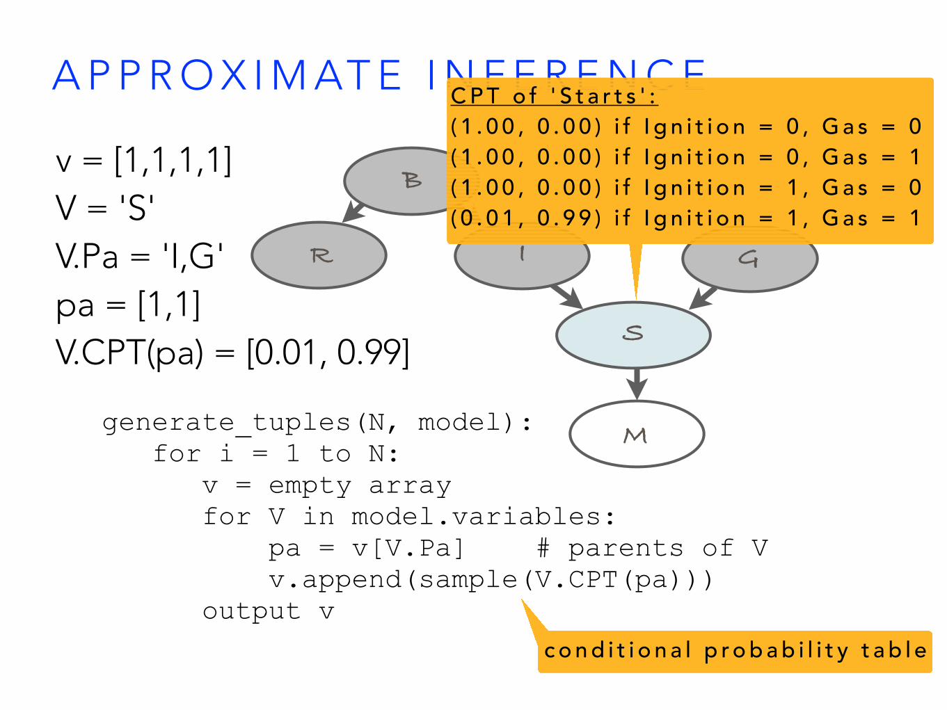
v = [1,1,1,1] V = 'S' V.Pa = 'I,G' pa = [1,1] V.CPT(pa) = [0.01, 0.99]

C P T o f ' S t a r t s ' : ( 1 . 0 0 , 0 . 0 0 ) i f I g n i t i o n = 0 , G a s = 0 ( 1 . 0 0 , 0 . 0 0 ) i f I g n i t i o n = 0 , G a s = 1 ( 1 . 0 0 , 0 . 0 0 ) i f I g n i t i o n = 1 , G a s = 0 ( 0 . 0 1 , 0 . 9 9 ) i f I g n i t i o n = 1 , G a s = 1









R

B

I G

S

M

v = [1,1,1,1,1] V = 'M' V.Pa = 'S' pa = [1] V.CPT(pa) = [0.01, 0.99]









R

B

I G

S

M

v = [1,1,1,1,1,1]









R

B

I G

S

M

v = [1,1,1,0,0,0]









R

B

I G

S

M

v = [1,1,0,1,0,0]

• Spam filter! (and million other naive Bayes classifiers)

• Dynamic Bayesian networks for ecological modelling

• Medical diagnostics (causal factors –> disease status –> symptoms)

• Player matching: Microsoft TrueSkillTM

(well, factors graphs really, but closely related graphical models)

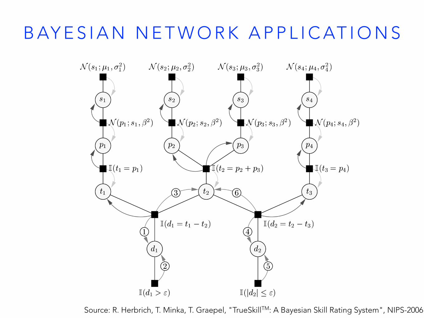
B AY E S I A N N E T W O R K A P P L I C AT I O N S


Source: R. Herbrich, T. Minka, T. Graepel, "TrueSkillTM: A Bayesian Skill Rating System", NIPS-2006

• Spam filter! (and million other naive Bayes classifiers)

• Dynamic Bayesian networks for ecological modelling

• Medical diagnostics (causal factors –> disease status –> symptoms)

• Player matching: Microsoft TrueSkillTM

(well factors graphs really, but closely related graphical models)

• Error correcting codes ("Turbo codes", e.g., Mars mission)

• Football score prediction

• ...


1. N E T W O R K S T R U C T U R E S

2. C A R E X A M P L E

3. I N F E R E N C E ( E X A C T A N D A P P R O X I M AT E )

S U M M A R YZ

X

Y

Å

[1,1,1,1,1,1][1,1,1,0,0,0] [1,1,0,1,0,0] ⋮

P(B,¬S,R,G) P(B | ¬S,R,G) = ----------- P(¬S,R,G)

N E X T W E E K : M A C H I N E L E A R N I N G

5) 6) 7) 8) 9) INTRODUCTION TO - Courses · 2018-09-20 · BAYESIAN NETWORKS • A Bayesian network...

Documents

Transcript of 5) 6) 7) 8) 9) INTRODUCTION TO - Courses · 2018-09-20 · BAYESIAN NETWORKS • A Bayesian network...