


Langages
Pages
Légal

Universite de Montreal
Disintegration Methods in the Optimal Transport Problem
Par
Justin Belair
Departement de Sciences economiques. Faculte des Arts et Sciences.
Universite de Montreal
Memoire presente en vue de l’obtention du grade de Maitrise, M.Sc. en
Sciences economiques, option memoire
Juin 2019
c© Justin Belair, 2019
1
Resume et mots-cles
Ce travail consiste a expliciter des techniques applicables a certaines classes
de problemes de transport (Optimal Transport). En effet, le probleme de
transport est une formulation abstraite d’un probleme d’optimisation qui
s’etend aujourd’hui a une panoplie d’applications dans des domaines tres di-
versifies (meteorologie, astrophysique, traitement d’images, et de multiples
autres). Ainsi, la pertinence des methodes ici decrites s’etend a beaucoup plus
que des problemes mathematiques. En particulier, ce travail cherche a mon-
trer comment certains theoremes qui sont habituellement presentes comme
des problemes combinatoires qui valent sur des ensembles finis peuvent etre
generalises a des ensembles infinis a l’aide d’outils de theorie de la mesure:
le theoreme de decomposition de mesures. Ainsi, le domaine d’application
concret de ces techniques s’en trouve grandement elargi au moyen d’une plus
grande abstraction mathematique.
Mots-cles: Transport Optimal, Decomposition de mesures, Dualite, Op-
timisation
2
Summary and Keywords
The present work hopes to illustrate certain techniques that can be applied to
certain classes of Optimal Transport problems. Today, the Optimal Trans-
port problem has come to be a mathematical formulation of very diverse
problems (meteorology, astrophysics, image processing, etc.) Thus, the per-
tinence of the methods described is much larger than mathematical problems.
In particular, it is shown how certain theorems that are usually approached
with combinatorial tools over finite sets can be extended by measure-theoretic
tools to infinite sets. We see that this higher level of abstraction gives rise
to more powerful and widely-applicable tools, in very concrete problems.
Keywords: Optimal Transport, Disintegration of Measures, Duality, Op-
timization
3
Composition du Jury
Horan, Sean; President – Rapporteur
Amarante, Massimiliano; Directeur de recherche
Dizdar, Deniz; Codirecteur de recherche
Klein, Nicolas; Membre
4
Contents
1 History, Economics Applications, and Introduction of the
Optimal Transport Problem 10
1.1 History of the Problem . . . . . . . . . . . . . . . . . . . . . . 10
1.2 Economics Applications of the Optimal Transport Problem . . 13
1.2.1 Matching Problems . . . . . . . . . . . . . . . . . . . . 13
1.2.2 Models of Differentiated Demand . . . . . . . . . . . . 14
1.2.3 Derivative Pricing . . . . . . . . . . . . . . . . . . . . . 15
1.2.4 Econometric modelling . . . . . . . . . . . . . . . . . . 15
1.3 Presentation of This Work . . . . . . . . . . . . . . . . . . . . 16
1.4 A simple example . . . . . . . . . . . . . . . . . . . . . . . . . 18
1.5 Monge’s original formulation . . . . . . . . . . . . . . . . . . . 20
2 Well-known Problems as Particular Cases of Optimal Trans-
port 24
2.1 Economics Flavoured Matching Problems . . . . . . . . . . . . 24
2.1.1 Discrete Optimal Assignment Problem . . . . . . . . . 24
2.1.2 Discrete Pure Optimal Assignment Problem . . . . . . 26
2.2 The Road Towards Abstraction . . . . . . . . . . . . . . . . . 31
2.2.1 Our ”simple example” made ”Not so Simple” . . . . . 31
2.2.2 General Matching Problem . . . . . . . . . . . . . . . . 35
2.3 The Maximal Flow Problem . . . . . . . . . . . . . . . . . . . 35
2.3.1 The ”Source and Sink Maximal Flow Problem” . . . . 37
5
2.3.2 The Source and Sink Maximal Flow Problem as a Lin-
ear Program . . . . . . . . . . . . . . . . . . . . . . . . 38
2.3.3 The Minimal Cut Problem as a Linear Program . . . . 41
2.3.4 Duality of Linear Programs and Convex Analysis . . . 43
2.3.5 From Matching Problem to Flow Problem . . . . . . . 46
3 Kantorovich’s Optimal Transport Problem or Optimal Trans-
port as a Linear Program 48
3.1 The Optimal Transport Problem as a Linear Program: The
Discrete Case . . . . . . . . . . . . . . . . . . . . . . . . . . . 48
3.1.1 The Primal Problem: Minimizing the Cost of Transport 48
3.1.2 The Dual Problem: Maximizing Kantorovich Potentials 50
3.1.3 Extending the Finite Linear Program to Kantorovich’s
Optimal Transport Problem . . . . . . . . . . . . . . . 52
3.2 Kantorovich’s problem . . . . . . . . . . . . . . . . . . . . . . 55
3.3 Kantorovich Duality . . . . . . . . . . . . . . . . . . . . . . . 56
3.3.1 An Abstract Duality as Bilinear Forms Separating Points 56
3.3.2 Kantorovich Duality . . . . . . . . . . . . . . . . . . . 57
3.4 Kantorovich Monge . . . . . . . . . . . . . . . . . . . . . . 59
3.4.1 Kantorovich’s Problem as a Generalization of Monge’s
Problem . . . . . . . . . . . . . . . . . . . . . . . . . . 59
3.4.2 Kantorovich’s Problem as a Relaxation of Monge’s Prob-
lem . . . . . . . . . . . . . . . . . . . . . . . . . . . . . 61
4 The ”Existence Flow Problem” 62
6
4.1 The ”Existence Flow Problem” as an Optimal Transport Prob-
lem over a Finite Set and its Underlying Vectorial Structure . 62
4.2 The ”Existence Flow Problem” as an Optimal Transport Prob-
lem over a Finite Set and its Underlying Measure-Theoretic
Structure . . . . . . . . . . . . . . . . . . . . . . . . . . . . . 67
4.2.1 A motivating example . . . . . . . . . . . . . . . . . . 68
5 Mathematical Tools : Disintegration Method 70
5.1 Infinite Networks . . . . . . . . . . . . . . . . . . . . . . . . . 70
5.1.1 Abstract Disintegration Theorem . . . . . . . . . . . . 71
5.1.2 Disintegration Theorem applied to Flow Problem . . . 78
6 Possible Novel Applications and Extensions, and Concluding
Remarks 86
6.1 Sandwich Theorem for Measures . . . . . . . . . . . . . . . . . 86
6.2 Choquet Theory . . . . . . . . . . . . . . . . . . . . . . . . . . 87
6.3 Probability Theory . . . . . . . . . . . . . . . . . . . . . . . . 87
6.4 Localized orders . . . . . . . . . . . . . . . . . . . . . . . . . . 87
6.5 Abstract Algebra . . . . . . . . . . . . . . . . . . . . . . . . . 88
6.6 Convex Analysis . . . . . . . . . . . . . . . . . . . . . . . . . . 88
6.7 Operator Theory . . . . . . . . . . . . . . . . . . . . . . . . . 88
6.8 Optimal Transport . . . . . . . . . . . . . . . . . . . . . . . . 89
6.9 Possible Novel Applications . . . . . . . . . . . . . . . . . . . 89
6.10 Concluding Remarks . . . . . . . . . . . . . . . . . . . . . . . 90
7
Acknowledgements
I would like to thank the honesty of my advisor and mentor, Prof. Amarante,
for (maybe unknowingly) helping me gain much needed confidence in my
abilities to pursue mathematics seriously.
Another important part of this work owes a lot to Fuchssteiner, whom I
cannot thank enough for giving me weeks of work to understand the ”quite
obvious” and such of his papers.
Next, I couldn’t omit acknowledging my peers who were brave enough to
choose the option of doing a memoir, as I did, at the cost of an extra year
in the Master’s program, when the ”Atelier de recherche” was available and
obviously could produce work of equal quality in 3 months.
I warmly thank Prof. Frigon from the Mathematics Department at Uni-
versite de Montreal who taught me Functional Analysis, for harshly making
me realize I was no mathematician until I got good and became one. Her
kind smile and friendly advice have helped me grow through this learning
experience.
My deepest admiration and greatest thanks go to Fabrice Nonez, my
friend from the Mathematics Department, who happens to be the most pas-
sionate mathematician I know. His countless hours in building my mathe-
matical intuition from the ground up, whether it be over beer, pho soup, or
particularly dusty chalk from the Mathematics Department, have completely
changed my life. Other important mathematician friends were met along the
way, most notably Antoine Giard, who shares an office with Mr. Nonez. I
also need to mention my non-mathematician friend (although recently versed
8

in calculus) Charles-Etienne Chaplain-Corriveau, for making me realize that
life is too short and knowledge too vast to ever think we know something, and
that hard work, dedication (and years of reading) are the only remedies to
our ignorance. The last friend I must thank is J-R Jr. ”Jun” Guillemette, for
keeping me focused on working out and not diving too deep into the insanity
of doing mathematics all day and all night.
I also thank in advance the committee who will be charged with the
dreadful task of reading these pages during nice May weather and reporting
back in a month.
Finally, I have to thank my mother and my sister with whom I grew up,
for I would be decomposed if it were not for their support, throughout this
work and throughout this life.
9
Chapter 1: History, Economics Applications,
and Introduction of the Optimal
Transport Problem
1.1 History of the Problem
The problem which is today known as Optimal Transport, might be referred
to as Hitchcock-Koopmans transportation, optimal assignment, matching with
transferable utility, optimal coupling, etc. This diversity of naming partially
reflects the wide-array of formulations and interpretations appropriate for
this problem, as well as the number of important applications the problem
has come to embody.
The problem of optimal transport has a very rich history. There were
often simultaneous discoveries made, best embodied by its initial modern
formulation as a Linear Programming problem made by Kantorovich in the
Soviet Union and Koopmans in the USA, at a time where scientists of the
Soviet Bloc were mostly cut off from the West. The simultaneous discoveries
partially reflect how intimately these problems were at first connected with
post Second World War mass industrialization where concerns for planning
huge resource allocation over massive geographical areas stimulated intense
research efforts. As proof of such, the most notable 20th Century results
have been the fruit of mathematicians either from the Department of De-
fense funded RAND Corporation or Soviet scientists under Stalin’s planning
regime. It is surely one of History’s great ironies that, independently, both
10
the ”Land of the Free” and the Communist Soviet Republic’s ”Politburo”
independently developed a mathematical theory in order to assist them in
planning allocation of huge amounts of resources over vast territory. A fur-
ther historical note of interest, is that these problems and the mathematicians
working on them are intimately linked with the professionalization of aca-
demic work and, in particular, mathematics. Out of these efforts, grew the
whole field of Operations Research, and vast domains of modern Economic
Theory, amongst others.
But the problem has come to be more than a formalization of economic
concerns. As its study grew, it took contributions from various fields and it
reciprocated the favour by elucidating ways to reinterpret problems in other
fields. Today, its tools are at the intersection of many important theories
such as statistical mechanics, fluid dynamics, linear programming, convex
optimization, calculus of variations, partial differential equations, measure
theory, functional analysis and many others. As such, it continues to attract
a great number of scientists from many fields.
The first known formalization of the transportation problem can be traced
backed to a French revolutionary, Gaspard Monge, in his 1781 memoir, ti-
tled Memoire sur la theorie des deblais et remblais [Mon81]. Working for
the French government, he was interested in a mathematical formalization of
civil engineering problems related to excavation and landfills. As a matter of
fact, Monge was interested in a mathematical formalization of transporting
piles of sand into holes that needed to be filled. Obviously, this had to be
done at a minimal cost. Monge’s original formulation of the problem was a
particularly difficult version of it, which he obviously was unaware of at the
11

time. We will see in Section 1.5 what exactly this formalization was, and
why it was particularly difficult. Monge’s original formulation anticipated
the whole field of linear programming, that is the now well-known theory
of optimizing a function under a set of linear constraints. As a matter of
fact, no major progress on the problem was made until the problem was re-
laxed and solved by Russian mathematician Leonid Kantorovitch [Kan58].
How did Kantorovitch do this? By formulating it as a linear programming
problem, which he had himself introduced in [Kan60]. Kantorovich was af-
fected to work on problems related to industrialization in the USSR. He used
the techniques he developed and the insights he gained to tackle economics
problems, eventually going on to share the Nobel Prize in Economics with
the American-Dutch mathematician Tjalling Koopmans in 1975. Koopmans
had worked independently with Dantzig, Fulkerson, and others in developing
linear programming and its applications in the USA. During that time, Eco-
nomics attracted scientists working on many problems which would today be
called Operations Research.
Then, in the 1980s, Yann Brenier, Mike Cullen and John Mather inde-
pendently revolutionized the field. Brenier was able to formulate problems
in non-compressible and non viscous fluid mechanics as Optimal Transport
problems. At the same time, Cullen studied weather fronts and was able
to place Optimal Transport at the center of his meteorological studies. Fi-
nally, Mather successfully applied Optimal Transport to the field of dynamic
systems. We will not pretend to understand how Optimal Transport ap-
plies to these fields, but the modern interest for Optimal Transport is often
attributed to these ground-breaking discoveries.
12
This renewed interest sparked much scientific research, which might have
found its apex in the 2018 Field’s Medal award attributed to Alessio Figalli,
an Italian mathematician at ETH Zurich. Also, Cedric Villani (Figalli’s
advisor), a French mathematician who wrote the two most exhaustive mono-
graphs (which we will heavily rely on) on the subject Topics in Optimal
Transport [Vil03] and, Optimal Transport: Old and New [Vil08], respectively
in 2003 and 2008, was also awarded a 2010 Field’s Medal for contributions
on Landau damping, a long-standing problem in theoretical physics.
1.2 Economics Applications of the Optimal Transport
Problem
As has been hinted in the previous section, Optimal Transport is applied
in very diverse areas of mathematics, engineering and physics, amongst oth-
ers. Here, we are interested in its applications in more modest economics
problems, which are closer to its humble linear programming applications of
the 20th century. Therefore, I will draw heavily on French mathematician-
economist Alfred Galichon’s 2016 introduction to the book Optimal Transport
Methods in Economics [Gal16].
1.2.1 Matching Problems
The most natural economic problem that can be apprehended as an Optimal
Transport problem, is one of assigning workers to jobs. That is, given a set
of workers and a set of jobs, each with heterogeneous characteristics, hence
heterogeneous complementarity between both groups, how does one assign
the workers to jobs in order to maximize the economic output, or utility?
13
One can replace the workers and jobs in the above problem to obtain a
number of applications that present a similar structure: men and women on
a marriage market or workers and machines in a factory, are two examples.
These are known as matching models, and economic theory mainly deals with
two central questions in these types of problems: the optimal assignment,
that is one a rational central planner would chose to maximize utility, and
the equilibrium assignment, that is the natural assignment that would arise
if the market was left to its own. As usual, economists are particularly
interested in the situations where both solutions coincide, that is where the
optimal solution is found at equilibrium. It is fairly intuitive to see why these
problems have the same structure as problems that wish to transport objects
between given points at a minimal cost, given we have an idea of the latter.
In Section 2.1, we will give a more thorough–and formal–explanation of this
particular problem seen in the light of Optimal Transport.
1.2.2 Models of Differentiated Demand
The next type of problem pertains to models of differentiated demand, that is
”models where consumers who choose a differentiated good have unobserved
variations in preference” [Gal16]. By observing variations in demand and
making assumptions on the distribution of the variation in preferences, the
preferences are identified on the basis of the distribution of the observed
demanded quantities. It turns out this problem is the dual to the optimal
transport problem. We will see further the central part played by duality in
this theory.
14
1.2.3 Derivative Pricing
In financial economics, derivative pricing and risk management can draw
from Optimal Transport. That is, in cases where both derivatives or risk
measures depend on multiple underlying assets or risks each having a known
marginal distribution but an unknown dependence structure, Optimal Trans-
port is useful in determining bounds on our prices or risk measures. That
is, by estimating marginal distributions observed in financial data, one can
use Optimal Transport to place bounds on the unknown joint distribution
of prices or risk measures. This has much to do with probability theory and
namely coupling, an important concept that lets one create a random variable
whose marginals correspond to given distributions. For our purposes here,
we will not be entering in the details of coupling.
1.2.4 Econometric modelling
Finally, econometricians might be happy to find out even they can apply
Optimal Transport to problems pertaining to incomplete models, quantile
methods, or even contract theory. Identification issues arise when data is in-
complete or missing. The problem of identifying the set of parameters that
best fits the incomplete observed distribution can be reformulated as an Op-
timal Transport problem. The main interest in this approach lies in the com-
putational properties of Optimal Transport problems. As a matter of fact,
a large portion of the post-Second World War work done by Dantzig, Ford,
Fulkerson, and company pertains to finding efficient algorithms constructing
the solution. As for quantile methods (quantile regression, quantile treat-
ment effect, etc.), Optimal Transport provides a way to generalize the notion
15
of a quantile. Also, typical principal-agent problems can be reformulated
as Optimal Transport problems, which lets one use econometric methods to
infer about an agent’s unobserved type based on his observed choices.
All these economic applications are treated in Galichon’s book [Gal16]
with an emphasis on computing and constructing the solutions, which is of
interest in a field like economics that concerns itself with applications of
this problem. This is in contrast with the previously cited monographs by
Cedric Villani [Vil03] and [Vil08], which are mainly addressed to mathemat-
ical physicists. Here, we will not delve into computational issues: we are
more interested in the mathematical ideas of the theory.
1.3 Presentation of This Work
In this work, we will be mainly concerned with three things: first, to show a
grasp of the central abstract ideas behind Optimal Transport (which means
we will not state existence or stability results, for it was judged that they are
not very useful until we have a true novel problem at hand); second, showing
how various well-known problems can in fact be seen as an Optimal Trans-
port problem; finally, showing how some methods related to disintegration
of measures can be brought into Optimal Transport, to, we hope, eventually
serve as building blocks to novel theorizing and problem-solving. The main
difficulty lied in presenting and arranging a wide array of somewhat deep
ideas and theories (which were all new to the author not too long ago): we
hope the job will be appreciated.
When it comes to definitions, we will introduce concepts as we go. Some
definitions will be stated directly in the text, with the defined term in bold,
16
while some more important definitions will be defined in Definition sections
removed from the text. We have made an attempt to be as thorough as
possible, even in cases where some definitions seem very elementary and su-
perfluous. There are certainly some omissions (it is practically impossible to
formally define every single concept), but we hope that it will not impact the
understanding of the reader. On a somewhat abstract level, the mathemat-
ical concepts used come in large part either from Measure Theory, Convex
Analysis, Functional Analysis, or Graph Theory, and, a part from Chapter
5, everything said can be found in textbooks. There will be some more con-
crete terminology proper to specific applied problems, which shouldn’t be too
difficult to grasp, even for someone who has never heard of said problems.
For what concerns notation, we have made a valiant effort in being consis-
tent and using notation throughout different sections that helps in showing
the analogy between two different concepts. For example, if a finite space
X is then taken to be infinite in a more general case in a further section,
we have tried to redefine X, in order for the reader to see the kinship (and
the differences) between the finite X and the infinite X. Pushing this to the
extreme was nearly impossible, and there will surely be some notations that
could’ve been better chosen.
In statements that need to be proved, we have taken the approach to prove
what is important. Some statements are left unproved: either because the
result is very well-known and can be proved in a variety of ways, depending
on our interests, or, we judged that the proof was too involved to encumber
the work. None of the results are truly original, yet none of the proofs were
copied: we have always made the effort to rewrite the proof in a way which
17
was judged to be insightful.
Some sections may appear incomplete, or even begging to be pushed
further. In most cases, it was either a lack of time or of knowledge (induced
by a lack of time) that forced these sections to be cut short. In Chapter 6,
we will address subjects that the author wishes to address further in future
studies.
Now, lets start with a simple example that will be useful to give us an
intuition for the problem before we fully formalize it in its most general
setting.
1.4 A simple example
Say there are n ∈ N oil mines (producers) that must supply raw oil to n ∈ N
refineries (consumers). Say these are points in a plane. If X ∈ R2 and
Y ∈ R2 are respectively the (disjoint) sets of mines and refineries, then using
R2 as the ambient space lets us see the problem as one of looking at a plane
geographical map and choosing which combination of paths from mines to
refineries are, lets say, of shortest Euclidian-distance.
The question we ask is then one of building a network of (directed)
pipelines such that the total distance of our pipelines is minimal, i.e. the
distance the oil travels is minimal. So, we introduce T : X → Y , our trans-
port map, that is the map assigning to refineries from which mine their
oil is to be supplied (i.e. the ”literal” map of our pipeline network, if we
may). Let’s force T into being a bijection, which can obviously be inter-
preted as each and every mine supplying one and only one refinery (i.e. each
supplier has exactly one out-flowing pipeline that connects him with exactly
18
one consumer). Given this extra condition on T , we can find an equivalent
interpretation to the problem. That is, assume there are n producers and
n consumers, such that all of them are already connected by a network of
pipelines. If shipments are not split–i.e. oil leaving a mine goes to one and
only one refinery–and that each refinery receives its supply from one and only
one producer, we ask which pipeline should a given producer use (if pipelines
cannot be shared). Obviously, the choice is arbitrary unless we specify under
which condition it is optimal (for example, minimal distance travelled). In
this case where there are as many producers as consumers, another way of
looking at this problem is one of finding an optimal permutation–i.e. a
bijection between X and Y .
We define the total cost under the transport map T as
c(T ) :=∑x∈X
c(x, T (x)). (1.1)
Our problem is then to minimize c(T ) over all relevant transport maps T ,
i.e. over all possible configurations of pipelines. This problem is a somewhat
trivial one, for all we need to do is minimize over a finite (although maybe
very large) discrete set by considering all the n! permutations of the set of
consumers. In the language of graph theory, finding optimal permutations of
this sort is what is referred to as a matching problem, which have many ap-
plications, notably in Economics (See Matching Problems of the next Section
2.1.).
19
1.5 Monge’s original formulation
Here, we will give more substance to the statement that Monge’s original
1781 version of the Optimal Transport problem was a particularly difficult
one. Monge was interested in finding the least costly way of moving dirt from
piles into holes.
In its most general setting, interesting results of the problem are often
formulated in Polish spaces, that is separable and completely metriz-
able topological spaces–obviously, Rd is an example of such a space. We
will keep in back of mind that the problem can be brought to quite high levels
of abstraction, but we will introduce it in somewhat less abstract terms.
Let X, Y ⊂ Rd, represent respectively the ”spatial configurations” of our
pile of dirt and our hole to fill. We will sometimes refer to our piles of dirt
as mass, a term that is a bit more mathematically appropriate. Next, equip
these spaces with a σ-algebra and consider α and β measures which will give
us two measure spaces to work with. Here, α can be seen as the distribution
of mass of dirt–i.e. the density–in ”the space” X. On the other hand, β
represents the distribution of mass we would like to achieve in Y . In order
to achieve this, we must transport dirt from X to Y . So, let T : X → Y , the
transport map, that is, one that assigns to a point in our initial pile of dirt,
a destination in the hole to fill.
Take our initial pile of dirt X which is ”distributed” according to a certain
density α. Obviously, our concerns lie with finite piles of dirt–this is an
applied problem after all! We may then normalize our density to take values
in [0, 1] which lets us work with probability measures. We will denote the
20
space of probability measures on X and Y by P(X) and P(Y ), respectively.
Let’s assume for simplicity of exposition that both X and Y are standard
probability spaces, i.e. they are equipped with the Borel σ-algebra, which we
will denote B(X) and B(Y ), respectively. Also for simplicity’s sake, when
we refer to X and Y , we will refer to their probability space structure with
the Borel σ-algebra, and omit explicitly defining the measure space triple
when the context is clear.
Definition 1.1. (Push-forward) Let X, Y , T , and α be defined as
in the paragraph above. Then, the push-forward or image measure of a
measure α through T , which we denote T#α, is such that for all B ∈ B(Y ),
T#α(B) = α(T−1(B)).
Remark 1.1. Given a probability space X with probability measure α and a
map T with values in an abitrary space Y , we can make Y into a probability
space by ”pushing-forward” α, and building the trivial σ-algebra on Y that
makes T a measurable function. Defining β := T#α is unambiguous as β will
be unique. This is a warm-up exercise in Villani’s book [Vil08]. As we will
see, the ”real” problem lies in being given beforehand measures α on X and β
on Y , and choosing a certain transport map T such that T#α = β. Obviously,
to this transport we will associate a cost, and we would like minimize that
cost.
Definition 1.2. (Cost function.) Let c : X × Y → R≥0 ∪ +∞, our
cost function. Then, obviously, c(x, y) represents the cost of moving dirt
from x ∈ X to y ∈ Y . Note that by allowing c to take values at +∞, we can
21
exclude certain pairs (x, y) of being part of a solution at minimal cost. We
will sometimes write cxy to represent c(x, y).
Now, in a somewhat more abstract setting than using Rd as in Section
1.5, Monge’s problem can be stated as:
(MP) inf
ET (c) :=
∫X
c(x, T (x))dα(x) : T#α = β
.
In the language of probability theory, we are looking for a transport map
that pushes α onto β such that the expected value of our cost function–i.e.
the integral in (MP)–is minimal.
Remark 1.2. This is our first obvious concern: the set for which we are
trying to find a minimizer in (MP) may be empty. It is easy to give an
example where there exists no transport map that effectively pushes α onto
β: take α to be a single Dirac-mass–all the mass is concentrated on one point,
i.e. α is a single atom–and β that is not one. Then, obviously, there is no
way to push α onto β with a transport map. An analogous statement can
be obtained from the case where β is a single Dirac-mass: the only transport
map that pushes α onto β is the constant map that sends all the mass to β’s
atom.
This was the problem one had to face when dealing with Monge’s Optimal
Transport problem for close to 150 years. Also, to complicate matters even
further, Monge chose his cost map to be the absolute value difference–i.e.
c(x, T (x)) = |x− T (x)|–which is not well-behaved with respect to minimiza-
tion.
Lets leave it at this for the moment, and look at particular cases of
22
problems that do not seem to be Optimal Transport at first glance, but
turn out to be when the right light is shone upon them.
We shall note that the structure of such particular cases will not be in
terms of Monge’s formulation (i.e. we will not use a transport map per se, in
order to avoid the possibility of the non-existence of a solution): we will come
back to classical Optimal Transport and its details with the much superior
modern formulation of the Optimal Transport problem in Chapter 3. In other
words, in Chapter 2 we will explain how some well-known problems from
various fields in applied mathematics can be given an ”Optimal Transport
flavour”, then, in Chapter 3, we will see how all these problems can be
encompassed in the modern formulation of Optimal Transport.
23
Chapter 2: Well-known Problems as Particu-
lar Cases of Optimal Transport
2.1 Economics Flavoured Matching Problems
Mathematical economists will be familiar with this type of problem. As
a matter of fact, this section will draw heavily on French mathematician-
economist Alfred Galichon’s book Optimal Transport Methods in Economics
[Gal16]. There will also be material from the previously cited Villani’s Topics
in Optimal Transport [Vil03]. These sort of problems are also of interest in
Operations Research and Computer Science, namely via Graph Theory.
2.1.1 Discrete Optimal Assignment Problem
One well-known Economics flavoured variation is the optimal assignment
problem. The framework is simple: we are in the context of a job market.
Thus, we have a set X representing the type of workers and a set Y the
type of jobs. Both X and Y are finite with, say X having cardinality K,
and Y having cardinality I. Each set is given a distribution: there are αk
of workers with type k ∈ X and βi of jobs of type i ∈ Y , both normalized
to 1 (i.e.∑
k αk =∑
i βi = 1). This situation is obviously the same as
in the ”simple example” of Section 1.4 except for two things. First, in the
previous section, we implicitly chose our distributions to be equiprobable on
both spaces, whereas here α and β are arbitrary. Second, we were minimizing
costs whereas now we will maximize a surplus.
Define Uki as the surplus created from assigning a worker of type k to a
24
job of type i. Obviously, we want to maximize this surplus, under the con-
ditions imposed by the distribution. This is an Optimal Transport problem:
maximize a function under constraints given by probability distributions. In
other words, we can see the problem as one of transporting the workers to
jobs, where the transport generates a surplus.
Remark 2.1. As we said in the concluding paragraph of Section 1.5, we
have no notion of a transport map, per se. As a matter of fact, this type of
problem is not a Monge Optimal Transport problem, but we will get to the
details later.
Now, interesting results stem from this simple example. In this finite
case, we can model the transport by deciding how much of workers of type
αk will be sent to jobs of type βi, for each pairs of types (k, i) ∈ X × Y .
Thus, we will represent such a transport plan (which we will formally define
in Chapter 3), as a K × I real-valued matrix. We will also see in more detail
in Section 4.1 that choosing a matrix is not insignificant: the space of maps
on a set is a vector space and, in particular, the spaces of maps on a cartesian
product can be seen as a space of matrices. Denote such space of matrices
MK×I(R). Define
Π(α, β) := M ∈MK×I(R) :∑i
πki = αk and∑k
πki = βi,
where πki is the kth row and ith column entry of the matrix. Thus, the
problem becomes one of optimizing the surplus,∑
(k,i)∈X×Y Uki, over matrices
Π(α, β) ∈MK×I(R), such that∑
k αk =∑
i βi = 1–i.e. α and β are discrete
probability distributions.
25
2.1.2 Discrete Pure Optimal Assignment Problem
In this type of problem, workers of type k must all be matched to a job of
type i. For this to make sense, we must impose that the cardinality of X
and Y are equal, lets say, card(X) = card(Y ) = n and that there is only ” 1n”
workers of each type. Hence, the problem becomes one of maximizing the
surplus, over matrices πki ∈ Π(α, β), such that∑
i πki = 1n
and∑
k πki = 1n.
Lets multiply out by n, in order to obtain the following conditions:∑i
πki = 1 and∑k
πki = 1.
That is, such matrices are called bistochastic, or doubly stochastic: the
sum of each row is equal to 1, same with each column. Lets denote the space
of such matrices by B. This space is known as Birkhoff’s polytope.
Proposition 2.1. The n × n-dimensional Birkhoff polytope is convex.
In a space of real finite-dimensional matrices M(R), it is also compact.
Proof. Let M ∈ B. In our setting, B is the unit ball of Mn×n(R) with
the sup-norm(i.e. sup
||x||≤1
Mx), which is compact in finite dimension. The
convexity is trivial.
One major result in this direction, is a version Choquet’s Theorem, which
we state after a minor definition and another theorem that will serve as a
lemma in the proof of Choquet, followed by an important theorem on the
Birkhoff polytope.
Definition 2.1. (Convex set and extreme points of a convex set.)
We say that C is a convex set if c, d ∈ C imples λc + (1 − λ)d ∈ C for all
26
λ ∈ [0, 1]. We say that c is an extreme point of a convex set C, if c cannot
be written as non trivial convex combination of points in C. In other words,
there does not exist cn ∈ C such that c =∑∞
n=1 λncn, for∑∞
n=1 λn = 1 and
at least one of the λn ∈ (0, 1), but no more than a finite amount of such λn.
We denote the set of extreme points of C by E(C).
Theorem 2.1. (Krein-Milman Theorem.) Let B be a compact con-
vex subset of MJ×J(R). Then, for each M ∈ B, there exists a probability
measure ρM on E(B), such that
M =
∫E(B)
c dρM(c).
Proof. The result is trivial in finite dimension, and holds in much more gen-
erality. If M ∈ E(B), then the Dirac-mass at M will do. If M 6∈ E(B),
then by definition, it is a non trivial convex combination of points in B–i.e.
M =∑∞
n=1 λnMn,Mn ∈ B and λn ∈ (0, 1), for at least one n, but for no
more than a finite number of n. Take ρM(Mn) = λn, and we have the desired
probability measure, and the integral reduces to a finite sum.
Theorem 2.2. (A Simple Version of Choquet’s Theorem.) Let
B be a compact convex subset of MJ×J(R). Let f : B → R, the restriction
of a continuous linear functional on MJ×J(R). Then, f admits a minimizer
on B, and there is at least one of f ’s minimizers which lies in E(B).
Proof. The compacity of B and the continuity of f implies that f admits at
least one minimizer: denote it b. Lets suppose that no minimizers are extreme
points: they are all non-trivial convex combinations of points in B. In fact,
by Krein-Milman, we can write them as nontrivial convex combinations of
27
E(B):
b =∞∑n=1
λnxn,
where all the xn ∈ E(B),∑∞
n=1 λn = 1, there are only a finite number of
λn > 0, and f(xn) > f(b) for all n.
Suppose f 6≡ 0, for there would be nothing to show. Now,
f(b) =∞∑n=1
λnf(xn) >∞∑n=1
λnf(b) = f(b),
an obvious contradiction, which yields the result.
Remark 2.2. In finite dimension, these results are trivial. These results
hold in general for Banach spaces, modulo rearranging the proofs to take
care of infinite dimensionality. We can even extend them to abstract lo-
cally convex (Hausdorff) topological vector spaces. The extension to
infinite-dimensional spaces are not elementary, and will be avoided, for the
sake of not encumbering ourselves. Make no mistake, they are very interest-
ing in their own right and even in their applications to Optimal Transport.
Definition 2.2. (Permutation matrices and the Kronecker symbol.)
Let σ : 1, 2, . . . , J → 1, 2, . . . , J be a permutation (i.e. a bijection).
Then, a permutation matrix is a matrix that has entries of the form
πki = δk,σ(k), where δk,i is the Kronecker symbol–i.e. δk,i = 1 if k = i, 0
otherwise.
Theorem 2.3. (Birkhoff-von Neumann Theorem.) The set of
extreme points of Birkhoff’s polytope, denoted E(B), is exactly the set of
permutation matrices .
28
Proof. Let Γ ∈ B. We first show that if all the entries of Γ are 0 or 1, then
it is a permutation matrix.
If Γ ∈ B is such that γij = 0 or 1 for all i × j, then, by bistochasticity,
every row has only one entry equal to 1, same for every column. Thus,
there obviously exists a bijection σ from the rows into columns that yields
precisely Γ. Thus, we have established that bistochastic matrices with only
0 or 1 entries are permutation matrices. Also, by definition, a permutation
matrix is bistochastic and has only 0 or 1 entries. Thus,
Γ is a permutation matrix ⇐⇒ Γ is bistochastic with all γij = 0 or 1.
Then, we only need to show that an extremal point has only 0 or 1 entries.
Let Γ ∈ E(B). Suppose there is at least one entry γij 6= 0 or 1. In
fact, by bistochasticity, this implies that there is at least 2 entries on row
i and two entries on row j that are different from 0 or 1. We will call
them γij, γi′j, γij′ , and γi′j′ . Suppose there are only 2 such rows and 2 such
columns. Then, we can write this matrix as the midpoint of 2 bistochastic
matrices, M,N , by simply taking mij =1−γij
2, and nij =
γij2
, same for
i′j, ij′, and i′j′, with all other entries in M and N equal to the entries in Γ.
This process can be repeated for any even number of entries that lie in (0, 1).
If there is an odd number of such entries, it is always possible to remove an
entry and ”distribute” its excess over the remaining even number of entries
(both in rows and columns). Thus, Γ ∈ E(B) cannot have entries stricly
in (0, 1), for they would be nontrivial convex combinations of bistochastic
matrices, as we have ”shown”.
This establishes the result: E(B) is exactly the set of permutation matri-
ces.
29
Remark 2.3. Although the last bit of the proof might lack a bit of rigour,
it is fairly obvious and easy. The reasoning is very algorithmic so using
the required rigour is very tedious, and we hope that the proof offered is
satisfying (it is as suggested in an exercise in [Vil08]). Nonetheless, this is a
very well-known result, it is very intuitive, and there exists countless proofs.
One very direct approach uses induction, as in [HW53].
Then, we can use Choquet’s theorem (Theorem 2.2) in conjunction with
Birkhoff-von Neumann’s theorem (Theorem ??). That is, we know that our
discrete pure optimal assignment problem has a minimizer which is simply an
extreme point of the Birkhoff polytope–i.e. a permutation of worker types–
and it turns out that only considering permutations yields the same optimal
value of the surplus.
As a matter of fact, the discrete pure optimal assignment problem we’ve
just described, consists in a linear optimization problem over a compact (and
in particular bounded, even in infinite dimension) convex set, which makes
it a linear programming problem (we will go further into these matters in
Section 2.3.2 and Chapter 3).
Remark 2.4. This is interesting in applications for it greatly reduces the
amount of solutions one needs to check from (n2)! to n!, the n×n permutation
matrices. It is also interesting from a mathematical point of view, because it
opens the door to very interesting theoretical ideas, namely Choquet Theory
and Convex Analysis. We will briefly say a bit more on Convex Analysis in
Sections 2.3.4 and 3.3.
We will also see in Section 2.3.5 that, in general, matching problems can
be seen as flow problems (which we will now delve into in this next section).
30
2.2 The Road Towards Abstraction
Now, lets recall our ”simple example” in Section 1.4 (the finite mine-refineries
transport problem) which we will generalize.
2.2.1 Our ”simple example” made ”Not so Simple”
Suppose there are now K mines, M1, ...,MK each producing respectively sk
of a certain commodity, say oil. There are also I refineries, R1, ..., RI , each
having to meet demand ri. In our ”simple example”, we implicitly chose sk =
ri = 1 for all k, i. Now we allow these values to be any real number. Then, as
in the simple example, our problem consists in finding T , a transport map,
such that the cost is minimal and the demand is satisfied for all refineries.
This is a simple version of the Optimal Transport problem which we will
consider as a linear program in Section 3.1, once we’ve developed certain
concepts.
Remark 2.5. The alert reader will notice that this problem is identical
to the discrete optimal assignment problem, if not for the fact that we are
minimizing a cost. This difference is in fact insignificant, for in Section 2.1.1
on the optimal assignment problem, we could’ve set cki = −Uki, and the
problem would be the same.
Lets further generalize this problem by allowing each of our J := K + I
mines and refineries to be at the same time both producers and consumers
of oil. All we need in order to attain this is to introduce a parameter, which
we define as production minus consumption, i.e net production:
µj = sj − rj, for all j.
31
Then, obviously this parameter takes on positive values for net production
and negative values for net consumption at any given node i. In order to
simplify terminology, we will call all of our J producers and consumers agents
and let X denote the finite set of such agents. Note that the cardinality of
X, card(X) is equal to J .
Next, we can define a binary relation ≤G on X such that i ≤G k means
that there is a pipeline connecting i and k. This situation can be modelled
by a graph G, that is G = (X,≤G), a (usually finite) set with a certain
binary relation ≤G. In graph theory terminology, we call our agents nodes,
vertices or simply points. One of the major strengths of graph theory is that
any binary relation imaginable over a finite set gives us a graph. This allows
for very flexible models.
Remark 2.6. As we shall see in Chapters 4 and 5, a more analytic way
to deal with networks (that will come in hand when extending the results
to infinite networks) is to forego using a binary relation at all, and directly
define maps on X ×X, or even on its power-set. Then, for example, a ”non-
existing” arc in a network could have 0 ”capacity”, thus in essence eliminating
it from the problem. Anyhow, basic graph theory deals usually with finite
(or at most countable) sets, so we introduce the graph theoretic notions in
order to draw parallels between common formulations of network problems
and the somewhat more obscure methods we will develop in Chapters 4 and
5.
32
Define a capacity map τ :
τ : X ×X → R≥0 ∪ +∞
(k, i) 7→ τki.
Remark 2.7. Note the following: we allow τ to take +∞ as to (maybe)
admit certain unconstrained arcs in our network; also, τki = 0 can be inter-
preted as having no pipeline between k and i (see Remark 2.6).
Obviously, the flow in a given pipeline cannot exceed the capacity of
that pipeline. In graph theory terminology, we could call our capacity map
weights, in order to talk about a weighted graph.
Remark 2.8. In the ”simple example” of Section 1.4, this parameter τ was
”hidden”: we implicitely specified τki ≡ +∞.
Then, we can notice that we are in a very similar setting than the one of
our ”simple example”: we are merely changing our focus from transporting
between producers and consumers to transporting net production surplus
between a network of agents: those of which are net producers are discharging
their surplus onto those of which are net consumers.
Now that we have some formalities out of the way, what are the interesting
questions we can ask about such a situation? We could think of the following:
(i) Given the constraint map, is there an allocation of production surplus
that satisfies consumption demand for every agent in the network? We
will call this problem the existence flow problem.
33
(ii) If there are more than one satisfying allocations, which one is done at
a minimal cost–i.e. which one minimizes c? This is obviously a optimal
transport problem.
(iii) If we would like X to be an infinite set, can we find a nice formalization
in order to study the two questions just above?
For point (i), we will state obvious necessary conditions in Section 3.1. An
incursion into infinite networks will give us a theorem that allows us to answer
simultaneously questions (i) and (iii), in Chapter 5. A final motivation for
studying infinite networks that might not be obvious, is that doing so lets
us consider dynamic network problems, i.e. where we can ask questions
pertaining to the evolution of our flow network with respect to a continuous
time scale, as mentioned by Fuchssteiner in [Fuc81b]. As for question (ii),
we will see how it related to the main subject we address in this work, the
Optimal Transport problem in Chapter 3.
A few more notes on these before delving into the details. First, as we
might expect, the type of cost function we choose greatly influences the ex-
istence and characteristics of our solutions. Next, choosing certain ambient
spaces over others obviously involves changing our tools and our approaches
in finding solutions, but our interpretations can sometimes be transferred
over. We will exploit this area as a guiding principle in this work: most no-
tably, we will delve into a somewhat natural kinship between vector spaces
and measure theory, the latter being in this case a sort of continuous exten-
sion of some of the methods of the former. We will try to explicitly highlight
the deep links between linearity–the defining characteristic of vector spaces–
and the additivity of measures. As a matter of fact, measures are to measure
34
spaces in some ways analogous to what linear operators are to vector spaces.
2.2.2 General Matching Problem
Now that we have a bit of graph theory terminology, we will state the general
matching problem, for sake of completeness.
Definition 2.3. (Matching and maximal matching.) Given a graph
(G,≤G), a matching M ⊂≤G is a set of edges such that none have a com-
mon vertex (this also excludes loops.) A matching is maximal if there exists
no other matching that strictly includes it.
Then, a classic optimization problem is one of finding a maximal match-
ing.
Definition 2.4. (Edge cover and minimal edge cover.) Given a
graph (G,≤G), an edge cover is a set C ⊂≤G such that each vertex in G is
incident with at least one edge in C–i.e. for all g ∈ G, there exists e ∈ G
such that g ≤G e. We say that C covers G. A minimal edge cover is an edge
cover that is strictly included in all possible edge covers.
It turns out (we will not show it), under certain mild assumptions, find-
ing a maximal matching is the same as finding a minimum edge cover: the
solutions coincide. It is our first of example of dual problems, which we will
leave for now and delve into in detail in Sections 2.3.4 and 3.3.
2.3 The Maximal Flow Problem
In the seminal work of Dantzig, Fulkerson, Koopmans, and others, most
notably on the RAND Corporation technical report of Dantzig and Fulkerson
35
[DF55], they are interested in what we will call the maximal flow problem.
Recall the situation where we are given a graph G = (X,≤G), a map
µ : X → R representing net production and a capacity map τ : X × X →
[0,+∞]. Let
ν : X ×X → R≥0
(k, i) 7→ νki,
the net number of commodities leaving agent k and transported to agent i.
Such a map is called a flow–i.e. it assigns to a pair of agents the quantity
of commodities ”flowing” between them. We also ask of such a map that it
preserves flow : ∑k
νki −∑j
νij = 0, for all i (2.1)
that is that the total flow entering a given node i is equal to the total flow
exiting that node.
Remark 2.9. Note that this does mean that the agents only act as ”inter-
mediaries” of some sort: all they can do is distribute flow; they are not really
important to the problem, which is not true of some more general forms of
the problem we will see later (Sections 3.1 and 4.1). For simplicity, we ask
that k 6≤G i implies νki = 0–i.e. there can be no flow on a non-existent arc.
Finally, we call such an object–i.e. a weighted (by the capacity map)
graph with a flow map–a flow network.
Now, to see this problem as one of Optimal Transport, we get rid of the
cost parameter: that is, by setting c ≡ 0, we forego our interest in minimizing
36
the cost. On the other hand, in the maximal flow problem of this section,
the τki are ”small enough” to introduce additional constraints which reduce
the solution space. So, in some sense, we can define a more general class
of Optimal Transport problems by adding an additional constraint map τ ,
that is not usually considered in the literature on the subjet. That is, by
”toggling” on and off a map c we wish to optimize (by setting c ≡ 0 or not),
and/or by ”toggling” on and off a capacity map τ (by setting τ ≡ +∞ or not),
we can narrow or expand the problems admissible as Optimal Transport.
Clearly, formulated as such, both the ”simple example” of Section 1.4 and
the ”maximal flow problem” of this section are but special cases of more
general Optimal Transport problems (even a class of ”generalized” Optimal
Transport problems, that is those that also contain capacity maps).
2.3.1 The ”Source and Sink Maximal Flow Problem”
What is traditionnaly refered to as the maximal flow problem, will be refered
to as source and sink maximal flow problem in this work. The latter is an
archetypical Operations Research problem of the mid 20th Century, which
is why we bring attention to it, even if it clearly not as general as the other
problems we are dealing with in this work.
In the souce and sink maximal flow problem, we are given a flow net-
work–that is a graph with flow and capacity maps–where two agents are
labelled : the source s, and the sink t. As the naming suggests, the source
is the only ”producer” and the sink the only ”consumer”. All other inter-
mediary nodes only act as additional constraints. This can be done in our
formalism above by setting µi = 0 for all i ∈ X \ s, t, that is for all agents
37
except the source and the sink. Obviously, the source will have positive µ
and the sink negative µ. See [FF10] and [Dan16] as excellent and exhaus-
tive references on the subject (they can be found polycopied in .pdf format
online).
Definition 2.5. (Value of the flow.) Given G a flow network, define
the value of the flow as
|ν| :=∑i
νsi,
that is the total flow coming from the source. Equivalently, the value of the
flow is the total flow coming into the sink,∑
k νkt, which can easily be proved
via flow preservation (2.1). The formal proof and more details can be found
in [Tuc06], amongst others.
Formally, the source and sink maximal flow problem is one of maximizing
|ν|, the value of the flow, over a given network. This can be seen a special
case of an Optimal Transport problem. Now, lets delve deeper into the flow
problem and the famous tools that are associated with it.
2.3.2 The Source and Sink Maximal Flow Problem as a Linear
Program
The defining characteristics of what are called linear programs (or Linear
Programming Theory) are the optimization of a linear map subject to
convex constraints; in most cases, the constraints are linear inequalities.
There are multiple different but equivalent ways to set up the source and
sink flow problem as a linear program (as in [DF55] or [FF10]).
38
In order to give an idea on how to do so and hint at deeper tools and
properties connected with flow problems, lets take a really simple network:
X = s, 2, 3, t and ≤G= (s, 2), (s, 3), (2, t), (3, t) and we set τki = νki = 0
for all (k, i) such that k 6≤G i, that is all pairs of nodes that are not connected
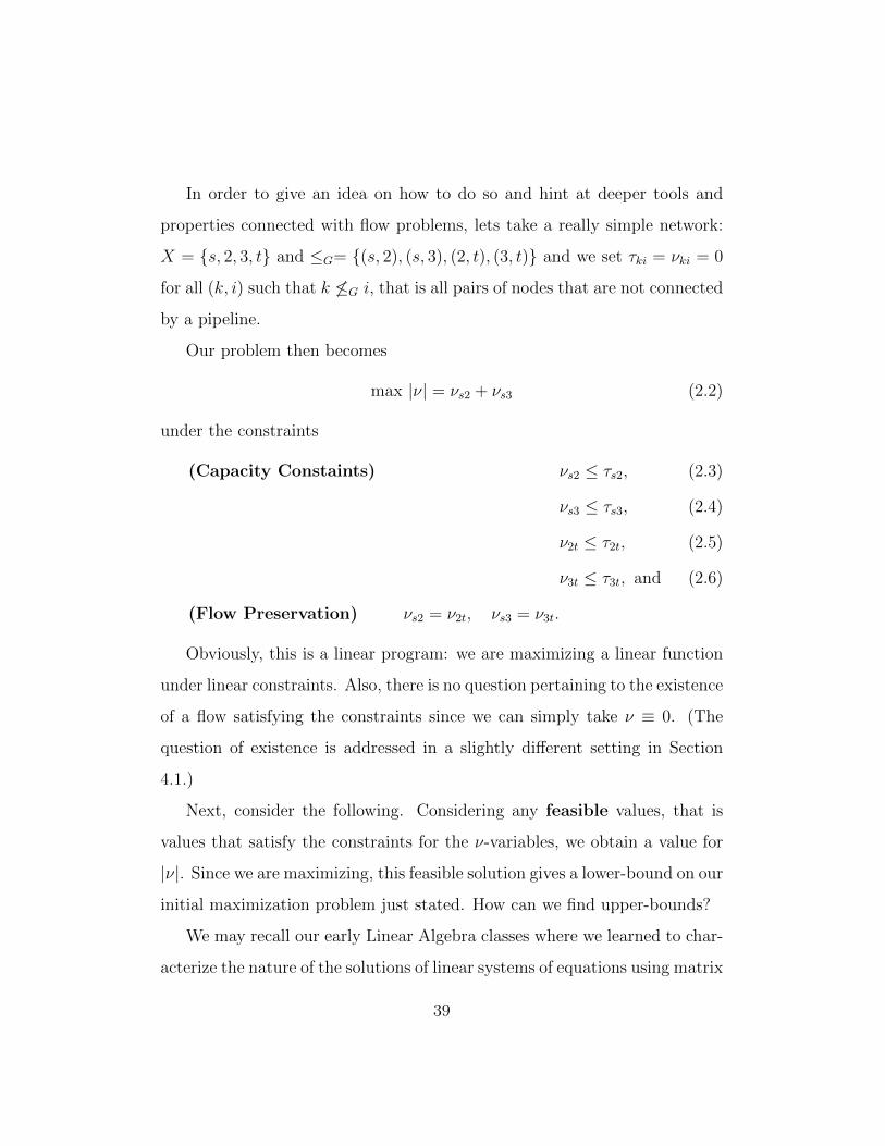
by a pipeline.
Our problem then becomes
max |ν| = νs2 + νs3 (2.2)
under the constraints
(Capacity Constaints) νs2 ≤ τs2, (2.3)
νs3 ≤ τs3, (2.4)
ν2t ≤ τ2t, (2.5)
ν3t ≤ τ3t, and (2.6)
(Flow Preservation) νs2 = ν2t, νs3 = ν3t.
Obviously, this is a linear program: we are maximizing a linear function
under linear constraints. Also, there is no question pertaining to the existence
of a flow satisfying the constraints since we can simply take ν ≡ 0. (The
question of existence is addressed in a slightly different setting in Section
4.1.)
Next, consider the following. Considering any feasible values, that is
values that satisfy the constraints for the ν-variables, we obtain a value for
|ν|. Since we are maximizing, this feasible solution gives a lower-bound on our
initial maximization problem just stated. How can we find upper-bounds?
We may recall our early Linear Algebra classes where we learned to char-
acterize the nature of the solutions of linear systems of equations using matrix
39
reduction techniques. We would place our system of linear equalities in a ma-
trix and consider linear combinations of these different equalities in order to
simplify our problem to where we could directly determine the rank of our
system. So, in this spirit, consider adding together (2.3) and (2.4) which
gives
νs2 + νs3 ≤ τs2 + τs3.
By recalling that |ν| = νs2 + νs3, we have found an upper-bound on our
function we wish to maximize. To apply this idea in general, we would
multiply each of our constraints by new y-variables and consider a linear
combination of these. Slightly abusing notation, our constraints are now
something like
ys2(νs2 ≤ τs2) + ys3(νs3 ≤ τs3) + y2t(ν2t ≤ τ2t) + y3t(ν3t ≤ τ3t)
+ y2(νs2 = ν2t) + y3(νs3 = ν3t).
Thus, we are now interested in minimizing all possible upper-bounds of
|ν| in (2.2), that is, in our case, linear combinations of the τki via the y-
coefficients. The constraints on these y-variables are given by the original
coefficients of (2.2), namely, linear combinations of each of the νki must add
up to their coefficients in (2.2).
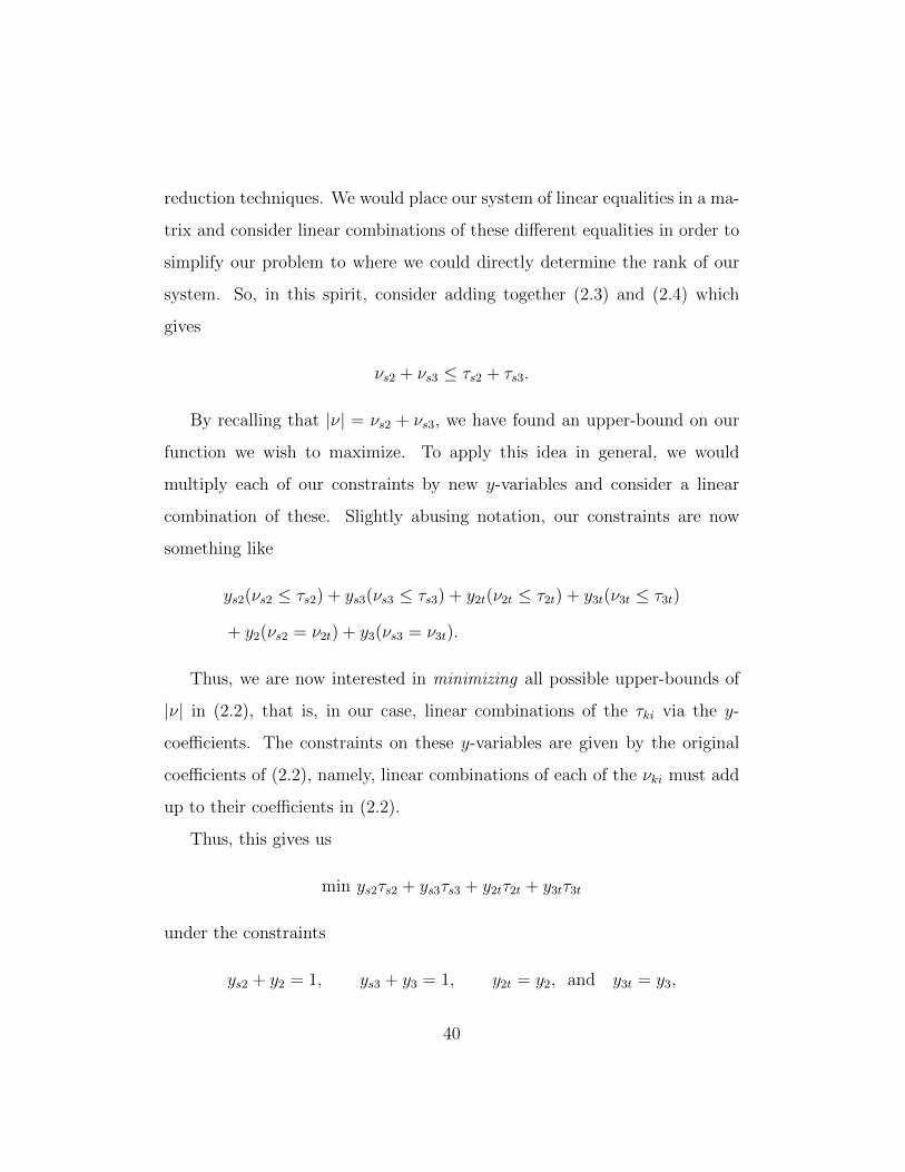
Thus, this gives us
min ys2τs2 + ys3τs3 + y2tτ2t + y3tτ3t
under the constraints
ys2 + y2 = 1, ys3 + y3 = 1, y2t = y2, and y3t = y3,
40
which, by combining of constraints becomes
min ys2τs2 + ys3τs3 + y2tτ2t + y3tτ3t (2.7)
under the constraints
ys2 + y2t = 1, and ys3 + y3t = 1.
Now, without loss of generality, suppose that none of our τki are equal.
Using this, we notice how the constraints become about assigning a value of
1 to one of ys2 and y2t and 0 to the other, in the first constraint. We do the
same with ys3 and y3t in the second constraint. That is, we are given binary
choices over our network: we must choose one arc from each set ys2, y2t and
ys3, y3t, such that the sum of their capacities are minimal. Notice how any
one of our 4 possible choices disconnects the source from sink. This rather
trivial example hints at something fundamental about linear programs.
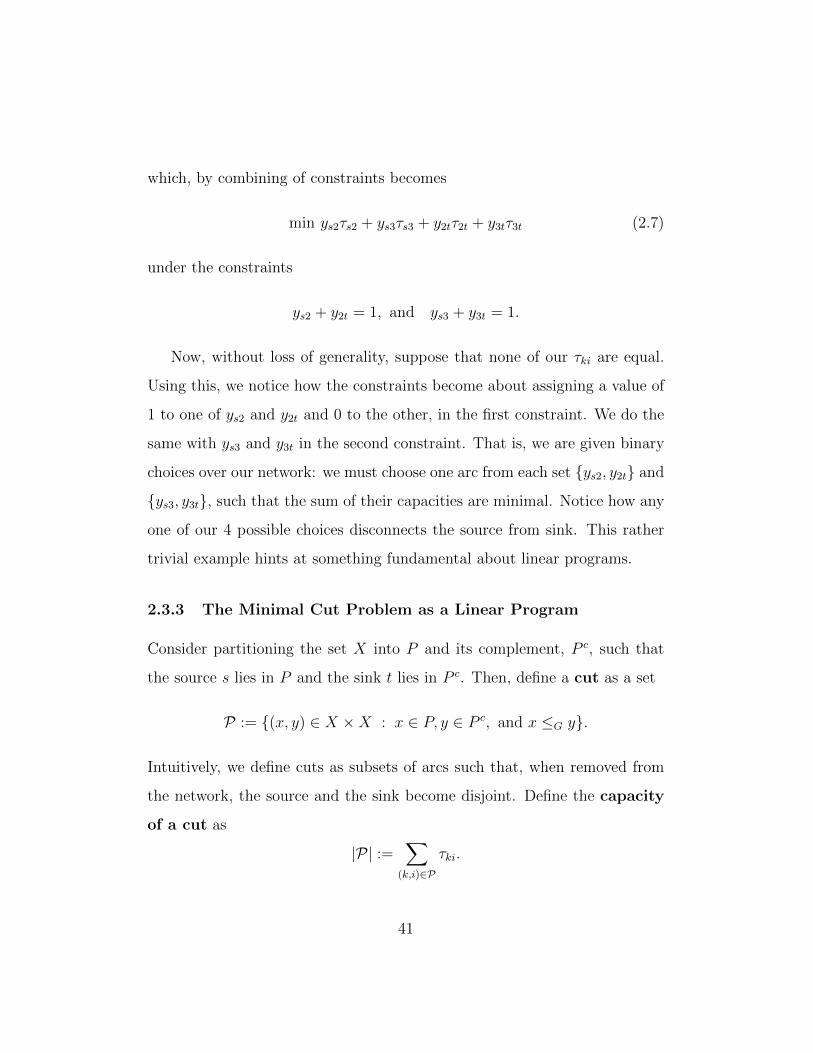
2.3.3 The Minimal Cut Problem as a Linear Program
Consider partitioning the set X into P and its complement, P c, such that
the source s lies in P and the sink t lies in P c. Then, define a cut as a set
P := (x, y) ∈ X ×X : x ∈ P, y ∈ P c, and x ≤G y.
Intuitively, we define cuts as subsets of arcs such that, when removed from
the network, the source and the sink become disjoint. Define the capacity
of a cut as
|P| :=∑
(k,i)∈P
τki.
41
With this terminology, we can say that our problem (2.7) of finding the
minimal cut in our network is the same as finding the maximal flow (under
some mild assumptions that will be soon addressed).
The general result pertaining to this is the well-known Max-Flow Min-Cut
Theorem due to Dantzig [FF56].
Theorem 2.4. (Max Flow-Min Cut.) Given a flow network, finding
its maximal flow value is the same as finding the minimal capacity over all
cuts.
Proof. We will not formally prove it but give a quick heuristic as to why
it is reasonable to expect the theorem to be true. Formally proving it can
be done in various ways, and Operations Researchers or Computer Scientists
will probably prefer using algorithmic reasoning or combinatorial results that
give insight into constructing solutions, see [Tuc06] for the combinatorial or
algorithmic reasoning.
The intuition of this solution is straightforward. Find the smallest cut
and assign to it its maximal flow. Now, this cut is at maximum capacity. If
we could pass more flow through the network using some alternative route,
this would violate the definition a cut. Intuitively, the smallest cut acts as a
bottleneck. Our flow is thus maximized.
Remark 2.10. This last result is in fact a particular case of the infinite
network Flow Theorem that stems as a consequence of the Abstract Disinte-
gration Theorem that is the main focus of this work (See Section 5.1.2, and
more generally all of Chapter 5).
42
2.3.4 Duality of Linear Programs and Convex Analysis
Lets briefly state some elements of linear programming theory. First, we
say that the problem is feasible if the solution space is non-empty–i.e. there
exists a solution. Second, we say that the problem is bounded if the solution
space is a bounded set. If the problem is one of maximization, we will be
interested in the problem being at least bounded above, and similarly a
minimization problem will be interesting if it is at least bounded below.
We say that a linear program is in its standard form if it is of the form
sup cTx
Ax ≤ b, x ≥ 0
where x represents a vector of variables over which to optimize, c a vector
of coefficients, A a matrix of constraints and b a vector of numbers. We also
have the standard form
inf yT b
yTA ≥ cT , y ≥ 0,
where A, b, and c are the same vectors as before, but we change our variables
under consideration from x to y according to a reasoning analogous to the one
done in the example of Section 2.3.2. Note that we have no issues pertaining
to the form of our problem because it is always trivial to transform a linear
programming problem into its standard form (we will not explicitly see how
to transform said problems, but any standard reference on the subject will
adress this, namely [Mic15], or [Tho]). We say that two problems of this type
are dual to each other.
43
Definition 2.6. (Hyperplane.) Let E be a vector space. Consider
f : E → R a continuous linear functional and β ∈ R \ 0. A hyperplane
is a set
H = x ∈ E : f(x) = β,
for which we often shorten notation by defining [f = β] := H. Intuitively,
in finite-dimensional settings, a hyperplane is a subspace of ”1 less dimen-
sion”. So, for example, a hyperplane in R3 is a plane–hence the ”hyperplane”
terminology as a natural extension of the concept of a plane embedded in
R3.
Definition 2.7. (Half-space.) A hyperplane ”separates” space into
two open half-spaces, that is
H+ = x ∈ E : f(x) > β and
H− = x ∈ E : f(x) < β.
We call H ∪H+ and H ∪H− closed half-spaces.
Now, linear inequalities of linear programming are closed half-spaces.
Hence, if the intersection of such half-spaces is bounded, it gives rise to
a convex polyhedral solution space. In fact, being the intersection of all
half-spaces that contain them is in fact a very nice way of characterizing
convex polyhedra [BL00]. This fact hints at the intimate link between linear
programming and convex analysis, the latter for which we will later briefly
introduce theory and tools in an attempt to bridge this gap.
The main result pertaining to linear programming is:
44
Theorem 2.5. (Strong Duality Theorem of Linear Programming.)
If a standard linear program is bounded feasible, then so is its dual problem,
and the optimal solutions of both coincide.
Proof. There exists an algorithmic proof of this via Dantzig’s famous Simplex
algorithm, which I admittedly never took the time to study in detail.
Before stating the result, we need a few definitions.
Definition 2.8. (Topological dual.) Let E be a vector space. Then,
the space of all real-valued continuous linear functionals on E, which we
denote E∗, is called the topological dual of E. For example, when E is a
Banach space, E∗ is a Banach space endowed with the sup-norm on linear
functionals(i.e. ||f || = sup
||x||≤1
||f(x)||).
Definition 2.9. (Duality bracket.) Let E be a vector space and E∗
its topological dual. We define the duality bracket or the dual pairing as
〈·, ·〉 : E∗ × E → [−∞,+∞].
For example, in a real vector space, the scalar product is an example of a
dual pairing. We will return to the abstract notion of duality in Section 3.3.1.
Definition 2.10. (Fenchel conjugation.) Let E be a vector space
and h : E → [−∞,+∞]. The Frenchel conjugate of h, is
h∗ : E∗ → [−∞,+∞]
f 7→ supx∈E〈f, x〉 − h(x).
45
Theorem 2.6. (Fenchel-Rockafeller duality.) Let E be a normed
vector space, and E∗ its topological dual. Define two convex functions on E,
f and g, that take values in R ∪ +∞. If there exists x0 ∈ E such that
f(x0) < +∞ and g(x0) < +∞ and f is continuous at x0, then,
infEf + g = max
x∗∈E∗−f ∗(−x∗)− g∗(x∗),
where f ∗ and g∗ represent the Fenchel conjugates of f and g, respectively.
Corollary 2.1. The strong duality principle of linear programming (Theorem
2.5) holds a consequence of Fenchel-Rockafellar duality.
Proof. We omit the proof.
For more on linear programming, see [Mic15] and [Tho], or any one the
standard references on the subject. For more on convex analysis, see Rock-
afeller’s classic Convex Analysis, [Roc70], with which the author is not very
familiar, or, Borwein and Lewis’ Convex Analysis and Nonlinear Optimiza-
tion, [BL00], which was used as the reference for this section, or many of the
references on the subject.
2.3.5 From Matching Problem to Flow Problem
Recall the matching problem of Section 2.2.2. There is a convenient way to
turn such a maximal matching problem into a source and sink maximal flow
problem.
Definition 2.11. (Bipartite Graph.) A bipartite graphG = X, Y,≤G is an undirected graph with two disjoint sets of nodes, X and Y , such that
every arc a ∈≤G is of the form x ≤G y for x ∈ X and y ∈ Y .
46
Given a bipartite graph G with parts X and Y , first, introduce a new
node to G, which we will call s. Connect s with directed arcs to every node
x ∈ X. Assign to each of these arcs a capacity of 1. Then, introduce a
new node t and have every every node of Y connected with a directed arc
to t. Again, have each of these arcs assigned a capacity of 1. On all other
nodes, assign a capacity of +∞. Then, finding a maximal matching becomes
equivalent to finding a maximal flow in our new network. Such a construction
is called a matching network.
47
Chapter 3: Kantorovich’s Optimal Transport
Problem or Optimal Transport as
a Linear Program
This section will draw heavily on Filippo Santambrogio’s book Optimal Trans-
port for Applied Mathematicians [San15] as well as Cedric Villani’s previously
cited monographs [Vil03], and [Vil08].
3.1 The Optimal Transport Problem as a Linear Pro-
gram: The Discrete Case
3.1.1 The Primal Problem: Minimizing the Cost of Transport
Now that we have developed linear programming tools lets recall our ”Not
so Simple” example of Section 2.2.1. We have a set X of J agents, each
supplying sj and consuming rj units of oil. We have their net consumption,
µj = sj − rj. So, some agents will be net producers (µj > 0), while others
will be net consumers (µj < 0). Without loss of generality, assume µj 6= 0
for all j, for we can neglect those having µj = 0 from the problem and work
around them if needed. We have a cost map, cki, giving us the cost moving
a unit of oil from k to i. This problem can be interpreted as finding a sort
of minimal cost flow, but it is better understood as a simple version of an
Optimal Transport problem: we are looking to minimize the cost under all
possible transport configurations such that supply meets demand. We will
note by νki, the quantity of goods transported from mine k to refinery i.
48
Also, we will take ν to be positive, which is a reasonable assumption if we
only consider net flow between agents.
We write out our total cost as
C :=∑k
∑i
ckiνki. (3.1)
Let
µ+j := max(µj, 0) =
µj if net producer,
0 if net consumer,
and µ−j := max(−µj, 0) =
0 if net producers,
−µj if net consumer,
respectively the positive part and the negative part of µj. In light of
our Optimal Transport setting, lets informally call them respectively the net
production part of µj and the net consumption part of µj.
Then, we wish to minimize C under these conditions. First,∑i
νji ≤ µ+j , for all j,
i.e the total commodities exiting a given agent j–its supply–cannot exceed its
net production part, µ+j . If j is not a net producer, than he supplies nothing:
he is better off keeping what he has produced (if anything) for himself.
Second, the equivalent demand condition is given by∑k
νkj ≥ µ−j , for all j,
with the same note about the case where j is not a net consumer: than he
demands nothing from others and consumes his own production, shipping
away his surplus.
49
We will return to this later in Section 4.1 as motivation for Chapter 5, the
main discussion of this work. But for now, we are interested in understanding
the dual linear program of the Optimal Transport problem as just defined.
3.1.2 The Dual Problem: Maximizing Kantorovich Potentials
Lets take a small example. Let K = 1, 2 and I = a, b, c, so that 2
mines are supplying 3 refineries. We note the suppliers with numbers and
the consumers with letters, as to distinguish them. Writing the problem
explicitly in its standard form we have:
minν
c1aν1a + c1bν1b + c1cν1c + c2aν2a + c2bν2b + c2cν2c
under constraints ν1a + ν1b + ν1c ≤ s1
ν2a + ν2b + ν2c ≤ s2
ν1a + ν2a ≥ ra
ν1b + ν2b ≥ rb
ν1c + ν2c ≥ rc.
Now, as we did in Section 2.3.2, we consider linear combinations of our
50
constraints through the y-variables that we introduce. Doing so, we obtain
maxy− s1y1 − s2y2 + r1ya + r2yb + r3yc
under constraints − y1 + ya ≤ c1a
−y1 + yb ≤ c1b
−y1 + yc ≤ c1c
−y2 + ya ≤ c2a
−y2 + yb ≤ c2b
−y2 + yc ≤ c2c.
Now, we are interested in the interpretation can be given to the dual
problem and its y-variables. Lets take the first constraint:
−y1 + ya ≤ c1a.
Note that y1 is the coefficient of −s1 and ya is the coefficient of r1 in the
maximization function. Thus, imagine a third-party involved in the transport
of the oil. This third-party would be the one solving the dual problem as
follows: he pays y1 per unit from supplier 1 in order to deliver these goods to
a who pays him ya per unit. Obviously, our third-party would then attempt
to maximize −s1y1−s2y2 +r1ya+r2yb+r3yc in order to have maximal profit.
The constraints then appear naturally: the third-party would be useless in
the problem if he could not perform the transportation at a lesser cost than in
the primal problem, hence his operational profits (i.e. −y1 +ya) are bounded
by the cost function of primal problem (i.e. c1a). As a matter of fact, in
this finite case, by the strong duality principle of linear programming, we
have that the third-party saturates every condition: his operational profit is
51
exactly the same as the cost function of the primal problem, assuming it is
bounded feasible.
Now, this example is somewhat trivial, but it sheds light on what has be-
come a very important concept of Kantorovich’s formulation: the y-variables
are referred to as Kantorovich potentials. The dual interpretation of the
problem turns out to be one the reasons that Optimal Transport is so widely
applicable to different problems. Also, this somewhat trivial example can be
directly extended to a continuous setting to obtain the modern formulation of
Kantorovich’s Optimal Transport duality that is far superior to Monge’s for-
mulation we introduced in Section 1.5. As Villani says on page 23 of [Vil03],
doing so is ”Very tedious!”. To avoid tedious work, in the spirit of a good
mathematician, lets give a sort of heuristic as to why we should expect to be
able to extend linear programming duality, and in particular Kantorovich’s
Optimal Transport duality, to a continuous setting.
3.1.3 Extending the Finite Linear Program to Kantorovich’s Op-
timal Transport Problem
Now, lets consider Kantorovich’s problem, which, as we have already said,
is the modern formulation of what is called the Optimal Transport problem.
The main difference between this formulation and Monge’s, is that we will
forego the idea of using the transport map T . Instead, let’s introduce the
notion of a transport plan.
Definition 3.1. (Probability space and probability measure.) Let
(X,Σ) be a measurable space. A measure P is called a probability measure if
P(X) = 1. In other words, a finite measure can always be normalized to 1 in
52
other to yield a probability measure. This turns (X,Σ) into a probability
space, which we will note P(X).
Definition 3.2. (Transport plan.) A transport plan is a probability
measure γ over the product probability space P(X×Y ), such that (πx)#γ =
α and (πy)#γ = β, where πx and πu are the projections of X × Y onto X
and Y , respectively. Then, we define the set of transport plans, denoted
Π(α, β) = γ ∈P(X × Y ) : (πx)#γ = α, (πy)#γ = β.
In the language of probability theory, Π(α, β) is the set of couplings of α
and β. Equivalently, it represents the set of joint laws over the product
space of X and Y . In this setting, α and β are called the marginal densities
of γ. Thus, the optimal transport problem in this form can be stated as one
of probability theory which consists in finding an optimal coupling or an
optimal joint law of two probability measures. That is, finding a coupling
which has two given densities as its given marginals such that a certain
quantity is optimal in a precise sense.
Remark 3.1. Villani gives a list of famous couplings which can be consulted
on page 7 of [Vil08].
Remark 3.2. Recall Section 3.1, where we developed the finite Optimal
Transport problem as a linear program. There, we opted for a transport
plan ν, which specified how many of units would be moved from, say, Mine
1 to Refinery a. Thus, we implicitly forewent our transport map specifying
where each unit would be moved. It is this shift that gave rise to the linear
programming structure. We notice even further that the situation where the
53
total number of commodities produced and the total number of commodities
desired to be consumed are equal is of particular interest. In this situation,
normalizing the quantities by the total amount gives us a slightly different
interpretation for ν: it represents the fraction of the total oil that is trans-
ported between a mine a refinery. Also, it draws obvious parallel with the
probability theory elements we just introduced: given an initial distribution
of goods supplied by the mines–i.e. an initial density distribution–, a final
distribution of goods that the refineries would like to consume–i.e. a final
density distribution–, find a ν–i.e. a transport plan assigning oil from mines
to refineries–such that the total cost of transporting the initial density to
the final density is minimal. Since linear programming consists in optimizing
linear functionals over convex sets, in order for the continuous extension to
hold, we need for the continuous extension of the finite linear combination of
costs to be a linear functional, and for the set of joint densities–i.e. ν–with
given marginals–i.e. the initial and final distributions–to still be convex when
the densities are extended to the continuous setting.
Proposition 3.1. (Convexity of the set of transport plans.) Let
X, Y , α, β, and Π(α, β) be defined as in Definition 3.2. Then, Π(α, β) is a
convex set.
Proof. The proof is trivial as the conditions for γ to lie in Π(α, β) are closed
under convex combinations.
Remark 3.3. Lets give a heuristic reasoning as to why the continuous ex-
tension of linear programming holds. Recall our cost function (3.1) C :=∑k
∑i ckiνki of Section 3.1.1. Now, in the case where ν represents a prob-
54
ability density–in particular it is a measure–over X × Y , we can write C
as
C =
∫X×Y
cki1k×i dν,
that is, C is a Lebesgue integral of a nonnegative simple measurable
function with respect to ν (we formally define such well-known functions
in Definition 5.4). Then, in a continuous setting, we can define the linear
functional to maximize as the limit of an increasing sequence of nonnegative
simple measurable functions (it is a well-known lemma of measure theory).
In other words, the continuous version of the problem can be defined as the
limit of a sequence of discrete problems. The difficulty lies in rigorously
ascertaining that the limit of the optimal solutions is in fact the optimal
solution of the limits. We omit this work for now. The proof (which the
author has not consulted) can be found in [Eva99], as Villani says on page
23 of [Vil03].
3.2 Kantorovich’s problem
Let X, Y , α, β and c be defined as above. Now, Kantorovich’s problem can
be stated as
(KP ) inf
Kγ(c) :=
∫X×Y
cki dγ(k, i) : γ ∈ Π(α, β)
.
Again, note that the integral in the above expression is in fact an expected
value.
Proposition 3.2. The set of transport plans Π(α, β) is never empty.
55
Proof. Define
α⊗ β : X × Y → [0,∞]
A×B 7→ α(A)β(B).
Then, one can easily show that α⊗ β always lies in Π(α, β).
This triviality is already an important step forward, as was hinted when
we introduced the discrete version as a linear program (Section 3.1). Now,
explicitly, the linear functional over Π(α, β) that we would like to minimize
is:
γ 7→∫
Π(α,β)
ckidγ(k, i).
It can be shown that it is indeed linear by defining the sum of two measures,
(γ+β)(·) as γ(·) +β(·). The other linear properties derive from the linearity
of the Lebesgue integral. So, we have in fact ”shown” that Kantorovich’s
problem is in fact a linear programming problem, giving rise to all the tools
we know and love, namely the duality principles.
3.3 Kantorovich Duality
3.3.1 An Abstract Duality as Bilinear Forms Separating Points
Before delving into Kantorovich duality (a most essential feature of the Op-
timal Transport problem), lets make a very important note on what we wish
to call abstract duality.
Definition 3.3. (Abstract Duality.) Consider an abstract vector
space E and another space E∗ (for now, just consider E∗ to be another
56
abstract space). We say that there is a duality between E and E∗, or
that E and E∗ are dual to each other, if there exists a bilinear form,
〈·, ·〉 : E × E∗ → R,
such that 〈x, ·〉 and 〈·, x〉 separates points. To separate points means
y 6= z =⇒ 〈x, y〉 6= 〈x, z〉, for all x ∈ E.
3.3.2 Kantorovich Duality
Now, lets try to find the duality in (KP). Recall the primal problem,
(KP ) inf
Kγ(c) :=
∫X×Y
cki dγ(k, i) : γ ∈ Π(α, β)
.
Here, Kγ(c) can be seen as a bilinear form, namely
〈c, γ〉 := Kγ(c),
where c is an integrable function with respect to γ (i.e. c ∈ L1(γ)) and γ is
probability measure over X × Y . We already explained how Kγ(c) is linear
in both c and γ, so we do in fact have a bilinear form. It distinguishes points,
if we consider c ∼= c′ if they coincide γ-almost everywhere (i.e. we define L1
as the usual quotient of maps that coincide almost everywhere).
Then, obviously, (KP) can be written as
infγ∈Π(α,β)
〈c, γ〉.
This highlights more directly the linear programming structure of the
problem, as Π(α, β) is convex, as shown in Proposition 3.1.
57
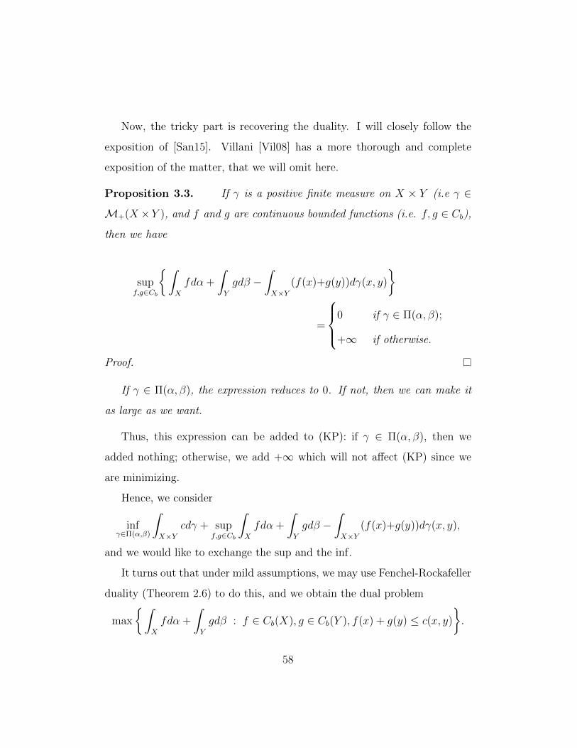
Now, the tricky part is recovering the duality. I will closely follow the
exposition of [San15]. Villani [Vil08] has a more thorough and complete
exposition of the matter, that we will omit here.
Proposition 3.3. If γ is a positive finite measure on X × Y (i.e γ ∈
M+(X ×Y ), and f and g are continuous bounded functions (i.e. f, g ∈ Cb),
then we have
supf,g∈Cb
∫X
fdα +
∫Y
gdβ −∫X×Y
(f(x)+g(y))dγ(x, y)
=
0 if γ ∈ Π(α, β);
+∞ if otherwise.
Proof.
If γ ∈ Π(α, β), the expression reduces to 0. If not, then we can make it
as large as we want.
Thus, this expression can be added to (KP): if γ ∈ Π(α, β), then we
added nothing; otherwise, we add +∞ which will not affect (KP) since we
are minimizing.
Hence, we consider
infγ∈Π(α,β)
∫X×Y
cdγ + supf,g∈Cb
∫X
fdα +
∫Y
gdβ −∫X×Y
(f(x)+g(y))dγ(x, y),
and we would like to exchange the sup and the inf.
It turns out that under mild assumptions, we may use Fenchel-Rockafeller
duality (Theorem 2.6) to do this, and we obtain the dual problem
max
∫X
fdα +
∫Y
gdβ : f ∈ Cb(X), g ∈ Cb(Y ), f(x) + g(y) ≤ c(x, y)
.
58
As we had hinted in Section 3.1.2, f and g are in fact the Kantorovich
potentials, and the interpretation given in that Section still holds, although
the result is a lot more technical.
3.4 Kantorovich Monge
3.4.1 Kantorovich’s Problem as a Generalization of Monge’s Prob-
lem
Next, we must understand why Kantorovich’s problem generalizes Monge’s
problem. In [San15], Santambrogio gives a thorough explanation of how to
go from one to the other. Here, we will limit ourself to reformulating and
rearranging what he has already said.
As we have already said, the change of focus has been one of going from
a transport map to a transport plan. We have allowed for a more general
solution to be found. Also, the solution space of our new problem, (KP),
is never empty. In this section, we will examine in which case these two
formalizations coincide.
Consider
γT := (id, T )#µ,
where
(id, T ) : X → X × Y
x 7→ (x, T (x)).
In other words, the map (id, T ) maps a point x ∈ X to its graph by T and
γT can be seen as the transport plan associated with the transport map T .
59
Proposition 3.4. The measure γT = (id, T )#α lies in Π(α, β) if and
only if T#α = β. In other words γT is a transport plan if and only if T
pushes α onto β.
Proof. Lets begin by showing that if γT is a transport plan, then T pushes
α onto β.
Let A ∈ B(X) and B ∈ B(Y ). Define Π(α, β) := Π. If γT ∈ Π, then by
applying definitions
α((id, T )−1(X ×B)
)= β(B).
But
(id, T )−1(X ×B) = T−1(B),
as you can easily check. Therefore, α(T−1(B)) = β(B), that is T pushes α
onto β, if γT is a transport plan. The other implication is trivial: if T#α = β,
then γT ∈ Π. Next, we note that (πk)#γT always equals α. That is((πk)#γT
)(A) = α
((id, T )−1(A× I).
But
(id, T )−1(A× I) = A.
Which establishes that
(πk)#γT = α.
So, γT ∈ Π.
Remark 3.4. We say of a transport plan γ between α and β that it is
deterministic, if there exists a measurable map T such that β = T#α.
60
Lemma 3.1. Let T be a deterministic transport plan. Then,∫X×Y
c(k, i)dγT (k, i) =
∫X
c(k, T (k))dα(k)
Proof. The proof is trivial, using the definition of γT .
Putting together Theorem 3.4 and Lemma 3.1, we can easily see that
an optimal transport map T will induce an optimal transport plan γT . By
recalling that we may be faced with the non-existence of a transport map
but that the set of transport plans is never empty, we can see how (KP)
generalizes (MP).
But still, how can we be sure that the cost of an optimal transport plan
of (KP) will be at most the cost of an optimal transport map of (MP)?
3.4.2 Kantorovich’s Problem as a Relaxation of Monge’s Problem
It can also be shown that Kantorovich’s problem is a relaxation of Monge’s
problem, in the variational sense that if Monge’s problem has a solution,
then Kantorovich’s problem will yield a solution equal or better. We do not
go into the details of this, but one can consult [San15] Section 1.5 on the
matter.
61
Chapter 4: The ”Existence Flow Problem”
In this section, we will address a variation of the maximal flow problem
that we mentioned as question (i) of Section 2.2.1, that is, instead of being
interested in an optimization problem, we turn to a more primitive problem
of finding the existence of a flow that satisfies consumption. In the language
of Optimal Transport, recall that the set of transport plans is always non-
empty: there is at least a trivial transport plan that will do the job. In the
case of the existence problem, we constrain the solution space so as to make
the possibility of a transport plan non-trivial: namely, we will require the
transport plan to be dominated by capacity map, and we will present a tool
which solves these classes of problems, even in cases not typically addressed
by Operations Research (i.e. infinite networks).
4.1 The ”Existence Flow Problem” as an Optimal Trans-
port Problem over a Finite Set and its Underlying
Vectorial Structure
Once again, we take the setting where have a set X of J agents, each sup-
plying sj and consuming rj units of oil, for which we can define their net
production µj = sj− rj. Before asking the question of optimal transport–i.e.
minimizing a cost map–we must first ask if there even exists a flow that can
satisfy the consumption demand. It is what we refer to informally as the
existence flow problem and it is an answer to question (i) of section 2.2.1.
Lets consider the set E of all maps from X to R. The set X being finite, E
62
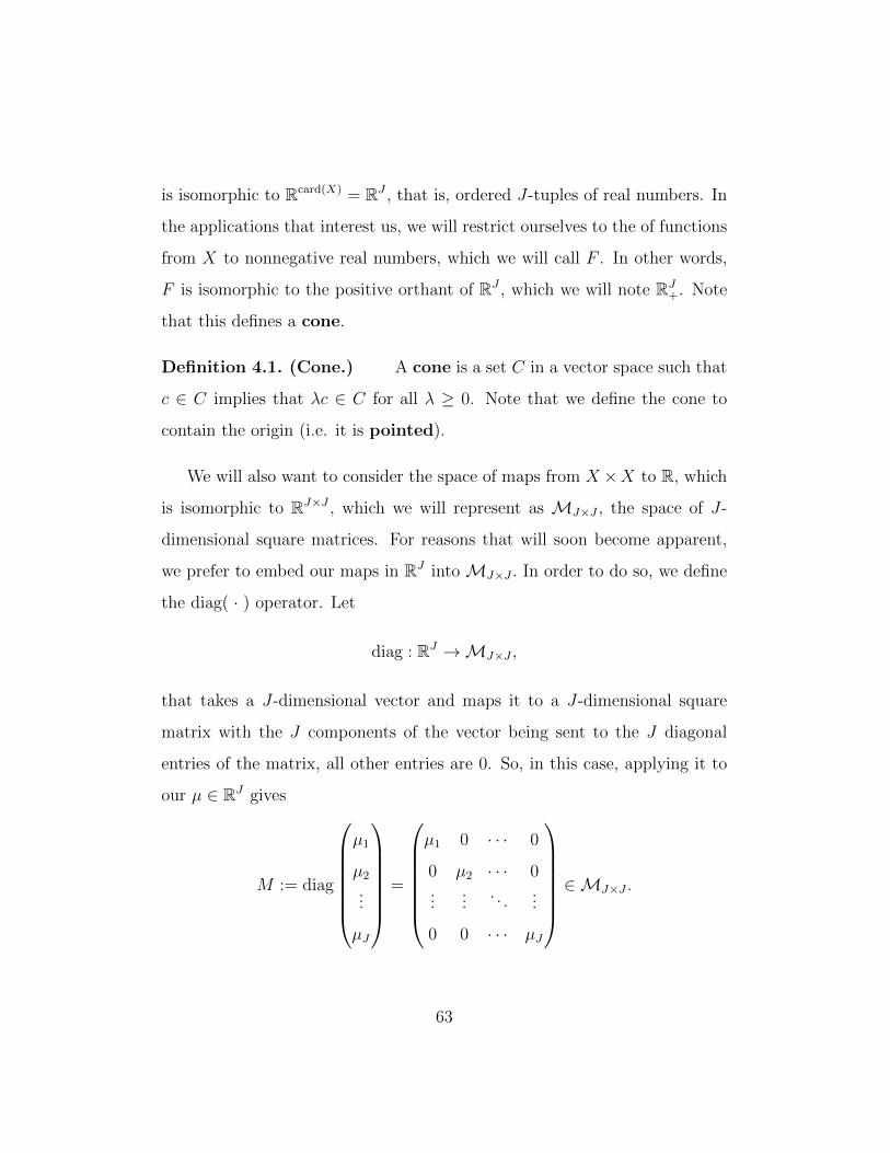
is isomorphic to Rcard(X) = RJ , that is, ordered J-tuples of real numbers. In
the applications that interest us, we will restrict ourselves to the of functions
from X to nonnegative real numbers, which we will call F . In other words,
F is isomorphic to the positive orthant of RJ , which we will note RJ+. Note
that this defines a cone.
Definition 4.1. (Cone.) A cone is a set C in a vector space such that
c ∈ C implies that λc ∈ C for all λ ≥ 0. Note that we define the cone to
contain the origin (i.e. it is pointed).
We will also want to consider the space of maps from X ×X to R, which
is isomorphic to RJ×J , which we will represent as MJ×J , the space of J-
dimensional square matrices. For reasons that will soon become apparent,
we prefer to embed our maps in RJ into MJ×J . In order to do so, we define
the diag( · ) operator. Let
diag : RJ →MJ×J ,
that takes a J-dimensional vector and maps it to a J-dimensional square
matrix with the J components of the vector being sent to the J diagonal
entries of the matrix, all other entries are 0. So, in this case, applying it to
our µ ∈ RJ gives
M := diag
µ1
µ2
...
µJ
=
µ1 0 · · · 0
0 µ2 · · · 0...
.... . .
...
0 0 · · · µJ
∈MJ×J .
63
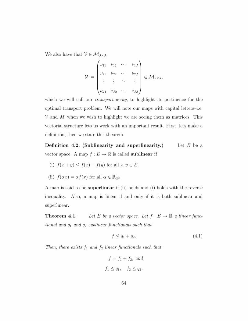
We also have that V ∈ MJ×J ,
V :=
ν11 ν12 · · · ν1J
ν21 ν22 · · · ν2J
......
. . ....
νJ1 νJ2 · · · νJJ
∈MJ×J ,
which we will call our transport array, to highlight its pertinence for the
optimal transport problem. We will note our maps with capital letters–i.e.
V and M–when we wish to highlight we are seeing them as matrices. This
vectorial structure lets us work with an important result. First, lets make a
definition, then we state this theorem.
Definition 4.2. (Sublinearity and superlinearity.) Let E be a
vector space. A map f : E → R is called sublinear if
(i) f(x+ y) ≤ f(x) + f(y) for all x, y ∈ E.
(ii) f(αx) = αf(x) for all α ∈ R≥0.
A map is said to be superlinear if (ii) holds and (i) holds with the reverse
inequality. Also, a map is linear if and only if it is both sublinear and
superlinear.
Theorem 4.1. Let E be a vector space. Let f : E → R a linear func-
tional and q1 and q2 sublinear functionals such that
f ≤ q1 + q2. (4.1)
Then, there exists f1 and f2 linear functionals such that
f = f1 + f2, and
f1 ≤ q1, f2 ≤ q2.
64
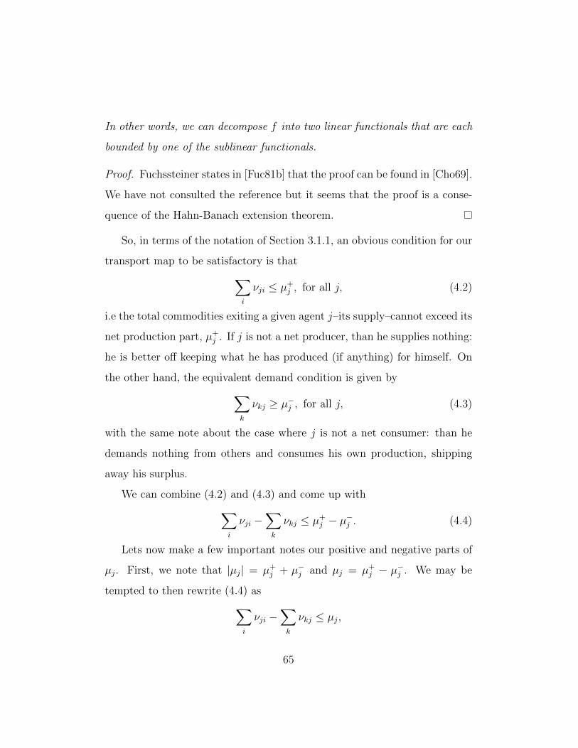
In other words, we can decompose f into two linear functionals that are each
bounded by one of the sublinear functionals.
Proof. Fuchssteiner states in [Fuc81b] that the proof can be found in [Cho69].
We have not consulted the reference but it seems that the proof is a conse-
quence of the Hahn-Banach extension theorem.
So, in terms of the notation of Section 3.1.1, an obvious condition for our
transport map to be satisfactory is that∑i
νji ≤ µ+j , for all j, (4.2)
i.e the total commodities exiting a given agent j–its supply–cannot exceed its
net production part, µ+j . If j is not a net producer, than he supplies nothing:
he is better off keeping what he has produced (if anything) for himself. On
the other hand, the equivalent demand condition is given by∑k
νkj ≥ µ−j , for all j, (4.3)
with the same note about the case where j is not a net consumer: than he
demands nothing from others and consumes his own production, shipping
away his surplus.
We can combine (4.2) and (4.3) and come up with∑i
νji −∑k
νkj ≤ µ+j − µ−j . (4.4)
Lets now make a few important notes our positive and negative parts of
µj. First, we note that |µj| = µ+j + µ−j and µj = µ+
j − µ−j . We may be
tempted to then rewrite (4.4) as∑i
νji −∑k
νkj ≤ µj,
65
that is, the net flow out of j cannot exceed the net production of j. But, for
reasons that will soon become apparent, condition (4.4) is superior. Second,
note that (4.4) is equivalent to the condition that the sum over the jth column
of V minus the sum over the jth row of V not exceed µj. Then, obviously,
the map
V 7→∑i
νji −∑k
νkj, (4.5)
is linear. It can explicitly be given as
V 7→ (VT − V)1,
where 1 is a J-dimensional column vector of 1s in the standard basis. Third,
note that µ+j is sublinear and µ−j is superlinear.
Now, consider taking the linear map from (4.5) and the two sublinear
maps µ+j and (−µ−j ). Therefore, we can apply Theorem 4.1 to find
f1 ≤ µ+j and f2 ≤ −µ−j such that f1 + f2 = f.
So, Theorem 4.1 lets us find f1 and f2 which can be seen to be respectively
some sort of a production plan and a consumption plan. But, we already
knew that f1 = V 7→∑
i νji and f2 = V 7→∑
k νkj, as in (4.2) and (4.3).
Although in this case our theorem is rather trivial, it begs the question of
generalization. So, lets make a few notes before addressing the question of
generalizing this result.
66
4.2 The ”Existence Flow Problem” as an Optimal Trans-
port Problem over a Finite Set and its Underlying
Measure-Theoretic Structure
Before attacking this problem, lets work out some important formalities.
For A ⊂ X, and i, k ∈ X \ A, define
ν(A, i) :=∑j∈A
νji and
ν(k,A) :=∑j∈A
νkj,
that is, the total flow out of A and the total flow into A, respectively. We
can extend this definition to consider, for A,B ⊂ X:
ν(A,B) :=∑i∈B
∑j∈A
νji,
that is the total flow out of A and into B. Similarly, we can extend all of our
functions on our network to subsets of X. Let
τ(A,B) :=∑i∈B
∑j∈A
τji, and
µ(A) :=∑i∈A
µi,
that is, the total capacity between two subsets of agents A and B and the
total net production of A, respectively.
Now, these are more than mere notational tricks. Consider the map
ν(A, · ) 7→ ν(A,B).
67
Obviously, this map is countably additive, equal to zero on the empty set
and defined for all B ∈ 2X , the power-set of X. The properties are identical
if we consider
ν( · , B) 7→ ν(A,B).
Thus, we have defined a bimeasure–i.e. a signed measure in both variables–
over 2X×X , the trivial σ-algebra over X ×X. Also, µ( · ) is a measure over
2X .
Now, this is a huge step forward. Why? Because noticing the measure-
theoretic nature of the problem will be precisely what takes us to the next
step in considering infinite networks. Lets build a few more measure-theoretic
tools in order to answer questions (i) and (iii) of Section 2.2.
4.2.1 A motivating example
Now, consider Ω = 1, 2, a network of 2 points, with its power-set as a
σ-algebra, that is Σ = 2Ω. Let m be the counting measure on Σ in order
to obtain a (trivial) measure space, (Ω,Σ,m). Now, consider L1(m), that
is the space of real-valued functions on Ω whose absolute value has a finite
integral with respect to m over Ω–i.e.
µ ∈ L1(m) ⇐⇒∫
Ω
|µ|dm <∞.
The integral evaluates to∫Ω
|µ|dm =∑j∈Ω
|µ(j)|m(j) =∑j∈Ω
|µ(j)|.
Thus, in this setting, L1(m) represents the space of all real-valued func-
tions over Ω (because Ω is finite). We have already seen this space as an
isomorphism of RJ . Consider E, a vector space (as in Theorem 4.1).
68
Let Q : E → L1(m), and define
Q(x)(j) = qj(x),
where x ∈ E, j ∈ Ω, and qj are defined as in Theorem 4.1–i.e. they are
sublinear.
Obviously, Q is then sublinear. What is more, we can now write condition
(4.1) in Theorem 4.1 as
µ(x) ≤∫
Ω
Q(x)dm, for all x ∈ E.
Then, we get the result that there exists a linear operator T : E → L1(m),
such that
T ≤ Q
and
µ(x) =
∫Ω
T (x)dm, for all x ∈ E.
The question we must now face is that of generalizing this result to more
abstract measure spaces; this example was all built around trivial objects.
As a matter of fact, this is what is done in [Fuc81b] by Fuchssteiner. We will
get to these considerations shortly.
69
Chapter 5: Mathematical Tools : Disintegra-
tion Method
5.1 Infinite Networks
Remark 5.1. In the previous sections, the parameter µ was defined as excess
supply over demand–i.e. µj = sj − rj. In a unfortunate turn of events, we
chose µ as production while Fuchssteiner chose µ as consumption. There is
obviously no fundamental difference, but the reader might be confused if he
is not aware that µ in the next section is ”different” than µ in the previous
section. It was too late to make the according modifications when we were
made aware of the situation.
In [Fuc81b], Fuchssteiner generalizes the flow problem to an infinite net-
work. We have already hinted at an approach to do so in section 4.2. Now,
let X be an infinite set, which we equip with a σ-algebra, Σ. Recall the
measures we introduced in that section. Namely, for A,B ⊂ X,
ν(A,B) :=∑i∈B
∑j∈A
νji,
τ(A×B) :=∑i∈B
∑j∈A
τji, and
µ(A) :=∑i∈A
µi,
respectively the total flow out of A and into B, the total capacity from A
to B and the total net consumption of A. The ”Existence Flow Problem”,
is now one of finding a flow ν–i.e. a bimeasure– that respects the following
conditions.
70
(i) The flow is positive : ν(A,B) ≥ 0, for all disjoint A,B ∈ Σ.
(ii) The flow is possible : ν(A,B) ≤ τ(A×B), for all A,B ∈ Σ.
(iii) The flow satisfies consumption : µ(A) ≤ ν(A,Ac) − ν(Ac, A) for all
A ∈ Σ.
To solve this problem, in a very similar fashion than we did with our
trivial example of Section 4.2.1, we will need a more abstract disintegration
theorem. It will be our main tool in solving the problem.
5.1.1 Abstract Disintegration Theorem
This theorem and its proof can be found in [Fuc81a]. We will rewrite the
proof in more details and in our own words, but all the ideas are owed to
Fuchssteiner.
In this section, we first begin by extending the concepts of sublinearity
and superlinearity (Definition 4.2) to measures. Then we give a couple of
straightforward definitions needed to state our main result.
Definition 5.1. (Submeasure and supermeasure.) Given (X,Σ),
a submeasure ρ : Σ→ R≥0 is a set function such that:
(i) ρ(A ∪B) ≤ ρ(A) + ρ(B) for all A,B ∈ Σ
(ii) If An ∈ Σ is a decreasing sequence, that is An+1 ⊂ An for all n ∈ N,
then
infn∈N
ρ(An) = ρ(∩n∈N
An).
Equivalently, a supermeasure ξ : Σ→ R≥0 is a set function such that:
71
(i) ξ(A ∪B) ≥ ξ(A) + ξ(B) for all A ∩B = ∅
(ii) If An ∈ Σ is an increasing sequence, that is An ⊂ An+1 for all n ∈ N,
then
supn∈N
ξ(An) = ξ(∪n∈N
An).
A submeasure (resp. supermeasure) is a measure where additivity is replaced
by subadditivity (resp. superadditivity).
Remark 5.2. Let m be a positive, finite measure: m : Ω→ R≥0 and define
ρ(A) = m(A×Ac) for all A ∈ Σ. Then ρ is a submeasure. We will soon see
such a submeasure which represents the capacity over a flow network (see
Proposition 5.1).
Definition 5.2. (L1∗(Ω), a certain variant of an L1 space.) In order
to deal with certain formalities, we will consider the extended real number
system R∗ = R ∪ −∞ (where 0 · −∞ = 0, x+−∞ = −∞, for all x ∈ R).
Then, let L1∗(Ω) be the cone of measurable R∗-valued functions f on
Ω such that the positive part f+ = max(f, 0) ∈ L1(Ω). Note that f ≡
−∞ ∈ L1∗(Ω).
Definition 5.3. (Convex cone.) A convex cone F is a cone (see
Definition 4.1) that is also closed under convex combinations–i.e ϕ1, ϕ2 ∈ F
implies tϕ1 + (1 − t)ϕ2 ∈ F , for all t ∈ [0, 1]. Note that this implies that
aϕ1 + bϕ2 ∈ F for all a, b ∈ R≥0.
Definition 5.4. (Simple measurable functions.) Let (Ω,Σ) be a
measurable space. Then, one way of characterizing a simple measurable
function on Ω, is to consider the functions that take on a finite number
72
of values (i.e. simple) and such that ϕ−1(x) ∈ Σ for all x ∈ R≥0 (i.e.
measurable). (Obviously, the codomain of the function must itself be a mea-
surable space for the definition to make sense. We often take R with the
Borel σ-algebra.)
Remark 5.3. We note the following:
(i) The space Φ of all simple nonnegative measurable functions defines
a convex cone.
(ii) Every simple nonnegative measurable function can be represented in
its canonical form:
ϕ =k∑
n=1
λn1An (5.1)
where k ∈ N, λn ≥ 0, An ∈ Σ are pairwise disjoint, and 1A denotes the
indicator function of the set A. Then, obviously (5.1) is not the only
way of defining ϕ: we will see another useful form later in Lemma 5.2.
Definition 5.5. (Compatible pre-order.) A pre-order is a reflexive
and transitive binary relation on a set: a partial order without antisymmetry.
We say that an order relation is compatible with the structure of the
cone if ϕ′ ≤ ϕ′′ and γ′ ≤ γ′′ implies ϕ′ + γ′ ≤ ϕ′′ + γ′′ and λϕ′ ≤ λϕ′′ for all
λ ≥ 0: the inequalities can be handle in the usual way.
Remark 5.4. Recalling the decomposition of sublinear functionals (The-
orem 4.1), the linear functionals we obtained (f1, f2) directly inherit the
monotonicity properties from the q1, q2 that bound them. This is because in
a vector space, order relations are characterized by the positive orthant. But
73
in the case of a convex cone, we do not have this convenience. In order to
circumvent this problem, we must introduce a somewhat mysterious order
structure, that we now define.
Definition 5.6. (Localized order on Ω and Ω-monotonicity.) Let
F be an abitrary convex cone and (Ω,Σ, µ) a measure space. As we will soon
see, we will be interested in operators F → L1∗(Ω), for which we will introduce
a particular kind of order on F , which we will call an order that is localized
on Ω: consider ≤ω |ω ∈ Ω a family of pre-order relations compatible
with the structure of the convex cone F . An operator Q : F → L1∗(Ω) is
Ω-monotone if for all ϕ, φ ∈ F , Q(ϕ) ≤ Q(φ)µ-almost everywhere on the
set ω ∈ Ω |ϕ ≤ω φ.
We give a very well-known theorem on the representation of functionals
with measures, that we will use in the proof of the Abstract Disintegration
Theorem 5.1 (we do not prove the following lemma).
Lemma 5.1. (Radon-Nikodym Theorem.) Let (Ω,Σ) be a mea-
surable space, on which we have two σ-finite measures, µ and ν, such that
µ ν–i.e. µ is absolutely continuous with respect to ν–,then there exists
a positive measurable function g : Ω→ R≥0 such that
ν(A) =
∫A
gdµ, for all A ∈ Σ.
We note g := dνdµ
and call it the Radon-Nikodym derivative, for its obvi-
ous parallel with the classic fundamental theorem of calculus (with the Rie-
mann integral).
We are now ready to state our main result.
74
Theorem 5.1. (Abstract disintegration theorem.) Let (Ω,Σ, µ)
be a measure space, F a convex cone, f : F → R∗ a linear functional and
Q : F → L1∗(Ω) a sublinear Ω-monotone operator with
f(ϕ) ≤∫
Ω
Q(ϕ)dµ for all ϕ ∈ F.
Then, there is a Ω-monotone linear operator T : F → L1∗(m) with
T ≤ Q (5.2)
such that
f(ϕ) ≤∫
Ω
T (ϕ)dµ for all ϕ ∈ F. (5.3)
Proof. The proof is found in [Fuc81a].
The first step is to use a classic sandwich theorem giving the existence
of a linear functional sandwiched in between a superlinear functional and a
sublinear functional (Fuchssteiner appeals to one of the theorems in [Fuc77]).
First, consider Φ = ϕ : Ω → F | ϕ is a simple measurable function, in
which we introduce the preorder
ϕ1 ≤ ϕ2 ⇐⇒ ϕ1(ω) ≤ω ϕ2(ω), µ-almost everywhere on Ω.
Consider ϕq7→∫
ΩQ(ϕ)dµ, which is obviously sublinear and Ω-monotone. We
will want to ”superlinearize” f in order to apply the sandwich theorem. Let
δ(ϕ) =
f(ϕ(ω)) if ϕ is constant on Ω;
−∞ if otherwise,
75
and note that δ is obviously superlinear and is such that δ ≤ q. We can
quickly note that the disintegration theorem would hold for f being already
superlinear, as we would hence avoid this ”superlinearization” step. Hence,
applying a classical sandwich theorem ([Fuc77] or [Fuc74]), we get a linear
monotone functional ν such that δ ≤ ν ≤ q, and we can choose ν to be
maximal amongst all such functionals. (The maximality argument is an
easy application of Zorn’s lemma: the set of such functionals is nonempty,
partially ordered pointwise, and all the chains are bounded above by q.)
Now, we use our functional ν in order to define,
d : Σ× F → R∗
(A, x) 7→ ν(1Ax).
Now, the rest of the proof lies in characterizing d. Lets break it down into
small steps.
First, lets show that d(·, x) is a signed measure on Ω. Obviously, it is
finitely additive by linearity of ν, and d(∅, x) = 0. To show its σ-additivity,
consider An be a sequence of pairwise disjoint sets in Σ. Let φ ∈ Φ and
define
ρ(φ) = ν(1Bφ) + lim infm→∞
m∑n=1
ν(1Anφ), (5.4)
where B = (∪An)c. Obviously, ρ is superlinear, and recall that ν ≤ q, which
76
yields
ρ(φ) ≤ q(1Bφ) +∞∑n=1
q(1Anφ)
=
∫B
Q(φ(ω))dµ+∞∑n=1
∫An
Q(φ(ω))dµ
= q(φ).
Thus, ρ ≤ q. Now, we want to show that ρ ≥ ν. Let
Cm =
(B ∪
m⋃n=1
An
)c=
∞⋃n=m+1
An.
Obviously, Cm ↓ ∅, which implies
lim supm→∞
ν(1Cmφ) ≤ lim supm→∞
q(1Cmφ) = lim supm→∞
∫Cm
Q(φ(ω))dµ = 0,
where the last equality is given by the σ-additivity of the integral. We can
now reapply the sandwich theorem to obtain a monotone linear ν such that
δ ≤ ν ≤ ρ ≤ ν ≤ q, but ν was already chosen to be maximal, hence
ν = ν = ρ. Now, in (5.4), choose φ = 1∪Anx, which yields
d(∪An, x) = d((∪An)c, x)︸ ︷︷ ︸=0
+lim infm→∞
m∑n=1
ν(1An1∪Anx)
⇐⇒ d(∪An, x) = lim infm→∞
m∑n=1
d(An, x),
then d(·, x) is a signed measure on Ω.
Second, we would like to apply a Radon-Nikodym argument, by showing
that it is absolutely continuous with respect to µ. We start by noticing that
x ≤ω y for µ-almost all ω ∈ A implies that 1Ax ≤ 1Ay. By monotonicity of
ν, we get that d(A, x) = ν(1Ax) ≤ ν(1Ay) = d(A, y). Now, we show that
77
this implies the absolute continuity of d(·, x) with respect to µ. Let A ∈ Σ
such that µ(A) = 0. Then, the Ω-monotonicity on A holds trivially for any
two functions in Φ, and, in particular, we get x ≤ω 0 and 0 ≤ω x, which then
implies that d(A, x) = d(A, 0) = 0.
We can now apply Radon-Nikodym to get a measurable function, that
we will note T (x), such that
d(A, x) =
∫A
T (x)dµ.
Third, we deduce the required properties of T (·). By δ ≤ ν ≤ q, we
obviously have that d(A, x) ≤∫AQ(x)dµ, for all A ∈ Σ, in particular for
A = Ω. So, this shows that f(x) ≤ d(Ω, x) =∫
ΩT (x)dµ, which is (5.3), also,
we get that T (x) ∈ L1∗(Ω), (i.e. T (x) is absolutely integrable with respect to
µ). Linearity of ν means that d(A, ·) is linear, which in turns implies that
T (·) is linear.
Now, all we have left to do is show the Ω-monotonicity of T (·). Let
x, y ∈ F , and consider B = ω ∈ Ω | x ≤ω y. We have already shown that
this implies d(B, x) ≤ d(B, y). Hence, if T (x)(ω) > T (y)(ω) for a certain
subset A ⊂ B such that µ(A) > 0, this would be a contradiction (without
loss of generality, assume∫AT (x)dµ > −∞).
5.1.2 Disintegration Theorem applied to Flow Problem
To show how the theorem can be applied to pertinent problems, we will apply
it to the flow problem. Recall that a flow problem is a particular case of
an optimal transport problem (See Section 2.3): therefore, the disintegration
theorem can be applied to solve certain classes of optimal transport problems.
78
In [HT78], they highlight the intimate connection between disintegrating
measures that are dominated by a certain measure (the situation we are now
considering) and the Max-flow Min-cut theorem (which they rightfully call
the Ford-Fulkerson theorem).
Now, we set up our flow problem in order to use the disintegration theo-
rem. We have an infinite network, X, with a σ-algebra Σ and a measure µ
(as defined in the beginning of this Section 5.1). Let Ω = X ×X equipped
with the product σ-algebra Σ⊗Σ and a measure τ . Then, A×B ∈ Σ⊗Σ
represent arcs from out network.
Consider once again F the convex cone consisting of all non-negative
simple measurable functions on X.
Lemma 5.2. Let ϕ =∑k
n=1 λn1An ∈ F , its canonical representation.
Then, there exists Bn ∈ Σ, δn ≥ 0, such that
ϕ =k∑
n=1
δn1Bn ,
B1 ⊃ B2 ⊃ · · · ⊃ Bk, and δn ≥ 0.
Proof. First, order the values of λn in the canonical form of ϕ by increas-
ing order, label them λ(1), λ(2), . . . , λ(k), and label their corresponding sets
A(1), A(2), . . . , A(k). Then, define B1 = ∪An and δ1 = λ(1), B2 = ∪An \ B1
and δ2 = λ(2) − λ(1), . . . , Bk = ∪An \ Bk−1 and δk = λ(k) − λ(k−1). Then,
obviously, the Bk form a decreasing chain, the δ are positive by the order-
ing of the λ, and a straightforward computations yields that the two forms
coincide.
79
Define
ϕ : Ω→ R≥0
(i, j) 7→ max(ϕ(i)− ϕ(j), 0).
Note that ϕ ∈ L1∗(Ω). We will want to consider the operator
Q : F → L1∗(Ω)
ϕ 7→ ϕ.
We need one more lemma on Q before stating the next proposition.
Lemma 5.3.
(i) The operator Q is sublinear.
(ii) Consider ϕ1, ϕ2 ∈ F such that
ϕ2(j) > 0 =⇒ ϕ1(j) = supi∈X
ϕ1(i),
Then Q(ϕ1+ϕ2) = Q(ϕ1)+Q(ϕ2), which we will call a partial linearity.
Proof. The fact that Q is sublinear is trivial, as we only need to apply the
sublinearity of the maximum. The second part is done by direct computation.
Then, Fuchssteiner shows
Proposition 5.1. The following are equivalent :∫X
ϕdµ ≤∫
Ω
ϕ dτ for all ϕ ∈ F, (5.5)
and
µ(A) ≤ τ(A× Ac) for all A ∈ Σ. (5.6)
80
Proof. To prove (5.5) =⇒ (5.6), simply take ϕ = 1A and notice that this
gives ϕ = 1A×Ac , which yields directly the result. To prove (5.6) =⇒ (5.5)
is less trivial, but the only difficulty is is combining Lemmas 5.3 and 5.2.
Using the definition of the integral and (5.6),∫X
ϕ dµ =k∑
n=1
δnµ(Bn) ≤k∑
n=1
δnτ(Bn ×Bcn)
=k∑
n=1
δn
∫Ω
Q(1Bn) dτ =
∫Ω
k∑n=1
Q(δn1Bn) dτ.
Now, in general, Q is not linear (but sublinear), but we would like to use
the partial linearity we discovered. We consider the sum in the integral,
Q(δ11B1) +Q(δ21B2) + ...+Q(δk1Bk),
and we note that by construction of the sequence of sets Bn, considering
δ21B2 as ϕ2 and δ11B1 as ϕ1, we can apply lemma 5.3 to the first two terms
of the sum, yielding
Q(δ11B1 + δ21B2) +Q(δ31B3) + · · ·+Q(δk1Bk).
We can again reapply the lemma to the two first terms in the sum, and
proceed inductively, until we get∫Ω
k∑n=1
Q(δn1Bn) dτ =
∫Ω
Q(k∑
n=1
δn1Bn) dτ =
∫Ω
Q(ϕ) dτ =
∫Ω
ϕ dτ,
which yields the inequality we wanted to show.
Remark 5.5. A few notes on condition (5.6). If we interpret µ(A) as being
the total consumption of the agents in A, as in the Section 4.2, and τ(A ×
Ac) as the total capacity of the arcs going into A, then the condition (5.6)
81
says that we have sufficient import capacity for A. Note that this implies
µ(X) ≤ τ(X × ∅) = 0, which means that as a particular case of sufficient
import capacity, we demand that net consumption be dominated by net
production. Obviously, without respecting this condition for all A ∈ Σ, we
cannot hope to find a flow satisfying the network. Also, as τ is positive and
finite, we can define a measure ρ(A) = τ(A×Ac), which is a submeasure (See
definition 5.1). So, the equivalence given by Proposition 5.1 really gives us the
bridge between decomposition of a linear functional bounded by a sublinear
functional and decomposition of a measure bounded by a submeasure. The
key fact is that their is an analogy between the convex cone of nonnegative
simple measurable functions as linear combinations of indicator functions,
and the positive orthant of a vector space where its elements (i.e. vectors)
are positive linear combinations of its basis.
Proposition 5.2. Consider the following family of pre-orders on F :
ϕ1 ≤ω ϕ2 ⇐⇒ ϕ1(x) ≤ ϕ2(x) and ϕ1(y) ≥ ϕ2(y),
where ω = (x, y). Then, the operator
Q : F → L1∗(Ω)
ϕ 7→ ϕ
is Ω-monotone.
Proof. The proof is given by a straightforward computation.
Before stating the flow theorem, we need a well-known lemma, which we
will not prove:
82
Lemma 5.4. (Lebesgue’s Dominated Convergence Theorem.) Let
ϕn be a sequence of positive µ measurable functions on X that converges
pointwise to a measurable function ϕ and that is dominated by an integrable
function γ, then
limn→∞
∫X
ϕndµ =
∫X
ϕdµ.
Theorem 5.2. (Flow theorem.) The following are equivalent:
(i) There is sufficient import capacity :
µ(A) ≤ τ(A× Ac) for all A ∈ Σ.
(ii) There exists a bimeasure ν on Ω (i.e the flow) such that:
(a) The flow satisfies consumption :
µ(A) ≤ ν(A,X), for all A ∈ Σ
(b) The flow is possible :
ν(A,B) ≤ τ(A× (B ∩ Ac)), for all A,B ∈ Σ
(c) The flow is positive :
ν(A,B) ≥ 0, for all disjoint A,B ∈ Σ
In other words, there is a positive and possible flow that satisfies consumption
if and only if there is sufficient import capacity.
83
Proof. The proof consists in a straightforward application of the flow theo-
rem, as well a clever use of the linear functional obtained. First, consider the
linear functional ϕf7→∫Xϕdµ. By Proposition 5.1, condition (i) is equivalent
to saying that f(ϕ) is dominated by ϕq7→∫
ΩQ(ϕ)dτ . As a composition of
a Ω-monotone sublinear functional with a linear function (i.e. the integral),
q is sublinear and Ω-monotone, which is precisely the condition in Theorem
5.1, the Abstract Disintegration Theorem. Thus, we obtain a linear operator
T : F → L1∗, which we use to define
ν(A,B) :=
∫X×B
T (1A)dτ.
Then, the flow satisfies consumption:
ν(A,X) =
∫Ω
T (1A)dτ ≥∫X
1Adµ = µ(A),
where the inequality is given by (5.3). The flow is possible:
ν(A,B) =
∫X×B
T (1A)dτ ≤∫X×B
Q(1A)dτ = τ(A× (B ∩ Ac)),
where the inequality is given by (5.2). The flow is positive: notice that
0 ≤ 1A and apply the Ω-monotonicity of T along with the monotonicity of
the Lebesgue integral to get
ν(A,B) =
∫X×B
T (1A)dτ ≥∫X×B
T (0)dτ = 0.
Now, the intricacy of the proof is the two-sided σ-additivity of ν(·, ·). Well,
the σ-additivity of the second variable is quite trivial: the Lebesgue inte-
gral is σ-additive with respect to the set of integration (i.e.∫∪∞An
fdµ =∑∞ ∫Anfdµ). For the first variable, we know that it is finitely additive by
84
linearity of T , but for σ-additivity the argument consists in intelligently rear-
ranging ν in order to use the σ-additivity of τ that dominates it. Let An ↓ ∅,
a chain of sets in Σ decreasing to ∅. Consider
ν(An, B) = ν(An, B ∩ Acn) + ν(An, B ∩ An)
= ν(An, B ∩ Acn) + ν(An ∩Bc, B ∩ An) + ν(An ∩B,B ∩ An)
= ν(An, B ∩ Acn) + ν(An ∩Bc, B ∩ An) + ν(An ∩B,X)
− ν(An ∩B, (B ∩ An)c).
Now, take the first term on the right-hand side, by the possible flow inequal-
ity, we have
ν(An, B ∩ Acn) ≤ τ(An ×B ∩ Acn) =
∫1An×B∩Ac
ndτ →
n→∞0,
by Lebesgue’s dominated convergence theorem (Lemma 5.4). A similar ar-
gument holds for the second and fourth term on the right-hand side. So, we
consider the third term:
µ(An ∩B) ≤ ν(An ∩B,X) ≤ τ((An ∩B)×X),
with both the left and right side converging to 0. Thus, we have established
that
infnν(An, B) = ν(∩∞n=1An, B) = 0,
which proves the σ-additivity of the first variable of ν.
The fact that sufficient import capacity is necessary is rather intuitively
trivial and can be derived easily. The surprising fact is that the condition is
sufficient.
85
Chapter 6: Possible Novel Applications and Ex-
tensions, and Concluding Remarks
In this final Chapter, I will give an insight into subjects that interest me and
that I plan on pursuing in the future. Most of them are closely related to
this work, some are less.
6.1 Sandwich Theorem for Measures
In [Fuc81b], the paper stating the main result on the Abstract Disintegration
Theorem, Fuchssteiner states that problems related to supply and demand
models, often reduce to finding a measure m, sandwiched in between a su-
permeasure and a submeasure (See Definition 5.1). Now, at the time this
was written, Fuchssteiner says that, contrary to the case where we consider
superlinear and sublinear functionals, we do not have a general sandwich
theorem (for more on ”classical” sandwich theorems, see [Fuc74]).
This is no longer true. As a matter of fact, Amarante has shown in
[Ama19] that there exists necessary and sufficient conditions to finding a
such a sandwiched measure.
The theorem uses the Lehrer-Teper integral, which is thoroughly exposed
in [LT08]. This integral shares a natural kinship with the Choquet integral.
Also, in [Fuc74], Fuchssteiner addresses a multitude of variations of sand-
wich theorems on preordered abelian semigroups (eg. cones), and my lack of
knowledge in algebra prevented me from exploring these matters in depth.
86
6.2 Choquet Theory
Choquet theory and the results associated to the Choquet integral, were not
addressed here. I would like to pursue these matters, for I am generally
interested in Probability Theory, and the higher level of abstraction and
generality offered via Choquet seems to be a good investment. Also, I am
curious on the matter as I stumbled upon a lot of Choquet while working on
this memoir.
6.3 Probability Theory
On somewhat of a unrelated subject, I am interested in the philosophical
underpinnings of Probability Theory, and also the differences and similar-
ities between Probability Theory and Fuzzy Logic (both philosophical and
mathematical). These are things I read on weekends.
Also, I have started studying Complex Analysis, with the goal to eventu-
ally use it in studying probability theory.
6.4 Localized orders
In Section 5.1.1, we used a somewhat bizarre localized order (see Definition
5.6) on cones. Fuchssteiner states that it ”looks somewhat artificial, but it
certainly has some interest in its own since it turns out that the disintegration
is compatible with this order structure”, on the first page of [Fuc81a].
At this point, it still seems to me more ”artifical” than it should. I have
not seen it used anywhere else, and, although I understand why we need it
in order to prove the Abstract Disintegration Theorem (Theorem 5.1), I am
87
not satisfied with my understanding for the moment. This is something I
would like to undertake.
Fuchssteiner and Wright wrote a paper Representing Isotone Operators
on Cones, [FW77], which deals with these sort of orders on cones, which I
would like to study further.
6.5 Abstract Algebra
I would like to slowly gain a knowledge of algebra, for now I have more
of an analytic view on problems, and extra angles and abstraction from
which to attack problems is always welcomed. This would also help to draw
parallels with the order structures we build on cones, which appear naturally
in Convex Analysis.
6.6 Convex Analysis
Although we touched upon a little bit of Convex Analysis, I undertook my
studies of the subject late in this work. I have a rudimentary knowledge of
Convex Analysis but the subject seems fascinating and would certainly be a
good companion in a wide-array of optimization problems.
Namely, I would like to further my knowledge of Fenchel conjugation, as
I see it used a lot as an important tool.
6.7 Operator Theory
In the same spirit as gaining an abstract algebraic intuition, I would like
to push my knowledge of functional analysis further by learning Operator
88
Theory. Some operators were used in Fuchssteiner’s work (although they
were relatively simple), and I could see operators arising naturally in the
different subjects explored in this memoir.
6.8 Optimal Transport
I still judge that my knowledge of Optimal Transport is elementary: I be-
lieve I showed that I understand the ideas behind the problem, the crucial
difference in Kantorovich’s formulation, and why it is so widely applicable.
I believe I need to put more time and effort in understanding fully the
Kantorovich duality: I think I am better equipped at this point than I was the
first time I studied it. Namely, my grasp of duality and functional analysis
is a lot better. With this, comes the study of different notions related to
convexity, that I have not addressed in this work.
Also, I am interested in understanding more existence results, as they
often require a good deal of Analysis and Measure Theory (namely dualities),
and the tools used in the proofs are often from Convex Analysis or Calculus
of Variations, both subjects I wish to pursue.
6.9 Possible Novel Applications
I believe that these methods could successfully be applied in order to solve
novel pertinent problems in Computer Science, either in network related
areas, or in optimization problems related to Machine Learning.
Also, I believe that, given some time, I would be able to apply these
methods to, lets say, a matching problem. Although it wouldn’t be anything
truly novel, it would be an area that I didn’t learn out of a book or a research
89
paper. As a matter of fact, it is something I will pursue in the coming weeks,
as a sort of ”final exercise”. Once again, it would’ve been ideal to include
this exercise in this work, but, sadly, I was not able to.
6.10 Concluding Remarks
Now, all of these further studies seem very ambitious: it is probably a corol-
lary of my relative youth. I am aware that I will never learn everything I
would like to in these subjects, and that all of these quests will require focus
and patience. Still, I am more motivated than ever to study the fascinating
subjects diligently, as part of research efforts, or even for the joy of challeng-
ing myself and learning new mathematics. I guess one way of characterizing
the strictly positive effectiveness of this work, is that I am left with more
questions than I had before I started.
Thank you for reading.
90
References
[Ama19] Massimiliano Amarante. Sandwich theorems for set functions: An
application of the lehrer-teper integral. Fuzzy Sets and Systems,
355:59–66, 2019.
[BL00] J.M. Borwein and A.S. Lewis. Convex Analysis and Nonlinear Op-
timization: Theory and Examples. CMS books in mathematics.
Springer, 2000.
[Cho69] Gustave Choquet. Lectures on analysis. Mathematics lecture notes
series. W.A. Benjamin, N.Y., 1969.
[Dan16] G. Dantzig. Linear Programming and Extensions. Princeton Land-
marks in Mathematics and Physics. Princeton University Press,
2016.
[DF55] G. B. Dantzig and D. R. Fulkerson. On the max flow min cut theorem
of networks. Technical report, RAND Corp, Santa Monica, CA,
1955.
[Eva99] Lawrence C. Evans. Partial differential equations and monge-
kantorovich mass transfer (surveypaper. In Current Developments
in Mathematics, 1997, International Press, 1999.
[FF56] L. R. Ford and D. R. Fulkerson. Maximal flow through a network.
Canadian Journal of Mathematics, 8:399–404, 1956.
[FF10] D. R. Ford and D. R. Fulkerson. Flows in Networks. Princeton
University Press, Princeton, NJ, USA, 2010.
91
[Fuc74] Benno Fuchssteiner. Sandwich theorems and lattice semigroups.
Journal of Functional Analysis, 1974.
[Fuc77] Benno Fuchssteiner. Decomposition theorems. Manuscripta Math.,
1977.
[Fuc81a] Benno Fuchssteiner. Abstract disintegration theorem. Pacific Jour-
nal of Mathematics, 1981.
[Fuc81b] Benno Fuchssteiner. Disintegration methods in mathematical eco-
nomics. Game Theory and Mathematical Economics, 1981.
[FW77] Benno Fuchssteiner and Maitland Wright. Representing Isotone Op-
erators on Cones. The Quarterly Journal of Mathematics, 28(2):155–
162, 06 1977.
[Gal16] Alfred Galichon. Optimal Transport Methods in Economics. Prince-
ton University Press, 2016.
[HT78] G. Hansel and J.P Troallic. Mesures marginales et theoreme de
ford-fulkerson. Z.Wahrscheinlichkitstheorie, 1978.
[HW53] A. J. Hoffman and H. W. Wielandt. The variation of the spectrum
of a normal matrix. Duke Math. J., 20(1):37–39, 03 1953.
[Kan58] L. V. Kantorovitch. On the translocation of masses. Management
Science, 5(1):1–4, 1958.
[Kan60] L. V. Kantorovich. Mathematical methods of organizing and plan-
ning production. Manage. Sci., 6(4):366–422, July 1960.
92
[LT08] Ehud Lehrer and Roee Teper. The concave integral over large spaces.
Fuzzy Sets and Systems, 159(16):2130–2144, 2008.
[Mic15] Michel Goemans. Linear Programming. http://math.mit.edu/
~goemans/18310S15/lpnotes310.pdf, 2015. [Online; accessed 17-
April-2019].
[Mon81] Gaspard Monge. Memoire sur la theorie des deblais et des remblais.
Histoire de l’Academie Royale des Sciences de Paris, 1781.
[Roc70] R. Tyrrell Rockafellar. Convex analysis. Princeton mathematical
series, v.28. Princeton University Press, Princeton, N.J., 1970.
[San15] F. Santambrogio. Optimal Transport for Applied Mathematicians:
Calculus of Variations, PDEs, and Modeling. Progress in Nonlin-
ear Differential Equations and Their Applications. Springer Interna-
tional Publishing, 2015.
[Tho] Thomas S. Ferguson. Linear Programming: A Concise Introduction.
https://www.math.ucla.edu/~tom/LP.pdf. [Online; accessed 17-
April-2019].
[Tuc06] Alan Tucker. Applied Combinatorics. John Wiley & Sons, Inc., New
York, NY, USA, 2006.
[Vil03] C. Villani. Topics in Optimal Transportation. Graduate studies in
mathematics. American Mathematical Society, 2003.
[Vil08] C. Villani. Optimal Transport: Old and New. Grundlehren der
mathematischen Wissenschaften. Springer Berlin Heidelberg, 2008.
93
Top Related