


Langages
Pages
Légal

Spatial eigenfunction modelling:recent developments
Pierre LegendreDépartement de sciences biologiques
Université de Montréalhttp://www.NumericalEcology.com/
© Pierre Legendre 2017
1. Spatial eigenfunction analysis
2. Distance-based Moran’s eigenvector maps (dbMEM)
3. Generalized MEM analysis
4. Asymmetric eigenvector maps (AEM)
5. AEM analysis of time series
6. Other methods that use spatial eigenfunctions
7. R software
8. References
Outline of the presentation
Spatial eigenfunction modelling
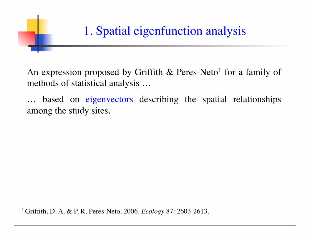
An expression proposed by Griffith & Peres-Neto1 for a family of methods of statistical analysis …
… based on eigenvectors describing the spatial relationships among the study sites.
1. Spatial eigenfunction analysis
1 Griffith, D. A. & P. R. Peres-Neto. 2006. Ecology 87: 2603-2613.
1 2 3 4 5 6 7 8 9
1 1 1 1 0 0 0 0 0
2 1 0 1 0 0 0 1
3 1 1 1 0 0 0
4 0 1 1 0 0
5 1 0 1 1
6 1 1 0
7 1 1
8 1
9
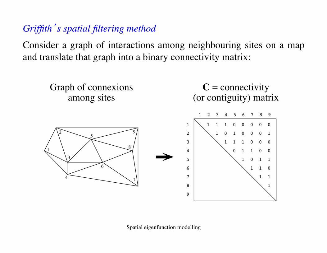
C = connectivity(or contiguity) matrix
1
4
2
3
9
7
5
6
8
Graph of connexionsamong sites
Griffith’s spatial filtering method Consider a graph of interactions among neighbouring sites on a map and translate that graph into a binary connectivity matrix:
Spatial eigenfunction modelling
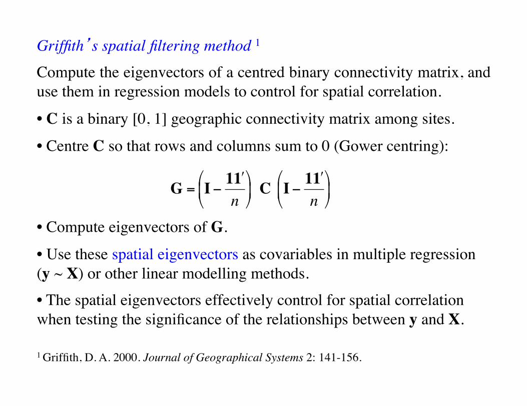
Griffith’s spatial filtering method 1 Compute the eigenvectors of a centred binary connectivity matrix, and use them in regression models to control for spatial correlation.
• C is a binary [0, 1] geographic connectivity matrix among sites.
• Centre C so that rows and columns sum to 0 (Gower centring):
• Compute eigenvectors of G.
• Use these spatial eigenvectors as covariables in multiple regression (y ~ X) or other linear modelling methods.• The spatial eigenvectors effectively control for spatial correlation when testing the significance of the relationships between y and X.
€
G = I− 1 # 1 n
$
% &
'
( ) C I− 1 # 1
n$
% &
'
( )
1 Griffith, D. A. 2000. Journal of Geographical Systems 2: 141-156.
In spatial eigenfunction analysis –•.eigenvectors of spatial configuration matrices are computed
•.and used as predictors in linear models, including the full range of general and generalized linear models. (Other models are possible.)
The expression covers both the early methods developed by geographers to analyse binary spatial connection matrices (Garrison & Marble, 1964; Gould, 1967; Tinkler, 1972; Griffith, 1996; these methods are briefly described here as binary MEM), and the more recent methods that take into account the distances among localities, described in this talk.
Extension to multivariate time series analysis is straightforward1.
1 Legendre, P. & O. Gauthier. 2014. Proc. R. Soc. B 281: 20132728.
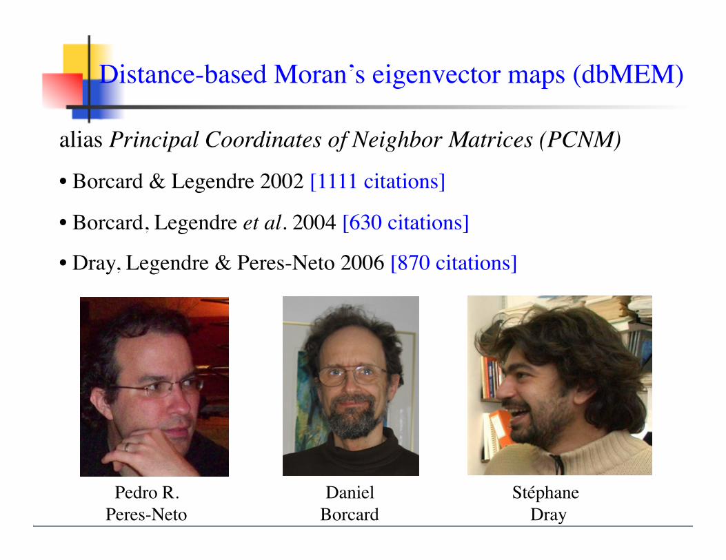
alias Principal Coordinates of Neighbor Matrices (PCNM)
• Borcard & Legendre 2002 [1111 citations]
• Borcard, Legendre et al. 2004 [630 citations]
• Dray, Legendre & Peres-Neto 2006 [870 citations]
Pedro R. Daniel Stéphane Peres-Neto Borcard Dray
Distance-based Moran’s eigenvector maps (dbMEM)
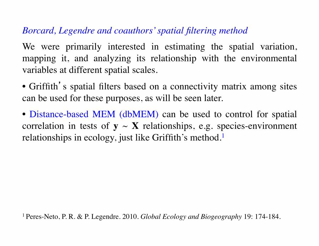
Borcard, Legendre and coauthors’ spatial filtering methodWe were primarily interested in estimating the spatial variation, mapping it, and analyzing its relationship with the environmental variables at different spatial scales.
• Griffith’s spatial filters based on a connectivity matrix among sites can be used for these purposes, as will be seen later.• Distance-based MEM (dbMEM) can be used to control for spatial correlation in tests of y ~ X relationships, e.g. species-environment relationships in ecology, just like Griffith’s method.1
1 Peres-Neto, P. R. & P. Legendre. 2010. Global Ecology and Biogeography 19: 174-184.
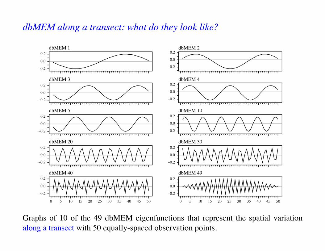
Graphs of 10 of the 49 dbMEM eigenfunctions that represent the spatial variation along a transect with 50 equally-spaced observation points.
–0.2
0.0
0.2
–0.2
0.0
0.2
–0.2
0.0
0.2
–0.2
0.0
0.2
–0.2
0.0
0.2
1050 15 20 25 30 35 40 45 50
dbMEM 1
dbMEM 3
dbMEM 5
dbMEM 20
dbMEM 40
dbMEM 2
dbMEM 4
dbMEM 10
dbMEM 30
dbMEM 49
–0.2
0.0
0.2
–0.2
0.0
0.2
–0.2
0.0
0.2
–0.2
0.0
0.2
–0.2
0.0
0.2
1050 15 20 25 30 35 40 45 50
dbMEM along a transect: what do they look like?
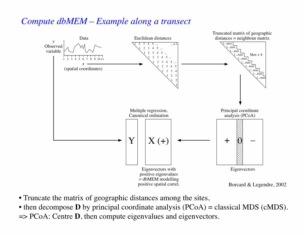
Compute dbMEM – Example along a transect
+
Principal coordinateanalysis (PCoA)
Eigenvectors
–0
Truncated matrix of geographicdistances = neighbour matrix
1...max
Max ! 4
1...max
1...max
1...max
1...max
1...max
1...max
1...max
1...max
1...max
X (+)Y
Multiple regression,Canonical ordination
Eigenvectors withpositive eigenvalues= dbMEM modellingpositive spatial correl.
x(spatial coordinates)
yObservedvariable
Data
1 2 3 4 5 6 7 8 9 10 11
Euclidean distances
... n-1
1 2 3 4 5 ...
1 2 3 4 5 ...
1 2 3 4 5 ...
1 2 3 4 5 ...
1 2 3 4 5
1 2 3 4 5 ...
1 2 3 4
1 2 3
1 2
1
Borcard & Legendre, 2002
• Truncate the matrix of geographic distances among the sites, • then decompose D by principal coordinate analysis (PCoA) = classical MDS (cMDS).=> PCoA: Centre D, then compute eigenvalues and eigenvectors.
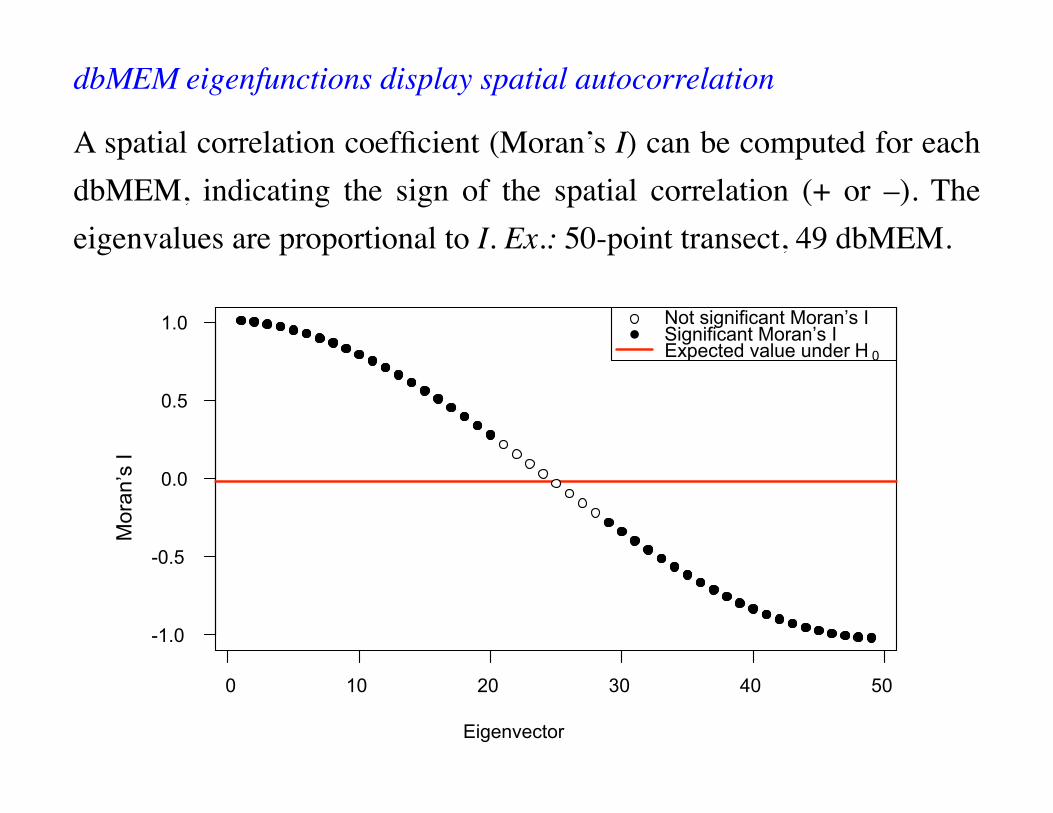
dbMEM eigenfunctions display spatial autocorrelation
A spatial correlation coefficient (Moran’s I) can be computed for each dbMEM, indicating the sign of the spatial correlation (+ or –). The eigenvalues are proportional to I. Ex.: 50-point transect, 49 dbMEM.
0 10 20 30 40 50
-1.0
-0.5
0.0
0.5
1.0
Eigenvector
Not significant Moran’s ISignificant Moran’s IExpected value under H 0
Mor
an’s
I
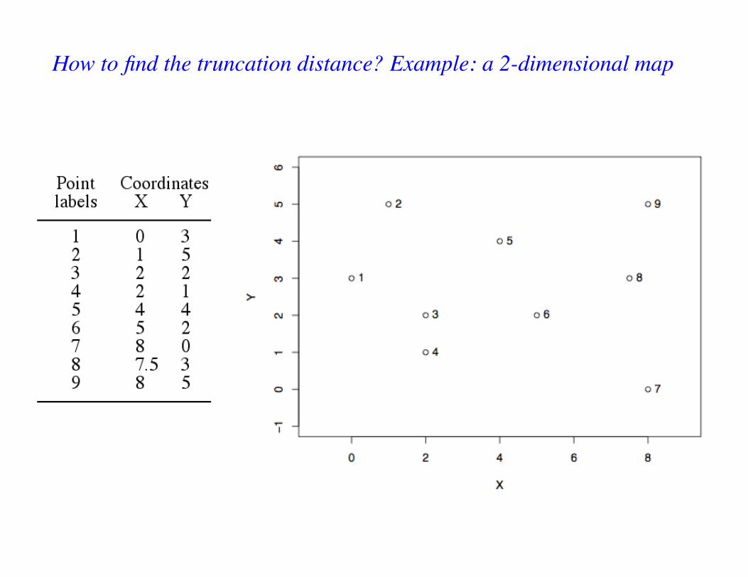
How to find the truncation distance? Example: a 2-dimensional map
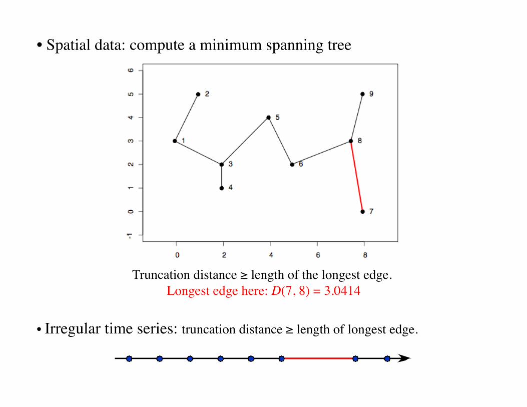
• Spatial data: compute a minimum spanning tree
Truncation distance ≥ length of the longest edge. Longest edge here: D(7, 8) = 3.0414
• Irregular time series: truncation distance ≥ length of longest edge.
Technical notes on dbMEM eigenfunctions
dbMEM variables represent a spectral decomposition of the spatial/temporal relationships among the study sites. They can be computed for regular or irregular sets of points in space or time.
dbMEM eigenfunctions are orthogonal. If the sampling design is regular, they look like sine waves; this is a property of the eigen-decomposition of the centred form of a distance matrix. If the design is irregular, the sine waves are distorted.
Simulation study
Type I error study Simulations showed that the procedure is honest. It does not generate more significant results that it should for a given significance level α.Power studySimulations showed that dbMEM analysis is capable of detecting spatial structures of many kinds: • random autocorrelated data,• bumps and sine waves of various sizes, without or with random noise, representing deterministic structures, as long as the structures are larger than the truncation value used to create the dbMEM (PCNM) eigenfunctions.Detailed results are found in Borcard & Legendre 2002.
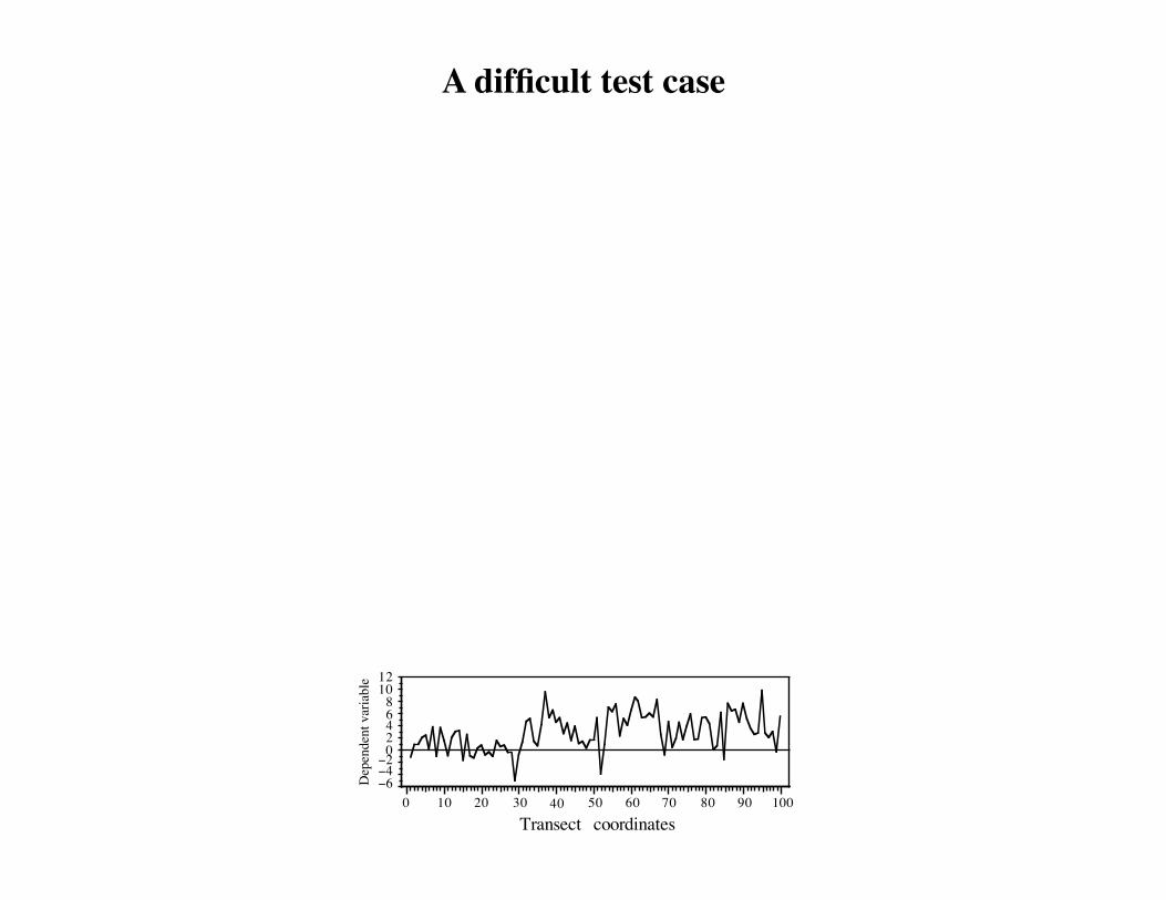
A difficult test case
−6−4−2
02468
1012
Transect coordinates0 10 20 30 40 50 60 70 80 90 100
Dep
ende
nt v
aria
ble
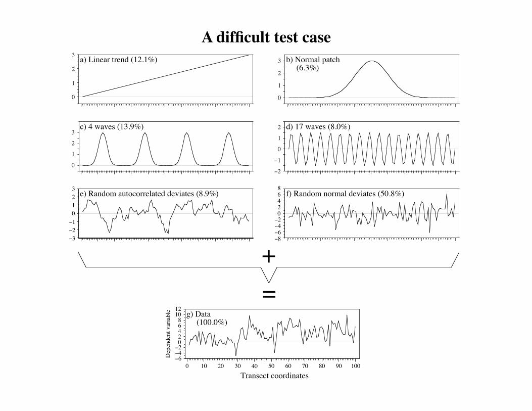
A difficult test case.
0
1
2
3 b) Normal patch (6.3%)
0
1
2
3 a) Linear trend (12.1%)
−8−6−4−202468
f) Random normal deviates (50.8%)e) Random autocorrelated deviates (8.9%)
−3−2−10123
−6−4−202468
1012
g) Data (100.0%)
Transect coordinates0 10 20 30 40 50 60 70 80 90 100
Dep
ende
nt v
aria
ble
c) 4 waves (13.9%)
0
1
2
3
−2
−1
0
1
2 d) 17 waves (8.0%)
=+
A difficult test case
.
−6−4−2
02468
1012
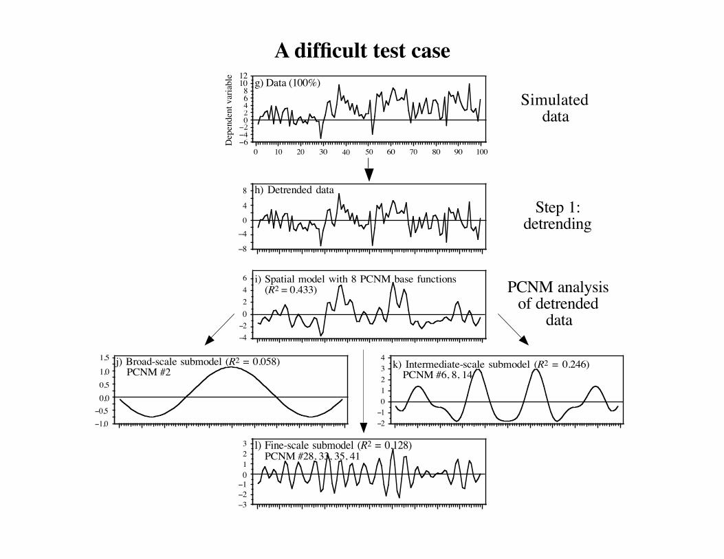
g) Data (100%)
0 10 20 30 40 50 60 70 80 90 100
0,00,5
1,0
1,5 j) Broad-scale submodel (R2 = 0.058) PCNM #2
−2−101234
k) Intermediate-scale submodel (R2 = 0.246) PCNM #6, 8, 14
−3−2−1
0123 l) Fine-scale submodel (R2 = 0.128)
PCNM #28, 33, 35, 41
−4−20246 i) Spatial model with 8 PCNM base functions
(R2 = 0.433)
−1,0−0,5
−8
−40
4
8 h) Detrended data
Simulateddata
Step 1:detrending
PCNM analysisof detrended
data
Dep
ende
nt v
aria
ble
dbMEM 1 dbMEM 2
dbMEM 3 dbMEM 4
dbMEM 5 dbMEM 6
dbMEM 10 dbMEM 20
dbMEM 30 dbMEM 40
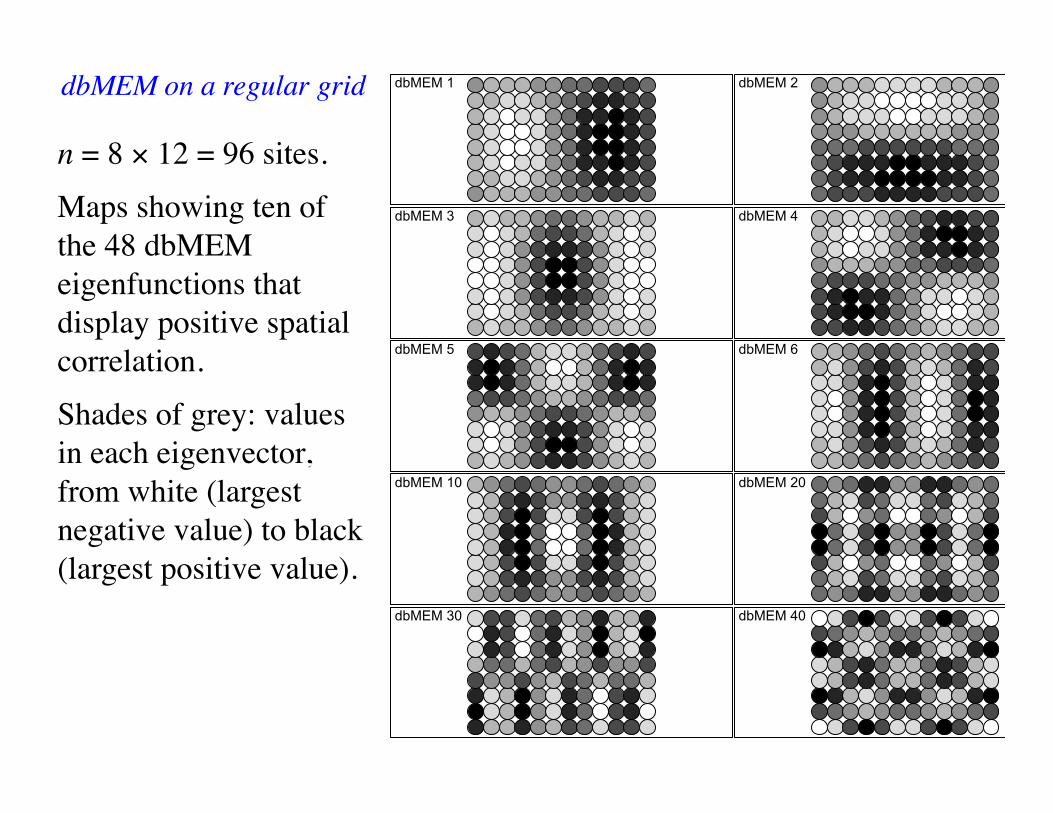
n = 8 × 12 = 96 sites.Maps showing ten of the 48 dbMEM eigenfunctions that display positive spatial correlation. Shades of grey: values in each eigenvector, from white (largest negative value) to black (largest positive value).
dbMEM on a regular grid
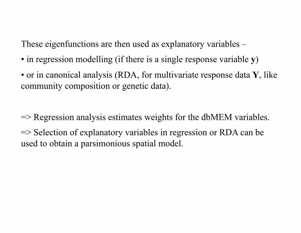
These eigenfunctions are then used as explanatory variables –
• in regression modelling (if there is a single response variable y)
• or in canonical analysis (RDA, for multivariate response data Y, like community composition or genetic data).
=> Regression analysis estimates weights for the dbMEM variables.
=> Selection of explanatory variables in regression or RDA can be used to obtain a parsimonious spatial model.
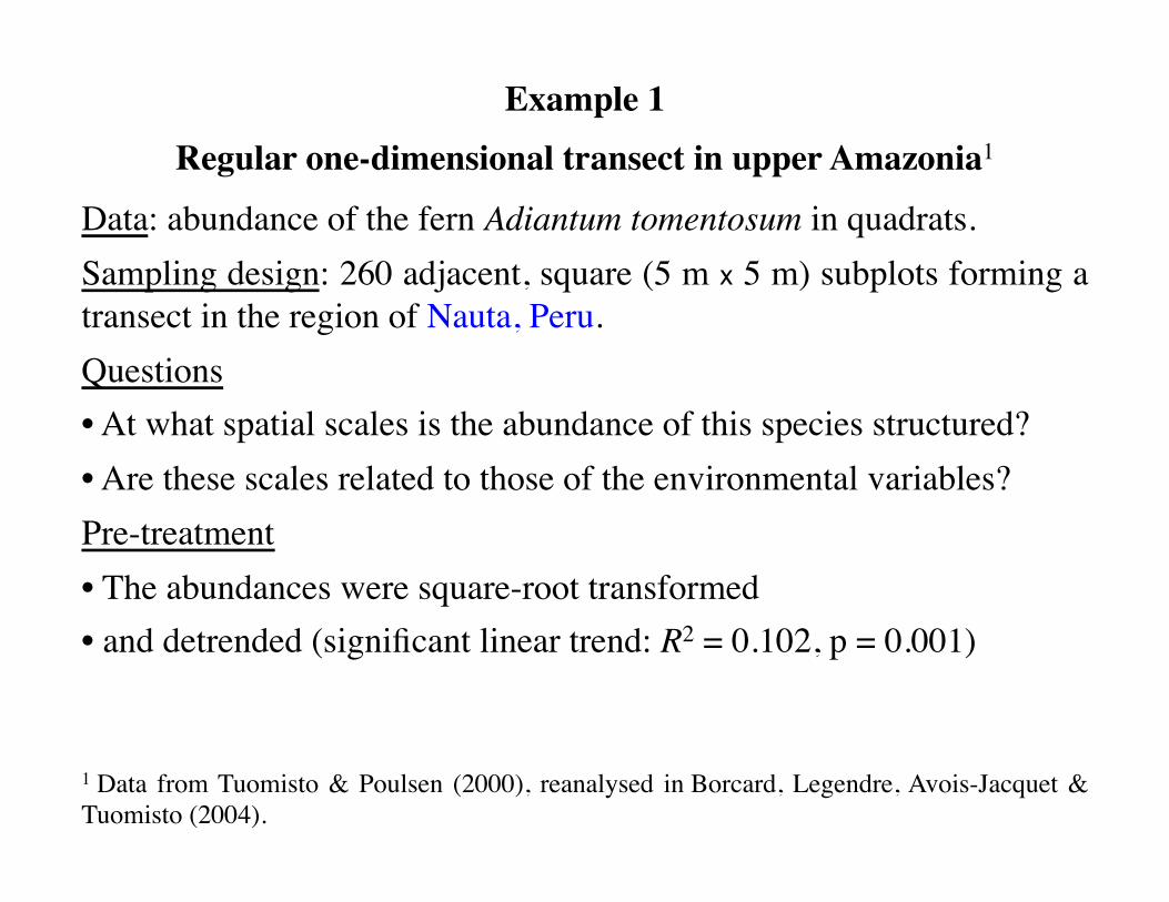
Example 1Regular one-dimensional transect in upper Amazonia1
Data: abundance of the fern Adiantum tomentosum in quadrats.Sampling design: 260 adjacent, square (5 m x 5 m) subplots forming a transect in the region of Nauta, Peru.Questions • At what spatial scales is the abundance of this species structured?• Are these scales related to those of the environmental variables?Pre-treatment• The abundances were square-root transformed• and detrended (significant linear trend: R2 = 0.102, p = 0.001)
1 Data from Tuomisto & Poulsen (2000), reanalysed in Borcard, Legendre, Avois-Jacquet & Tuomisto (2004).
–2
–1
0
1
2
3(a) R2 = 0.815
1 21 41 61 81 101 121 141 161 181 201 221 241 260
-2
-1,5-1
-0,5
0
0,51
1,5
2
1 21 41 61 81 101 121 141 161 181 201 221 241 260
(b) Very-broad-scale submodel, 10 PCNMs, R2 = 0.333
-1,5
-1
-0,5
0
0,5
1
1,5
1 21 41 61 81 101 121 141 161 181 201 221 241 260
(c) Medium-scale submodel, 12 PCNMs, R2 = 0.126
-2
-1,5
-1
-0,5
0
0,5
1
1,5
1 21 41 61 81 101 121 141 161 181 201 221 241 260
(d) Fine-scale submodel, 20 PCNMs, R2 = 0.117
Data
PCNM model (50 significant PCNMs out of 176)
Broad-scale submodel, 8 PCNMs, R2 = 0.239
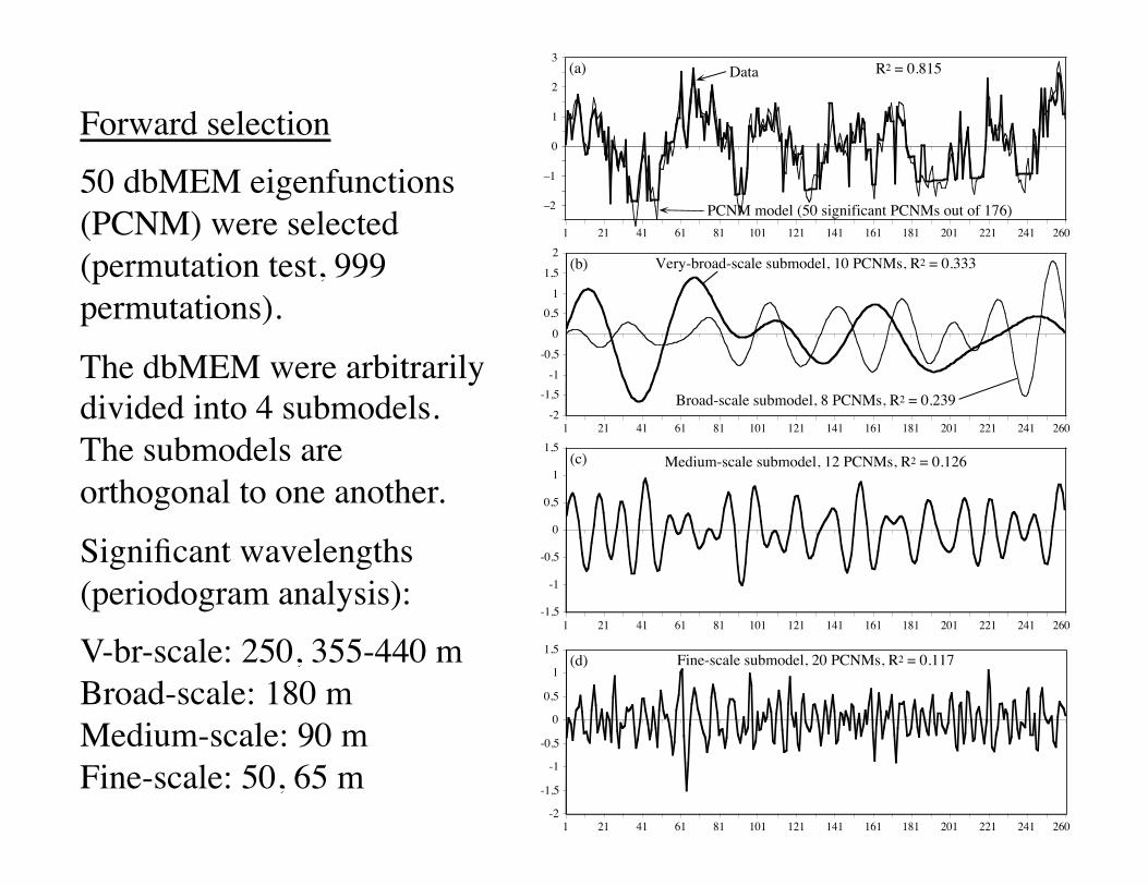
Forward selection50 dbMEM eigenfunctions (PCNM) were selected (permutation test, 999 permutations).
The dbMEM were arbitrarily divided into 4 submodels. The submodels are orthogonal to one another.
Significant wavelengths (periodogram analysis):V-br-scale: 250, 355-440 mBroad-scale: 180 mMedium-scale: 90 mFine-scale: 50, 65 m
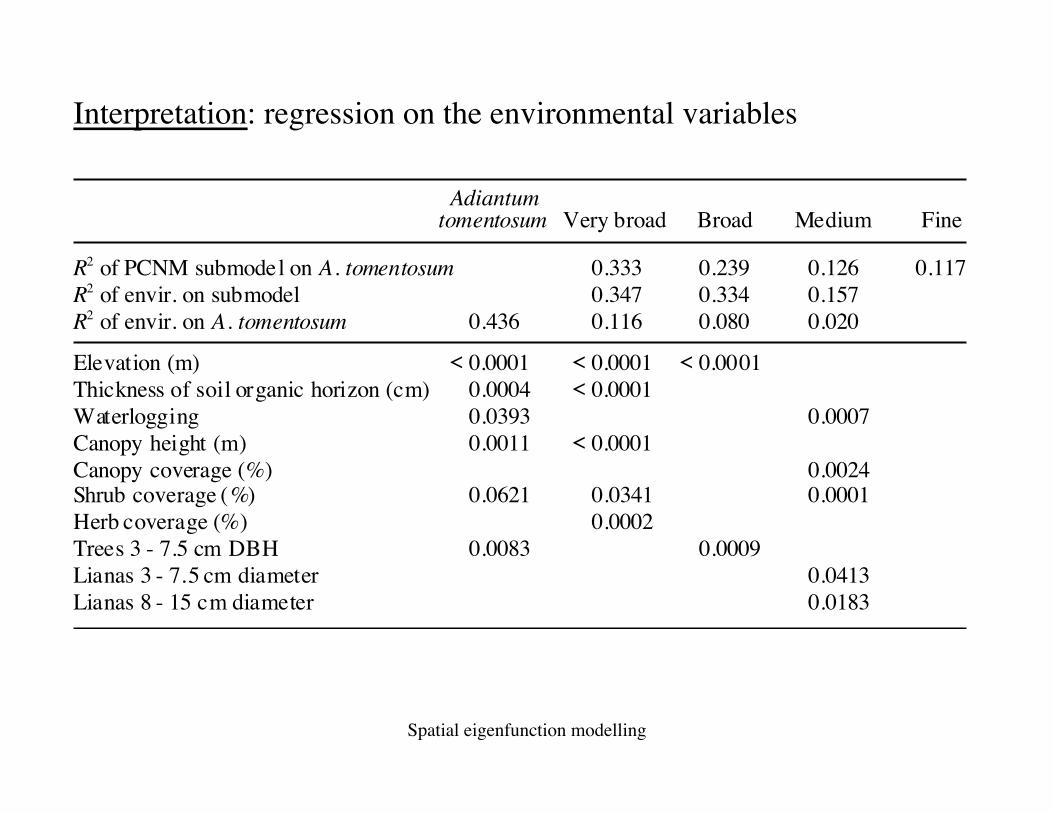
Interpretation: regression on the environmental variables
tomentosum Very broad Broad Medium FineAdiantum
R2 of PCNM submodel on A. tomentosumR2 of envir. on submodelR2 of envir. on A. tomentosum
Elevation (m)Thickness of soil organic horizon (cm)WaterloggingCanopy height (m)Canopy coverage (%)Shrub coverage (%)Herb coverage (%)Trees 3 - 7.5 cm DBHLianas 3 - 7.5 cm diameterLianas 8 - 15 cm diameter
0.333 0.239 0.126 0.1170.347 0.334 0.157
0.436
< 0.00010.00040.03930.0011
0.0621
0.0083
0.116 0.080 0.020
< 0.0001 < 0.0001< 0.0001
0.0007< 0.0001
0.00240.0341 0.00010.0002
0.00090.04130.0183
Spatial eigenfunction modelling
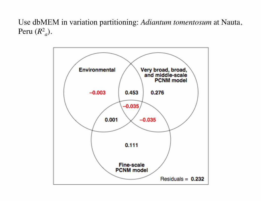
Use dbMEM in variation partitioning: Adiantum tomentosum at Nauta, Peru (R2
a).
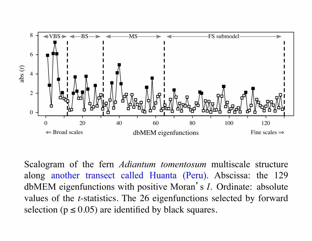
Scalogram of the fern Adiantum tomentosum multiscale structure along another transect called Huanta (Peru). Abscissa: the 129 dbMEM eigenfunctions with positive Moran’s I. Ordinate: absolute values of the t-statistics. The 26 eigenfunctions selected by forward selection (p ≤ 0.05) are identified by black squares.
0 20 40 60 80 100 120
0
2
4
6
8
abs(t)
dbMEM eigenfunctions! Broad scales Fine scales"
VBS BS MS FS submodel
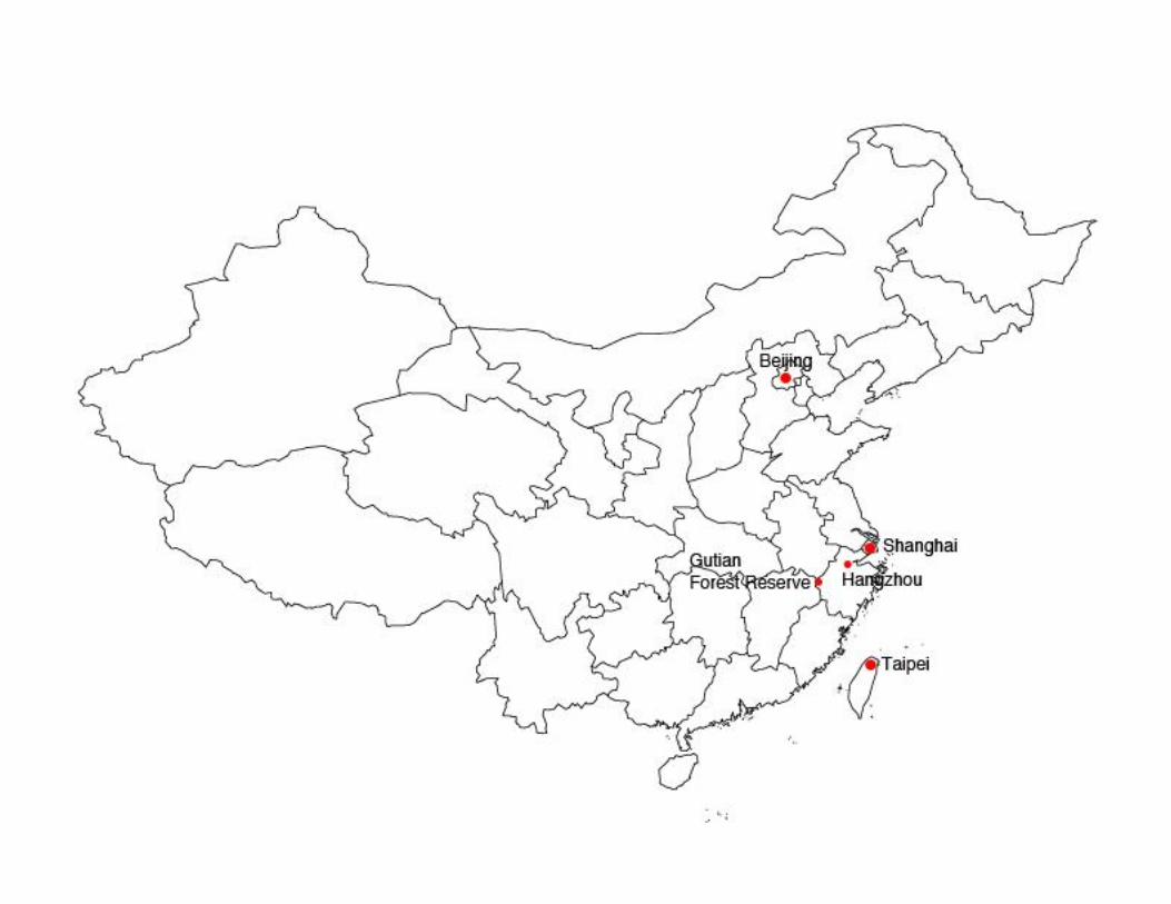
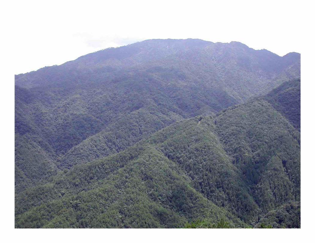
Example 2Gutianshan forest plot in China1
• Evergreen forest in Gutianshan Forest Reserve, Zhejiang Province.• Fully-surveyed 24-ha forest plot in subtropical forest, 29º15'N.• Plot divided into 600 cells of 20 m × 20 m. • 159 tree species. Richness: 19 to 54 species per cell.• Data collection: 2005 Legendre, P., X. Mi, H. Ren, K. Ma, M. Yu, I. F. Sun, and F. He. 2009. Partitioning beta diversity in a subtropical broad-leaved forest of China. Ecology 90: 663-674.
1 The Gutianshan forest plot is a member of the Center for Tropical Forest Science (CTFS). Details on the plot available at http://www.ctfs.si.edu/site/Gutianshan/.

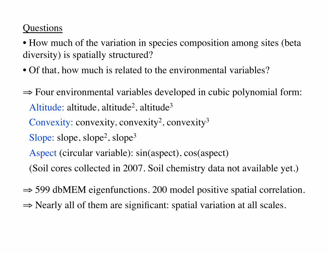
Questions • How much of the variation in species composition among sites (beta diversity) is spatially structured?• Of that, how much is related to the environmental variables?
⇒ Four environmental variables developed in cubic polynomial form: Altitude: altitude, altitude2, altitude3 Convexity: convexity, convexity2, convexity3Slope: slope, slope2, slope3Aspect (circular variable): sin(aspect), cos(aspect)(Soil cores collected in 2007. Soil chemistry data not available yet.)
⇒ 599 dbMEM eigenfunctions. 200 model positive spatial correlation.⇒ Nearly all of them are significant: spatial variation at all scales.
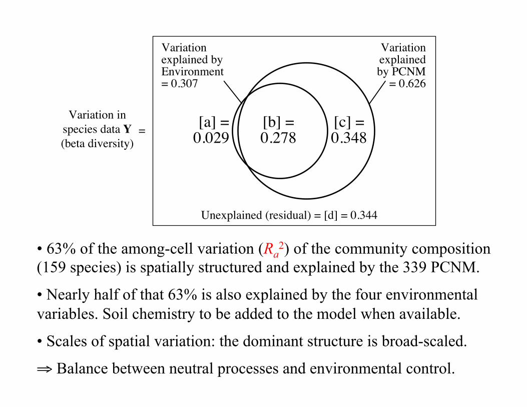
• 63% of the among-cell variation (Ra2) of the community composition
(159 species) is spatially structured and explained by the 339 PCNM.
• Nearly half of that 63% is also explained by the four environmental variables. Soil chemistry to be added to the model when available.
• Scales of spatial variation: the dominant structure is broad-scaled.
⇒ Balance between neutral processes and environmental control.
[a] =0.029
[b] =0.278
[c] =0.348
Variationexplained byEnvironment= 0.307
Variationexplainedby PCNM
= 0.626
Unexplained (residual) = [d] = 0.344
Variation inspecies data Y(beta diversity)
=
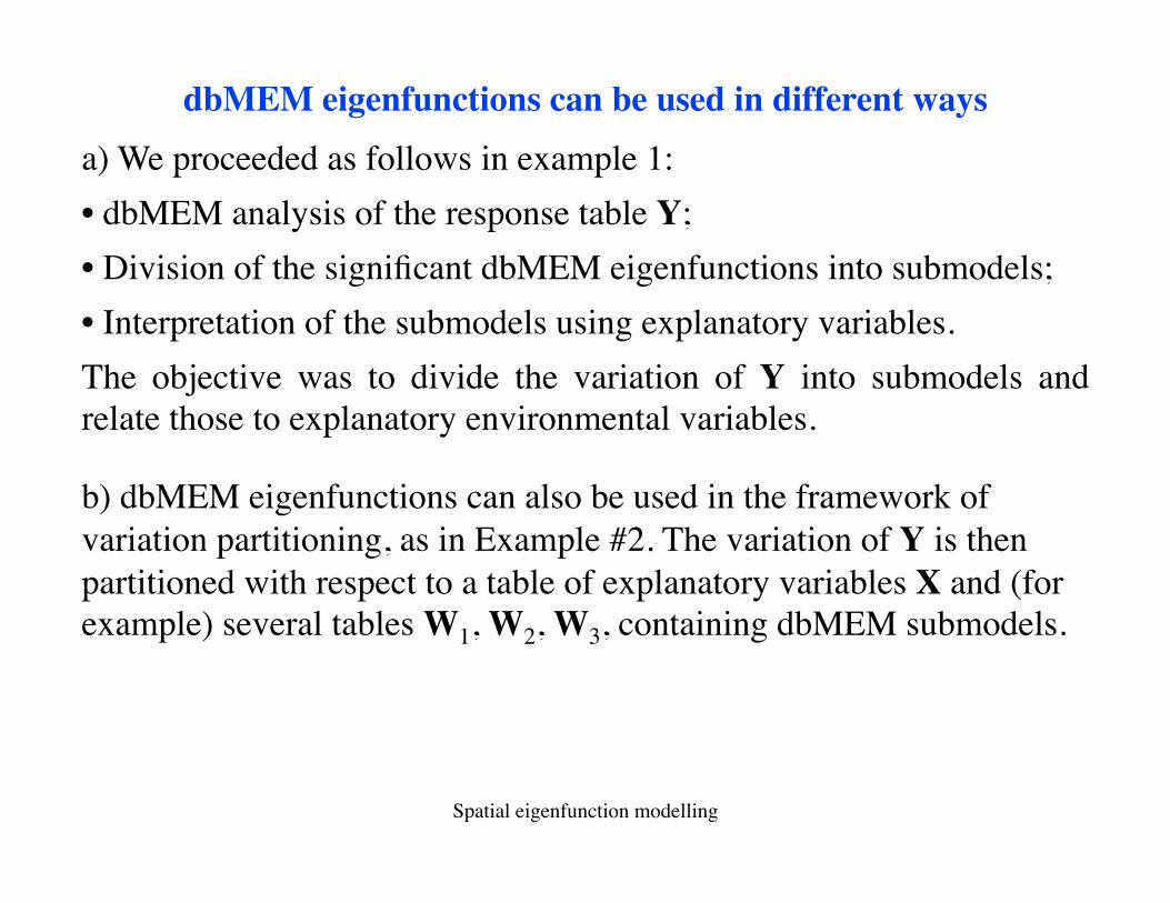
dbMEM eigenfunctions can be used in different waysa) We proceeded as follows in example 1:• dbMEM analysis of the response table Y;• Division of the significant dbMEM eigenfunctions into submodels;• Interpretation of the submodels using explanatory variables.The objective was to divide the variation of Y into submodels and relate those to explanatory environmental variables.
b) dbMEM eigenfunctions can also be used in the framework of variation partitioning, as in Example #2. The variation of Y is then partitioned with respect to a table of explanatory variables X and (for example) several tables W1, W2, W3, containing dbMEM submodels.
Spatial eigenfunction modelling
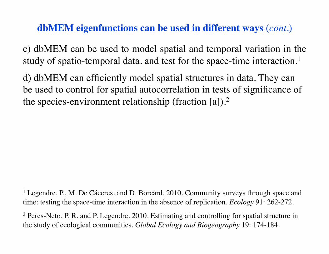
dbMEM eigenfunctions can be used in different ways (cont.)
c) dbMEM can be used to model spatial and temporal variation in the study of spatio-temporal data, and test for the space-time interaction.1
d) dbMEM can efficiently model spatial structures in data. They can be used to control for spatial autocorrelation in tests of significance of the species-environment relationship (fraction [a]).2
1 Legendre, P., M. De Cáceres, and D. Borcard. 2010. Community surveys through space and time: testing the space-time interaction in the absence of replication. Ecology 91: 262-272.2 Peres-Neto, P. R. and P. Legendre. 2010. Estimating and controlling for spatial structure in the study of ecological communities. Global Ecology and Biogeography 19: 174-184.
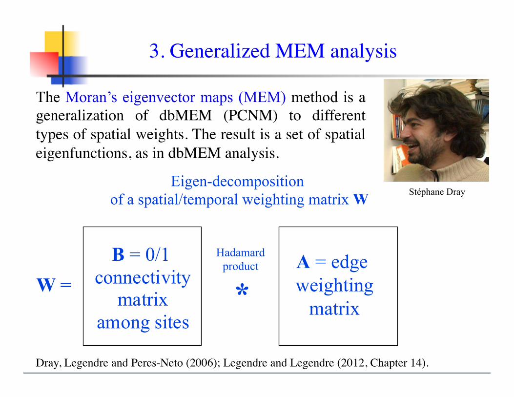
The Moran’s eigenvector maps (MEM) method is a generalization of dbMEM (PCNM) to different types of spatial weights. The result is a set of spatial eigenfunctions, as in dbMEM analysis.
Dray, Legendre and Peres-Neto (2006); Legendre and Legendre (2012, Chapter 14).
Eigen-decomposition of a spatial/temporal weighting matrix W
B = 0/1connectivity
matrixamongsites
*Hadamard
product A = edge weighting
matrix W =
3. Generalized MEM analysis
Stéphane Dray
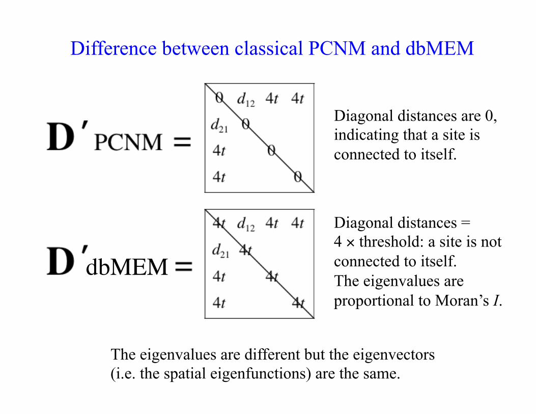
dbMEM
Diagonal distances are 0, indicating that a site is connected to itself.
Diagonal distances = 4 × threshold: a site is not connected to itself. The eigenvalues are proportional to Moran’s I.
Difference between classical PCNM and dbMEM
The eigenvalues are different but the eigenvectors (i.e. the spatial eigenfunctions) are the same.
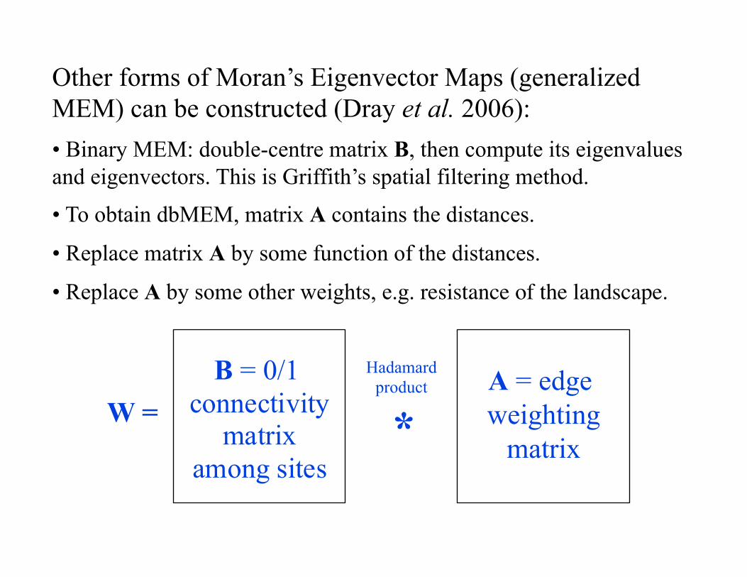
Other forms of Moran’s Eigenvector Maps (generalized MEM) can be constructed (Dray et al. 2006): • Binary MEM: double-centre matrix B, then compute its eigenvalues and eigenvectors. This is Griffith’s spatial filtering method.
• To obtain dbMEM, matrix A contains the distances.
• Replace matrix A by some function of the distances.
• Replace A by some other weights, e.g. resistance of the landscape.
B = 0/1connectivity
matrixamongsites
*Hadamard
product A = edge weighting
matrix W =
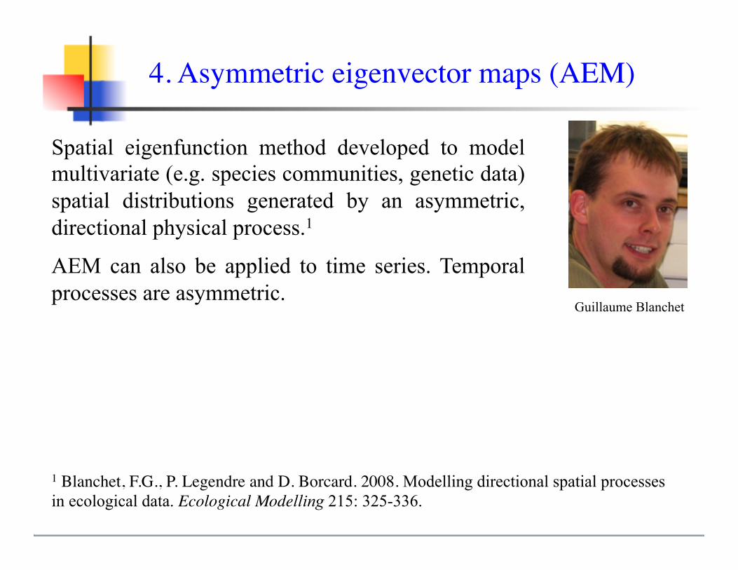
Spatial eigenfunction method developed to model multivariate (e.g. species communities, genetic data) spatial distributions generated by an asymmetric, directional physical process.1
AEM can also be applied to time series. Temporal processes are asymmetric.
1 Blanchet, F.G., P. Legendre and D. Borcard. 2008. Modelling directional spatial processes in ecological data. Ecological Modelling 215: 325-336.
4. Asymmetric eigenvector maps (AEM)
Guillaume Blanchet
N2
N3 N4
N6
Node 0(origin)
N1
N4 N5
E1 E2
E3 E4
E5
E6E8E7
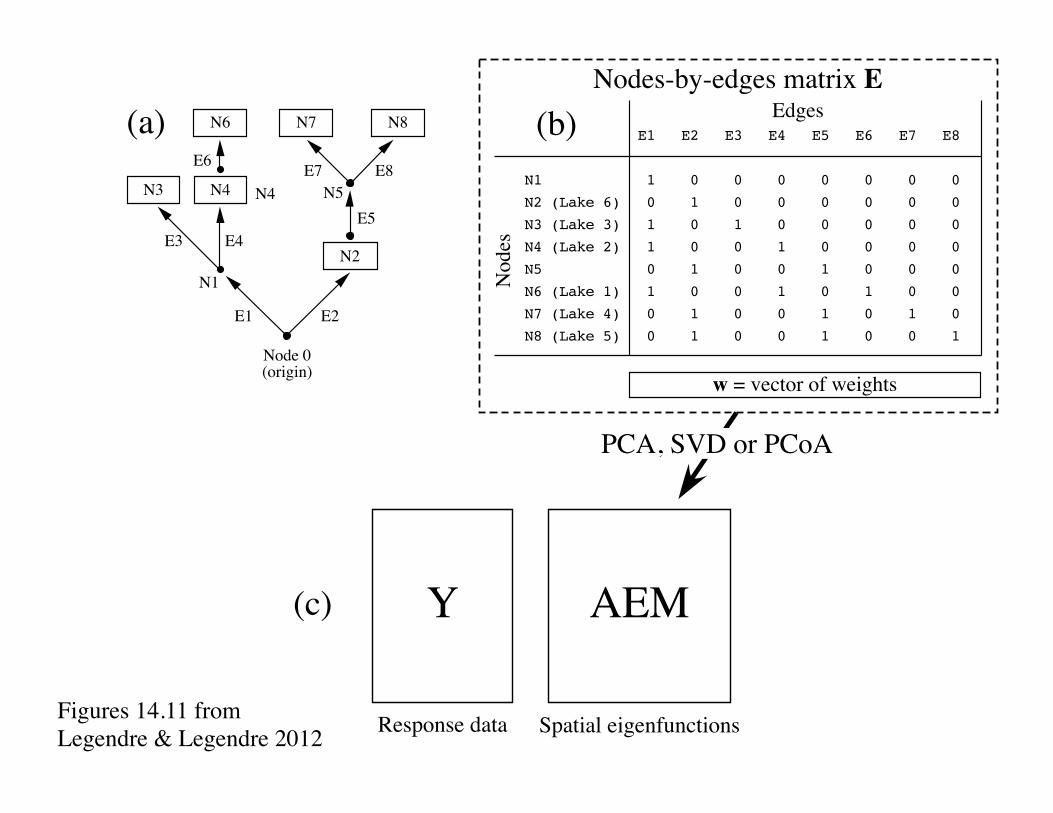
N7 N8(a) E1 E2 E3 E4 E5 E6 E7 E8
N1 1 0 0 0 0 0 0 0
N2 (Lake 6) 0 1 0 0 0 0 0 0
N3 (Lake 3) 1 0 1 0 0 0 0 0
N4 (Lake 2) 1 0 0 1 0 0 0 0
N5 0 1 0 0 1 0 0 0
N6 (Lake 1) 1 0 0 1 0 1 0 0
N7 (Lake 4) 0 1 0 0 1 0 1 0
N8 (Lake 5) 0 1 0 0 1 0 0 1
Edges
Nodes
w = vector of weights
Y AEM
Response data Spatial eigenfunctions
PCA, SVD or PCoA
(c)
(b)
Nodes-by-edges matrix E
Figures 14.11 from Legendre & Legendre 2012
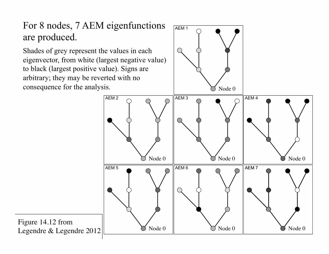
AEM 4
Node 0
AEM 5
Node 0
AEM 6
Node 0
AEM 3
Node 0
AEM 2
Node 0
AEM 1
Node 0
For 8 nodes, 7 AEM eigenfunctions are produced. Shades of grey represent the values in each eigenvector, from white (largest negative value) to black (largest positive value). Signs are arbitrary; they may be reverted with no consequence for the analysis.
Figure 14.12 from Legendre & Legendre 2012
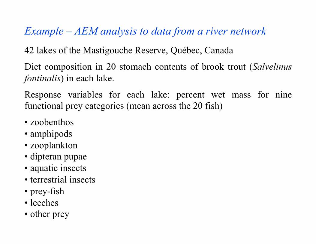
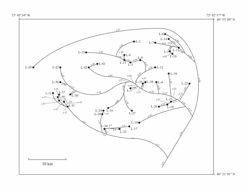
Example – AEM analysis to data from a river network
42 lakes of the Mastigouche Reserve, Québec, Canada
Diet composition in 20 stomach contents of brook trout (Salvelinus fontinalis) in each lake.
Response variables for each lake: percent wet mass for nine functional prey categories (mean across the 20 fish)
• zoobenthos • amphipods • zooplankton • dipteran pupae • aquatic insects • terrestrial insects • prey-fish • leeches • other prey
L-1
L-2
L-4
L-5
L-6L-9
L-11
L-12
L-25L-35 L-38
L-39
L-3
L-7
L-8
L-10
L-13
L-14
L-15
L-22L-29
L-30L-31
L-32
L-33
L-36
L-37
L-40
L-43
L-41
L-42
L-16
L-17
L-19
L-23
L-24L-27L-28
L-34
L-18
L-21
L-26
10 km
46° 21' 01" N
46° 53' 09" N
73° 02' 57" W73° 45' 34" W
e-0
e-1
e-1
6
e-6
e-5
e-4e-3
e-2
e-7
e-8
e-51
e-9
e-10e-19
e-21
e-2
0
e-18
e-1
7
e-12
e-13
e-14
e-15
e-11
e-2
6
e-25
e-24
e-23
e-22
e-27
e-34
e-33
e-32
e-31
e-3
0
e-29
e-2
8
e-40
e-41
e-39 e-38
e-3
7
e-36
e-35
e-44
e-49
e-4
8
e-47
e-46
e-45
e-42
e-43
e-5
0
e-5
5
e-54e-53
e-52
e-5
6
e-57
e-58
e-59
e-60
e-65
e-6
4
e-63 e-62
e-61
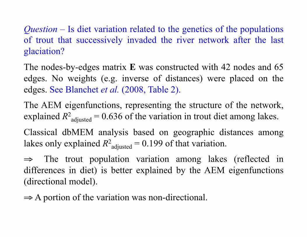
Question – Is diet variation related to the genetics of the populations of trout that successively invaded the river network after the last glaciation?
The nodes-by-edges matrix E was constructed with 42 nodes and 65 edges. No weights (e.g. inverse of distances) were placed on the edges. See Blanchet et al. (2008, Table 2).
The AEM eigenfunctions, representing the structure of the network, explained R2
adjusted = 0.636 of the variation in trout diet among lakes.
Classical dbMEM analysis based on geographic distances among lakes only explained R2
adjusted = 0.199 of that variation.
⇒ The trout population variation among lakes (reflected in differences in diet) is better explained by the AEM eigenfunctions (directional model).
⇒ A portion of the variation was non-directional.
Three other applications of AEM analysis to spatial data – Blanchet, F. G., P. Legendre, R. Maranger, D. Monti & P. Pepin. 2011. Modelling the effect of directional spatial ecological processes at different scales. Oecologia 166: 357-368. Here is one of them =>
Spatial eigenfunction modelling
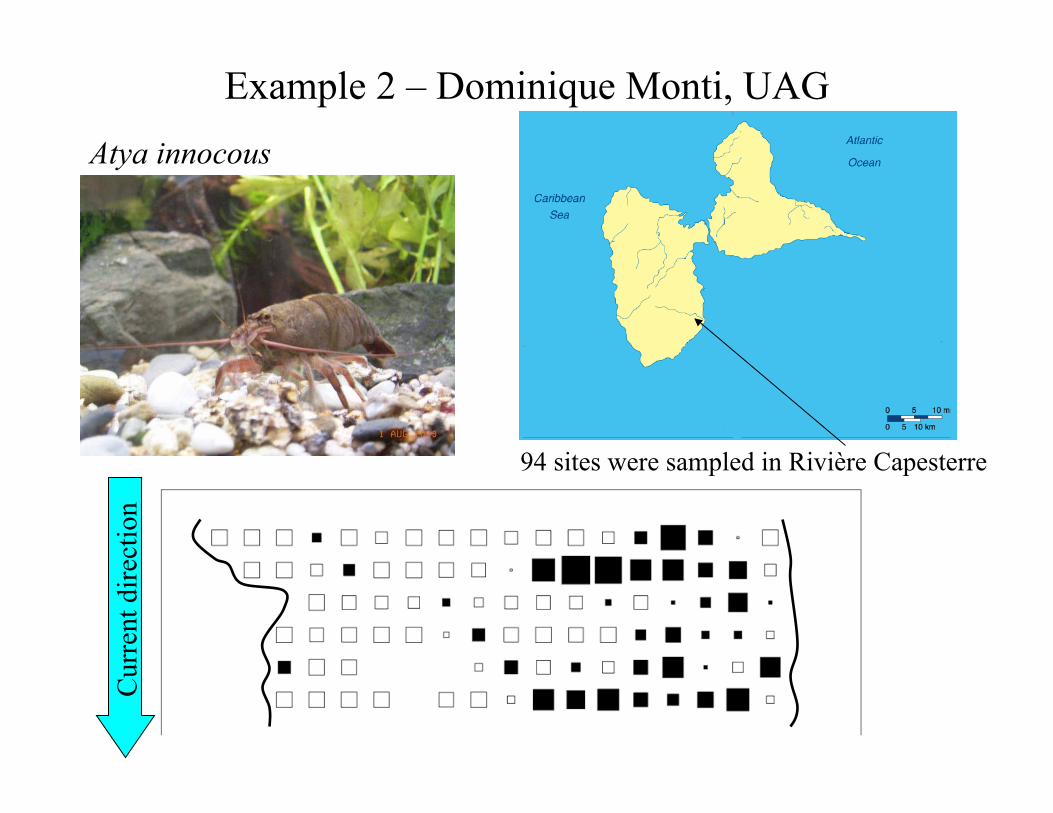
94 sites were sampled in Rivière Capesterre
Cur
rent
dire
ctio
n Atya innocous
Example 2 – Dominique Monti, UAG
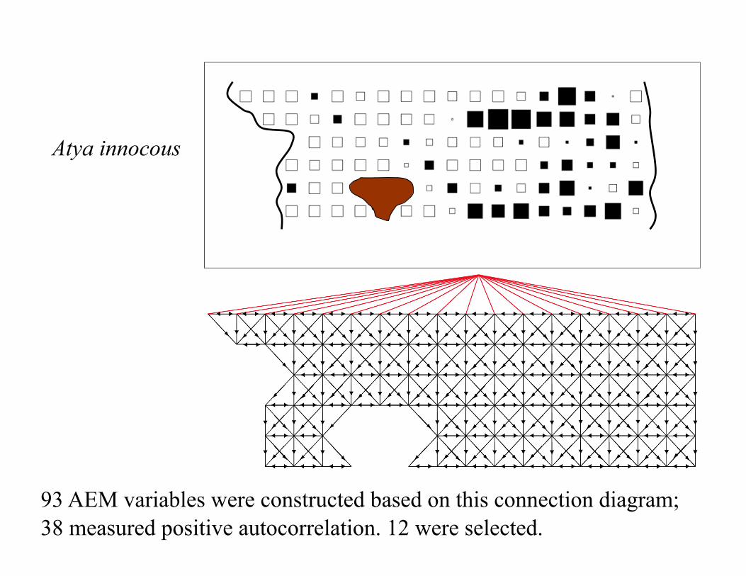
93 AEM variables were constructed based on this connection diagram; 38 measured positive autocorrelation. 12 were selected.
Atya innocous
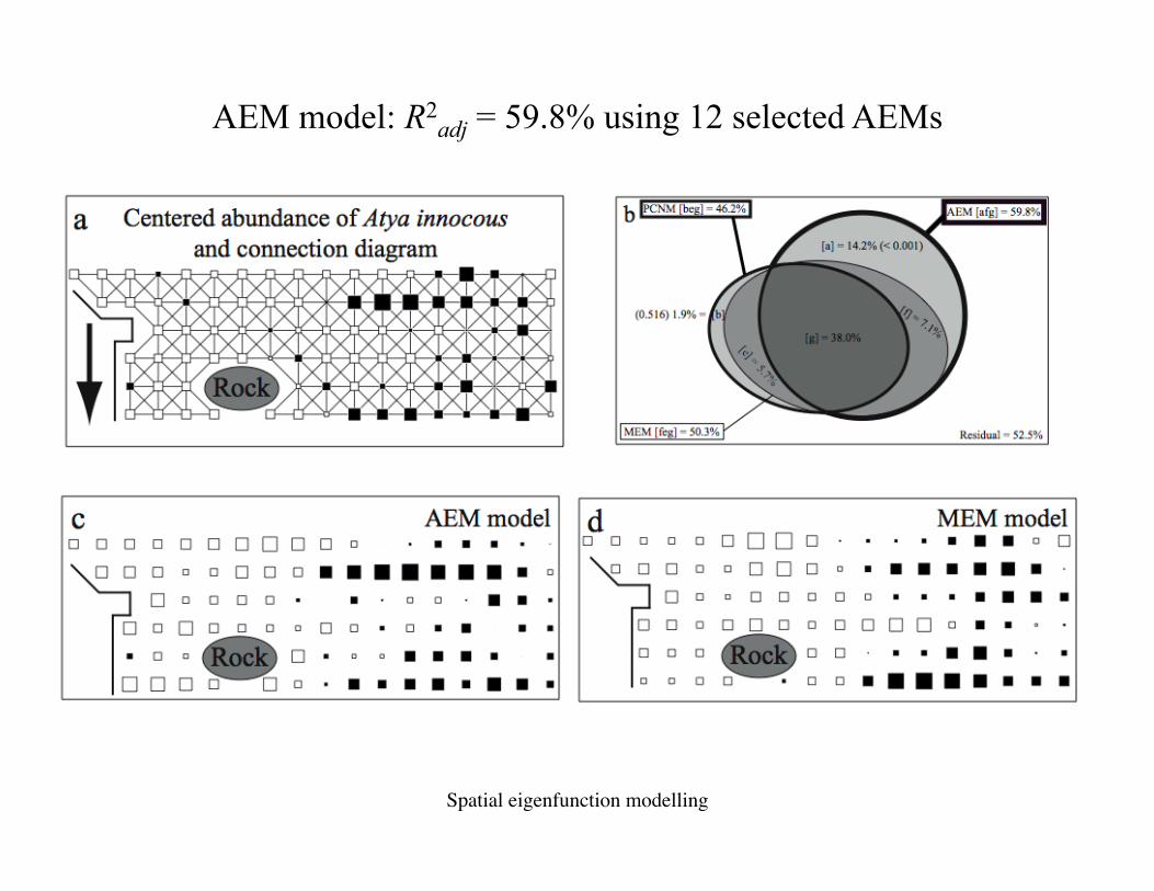
AEM model: R2adj = 59.8% using 12 selected AEMs
Spatial eigenfunction modelling
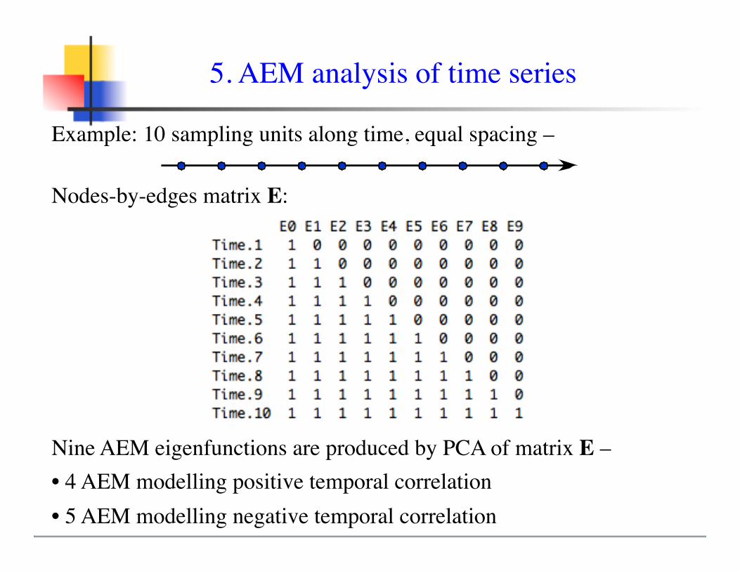
Example: 10 sampling units along time, equal spacing –
Nodes-by-edges matrix E:
Nine AEM eigenfunctions are produced by PCA of matrix E –• 4 AEM modelling positive temporal correlation • 5 AEM modelling negative temporal correlation
5. AEM analysis of time series
Eigenfunction analysis of multivariate time seriesAnalysis of multivariate community composition data:A full Practical exercise in R about temporal eigenfunction analysis of the Chesapeake Bay Benthic Monitoring Program (USA) is available as Appendix S2 of:
Legendre, P. & O. Gauthier. 2014. Statistical methods for temporal and space-time analysis of community composition data. Proc. R. Soc. B 281: 20132728. See Web page of the course Bio 6077:Legendre-Gauthier practicals: Temporal eigenfunction methods
Spatial eigenfunction modelling

AEM and MEM analyses are complementary
• To emphasize the directional nature of the process influencing the data, AEM analysis, which was designed to take trends into account, should be applied to the non-detrended series.
• MEM analysis can be applied to data series that were detrended to remove the directional component.
⇒ By applying both methods to spatial data, one can differentiate the directional and non-directional components of variation in a [multivariate] data matrix.
⇒ Processes acting along time series produce a single gradient in data. For time series, MEM and AEM modelling can both be applied to the undetrended data, even when a trend is present.
⇒ Example: detrended palaeoecological core data could be studied by MEM analysis, the undetrended data by MEM or AEM analysis.
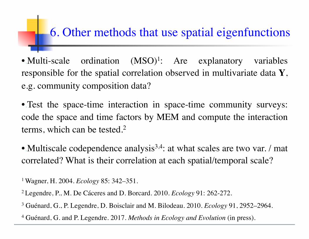
•.Multi-scale ordination (MSO)1: Are explanatory variables responsible for the spatial correlation observed in multivariate data Y, e.g. community composition data?
•.Test the space-time interaction in space-time community surveys: code the space and time factors by MEM and compute the interaction terms, which can be tested.2
•.Multiscale codependence analysis3,4: at what scales are two var. / mat correlated? What is their correlation at each spatial/temporal scale?
1 Wagner, H. 2004. Ecology 85: 342–351.2 Legendre, P., M. De Cáceres and D. Borcard. 2010. Ecology 91: 262-272.3 Guénard, G., P. Legendre, D. Boisclair and M. Bilodeau. 2010. Ecology 91, 2952–2964.4 Guénard, G. and P. Legendre. 2017. Methods in Ecology and Evolution (in press).
6. Other methods that use spatial eigenfunctions
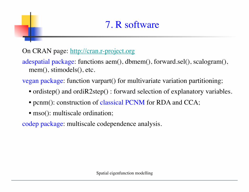
On CRAN page: http://cran.r-project.orgadespatial package: functions aem(), dbmem(), forward.sel(), scalogram(),
mem(), stimodels(), etc.vegan package: function varpart() for multivariate variation partitioning; • ordistep() and ordiR2step() : forward selection of explanatory variables.• pcnm(): construction of classical PCNM for RDA and CCA;• mso(): multiscale ordination;
codep package: multiscale codependence analysis.
7. R software
Spatial eigenfunction modelling
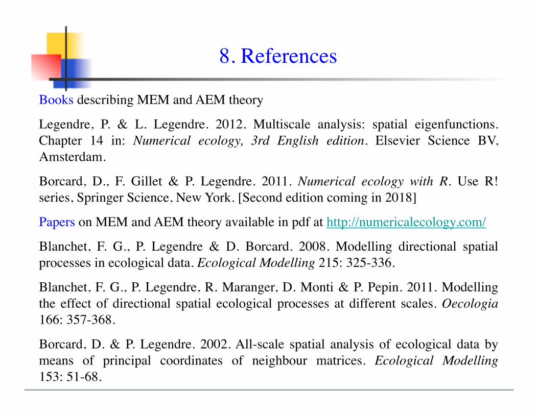
Books describing MEM and AEM theory
Legendre, P. & L. Legendre. 2012. Multiscale analysis: spatial eigenfunctions. Chapter 14 in: Numerical ecology, 3rd English edition. Elsevier Science BV, Amsterdam.
Borcard, D., F. Gillet & P. Legendre. 2011. Numerical ecology with R. Use R! series, Springer Science, New York. [Second edition coming in 2018]
Papers on MEM and AEM theory available in pdf at http://numericalecology.com/
Blanchet, F. G., P. Legendre & D. Borcard. 2008. Modelling directional spatial processes in ecological data. Ecological Modelling 215: 325-336.
Blanchet, F. G., P. Legendre, R. Maranger, D. Monti & P. Pepin. 2011. Modelling the effect of directional spatial ecological processes at different scales. Oecologia 166: 357-368.
Borcard, D. & P. Legendre. 2002. All-scale spatial analysis of ecological data by means of principal coordinates of neighbour matrices. Ecological Modelling 153: 51-68.
8. References
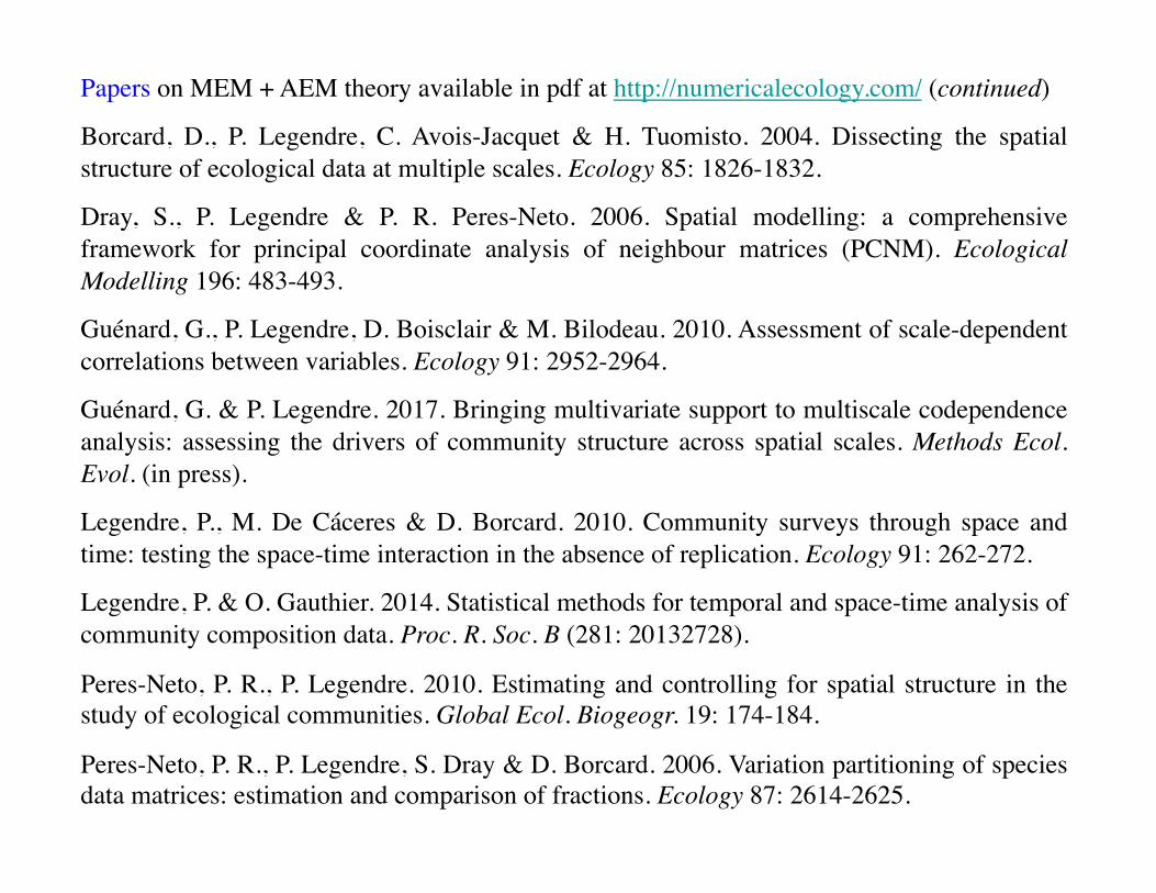
Papers on MEM + AEM theory available in pdf at http://numericalecology.com/ (continued)
Borcard, D., P. Legendre, C. Avois-Jacquet & H. Tuomisto. 2004. Dissecting the spatial structure of ecological data at multiple scales. Ecology 85: 1826-1832.
Dray, S., P. Legendre & P. R. Peres-Neto. 2006. Spatial modelling: a comprehensive framework for principal coordinate analysis of neighbour matrices (PCNM). Ecological Modelling 196: 483-493.
Guénard, G., P. Legendre, D. Boisclair & M. Bilodeau. 2010. Assessment of scale-dependent correlations between variables. Ecology 91: 2952-2964.
Guénard, G. & P. Legendre. 2017. Bringing multivariate support to multiscale codependence analysis: assessing the drivers of community structure across spatial scales. Methods Ecol. Evol. (in press).
Legendre, P., M. De Cáceres & D. Borcard. 2010. Community surveys through space and time: testing the space-time interaction in the absence of replication. Ecology 91: 262-272.
Legendre, P. & O. Gauthier. 2014. Statistical methods for temporal and space-time analysis of community composition data. Proc. R. Soc. B (281: 20132728).
Peres-Neto, P. R., P. Legendre. 2010. Estimating and controlling for spatial structure in the study of ecological communities. Global Ecol. Biogeogr. 19: 174-184.
Peres-Neto, P. R., P. Legendre, S. Dray & D. Borcard. 2006. Variation partitioning of species data matrices: estimation and comparison of fractions. Ecology 87: 2614-2625.
Griffith, D. A. 2000. A linear regression solution to the spatial autocorrelation problem. Journal of Geographical Systems 2: 141-156.
Griffith, D. A. & P. R. Peres-Neto. 2006. Spatial modeling in ecology: the flexibility of eigenfunction spatial analyses. Ecology 87: 2603-2613.
Legendre, P., X. Mi, H. Ren, K. Ma, M. Yu, I. F. Sun & F. He. 2009. Partitioning beta diversity in a subtropical broad-leaved forest of China. Ecology 90: 663-674.
Tuomisto, H. & A. D. Poulsen. 2000. Pteridophyte diversity and species composition in four Amazonian rain forests. J. Veg. Sci. 11: 383-396.
Wagner, H. H. 2004. Direct multi-scale ordination with canonical correspondence analysis. Ecology 85: 342-351.
Other references in this presentation
Spatial eigenfunction modelling

End of the presentation
Spatial eigenfunction modelling
Top Related