


Langages
Pages
Légal

UNIVERSITÉ DU QUÉBEC À MONTRÉAL
EFFETS D'UN ABAISSEMENT DE LA THERMOCLINE SUR LA DYNAMIQUE
DES COMMUNAUTÉS DE ZOOPLANCTON
MÉMOIRE
PRÉSENTÉ
COMME EXIGENCE PARTIELLE
DE LA MAÎTRISE EN BIOLOGIE
PAR
JOANNA GAUTHIER
NOVEMBRE 2012
UNIVERSITÉ DU QUÉBEC À MONTRÉAL Service des bibliothèques ·
Avertissement
La diffusion de ce mémoire se fait dans le~ respect des droits de son auteur, qui a signé le formulaire Autorisation de repioduire. et de diffuser un travail de recherche de cycles sup~rleurs (SDU-522- Rév.01-2006). Cette autorisation stipule que <•conformément à l'article 11 du Règlement no 8 des études de cycles supérieurs, [l'auteur] concède à l'Université du Québec à Montréal une llc~nce non exclusive d'utilisation et de . publication ôe la totalité ou d'une partie importante de [son] travail de recherche pour des fins pédagogiques et non commèrciales. Plus précisément, [l'auteur] autorise l'Université du Québec à Montréal à reproduire, diffuser, prêter, distribuer ou vendre des . copies de. [son] travail de recherche à des fins non commerciales sur quelque support que ce soit, y compris l'Internet. Cette licence et cette autorisation n'entrainent pas une renonciation de [la] part [de l'auteur) à [ses] droits moraux ni à [ses) droits de propriété intellectuelle. Sauf ententé contrair~, [l'auteur) conserve la liberté de diffuser et de commercialiser ou non ce travail dont [il] possède un exemplaire .. »
AVANT-PROPOS
La connaissance des effets potentiels des changements climatiques sur les
écosystèmes aquatiques est d'une importance majeure. Évidemment, l'eau est la
ressource la plus essentielle pour tous les êtres vivants. De plus, les cours d' eau
contiennent plusieurs ressources nutritives pour les humains, comme les poissons. Il
est donc indispensable de connaître la dynamique des systèmes aquatiques face aux
changements climatiques pour être en mesure de mieux gérer nos ressources en
provenance de ces milieux. Cette raison ainsi que le désir d'approfondir mes
connaissances en limnologie ont motivé le choix de mon sujet de recherche sous la
direction de Beatrix Beisner et la codirection de Yves Prairie. Le but principal de ma
recherche était d'évaluer les effets potentiels d'un abaissement de la thermocline, qui
pourraient être occasionnés par les changements climatiques ou des activités
anthropiques, sur la dynamique des communautés de zooplancton. Le zooplancton est
d'ailleurs un élément central dans les réseaux trophiques aquatiques. Des
changements à ce niveau trophique pourraient donc occasionner des modifications
importantes au niveau de tout le réseau trophique aquatique.
Ma maîtrise fait partie d'un projet d'envergure qui se déroule au Lac Croche,
St-Hippolyte, Québec, Canada. Le projet TIMEX (Thermocline Induced Mixing
Experiment) a débuté en 2007 et a pour but principal de comprendre les effets
potentiels d'un abaissement de la thermocline sur plusieurs éléments biotiques et
abiotiques d'un lac. Ce projet est une collaboration entre professeurs de différentes
universités, dont ma directrice Beatrix Beisner, mon codirecteur Yves Prairie, Marc
Amyot de l 'Université de Montréal et John Gunn de l 'Universi té Laurentienne de
Sudbury en Ontario.
lll
La rédaction de ce mémoire a été faite sous la forme d'un mémoire par article.
Le premier chapitre contient un état des connaissances sur le sujet et le deuxième
chapitre est sous la forme d 'un article scientifique rédigé en anglais à des fins de
publication. Pour cet article, j'ai réalisé 1' échantillonnage, 1 'analyse des d01mées ainsi
que la rédaction. Le deuxième auteur est ma directrice, Beatrix Beisner, qui a
commenté, corrigé et conseillé tout au long de la rédaction de l' article. Le troisième
coauteur est mon codirecteur, Yves Prairie, qui a révisé l 'article.
Je voudrais remercier tout spécialement ma directrice Beatrix Beisner pour
m'avoir guidée, épaulée et soutenue tout au long de ma maîtrise. J'aimerais
également remercier mon codirecteur Yves Prairie pour m'avoir donné de judicieux
conseils . Je voudrais aussi remercier plusieurs personnes qui ont considérablement
contribué et aidé au projet. Tout d'abord, je remercie tous les aides de terrain : Robin
Beauséjour, Sara Mercier-Blais, Vincent Ouellet-Jobin, Tiffany Lachartre, Maria
Mercedes, Maria Eugenia, Clément Dalmas, Simon Bédard. J'aimerais aussi
remercier Annick St-Pierre, Alice Parkes et Julien Arseneault pour leur aide autant
sur le terrain qu'au laboratoire. Je tiens à remercier Akash Sastri pour l'aide sur le
terrain, mais également pour les idées et les discussions en lien avec mon projet. Il est
également important pour moi de remercier Ariane Cantin, l'étudiante qui m'a
précédée sur ce projet, pour m'avoir aidée dans l' apprentissage des méthodes
d'échantillonnage. Je voudrais également dire un merci tout particulier à Nicolas
Fortin-St-Gelais et Pierre Legendre pour m'avoir énormément aidée dans l'analyse
statistique de mes dom1ées. Les dernières personnes à remercier sont Julia Solomon et
Geneviève Thibodeau pour la vérification et la correction de mes textes en anglais et
en français respectivement. Pour finir, je voudrais remercier le Conseil de recherches
en sciences naturelles et génie du Canada (CRSNG), les Fonds de recherche du
Québec- Nature et technologie (FQRNT), le Groupe interuniversitaire en limnologie
(GRIL) et la Société canadienne de limnologie (SCL) pour leur soutien financier au
cours de ma maîtrise.
TABLE DES MATIÈRES
LISTE DES FIGURES ........ ... ... .... .. ...... ........ .... ..... ...... .. ....... ... ..... ... .... ..... .... ...... ... .. .. . vii
LISTE DES TABLEAUX .................................. ............................... ... ...... .. ...... .... ... .. xii
RÉSUMÉ ... ... .... ... ........ ............. .................... . .. .. ....... ... .. ... .......... .. .. ..... .... ....... ... ... .... . xiii
INTRODUCTION .... ...... .. ..... ... ...................... ............. ........ .. ..... ... .... .. ... ......... ..... .... .... 1
CHAPITRE! REVUE DE LITTÉRATURE ....... .......... ........................ .............................. .... ... .. ....... 6
1.1 Abaissement potentiel de la thermocline et mélange expérimental utilisé ............. 6
1.1.1 Abaissement de la thermocline par 1' augmentation des vents .... .... ........ ... . 6
1.1.2 Abaissement de la thermocline suite à un changement de précipitations ... 7
1.1.3 Mélange expérimental utilisé ...... .... .... .. ... .. .. ............... ............ .. .... ...... ... .... . 7
1.2 Études pertinentes sur le sujet.. .......... .... ....... ...... ........ ....... .. ......... .. ... .... ... ........ .. .... 9
1.3 Écologie de base du zooplancton ............ ....... ... ...... .. .. ........ ....... .. ... ..... ........ ...... ... 10
1.4 Succession saisonnière du zooplancton .. ..... .. ...... .. ... .... ............. ........... ..... ........... 12
1.5 Effets potentiels de l 'abaissement de la thermocline et du mélange sur les
communautés de zooplancton .. ....... ....... .. ............ ..... ..... ... ... .. ..... ...... .. ..... ...... .. .... 14
CHAPITRE II THERMOCLINE DEEPENING CAUSES ALTERED ZOOPLANKTON PHENOLOGY, REDUCED BODY SIZE AND GREA TER COMMUNITY BIOMASS IN A WH OLE LAKE EXP BRIMENT ... ..................... ........... ..... ............ 18
2.1 Abstract ....... ..... .... ........ ... ................ ............ ... ........... ...... ... ............. ..... ......... ... .. ... 19
2.2 Introduction ..... .. ... .. ....................... .... ....... ...... ... ......................... .......... ...... .. ...... ... 20
2.3 Materials and methods ............................ .... ...... ........... ... ... ........ .... .. .. .... ... .. ... ..... .. 24
2.3 .1 S tudy site and experimental design ............. .... ...... .... ... .......... ............. ... .. 24
2.3 .2 Sampling ........ .. ... .... .... ....... ........ ...... .... ..... ..... ............................ ............ ... 26
2.3 .2.1 Schedule
2.3.2.2 Environmental variables
26
26
v
2.3.2.3 Zooplankton community composition 27
2.3.3 Data processing and statistical analyses .................... .. .... .. .... ........ .. ... ...... 27
2.3.3.1 Community composition 28
2.4 Results ............... ........................................................... ..................... ..... ..... .......... 30
2.4.1 lee-off and Thermocline depth ...... .. ........... .............................. .......................... 30
2.4.2 Mean water column temperature ...... .... ... ... ....... .. .......... ........ ..... ........................ 31
2.4.3 Chlorophyll ................................................................................ ... ............. ........ 31
2.4.4 Environmental drivers of zooplankton community changes .............................. 33
2.4.5 Biomass responses of indicator species .................... ................................. ..... ... 41
2.4.6 Timing of indicator species .... ............ ......... ....................... ..... ........................... 45
2.4.7 Total zooplankton biomass .... .... .. ......................... .... ............ ......... .................... 46
2.4.8 Mean community body size ............................................................................... 46
2.5 Discussion ................ ..... .......... .. ...... ... ..... ... ..... ................. .......... ................. 0000 ...... 49
2.6 Acknowledgements ............................................................................................... 56
CONCLUSION .. ... ................. ..... ............... ........................ ... ...... ... 00 ...... .......... . .... . ... 00 57
3.1 Conclusion du chapitre II ........................................................................... ....... .... 57
3.2 Recommandations pour des études futures ......... 00 ....... . .... 00 ..... 00 ....................... .. .. 60
APPENDICE A ZOOPLANCTON PRÉSENT DANS LE LAC CROCHE ......................................... 61
APPENDICEB COMPARAISON DES GROUPES MAJEURS DE ZOOPLANCTON ENTRE LES DEUX ANNÉES CONTRÔLES (2007 ET 2011) ...... ........................................ 63
APPENDICEC ANALYSES DE REDONDANCE PARTIELLE POUR LES COMMUNAUTÉS DE ROTIFÈRES PENDANT LA PÉRIODE DU PRINTEMPS ET DE L'ÉTÉ ....... 65
APPENDICED SÉRIES TEMPORELLES DES ESPÈCES INDICATRICES .... ...... .... ...... ..... .......... 69
APPENDICEE ANALYSES DE REDONDANCE PARTIELLE SUR LES COMMUNAUTÉS CRUSTACÉS POUR LA PÉRIODE ENTIÈRE D'ÉCHANTILLONNAGE ET LE PRINTEMPS ............................................................ ........................................... .. 76

APPENDICEF ANALYSES DE REDONDANCE PARTIELLE SUR LES COMMUNAUTÉS ROTIFÈRES POUR LA PÉRIODE ENTIÈRE D'ÉCHANTILLONNAGE ET
Vl
LE PRINTEMPS ..... .... .. .. ...... ...... ............... .. ........ ....... ... .. .... .... ......... .... .. .... ....... ..... .. .. 80
BIBLIOGRAPHIE .. ..... ..... .... ..... · .. ............. ...... .... ... .. ..... ........ ..... ... ... .... .. .. .... .... .. .... .... . 83

-- - ---------
LISTE DES FIGURES
Figure Page
1.1 Fonctionnement de l'éolienne aquatique (SolarBee®) utilisée pour le mélange expérimental (figure modifiée de Medora Corporation, 2012)... 8
2.1 Bathymetrie map of Lac Croche. The stars represent the sampling docks, the black line represents the curtain and the circle with an X represent the location of the SolarBee®. The control, the intermediate and the manipulated basins are respectively B1 , B2 and B3. Map was modified from the original by Richard Carignan, University of Montreal. . . . . . . . . . . . . . . . . . . . . . . . . . . . . . . . . . . . . . . . . . . . . . . . . . . . . . . . . . . . . . . . . . . . . . . . . . . . . 25
2.2 Thermocline depth for control (2011) and experimental (2009-2010) years over time in each basin. The vertical dashed line represents the day of year at which the thermocline depth reached the average for the en tire sampling period...... . . . . . . . . . . . . . . . . . . . . . . . . . . . . . . . . . . . . . . . . . . . . . . . . . . . . .. 30
2.3 Partial redundancy analysis (RDA) biplots indicating site and species scores for crustacean species found in spring and surnmer periods by BACI-derived treatment (deepened, deepened+mixed and mixed). The percentage of constrained variance (R 2) explained by the axes is indicated with statistically significant axes indicated by an asterisk. White square markers indicate sampling dates in 2009, solid circles indicated 20 10 dates and triangles indicate 20 11 dates. Ellipses containing 80% of observations are indicated for the control year (solid line) and the two experimental years toge th er ( dashed line ). Panels are: (a) Deepened treatment (B2-B1) in spring (RDA model P=O.Oll); (b) Deepened treatment in summer (P =0.001); (c) Deepened+mixed treatment (B3-Bl) in spring (P =0.001); (d) Deepened+mixed treatment in summer (P =0.001); (e) Mixed treatment (B3-B2) in spring (P =0.001); (f) Mixed treatment in summer (P =0.001). Species abbreviations are: Bosmina longirostris (Boslon), Daphnia ambigua (Dapamb ), Daphnia catawba (Dapcat), Daphnia longiremis (Daplon), Holopedium gibberum (Holgib ), Epischura lacustris (Epilac ), Leptodiaptomus minutus (Lepmin), Cyclops scutifer (Cycscu), Mesocyclops edax (Meseda), Orthocyclops modestus (Ortmod),
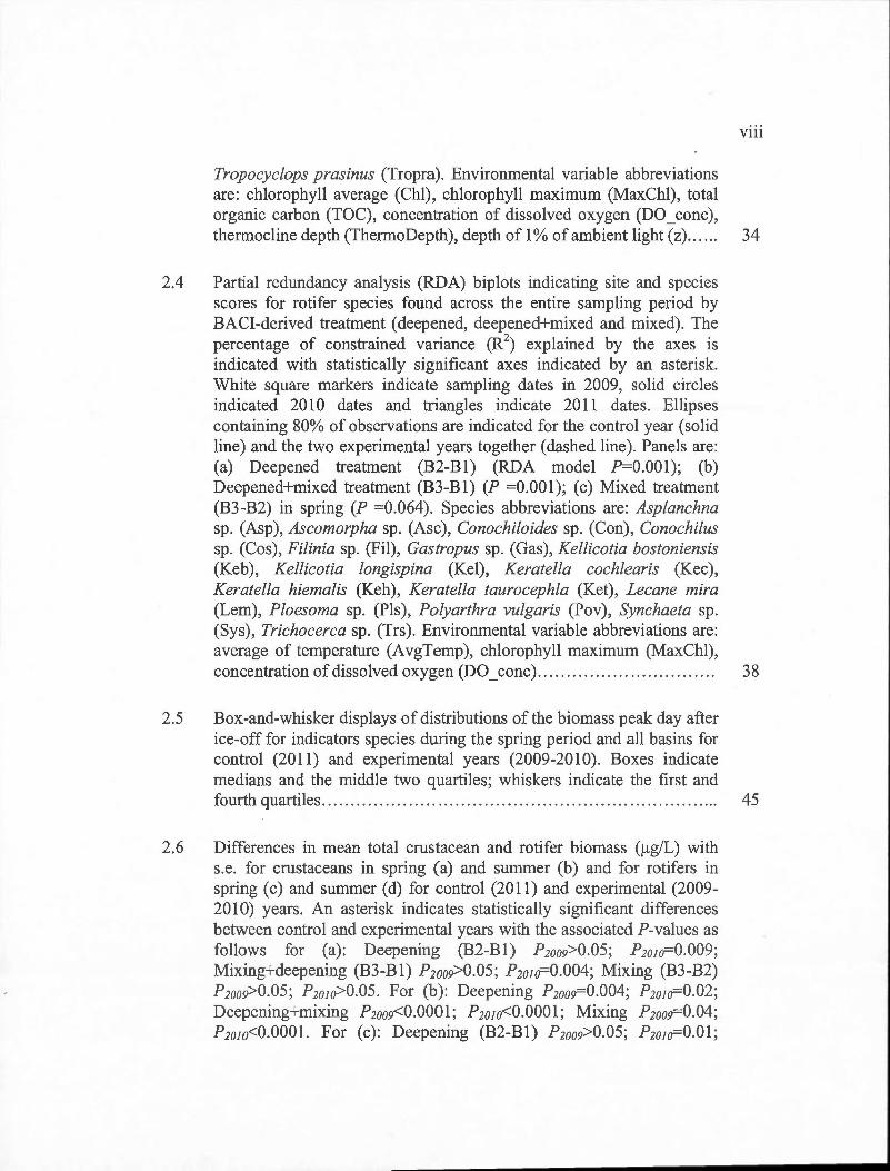
Tropocyclops prasinus (Tropra). Environmental variable abbreviations are: chlorophyll average (Chl), chlorophyll maximum (MaxChl), total organic carbon (TOC), concentration of dissolved oxygen (DO_ conc ),
Vlll
thermocline depth (ThermoDepth), depth of 1% of ambient light (z).... .. 34
2.4 Partial redundancy analysis (RDA) biplots indicating site and species scores for rotifer species found across the entire sampling period by BACI-derived treatment (deepened, deepened+mixed and mixed). The percentage of constrained variance (R2
) explained by the axes is indicated with statistically significant axes indicated by an asterisk. White square markers indicate sampling dates in 2009, solid circles indicated 2010 dates and triangles indicate 2011 dates . Ellipses containing 80% of observations are indicated for the control year (solid line) and the two experimental years together ( dashed line ). Panels are: (a) Deepened treatment (B2-B1) (RDA model P=0.001); (b) Deepened+mixed treatment (B3-B 1) (P =0.00 1 ); ( c) Mixed treatment (B3 -B2) in spring (P =0.064). Species abbreviations are: Asplanchna sp. (Asp), Ascomorpha sp. (Asc), Conochiloides sp. (Con), Conochilus sp. (Cos), Filinia sp. (Fil), Gastropus sp. (Gas), Kellicotia bostoniensis (Keb ), Kellicotia longispina (Kel), Keratella cochlearis (Kec ), Keratella hiemalis (Keh), Keratella taurocephla (Ket), Lecane mira (Lem), Ploesoma sp. (Pls), Polyarthra vulgaris (Pov), Synchaeta sp. (Sys), Trichocerca sp. (Trs). Environmental variable abbreviations are: average of temperature (AvgTemp), chlorophyll maximum (MaxChl), concentration of dissolved oxygen (DO_ co ne)................ . . . . . . . . . . . . . . . 3 8
2.5 Box-and-whisker displays of distributions of the biomass peak day after ice-off for indicators species during the spring period and all basins for control (2011) and experimental years (2009-2010) . Boxes indicate medians and the middle two quartiles; whiskers indicate the first and fourth quartiles............. . ............ . ...... . . . . . ...... . . . ............... . ...... 45
2.6 Differences in mean total crustacean and rotifer biomass (!lg/L) with s.e. for crustaceans in spring (a) and sumrner (b) and for rotifers in spring ( c) and summer ( d) for control (20 11) and experimental (2009-20 1 0) years. An asterisk indicates statistically significant differences between control and experimental years with the associated P-values as follows for (a): Deepening (B2-B1) P2oog>0.05; P2010=0.009; Mixing+deepening (B3-B1) P2oo9>0.05; ? 2010=0.004; Mixing (B3-B2) P2oo9>0.05; P2oJo>0.05. For (b): Deepening P2oog=0.004; P2o1o=0.02; Deepening+mixing P2oo9<0.000l; P2o1o<0.0001; Mixing P2oog=0.04; P2o1o<0.0001. For (c): Deepening (B2-B1) P2oog>0.05; P2o1o=0.01;

---------------------------------------
Deepening+mixing (B3-B1) P2oo9>0.05 ; P2o1o>0.05; Mixing (B3-B2) P2oo9>0.05 ; P2o1o=O.Ol. For (d): Deepening P2oo9>0.05; P2oio>0.05; Deepening+mixing P2oo9>0.05; P2oio>0.05; Mixing P2oo9>0.05;
IX
P2o1o>0.05.. ... .... . ... ....... .... ... ... ... ... .. ......... . .... ...... ..... .. ....... .. 47
2.7 Differences in mean adult body size in dry weight (~J.g) with s.e. for crustaceans in spring (a) and summer (b) and for rotifers in spring (c) and surnmer (d) for control (2011) and experimental (2009-2010) years . An asterisk indicates statistically significant differences between control and experimental years with the associated P-va1ues as follows for (a): Deepening (B2-B 1) P 20o9=0. 01; P 201 o=O. 01; Deepening+mixing treatment (B3 -B1) P2oo9=0.03; P2o1o=0.03; Mixing (B3-B2) P2oo9>0.05 ; P2oio>0.05. For (b): Deepening (B2-B1) P2oo9=0.001; P2oio<0.03; Deepening+mixing treatment (B3-B1) P2oo9=0.001; P2o1o=0.002; Mixing (B3-B2) P2oo9>0.05; P2o1o>0.05; (c): Deepening (B2-B1) P2oo9>0.05; P20lo<0.04; Deepening+mixing treatment (B3-B1) P2oo9>0.05; P2o1o<0.02; Mixing (B3-B2) P2oo9>0.05; P2oio>0.05. For (d): Deepening (B2-Bl) P2oo9>0.05; P2oio>0.05; Deepening+mixing treatment (B3 -B1) P2oo9>0.05; P201o>0.05; Mixing (B3-B2) P2oo9>0.05; P2o1o>0.05 ...... .. .. ... . ... ...... ...... . .... ....... . .... .. ................. ... .... .. 48
C.1 Partial redundancy analysis (RDA) biplots indicating site and species scores for rotifer species founded in spring and summer periods by BACI-derived treatment (deepened, deepened+mixed and mixed). The percentage of constrained variance (R2
) explained by the axes is indicated with statistically significant axes indicated by an asterisk. White square markers indicate sampling dates in 2009, solid circles indicated 2010 dates and triangles indicate 2011 dates . Ellipses containing 80% of observations are indicated for the control year (solid line) and the two experimental years together (dashed line). Panels are: (a) Deepened treatment (B2-B1) in spring (RDA model P =0.095); (b) Deepened treatment in summer (P =0.001); (c) Deepened+mixed treatment (B3-B1) in spring (P <0.005); (d) Deepened+mixed treatment in summer (P =0.012); (e) Mixed treatment (B3-B2) in spring (P =0.053) ; (f) Mixed treatment in summer (P =0.033). Species abbreviations are: Asplanchna sp. (Asp), Ascomorpha sp. (Asc), Conochiloides sp. (Con), Conochilus sp. (Cos), Filinia sp. (Fil), Gastropus sp. (Gas), Kellicotia · bostoniensis (Keb), Kellicotia longispina (Kel), Keratella cochlearis (Kec ), Keratella hiemalis (Keh), Keratella taurocephla (Ket), Lecane mira (Lem), Ploesoma sp. (Pls), Polyarthra vulgaris (Pov), Synchaeta sp. (Sys), Trichocerca sp. (Trs). Environmental variable abbreviations are: chlorophyll average (Chl),
x
chlorophyll maximum (MaxChl), concentration of dissolved oxygen (DO _conc). . . .. .. ... . .. . . . . . . . . . . . . . . . . . . . . . . . . . . . . . . . .. . . . . . . . . . . . . . . . . . . . . . . . . . .. 65
D.l Time series of the biomass of important cladoceran species for each basin in the control (2011) and experimental (2009-2010) years . (a) Bosmina longirostris; (b) Daphnia ambigua; ( c) Daphnia catawba; ( d) Daphnia longiremis; ( e) Holopedium gibberum. The vertical dashed line represents the day of year at which the thermocline depth reached the average for the entire sampling period . ...... . . . .. .. .... . . . . . . . . . . .. . . . ... 69
D.2 Time series of the biomass of important calanoid copepod species for each basin in the control (2011) and experimental (2009-2010) years . (a) Epischura lacustris ; (b) Leptodiaptomus minutus. The vertical dashed line represents the day of year at which the thermocline depth reached the average for the entire sampling period .. . . ... ... .. .. .... ... . . . .. . 72
D.3 Time series of the biomass of important calanoid copepod species for each basin in the control (2011) and experimental (2009-2010) years . (a) Cyclops scutifer; (b) Orthocyclops modestus; (b) Tropocyclops prasinus. The vertical dashed line represents the day of year at which the thermocline depth reached the average for the entire sampling period. . . ... .. . . . . . . . . . . . .. . . .. .. . . . . . .. . .. . .. . . . . . . .... .. .. .. .. . . .. . . . . . . . . . . . . . . . .. 74
E.l Graphique de l'analyse de redondance partielle (RDA) pour les crustacés présents pendant toute la période d 'échantillonnage et au printemps pour chaque traitement dérivé du BACI (abaissement, abaissement+mélange, mélange). La RDA partielle contrôle pour l 'effet du temps (jour de l'année) . Les covariables dans les RDA du printemps représentent le jour de l'année et non le nombre de jours après la fonte de la glace comme dans le Chapitre II. Le pourcentage de la variance contrainte (R2
) expliquée par les axes est indiqué et un astérisque indique que l' axe est significatif. Les carrés vides, les cercles pleins et les triangles pleins indiquent respectivement les dates en 2009, 2010 et 2011. Les ellipses contiennent 80% des observations et sont indiquées pour l' année contrôle (ligne pleine) et les années expérimentales ensemble (ligne pointillée). Les panneaux sont: (a) traitement d' abaissement (B2-Bl ) pour toute la période d'échantillonnage (modèle RDA P=O,OOl) ; (b) traitement d'abaissement (B2-Bl) pour le printemps (modèle RDA P=0,002) ; ( c) traitement d' abaissement+mélange (B3-Bl) pour toute la période d' échantillonnage (modèle RDA P =O,OOl) ; (d) traitement
d'abaissement+mélange (B3-Bl) pour le printemps (modèle RDA P=O,OOl); (e) traitement du mélange (B3-B2) pour toute la période d' échantillonnage (modèle RDA P=O,OOl); (f) traitement du mélange (B3-B2) pour le printemps (modèle RDA P=O,OOl). Les abbréviations des espèces sont : Bosmina longirostris (Boslon) , Daphnia ambigua (Dapamb ), Daphnia catawba (Dapcat), Daphnia longiremis (Daplon), Holopedium gibberum (Holgib), Epischura lacustris (Epilac), Leptodiaptomus minutus (Lepmin), Cyclops scutifer (Cycscu), Mesocyclops edax (Meseda), Orthocyclops modestus (Ortmod), Tropocyclops prasinus (Tropra). Les abbréviations des variables environnementales sont : concentration en oxygène dissous (DO_ corre), moyenne de la biomasse de chlorophylle dans la zone euphotique (Chl), température moyenne de la colonne d'eau (AvgTemp), carbone organique total (TOC), profondeur de la thermocline (ThermoDepth),
Xl
profondeur de la zone euphotique (z) et phosphore total (TP). . . . . . .. . . .. .. 76
F.l Graphique de l'analyse de redondance partielle (RDA) pour les rotifères présents au printemps pour chaque traitement dérivé du BACI (abaissement, abaissement+mélange, mélange). La RDA partielle contrôle pour l'effet du temps (jour de l'année). Les covariables dans les RDA du printemps représentent le jour de l'année et non le nombre de jours après la fonte de la glace comme dans l'Appendice C. Le pourcentage de la variance contrainte (R2
) expliquée par les axes est indiqué et un astérisque indique que l'axe est significatif. Les carrés vides, les cercles pleins et les triangles pleins indiquent respectivement les dates en 2009, 2010 et 2011. Les ellipses contiennent 80% des observations et sont indiquées pour l'année contrôle (ligne pleine) et les années expérimentales ensemble (ligne pointillée). Les panneaux sont : (a) traitement d'abaissement (B2-Bl ; modèle RDA P=0,069); (b) traitement d'abaissement+mélange (B3-Bl ; modèle RDA P=0,002); (c) traitement du mélange (B3-B2; modèle RDA P=0,006) . Les abbréviations des espèces sont : Asplanchna sp. (Asp ), Ascomorpha sp. (Asc) , Conochiloides sp. (Con) , Conochilus sp. (Cos), Filinia sp. (Fil), Gastropus sp. (Gas), Kellicotia bostoniensis (Keb), Kellicotia longispina (Kel), Keratella cochlearis (Kec), Keratella hiemalis (Keh), Keratella taurocephla (Ket), Lecane mira (Lem), Ploesoma sp. (Pls), Polyarthra vulgaris (Pov), Synchaeta sp. (Sys), Trichocerca sp. (Trs). Les abbréviations des variables environnementales sont : concentration en oxygène dissous (DO_ corre), maximum de chlorophylle (MaxChl), température moyenne de la colonne d'eau (AvgTemp)...... . ............ . . 80
LISTE DES TABLEAUX
Tableau
2.1 Mean (±SE) and ?-values from t-tests for treatment year effects (vs. control year) on the differences between basins for temperature (shaded) and chlorophyll-a biomass (white) for the spring and summer
Page
periods....... ... . . ... .. . .. .. . . .. .. . . . . ..... . . . .. . .. . . . . . . . . . . . .. . . . .. .. .. . . . . . . . .... 32
2.2 Mean (±SE) and ?-values from t-tests for treatment year effects (vs. control year) on the differences between basins for each spring indicator spectes.............................................................................. 41
2.3 Mean (±SE) and ?-values from t-tests for treatment year effects (vs. control year) on the differences between basins for each summer indicator species. . . . . . . . . . . . . . . . . . . . . . . . . . . . . . . . . . . . . . . . . . . . . . . . . . . . . . . . . . . . . . . . . . 44
A.l Caractéristiques qualitatives des espèces de zooplancton présentes dans le Lac Croche. Le groupe trophique représente leur préférence de type de proies et le type d'alimentation sépare les différentes habitudes alimentaires.. . . . . . . . . . . . . . . . . . . . . . . . . . . . . . . . . . . . . . . . . . . . . . . . . . . . . . . . . . . . . . . . . . . . . . . 61
A.2 Liste des espèces ou genres des rotifères présents dans le Lac Croche. L'habitat des rotifères est principalement pélagique. Les rotifères sont majoritairement herbivores et ils s'alimentent habituellement par filtration R. Le groupe représente une caractéristique physique ou comporten1entale..................................................... . ............ 62
B.1 Mean (SE) and ?-values from the Student t-test comparison of the variation in biomass of the major zooplankton groups between the two "Before" years 2007 and 20 11. The comparisons were analyzed statistically under the BACI design to test for treatment effects (for further explanation see Materials and Methods) . ... . . .. . .... . . . . . .. . . . .. . . ... 63
RÉSUMÉ
La stratification thermique, caractérisée par la présence d'une thermocline, est un facteur clé structurant les communautés de plancton dans la zone pélagique des lacs. Les changements climatiques (vents forts, orages fréquents, sécheresses intenses) et les activités anthropiques près des lacs (déforestation) pourraient occasionner un abaissement de la thermocline dans les lacs tempérés. Les effets d 'un tel abaissement sur la phénologie, la biomasse totale et la taille des individus du zooplancton dans le temps ont été évalués. La thermocline d'un bassin du Lac Croche (constitué de trois bassins), Québec, Canada, a été abaissée par mélange à 1' aide d'une éolienne aquatique. L'échantillonnage a eu lieu sur une mmée contrôle (sans manipulation) et deux années expérimentales (avec abaissement). Le protocole statistique BACI a permis d'évaluer les effets de trois traitements différents, soit l'abaissement, l'abaissement+mélange et le mélange. Au printemps, certains effets des traitements ont été discernés indirectement par le réchauffement des sédiments, mais le climat semblait avoir une grande influence sur la dynamique des communautés de crustacés. Pendant l 'été, les changements de la communauté de crustacés étaient principalement influencés par la profondeur de la thermocline. De plus, la biomasse de chlorophylle et celle des crustacées ont augmenté face aux traitements pendant l'été. Tropocyclops prasinus et Bosmina longirostris étaient plus abondantes lors de l'abaissement de la thermocline pendant l'été, ce qui a réduit significativement la taille individuelle de la communauté des . crustacés. Les assemblages de rotifères étaient dominés par des espèces ayant des caractéristiques pour les protéger de la prédation. Cette étude suggère qu'un abaissement de la thermocline dans les lacs tempérés pourrait mener à une augmentation des productions primaire et secondaire, mais également à une réduction des proies zooplanctoniques pour les poissons suite à un changement dans la composition et la taille individuelle de la communauté.
Mots-clés : abaissement de la thermocline, zooplancton, phénologie, taille individuelle, biomasse totale, structure des communautés

INTRODUCTION
Les relations trophiques permettent à 1' énergie et à la matière de voyager à
travers les écosystèmes. Dans le milieu pélagique des écosystèmes aquatiques, le
phytoplancton occupe la base du réseau trophique. Ces organismes sont autotrophes,
ce qui signifie qu'ils utilisent l'énergie solaire pour faire la photosynthèse. Le
phytoplancton sert alors de ressource nutritionnelle de base pour les communautés de
zooplancton, qui fournissent à leur tour les ressources et 1' énergie pour le niveau
trophique supérieur, soit les poissons planctivores. Par conséquent, le zooplancton
occupe un rôle central dans les réseaux trophiques aquatiques. D'une part, il contrôle
les communautés de phytoplancton par contrôle descendant (McCauley et Briand,
1979; Stemer, 1989) et d'autre part, il permet le transfert d 'énergie aux niveaux
trophiques supérieurs par contrôle ascendant (Sommer, 1989). Des perturbations
majeures au sein de ce niveau trophique pourraient donc avoir d'importantes
conséquences sur l'intégralité de l'écosystème aquatique (Berger et al. , 2010 ; Platt,
Fuentes-Yaco et Frank, 2003).
La composition de la communauté de zooplancton est régulée par des facteurs
biotiques et abiotiques, dont plusieurs peuvent également influencer la phénologie
des espèces. Autant la biomasse de phytoplancton que la prédation sont des facteurs
significatifs pour la régulation des communautés lacustres de zooplancton (Sommer,
1989). Plusieurs facteurs physiques et chimiques peuvent affecter le zooplancton. Par
exemple, dans les lacs tempérés, la stratification thermique est un des facteurs clés
pour les organismes qui vivent dans l' environnement pélagique (Kalff, 2003 ;
Thackeray et al. , 2006).
Dans les lacs tempérés dimictiques, la colonne d'eau est divisée en trois
couches distinctes pendant la saison estivale. La couche de surface, l ' épilirnnion, est
2
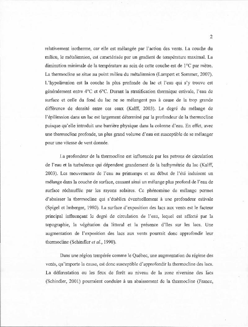
relativement isotherme, car elle est mélangée par l'action des vents. La couche du
milieu, le métalimnion, est caractérisée par un gradient de température maximal. La
diminution minimale de la température au sein de cette couche est de 1 °C par mètre.
La thermocline se situe au point milieu du métalimnion (Lampert et Sommer, 2007).
L'hypolimnion est la couche la plus profonde du lac et l'eau qui s'y trouve est
généralement entre 4°C et 6°C. Durant la stratification thermique estivale, l'eau de
surface et celle du fond du lac ne se mélangent pas à cause de la trop grande
différence de densité entre ces eaux (Kalff, 2003). Le degré du mélange de
1' épilimnion dans un lac est largement déterminé par la profondeur de la thermocline
puisque qu'elle introduit une barrière physique dans la colonne d'eau. En effet, avec
une thermocline profonde, un plus grand volume d'eau est susceptible de se mélanger
pour une vitesse de vent donnée.
La profondeur de la thermocline est influencée par les patrons de circulation
de 1' eau et la turbulence qui dépendent grandement de la bathymétrie du lac (Kalff,
2003). Les mouvements de l'eau au printemps et au début de l'été induisent un
mélange dans la couche de surface, causant ainsi un mélange plus profond de l'eau de
surface réchauffée par les rayons solaires. Ce phénomène de mélange permet
d'abaisser la thermocline qui s'établira éventuellement à une profondeur estivale
(Spigel et lm berger, 1980). La surface d'exposition des lacs aux vents est le facteur
principal influençant le degré de circulation de 1' eau, lequel est affecté par la
topographie, la végétation du littoral et la présence d 'îles sur les lacs. Une
augmentation de 1 'exposition des lacs aux vents poun·ait donc approfondir leur
thermocline (Schindler et al., 1990).
Dans une région tempérée comme le Québec, une augmentation du régime des
vents, qu'importe la cause, est donc susceptible d'approfondir la thermocline des lacs .
La déforestation ou les feux de forêt au niveau de la zone riveraine des tacs
(Schindler, 2001) pourraient conduire à un abaissement de la thermocline (France,
3
1997). L'exploitation forestière près d'un lac retire la végétation servant de brise
vent, résultant ainsi en une plus grande exposition du lac aux vents (Scully, Leavitt et
Carpenter, 2000). Par conséquent, le mélange des eaux de surface se fera plus
profondément et abaissera la thermocline du lac.
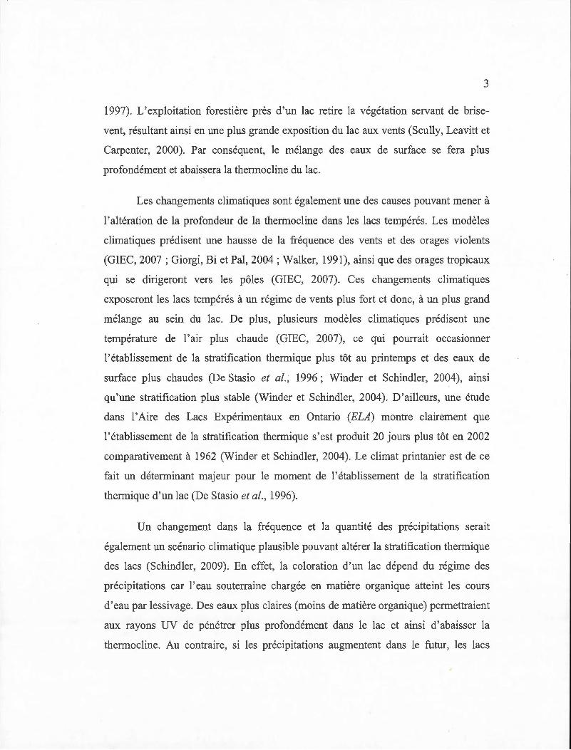
Les changements climatiques sont également une des causes pouvant mener à
l'altération de la profondeur de la thermocline dans les lacs tempérés. Les modèles
climatiques prédisent une hausse de la fréquence des vents et des orages violents
(GIEC, 2007 ; Giorgi, Bi et Pal, 2004; Walker, 1991), ainsi que des orages tropicaux
qui se dirigeront vers les pôles (GIEC, 2007). Ces changements climatiques
exposeront les lacs tempérés à un régime de vents plus fort et donc, à un plus grand
mélange au sein du lac. De plus, plusieurs modèles climatiques prédisent une
température de l'air plus chaude (GIEC, 2007), ce qui pourrait occasionner
l'établissement de la stratification thermique plus tôt au printemps et des eaux de
surface plus chaudes (De Stasio et al., 1996; Winder et Schindler, 2004), ainsi
qu'une stratification plus stable (Winder et Schindler, 2004). D'ailleurs, une étude
dans l'Aire des Lacs Expérimentaux en Ontario (ELA) montre clairement que
l'établissement de la stratification thermique s'est produit 20 jours plus tôt en 2002
comparativement à 1962 (Winder et Schindler, 2004). Le climat printanier est de ce
fait un déterminant majeur pour le moment de l'établissement de la stratification
thermique d'un lac (De Stasio et al., 1996).
Un changement dans la fréquence et la quantité des précipitations serait
également un scénario climatique plausible pouvant altérer la stratification thermique
des lacs (Schindler, 2009). En effet, la coloration d 'un lac dépend du régime des
précipitations car l'eau souterraine chargée en matière organique atteint les cours
d'eau par lessivage. Des eaux plus claires (moins de matière organique) permettraient
aux rayons UV de pénétrer plus profondément dans le lac et ainsi d'abaisser la
thermocline. Au contraire, si les précipitations augmentent dans le futur, les lacs

4
pourraient devenir plus colorés. Ce phénomène occasionnerait donc une thermocline
moins profonde dans la colonne d'eau, car la matière organique agit comme écran
solaire face aux rayons UV qui pénètrent alors moins profondément dans le lac
(Snucins et Gunn, 2000). Il est difficile de prédire si la thermocline des lacs sera plus
ou moins profonde dans le futur, mais il est certain que les changements climatiques
et les activités anthropiques près des plans d'eau auront un effet majeur sur la
stratification thermique des lacs. Les conséquences se feront ressentir non seulement
sur les paramètres physico-chimiques des lacs, mais également sur les organismes
vivants . Des études antérieures, qui ont examiné les effets de l'abaissement de la
thermocline sur les communautés biologiques, ont d 'ailleurs montré des changements
considérables au niveau de la composition et de l'abondance autant pour les
communautés de phytoplancton que de zooplancton (Cantin et al., 2011 ; Berger et
al., 2010; ; Berger et al., 2007; Berger, Diehl and Kunz, 2006; Lydersen et al.,
2008 ).
Cette étude s'insère dans le projet TIMEX (Thermocline Induced Mixing
Experiment), qui a débuté en 2007. Le but de ce projet était d'évaluer les effets de
l'abaissement expérimental de la thermocline sur différents paramètres biotiques et
abiotiques d'un lac. La thermocline d'un des trois bassins du Lac Croche, situé sur le
territoire de la Station de Biologie de l'Université de Montréal à St-Hippolyte,
Québec, Canada, a été abaissée artificiellement pour simuler une augmentation des
. vents sur le lac. Cette manipulation a permis d'abaisser la thermocline à une
profondeur de 7-8 m. Le bassin adjacent à celui manipulé a été séparé par un rideau
de polyéthylène. La thermocline de ce bassin a été abaissée à 5-6 rn par transfert de
chaleur à travers le rideau. Ce bassin intermédiaire a donc permis d 'évaluer 1 'effet
d'une diminution des précipitations et donc, d'une baisse de l'apport de matière
organique dans le lac. Les deux bassins expérimentaux ont été comparés à un bassin
contrôle du même lac, dont la thermocline naturelle se situait autour de 4-5 m. De
plus, l'échantillonnage a eu lieu pendant cinq années consécutives, dont deux années

5
contrôles, ce qui signifie que le mélange n'a pas eu lieu dans le bassin manipulé, et
trois années expérimentales (avec mélange). L'objectif principal du projet de
recherche présenté ici était d'évaluer l'effet d'un abaissement artificiel de la
thermocline sur la dynamique des communautés de zooplancton dans le temps, plus
précisément, sur la phénologie, la biomasse et la taille des individus du zooplancton.
Les variables réponses suivies de façon hebdomadaire pendant la période sans glace
étaient la composition taxonomique et la biomasse de zooplancton. Plusieurs
paramètres physico-chimiques et biologiques (phytoplancton) ont été mesurés afin de
comprendre le changement dans le temps des variables réponses.
Cette étude est unique en son geme car elle a permis d'évaluer non seulement
l'augmentation du régime des vents sur les lacs, mais aussi un autre scénario
climatique plausible, celui d'une baisse des précipitations qui mène à une eau plus
claire et donc, à un abaissement de la thermocline. Ces deux scénarios sont probables
dans le futur et permettent ainsi d'évaluer les conséquences d'un abaissement de la
thermocline avec et sans mélange accm. De plus, l'approche expérimentale permet
d'obtenir plus rapidement des résultats sur les effets potentiels occasionnés par les
changements climatiques ou les activités anthropiques près des plans d'eau par
rapport à une étude descriptive qui doit s'étendre sur plusieurs décennies. En outre,
peu d'études expérimentales (e.g. Berger et al., 2010; Berger et al., 2007) de se geme
se sont attardées à 1' évaluation de la dynamique des communautés de zooplancton
dans le temps.
Ce mémoire contient deux chapitres. Le premier chapitre (Chapitre I)
constitue une revue de la littérature sur la théorie de base de cette étude ainsi que la
méthode utilisée pour abaisser la thermocline du lac. Il permet donc de situer l 'étude
dans son contexte actuel. Le deuxième chapitre (Chapitre II) est écrit en anglais sous
la formule d' un article scientifique à des fins de publication. Il répond à l' objectif de
cette étude mentionné précédemment.
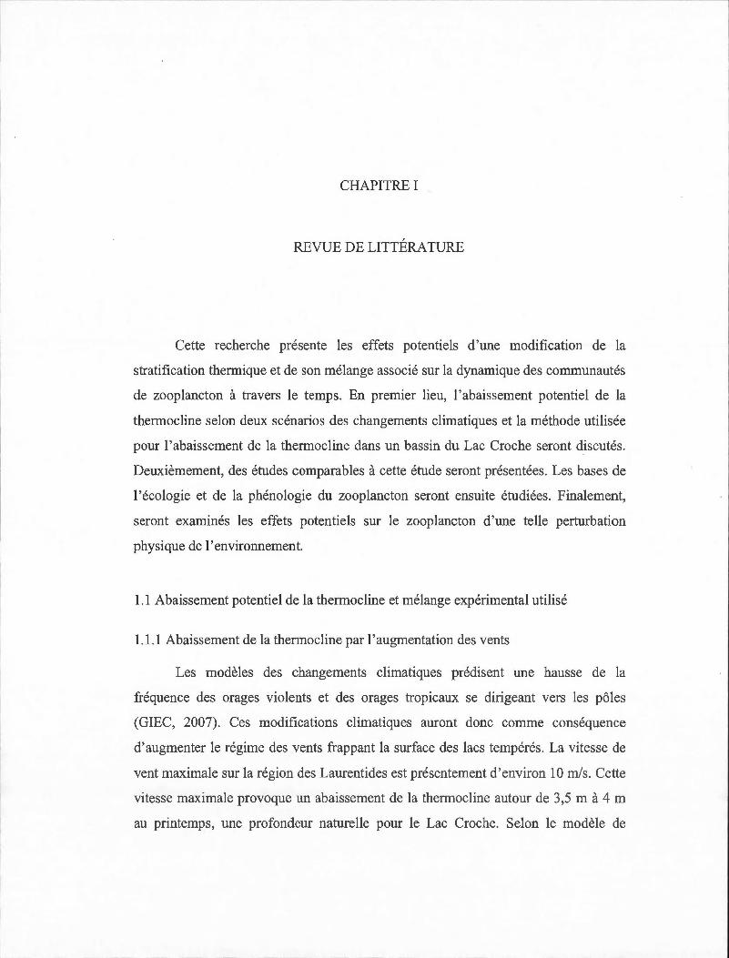
CHAPITRE I
REVUE DE LITTÉRATURE
Cette recherche présente les effets potentiels d'une modification de la
stratification thermique et de son mélange associé sur la dynamique des communautés
de zooplancton à travers le temps. En premier lieu, l'abaissement potentiel de la
thermocline selon deux scénarios des changements climatiques et la méthode utilisée
pour l'abaissement de la thermocline dans un bassin du Lac Croche seront discutés.
Deuxièmement, des études comparables à cette étude seront présentées. Les bases de
l'écologie et de la phénologie du zooplancton seront ensuite étudiées. Finalement,
seront examinés les effets potentiels sur le zooplancton d'une telle perturbation
physique de l'environnement.
1.1 Abaissement potentiel de la thermocline et mélange expérimental utilisé
1.1.1 Abaissement de la thermocline par 1 'augmentation des vents
Les modèles des changements climatiques prédisent une hausse de la
fréquence des orages violents et des orages tropicaux se dirigeant vers les pôles
(GIEC, 2007). Ces modifications climatiques auront donc comme conséquence
d'augmenter le régime des vents frappant la surface des lacs tempérés. La vitesse de
vent maximale sur la région des Laurentides est présentement d 'environ 10 rn/s. Cette
vitesse maximale provoque un abaissement de la thermocline autour de 3,5 rn à 4 rn
au printemps, une profondeur naturelle pour le Lac Croche. Selon le modèle de
7
Gorham et Boyce (1989), si la vitesse maximale du vent passe à 22 m/s dans la région
du Lac Croche, la thermocline passerait de 4 rn à 7 rn environ, ce qui est juste au
dessous de la zone photique pour le Lac Croche. Une augmentation des vents
maximaux à 35-40 m/s serait suffisante pour causer une déstratification complète de
la colonne d'eau. L' appareil utilisé pour abaisser la thermocline du lac à l'étude suit
d'ailleurs le modèle d'abaissement de la thermocline suite à une augmentation des
vents de Gorham et Boyce (1989) (Cantin, 2009).
1.1 .2 Abaissement de la thermocline suite à un changement de précipitations
Un changement dans le régime des précipitations est également un scénario à
prévoir dans le futur. Les modèles climatiques prédisent d'ailleurs des périodes de
sécheresse intense plus fréquentes (GIEC, 2007). Une baisse de la fréquence et de la
quantité des précipitations pourrait réduire- la quantité d'eau chargée en matière
organique se dirigeant vers les lacs. En effet, les cours d'eau reçoivent une grande
quantité de matière organique en provenance du bassin versant par lessivage des eaux
de pluies ou de fonte de la neige. Cette matière organique sert d'écran solaire dans les
lacs en limitant la pénétration des rayons ultraviolets (Scully et Lean, 1994). Par
conséquent, les lacs qui reçoivent moins de matière organique deviennent plus clairs
et leur thermocline s'abaisse alors plus profondément (Gunn et al., 2001 ; Schindler,
Parker et Stainton, 1996 ; Schindler et al., 1996). Dans ce scénario, le vent n'est pas
pris en compte, ce qui pourrait donc abaisser la thennocline moins profondément que
le ferait une hausse de la vitesse maximale des vents. La profondeur de la thermocline
pourrait donc se situer au-dessus de la zone euphotique, c'est-à-dire autour de 5 m à
6 m pour le Lac Croche.
1.1.3 Mélange expérimental utilisé
Une éolienne aquatique a été utilisée pour mélanger mécaniquement la
colonne d'eau d'un des trois bassins du Lac Croche. Cet appareil utilise l'énergie
8
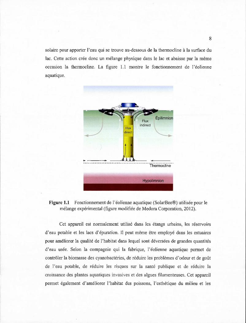
solaire pour apporter l'eau qui se trouve au-dessous de la thermocline à la surface du
lac. Cette action crée donc un mélange physique dans le lac et abaisse par la même
occasion la thermocline. La figure 1.1 montre le fonctionnement de l' éolienne
aquatique.
,_ ___ __ Thermocline
Figure 1.1 Fonctionnement de l'éolienne aquatique (SolarBee®) utilisée pour le mélange expérimental (figure modifiée de Medora Corporation, 20 12).
Cet appareil est normalement utilisé dans les étangs urbains, les réservoirs
d ' eau potable et les lacs d'épuration. Il peut même être employé dans les estuaires
pour améliorer la qualité de 1 'habitat dans lequel sont déversées de grandes quantités
d'eau usée. Selon la compagnie qui la fabrique, l'éolienne aquatique permet de
contrôler la biomasse des cyanobactéries, de réduire les problèmes d 'odeur et de goût
de 1 'eau potable, de réduire les risques sur la santé publique et de réduire la
croissance des plantes aquatiques invasives et des algues filamenteuses. Cet appareil
permet également d 'améliorer 1 'habitat des poissons, 1 'esthétique du milieu et les
9
mveaux d'oxygène dissous et de pH. Il est aussi mentionné que son utilisation
hypolinmétique préviendrait une accumulation de différents éléments comme le Mn,
Fe, H2S et le méthylmercure (Medora Corporation, 2012).
Pour cette expérience, le tuyau de l'appareil qui récolte l'eau en profondeur a
été placé à 8 rn, ce qui a permis d'abaisser la the1mocline entre 7 rn et 8 rn pendant la
saison estivale. Le bassin adjacent à celui où 1' appareil a été installé, a également
connu un abaissement de la them1ocline à cause d'un transfert de chaleur à travers le
rideau installé pour séparer ces deux bassins. La thermocline de ce bassin
intermédiaire se situait autour de 5-6 m. L'expérience a donc permis de tester les
deux scénarios potentiels d'abaissement de la the1mocline des lacs tempérés, soit 1)
une augmentation du régime des vents, et 2) une diminution des précipitations.
1.2 Études pertinentes sur le sujet
Depuis les dernières années, plusieurs études ont été menées afin d'examiner
le rôle de la stratification thermique, la stabilité et la turbulence sur l'interaction entre
les communautés de plancton et les aspects physico~chimiques des lacs . Par exemple,
il est bien connu que le phénomène El Nifio affecte le mélange de l'océan Pacifique et
a ainsi des effets majeurs sur la dynamique du plancton. Il a d'ailleurs été démontré
que la croissance accrue du phytoplancton suivant les années El Nifio influence
l'entièreté du réseau trophique dans les écosystèmes marins (Chavez et al., 1999).
Une panoplie d'études ont aussi examiné les effets du mélange et de la turbulence sur
le plancton dans les écosystèmes marins (Metcalfe, Pedley et Thingstad, 2004 ;
Petersen, Sanford et Kemp, 1998 ; Visser et Stips, 2002). Dans les eaux continentales,
plusieurs expériences ont été effectuées en mésocosmes pour comprendre les
conséquences d 'un changement de stratification thermique, du mélange ou de la
turbulence sur le plancton (Beisner, 2001a ; Beisner, 2001b ; Berger et al., 2007 ;
Berger et al. , 2010 ; Berger, Diehl and Kunz, 2006 ; Metcalfe, Pedley et Thingstad,
10
2004; Petersen, Sanford et Kemp, 1998; Rhew et al., 1999; Weithoff, Lorke et
Walz, 2000). Par ailleurs, certaines études ont considéré les effets d'une modification
de la stratification thermique et du mélange sur des lacs naturels (Antenucci et al.,
2005 ; Huisman et al., 2004), mais elles ont examiné uniquement le phytoplancton. À
1' échelle d'un lac, des expériences ont été effectuées sur 1' effet de la déstratification
complète d'un lac par aération de l'hypolimnion de réservoirs (Becker, Herschel et
Wilhelm, 2006 ; Heo et Kim, 2004). Toutefois, cette technique diffère de celle
utilisée dans l'expérience présentée ici et induit des changements écosystémiques non
naturels par l'addition d'air dans l'environnement. Plus récemment, un groupe de
chercheurs ont abaissé expérimentalement la therrnocline d'un lac naturel dans le sud
de la Finlande par un mélange physique. Cependant, ils se sont concentrés seulement
sur les dynamiques du mercure (Verta et al., 201 0) ainsi que sm les conséquences
physiques et chimiques (Forsius et al. , 2010) d'un abaissement artificiel de la
therrnocline. D'autres études conduites dans les lacs boréaux, incluant une de notre
groupe (Cantin et al., 2011), ont considéré les effets d'un abaissement artificiel de la
therrnocline sur la composition taxonomique et l'abondance du plancton ainsi que sur
leur distribution verticale (Cantin et al. , 2011 ; Lydersen et al., 2008). Toutefois, à
notre connaissance, les effets d'un abaissement de la thermocline sur la dynamique de
communauté dans le temps n'ont jamais été examinés à l'échelle d'un lac.
1.3 Écologie de base du zooplancton
Les classes de taille sont souvent utilisées pour décrire le zooplancton. En
limnologie, cette guilde est divisés en deux classes : le microzooplancton ( <200 f-1-m
en longueur) et le macrozooplancton (>200 f-1-m) . Les deux groupes taxonomiques
majeurs de zooplancton lacustre sont les rotifères et les crustacés, qui sont à leur tour
séparés en deux grands groupes, les cladocères et les copépodes (Kalff, 2003 ;
Wetzel, 1983).
----- -----------------------------------------------------------------------------------------
11
Les rotifères (embranchement Rotifera) sont les principaux composants du
microplancton, mais ils varient grandement en taille. Ces organismes sont les plus
importants invertébrés multicellulaires possédant un corps mou dans les
communautés de plancton lacustre (Kalff, 2003). Les rotifères ont un cycle de vie
court qui est fortement relié aux conditions de température, aux ressources et à la
photopériode. Ils peuvent s 'adapter rapidement à des changements
environnementaux, ce qm en fait des organismes ayant des réponses plutôt
stochastiques. De plus, leur reproduction se fait principalement par parthénogenèse.
En général, les organismes appartenant à cet embranchement s 'alimentent par
filtration. Les genres les plus communs sont omnivores et se nourrissent de
picoplancton, de petits flagellés et de ciliés. Cependant, certains genres tendent à
sélectionner de plus grandes particules dans leur alimentation, incluant des crustacés.
Généralement, la taille des rotifères détermine la taille de leurs proies (Kalff, 2003 ;
Wetzel, 1983). Dans le lac à l'étude, les genre les plus communs sont : Asplanchna,
Conochiloides, Chonochilus, Filinia, Gastropus, Kellicotia, Keratella, Synchaeta et
Trichocerca.
Les cladocères (sous-ordre Cladocera) sont généralement couverts d'un
manteau rigide de chitine qui se nomme la carapace. La plupart des organismes
appartenant à ce groupe s' alimentent par filtration, mais ils peuvent sélectionner les
particules en se basant sur leur taille, leur disponibilité, leur forme et leur qualité
nutritionnelle. Toutefois, certains genres comme Polyphemus et Leptodora sont des
organismes prédateurs. Les cladocères ont un temps de génération plus long que les
rotifères et se reproduisent la plupart du temps par parthénogenèse avec des œufs
diploïdes (2N). Toutefois, des œufs haploïdes (N) et des mâles peuvent être produits
sous des conditions défavorables. Même si leur cycle de vie est plus long que celui
des rotifères, ce sont tout de même des organismes à cycle de vie plus court que les
copépodes (Kalff, 2003 ; Wetzel, 1983).
------------,
12
Les copépodes (Classe Copepoda) se reproduisent sexuellement et ont le plus
long cycle de vie parmi le zooplancton lacustre (Kalff, 2003 ; Wetzel, 1983). En effet,
les copépodes ont cinq ou six stades nauplii et cinq stades copépodites avant
d'atteindre le stade adulte (Santer et Lampert, 1995). Par conséquent, ils réagissent
plus lentement aux changements des conditions biotiques et abiotiques. La
température est un des facteurs importants influençant le taux de développement de
tous les stades de vie (Vijverberg, 1980). Les copépodes sont divisés
taxonomiquement en trois ordres : les cyclopoides, les calanoides et les
harpactacoides. Les cyclopoides sont généralement carnivores, mais leur diète peut
également être composée d'algues, de bactéries et de détritus. Longtemps considérés
exclusivement herbivore, les calanoides sont maintenant classifiés comme omnivores,
s'alimentant autant de rotifères et de ciliés que d'algues, de bactéries et de détritus.
Leur stade, leur sexe, la saison et la disponibilité de la nourriture sont tous des
facteurs pouvant influencer la diète des cyclopoides et des calanoides. Le troisième
groupe, les harpactacoides, ne seront pas considérés dans cette recherche puisque
qu'ils sont principalement benthiques (Kalff, 2003 ; Wetzel, 1983).
Les larves d'insectes sont aussi communes dans les lacs et peuvent donc être
incluses dans le zooplancton. Les larves de diptères du genre Chaoborus influencent
de façon importante la communauté de zooplancton par la prédation (Kalff, 2003 ;
Wetzel, 1983). Les espèces et genres de tous les différents groupes de zooplancton
présents dans le lac à l'étude ainsi que certaines caractéristiques associées à chaque
taxon sont présentés dans 1' appendice A.
1.4 Succession saisonnière du zooplancton
La succession en espèces est un important phénomène observé dans tous les
écosystèmes et est définie comme le changement dans le temps de la composition en
espèce au sein de la communauté, puisque les conditions environnementales et les

13
ressources changent (Lampert et Sommer, 2007 ; Townsend, Begon et Harper, 2003).
Dans les lacs tempérés, la succession du zooplancton est grandement influencée par la
succession du phytoplancton comme le décrit le modèle PEG. Ce modèle verbal
illustre la séquence des changements saisonniers des communautés de phytoplancton
et de zooplancton dans un lac dimictique idéal (Sommer et al. , 1986).
Après la fonte de la glace du lac au printemps, le phytoplancton croît
rapidement puisque la lumière ainsi que les nutriments deviennent disponibles.
Ensuite, vient la phase d'eau claire (Clear-water phase) durant laquelle la biomasse
de phytoplancton diminue à cause de l' importance de l'herbivorie . De grands
herbivores à haute efficacité et à cycle de vie rapide, soient le geme Daphnia,
dominent alors la communauté de zooplancton. Une grande communauté de rotifères
est également présente pendant cette phase. Subséquemment, les ressources
diminuent, ce qui entraîne une plus forte compétition entre les zooplanctons
herbivores et une plus forte pression des prédateurs. La compétition et la prédation
accélèrent le déclin des populations de zooplancton herbivore. Les populations de
phytoplancton peuvent alors commencer à construire leur biomasse estivale à cause
de la disponibilité des nutriments et d 'une réduction de la pression d 'herbivorie. Une
fois que les biomasses estivales sont établies, les communautés de phytoplancton et
de zooplancton suivent un patron similaire, avec une dominance en espèces qui sera
différente dépendamment des facteurs abiotiques et biotiques. En été, ce sont
majoritairement des espèces à cycle plus lent, comme les copépodes, qui vont
dominer les communautés. Les facteurs biotiques et abiotiques qui influencent la
composition des communautés de plancton incluent la disponibilité des ressources
spécifiques, l' interaction entre les espèces ( e.g. compétition, prédation), la structure
de 1' environnement physique ( e.g. température) et les interactions entre ces différents
facteurs (Sommer et al., 1986).

14
Les modifications thermiques dans les lacs peuvent avoir autant des effets
indirects que directs sur le plancton pélagique. Indirectement, les effets se produisent
par un changement de la structure de 1 'habitat qu'occasionne la stratification
thermique, tandis que les changements de température vont affecter directement la
physiologie et le comportement du plancton (Anneville et al., 2010). La température
et les réserves de nourriture sont d'ailleurs deux facteurs considérables pouvant
influencer la compétition entre les espèces, affectant par le fait même la succession
du zooplancton. Plusieurs prédateurs sont également sensibles aux changements
thermiques. La succession du zooplancton pourrait par conséquent être affectée par
les changements de pression de prédation qui en découlent. De plus, la température
est un facteur considérable dans la vitesse de développement des organismes
planctoniques. Généralement, plus la température est élevée, plus le développement
des organismes est rapide (Feniova et Zilitinkevich, 2012; Maier, 1989), ce qui peut
ainsi· influencer la phénologie du zooplancton. La température est également un
facteur critique pour l'émergence des œufs d01mants des espèces de Daphnia
(Caceres, 1998). Des modifications de la stratification thermique des lacs à travers les
changements climatiques ou les activités anthropiques pourraient donc avoir des
conséquences majeures dans la dynamique des communautés de zooplancton.
1.5 Effets potentiels de l'abaissement de la thermocline et du mélange sur les
communautés de zooplancton
La stratification thermique et le mélange induit dans l'épilirnnion par cette
stratification ont potentiellement d'importants effets sur les communautés de
zooplancton. Certaines espèces pourraient bénéficier des changements d 'une
stratification thermique et d 'un mélange dans leur environnement. Inversement,
d'autres organismes pourraient être désavantagés face à un tel changement. La
réponse dépendra principalement des caractéristiques écologiques de chaque espèce
de zooplancton. Dans les rivières, qes études ont montré que les groupes de
15
zooplancton de faible taille individuelle (rotifères, petits copépodes, Bosmina) sont
généralement plus tolérants à la turbulence que les grandes espèces de cladocères
(Basu et Pick, 1996 ; Pace, Findlay et Lints, 1992). Une turbulence qui accompagne
un mélange plus profond peut aussi influencer l'alimentation des zooplanctons. La
turbulence augmente la suspension des particules dans l'eau qui peuvent ainsi
interférer avec la détection sensorielle des proies par les prédateurs. D'un autre côté,
la turbulence permet d'augmenter le taux de rencontre entre prédateurs et proies
(Lewis et Pedley, 2001 ; Visser et al., 2001). Toutefois, le temps de consommation
des proies est plus long dans un environnement turbulent (Lewis et Pedley, 2001 ;
Visser et Stips, 2002) . Les effets que peuvent avoir le mélange (et la turbulence
associée) dépendent grandement des caractéristiques comportementales de chaque
espèce et de la motilité des prédateurs et des proies (Kiorboe et Saiz, 1995 ; Lewis et
Pedley, 2001). Certaines espèces peuvent d 'ailleurs s'adapter à une augmentation de
la turbulence en modifiant leur comportement par une migration verticale ou un
changement dans la sélection des proies (Visser et Stips, 2002). Selon Visser et al.
(200 1 ), la turbulence affecte négative.ment 1' acquisition de nourriture chez les
copépodes qui s'alimentent par suspension dans la colonne d 'eau. Par contre, les
prédateurs qui chassent par embuscade peuvent bénéficier d'un environnement plus
turbulent (Kiorboe et Saiz, 1995). Dans le lac à l'étude, Cantin et al. (2011) ont
similairement trouvé que les cyclopoides (prédateurs par embuscade) sont favorisés
par un abaissement de la thermocline et de son mélange associé. Donc, une
modification de l'environnement qui augmente la profondeur du mélange pomnit
conduire vers une dominance de ce groupe fonctiom1el dans la communauté de
zooplancton.
La dominance d'un groupe fonctionnel donné pourrait avoir des conséquences
sur la bi~masse totale de la communauté de zooplancton. Les effets qu'aura
l'abaissement de la thermocline sur le phytoplancton pourraient aussi jouer un rôle
important sur la biomasse totale de zooplancton. En effet, plus l'épilimnion se
16
mélange profondément, plus le phytoplancton passera de temps dans les eaux
profondes et sombres. Un manque de lumière occasionnera donc une baisse de la
production chez le phytoplancton, ce qui aura pour effet de diminuer les ressources de
base du zooplancton. Berger, Diehl et Kunz (2006) ont d'ailleurs observé que la
biomasse de zooplancton diminuait avec une augmentaiton de la profondeur de la
thermocline.
Une couche d ' eau mélangée plus profondément pourrait également modifier
le moment des événements successifs au printemps dans la communauté de plancton.
Un mélange plus profond tend à réduire l'importance du pic de phytoplancton et du
pic subséquent de Daphnia au printemps (Berger et al., 2010; Berger et al., 2007).
De plus, le moment de la phase d'eau claire (grande abondance d'herbivores) pounait
être devancée au printemps par une température plus chaude de la colonne d'eau
puisque le mélange se fera plus profondément. En effet, la température de 1' eau est un
important facteur influençant le taux de croissance de la population d'importants
herbivores comme les Daphnia (Berger et al., 2007). Les espèces à croissance rapide
( cladocères et rotifères) qui dominent la communauté au printemps, peuvent aussi
être affectées par la durée de la période du couvert de glace sur le lac ainsi que la date
à laquelle la glace disparaît du lac (Adrian et al., 1999). En effet, les espèces de
rotifères et cladocères atteignent leur biomasse maximale plus tôt suite à des hivers
plus doux (Adrian et al., 1999). Par conséquent, le climat hivernal ainsi que le climat
printanier peuvent avoir une influence particulière sur le moment du pic de certains
groupes d'espèces. Cependant, la magnitude du pic semble être indépendante de la
durée du couvert de glace (Adrian et al., 1999). Il s'avère que la température de l'eau
est un facteur critique pour la dynamique du zooplancton durant la période du
printemps (Berger et al. , 2010 ; Schalau et al. , 2008; Scheffer et al., 2001), pendant
laquelle l'eau est encore fro ide et que les ressources de haute qualité sont abondantes
(Sommer et al., 1986). Durant les mois d'été, les forces biotiques comme la
compétition pour les ressources de haute qualité et la pression de prédation
17
deviennent d'importants régulateurs pour la phénologie du zooplancton (Sommer et
al., 1986).
Pendant l'été, les communautés de zooplancton sont surtout dominées par des
espèces à croissance lente comme les copépodes. Ces organismes ont des cycles de
vie beaucoup plus complexes que les cladocères et les rotifères (Adrian, Wilhelm et
Gerten, 2006 ; Maier, 1989 ; Vijverberg, 1980). La variation des populations de
copépodes est fortement reliée aux caractéristiques hydrodynamiques de la colonne
d'eau, le cycle saisonnier du microplancton (phytoplancton et ciliés) et les
caractéristiques de chaque espèce (Rodriguez et al., 2000). La réponse de ces espèces
face à un changement de stratification thermique et de mélange est donc complexe à
prédire (Adrian, Wilhelm et Gerten, 2006; Nicolle et al., 2012). Petersen Sandfort et
Kemp (1998) ont montré que le mélange peut modifier le moment où la densité
maximale des copépodes est atteinte. De plus, une altération des événements
phénologiques au printemps ou un changement du climat printanier et hivernale
pourraient avoir des effets de propagation dans le temps et ainsi affecter la phénologie
des espèces estivales (Adrian et al., 1999).
Selon Daufresne, Lengfellner et Sommer (2009), la modification de la
phénologie des espèces est une des trois grandes réponses face aux changements
climatiques avec un changement dans la distribution régionale des espèces ainsi que
la réduction de la taille individuelle des organismes. En effet, il est bien comm que
des températures plus chaudes produisent des organismes de plus petites tailles
(Daufresne, Lengfeller et Sommer, 2009; Vijverberg, 1980). Dans une experience
d'abaissement de la the1mocline, l'épilinmion se mélange plus profondément, mais sa
température n'augmente pas. Conséquemment, la taille individuelle de la
communauté de zooplancton ne devrait pas être réduite.
CHAPITRE II
THERMOCLINE DEEPENING CAUSES ALTERED ZOOPLANKTON
PHENOLOGY, REDUCED BODY SIZE AND GREA TER COMMUNITY
BIOMASS IN A WHOLE LAKE EXPERIMENT
Ce chapitre a été rédigé en anglais sous la forme d'un article scientifique à des
fins de publication. La rédaction ainsi que le processus scientifique précédant celle-ci
ont été réalisés par J. Gauthier sous la direction de B. Beisner et la codirection de Y.
Prairie. Ce chapitre répond à l'objectif du projet qui était d'évaluer les effets d'un
abaissement de la thermocline sur la dynamique des communautés de zooplancton
dans le temps.
19
2.1 Abstract
Thermal stratification, characterized by thermocline depth, is thought to be one of the key structuring physical factors for lake plankton. Climate changes ( strong winds, frequent storms, intense droughts) and large-scale human activities around lakes (fires, logging) potentially lead to thermocline deepening in stratified lakes. The effects of thermocline deepening on zooplankton phenology, total biomass and mean body size were assessed in a whole-lake experiment. The thermocline of a three-basin north temperate lake was deepened in one basin to 7 -8m using a lake mixer. Through beat transfer, the thermocline of the adjacent basin was deepened to 6-7m, and the third basin served as an unrnanipulated control (4-Sm deep thermocline). Zooplankton community dynamics were followed weekly in a control year (no manipulation) and two experimental years (with deepening) . The BACI statistical protocol was used to assess the effects of three distinct treatments: thermocline deepening, deepening+mixing and mixing. In spring, zooplankton community dynamics were mainly indirectly affected by the treatments through sediment warming, with annual variation in spring climatic conditions having greater influence. In summer, thermocline depth was the main factor influencing zooplankton community changes, including greater total crustacean biomass. The biomass of Tropocyclops prasinus and Bosmina longirostris increased with thermocline deepening, leading to a decline in crustacean mean body size. Rotifer assemblages were dominated by species well-protected from predation during experimental years in mixing treatments. Our study suggests that while thermocline deepening accompanying global change in temperate lakes could lead to increases in secondary standing production, zooplankton prey resources for fish will decline because of shifts in community composition and body size.

20
2.2 Introduction
Thermal stratification features of temperate lakes in summer have potential
importance for plankton community structure (Berger, Diehl and Kunz, 2006; Berger
et al., 2010; Cantin et al. , 2011; Longhi and Beisner, 2010; Lydersen et al., 2008).
Altered stratification, and in particular, thermocline depth is a likely outcome of
climate change in north temperate regions through a number of direct and indirect
mechanisms. Thermocline depth is determined primarily by the degree of water
circulation in a lake through mixing by wind (France, 1997). Meteorological models
predict an increase in the frequency of violent winds and storms (GIEC, 2007; Giorgi,
Bi and Pal, 2004; Walker, 1991), as well as an increased tendency of tropical storms
to reach higher latitudes (GIEC, 2007), thereby exposing temperate lakes to stronger
winds and greater mixing. Furthermore, climate change models forecast higher air
temperatures (GIEC, 2007), which could lead to an earlier onset of spring
stratification and wanner surface waters (De Stasio et al., 1996; Winder and
Schindler, 2004) as well as more stable stratification (Winder and Schindler, 2004).
Wind exposure depends greatly on topography, shore vegetation, the presence of
islands and on lake morphometry itself (Kalff, 2003). Thus indirectly, increases in
forest fire frequency with climate change and loss of tree cover near lakes will
increase surface wind stress (Schindler, 2001) producing deeper spring mixing
(Scully, Leavitt and Carpenter, 2000), leading to deeper thermoclines (France, 1997).
Finally, climate change-induced alterations to precipitation patterns will also affect
thermocline depths, with the direction of the effect depending on precipitation
frequency. Runoff affects the tenestrial influx of colored dissolved organic carbon
(DOC) to lakes. Ultimately, if lake waters become less stained with climate change
(lower DOC because of infrequent precipitation), they will experience greater UV
light penetration for longer, resulting in deeper thermoclines (Schindler, 2001). While
changes in precipitation patterns are more difficult to model (GIEC, 2007) making
the direction of change in thermocline depth difficult to predict, alterations in
21
therrnocline depth as a critical physical feature of stratified lakes, have potential
consequences for zooplankton communities that must be explored to fully understand
climate change impacts on lakes. Because of their central position in lake food webs
in structuring phytoplankton communities (McCauley and Briand, 1979; Sterner,
1989) while transferring energy to higher trophic levels like fish (Sommer et al.
1986), perturbation to zooplankton communities driven directly by change in thermal
stratification could thus have repercussions on other components of the food web
(Berger et al. , 2010; Platt, Fuentes-Yaco and Frank, 2003).
In recent years, several studies have examined the role of thermal stratification
patterns and stability on the interaction between plankton community structure and
lake physics and chemistry ( e.g. Adrian, Wilhem and Gerten, 2006; Beisner, 2001 a;
Berger et al., 2010; Berger et al. , 2007; Cantin et al. , 2011). Many experiments on the
effects of altered thermal regimes, stratification and mixing on plankton communities
have been conducted in mesocosms (Beisner, 2001a; Beisner, 2001b; Berger et al.,
2010; Berger et al. , 2007; Metcalfe, Pedley and Thingstad, 2004; Petersen, Sanford
and Kemp, 1998; Rhew et al., 1999; Weithoff, Lorke and Walz, 2000), although
sorne have been conducted onlakes themselves (Antenucci et al. , 2005; Berger, Diehl
and Kunz, 2006; Cantin et al., 2011 ; Forsius et al. , 2010; Huisman et al. , 2004;
Lydersen et al., 2008; Verta et al., 2010). Sorne of the studies conducted in lakes,
including the foreru1111er of this current study (Cantin et al. , 2011), have considered
the effect of an artificially deepened therrnocline on composition, abundance and
vertical distribution of plankton (Cantin et al., 2011; Lydersen et al. , 2008). To date,
however, no one has specifically examined the effects of thermocline alteration at a
whole basin scale on zooplankton community dynamics and phenology through time.
Dynamical and phenological shifts in zooplankton in response to therrnocline
deepening may differ between spring and summer periods. Deeper mixing in spring
has been shown in mesocosms to reduce the importance of the phytoplankton bloom
---------------,
-- -------------------- --- ---------------
22
and reduce and/or delay the subsequent Daphnia peak (Berger et al., 201 0; Berger et
al., 2007) owing to the negative effect of water colder temperatme on population
growth rates of important herbivores like Daphnia (Berger et al., 2007; Caceres,
1998). However, time series studies have demonstrated that the duration of ice cover
and the ice-off date also affect the spring dynamics of the dominant fast-growing
species (cladocerans and rotifers) (Adrian et al. , 1999). Change through time in mean
water temperature appears to be the critical factor for springtime zooplankton
dynamics (Berger et al. , 2010; Schalau et al., 2008; Scheffer et al., 2001), affecting
physiology and behaviour (Anneville et al., 2010) in a period when lakes are still cold
and high-quality food is abundant. During the summer months, biotic forces such as
competition for limited high-quality food and predation pressure become more
important drivers (Sommer, 1989).
Summer zooplankton communities of temperate lakes are often dominated by
slow-growing species like copepods, which have more complex life cycle than
cladocerans and rotifers (Adrian, Wilhem and Gerten, 2006; Maier, 1989; Vijverberg,
1980). Variation in copepod populations is strongly related to the hydrodynamic
characteristics of the water column, the seasonal cycle of microplankton
(phytoplankton and ciliates) and the ecological traits of each copepod species
(Rodriguez et al. , 2000). The response to climate change of copepods is therefore
more complex to predict and likely to be species-specific (Adrian, Wilhem and
Gerten, 2006; Nicolle et al. , 2012). With respect to the phenology of zooplankton,
greater mixing (such as with a deeper thermocline) may alter the timing of peak
copepod densities (Petersen, Sanford and Kemp, 1998). Adrian, Wilhem and Gerten
(2006) hypothesized that winter and spring conditions could further affect the
phenology of summer species by propagating effects through time. The complexity
and idiosynchracies inherent in the response of summertime zooplankton is likely
wh y very few studies ( e.g. Adrian, Wilhem and Gerten, 2006; Berger, Diehl and
Kunz, 2006; Gerten & Adrian, 2002) to date have examined the effects of physico-
------------------------------~--------·-----·---------------------------~---------------
23
chemical changes associated with climate change on dynamics and phenology of
these communities.
Overall, when considering the entire growing season (spring and summer) of
dimictic north temperate lakes, a deeper thermocline and its related mixing should
have the potential to greatly affect the biomass as well as successional patterns of
zooplankton communities. Following the modelling results of Berger, Diehl and
Kunz (2006), we hypothesize that zooplankton biomass will be lower with a deeper
thermocline. This prediction arises because non-motile phytoplankton will spend
more time in darker waters with increased mixing depth, leading to a decrease in
phytoplankton biomass and thus less of a resource base for zooplankton. We further
hypothesize, based on the observations in the preliminary work on this lake (Cantin et
al., 2011), that rotifers that are well-protected from predators through spiny
appendages will be more abundant with thermocline deepening. A third hypothesis is
an expectation for a differentiai response in cladocera versus copepod phenology with
the experimental treatments . Corresponding to the preliminary study results,
cladoceran species are expected to -decline with thermocline deepening and mixing.
The responses of copepods are more complex to predict because of their longer life
cycle (Adrian, Wilhem and Gerten, 2006; Nicolle et al., 2012). A final hypothesis
addresses the conclusions of Daufresne, Lengfellner and Sommer (2009) who found
that reduced body size is an important effect of climate change because of allometric
temperature relationships. However, in our case, because thermocline deepening is
mainly a redistribution of the temperature and not a warming of the epilimnetic water
perse, we did not expect a reduction in body size.
This study reports on the effects of an experimental deepening of thermoclines
with different mixing applications for zooplankton community dynamics. Responses
in the plankton community under conditions of experimental thermocline deepening
(7-8m depth) in one lake basin are compared with a more intermediate thermocline
24
depth (6-7m) in an adjacent basin, and to a normal thermocline depth (4-Sm) in a
control basin. The main goal was to assess the effect of a change in thermal
stratification and the accompanying mixing on the zooplankton phenology, biomass
and body sizes.
2.3 Materials and methods
2.3 .1 Study site and experimental design
This study is part of TIMEX (Thermocline Induced Mixing Experiment),
which began in 2007 with a control year (Cantin et al., 2011). The experiment took
place in Lac Croche (4Y59'35"N 74°00'28"W) at the Station de Biologie des
Laurentides in St-Hippolyte, Quebec, Canada. This headwater lake is meso
oligotrophic and its area is 0.19 km2. Its watershed covers 0.7 km2 and it is relatively
undisturbed by anthropogenic activities. This lake was chosen because of the relative
absence of human influences and because of its shape, with three relatively distinct
basins. The control basin (B 1) and the intermediate basin (B2) are separated by a
narrow and shallow channel (2 rn deep ). B2 is separated from the manipulated basin
(B3) by an island, a very shallow section (1 rn deep) on the south side, and a shallow
section of approximately 120 rn wide and 6 rn deep on the north side (Fig. 2.1) . In
November 2007, a black polyethylene curtain was installed in the larger opening
between B2 and B3 to isolate the mixed basin from the rest of the lake. In years
where mixing of B3 occurred, a deepening of the thermocline also occurred in B2
because of passive beat transfer. The three basins have maximum depths of 11-13 m.
Sampling docks were anchored at the deepest point of each basin.
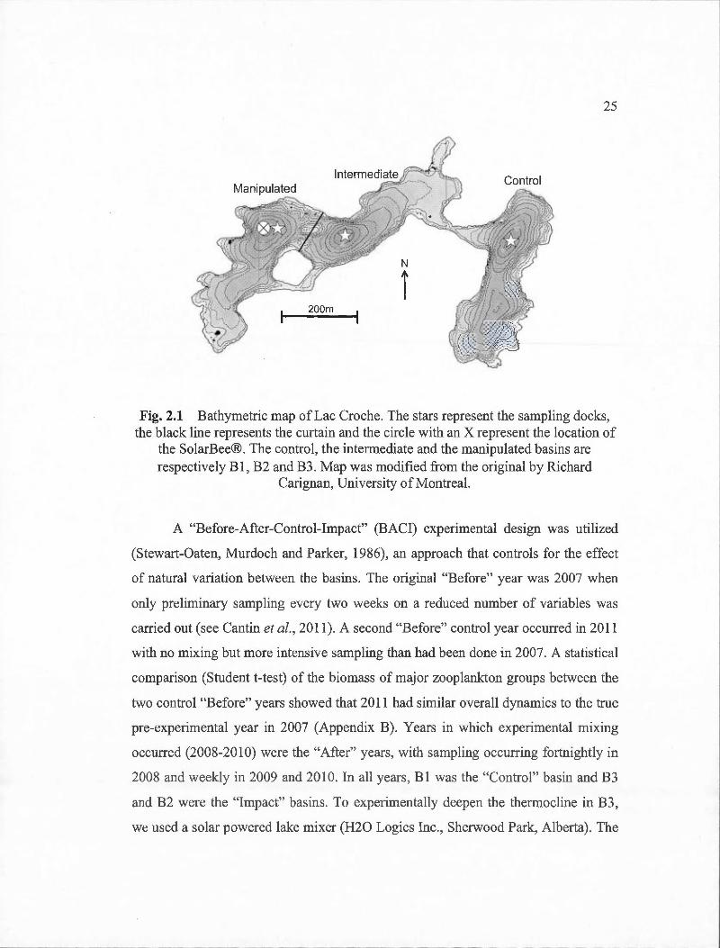
25
Fig. 2.1 Bathymetrie map of Lac Croche. The stars represent the sampling docks, the black line represents the curtain and the circle with an X represent the location of
the SolarBee®. The control, the intermediate and the manipulated basins are respectively B 1, B2 and B3. Map was modified from the original by Richard
Carignan, University ofMontreal.
A "Before-After-Control-Impact" (BACI) experimental design was utilized
(Stewart-Oaten, Murdoch and Parker, 1986), an approach that controls for the effect
of natural variation between the basins. The original "Before" year was 2007 when
only preliminary sampling every two weeks on a reduced number of variables was
canied out (see Cantin et al., 2011). A second "Before" control year occuned in 2011
with no mixing but more intensive sampling than had been do ne in 2007. A statistical
comparison (Student t-test) of the biomass of major zooplankton groups between the
two control "Before" years showed that 2011 had similar overall dynamics to the true
pre-experimental year in 2007 (Appendix B). Y ears in which experimental mixing
occuned (2008-2010) were the "After" years, with sampling occurring fortnightly in
2008 and weekly in 2009 and 201 O. In all years, B 1 was the "Control" basin and B3
and B2 were the "Impact" basins. To experimentally deepen the thermocline in B3 ,
we used a solar powered lake mixer (H20 Logics Inc., Sherwood Park, Alberta). The
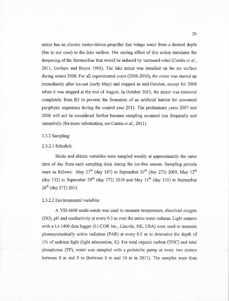
- - ---------- - - ------- ---------- -------
26
mixer has an electric motor-driven propeller that brings water from a desired depth
(8m in our case) to the lake surface. The mixing effect of this action simulates the
deepening of the thermocline that would be induced by increased wind (Cantin et al.,
2011; Gorham and Boyce 1989). The lake mixer was installed on the ice surface
during winter 2008. For all experimental years (2008-2010), the mixer was started up
imrnediately after ice-out (early May) and stopped in mid-October, except for 2008
when it was stopped at the end of August. In October 2010, the mixer was removed
cornpletely from B3 to prevent the formation of an artificial habitat for unwanted
periphytic organisrns during the control year 2011. The prelirninary years 2007 and
2008 will not be considered further because sampling occurred less frequently and
intensively (for more information, see Cantin et al., 2011 ).
2.3.2 Sarnpling
2.3 .2.1 Schedule
Biotic and abiotic variables were sampled weekly at approximately the same
time of day from each sarnpling dock during the ice-free season. Sampling periods
were as follows: May 2ih (day 147) to September 301h (day 273) 2009, May l21h
(day 132) to September 291h (day 272) 2010 and May 11 111 (day 131) to September
281h (day 271) 2011.
2.3.2.2 Environmental variables
A YSI-6600 multi-sonde was used to measure temperature, dissolved oxygen
(DO), pH and conductivity at every 0.5 rn over the entire water colurnn. Light sensors
with a LI-1400 data logger (LI-COR Inc., Lincoln, NE, USA) were used to measure
photosynthetically active radiation (PAR) at every 0.5 rn to detem1ine the depth of
1% of arnbient light (light attenuation, K). For total organic carbon (TOC) and total
phosphorus (TP), water was sarnpled with a peristaltic pump at every two rneters
between 0 rn and 8 rn (between 0 rn and 10 m in 2011). The samples were then
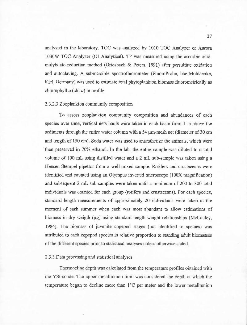
27
analyzed in the laboratory. TOC was analyzed by 1010 TOC Analyzer or Aurora
1030W TOC Analyzer (OI Analytical). TP was measured using the ascorbic acid
molybdate reduction method (Griesbach & Peters, 1991) after persulfate oxidation
and autoclaving. A submersible spectrofluorometer (FluoroProbe, bbe-Moldaenke,
Kiel, Germany) was used to estimate total phytoplankton biomass fluorometrically as
chlorophyll a (ch1-a) in profile.
2.3.2.3 Zooplankton community composition
To assess zooplankton community composition and abundances of each
species over time, vertical nets hauls were taken in each basin from 1 rn above the
sediments through the en tire water column with a 54 fA.m-mesh net ( diameter of 30 cm
and length of 150 cm). Soda water was used to anaesthetize the animais, which were
· then preserved in 70% ethanol. In the lab, the entire sample was diluted to a total
volume of 100 mL using distilled water and a 2 mL sub-sample was taken using a
Hensen-Stempel pipettor from a well-mixed sample. Rotifers and crustaceans were
identified and counted using an Olympus inverted microscope (lOOX magnification)
and subsequent 2 mL sub-samples were taken until a minimum of 200 to 300 total
individuals was counted for each group (rotifers and crustaceans). For each species,
standard length measurements of approximately 20 individuals were taken at the
moment of each summer when each was most abundant to allow estimations of
biomass in dry weigth (fA.g) using standard length-weight relationships (McCauley,
1984). The biomass of juvenile copepod stages (not identified to species) was
attributed to each copepod species in relative proportion to standing adult biomasses
of the different species prior to statistical analyses unless otherwise stated.
2.3.3 Data processing and statistical analyses
Thermocline depth was ca1culated from the temperature profiles obtained with
the YSI-sonde. The upper metalimnion limit was considered the depth at which the
temperature began to decline more than 1 °C per meter and the lower metalimnion
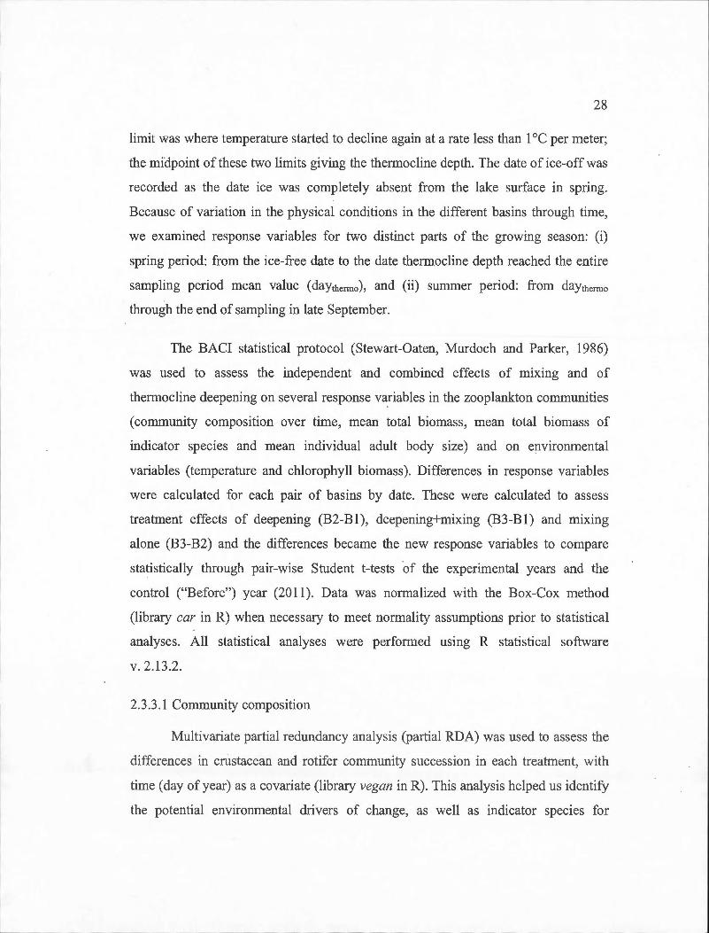
28
limit was where temperature started to decline again at a rate less than 1 °C per meter;
the midpoint of these two limits giving the the1mocline depth. The date of ice-off was
recorded as the date ice was completely absent from the lake surface in spring.
Because of variation in the physical conditions in the different basins through time,
we examined response variables for two distinct parts of the growing season: (i)
spring period: from the ice-free date to the date thermocline depth reached the entire
sampling period mean value ( daythenno), and (ii) summer period: from day1hermo
tbrough the end of sampling in late September.
The BACI statistical protocol (Stewart-Oaten, Murdoch and Parker, 1986)
was used to assess the independent and combined effects of mixing and of
thermocline deepening on several response variables in the zooplankton communities
( community composition over time, mean total biomass, mean total biomass of
indicator species and mean individual adult body size) and on environmental
variables (temperature and chlorophyll biomass). Differences in response variables
were calculated for each pair of basins by date. These were calculated to assess
treatment effects of deepening (B2-Bl), deepening+mixing (B3-Bl) and mixing
alone (B3-B2) and the differences became the new response variables to compare
statistically through pair-wise Student t-tests of the experimental years and the
control ("Before") year (2011). Data was normalized with the Box-Cox method
(library car in R) when necessary to meet normality assumptions prior to statistical
analyses. All statistical analyses were performed using R statistical software
v. 2.13.2.
2.3.3.1 Community composition
Multivariate partial redundancy analysis (partial RDA) was used to assess the
differences in cnistacean and rotifer community succession in each treatment, with
time (day ofyear) as a covariate (library vegan in R). This analysis helped us identify
the potential environmental drivers of change, as well as indicator species for
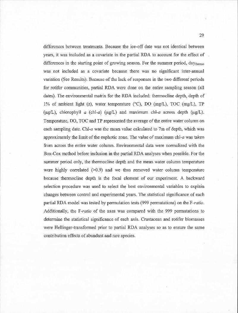
29
differences between treatments. Because the ice-off date was not identical between
years, it was included as a covariate in the partial RDA to account for the effect of
differences in the starting point of growing season. For the summer period, daythermo
was not included as a covariate because there was no significant inter-ammal
variation (See Results). Because of the lack of responses in the two different periods
for rotifer communities, partial RDA were done on the entire sampling season (all
dates). The environmentalmatrix for the RDA included: thermocline depth, depth of
1% of ambient light (z), water temperature CC), DO (mg/L), TOC (mg/L), TP
(!lg/L), chlorophyll a (chl-a) (!lg/L) and maximum chl-a across depth (!lg/L).
Temperature, DO, TOC and TP represented the average of the entire water column on
each sampling date. Chl-a was the mean value calculated to 7m of depth, which was
approximately the limit of the euphotic zone. The value of maximum chl-a was taken
from across the entire water column. Environmental data were normalized with the
Box-Cox method before inclusion in the partial RDA analyses when possible. For the
summer period only, the thermocline depth and the mean water column temperature
were highly correlated (>0.9) and we thus removed water column temperature
because thermocline depth is the focal element of our experiment. A backward
selection procedure was used to select the best environmental variables to explain
changes between control and experimental years. The statistical significance of each
partial RDA model was tested by permutation tests (999 pennutations) on the F-ratio.
Additionally, the F-ratio of the axes was compared with the 999 permutations to
determine the statistical significance of each axis. Crustacean and rotifer biomasses
were Hellinger-transformed prior to partial RDA analyses so as to ensure the same
contribution effects of abundant and rare species.
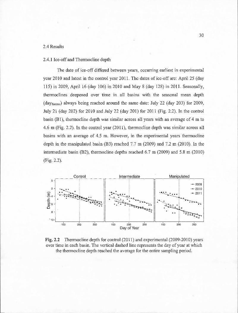
30
2.4 Results
2.4.1 lee-off and Thermocline depth
The date of ice-off differed between years, occurring earliest in experimental
year 2010 and latest in the control year 2011. The dates of ice-off are: April 25 (day
115) in 2009, April 16 (day 106) in 2010 and May 8 (day 128) in 2011. Seasonally,
thermoclines deepened over time in all basins with the seasonal mean depth
(daythermo) always being reached around the same date: July 22 (day 203) for 2009,
July 21 (day 202) for 2010 and July 22 (day 201) for 2011 (Fig. 2.2). In the control
basin (B1), thermocline depth was similar across all years with an average of 4 m to
4.6 m (Fig. 2.2). In the control year (2011), thermocline depth was similar across all
basins with an average of 4.5 m. However, in the experimental years thermocline
depth in the manipulated basin (B3) reached 7.7 m (2009) and 7.2 m (2010). In the
intermediate basin (B2), thermocline depths reached 6.7 rn (2009) and 5.8 m (2010)
(Fig. 2.2).
Control lntermediate Manipulated
~-E 0
: 1_r--.. ~---~---~.-~:-· .... -.~.::_:_:~:.:: . . ---,11,-1 ----,,- :-----
1
'· ~:--.. _ -:-.: 0
, 0
i ~~~~ -•e.:~:· • • i, :: ::::1 .. ---- .... _..! • -
.s::::. ~ • • • Il .----~-< .· .. · ·-:·-·-.. ~- - IJ · .... · ---t ... -h___ 1 gs r··· ---.;~·~:~,. .. 11 ~ ---·--·-;.-. 11. · · ··~·~·· ...... : ........ -;-. 1 o i ... r·~ . '-!,t·
.1] 1 Il 1 ····11 . . . . ;·l·:-~ -~.:. : 1
150 200 250 150 200 250 150 200 250 Day of Year
Fig. 2.2 Thermocline depth for control (2011) and experimental (2009-2010) years over time in each basin. The vertical dashed line represents the day of year at which
the thermocline depth reached the average for the entire sampling period.
31
2.4.2 Mean water column temperature
As a consequence of thermocline deepening, overall mean water column
temperature was greater in the manipulated basin, especially during the summer.
Mean column temperatures increased by 2.5°C in spring and 4°C in summer in the
deepening+mixing treatment (B3-B1) in the two experimental years (Table 2.1).
Similarly, although the differences were not as great, the mean water colunm
temperature of the intermediate basin was significantly higher than the control (B2-
B1) and the manipulated basin was higher than the intermediate (B3-B2) in both
spring and summer periods (Table 2.1 ).
2.4.3 Chlorophyll
Significant mcreases m ebl-a were generally observed only in 2010 and
especially in the summer (Table 2.1). Summer ebl-a was significantly higher in both
experimental years for the mixing treatment but only in 201 0 for the two deepening
treatments (Table 2.1 ). Spring ebl-a was only significantly greater in the
deepening+mixing treatment in 2010 (Table 2.1 ).
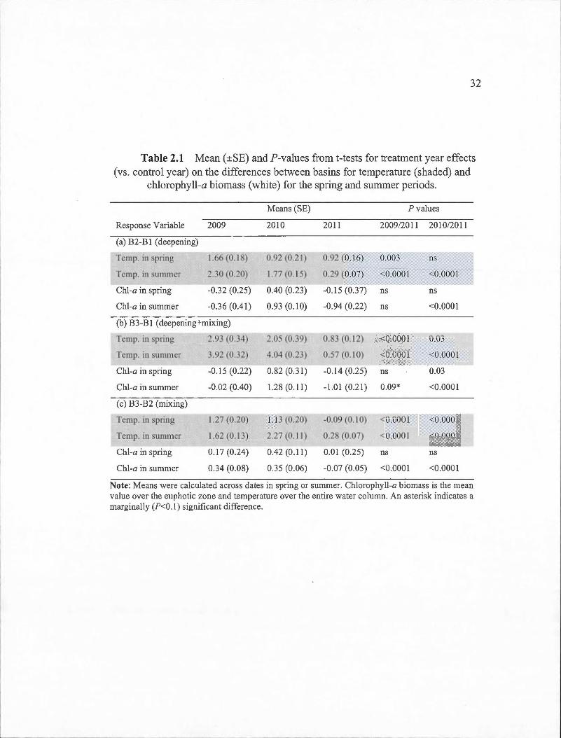
32
Table 2.1 Mean (±SE) and P-values from t-tests for treatment year effects (vs. control year) on the differences between basins for temperature (shaded) and
chlorophyll-a biomass (white) for the spring and summer periods.
Means (SE) P values
Response Variable 2009 2010 2011 2009/2011 2010/2011
(a) B2-Bl (deepening)
Temp. in sp1ing? 1.66 (0.18) 0.92 (0.21) 0.92 (0.16) 0.003 ns
2.30 (0.20) 1.77 (0.15) 0.29 (0.07) <0.0001
Chi-a in spring -0.32 (0 .25) 0.40 (0.23) -0.15 (0.37) ns ns
Chi-a in summer -0.36 (0.41) 0.93 (0.1 0) -0.94 (0 .22) ns <0.0001
(b) 83-B1 (deepening+mixing)
2.05 (0:39) 0.83 (0.12) <0.0001 0.03
Temp. in sumTQ;~r 3.~,f (0.32) 4.04 (0.23) 0.57 (0.10) <0.0001 <0.0001
Chi-a in spring -0.15 (0.22) 0.82 (0.31) -0.14 (0.25) ns 0.03
Chi-a in summer -0.02 (0.40) 1.28 (0.11) -1.01 (0.21) 0.09* <0.0001
(c) B3-B2 (mixing)
Temp. in'Spnng 1.13 (0.20) -0.09 (0.10) <0.0001 <0.0001
, '<femp, in,sumnier 2.27 (0.11) 0.28 (0.07) <0.0001 <0.0001 . Chi-a in spring 0.17 (0.24) 0.42 (0.11) 0.01 (0.25) ns ns
Chl-a in summer 0.34 (0.08) 0.3 5 (0.06) -0.07 (0.05) <0.0001 <0.0001
Note: Means were calculated across dates in spring or summer. Chlorophyll-a biomass is the mean value over the euphotic zone and temperature over the entire water column. An asterisk indicates a marginally (P<O.l) significant difference.
33
2.4.4 Environmental drivers of zooplankton community changes
From the spring RDA biplots (Fig. 2.3a,c,e), the crustacean communities in
the control and experimental years overlapped greatly in all treatments (Fig. 2.3a,c,e) .
Primary environmental factors identified as drivers of spring period phenology were
dissolved oxygen, chl-a, chl-a maximum, depth of 1% of light and TOC. Thermocline
depth was notably not a primary factor influencing the differences between sampling
years in the spring period (Fig. 2.3a,c,e ).
In the summer, the control and experimental years were completely isolated
from each other in canonicat (RDA) space (ellipses did not overlap) (Fig. 2.3b,d,f) .
For this period, thermocline depth was the major factor identified in driving the
separation between crustacean communities between experimental and control years
in all treatments. Chl-a was also identified as an important environmental factor for
deepening and deepening+mixing treatments (Fig 2.3b,d), but instead explaining
mainly the differences between experimental years (2009 and 201 0).
Partial RDA analyses did not reveal consistent patterns in the effect of
thermocline deepening and mixing treatments on rotifer communities, nor an effect of
thermocline depth as a driver · of community change (Appendix C). Rotifer
communities did not respond with a consistent pattern to the treatments in either
spring or summer periods, being mainly related to changes in chlorophyll. However,
when the entire growing season was used in the partial RDA analyses, the ellipse of
the control and experimental years did not ovelap for ' the mixing treatments
( deepening+mixing and mixing; Fig. 2.4b,c ). The average of temperature of the water
colurnn was the main variable separating the control and experimental years (Fig.
2.4b,c) . For the deepening treatment only, the control and experimental years were
not separated from each other (Fig. 2.4a).
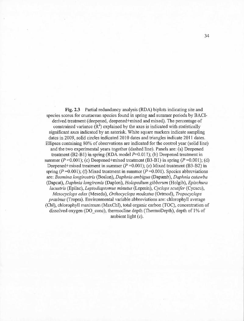
34
Fig. 2.3 Partial redundancy analysis (RDA) biplots indicating site and species scores for crustacean species found in spring and summer periods by BACI
derived treatment (deepened, deepened+mixed and mixed). The percentage of constrained variance (R2
) explained by the axes is indicated with statistically significant axes indicated by an asterisk. White square markers indicate sampling dates in 2009, solid circles indicated 2010 dates and triangles indicate 2011 dates.
Ellipses containing 80% of observations are indicated for the control year (solid line) and the two experimental years together (dashed line). Panels are: (a) Deepened treatment (B2-B1) in spring (RDA madel ? =0.011); (b) Deepened treatment in
summer (P =0.001); (c) Deepened+mixed treatment (B3-Bl) in spring (P =0.001); (d) Deepened+mixed treatment in summer (P =0.001); (e) Mixed treatment (B3-B2) in spring (P =0.001); (f) Mixed treatment in summer (P =0.001). Species abbreviations are: Bosmina longirostris (Boslon), Daphnia ambigua (Dapamb ), Daphnia catawba (Dapcat), Daphnia longiremis (Daplon), Holopedium gibberum (Holgib ), Epischura
lacustris (Epilac), Leptodiaptomus minutus (Lepmin), Cyclops scutifer (Cycscu), Mesocyclops edax (Meseda), Orthocyclops modestus (Ortmod), Tropocyclops
prasinus (Tropra). Environmental variable abbreviations are: chlorophyll average (Chl), chlorophyll maximum (MaxChl), total organic carbon (TOC), concentration of
dissolved oxygen (DO_ conc ), thermocline depth (ThermoDepth), depth of 1% of ambient light (z) .
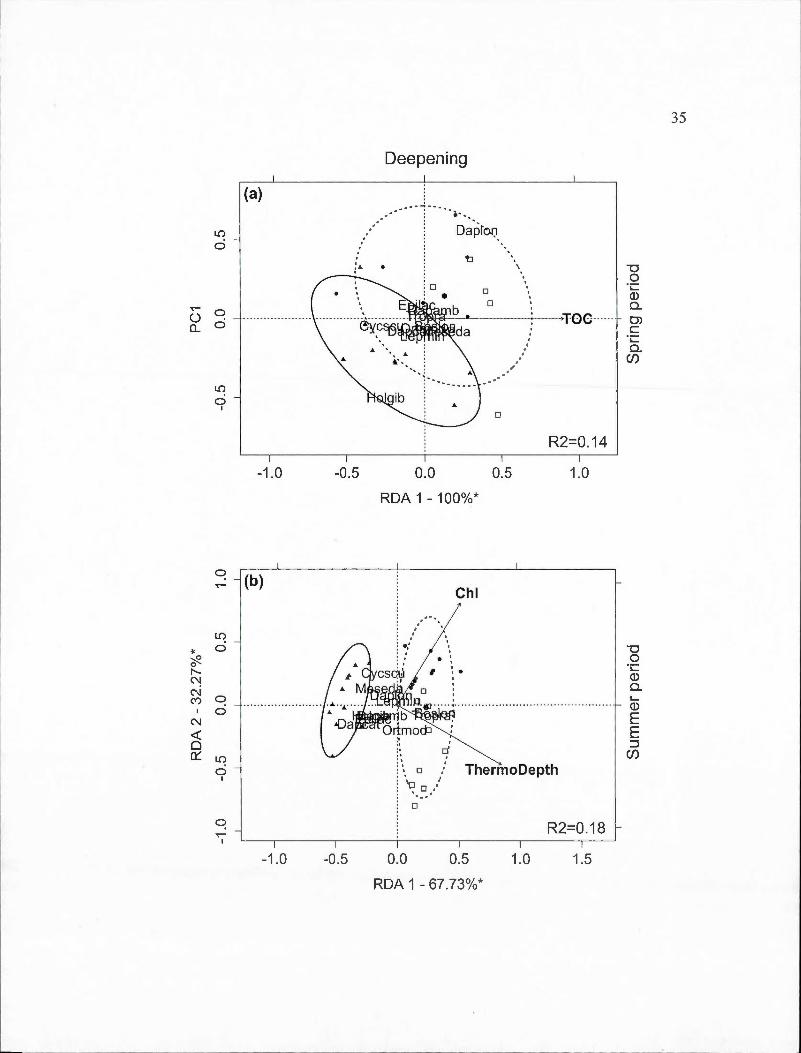
.. cf-l'N
0
0
~ 0 1 0
N <( 0 0::: l()
0 1
0 '<"'"
1
-1.0 -0.5
Deepening
Chi
: •,' . . . : , : .
1
.,
:: o' . , : ', 0
: ''ç:J t
i ·. ~ .... ThermoDepth
: 0
0.0 0.5 1.0
RDA 1 - 67.73%*
1.5
TI 0
ï::: Q) 0... 1...... Q)
E E :J
Cl)
35

~
~ 0
N 0 t'--......
N <( 0 0:::
~
~ 0 ...... <.0 co ......
N <( 0 0:::
l()
0
0 0
l()
0 1
l()
0
0 0
l()
0 1
0 ......
1
Deepening+Mixing
(c)
...
DO ne -o c • 0 -ï:::: Q) 0... 0')
z c ·;:::: 0...
(f)
-... : .. . R2=0.44
-1.0 -0.5 0.0 0.5 1.0
RDA 1 - 66.85%*
(d) Chi .. ;.
. , · : . M .. Cd'csc~ :' • ;
e e IDaP;Io . Q •0
; -g ...................... "" ·· .:Pw~~-~;~ ·· -- .frroprà.. .. . .... . ............... ... ..... .. .. -~
-1. 0 -0.5
Ort~qd o Ther oDepth :Q . : · o G :: . .. .. . ' :' ~ · .. o:
:o
0.0 0.5
RDA 1 - 81.39%*
R2=0.29
1.0 1.5
..... Q)
E E :::::1
Cf)
36

l!)
0
u 0 0... 0
....... u 0...
l!)
0 1
0 .......
l!)
0
0 0
l!)
0 1
-1.0 -0.5
(f)
..
-1 .0 -0.5
Mixing
..
Leprain
0
cs ca
0
.·
. :
0.0 0.5
RDA 1 - 100%*
0 . '
0.0 0.5
RDA 1 -100%*
37
·. "'0 i 0
·c ·· G<>A- ·
Q) 0.. Ol c ·c 0..
(f)
R2=0 .17
1.0
""0 0 ·c Q) 0..
ThermoDept ,__ Q)
E E ::J
(f)
R2=0.13
1.0 1.5
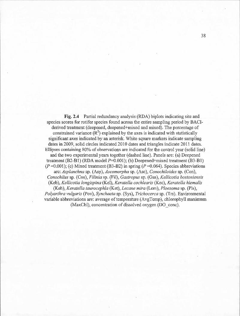
38
Fig. 2.4 Partial redundancy analysis (RDA) biplots indicating site and species scores for rotifer species found across the entire sampling period by BACI
derived treatment ( deepened, deepened+mixed and mixed) . The percentage of constrained variance (R2
) explained by the axes is indicated with statistically significant axes indicated by an asterisk. White square markers indicate sampling dates in 2009, solid ci rel es indicated 2010 dates and triangles indicate 2011 dates .
Ellipses containing 80% of observations are indicated for the control year (solid line) and the two experimental years together (dashed line) . Panels are: (a) Deepened
treatment (B2-Bl) (RDA model P=0.001); (b) Deepened+mixed treatment (B3-Bl) (P =0.001); (c) Mixed treatment (B3-B2) in spring (P =0.064). Species abbreviations
are: Asplanchna sp. (Asp), Ascomorpha sp. (Asc), Conochiloides sp. (Con), Conochilus sp. (Cos), Filinia sp. (Fil), Gastropus sp. (Gas), Kellicotia bostoniensis (Keb ), Kellicotia longispina (Kel), Keratella cochlearis (Kec ), Keratella hiemalis
(Keh), Keratella taurocephla (Ket), Lecane mira (Lem), Ploesoma sp. (Pls), Polyarthra vulgaris (Pov), Synchaeta sp. (Sys), Trichocerca sp. (Trs) . Environmental variable abbreviations are: average of temperature (AvgTemp), chlorophyll maximum
(MaxChl), concentration of dissolved oxygen (DO_ conc ).
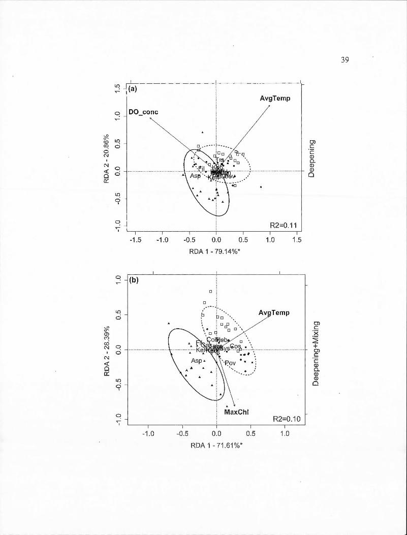
:::R 0 (!) 00 0 N
N <( 0 0:::
:::R 0 Ol '"? 00 N
N <( 0 0:::
1.{)
~
L0 0
~ 0
L0 0
1
0 ..-
1
1.{)
ci
0 ci
L0 0
1
~ ..-
1
(a)
DO co ne -
-1.5 -1 .0
(b)
...
-1 .0
-0.5 0.0 0.5
RDA 1- 79. 14%*
0
0
.. p- ~ -~ - ......
b po ·· .. •• : 000 •• •• \ . : 0 0 ' •OD
AvgTemp
R2=0.11
1.0 1.5
Av Temp
· orffeb o \ ~J.,_I'R.ys~ocP . ~- .. ':. ..... .. ..... ... ............... . . .. , \ . . :
.... .. . :
-0.5 0.0 0.5 1.0
RDA 1 - 71.61 %*
0) c c Q) Q. Q) Q)
0
0) c :8 2 + 0) c c Q) Q. Q) Q)
0
39
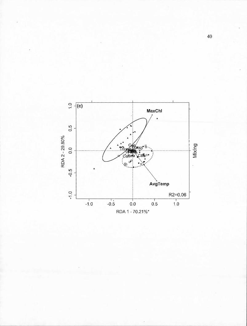
~ 0 0 co m N
1
N <( 0 0:::
0
lO
0
0 0
lO
0 1
0 ..--
1
(c)
40
MaxChl
..
AvgTemp
-1.0 -0.5 0.0 0.5 1.0
RDA 1 - 70.21 %*

41
2.4.5 Biomass responses of indicator species
From the spring partial RDA biplots, crustacean indicator species were not
cl earl y associated with control or experimental years (Fig. 2.3a,c,e ). Although the
overlapping of sampling years, Daphnia longiremis and Holopedium gibberum could
be identified as indicator species for the deepening treatments (Fig. 2.3a,c). Daphnia
biomass increased while Holopedium decreased with thermocline deepening.
Daphnia biomass was significantly higher in the experimental years for both
deepening treatments (Table 2.2a,b). The decrease of Holopedium biomass during
experimental years was significant, but not for spring 2009 in the deepening
treatment (B2-Bl) (Table 2.2a,b) .
Table 2.2 Mean (±SE) and P-values from t-tests for treatment year effects (vs. control year) on the differences between basins for each spring indicator species.
Means (SE) P values
Response Variable 2009 2010 2011 2009/2011 2010/2011
(a) B2-B 1 ( deepening)
D.longiremis -3.63 (3.13) 4.99 (6.33) -53.24 (15.15) <0.005 <0.005
H. gibberum 1.33 (5.38) -1.53 (1.10) 9.90 (4.11) ns 0.03
(b) B3-B 1 (mixing+deepening)
D.longiremis -4.13 (2 .84) 7.88 (6.96) -57.78 (17.15) <0.01 <0.005
H. gibberum 7.52 (3.99) 0.69 (0.95) 24.94 (8.40) 0.03 <0.005
(c) B3 -B2 (mixing)
C.scutifer 7.38 (3.61) 14.09 (4.81) -2.44 (2.08) 0.04 <0.005
L.minutus 1.81 (4.41) -2.85 (2.58) -2.15 ( 1.25) ns ns
Note: Means were calcu1ated across springtime dates.
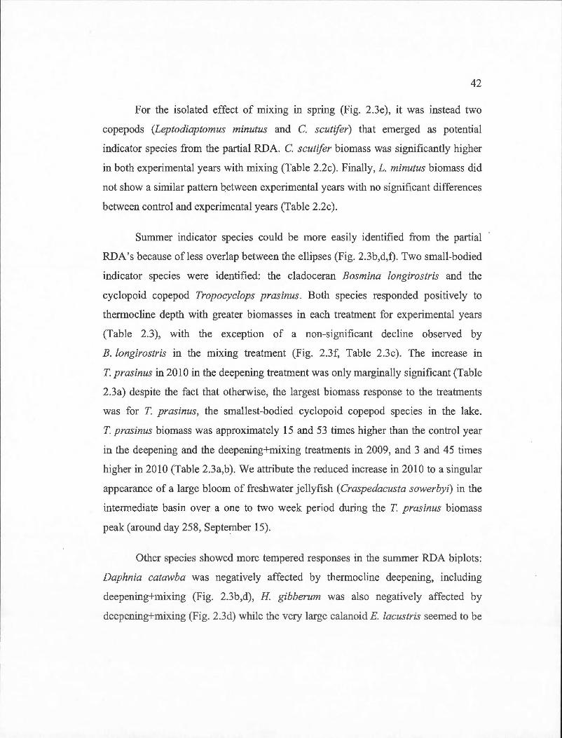
42
For the isolated effect of mixing in spring (Fig. 2.3e), it was instead two
copepods (Leptodiaptomus minutus and C. scutifer) that emerged as potential
indicator species from the partial RDA. C. scutifer biomass was significantly higher
in both experimental years with mixing (Table 2.2c ). Finally, L. minutus biomass did
not show a similar pattern between experimental years with no significant differences
between control and experimental years (Table 2.2c ).
Summer indicator species could be more easily identified from the partial
RDA's because ofless overlap between the ellipses (Fig. 2.3b,d,f). Two small-bodied
indicator species were identified: the cladoceran Bosmina longirostris and the
cyclopoid copepod Tropocyclops prasinus. Both species responded positively to
thermocline depth with greater biomasses in each treatment for experimental years
(Table 2.3), with the exception of a non-significant decline observed by
B. longirostris in the mixing treatment (Fig. 2.3f, Table 2.3c). The increase in
T. prasinus in 2010 in the deepening treatment was only marginally significant (Table
2.3a) despite the fact that otherwise, the largest biomass response to the treatments
was for T. prasinus, the smallest-bodied cyclopoid copepod species in the lake.
T. prasinus biomass was approximately 15 and 53 times higher than the control year
in the deepening and the deepening+mixing treatments in 2009, and 3 and 45 times
higher in 2010 (Table 2.3a,b ). We attribute the reduced increase in 2010 to a ·singular
appearance of a large bloom of freshwater jellyfish ( Craspedacusta sowerbyi) in the
intermediate basin over a one to two week period during the T. prasinus biomass
peak (around day 258, September 15).
Other species showed more tempered responses in the summer RDA biplots:
Daphnia catawba was negatively affected by thermocline deepening, including
deepening+mixing (Fig. 2.3b,d), H. gibberum was also negatively affected by
deepening+mixing (Fig. 2.3d) while the very large calanoid E. lacustris seemed to be
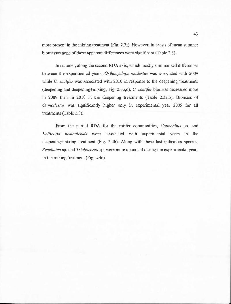
43
more present in the mixing treatment (Fig. 2.3f). However, in t-tests of mean summer
biomasses none ofthese apparent differences were significant (Table 2.3).
In summer, along the second RDA axis, which mostly summarized differences
between the experimental years, Orthocyclops modestus was associated with 2009
while C. scutifer was associated wi th 20 10 in response to the deepening treatments
( deepening and deepening+mixing; Fig. 2.3b,d). C. scutifer biomass decreased more
in 2009 than in 2010 in the deepening treatments (Table 2.3a,b). Biomass of
O. modestus was significantly higher only in experimental year 2009 for all
treatments (Table 2.3).
From the partial RDA for the rotifer communities, Conochilus sp. and
Kellicotia bostoniensis were associated with experimental years m the
deepening+mixing treatment (Fig. 2.4b ). Along with these last indicators spec1es,
Synchatea sp. and Trichocerca sp. were more abundant during the experimental years
in the mixing treatment (Fig. 2.4c ).
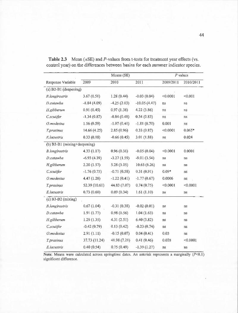
44
Table 2.3 Mean (±SE) and P-values from t-tests for treatment year effects (vs. control year) on the differences between basins for each summer indicator species.
Means (SE) P values
Response Variable 2009 2010 2011 2009/20 11 20 10/20 11
(a) B2-B1 (deepening)
B.longirostris 3.67 (0.51) 1.28 (0.44) -0.03 (0.04) <0.0001 <0.001
D.catawba -8.84 (4.09) -4.25 (2.03) -10.05 (4.47) ns ns
H.gibberum 0.91 (0.45) 0.97 (1.38) 4.22 (3.86) ns ns
C.scutifer -1.34 (0.87) -0.84 (0.48) 0.54 (0.83) ns ns
O. modestus 1.56 (0.59) -1.07 (0.41) -1.81 (0 . 70) 0.001 ns
T.prasinus 14.66 (4.25) 2.85 (0.96) 0.3 3 (0 .87) <0.000 1 0.065*
E.lacustris 0.33 (0.18) -0.66 (0.45) 3.01 (1.88) ns 0.024
(b) B3-B1 (mixing+deepening)
B.longirostris 4.33 (1.17) 0.96 (0 .31) -0.05 (0.04) <0.0001 0.0001
D.catawba -6.93 ( 4.39) -3 .27 (1.59) -9.01 (3.54) ns ns
H.gibberum 2.20 (1 .57) 5.28 (3 .05) 10.63 (6.26) ns ns
C.scutifer -1.76 (0.75) -0.7 1 (0.58) 0.31 (0 .91) 0.09* ns
O. modestus 4.47 (1.28) -1.22 (0.41) -1.77 (0.67) 0.0006 ns
T.prasin.us 52.39 (10.61) 44.83 (7 .07) 0.74 (0.75) <0.0001 <0.0001
E.lacustris 0.73 (0.60) 0.09 (0 .34) 1.61 (1.10) ns ns
(c) B3-B2 (mixing)
B.longirostris 0.67 (1 .04) -0.31 (0.38) -0.02 (0.0 1) ns ns
D.catawba 1.91 (1 .77) 0.98 (0.56) 1.04 (1.63) ns ns
H.gibberum 1.29 (1.35) 4.31 (2.51) 6.40 (3 .82) ns ns
C.scutifer -0.42 (0.79) 0.1 3 (0.42) -0.23 (0.74) ns ns
O. modestus 2.9 1 (1.11) -0.15 (0.07) 0.04 (0.41) 0.03 ns
T.prasinus 37.73 (11.24) 41.98 (7.21) 0.41 (0.46) 0.028 <0.0001
E.lacustris 0.40 (0.54) 0.75 (0.49) -1.39 (1.27) ns ns
Note: Means were calculated a cross springtime dates. An asterisk represents a marginally (P<0.1) significant difference.
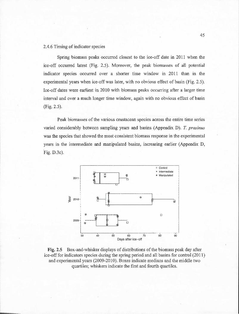
1
1
1
1
L
45
2.4.6 Timing of indicator species
Spring biomass peaks occurred clos est to the ice-off date in 2011 when the
ice-off occurred latest (Fig. 2.5). Moreover, the peak biomasses of all potential
indicator species occmTed over a shorter time window in 2011 than in the
experimental years when ice-off was later, with no obvious effect of basin (Fig. 2.5).
lee-off dates were earliest in 2010 with biomass peaks occurring after a larger time
interval and over a much longer time window, again with no obvious effect of basin
(Fig. 2.5).
Peak biomasses of the various crustacean species across the entire time series
varied considerably between sampling years and basins (Appendix D). T. prasinus
was the species that showed the most consistent biomass response in the experimental
years in the intermediate and manipulated basins, increasing earlier (Appendix D,
.Fig. D.3c).
2011 ~ o Control -l • lntermediate
* Manipulated
<ü ~ 2010 ~'-1'T---i _}h----:.
'00'1 ;-co-D 1 1 1 1
~ ~ ~ ~ ro Days after ice-off
0
1 80
1
90
Fig. 2.5 Box-and-whisker displays of distributions of the biomass peak day after ice-off for indicators species during the spring period and all basins for control (20 11)
and experimental years (2009-2010). Boxes indicate medians and the middle two quartiles; whiskers indicate the first and fourth quartiles.
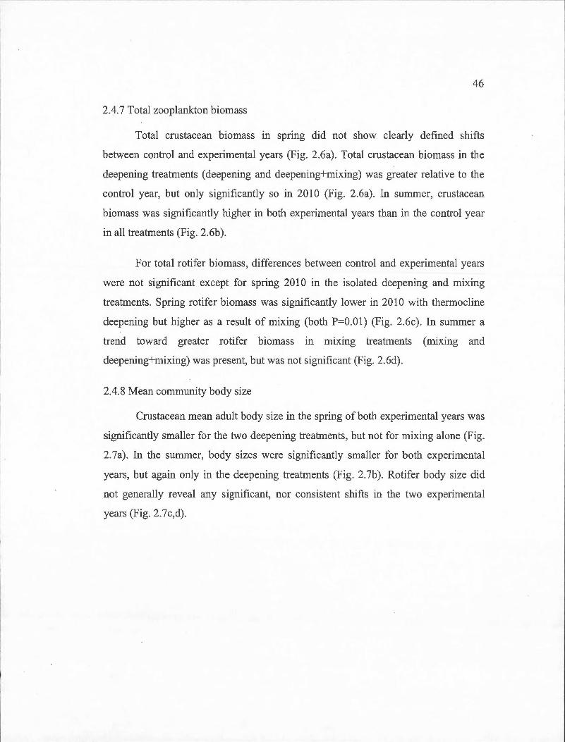
46
2.4.7 Total zooplankton biomass
Total crustacean biomass m spnng did not show clearly defined shifts
between control and experimental years (Fig. 2.6a). Total crustacean biomass in the
deepening treatments (deepening and deepening+mixing) was greater relative to the
control year, but only significantly so in 2010 (Fig. 2.6a). In summer, crustacean
biomass was significantly higher in both experimental years than in the control year
in all treatments (Fig. 2.6b ).
For total rotifer biomass, differences between control and experimental years
were not significant except for spring 2010 in the isolated deepening and mixing
treatments. Spring rotifer biomass was significantly lower in 2010 with therrnocline
deepening but higher as a result of mixing (both P=O.Ol) (Fig. 2.6c). In summer a
trend toward greater rotifer biomass in mixing treatments (mixing and
deepening+mixing) was present, but was not significant (Fig. 2.6d).
2.4.8 Mean community body size
Crustacean mean adult body size in the spring of both experimental years was
significantly smaller for the two deepening treatments, but not for mixing alone (Fig.
2.7a) . In the summer, body sizes were significantly smaller for both experimental
years, but again only in the deepening treatments (Fig. 2. 7b ). Rotifer body size did
not generally reveal any significant, nor consistent shifts in the two experimental
years (Fig. 2.7c,d).
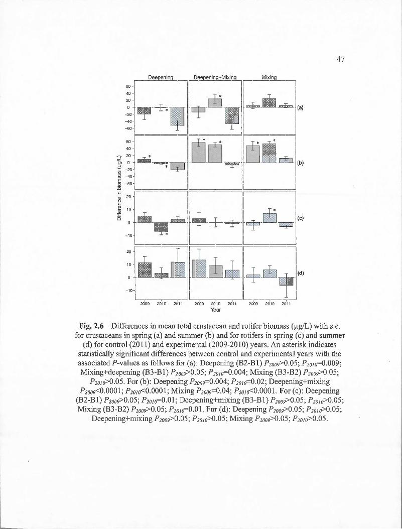
i
r--~~--~~--~
i ~,r-~~~+~~Cfj~(<) ~:C-T1Jl rL ;ll--l _:J -~lill fWlJ.Jq:~ rcJ=_cbrp 1 ~·~
1 1 1 j
2009 2010 2011 2009 2010 201 1 2009 2010 2011
Year
47
Fig. 2.6 Differences in mean total crustacean and rotifer biomass (~-tg/L) with s.e. for crustaceans in spring (a) and summer (b) and for rotifers in spring (c) and summer
(d) for control (2011) and experimental (2009-2010) years . An asterisk indicates statistically significant differences between control and experimental years with the associated P-values as follows for (a): Deepening (B2-Bl) P2oo9>0.05; P2oio=0.009; Mixing+deepening (B3-Bl) P2oo9>0.05; P2oio=0.004; Mixing (B3-B2) P2oo9>0.05;
P2oio>0.05. For (b): Deepening P2oo9=0.004; P2o1o=0.02; Deepening+mixing P2oo9<0.000l; P2oJo<O.OOOl; Mixing P2oo9=0.04; P2oio<O.OOOl. For (c): Deepening
(B2-Bl) P2oo9>0.05; P2o1o=0.01; Deepening+mixing (B3-Bl) P2oo9>0.05; P2o1o>0.05; Mixing (B3-B2) P2oo9>0.05; P2o1o=O.Ol. For (d): Deepening P2oo9>0.05; P2o1o>0.05;
Deepening+mixing P2oo9>0.05 ; P2oio>0.05 ; Mixing P2oo9>0.05 ; P2o1o>0.05.
L _ ------------- - - - -----
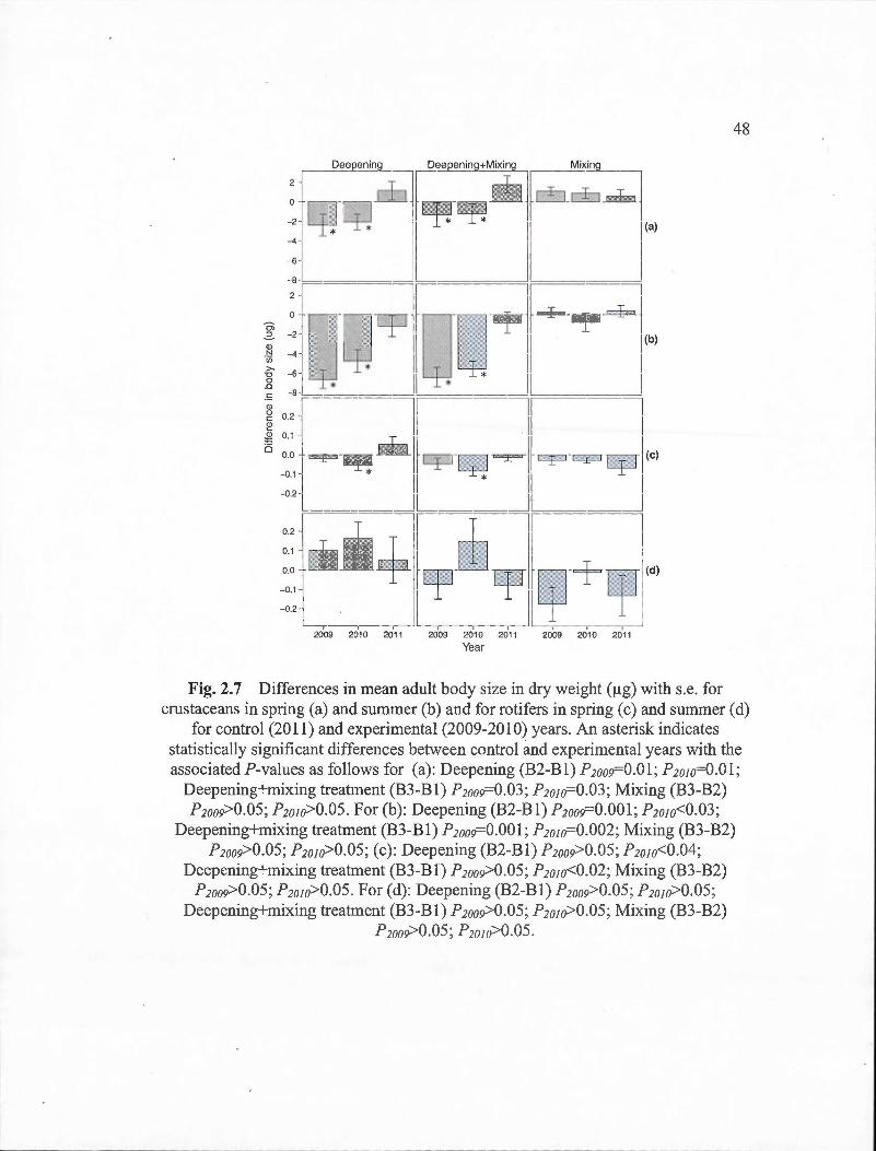
48
Fig. 2.7 Differences in mean adult body size in dry weight (!lg) with s.e. for crustaceans in spring (a) and summer (b) and for rotifers in spring ( c) and summer ( d)
for control (2011) and experimental (2009-2010) years . An asterisk indicates statistically significant differences between control and experimental years with the associated P-values as follows for (a): Deepening (B2-Bl) P20o9=0.01; P20,0=0.01;
Deepening+mixing treatment (B3-Bl) P2oo9=0.03; P20/o=0.03; Mixing (B3-B2) P2oo9>0.0S; P2o1 o>O.OS. For (b) : Deepening (B2-Bl) P2oo9=0.00l; P2oJo<0.03;
Deepening+mixing treatment (B3-Bl) P2oo9=0.00l; P2o1o=0.002; Mixing (B3-B2) P2oo9>0.0S; P2o1o>O.OS; (c): Deepening (B2-Bl) P2oo9>0.0S ; P2o1o<0.04;
Deepening+mixing treatment (B3-Bl) P2oo9>0.0S; P2o1o<0.02; Mixing (B3-B2) P2oo9>0.0S; P2o1o>O.OS. For (d): Deepening (B2-Bl) P2oo9>0.0S ; P2o1o>O.OS ;
Deepening+mixing treatment (B3-Bl) P2oo9>0.0S; P2o1o>O.OS ; Mixing (B3-B2) P2oo9>0.0S ; P2o1o>O.OS.
49
2.5 Discussion
Several recent studies indicate that climate change and the expected
thermocline depth shifts should have important effects on plankton community
phenology through composition and biomass shifts (e.g. Adrian, Wilhem and Gerten,
2006; Berger et al., 2010; Cantin et al., 2011; Lydersen et al., 2008). Furthermore,
Daufresne, Lengfellner and Sommer (2009) concluded that reduced body size is a
third important component of the response of plankton communities to climate
warming. Our experiment provides convincing evidence at the whole-lake scale that
altering lake thermoclines affects zooplankton body size and phenology through
changes in composition and total biomass in a dimictic north ternperate lake, with the
most profound effects occurred during high summer.
In our experimental manipulation of thermocline depths, total crustacean
zooplankton biomass and mean body size were governed mainly by climatic factors.
Small indications of indirect treatment effects may have included physical mixing or
sediment warming. Increases in biomass were especially variable between
experimental years and treatments. Contrary to our original hypothesis that stipulated
a decrease in zooplankton biomass, total zooplankton biomass in spring was
significantly enhanced in the experimental year 2010 wh en ice-off occurred earliest.
We suspect that the same trends in the biomass response were not significant in 2009
because of a later ice-off date. In 2010, ice-off occurred nine da ys earlier, which
would have meant a longer period for zooplankton growth and succession, potentially
leading to greater total biomass. In summer, crustacean biomass was also consistently
higher in aU treatments, indicating strong positive influences on biomass of both
mixing and thermocline deepening. Instead of a decrease in zooplankton biomass
owing to a lower phytoplankton stock with deeper mixing depth as predicted in the
model by Berger, Diehl and Kunz (2006), we conclude that zooplankton and likely
their phytoplankton food would have had greater growth rates because of being
50
exposed to a larger volume of warm epilirnnetic water with our experimental
thermocline deepenening. Warmer water would positively enhance the metabolism as
well as population growth rates of most species (Mai er, 1989) with plankton reaching
adult reproductive stages more quickly (Sastri et al., submitted manuscript).
In line with the expectation of reduced body size with climate warming owing
to temperature-size relationships (Daufresne, Lengfellner and Sommer, 2009), mean
crustacean body size was reduced in the thermocline deepening treatments and
especially during summer. This is not what we predicted would occur based on the re
distribution of heat in the water column. Although epilimnetic temperatures were not
warmer with thermocline deepening, greater mixing depths could have reduced the
time zooplankton spent in cooler hypolimnetic waters. A mixing effect in either time
period was not observed suggesting that the presence of a larger epilimnion is
responsible. Reduced mean crustacean body sizes resulted mainly from the increases
in the relative abundance oftwo small-bodied species, B. longirostris and T. prasinus,
in the experimental years. Moreover, O. modestus, which was more abundant in
2009, lead to a further greater reduction of the mean summer body size in 2009
relative to 2010. In contrast to our earlier conclusions from this experiment based on
preliminary data from 2007-08 (Cantin et al., 2011), we now conclude that this shift
in body size was predominantly a result of a wanner water columns rather than
potentially negative effects of turbulence on lm·ger body-sized zooplankton species.
Furthermore, we can exclude the effect of differences in planktivorous fish
population sizes between basins as a driver of the shifts in zooplankton body size for
two reasons: Firstly, because fish population sizes did not vary from year to year in
the basins (M. Gillespie and J. Gunn, Laurentian University, unpublished data).
Secondly, because our control year (2011) occurred after our treatment years (2009-
2010), we would expect that greater fish population sizes associated with the
treatment effects in our experimental basins would carry over into greater predation
rates in these same basins in the control year as well because of the multi-year life
51
span of fish. And in fact, we would expect even greater predation rates by warm
water fish in the control year in the experimental basins if population sizes had
increased with our treatments because larger fish populations would have been
constrained to a smaller volume of water with a thermocline at its regular depth.
Consequently, the zooplankton body size reduction was not a result of changes in the
planktivorous fish populations with our treatments. Furthermore, because invertebrate
predation generally targets smaller zooplankton species as prey (Hanazato and
Yasuno, 2004), this is also an unlikely mechanism for the community body size shifts
we observed.
Crustacean zooplankton community composition m summer was strongly
governed by thermocline depth, with other factors coming into play in the spring. The
stronger effect in summer is not entirely surprising given that lake thermoclines are
more stable at this time and less easily eradicated by winds. Thus, as others have also
found, thermocline depth should be considered one of the predominant structuring
forces for plankton communities, mediating plankton community dynamics through
the physical environment (e .g. Berger et al., 2010; Cantin et al., 2011; Lydersen et
al., 2008).
The pnmary factors affecting zooplankton community composition m the
spring did not include thermocline depth. Rather, our mixing treatment application
acted by introducing more dissolved oxygen into the manipulated basin; DO
concentration was the only factor accounting for the differences between
experimental and control years in the mixing treatment (B3-B2) and was also
important in the deepening+mixing treatment (B3-Bl) . Other environmental factors
emerging as critical to the zooplankton community structure in the spring were light
attenuation, chlorophyll-a biomass and chlorophyll-a maximum (deepening+mixing
treatment) . Light attenuation in springtime generally reflects phytoplankton
production. Finally, in the deepening treatment (B2-B l ), TOC was the only
------ ·- --------- --------· ----------
52
environmental variable explaining community composition differences. This is
consistent with the fact that DOC bas been shown to be one of the major determinants
of zooplank:ton species richness across a large number of the world 's lakes (Shurin et
al., 201 0). Winter and spring conditions greatly affect the amount of DOC entering
lakes from the terrestrial environment (Schindler, Parker and Stainton, 1996). Thus,
overall, our RDA results indicate that factors related to winter and spring climate are
an important for zooplank:ton phenology during spring as suggested by others (Adrian
and Deneke, 1996; Adrian et al., 1999; Berger et al., 2007; Berger et al., 2010;
Nicolle et al., 2012). Such effects were visible even with our experimental
thermocline deepening application (i.e. thermocline depth itself was never a major
factor), although sorne experimentally-induced changes were visible as well (e.g.
effects of mixing on DO). The differences in zooplank:ton communities observed in
spring between years in our study therefore likely reflect mainly inter-annual
differences in springtime conditions, including altered timing of ice-off, in addition to
the treatment applications. Upon closer inspection of the factors to which the
indicator species responded however, one can observe sorne interactions between the
spring climate and treatment effects.
Interactions with treatment effects were evidenced by the fact that sorne
indicator species emerged in the spring, responding significantly to our treatments.
Springtime indicator species were the cladocerans Daphnia longiremis and
Holopedium gibberum and the cyclopoid Cyclops scutifer. These species were most
responsive to environmental parameters associated with the treatments. D. longiremis
was positively affected by thermocline deepening, C. scutifer by mixing and H.
gibberum negatively affected by both treatments. These species were superseded as
indicators in summer by the cladoceran Bosmina longirostris, which responded
positively to thermocline deepening and the cyclopoid Tropocyclops prasinus, which
responded positively to all treatments. The copepod Orthocyclops modestus also
demonstrated positive responses to all treatments but only in 2009. Cladocera (with
53
the exception of H. gibberum) were thus mostly favoured by thermocline deepening
and copepods by mixing and deepening, indicating sorne conservation of the
mechanism by which species of each major taxon were affected. The calanoid
copepod Epischura lacustris was also an indicator species in summer but only in
2010. The idiosyncratic response of this species will be discussed separately.
Cladocerans, especially larger species like the daphnids, are generally thought
to be less resistant to mixing of the water column than are copepods, especially
cyclopoids (Basu and Pick, 1996; Pace, Findlay and Lints, 1992). This contention is
corroborated to some extent by our results wherein no positive responses to the
mixing treatment by cladocerans were observed, even for smaller-bodied species like
B. longirostris which can persist in turbulent or lotie environments (Pace, Findlay and
Lints, 1992). However, we also did not observe significant declines in most cladocera
with our mixing treatment as expected, which suggests that the environment imposed
by our experiment may not be overly critically turbulent for most cladocerans (with
the exception of H. gibberum), contrary to the conclusions of a precursor study using
less resolved data (Cantin et al., 2011). Rather in our current study, Daphnia in spring
and B. longirostris in summer responded positively only to the thermocline deepening
effect. Positive responses of these cladocerans to deepening can be attributed to an
increase of the surface area of sediments in contact with wann epilimnetic water in
the experimental basins. Temperature is one of the critical emergence eues for
dormant cladoceran eggs (Caceres, 1998). The bathymetry of the warmed basins
slopes gradually, so that the surface area of sediments in contact with epilimnetic
water was more than the double with thermoclines that were 1.5 (in B2) and 2 (in B3)
times deeper in experimental years. The higher temperature of the sediments likely
allowed greater hatching of cladoceran resting eggs in the spring as well as summer.
This appears to be one case therefore, where the experimental application did have a
strong effect on spring phenology and composition. On the other band, the cladoceran
H. gibberum, which relies on physical protection from predation using a potentially
54
sensitive jelly exudate, was relatively intolerant of both thermocline deepening and
associated mixing and showed reduced biomass primarily observable in the spring
period in the line with our expectation for cladocerans.
In contrast to the cladoceran response, increased mixing was likely behind the
generally positive responses in copepod indicator species to mixing in spring and to
all treatments in the summer. Turbulence that accompanies greater mixing and
mixing depth can affect the feeding rate of zooplankton, although the effects depend
on the behavioral features of the species and the motility of both predator and prey
(Kiorboe and Saiz, 1995; Lewis and Pedley, 2001). Ambush predators, characteristic
of cyclopoid copepods (Barnett, Finlay and Beisner, 2007) like the indicator species
C. scutifer (spring) and T. prasinus (summer), generally benefit from turbulent
environments because of increased encounter rates between predators and prey
(Kiorboe and Saiz, 1995; Lewis and Pedley, 2001; Visser et al., 2001); thereby
providing a mechanism for the relative success of these indicator species in our
experiment. Note that O. modestus, which would use a similar ambush predation
strategy only responded positively to deepening and mixing in one of our
experimental years (2009).
Variation between years in responses to our treatments occurred mainly in the
copepods. This result suggests that copepod community responses to climate change
may be more idiosyncratic and less predictable than that for cladocerans as expected.
We hypothesize that this is related to complex roles that copepods play in lake food
webs wherein they may act as herbivores, omnivores or predators (Barnett, Finlay
and Beisner, 2007). Two cases in particular emerge from our study. In the first, the
camivorous O. modestus only showed large significant increases in biomass in the
summer of 2009, and in the RDA sumrner inter-mmual differences were attributable
to chlorophyll-a. O. modestus thus appeared to benefit more from thermocline
deepening when there were no significant increases in phytoplankton resources,
55
perhaps because potential prey like rotifers were high (as also observed in 2009).
Furthermore, in spring 2010 rotifer biomass was significantly lower in the deepening
treatment, which may have precluded a response by O. modestus that summer. The
herbivorous calanoid copepod, E. lacustris also showed idiosyncratic responses,
decreasing only in summer 2010 with deepening. The mechanism behind the negative
response to thermocline deepening in summer of that year by E. lacustris is not clear
given that chlorophyll was higher. However, it is likely that E. lacustris was subject
to heavy predation in 2010, as hypothesized for T. prasinus, by the freshwater
jellyfish (Craspedacustt_l sowerbyi) that bloomed in the intermediate basin that year.
Although we analyzed the spring and summer dynamics separately, they are
not fully independent, with effects of spring values on summer ones. For example,
while summer T. prasinus biomass increased significantly more during experimental
years with its peak biomass occurring on almost the same date each year, the start of
the biomass increase was earlier in 2010 when the ice-off date was earlier than in
2009. Consequently, the spring dynamics may have also affected sorne aspects of
summer phenology of T. prasinus, if not the date of its peak.
Fast-growing species like rotifers should have more stochastic responses to
.environmental drivers. In the line with the preliminary study (Cantin et al., 2011),
species that were more abundant during experimental years were all well-protected
from predation with spiny appendages. We hypothesize that their higher biomass
during experimental years only in the mixing treatments ( deepening+mixing and
mixing) is likely due to the increase rate of encounter with predators causes by the
mixing. The difference in total rotifer biomass did not show a similar pattern in all
treatments and also, within treatments, except for the deepening+mixing treatment in
which the biomass increased for both experimental years. Although the differences
between experimental and control years were not significant for the
deepening+mixing treatment, the increase of rotifer biomass concords with earlier

56
conclusions from this experiment (Cantin et al. , 2011). The weak response in rotifer
biomass can be explained by the difference in the crustacean community between
experimental years, resulting in changes in the community of possible rotifer
predators as was the case with the variable response in O. modestus.
Finally, our experiment on thermocline deepening in a temperate lake shows
that the phenology of zooplankton is affected directly in summer and through
interactions with climatic factors during springtime. Because phytoplankton and
crustacean biomasses were higher during the summer with our treatments, our results
suggest that augmented primary and secondary productivity are possible. However,
because it was mainly small copepod biomass that increased, the net effects for
higher trophic levels such as planktivorous fish are likely to be negative and the wider
food web consequences of such shifts in the zooplankton remain to be explored.
2.6 Acknowledgements
Thanks to A. Cantin, R. Beauséjour, S. Mercier-Blais, V. Ouellet-Jobin, C.
Dalmas, T. Lachartre, A. St-Pierre, A. Parkes, J. Arseneault for field and lab
assistance. Thanks also to J. Gunn and Laurentian University for providing the
SolarBee and to the staff of H20 logics Inc for technical support. We acknowledge
the financial contribution of J. Gunn and M. Amyot toward purchase of the curtain.
We also would like to thank the staff of the Station de Biologie des Laurentides for
technical support. Funding was provided through a group FQRNT grant to YTP and
BEB, a Discovery Grant to BEB, as well as through NSERC, FQRNT Graduate
Scholarships to JG. Financial support from the Groupe de Recherche
Interuniversitaire en Limnologie (GRIL) is also acknowledged.
CONCLUSION
3.1 Conclusion du chapitre II
Les changements climatiques et les activités anthropiques ont des effets
majeurs sur tous les écosystèmes. Une augmentation du régime des vents et des
coupes forestières ainsi qu'une diminution des précipitations pourraient influencer la
stratification thermique des lacs de façon importante. Une modification de la
stratification thermique entraînerait des effets majeurs autant au niveau physico
chimique que biologique. En effet, le zooplancton est influencé indirectement par la
structure thermique des lacs par des changements de la structure de l'habitat. De plus,
la température peut affecter directement la physiologie et le comportement du
zooplancton. Le zooplancton possède un rôle central dans la chaine trophique
puisqu'il se nourrit du phytoplancton et transfère l'énergie aux niveaux trophiques
supérieurs. Un changement au sein de ce niveau trophique pourrait donc entraîner des
effets considérables à travers tout le réseau trophique aquatique.
Ma maîtrise s'insérait dans le projet TIMEX, un projet d 'envergure qui a pris
place au Lac Croche, St-Hippolyt~, Québec, Canada et qui a débuté en 2007. Ce
projet a pour objectif d'évaluer les effets d'un abaissement de la thermocline sur
plusieurs paramètres physico-chimiques et biologiques. Une étude préliminaire s'est
déroulée en 2007 et 2008. Le projet de maîtrise présenté dans ce mémoire s'est plutôt
concentré sur les trois années d 'expérimentation subséquentes (2009, 2010 et 2011).
L'objectif principal de ce projet de maîtrise était d'évaluer les effets d'un
abaissement de la therrnocline et du mélange associé sur la dynamique des
58
communautés de zooplancton dans le temps, plus précisément sur la phénologie, la
biomasse et la taille des individus. L'appareil utilisé pour abaisser la thermocline d'un
des trois bassins a permis d'approfondir celle-ci de 4 rn à 8 rn environ. Le mélange
mécanique dans un basin du Lac Croche simulait un abaissement de la them1ocline
suite à une augmentation du régime des vents. Comme il y a eu un transfert de
chaleur à travers le rideau séparant le bassin manipulé de son bassin adjacent
(intermédiaire), la thermocline de ce ·dernier bassin a été abaissée entre 5 rn et 6 rn de
profondeur. Cet abaissement a donc permis de simuler un deuxième scénario des
changements climatiques, celui d'une diminution des précipitations.
L'expérience s'est déroulée dans un lac qui est constitué naturellement de
trois bassins, ce qui a permis de comparer les bassins expérimentaux à un bassin
contrôle au sein du même lac. De plus, l'expérience s'est déroulée sur trois années, ce
qui a permis de comparer une année contrôle (sans manipulation) à deux années
expérimentales (avec manipulation). Une étude expérimentale à l'échelle d'un lac
peut s'avérer laborieuse puisqu'aucun contrôle sur les intrants et les extrants dans le
système n'est possible, contrairement aux mésocosmes. Les différentes comparaisons
entre sites et années permettent donc d'éliminer les variations potentielles spatiales et
temporelles des variables environnementales. Ce type de comparaison permet
également d'évaluer trois différents types de traitement pour notre expérience :
l'abaissement de la thermocline, l'abaissement+mélange et le mélange.
La période d'échantillonnage a été séparée en deux périodes importantes pour
l'analyse des résultats, puisqu'au printemps la thermocline est peu présente et
facilement éradiquée par les vents. Inversement, pendant 1' été, elle est bien établie et
plus difficile à éradiquer par les vents. Cette séparation s'est faite au moment où la
thermocline atteignait la moyenne de la période d'échantillonnage qui était toujours
autour du jour 201 (21 juillet) peu importe la date de dégel du lac. Au printemps, le
climat printanier semblait être le facteur majeur influençant la dynamique des
59
communautés de zooplancton puisque les patrons n'étaient pas toujours similaires
entre les deux années expérimentales. D'ailleurs, les deux années expérimentales
n' avaient pas la même date de dégel du lac (jour 115 en 2009 et jour 106 en 2010).
Cependant, puisque les Daphnia étaients plus abondantes dans les différents
traitements pendant la période du printemps, des effets indirects des traitements à
travers le réchauffement des sédiments se sont faits ressentir. Pendant l'été, le
changement des communautés de zooplancton était principalement influencé par la
profondeur de la thermocline. La biomasse totale des crustacés ainsi que celle de la
chlorophylle de la zone euphotique ont augmenté suite aux traitements pendant l'été.
Les principales espèces de crustacés affectées par les"traitements étaient les deux plus
petites espèces du lac, soit T. prasinus et B. longirostris. L'augmentation importante
de ces espèces a provoqué une réduction significative de la taille individuelle de la
communauté des crustacés pendant l'été. La taille des individus a également
diminuée au printemps. La réduction de la taille individuelle est d 'ailleurs une des
réponses aux changements climatiques dans les écosystèmes aquatiques. Pendant
l'été, les deux années expérimentales ont montré une différence de composition dans
la communauté de crustacés. O. modestus était plus présente en 2009 tandis que C.
scutifer était plus présente en 2010. Cette différence entre les deux années
expérimentales suggère que les caractéristiques spécifiques des copépodes auront une
influence majeure sur leur réponse face à un abaissement de la thermocline. La
réponse des rotifères était encore plus stochastique à travers les traitements et les
années expérimentales. Toutefois, dans les traitements mélange
(abaissement+mélange et mélange), toutes les espèces ayant augmentées ont des
appendices pour se protéger contre la prédation. Puisqu'une augmentation de la
biomasse de la chlorophylle et des crustacés s'est produite suite aux traitements
appliqués, une augmentation de la production primaire et secondaire dans un
écosystème aquatique est possible s'il y a abaissement de la thermocline dans un lac
tempéré. Cependant, cet abaissement de la thermocline pourrait provoquer une
diminution de l'abondance des proies potentielles de zooplancton pour les prédateurs
---------------·--·-
60
invertébrés et les po1ssons à cause d'une dominance des cyclopoides dans la
communauté, qui sont des proies plus difficiles à attraper.
3.2 Recommandations pour des études futures
Pour approfondir les connaissances sur la réponse du zooplancton sur ce type
d'expérience, il faudrait reg.arder le contenu des sédiments en œufs et en différents
stades de développement. Cette évaluation pourrait permettre de comprendre
davantage la dynamique au sein de la communauté pélagique. De plus, il serait
intéressant de construire un bilan global pour le réseau trophique entier afin de
connaître quel niveau trophique serait le plus avantagé face à un tel changement.
Puisque l'abaissement de la thermocline augmente la biomasse de la chlorophylle et
celle des crustacés, il pourrait également être astucieux de savoir si cette production
plus élevée se poursuit également chez les invertébrés prédateurs et les poissons. La
boucle microbienne est aussi un phénomène d 'une importance considérable dans les
systèmes lacustres. Il serait donc important de se pencher sur les effets d 'un
abaissement de la thermocline sur un tel phénomène. La poursuite de cette expérience
sur plusieurs lacs d'une même région pourrait permettre d'évaluer si les lacs suivront
une réponse similaire ou différente suite à l'abaissement de leur thermocline. Par
exemple, il serait intéressant de connaître la réponse de lacs ayant un niveau
d'eutrophisation et d'utilisation anthropique différents.

APPENDICE A
ZOOPLANCTON PRÉSENT DANS LE LAC CROCHE
Tableau A.l Caractéristiques* qualitatives des espèces de zooplancton présentes dans le Lac Croche. Le groupe trophique représente leur préférence de type de proies
et le type d'alimentation sépare les différentes habitudes alimentaires.
Espèces
Cladocera
Bosmina longirostris 0 . F. Müller, 177 6
Daphnia ambigua Scourfield, 194 7
Daphnia catawba Coker, 1926
Daphnia longiremis G. O. Sars, 1861
Diaphanosoma brachyurum Liévin, 1848
Holopedium gibberum Zakkach Zaddach, 1855
Leptodora kindtii Focke, 1844
Calanoida
Epischura lacustris S. A. Forbes, 1882
Leptodiaptomus minutus Lilljeborg in Guerne and Richard, 1889
Cyclopoida
Cyclops scutifer G. O. Sars, 1863
Mesocyclops edax S. A. Forbes, 1890
Orthocyclops modestus Herrick, 1883
Tropocyclops prasinus Fischer, 1860
Diptera
Chaoborus flavicans Meigen, 1830
Chaoborus punctipennis Say, 1823
Groupe trophique Type d'alimentation
Herbivore Filtration B
Herbivore Filtration D
Herbivore Filtration D
Herbivore Filtration D
Herbivore Filtration S
Herbivore Filtration S
Carnivore Prédateur
Herbivore Suspension stationnaire
Herbivore Suspension stationnaire
Omnivore Prédateur
Omnivore/Carnivore Prédateur
Carnivore Prédateur
Omnivore/Herbivore Prédateur
Carnivore Prédateur
Camivore Prédateur
*Basées sur Barnett, Finlay et Beisner, 2007 et B.E. Beisner, données non publiées.

62
Tableau A.2 Liste des espèces ou genres des rotifères présents dans le Lac Croche. L'habitat des rotifères est principalement pélagique. Les rotifères sont
majoritairement herbivores et ils s'alimentent habituellement par filtration R. Le groupe représente une caractéristique physique ou comportementale.
Espèces
Anuraeopsis sp. Lauterbom, 1900
Ascomorpha sp. Perty, 1850
Asplanchna sp. Gosse, 1850
Brachionus sp. Pallas 1766
Conochiloides sp. Hlava, 1904
Conochilus sp. Ehrenberg, 1834
Filinia sp. Bory de St. Vincent, 1824
Gastropus sp. lmhof, 1888
Kellicottia bostoniensis Rousselet, 1908
Kellicottia longispina Kellicott, 1879
Keratella cochlearis Gosse, 1851
Keratella hiemalis Carlin, 1943
Keratella taurocephala Myers, 1938
Lecane mira Murray, 1913
Monostyla copeis HatTing et Myers, 1926
Ploesoma sp. Herrick, 1885
Polyarthra vulgaris Carlin, 1943
Synchaeta sp. Ehrenberg, 1832
Trichocerca sp. Lamarck, 1801
Groupe
Corps mou
Corps mou
Corps mou
Corps mou
Corps mou
Colonial
Corps armé
Corps armé
Corps armé
Corps armé
Corps armé
Corps armé
Corps armé
Corps armé
Corps armé
Corps mou
Corps mou
Corps mou
Corps mou
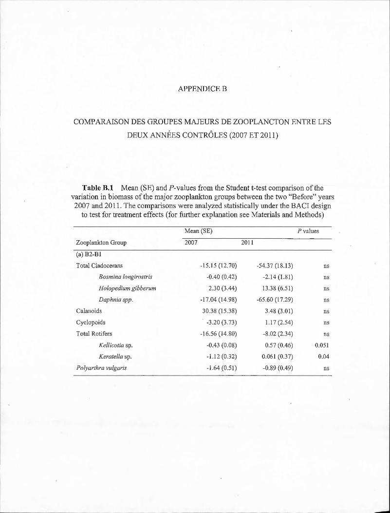
APPENDICEB
COMPARAISON DES GROUPES MAJEURS DE ZOOPLANCTON ENTRE LES
DEUX ANNÉES CONTRÔLES (2007 ET 2011)
Table B. l Mean (SE) and P -values from the Student t-test comparison of the variation in biomass of the major zooplankton groups between the two "Before" years 2007 and 20 11. The comparisons were analyzed statistically under the BACI design
to test for treatment effects (for further explanation see Materials and Methods)
Mean (SE) P values
Zooplankton Group 2007 2011
(a) B2-B1
Total Cladocerans -15.15 (12.70) -54.37 (18.13) ns
Bosmina longirostris -0.40 (0.42) -2.14 (1.8 1) ns
Holopedium gibberum 2.30 (3.44) 13.38 (6.51) ns
Daphnia spp. -17.04 (14.98) -65.60 (17.29) ns
Ca lano ids 30.38 (15.38) 3.48 (3 .01) ns
Cyclopoids -3 .20 (3 .73) 1.17 (2.54) ns
Total Rotifers -1 6.56 (14.80) -8.02 (2.34) ns
Kellicotia sp. -0.43 (0.08) 0.57 (0.46) 0.051
Keratella sp. -l.l 2 (0 .32) 0.061 (0 .37) 0.04
Polyarthra vulgaris -1.64 (0.51) -0.89 (0.49) ns
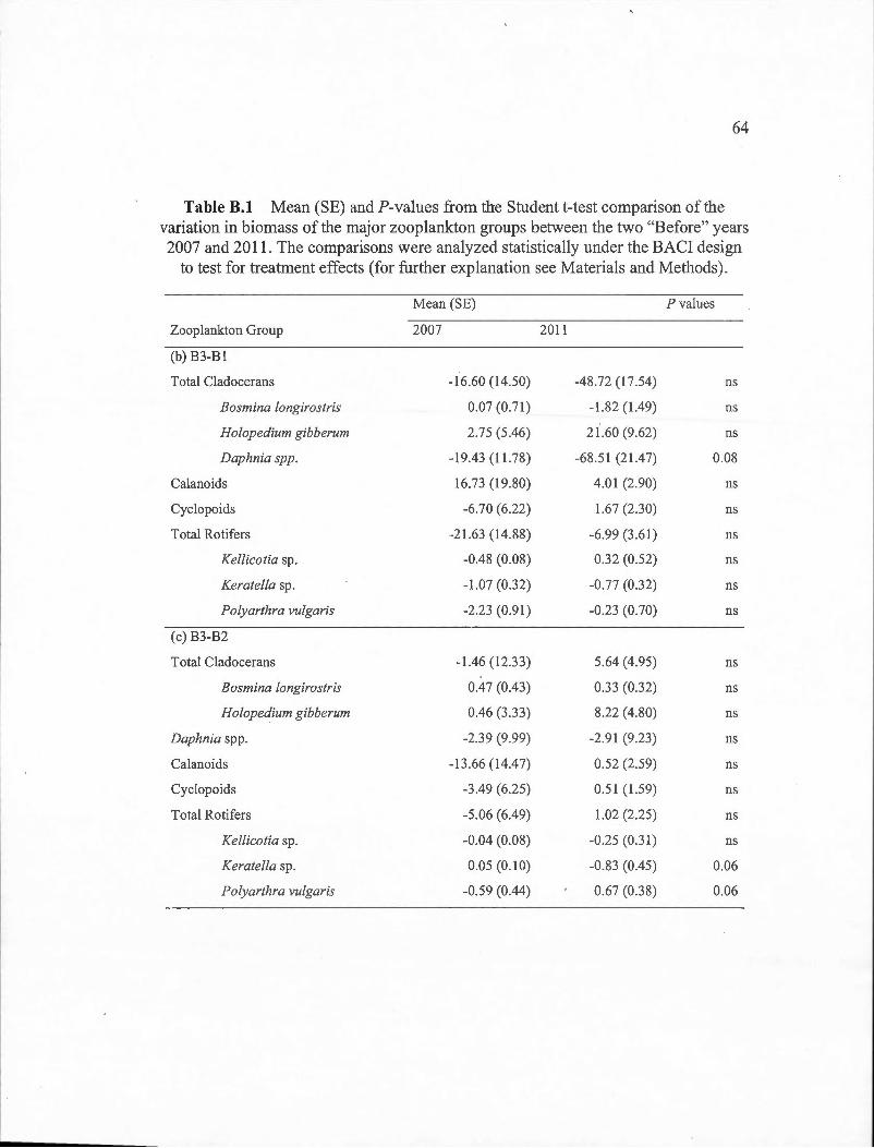
64
Table B. l Mean (SE) and P-values from the Student t-test comparison ofthe variation in biomass of the major zooplankton groups between the two "Before" years 2007 and 2011 . The comparisons were analyzed statistically under the BACI design
to test for treatment effects (for further explanation see Materials and Methods).
Mean (SE) P values
Zooplankton Group 2007 2011
(b) 83-81
Total Cladocerans -16.60 (14.50) -48 .72 (1 7.54) ns
Bosmina longirostris 0.07 (0.71) -1.82 (1.49) ns
Holopedium gibberum 2.75 (5.46) 21.60 (9.62) ns
Daphnia spp . -19.43 (11.78) -68 .51 (21.47) 0.08
Calanoids 16.73 (19.80) 4.01 (2.90) ns
Cyclopoids -6.70 (6.22) 1.67 (2.30) ns
Total Rotifers -21.63 (14.88) -6.99 (3.61) ns
Kellicotia sp. -0.48 (0.08) 0.32 (0.52) ns
Keratella sp. -1.07 (0.32) -0.77 (0.32) ns
Polyarthra vulgaris -2.23 (0.91) -0.23 (0.70) ns
(c) 83-82
Total Cladocerans -1.46 (12.33) 5.64 (4.95) ns
Bosmina longirostris 0.47 (0.43) 0.33 (0.32) ns
Holopedium gibberum 0.46 (3 .33) 8.22 (4.80) ns
Daphnia spp. -2.39 (9 .99) -2 .91 (9.23) ns
Calanoids -13.66 (14.47) 0.52 (2.59) ns
Cyclopoids -3.49 (6.25) 0.51 (1.59) ns
Total Rotifers -5.06 (6.49) 1.02 (2.25) ns
Kellicotia sp . -0.04 (0.08) -0.25 (0.31) ns
Keratella sp. 0.05 (0.10) -0.83 (0.45) 0.06
Polyarthra vulgaris -0.59 (0.44) 0.67 (0.38) 0.06

APPENDICEC
ANALYSES DE REDONDANCE PARTIELLE POUR LES COMMUNAUTÉS DE
ROTIFÈRES PENDANT LA PÉRIODE DU PRINTEMPS ET DE L'ÉTÉ
Fig. C.l PartiaLredundancy analysis (RDA) biplots indicating site and species scores for rotifer species founded in spring and summer periods by BACI-derived treatment (deepened, deepened+mixed and mixed). The percentage of constrained variance (R2
) explained by the axes is indicated with statistically significant axes indicated by an asterisk. White square markers indicate sampling dates in 2009, solid
circles indicated 2010 dates and triangles indicate 2011 dates. Ellipses containing 80% of observations are indicated for the control year (solid line) and the two
experimental years together (dashed line). Panels are: (a) Deepened treatment (B2-B1) in spring (RDA model P =0.095); (b) Deepened treatment in summer (P =0.001);
(c) Deepened+mixed treatment (B3-Bl) in spring (P <0.005); (d) Deepened+mixed treatment in summer (P =0.012); (e) Mixed treatment (B3-B2) in spring (P =0.053);
(f) Mixed treatment in summer (P =0.033). Species abbreviations are: Asplanchna sp. (Asp), Ascomorpha sp. (Asc), Conochiloides sp. (Con), Conochilus sp. (Cos), Filinia
sp. (Fil), Gastropus sp. (Gas), Kellicotia bostoniensis (Keb), Kellicotia longispina (Kel), Keratella cochlearis (Kec), Keratella hiemalis (Keh), Keratella taurocephla
(Ket), Lecane mira (Lem), Ploesoma sp. (Pls), Polyarthra vulgaris (Pov), Synchaeta sp. (Sys), Trichocerca sp. (Trs). Environmental variable abbreviations are:
chlorophyll average (Chl), chlorophyll maximum (MaxChl), concentration of dissolved oxygen (DO_conc).

Deepening
-1.0 -0.5 0.0 0.5
RDA 1 - 100%*
0 (b) .....-
l!)
· ·éo·~r · · · 0
Fil
Keh .....-() 0... 0
0
.. '
l!) A~>'P.. Trs• 0 0
1
-1 .0 -0.5 0.0
RDA 1 - 100%*
R2=0.09
1.0
·Ch!······ 1
.
R2=0.12
0.5 1.0
""0 0
·= (j) 0.. CJ) c ·= 0.. U)
""0 0
·;:::: (j) 0.. .._ (j)
E E ::J
U)
66
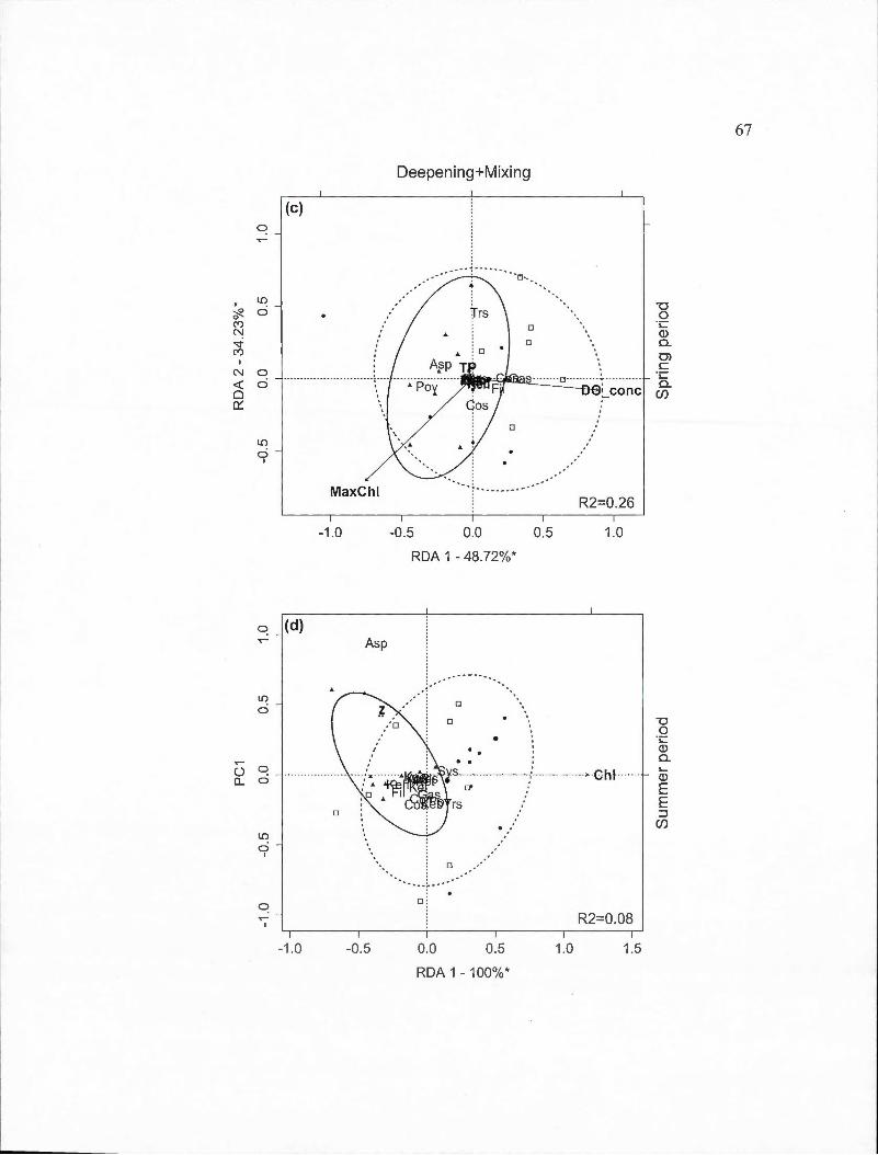
~
~ 0 ('f) N "<:t ('f)
N <( 0 0:::
..---0 0..
(c)
L{)
0
Deepening+Mixing
·~:~ ..
0
0
-o 0 ï:::: Q) o. CJ) c
---------- ---·-··· ········ -; ···· ···- ~ -Pëiy······--~~~!:1i:Qc_:_:··.:.:_:···.:..:..···~o~---~--~---~- - -~- - "§_ :_conc en
0 0
L{)
0 1
~
L{)
0
~ 0
L{)
0 1
MaxChl
-1.0
(d) Asp
-1.0 -0.5
0
-0.5 0.0 0.5
RDA 1 - 48 .72%*
. ' 0
0
0.0 0.5 1.0
RDA 1 - 100%*
- --- ---------------
R2=0.26
1.0
-o 0 ï :::: Q) o. 1... Q)
E E ::::l
Cf)
1.5
67

;!2. 0 .,...-r--0
N <{ 0 0:::
l()
ci
l()
0 1
l()
~
l()
ci
0 ci
l()
0 1
Mixirig
(e)
0
-0.5 0.0 0.5
RDA 1 - 100%*
(f)
Chi
... ... ..... ---- .... ..... .. -- -~ - - ..
a ,
'
-1.0 -0.5 0.0
RDA 1 - 89.29%*
0.5
R2=0.09
1.0 1.5
MaxChl
1:l 0
·;:: <ll 0.. ,_ <ll E
········ -· ····· ---- ·-··· --- ·· E
R2=0.12
1.0
::J (/)
68
APPENDICED
SÉRIES TEMPORELLES DES ESPÈCES INDICATRICES
Fig. D.l Ti me series of the biomass of important cladoceran species for each basin in the control (2011) and experimental (2009-2010) years. (a) Bosmina longirostris;
(b) Daphnia ambigua; (c) Daphnia catawba; (d) Daphnia longiremis; (e) Holopedium gibberum. The vertical dashed line represents the day ofyear at which
the thermocline depth reached the average for the entire sampling period.
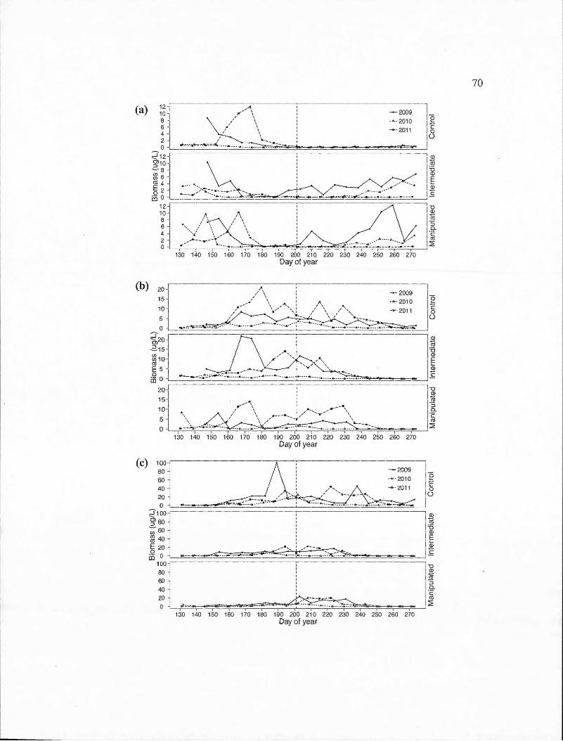
(a)
(b)
(c)
~~[------.//,.,-"\\ -----:----------= ~~~~-~ ~
i .. <~~---.--~,/ ::._::_= --·--:~~~ i --------~=J8 ~~ ~[---------------! -------------~~ ';;;' 86 : 1-g oo - : l E
j ~ ~ :~~:>~~-:::.~~:~~- - ~~-------~=-~~:·:~~-::~:~-~~-~~:J ~ 12 . ---------------,----------------------, "0
10 • ~ : 12 .... /\ 1 C\1
s • .: , / \ I:J 6 _: ' \ l a. 4 ··,:.' , \ .. ~
1·s
2 ... ...... -- .... - -~"' ' \ \,1
0 ~- ~---~ - - - · • · · ·· > 1 ~ 130 140 150 160 170 180 190 200 210 220 230 240 250 260 270
Day of year
130 140 150 160 170 180 190 200 210 220 230 240 250 260 270 Day of year
~ooof _______________ : ------------=._ 2009-1 _
60 : . • 201 0 1 _g 40 l : ' -· 2011 1 § 20 J / -:~ ' . // .. .. __ .... - ~.... l 0 a L ---------~r.: .... .,...-::-:::.:~ ... -=---~-.:__~-: .. .. ___ ..., __ __ ... ___ _ .... ___ ..., _~- -~::::__~
;g:18000 r _ _ _____________ : -------------~ * 2 : 1 ~ oo60 l ' I ID ~ 4o ; lE E 20 _-- · -, : " -- - -. 2 ffi a L~~~~=--=--~~~~~ ... ~------~.s
100 ---------------: --------------------1 -g 80 : JCiî 60 1 ~ ~ 1 ~ 2~ Ç-~- 1 ~
130 140 150 160 170 180 190 200 21 0 220 230 240 250 260 270 Day of year
70
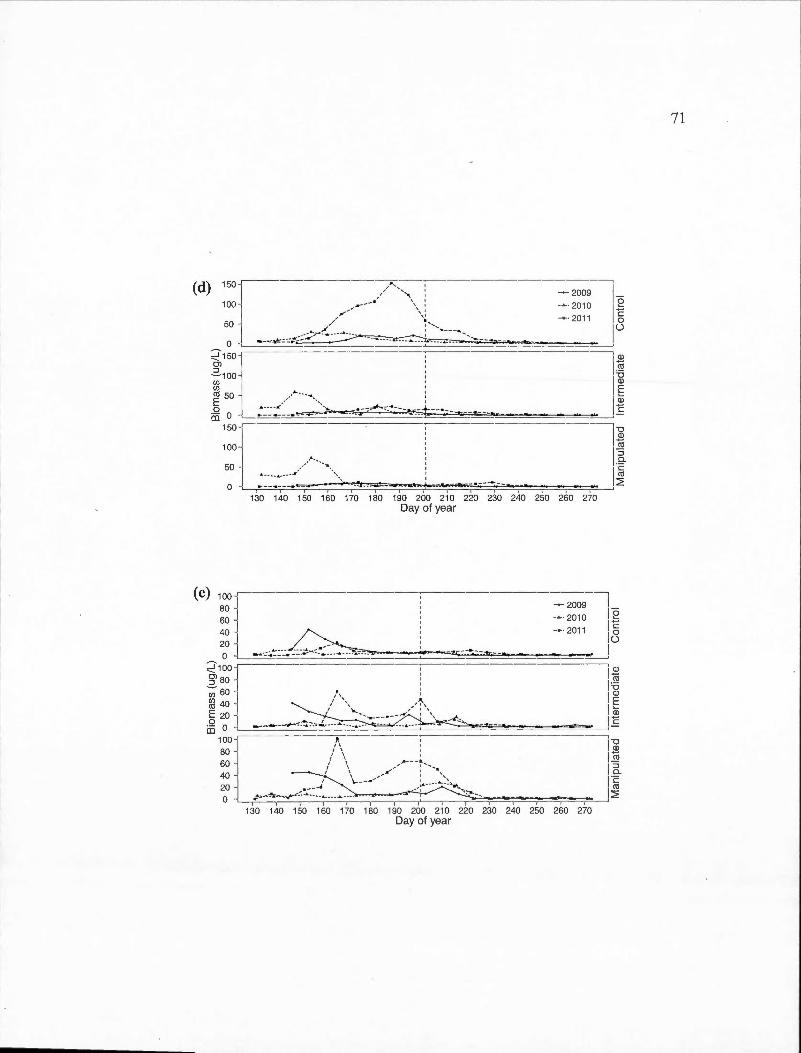
(d) 150[-----7,~-: ------=-2009- ---,1 -, \ 1 0
100 _. --- · ' ' -· · 2010 1 ~ ...- \ 1 +-'
•' \ - -W11 § 50 ~ _., / :' ..... , ___ ., 0
• • -· ,.-- · ----• -- . . 1 ......
0 ~-~,..---.:;'-- ---- -- -· ---- -- --· -- - ---- ·- --- ...._ __ ~ - 1 - ~ ~ !:::[ ________ ! -------------~~~
~5o __ .. ____ , : E E - -- ' 1 Q) 0 .. .. . . . . ·· ··-~- · --=~=-_ ...... __ _, _ _l__ · -- ë Iii 0 ·--~---·~----· _ __ __ .. -~-- 2.._ -..- -----· ~-
150 r ________ : ------~~
100 i 1 ~ · "' ··- 1 o. 50 -- -.. ' ·-
· ·--· · ---- ·/ ··· ·... .. : 1 ~ 0 ;• -- ... Ï--• t: ,=-- 1 ;-?:t .. ~-w;=-~ 1! . -""7-1a ~ ·- -;--, ~ -, 7 1 1 ' ~
130 140 150 160 170 180 190 200 210 220 230 240 250 260 270 Day of year
(e) 100__.---------, ----------------,
80 j : - 2009 1_ 60 : -• 2010 lg 40 : -· 201 1 1 § 20 1 .-- ! lo o L .. -.: :.:::-~. ~:-;-~- .~-~-----~~-==---.2_. ___ =-.-J
~100 -1,----------------, -------- ---- --------,1 Q)
rn ' -2- 80 ] : 1 ~ ~ 60 J /', " 1 Cl)
Cil 4o 1 , \ ... / : ', 1 E ~ 2oo L~----<~~-~~:- - - ~----· ~-~~::.-- ~:: ... ~:::":::.----=:=-=-------=.-J ~
100~------!\-------: -------------~ u
80 j : \ : 1* 60 / \ .---•.. -40 / \ , ... . ... ·"" : ....... ,, 1.9. 20 1 ~1 \._ ...... . ... !. - --- "- -~ ... .... 1 ~ 0 J .:--~- ,,....,::-.:.: ....... ~~---- ·· .. ~'- .• j ! 2
, , 1 1 1 1 : T 1 ,
130 140 150 160 170 180 190 200 210 220 230 240 250 260 270 Day of year
71
72
Fig. D.2 Time series of the biomass of important calanoid copepod species for each basin in the control (2011) and experimental (2009-2010) years. (a) Epischura
lacustris; (b) Leptodiaptomus minutus. The vertical dashed line represents the day of year at which the thermocline depth reached the average for the entire sampling
period.
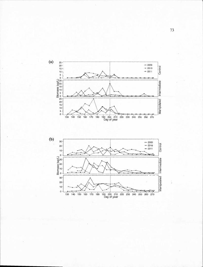
- -------------------- ------- ------------------ - -- -- -------- ---- ----· ---- ---------------,
(a)
(b)
15 10 5 0
....... .. _
-~~ ..... .......
130 140 150 160 170 180 190 200 210 220 230 240 250 260 270 Day of year
130 140 150 160 170 180 190 200 210 220 230 240 250 260 270 Day of year
73

74
Fig. D.3 Time series of the biomass of important calanoid copepod species for each basin in the control (2011) and experimental (2009-2010) years. (a) Cyclops scutifer;
(b) Orthocyclops modestus; (b) Tropocyclops prasinus. The vertical dashed line represents the day of year at which the thermocline depth reached the average for the
entire sampling period.

----
1
75
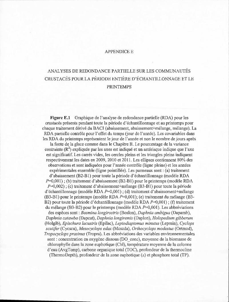
APPENDICEE
ANALYSES DE REDONDANCE PARTIELLE SUR LES COMMUNAUTÉS
CRUSTACÉS POUR LA PÉRIODE ENTIÈRE D 'ÉCHANTILLONNAGE ET LE
PRINTEMPS
Figure E.l Graphique de l'analyse de redondance partielle (RDA) pour les crustacés présents pendant toute la période d'échantillonnage et au printemps pour
chaque traitement dérivé du BACI (abaissement, abaissement+mélange, mélange). La RDA partielle contrôle pour l'effet du temps Uour de l'année). Les covariables dans
les RDA du printemps représentent le jour de l'année et non le nombre de jours après la fonte de la glace comme dans le Chapitre II. Le pourcentage de la variance
contrainte (R2) expliquée par les axes est indiqué et un astérisque indique que l'axe
est significatif Les carrés vides, les cercles pleins et les triangles pleins indiquent respectivement les dates en 2009, 2010 et 2011. Les ellipses contiennent 80% des
observations et sont indiquées pour l 'année contrôle (ligne pleine) et les années expérimentales ensemble (ligne pointillée). Les panneaux sont: (a) traitement d'abaissement (B2-Bl) pour toute la période d'échantillmmage (modèle RDA
P=O,OOl); (b) traitement d'abaissement (B2-Bl) pour le printemps (modèle RDA P=0,002); (c) traitement d'abaissement+mélange (B3-Bl) pour toute la période
d'échantillonnage (modèle RDA P=O,Oül); (d) traitement d'abaissement+mélange (B3-Bl) pour le printemps (modèle RDA P=O,Oül); (e) traitement du mélange (B3-B2) pour toute la période d'échantillonnage (modèle RDA P=O,OOl) ; (f) traitement du mélange (B3-B2) pour le printemps (modèle RDA P=O,Oül). Les abbréviations
des espèces sont : Bosmina longirostris (Boslon), Daphnia ambigua (Dapamb ), Daphnia catawba (Dapcat), Daphnia longiremis (Daplon), Holopediwn gibberum (Holgib ), Epischura lacustris (Epi lac), Leptodiaptomus minutus (Lepmin), Cyclops scutifer (Cycscu), Mesocyclops edax (Meseda), Orthocyclops modestus (Ortmod),
Tropocyclops prasinus (Tropra). Les abbréviations des variables environnementales sont : concentration en oxygène dissous (DO_ conc ), moyenne de la biomasse de chlorophylle dans la zone euphotique (Chl), température moyenne de la colmme d'eau (AvgTemp), carbone organique total (TOC), profondeur de la thermocline (ThermoDepth), profondeur de la zone euphotique (z) et phosphore total (TP).
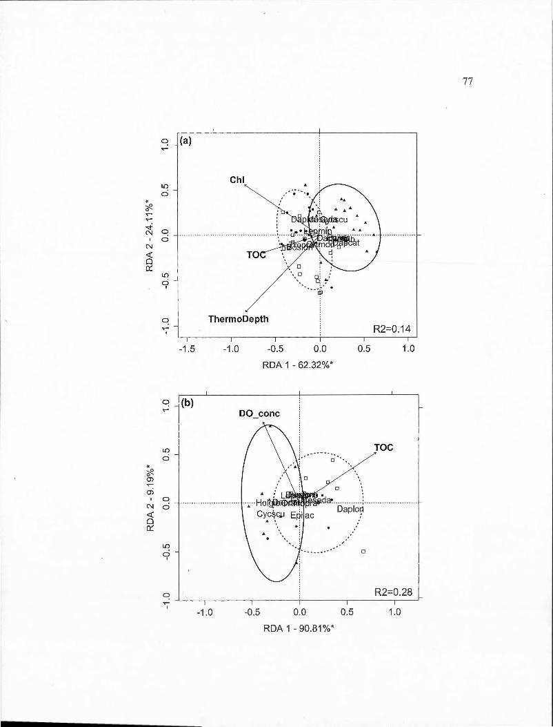
77
~ (a) "'""""
Chi l{)
ci . ~
~ . . 0 . "'""""
-.i ~ N
1 0 N <( 0 ~ 1
0::: ~ :' l{) ' 0
ci .. 1
·- - ~ .
0 ThermoDepth "'"""" R2=0.14 1
-1.5 -1 .0 -0 .5 0.0 0.5 1.0
RDA 1 - 62.32%*
~ (b) "'""""
~ TOC
0 0 ~
~ 0 en .,..-o) 0
1 ~ N 0 <( 0 0:::
/ l{)
0 0
1
-1 .0
RDA 1 - 90.81 %*
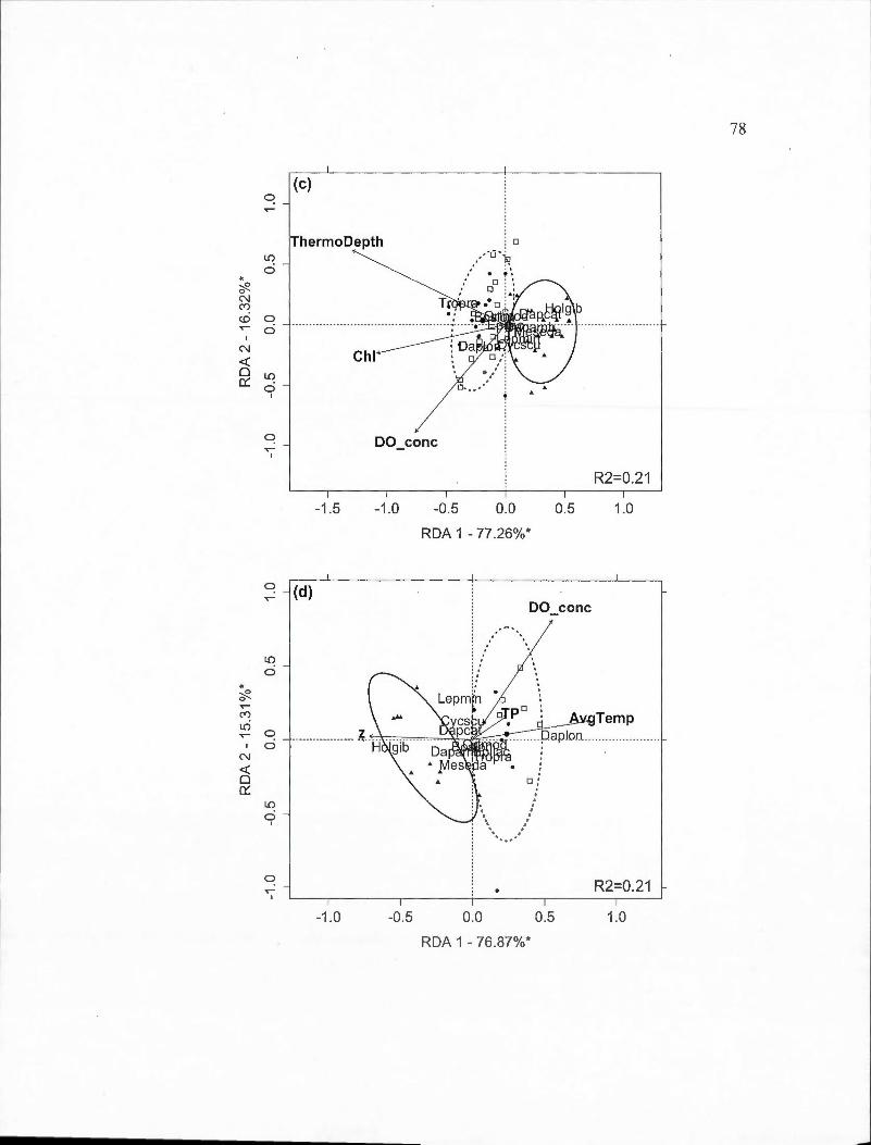
(c) <?_ ....-
ThermoDepth LO -0 ..
~ 0 N (")
(0 0 ....- ci - .
N <{ 0 LO cc: 0
.. cf?. ....-(")
1
0 ..-
1
0
LO ci
LO 0
1 0 N <{ 0 cc:
LO 0
1
(d)
-1 .5
-1 .0
Chi
n ... /
DO_conc
-1.0 -0.5 0.0 0.5
RDA 1 - 77.26%*
DO_conc
:
0 :
-0. 5 0.0 0.5
RDA 1 - 76.87%*
78
R2=0.21
1.0
R2=0.21
1.0

0
1.()
ci ~
~ 0 '<j"
~ (J)
0 N 1 ci
N <( 0 n::
~ 0
1
0 ..-
1
0
u ~ n... 0
~ 0
1
0 ... 1
(e)
Thermo
-1.5 -1.0
-1.0 -0.5
79
. . . . : .
DO - conc t
-0.5 0.0 0.5 1.0
RDA 1 - 70.36%*
: o
• 1' - ~.
E.p i~~-c i . . . . ·.
0 . !'' t.~pm~ .· :
R2=0.17
0.0 0.5 1.0
RDA 1 -100%*
APPENDICEF
ANALYSES DE REDONDANCE PARTIELLE SUR LES COMMUNAUTÉS
ROTIFÈRES POUR LA PÉRIODE ENTIÈRE D'ÉCHANTILLONNAGE ET LE
PRINTEMPS
Figure F.l Graphique de l 'analyse de redondance partielle (RDA) pour les rotifères présents au printemps pour chaque traitement dérivé du BACI (abaissement,
abaissement+mélange, mélange). La RDA partielle contrôle pour l'effet du temps (jour de l'année). Les covariables dans les RDA du printemps représentent le jour de l'année et non le nombre de jours après la fonte de la glace comme dans l'Appendice C. Le pourcentage de la variance contrainte (R2
) expliquée par les axes est indiqué et un astérisque indique que l'axe est significatif. Les carrés vides, les cercles pleins et
les triangles pleins indiquent respectivement les dates en 2009, 2010 et 2011. Les ellipses contiennent 80% des observations et sont indiquées pour l'année contrôle
(ligne pleine) et les années expérimentales ensemble (ligne pointillée). Les patmeaux sont: (a) traitement d'abaissement (B2-Bl ; modèle RDA P=0,069); (b) traitement
d'abaissement+mélange (B3-Bl ; modèle RDA P=0,002); (c) traitement du mélange (B3-B2; modèle RDA P=0,006) . Les abbréviations des espèces sont: Asplanchna sp. (Asp), Ascomorpha sp. (Asc), Conochiloides sp. (Con), Conochilus sp. (Cos), Filinia
sp. (Fil), Gastropus sp. (Gas), Kellicotia bostoniensis (Keb), Kellicotia longispina (Kel), Keratella cochlearis (Kec), Keratella hiemalis (Keh), Keratella taurocephla
(Ket), Lecane mira (Lem), Ploesoma sp. (Pls), Polyarthra vulgaris (Pov), Synchaeta sp. (Sys), Trichocerca sp. (Trs). Les abbréviations des variables environnementales
sont : concentration en oxygène dissous (DO_ conc ), maximum de chlorophylle (MaxChl), température moyenne de la colonne d'eau (AvgTemp).
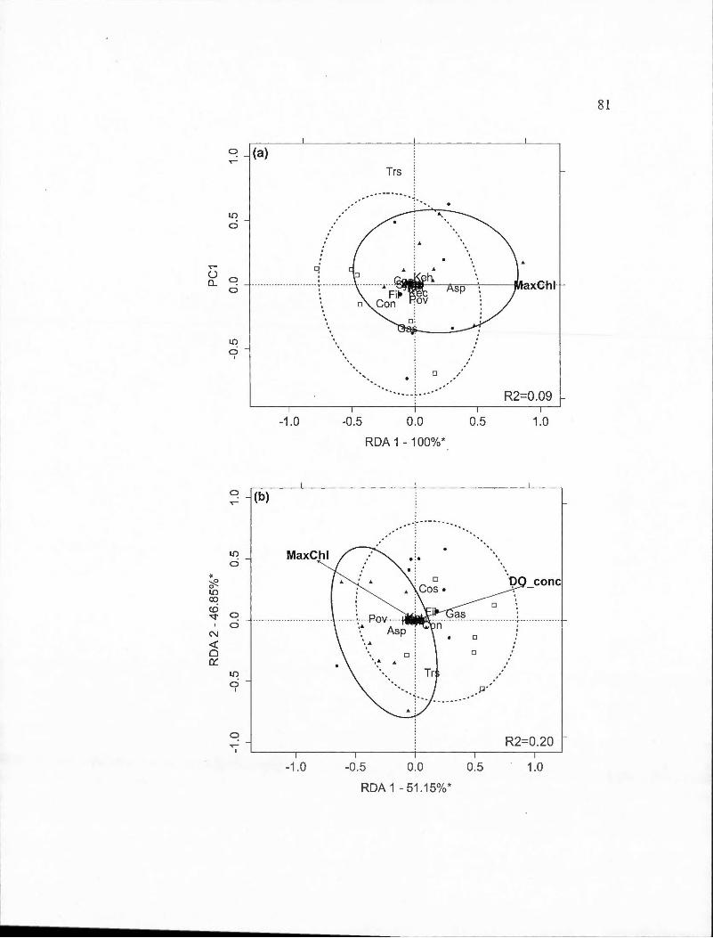
~ (a)
1.!)
0
..--() 0 0.. 0
~
~ 0 1.!) ro (.() "<:!'
N <{ 0 a:
1.!)
0 1
1.!)
0
~ 0
1.!)
0 1
0 ..--
1
q
-1 .0
MaxChl
-1.0
81
Trs
-0 .5 0.0 0.5 1.0
RDA 1- 100%*
.. co ne
:
R2=0.20
-0.5 0.0 0.5 1.0
RDA 1- 51.15%*
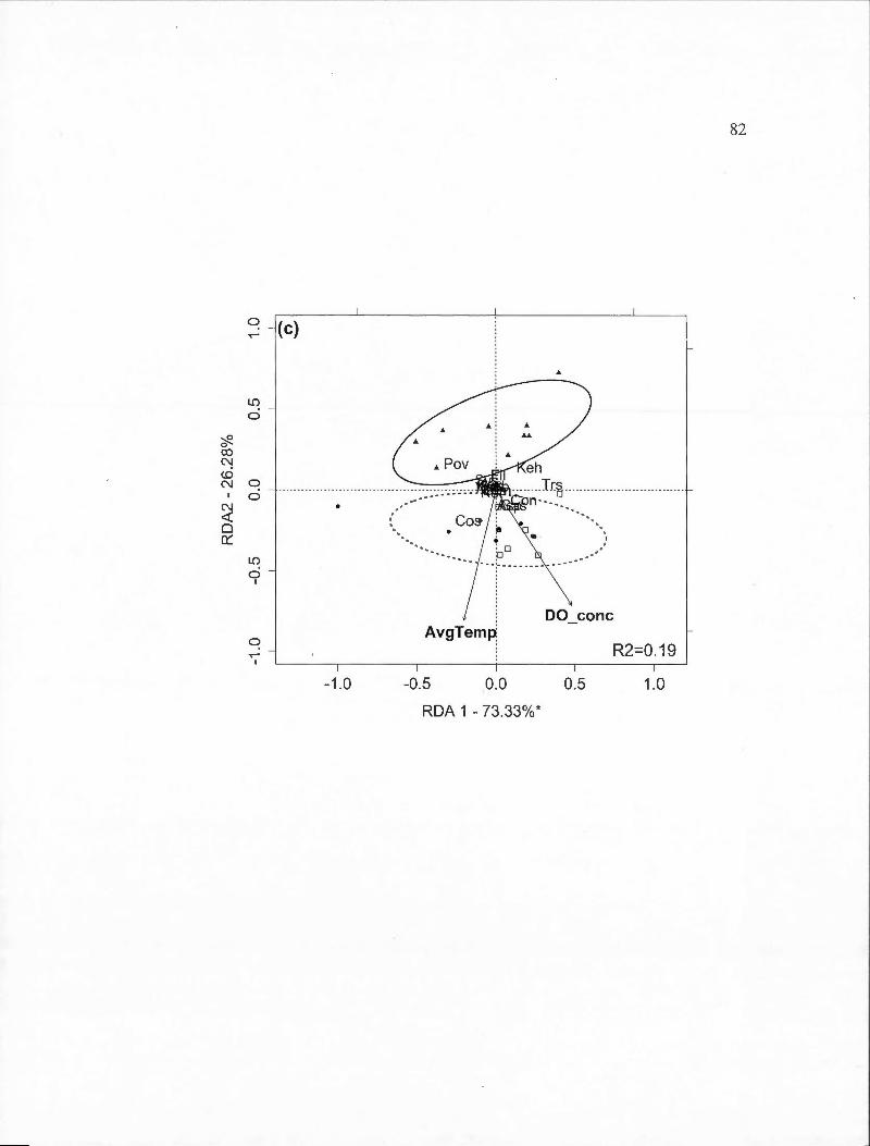
~ 0
co N c.o N
1
N <( 0 0::::
0
l()
0
0 0
1.{)
0 1
0 ..-
1
-1 .0
82
..
DO conc AvgTemp
R2=0.19
-0.5 0.0 0.5 1.0
RDA 1 - 73.33% *

BIBLIOGRAPHIE
Adrian, R., et R. Deneke, 1996. «Possible impact of mild winters on zooplankton succession in eutrophie lakes of the Atlantic European area». Freshwater Biology, vo1.36, no 3, p. 757-770.
Adrian, R. , N. Walz, T. Hintze, S. Hoeg et R. Rusche. 1999. «Effects of ice duration on plankton succession during · spring in a shallow polymictic lake». Freshwater Biology, vol. 41, no 3, p. 621 -632.
Adrian, R., S. Wilhelm et D. Gerten. 2006. «Life-history traits of lake plankton species may govern their phenological response to climate warming». Global Change Biology, vol. 12, no 4, p. 652-661.
Anneville, 0 ., J. C. Molinero, S. Souissi et D. Gerdeaux. 2010. «Seasonal and interannual variability of cladoceran communities in two peri-alpine lakes: uncoupled response to the 2003 heat wave». Journal of Plankton Research, vol. 32, no 6, p. 913-925 .
Antenucci, J. P., A. Ghadouani, M. A. Burford et J. R. Romero. 2005 . «The long-term effect of artificial destratification on phytoplankton species composition in a subtropical reservoir». Freshwater Biology, vol. 50, no 6, p. 1081-1093.
Barnett, A. J. D, K. Finlay et B. E. Beisner. 2007. «Functional diversity of crustacean zooplankton communities: towards a trait-based classification». Freshwater Biology, vol. 52, p. 796-813.
Basu, B. K., et F. R. Pick. 1996. «Factors regulating phytoplankton and zooplankton biomass in temperate rivers» . Limnology and Oceanography, vol. 41 , no 7, p. 1572-1577.
Becker, A., A. Herschel et C. Wilhelm. 2006. «Biological effects of incomplete destratification of hypertrophie freshwater reservoir». Hydrobiologia, vol. 559, p. 85-100.
Beisner, B. E. 2001a. «Herbivory in variable environments: an experimental test of the effects of vertical mixing and Dap1mia on phytoplankton community structure». Canadian Journal of Fisheries and Aquatic Sciences, vol. 58, p. 1371-1379.
~~~~~~~~~~---------
84
Beisner, B.E. 2001 b. «Plank:ton community structure in fluctuating environments and the roles ofproductivity and herbivory». Oikos, vol. 95 , p. 496-510.
Berger, S. A., S. Diehl, T . J. Kunz. 2006. «Light supply, plankton biomass, and seston stoichiometry in a gradient of lake mixing depths» . Limnology and Oceanography, vol. 51, no 4, p . 1898-1905.
Berger, S. A., S. Diehl, H. Stibor, G. Trommer et M. Ruhenstroth. 2010. «Water temperature and stratification depth independently shift cardinal events during plankton spring succession». Global Change Biology, vol. 16, no 7, p. 1954-1965.
Berger, S. A., S. Diehl, H. Stibor, G . Trommer, M. Ruhenstroth, A. Wild, A . Weigert, C. G. Jager et M. Striebel. 2007. «Water temperature and mixing depth affect timing and magnitude of events during spring succession of the plankton». Oecologia, vol. 150, no 4, p . 643-654.
Caceres, C. E . 1998. «lnterspecific variation in the abundance, production, and emergence of Daphnia diapausing eggs». Ecology, vol. 79, no 5, p. 1699-1710.
Cantin, A. 2009. «Abaissement artificiel de la them1ocline d'un lac : effets sur la plancton». Mémoire de maîtrise, Montréal, Université du Québec à Montréal, 89 p.
Cantin, A., B. E. Beisner, J. M. Gunn, Y. T. Praire et J. G. Winter. 2011. «Effects of thermocline deepening on lake plank:ton communities». Canadian Journal of Fisheries and Aquatic Sciences, vol. 68, p . 260-276.
Chavez, F. P., P. G. Strutton, G. E. Friedrich, R. A. Feely, G. C. Feldman, D. G. Foley et M. J. McPhaden. 1999. «Biological and chemical response of the equatorial Pacifie Ocean to the 1997-98 El Nino». Science, vol. 286, no 5447, p. 2126-2131.
Daufresne, M. , K. Lengfellner et U. Sommer. 2009. «Global wanning benefits the small in aquatic ecosystems». Proceedings of the National Academy of Sciences ofthe United States of America, vol. 106, no 31 , p. 12788-12793. En ligne.
De Stasio, B. T., Ir. , D. K. Hill, J. M. Kleinhans, N . P. Nibbelink et J. J. Magnuson . 1996. «Potential effects of global climate change on small north-temperate lakes: Physics, fi sh, and plankton». Limnology and Oceanography, vol. 41 , no 5, p . 1136-1149.
85
Feniova, I. Y. , et N. S. Zilitinkevich. 2012. «Dependence ofDemographic Parameters and Results of Competition on Temperature in Cladocerans». Russian Journal ofEcology, vol. 43 , no 2, p. 131 -136.
Forsius, M. , T. Saloranta, L. Arvola, S. Salo, M. Verta, P. Ala-Opas, M. Rask et J. Vuorenmaa. 2010. «Physical and chemical consequences of artificially deepened thermocline in a small humic lake-a paired whole-lake climate change experiment». Hydrology and Earth System Sciences Discussions, vol. 7, no 3, p. 2915-2947.
France, R. 1997. «Land-water linkages: Influences of riparian deforestation on lake thermocline depth and possible consequences for cold stenotherms» . Canadian Journal of Fisheries and Aquatic Sciences, vol. 54, no 6, p. 1299-1305. In ProQuest Deep Indexing: Biological Sciences.
GIEC, 2007 :Bilan 2007 des changements climatiques. Contribution des Groupes de travail!, II et III au quatrième Rapport d'évaluation du Groupe d 'experts intergouvernemental sur l 'évolution du climat [Équipe de rédaction principale, Pachauri, R.K. et Reisinger, A. (publié sous la direction de~)].
GIEC, Genève, Suisse, 103 pages.
Giorgi, F., X. Bi et J. Pal. 2004. «Mean, interannual variability and trends in a regional climate change experiments over Europe. II : Climate change scenarios». Climate Dynamics, vol. 23, no 7-8, p. 839-858.
Gorham, E., et F. M. Boyce. 1989. «Influence of lake surface area and depth upon thermal stratification and the depth of the summer thermocline». Journal of Great Lakes Research, vol. 15, no 2, p. 233-245.
Gunn, J. M., E. Snucins, N. D. Yan et M. T. Arts . 2001. «Use of water clarity to monitor the effects of climate change and other stressors on oligotrophic lakes». Environ. Monit. Assess., vol. 67, p. 69-88.
Hanazato T et M. Yasuno. 2004. «Zooplankton community structure driven by vertebrate and invertebrate predators». Oecologia, vol 81 , p. 450-458.
Heo, W., et B. Kim. 2004. «The effect of artificial destratifi cation on phytoplankton in a reservoir». Hydrobiologia, vol. 524, no 1, p. 229-239.
Huisman, J., J. Sharples, J. M. Stroom, P. M. Visser, W. E. A. Kardinaal, J. M. H. Verspagen et B. Somrneij er. 2004. «Changes in turbulent mixing shift competition for light between phytoplankton species». Ecology, vol. 85, no 11 , p. 2960-2970.

86
Kalff, 1. 2003. Limnology: Inland Water Ecosystems. Upper Saddle River: Prentice Hall, 592 p.
Kiorboe, T. , et E. Saiz. 1995. «Planktivorous feeding in calm and turbulent environments, with emphasis on copepods». Marine Ecology Progress Series, vol. 122, no 1-3, p. 135-145.
Lampert, W ., et U. Sommer. 2007. Limnoecology:The Ecology of Lakes and Streams. New York : Oxford University Press, 324 p.
Lewis, D. M., et T. 1. Pedley. 2001. «The influence of turbulence on plankton predation strategies». Journal of Theoretical Bio/ogy, vol. 210, no 3, p. 347-365.
Longhi, M. L., et B. E. Beisner. 2010. «Patterns in taxonomie and functional diversity oflake phytoplankton». Freshwater Biology, vol. 55, no 6, p. 1349-1366.
Lydersen, E., K. 1. Aanes, S. Andersen, T. Andersen, P. Brettum, T. Baekken, L. Lien, E. A. Lindstroem, 1. E. Loevik, M. Mjelde, T. 1. Oredalen, A. L. Solheim, R. Romstad et R . F. Wright. 2008. «Ecosystem effects of thermal manipulation of a whole lake, Lake Breisjoeen, southern Norway (THERMOS project)». Hydrology and Earth System Sciences, vol. 12, no 2, p. 509-522.
Maier, G. 1989. «The effect of temperature on the development times of eggs, naupliar and copepodite stages of five species of cyclopoid copepods». Hydrobiologia, vol. 184, p. 79-88.
McCauley, E. 1984. «The estimation of the abundance and biomass of zooplankton samples». In A Manual on Methods for the Assessment of Secondary Productivity in Fresh Water, sous la direction de J. A. Downing et F. H. Rigler, p. 228-265. Oxford : Blackwell Scientific Publications.
McCau1ey, E., et F. Briand. 1979. «Zooplankton grazing and phytoplankton species richness: Field tests of the predation hypothesis». Limnology and Oceanography, vol. 24, p. 243 -252.
Medora Corporation. 2012. «Circulating the World's Water With SolarBee & GridBee Products». En ligne. <www.medora.com>. Consulté le 29 juillet 201 2.
Metcalfe, A. M., T. 1. Pedley et T. F. Thingstad. 2004. «lncorporating turbulence into a plankton foodweb madel». Journal of Marine Systems, vol. 49, no 1-4, p. 105-122.
87
Nicolle, A., P. Hallgren, J. von Einem, E. S. Kritzberg, W. Graneli , A. Persson, C. Bronmark et L. A. Hansson. 2012. «Predicted warming and browning affect timing and magnitude of plankton phenological events in lakes: a mesocosm study». Freshwater Biology, vol. 57, no 4, p . 684-695 .
Pace, M . L. , S. E. G. Findlay et D . Lints. 1992. «Zooplankton in advective environments: The Hudson River community and a comparative analysis». Canadian Journal of Fisheries and Aquatic Sciences, vol. 49, no 5, p. 1060-1069.
Petersen, J. E., L. P. Sanford et W. M. Kemp. 1998. «Coastal plankton responses to turbulent mixing in experimental ecosystems». Marine Eco/ogy Progress Series, vol. 171, p. 23-41.
Platt, T., C. Fuentes-Yaco et K. T. Frank. 2003. «Marine ecology: Spring algal bloom and larval fish survival». Nature, vol. 423, no 6938, p. 398-399.
Rhew, K., R. M . Baca, C. A. Ochs et S. T. Threlkeld. 1999. «Interaction effects of fish, nutrients, mixing and sediments on autotrophic picoplankton and algal composition». Freshwater Biology, vol. 42, no 1, p. 1999.
Rodriguez, F., E . Femandez, R. N. Head, D. S. Harbour, G. Bratbak, M. Heldal et R. P . Harris. 2000. «Temporal variability of viruses, bacteria, phytoplankton and zooplankton in the western English Channel off Plymouth». Journal of the Marine Biological Association of the United Kingdom, vol. 80, no 4, p. 575-586.
Santer, B ., et W. Lampert. 1995. «Summer diapause in cyclopoid copepods -adaptative response to a food bottleneck». Journal of Animal Ecology, vol. 64, no 5, p. 600-613.
Sastri, A. R., P. Juneau et B. E. Beisner. 2012.«Evaluation of chitobiase-based estimates of secondary productivity for freshwater crustacean zooplankton». Manuscript soumis à Journal of Plankton Research.
Schalau, K., K. Rinke, D. Strai1e et F. Peeters. 2008. «Temperature is the key factor explaining interannual variability of Daphnia development in spring: a modelling study». Oecologia, vol. 157, no 3, p. 531-543.
Scheffer, M., D. Straile, E. H. van Nes etH. Hosper. 2001. «Climatic warming causes regime shifts in lake food webs». Limnology and Oceanography, vol. 46, no 7, p. 1780-1 783.

88
Schindler, D. 2009. «Lakes as sentinels and integrators for the effects of climate change on watersheds, airsheds, and landscapes». Limnol. Oceanogr., vol. 54, no 6, part 2, p. 2349-2358.
Schindler, D., B. R. Parker et M. P. Stainton. 1996. «Consequences of climate warming and lake acidification for UV-b penetration in North American boreal lakes». Nature, vol. 379, p. 705-708.
Schindler, D. W. 2001. «The cumulative effects of climate wanning and other human stresses on Canadian freshwaters in the new millennium». Canadian Journal ofFisheriesandAquaticSciences, vol. 58, p.18-29.
Schindler, D. W. , K. G. Beaty, E. J. Fee, E. R. Cruikshank, E. R. DeBruyn, D. L. Findlay, G. A. Linsey, J. A. Shearer, M. P. Stainton et M. A. Turner. 1990. «Effects of climatic warming on lakes of the central boreal forest». Science, vol. 250, p. 967-970.
Schindler, D. W., S. E. Bayley, B. R. Parker, K. G. Beaty, D. R. Cruikshank, E. J. Fee, E. U. Schindler et M. P. Stainton. 1996. «The effects of climatic warming on the properties of Boreal lakes and streams at the Experimental Lakes Area, Northwestem Ontario». Limnology and Oceanography, vol. 41, no 5, p. 1004-1017.
Scully, N. M., et D.R.S Lean. 1994. «The attenuation of ultraviolet radiation in temperate lakes». Arch. Hydrobiol. Bieh. Ergebn. Limnol., vol. 43 , p. 135-144.
Scully, N. M. , P. R. Leavitt et S. R. Cm-penter. 2000. «Century-1ong effects of forest harvest on the physical structure and autotrophic community of a small tempera te lake». Canadian Journal of Fisheries and A qua tic Sciences, vol. 57, p. 50-59.
Shurin J. B., B. Winder, R. Adrian, W. B. Keller, B. Matthews, A. M. Paterson, M. J. Paterson, B. Pinel-Alloul, J. A. Rusak, N. D. Yan. 2010. «Environmental stability and lake zooplankton diversity - contrasting effects of chemical and thermal variability». Eco/ogy Letters, vol. 13, p. 453-463.
Snucins, E., et J.M. Gunn. 2000. «lnteratmual variation in the thermal structure of clear and colored lakes». Limnology and Oceanography, veil. 45, no 7, p . 1639-1646.
Sommer, U. 1989. «Toward a Darwinian ecology ofplanktom>. In Plankton Eco/ogy: Succession in Plankton Communities. p. 1-8. Berlin: Springer-Verlag.
89
Sommer, U., Z. M. Gliwicz, W. Lampert et A. Duncan. 1986. «The PEG-model of seasonal succession of planktonic events in fresh waters». Arch. Hydrobiol. , vol. 106, p. 433-471.
Spigel, R. H., et J. Imberger. 1980. «The classification of mixed-layer dynamics in lakes of small to medium size». Journal of Physical Oceanography, vol. 10, no 7, p. 1104-1121.
Sterner, R. W. 1989. «The role of grazers in phytoplankton succession». In Plankton ecolo gy, sous la direction de U. Sommer, p. 107-170. New York : SpringerVerlag.
Stewart-Oaten, A. W. W. Murdoch et K. R. Parker. 1986. «Environmental impact assessment: "Pseudoreplication intime?". Eco/ogy, vol. 67, no 4, p. 929-940.
Thackeray, S. J. , D. G. George, R. I. Jones et I. J. Winfield. 2006. «Statistical quantification of the effect of thermal stratification on patterns of dispersion in a freshwater zooplankton community». Aquatic Eco/ogy, vol. 40, no 1, p. 23-32.
Townsend, C. R. , M. Begon et J. L. Harper. 2003. Essentials of Eco/ogy, second. Oxford: Blackwell Sciences, 530 p.
Verta, M., S. Salo, M. Korhonen, P. Porvari, A. Paloheimo et J. Munthe. 2010. «Climate induced therrnocline change has an effect on the methyl mercury cycle in small boreal lakes». Science of the Total Environment, vol. 408, no 17, p. 3639-3647.
Vijverberg, J. 1980. «Effect of temperature in laboratory studies on development and growth of Cladocera and Copepoda from Tjeukemeer, The Netherlands». Freshwater Bio/ogy, vol. 10, p. 317-340.
Visser, A. W., H. Saito, E. Saiz et T. Kiorboe. 2001. «Observations of copepod feeding and vertical distribution under natural turbulent conditions in the North Sea>>. Marine Bio/ogy, vol. 138, no 5, p. 1011-1019.
Visser, A. W., et A. Stips. 2002. «Turbulence and zooplankton production: insights from PROVESS». Journal of sea research, special issue, vol. 47, no 3-4, p. 317-329.
Walker, B. H. 1991. «Ecological consequences of atmospheric and climate change». Climatic Change, vol. 18, p. 301-316.
90
Weithoff, G., A. Lorke et N. Walz. 2000. «Effects of water-column mixing on bacteria, phytoplankton, and rotifers under different levels of herbivory in a shallow eutrophie lake». Oecologia, vol. 125, no 1, p. 91-100.
Wetzel, R. G. 1983. Limnology. New York: Saunders College, 767 p.
Winder, M., et D. E. Schindler. 2004. «Climate change uncouples trophic interactions in an aquatic ecosystem». Eco/ogy, vol. 85, no 8, p. 2100-2106.
Top Related