Download - Dynamics of Investment and Firm Performance: Comparative ... · The comparative approach is aimed at testing the robustness of the results to changes in the institutional context.

DYNAMICS OF INVESTMENT AND FIRM PERFORMANCE: COMPARATIVE EVIDENCE FROM MANUFACTURING INDUSTRIES

Documents de travail GREDEG GREDEG Working Papers Series

Marco GrazziNadia JacobyTania Treibich

GREDEG WP No. 2013-09

http://www.gredeg.cnrs.fr/working-papers.html

Les opinions exprimées dans la série des Documents de travail GREDEG sont celles des auteurs et ne reflèlent pas nécessairement celles de l’institution. Les documents n’ont pas été soumis à un rapport formel et sont donc inclus dans cette série pour obtenir des commentaires et encourager la discussion. Les droits sur les documents appartiennent aux auteurs.

The views expressed in the GREDEG Working Paper Series are those of the author(s) and do not necessarily reflect those of the institution. The Working Papers have not undergone formal review and approval. Such papers are included in this series to elicit feedback and to encourage debate. Copyright belongs to the author(s).

Groupe de REcherche en Droit, Economie, GestionUMR CNRS 7321

Dynamics of Investment and Firm Performance:

Comparative evidence from manufacturing industries.∗

Marco Grazzi†

University of Bologna - Department of Economics

Nadia Jacoby‡

University of Paris 1 Pantheon-Sorbonne - Centre d’Economie de la Sorbonne

Tania Treibich§

OFCE/DRIC; GREDEG, University of Nice-Sophia Antipolis, Nice, France and SKEMABusiness School

March 12, 2013

Abstract

Although the relation between investment and economic growth has been well established in themacroeconomic literature, the existence of a similar link at firm level has been challenged by em-pirical work. This paper investigates the channels linking investment and firm performance in theFrench and Italian manufacturing industries by proposing a novel methodology to identify invest-ment spikes, which corrects for size dependence. While maintaining the desired properties of a spikemeasure, our chosen proxy accounts for the expected relation between investment and firm perfor-mance. Ex-ante, more efficient and fast growing firms demonstrate a higher probability to invest; inturn, following an investment spike, the group of investing firms shows further performance gains.We show also that expansionary investment episodes, proxied by the opening of new plants, have anegative effect on profitability but are associated with higher sales and higher levels of employment.

JEL codes: C14, D22, D24, D92, E22, L11, L23, L60

Keywords: Firm heterogeneity, investment spike, industrial dynamics, corporate performance, capitalaccumulation, technical change.

∗We thank Giulio Bottazzi, Giovanni Dosi, Angelo Secchi and Federico Tamagni for many useful discussions and com-ments at various stages of this work. We benefited from comments from several conference participants at EARIE 2011,Stockholm, SIE 2011 Rome, CAED 2012 Nuremberg, University of Nice-Sophia Antipolis and University of Paris. Thestatistical exercises would not have been possible without the valuable help of the Italian Statistical Office (ISTAT), andparticularly Roberto Monducci, and the French Statistical Office (INSEE). Authors acknowledge financial support fromthe European Commission 7th Framework Programme (FP7/2007-2013) under Socio-economic Sciences and Humanities,FINNOV grant agreement n. 217466 and from the Institute for New Economic Thinking, INET inaugural grant 220.The usual disclaimer applies.

†Department of Economics, Piazza Scaravilli 2, 40126 Bologna, Italy. tel: +39-051-2098130, email:

[email protected]‡CES - Centre d’economie de la Sorbonne Maison des Sciences Economiques 106-112 Boulevard de l’hopital F-75647

Paris cedex 13 tel: +: +33-1-44078145, email: [email protected]§GREDEG, 250 rue Albert Einstein - Bat.2, 06560 Valbonne, France, tel: +33-4-93954230, email:

[email protected]

1

1 Introduction

In this paper we investigate the relation between firms’ investments in tangible assets, and corporateperformance. At the macroeconomic level equipment investment is associated with economic growth(De Long and Summers, 1991), but the idiosyncratic impact of firms’ investment on their abilityto grow or to increase efficiency has not been proven. Moreover, firms’ decisions to pursue largeinvestment projects, and the timing of these investments, are also related to managers’ expectationsof future business opportunities and to the phases of the cycle. In this respect, Gourio and Kashyap(2007) show that most of the variation in aggregate investment can be explained by changes in thenumber of establishments undergoing investment episodes (the “extensive margin”).1 Thus, it isapparent that in order to interpret changes in aggregate investment and also how those changes relateto economic growth, we need a thorough understanding of the heterogeneous behavior occurring atfirm level. It is on this area that we focus in this paper.

Assessing the impact of investment at the level of the firm has not always been a viable researchtopic because for many years it was hindered by lack of observed investment data. It is only recentlythat scholars have started to document the nature of firms’ investment behavior. One of the firstattempts was by Doms and Dunne (1998) who used data on U.S. plants and firms. This seminal paperhas inspired a growing body of work reporting similar results for other countries and industries.2 Acommon finding of these studies is the lumpy nature of firm-level investment: years of inactivity orrepair and maintenance are followed by one or several years of heavy investment - with respect to boththe firm and the industry as a whole. For instance, Carlsson and Laseen (2005) show that non-convexadjustment cost models provide a more appropriate framework for explaining investment decisions,and reject those that assume a smooth pattern of capital accumulation. The observed lumpiness ofinvestment rates at both plant and firm level can also be explained more generally as due to investmentirreversibility, resulting from the idiosyncratic nature of the capital purchase and the indivisibility ofphysical capital.

Almost inevitably, unusually large investment projects require corresponding financial commit-ment. If internal resources are insufficient, the firm must rely on an external financial contribution torealize the project. There are two possible outcomes associated with dependence on external financing.First, the investment activity might be limited if the firm is financially constrained, see among theothers Schiantarelli (1996); Audretsch and Elston (2002); Whited (2006). That is, the firm’s desiredlevel of investment is curbed (set to zero) because of poor (complete lack of) access to external finance.Second, to the extent that investment is associated with firm growth,3 the existence of financial con-straints will preclude the possibilities to exploit opportunities for growth. In this case, limited accessto external finance, which results in insufficient investment, will in turn constrain firm growth. Thus,the present study contributes also to the literature on financial constraints on firm growth (see, amongthe others Oliveira and Fortunato, 2006; Whited, 2006; Angelini and Generale, 2008; Bottazzi et al.,forthcoming).

There is a stream of literature that investigates the relationship between capital adjustmentepisodes and firm level (performance) characteristics, such as productivity4 and its growth rate (Power,1998; Bessen, 1999; Huggett and Ospina, 2001; Nilsen et al., 2009; Shima, 2010), employment growth(Asphjell et al., 2010), sales growth (Licandro et al., 2004) or other factors of production (Sakellaris,2004; Nilsen et al., 2009). Investment should affect productivity in the long run since new capitalembodies the latest technology (Jensen et al., 2001). “Learning by doing” models predict that it takestime for workers to learn to use new technology; therefore labor productivity following an investmentepisode is likely to take a U shape, initially falling and then gradually rising to a higher level thanbefore. Most of the empirical literature (Power, 1998; Huggett and Ospina, 2001; Sakellaris, 2004;

1The authors focus on investment spikes: as we discuss extensively below, significantly large investment episodes arerare at firm level.

2Among the papers using a comparable methodology to Doms and Dunne (1998), the reader could refer to Duhautoisand Jamet (2001) for France, Nilsen and Schiantarelli (2003) and Nilsen et al. (2009) for Norway and Carlsson andLaseen (2005) for Sweden.

3Firm growth considered either in terms of sales or of employment.4Either labor productivity or total factor productivity is considered. The former is used in Power (1998), Bessen

(1999), and Nilsen et al. (2009), ), the latter is used in Huggett and Ospina (2001) and Shima (2010).

2

Shima, 2010) reports that the effect of investment spikes on productivity growth is negative in theshort run, and studies evaluating long run impacts fail to report a positive relation between investmentlumps and productivity growth.5 The absence of a positive relation between investment in tangibleassets and productivity growth is so frequent as to induce some authors, such as Power (1998), to offerrecommendations for policy. For example: “I find little evidence of a robust, economically meaningfulcorrelation between high productivity and high recent investment. This cautions against the efficacyof fiscal policy that is based on the premise that investment causes high productivity” (Power, 1998, p.311). This absence of a positive relation between investment and productivity presents a huge puzzlefor both the theoretical and empirical literatures: why invest in tangible assets if this investmentbrings no apparent benefit? In this paper, using the cases of France and Italy, we show how the use ofa more sophisticated methodology provides evidence that investment events do result in improvementsin firm performance. The comparative approach is aimed at testing the robustness of the results tochanges in the institutional context.

Also, the type of investment can affect the outcome at firm level. Replacing obsolete machinerywith modern equipment that uses more up-to-date technologies is more likely to result in increasedproductivity than pure “expansionary” investment which does not involve technological upgrading, forexample, establishing an additional plant to increase production capacity. Less intuitive is that expan-sion achieved by replicating already existing activities might promote problems related to knowledgetransfer within the organization (Szulanski, 1996). The French database allows us to investigate thisissue by enabling observation of increases in numbers of plants.

A few studies have addressed similar research questions related to French or Italian firms. However,they either rely on surveys to obtain actual investment data, which limits the scale of their analysis(Parisi et al., 2006 for Italy) or they rely on investment data computed as the (adjusted) difference incapital stock over two consecutive years (Bontempi et al., 2004; Del Boca, Galeotti, Himmelberg andRota, 2008; Del Boca, Galeotti and Rota, 2008 for Italy and Mairesse et al., 1999; Hall et al., 1999;Bond et al., 2003 for France). The present work is the first large scale study of patterns of firm levelinvestment and their relation to firm performance, for Italy and France.6

We focus on the heterogeneity in investment patterns - across as well as within firms’ time series.The former indicates those characteristics that differentiate investing and non-investing firms; thelatter should provide a better understanding of the factors affecting the timing of the decisions. Weexamine relevant episodes of firm level investment that are not related to the routine activities ofannual repair and maintenance conducted by manufacturing firms. We propose a methodology toidentify exceptional episodes of investment, often referred to in the literature as investment spikes.We investigate which firm characteristics make an investment project more likely, and relatedly, howan investment episode impacts on firm performance in the following periods.

The rest of the paper is organized as follows. Section 2 describes the French and Italian databases.Section 3 discusses the lumpy nature of firm-level investment, and considers and compares differentmeasures of spikes of investment for large capital purchases. We also propose a measure of investmentspikes. Section 4 analyzes the determinants of the probability of observing a spike, and examines theeffects of such an event on firm performance. Section 5 concludes.

2 Data and Descriptive Statistics

The paper draws on two similar firm-level databases for France and Italy, respectively, the EnqueteAnnuelle d’Entreprise (EAE) and Micro.3.7 A unique feature of these databases is that as wellas reporting standard accounting information they include the value of acquisitions of tangible andintangible assets in each year.

5Licandro et al. (2004) find a positive effect on productivity but it is limited to the sub-group of innovative firms.6Duhautois and Jamet (2001) used observed investment from the French tax dataset (fichier des Benefices reels

normaux, INSEE), however they do not investigate the relation between investment spikes and firm performance.7Both databanks were made available to the authors under the mandatory condition of censorship of individual

information. The Micro.3 database was developed in a collaboration between the Italian Statistical Office (ISTAT)and members of the Laboratory of Economics and Management of Scuola Superiore SantAnna, Pisa. More detailedinformation on the development of the Micro.3 database can be found in Grazzi et al. (2009).

3

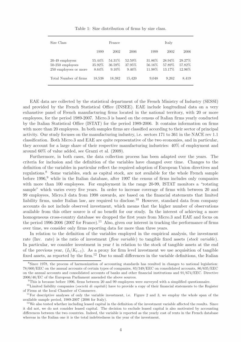
Table 1: Size distribution of firms by size class.

Size Class France Italy

1999 2002 2006 1999 2002 2006

20-49 employess 55.44% 54.31% 52.59% 31.86% 28.94% 29.27%50-250 employees 35.92% 36.59% 37.95% 56.16% 57.89% 57.82%250 employees or more 8.64% 9.10% 9.46% 11.98% 13.17% 12.96%

Total Number of firms 18,538 18,382 15,420 9,048 9,262 8,419

EAE data are collected by the statistical department of the French Ministry of Industry (SESSI)and provided by the French Statistical Office (INSEE). EAE include longitudinal data on a veryexhaustive panel of French manufacturing firms located in the national territory, with 20 or moreemployees, for the period 1989-2007. Micro.3 is based on the census of Italian firms yearly conductedby the Italian Statistical Office (ISTAT) for the period 1989-2006. It contains information on firmswith more than 20 employees. In both samples firms are classified according to their sector of principalactivity. Our study focuses on the manufacturing industry, i.e. sectors 171 to 361 in the NACE rev 1.1classification. Both Micro.3 and EAE are quite representative of the two economies, and in particular,they account for a large share of their respective manufacturing industries: 40% of employment andaround 60% of value added, see Grazzi et al. (2009).

Furthermore, in both cases, the data collection process has been adapted over the years. Thecriteria for inclusion and the definition of the variables have changed over time. Changes to thedefinition of the variables in particular reflect the required adoption of European Union directives andregulations.8 Some variables, such as capital stock, are not available for the whole French samplebefore 1996,9 while in the Italian database, after 1997 the census of firms includes only companieswith more than 100 employees. For employment in the range 20-99, ISTAT monitors a “rotatingsample” which varies every five years. In order to increase coverage of firms with between 20 and99 employees, Micro.3 data from 1998 onwards, are based on the financial statements that limitedliability firms, under Italian law, are required to disclose.10 However, standard data from companyaccounts do not include observed investment, which means that the higher number of observationsavailable from this other source is of no benefit for our study. In the interest of achieving a morehomogeneous cross-country database we dropped the first years from Micro.3 and EAE and focus onthe period 1996-2006 (2007 for France).11 Also, given our interest in tracking the performance of firmsover time, we consider only firms reporting data for more than three years.

In relation to the definition of the variables employed in the empirical analysis, the investmentrate (Inv. rate) is the ratio of investment (flow variable) to tangible fixed assets (stock variable).In particular, we consider investment in year t in relation to the stock of tangible assets at the endof the previous year, (It/Kt−1). As a proxy for firm level investment we use acquisition of tangiblefixed assets, as reported by the firm.12 Due to small differences in the variable definitions, the Italian

8Since 1978, the process of harmonization of accounting standards has resulted in changes to national legislation:78/660/EEC on the annual accounts of certain types of companies, 83/349/EEC on consolidated accounts, 86/635/EECon the annual accounts and consolidated accounts of banks and other financial institutions and 91/674/EEC. Directive2006/46/EC of the European Parliament amended the above sources.

9This is because before 1996, firms between 20 and 99 employees were surveyed with a simplified questionnaire.10Limited liability companies (societa di capitali) have to provide a copy of their financial statements to the Register

of Firms at the local Chamber of Commerce.11For descriptive analyses of only the variable investment, i.e. Figure 2 and 3, we employ the whole span of the

available sample period, 1989-2007 (2006 for Italy).12We also tested whether including leased capital in the definition of the investment variable affected the results. Since

it did not, we do not consider leased capital. The decision to exclude leased capital is also motivated by accountingdifferences between the two countries. Indeed, the variable is reported as the yearly cost of rents in the French databasewhereas in the Italian one it is the total indebtedness in the year of the investment.

4

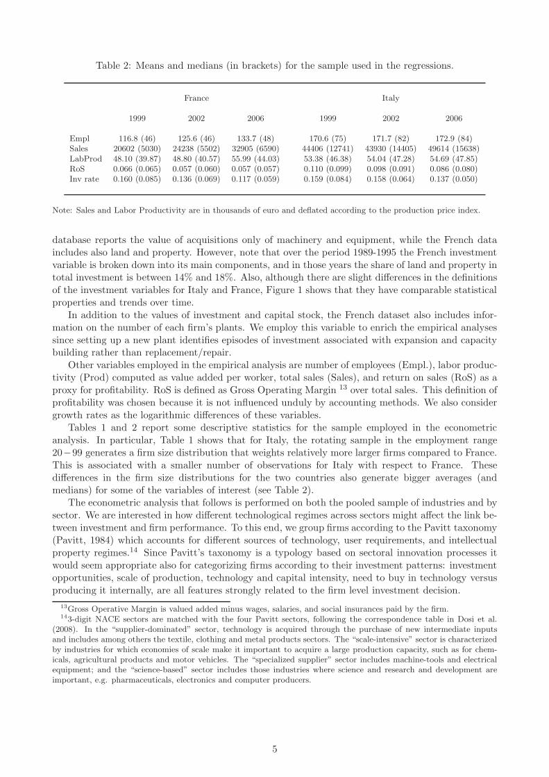
Table 2: Means and medians (in brackets) for the sample used in the regressions.

France Italy

1999 2002 2006 1999 2002 2006

Empl 116.8 (46) 125.6 (46) 133.7 (48) 170.6 (75) 171.7 (82) 172.9 (84)Sales 20602 (5030) 24238 (5502) 32905 (6590) 44406 (12741) 43930 (14405) 49614 (15638)LabProd 48.10 (39.87) 48.80 (40.57) 55.99 (44.03) 53.38 (46.38) 54.04 (47.28) 54.69 (47.85)RoS 0.066 (0.065) 0.057 (0.060) 0.057 (0.057) 0.110 (0.099) 0.098 (0.091) 0.086 (0.080)Inv rate 0.160 (0.085) 0.136 (0.069) 0.117 (0.059) 0.159 (0.084) 0.158 (0.064) 0.137 (0.050)

Note: Sales and Labor Productivity are in thousands of euro and deflated according to the production price index.

database reports the value of acquisitions only of machinery and equipment, while the French dataincludes also land and property. However, note that over the period 1989-1995 the French investmentvariable is broken down into its main components, and in those years the share of land and property intotal investment is between 14% and 18%. Also, although there are slight differences in the definitionsof the investment variables for Italy and France, Figure 1 shows that they have comparable statisticalproperties and trends over time.

In addition to the values of investment and capital stock, the French dataset also includes infor-mation on the number of each firm’s plants. We employ this variable to enrich the empirical analysessince setting up a new plant identifies episodes of investment associated with expansion and capacitybuilding rather than replacement/repair.

Other variables employed in the empirical analysis are number of employees (Empl.), labor produc-tivity (Prod) computed as value added per worker, total sales (Sales), and return on sales (RoS) as aproxy for profitability. RoS is defined as Gross Operating Margin 13 over total sales. This definition ofprofitability was chosen because it is not influenced unduly by accounting methods. We also considergrowth rates as the logarithmic differences of these variables.

Tables 1 and 2 report some descriptive statistics for the sample employed in the econometricanalysis. In particular, Table 1 shows that for Italy, the rotating sample in the employment range20−99 generates a firm size distribution that weights relatively more larger firms compared to France.This is associated with a smaller number of observations for Italy with respect to France. Thesedifferences in the firm size distributions for the two countries also generate bigger averages (andmedians) for some of the variables of interest (see Table 2).

The econometric analysis that follows is performed on both the pooled sample of industries and bysector. We are interested in how different technological regimes across sectors might affect the link be-tween investment and firm performance. To this end, we group firms according to the Pavitt taxonomy(Pavitt, 1984) which accounts for different sources of technology, user requirements, and intellectualproperty regimes.14 Since Pavitt’s taxonomy is a typology based on sectoral innovation processes itwould seem appropriate also for categorizing firms according to their investment patterns: investmentopportunities, scale of production, technology and capital intensity, need to buy in technology versusproducing it internally, are all features strongly related to the firm level investment decision.

13Gross Operative Margin is valued added minus wages, salaries, and social insurances paid by the firm.143-digit NACE sectors are matched with the four Pavitt sectors, following the correspondence table in Dosi et al.

(2008). In the “supplier-dominated” sector, technology is acquired through the purchase of new intermediate inputsand includes among others the textile, clothing and metal products sectors. The “scale-intensive” sector is characterizedby industries for which economies of scale make it important to acquire a large production capacity, such as for chem-icals, agricultural products and motor vehicles. The “specialized supplier” sector includes machine-tools and electricalequipment; and the “science-based” sector includes those industries where science and research and development areimportant, e.g. pharmaceuticals, electronics and computer producers.

5

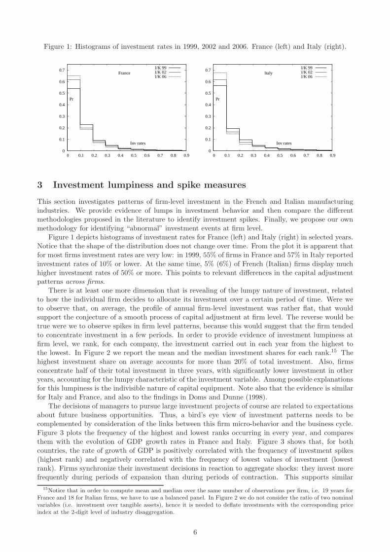
Figure 1: Histograms of investment rates in 1999, 2002 and 2006. France (left) and Italy (right).

0

0.1

0.2

0.3

0.4

0.5

0.6

0.7

0 0.1 0.2 0.3 0.4 0.5 0.6 0.7 0.8 0.9

France

Inv rates

Pr

I/K 99I/K 02I/K 06

0

0.1

0.2

0.3

0.4

0.5

0.6

0.7

0 0.1 0.2 0.3 0.4 0.5 0.6 0.7 0.8 0.9

Italy

Inv rates

Pr

I/K 99I/K 02I/K 06

3 Investment lumpiness and spike measures

This section investigates patterns of firm-level investment in the French and Italian manufacturingindustries. We provide evidence of lumps in investment behavior and then compare the differentmethodologies proposed in the literature to identify investment spikes. Finally, we propose our ownmethodology for identifying “abnormal” investment events at firm level.

Figure 1 depicts histograms of investment rates for France (left) and Italy (right) in selected years.Notice that the shape of the distribution does not change over time. From the plot it is apparent thatfor most firms investment rates are very low: in 1999, 55% of firms in France and 57% in Italy reportedinvestment rates of 10% or lower. At the same time, 5% (6%) of French (Italian) firms display muchhigher investment rates of 50% or more. This points to relevant differences in the capital adjustmentpatterns across firms.

There is at least one more dimension that is revealing of the lumpy nature of investment, relatedto how the individual firm decides to allocate its investment over a certain period of time. Were weto observe that, on average, the profile of annual firm-level investment was rather flat, that wouldsupport the conjecture of a smooth process of capital adjustment at firm level. The reverse would betrue were we to observe spikes in firm level patterns, because this would suggest that the firm tendedto concentrate investment in a few periods. In order to provide evidence of investment lumpiness atfirm level, we rank, for each company, the investment carried out in each year from the highest tothe lowest. In Figure 2 we report the mean and the median investment shares for each rank.15 Thehighest investment share on average accounts for more than 20% of total investment. Also, firmsconcentrate half of their total investment in three years, with significantly lower investment in otheryears, accounting for the lumpy characteristic of the investment variable. Among possible explanationsfor this lumpiness is the indivisible nature of capital equipment. Note also that the evidence is similarfor Italy and France, and also to the findings in Doms and Dunne (1998).

The decisions of managers to pursue large investment projects of course are related to expectationsabout future business opportunities. Thus, a bird’s eye view of investment patterns needs to becomplemented by consideration of the links between this firm micro-behavior and the business cycle.Figure 3 plots the frequency of the highest and lowest ranks occurring in every year, and comparesthem with the evolution of GDP growth rates in France and Italy. Figure 3 shows that, for bothcountries, the rate of growth of GDP is positively correlated with the frequency of investment spikes(highest rank) and negatively correlated with the frequency of lowest values of investment (lowestrank). Firms synchronize their investment decisions in reaction to aggregate shocks: they invest morefrequently during periods of expansion than during periods of contraction. This supports similar

15Notice that in order to compute mean and median over the same number of observations per firm, i.e. 19 years forFrance and 18 for Italian firms, we have to use a balanced panel. In Figure 2 we do not consider the ratio of two nominalvariables (i.e. investment over tangible assets), hence it is needed to deflate investments with the corresponding priceindex at the 2-digit level of industry disaggregation.

6

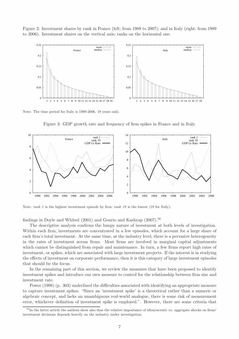
Figure 2: Investment shares by rank in France (left; from 1989 to 2007); and in Italy (right; from 1989to 2006). Investment shares on the vertical axis; ranks on the horizontal one.

0

0.05

0.1

0.15

0.2

0.25

1 2 3 4 5 6 7 8 9 10 11 12 13 14 15 16 17 18 19

Francemean

median

0

0.05

0.1

0.15

0.2

0.25

1 2 3 4 5 6 7 8 9 10 11 12 13 14 15 16 17 18

Italymean

median

Note: The time period for Italy is 1989-2006, 18 years only.

Figure 3: GDP growth rate and frequency of firm spikes in France and in Italy.

0

2

4

6

8

10

1990 1992 1994 1996 1998 2000 2002 2004 2006

Francerank 1

rank 19GDP Gr Rate

0

2

4

6

8

10

12

14

1990 1992 1994 1996 1998 2000 2002 2004 2006

Italyrank 1

rank 18GDP Gr Rate

Note: rank 1 is the highest investment episode by firm, rank 19 is the lowest (18 for Italy).

findings in Doyle and Whited (2001) and Gourio and Kashyap (2007).16

The descriptive analysis confirms the lumpy nature of investment at both levels of investigation.Within each firm, investments are concentrated in a few episodes, which account for a large share ofeach firm’s total investment. At the same time, at the industry level, there is a pervasive heterogeneityin the rates of investment across firms. Most firms are involved in marginal capital adjustmentswhich cannot be distinguished from repair and maintenance. In turn, a few firms report high rates ofinvestment, or spikes, which are associated with large investment projects. If the interest is in studyingthe effects of investment on corporate performance, then it is this category of large investment episodesthat should be the focus.

In the remaining part of this section, we review the measures that have been proposed to identifyinvestment spikes and introduce our own measure to control for the relationship between firm size andinvestment rate.

Power (1998) (p. 303) underlined the difficulties associated with identifying an appropriate measureto capture investment spikes: “Since an ‘investment spike’ is a theoretical rather than a numeric oralgebraic concept, and lacks an unambiguous real-world analogue, there is some risk of measurementerror, whichever definition of investment spike is employed.”. However, there are some criteria that

16In the latter article the authors show also that the relative importance of idiosyncratic vs. aggregate shocks on firms’investment decisions depends heavily on the industry under investigation.

7

can be used to identify a spike measure. Nilsen et al. (2009) state that the investment must be large inrelation to the firm’s history and to a cross section of the industry, and must be a rare event. Also, thedefinition of a spike must be able to account for a relevant share of total industry investment. Nilsenet al. (2009) hint, too, at the necessity to account for a possible relationship between investment rateand capital stock.

We discuss four alternative methodologies to identify investment spikes, namely the Absolute rule,the Relative rule, the Linear rule and finally the Kernel rule. The first three are from Cooper et al.(1999), Power (1998) and Nilsen et al. (2009), respectively. The last is our contribution to identifyinginvestment spikes, and overcomes some of the shortcomings of the other three measures.

The first investment spike proxy we consider classifies lumps as investment rates above a thresholdthat is fixed across firms and industries, hence our label the Absolute rule. To increase comparabilityof results with previous studies we pick 0.20 as the threshold value, following Cooper et al. (1999) andother work. The purpose of this threshold is to eliminate routine maintenance expenditure.

Some, such as Power (1998) consider spikes as large investment events relative to each firm’sinvestment behavior. According to this rule, all investment events that are larger than a multiple αof the firm’s median investment rate over the period of interest, τ , are spikes:

Ii,t/Ki,t−1 > αmedianτ

(Ii,τ/Ki,τ−1)

Power (1998) considers different values of α and finally chooses the value of 1.75;17 we also choosethis value for α. This methodology presents the problem that half of the observations classified asspikes according to the relative rule, correspond to investment rates of below 0.20: for firms with verylow median investment rates, spikes would not correspond to very active investment behavior. Weimpose a threshold on the minimum value of the investment rate, resulting in the spike dummy Si,t

being identified according to the following rule:18

Si,t =

{

1 if It/Ki,t−1 > max[αmedianτ

(Ii,τ/Ki,τ−1), 0.20]

0 otherwise

In what follows we refer to this spike measure as the Relative rule.As already acknowledged by Nilsen et al. (2009), there is a problem with traditional spike measures

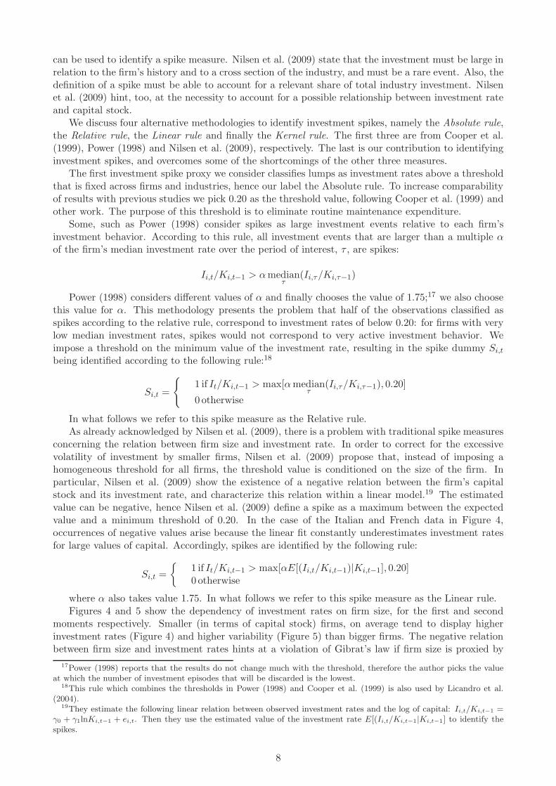
concerning the relation between firm size and investment rate. In order to correct for the excessivevolatility of investment by smaller firms, Nilsen et al. (2009) propose that, instead of imposing ahomogeneous threshold for all firms, the threshold value is conditioned on the size of the firm. Inparticular, Nilsen et al. (2009) show the existence of a negative relation between the firm’s capitalstock and its investment rate, and characterize this relation within a linear model.19 The estimatedvalue can be negative, hence Nilsen et al. (2009) define a spike as a maximum between the expectedvalue and a minimum threshold of 0.20. In the case of the Italian and French data in Figure 4,occurrences of negative values arise because the linear fit constantly underestimates investment ratesfor large values of capital. Accordingly, spikes are identified by the following rule:

Si,t =

{

1 if It/Ki,t−1 > max[αE[(Ii,t/Ki,t−1)|Ki,t−1], 0.20]0 otherwise

where α also takes value 1.75. In what follows we refer to this spike measure as the Linear rule.Figures 4 and 5 show the dependency of investment rates on firm size, for the first and second

moments respectively. Smaller (in terms of capital stock) firms, on average tend to display higherinvestment rates (Figure 4) and higher variability (Figure 5) than bigger firms. The negative relationbetween firm size and investment rates hints at a violation of Gibrat’s law if firm size is proxied by

17Power (1998) reports that the results do not change much with the threshold, therefore the author picks the valueat which the number of investment episodes that will be discarded is the lowest.

18This rule which combines the thresholds in Power (1998) and Cooper et al. (1999) is also used by Licandro et al.(2004).

19They estimate the following linear relation between observed investment rates and the log of capital: Ii,t/Ki,t−1 =γ0 + γ1lnKi,t−1 + ei,t. Then they use the estimated value of the investment rate E[(Ii,t/Ki,t−1|Ki,t−1] to identify thespikes.

8

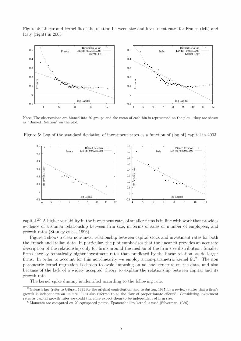
Figure 4: Linear and kernel fit of the relation between size and investment rates for France (left) andItaly (right) in 2003

-0.1

0

0.1

0.2

0.3

0.4

0.5

4 6 8 10 12

France

log Capital

Inv

rate

s

Binned RelationLin fit: -0.029± 0.003

Kernel Fit

-0.1

0

0.1

0.2

0.3

0.4

0.5

4 5 6 7 8 9 10 11 12

Italy

log Capital

Inv

rate

s


Kernel Regr

Note: The observations are binned into 50 groups and the mean of each bin is represented on the plot - they are shownas “Binned Relation” on the plot.

Figure 5: Log of the standard deviation of investment rates as a function of (log of) capital in 2003.

-0.1

0

0.1

0.2

0.3

0.4

0.5

0.6

4 5 6 7 8 9 10 11 12

France

log Capital

std

dev

(Inv

Rat

e)


-0.1

0

0.1

0.2

0.3

0.4

0.5

0.6

0.7

0.8

4 5 6 7 8 9 10 11

Italy

log Capital

std

dev

(Inv

Rat

e)


capital.20 A higher variability in the investment rates of smaller firms is in line with work that providesevidence of a similar relationship between firm size, in terms of sales or number of employees, andgrowth rates (Stanley et al., 1996).

Figure 4 shows a clear non-linear relationship between capital stock and investment rates for boththe French and Italian data. In particular, the plot emphasizes that the linear fit provides an accuratedescription of the relationship only for firms around the median of the firm size distribution. Smallerfirms have systematically higher investment rates than predicted by the linear relation, as do largerfirms. In order to account for this non-linearity we employ a non-parametric kernel fit.21 The nonparametric kernel regression is chosen to avoid imposing an ad hoc structure on the data, and alsobecause of the lack of a widely accepted theory to explain the relationship between capital and itsgrowth rate.

The kernel spike dummy is identified according to the following rule:

20Gibrat’s law (refer to Gibrat, 1931 for the original contribution, and to Sutton, 1997 for a review) states that a firm’sgrowth is independent on its size. It is also referred to as the “law of proportionate effects”. Considering investmentrates as capital growth rates we could therefore expect them to be independent of firm size.

21Moments are computed on 20 equispaced points, Epanenchnikov kernel is used (Silverman, 1986).

9

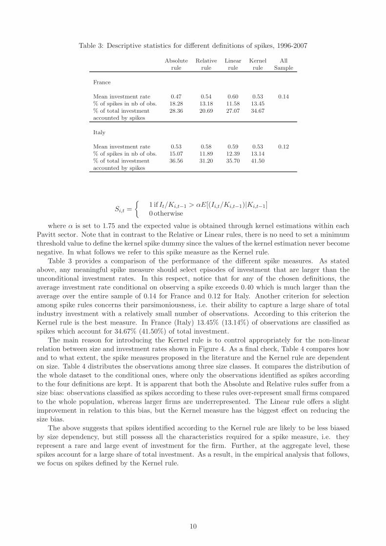
Table 3: Descriptive statistics for different definitions of spikes, 1996-2007

Absolute Relative Linear Kernel Allrule rule rule rule Sample

France

Mean investment rate 0.47 0.54 0.60 0.53 0.14% of spikes in nb of obs. 18.28 13.18 11.58 13.45% of total investment 28.36 20.69 27.07 34.67accounted by spikes

Italy

Mean investment rate 0.53 0.58 0.59 0.53 0.12% of spikes in nb of obs. 15.07 11.89 12.39 13.14% of total investment 36.56 31.20 35.70 41.50accounted by spikes

Si,t =

{

1 if It/Ki,t−1 > αE[(Ii,t/Ki,t−1)|Ki,t−1]0 otherwise

where α is set to 1.75 and the expected value is obtained through kernel estimations within eachPavitt sector. Note that in contrast to the Relative or Linear rules, there is no need to set a minimumthreshold value to define the kernel spike dummy since the values of the kernel estimation never becomenegative. In what follows we refer to this spike measure as the Kernel rule.

Table 3 provides a comparison of the performance of the different spike measures. As statedabove, any meaningful spike measure should select episodes of investment that are larger than theunconditional investment rates. In this respect, notice that for any of the chosen definitions, theaverage investment rate conditional on observing a spike exceeds 0.40 which is much larger than theaverage over the entire sample of 0.14 for France and 0.12 for Italy. Another criterion for selectionamong spike rules concerns their parsimoniousness, i.e. their ability to capture a large share of totalindustry investment with a relatively small number of observations. According to this criterion theKernel rule is the best measure. In France (Italy) 13.45% (13.14%) of observations are classified asspikes which account for 34.67% (41.50%) of total investment.

The main reason for introducing the Kernel rule is to control appropriately for the non-linearrelation between size and investment rates shown in Figure 4. As a final check, Table 4 compares howand to what extent, the spike measures proposed in the literature and the Kernel rule are dependenton size. Table 4 distributes the observations among three size classes. It compares the distribution ofthe whole dataset to the conditional ones, where only the observations identified as spikes accordingto the four definitions are kept. It is apparent that both the Absolute and Relative rules suffer from asize bias: observations classified as spikes according to these rules over-represent small firms comparedto the whole population, whereas larger firms are underrepresented. The Linear rule offers a slightimprovement in relation to this bias, but the Kernel measure has the biggest effect on reducing thesize bias.

The above suggests that spikes identified according to the Kernel rule are likely to be less biasedby size dependency, but still possess all the characteristics required for a spike measure, i.e. theyrepresent a rare and large event of investment for the firm. Further, at the aggregate level, thesespikes account for a large share of total investment. As a result, in the empirical analysis that follows,we focus on spikes defined by the Kernel rule.

10

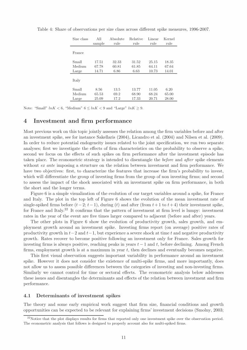
Table 4: Share of observations per size class across different spike measures, 1996-2007.

Size class All Absolute Relative Linear Kernelsample rule rule rule rule

France

Small 17.51 32.33 31.52 25.15 18.35Medium 67.78 60.81 61.85 64.11 67.64Large 14.71 6.86 6.63 10.73 14.01

Italy

Small 8.56 13.5 13.77 11.05 6.20Medium 65.53 69.2 68.90 68.24 65.00Large 25.09 17.2 17.33 20.71 28.00

Note: “Small” lnK < 6, “Medium” 6 ≤ lnK < 9 and “Large” lnK ≥ 9.

4 Investment and firm performance

Most previous work on this topic jointly assesses the relation among the firm variables before and afteran investment spike, see for instance Sakellaris (2004), Licandro et al. (2004) and Nilsen et al. (2009).In order to reduce potential endogeneity issues related to the joint specification, we run two separateanalyses; first we investigate the effects of firm characteristics on the probability to observe a spike,second we focus on the effects of such spikes on firm performance after the investment episode hastaken place. The econometric strategy is intended to disentangle the before and after spike elementswithout ex ante imposing a structure on the relation between investment and firm performance. Wehave two objectives: first, to characterize the features that increase the firm’s probability to invest,which will differentiate the group of investing firms from the group of non investing firms; and secondto assess the impact of the shock associated with an investment spike on firm performance, in boththe short and the longer terms.

Figure 6 is a simple visualization of the evolution of our target variables around a spike, for Franceand Italy. The plot in the top left of Figure 6 shows the evolution of the mean investment rate ofsingle-spiked firms before (t−2; t−1), during (t) and after (from t+1 to t+4) their investment spike,for France and Italy.22 It confirms that the pattern of investment at firm level is lumpy: investmentrates in the year of the event are five times larger compared to adjacent (before and after) years.

The other plots in Figure 6 show the evolution of productivity growth, sales growth, and em-ployment growth around an investment spike. Investing firms report (on average) positive rates ofproductivity growth in t−2 and t−1, but experience a severe shock at time t and negative productivitygrowth. Rates recover to become positive following an investment only for France. Sales growth forinvesting firms is always positive, reaching peaks in years t− 1 and t, before declining. Among Frenchfirms, employment growth is at a maximum in year t, then declines and eventually becomes negative.

This first visual observation suggests important variability in performance around an investmentspike. However it does not consider the existence of multi-spike firms, and more importantly, doesnot allow us to assess possible differences between the categories of investing and non-investing firms.Similarly we cannot control for time or sectoral effects. The econometric analysis below addressesthese issues and disentangles the determinants and effects of the relation between investment and firmperformance.

4.1 Determinants of investment spikes

The theory and some early empirical work suggest that firm size, financial conditions and growthopportunities can be expected to be relevant for explaining firms’ investment decisions (Smolny, 2003;

22Notice that the plot displays results for firms that reported only one investment spike over the observation period.The econometric analysis that follows is designed to properly account also for multi-spiked firms.

11

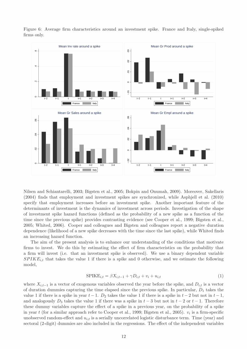
Figure 6: Average firm characteristics around an investment spike. France and Italy, single-spikedfirms only.

0.2

.4.6

t−2 t−1 t t+1 t+2 t+3 t+4

Mean Inv rate around a spike

France Italy

−.0

10

.01

.02

.03

t−2 t−1 t t+1 t+2 t+3 t+4

Mean Gr Prod around a spike

France Italy

0.0

2.0

4.0

6

t−2 t−1 t t+1 t+2 t+3 t+4

Mean Gr Sales around a spike

France Italy

−.0

20

.02

.04

.06

t−2 t−1 t t+1 t+2 t+3 t+4

Mean Gr Empl around a spike

France Italy

Nilsen and Schiantarelli, 2003; Bigsten et al., 2005; Bokpin and Onumah, 2009). Moreover, Sakellaris(2004) finds that employment and investment spikes are synchronized, while Asphjell et al. (2010)specify that employment increases before an investment spike. Another important feature of thedeterminants of investment is the dynamics of investment across periods. Investigation of the shapeof investment spike hazard functions (defined as the probability of a new spike as a function of thetime since the previous spike) provides contrasting evidence (see Cooper et al., 1999; Bigsten et al.,2005; Whited, 2006). Cooper and colleagues and Bigsten and colleagues report a negative durationdependence (likelihood of a new spike decreases with the time since the last spike), while Whited findsan increasing hazard function.

The aim of the present analysis is to enhance our understanding of the conditions that motivatefirms to invest. We do this by estimating the effect of firm characteristics on the probability thata firm will invest (i.e. that an investment spike is observed). We use a binary dependent variableSPIKEi,t that takes the value 1 if there is a spike and 0 otherwise, and we estimate the followingmodel,

SPIKEi,t = βXi,t−1 + γDi,t + vi + ui,t (1)

where Xi,t−1 is a vector of exogenous variables observed the year before the spike, and Di,t is a vectorof duration dummies capturing the time elapsed since the previous spike. In particular, D1 takes thevalue 1 if there is a spike in year t− 1. D2 takes the value 1 if there is a spike in t− 2 but not in t− 1,and analogously D3 takes the value 1 if there was a spike in t− 3 but not in t− 2 or t− 1. Thereforethese dummy variables capture the effect of a spike in a previous year, on the probability of a spikein year t (for a similar approach refer to Cooper et al., 1999; Bigsten et al., 2005). vi is a firm-specificunobserved random-effect and ui,t is a serially uncorrelated logistic disturbance term. Time (year) andsectoral (2-digit) dummies are also included in the regressions. The effect of the independent variables

12

on the probability of observing a spike is estimated using a random effects logistic regression.23

We run a series of specifications in which the dependent variable is defined with the Kernel rule.24

Table 5 reports the results for France and Italy. Firm performance variables include firm size, laborproductivity in levels, and return on sales (RoS). As proxies for firm size we use the log of the number ofemployees (Empl.) for both countries, and for France only, the number of plants (Plant). In contrast tosome of the specifications in the literature (Whited, 1992, 2006), we use profitability computed as RoSrather than cash flow ratio, to proxy for access to internal finance.25 In a second set of specifications,Table 5 columns (iii), (iv) and (vi), we consider another set of variables that includes rates of growthof labor productivity (Prod.Growth), sales (Sales.Growth), and employment (Empl.Growth). We usea dummy to control for firms’ export status at time t− 1. Much of the recent trade literature showsthat the status of exporter is a prominent signal of heterogeneity among firms in the same sector(see among others Melitz, 2003; Bernard et al., 2003). Hence being an exporter could also affect theprobability of an investment spike, and in the absence of firm fixed effects, we use an export dummyto account for this possibility.

We control also for the influence of the macroeconomic environment on firms’ investment deci-sions, using time dummies. Figure 3 and several previous studies (Federer, 1993; Doms and Dunne,1998; Chatelain et al., 2003; Gourio and Kashyap, 2007), show that investment decisions are deter-mined largely by the business cycle and the accompanying changes in demand, monetary policy, anduncertainty.

We run our set of regressions first on the whole sample of observations for France and Italy,controlling for sectoral characteristics using 2-digit sectoral dummies. This is an effective way toreport results for numerous sectors, condensed within a few tables. However this choice also includesthe inconvenience of imposing a common structure on the data because it does not allow the coefficientswe are most interested in, to vary across sectors. In an attempt to reconcile for sectoral variability andto keep the number of tables as small as possible, we aggregate 3-digit industries into Pavitt sectors(refer to Pavitt, 1984 for the original contribution and to Dosi et al., 2008 for a correspondence tablebetween Pavitt sectors and 3 digit NACE industries). Therefore we run the same specifications onthe four macro industrial sectors according to Pavitt’s taxonomy. Finally, we evaluate the accuracyof the different specifications using the Brier Score (Brier, 1950) which measures the average squareddeviation between the predicted probabilities of observing a spike given the estimated coefficients andthe actual data.26 Thus a lower score provides evidence of a better model performance.

The results are reported in Table 5. Figure 7 depicts the marginal effects of profitability andproductivity, computed at the deciles of the respective distributions, on the probability to observean investment spike. Table 5 columns (i) and (v) of Table 5 use number of employees as a proxyfor firm size and suggest that, in both countries, higher employment in t − 1 has a positive effecton the probability of a spike in year t. This represents a residual effect of size given that our spikemeasure already accounts for differences in firms’ capital stock. A higher profit rate in year t − 1,captured by RoS, increases the probability of a spike in the following year. In this work we do notrely on a direct measure of financial constraints; however profitability, which is our measure of thefirm’s capacity to self-finance, is shown to be relevant for an increased probability of carrying out aninvestment project. The probability of a (French or Italian) firm investing is sensitive to changes in

23The fixed effect estimator is not as appropriate for our analysis given the way that the dummies Di,t are constructed.These dummies capture the time since the last investment spike and control for other conditions that depend on thetiming of the spike. In particular the firm-level average will differ for firms with the same number of spikes but a differentspike distribution over the years. Thus within transformation of these firm level dummies would be misleading. Thereforethe Generalized Method of Moments, which identifies the parameters by minimizing the weighted average of deviationsfrom a group of moment conditions, is also discarded.

24As a robustness check, we also ran the regressions using the investment rate as a dependent variable, which allowedus to test whether our spike definition allows for the clearing out of routine investment events as well as the size biasdescribed in section 3. Results are not shown here but they confirm this proposition.

25This is due to a comparability issue, indeed both the French and Italian databases provide the same set of variablesto compute RoS, while the cash flow measure is computed differently for the two countries. However, in both samples,the cash flow and RoS variables are strongly correlated, indicated by a Spearman’s rho coefficient of around 0.9.

26More precisely, for each firm i, the score is given by 1

N

∑N

i=1(Yi − Pi)

2, where N is the number of firms, Yi is theobserved event (Yi = 1 if there is a spike and Yi = 0 if not), and Pi is the probability that firm i experiences a spikegiven the estimated coefficients of the dynamic logit regression.

13

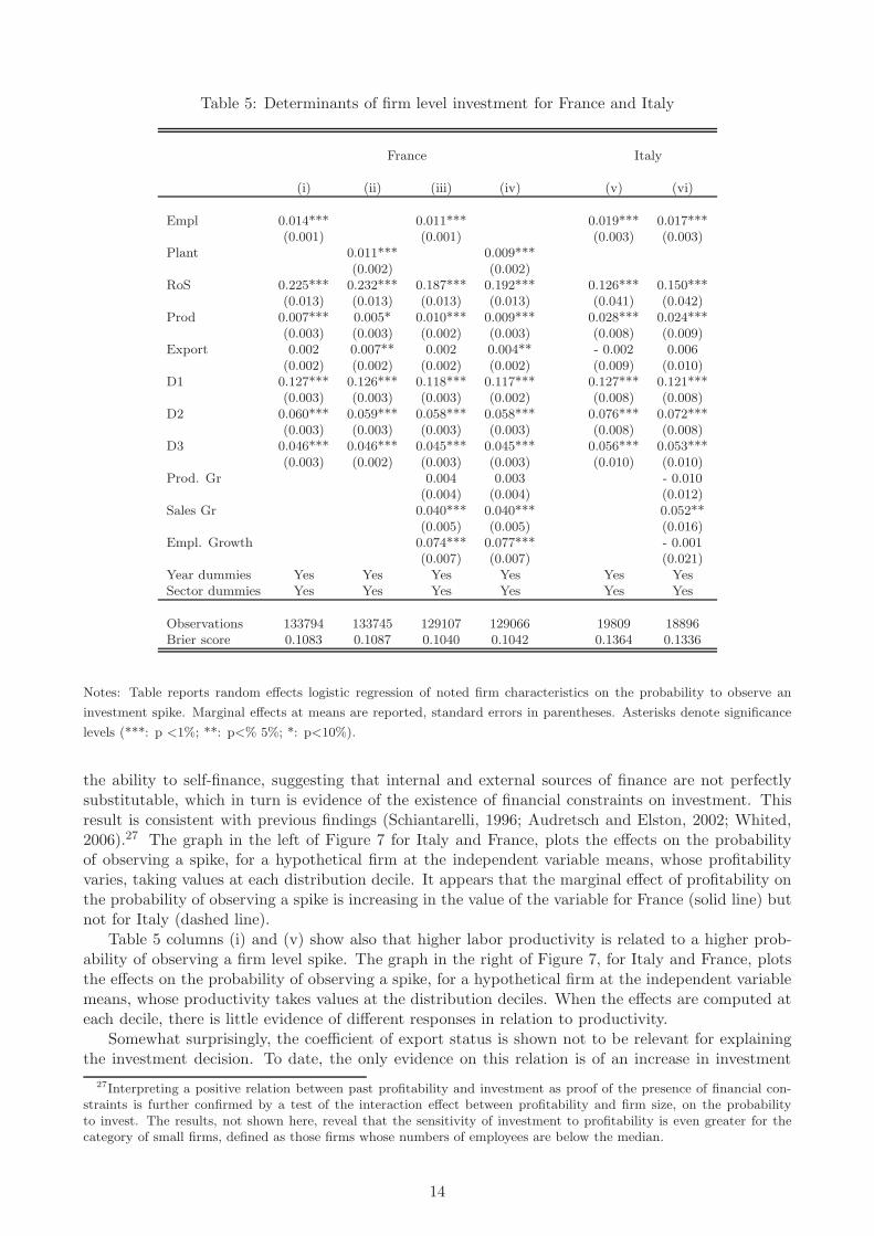
Table 5: Determinants of firm level investment for France and Italy

France Italy

(i) (ii) (iii) (iv) (v) (vi)

Empl 0.014*** 0.011*** 0.019*** 0.017***(0.001) (0.001) (0.003) (0.003)

Plant 0.011*** 0.009***(0.002) (0.002)

RoS 0.225*** 0.232*** 0.187*** 0.192*** 0.126*** 0.150***(0.013) (0.013) (0.013) (0.013) (0.041) (0.042)

Prod 0.007*** 0.005* 0.010*** 0.009*** 0.028*** 0.024***(0.003) (0.003) (0.002) (0.003) (0.008) (0.009)

Export 0.002 0.007** 0.002 0.004** - 0.002 0.006(0.002) (0.002) (0.002) (0.002) (0.009) (0.010)

D1 0.127*** 0.126*** 0.118*** 0.117*** 0.127*** 0.121***(0.003) (0.003) (0.003) (0.002) (0.008) (0.008)

D2 0.060*** 0.059*** 0.058*** 0.058*** 0.076*** 0.072***(0.003) (0.003) (0.003) (0.003) (0.008) (0.008)

D3 0.046*** 0.046*** 0.045*** 0.045*** 0.056*** 0.053***(0.003) (0.002) (0.003) (0.003) (0.010) (0.010)

Prod. Gr 0.004 0.003 - 0.010(0.004) (0.004) (0.012)

Sales Gr 0.040*** 0.040*** 0.052**(0.005) (0.005) (0.016)

Empl. Growth 0.074*** 0.077*** - 0.001(0.007) (0.007) (0.021)

Year dummies Yes Yes Yes Yes Yes YesSector dummies Yes Yes Yes Yes Yes Yes

Observations 133794 133745 129107 129066 19809 18896Brier score 0.1083 0.1087 0.1040 0.1042 0.1364 0.1336

Notes: Table reports random effects logistic regression of noted firm characteristics on the probability to observe an

investment spike. Marginal effects at means are reported, standard errors in parentheses. Asterisks denote significance

levels (***: p <1%; **: p<% 5%; *: p<10%).

the ability to self-finance, suggesting that internal and external sources of finance are not perfectlysubstitutable, which in turn is evidence of the existence of financial constraints on investment. Thisresult is consistent with previous findings (Schiantarelli, 1996; Audretsch and Elston, 2002; Whited,2006).27 The graph in the left of Figure 7 for Italy and France, plots the effects on the probabilityof observing a spike, for a hypothetical firm at the independent variable means, whose profitabilityvaries, taking values at each distribution decile. It appears that the marginal effect of profitability onthe probability of observing a spike is increasing in the value of the variable for France (solid line) butnot for Italy (dashed line).

Table 5 columns (i) and (v) show also that higher labor productivity is related to a higher prob-ability of observing a firm level spike. The graph in the right of Figure 7, for Italy and France, plotsthe effects on the probability of observing a spike, for a hypothetical firm at the independent variablemeans, whose productivity takes values at the distribution deciles. When the effects are computed ateach decile, there is little evidence of different responses in relation to productivity.

Somewhat surprisingly, the coefficient of export status is shown not to be relevant for explainingthe investment decision. To date, the only evidence on this relation is of an increase in investment

27Interpreting a positive relation between past profitability and investment as proof of the presence of financial con-straints is further confirmed by a test of the interaction effect between profitability and firm size, on the probabilityto invest. The results, not shown here, reveal that the sensitivity of investment to profitability is even greater for thecategory of small firms, defined as those firms whose numbers of employees are below the median.

14

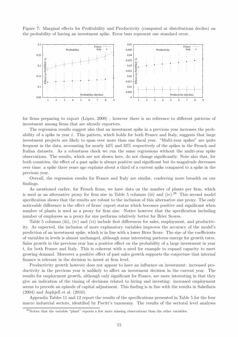
Figure 7: Marginal effects for Profitability and Productivity (computed at distributions deciles) onthe probability of having an investment spike. Error bars represent one standard error.

0.05

0.1

0.15

0.2

0.25

0.3

1 2 3 4 5 6 7 8 9

Profitability

Profitability (deciles)

Eff

ects

on

Pr(S

PIK

E=

1)France

Italy

0

0.005

0.01

0.015

0.02

0.025

0.03

0.035

0.04

0.045

0.05

1 2 3 4 5 6 7 8 9

Productivity

Productivity (deciles)

Eff

ects

on

Pr(S

PIK

E=

1)

FranceItaly

for firms preparing to export (Lopez, 2009) ; however there is no reference to different patterns ofinvestment among firms that are already exporters.

The regression results suggest also that an investment spike in a previous year increases the prob-ability of a spike in year t. This pattern, which holds for both France and Italy, suggests that largeinvestment projects are likely to span over more than one fiscal year. “Multi-year spikes” are quitefrequent in the data, accounting for nearly 44% and 33% respectively of the spikes in the French andItalian datasets. As a robustness check we run the same regressions without the multi-year spikeobservations. The results, which are not shown here, do not change significantly. Note also that, forboth countries, the effect of a past spike is always positive and significant but its magnitude decreasesover time: a spike three years ago explains about a third of a current spike compared to a spike in theprevious year.

Overall, the regression results for France and Italy are similar, conferring more breadth on ourfindings.

As mentioned earlier, for French firms, we have data on the number of plants per firm, whichis used as an alternative proxy for firm size in Table 5 columns (iii) and (iv).28 This second modelspecification shows that the results are robust to the inclusion of this alternative size proxy. The onlynoticeable difference is the effect of firms’ export status which becomes positive and significant whennumber of plants is used as a proxy for firm size. Notice however that the specification includingnumber of employees as a proxy for size performs relatively better for Brier Scores.

Table 5 columns (iii), (iv) and (vi) include first differences for sales, employment, and productiv-ity. As expected, the inclusion of more explanatory variables improves the accuracy of the model’sprediction of an investment spike, which is in line with a lower Brier Score. The size of the coefficientsof variables in levels is almost unchanged, although some interesting patterns emerge for growth rates.Sales growth in the previous year has a positive effect on the probability of a large investment in yeart, for both France and Italy. This is coherent with a need for example to expand capacity to meetgrowing demand. Moreover a positive effect of past sales growth supports the conjecture that internalfinance is relevant in the decision to invest at firm level.

Productivity growth however does not appear to have an influence on investment: increased pro-ductivity in the previous year is unlikely to affect an investment decision in the current year. Theresults for employment growth, although only significant for France, are more interesting in that theygive an indication of the timing of decisions related to hiring and investing: increased employmentseems to precede an episode of capital adjustment. This finding is in line with the results in Sakellaris(2004) and Asphjell et al. (2010).

Appendix Tables 11 and 12 report the results of the specifications presented in Table 5 for the fourmacro industrial sectors, identified by Pavitt’s taxonomy. The results of the sectoral level analyses

28Notice that the variable “plant” reports a few more missing observations than the other variables.

15

are in line with those for the entire sample. Table 11 shows that size, return on sales, productivityand past spikes have a positive and significant effect on the probability of an investment spike, whichis in line with the results for the entire sample (Table 5 columns i, ii and iv). Nevertheless there issome heterogeneity in the strength of these impacts across sectors. For example RoS has a weakerimpact in the French science-based sector and is not significant in the Italian supplier-dominated andscience-based sectors. This points to differences in reliance on self-financing across sectors. Table 12mostly confirms the results, at the aggregate level, when variables in first differences are included.Although productivity growth has no significant impact for the whole sample of French firms, wefind a negative relation for the science-based sector (Table 12). Also, in this sector for France, theprobability of investment is strongly associated with a past increase in sales (with a coefficient muchhigher than for other sectors), but not with an increase in the employee numbers. Finally, althoughthe export dummy turns out not to be significant for explaining an investment spike, the sectoralanalysis shows some differences for the French dataset: the export dummy is significant and positivefor the scale-intensive sector and significant and negative for the supplier-dominated sector.

To sum up, our analysis of the determinants of investment spikes suggests a high degree of similarityamong French and Italian firms. Fast growing, profitable and productive firms are more likely to invest,and past productivity growth has almost no impact. Further, export status is not systematicallyassociated with a higher probability to invest. Finally, the hazard function is decreasing over time.

4.2 Effect of investment spikes on firm performance

The second broad research question that we address relates to the effects of investment spikes on firmperformance. There are several reasons why firms might invest in tangible assets such as to satisfyincreasing demand, or to buffer against technological obsolescence by replacing existing machinery andequipment, or prepare for the launch of a new series of products requiring new machinery. We wouldexpect therefore that investment spikes should be positively correlated with firm size, firm growth,and also firm efficiency.

A number of papers investigate the link between investment and productivity, and productivitygrowth rates. Starting with the seminal work of Power (1998) which relies on a rich set of US plant leveldata, many scholars have investigated the relation between investment and firm performance. Amongthese, we would refer the reader to Bessen (1999), Huggett and Ospina (2001), Sakellaris (2004),Licandro et al. (2004), Nilsen et al. (2009) and Shima (2010). In particular, Power (1998) finds almostno evidence of a positive correlation between productivity and high levels of recent investment, whileHuggett and Ospina (2001) report a fall in productivity after an investment spike. Bessen (1999)finds that for new plants, labor productivity increases with time, which he attributes to a learning-by-doing process. Power also finds a positive correlation between labor productivity and plant age, andconcludes that “selection and learning could be important determinants of the pattern of productivityacross plants” (Power, 1998, p. 311). However, and more relevant to the present work, Power findsno relation with investment age. Finally, Shima (2010) reports a negative relation between technicalefficiency and machinery age.

Using a different econometric approach, Nilsen et al. (2009) find evidence of a positive and signif-icant effect of contemporaneous (same year) investment in labor productivity, but this positive effectdisappears in the following years. However their analysis reveals also that the group of firms withat least one investment spike over the sample period shows significantly higher levels of productivitythan the group with no investment spike. Licandro et al. (2004), matching information on type ofinvestment and the innovation process at firm level, try to identify groups of firms with investmentepisodes that show similar firm-level characteristics. The underlying hypothesis is that different typesof investment are related to different effects of the variables of interest. They classify a firm as ex-pansionary if it declares an increased number of plants in the sample period; they proxy replacementinvestment by an innovative firm, classed as a firm declaring more frequent process innovation. Apply-ing this distinction, Licandro et al. (2004) find that expansionary firms show relatively strong increasesin productivity levels in the year of a spike, while the impact on innovative firms’ productivity is ob-served after a delay of four years. They explain that the former are able instantly to integrate theproductivity gains from the investment, while the latter exhibit longer learning curves. In this work,

16

we consider increase in the number of plants as evidence of expansionary investment. Note howeverthat we define expansionary episodes, while Licandro et al. (2004) identified expansionary firms.

A thorough assessment of the link between productivity growth and investment spikes, requiresstudy of the dynamics of the interrelation between the adjustment episode and other firm level variablesover time. In order to account properly for these dynamics, we rely on the methodology proposed bySakellaris (2004) using US data and employed (with some modifications) by Nilsen et al. (2009) usingNorwegian data, and Asphjell et al. (2010) using Dutch data.

Building on this approach, we investigate the impact of investment spikes on seven performancevariables including total sales29 (Sales), the number of employees (Empl) and labor productivity(Prod). We also consider the growth rates of these variables and study the effect of an investmentspike and its timing on RoS. We regress each performance variable on a group of spike dummyvariables. For each of the seven regressions, taking Xi,t as one of our variables of interest, we estimatethe following model:

Xi,t = βDi,t + γ1DBeforei,t + γ2DLeasti + vi + ǫi,t (2)

where Di,t is a vector of the duration dummies composed of three elements Dt0, Dt1 and Dt2. Similarto our investigation of the determinants of investments, Dt0 takes the value 1 if the investment spike iscontemporaneous, i.e. occurring in year t; Dt1 takes the value 1 if the investment took place at t− 1,but not in t and finally Dt2 takes the value 1 if the spike occurred at t− 2, but not in t − 1 or in t.DBeforei,t is a dummy that takes the value 1 if the last investment spike was observed more than twoyears before t and zero otherwise. Thus the coefficient γ1 accounts for the effect of investment spikes onlong run firm performance. The dummy DLeasti takes the value 1 if firm i has at least one investmentspike over the sample period and zero otherwise, hence it represents a sort of fixed effects for the groupof firms reporting at least one investment spike. This allows us to differentiate between the effects onperformance of belonging to the group of “investing firms”, those with DLeast = 1, versus the groupof firms never reporting an investment spike. Finally, vi is a firm-specific unobserved random-effectand ǫi,t is the error term. Time (year) and sectoral (2-digit) dummies are also included. The sameargument as before applies for choosing a random over a fixed effects model (see also footnote 23).

We also consider a specification of the model that enables us to distinguish the effects of strictlyexpansionary events versus non-expansionary events. Using the number of plants, available in theFrench database, we construct a dummy, DPlanti,t, which takes the value 1 if the firm has increasedits number of plants between t − 1 and t.30 This captures expansionary episodes and allows us tostudy the effect of setting up a new plant on firm performance. We estimate the following model:31

Xi,t = βDi,t + λDPlanti,t + γ1DBeforei,t + γ2DLeasti + vi + ǫi,t (3)

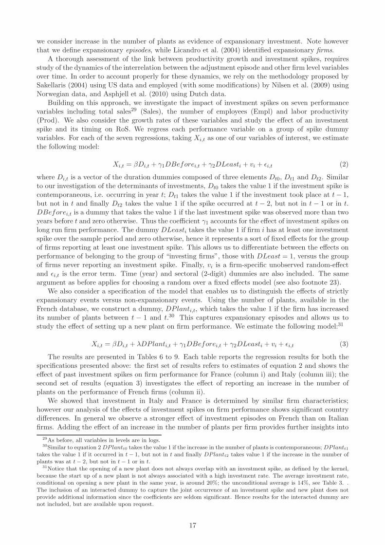
The results are presented in Tables 6 to 9. Each table reports the regression results for both thespecifications presented above: the first set of results refers to estimates of equation 2 and shows theeffect of past investment spikes on firm performance for France (column i) and Italy (column iii); thesecond set of results (equation 3) investigates the effect of reporting an increase in the number ofplants on the performance of French firms (column ii).

We showed that investment in Italy and France is determined by similar firm characteristics;however our analysis of the effects of investment spikes on firm performance shows significant countrydifferences. In general we observe a stronger effect of investment episodes on French than on Italianfirms. Adding the effect of an increase in the number of plants per firm provides further insights into

29As before, all variables in levels are in logs.30Similar to equation 2DPlantt0 takes the value 1 if the increase in the number of plants is contemporaneous; DPlantt1

takes the value 1 if it occurred in t− 1, but not in t and finally DPlantt2 takes value 1 if the increase in the number ofplants was at t− 2, but not in t− 1 or in t.

31Notice that the opening of a new plant does not always overlap with an investment spike, as defined by the kernel,because the start up of a new plant is not always associated with a high investment rate. The average investment rate,conditional on opening a new plant in the same year, is around 20%; the unconditional average is 14%, see Table 3. .The inclusion of an interacted dummy to capture the joint occurrence of an investment spike and new plant does notprovide additional information since the coefficients are seldom significant. Hence results for the interacted dummy arenot included, but are available upon request.

17

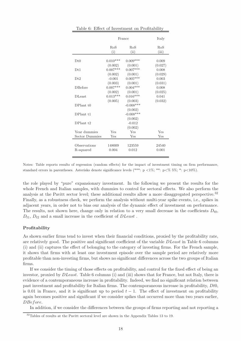
Table 6: Effect of Investment on Profitability

France Italy

RoS RoS RoS(i) (ii) (iii)

Dt0 0.010*** 0.009*** 0.009(0.002) (0.001) (0.027)

Dt1 0.007*** 0.007*** 0.008(0.002) (0.001) (0.029)

Dt2 -0.001 0.005*** 0.003(0.003) (0.001) (0.031)

DBefore 0.007*** 0.004*** 0.008(0.002) (0.001) (0.025)

DLeast 0.013*** 0.016*** 0.041(0.005) (0.003) (0.032)

DPlant t0 -0.008***(0.002)

DPlant t1 -0.008***(0.002)

DPlant t2 -0.012(0.002)

Year dummies Yes Yes YesSector Dummies Yes Yes Yes

Observations 148009 123559 24540R-squared 0.004 0.012 0.001

Notes: Table reports results of regression (random effects) for the impact of investment timing on firm performance,

standard errors in parentheses. Asterisks denote significance levels (***: p <1%; **: p<% 5%; *: p<10%).

the role played by “pure” expansionary investment. In the following we present the results for thewhole French and Italian samples, with dummies to control for sectoral effects. We also perform theanalysis at the Pavitt sector level; these additional results allow a more disaggregated perspective.32

Finally, as a robustness check, we perform the analysis without multi-year spike events, i.e., spikes inadjacent years, in order not to bias our analysis of the dynamic effect of investment on performance.The results, not shown here, change only in relation to a very small decrease in the coefficients Dt0,Dt1, Dt2 and a small increase in the coefficient of DLeast .

Profitability

As shown earlier firms tend to invest when their financial conditions, proxied by the profitability rate,are relatively good. The positive and significant coefficient of the variable DLeast in Table 6 columns(i) and (ii) captures the effect of belonging to the category of investing firms. For the French sample,it shows that firms with at least one investment episode over the sample period are relatively moreprofitable than non-investing firms, but shows no significant differences across the two groups of Italianfirms.

If we consider the timing of those effects on profitability, and control for the fixed effect of being aninvestor, proxied by DLeast. Table 6 columns (i) and (iii) shows that for France, but not Italy, there isevidence of a contemporaneous increase in profitability. Indeed, we find no significant relation betweenpast investment and profitability for Italian firms. The contemporaneous increase in profitability, Dt0,is 0.01 in France, and it is significant up to period t − 1. The effect of investment on profitabilityagain becomes positive and significant if we consider spikes that occurred more than two years earlier,DBefore.

In addition, if we consider the differences between the groups of firms reporting and not reporting a

32Tables of results at the Pavitt sectoral level are shown in the Appendix Tables 13 to 19.

18

Table 7: Effect of Investment on Productivity and its growth rate

France Italy

Prod Prod Gr rate Gr rate Prod Gr rate(i) (ii) (iii) (iv) (v) (vi)

Dt0 0.016*** 0.013*** -0.013*** -0.015*** 0.021*** 0.000(0.003) (0.003) (0.002) (0.003) (0.007) (0.007)

Dt1 0.013*** 0.013*** 0.001 0.003 0.013* 0.008(0.003) (0.003) (0.003) (0.003) (0.007) (0.007)

Dt2 0.011*** 0.009*** 0.001 -0.001 0.003 -0.003(0.003) (0.003) (0.003) (0.003) (0.008) (0.008)

DBefore 0.015*** 0.017*** -0.005** -0.003 0.014** -0.002(0.002) (0.002) (0.002) (0.002) (0.006) (0.006)

DLeast 0.077*** 0.080*** 0.011*** 0.010*** 0.033*** 0.001(0.006) (0.006) (0.002) (0.003) (0.012) (0.006)

DPlant t0 -0.001 -0.009**(0.004) (0.004)

DPlant t1 -0.003 0.004(0.004) (0.004)

DPlant t2 0.003 0.010**(0.004) (0.004)


Observations 147451 123040 147167 122822 24726 24498R-squared 0.132 0.130 0.004 0.004 0.123 0.006



spike (Dt0+DLeast), in the year of the investment the recorded increase in profitability is substantiallylarger. The coefficients DPlantt0, DPlantt1 and DPlantt2 in Table 6 column (ii) allow us to identifythe effect on French firms of setting up a new plant. We find that the effect on profitability of startinga new plant is negative and significant, for the same year and for a one year lag.

This set of results identifies a relevant difference between the firms in France and Italy, whichunderlies much of the difficulties faced by Italian manufacturing since the mid 1990s: large investmentprojects resulted in no appreciable returns to shareholders in the period 1997-2006 (for a complemen-tary analysis refer to Dosi et al., 2012). In contrast, the results for France show a positive effect ofinvestment on return on sales, although the setting up of a new plant produces a negative shock.

Productivity and productivity growth

Results in Table 7 columns (i), (ii) and (v) show that reporting at least one spike during the observationperiod,DLeast, is associated with higher productivity in both France and Italy. There is also a positivecontemporaneous effect on productivity of an investment spike for both countries, Dt0. This positiveeffect persists for at least one year after the year of the spike for both countries, Dt1, and also overlonger lags, DBefore. If we add the effect of being an investor (DLeast), then in the year of the spikean investing firm in France is on average 0.093 log points (10 percent) more productive; the differenceis smaller for Italy - 0.054 log points (5.5 percent). The impact of investment on productivity is fairlystable in the years after a spike in the French case, and shows a slight decrease in the case of Italianfirms.

When accounting for the occurrence of expansionary episodes proxied by the setting up of a newplant, Table 7 column (ii), the lasting positive effect of an investment spike on productivity is con-firmed. However, it is interesting that starting a new plant is not associated with higher productivity,as DPlantt0 is not positive. Overall, the results in Table 7 column (ii) support the conjecture that

19

purely expansionary investment episodes do not spur an increase in productivity.In columns (iii), (iv) and (vi) of Table 7, where the dependent variable is productivity growth, we

can detect no effect of investment spikes for Italian firms, contrary to what emerges for France. Inthis case (column iii), the positive coefficient of the dummy variable DLeast shows that productivitygrowth is higher for the group of investing firms than for their counterparts. The results for Frenchfirms provides more information on the dynamics of productivity growth after an investment episode.The overall contemporaneous effect of spikes on productivity growth (Dt0+DLeast) is slightly negative(−0.02 log points) but becomes positive afterwards: Dt1 + DLeast, Dt2 + DLeast and DBefore +DLeast have respectively values of 0.011, 0.011 and 0.006 log points. This suggests that spikes producea negative shock on productivity growth in the same year but that this negative effect soon disappears.The same dynamics is confirmed when we control for expansionary episodes (column iv). The resultsshow that following a contemporaneous negative shock related to the integration of new capital, alearning process allows the benefits of the investment to be exploited which translates into higherlabor productivity growth.

Among the reasons for the lack of such an effect for Italy is the continuing stagnation of theeconomy during the period analyzed. This pattern is apparent at the aggregate (OECD, 2008) and toa lesser extent at the firm level (Dosi et al., 2012). In addition, the low variability of the dependentvariable, labor productivity, for Italy over the period makes it more difficult to identify factors which,even if marginally, might have contributed to productivity growth in the Italian manufacturing sectorsince the early 1990s.

Sales and sales growth

The positive effect of investment spikes on sales is consistent with the hypothesis of expansion in salesfollowing investment(see Table 8). The positive coefficient of DLeast in Table 8 columns (i) and (v),shows that firms in both countries that invested at least once in the period achieve relatively highersales: the effect on French firms is 0.22 log points (25%) and for Italian firms is relatively higher at0.36 log points (43%). For both countries, the overall contemporaneous effect of a spike on sales levels(Dt0+DLeast) is even larger (0.31 log points for France and 0.39 for Italy). While this increase in thelevel of sales is maintained over time for France, Dt1, Dt2 and DBefore are positive and significant,it decreases for Italy where only the coefficient of Dt1 is significant, although much lower than for thecontemporaneous effect. This evidence is robust and holds if we control for increases in the number ofplants (column ii). Note in this context that the increase in the number of plants which we associatewith “pure” expansionary events, is systematically related to an even larger increase in sales than fora “simple” spike.

If we consider first differences of sales for both countries, Table 8 columns (iii) and (vi), firms thatinvested at least once during the sample period enjoy higher sales growth than their non-investingcounterparts. The effect of investment is strongest in year t (values of Dt0 + DLeast are 0.07 logpoints for France and 0.04 for Italy) and decreases afterwards. Note that although the coefficient ofDBefore is negative in the French case, the overall impact of spikes on sales growth is still positivetwo years after the event (Dleast+Dbefore). For French firms, expansionary episodes contribute tofurther increased sales growth both contemporaneously and at all the lags considered (column iv).

This third set of results shows that investment spikes enable the firm to increase both its produc-tivity and its capacity, proxied by level of sales. Also, we do not observe a lag between the investmentand the impact on revenues; in fact, the biggest effect on firm growth occurs in the same year of theinvestment episode.

Number of employees and growth rates

Results for employment are in line with our findings on sales: we find that investment spikes arepositively related with employment. DLeast, the variable for the group of investing firms, has apositive and significant coefficient for all the specifications in Table 9, and for both France and Italy.Employment is positively affected by an investment spike, and this effect persists for more than twoyears for both countries, with the coefficient of DBefore significant and positive. The second model

20

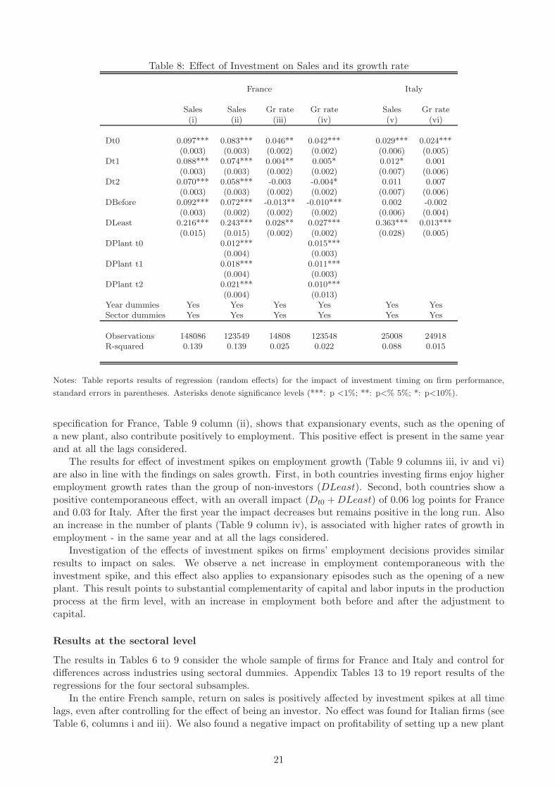
Table 8: Effect of Investment on Sales and its growth rate

France Italy

Sales Sales Gr rate Gr rate Sales Gr rate(i) (ii) (iii) (iv) (v) (vi)

Dt0 0.097*** 0.083*** 0.046** 0.042*** 0.029*** 0.024***(0.003) (0.003) (0.002) (0.002) (0.006) (0.005)

Dt1 0.088*** 0.074*** 0.004** 0.005* 0.012* 0.001(0.003) (0.003) (0.002) (0.002) (0.007) (0.006)

Dt2 0.070*** 0.058*** -0.003 -0.004* 0.011 0.007(0.003) (0.003) (0.002) (0.002) (0.007) (0.006)

DBefore 0.092*** 0.072*** -0.013** -0.010*** 0.002 -0.002(0.003) (0.002) (0.002) (0.002) (0.006) (0.004)

DLeast 0.216*** 0.243*** 0.028** 0.027*** 0.363*** 0.013***(0.015) (0.015) (0.002) (0.002) (0.028) (0.005)

DPlant t0 0.012*** 0.015***(0.004) (0.003)

DPlant t1 0.018*** 0.011***(0.004) (0.003)

DPlant t2 0.021*** 0.010***(0.004) (0.013)





specification for France, Table 9 column (ii), shows that expansionary events, such as the opening ofa new plant, also contribute positively to employment. This positive effect is present in the same yearand at all the lags considered.

The results for effect of investment spikes on employment growth (Table 9 columns iii, iv and vi)are also in line with the findings on sales growth. First, in both countries investing firms enjoy higheremployment growth rates than the group of non-investors (DLeast). Second, both countries show apositive contemporaneous effect, with an overall impact (Dt0 +DLeast) of 0.06 log points for Franceand 0.03 for Italy. After the first year the impact decreases but remains positive in the long run. Alsoan increase in the number of plants (Table 9 column iv), is associated with higher rates of growth inemployment - in the same year and at all the lags considered.

Investigation of the effects of investment spikes on firms’ employment decisions provides similarresults to impact on sales. We observe a net increase in employment contemporaneous with theinvestment spike, and this effect also applies to expansionary episodes such as the opening of a newplant. This result points to substantial complementarity of capital and labor inputs in the productionprocess at the firm level, with an increase in employment both before and after the adjustment tocapital.

Results at the sectoral level

The results in Tables 6 to 9 consider the whole sample of firms for France and Italy and control fordifferences across industries using sectoral dummies. Appendix Tables 13 to 19 report results of theregressions for the four sectoral subsamples.

In the entire French sample, return on sales is positively affected by investment spikes at all timelags, even after controlling for the effect of being an investor. No effect was found for Italian firms (seeTable 6, columns i and iii). We also found a negative impact on profitability of setting up a new plant

21

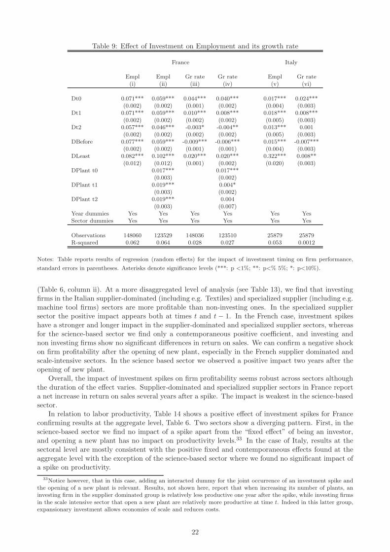
Table 9: Effect of Investment on Employment and its growth rate

France Italy

Empl Empl Gr rate Gr rate Empl Gr rate(i) (ii) (iii) (iv) (v) (vi)

Dt0 0.071*** 0.059*** 0.044*** 0.040*** 0.017*** 0.024***(0.002) (0.002) (0.001) (0.002) (0.004) (0.003)

Dt1 0.071*** 0.059*** 0.010*** 0.008*** 0.018*** 0.008***(0.002) (0.002) (0.002) (0.002) (0.005) (0.003)

Dt2 0.057*** 0.046*** -0.003* -0.004** 0.013*** 0.001(0.002) (0.002) (0.002) (0.002) (0.005) (0.003)

DBefore 0.077*** 0.059*** -0.009*** -0.006*** 0.015*** -0.007***(0.002) (0.002) (0.001) (0.001) (0.004) (0.003)

DLeast 0.082*** 0.102*** 0.020*** 0.020*** 0.322*** 0.008**(0.012) (0.012) (0.001) (0.002) (0.020) (0.003)

DPlant t0 0.017*** 0.017***(0.003) (0.002)

DPlant t1 0.019*** 0.004*(0.003) (0.002)

DPlant t2 0.019*** 0.004(0.003) (0.007)





(Table 6, column ii). At a more disaggregated level of analysis (see Table 13), we find that investingfirms in the Italian supplier-dominated (including e.g. Textiles) and specialized supplier (including e.g.machine tool firms) sectors are more profitable than non-investing ones. In the specialized suppliersector the positive impact appears both at times t and t − 1. In the French case, investment spikeshave a stronger and longer impact in the supplier-dominated and specialized supplier sectors, whereasfor the science-based sector we find only a contemporaneous positive coefficient, and investing andnon investing firms show no significant differences in return on sales. We can confirm a negative shockon firm profitability after the opening of new plant, especially in the French supplier dominated andscale-intensive sectors. In the science based sector we observed a positive impact two years after theopening of new plant.

Overall, the impact of investment spikes on firm profitability seems robust across sectors althoughthe duration of the effect varies. Supplier-dominated and specialized supplier sectors in France reporta net increase in return on sales several years after a spike. The impact is weakest in the science-basedsector.

In relation to labor productivity, Table 14 shows a positive effect of investment spikes for Franceconfirming results at the aggregate level, Table 6. Two sectors show a diverging pattern. First, in thescience-based sector we find no impact of a spike apart from the “fixed effect” of being an investor,and opening a new plant has no impact on productivity levels.33 In the case of Italy, results at thesectoral level are mostly consistent with the positive fixed and contemporaneous effects found at theaggregate level with the exception of the science-based sector where we found no significant impact ofa spike on productivity.

33Notice however, that in this case, adding an interacted dummy for the joint occurrence of an investment spike andthe opening of a new plant is relevant. Results, not shown here, report that when increasing its number of plants, aninvesting firm in the supplier dominated group is relatively less productive one year after the spike, while investing firmsin the scale intensive sector that open a new plant are relatively more productive at time t. Indeed in this latter group,expansionary investment allows economies of scale and reduces costs.

22

One might have expected a stronger impact of investment on productivity for the science-basedsector due to the higher returns on investment, and a weaker impact for the scale-intensive sector whereinvestment might be driven by capacity expansion. Instead, we find that the productivity of science-based firms is hardly affected by investment, while expansionary investment in the scale-intensivesector enhances productivity. One possible interpretation of this result is that gains in productivityfor firms in the science-based sector are related more to intangible assets or a skilled workforce than toinvestment in tangible assets. The reverse is true for the scale-intensive sector, where increasing thenumber of operating plants and investing allows further gains in productivity due to scale economies.

Table 15 validates the findings at aggregate level for the link between investment spikes andproductivity growth. We observe a short-term negative shock in the French supplier-dominated andscale-intensive sectors and a positive effect of belonging to the group of investing firms for the Frenchsupplier-dominated sector. At the aggregate level the impact of setting up a new plant is negative attime t then positive two years later. This pattern is confirmed only for the supplier dominated group,with no impact observed for the other three sectors. In the case of Italy, we found no impact at theaggregate level, and among the separate sectors, we found a positive contemporaneous effect for thescale-intensive sector, and a negative two year lag relation for the specialized supplier group.

Finally, Tables 16 to 19 almost mirror Table 8 and 9 for the link between investment spikes andsales, sales growth, employment, and employment growth. Investment allows for increases in sizemeasured as sales and number of employees, in all sectors, although the benefits persist for a longerperiod for French firms. For most of the cases analyzed above the results at the aggregate level stillhold for the separate Pavitt sectors. However there are some differences. In particular, firms in thescale-intensive sector appear to gain most from setting up a new plant and this result supports theconjecture that for this sector, scale-economies are more relevant than for other sectors.

5 Conclusions

The present paper examined the pattern of firm-level investments in France and Italy. We investigatedthe characteristics that make it more likely that a business company will invest, and the effects onfirm performance following an investment spike. Using data on the acquisition of tangible assets weprovide the first large scale study for France and Italy documenting the lumpy nature of investments,confirming previous findings for other countries (see, among the others Doms and Dunne, 1998; Nilsenet al., 2009).

The paper proposes a methodology for identifying investment spikes that allows the researcher todisentangle repair and maintenance episodes from large adjustments in the stock of tangible assets.We call our proposed investment spike measure the Kernel rule; it allows better correction for sizedependence than other methods, and also retains all the desired properties of a spike measure. Ourproposed measure captures large investments events across companies in the same size classes, andat the same time accounts for a large share of aggregate investment. Analysis of the determinantsof investment spikes emphasizes many similarities between France and Italy. Fast growing, profitableand productive firms are more likely to invest, in both France and Italy. The probability of observingan investment spike is higher if there have been past investment episodes, but this positive effectdecreases over time. Further, we found that export status is not systematically associated with ahigher probability to invest. Most of the differences between France and Italy emerged from ourinvestigation of firm performance following an investment spike. The impact of investment on Italianfirms is more nuanced for most indicators. We found differences in performance between the groupsof investing and non-investing firms - a gap that is always significant in the case of French firms.Profit rates, productivity, sales, and employment levels are higher for the category of firms reportinginvestment spikes. In addition to this sort of “fixed effect” for investing firms, with the exceptionof productivity growth, we also observed a positive net effect in the year of the investment. Theavailability, for France only, of firms’ number of plants allowed us to investigate the pattern of firmperformance after an increase in the number of plants. This event, which captures “expansionary”investment episodes, has a negative effect on profitability, but is associated with higher sales andhigher levels of employment.

23

References

Angelini, P. and Generale, A. (2008). On the evolution of firm size distributions, American EconomicReview 98(1): 426–438.

Asphjell, M., Letterie, W., G.A., P. and Nilsen, O. (2010). Sequentiality versus simultaneity: Interre-lated factor demand, NHH Department of Economics Discussion Paper 29/2010, IZA.

Audretsch, D. B. and Elston, J. A. (2002). Does firm size matter? Evidence on the impact ofliquidity constraints on firm investment behavior in Germany, International Journal of IndustrialOrganization 20(1): 1–17.

Bernard, A. B., Eaton, J., Jensen, J. B. and Kortum, S. S. (2003). Plants and productivity ininternational trade, American Economic Review 93(4): 1268–1290.

Bessen, J. E. (1999). New plants as natural experiments in economic adjustment: Adjustment costs,learning-by-doing and lumpy investment, Working paper, Boston University.

Bigsten, A., Collier, P., Dercon, S., Fafchamps, M., Gauthier, B., Gunning, J., Oostendorp, R.,Pattillo, C., Soderbom, M. and Teal, F. (2005). Adjustment costs and irreversibility as determinantsof investment: Evidence from African manufacturing, Contributions to Economic Analysis andPolicy 4(1): 1–27.

Bokpin, G. and Onumah, J. (2009). An empirical analysis of the determinants of corporate investmentdecisions: Evidence from emerging market firms, International Research Journal of Finance andEconomics 33: 134–141.

Bond, S., Elston, J. A., Mairesse, J. and Mulkay, B. (2003). Financial factors of investment inBelgium, France, Germany, and the United Kingdom: a comparison using company data, Reviewof Economics and Statistics 85(1): 153–165.

Bontempi, E., Boca, A. D., Franzosi, A., Galeotti, M. and Rota, P. (2004). Capital heterogeneity:Does it matter? Fundamental Q and investment on a panel of Italian firms, The RAND Journal ofEconomics 35: 674–690.

Bottazzi, G., Secchi, A. and Tamagni, F. (forthcoming). Financial constraints and firm dynamics,Small Business Economics . DOI: 10.1007/s11187-012-9465-5.

Brier, G. W. (1950). Verification of forecasts expressed in terms of probability, Monthly WeatherReview 78(1): 1–3.

Carlsson, M. and Laseen, S. (2005). Capital adjustment patterns in Swedish manufacturing firms:What model do they suggest?, Economic Journal 115(506): 969–986.

Chatelain, J.-B., Generale, A., Hernando, I., von Kalckreuth, U. and Vermeulen, P. (2003). Newfindings on firm investment and monetary policy transmission in the euro area, Oxford review ofEconomic Policy 19(1): 1–11.

Cooper, R., Haltiwanger, J. and Power, L. (1999). Machine replacement and the business cycle: Lumpsand bumps, American Economic Review 89: 921–46.

De Long, J. B. and Summers, L. H. (1991). Equipment investment and economic growth, The QuarterlyJournal of Economics 106(2): 445–502.

Del Boca, A., Galeotti, M., Himmelberg, C. P. and Rota, P. (2008). Investment and time to plan andbuild: A comparison of structures vs. equipment in a panel of Italian firms, Journal of the EuropeanEconomic Association 6(4): 864–889.

Del Boca, A., Galeotti, M. and Rota, P. (2008). Non-convexities in the adjustment of different capitalinputs: A firm-level investigation, European Economic Review 52(2): 315–337.

24

Doms, M. and Dunne, T. (1998). Capital adjustment patterns in manufacturing plants, Review ofEconomic Dynamics 1: 409–29.

Dosi, G., Gambardella, A., Grazzi, M. and Orsenigo, L. (2008). Technological revolutions and theevolution of industrial structures: Assessing the impact of new technologies upon the size andboundaries of firms, Capitalism and Society 3(1).

Dosi, G., Grazzi, M., Tomasi, C. and Zeli, A. (2012). Turbulence underneath the big calm: whatis happening behind the flat trend of productivity in Italy, Small Business Economics Journal39(4): 1043–1067.

Doyle, J. and Whited, T. (2001). Fixed costs of adjustment, coordination, and industry investment,The Review of Economics and Statistics 83: 628–637.

Duhautois, R. and Jamet, S. (2001). Heterogeneite des comportements d’investissement et fluctuationsde l’investissement aggrege, Economie et Previsions 2001/3: 103–115.

Federer, J. (1993). The impact of uncertainty on aggregate investment spending: An empirical analysis,Journal of Money, Credit and Banking 25(1): 30–48.

Gibrat, R. (1931). Les inegalites economiques, Librairie du Recuil Sirey, Paris.

Gourio, F. and Kashyap, A. K. (2007). Investment spikes: New facts and a general equilibriumexploration, Journal of Monetary Economics 54(Supplement): 1–22.

Grazzi, M., Sanzo, R., Secchi, A. and Zeli, A. (2009). Micro.3 some notes on the development of theintegrated system of data 1989-2004, Documenti n. 11, Istat.

Hall, B. H., Mairesse, J., Branstetter, L. and Crepon, B. (1999). Does cash flow cause investmentand R&D: An exploration using panel data for French, Japanese, and United States scientific firms,Finance 9902005, EconWPA.

Huggett, M. and Ospina, S. (2001). Does productivity growth fall after the adoption of new technol-ogy?, Journal of Monetary Economics 48(1): 173–195.

Jensen, J. B., McGuckin, R. H. and Stiroh, K. J. (2001). The impact of vintage and survival onproductivity: Evidence from cohorts of U.S. manufacturing plants, The Review of Economics andStatistics 83(2): 323–332.

Licandro, O., Maroto, R. and Puch, L. (2004). Innovation, investment and productivity: evidencefrom spanish firms, Research paper in Economics ECO2004/07, European University Institute.

Lopez, R. A. (2009). Do firms increase productivity in order to become exporters?, Oxford Bulletinof Economics and Statistics 71(5): 621–642.

Mairesse, J., Hall, B. H. and Mulkay, B. (1999). Firm-level investment in France and the United States:An exploration of what we have learned in twenty years, Annales d’Economie et de Statistique55/56: 27–67.

Melitz, M. J. (2003). The impact of trade on intra-industry reallocations and aggregate industryproductivity, Econometrica 71(6): 1695–1725.

Nilsen, O. A., Raknerud, A., Rybalka, M. and Skjerpen, T. (2009). Lumpy investments, factoradjustments, and labour productivity, Oxford Economic Papers 61(1): 104–127.

Nilsen, O. A. and Schiantarelli, F. (2003). Zeros and lumps in investment: Empirical evidence onirreversibilities and nonconvexities, The Review of Economics and Statistics 85(4): 1021–1037.

OECD (2008). Compendium of Productivity Indicators, OECD Publishing.

25

Oliveira, B. and Fortunato, A. (2006). Firm growth and liquidity constraints: A dynamic analysis,Small Business Economics 27(2): 139–156.

Parisi, M. L., Schiantarelli, F. and Sembenelli, A. (2006). Productivity, innovation and R&D: Microevidence for Italy, European Economic Review 50(8): 2037–2061.

Pavitt, K. (1984). Sectoral pattern of technical change: Towards a taxonomy and a theory, ResearchPolicy 13: 343–373.

Power, L. (1998). The missing link: Technology, investment, and productivity, The Review of Eco-nomics and Statistics 80(2): 300–313.

Sakellaris, P. (2004). Patterns of plant adjustment, Journal of Monetary Economics 51(2): 425–450.

Schiantarelli, F. (1996). Financial constraints and investment: Methodological issues and internationalevidence, Oxford Review of Economic Policy 12(2): 70–89.

Shima, K. (2010). Lumpy capital adjustment and technical efficiency, Economics Bulletin 30: 2817–2824.

Silverman, B. W. (1986). Density Estimation for Statistics and Data Analysis, London: Chapman &Hall/CRC.

Smolny, W. (2003). Determinants of innovation behaviour and investment estimates for West-Germanmanufacturing firms, Economics of Innovation and New Technology 12(5): 449–465.

Stanley, M., Amaral, L., Buldyrev, S., Havlin, S., Leschhorn, H., Maass, P., Salinger, M. and Stanley,H. (1996). Scaling behaviour in the growth of companies, Nature 379: 804–806.

Sutton, J. (1997). Gibrat’s legacy, Journal of Economic Literature 35(1): 40–59.

Szulanski, G. (1996). Exploring internal stickiness: Impediments to the transfer of best practice withinthe firm, Strategic Management Journal 17: 27–43.

Whited, T. M. (1992). Debt, liquidity constraints, and corporate investment: evidence from paneldata, Journal of Finance 47(4): 1425–1460.

Whited, T. M. (2006). External finance constraints and the intertemporal pattern of intermittentinvestment, Journal of Financial Economics 81(3): 467–502.

A Appendix

26

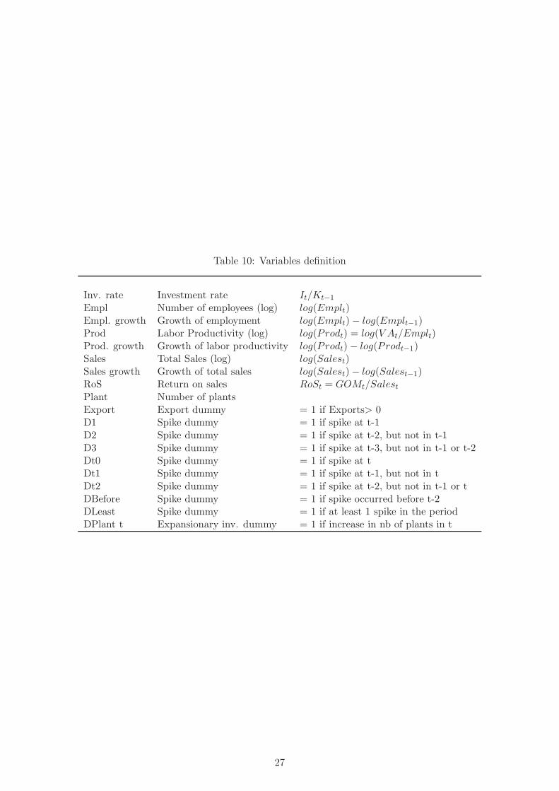
Table 10: Variables definition

Inv. rate Investment rate It/Kt−1

Empl Number of employees (log) log(Emplt)Empl. growth Growth of employment log(Emplt)− log(Emplt−1)Prod Labor Productivity (log) log(Prodt) = log(V At/Emplt)Prod. growth Growth of labor productivity log(Prodt)− log(Prodt−1)Sales Total Sales (log) log(Salest)Sales growth Growth of total sales log(Salest)− log(Salest−1)RoS Return on sales RoSt = GOMt/SalestPlant Number of plantsExport Export dummy = 1 if Exports> 0D1 Spike dummy = 1 if spike at t-1D2 Spike dummy = 1 if spike at t-2, but not in t-1D3 Spike dummy = 1 if spike at t-3, but not in t-1 or t-2Dt0 Spike dummy = 1 if spike at tDt1 Spike dummy = 1 if spike at t-1, but not in tDt2 Spike dummy = 1 if spike at t-2, but not in t-1 or tDBefore Spike dummy = 1 if spike occurred before t-2DLeast Spike dummy = 1 if at least 1 spike in the periodDPlant t Expansionary inv. dummy = 1 if increase in nb of plants in t

27

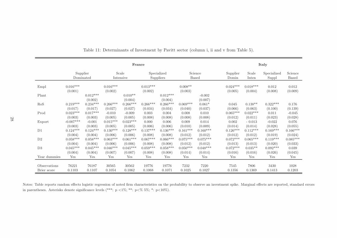
Table 11: Determinants of Investment by Pavitt sector (column i, ii and v from Table 5).

France Italy

Supplier Scale Specialized Science Supplier Scale Specialized ScienceDominated Intensive Suppliers Based Domin Inten Suppl Based

Empl 0.016*** 0.016*** 0.013*** 0.008** 0.024*** 0.018*** 0.012 0.012(0.001) (0.002) (0.002) (0.003) (0.005) (0.004) (0.008) (0.009)

Plant 0.012*** 0.010** 0.012*** -0.002(0.002) (0.004) (0.004) (0.007)

RoS 0.219*** 0.234*** 0.266*** 0.266*** 0.266*** 0.266*** 0.069*** 0.061* 0.045 0.138** 0.322*** 0.176(0.017) (0.017) (0.027) (0.027) (0.034) (0.034) (0.040) (0.037) (0.066) (0.063) (0.100) (0.139)

Prod 0.023*** 0.017*** -0.010 -0.009 0.003 0.004 0.008 0.010 0.065*** 0.022*** 0.011 -0.045(0.003) (0.003) (0.005) (0.005) (0.008) (0.008) (0.008) (0.008) (0.012) (0.011) (0.023) (0.028)

Export -0.007*** -0.001 0.015*** 0.023*** 0.000 0.006 0.009 0.014 0.002 - 0.013 -0.022 0.076(0.003) (0.003) (0.005) (0.005) (0.006) (0.006) (0.010) (0.009) (0.014) (0.014) (0.028) (0.055)

D1 0.124*** 0.124*** 0.130*** 0.128*** 0.137*** 0.136*** 0.161*** 0.160*** 0.126*** 0.112*** 0.169*** 0.166***(0.004) (0.004) (0.006) (0.006) (0.008) (0.008) (0.012) (0.012) (0.012) (0.012) (0.019) (0.024)

D2 0.058*** 0.058*** 0.063*** 0.061*** 0.067*** 0.066*** 0.075*** 0.075*** 0.072*** 0.065*** 0.119*** 0.085***(0.004) (0.004) (0.006) (0.006) (0.008) (0.008) (0.012) (0.012) (0.013) (0.013) (0.020) (0.033)

D3 0.045*** 0.045*** 0.046*** 0.045*** 0.059*** 0.058*** 0.050*** 0.048*** 0.072*** 0.035** 0.092*** 0.039(0.004) (0.004) (0.007) (0.007) (0.008) (0.008) (0.014) (0.014) (0.016) (0.016) (0.026) (0.045)

Year dummies Yes Yes Yes Yes Yes Yes Yes Yes Yes Yes Yes Yes

Observations 76221 76187 30565 30562 19776 19776 7232 7220 7545 7806 3430 1028Brier score 0.1103 0.1107 0.1054 0.1062 0.1068 0.1071 0.1025 0.1027 0.1356 0.1369 0.1413 0.1203

Notes: Table reports random effects logistic regression of noted firm characteristics on the probability to observe an investment spike. Marginal effects are reported, standard errors

in parentheses. Asterisks denote significance levels (***: p <1%; **: p<% 5%; *: p<10%).

28

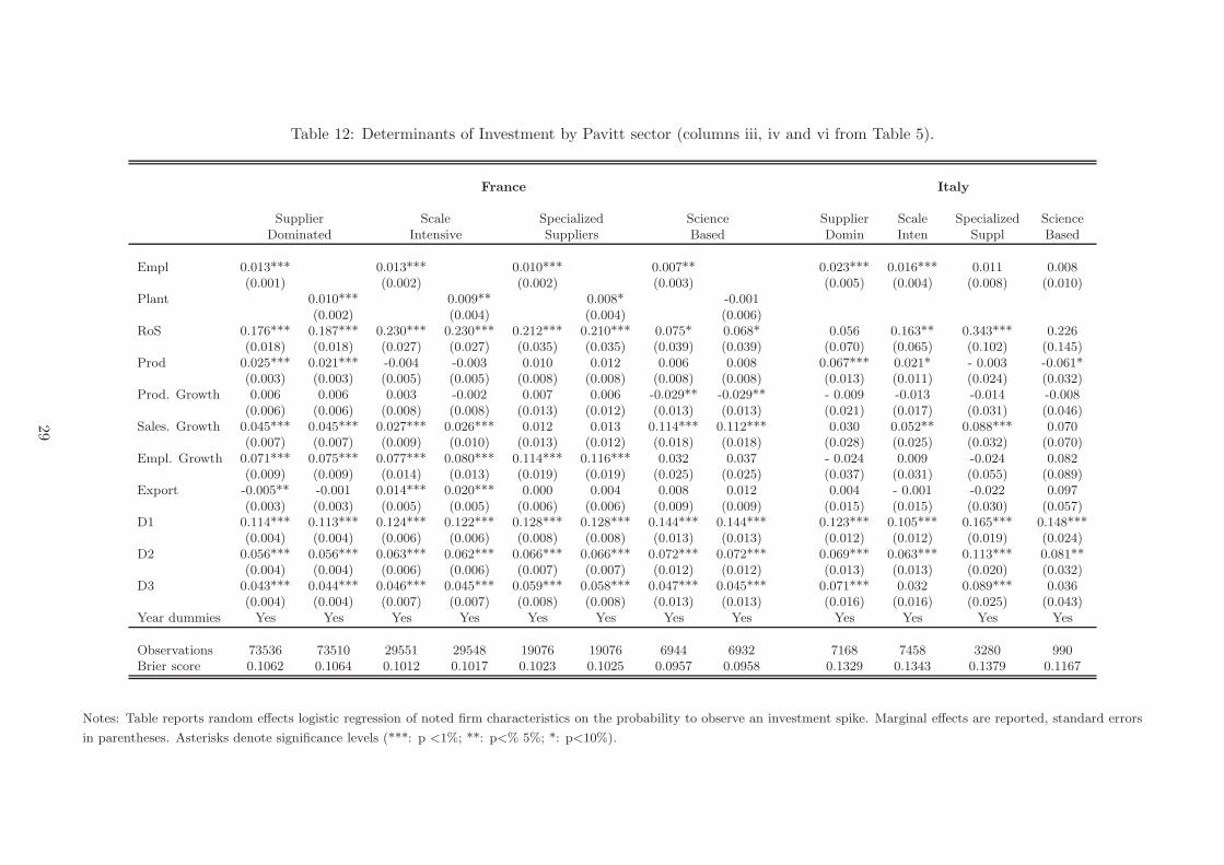
Table 12: Determinants of Investment by Pavitt sector (columns iii, iv and vi from Table 5).

France Italy


Empl 0.013*** 0.013*** 0.010*** 0.007** 0.023*** 0.016*** 0.011 0.008(0.001) (0.002) (0.002) (0.003) (0.005) (0.004) (0.008) (0.010)

Plant 0.010*** 0.009** 0.008* -0.001(0.002) (0.004) (0.004) (0.006)

RoS 0.176*** 0.187*** 0.230*** 0.230*** 0.212*** 0.210*** 0.075* 0.068* 0.056 0.163** 0.343*** 0.226(0.018) (0.018) (0.027) (0.027) (0.035) (0.035) (0.039) (0.039) (0.070) (0.065) (0.102) (0.145)

Prod 0.025*** 0.021*** -0.004 -0.003 0.010 0.012 0.006 0.008 0.067*** 0.021* - 0.003 -0.061*(0.003) (0.003) (0.005) (0.005) (0.008) (0.008) (0.008) (0.008) (0.013) (0.011) (0.024) (0.032)

Prod. Growth 0.006 0.006 0.003 -0.002 0.007 0.006 -0.029** -0.029** - 0.009 -0.013 -0.014 -0.008(0.006) (0.006) (0.008) (0.008) (0.013) (0.012) (0.013) (0.013) (0.021) (0.017) (0.031) (0.046)

Sales. Growth 0.045*** 0.045*** 0.027*** 0.026*** 0.012 0.013 0.114*** 0.112*** 0.030 0.052** 0.088*** 0.070(0.007) (0.007) (0.009) (0.010) (0.013) (0.012) (0.018) (0.018) (0.028) (0.025) (0.032) (0.070)

Empl. Growth 0.071*** 0.075*** 0.077*** 0.080*** 0.114*** 0.116*** 0.032 0.037 - 0.024 0.009 -0.024 0.082(0.009) (0.009) (0.014) (0.013) (0.019) (0.019) (0.025) (0.025) (0.037) (0.031) (0.055) (0.089)

Export -0.005** -0.001 0.014*** 0.020*** 0.000 0.004 0.008 0.012 0.004 - 0.001 -0.022 0.097(0.003) (0.003) (0.005) (0.005) (0.006) (0.006) (0.009) (0.009) (0.015) (0.015) (0.030) (0.057)

D1 0.114*** 0.113*** 0.124*** 0.122*** 0.128*** 0.128*** 0.144*** 0.144*** 0.123*** 0.105*** 0.165*** 0.148***(0.004) (0.004) (0.006) (0.006) (0.008) (0.008) (0.013) (0.013) (0.012) (0.012) (0.019) (0.024)

D2 0.056*** 0.056*** 0.063*** 0.062*** 0.066*** 0.066*** 0.072*** 0.072*** 0.069*** 0.063*** 0.113*** 0.081**(0.004) (0.004) (0.006) (0.006) (0.007) (0.007) (0.012) (0.012) (0.013) (0.013) (0.020) (0.032)

D3 0.043*** 0.044*** 0.046*** 0.045*** 0.059*** 0.058*** 0.047*** 0.045*** 0.071*** 0.032 0.089*** 0.036(0.004) (0.004) (0.007) (0.007) (0.008) (0.008) (0.013) (0.013) (0.016) (0.016) (0.025) (0.043)


Observations 73536 73510 29551 29548 19076 19076 6944 6932 7168 7458 3280 990Brier score 0.1062 0.1064 0.1012 0.1017 0.1023 0.1025 0.0957 0.0958 0.1329 0.1343 0.1379 0.1167

Notes: Table reports random effects logistic regression of noted firm characteristics on the probability to observe an investment spike. Marginal effects are reported, standard errors

in parentheses. Asterisks denote significance levels (***: p <1%; **: p<% 5%; *: p<10%).

29

Table 13: Effect of Investment on Profitability by Pavitt sector (Table 6)

France Italy

RoS Supplier Scale Specialized Science Supplier Scale Specialized ScienceDominated Intensive Suppliers Based Domin Inten Suppl Based

Dt0 0.008*** 0.005*** 0.004** 0.005** 0.013*** 0.014*** 0.092** 0.068*** 0.002 0.015 0.012*** 0.012(0.002) (0.001) (0.002) (0.002) (0.002) (0.002) (0.038) (0.021) (0.002) (0.069) (0.003) (0.008)

Dt1 0.008*** 0.007*** 0.001 0.002 0.009*** 0.012*** 0.023 0.019 0.001 0.008 0.010*** 0.002(0.002) (0.001) (0.002) (0.002) (0.002) (0.003) (0.041) (0.023) (0.002) (0.076) (0.003) (0.008)

Dt2 0.004** 0.004*** 0.002 0.002 0.007*** 0.007*** -0.076* 0.017 -0.002 0.005 -0.000 0.005(0.002) (0.001) (0.002) (0.002) (0.002) (0.003) (0.041) (0.023) (0.002) (0.079) (0.004) (0.008)

DBefore 0.004** 0.005*** 0.003 0.002 0.005** 0.007*** 0.064* -0.007 0.001 0.012 -0.003 0.008(0.002) (0.001) (0.002) (0.002) (0.003) (0.002) (0.033) (0.019) (0.002) (0.064) (0.003) (0.007)

DLeast 0.026*** 0.028*** 0.020*** 0.021*** 0.016*** 0.014*** -0.117 -0.049 0.014*** 0.087 0.012** 0.014(0.002) (0.002) (0.004) (0.004) (0.004) (0.005) (0.074) (0.039) (0.003) (0.083) (0.005) (0.010)

DPlant t0 -0.008*** - 0.002 -0.005* -0.033(0.002) (0.003) (0.003) (0.026)

DPlant t1 -0.005*** -0.010*** -0.007** 0.034(0.002) (0.003) (0.003) (0.028)

DPlant t2 -0.002 -0.007** -0.007** 0.119***(0.002) (0.003) (0.003) (0.028)


Observations 84117 70256 33889 28388 21945 18229 8148 6686 9511 9533 4168 1328R-squared 0.008 0.020 0.012 0.012 0.012 0.013 0.001 0.001 0.031 0.001 0.026 0.021

Notes: Table reports results of regression (random effects) for the impact of investment timing on firm performance, standard errors in parentheses. Asterisks denote significance

levels (***: p <1%; **: p<% 5%; *: p<10%).

30

Table 14: Effect of Investment on Productivity by Pavitt sector (Table 7)

France Italy

Prod Supplier Scale Specialized Science Supplier Scale Specialized ScienceDominated Intensive Suppliers Based Domin Inten Suppl Based

Dt0 0.016*** 0.012*** 0.012** 0.010 0.023** 0.025*** 0.011 0.015 -0.002 0.030** 0.042*** 0.049(0.003) (0.004) (0.006) (0.006) (0.007) (0.007) (0.014) (0.015) (0.010) (0.012) (0.014) (0.036)

Dt1 0.013*** 0.013*** 0.009 0.010 0.016** 0.020*** 0.018 0.001 -0.008 0.020 0.037** 0.021(0.003) (0.004) (0.006) (0.007) (0.007) (0.008) (0.015) (0.016) (0.011) (0.013) (0.015) (0.038)

Dt2 0.010*** 0.007* 0.006 0.005 0.017** 0.015** 0.031 0.020 -0.011 0.009 -0.003 0.057(0.004) (0.004) (0.006) (0.007) (0.007) (0.008) (0.015) (0.016) (0.011) (0.014) (0.016) (0.038)

DBefore 0.015*** 0.015*** 0.028*** 0.026 0.004 0.009 0.011 0.014 -0.002 0.026** 0.000 0.034(0.003) (0.003) (0.005) (0.006) (0.006) (0.006) (0.012) (0.014) (0.010) (0.012) (0.014) (0.033)

DLeast 0.147*** 0.151*** 0.039*** 0.044*** 0.058*** 0.055*** 0.062* 0.061* 0.093*** 0.062*** -0.010 -0.031(0.008) (0.009) (0.015) (0.016) (0.013) (0.014) (0.033) (0.036) (0.020) (0.021) (0.027) (0.057)

DPlant t0 -0.002 0.003 -0.013 -0.017(0.005) (0.009) (0.009) (0.018)

DPlant t1 -0.002 -0.013 -0.012 -0.009(0.006) (0.010) (0.010) (0.019)

DPlant t2 -0.008 -0.008 -0.004 0.015(0.006) (0.010) (0.010) (0.020)


Observations 83788 69992 33716 28239 21871 18174 8076 6635 9458 9667 4296 1305R2 overall 0.025 0.025 0.011 0.012 0.040 0.038 0.037 0.034 0.010 0.010 0.007 0.003


levels (***: p <1%; **: p<% 5%; *: p<10%).

31

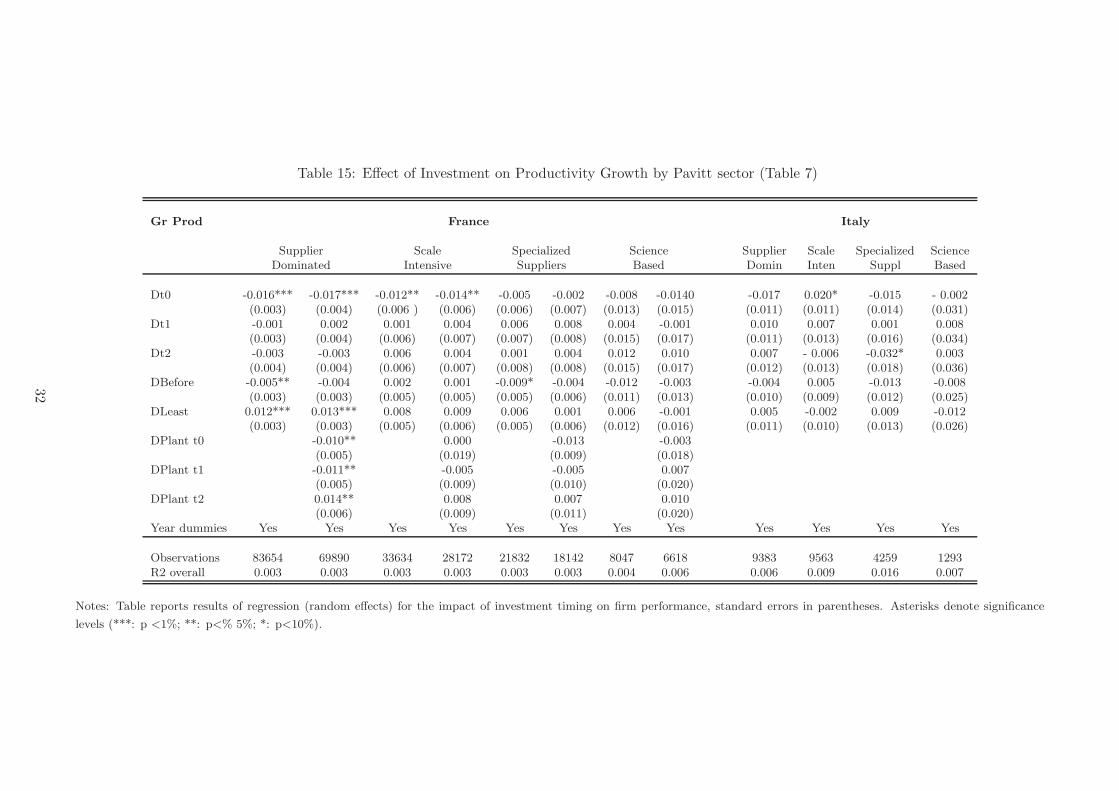
Table 15: Effect of Investment on Productivity Growth by Pavitt sector (Table 7)

Gr Prod France Italy


Dt0 -0.016*** -0.017*** -0.012** -0.014** -0.005 -0.002 -0.008 -0.0140 -0.017 0.020* -0.015 - 0.002(0.003) (0.004) (0.006 ) (0.006) (0.006) (0.007) (0.013) (0.015) (0.011) (0.011) (0.014) (0.031)

Dt1 -0.001 0.002 0.001 0.004 0.006 0.008 0.004 -0.001 0.010 0.007 0.001 0.008(0.003) (0.004) (0.006) (0.007) (0.007) (0.008) (0.015) (0.017) (0.011) (0.013) (0.016) (0.034)

Dt2 -0.003 -0.003 0.006 0.004 0.001 0.004 0.012 0.010 0.007 - 0.006 -0.032* 0.003(0.004) (0.004) (0.006) (0.007) (0.008) (0.008) (0.015) (0.017) (0.012) (0.013) (0.018) (0.036)

DBefore -0.005** -0.004 0.002 0.001 -0.009* -0.004 -0.012 -0.003 -0.004 0.005 -0.013 -0.008(0.003) (0.003) (0.005) (0.005) (0.005) (0.006) (0.011) (0.013) (0.010) (0.009) (0.012) (0.025)

DLeast 0.012*** 0.013*** 0.008 0.009 0.006 0.001 0.006 -0.001 0.005 -0.002 0.009 -0.012(0.003) (0.003) (0.005) (0.006) (0.005) (0.006) (0.012) (0.016) (0.011) (0.010) (0.013) (0.026)

DPlant t0 -0.010** 0.000 -0.013 -0.003(0.005) (0.019) (0.009) (0.018)

DPlant t1 -0.011** -0.005 -0.005 0.007(0.005) (0.009) (0.010) (0.020)

DPlant t2 0.014** 0.008 0.007 0.010(0.006) (0.009) (0.011) (0.020)




levels (***: p <1%; **: p<% 5%; *: p<10%).

32

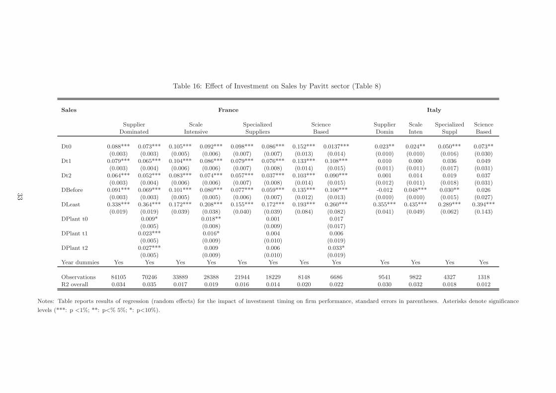
Table 16: Effect of Investment on Sales by Pavitt sector (Table 8)

Sales France Italy


Dt0 0.088*** 0.073*** 0.105*** 0.092*** 0.098*** 0.086*** 0.152*** 0.0137*** 0.023** 0.024** 0.050*** 0.073**(0.003) (0.003) (0.005) (0.006) (0.007) (0.007) (0.013) (0.014) (0.010) (0.010) (0.016) (0.030)

Dt1 0.079*** 0.065*** 0.104*** 0.086*** 0.079*** 0.076*** 0.133*** 0.108*** 0.010 0.000 0.036 0.049(0.003) (0.004) (0.006) (0.006) (0.007) (0.008) (0.014) (0.015) (0.011) (0.011) (0.017) (0.031)

Dt2 0.064*** 0.052*** 0.083*** 0.074*** 0.057*** 0.037*** 0.103*** 0.090*** 0.001 0.014 0.019 0.037(0.003) (0.004) (0.006) (0.006) (0.007) (0.008) (0.014) (0.015) (0.012) (0.011) (0.018) (0.031)

DBefore 0.091*** 0.069*** 0.101*** 0.080*** 0.077*** 0.059*** 0.135*** 0.106*** -0.012 0.048*** 0.030** 0.026(0.003) (0.003) (0.005) (0.005) (0.006) (0.007) (0.012) (0.013) (0.010) (0.010) (0.015) (0.027)

DLeast 0.338*** 0.364*** 0.172*** 0.208*** 0.155*** 0.172*** 0.193*** 0.260*** 0.355*** 0.435*** 0.289*** 0.394***(0.019) (0.019) (0.039) (0.038) (0.040) (0.039) (0.084) (0.082) (0.041) (0.049) (0.062) (0.143)

DPlant t0 0.009* 0.018** 0.001 0.017(0.005) (0.008) (0.009) (0.017)

DPlant t1 0.023*** 0.016* 0.004 0.006(0.005) (0.009) (0.010) (0.019)

DPlant t2 0.027*** 0.009 0.006 0.033*(0.005) (0.009) (0.010) (0.019)




levels (***: p <1%; **: p<% 5%; *: p<10%).

33

Table 17: Effect of Investment on Sales Growth by Pavitt sector (Table 8)

Gr sales France Italy


Dt0 0.041*** 0.037*** 0.047*** 0.048*** 0.051*** 0.050*** 0.088*** 0.068*** 0.023*** 0.025*** 0.021* 0.035(0.003) (0.003) (0.004) (0.005) (0.006) (0.006) (0.010) (0.011) (0.008) (0.008) (0.013) (0.024)

Dt1 0.004 0.003 0.009* 0.013*** 0.006 0.006 -0.003 -0.009 -0.007 0.004 0.004 0.004(0.003) (0.003) (0.004) (0.005) (0.006) (0.007) (0.011) (0.012) (0.009) (0.008) (0.014) (0.026)

Dt2 -0.003 -0.004 0.001 0.000 -0.013* -0.014** -0.008 0.004 0.019** 0.002 -0.012 0.007(0.003) (0.004) (0.004) (0.005) (0.006) (0.007) (0.012) (0.013) (0.010) (0.009) (0.016) (0.027)

DBefore -0.013*** -0.010*** 0.003* -0.011*** -0.009** -0.004 -0.015* -0.012 -0.015** -0.009 -0.002 0.005(0.002) (0.002) (0.002) (0.004) (0.004) (0.005) (0.008) (0.009) (0.007) (0.007) (0.011) (0.020)

DLeast 0.036*** 0.034*** 0.020*** 0.023*** 0.020*** 0.015*** 0.024*** 0.031*** 0.016* 0.016** 0.009 0.000(0.002) (0.003) (0.004) (0.004) (0.005) (0.005) (0.009) (0.011) (0.008) (0.008) (0.012) (0.021)

DPlant t0 0.010** 0.022*** 0.015** 0.019(0.004) (0.007) (0.008) (0.014)

DPlant t1 0.019*** 0.000 0.007 -0.007(0.004) (0.007) (0.009) (0.015)

DPlant t2 0.011** 0.004 0.004 0.020(0.012) (0.007) (0.009) (0.015)




levels (***: p <1%; **: p<% 5%; *: p<10%).

34

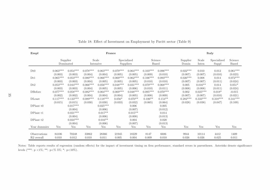
Table 18: Effect of Investment on Employment by Pavitt sector (Table 9)

Empl France Italy


Dt0 0.063*** 0.054*** 0.078*** 0.063*** 0.079*** 0.064*** 0.103*** 0.096*** 0.022*** 0.010 0.012 0.061***(0.003) (0.003) (0.004) (0.004) (0.005) (0.005) (0.009) (0.010) (0.007) (0.007) (0.010) (0.023)

Dt1 0.065*** 0.053*** 0.080*** 0.066*** 0.069*** 0.062*** 0.106*** 0.093*** 0.026*** 0.008 0.014 0.072***(0.003) (0.003) (0.004) (0.005) (0.005) (0.005) (0.010) (0.010) (0.007) (0.007) (0.011) (0.024)

Dt2 0.053*** 0.044*** 0.066*** 0.056*** 0.048*** 0.031*** 0.079*** 0.068*** 0.005 0.016** 0.014 0.051*(0.003) (0.003) (0.004) (0.005) (0.005) (0.006) (0.010) (0.011) (0.008) (0.008) (0.011) (0.024)

DBefore 0.077*** 0.058*** 0.082*** 0.064*** 0.069*** 0.048*** 0.095*** 0.070*** 0.002 0.025*** 0.018* -0.015(0.002) (0.002) (0.004) (0.004) (0.004) (0.005) (0.008) (0.009) (0.007) (0.007) (0.010) (0.021)

DLeast 0.117*** 0.133*** 0.089*** 0.118*** 0.056* 0.070** 0.106** 0.154** 0.282*** 0.333*** 0.318*** 0.341***(0.015) (0.015) (0.030) (0.030) (0.033) (0.032) (0.065) (0.064) (0.028) (0.038) (0.047) (0.109)

DPlant t0 0.017*** 0.025*** 0.006 0.005(0.004) (0.006) (0.007) (0.012)

DPlant t1 0.021*** 0.017** 0.015** 0.014(0.004) (0.006) (0.008) (0.013)

DPlant t2 0.024*** 0.016** 0.004 0.020(0.004) (0.006) (0.007) (0.013)




levels (***: p <1%; **: p<% 5%; *: p<10%).

35

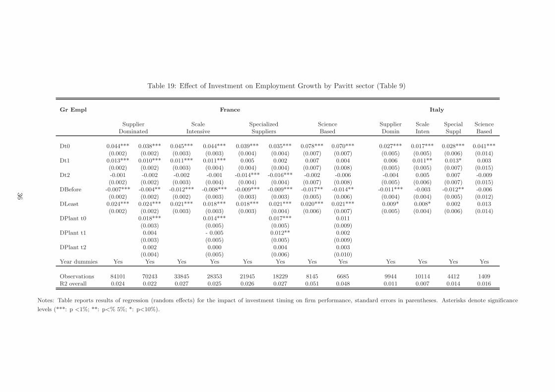
Table 19: Effect of Investment on Employment Growth by Pavitt sector (Table 9)

Gr Empl France Italy

Supplier Scale Specialized Science Supplier Scale Special ScienceDominated Intensive Suppliers Based Domin Inten Suppl Based

Dt0 0.044*** 0.038*** 0.045*** 0.044*** 0.039*** 0.035*** 0.078*** 0.070*** 0.027*** 0.017*** 0.028*** 0.041***(0.002) (0.002) (0.003) (0.003) (0.004) (0.004) (0.007) (0.007) (0.005) (0.005) (0.006) (0.014)

Dt1 0.013*** 0.010*** 0.011*** 0.011*** 0.005 0.002 0.007 0.004 0.006 0.011** 0.013* 0.003(0.002) (0.002) (0.003) (0.004) (0.004) (0.004) (0.007) (0.008) (0.005) (0.005) (0.007) (0.015)

Dt2 -0.001 -0.002 -0.002 -0.001 -0.014*** -0.016*** -0.002 -0.006 -0.004 0.005 0.007 -0.009(0.002) (0.002) (0.003) (0.004) (0.004) (0.004) (0.007) (0.008) (0.005) (0.006) (0.007) (0.015)

DBefore -0.007*** -0.004** -0.012*** -0.008*** -0.009*** -0.009*** -0.017** -0.014** -0.011*** -0.003 -0.012** -0.006(0.002) (0.002) (0.002) (0.003) (0.003) (0.003) (0.005) (0.006) (0.004) (0.004) (0.005) (0.012)

DLeast 0.024*** 0.024*** 0.021*** 0.018*** 0.018*** 0.021*** 0.020*** 0.021*** 0.009* 0.008* 0.002 0.013(0.002) (0.002) (0.003) (0.003) (0.003) (0.004) (0.006) (0.007) (0.005) (0.004) (0.006) (0.014)

DPlant t0 0.018*** 0.014*** 0.017*** 0.011(0.003) (0.005) (0.005) (0.009)

DPlant t1 0.004 - 0.005 0.012** 0.002(0.003) (0.005) (0.005) (0.009)

DPlant t2 0.002 0.000 0.004 0.003(0.004) (0.005) (0.006) (0.010)




levels (***: p <1%; **: p<% 5%; *: p<10%).

36

DOCUMENTS DE TRAVAIL GREDEG PARUS EN 2013GREDEG Working Papers Released in 2013

2013-01 Raphaël Chiappini Persistence vs. Mobility in Industrial and Technological Specialisations: Evidence from 11 Euro Area Countries2013-02 Kevin D. Hoover Was Harrod Right?2013-03 Kevin D. Hoover Man and Machine in Macroeconomics2013-04 Isabelle Corbett-Etchevers & Aura Parmentier-Cajaiba Toying with Regulation: ‘Strategizing Tools’ as Organizational Bricolage2013-05 Aura Parmentier-Cajaiba Research Diary Mapping: Enhancing Reflectivity in Process Research2013-06 Richard Arena Sraffa’s and Wittgenstein’s Crossed Influences: Forms of Life and Snapshots 2013-07 Christophe Charlier & Sarah Guillou Distortion Effects of Export Quota Policy: An Analysis of the China - Raw Materials Dispute2013-08 Cristiano Antonelli & Alessandra Colombelli Knowledge Cumulability and Complementarity in the Knowledge Generation Function2013-09 Marco Grazzi, Nadia Jacoby & Tania Treibich Dynamics of Investment and Firm Performance: Comparative Evidence from Manufacturing Industries