Validation of Vector Data using Oblique Images Pragyana Mishra Microsoft Corporation One Microsoft Way

Redmond, WA 98052 +1 425 421 8518

pragyanm@microsoft.com

Eyal Ofek Microsoft Corporation One Microsoft Way

Redmond, WA 98052 +1 425 706 8866

eyalofek@microsoft.com

Gur Kimchi Microsoft Corporation One Microsoft Way

Redmond, WA 98052 +1 425 722 2050

gkimchi@microsoft.com

ABSTRACT

Oblique images are aerial photographs taken at oblique angles to

the earth’s surface. Projections of vector and other geospatial data

in these images depend on camera parameters, positions of the

entities, surface terrain, and visibility. This paper presents a robust

and scalable algorithm to detect inconsistencies in vector data

using oblique images. The algorithm uses image descriptors to

encode the local appearance of a geospatial entity in images.

These image descriptors combine color, pixel-intensity gradients,

texture, and steerable filter responses. A Support Vector Machine

classifier is trained to detect image descriptors that are not

consistent with underlying vector data, digital elevation maps,

building models, and camera parameters. In this paper, we train

the classifier on visible road segments and non-road data.

Thereafter, the trained classifier detects inconsistencies in vectors,

which include both occluded and misaligned road segments. The

consistent road segments validate our vector, DEM, and 3-D

model data for those areas while inconsistent segments point out

errors. We further show that a search for descriptors that are

consistent with visible road segments in the neighborhood of a

misaligned road yields the desired road alignment that is

consistent with pixels in the image.

Categories and Subject Descriptors

I.4.8 [Image Processing and Computer Vision]: Scene Analysis

– Surface fitting.

General Terms

Algorithms

Keywords

Computer vision, Machine learning, Mapping, Vector data, Pixel

statistics, Oblique image analysis, Multi-cue integration,

Conflation.

1. INTRODUCTION Generating a map may involve several sources of information—a

few of which include vector data, map projection parameters,

digital elevation maps (DEM’s), and 3-dimensional (3-D) models.

Errors or inaccuracies in these data sources contribute to the

overall accuracy and quality of the map. Detecting these errors is

difficult as there is little or none ground truth available against

which the data can be compared to.

Most aerial and satellite images that may be used as ground truth

for data validation are nadir views of the world. However, the set

of attributes of data that can be validated using aerial images is

limited. This is due to the fact that the projection is orthographic

in nature and 3-D—both terrain and building structure-

dependent—attributes of the scene are not entirely captured in

nadir orthographic views.

Inaccuracies in altitude, heights of buildings, and vertical

positions of structures cannot be easily detected by means of nadir

imagery. These inaccuracies can be detected in an image where

the camera views the scene at an oblique angle. Oblique-viewing

angles enable registration of altitude-dependent features.

Additionally, oblique viewing angles bring out the view-

dependency of 3-dimensional geospatial data; occluding and

occluded parts of the world are viewed in the image depending on

the position and orientation at which the image was taken. Image

pixel regions that correspond to occluding and occluded objects

can be used to derive consistency of the geospatial entities as they

appear in the image. The consistency can be further used to rectify

any inaccuracies in data used for segmenting and labeling of the

objects.

Oblique images are aerial photographs of a scene taken at oblique

angles to the earth’s surface. These images have a wide field of

view and therefore, cover a large expanse of the scene as can be

seen in Figures 4 through 7. Oblique images capture the terrain of

earth’s surface and structures such as buildings and highways. For

example, straight roads that are on the slope of a hill will appear

curved. The mapping between a 3-D point of the world and its

corresponding point on the image is a non-linear function that

depends on the elevation, latitude, and longitude of the 3-D point

in space. Additionally, visibility of the 3-D point depends on the

camera’s position and orientation, and the structure of the world

in the neighborhood of that 3-D point; the point may not be visible

in the image if it is occluded by a physical structure in the line-of-

sight of the camera. These properties can, therefore, be used to

detect and rectify any errors of the 3-D point’s position as well as

any inconsistencies of structures in the neighborhood of the point.

Pixels of oblique images can be analyzed to detect, validate, and

correct disparate sources of data, such as vectors, projection

parameters of camera, digital elevation maps (DEM’s), and 3-D

models. This is a novel use of oblique imagery wherein errors due

Permission to make digital or hard copies of all or part of this work for personal or classroom use is granted without fee provided that copies are

not made or distributed for profit or commercial advantage and that

copies bear this notice and the full citation on the first page. To copy otherwise, or republish, to post on servers or to redistribute to lists,

requires prior specific permission and/or a fee.

ACM GIS '08 , November 5-7, 2008. Irvine, CA, USA. © 2008 ACM ISBN 978-1-60558-323-5/08/11...$5.00

to inaccurate and imprecise vectors, DEM, map projection

parameters, and 3-D model data are detected and rectified using

pixel statistics of oblique images. We present a statistical-learning

algorithm to learn image-based descriptors that encode visible

data consistencies, and then apply the learnt descriptors to classify

errors and inconsistencies in geospatial data. The algorithm

combines different descriptors such as color, texture, image-

gradients, and filter responses to robustly detect, validate, and

correct inconsistencies.

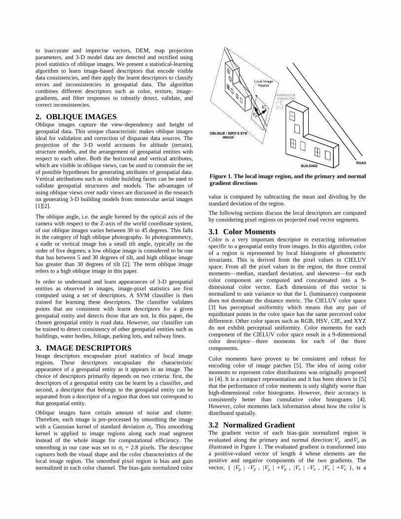
2. OBLIQUE IMAGES Oblique images capture the view-dependency and height of

geospatial data. This unique characteristic makes oblique images

ideal for validation and correction of disparate data sources. The

projection of the 3-D world accounts for altitude (terrain),

structure models, and the arrangement of geospatial entities with

respect to each other. Both the horizontal and vertical attributes,

which are visible in oblique views, can be used to constrain the set

of possible hypotheses for generating attributes of geospatial data.

Vertical attributions such as visible building facets can be used to

validate geospatial structures and models. The advantages of

using oblique views over nadir views are discussed in the research

on generating 3-D building models from monocular aerial images

[1][2].

The oblique angle, i.e. the angle formed by the optical axis of the

camera with respect to the Z-axis of the world coordinate system,

of our oblique images varies between 30 to 45 degrees. This falls

in the category of high oblique photography. In photogrammetry,

a nadir or vertical image has a small tilt angle, typically on the

order of five degrees; a low oblique image is considered to be one

that has between 5 and 30 degrees of tilt, and high oblique image

has greater than 30 degrees of tilt [2]. The term oblique image

refers to a high oblique image in this paper.

In order to understand and learn appearances of 3-D geospatial

entities as observed in images, image-pixel statistics are first

computed using a set of descriptors. A SVM classifier is then

trained for learning these descriptors. The classifier validates

points that are consistent with learnt descriptors for a given

geospatial entity and detects those that are not. In this paper, the

chosen geospatial entity is road data. However, our classifier can

be trained to detect consistency of other geospatial entities such as

buildings, water bodies, foliage, parking lots, and railway lines.

3. IMAGE DESCRIPTORS Image descriptors encapsulate pixel statistics of local image

regions. These descriptors encapsulate the characteristic

appearance of a geospatial entity as it appears in an image. The

choice of descriptors primarily depends on two criteria: first, the

descriptors of a geospatial entity can be learnt by a classifier, and

second, a descriptor that belongs to the geospatial entity can be

separated from a descriptor of a region that does not correspond to

that geospatial entity.

Oblique images have certain amount of noise and clutter.

Therefore, each image is pre-processed by smoothing the image

with a Gaussian kernel of standard deviation s. This smoothing

kernel is applied to image regions along each road segment

instead of the whole image for computational efficiency. The

smoothing in our case was set to s = 2.8 pixels. The descriptor

captures both the visual shape and the color characteristics of the

local image region. The smoothed pixel region is bias and gain

normalized in each color channel. The bias-gain normalized color

value is computed by subtracting the mean and dividing by the

standard deviation of the region.

The following sections discuss the local descriptors are computed

by considering pixel regions on projected road vector segments.

3.1 Color Moments Color is a very important descriptor in extracting information

specific to a geospatial entity from images. In this algorithm, color

of a region is represented by local histograms of photometric

invariants. This is derived from the pixel values in CIELUV

space. From all the pixel values in the region, the three central

moments—median, standard deviation, and skewness—for each

color component are computed and concatenated into a 9-

dimesional color vector. Each dimension of this vector is

normalized to unit variance so that the L (luminance) component

does not dominate the distance metric. The CIELUV color space

[3] has perceptual uniformity which means that any pair of

equidistant points in the color space has the same perceived color

difference. Other color spaces such as RGB, HSV, CIE, and XYZ

do not exhibit perceptual uniformity. Color moments for each

component of the CIELUV color space result in a 9-dimensional

color descriptor—three moments for each of the three

components.

Color moments have proven to be consistent and robust for

encoding color of image patches [5]. The idea of using color

moments to represent color distributions was originally proposed

in [4]. It is a compact representation and it has been shown in [5]

that the performance of color moments is only slightly worse than

high-dimensional color histograms. However, their accuracy is

consistently better than cumulative color histograms [4].

However, color moments lack information about how the color is

distributed spatially.

3.2 Normalized Gradient The gradient vector of each bias-gain normalized region is

evaluated along the primary and normal direction:p andn as

illustrated in Figure 1. The evaluated gradient is transformed into

a positive-valued vector of length 4 whose elements are the

positive and negative components of the two gradients. The

vector, { |p | -p , |p | +p , |n | -n , |n | +n }, is a

Figure 1. The local image region, and the primary and normal

gradient directions

quantization of orientation in the four directions. Normalized

gradients and multi-orientation filter banks such as steerable

filters when combined with the color descriptor encode the

appearance of the geospatial entity in a local neighborhood as and

not at a point or a few points.

3.3 Steerable Filter Response Steerable filters are applied at each sampled position along a

vector-road segment along the primary and normal direction. The

magnitude response from quadrature pairs [6] using these two

orientations on the image plane yields two values. A vector of

length 8 can be further computed from the rectified quadrature

pair responses directly. The steerable filters are based on second-

derivative.

We normalize all the descriptors to unit length after projection

onto the descriptor subspace. The pixel regions used in computing

the descriptors were patches of 24 x 24 pixels sampled at every 12

pixel distance along the projected road segments.

3.4 Eigenvalues of Hessian The Hessian matrix comprises the second partial derivatives of

pixel intensities in the region. The Hessian is a real-valued and

symmetric 2x2 matrix. The two eigenvalues are used for the

classification vector. Two small eigenvalues mean approximately

uniform intensity profile within the region. Two large eigenvalues

may represent corners, salt-and-pepper textures, or any other non-

directional texture. A large and a small eigenvalue, on the other

hand, correspond to a unidirectional texture pattern.

3.5 Difference of Gaussians The smoothed patch is convolved with another two Gaussians—

the first s1 = 1.6s and the second s2 = 1.6s1. The pre-smoothed

region, s, is used as the first Difference of Gaussians (DoG)

center and the wider Gaussian of resolution s1 = 1.6s is used as

the second DoG center. The difference between the Gaussians

pairs (difference between s1 and s difference between s2 and

s1 ) produces two linear DoG filter responses. The positive and

negative rectified components of these two responses yield a 4-

dimensional descriptor.

4. DISCRIPTOR CLASSIFIER While validating vector data, road vectors are classified into two

classes—first, visible and consistent and second, inconsistent.

This classification uses training data with binary labels. We have

used a Support Vector Machine (SVM) with a non-linear kernel

for this binary classification. In their simplest form, SVM’s are

hyperplanes that separate the training data by a maximal margin

[7]. The training descriptors that lie on closest to the hyperplane

are called support vectors.

Consider a set of N linearly-separable training samples of

descriptors di (i =1… N), which are associated with the

classification label ci (i =1… N). The descriptors in our case are

composed of the vector of color moments, normalized gradients,

steerable filter responses, eigenvalues of Hessian, and difference

of Gaussians. The binary classification label, ci {-1, +1}, is +1

for sampled road vectors that are consistent with underlying

image regions and -1 for points where road segments are

inconsistent with corresponding image regions. This

inconsistency, as we have pointed out earlier, could be due to

inaccurate vector, DEM, building model data, or camera

projection parameters.

The set of hyperplanes separating the two classes of descriptors is

of the general form w, d + b = 0. w, d is the dot product

between a weight vector w and d, and b R is the bias term. Re-

scaling w and b such that the point closest to the hyperplane

satisfy w, d + b= 1, we have a canonical form (w, b) of the

hyperplane that satisfies ci ( w, di + b ) 1 for i =1… N. For

this form the distance of the closest descriptor to the hyperplane is

1/||w||. For the optimal hyperplane this distance has to be

maximized, that is:

minimize (𝒘) = 1

2 ||𝒘||2

subject to 𝑐𝑖 𝒘, 𝒅𝒊 + 𝑏 1 for all 𝑖 = 1 … 𝑁

The objective function (w) is minimized by using Lagrange

multipliers i 0 for all i =1… N and a Lagrangian of the form

𝐿 𝒘, 𝑏, = 1

2||𝒘||2 − 𝑁

𝑖=1 𝑖 ( 𝑐𝑖 𝒘, 𝒅𝒊 + 𝑏 –1) )

The Lagrangian L is minimized with respect to the primal

variables w and b, and maximized with respect to the dual

variables i. The derivatives of L with respect to the primal

variables must vanish and therefore, 𝑁𝑖=1

𝑖𝑐𝑖 = 0 and 𝒘 =

𝑁𝑖=1

𝑖 𝑐𝑖 𝒅𝒊. The solution vector is a subset of the training

patterns, namely those descriptor vectors with non-zero i, called

Support Vectors. All the remaining training samples (di ,ci) are

irrelevant: their constraint ci ( w, di + b ) 1 need not be

considered, and they do not appear in calculating 𝒘 = 𝑁

𝑖=1 𝑖 𝑐𝑖 𝒅𝒊. The desired hyperplane is completely determined

by the descriptor vectors closest to it, and not dependent on the

other training instances. Eliminating the primal variables w and b

from the Lagrangian, we have the new optimization problem:

minimize 𝑊 = 𝑖

𝑁

𝑖=1 −

1

2 𝑖 𝑗

𝑁

𝑖 ,𝑗=1𝑐𝑖 𝑐𝑗 𝒅, 𝒅𝒊

subject to i 0 for all 𝑖 = 1 … 𝑁 and 𝑖

𝑁

𝑖=1𝑐𝑖 = 0

Once all i for i =1… N are determined, the bias term b is

calculated. We construct a set S of support vectors of size s from

descriptor vectors di with 0 < i <1. This set of support vectors has

equal number of descriptor vectors for ci = -1 and for ci = +1. The

bias term is

𝑏 = −1

𝑠

𝒅∈𝑆 𝑗

𝑁

𝑗 =1𝑐𝑗 𝒅, 𝒅𝒋

The classifier can thus be expressed

as 𝑓 𝒅 = sgn( 𝑁𝑖=1

𝑖 𝑐𝑖 𝒅, 𝒅𝒊 + 𝑏 ) for a descriptor vector

d. In our case, the descriptors are not linearly separable; therefore,

they are mapped into a high-dimensional feature space using a

mapping function or kernel. The hyperplane is computed in the

high-dimensional feature space. The kernel k is evaluated on the

descriptors d and di as 𝑘 𝒅, 𝒅𝒊 = 𝒅, 𝒅𝒊 .

Several kernel were tested—linear, sigmoid, homogenous

polynomial, Gaussian Radial Basis, and exponential kernels.

Based on the performance of different kernels, we selected a

Gaussian Radial Basis kernel for validation:

𝑘 𝒅, 𝒅𝒊 =1

𝑚 𝑒

−(𝑑𝑘−𝑑𝑖𝑘 ) 2

22

𝑚

𝑘=1

5. CLASSIFIER PERFORMANCE The training and testing sets are generated from visually verifying

road vectors projected onto oblique images for areas that had

accurate camera projection parameters, road vectors, DEM, and

3-D building models. The positive class consisted of 1876 regions

that are sampled on 192 road segments. These road segments were

visible and well aligned with underlying image regions. A

majority of these positive samples were from areas that did not

have high-rise buildings and foliage; therefore, the corresponding

oblique images had few occlusions and shadows. The negative

class had 2954 negative regions that were sampled from image

areas corresponding to building facades, foliage, and offset road

vectors. 250 samples from each class were randomly selected for

testing the classifier’s accuracy. The rest of the samples were used

for training. Selection, training, and testing steps are repeated over

80 such random splits of the data for the estimation of

classification rates.

In our validation problem, the true positive rate, i.e. the rate of

positive samples that are correctly classified, and the false positive

rate, i.e. the rate of negative samples that are incorrectly classified

as positive ones, can be used as measures of the validation

classifier’s accuracy. We wish to achieve a high true positive

rate while keeping the false positive rate low. The curve of the

true positive rate versus the false positive rate is known as the

receiver operating characteristic (ROC) curve. ROC curves for

different kernels are shown in Figure 2.

The area under a ROC curve is of significance; closer to 1 means

better classifier performance. We found that the Gaussian Radial

Basis kernel has a better performance in classifying visibility of

roads than other kernels such as linear, sigmoid, homogenous

polynomial, and exponential radial basis kernel as can be

observed in Figure 2. The parameter for the Gaussian kernel

was set to 0.8.

Performance of the SVM classifier with the Gaussian RBF kernel

was numerically assessed by the following measures:

sensitivity = TP / ( TP + FN )

specificity = TN / ( FP + TN )

accuracy = ( TP + TN ) / ( TP + FP + TN + FN )

where TP, TN, FP, and FN respectively denote the number of

descriptors classified as true positive, true negative, false positive,

and false negative. Higher sensitivity values indicate better

validation rates, whereas higher specificity values indicate better

detection of erroneous or inconsistent data. The sensitivity,

specificity, and accuracy of our classifier are 89%, 71%, and 80%

respectively.

Since pixel statistics are calculated locally, all image pixels need

not be checked for validation or correction. Only pixel statistics

along given vector data need to be examined for data validation.

This makes our algorithm scalable, computationally efficient, and

applicable to validating geospatial data using a variety of imagery.

Analyzing vector data projected into an oblique image of 4000 x

3000 pixels taken in an urban region takes less than 400

milliseconds on a 3.4GHz. Intel Pentium 4, 2GB RAM machine.

One salient quality of SVM’s is that the classifying hyperplane

relies on only a small set of training examples or support vectors.

However, finding these support vectors often requires an

intelligent sampling of the training data for learning within large

datasets in a reasonable amount of time. In non-linear SVM’s,

time require for training the classifier increases cubically with the

number of training examples. Finding support vectors and

discarding descriptors that are unlikely to become support vectors

is important for speeding up the training time of our SVM

classifier and scaling it for large training datasets. This is a part of

our ongoing effort towards improving this classifier’s

performance during training.

6. RESULTS AND DISCUSSION We have labeled a large repository of oblique images by

combining camera projection parameters, digital elevation maps,

3-D building models, vector data, and landmark data. The

labeling scheme, as seen in Figure 4, accounts for occlusions,

non-planarity of surface terrain, and foreshortening. Road labels

are placed on visible road areas while building and landmark

labels are placed on corresponding building areas in images.

Segments of roads that are occluded by buildings are marked by

dashed lines. However, there are a few areas where solid roads

markings appear on occluding buildings. Figure 4 shows a few

such cases outlined in red. These errors are due to missing or

outdated building models. Road segments in few other areas are

not aligned with their corresponding pixel regions in the image.

These are due to inaccurate road vectors and road elevation.

Errors or inaccuracies in vectors, DEM, building models, or

camera projection parameters can contribute to misalignment of

labeling in images.

6.1 Data Validation Figure 5 shows the output of the SVM classifier; all visible road

segments in the image were tested for data consistency. The

segments in blue have descriptors that are consistent with well-

aligned and visible road pixel statistics. Vector, model, DEM, and

map projection data are validated for all the blue road segments.

The road segments marked in red are either occluded or

misaligned with the underlying road pixel regions. The two areas

Figure 2. ROC curves for different SVM classifier kernels

that have missing or obsolete building models as highlighted in

Figure 4 have been successfully indentified by the classifier’s

output. The road segment that is misaligned with its

corresponding image region due to inaccurate vector data and

altitude has been classified in red as well.

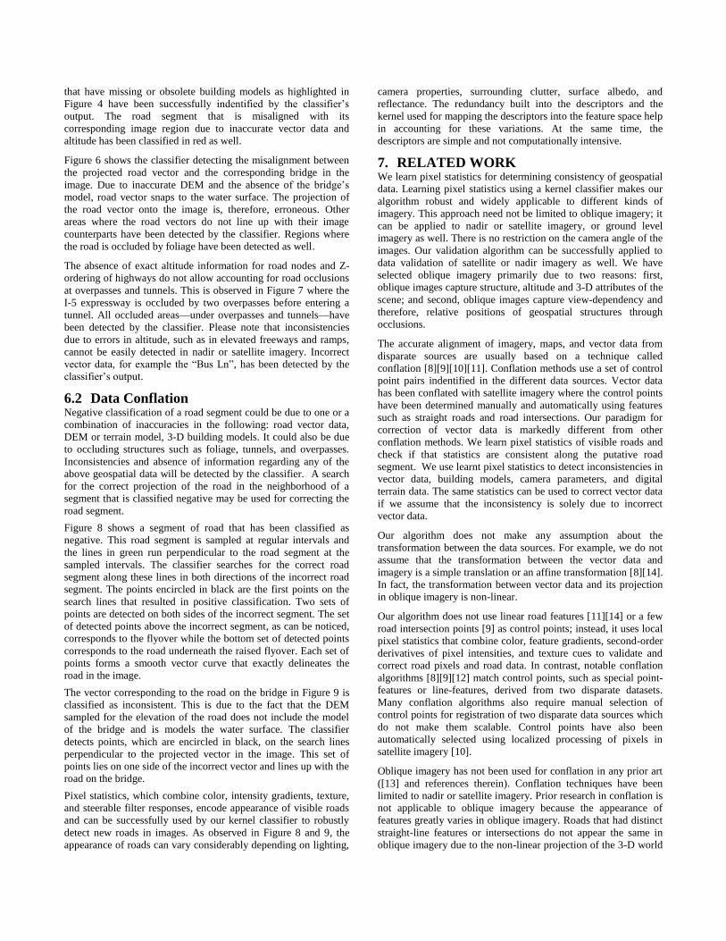
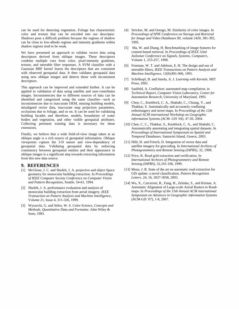
Figure 6 shows the classifier detecting the misalignment between

the projected road vector and the corresponding bridge in the

image. Due to inaccurate DEM and the absence of the bridge’s

model, road vector snaps to the water surface. The projection of

the road vector onto the image is, therefore, erroneous. Other

areas where the road vectors do not line up with their image

counterparts have been detected by the classifier. Regions where

the road is occluded by foliage have been detected as well.

The absence of exact altitude information for road nodes and Z-

ordering of highways do not allow accounting for road occlusions

at overpasses and tunnels. This is observed in Figure 7 where the

I-5 expressway is occluded by two overpasses before entering a

tunnel. All occluded areas—under overpasses and tunnels—have

been detected by the classifier. Please note that inconsistencies

due to errors in altitude, such as in elevated freeways and ramps,

cannot be easily detected in nadir or satellite imagery. Incorrect

vector data, for example the ―Bus Ln‖, has been detected by the

classifier’s output.

6.2 Data Conflation Negative classification of a road segment could be due to one or a

combination of inaccuracies in the following: road vector data,

DEM or terrain model, 3-D building models. It could also be due

to occluding structures such as foliage, tunnels, and overpasses.

Inconsistencies and absence of information regarding any of the

above geospatial data will be detected by the classifier. A search

for the correct projection of the road in the neighborhood of a

segment that is classified negative may be used for correcting the

road segment.

Figure 8 shows a segment of road that has been classified as

negative. This road segment is sampled at regular intervals and

the lines in green run perpendicular to the road segment at the

sampled intervals. The classifier searches for the correct road

segment along these lines in both directions of the incorrect road

segment. The points encircled in black are the first points on the

search lines that resulted in positive classification. Two sets of

points are detected on both sides of the incorrect segment. The set

of detected points above the incorrect segment, as can be noticed,

corresponds to the flyover while the bottom set of detected points

corresponds to the road underneath the raised flyover. Each set of

points forms a smooth vector curve that exactly delineates the

road in the image.

The vector corresponding to the road on the bridge in Figure 9 is

classified as inconsistent. This is due to the fact that the DEM

sampled for the elevation of the road does not include the model

of the bridge and is models the water surface. The classifier

detects points, which are encircled in black, on the search lines

perpendicular to the projected vector in the image. This set of

points lies on one side of the incorrect vector and lines up with the

road on the bridge.

Pixel statistics, which combine color, intensity gradients, texture,

and steerable filter responses, encode appearance of visible roads

and can be successfully used by our kernel classifier to robustly

detect new roads in images. As observed in Figure 8 and 9, the

appearance of roads can vary considerably depending on lighting,

camera properties, surrounding clutter, surface albedo, and

reflectance. The redundancy built into the descriptors and the

kernel used for mapping the descriptors into the feature space help

in accounting for these variations. At the same time, the

descriptors are simple and not computationally intensive.

7. RELATED WORK We learn pixel statistics for determining consistency of geospatial

data. Learning pixel statistics using a kernel classifier makes our

algorithm robust and widely applicable to different kinds of

imagery. This approach need not be limited to oblique imagery; it

can be applied to nadir or satellite imagery, or ground level

imagery as well. There is no restriction on the camera angle of the

images. Our validation algorithm can be successfully applied to

data validation of satellite or nadir imagery as well. We have

selected oblique imagery primarily due to two reasons: first,

oblique images capture structure, altitude and 3-D attributes of the

scene; and second, oblique images capture view-dependency and

therefore, relative positions of geospatial structures through

occlusions.

The accurate alignment of imagery, maps, and vector data from

disparate sources are usually based on a technique called

conflation [8][9][10][11]. Conflation methods use a set of control

point pairs indentified in the different data sources. Vector data

has been conflated with satellite imagery where the control points

have been determined manually and automatically using features

such as straight roads and road intersections. Our paradigm for

correction of vector data is markedly different from other

conflation methods. We learn pixel statistics of visible roads and

check if that statistics are consistent along the putative road

segment. We use learnt pixel statistics to detect inconsistencies in

vector data, building models, camera parameters, and digital

terrain data. The same statistics can be used to correct vector data

if we assume that the inconsistency is solely due to incorrect

vector data.

Our algorithm does not make any assumption about the

transformation between the data sources. For example, we do not

assume that the transformation between the vector data and

imagery is a simple translation or an affine transformation [8][14].

In fact, the transformation between vector data and its projection

in oblique imagery is non-linear.

Our algorithm does not use linear road features [11][14] or a few

road intersection points [9] as control points; instead, it uses local

pixel statistics that combine color, feature gradients, second-order

derivatives of pixel intensities, and texture cues to validate and

correct road pixels and road data. In contrast, notable conflation

algorithms [8][9][12] match control points, such as special point-

features or line-features, derived from two disparate datasets.

Many conflation algorithms also require manual selection of

control points for registration of two disparate data sources which

do not make them scalable. Control points have also been

automatically selected using localized processing of pixels in

satellite imagery [10].

Oblique imagery has not been used for conflation in any prior art

([13] and references therein). Conflation techniques have been

limited to nadir or satellite imagery. Prior research in conflation is

not applicable to oblique imagery because the appearance of

features greatly varies in oblique imagery. Roads that had distinct

straight-line features or intersections do not appear the same in

oblique imagery due to the non-linear projection of the 3-D world

into the 2-D image and clutter. Furthermore, the presence of

regular texture, mostly straight-line features, on building facades

makes it impossible to do conflation using corners, edges, or

straight-line image features. For example, conflation schemes that

use straight line features would snap the road to the shadow of the

bridge on the water surface as seen in Figure 6 and 9.

Our algorithm finds inconsistencies and inaccuracies in 3-D

models and DEM (terrain) as well. Unlike all prior research, we

do not limit our scope to detecting inconsistencies due to incorrect

vector data alone.

Image segmentation is not done at any stage of our algorithm.

Image segmentation is expensive and does not work well for high-

resolution imagery, oblique or otherwise, due to the presence of

clutter and variability in image regions such as presence of foliage

or traffic. Our algorithm does not perform image segmentation to

identify spatial entities or objects [10].

Structure-from-motion (SfM) or stereo algorithms compute the 3-

D model or structure of the scene. Unlike SfM and stereo, our

algorithm does not model roads, building models, or terrain from

multiple images to determine their consistency. Instead, it uses a

single image to determine data consistency by using a classifier.

This makes it especially useful for data validation using new user-

contributed images. We can also apply the same algorithm to

multiple or a sequence of images, where the validation scheme

can be further strengthened by combining inferences from

multiple images.

8. CONCLUDING REMARKS Oblique images are a rich source of geospatial information. They

also capture the view dependency of geospatial entities; relative

positions, heights, structures, and extents of geospatial entities are

better observed in oblique images when compared to satellite or

nadir imagery. We believe that oblique views of the world will

play an increasingly significant role in many mapping

applications. This paper presents the novel use of oblique images

in validating geospatial data.

Oblique images capture the subtle spatial interdependency

between different geospatial entities that are in close proximity.

Perspective and foreshortening effects, occlusions, and relative

delineation of image features arise from this interdependency. Let

us explain the occlusion aspect of this interdependency by

considering a simple example of a road being occluded by a

building as illustrated in Figure 3. A road in 3-D space has error

bounds in its position lr1 and lr2 with respect to the centerline. The

uncertainty in its position is ε1. As observed in the oblique image,

the projection of the road in the image has uncertainty εp. Please

note that this projection is a non-linear (perspective) and takes

into account the altitude, in addition to latitude and longitude, of

points on the road. The error bounds undergo a transform and are

projected on the image as lp1 and lp2. The road is occluded by

another geospatial entity, a building in this case, in the oblique

view. If road’s pixel statistics in the oblique image can be used to

determine this interdependency between the two geospatial

entities, the fact that the road is being occluded by the building

can be used to reduce the error bounds of the road. Note that this

reduction in error bounds does not take into account any image

features, which can further reduce the error bounds. The projected

error bounds are limited to li1 and li2 at points PA and PB. As one

may notice, the uncertainty is reduced to εi as εi < εp. That is to

say, given the view-dependency of 3-D geo-spatial entities in

oblique images, inconsistencies in observed data can be detected

and corrected at a much finer level.

We have shown that richness of geospatial information in oblique

images can be exploited by analyzing pixel statistics of regions

that correspond to geospatial entities. Image regions belonging to

different entities have characteristic patterns and statistics, which

help in discriminating one region from another, and therefore, one

entity from another. However, analyzing pixel statistics for

inferring consistency of an observed geospatial entity requires

understanding and modeling the variability in appearance of that

entity in different images. Our SVM classifier accounts for this

variability and makes it possible to discriminate between different

entities while enforcing consistency in the appearance of a given

entity.

The advantage of using SVM is that the discriminating hyperplane

and therefore, the classification depend on a small set of training

descriptors, or the support vectors. In our application, these

support vectors are those descriptors that are responsible for

separating two classes of geospatial entities. These support

vectors encode the characteristic appearance of a given entity,

which makes them useful for validation of that entity using

images. The small set of support vectors makes our approach

computationally efficient.

We analyze consistency of a geospatial entity in an oblique image

by combining color, pixel-intensity gradients, texture, and

steerable filter responses—all of which contribute to the

appearance of the entity. Consistency of the entity in an image or

multiple images validates vector and elevation attributes of the

entity, DEM and 3-D model data. The 3-D model data may also

include occluded and occluding models in the neighborhood of

the entity.

A few unique challenges posed by oblique views include

occlusions due to foliage and shadows. Figure 6 shows that road

segments occluded by foliage have been classified negative. The

same kernel classifier trained with occlusion data due to foliage

Figure 3. A road and building as viewed in the 3-D world in an

oblique image along with the error bounds

can be used for detecting vegetation. Foliage has characteristic

color and texture that can be encoded into our descriptor.

Shadows pose a difficult problem because the regions of shadow

can be close to low-albedo regions and intensity gradients within

shadow regions tend to be weak.

We have presented an approach to validate vector data using

descriptors derived from oblique images. These descriptors

combine multiple cues from color, pixel-intensity gradients,

texture, and steerable filter responses. A SVM classifier with a

Gaussian RBF kernel learns the descriptors that are consistent

with observed geospatial data. It then validates geospatial data

using new oblique images and detects those with inconsistent

descriptors.

This approach can be improved and extended further. It can be

applied to validation of data using satellite and user-contributes

images. Inconsistencies due to different sources of data can be

identified and categorized using the same classifier—such as

inconsistencies due to inaccurate DEM, missing building models,

misaligned vector data, inaccurate map projection parameters,

occlusions due to foliage, and so on. It can be used for validating

building facades and therefore, models, boundaries of water

bodies and vegetation, and other visible geospatial attributes.

Collecting pertinent training data is necessary for these

extensions.

Finally, we believe that a wide field-of-view image taken at an

oblique angle is a rich source of geospatial information. Oblique

viewpoints capture the 3-D nature and view-dependency of

geospatial data. Validating geospatial data by enforcing

consistency between geospatial entities and their appearance in

oblique images is a significant step towards extracting information

from this new data source.

9. REFERENCES [1] McGlone, J. C. and Shufelt, J. A. projective and object Space

geometry for monocular building extraction. In Proceedings

of IEEE Computer Society Conference on Computer Vision

and Pattern Recognition, Seattle. 54-61, 1994.

[2] Shufelt, J. A. performance evaluation and analysis of

monocular building extraction from aerial imagery. IEEE

Transaction on Pattern Analysis and Machine Intelligence,

Volume 21, Issue 4, 311-326, 1999.

[3] Wyszecki, G. and Stiles, W. S. Color Science, Concepts and

Methods, Quantitative Data and Formulae. John Wiley &

Sons, 1983.

[4] Stricker, M. and Orengo, M. Similarity of color images. In

Proceedings of SPIE Conference on Storage and Retrieval

for Image and Video Databases III, volume 2420, 381-392,

1995.

[5] Ma, W. and Zhang, H. Benchmarking of image features for

content-based retrieval. In Proceedings of IEEE 32nd

Asilomar Conference on Signals, Systems, Computers,

Volume 1, 253-257, 1998.

[6] Freeman, W. T. and Adelson, E. H. The design and use of

steerable filters, IEEE Transactions on Pattern Analysis and

Machine Intelligence, 13(9):891-906, 1991.

[7] Schölkopf, B. and Smola, A. J. Learning with Kernels. MIT

Press, 2002.

[8] Saalfeld, A. Conflation: automated map compilation, in

Technical Report, Computer Vision Laboratory, Center for

Automation Research, University of Maryland, 1993.

[9] Chen, C., Knoblock, C. A., Shahabi, C., Chiang, Y., and

Thakkar, S. Automatically and accurately conflating

orthoimagery and street maps. In Proceedings of the 12th

Annual ACM international Workshop on Geographic

information Systems (ACM- GIS '04), 47-56. 2004.

[10] Chen, C. C., Thakkar, S., Knoblock, C. A., and Shahabi, C.

Automatically annotating and integrating spatial datasets. In

Proceedings of International Symposium on Spatial and

Temporal Databases. Santorini Island, Greece, 2003.

[11] Hild, H. and Fritsch, D. Integration of vector data and

satellite imagery for geocoding. In International Archives of

Photogrammetry and Remote Sensing (IAPRS), 32, 1998.

[12] Price, K. Road grid extraction and verification. In

International Archives of Photogrammetry and Remote

Sensing (IAPRS), 32,101-106, 1999.

[13] Mena, J. B. State of the art on automatic road extraction for

GIS update: a novel classification. Pattern Recognition

Letters. 24, 16, 3037-3058, 2003.

[14] Wu, X., Carceroni, R., Fang, H., Zelinka, S., and Kirmse, A.

Automatic Alignment of Large-scale Aerial Rasters to Road-

maps. In Proceedings of the 15th Annual ACM international

Symposium on Advances in Geographic information Systems

(ACM-GIS '07), 1-8, 2007.

Figure 4. Vector data is projected onto an oblique image by accounting for terrain and occlusions.

Figure 5. Road segments consistent with corresponding pixels in the oblique image are classified in blue while

inconsistent road segments are in red. Inconsistencies outlined in Figure 3 have been detected above.

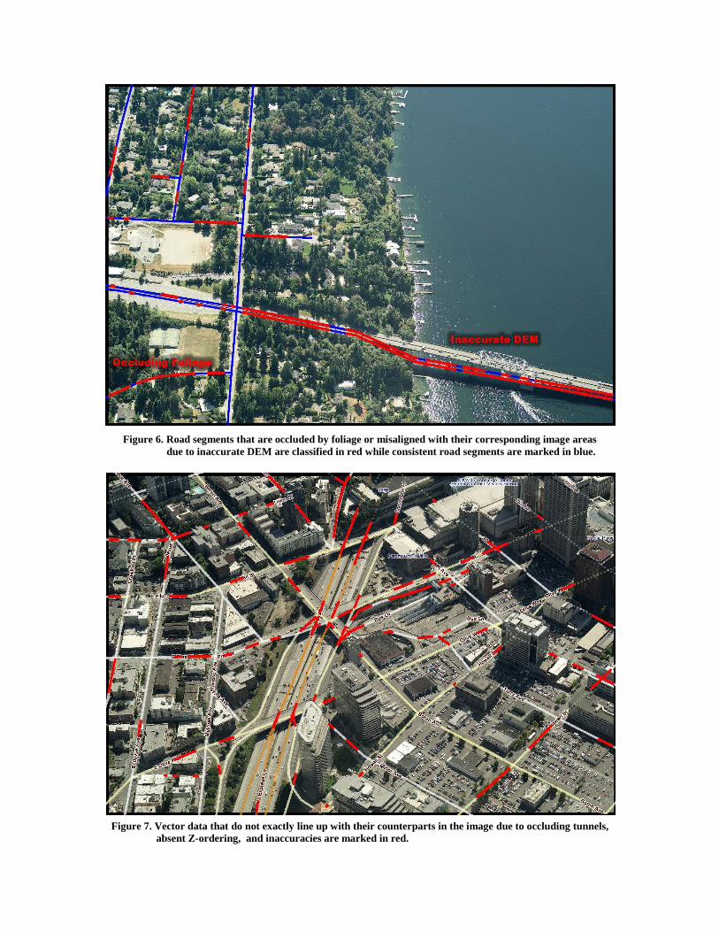
Figure 6. Road segments that are occluded by foliage or misaligned with their corresponding image areas

due to inaccurate DEM are classified in red while consistent road segments are marked in blue.

Figure 7. Vector data that do not exactly line up with their counterparts in the image due to occluding tunnels,

absent Z-ordering, and inaccuracies are marked in red.

Figure 8. The classifier is applied along the green lines that are perpendicular to each inconsistent road segment.

The encircled points in black delineate the new road vectors.

Figure 9. A search for the first point along each green line where the classifier responds positive yields the encircled

point in black. These points delineate the corrector vector of the road on the bridge.