
UNIVERSITE´ FRANC¸OIS - RABELAIS THESE` · PDF fileCotutelle thesis between...
186
UNIVERSIT ´ E FRANC ¸ OIS - RABELAIS DE TOURS ´ Ecole Doctorale Sant´ e, Sciences, Technologies Laboratoire d’Informatique (EA 2101) ´ Equipe Reconnaissance des Formes et Analyse d’Images Th` ese en cotutelle entre l’Universit´ e Fran¸cois - Rabelais de Tours, France et l’Universitat Aut` onoma de Barcelona, Espagne. TH ` ESE pr´ esent´ e par : Muhammad Muzzamil LUQMAN soutenue le : 02 mars 2012 pour obtenir le grade de : Docteur de l’universit´ e Fran¸cois - Rabelais Discipline/ Sp´ ecialit´ e : Informatique Fuzzy Multilevel Graph Embedding for Recognition, Indexing and Retrieval of Graphic Document Images DIRECTEURS DE TH ` ESE RAMEL Jean-Yves Professeur, Universit´ e Fran¸cois - Rabelais de Tours, France. LLADOS Josep Professeur, Universit´ e Autonoma de Barcelone, Espagne. CO-ENCADRANT BROUARD Thierry Maˆ ıtre de conf´ erences, Universit´ e Fran¸cois - Rabelais de Tours. RAPPORTEURS BUNKE Horst Professeur ´ em´ erite, Universit´ e de Bern, Suisse. OGIER Jean-Marc Professeur, Universit´ e de La Rochelle, France. JURY DE TH ` ESE BROUARD Thierry Maˆ ıtre de conf´ erences, Universit´ e Fran¸cois - Rabelais de Tours. BUNKE Horst Professeur ´ em´ erite, Universit´ e de Bern, Suisse. LLADOS Josep Professeur, Universit´ e Autonoma de Barcelone, Espagne. RAMEL Jean-Yves Professeur, Universit´ e Fran¸cois - Rabelais de Tours, France. TABBONE Salvatore-Antoine Professeur, Universit´ e de Lorraine, France. VALVENY Ernest Maˆ ıtre de conf´ erences, Universit´ e Autonoma de Barcelone.
Transcript of UNIVERSITE´ FRANC¸OIS - RABELAIS THESE` · PDF fileCotutelle thesis between...

UNIVERSITEFRANCOIS - RABELAIS
DE TOURS
Ecole Doctorale Sante, Sciences, Technologies
Laboratoire d’Informatique (EA 2101)Equipe Reconnaissance des Formes et Analyse d’Images
These en cotutelle entre l’Universite Francois - Rabelais de Tours, France etl’Universitat Autonoma de Barcelona, Espagne.
THESE presente par :
Muhammad Muzzamil LUQMAN
soutenue le : 02 mars 2012
pour obtenir le grade de : Docteur de l’universite Francois - Rabelais
Discipline/ Specialite : Informatique
Fuzzy Multilevel Graph Embedding for Recognition, Indexingand Retrieval of Graphic Document Images
DIRECTEURS DE THESERAMEL Jean-Yves Professeur, Universite Francois - Rabelais de Tours, France.LLADOS Josep Professeur, Universite Autonoma de Barcelone, Espagne.
CO-ENCADRANTBROUARD Thierry Maıtre de conferences, Universite Francois - Rabelais de Tours.
RAPPORTEURSBUNKE Horst Professeur emerite, Universite de Bern, Suisse.OGIER Jean-Marc Professeur, Universite de La Rochelle, France.
JURY DE THESE
BROUARD Thierry Maıtre de conferences, Universite Francois - Rabelais de Tours.BUNKE Horst Professeur emerite, Universite de Bern, Suisse.LLADOS Josep Professeur, Universite Autonoma de Barcelone, Espagne.RAMEL Jean-Yves Professeur, Universite Francois - Rabelais de Tours, France.TABBONE Salvatore-Antoine Professeur, Universite de Lorraine, France.VALVENY Ernest Maıtre de conferences, Universite Autonoma de Barcelone.


Cotutelle thesis between Universitat Autonoma de Barcelona, Spain andUniversite Francois - Rabelais de Tours, France.
Fuzzy Multilevel Graph Embedding for
Recognition, Indexing and Retrieval of
Graphic Document Images
A dissertation submitted by Muhammad MuzzamilLuqman at Universitat Autonoma de Barcelona to fulfilthe degree of Doctor of Philosophy.
Bellaterra, 2012.

Directors: Dr. Josep LladosProfessorAutonoma University of Barcelona, Spain
Dr. Jean-Yves RamelProfessorFrancois - Rabelais University of Tours, France
Co-director: Dr. Thierry BrouardAssistant ProfessorFrancois - Rabelais University of Tours, France
This document was typeset by the author using LATEX2!.
The research described in this book was carried out at the Computer Vision Center,Universitat Autonoma de Barcelona and Computer Science Laboratory, UniversiteFrancois - Rabelais de Tours.
Copyright c! 2012 by Muhammad Muzzamil Luqman. All rights reserved. Nopart of this publication may be reproduced or transmitted in any form or by anymeans, electronic or mechanical, including photocopy, recording, or any informationstorage and retrieval system, without permission in writing from the author.

I am thankful to Higher Education Commission1,Government of Pakistan, for award of scholarshipunder grant PD-2007-1/Overseas/FR/HEC/222, to pur-sue my master’s and doctorate.
1http://www.hec.gov.pk/


Acknowledgments
Alhamdulilah.
I would like to present my foremost sincere gratitude to Professor Jean-Yves Ramel
and Professor Josep Llados. I passed a long journey under their kind supervision. All
credit for the successful completion of this thesis goes to their patient attitude, openness
to new ideas and the freedom that they provided me to carry out the research work at my
pace. Thank you very much Jean-Yves and Josep.
I am thankful to Dr. Thierry Brouard for his guidance during initial phase of the thesis
research and for his support during all important phases of the thesis work.
I am thankful to Professor Horste Bunke and Professor Jean-Marc Ogier for carefully
reading my dissertation and providing me very useful feedback.
I would also like to acknowledge the support of the administration sta! of Computer
Science Laboratory of Tours and Computer Vision Center Barcelona for their assistance
and support during the course of my thesis research.
Thank you very much all my colleagues at Computer Science Laboratory of Tours and
Computer Vision Center Barcelona for your support and the wonderful years that I passed
among you.
Tons of thanks to my parents, brothers and sisters. Your love and moral support
actually made me successfully complete this important phase of my life.
Bundles of thanks to all my friends. I don’t want to miss any one and I will not cite
any names. But all of you are very dear to me and all of you helped me at various stages
to keep my moral high. You made me go through the crucial and di"cult stages of my
thesis.


Abstract
Structural pattern recognition approaches o↵er the most expressive, convenient andpowerful but computational expensive representations of underlying relational information.These representations can benefit from mature, less expensive and e�cient state-of-the-artmachine learning models of statistical pattern recognition, only after being mapped to alow-dimensional vector space.
This thesis addresses the problem of lack of e�cient computational tools for graph basedstructural pattern recognition approaches and proposes to exploit computational strengthof statistical pattern recognition. The contribution of this thesis is two-fold.
The first contribution of this thesis is a new method of explicit graph embedding. Theproposed graph embedding method exploits multilevel analysis of graph for extractinggraph level information, structural level information and elementary level informationfrom graphs. It embeds this information into a numeric feature vector. The methodemploys fuzzy overlapping trapezoidal intervals for addressing the noise sensitivity of graphrepresentations and for minimizing the information loss while mapping from continuousgraph space to discrete vector space. The method has unsupervised learning abilities andis capable of automatically adapting its parameters to underlying graph dataset.
The second contribution of this thesis is a framework for automatic indexing of graphrepositories for graph retrieval and subgraph spotting. This framework exploits explicitgraph embedding together with classification and clustering tools. It achieves the auto-matic indexing of a graph repository during its o↵-line learning phase, where its extractsthe cliques of order 2 from graphs and embeds them into feature vectors by employing theaforementioned explicit graph embedding technique. It clusters the feature vectors intoclasses, learns a classifier and builds an index for the graph repository. During on-line spot-ting phase, it extracts the cliques of order 2 from query graph, embeds them into featurevectors and uses the index of the graph repository to retrieve the graphs from repository.The framework does not require a labeled learning set and can be easily deployed to arange of application domains, o↵ering ease of query by example (QBE) and granularity offocused retrieval.
Experimentation on latest public graph datasets from International Association of Pattern
9

ABSTRACT
Recognition’s Technical Committee on graph-based representations (TC-15) evaluates thepower and applicability of our graph embedding framework for the problems of graph clas-sification and graph clustering. A second set of experimentation evaluates the frameworkfor automatic indexing of graph repositories for graph retrieval and subgraph spotting.
Application to the real problems of recognition, indexing and retrieval of graphic documentimages is also presented.
Keywords : Pattern recognition, graph clustering, graph classification, graph embed-ding, subgraph spotting, fuzzy logic, graphics recognition.
10
Resume
Cette these aborde le probleme du manque de performance des outils exploitant desrepresentations a base de graphes en reconnaissance des formes. Nous proposons de con-tribuer aux nouvelles methodes proposant de tirer partie, a la fois, de la richesse desmethodes structurelles et de la rapidite des methodes de reconnaissance de formes statis-tiques.
Deux principales contributions sont presentees dans ce manuscrit.
La premiere correspond a la proposition d’une nouvelle methode de projection explicitede graphes procedant par analyse multi-facettes des graphes. Cette methode e↵ectue unecaracterisation des graphes suivant di↵erents niveaux qui correspondent, selon nous, auxpoint-cles des representations a base de graphes. Il s’agit de capturer l’information porteepar un graphe au niveau global, au niveau structure et au niveau local ou elementaire. Cesinformations capturees sont encapsulees dans un vecteur de caracteristiques numeriquesemployant des histogrammes flous. L’approche floue a base d’intervalles trapezodaux, per-met de mieux apprehender la sensibilite aux bruits des representations a base de grapheset de reduire au minimum la deformation de l’information liee au positionnement ar-bitraire des frontiers lors du passage d’un espace continu a un espace vectoriel discretchoisi et utilise pour decrire certaines caracteristiques des graphes. La methode proposeeutilise, de plus, un mecanisme d’apprentissage non supervisee pour adapter automatique-ment ses parametres en fonction de la base de graphes a traiter sans necessiter de phased’apprentissage prealable.
La deuxieme contribution correspond a la mise en place d’une architecture pour l’indexationde masses de graphes afin de permettre, par la suite, la recherche de sous-graphes presentsdans cette base. Cette architecture utilise la methode precedente de projection explicitede graphes appliquee sur toutes les cliques d’ordre 2 pouvant etre extraites des graphespresents dans la base a indexer afin de pouvoir les classifier. Un partitionnement descliques permet de constituer l’index qui sert de base a la description des graphes et donc aleur indexation en ne necessitant aucune base d’apprentissage pre-etiquetees. Cela procurea cette methode une genericite tres forte et donc un deploiement facile. Lors de la phase derecherche d’un sous-graphe dans la base pre-indexee, la reponse a la requete est formee del’ensemble des graphes contenant toutes les cliques d’ordre 2 obtenues par decomposition
11

RESUME
de la requete. Enfin, le sous-graphe associe a la requete est repere dans chacun des graphesidentifies. La methode proposee est applicable a de nombreux domaines, apportant la sou-plesse d’un systeme de requete par l’exemple et la granularite des techniques d’extractionciblee (focused retrieval).
Des experimentations sur les bases de graphes publiques recentes proposees par le TC15de l’IAPR (groupe de rechercher sur les methodes a base de graphes) sont presentees etpermettent d’evaluer les performances et l’applicabilite des propositions faites dans cettethese sur des problemes de classification et de partitionnement de graphes. Un deuxiemejeu d’experimentations presente les resultats obtenus par notre methode d’indexation au-tomatique de bases de graphes pour la recherche de sous-graphes.
Des exemples d’applications des approches proposees a des problemes reels de reconnais-sance, d’indexation et de reperage d’images de documents graphiques sont aussi presentestout au long du manuscrit.
Mots cles : Reconnaissance des formes, partitionnement de graphes, classification degraphes, projection de graphes, reperage de sous-graphes, logique floue, reconnaissance degraphiques.
12

Contents
Introduction 23
1 Definitions and notations 27
1.1 Introduction . . . . . . . . . . . . . . . . . . . . . . . . . . . . . . . . . . . . 27
1.2 Terminology on graphs . . . . . . . . . . . . . . . . . . . . . . . . . . . . . . 28
Graph . . . . . . . . . . . . . . . . . . . . . . . . . . . . . . . . . . . . . 28
Subgraph . . . . . . . . . . . . . . . . . . . . . . . . . . . . . . . . . . . 28
Clique . . . . . . . . . . . . . . . . . . . . . . . . . . . . . . . . . . . . . 29
Attributed Graph (AG) . . . . . . . . . . . . . . . . . . . . . . . . . . . 30
1.3 Important features of graphs . . . . . . . . . . . . . . . . . . . . . . . . . . 31
Graph order . . . . . . . . . . . . . . . . . . . . . . . . . . . . . . . . . 31
Graph Size . . . . . . . . . . . . . . . . . . . . . . . . . . . . . . . . . . 31
Node degree . . . . . . . . . . . . . . . . . . . . . . . . . . . . . . . . . 32
1.4 Representation and processing of graphs . . . . . . . . . . . . . . . . . . . . 33
Adjacency matrix of a graph . . . . . . . . . . . . . . . . . . . . . . . . 33
Laplacian matrix of a graph . . . . . . . . . . . . . . . . . . . . . . . . . 33
Graph matching and graph isomorphism . . . . . . . . . . . . . . . . . . 34
Subgraph isomorphism . . . . . . . . . . . . . . . . . . . . . . . . . . . . 35
Maximum common subgraph (mcs) . . . . . . . . . . . . . . . . . . . . 36
Median graph . . . . . . . . . . . . . . . . . . . . . . . . . . . . . . . . . 36
Graph edit distance (GED) . . . . . . . . . . . . . . . . . . . . . . . . . 36
Graph Embedding (GEM) . . . . . . . . . . . . . . . . . . . . . . . . . . 37
Explicit Graph Embedding . . . . . . . . . . . . . . . . . . . . . . . . . 37
1.5 Graph retrieval and subgraph spotting . . . . . . . . . . . . . . . . . . . . . 38
13

CONTENTS
2 State of the art 39
2.1 Introduction . . . . . . . . . . . . . . . . . . . . . . . . . . . . . . . . . . . . 39
2.1.1 Structural pattern recognition . . . . . . . . . . . . . . . . . . . . . . 40
2.1.2 Statistical pattern recognition . . . . . . . . . . . . . . . . . . . . . . 40
2.2 Graph representation of images . . . . . . . . . . . . . . . . . . . . . . . . . 42
2.2.1 Graph of pixels . . . . . . . . . . . . . . . . . . . . . . . . . . . . . . 43
2.2.2 Graph of characteristic points . . . . . . . . . . . . . . . . . . . . . . 44
2.2.3 Graph of primitives . . . . . . . . . . . . . . . . . . . . . . . . . . . 45
2.2.4 Region adjacency graph . . . . . . . . . . . . . . . . . . . . . . . . . 46
2.2.5 Conclusion . . . . . . . . . . . . . . . . . . . . . . . . . . . . . . . . 47
2.3 Graph matching . . . . . . . . . . . . . . . . . . . . . . . . . . . . . . . . . 48
2.3.1 Exact graph matching and graph isomorphism . . . . . . . . . . . . 49
2.3.2 Error tolerant graph matching . . . . . . . . . . . . . . . . . . . . . 55
2.3.3 Distance between two graphs . . . . . . . . . . . . . . . . . . . . . . 57
2.3.4 Graph embedding . . . . . . . . . . . . . . . . . . . . . . . . . . . . 61
2.4 Fuzzy logic . . . . . . . . . . . . . . . . . . . . . . . . . . . . . . . . . . . . 67
2.5 Limitations of existing methods and our contributions . . . . . . . . . . . . 71
3 Fuzzy Multilevel Graph Embedding 75
3.1 Introduction . . . . . . . . . . . . . . . . . . . . . . . . . . . . . . . . . . . . 75
3.2 Overview of fuzzy multilevel graph embedding (FMGE) . . . . . . . . . . . 78
3.2.1 Description of feature vector of FMGE . . . . . . . . . . . . . . . . . 79
3.3 Framework of fuzzy multilevel graph embedding (FMGE) . . . . . . . . . . 88
3.3.1 Unsupervised learning phase . . . . . . . . . . . . . . . . . . . . . . 88
3.3.2 Graph embedding phase . . . . . . . . . . . . . . . . . . . . . . . . . 94
3.4 Conclusion . . . . . . . . . . . . . . . . . . . . . . . . . . . . . . . . . . . . 98
4 Graph retrieval and subgraph spotting through explicit graph embed-ding 101
4.1 Introduction . . . . . . . . . . . . . . . . . . . . . . . . . . . . . . . . . . . . 101
4.2 Automatic indexing of a graph repository . . . . . . . . . . . . . . . . . . . 103
4.3 Subgraph spotting . . . . . . . . . . . . . . . . . . . . . . . . . . . . . . . . 107
4.4 Conclusion . . . . . . . . . . . . . . . . . . . . . . . . . . . . . . . . . . . . 112
14

CONTENTS
5 Experimentations 113
5.1 Introduction . . . . . . . . . . . . . . . . . . . . . . . . . . . . . . . . . . . . 113
5.2 Graph databases . . . . . . . . . . . . . . . . . . . . . . . . . . . . . . . . . 114
5.3 Graph classification . . . . . . . . . . . . . . . . . . . . . . . . . . . . . . . . 117
5.4 Graph clustering . . . . . . . . . . . . . . . . . . . . . . . . . . . . . . . . . 121
5.5 Graph retrieval and subgraph spotting . . . . . . . . . . . . . . . . . . . . . 128
5.6 Application of FMGE to graphics recognition . . . . . . . . . . . . . . . . . 135
5.6.1 Representation phase . . . . . . . . . . . . . . . . . . . . . . . . . . 136
5.6.2 Description phase (FMGE) . . . . . . . . . . . . . . . . . . . . . . . 137
5.6.3 Classifier learning phase . . . . . . . . . . . . . . . . . . . . . . . . . 138
5.6.4 Classification phase (graphic symbol recognition) . . . . . . . . . . . 138
5.6.5 Symbols with vectorial and binary noise . . . . . . . . . . . . . . . . 140
5.6.6 Symbols with contextual noise . . . . . . . . . . . . . . . . . . . . . 142
5.6.7 Complexity of FMGE . . . . . . . . . . . . . . . . . . . . . . . . . . 147
5.7 Conclusion . . . . . . . . . . . . . . . . . . . . . . . . . . . . . . . . . . . . 148
6 Discussion and Conclusions 149
6.1 Discussion about FMGE . . . . . . . . . . . . . . . . . . . . . . . . . . . . . 149
6.1.1 Parameters . . . . . . . . . . . . . . . . . . . . . . . . . . . . . . . . 149
6.1.2 Complexity . . . . . . . . . . . . . . . . . . . . . . . . . . . . . . . . 152
6.2 Conclusions . . . . . . . . . . . . . . . . . . . . . . . . . . . . . . . . . . . . 153
6.3 Future challenges . . . . . . . . . . . . . . . . . . . . . . . . . . . . . . . . . 155
Appendix 159
A Graph databases 159
A.1 IAM graph database repository . . . . . . . . . . . . . . . . . . . . . . . . . 159
A.1.1 Letter graphs . . . . . . . . . . . . . . . . . . . . . . . . . . . . . . . 159
A.1.2 GREC graphs . . . . . . . . . . . . . . . . . . . . . . . . . . . . . . . 161
A.1.3 Fingerprint graphs . . . . . . . . . . . . . . . . . . . . . . . . . . . . 163
A.1.4 Mutagenicity graphs . . . . . . . . . . . . . . . . . . . . . . . . . . . 163
A.2 GEPR graphs . . . . . . . . . . . . . . . . . . . . . . . . . . . . . . . . . . . 165
15

CONTENTS
B Graphs representation of graphic document images 167
16

List of Tables
2.1 Defining operators for fuzzy sets. . . . . . . . . . . . . . . . . . . . . . . . . 69
5.1 IAM graph database details. . . . . . . . . . . . . . . . . . . . . . . . . . . . 114
5.2 GEPR graph database details. . . . . . . . . . . . . . . . . . . . . . . . . . 115
5.3 SESYD graph database details. . . . . . . . . . . . . . . . . . . . . . . . . . 116
5.4 Experimental results (%), for graph classification on IAM graph databaserepository. . . . . . . . . . . . . . . . . . . . . . . . . . . . . . . . . . . . . . 120
5.5 Quality of k-means clustering for IAM graph database repository. . . . . . . 124
5.6 Performance indexes for GEPR graphs. . . . . . . . . . . . . . . . . . . . . 127
5.7 Results of symbol recognition experiments for vectorial and binary noise. . . 141
5.8 Results of symbol recognition experiments for context noise. . . . . . . . . . 145
17

LIST OF TABLES
18

List of Figures
1.1 Example of a graph (left) and a subgraph (right). . . . . . . . . . . . . . . . 29
1.2 Example of a clique in a graph. . . . . . . . . . . . . . . . . . . . . . . . . . 29
1.3 Example of graph isomorphism. . . . . . . . . . . . . . . . . . . . . . . . . . 34
1.4 Example of subgraph isomorphism. . . . . . . . . . . . . . . . . . . . . . . . 35
2.1 Representation of an image by graph of pixels.1 . . . . . . . . . . . . . . . . 43
2.2 Representation of an image by graph of characteristic points.1 . . . . . . . . 44
2.3 Representation of a graphic symbol by graph of primitives. . . . . . . . . . 45
2.4 Representation of graphics content by a region adjacency graph.1 . . . . . . 46
2.5 Graph isomorphism through association graph.1 . . . . . . . . . . . . . . . . 50
2.6 A graph and its adjacency matrices.1 . . . . . . . . . . . . . . . . . . . . . . 52
2.7 Decision tree constructed from the adjacency matrices of two graphs G1
and G2
.1 . . . . . . . . . . . . . . . . . . . . . . . . . . . . . . . . . . . . . . 53
2.8 A graph and a lexicon generated from a non-isomorphic graph network. . . 64
2.9 Example of fuzzy logic (temperature).1 . . . . . . . . . . . . . . . . . . . . . 67
2.10 Some shapes commonly employed for the membership function S(x).1 . . . 68
2.11 Pictorial illustration of operations on boolean and fuzzy logic.1 . . . . . . . 69
3.1 Attributed graph representation of basic geometric shapes of unit length. . 77
3.2 Overview of Fuzzy Multilevel Graph Embedding (FMGE). . . . . . . . . . . 78
3.3 The Fuzzy Structural Multilevel Feature Vector (FSMFV). . . . . . . . . . 80
3.4 Embedding of structural level information. . . . . . . . . . . . . . . . . . . . 81
3.5 Resemblance attributes for the attributed graph representation of basic ge-ometric shapes of unit length. . . . . . . . . . . . . . . . . . . . . . . . . . . 85
3.6 Embedding of elementary level information. . . . . . . . . . . . . . . . . . . 86
19

LIST OF FIGURES
3.7 The unsupervised learning phase of FMGE. . . . . . . . . . . . . . . . . . . 88
3.8 Learning fuzzy intervals for an attribute i. . . . . . . . . . . . . . . . . . . . 89
3.9 5 fuzzy overlapping trapezoidal intervals (si
) defined over 9 equally spacedcrisp intervals (n
i
). . . . . . . . . . . . . . . . . . . . . . . . . . . . . . . . . 90
3.10 The graph embedding phase of FMGE. . . . . . . . . . . . . . . . . . . . . . 94
3.11 Histogram encoding of information and Fuzzy Structural Multilevel FeatureVectors for the example attributed graphs. . . . . . . . . . . . . . . . . . . . 97
4.1 Automatic indexing of a graph repository. . . . . . . . . . . . . . . . . . . . 106
4.2 Illustration of score function computation for a subgraph around a cliqueof order 2 in a retrieved graph. . . . . . . . . . . . . . . . . . . . . . . . . . 110
4.3 Graph retrieval and subgraph spotting. . . . . . . . . . . . . . . . . . . . . . 111
5.1 Number of clusters versus average Silhouette width for k-means clustering,for IAM graph database repository. . . . . . . . . . . . . . . . . . . . . . . . 123
5.2 Precision and recall plot for graph retrieval from SESYD graph database. . 130
5.3 A snapshot of retrieved results for a query image (single instance of querysymbol). . . . . . . . . . . . . . . . . . . . . . . . . . . . . . . . . . . . . . . 132
5.4 A snapshot of retrieved results for a query image (multiple instances ofquery symbol). . . . . . . . . . . . . . . . . . . . . . . . . . . . . . . . . . . 133
5.5 Representing a graphic symbol image by an attributed graph. . . . . . . . . 136
5.6 FMGE embedding of an attributed graph of a graphic symbol. . . . . . . . 137
5.7 Model symbol with deformations, used for simulating hand-drawn symbols. 140
5.8 Model symbol with degraded example, used to simulate photocopying /printing / scanning. . . . . . . . . . . . . . . . . . . . . . . . . . . . . . . . 140
5.9 An arm chair with 2 examples of each di↵erent level of contextual noise. . . 142
5.10 Model symbols from electronic drawings. . . . . . . . . . . . . . . . . . . . . 143
5.11 Model symbols from floor plans. . . . . . . . . . . . . . . . . . . . . . . . . 144
5.12 Time complexity of unsupervised learning phase of FMGE. . . . . . . . . . 147
6.1 Bijective match of nodes of two graphs. . . . . . . . . . . . . . . . . . . . . 156
A.1 Prototypes of letters A to Z. . . . . . . . . . . . . . . . . . . . . . . . . . . . 160
A.2 Instances of letter A at distortion level low. . . . . . . . . . . . . . . . . . . 160
A.3 Instances of letter A at distortion level medium. . . . . . . . . . . . . . . . . 160
A.4 Instances of letter A at distortion level high. . . . . . . . . . . . . . . . . . . 160
20

LIST OF FIGURES
A.5 The prototype images of the 22 GREC classes. . . . . . . . . . . . . . . . . 162
A.6 The five distortion levels (bottom to top) applied to three sample images. . 162
A.7 Fingerprint examples from the Galton-Henry class Arch. . . . . . . . . . . . 164
A.8 Fingerprint examples from the Galton-Henry class Left loop. . . . . . . . . . 164
A.9 Fingerprint examples from the Galton-Henry class Right loop. . . . . . . . . 164
A.10 Fingerprint examples from the Galton-Henry class Whorl. . . . . . . . . . . 164
A.11 Some examples of the images in the ALOI database. . . . . . . . . . . . . . 166
A.12 Some examples of the images in the COIL database. . . . . . . . . . . . . . 166
A.13 Some examples of the images in the ODBK database. . . . . . . . . . . . . 166
B.1 Representing graphic content by an attributed graph. . . . . . . . . . . . . 168
B.2 An example architectural floor plan image from SESYD dataset. . . . . . . 169
B.3 An example electronic diagram image from SESYD dataset. . . . . . . . . . 170
B.4 An arm chair with 2 examples of each di↵erent level of contextual noise. . . 170
21

LIST OF FIGURES
22
Introduction
Ability to recognize patterns is among the most crucial capabilities of human beings fortheir survival, which enables them to employ their sophisticated neural and cognitive
systems [Duda et al., 2000], for processing complex audio, visual, smell, touch and tastesignals. Man is the most complex and the best existing system of pattern recognition.Without any explicit thinking, we continuously compare, classify and identify huge amountof signally data everyday [Kuncheva, 2004], start from the time we get up in the morningtill the last second we fall asleep. This includes recognizing the face of a friend in a crowd,a spoken word embedded in noise, the proper key to lock the door, smell of co↵ee, thevoice of a favorite singer, the recognition of alphabetic characters and millions of moretasks that we perform on regular basis.
The scientific domains of artificial intelligence (AI) and pattern recognition (PR) canbe seen as the transportation of the human capability of analyzing - to compare, to classifyand to identify - the audio and visual signals, to computers. So that computers may assisthumans for pattern recognition tasks and to replace humans for some of them.
Pattern recognition has emerged as an important research domain and has supportedthe development of numerous applications in many di↵erent areas of activity. Robotassisted manufacture, medical diagnostic systems, forecast of economic variables, explo-ration of earth resources, analysis of satellite data, face detection, verification and recogni-tion, object detection and recognition, handwritten digit and character recognition, speechand speaker verification and recognition, information and image retrieval, text detectionand categorization, gender classification and prediction ([Byun, 2003], [De Sa, 2001] and[Friedman and Kandel, 1999]), being some of the important to mention.
The problems of pattern recognition are often very complex and it is nearly impossibleto write an explicitly programmed solution for them. For example it is impossible to writean analytical program for recognizing a face in a photo [Shawe-Taylor and Cristianini, 2004].The pattern recognition research community has overcome this problem by adapting alearning methodology which is highly inspired by human ability to learn. A learningmethodology refers to the approach where instead of precisely defining a set of specifi-cations for solving a problem analytically, the machine is trained on data and it learnsthe concept of a class by discriminating between groups of similar objects. Based on the
23
INTRODUCTION
inferred rules and learning performed during training, the machine is able to make pre-dictions about new and unseen data. More formally, the machine acquires generalizationpower through learning [Riesen, 2010].
A pattern recognition task for computers can be looked upon as consisting of two mainsteps - (i) the representation of the signal data by a data structure and (ii) the computationof desired operation (pattern recognition). The two important sub domains of patternrecognition - the structural pattern recognition and the statistical pattern recognition -each have its strength only in one of the two aforementioned steps, respectively.
The structural pattern recognition o↵ers the most powerful relational data structure ofgraph. For the last three decades, graphs have been used for pattern recognition and imageanalysis, for extracting and representing complex relations in underlying data. However,there is still a lack of e�cient computational tools and learning models which can processthis data structure.
On the other side, the statistical pattern recognition o↵ers highly e�cient computa-tional models of machine learning, classification and clustering, by employing the wellestablished theory of statistics. But these computational models can work only on simplenumeric vectors and can not process complex high dimensional relational data structures.
Over decades of parallel research in both of these sub domains of pattern recognition- structural and statistical pattern recognition - powerful representations and e�cientcomputational models have been built. But little progress has been made towards thelong desired objective (of research in pattern recognition), to join the advantages of thestructural and statistical pattern recognition approaches for building more powerful ande�cient algorithms.
This thesis is a step forward to achieve this objective of joining the advantages of struc-tural and statistical pattern recognition approaches. We propose an algorithm which per-mits the pattern recognition applications to employ the powerful relational data structureof attributed graphs along with the computational strengths of state of the art statisticalmodels of machine learning, classification and clustering.
24

INTRODUCTION
The contribution of this thesis is two-fold.
The first contribution of this thesis is a new method of explicit graph embedding. Theproposed graph embedding method exploits multilevel analysis of graph for extractinggraph level information, structural level information and elementary level informationfrom graphs. It embeds this information into a numeric feature vector. The methodemploys fuzzy overlapping trapezoidal intervals for addressing the noise sensitivity of graphrepresentations and for minimizing the information loss while mapping from continuousgraph space to discrete vector space. The method has unsupervised learning abilities andis capable of automatically adapting its parameters to underlying graph dataset.
The second contribution of this thesis is a framework for automatic indexing of graphrepositories for graph retrieval and subgraph spotting. This framework exploits explicitgraph embedding together with classification and clustering tools. It achieves the auto-matic indexing of a graph repository during its o↵-line learning phase, where its extractsthe cliques of order 2 from graphs and embeds them into feature vectors by employing theaforementioned explicit graph embedding technique. It clusters the feature vectors intoclasses, learns a classifier and builds an index for the graph repository. During on-line spot-ting phase, it extracts the cliques of order 2 from query graph, embeds them into featurevectors and uses the index of the graph repository to retrieve the graphs from repository.The framework does not require a labeled learning set and can be easily deployed to arange of application domains, o↵ering ease of query by example (QBE) and granularity offocused retrieval.
25

INTRODUCTION
The dissertation is organized in six chapters and two appendices. A brief introductionto the contents of each chapter is given below:
In chapter 1 we present important definitions and concepts and we formalize the no-tations that have been used in this dissertation.
In chapter 2 we present a literature review on state of the art of structural patternrecognition, statistical pattern recognition, graph representation of images, exact graphmatching, graph isomorphism, subgraph isomorphism, error tolerant graph matching, dis-tance between graphs, graph embedding, graph classification and fuzzy logic. We summa-rize the important contributions of our work in light of the limitations of existing methods.
In chapter 3 we outline our explicit graph embedding method i.e. the Fuzzy MultilevelGraph Embedding (FMGE). We first present an overall global description of FMGE andthen present details on the FMGE framework. We conclude this chapter by introducingthe application of FMGE to graph classification, graph clustering and graph retrieval.
In chapter 4 we present a framework for automatic indexing of attributed graph repos-itories. We demonstrate a practical application of Fuzzy Multilevel Graph Embedding(FMGE) together with classification and clustering tools, for achieving graph retrievaland subgraph spotting.
In chapter 5 we present the experimental evaluations of FMGE for the problems ofgraph clustering and graph classification. We present the experimental evaluations of theframework for automatic indexing of graph repositories for graph retrieval and subgraphspotting, with an application to content spotting in graphic document image repositories.We provide experimental results for the application of the thesis work to the real problemsof recognition, indexing and retrieval of graphic document images.
In chapter 6 we present a discussion on the presented work. We highlight the im-provements of the proposed method which should be further studied and conclude thisdissertation. We point out the possible lines of future research.
In appendix A we provide details on the graph databases used in this thesis.
In appendix B we provide details on the graph repository extracted from electronicdiagrams and architectural floor plans document images.
26
Chapter 1
Definitions and notations
In this chapter we present important definitions and concepts and we formalize the nota-tions that have been used in this dissertation.
1.1 Introduction
This chapter presents important definitions and concepts adapted to the way we haveused them and to the vocabulary of this dissertation. We first define the terms which areused throughout the dissertation. These include graph, subgraph, clique and attributedgraph. This is followed by a section on defining important features of graphs and a sectionintroducing important concepts on representation and processing of graphs. Along withpresenting the definitions, in the meantime we also formalize the notations for facilitatingthe understanding of the work presented in upcoming chapters of the dissertation.
27

1.2. TERMINOLOGY ON GRAPHS
1.2 Terminology on graphs
Definition 1: Graph
Let V denote the set of vertices and E denote the set of edges. A graph G is a set ofvertices (V ) connected by edges (E). It is given by the ordered pair:
G = (V (G), E(G))
where,
V (G) is the set of vertices in graph G and
E(G) is a set of 2 element subsets of V(G), given by:E ✓ {{u, v} : u, v 2 V (G)}
For a directed graph, the ordered pair (u, v) represents an edge from vertex u tovertex v. Where as, for an undirected graph it represents an edge between vertex uand vertex v without signifying any direction.
Definition 2: Subgraph
A graph subG = (V (subG), E(subG)) is called a subgraph of a graphG = (V (G), E(G))if it contains no vertices or edges that are not in graph G.
Mathematically,
V (subG) ✓ V (G) and
E (subG) ✓ E (G)
Figure 1.1 shows a subgraph in a graph.
28

1.2. TERMINOLOGY ON GRAPHS
Figure 1.1: Example of a graph (left) and a subgraph (right).
Definition 3: Clique
A clique in an undirected graph G is a subset of its vertices V (G) such that each pairof vertices in the subset is connected by an edge. Figure 1.2 shows a clique (representedby {d, e, h}) in a graph.
Figure 1.2: Example of a clique in a graph.
A maximum clique is a clique of the largest possible size in a given graph. The cliquenumber of a graph is the number of vertices in its maximum clique.
29

1.2. TERMINOLOGY ON GRAPHS
Definition 4: Attributed Graph (AG)
Let AV
and AE
denote the domains of possible values for attributed vertices and edgesrespectively. These domains are assumed to include a special value that represents a nullvalue of a vertex or an edge. An attributed graph AG over (A
V
, AE
) is defined to be afour-tuple:
AG = (V,E, µV , µE)
where,
V is a set of vertices,
E ✓ V ⇥ V is a set of edges,
µV : V �! Ak
V
is function assigning k attributes to vertices and
µE : E �! Al
E
is a function assigning l attributes to edges.
In this dissertation we use the term attributed graph to refer to an undirected at-tributed graph, unless otherwise explicitly specified.
30

1.3. IMPORTANT FEATURES OF GRAPHS
1.3 Important features of graphs
We present the definitions in this section in terms of attributed graphs, as we haveused them in this dissertation. However, these definitions are equally applicable to graphsin general.
Definition 5: Graph order
The order of an attributed graph AG = (V,E, µV , µE) is given by |V | i.e. the numberof vertices in AG.
Let AG1
and AG2
be two attributed graphs, then:
AG1
is smaller than AG2
i↵ |V1
| < |V2
|
AG1
and AG2
are equal ordered i↵ |V1
| = |V2
|
AG1
is larger than AG2
i↵ |V1
| > |V2
|
Definition 6: Graph Size
The size of an attributed graph AG = (V,E, µV , µE) is given by |E| i.e. the numberof edges in AG.
Let AG1
and AG2
be two attributed graphs, then:
AG1
is thinner than AG2
i↵ |E1
| < |E2
|
AG1
and AG2
are equal sized i↵ |E1
| = |E2
|
AG1
is thicker than AG2
i↵ |E1
| > |E2
|
31

1.3. IMPORTANT FEATURES OF GRAPHS
Definition 7: Node Degree
The degree of a (vertex or) node Vi
in graph AG = (V,E, µV , µE) refers to the numberof edges connected to V
i
.
If AG is a directed graph then each of its nodes has an in-degree and an out-degreeassociated to it. The in-degree refers to the number of incoming edges and out-degreerefers to the number of outgoing edges for a node.
Generally, the terms densely connected graph and sparsely connected graph are usedfor abstractly categorizing a graph on the basis of its node degrees.
32

1.4. REPRESENTATION AND PROCESSING OF GRAPHS
1.4 Representation and processing of graphs
The most simple and generic data structure used for representation of graphs is a setof nodes and a set of edges (each linking a pair of nodes together). However because ofits ease of manipulation and computation, the widely used representation of a graph isby an adjacency matrix. An adjacency matrix of a graph is a square matrix having sizeof the graph order. The coe�cients of the matrix are boolean values - representing theexistence of an edge between the two corresponding nodes (represented by indexes of thesquare matrix) in the graph.
Generally, lists are used for storing the attributes of nodes and edges of graph.
Definition 8: Adjacency matrix of a graph
Let G = (V (G), E(G)) be a graph of order n = |V (G)|. The adjacency matrix A ofgraph G has the size of n⇥ n. The coe�cients of the matrix are given as:
Aij
=
����1 an edge exists between vertex i and vertex j0 otherwise
����
The adjacency matrix of an undirected graph is a symmetric matrix.
Definition 8: Laplacian matrix of a graph
Let G = (V (G), E(G)) be a graph of order n = |V (G)|. The Laplacian matrix L ofgraph G has the size of n⇥ n. The coe�cients of the matrix are given as:
Aij
=
������
|vi
| if i = j�1 if i6= j and an edge exists between vertex i and j0 otherwise
������
33

1.4. REPRESENTATION AND PROCESSING OF GRAPHS
Definition 9: Exact graph matching and graph isomorphism
Let G1
= (V (G1
), E(G1
)) and G2
= (V (G2
), E(G2
)) be two graphs. Exact graphmatching problem is to find a one-to-one mapping:
f : V (G2
) �! V (G1
)
such that:
(u, v) 2 E(G2
) i↵ (f(u), f(v)) 2 E(G1
)
If such a mapping f exists, G1
is called isomorphic to G2
and the phenomenon is calledgraph isomorphism.
Figure 1.3 shows an example of graph isomorphism.
Figure 1.3: Example of graph isomorphism.
Graph isomorphism is reflexive, symmetric and transitive.
34

1.4. REPRESENTATION AND PROCESSING OF GRAPHS
Definition 10: Subgraph isomorphism
Let G1
= (V (G1
), E(G1
)) and G2
= (V (G2
), E(G2
)) be two graphs, such that:
V (G2
) ⇢ V (G1
) and
E(G2
) ⇢ E(G1
)
Subgraph isomorphism refers to the problem to find a mapping between G1
and G2
,as given by:
f 0 : V (G2
) �! V (G1
)
such that:
(u, v) 2 E(G2
) i↵ (f 0(u), f 0(v)) 2 E(G1
)
If such a mapping f 0 exists, there exists a subgraph isomorphism from G1
to G2
.
Figure 1.4 shows an example of subgraph isomorphism.
Figure 1.4: Example of subgraph isomorphism.
35

1.4. REPRESENTATION AND PROCESSING OF GRAPHS
Definition 11: Maximum common subgraph (mcs)
Let G1
= (V (G1
), E(G1
)) and G2
= (V (G2
), E(G2
)) be two graphs.
A graph G = (V (G), E(G)) is said to be a common subgraph of G1
and G2
if there existsubgraph isomorphism from G to G
1
and from G to G2
. The largest common subgraph(w.r.t. graph order i.e. |V (G)|) is called the maximum common subgraph of G
1
and G2
.
Definition 12: Median graph
A median graph of a collection of graphs C is a graph m that minimizes the sum ofdistances to all other graphs in this collection. Mathematically,
m = argming12C
X
g22Cd{g
1
, g2
}
where,
d{g1
, g2
} is represents the distance between graph g1
and graph g2
.
A commonly used distance measure in graph domain is the graph edit distance.
Definition 13: Graph edit distance (GED)
Let g1
= (V (g1
), E(g1
)) and g2
= (V (g2
), E(g2
)) be two graphs. The graph editdistance between g
1
and g2
is defined as:
d(g1
, g2
) = min(e1,...,e
k
)2�(g1,g2)
kX
i=1
c(ei
)
where,
�(g1
, g2
) denotes the set of edit paths transforming g1
into g2
and
c denotes the cost function measuring the strength c(ei
) of edit operation ei
.The edit operations include e.g. addition of node/edge and deletion of node/edge.
36

1.4. REPRESENTATION AND PROCESSING OF GRAPHS
We will describe graph edit distance in further details, while reviewing the state of theart in Chapter 2 (Section 2.3.3.1).
Definition 14: Graph Embedding (GEM)
Graph Embedding is a methodology aimed at representing a whole graph (with at-tributes attached to its nodes and edges) as a point in a suitable vector space; preservingthe similarity/distance between the graphs that have been embedded i.e. the more twographs are considered similar, the closer should be the corresponding points in the vectorspace.
Definition 15: Explicit Graph Embedding
Explicit graph embedding maps a graph to a point in suitable vector space. It encodesthe graphs by equal size vectors and produces one vector per graph.
Mathematically, for a given graph AG = (V,E, µV , µE), explicit graph embedding isa function �, which maps graph AG from graph space G to a point (f
1
, f2
, ..., fn
) in ndimensional vector space Rn. It is given as:
� : G �! Rn
AG 7�! �(AG) = (f1
, f2
, ..., fn
)
The main contribution of the thesis work is a method of explicit graph embedding.
37

1.5. GRAPH RETRIEVAL AND SUBGRAPH SPOTTING
1.5 Graph retrieval and subgraph spotting
Graph retrieval deals with retrieving a graph G from a graph repository, based on thesimilarity of graph G with an example (or query) graph.
Subgraph spotting takes the definition of graph retrieval to further granularity. Basedon the similarity of a subgraph in G with the example (or query) graph, subgraph spottingrefers to retrieving graph G from graph repository.
The second contribution of the thesis work concerns these research fields.
38

Chapter 2
State of the art
In this chapter we present a literature review on state of the art of structural patternrecognition, statistical pattern recognition, graph representation of images, exact graphmatching, graph isomorphism, subgraph isomorphism, error tolerant graph matching, dis-tance between graphs, graph embedding, graph classification and fuzzy logic. We summa-rize the important contributions of our work in light of the limitations of existing methods.
2.1 Introduction
Pattern recognition has emerged as an important research domain and has supportedthe development of numerous applications in many di↵erent areas of activity [De Sa, 2001]and [Friedman and Kandel, 1999]. The methods for pattern recognition are broadly cat-egorized as statistical, structural or syntactic approaches [Bunke et al., 2001]. The sta-tistical approaches are characterized by the use of numeric feature vectors, the structuralapproaches by the use of symbolic data structures and the syntactic approaches are char-acterized by the use of grammars. These three categories of methods have their ownadvantages and limitations.
This dissertation lies at the frontiers of the structural and statistical pattern recogni-tion. Before proceeding with an in-depth review of state of the art on interesting topics forthe work presented in the dissertation, we first briefly introduce the two aforementionedcategories of pattern recognition.
39

2.1. INTRODUCTION
The presentation of state of the art on graph matching and graph embedding is inspiredby the PhD dissertations of [Qureshi, 2008] and [Sidere, 2012], respectively.
2.1.1 Structural pattern recognition
Structural pattern recognition is characterized by the utilization of symbolic data struc-tures. The widely used symbolic data structures are graphs, strings and trees. Overtimethe use of graph representations has become very popular in structural pattern recogni-tion. This is because of the fact that both strings and trees are special instances of graphs[Bunke and Riesen, 2011b]. Thus we can safely term graphs to be the representative ofsymbolic data structures.
Graph based representations have their application to a wide range of domains, asgraphs provide a convenient and powerful representation of relational information. Theyare able to represent not only the values of both symbolic and numeric properties of anobject, but can also explicitly model the spatial, temporal and conceptual relations thatexist between its parts. Graph do not su↵er from the constraint of fixed dimensionality. Forexample the number of nodes and edges in a graph is not limited a priori and depends onthe size and the complexity of the actual object to be modeled [Riesen and Bunke, 2009].The most important advantage that graphs have is that they have foundations in strongmathematical formulation and have a mature theory at their basis.
However, along with the various advantages of graphs they have a serious drawback.Graph based representations are computational expensive. The much needed operationsof graph matching and graph isomorphism are NP-complete.
A second serious drawback of graphs is that they are sensitive to noise.
We recommend [Riesen and Bunke, 2009], [Conte et al., 2004], [Bunke et al., 2005],[Bunke and Riesen, 2011b] and [Shokoufandeh et al., 2005] for an in-depth reading onstructural pattern recognition.
2.1.2 Statistical pattern recognition
Statistical pattern recognition is characterized by the utilization of numeric featurevectors. The feature vectors are very basic representations. A very important advantageof these representations is that because of their simple structure, the basic operationsthat are needed in machine learning can easily be executed on them. This makes a largenumber of mature algorithms for pattern analysis and classification immediately availableto statistical pattern recognition. And as a result of this fact, the statistical patternrecognition o↵ers state of the art computational e�cient tools of learning, classification
40

2.1. INTRODUCTION
and clustering.
However, feature vector based representations have associated representational limita-tions. These limitations arise from their simple structure and the fact that feature vectorshave same length and structure regardless of the complexity of object to be modeled[Ferrer et al., 2010].
We recommend [Duda et al., 2000] for a more detailed reading on statistical patternrecognition and classification.
41

2.2. GRAPH REPRESENTATION OF IMAGES
2.2 Graph representation of images
Graph based structural pattern recognition representations are widely and successfullyemployed for image analysis and pattern recognition, at-least for the last 3 decades. Amongthe first few works using graphs for pattern recognition, the work of [Pavlidis, 1972] wasbased on the representation of topological properties of polygonal shapes by labeled graphs.
However, the problems of graph matching, graph isomorphism, maximum commonsubgraph and computation of edit distance between two graphs, which are very useful forpattern recognition, requires exponential computation time and are NP-complete.
Another important issue for pattern recognition with graph representations is theirsensitivity to noise. As a result of noise and distortions in images, some variability instructural representation of di↵erent instances of same object may occur.
This makes it very important to increase their robustness against noise and distortionsalong with increasing computational strength of graph based representations of imagecontent for pattern recognition.
Generally, graph representations of images are obtained by defining the image contentsby using a set of primitives. These primitives form the vertices of the graph and thebinary relations of compatibility between the primitives define the edges of the graph.The attributes of the graph (if any) represent the properties of the primitives and theircompatibility relations in underlying image.
In this section we present some common graph based methods used in pattern recog-nition and image analysis with a focus on graphics recognition.
42

2.2. GRAPH REPRESENTATION OF IMAGES
2.2.1 Graph of pixels
The graph of pixels is the classical representation of image content. The graph isconstructed by representing each pixel by a vertex. The 4-connectivity or 8-connectivityof pixels defines the edges of graph.
Figure 2.1 shows an example for representation of an image of a character by graphof pixels, as used by [Franco et al., 2003] for character recognition and graphic symbolrecognition.
Figure 2.1: Representation of an image by graph of pixels.1
Graph of pixels is a mere change of representation of data and does not attempt toextract information from the image. The size of these graphs is often large. The compu-tational limitation of classical graph processing algorithms prohibits the use of graph ofpixels representation of images for real problems.
1Image from [Qureshi, 2008]
43

2.2. GRAPH REPRESENTATION OF IMAGES
2.2.2 Graph of characteristic points
The graph of characteristic points can be seen as an extension to graph of pixels. Theyuse only certain characteristic points in the image. A very common method to extractgraph of characteristic points for object images is to first skeletonize the main parts of theobject and then represent endpoints and junctions as vertices. The branches of skeletonbetween the endpoints and junctions define the edges between vertices of the graph.
Figure 2.2 shows an example for representation of an object by graph of characteristicpoints, as used by [Brunner and Brunnett, 2004] for 3D mesh segmentation and patternrecognition.
Figure 2.2: Representation of an image by graph of characteristic points.1
The methods for skeletonizing are not very computational expensive. However, skele-tonizing of an image is not stable as the information in small segments may not necessarilybe very representative of the image - considering the bigger aggregate.
1Image from [Qureshi, 2008]
44

2.2. GRAPH REPRESENTATION OF IMAGES
2.2.3 Graph of primitives
Graph of primitives are based on more higher level of information than pixels or charac-teristic points, called primitives. Graph representation of image is achieved by representingthe primitives in image as vertices of graph and the topological relationships between themas edges.
Figure 2.3 shows an example for representation of a graphic symbol by graph of prim-itives, as proposed by [Qureshi et al., 2007]. The image is vectorized to obtain a set ofvectors (lines). The vectors are represented as vertices in graph and their topologicalrelationships define the edges of the graph.
Figure 2.3: Representation of a graphic symbol by graph of primitives.
45

2.2. GRAPH REPRESENTATION OF IMAGES
2.2.4 Region adjacency graph
Region adjacency graph represent the contents of an image by topology in which thecontextual relationships are very important. Graph representation of an image is achievedby segmenting the image into a limited number of regions, such that each region representsthe pixels that compose it. These regions are represented by vertices of the graph and theneighborhood relations between them define the edges of the graph.
Figure 2.4 shows an example of a region adjacency graph, as defined by [Ramel, 1992].
Figure 2.4: Representation of graphics content by a region adjacency graph.1
1Image from [Ramel, 1992]
46
2.2. GRAPH REPRESENTATION OF IMAGES
2.2.5 Conclusion
Many other graph representations of images exists in literature. An exhaustive reviewof these graphs representations is not interesting for this dissertation, and thus we havediscussed only the common graph representations which are used for pattern recognition.
The choice of the representation is very important for the genericity of the final system.The selection of attributes to be associated to the nodes and edges is a very importantissue and it greatly influences performance of the tools that are eventually used to processand analyze the graphs. These attributes raise many computational constraints, whichprohibit the use of classical methods from graph theory.
A important di↵erence between the graphs used in pattern recognition for representingimages, and the graphs used in other fields (for example the classical operational researchdealing with problems of shortest path, graph coloring and graph partitioning etc.), is thatin pattern recognition for representing various properties of the pixels regions in images,there is a necessity of both symbolic and numeric attributes on nodes and edges of thegraphs.
Furthermore, in pattern recognition and image analysis, we often have a huge collectionof graphs for representing the underlying data, which are often deformed by the noise in thedata. These graphs, including the deformed ones, have to be compared for determiningclasses in data. This makes graph matching the most important operation for graphbased pattern recognition and image analysis. In next section we outline some importantmethods of graph matching used for pattern recognition.
47

2.3. GRAPH MATCHING
2.3 Graph matching
Graph based pattern recognition provides two very important advantages over statisti-cal pattern recognition. These methods are flexible to adapt to underlying data and theyhave the representation power to model the spatial, temporal and conceptual relations indata. However, the much needed operation of graph comparison (i.e. determining if twographs represent the objects in same class), is not simple and is computationally expensive.
The first works on graph matching, such as [Winston, 1970], [Pavlidis, 1972] or[Fischler and Elschlager, 1973], used exact algorithms. These graph matching algorithmsare non tolerant to variations and try to find a exact match between two graphs. However,the recent works in literature, such as [Riesen et al., 2007] or [Solnon, 2010], more oftenemploy the error tolerant versions of graph matching algorithms. The use of error tolerantalgorithms permits to handle the variations between object of same class.
In this section we summarize the most representative techniques of graph matching forimage processing and pattern recognition. For a comprehensive reading on the former, werecommend the reading of the classical reference [Conte et al., 2004] and the recent stateof the art review in [Bunke and Riesen, 2011b].
Graph matching methods for pattern recognition are divided into several categories.An exhaustive review of all the methods is not possible in this dissertation. In this sectionwe will only review the interesting methods for better placing our work w.r.t. the existingworks in literature.
The first category of graph matching methods is the exact graph matching. This typeof graph matching tries to find an exact match between the corresponding substructuresof two graphs under consideration.
The second category of graph matching methods introduces some flexibility and toler-ance to variations and is called error-tolerant graph matching. This type of graph matchingconsiders the fact that some variations in graphs may occur as a result of noise in under-lying data.
The third category of graph matching methods, discussed in this section, take booleangraph matching (i.e. aforementioned categories) one step forward and quantify the sim-ilarity between graphs. This type of graph matching defines a distance between graphs,for measuring the similarity between them.
The fourth category of graph matching methods, answers the computational complexityof distance based methods of graph matching. This type of graph matching embeds thegraphs into feature vectors and exploits the computational strength of feature vector basedstatistical pattern recognition.
48

2.3. GRAPH MATCHING
2.3.1 Exact graph matching and graph isomorphism
Formal definitions of the exact graph matching and graph isomorphism have beenprovided in Section 1.4 of the dissertation.
The exact graph matching algorithms tries to find a mapping between the nodes of twographs, between their edges and between their labeling functions. The nodes and edges in agraph have no order associated to them. This makes the problem of exact graph matchingmore di�cult and normally brute force approach is used to map the nodes, edges andlabeling function of one graph to those of the other. The exact graph matching algorithmstries to find an isomorphism between graphs or between subgraphs (of two graphs). Thesemethods are based on the use of a search tree with backtracking or are based on the useof adjacency matrix of graph for finding isomorphism between two graphs. Like all exactmethods, these methods share the problem of combinatorial search space explosion - atworst exact graph matching algorithms are NP complete.
Graph isomorphism can be considered as the concept of formal equality of graphs.A related concept to graph isomorphism is the subgraph isomorphism, which could beconsidered as the concept of formal equality of subgraphs. The definition of subgraphisomorphism is given in Section 1.4 of the dissertation.
The algorithm presented in [Reingold et al., 1997] determines the exact isomorphismbetween two graphs by combinatorics. In a brute force manner, it finds and tests all themapping functions f for isomorphism between the two graphs. In worst case this searchrequires n! functions to be generated (n being the size of the graph). The complexityof this algorithm is considered to be in class NP [Garey and Johnson, 1979], there is noalgorithm to solve it in polynomial time (P) and its membership in class NP-completeis not yet demonstrated [Kobler et al., 1993]. However, subgraph isomorphism has beenshown to be in NP-complete [Read and Corneil, 1977]. The literature therefore focuses onreducing the complexity of graph isomorphism.
Below we introduce some of the methods for resolving the problem of graph isomor-phism.
2.3.1.1 Graph isomorphism through association graphs
[Messmer, 1995] has proposed a method to find isomorphism between two graphs byemploying an association graph. To find isomorphism between two graphs, an associationgraph is constructed from these two graphs. The total number of nodes in associationgraph is equal to the product of the number of nodes in given graphs. Each node inassociation graph is represented by a pair of nodes from the given graphs. The arcsbetween the nodes of the association graph are drawn according to following criteria; draw
49

2.3. GRAPH MATCHING
an arc in association graph if there are arcs between both the pairs in original graphs or ifthere aren’t any arcs between both the pairs in original graphs. Each clique of associationgraph corresponds to a subgraph isomorphism. We find the maximum clique in associationgraph to find the largest common sub graph between two given graphs. This method canhave a complexity of O((nm)n), where n and m are the number of nodes of two graphs.
An illustration of this method is shown in Figure 2.5.
(a) Two graphs GM
and GD
.
(b) Association graph for GM
and GD
. The cliques are marked with a green and a red triangle inassociation graph.
Figure 2.5: Graph isomorphism through association graph.1
1Image from [Qureshi, 2008]
50
2.3. GRAPH MATCHING
2.3.1.2 Method based on decision trees
Decision trees have been employed for graph mapping by [Corneil and Gotlie, 1970].To find a mapping between two graphs G
M
and GD
; each node of GD
is iteratively mappedto the nodes of the G
M
, provided that the structure of the arcs of the GD
is preserved.Thus if the two graphs have same number of nodes and if all the nodes of the two graphs aremapped, then there exists an isomorphism between them. This method is based on bruteforce or exhaustive search and has a complexity of O(N4). [Ullman, 1976] has improvedthis method by introducing backtracking and a procedure of forward checking for reducingthe search space.
2.3.1.3 Method based on ordered graphs
[Jiang and Bunke, 1999] have proposed a graph isomorphism method based on orderedgraphs. In this method, first the original graph is transformed to an Eulers Graph. Thenby using Eulers circuit a code (string) is generated for each graph. The isomorphismbetween given two graphs can then be found by using a simple algorithm on these codes.This method solves the isomorphism problem in quadratic time to the number of nodes ofgraphs.
2.3.1.4 Method based on decision trees and adjacency matrix
[Messmer, 1995] has also proposed a method based on the use of decision trees and ad-jacency matrices for finding isomorphism between two graphs or their sub graphs. Di↵erentpermutations of the adjacency matrix are generated for each graph. Then a decision treeis generated from these adjacency matrices. This method solves the isomorphism problemin quadratic time to the number of nodes of graphs.
Figure 2.6 shows a graph and di↵erent permutations of its adjacency matrices. AndFigure 2.7 illustrates the graph isomorphism method of [Messmer, 1995].
51

2.3. GRAPH MATCHING
(a) Graph.
(b) Adjacency matrices.
Figure 2.6: A graph and its adjacency matrices.1
1Image from [Qureshi, 2008]
52

2.3. GRAPH MATCHING
(a) Graphs.
(b) Adjacency matrices G1.
(c) Adjacency matrices G2.
(d) Decision tree.
Figure 2.7: Decision tree constructed from the adjacency matrices of two graphs G1
andG
2
.1
1Image from [Qureshi, 2008]
53

2.3. GRAPH MATCHING
2.3.1.5 Methods based on decomposition of graphs
[Sonbaty and Ismail, 1998] have proposed a method of graph isomorphism based ondecomposition of graphs. The idea behind these methods is to decompose the graph intoseveral small graphs, which are named Basic Attributed Relational Graphs (BARG). OneBARG is generated for each node of the original graph. The BARG of a node X hasnode X as root node and the nodes which are directly connected to X in original graph asdirect children of root. The problem of graph mapping is, in this way, reduced to mappingbetween the BARG. A matrix of graph edit distances is constructed by computing distancebetween every pair of BARGs. The distance between two BARGs is computed on basisof the number of basic operations required for converting one to other (e.g. additionof node/edge, deletion of node/edge). The complexity of the algorithm is O(m2 ⇤ n2),where m and n are the number of nodes of two graphs. Another algorithm under thiscategory decomposes the graphs repeatedly into subgraphs to obtain small parts, whichare composed of a single node. A hierarchical structure is constructed from these smallparts. The isomorphism can then be found incrementally, by progressively traversing thishierarchical structure of sub graphs.
54

2.3. GRAPH MATCHING
2.3.2 Error tolerant graph matching
In certain applications, the representation of an object by graph can slightly fluctuatebecause of noise and distortion in images. It therefore becomes necessary to introduce anerror model or to integrate the concept of tolerance during the mapping of the graphs.Thus, the term “error tolerant” applied to certain problems of graph matching means thatit is not always possible to find an isomorphism between the two graphs. This can arise incases where the number of nodes is di↵erent in the two graphs. Consequently, the problemof graph matching no longer remains the problem of finding an exact match but findingthe similarity between graphs.
2.3.2.1 Method based on decision trees
[Messmer and Bunke, 1998] have adapted their method of graph isomorphism[Messmer, 1995], to achieve error tolerant graph matching. They have envisaged the cor-rection of errors during the creation of decision tree. For each model graph, exampleswith distortions are generated and compiled in the decision tree. The number of examplesdepends upon the maximum acceptable error. During the matching (recognition), thedecision tree is used in a traditional way.
The complexity of execution time of this process remains quadratic compared to thenumber of nodes in the query graph. However, the size of the decision tree increasesexponentially with the number of nodes in the model graphs and thus depends much onthe envisaged degree of deformations. Consequently, this approach is limited to the graphsof very small size. Moreover, it is very di�cult to envisage the types of errors which willoccur in the real cases.
In a second approach in [Messmer and Bunke, 1998], the corrections of errors are con-sidered during a later stage. The decision tree representing the whole of model graphs doesnot incorporate any information about the possible errors. It is, in fact, the query graphwhich is transformed to produce a set of deformed copies of the graph. Each graph is thenclassified by the decision tree. Execution time complexity of this method is O(d ⇤ n2(d+1))where n is the number of nodes in the query graph and d is a threshold which definesthe maximum number of acceptable operations of edition to carry out the deformations[Messmer and Bunke, 1998].
55

2.3. GRAPH MATCHING
2.3.2.2 Spectral methods
The adjacency and Laplacian matrices of graphs provide an interesting representation,given the available mathematical tools available for matrices. However, the matching oftwo graphs using the matrices is complex. Actually the adjacency and Laplacian matricesof graphs are based on the ordering of numbers assigned to the nodes. The latter is assignedrandomly. The rows and columns can be swapped between two matrices representing thesame graph. The problem of error tolerant graph isomorphism can be considered a com-binatorial problem since it requires a step for assigning rows of a matrix to another. Oneof the methods employed, is the Hungarian algorithm which is of polynomial complexity(thus the advantage of the use of matrices is limited).
In contrast, the methods based on spectral theory of graphs, [Chung, 1997] and[Godsil and Royle, 2011], analyze the values and eigenvectors of adjacency or Laplacianmatrices. The eigenvalues are independent of permutations of vertices. In fact, if twographs are isomorphic, then their spectrum are equal, without using an assignment inadvance. The reverse is not true - non isomorphic graphs can have the same spectrum(they are called co-spectral).
Among the first methods, is a method proposed by [Umeyama, 1988]. The authoruses the decomposition of eigenvalues and eigenvectors of adjacency matrices, to deducethe orthogonal matrix that is optimized later. For this, suppose a priori that graphs areisomorphic. If they are, then the method finds the optimal permutation. If graphs areclose to the isomorphism, then the solution is suboptimal. However, for non-isomorphicgraphs the quality of results decreases.
This idea is used in combination with an approach of clustering by [Jain et al., 1999].A first work propose to use a clustering of the vertices before matching to associate theclusters first and then the vertices [Carcassoni and Hancock, 2001]. A second work onthe other hand propose to project the vertices in the graphs eigen space and then usethe clustering in this space to find the matching of nodes [Caelli and Kosinov, 2004]. Thespectral methods also give rise to methods exploiting the characteristics random paths[Gori et al., 2005].
The weakness of these approaches is that they are based on the matrices of graphswhich do not take the labels of nodes and edges into account. This limits them only tosome restricted set of applications.
56

2.3. GRAPH MATCHING
2.3.3 Distance between two graphs
The graph matching methods mentioned above are based on exact or error tolerantgraph matching. These algorithms makes it possible to find if two graphs are identicalor if they meet the possible tolerance constraints. Two graphs with certain di↵erences,not enough to be matched, are considered dissimilar. Which means that the similaritybetween them is deemed void and distance between them is regarded as infinity.
In many applications the comparison is seldomly done as a boolean operator of identicaland non-identical. Generally, comparison is regarded more as a continuous measure ofsimilarity. From this point of view, the graph matching methods (exact and error tolerant)doest not always e↵ectively respond to the issues of pattern recognition. To overcome thisshortcoming, the methods detailed in this section propose to establish a measure of distancebetween graphs.
Formally in mathematics, the distance is an application on a set E, called metric space,such as:
d : E ⇥ E �! Rn
In addition, it must verify the following properties:
symmetry: 8x, y 2 E, d(x, y) = d(y, x)
Separation: 8x, y 2 E, d(x, y) = 0, x = y
triangular inequality: 8x, y 2 E, d(x, z) d(x, y) + d(y, z)
This definition is directly applicable to two shapes which are represented by featurevectors. The Euclidean space in which the vectors (for statistical pattern recognitionmethods) are defined, by definition allows to use all the metrics defined in this space(including the distances).
In this section we introduce two widely employed distances for graphs, namely thegraph edit distance and the distance from the largest common subgraph.
57

2.3. GRAPH MATCHING
2.3.3.1 Graph edit distance
A formal definition of graph edit distance is introduced in Section 1.4 of the dissertation.
The graph edit distance is a method inspired by the work on string edit distance[Levenshtein, 1966], and generalized to the case of graphs. The main idea of this distanceis a dissimilarity measure based on the number and strength of the transformations to beapplied on a set - a string - to transform it into another. The concept of edit distancehas been extended from strings to more complex structures like trees in a first attempt([Selkow, 1977] and [Tai, 1979]) and then to attributed graphs ([Tsai and Fu, 1979] and[Eshera and Fu, 1984]).
The general idea of graph edit distance is to define the dissimilarity of two graphs bythe distortion required to transform one graph into another. Specifically, the graph editdistance is modeled by the path of least edition cost representing the sequence of processingoperations by associating a cost. The cost is low if the graphs have many similarities, andotherwise the cost is higher.
Let g1
= (V 1, E1, µV
1, µE
1) and g
2
= (V 2, E2, µV
2, µE
2) be two graphs. The graph
edit distance between g1
and g2
is defined as:
d(g1
, g2
) = min(e1,...,e
k
)2�(g1,g2)
kX
i=1
c(ei
)
where,
�(g1
, g2
) denotes the set of edit paths transforming g1
into g2
and
c denotes the cost function measuring the strength c(ei
) of edit operation ei
.
The function c includes all possible costs of edit operations. The edit operations(distortions) are usually adding or removing a node, the addition or deletion of an edgeand changing a node label and changing an edge label. The strengths and weaknesses ofthis distance are concentrated to the function c. It allows to adapt the cost, dependingon the problem domain, by penalizing, more or less, the various distortions to apply.And because of the very same reason, these cost functions parameters are sensitive anddi�cult to resolve [Bunke, 1999]. Some work propose the automatic learning of these costs,thus facilitating the parameter setting of the cost function ([Neuhaus and Bunke, 2004],[Neuhaus and Bunke, 2007]). One of the strengths of this technique is its genericity. Thisdistance is therefore often referred to evaluate the quality of a similarity measure betweentwo graphs.
58

2.3. GRAPH MATCHING
The calculation of the edit distance is based on a search tree representing all solutionsof matches, each node of the tree represents a pairing and a path - path from the rootto a leaf - is a possible match, but not necessarily optimal, between two graphs. Thistree is built dynamically - like the pairing with the tree - by optimizing the probablesearch cases of vertices to vertices matching by employing a heuristic (A⇤ for example([Hart et al., 1968])). The complexity of the algorithm is still exponential in the numberof vertices. The flexibility of the edit distance can thus be used on a wide variety of graphswithout constraints on labels or on the topology, but its application is restricted to smallgraphs only. In [Neuhaus, M. et Bunke, 2006], the authors propose a solution to reducethis complexity at the cost of suboptimal matching.
2.3.3.2 Distance from the largest common subgraph
The search for the largest common subgraph is also a common method used for thecalculation of distance between graphs. Other methods based on its complement, thesearch for the smallest super graph, also exist.
The largest common subgraph of two graphs g1
and g2
is the largest graph that isboth subgraph of g
1
and subgraph of g2
. It can therefore be seen as an intersection ofg1
and of g2
. A standard approach to extract the greatest common graph of two graphsis related to the notion of finding maximum clique. Methods based on this approachand their comparison are presented in [Bunke et al., 2002]. The approach of McGregor[McGregor, 1982] is recognized as a reference.
The largest common subgraph permits to measure the similarity between two objects.Intuitively, a larger common subgraph of g
1
and g2
will be large if the two graphs are verysimilar, small otherwise. From the largest common subgraph determined, more distancecalculations are envisaged. The distance so determined is used to translate the similaritybetween graphs. [Pelillo, 1999] formalizes the pelillo metric space and the definition ofdistance from larger common subgraph. For example, we present the two distances themost commonly used in the literature.
In [Bunke, 1997], Bunke defines a distance such that:
d(g1
, g2
) = |g1
|+ |g2
|� 2⇥ |mcs(g1
, g2
)|
where mcs refers to maximum common subgraph.
This distance establishes a relationship between the graph edit distance and the sizeof the largest common subgraph.
59

2.3. GRAPH MATCHING
In [Bunke and Shearer, 1998], the authors define the distance:
d(g1
, g2
) = |mcs(g1,g2)|max(|g1|,|g2|)
The distance is normalized between 0 and 1.
60

2.3. GRAPH MATCHING
2.3.4 Graph embedding
Over decades of research in pattern recognition, the research community has developeda range of expressive and powerful approaches for diverse problem domains. Graph basedstructural representations are usually employed for extracting the structure, topology andgeometry, in addition to the statistical details of underlying data. During the next step inthe processing chain, generally these representations could not be exploited to their fullstrength because of limited availability of computational tools for them. On the other hand,the e�cient and mature computational models, o↵ered by statistical approaches, work onlyon vector data and cannot be directly applied to these high-dimensional representations.Recently, this problem has been addressed by the emerging research domain of graphembedding.
Graph embedding is a natural outcome of parallel advancements in structural andstatistical pattern recognition. It o↵ers a straightforward solution, by employing therepresentational power of symbolic data structures and the computational superiority offeature vectors [Bunke et al., 2005]. It acts as a bridge between structural and statis-tical approaches [Bunke et al., 2001, Roth et al., 2003], and allows a pattern recognitionmethod to benefit from computational e�ciency of state-of-the-art statistical models andtools [Chen et al., 2007] along-with the convenience and representational power of classi-cal symbolic representations. This permits the last three decades of research on graphbased structural representations in various domains [Conte et al., 2004], to benefit fromthe state-of-the-art machine learning models and tools. Graph embedding has its ap-plication to the whole variety of domains which are entertained by pattern recognitionand where the use of a relational data structure is mandatory for performing high leveltasks. Apart from reusing the computational e�cient methods for vector spaces, an-other important motivation behind graph embedding methods is to solve the computa-tionally hard problems geometrically [Shaw and Jebara, 2009]. The pattern recognitionresearch community acknowledges the emerging importance of graph embedding methods[Foggia and Vento, 2010] for realizing the classical idea of using the structural and statis-tical methods together. We refer the interested reader to [Lee and Madabhushi, 2010] forfurther reading on the applications of graph embedding.
The graph embedding methods are formally categorized as implicit graph embeddingor explicit graph embedding.
The implicit graph embedding methods are based on graph kernels. A graph ker-nel is a function that can be thought of as a dot product in some implicitly existingvector space. Instead of mapping graphs from graph space to vector space and then com-puting their dot product, the value of the kernel function is evaluated in graph space.Such an embedding satisfies the main mathematical properties of dot product. Sinceit doest not explicitly map a graph to a point in vector space, a strict limitation ofimplicit graph embedding is that it does not permit all the operations that could bedefined on vector spaces. We refer the interested reader to [Riesen and Bunke, 2010a],
61

2.3. GRAPH MATCHING
[Riesen and Bunke, 2010b, Foggia and Vento, 2010] for further reading on graph kernelsand implicit graph embedding.
On the other hand, the more useful, explicit graph embedding methods explicitly embedan input graph into a feature vector and thus enable the use of all the methodologiesand techniques devised for vector spaces. The vectors obtained by an explicit graphembedding method can also be employed in a standard dot product for defining an implicitgraph embedding function between two graphs [Bunke and Riesen, 2011b]. Explicit graphembedding requires that graphs must be embedded in pattern spaces in a manner thatsimilar structures come close to each other and di↵erent structures goes far away i.e. animplicit clustering is achieved [Wilson et al., 2005]. Another important property of explicitgraph embedding is that the graphs of di↵erent size and order needs to be embedded into afixed size feature vector. This means that for constructing the feature vector, an importantstep is to mark the important details that are available in all the graphs and are applicableto a broad range of graph types. We refer the interested reader to [Foggia and Vento, 2010]for further reading on explicit graph embedding.
Graph embedding is an interesting solution for addressing the computational limita-tions of structural pattern recognition and in particular for addressing the problem ofgraph isomorphism which belongs to the class of NP-complete problems. The mapping ofhigh dimensional graph to a point in suitable vector space permits to perform the basicmathematical computations which are required by various statistical pattern recognitiontechniques. This makes graph embedding a good solution to address the problems of graphclustering and classification. However, in our opinion, graph embedding lacks the capa-bilities to address the problem of graph matching. This is because of the strict limitationof the resulting feature vector which is not capable of preserving the matching betweennodes of graphs.
Recent research surveys on graph embedding are presented by [Lee and Madabhushi, 2010,Foggia and Vento, 2010, Bunke and Riesen, 2011b].
In literature the problem of explicit graph embedding has been approached by threeimportant families of algorithms.
Graph probing based methods
Spectral based graph embedding
Dissimilarity based graph embedding
62

2.3. GRAPH MATCHING
2.3.4.1 Graph probing based methods
The first family of graph embedding methods is based on the frequencies of appear-ance of specific knowledge-dependent substructures in graph. This embedding is basedon feature extraction on structural data. These numeric features capture both topologyinformation (number of nodes, arcs, degree of nodes) and the contents of the graph (his-togram of the labels for example). This embeds a graph into a feature vector in Euclideanspace.
One of the first methods of graph probing dates back to 1940’s ([Wiener, 1947]). Inthis method, each graph is represented by an index called Wiener index. The index is atopological descriptor defined by the sum of all shortest paths in the graph, such that ifG = (G(V ), G(E)) is a graph, then the Wiener index W (G) of G is:
W (G) =P
v
i
2G(V )
Pv
j
2G(V )
l(vi
, vj
)
where l(vi
, vj
) is a function that defines the length of the shortest path between thenode and the node v
i
and vj
in the graph G.
Another approach is introduced in [Papadopoulos, A. N. et Manolopoulos, 1999]. Forundirected and unattributed graphs, the authors calculate the degree of each node thenform a sorted histogram of degrees. So they get the vector �(G) 2 Rn such that ifG = (V (G), E(G)) is a graph then �(G) = (n
0
, n1
, n2
, ...) where ni
= {v 2 V |dG
(v) = i}.The features of the resulting vector are the number of nodes of degree 1, the number ofnodes of degree 2, and so on.
An extension of this technique is proposed in [Lopresti and Wilfong, 2003]. The au-thors also suggest a representation based on local descriptors of nodes and generalize themethod for all types of graphs. This representation is based on the degree of vertices in thecase of undirected and unlabeled graphs. In the case of directed graphs, the representationuses in degree and out degree of nodes. This representation can be adapted to take intoconsideration labeled graphs, taking into account, in addition to the degree of the nodes,the labels of the connected edges. On the other hand, the authors present an interestingrelationship between the graph edit distance and the distance between the embedding oftwo graphs. They have shown that the distance between the embedding of two graphs g
1
and g2
, given by dGEM
(g1
, g2
), is less than 4 times of the graph edit distance between them,given by d
GED
(g1
, g2
). Mathematically this is given as dGEM
(g1
, g2
) 4⇥ dGED
(g1
, g2
).
Recently, in [Gibert et al., 2011a] and [Gibert et al., 2011c], the authors have proposeda graph embedding method by counting the frequency of appearance of specific set ofrepresentatives of labels of nodes and their corresponding edges. In [Gibert et al., 2011b]the authors propose an improvement of their graph embedding technique by dimensionalityreduction of the obtained feature vector.
63

2.3. GRAPH MATCHING
The algorithms presented in the cited works provide an embedding of graph into featurevector, in linear time complexity. Their simplicity of implementation is an importantadvantage of this family of methods. However, the features they use, are very localized tonodes and arcs. The graph embedding contains little information on the topology, whichcan have a negative impact on the classification results.
A sub family of this category of graph embedding methods is based on the frequenciesof appearance of specific knowledge-dependent substructures in graph. These works aremostly proposed for chemical compounds and molecular structures. Graph representationof molecules are assigned feature vectors whose components are the frequencies of appear-ance of specific knowledge-dependent substructures in graphs ([Kramer and Raedt, 2001]and [Inokuchi et al., 2000] for example).
Recently, Sidere in [Sidere et al., 2008], [Sidere et al., 2009a], [Sidere et al., 2009b] andPhD thesis [Sidere, 2012], has proposed a graph embedding method. The method is basedon the extraction of substructures of 2 nodes, 3 nodes , 4 nodes and so on, from a graph.The feature vector representation is then obtained by counting the frequencies of these sub-structures in the graph (Figure 2.8). The method proposed by Sidere is rich in topologicalinformation and is very interesting for pattern recognition.
The methods based on the frequencies of appearance of specific knowledge-dependentsubstructures in graph, are based on finding subgraphs in graph and are capable of ex-ploiting domain knowledge. However, they have a drawback that finding substructures ingraphs is computationally challenging.
Figure 2.8: A graph and a lexicon generated from a non-isomorphic graph network.
64
2.3. GRAPH MATCHING
2.3.4.2 Spectral based graph embedding
The second family of graph embedding algorithms is spectral based embedding. Spec-tral based embedding is a very prominent class of graph embedding methods and isproposed by lots of works in literature. In order to embed graphs into feature vectors,this family of methods extract features from graphs by eigen-decomposition of adja-cency and Laplacian matrices and then apply a dimensionality reduction technique onthe eigen-features. Many work for graph embedding exploit the spectral theory of graphs([Chung, 1997]) and are interested in the properties of the spectrum of a graph and thecharacterization of the topology graph using eigenvalues and eigenvectors of the adjacencymatrix or Laplacian matrix.
In [Harchaoui, 2007], graph embedding using the spectral approach is proposed. Theauthors use the leading eigenvectors of the adjacency matrix to define the eigenspacesof adjacency matrices. Spectral properties are then calculated for each eigenmode. In[Luo et al., 2003], the authors also use the adjacency matrices of graphs as a supportand then compute their eigenvectors and thus obtain modes to define the vector space(perimeter, volume, Cheeger number etc.). Construction of the vector is completed byapplying the dimensionality reduction using PCA (Principal Component Analysis), ICA(Independent Component Analysis) or MDS (Multidimensional Scaling).
Graph embedding has also been approached by using Laplacian matrix. For example,in [Robles-Kelly and Hancock, 2007], a spectral approach is proposed using the Laplace-Beltrami operator to embed the graphs in a Riemannian manifold or a metric whereone can define the length of a path (called a geodesic) between two points of the man-ifold. This length of the path is then used to calculate similarity between graphs. In[Kosinov and Caelli, 2002], the embedding of the nodes of a graph is performed on aneigenspace defined by the first eigenvectors. In [Wilson et al., 2005], the authors proposeto use a spectral decomposition of Laplacian matrix, and construct the symmetric poly-nomials. The coe�cients of these polynomials are then used for graph embedding.
As for graph matching techniques, the spectral theory of graphs shows interestingproperties that can be used for graph embedding. Its main benefit is the linear complexityassociated with operations on matrices. The spectral family of graph embedding methodsprovide solid theoretical insight into the meaning and significance of extracted features.However these approaches have some limitations. Spectral methods are sensitive to noise,removing a node, for example, changes the matrices (adjacency or Laplacian) and these er-rors a↵ect the embedding functions. In addition, their use is restricted to unlabeled graphsmaking it di�cult to use these approaches in most applications of pattern recognition.
65

2.3. GRAPH MATCHING
2.3.4.3 Dissimilarity based graph embedding
Finally the third family of graph embedding algorithms is based on dissimilarity ofa graph from a set of prototypes. The dissimilarity based graph embedding can handlearbitrary graphs. The dissimilarity based graph embedding methods usually use graph editdistance and exploit domain knowledge. But since graph edit distance is computationallyexpensive, the dissimilarity based graph embedding methods may become computationallychallenging.
Unlike the aforementioned approaches of graph embedding, the dissimilarity basedgraph embedding techniques do not focus on the extraction of a vector from the graph.Rather, the idea is to construct a vector by comparing a graph with a selection of graphs- called prototypes.
In [Pekalska and Duin, 2005], the authors present dissimilarity based representation asan alternative to the feature vectors. Starting from the postulate that the dissimilarity isused to separate a class of objects from another, the authors o↵er to characterize objectsnot by absolute attributes but as a vector of dissimilarity from objects of other classes.An object is defined by its embedding in a dissimilarity space.
In [Riesen et al., 2007], [Ferrer et al., 2008], [Riesen and Bunke, 2009] and[Riesen and Bunke, 2010c], the authors propose to adapt this dissimilarity space for theconstruction of a graph embedding function. The main idea of this work is to construct avector of graph edit distances from the graph to be embedded and a set of k prototypesselected in the graph database. The embedding of the graph is thus a vector of k distances.Formally, let � = g
1
, ..., gn
be a set of graphs and p = p1
, ..., pk
⇢ � be a subset of selectedprototypes from �. The graph embedding is defined as the function � : � 7�! (R)k, suchthat �(g) = [d(g, p
1
), ..., d(g, pk
)] where d(g, pi
) is the graph edit distance between graphg and the ith prototype graph in p.
In [Bunke and Riesen, 2011a] and [Bunke and Riesen, 2011b], the authors propose animprovement of the graph embedding method by using feature selection method.
This type of projection is very e�cient. The di�culty of setting the edit distance -mentioned above - is found in this method. In addition, the choice of prototype graphsis also a significant parameter as it determines the size of the vector and its capacity toe↵ectively represent the graph in the vector space. In addition, it remains highly dependenton the application and its learning set. In [Riesen and Bunke, 2009] and [Riesen, 2010],the authors have given some indications on the choice of the prototype graphs.
66
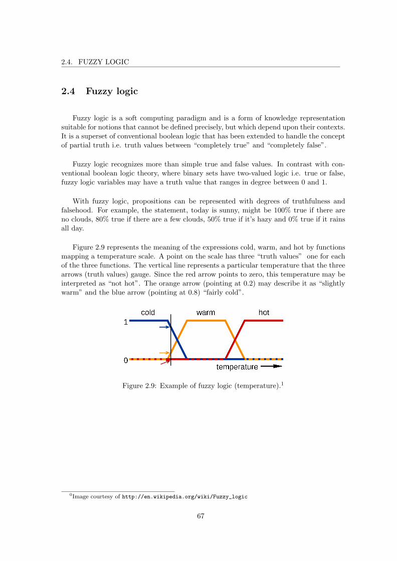
2.4. FUZZY LOGIC
2.4 Fuzzy logic
Fuzzy logic is a soft computing paradigm and is a form of knowledge representationsuitable for notions that cannot be defined precisely, but which depend upon their contexts.It is a superset of conventional boolean logic that has been extended to handle the conceptof partial truth i.e. truth values between “completely true” and “completely false”.
Fuzzy logic recognizes more than simple true and false values. In contrast with con-ventional boolean logic theory, where binary sets have two-valued logic i.e. true or false,fuzzy logic variables may have a truth value that ranges in degree between 0 and 1.
With fuzzy logic, propositions can be represented with degrees of truthfulness andfalsehood. For example, the statement, today is sunny, might be 100% true if there areno clouds, 80% true if there are a few clouds, 50% true if it’s hazy and 0% true if it rainsall day.
Figure 2.9 represents the meaning of the expressions cold, warm, and hot by functionsmapping a temperature scale. A point on the scale has three “truth values” one for eachof the three functions. The vertical line represents a particular temperature that the threearrows (truth values) gauge. Since the red arrow points to zero, this temperature may beinterpreted as “not hot”. The orange arrow (pointing at 0.2) may describe it as “slightlywarm” and the blue arrow (pointing at 0.8) “fairly cold”.
Figure 2.9: Example of fuzzy logic (temperature).1
0Image courtesy of http://en.wikipedia.org/wiki/Fuzzy_logic
67

2.4. FUZZY LOGIC
Fuzzy sets were first proposed by Lofti A. Zadeh in [A. and Zadeh, 2008]. This paperlaid the foundation for the modern fuzzy logic. It mathematically defined fuzzy sets andtheir properties, as given by:
Let X be a space of points, with a generic element of X denoted by x. Thus X = {x}.A fuzzy set A in X is characterized by a membership function f
A
(x) which associateswith each point in X a real number in the interval [0, 1], with the values of f
A
(x) at xrepresenting the “grade of membership” of x in A. Thus, the nearer the value of f
A
(x) tounity, the higher the grade of membership of x in A.
This definition of a fuzzy set is like a superset of the definition of a set in the ordinarysense of the term. The grades of membership of 0 and 1 correspond to the two possibilitiesof truth and false in an ordinary set. The ordinary boolean operators that are used tocombine sets no longer apply; we know that 1 AND 1 is 1, but what is 0.7 AND 0.3?
Membership functions for fuzzy sets can be defined in any number of ways as longas they follow the rules of the definition of a fuzzy set. The shape of the membershipfunction used defines the fuzzy set and so the decision on which type to use is dependenton the purpose. The membership function choice is the subjective aspect of fuzzy logic, itallows the desired values to be interpreted appropriately. Figure 2.10 shows the commonlyemployed shapes of trapezoid, triangle and Gaussian, for the fuzzy membership functions.
Figure 2.10: Some shapes commonly employed for the membership function S(x).1
1Image from [Borges, 1996]
68

2.4. FUZZY LOGIC
Traditional boolean logic uses the boolean operators AND, OR, and NOT to performthe intersection, union and complement operations. These operators work well forboolean sets but fuzzy logic does not have a finite set of possibilities for each input. Theoperators need to be defined as functions for all possible fuzzy values, that is, all realnumbers from 0 to 1 inclusive. The operators for fuzzy sets are given in Table 2.1. Figure2.11 shows an illustration of these operators for triangular membership function of fuzzylogic.
Table 2.1: Defining operators for fuzzy sets.
Operator For fuzzy sets
A AND B min(A, B)
A OR B max(A, B)
NOT A (1 - A)
Figure 2.11: Pictorial illustration of operations on boolean and fuzzy logic.1
1Image courtesy of http://www.mathworks.fr/help/toolbox/fuzzy/bp78l6_-1.html
69

2.4. FUZZY LOGIC
We refer the interested reader to [Klir and Yuan, 1995], [A. and Zadeh, 2008],[Radzikowska and Kerre, 2002] and [Liu, 2010] for further reading on fuzzy logic and softcomputing.
We have employed fuzzy logic to incorporate smooth transitions between the overlap-ping intervals of data (representing the various attributes of graphs). This enables ourmethod to minimize the information loss while mapping from continuous graph space todiscrete feature vector space, and to gracefully handle noise (and deformations) in graphs,for proposing a robust embedding of graphs into numeric feature vectors.
70

2.5. LIMITATIONS OF EXISTING METHODS AND OUR CONTRIBUTIONS
2.5 Limitations of existing methods and our contributions
In this section, we discussed the broad classification of graph comparison methods byproviding a summary of the important methods in each category.
First we introduced the methods of exact graph matching. From a graph theory ap-proach, such as the isomorphism of graphs and subgraphs, these techniques are designedto verify the similarity between two graphs. However, their rigid character penalize thedistortions in graphs. Their performance is related to the quality of representation of databy graphs. In addition to computing the similarity between two graphs, these methodsof graph matching provide details on the comparison of the topologies of the two graphswith a proposed mapping between the nodes of the two graphs nodes. This informationturns out to be very useful in a system of information retrieval where the query is a partialobject that we are looking to locate in a bigger object. Pattern recognition by graphsallows this type of search through the use of matches. On the other hand the statisticalapproaches require a priori segmentation of objects, or using a sliding window, involving adi�cult parameter which highly influences the the quality of results. The graph matchingalgorithms provide the node to node mapping between two graphs only if an isomorphismexists (and is established) between them.
All distortions result into a no-match, whatsoever the are. To address this problem, theerror tolerant graph matching methods suggest to relax the constraints on the matchingof nodes and arcs. They find the isomorphism, tolerant to noise. This allows them tobe applicable to the data that contains distortions (which exist very often in patternrecognition and image analysis). The inexact matching methods o↵er greater tolerance tomatch two nodes (or two edges) with slight di↵erence. But these methods are complex toimplement.
We have seen that the other proposed methods allow more tolerance to noise but losethe matching between vertices of graphs. The distances between graphs are defined as themost intuitive to quantify similarities between graphs. They provide a measure that ise↵ective when used in classification and robust to di↵erent noise. However, the algorithmsare complex and this complexity can be a significant obstacle in some cases.
Implicit graph embedding in a vector space, bridge the e↵ectiveness of statistical classi-fication tools with the flexibility and descriptive power of graphs. However, the algorithmsused are very complex. The distance calculation performed in the graph space is itselfcomplex.
The vector representation of graphs by an explicit graph embedding algorithm seemsto be the track to meet the technical obstacles for pattern recognition. This is becauseof the fact that they can, in theory, combine e↵ectively the power and flexibility of graphrepresentation with the diversity and complexity of statistical tools. However, no e�cientand simple method to adapt to the data is yet available.
71

2.5. LIMITATIONS OF EXISTING METHODS AND OUR CONTRIBUTIONS
By analyzing all the methods described in this chapter, we can mention the followingimportant limitations of graph matching methods:
Exact methods cannot deal with noise and deformations.
Exact methods cannot deal with attributes on nodes and edges of the graph.
Exact methods cannot deal with huge graphs.
Error tolerant methods are time consuming.
Error tolerant methods do not have the ability to achieve unsupervised learning.
Error tolerant methods need training dataset.
Error tolerant methods have the worst management of discretization step.
The computation of distance between graphs is computational expensive.
To the best of our knowledge, most of the existing works on graph embedding canhandle only the graphs which are comprised of edges with a single attribute and verticeswith either no or only symbolic attributes. These methods are only useful for specificapplication domains for which they are designed. Our proposed method of explicit graphembedding can embed attributed graphs with many symbolic as well as numeric attributeson both nodes and edges.
Our proposed method of explicit graph embedding does not require any dissimilaritymeasure between graphs and proposes a natural embedding of topological, structural andattribute information of an input graph into a feature vector.
The method is applicable to undirected as well as directed attributed graphs, withoutimposing any restriction on the size of graphs.
We employ fuzzy overlapping trapezoidal intervals for minimizing the information losswhile mapping from continuous graph space to discrete feature vector space. The use offuzzy logic enables our method to gracefully handle noise (deformations) in graphs and topropose a robust embedding of graphs into numeric feature vectors.
Our method does not necessarily need any labeled training set and has built-in un-supervised learning abilities. In scenarios where no additional training set is available,the method has the capability to exploit the graph dataset to be embedded into featurevectors, for adapting its parameters during an o↵-line unsupervised learning phase. Oncethe learning is performed it o↵ers real-time embedding of attributed graphs into featurevectors.
72

2.5. LIMITATIONS OF EXISTING METHODS AND OUR CONTRIBUTIONS
Many existing solutions for graph embedding are based on spectral analysis of theadjacency matrix of graphs and o↵er to utilize the statistical significant details in graphsfor embedding them into feature vectors. Our method exploits the topological, structuraland attribute information of the graphs along-with the statistical significant information,for constructing feature vectors. The proposed feature vector is very significant for ap-plication domains where the use of graphs is mandatory for representing rich structuraland topological information, and an approximate but computational e�cient solution isneeded.
Our proposed method of graph embedding does not require any labeled learning set,another important extension to the existing works is the inexpensive deployment of ourgraph embedding method to a wide range of application domains.
We propose to extend the methods in literature by o↵ering the embedding of directedand undirected attributed graphs with numeric as well as symbolic attributes on bothnodes and edges. We propose a consistent embedding of graphs i.e. two similar graphs aremapped to points near to each other in feature vector space. Multi facet information fromglobal, topological and local point of view seems very important to be preserved. Theextraction of topological and structural level details and multilevel distribution analysisof graph are the novelty of our work.
In the rest of the dissertation we present our work on explicit graph embedding. Wepropose an e�cient method to achieve simple and straightforward embedding of attributedgraphs into feature vectors, for answering the problems of graph classification and graphclustering.
73

2.5. LIMITATIONS OF EXISTING METHODS AND OUR CONTRIBUTIONS
74
Chapter 3
Fuzzy Multilevel GraphEmbedding
In this chapter we outline our explicit graph embedding method i.e. the Fuzzy MultilevelGraph Embedding (FMGE). We first present an overall global description of FMGE andthen present details on the FMGE framework. We elaborate the description of FMGEby example graphs of primitive geometric shapes. We briefly introduce the application ofFMGE to graph classification, graph clustering and graph retrieval.
3.1 Introduction
This chapter presents detailed description of our proposed method of explicit graphembedding i.e. the Fuzzy Multilevel Graph Embedding. For improving the continuity andreadability of the dissertation we use the abbreviation FMGE for referring to the FuzzyMultilevel Graph Embedding.
For embedding an attributed graph into a numeric feature vector, FMGE performsmultilevel analysis of graph to extract discriminatory information of three di↵erent levelsfrom a graph. This includes the graph level information, structural level information andthe elementary level information. The three levels of information represent three di↵erentviews of graph for extracting coarse (global) details, then going more deep to the details
75

3.1. INTRODUCTION
on the topology of graph and then penetrating into details on the elementary buildingunits of the graph. The multilevel analysis of a graph enables FMGE to look upon it fromthree di↵erent perspectives. Graph level information permits FMGE to extract generalinformation about a graph. The structural level information allows FMGE to extracthomogeneity of subgraphs in a graph. And the elementary level information allows FMGEto penetrate into more in-depth and granular view of a graph, for extracting discriminatoryinformation from the elementary building blocks of graphs.
FMGE encodes the numeric part of each of the di↵erent levels of information by fuzzyhistograms. It constructs the fuzzy histograms by employing fuzzy logic. The use of fuzzylogic permits FMGE to use smooth transition between the intervals of the histogramsand enables FMGE to minimize the information loss while embedding graphs into featurevectors. FMGE encodes the symbolic part of the multilevel information of a graph bycrisp histograms. Once the histograms are constructed, FMGE employs the histogramrepresentation of the multilevel information of a graph for embedding it into a numericfeature vector.
FMGE adapts the parameters for constructing the fuzzy and crisp histograms to un-derlying graphs by its unsupervised learning capabilities, without requiring any labeledlearning set.
In this chapter we first describe the input, output and the multilevel information in thefeature vector of FMGE. Afterwards, we present a detailed description of FMGE frame-work: we present the unsupervised learning phase of FMGE and the graph embeddingphase of FMGE.
Initial versions of this work have been published in [Luqman et al., 2009b],[Luqman et al., 2009a], [Luqman et al., 2010c], [Luqman et al., 2010d] and[Luqman et al., 2010a].
To facilitate the explanation and comprehension of the description of FMGE, we haveused example graphs of primitive geometric shapes, of unit length, of a rectangle, anoccluded square and a triangle. The example graphs and their corresponding shapes areshown in Figure 3.1.
In Figure 3.1, a vertex in graph is an abstract representation of a primitive line inunderlying content, with an attribute of length L. An edge in graph represents the con-nectivity relationship between two primitive lines in underlying content, with their relativelength RL and angle Angle between them as the edge attributes.
76

3.1. INTRODUCTION
(a) A rectangle.
(b) An occluded square.
(c) A triangle.
Figure 3.1: Attributed graph representation of basic geometric shapes of unit length.
77

3.2. OVERVIEW OF FUZZY MULTILEVEL GRAPH EMBEDDING (FMGE)
3.2 Overview of fuzzy multilevel graph embedding (FMGE)
A block diagram of FMGE is presented in Figure 3.2. It accepts a collection of mattributed graphs as input and encodes their topological, structural and attribute detailsinto m equal size feature vectors.
Figure 3.2: Overview of Fuzzy Multilevel Graph Embedding (FMGE).
As shown in Figure 3.2, FMGE accepts a collection of m attributed graphs as input, asgiven by:
{AG1
, AG2
, ..., AGe
, ..., AGm
}
where the eth graph is denoted by:
AGe
= (Ve
, Ee
, µV
e , µE
e).
For the input collection of m attributed graphs, FMGE produces a collection of msame size feature vectors as output, as given by:
{FSMFV1
, FSMFV2
, ..., FSMFVe
, ..., FSMFVm
}
The eth input graph AGe
is embedded into feature vector FSMFVe
:
78
3.2. OVERVIEW OF FUZZY MULTILEVEL GRAPH EMBEDDING (FMGE)
AGe
7�! �(AGe
) = FSMFVe
where FSMFVe
is a point in n dimensional vector space Rn:
FSMFVe
= (fe1 , fe2 , ..., fen)
3.2.1 Description of feature vector of FMGE
We have named the feature vector of FMGE as Fuzzy Structural Multilevel FeatureVector and abbreviated it as FSMFV. It contains features extracted from three levels ofinformation in graph:
i) Graph level information
ii) Structural level information
iii) Elementary level information
The features for graph level information represent a coarse view of graph and give ageneral information about the graph. These features include the graph order and graphsize.
The features for structural level information represent a deeper view of graph and areextracted from the node degrees and subgraph homogeneity in graph.
The third level of information is extracted by penetrating into further depth and moregranular view of graph and employing details of the elementary building blocks of graph.These features represent the information extracted from the node and edge attributes.
FSMFV is a vector in n dimensional vector space Rn, given as:
FSMFV = (f1
, f2
, ..., fn
)
The overall structure of FSMFV is presented in Figure 3.3.
79

3.2. OVERVIEW OF FUZZY MULTILEVEL GRAPH EMBEDDING (FMGE)
Structural Level Information
[intermediate details]
Elementary Level Information
[micro details]
Graph Level Information
[macro details]
Figure 3.3: The Fuzzy Structural Multilevel Feature Vector (FSMFV).
In subsequent subsections we present detailed discussion on each of the three di↵erentlevels of information in FSMFV.
3.2.1.1 Embedding of graph level information
The graph level information in FSMFV is embedded by two numeric features, encodingthe order and the size of graph.
Graph order: A graph vertex is an abstract representation of the primitive compo-nents of underlying content. The order of a graph provides very important discriminatorytopological information on the graph.
Graph order (|V |) allows to discriminate between a small graph in Figure 3.1(c) andbigger graphs in Figure 3.1(b) and Figure 3.1(a) (|V | = 3 vs |V | = 4). At the same timeit permits to define a similarity between two equal ordered graphs in Figure 3.1(b) andFigure 3.1(a) (|V | = 4).
Graph size: An edge is an abstract representation of the relationship between theprimitive components of underlying content. Graph size also provides important discrim-inatory information on the topological details of graph.
Two equal ordered graphs in Figure 3.1(b) and Figure 3.1(a) are di↵erentiated by graphsize (|E|) i.e. a thin graph in Figure 3.1(b) is di↵erentiated from a thicker graph in Figure3.1(a) (|E| = 3 vs |E| = 4). At the same time it permits to define a similarity betweentwo equal sized graphs in Figure 3.1(c) and Figure 3.1(b) (|E| = 3).
80

3.2. OVERVIEW OF FUZZY MULTILEVEL GRAPH EMBEDDING (FMGE)
3.2.1.2 Embedding of structural level information
The embedding of structural level information is a novelty and the most critical part ofFMGE. Very few existing works on graph embedding clearly use this information. We usenode degrees information and subgraph homogeneity measure embedded by histograms ofnode attributes resemblance and edge attributes resemblance, for embedding structurallevel information. Figure 3.4 outlines this part of FSMFV.
Histograms of node attributes resemblancehnrd
and hnr1
, hnr2
, . . . , hnrk
Histograms of edge attributes resemblanceher1
, her2
, . . . , herl
Histogram of node degreeshd
Figure 3.4: Embedding of structural level information.
Node degrees: The degrees of nodes represent the distribution of edges in graphand provide complementary discriminatory information on the structure and topology ofgraph. It permits to discriminate between densely connected graphs and sparsely con-nected graphs. Node degrees information is encoded by a histogram of s
i
fuzzy intervals.The fuzzy intervals are learned during a prior learning phase, which employs degrees ofall the nodes of all graphs in dataset. Node degrees features (hd in Figure 3.4), for anattributed graph, embeds the histogram of its nodes for the s
i
fuzzy intervals. In Figure3.4, the histogram hd is a fuzzy histogram as node degrees is a numeric information.
For directed graphs this feature is represented by two sub-features of in-degree andout-degree i.e. a fuzzy histogram for encoding the distribution of in-degrees and an otherfuzzy histogram for encoding the distribution of out-degrees of nodes.
The node degree information for the graphs in Figure 3.1(c), 3.1(b) and 3.1(a) permitsto increase the precision of the similarity between graphs. For example, the graphs inFigure 3.1(c) and Figure 3.1(b) represent two di↵erent topologies (|V | = 3 and |V | = 4)and a relatively similar geometry (|E| = 3). On the other hand, the graphs in Figure3.1(b) and Figure 3.1(a) represent two di↵erent geometries (|E| = 3 and |E| = 4) and aquite similar topology (|V | = 4). Furthermore, the graphs in Figure 3.1(c) and Figure3.1(a) represent two di↵erent topologies (|V | = 3 and |V | = 4) and geometries (|E| = 3and |E| = 4). By incorporating the node degree information, it is very straightforwardto conclude that graphs in Figure 3.1(b) and Figure 3.1(a) are more similar to each otherthan the graph in Figure 3.1(c).
81

3.2. OVERVIEW OF FUZZY MULTILEVEL GRAPH EMBEDDING (FMGE)
Node attribute’s resemblance for edges: The resemblance between two primi-tive components that have a relationship between them, in a graph, is a supplementaryinformation available in the graph. The node attribute’s resemblance for an edge encodesstructural information for the respective node-couple. To compute resemblance informa-tion for an edge, the node degrees of its two nodes and the list of node attributes as givenby µV are employed for extracting additional information. This additional information isrepresented as new edge attributes and is processed like other edge attributes.
Given an edge between two nodes, say node1
and node2
in a graph. The resemblancebetween a numeric node attribute a is computed by Equation 3.1 and the resemblancebetween a symbolic node attribute b is computed by Equation 3.2.
For each numeric node attribute, the resemblance attribute nr is represented by snr
features in FSMFV. This resemblance information is encoded by a fuzzy histogram ofsnr
fuzzy intervals. The fuzzy intervals are learned during a prior learning phase, whichemploys resemblance attribute nr of all the edges of all graphs in dataset.
resemblance(a1
, a2
) = min(|a1
|, |a2
|)/max(|a1
|, |a2
|) (3.1)
where,a 2 {node degree, µV },a1
is the value of the attribute a for node1
anda2
is the value of the same attribute a for node2
.
resemblance(b1
, b2
) =
����1 b
1
= b2
0 otherwise
���� (3.2)
where,b 2 µV ,b1
is the value of the attribute b for node1
andb2
is the value of the same attribute b for node2
.
For each symbolic node attribute, we represent the resemblance attribute nr by exactlytwo possible numeric features. The resemblance for symbolic attributes can either be 0or 1 (Equation 3.2). The cardinalities of the two resemblance values in input graph, areencoded by a crisp histogram which is used as features in FSMFV.
In Figure 3.4 the histogram hnrd
represents the features for encoding resemblance at-tribute for node degrees. Whereas, the histograms hnr
1
, hnr2
, . . . , hnrk
represent the featuresfor encoding resemblance attributes for k node attributes µV . The histogram hnr
d
is afuzzy histogram since node degree is a numeric information. Each of the histograms
82

3.2. OVERVIEW OF FUZZY MULTILEVEL GRAPH EMBEDDING (FMGE)
hnr1
, hnr2
, . . . , hnrk
, is a crisp histogram if its corresponding attribute is symbolic and is afuzzy histogram if the attribute that it is encoding is a numeric attribute.
Node attribute’s resemblance for edges of example graphs is shown in Figure 3.5. Twonew attributes are added to the edges of the example graphs: the resemblance attribute“resemblanceL” and the resemblance attribute “resemblanceNodeDegree”. These newattributes on edges provides more precision to FMGE for discriminating between thegraphs.
Edge attribute’s resemblance for nodes: The resemblance among the relation-ships associated to a primitive component, is a supplementary information available in thegraph. The edge attribute’s resemblance for a node encodes the structural informationfor the respective edges of node and brings more topological information to FSMFV. Tocompute resemblance information for a node, each attribute of its edges (as given by µE) isemployed for extracting additional information. This additional information is representedas new node attributes and is processed like other node attributes.
Given a node, say node in a graph, the resemblance for the edges connected to nodeis computed as the mean of the resemblances between all the pair of edges connected tonode. For a pair of edges, say edge
1
and edge2
connected to node, the resemblance for anumeric attribute c is computed by Equation 3.3 and the resemblance between a symbolicedge attribute d is computed by Equation 3.4.
resemblance(c1
, c2
) = min(|c1
|, |c2
|)/max(|c1
|, |c2
|) (3.3)
where,c 2 µE ,c1
is the value of the attribute c for edge1
andc2
is the value of the same attribute c for edge2
.
resemblance(d1
, d2
) =
����1 d
1
= d2
0 otherwise
���� (3.4)
where,d 2 µE ,d1
is the value of the attribute d for edge1
andd2
is the value of the same attribute d for edge2
.
For each symbolic edge attribute, the resulting resemblance attribute er is treated asa numeric attribute and is embedded by a fuzzy histogram. The resemblance for symbolicedge attributes is computed as mean of the resemblances between all the pair of edges
83

3.2. OVERVIEW OF FUZZY MULTILEVEL GRAPH EMBEDDING (FMGE)
connected to a node. Although the resemblance for a pair of edges is always either 0 or 1but mean resemblance for all the pair of edges of a node can be any numeric value (thisis di↵erent from the symbolic node attribute’s resemblance which is always either 0 or1). Therefore, for each symbolic and numeric edge attribute, the resemblance attributeer is represented by s
er
features in FSMFV. This resemblance information is encoded bya fuzzy histogram of s
er
fuzzy intervals. The fuzzy intervals are learned during a priorlearning phase, which employs resemblance attribute er of all the nodes of all graphs indataset.
In Figure 3.4 the histograms her1
, her2
, . . . , herl
represent the features for encoding re-semblance attributes for l edge attributes µE . Each of the histograms her
1
, her2
, . . . , herl
, isa fuzzy histogram.
Edge attribute’s resemblance for nodes of example graphs is shown in Figure 3.5. Twonew resemblance attributes are added on the nodes of the example graphs: the resemblanceattribute “resemblanceRL” and the resemblance attribute “resemblanceAngle”. These newattributes on nodes compliments the node attribute’s resemblance on edges and enablesFMGE to extract information for discriminating between the graphs.
84

3.2. OVERVIEW OF FUZZY MULTILEVEL GRAPH EMBEDDING (FMGE)
(a) Rectangle.
(b) Occluded square.
(c) Triangle.
Figure 3.5: Resemblance attributes for the attributed graph representation of basic geo-metric shapes of unit length.
85

3.2. OVERVIEW OF FUZZY MULTILEVEL GRAPH EMBEDDING (FMGE)
3.2.1.3 Embedding of elementary level information
Embedding of elementary level information allows FMGE to extract discriminatoryinformation from individual nodes and edges of the graph. The symbolic attributes areencoded by crisp histograms and the numeric attributes by fuzzy histograms. FMGE canembed attributed graphs with many symbolic and numeric attributes on both nodes andedges.
For every symbolic node attribute, each modality that can be taken by this attribute isrepresented by exactly one numeric feature in FSMFV. This feature encodes the cardinalityof this modality in an input graph.
Each numeric node attribute is encoded by a fuzzy histogram of its si
fuzzy intervals.The fuzzy intervals are learned for each of the numeric node attributes in the input graphdataset during a prior learning phase. The features for a numeric attribute of an inputgraph, embeds the histogram for these s
i
fuzzy intervals.
Figure 3.6 outlines this part of FSMFV.
Histograms of node attributeshn1
, hn2
, . . . , hnk
Histograms of edge attributeshe1
, he2
, . . . , hel
Figure 3.6: Embedding of elementary level information.
Node attributes: The node attributes provide additional details on primitive compo-nents of underlying content and aid FSMFV to discriminate between two similar structuredgraphs. In Figure 3.6 the histograms hn
1
, hn2
, . . . , hnk
represent the features for encoding knode attributes µV . Each of the histograms hn
1
, hn2
, . . . , hnk
, is a crisp histogram if its corre-sponding attribute is symbolic and is a fuzzy histogram if the attribute that it is encodingis a numeric attribute.
The node attributes are very important information for discriminating between twoequal ordered and equal sized graphs, which are representing quite similar structure aswell (for example the graph of a small square can be di↵erentiated from that of a bigsquare by using a length attribute on the nodes).
The length attribute L of the graph nodes in Figure 3.5(a) provide additional detailson the graph and clearly discriminates it from the graph in Figure 3.5(b).
86

3.2. OVERVIEW OF FUZZY MULTILEVEL GRAPH EMBEDDING (FMGE)
Edge attributes: The edge attributes provide supplementary details on the rela-tionships between the primitive components of the underlying content and aid FSMFVto discriminate between two similar structured graphs. In Figure 3.6 the histogramshe1
, he2
, . . . , hel
represent the features for encoding l edge attributes µE . Each of the his-tograms he
1
, he2
, . . . , hel
, is a crisp histogram if its corresponding attribute is symbolic andis a fuzzy histogram if the attribute that it is encoding is a numeric attribute.
The edge attributes are very important information for discriminating between twoequal ordered and equal sized graphs, which are representing quite similar structure aswell (for example the graph of a square can be di↵erentiated from that of a rhombus byusing angle attribute on the edges).
The relative length RL and angle A attribute of the graph edges in Figure 3.5(b)provide additional details on the graph and clearly discriminates it from the graph inFigure 3.5(c).
87

3.3. FRAMEWORK OF FUZZY MULTILEVEL GRAPH EMBEDDING (FMGE)
3.3 Framework of fuzzy multilevel graph embedding (FMGE)
In FMGE framework, the mapping of input collection of graphs to appropriate points ina suitable vector space Rn is achieved in two phases i.e. the o↵-line unsupervised learningphase and the on-line graph embedding phase.
The unsupervised learning phase learns a set of fuzzy intervals for features linked todistribution analysis of the input graphs i.e. features for node degree, numeric node andedge attributes and the corresponding resemblance attributes. We refer each of them asan attribute i. For symbolic node and edge attributes and the corresponding resemblanceattributes, the unsupervised learning phase employs the modalities taken by this attributeand treat them as crisp intervals.
The graph embedding phase employs these intervals for computing di↵erent bins of therespective fuzzy or crisp histograms.
3.3.1 Unsupervised learning phase
The o↵-line unsupervised learning phase of FMGE is outlined in Figure 3.7. It learnsa set of fuzzy intervals for encoding numeric information and crisp intervals for encodingsymbolic information in graphs.
Figure 3.7: The unsupervised learning phase of FMGE.
88

3.3. FRAMEWORK OF FUZZY MULTILEVEL GRAPH EMBEDDING (FMGE)
List of values ofattribute i
in input collectionof graphs
Discretization0n0
i
crisp intervalsCrisp to fuzzy intervals 0s0
i
fuzzy intervalsfor attribute i
Figure 3.8: Learning fuzzy intervals for an attribute i.
3.3.1.1 Input and output
The input to unsupervised learning phase of FMGE is the collection of m attributedgraphs, given by:
{AG1
, AG2
, ..., AGe
, ..., AGm
}
where the eth graph is denoted by:
AGe
= (Ve
, Ee
, µV
e , µE
e)
A second input to this phase, could be if necessary, for each feature the desired numberof fuzzy intervals. This is referred by s
i
for an attribute i. Some methods of discretizationare able to find the “optimal” number of intervals by themselves (for example, equalfrequency bins, as discussed in next subsection).
As output the unsupervised learning phase of FMGE produces si
fuzzy overlappingtrapezoidal intervals for an attribute i in input graphs (example in Figure 3.9).
3.3.1.2 Description
The main steps for learning of fuzzy intervals for an attribute i are outlined in Figure3.8 and are explained in subsequent paragraphs.
The first step is the computation of crisp intervals from the list of values of attribute ifor all the graphs in input collection of graphs. This is straightforward and is achieved byany standard data discretization technique. A survey of popular discretization techniquesis presented by Liu et al. [Liu et al., 2002].
We propose to use equally spaced bins for obtaining an initial set of crisp intervals, asthey avoid over-fitting and o↵ers FMGE a better generalization capability to unseen graphsduring graph embedding phase. Algorithm 3.3.1 outlines the pseudo-code for computingan initial set of crisp intervals for an attribute i. It uses a pseudo-call ‘GetEqualSpacBin’
89

3.3. FRAMEWORK OF FUZZY MULTILEVEL GRAPH EMBEDDING (FMGE)
for getting an initial set of equally spaced bins. This pseudo-call refers to an appropriatedata discretization function (available in underlying implementation platform).
Another possibility is to use the equal frequency bins. An example of this type ofdiscretization is the technique proposed by [Colot et al., 1994] for discretization of con-tinuous data. It is based on use of Akaike Information Criterion (AIC). It starts withan initial histogram of data and finds optimal number of bins for underlying data. Theadjacent bins are iteratively merged using an AIC-based cost function until the di↵erencebetween AIC-beforemerge and AIC-aftermerge becomes negative. Thus, we get an optimalset of crisp intervals for the underlying data. This set of intervals is representative of theunderlying data. The use of an equal frequency discretization technique is demonstratedin Section 5.4 for graph clustering.
The initial set of equally spaced bins (or equal frequency bins) are used to constructa data structure, which stores the crisp intervals. This data structure is employed forcomputing s
i
fuzzy intervals for attribute i.
After computing the initial set of crisp intervals, in next step, these crisp intervals arearranged in an overlapping fashion to get fuzzy overlapping intervals. Normally trape-zoidal, triangular and Gaussian arrangements are popular choices for fuzzy membershipfunctions [Ishibuchi and Yamamoto, 2003]. We propose to use the trapezoidal member-ship function, which is the generally used fuzzy membership function. It allows a rangeof instances to lie under full membership and assigns partial membership to the boundaryinstances.
Figure 3.9 outlines a trapezoidal interval defined over crisp intervals. A trapezoidalinterval is defined by four points; as is given by points a, b, c, d in Figure 3.9.
ni
......
0
1Membership
weighta
b c
d
1 2 3 4 5 6 7 8 9
Figure 3.9: 5 fuzzy overlapping trapezoidal intervals (si
) defined over 9 equally spacedcrisp intervals (n
i
).
90

3.3. FRAMEWORK OF FUZZY MULTILEVEL GRAPH EMBEDDING (FMGE)
It is very important to highlight here that the first fuzzy overlapping trapezoidal inter-val covers all values till �1 and the last fuzzy overlapping trapezoidal interval is limitedby 1. This makes sure that during the graph embedding phase every attribute instancefalls under the range of fuzzy overlapping trapezoidal intervals and it further strengthensthe generalization abilities of the method to unseen graphs.
A fuzzy interval defined in trapezoidal fashion assigns a membership weight of 1 (fullmembership) between points b and c. The membership weight gradually approaches 0as we move from b to a and from c to d. This trapezoidal behavior allows to assignfull membership, partial membership and no membership to attribute instances. This isimportant to highlight here that the total membership assigned to an instance is alwaysexactly equal to 1 i.e. either one full membership or two partial memberships are assignedto each attribute instance.
Algorithm 3.3.2 outlines the pseudo-code for computing fuzzy overlapping trapezoidalintervals from an initial set of crisp intervals for an attribute i in input collection of graphs.It first computes the initial set of crisp intervals using Algorithm 3.3.1 and then arrangesthem in an overlapping trapezoidal fashion for obtaining a set of fuzzy overlapping trape-zoidal intervals for attribute i. The number of fuzzy intervals for attribute i depends uponthe number of features desired for attribute i in FSMFV, and is controlled by parameter s
i
which can either be manually specified, automatically learned by using an equal frequencybased discretization or empirically learned and optimized on validation set.
The number of crisp intervals ni
for desired number of fuzzy intervals si
is computedby Equation 3.5.
ni
= 2⇥ si
� 1 (3.5)
For the sake of continuity and readability, we have used the terms fuzzy intervals, fuzzyoverlapping intervals and fuzzy overlapping trapezoidal intervals interchangeably, in thisdissertation.
91

3.3. FRAMEWORK OF FUZZY MULTILEVEL GRAPH EMBEDDING (FMGE)
Algorithm 3.3.1: GetInitCrispInterval(listvaluesAttributei
, ni
)
comment:Computes equally spaced crisp intervals.
comment:Requires: List of values of an attribute i
comment:Requires: Number of crisp intervals for attribute i (ni
�2)comment:Returns: ‘n
i
’ crisp intervals for attribute i
equallySpacedBins GetEqualSpacBin(listvaluesAttributei
, ni
)
crispIntervals emptyst �1en equallySpacedBins[1]
j 1repeat8>>>><
>>>>:
crispIntervals[j].start stcrispIntervals[j].end enst enen equallySpacedBins[j + 1]j j + 1
until j>ni
return (crispIntervals)
92

3.3. FRAMEWORK OF FUZZY MULTILEVEL GRAPH EMBEDDING (FMGE)
Algorithm 3.3.2: GetFuzzyOvlapTrapzInterval(listvaluesAttributei
, si
)
comment:Computes fuzzy intervals for an attribute i.
comment:Requires: List of values of an attribute i
comment:Requires: Number of fuzzy intervals for attribute i (si
�2)comment:Returns: ‘s
i
’ fuzzy intervals for attribute i
ni
2 ⇤ si
� 1crispIntervals GetInitCrispInterval(listvaluesAttribute
i
, ni
)
fuzzyIntervals empty
fuzzyIntervals[1].a �1fuzzyIntervals[1].b �1fuzzyIntervals[1].c crispIntervals[1].endfuzzyIntervals[1].d crispIntervals[2].end
j 1jcrisp 0repeat8>>>>>>>>>>>>>>>>>>><
>>>>>>>>>>>>>>>>>>>:
j j + 1jcrisp jcrisp+ 2fuzzyIntervals[j].a fuzzyIntervals[j � 1].cfuzzyIntervals[j].b fuzzyIntervals[j � 1].d
if (jcrisp+ 1 � ni
)
then
8<
:
fuzzyIntervals[j].c 1fuzzyIntervals[j].d 1break
fuzzyIntervals[j].c crispIntervals[jcrisp+ 1].endfuzzyIntervals[j].d crispIntervals[jcrisp+ 2].end
until j � si
return (fuzzyIntervals)
93
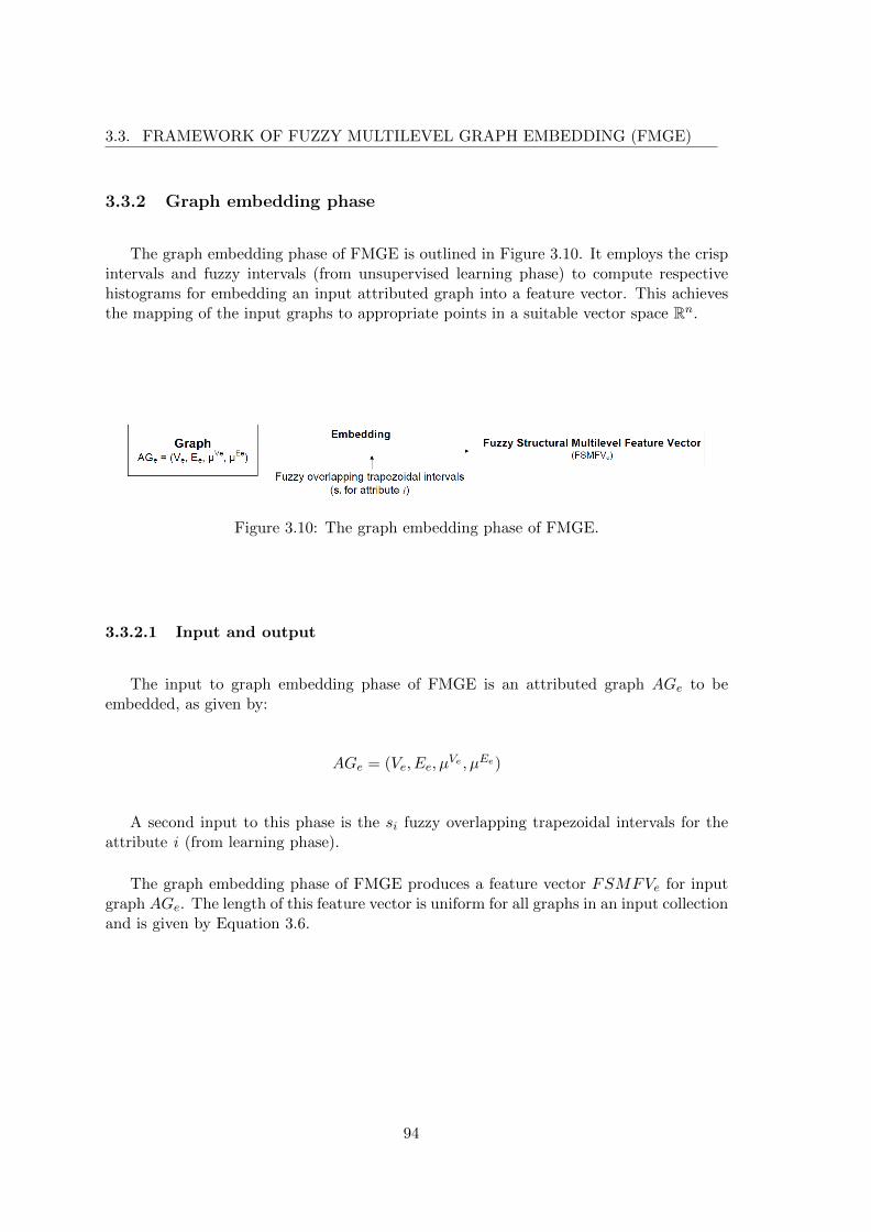
3.3. FRAMEWORK OF FUZZY MULTILEVEL GRAPH EMBEDDING (FMGE)
3.3.2 Graph embedding phase
The graph embedding phase of FMGE is outlined in Figure 3.10. It employs the crispintervals and fuzzy intervals (from unsupervised learning phase) to compute respectivehistograms for embedding an input attributed graph into a feature vector. This achievesthe mapping of the input graphs to appropriate points in a suitable vector space Rn.
Figure 3.10: The graph embedding phase of FMGE.
3.3.2.1 Input and output
The input to graph embedding phase of FMGE is an attributed graph AGe
to beembedded, as given by:
AGe
= (Ve
, Ee
, µV
e , µE
e)
A second input to this phase is the si
fuzzy overlapping trapezoidal intervals for theattribute i (from learning phase).
The graph embedding phase of FMGE produces a feature vector FSMFVe
for inputgraph AG
e
. The length of this feature vector is uniform for all graphs in an input collectionand is given by Equation 3.6.
94
3.3. FRAMEWORK OF FUZZY MULTILEVEL GRAPH EMBEDDING (FMGE)
Length of FSMFV = 2 +X
si
+X
ci
(3.6)
where,- 2 refers to the features for graph order and graph size,-P
si
refers to the sum of number of bins in fuzzy interval encodedhistograms for numeric information in graph (i.e. attribute i),
-P
ci
refers to the sum of number of bins in crisp interval encodedhistograms for symbolic information in graph.
The length of the feature vector is strictly dependent on the size of histograms usedfor encoding the three levels of information. In order to give an idea on the maximumlength of the feature vector, we can safely precise that its upper limit is 150.
3.3.2.2 Description
The values of attribute i in input graph AGe
are fuzzified by employing its si
fuzzyintervals (learned during unsupervised learning phase) and trapezoidal membership func-tion.
Mathematically, the membership function ↵ defined over a trapezoidal interval x isgiven by Equation 3.7.
↵(x) =
��������
(x� a)/(b� a) a x<b1 b x c
(x� d)/(c� d) c<x d0 otherwise
��������(3.7)
In Equation 3.7, x refers to an instance of attribute i to be fuzzified and a, b, c, d refersto the limits of a trapezoidal fuzzy interval for attribute i. Function ↵(x) computes thedegree of membership of an instance x with the trapezoidal interval defined by a, b, c, d.The possible memberships can be a full membership if x is between b and c, a partialmembership if x is between a and b or is between c and d, or it can be a no membershipif x is outside the interval a, b, c, d.
We represent the fuzzy histogram of attribute i as hnumi
, which actually refers to thefuzzy histogram for node degrees (hd in Figure 3.4), the fuzzy histograms for numeric nodeattributes resemblance (hnr
d
and hnr1
, hnr2
, . . . , hnrk
in Figure 3.4), the fuzzy histograms fornumeric and symbolic edge attributes resemblance (her
1
, her2
, . . . , herl
in Figure 3.4), the
95

3.3. FRAMEWORK OF FUZZY MULTILEVEL GRAPH EMBEDDING (FMGE)
fuzzy histograms for numeric node attributes (hn1
, hn2
, . . . , hnk
in Figure 3.6) and the fuzzyhistograms for numeric edge attributes (he
1
, he2
, . . . , hel
in Figure 3.6). The fuzzy histogramof an attribute i represents the embedding of attribute i for input graph AG
e
. For an inputgraph AG
e
, the fuzzy histogram hnumi
for attribute i is constructed by first computing thedegree-of-memberships of all instances of attribute i in AG
e
for the si
fuzzy intervals. Andthen summing the memberships for each of the s
i
fuzzy interval.
Each symbolic attribute j in input graph AGk
is encoded by a histogram of all itspossible modalities (or labels). This histogram encodes the number of instances for eachpossible label of the symbolic attribute. We call this histogram as a crisp histogram(in-contrary to fuzzy histogram for numeric attributes). We call a crisp histogram for asymbolic attribute j as hsym
j
, which actually referrers to the crisp histograms for symbolicnode attributes resemblance (hnr
1
, hnr2
, . . . , hnrk
in Figure 3.4), the crisp histograms for sym-bolic node attributes (hn
1
, hn2
, . . . , hnk
in Figure 3.6) and the crisp histograms for symbolicedge attributes (he
1
, he2
, . . . , hel
in Figure 3.6).
After constructing the fuzzy interval encoded histograms for each numeric attribute iand crisp histogram for each symbolic attribute j, the FSMFV
e
for input graph AGe
isconstructed from the value of graph order, the value of graph size and fuzzy interval en-coded histograms hnum
i
of its node degree, numeric node and edge attributes appended bythe crisp histograms hsym
j
for symbolic node and edge attributes. This gives an embeddingof the input graph AG
e
into a feature vector FSMFVe
.
The histogram illustration of the graph embedding phase and the resulting featurevectors for the example attributed graphs of basic geometric shapes are given in Figure3.11. Two fuzzy trapezoidal intervals are used for embedding node degree ([�1,�1,1,2]and [1,2,1,1]) whereas three fuzzy trapezoidal intervals are used for node attribute ‘L’and edge attribute ‘RL’ ([�1, �1, 0.5, 1], [0.5, 1, 1.5, 2] and [1.5, 2, 1, 1]) and threefuzzy intervals are used for embedding numeric resemblance attributes ([�1, �1, 0.25,0.5], [0.25, 0.5, 0.75, 1.0], [0.75, 1.0, 1, 1]). Two fuzzy intervals are used for embeddingresemblance attribute for ‘Angle’ ([�1, �1, 0, 1.0], [0, 1.0, 1, 1]). The symbolic edgeattribute ‘Angle’ has two possible labels. Thus, in total the FSMFV for these graphs iscomprised of 23 features (1 for graph order, 1 for graph size, 2 for node degree, 3 for nodeattribute ‘L’, 3 for resemblance on edge attribute ‘RL’, 2 for resemblance on edge attribute‘Angle’, 3 for edge attribute ‘RL’, 2 for edge attribute ‘Angle’, 3 for resemblance on ‘L’, 3for resemblance on ‘nodeDegree’).
In Figure 3.11, the histograms in first row for each graph, present the histograms forgraph order and graph size (left to right). The center row presents histograms for nodedegree, node attributes L, resemblanceRL and resemblanceAngle respectively from left toright. The last row presents the histograms for edge attributes RL, Angle, resemblanceLand resemblanceNodeDegree respectively from left to right.
96
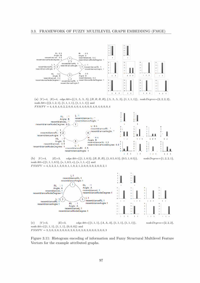
3.3. FRAMEWORK OF FUZZY MULTILEVEL GRAPH EMBEDDING (FMGE)
(a) |V |=4, |E|=4, edgeAtt={{.5, .5, .5, .5}, {B,B,B,B}, {.5, .5, .5, .5}, {1, 1, 1, 1}}, nodeDegree={2, 2, 2, 2},nodeAtt={{2, 1, 2, 1}, {1, 1, 1, 1}, {1, 1, 1, 1}} and
FSMFV = 4, 4, 0, 4, 0, 2, 2, 0, 0, 4, 0, 4, 4, 0, 0, 0, 4, 0, 4, 0, 0, 0, 4
(b) |V |=4, |E|=3, edgeAtt={{1, 1, 0.5}, {B,B,B}, {1, 0.5, 0.5}, {0.5, 1, 0.5}}, nodeDegree={1, 2, 2, 1},nodeAtt={{1, 1, 1, 0.5}, {⇤, 1, 0.5, ⇤}, {⇤, 1, 1, ⇤}} and
FSMFV = 4, 3, 2, 2, 1, 3, 0, 0, 1, 1, 0, 2, 1, 2, 0, 0, 3, 0, 2, 0, 0, 2, 1
(c) |V |=3, |E|=3, edgeAtt={{1, 1, 1}, {A,A,A}, {1, 1, 1}, {1, 1, 1}}, nodeDegree={2, 2, 2},nodeAtt={{1, 1, 1}, {1, 1, 1}, {0, 0, 0}} and
FSMFV = 3, 3, 0, 3, 0, 3, 0, 0, 0, 3, 0, 3, 0, 3, 0, 3, 0, 0, 0, 3, 0, 0, 3
Figure 3.11: Histogram encoding of information and Fuzzy Structural Multilevel FeatureVectors for the example attributed graphs.
97

3.4. CONCLUSION
3.4 Conclusion
In this chapter we have presented a method of explicit graph embedding - the FuzzyMultilevel Graph Embedding (FMGE). The method is a straightforward, simple and com-putational e�cient solution for facilitating the use of graph based powerful representationstogether with learning and computational strengths of state-of-the-art machine learning,classification and clustering. The method exploits multilevel analysis of graphs for ex-tracting three levels of information from graphs (i.e. graph level, structural level andelementary level) and embedding them into numeric feature vectors. The method o↵ersthe embedding of attributed graphs with numeric as well as symbolic attributes on bothnodes and edges. It has built-in learning abilities for adapting its parameters to underlyinggraph repositories.
However, the method is strongly dependent on the attributes of the nodes and edges inthe graph. Apart, from the elementary level details, the structural level details, which areextracted by the homogeneity of subgraphs in the graph, are also defined in terms of thenode and edge attributes. The proposed feature vector lacks in information on the topologyof the graph. This makes this method very useful for the application domains whichextract attribute rich graphs from data - i.e. there are lots of meaningful attributes. Themethod is less useful for application domains where graphs have less number of attributesand topological details (without using attributes) are required to be extracted for graphembedding.
FMGE is very useful for addressing the problems of graph classification, graph clus-tering and graph retrieval for large graph repositories.
The classification of a query graph to one of the graph classes is an important prob-lem domain of pattern recognition and is very interesting for graphics recognition, objectrecognition and shape classification. For classification problems, generally, labeled learn-ing and validation sets (with class information) are available. FMGE is fully capableof exploiting the learning set for adapting its parameters, for histogram construction, tounderlying graphs and exploiting the validation set for optimizing these parameters andselecting the best parameters for embedding underlying graphs. For such problem domainsthe use of equal space bins permits FMGE to train on learning set, validate its parameterson validation set and generalize to unseen graphs (in test set). Application of FMGE toclassification problem is further studied in Section 5.3 of the dissertation.
The clustering of a collection of graphs in groups (or clusters) is another very importantproblem domain of pattern recognition, which is very interesting for real application do-mains where the manual labeling of data is not possible or is expensive and an automatic(or semi-automatic) solution is desired. For clustering problems, generally, no labeledlearning or validation sets are available. The goal of such problems is to identify groupsof graphs in a given collection of graphs. FMGE is fully capable of solving such problems.It exploits the (same) collection of graphs during a first pass, for automatically adapting
98

3.4. CONCLUSION
its histogram construction parameters to underlying graph collection. And then duringa second pass it embeds the graphs in the collection by using the learned parameters forhistogram construction. For such problem domains the use of an equal frequency binspermits FMGE to over-fit its parameters to the underlying graphs and to o↵er the bestpossible partitioning of graphs into clusters.
For clustering problems, a second possible way of adapting the histogram constructionparameters of FMGE is by exploiting the domain knowledge. This semi-automatic wayallows a domain expert to manually adjust the number of intervals for (some or all) his-tograms of the multilevel information. FMGE then uses these parameters for embeddingthe graphs into numeric feature vectors. Application of FMGE to clustering problem isfurther studied in Section 5.4 of the dissertation.
Graph retrieval and subgraph spotting is an other widely employed problem domainof pattern recognition. It is useful for application domains where automatic indexing isdesired for graph repositories. The use of FMGE not only o↵ers automatic indexing ofgraph repositories but also the ease of query by example (QBE) and the granularity offocused retrieval. In next chapter we present details on the use of FMGE for building anunsupervised framework for such application domains.
99

3.4. CONCLUSION
100

Chapter 4
Graph retrieval and subgraphspotting through explicit graphembedding
In this chapter we present a framework for automatic indexing of attributed graph repos-itories. We demonstrate a practical application of Fuzzy Multilevel Graph Embedding(FMGE) together with classification and clustering tools, for achieving graph retrievaland subgraph spotting.
4.1 Introduction
This chapter presents detailed description on our proposed framework for automatic in-dexing of graph repositories, for performing graph retrieval and subgraph spotting. Graphretrieval refers to the problem of retrieving a graph from a graph repository, based onits similarity with an example (or query) graph. Whereas, subgraph spotting takes thegraph retrieval to further granularity and refers to the problem of retrieving a graph froma repository of graphs, based on the similarity of its subgraph with the example (or query)graph.
In our proposed framework the subgraph spotting is achieved through explicit graph
101

4.1. INTRODUCTION
embedding. The framework employs FMGE as the graph embedding method and it worksin two phases: during an o↵-line unsupervised learning phase it constructs an index for thegraph repository and during an on-line spotting phase it exploits the index for achievingsubgraph spotting.
The automatic indexing of a graph repository is achieved during o↵-line learning phase,where we:
i) break the graphs into 2-node subgraphs (a.k.a. cliques of order 2), which are primi-tive building-blocks of a graph,
ii) embed the 2-node subgraphs into feature vectors by employing our recently proposedexplicit graph embedding technique,
iii) cluster the feature vectors in classes by employing a classic agglomerative clusteringtechnique,
iv) build an index for the graph repository and
v) learn a Bayesian network classifier.
The subgraph spotting is achieved during the on-line querying phase, where we:
i) break the query graph into 2-node subgraphs,
ii) embed them into feature vectors,
iii) employ the Bayesian network classifier for classifying query 2-node subgraphs and
iv) retrieve the respective graphs by looking-up in the index of the graph repository.
The graphs containing all query 2-node subgraphs form the set of result graphs for thequery. Finally, we employ the adjacency matrix of each result graph along-with a scorefunction, for spotting the query graph in it.
The method is equally applicable to a wide range of domains, o↵ering ease of query byexample (QBE) and granularity of focused retrieval.
In this chapter we present a detailed description of the two phases of our subgraphspotting framework. To facilitate the explanation and comprehension of the presentedmaterial, we have used the terms clique of order 2 and 2-node subgraph interchangeablyas appropriate.
An initial version of this work has been published in [Luqman et al., 2010b]. A com-plete version of the work is published in [Luqman et al., 2011b] and [Luqman et al., 2012].
102

4.2. AUTOMATIC INDEXING OF A GRAPH REPOSITORY
4.2 Automatic indexing of a graph repository
The automatic indexing of a graph repository is performed during the o↵-line unsuper-vised learning phase. This phase is outlined in Figure 4.1 and is explained in succeedingparagraphs.
The input to the o↵-line unsupervised learning phase is a collection of graphs, givenby:
{AG1
, AG2
, ..., AGk
, ..., AGn
}
where, the kth graph is:
AGk
= (Vk
, Ek
, µV
k , µE
k)
First of all, these graphs are preprocessed and new resemblance attributes are addedto nodes and edges of the graphs. These resemblance attributes incorporate informationon the homogeneity in neighborhood of nodes and edges. The way these attributes arecomputed is described in section 3.2.1.2.
The next step of o↵-line unsupervised learning phase, extracts cliques of order 2 (i.e.the 2-node subgraphs) from all graphs in the input collection of graphs.
Our choice of extracting the cliques of order 2 is partly because of the fact that aclique of order 2 is the basic building block of a graph (with some structural information).And partly because the extraction of cliques of higher order (i.e. � 2) is computationalexpensive, whereas extraction of cliques of order 2 is simple and straight forward. It isachieved by a mere look-up in the adjacency matrix of graph. The set of cliques for theinput collection of graphs is given by:
{{subAG1
}, {subAG2
}, ..., {subAGk
}, ..., {subAGn
}}
where the set of subgraphs for kth input graph (AGk
) is:
subAGk
= {subAG1
k
, subAG2
k
, ..., subAGi
k
}
and ith 2-node subgraph for kth input graph (AGk
) is:
103

4.2. AUTOMATIC INDEXING OF A GRAPH REPOSITORY
subAGi
k
= (V i
k
, Ei
k
, µV
i
k , µE
i
k)
The next step in o↵-line unsupervised learning phase of our method, embeds the set of2-node subgraphs by equal size feature vectors (the FSMFVs). This is achieved by FuzzyMultilevel Graph Embedding (FMGE). The set of FSMFVs for the input collection ofgraphs is given by:
{{FSMFV1
}, {FSMFV2
}, ..., {FSMFVk
}, ..., {FSMFVn
}}
where, set of feature vectors for the 2-node subgraphs of kth input graph (AGk
) is:
FSMFVk
= {FSMFV 1
k
, FSMFV 2
k
, ..., FSMFV i
k
}
and the ith 2-node subgraph for kth input graph (AGk
) is embedded by feature vectorFSMFV i
k
.
The feature vectors are clustered into classes by an agglomerative (also called hierarchi-cal) clustering method. The clustering process starts by computing a pairwise city-block-distance metric for the features in FSMFV and builds a linkage tree using the single linkalgorithm. We use a method from [Okada et al., 2005] for getting an optimal cuto↵ forclusters - [Okada et al., 2005] is based on an econometric approach to verify that variablesin multiple regression are linearly independent.
The use of agglomerative clustering approach keeps our method free of any parameterfor number of clusters. Each cluster represents (a class of) similar 2-node subgraphs.The clustering step of (o↵-line unsupervised) learning phase assigns cluster labels to theFSMFVs of 2-node subgraphs. The cluster labels for set of cliques (FSMFV
k
) in graphAG
k
are given as:
{label FSMFV 1
k
, label FSMFV 2
k
, ..., label FSMFV i
k
}
where, label FSMFV i
k
represents the cluster label assigned to the FSMFV of the ith
clique in graph AGk
.
The labeled FSMFVs are employed for learning a Bayesian network classifier. Thisclassifier serves as a computational e�cient tool for recognizing the 2-node subgraphs inquery subgraph, during the subgraph spotting phase of our method. All state of theart classifiers are equally qualified to be used in place of the Bayesian network classifier.Our choice of using a Bayesian network classifier is primarily motivated by the fact that
104

4.2. AUTOMATIC INDEXING OF A GRAPH REPOSITORY
the probabilistic reasoning of Bayesian networks enables our framework to handle theuncertainties in the feature vector representation of the cliques in graphs.
Finally, as a last step of (o↵-line unsupervised) learning phase of our method, an indexis constructed for the input collection of graphs. This index maps a graph to the cliquesof order 2 in it. And the latter to the cluster labels. For a graph AG
k
, this is given by:
AGk
vs subAGk
= {subAG1
k
, subAG2
k
, ..., subAGi
k
}
vs {FSMFV 1
k
, FSMFV 2
k
, ..., FSMFV i
k
} vs
{label FSMFV 1
k
, label FSMFV 2
k
, ..., label FSMFV i
k
}
To facilitate the maintenance of information and ease of querying we propose to use astandard DBMS for storing the index. Given a cluster label c, the index permits to retrievethe list of cliques (which are assigned cluster label c) and the corresponding graphs.
The use of index is further elaborated in next section.
105

4.2. AUTOMATIC INDEXING OF A GRAPH REPOSITORY
OUTPUT1. Bayesian network classifier2. Index for graph repository
INPUTGraph repository
{AG1
, AG2
, ..., AGk
, ..., AGn
}
Preprocessing: Add resemblance attributes
Extract 2-node subgraphs{ {subAG
1
}, {subAG2
}, ..., {subAGk
}, {subAGn
} }
Explicit graph embedding of 2-node subgraphsinto feature vectors
{ {FSMFV1
}, ..., {FSMFVk
}, ..., {FSMFVn
} }
Cluster feature vectors in classes(i.e. assign cluster-id to each 2-node subgraph)
Learn a Bayesian network classifier
Prepare an index for graph repository( AG
k
vs {subAGk
} vs {cluster-ids for {subAGk
}} )
Figure 4.1: Automatic indexing of a graph repository.
106

4.3. SUBGRAPH SPOTTING
4.3 Subgraph spotting
The subgraph spotting is performed during on-line querying phase. The goal of sub-graph spotting phase is to retrieve the set of graphs based on a query graph AG
q
, and tohighlight the subgraphs in the retrieved graphs which are similar to AG
q
. This phase isoutlined in Figure 4.3 and is detailed in this section.
The input to on-line querying phase is a query graph comprising of at-least one cliqueof order 2. As detailed in previous section for automatic indexing of graph repository thequery graph (AG
q
) also passes through the steps of preprocessing and extraction of cliquesof order 2, as given by:
subAGq
= {subAG1
q
, subAG2
q
, ..., subAGi
q
}
and ith 2-node subgraph for query graph (AGq
) is:
subAGi
q
= (V i
q
, Ei
q
, µV
i
q , µE
i
q)
The next step is the embedding of the cliques of order 2 in query graph into featurevectors ({FSMFV
q
}), as given by:
FSMFVq
= {FSMFV 1
q
, FSMFV 2
q
, ..., FSMFV i
q
}
and the ith clique of order 2 in the query graph (AGq
) is embedded by feature vectorFSMFV i
q
.
During the next step of on-line querying phase the Bayesian network classifier is em-ployed to classify FSMFV of each query 2-node subgraph ({subAG
q
}) as belonging to oneof the cluster labels.
For each query 2-node subgraph, the Bayesian network classifier outputs a list ofposterior-probabilities for all clusters. The query 2-node subgraph is classified as high-est posterior-probability cluster.
We look-up this cluster label in repository index for getting a list of possible combi-nations of 2-node subgraphs corresponding to query. The graphs containing all the query2-node subgraphs ({subAG
q
}) form the set of result graphs for the query graph AGq
.
107

4.3. SUBGRAPH SPOTTING
The result graph set is given by:
{result AG1
, result AG2
, ..., result AGk
, ..., result AGm
}
where, the kth result graph is:
result AGk
= (Vk
, Ek
, µV
k , µE
k)
For spotting the query graph AGq
in a result graph result AGk
, we employ the adja-cency matrix of graph result AG
k
along-with a score function.
For two nodes “i” and “j”, the possible values in the adjacency matrix are summarizedin Equation 4.1. The adjacency matrix of graph result AG
k
has a value of “0” if there isno edge between “i” and “j” in the original graph result AG
k
, a value of “1” if there isan edge between “i” and “j” in the original graph result AG
k
and a value of “2” if one ofthe query 2-node subgraphs is classified (by Bayesian network) as belonging to the clusterof this 2-node subgraph (which is comprising of edge between “i” and “j”).
result AGk
(i, j) =
������
0 no edge between i and j1 an edge between i and j2 2-node subgraph in result
������(4.1)
The query graph AGq
is finally spotted in the result graph result AGk
, by looking upin the neighborhood of each 2-node subgraph of result AG
k
which is in the result i.e. each“AG
k
(i, j) = 2” in the adjacency matrix of result graph result AGk
.
We explore “w” connected neighbors of each “result AGk
(i, j) = 2”. The parameter“w” is proportional to the graph order of query graph AG
q
(|Vq
|). This ensures that theretrieved graph contains a subgraph proportional in size to query graph.
108

4.3. SUBGRAPH SPOTTING
We compute a score for each “result AGk
(i, j) = 2” using Equation 4.2.
score =2X
z=0
(z ⇥ |z|w
) (4.2)
In Equation 4.2,z is a value in the adjacency matrix (either 0,1 or 2),|z| is number of times the value z occurs in neighborhoodandw is number of connected neighbors that are looked-up.
For a clique in result graph result AGk
having the same cluster label as one of thecliques in the query graph AG
q
, Equation 4.2 actually computes a score considering wadjacent neighbors in the adjacency matrix of “result AG
k
(i, j) = 2”. The score is com-puted by summing the number of cliques of order 2 in the w adjacent neighbors (z = 1)and the number of cliques that have the same cluster label as one of the cliques in querygraph AG
q
(z = 2). The latter is given double importance than the former. The sum isnormalized by the size w of the neighborhood under consideration.
The computed score of “result AGk
(i, j) = 2” gives a confidence value for subgraphspotting of query graph AG
q
in result graph result AGk
. Score is calculated for subgrapharound all cliques in a result graph having “result AG
k
(i, j) = 2”. And then based on athreshold on the confidence values (score), the subgraphs in the result graph result AG
k
are discarded or included in the final results for subgraph spotting.
Figure 4.2 illustrates the computation of the score for a subgraph in an example adja-cency matrix. The score is computed for a clique in result graph result AG
k
having thesame cluster label as one of the cliques in the query graph AG
q
(i.e. result AGk
(i, j) = 2).The value of w is taken to be 9.
In Figure 4.2, score is computed for a clique in the result graph result AGk
. Thisclique is highlighted as green in the adjacency matrix of graph result AG
k
. The cliqueshighlighted as yellow, are the cliques that have the same cluster label as a clique in querygraph.
The cliques highlighted as cyan are the cliques of the graph result AGk
which do nothave the same label as a clique of the query graph. The inclusion of these cliques does notnecessarily mean that the method finds only connected subgraphs in the graph.
109

4.3. SUBGRAPH SPOTTING
Figure 4.2: Illustration of score function computation for a subgraph around a clique oforder 2 in a retrieved graph.
110

4.3. SUBGRAPH SPOTTING
INPUTQuery graph (AG
q
)
OUTPUTSet of m graphs which contain query graph{resultAG
1
, resultAG2
, ..., resultAGm
}
Preprocessing: Add resemblance attributes
Extract 2-node subgraphs{ {subAG
q
} }
Explicit graph embedding of 2-nodesubgraphs into feature vectors
{ {FSMFVq
} }
Classify feature vectors ({FSMFVq
}) usingBayesian network classifier
Look-up in repository index and retrieve graphs{resultAG
1
, resultAG2
, ..., resultAGm
}
Spot query subgraph in retrieved graphs
Figure 4.3: Graph retrieval and subgraph spotting.
111

4.4. CONCLUSION
4.4 Conclusion
In this chapter, we have presented a method of graph retrieval and subgraph spottingthrough explicit graph embedding. The method is a straightforward, simple and computa-tional e�cient solution clearly illustrating the use of graph based powerful representationstogether with learning and computational strengths of machine learning, classification andclustering. The method does not rely on any domain specific details and o↵ers a very gen-eral solution to the problem of subgraph spotting. This enables its less expensive and fastdeployment to a wide range of application domains. Apart from the advantages of in-corporating learning abilities in structural representations (without requiring any labeledtraining set) and o↵ering the ease of query by example (QBE) and the granularity offocused retrieval, the system does not impose any strict restrictions on the size of querysubgraph.
We have used the cliques of order 2 for constructing the index of the graph repository. Aclique of order 2 represents the basic structural unit of a graph. It contains discriminatoryinformation that FMGE extracts and embeds into feature vector. The computation forobtaining the list of cliques of order 2 (for a given graph) is simple and is achieved bya simple lookup in the adjacency matrix of graph. Our choice of a low order clique forindexing a graph repository is also motivated from the fact that the extraction of cliquesof higher order (� 2) is computational expensive and is a combinatorial problem.
112

Chapter 5
Experimentations
In this chapter we present the experimental evaluations of FMGE for the problems ofgraph clustering and graph classification. We present the experimental evaluations of theframework for automatic indexing of graph repositories for graph retrieval and subgraphspotting, with an application to content spotting in graphic document image repositories.We provide experimental results for the application of the thesis work to the real problemsof recognition, indexing and retrieval of graphic document images.
5.1 Introduction
The experimental evaluation of FMGE is performed on various standard graph datasets,by International Association of Pattern Recognition’s Technical Committee on graph-basedrepresentations (TC-15), from the fields of document image analysis, graphics recognitionand object recognition, in context of clustering, classification, retrieval and subgraph spot-ting tasks.
A first set of experimentations is performed with an aim to confirm that FMGE andthe subsequent classification and clustering in real vector spaces is applicable to di↵erentgraph classification and graph clustering problems, and also to confirm that in certaincases it outperforms the classical techniques for the latter.
113

5.2. GRAPH DATABASES
A second set of experimentations is performed to evaluate the graph retrieval andsubgraph spotting framework, with an application to content spotting in graphic documentimage repositories.
Experimental results for the application of the thesis work to the real problems ofrecognition, indexing and retrieval of graphic document images are also presented.
5.2 Graph databases
IAM graph database: Six datasets from IAM graph database repository havebeen employed for the experimentations. The IAM graph database repository is originallyproposed by [Riesen and Bunke, 2010c]. These graph datasets are publicly available1. TheIAM graph database repository contains graphs from the field of document image analysisand graphics recognition. The six datasets used for the experimentation include threeversions of letter dataset (low, medium and high level of distortions), GREC dataset,fingerprint dataset and the mutagenicity dataset.
Table 5.1 summarizes the details on the graphs in these datasets.
Table 5.1: IAM graph database details.
Dataset Size Classes Avg Max Attributesa
Train Valid Test |V | |E| |V | |E| V E
Letter LOW 750 750 750 15 4.7 3.1 8 6 2;0 0;0
Letter MED 750 750 750 15 4.7 3.2 9 7 2;0 0;0
Letter HIGH 750 750 750 15 4.7 4.5 9 9 2;0 0;0
GREC 836 836 1628 22 11.5 12.2 25 30 2;1 1;1
Fingerprint 500 300 2000 4 5.4 4.4 26 25 2;0 1;0
Mutagenicity 500 500 1500 2 30.3 30.8 417 112 0;1 1;0
a Number of attributes is given as a pair “numeric;symbolic”.
1http://www.greyc.ensicaen.fr/iapr-tc15/links.html
114

5.2. GRAPH DATABASES
GEPR graph database: GEPR graph database [Foggia and Vento, 2010] has beenemployed for experimentation on graphs from the field of object recognition. The GEPRdatabase is comprised of three graph datasets, extracted from large publicly available imagerepositories, namely the Amsterdam Library of Object Images (ALOI), the ColumbiaObject Image Library (COIL) and the Object Data Bank by Carnegie-Mellon University(ODBK).
The summary of performance evaluation subset of ALOI, COIL and ODBK graphdatasets in GEPR graph database, together with some characteristic properties, is givenin Table 5.2.
Table 5.2: GEPR graph database details.Dataset Size Classes Avg Max Attributesa
|V | |E| |V | |E| V EALOI 1800 25 18.37 17.25 134 156 2;0 0;0COIL 1800 25 34.88 32.33 100 92 2;0 0;0ODBK 1248 104 56.91 54.37 528 519 2;0 0;0a Number of attributes is given as a pair “numeric;symbolic”.
Further details on the IAM and GEPR graph datasets are presented in Appendix A ofthis dissertation.
115

5.2. GRAPH DATABASES
SESYD graph database: A new graph repository is constructed by extractinggraphs from images of architectural floor plans and electronic diagrams in SESYD imagedataset [Delalandre et al., 2010], for experimentation of the framework for automatic in-dexing of graph repositories for graph retrieval and subgraph spotting. The correspondinggraph repository is made publicly available2 for academia and scientific community forresearch purposes.
The summary of SESYD graph datasets, together with some characteristic properties,is given in Table 5.3.
Table 5.3: SESYD graph database details.Image Attributed graph
Electronic diagrams
Backgrounds 8 Avg. order 212Models 21 Avg. size 363Symbols 9600 Node attribs. 4
Edge attribs. 2Documents 800 Graphs 800Queries 1000 Graphs 1000
Architectural floor plans
Backgrounds 2 Avg. order 359Models 16 Avg. size 733Symbols 4216 Node attribs. 4
Edge attribs. 2Documents 200 Graphs 200Queries 1000 Graphs 1000
The extraction of graphs from SESYD image dataset is explained in detail in AppendixB of the dissertation.
2http://www.rfai.li.univ-tours.fr/PagesPerso/mmluqman/public/SESYD_graphs.zip
116

5.3. GRAPH CLASSIFICATION
5.3 Graph classification
The graph classification experimentation has been performed on the six graph datasetsfrom IAM graph database repository.
The three distorted versions of letter graph dataset, GREC graph dataset, fingerprintgraph dataset and the mutagenicity graph dataset are all composed of training, validationand test sets. We have employed the training set for unsupervised learning phase of FMGEand the validation set to optimize the number of fuzzy intervals for structural level andelementary level information of graphs.
To obtain the initial set of crisp intervals for graph classification experimentation, wehave used an equal spaced discretization technique. The use of an equal spaced discretiza-tion technique demonstrates the learning abilities of FMGE and its generalization abilitiesto unseen graphs in test set. Equal spaced discretization allows FMGE to ignore the shapeof distribution of the attribute i instances (structural and elementary level numeric infor-mation), for learning the s
i
fuzzy intervals for it. The shape of this distribution is notimportant and keeping FMGE independent of it allows FMGE to generalize to graphs inmany diverse test sets.
The number of fuzzy intervals to be used for an attribute i in a given graph datasethas been optimized empirically on the respective validation set. The experimentation wasrepeated for 2 to 30 fuzzy intervals for each attribute i. The number of intervals maximizingthe classification rate on validation set were used for evaluating the performance of FMGEon graphs in test set.
For graph classification experimentation we have employed a nearest neighbor classifier(1-NN) with Euclidean distance.
Table 5.4 presents the classification results of FMGE and compares them with the beststate-of-the-art results from dissimilarity based graph embedding technique of Bunke etal. [Bunke and Riesen, 2011b], on these datasets.
Contrary to our choice of nearest neighbor classifier Bunke et al. have employed anSVM for their experimentation; which is a more sophisticated classifier. For comparisonpurposes this does not make a great di↵erence and the use of a sophisticated classifier willonly increase the performance of our graph embedding method.
117

5.3. GRAPH CLASSIFICATION
The first column of Table 5.4 presents the classification results for the reference system.The reference system is comprised of a graph edit distance based nearest neighbor classifier[Bunke and Riesen, 2011b]. The choice of reference system is a direct outcome of the factthat there is a lack of general classification algorithms that can be applied to graphs.One of the few classifiers directly applicable to arbitrary graphs is the k-nearest-neighborclassifier (k-NN). Given a labeled set of training graphs, an unknown graph is assignedto the class that occurs most frequently among the k nearest graphs (in terms of editdistance) from the training set. The decision boundary of this classifier is a piecewiselinear function which makes it very flexible [Bunke and Riesen, 2011b]. This classifier inthe graph domain also serves as the reference system for our experimentation.
Table 5.4 presents the classification results for two setups of FMGE. These setups referto the way in which we have computed edge attributes resemblance for nodes. Column 3shows the classification results, when the average (or mean) resemblance of the couple ofedges is used for defining edge attributes resemblance for nodes - the AVG setup. Column4 shows the classification results, when the standard deviation of the resemblance of thecouple of edges is used for defining edge attributes resemblance for nodes - the STD setup.Both setups give the same classification rates except for fingerprint graphs. This illustratesthat for these graph datasets the resemblance between the couple of edges for the nodesremains stable in both AVG and STD setups.
The three letter graph datasets, the GREC graph dataset, the fingerprint graph datasetand the mutagenicity graph dataset are all comprised of graphs with only two numericattributes (x,y position of primitive in underlying image) on nodes. The only datasetamong these is the GREC graph dataset which has one symbolic attribute on nodes inaddition to the numeric position attributes. Similarly only GREC graphs, fingerprintgraphs and mutagenicity graphs have attributes on edges.
Given the fact that the structural and elementary level information extracted by FMGEis directly or indirectly linked with the attributes of nodes and edges in graphs. In ouropinion the attributes, on graphs in these six datasets, are not enough for extracting a lotof discriminatory information by FMGE. However, even then the results are comparableto state-of-the-art results on these datasets.
FMGE has the highest classification rate on GREC graphs and mutagenicity graphs.For letter low graphs and fingerprint graphs the FMGE results are comparable to the state-of-the-art results and the reference system. But for letter MED graphs and letter HIGHgraphs the FMGE results are not very good. This is because of the fact that the level ofdistortion for these graphs is very high. The medium and high levels of distortions totallychange the topology of the graphs (and the underlying letter becomes unrecognizable).Most of the letters that undergo distortions of medium and high strength are di�cult tobe recognized, even for a human observer [Riesen, 2010].
118

5.3. GRAPH CLASSIFICATION
If more information is put on the nodes and edges of the graphs the FMGE resultsfor these datasets will be improved; as FMGE extracts most of the information from nodeand edge attributes (directly or indirectly). More interesting information that may beextracted from underlying image content may include color, shape, rotation and scaleinformation. More details on the nodes and edges of graphs will result into extraction(and eventually embedding) of more discriminatory information by FMGE. The latter willresult into improved classification results.
119

5.3. GRAPH CLASSIFICATION
Tab
le5.4:
Exp
erim
entalresults(%
),forgrap
hclassification
onIA
Mgrap
hdatab
aserepository.
Data
set
Gra
ph
edit
dista
nce
Dissimilarity
FM
GE
FM
GE
based
refere
ncesy
stem
based
embedding
resemblance:AVG
resemblance:STD
Bunke
etal.[Bunke
andRiesen,20
11b]
[k-N
Nclassifier]
[SVM
classifier]
[1-N
Nclassifier]
[1-N
Nclassifier]
LetterLOW
99.3
99.3
97.1
97.1
LetterMED
94.4
94.9
75.7
75.7
LetterHIG
H89
.192
.960
.560
.5
GREC
82.2
92.4
97.5
97.5
Fingerprint
79.1
74.9
73.5
Mutagenicity
66.9
68.6
68.6
120

5.4. GRAPH CLUSTERING
5.4 Graph clustering
The graph clustering experimentation has been performed on the six graph datasetsfrom IAM graph database repository (the three distorted versions of letter graph dataset,GREC graph dataset, fingerprint graph dataset and the mutagenicity graph dataset) andthe GEPR graphs.
In this section we present details on the two sets of experimentations.
IAM graph database: The six graph datasets, namely, three letter graph datasets,GREC graph dataset, fingerprint graph dataset and the mutagenicity graph dataset, wereemployed for graph clustering experimentation. We merged the graphs in training, vali-dation and test sets of the respective graph datasets for constructing datasets for graphclustering experimentation.
Generally, for clustering tasks no separate learning set is available. This scenario is verywell simulated by our experimentation. The unsupervised learning phase of FMGE usedthe graphs to be clustered for learning the fuzzy intervals for various numeric attributesin graphs.
The experimentation was performed for each of the six graph datasets, independentof other datasets. For each of the six graph datasets, during a first pass (unsupervisedlearning phase) FMGE learned a set of fuzzy intervals for the numeric attributes (structuraland elementary level information in graphs). These fuzzy intervals were then employedduring the graph embedding phase of FMGE.
For clustering experimentation we have used a more sophisticated discretization tech-nique for obtaining the initial set of crisp intervals. This technique is originally proposedby [Colot et al., 1994] for discretization of continuous data and is based on use of AkaikeInformation Criterion (AIC). It starts with an initial histogram of data and finds optimalnumber of bins for underlying data. The adjacent bins are iteratively merged using anAIC-based cost function until the di↵erence between AIC-beforemerge and AIC-aftermergebecomes negative. Thus, we get an optimal set of crisp intervals for the underlying data.This set of intervals could be safely termed as equal frequency intervals and is representa-tive of the underlying data.
In other words we can say that the number of fuzzy intervals for node degree, numericnode attributes and numeric edge attributes is calculated from the spread of the respectiveattributes values for the graph dataset. The resulting fuzzy intervals are true representativeof the shape of distribution of these attribute values and are very interesting for embeddingthe respective graphs by FMGE.
121

5.4. GRAPH CLUSTERING
The use of an equal frequency discretization technique (without any training set)demonstrates the unsupervised learning abilities of FMGE in scenarios where no sepa-rate training set is available.
We have employed the well known and popular k-means clustering paradigm withEuclidean distance and random non-deterministic initialization, for our graph clusteringexperimentation.
Figure 5.1 presents the Silhouette metric [Kaufman and Rousseeuw, 1990] for datasetsin IAM graph database repository, for analyzing the quality of clustering. The Silhou-ette metric is a standard cluster fitness validation metric. It measures the standardizeddi↵erence between separation of clusters and the average spread of clusters. The averageSilhouette width over all clusters is a value in the range [-1, 1] - the closer this value is to1 the better is the cluster quality.
The curves in Figure 5.1 presents the Silhouette metric for 2 to 25 clusters. The numberof classes in the graph datasets are given in Table 5.1. For example, the mutagenicitygraphs originally have 2 classes and the Silhouette metric for mutagenicity graphs for 2classes in Figure 5.1 is 0.58. Figure 5.1 shows that the Silhouette metric for the actualnumber of clusters in each of the datasets, is always near or superior to 0.2. The latter isa generally used threshold for Silhouette metric, for compact, better separable and goodstructure clusters.
These results demonstrate the graph clustering abilities of FMGE and highlight itsunsupervised learning capabilities i.e. FMGE does not require any labeled training set.
122

5.4. GRAPH CLUSTERING
(a) Letter LOW (b) Letter MED
(c) Letter HIGH (d) GREC
(e) Fingerprint (f) Mutagenicity
Figure 5.1: Number of clusters versus average Silhouette width for k-means clustering, forIAM graph database repository.
123

5.4. GRAPH CLUSTERING
Apart from the Silhouette metric we have also evaluated the quality of clusteringachieved by FMGE by the percentage of correctly clustered graph instances. Table 5.5presents the graph clustering experimentation results for the actual number of classes invarious datasets of IAM graph database repository.
Table 5.5: Quality of k-means clustering for IAM graph database repository.
Dataset FMGE feature vector space
correctly clustered graphs (%)
Letter LOW 89
Letter MED 60
Letter HIGH 41
GREC 82
Fingerprint 57
Mutagenicity 82
For each of the six graph datasets, we have used the actual number of classes in dataset(see Table 5.1) as the number of clusters to be found by k-means clustering. The presentedresults show the quality of k-means clustering in the FSMFV feature space. It has beencalculated as the ratio of correctly clustered graphs to the total number of graphs in agiven dataset. For example, a 89% clustering quality for letter LOW graph dataset meansthat 89% of the graphs are correctly clustered.
These results demonstrate that the proposed methodology of first embedding graphsinto feature vectors and then applying a clustering technique has the significant potentialto turn an impossible operation in original graph space into a realizable operation with anacceptable accuracy in the resulting FSMFV feature vector space.
The percentage of correctly clustered graphs for letter LOW graphs, GREC graphs andmutagenicity graphs is very good (�82%). However, for letter MED graphs and fingerprintgraphs its not so good. And for letter HIGH graphs the resulting clustering quality is bad.The low clustering quality for letter HIGH graphs is because of the fact that the high levelof distortions applied to graphs in this dataset entirely changes the topology of the graphs.This e↵ects the FSMFV of the graphs in this dataset and results into too much overlapbetween the clusters.
124

5.4. GRAPH CLUSTERING
Apart from this another reason, as we have already discussed for graph classificationexperimentation results, is that there are not enough attributes on the nodes and edges ofgraphs. FMGE extracts all the structural and elementary level information from graphs byexploiting the node and edge level attributes. The less number of attributes on nodes andedges (and lack of meaningful and discriminatory attributes) is one of the main reasonsfor low quality of clustering for these datasets.
If more meaningful and discriminatory attributes are attached to the nodes and edgesof graphs, the quality of clustering achieved by FMGE will certainly improve. The latter isbecause of the fact that the attributes are critical to provide the structural and elementarylevel details to FMGE.
125

5.4. GRAPH CLUSTERING
GEPR graph database: A second set of clustering experimentation was performedon GEPR graphs.
This part of experimentations has been published in [Luqman et al., 2010a] and isreproduced here.
Each of the three graph datasets in this repository are employed independently ofothers, for graph clustering experimentation. Like the first set of graph clustering exper-imentation (i.e. IAM graph database repository), during unsupervised learning phase weemployed the AIC based equal frequency discretization technique for obtaining an initialset of crisp bins. These bins were then arranged in fuzzy overlapping trapezoidal intervalsfor embedding the details of graphs into feature vectors.
The scripts from GEPR graph database repository were employed to evaluate theperformance index for the clustering of the resulting feature vectors. For evaluating thequality of clustering these scripts employ the clustering validation index to evaluate theseparation between classes, as proposed by [Foggia and Vento, 2010]. This cluster valida-tion index is based on original C index. For computing it first the Euclidean distancesdij
between each pair of graphs (feature vectors) is computed. Given the distances, theC index is defined as follows: first the set S
w
of the distances dij
such that gi
and gj
liein the same class is computed; M is the cardinality of S
w
. Then, the sets Smin
and Smax
are computed taking respectively the M shortest distances and the M largest distancesamong all the possible values of d
ij
. Finally, the index is computed as:
C = sum(S
w
)�sum(S
min
)
sum(S
max
)�sum(S
min
)
The smaller the value, the better is the separation of the classes - the index value isin the interval [0, 1], reaching 0 in the ideal case in which all the inter-class distances aresmaller than all the intra-class distances [Foggia and Vento, 2010].
126

5.4. GRAPH CLUSTERING
Table 5.6 provides the cluster validation index for graph datasets of three imagedatabases in GEPR graph repository.
Table 5.6: Performance indexes for GEPR graphs.
Dataset Performance index
ALOI 0.379
COIL 0.377
ODBK 0.355
The clustering results for graphs in GEPR graph repository are adequate and are notvery good. The GEPR graphs have attributes only on nodes. The 2 node attributes encodethe size and the average color of the image area (represented by RGB values) represented bya node. These are numeric attributes and were encoded by fuzzy overlapping trapezoidalintervals.
The lack of attributes on edges and less number of attributes on nodes is the mainreason for average clustering quality. As we have detailed in the discussion on experi-mentation for IAM graph database, all the information extracted by FMGE is directlyor indirectly related to attributes of nodes and edges. If there are not enough attributeson nodes and edges of graphs, FMGE is not able to embed the graphs into discriminantfeature vectors. For graphs extracted from object images a very important attribute thatcan be extracted from images is the relations between neighboring parts of the object. Ina region adjacency graph this could be represented by the relationship between adjacentregions of the image.
The addition of more attributes on nodes and edges of the graphs will enable FMGEto extract and eventually embed more information on graphs. This will result into morediscriminant feature vectors which will result into higher quality clustering.
127
5.5. GRAPH RETRIEVAL AND SUBGRAPH SPOTTING
5.5 Graph retrieval and subgraph spotting: an applicationto content spotting in graphic document image reposi-tories
Subgraph spotting is a very interesting research problem for various application do-mains where the use of a relational data structure is mandatory. The Query By Example(QBE) based content retrieval systems for graphic document image repositories is a clas-sical application domain of subgraph spotting.
The graph retrieval experimentations have been performed on SESYD graphs (Ta-ble 5.3), presenting an application of the proposed framework to the problems of queryby example (QBE) and focused retrieval for graphic document image repositories. Thegraphs have been extracted from two document image repositories comprised of electronicdiagrams and architectural floor plans.
The extraction of the graphs is detailed in Appendix B. A document image is repre-sented by a graph in our system. To facilitate the explanation we have used the two termsinterchangeable while discussing the experimental results.
An initial version of this work has been published in [Luqman et al., 2010b]. A com-plete version of the work is published in [Luqman et al., 2011b] and is reproduced here.
In last few years, content based information retrieval (CBIR) systems for graphic doc-ument image repositories, have emerged as an important application domain. This hasresulted into a gradual shift of attention from the hard problems of symbol recognitionand localization to the relatively softer problem of content spotting (a.k.a. symbol spot-ting). This is a direct outcome of growing size of document image repositories and theincreasing demand from users to have an e�cient browsing mechanism for graphic con-tent. The format of these documents restricts the use of classical keyword based index-ing mechanisms. Thus a very interesting research problem is to investigate into mech-anisms of automatically indexing the content of graphic document images; in order too↵er to users the ease of query by example (QBE) and granularity of focused retrieval.Graphs have remained a very popular choice of graphics recognition research community[Llados et al., 2002, Tombre et al., 2006] and keeping in view the wide use of graph basedrepresentations for graphic document images, the problem of content spotting in graphicdocument image repositories, in fact, becomes the problem of subgraph spotting.
In our experimentation, the electronic diagrams and architectural floor plans graphrepositories were treated independently of each other for learning and querying phases ofthe system.
The unsupervised learning phase was performed o↵-line for automatically indexing thegraphs in each of these repositories. This was followed by posing 1000 queries (during an
128

5.5. GRAPH RETRIEVAL AND SUBGRAPH SPOTTING
on-line phase) to each of the repositories for evaluating the performance of the system.
During the automatic indexing phase of graph repositories, a total of 516714 2-nodesubgraphs (i.e. cliques of order 2) were extracted for electronic diagrams and 305824 2-node subgraphs (i.e. cliques of order 2) for architectural floor plans. These cliques wereclustered into 455 classes for electronic diagrams and 211 classes for architectural floorplans. The indexing of electronic diagrams graph repository took 17 hours on a standardPC with 2GB of RAM and the subgraph spotting was performed in real-time.
For evaluating the performance of our method, we have employed the standard preci-sion and recall measure. Figure 5.2 presents the precision and recall plot for the centraltendency of the queries of respective attributed graph datasets. The curves are obtainedby retrieving the graphs until the system achieves 100% recall.
It is important to highlight here, that the results in Figure 5.2 shows the retrievalperformance of the system. This means that a graph (a document image) in result isconsidered a good retrieval, if it contains the query graph (query graphic content). Themethod highlights the spotted subgraphs in the result graphs (zones in the retrieved docu-ment images) but we have not taken them into account for computing the precision recallcurve. Our this choice is mainly because of the reason that there is no widely accepted(standard) mechanism for focused retrieval results.
129

5.5. GRAPH RETRIEVAL AND SUBGRAPH SPOTTING
Figure 5.2: Precision and recall plot for graph retrieval from SESYD graph database.
130
5.5. GRAPH RETRIEVAL AND SUBGRAPH SPOTTING
The focused retrieval performance of the system was evaluated manually for a subsetof queries. The results are not very good but are encouraging. Some snapshots of thefocused retrieved results for query images are presented in Figure 5.3 and Figure 5.4. Asshow in Figure 5.3, if the document image contains only one instance of the query symbol,the focused retrieval results are very good. The system retrieves only relevant documentimages and correctly highlights the interesting zones (corresponding the to query image)in the retrieved document images.
Figure 5.4 shows an example for the scenario where the system confuses the interestingzones in the retrieved document images. The case when a retrieved document imagecontains multiple instances of the query image is a good example of latter. The systemwrongly highlights the zones in the vicinity of the interesting zones (corresponding to thequery image).
This behavior of the system is mainly influenced by the size of the subgraph for spottingthe query graph in a retrieved graph. To recall the reader: this is controlled by theparameter w for computing score of zones in retrieved graphs. The calculation of scorehas already been discussed in detail in Section 4.3 of the dissertation.
131

5.5. GRAPH RETRIEVAL AND SUBGRAPH SPOTTING
(a) Query image.
(b) Documents retrieved.
Figure 5.3: A snapshot of retrieved results for a query image (single instance of querysymbol).
132

5.5. GRAPH RETRIEVAL AND SUBGRAPH SPOTTING
(a) Query image.
(b) Documents retrieved.
Figure 5.4: A snapshot of retrieved results for a query image (multiple instances of querysymbol).
133
5.5. GRAPH RETRIEVAL AND SUBGRAPH SPOTTING
The graph retrieval experimentation results demonstrate that the proposed method ofgraph embedding (FMGE) is capable of automatically indexing graph repositories and iscapable of maintaining a high precision rate for su�ciently large graph repositories.
The performance of the system strongly depends upon the graph extraction phase. Inour case, we have used a graph extraction method, which is based on a prior vectoriza-tion phase [Qureshi et al., 2007]. The employed vectorization technique approximates thecircles and arcs by a set of straight lines. A small distortion in the shape of underlyingcontent results into a change in topology of the graph and it e↵ects the graph embeddingphase of the system. Because of the latter and the fact that architectural floor plans arecomprised of many symbols with arcs and circles, the system has a low performance forthis dataset.
The number of clusters and the size of the resulting index is also very important andinfluences the performance of the system. We have used an agglomerative clustering andused an automatic cut-o↵ for determining the number of clusters for graphs in a repository.This makes the system independent of manually setting the number of clusters. Too largenumber of classes means that the system indexes too many classes of the cliques of order2. On the other hand, too small number of clusters means that the system merges theclasses of the cliques of order 2. The quality of the learned classifier, in both cases, will bea↵ected. And during the graph spotting phase the system will confuse to determine theclass of the cliques of order 2 in query graph. The number of clusters, size of the indexand the quality of the learned classifier are inter linked and depend on each other.
However, generally (for the given datasets) the system is able to maintain a highprecision value for the series of di↵erent recall values. This provides a very interestingsolution for the automatic indexing of graph repositories for retrieval and (specially for)browsing of content in graph representation of graphic document image repositories.
134

5.6. APPLICATION OF FMGE TO GRAPHICS RECOGNITION
5.6 Application of FMGE to graphics recognition
This section demonstrates a real application of FMGE to the problem of graphicsrecognition. We have achieved graphic symbol recognition by a framework operating inrepresentation, description, classifier learning and classification phases. The representationphase represents the images of graphic entities by attributed graphs. The descriptionphase employs FMGE based graph embedding for encoding the graphs into numeric featurevectors. The classifier learning and classification phases employ Bayesian network classifierto achieve graphics recognition.
Several initial prototypes of FMGE have been used for graphic symbol recognition.These works have been published in [Luqman et al., 2009b], [Luqman et al., 2009a],[Luqman et al., 2010c], [Luqman et al., 2010d] and [Brouard et al., 2010].
Graphics recognition deals with graphic entities in document images and is a subfield ofdocument image analysis. These graphic entities could correspond to symbols, mathemat-ical formulas, musical scores, silhouettes, logos etc., depending on the application domain.[Llados and Sanchez, 2003] has very correctly pointed out that the documents from elec-tronics, engineering, music, architecture and various other fields use domain-dependentgraphic notations which are based on particular alphabets of symbols. These industrieshave a rich heritage of hand-drawn documents and because of high demands of appli-cation domains, overtime symbol recognition is becoming core goal of automatic imageanalysis and understanding systems. Hand-drawn based user interfaces, backward conver-sion from raster images to CAD, content based retrieval from graphic document databasesand browsing of graphic documents are some of the typical applications of symbol recogni-tion. Detailed discussion on the application domains of symbol recognition has been pro-vided by research surveys [Chhabra, 1998, Llados et al., 2002, Cordella and Vento, 2000,Tombre et al., 2006].
135

5.6. APPLICATION OF FMGE TO GRAPHICS RECOGNITION
5.6.1 Representation phase
This important and basic phase concerns the representation of images of graphic sym-bols by an Attributed Relational Graph (ARG), as proposed by [Qureshi et al., 2007], andis summarized in Figure 5.5.
The topological and geometric details about structure of symbol are extracted and arerepresented by an ARG. In first step, the symbol is vectorized and is represented by aset of primitives. These are given by labels 1, 2, 3, 4 in the vectorization part of Figure5.5). In next step, the graph is constructed by using the aforementioned primitives as thenodes and the topological relations between them as the edges. Nodes are assigned the‘relative length’ (normalized between 0 and 1) and ‘primitive-type’ (Vector for filled regionsof shape and Quadrilateral for thin regions) as attributes; whereas edges of the graph have‘connection-type’ (L, X, T, P, S) and ‘relative angle’ (normalized between 0 and 90) asattributes.
Figure 5.5: Representing a graphic symbol image by an attributed graph.
136

5.6. APPLICATION OF FMGE TO GRAPHICS RECOGNITION
5.6.2 Description phase (FMGE)
This phase concerns the description of attributed graph representations of graphicsymbols by feature vectors. The is achieved through Fuzzy Multilevel Graph Embedding(FMGE). FMGE extracts the graph level details, subgraph homogeneity details and ele-mentary level details from graph representations of symbols in learning set and adapts itsparameters to underlying graphs, during the o↵-line unsupervised learning phase. It em-beds the attributed graph representations of the symbols into Fuzzy Structural MultilevelFeature Vectors (FSMFV), during the on-line graph embedding phase. The use of fuzzylogic enables FMGE to increase the robustness of the graph embedding and provides resis-tance against the irregularities and uncertainties introduced in shape of symbol as resultof degradations and deformations.
The features in the signature for attributed graphs of graphic symbols are adapted tothe underlying graph representation and are given in Figure 5.6. As show in the Figure 5.6,three intervals are used for encoding numeric information in graphs i.e. for density of con-nections at nodes (node degree), distribution of relative length of primitives (the relativelength attribute of nodes) and distribution of relative angle of connections (the relativeangle attribute of edges). We have not used the resemblance attributes for embeddingthese graphs.
Figure 5.6: FMGE embedding of an attributed graph of a graphic symbol.
137

5.6. APPLICATION OF FMGE TO GRAPHICS RECOGNITION
5.6.3 Classifier learning phase
We have used a Bayesian network classifier for modeling the joint probability distri-bution of the FSMFVs of the attributed graph representations of the graphic symbolsin learning set. Our choice of using a Bayesian network classifier is primarily motivatedby the fact that the probabilistic reasoning of Bayesian networks enables the frameworkto handle the uncertainties in the feature vector embedding of the attributed graphs (ofsymbols). As lots of information is lost while mapping from high dimensional continuousgraph space to discrete feature vector space.
The feature vectors are first discretized [Leray and Francois, 2004]. We discretize eachfeature of the feature vector separately and independently of others. The class labels arechosen intelligently in order to avoid the need of any discretization for them.
The Bayesian network is learned in two steps.
First we learn the structure of the network by genetic algorithms proposed by Delaplaceet al. [Delaplace et al., 2006]. These are evolutionary algorithms, but in our case they haveprovided stable results (for a given dataset multiple invocations always returned identicalnetwork structures). Each feature in feature vector becomes a node of network. The goal ofstructure learning stage is to find the best network structure from underlying data whichcontains all possible dependency relationships between all feature pairs. The structureof the learned network depicts the dependency relationships between di↵erent features insignature.
The second step is learning of parameters of network; which are conditional probabilitydistributions Pr(node
i
|parentsi
) associated to nodes of the network and which quantifythe dependency relationships between nodes. The network parameters are obtained bymaximum likelihood estimation (MLE); which is a robust parameter estimation techniqueand assigns the most likely parameter values to best describe a given distribution of data.We avoid null probabilities by using Dirichlet priors with MLE. The learned Bayesiannetwork encodes joint probability distribution of the symbol signatures.
5.6.4 Classification phase (graphic symbol recognition)
For recognizing a query symbol we use Bayesian probabilistic inference on the encodedjoint probability distribution. This is achieved by using junction tree inference enginewhich is the most popular exact inference engine for Bayesian probabilistic inference and isimplemented in [Leray and Francois, 2004]. The inference engine propagates the evidence(feature vector of query symbol) in network and computes posterior probability for eachsymbol class. Equation 5.1 gives Bayes rule for the system. It states that posteriorprobability or probability of a symbol class c
i
given a query signature ‘evidence e’ is
138

5.6. APPLICATION OF FMGE TO GRAPHICS RECOGNITION
computed from likelihood (probability of e given ci
), prior probability of ci
and marginallikelihood (prior probability of e). The marginal likelihood is to normalize the posteriorprobability; it ensures that the probabilities fall between 0 and 1.
Pr(ci
|e) = Pr(e, ci
)
Pr(e)=
Pr(e|ci
)⇥ Pr(ci
)
Pr(e)(5.1)
where,e = f1, f2, f3, ..., f16 and
Pr(e) =P
k
i=1
Pr(e, ci
) =P
k
i=1
Pr(e|ci
)⇥ Pr(ci
)
The posterior probabilities are computed for all ‘k’ symbol classes in learning set andthe query symbol is then assigned to class which maximizes the posterior probability i.e.which has highest posterior probability for the given query symbol.
139

5.6. APPLICATION OF FMGE TO GRAPHICS RECOGNITION
5.6.5 Symbols with vectorial and binary noise
We have performed this set of symbol recognition experimentations on syntheticallygenerated 2D symbols of models collected from database of GREC2005[Dosch and Valveny, 2006]. In order to get a true picture of the scalability performanceof the system on this database, we have experimented with 20, 50, 75, 100, 125 & 150symbol classes. The learning and test sets are generated based on the deformations anddegradations of GREC2005. For each class the perfect symbol i.e. the model, along withits 36 rotated and 12 scaled examples was used for learning as generally Bayesian networklearning algorithms perform better on datasets with large number of examples. The systemhas been tested for its scalability on clean symbols (rotated and scaled), various levels ofvectorial deformations and for binary degradations of GREC symbol recognition contest(Figure 5.7 and Figure 5.8). Each test dataset is composed of 10 query symbols for eachclass.
Model Level-1 Level-2 Level-3
Figure 5.7: Model symbol with deformations, used for simulating hand-drawn symbols.
Model GREC’05 Degrade-1
Figure 5.8: Model symbol with degraded example, used to simulate photocopying / print-ing / scanning.
140

5.6. APPLICATION OF FMGE TO GRAPHICS RECOGNITION
Table 5.7: Results of symbol recognition experiments for vectorial and binary noise.Number of classes (models) 20 50 75 100 125 150
Clean symbols (rotated & scaled) 100% 100% 100% 100% 100% 99%
Hand-drawn deformationLevel-1 99% 96% 93% 92% 90% 89%Level-2 98% 95% 92% 90% 89% 87%Level-3 95% 77% 73% 70% 69% 67%
Binary degrade 98% 96% 93% 92% 89% 89%
Table 5.7 summarizes the experimental results. A 100% recognition rate for clean sym-bols illustrates the invariance of our method to rotation and scaling. Our system outper-forms all GREC participants (available results from GREC2003 [Valveny and Dosch, 2004]and GREC2005 [Dosch and Valveny, 2006] competetions) in scalability tests and is com-parable to contest participants for low levels of deformation and degradations. The recog-nition rates decrease with level of deformation and drop drastically for high binary degra-dations. This is an expected behaviour and is a result of the irregularities produced insymbol signature; which is a direct outcome of the noise sensitivity of vectorization step,as also pointed out by [Llados et al., 2002]. We used only clean symbols for learning and(thus) the recognition rates truely illustrate the robustness of our system against vectorialand binary noise.
141
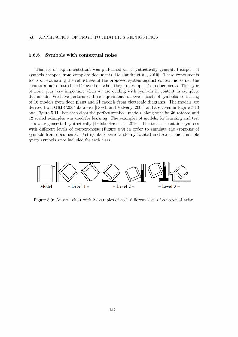
5.6. APPLICATION OF FMGE TO GRAPHICS RECOGNITION
5.6.6 Symbols with contextual noise
This set of experimentations was performed on a synthetically generated corpus, ofsymbols cropped from complete documents [Delalandre et al., 2010]. These experimentsfocus on evaluating the robustness of the proposed system against context noise i.e. thestructural noise introduced in symbols when they are cropped from documents. This typeof noise gets very important when we are dealing with symbols in context in completedocuments. We have performed these experiments on two subsets of symbols: consistingof 16 models from floor plans and 21 models from electronic diagrams. The models arederived from GREC2005 database [Dosch and Valveny, 2006] and are given in Figure 5.10and Figure 5.11. For each class the perfect symbol (model), along with its 36 rotated and12 scaled examples was used for learning. The examples of models, for learning and testsets were generated synthetically [Delalandre et al., 2010]. The test set contains symbolswith di↵erent levels of context-noise (Figure 5.9) in order to simulate the cropping ofsymbols from documents. Test symbols were randomly rotated and scaled and multiplequery symbols were included for each class.
Figure 5.9: An arm chair with 2 examples of each di↵erent level of contextual noise.
142

5.6. APPLICATION OF FMGE TO GRAPHICS RECOGNITION
Figure 5.10: Model symbols from electronic drawings.
143

5.6. APPLICATION OF FMGE TO GRAPHICS RECOGNITION
Figure 5.11: Model symbols from floor plans.
144

5.6. APPLICATION OF FMGE TO GRAPHICS RECOGNITION
Table 5.8 summarizes the results of experiments for context noise. We have not usedany sophisticated de-noising or pretreatment and our method derives its ability to resistagainst context noise, directly from underlying vectorization technique, the fuzzy approachused for computing structural signature and the capabilities of Bayesian networks to copewith uncertainties. The models for electronic diagrams contain symbols consisting ofcomplex arrangement of lines and arcs, which a↵ects the features in structural signatureas the employed vectorization technique is not able to cope with arcs and circles; as isdepicted by the recognition rates for these symbols. But keeping in view the fact that wehave used only clean symbols for learning and noisy symbols for testing, we believe thatthe results show the ability of our signature to exploit the su�cient structural details ofsymbols and it could be used to discriminate and recognize symbols with context noise.
Table 5.8: Results of symbol recognition experiments for context noise.
NoiseModelsymbol(classes)
Querysymbol(eachclass)
Recognition
rate (match
with
topmost
result)
Recognition
rate (a
match in
top-3
results)
Floor plansLevel-1 16 100 84% 95 %Level-2 16 100 79% 90 %Level-3 16 100 76% 87 %
Average recognition rate 80% 91%
Electronic diagramsLevel-1 21 100 69% 89%Level-2 21 100 66% 88%Level-3 21 100 61% 85%
Average recognition rate 65% 87%
145

5.6. APPLICATION OF FMGE TO GRAPHICS RECOGNITION
Structural methods are the strongest methods for graphics representation and sta-tistical classifiers provide e�cient recognition techniques. By designing a mechanism toconvert a structural representation to feature vector, the whole range of statistical tools(classifiers) are opened for that structural representation.
The application of FMGE to graphic symbol recognition does not use any sophisti-cated de-noising or pretreatment and it drives its power to resist against deformations anddegradations, directly from representation, description, learning and classification phases.FMGE addresses the issue of sensitivity of structural representations to noise and defor-mations by introducing fuzzy overlapping trapezoidal intervals for computing structuralsignature.
Promising experimental results confirm that the proposed methodology of combiningstructural representation and statistical classifier is useful for graphics recognition.
146

5.6. APPLICATION OF FMGE TO GRAPHICS RECOGNITION
5.6.7 Complexity of FMGE
The graph embedding phase of one attributed graph by FMGE requires only a fractionof a second and can be performed in real-time on standard PC.
The unsupervised learning phase of FMGE can be computational intensive dependingon the size of dataset and the graphs. However, this phase is performed o↵-line andhas linear time complexity. This is illustrated by Figure 5.12, which presents the timerequirements of the unsupervised learning phase of FMGE for synthetically generatedgraphs from IAM GREC dataset. All parameters except the number of attributes arekept constant.
Figure 5.12: Time complexity of unsupervised learning phase of FMGE.
147

5.7. CONCLUSION
5.7 Conclusion
In this chapter we have presented the experimental evaluations of FMGE for the prob-lems of graph clustering and graph classification. We have also presented the experimentalevaluation of the frame work for automatic indexing of graph repositories for graph retrievaland subgraph spotting. Along with the experimental evaluations we have presented theapplication of FMGE to the real problems of recognition, indexing and retrieval of graphicdocument image repositories.
The experimental evaluations have confirmed that FMGE and the subsequent classi-fication and clustering in real vector spaces is applicable to di↵erent graph classificationand graph clustering problems. The NP-complete operations in graph space can be solvedin polynomial time (P) in FMGE feature vector space. Also, In certain cases FMGE out-performs the classical techniques for graph classification and graph clustering, in terms ofrecognition rate and quality of clustering respectively.
However, a limitation of FMGE is that it is dependent on the attributes of the graphnodes and edges, for extracting discriminatory information. The features for the structuralinformation, also, use the node and edge attributes for extracting subgraph homogeneity.The direct consequence of the dependence on the node and edge attributes in graph, isthat the performance of FMGE is a↵ected if the graphs do not have many attributes onnodes and edges.
On the other side, less dependent on the topology of the graph is useful in case ofnoisy data. Generally, the noise in underlying data has a direct impact on the topologyof the graph. Less dependence on the topology helps FMGE in robustness against thedeformations in graph.
The framework for automatic indexing of graph repositories proposes a very generalsolution, applicable to a wide range of domains where the use of graphs is mandatory.Experimental results for the two repositories of electronic diagrams and architecture floorplans are very encouraging.
The application of FMGE to graphics recognition, demonstrates that the graph basedstructural representations for graphic document images could be adapted modern compu-tational tools.
148

Chapter 6
Discussion and Conclusions
In this chapter we present a discussion on the presented work. We highlight the possi-ble improvements which should be further studied for improving the proposed method ofexplicit graph embedding. We conclude this dissertation and point out some importantpossible lines of future research.
6.1 Discussion about FMGE
6.1.1 Parameters
The Fuzzy Multilevel Graph Embedding (FMGE) method presented in this thesis hasproposed a framework for extracting three levels of details from the attributed graphs byperforming multilevel analysis of graphs. The three levels of details include graph leveldetails, structural level details and the elementary level details. It can process graphs withsymbolic as well as numeric attributes on both nodes and edges. The size of the graphs isnot an issue, FMGE can embed small as well as big graphs.
The framework permits the embedding of these details of graphs into numeric featurevectors, by employing fuzzy histograms for numeric part of the information and crisphistogram for symbolic part of the information. The framework employs fuzzy overlappingtrapezoidal intervals for smooth transition between the intervals for constructing the fuzzy
149

6.1. DISCUSSION ABOUT FMGE
histogram, in order to minimize the information loss while mapping from continuous graphspace to discrete feature vector space.
The size of the resulting feature vectors is mainly based on the histograms (of frequen-cies) for encoding the information extracted by multilevel analysis of graphs.
The presented framework is quite modular in nature. The possible customizations ofits various modules are discussed below:
6.1.1.1 Discretization technique
For embedding numeric attributes, we have outlined to use two basic discretizationtechniques i.e. equally spaced discretization and AIC based equal frequency discretiza-tion. However FMGE is fully capable of employing sophisticated state-of-the-art dis-cretization methods. A survey of popular discretization techniques is presented by Liu etal. [Liu et al., 2002].
6.1.1.2 Fuzzy membership function
Our proposed framework employs trapezoidal membership function from fuzzy logicbut FMGE is fully capable of utilizing any of the available membership functions. Otherpopular choices for fuzzy membership function include triangular and Gaussian arrange-ments [Ishibuchi and Yamamoto, 2003]. In light of domain knowledge, appropriate choicescould be made for discretization technique and fuzzy membership function.
6.1.1.3 Number of fuzzy intervals for numeric attributes
An important parameter of FMGE’s unsupervised learning phase is the number of fuzzyintervals to be associated to each attribute. The unsupervised learning phase of FMGElearns s
i
fuzzy intervals for attribute i in input collection of graphs. The attribute i refersto structural and elementary level numeric information in input graphs (i.e. node degree,numeric node attributes and numeric edge attributes in input graphs). The parametersi
for attribute i is independent of other attributes. It is also important to highlighthere that this parameter is not necessarily same for all attributes. This parameter canbe learned and tested on a validation dataset; if one is available. This is demonstratedby our experimentation on graph classification. If no validation dataset is available thenumber of fuzzy intervals s
i
has to be specified manually. A third possibility is that ifthe training set can be considered to be a true representative of the test set, an equalfrequency discretization technique could be used for automatically finding the appropriatenumber of fuzzy intervals. This is demonstrated by our graph clustering experimentation.
150

6.1. DISCUSSION ABOUT FMGE
As a general rule of thumb, using 3 fuzzy intervals (i.e. small, medium and large) for theattributes is a safe choice. However, a more intelligent choice could be made in the lightof domain knowledge.
6.1.1.4 Resemblance attributes
For embedding edge attributes resemblance for nodes (structural level information),we have outlined the use of a measure of central tendency i.e. mean and the spread ofthe attribute’s resemblance i.e. the standard deviation on the attribute resemblance of allcouple of edges for a node.
6.1.1.5 Classifier
We have used a simple non-parametric classifier for graph classification experimentationand a basic clustering technique for graph clustering experimentation, for demonstrationpurposes. However, all sophisticated classifiers and clustering methods are fully applicableto the resulting feature vectors of FMGE.
We have illustrated the application of FMGE in di↵erent domains but have mainlyfocused on the graphic document images, because the graphic document images need togenerate sophisticated graph representations.
Another important contribution of this work is the proposed method to spot subgraphsin huge repositories of attributed graphs. This is achieved by automatically constructingthe index of a graph repository by employing FMGE together with clustering and classi-fication tools on the cliques of order 2 in the graphs in the repository.
151

6.1. DISCUSSION ABOUT FMGE
6.1.2 Complexity
The unsupervised learning phase of FMGE can be computational expensive, dependingon the size of the graphs and that of the graph dataset. This is dependent on the numberof attributes of nodes and edges in the graph. However, the complexity of this phase islinear to the number of attributes in graph.
The graph embedding phase of FMGE is fast. It is performed in less that a fractionof a second on a standard PC.
152

6.2. CONCLUSIONS
6.2 Conclusions
We have presented a method of explicit graph embedding and a framework for auto-matic indexing of graph repositories, with an aim to bridge the gap between structuraland statistical approaches of pattern recognition. Our work proposes a straightforward,simple and computational e�cient solution for facilitating the use of graph based power-ful representations together with learning and computational strengths of state-of-the-artmachine learning, classification and clustering.
The proposed graph embedding method exploits multilevel analysis of graph for em-bedding it into a feature vector. The feature vector contains graph level features (graphorder and graph size), along-with structural level features (node degree, node attributesresemblance for edges and edge attributes resemblance for nodes) and elementary level fea-tures (node attributes and edge attributes). We have minimized the information loss, whilemapping from continuous graph space to discrete vector space, by employing fuzzy over-lapping trapezoidal intervals. These intervals are learned during an unsupervised learningphase. The intervals are employed during graph embedding phase for constructing fuzzyinterval encoded histograms for structural and elementary level features. This achieves aneventual embedding of a graph into a feature vector.
The experimental results are encouraging and demonstrates the applicability of ourmethod to graph clustering and classification problems. The method could be deployedin an unsupervised fashion for graph clustering problem even if no separate learning set isavailable as it has built-in capability to implicitly learn from the input collection of graphs.Its unsupervised learning capabilities also allows it to generalize to unseen graphs i.e. tobe deployed in a supervised fashion where it learns on a graph dataset and embeds unseengraphs. The proposed method is applicable to a wide range of domains for solving theproblems of graph clustering and graph classification.
However, our method is too much dependent on the attributes of graph for extractingdiscriminant information from graph and it lacks information on the topology of graph.
The framework for automatic indexing of attributed graph repositories employs ex-plicit graph embedding and gives a very general solution for graph retrieval and subgraphspotting. The automatic indexing of attributed graph repositories doest not require alabeled training set and thus has the capability of less expensive and fast deployment tovarious domains where the use of a relational data structure is mandatory.
153

6.2. CONCLUSIONS
We have obtained promising experimental results, which clearly demonstrate thatFuzzy Multilevel Graph Embedding (FMGE) enables the structural representations tobenefit from the computational e�cient statistical models and tools, for the problems ofgraph classification, graph clustering, graph retrieval and subgraph spotting.
154

6.3. FUTURE CHALLENGES
6.3 Future challenges
The current research findings are encouraging and one of the future lines of work is totake this work forward for improving the quality of embedding achieved by FMGE.
An important direction of future research in this regard is to study the feature vec-tor of FMGE in further details. We have reported some very preliminary results in[Luqman et al., 2011a]. The application of dimensionality reduction, using principal com-ponent analysis (PCA), independent component analysis (ICA) and their kernel ver-sions, will be very interesting. An interesting reference to proceed in this direction is[Bunke and Riesen, 2011b].
Linked to the dimensionality reduction of feature vector of FMGE, an interestingdirection of future research is to use feature selection methods for selecting meaning-ful features and reducing the size of the feature vector. A reference in direction is[Bunke and Riesen, 2011a].
For extracting more topological information from graphs and to include it in theFMGE, graph paths and Morgan index [Morgan, 1965] are interesting pointers for futureresearch.
The scenarios where learning set is available and FMGE adapts its parameter to thegraphs in the learning set, the detection of outliers for cleaning the learning set is impor-tant. This is another important challenge for future research.
To take the subgraph spotting work forward, future research work can improve thequality of indexing of the graph repository by exploring cliques of higher order (� 3) andto build a multi-resolution index of a graph repository. This will index the graphs onthe basis of substructures of di↵erent sizes, which will improve the quality of subgraphspotting by removing false positives as we move down to the resolution defined by lowerorder cliques.
A very interesting future lines of research, for addressing the current main limitationof graph embedding methods in general, is to try to get the surjective matching of thenodes of two attributed graphs that have been compared in feature vector space. This hasbeen illustrated for two example graphs in Figure 6.1.
155

6.3. FUTURE CHALLENGES
Figure 6.1: Bijective match of nodes of two graphs.
156

Appendix
157


Appendix A
Graph databases
A.1 IAM graph database repository
Six datasets from IAM graph database repository, proposed by [Riesen and Bunke, 2010c],have been employed for our experimentation. These graph datasets are publicly available1.The IAM graph database repository contains graphs from the field of document image anal-ysis and graphics recognition. The datasets in IAM graph database repository are detailedin subsequent subsections. The example images are reproduced from [Riesen, 2010].
A.1.1 Letter graphs
The letter graph dataset is comprised of graphs extracted from drawings of 15 capitalletters of Roman alphabet that consists of straight lines only viz. A, E, F, H, I, K, L, M, N,T, V, W, X, Y and Z. For each class, a prototype line drawing is manually constructed. Anillustration of the prototype line drawings is given in Figure A.1. These prototype drawingsare then converted into prototype graphs by representing lines by undirected edges andending points of lines by nodes. Each node is labeled with a two-dimensional attributegiving its position relative to a reference coordinate system. Edges are unlabeled. Inorder to test classifiers under di↵erent conditions, distortions are applied on the prototypegraphs with three di↵erent levels of strength. This results in three di↵erent versions ofthis database, including graphs with a low, medium and high level of distortion. Thesethree graph dataset consist of a training set, a validation set, and a test set of size 750each. The graphs are uniformly distributed over the 15 classes [Bunke and Riesen, 2011b].Figure A.2, A.3 and A.4 illustrate ten graph instances for each distortion level representingthe letter A. Note that letters that undergo distortions of medium and high strength are
1http://www.greyc.ensicaen.fr/iapr-tc15/links.html
159

A.1. IAM GRAPH DATABASE REPOSITORY
di�cult to be recognized, even for a human observer [Riesen, 2010].
Figure A.1: Prototypes of letters A to Z.
Figure A.2: Instances of letter A at distortion level low.
Figure A.3: Instances of letter A at distortion level medium.
Figure A.4: Instances of letter A at distortion level high.
160

A.1. IAM GRAPH DATABASE REPOSITORY
A.1.2 GREC graphs
Automatic conversion of line drawings from paper to electronic form requires therecognition of geometric primitives like lines, arcs, circles etc. in scanned documents[Riesen, 2010]. The GREC graph dataset is comprised of graphs representing 22 symbolsfrom architectural and electronic drawings. The prototype images of each class are pre-sented in Figure A.5. The images occur at five di↵erent distortion levels (Figure A.6).Depending on the distortion level, either erosion, dilation, or other morphological opera-tions are applied. The result is thinned to obtain lines of one pixel width. Finally, graphsare extracted from the resulting denoised images by tracing the lines from end to endand detecting intersections as well as corners. Ending points, corners, intersections andcircles are represented by nodes and labeled with a two-dimensional attribute giving theirposition. The nodes are connected by undirected edges which are labeled as line or arc.An additional attribute specifies the angle with respect to the horizontal direction or thediameter in case of arcs. For an adequately sized set, the five graphs per distortion levelare individually distorted 30 times to obtain a data set containing 3300 graphs uniformlydistributed over the 22 classes. These distortions consists of translations and scalings ofthe graphs in a certain range, and random deletions and insertions of both nodes andedges. The resulting set is split into a training and a validation set of size 836 each, anda test set of size 1628 [Bunke and Riesen, 2011b].
161

A.1. IAM GRAPH DATABASE REPOSITORY
Figure A.5: The prototype images of the 22 GREC classes.
Figure A.6: The five distortion levels (bottom to top) applied to three sample images.
162

A.1. IAM GRAPH DATABASE REPOSITORY
A.1.3 Fingerprint graphs
The Fingerprint data set stems from the emerging field of biometric person authen-tication. Biometric person authentication refers to the task of automatically recognizingthe identity of a person from his or her physiological or behavioral characteristics. Fin-gerprint images are particularly interesting as a biometric measurement since each personpossess this biometric, persons are believed to have unique fingerprints, and fingerprintsdo not change over time. Moreover, fingerprint images are rather easy to be captured bysensors [Riesen, 2010]. Fingerprints are converted into graphs by filtering the images andextracting regions that are relevant. In order to obtain graphs from fingerprint images,the relevant regions are binarized and a noise removal and thinning procedure is applied.This results in a skeletonized representation of the extracted regions. Ending points andbifurcation points of the skeletonized regions are represented by nodes. Additional nodesare inserted in regular intervals between ending points and bifurcation points. Finally,undirected edges are inserted to link nodes that are directly connected through a ridge inthe skeleton. Each node is labeled with a two-dimensional attribute giving its position.The edges are attributed with an angle denoting the orientation of the edge with respect tothe horizontal direction. The fingerprint dataset consists of a training set of size 500, a val-idation set of size 300, and a test set of size 2000. Thus, there are 2800 fingerprint imagestotally; out of the four classes arch, left, right, and whorl from the Galton-Henry classifi-cation system [Riesen and Bunke, 2010c]. The example fingerprint images for these fourclasses are presented in Figure A.7, Figure A.8, Figure A.9 and Figure A.10 respectively.
A.1.4 Mutagenicity graphs
Mutagenicity is the ability of a chemical compound to cause mutations in DNA and istherefore one of the numerous adverse properties of a compound that hampers its potentialto become a marketable drug. Mutagenic compounds pose a toxic risk to humans andscreening of drug candidates for mutagenicity is a regulatory requirement for drug approval[Riesen, 2010]. The molecules are converted into attributed graphs in a straightforwardmanner by representing atoms as nodes and the covalent bonds as edges. Nodes are labeledwith the number of the corresponding chemical symbol and edges by the valence of thelinkage. The mutagenicity data set is divided into two classes mutagen and nonmutagen.We use a training set of size 1500, a validation set of size 500, and a test set of size 2337.Thus, there are 4337 elements totally (2401 mutagen elements and 1936 nonmutagenelements) [Riesen and Bunke, 2010c].
163

A.1. IAM GRAPH DATABASE REPOSITORY
Figure A.7: Fingerprint examples from the Galton-Henry class Arch.
Figure A.8: Fingerprint examples from the Galton-Henry class Left loop.
Figure A.9: Fingerprint examples from the Galton-Henry class Right loop.
Figure A.10: Fingerprint examples from the Galton-Henry class Whorl.
164

A.2. GEPR GRAPHS
A.2 GEPR graphs
The GEPR graph database consists of graphs extracted from three large publicly avail-able image databases viz. the Amsterdam Library of Object Images (ALOI), the ColumbiaObject Image Library (COIL) and the Object Databank by Carnegie-Mellon University(ODBK). The Amsterdam Library of Object Images is a collection of images of 1000 smallobjects. Each object has been acquired several times changing the orientation and theillumination, for a total of 110250 images. Figure A.11 presents some example images.GEPR graph database is composed of 50 objects from ALOI and 72 views for each object(i.e. 3600 images). The Columbia Object Image Library is a collection of images of 100small objects, each acquired from 72 di↵erent orientations. Figure A.12 presents some ex-ample images from COIL. GEPR graph database contains 50 objects with 72 views each,from COIL (i.e. 3600 images). The Object Data Bank has been obtained from a collectionof 209 3D object models, that have been rendered with photo-realistic quality using 14di↵erent view points. Figure A.13 presents some examples of the pictures from ODBK.The GEPR graph database contains 208 objects and 12 of the 14 view points for each,from ODBK (i.e. 2496 images). The images of each database have been divided into afirst set that has been distributed in order to tune the algorithms, and a second set forthe performance evaluation [Foggia and Vento, 2010].
Each image has been smoothed using a Gaussian filter, and then it has been seg-mented using a Pyramidal segmentation algorithm. Finally, from the segmentation theRegion Adjacency Graph (RAG) has been constructed as the image graph-based represen-tation. The nodes of the graph have as attributes the relative size and the average colorcomponents of the corresponding regions, while the edges of the graph have no attributes[Foggia and Vento, 2010]. The example images of ALOI, COIL and ODBK are reproducedfrom [Foggia and Vento, 2010].
165

A.2. GEPR GRAPHS
Figure A.11: Some examples of the images in the ALOI database.
Figure A.12: Some examples of the images in the COIL database.
Figure A.13: Some examples of the images in the ODBK database.
166
Appendix B
Graphs representation of graphicdocument images
A new graph repository is constructed by extracting graphs from images of architecturalfloor plans and electronic diagrams in SESYD image dataset [Delalandre et al., 2010], forexperimentation of the framework for automatic indexing of graph repositories for graphretrieval and subgraph spotting. The corresponding graph repository is made publiclyavailable1 for academia and scientific community for research purposes.
The SESYD graph database consists of graph extracted from line drawing documentimages in SESYD dataset [Delalandre et al., 2010]. The SESYD dataset contains 100synthetically generated line drawing document images of architectural floor plans andelectronic diagrams each, for 10 di↵erent levels of degradations. The architectural floorplans and the electronic diagrams are composed of 16 and 21 unique symbol models respec-tively. For architectural floor plans a total of 200 document images were selected. Thesedocument images are comprised of 4216 symbols which come from 16 di↵erent classes ofsymbols. An example architectural floor plan is presented in Figure B.2. On the otherhand, 800 electronic diagram images were selected for constructing our graph dataset. Theelectronic diagrams are comprised of a total of 9600 symbols which belong to 21 di↵erentclasses. Figure B.3 presents an example electronic diagram image. The query imagessimulate the contextual noise. This type of noise occurs in cropped regions of graphicdocument images. An interesting application of the latter is selecting a region in a graphicdocument image (on a modern tactile interface), for querying a graphic document contentbased image retrieval (CBIR) system. The query images are synthetically generated withthree di↵erent levels of noise; simulating di↵erent levels of contextual noise. Figure B.4presents example query images.
The document images in SESYD dataset were represented by attributed graphs by
1http://www.rfai.li.univ-tours.fr/PagesPerso/mmluqman/public/SESYD_graphs.zip
167

GRAPHS FROM GRAPHIC DOCUMENT IMAGES (FOR SUBGRAPH SPOTTING)
using the work of Qureshi et al. [Qureshi et al., 2007]. The graph extraction phase isillustrated in Figure B.1 for a part of graphic document image. The topological andgeometric details about structure of graphic content are extracted and are represented byan attributed relational graph (ARG). In first step, the graphic content is vectorized andis represented by a set of primitives (labels 1, 2, 3, 4 in Figure B.1). In next step, theseprimitives become nodes and topological relations between them become arcs in ARG.Nodes have relative length (normalized between 0 and 1) and primitive-type (Vector forfilled regions of shape and Quadrilateral for thin regions) as attributes; whereas arcs ofthe graph have connection-type (L, X, T, P, S) and relative angle (normalized between 0�
and 90�) as attributes.
Figure B.1: Representing graphic content by an attributed graph.
168

GRAPHS FROM GRAPHIC DOCUMENT IMAGES (FOR SUBGRAPH SPOTTING)
Figure B.2: An example architectural floor plan image from SESYD dataset.
169

GRAPHS FROM GRAPHIC DOCUMENT IMAGES (FOR SUBGRAPH SPOTTING)
Figure B.3: An example electronic diagram image from SESYD dataset.
Figure B.4: An arm chair with 2 examples of each di↵erent level of contextual noise.
170
Bibliography
[A. and Zadeh, 2008] A., L. and Zadeh (2008). Is there a need for fuzzy logic? InformationSciences, 178(13):2751–2779.
[Borges, 1996] Borges, P. S. d. S. (1996). A model of strategy games based on the paradigmof the Iterated Prisoner’s Dilemma employing Fuzzy Sets. PhD thesis, UniversidadeFederal de Santa Catarina.
[Brouard et al., 2010] Brouard, T., Delaplace, A., Luqman, M. M., Cardot, H., andRamel, J.-Y. (2010). Design of evolutionary methods applied to the learning of Bayesiannetwork structures. In Bayesian Network, pages 13–38.
[Brunner and Brunnett, 2004] Brunner, D. and Brunnett, G. (2004). Mesh SegmentationUsing the Object Skeleton Graph. In International Conference on Computer Graphicsand Imaging, pages 48–55.
[Bunke, 1997] Bunke, H. (1997). On a relation between graph edit distance and maximumcommon subgraph. Pattern Recognition Letters.
[Bunke, 1999] Bunke, H. (1999). Error correcting graph matching : On the influence ofthe underlying cost function. IEEE Transactions on Pattern Analysis and MachineIntelligence.
[Bunke et al., 2002] Bunke, H., Foggia, P., Guidobaldi, C., Sansone, C., and M., V. (2002).A comparison of algorithms for maximum common subgraph on randomly connectedgraphs. In International Workshops on Structural, Syntactic, and Statistical PatternRecognition.
[Bunke et al., 2001] Bunke, H., Gunter, S., and Jiang, X. (2001). Towards bridging thegap between statistical and structural pattern recognition: Two new concepts in graphmatching. In International Conference on Advances in Pattern Recognition, pages 1–11.Springer.
[Bunke et al., 2005] Bunke, H., Irniger, C., and Neuhaus, M. (2005). Graph Matching -Challenges and Potential Solutions. In International Conference on Image Analysis andProcessing, pages 1–10.
171
BIBLIOGRAPHY
[Bunke and Riesen, 2011a] Bunke, H. and Riesen, K. (2011a). Improving vector spaceembedding of graphs through feature selection algorithms. Pattern Recognition,44(9):1928–1940.
[Bunke and Riesen, 2011b] Bunke, H. and Riesen, K. (2011b). Recent advances in graph-based pattern recognition with applications in document analysis. Pattern Recognition,44(5):1057–1067.
[Bunke and Shearer, 1998] Bunke, H. and Shearer, K. (1998). A graph distance metricbased on the maximal common subgraph. Pattern Recognition Letters.
[Byun, 2003] Byun, H. (2003). A survey on pattern recognition applications of supportvector machines. International Journal of Pattern Recognition and Artificial Intelli-gence, 17(3):459–486.
[Caelli and Kosinov, 2004] Caelli, T. and Kosinov, S. (2004). Inexact graph matchingusing eigen-subspace projection clustering. International Journal of Pattern Recognitionand Artificial Intelligence.
[Carcassoni and Hancock, 2001] Carcassoni, M. and Hancock, E. R. (2001). Weightedgraph-matching using modal clusters. In 9th International Conference on ComputerAnalysis of Images and Patterns.
[Chen et al., 2007] Chen, T., Yang, Q., and Tang, X. (2007). Directed graph embedding.In International Joint Conference on Artificial Intelligence, pages 2707–2712.
[Chhabra, 1998] Chhabra, A. (1998). Graphic symbol recognition: An overview. GraphicsRecognition Algorithms and Systems, pages 68–79.
[Chung, 1997] Chung, F. R. K. (1997). Spectral Graph Theory. American MathematicalSociety.
[Colot et al., 1994] Colot, O., Courtellemont, P., and El-Matouat, A. (1994). Informationcriteria and abrupt changes in probability laws. In Signal Processing VII: Theories andApplications, pages 1855–1858.
[Conte et al., 2004] Conte, D., Foggia, P., Sansone, C., and Vento, M. (2004). Thirty yearsof graph matching in pattern recognition. International Journal of Pattern Recognitionand Artificial Intelligence, 18(3):265–298.
[Cordella and Vento, 2000] Cordella, L. and Vento, M. (2000). Symbol recognition indocuments: a collection of techniques? International Journal on Document Analysisand Recognition, 3(2):73–88.
[Corneil and Gotlie, 1970] Corneil, D. and Gotlie, C. (1970). An E�cient Algorithm forGraph Isomorphism. Journal of the Association for Computing Machinery, 17:51–64.
[De Sa, 2001] De Sa, J. (2001). Pattern recognition: concepts, methods, and applications.Springer Verlag.
172

BIBLIOGRAPHY
[Delalandre et al., 2010] Delalandre, M., Valveny, E., Pridmore, T., and Karatzas, D.(2010). Generation of synthetic documents for performance evaluation of symbol recog-nition & spotting systems. International Journal on Document Analysis and Recogni-tion, pages 1–21.
[Delaplace et al., 2006] Delaplace, A., Brouard, T., and Cardot, H. (2006). Two evolution-ary methods for learning Bayesian network structures. 2006 International Conferenceon Computational Intelligence and Security, pages 137–142.
[Dosch and Valveny, 2006] Dosch, P. and Valveny, E. (2006). Report on the Second Sym-bol Recognition Contest. In Liu, W. and Llados, J., editors, Graphics Recognition.Ten Years Review and Future Perspectives, volume 3926 of Lecture Notes in ComputerScience, pages 381–397. Springer Berlin / Heidelberg.
[Duda et al., 2000] Duda, R., Hart, P., and Stork, D. (2000). Pattern classification, vol-ume 2. Wiley Interscience.
[Eshera and Fu, 1984] Eshera, M. and Fu, K. (1984). A graph distance measure for imageanalysis. IEEE Transactions on Systems, Man, and Cybernetics, 14:394–408.
[Ferrer et al., 2008] Ferrer, M., Valveny, E., Serratosa, F., Riesen, K., and Bunke, H.(2008). An approximate algorithm for median graph computation using graph embed-ding. In International Conference on Pattern Recognition, pages 1–4. Ieee.
[Ferrer et al., 2010] Ferrer, M., Valveny, E., Serratosa, F., Riesen, K., and Bunke, H.(2010). Generalized median graph computation by means of graph embedding in vectorspaces. Pattern Recognition, 43(4):1642–1655.
[Fischler and Elschlager, 1973] Fischler, M. and Elschlager, R. (1973). The representationand matching of pictorial structures. IEEE Transactions on Computers.
[Foggia and Vento, 2010] Foggia, P. and Vento, M. (2010). Graph Embedding for PatternRecognition. In Unay, D., Cataltepe, Z., and Aksoy, S., editors, Recognizing Patterns inSignals, Speech, Images and Videos, volume 6388 of Lecture Notes in Computer Science,pages 75–82. Springer.
[Franco et al., 2003] Franco, P., Ogier, J.-M., Loonis, P., and Mullot, R. (2003). A Topo-logical Measure for Image Object Recognition. In Lecture Notes in Computer Science,volume 3088, pages 279–290.
[Friedman and Kandel, 1999] Friedman, M. and Kandel, A. (1999). Introduction to pat-tern recognition. World Scientific.
[Garey and Johnson, 1979] Garey, M. R. and Johnson, D. S. (1979). Computers and In-tractability: A Guide to the Theory of NP-Completeness. W. H. Freeman.
[Gibert et al., 2011a] Gibert, J., Valveny, E., and Bunke, H. (2011a). DimensionalityReduction for Graph of Words Embedding. In Graph-Based Representations in PatternRecognition, pages 22–31.
173

BIBLIOGRAPHY
[Gibert et al., 2011b] Gibert, J., Valveny, E., and Bunke, H. (2011b). DimensionalityReduction for Graph of Words Embedding. In LNCS 6658, pages 22–31.
[Gibert et al., 2011c] Gibert, J., Valveny, E., and Bunke, H. (2011c). Vocabulary Selectionfor Graph of Words Embedding. In 5th Iberian Conference on Pattern Recognition andImage Analysis, pages 216–223. LNCS. Berlin: Springer, 6669 edition.
[Godsil and Royle, 2011] Godsil, C. and Royle, G. (2011). Algebraic Graph Theory.Springer.
[Gori et al., 2005] Gori, M., Maggini, M., and Sarti, L. (2005). Exact and approximategraph matching using random walks. IEEE transactions on pattern analysis and ma-chine intelligence, 27.
[Harchaoui, 2007] Harchaoui, Z. (2007). Image classification with segmentation graphkernels. In IEEE Conference on Computer Vision and Pattern Recognition.
[Hart et al., 1968] Hart, P., Nilsson, N., and Raphael, B. (1968). A Formal Basis for theHeuristic Determination of Minimum Cost Paths. IEEE Transactions on Systems, Manand Cybernetics.
[Inokuchi et al., 2000] Inokuchi, A., Washio, T., and Motoda, H. (2000). An Apriori-Based Algorithm for Mining Frequent Substructures from Graph Data. Lecture Notesin Computer Science, 1910:13–23.
[Ishibuchi and Yamamoto, 2003] Ishibuchi, H. and Yamamoto, T. (2003). Deriving fuzzydiscretization from interval discretization. In International Conference on Fuzzy Sys-tems, pages 749–754. IEEE.
[Jain et al., 1999] Jain, A. K., Murty, M. N., and Flynn, P. J. (1999). Data clustering : areview. ACM Computing Surveys.
[Jiang and Bunke, 1999] Jiang, X. and Bunke, H. (1999). Optimal Quadratic-Time Iso-morphism of Ordered Graphs. Pattern Recognition, 32:1273–1283.
[Kaufman and Rousseeuw, 1990] Kaufman, L. and Rousseeuw, P. J. (1990). FindingGroups in Data: An Introduction to Cluster Analysis, volume 39 of Wiley Series inProbability and Mathematical Statistics. John Wiley & Sons.
[Klir and Yuan, 1995] Klir, G. and Yuan, B. (1995). Fuzzy sets and fuzzy logic. Prentice-Hall, Englewood Cli↵s.
[Kobler et al., 1993] Kobler, J., Schoning, U., and Toran, J. (1993). The graph isomor-phism problem : its structural complexity. Birkhauser Verlag.
[Kosinov and Caelli, 2002] Kosinov, S. and Caelli, T. (2002). Inexact multisubgraphmatching using graph eigenspace and clustering models. In SSPR/SPR, pages 133–142.
174
BIBLIOGRAPHY
[Kramer and Raedt, 2001] Kramer, S. and Raedt, L. (2001). Feature construction withversion spaces for biochemical application. In 18th International Conference on MachineLearning, pages 258–265.
[Kuncheva, 2004] Kuncheva, L. (2004). Combining Pattern Classifiers: Methods and Al-gorithms. John Wiley.
[Lee and Madabhushi, 2010] Lee, G. and Madabhushi, A. (2010). Semi-Supervised GraphEmbedding Scheme with Active Learning (SSGEAL): Classifying High DimensionalBiomedical Data. In Pattern Recognition in Bioinformatics, volume 6282 of LectureNotes in Computer Science, pages 207–218. Springer.
[Leray and Francois, 2004] Leray, P. and Francois, O. (2004). BNT Structure LearningPackage : Documentation and Experiments. Structure, (November).
[Levenshtein, 1966] Levenshtein, V. I. (1966). Binary codes capable of correcting deletions,insertions and reversals. Soviet Physics Doklady.
[Liu, 2010] Liu, B. (2010). Uncertainty Theory. In Uncertainty Theory, volume 300 ofStudies in Computational Intelligence, pages 1–79. Springer Berlin / Heidelberg.
[Liu et al., 2002] Liu, H., Hussain, F., Tan, C., and Dash, M. (2002). Discretization: Anenabling technique. Data Mining and Knowledge, pages 393–423.
[Llados and Sanchez, 2003] Llados, J. and Sanchez, G. (2003). Symbol recognition usinggraphs. In International Conference on Image Processing, volume 2, pages 49–52. IEEE.
[Llados et al., 2002] Llados, J., Valveny, E., Sanchez, G., and Martı, E. (2002). SymbolRecognition: Current Advances and Perspectives. In Graphics Recognition Algorithmsand Applications, volume 2390, pages 104–128.
[Lopresti and Wilfong, 2003] Lopresti, D. and Wilfong, G. (2003). A fast technique forcomparing graph representations with applications to performance evaluation. Interna-tional Journal of Document Analysis and Recognition.
[Luo et al., 2003] Luo, B., Wilson, R., and Hancock, E. (2003). Spectral embedding ofgraphs. Pattern Recognition, 36(10):2213–2230.
[Luqman et al., 2010a] Luqman, M., Llados, J., Ramel, J.-Y., and Brouard, T. (2010a). AFuzzy-Interval Based Approach for Explicit Graph Embedding. In Recognizing Patternsin Signals, Speech, Images and Videos, volume 6388, pages 93–98.
[Luqman et al., 2009a] Luqman, M. M., Brouard, T., and Ramel, J.-Y. (2009a). GraphicSymbol Recognition using Graph Based Signature and Bayesian Network Classifier. InTenth International Conference on Document Analysis and Recognition (ICDAR), pages1325–1329, Barcelona. IEEE Computer Society.
[Luqman et al., 2010b] Luqman, M. M., Brouard, T., Ramel, J.-y., and Llados, J. (2010b).A Content Spotting System For Line Drawing Graphic Document Images. In 20thInternational Conference on Pattern Recognition, volume 20, pages 3420–3423.
175

BIBLIOGRAPHY
[Luqman et al., 2010c] Luqman, M. M., Brouard, T., Ramel, J.-Y., and Llados, J. (2010c).Vers une approche floue d encapsulation de graphes : application a la reconnaissancede symboles. In Colloque International Francophone sur l’Ecrit et le Document, pages169–184.
[Luqman et al., 2012] Luqman, M. M., Brouard, T., Ramel, J.-Y., and Llados, J. (2012).Recherche de sous-graphes par encapsulation floue des cliques dordre 2: Applicationa la localisation de contenu dans les images de documents graphiques. In ColloqueInternational Francophone sur l’Ecrit et le Document, page accepted.
[Luqman et al., 2009b] Luqman, M. M., Delalandre, M., Brouard, T., Ramel, J.-Y., andLlados, J. (2009b). Employing fuzzy intervals and loop-based methodology for designingstructural signature : an application to symbol recognition. In GREC, pages 22–31.
[Luqman et al., 2010d] Luqman, M. M., Delalandre, M., Brouard, T., Ramel, J.-Y., andLlados, J. (2010d). Fuzzy Intervals for Designing Structural Signature: An Applicationto Graphic Symbol Recognition. In Ogier, J.-M., Liu, W., and Llados, J., editors,Graphics Recognition. Achievements, Challenges, and Evolution, volume 6020, pages12–24. Springer Berlin / Heidelberg.
[Luqman et al., 2011a] Luqman, M. M., Llados, J., Ramel, J.-Y., and Brouard, T. (2011a).Dimensionality Reduction for Fuzzy-Interval Based Explicit Graph Embedding. InGREC, pages 117–120.
[Luqman et al., 2011b] Luqman, M. M., Ramel, J.-Y., Llados, J., and Brouard, T.(2011b). Subgraph Spotting through Explicit Graph Embedding : An Application toContent Spotting in Graphic Document Images. In Eleventh International Conferenceon Document Analysis and Recognition (ICDAR), pages 870–874.
[McGregor, 1982] McGregor, J. J. (1982). Backtrack search algorithms and the maximalcommon subgraph problem. Software Practice and Experience.
[Messmer, 1995] Messmer, B. (1995). E�cient Graph Matching Algorithms. PhD thesis,University of Bern, Switzerland.
[Messmer and Bunke, 1998] Messmer, B. and Bunke, H. (1998). Error-Correcting GraphIsomorphism using Decision Trees. Int. Journal of Pattern Recognition and Art. Intel-ligence, 12:721–742.
[Morgan, 1965] Morgan, H. L. (1965). The Generation of a Unique Machine Description forChemical Structures - A Technique Developed at Chemical Abstracts Service. Journalof Chemical Documentation, 5(2):107–113.
[Neuhaus and Bunke, 2004] Neuhaus, M. and Bunke, H. (2004). A probabilistic approachto learning costs for graph edit distance. In 17th International Conference on PatternRecognition.
[Neuhaus and Bunke, 2007] Neuhaus, M. and Bunke, H. (2007). Automatic learning ofcost functions for graph edit distance. Information Sciences.
176
BIBLIOGRAPHY
[Neuhaus, M. et Bunke, 2006] Neuhaus, M. et Bunke, H. (2006). Edit distance-based ker-nel functions for structural pattern classification. Pattern Recognition.
[Okada et al., 2005] Okada, Y., Sahara, T., Ohgiya, S., and Nagashima, T. (2005). Detec-tion of cluster boundary in microarray data by reference to mips functional cataloguedatabase. In International Conference on Genome Informatics, pages 2–3.
[Papadopoulos, A. N. et Manolopoulos, 1999] Papadopoulos, A. N. et Manolopoulos, Y.(1999). Structure-based similarity search with graph histograms. In International Work-shop on Database and Expert Systems Applications.
[Pavlidis, 1972] Pavlidis, T. (1972). Representation of Figures by Labeled Graphs. PatternRecognition, 4:5–17.
[Pekalska and Duin, 2005] Pekalska, E. and Duin, R. P. W. (2005). The Dissimilarity Rep-resentation for Pattern Recognition : Foundations And Applications. World ScientificPublishing.
[Pelillo, 1999] Pelillo, M. (1999). Replicator equations, maximal cliques, and graph iso-morphism. Neural Computation.
[Qureshi, 2008] Qureshi, R. J. (2008). Reconnaissance de formes et symboles graphiquescomplexes dans les images de documents. PhD thesis, Universite Francois-Rabelais deTours, France.
[Qureshi et al., 2007] Qureshi, R. J., Ramel, J.-Y., Cardot, H., and Mukherji, P. (2007).Combination of Symbolic and Statistical Features for Symbols Recognition. In In-ternational Conference on Signal Processing, Communications and Networking, pages477–482.
[Radzikowska and Kerre, 2002] Radzikowska, A. M. and Kerre, E. E. (2002). A compar-ative study of fuzzy rough sets. Fuzzy Sets and Systems, 126(2):137–155.
[Ramel, 1992] Ramel, J.-Y. (1992). Lecture Automatique de Partitions Musicales. PhDthesis, INSA Lyon, France.
[Read and Corneil, 1977] Read, R. C. and Corneil, D. G. (1977). The graph isomorphismdisease. Journal of Graph Theory.
[Reingold et al., 1997] Reingold, E., Nievergelt, J., and Deo, N. (1997). Combinatorialalgorithms : theory and practice. Prentice-Hall.
[Riesen, 2010] Riesen, K. (2010). Classification and clustering of Vector Space EmbeddedGraphs. PhD thesis, University of Bern, Switzerland.
[Riesen and Bunke, 2009] Riesen, K. and Bunke, H. (2009). Graph classification basedon vector space embedding. International Journal of Pattern Recognition and ArtificialIntelligence, 23(6):1053–1081.
[Riesen and Bunke, 2010a] Riesen, K. and Bunke, H. (2010a). Graph Classification andClustering Based on Vector Space Embedding. World Scienti c.
177

BIBLIOGRAPHY
[Riesen and Bunke, 2010b] Riesen, K. and Bunke, H. (2010b). Graph Classification AndClustering Based On Vector Space Embedding. World Scientific Publishing Co., Inc.
[Riesen and Bunke, 2010c] Riesen, K. and Bunke, H. (2010c). IAM graph database reposi-tory for graph based pattern recognition and machine learning. In Structural, Syntactic,and Statistical Pattern Recognition, pages 287–297. Springer.
[Riesen et al., 2007] Riesen, K., Neuhaus, M., and Bunke, H. (2007). Graph embedding invector spaces by means of prototype selection. In International Conference on Graph-based Representations in Pattern Recognition, pages 383–393. Springer-Verlag.
[Robles-Kelly and Hancock, 2007] Robles-Kelly, A. and Hancock, E. (2007). A Rieman-nian approach to graph embedding. Pattern Recognition, 40(3):1042–1056.
[Roth et al., 2003] Roth, V., Laub, J., Kawanabe, M., and Buhmann, J. (2003). Opti-mal cluster preserving embedding of nonmetric proximity data. IEEE Transactions onPattern Analysis and Machine Intelligence, 25(12):1540–1551.
[Selkow, 1977] Selkow, S. (1977). The tree-to-tree editing problem. Information ProcessingLetters.
[Shaw and Jebara, 2009] Shaw, B. and Jebara, T. (2009). Structure preserving embed-ding. International Conference on Machine Learning, pages 1–8.
[Shawe-Taylor and Cristianini, 2004] Shawe-Taylor, J. and Cristianini, N. (2004). Kernelmethods for pattern analysis. Cambridge University Press.
[Shokoufandeh et al., 2005] Shokoufandeh, A., Macrini, D., Dickinson, S., Siddiqi, K., andZucker, S. (2005). Indexing hierarchical structures using graph spectra. IEEE Transac-tions on Pattern Analysis and Machine Intelligence, 27(7):1125–1140.
[Sidere, 2012] Sidere, N. (2012). Contribution aux methodes de reconnaissance structurellede formes : approche a base de projections de graphes. PhD thesis, Universite Francois-Rabelais de Tours, France.
[Sidere et al., 2008] Sidere, N., Heroux, P., and Ramel, J.-Y. (2008). A Vectorial Repre-sentation for the Indexation of Structural Informations, in Structural, Syntactic, andStatistical Pattern Recognition. In Lecture Notes in Computer Science, 5342, pages45–54.
[Sidere et al., 2009a] Sidere, N., Heroux, P., and Ramel, J.-Y. (2009a). Embedding labeledgraphs into occurence matrix. In 8th International Workshop on Graphics Recognition,pages 44–50.
[Sidere et al., 2009b] Sidere, N., Heroux, P., and Ramel, J.-Y. (2009b). Vector Representa-tion of Graphs: Application to the Classification of Symbols and Letters. InternationalConference on Document Analysis and Recognition, pages 681–685.
[Solnon, 2010] Solnon, C. (2010). All di↵erent-based filtering for subgraph isomorphism.Artificial Intelligence.
178

BIBLIOGRAPHY
[Sonbaty and Ismail, 1998] Sonbaty, Y.-E. and Ismail, M. (1998). A New Algorithm forSubgraph Optimal Isomorphism. Pattern Recognition, 31(2):205–218.
[Tai, 1979] Tai, K.-C. (1979). The tree-to-tree correction problem. Journal of the Associ-ation for Computing Machinery.
[Tombre et al., 2006] Tombre, K., Tabbone, S., and Dosch, P. (2006). Musings on symbolrecognition. In Graphics Recognition. Ten Years Review and Future Perspectives, pages23–34.
[Tsai and Fu, 1979] Tsai, W. and Fu, K. (1979). Error-correcting isomorphisms of at-tributed relational graphs for pattern analysis. IEEE Transaction on Systems, Manand Cybernetics.
[Ullman, 1976] Ullman, J. R. (1976). An Algorithm for Subgraph Isomorphism. Journalof the Association for Computing Machinery, 23(1):31–42.
[Umeyama, 1988] Umeyama, S. (1988). An eigendecomposition approach to weightedgraph matching problems. IEEE Transactions on Pattern Analysis and Machine In-telligence.
[Valveny and Dosch, 2004] Valveny, E. and Dosch, P. (2004). Symbol recognition contest:A synthesis. Graphics Recognition, pages 368–385.
[Wiener, 1947] Wiener, H. (1947). Structural determination of para�n boiling points.Journal of the American Chemical Society.
[Wilson et al., 2005] Wilson, R. C., Hancock, E. R., and Luo, B. (2005). Pattern vectorsfrom algebraic graph theory. IEEE Transactions on Pattern Analysis and MachineIntelligence, 27(7):1112–24.
[Winston, 1970] Winston, P. (1970). Learning structural descriptions from examples.Technical report, Massachusetts Institute of Technology.
179

BIBLIOGRAPHY
180
List of publications
The following publications are a direct consequence of the research carried out duringthe elaboration of this thesis. They give a clear idea of the progression that has beenachieved over the span of thesis lifetime.
Journal paper
Muhammad Muzzamil Luqman, Jean-Yves Ramel, Josep Llados and Thierry Brouard.(2012). Fuzzy Multilevel Graph Embedding. under review, submitted December 2011.Pattern Recognition.
Book chapter
Thierry Brouard, Alain Delaplace, Muhammad Muzzamil Luqman, Hubert Cardot,and Jean-Yves Ramel. (2010). Design of evolutionary methods applied to the learning ofBayesian network structures. in Bayesian Network, ISBN: 978-953-307-124-4, Sciyo, pp.13-38.
International conference contributions
Muhammad Muzzamil Luqman, Jean-Yves Ramel, Josep Llados and Thierry Brouard.(2011). Subgraph Spotting through Explicit Graph Embedding: An Application to Con-tent Spotting in Graphic Document Images. in Eleventh International Conference onDocument Analysis and Recognition (ICDAR), volume 11, IEEE Computer Society, pp.870-874.
181

LIST OF PUBLICATIONS
Muhammad Muzzamil Luqman, Thierry Brouard, Jean-Yves Ramel and Josep Llados.(2010). A Content Spotting System For Line Drawing Graphic Document Images. inTwentieth International Conference on Pattern Recognition (ICPR), volume 20, IEEEComputer Society, pp. 3420-3423.
MuhammadMuzzamil Luqman, Thierry Brouard and Jean-Yves Ramel. (2009). GraphicSymbol Recognition using Graph Based Signature and Bayesian Network Classifier. inTenth International Conference on Document Analysis and Recognition (ICDAR), volume10, IEEE Computer Society, pp. 1325-1329.
Selected papers for post-workshop LNCS publication
Muhammad Muzzamil Luqman, Josep Llados, Jean-Yves Ramel and Thierry Brouard.(2010). A Fuzzy-Interval Based Approach For Explicit Graph Embedding. in LectureNotes in Computer Science, Recognizing Patterns in Signals, Speech, Images, and Videos,volume 6388, pp. 93-98.
Muhammad Muzzamil Luqman, Mathieu Delalandre, Thierry Brouard, Jean-YvesRamel and Josep Llados. (2010). Fuzzy Intervals for Designing Structural Signature:An Application to Graphic Symbol Recognition. in Lecture Notes in Computer Science,Graphics Recognition. Achievements, Challenges, and Evolution, volume 6020, pp. 12-24.
International workshop contributions
Muhammad Muzzamil Luqman, Josep Llados, Jean-Yves Ramel and Thierry Brouard.(2011). Dimensionality Reduction for Fuzzy-Interval Based Explicit Graph Embedding.in Ninth IAPR International Workshop on Graphics RECognition (GREC), volume 9, pp.117-120.
Muhammad Muzzamil Luqman, Mathieu Delalandre, Thierry Brouard, Jean-YvesRamel and Josep Llados. (2009). Employing fuzzy intervals and loop-based methodol-ogy for designing structural signature: an application to symbol recognition. in EighthIAPR International Workshop on Graphics RECognition (GREC), volume 8, p. 22-31.
182

LIST OF PUBLICATIONS
Francophone conference contributions
Muhammad Muzzamil Luqman, Thierry Brouard, Jean-Yves Ramel and Josep Llados.(2012). Recherche de sous-graphes par encapsulation floue des cliques d’ordre 2: Appli-cation a la localisation de contenu dans les images de documents graphiques. in ColloqueInternational Francophone sur l’Ecrit et le Document, to appear (accepted).
Muhammad Muzzamil Luqman, Thierry Brouard, Jean-Yves Ramel and Josep Llados.(2010). Vers une approche floue d’encapsulation de graphes: application a la reconnais-sance de symboles. in Colloque International Francophone sur l’Ecrit et le Document, pp.169-184.
183


Abstract :
This thesis addresses the problem of lack of e�cient computational tools for graph based structural
pattern recognition approaches and proposes to exploit computational strength of statistical pattern
recognition. It has two fold contributions. The first contribution is a new method of explicit
graph embedding. The proposed graph embedding method exploits multilevel analysis of graph for
extracting graph level information, structural level information and elementary level information
from graphs. It embeds this information into a numeric feature vector. The method employs fuzzy
overlapping trapezoidal intervals for addressing the noise sensitivity of graph representations and
for minimizing the information loss while mapping from continuous graph space to discrete vector
space. The method has unsupervised learning abilities and is capable of automatically adapting
its parameters to underlying graph dataset. The second contribution is a framework for automatic
indexing of graph repositories for graph retrieval and subgraph spotting. This framework exploits
explicit graph embedding for representing the cliques of order 2 by numeric feature vectors, together
with classification and clustering tools for automatically indexing a graph repository. It does not
require a labeled learning set and can be easily deployed to a range of application domains, o↵ering
ease of query by example (QBE) and granularity of focused retrieval.
Keywords :
Pattern recognition, graph clustering, graph classification, graph embedding, subgraph spotting,
fuzzy logic, graphics recognition.
Resume :
Cette these aborde le probleme du manque de performance des outils exploitant des representations
a base de graphes en reconnaissance des formes. Nous proposons de contribuer aux nouvelles
methodes proposant de tirer partie, a la fois, de la richesse des methodes structurelles et de la ra-
pidite des methodes de reconnaissance de formes statistiques. Deux principales contributions sont
presentees dans ce manuscrit. La premiere correspond a la proposition d’une nouvelle methode de
projection explicite de graphes procedant par analyse multi-facettes des graphes. Cette methode
e↵ectue une caracterisation des graphes suivant di↵erents niveaux qui correspondent, selon nous,
aux point-cles des representations a base de graphes. Il s’agit de capturer l’information portee
par un graphe au niveau global, au niveau structure et au niveau local ou elementaire. Ces in-
formations capturees sont encapsulees dans un vecteur de caracteristiques numeriques employant
des histogrammes flous. La methode proposee utilise, de plus, un mecanisme d’apprentissage non
supervisee pour adapter automatiquement ses parametres en fonction de la base de graphes a
traiter sans necessiter de phase d’apprentissage prealable. La deuxieme contribution correspond
a la mise en place d’une architecture pour l’indexation de masses de graphes afin de permettre,
par la suite, la recherche de sous-graphes presents dans cette base. Cette architecture utilise la
methode precedente de projection explicite de graphes appliquee sur toutes les cliques d’ordre 2
pouvantetre extraites des graphes presents dans la base a indexer afin de pouvoir les classifier.
Un partitionnement des cliques permet de constituer l’index qui sert de base a la description des
graphes et donc a leur indexation en ne necessitant aucune base d’apprentissage pre-etiquetees. La
methode proposee est applicable a de nombreux domaines, apportant la souplesse d’un systeme de
requete par l’exemple et la granularite des techniques d’extraction ciblee (focused retrieval).
Mots cles :
Reconnaissance des formes, partitionnement de graphes, classification de graphes, projection de
graphes, reperage de sous-graphes, logique floue, reconnaissance de graphiques.