TRAN Thi-Minh-Dung - theses.fr · THÈSE Pour obtenir le grade de DOCTEUR DE L’UNIVERSITÉ DE...
211
THÈSE Pour obtenir le grade de DOCTEUR DE L’UNIVERSITÉ DE GRENOBLE Spécialité : Automatique-Productique Arrêté ministériel : 7 août 2006 Présentée par TRAN Thi-Minh-Dung Thèse dirigée par M. Carlos CANUDAS DE WIT et codirigée par M. Alain Y. KIBANGOU préparée au sein GIPSA-Lab, Département Automatique et de Électronique, Électrotechnique, Automatique, Traitement du Sig- nal Methods for Finite-time Average Consensus Proto- cols Design, Network Robustness Assessment and Network Topology Reconstruction Thèse soutenue publiquement le 26 Mars 2015, devant le jury composé de : M. Christian COMMAULT Professeur, GIPSA-Lab, Université Grenoble Alpes (Grenoble, France), Président M. Jean-Marie GORCE Professeur, INSA-Lyon, (Lyon, France), Rapporteur M. Alessandro GIUA Professeur, Aix-Marseille University (France) - University of Cagliari (Italy), Rapporteur M. Antoine GIRARD Maître de conférences, HDR, Université Grenoble Alpes (Grenoble, France), Examinateur M. Walid HACHEM Directeur de recherche CNRS Telecom Paris Tech (Paris, France), Examinateur M. Alain KIBANGOU Maître de Conférences, Université Grenoble Alpes (Grenoble, France), Encadrant M. Fabio MORBIDI Maître de conférences, Université de Picardie Jules Verne (France), Examinateur
Transcript of TRAN Thi-Minh-Dung - theses.fr · THÈSE Pour obtenir le grade de DOCTEUR DE L’UNIVERSITÉ DE...

THÈSE
Pour obtenir le grade de
DOCTEUR DE L’UNIVERSITÉ DE GRENOBLESpécialité : Automatique-Productique
Arrêté ministériel : 7 août 2006
Présentée par
TRAN Thi-Minh-Dung
Thèse dirigée par M. Carlos CANUDAS DE WIT
et codirigée par M. Alain Y. KIBANGOU
préparée au sein GIPSA-Lab, Département Automatique
et de Électronique, Électrotechnique, Automatique, Traitemen t du Sig-
nal
Methods for Finite-time Average Consensus Proto-cols Design, Network Robustness Assessment andNetwork Topology Reconstruction
Thèse soutenue publiquement le 26 Mars 2015 ,
devant le jury composé de :
M. Christian COMMAULTProfesseur, GIPSA-Lab, Université Grenoble Alpes (Grenoble, France), Président
M. Jean-Marie GORCEProfesseur, INSA-Lyon, (Lyon, France), Rapporteur
M. Alessandro GIUAProfesseur, Aix-Marseille University (France) - University of Cagliari (Italy),
Rapporteur
M. Antoine GIRARDMaître de conférences, HDR, Université Grenoble Alpes (Grenoble, France),
Examinateur
M. Walid HACHEMDirecteur de recherche CNRS Telecom Paris Tech (Paris, France), Examinateur
M. Alain KIBANGOUMaître de Conférences, Université Grenoble Alpes (Grenoble, France), Encadrant
M. Fabio MORBIDIMaître de conférences, Université de Picardie Jules Verne (France), Examinateur

Table of contents
1 Introduction 17
1.1 Context of the thesis . . . . . . . . . . . . . . . . . . . . . . . . . . . . . 18
1.1.1 Multi-agent systems . . . . . . . . . . . . . . . . . . . . . . . . . 18
1.1.2 Motivation . . . . . . . . . . . . . . . . . . . . . . . . . . . . . . . 19
1.1.3 Goals of the thesis . . . . . . . . . . . . . . . . . . . . . . . . . . 21
1.2 The consensus problem . . . . . . . . . . . . . . . . . . . . . . . . . . . . 21
1.2.1 Preliminaries . . . . . . . . . . . . . . . . . . . . . . . . . . . . . 22
1.2.2 Consensus algorithms . . . . . . . . . . . . . . . . . . . . . . . . . 22
1.2.3 Convergence conditions . . . . . . . . . . . . . . . . . . . . . . . . 24
1.2.4 Design of the weight matrix. . . . . . . . . . . . . . . . . . . . . . 26
1.3 Network robustness . . . . . . . . . . . . . . . . . . . . . . . . . . . . . . 31
1.3.1 Vertex (Edge) connectivity . . . . . . . . . . . . . . . . . . . . . . 31
1.3.2 Algebraic connectivity . . . . . . . . . . . . . . . . . . . . . . . . 32
1.3.3 Number of spanning trees ξ . . . . . . . . . . . . . . . . . . . . . 32
1.3.4 Effective graph resistance R . . . . . . . . . . . . . . . . . . . . . 33
1.4 Outline of this Thesis . . . . . . . . . . . . . . . . . . . . . . . . . . . . . 33
1.5 Publications list . . . . . . . . . . . . . . . . . . . . . . . . . . . . . . . . 35
1.5.1 International conference papers with proceedings . . . . . . . . . 35
1.5.2 Journals . . . . . . . . . . . . . . . . . . . . . . . . . . . . . . . . 36
2 Graph Theory 37
2.1 Connectivity of a graph . . . . . . . . . . . . . . . . . . . . . . . . . . . 38
2.2 Algebraic graph properties . . . . . . . . . . . . . . . . . . . . . . . . . . 39
2.3 Spectral graph properties . . . . . . . . . . . . . . . . . . . . . . . . . . . 41
2.4 Standard classes of graphs . . . . . . . . . . . . . . . . . . . . . . . . . . 42
3 Distributed design of finite-time average consensus protocols 45
3.1 Introduction . . . . . . . . . . . . . . . . . . . . . . . . . . . . . . . . . . 45
3.2 Literature review . . . . . . . . . . . . . . . . . . . . . . . . . . . . . . . 47
3.2.1 Minimal polynomial concept based approach . . . . . . . . . . . . 47
3.2.2 Matrix factorization based approach . . . . . . . . . . . . . . . . 49
iii
3.2.3 Comparison between the minimal polynomial approach and the
matrix factorization approach . . . . . . . . . . . . . . . . . . . . 55
3.3 Distributed solution to the matrix factorization problem. . . . . . . . . . 56
3.4 Numerical results . . . . . . . . . . . . . . . . . . . . . . . . . . . . . . . 64
3.4.1 Example 1 . . . . . . . . . . . . . . . . . . . . . . . . . . . . . . . 65
3.4.2 Example 2 . . . . . . . . . . . . . . . . . . . . . . . . . . . . . . . 68
3.5 Conclusion and discussion . . . . . . . . . . . . . . . . . . . . . . . . . . 70
4 Distributed network robustness assessment 73
4.1 Introduction . . . . . . . . . . . . . . . . . . . . . . . . . . . . . . . . . . 73
4.2 Literature review . . . . . . . . . . . . . . . . . . . . . . . . . . . . . . . 75
4.3 Distributed solutions to the network robustness . . . . . . . . . . . . . . 79
4.3.1 Distributed Laplacian eigenvalues estimation . . . . . . . . . . . . 79
4.3.2 Laplacian spectrum retrieving . . . . . . . . . . . . . . . . . . . . 102
4.4 Simulation results . . . . . . . . . . . . . . . . . . . . . . . . . . . . . . . 105
4.4.1 Cases of perfect consensus value x . . . . . . . . . . . . . . . . . . 106
4.4.2 Imperfect consensus value x . . . . . . . . . . . . . . . . . . . . . 116
4.4.3 Unknown consensus value x . . . . . . . . . . . . . . . . . . . . . 125
4.5 Conclusion . . . . . . . . . . . . . . . . . . . . . . . . . . . . . . . . . . . 129
5 Network topology reconstruction 131
5.1 Introduction . . . . . . . . . . . . . . . . . . . . . . . . . . . . . . . . . . 131
5.2 Literature review . . . . . . . . . . . . . . . . . . . . . . . . . . . . . . . 132
5.3 Problem statement . . . . . . . . . . . . . . . . . . . . . . . . . . . . . . 138
5.4 Distributed solution to the network topology reconstruction problem . . . 139
5.4.1 Estimation of the eigenvectors of the Laplacian-based consensus
matrix . . . . . . . . . . . . . . . . . . . . . . . . . . . . . . . . . 139
5.4.2 Network topology reconstruction . . . . . . . . . . . . . . . . . . 140
5.5 Numerical result . . . . . . . . . . . . . . . . . . . . . . . . . . . . . . . 142
5.6 Conclusion . . . . . . . . . . . . . . . . . . . . . . . . . . . . . . . . . . . 147
6 General conclusions and future works 149
6.1 Review of contributions and conclusions . . . . . . . . . . . . . . . . . . 149
6.2 Ongoing and future works . . . . . . . . . . . . . . . . . . . . . . . . . . 151
A. Khatri-Rao Product 155
B. Resume en francais 157
B.1 Introduction . . . . . . . . . . . . . . . . . . . . . . . . . . . . . . . . . . 158
B.1.1 Contexte de la these . . . . . . . . . . . . . . . . . . . . . . . . . 158
B.1.2 Structure du document . . . . . . . . . . . . . . . . . . . . . . . . 161
B.2 Conception distribuee des Protocoles de Consensus de Moyenne en temps
fini . . . . . . . . . . . . . . . . . . . . . . . . . . . . . . . . . . . . . . . 164
B.2.1 Introduction . . . . . . . . . . . . . . . . . . . . . . . . . . . . . . 164
B.2.2 La solution distribuee du probleme de la factorisation de la matrice 165
B.3 L’evaluation distribuee de la robustesse du reseau . . . . . . . . . . . . . 170
B.3.1 Introduction . . . . . . . . . . . . . . . . . . . . . . . . . . . . . . 170
B.3.2 Les solutions distribuees de la robustesse du reseau . . . . . . . . 171
B.4 Reconstruction de la topologie du reseaux . . . . . . . . . . . . . . . . . 189
B.4.1 Introduction . . . . . . . . . . . . . . . . . . . . . . . . . . . . . . 189
B.5 La solution distribuee de reconstruction de la topologie du reseau . . . . 190
B.5.1 Estimation des vecteurs propres de la matrice de consensus basee
matrice de Laplace . . . . . . . . . . . . . . . . . . . . . . . . . . 191
B.5.2 Network topology reconstruction . . . . . . . . . . . . . . . . . . 191
B.6 Conclusions generales . . . . . . . . . . . . . . . . . . . . . . . . . . . . . 192
B.6.1 Resume des contributions et conclusions . . . . . . . . . . . . . . 192
B.6.2 Travaux en cours et a venir . . . . . . . . . . . . . . . . . . . . . 195
Bibliography 196


List of Acronyms
MAS Multi-agent System
FC Fusion Center
WSN Wireless Sensor Network
ADMM Alternating Direction of Multipliers Method
MSE Mean Square Error
FFT Fast Fourier Transform
SRG Strongly Regular Graph
SREL Success rate of existing links
SRNL Success rate of non-existing links
vii


Acknownledgement
First and foremost, I would like to express my appreciation to my supervisor, Dr. Alain
Y. Kibangou, for his guidance, advice, kindness and support during my study in Necs-
team, Gipsa-Lab of the University of Grenoble. When I arrived here, I was very short
on this research domain. But, Alain guided me how to get insight into this problem step
by step without hesitation. He taught me how to do a research. All of my works in this
dissertation cannot be accomplished without his support.
I would like to express my gratitude to Prof. Caslos Canuda-de-Wits for his help, guid-
ance and the opportunities he gave me to improve myself during the time in Necs-team.
I would like to thank my friends, especially all members in Necs-team for their encour-
agement, discussion and friendship.
My family has been a constant source of inspiration and support for me through the good
and hard times. I owe a deep debt for their love. Without them, I cannot do anything,
including this thesis.
Most of all, I would like to express my deepest gratitude to my husband AN. He gives me
so much more than I ever expected. Thanks for his understanding, support and staying
by my side up till now.
1


Abstract
Consensus of Multi-agent System (MAS)s has received tremendous attention during the
last decade. Consensus is a cooperative process in which agents interact in order to reach
an agreement. Most of studies are committed to the analysis of the steady-state behavior
of this process. However, during the transient of this process a huge amount of data
is produced. In this thesis, our aim is to exploit data produced during the transient of
asymptotic average consensus algorithms in order to design finite-time average consensus
protocols, assess the robustness of the graph, and eventually recover the topology of the
graph in a distributed way.
Finite-time average consensus guarantees a minimal execution time that can ensure the
efficiency and the accuracy of sophisticated distributed algorithms in which it is involved.
We first focus on the configuration step devoted to the design of consensus protocols that
guarantee convergence to the exact average in a given number of steps. By considering
networks of agents modelled with connected undirected graphs, we formulate the prob-
lem as the factorization of the averaging matrix JN = 1N11T and investigate distributed
solutions to this problem. Since communicating devices have to learn their environment
before establishing communication links, we suggest the usage of learning sequences in
order to solve the factorization problem. Then a gradient back-propagation-like algo-
rithm is proposed to solve a non-convex constrained optimization problem. We show
that any local minimum of the cost function provides an accurate factorization of the
averaging matrix.
By constraining the factor matrices to be Laplacian-based consensus matrices, it is now
well known that the factorization of the averaging matrix is fully characterized by the
nonzero Laplacian eigenvalues. Therefore, solving the factorization of the averaging
matrix in a distributed way with such Laplacian matrix constraint allows estimating the
spectrum of the Laplacian matrix. Since that spectrum can be used to compute some
robustness indices (number of spanning trees and effective graph resistance also known
as Kirchoff index), the second part of this dissertation is dedicated to network robustness
assessment through distributed estimation of the Laplacian spectrum. The problem is
posed as a constrained consensus problem formulated in two ways. The first formulation
(direct approach) yields a non-convex optimization problem solved in a distributed way
3
by means of the method of Lagrange multipliers. The second formulation (indirect
approach) is obtained after an adequate re-parametrization. The problem is then convex
and solved by using the distributed sub-gradient algorithm and the Alternating Direction
of Multipliers Method (ADMM). Furthermore, three cases are considered: the final
average value is perfectly known, approximated, or completely unknown. We also provide
a way for computing the multiplicities of the estimated eigenvalues by means of integer
programming.
In this spectral approach, given the Laplacian spectrum, the network topology can be
reconstructed through estimation of Laplacian eigenvector. In particular, we study the
reconstruction of the network topology in the presence of anonymous nodes.
The efficiency of the proposed solutions is evaluated by means of simulations. However,
in several cases, convergence of the proposed algorithms is slow and needs to be improved
in future works. In addition, the indirect approach is not scalable to very large graphs
since it involves the computation of roots of a polynomial with degree equal to the size
of the network. However, instead of estimating all the spectrum, it can be possible to
recover only a few number of eigenvalues and then deduce some significant bounds on
robustness indices.
4

Resume
Durant la derniere decennie, une attention considerable a ete consacree au consensus
des systemes multi-agents. Le consensus est un processus cooperatif dans lequel les
agents interagissent afin de parvenir a un accord. La plupart des etudes ont ete orientees
vers l’analyse en regime permanent de ce processus d’agrement. Or, durant le regime
transitoire, les algorithmes de consensus a convergence asymptotique generent un grand
nombre de donnees. Dans cette these, notre objectif est d’exploiter ces donnees afin de
concevoir des protocoles de consensus moyenne en temps fini, evaluer la robustesse du
graphique, et eventuellement reconstituer la topologie du reseau de maniere distribuee.
Le consensus de moyenne en temps fini garantit un temps d’execution minimal qui peut
assurer l’efficacite et la precision des algorithmes distribues complexes dans lesquels il
est utilise comme une sous-composante. Nous nous concentrons d’abord sur l’etape de
configuration consacree a la conception de protocoles de consensus qui garantissent la
convergence vers la moyenne de la condition initiale dans un nombre donne d’etapes.
En considerant des reseaux d’agents modelises avec des graphes non orientes connectes,
nous formulons ce probleme comme etant un probleme de factorisation de la matrice
de moyenne JN = 1N11T et etudions des solutions distribuees a ce probleme. Puisque,
les objets communicants doivent apprendre leur environnement avant d’etablir des liens
de communication, nous suggerons l’utilisation de sequences d’apprentissage afin de re-
soudre le probleme de la factorisation. Ensuite, un algorithme semblable a l’algorithme
de retro-propagation du gradient est propose pour resoudre un probleme d’optimisation
non convexe sous contrainte. Nous montrons que tout minimum local de la fonction de
cout donne une factorisation exacte de la matrice de moyenne.
En contraignant les matrices facteur a etre comme les matrices de consensus basees sur
la matrice laplacienne, il est maintenant bien connu que la factorisation de la matrice
de moyenne est entierement caracterisee par les valeurs propres non nulles de la matrice
Laplacienne du graphe. Par consequent, la resolution de la factorisation de la matrice de
moyenne de maniere distribuee, avec une telle contrainte, permet d’estimer le spectre de
la matrice Laplacienne. Puisque, spectre peut etre utilise pour calculer des indices de ro-
bustesse (Nombre d’arbres couvrant et resistance effective du graphe, aussi connu comme
l’indice de Kirchhoff), la deuxieme partie de cette these est consacree a l’evaluation de
5

la robustesse du reseau a travers l’estimation distribuee du spectre du Laplacien. Le
probleme est pose comme un probleme de consensus sous contrainte formule de deux
facons differentes. La premiere formulation (approche directe) conduit a un probleme
d’optimisation non-convexe resolu de maniere distribuee au moyen de la methode des
multiplicateurs de Lagrange. La seconde formulation (approche indirecte) est obtenue
apres une reparametrisation adaptee. Le probleme devient alors convexe et est resolu
en utilisant l’algorithme du sous-gradient distribue et la methode de direction alternee
de multiplicateurs (ADMM). En outre, trois cas sont consideres: la valeur moyenne
est parfaitement connue, elle est approximativement connue, ou completement inconnue.
Nous fournissons egalement une technique de calcul des multiplicites des valeurs propres
estimees au moyen d’une programmation lineaire en nombres entiers.
Dans cette approche spectrale, compte tenu du spectre du Laplacien, la topologie du
reseau peut etre reconstruite a travers l’estimation des vecteurs propres du Laplacien.
Nous proposons une nouvelle approche permettant a chaque nœud du reseau de pouvoir
reconstruire la topologie du reseau meme en cas de presence de nœuds anonymes.
L’efficacite des solutions proposees est evaluee au moyen de simulations. Cependant, dans
plusieurs cas, la convergence des algorithmes proposes est lente et doit etre amelioree
dans les travaux futurs. La passage a l’echelle des methodes developpees est une question
crucial qui meriterait d’etre approfondie. Cependant, au lieu d’estimer tout le spectre,
il peut etre plus judicieux de ne restreindre l’estimation qu’a quelques valeurs propres et
de pouvoir en deduire des bornes significatives sur les mesures de robustesse.
6

7

List of Notations
, Definition
IR Set of real numbers
IR++ Set of positive real numbers
x Vector x
xi The ith element of the vector x
X Matrix X
XT Transpose of the matrix X
‖x‖ Euclidien norm, ‖x‖ ,√xTx
G The (undirected) graph G(V,E)
V Set of vertices (or nodes or agents)
E Set of edges (or links)
di Degree of node i
dmax Maximum degree, dmax = maxi di
Ni Neighborhood of node i
N Number of nodes
d(G) Diameter of graph G
|S| The number of elements in the set S (i.e. cardinality of the set S)
A Adjacency matrix
D Degree matrix
L Laplacian matrix
sp(L) Laplacian Spectrum
Λ The set of nonzero distinct Laplacian eigenvalues
λi(L) The ith eigenvalue of the Laplacian matrix
W Consensus Matrix
wij The element on row i and column j of the matrix W (the (i, j) element of matrix W)
sp(W) The spectrum of matrix W
8

SG The set of matrices, SG = W ∈ IRN×N |wij = 0 if (i, j) /∈ E and i 6= j1N Column vector with all N elements equal to 1
ρ(A) Spectral radius ρ(A) = max|λ1(A)|, . . . , |λN(A)|JN Averaging matrix, JN = 11T
N
I Identity matrix (the N ×N matrix)
IN Identity matrix in IRN×N
Kv(Ke) Vertex (Egde) Connectivity
ξ Number of spanning trees
R Effective graph resistance
ΩC [x] Euclidian projection of x on the contraint set C, ΩC [x] = arg minz∈C‖x− z‖2|⊙ Khatri-Rao product
⊗ Kronecker product
Hamadard product
vec(.) operator stacks the column of its matrix argument
vecd(.) the column vector built with the diagonal entries of the matrix in the argument.
9

List of Tables
4.1 The achievement of the proposed algorithms with respect to the variation
of β . . . . . . . . . . . . . . . . . . . . . . . . . . . . . . . . . . . . . . 127
4.2 The achievement of the proposed algorithms with respect to the variation
of β . . . . . . . . . . . . . . . . . . . . . . . . . . . . . . . . . . . . . . 129
11


List of Figures
1.1 General architecture of a MAS. . . . . . . . . . . . . . . . . . . . . . . . 18
1.2 A network of wireless sensors on the light poles all over the city of
Chicago. (Source:http://mostepicstuff.com/chicago-city-installing-smart-
sensors-city-wide-to-monitor-everything) . . . . . . . . . . . . . . . . . . 19
1.3 Average consensus in a network: initial condition (left) and steady state
(right). . . . . . . . . . . . . . . . . . . . . . . . . . . . . . . . . . . . . . 22
1.4 Classification of Consensus protocols. . . . . . . . . . . . . . . . . . . . . 23
1.5 Scheme of the thesis . . . . . . . . . . . . . . . . . . . . . . . . . . . . . 33
2.1 6-node undirected and 5-node directed networks. . . . . . . . . . . . . . . 38
2.2 A connected undirected graph. . . . . . . . . . . . . . . . . . . . . . . . . 39
2.3 A disconnected graph. . . . . . . . . . . . . . . . . . . . . . . . . . . . . 39
2.4 A complete graph. . . . . . . . . . . . . . . . . . . . . . . . . . . . . . . 39
2.5 A weighted graph. . . . . . . . . . . . . . . . . . . . . . . . . . . . . . . 42
2.6 A 3-regular graph . . . . . . . . . . . . . . . . . . . . . . . . . . . . . . . 43
2.7 A distance-regular graph . . . . . . . . . . . . . . . . . . . . . . . . . . . 43
2.8 A 5-regular Clebsch graph (SRG(16, 5, 0, 2)) . . . . . . . . . . . . . . . . 44
3.1 A H(4, 2) Hamming graph. . . . . . . . . . . . . . . . . . . . . . . . . . . 52
3.2 Linear iteration scheme in space and time. . . . . . . . . . . . . . . . . . 57
3.3 Mechanism of the proposed back-propagation based method. . . . . . . . 63
3.4 6-node graph . . . . . . . . . . . . . . . . . . . . . . . . . . . . . . . . . 64
3.5 MSE comparison for the two possible numbers of factors . . . . . . . . . 66
13
List of Figures
3.6 (a)Trajectory of the proposed finite-time consensus protocol
(b)Trajectory of an asymptotic consensus protocol by using optimal con-
stant edge weights . . . . . . . . . . . . . . . . . . . . . . . . . . . . . . 67
3.7 10-node graph . . . . . . . . . . . . . . . . . . . . . . . . . . . . . . . . . 68
3.8 Final MSE comparison for different values of D . . . . . . . . . . . . . . 69
3.9 Trajectory of an arbitrary state vector for a 10-node network . . . . . . . 69
4.1 Diagram of distributed estimation of network robustness. . . . . . . . . . 75
4.2 Mechanism of network robustness estimation . . . . . . . . . . . . . . . . 82
4.3 Several solutions of c in the case of a not-a-full-rank matrix Q. . . . . . . 88
4.4 Two graphs with the same number of nodes but different number of edges. 105
4.5 Trajectory of the stepsizes αk. . . . . . . . . . . . . . . . . . . . . . . . . 107
4.6 Convergence of the Algorithm decribed via the cost function H(α). . . . 108
4.7 Trajectory of the estimated coefficients ck at each node obtained by means
of distributed projected subgradient method . . . . . . . . . . . . . . . . 109
4.8 Convergence of the distributed projected subgradient method via E(c) . 110
4.9 Trajectory of the estimated coefficients ck at each node obtained by means
of ADMM . . . . . . . . . . . . . . . . . . . . . . . . . . . . . . . . . . . 111
4.10 Convergence rate of the ADMM-based method with different values of ρ. 111
4.11 Zoom in the trajectory of each node on the stepsize αk . . . . . . . . . . 113
4.12 Convergence of Algorithm 4 performed through the cost function H(α) . 113
4.13 Trajectory of the estimated coefficients ck at each node obtained by means
of distributed projected subgradient method . . . . . . . . . . . . . . . . 114
4.14 Convergence speed of the distributed subgradient projected method via
E(c) . . . . . . . . . . . . . . . . . . . . . . . . . . . . . . . . . . . . . . 114
4.15 Trajectory of the estimated coefficients ck at each node obtained by means
of distributed ADMM . . . . . . . . . . . . . . . . . . . . . . . . . . . . 115
4.16 Convergence of the distributed ADMM-based method via E(c) . . . . . . 116
4.17 Trajectory of the network state during average consensus protocol. . . . . 117
4.18 Performance of Laplacian eigenvalues estimation for different values of the
number of iterations of the standard average consensus algorithm. . . . . 118
14
List of Figures
4.19 Rate of nodes succeeded to compute the Laplacian eigenvalues. . . . . . . 118
4.20 Trajectory of each node on the effective graph resistance R . . . . . . . . 119
4.21 Trajectory of each node on the number of spanning trees ξ . . . . . . . . 119
4.22 Relative errors RER and REξ versus MSE. . . . . . . . . . . . . . . . . . 120
4.23 Estimation of the polynomial coefficients ck at M = 24. . . . . . . . . . . 120
4.24 Trajectory of the network state during average consensus protocol. . . . . 121
4.25 Estimation of the polynomial coefficients for (M = 17). . . . . . . . . . . 122
4.26 Performance of Laplacian eigenvalues estimation for different values of the
number of iterations of the standard average consensus algorithm. . . . . 122
4.27 Rate of the nodes succeed to compute the Laplacian eigenvalues. . . . . . 123
4.28 Trajectory of each node on the effective graph resistance R . . . . . . . . 123
4.29 Trajectory of each node on the number of spanning trees ξ . . . . . . . . 123
4.30 Relative Errors RER and REξ versus MSE. . . . . . . . . . . . . . . . . 124
4.31 Convergence of Algorithm 7 for distinct Laplacian estimation for M =
7, 17, 40. . . . . . . . . . . . . . . . . . . . . . . . . . . . . . . . . . . . 124
4.32 Nodes trajectories for the estimation of the coefficients ck. . . . . . . . . 125
4.33 Nodes trajectories converging to the average of the initial condition. . . . 126
4.34 Mean square error between the estimated values and actual values with
respect to ci (MSEc) and xi (MSEx). . . . . . . . . . . . . . . . . . . . 126
4.35 Nodes trajectories for the estimation of the coefficients ck. . . . . . . . . 128
4.36 Nodes trajectories converging to the average of the initial condition. . . . 128
5.1 An generic network with 6 nodes. . . . . . . . . . . . . . . . . . . . . . . 142
5.2 Success rate of existing links for 4 graphs with different sizes on the dif-
ferent values of norm of estimation error of Laplacian eigenvalues. . . . . 146
5.3 Success rate of non-existing links for 4 graphs with different sizes on the
different values of norm of estimation error of Laplacian eigenvalues. . . . 146
1 L’architecture generale d’un MAS. . . . . . . . . . . . . . . . . . . . . . . 158
15

List of Figures
2 Un reseau de capteurs sans fil sur les lampadaires dans toute
la ville. (Source:http://mostepicstuff.com/chicago-city-installing-smart-
sensors-city-wide-to-monitor-everything) . . . . . . . . . . . . . . . . . . 159
3 Schema de la these . . . . . . . . . . . . . . . . . . . . . . . . . . . . . . 162
4 Mecanisme de la methode proposee basee sur le concept de retropropagation.169
5 Schema d’estimation distribuee de la robustesse du reseau. . . . . . . . . 171
6 Mechanism of Network Robustness Estimation . . . . . . . . . . . . . . . 174
7 Plusieurs solutions de c dans le cas d’une matrice de rang que n’est pas
plein Q. . . . . . . . . . . . . . . . . . . . . . . . . . . . . . . . . . . . . 177
16
Chapter 1
Introduction
Contents
1.1 Context of the thesis . . . . . . . . . . . . . . . . . . . . . . . 18
1.1.1 Multi-agent systems . . . . . . . . . . . . . . . . . . . . . . . . 18
1.1.2 Motivation . . . . . . . . . . . . . . . . . . . . . . . . . . . . . 19
1.1.3 Goals of the thesis . . . . . . . . . . . . . . . . . . . . . . . . . 21
1.2 The consensus problem . . . . . . . . . . . . . . . . . . . . . . 21
1.2.1 Preliminaries . . . . . . . . . . . . . . . . . . . . . . . . . . . . 22
1.2.2 Consensus algorithms . . . . . . . . . . . . . . . . . . . . . . . 22
1.2.3 Convergence conditions . . . . . . . . . . . . . . . . . . . . . . 24
1.2.4 Design of the weight matrix. . . . . . . . . . . . . . . . . . . . 26
1.3 Network robustness . . . . . . . . . . . . . . . . . . . . . . . . 31
1.3.1 Vertex (Edge) connectivity . . . . . . . . . . . . . . . . . . . . 31
1.3.2 Algebraic connectivity . . . . . . . . . . . . . . . . . . . . . . . 32
1.3.3 Number of spanning trees ξ . . . . . . . . . . . . . . . . . . . . 32
1.3.4 Effective graph resistance R . . . . . . . . . . . . . . . . . . . 33
1.4 Outline of this Thesis . . . . . . . . . . . . . . . . . . . . . . . 33
1.5 Publications list . . . . . . . . . . . . . . . . . . . . . . . . . . 35
1.5.1 International conference papers with proceedings . . . . . . . . 35
1.5.2 Journals . . . . . . . . . . . . . . . . . . . . . . . . . . . . . . . 36
17

Chapter 1. Introduction
1.1 Context of the thesis
1.1.1 Multi-agent systems
Multi-agent systems (MASs) have received a growing interest in the last decades. They
are developed for the demand of flexibility, robustness, and re-configuration features that
appear in various applications domains including manufacturing, logistics, smart power
grids, building automation, disaster relief, intelligent transportation systems, surveil-
lance, environmental monitoring and exploration, infrastructure security and protection,
etc.. A MAS is a system composed of multiple interacting intelligent agents (sensors,
plants, vehicles, robots, etc.) and their environment as shown in Figure 1.1.
Environment
Agent
Agent
Agent
AgentAgent
Agent
Agent
Figure 1.1: General architecture of a MAS.
An intelligent agent possesses the following key characteristics [26]:
• Autonomy : the ability to partially operate without the intervention of a human.
• Reactivity : the ability to react to changes in its environment and to behave correctly
in order to satisfy its goal.
• Pro-activeness : the ability to take a responsibility for setting its own goals.
• Social ability : the ability to interact with humans and other agents.
• Local views : No agent has a full global view of the system, or the system is too
complex for an agent to make practical use of such a knowledge.
A MAS can deal with tasks that are difficult or even impossible to be accomplished by an
individual agent. During the recent decades, MASs have gained a widespread interest in
18
Chapter 1. Introduction
many disciplines such as mathematics, physics, biology, computer science, social science.
An increasing range of research topics in MASs includes cooperation and coordination,
distributed computation, automatic control, wireless communication networks, etc..
In a typical centralized structure, a Fusion Center (FC) collects all measurements from
the agents and then makes the final computations. However, due to the high information
flow to FC, congestion can arise. Such a structure is vulnerable to FC failure. Also,
the hardware requirements to build wireless communications can be one of reasons for
an increase in the cost of the devices and thus, a higher overall cost of the network.
For these reasons, a centralized structure can be inefficient. Hence, the research trend
of MASs have shifted to decentralized structure where the interaction between agents
is implemented locally without global knowledge. A good example is Wireless Sensor
Network (WSN)s, which find broad application domains such as military applications
(battlefield surveillance, monitoring friendly forces, equipment and ammunition,etc.),
environment applications (forest fire detection, food detection,etc.), health applications
(telemonitoring of human physiological data,etc.), home automation, formation control,
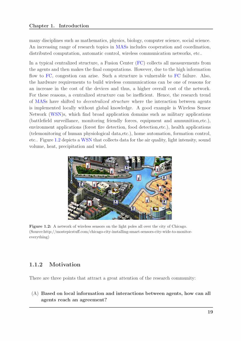
etc.. Figure 1.2 depicts a WSN that collects data for the air quality, light intensity, sound
volume, heat, precipitation and wind.
Figure 1.2: A network of wireless sensors on the light poles all over the city of Chicago.
(Source:http://mostepicstuff.com/chicago-city-installing-smart-sensors-city-wide-to-monitor-
everything)
1.1.2 Motivation
There are three points that attract a great attention of the research community:
(A) Based on local information and interactions between agents, how can all
agents reach an agreement?
19
Chapter 1. Introduction
This problem is called consensus problem, which is to design a network protocol
based on the local information obtained by each agent such that all agents finally
reach an agreement on certain quantities of interest.
Consensus problems of MASs have received tremendous attention from various
research communities due to their broad applications in many areas including multi-
sensors data fusion [64], flocking behavior of swarms [6, 38, 59, 60], multi-vehicle
formation control [17, 54, 62], distributed computation [5, 10, 48], rendez-vous
problems [15] and so on. More specifically, average consensus algorithms (i.e. the
consensus value corresponds to the average of the initial states) are commonly used
as building block for distributed control, estimation or inference algorithms.
In the recent literature, one can find average consensus algorithms embedded in
the distributed Kalman filter, [61]; Distributed Least Squares algorithms, [9]; Dis-
tributed Alternating Least Squares for tensors factorization, [45]; Distributed Prin-
cipal Component Analysis, [49]; or distributed joint input and state estimation, [24]
to cite few. However, the asymptotic convergence of the consensus algorithms is
not suitable for these kinds of sophisticated distributed algorithms. A slow asymp-
totic convergence can not ensure the efficiency and the accuracy of the algorithms,
which can lead to other unexpected effects. For example, regarding to the WSNs, a
reduction in the total number of iterations until convergence can lead to a reduction
in the total amount of energy consumption of the network, which is essential to
guarantee a longer life time for the entire network. On the other hand, the proto-
cols that guarantee a minimal execution time are much more appealing than those
ensuring asymptotic convergence. For this purpose, several contributions dedicated
to finite-time consensus have been recently published in the literature, meaning
that, consensus is obtained in a finite number of iterations.
(B) Can we assess the robustness of a network?
Generally, we are surrounded by networks of different kinds (social networks, sensor
networks, power networks, etc.). Therefore, the most important thing is that these
networks are robust. Meaning that, they can undergo through damage or failure.
Hence, the terminology robustness rapidly invades the research community.
Definition 1
Robustness is the ability of a network to continue performing well when it is subject
to failures or attacks [21].
In order to assess whether the network is robust, measuring the network robustness
is needed [21]. There are various proposed approaches to measure network robust-
ness metrics. However, the most popular approach in the literature is based on the
analysis of the graph. From data produced during consensus protocol can
we infer network robustness?
20

Chapter 1. Introduction
(C) Can we estimate the network topology?
Network topology is usually a schematic description of the arrangement of a net-
work, including its nodes and connecting edges. Network topology may describe
how data is transferred between these nodes.
Network topology identification refers to detecting and identifying the interested
network elements and the relationship between elements in this network and repre-
sents the topology construction in an appropriate form. Therefore, identification of
networks of systems becomes a growing attractive task for solving many problems
in different science and engineering domains.
Theoretically, there are some matrices that are associated with the graph represent-
ing a network. Therefore, one can find a method to identify the network topology
via the state matrix in a state space representation of linear dynamic systems,
which is related to the network topology. Eigenvalue decomposition of a matrix
shows that the structure of this matrix is linked to both eigenvalues and eigenvec-
tors of that matrix. In the other words, estimating both the eigenvalues and the
eigenvectors of network matrix can obviously infer the network structure.
1.1.3 Goals of the thesis
It is well-known that consensus protocols being iterative, a huge amount of data is pro-
duced. However, most of studies focus only on convergence properties of such algorithms.
With data collected from each iteration of the asymptotic consensus protocol in a dis-
tributed way, we aim to:
• Design finite-time average consensus protocols.
• Assess the network robustness.
• Reconstruct the network topology.
1.2 The consensus problem
Consensus issue in networks of autonomous agents has been widely investigated in various
fields, including computer science and engineering. In such networks, according to an
a priori specified rule, also called protocol, each agent updates its state based on the
information received from its neighbors with the aim of reaching an agreement to a
common value. When the common value corresponds to the average of the initial states,
average consensus is to be achieved.
21

Chapter 1. Introduction
1.2.1 Preliminaries
Let us consider a network modelled as a graph. In what follows, we first give some basic
notations and definitions from graph theory [32, 52].
Given a connected undirected graph G(V,E), where V = 1, 2, . . . , N is the set of
vertices (agents or nodes), and E ⊆ V × V is the set of edges (links) between agents.
The set of neighbors of node i and its degree are denoted by Ni = j|(i, j) ∈ E and
di = |Ni| respectively.
It is common to resort to some matrices for characterizing graphs. That is the case of
adjacency matrix A, degree matrix D of the graph, which has vertex degrees di, i ∈ V
on its diagonal and zeroes elsewhere, Laplacian Matrix L = D − A, clearly defined in
Chapter 2.
Through out this thesis, an undirected graph G(V,E) is mainly considered.
Example:
Consider an arbitrary network of 5 agents communicating with each other as described
in Figure 1.3. Each agent has an initial value. A consensus protocol is an interaction rule
that specifies the information exchange between an agent and all of its neighbors on the
network to reach an agreement regarding a certain quantity of interest that depends on
the state of all agents. Informally, despite the initial values of all agents, they converge
to the common value (in this case, the average of initial values).
1
23
4
5
2
45
6
7
initial values
At the beginning
1
23
4
5
4.8
4.84.8
4.8
4.8
average value
Finish
Figure 1.3: Average consensus in a network: initial condition (left) and steady state (right).
1.2.2 Consensus algorithms
The literature on consensus protocols can be organized as in Figure 1.4.
In this thesis, we concentrate on the consensus problem for discrete-time systems with
fixed topology.
22

Chapter 1. Introduction
Consensus Protocols
directed undirectedgraph graph
noiselesstime-
delay
continuoustime
systems
discretetime
systems
fixed
topology
noisy
switching
topology
instantaneous
Figure 1.4: Classification of Consensus protocols.
Given a graph G(V,E), each node has an associated value xi defined as the state of
node i. Let x(0) = [x1(0), x2(0), . . . , xN(0)]T be the vector of initial states of the given
network. In general, given the initial values at each node xi(0), i ∈ V , the main task is
to compute the final consensus value using distributed linear iterations. Each iteration
involves local communication between nodes. In particular, each node repeatedly updates
its value as a linear combination of its own value and those of its neighbors. The main
benefit of using a linear-iteration scheme is that, at each time-step, each node only has
to transmit a single value to each of its neighbors. The linear iteration-based consensus
update equation is expressed as:
xi(k + 1) = wii(k)xi(k) +∑
j∈Ni
wij(k)xj(k), i = 1, 2, . . . , N
or equivalently in matrix form:
x(k + 1) = W(k)x(k),
23
Chapter 1. Introduction
where: W(k) is the matrix with entries wij(k) = 0 if (i, j) /∈ E and∑
j∈Ni∪iwij(k) = 1.
The asymptotic consensus is reached if limk→∞ x(k) = µ1, meaning that all the nodes
agreed on the value µ. When µ is equal to the average of the initial values, i.e.
µ =1
N
N∑
i=1
xi(0),
it is called average consensus problem.
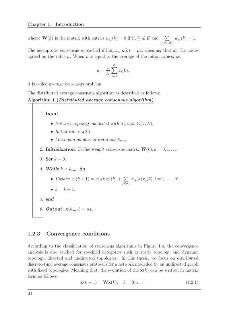
The distributed average consensus algorithm is described as follows:
Algorithm 1 (Distributed average consensus algorithm)
1. Input:
• Network topology modelled with a graph G(V,E),
• Initial values x(0),
• Maximum number of iterations kmax.
2. Initialization: Define weight consensus matrix W(k), k = 0, 1, . . ..
3. Set k = 0.
4. While k < kmax do
• Update: xi(k + 1) = wii(k)xi(k) +∑
j∈Ni
wij(k)xj(k), i = 1, . . . , N.
• k = k + 1;
5. end
6. Output: x(kmax) = µ1.
1.2.3 Convergence conditions
According to the classification of consensus algorithms in Figure 1.4, the convergence
analysis is also studied for specified categories such as static topology and dynamic
topology, directed and undirected topologies. In this thesis, we focus on distributed
discrete-time average consensus protocols for a network modelled by an undirected graph
with fixed topologies. Meaning that, the evolution of the x(k) can be written in matrix
form as follows:
x(k + 1) = Wx(k), k = 0, 1, . . . (1.2.1)
24

Chapter 1. Introduction
or equivalently,
x(k) = Wkx(0). (1.2.2)
Generally speaking, the system is said to achieve distributed consensus asymptotically if
limk→∞
x(k) = limk→∞
Wkx(0) = 1cccTx(0), (1.2.3)
where 111 ∈ RN×1 is the all-ones column vector and cccT is some constant row vector. There-
fore, it is good to view the conditions on the weight matrix W ensuring the convergence
of the consensus protocol as well as the average consensus protocol:
limk→∞
Wk = 1c1c1cT . (1.2.4)
The convergence conditions are described as follows:
Theorem 1.2.1 ([74])
Consider the linear iteration protocol (1.2.1), distributed consensus is achieved if
and only if the weight consensus matrix W satisfies the following conditions:
1. W1 = 111
2. ρ(W− 1c1c1cT ) < 1,
where ccc is chosen so that 111Tccc = 1 and ρ(W−1c1c1cT ) is the spectral radius of W−1c1c1cT .
To sum up, the weight matrix has row-sum equal to 1, 1 is a simple eigenvalue of W and
all other eigenvalues are strictly less than one in magnitude. It means that the weight
matrix W is a row-stochastic matrix.
When ccc = 1N111, the system is said to achieve average consensus (i.e the consensus value
is the average of all initial values):
limk→∞
Wk =1
N111111T . (1.2.5)
In order to achieve average consensus, beside the conditions in Theorem 1.2.1, the left
and right eigenvector of W corresponding to eigenvalue 1 are cT and 1, respectively.
Theorem 1.2.2
The equation (1.2.5) holds if and only if [74]:
1. 1TW = 111
2. W1 = 111
3. ρ(W− 1N111111T ) < 1
25

Chapter 1. Introduction
A necessary and sufficient condition to ensure the convergence of the average consen-
sus protocol for undirected graphs is that the weight consensus matrix W is a doubly
stochastic matrix.
1.2.4 Design of the weight matrix.
In the literature, there are some works devoted to the design of the weight matrixW that
satisfies the convergence conditions of the average consensus algorithms. For instance,
in [74, 75], it has been shown that the following weight matrices satisfy the convergence
conditions pointed out above.
1. Maximum-degree weights:
An approach to design the weight matrix W in a graph with fixed topology (time-
invariant topology) consists in assigning a weight on each edge equal to the inverse
of the maximum degree of the network, i.e.,
wij =
1dmax+1
if j ∈ Ni
1− didmax+1
if i = j
0 otherwise
(1.2.6)
where dmax = maxi∈V
di ≤ N . We can see that before running the consensus al-
gorithm, the maximum degree dmax should be known in a priori. The required
information on the graph topology is global, but can be obtained in a distributed
way by running a max consensus protocol [63].
2. Metropolis hasting weights:
The metropolis weights for a graph with a time-invariant topology are proposed in
[74]:
wij =
11+maxdi,dj , if j ∈ Ni
1− ∑
j∈Ni
11+maxdi,dj , if i = j
0, otherwise
(1.2.7)
Here, the nodes do not need any global information of the communication graph,
not even the number of the vertices N . They only need to know their own degree
and that of their neighbors to compute the weights. The metropolis weights are
very simple to compute and suited to a distributed implementation.
3. Constant edge weights:
26

Chapter 1. Introduction
By a result in [74], the simplest approach is to set all the edge weights for neigh-
boring nodes equal to a constant α. This is the most widely applied model for
the weight matrix in both time-variant and time-invariant topologies. The weight
matrix is defined as follows:
wij =
α, if j ∈ Ni
1− α|Ni|, if i = j
0, otherwise
(1.2.8)
where | · | denotes the cardinality of the set. The weight matrix can be expressed
in matrix form as follows:
W = IN − αL, (1.2.9)
where L, IN are the Laplacian matrix of the graph G and the N × N identity
matrix respectively. In general, α > 0 for the convergence condition 1.2.2 to hold.
Additionally, we can express the eigenvalues of W in terms of those of L:
λi(W) = 1− αλi(L), i = 1, . . . , N,
where λi(.) denotes the i-th largest eigenvalue of L. Therefore,
ρ(W− 1
N11T ) = maxλ2(W),−λN (W)
= max1− αλ2(L), αλN(L)− 1. (1.2.10)
The value of α that can ensure the convergence condition of the consensus protocols
is 0 < α < 2λN (L)
. There are some simple choices that do not require the knowledge
of the Laplacian spectrum, for example, the upper bound of the largest Laplacian
eigenvalue λN ≤ 2dmax. Hence, we can have a simple choice of α as 0 < α < 1dmax
.
Moreover, following the result in [74], the best possible constant edge weight in
terms of convergence speed is given by the following α:
α =2
λN(L) + λ2(L). (1.2.11)
In the analysis of consensus problems, convergence rate is an important index to evaluate
the performance of a consensus protocol. Therefore, there are several works dealing
with accelerating the rate of convergence of the consensus protocol by solving some
optimization problems in a centralized way or using Chebyshev polynomials.
Since the conditions of the weight consensus matrix W obviously influence on the con-
vergence of consensus algorithms, the main direction of research is now shifted to the
computation of W in order to improve the convergence rate, [47, 53, 74].
27

Chapter 1. Introduction
A. [74] proposed an optimization method to obtain the optimum weight matrix W
achieving average consensus in linear time-invariant topologies as the solution of a
semi-definite convex programming.
minW
ρ(W− 1N11T )
subject to W ∈ SG, 1TW = 1T , W1 = 1.
The condition W ∈ SG expresses the constraint on the sparsity pattern of the
matrix W with the set SG defined as follows:
SG = W ∈ RN×N |wij = 0 if (i, j) /∈ E and i 6= j.
B. In [47], the author proposed an interesting method to accelerate the speed of con-
vergence through polynomial filtering. The main idea is to apply a polynomial
filter on the consensus matrix W that will shape its spectrum in order to increase
the convergence rate.
Denote by pk(λ(W)) the polynomial filter of degree k that is applied on the spec-
trum of W,
pk(λ(W)) = α0 + α1λ(W) + α2λ2(W) + . . .+ αkλ
k(W). (1.2.12)
The matrix polynomial is defined as:
pk(W) = α0IN + α1W+ α2W2 + . . .+ αkW
k. (1.2.13)
where α0, . . . , αk are the coefficients of the polynomial.
For a given matrix W, and a certain degree k, instead of finding weight matrix
W to minimize the spectral radius ρ(W− 1N11T ), the problem is now to find the
polynomial coefficients αi, i = 0, . . . , k such that
minααα∈Rk+1
ρ(∑k
i=0 αiWi − 1
N11T )
subject to (∑k
i=0 αiWi)1 = 1.
After obtaining the coefficients αi, one can run the polynomial filtered distributed
consensus proposed in [47]:
Algorithm 2 (Polynomial filtered distributed consensus)
(a) Inputs:
28
Chapter 1. Introduction
• polynomial coefficients αi, i = 0, . . . , k+1, k degree of the polynomial filter.
• tolerance ε.
(b) Initialization: Consensus Matrix W, x(0);
(c) Set t=1;
(d) Repeat
• if mod(t, k + 1) == 0 then
xi[t] = α0xi[t− k − 1] + α1xi[t− k] + α2xi[t− k + 1] + . . .+ αkxi[t− 1].
xi[t] = wiixi[t] +∑
j∈Ni
wijxj [t], i = 1, 2, . . . , N
else
xi[t] = wiixi[t− 1] +∑
j∈Ni
wijxj [t− 1]
• end if
• t = t+ 1;
• x[t] = xi[t];
(e) until x[t]− x[t− 1] < ε.
(f) Outputs x[t]
C. Chebyschev polynomials for distributed consensus, [53]:
Denote the Chebyshev polynomial of degree k by Tk(x). These polynomials satisfy:
Tk(x) = cos(k arccosx), ∀x ∈ [−1, 1],
and |Tk(x)| > 1 when |x| > 1, ∀k ∈ N. These polynomials are defined by recurrence:
• T0(x) = 1,
• T1(x) = x,
• Tk(x) = 2xTk−1(x)− Tk−2(x), k ≥ 2.
Chebyshev polynomials have the following properties:
• Tk(x) = cos(k arccos x) ≤ 1, for x ∈ [−1, 1].
• maxx∈[−1,1]
|Tk(x)| = 1, Tk(−1) = (−1)k and |Tk(x)| > 1, ∀|x| > 1.
On the other hand, the direct expression of Tk(x) is characterized by:
Tk(x) =1 + τ 2k
2τk, τ = τ(x) = x−
√x2 − 1.
29
Chapter 1. Introduction
In order to speed up the consensus, the main idea consists in designing a distributed
linear iteration such that the execution of a fixed number of n steps is equivalent to
the evaluation of some polynomial, Pk(x), in the fixed matrix W. The polynomial
must satisfy that Pk(1) = 1 and |Pk(x)| < 1 if |x| < 1.
With two real coefficients κ, υ (−1 < κ < υ < 1), the polynomial is defined as:
Pk(x) =Tk(cx− d)
Tk(c− d),with c =
2
κ− υ, d =
κ+ υ
κ− υ, ∀k
which has the following properties:
• if x ∈ [κ, υ], then cx− d ∈ [−1, 1].
• Pk(1) = 1 and Pk(κ+ υ − 1) = (−1)k.
• |Pk(x)| < 1, ∀x ∈ (κ+ υ − 1, 1) and |Pk(x)| > 1 otherwise.
The polynomial satisfies the recurrence:
Pk(x) = 2Tk−1(c− d)
Tk(c− d)(cx− s)Pk−1(x)−
Tk−2(c− d)
Tk(c− d)Pk−2(x).
The consensus rule is then:
x(k) = Pk(W)x(0), (1.2.14)
where,
x(1) = P1(W)x(0) =1
T1(c− d)(cW− dIN )x(0),
and, x(k) = Pk(W)x(0)
=(
2Tk−1(c−d)
Tk(c−d)(cW− dIN)Pk−1(W)− Tk−2(c−d)
Tk(c−d)(cW− dIN )Pk−2(W)
)
x(0)
= 2Tk−1(c−d)
Tk(c−d)(cW− dIN)x(k − 1)− Tk−2(c−d)
Tk(c−d)(cW− dIN)x(k − 2), k ≥ 2.
The choice of the polynomial determine the convergence speed of the algorithm,
given by maxλi(W) |Pk(λi(W))|, where λi(W) is the i− th eigenvalue of W.
The convergence rate is given by:
maxλi(W)6=1
|Tk(cλi − d)|Tk(c− d)
= max|Tk(cλN(W)− d)|Tk(c− d)
,|Tk(cλ2(W)− d)|
Tk(c− d)
Using the Chebyshev polynomials means that we are minimizing maxλ∈[−1,1] Pk(λ),
therefore, getting high chances to obtain a good convergence rate. By an optimal
selection of κ, υ, we can maximize the convergence speed. Following the Theorem
4.2 in [53], the optimal parameters are κ = λN(W) and υ = λ2(W).
30
Chapter 1. Introduction
Let compare the convergence speed between the standard consensus protocol (1.2.1)
and the consensus protocol using the Chebyshev polynomials (1.2.14).
Denoting by vi, λi(W), i = 1, . . . , N the eigenvectors and eigenvalues of W, (1.2.1)
can be expressed as:
x(k) = Wkx(0) = v1 + λk2(W)v2 + . . .+ λk
N(W)vN .
Theorem 1.2.3 ([53])
Let λ = max(|λ2(W)|, |λN(W)|) be the convergence rate of the standard consensus
protocol (1.2.1). For any 0 < υ < 2λλ2+1
and κ = −υ, Pk(λ) goes to zero faster
than λk when k goes to infinity. Therefore, the consensus protocol using Chebyshev
polynomial converges faster than the standard one.
Since the average consensus protocols can be embedded in more sophisticated distributed
algorithms, protocols that guarantee a minimal execution time are more appealing than
those ensuring asymptotic convergence. For this purpose, several contributions dedicated
to finite-time consensus have been recently published in the literature, meaning that
consensus is obtained in a finite number of steps. The main contribution of this thesis is to
address the design of finite-time average consensus problem by making use of distributed
optimization methods.
1.3 Network robustness
The aim of network robustness research is to find a robustness measure to evaluate
the performance of a network, [16, 21]. Furthermore, understanding whether a network
is robust can protect and improve the performance of the network efficiently. By the
way, it is also used to design new networks that are able to perform well when facing
with failures or attacks.
Several robustness measures have been proposed in the literature. However, we are only
interested in topological measures, since it is well known that certain topologies exhibit
high robustness against failures. Therefore, they can be used to change the network
topology and decrease failures.
1.3.1 Vertex (Edge) connectivity
The vertex (edge) connectivity of an incomplete graph Kv(Ke) respectively represents
the minimal number of vertices (edges) that has to be removed to disconnect the graph.
Hence, Kv(Ke) depends on the least connected part of the graph. It has been shown in
[32] that Kv ≤ Ke ≤ dmin, where dmin is the minimum degree of the network.
31
Chapter 1. Introduction
For a complete graph of N nodes, Kv = Ke = N − 1.
Remark 1
• The measure value Kv(Ke) is an integer,
• The larger Kv(Ke), the harder it is to disconnect the graph, thus the graph is
more robust.
• In order to compute Kv(Ke), the network topology should be known at the first
sight.
1.3.2 Algebraic connectivity
The algebraic connectivity is the second smallest eigenvalue of the Laplacian matrix. If
λ2(L) = 0, the graph is disconnected. The algebraic connectivity of an incomplete graph
is not greater than the vertex connectivity Kv:
0 ≤ λ2(L) ≤ Kv ≤ Ke ≤ dmin
Remark 2
• A higher value of λ2(L) means that the graph is more robust.
• Sometimes, there is a problem that the algebraic connectivity is not strictly
increasing when an edge is added, [21].
1.3.3 Number of spanning trees ξ
A spanning tree is a sub-graph containing N − 1 edges, all N vertices, and no cycles.
The number of spanning trees is defined as a function of the Laplacian eigenvalues [21]
ξ =1
N
N∏
i=2
λi(L) (1.3.1)
The number of spanning trees can be used to assess the robustness of the network,[4].
Remark 3
The greater ξ, more robust is the graph.
32
Chapter 1. Introduction
1.3.4 Effective graph resistance R
Assume the graph is seen as an electrical circuit, where an edge (i, j) corresponds to a
resistor of unit resistance Rij = 1 Ohm. Informally, the effective resistance between two
vertices of a network (when a voltage is applied across them) can be calculated by series
and parallel manipulations. The effective graph resistance is the sum of the effective
resistances over all pairs of vertices, [21].
R =∑
1≤i<j≤N
Rij = N
N∑
i=2
1
λi(L)(1.3.2)
The effective graph resistance is the sum of the inverse of nonzero Laplacian eigenvalues.
Remark 4
The smaller R, more robust is the graph.
1.4 Outline of this Thesis
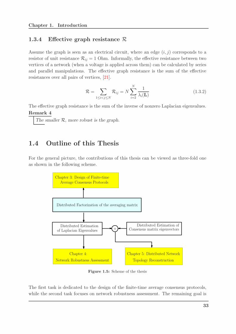
For the general picture, the contributions of this thesis can be viewed as three-fold one
as shown in the following scheme.
Distributed Estimationof Laplacian Eigenvalues Consensus matrix eigenvectors
Distributed Estimation of+
Distributed Factorization of the averaging matrix
Chapter 3: Design of Finite-time
Average Consensus Protocols
Chapter 4:
Network Robustness Assessment
Chapter 5: Distributed Network
Topology Reconstruction
Figure 1.5: Scheme of the thesis
The first task is dedicated to the design of the finite-time average consensus protocols,
while the second task focuses on network robustness assessment. The remaining goal is
33

Chapter 1. Introduction
dedicated to network topology reconstruction. Hereinafter, we present the outline of this
thesis as follows:
• Chapter 2: Graph Theory.
In this chapter, we give general definitions of graph theory.
• Chapter 3: Distributed Design of Finite-time Average Consensus Protocols.
This is one of the main contributions of this thesis, where the design of the finite-
time average consensus is solved in a distributed way. The problem is formulated
as a factorization of the averaging matrix JN = 11T
N. The solution is obtained by
solving a constrained optimization problem in a distributed way. For the simple
understanding, each linear iteration k, k = 0, . . . , D with D being the number of
steps is illustrated as a layer of a network (including D+1 layers). The main idea
is to compute the partial derivatives of the error between the actual output and
desired output, then propagate them back to each iteration k in order to update the
weights. Then, the proposed algorithm is based on the back-propagation method
and an associated gradient descent method. The evaluation of the proposed method
is assessed by numerical results.
• Chapter 4: Distributed network robustness assessment.
In this chapter, we make use of the metrics which are the number of spanning tree
ξ and the effective graph resistance R to assess the robustness of a given network.
By the nature of these metrics, they are all functions of the Laplacian eigenvalues
λi(L), hence, the Laplacian eigenvalues estimation is now the main purpose of
this task. In this chapter, instead of estimating the Laplacian eigenvalues directly,
we solve this problem as a constrained optimization problem with respect to the
inverse of the nonzero distinct Laplacian eigenvalues. As the result, by applying
the gradient descent method, we finally get the set of nonzero distinct Laplacian
eigenvalues. Furthermore, by using an integer programming algorithm, we can
estimate the multiplicities corresponding to these eigenvalues. Then, we deduce
the whole spectrum of the Laplacian matrix associated with the graph G(V,E).
Thanks to these results, the robustness measures can be estimated to evaluate the
robustness of the network.
For the task of Laplacian spectrum estimation, all methods proposed in this chapter
are divided into two categories: non-convex and convex formulations. According
to non-convex optimization problem (it is also called direct method), the problem
is viewed as a constrained optimization problem with respect to the stepsizes αk
of the Laplacian-based consensus protocol, whose inverses are equal to the nonzero
distinct Laplacian eigenvalues.
Solving the non-convex optimization problem, the main issue is the slowness of
the convergence speed. Therefore, we try to make the speed of the estimation of
34

Chapter 1. Introduction
the Laplacian eigenvalues as fast as possible. The main point is to transform the
nonconvex problem into a convex one. We solve the problem by two algorithms
using the distributed projection method, [57] and the Alternating Direction of
Multipliers Method (ADMM), [11]. We consider three cases: final average value
perfectly known, noisy and completely unknown.
• Chapter 5: Network topology reconstruction.
Since, the components used to infer the network structure are the eigenvalues and
eigenvectors of the weight consensus matrix, we first propose an algorithm to obtain
these eigenvectors. Besides that, the corresponding eigenvalues can be obtained by
using the algorithms proposed in the previous chapters. Finally, we can make use
of received eigenvectors and eigenvalues to reconstruct the network topology.
• Chapter 6: Conclusion and Future Works.
This chapter summarises the contributions of this thesis and also outlines possible
future directions.
1.5 Publications list
The main contributions of this thesis are the principal subject of the following publica-
tions:
1.5.1 International conference papers with proceedings
• Tran, T.M.D; Kibangou, A., ”Consensus-based Distributed Estimation of Laplacian
Eigenvalues of Undirected Graphs”, in 12th European Control Conference (ECC
2013)”, Zurich, Switzerland, July 2013.
• Tran, T.M.D; Kibangou, A., ”Distributed Design of Finite-time Average Consensus
Systems”, in IFAC Workshop on Distributed Estimation and Control in Networked
(NecSys), Koblenz, Germany, September 2013.
• Tran, T.M.D; Kibangou, A., ”Distributed Estimation of Graph Laplacian Eigen-
values by the Alternating Direction of Multipliers Method”, in the 19th World
Congress of the International Federation of Automatic Control, Cape Town, South
Africa, 24-29 August 2014.
35

Chapter 1. Introduction
1.5.2 Journals
• Tran, T.M.D; Kibangou, A., ”Distributed Estimation of Laplacian Eigenvalues of
Medium-Size Networks via Constrained Consensus Optimization Problems”, in Sys-
tems and Control Letters, 2015.
36

Chapter 2
Graph Theory
Contents
2.1 Connectivity of a graph . . . . . . . . . . . . . . . . . . . . . . 38
2.2 Algebraic graph properties . . . . . . . . . . . . . . . . . . . . 39
2.3 Spectral graph properties . . . . . . . . . . . . . . . . . . . . 41
2.4 Standard classes of graphs . . . . . . . . . . . . . . . . . . . . 42
Conceptually, a graph G(V,E) is formed by vertices and edges connecting the vertices.
As said in Subsection 1.2, a network can be modelled by a graph, where an agent is
represented by a vertex (node) and the communication between agents is set by an edge
(link).
According to the communication policy, the graph G(V,E) can be undirected or directed.
• Undirected Graph:
The communication topology of the network of N agents is represented by a graph
G(V,E), where V = 1, 2, . . . , N is the set of vertices (agents or nodes), and
E ⊆ V × V is the set of edges (links between agents).
If there is no direction assigned to the edges, then both edges (i, j) and (j, i) are
included in the set of edges E. The graph is called undirected graph.
If agent i and j are connected, then the link between i and j is included in E,
(i, j) ∈ E and i and j are called neighbors. The set of neighbors of agent i is
denoted by Ni and its degree is denoted by di = |Ni|, where |.| stands for the
cardinality.
• Directed Graph:
37

Chapter 2. Graph Theory
If a direction is assigned to the edges, the relations are asymmetric and the graph
is called a directed graph (or a digraph). For a directed graph as shown in Figure
2.1, for a directed edge (i, j), i is called the head and j is called the tail.
A vertex i is connected to j by a directed edge, or that j is a neighbor of i if
(i, j) ∈ E. The edge (i, j) is then an outgoing edge for i and an ingoing edge for j.
The out-degree douti of a vertex i is its number of outgoing edges, or number of
vertices to which it is connected. The in-degree dini is its number of ingoing edges
or number of vertices that are connected to it.
∑
i∈Vdouti =
∑
i∈Vdini = |E|.
1
23
45
vertex edge
6
Undirected graph Directed graph
1
2
3 4
5
Figure 2.1: 6-node undirected and 5-node directed networks.
Figure 2.1 shows:
• a 6-node undirected graph with set of vertices V = 1, 2, . . . , 6, and set of edges
E = (1, 2), (1, 3), (1, 4), (1, 5), (2, 3), (2, 5), (3, 4), (4, 5), (4, 6), (5, 6)
• a 5-node directed graph with set of vertices V = 1, 2, . . . , 5, and set of edges
E = (1, 5), (1, 3), (2, 1), (2, 4), (3, 2), (3, 5), (4, 3), (4, 5).
2.1 Connectivity of a graph
A path from a vertex i to a vertex j is a sequence of distinct vertices starting with vertex
i and ending with vertex j such that consecutive vertices are adjacent. A simple path is
a path with no repeated vertices.
• In an undirected graph G, two vertices i and j are connected if there is a path
from i to j. An undirected graph G is connected if for any two vertices in G
38
Chapter 2. Graph Theory
there is a path between them, see Figure 2.2. Conversely, two vertices i and j in
G are disconnected if there is no path from i to j. An undirected graph G is
disconnected if we can partition its vertices into two nonempty sets χ and Γ such
that no vertex in χ is adjacent to a vertex in Γ, see Figure 2.3.
• A directed graph is strongly connected if between every pair of distinct vertices
(i, j) in G, there is a directed path that begins at i and ends at j. It is called
weakly connected if replacing all of its directed edges with undirected edges
produces a connected undirected graph.
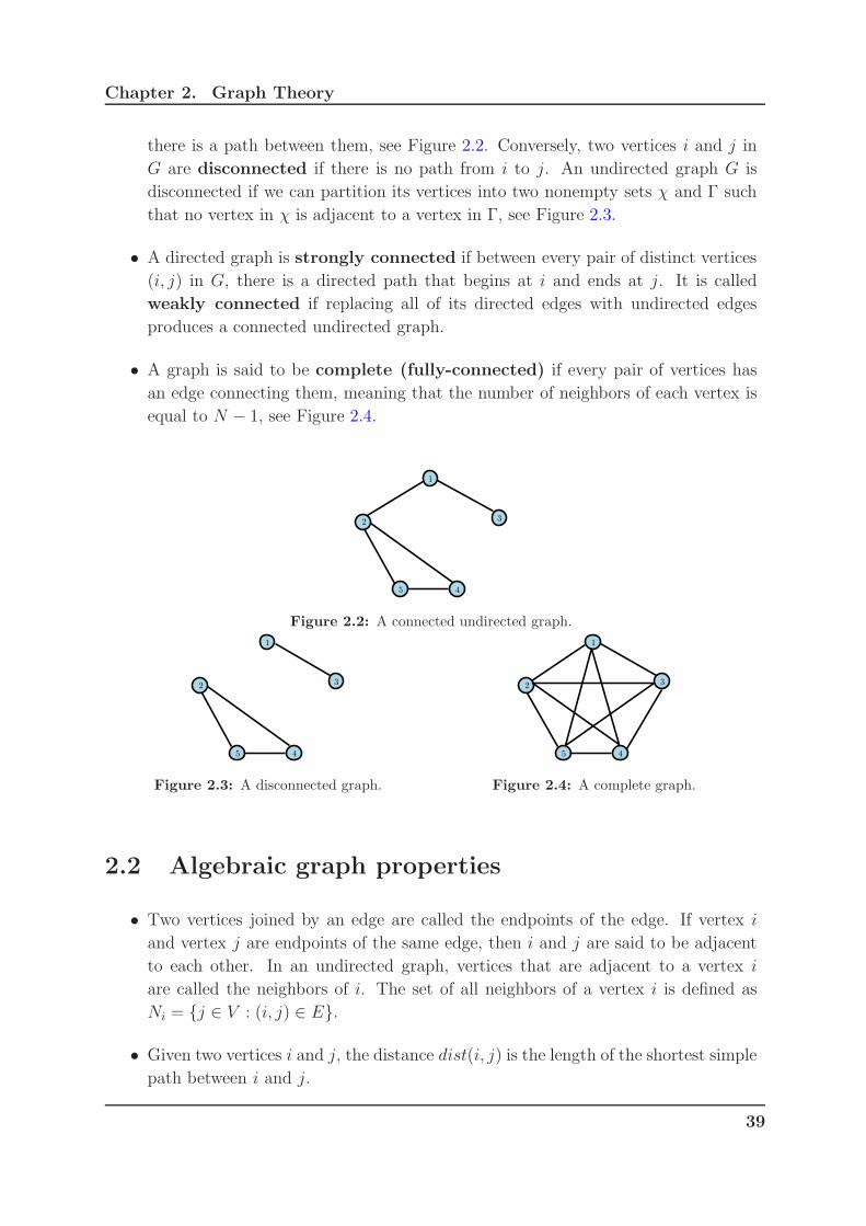
• A graph is said to be complete (fully-connected) if every pair of vertices has
an edge connecting them, meaning that the number of neighbors of each vertex is
equal to N − 1, see Figure 2.4.
1
23
45
Figure 2.2: A connected undirected graph.
1
23
45
Figure 2.3: A disconnected graph.
1
23
45
Figure 2.4: A complete graph.
2.2 Algebraic graph properties
• Two vertices joined by an edge are called the endpoints of the edge. If vertex i
and vertex j are endpoints of the same edge, then i and j are said to be adjacent
to each other. In an undirected graph, vertices that are adjacent to a vertex i
are called the neighbors of i. The set of all neighbors of a vertex i is defined as
Ni = j ∈ V : (i, j) ∈ E.
• Given two vertices i and j, the distance dist(i, j) is the length of the shortest simple
path between i and j.
39
Chapter 2. Graph Theory
• The eccentricity ǫi of a vertex i is the greatest distance between i and any other
vertex j ∈ V .
• The radius r(G) of a graph G is the minimum eccentricity of any vertex.
• The diameter d(G) of a graph is the maximum eccentricity of any vertex in the
graph, d(G) = maxi,j
dist(i, j).
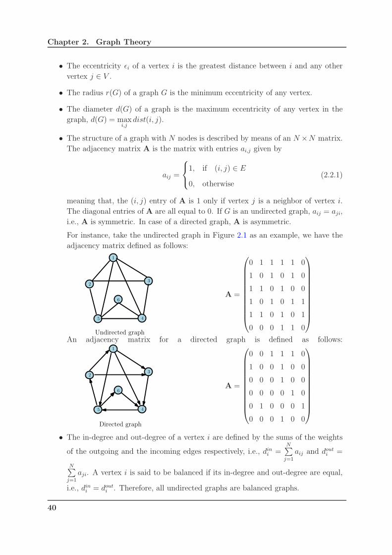
• The structure of a graph with N nodes is described by means of an N ×N matrix.
The adjacency matrix A is the matrix with entries ai,j given by
aij =
1, if (i, j) ∈ E
0, otherwise(2.2.1)
meaning that, the (i, j) entry of A is 1 only if vertex j is a neighbor of vertex i.
The diagonal entries of A are all equal to 0. If G is an undirected graph, aij = aji,
i.e., A is symmetric. In case of a directed graph, A is asymmetric.
For instance, take the undirected graph in Figure 2.1 as an example, we have the
adjacency matrix defined as follows:
1
23
45
6
Undirected graph
A =
0 1 1 1 1 0
1 0 1 0 1 0
1 1 0 1 0 0
1 0 1 0 1 1
1 1 0 1 0 1
0 0 0 1 1 0
An adjacency matrix for a directed graph is defined as follows:1
23
45
6
Directed graph
A =
0 0 1 1 1 0
1 0 0 1 0 0
0 0 0 1 0 0
0 0 0 0 1 0
0 1 0 0 0 1
0 0 0 1 0 0
• The in-degree and out-degree of a vertex i are defined by the sums of the weights
of the outgoing and the incoming edges respectively, i.e., dini =N∑
j=1
aij and douti =
N∑
j=1
aji. A vertex i is said to be balanced if its in-degree and out-degree are equal,
i.e., dini = douti . Therefore, all undirected graphs are balanced graphs.
40

Chapter 2. Graph Theory
• A digraph G is called balanced ifN∑
j 6=i
aij =N∑
j 6=i
aji.
The degree matrix D of G is the N ×N diagonal matrix with (i, j) entry given by:
Dij =
douti , if i = j
0, otherwise(2.2.2)
or equivalently,
D = diag(A1). (2.2.3)
2.3 Spectral graph properties
• The Laplacian matrix is used for mathematical convenience to describe the con-
nectivity in a more compact form. The graph Laplacian L is defined as the matrix
with entries lij given by:
lij =
N∑
k=1,k 6=i
aik if i = j
−aij if i 6= j
(2.3.1)
The Laplacian matrix L can be expressed in matrix form as follows:
L = D −A. (2.3.2)
Again, we take the 6-node graph in Figure 2.1 as an example:
1
23
45
6
Undirected graph
L =
4 −1 −1 −1 −1 0
−1 3 −1 0 −1 0
−1 −1 3 −1 0 0
−1 0 −1 4 −1 −1
−1 −1 0 −1 4 −1
0 0 0 −1 −1 2
• Some important properties of the Laplacian matrix are:
1. As can be seen in the definition of L, the row-sum of L is zero. Since L1 = 0,
where 0 is a zero vector of length N , L has at least one eigenvalue zero with
associated right eigenvector 1.
If the graph G(V,E) is undirected, then:
41
Chapter 2. Graph Theory
2. The spectrum of L, that is the set of all eigenvalues of the Laplacian matrix, is
denoted as sp(L) = λm11 , λm2
2 , . . . , λmD+1
D+1 , , wheremi stands for the multiplic-
ity of the i− th eigenvalue and D is the number of nonzero distinct Laplacian
eigenvalues. The multiplicity of the zero eigenvalue represents the number of
connected components of the graph. For undirected graphs, L is symmetric
and positive semi-definite, hence 0 = λ1 < λ2 < . . . < λD+1 < 2dmax, andD+1∑
i=1
mi = N with m1 = 1, where dmax is the maximum degree of the graph,
i.e., dmax = maxi
di. We denote by Λ = λ2, . . . , λD+1 the set of nonzero
distinct Laplacian eigenvalues.
3. λ2 is the second smallest eigenvalue, which is known as the algebraic con-
nectivity and reflects the degree of connectivity of the graph G, [28]. It is
well-known that the speed of convergence of a consensus protocol depends on
this second smallest Laplacian eigenvalue λ2, [32].
minx 6=0,1Tx=0
xTLx
‖x‖2 = λ2(L). (2.3.3)
From the literature, the second smallest Laplacian eigenvalue is upper
bounded by maxj∈Ni
di + dj.
4. In [51], another interesting property has been pointed out:
N∑
i=1
λi(L) =
N∑
i=1
di.
2.4 Standard classes of graphs
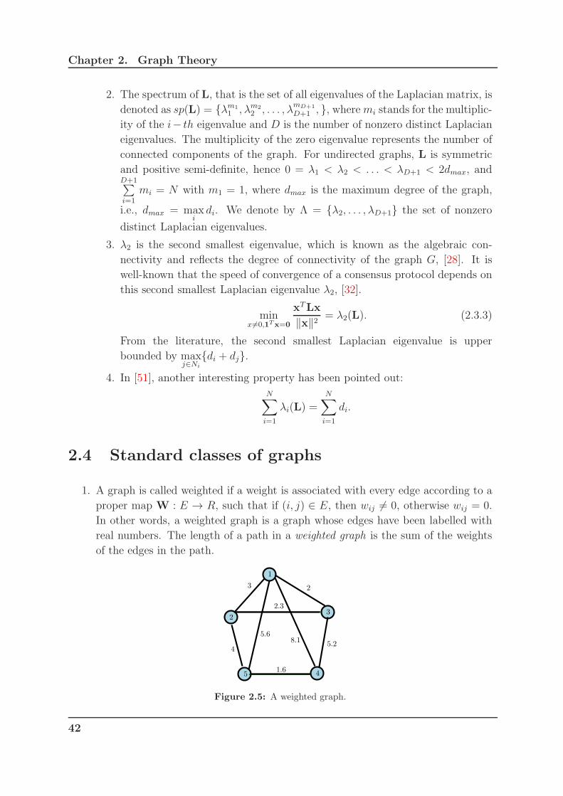
1. A graph is called weighted if a weight is associated with every edge according to a
proper map W : E → R, such that if (i, j) ∈ E, then wij 6= 0, otherwise wij = 0.
In other words, a weighted graph is a graph whose edges have been labelled with
real numbers. The length of a path in a weighted graph is the sum of the weights
of the edges in the path.
1
23
45
23
45.2
1.6
2.3
5.68.1
Figure 2.5: A weighted graph.
42

Chapter 2. Graph Theory
2. A graph is called a regular graph if all the vertices have the same number of neigh-
bors. The graph is written as n-regular if the number of neighboring vertices is n
for all vertices. n is called valency of the n-regular graph.
1
2 3
45
6
Figure 2.6: A 3-regular graph
3. A graph G(V,E) with diameter d(G) is said to be a distance-regular graph if for any
vertices i and j of V and any integers v, w = 0, 1, . . . , d(G) (where d(G) is diameter
of graph G), the number of vertices at distance v from i and distance w from j
depends only on v, w, and the graph distance between i and j, independently of
the choice of i and j.
1
2 3
4
5 6
8 7
Figure 2.7: A distance-regular graph
4. A graph G is said to be strongly regular, SRG(N ,κ,a,c), if it is neither complete
nor empty and there are integers κ, a, and c such that:
• G is regular with valency κ;
• any two adjacent vertices have exactly a common neighbors;
• any two distinct non-adjacent vertices have exactly c common neighbors.
These parameters are linked as follows:
(N − κ− 1)c = κ(κ− a− 1). (2.4.1)
Examples of strongly regular graphs are:
43
Chapter 2. Graph Theory
• Petersen graph (SRG(10, 3, 0, 1)),
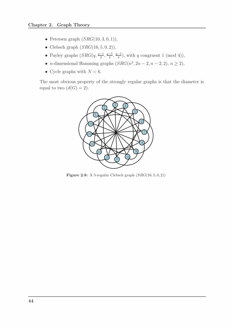
• Clebsch graph (SRG(16, 5, 0, 2)),
• Payley graphs (SRG(q, q−12, q−5
4, q−1
4), with q congruent 1 (mod 4)),
• n-dimensional Hamming graphs (SRG(n2, 2n− 2, n− 2, 2), n ≥ 2),
• Cycle graphs with N < 6.
The most obvious property of the strongly regular graphs is that the diameter is
equal to two (d(G) = 2).
1
23 4
5
6
7
8
9
1011
12
13
14
15
16
Figure 2.8: A 5-regular Clebsch graph (SRG(16, 5, 0, 2))
44
Chapter 3
Distributed design of finite-time
average consensus protocols
Contents
3.1 Introduction . . . . . . . . . . . . . . . . . . . . . . . . . . . . 45
3.2 Literature review . . . . . . . . . . . . . . . . . . . . . . . . . 47
3.2.1 Minimal polynomial concept based approach . . . . . . . . . . 47
3.2.2 Matrix factorization based approach . . . . . . . . . . . . . . . 49
3.2.3 Comparison between the minimal polynomial approach and the
matrix factorization approach . . . . . . . . . . . . . . . . . . . 55
3.3 Distributed solution to the matrix factorization problem. . 56
3.4 Numerical results . . . . . . . . . . . . . . . . . . . . . . . . . 64
3.4.1 Example 1 . . . . . . . . . . . . . . . . . . . . . . . . . . . . . . 65
3.4.2 Example 2 . . . . . . . . . . . . . . . . . . . . . . . . . . . . . . 68
3.5 Conclusion and discussion . . . . . . . . . . . . . . . . . . . . 70
3.1 Introduction
Consider an undirected connected graph G(V,E) with xi(k) being the state of node
i at time-step k and define the initial state of the given network as x(0) =
[x1(0), x2(0), . . . , xN(0)]T where N = |V |. A novel method is proposed in this chap-
ter to design finite-time average consensus protocols for MASs or WSNs in a distributed
way. In the discrete-time framework, a linear iteration scheme expresses its benefits for
a distributed algorithm since each node repeatedly updates its value as a weighted linear
45
Chapter 3. Distributed design of finite-time average consensus protocols
combination of its own value and those of its neighbors.
xi(k + 1) = wii(k)xi(k) +∑
j∈Ni
wij(k)xj(k), (3.1.1)
where
wij =
0, if (i, j) /∈ E
wij, if (i, j) ∈ E
or equivalently in matrix form:
x(k + 1) = W(k)x(k), (3.1.2)
W(k) ∈ SG where SG is the set of matrices that can be factorized as W(k) = Q(k) (IN +A) where Q(k) stands for an arbitrary square matrix, IN as the N × N identity
matrix, and denotes the Hadamard matrix product that corresponds to an entry-wise
matrix product.
As presented in the Chapter 1.2, average consensus is reached asymptotically if
limk→∞
x(k) =1
N11Tx(0), (3.1.3)
meaning that
limk→∞
Wk =1
N11T = JN . (3.1.4)
However, the foremost thing to note is that in order to run an average consensus algo-
rithm, two main steps are required: the configuration step (also called design step) and
the execution step. During the configuration step, a task can be achieved through a self-
configuration algorithm instead of resorting to a network manager. Self-configuration can
include graph discovering and distributed decision on some parameters. For instance, if
the protocol is the maximum degree weights one ( 1.2.6), each agent first computes the
number of its neighbors before running a max-consensus algorithm for computing the
maximum degree of the underlying graph. In the case of the Metropolis-Hasting based
protocol ( 1.2.7), each agent compares its degree with that of its neighbors in order to
compute the weights of the average consensus protocol. One commonly used protocol is
the constant edge weights, or graph Laplacian based average consensus protocol ( 1.2.8),
where a common stepsize is used by all agents. Asymptotic convergence is hence guaran-
teed if the stepsize is strictly positive and lower than 2λN
, where λN stands for the largest
Laplacian eigenvalue. Even through there are some simple bounds that give choices for
the stepsize without requiring exact knowledge of the Laplacian spectrum, agents have
to agree on an adequate stepsize.
To the best of our knowledge, there is no published work dealing with self-configuration
protocols for the constant edge weights based average consensus protocol.
46
Chapter 3. Distributed design of finite-time average consensus protocols
In real systems, the execution time is getting more and more impact. Therefore, the
purpose is now to design a finite-time average consensus algorithm allowing all nodes
to reach the average consensus value in a finite number of steps D for self-configuration
protocols, i.e.
x(D) =1
N11Tx(0) = JNx(0). (3.1.5)
3.2 Literature review
In the literature, the proposed finite-time consensus protocols can be classified by two
main approaches, namely: the minimal polynomial concept based approach and matrix
factorization based approach.
3.2.1 Minimal polynomial concept based approach
In [70], a finite-time consensus algorithm for linear time-invariant topologies based on
the minimal polynomial of the weight consensus matrix W was proposed. Specifically,
the minimal polynomial of the matrix W is the unique monic polynomial q(W) of the
smallest degree such that q(W) = 0.
Suppose that the minimal polynomial of W has degree D + 1 ≤ N . For some constants
α0, α1, . . . , αD, which are coefficients of the minimal polynomial q(W), since q(W) = 0,
we get:
WD+1 + αDWD + . . .+ α1W+ α0IN = 0.
By multiplying the two sides of this equation with x(k), we obtain:
WD+1x(k) + αDWDx(k) + . . .+ α1Wx(k) + α0x(k) = 0.
or equivalently:
x(k +D + 1) + αDx(k +D) + . . .+ α1x(k + 1) + α0x(k) = 0.
Therefore, ∀k ≥ 0 and 1 ≤ i ≤ N , xi(k) satisfies a linear difference equation of the form:
xi(k +D + 1) + αDxi(k +D) + . . .+ α1xi(k + 1) + α0xi(k) = 0. (3.2.1)
It was shown that:
xi =[xi(D) xi(D − 1) . . . xi(0)]s
[1 1 . . . 1]s,
47
Chapter 3. Distributed design of finite-time average consensus protocols
where
s =
1
1 + αD
1 + αD−1
...
1 +D∑
j=1
αj
The nodes need a sufficient observation time which is the degree of the minimal poly-
nomial to reconstruct the initial states. However, the design of this protocol requires a
strong knowledge on the underlying network topology. In fact, each node needs to store
N(N −1) samples with N being the network size. Therefore, a decentralized calculation
of the minimal polynomial was proposed although it is not entirely local, in the sense
that a local calculation is repeated over N independent iterations (where N is the total
number of nodes of the network) and at each iteration, it requires each node to store its
own values for N + 1 time steps in order to obtain the minimal polynomial.
An improved method which requires much less data storage has been proposed in [78].
The authors have proposed algorithms to compute the consensus value using the minimal
number of observations of an arbitrary chosen node in a network using 2(Di+1) successive
discrete-time steps, where Di + 1 is the degree of the monic minimal polynomial.
From equation (3.2.1), the measurable value at node i is determined by the mini-
mal of polynomial of the corresponding matrix observability pair [W, eTi ], where eTi =
[0, . . . , 0, 1i, 0, . . . , 0] ∈ IR1×N .
Definition 1 ([78])
The minimal polynomial associated with the matrix pair [W, eTi ] denoted by qi(t) ,
tDi+1 +∑Di
k=0 αi,ktk is the unique monic polynomial of minimal degree Di + 1 that
satisfies eTi qi(W) = 0.
Hence, the minimal integer value Di+1 necessary for (3.2.1) to hold for almost any initial
condition x(0) is given by the degree of the minimal polynomial of the observability pair
[W, eTi ] [79].
Consider the vector of difference between successive discrete-time values at node i,Xi(0, 1, 2 . . . , 2k) = xi(1) − xi(0), xi(2) − xi(1), . . . , xi(2k + 1) − xi(2k), k ∈ Z andits associated Hankel matrix:
ΓXi(0, 1, 2 . . . , 2k) ,
xi(1)− xi(0) xi(2)− xi(1) · · · xi(k + 1)− xi(k)
xi(2)− xi(1) xi(3)− xi(2) · · · xi(k + 2)− xi(k + 1)...
.... . .
...
xi(k + 1)− xi(k) xi(k + 2)− xi(k + 1) · · · xi(2k + 1)− xi(2k)
.
(3.2.2)
48
Chapter 3. Distributed design of finite-time average consensus protocols
The minimal number of steps is computed by checking a rank condition of a Hankel
matrix constructed from local output observations in a distributed way.
Increase the dimension k of the square Hankel matrix ΓXi(0, 1, 2 . . . , 2k) until it loses
rank and store the first defective Hankel matrix. In [78], the authors have shown
that by using a Vandermonde factorization of the Hankel matrix, one can see that
ΓXi(0, 1, 2 . . . , 2k) is defective if k ≥ Di + 1.
Then, the normalized kernel βββ = [β0 . . . βDi+1 1]T of the first defective Hankel matrix is
estimated.
Based on linear iteration (3.2.1), the following regression equation denoted by the output
observations of node i in minimal time is defined as:
xi(k +Di + 1) + αi,Dixi(k +Di) + . . .+ αi,1xi(k + 1) + αi,0xi(k) = 0. (3.2.3)
Consider the Z-transform of xi(k):
X(z) =
Di+1∑
j=1
αj
j−1∑
l=0
xi(l)zj−l
qi(z),
H(z)
qi(z).
In order to estimate the final consensus value at node i, we define the following polyno-
mial:
pi(z) ,qi(z)
z − 1,
Di∑
j=0
βjzj .
Then, the final consensus value is defined:
φ = limz→1
(z − 1)X(z) =H(1)
pi(1)=
yTi (Di)βββ
1Tβββ,
where yTi (Di) = [xi(0) xi(1) . . . xi(Di)] and βββ = [β0 . . . βDi−1 1]T is the vector of
coefficients of the polynomial pi(z).
In [78], the authors show that for an arbitrary initial condition, except for a set of initial
conditions with Lebesgue measure zero [7], the consensus value can be obtained from
local observations in a minimal number of steps that does not depend on the total size of
the graph. However, the computation of the rank of a given matrix and that of its kernel
are needed. Therefore, the computational cost is still the weakness of these methods.
3.2.2 Matrix factorization based approach
This approach is based on the factorization of the averaging matrix JN . More precisely,
we desire to find a finite sequence of matrices W(1),W(2), . . . ,W(D),W(k) ∈ SG
49

Chapter 3. Distributed design of finite-time average consensus protocols
such that
x(D) =
1∏
k=D
W(k)x(0) = JNx(0) for all x(0) ∈ IRN , (3.2.4)
with1∏
k=D
W(k) = JN . (3.2.5)
Finding this set of matrices is equivalent to solve a multi-variable polynomial system of
equations, which can be solved using Grobner basis theory. However, the computational
complexity is also burdens. In general, studying the existence of solutions to such a
system of equations can be intractable.
3.2.2.1 Existence
The existence issue has been deeply considered in [30] and [34]. It has been pointed out
that no solution exists if the factor matrices W(k) are all equal except if the graph is
complete. Since the diameter of the graph characterizes the time necessary for a given
information to reach all the nodes in the network, the number of factor matrices cannot
be lower than the diameter d(G).
In [34], an upper-bound of the number of factor matrices is given by 2r(G), with r(G)
being the radius of the given graph (trees and graphs with minimum diameter spanning
tree). Furthermore, for more general graphs, according to the results in [42], the number
D is upper bounded by N − 1. Hence, the number of steps D is bounded by:
d(G) ≤ D ≤ N − 1. (3.2.6)
The solution of the factorization problem is not unique and no distributed solution exists.
In [35], the authors have investigated the possibility of reaching (average) consensus
in finite time by making use of a linear iterations scheme with a finite sequence of T
consensus matrices, which are restricted to be stochastic with positive diagonals and
consistent with a connected undirected graph structure G(V,E) where N = |V |. In this
paper, the upper bound on the number of matrices was also given by N(N−1)2
. On the
other hand, for directed graphs, the authors have proven that finite-time consensus is
reached by a sequence of stochastic matrices with positive diagonals only if the graph is
strongly connected and contains a simple directed cycle with even length. However, if
the graph G is a simple directed cycle, then there is no sequence of stochastic matrices
with positive diagonals achieving consensus.
50

Chapter 3. Distributed design of finite-time average consensus protocols
3.2.2.2 Solutions for particular graphs
For distance regular graphs, a closed form expression of the matrix factorization exists
[39]. The factorization of the averaging matrix has been proposed based on parameters
of the intersection array characterizing the underlying graph constrained as a distance
regular graph.
Definition 2 ([12])
A graph G(V,E) with diameter d(G) is said to be distance regular if there exist
integers ak, bk, ck, k = 0, 1, . . . , d(G) such that for any two vertices i, j ∈ V and
distance k = dist(i, j), there are exactly ak neighbors of j in Vk(i), bk neighbors of
j in Vk+1(i), and ck neighbors of j in Vk−1(i), where Vk(i) is the set of vertices j of
G(V,E) with dist(i, j) = k.
The parameters of a distance regular graph with valency K are linked as ai+bi+ci = K,
with a0 = c0 = bd(G) = 0 and c1 = 1. Therefore, it is usual to characterize a distance
regular graph by its intersection array b0, b1, . . . , bd(G); c1, c2, . . . , cd(G) where b0 ≥ b1 ≥. . . ≥ bd(G) and 0 ≤ c1 ≤ c2 ≤ . . . ≤ cd(g).
Let us define Gk(V,Ek) with (i, j) ∈ Ek if and only if dist(i, j) = k and Ak be its
adjacency matrix.
d(G)∑
k=0
Ak = JN .
One property can be noted as follows:
AAk = bk−1Ak−1 + akAk + ck+1Ak+1,
where A = A1 stands for the graph adjacency matrix.
Example : The Hamming graph H(d(H), n) with d(H) being the diameter of the graph, and
nd(H) being the number of vertices.
51

Chapter 3. Distributed design of finite-time average consensus protocols
Figure 3.1: A H(4, 2) Hamming graph.
Therefore, its intersection array is given by 4, 3, 2, 1; 1, 2, 3, 4.
Additionally, in [39], the author has presented the factorization of the averaging matrix
for distance regular graphs. Herein, we review two main theorems that help to determine
the sequence of the consensus matrices.
Theorem 3.2.1 ([36])
Consider a graph G with N vertices and adjacency matrix A
1. There exist a polynomial H(ν) such that H(A) = JN if and only if G is a
connected regular graphs.
2. For a connected regular graph with valency K, the unique polynomial of least
degree satisfying H(A) = JN is H(ν) = Ng(K)
g(ν) where (ν − K)g(ν) is the
minimal polynomial of A.
The polynomial H(A) is called the Hoffman polynomial of G. We can note that the
degree of this polynomial is unknown, except for distance regular graph.
Lemma 1 ([39])
Consider a distance regular graph G(V,E) with |V | = N , valency K, diameter d(G)
and intersection array b0, b1, . . . , bd(G); c1, c2, . . . , cd(G). The averaging matrix 1NJN
is a d(G)-th order polynomial of the graph adjacency matrix A:
1
NJN = PG(A) =
d(G)∑
q=0
γqAq,
52
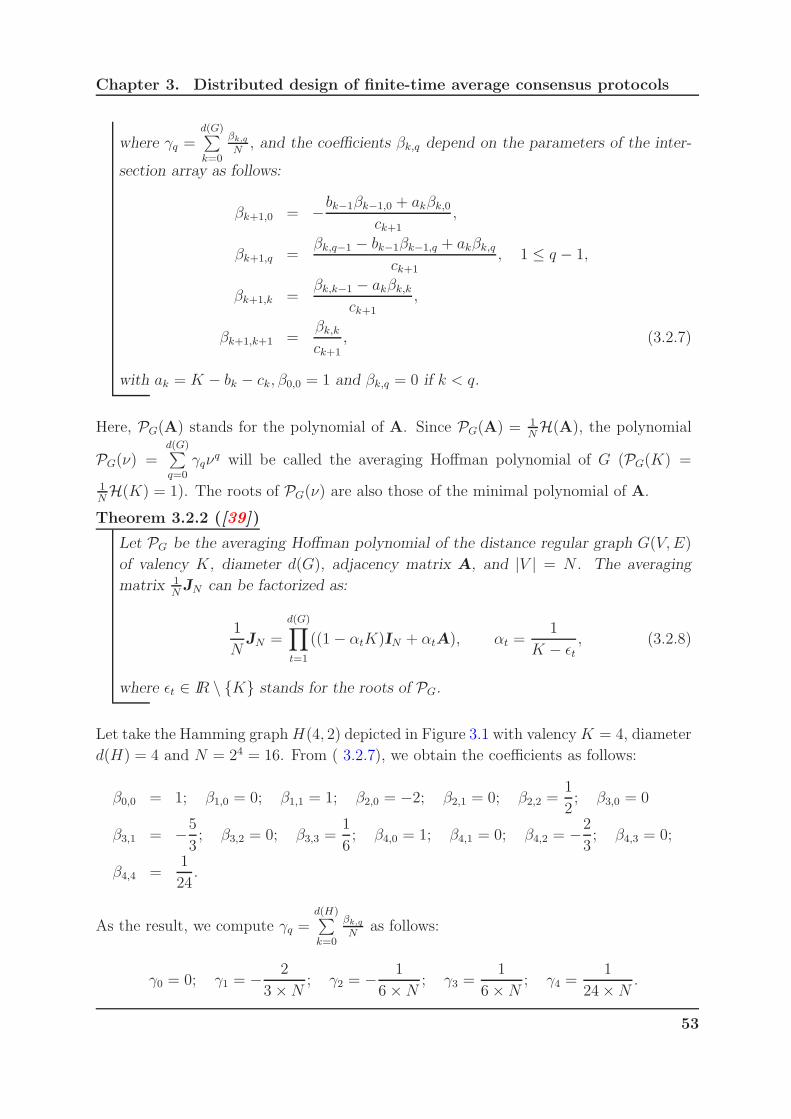
Chapter 3. Distributed design of finite-time average consensus protocols
where γq =d(G)∑
k=0
βk,q
N, and the coefficients βk,q depend on the parameters of the inter-
section array as follows:
βk+1,0 = −bk−1βk−1,0 + akβk,0
ck+1,
βk+1,q =βk,q−1 − bk−1βk−1,q + akβk,q
ck+1, 1 ≤ q − 1,
βk+1,k =βk,k−1 − akβk,k
ck+1,
βk+1,k+1 =βk,k
ck+1, (3.2.7)
with ak = K − bk − ck, β0,0 = 1 and βk,q = 0 if k < q.
Here, PG(A) stands for the polynomial of A. Since PG(A) = 1NH(A), the polynomial
PG(ν) =d(G)∑
q=0
γqνq will be called the averaging Hoffman polynomial of G (PG(K) =
1NH(K) = 1). The roots of PG(ν) are also those of the minimal polynomial of A.
Theorem 3.2.2 ([39])
Let PG be the averaging Hoffman polynomial of the distance regular graph G(V,E)
of valency K, diameter d(G), adjacency matrix A, and |V | = N . The averaging
matrix 1NJN can be factorized as:
1
NJN =
d(G)∏
t=1
((1− αtK)IN + αtA), αt =1
K − ǫt, (3.2.8)
where ǫt ∈ IR \ K stands for the roots of PG.
Let take the Hamming graphH(4, 2) depicted in Figure 3.1 with valencyK = 4, diameter
d(H) = 4 and N = 24 = 16. From ( 3.2.7), we obtain the coefficients as follows:
β0,0 = 1; β1,0 = 0; β1,1 = 1; β2,0 = −2; β2,1 = 0; β2,2 =1
2; β3,0 = 0
β3,1 = −5
3; β3,2 = 0; β3,3 =
1
6; β4,0 = 1; β4,1 = 0; β4,2 = −2
3; β4,3 = 0;
β4,4 =1
24.
As the result, we compute γq =d(H)∑
k=0
βk,q
Nas follows:
γ0 = 0; γ1 = − 2
3 ×N; γ2 = − 1
6 ×N; γ3 =
1
6×N; γ4 =
1
24×N.
53
Chapter 3. Distributed design of finite-time average consensus protocols
Hence, the averaging polynomial is given by PH(ν) =1N(−2
3ν − 1
6ν2 + 1
6ν3 + 1
24ν4). Solv-
ing this polynomial, we get the roots ǫ = −4,−2, 0, 2. Furthermore, from (3.2.8), the
corresponding stepsizes are obtained as α = 18, 16, 14, 12, which are exactly the nonzero
inverses of the Laplacian eigenvalues of the graph. Therefore, the sequence of the con-
sensus matrices are:
W(1) =1
2IN − 1
8A; W(2) =
1
3IN − 1
6A;
W(3) = A; W(4) = −IN +1
2A.
3.2.2.3 General solutions
In [46], the resulting solution yields a link scheduling on the complete graph to achieve
finite-time consensus. Such scheduling is to be controlled by a central node. They provide
necessary and sufficient conditions for finite-time consensus and compute the minimum
consensus time on the Boolean hypercube. In order to prove the existence of a finite
factorization of JN , the mechanism is that starting with a spanning tree T of graph G
and arbitrarily designate a node as the root. The basic idea is that all nodes pass all
their goods to the chosen root. Then, the root propagates the appropriate amount of
goods back into the network so that every node has an equal amount at the end. The
proposed method includes two actions. The first action is described that from vertices
farthest from the root of a spanning tree T , the proposed algorithm traverses upwards
to give all goods to their parents (they can be children of other parents), then remove
themself. This action terminates when only a single vertex (the root) remains. At this
point, the remain node (the root) contains the sum of all initial values. Then, the second
action is to propagate back down the tree while re-distributing the values to achieve the
average consensus value at termination.
For more general graphs, solutions based on graph Laplacian have been recently intro-
duced in closed-form, [41, 42].
Lemma 2 ([41])
The matrices W(k) = αkIN +βA, k = 1, . . . , D are jointly diagonalizable, consistent
with the network topology, and admit 1 as eigenvector.
Where, A is defined as A = dmaxIN − L whose properties are:
(a) A is symmetric;
(b) Its eigenvalues λk(A) = dmax−λk(L), where λk(L), dmax are the eigenvalues of the
Laplacian matrix L and the maximum degree respectively. In particular, dmax is a
simple eigenvalue.
54
Chapter 3. Distributed design of finite-time average consensus protocols
(c) The eigenvectors of the Laplacian matrix are also the eigenvectors of A. Meaning
that, 1 is the eigenvector associated with the eigenvalue dmax.
Theorem 3.2.3 ([41])
Given a connected undirected graph associated with the Laplacian matrix L, the set
of matrices W(k) = (αk + dmaxβ)IN − βL, k = 1, . . . , D, β 6= 0, allows reaching the
average consensus in D steps if:
(a) D + 1 is the number of distinct eigenvalues of the Laplacian matrix;
(b) the parameter β and αk are defined as:
β =1
D+1∏
i=2
D√
λi(L)
αk =λk+1(L)− dmax
D+1∏
i=2
D√
λi(L)
, k = 1, . . . , D.
with λi(L), i = 2, . . . , D + 1 being the nonzero distinct Laplacian eigenvalues.
More precisely, in [42], the solution was given by αk = 1 and βk = − 1λk+1(L)
, λk(L) being
a nonzero Laplacian eigenvalue.
Remark 5
• The number of factor matrices is the number of distinct nonzero Laplacian
eigenvalues.
• The proposed solutions make use of the Laplacian spectrum. For this purpose,
we propose distributed methods for Laplacian spectrum estimation in Chapter
4.
3.2.3 Comparison between the minimal polynomial approach
and the matrix factorization approach
To summarise the difference between the two approaches, we focus on two terms that
are design time and execution time.
• Design time:
(a) For the minimum polynomial approach, each node chooses weights to generate
the weight consensus matrixW that satisfies the convergence conditions 1.2.2.
55
Chapter 3. Distributed design of finite-time average consensus protocols
(b) The matrix factorization approach requires the storage and computation re-
sources for global information (network topology or Laplacian spectrum) to
design the weight consensus matrix W.
• Execution time:
(a) The minimum polynomial approach mainly needs data storage and computa-
tion resources: 2(Dr + 1) successive steps, [78].
(b) At this stage, the factorization of averaging matrix does not require storage
of past data. Hence, the execution time is as simple as a standard consensus
protocol.
The purpose of this thesis is to study a new algorithm for self-configuration for finite-
time average consensus where the weight matrices are not necessarily based on the graph
Laplacian. The aim is to design protocols that allow achieving average consensus in the
fastest possible time, possibly as fast as diameter of the underlying graph. More precisely,
we solve a matrix factorization problem in a distributed way.
3.3 Distributed solution to the matrix factorization
problem.
For a connected graph G(V,E), let x(0) = [x1(0), x2(0), . . . , xN (0)]T be the state vector
of the N−agent network associated with the graph G. For the sake of simplicity, N
agents (nodes) of the network (graph G) are arranged in the first layer that corresponds
to the initial state x(0) as described in the Figure 3.2 illustrating the linear iteration
scheme (3.1.2) in space and time.
As presented in Chapter 1.2, the linear iteration scheme is an useful tool that allows the
system to reach the finite-time average consensus inD steps. Therefore, according to each
iteration, the updated state vectors x(k), k = 1, . . . , D−1 are assigned to be consecutive
layers respectively. Finally, the last iteration is dedicated to the output values x(D).
The weight matrices W(k), k = 1, . . . , D have the entries wij(k) are correspondent to
the links between the nodes of two consecutive layers at time-step k. For instance, W(1)
is the weight matrix assigned to the link between the first layer and the second one.
56

Chapter 3. Distributed design of finite-time average consensus protocols
1
2
N
x(0)
x1(0)
x2(0)
xN(0)
1
2
N
x(1)
1
2
N
x(D − 1)
1
2
N
x(D)
x1(D)
x2(D)
xN(D)
W1 WD
w1
11
w1
NN
w1
2Nw
1
1N wD
1N
wD
2N
wD
NN
wD
11
Space
time
Figure 3.2: Linear iteration scheme in space and time.
Remark 6
The weight matrix W(k) ∈ SG is associated with the graph G. Therefore, the entries
wij(k) are designed following the rule defined as:
wij(k) =
wij(k), if j ∈ Ni
0, otherwise
To simplify the notation, we denote W(k) as Wk.
The linear iteration scheme in space and time can be viewed as a multilayer neural
network. The selection of the weights can be analyzed through the scope of training. By
using a set of P learning sequences, the mechanism is divided into two main steps, namely,
forward step and backward step. The main idea is to compute the partial derivatives of
the error between the actual output and desired output, then propagate them back to each
layer of the network in order to update the weights. The aim is to reduce the error criteria
E efficiently.
Remark 7
Indeed, in most systems where communication is involved, learning sequences are used
for communication channel identification or for synchronization. These sequences are
used during the mandatory configuration step before transmitting informative data,
i.e. running average consensus in our case. We assume that all the agents know the
57
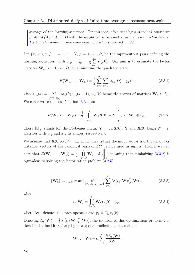
Chapter 3. Distributed design of finite-time average consensus protocols
average of the learning sequence. For instance, after running a standard consensus
protocol (Algorithm 1) with the weight consensus matrix as mentioned in Subsection
1.2.4 or the minimal time consensus algorithm proposed in [78].
Let xi,p(0), yi,p, i = 1, · · · , N , p = 1, · · · , P , be the input-output pairs defining the
learning sequences, with yi,p = yp = 1N
N∑
i=1
xi,p(0). Our aim is to estimate the factor
matrices Wk, k = 1, · · · , D, by minimizing the quadratic error
E(W1, · · · ,WD) =1
2
N∑
i=1
P∑
p=1
(xi,p(D)− yp)2, (3.3.1)
with xi,p(k) =∑
j∈Ni∪iwij(k)xj,p(k − 1), wij(k) being the entries of matrices Wk ∈ SG.
We can rewrite the cost function (3.3.1) as
E(W1, · · · ,WD) =1
2
∥∥∥∥∥
1∏
k=D
WkX(0)−Y
∥∥∥∥∥
2
F
, s.t Wk ∈ SG, (3.3.2)
where ‖.‖F stands for the Frobenius norm, Y = JNX(0), Y and X(0) being N × P
matrices with yi,p and xi,p as entries, respectively.
We assume that X(0)X(0)T = IN which means that the input vector is orthogonal. For
instance, vectors of the canonical basis of IRN can be used as inputs. Hence, we can
note that E(W1, · · · ,WD) = 12
∥∥∥∥
1∏
k=D
Wk − JN
∥∥∥∥
2
F
, meaning that minimizing (3.3.2) is
equivalent to solving the factorization problem (3.2.5):
W∗k|k=1,...,D = arg min
Wkt=1,...,D
1
2
P∑
p=1
tr(ǫp(W)ǫTp (W)
), (3.3.3)
with
ǫp(W) =
1∏
k=D
Wkxp(0)− yp, (3.3.4)
where tr(.) denotes the trace operator and yp = JNxp(0).
Denoting Ep(W) = 12tr(ǫp(W)ǫTp (W)
), the solution of this optimization problem can
then be obtained iteratively by means of a gradient descent method:
Wk := Wk − α
P∑
p=1
∂Ep(W)
∂Wk
58

Chapter 3. Distributed design of finite-time average consensus protocols
or a stochastic gradient one:
Wk := Wk − α∂Ep(W)
∂Wk
,
where the gradient of the cost function is approximated by the gradient at a single input-
output sequence. In what follows, we resort to a stochastic gradient method. For this
purpose, we first state the following technical lemma:
Lemma 3
The derivatives of the cost function Ep(W) = 12tr(ǫp(W)ǫTp (W)
)with ǫp(W) defined
in (3.3.4) can be computed as follows:
∂Ep(W)
∂WD
= δδδD,pxTp (D − 1) (3.3.5)
∂Ep(W)
∂Wk
= δδδk,pxTp (k − 1), k = 1, . . . , D − 1,
(3.3.6)
where δδδD,p = xp(D)− xp is the difference between the actual output and the desired
output with xp = yp = 1N
N∑
i=1
xi,p(0); and
δδδk−1,p = WTk δδδk,p, k = 1, . . . , D. (3.3.7)
Proof : The consensus network being a linear system we know that:
xp(k) = Wkxp(k − 1),
Therefore, we can explicitly write the output according to the weighting matrix of interest, i.e.
xp(D) = WDxp(D − 1)
=
k+1∏
j=D
WjWkxp(k − 1), k = 1, · · · ,D − 1.
Equivalently, by defining Zk+1 =∏k+1
j=D Wj, we get xp(D) = Zk+1Wkxp(k − 1). The cost
function can be written as
Ep(W) =1
2tr((WDxp(D − 1)− xp)(WDxp(D − 1)− xp)
T ).
We can easily deduce that∂Ep(W)∂WD
= δδδD,pxTp (D − 1) with δδδD,p = xp(D)− xp.
Now, we can express the cost function according to any matrix Wt, t = 1, · · · ,D − 1 as
Ep(W) =1
2tr((Zk+1Wkxp(k − 1)− xp)(Zk+1Wkxp(k − 1)− xp)
T ).
59
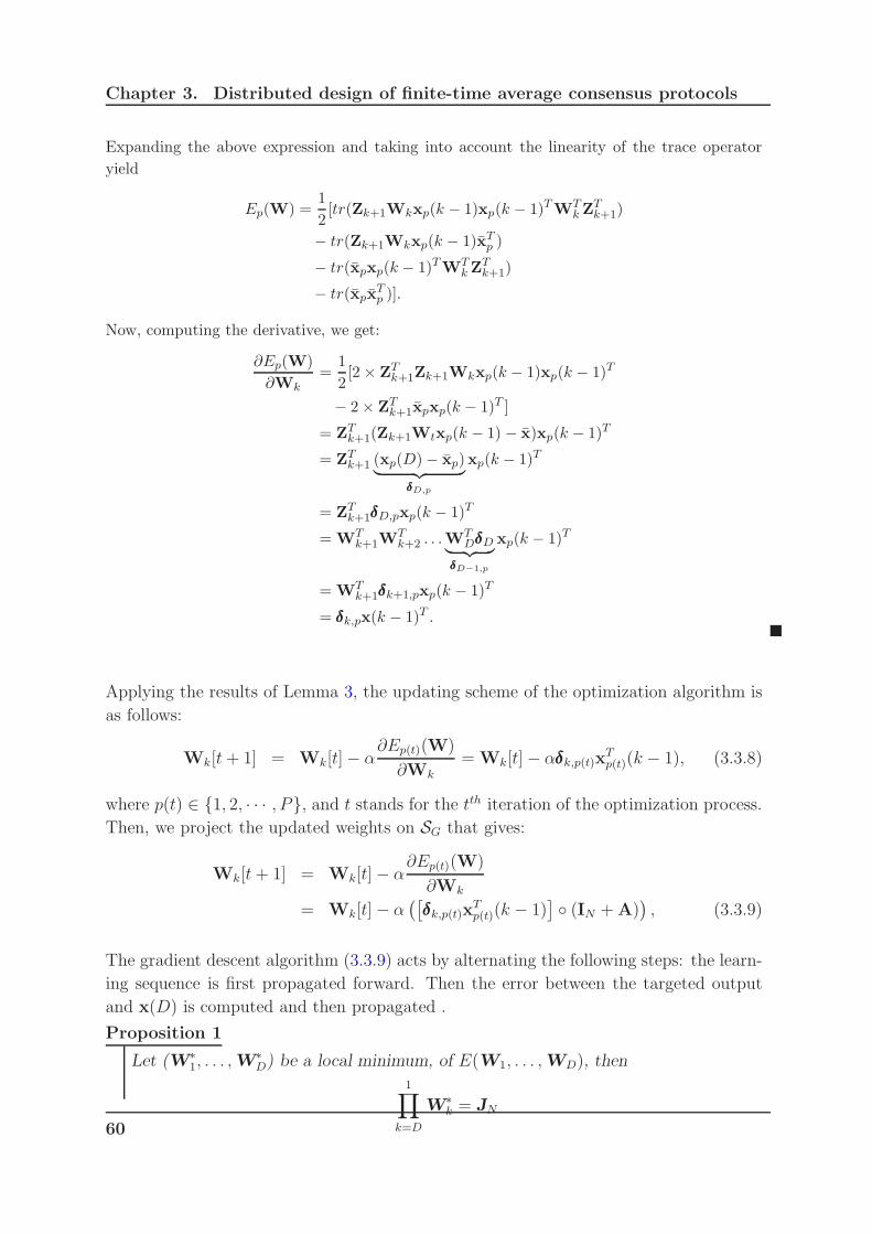
Chapter 3. Distributed design of finite-time average consensus protocols
Expanding the above expression and taking into account the linearity of the trace operator
yield
Ep(W) =1
2[tr(Zk+1Wkxp(k − 1)xp(k − 1)TWT
kZTk+1)
− tr(Zk+1Wkxp(k − 1)xTp )
− tr(xpxp(k − 1)TWTkZ
Tk+1)
− tr(xpxTp )].
Now, computing the derivative, we get:
∂Ep(W)
∂Wk=
1
2[2× ZT
k+1Zk+1Wkxp(k − 1)xp(k − 1)T
− 2× ZTk+1xpxp(k − 1)T ]
= ZTk+1(Zk+1Wtxp(k − 1) − x)xp(k − 1)T
= ZTk+1 (xp(D)− xp)
︸ ︷︷ ︸
δδδD,p
xp(k − 1)T
= ZTk+1δδδD,pxp(k − 1)T
= WTk+1W
Tk+2 . . .W
TDδδδD
︸ ︷︷ ︸
δδδD−1,p
xp(k − 1)T
= WTk+1δδδk+1,pxp(k − 1)T
= δδδk,px(k − 1)T .
Applying the results of Lemma 3, the updating scheme of the optimization algorithm is
as follows:
Wk[t+ 1] = Wk[t]− α∂Ep(t)(W)
∂Wk
= Wk[t]− αδδδk,p(t)xTp(t)(k − 1), (3.3.8)
where p(t) ∈ 1, 2, · · · , P, and t stands for the tth iteration of the optimization process.
Then, we project the updated weights on SG that gives:
Wk[t+ 1] = Wk[t]− α∂Ep(t)(W)
∂Wk
= Wk[t]− α([δδδk,p(t)x
Tp(t)(k − 1)
] (IN +A)
), (3.3.9)
The gradient descent algorithm (3.3.9) acts by alternating the following steps: the learn-
ing sequence is first propagated forward. Then the error between the targeted output
and x(D) is computed and then propagated .
Proposition 1
Let (W∗1, . . . ,W
∗D) be a local minimum, of E(W1, . . . ,WD), then
1∏
k=D
W∗k = JN
60

Chapter 3. Distributed design of finite-time average consensus protocols
.
Proof : Let W∗1, . . . ,W
∗D be the local minimum of the problem (3.3.2), then the derivatives
∂Ep(W∗)
∂W∗k
|k=1,...,D = 0.
Following Lemma 3,
δδδk,pxTp (k − 1) = 0, k = 1, . . . ,D.
Thus,
δδδD,pxTp (D − 1) = 0
⇔ δδδD,p = 0
⇔ xp(D) = xp, p = 1, . . . , P.
It can be rewritten in matrix form:
1∏
k=D
W∗kX(0) = JNX(0)
⇔(
1∏
k=D
W∗k − JN
)
X(0) = 0.
Since X(0)XT (0) = IN , then
1∏
k=D
W∗k − JN = 0
⇔1∏
k=D
W∗k = JN .
This mechanism is similar to the gradient back-propagation algorithm. Its convergence
has been well studied in the literature, see [14] and [50, 73] for instance. Convergence
towards a local minimum is guaranteed if the step-size α is appropriately chosen inside
the interval (0, 1). If the step-size α is set too large, the error E tends to oscillate,
never reaching a minimum. In contrast, too small α prevents the optimization from
making reasonable progress. Therefore, choosing an appropriate α is also an encountered
difficulty in practice. For a particular problem, choosing a suitable stepsize α involves
experimenting with different values to see how the convergence reacts. Such a step-size
also influences on speed of convergence of the consensus algorithm. Several rules have
been proposed for accelerating the convergence speed such as using the adaptive learning
rate α [29] or adaptive momentum [69] . However, these techniques are not consistent
61
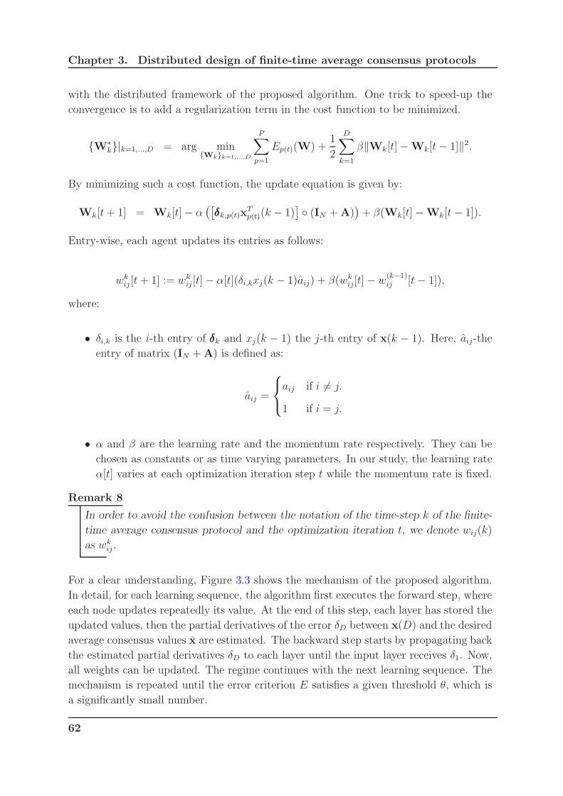
Chapter 3. Distributed design of finite-time average consensus protocols
with the distributed framework of the proposed algorithm. One trick to speed-up the
convergence is to add a regularization term in the cost function to be minimized.
W∗k|k=1,...,D = arg min
Wkk=1,...,D
P∑
p=1
Ep(t)(W) +1
2
D∑
k=1
β‖Wk[t]−Wk[t− 1]‖2.
By minimizing such a cost function, the update equation is given by:
Wk[t+ 1] = Wk[t]− α([δδδk,p(t)x
Tp(t)(k − 1)
] (IN +A)
)+ β(Wk[t]−Wk[t− 1]).
Entry-wise, each agent updates its entries as follows:
wkij [t+ 1] := wk
ij [t]− α[t](δi,kxj(k − 1)aij) + β(wkij[t]− w
(k−1)ij [t− 1]),
where:
• δi,k is the i-th entry of δδδk and xj(k − 1) the j-th entry of x(k − 1). Here, aij-the
entry of matrix (IN +A) is defined as:
aij =
aij if i 6= j.
1 if i = j.
• α and β are the learning rate and the momentum rate respectively. They can be
chosen as constants or as time varying parameters. In our study, the learning rate
α[t] varies at each optimization iteration step t while the momentum rate is fixed.
Remark 8
In order to avoid the confusion between the notation of the time-step k of the finite-
time average consensus protocol and the optimization iteration t, we denote wij(k)
as wkij.
For a clear understanding, Figure 3.3 shows the mechanism of the proposed algorithm.
In detail, for each learning sequence, the algorithm first executes the forward step, where
each node updates repeatedly its value. At the end of this step, each layer has stored the
updated values, then the partial derivatives of the error δD between x(D) and the desired
average consensus values x are estimated. The backward step starts by propagating back
the estimated partial derivatives δD to each layer until the input layer receives δ1. Now,
all weights can be updated. The regime continues with the next learning sequence. The
mechanism is repeated until the error criterion E satisfies a given threshold θ, which is
a significantly small number.
62
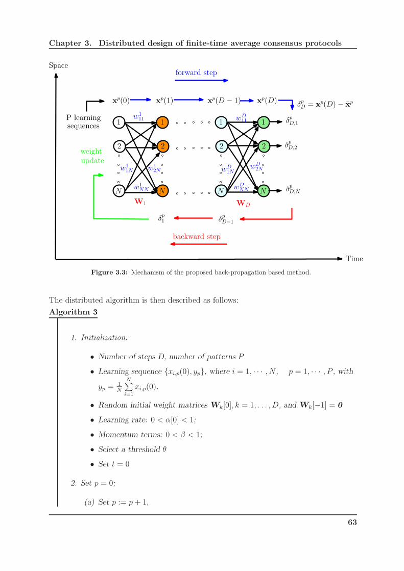
Chapter 3. Distributed design of finite-time average consensus protocols
1
2
N
xp(0)
1
2
N
xp(1)
1
2
N
xp(D − 1)
1
2
N
xp(D)
W1 WD
w1
11
w1
NN
w1
2Nw1
1N wD1N
wD2N
wDNN
wD11
forward step
δpD = x
p(D)− xp
δpD,1
δpD,2
δpD,N
δpD−1
δp1
backward step
weightupdate
P learningsequences
Space
Time
Figure 3.3: Mechanism of the proposed back-propagation based method.
The distributed algorithm is then described as follows:
Algorithm 3
1. Initialization:
• Number of steps D, number of patterns P
• Learning sequence xi,p(0), yp, where i = 1, · · · , N , p = 1, · · · , P , with
yp =1N
N∑
i=1
xi,p(0).
• Random initial weight matrices Wk[0], k = 1, . . . , D, and Wk[−1] = 0
• Learning rate: 0 < α[0] < 1;
• Momentum terms: 0 < β < 1;
• Select a threshold θ
• Set t = 0
2. Set p = 0;
(a) Set p := p+ 1,
63

Chapter 3. Distributed design of finite-time average consensus protocols
(b) Select the corresponding input-output sequence
xi(0) = xi,p(0), x = yp.
(c) Learning sequence propagation:
xi(k) =∑
j∈Ni∪iwk
ij [t]xj(k − 1), k = 1, · · · , D.
(d) Error computation:
δi,D = xi(D)− x; ei,p = δ2i,D.
(e) Error propagation:
δi,k−1 =∑
j∈Ni∪iwk
ji[t]δj,k, k = D, · · · , 2.
(f) Matrices updating: for k = 1, · · · , D, i = 1, · · · , N , and j ∈ Ni ∪ i,
wkij[t + 1] = wk
ij [t]− α[t]δi,kxj(k − 1)aij + β(wkij[t]− wk
ij[t− 1]).
(g) Increment t.
(h) If p = P , compute the mean square error
Ei =1N
P∑
p=1
ei,p, else return to 2a.
(i) If Ei < θ stop the learning process, else return to 2.
3.4 Numerical results
1
2 3
4 5
6
Figure 3.4: 6-node graph
In this section, we consider two examples of different network topologies to evaluate the
developed algorithm. The learning sequence is constituted by the vectors of the canonical
basis of IRN . The performance of designed protocols is evaluated by means of the mean
64

Chapter 3. Distributed design of finite-time average consensus protocols
square error (Mean Square Error (MSE)):
MSE =1
NP
N∑
i=1
P∑
p=1
(xi,p(D)− yp)2.
3.4.1 Example 1
Let us consider the graph depicted in Figure 3.4. Its diameter is d(G) = 3, hence the
bounds of the number of iterations D are d(G) < D < N −1 = 5. The Laplacian matrix
is defined as follows:
L =
2 −1 0 −1 0 0
−1 2 −1 0 0 0
0 −1 3 −1 0 −1
−1 0 −1 3 −1 0
0 0 0 −1 2 −1
0 0 −1 0 −1 2
The eigenvalues of the Laplacian matrix L are: 0, 1, 2, 3 and 5. According to [42],
the factorization of the average consensus matrix by means of graph Laplacian-based
consensus matrices needs D factor matrices, D being the number of nonzero distinct
eigenvalues of the Laplacian matrix, this number being, in general, greater than or equal
to the diameter of the graph. Therefore, we get the following factorization:
(IN − L)(IN − 1
2L)(IN − 1
3L)(IN − 1
5L) = J6,
meaning that consensus is achieved in 4 steps.
J6 =
0.1667 0.1667 0.1667 0.1667 0.1667 0.1667
0.1667 0.1667 0.1667 0.1667 0.1667 0.1667
0.1667 0.1667 0.1667 0.1667 0.1667 0.1667
0.1667 0.1667 0.1667 0.1667 0.1667 0.1667
0.1667 0.1667 0.1667 0.1667 0.1667 0.1667
0.1667 0.1667 0.1667 0.1667 0.1667 0.1667
Since the optimal number of steps is not a priori known, we run the algorithm fordifferent values of D taken in the interval of [d(G), N − 1]. Here, the possible values ofD are 3, 4, 5. Figures 3.5 shows that the best solution is obtained for D = 3. With theproposed algorithm we get a number of step lower than that given by Laplacian based
65

Chapter 3. Distributed design of finite-time average consensus protocols
0 0.5 1 1.5 2
x 105
10−15
10−10
10−5
100
105
Iterations
MS
E
D=3D=4
Figure 3.5: MSE comparison for the two possible numbers of factors
matrices proposed in [41, 42]. The weight matrices are:
W1 =
−0.4028 0.0415 0 0 0 0
0.4418 −0.0455 0 0 0 0
0.5749 0 0.0537 0.0537 0.9219 0
0 0.4053 0.3675 0.3675 0 0.3902
0 0 0 0 −1.3034 0.0806
0 0 0 0 0.1122 −0.0069
W2 =
0.7767 0.2508 0.1706 0 0 0
0.0201 0.6826 0 0.4527 0 0
0.6941 0 0.7680 0.2985 0.4385 0
0 0.2560 0.1578 0.5424 0 0.6013
0 0 0.3756 0 0.5232 0.8876
0 0 0 0.2684 −0.1270 0.5548
W3 =
0.7429 0.6296 0.3653 0 0 0
0.2881 0.2741 0 0.5699 0 0
0.7055 0 0.6403 0.2695 0.3771 0
0 0.4246 0.0716 0.1496 0 0.5491
0 0 0.4218 0 0.4556 0.9515
0 0 0 0.4958 0.3039 0.5832
We can easily check that:
W3W2W1 = J6.
Now, let us consider the finite-time consensus protocol in its execution step, i.e. after the
configuration step. For arbitrary initial values, the trajectories of the state of the network
are depicted in Figure 3.6(a). Exact average consensus is achieved in 3 steps. When
using the optimal constant edge weights protocol W = IN − αL where α = 2λ2(L)+λN (L)
proposed in [74], we get the trajectories in Figure 3.6(b). Showing that more iterations
66

Chapter 3. Distributed design of finite-time average consensus protocols
are actually needed to reach consensus.
Wα=0.3333 =
0.3333 0.3333 0 0.3333 0 0
0.3333 0.3333 0.3333 0 0 0
0 0.3333 0 0.3333 0 0.3333
0.3333 0 0.3333 0 0.3333 0
0 0 0 0.3333 0.3333 0.3333
0 0 0.3333 0 0.3333 0.3333
0 2 4 6 8 10−0.5
0
0.5
1
1.5
X: 3Y: 0.6095
Iterations
x i
(a)
0 2 4 6 8 100.2
0.4
0.6
0.8
1
Iterations
x i
(b)
Figure 3.6: (a)Trajectory of the proposed finite-time consensus protocol
(b)Trajectory of an asymptotic consensus protocol by using optimal constant edge weights
67
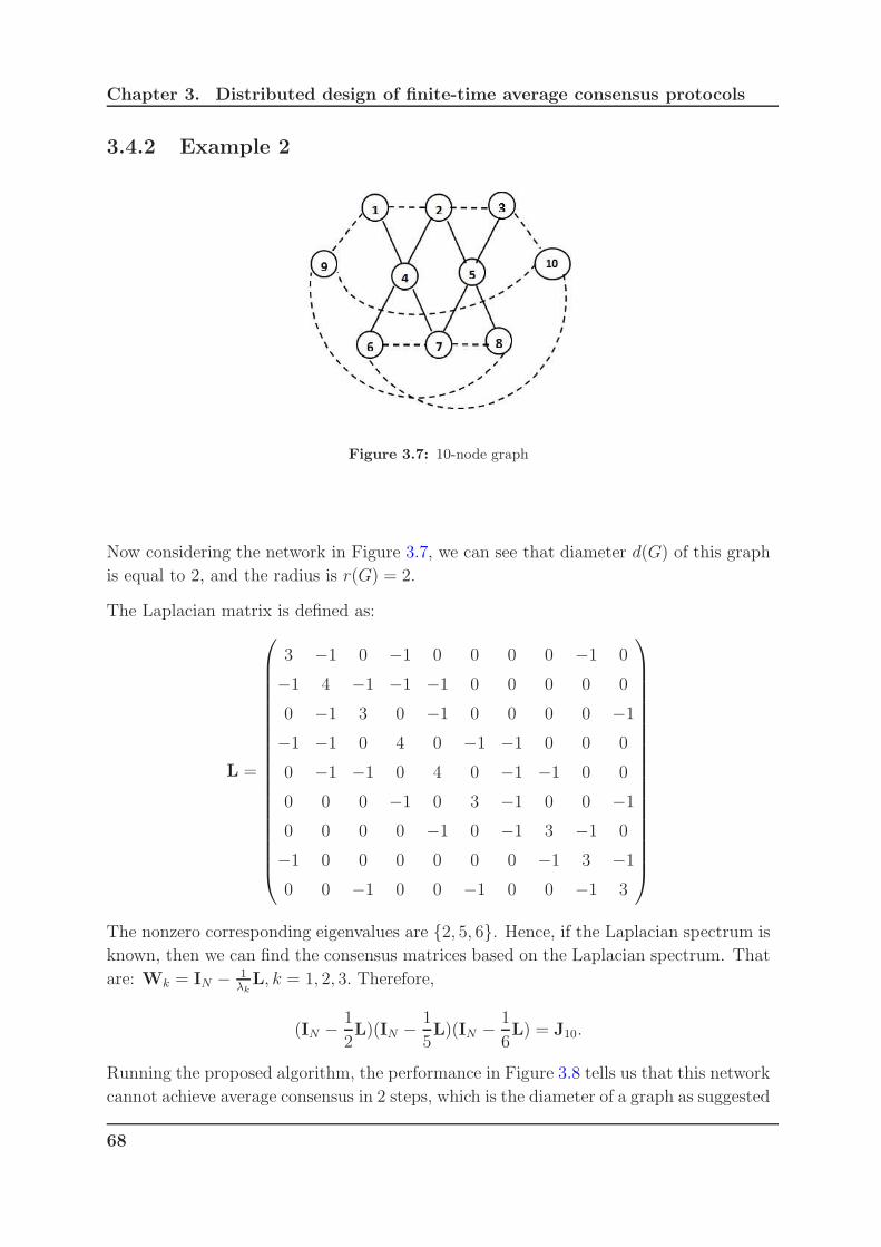
Chapter 3. Distributed design of finite-time average consensus protocols
3.4.2 Example 2
Figure 3.7: 10-node graph
Now considering the network in Figure 3.7, we can see that diameter d(G) of this graph
is equal to 2, and the radius is r(G) = 2.
The Laplacian matrix is defined as:
L =
3 −1 0 −1 0 0 0 0 −1 0
−1 4 −1 −1 −1 0 0 0 0 0
0 −1 3 0 −1 0 0 0 0 −1
−1 −1 0 4 0 −1 −1 0 0 0
0 −1 −1 0 4 0 −1 −1 0 0
0 0 0 −1 0 3 −1 0 0 −1
0 0 0 0 −1 0 −1 3 −1 0
−1 0 0 0 0 0 0 −1 3 −1
0 0 −1 0 0 −1 0 0 −1 3
The nonzero corresponding eigenvalues are 2, 5, 6. Hence, if the Laplacian spectrum is
known, then we can find the consensus matrices based on the Laplacian spectrum. That
are: Wk = IN − 1λkL, k = 1, 2, 3. Therefore,
(IN − 1
2L)(IN − 1
5L)(IN − 1
6L) = J10.
Running the proposed algorithm, the performance in Figure 3.8 tells us that this network
cannot achieve average consensus in 2 steps, which is the diameter of a graph as suggested
68

Chapter 3. Distributed design of finite-time average consensus protocols
in [30]. Such a result has been demonstrated analytically by [34]. However, by running
the algorithm as well as varying the value of D in the interval [d(G), 2r(G)], we can pick
the optimal D in this case. The final MSE was obtained by considering a sufficient large
number of iterations.
2 3 40
2
4
6
8x 10
−5
X: 3Y: 2.056e−08
D
MS
E
Figure 3.8: Final MSE comparison for different values of D
For this topology, D = 3 gives us the best solution for finite-time average consensus, see
Figure 3.8. Also, the trajectory of an arbitrary state vector is depicted in Figure 3.9
after getting the sequence of weight matrices.
0 2 4 6 8 100
0.2
0.4
0.6
0.8
1
1.2
1.4
X: 3Y: 0.4918
Iterations
x i
Figure 3.9: Trajectory of an arbitrary state vector for a 10-node network
69
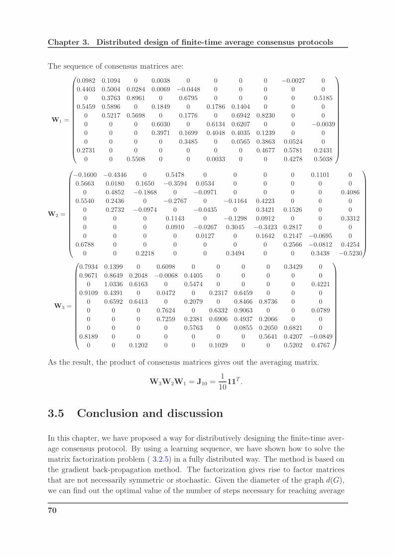
Chapter 3. Distributed design of finite-time average consensus protocols
The sequence of consensus matrices are:
W1 =
0.0982 0.1094 0 0.0038 0 0 0 0 −0.0027 0
0.4403 0.5004 0.0284 0.0069 −0.0448 0 0 0 0 0
0 0.3763 0.8961 0 0.6795 0 0 0 0 0.5185
0.5459 0.5896 0 0.1849 0 0.1786 0.1404 0 0 0
0 0.5217 0.5698 0 0.1776 0 0.6942 0.8230 0 0
0 0 0 0.6030 0 0.6134 0.6207 0 0 −0.0039
0 0 0 0.3971 0.1699 0.4048 0.4035 0.1239 0 0
0 0 0 0 0.3485 0 0.0565 0.3863 0.0524 0
0.2731 0 0 0 0 0 0 0.4677 0.5781 0.2431
0 0 0.5508 0 0 0.0033 0 0 0.4278 0.5038
W2 =
−0.1600 −0.4346 0 0.5478 0 0 0 0 0.1101 0
0.5663 0.0180 0.1650 −0.3594 0.0534 0 0 0 0 0
0 0.4852 −0.1868 0 −0.0971 0 0 0 0 0.4086
0.5540 0.2436 0 −0.2767 0 −0.1164 0.4223 0 0 0
0 0.2732 −0.0974 0 −0.0435 0 0.3421 0.1526 0 0
0 0 0 0.1143 0 −0.1298 0.0912 0 0 0.3312
0 0 0 0.0910 −0.0267 0.3045 −0.3423 0.2817 0 0
0 0 0 0 0.0127 0 0.1642 0.2147 −0.0695 0
0.6788 0 0 0 0 0 0 0.2566 −0.0812 0.4254
0 0 0.2218 0 0 0.3494 0 0 0.3438 −0.5230
W3 =
0.7934 0.1399 0 0.6098 0 0 0 0 0.3429 0
0.9671 0.8649 0.2048 −0.0068 0.4405 0 0 0 0 0
0 1.0336 0.6163 0 0.5474 0 0 0 0 0.4221
0.9109 0.4391 0 0.0472 0 0.2317 0.6459 0 0 0
0 0.6592 0.6413 0 0.2079 0 0.8466 0.8736 0 0
0 0 0 0.7624 0 0.6332 0.9063 0 0 0.0789
0 0 0 0.7259 0.2381 0.6906 0.4937 0.2066 0 0
0 0 0 0 0.5763 0 0.0855 0.2050 0.6821 0
0.8189 0 0 0 0 0 0 0.5641 0.4207 −0.0849
0 0 0.1202 0 0 0.1029 0 0 0.5202 0.4767
As the result, the product of consensus matrices gives out the averaging matrix.
W3W2W1 = J10 =1
1011T .
3.5 Conclusion and discussion
In this chapter, we have proposed a way for distributively designing the finite-time aver-
age consensus protocol. By using a learning sequence, we have shown how to solve the
matrix factorization problem ( 3.2.5) in a fully distributed way. The method is based on
the gradient back-propagation method. The factorization gives rise to factor matrices
that are not necessarily symmetric or stochastic. Given the diameter of the graph d(G),
we can find out the optimal value of the number of steps necessary for reaching average
70

Chapter 3. Distributed design of finite-time average consensus protocols
consensus by varying the value of D in the interval (d(G) ≤ D ≤ N − 1). However, it is
obviously inconvenient for large-scale networks.
On the other hand, we can see that, the obtained consensus matrices are not doubly
stochastic matrices.
Finally, the speed of convergence of the proposed algorithm is still an open issue. For
this purpose, future works encompass optimal step-size for the gradient descent based
method and other optimization methods with a particular focus on large size graphs.
In addition, the dependency of the convergence speed on the learning sequence is to be
studied. Hence, another interesting issue will be the design of optimal learning sequences.
Beside that, the robustness of the finite-time average consensus should be definitely paid
a great attention.
71


Chapter 4
Distributed network robustness
assessment
Contents
4.1 Introduction . . . . . . . . . . . . . . . . . . . . . . . . . . . . 73
4.2 Literature review . . . . . . . . . . . . . . . . . . . . . . . . . 75
4.3 Distributed solutions to the network robustness . . . . . . . 79
4.3.1 Distributed Laplacian eigenvalues estimation . . . . . . . . . . 79
4.3.2 Laplacian spectrum retrieving . . . . . . . . . . . . . . . . . . . 102
4.4 Simulation results . . . . . . . . . . . . . . . . . . . . . . . . . 105
4.4.1 Cases of perfect consensus value x . . . . . . . . . . . . . . . . 106
4.4.2 Imperfect consensus value x . . . . . . . . . . . . . . . . . . . . 116
4.4.3 Unknown consensus value x . . . . . . . . . . . . . . . . . . . . 125
4.5 Conclusion . . . . . . . . . . . . . . . . . . . . . . . . . . . . . 129
4.1 Introduction
The efficiency of a network is evaluated through its functionality and its robustness.
According to the latter property, some questions may arise. For instance, if there is an
accidental event, how does the network react? Will the network survive? In order to
answer these questions, the study of the robustness of networks has increasingly attracted
the attention of the scientific community.
In the literature, there is quite a lot of robustness measures (see Section 1.3), [20, 21].
For instance, the earliest measure is based on the connectivity of the graph representing
73

Chapter 4. Distributed network robustness assessment
the network [16]. In the other words, a network is robust if there exists the presence
of alternate paths, which ensure the possibility of communication in spite of damage
[16]. There are two classical concepts of connectivity for a graph which can be used to
model network robustness that are the vertex and edge connectivities. The vertex (edge)
connectivity Kv(Ke) is the minimal number of vertices (edges) to be removed in order to
disconnect the given graph (see Subsection 1.3.1). By this analytical approach, in order
to deduce the robustness index, we have to remove each edge to check for the connectivity
of the graph. Even if this approach is simple, it is also a burden if we analyse reasonable
larger complex networks.
In [72], the authors have proposed the concept of natural connectivity as a spectral
measure of robustness in complex networks. The natural connectivity is expressed in
mathematical form as the average eigenvalue of the adjacency matrix of the graph rep-
resenting the network topology. The advantage of this method is that the proposed
measure works in both connected and disconnected networks. On the other hand, the
Laplacian spectrum sp(L) can be used to compute the robustness indices that evaluate
the performance of the given network. For instance, the second smallest eigenvalue of
the Laplacian spectrum λ2(L), which is also known as algebraic connectivity [28], is
well-known as a critical parameter that influences on the performance and robustness
of dynamical systems due to its main role in the connectivity of the graph [20]. Hence,
there is a lot of researches on this algebraic connectivity in the literature [3, 51, 76]. Fur-
thermore, there are other remarkable measures for getting the desired robustness indices:
the effective graph resistance R and the number of spanning tree ξ (see Section 1.3),
which are based on the whole non-zero Laplacian spectrum.
We propose distributed methods to estimate both the effective graph resistance R and
the number of spanning trees ξ. Figure 4.1 shows that the distributed estimation of the
network robustness is divided into two main stages including Laplacian spectrum sp(L)
estimation, effective graph resistance and number of spanning trees (R, ξ) computation.
Firstly, we propose consensus-based methods to estimate the whole spectrum of the
Laplacian matrix in a distributed way. Primarily, we compute the average consensus
value x by using the standard consensus protocols (Algorithm 1) or the decentralized
minimum-time consensus value computation algorithm [78]. Next, the estimation of the
Laplacian spectrum can be divided in two steps that are the estimation of the distinct
Laplacian eigenvalues, and then evaluation of the corresponding multiplicities. Finally,
from the estimated sp(L) the robustness indices can be computed. Our focus is therefore
on the estimation of the Laplacian spectrum sp(L).
74
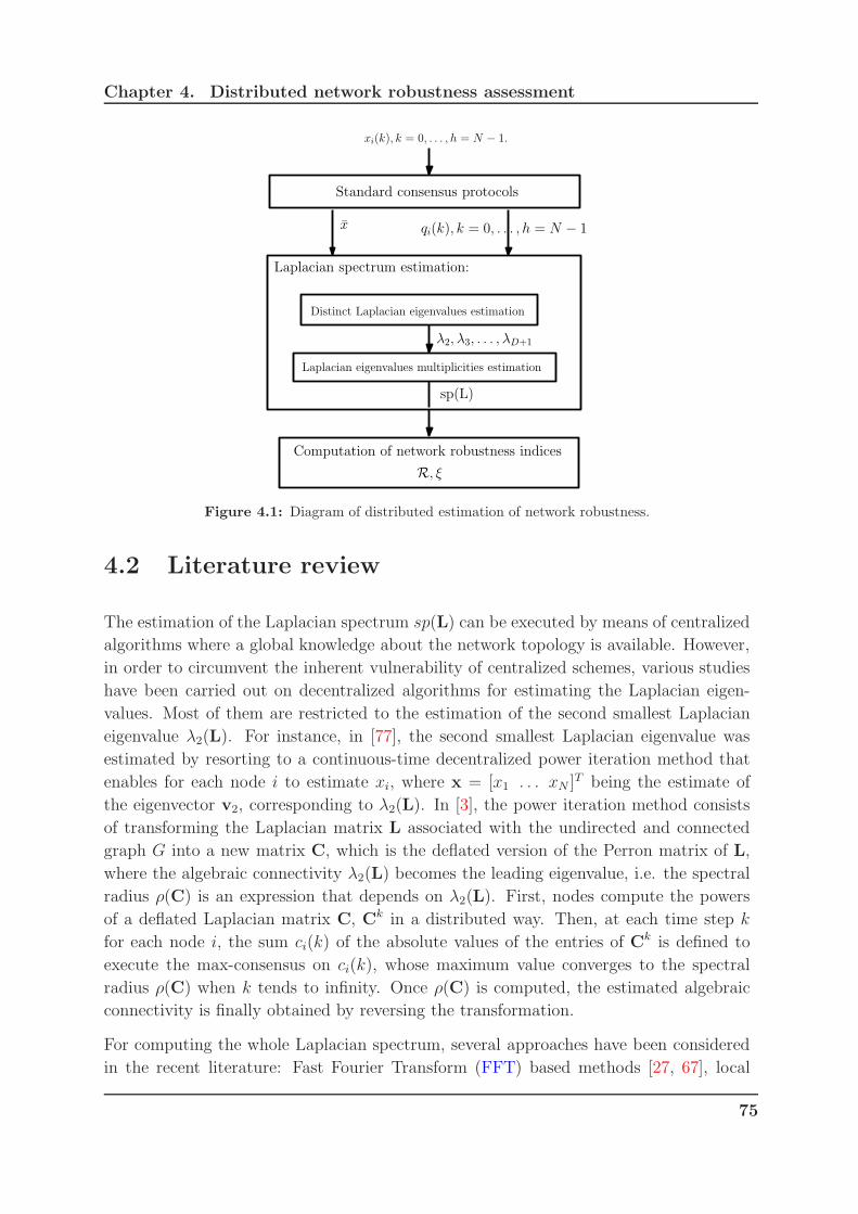
Chapter 4. Distributed network robustness assessment
Standard consensus protocols
xi(k), k = 0, . . . , h = N − 1.
Laplacian spectrum estimation:
Distinct Laplacian eigenvalues estimation
Laplacian eigenvalues multiplicities estimation
Computation of network robustness indices
x qi(k), k = 0, . . . , h = N − 1
λ2, λ3, . . . , λD+1
sp(L)
R, ξ
Figure 4.1: Diagram of distributed estimation of network robustness.
4.2 Literature review
The estimation of the Laplacian spectrum sp(L) can be executed by means of centralized
algorithms where a global knowledge about the network topology is available. However,
in order to circumvent the inherent vulnerability of centralized schemes, various studies
have been carried out on decentralized algorithms for estimating the Laplacian eigen-
values. Most of them are restricted to the estimation of the second smallest Laplacian
eigenvalue λ2(L). For instance, in [77], the second smallest Laplacian eigenvalue was
estimated by resorting to a continuous-time decentralized power iteration method that
enables for each node i to estimate xi, where x = [x1 . . . xN ]T being the estimate of
the eigenvector v2, corresponding to λ2(L). In [3], the power iteration method consists
of transforming the Laplacian matrix L associated with the undirected and connected
graph G into a new matrix C, which is the deflated version of the Perron matrix of L,
where the algebraic connectivity λ2(L) becomes the leading eigenvalue, i.e. the spectral
radius ρ(C) is an expression that depends on λ2(L). First, nodes compute the powers
of a deflated Laplacian matrix C, Ck in a distributed way. Then, at each time step k
for each node i, the sum ci(k) of the absolute values of the entries of Ck is defined to
execute the max-consensus on ci(k), whose maximum value converges to the spectral
radius ρ(C) when k tends to infinity. Once ρ(C) is computed, the estimated algebraic
connectivity is finally obtained by reversing the transformation.
For computing the whole Laplacian spectrum, several approaches have been considered
in the recent literature: Fast Fourier Transform (FFT) based methods [27, 67], local
75

Chapter 4. Distributed network robustness assessment
eigenvalue decomposition of given observability based matrices [40].
For FFT-based methods, the main idea is to make the state of each agent oscillate only
at frequencies corresponding to the eigenvalues of the network topology. The problem is
then mapped into a signal processing one that can be efficiently and independently solved
by each agent by means of FFT. In [27], the amplitude and phase of the oscillations
have been characterized as function of the eigenvectors of the Laplacian and the initial
conditions. In this paper, a connected undirected graph G(V,E) with N = |V | has beenconsidered. From an initial condition xi(0), zi(0) generated from a uniform distribution
in [−1, 1], each node i simulates the following local interaction rule with its neighbors
Ni(t):
xi(t) = zi(t) +∑
j∈Ni(zi(t)− zj(t)),
zi(t) = −xi(t)−∑
j∈Ni(xi(t)− xj(t)),
which can be expressed in vector form as:
[
x(t)
z(t)
]
= M
[
x(t)
z(t)
]
,
where M =
[
0 IN − L
IN + L 0
]
is skew symmetric and 0 is the null N × N matrix.
To any eigenvalue λ(L) it corresponds a couple of complex and conjugate eigenvalues
λ(M), λ(M), that is:
λ(M) = j(1 + λ(L)), λ(M) = −j(1 + λ(L)),
while the corresponding eigenvectors vM of M are function of the eigenvectors vL of L:
vM = [vTL jvTL ]T , vM = [vTL − jvTL ]
T .
It follows that each state of each node xi(t) follows an oscillating trajectory which is
a linear combination of sinusoids, whose amplitudes and phases shifted are function of
the initial conditions and of the graph topology, oscillating at and only at frequencies
corresponding to the eigenvalues of the network at time t. Also, the state trajectory
of xi(t) and zi(t) can be viewed as a function of Laplacian eigenvectors and the initial
conditions:
xi(t) =
N∑
j=1
[vLj(i)(cos((1 + λj(L))t)vTLjx(0) + sin((1 + λj(L))t)v
TLjz(0))],
zi(t) =
N∑
j=1
[vLj(i)(−sin((1 + λj(L))t)vTLjx(0) + cos((1 + λj(L))t)v
TLjz(0))].
76
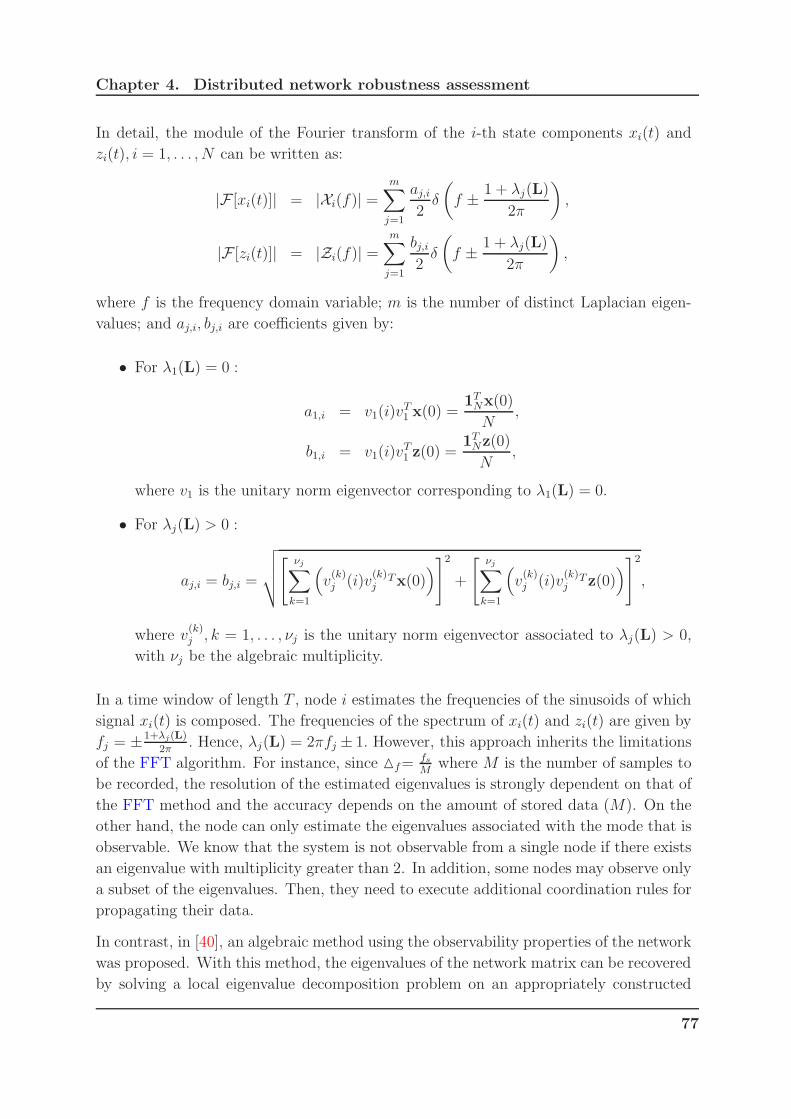
Chapter 4. Distributed network robustness assessment
In detail, the module of the Fourier transform of the i-th state components xi(t) and
zi(t), i = 1, . . . , N can be written as:
|F [xi(t)]| = |Xi(f)| =m∑
j=1
aj,i2δ
(
f ± 1 + λj(L)
2π
)
,
|F [zi(t)]| = |Zi(f)| =m∑
j=1
bj,i2δ
(
f ± 1 + λj(L)
2π
)
,
where f is the frequency domain variable; m is the number of distinct Laplacian eigen-
values; and aj,i, bj,i are coefficients given by:
• For λ1(L) = 0 :
a1,i = v1(i)vT1 x(0) =
1TNx(0)
N,
b1,i = v1(i)vT1 z(0) =
1TNz(0)
N,
where v1 is the unitary norm eigenvector corresponding to λ1(L) = 0.
• For λj(L) > 0 :
aj,i = bj,i =
√√√√
[νj∑
k=1
(
v(k)j (i)v
(k)j
Tx(0))]2
+
[νj∑
k=1
(
v(k)j (i)v
(k)j
Tz(0))]2
,
where v(k)j , k = 1, . . . , νj is the unitary norm eigenvector associated to λj(L) > 0,
with νj be the algebraic multiplicity.
In a time window of length T , node i estimates the frequencies of the sinusoids of which
signal xi(t) is composed. The frequencies of the spectrum of xi(t) and zi(t) are given by
fj = ±1+λj(L)
2π. Hence, λj(L) = 2πfj ± 1. However, this approach inherits the limitations
of the FFT algorithm. For instance, since f=fsM
where M is the number of samples to
be recorded, the resolution of the estimated eigenvalues is strongly dependent on that of
the FFT method and the accuracy depends on the amount of stored data (M). On the
other hand, the node can only estimate the eigenvalues associated with the mode that is
observable. We know that the system is not observable from a single node if there exists
an eigenvalue with multiplicity greater than 2. In addition, some nodes may observe only
a subset of the eigenvalues. Then, they need to execute additional coordination rules for
propagating their data.
In contrast, in [40], an algebraic method using the observability properties of the network
was proposed. With this method, the eigenvalues of the network matrix can be recovered
by solving a local eigenvalue decomposition problem on an appropriately constructed
77
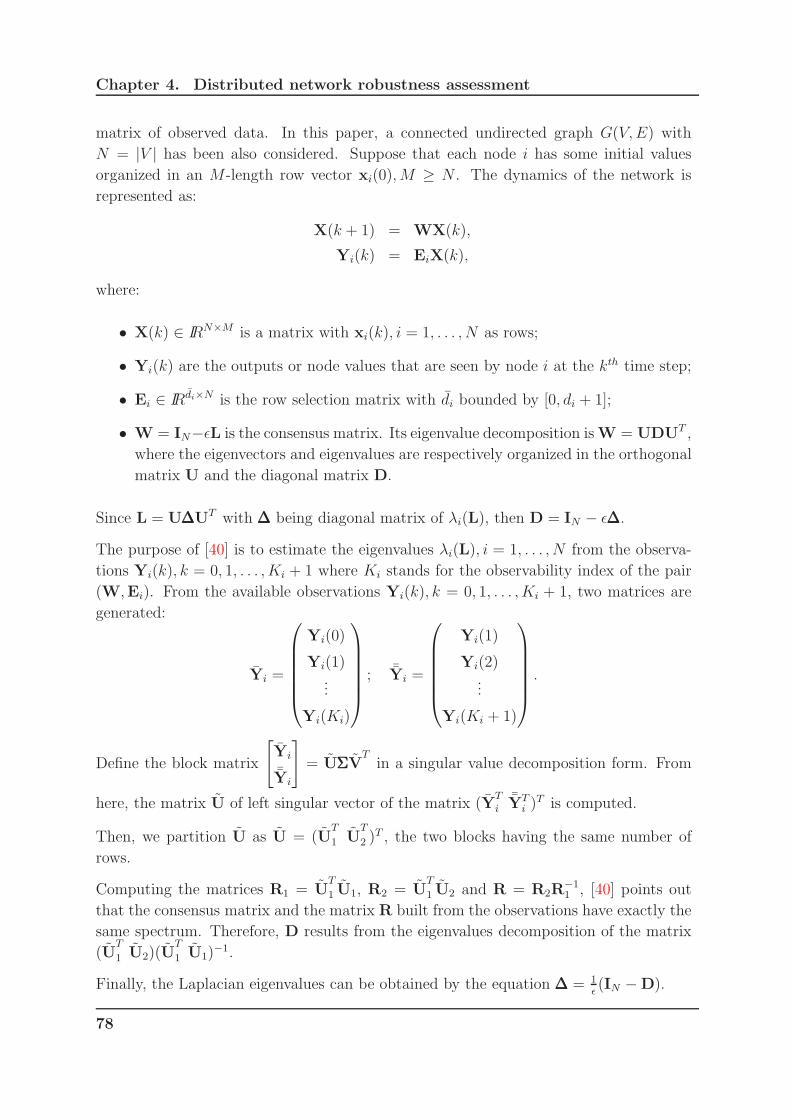
Chapter 4. Distributed network robustness assessment
matrix of observed data. In this paper, a connected undirected graph G(V,E) with
N = |V | has been also considered. Suppose that each node i has some initial values
organized in an M-length row vector xi(0),M ≥ N . The dynamics of the network is
represented as:
X(k + 1) = WX(k),
Yi(k) = EiX(k),
where:
• X(k) ∈ IRN×M is a matrix with xi(k), i = 1, . . . , N as rows;
• Yi(k) are the outputs or node values that are seen by node i at the kth time step;
• Ei ∈ IRdi×N is the row selection matrix with di bounded by [0, di + 1];
• W = IN−ǫL is the consensus matrix. Its eigenvalue decomposition isW = UDUT ,
where the eigenvectors and eigenvalues are respectively organized in the orthogonal
matrix U and the diagonal matrix D.
Since L = U∆∆∆UT with ∆∆∆ being diagonal matrix of λi(L), then D = IN − ǫ∆∆∆.
The purpose of [40] is to estimate the eigenvalues λi(L), i = 1, . . . , N from the observa-
tions Yi(k), k = 0, 1, . . . , Ki + 1 where Ki stands for the observability index of the pair
(W,Ei). From the available observations Yi(k), k = 0, 1, . . . , Ki + 1, two matrices are
generated:
Yi =
Yi(0)
Yi(1)...
Yi(Ki)
; ¯Yi =
Yi(1)
Yi(2)...
Yi(Ki + 1)
.
Define the block matrix
[
Yi
¯Yi
]
= UΣΣΣVTin a singular value decomposition form. From
here, the matrix U of left singular vector of the matrix (YT
i¯YT
i )T is computed.
Then, we partition U as U = (UT
1 UT
2 )T , the two blocks having the same number of
rows.
Computing the matrices R1 = UT
1 U1, R2 = UT
1 U2 and R = R2R−11 , [40] points out
that the consensus matrix and the matrix R built from the observations have exactly the
same spectrum. Therefore, D results from the eigenvalues decomposition of the matrix
(UT
1 U2)(UT
1 U1)−1.
Finally, the Laplacian eigenvalues can be obtained by the equation ∆∆∆ = 1ǫ(IN −D).
78

Chapter 4. Distributed network robustness assessment
However, this method is only applicable to networks having nodes with sufficient storage
and computation capabilities. Actually, data to be stored equals to diM(Ki + 2).
In this thesis, the approach is based on the fact that the averaging matrix can be viewed as
a product of Laplacian-based consensus matrices with step-sizes given by the inverses of
the Laplacian eigenvalues [42]. Therefore, by computing a factorization of the averaging
matrix in a distributed way, a distributed estimation of the Laplacian eigenvalues is
achieved.
Remark 9
Hereafter, we denote the Laplacian eigenvalue λi(L) as λi.
4.3 Distributed solutions to the network robustness
4.3.1 Distributed Laplacian eigenvalues estimation
4.3.1.1 Problem statement
Consider a network modelled by a connected undirected graph G(V,E). Its state x(k) =
[x1(k), x2(k), . . . , xN (k)]T evolves as:
x(k + 1) = (IN − αL)x(k) = (IN − αL)kx(0), (4.3.1)
where α is selected such as 0 < α < 1dmax
to ensure asymptotic convergence [74]. From
the state x(k), one can define q(k) = Lkx(0) as:
q(k) = (q1,k, . . . , qN,k)T =
1
(−α)k
(
x(k)−k−1∑
i=0
(k
i
)
(−α)iq(i)
)
, (4.3.2)
with q(0) = x(0).
1. Assumption 1: The number N of nodes is known.
2. Assumption 2: Each node i stores its initial value xi(0) and the consecutive values
qi,k, k = 0, . . . , h.
The problem under study can therefore be formulated as follows:
Given an arbitrary input-output pair x(0), x = x1, where x = 11T
Nx(0), and the in-
termediate observations q(k), k = 0, . . . , h, estimate in a distributed way the Laplacian
eigenvalues of the graph representing the network.
79
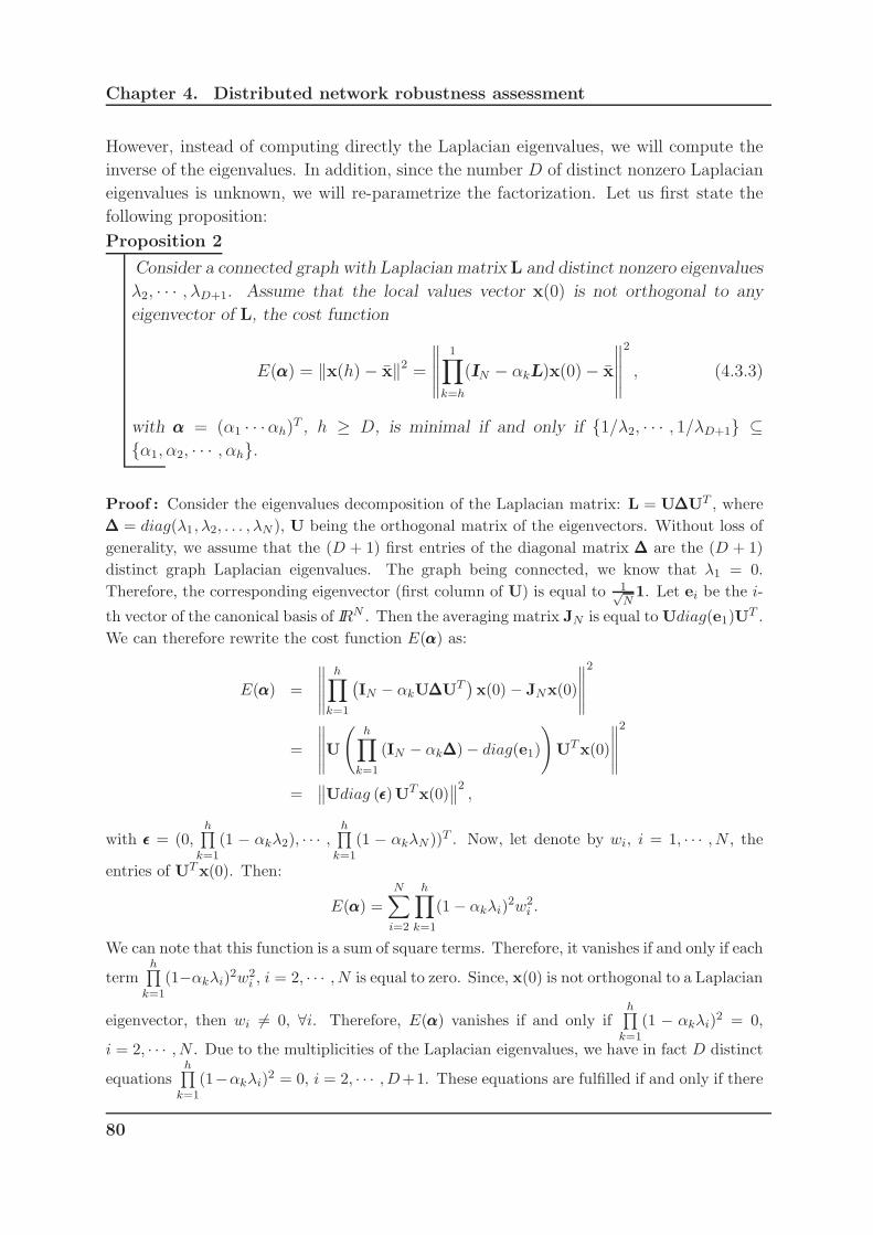
Chapter 4. Distributed network robustness assessment
However, instead of computing directly the Laplacian eigenvalues, we will compute the
inverse of the eigenvalues. In addition, since the number D of distinct nonzero Laplacian
eigenvalues is unknown, we will re-parametrize the factorization. Let us first state the
following proposition:
Proposition 2
Consider a connected graph with Laplacian matrix L and distinct nonzero eigenvalues
λ2, · · · , λD+1. Assume that the local values vector x(0) is not orthogonal to any
eigenvector of L, the cost function
E(ααα) = ‖x(h)− x‖2 =∥∥∥∥∥
1∏
k=h
(IN − αkL)x(0)− x
∥∥∥∥∥
2
, (4.3.3)
with ααα = (α1 · · ·αh)T , h ≥ D, is minimal if and only if 1/λ2, · · · , 1/λD+1 ⊆
α1, α2, · · · , αh.
Proof : Consider the eigenvalues decomposition of the Laplacian matrix: L = U∆∆∆UT , where
∆∆∆ = diag(λ1, λ2, . . . , λN ), U being the orthogonal matrix of the eigenvectors. Without loss of
generality, we assume that the (D + 1) first entries of the diagonal matrix ∆∆∆ are the (D + 1)
distinct graph Laplacian eigenvalues. The graph being connected, we know that λ1 = 0.
Therefore, the corresponding eigenvector (first column of U) is equal to 1√N1. Let ei be the i-
th vector of the canonical basis of IRN . Then the averaging matrix JN is equal toUdiag(e1)UT .
We can therefore rewrite the cost function E(ααα) as:
E(ααα) =
∥∥∥∥∥
h∏
k=1
(IN − αkU∆∆∆UT
)x(0) − JNx(0)
∥∥∥∥∥
2
=
∥∥∥∥∥U
(h∏
k=1
(IN − αk∆∆∆)− diag(e1)
)
UTx(0)
∥∥∥∥∥
2
=∥∥Udiag (ǫǫǫ)UTx(0)
∥∥2,
with ǫǫǫ = (0,h∏
k=1
(1 − αkλ2), · · · ,h∏
k=1
(1 − αkλN ))T . Now, let denote by wi, i = 1, · · · , N , the
entries of UTx(0). Then:
E(ααα) =
N∑
i=2
h∏
k=1
(1− αkλi)2w2
i .
We can note that this function is a sum of square terms. Therefore, it vanishes if and only if each
termh∏
k=1
(1−αkλi)2w2
i , i = 2, · · · , N is equal to zero. Since, x(0) is not orthogonal to a Laplacian
eigenvector, then wi 6= 0, ∀i. Therefore, E(ααα) vanishes if and only ifh∏
k=1
(1 − αkλi)2 = 0,
i = 2, · · · , N . Due to the multiplicities of the Laplacian eigenvalues, we have in fact D distinct
equationsh∏
k=1
(1−αkλi)2 = 0, i = 2, · · · ,D+1. These equations are fulfilled if and only if there
80

Chapter 4. Distributed network robustness assessment
are D coefficients αk respectively equal to the inverse of the D distinct Laplacian eigenvalues.
From Proposition 2, we can conclude that the set S1 = αk, k = 1, . . . , h, of solutions of(4.3.3) contains the inverse of Laplacian eigenvalues S2 = 1
λi, i = 2, . . . , D+1: S2 ⊂ S1.
Therefore, the estimation procedure is to be divided in two parts. We first get S1 by
solving (4.3.3) in a distributed way, then we retrieve the set S2 from S1 and deduce the
Laplacian eigenvalues locally.
We know that if αkhk=1 contains D inverses of the nonzero Laplacian eigenvalues, then
x =h∏
k=1
(I− αkL)x(0),
or equivalently,
x =h∑
k=0
ckLkx(0) =
h∑
k=0
ckq(k) = Qc, (4.3.4)
where Q = [q(0) q(1) · · · q(h)] ∈ IRN×(h+1) and c = [c0 c1 · · · ch]T ∈ IR(h+1)×1, the
coefficient ci being defined as:
ck =
1, if k = 0.
(−1)k∑
i<j<···<k αiαj · · ·αk, if k = 1, . . . , h− 1.
(−1)h∏h
k=1 αk, if k = h.
(4.3.5)
It is obvious that αk are the roots of the polynomial with coefficients ck, and c has an
alternating sign pattern.
We can state the following proposition which is a corollary of Proposition 2:
Proposition 3
Let P(c, :) be the hth degree polynomial with coefficients c = [c0 c1 . . . ch]T ∈
IR(h+1)×1 built from the set of stepsizes S1 = α1, α2, . . . , αh by using (4.3.5). For
any node i and intermediate measurements qi = [qi,0, qi,1, . . . , qi,h]T ∈ IR(h+1)×1 of the
consensus protocol (4.3.1), we get
x = P(c,qi) = qTi c (4.3.6)
if and only if the D inverses of the distinct Laplacian eigenvalues are contained in S1.
Given an upper-bound h for the number D of distinct Laplacian eigenvalues, the idea
is to minimize (4.3.3) and then reduce step by step the obtained set of coefficients ckbuilt from S1 until it is minimal. After all, the set of the inverses of distinct Laplacian
eigenvalues S2 is achieved. In order to obtain the whole Laplacian spectrum sp(L), the
81
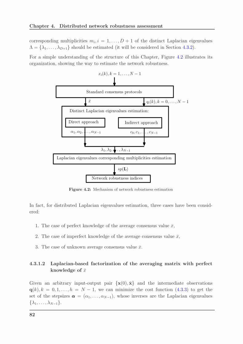
Chapter 4. Distributed network robustness assessment
corresponding multiplicities mi, i = 1, . . . , D + 1 of the distinct Laplacian eigenvalues
Λ = λ1, . . . , λD+1 should be estimated (it will be considered in Section 4.3.2).
For a simple understanding of the structure of this Chapter, Figure 4.2 illustrates its
organization, showing the way to estimate the network robustness.
Standard consensus protocols
xi(k), k = 1, . . . , N − 1
Distinct Laplacian eigenvalues estimation:
Direct approach Indirect approach
x qi(k), k = 0, . . . , N − 1
α1, α2, . . . , αN−1 c0, c1, . . . , cN−1
λ1, λ2, . . . , λN−1
Laplacian eigenvalues corresponding multiplicities estimation
Network robustness indices
sp(L)
Figure 4.2: Mechanism of network robustness estimation
In fact, for distributed Laplacian eigenvalues estimation, three cases have been consid-
ered:
1. The case of perfect knowledge of the average consensus value x,
2. The case of imperfect knowledge of the average consensus value x,
3. The case of unknown average consensus value x.
4.3.1.2 Laplacian-based factorization of the averaging matrix with perfect
knowledge of x
Given an arbitrary input-output pair x(0), x and the intermediate observations
q(k), k = 0, 1, . . . , h = N − 1, we can minimize the cost function (4.3.3) to get the
set of the stepsizes ααα = (α1, . . . , αN−1), whose inverses are the Laplacian eigenvalues
λ1, . . . , λN−1.
82

Chapter 4. Distributed network robustness assessment
In this way, the proposed direct method with respect to the stepsizes ααα consists in solving
a non-convex optimization (4.3.3) through the Lagrange method of multipliers.
Method 1: Direct distributed factorization of the averaging matrix.
Equation (4.3.3) shows that αk are global parameters. For distributively carrying out the
factorization of the averaging matrix as factors of Laplacian-based consensus matrices,
we can first note that the cost function (4.3.3) can be rewritten as:
E(ααα) = ‖x(h)− x‖2 = ‖1∏
k=h
(IN − diag(αααk)L)x(0)− x‖2, (4.3.7)
with αααk = [α1,k, α2,k, . . . , αN,k]T = αk1, k = 1, 2, . . . , h = N − 1.
The idea of the proposed method is to minimize the disagreement between neighbors on
the value of αk while ensuring that the factorization of the averaging matrix is achieved.
Such a factorization is assessed by constraining the values of the nodes after h iterations
of the consensus algorithm to be equal to the average of the initial values:
minαααk∈IRN×1,k=1,2,...,h
1
2
h∑
k=1
∑
i∈V
∑
j∈Ni
(αj,k − αi,k)2, (4.3.8)
subject to x(h) = x
or equivalently,
minαααk∈IRN×1,k=1,...,h
1
2
h∑
k=1
αααTkLαααk. (4.3.9)
subject to x(h) = x
Remark 10
Any solution of (4.3.9) contains the inverse of Laplacian eigenvalues according to
Proposition 2.
The constrained optimization problem (4.3.9) can then be performed as an unconstrained
optimization problem by means of a Lagrange method with a Lagrange function defined
as follows:
H(ααα1,ααα2, . . . ,αααh,y) =1
2
h∑
k=1
αααTkLαααk + yT (x(h)− x) (4.3.10)
where y ∈ IRN×1 is the vector of Lagrange multipliers.
The minimization of the Lagrange function (4.3.10) can be viewed as h consensus prob-
lems to be solved simultaneously with a constraint that provides a kind of external
reference to be tracked.
83
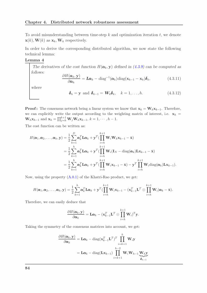
Chapter 4. Distributed network robustness assessment
To avoid misunderstanding between time-step k and optimization iteration t, we denote
x(k),W(k) as xk,Wk respectively.
In order to derive the corresponding distributed algorithm, we now state the following
technical lemma:
Lemma 4
The derivatives of the cost function H(αααk,y) defined in (4.3.9) can be computed as
follows:∂H(αααk,y)
∂αααk
= Lαααk − diag−1(αααk)diag(xk−1 − xk)δδδk, (4.3.11)
where
δδδh = y and δδδk−1 = Wkδδδk, k = 1, . . . , h. (4.3.12)
Proof : The consensus network being a linear system we know that xk = Wkxk−1. Therefore,
we can explicitly write the output according to the weighting matrix of interest, i.e. xh =
Whxh−1 and xh =∏k+1
j=hWjWkxk−1, k = 1, · · · , h− 1.
The cost function can be written as:
H(ααα1,ααα2, . . . ,αααh,y) =1
2
D∑
k=1
αααTkLαααk + yT (
k+1∏
i=h
WiWkxk−1 − x)
=1
2
h∑
k=1
αααTkLαααk + yT (
k+1∏
i=h
Wi(IN − diag(αααk)Lxk−1 − x)
=1
2
h∑
k=1
αααTkLαααk + yT (
k+1∏
i=h
Wixk−1 − x)− yTk+1∏
i=h
Widiag(αααk)Lxk−1).
Now, using the property (A.0.1) of the Khatri-Rao product, we get:
H(ααα1,ααα2, . . . ,αααh,y) =1
2
h∑
k=1
αααTkLαααk + yT (
k+1∏
i=h
Wixk−1 − (xTk−1L
T ⊙k+1∏
i=h
Wi)αααk − x).
Therefore, we can easily deduce that
∂H(αααk,y)
∂αααk
= Lαααk − (xTk−1L
T ⊙k+1∏
i=h
Wi)Ty.
Taking the symmetry of the consensus matrices into account, we get:
∂H(αααk,y)
∂αααk
= Lαααk − diag(xTk−1L
T )Th∏
i=k+1
Wiy
= Lαααk − diag(Lxk−1)
h−2∏
i=k+1
WiWh−1Why︸ ︷︷ ︸
δδδh−1
84

Chapter 4. Distributed network robustness assessment
= Lαααk − diag(Lxk−1)D−2∏
i=k+1
WiWh−1δδδh−1︸ ︷︷ ︸
δδδh−2
= Lαααk − diag(Lxk−1)δδδk.
Since xk = (IN −diag(αααk)L)xk−1, we can deduce that Lxk−1 = diag−1(αααk)(xk−1−xk). Hence,
diag(Lxk−1) = diag−1(αααk)diag(xk−1 − xk). As a consequence,
∂H(αααk,y)
∂αααk= Lαααk − diag−1(αααk)diag(xk−1 − xk)δδδk.
Applying the results of Lemma 4, the updating scheme of the optimization algorithm is
as follows:
αααk[t+ 1] = αααk[t]− β∂H(αααk,y)
∂αααk[t]
= (IN − βL)αααk[t] + βdiag−1(αααk)diag(xk−1[t]− xk[t])δδδk) (4.3.13)
y[t+ 1] = y[t] + µ(xh[t]− x). (4.3.14)
The proposed distributed algorithm can then be described as follows:
Algorithm 4 (Lagrange multipliers method for distributed averaging matrix factorization)
Inputs:
• An upper-bound h of the number of distinct Laplacian eigenvalues h = N − 1,
• learning rates 0 < µ < 1 and 0 < β < 1,
• initial input-output values xi(0), xi, i = 1, . . . , N with x = 1N
N∑
i=1
xi(0) ob-
tained from standard consensus protocols.
1. Initialization: Each node i, i = 1, . . . , N generates random steps-sizes
αi,k[0], k = 1, . . . , h and Lagrange multipliers yi[0] and then set t = 0.
2. Propagation of Lagrange multipliers:
(a) Set: δi,h[t] = yi[t]
(b) Propagate the Lagrange multipliers for k = h, · · · , 2:
δi,k−1[t] = δi,k[t] +∑
j∈Ni
(δj,k[t]− δi,k[t]).
3. Update of the factor matrices step-sizes:
(a) xi,0[t] = xi(0).
85
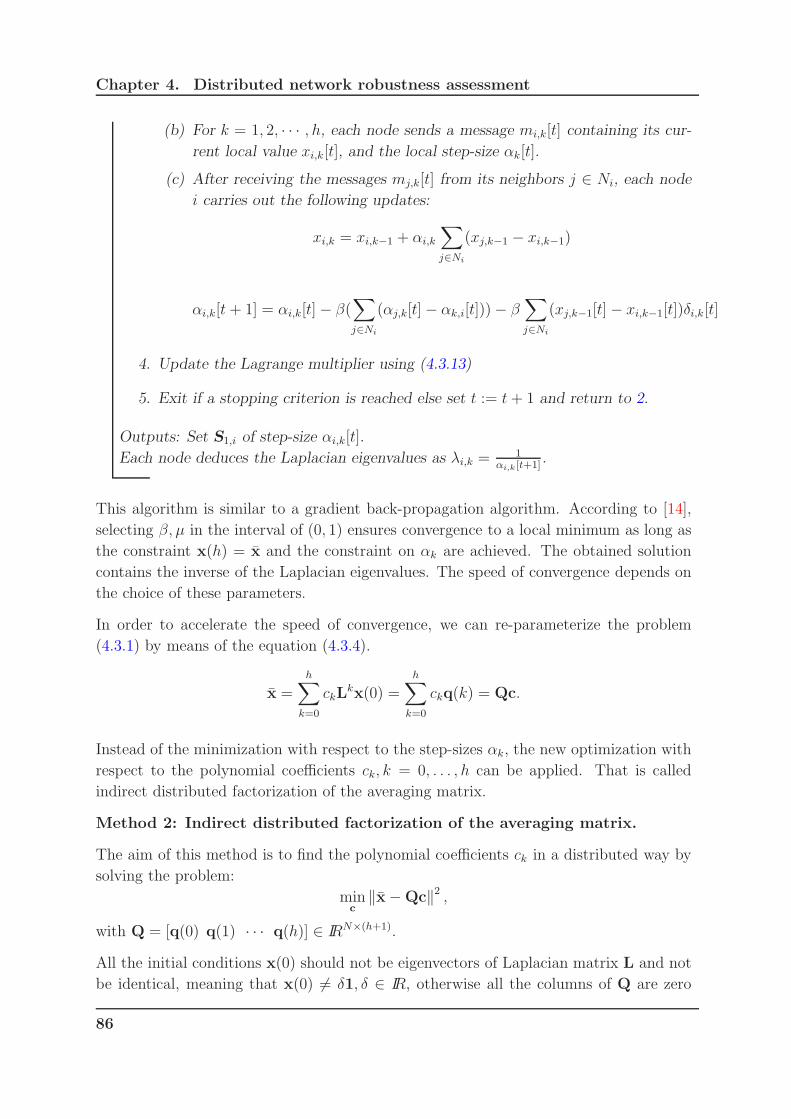
Chapter 4. Distributed network robustness assessment
(b) For k = 1, 2, · · · , h, each node sends a message mi,k[t] containing its cur-
rent local value xi,k[t], and the local step-size αk[t].
(c) After receiving the messages mj,k[t] from its neighbors j ∈ Ni, each node
i carries out the following updates:
xi,k = xi,k−1 + αi,k
∑
j∈Ni
(xj,k−1 − xi,k−1)
αi,k[t + 1] = αi,k[t]− β(∑
j∈Ni
(αj,k[t]− αk,i[t]))− β∑
j∈Ni
(xj,k−1[t]− xi,k−1[t])δi,k[t]
4. Update the Lagrange multiplier using (4.3.13)
5. Exit if a stopping criterion is reached else set t := t+ 1 and return to 2.
Outputs: Set S1,i of step-size αi,k[t].
Each node deduces the Laplacian eigenvalues as λi,k =1
αi,k [t+1].
This algorithm is similar to a gradient back-propagation algorithm. According to [14],
selecting β, µ in the interval of (0, 1) ensures convergence to a local minimum as long as
the constraint x(h) = x and the constraint on αk are achieved. The obtained solution
contains the inverse of the Laplacian eigenvalues. The speed of convergence depends on
the choice of these parameters.
In order to accelerate the speed of convergence, we can re-parameterize the problem
(4.3.1) by means of the equation (4.3.4).
x =h∑
k=0
ckLkx(0) =
h∑
k=0
ckq(k) = Qc.
Instead of the minimization with respect to the step-sizes αk, the new optimization with
respect to the polynomial coefficients ck, k = 0, . . . , h can be applied. That is called
indirect distributed factorization of the averaging matrix.
Method 2: Indirect distributed factorization of the averaging matrix.
The aim of this method is to find the polynomial coefficients ck in a distributed way by
solving the problem:
minc
‖x−Qc‖2 ,
with Q = [q(0) q(1) · · · q(h)] ∈ IRN×(h+1).
All the initial conditions x(0) should not be eigenvectors of Laplacian matrix L and not
be identical, meaning that x(0) 6= δ1, δ ∈ IR, otherwise all the columns of Q are zero
86
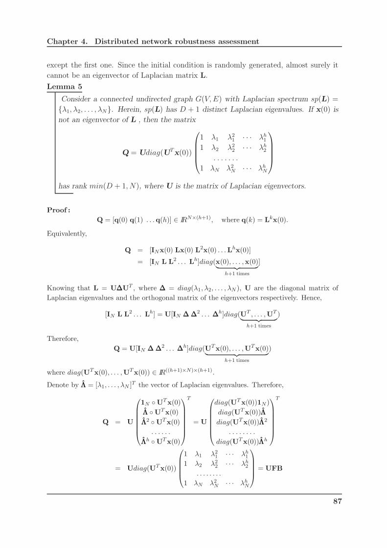
Chapter 4. Distributed network robustness assessment
except the first one. Since the initial condition is randomly generated, almost surely it
cannot be an eigenvector of Laplacian matrix L.
Lemma 5
Consider a connected undirected graph G(V,E) with Laplacian spectrum sp(L) =
λ1, λ2, . . . , λN. Herein, sp(L) has D + 1 distinct Laplacian eigenvalues. If x(0) is
not an eigenvector of L , then the matrix
Q = Udiag(UTx(0))
1 λ1 λ21 · · · λh
1
1 λ2 λ22 · · · λh
2
. . . . . . .
1 λN λ2N · · · λh
N
has rank min(D + 1, N), where U is the matrix of Laplacian eigenvectors.
Proof :
Q = [q(0) q(1) . . .q(h)] ∈ IRN×(h+1), where q(k) = Lkx(0).
Equivalently,
Q = [INx(0) Lx(0) L2x(0) . . .Lhx(0)]
= [IN L L2 . . . Lh]diag(x(0), . . . ,x(0)︸ ︷︷ ︸
h+1 times
]
Knowing that L = U∆∆∆UT , where ∆∆∆ = diag(λ1, λ2, . . . , λN ), U are the diagonal matrix of
Laplacian eigenvalues and the orthogonal matrix of the eigenvectors respectively. Hence,
[IN L L2 . . . Lh] = U[IN ∆∆∆∆∆∆2 . . . ∆∆∆h]diag(UT , . . . ,UT
︸ ︷︷ ︸
h+1 times
)
Therefore,
Q = U[IN ∆∆∆∆∆∆2 . . . ∆∆∆h]diag(UTx(0), . . . ,UTx(0)︸ ︷︷ ︸
h+1 times
)
where diag(UTx(0), . . . ,UTx(0)) ∈ IR((h+1)×N)×(h+1).
Denote by ΛΛΛ = [λ1, . . . , λN ]T the vector of Laplacian eigenvalues. Therefore,
Q = U
1N UTx(0)
ΛΛΛ UTx(0)
ΛΛΛ2 UTx(0)
. . . . . .
ΛΛΛh UTx(0)
T
= U
diag(UTx(0))1N )
diag(UTx(0))ΛΛΛ
diag(UTx(0))ΛΛΛ2
. . . . . . . .
diag(UTx(0))ΛΛΛh
T
= Udiag(UTx(0))
1 λ1 λ21 · · · λh
1
1 λ2 λ22 · · · λh
2
. . . . . . . .
1 λN λ2N · · · λh
N
= UFB
87
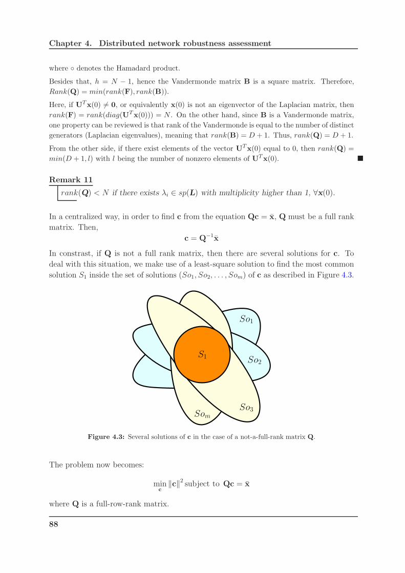
Chapter 4. Distributed network robustness assessment
where denotes the Hamadard product.
Besides that, h = N − 1, hence the Vandermonde matrix B is a square matrix. Therefore,
Rank(Q) = min(rank(F), rank(B)).
Here, if UTx(0) 6= 0, or equivalently x(0) is not an eigenvector of the Laplacian matrix, then
rank(F) = rank(diag(UTx(0))) = N . On the other hand, since B is a Vandermonde matrix,
one property can be reviewed is that rank of the Vandermonde is equal to the number of distinct
generators (Laplacian eigenvalues), meaning that rank(B) = D + 1. Thus, rank(Q) = D + 1.
From the other side, if there exist elements of the vector UTx(0) equal to 0, then rank(Q) =
min(D + 1, l) with l being the number of nonzero elements of UTx(0).
Remark 11
rank(Q) < N if there exists λi ∈ sp(L) with multiplicity higher than 1, ∀x(0).
In a centralized way, in order to find c from the equation Qc = x, Q must be a full rank
matrix. Then,
c = Q−1x
In constrast, if Q is not a full rank matrix, then there are several solutions for c. To
deal with this situation, we make use of a least-square solution to find the most common
solution S1 inside the set of solutions (So1, So2, . . . , Som) of c as described in Figure 4.3.
So1
So2
So3Som
S1
Figure 4.3: Several solutions of c in the case of a not-a-full-rank matrix Q.
The problem now becomes:
minc
‖c‖2 subject to Qc = x
where Q is a full-row-rank matrix.
88
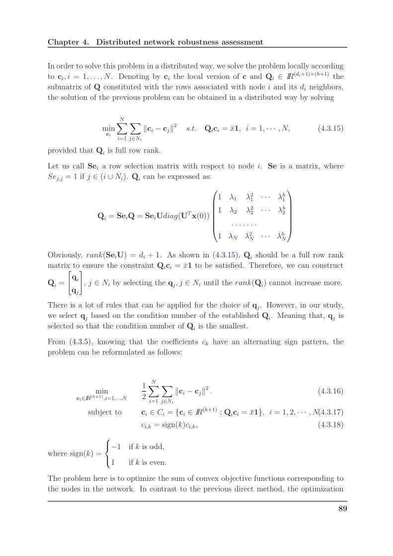
Chapter 4. Distributed network robustness assessment
In order to solve this problem in a distributed way, we solve the problem locally according
to ci, i = 1, . . . , N . Denoting by ci the local version of c and Qi ∈ IR(di+1)×(h+1) the
submatrix of Q constituted with the rows associated with node i and its di neighbors,
the solution of the previous problem can be obtained in a distributed way by solving
minci
N∑
i=1
∑
j∈Ni
‖ci − cj‖2 s.t. Qici = x1, i = 1, · · · , N, (4.3.15)
provided that Qi is full row rank.
Let us call Sei a row selection matrix with respect to node i. Se is a matrix, where
Sej,j = 1 if j ∈ (i ∪Ni). Qi can be expressed as:
Qi = SeiQ = SeiUdiag(UTx(0))
1 λ1 λ21 · · · λh
1
1 λ2 λ22 · · · λh
2
. . . . . . .
1 λN λ2N · · · λh
N
Obviously, rank(SeiU) = di + 1. As shown in (4.3.15), Qi should be a full row rank
matrix to ensure the constraint Qici = x1 to be satisfied. Therefore, we can construct
Qi =
[
qi
qj
]
, j ∈ Ni by selecting the qj , j ∈ Ni until the rank(Qi) cannot increase more.
There is a lot of rules that can be applied for the choice of qj . However, in our study,
we select qj based on the condition number of the established Qi. Meaning that, qj is
selected so that the condition number of Qi is the smallest.
From (4.3.5), knowing that the coefficients ck have an alternating sign pattern, the
problem can be reformulated as follows:
minci∈IR(h+1),i=1,...,N
1
2
N∑
i=1
∑
j∈Ni
‖ci − cj‖2 . (4.3.16)
subject to ci ∈ Ci = ci ∈ IR(h+1) : Qici = x1, i = 1, 2, · · · , N.(4.3.17)
ci,k = sign(k)ci,k, (4.3.18)
where sign(k) =
−1 if k is odd,
1 if k is even.
The problem here is to optimize the sum of convex objective functions corresponding to
the nodes in the network. In contrast to the previous direct method, the optimization
89

Chapter 4. Distributed network robustness assessment
problem (4.3.16) is convex. To solve it we will resort to a projected subgradient method
inspired from [57] and an alternating direction method of multipliers [11, 22].
(A) Distributed projected subgradient method
The main idea of the distributed projected subgradient method is to allow each node i
to update its estimate following two steps.
Firstly, a subgradient step is taken by minimizing the local objective function12
∑
j∈Ni‖ci − cj‖2. Then, the intermediate result is projected on the constraint set
Ci. Therefore, the first step yields:
ci[t + 1] = ci[t]− γ[t]∑
j∈Ni
(ci[t]− cj[t]) , (4.3.19)
where γ[t] > 0 is a stepsize, while the second step requires the computation of the
projection ci[t+1] = ΩCi[ci[t+1]]. This projection step is equivalent to solve a constrained
optimization problem formulated as:
min1
2‖ci[t+ 1]− ci[t+ 1]‖2 s.t. Qici[t+ 1] = x1.
To solve this constrained optimization problem, generally, the Lagrangian augmented
function is defined as follows:
L(ci[t+ 1],y) =1
2‖ci[t + 1]− ci[t + 1]‖2 + yT (Qici[t + 1]− x1).
Following the KKT (Karush-Kuhn-Tucker) conditions, we have to solve:
∇ci[t+1]L(ci[t + 1],y) = 0. (4.3.20)
∇yL(ci[t + 1],y) = 0. (4.3.21)
Let solve (4.3.20) first:
ci[t + 1]− ci[t + 1] +QTi y = 0
⇔ ci[t+ 1] = ci[t + 1]−QTi y. (4.3.22)
Then, we substitue ci into (4.3.21):
Qici[t+ 1]− x1 = 0
⇔ Qi(ci[t+ 1]−QTi y) = x1
⇔ Qici[t+ 1]−QiQTi y = x1
⇔ y = (QiQTi )
−1(Qici[t+ 1]− x1). (4.3.23)
Now, we substitute (4.3.23) into (4.3.22), we get:
ci[t+ 1] = ci[t + 1]−QTi (QiQ
Ti )
−1(Qici[t + 1]− x1)
90
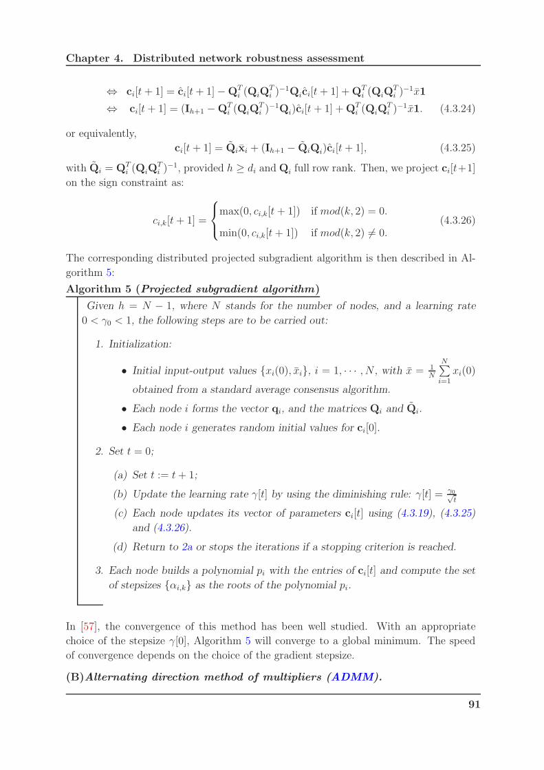
Chapter 4. Distributed network robustness assessment
⇔ ci[t + 1] = ci[t+ 1]−QTi (QiQ
Ti )
−1Qici[t+ 1] +QTi (QiQ
Ti )
−1x1
⇔ ci[t+ 1] = (Ih+1 −QTi (QiQ
Ti )
−1Qi)ci[t + 1] +QTi (QiQ
Ti )
−1x1. (4.3.24)
or equivalently,
ci[t + 1] = Qixi + (Ih+1 − QiQi)ci[t+ 1], (4.3.25)
with Qi = QTi (QiQ
Ti )
−1, provided h ≥ di andQi full row rank. Then, we project ci[t+1]
on the sign constraint as:
ci,k[t+ 1] =
max(0, ci,k[t + 1]) if mod(k, 2) = 0.
min(0, ci,k[t + 1]) if mod(k, 2) 6= 0.(4.3.26)
The corresponding distributed projected subgradient algorithm is then described in Al-
gorithm 5:
Algorithm 5 (Projected subgradient algorithm)
Given h = N − 1, where N stands for the number of nodes, and a learning rate
0 < γ0 < 1, the following steps are to be carried out:
1. Initialization:
• Initial input-output values xi(0), xi, i = 1, · · · , N , with x = 1N
N∑
i=1
xi(0)
obtained from a standard average consensus algorithm.
• Each node i forms the vector qi, and the matrices Qi and Qi.
• Each node i generates random initial values for ci[0].
2. Set t = 0;
(a) Set t := t+ 1;
(b) Update the learning rate γ[t] by using the diminishing rule: γ[t] = γ0√t
(c) Each node updates its vector of parameters ci[t] using (4.3.19), (4.3.25)
and (4.3.26).
(d) Return to 2a or stops the iterations if a stopping criterion is reached.
3. Each node builds a polynomial pi with the entries of ci[t] and compute the set
of stepsizes αi,k as the roots of the polynomial pi.
In [57], the convergence of this method has been well studied. With an appropriate
choice of the stepsize γ[0], Algorithm 5 will converge to a global minimum. The speed
of convergence depends on the choice of the gradient stepsize.
(B)Alternating direction method of multipliers (ADMM).
91

Chapter 4. Distributed network robustness assessment
ADMM is relatively easy to implement and its convergence properties have been well
studied in recent works such that in [8, 11, 23]. The pros of this method is that it is
guaranteed to converge for any choice of the tunning parameters under mild conditions
[11] while other techniques such as subgradient projection or dual decomposition depend
on the choice of the stepsize for the gradient updates. Unlike other methods, ADMM
has only one single penalty parameter ρ that can influence on the speed of convergence.
ADMM assures a very good convergence speed when its parameters are appropriately
chosen. There exist some works dealing with penalty parameter selection for accelerating
the convergence rate of ADMM [8, 19, 31, 66, 71]. The convergence analysis is also
studied in [8, 11, 19, 23, 25, 66]. However, in this study, our penalty parameter is a fixed
constant.
The ADMM algorithm acts by introducing some auxiliary variables zij , so that a strictly
equivalent optimization problem can be formulated as follows:
minci∈IR(h+1),i=1,...,N
1
2
N∑
i=1
∑
j∈Ni
‖ci − cj‖2 . (4.3.27)
subject to ci = zij, j ∈ Ni,
zji = zij ,
zkij = sign(k)zkij,
ci ∈ Ci = ci ∈ IRh+1 : Qici = x1, i = 1, 2, · · · , N.
where sign(k) =
1 if k is even,
−1 if k is odd.
The corresponding augmented Lagrangian function is given by:
Lρ(c, z,y) =N∑
i=1
L(i)ρ (ci, z,y),
with
L(i)ρ (ci, z,y) =
∑
j∈Ni
(1
2‖ci − cj‖2 + yT
ij (ci − zij) +ρ
2‖ci − zij‖2
)
, (4.3.28)
where ρ is a penalty coefficient. In contrast to the method of Lagrange multipliers, in
ADMM the minimization of the cost function according to the primal variables ci and zijis carried out sequentially. So, given the primal variables and the dual variables yij, the
cost function is first minimized according to ci and the obtained solution projected on
the constrained set (c-minimization). Then zij are obtained from the given dual variables
and the updated values of ci (z-minimization). The third step corresponds to the update
of the dual variables from the updated primal ones (y-minimization):
ci[t+ 1] = ΩCi[argmin Lρ(ci[t + 1], zij [t],yij[t])]; (4.3.29)
92

Chapter 4. Distributed network robustness assessment
zij [t+ 1] = argmin Lρ(ci[t+ 1], zij,yij [t])]; (4.3.30)
yij[t + 1] = argmin Lρ(ci[t+ 1], zij[t + 1],yij [t])]. (4.3.31)
These iterations indicate that the method is particularly useful when the c− and z−minimizations can be carried out efficiently. First, we solve the c-minimization:
∇ciLρ(ci[t+ 1], zij[t],yij [t]) = 0.
⇔∑
j∈Ni
(ci[t + 1]− cj [t]) +∑
j∈Ni
yij[t] + ρ(ci[t+ 1]− zij[t]) = 0
⇔ (di(1 + ρ))ci[t+ 1] =∑
j∈Ni
cj [t] + ρ∑
j∈Ni
zij[t]−∑
j∈Ni
yij[t]
⇔ ci[t + 1] = (di(1 + ρ))−1(∑
j∈Ni
cj [t] + ρ∑
j∈Ni
zij [t]−∑
j∈Ni
yij [t]),
where di is the degree of node i.
For the cost function considered herein, we can note that the c-minimization problem
(4.3.29) is solved by:
ci[t + 1] = (di(1 + ρ))−1(∑
j∈Ni
cj [t] + ρ∑
j∈Ni
zij [t]−∑
j∈Ni
yij [t]), (4.3.32)
di being the degree of node i. Then, as for the projected subgradient case we get the
same expression for ci[t + 1] as in (4.3.25).
Next, we solve the sub-optimization (4.3.30) analogically, meaning that ∇zijL(ci[t +
1], zij [t + 1],yi[t]) = 0 with respect to the term that zij = zji. Rewrite the augmented
Lagrange function:
Lρ(ci, z,y) =∑
j∈Ni
(1
2‖ci − cj‖2 + yT
ij (ci − zij) +ρ
2‖ci − zij‖2 + yT
ji (cj − zji) +ρ
2‖cj − zji‖2
)
,
Since ∇zijL(ci[t+ 1], zij[t + 1],yi[t]) = 0 with zij = zji, it is equivalent to:
−(yij[t] + yji[t])− ρ(ci[t+ 1] + cj[t + 1]) + 2ρzij[t + 1] = 0
⇔ zij [t+ 1] = 12(ci[t+ 1] + cj[t + 1]) + 1
2ρ(yij [t] + yji[t]). (4.3.33)
Then, we project zij[t + 1] on the sign constraint as:
zkij [t+ 1] =
max(0, zkij [t+ 1]) if mod(k, 2) = 0.
min(0, zkij [t+ 1]) if mod(k, 2) 6= 0.(4.3.34)
The Lagrange multipliers are updated as:
yij [t+ 1] = yij [t] + ρ(ci[t+ 1]− zij [t+ 1]). (4.3.35)
This fully decentralized algorithm is summarized as follows:
93

Chapter 4. Distributed network robustness assessment
Algorithm 6 (Distributed ADMM algorithm)
Given h = N − 1, where N stands for the number of nodes N , and a penalty
parameter ρ, the following steps are to be carried out:
1. Initialization:
• Initial input-output values xi(0), xi, i = 1, · · · , N , with x = 1N
N∑
i=1
xi(0)
obtained from a standard average consensus algorithm,
• Each node i forms the vector qi, and the matrices Qi and Qi.
• Each node i generates random values for ci[0], zij[0] and yij [0], j ∈ Ni.
2. Set t = 0;
(a) Set t := t+ 1;
(b) Update equations: each node i
• updates its primary variable ci[t] using (4.3.32) and (4.3.25).
• updates the primary variables zij[t] associated with its neighbors using
(4.3.33) and (4.3.34).
• update the dual variables yij using (4.3.35).
• Return to 2a until a stopping criterion is reached.
(c) Each node builds a polynomial pi with the entries of ci[t] and compute the
set of the stepsizes αi,k as the roots of the polynomial pi.
The convergence analysis for distributed quadratic programming has been studied deeply
in [8, 25].
4.3.1.3 Laplacian-based factorization of the averaging matrix with imperfect
knowledge of x
For all methods proposed in previous case 4.3.1.2, the consensus value x is the foremost
required parameter. We now relax this requirement by means of a novel method that
deals with Laplacian eigenvalues estimation when an exact average consensus value is
unknown.
In what follows, we assume that the nodes run a standard average consensus protocol
( 1.2.1), which is stopped after M iterations, and store their local values xi,M . In this
study, we want to show the performance of the proposed algorithm with respect to some
values of M .
Since x is unknown exactly, for a sufficiently large value of M , x(M) can be viewed as its
94
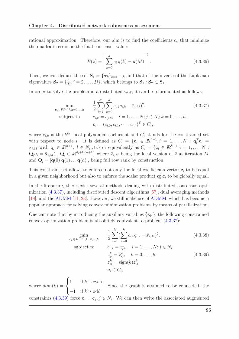
Chapter 4. Distributed network robustness assessment
rational approximation. Therefore, our aim is to find the coefficients ck that minimize
the quadratic error on the final consensus value:
E(c) =
∥∥∥∥∥
h∑
k=0
ckq(k)− x(M)
∥∥∥∥∥
2
. (4.3.36)
Then, we can deduce the set S1 = αααkk=1,··· ,h and that of the inverse of the Laplacian
eigenvalues S2 = 1λi, i = 2, . . . , D, which belongs to S1 : S2 ⊂ S1.
In order to solve the problem in a distributed way, it can be reformulated as follows:
minccck∈IRN×1,k=0,...,h
1
2
N∑
i=1
(
h∑
k=0
ci,kqi,k − xi,M)2, (4.3.37)
subject to ci,k = cj,k, i = 1, . . . , N ; j ∈ Ni; k = 0, . . . , h.
ci = (ci,0, ci,1, · · · , ci,h)T ∈ Ci,
where ci,k is the kth local polynomial coefficient and Ci stands for the constrained set
with respect to node i. It is defined as Ci = ci ∈ IRh+1, i = 1, . . . , N : qTl ci =
xi,M with ql ∈ IRh+1, l ∈ Ni ∪ i or equivalently as Ci = ci ∈ IRh+1, i = 1, . . . , N :
Qici = xi,M1, Qi ∈ IRdi+1×h+1 where xi,M being the local version of x at iteration M
and Qi = [q(0) q(1) . . .q(h)], being full row rank by construction.
This constraint set allows to enforce not only the local coefficients vector ci to be equal
in a given neighborhood but also to enforce the scalar product qTi ci to be globally equal.
In the literature, there exist several methods dealing with distributed consensus opti-
mization (4.3.37), including distributed descent algorithms [57], dual averaging methods
[18], and the ADMM [11, 23]. However, we still make use of ADMM, which has become a
popular approach for solving convex minimization problems by means of parallelization.
One can note that by introducing the auxiliary variables zij, the following constrained
convex optimization problem is absolutely equivalent to problem (4.3.37):
minccck∈IRN×1,k=0,...,h
1
2
N∑
i=1
(h∑
r=0
ci,kqi,k − xi,M)2. (4.3.38)
subject to ci,k = zkij , i = 1, . . . , N ; j ∈ Ni
zkji = zkij , k = 0, . . . , h. (4.3.39)
zkij = sign(k)zkij ,
ci ∈ Ci,
where sign(k) =
1 if k is even,
−1 if k is odd. Since the graph is assumed to be connected, the
constraints (4.3.39) force ci = cj , j ∈ Ni. We can then write the associated augmented
95

Chapter 4. Distributed network robustness assessment
Lagrangian:
Lρ(c, z,y) =
N∑
i=1
[
1
2
h∑
k=0
(ci,kqi,k − xi,M)2 +
h∑
k=0
(∑
j∈Ni
ykij(ci,k − zij,k)
)
+∑
j∈Ni
ρ
2‖ci − zij‖2
]
.
or in vector form:
Lρ(c, z,y) =N∑
i=1
[
1
2(qT
i ci − xi,M)2 +∑
j∈Ni
yTij(ci − zij) +
∑
j∈Ni
ρ
2‖ci − zij‖2
]
.
The ADMM solution to this problem acts in three steps:
• First, minimization with respect to ci:
ci[t + 1] = ΩCi[argmin L(ci, zij [t],yi[t])]. (4.3.40)
where ΩCi[·] stands for the projection in the constraints set of the vector in the
argument.
• Second, minimization with respect to zij with the constraint zji = zij:
zij [t+ 1] = argmin L(ci[t+ 1], zij,yi[t]). (4.3.41)
• Third, Lagrange multiplier update:
yij[t + 1] = yij [t] + ρ(ci[t + 1]− zij [t+ 1]). (4.3.42)
Solving the sub-optimization problem (4.3.40) through ∂Lρ(c,z,y)∂ci
= 0, we get:
(qiqTi − xi,M)qi +
∑
j∈Ni
yTij(ci − zij) +
ρ
2
∑
j∈Ni
(ci − zij)2 = 0.
⇔ (qiqTi + ρdiIh+1)ci = xi,Mqi + ρ
∑
j∈Ni
zij −∑
j∈Ni
yij .
Then,
ci[t + 1] = (qiqTi + ρdiIh+1)
−1(xi,Mqi + ρ∑
j∈Ni
zij[t]−∑
j∈Ni
yij [t]).
Then, projecting the obtained solution in the constraints set
ci[t+ 1] = ΩCi[ci[t+ 1]],
we get:
ci[t + 1] = Qixi,M + (Ih+1 − QiQ)ci[t+ 1], (4.3.43)
with Qi = QTi (QiQ
Ti )
−1 and Qi be a full-row rank matrix.
96
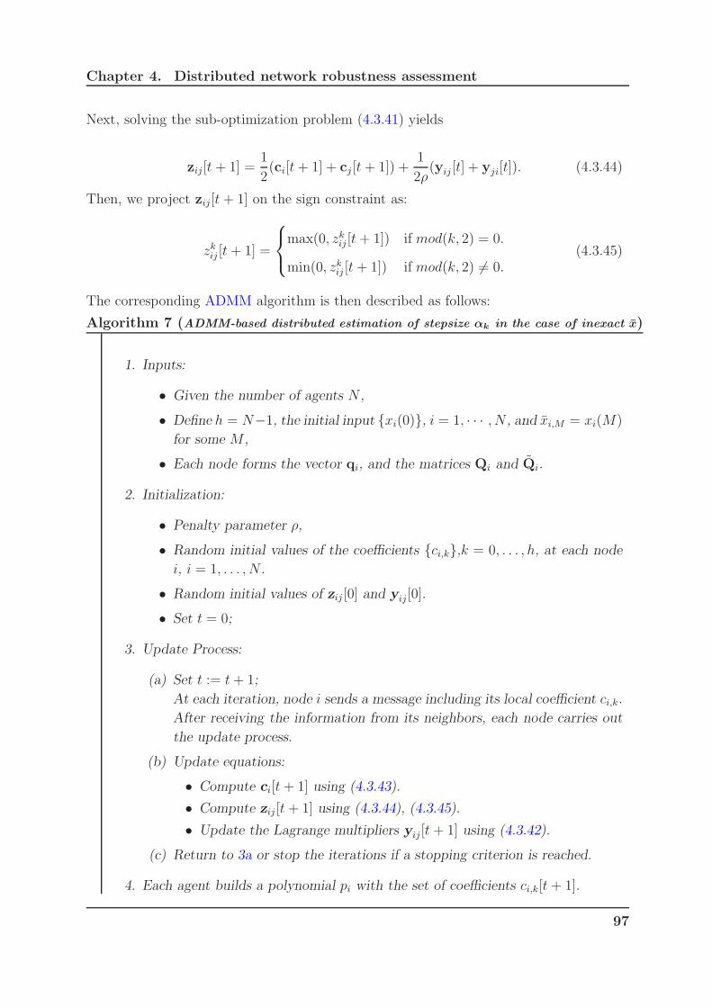
Chapter 4. Distributed network robustness assessment
Next, solving the sub-optimization problem (4.3.41) yields
zij[t + 1] =1
2(ci[t+ 1] + cj [t+ 1]) +
1
2ρ(yij [t] + yji[t]). (4.3.44)
Then, we project zij[t + 1] on the sign constraint as:
zkij [t+ 1] =
max(0, zkij [t+ 1]) if mod(k, 2) = 0.
min(0, zkij [t+ 1]) if mod(k, 2) 6= 0.(4.3.45)
The corresponding ADMM algorithm is then described as follows:
Algorithm 7 (ADMM-based distributed estimation of stepsize αk in the case of inexact x)
1. Inputs:
• Given the number of agents N ,
• Define h = N−1, the initial input xi(0), i = 1, · · · , N , and xi,M = xi(M)
for some M ,
• Each node forms the vector qi, and the matrices Qi and Qi.
2. Initialization:
• Penalty parameter ρ,
• Random initial values of the coefficients ci,k,k = 0, . . . , h, at each node
i, i = 1, . . . , N .
• Random initial values of zij [0] and yij[0].
• Set t = 0;
3. Update Process:
(a) Set t := t+ 1;
At each iteration, node i sends a message including its local coefficient ci,k.
After receiving the information from its neighbors, each node carries out
the update process.
(b) Update equations:
• Compute ci[t+ 1] using (4.3.43).
• Compute zij [t+ 1] using (4.3.44), (4.3.45).
• Update the Lagrange multipliers yij[t + 1] using (4.3.42).
(c) Return to 3a or stop the iterations if a stopping criterion is reached.
4. Each agent builds a polynomial pi with the set of coefficients ci,k[t + 1].
97

Chapter 4. Distributed network robustness assessment
5. Each agent computes the set of the stepsizes αi,k as the roots of the polyno-
mial pi.
When the coefficients ck are approximately obtained, we can make use of Algorithms 9
and 10 that will be presented later in Subsection 4.3.2 to estimate the whole spectrum
of Laplacian matrix L, that can be used to estimate the network robustness indices.
4.3.1.4 Laplacian-based factorization of the averaging matrix with unknown
consensus value x
According to the previous section, one way for estimating the Laplacian eigenvalues is:
• solve the average consensus problem.
• solve the averaging matrix factorization problem (4.3.15), Algorithms 5 and 6.
• retrieve the Laplacian eigenvalues using Algorithm 9 and 10.
Instead of following these steps, in this section, we propose a method to merge the first
two steps. For this purpose, we propose to solve a convex combination of two convex
functions, i.e.
minxi,ci,i=1,··· ,N
θ
2
N∑
i=1
∑
j∈Ni
‖ci − cj‖2 +1− θ
2
N∑
i=1
(xi − xi(0))2,
s.t. Qici = xi1, i = 1, . . . , N, (4.3.46)
with θ- an adjustable scalar parameter (0 ≤ θ ≤ 1), xi- a local estimate of the average
value, and xi(0)- a fixed initial value of node i.
It can be seen that, the objective function (4.3.46) is a combination of two convex
functions. The first one takes into account the estimation of the polynomial coefficients
whose roots are the inverse of the nonzero distinct Laplacian eigenvalues while the second
one concerns the average consensus problem. And this convex optimization problem can
be solved efficiently using the ADMM approach.
In order to derive an ADMM algorithm for the problem (4.3.46), we introduce the auxil-
iary variables zij, µij. Therefore, the following constrained convex optimization prob-
lem is absolutely equivalent to the problem (4.3.46):
minxi,ci,i=1,··· ,N
θ
2
N∑
i=1
∑
j∈Ni
‖ci − cj‖2 +1− θ
2
N∑
i=1
(xi − xi(0))2,
s.t xi = µij, i = 1, . . . , N, j ∈ Ni.
98

Chapter 4. Distributed network robustness assessment
ci = zij .
zkij = sign(k)zkij ,
ci ∈ Ci(xi).
where
• sign(k) =
1 if k is even,
−1 if k is odd.
• Ci(xi) stands for the constrained set with respect to node i. It is defined as Ci =
c ∈ IRh+1| Qic = xi1.
Now, introducing the dual variables υυυ and y, the augmented Lagrangian is defined as :
Lρ1ρ2(x, c,µµµ, z, υυυ,y) = Lρ1(c, z,y) + Lρ2(x,µµµ,υυυ).
where:
Lρ1(c, z,y) =θ
2
N∑
i=1
∑
j∈Ni
‖ci − cj‖2 +∑
j∈Ni
ρ12‖ci − zij‖2 +
∑
j∈Ni
yTij(ci − zij),
Lρ2(x,µµµ,υυυ) =1− θ
2
N∑
i=1
(xi − xi(0))2 +
∑
j∈Ni
ρ22(xi − µij)
2 +∑
j∈Ni
υij(xi − µij),
where ρ1, ρ2 are penalty terms assumed to be constant.
ADMM provides an iterative solution that acts following the five steps below:
• Minimization with respect to the average consensus value xi:
xi[t+ 1] = argmin Lρ2(xi[t], µij[t], υij [t]). (4.3.47)
• Minimization with respect to the polynomial coefficients ci:
ci = argmin Lρ1(ci[t], zij [t],yij [t]), (4.3.48)
ci[t+ 1] = ΩCi(xi[t+1])[ci] (4.3.49)
where ΩCi(xi[t+1])[·] stands for the projection into the constraints set Ci(xi[t + 1])
of the vector in the argument.
• Minimization with respect to the auxiliary variables µij with the constraint µji =
µij:
µij[t+ 1] = argmin Lρ2(xi[t+ 1], µij[t], υij[t]). (4.3.50)
99

Chapter 4. Distributed network robustness assessment
• Minimization with respect to the auxiliary variables zij :
zij[t + 1] = argmin Lρ1(ci[t + 1], zij [t],yij [t]). (4.3.51)
• Lagrange multipliers update:
υij [t+ 1] = υij[t] + ρ2(xi[t + 1]− µij[t + 1]), (4.3.52)
yij [t+ 1] = yij [t] + ρ1(ci[t + 1]− zij [t+ 1]). (4.3.53)
Solving the sub-optimization problems (4.3.47) and (4.3.48) is equivalent to solve the
following equations:
1. ∂Lρ1 (c,z,y)
∂ci= 0
∂Lρ1(c, z,y)
∂ci= θ
∑
j∈Ni
(ci − cj) +∑
j∈Ni
yij +∑
j∈Ni
ρ1(ci − zij) = 0.
We get:
⇔ ci[t + 1] =θ∑
j∈Nicj[t] + ρ1
∑
j∈Nizij[t]−
∑
j∈Niyij [t]
di(θ + ρ1).
2. ∂Lρ2 (x,µµµ,υυυ)
∂xi= 0
∂Lρ2(x,µµµ,υυυ)
∂xi
= (1− θ)(xi − xi(0)) +∑
j∈Ni
υij +∑
j∈Ni
ρ2(xi − µij) = 0
⇔ (1− θ + ρ2di)xi = (1− θ)xi(0) + ρ∑
j∈Ni
µij −∑
j∈Ni
υij
⇔ xi[t+ 1] =(1− θ)xi(0) + ρ2
∑
j∈Niµij[t]−
∑
j∈Niυij[t]
1− θ + ρ2di. (4.3.54)
Then, projecting the obtained solution in the constraints set
ci[t+ 1] = ΩCi(xi[t+1])[ci[t+ 1]],
we get:
ci[t + 1] = Qixi[t+ 1]1+ (Ih+1 − QiQ)ci[t+ 1], (4.3.55)
with Qi = QTi (QiQ
Ti )
−1, Qi being full row rank by construction.
Next, solving the sub-optimization problems (4.3.50) and (4.3.51), in the same way, yields
100

Chapter 4. Distributed network robustness assessment
1. The derivative of Lρ2(x,µµµ,υυυ) with respect to µij with respect to the constraint
µij = µji:∂Lρ2(x,µµµ,υυυ)
∂µij
= −υij − υji − ρ2(xi + xj) + 2ρ2µij = 0
⇔ µij[t+ 1] =xi[t + 1] + xj [t+ 1]
2+
υij[t] + υji[t]
2ρ2. (4.3.56)
2. The derivative of Lρ1(c, z,y) with respect to zij
∂Lρ1(ci,zij ,yij)
zij= 0
⇔ −yij[t]− ρ(ci[t+ 1]− zij[t + 1]) = 0
⇔ zij [t+ 1] = ci[t + 1] + 1ρ1yij [t]. (4.3.57)
Then, we project zij[t + 1] on the sign constraint as:
zkij [t+ 1] =
max(0, zkij [t+ 1]) if mod(k, 2) = 0.
min(0, zkij [t+ 1]) if mod(k, 2) 6= 0.(4.3.58)
The parameter θ allows weighting the two combined cost functions. Since the constraint
set Ci(xi) depends on the consensus value xi. The optimization procedure can initially
give more weight to the average consensus problem and then to the factorization one.
For this purpose, instead of keeping θ constant, we adopt a time varying coefficient:
θ(t) =1− e−βt
1 + e−βt, 0 < β < 1, (4.3.59)
to keep it in the range [0, 1] and to increase the importance of the factorization progres-
sively while decreasing that of the average consensus.
Remark 12
Practically, we can see that the average consensus term converges much faster than
the term relative to the averaging matrix factorization problem. Hence, θ can be
chosen close to 1.
The corresponding ADMM algorithm is then described as follows:
Algorithm 8 (ADMM-based joint distributed average consensus and estimation of Laplacian eigenvalues)
1. Inputs:
• Given the number of nodes N , h = N − 1,
• The initial measurements values xi(0), i = 1, · · · , N ,
2. Initialization:
101
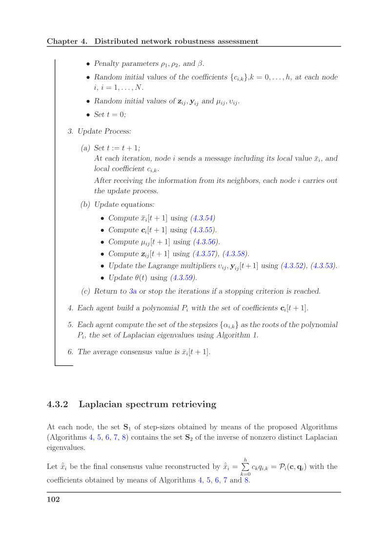
Chapter 4. Distributed network robustness assessment
• Penalty parameters ρ1, ρ2, and β.
• Random initial values of the coefficients ci,k,k = 0, . . . , h, at each node
i, i = 1, . . . , N .
• Random initial values of zij ,yij and µij, υij.
• Set t = 0;
3. Update Process:
(a) Set t := t+ 1;
At each iteration, node i sends a message including its local value xi, and
local coefficient ci,k.
After receiving the information from its neighbors, each node i carries out
the update process.
(b) Update equations:
• Compute xi[t + 1] using (4.3.54)
• Compute ci[t+ 1] using (4.3.55).
• Compute µij [t+ 1] using (4.3.56).
• Compute zij [t+ 1] using (4.3.57), (4.3.58).
• Update the Lagrange multipliers υij,yij [t+1] using (4.3.52), (4.3.53).
• Update θ(t) using (4.3.59).
(c) Return to 3a or stop the iterations if a stopping criterion is reached.
4. Each agent build a polynomial Pi with the set of coefficients ci[t+ 1].
5. Each agent compute the set of the stepsizes αi,k as the roots of the polynomial
Pi, the set of Laplacian eigenvalues using Algorithm 1.
6. The average consensus value is xi[t + 1].
4.3.2 Laplacian spectrum retrieving
At each node, the set S1 of step-sizes obtained by means of the proposed Algorithms
(Algorithms 4, 5, 6, 7, 8) contains the set S2 of the inverse of nonzero distinct Laplacian
eigenvalues.
Let ˆxi be the final consensus value reconstructed by ˆxi =h∑
k=0
ckqi,k = Pi(c,qi) with the
coefficients obtained by means of Algorithms 4, 5, 6, 7 and 8.
102
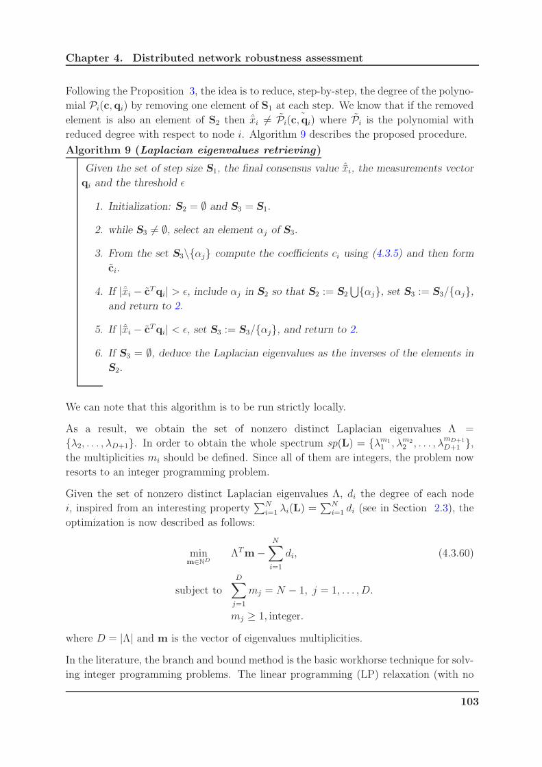
Chapter 4. Distributed network robustness assessment
Following the Proposition 3, the idea is to reduce, step-by-step, the degree of the polyno-
mial Pi(c,qi) by removing one element of S1 at each step. We know that if the removed
element is also an element of S2 then ˆxi 6= Pi( ˜c,qi) where Pi is the polynomial with
reduced degree with respect to node i. Algorithm 9 describes the proposed procedure.
Algorithm 9 (Laplacian eigenvalues retrieving)
Given the set of step size S1, the final consensus value ˆxi, the measurements vector
qi and the threshold ǫ
1. Initialization: S2 = ∅ and S3 = S1.
2. while S3 6= ∅, select an element αj of S3.
3. From the set S3\αj compute the coefficients ci using (4.3.5) and then form
ci.
4. If |ˆxi − cTqi| > ǫ, include αj in S2 so that S2 := S2
⋃αj, set S3 := S3/αj,and return to 2.
5. If |ˆxi − cTqi| < ǫ, set S3 := S3/αj, and return to 2.
6. If S3 = ∅, deduce the Laplacian eigenvalues as the inverses of the elements in
S2.
We can note that this algorithm is to be run strictly locally.
As a result, we obtain the set of nonzero distinct Laplacian eigenvalues Λ =
λ2, . . . , λD+1. In order to obtain the whole spectrum sp(L) = λm11 , λm2
2 , . . . , λmD+1
D+1 ,the multiplicities mi should be defined. Since all of them are integers, the problem now
resorts to an integer programming problem.
Given the set of nonzero distinct Laplacian eigenvalues Λ, di the degree of each node
i, inspired from an interesting property∑N
i=1 λi(L) =∑N
i=1 di (see in Section 2.3), the
optimization is now described as follows:
minm∈ND
ΛTm−N∑
i=1
di, (4.3.60)
subject to
D∑
j=1
mj = N − 1, j = 1, . . . , D.
mj ≥ 1, integer.
where D = |Λ| and m is the vector of eigenvalues multiplicities.
In the literature, the branch and bound method is the basic workhorse technique for solv-
ing integer programming problems. The linear programming (LP) relaxation (with no
103

Chapter 4. Distributed network robustness assessment
integer restrictions) is adopted to estimate the optimal solution of an integer program-
ming [13]. Therefore, problem (4.3.60) is now rewritten strictly equivalently in linear
programming form as follows:
minm∈ND
ΛTm, (4.3.61)
subject toD∑
j=1
mj = N − 1;
ΛTm =N∑
i=1
di, (M)
mj ≥ 1,
where M is the constraint set without integer restriction. Hence, M can be expressed as
M = m ∈ IRD|∑D
j=1mj = N − 1,ΛTm =∑N
i=1 di and m ≥ 1. The problem (4.3.61)
without integer restriction is called linear programming (LP) relaxation.
The branch-and-bound-based algorithm is described as:
Algorithm 10 (Brand-and-bound-based multiplicities estimation)
1. Initialization:
(a) Number of nodes N , di, Λ.
(b) t = 0;
(c) S = ∅ set of integer solutions.
(d) Fbest = ∅ function value of feasible solution.
(e) V = ∅ set of nodes, that the program will visit.
(f) Compute m[0] = argmin ΛTm, s.t m ∈ M
• If the stopping criteria is satisfied, then stop.
• Compute the upper bound (UB), which is the function value of the
rounded-up feasible solution, Fbest = UB.
• S4 = m[0].
(g) Order of variables in S to be branched on.
2. While S4 = ∅, select an ordered variable mj to be branched on and S4 :=
S4\mj.
(a) t = t + 1;
(b) Create 2 new nodes for 2 new sub-problems.
(c) m1 = argmin ΛTm, s.t m ∈ M1 = M ∪ mj ≤ ⌊mj⌋ .
104

Chapter 4. Distributed network robustness assessment
(d) m2 = argmin ΛTm, s.t m ∈ M2 = M ∪ mj ≥ ⌈mj⌉• If m1 (or m2) is integer, S = m1(or m2) then stop.
• If there is an infeasible solution, then prun the corresponding node.
• Compute UB1 (or UB2).
(e) If UB1(UB2) < UB2(UB1), then pick m1 (or m2) is the next node to
create 2 new nodes and V = V ∪m2(m1), and M = M1(M2).
3. Return to step 2a.
The policy of selecting a variable to be branched on in this algorithm is that the variable
with the greatest fractional part is the first order then the variable with the smallest
fractional part is the next. After that, the policy is repeated for the rest of unselected
variables.
Since, the Laplacian spectrum sp(L) is obtained, we can compute the effective graph
resistance R and the number of spanning trees ξ to assess the robustness of a given
network using ( 1.3.2) and ( 1.3.1).
4.4 Simulation results
In this section, several examples will be carried out to test the efficiency of the proposed
methods to assess the network robustness (via R, ξ). As presented obviously in previous
Section, the procedure of all proposed methods are devided into three categories accord-
ing to the consensus value x that are: perfect consensus value (Algorithms 4, 5 and 6);
imperfect consensus value (Algorithm 7) and unknown consensus value (Algorithm 8).
In order to evaluate the network robustness, let us take two networks which have the
same nodes but different number of edges as examples.
1
2 3
4 5
6
(a) (b)
1
2 3
4 5
6
Figure 4.4: Two graphs with the same number of nodes but different number of edges.
105
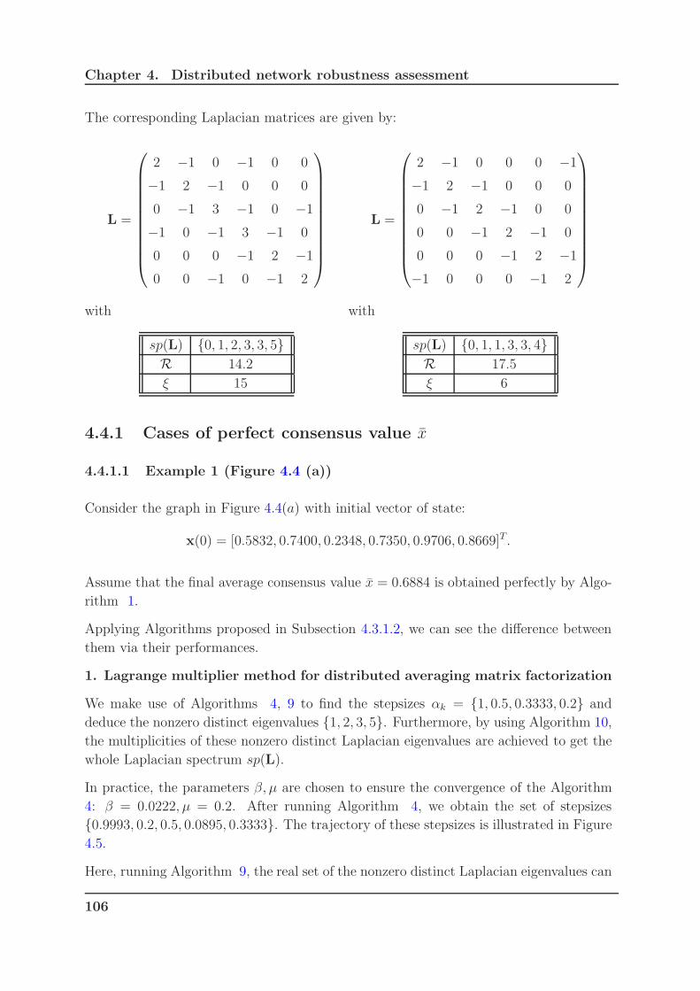
Chapter 4. Distributed network robustness assessment
The corresponding Laplacian matrices are given by:
L =
2 −1 0 −1 0 0
−1 2 −1 0 0 0
0 −1 3 −1 0 −1
−1 0 −1 3 −1 0
0 0 0 −1 2 −1
0 0 −1 0 −1 2
with
sp(L) 0, 1, 2, 3, 3, 5R 14.2
ξ 15
L =
2 −1 0 0 0 −1
−1 2 −1 0 0 0
0 −1 2 −1 0 0
0 0 −1 2 −1 0
0 0 0 −1 2 −1
−1 0 0 0 −1 2
with
sp(L) 0, 1, 1, 3, 3, 4R 17.5
ξ 6
4.4.1 Cases of perfect consensus value x
4.4.1.1 Example 1 (Figure 4.4 (a))
Consider the graph in Figure 4.4(a) with initial vector of state:
x(0) = [0.5832, 0.7400, 0.2348, 0.7350, 0.9706, 0.8669]T.
Assume that the final average consensus value x = 0.6884 is obtained perfectly by Algo-
rithm 1.
Applying Algorithms proposed in Subsection 4.3.1.2, we can see the difference between
them via their performances.
1. Lagrange multiplier method for distributed averaging matrix factorization
We make use of Algorithms 4, 9 to find the stepsizes αk = 1, 0.5, 0.3333, 0.2 and
deduce the nonzero distinct eigenvalues 1, 2, 3, 5. Furthermore, by using Algorithm 10,
the multiplicities of these nonzero distinct Laplacian eigenvalues are achieved to get the
whole Laplacian spectrum sp(L).
In practice, the parameters β, µ are chosen to ensure the convergence of the Algorithm
4: β = 0.0222, µ = 0.2. After running Algorithm 4, we obtain the set of stepsizes
0.9993, 0.2, 0.5, 0.0895, 0.3333. The trajectory of these stepsizes is illustrated in Figure
4.5.
Here, running Algorithm 9, the real set of the nonzero distinct Laplacian eigenvalues can
106

Chapter 4. Distributed network robustness assessment
100
102
104
105
0
0.2
0.4
0.6
0.8
1
Iterations
α 1
100
102
104
105
0
0.2
0.5
Iterations
α 2
100
102
104
105
0
0.2
0.5
Iterations
α 3
100
102
104
0.0895
0,5
Iterations
α 4
100
102
104
0
0,2
0.3333
0,6
0,8
1
Iterations
α 5
Figure 4.5: Trajectory of the stepsizes αk.
107
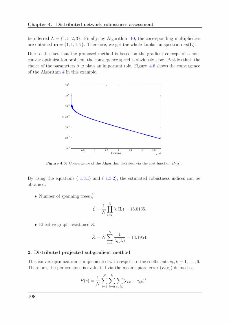
Chapter 4. Distributed network robustness assessment
be inferred Λ = 1, 5, 2, 3. Finally, by Algorithm 10, the corresponding multiplicities
are obtained m = 1, 1, 1, 2. Therefore, we get the whole Laplacian spectrum sp(L).
Due to the fact that the proposed method is based on the gradient concept of a non-
convex optimization problem, the convergence speed is obviously slow. Besides that, the
choice of the parameters β, µ plays an important role. Figure 4.6 shows the convergence
of the Algorithm 4 in this example.
0.5 1 1.5 2 2.5 3 3.5
x 105
10−10
10−8
10−6
10−4
10−2
100
102
Iterations
H
Figure 4.6: Convergence of the Algorithm decribed via the cost function H(α).
By using the equations ( 1.3.1) and ( 1.3.2), the estimated robustness indices can be
obtained:
• Number of spanning trees ξ:
ξ =1
N
N∏
i=2
λi(L) = 15.0135.
• Effective graph resistance R
R = NN∑
i=2
1
λi(L)= 14.1954.
2. Distributed projected subgradient method
This convex optimization is implemented with respect to the coefficients ck, k = 1, . . . , 6.
Therefore, the performance is evaluated via the mean square error (E(c)) defined as:
E(c) =1
N
N∑
i=1
h∑
k=0
∑
j∈Ni
(ci,k − cj,k)2.
108
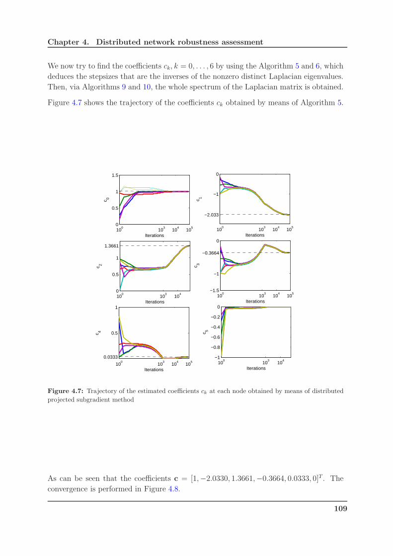
Chapter 4. Distributed network robustness assessment
We now try to find the coefficients ck, k = 0, . . . , 6 by using the Algorithm 5 and 6, which
deduces the stepsizes that are the inverses of the nonzero distinct Laplacian eigenvalues.
Then, via Algorithms 9 and 10, the whole spectrum of the Laplacian matrix is obtained.
Figure 4.7 shows the trajectory of the coefficients ck obtained by means of Algorithm 5.
100
103
104
105
0
0.5
1
1.5
Iterations
c 0
100
103
104
105
−2.033
−1
0
Iterations
c 1
100
103
104
0
0.5
1
1.3661
Iterations
c 2
100
103
104
105
−1.5
−1
−0.3664
0
Iterations
c 3
100
103
104
105
0.0333
0.5
1
Iterations
c 4
100
103
104
−1
−0.8
−0.6
−0.4
−0.2
0
Iterations
c 5
Figure 4.7: Trajectory of the estimated coefficients ck at each node obtained by means of distributed
projected subgradient method
As can be seen that the coefficients c = [1,−2.0330, 1.3661,−0.3664, 0.0333, 0]T . The
convergence is performed in Figure 4.8.
109
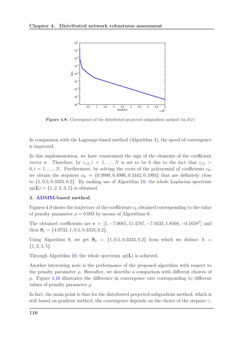
Chapter 4. Distributed network robustness assessment
0.5 1 1.5 2 2.5 3 3.5 4 4.5 5
x 104
10−8
10−7
10−6
10−5
10−4
10−3
10−2
10−1
100
Iterations
E(c
)
Figure 4.8: Convergence of the distributed projected subgradient method via E(c)
In comparison with the Lagrange-based method (Algorithm 4), the speed of convergence
is improved.
In this implementation, we have constrained the sign of the elements of the coefficient
vector c. Therefore, by ci,5, i = 1, . . . , N is set to be 0 due to the fact that ci,5 >
0, i = 1, . . . , N . Furthermore, by solving the roots of the polynomial of coefficients ck,
we obtain the stepsizes αk = 0.9998, 0.4996, 0.3342, 0.1993 that are definitely close
to 1, 0.5, 0.3333, 0.2. By making use of Algorithm 10, the whole Laplacian spectrum
sp(L) = 1, 2, 3, 3, 5 is obtained.
3. ADMM-based method
Figures 4.9 shows the trajectory of the coefficients ck obtained corresponding to the value
of penalty parameter ρ = 0.003 by means of Algorithms 6 .
The obtained coefficients are c = [1,−7.0065, 11.4787,−7.1633, 1.8568,−0.1658T ] and
then S1 = 4.9732, 1, 0.5, 0.3333, 0.2.
Using Algorithm 9, we get S2 = 1, 0.5, 0.3333, 0.2 from which we deduce Λ =
1, 2, 3, 5.
Through Algorithm 10, the whole spectrum sp(L) is achieved.
Another interesting note is the performance of the proposed algorithm with respect to
the penalty parameter ρ. Hereafter, we describe a comparison with different choices of
ρ. Figure 4.10 illustrates the difference in convergence rate corresponding to different
values of penalty parameter ρ
In fact, the main point is that for the distributed projected subgradient method, which is
still based on gradient method, the convergence depends on the choice of the stepsize γ.
110

Chapter 4. Distributed network robustness assessment
100
102
−1
0
1
2
Iterations
c 0
100
102
−7,0065
−1
Iterations
c 110
010
20.01
1
11.4787
Iterations
c 2
100
102
−7.1633
−1
Iterations
c 3
100
102
1
1.8568
Iterations
c 4
100
102
−1
−0.5
−0.1658
0.5
Iterations
c 5
Figure 4.9: Trajectory of the estimated coefficients ck at each node obtained by means of ADMM
0 0.5 1 1.5 2 2.5 3
x 104
10−15
10−10
10−5
100
Iterations
E(c
)
ρ=0.001ρ=0.005ρ=0.003
Figure 4.10: Convergence rate of the ADMM-based method with different values of ρ.
On the other hand, the ADMM-based method seems to be the most attracting method
when the only parameter needs to be noticed is the penalty parameter ρ to regulate the
111
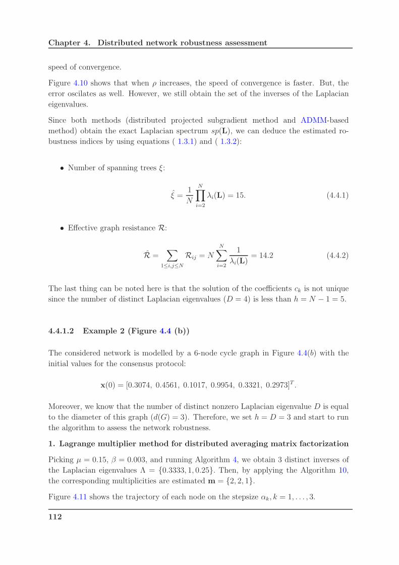
Chapter 4. Distributed network robustness assessment
speed of convergence.
Figure 4.10 shows that when ρ increases, the speed of convergence is faster. But, the
error oscilates as well. However, we still obtain the set of the inverses of the Laplacian
eigenvalues.
Since both methods (distributed projected subgradient method and ADMM-based
method) obtain the exact Laplacian spectrum sp(L), we can deduce the estimated ro-
bustness indices by using equations ( 1.3.1) and ( 1.3.2):
• Number of spanning trees ξ:
ξ =1
N
N∏
i=2
λi(L) = 15. (4.4.1)
• Effective graph resistance R:
R =∑
1≤i,j≤N
Rij = N
N∑
i=2
1
λi(L)= 14.2 (4.4.2)
The last thing can be noted here is that the solution of the coefficients ck is not unique
since the number of distinct Laplacian eigenvalues (D = 4) is less than h = N − 1 = 5.
4.4.1.2 Example 2 (Figure 4.4 (b))
The considered network is modelled by a 6-node cycle graph in Figure 4.4(b) with the
initial values for the consensus protocol:
x(0) = [0.3074, 0.4561, 0.1017, 0.9954, 0.3321, 0.2973]T .
Moreover, we know that the number of distinct nonzero Laplacian eigenvalue D is equal
to the diameter of this graph (d(G) = 3). Therefore, we set h = D = 3 and start to run
the algorithm to assess the network robustness.
1. Lagrange multiplier method for distributed averaging matrix factorization
Picking µ = 0.15, β = 0.003, and running Algorithm 4, we obtain 3 distinct inverses of
the Laplacian eigenvalues Λ = 0.3333, 1, 0.25. Then, by applying the Algorithm 10,
the corresponding multiplicities are estimated m = 2, 2, 1.
Figure 4.11 shows the trajectory of each node on the stepsize αk, k = 1, . . . , 3.
112

Chapter 4. Distributed network robustness assessment
100
102
104
0.2
0.3333
0.6
0.8
Iterations
α 1
100
102
104
0
0.2
0.4
0.6
0.8
1
Iterations
α 2
100
102
104
0.001
0.01
0.1
0.25
1
Iterations
α 3
Figure 4.11: Zoom in the trajectory of each node on the stepsize αk
Figure 4.12 shows the convergence of Algorithm 4 in this example.
1 2 3 4 5 6 7 8 9 10 11 12
x 104
10−10
10−8
10−6
10−4
10−2
100
102
Iterations
H
Figure 4.12: Convergence of Algorithm 4 performed through the cost function H(α)
2. Distributed projected subgradient method
Figure 4.13 shows the trajectory of the coefficients ck obtained by means of Algorithms
5.
113
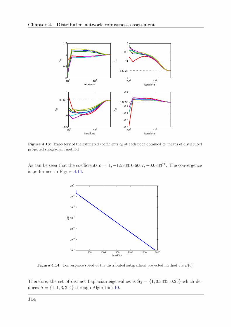
Chapter 4. Distributed network robustness assessment
100
102
0
0.5
1
1.5
Iterations
c 0
100
102
−2
−1.5833
−1
−0.5
0
Iterations
c 1
100
102
−0.5
0
0.6667
1
Iterations
c 2
100
102
−0.8
−0.6
−0.4
−0.2
−0.0833
0.2
Iterations
c 3
Figure 4.13: Trajectory of the estimated coefficients ck at each node obtained by means of distributed
projected subgradient method
As can be seen that the coefficients c = [1,−1.5833, 0.6667,−0.0833]T . The convergence
is performed in Figure 4.14.
500 1000 1500 2000 2500 300010
−12
10−10
10−8
10−6
10−4
10−2
100
Iterations
E(c
)
Figure 4.14: Convergence speed of the distributed subgradient projected method via E(c)
Therefore, the set of distinct Laplacian eigenvalues is S2 = 1, 0.3333, 0.25 which de-
duces Λ = 1, 1, 3, 3, 4 through Algorithm 10.
114

Chapter 4. Distributed network robustness assessment
3. ADMM-based method
Figure 4.15 shows the trajectory of the coefficients ck obtained by means of Algorithms
6.
500 1000 1500 20000
0.5
1
1.5
Iterations
c 0
100
102
−5
−4
−3
−1.5833
−1
0
Iterations
c 1
100
102
0
0.6667
1
1.5
2
2.5
3
Iterations
c 2
100
102
−0.8
−0.6
−0.4
−0.2
−0.0833
Iterations
c 3
Figure 4.15: Trajectory of the estimated coefficients ck at each node obtained by means of distributed
ADMM
Due to the fact that D = 3 is assumed to be known in a priori, then the achieved
coefficients c = [1,−1.5833, 0.6667,−0.0833]T is a unique solution. The convergence is
performed in Figure 4.16 with respect to two values of ρ = 0.1, 0.01.
115
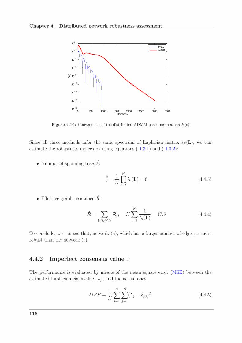
Chapter 4. Distributed network robustness assessment
0 500 1000 1500 2000 2500 3000 350010
−16
10−14
10−12
10−10
10−8
10−6
10−4
10−2
100
Iterations
E(c
)
ρ=0.1ρ=0.01
Figure 4.16: Convergence of the distributed ADMM-based method via E(c)
Since all three methods infer the same spectrum of Laplacian matrix sp(L), we can
estimate the robustness indices by using equations ( 1.3.1) and ( 1.3.2):
• Number of spanning trees ξ:
ξ =1
N
N∏
i=2
λi(L) = 6 (4.4.3)
• Effective graph resistance R:
R =∑
1≤i,j≤N
Rij = NN∑
i=2
1
λi(L)= 17.5 (4.4.4)
To conclude, we can see that, network (a), which has a larger number of edges, is more
robust than the network (b).
4.4.2 Imperfect consensus value x
The performance is evaluated by means of the mean square error (MSE) between the
estimated Laplacian eigenvalues λj,i and the actual ones.
MSE =1
N
N∑
i=1
D∑
j=1
(λj − λj,i)2. (4.4.5)
116

Chapter 4. Distributed network robustness assessment
4.4.2.1 Example 1
Firstly, we run an average consensus protocol using the constant edge weights
consensus protocol 1.2.9 with α = 0.2 as a stepsize, and x(0) =
[0.4401, 0.5271, 0.4574, 0.8754, 0.5181, 0.9436]T as an initial condition.
Figure 4.17 depicts the trajectory of the state of each node.
5 10 15 20 25 30 35 40 45 50 55 600.4
0.5
0.6
0.7
0.8
0.9
1
Iterations (M)
x
Figure 4.17: Trajectory of the network state during average consensus protocol.
We can note that a reasonable agreement is obtained after iteration 22. Then, Algorithm
7 for computing the factorization of the averaging matrix was performed for different
values for the number of iterations M of the average consensus algorithm.
For M ≤ 22, xM was too far from x. As a consequence, the obtained polynomial gave
rise to negative or complex-valued roots meaning that the coefficients c created from
these roots do not satisfy ˆxi = cTi qi in Algorithm 9. For M > 22, Algorithm 9 was
successfully applied for retrieving the Laplacian eigenvalues approximately.
117
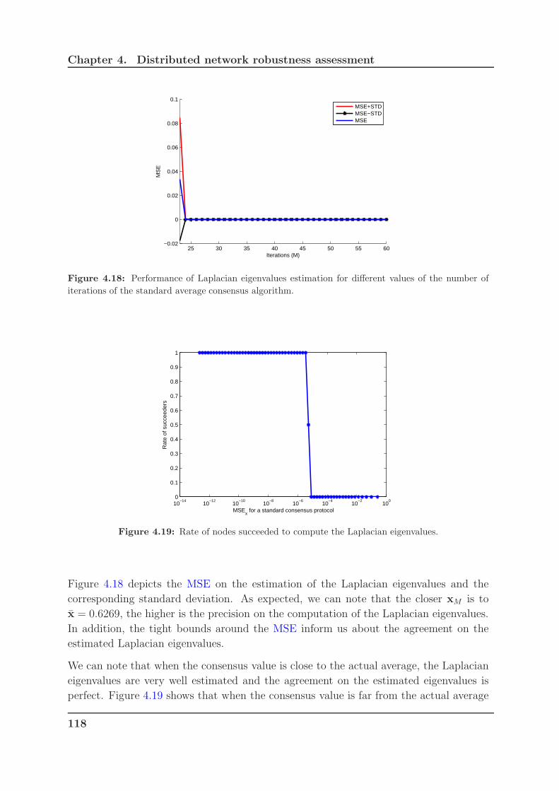
Chapter 4. Distributed network robustness assessment
25 30 35 40 45 50 55 60−0.02
0
0.02
0.04
0.06
0.08
0.1
Iterations (M)
MS
E
MSE+STDMSE−STDMSE
Figure 4.18: Performance of Laplacian eigenvalues estimation for different values of the number of
iterations of the standard average consensus algorithm.
10−14
10−12
10−10
10−8
10−6
10−4
10−2
100
0
0.1
0.2
0.3
0.4
0.5
0.6
0.7
0.8
0.9
1
MSEx for a standard consensus protocol
Rat
e of
suc
ceed
ers
Figure 4.19: Rate of nodes succeeded to compute the Laplacian eigenvalues.
Figure 4.18 depicts the MSE on the estimation of the Laplacian eigenvalues and the
corresponding standard deviation. As expected, we can note that the closer xM is to
x = 0.6269, the higher is the precision on the computation of the Laplacian eigenvalues.
In addition, the tight bounds around the MSE inform us about the agreement on the
estimated Laplacian eigenvalues.
We can note that when the consensus value is close to the actual average, the Laplacian
eigenvalues are very well estimated and the agreement on the estimated eigenvalues is
perfect. Figure 4.19 shows that when the consensus value is far from the actual average
118

Chapter 4. Distributed network robustness assessment
the nodes fail to compute the Laplacian eigenvalues. However, some of them are able to
carry out such a computation while the other fail. For instance, at iteration M = 22,
there are only 3 nodes estimating the inverse of the Laplacian eigenvalues approximately.
Figures 4.20 and 4.21 show the trajectories of each node on the network robustness
indices (R, ξ) corresponding to the iterations of the standard consensus protocol (M),
started from M = 23.
23 27 32 3713.5
14.2
15
16
17
18
Iterations (M)
Effe
ctiv
e G
raph
Res
ista
nce
(R)
Figure 4.20: Trajectory of each node on
the effective graph resistance R
23 27 32 37
3
6
9
12
15
Iterations (M)
Num
ber
of s
pann
ing
tree
s (ξ
)
Figure 4.21: Trajectory of each node on the num-
ber of spanning trees ξ
From these two Figures, the nodes estimate different values of R and ξ until M = 35.
Then, they estimate almost the same value of the Robustness Indices.
Figure 4.22 describes the sensitiveness of the effective graph resistance (R) and the num-
ber spanning trees (ξ) to the MSE via the relative errors which are defined respectively
as:
RER =‖1R−RRR‖2
R2,
REξ =‖1ξ − ξξξ‖2
ξ2.
Where RRR, ξξξ are the estimated vectors of local estimated Effective Graph Resistance
Ri, i = 1, . . . , N and locally estimated the number of spanning trees ξi, i = 1, . . . , N
respectively.
Figure 4.22 shows that the effective graph resistance R is more sensitive to the MSE
than the number of spanning trees ξ.
119

Chapter 4. Distributed network robustness assessment
10−12
10−10
10−8
10−6
10−4
10−2
100
10−10
10−8
10−6
10−4
10−2
100
MSE
Rel
ativ
e E
rror
s
REξ
RER
Figure 4.22: Relative errors RER and REξ versus MSE.
100
101
102
103
0.5
0.9999
1.5
2
Iterations
c 0
100
101
102
103
104
−4
−2.6224−2
0
2
Iterations
c 1
100
101
102
103
104
0
22.5714
Iterations
c 2
100
102
103
104
−0,5
0
Iterations
c 3
100
101
102
103
104
0.2517
Iterations
c 4
100
101
102
103
104
−0.05
−0.0199
0.05
Iterations
c 5
Figure 4.23: Estimation of the polynomial coefficients ck at M = 24.
120
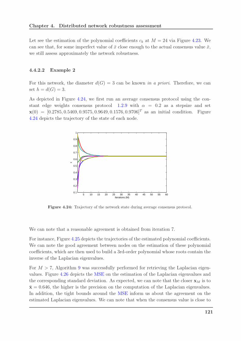
Chapter 4. Distributed network robustness assessment
Let see the estimation of the polynomial coefficients ck at M = 24 via Figure 4.23. We
can see that, for some imperfect value of x close enough to the actual consensus value x,
we still assess approximately the network robustness.
4.4.2.2 Example 2
For this network, the diameter d(G) = 3 can be known in a priori. Therefore, we can
set h = d(G) = 3.
As depicted in Figure 4.24, we first run an average consensus protocol using the con-
stant edge weights consensus protocol 1.2.9 with α = 0.2 as a stepsize and set
x(0) = [0.2785, 0.5469, 0.9575, 0.9649, 0.1576, 0.9706]T as an initial condition. Figure
4.24 depicts the trajectory of the state of each node.
5 10 15 20 25 30 35 40 45 50 55 600.1
0.2
0.3
0.4
0.5
0.6
0.7
0.8
0.9
1
Iterations (M)
x
Figure 4.24: Trajectory of the network state during average consensus protocol.
We can note that a reasonable agreement is obtained from iteration 7.
For instance, Figure 4.25 depicts the trajectories of the estimated polynomial coefficients.
We can note the good agreement between nodes on the estimation of these polynomial
coefficients, which are then used to build a 3rd-order polynomial whose roots contain the
inverse of the Laplacian eigenvalues.
For M > 7, Algorithm 9 was successfully performed for retrieving the Laplacian eigen-
values. Figure 4.26 depicts the MSE on the estimation of the Laplacian eigenvalues and
the corresponding standard deviation. As expected, we can note that the closer xM is to
x = 0.646, the higher is the precision on the computation of the Laplacian eigenvalues.
In addition, the tight bounds around the MSE inform us about the agreement on the
estimated Laplacian eigenvalues. We can note that when the consensus value is close to
121

Chapter 4. Distributed network robustness assessment
100
101
102
103
0.8
0.9999
1.2
1.4
1.6
Iterations
c 0
100
101
102
103
−3
−1.5813
−1
0
1
Iterations
c 1
100
101
102
103
−0.5
0
0.6649
1
1.5
Iterations
c 2
100
101
102
103
−0.4
−0.083
0.2
0.4
Iterations
c 3
Figure 4.25: Estimation of the polynomial coefficients for (M = 17).
10 15 20 25 30 35 40 45 50 55 60−0.4
−0.2
0
0.2
0.4
0.6
0.8
1
1.2
1.4
1.6
Iterations (M)
MS
E
MSE+STDMSE−STDMSE
Figure 4.26: Performance of Laplacian eigenvalues estimation for different values of the number of
iterations of the standard average consensus algorithm.
the actual average, the Laplacian eigenvalues are very well estimated and the agreement
on the estimated eigenvalues is perfect. Figure 4.27 shows that when the consensus value
is far from the actual average (M < 7) the nodes fail to compute the Laplacian eigen-
values. However, some of them are able to carry out such a computation while the other
fail (M = 7, . . . , 17).
122

Chapter 4. Distributed network robustness assessment
10−14
10−12
10−10
10−8
10−6
10−4
10−2
100
0
0.1
0.2
0.3
0.4
0.5
0.6
0.7
0.8
0.9
1
MSEx for a standard consensus protocol
Rat
e of
suc
ceed
ers
Figure 4.27: Rate of the nodes succeed to compute the Laplacian eigenvalues.
Since started from M = 18, all nodes can compute the robustness metrics, then Fig-
ures 4.28 and 4.29 demonstrate the trajectories of each node versus iterations (M =
18, . . . , 60).
18 22 27 32 37 42 4717.35
17.4
17.45
17.5
17.55
17.6
17.65
17.7
Iterations (M)
Effe
ctiv
e G
raph
Res
ista
nce
(R)
Figure 4.28: Trajectory of each node on
the effective graph resistance R
18 22 27 32 37 42 475.9
5.95
6
6.05
6.1
6.15
6.2
Iterations (M)
The
num
ber
of s
pann
ing
tree
s (ξ
)
Figure 4.29: Trajectory of each node on the num-
ber of spanning trees ξ
Furthermore, Figure 4.30 describes the comparison between two robustness metrics on
the sensitiveness to the MSE. Figure 4.30 shows that the effective graph resistance R is
more sensitive to the MSE than the number of spanning trees ξ.
In this example, since the number of the distinct Laplacian eigenvalues is known, then
the solution of the polynomial coefficients ck is unique. Moreover, the convergence of
Algorithm 7 assessed through the performance of the cost function E(c) due to different
values of M is presented in Figure 4.31. We can see that when the choice of M make xM
123
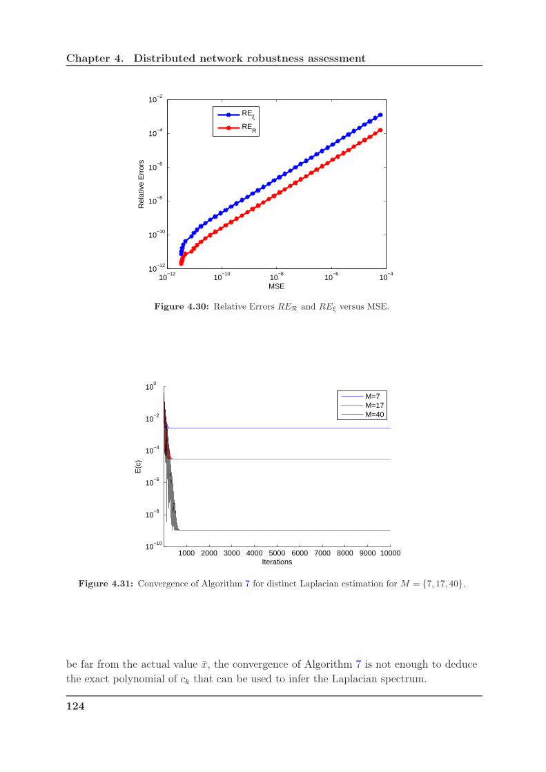
Chapter 4. Distributed network robustness assessment
10−12
10−10
10−8
10−6
10−4
10−12
10−10
10−8
10−6
10−4
10−2
MSE
Rel
ativ
e E
rror
s
REξ
RER
Figure 4.30: Relative Errors RER and REξ versus MSE.
1000 2000 3000 4000 5000 6000 7000 8000 9000 1000010
−10
10−8
10−6
10−4
10−2
100
Iterations
E(c
)
M=7M=17M=40
Figure 4.31: Convergence of Algorithm 7 for distinct Laplacian estimation for M = 7, 17, 40.
be far from the actual value x, the convergence of Algorithm 7 is not enough to deduce
the exact polynomial of ck that can be used to infer the Laplacian spectrum.
124

Chapter 4. Distributed network robustness assessment
4.4.3 Unknown consensus value x
4.4.3.1 Example 1
We first generate the vector of initial values x(0) =
[0.5356, 0.1649, 0.8834, 0.6665, 0.8477, 0.7627]T .
According to the proposed Algorithm 8, the nodes have to achieve agreement on the
values of the polynomial coefficients ck and that of the average consensus value x simul-
taneously.
Figure 4.32 and Figure 4.33 depict the trajectories of the nodes for the estimation of
the coefficients ci,k, k = 0, . . . , N − 1, and that of the consensus value x. Note that, the
average consensus value is obtained much more faster than the common values of the
coefficients ck.
100
102
−4
−2
1
4
Iterations
c 0
100
102
−10
−5−3.0864
5
Iterations
c 1
100
102
−5
0
3.508
10
Iterations
c 2
100
102
−10
−5
−1.8059
5
Iterations
c 3
100
102
−2
0.4195
2
4
6
Iterations
c 4
100
102
−2
−1
−0.0351
1
Iterations
c 5
Figure 4.32: Nodes trajectories for the estimation of the coefficients ck.
To assess the independence of the estimates on the initial condition x(0), a Monte-Carlo
simulation has been carried out. 100 initial vectors x(0) drawn independently from a
uniform distribution have been generated.
125

Chapter 4. Distributed network robustness assessment
50 100 150 200 250 300 350−1
−0.5
0
0.6435
1
1.5
2
Iterations
x
Figure 4.33: Nodes trajectories converging to the average of the initial condition.
Figure 4.34 describes the performance in terms of the MSE between the estimated values
and the actual values for the polynomial coefficients ci and the average consensus values
xi as:
MSEc =1
N
N∑
i=1
‖ci − c‖2‖c‖2 , and MSEx =
1
N
N∑
i=1
(xi − x)2
x2,
where x, c stand for the actual average consensus value and actual polynomial coefficients
respectively.
0 200 400 600 800 1000 120010
−15
10−10
10−5
100
105
Iterations
MS
E
MSEc
MSEx
θ
Figure 4.34: Mean square error between the estimated values and actual values with respect to ci
(MSEc) and xi (MSEx).
Figure 4.34 indicates the performances of MSEc,MSEx with respect to the variation of
θ(t). As can be seen from the figure, when θ(t) is near to 0, the convergence speed of
126
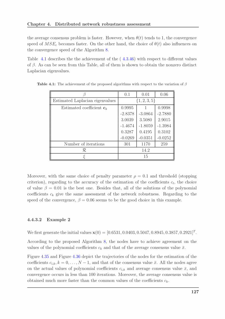
Chapter 4. Distributed network robustness assessment
the average consensus problem is faster. However, when θ(t) tends to 1, the convergence
speed of MSEc becomes faster. On the other hand, the choice of θ(t) also influences on
the convergence speed of the Algorithm 8.
Table 4.1 describes the the achievement of the ( 4.3.46) with respect to different values
of β. As can be seen from this Table, all of them is shown to obtain the nonzero distinct
Laplacian eigenvalues.
Table 4.1: The achievement of the proposed algorithms with respect to the variation of β
β 0.1 0.01 0.06
Estimated Laplacian eigenvalues 1, 2, 3, 5Estimated coefficient ck 0.9995 1 0.9998
-2.8378 -3.0864 -2.7880
3.0039 3.5080 2.9015
-1.4674 -1.8059 -1.3984
0.3287 0.4195 0.3102
-0.0269 -0.0351 -0.0252
Number of iterations 301 1170 259
R 14.2
ξ 15
Moreover, with the same choice of penalty parameter ρ = 0.1 and threshold (stopping
criterion), regarding to the accuracy of the estimation of the coefficients ct, the choice
of value β = 0.01 is the best one. Besides that, all of the solutions of the polynomial
coefficients ck give the same assessment of the network robustness. Regarding to the
speed of the convergence, β = 0.06 seems to be the good choice in this example.
4.4.3.2 Example 2
We first generate the initial values x(0) = [0.6531, 0.0403, 0.5047, 0.8945, 0.3857, 0.2921]T.
According to the proposed Algorithm 8, the nodes have to achieve agreement on the
values of the polynomial coefficients ck and that of the average consensus value x.
Figure 4.35 and Figure 4.36 depict the trajectories of the nodes for the estimation of the
coefficients ci,k, k = 0, . . . , N − 1, and that of the consensus value x. All the nodes agree
on the actual values of polynomial coefficients ci,k and average consensus value x, and
convergence occurs in less than 100 iterations. Moreover, the average consensus value is
obtained much more faster than the common values of the coefficients ck.
127
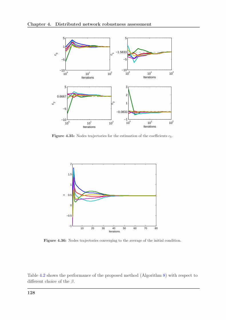
Chapter 4. Distributed network robustness assessment
100
101
102
−10
−5
1
5
Iterations
c 0
100
101
102
−10
−5
−1.5833
5
Iterations
c 1
100
101
102
−10
−5
0.6667
5
Iterations
c 2
100
101
102
−1
−0.0833
1
2
3
Iterations
c 3
Figure 4.35: Nodes trajectories for the estimation of the coefficients ck.
10 20 30 40 50 60 70 80−1
−0.5
0
0.5
1
1.5
2
Iterations
x
Figure 4.36: Nodes trajectories converging to the average of the initial condition.
Table 4.2 shows the performance of the proposed method (Algorithm 8) with respect to
different choice of the β.
128

Chapter 4. Distributed network robustness assessment
Table 4.2: The achievement of the proposed algorithms with respect to the variation of β
β 0.1 0.01 0.06
Estimated Laplacian eigenvalues 1, 3, 4Estimated coefficient ck 1
-1.5833
0.6667
-0.0833
Number of iterations 151 1188 232
R 17.5
ξ 6
As can be seen from this Table, despite of the different choices of β, the proposed method
gives exactly the same polynomial coefficients ck, which can be used to infer the same
assessment of the network robustness. However, with β = 0.1, the speed of convergence
is the fastest.
4.5 Conclusion
In this Chapter, we have proposed some methods to assess the robustness of a given
network in a distributed way. Formally, the robustness metrics called the effective graph
resistance R and the number of spanning trees ξ are functions of the Laplacian spectrum
sp(L). Therefore, these proposed methods are distinguished by the way to estimate the
Laplacian spectrum. In detail, three cases have been considered with respect to the con-
sensus value x, that are: perfect consensus value x, imperfect consensus value xM and
unknown consensus value x. Based on recent results, the average consensus matrix can
be factored in D Laplacian based consensus matrices, where D stands for the number of
nonzero distinct Laplacian eigenvalues. For this purpose, all proposed methods are char-
acterized into two approaches, which are the direct approach and indirect approach in the
case of perfect consensus value x. A direct approach was first presented. It gives rise to a
non-convex optimization problem with respect to the stepsizes αk, k = 1, . . . , D = N − 1
that are the inverse of the nonzero distinct Laplacian eigenvalues. For this approach,
since it is based on the gradient descent method, the main issue is that it suffers from
slow convergence towards a local minimum. To improve that, a convex optimization
problem has been considered to estimate the optimal coefficients ck, k = 0, . . . , N − 1
of a given polynomial whose roots are the stepsizes αk, k = 1, . . . , N − 1 that allow to
factorize the averaging matrix. In this way, we have applied two well-known methods
that are the projected subgradient method and the ADMM to solve the convex problem.
After that, the Laplacian eigenvalues are thus estimated by taking the inverse of these
129

Chapter 4. Distributed network robustness assessment
obtained stepsizes αk, k = 1, . . . , N − 1. Then the real set of nonzero distinct Lapla-
cian eigenvalues Λ = λi, i = 2, . . . , D is captured by a retrieving algorithm. Finally,
the whole Laplacian spectrum is obtained via defining the corresponding multiplicities
of these eigenvalues. In what follows, the network robustness measure can be easily
deduced.
The drawback of the proposed methods is their scalability. In fact, for large graphs,
the whole Laplacian spectrum estimation becomes a significant burden. Therefore, the
estimation can be restricted to that of the most significant eigenvalues used to estimate
bound of the network robustness index. For example, λ2(L) is a lower-bound of the
vertex connectivity (K). Furthermore, we may encounter ill-conditioned problem in
implementation of the indirect proposed methods. Hence, we can investigate new method
for preconditioning the problem.
In the case of imperfect consensus value, we assume that a standard consensus protocol
has been run and stores some intermediate values of xM according to the iteration M .
Then, we make use of the ADMM-based Algorithm 7 to see how the network robustness
reacts. Finally, it claims that when the intermediate value of x is as close as possible to
the real one, the network robustness index can be taken approximately.
In the case of unknown consensus value x, we consider the convex optimization problem
which resorts to a convex combination of two convex functions. The first one takes into
account the average consensus problem while the second one concerns the estimation of
the Laplacian matrix. It is an indirect method where parameters of the factorization of
the averaging matrix are computed first and then the Laplacian eigenvalues are estimated
as the roots of a given polynomial. For large graphs, such a solution is clearly intractable.
Therefore, the proposed Algorithms 5, 6, 7, 8 are efficient and well adapted for networks
with medium size.
The ADMM seems to be the best method compared with all the methods proposed.
Therefore, the study of the convergence rate must be more interesting. In the near future,
we will investigate the convergence rate of the ADMM for the quadratic programming
based on the work in [25].
130

Chapter 5
Network topology reconstruction
Contents
5.1 Introduction . . . . . . . . . . . . . . . . . . . . . . . . . . . . 131
5.2 Literature review . . . . . . . . . . . . . . . . . . . . . . . . . 132
5.3 Problem statement . . . . . . . . . . . . . . . . . . . . . . . . 138
5.4 Distributed solution to the network topology reconstruc-
tion problem . . . . . . . . . . . . . . . . . . . . . . . . . . . . 139
5.4.1 Estimation of the eigenvectors of the Laplacian-based consen-
sus matrix . . . . . . . . . . . . . . . . . . . . . . . . . . . . . . 139
5.4.2 Network topology reconstruction . . . . . . . . . . . . . . . . . 140
5.5 Numerical result . . . . . . . . . . . . . . . . . . . . . . . . . . 142
5.6 Conclusion . . . . . . . . . . . . . . . . . . . . . . . . . . . . . 147
5.1 Introduction
Network topology is usually a schematic description of the arrangement of a network, in-
cluding its nodes and connecting edges. Briefly speaking, network topology may describe
how the data is transferred between these nodes.1
Network topology identification refers to detecting and identifying the interested network
elements and the relationship between elements in target network and represents the
topology construction in an appropriate form. Therefore, identification of networks of
systems becomes a growing attractive task for solving many problems in different science
and engineering domains, for instance, in biology (biochemical, neural and ecological
1Source: http://whatis.techtarget.com/definition/network-topology
131
Chapter 5. Network topology reconstruction
networks [2]), finance, computer science (Internet and World Wide Web), transportation
(delivery and distribution network), and electrical engineering.
For example, the architecture of an overlay network - how it allocates addresses, etc.-
may be significantly optimized by knowledge of the distribution and connectivity of
the nodes on the underlay network that actually carries the traffic. Several important
systems, such as P4P (stands for provider portal for Peer–to–Peer (P2P) applications)
and RMTP (reliable multicast transport protocol), utilize information about the topology
of the underlay network for optimization as well as management [1].
In the Internet, for instance, the usual mechanism for generating the topology of a
network is by the use of Traceroute. Traceroute is executed on a node, called the source,
by specifying the address of a destination node. This execution produces a sequence of
identifiers, called a trace, corresponding to the route taken by packets travelling from the
source to the destination. A trace set T is generated by repeatedly executing Traceroute
over a network, varying the terminal nodes, i.e. the source and destination. If T contains
traces that identify every instance when an edge is incident on a node, it is possible to
reconstruct the network exactly [1].
Following our study, from a general consensus network and consensus measurements,
we deal with the problem of inferring the correct network topology in the presence of
anonymous nodes (or unlabelled nodes). In other words, is it possible for an arbitrary
node j to reconstruct the correct network from average consensus measurements?
5.2 Literature review
In the literature, there are various methods proposed for reconstructing the network
topology.
For centralized framework, in [56], the authors introduced a network identification scheme
which involves the excitation and observation of nodes running consensus-type protocols.
The problem is to identify the interaction geometry among a known number of nodes,
adopting a (weighted) consensus-type algorithm for their coordination. In the considered
procedure, the node broadcasts a zero state to its neighbors without being removed
from the network. This node is called node knockout, which is essentially a grounding
procedure. Starting with the number of vertices in the network as a known parameter as
well as the controllability and observability of the resulting steered-and-observed network,
define the characteristic polynomial of the grounded consensus at assumed known node
i, which leads to deduce the matrix ΨΨΨ as the adjugate of the matrix (IN + L) in order
to determine the entries of L. The advantage of this paper is the ramifications for exact
identification from boundary nodes of networks that have an embedded consensus-based
distributed algorithm used for flocking and distributed estimation.
132

Chapter 5. Network topology reconstruction
In [68], the problem of identifying the topology of an unknown directed network of linear
time-invariant (LTI) systems stimulated by a wide-sense stationary noise of unknown
power spectral density has been considered. The authors have proposed several recon-
struction algorithms based on the power spectral properties of the network response to
the noise. In [33], the identifiability of the structure and dynamics of an unknown net-
work driven by unknown noise has been assessed based on factorizations of the output
spectral density. In this paper, the authors have claimed that for networks with closed-
loop transfer matrices that are minimum phase, the network reconstruction problem can
have a unique solution from its output spectral density.
In [37], the reconstruction concepts are based on paradigmatic dynamical models such as
phase oscillators. The authors have discovered a general connection between dynamical
correlation among oscillators and the underlying topology in the presence of noise. In
particular, the correspondence between the dynamical correlation matrix of nodal time
series and the connection matrix of structures, due to the presence of noise.
In order to bridge dynamical correlation and topology, consider N non-identical coupled
oscillators xi ∈ IRm, i = 1, . . . , N , which denotes the m-dimensional state variables of
i-th oscillator. In the presence of noise, the dynamics of the whole coupled-oscillator
system can be expressed as:
xi = Fi(xi)− γ
N∑
j=1
lijP(xj) + ηηηi, (5.2.1)
where:
• Fi : IRm → IRm is intrinsic dynamics of the i-th oscillator,
• P : IRm → IRm is the coupling function of oscillators,
• lij is an element at i-th row and j-th column of the Laplacian matrix L,
• γ > 0 is the coupling strength,
• ηηη = [η1, . . . , ηN ]T is the noise vector with covariance matrix D.
Let xi be the counterpart of xi in the absence of noise and assume a small perturbation
ξi, then xi = xi + ξi. Substituting this into (5.2.1), the variational equation can be
obtained:
ξξξ = (DF(x)− γL⊗DP(x)) ξξξ + ηηη,
where ξξξ = [ξ1, . . . , ξN ]T denotes the deviation vector, DF(x) =
diag (DF1(x1), . . . , DFN(xN)) and DFi, DP are m × m Jacobian matrices of Fi
133

Chapter 5. Network topology reconstruction
and P respectively. Denoting C , 1T
T∫
0
ξξξξξξTdt the dynamical correlation of oscillators,
with [0, T ] is the time interval in which the time average is performed, we have:
0 =d
dt
1
T
T∫
0
ξξξξξξTdt
= −MC−CMT +1
T
T∫
0
ηηηξξξTdt+1
T
T∫
0
ξξξηηηTdt, (5.2.2)
where M = − (DF(x) + γL⊗DP(x)). After a few basic manipulations, (5.2.2) can be
rewritten as:
MC +CMT = D. (5.2.3)
This equation illustrates a general relationship between the dynamical correlation C and
the Laplacian L in the presence of noise as characterized by D. If we consider one-
dimensional state variable and linear coupling such that DP = 1, with Gaussian white
noise D = σ2ImN , and further regard the intrinsic dynamics DF as small perturbations.
Then, (5.2.3) can be simplified to LC+CLT = σ2 ImN
γ. For an undirected network with
symmetric coupling matrix, the solution of C can be expressed as
C =σ2
2γL+, (5.2.4)
where L+ denotes the pseudo inverse of the Laplacian matrix.
Hence, the dynamic correlation matrix C is closely related to the network connection
matrix L, which can be used to infer network structures when no knowledge about nodal
dynamics is available.
From (5.2.4), the Laplacian L can be extracted from the knowledge of noise-corrupted
time series:
L =σ2
2γC+, (5.2.5)
where C+ is the pseudo inverse. The correlation matrix is inversely proportional to
the Laplacian matrix that contains full information about the network structure. The
reconstruction of the network topology based on time series then becomes possible for
undirected networks. In case of directed networks, there is no unique solution for L from
C, because the asymmetric L has twofold degree of freedom as that of symmetric of C.
Thus, the global structure of directed networks cannot be inferred solely depending on
the correlation, but we can still infer the local structure.
Based from this method, in [55] the authors have presented a fully distributed algorithm
for reconstructing the topology of an undirected consensus network by using a distributed
least-squares algorithm.
Assume the number of nodes N is known, the noisy consensus dynamics is given by:
x = −γLx + ηηη, (5.2.6)
134

Chapter 5. Network topology reconstruction
(5.2.7)
where x = [x1, . . . , xN ]T ∈ IRN and ηηη ∈ IRN .
From (5.2.5), we obtain:
L =σ2
2γC+ =
[σ2
2γC+ JN
]−1
− JN , (5.2.8)
where JN is the averaging matrix. And C is obtained as:
C =1
T
T∫
0
(x(t)− x1)(x− x1)Tdt
where
x =1
N
N∑
i=1
xi.
Therefore,
L =
[σ2
2γ(IN − JN )CR(IN − JN) + JN
]−1
− JN , (5.2.9)
where
CR =1
T
T∫
0
x(t)xT (t)dt.
Assuming s discrete observations in the time interval [0, T ], CR can be expressed ap-
proximately as:
CR ≃ 1
s
s−1∑
k=0
x(k)xT (k).
In order to estimate the CR, the measurement equation for node i is introduced:
yi(k) = Eix(k)
where Ei ∈ 0, 1(|Ni|+1)×N is a selection matrix. By collecting the measurements of
all nodes at time k, y(k) = Ex(k), k ∈ 0, 1, . . . , S − 1 where y = [yT1 . . . yT
N ]T and
E = [ET1 . . . ET
N ]T .
If ETE is invertible, then the least-squares estimate of x(k) is
x(k) = E+y(k) = (ETE)−1ETy(k) =
[
1
N
N∑
i=1
ETi Ei
]−1 [
1
N
N∑
i=1
ETi yi(k)
]
Let assume node i maintains a matrix Bi ∈ IRN×N and a vector zi ∈ IRN and executes
the following iterations for h ∈ 0, 1, . . . , D − 1, D > 1
Bi(h+ 1) = Bi(h) + ζ∑
j∈Ni
(Bj(h)−Bi(h)), (5.2.10)
135

Chapter 5. Network topology reconstruction
zi(h+ 1) = zi(h) + ζ∑
j∈Ni
(zj(h)− zi(h)), (5.2.11)
where Bi(0) = ETi Ei and zi(0) = ET
i yi(k), i = 1, . . . , N . If ζ ∈ (0, 1) satisfies the
condition ζ < 2λN (L)
, then
limh→∞
Bi(h) =1
N
N∑
i=1
ETi Ei (5.2.12)
limh→∞
zi(h) =1
N
N∑
i=1
ETi yi(k), (5.2.13)
and node i asymptotically obtains an estimate xi of vector x at time k:
xi(k) = limh→∞
B−1i (h)zi(h).
Node i can then compute its local estimate CR,i of CR as:
CR,i =1
s
s−1∑
k=0
xi(k)xTi (k).
and eventually obtains the Laplacian matrix through (5.2.9).
In [40], the authors have proposed a decentralized reconstruction algorithm using an
algebraic method using observability properties of a network. Consider a connected
undirected graph G(V,E) with the dynamics presented as:
X(k + 1) = WX(k).
Yi(k) = EiX(k).
Where:
• X(k) ∈ IRN×M is a matrix with xi(k), i = 1, . . . , N as rows;
• Yi(k) is the outputs or node values that are seen by node i at the kth time step;
• Ei ∈ IRdi×N is the row selection matrix with di in the interval [0, di + 1];
• W = IN−ǫL is the consensus matrix. Its eigenvalue decomposition isW = UDUT ,
where the eigenvector and eigenvalues are respectively organized in the orthogonal
matrix U and the diagonal matrix D.
The identification of the network topology is implemented by estimating both eigenvalues
(in Chapter 4.2) and eigenvectors of the network matrix. From the observability theory,
136

Chapter 5. Network topology reconstruction
the pair (W,Ei) is observable if and only if the observability matrix Oi,Ki∈ IR(Ki+1)di×N
defined as:
Oi,Ki=
Ei
EiW
EiW2
...
EiWKi
=
Vi
ViD...
ViDKi
UT = Oi,KiUT
with Vi = EiU is full column rank, i.e (Oi) = N.
From the available observations Yi(k), k = 0, 1, . . . , Ki + 1, and the two generated ma-
trices:
Yi =
Yi(0)
Yi(1)...
Yi(Ki)
; ¯Yi =
Yi(1)
Yi(2)...
Yi(Ki + 1)
,
we can show that
Yi = Oi,KiCT
¯Yi = Oi,KiDCT ,
with CT = UTX(0).
As presented in Chapter 4.2, U1, U2 are respectively the top and the bottom parts
of U of left singular vectors of matrix (YT
i¯YTi )
T corresponding to U1 = Oi,KiTT and
U2 = Oi,KiDTT .
By defining G = TOT
i,KiOi,Ki
, we get R1 = GTT and R2 = GDTT . Then, with
R = R2R−11 , we get RG = GD, which is a standard eigenvalue problem. Then, D,G
can be deduced.
Then, we can estimate TT = G−1R1 and Oi,Ki= R−1
1 GU1. As a result, CT =
G−1R1Y1.
In order to infer the structure of the network, assume that each node knows Ei,C,D,
the authors try to compute U.
At first, build the matrices ΦΦΦi and the vectors ΨΨΨi defined as:
ΦΦΦi =
C⊗ Ei
CD⊗ Ei
...
CDKi ⊗ Ei
, ΨΨΨi =
vec(Yi(0))
vec(Yi(1))...
vec(Yi(Ki))
137
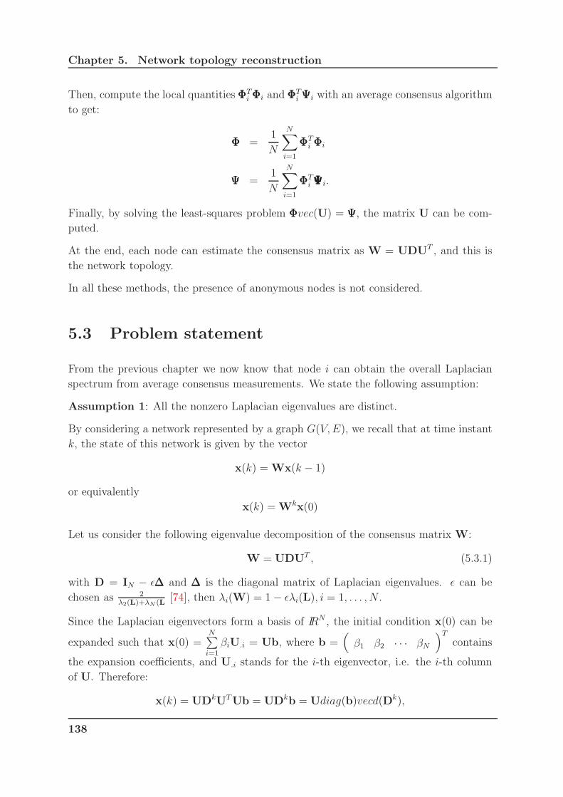
Chapter 5. Network topology reconstruction
Then, compute the local quantities ΦΦΦTi ΦΦΦi and ΦΦΦT
i ΨΨΨi with an average consensus algorithm
to get:
ΦΦΦ =1
N
N∑
i=1
ΦΦΦTi ΦΦΦi
ΨΨΨ =1
N
N∑
i=1
ΦΦΦTi ΨΨΨΨΨΨΨΨΨi.
Finally, by solving the least-squares problem ΦΦΦvec(U) = ΨΨΨ, the matrix U can be com-
puted.
At the end, each node can estimate the consensus matrix as W = UDUT , and this is
the network topology.
In all these methods, the presence of anonymous nodes is not considered.
5.3 Problem statement
From the previous chapter we now know that node i can obtain the overall Laplacian
spectrum from average consensus measurements. We state the following assumption:
Assumption 1: All the nonzero Laplacian eigenvalues are distinct.
By considering a network represented by a graph G(V,E), we recall that at time instant
k, the state of this network is given by the vector
x(k) = Wx(k − 1)
or equivalently
x(k) = Wkx(0)
Let us consider the following eigenvalue decomposition of the consensus matrix W:
W = UDUT , (5.3.1)
with D = IN − ǫ∆∆∆ and ∆∆∆ is the diagonal matrix of Laplacian eigenvalues. ǫ can be
chosen as 2λ2(L)+λN (L
[74], then λi(W) = 1− ǫλi(L), i = 1, . . . , N .
Since the Laplacian eigenvectors form a basis of IRN , the initial condition x(0) can be
expanded such that x(0) =N∑
i=1
βiU.i = Ub, where b =(
β1 β2 · · · βN
)T
contains
the expansion coefficients, and U.i stands for the i-th eigenvector, i.e. the i-th column
of U. Therefore:
x(k) = UDkUTUb = UDkb = Udiag(b)vecd(Dk),
138

Chapter 5. Network topology reconstruction
where vecd(·) is the column vector built with the diagonal entries of the matrix in the
argument.
We can equivalently write the above equation as:
x(k) = Uvecd(Dk), with U = Udiag(b)
Therefore, UUT = Udiag(b.2)UT and UT U = diag(b.2). We can conclude that:
W = UDdiag(b.2)−1UT . (5.3.2)
5.4 Distributed solution to the network topology re-
construction problem
5.4.1 Estimation of the eigenvectors of the Laplacian-based
consensus matrix
At node j, the state at instant k is then given by:
xj(k) =
N∑
i=1
λki (W)βiuj,i,
uj,i being the jth entry of the eigenvector U.i. By stacking N consecutive measurements
node j obtains:
xj(0)
xj(1)...
xj(N − 1)
=
1 1 · · · 1
1 λ2(W) · · · λN(W)...
.... . .
...
1 λN−12 (W) · · · λN−1
N (W)
uj,1
uj,2
...
uj,N
, uj,i = uj,iβi
or equivalently
xj = ΥΥΥUTj. (5.4.1)
From Assumption 1, we can conclude that ΥΥΥ is a full rank matrix. Therefore node j can
efficiently solve the above problem and get:
UTj. = ΥΥΥ−1xj . (5.4.2)
Now, the node only knows the jth row of U.
139

Chapter 5. Network topology reconstruction
Let us consider a message passing scheme where the nodes send to their neighbors the
rows they have. Then after a number of message exchanges, at least equal to the diameter
of the graph, node j has all the rows of U. However, since some of the nodes are assumed
to be anonymous, they do not send the label of the row they have. Two kinds of
messages are transmitted in the network. The rows associated to non-anonymous nodes
are correctly labelled while those associated to anonymous nodes are not labelled. As a
consequence, node j only receives U up to rows permutation, i.e. it receives U = ΠΠΠU,
ΠΠΠ being a permutation matrix.
5.4.2 Network topology reconstruction
We can note that UT U = diag(b2). Therefore, from (5.3.2), we get:
W = ΠΠΠWΠΠΠT , with W = UD(UT U)−1UT . (5.4.3)
We can conclude that from the estimated matrix W, we obtain a graph that is isomorphic
to the original graph. In what follows we state two sufficient conditions to ensure correct
reconstruction of the graph. We first recall the following notions of observability:
A network is said to be [44]:
• node-observable from a given node if that node is able to reconstruct the entire
network state from its own measurements. This issue has been studied for instance
in [58] and [65] where it has been stated that a network with a consensus matrix
having at least one non-simple eigenvalue is not node-observable.
• neighborhood observable from a given node if that node can reconstruct the entire
network state from its own measurements and those of its neighbors. This issue
was studied in [43].
• globally observable if it is neighborhood observable from any node.
Proposition 4
Assume that the graph is node-observable or neighborhood observable from node j.
If all the entries of the initial condition are distinct then the network topology can
be exactly reconstructed from node j.
Proof: From U and diag(b2) the initial condition x(0) can be reconstructed as follows:
x(0) = Udiag(b2)βββ, with βββ =(
1/β21 1/β2
2 · · · 1/β2N
)T
. Since U is known only up
to rows permutation through U, the reconstructed initial condition x(0) = Udiag(b2)βββ
is related to the actual initial condition as follows: x(0) = ΠΠΠx(0). The graph being
node-observable or neighborhood-observable from node j, node j can reconstruct the
140

Chapter 5. Network topology reconstruction
initial condition from its consecutive measurements. It can therefore compare x(0) with
x(0). If all the entries of x(0) are distinct then the permutation matrix can be retrieved
and the matrix W exactly recovered from W.
Proposition 5
Assume that the network contains a set A of anonymous nodes and the graph is node-
observable or neighborhood observable from node j. If all the entries of the initial
condition associated with the anonymous nodes are all distinct then the network
topology can be exactly reconstructed from node j.
The proof of this proposition is similar to the previous one. Here, the permutation
ambiguity is restricted to the entries associated with the anonymous nodes.
We can also note that if the initial condition is driven from a continuous joint probability
distribution, then the reconstruction of the network topology is almost sure.
The proposed network topology reconstruction algorithm is described as followed:
Algorithm 11 (Network topology reconstruction)
1. Inputs:
• Given the Laplacian spectrum sp(L) and the number of nodes N .
• Given a stepsize ǫ of consensus protocol with matrix W = IN − ǫL.
• Given the firstN−1 consensus measurements xi = [xi(0), xi(1), . . . , xi(N−1)]T , i = 1, . . . , N .
2. Initialization:
• Set of eigenvalues λi(W) = 1− ǫλi(L) for i = 1, . . . , N .
• Matrix ΥΥΥ in equation (5.4.1).
3. Each node j estimates the j-th row of U using (5.4.2).
4. Each node sends to its neighbors the rows it has. After a number of message
exchanges, each node j obtains U = ΠΠΠU.
5. Since diag(b2) = UTU is a diagonal matrix, then each node can then estimate
the matrix topology as W = ΠΠΠ(
UDdiag(UTU)−1U
T)
ΠΠΠT
6. Define the estimated Laplacian matrix L = 1ǫ(IN −W). Then take the rounded
estimated Laplacian matrix to see the effectiveness of the proposed method.
141
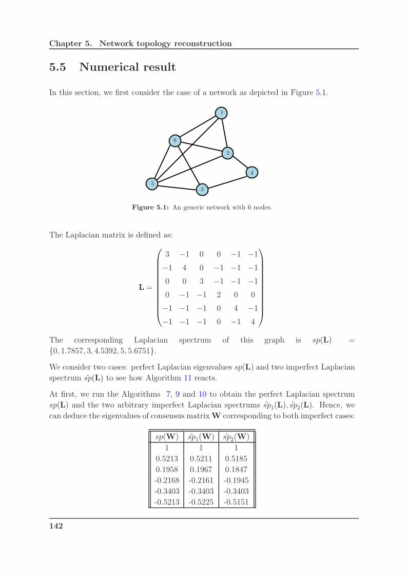
Chapter 5. Network topology reconstruction
5.5 Numerical result
In this section, we first consider the case of a network as depicted in Figure 5.1.
1
3
4
5
6
2
Figure 5.1: An generic network with 6 nodes.
The Laplacian matrix is defined as:
L =
3 −1 0 0 −1 −1
−1 4 0 −1 −1 −1
0 0 3 −1 −1 −1
0 −1 −1 2 0 0
−1 −1 −1 0 4 −1
−1 −1 −1 0 −1 4
The corresponding Laplacian spectrum of this graph is sp(L) =
0, 1.7857, 3, 4.5392, 5, 5.6751.
We consider two cases: perfect Laplacian eigenvalues sp(L) and two imperfect Laplacian
spectrum sp(L) to see how Algorithm 11 reacts.
At first, we run the Algorithms 7, 9 and 10 to obtain the perfect Laplacian spectrum
sp(L) and the two arbitrary imperfect Laplacian spectrums sp1(L), sp2(L). Hence, we
can deduce the eigenvalues of consensus matrixW corresponding to both imperfect cases:
sp(W) sp1(W) sp2(W)
1 1 1
0.5213 0.5211 0.5185
0.1958 0.1967 0.1847
-0.2168 -0.2161 -0.1945
-0.3403 -0.3403 -0.3403
-0.5213 -0.5225 -0.5151
142

Chapter 5. Network topology reconstruction
From now, we can build the matrix ΥΥΥ and ΥΥΥ1, ΥΥΥ2 as follows:
ΥΥΥ =
1 1 1 1 1 1
1 0.5213 0.1958 −0.2168 −0.3403 −0.5213
1 0.2718 0.0383 0.0470 0.1158 0.2718
1 0.1417 0.0075 −0.0102 −0.0394 −0.1417
1 0.0739 0.0015 0.0022 0.0134 0.0739
1 0.0385 0.0003 −0.0005 −0.0046 −0.0385
ΥΥΥ1 =
1 1 1 1 1 1
1 0.5211 0.1967 −0.2161 −0.3403 −0.5225
1 0.2715 0.0387 0.0467 0.1158 0.2730
1 0.1415 0.0076 −0.0101 −0.0394 −0.1427
1 0.0737 0.0015 0.0022 0.0134 0.0745
1 0.0384 0.0003 −0.0005 −0.0046 −0.0390
ΥΥΥ2 =
1 1 1 1 1 1
1 0.5185 0.1847 −0.1945 −0.3403 −0.5151
1 0.2688 0.0341 0.0378 0.1158 0.2653
1 0.1394 0.0063 −0.0074 −0.0394 −0.1367
1 0.0723 0.0012 0.0014 0.0134 0.0704
1 0.0375 0.0002 −0.0003 −0.0046 −0.0363
Next, we take the first N − 1 consecutive measurements xi that can be expressed in
matrix form:
X =
0.9933 0.5656 0.6131 0.5651 0.5574 0.5477
0.3567 0.5455 0.5618 0.5332 0.5492 0.5378
0.7529 0.4524 0.5382 0.5148 0.5371 0.5332
0.1100 0.3485 0.4291 0.4939 0.5101 0.5278
0.5970 0.6360 0.5588 0.5635 0.5445 0.5466
0.4306 0.6927 0.5395 0.5700 0.5423 0.5474
By (5.4.1), each node i gets the row Ui. of the matrix U and sends it to its neighbors.
After a number of message exchanges, we can obtain U and U1, U2 as:
143

Chapter 5. Network topology reconstruction
U =
0.5401 0.2146 −0.0746 0.3006 −0.0000 0.0127
0.5401 0.0351 −0.0746 −0.2407 −0.0000 0.0969
0.5401 −0.1128 0.1492 0.1109 −0.0000 0.0654
0.5401 −0.3624 −0.0746 0.0511 −0.0000 −0.0441
0.5401 0.1128 0.0373 −0.1109 0.0832 −0.0654
0.5401 0.1128 0.0373 −0.1109 −0.0832 −0.0654
U1 =
0.5401 0.2149 −0.0750 0.2989 0.0021 0.0124
0.5401 0.0351 −0.0742 −0.2417 0.0019 0.0956
0.5401 −0.1131 0.1493 0.1100 0.0020 0.0645
0.5401 −0.3627 −0.0740 0.0504 0.0000 −0.0437
0.5401 0.1129 0.0370 −0.1088 0.0802 −0.0643
0.5401 0.1129 0.0370 −0.1088 −0.0862 −0.0643
U2 =
0.5402 0.2176 −0.0868 0.2757 0.0363 0.0105
0.5402 0.0340 −0.0736 −0.1966 −0.0564 0.1090
0.5399 −0.1115 0.1513 0.0889 0.0177 0.0666
0.5399 −0.3679 −0.0680 0.0368 0.0185 −0.0493
0.5402 0.1140 0.0386 −0.1024 0.0751 −0.0684
0.5402 0.1140 0.0386 −0.1024 −0.0913 −0.0684
Finally, each node can estimate the matrix topology W and W1,W2 as:
W =
0.1958 0.2681 0.0000 −0.0000 0.2681 0.2681
0.2681 −0.0723 −0.0000 0.2681 0.2681 0.2681
−0.0000 0.0000 0.1958 0.2681 0.2681 0.2681
−0.0000 0.2681 0.2681 0.4639 0.0000 −0.0000
0.2681 0.2681 0.2681 −0.0000 −0.0723 0.2681
0.2681 0.2681 0.2681 −0.0000 0.2681 −0.0723
W1 =
0.1958 0.2681 0.0000 −0.0000 0.2681 0.2681
0.2667 −0.0724 0.0000 0.2679 0.2721 0.2656
−0.0012 −0.0001 0.1958 0.2679 0.2719 0.2657
0.0026 0.2683 0.2680 0.4641 −0.0080 0.0050
0.2680 0.2681 0.2681 −0.0000 −0.0722 0.2680
0.2680 0.2681 0.2681 −0.0000 0.2681 −0.0723
144
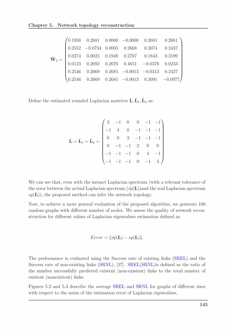
Chapter 5. Network topology reconstruction
W2 =
0.1958 0.2681 0.0000 −0.0000 0.2681 0.2681
0.2552 −0.0734 0.0005 0.2668 0.3074 0.2437
0.0274 0.0025 0.1948 0.2707 0.1843 0.3199
0.0123 0.2692 0.2676 0.4651 −0.0376 0.0233
0.2546 0.2669 0.2685 −0.0013 −0.0313 0.2427
0.2546 0.2669 0.2685 −0.0013 0.3091 −0.0977
Define the estimated rounded Laplacian matrices L, L1, L2 as:
L = L1 = L2 =
3 −1 0 0 −1 −1
−1 4 0 −1 −1 −1
0 0 3 −1 −1 −1
0 −1 −1 2 0 0
−1 −1 −1 0 4 −1
−1 −1 −1 0 −1 4
We can see that, even with the inexact Laplacian spectrum (with a relevant tolerance of
the error between the actual Laplacian spectrum (sp(L))and the real Laplacian spectrum
sp(L)), the proposed method can infer the network topology.
Now, to achieve a more general evaluation of the proposed algorithm, we generate 100
random graphs with different number of nodes. We assess the quality of network recon-
struction for different values of Laplacian eigenvalues estimation defined as
Error = ‖sp(L)− sp(L)‖.
The performance is evaluated using the Success rate of existing links (SREL) and the
Success rate of non-existing links (SRNL), [37]. SREL(SRNL)is defined as the ratio of
the number successfully predicted existent (non-existent) links to the total number of
existent (nonexistent) links.
Figures 5.2 and 5.3 describe the average SREL and SRNL for graphs of different sizes
with respect to the norm of the estimation error of Laplacian eigenvalues.
145
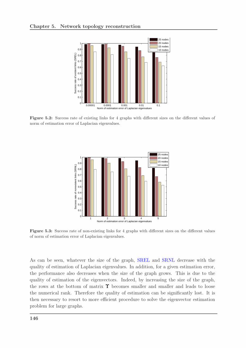
Chapter 5. Network topology reconstruction
0.00001 0.0001 0.001 0.01 0.10
0.1
0.2
0.3
0.4
0.5
0.6
0.7
0.8
0.9
1
Suc
cess
rat
e of
exi
sten
t lin
ks (
SR
EL)
Norm of estimation error of Laplacian eigenvalues
25 nodes20 nodes15 nodes10 nodes
Figure 5.2: Success rate of existing links for 4 graphs with different sizes on the different values of
norm of estimation error of Laplacian eigenvalues.
1 2 3 4 50
0.1
0.2
0.3
0.4
0.5
0.6
0.7
0.8
0.9
1
Suc
cess
rat
e of
non
exis
tent
link
s (S
RN
L)
Norm of estimation error of Laplacian eigenvalues
25 nodes20 nodes15 nodes10 nodes
Figure 5.3: Success rate of non-existing links for 4 graphs with different sizes on the different values
of norm of estimation error of Laplacian eigenvalues.
As can be seen, whatever the size of the graph, SREL and SRNL decrease with the
quality of estimation of Laplacian eigenvalues. In addition, for a given estimation error,
the performance also decreases when the size of the graph grows. This is due to the
quality of estimation of the eigenvectors. Indeed, by increasing the size of the graph,
the rows at the bottom of matrix ΥΥΥ becomes smaller and smaller and leads to loose
the numerical rank. Therefore the quality of estimation can be significantly lost. It is
then necessary to resort to more efficient procedure to solve the eigenvector estimation
problem for large graphs.
146

Chapter 5. Network topology reconstruction
5.6 Conclusion
In this chapter, we have proposed a way for reconstructing the network topology in the
presence of anonymous nodes from average consensus measurements. The consensus
matrix is determined from its eigenstructure estimated in distributed way. Since the
Laplacian spectrum can be obtained by means of the algorithms proposed in the pre-
vious chapter, each node can deduce the matrix U up to rows permutation because of
anonymous nodes. Therefore, the obtained graph is isomorphic to the original graph.
In the case that the graph is node-observable or neighborhood observable from node j,
if all the entries of x(0) are distinct then node j can exactly reconstruct the network
topology.
Algorithm 11 works with the assumption that all eigenvalues are distinct. Therefore,
future works encompass the design of network reconstruction protocols that deal with
spectrum in which the multiplicities of the corresponding eigenvalues can be higher than
1. In addition, numerical issues for large graphs are to be considered for making the
proposed method scalable.
147

Chapter 6
General conclusions and future
works
Contents
6.1 Review of contributions and conclusions . . . . . . . . . . . 149
6.2 Ongoing and future works . . . . . . . . . . . . . . . . . . . . 151
To conclude this dissertation, we give a brief summary and discussion on future works.
6.1 Review of contributions and conclusions
Finite-time consensus problems have received a vast attention from the research
community due to their benefits in many application domains, especially in distributed
computation. Briefly speaking, the finite-time average consensus algorithms (for which
consensus can be obtained in a finite number of steps) are commonly used as building
blocks for more sophisticated distributed control, estimation or inference algorithms.
Due to the fact that they can guarantee a minimal execution time, they are much more
appealing than those ensuring asymptotic convergence.
This thesis impacts with the design of finite-time average consensus protocols regardless
of the Laplacian matrix of a given graph in a distributed way and its application to
network robustness assessment.
First, we proposed a new distributed algorithm for self-configuration of finite-time aver-
age consensus where matrices are not necessarily based on the Laplacian matrix of a given
graph. More precisely, we solved a matrix factorization problem in a distributed way by
using a learning sequence. The method is based on the back-propagation method and an
associated gradient descent method. Conceptually, each linear iteration k, k = 0, . . . , D
149
Chapter 6. General conclusions and future works
is illustrated as a layer of a network. The main idea is to compute the partial derivatives
of the error between the actual output and desired output, and then propagate them
back to each iteration k in order to update the weights.
Obviously, this method is impractical for large-scale networks. However, one interesting
point can be noted in this work is that the obtained consensus matrices are not doubly
stochastic matrices and allow to reach consensus in a minimum number of steps.
Second, the study on the robustness of networks has increasingly attracted the attention
of the research community. Therefore, in this thesis, the assessment of the network ro-
bustness via the effective graph resistance (R) and the number of spanning trees (ξ) in a
distributed way, obviously becomes a promising application domain. Since both robust-
ness metrics are functions of the Laplacian spectrum sp(L), thus the main task is now
to estimate the Laplacian spectrum. More precisely, three cases have been considered:
perfectly known x, approximated, and unknown x.
The average consensus matrix can be factored in D Laplacian based consensus matrices,
where D stands for the number of nonzero distinct Laplacian eigenvalues. For the first
case (perfectly known x), all methods are characterized into two approaches, which are
direct approach and indirect approach. The direct method gives rise to a non-convex
optimization problem with respect to the stepsizes αk, k = 1, . . . , N − 1 that are the
inverse of the nonzero distinct Laplacian eigenvalues. Since, this is a gradient based
method, it suffers the slow convergence. To improve that, a convex optimization problem
is introduced to estimate the coefficients ck, k = 0, . . . , N − 1, of a given polynomial
whose roots are the stepsizes αk, k = 1, . . . , N − 1, that allows to factorize the averaging
matrix JN = 11T
N. In this way, two famous methods (the subgradient projected method
and ADMM) are applied to solve this convex optimization problem. By means of these
proposed methods, the distinct Laplacian eigenvalues can be deduced. Then, by means of
an integer programming, the whole spectrum sp(L) is obtained to compute the robustness
indices.
The drawback of these methods is scalability. For large-scale graphs, the whole spectrum
sp(L) estimation is significantly difficult to obtain. Therefore, the estimation can be
restricted to that of the most significant eigenvalues to estimate some bounds of the
network robustness indices.
Projected subgradient method is very applicable due to its simplicity. However, the
drawback is that it can be slow. Therefore, the choice of the stepsize γ(t) is typical
critical. In contrast, under mild conditions, the ADMM is guaranteed to converge for all
tunning parameters. It has a single penalty parameter ρ that influences on the speed of
convergence. Therefore, in the left cases, ADMM is to be the best choice.
In the case of imperfect consensus value x, we assumed that a standard consensus protocol
has been run and stored some intermediate values of xM according to the iteration M .
150
Chapter 6. General conclusions and future works
Then, we made use of the ADMM-based Algorithm 7 to evaluate the network robustness.
Finally, it claims that when the intermediate value of x is as close as possible to the real
one, the network robustness index can be estimated with a very good accuracy.
In the case of unknown consensus value x, we considered a convex optimization problem
which resorts to a convex combination of two convex functions. The first one takes into
account the average consensus problem while the second one concerns the estimation of
the Laplacian eigenvalues.
For large graphs, numerical problems can appear. Therefore, the current formulations of
the proposed Algorithms 5, 6, 7, 8 are efficient and well adapted for networks of medium
size.
Finally, network topology identification refers to detecting and identifying the interested
network elements and the relationship between elements in target network and represents
the topology construction in an appropriate form. Therefore, identification of networks
of systems becomes a growing attractive task for solving many problems in different
science and engineering domains.
Theoretically, the consensus matrix W admits the eigenvalues decomposition W =
UDUT , where D = IN −ǫ∆∆∆, with ∆∆∆ be diagonal matrix of λi(L), stands for the diagonal
matrix of the eigenvalues and U the matrix of eigenvectors. Since Laplacian spectrum
sp(L) can be achieved by means of proposed methods in Chapter 4, we proposed a
method to reconstruct the network topology via the estimation of eigenvectors of the
matrix W.
6.2 Ongoing and future works
In what follows, we state some issues that are still open and worth of investigations:
1. Design of finite-time average consensus protocols:
(a) The dependence of the convergence speed on the learning sequence is to be
studied. Thus, the design of optimal learning sequences can be dig in.
(b) Researching on the robustness of the finite-time average consensus.
2. Network robustness assessment:
(a) Novel methods that can be applied to large-scale networks.
(b) For indirect method, in practice, it may encounter with the ill-conditioned
problem when establishing submatrices Qi, which leads to loose the numerical
rank of these submatrices. Therefore, one can investigate in the precondition-
ing of these matrices to keep the accuracy of the proposed methods.
151

Chapter 6. General conclusions and future works
(c) Investigating in the convergence rate analysis based on the study in [25].
3. Reconstruction of the network topology:
(a) Design a new method that deals with a Laplacian spectrum sp(L), whose
eigenvalues are not all distinct.
(b) Assess the robustness of these methods when the data exchange are prone to
imperfect communications.
152

Appendix
153


A. Khatri-Rao Product
Given two matrices A ∈ IRI×F , B ∈ IRJ×F with the same number of columns, the
Khatri-Rao product A⊙B ∈ IRIJ×F is defined as:
A⊙B := [a1 ⊗ b1 · · ·aF ⊗ bF ] = B
diag1(A)...
diagI(A)
where af is the f th column of A, similarly for bf , and ⊗ denotes the Kronecker product
of two column vectors, whereas diagi(A) stands for the diagonal matrix built with the ith
row of A. The Khatri-Rao product can be viewed as a column-wise Kronecker product.
Its main property, which will be used herein, is related to the vectorization operation of
a given matrix:
vec(Adiag(d)BT ) = (B⊙A)d.
where the vec(.) operator stacks the columns of its matrix argument and d ∈ RF×1.
Therefore we can deduce the following identity:
Adiag(d)b = (bT ⊙A)d. (A.0.1)
155


B. Resume en francais
Contents
B.1 Introduction . . . . . . . . . . . . . . . . . . . . . . . . . . . . 158
B.1.1 Contexte de la these . . . . . . . . . . . . . . . . . . . . . . . . 158
B.1.2 Structure du document . . . . . . . . . . . . . . . . . . . . . . 161
B.2 Conception distribuee des Protocoles de Consensus de
Moyenne en temps fini . . . . . . . . . . . . . . . . . . . . . . 164
B.2.1 Introduction . . . . . . . . . . . . . . . . . . . . . . . . . . . . 164
B.2.2 La solution distribuee du probleme de la factorisation de la
matrice . . . . . . . . . . . . . . . . . . . . . . . . . . . . . . . 165
B.3 L’evaluation distribuee de la robustesse du reseau . . . . . . 170
B.3.1 Introduction . . . . . . . . . . . . . . . . . . . . . . . . . . . . 170
B.3.2 Les solutions distribuees de la robustesse du reseau . . . . . . . 171
B.4 Reconstruction de la topologie du reseaux . . . . . . . . . . 189
B.4.1 Introduction . . . . . . . . . . . . . . . . . . . . . . . . . . . . 189
B.5 La solution distribuee de reconstruction de la topologie du
reseau . . . . . . . . . . . . . . . . . . . . . . . . . . . . . . . . 190
B.5.1 Estimation des vecteurs propres de la matrice de consensus
basee matrice de Laplace . . . . . . . . . . . . . . . . . . . . . 191
B.5.2 Network topology reconstruction . . . . . . . . . . . . . . . . . 191
B.6 Conclusions generales . . . . . . . . . . . . . . . . . . . . . . . 192
B.6.1 Resume des contributions et conclusions . . . . . . . . . . . . . 192
B.6.2 Travaux en cours et a venir . . . . . . . . . . . . . . . . . . . . 195
157
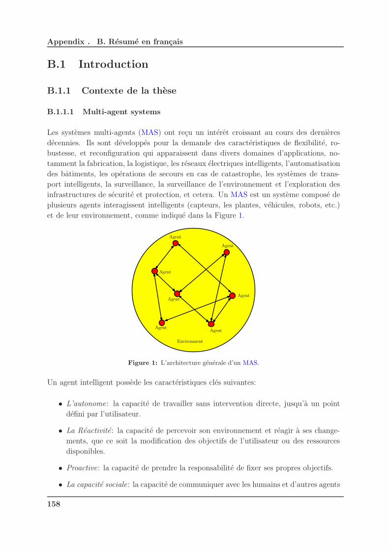
Appendix . B. Resume en francais
B.1 Introduction
B.1.1 Contexte de la these
B.1.1.1 Multi-agent systems
Les systemes multi-agents (MAS) ont recu un interet croissant au cours des dernieres
decennies. Ils sont developpes pour la demande des caracteristiques de flexibilite, ro-
bustesse, et reconfiguration qui apparaissent dans divers domaines d’applications, no-
tamment la fabrication, la logistique, les reseaux electriques intelligents, l’automatisation
des batiments, les operations de secours en cas de catastrophe, les systemes de trans-
port intelligents, la surveillance, la surveillance de l’environnement et l’exploration des
infrastructures de securite et protection, et cetera. Un MAS est un systeme compose de
plusieurs agents interagissent intelligents (capteurs, les plantes, vehicules, robots, etc.)
et de leur environnement, comme indique dans la Figure 1.
Environment
Agent
Agent
Agent
AgentAgent
Agent
Agent
Figure 1: L’architecture generale d’un MAS.
Un agent intelligent possede les caracteristiques cles suivantes:
• L’autonome: la capacite de travailler sans intervention directe, jusqu’a un point
defini par l’utilisateur.
• La Reactivite: la capacite de percevoir son environnement et reagir a ses change-
ments, que ce soit la modification des objectifs de l’utilisateur ou des ressources
disponibles.
• Proactive: la capacite de prendre la responsabilite de fixer ses propres objectifs.
• La capacite sociale: la capacite de communiquer avec les humains et d’autres agents
158
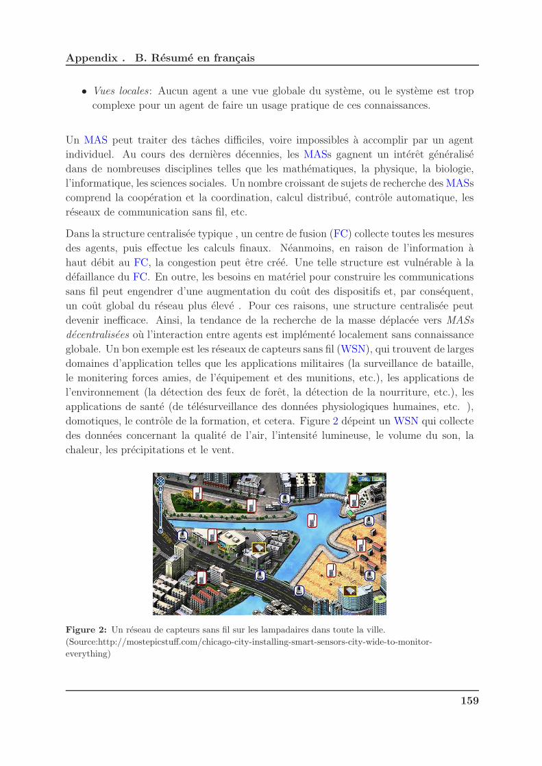
Appendix . B. Resume en francais
• Vues locales : Aucun agent a une vue globale du systeme, ou le systeme est trop
complexe pour un agent de faire un usage pratique de ces connaissances.
Un MAS peut traiter des taches difficiles, voire impossibles a accomplir par un agent
individuel. Au cours des dernieres decennies, les MASs gagnent un interet generalise
dans de nombreuses disciplines telles que les mathematiques, la physique, la biologie,
l’informatique, les sciences sociales. Un nombre croissant de sujets de recherche des MASs
comprend la cooperation et la coordination, calcul distribue, controle automatique, les
reseaux de communication sans fil, etc.
Dans la structure centralisee typique , un centre de fusion (FC) collecte toutes les mesures
des agents, puis effectue les calculs finaux. Neanmoins, en raison de l’information a
haut debit au FC, la congestion peut etre cree. Une telle structure est vulnerable a la
defaillance du FC. En outre, les besoins en materiel pour construire les communications
sans fil peut engendrer d’une augmentation du cout des dispositifs et, par consequent,
un cout global du reseau plus eleve . Pour ces raisons, une structure centralisee peut
devenir inefficace. Ainsi, la tendance de la recherche de la masse deplacee vers MASs
decentralisees ou l’interaction entre agents est implemente localement sans connaissance
globale. Un bon exemple est les reseaux de capteurs sans fil (WSN), qui trouvent de larges
domaines d’application telles que les applications militaires (la surveillance de bataille,
le monitering forces amies, de l’equipement et des munitions, etc.), les applications de
l’environnement (la detection des feux de foret, la detection de la nourriture, etc.), les
applications de sante (de telesurveillance des donnees physiologiques humaines, etc. ),
domotiques, le controle de la formation, et cetera. Figure 2 depeint un WSN qui collecte
des donnees concernant la qualite de l’air, l’intensite lumineuse, le volume du son, la
chaleur, les precipitations et le vent.
Figure 2: Un reseau de capteurs sans fil sur les lampadaires dans toute la ville.
(Source:http://mostepicstuff.com/chicago-city-installing-smart-sensors-city-wide-to-monitor-
everything)
159

Appendix . B. Resume en francais
B.1.1.2 Motivation
Il y a deux points qui attirent une grande attention de la communaute de recherche:
(A) Sur la base de l’information locale et les interactions entre les agents,
comment peuvent tous les agents parvenir a un accord?
Ce probleme est appele probleme du consensus, ce qui est pour concevoir un pro-
tocole de reseau base sur les informations locales obtenus par chaque agent de telle
sorte que tous les agents atteignent finalement un accord sur certaines quantites
d’interet
Problemes de consensus ont recu une attention considerable de diverses communi-
tities de recherche en raison de ses larges applications dans de nombreux domaines,
y compris multi-capteurs fusion de donnees [64], le flocage comportement des es-
saims [6, 38, 59, 60], multi-vehicule de controle de la formation [17, 54, 62], distribue
calcul [5, 10, 48], rendez-vous des problemes [15], etc.. Plus particulierement, les
algorithmes de consensus de moyenne (c’est a dire l’accord correspond a la moyenne
des valeurs initiales) sont couramment utilises comme la composante pour plusieurs
algorithmes de controle, estimation ou inference distribues.
Dans la litterature recente, on peut trouver des algorithmes de consensus moyens
embarques dans le filtre de Kalman distribue, [61]; Distribue algorithme des moin-
dres carres, [9]; Distribue alternatif methode des moindres carres pour la factori-
sation des tenseurs, [45]; Principal Distributed Component Analysis, [49]; ou dis-
tribue entree commune et estimation d’etat, [24] pour citer quelques-uns. Nean-
moins, la convergence asymptotique des algorithmes de consensus ne sont pas adap-
tes a ces types d’algorithmes distribues sophistiques. La convergence faible asymp-
totique ne peut pas assurer l’efficacite et l’exactitude des algorithmes, ce qui peut
conduire a d’autres effets inattendus. Par exemple, en ce qui concerne les reseaux
de capteurs sans fil (WSNs), une reduction du nombre total d’iterations jusqu’a ce
que la convergence peut conduire a une reduction de la quantite totale de consom-
mation d’energie du reseau, ce qui est indispensable pour garantir une duree de vie
plus longue pour l’ensemble du reseau. D’autre part, les protocoles qui garantissent
un temps d’execution minimum sont plus attrayants que ceux assurant la conver-
gence asymptotique. Dans ce but, plusieurs contributions dediees a consensus en
temps fini ont recemment ete publies dans la litterature. Ce qui signifie que le
consensus est obtenu dans un nombre fini d’etapes.
(B) Pouvons-nous evaluer la robustesse de ce reseau?
En general, nous sommes entoures par des reseaux de differents types (reseaux
sociaux, reseaux de capteurs, reseaux d’energie, et cetera). Consequent, la chose la
plus importante est que ces reseaux sont robustes. Ce qui signifie que, ils peuvent
160
Appendix . B. Resume en francais
subir des dommages ou des defaillances travers. Par consequent, la terminologie
robustesse envahit rapidement le communaute de la recherche.
Definition 2
La robustesse est la capacite d’un reseau de continuer a bien fonctionner quand il est
sujette a des defaillances ou des attaques, [21].
Pour evaluer si le reseau est robuste, la mesure de la robustesse du reseau est neces-
saire [21]. Il existe differentes approches proposees pour mesurer les parametres de
robustesse du reseau. Cependant, l’approche la plus populaire dans la litterature
est basee sur l’analyse du graphe. Avec les donnees produites durant proto-
cole de consensus pouvons-nous deduire des mesures de robustesse du
reseau?
(C) Pouvons-nous reconstruit la topologie du reseau? L’identification de la
topologie du reseau se refere a detecter et identifier les elements du reseau interesses
et la relation entre les elements du reseau destinataire et represente la construc-
tion de la topologie sous une forme appropriee. Consequent, l’identification des
reseaux de systemes devient une tache de plus en plus attrayante pour resoudre de
nombreux problemes dans differents domaines scientifiques et techniques.
B.1.1.3 Objectifs de la these
Il est bien connu que les protocoles de consensus etant iterative, de nombreuses donnees
sont produites. Cependant, la plupart des etudes se concentrent uniquement sur les
proprietes de la convergence de ces algorithmes. Avec les donnees collectees aupres
chaque iteration du protocole de consensus asymptotique de maniere distribuee, nous
visons a:
• Concevoir des protocoles de consensus de moyenne en temps fini pour les accords
subsequents.
• Evaluer la robustesse du reseau.
• Reconstruit la topologie du reseau.
B.1.2 Structure du document
Afin d’avoir une vue globale, les contributions de cette these peuvent etre consideres
triple comme indique dans le schema suivant.
161
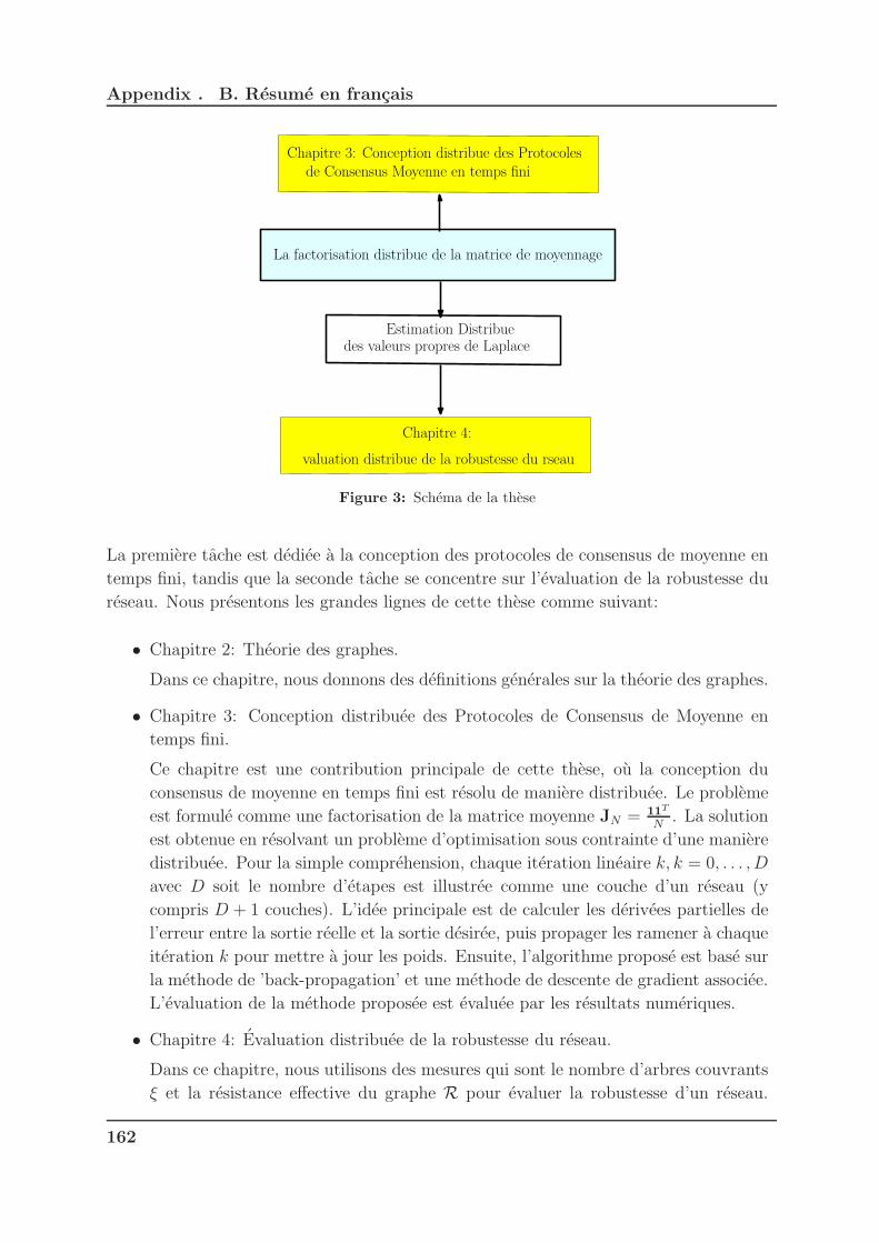
Appendix . B. Resume en francais
Estimation Distribuedes valeurs propres de Laplace
La factorisation distribue de la matrice de moyennage
Chapitre 3: Conception distribue des Protocoles
de Consensus Moyenne en temps fini
Chapitre 4:
valuation distribue de la robustesse du rseau
Figure 3: Schema de la these
La premiere tache est dediee a la conception des protocoles de consensus de moyenne en
temps fini, tandis que la seconde tache se concentre sur l’evaluation de la robustesse du
reseau. Nous presentons les grandes lignes de cette these comme suivant:
• Chapitre 2: Theorie des graphes.
Dans ce chapitre, nous donnons des definitions generales sur la theorie des graphes.
• Chapitre 3: Conception distribuee des Protocoles de Consensus de Moyenne en
temps fini.
Ce chapitre est une contribution principale de cette these, ou la conception du
consensus de moyenne en temps fini est resolu de maniere distribuee. Le probleme
est formule comme une factorisation de la matrice moyenne JN = 11T
N. La solution
est obtenue en resolvant un probleme d’optimisation sous contrainte d’une maniere
distribuee. Pour la simple comprehension, chaque iteration lineaire k, k = 0, . . . , D
avec D soit le nombre d’etapes est illustree comme une couche d’un reseau (y
compris D + 1 couches). L’idee principale est de calculer les derivees partielles de
l’erreur entre la sortie reelle et la sortie desiree, puis propager les ramener a chaque
iteration k pour mettre a jour les poids. Ensuite, l’algorithme propose est base sur
la methode de ’back-propagation’ et une methode de descente de gradient associee.
L’evaluation de la methode proposee est evaluee par les resultats numeriques.
• Chapitre 4: Evaluation distribuee de la robustesse du reseau.
Dans ce chapitre, nous utilisons des mesures qui sont le nombre d’arbres couvrants
ξ et la resistance effective du graphe R pour evaluer la robustesse d’un reseau.
162
Appendix . B. Resume en francais
Par la nature de ces mesures, elles sont toutes les fonctions des valeurs propres du
laplacien λi(L), par consequent, l’estimation des valeurs propres du laplacien est
le but principal de cette tache. Dans ce chapitre, au lieu d’estimer directement
des valeurs propres du laplacien, nous resolvons le probleme comme un probleme
d’optimisation sous contrainte en ce qui concerne a l’inverse des valeurs propres du
laplacien distinctes differents de zero. Par consequent, en appliquant la methode
de descente de gradient, nous obtenons finalement l’ensemble des valeurs propres
du laplacien distinctes differents de zero. En outre, en utilisant un algorithme de
programmation en nombres entiers, on peut estimer les multiplicites correspondant
a ces valeurs propres. Ensuite, on en deduit l’ensemble du spectre de la matrice
de Laplace associee au graphe G(V,E). A partir de ce moment, les mesures de
robustesse peuvent etre estimes a evaluer la robustesse du reseau.
Pour la tache d’estimation du spectre de Laplace, toutes les methodes proposees
dans ce chapitre sont divisees en deux categories qui sont des formulations non-
convexes et convexes. Selon probleme d’optimisation non convexe (appelle aussi
methode directe), le probleme est vue comme un probleme d’optimisation sous
contrainte en ce qui concerne la stepsizes αk de protocole base sur la Laplace
matrice de consensus, dont les inverses sont egales aux valeurs propres du laplacien
distinctes differents de zero.
Resoudre le probleme d’optimisation non convexe, le principal probleme est la
lenteur de la vitesse de convergence. Nous essayons donc d’accelerer la vitesse de
l’estimation des valeurs propres du laplacien le plus vite possible. Le point principal
est de tranformer le probleme non convexe dans l’une convexe. Nous resolvons le
probleme en deux algorithmes utilisant la methode de projection distribue, [57]
et la Direction alternatif de la Methode de multiplicateurs (ADMM), [11]. Nous
considerons trois cas: la valeur moyenne finale parfaitement connue, bruyant et
totalement inconnu.
• Chapitre 5: Reconstruction de la topologie du reseau. En theorie, la matrice
de consensus W admet la decomposition des valeurs propres W = UΛΛΛUT , ou
ΛΛΛ = IN−ǫ∆∆∆, avec ∆∆∆ est matrice diagonale de λi(L), represente la matrice diagonale
des valeurs propres et U la matrice de vecteurs propres. Nous pouvons trouver un
moyen d’obtenir U. Puisque la spectre de Laplace sp(L) peut etre realisee en
utilisant le methodes proposees dans le Chapitre 4, nous pouvons reconstruire la
topologie du reseau.
• Chapitre 6: Conclusions generales et travaux futurs.
Ce dernier chapitre resume les contributions de cette these et suggerent egalement
les orientations futures.
163
Appendix . B. Resume en francais
B.2 Conception distribuee des Protocoles de Con-
sensus de Moyenne en temps fini
B.2.1 Introduction
Considerons un graphe connexe non oriente G(V,E) avec xi(k) etant l’etat de nœud
i au etape temporelle k et definir l’etat initial du reseau donne comme x(0) =
[x1(0), x2(0), . . . , xN(0)]T ou N = |V |, une nouvelle methode est propose de concevoir les
protocoles de consensus de moyenne en temps fini pour MASs ou les reseaux de capteurs
sans fil (WSNs) de maniere distribuee. Dans le contexte en temps discret, un schema
d’iteration lineaire exprime ses avantages pour un algorithme distribue depuis dans lequel,
chaque nœud met a jour a plusieurs reprises sa valeur comme une combinaison lineaire
ponderee de sa propre valeur et celles de ses voisins.
xi(k + 1) = wii(k)xi(k) +∑
j∈Ni
wij(k)xj(k), (B.2.1)
ou
wij =
0, if (i, j) /∈ E
wij, if (i, j) ∈ E
ou de facon equivalente sous forme de matrice:
x(k + 1) = W(k)x(k). (B.2.2)
W(k) ∈ SG ou SG est l’ensemble des matrices qui peuvent etre factorisees comme
W(k) = Q(k) (IN + A) ou Q(k) supports pour une matrice carree d’arbitraire, INetant le N × N matrice d’identite, tandis que designe le produit de la matrice de
Hadamard correspondant a un produit de la matrice element par element.
Comme presentes au Chapitre 1.2, le consensus de moyenne est atteint asymptotiquement
si
limk→∞
x(k) =1
N11Tx(0), (B.2.3)
qui signifie que
limk→∞
Wk =1
N11T = JN . (B.2.4)
Cependant, il faut noter que pour executer l’algorithme de consensus de moyenne, deux
etapes principales sont necessaires: l’etape de configuration (egalement appele etape
de la conception) et l’etape de l’execution. Au cours de l’etape de configuration, une
tache peut etre realisee par un algorithme d’auto-configuration au lieu de recourir a un
gestionnaire de reseau. L’auto-configuration peut inclure des graphes decouvertes et la
164
Appendix . B. Resume en francais
prise distribue sur certains parametres. Par exemple, si le protocole a les poids de degre
maximum ( 1.2.6), chaque agent calcule d’abord le nombre de ses voisins avant d’executer
un algorithme de Max-consensus pour le calcul du degre maximum de le graphe. Dans
le cas du protocole base sur Metropolis-Hasting ( 1.2.7), chaque agent compare son
degre avec celle de ses voisins afin de calculer les poids du protocole de consensus de
moyenne. Un protocole couramment est le poids des bords constantes, ou un protocole
de consensus moyen base sur le graphe de Laplace ( 1.2.8), ou un stepsize commun est
utilise par tous les agents. Convergence asymptotique est donc garantie si le stepsize est
strictement positif et inferieur a 2λN
, ou λN represente la plus grande valeur propre de
Laplace. Meme a travers, il y a quelques bornes simples qui donnent des choix pour le
stepsize sans necessiter une connaissance exacte du spectre de Laplace, les agents doivent
s’accorder dans un stepsize adequate.
Au meilleur de notre connaissance, il n’y a pas de travail publie traitant avec protocoles
d’auto-configuration pour le protocole de consensus de moyenne sur la base des poids
des bords constantes. Dans les systemes complexes reels, le temps d’execution devient
de plus en plus impactant. Consequent, le but est maintenant de concevoir un algo-
rithme de consensus de moyenne en temps fini permettant a tous les nœuds d’atteindre
la valeur moyenne du consensus en un nombre fini d’etapes D pour les protocoles d’auto-
configuration, c’est-a-dire,
x(D) =1
N11Tx(0) = JNx(0). (B.2.5)
B.2.2 La solution distribuee du probleme de la factorisation de
la matrice
Pour un graphe connexe G(V,E), soit x(0) = [x1(0), x2(0), . . . , xN(0)]T le vecteur d’etat
du reseau N−agent associe a un graphe G.
Comme presente dans le chapitre 1.2, schema d’iteration lineaire est un outil utile qui
permet au systeme d’atteindre le consensus de moyenne en temps fini dans D etapes. Par
consequent, conformement a chaque iteration, les vecteurs d’etat mises a jour x(k), k =
1, . . . , D − 1 sont assignes a etre des couches consecutives respectivement. Enfin, la
derniere iteration est dediee a des valeurs output x(D).
Les matrices de poids W(k), k = 1, . . . , D qui ont les entrees wkij sont correspondant aux
liens entre les nœuds de deux couches consecutives a etape temporelle k.
Remark 13
Les matrices de poids W(k) ∈ SG est associees a un graphe G. Par consequent, les
165

Appendix . B. Resume en francais
entrees wij(k) sont concus suivant la regle definie comme:
Wij(k) =
wkij, if j ∈ Ni
0, otherwise
Afin de simplifier, a partir de maintenant, nous noterons W(k) comme Wk.
Le schema des iterations lineaires dans l’espace et le temps peut etre considere comme
un reseau neuronal multicouche. La selection des poids peut etre analysee a travers
le portee de la formation. En utilisant l’ensemble des P sequences d’apprentissage, le
mecanisme est divise en deux etapes principales, a savoir, etape en avant et etape en
arriere. L’idee principale est de calculer les derivees partielles de l’erreur entre le output
reell et le output desire, puis propager les ramener a chaque couche du reseau afin de
mettre a jour les poids. L’objectif est de reduire le critere d’erreur E efficacement.
Soit xi,p(0), yi,p, i = 1, · · · , N , p = 1, · · · , P , le input-output paires definissant les
sequences d’apprentissage, avec yi,p = yp =1N
N∑
i=1
xi,p(0). Notre objectif est d’estimer les
matrices de facteurs Wk, k = 1, · · · , D, en minimisant l’erreur quadratique
E(W1, · · · ,WD) =1
2
N∑
i=1
P∑
p=1
(xi,p(D)− yp)2, (B.2.6)
avec xi,p(k) =∑
j∈Ni∪iwk
ijxj,p(k − 1), wkij etant les entrees de matrices Wk ∈ SG. Nous
pouvons reecrire la fonction de cout (B.2.6) comme
E(W1, · · · ,WD) =1
2
∥∥∥∥∥
1∏
k=D
WkX(0)−Y
∥∥∥∥∥
2
F
, s.t Wk ∈ SG, (B.2.7)
ou ‖.‖F supports pour la norme de Frobenius, Y = JNX(0), Y et X(0) etant N × P
matrices avec yi,p and xi,p comme entrees, respectivement.
Nous supposons que X(0)X(0)T = IN ce qui signifie que le vecteur d’entree est or-
thogonal. Par exemple, les vecteurs de la base canonique de IRN peuvent etre util-
ises comme ’inputs’. Par consequent, nous pouvons noter que E(W1, · · · ,WD) =
12
∥∥∥∥
1∏
k=D
Wk − JN
∥∥∥∥
2
F
, ce qui signifie que la minimisation (B.2.7) est equivalent a resoudre
le probleme de la factorisation (3.2.5):
W∗k|k=1,...,D = arg min
Wkt=1,...,D
1
2
P∑
p=1
tr(ǫp(W)ǫTp (W)
), (B.2.8)
166

Appendix . B. Resume en francais
avec
ǫp(W) =1∏
k=D
Wkxp(0)− yp, (B.2.9)
ou tr(.) designe l’operateur de trace et yp = JNxp(0).
En denotant Ep(W) = 12tr(ǫp(W)ǫTp (W)
), la solution de ce probleme d’optimisation
peut alors etre obtenue par iteration au moyen d’une methode de descente de gradient:
Wk := Wk − α
P∑
p=1
∂Ep(W)
∂Wk
ou une methode de gradient stochastique:
Wk := Wk − α∂Ep(W)
∂Wk
,
ou le gradient de la fonction cout est approxime par le gradient a une sequence d’entree-
sortie unique. Dans ce qui suit, nous avons recours a une methode de gradient stochas-
tique. Dans ce but, nous affirmons d’abord le lemme technique suivant:
Lemma 6
Les derives de la fonction de cout Ep(W) = 12tr(ǫp(W)ǫTp (W)
)avec ǫp(W) defini
dans la (B.2.9) peuvent etre calculees comme suit:
∂Ep(W)
∂Wk
= δδδk,pxTp (k − 1), k = 1, . . . , D (B.2.10)
∂Ep(W)
∂WD
= δδδD,pxTp (D − 1) (B.2.11)
ou δδδD,p = xp(D) − xp est la difference entre la sortie reelle et la sortie desiree avec
xp = yp = 1N
N∑
i=1
xi,p(0); et
δδδk−1,p = WTk δδδk,p, k = 1, . . . , D. (B.2.12)
En appliquant les resultats de Lemme 6, le schema de mise a jour de l’algorithme
d’optimisation est la suivante:
Wk[t+ 1] = Wk[t]− α∂Ep(t)(W)
∂Wk
= Wk[t]− αδδδk,p(t)xTp(t)(k − 1), (B.2.13)
ou p(t) ∈ 1, 2, · · · , P, et t supports pour les tth iteration du processus d’optimisation.
Ensuite, nous projetons les poids mis a jour sur SG qui donne:
Wk[t+ 1] = Wk[t]− α∂Ep(t)(W)
∂Wk
167

Appendix . B. Resume en francais
= Wk[t]− α([δδδk,p(t)x
Tp(t)(k − 1)
] (IN +A)
), (B.2.14)
L’algorithme de descente de gradient (B.2.14) aagit en alternant les etapes suivantes:
la sequence d’apprentissage est d’abord propage vers l’avant. Ensuite, l’erreur entre la
sortie ’output’ ciblee et x(D) est calculee et ensuite propage.
Proposition 6
Soit (W∗1, . . . ,W
∗D) be a local solution of E(W1, . . . ,WD), puis
1∏
k=D
W∗k = JN
.
Ce mecanisme est similaire a l’algorithme de retro-propagation de gradient. Sa conver-
gence a ete bien etudie dans la litterature, voir [14] et [50] par exemple. Convergence
vers un minimum local est garanti si le step-size α est choisi de maniere appropriee dans
l’intervalle (0 < α < 1). Si le step-size α est trop grande, l’erreur E tend a osciller,
n’atteint jamais un minimum. En revanche, trop petite α empeche l’optimisation de
faire des progres raisonnables. Consequent, le choix d’un appropriee α est aussi une dif-
ficulte. Une telle step-size influe egalement sur la vitesse de convergence de l’algorithme.
Une astuce pour accelerer la convergence est d’ajouter un terme de regularisation dans
la fonction de cout a minimiser.
W∗k|k=1,...,D = arg min
Wkk=1,...,D
P∑
p=1
Ep(t)(W) +1
2
D∑
k=1
β‖Wk[t]−Wk[t− 1]‖2.
En minimisant une fonction de cout, la mise a jour equation est donnee par:
Wk[t+ 1] = Wk[t]− α([δδδk,p(t)x
Tp(t)(k − 1)
] (IN +A)
)+ β(Wk[t]−Wk[t− 1]).
Element par element, chaque agent met a jour les entrees de la facon suivante:
wkij := wk
ij − α(δi,kxj(k − 1)aij + β(wkij − w
(k−1)ij ),
ou:
• δi,k est le i-eme entree de δδδk et xj(k−1) le j-eme entree de x(k−1). Ici, aij-l’entree
de la matrice (IN +A) est defini comme:
aij =
aij if i 6= j.
1 if i = j.
168
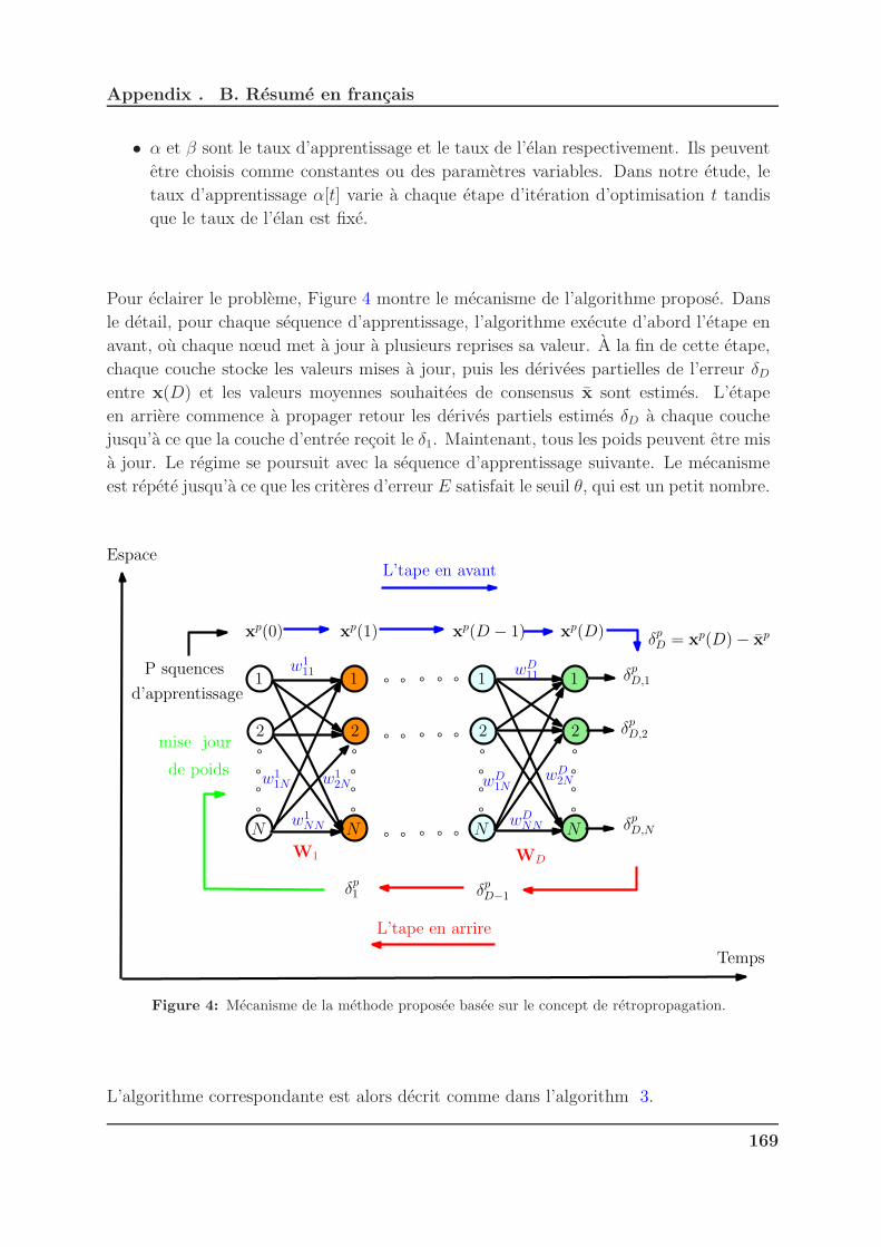
Appendix . B. Resume en francais
• α et β sont le taux d’apprentissage et le taux de l’elan respectivement. Ils peuvent
etre choisis comme constantes ou des parametres variables. Dans notre etude, le
taux d’apprentissage α[t] varie a chaque etape d’iteration d’optimisation t tandis
que le taux de l’elan est fixe.
Pour eclairer le probleme, Figure 4 montre le mecanisme de l’algorithme propose. Dans
le detail, pour chaque sequence d’apprentissage, l’algorithme execute d’abord l’etape en
avant, ou chaque nœud met a jour a plusieurs reprises sa valeur. A la fin de cette etape,
chaque couche stocke les valeurs mises a jour, puis les derivees partielles de l’erreur δDentre x(D) et les valeurs moyennes souhaitees de consensus x sont estimes. L’etape
en arriere commence a propager retour les derives partiels estimes δD a chaque couche
jusqu’a ce que la couche d’entree recoit le δ1. Maintenant, tous les poids peuvent etre mis
a jour. Le regime se poursuit avec la sequence d’apprentissage suivante. Le mecanisme
est repete jusqu’a ce que les criteres d’erreur E satisfait le seuil θ, qui est un petit nombre.
1
2
N
xp(0)
1
2
N
xp(1)
1
2
N
xp(D − 1)
1
2
N
xp(D)
W1 WD
w1
11
w1
NN
w1
2Nw1
1N wD1N
wD2N
wDNN
wD11
L’tape en avant
δpD = x
p(D)− xp
δpD,1
δpD,2
δpD,N
δpD−1
δp1
L’tape en arrire
mise jour
de poids
P squences
d’apprentissage
Espace
Temps
Figure 4: Mecanisme de la methode proposee basee sur le concept de retropropagation.
L’algorithme correspondante est alors decrit comme dans l’algorithm 3.
169

Appendix . B. Resume en francais
B.3 L’evaluation distribuee de la robustesse du
reseau
B.3.1 Introduction
L’efficacite d’un reseau est evaluee par sa fonctionnalite et sa robustesse. Selon la pro-
priete plus tard, certaines questions peuvent se poser. Par exemple, s’il y a un evenement
accidentel, comment reagit-il le reseau? Sera le reseau survecu? Afin de repondre a ces
questions, l’etude sur la robustesse des reseaux de plus en plus attire une attention de la
communaute scientifique.
Dans la litterature, il y a beaucoup de mesures de robustesse propose (voir la Section 1.3),
[20, 21]. Par exemple, la premiere mesure est basee sur la connexite du graphe represen-
tant le reseau [16]. Par les autres mots, le reseau est robuste s’il existe la presence des
chemins alternatif, qui assurent la possibilite de communication en depit des dommages
[16]. Il y a deux concepts classiques de connectivite pour un graphe qui peut etre utilise
pour modeliser la robustesse du reseau qui sont les sommet et bord connectivites. Le
sommet (bord) connectivite Kv(Ke) est le nombre minimal de sommets (de bords) d’etre
retire afin de deconnecter le graphe donne (voir Subsection 1.3.1). Par cette approche
analytique, afin d’en deduire l’indice de la robustesse, nous devons enlever chaque bord
pour verifier la connectivite du graphe. Meme si cette approche est simple, c’est aussi
un fardeau si nous analysons des reseaux plus grands et plus complexes raisonnables.
Dans [72], les auteurs ont propose le concept de la connectivite naturelle comme une
mesure spectrale de robustesse dans les reseaux complexes. La connectivite naturel est
exprimee sous forme mathematique comme la moyenne des valeurs propres de la matrice
d’adjacence du graphe representant la topologie du reseau. L’avantage de cette methode
est que la mesure proposee fonctionne dans les deux reseaux connectes et deconnectes.
D’autre part, le spectre de Laplace sp(L) peut etre utilise pour calculer les indices de
robustesse qui evalue la performance du reseau donne. Par exemple, la deuxieme plus
petite valeur propre du spectre de Laplace λ2(L), defini egalement comme la connec-
tivite algebrique [28], est bien connu comme un parametre critique que influence sur la
performance et robustesse des systemes dynamiques en raison de son role principal dans
la connectivite du graphe [20]. Par consequent, il y a beaucoup de recherches sur cette
connectivite algebrique dans la litterature [3, 51, 76]. En outre, il existe des mesures
remarquables pour obtenir les indices de robustesse souhaites: la resistance effective du
graphe R et Nombre d’arbres couvrants ξ (voir Section 1.3), qui sont basees sur la tout
le spectre de Laplace differents de zero.
Nous proposons des methodes pour estimer la resistance effective du grapheR et Nombre
d’arbres couvrants ξ. Figure 5 montre que l’estimation distribue de la robustesse du
170
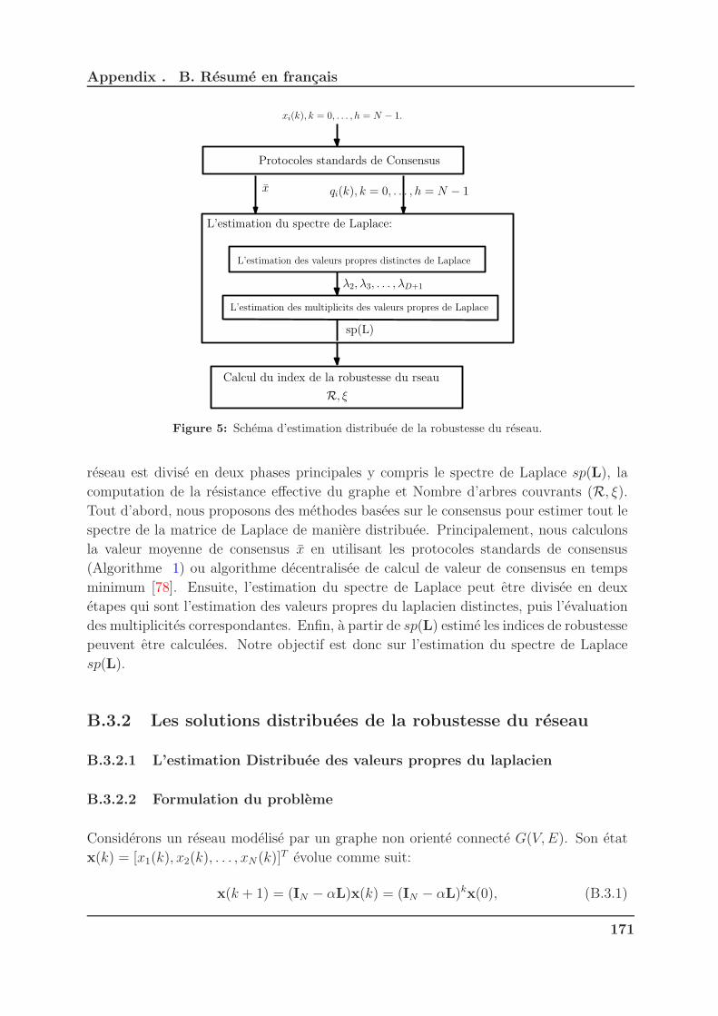
Appendix . B. Resume en francais
Protocoles standards de Consensus
xi(k), k = 0, . . . , h = N − 1.
L’estimation du spectre de Laplace:
L’estimation des valeurs propres distinctes de Laplace
L’estimation des multiplicits des valeurs propres de Laplace
Calcul du index de la robustesse du rseau
x qi(k), k = 0, . . . , h = N − 1
λ2, λ3, . . . , λD+1
sp(L)
R, ξ
Figure 5: Schema d’estimation distribuee de la robustesse du reseau.
reseau est divise en deux phases principales y compris le spectre de Laplace sp(L), la
computation de la resistance effective du graphe et Nombre d’arbres couvrants (R, ξ).
Tout d’abord, nous proposons des methodes basees sur le consensus pour estimer tout le
spectre de la matrice de Laplace de maniere distribuee. Principalement, nous calculons
la valeur moyenne de consensus x en utilisant les protocoles standards de consensus
(Algorithme 1) ou algorithme decentralisee de calcul de valeur de consensus en temps
minimum [78]. Ensuite, l’estimation du spectre de Laplace peut etre divisee en deux
etapes qui sont l’estimation des valeurs propres du laplacien distinctes, puis l’evaluation
des multiplicites correspondantes. Enfin, a partir de sp(L) estime les indices de robustesse
peuvent etre calculees. Notre objectif est donc sur l’estimation du spectre de Laplace
sp(L).
B.3.2 Les solutions distribuees de la robustesse du reseau
B.3.2.1 L’estimation Distribuee des valeurs propres du laplacien
B.3.2.2 Formulation du probleme
Considerons un reseau modelise par un graphe non oriente connecte G(V,E). Son etat
x(k) = [x1(k), x2(k), . . . , xN (k)]T evolue comme suit:
x(k + 1) = (IN − αL)x(k) = (IN − αL)kx(0), (B.3.1)
171
Appendix . B. Resume en francais
ou α est choisi tel que 0 < α < 1dmax
pour assurer la convergence asymptotique [74]. De
l’etat x(k), on peut definir q(k) = Lkx(0) comme:
q(k) = (q1,k, . . . , qN,k)T =
1
(−α)k
(
x(k)−k−1∑
i=0
(k
i
)
(−α)iq(i)
)
, (B.3.2)
avec q(0) = x(0).
1. Hypothese 1: Le nombre N de nœuds est connue.
2. Hypothese 2: Chaque nœud i sauve sa valeur initiale xi(0) et les valeurs consecu-
tives qi,k, k = 0, . . . , h.
Le probleme etude peut donc etre formule comme suit:
Etant donne une paire d’entree-sortie arbitraire x(0), x = x1, ou x = 11T
Nx(0), et les
observations intermediaires q(k), k = 0, . . . , h, estimer de maniere distribuee les valeurs
propres du laplacien du graphe representant le reseau.
Cependant, au lieu de calculer directement les valeurs propres du laplacien, nous allons
calculer l’inverse des valeurs propres du laplacien. En outre, puisque le nombre D de
valeurs propres du laplacien distinctes differents de zero est inconnu, la factorisation sera
re-parametre. Enoncons d’abord la proposition suivante:
Proposition 7
Considerons un graphe connexe avec la matrice de Laplace L et ses valeurs propres
distinctes differents de zero λ2, · · · , λD+1. Supposons que le vecteur des valeurs locales
x(0) n’est pas orthogonal a n’importe quel vecteur propre de L, la fonction de cout
E(ααα) = ‖x(h)− x‖2 =∥∥∥∥∥
1∏
k=h
(IN − αkL)x(0)− x
∥∥∥∥∥
2
, (B.3.3)
avec ααα = (α1 · · ·αh)T , h ≥ D, est minimale si et seulement si 1/λ2, · · · , 1/λD+1 ⊆
α1, α2, · · · , αh.
De la Proposition 7, nous pouvons conclure que l’ensemble S1 = αk, k = 1, . . . , h, des
solutions de (B.3.3) contient l’inverse des valeurs propres du laplacien S2 = 1λi, i =
2, . . . , D + 1: S2 ⊂ S1. Par consequent, la procedure d’estimation doit etre divisee en
deux parties. Nous recevons d’abord S1 en resolvant (B.3.3) de maniere distribuee, nous
mettons a l’ensemble S2 de S1 et deduisons la valeurs propres du laplacien localement.
Nous savons que si αkhk=1 contient D inverses des valeurs propres du laplacien different
de zero, puis
x =
h∏
k=1
(I− αkL)x(0),
172
Appendix . B. Resume en francais
ou de facon equivalente,
x =h∑
k=0
ckLkx(0) =
h∑
k=0
ckq(k) = Qc, (B.3.4)
ouQ = [q(0) q(1) · · · q(h)] ∈ IRN×(h+1) and c = [c0 c1 · · · ch]T ∈ IR(h+1)×1, le coefficient
ci etant defini comme:
ck =
1, if k = 0.
(−1)k∑
i<j<···<k αiαj · · ·αk, if k = 1, . . . , h− 1.
(−1)h∏h
k=1 αt, if k = h.
(B.3.5)
Il est evident que αk sont les racines du polynome avec des coefficients ck. Et, c a un
motif de signe alternatif.
Nous pouvons affirmer la proposition suivante qui est un corollaire de Proposition 7:
Proposition 8
Soit P(c, :) le polynome de hemedegravecdescoefficientsc=[c0 c1 . . . ch]T ∈
IR(h+1)×1 construit de l’ensemble de stepsize S1 = α1, α2, . . . , αh en utilisant (B.3.5).
Pour ne importe quel nœud i et des mesures intermediaires qi = [qi,0, qi,1, . . . , qi,h]T ∈
IR(h+1)×1 du protocole de consensus (B.3.1), nous obtenons
x = P(c,qi) = qTi c (B.3.6)
si et seulement si les D inverses des valeurs propres du laplacien distinctes sont
contenus dans S1.
Etant donne une limite superieure h pour le nombre D de valeurs propres du laplacien
distinctes, l’idee est de minimiser (B.3.3) puis de reduire etape par etape l’ensemble
obtenu des coefficients ck construite de S1 jusqu’a ce qu’il soit minime. Apres tout,
l’ensemble des inverses des valeurs propres du laplacien distinctes S2 est atteint. est at-
teint. Afin d’obtenir l’ensemble de spectre de Laplace sp(L), les multiplicites correspon-
dantesmi, i = 1, . . . , D+1 des valeurs propres du laplacien distinctes Λ = λ1, . . . , λD+1doit etre estimee (il sera considere dans la Section B.3.2.6).
Afin de mieux comprendre la structure de ce Chapitre, Figure 6 illustre sa construction
en montrant la facon d’estimer la robustesse du reseau.
En fait, pour estimation distribue des valeurs propres du laplacien, trois cas ont ete
profondement considere:
1. Le cas de la parfaite connaissance de la valeur moyenne du consensus x,
173
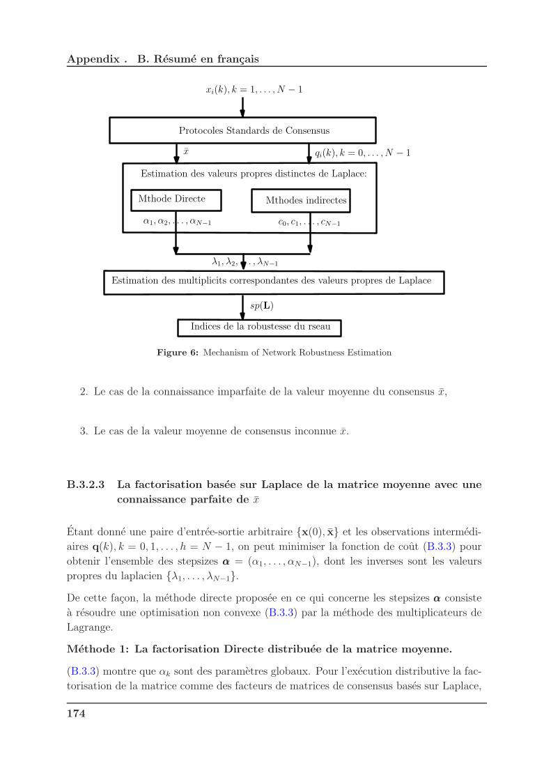
Appendix . B. Resume en francais
Protocoles Standards de Consensus
xi(k), k = 1, . . . , N − 1
Estimation des valeurs propres distinctes de Laplace:
Mthode Directe Mthodes indirectes
x qi(k), k = 0, . . . , N − 1
α1, α2, . . . , αN−1 c0, c1, . . . , cN−1
λ1, λ2, . . . , λN−1
Estimation des multiplicits correspondantes des valeurs propres de Laplace
Indices de la robustesse du rseau
sp(L)
Figure 6: Mechanism of Network Robustness Estimation
2. Le cas de la connaissance imparfaite de la valeur moyenne du consensus x,
3. Le cas de la valeur moyenne de consensus inconnue x.
B.3.2.3 La factorisation basee sur Laplace de la matrice moyenne avec une
connaissance parfaite de x
Etant donne une paire d’entree-sortie arbitraire x(0), x et les observations intermedi-
aires q(k), k = 0, 1, . . . , h = N − 1, on peut minimiser la fonction de cout (B.3.3) pour
obtenir l’ensemble des stepsizes ααα = (α1, . . . , αN−1), dont les inverses sont les valeurs
propres du laplacien λ1, . . . , λN−1.
De cette facon, la methode directe proposee en ce qui concerne les stepsizes ααα consiste
a resoudre une optimisation non convexe (B.3.3) par la methode des multiplicateurs de
Lagrange.
Methode 1: La factorisation Directe distribuee de la matrice moyenne.
(B.3.3) montre que αk sont des parametres globaux. Pour l’execution distributive la fac-
torisation de la matrice comme des facteurs de matrices de consensus bases sur Laplace,
174
Appendix . B. Resume en francais
nous pouvons d’abord noter que la fonction de cout (B.3.3) peut etre reecrite comme:
E(ααα) = ‖x(h)− x‖2 = ‖1∏
k=h
(IN − diag(αααk)L)x(0)− x‖2, (B.3.7)
avec αααk = [α1,k, α2,k, . . . , αN,k]T = αk1, k = 1, 2, . . . , h = N − 1.
L’idee de la methode proposee est de minimiser le desaccord entre voisins sur la valeur
de αk tout en veillant que la factorisation de la matrice moyenne est obtenue. Une
telle factorisation est evaluee en contraignant les valeurs des nœuds apres h iterations de
l’algorithme de consensus pour etre egale a la moyenne des valeurs initiales:
minαααk∈IRN×1,k=1,2,...,h
1
2
h∑
k=1
∑
i∈V
∑
j∈Ni
(αj,k − αi,k)2, (B.3.8)
subject to x(h) = x
or equivalently,
minαααk∈IRN×1
1
2
h∑
k=1
αααTkLαααk. (B.3.9)
subject to x(h) = x
Remark 14
Importe quelle solution de (B.3.9) contient l’inverse des valeurs propres du laplacien
selon a Proposition 7.
Le probleme d’optimisation sous contrainte (B.3.9) peut ensuite etre realisee comme un
probleme d’optimisation non contrainte au moyen d’une methode de Lagrange avec une
fonction de Lagrange definis comme suit:
H(ααα1,ααα2, . . . ,αααh,y) =1
2
h∑
k=1
αααTkLαααk + yT (x(h)− x) (B.3.10)
ou y ∈ IRN×1 est le vecteur des multiplicateurs de Lagrange.
La minimisation de la fonction de Lagrange (B.3.10) peut etre considere comme h des
problemes de consensus a resoudre simultanement avec une contrainte qui donne une
sorte de reference externe a suivre.
Pour eviter tout malentendu entre l’etape temporelle k et l’iteration de l’optimisation t,
nous notons x(k),W(k) comme xk,Wk respectivement.
Afin de tirer l’algorithme distribue correspondant, nous enoncons maintenant le lemme
technique suivant:
175
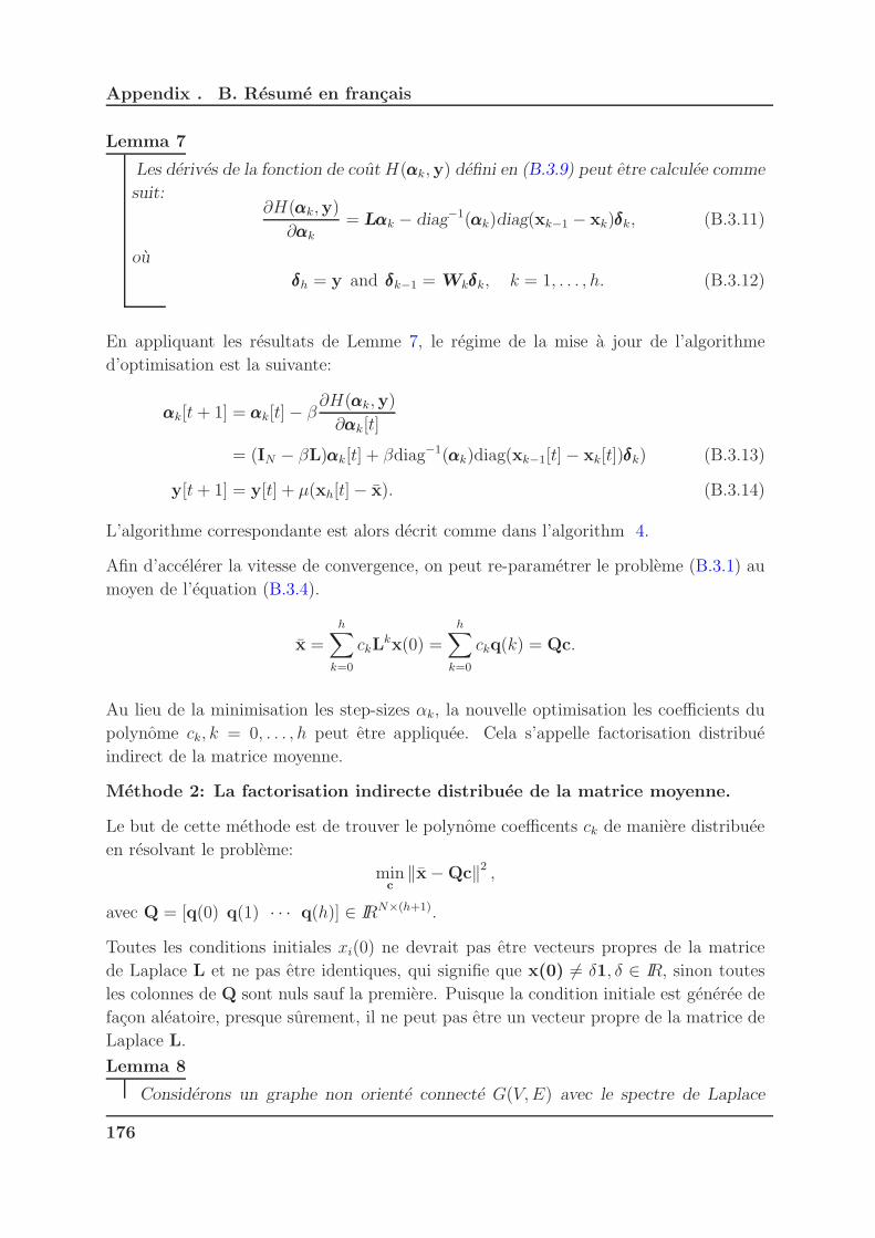
Appendix . B. Resume en francais
Lemma 7
Les derives de la fonction de coutH(αααk,y) defini en (B.3.9) peut etre calculee comme
suit:∂H(αααk,y)
∂αααk
= Lαααk − diag−1(αααk)diag(xk−1 − xk)δδδk, (B.3.11)
ou
δδδh = y and δδδk−1 = Wkδδδk, k = 1, . . . , h. (B.3.12)
En appliquant les resultats de Lemme 7, le regime de la mise a jour de l’algorithme
d’optimisation est la suivante:
αααk[t + 1] = αααk[t]− β∂H(αααk,y)
∂αααk[t]
= (IN − βL)αααk[t] + βdiag−1(αααk)diag(xk−1[t]− xk[t])δδδk) (B.3.13)
y[t+ 1] = y[t] + µ(xh[t]− x). (B.3.14)
L’algorithme correspondante est alors decrit comme dans l’algorithm 4.
Afin d’accelerer la vitesse de convergence, on peut re-parametrer le probleme (B.3.1) au
moyen de l’equation (B.3.4).
x =
h∑
k=0
ckLkx(0) =
h∑
k=0
ckq(k) = Qc.
Au lieu de la minimisation les step-sizes αk, la nouvelle optimisation les coefficients du
polynome ck, k = 0, . . . , h peut etre appliquee. Cela s’appelle factorisation distribue
indirect de la matrice moyenne.
Methode 2: La factorisation indirecte distribuee de la matrice moyenne.
Le but de cette methode est de trouver le polynome coefficents ck de maniere distribuee
en resolvant le probleme:
minc
‖x−Qc‖2 ,
avec Q = [q(0) q(1) · · · q(h)] ∈ IRN×(h+1).
Toutes les conditions initiales xi(0) ne devrait pas etre vecteurs propres de la matrice
de Laplace L et ne pas etre identiques, qui signifie que x(0) 6= δ1, δ ∈ IR, sinon toutes
les colonnes de Q sont nuls sauf la premiere. Puisque la condition initiale est generee de
facon aleatoire, presque surement, il ne peut pas etre un vecteur propre de la matrice de
Laplace L.
Lemma 8
Considerons un graphe non oriente connecte G(V,E) avec le spectre de Laplace
176

Appendix . B. Resume en francais
sp(L) = λ1, λ2, . . . , λN. Ici, sp(L) a D + 1 valeurs propres du laplacien distinctes.
Si x(0) n’est pas un vecteur propre de la matrice de Laplace L , alors la matrice
Q = Udiag(UTx(0))
1 λ1 λ21 · · · λh
1
1 λ2 λ22 · · · λh
2
. . . . . . .
1 λN λ2N · · · λh
N
a rang min(D + 1, N). Ou U est la matrice des vecteurs propres de Laplace.
Remark 15
rank(Q) < N si existe λi ∈ sp(L) avec multiplicite superieure a 1, ∀x(0).
D’une maniere centralisee, afin de trouver c de l’equation Qc = x, Q doit etre une
matrice de rang plein . Ensuite,
c = Q−1x
En contraste, si Q n’est pas une matrice de rang plein, alors il y a plusieurs solutions de
c. Pour faire face a cette situation, nous utilisons la solution des moindres carres per-
mettant de trouver la plus courante solution S1 a l’interieur de L’ensemble des solutions
(So1, So2, . . . , Som) de c comme decrit dans Figure 7.
So1
So2
So3Som
S1
Figure 7: Plusieurs solutions de c dans le cas d’une matrice de rang que n’est pas plein Q.
Le probleme devient:
minc
‖c‖2 subject to Qc = x
Ici, Q est une matrice de la ligne rang plein.
177
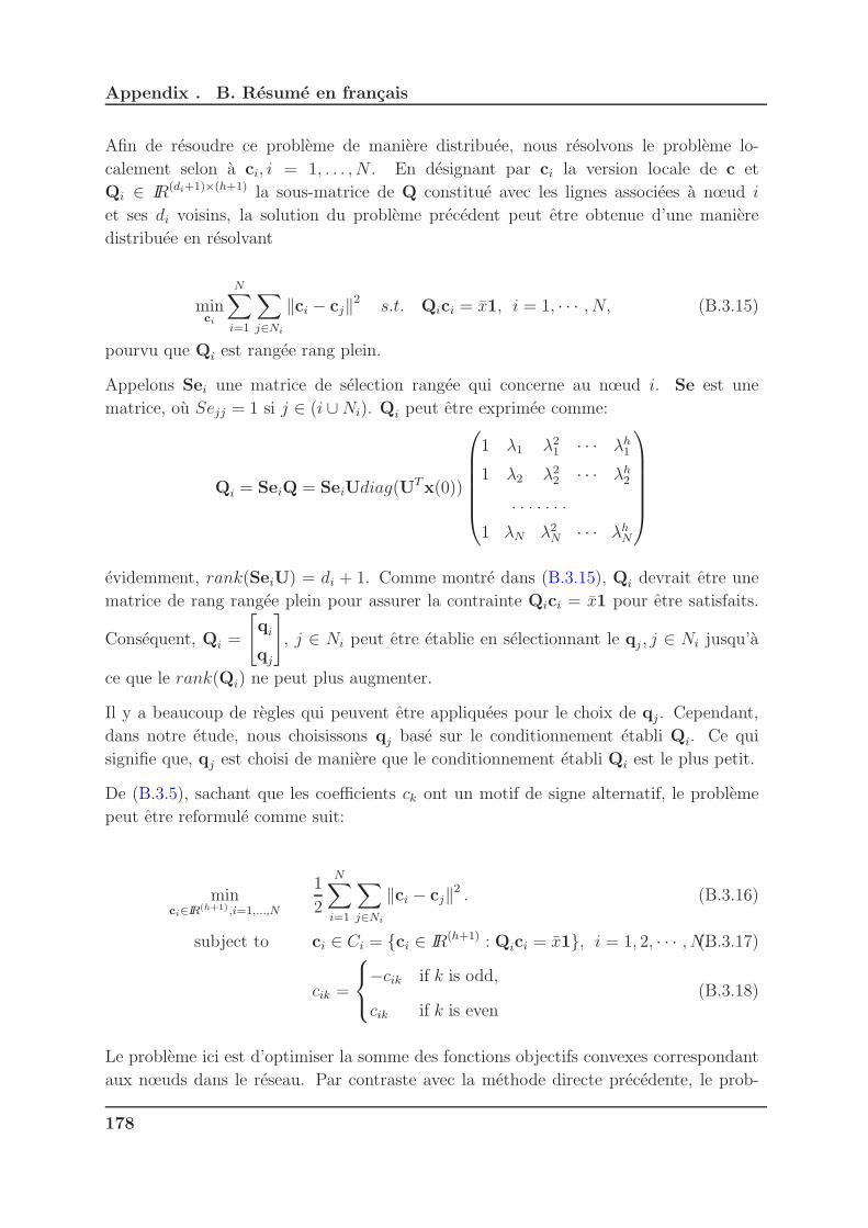
Appendix . B. Resume en francais
Afin de resoudre ce probleme de maniere distribuee, nous resolvons le probleme lo-
calement selon a ci, i = 1, . . . , N . En designant par ci la version locale de c et
Qi ∈ IR(di+1)×(h+1) la sous-matrice de Q constitue avec les lignes associees a nœud i
et ses di voisins, la solution du probleme precedent peut etre obtenue d’une maniere
distribuee en resolvant
minci
N∑
i=1
∑
j∈Ni
‖ci − cj‖2 s.t. Qici = x1, i = 1, · · · , N, (B.3.15)
pourvu que Qi est rangee rang plein.
Appelons Sei une matrice de selection rangee qui concerne au nœud i. Se est une
matrice, ou Sejj = 1 si j ∈ (i ∪Ni). Qi peut etre exprimee comme:
Qi = SeiQ = SeiUdiag(UTx(0))
1 λ1 λ21 · · · λh
1
1 λ2 λ22 · · · λh
2
. . . . . . .
1 λN λ2N · · · λh
N
evidemment, rank(SeiU) = di + 1. Comme montre dans (B.3.15), Qi devrait etre une
matrice de rang rangee plein pour assurer la contrainte Qici = x1 pour etre satisfaits.
Consequent, Qi =
[
qi
qj
]
, j ∈ Ni peut etre etablie en selectionnant le qj , j ∈ Ni jusqu’a
ce que le rank(Qi) ne peut plus augmenter.
Il y a beaucoup de regles qui peuvent etre appliquees pour le choix de qj . Cependant,
dans notre etude, nous choisissons qj base sur le conditionnement etabli Qi. Ce qui
signifie que, qj est choisi de maniere que le conditionnement etabli Qi est le plus petit.
De (B.3.5), sachant que les coefficients ck ont un motif de signe alternatif, le probleme
peut etre reformule comme suit:
minci∈IR(h+1),i=1,...,N
1
2
N∑
i=1
∑
j∈Ni
‖ci − cj‖2 . (B.3.16)
subject to ci ∈ Ci = ci ∈ IR(h+1) : Qici = x1, i = 1, 2, · · · , N.(B.3.17)
cik =
−cik if k is odd,
cik if k is even(B.3.18)
Le probleme ici est d’optimiser la somme des fonctions objectifs convexes correspondant
aux nœuds dans le reseau. Par contraste avec la methode directe precedente, le prob-
178

Appendix . B. Resume en francais
leme d’optimisation (B.3.16) est convexe. Pour le resoudre, nous allons recourir a une
methode de sous-gradient projete inspire de [57] et une methode de direction alternee de
multiplicateurs [11, 22].
(A): Methode de sous-gradient distribuee
L’idee principale de la methode de sous-gradient projete distribuee est de permettre a
chaque nœud i de mettre a jour son estimation apres deux etapes.
Tout d’abord, une etape de sous-gradient est prise en minimisant la fonction objective
locale 12
∑
j∈Ni‖ci − cj‖2. Ensuite, le resultat intermediaire est projete sur l’ensemble
des contraintes Ci. Par consequent, la premiere etape deduit:
ci[t + 1] = ci[t]− γ[t]∑
j∈Ni
(ci[t]− cj[t]) , (B.3.19)
ou γ[t] > 0 est un stepsize, tandis que la deuxieme etape necessite le calcul de la pro-
jection ci[t + 1] = ΩCi[ci[t + 1]].Cette etape de projection est equivalente a resoudre un
probleme d’optimisation sous contrainte formulee comme:
min1
2‖ci[t+ 1]− ci[t+ 1]‖2 s.t. Qici[t+ 1] = x1.
Pour resoudre ce probleme d’optimisation sous contrainte, de maniere generale, la fonc-
tion Lagrangien augmente est defini comme suit:
L(ci[t+ 1],y) =1
2‖ci[t + 1]− ci[t + 1]‖2 + yT (Qici[t + 1]− x1).
Chaque nœud met a jour son vecteur de parametres en utilisant:
ci[t + 1] = Qixi + (Ih+1 − QiQi)ci[t+ 1], (B.3.20)
avec Qi = QTi (QiQ
Ti )
−1, a condition que h ≥ di et Qi rang rangee plein. Ensuite, nous
projetons ci[t+ 1] ur le signe contrainte comme:
ci,k[t+ 1] =
max(0, ci,k[t + 1]) if mod(k, 2) = 0.
min(0, ci,k[t + 1]) if mod(k, 2) 6= 0.(B.3.21)
De [57], l’analyse de la convergence de cette methode a ete bien etudie. Avec un choix
approprie du stepsize γ[0], l’algorithme 5 converge vers un minimum global. La vitesse
de convergence depend encore le choix du stepsize gradient.
(B):Methode de la direction alternee des multiplicateurs (ADMM).
ADMM est relativement facile a mettre en œuvre et ses proprietes de convergence ont
ete bien etudiee dans des travaux recents tels que, dans [8, 11, 23]. Les avantages de
179
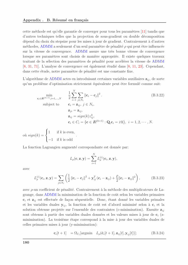
Appendix . B. Resume en francais
cette methode est qu’elle garantie de converger pour tous les parametres [11] tandis que
d’autres techniques telles que la projection de sous-gradient ou double decomposition
depend du choix du stepsize pour les mises a jour de gradient. Contrairement a d’autres
methodes, ADMM a seulement d’un seul parametre de penalite ρ qui peut etre influencee
sur la vitesse de convergence. ADMM assure une tres bonne vitesse de convergence
lorsque ses parametres sont choisis de maniere appropriee. Il existe quelques travaux
traitant de la selection des parametres de penalite pour accelerer la vitesse de ADMM
[8, 31, 71]. L’analyse de convergence est egalement etudie dans [8, 11, 23]. Cependant,
dans cette etude, notre parametre de penalite est une constante fixe.
L’algorithme de ADMM actes en introduisant certaines variables auxiliaires zij, de sorte
qu’un probleme d’optimisation strictement equivalente peut etre formule comme suit:
minci∈IR(h+1),i=1,...,N
1
2
N∑
i=1
∑
j∈Ni
‖ci − cj‖2 . (B.3.22)
subject to ci = zij , j ∈ Ni,
zji = zij,
zij = sign(k)zkij,
ci ∈ Ci = c ∈ IR(h+1) : Qici = x1, i = 1, 2, · · · , N.
ou sign(k) =
1 if k is even,
−1 if k is odd.
La fonction Lagrangien augmente correspondante est donnee par:
Lρ(c, z,y) =
N∑
i=1
L(i)ρ (ci, z,y),
avec
L(i)ρ (ci, z,y) =
∑
j∈Ni
(1
2‖ci − cj‖2 + yT
ij (ci − zij) +ρ
2‖ci − zij‖2
)
, (B.3.23)
avec ρ-un coefficient de penalite. Contrairement a la methode des multiplicateurs de La-
grange, dans ADMM la minimisation de la fonction de cout selon les variables primaires
ci et zij est effectuee de facon sequentielle. Donc, etant donne les variables primales
et les variables duales yij , la fonction de cout est d’abord minimise selon a ci et la
solution obtenue projetee sur l’ensemble des contraintes (c-minimisation). Ensuite zijsont obtenus a partir des variables duales donnees et les valeurs mises a jour de ci (z-
minimisation). La troisieme etape correspond a la mise a jour des variables duales de
celles primaires mises a jour (y-minimisation):
ci[t+ 1] = ΩCi[argmin Lρ(ci[t + 1], zij [t],yij[t])]; (B.3.24)
180
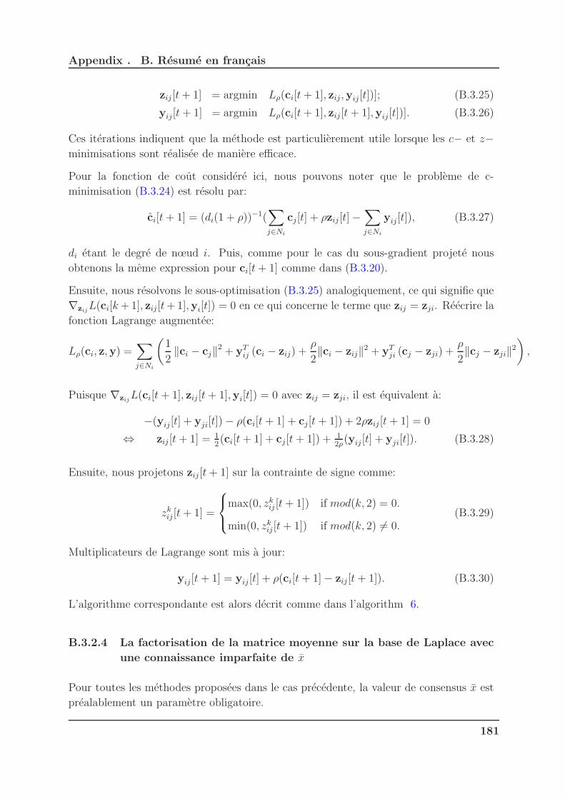
Appendix . B. Resume en francais
zij [t+ 1] = argmin Lρ(ci[t+ 1], zij,yij [t])]; (B.3.25)
yij[t + 1] = argmin Lρ(ci[t+ 1], zij[t + 1],yij [t])]. (B.3.26)
Ces iterations indiquent que la methode est particulierement utile lorsque les c− et z−minimisations sont realisee de maniere efficace.
Pour la fonction de cout considere ici, nous pouvons noter que le probleme de c-
minimisation (B.3.24) est resolu par:
ci[t+ 1] = (di(1 + ρ))−1(∑
j∈Ni
cj[t] + ρzij [t]−∑
j∈Ni
yij [t]), (B.3.27)
di etant le degre de nœud i. Puis, comme pour le cas du sous-gradient projete nous
obtenons la meme expression pour ci[t+ 1] comme dans (B.3.20).
Ensuite, nous resolvons le sous-optimisation (B.3.25) analogiquement, ce qui signifie que
∇zijL(ci[k+1], zij [t+1],yi[t]) = 0 en ce qui concerne le terme que zij = zji. Reecrire la
fonction Lagrange augmentee:
Lρ(ci, z,y) =∑
j∈Ni
(1
2‖ci − cj‖2 + yT
ij (ci − zij) +ρ
2‖ci − zij‖2 + yT
ji (cj − zji) +ρ
2‖cj − zji‖2
)
,
Puisque ∇zijL(ci[t+ 1], zij [t+ 1],yi[t]) = 0 avec zij = zji, il est equivalent a:
−(yij [t] + yji[t])− ρ(ci[t + 1] + cj[t + 1]) + 2ρzij [t+ 1] = 0
⇔ zij [t+ 1] = 12(ci[t+ 1] + cj[t + 1]) + 1
2ρ(yij [t] + yji[t]). (B.3.28)
Ensuite, nous projetons zij [t+ 1] sur la contrainte de signe comme:
zkij [t+ 1] =
max(0, zkij [t+ 1]) if mod(k, 2) = 0.
min(0, zkij [t+ 1]) if mod(k, 2) 6= 0.(B.3.29)
Multiplicateurs de Lagrange sont mis a jour:
yij [t+ 1] = yij [t] + ρ(ci[t+ 1]− zij [t+ 1]). (B.3.30)
L’algorithme correspondante est alors decrit comme dans l’algorithm 6.
B.3.2.4 La factorisation de la matrice moyenne sur la base de Laplace avec
une connaissance imparfaite de x
Pour toutes les methodes proposees dans le cas precedente, la valeur de consensus x est
prealablement un parametre obligatoire.
181

Appendix . B. Resume en francais
Nous detendons maintenant cette exigence au moyen d’une nouvelle methode qui traite
l’estimation des valeurs propres du laplacien quand une valeur de consensus de moyenne
exacte n’est pas connue.
Dans ce qui suit, nous supposons que les nœuds executent un protocole standard de
consensus de moyenne ( 1.2.1), qui est arrete apres M iterations, et rangent leurs valeurs
locales xi,M . Dans cette etude, nous voulons montrer la performance de l’algorithme
propose en ce qui concerne certaines valeurs de M .
Puisque on ne sait pas exactement x, pour une valeur suffisamment grande de M , x(M)
peut etre considere comme son approximation rationnelle. Consequent, notre objectif
est de trouver les coefficients ck qui minimisent l’erreur quadratique sur la valeur finale
de consensus:
E(c) =
∥∥∥∥∥
h∑
k=0
ckq(k)− x(M)
∥∥∥∥∥
2
. (B.3.31)
Ensuite, nous pouvons en deduire l’ensemble S1 = αααkk=1,··· ,h et celle de l’inverse des
valeurs propres du laplacien S2 =1λi, i = 2, . . . , D, qui appartient a S1 : S2 ⊂ S1.
Afin de resoudre le probleme d’une maniere repartie, le probleme d’optimisation peut
etre reformule comme suit:
minccck∈IRN×1,k=0,...,h
1
2
N∑
i=1
(
h∑
k=0
ci,kqi,k − xi,M)2, (B.3.32)
subject to ci,k = cj,k, i = 1, . . . , N ; j ∈ Ni; k = 0, . . . , h.
ci = (ci,0, ci,1, · · · , ci,h)T ∈ Ci,
ou ci,k le kth coefficient de polynome local et Ci signifie l’ensemble des contraintes en
ce qui concerne nœud i. On le definit comme Ci = ci ∈ IRh+1, i = 1, . . . , N : qTl ci =
xi,M with ql ∈ IRh+1, l ∈ Ni ∪ i ou de facon equivalente comme Ci = ci ∈ IRh+1, i =
1, . . . , N : Qici = xi,M1, Qi ∈ IRdi+1×h+1 ou Qi = [q(0) q(1) . . .q(h)], etant rang plein
de rangee en construction.
Cet ensemble de contraintes permet de respecter non seulement l’egalite du vecteur des
coefficients locaux ci si dans un voisinage donne, mais aussi pour faire appliquer le pro-
duit scalaire qTi ci etre egal globalement. a noter que, en introduisant les variables aux-
iliaires zij, le probleme d’optimisation convexe sous contrainte suivant est absolument
equivalent au probleme (B.3.32):
minccck∈IRN×1,k=0,...,h
1
2
N∑
i=1
(
h∑
r=0
ci,kqi,k − xi,M)2. (B.3.33)
subject to ci,k = zkij , i = 1, . . . , N ; j ∈ Ni
zkji = zkij , k = 0, . . . , h. (B.3.34)
zkij = zkij, if k is even,
182

Appendix . B. Resume en francais
zkij = −zkij , if k is odd,
ci ∈ Ci.
Puisque le graphe est suppose etre connecte, les contraintes (B.3.34) forcent ci = cj , j ∈Ni. Nous pouvons alors ecrire le Lagrangien augmente associe:
Lρ(c, z,y) =
N∑
i=1
[
1
2
h∑
k=0
(ci,kqi,k − xi,M)2 +
h∑
k=0
(∑
j∈Ni
ykij(ci,k − zij,k)
)
+∑
j∈Ni
ρ
2‖ci − zij‖2
]
.
ou sous forme de vecteur:
Lρ(c, z,y) =
N∑
i=1
[
1
2(qT
i ci − xi,M)2 +∑
j∈Ni
yTij(ci − zij) +
∑
j∈Ni
ρ
2‖ci − zij‖2
]
.
La solution a ce probleme ADMM agit en trois etapes:
• Tout d’abord, la minimisation de ci:
ci[t + 1] = ΩCi[argmin L(ci, zij [t],yi[t])]. (B.3.35)
ou ΩCi[·] represente la projection dans l’ensemble des contraintes du vecteur dans
l’argumentation.
• Deuxiemement, la minimisation en ce qui concerne a zji = zij :
zij [t+ 1] = argmin L(ci[t+ 1], zij,yi[t]). (B.3.36)
• Troisieme, la mise a jour de multiplicateur de Lagrange:
yij[t + 1] = yij [t] + ρ(ci[t + 1]− zij [t+ 1]). (B.3.37)
Resoudre le probleme sous-optimisation (B.3.35) par ∂Lρ(c,z,y)∂ci
= 0, nous obtenons:
(qiqTi − xi,M)qi +
∑
j∈Ni
yTij(ci − zij) +
ρ
2
∑
j∈Ni
(ci − zij)2 = 0.
⇔ (qiqTi + ρdiIh+1)ci = xi,Mqi + ρ
∑
j∈Ni
zij −∑
j∈Ni
yij .
Puis,
ci[t + 1] = (qiqTi + ρdiIh+1)
−1(xi,Mqi + ρ∑
j∈Ni
zij[t]−∑
j∈Ni
yij [t]).
Puis, projeter la solution obtenue a l’ensemble des contraintes
ci[t+ 1] = ΩCi[ci[t+ 1]],
183
Appendix . B. Resume en francais
nous obtenons:
ci[t + 1] = Qixi,M + (Ih+1 − QiQ)ci[t+ 1], (B.3.38)
avec Qi = QTi (QiQ
Ti )
−1 et Qi etre une matrice de rang plein rangee.
Ensuite, resoudre le probleme sous-optimisation (B.3.36) deduit
zij[t + 1] =1
2(ci[t+ 1] + cj [t+ 1]) +
1
2ρ(yij [t] + yji[t]). (B.3.39)
L’algorithme correspondante est alors decrit comme dans l’algorithm 7. Quand les
coefficients ck sont obtenus approximativement, nous pouvons utiliser des Algorithmes
9 et 10 pour estimer tout le spectre de matrice de Laplace L, qui peut etre utilise pour
estimer les indices de la robustesse du reseau.
B.3.2.5 La factorisation de la matrice moyenne sur la base de Laplace avec
une valeur de consensus inconnue x
Selon la section precedente, une facon pour l’estimation des valeurs propres du laplacien
est:
• resoudre le probleme du consensus de moyenne.
• resoudre le probleme de la factorisation de la matrice de moyennage (B.3.15), Al-
gorithmes 5 et 6.
• recuperer les valeurs propres du laplacien en utilisant les algorithmes 9 et 10.
Au lieu de suivre ces etapes, dans cette section, nous proposons une methode pour
fusionner les deux premieres etapes. Dans ce but, nous proposons de resoudre une
combinaison convexe des deux fonctions convexes, c’est-a-dire
minxi,ci,i=1,··· ,N
θ
2
N∑
i=1
∑
j∈Ni
‖ci − cj‖2 +1− θ
2
N∑
i=1
(xi − xi(0))2,
s.t. Qici = xi1, i = 1, . . . , N, (B.3.40)
avec θ-un parametre scalaire ajustable (0 ≤ θ ≤ 1), xi-une estimation locale de la valeur
moyenne, tandis que xi(0) est une valeur initiale fixe de nœud i.
On voit que, la fonction d’objectif (B.3.40) est une combinaison de deux fonctions con-
vexes. La premiere prend en compte le probleme du consensus de moyenne, tandis
que la seconde concerne l’estimation des coefficients du polynome dont les racines sont
184
Appendix . B. Resume en francais
l’inverse des valeurs propres du laplacien distinctes differents de zero. Et ce probleme
d’optimisation convexe peut etre resolu efficacement en utilisant l’approche de l’ADMM.
Afin de deriver un algorithme ADMM pour le probleme (B.3.40), nous introduisons les
variables auxiliaires zij, µij. Par consequent, le probleme d’optimisation convexe sous
contrainte suivant est absolument equivalente au probleme (B.3.40):
minxi,ci,i=1,··· ,N
θ
2
N∑
i=1
∑
j∈Ni
‖ci − cj‖2 +1− θ
2
N∑
i=1
(xi − xi(0))2,
s.t xi = µij, i = 1, . . . , N, j ∈ Ni.
ci = zij .
zij = sign(k)zkij,
ci ∈ Ci(xi).
ou
• sign(k) =
1 if k is even,
−1 if k is odd.
• Ci(xi) signifie l’ensemble des constraintes ec ce qui concern nœud i. On le definit
comme Ci = c ∈ IRh+1| Qic = xi1.
Maintenant, en introduisant certaines variables duales υυυ and y, le Lagrangien augmente
est defini comme:
Lρ1ρ2(x, c,µµµ, z, υυυ,y) = Lρ1(c, z,y) + Lρ2(x,µµµ,υυυ).
ou:
Lρ1(c, z,y) =θ
2
N∑
i=1
∑
j∈Ni
‖ci − cj‖2 +∑
j∈Ni
ρ12‖ci − zij‖2 +
∑
j∈Ni
yTij(ci − zij),
Lρ2(x,µµµ,υυυ) =1− θ
2
N∑
i=1
(xi − xi(0))2 +
∑
j∈Ni
ρ22(xi − µij)
2 +∑
j∈Ni
υij(xi − µij),
ou ρ1, ρ2 sont des termes de penalite supposes constants.
ADMM fournit une solution iterative qui agit les cinq etapes suivant ci-dessous:
• Minimisation ec ce qui concerm la valeur moyenne du consensus xi:
xi[t+ 1] = argmin Lρ2(xi[t], µij[t], υij [t]). (B.3.41)
185

Appendix . B. Resume en francais
• Minimisation en ce qui concern les coefficients polynomiaux ci:
ci = argmin Lρ1(ci[t], zij [t],yij [t]), (B.3.42)
ci[t+ 1] = ΩCi(xi[t+1])[ci] (B.3.43)
ou ΩCi(xi[k+1])[·] dresse pour la projection dans l’ensemble des contraintes Ci(xi[k+
1]) du vecteur dans l’argumentation.
• Minimisation en ce qui concerm les variables auxiliaires µij avec la contrainte µji =
µij:
µij[t+ 1] = argmin Lρ2(xi[t+ 1], µij[t], υij[t]). (B.3.44)
• Minimisation en ce qui concerm les variables auxiliaires zij :
zij[t + 1] = argmin Lρ1(ci[t + 1], zij [t],yij [t]). (B.3.45)
• La mise a jour Multiplicateurs de Lagrange:
υij [t+ 1] = υij[t] + ρ2(xi[t + 1]− µij[t + 1]). (B.3.46)
yij [t+ 1] = yij [t] + ρ1(ci[t + 1]− zij [t+ 1]). (B.3.47)
Resoudre les problemes de sous-optimisation (B.3.41) et (B.3.42) est equivalent a re-
soudre les equations suivantes:
Nous obtenons:Lρ2(x,µµµ,υυυ)
∂xi
= 0
⇔ xi[t+ 1] =(1− θ)xi(0) + ρ2
∑
j∈Niµij[t]−
∑
j∈Niυij[t]
1− θ + ρ2di. (B.3.48)
Puis, projeter la solution obtenue dans l’ensemble des contraintes:
ci[k + 1] = ΩCi(xi[k+1])[ci[k + 1]],
nous obtenons:
ci[k + 1] = Qixi[k + 1]1+ (Ih+1 − QiQ)ci[k + 1], (B.3.49)
avec Qi = QTi (QiQ
Ti )
−1, Qi etant rang plein de rangee en construction.
Ensuite, la solution des problemes sous-optimisation (B.3.44) et (B.3.45), de la meme
facon, deduit
186

Appendix . B. Resume en francais
1. Le derive de Lρ2(x,µµµ,υυυ) en ce qui concern µij par rapport a la contrainte µij = µji:
∂Lρ2(x,µµµ,υυυ)
∂µij
= −υij − υji − ρ2(xi + xj) + 2ρ2µij = 0
⇔ µij [t+ 1] =xi[t+ 1] + xj [t + 1]
2+
υij[t] + υji[t]
2ρ2. (B.3.50)
2. Le derive de Lρ1(c, z,y) en ce qui concern zij
Lρ1(ci,zij ,yij)
zij= 0
⇔ −yij[t]− ρ(ci[t+ 1]− zij[t + 1]) = 0
⇔ zij [t+ 1] = ci[t + 1] + 1ρ1yij [t]. (B.3.51)
Le parametre θ permet ponderation des deux fonctions combinees de couts. Puisque
l’ensemble des contraintes Ci(xi) depend de la valeur de consensus xi. La procedure
d’optimisation peut d’abord donner plus de poids au probleme de consensus de moyenne,
puis au probleme de la factorisation. Dans ce but, au lieu de garder θ constant, nous
adoptons un temps coefficient variant pris comme
θ(t) =1− e−βt
1 + e−βt(0 < β < 1) (B.3.52)
pour le garder dans la gamme [0, 1] et d’augmenter l’importance de la factorisation
progressivement tout en diminuant celle de le consensus de moyenne.
Remark 16
Pratiquement, nous pouvons voir que le terme de consensus de moyenne converge
beaucoup plus rapide que le probleme de la factorisation de la matrice moyenne.
Ainsi, θ peut etre choisi pres de 1.
L’algorithme correspondante est alors decrit comme dans l’algorithm 8.
B.3.2.6 Recuperation du spectre de Laplace
A chaque nœud, l’ensemble S1 du step-size obtenu au moyen de les algorithmes proposees
(Algorithmes 4, 5, 6, 7, 8) contient l’ensemble S2 de l’inverse des valeurs propres du
laplacien distinctes differents de zero.
Soit ˆxietre la valeur finale de consensus reconstruit par ˆxi =h∑
k=0
ckqi,k = Pi(c,qi) avec
les coefficients obtenus au moyen d’algorithmes 4, 5, 6, 7 et 8.
Suite a la Proposition 8, l’idee est de reduire, etape par etape, le degre du polynome
Pi(c,qi) par enlever un element de S1 a chaque etape. Nous savons que si l’element
187
Appendix . B. Resume en francais
enleve est egalement un element de S2 puis ˆxi 6= Pi( ˜c,qi) ou Pi est le polynome de degre
reduit en ce qui concern nœud i. Algorithme 9 decrit la procedure proposee.
Ensuite, nous obtenons l’ensemble des valeurs propres du laplacien distincts differents de
zero Λ = λ2, . . . , λD+1. Afin d’obtenir tout le spectre Sp(L) = λm11 , λm2
2 , . . . , λmD+1
D+1 ,les multiplicites mi devraient etre definis. Puisque, elles sont toutes entier, le probleme
a recours actuellement a un probleme de la programmation en nombres entiers.
Etant donne l’ensemble des valeurs propres du laplacien distinctes differents de zero Λ,
di le degre de chaque nœud i, inspire d’une propriete interessante∑N
i=1 λi(L) =∑N
i=1 di(voir dans Section 2.3), l’optimisation est maintenant decrit comme suit:
minm∈IRD
ΛTm−N∑
i=1
di, (B.3.53)
subject to
D∑
j=1
mj = N − 1, j = 1, . . . , D.
mj ≥ 1, integer.
ou D = |Λ| et m est le vecteur des multiplicites des valeurs propres.
Dans la litterature, la methode de separation et d’evaluation progressive est la technique
basique pour resoudre le probleme de programmation entier. La programmation lineaire
(LP) de la relaxation (sans restriction de nombre entier) est adoptee pour estimer la
solution optimale d’une programmation en nombres entiers [13]. Consequent, le probleme
(B.3.53) est maintenant reecrit strictement equivalente sous la forme de programmation
lineaire comme suit:
minm∈RD
ΛTm, (B.3.54)
subject to
D∑
j=1
mj = N − 1;
ΛTm =
N∑
i=1
di, (M)
mj ≥ 1, integer.
Ou M est l’ensemble des contraintes sans restriction en nombres entiers. De ce fait, M
peut etre exprimee comme M = m ∈ IRD|∑D
j=1mj = N − 1,ΛTm =∑N
i=1 di and m ≥1. Le probleme (B.3.54) sans restriction en nombres entiers est appele la programmation
lineaire (LP) de la relaxation.
La Algorithme de separation et d’evaluation progressive est decrit comme dans
l’algorithme 10.
188

Appendix . B. Resume en francais
B.4 Reconstruction de la topologie du reseaux
B.4.1 Introduction
Une topologie de reseau est en informatique une definition de l’architecture (physique
ou logique) d’un reseau, definissant les connexions entre ces postes et une hierarchie
eventuelle entre eux ; elle peut definir la facon dont les equipements sont interconnectes
ou la representation, spatial du reseau (topologie physique) ou la facon dont les donnees
transitent dans les lignes de communication (topologie logique).
L’identification de la topologie de reseau se refere a detecter et identifier les elements
de reseau interesses et la relation entre les elements de reseau cible et represente la con-
struction de la topologie sous une forme appropriee. Par consequent, l’identification des
reseaux de systemes devient une tache de plus en plus attrayant pour resoudre de nom-
breux problemes dans differents domaines scientifiques et techniques, par exemple, en bi-
ologie (biochimique, de neurones et des reseaux ecologiques [2]), la finance, l’informatique
(Internet et le World Wide Web), le transport (livraison et reseau de distribution), et de
l’ingenierie electrique.
Par exemple, l’architecture d’un reseau de recouvrement- comment il alloue les adresses,
etc.- peut etre optimise significativement par la connaissance de la distribution et la con-
nectivite des nœuds sur le reseau de sous-couche qui transporte effectivement le trafic.
Plusieurs systemes importants, tels que l’initiative P4P et RMTP, utilisent des infor-
mations sur la topologie du reseau sous-couche pour l’optimisation ainsi que la gestion
[1].
Dans l’Internet, par exemple, le mecanisme habituel pour generer la topologie d’un reseau
par l’utilisation d’Traceroute. Traceroute est execute sur un noeud, appele la source, en
specifiant l’adresse de destination d’un noeud. Cette execution produit une sequence
d’identifiants, appele trace, correspondant a la route empruntee par les paquets qui
voyagent a partir de la source vers la destination. Un ensemble de trace T est generee en
executant plusieurs reprises traceroute sur un reseau, en variant les noeuds terminaux,
ce est a dire la source et la destination. Si T contient des traces qui identifient chaque
cas lorsqu’un bord est incident sur un nœud, il est possible de reconstruire le reseau
exactement [1].
Suite a notre etude, a partir d’un reseau de consensus general et les mesures de consensus,
nous traitons le probleme de deduire la topologie correcte du reseau en presence de noeuds
anonymes (ou noeuds non marques). En d’autres termes, est-il possible pour un noeud
arbitraire j de reconstruire le reseau correct par des mesures consensuelles moyennes?
189

Appendix . B. Resume en francais
B.5 La solution distribuee de reconstruction de la
topologie du reseau
Dans le chapitre precedent, nous savons maintenant que noeud i peux obtenir le spec-
tre du laplacien par des mesures consensuelles moyennes. Nous affirmons l’hypothese
suivante:
Hypothese 1: Toutes les valeurs propres non nulles de Laplace sont distincts.
En considerant un reseau represente avec un graphe G(V,E), nous rappelons que a
l’instant de temps k,
x(k) = Wx(k − 1)
ou de facon equivalente
x(k) = Wkx(0)
Considerons la decomposition suivante valeur propre de la matrice de consensus W:
W = UDUT . (B.5.1)
avec D = IN − ǫ∆∆∆ et ∆∆∆ est la matrice diagonale des valeurs propres de L. ǫ peut etre
choisi comme 2λ2(L)+λN (L
) [74], puis λ(W) = 1− ǫλ(L).
Etant donne que les vecteurs propres laplaciennes forment une base de IRN , la con-
dition initiale x(0) peut etre etendu telle que x(0) =N∑
i=1
βiU.i = Ub, ou b =
(
β1 β2 · · · βN
)T
contient les coefficients de expansion, et U.i est le i-ere vecteur
propre, i.e. le i-ere colonne de U.
Par consequent:
x(k) = UDkUTUb = UDkb = Udiag(b)vecd(Dk),
ou vecd(·) est le vecteur colonne construit avec les elements diagonaux de la matrice en
argument.
Nous pouvons ecrire l’equation equivalente ci-dessus:
x(k) = Uvecd(Dk), avec U = Udiag(b)
Par consequent, UUT = Udiag(b2)UT et UT U = diag(b2). Nous pouvons conclure
que:
W = UDdiag(b2)−1UT . (B.5.2)
190

Appendix . B. Resume en francais
B.5.1 Estimation des vecteurs propres de la matrice de consen-
sus basee matrice de Laplace
Au noeud j, l’etat a l’instant k est alors donnee par:
xj(k) =N∑
i=1
λki (W)βiuj,i,
En empilant N mesures consecutives noeud j obtient:
xj(0)
xj(1)...
xj(N − 1)
=
1 1 · · · 1
1 λ2(W) · · · λN(W)...
.... . .
...
1 λN−12 (W) · · · λN−1
N (W)
uj,1
uj,2
...
uj,N
, uj,i = uj,iβi
ou de facon equivalente
xj = ΥΥΥUTj. (B.5.3)
De Hypothese 1, nous pouvons conclure que ΥΥΥ est une matrice de rang plein. Par
consequent, noeud j peut resoudre le probleme ci-dessus efficacement et obtenir:
UTj. = ΥΥΥ−1xj . (B.5.4)
Maintenant, le nœud ne connaıt que le j-ere rangee de U.
Considerons un message passant schema ou les nœuds envoient a leurs voisins les rangees
qu’ils ont.
Puis, un certain nombre d’echanges des messages, au moins egale au diametre du graphe,
noeud j a toutes les rangees de U. Cependant, etant donne que certains des nœuds sont
supposes etre anonymes, ils ne envoient pas le label de la rangee qu’ils ont. Deux types de
messages sont transmis dans le reseau. les rangees associees a des nœuds non-anonymes
sont correctement etiquetes tandis que ceux qui sont associes a des nœuds anonymes
ne sont pas etiquetes. En consequence, noeud j ne recoit U allant jusqu’a rangees
permutation, i.e. il recoit les U = ΠΠΠU, ΠΠΠ etant une matrice de permutation.
B.5.2 Network topology reconstruction
Nous pouvons noter que UT U = diag(b2). Par consequent, de (B.5.2), nous obtenons:
W = ΠΠΠWΠΠΠT , with W = UD(UT U)−1UT . (B.5.5)
191

Appendix . B. Resume en francais
Nous pouvons conclure que de la matrice estimee W, on obtient un graphe qui est iso-
morphe au graphe original. Dans ce qui suit, nous indiquons deux conditions suffisantes
pour assurer la reconstruction correcte du graphique. Nous rappelons d’abord les notions
suivantes de observabilite:
Un reseau est dit etre [44]:
• noeud observable d’un noeud donne, si ce noeud est en mesure de reconstruire
l’etat du reseau de ses propres mesures. Cette question a ete etudiee par exemple
dans [58] and [65] ou il a ete declare que un reseau avec une matrice d’etat ayant
au moins une valeur propre non simple n’est pas le noeud observable.
• voisinage observable d’un noeud donne si ce nœud peut reconstruire l’etat du reseau
entier de ses propres mesures et celles de ses voisins. Cette question a ete etudiee
dans [43].
• globalement observable si elle est la voisinage observable depuis ne importe quel
noeud.
Proposition 9
Supposons que le graphe est noeud-observable ou voisinage observable du noeud j. Si
toutes les entrees de la condition initiale sont distinctes alors la topologie du reseau
peut etre reconstruit exactement du noeud j.
Proposition 10
Supposons que le reseau contient un ensemble A de noeuds anonymes et le graphe
est noeud-observable ou voisinage observable du noeud j. Si toutes les entrees de
la condition initiale associee aux noeuds anonymes sont toutes distinctes alors la
topologie de reseau peut etre reconstruit exactement du noeud j.
Ici, l’ambiguıte de permutation est limitee a des entrees associees aux noeuds anonymes.
B.6 Conclusions generales
B.6.1 Resume des contributions et conclusions
Ce chapitre a pour l’objective de conclure la these a travers un bref summerization ainsi
qu’une perspective pour des travaux futurs.
Les Problemes de Consensus en temps fini ont ete recus une vaste attention de
la communaute de recherche en raison de ses avantages dans de nombreux domaines
d’application, en particulier dans le calcul distribue. Brievement parlant, les algorithmes
192

Appendix . B. Resume en francais
de consensus de moyenne en temps fini (pour lesquelles un consensus peut etre obtenu en
un nombre fini d’etapes) sont couramment utilises comme element de base pour plusieurs
algorithmes de controle, estimation ou inference distribues en raison du fait qu’elles
peuvent garantir une execution en temps minimal, ces algorithmes sont donc beaucoup
plus attrayant que ceux qui assurent la convergence asymptotique.
Ceci impact sur la these avec la conception de protocole de consensus de moyenne en
temps fini independamment de la matrice de Laplace d’un graphe donne de maniere
distribuee et son application dans l’evaluation de la robustesse du reseau.
Tout d’abord, nous avons propose un nouvel algorithme pour le protocole d’auto-
configuration d’un consensus de moyenne en temps fini ou matrices ne sont pas neces-
sairement basees sur la matrice de Laplace d’un graphe donne de maniere distribuee.
Plus precisement, nous avons resolu un probleme de la factorisation de la matrice de
maniere distribuee en utilisant une sequence d’apprentissage. La methode est basee sur
la methode de retro-propagation et une methode de descente de gradient associee. Con-
ceptuellement, chaque iteration lineaire k, k = 0, . . . , D est illustree comme une couche
d’un reseau. L’idee principale est de calculer les derivees partielles de l’erreur entre la
sortie reelle et en sortie souhaite, puis propager les ramener a chaque iteration k pour
mettre a jour les poids. Etant donne le diametre du graphe d(G), la valeur optimale du
nombre d’etapes necessaires pour atteindre un consensus de moyenne en faisant varier
la valeur de D dans (d(G) ≤ D ≤ N − 1).
Evidemment, il est incommode pour les reseaux de grande envergure. Cependant, un
point interessant peut etre indiquee dans ce travail est que les matrices de consensus
obtenus ne sont pas des matrices doublement stochastiques. Ceci est la condition de la
convergence pour un protocole de consensus selon [74].
Deuxiemement, l’etude sur la robustesse des reseaux de plus en plus attire un attention de
la communaute scientifique. Consequent, dans cette these, l’evaluation de la robustesse
du reseau, qui est mis en œuvre par la Resistance effective du graphe (R) et le nombre
d’arbres couvrants (ξ) d’une maniere distribuee, devient evidemment une application
domaine prometteuse. Puisque deux mesures de la robustesse sont des fonctions du
spectre de Laplace sp(L), donc la tache principale est maintenant d’estimer le spectre
de Laplace. Precisement, trois cas ont ete consideres: parfaitement connue x, bruyant,
et inconnu x.
La matrice de consensus moyen peut etre prise en D la matrice basee sur Laplace de
consensus, ou D represente le nombre de valeurs propres du laplacien distinctes differents
de zero. Pour le premier cas (parfaitement connue x), toutes les methodes sont carac-
terisees en deux approches, qui sont approche directe et l’approche indirecte. La methode
directe donne lieu a un probleme d’optimisation non convexe en ce qui concern les step-
sizes αk, k = 1, . . . , N − 1 qui sont l’inverse des valeurs propres du laplacien distinctes
193

Appendix . B. Resume en francais
differents de zero. Puisque, c’est une methode basee sur gradient, il souffre de conver-
gence lent. Pour ameliorer la vitesse de convergence, un probleme d’optimisation convexe
est introduit pour estimer les coefficients ck, k = 0, . . . , N −1 d’un polynome donne dont
les racines sont les stepsizes αk, k = 1, . . . , N − 1 qui permet de factoriser la matrice
de moyennage JN = 11T
N. De cette facon, deux methodes fameux (les methode de sous-
gradient projete et ADMM) sont appliquees pour resoudre ce probleme d’optimisation
convexe. Par ces methodes proposees, les valeurs propres du laplacien distinctes peu-
vent etre deduites. Ensuite, au moyen d’une programmation en nombres entiers, tout le
spectre sp(L) est obtenu pour calculer les indices de la robustesse.
L’inconvenient de ces methodes est l’evolutivite. Pour les graphes de grande echelle,
l’estimation de tout le spectre sp(L) est significativement difficile a executer. Par con-
sequent, l’estimation peut etre limitee a celle des valeurs propres les plus significatifs
pour estimer la limite de l’indice de la robustesse du reseau (λ2(L)).
Methode de sous-gradient projete est tres applicable en raison de sa simplicite. Cepen-
dant, l’inconvenient est qu’il peut etre lente. Consequent, il faut faire attention au choix
du stepsize γ(t). En revanche, l’ADMM est garanti a converger pour tous les parametres.
Il a seulement un seul parametre de penalite ρ qui peut etre influencee sur la vitesse de
convergence. Ainsi, dans les cas restants, ADMM est le meilleur choix.
Dans le cas de la valeur de consensus imparfaite x,nous avons suppose un protocole
standard de consensus a ete execute et conserve certaines valeurs intermediaires de xM
selon l’iteration M .Ensuite, nous avons utilise la basee algorithme basee sur ADMM 7
de voir comment la robustesse du reseau reagit. Enfin, il pretend que quand la valeur
intermediaire de x est aussi proche que possible de la valeur reelle, l’indice de la robustesse
du reseau peut etre pris environ.
Dans le cas de la valeur de consensus inconnue x, nous avons considere le probleme
d’optimisation convexe qui recourt a une combinaison convexe de deux fonctions con-
vexes. Le premier prend en compte le probleme du consensus de moyenne, tandis que le
second concerne l’estimation des valeurs propres du laplacien. Pour les grands graphes,
une telle solution est evidemment insolubles. Consequent, les Algorithmes 5, 6, 7, 8 sont
efficaces et bien adaptees pour les reseaux de taille moyenn.
L’identification de la topologie du reseau se refere a detecter et identifier les elements
du reseau interesses et la relation entre les elements du reseau destinataire et represente
la construction de la topologie sous une forme appropriee. Consequent, l’identification
des reseaux de systemes devient une tache de plus en plus attrayante pour resoudre de
nombreux problemes dans differents domaines scientifiques et techniques.
En theorie, la matrice de consensus W admet la decomposition des valeurs propres
W = UΛΛΛUT , ou ΛΛΛ = IN − ǫ∆∆∆, avec ∆∆∆ est matrice diagonale de λi(L), represente
la matrice diagonale des valeurs propres et U la matrice de vecteurs propres. Nous
194
Appendix . B. Resume en francais
pouvons trouver un moyen d’obtenir U. Puisque la spectre de Laplace sp(L) peut etre
realisee en utilisant le methodes proposees dans le Chapitre 4, nous pouvons reconstruire
la topologie du reseau.
B.6.2 Travaux en cours et a venir
1. Conception des Protocoles de consensus de moyenne en temps fini:
(a) La dependance de la vitesse de convergence sur la sequence d’apprentissage
reste a etudier. Ainsi, la conception de sequences d’apprentissage optimales
peut etre etudiee.
(b) La recherche sur la robustesse du consensus de moyenne en temps fini.
2. L’evaluation de la robustesse du reseau:
(a) Nouveaux methodes qui peuvent etre appliquees pour les graphes de grande
echelle.
(b) Pour la methode indirecte, dans la pratique, il peut rencontrer le probleme
mal conditionne lors de l’etablissement sous-matrices Qi, c le probleme mal
conditionne lors de l’etablissement sous-matrices Qi qui conduit a perdre le
rang de ces sous-matrices. Consequent, on peut etudier dans la precondition
de ces matrices pour conserver la precision des methodes proposees.
3. Reconstruire la topologie du reseau:
(a) Concevoir une nouvelle methode qui traite avec le spectre de Laplace sp(L)
dont les valeurs propres ne sont pas toutes distinctes.
(b) D’evaluer la robustesse de ces methodes lorsque l’echange de donnees sont
sujettes a des communications imparfaites.
195


Bibliography
[1] H.B. Acharya and M.G. Gouda. On the hardness of topology inference. In proc. of
12th International Conference on Distributed Computing and Networking (ICDCN
2011), pages 251–262, Bangalore, India, January 2011.
[2] A. Aderhold, D. Husmeier, J. J. Lennon, M. Colin Beale, and V. Anne Smith. Hi-
erarchical Bayesian models in ecology: Reconstructing species interaction networks
from non-homogeneous species abundance data. Ecological Informatics, 11(0):55 –
64, 2012.
[3] R. Aragues, G. Shi, D. V. Dimarogonas, C. Sagues, and K. H. Johansson. Dis-
tributed algebraic connectivity estimation for adaptive event-triggered consensus.
In Proc. of American Control Conference (ACC), pages 32–37, June 2012.
[4] J.S. Baras and P. Hovareshti. Efficient and robust communication topologies for
distributed decision making in networked systems. In Proc. of the 48th IEEE Con-
ference on Decision and Control (CDC), held jointly with the 28th Chinese Control
Conference (CCC), pages 3751–3756, December 2009.
[5] D. P. Bertsekas and J. N. Tsitsiklis. Parallel and Distributed Computation: Numer-
ical Methods. Prentice-Hall, Inc., Upper Saddle River, NJ, USA, 1989.
[6] V. D. Blondel, J. M. Hendrickx, A. Olshevsky, and J. N. Tsitsiklis. Convergence
in multiagent coordination, consensus, and flocking. In Proc. of the 44th IEEE
Conference on Decision and Control, 2005 and 2005 European Control Conference.
CDC-ECC ’05, pages 2996–3000, December 2005.
[7] V.D. Blondel, J.M. Hendrickx, and J. N. Tsitsiklis. Continuous-time average-
preserving opinion dynamics with opinion-dependent communications. SIAM Jour-
nal on Control and Optimization,, 48:5214–5240, 2010.
[8] D. Boley. Local linear convergence of ADMM on quadratic or linear programs.
SIAM Journal on Optimization, 23(4):2183–2207, 2013.
[9] S. Bolognani, S. Del Favero, L. Schenato, and D. Varagnolo. Distributed sensor
calibration and least-squares parameter identification in WSNs using consensus al-
197
Bibliography
gorithms. In Proc. of 46th annual Allerton Conference, pages 1191–1198, Allerton
House, UIUC, Illinois, USA, 2008.
[10] V. Borkar and P.P. Varaiya. Asymptotic agreement in distributed estimation. IEEE
Transactions on Automatic Control, 27(3):650–655, Jun 1982.
[11] S. Boyd, N. Parikh, E. Chu, B. Peleato, and J. Eckstein. Distributed optimization
and statistical learning via the alternating direction method of multipliers. Found.
Trends Mach. Learn., 3(1):1–122, January 2011.
[12] A. E Brouwer, A. M Cohen, and A Neumaier. Distance-Regular Graphs. Springer,
1989.
[13] J. W. Chinneck. Practical optimization: A gentle introduction. Systems and Com-
puter Engineering. Carleton University. Ottawa, Canada, 2012.
[14] E. K. P. Chong and S. H. Zak. An Introduction to Optimization. John Wiley &
Sons, third edition, 2012.
[15] J. Cortes, S. Martinez, and F. Bullo. Robust rendezvous for mobile autonomous
agents via proximity graphs in arbitrary dimensions. IEEE Transactions on Auto-
matic Control, 51(8):1289–1298, Aug 2006.
[16] A. H. Dekker and B. D. Colbert. Network robustness and graph topology. In
Proceedings of the 27th Australasian Conference on Computer Science (ACSC) -
Volume 26, 2004.
[17] D.V. Dimarogonas and K.J. Kyriakopoulos. Formation control and collision avoid-
ance for multi-agent systems and a connection between formation infeasibility and
flocking behavior. In Proc. of the 44th IEEE Conference on Decision and Control
and European Control Conference. (CDC-ECC), pages 84–89, Dec 2005.
[18] J. C. Duchi, A. Agarwal, and M. J. Wainwright. Dual averaging for distributed
optimization: Convergence analysis and network scaling. IEEE Transactions on
Automatic Control, 57(3):592–606, 2012.
[19] I. Shames E. Ghadimi, A. Teixeira and M. Johansson. Optimal parameter selection
for the alternating direction method of multipliers ADMM: quadratic problems.
IEEE Transactions on Automatic Control, PP(99), 2014.
[20] W. Ellens and R. E. Kooij. Graph measures and network robustness. e-version,
arXiv, 2013.
[21] W. Ellens, F.M. Spieksma, P. VanMieghem, A. Jamakovic, and R.E. Kooij. Effective
graph resistance. Linear Algebra and its Applications, 435(10):2491 – 2506, 2011.
Special Issue in Honor of Dragos Cvetkovic.
198
Bibliography
[22] T. Erseghe. A distributed and scalable processing method based upon ADMM.
Signal Processing Letters, IEEE, 19(9):563–566, September 2012.
[23] T. Erseghe, D. Zennaro, E. Dall’Anese, and L. Vangelista. Fast consensus by the
alternating direction multipliers method. IEEE Transactions on Signal Processing,
59(11):5523–5537, 2011.
[24] A. Esna-Ashari, A.Y. Kibangou, and F. Garin. Distributed input and state esti-
mation for linear discrete-time systems. In Proc. 51st IEEE Conf. on Decision and
Control (CDC), Maui, Hawaii, USA, December 2012.
[25] Ph. Ciblat F. Iutzeler, P. Bianchi and W. Hachem. Explicit convergence rate of a
distributed alternating direction method of multipliers. Under review, 2014.
[26] J. Ferber. Multi-Agent Systems: An Introduction to Distributed Artificial Intel-
ligence. Addison-Wesley Longman Publishing Co., Inc., Boston, MA, USA, 1st
edition, 1999.
[27] M. Franceschelli, A. Gasparri, A. Giua, and C. Seatzu. Decentralized estimation of
Laplacian eigenvalues in multi-agent systems. Automatica, 49(4):1031–1036, April
2013.
[28] M. Friedler. Algebraic connectivity of graphs. Czechoslovak Mathematical Journal,
23:298–305, 1973.
[29] M.N. Vrahatis G.D. Magoulas and G.S. Androulakis. Improving the convergence
of the backpropagation algorithm using learning rate adaptation methods. Neural
Computation, 11:1769–1796, November 1999.
[30] L. Georgopoulos. Definitive consensus for distributed data inference. PhD thesis,
EPFL, Lausanne, 2011.
[31] E. Ghadimi, A. Teixeira, I. Shames, and M. Johansson. On the optimal step-size
selection for the alternating direction method of multipliers. volume 3, pages 139–
144, Santa Barbara, USA, 2012.
[32] C. Godsil and G. Royle. Algebraic graph theory. Springer, 2001.
[33] D. Hayden, Y. Yuan, and J. Goncalves. Network reconstruction from intrinsic noise:
Minimum-phase systems. In In proc. of American Control Conference (ACC), pages
4391–4396, June 2014.
[34] J.M. Hendrickx, R.M. Jungers, A. Olshevsky, and G. Vankeerberghen. Graph diam-
eter, eigenvalues, and minimum-time consensus. Automatica, 50(2):635–640, 2014.
199

Bibliography
[35] J.M. Hendrickx, G. Shi, and K.H. Johansson. Finite-time consensus using stochas-
tic matrices with positive diagonals. IEEE Transactions on Automatic Control,
PP(99):1–1, 2014. doi:10.1109/TAC.2014.2352691.
[36] A. J. Hoffman and M. H. McAndrew. The polynomial of a directed graph. Proc.
American Mathematical Society, 16:303–309, 1965.
[37] B. Li J. Ren, W.-Xu Wang and Y.-C. Lai. Noise bridges dynamical correlation
and topology in coupled oscillator networks. Physical Review Letters, 104:058701,
February 2010.
[38] A. Jadbabaie, Jie Lin, and A.S. Morse. Coordination of groups of mobile autonomous
agents using nearest neighbor rules. IEEE Transactions on Automatic Control,
48(6):988–1001, June 2003.
[39] A. Y. Kibangou. Step-size sequence design for finite-time average consensus in secure
wireless sensor networks. Systems and Control Letters, 67:19–23, March 2014.
[40] A. Y. Kibangou and C. Commault. Decentralized Laplacian eigenvalues estimation
and collaborative network topology identification. In 3rd IFAC Workshop on Dis-
tributed Estimation and Control in Networked Systems (NecSys’12),Santa Barbara,
USA, pages 7–12, 2012.
[41] A.Y. Kibangou. Finite-time average consensus based protocol for distributed esti-
mation over awgn channels. In Proc. of the 50th IEEE Conference on Decision and
Control (CDC), pages 261–265, Orlando, Fl, USA, December, 12-15 2011.
[42] A.Y. Kibangou. Graph Laplacian based matrix design for finite-time distributed
average consensus. In Proc. of the American Conference on Control(ACC), pages
261–265, Montreal, Canada, 2012.
[43] A.Y. Kibangou and C. Commault. Algebraic characterization of observability in
distance-regular consensus networks. In In 52nd IEEE Annual Conference on De-
cision and Control (CDC), pages 1313–1318, December 2013.
[44] A.Y. Kibangou and C. Commault. Observability in connected strongly regular
graphs and distance regular graphs. IEEE Transactions on Control of Network
Systems, 1(4):360–369, December 2014.
[45] A.Y. Kibangou and A.L.F. de Almeida. Distributed PARAFAC based DS-CDMA
blind receiver for wireless sensor networks. In Proc. of the IEEE Workshop SPAWC,
Marrakech, Morocco, June 20-23, 2010.
[46] C.K. Ko. On matrix factorization and scheduling for finite-time average consensus.
PhD thesis, January, 2010.
200
Bibliography
[47] E. Kokiopoulou and P. Frossard. Polynomial filtering for fast convergence in dis-
tributed consensus. IEEE Transactions on Signal Processing, 57:342–354, January
2009.
[48] N. A. Lynch. Distributed Algorithms. Morgan Kaufmann Publishers Inc., San Fran-
cisco, CA, USA, 1996.
[49] S. V. Macua, P. Belanovic, and S. Zazo. Consensus-based distributed principal
component analysis in wireless sensor networks. In Proc. of the IEEE Workshop
SPAWC, Marrakech, Morocco, June 20-23 2010.
[50] O. L. Mangasarian and M. V. Solodov. Serial and parallel backpropagation conver-
gence via nonmonotone perturbed minimization (1994). Optimzation Methods and
Software, 4:103–116, 1994.
[51] R. Merris. Laplacian matrices of a graph: a survey. Linear Algebra and its Appli-
cations, 197:143–176, 1994.
[52] M. Mesbahi and M. Egerstedt. Graph theoretic methods in multiagent networks.
Princeton University Press, 2010.
[53] E. Montijano, J.I. Montijano, and C. Sagues. Fast distributed consensus with Cheby-
shev polynomials. In American Control Conference (ACC), 2011, pages 5450–5455,
June 2011.
[54] B.J. Moore and Carlos Canudas-de Wit. Formation control via distributed opti-
mization of alignment error. In Proc. of the 48th IEEE Conference on Decision and
Control, held jointly with the 28th Chinese Control Conference (CDC/CCC), pages
3075–3080, December 2009.
[55] F. Morbidi and A. Y. Kibangou. A distributed solution to the network reconstruction
problem. Systems & Control Letters, 70:85 – 91, 2014.
[56] M. Nabi-Abdolyousefi and M. Mesbahi. Network identification via node knockout.
IEEE Transactions on Automatic Control, 57(12):3214–3219, December 2012.
[57] A. Nedic, A. Ozdaglar, and P.A. Parrilo. Constrained consensus and optimization
in multi-agent networks. IEEE Transactions on Automatic Control, 55(4):922–938,
2010.
[58] N. O’Clery, Y. Yuan, G.B. Stan, and M. Barahona. Observability and coarse grain-
ing of consensus dynamics through the external equitable partition. Physical Review
E, 88:042805, October 2013.
[59] R. Olfati-Saber. Flocking for multi-agent dynamic systems: algorithms and theory.
IEEE Transactions on Automatic Control,, 51(3):401–420, March 2006.
201
Bibliography
[60] R. Olfati-Saber. Swarms on sphere: A programmable swarm with synchronous
behaviors like oscillator networks. In The 45th IEEE Conference on Decision and
Control (CDC), pages 5060–5066, Dec 2006.
[61] R. Olfati-Saber. Distributed Kalman filtering for sensor networks. In Proc. of the
46th IEEE Conf. on Decision and Control, pages 5492–5498, New Orleans, LA,
USA, December 12–14 2007.
[62] R. Olfati-Saber and R. M. Murray. Distributed cooperative control of multiple
vehicle formations using structural potential functions. In IFAC World Congress,
pages 346–352, 2002.
[63] R. Olfati-Saber and R.M. Murray. Consensus problems in networks of agents with
switching topology and time-delays. IEEE Transactions on Automatic Control,
49(9):1520–1533, September 2004.
[64] R. Olfati-Saber and J.S. Shamma. Consensus filters for sensor networks and dis-
tributed sensor fusion. In Proc. of the 44th IEEE Conference on Decision and Con-
trol and European Control Conference. (CDC-ECC), pages 6698–6703, December
2005.
[65] G. Parlangeli and G. Notarstefano. On the reachability and observability of path
and cycle graphs. IEEE Transactions on Automatic Control, 57(3):743–748, March
2012.
[66] A. U. Raghunathan and S. D. Cairano. Optimal step-size selection in alternating
direction method of multipliers for convex quadratic programs and model predictive
control. In the 21st International Symposium on Mathematical Theory of Networks
and Systems, pages 807–811, Groningen, The Netherlands, 7-11 July 2014.
[67] T. Sahai, A. Speranzon, and A. Banaszuk. Hearing the cluster of a graph: A
distributed algorithm. Automatica, 48(1):15–24, January 2012.
[68] S. Shahrampour and V. M. Preciado. Topology identification of directed dynamical
networks via power spectral analysis. IEEE Transactions on Automatic Control,,
60(99):1–1, 2015.
[69] H. Shao and G. Zheng. Convergence analysis of a back-propagation algorithm with
adaptive momentum. Neurocomputing, 74(5):749–752, 2011.
[70] S. Sundaram and C.N Hadjicostis. Finite-time distributed consensus in graphs with
time-invariant topologies. In Proc. of American Control Conference (ACC), pages
711–716, New York, USA, July 2007.
202
Bibliography
[71] A. Teixeira, E. Ghadimi, I. Shames, H. Sandberg, and M. Johansson. Optimal
scaling of the ADMM algorithm for distributed quadratic programming. In Proc.
of the 52nd IEEE Conference on Decision and Control (CDC), pages 6868–6873,
Florence, Italy, December 10-13, 2013.
[72] J. Wu, M. Barahona, Y. Tan, and H. Deng. Spectral measure of structural robustness
in complex networks. IEEE Transactions on Systems, Man and Cybernetics, Part
A: Systems and Humans, 41(6):1244–1252, November 2011.
[73] W. Wu. Convergence of gradient method with momentum for back-propagation
neural networks. Computational Mathematics, 26(4):613–623, 2008.
[74] L. Xiao and S. Boyd. Fast linear iterations for distributed averaging. Systems
Control Letters, 53:65–78, 2004.
[75] L. Xiao, S. Boyd, and S. Kim. Distributed average consensus with least-mean-square
deviation. Journal on Parallel Distributed Computation, 67(1):33–46, January 2007.
[76] P. Yang, R. A. Freeman, G. Gordon, K. Lynch, S. Srinivasa, and R. Sukthankar.
Decentralized estimation and control of graph connectivity in mobile sensor net-
works. In Proc. of American Control Conference,(ACC), pages 2678 – 2683, June
2008.
[77] P. Yang, R. A. Freeman, G. Gordon, K. Lynch, S. Srinivasa, and R. Sukthankar. De-
centralized estimation and control of graph connectivity for mobile sensor networks.
Automatica 49, pages 390–396, 2010.
[78] Y. Yuan, G. Stan, L. Shi, M. Barahona, and J. Goncalves. Decentralized minimim-
time consensus. Automatica 49, pages 1227–1235, 2013.
[79] Y. Yuan, G. B. Stan, L. Shi, and J. Goncalves. Decentralised final value theorem for
discrete-time LTI systems with application to minimal-time distributed consensus.
In Proc. of the 48th IEEE Conference on Decision and Control, 2009 held jointly
with the 2009 28th Chinese Control Conference. (CDC/CCC), pages 2664–2669,
December 2009.
203