THÈSEPRÉSENTÉE À

L’UNIVERSITÉ PIERRE ET MARIE CURIE

École doctorale Informatique, Télécommunications et Électronique (Paris) (ED130)

Présentée par Thomas GARCIA

pour obtenir le grade de DOCTEUR

DÉTERMINANTS ÉVOLUTIONNISTES DE LA SOCIALITÉ :

LE RÔLE DE LA FORMATION DE GROUPE

Directeur de recherche : Édith PERRIER

Co-directeurs de recherche : Silvia DE MONTE et Leonardo GREGORY BRUNNET

Soutenance le 4 décembre 2013 à l’École Normale Supérieure (Paris) devant la commission d’examen formée de :

Pr. Bernard CAZELLES UMR 7625 CNRS, Laboratoire Écologie et Évolution, ENS, Paris Président du juryPr. Paul RAINEY NZ Institute for Advance Study, Massey University, Auckland RapporteurPr. Guillaume BESLON UMR 5205 CNRS, Institut National des Sciences Appliquées, Lyon RapporteurDr. Minus VAN BAALEN UMR 7625 CNRS, Laboratoire Écologie et Évolution, ENS, Paris ExaminateurPr. Michael DOEBELI Department of Zoology, University of British Columbia, Vancouver ExaminateurDr. Clément NIZAK UMR 5588, Laboratoire Interdisciplinaire de Physique, Saint Martin d’Hères ExaminateurDR Édith PERRIER UMI UMMISCO, Centre IRD Île-de-France, Bondy Dir. de thèseDr. Silvia DE MONTE UMR 7625 CNRS, Laboratoire Écologie et Évolution, ENS, Paris Dir. de thèse

Remerciements

Je tiens d'abord à remercier Silvia, qui a été mon interlocutrice principale pendant ces trois ans et qui s’est toujours montrée disponible malgré un emploi du temps chargé. Elle a su orienter ma recherche dans la bonne direction en me détournant de mes (((bien) trop) nombreuses) digressions sans les censurer et en me laissant une marge de liberté considérable. C’est pour moi un attrait décisif de la recherche, et je lui suis reconnaissant d’avoir su le respecter. Grazie !

Leonardo, qui m’a gentiment accueilli dans son labo de Porto Alegre, et hébergé dans sa famille pendant un mois. Le reste du temps, il a été l’interlocuteur idéal pour comprendre le comportement parfois capricieux de mes particules bleues et rouges. Obrigado, je n’oublierai pas les foisonnants barbecues et les délicieux vins chiliens.

Enfin, je remercie Edith pour son soutien constant dans mes démarches et ses conseils avisés, ainsi que l’équipe du PDI-MSC et ses étudiants des quatre coins du monde.

Je voudrais au moins mentionner également, en vrac :

les collègues de l’équipe Ecologie et évolution ; les thésard-e-s croisé-e-s à Dresde et Göttingen, avec qui j'ai partagé aussi bien des discussions techniques que des Lagavulin, et celles et ceux qui ont fait de l’institut de physique de l’université de Porto Alegre une terre accueillante pour un non-lusophone ; Guilhem et Orso, brillants collègues de fin de thèse ; Antoine et Joseph, compagnons de pauses café-madeleines, pour les discussions scientifiques et politiques ; mes autres ami-e-s et collègues parisiens avec qui j’ai pu discuter de tout, tant qu’il ne s’agit pas de la thèse !

Enfin un grand merci à ma famille pour m’avoir sorti la tête de mes modèles à l’occasion de repas toujours gargantuesques, ainsi qu’à Canelle et Chlamy-von-Dindon (glou glou !) pour les séquences grattouilles.

Et surtout, ma mère, qui s’est pliée en quatre pour que j’en sois là aujourd’hui et m’a toujours épaulé, et Margot, soutien indéfectible malgré mes doutes et sautes d’humeur. Sans vous ces cent-je-ne-sais-combien pages n’auraient été rédigées. Merci pour tout.

Contents

1 Evolutionary game theory for the evolution of cooperation in microbes 11.1 The intimidating field of social evolution . . . . . . . . . . . . . . . . . . . . . . 2

1.1.1 Sociality/cooperation is puzzling for the evolutionary biologist . . . . . . 21.1.2 A scientific shift in the current approach . . . . . . . . . . . . . . . . . . 3

1.2 Sociality and cooperation in microbes . . . . . . . . . . . . . . . . . . . . . . . 41.2.1 Microorganisms are good systems to test evolutionary hypotheses . . . . 41.2.2 Sociality and cooperation are pervasive in microbes . . . . . . . . . . . . 51.2.3 The tragedy of the commons in microbes . . . . . . . . . . . . . . . . . 61.2.4 The chicken-and-egg of cooperation and sociality . . . . . . . . . . . . . 8

1.3 Solving the paradox of cooperation . . . . . . . . . . . . . . . . . . . . . . . . . 91.3.1 Reciprocity . . . . . . . . . . . . . . . . . . . . . . . . . . . . . . . . . 91.3.2 Policing (reward / punishment) . . . . . . . . . . . . . . . . . . . . . . . 101.3.3 Interactions directed toward genealogical kin . . . . . . . . . . . . . . . 111.3.4 Assortment between cooperators . . . . . . . . . . . . . . . . . . . . . . 121.3.5 Direct benefits . . . . . . . . . . . . . . . . . . . . . . . . . . . . . . . 131.3.6 Game definition . . . . . . . . . . . . . . . . . . . . . . . . . . . . . . . 14

1.4 Game structure . . . . . . . . . . . . . . . . . . . . . . . . . . . . . . . . . . . 141.4.1 Dyadic games . . . . . . . . . . . . . . . . . . . . . . . . . . . . . . . . 151.4.2 N-player games . . . . . . . . . . . . . . . . . . . . . . . . . . . . . . . 171.4.3 The difficulty finding the right game . . . . . . . . . . . . . . . . . . . . 22

1.5 Population structure . . . . . . . . . . . . . . . . . . . . . . . . . . . . . . . . . 251.5.1 Lattices . . . . . . . . . . . . . . . . . . . . . . . . . . . . . . . . . . . 251.5.2 Graphs . . . . . . . . . . . . . . . . . . . . . . . . . . . . . . . . . . . 271.5.3 Continuous space . . . . . . . . . . . . . . . . . . . . . . . . . . . . . . 28

1.6 Group structure . . . . . . . . . . . . . . . . . . . . . . . . . . . . . . . . . . . 291.6.1 Groups as equivalence classes . . . . . . . . . . . . . . . . . . . . . . . 291.6.2 Groups as sets . . . . . . . . . . . . . . . . . . . . . . . . . . . . . . . 291.6.3 Non-delimited groups . . . . . . . . . . . . . . . . . . . . . . . . . . . 30

1.7 Outline . . . . . . . . . . . . . . . . . . . . . . . . . . . . . . . . . . . . . . . 31

2 Group formation and the evolution of sociality 352.1 Introduction . . . . . . . . . . . . . . . . . . . . . . . . . . . . . . . . . . . . . 352.2 General formulation . . . . . . . . . . . . . . . . . . . . . . . . . . . . . . . . . 39

i

2.2.1 Hypotheses . . . . . . . . . . . . . . . . . . . . . . . . . . . . . . . . . 392.2.2 Payoff difference for a general aggregation process . . . . . . . . . . . . 412.2.3 Payoff difference: case of no assortment a priori . . . . . . . . . . . . . 43

2.3 Group formation by differential attachment . . . . . . . . . . . . . . . . . . . . 462.3.1 Description of the toy model . . . . . . . . . . . . . . . . . . . . . . . . 462.3.2 Group size distributions and payoff difference . . . . . . . . . . . . . . . 492.3.3 Evolutionary dynamics and effect of the parameters . . . . . . . . . . . . 492.3.4 Other rules for group formation . . . . . . . . . . . . . . . . . . . . . . 54

2.4 Decoupling cooperation and attachment . . . . . . . . . . . . . . . . . . . . . . 552.4.1 Hypotheses . . . . . . . . . . . . . . . . . . . . . . . . . . . . . . . . . 552.4.2 Evolutionary outcome . . . . . . . . . . . . . . . . . . . . . . . . . . . 572.4.3 Conclusion . . . . . . . . . . . . . . . . . . . . . . . . . . . . . . . . . 60

2.5 Extension to a continuous trait . . . . . . . . . . . . . . . . . . . . . . . . . . . 612.5.1 Changes in the model . . . . . . . . . . . . . . . . . . . . . . . . . . . . 612.5.2 Resident / mutant analysis . . . . . . . . . . . . . . . . . . . . . . . . . 642.5.3 Application to an aggregation process . . . . . . . . . . . . . . . . . . . 672.5.4 Condition for altruism . . . . . . . . . . . . . . . . . . . . . . . . . . . 68

2.6 Discussion . . . . . . . . . . . . . . . . . . . . . . . . . . . . . . . . . . . . . . 702.6.1 Social groups formation and evolution . . . . . . . . . . . . . . . . . . . 702.6.2 Aggregative sociality in microorganisms . . . . . . . . . . . . . . . . . . 732.6.3 Nonnepotistic greenbeards? . . . . . . . . . . . . . . . . . . . . . . . . 742.6.4 About altruism and direct benefits . . . . . . . . . . . . . . . . . . . . . 752.6.5 Toward a re-evaluation of the group formation step . . . . . . . . . . . . 77

3 Differential adhesion between moving particles for the evolution of social groups 793.1 Introduction . . . . . . . . . . . . . . . . . . . . . . . . . . . . . . . . . . . . . 79

3.1.1 Main issue . . . . . . . . . . . . . . . . . . . . . . . . . . . . . . . . . 793.1.2 Outline . . . . . . . . . . . . . . . . . . . . . . . . . . . . . . . . . . . 81

3.2 Model . . . . . . . . . . . . . . . . . . . . . . . . . . . . . . . . . . . . . . . . 823.2.1 Aggregation model . . . . . . . . . . . . . . . . . . . . . . . . . . . . . 833.2.2 Social dilemma . . . . . . . . . . . . . . . . . . . . . . . . . . . . . . . 863.2.3 Evolutionary algorithm . . . . . . . . . . . . . . . . . . . . . . . . . . . 90

3.3 Results . . . . . . . . . . . . . . . . . . . . . . . . . . . . . . . . . . . . . . . . 913.3.1 Local differences in adhesion rule group formation and spatial assort-

ment in the aggregation phase . . . . . . . . . . . . . . . . . . . . . . . 913.3.2 Assortment and differential volatility between strategies drive the evolu-

tion of sociality . . . . . . . . . . . . . . . . . . . . . . . . . . . . . . . 933.3.3 Parameters of motion and interaction condition the evolution of sociality 97

3.4 Discussion . . . . . . . . . . . . . . . . . . . . . . . . . . . . . . . . . . . . . . 1053.4.1 Evolution of sociality via differential adhesion . . . . . . . . . . . . . . 1053.4.2 Strategy assortment and differential volatility . . . . . . . . . . . . . . . 1053.4.3 Role of group formation . . . . . . . . . . . . . . . . . . . . . . . . . . 1073.4.4 Conclusion . . . . . . . . . . . . . . . . . . . . . . . . . . . . . . . . . 108

ii

3.5 Effect of ecological vs. evolutionary time scale . . . . . . . . . . . . . . . . . . 1093.5.1 Hypotheses . . . . . . . . . . . . . . . . . . . . . . . . . . . . . . . . . 1093.5.2 Evolutionary trajectories . . . . . . . . . . . . . . . . . . . . . . . . . . 1103.5.3 Effect of the generation time . . . . . . . . . . . . . . . . . . . . . . . . 1133.5.4 Conclusion: role of time scales . . . . . . . . . . . . . . . . . . . . . . . 116

4 Conclusion 1194.1 Main results . . . . . . . . . . . . . . . . . . . . . . . . . . . . . . . . . . . . . 1194.2 Perspectives for future work . . . . . . . . . . . . . . . . . . . . . . . . . . . . 128

Appendix A Derivation of the payoff difference, general case 145

Appendix B Group size distributions for differential attachment 151

Appendix C Condition for sociality to be altruistic for differential attachment 155

Appendix D Evolutionary algorithm for chapter 3 157

iii

List of Figures

1.1 A Venn diagram for cooperation and sociality . . . . . . . . . . . . . . . . . . . 81.2 Representation of the Prisoner’s Dilemma, the Snowdrift Game, the Stag Hunt

and the Harmony Game in the (T, S) plane. . . . . . . . . . . . . . . . . . . . . 171.3 Payoff difference between cooperators and defectors in a threshold game. . . . . 221.4 Payoff difference between cooperators and defectors in a threshold game when

N varies. . . . . . . . . . . . . . . . . . . . . . . . . . . . . . . . . . . . . . . 23

2.1 Life cycle used in the model . . . . . . . . . . . . . . . . . . . . . . . . . . . . 402.2 Payoff difference changing one parameter at a time . . . . . . . . . . . . . . . . 502.3 Evolutionary trajectory and group size dynamics . . . . . . . . . . . . . . . . . . 512.4 Social invasion thresholds . . . . . . . . . . . . . . . . . . . . . . . . . . . . . . 522.5 Mean fitnesses of the S and A strategies when Ss invade from scratch in a small

population (Npop = 1000) . . . . . . . . . . . . . . . . . . . . . . . . . . . . . . 532.6 Payoff differences for other rules of attachment . . . . . . . . . . . . . . . . . . 562.7 Equilibrium frequencies of each strategy SC, SD, AC, AD when sociality is

decoupled from cooperation. . . . . . . . . . . . . . . . . . . . . . . . . . . . . 582.8 A non-generic case of evolutionary trajectories in the 3D-simplex for various

initial conditions. . . . . . . . . . . . . . . . . . . . . . . . . . . . . . . . . . . 602.9 Pairwise invasibility plots (PIP) . . . . . . . . . . . . . . . . . . . . . . . . . . . 642.10 Analytical and computational pairwise invasibility plots for the continuous model 682.11 Sensitivity of the pairwise invasibility plot on parameters b/c and T . . . . . . . 692.12 The Simpson’s paradox . . . . . . . . . . . . . . . . . . . . . . . . . . . . . . . 722.13 Minimal b/c ratio to promote sociality vs. maximal b/c ratio for sociality to be

altruistic. . . . . . . . . . . . . . . . . . . . . . . . . . . . . . . . . . . . . . . 76

3.1 Local rules for interaction . . . . . . . . . . . . . . . . . . . . . . . . . . . . . . 853.2 Segmentation of a structured population into groups . . . . . . . . . . . . . . . . 883.3 Snapshots of an aggregation process . . . . . . . . . . . . . . . . . . . . . . . . 933.4 Evolutionary dynamics . . . . . . . . . . . . . . . . . . . . . . . . . . . . . . . 953.5 Effect of motion noise on uS , uA, RS and RA and on the evolutionary equilibria . 993.6 Effect of velocity on uS , uA, RS and RA and on the evolutionary equilibria . . . . 1013.7 Effect of the interaction radius on uS , uA, RS and RA and on the evolutionary

equilibria . . . . . . . . . . . . . . . . . . . . . . . . . . . . . . . . . . . . . . 1033.8 Effect of density on the evolutionary equilibria . . . . . . . . . . . . . . . . . . 104

v

3.9 Snapshots of an evolutionary trajectory with motion and reproduction concomi-tant: case when Ss dominate . . . . . . . . . . . . . . . . . . . . . . . . . . . . 111

3.10 Snapshots of an evolutionary trajectory with motion and reproduction concomi-tant: case when As dominate . . . . . . . . . . . . . . . . . . . . . . . . . . . . 112

3.11 Example of bistable equilibrium when the evolutionary and ecological time scalesare no longer separated. . . . . . . . . . . . . . . . . . . . . . . . . . . . . . . . 114

3.12 Effect of the generation time tR on the average equilibrium frequency of S players.1153.13 Evolutionary fate of the cooperative trait in Cremer et al.’s model, as a function

of regrouping time T . . . . . . . . . . . . . . . . . . . . . . . . . . . . . . . . 116

4.1 Effect of the group size distribution on the maximal benefit-to-cost ratio for al-truism . . . . . . . . . . . . . . . . . . . . . . . . . . . . . . . . . . . . . . . . 122

4.2 Invasion barrier required to trigger sociality, as a function of the patch size T . . . 1244.3 Formation of groups in Dictyostelium discoideum and in cadherin-expressing L

cells . . . . . . . . . . . . . . . . . . . . . . . . . . . . . . . . . . . . . . . . . 1274.4 Spatial cell sorting in S. cerevisiae and in cadherin-expressing L cells . . . . . . 128

B.1 Theoretical group size distributions for social and asocial individuals. . . . . . . 153

vi

Chapter 1

Evolutionary game theory for the evolution

of cooperation in microbes

Foreword

The following work pertains to the sub-discipline of evolutionary biology coined “the evolution

of cooperation” and widely borrows from its formalism, lexicon and, possibly, shortcomings.

Hopefully, it will manage to question some of its presuppositions at the same time. While this

introduction chapter provides a – short – overview on the – extensive – literature on cooperation

theory, it does certainly not claim exhaustiveness. Rather, it is intended to give the minimal

context necessary to understand the stakes of the thesis, and supply readers with a methodolog-

ical toolbox. In three years, my understanding of this research field has been constantly shaped

by going back and forth through some of its numerous sides, and primarily guided by my own

interests at a given point in time. As a consequence, my goal is to paint here my own, idiosyn-

cratic vision of the landscape of sociobology, and give clues on how I hobbled along through the

paths of theoretical evolutionary biology to end up writing this. Some details will be eventually

re-discussed in the following chapters, but I think they will be best kept in mind if hinted at

1

beforehand.

A lexical word of caution: the terms sociality and cooperation will be used indifferently

in the few first sections. However, it is actually one of my main points to stress a distinction

between the two, and to underline what implications the confusion between these two concepts

might have had on the methodology employed in theoretical / conceptual models.

The main framework is evolutionary modeling; the main issue is living in groups; the main

question is “how?”; the main focus, on microorganisms. So let us start.

1.1 The intimidating field of social evolution

1.1.1 Sociality/cooperation is puzzling for the evolutionary biologist

With more than half a century of controversies, semantic issues and rises and falls of its succes-

sive towering paradigms, the field of social evolution might not be the most friendly one. While

undeniable progress has been made, decades of field and lab work, abstract models and episte-

mological questioning have not succeeded in establishing a consensual theory to describe and

rank the main driving forces behind the emergence and sustainability of sociality in the living

world. How is collective structuring of populations conceivable in a Darwinian – thus intrinsi-

cally competitive – world ? The issue is still puzzling considering the ubiquity of social behavior

at all levels of biological organization. Charles Darwin himself identified it as a potential weak

spot in his theory when he described sociality in ants as “one special difficulty, which at first

appeared to [himself] insuperable, and actually fatal to [his own] theory” (Darwin, 1871). The

question of the origin and sustainability of social traits has been revived in the last decades fol-

lowing Hamilton’s breakthrough paper on kin selection (Hamilton, 1964) and Maynard Smith’s

identification of multicellularity and eusociality as ones of life’s major transitions (Maynard-

Smith and Szathmary, 1995). Since then, this issue has spawned a plethoric literature (Sumpter,

2

2010) that reaches fields as diverse as ethology, theoretical ecology, microbiology, anthropol-

ogy, sociology (or rather, a new portmanteau word, “sociobiology”), mathematics, economics,

statistical physics, etc.

Disclaimer: in some circumstances, biologists might have the tendency to overestimate the

scope of their perception of the mechanisms behind sociality. The point of view of the evolution-

ary biologist should not however obfuscate the work of researchers in humanities, and certainly

the issues we tackle as biologists are not the alpha and omega on social theory.

1.1.2 A scientific shift in the current approach

The history of evolutionary biology is tempestuous. I will not try to trace it back; refer to

Kutschera and Niklas (2004) for a global overview. While efforts have been made to assem-

ble the disparate works and conceptions into an harmonized global theory (a.k.a. the “Modern

Synthesis”), controversies abound and dogmas clash; in the field of social evolution, perhaps

more than elsewhere (see the recent dispute on the generality or not of kin selection launched by

Nowak 2010’s article on Nature (Nowak et al., 2010a)).

Inherited from Darwin, evolutionary biology has kept an ethologist bias. For decades, works

on the evolution of cooperation/sociality have mainly focused on large animals, and theoretical

works have been motivated by observational studies (Maynard-Smith and Price, 1973; Maynard-

Smith, 1982). Examples include social Hymenoptera, e.g. ants and honeybees (Ratnieks et

al., 2006; Nowak et al., 2010a) and mammals (most notably, primates (Kappeler and van Schaik,

2002) among which, of course, humans (Melis and Semmann, 2010)). Recent progress in micro-

biology techniques allows to re-examine in a brand new light the generality and the relevance of

the theorems of evolutionary biology on cooperation. The rich social life evidenced in microbes

raises new questions and might put in perspective some of its presuppositions.

3

1.2 Sociality and cooperation in microbes

(The aim of this section is to make readers convinced that microorganisms might hold new keys

on the enigma of sociality.)

1.2.1 Microorganisms are good systems to test evolutionary hypotheses

In recent years, the number of studies focusing explicitely on non-intuitive collective behaviors

in microbes has dramatically increased, to such extent that species such as D. discoideum, M.

xanthus, P. aeruginosa and others have become “superstars” in evolutionary circles (Buckling et

al., 2009). There are several good reasons for that. Typically, microorganisms have short gener-

ation times and can be monitored in vitro in the lab, which allows to follow entire evolutionary

trajectories, something that is difficult with larger, slowly reproducing organisms. Moreover,

the genomes of several famous species being well documented, they can be easily genetically

manipulated and engineered to test various evolutionary scenarii. Experimental biologists can

now easily knock out wild-type cooperative genes in social microbes to create cheater mutants

and assess the conditions of their failure or success. Importantly enough, microbes amount to

a large percentage of life on Earth and no account of sociality is complete were it not validated

on smaller organisms. Finally, one of the fundamental questions related to the evolution of so-

ciality is the origin of multicellularity: crudely, how free-living cells form organisms composed

of many cells, that can stand on their own? This is a hot scientific issue (Michod and Roze,

2001; Wolpert and Szathmary, 2002; Sachs, 2008; Rainey and Kerr, 2010; Ratcliff et al., 2012)

that combines several sub-questions (the differentiation and division of labor between somatic

and germinal cells, the transfer of fitness from the individual to the aggregate, so that the latter

become the unit of selection, etc.) Even though the branching of multicellular organisms is deep

in the phylogenetic tree, and extant organisms are only exceptionally capable of facultative mul-

ticellular states, studying microorganisms that alternate unicellular and multicellular phases may

4

help decipher the origin of multicellularity.

1.2.2 Sociality and cooperation are pervasive in microbes

Microorganisms display a great variety of social behaviors (Crespi, 2001; Velicer, 2003; West

et al., 2007a; Nanjundiah and Sathe, 2011; Celiker and Gore, 2013). Here are some examples

among the most studied species:

Dictyostelium discoideum is a social amoeba mostly living in a unicellular state that feeds on

bacteria. When food is lacking in their environment, cells have the ability to emit a molecular

signal (cAMP) that is relayed by their neighbors. Cells follow cAMP gradients until they gather

in structured multicellular aggregates that end up forming a mobile slug guided by phototaxis.

The slug then morphs into a fruiting body whose stalk is composed of cells that sacrifice to let

other cells (spores) at the top be dispersed and colonize new environments (Jiang et al., 1998;

Ponte et al., 1998; Li and Purugganan, 2011; Strassmann and Queller, 2011). Similar multi-

cellular stages, where cells undergo differentiation as in metazoans, are found as well in other

dyctiostelids, even though aggregation mechanisms differ among species.

Myxococcus xanthus is a bacterium that displays a comparable fruiting body life cycle. M.

xanthus participates in other kinds of cooperative endeavors as well, e.g. collective swarming

(aggregates form by adhesion of extracellular pili at the cell surface and move cohesively owing

to a complex motility system; Shimkets (1986a); Velicer and Yu (2003)) or collective predation

(cells secrete enzymes that makes prey digestion possible outside the membrane, thus exploitable

by potential cheats).

Saccharomyces cerevisiae (a.k.a. budding yeast) can break sucrose into glucose and fructose

by externally secreting an enzyme called invertase. The local concentration of invertase in the

medium thus acts as a public goods that might be used by nonproducers. Wild-type yeast also

tends to bind together and form aggregates (flocculate) that provides them with better protection

from chemical stresses (Smukalla et al., 2008). Multicellular states can also be the outcome of

5

directed evolutionary experiments (Ratcliff et al., 2012).

Pseudomonas aeruginosa produces iron-scavenging siderophores that enable cells to trans-

form the environmentally available iron into a form they can feed on. Once emitted outside

the cellular membrane, siderophores benefit to any cell in the neighborhood – even potential

cheaters – and are as such tantamount to a “common good” (Griffin et al., 2004). Evolutionary

experiments evidenced the conflicting propensity to sociality and vulnerability to cheats in Pseu-

domonas fluorescens that socialize by over-secreting adhesive polymers (Rainey and Rainey,

2003).

Other noteworthy examples include biofilms, that provides enhanced protection from pre-

dation: the extracellular polymeric matrices that hold the films together are made of substances

secreted at the individual level (Nadell et al., 2009); the secretion of virulence factors, antibiotics,

exopolysaccharides, signaling molecules used in quorum-sensing, etc.

These examples concur to illustrate that numerous forms of cooperation and sociality are

observable in the microbial world. However, they do not all display the same level of elabora-

tion and possibly do not all pertain to the same step in the evolutionary path toward collective

structuring. One must indeed distinguish between acts of cooperation that help neighbors or in-

teraction partners in established population and interaction structures, and the very first behaviors

that onset those population and interaction structures (Rainey, 2007; Szathmary, 2011). Inter-

estingly, while many studies focus on the mechanisms supporting the maintenance of the former

sophisticated forms of helping traits, far less address the latter. An evolutionary account of the

origin of grouping traits is still needed to understand the whole process of microbial sociality.

1.2.3 The tragedy of the commons in microbes

Microorganisms socialize/cooperate in vivo. These behaviors are typically costly: they involve

metabolic costs (e.g. to produce enzymes) or even the death of the cell, e.g. in the case of fruiting

bodies (Nedelcu et al., 2011). In vitro experiments show that cooperation, while beneficial for

6

the community (WT cooperating-only populations grow faster than mutant cheating-only popu-

lations) is generally costly (in chimeric populations of cooperators + cheaters, cheaters perform

better) (Rainey and Rainey, 2003; Gore et al., 2009). Thus cooperation is a trait likely to be

exploited by non-cooperators that benefit from the cooperation of others while not paying its

cost. Through Darwinian lenses, collective welfare is then expected to collapse, and cooperators

to go extinct. This seemingly paradoxical stability of social populations despite what is often

referred to as a “tragedy of the commons” (Hardin, 1968; Rankin et al., 2007) is the main puzzle

of sociality for the evolutionist.

Box 1.1. A brief lexicon on sociality and cooperation

cooperation: a behavior that benefits to one or several recipient(s), and has evolved for this effect.

altruism: a behavior that benefits to one or several recipient(s) and entails a net cost for the actor.

Altruistic acts are a subset of cooperative acts, and are way more challenging to explain.

directly beneficial behavior (or mutualistic cooperation): a behavior that benefits to one or several

recipient(s) but profits to the actor as well.

spite: a behavior that imposes a cost on one or several recipient(s) (often at a cost to the actor itself)

sociality: most often, “social” traits are equated to “cooperative” traits in the literature. This leads

to the confusion that explaining some forms of cooperation is equivalent to explaining social behavior

as a whole. Here, we rather term “social” any trait that enhances the ability of an individual to interact.

Sociality could thus refer to a trait that does not provide any benefit to others, i.e. non-cooperative (see

Fig. 1.1) In this thesis however, I will focus on social traits that increase individual attachment to a group

and enhance group success (e.g. group cohesion), thus also cooperative (see chaps. 2 and 3). Sociality

is sometimes referred to as “grouping” (e.g. in Aviles (2002), except that in our work it is costly, hence

more challenging to account for).

7

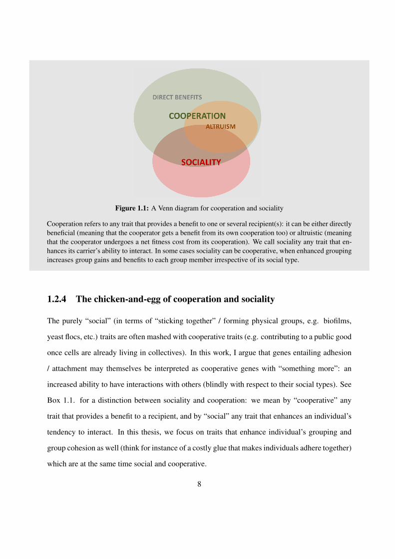
Figure 1.1: A Venn diagram for cooperation and sociality

Cooperation refers to any trait that provides a benefit to one or several recipient(s): it can be either directlybeneficial (meaning that the cooperator gets a benefit from its own cooperation too) or altruistic (meaningthat the cooperator undergoes a net fitness cost from its cooperation). We call sociality any trait that en-hances its carrier’s ability to interact. In some cases sociality can be cooperative, when enhanced groupingincreases group gains and benefits to each group member irrespective of its social type.

1.2.4 The chicken-and-egg of cooperation and sociality

The purely “social” (in terms of “sticking together” / forming physical groups, e.g. biofilms,

yeast flocs, etc.) traits are often mashed with cooperative traits (e.g. contributing to a public good

once cells are already living in collectives). In this work, I argue that genes entailing adhesion

/ attachment may themselves be interpreted as cooperative genes with “something more”: an

increased ability to have interactions with others (blindly with respect to their social types). See

Box 1.1. for a distinction between sociality and cooperation: we mean by “cooperative” any

trait that provides a benefit to a recipient, and by “social” any trait that enhances an individual’s

tendency to interact. In this thesis, we focus on traits that enhance individual’s grouping and

group cohesion as well (think for instance of a costly glue that makes individuals adhere together)

which are at the same time social and cooperative.

8

1.3 Solving the paradox of cooperation

Game theory is the mathematical framework to address decision-making in rational agents able

to adopt several strategies in situations of conflicting interests. In the last few decades, it has

been extended to evolutionary biology to describe competition between genetically encoded be-

haviors. Individuals garner benefits and costs from their interactions, and the frequency of each

trait in the population changes in time with natural selection acting the same way as rational

choice of strategies: if a trait codes for a behavior that benefits its carrier (in terms of relative

reproductive fitness), it will increase in frequency in the population. Here, we review the main

mechanisms suggested in the framework of evolutionary game theory to account for the persis-

tence of paradoxical cooperative traits. Numerours attempts to systematize models and classify

mechanisms have been made (e.g. by Lehmann and Keller (2006); Nowak (2006); West et al.

(2007b)), that bear the ideological standpoints of their authors.

1.3.1 Reciprocity

Modeled on the idea that we humans tend to be more prone to help someone if she has helped

us before, Trivers (1971) suggested direct reciprocation as a driving mechanism for coopera-

tion in humans, encapsulated by the cathphrase “If you scratch my back, I’ll scratch yours”. In

other words: if A helps B, then B helps A. Tit-for-tat strategy was found by Axelrod (1984) to

be more successful than most complex strategies in competitions between humans playing the

Iterated Prisoner’s Dilemma, but how it applies to animal communities and a fortiori microbes is

much less straightforward. Indeed, reciprocation strategies require that interactions are repeated

with the same player, and that the individual is able to recognize her interaction partner, mem-

orize what she did at the previous timestep and react to the outcome of its last encounter. As a

consequence, it remains a very unlikely way toward collective cooperation in microbial species.

Even more cognitively demanding is indirect (reputation-based) reciprocation (Nowak and

9

Sigmund, 1998), that can be summed up as “If I’m seen scratching your back, people will scratch

mine”: C sees A helping B, then C helps A. Indirect reciprocity thus requires that interactions are

conspicuous and that others are able to monitor and memorize what everyone did in the previous

time steps.

A last form coined generalized reciprocity, that relies on lighter constraints, was modeled by

Pfeiffer et al. (2005): “If someone scratch my back, I’ll scratch the next one”: B is helped by

A, B helps C. Individuals base their behavior on their previous encounter, irrespective of their

interaction partner. The requirements are basically the same as before minus the memorizing of

who did what; yet, generalized reciprocity, as well as other (more complex) conditional strategies

(Szolnoki and Perc, 2012), seem out of reach of the simplest organisms.

An other critical shortcoming of reciprocation mechanisms to explain the advent of grouping

features is their dyadic aspect by definition.

1.3.2 Policing (reward / punishment)

Cooperation may be enforced by individuals able to punish free-riders (resp. reward cooperators)

(Clutton-Brock and Parker, 1995). The ability to punish (resp. reward) is itself costly. Once

again, policing requires the ability for individuals to monitor others’ behaviors and to direct

the punishment/reward toward them. Moreover, even though punishment may in principle deter

defection, the survival of the cooperative-punisher type is complicated by “second-order free-

riders”, i.e. cooperators that do not punish (Sigmund, 2007).

While both theoretical (Boyd et al., 2003) and experimental or observational (Fehr and

Gachter, 2002; Flack et al., 2006) studies suggest that policing mechanisms might have an im-

portant role in sustaining collective cooperation in humans and other primates, the evidence of

punishing/rewarding behaviors in microbes remains at best elusive.

10

1.3.3 Interactions directed toward genealogical kin

The rough idea behind interactions directed toward kins is encapsulated in this maxim by J.B.S.

Haldane: “Would I lay down my life to save my brother? No, but I would to save two brothers

or eight cousins”. If for some reason individuals tend to interact mostly with partners that share

genes that are identical by descent to their own (i.e. if the actor and recipient are genealogically

related), then cooperative behaviors may be promoted if the benefit conferred to kins weighted

by the relatedness coefficient between interactants exceeds the cost. This idea is enclosed in

the famous rule of Hamilton: rb > c, which has remained, since Hamilton’s pioneering work

half a century ago, the formulaic rule of thumb to assess the sustainability of helping behaviors

in biological settings (Hamilton, 1964). Yet, its generality is recurrently questioned (Nowak et

al., 2010a) and its application by mis-informed experimenters and theoreticians often inaccurate.

Indeed, the rigorous evaluation of each parameter (r, b and c) is nowhere near as straightforward

as posited by some and rely on complex regression coefficient calculations. For instance, popu-

lation genetics calculations show that the “right” r coefficient does not solely includes genealog-

ical relations, but also the way population is structured and individuals interact. Even though

general (as derived from another totem of population genetics, the Price’s equation (Gardner et

al., 2011)), Hamilton’s rule might be of little use to describe the conditions for the evolution of

cooperation in experiments and analytical models, some claim (Nowak et al., 2010a). Nonethe-

less, Hamilton’s main point remains a milestone in alleviating the challenge of cooperation for

species, as diverse as social insects and many microbial species, characterized by a high level of

inbreeding (e.g. generated from a single lineage).

In any case, what Hamilton’s rule does not say is how individuals are led to interact preferen-

tially with their kins. The two main mechanisms invoked in the literature are kin discrimination

(crudely: individuals are able to recognize their brothers and sisters and interact predominantly

within the family) or spatial structure (when limited dispersal or environment viscosity imply

11

that lineages remain clustered).

1.3.4 Assortment between cooperators

When cooperators tend, for some reason, to interact more with other cooperators than defectors

do, they get a higher average benefit from their interactions that may ultimately offset their

cost (Wilson and Dugatkin, 1997; Fletcher and Doebeli, 2009). Assortment has some overlap

with the previous family of mechanisms (insofar as if cooperating individuals tend to interact

with their kins, de facto they interact with partners likely to share the cooperative gene), but

is more general, the mechanisms liable to make cooperators interact together and not based on

shared ancestry being numerous. The tricky part is to find those mechanisms. A key lies in the

way populations are structured, in terms of spatial structure and interaction structure, motivating

researchers to explore how networks, group shapes etc. influence this degree of assortment (see

sections 1.5 and 1.6). A particular case is when cooperators interact together because they can

identify each other. We refer to the Box 1.2. for a discussion about this issue.

Box 1.2. Green beards

A “green beard” refers to any gene, or set of linked genes, that encodes at the same time for 1) a

given behavior; 2) the ability to recognize other carriers of the green beard; 3) the propensity to direct

the behavior preferentially towards these carriers. The term was first used by Dawkins to make a hy-

pothetical claim (Dawkins, 1976), and examples of green beards proved difficult to find until recently.

For most of them, the “green beard” label remains controversial and one can argue that the three above

requirements are not always fulfilled. Green beards can be either cooperative toward carriers, or spiteful

against non-carriers. Examples of proclaimed green beards include (this list is widely inspired by Brown

and Buckling (2008)):

12

• the csA gene in Dicty (Ponte et al., 1998; Queller et al., 2003) that encodes a cell adhesion protein

that binds to homologous adhesion proteins (cooperative);

• the recognition of kins in Proteus mirabilis (Gibbs et al., 2008) (cooperative);

• the FLO1 gene in S. cerevisiae (Smukalla et al., 2008) between sticky cells, though cooperating

sticky cells can also connect to nonsticky cells, although less probably (cooperative);

• the “queen-killer” allele in red fire ants (Keller and Ross, 1998) (spiteful);

• genes encoding bacteriocins (kind of chemical weapons) that at the same time make their carriers

immune to their effect (Riley and Wertz, 2002) (spiteful);

Green beards may be subject to cheating as, very often, a set of linked genes rather than a single

gene encodes the “beard”: there is thus a risk of invasion by mutants that display the tag without the

costly behavior. A retort to this can be found in the possibility of multiple beard colors (Jansen and

van Baalen, 2006). For instance, the FLO1 gene is known to be highly variable among species (more

or less adhesive). In many cases, it is actually difficult to contend with certainty that a given behavior

relates to a green beard. Indeed, the “preferentially directed” condition is not necessarily needed to get

behaviors that are differentially directed toward carriers or non-carriers. This subtle difference will be

more thoroughly developed later on in chapter 2.

1.3.5 Direct benefits

Although situations in which the evolution of a costly cooperative trait is paradoxical are empha-

sized in the literature, the evolution of cooperation needs not necessarily be a social dilemma.

In some cases, the cost incurred by cooperators is immediately offset by the marginal benefit

they get from their own contribution to the group. In the standard Public Goods Games (sec-

tion 1.4.2), such case would translate as b > Nc. In invertase-secreting yeast, a small proportion

of the hydrolized glucose is retained by the producer, advantaging cooperator cells at low fre-

13

quencies (Gore et al., 2009). Similarly, the bacterium Lactococcus lactis expresses an extracel-

lular protease that helps transform milk proteins into digestible peptides. Bachmann et al. (2011)

showed that such cooperative behavior can persist owing to a small fraction of the peptides being

immediately captured by the proteolytic cells.

1.3.6 Game definition

While the Prisoner’s Dilemma and variations account for a large portion of the archetypal games

used in evolutionary game theory, every social dilemma is actually not as hostile to cooperation.

There are other possible game structures allowing to escape from the paradox of the tragedy of

commons. Sometimes the hypotheses formulated by evolutionary game theory to untangle the

enigma of cooperation make it artificially too challenging compared to real biological situations.

For instance, nonlinear payoff profiles that are more consistent with biological settings than the

(most often used) linear payoffs can alleviate the paradox and account for the sustainability of

cooperative traits very easily, even in the absence of kinship, assortment or external mechanisms.

In the next sections, I review some important findings about the influence of the structure of

interactions (i.e., the “game” that is played), the structure of population and the way group are

defined on the emergence and maintenance of cooperation.

1.4 Game structure

Evolutionary game theory relies on archetypal (some may say artificial) games to capture the

main features of dilemmas encountered in biological populations. Depending on the nature of

interactions, these are played between two or an arbitrary number N of players.

14

1.4.1 Dyadic games

These games relate to pairwise interactions. Individuals can be either cooperators (C) or defec-

tors (D). The interaction results in the allocation of a payoff for each player. Such games can be

summarized with this general payoff matrix:

C D

C (R,R) (S, T )

D (T, S) (P, P )

R stands for “reward” (when both individuals cooperate), S for “sucker” (when a cooperator

is exploited by a defector), T is the “temptation” to cheat and P the “penalty” for no one co-

operating. Depending on the values of R, S, T , P , the expected evolutionary dynamics and

equilibria of populations playing the game in couples change drastically. Readers familiar with

the archetypal dyadic games (Prisoner’s Dilemma, Snowdrift Game, etc.) shall skip the next

paragraphs.

The Prisoner’s Dilemma Two members of a gang A and B are questioned separately by the

police. Cooperating means staying silent; defecting means denouncing the other one to the

police. If both cooperate, each serves a 1-year prison sentence; if each one betrays the other,

they both serve 2 years. If A betrays B and B stays silent, A is set free and B serves 3 years in

prison (and conversely). Therefore, whatever the other guy does, there is a temptation to defect

as it warrants the lighter sentence in any case. However, the best result is obtained when both

cooperate. This game can be summarized as T > R > P > S (plus 2R > T + S in the iterated

form). In the previous example, T = 0, R = −1, P = −2, S = −3. Collective defection (D,D)

is the unique Nash equilibrium (and evolutionay stable strategy) of the game. This game models

situations when a cooperator provides a benefits b > 0 to its interaction partner but pays a cost

c > 0; the payoff matrix can then be re-written as:

15

C D

C b− c −c

D b 0

This game is widely used as a metaphor for any “free-rider” dilemma where cooperation

might be exploited by non-contributing individuals. As cooperation is doomed were no other

assumption made, it is the most challenging, hence the most investigated of all 2-player games.

The Snowdrift Game (a.k.a. Chicken or Hawk-Dove Game) Two drivers are trapped behind

a pile of snow. Someone must shovel off the snow or nobody will come back home; but each

driver is better off if the other one does the job. In this game, T > R > S > P : the only differ-

ence with the Prisoner’s Dilemma is that it is still better to do the work by yourself than waiting

the other guy to do it in vain. It is thus best to do the opposite of the other player. (C,D) and

(D,C) are pure (unstable) Nash equilibria, and there exists a mixed equilibrium that is stable:

this means that in populations where the two types compete, the expected evolutionary equilib-

rium is polymorphic, with one fraction of the population (that depends on the game parameters)

cooperating and the rest defecting. In the context when achieving the common goal provides a

benefit b and doing the whole work costs c, the payoff matrix can be re-written as, for instance:

C D

C b− c/2 b− c

D b 0

The Stag Hunt (a.k.a. Coodination Game:) In this game (less popular in the literature than

the two former), individuals must coordinate to achieve a common goal. Therefore, it is best to

do as the other player does. The payoffs are ranked as followed: R > T > P > S. (C,C) and

(D,D) are both (stable) Nash equilibria, and there exists a mixed equilibrium that is unstable.

In population settings, the outcome is thus dependent on the initial condition: if the proportion

16

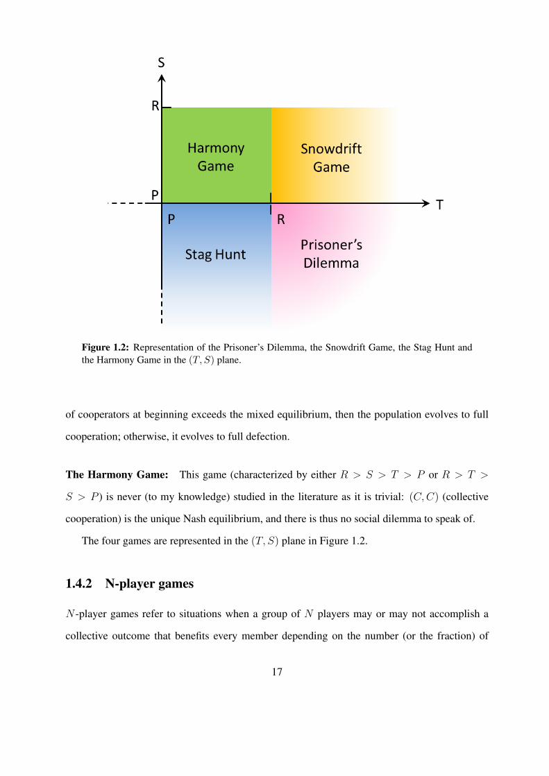
Figure 1.2: Representation of the Prisoner’s Dilemma, the Snowdrift Game, the Stag Hunt andthe Harmony Game in the (T, S) plane.

of cooperators at beginning exceeds the mixed equilibrium, then the population evolves to full

cooperation; otherwise, it evolves to full defection.

The Harmony Game: This game (characterized by either R > S > T > P or R > T >

S > P ) is never (to my knowledge) studied in the literature as it is trivial: (C,C) (collective

cooperation) is the unique Nash equilibrium, and there is thus no social dilemma to speak of.

The four games are represented in the (T, S) plane in Figure 1.2.

1.4.2 N-player games

N -player games refer to situations when a group of N players may or may not accomplish a

collective outcome that benefits every member depending on the number (or the fraction) of

17

cooperators in the group. N -player games are inherently irreductible to the corresponding sum

of dyadic interactions, and are as such different social dilemmas (Perc et al., 2013). In the most

basic case, the population is well-mixed and players meet at random.

The Public Goods Game: The Public Goods Game (PGG) can be seen as a logical extension

of the Prisoner’s Dilemma to interactions between N players. The principle is the following:

each cooperator contributes b to a common goods at a cost c to their fitness; defectors contribute

nothing, and do not undergo any cost. The sum of all contributions in the group is then shared

equally among all members, irrespective of their strategy. The respective payoffs of a cooperator

and a defector, provided m of its N −1 co-members cooperate and N −m−1 free-ride, are thus

PC(m+ 1, N) = bm+ 1

N− c (1.1)

and

PD(m,N) = bm

N(1.2)

Let us now suppose that individuals in the population are randomly distributed into groups

of size N , and let us call x the frequency of cooperators in the population (then, 1 − x is the

frequency of defectors). The expected payoffs PC(N) and PD(N) of each strategy are calculated

summing the payoffs obtained in the situation when there are m cooperators among the N − 1

co-players weighted by the probability(N−1m

)xm (1 − x)N−1−m of it happening with random

18

sampling. The average payoff difference between cooperators and defectors is thus

∆P = PC(N)− PD(N)

=N−1∑m=0

(N − 1

m

)PC(m+ 1, N)xm(1− x)N−1−m

−N−1∑m=0

(N − 1

m

)PD(m,N)xm(1− x)N−1−m

=N−1∑m=0

(N − 1

m

)[bm+ 1

N− c− b

m

N

]∆P =

b

N− c (1.3)

Therefore, under random allocation of players within groups, ∆P does not depend on x. Gen-

erally, b < Nc is assumed, so that the evolution of cooperation is challenging. Otherwise,

cooperation evolves simply by direct benefits. A way to represent PGGs in cases other than

random allocation uses the concept of average interaction environments (Box 1.3.)

Box 1.3. Average interaction environments

I here present the formalism of Fletcher and Doebeli (2009), which will be useful in chapter 2. An

individual’s payoff can be split between a payoff due to self (b/N− c for cooperators, as they get a share

b/N of their own contribution and pay a cost −c, and 0 for defectors) and a payoff due to the group

co-members (b/N × the number of cooperative co-players).

Let us denote eC and eD the average number of cooperative co-players in a cooperator’s (resp.

defector’s) group, then the average payoffs of a cooperator and a defector are:

PC = beCN

+b

N− c

PD = beDN

19

Therefore, if the cooperative trait has no effect on the groups an individual encounters, there is no

assortment between cooperators and defectors and eC = eD: cooperation outcompetes sociality only

when b/N > c, i.e. if cooperation provides a direct benefit to the actor. This case is usually discarded

as trivial in models addressing the evolution of cooperation. When b/N < c, cooperation vanishes at

the evolutionary equilibrium. Hence, for cooperation to be maintained, thus must be a way to obtain

eC > eD (positive assortment).

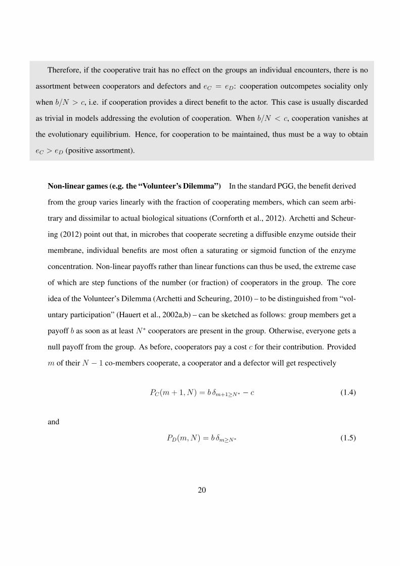
Non-linear games (e.g. the “Volunteer’s Dilemma”) In the standard PGG, the benefit derived

from the group varies linearly with the fraction of cooperating members, which can seem arbi-

trary and dissimilar to actual biological situations (Cornforth et al., 2012). Archetti and Scheur-

ing (2012) point out that, in microbes that cooperate secreting a diffusible enzyme outside their

membrane, individual benefits are most often a saturating or sigmoid function of the enzyme

concentration. Non-linear payoffs rather than linear functions can thus be used, the extreme case

of which are step functions of the number (or fraction) of cooperators in the group. The core

idea of the Volunteer’s Dilemma (Archetti and Scheuring, 2010) – to be distinguished from “vol-

untary participation” (Hauert et al., 2002a,b) – can be sketched as follows: group members get a

payoff b as soon as at least N∗ cooperators are present in the group. Otherwise, everyone gets a

null payoff from the group. As before, cooperators pay a cost c for their contribution. Provided

m of their N − 1 co-members cooperate, a cooperator and a defector will get respectively

PC(m+ 1, N) = b δm+1≥N∗ − c (1.4)

and

PD(m,N) = b δm≥N∗ (1.5)

20

where

δcondition =

1 if condition is met

0 otherwise(1.6)

In the case of random allocation of individuals into groups of size N , the expected payoff

difference is then

∆P = PC(N)− PD(N)

=N−1∑m=0

(N − 1

m

)[PC(m+ 1, N)− PD(m,N)] xm(1− x)N−1−m

= bN−1∑

m=N∗−1

(N − 1

m

)xm(1− x)N−1−m − c

− bN−1∑m=N∗

(N − 1

m

)xm(1− x)N−1−m

∆P = b

(N − 1

N∗ − 1

)xN∗−1(1− x)N−N∗ − c (1.7)

Figure 1.3 displays the payoff difference ∆P as a function of the cooperator frequency x.

When x is too low, the amount of cooperators N∗ required to trigger the common goods b is

unlikely to be reached, so that being a cooperator is unprofitable on average. Conversely, when

x is high, it will most likely be reached anyway so that it is no use to contribute from the point

of view of a focal player. As a consequence, ∆P is positive in a range [xthres, xpoly], where the

incentive is strong enough to justify cooperation. In addition to stable equilibria x = 0 and x = 1,

the replicator equation has thus one unstable equilibrium xthres and one stable polymorphic

equilibrium xpoly. This means that as soon as a frequency xthres is reached in the population,

cooperators rise in frequency until x = xpoly and the stable population is a mixture of cooperators

and defectors.

The lesson to be learned from this simple game is that even in the absence of kinship and

assortative mechanisms, a certain level of cooperation may be stable provided benefits retrieved

21

Figure 1.3: Payoff difference between cooperators and defectors in a threshold game.

Apart from the absorbing states x = 0 and x = 1, the game has two interior equilibria, oneunstable and one stable. Thus, cooperation rises in frequency from a threshold value xthres untilit reaches a value xpoly. Parameters values: b = 20, c = 1, N = 10, N∗ = 4

from groups do not increase linearly (Archetti and Scheuring, 2012). While a plausible expla-

nation for the persisting presence of helping behaviors in biological populations, this way out

of the puzzle of cooperation might be nuanced in the case of large groups, as the range where

cooperation is promoted shrinks when group size increases given a fixed benefit-to-cost ratio b/c

(Fig. 1.4).

1.4.3 The difficulty finding the right game

How biological dilemmas relate to such abstract games is often unclear. In an interesting exper-

iment on yeast, Gore et al. (2009) claim to have found a microbiological instance of a Snowdrift

Game (SD). Wild-type yeast breaks the sucrose in their medium into fructose and glucose they

22

Figure 1.4: Payoff difference between cooperators and defectors in a threshold game when Nvaries.

Cooperation has to reach an increasingly higher threshold frequency as the group size increases,and when it does it stabilizes to smaller frequency equilibrium levels. Parameters values: b = 20,c = 1. N ranges from 10 to 100, and the threshold N∗ is kept proportional to N (thus rangingfrom 4 to 40).

can more easily feed on. However, while doing so, 99% of the glucose and fructose escape

diffusing in the medium when only 1% is imported in the cytoplasm of the invertase-producing

cell, therefore exposing the producing type to exploitation by nonproducers. Gore et al. (2009)

mixed one WT cooperative strain of yeast and one mutant defective type lacking the invertase

gene, with various starting frequencies of each. They found out that each type tends to rise in

frequency when initially rare, reaching an equilibrium level that depends only on the cost of

cooperation, and not on the initial frequencies. They explain that the growth rate is a concave

function of glucose, that is, marginal growth gains for getting more glucose tend to decrease as

its concentration increases. Therefore, defectors, that have a hard time to thrive when coopera-

23

tion is rare, can persist when it reaches a threshold level in the population and outcompete them

for high levels. The authors interpreted such striking example of coexistence between coopera-

tors and defectors as the effect of a SD played between yeast cells. However, this conclusion is

debated. Archetti and Scheuring (2012) assert that the SD is inappropriate to account for such

instance of frequency-dependent selection as it is primarily a 2-player game, unlike interactions

in yeast. They also point out that in the SD, the maximal cumulated payoff for all players is

obtained in the case of total cooperation (citing MacLean et al. (2010)), while the experiments

found that the maximal value for the total population growth was obtained for an intermediate

frequency of producers. Their two points are however questionable:

1) The SD can be easily extended to N -player interactions. Coming back to the metaphor

that gives its name to the game, if N∗ cooperators are required to shovel off the snow, the payoff

assigned to a cooperator (resp. defector) in the N -player SD game could be, if there are m

cooperators within the N − 1 focal player’s co-members:

PC(m+ 1, N) = b δm+1≥N∗ − c

m+ 1(1.8)

and

PD(m,N) = b δm≥N∗ (1.9)

However, general formulations of the SD such as the former generally imply that the cost

payed by a cooperator decreases with the number of cooperators within the group (here, c/(m+

1)); it is unsure wether or not such property applies to invertase production in yeast.

2) The maximal cumulated payoff for all players is not necessarily obtained in the case of

total cooperation: while it does so for the usual, handbook payoff matrix of 2-player SD (in

which the cost payed by each of two interacting cooperators is half that of the cost payed by a

cooperator alone), such assertion does not hold anymore – as MacLean et al. (2010) themselves

observe – for variants that are still SDs, e.g. games represented by the payoff matrix

24

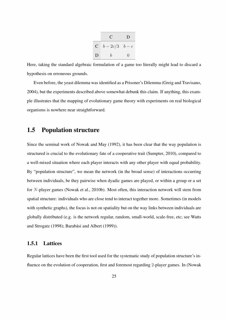
C D

C b− 2c/3 b− c

D b 0

Here, taking the standard algebraic formulation of a game too literally might lead to discard a

hypothesis on erroneous grounds.

Even before, the yeast dilemma was identified as a Prisoner’s Dilemma (Greig and Travisano,

2004), but the experiments described above somewhat debunk this claim. If anything, this exam-

ple illustrates that the mapping of evolutionary game theory with experiments on real biological

organisms is nowhere near straightforward.

1.5 Population structure

Since the seminal work of Nowak and May (1992), it has been clear that the way population is

structured is crucial to the evolutionary fate of a cooperative trait (Sumpter, 2010), compared to

a well-mixed situation where each player interacts with any other player with equal probability.

By “population structure”, we mean the network (in the broad sense) of interactions occurring

between individuals, be they pairwise when dyadic games are played, or within a group or a set

for N -player games (Nowak et al., 2010b). Most often, this interaction network will stem from

spatial structure: individuals who are close tend to interact together more. Sometimes (in models

with synthetic graphs), the focus is not on spatiality but on the way links between individuals are

globally distributed (e.g. is the network regular, random, small-world, scale-free, etc; see Watts

and Strogatz (1998); Barabasi and Albert (1999)).

1.5.1 Lattices

Regular lattices have been the first tool used for the systematic study of population structure’s in-

fluence on the evolution of cooperation, first and foremost regarding 2-player games. In (Nowak

25

and May, 1992), each site is occupied by one player, either a cooperator or a defector. Every

generation, each individual plays a Prisoner’s Dilemma with its immediate neighbors, and its

total payoff is the sum of payoffs in each game. Population is updated changing the strategy

in each site to that of the most successful player in the neighborhood. Nowak and May (1992)

showed that such simple rules suffice to obtain coexistence between cooperators and defectors in

a large range of parameters, as well as a wide variety of spatial patterns, from stable cooperating

clusters in a sea of defectors to chaotic “Turkish carpet”-looking repartition of each type on the

lattice. Possibly owing as much to the beauty of the figures as the main message (spatial structure

is key to facilitate the stability of cooperation), this work has stimulated an important amount of

work to explore the dynamics made possible by more convoluted strategies, lattice structures, or

update rules, to such an extent that the field of the evolution of cooperation in spatially-structured

populations has taken a life on its own (some would lament, faraway from realistic biological

settings, e.g. Leimar and Hammerstein (2006)). Since then, the main properties of the PD on

lattices have been thoroughly explored, and the ability for players to be mobile, tested (e.g. by

Vainstein et al. (2007); Roca and Helbing (2011)). The main idea to retain from this subset of the

literature on social evolution is that spatial structure may generate self-organized clusters of co-

operators that are robust to exploitation at their border. Or, more crudely: spatiality may generate

assortment between cooperators (or relatedness – in the broad sense of the word –, depending

on who is talking). The range of parameters in which cooperation survives is itself dependent

both on the update rule (deterministic or stochastic) and the lattice clustering coefficient. When

N -player, rather than dyadic games, are played however (e.g., when each player takes part in k

Public Goods Games, k being the degree of the lattice), the topological properties of the lattice

become irrelevant because group interactions effectively link non-directed connected players to-

gether. I refer to Doebeli and Hauert (2005) and Perc et al. (2013) for reviews on social evolution

on lattices.

26

1.5.2 Graphs

Lattices define very constrained interaction structures. To disentangle the effects of spatial struc-

ture implied by lattices from that of the number of neighbors of each individual, researchers have

implemented evolutionary games on random homogeneous graphs (i.e. where each node has the

same number k of links). They evidenced that it makes little difference with lattices on the equi-

libria obtained when the game is a Prisoner’s Dilemma, though it favors cooperation in the Stag

Hunt and inhibits it in the Snowdrift Game (Roca et al., 2009). More dramatic is the effect of

degree heterogeneity (“heterogeneous graphs”). Santos et al. (2006) showed that the more het-

erogeneous is the pattern of connectivity, the more cooperation is likely to take over. Pinheiro

et al. (2012) indeed showed that individuals playing the Prisoner’s Dilemma at the microscopic

level in a structured population was somewhat equivalent to them playing a Snowdrift Game (in

homogeneous networks) or a coordination game (in heterogeneous networks) at the macroscopic

(population-wide) level. The same team then pushed the analysis to N -player games (Santos et

al., 2008). In their model, each node i plays ki Public Goods Games, where ki is its degree. They

tested two different cases: (1) the cost applies to each case (i.e., the more links a cooperator has,

the higher the cost); (2) the cost is fixed for one player (i.e., a cooperator divides a fixed cost

c between all its links). Their work shows that cooperation is enhanced for heterogenous net-

works (compared to regular graphs) because of the major influence of cooperative hubs, and that

it does so in a larger parameter range in case (2) than in case (1). As for lattices, the science of

network cooperation has bloomed since then; notably, many studies have implemented complex

degree-based policies for cooperation, as well as the possible coevolution of cooperation and link

formation (see the reviews by Perc et al. (2013) and Perc and Szolnoki (2010), respectively).

27

1.5.3 Continuous space

More recently, models have started to consider pairwise or group interactions as emerging from

the spatial reallocation of mobile individuals in a continuous 2D space. The purpose of these

models is twofold: 1) they allow to specify the origin of interactions in a more realistic way.

Indeed, most social organisms are mobile (from microbes such as Myxobacteria to humans) and

by moving they find new interactions; models in continuous space can thus in principle draw

inspiration from real life data on motion and be implemented within an evolutionary frame-

work. Theoretical descriptions of animal aggregation are commonplace in fields such as ecology

or statistical physics, but are only beginning to permeate social evolution theory. 2) They are

instrinsically dynamic, unlike lattices models in which groups are fixed and most models on

graphs (except coevolutionary models or cases when a specific grouping behavior is associated

to cooperation, e.g. in Pacheco et al. (2006)): the emphasis made on movement implies that an

individual’s interaction network may change at each time step. Meloni et al. (2009) designed a

model where individuals, either cooperators or defectors, are mere random walkers that play a

Prisoner’s Dilemma with their neighbors within some radius at each timestep. Individuals update

their strategies imitating one of their neighbors with a probability that depends on the difference

of their payoffs. In this simple setting, cooperation is able to arise thanks to cooperative clusters

forming by chance and slowly expanding by successive victories against defective individuals in

their immediate surroundings. Later, Cardillo et al. (2012) expanded this framework to Public

Goods Games. Another set of rules for movement based on flocking in birds has been used by

Chen et al. (2011a,b). Note that in all these models, the groups in which the games are played

overlap (cf. section 1.6.2), and movement is uncorrelated from the evolutionary dynamics, un-

like some models on lattices. A model of aggregation where these two assumptions are relaxed

will be described in chapter 3 of this manuscript to study the evolution of social adhesion traits.

28

1.6 Group structure

1.6.1 Groups as equivalence classes

Possibly inspired by the ecological literature, many models for the evolution of cooperation

consider groups as separate entities, with, possibly, occasional migration between them. This

assumption is in accordance with many biological systems, such as animals foraging in distinct

herds, or slime moulds, to name but a few examples. Actually, an important part of the theoretical

literature in the field deals with competing individuals within competing groups, raising the issue

of potential conflicts between levels of biological organization (Wilson, 1975; Chuang et al.,

2009). The range of models that explicitely assume groups as a partition (in the mathematical

sense) of the population is too large to review it properly in a few lines; among these works, let us

cite arbitrarily the papers by Wilson and Dugatkin (1997); Aviles (2002); Hauert et al. (2002a);

Fletcher and Zwick (2004); Killingback et al. (2006); Traulsen and Nowak (2006); van Veelen

et al. (2010); Powers et al. (2011); Cremer et al. (2012). A notable feature of most models with

separate groups (though exceptions can be found in those just mentioned) is that they assume

group size is fixed. What is a convenient hypothesis for analytical calculations may however

obfuscate the role of distributed group sizes on the onset and maintenance of cooperative traits, as

pointed out by Pena (2012), who studied games in groups of cooperators and defectors obeying

an externally imposed size distribution. I refer to the small opening review of chapter 2 for a

discussion of works displaying varying group sizes.

1.6.2 Groups as sets

Rather than considering groups that are separate, non-overlapping entities, recent work suggested

that allowing individuals to belong to several groups at a time may be more relevant to address

social dilemmas. This observation is particularly appropriate for us humans, as we tend to take

29

part in numerous collective activities, be they within the family, at work, or in our leisure time.

Under this hypothesis, groups are called “sets” and the encompassing framework “evolutionary

set theory” (Tarnita et al., 2009). Sets can in principle be of any size and one set can be a subset

of an other set. Tarnita et al. (2009) designed a model in which individuals play the Prisoner’s

Dilemma in a set structure and where both their strategy (cooperator or defector) and their set

membership are subject to updating through imitation. They calculated the critical benefit-to-

cost ratio from which cooperation outcompetes defection in the particular case when individuals

all belong to the same number of sets K. They showed that, given a number of sets M in

the population, cooperation evolves more easily the smaller K is. This result is relaxed when

cooperators only cooperate provided they share a minimum number L of sets with their partners:

in this case, belonging to more sets proves advantageous to evolve cooperation. It is difficult,

though, to assess the scope of such theoretical in non-human animals and, a fortiori, microbial

communities, as the initial assumptions of individuals belonging to several distinct collective

endeavors is not much discussed empirically. Indeed, even though microbes do participate in

several social dilemmas at once (e.g. Myxobacteria or Pseudomonas mentioned above), the

model of Tarnita et al. only makes predictions in the case when cooperation applies the same

way to each of them (i.e., an individual is either cooperative in all sets or defective in all sets).

Cooperative behaviors in microorganic populations rather relate to different mechanisms at the

molecular level: a cell is not cooperative or defective per se, but relative to one specific social

need (and, arguably, to a specific ecological context, but this is out of the scope of my discussion).

1.6.3 Non-delimited groups

In some theoretical works on social evolution, there is no defined group, although the inter-

actions are not dyadic either: instances of these are models of individuals producing a public

goods substance in their medium that is available to all individuals in the vicinity. Such models

are more readily comparable to biological situations such as Pseudomonas competing for the

30

access to siderophores. Driscoll and Pepper (2010) have developed a general framework that

combines the physics of diffusion with a game-theoretical model. They show that the success of

the “producer” type depends on the diffusion coefficient of the secreted compound and its uptake

rate. Low diffusions favor producers as they prevent the substance to be shared too much with

defectors, enabling production to evolve by direct benefits; similarly, high uptake rates ensure

that producers deplete the substance sufficiently for themselves before it reaches the free-riding

nonproducers. This work makes an important point stressing the continuum between private and

public goods, and that public goods, non-excludable as they are, may in some conditions pro-

vide enough direct benefits to offset production costs. Here, spatial structure and environment

viscosity entail that the goods is differentially shared with others according to their distance. In

an other instance of model for the diffusion of a resource in space, Borenstein et al. (2013) chal-

lenge the conclusions of classic spatial models displaying frequent coexistence of cooperators

and defectors by spatial clustering of uninvadable clusters of cooperators. They claim that the

main assumption of such works, namely the nearest-neighbors interaction rule, artificially gen-

erates coexistence while more realistic hypotheses generate longe-range interaction that disrupt

it.

1.7 Outline

In this work, I will try to assess the conditions for the emergence and persistence of an individ-

ually costly trait that enhances grouping tendency and supports group cohesion. This will lead

me to emphasize the mechanics of aggregation as a decisive feature – yet generally overlooked

in the literature – for the sustainability of social traits. More specifically, the following questions

will be addressed:

• how does selection act on population structure through the traits underpinning group for-

mation?

31

• how do the structure of the population and its social composition feed back onto each

other?

• is the existence of a biologically trait that at the same time enhances individual attachment

and benefits groups plausible?

• what if sociality is a continuously regulated feature, rather than an on/off individual char-

acteristic?

• is the “social dilemma” necessarily a dilemma? How does it relate to population structure?

• what are the microscopic features that promote, or hinder sociality?

• is preferentially directed attachment to carriers of the social trait necessary for social indi-

viduals to persist?

• to what extent are the modeling results consistent with observations on actual microbial

population structures?

In chapter 2, I describe a general framework to assess the evolution of a social trait in an

arbitrary group formation configuration, using group size distributions experienced by distinct

social types as a proxy to infer their evolutionary fates. I introduce a toy model for aggregation

to pinpoint how costly sociality can evolve with minimal hypotheses for individual interactions,

suggesting a mechanistic scenario for its emergence ahead of more sophisticated collective be-

havior. I then explore the evolutionary dynamics under weaker hypotheses, namely by relaxing

the coupling between aggregation and in-group behavior and the characterization of sociality by

a discrete trait.

In chapter 3, I embed the former framework in a generic class of group formation processes

intended to capture the main features of microbial aggregation. I decipher the evolutionary out-

come of a social mutation by means of appropriately defined macroscopic observables reflecting

the social composition of the population. I precise the ecological and microscopic conditions on

individual motion and interaction necessary to support sociality. Finally, I relax the hypothesis

32

of the existence of a pre-defined life cycle assumed until then.

In chapter 4, I discuss the main results of chapters 2 and 3 in the light of the aforementioned

questions, and sketch possible extensions of the work and open questions.

33

Chapter 2

Group formation and the evolution of

sociality

Sections 2.1, 2.2, 2.3 and parts of the discussion are adapted from “Garcia, T., and De Monte, S.

2013. Group formation and the evolution of sociality. Evolution, 67, 131-141.” The analysis of

section 2.5.4 was performed in collaboration with Guilhem Doulcier during his internship in the

lab. He also made Figures 2.10 and 2.11 and the computer code to generate them.

2.1 Introduction

The emergence and persistence of social ventures, where individuals concur to the sustainment of

a community at a personal cost, has been classically addressed in a game-theoretical framework.

The evolution of cooperation was first formalized in the context of dyadic interactions, where the

formation of pairs and the accomplishment of the game are concomitant. When individuals play

in couple, several mechanisms effectively promote cooperation even for a Prisoner’s Dilemma

type of interactions, where it is always in one own’s interest to defect in a single round of the

game (cf. section 1.4.1). Cooperators can thrive provided they interact preferentially with other

35

cooperators, e.g. via the knowledge of the co-player’s past behavior (Trivers, 1971; Axelrod and

Hamilton, 1981), reputation (Nowak and Sigmund, 1998), spatial structure (Nowak and May,

1992), or mechanisms enhancing individuals’ interactions with kins (Hamilton, 1964).

Those results have then been extended to games involving N > 2 players, where the Public

Goods Game (PGG) plays the same prototypic role as the Prisoner’s Dilemma (Kollock, 1998;

Doebeli and Hauert, 2005). The PGG formalizes the so-called tragedy of the commons (Hardin,

1968; Rankin et al., 2007), whereby cheaters who do not contribute to the public goods are

always better off, in a one-shot game, than cooperators who pay a cost to sustain the collective

entreprise (cf. section 1.4.2)

Sociality, however, relates not only to the act of helping others, but also affects the context

where social games are played, among which the way groups are formed in the first place. In

extending the framework from 2-player to N -player games, the processes that lead to group

formation have often been overlooked and group size generally held constant.

This assumption has been recently relaxed in different ways. Group size variations can be

externally forced by imposing bottlenecks that periodically increase the variance among groups

(Chuang et al., 2009), leading to a “Simpson’s paradox” in which cooperation is disavantaged

locally but a winning strategy on the whole (Wilson, 1975). They can also result from demo-

graphic fluctuations (Hauert et al., 2006a) or facultative participation to the game (Hauert et al.,

2002a,b). The effect of a fixed group size distribution with binomial allocation of individuals

within groups has also been investigated in various types of games and can either promote or

hinder cooperation (Pena, 2012).

Group size can be directly affected by traits that co-evolve with cooperation. Pfeiffer and

Bonhoeffer (2003) illustrated how group clustering (defined in terms of spatial proximity) is

selected together with nonexploiting, cooperative behavior if resources are sufficiently concen-

trated. Aviles and co-workers (Aviles, 2002; van Veelen et al., 2010) showed that grouping

tendency and cooperativeness may be favored jointly, resulting in the emergence of viable co-

36

operative groups. This result relies on two features of the model: on the one hand, while coop-

eration is costly, the ability to join groups is not ; thus, as soon as some cooperators are present

in the population, individuals are better off in a group than alone, making the lonely lifestyle

unprofitable and the dispersed population structure unstable. On the other hand, the introduction

of a hump-shaped fitness function implies from the start the existence of intermediate optimal

group sizes, at fixed average level of cooperation within the group. The cheating load is then

twofold: “freeloaders” both hamper the benefits retrieved from the group and crowd them use-

lessly. Powers et al. (2011) similarly evidenced that inheritable aggregative features may evolve

together with cooperation. They let players have a clear-cut group size preference, whereby

groups form by gathering individuals that share the same preference. In their model, cooperation

ends up being tightly linked with small group sizes that support it more easily, even when direct

selection pressures for large groups or weaker selection against cooperation is applied.

In line with these studies, I address here the evolution of aggregative traits in a context that

is dynamically shaped by the traits themselves. Such traits require an individual investment and

produce collective benefits, and can therefore be regarded as cooperative once individuals have

been allocated in groups by the aggregation process. The quest for simple mechanisms that allow

grouping tendency to evolve is of particular relevance to understand sociality in microrganisms,

where individuals interact in clusters of many individuals, a setting that is recognized as unfa-

vorable to social ventures (Olson, 1971). In this model, individuals have different propensities to

form cohesive aggregates, and group cohesion itself is a common good. Individuals are endowed

with a unique gene that codes for a costly trait (coined hereafter sociality). The social trait pro-

motes aggregative cohesion during both the group formation process and the reproductive stage,

where the fitness is the individual payoff in a PGG. The outcome of the social interaction is thus

considered to hinge upon the physical properties of the groups: more cohesive groups are fitter

than groups weakened by looser attachment of their members.

This setting is relevant at least for several microbial organisms usually taken as examples of

37

primitive social behavior (Crespi, 2001; West et al., 2006; Smukalla et al., 2008; Nanjundiah and

Sathe, 2011), where physical stickiness is coupled to cooperative behavior once aggregates are

formed. For instance, in D. discoideum populations, chimeras composed of aggregative wild type

(WT) and non-aggregative mutants produce slugs whose motility increases with the proportion

of WT cells (Inouye, personal communication). In D. discoideum, slug motility allows more

effecient chemo- and phototaxis, benefiting all cells equally. In Myxobacteria as well, WT’s

social motility multigene system enables cell clumping. The presence of mutants deprived of

this social ability impairs swarming and ultimately mar individual fitness in the group.

To evolve, an altruistic trait must ultimately entail some kind of assortment between its bear-

ers (Fletcher and Doebeli, 2009). When the gene giving rise to such assortment also codes for

cooperative behavior, it is framed under the term of “green beards” (Dawkins, 1976; Gardner and

West, 2010) (see Box 1.2.). This general definition actually brings together very different mech-

anisms able to generate assortment, based or not on direct recognition of others’ traits. Here,

no recognition is involved but assortment emerges spontaneously from blind interactions among

individual players. The environment is in this case shaped by the group formation process and

changes jointly with the frequency of the social strategy. The advent of sociality stems from

merely quantitative differences in the probabilities of attachment, so that even mechanisms that

do not produce assortment within groups of fixed size can lead to its evolution if group sizes are

distributed.

Section 2.2 describes the evolutionary consequences of group formation schemes where so-

cial and asocial individuals differ quantitatively in their ability to aggregate. Group formation

is considered a “black box” generating the group size distributions experienced by players. The

average fitness advantage of sociality depends on the distributions of group sizes experienced by

players of each strategy. I derive the condition for sociality to outcompete asociality under the

assumption that no nepotistic grouping between social individuals generates assortment a priori.

Section 2.3 applies the results of section 2.2 to a toy model based on differential attachment and

38

shows that full sociality in a population can be attained, along with sizeable average group sizes,

as soon as a threshold frequency of socials is overcome. The role of lonely individuals, usually

neglected when fixed group sizes are considered, is also stressed in the balance of benefits and

costs of the social game. I eventually point out that the described mechanism for explaining

sociality does not condemn large social groups, and may thus be relevant to account for sociality

in microorganisms. Different interaction rules leading to nonzero a priori assortment are briefly

addressed by numerical simulation. In section 2.4, I relax the hypothesis made on the coupling

of sociality in the aggregation phase and cooperation in the PGG considering four distinct strate-

gies. In section 2.5, I adapt the model to the case when the social trait can vary continuously and

the evolutionary dynamics is computed in an adaptive dynamics framework. In section 2.6, I dis-

cuss the implications of these results for biological systems and the perspectives in elucidating

the mechanistic basis of group formation processes.

2.2 General formulation

2.2.1 Hypotheses

It is assumed that group formation happens at a much faster time scales than evolutionary

changes. Individuals undergo life cycles that consist of 1) a phase of aggregation; 2) a phase of

differential reproduction that modifies the frequencies of each type in the following generation;

3) a dispersal phase (see Fig. 2.1). The whole population is re-shuffled at each generation, unlike

models involving lasting groups (Fletcher and Zwick, 2004; Killingback et al., 2006; Traulsen

and Nowak, 2006). Sociality consists primarily in a quantitative difference in the ability to ag-

gregate, that affects both the group formation phase and the competitive success of aggregates.

Once groups are formed, their cohesion constitutes a public good, so that groups composed of a

larger fraction of cohesive individuals confer more benefits to their members.

39

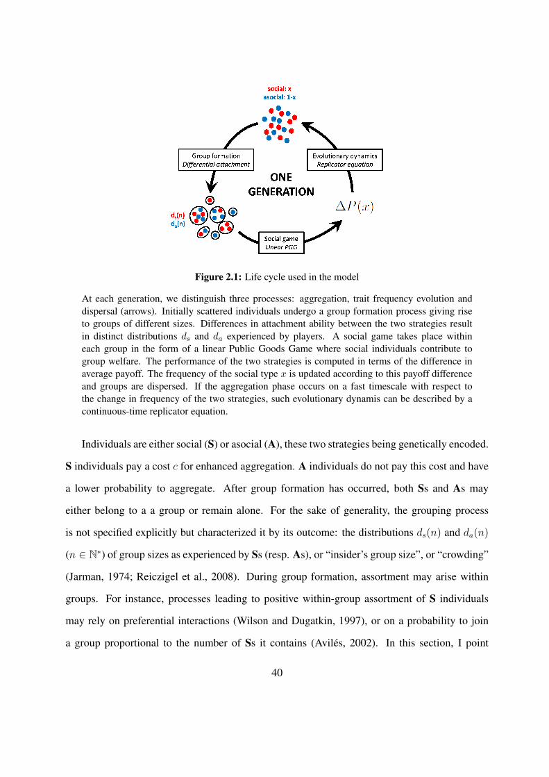
Figure 2.1: Life cycle used in the model

At each generation, we distinguish three processes: aggregation, trait frequency evolution anddispersal (arrows). Initially scattered individuals undergo a group formation process giving riseto groups of different sizes. Differences in attachment ability between the two strategies resultin distinct distributions ds and da experienced by players. A social game takes place withineach group in the form of a linear Public Goods Game where social individuals contribute togroup welfare. The performance of the two strategies is computed in terms of the difference inaverage payoff. The frequency of the social type x is updated according to this payoff differenceand groups are dispersed. If the aggregation phase occurs on a fast timescale with respect tothe change in frequency of the two strategies, such evolutionary dynamis can be described by acontinuous-time replicator equation.

Individuals are either social (S) or asocial (A), these two strategies being genetically encoded.

S individuals pay a cost c for enhanced aggregation. A individuals do not pay this cost and have

a lower probability to aggregate. After group formation has occurred, both Ss and As may

either belong to a a group or remain alone. For the sake of generality, the grouping process

is not specified explicitly but characterized it by its outcome: the distributions ds(n) and da(n)

(n ∈ N∗) of group sizes as experienced by Ss (resp. As), or “insider’s group size”, or “crowding”

(Jarman, 1974; Reiczigel et al., 2008). During group formation, assortment may arise within

groups. For instance, processes leading to positive within-group assortment of S individuals

may rely on preferential interactions (Wilson and Dugatkin, 1997), or on a probability to join

a group proportional to the number of Ss it contains (Aviles, 2002). In this section, I point

40

out that whereas some kind of assortment is necessary for sociality to evolve, no preferentially

assortative feature needs to be assumed a priori as soon as the group size is not fixed; as such, it

is compatible with the scenario where groups form by random and blind interaction processes.

Once groups are assembled, S players contribute b to a linear Public Goods Game (PGG),

whereas A players do not contribute. In a group of size n with m social players, all individuals

thus gain bm/n irrespective of their strategy. Different choices of the gain function (notably

accounting for discount or synergy, as in Hauert et al. (2006b); Archetti and Scheuring (2010);

Cornforth et al. (2012)) are possible, but I opt here for the standard linear formulation, so as

to focus only on the nonlinearities generated by the aggregation process. Thus, no group size

is inherently beneficial to group members, and the payoff only depends on the proportion and

not on the absolute number of Ss in a group. This is a conservative hypothesis since any payoff

function increasing with group size would be further favored whenever sociality is associated

with larger groups.

2.2.2 Payoff difference for a general aggregation process

Let us compute the average payoff of each strategy in a population where a fraction x of individ-

uals is social and a fraction (1−x) is asocial. After the aggregation process, Ss and As belong to

groups of variable sizes. A PGG is played within each group, and the resulting average payoffs

for both types determines the change in their frequencies at the next generation.

Consider first groups of size n (n ≥ 2). Following Fletcher and Doebeli (2009), individual

payoffs are split in a part due to self and an other due to the interaction environment, that depends

only on the composition of the group (Box 1.3.). The payoff due to self is b/n−c for an S player,

who pays a cost −c for sociality and gets a share b/n of its own contribution to the common

goods; for an A player, who does not contribute to the PGG, it is 0.

For a linear PGG, the payoff due to the interaction environment is proportional to the average

number es(n) (resp. ea(n)) of Ss among the n− 1 coplayers of an S (resp. A) player, so that the

41

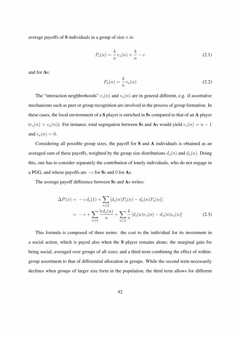
average payoffs of S individuals in a group of size n is:

Ps(n) =b

nes(n) +

b

n− c (2.1)

and for As:

Pa(n) =b

nea(n) (2.2)

The “interaction neighborhoods” es(n) and ea(n) are in general different, e.g. if assortative

mechanisms such as peer or group recognition are involved in the process of group formation. In

these cases, the local environment of a S player is enriched in Ss compared to that of an A player

(es(n) > ea(n)). For instance, total segregation between Ss and As would yield es(n) = n − 1

and ea(n) = 0.

Considering all possible group sizes, the payoff for S and A individuals is obtained as an

averaged sum of these payoffs, weighted by the group size distributions ds(n) and da(n). Doing

this, one has to consider separately the contribution of lonely individuals, who do not engage in

a PGG, and whose payoffs are −c for Ss and 0 for As.

The average payoff difference between Ss and As writes:

∆P (x) = − c ds(1) +∑n≥2

[ds(n)Ps(n)− da(n)Pa(n)]

= − c+∑n≥2

b ds(n)

n+∑n≥2

b

n[ds(n)es(n)− da(n)ea(n)] (2.3)

This formula is composed of three terms: the cost to the individual for its investment in

a social action, which is payed also when the S player remains alone; the marginal gain for

being social, averaged over groups of all sizes; and a third term combining the effect of within-

group assortment to that of differential allocation in groups. While the second term necessarily

declines when groups of larger size form in the population, the third term allows for different

42

repartitions between groups (ds and da) to compensate for unfavorable average interaction envi-

ronment within groups of a given size. This compensatory effect may in principle even overcome

negative within-group assortment (i.e. ea(n) > es(n)).

When only one group size is present in the population, from eq. (2.3) one immediately re-

trieves the condition for the evolution of sociality found by Fletcher and Doebeli (2009). In case

group formation is governed by an extreme recognition process leading Ss to form groups only

with their kind (es(n) = n − 1 and ea(n) = 0 for all n), the condition ∆P (x) > 0 reduces to

b/c > 1/(1 − ds(1)). Were no individual left alone, b > c suffices in this case for sociality to

evolve.

2.2.3 Payoff difference: case of no assortment a priori

When groups of different size are present, sociality can however thrive even in the absence of

such within-group assortment, i.e. when es(n) = ea(n) for all n ≥ 2. I refer to Appendix A for a

treatment of the most general case (unspecified assortment). In the case of random within-group

repartition, the interaction neighborhoods are equal:

es(n) = ea(n) = (n− 1) p(s|n) (2.4)

with p(s|n) the fraction of social players within groups of size n. Given the distributions ds(n)

and da(n), this equates to the quotient of the probability ds(n) x to pick a S individual that

belongs to a group of size n and the probability ds(n)x+ da(n) (1− x) to pick anyone (S or A)

that belongs to a group of size n:

p(s|n) = ds(n)x

ds(n)x+ da(n) (1− x)(2.5)

43

Hence, eqs. (2.3), (2.4) and (2.5) yield:

∆P (x) = −c++∞∑n=2

b

n

[(n− 1)

(ds(n)− da(n))x

(ds(n)− da(n))x+ da(n)+ 1

]ds(n) (2.6)

Note that the population composition x and the aggregation rules, which together determine

the distributions ds and da, are held fixed during group formation.

The fraction of S players will increase in the next generation whenever ∆P (x) is positive,

and the evolutionary equilibria xeq of the system are those such that ∆P (xeq) = 0. A condition

for sociality to be favored when initially absent in the population writes ∆P (x = 0) > 0 i.e.

b∑

n≥2 ds(n)/n > c. It is also the requirement for sociality to evolve when grouping tendencies

are equal for both strategies (ds(n) = da(n) ∀ n) and can be interpreted as the condition for so-

ciality to pertain to directly beneficial cooperation (see Box 2.2. of section 2.3.3). As illustrated

by a toy model in the next section, sociality may be favored even when it is altruistic as soon

as the distributions da(n) and ds(n) experienced by the two strategies differ sufficiently. In the

following, selection is assumed to be weak enough to guarantee a small change in frequencies

from one generation to the next. The evolutionary dynamics is in this case approximated by

a continuous-time replicator equation (Taylor and Jonker, 1978; Schuster and Sigmund, 1983;

Hofbauer and Sigmund, 1998) (see Box 2.1.):

x ∝ x (1− x)∆P (x), (2.7)

where the aggregation phase occurs infinitely fast with respect to evolutionary changes. If the

time scales of aggregation and evolution were not separated, the evolutionary dynamics would be

more correctly described by a discrete-time replicator equation that displays a potentially much

more complex behavior (Villone et al., 2011).

44

Box 2.1. The replicator equation

The replicator equation is a fundamental equation to describe evolutionary dynamics with frequency-

dependent selection. It was introduced by Taylor and Jonker (1978) (but see also Hofbauer and Sigmund

(1998)). Let us consider n strategies that coexist in the population, and let us denote x = (x1, . . . , xn)

their respective frequencies (so that∑n

i=1 xi = 1). In its most common form, the replicator equation

does not allow for mutations (but see below), so that a strategy that is missing initially remains absent.

The general form can be written as a system of coupled differential equations as follows; for each

i = 1 . . . n,

xi = xi

(fi(x)− f(x)

)(2.8)

where fi(x) is the fitness of strategy i (that depends on the population state x) and f(x) =∑n

i=1 xifi(x)

is the average population fitness. The interpretation is straightforward: the relative variation in evolu-

tionary time xi/xi of the strategy i’s frequency is obtained comparing its finess to that of the global

population. The set Sn of the n-tuples (x1, . . . , xn) such that∑n

i=1 xi = 1, called n-dimensional sim-

plex, is invariant under replicator dynamics, which ensures consistency with the biological interpretation.

Each corner point of the simplex is an equilibrium (corresponding of a monomorphic population with

one of the n strategies).

The replicator equation describes selection only, with neither drift nor mutation. It also relies on the

hypothesis that the population is infinite (although there exists a discrete form, see for instance Villone

et al. (2011)). In the case of two strategies S and A with respective frequencies x and 1− x and average

payoffs PS(x) and PA(x) examined here, the equation can be simplified as follows:

x ∝ x [PS(x)− (xPS(x) + (1− x)PA(x))] (2.9)

∝ x(1− x) (PS(x)− PA(x)) (2.10)

(here, the “=” sign has been replaced by a proportionality sign “∝” as we define fitnesses as linear re-

45

scaling of the game payoffs). Therefore, x = 0 and x = 1 are two absorbing equilibria of the dynamics,

and every other equilibrium xeq must satisfy PS(xeq) = PA(xeq).

The replicator equation can also be generalized to include mutations, e.g. in a two-strategy case

x = [x(1− u) + (1− x)u] f1(x)− xf(x) (2.11)

where u is the mutation rate between strategy 1 and strategy 2.

The next section illustrates these conclusions by a toy model with an explicit mechanism of

aggregation underpinning different group size distributions for the two strategies. This mecha-

nism is chosen such that it creates no assortment a priori. The equations derived in this section

can then be applied to study the evolutionary dynamics of the social strategy along with that of

the group size distributions.

2.3 Group formation by differential attachment

2.3.1 Description of the toy model

In this section, I apply the former results to an illustrative model where group formation is based

on simple hypotheses regarding individual interactions. I explain how social behavior charac-

terized by an increase in individual “stickiness” might evolve, and clarify the mechanism giving

rise to assortment at the population level even in the absence of peer recognition. S individu-

als produce a costly glue that increases their chances to attach to any individual they come in

contact with. At the same time, it enhances overall group cohesion to a higher extent than an A

individual more loosely glued to its group. This is consistent with the assumption that sociality

entails differences both in the process of group formation, and in the contribution to group wel-

fare. The following scheme for group formation is deliberately crude so as to remain analytically

46

tractable and make the conditions for evolution of social attachment explicit. It should nonethe-

less be taken as a proof of principle that a social behavior can evolve via a biologically plausible

mechanism of blind interactions among unrelated individuals, where assortment is an emergent

property of the group formation process.

This model reflects some features of social microbes that are able to produce adhesive pro-

teins at their surface. Although in some cases adhesion proteins are strain-specific and allow

to recognize other bearers by direct matching, one can imagine that, in the early stages of so-

cial evolution, cells might have been endowed with generic adhesion-enhancing properties. In

this case, stickiness can be regarded as an a priori property of a subpopulation of cells, that

is energetically costly and entrains higher group-level productivity (e.g. in the search for prey,

protection against predators, dispersal efficiency, etc.) since aggregates composed of a higher

proportion of adhesive cells are more cohesive.

More specifically, this model mirrors the properties of, for instance, social amoebas and

bacteria. These microbes are thought to possess inheritable social strategies, whereby cells have

different propensities to sacrifice for others, participating to the construction of the stalk of a

fruiting body rather than becoming spores. The success of the genes that are passed on to the

following generation is determined by the composition of the spore pool in all the groups (fruiting

bodies) that are formed within the population at the aggregation stage of the life cycle. Enhanced

probabilities to end up in the stalk are moreover often found associated to a higher stickiness

(Strassmann and Queller, 2011).

Let us consider an infinite population composed of a fraction x of S and a fraction (1− x) of

A individuals that differ in their attachment abilities. At each generation, aggregates form from

patches of T individuals that are randomly drawn from the population pool. Group formation

in each patch is nucleated by one individual, named recruiter, that is chosen at random within

the set. The remaining (T − 1) individuals are sequentially given one possibility to attach to

the recruiter and hence to join the group. This one-shot adhesion step leaves some players

47

outside the groups. Such lonely individuals are commonly observed in microorganisms (see for

instance Smukalla et al. (2008); Dubravcic et al. (submitted)) and will play an important role in

the emergence of sociality in this model. Attachment probabilities are fixed for any couple of

strategies: between two S (resp. an S and an A individual; two A) individuals, it is denoted by

πss (resp. πas;πaa).

S individuals attach more efficiently, so that πss ≥ πas ≥ πaa. Moreover, we choose these

probabilities such that no preferential interactions favor assortment between S players. This

hypothesis reflects the requirement that interactions are not assortative a priori, unlike when

social individuals recognize and select groups that are composed of a larger fraction of their

kind. For a given composition of the population, it means that, among the individuals you attach

to in dyadic interactions, the expected proportion of Ss does not depend on your type. For an S

(resp. A) focal player, the probability to attach to a random individual is xπss+(1−x)πas (resp.

xπas + (1 − x)πaa), and the probability to attach to a S is xπss (resp. xπas), so that the former

condition becomesxπss

xπss + (1− x)πas

=xπas

xπas + (1− x)πaa

, (2.12)

that is fulfilled for every x provided

πas =√πssπaa (2.13)

This condition is consistent with that found by Taylor and Nowak (2006). When πas ≤√πssπaa, the expected proportion of S co-players is higher for S than for A individuals, i.e. pos-

itive assortment among S would occur if the interactions were only pairwise. On the other hand,

πas ≥√πssπaa would denote prior negative assortment in a dyadic context. In the analytical cal-

culation, attachment probabilities will be chosen so as to satisfy eq. (2.13), but this assumption

will be relaxed in section 2.3.4 and rules of attachment generating non-null prior assortment will

be considered.

48

2.3.2 Group size distributions and payoff difference

In Appendix B, I derive analytically the size distributions for the S and A types, given the previ-

ously described mechanism for group formation. These distributions are illustrated in Fig. B.1.

They are the superposition of a component in n = 1 (players remaining alone) and of two

binomial distributions of respective averages T [xπss + (1− x)πas] and T [xπas + (1− x)πaa],

corresponding to group nucleated by S (resp. A) recruiters. Their relative weights depend on the

social type: Ss are less often alone than As. Increasing the fraction of Ss, the two nonsingular

distributions shift toward higher group sizes.

Knowing the group size distributions emerging from the aggregation process, the payoff

difference ∆P (x) can be computed for a given composition of the population. Figure 2.2 shows

such payoff difference obtained by substituting eqs. (B.1) and (B.2) of Appendix B in eq. (2.6).

∆P (x) is displayed for different values of the game parameters b and c and the aggregation

parameters πss, πaa and T . The advantage of social over asocial players increases monotonically

with x, and is zero at most at one (unstable) equilibrium x∗.

2.3.3 Evolutionary dynamics and effect of the parameters

The internal equilibrium x∗ exists in a large region of the parameters space. In this region,

the evolutionary dynamics ruled by the replicator equation (2.7) is bistable, with two additional

stable monomorphic equilibria of full asociality x = 0 and full sociality x = 1. Sociality invades

as soon as x is larger than the threshold value x∗. Once established, full sociality is stable against

the invasion by As. This scenario is qualitatively different from the case of one single group size,

where the evolutionary dynamics can only lead to full asociality for linear PGGs.

Figure 2.3 displays the coupled dynamics of the social strategy and of the group size dis-

tributions in a numerical simulation of a large population. Initially, only As are present in the

population, and the threshold is reached thanks to random mutations. As the frequency of Ss

49

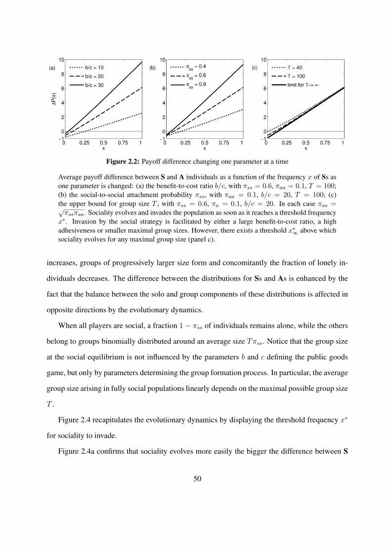
Figure 2.2: Payoff difference changing one parameter at a time

Average payoff difference between S and A individuals as a function of the frequency x of Ss asone parameter is changed: (a) the benefit-to-cost ratio b/c, with πss = 0.6, πaa = 0.1, T = 100;(b) the social-to-social attachment probability πss, with πaa = 0.1, b/c = 20, T = 100; (c)the upper bound for group size T , with πss = 0.6, πa = 0.1, b/c = 20. In each case πas =√πssπaa. Sociality evolves and invades the population as soon as it reaches a threshold frequency

x∗. Invasion by the social strategy is facilitated by either a large benefit-to-cost ratio, a highadhesiveness or smaller maximal group sizes. However, there exists a threshold x∗∞ above whichsociality evolves for any maximal group size (panel c).

increases, groups of progressively larger size form and concomitantly the fraction of lonely in-

dividuals decreases. The difference between the distributions for Ss and As is enhanced by the

fact that the balance between the solo and group components of these distributions is affected in

opposite directions by the evolutionary dynamics.

When all players are social, a fraction 1− πss of individuals remains alone, while the others

belong to groups binomially distributed around an average size Tπss. Notice that the group size

at the social equilibrium is not influenced by the parameters b and c defining the public goods

game, but only by parameters determining the group formation process. In particular, the average

group size arising in fully social populations linearly depends on the maximal possible group size

T .

Figure 2.4 recapitulates the evolutionary dynamics by displaying the threshold frequency x∗

for sociality to invade.

Figure 2.4a confirms that sociality evolves more easily the bigger the difference between S

50

Figure 2.3: Evolutionary trajectory and group size dynamics

One run of the evolutionary algorithm, starting from a population of A individuals with randommutations on newborns, with rate u = 0.01. (a) time evolution of the frequency x of the socialtype. (b-d) snapshots at generation 120 (b), 260 (c) and 400 (d), indicated by the arrows in panel(a), of the group size distributions experienced by S (red) and A (blue) individuals. The socialtrait rises towards fixation in the population while distributions displace towards larger groupsizes. Parameters: πss = 0.8, πaa = 0.3, πas =

√πssπaa, b/c = 20, T = 100, carrying capacity

= 106, x(0) = 0, fmax = 0.5, fmin = 0.1.

and A individuals’ attachment probabilities. Figure 2.4b shows that the threshold frequency x∗

decreases, as one would expect, as b/c increases. The threshold x∗ increases with T , consistently

with the common claim that the evolution of altruism is easier in small groups (Olson, 1971).

However, when T → +∞, it converges to a value x∗ < 1 (Figure 2.2c), meaning that there exist

a critical initial frequency of Ss such that sociality will invade whatever is the maximal group

size. Although higher cooperation levels are believed to occur more easily in small groups, group

formation by differential attachment thus does not impose an a priori burden on large groups.

This suggests that unsophisticated interaction rules may be relevant in explaining how sociality

is maintained in the microbial world, where social aggregates are commonly composed of a large

51

Figure 2.4: Social invasion thresholds

Threshold frequency x∗ of social individuals required to trigger the evolution of socialilty throughthe replicator equation: (a) x∗ as a function of adhesiveness πss and πaa (with πas =

√πssπaa,

b/c = 20, T = 100); (b) x∗ as a function of b/c and T (πss = 0.6, πaa = 0.2, πas =√πssπaa).

For values of b/c below the grey line, the evolution of cooperative sociality is trivial, correspond-ing to direct benefits, whereas above the line it is altruistic.

number of cells, e.g. thousands of them in flocculating yeast (Smukalla et al., 2008), or up to 105

in D. discoideum (Tang et al., 2002).

The fact that x∗ is always positive means that, in general, an infinitesimal initial load of Ss,

as is generated by extremely rare random mutations, is not sufficient for sociality to evolve in the

first place. However, when the threshold is low, numerous mechanisms can lead the frequency

of the social strategy over the threshold, e.g. random fluctuations due to finite-size effects, non-

infinitesimal mutation rates or incomplete reshuffling from one generation to the next. Numerical

simulations show that, in finite populations subject to a small mutation rate, the evolution of

52

0 500 1000 15000.1

0.12

0.14

0.16

0.18

0.2

0.22

0.24

0.26

generation

mea

n fit

ness

social

asocial

Figure 2.5: Mean fitnesses of the S and A strategies when Ss invade from scratch in a smallpopulation (Npop = 1000)

Initially, Ss (red) are outcompeted by As (blue) and thus cannot rise in frequency. However, theconstant mutation load keeps sociality away from extinction. When some of the few Ss happento accrue larger payoffs than the average A player by chance, social frequency might reach theinvasion threshold and fixate in the population.

sociality is indeed easier than analytically expected (Fig. 2.5)

The region where sociality is evolutionary stable is larger than the region where the social

behavior implies direct benefits, i.e. when the marginal gain of a social individual is larger than

c (Wilson, 1979; Pepper, 2000). See Box 2.2. for the definition and calculation of the condition

that delimits such region where sociality trivially evolves. Figure 2.4 shows that sociality evolves

and is maintained in the population for a wide range of nontrivial parameters, i.e. even when it

is an essentially altruistic act right at its onset.

Box 2.2. Condition for sociality to be altruistic

In the case of a Public Goods Game played in a group of fixed size N , cooperation can evolve if and only

if the marginal benefit from one’s own cooperation b/N is large enough to compensate the investment

c, that is when b/c > N . Nontrivial cases, where additional assumptions are required for cooperation to

53

evolve, are thus characterized by the condition:

b

c< N. (2.14)

To generalize this condition when group size is no longer fixed but stems from an aggregation pro-

cess, the marginal benefits b/n needs to be averaged over all group sizes n ≥ 2. As Ss experience a

group size distribution ds(n), the condition for altruism reads:

∑n≥2

b

nds(n)− c < 0

i.e.b

c<

1∑n≥2

ds(n)

n

:= ralt(x) (2.15)

In the case of group formation by differential attachment, the critical benefit-to-cost ratio ralt can

be calculated from the analytical expressions of the distribution ds of Ss’ experienced group size. This

calculation is performed in Appendix C.

2.3.4 Other rules for group formation

So far, it was assumed that players undergo blind interactions whereby individuals attach, accord-

ing to their strategies, with probabilities πaa, πas and πss in geometric progression, ensuring no a

priori assortment. However, other formulations of the adhesion probability, reflecting different

settings of pairwise interactions, can be contemplated, and will in general result in nonrandom

assortment within groups of a given size. In these cases, eq. (2.6) does not hold any longer,

but the payoff difference can anyway be numerically computed by repeatedly simulating the

aggregation process.

54

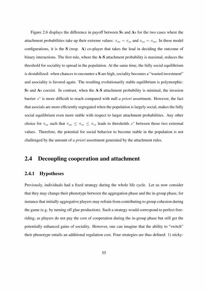
Figure 2.6 displays the difference in payoff between Ss and As for the two cases where the

attachment probabilities take up their extreme values: πas = πss and πas = πaa. In these model

configurations, it is the S (resp. A) co-player that takes the lead in deciding the outcome of

binary interactions. The first rule, where the A-S attachment probability is maximal, reduces the

threshold for sociality to spread in the population. At the same time, the fully social equilibrium

is destabilized: when chances to encounter a S are high, sociality becomes a “wasted investment”

and asociality is favored again. The resulting evolutionarily stable equilibrium is polymorphic:

Ss and As coexist. In contrast, when the A-S attachment probability is minimal, the invasion

barrier x∗ is more difficult to reach compared with null a priori assortment. However, the fact

that asocials are more efficiently segregated when the population is largely social, makes the fully

social equilibrium even more stable with respect to larger attachment probabilities. Any other

choice for πas such that πaa ≤ πas ≤ πss leads to thresholds x∗ between those two extremal

values. Therefore, the potential for social behavior to become stable in the population is not

challenged by the amount of a priori assortment generated by the attachment rules.

2.4 Decoupling cooperation and attachment

2.4.1 Hypotheses

Previously, individuals had a fixed strategy during the whole life cycle. Let us now consider

that they may change their phenotype between the aggregation phase and the in-group phase, for

instance that initially aggregative players may refrain from contributing to group cohesion during

the game (e.g. by turning off glue production). Such a strategy would correspond to perfect free-

riding, as players do not pay the cost of cooperation during the in-group phase but still get the

potentially enhanced gains of sociality. However, one can imagine that the ability to “switch”

their phenotype entails an additional regulation cost. Four strategies are thus defined: 1) sticky-

55

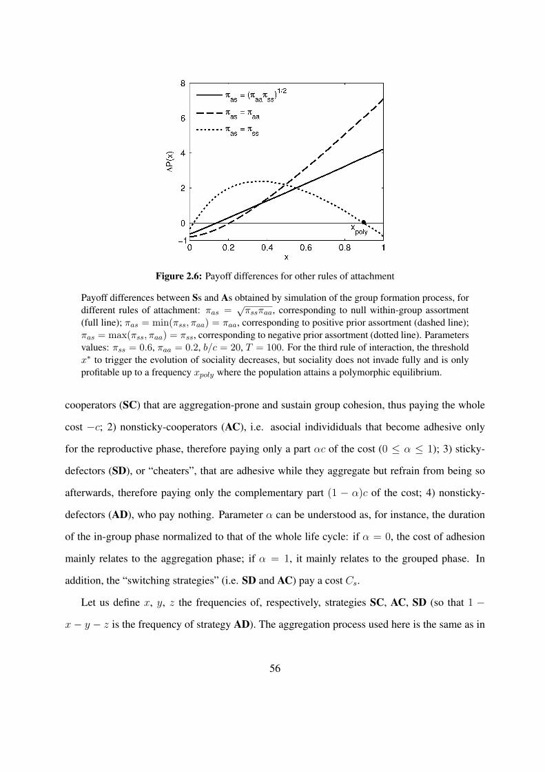
Figure 2.6: Payoff differences for other rules of attachment

Payoff differences between Ss and As obtained by simulation of the group formation process, fordifferent rules of attachment: πas =

√πssπaa, corresponding to null within-group assortment

(full line); πas = min(πss, πaa) = πaa, corresponding to positive prior assortment (dashed line);πas = max(πss, πaa) = πss, corresponding to negative prior assortment (dotted line). Parametersvalues: πss = 0.6, πaa = 0.2, b/c = 20, T = 100. For the third rule of interaction, the thresholdx∗ to trigger the evolution of sociality decreases, but sociality does not invade fully and is onlyprofitable up to a frequency xpoly where the population attains a polymorphic equilibrium.

cooperators (SC) that are aggregation-prone and sustain group cohesion, thus paying the whole

cost −c; 2) nonsticky-cooperators (AC), i.e. asocial individiduals that become adhesive only

for the reproductive phase, therefore paying only a part αc of the cost (0 ≤ α ≤ 1); 3) sticky-

defectors (SD), or “cheaters”, that are adhesive while they aggregate but refrain from being so

afterwards, therefore paying only the complementary part (1 − α)c of the cost; 4) nonsticky-

defectors (AD), who pay nothing. Parameter α can be understood as, for instance, the duration

of the in-group phase normalized to that of the whole life cycle: if α = 0, the cost of adhesion

mainly relates to the aggregation phase; if α = 1, it mainly relates to the grouped phase. In

addition, the “switching strategies” (i.e. SD and AC) pay a cost Cs.

Let us define x, y, z the frequencies of, respectively, strategies SC, AC, SD (so that 1 −

x− y − z is the frequency of strategy AD). The aggregation process used here is the same as in

56

the toy model of the previous section, so that the distribution dS•(n) (resp. dA•(n)) experienced

by the two sticky strategies SC and SD (resp. the two nonsticky strategies AC and AD) is the

same as dS(n) (resp. dA(n)) in the former section, substituting x by the total proportion of

sticky individuals x+ z (resp. substituting 1− x by the total proportion of nonsticky individuals

1− x− z).

Mean payoffs can also be calculated similarly as before:

PSC = b∑n≥2

dS•(n)

n

[x dS•(n) + y dA•(n)

(x+ z)dS•(n) + (1− x− z)dA•(n)+ 1

]− c (2.16)

PAC = b∑n≥2

dA•(n)

n

[x dS•(n) + y dA•(n)

(x+ z)dS•(n) + (1− x− z)dA•(n)+ 1

]− α c− Cs (2.17)

PSD = b∑n≥2

dS•(n)

n

[x dS•(n) + y dA•(n)

(x+ z)dS•(n) + (1− x− z)dA•(n)

]− (1− α) c− Cs (2.18)

PAD = b∑n≥2

dA•(n)

n

[x dS•(n) + y dA•(n)

(x+ z)dS•(n) + (1− x− z)dA•(n)

](2.19)

2.4.2 Evolutionary outcome

Knowing the mean payoffs, evolutionary trajectories can be computed using the replicator equa-

tion. Figure 2.7 displays the evolutionary endpoints for a given set of parameters and an initial

population with 25% of each strategy, as a function of the parameter α and the switching cost

Cs. The frequency of each strategy is represented at equilibrium for c = 1.

In most cases, the equilibrium is monomorphic. The results may be somewhat tricky to

interprete, as in mixed populations each strategy affects the three others. They can however be

crudely understood as follows (readers in a hurry can jump to the conclusion in section 2.4.3):

• For α ' 0, SDs are disavantaged compared to SCs as the former actually pay a larger cost

(' 1+Cs) than the latter (= 1), and do not get direct benefits. They disappear quickly and

SCs tend to get assorted positively with the remaining other sticky players that are thus

all cooperators too. As ACs tend to get assorted positively with other nonsticky players,

57

Figure 2.7: Equilibrium frequencies of each strategy SC, SD, AC, AD when sociality is decou-pled from cooperation.

Frequencies range from 0 (white) to 1 (black). Equilibrium frequencies are represented for adifferent benefit-to-cost ratio b/c in each line. In most cases, the equilibrium population is eitherfully SC or fully AD. High values of Cs and low values α of favor the SC strategy. For a fewcombinations of parameters Cs and α, the SD strategy can take over (here when b = 30) or co-exist at equilibrium with the SC strategy (here when b = 30, gray line). Parameters: x0 = y0 =z0 = 0.25, c = 1, Cs = 0.44, α = 0.74, πss = 0.6, πaa = 0.3, πas =

√πssπaa, T = 100.

58

among whom ADs, they experience less cooperative groups and are outcompeted by SCs.

Cooperation levels in nonsticky players’ average groups decrease and ADs, even though

they pay no cost, are themselves defeated by SCs that belong to highly cooperative groups.

As a result, SCs take over.

• Let us consider now intermediate to large α. When Cs is high, SDs pay a cost (1−α)+Cs

that tends to outgrow the fixed cost 1 of SCs, and are again defeated by them as they

experience the same groups and get no direct benefits, unlike SCs. Similarly to the case

of low α, SCs thrive as they get assorted in highly cooperative (thus profitable) groups,

unlike the two nonsticky strategies.

When Cs decreases however, the cost payed by SDs gets smaller than the cost payed by

SCs. When the nonsticky strategies are eliminated successively (first ACs, as they pay

too high a cost to rival the sticky strategies, then ADs, as they get assorted with mainly

nonsticky, and now defective, individuals), the direct benefit b∑

n≥2 dS•(n, x+ z = 1)/n

earned by SCs is constant. SCs and SDs experience the same average groups, so that

at some point, the cost 1 − α + Cs payed by SDs might compensate exactly the (cost

+ direct benefit) 1 + b∑

n≥2 dS•(n, x+ z = 1)/n of the SCs. This results in a mixed

equilibrium of SCs and SDs (e.g., for b = 30, the gray diagonal of equation Cs = α −

b∑

n≥2 dS•(n, x+ z = 1)/n in Figure 2.7), as both strategies have the same mean payoffs.

Other initial frequencies lead to different mixtures of SCs and SDs (Fig. 2.8), as all of them

are stable. It is however a non-generic situation.

When Cs is decreased further, SDs outcompete SCs and get assorted among other sticky

players, that are now mainly defectors. SDs thus get poor payoffs from their groups and

are defeated by the nonsticky strategies. ADs finally take over, as they do not pay any cost

unlike ACs.

When the benefit-to-cost ratio decreases, the parameters range where the population end up

59

Figure 2.8: A non-generic case of evolutionary trajectories in the 3D-simplex for various initialconditions.

Evolutionary trajectories start setting initial frequencies of each strategies represented by bluecircles and end at equilibrium frequencies represented by red crosses. Apart from the full-SC andfull-AD monomorphic equilibria, any mixed equilibrium with SCs and SDs is stable. This resultsfrom average payoffs PSC and PSD being equal (with the chosen costs) when asocial strategiesAC and AD are eliminated in the population. Parameters: b = 30, c = 1, Cs = 0.44, α = 0.74,πss = 0.6, πaa = 0.3, πas =

√πssπaa, T = 100. Parameters Cs and α are chosen such that

Cs = αc− b∑

n≥2 dS•(n, x+ z = 1) (on the grey line in the first line of Figure 2.7).

being fully SC shrinks, as cooperation becomes less profitable.

2.4.3 Conclusion

An interesting feature of this model is that in most cases, either SCs or ADs take over the popu-

lation: only in very rare situations do the “switching strategies” SD and AC persist. This tends

to legitimate a posteriori the assumption made formerly that sociality (or stickiness) and coop-

eration can be regarded as coupled.

60

2.5 Extension to a continuous trait

In some cases, social propensity can result from individual features that do not abide by an binary

logic (a tunable motility or adhesion force, etc.) For instance, the FLO1 gene governing adhesion

in yeast is highly variable: the level of adhesion indeed changes as a function of the number of

tandem repeats within FLO1 (Smukalla et al., 2008). It may then be instructive to check whether

the mechanism described above still hold for mutations that affects continuously an individual’s

social inclination.

2.5.1 Changes in the model

Let us assume the existence of a social trait z that can take any value in the interval [0, 1]. z = 1

means the individual is “fully social”, z = 0 that he is “fully asocial”. The associated cost

c(z) is an increasing function of z. In the following, I will assume it linear (c(z) = −Cz),

but keep in mind that nonlinear functions can diversify possible dynamics: e.g. in (Doebeli et

al., 2004), quadratic cost functions lead to a branching process used to explain the origin of

cooperators with a fixed contribution. Individuals assemble into groups according to some rules.

This analysis only considers the case of a rare mutant characterized by z in a monomorphic

population characterized by a sociality z. The question is whether a rare mutant trait z can

invade or not a resident monomorphic population characterized by z. Accordingly to the adaptive

dynamics formalism (Geritz et al., 1998; Waxman and Gavrilets, 2005), it is assumed that 1) the

mutation rate is small enough so that the population has time to reach its equilibrium before

another mutation occurs; 2) mutations are infinitesimal. Those classical hypotheses, however

strong as they may seem, are necessary to circumvent some untractable calculatory issues and

still shed light on which dynamics are to be expected (see Box 2.3.). Group size distributions

experienced by an individual depend on the z-values of others as well as its own: for a z-mutant

in a z-population, it is denoted g(n, z, z); for a resident individual, g(n, z, z). Unless she is alone,

61

the group-related payoff derived by an individual is bz, where z is the mean value of the group

members’ traits.

Box 2.3. The adaptive dynamics framework

Adaptive dynamics is a methodological tool formalized by Geritz et al. (1998) and aimed at describ-

ing the long-term phenotypic changes that result from small mutations on a specific gene in an evolving

population (see also Waxman and Gavrilets (2005) for a very clear tutorial). Let us consider a population

characterized by a single, continuously varying phenotypic trait. Adaptive dynamics relies on several

(somewhat unrealistic) assumptions, namely:

• that each mutation cause infinitesimal phenotypic change;

• that the ecological time scale is much quicker than the evolutionary time scale, to such extent that

before a novel mutation arises, the population has time to stabilize to a monomorphic state;

• that the success of a mutant trait in replacing or not the resident trait in the population depends on

its growth rate when it is still infinitely rare in the population.

Let then r be the resident value of the trait at some point in time. We need to assess whether it can be

outcompeted by a small mutation m. We thus calculate the invasion fitness (i.e. the relative growth rate

when rare) S(m, r)− S(r, r) = S(m, r) of the mutant in a full-r population (here S(r, r) is set to 0 due

to the population being at a dynamical equilibrium). As mutation are small, the linear approximation

S(m, r) ' [∂S(m, r)/∂m]m=r (m− r) is valid and the fate of the mutant can be determined by the sign

of the selection gradient [∂S(m, r)/∂m]m=r. If the selection gradient is = 0 for values r = r∗, then

the fitness landscape is flat near r∗. Such particular values are called evolutionary singular strategies.

If it is positive (resp. negative), then mutants with larger (smaller) phenotypic values than the resident

population’s invade.

Adaptive dynamics is particularly useful as it enables to characterize the equilibria or singular strate-

62

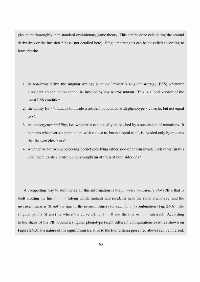
gies more thoroughly than standard evolutionary game theory. This can be done calculating the second

derivatives or the invasion fitness (not detailed here). Singular strategies can be classified according to

four criteria:

1. its non-invasibility: the singular strategy is an evolutionarily singular strategy (ESS) whenever

a resident r∗-population cannot be invaded by any nearby mutant. This is a local version of the

usual ESS condition;

2. the ability for r∗-mutants to invade a resident population with phenotype r close to, but not equal

to r∗;

3. its convergence-stability, i.e. whether it can actually be reached by a succession of mutations. It

happens whenever a r-population, with r close to, but not equal to r∗, is invaded only by mutants

that lie even closer to r∗;

4. whether or not two neighboring phenotypes lying either side of r∗ can invade each other; in this

case, there exists a protected polymorphism of traits at both sides of r∗.

A compelling way to summarize all this information is the pairwise invasibility plot (PIP), that is

built plotting the line m = r (along which mutants and residents have the same phenotype, and the

invasion fitness is 0) and the sign of the invasion fitness for each (m, r) combination (Fig. 2.9A). The

singular points (if any) lie where the curve S(m, r) = 0 and the line m = r intersect. According

to the shape of the PIP around a singular phenotype (eight different configurations exist, as shown on

Figure 2.9B), the nature of the equilibrium (relative to the four criteria presented above) can be inferred.

63

Figure 2.9: Pairwise invasibility plots (PIP)

Panel A: example of a PIP. The gray (resp. white) areas are those where the invasion fitness is positive(resp. negative); r∗ is an evolutionary singular strategy. The shape of the PIP near (r∗, r∗) enables tocharacterize the equilibrium. Panel B: the eight configurations for a singular strategy. The shape of thePIP near the singular strategy is determined by the algebraic value of second derivatives of the invasionfitness. According to these values, one can determine which of the four properties of the equilibriumpresented above are satisfied and infer the evolutionary dynamics. Adapted from Geritz et al. (1998).

2.5.2 Resident / mutant analysis

In a given group of size n, a resident individual gets a payoff

Pn(z, z) = b z (2.20)

as z = z; whereas, for a z-mutant,

Pn(z, z) = b [(n− 1)z + z] / n = b z + b (z − z)/n (2.21)

Let us call u(z, z) (resp. u(z, z)) the proportion of z-individuals (resp. z-individuals) left

ungrouped (u(z, z) = g(1, z, z) and u(z, z) = g(1, z, z)). Weigthing for any possible group size,

64

the final net payoff of the resident trait is:

P (z, z) =∑n≥2

g(n, z, z)Pn(z, z)− c(z) (2.22)

= b z [1− u(z, z)]− Cz (2.23)

and, for a mutant,

P (z, z) =∑n≥2

g(n, z, z)Pn(z, z)− c(z) (2.24)

= b z (1− u(z, z)) + b(z − z)∑n≥2

g(n, z, z)/n− Cz (2.25)

The mutants being at very small frequency by assumption, the average payoff in the popula-

tion P ≈ P (z, z); therefore, the relative growth rate of the mutant trait is:

S(z, z) = P (z, z)− P (z, z) (2.26)

= b z [u(z, z)− u(z, z)] + b(z − z)∑n≥2

g(n, z, z)/n− C(z − z) (2.27)

and that of a resident, S(z, z) = 0.

Now, let us calculate the fitness gradient of the z-resident, supposing that all relevant func-

tions are differentiable:

dS(z, z)

dz

∣∣∣∣z=z

= limz→z

S(z, z)

z − z(2.28)

= limz→z

{−b z

u(z, z)− u(z, z)

z − z+ b

∑n≥2

g(n, z, z)

n− C

}(2.29)

= − b zdu(z, z)

dz

∣∣∣∣z=z

+ b∑n≥2

1

n

dg(n, z, z)

dz

∣∣∣∣z=z

− C (2.30)

(the sum being in practice bounded, as group size necessarily has an upper limit, the interversion

65

of the limit and the sum is valid).

To carry on with the calculations, an approximation is needed. For very large groups, the

second term tends to become very small compared to the two others. For instance, in the case

of the aggregation toy model, calculations show that it converges to 0 as T → +∞. Below, I

simply neglect it (but see the discussion afterwards). Denoting

h(z) = − du(z, z)

dz

∣∣∣∣z=z

(2.31)

we obtaindS(z, z)

dz

∣∣∣∣z=z

≈ b z h(z)− C (2.32)

or, in a more ’readable’ form:

dS(z, z) ≈ b z h(z)dz − Cdz (2.33)

Noticing that h(z) is the variation in the probability for an individual to join some group if

she deviates with an infinitesimal positive quantity from the resident social trait, it can reasonably

be assumed, in the general case, that h(z) > 0: being more social decreases the risk to remain

ungrouped. Then, the interpretation of the obtained formula is straightforward: the variation in

growth rate induced by a small mutation in the social propensity is equal to the increased chance

it gives to join a group, times the payoff drawn from the group (i.e., b z), minus the marginal,

additional cost paid:

increase in growth rate = earned probability to be in a group × group payoff − additional cost

(2.34)

If z > z, that is, for a pro-social mutation to invade, the grouping opportunities earned compared

to the residents must be sufficient to offset the additional cost: this is a very general condition

66

analogous to many established in the literature for other mechanisms. Lastly, let us remark

that not neglecting the term b∑

n≥2 1/n dg(n, z, z)/dz|z=z (for instance, if groups are not large

enough) makes the growth rate’s derivative more positive; therefore, the invasion of a positive

mutation easier: once again, social behaviors are easier to establish in small groups.

2.5.3 Application to an aggregation process

Coming back to the toy aggregation process of the two-strategy analysis, the relevant continuous

trait here is z = π, i.e. the individual tendency or probability to stick to another individual

(z ∈ [0, 1]). We assume T to be very large, so that every recruiter is a resident: therefore the

probability for an individual to join a group is z if she is a resident and√zz if she is a mutant

(in the two-trait model, A − A adhesion occurs with probability πaa =√πaaπaa, S − S with

probability πss =√πssπss and A−S with probability πas =

√πaaπss). Hence u(z, z) = 1−

√zz

and h(z) = 1/2. The condition for a small pro-social mutation to invade is then that

z >2C

b(2.35)

Further calculations not showed here (involving second derivatives) make it possible to char-

acterize the singular point z∗ = 2C/b as a repellent equilibrium that is not convergence-stable,

invasible and does not allow for protected polymorphism.

In the end, given those aggregation rules, a monomorphic population can be invasible by

more and more social mutations until z = 1 (full sociality), provided the starting common trait is

greater than z∗. Below this threshold, pro-social mutations cannot invade while anti-social can,

until z = 0 (full asociality) in the whole population. Notice that, as previously, this holds in the

case when T is infinitely large. When T is finite, the term we neglected may not be rightly so,

so that pro-social mutations can invade for a wider range of initial social traits in the population;

in other words, the condition z0 > z∗ is alleviated as groups get smaller.

67

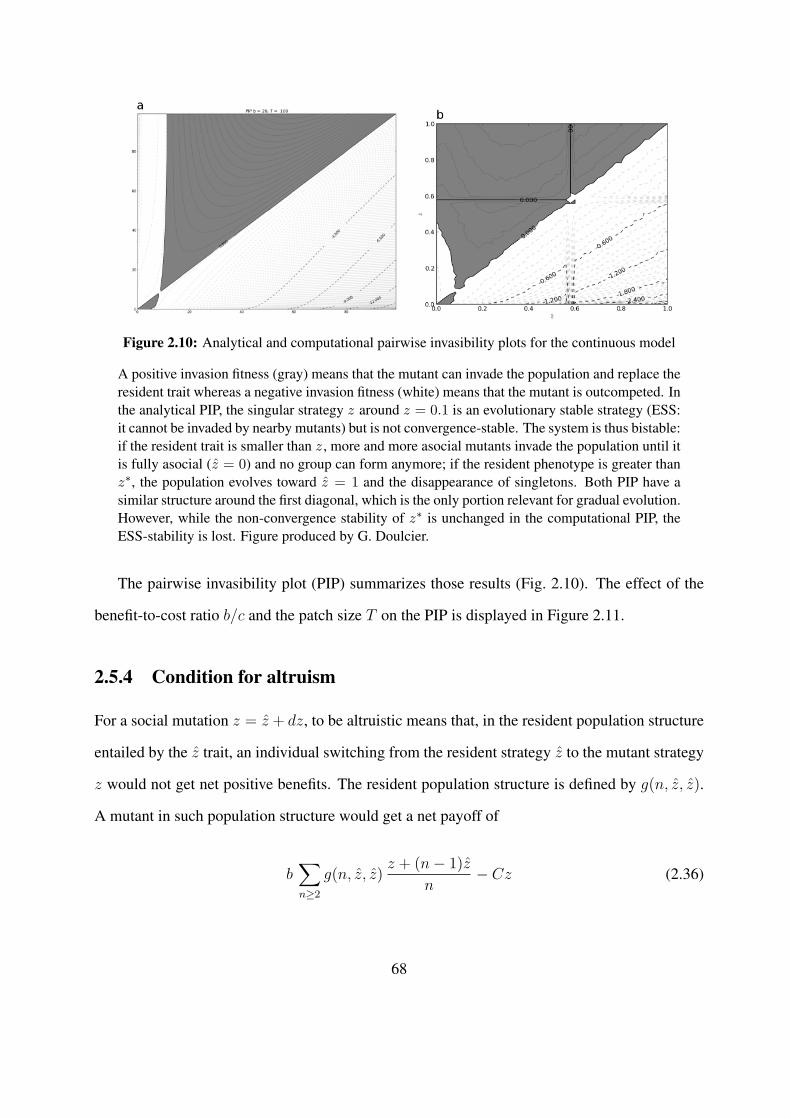
Figure 2.10: Analytical and computational pairwise invasibility plots for the continuous model

A positive invasion fitness (gray) means that the mutant can invade the population and replace theresident trait whereas a negative invasion fitness (white) means that the mutant is outcompeted. Inthe analytical PIP, the singular strategy z around z = 0.1 is an evolutionary stable strategy (ESS:it cannot be invaded by nearby mutants) but is not convergence-stable. The system is thus bistable:if the resident trait is smaller than z , more and more asocial mutants invade the population until itis fully asocial (z = 0) and no group can form anymore; if the resident phenotype is greater thanz∗, the population evolves toward z = 1 and the disappearance of singletons. Both PIP have asimilar structure around the first diagonal, which is the only portion relevant for gradual evolution.However, while the non-convergence stability of z∗ is unchanged in the computational PIP, theESS-stability is lost. Figure produced by G. Doulcier.

The pairwise invasibility plot (PIP) summarizes those results (Fig. 2.10). The effect of the

benefit-to-cost ratio b/c and the patch size T on the PIP is displayed in Figure 2.11.

2.5.4 Condition for altruism

For a social mutation z = z + dz, to be altruistic means that, in the resident population structure

entailed by the z trait, an individual switching from the resident strategy z to the mutant strategy

z would not get net positive benefits. The resident population structure is defined by g(n, z, z).

A mutant in such population structure would get a net payoff of

b∑n≥2

g(n, z, z)z + (n− 1)z

n− Cz (2.36)

68

Figure 2.11: Sensitivity of the pairwise invasibility plot on parameters b/c and T

The invasion fitness is here computed applying the analytical method. The structure of the PIP andthe nature of the equilibrium z∗ is largely independent of the parameters, but its position changes:when b/c increases, sociality is more easily promoted and z∗ decreases. Smaller values of T alsotend to decrease z∗ (albeit to a smaller amount); this is consistent with the well-known facilitatingeffect of small group sizes on social behavior. Figure produced by G. Doulcier.

while a resident gets

b∑n≥2

g(n, z, z) z − Cz (2.37)

Therefore, the social mutation is altruistic if

b∑n≥2

g(n, z, z)z + (n− 1)z

n− Cz < b

∑n≥2

g(n, z, z) z − Cz (2.38)

69

i.e. whenever

b∑n≥2

g(n, z, z)z − z

n< C(z − z)

⇐⇒ b

c<

[g(n, z, z)

n

]−1

:= ralt(z) (2.39)

This condition is comparable to that found in the discrete model (eq. 2.15). The threshold ralt(z)

is homogeneous to a group size. Indeed, excluding loners, the mean group size in the population

is:

γz =

∑Tn≥2 nΓ(n)∑Tn≥2 Γ(n)

(2.40)

where Γ(n) =1

T

g(n, z, z)

nis the number of n-sized groups. Thus,

γz =

∑Tn≥2 n

1T

g(n,z,z)n∑T

n≥21T

g(n,z,z)n

=

∑Tn≥2 g(n, z, z)∑Tn≥2

g(n,z,z)n

= (1− u(z, z)) ralt(z) (2.41)

As the proportion of ungrouped individuals u(z, z) = 1− z, we finally get:

ralt(z) =γzz

(2.42)

2.6 Discussion

2.6.1 Social groups formation and evolution

In this work, I address the coupling between the process of group formation and the evolutionary

dynamics of individual “social” traits that affect both aggregation propensity and group cohesion,

e.g. cell-to-cell adhesiveness. In addition to entailing a different contribution to group welfare,

70

such traits underpin a difference in expected group size distributions. This difference ultimately

generates assortment at the population level even in the absence of preferentially directed inter-

actions based on peer recognition. Rather, I evidence that, whenever the size of groups is not

fixed, simple non-assortative rules can still generate average local environments that favor the

evolution of sociality even when it is not associated to direct benefits. This claim is illustrated

by a toy model where groups form by blind interactions among individuals with different attach-

ment abilities, stemming for instance from signalling or due to the production of a costly glue.

This deliberately simple setting shows that even when attachment rules are indiscriminate toward

the strategies of partners (and groups of any size are randomly assorted), socials individuals fare

better than asocials thanks to the distinct allocations of the two types in group of various sizes

and in particular to different chances of ending up alone. The emergent population structure

gives rise to a Simpson’s paradox where one strategy’s advantage is reversed when one goes

from the group to the population level (Box 2.4.). This has already been related to the evolution

of cooperation when group size changes in time (Hauert et al., 2006a; Chuang et al., 2009). It is

noteworthy that in the toy model there is no intrinsic limitation to the size of the evolutionarily

viable groups, contrary to most previous models of N -player games, e.g. (Matessi and Jayakar,

1976; Powers et al., 2011). This suggests that sociality in large groups, such as in microbial

communities, can be sustained with unsophisticated mechanisms that do not require information

transfer between partners.

Box 2.4. The Simpson’s paradox

The so-called Simpson’s paradox (Chuang et al., 2009) encapsulates the counterintuitive situations

that may arise when two levels of description conflict. Consider individuals, either cooperators or de-

fectors, playing in groups and multiplying at rates that depend on their net payoffs. Within one group,

every member gets the same benefit but cooperators pay an additional cost, so that defectors are always

71

better off than their cooperating group partners. Yet, at the same time, groups where cooperators are

overrepresented fare better than groups composed of many defectors to such extent that, in the gene

pool of the global population, cooperation might rise in frequency. The Simpson’s paradox is a purely

statistical mechanism, but one that has a key role in evolutionary biology and is very much in line with

arguments of group (or multilevel-) selection.

Figure 2.12: The Simpson’s paradox

Simpson’s paradox refers to a situation in which several groups, composed of two types of elements, P andNP, evolve so that the proportion of P elements decreases within each group but nevertheless increases inaverage overall. The right side shows the evolution of Simpson’s paradox: three hypothetical subpopula-tions represented by pie charts of P (green) and NP (white) slices; the initial and final subpopulations areconnected by solid black arrows. The left side shows the corresponding composition of the initial and finalglobal population formed by these three subpopulations (dotted lines). As a whole, the figure illustratesthe paradox of P decreasing in each subpopulation (∆pi < 0 for every group i ) but increasing overall(∆p > 0). This “paradox” is a purely statistical effect, based on the fact that the global proportion of Pis a group size-weighted average that differs from the nonweighted average. In general, if we start fromn groups of equal sizes and proportions pi of P (i = 1, . . . , n), whether Simpson’s paradox is observeddepends on the changes in proportion of P within each group, ∆pi, and on the overall growth of eachgroup, wi. Figure and caption taken from (Chuang et al., 2009).

72

2.6.2 Aggregative sociality in microorganisms

In the microbial world, the formation of biofilms and their cohesion are reckoned to be beneficial

to cells in many respects (Velicer, 2003). In several microorganisms, the same costly individ-

ual traits that support the stability of groups may enhance the probabilities for cells to be part

of them in the first place. Velicer and Yu featured costly “stickiness” as an adaptive prerequi-

site in swarming microorganisms (Velicer and Yu, 2003). In D. discoideum, the production of

cell-adhesion molecules required for the aggregation cycle is thought to reduce the chances to

become a spore: more adhesive strains are primarily found in the dead tissues of the fruiting

body (Ponte et al., 1998; Strassmann and Queller, 2011). Myxobacteria form multicellular ag-

gregates as well, that enhance survival by decreasing predation and favoring disperal (Shimkets,

1986a,b). Both agglutination and social cohesion are mediated in these bacteria by the produc-

tion of a costly extracellular matrix of fibrils, increasing at the same same time cell adherence

and enabling collective gliding (Velicer and Yu, 2003). Mutations that affect a gene located

at a single locus impair fibril binding and result in both lower cell-cell adhesion and cohesion

of aggregates (Shimkets, 1986b). In S. cerevisiae, an adhesion protein expressed by a social

gene (FLO1) prompts individuals to form flocs that provide them with enhanced resistance to

chemical stresses (Smukalla and al., 2008). When this strain is mixed with non-flocculating

variants, heterogeneous aggregates still contain a majority of FLO1+ cells, while individuals

outside groups are more often FLO1−, thus denoting assortment emerging from mere different

adhesive abilities.

Although the processes involved in group formation become more complex as the cogni-

tive abilities of players increase, our general conclusions might be also of interest for higher

organisms that interact via mechanisms parallel to physical adhesiveness. For instance, Dunbar

interpreted grooming in monkeys as a behavior likely to provide higher grouping opportunities as

well as cement social bonding once the group is formed (Dunbar, 1993), and further extended the

73

argument to humans, based on the presumed genetic foundations of language (Pinker and Bloom,

1990). Even if we have focused here on an aggregation mechanism that is more promptly related

to social microrganisms, our conclusions hold in general for any inheritable trait, not necessarily

involving physical adhesion, that plays a role both in group formation and group cohesion.

2.6.3 Nonnepotistic greenbeards?

In this model, assortment is generated among carriers of the social gene alone, and not on the

whole genome. Therefore, sociality here pertains to green beard mechanisms as termed by the

recent classification of Gardner and West (West et al., 2007b; Gardner and West, 2010). In their

review, the authors stressed that such genes need not code for conspicuous traits as was posited

in the original formulations (Hamilton, 1964; Dawkins, 1976). We argue that assortment at a

single locus does not require nepotistic behavior of the gene towards other carriers neither, at

least not in the usual sense imposed by dyadic or fixed-N frameworks. Indeed, assortment may

mechanistically occur even when social individuals interact with each type in the same propor-

tions as asocial individuals, provided they do it more often. A blind increase in the propensity to

interact can thus have the same effect as preferentially directed interactions with peer discrim-

ination, that may be more demanding on the cognitive level. This might be of interest for the

interpretation of social behavior in organisms where the existence of recognition mechanisms

is not straightforward. More in general, it might be useful to disentangle more explicitly green

beard mechanisms that rely on active sorting of interaction partners from passive, indiscriminate

mechanisms generating assortment with weaker requirements (Eshel and Cavalli-Sforza, 1982).

Such differentiation would echo and complement that of obligate vs. facultative green beards

formulated in the case of dyadic interactions (Gardner and West, 2010).

74

2.6.4 About altruism and direct benefits

An important point is that a cooperative trait is not altruistic or directly beneficial per se, but

relative to a given population structure, that it itself contributes to shape. In particular, its status

can change along an evolutionary trajectory. Let us plot the minimal benefit-to-cost ratio rmin

necessary to promote sociality and the maximal benefit-to-cost ratio ralt below which the social

trait is altruistic in the toy model. According to eqs. (2.6) and (2.15),

rmin(x) =

[+∞∑n=2

1

n

((n− 1)

(ds(n)− da(n))x

(ds(n)− da(n))x+ da(n)+ 1

)ds(n)

]−1

(2.43)

and

ralt(x) =1∑

n≥2

ds(n)

n

(2.44)

These two ratios are equal for x = 0. For x = 1 and large T , we can show that ralt ' T .

Figure 2.13 displays rmin(x) and ralt(x) as a function of x for a given set of parameters. We can

distinguish four cases:

1. when b/c ≥ ralt(x = 1), sociality can evolve from scratch as it is always directly benefi-

cial. If maximal group size is large, this corresponds to the usual condition b/c > T for

sociality to evolve via direct benefits in groups of size T .

2. when rmin(x = 0) ≤ b/c < ralt(x = 1), sociality can evolve from scratch and switches

from directly beneficial to altruistic as x increases. This is due to the fact that when the

population is poorly social, groups are smaller and the marginal gain retrieved by one’s

own social contribution cancels its cost.

3. when rmin(x = 1) ≤ b/c < rmin(x = 0), sociality steadily evolves as soon as it reaches

some threshold frequency x∗ such as b/c = rmin(x = x∗). All along the evolutionary

dynamics, the social trait is altruistic.

75

0 0.2 0.4 0.6 0.8 10

20

40

60

80

100

120

ralt T

rmin

(b/c)4

(b/c)3

(b/c)2

(b/c)1

x

b/c

Figure 2.13: Minimal b/c ratio to promote sociality vs. maximal b/c ratio for sociality to bealtruistic.

According to the benefit-to-cost ratio, we distinguish four cases: 1) directly beneficial socialityevolves from scratch (e.g. (b/c)1); 2) sociality evolves from scratch by direct benefits but becomesaltruistic during the evolutionary trajectory (e.g. (b/c)2); 3) altruistic sociality can evolve onlyfrom a threshold frequency x∗ (e.g. (b/c)3); 4) sociality never evolves (e.g. (b/c)4). The benefit-to-cost ratio thus also influences the “status” of the social trait, and this status can change alongthe evolutionary trajectory.

4. when b/c < rmin(x = 1), (altruistic) sociality can never prosper and the population is

doomed to full asociality.

This suggests that in real microbial populations, a social trait is likely to change status along

its rise in frequency in the population: the advent of sociality might be first triggered by a relaxed

social dilemma because the groups that form are still small. When the social frequency rises,

positive assortment between socials makes it possible for sociality to attain fixation even though

it has become an altruistic trait.

76

2.6.5 Toward a re-evaluation of the group formation step

I have stressed that the process of group formation can play an essential role in the unfolding of

the evolutionary dynamics of social traits. A complete account of the evoution of cooperative

groups requires to trace back the entire process leading to their formation. The toy model used

here is a useful tool to illustrate my conclusion in a simple and extreme setting. It is however

missing many features of actual biological systems. One could instead wish to predict, based on

individual properties of physical attachment, the group size dynamics and the degree and nature

of assortment between the social and asocial types in a more realistic aggregation model. This

requires to further specify the mechanism of group formation, and notably explicit the individual

rules of interaction and the topology structuring individual encounters. For organisms moving

on a plane, such as cells gliding on a surface, grouping patterns and the resulting group size

distributions have been mimicked by models based on simple rules (e.g. Okubo, 1986; Vicsek

et al., 1995; Bonabeau et al., 1999). Recently, social games have been implemented in explicit

schemes of aggregation for self-propelled particles interacting locally with their neighbors (Chen

et al., 2011a,b). The way aggregative traits themselves can be sustained in a landscape shaped

by a realistic group formation process however is still to be explored. Yet, the propensity to seek

interactions, before that of behaving altruistically once the interaction is established, may be the

very first, and a prerequisite, of all social actions.

77

Chapter 3

Differential adhesion between moving

particles for the evolution of social groups

This chapter (minus section 3.5) is adapted from “Garcia, T., Brunnet, L.G., and De Monte,

S. Differential adhesion between moving particles as a mechanism for the evolution of social

groups”, in review in Plos Computational Biology.

3.1 Introduction

3.1.1 Main issue

The ability to form and sustain collective ventures is observed at all levels of the living world,

spanning from human societies to microbial populations. In many biological settings, grouping

requires individual traits that are costly for their carriers (Velicer, 2003; Xavier, 2011; Schtickzelle

et al., 2009). Sociality is thus an apparent paradox of evolutionary theory, as asocial “cheaters”

who do not contribute to social welfare but reap group benefits should be favored by natural se-

lection. This issue, that was first raised by Charles Darwin, has been revived in the last decades

and is still pivotal in evolutionary biology, giving rise to an extensive literature on the evolution

79

of cooperation.

The difficulty to explain the evolutionary emergence and maintenance of cooperation is par-

ticularly acute when the organisms diplaying social behavior are relatively simple such as mi-

crobes, so that they cannot rely on the complex cognitive and cultural abilities that are usually

invoked as supporting cooperation in animals. Such simpler interactions and behaviors, together

with the ease of cultivating bacterial populations in controlled environments, offer on the other

hand the opportunity to address elementary mechanisms that underlie the evolution of sociality

in general settings (Velicer, 2003; Crespi, 2001; West et al., 2007a; Celiker and Gore, 2013).

Here, I consider the evolution of a social (adhesive and cooperative) trait in a population with

a life cycle of aggregation-reproduction-dispersal, commonly observed in microbes displaying

high degrees of cooperation, such as social amoebae or Myxobacteria (West et al., 2007a). In

such cases, the existence of recurrent chimeric aggregates of potentially unrelated individuals

appear to contrast with the classic expectation that cooperative behavior should be expressed to

a lesser extent the weaker the genetical relatedness within social groups. I make the aggregation

phase explicit by modeling cells as self-propelled particles moving on a plane, and study under

which conditions social traits evolve through natural selection, and to what spatial patterns they

are associated.

Game theory has been long used to account for the evolutionary sustainability of genetically

determined cooperative traits that benefit others while being costly to the individual (Hofbauer

and Sigmund, 1998). Several different formalizations have been proposed to describe the effect

of an individual’s trait and its interactions on its own reproductive success. Among those, coop-

eration in social settings is classically modeled as N -player games, where fitness depends on the

features of the group. The simplest formulation of such games is the Public Goods Game (PGG)

(Olson, 1971), where the benefits yielded by the group depend on the fraction of cooperators in

it.

In questioning the mechanisms by which cooperative behavior can prosper, most models

80

consider environments where group size is constant and independent of individual strategies. A

growing number of studies has recently started to address cases when the interaction topology,

and notably the size of the social groups, is an emergent property of individual-level features.

These studies have modeled specific rules for entering groups with limited carrying capacity

(Aviles, 2002; van Veelen et al., 2010); evolvable preferences for group size (Powers et al., 2011);

competition for the use of a diffusible compound (Nadell et al., 2010), or for empty space (Pfeif-

fer and Bonhoeffer, 2003; Hauert et al., 2006a); the voluntary participation to groups (Hauert et

al., 2002a,b); but also differential attachment supported by the cooperative trait (Pacheco et al.,

2006; Garcia and De Monte, 2013). In many cases however, group formation has been modeled

in well-mixed populations, or on a regular lattice where each individual occupies a cell and has a

constant number of partners. While these assumptions are justified whenever individuals are ei-

ther extremely motile or sessile respectively, they fall short in describing self-structuring traits in

microbial populations with complex grouping patterns. More realistic models for the formation

of groups from initially sparse individuals thus require an explicit account of particle movement

in space and of the interaction forces that underpin the emergent “social landscape”.

With this respect, Self-Propelled Particles (SPP) models have proved useful to account for

the formation of collective structures (e.g. swarms) based on simple local rules for interaction.

Although SPP models have now become a primary tool to address collective behavior both in

the physical and biological sciences, the exploration of their interplay with the evolutionary

dynamics of individual traits is still in its infancy (but see Guttal and Couzin (2010); Chen et al.

(2011a,b); Zhang et al. (2011a); Perc et al. (2013)).

3.1.2 Outline

In this chapter, I explore the conditions for a genetic costly trait that enhances interactions to

evolve in a population, in a context where the aggregation scheme is explicit and the ecologi-

cal and evolutionary timescales are separated. In the Model section, I define a SPP model in

81

which particles exert interaction forces on their neighbors whose intensities differ according to

their strategies, social (S) or asocial (A). After a fixed number of time steps, individuals are as-

signed a fitness according to their strategy and the cohesiveness of their group. In the Results

section, I discuss the ecological dynamics of aggregation and the evolutionary trajectories of the

social frequency across generations, I highlight the key role of microscopic parameters on the

evolutionary dynamics, and stress that sociality might be promoted only in specific ecological

contexts. Finally, after discussing the main results, I extend the analysis to include cases in which

individuals are able to reproduce during the aggregation phase, i.e. cases when ecological and

evolutionary time scales are no longer separated.

3.2 Model

In this section, I motivate and describe a model which combines a Self Propelled Particles frame-

work and a linear Public Goods Game. Cells are modeled as a population of particles differing

in their adhesineveness that undergo successive cycles of aggregation, reproduction and disper-

sion, so that groups are “ephemeral”, and not persistent, structures (Godfrey-Smith and Kerr,

2009). Such description is not only relevant to understand the evolution of facultative multi-

cellular microbes, it also provides a “thought experiment” to test hypotheses on the origins of

multicellularity itself (Michod and Roze, 2001; Godfrey-Smith, 2008; Sachs, 2008). In the case

when groups are persistent, the evolution of cooperation is made easier by mechanisms such as

colony growth, low dispersal and incomplete separation after cell division (Nadell et al., 2010;

Kummerli et al., 2009; Koschwanez et al., 2011; Van Dyken et al., 2013).

Within a cycle, the aggregation phase is ruled by a SPP (section 3.2.1) and is followed by

a reproduction phase where particles leave offspring according to their payoff in a PGG (sec-

tion 3.2.2). Particles are then dispersed, so that interactions in the following generation bear no

memory of their previous positions. At the following generation, groups are thus formed again

82

by genetically unrelated individuals. Iterating this cycle across many generations, it is possible

to compute the evolutionary trajectory of the social trait (section 3.2.3).

3.2.1 Aggregation model

Here, I sketch a minimal model for collective motion that represents microbial populations with

self-propelled particles moving on a plane. This kind of models has been widely explored in

statistical physics (e.g. Vicsek et al. (1995); Gregoire et al. (2003); Gregoire et Chate (2004)),

demonstrating that simple short-range interactions are sufficient to achieve spatial repartition of

particles (typically of one single type) into clusters.

More in particular, it draws inspiration from Myxobacteria and Dictyostelids, that upon nu-

trient exhaustion abandon a solitary lifestyle to form multicellular aggregates. Even though

interactions between cells in these aggregation processes are very complex, and several models

have directly addressed specific features (e.g. the role of cyclic AMP oscillations and chemotaxis

in the aggregation of D. discoideum (Guven et al, 2013), or that of the rod shape in M. xanthus

streaming (Peruani et al., 2012)), the present model retains only few essential characteristics of

the aggregation process and investigates their evolutionary consequences.

In the absence of interaction, cells display a persistent random walk – i.e. with correlation

between successive step directions (Codling et al., 2008) – as observed in the vegetative phase

of Dictyostelium life cycle (Li et al., 2011; Gole et al., 2011), the directed and stochastic compo-

nents being modeled here by force and noise terms. The interaction forces may in practice result

from chemotaxis or adhesion proteins at the cell surface (Coates and Harwood, 2001).

Natural microbial populations display differences in interaction modes (for instance, in stick-

iness or responsiveness to chemotaxis) that are often associated with differences in the capacity

of specific strains to be overrepresented in spores (Strassmann and Queller, 2011). The mod-

eled populations is composed of particles of two types –“social” (S) and “asocial” (A) – that

have distinct interaction forces intensities, S particles being more attractive than A particles.

83

The interaction strategy is deemed genetically encoded and unconditional. Previous models in

which self-propelled particles differ in some microscopic feature (e.g. adhesion or motility) have

been designed to study cell sorting within tissues (Belmonte et al., 2008; Beatrici and Brunnet,

2011; Zhang et al., 2011b), where the phase of aggregation from a dispersed initial condition

was irrelevant.

Consider a population of Npop particles, either S or A, moving on a square of side L with

periodic boundaries (so that it is actually a torus). Irrespective of the orientation of their ve-

locity vector v, particles move all at the same speed v = ||v||, reflecting the inherent ability of

propulsion of cells. Every particle has a finite spatial extension and exerts an interaction force

on other particles as a function of their distances. Let us consider a particle indexed j of type

σ(j) ∈ {S,A}. A second particle k 6= j exerts a force fjk = fjkujk (where ujk is a unitary vector

directed from j to k) upon the focal particle j. The dependence of the force fjk on the distance

rjk = ||xj − xk|| between particles j and k is illustrated in Figure 3.1. It is infinitely repulsive

at short range (within a hard-core radius r0 to account to the particle’s spatial extension), null at

long range (above the interaction radius r1) and is otherwise a linear elastic force:

fjk =

−∞ if rjk < r0

−f0 +rjk − r0r1 − r0

(βσ(j)σ(k) + 1)f0 if r0 ≤ rjk ≤ r1

0 if rjk > r1

(3.1)

This force reflects the existence of a finite action range of a glue, that keeps cells apart at an

equilibrium distance around which they fluctuate below a cut-off radius. Cells may also interact

via signaling, so that the interaction potential is continuous. It is expected that as long as the

interaction remains short-range, the model will be qualitatively unaffected, as occurs to the phase

diagrams of SPP models where different kinds of forces have been tested (Gregoire et Chate,

2004; Belmonte et al., 2008).

The coefficient βσ(j)σ(k) tunes the effect of the force exerted by k on the movement of j, which

84

Figure 3.1: Local rules for interaction

Local rules for interaction: a) each individual undergoes an interaction force from its close neigh-bors (i.e. within a radius r1); b) this force is repulsive within a radius r0 and becomes attractiveuntil a radius r1; c) the interaction forces between two individuals are modulated by a coefficientdepending on their respective strategies: βss if both are social, βaa if both are asocial and βas ifone is social and the other asocial. We assume βss > βas > βaa.

depends on the particles’ types. It thus can take four values βSS, βSA, βAS and βAA. Consistently

with the hypothesis of differential attachment, I assume that βSS > βAS = βSA > βAA > 0. As a

consequence, the equilibrium radius req such that fjk = 0 is shorter in S-S interactions than in A-

A interactions (see Fig. 3.1 b). In the following, βSS, βAS, βAA are in geometric progression (that

is, βAS =√βSSβAA) so that sociality entails a differential propensity to attach to other particles,

but not a preferential bias toward other S particles, when compared with asociality (Taylor and

Nowak, 2006; Garcia and De Monte, 2013). This means that a focal S particle gets attracted

to Ss and As in the same proportions as a focal A particle does, as βSS/βAS = βAS/βAA; only

to a larger amount. This warrants that no preferential assortment of strategies takes place just

because of the choice of interaction intensities parameters.

For each particle, the direction of motion θ is updated according to the resulting force; at

time t+∆t, the velocity of particle j is vj(t+∆t) = veiθ

(t+∆t)j where

θ(t+∆t)j = arg

{vj

(t) + α∑k 6=j

fjk(t)

}+ η dθ (3.2)

with α a coefficient with dimensions of a speed/force (in what follows, α = 1) and η dθ an

85

additive noise randomly drawn between −η π and η π : dθ ∼ U([−π, π]). The position of each

particle at time t+∆t is computed accordingly:

xj(t+1) = xj

(t) + vj(t+1)∆t (3.3)

The ecological dynamics resulting from this scheme of aggregation is detailed in section 3.3.1.

3.2.2 Social dilemma

The aggregation process is stopped after a fixed number of time steps tf , that defines the “ecolog-

ical” time scale of the system. tf reflects the finite time before novel reproduction/death events.

After aggregation, the population is segmented into groups according to a criterion described in

Box 3.1.

Box 3.1. Determination of groups

Criterion 1: In order to calculate statistics on aggregation as well as individual payoffs, a robust

procedure to determine groups from particle positions and movements in the last time steps is needed.

A first step is to decide, for each particle, whether it is stuck with a group or not. A simple recursive

procedure will then be applied on the individuals found to be in a group to clusterize the population.

The results presented in the main text correspond to the following implemented criterion, based on the

assessment of the influence of the resulting force undergone by an individual j over the update of its

movement. The idea is that an individual in a group is under the influence of more attraction forces than

a free individual. We then assess to what extent such forces affect the speed vector of an individual and

we do it for nstep timesteps in order to average out time fluctuations. A free individual is one that does

86

not undergo sufficient attraction forces enough times during the last nstep timesteps:

j is free ⇔tf∑

t=tf−nstep

1{||∑k fjk(t)||/v>1} < γ nstep (3.4)

where γ is some threshold coefficient between 0 and 1 (e.g. 0.5).

This criterion focuses on a priori causes of aggregation, and allows for a more or less stringent defi-

nition of “grouped”, by tuning γ. The result of a segmentation of the population into groups according

to this criterion is shown in Figure 3.2.

Criterion 2 To check robustness, I also tested a second criterion that focuses on the effect of aggre-

gation behavior on individuals and their movement a posteriori. It is based on the comparison of the

distance covered by the focal individual j with that expected from a random walker. Indeed, for low to

moderate noise values a grouped individual’s movement is characterized by a shorter correlation length

than with Brownian movement. We thus sample the positions of the individual j at nstep distinct, non-

successive timesteps before the ending of aggregation, i.e. at times τ0 = tf − (nstep − 1)lstep, τ1 =

tf − (nstep − 2)lstep, . . . τnstep−1 = tf , where lstep is the duration between two sampling events. If the

cumulated distance covered by individual j if greater than the average cumulated distance covered by a

random walker (= v · nstep

√lstep), it is considered free, otherwise it is deemed grouped:

j is free ⇔nstep−1∑k=0

||xj(τk+1) − xj

(τk)|| > v · nstep

√lstep (3.5)

This second criterion leads to comparable separations between grouped and nongrouped individuals

as criterion 1 in most cases; for very large noise values (such that the interaction forces and current

speed vectors play little role in the update of movement compared to the random component), it however

inaccurately regards a proportion of individuals as grouped whereas none is, as correlation lengths are

now all comparable to that of a random walker.

87

Once is decided which individuals are free and which are in a group, actual groups are determined

applying a simple recursive procedure on grouped individuals: any grouped individual within a radius

r1 near another grouped individual belongs to the same group. In the end, for each individual j it is

possible to compute the size nj of its group as well as, if nj > 1, the number sj of social individuals in

it.

Figure 3.2: Segmentation of a structured population into groups

In this picture, each group is determined by criterion 1 and assigned a random color. Individuals thatare deemed free are represented in dark brown. Some of them are isolated while others are found at theperiphery of groups or within small, unstable groups.

Once aggregation is over, the reproductive success of every particle is determined as its

payoff in a PGG played in its group. The common good at stake here is group cohesion itself,

so that the payoff individuals derive from their group depends on the proportion of S members

(Garcia and De Monte, 2013). Sociality thus plays a role both in the aggregation process and in

the performance of groups. This assumption is consistent with what happens in several social

microorganisms, where cell adhesion is a major factor determining the cohesiveness (and as a

consequence, the viability) of cell aggregates (Ponte et al., 1998; Smukalla et al., 2008; Velicer

88

and Yu, 2003). Equivalent assumptions have also been made in the theoretical literature, e.g. in

(Simon et al., 2012): there, adhesive social cells entail higher group sizes and large groups are

supposed to be more viable than small ones, leading to the maintenance of sticky cells through

the interplay of individual and the group levels.

In a linear PGG, each S contributes b to group cohesion at a cost −c to its reproductive suc-

cess, whereas As neither contribute nor pay a cost. Within a group, contributions are summed

and shared among all members, irrespective of their strategy. Once again, an individual pay-

off can be split in a payoff due to self (b/n − c for Ss, as they get a share b/n of their own

contribution and pay a cost −c, and 0 for As) and a payoff due to the group co-members

(b/n × the number of S co-players). Singletons do not earn any group benefits, and thus have a

payoff of −c or 0 according to their type. If an individual of strategy S or A belongs to a group of

size n, eS(n) and eA(n) respectively denote the average number of S co-players in their groups.

The average payoffs of an S and an A particle in groups of size n are thus:

PS(n) = beS(n)

n+

b

n− c

PA(n) = beA(n)

n

If the social trait has no effect on the groups an individual belongs to (as for instance for ran-

domly formed groups of fixed size N ), there is no positive assortment between Ss and eS = eA:

sociality outcompetes asociality only when b/N > c, that is when a S’s share of its own contri-

bution suffices to make its investment profitable (direct benefits case). Excluding this trivial case,

sociality provides an advantage within groups of fixed size only if sufficient assortment within

strategies (eS(n) > eA(n)) tips the balance in its favor (altruism case). In more general cases,

when a group formation process produces groups of different sizes and different compositions,

the social trait assumes a different status (directly beneficial or altruist) depending on the realized

population structure, and may change along an evolutionary trajectory.

89

3.2.3 Evolutionary algorithm

The evolutionary trajectory of the population throughout successive generations is obtained by

numerically evaluating the payoff of every particle at the end of the aggregation phase. At any

given generation, the mean payoffs of Ss and As, which depend on the population structure at

time tf , provide their respective reproduction rates after a mere linear re-scaling between two

boundary fitnesses (cf. Appendix D). Particles then may die, irrespective of their strategy, with

a density-dependent mortality rate that keeps the total population size constant.

At the end of the generation, the resulting population is dispersed: the position and orienta-

tion of each particle is randomly assigned at the beginning of the next generation’s aggregation

phase. The complete re-shuffling of particles corresponds to the worst-case scenario in which as-

sortment at one generation cannot be maintained (and enhanced) in evolutionary time. Sociality

would be further favored if the spatial structure was inherited, so that cooperative traits may be

boosted by groups engaging in between-group competition (Fletcher and Zwick, 2004; Cremer

et al., 2012).

The probability to leave offspring is obtained normalizing the particle’s payoff in a range

{fmin, fmax}. For weak selection strengths (i.e. small fmax − fmin), the evolutionary trajectory

generated by this algorithm is well approximated by a continuous-time replicator equation. Ac-

cording to this equation, the only determinant of the variation in S frequency is its average payoff

advantage with respect to the A strategy. In section 3.3.2, I show that such average payoff can

be expressed in terms that reflect different features of the population structure at the end of the

aggregation phase.

In the simulations, the evolutionary algorithm is iterated for a number of generations (300)

sufficient for the frequency in the population to reach a stable equilibrium state. The algorithm

is described with more details in Appendix D. The nature of the evolutionary equilibria and their

associated population structures are discussed in section 3.3.2. Section 3.3.3 describes how these

90

evolutionary equilibria depend on the microscopic properties of the system: particle speed, noise

intensity, interaction radius and density.

3.3 Results

Expliciting the process by which particles interact and form groups enables to study the interplay

of the ecological time scale – relative to the aggregation phase – and the evolutionary time scale,

over which the frequencies of social and asocial strategies change in the population. In the

following sections, I will examine these time scales separately and eventually discuss what are

the features at the particle level that support the evolution of sociality, and to what population

structures this evolution is associated. Section 3.3.1 focuses on the outcome of the aggregation

step within one generation. Section 3.3.2 addresses the evolutionary dynamics of the social

trait across generations and highlights the role of assortment and volatility in determining the

success of the social strategy. Finally, section 3.3.3 describes the dependence of the evolutionary

equilibrium on microscopic parameters of motion and interaction.

3.3.1 Local differences in adhesion rule group formation and spatial as-

sortment in the aggregation phase

Within one generation, particles interact for a finite number of time steps tf , according to the

numerical model described in section 3.2.1. Initialized in random positions, particles will aggre-

gate or not in groups depending on the ecological parameters, analogously with what is observed

for other models of SPP (Vicsek et al., 1995; Gregoire et al., 2003; Gregoire et Chate, 2004).

The simulations being halted before the asymptotic state is reached, I focus on the clustering of

the population into groups that occurs on a fast time scale, and neglect all features such as group

diffusion, merging and internal reassortment that occur on longer time scales. Slow relaxation

to the asymptotic state mainly induces sorting within groups, which in this model has no fitness

91

effect, hence no qualitative effect on the evolutionary outcomes.

The population forms groups in a broad range of the parameter space, but the size distribu-

tion of the groups and the proportions of grouped vs. free particles depend on the ecological

parameters ruling particle motion and interaction. Movies of the aggregation process bear a

strong resemblance with low magnification movies of the aggregation of D. discoideum, where

initially dispersed cells form clumps of different sizes, while some cells keep moving outside the

aggregates (Dubravcic et al., submitted).

The population remains scattered and no group is recognizable when directed motion over-

comes the interaction forces. This occurs when the interaction cut-off radius r1 is short; the

population density ρ = Npop/L2 is small; the noise level η is high; the velocity v is large. Oth-

erwise, local fluctuations are amplified and particles start to cluster until a quasi-steady state is

reached where most particles are clumped into groups of different sizes, while some particles

move in the “gas” phase between groups (Fig. 3.3). Within groups, each particle vibrates around

an equilibrium position corresponding to the balance between all attractive and repulsive forces

exerted by its neighbors, plus the noise component. Groups typically have a circular shape and

are separated by a distance of the same order of magnitude as r1.

In many parameters regions, and as long as βss and βaa are different enough, groups display

spatial segregation with more adhesive particles occupying equilibrium locations at the group

core and less adhesive particles gravitating at the periphery in a unstable fashion. Such sorting

within aggregates of cells with heterogenous adhesion, motility or chemotactic properties is

a well-studied phenomenon (Graner and Glazier, 1992; Glazier and Graner, 1993; Belmonte

et al., 2008; Beatrici and Brunnet, 2011; Zhang et al., 2011b; Bai et al., 2013). It resembles

moreover the observed spatial segregation between WT flocculating cells and nonflocculating

cells in species like S. cerevisiae (Smukalla et al., 2008). In more ad hoc models, the influence

of within-group structure on particle fitness might be implemented. For instance, we expect the

evolution of sociality to be further favored if the public good is explicitly modeled as a diffusible

92

Figure 3.3: Snapshots of an aggregation process

Simulation of a population undergoing an aggregation process such as described in section 3.2.1,sampled at different timesteps. S individuals (red) are more adhesive than A individuals (blue).At each timestep, every individual updates its position and direction according to its neighborswithin a radius r1. Individuals begin to form clusters and then to spatially re-arrange themselveswithin clusters. Some of them may remain alone (not attached to any group). At the end of theaggregation phase, a spatial criterion makes it possible to distinguish groups and to find out eachgroup’s size and composition. Parameters: Npop = 2048, L = 32.0, x0 = 0.05, v = 0.05, r1 =1.0, r0 = 0.2, f1 = 5 · 10−3, α = 1.0, βss = 1.8, βaa = 1.2, βas =

√βssβaa, η = 0.3.

substance (Driscoll and Pepper, 2010; Borenstein et al., 2013), thus reducing further the potential

benefits of cheater cells that are found at the periphery of groups. (Julou et al., 2013).

3.3.2 Assortment and differential volatility between strategies drive the

evolution of sociality

On the evolutionary time scale, the fate of the social type hinges upon the emergent structure of

the population after the aggregation process. In simulations of the evolutionary dynamics, the

population always stabilizes to a monomorphic equilibrium, either fully social or fully asocial.

This is probably the consequence of the simple linear form of the PGG, which generally does

not support the coexistence of different strategies, whereas payoff functions that are nonlinear

in the fraction of S particles in a group have been shown to produce polymorphic equilibria

(Archetti and Scheuring, 2010). The population structure that is achieved at the evolutionary

equilibrium depends on the microscopic features of the dominant particle type, and falls under

three categories: asocial and grouped; asocial and dispersed; social and grouped. A fully social

93

dispersed equilibrium is always evolutionarily unstable: indeed, if S particles are unable to form

clusters, they do not get any group benefits and are thus defeated by A particles that do not pay

the cost of sociality. In the case of a fully asocial equilibrium, the population can either remain

dispersed or grouped, depending on the ecological parameters.

Figure 3.4 recapitulates the evolutionary dynamics observed in the cases when sociality takes

over the population. It displays the frequency x of S particles in the population through gener-

ations (Fig. 3.4a), starting from the initial condition x0 = 0.05, and the spatial pattern achieved

at the end of the aggregation phase (the ecological timescale is hidden here). Ss initially have a

higher average payoff than As and thus replicate faster. The evolutionary feedback on the ecolog-

ical time scale thus boosts S particles, that in turn give rise to larger groups, and ultimately leads

to the fixation of sociality in the population. When Ss are rare (Fig. 3.4b), group cohesion is low

and most of the particles remain ungrouped. When x increases (Fig. 3.4c), groups are nucleated

by a hard core of S particles. As thus get less benefits from groups. Finally, when sociality has

invaded the population (Fig. 3.4d), groups are much more cohesive and very few individuals are

ungrouped. Mean group size saturates, and groups become denser since equilibrium distances

are shorter among socials.

The condition for Ss to be favored over As depends on the game parameters b and c, as

well as on the emergent population structure shaped by the ecological parameters (form and

intensity of the forces, population size and density, noise level, velocity, radii of interactions)

that govern the relative importance of diffusion (the persistent random motion) vs. cohesion

(the interaction forces). If nonlinear payoff functions are chosen, the evolutionary success of

sociality may as well depend on other game parameters, e.g. a threshold to activate the public

goods (Archetti and Scheuring, 2010) or a synergy/discounting rate (Hauert et al., 2006b). Once

the population structure is known, however, such condition can be expressed in terms of the

evolutionary parameters and of two aggregated observables that quantify statistically the effect

of population structure on particle assortment.

94

Figure 3.4: Evolutionary dynamics

Panel A: Evolutionary dynamics of the population: S mutants, initially in small frequency, arefavored as they derive more net benefits from groups on average than A particles, and ultimatelyinvade the population. Parameters: Npop = 2048, L = 32.0, x0 = 0.05, v = 0.05, r1 = 1.0, r0 =0.2, f0 = 5 · 10−3, α = 1.0, βss = 2.0, βaa = 1.0, βas =

√βssβaa, η = 0.3, b/c = 20. Panels

B, C, D: snapshots of the population after the aggregation step (t = tf ) at frequencies x = 0.05,x = 0.50 and x = 0.95 during the evolutionary trajectory depicted in panel A. As x increases, thepopulation gets more and more clustered and free individuals fewer and fewer. When Ss and Ascoexist in the population, groups tend to be spatially segregated with S particles strongly bound attheir core and A particles loosely attached at their periphery. As a consequence, more S particlesfind themselves grouped and Ss tend to be better off than As.

95

Following Garcia and De Monte (2013), a simple condition for sociality to be favored in a

population after aggregation can be derived. Let us define uS (resp. uA) the proportion of S

(resp. A) particles that remain ungrouped at the end of the aggregation step, and RS (resp. RA)

the average fraction of Ss experienced in the group of a focal S (resp. A) particle. According to

the notations of section 3.2.2,

RS =1

1− uS

∑n≥2

eS(n)dS(n)

n

and

RA =1

1− uA

∑n≥2

eA(n)dA(n)

n

where dS(n) and dA(n) are the probability distributions for a S (resp. A) particle to be in a

group of size n. The terms 1/(1− uS) and 1/(1− uA) appear as the these values are calculated

conditioned to the fact that the S or A particle is not a singleton. The condition for the social trait

to be favored at this generation is:

b(1− uS)RS + b∑n≥2

dS(n)

n− c > b(1− uA)RA (3.6)

The b∑

dS(n)/n term in the LHS corresponds to the average marginal gain an S particle

gets from its own contribution in the PGG within its group. The frequency of sociality therefore

increases at the next generation as soon as the aggregation process entails sufficient differences

in assortment (i.e. RS −RA is large enough) or volatility (i.e. uA − uS is large enough) between

Ss and As.

Such two macroscopic quantities can be in principle measured experimentally in microbial

populations by mixing two strains stained with different fluorescent markers. The main obstacle

to quantify them precisely is a technical one: such measure requires to resolve single cells and

at the same time to span a sufficiently wide field so that many aggregates are visible.

96

3.3.3 Parameters of motion and interaction condition the evolution of so-

ciality

Sociality can get established as an effect of the feedback between ecological processes – linked

to the emergence of particle aggregates – and the evolutionary change in frequencies of each

type: it is favored when the microscopic aggregation parameters create a sufficient degree of

assortment within groups and enhance group volatility. We explore now when these conditions

are met as a function of four fundamental parameters underpinning particle motion and inter-

action: noise intensity, particle velocity, population density and interaction radius. The effects

of changes in particle diameter can be also understood based on this analysis, since its value is

directly obtained by rescaling the other parameters. Although in some cases random mutations

and finite-size fluctuations are sufficient to cause the evolutionary invasion of social particles,

most often the initial fraction x0 of Ss must exceed a threshold in order for the positive eco-

evolutionary feedback to get established. Therefore, we initialized the system with x0 = 0.1.

The diagrams in this section illustrate how qualitatively different regimes can be attained as the

microscopic parameters are changed, and how two different kinds of transitions between them

are understandable with regard to the emergent population structure. They also display how the

macroscopic observables uS , uA, RS and RA at the onset of the evolutionary dynamics (with

x0 = 1) change as a function of each parameter.

Noise intensity: The noise parameter η quantifies the extent to which random perturbations

override the interaction forces between particles. A value of 0 for η corresponds to the case

when a particle’s direction at each timestep is completely determined by its current direction

and the total force exerted by its neighbors. Conversely, a value of 1 means that its direction is

chosen uniformly randomly within the range [−π, π], so that the particle undergoes uncorrelated

Brownian motion. A sharp transition is observed between a regime of clustered, highly social

populations when noise is low and a regime where the population remains dispersed and asocial

97

when the noise exceeds a threshold value (Fig. 3.5). In the first phase, noise is low enough to

keep S particles together once they have joined a group, as they are bound by strong interactions

forces. On the same timescale, instead, A particles, that are linked by weaker interactions,

aggregate less (thus collecting less often group benefits than Ss), and experience less social

group environments when they do. Above the noise threshold, particles of any type become

detached from each other and the population is highly volatile, as reflected by the concomitant

drop in group sizes.

A certain level of inertia is thus required for a social variant to be selected in a population.

This suggests that turbulent environments might be less favorable to the establishment of social

behavior also because they hinder the formation of groups, other than because they offer a smaller

number of niches to drive the evolution of more adapted types (Rainey and Travisano, 1998).

98

Figure 3.5: Effect of motion noise on uS , uA, RS and RA and on the evolutionary equilibria

Top: in general, S players are less often alone than A players (uS < uA): this differential volatil-ity helps boost sociality. Moreover, positive assorment of Ss occurs such that RS > RA. Whennoise is high however, both types are highly volatile so that Ss cannot outcompete As, and, asgroups do not form anymore, social ratios RS and RA become irrelevant ; Bottom: Evolutionaryendpoints and mean group size at equlibrium when the noise parameter η varies. Two phases canbe observed: for low values of η, particles form groups and S players are favored until invasion ofthe population; for values of η exceeding a threshold, individuals are not able to aggregate any-more and sociality is no longer profitable: the final state is a dispersed, asocial population. Insets:representative snapshots of the population after the aggregation step (t = tf ) at the evolutionaryequilibrium. Parameters: Npop = 2048, L = 32.0, x0 = 0.05, v = 0.05, r1 = 1.0, r0 = 0.2, f0 =5 · 10−3, α = 1.0, βss = 1.8, βaa = 1.2, βas =

√βssβaa, b/c = 20

99

Particle velocity: The same effect observed for high values of noise also occurs for high ve-

locities, that make interaction forces insufficient to hinder volatility. Figure 3.6 displays the same

kind of transition from dispersed, asocial evolutionary equilibria to grouped, social populations

as the velocity decreases. However, a transition of different nature can be seen when the veloc-

ity is diminished further. Groups keep forming when particles are slow, but their composition

is mostly determined by the initial position of particles before aggregation, and is thus close to

random assortment. Contrary to the transition occurring at higher velocity, groups keep existing

across the transition, and their size does not drastically vary. The intermediate interval where

sociality thrives corresponds to speeds that are sufficient to hinder cohesion among A, but not S

particles.

The conflict between diffusion and cohesion (i.e., between speed of movement and interac-

tion forces) thus results in a range of velocities where S particles are assorted and poorly volatile,

while A particles are strongly volatile. Elsewhere, either Ss are too poorly assorted, or the pop-

ulation too volatile. This suggests that the environments that promote social adhesion are those

that are neither too fluid nor too viscous. These results are consistent with other recent stud-

ies: Meloni et al. (2009) discuss a model in which agents move freely with constant speed on

a 2D-plane (thus with no interaction forces between them) and play a Prisoner’s Dilemma with

their closest neighbors at each time step. They found that high velocities are detrimental to the

evolution of cooperation, as the neighborhood of each particle then resembles a well-mixed pop-

ulation. The effect of velocity on the evolutionary dynamics is even more close to our model

when the game is changed to a PGG, showing a similar rise-and-fall pattern (Cardillo et al.,

2012).

100

Figure 3.6: Effect of velocity on uS , uA, RS and RA and on the evolutionary equilibria

Top: proportions of ungrouped individuals increase with velocity, as it makes the influence ofadhesion forces comparatively less important. At some point velocity has a beneficial effect onSs grouping as it allows them to explore their surroundings more in search of a group; howeverit does not for As and uS < uA, until high velocities disrupt everyone’s aggregation tendencies.Social ratio RS in Ss is slightly higher than RA in As. Bottom: Evolutionary endpoints whenthe velocity v varies. Three phases can be observed: for small v, particles form groups thatare poorly assorted between Ss and As, so that sociality is not profitable enough to offset itscost: A players dominate at the evolutionary equilibrium; for intermediate v, groups are morevolatile and sufficient assortment between Ss occurs to promote sociality: S players dominateat the evolutionary equilibrium; for high v, individuals are not able to aggregate anymore andsociality is no longer profitable: the final state is a dispersed, asocial population. Insets: snapshotsof the population after the aggregation step (t = tf ) at the evolutionary equilibrium. Parameters:Npop = 2048, L = 32.0, x0 = 0.05, r1 = 1.0, r0 = 0.2, f1 = 5 ·10−3, α = 1.0, βss = 1.8, βaa =1.2, βas =

√βssβaa, η = 0.3, b/c = 20 101

Interaction radius: The same two transitions are observed when the interaction radius is

changed (Fig. 3.7). When r1 is low, particles are not able to form clusters: each particle’s

neighborhood is too small for cohesion to overcome diffusion and the population remains in

the gas state. The transition to a fully social evolutionary equilibrium is concomitant with the

appearance of groups. When r1 increases, particles experience more populated neighborhoods

and the resulting forces exerted on them are sufficient to compensate for S particles’, but not A

particles’, diffusion. For still higher interaction radii, particles tend to stick to the group they

initially belong to, and volatility remains low, so that assortment is closer to random. In the end,

sociality is no longer profitable and vanishes. Whatever the winning strategy, the average group

size in the population keeps increasing as the interaction radius becomes larger.

It appears that both short-range and long-range interactions are detrimental to the advent of

sociality. Similarly to the case of the velocity, the interaction radius must belong to an interme-

diate range so that the S strategy is sufficiently assorted to be selectively advantaged.

Density: Here again, we observe a rise and fall pattern of the social frequency at equilibrium as

a function of the population density ρ = Npop/L2 (Fig. 3.8). When density is too low, particles

are too distant to form clusters within time tf , so that A particles are favored and take over the

population. When density is too high, particles are close to one another and very few of them

are left alone, decreasing the effect of differential volatility, hence favoring A particles anew.

Sociality can only invade the population when density is restricted to an intermediate range.

Outside this range, either the absence of groups or the intensity of the competition favors the less

costly type. A similar result has been found by Meloni et al. (2009) with a different model for

individual motion and social game.

102

Figure 3.7: Effect of the interaction radius on uS , uA, RS and RA and on the evolutionaryequilibria

Top: when r1 is too low, particles do not have time to get in contact with one another and uS =uA = 1; when it increases, the proportions of ungrouped particles falls and uS > uA throughoutthanks to enhanced adhesion forces. Bottom: Evolutionary endpoints when the interaction radiusr1 varies. Three phases can be observed: for small r1, particles do not manage to form any groupand asociality takes over the population; for intermediate r1, groups form such that differentialvolatility + assortment of Ss combined favor sociality until invasion; for high r1, interactionsresemble that in well-mixed populations (so that assortment between Ss is low) and very fewindividuals remain ungrouped (so that differential volatility is low), thus impeding the advent ofsociality. Insets: representative snapshots of the population after the aggregation step (t = tf ) atthe evolutionary equilibrium. Parameters: Npop = 2048, L = 32.0, x0 = 0.05, v = 0.05, r0 =0.2, f1 = 5 · 10−3, α = 1.0, βss = 1.8, βaa = 1.2, βas =

√βssβaa, η = 0.3, b/c = 20

103

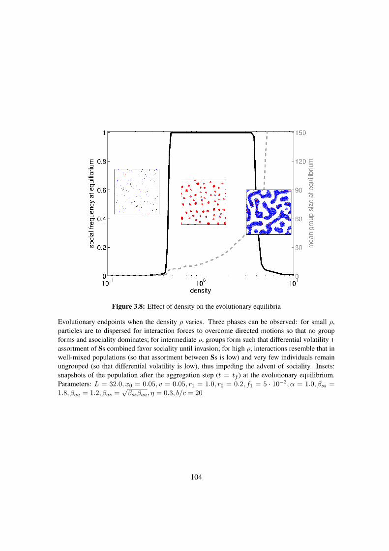
Figure 3.8: Effect of density on the evolutionary equilibria

Evolutionary endpoints when the density ρ varies. Three phases can be observed: for small ρ,particles are to dispersed for interaction forces to overcome directed motions so that no groupforms and asociality dominates; for intermediate ρ, groups form such that differential volatility +assortment of Ss combined favor sociality until invasion; for high ρ, interactions resemble that inwell-mixed populations (so that assortment between Ss is low) and very few individuals remainungrouped (so that differential volatility is low), thus impeding the advent of sociality. Insets:snapshots of the population after the aggregation step (t = tf ) at the evolutionary equilibrium.Parameters: L = 32.0, x0 = 0.05, v = 0.05, r1 = 1.0, r0 = 0.2, f1 = 5 · 10−3, α = 1.0, βss =1.8, βaa = 1.2, βas =

√βssβaa, η = 0.3, b/c = 20

104

3.4 Discussion

3.4.1 Evolution of sociality via differential adhesion

The evolution of social behavior is a riddle for evolutionary biology because of the disruptive

power of within-group competition between individuals that invest or not in the public good.

In microbes and in the early stages of the transition to multicellularity, most mechanisms that

sustain coperation through the use of cognitive abilities are ruled out. On the other hand, genetic

relatedness may not be the only driver of the evolution of collective behavior, since microbial

aggregates are commonly observed even when cells of potentially different origin come together.

Here, I have explored one possible mechanism that allows the evolution of sociality and sizeable

groups, when sticky self-propelled particles moving on a plane are assigned a fitness that de-

pends on their social environment. The emergent structure of the population, underpinned by

the adhesion forces between particles, feeds back onto the evolutionary dynamics of more or

less adhesive types. By analyzing a model with successive cycles of aggregation-reproduction-

dispersal, I have shown that sociality gets established in a limited range of parameter values:

intermediate particle velocities; intermediate interaction radii; sufficient persistence in the parti-

cle directed movement; intermediate densities. These results can be understood in terms of two

features of the population structure: assortment within groups and volatility, both of which affect

the average fitness of particles with different interaction forces.

3.4.2 Strategy assortment and differential volatility

Assortment among types has long been pointed out as a requirement for the evolution of costly

cooperative behaviors (e.g. Wilson and Dugatkin (1997); Fletcher and Zwick (2006); Fletcher

and Doebeli (2009)). However, experimentalists as well as theorists still debate on how such

assortment is actually reached when genetic relatedness does not appear to play a central role..

105

Most solutions involve some kind of recognition of other individuals’ strategies, or at least in-

formation about a variable correlated with the strategy: a “green beard” gene coding for both the

character, the recognition of copies of the genes among partners and preferential interaction with

their carriers (Dawkins, 1976); partner choice (Kun et al., 2010; Andre and Baumard, 2011);

conditional strategies involving choosiness (McNamara et al., 2008); matching by group size

preference (Powers et al., 2011); direct (Trivers, 1971; Axelrod, 1984) or indirect/generalized

reciprocation (Nowak and Sigmund, 1998; Wedekind and Milinski, 2000; Pfeiffer et al., 2005),

etc. Here, I describe a mechanistic process by which particles are endowed with attractive forces

that are independent of the social context. Assortment occurs with no need to assume that S par-

ticles attach preferentially with other Ss; only differential attachment of Ss and As is required.

This important distinction has been alluded to or stressed in several recent works (Smukalla et

al., 2008; Strassmann et al., 2011; Garcia and De Monte, 2013). Ultimately, S particles enjoy

the advantages of group cohesion to a larger extent, to the point that they can offset the cost of

sociality.

Volatility is a much more neglected factor to achieve distinct reproductive successes for each

type. Differential volatility means that asocials are less prone to be in a group, or at least more

loosely stuck to the group ; therefore, more likely to get no group benefits or a lesser share of

them. Surprisingly, the possibility that individuals do not participate in any group has been over-

looked in models of the evolution of cooperation. In the papers that did, being alone results either

from an encoded strategy, (e.g. Hauert et al. (2002a,b)), or to coercion by cooperators (Sasaki

and Uchida., 2013), rather than being a by-product of an explicit group formation process. Re-

cently, detailed models of motion began to be implemented in evolutionary models that allow

in principle for the existence of lonely individuals (Meloni et al., 2009; Cardillo et al., 2012).

Indeed, in many actual group-structured biological populations, a proportion of individuals typ-

ically fail to join any group (Smukalla et al., 2008; Dubravcic et al., submitted). We stress that,

as soon as the proportion of ungrouped particles differ for both types, the evolutionary dynamics

106

is affected in favor of the more strongly aggregating type. In our model, differential volatility

occurs as the cooperative trait is related to grouping ability itself, as stronger adhesion forces

confer cohesiveness to groups but also enhance individual attachment. Any cooperative trait in-

creasing the probability to end up in a group would yield qualitatively similar results: socials

and asocials may be defined on the basis of differences in properties other than attachment, e.g.

their interaction radius.

In general, assortment and volatility are not independent features of the emergent population

structure. In our simulations, the faculty for S particles to become positively assorted comes

along with a lesser tendency to be left alone by the aggregation process. However, it is note-

worthy that, in situations when sociality is the winning strategy, positive assortment alone may

not be sufficient to account for its advantage. Indeed, assuming that RS > RA and uS < uA,

the two conditions 1) bRS − c+ b∑

dS(n)/n < bRA (assortment alone is not enough to favor

sociality) and 2) bRS (1 − uS) + b∑

dS(n)/n − c > bRA (1 − uA) (assortment + differential

volatility combined favor sociality) are compatible as soon as RA uA > RS uS . In this case,

differential volatility drives the rise in frequency of sociality, while it would not be the case dis-

counting singletons. This suggests that in real settings where group size is distributed and not

fixed, models and experiments might overestimate the constraints for cooperative behavior to be

favored. While positive assortment and differential volatility are two complementary effects that

promote sociality, they both stem from the biologically plausible hypothesis that a character may

affect the expected group size distribution. Examples of traits regulating group size are known

in D. discoideum (Roisin-Bouffay et al., 2000; Gole et al., 2011), although their effects on the

group size distribution have to my knowledge never been quantified.

3.4.3 Role of group formation

I highlighted that parameters related to particle motion are key in the evolutionary success of

social individuals. Noise, velocity, density and interaction radius must be restricted to specific

107

ranges for sociality to be able to take over the population; otherwise asociality dominates. In

actual biological settings, these parameters might have co-evolved with adhesion properties, and

their evolutionary dynamics may be explored with a multi-trait model.

This model stresses that observing and quantifying the properties of the population struc-

ture generated by a given mixture of strains may inform on the mechanisms that underlie the

evolutionary process. The issue of being able to count a large amount of aggregates (so that

statistics are reliable) can be overcome by means of microscopes screening a large surface and

still maintaining a single-cell resolution (Houchmandzadeh, 2008; Dubravcic et al., submitted).

The analysis performed in section 3.3.3 indicates what are the expected patterns if evolution-

ary experiments are carried out under different environmental conditions that affect cell-level

properties, such as cell density or substrate hardness (that conditions cell movement). More im-

portantly, they indicate two statistics that may predict if a given population would evolve towards

more or less sociality.

3.4.4 Conclusion

Although unicellular organisms are often found in large aggregates, their high dispersal abilities

and the consequent mixing of genotypes makes the establishment and maintenance of social

behavior aparently paradoxical. When physical mechanisms underlying the formation of groups

are made explicit however, the evolution of sociality looks less mysterious, and one can start

asking quantitative questions on the processes that led to the emergence of cellular aggregates.

The simple model presented here can be enriched with further details implementing additional

features of microbial organisms, such as alignment terms (Vicsek et al., 1995; Gregoire et Chate,

2004), an explicit account of the cell shape (Peruani et al., 2012) and chemotaxis (Jiang et al.,

1998; Calovi et al., 2010). The exploration of the mechanistic role of cell-cell interaction terms

in shaping the social structure is a fundamental step to understand altruism in microbes, as well

as the possible evolutionary paths towards multicellularity.

108

3.5 Effect of ecological vs. evolutionary time scale

This section is very much a work in progress; more simulations and analyses are required to

confirm the exposed results. However, I believe it already displays some interesting features on

conflicting levels of selection and group dynamics.

3.5.1 Hypotheses

Until now, the impact of natural selection on the composition of the population was deemed to

occur on timescales much longer than that of group formation: individuals were let the time to

swarm before a reproduction event occurs, and re-dispersed afterwards. This setting is mostly

relevant for microorganisms such as Myxobacteria or social amoeba that alternate a phase of

aggregation triggered by the depletion of nutrients in the environment with a sporulating phase

where a proportion of the population is able to disperse and colonize a new environment. How-

ever, other microorganisms divide while they forage (Nadell et al., 2010; Simon et al., 2012). Let

us consider that reproductive events are periodic. We denote tR the period between two succes-

sive reproductive events. At each time step, the payoff of each individual is calculated according

to a PGG in its current group (if any). Every tR time steps, the cumulated payoff of the last

tR time steps is used to define an individual’s probability to leave offspring. Offsprings appear

just next to their ancestors (at a distance 2r0), in a random orientation. To isolate the role of

the interplay of time scales from that of varying population densities on evolutionary dynamics

(Sanchez and Gore, 2013), the total population size is still kept constant : each time a offspring

appears, an individual is chosen at random to die. Therefore, groups dynamically grow or shrink

due to internal reproductive dynamics and the two conflicting levels of selection are immediately

apparent in simulations: S individuals are disadvantaged compared to A individuals in their own

groups but groups comprised of many S individuals yield more benefits and thus expand more

(see Box 2.4.).

109

3.5.2 Evolutionary trajectories

In Figure 3.9, the population begins to form clusters on a fast time scale (t = 100 ∼ 200).

Among them, groups of a few Ss emerge by chance (t = 300) and grow more rapidly than

groups composed mostly of As. However, as soon as they merge with nearby mostly-A groups

or free As are attracted by them (t = 400), intra-group competition occurs while they keep on

expanding (t = 500). When these group are marred by too many As, they cannot compete

against newly formed mostly-S groups (t = 800) and collapse (t = 900 ∼ 1000). In the end,

many As die and the social frequency in the population increases. A contradiction seems to

arise: when there remains only one group in the population, how come this group is not invaded

by the few As left until they take over? The maintenance of sociality relies on two mechanisms:

1) as, unlike mostly-S groups that are very cohesive, mostly-A groups are more volatile, the

proliferation of A individuals would make the group split in several parts and re-generate group

competition. However, this does not even happen in practice as 2) As at the border actually do

not belong to the group according to the criterion used, as they are not “stuck” to it like a solid

but circulate like a liquid around its surface. Therefore, even though in-group As have a payoff

advantage relative to in-group Ss, it is compensated on average by these free A individuals that

earn nothing from the group, thus dying quickly and being replaced at the periphery by volatile,

formerly in-group As. Thanks to this, once a high level of sociality is reached it is generally very

resistant to a novel exploitation by asocials, as confirmed qualitatively by simulations.

110

Figure 3.9: Snapshots of an evolutionary trajectory with motion and reproduction concomitant:case when Ss dominate

The population is represented at distinct instants of the evolutionary trajectory. The bottom paneldisplays the variation of social frequency in time. See explanations in the main text. Parameters:Npop = 2048, L = 32.0, v = 0.05, x0 = 0.1, r1 = 1.0, r0 = 0.2, πss = 1.8, πaa = 1.2,πas =

√πssπaa, f1 = −f0 = 5 · 10−3, η = 0.3, b/c = 20, tR = 5. There are no mutations.

111

Figure 3.10: Snapshots of an evolutionary trajectory with motion and reproduction concomitant:case when As dominate

The population is represented at distinct instants of the evolutionary trajectory. The bottom paneldisplays the variation of social frequency in time. See explanations in the main text. Parameters:Npop = 2048, L = 32.0, v = 0.05, x0 = 0.1, r1 = 1.0, r0 = 0.2, πss = 1.8, πaa = 1.2,πas =

√πssπaa, f1 = −f0 = 5 · 10−3, η = 0.3, b/c = 10, tR = 5. There are no mutations.

112

What also appears in simulations, and needs to be quantified further, is that such robustness

of sociality when very few groups remain requires S players to have reached a critical mass and

a critical fraction in their respective groups, as pointed out in a different way in a non-spatially

explicit model where groups form randomly and are let evolve for a fixed amount of time (Cremer

et al., 2012). In Figure 3.10, b/c has been decreased. Despite forming a promising small group at

t = 2700, Ss soon do not manage to dominate their group even though they make it grow rapidly.

Between t = 3300 and t = 5000, the fusion of a solid all-S group with a much larger mostly-

A group proves lethal to the former, impeding the takeover of sociality. In this simulation, the

evolution of the social trait in future times is probably doomed: to happen, it would require S

individuals to form a cluster far enough from the gigantic A-group so as to outcompete it and not

be “phagocyted” by it; but it seems impossible as individuals are born close to their ancestor.

In some cases, the dynamics of the social trait for a given set of parameters result in either

full invasion or full extinction depending of its initial frequency (Fig. 3.11; here, social and aso-

cial interaction forces are more distant from each other than formerly). Such bistability (akin to

what is predicted by, for instance, a Stag Hunt game) results from S players being able or not

to form small clusters locally that are immune to asocial exploitation for a sufficient amount of

time. Unlike for instance in Figure 3.10, once sociality is triggered it generally does not falls

back; conversely, when sociality becomes too scarce it cannot recover. A wide parameter explo-

ration would be needed to assess the influence of microscopic parameters on the evolutionary

outcome, and “map” the (possibly) different dynamics (directed, bistable, polymorphic, etc.) on

the parameter space, but it is out of the scope of this thesis.

3.5.3 Effect of the generation time

To analyze the influence of the discrepancy between the ecological and evolutionary time scales,

I performed repeated evolutionary simulations for different values of tR and computed the av-

erage final social frequency. Figure 3.12 suggests that concomitant ecological and evolutionary

113

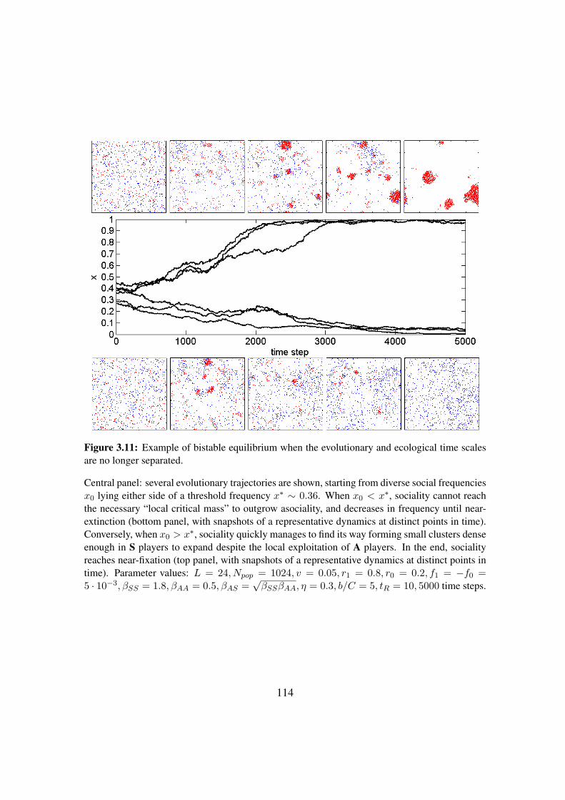
Figure 3.11: Example of bistable equilibrium when the evolutionary and ecological time scalesare no longer separated.

Central panel: several evolutionary trajectories are shown, starting from diverse social frequenciesx0 lying either side of a threshold frequency x∗ ∼ 0.36. When x0 < x∗, sociality cannot reachthe necessary “local critical mass” to outgrow asociality, and decreases in frequency until near-extinction (bottom panel, with snapshots of a representative dynamics at distinct points in time).Conversely, when x0 > x∗, sociality quickly manages to find its way forming small clusters denseenough in S players to expand despite the local exploitation of A players. In the end, socialityreaches near-fixation (top panel, with snapshots of a representative dynamics at distinct points intime). Parameter values: L = 24, Npop = 1024, v = 0.05, r1 = 0.8, r0 = 0.2, f1 = −f0 =5 · 10−3, βSS = 1.8, βAA = 0.5, βAS =

√βSSβAA, η = 0.3, b/C = 5, tR = 10, 5000 time steps.

114

1 10 20 30 40 50 60 700

0.2

0.4

0.6

0.8

1

tR

aver

age

xeq

Figure 3.12: Effect of the generation time tR on the average equilibrium frequency of S players.

Although dynamics are highly variable given a set of parameters and a generation time tR, meanvalues of the social frequency at equilibrium appear to decrease with tR. This can be accountedby the decreased ability for S players to form quickly expanding clusters that are robust againstthe exploitation of As when reproduction is slow relative to motion, thus enabling As to join andmar newborn social groups. Parameters:

time scales (i.e., frequent reproductive events during motion) makes it easier for high levels of

sociality to arise in populations.

Recently, Cremer et al. (2012) published a model that bears conceptual similarities to this

one. Individuals undergo lifecycles characterized by 1) a phase of group formation in which

separate groups of fixed size are formed by an unbiased stochastic process; 2) a phase of group

evolution in which groups evolve separately for a fixed “regrouping time”. Highly cooperative

groups yield higher benefits and reach larger carrying capacities, but internal competition ad-

vantages defectors; 3) a phase of re-merging of groups into a global pool. In their model, short

regrouping times favor the evolution of cooperation until fixation; intermediate regrouping times

favor coexistence between cooperators and defectors; and high regrouping times favor bistabil-

ity between full cooperation and full defection (Fig. 3.13). Again, a more thorough look on

simulation data will be required to compare further my preliminary results with Cremer et al.’s.

115

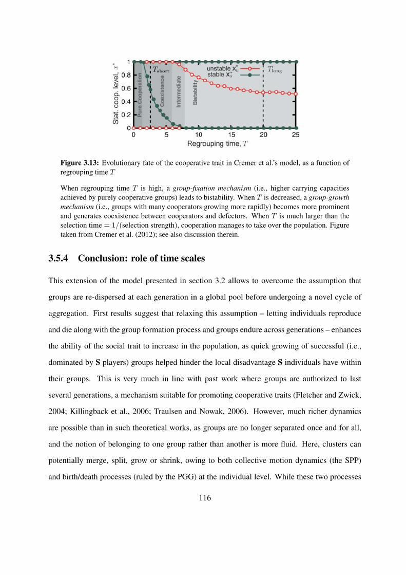
Figure 3.13: Evolutionary fate of the cooperative trait in Cremer et al.’s model, as a function ofregrouping time T

When regrouping time T is high, a group-fixation mechanism (i.e., higher carrying capacitiesachieved by purely cooperative groups) leads to bistability. When T is decreased, a group-growthmechanism (i.e., groups with many cooperators growing more rapidly) becomes more prominentand generates coexistence between cooperators and defectors. When T is much larger than theselection time = 1/(selection strength), cooperation manages to take over the population. Figuretaken from Cremer et al. (2012); see also discussion therein.

3.5.4 Conclusion: role of time scales

This extension of the model presented in section 3.2 allows to overcome the assumption that

groups are re-dispersed at each generation in a global pool before undergoing a novel cycle of

aggregation. First results suggest that relaxing this assumption – letting individuals reproduce

and die along with the group formation process and groups endure across generations – enhances

the ability of the social trait to increase in the population, as quick growing of successful (i.e.,

dominated by S players) groups helped hinder the local disadvantage S individuals have within

their groups. This is very much in line with past work where groups are authorized to last

several generations, a mechanism suitable for promoting cooperative traits (Fletcher and Zwick,

2004; Killingback et al., 2006; Traulsen and Nowak, 2006). However, much richer dynamics

are possible than in such theoretical works, as groups are no longer separated once and for all,

and the notion of belonging to one group rather than another is more fluid. Here, clusters can

potentially merge, split, grow or shrink, owing to both collective motion dynamics (the SPP)

and birth/death processes (ruled by the PGG) at the individual level. While these two processes

116

have been well studied in the literature, to my knowledge their combined effect in the context of

social dilemmas has not been addressed so far. Although groups are not allowed to reproduce or

die by themselves, this model could be interpreted in the framework of recent theoretical works

attempting to solve the puzzle of multilevel selection (Simon et al., 2012).

117

Chapter 4

Conclusion

4.1 Main results

In this section are summarized the main conclusions and issues that I judge noteworthy of dis-

cussion.

Costly sociality can evolve via blind assortment, even when altruistic. In this manuscript,

I focused on the basic requirements for primitive collective lifestyle. In the literature, one can

notice an ongoing trend to explain cooperation by assuming the pre-existence of very elaborate

individual behaviors in more or less explicit ways. Sometimes, a combination of several cog-

nitively demanding or socially acquired abilities (e.g. memory, peer recognition, conditional

behavior, obedience to a norm, risk aversion, etc.) is invoked. While such assumptions are plau-

sible in rational, socially-driven humans, they fall short in providing real insight on the ubiquity

and diversity of sociality as evidenced in recent years in very simple, e.g. microbial, species.

Second, most of these models put the emphasis on helping / sharing behavior in settings where

individuals do interact and form groups, but elude the issue of how individual traits generat-

ing and sustaining such groups can emerge. As this is the basic brick for the ulterior evolution

119

of more complex interactions, it must be accounted for with minimal hypotheses on the social

context.

In chapter 2, I show that a costly, genetically encoded trait that increases its carrier’s propen-

sity to form groups (by any mechanism), and benefits to other group members owing to enhanced

cohesion, can emerge and expand in a biological population. Social individuals thrive because

they manage to get assorted together, i.e. the average social individual experiences more social

groups than the average asocial individual. Additionally, socials end up ungrouped less often

than asocials. Positive assortment of social individuals occurs without them being able to rec-

ognize one another, or interact preferentially. This is of particular importance to account for

sociality in microbes, as it keeps the cognitive requirements as minimal as possible: differential

attachment in both types (social and asocial) is sufficient with no need of preferential attachment,

thus providing a parcimonious scenario for the evolution of grouping traits in microbes.

In what was at first a thought experiment, Dawkins (1976) imagined the evolutionary con-

sequences of a “green beard” gene (or set of linked genes), defined as a gene encoding three

behaviors: 1) a phenotypic tag (the “green beard”); 2) the ability to recognize other carriers

of the tag; 3) a cooperative behavior preferentially directed toward them. Green beard genes

were considered improbable until several presumed examples of such genes were reported in

the literature (Keller and Ross, 1998; Ponte et al., 1998; Riley and Wertz, 2002; Gibbs et al.,

2008; Smukalla et al., 2008). In two recent papers, Gardner and West re-phrased the defini-

tion of green beards as traits that are cooperative (resp. spiteful) and entail assortment with

other carriers (resp. noncarriers).This re-definition is however misleading compared to the ini-

tial formulation by Dawkins as it leaves behind the notion of preferential interaction; moreover,

it focuses on dyadic interactions, whereas N -player interactions cannot be formally reduced to

those.

In chapter 2, S individuals do not interact preferentially with other Ss, compared to As them-

selves; but assortment happens to emerge all the same as S individuals interact more, as a whole.

120

Biased interactions are a ultimate effect rather than a proximate cause (Nowak et al., 2010a).

Neglecting such possibility, Gardner and West treated preferential and differential interaction

as equal and coined any cooperative behavior that entails assortment at a single locus a “green

beard” trait, while it is not necessarily so according to the original definition. Combined with the

widespread intuition that green beards are rare in nature, such confusion in terms might let one

think that assortment at a single locus itself is dubious, and that assortment on the whole genome

(i.e., kin selection) is the process par excellence to promote cooperative behavior. Actually, many

distinct mechanisms can lead to assortment in otherwise unrelated individuals.

The altruistic / directly beneficial status of a social trait depends on the population struc-

ture. The evolution of a costly cooperative trait is only paradoxical if the cost incurred by the

carrier is not canceled by compensatory direct benefits. Consequently, a whole family of models

describes mechanisms that, at some point, “relieve the dilemma”. In the PGG framework, this

can be achieved by reducing the size of the group, as the direct benefit accrued by a cooperator

is b/N , e.g. considering lonely individuals that do not participate to the game (Hauert et al.,

2002a,b), allowing multigenerational (Fletcher and Zwick, 2004; Killingback et al., 2006), even

splitting (Traulsen and Nowak, 2006) groups, or letting group size preference co-evolve with

cooperation, and individuals group with those matching their preference (Aviles, 2002; Powers

et al., 2011), etc. In these settings, cooperation might be altruistic at some point when groups

are large, then become directly beneficial because of the large-size group depletion subsequent

to free-riders exploitation. In chapter 2, I stress that the benefit-to-cost ratio conditions not only

the evolutionary fate of the social trait (in the toy model, either fixation or extinction), but also

its “status” throughout the evolutionary trajectory. When socials are rare, groups are still small

and sociality can increase in frequency via direct benefits. Once the social trait reaches a thresh-

old frequency, it keeps on spreading until fixation thanks to positive assortment even though the

social trait has become altruistic in the meantime.

121

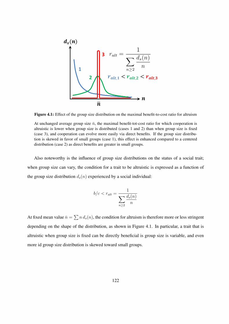
Figure 4.1: Effect of the group size distribution on the maximal benefit-to-cost ratio for altruism

At unchanged average group size n, the maximal benefit-tot-cost ratio for which cooperation isaltruistic is lower when group size is distributed (cases 1 and 2) than when group size is fixed(case 3), and cooperation can evolve more easily via direct benefits. If the group size distribu-tion is skewed in favor of small groups (case 1), this effect is enhanced compared to a centereddistribution (case 2) as direct benefits are greater in small groups.

Also noteworthy is the influence of group size distributions on the status of a social trait;

when group size can vary, the condition for a trait to be altruistic is expressed as a function of

the group size distribution ds(n) experienced by a social individual:

b/c < ralt =1∑

n≥2

ds(n)

n

At fixed mean value n =∑

n ds(n), the condition for altruism is therefore more or less stringent

depending on the shape of the distribution, as shown in Figure 4.1. In particular, a trait that is

altruistic when group size is fixed can be directly beneficial is group size is variable, and even

more id group size distribution is skewed toward small groups.

122

Sociality naturally gets coupled with cooperation for group cohesion during the in-group

phase. In section 2.4, I modeled the case when the assumption on the coupling of stickiness in

the aggregation phase and cooperation in the in-group phase is relaxed. This corresponds to situ-

ations when a cell is genetically programmed to, for instance, secrete adhesive substances during

the former phase and refrain doing so during the latter. I assume that such a switching behavior

entails an additional cost, e.g. imposed by a quorum-sensing ability to detect the beginning of the

in-group phase and halt or trigger the cellular machinery consequently, whereas non-switching

strategies do not need such ability. I show that, for a very large portion of the parameters ranges,

switching strategies are eliminated, so that the only viable strategies are to be either social or

asocial all along the life cycle. The argument actually works even for null additional regulatory

cost: indeed, when SCs (sticky cooperators) are not able to outcompete SDs (sticky defectors),

ADs (non-sticky defectors) outcompete both anyway.

A minimal initial amount of sociality is required. The 2-strategy model is based on the

assumption that the social trait can take up discrete values, such that pro-social mutations en-

code for a specific function that discontinuously enhances the propensity to form groups. The

continuous trait model rather assumes that such function pre-exist but is expressed at various

levels. In both cases, a condition for an increase in sociality to be selected for is that a certain

level of sociality is present in the population to begin with. The frequency of the social trait in

the 2-strategy case, and the resident ability to interact in the continuous case, must overcome a

threshold below which sociality is wiped away. As soon as this condition is met, sociality rises to

its utmost level in the nonassortative case. The necessity of a minimal core of sociality to trigger

its own evolution is a recurring pitfall in evolutionary models: for instance, in nonlinear games,

an invasion threshold has to be reached to make cooperation increase and persist. Actual models

often avoid the issue altogether, rather focusing on the less challenging puzzle of maintenance

(e.g. initializing models with a 50-50 mixture of cooperators and cheaters). However, such con-

123

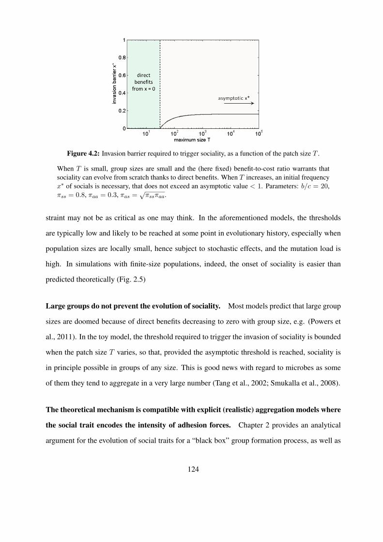
Figure 4.2: Invasion barrier required to trigger sociality, as a function of the patch size T .

When T is small, group sizes are small and the (here fixed) benefit-to-cost ratio warrants thatsociality can evolve from scratch thanks to direct benefits. When T increases, an initial frequencyx∗ of socials is necessary, that does not exceed an asymptotic value < 1. Parameters: b/c = 20,πss = 0.8, πaa = 0.3, πas =

√πssπaa.

straint may not be as critical as one may think. In the aforementioned models, the thresholds

are typically low and likely to be reached at some point in evolutionary history, especially when

population sizes are locally small, hence subject to stochastic effects, and the mutation load is

high. In simulations with finite-size populations, indeed, the onset of sociality is easier than

predicted theoretically (Fig. 2.5)

Large groups do not prevent the evolution of sociality. Most models predict that large group

sizes are doomed because of direct benefits decreasing to zero with group size, e.g. (Powers et

al., 2011). In the toy model, the threshold required to trigger the invasion of sociality is bounded

when the patch size T varies, so that, provided the asymptotic threshold is reached, sociality is

in principle possible in groups of any size. This is good news with regard to microbes as some

of them they tend to aggregate in a very large number (Tang et al., 2002; Smukalla et al., 2008).

The theoretical mechanism is compatible with explicit (realistic) aggregation models where

the social trait encodes the intensity of adhesion forces. Chapter 2 provides an analytical

argument for the evolution of social traits for a “black box” group formation process, as well as

124

a proof of principle with a toy example; chapter 3 confirms that this result is compatible with

a more realistic and spatially explicit aggregation scheme, serving as a validation of chapter 2.

The self-propelled particles model used in this chapter is intended to be specific enough to draw

precise conclusions on the effect of microscopic parameters on sociality, but generic enough

to encapsulate zeroth-order behaviors of a wide range of species. The assumptions made (spa-

tial extension of particles; interaction forces depending on their distance; inertia on movement)

remain weak and are consistent with many empirical studies on microbial motion.

The evolution of sociality is only possible in specific conditions on ecological and micro-

scopic parameters of motion. The coupling of the SPP aggregation model and the game-

theoretical framework allows to “read” directly the conditions that are favorable to sociality

upon the obtained ESSs . High noise (e.g. due to locally perturbed environments) – that brings

particle movement closer to an unbiased Brownian motion –, low density, and high velocity /

low interaction radius – that rather emphasize directed motion over attraction between particles

– all mar individual clustering, hence sociality. High interaction radius and high density make

individuals neighborhood close to well-mixed, and low velocity hinders sufficient mixing of in-

dividuals, thus thwarting the assortment of socials during the transient. As a result, intermediate

values of the population density, particle velocity and interaction radius, and moderate noise are

required for a social mutant strain to replace a resident asocial strain. I also stress that the success

or not of the social trait can be derived from the knowledge of macroscopic observables on the

population structure, namely:

• the average ratio of sociality experienced by the average social (resp. asocial) individual

within its group. This quantifies the level of assortment of socials;

• the proportion of ungrouped individuals of each type.

125

Whereas positive assortment of socials within groups is a well-known determinant for their suc-

cess, differential volatility (i.e., the difference in proportions of social and asocial individuals

staying outside groups) is a neglected factor in the literature, although it is equally likely to

boost sociality. This is because most models 1) consider group size constant, and no individual

alone; 2) focus on helping traits that take place in pre-existing group structures.

The emergent population structure resembles that of real microbes. Chapter 3 evidences

that with very simple assumption on particle movement (namely, volume exclusion and attraction

until a cut-off radius), it is possible to generate aggregation patterns and population structures that

are quite close to some encountered in real microbes (Fig. 4.3). For instance, in Dictyostelium

discoideum, cells converge toward centers of attraction by relaying cAMP signals, resulting in

local clusters of circular shape and comparable sizes (Fig. 4.3A). While several works describe

more thoroughly group formation in Dicty – e.g. explicitly modeling chemotaxis (van Oss et al.,

1996; Palsson and Othmer, 2000; Calovi et al., 2010) – and capture more exactly the features of

the transient phase (for instance the spiral waves and star-shaped streams resulting from cAMP

gradients – not shown here), the generic model I used still retains some of the main qualitative

characteristics of aggregation. The ability to aggregate, and the sizes of the resulting groups

depends on the intensity of the attachment force between mobile cells, which is consistent with

what is experimentally observed in cells expressing adhesion protein on their membrane (Foty

and Steinberg (2005), Fig. 4.3B).

Another striking feature of the model of chapter 3 is the spatial segregation occurring be-

tween sticky and less sticky cells, which is consistent with experiments on flocculating yeast and

N-cadherin expressing L cells. In yeast, Smukalla et al. (2008) mixed wild-type cells endowed

with a social gene FLO1, coding for the expression of an adhesion protein, with FLO1-knockout

cells. They observed that 1) while groups contain cells of both types, FLO1− cells are under-

represented in groups and make for most of the ungrouped cells; 2) within groups, FLO1− cells

126

Figure 4.3: Formation of groups in Dictyostelium discoideum and in cadherin-expressing L cells

Panel A: Temporal snapshots of a group formation process in Dictyostelium discoideum: whenstarved, “pacemaker” cells secrete a cAMP signal that is relayed by successive waves to neigh-bors. Cells follow cAMP gradients until they gather into localized, circular-shaped aggregates ofsizes of the same order of magnitude (not all cells enter an aggregate, though (Dubravcic et al.,submitted)). Later on, they will form a mobile slug oriented by phototaxis and morph into a fruit-ing body whose spores are dispersed and stall cells die. Pictures produced by Darja Dubravcic.Panel B: Result of aggregations of N-cadherine-transfected L cell lines with increasing cadherinexpressions levels. Cell aggregation rate increases with the level of expression of the adhesionprotein. Reproduced from (Foty and Steinberg, 2005).

tend to occupy the outermost layer of the floc (Fig. 4.4A). Three years before, Foty and Stein-

berg (2005) reported a similar pattern in N-cadherin expressing L cells: they mixed strains that

express distinct levels of the protein, and found out that low cadherin-level cells were relegated

to the periphery of aggregates, with high cadherin-level cells clumped together within.

The rate of reproduction, relative with the time scale of motion, influence the evolutionary

equilibrium. The preliminary results of the last section of chapter 3 seem to evidence that the

interplay of reproduction and mobility may change drastically the evolutionary dynamics of the

social trait, not only during the transient but also the evolutionary equilibrium itself. This is of

interest for species whose life cycle, unlike Dictyostelids and Myxobacteria, is not separated in

a group formation and a reproduction phases. The preliminary results shown in section 3.5 need

however further work to assess accurately the effect of the concomitant (ecological and evolu-

tionary) time scales, and the nature of equilibria that are expected (monomorphic or dimorphic;

bistable or not) according to the reproduction time tR.

127

Figure 4.4: Spatial cell sorting in S. cerevisiae and in cadherin-expressing L cells

Panel A: in mixed cultures in budding yeast, flocculating cells endowed with the FLO1 geneoccupy the core of aggregates and nonflocculating cells agglutinate at the periphery. Reproducedfrom (Smukalla et al., 2008). Panel B: two N-cad-transfected L cell clones expressing N-cad attheir surfaces in the ratio of 2.4:1 are mixed in equal proportions and cultured as hanging drops.The first picture displays the inital cell mixture; after 24h of incubation, the cell line expressingthe lower level of N-cad, here labeled red, envelops the cell line expressing higher amounts ofN-cad, here labeled green. Reproduced from (Foty and Steinberg, 2005).

4.2 Perspectives for future work

This work may be expanded in several ways. First, for simplicity I considered the social strategy

to be binary in the explicit spatial model of chapter 3, i.e. either asocial (entailing an interaction

coefficient βAA) or social (entailing a cost c and an interaction force βSS > βAA). However, one

can consider that sociality depends, for instance, on the secretion of an adhesive polymer in a

variable quantity, that is encoded in the adhesion gene. This would change the trait under selec-

tion from a binary trait to a continuous trait, associated with a cost that is a growing function of

the entailed adhesiveness c = c(β). Such change in the model might lead to richer evolutionary

dynamics, as from some point a costly increase in adhesiveness is of no use for individuals. Evo-

lution might then lead to a monomorphic population endowed with a unique (optimal) adhesion

coefficient β or, more intricately, a polymorphism of adhesion traits whose distribution is not

straightforward. As specific ranges for microscopic parameters are required for a social muta-

128

tion to be selected, and as these ranges may change as a function of the different interaction force

intensities at play in the population, it is not said that successive pro-social mutations will invade

for any set of microscopic and ecological parameters. The outcome is thus tricky to conjecture,

and extensive computations will be needed.

A second aspect to investigate is to let parameters other than the adhesion intensity evolve;

indeed, there are other ways to enhance the amount of interactions such as a larger interaction

radius, that can themselves relate to “being social”. We showed for instance that too high a

velocity puts the population to a gas state, while too low a velocity impedes assortment, and both

these features of the population structure are detrimental to sociality. Exploring how adhesion

forces co-evolve with velocity may account for social specializations relevant in the microbial

world: superadhesive individuals, explorators, long-distance attractors, etc. (Guttal and Couzin,

2010)

Lastly, we opted for very basic rules of interaction as a blueprint to study collective motion

and social evolution jointly. In a second step, these rules could be enriched to fit a specific

microorganism, implementing additional components in the SPP model such as alignment terms,

chemotaxic processes, etc.

129

Bibliography

Andre, J.B., and Baumard, N. 2011. The evolution of fairness in a biological market. Evolution65, 1447-1456. I 106

Antal, T., Ohtsuki, H., Wakeley, J., Taylor, P.D., and Nowak, M.A. 2009. Evolution of coopera-tion by phenotypic similarity. Proc. Natl. Acad. Sci. USA 106, 8597-8600. I 147

Archetti, M., and Scheuring, I. 2010. Coexistence of cooperation and defection in public goodsgames. Evolution. 65, 1140-1148. I 20, 41, 93, 94

Archetti, M., and Scheuring, I. 2012. Review: Game theory of public goods in one-shot socialdilemmas without assortment. J. Theor. Biol. 299, 9-20. I 20, 22, 24

Aviles, L., 2002. Solving the freeloaders paradox: genetic associations and frequency dependentselection in the evolution of cooperation among relatives. Proc. Natl. Acad. Sci. USA 99,14268-14273. I 7, 29, 36, 40, 81, 121

Axelrod, R., and Hamilton, W.D. 1981. The evolution of cooperation. Science 211, 1390-1396.I 36

Axelrod, R. 1984. The evolution of cooperation. Basic Books. I 9, 106

Bachmann, H., Molenaar, D., Kleerebezem, M., and Vlieg, J.E.T.V. 2011. High local substrateavailability stabilizes a cooperative trait. ISME J. 5, 929-932. I 14

Bai, L., Eyiyurekli, M., Lelkes, P.I., and Breen, D.E. 2013. Self-organized sorting of heterotypicagents via a chemotaxis paradigm. Sci. Comput. Program. 78, 594-611. I 92

Barabasi, A.-L., and Albert, R. Emergence of scaling in random networks. Science 286, 509-512.I 25

Beatrici, C.P., and Brunnet, L.G. 2011. Cell sorting based on motility differences. Phys. Rev. E84, 031927. I 84, 92

Belmonte, J.M., Thomas, G.L., Brunnet, L.G., de Almeida, R.M.C., and Chate, H. 2008. Self-propelled particle model for cell-sorting phenomena. Phys. Rev. Lett. 100, 248702. I 84,92

131

Bonabeau, E., Dagorn, L., and Fron, P. 1999. Scaling in animal group-size distributions. Proc.Natl. Acad. Sci. USA 96, 4472-4477. I 77

Borenstein, D.B., Meir, Y., Shaevitz, J.W., and Wingreen, N.S. 2013. Non-local interaction viadiffusible resource prevents coexistence of cooperators and cheaters in a lattice model. PLoSOne 8, e63304. I 31, 93

Boyd, R., Gintis, H., Bowles, S., and Richerson, P.J. 2003. The evolution of altruistic punish-ment. Proc. Natl. Acad. Sci. USA 100, 3531-3535. I 10

Brown, S.P., and Buckling, A. 2008. A social life for discerning microbes. Cell 135, 600-603. I12

Buckling, A., Maclean, R.C., Brockhurst, M.A., and Colegrave, N. 2009. The Beagle in a bottle.Nature 457, 824-829. I 4

Calovi, D.S., Brunnet, L.G., and de Almeida, R.M. 2010. cAMP diffusion in Dictyosteliumdiscoideum: a Green’s function method. Phys. Rev. E 89, 011909. I 108, 126

Cardillo, A., Meloni, S., Gomez-Gardenes, J., and Moreno, Y. 2012. Velocity-enhanced coop-eration of moving agents playing public goods games. Phys. Rev. E 85, 067101. I 28, 100,106

Celiker, H., and Gore, J. 2013. Cellular cooperation: insights from microbes. Trends Cell. Biol.23, 9-14. I 5, 80

Chen, Z., Gao, J., Cai, Y., and Xu, X. 2011a. Evolutionary prisoner’s dilemma game in flocks.Physica A 390, 50-56. I 28, 77, 81

Chen, Z., Gao, J., Cai, Y., and Xu, X. 2011b. Evolution of cooperation among mobile agents.Physica A 390, 1615-1622. I 28, 77, 81

Chuang, J.S., Rivoire, O., and Leibler, S. 2009. Simpson’s paradox in a synthetic microbialsystem. Science 323, 272-275. I 29, 36, 71, 72

Clutton-Brock, T.H., and Parker, G.A. 1995. Punishment in animal societies. Nature 373, 209-216. I 10

Coates, J.C., and Harwood, A.J. 2001. Cell-cell adhesion and signal transduction during Dic-tyostelium development. J. Cell Sci. 114, 4349-4358. I 83

Codling, E.A., Plank, M.J., and Benhamou, S. 2008. Random walk models in biology. J. R. Soc.Interface 5, 813-834. I 83

Cornforth, D.M., Sumpter, D.J.T., Brown, S.P., and Brannstrom, A. 2012. Synergy and groupsize in microbial cooperation. Am. Nat. 180, 296-305. I 20, 41

132

Cremer, J., Melbinger, A., and Frey, E. 2012. Growth dynamics and the evolution of cooperationin microbial populations. Sci. Rep. 2, 281. I 29, 90, 113, 115, 116

Crespi, B.J. 2001. The evolution of social behavior in microorganisms. Trends Ecol. Evol. 16,178-183. I 5, 38, 80

Darwin, C. 1871. The descent of man, and selection in relation to sex. I 2

Dawkins, R. 1976. The selfish gene. Oxford Univ. Press. I 12, 38, 74, 106, 120

Doebeli, M., Hauert, C., and Killingback, T. 2004. The evolutionary origin of cooperators anddefectors. Science 306, 859-862. I 61

Doebeli, M., and Hauert, C. 2005. Models of cooperation based on the Prisoner’s Dilemma andthe Snowdrift game. Ecol. Lett. 8, 748-766. I 26, 36

Driscoll, W.W., and Pepper, J.W. 2010. Theory for the evolution of diffusible external goods.Evolution 64, 2682-2687. I 31, 93

Dubravcic, D., van Baalen, M., and Nizak, C., submitted. Bet hedging between unicellular andmulticellular responses to starvation stress in Dictyostelium social amoebae. I 48, 92, 106,108, 127

Dunbar, R.I.M. 1993. Coevolution of neocortical size, group size and language in humans. Be-hav. Brain Sci. 16, 681-735. I 73

Eshel, I., and Cavalli-Sforza, L.L. 1982. Assortment of encounters and evolution of cooperative-ness. Proc. Natl. Acad. Sci. USA 79, 1331-1335. I 74, 147

Fehr, E., and Gachter, S. 2002. Altruistic punishment in humans. Nature 415, 137-140. I 10

Flack, J.C., Girvan, M., de Waal, F.B.M., and Krakauer, D.C. 2006. Policing stabilizes construc-tion of social niches in primates. Nature 439, 426-429. I 10

Fletcher, J.A., and Zwick, M. 2004. Strong altruism can evolve in randomly formed groups. J.Theor. Biol. 228, 303-313. I 29, 39, 90, 116, 121

Fletcher, J.A., and Zwick, M. 2006. Unifying the theories of inclusive fitness and reciprocalaltruism. Am. Nat. 168, 252-262. I 105

Fletcher, J.A., and Doebeli, M. 2009. A simple and general explanation for the evolution ofaltruism. Proc. R. Soc. B 276, 13-19. I 12, 19, 38, 41, 43, 105

Foty, R.A., and Steinberg, M.S. 2005. The differential adhesion hypothesis: a direct evaluation.Dev. Biol. 278, 255-273. I 126, 127, 128

Garcia, T., and De Monte, S. 2013. Group formation and the evolution of sociality. Evolution,67, 131-141. I 81, 85, 88, 96, 106

133

Gardner, A., and West, S.A. 2010. Greenbeards. Evolution 45, 25-38. I 38, 74, 147

Gardner, A., West, S.A., and Wild, G. 2011. The genetical theory of kin selection. J. Evol. Biol.24, 1020-1043. I 11

Geritz, S.A.H., Kisdi, E., Meszena, G., and Metz, J.A.J. 1998. Evolutionary singular strategiesand the adaptive growth and branching of the evolutionary tree. Evol. Ecol. 12, 35-57. I 61,62, 64

Gibbs, K.A., Urbanowski, M.L., and Greenberg, E.P. 2008. Genetic determinants of self identityand social recognition in bacteria. Science 321, 256-259. I 13, 120

Glazier, J.A., and Graner, F. 1993. Simulation of the differential adhesion driven rearrangementof biological cells. Phys. Rev. E 47, 2128-2154. I 92

Godfrey-Smith, P. 2008. Darwinian populations and natural selection. Oxford Univ Press. I 82

Godfrey-Smith, P., and Kerr, B. 2009. Selection in ephemeral networks. Am. Nat. 174, 906-911.I 82

Gole, L., Riviere, C., Hayakawa, Y., Rieu, J.-P. 2011. A quorum-sensing factor in vegetativeDictyostelium Discoideum cells revealed by quantitative migration analysis. PLoS One, 6,e26901. I 83, 107

Gore, J., Youk, H., and van Oudenaarden, A. 2009. Snowdrift game dynamics and facultativecheating in yeast. Nature 459, 253-256. I 7, 14, 22, 23

Graner, F., and Glazier, J.A. 1992. Simulation of biological cell sorting using a 2-dimensionalextended Potts-model. Phys. Rev. Lett. 69, 2013-2016. I 92

Greig, D., and Travisano, M. 2004. The Prisoner’s Dilemma and polymorphism in yeast SUCgenes. Proc. R. Soc. Lond. B 271, S25-26. I 25

Gregoire, G., Chate, H., Tu, Y.H. 2003. Moving and staying together without a leader. PhysicaD 181, 157-170. I 83, 91

Gregoire, G., Chate, H. 2004. Onset of collective and cohesive motion. Phys. Rev. Lett. 92,025702. I 83, 84, 91, 108

Griffin, A.S., West, S.A., and Buckling, A. 2004. Cooperation and competition in pathogenicbacteria. Nature 430, 1024-1027. I 6

Guttal, V., and Couzin, I.D. 2010. Social interactions, information use, and the evolution ofcollective migration. Proc. Natl. Acad. Sci. USA 107, 16172-16177. I 81, 129

Guven, C., Rericha, E., Ott, E., and Losert, W. 2013. Modeling and measuring signal relay innoisy directed migration of cell groups. PLoS Comp. Biol. 9, e1003041. I 83

134

Hamilton, W.D. 1964. The genetical evolution of social behaviour I & II. J. Theor. Biol. 7, 1-52.I 2, 11, 36, 74

Hardin, G. 1968. The tragedy of the commons. Science 162, 1243-1248. I 7, 36

Hauert, C., De Monte, S., Hofbauer, J., and Sigmund, K. 2002. Replicator dynamics for optionalpublic good games. J. Theor. Biol. 218, 187-194. I 20, 29, 36, 81, 106, 121

Hauert, C., De Monte, S., Hofbauer, J., and Sigmund, K. 2002. Volunteering as red queen mech-anism for cooperation in public goods games. Science 296, 1129-1132. I 20, 36, 81, 106,121

Hauert, C., Holmes, M., and Doebeli, M. 2006. Evolutionary games and population dynamics:maintenance of cooperation in public goods games. Proc. R. Soc. Lond. B. 273, 2565-2570.I 36, 71, 81

Hauert, C., Michor, F., Nowak, M.A., and Doebeli, M. 2006. Synergy and discounting of coop-eration in social dilemmas. J. Theor. Biol. 239, 195-202. I 41, 94

Hofbauer, J., and Sigmund, K. 1998. Evolutionary games and population dynamics. CambridgeUniversity Press. I 44, 45, 80

Houchmandzadeh, B. 2008. Neutral clustering in a simple experimental ecological community.Phys. Rev. Lett. 101, 078103. I 108

Jarman, P.J. 1974. The social organisation of antelope in relation to their ecology. Behaviour 48,215-268. I 40

Jansen, V.A.A., and van Baalen, M. 2006. Altruism through beard chromodynamics. Nature 440,663-666. I 13, 147

Jiang, Y., Levine, H., and Glazier, J. 1998. Possible cooperation of differential adhesion andchemotaxis in mound formation of Dictyostelium. Biophys. J. 75, 2615-1625. I 5, 108

Julou, T., Mora, T., Guillon, L., Croquette, V., Schalk, I.J., Bensimon, D., and Desprat, N.2013. Cell-cell contacts confine public goods diffusion inside Pseudomonas aeruginosa clonalmicrocolonies. Proc. Natl. Acad. Sci. USA 110, 12577-12582. I 93

Kappeler, P.M., and van Schaik, C.P. 2002. Evolution of primate social systems. Int. J. Primatol.23, 707-740. I 3

Keller, L., and Ross, K.G. 1998. Selfish genes: a green beard in the red fire ant. Nature 394,573-575. I 13, 120

Killingback, T., Bieri, J., and Flatt, T. 2006. Evolution in group-structured populations can re-solve the tragedy of the commons. Proc. R. Soc. Lond. B. 273, 1477-1481. I 29, 39, 116,121

135

Kollock, P. 1998. Social dilemmas: the anatomy of cooperation. Annu. Rev. Sociol. 24, 183-214.I 36

Koschwanez, J.H., Foster, K.R., and Murray, A.W. 2011. Sucroze utilization in budding yeast asa model for the origin of undifferentiated multicellularity. PLoS Biol. 9, e1001122. I 82

Kummerli, R., Griffin, A.S., West, S.A., Buckling, A., and Harrison, F. 2009. Viscous mediumpromotes cooperation in the pathogenic bacterium Pseudomonas aeruginosa. Proc. R. Soc. B276, 3531-3538. I 82

Kun, A., Boza, G., and Scheuring, I. 2010. Cooperators unite! Assortative linking promotescooperation particularly for medium sized associations. BMC Evol. Biol. 10, 173-182. I 106

Kutschera, U., and Niklas, K.J. 2004. The modern theory of biological evolution: an expandedsynthesis. Naturwissenschaften 91, 255-276. I 3

Lehmann, L., and Keller, L. 2006. The evolution of cooperation and altruism – a general frame-work and a classification of models. J. Evol. Biol. 19, 1365-1376. I 9

Leimar, O., and Hammerstein, P. 2006. Facing the facts. J. Evol. Biol. 19, 1403-1405. I 26

Li, L., Cox, E.C., and Flyvbjerg, H. 2011. “Dicty dynamics”: Dictyostelium motility as persistentrandom motion. Phys. Biol. 8, 046006. I 83

Li, S.I., and Purugganan, M.D. 2011. The cooperative amoeba: Dictyostelium as a model forsocial evolution. Trends Genet. 27(2), 48-53. I 5

MacLean, R.C., Fuentes-Hernandez, A., Greig, D., Hurst, L.D., and Gudelj, I. 2010. A mixtureof “cheats” and “co-operators” can enable maximal group benefit. PLoS Biol. 8, e1000486. I24

Matessi, C., and Jayakar, S.D., 1976. Conditions for the evolution of altruism under Darwinianselection. Th. Pop. Biol. 9, 360-387. I 71, 147

Maynard-Smith, J., and Price, G.R. 1973. The logic of animal conflict. Nature 246, 15-18. I 3

Maynard-Smith, J. 1982. Evolution and the theory of games. Cambridge Univ. Press. I 3

Maynard-Smith, J., and Szathmary, E. 1995. The major transitions in evolution. Oxford Univ.Press. I 2

McNamara, J.M., Barta, Z., Fromhage, L., and Houston, A.I. 2008. The coevolution of choosi-ness and cooperation. Nature 451, 189-192. I 106

Melis, A.P., and Semmann, D. 2010. How is human cooperation different? Phil. Trans. R. Soc.B 365, 2663-2674. I 3

136

Meloni, S., Buscarino, A., Fortuna, L., Frasca, M., Gomez-Gardenes, J., et al. 2009. Effects ofmobility in a population of prisoners dilemma players. Phys. Rev. E 79, 067101. I 28, 100,102, 106

Michod, R.E., and Roze, D. 2001. Cooperation and conflict in the evolution of multicellularity.Heredity 86, 1-7. I 4, 82

Nadell, C.D., Xavier, J.B., and Foster, K.R. 2009. The sociobiology of biofilms. FEMS Micro-biol. Rev. 33, 206-224. I 6

Nadell, C.D., Foster, K.R., and Xavier, J.B. 2010. Emergence of spatial structure in cell groupsand the evolution of cooperation. PLoS Comp. Biol., 6, e1000716. I 81, 82, 109

Nanjundiah V., and Sathe S. 2011. Social selection and the evolution of cooperative groups: theexample of the cellular slime moulds. Integr. Biol. 3, 329-342. I 5, 38

Nedelcu, A., Driscoll, W.W., Durand, P.M., Herron, M.D., and Rashidi, A. 2011. On theparadigm of altruistic suicide in the unicellular world. Evolution 65, 3-20. I 6

Nowak, M.A., and May, R.M. 1992. Evolutionary games and spatial chaos. Nature 359, 826-828.I 25, 26, 36

Nowak, M.A., and Sigmund, K. 1998. Evolution of indirect reciprocity by image scoring. Nature393, 573-577. I 9, 36, 106

Nowak, M.A. 2006. Five rules for the evolution of cooperation. Science 314, 1560-1563. I 9

Nowak, M.A., Tarnita, C.E., and Wilson, E.O. 2010. The evolution of eusociality. Nature 466,1057-1062. I 3, 11, 121

Nowak, M.A., Tarnita, C.E., and Antal, T. 2010. Evolutionary dynamics in structured popula-tions. Phil. Trans. R. Soc. B 365, 19-30. I 25

Okubo, A. 1986. Dynamical aspects of animal grouping: swarms, schools, flocks and herds.Adv. Biophys. 22, 1-94. I 77

Olson, M. 1971. The logic of collective action. Harvard Univ. Press, pp. 16-65. I 37, 51, 80

Pacheco, J.M., Traulsen, A., and Nowak, M.A. 2006. Active linking in evolutionary games. J.Theor. Biol. 243, 437-443. I 28, 81

Palsson, E., and Othmer, H.G. 2000. A model for individual and collective cell movement inDictyostelium discoideum. Proc. Natl. Acad. Sci. USA 97, 10448-10453. I 126

Pena, J. 2012. Group size diversity in public goods games. Evolution. 66, 623-636. I 29, 36

Pepper, J.W. 2000. Relatedness in trait group models of social evolution. J. Theor. Biol. 224,115-126. I 53

137

Perc, M., and Szolnoki, A. 2010. Coevolutionary games – a mini review. Biosystems 99, 109-125. I 27

Perc, M., Gomez-Gardenes, J., Szolnoki, A., Florıa, L.M., and Moreno, Y. 2013. Evolutionarydynamics of group interactions on structured populations: a review. J. R. Soc. Interface 10,20120997. I 18, 26, 27, 81

Peruani, F., Starruß, J., Jakovljevic, V., Søgaard-Andersen, L., Deutsch, A., and Bar, M. 2012.Collective motion and nonequilibrium cluster formation in colonies of gliding bacteria. Phys.Rev. Lett. 108, 098102. I 83, 108

Pfeiffer, T., and Bonhoeffer, S. 2003. An evolutionary scenario for the transition to undifferenti-ated multicellularity. Proc. Natl. Acad. Sci. USA 100, 1095-1098. I 36, 81

Pfeiffer, T., Rutte, C., Killinback, T., Taborsky, M. and Bonhoeffer, S. 2005. Evolution of coop-eration by generalized reciprocity. Proc. R. Soc. B 272, 1115-1120. I 10, 106

Pinker, S., and Bloom, P. 1990. Natural language and natural selection. Behav. Brain Sci. 13,707-784. I 74

Pinheiro, F.L., Pacheco, J.M., and Santos, F.C. 2012. From local to global dilemmas in socialnetworks. PLoS One 7, e32114. I 27

Ponte, E., Bracco, E., Faix, J., and Bozzaro, S. 1998. Detection of subtle phenotypes: The case ofthe cell adhesion molecule csA in Dictyostelium. Proc. Natl. Acad. Sci. USA 95, 9360-9365.I 5, 13, 73, 88, 120

Powers, S.T., Penn, A.S., and Watson, R.A. 2011. The concurrent evolution of cooperation andthe population structures that support it. Evolution 65, 1527-1543. I 29, 37, 71, 81, 106, 121,124

Queller, D.C., Ponte, E., Bozzaro, S., and Strassmann, J.E. 2003. Single-gene greenbeard effectsin the social amoeba Dictyostelium discoideum. Science 299, 105-106. I 13

Rainey, P.B., and Travisano, M. 1998. Adaptive radiation in a heterogeneous environment. Na-ture 394, 69-72. I 98

Rainey, P.B., and Rainey, K. 2003. Evolution of cooperation and conflict in experimental bacte-rial populations. Nature 425, 72-74. I 6, 7

Rainey, P.B. 2007. Unity from conflict. Nature 446, 616-616. I 6

Rainey, P.B., and Kerr, B. 2010. Cheats as first propagules: a new hypothesis for the evolution ofindividuality during the transition from single cells to multicellularity. Bioessays 32, 872-880.I 4

Rankin, D.J., Bargum, K., and Kokko, H. 2007. The tragedy of the commons in evolutionarybiology. Trends Ecol. Evol. 22, 643-651. I 7, 36

138

Ratcliff, W.C., Denison, R.F., Borrello, M., and Travisano, M. 2012. Experimental evolution ofmulticellulariy. Proc. Natl. Acad. Sci. USA 109, 1595-1600. I 4, 6

Ratnieks, F.L.W., Foster, K.R., and Wenseleers, T. 2006. Conflict resolution in insect societies.Annu. Rev. Entomol. 51, 581-608. I 3

Reiczigel, J., Lang, Z., Rozsa, L., and Tothmeresz, B. 2008. Measures of sociality: two differentviews of group size. Anim. Behav. 75, 715-721. I 40

Roca, C.P., Cuesta, J.A., Sanchez, A. 2009. Evolutionary game theory: temporal and spatialeffects beyond replicator dynamics. Phys. Life Rev. 6, 208-249. I 27

Roca, C.P., and Helbing, D. 2011. Emergence of social cohesion in a model society of greedy,mobile individuals. Proc. Natl. Acad. Sci. USA 108, 11370-11374. I 26

Roisin-Bouffay, C., Jang, W., Caprette, D.R., and Gomer, R.H. 2000. A precise group size inDictyostelium is generated by a cell-counting factor modulating cell-cell adhesion. Mol. Cell6, 953-959. I 107

Riley, M.A., and Wertz, J.E. 2002. Bacteriocins: evolution, ecology and application. Ann. Rev.Microbiol. 56, 117-137. I 13, 120

Sachs, J.L. 2008. Resolving the first steps to multicellularity. Trends Ecol. Evol. 23, 245-248. I4, 82

Sanchez, A., and Gore, J. 2013. Feedback between population and evolutionary dynamics deter-mines the fate of social microbial populations. PLoS Biol. 11, e1001547. I 109

Santos, F.C., Pacheco, J.M., and Lenaerts, T. 2006. Evolutionary dynamics of social dilemmasin structured heterogeneous populations. Proc. Natl. Acad. Sci. USA 103, 34903494. I 27

Santos, F.C., Santos, M.D., and Pacheco, J.M. 2008. Social diversity promotes the emergence ofcooperation in public goods games. Nature 454, 213-217. I 27

Sasaki, T., and Uchida, S. 2013. The evolution of cooperation by social exclusion. Proc. R. Soc.B 280, 20122498. I 106

Schtickzelle, N., Fjerdingstad, E.J., Chaine, A., and Clobert, J. 2009. Cooperative social clustersare not destroyed by dispersal in a ciliate. BMC Evo. Biol. 9, 251. I 79

Schuster, P., and Sigmund, K. 1983. Replicator dynamics. J. Theor. Biol. 100, 533-538. I 44

Shimkets, L.J. 1986a. Correlation of energy-dependent cell cohesion with social motility in Myx-ococcus xanthus. J. Bacteriol. 166, 837-841. I 5, 73

Shimkets, L.J. 1986b. Role of cell cohesion in Myxococcus xanthus fruiting body formation. J.Bacteriol. 166, 842-848. I 73

139

Sigmund, K. 2007. Punish or perish? Retaliation and collaboration among humans. Trends Ecol.Evol. 22, 593-600. I 10

Simon, B., Fletcher, J.A., and Doebeli, M. 2012. Towards a general theory of group selection.Evolution 67, 1561-1572. I 89, 109, 117

Smukalla, S., Caldara, M., Pochet, N., Beauvais, A., Guadagnini, S., Yan, C., Vinces, M.D.,Jansen, A., Prevost, M.C., Latge, J.P., Fink, G.R., Foster, K.R., Verstrepen, K.J. 2008. FLO1is a variable green beard gene that drives biofilm-like cooperation in budding yeast. Cell 135,726-737. I 5, 13, 38, 48, 52, 61, 88, 92, 106, 120, 124, 126, 128

Strassmann, J.E., and Queller, D.C. 2011. Evolution of cooperation and control of cheating in asocial microbe. Proc. Natl. Acad. Sci. USA 108, 10855-10862. I 5, 47, 73, 83

Strassmann, J.E., Gilbert, O.M., and Queller, D.C. 2011. Kin discrimination and cooperation inmicrobes. Annu. Rev. Microbiol. 65, 349-367. I 106

Sumpter, D.J.T., 2010. Collective animal behavior. Princeton Univ. Press. I 2, 25

Szathmary, E. 2011. To group or not to group? Science 334, 1648-1649. I 6

Szolnoki, A., and Perc, M. 2012. Conditional strategies and the evolution of cooperation inspatial public goods games. Phys. Rev. E 85, 026104. I 10

Tang, L., Gao, T., McCollum, C., Jang, W., Vicker, M.G., Ammann, R.R., and Gomer, R.H. 2002.A cell number-counting factor regulates the cytoskeleton and cell motility in Dictyostelium.Proc. Natl. Acad. Sci. USA 99, 1371-1376. I 52, 124

Tarnita, C.E., Antal, T., Ohtsuki, H., and Nowak, M.A. 2009. Evolutionary dynamics in setstructured populations. Proc. Natl. Acad. Sci. USA 106, 8601-8604. I 30

Taylor, P.D., and Jonker, L.B. 1978. Evolutionary stable strategies and game dynamics. Math.Biosci. 40, 145-156. I 44, 45

Taylor, C., and Nowak, M.A. 2006. Evolutionary game dynamics with non-uniform interactionrates. Theor. Pop. Biol. 69, 243-252. I 48, 85

Traulsen, A., and Nowak, M.A. 2006. Evolution of cooperation by multilevel selection. Proc.Natl. Acad. Sci. USA 103, 10952-10955. I 29, 39, 116, 121

Trivers, R.L. 1971. The evolution of reciprocal altruism. Q. Rev. Biol. 46, 35-57. I 36, 106

Vainstein, M.H., Silva, A.T.C., Arenzon, J.J. 2007. Does mobility decrease cooperation? J.Theor. Biol. 244, 722-728. I 26

Van Dyken, J.D., Muller, M.J.I., Mack, K.M.L., and Desai, M.M. 2013. Spatial population ex-pansion promotes the evolution of cooperation in an experimental prisoner’s dilemma. Curr.Biol. 23, 919-923. I 82

140

van Oss, C., Panfilov, A.V., Hogeweg, P., Siegert, F., and Weijer, C.J. 1996. Spatial patternformation during aggregation of the slime mould Dictyostelium discoideum. J. Theor. Biol.181, 203-213. I 126

van Veelen, M., Garcıa, J., and Aviles, A. 2010. It takes grouping and cooperation to get sociality.J. Theor. Biol. 264, 1240-1253. I 29, 36, 81

Velicer, G.J. 2003. Social strife in the microbial world. Trends Microbiol. 11, 330-337. I 5, 73,79, 80

Velicer, G.J., and Yu, Y.N. 2003. Evolution of novel cooperative swarming in the bacteriumMyxococcus xanthus. Nature 425, 75-78. I 5, 73, 88

Vicsek, T., Czirok, A., Ben-Jacob, E., Cohen, I., and Shochet, O. 1995. Novel type of phasetransition in a system of self-driven particles. Phys. Rev. Lett. 1995, 1226-1229. I 77, 83, 91,108

Villone, D., Robledo, A., and Sanchez, A. 2011. Chaos and unpredictability in evolutionarydynamics in discrete time. Phys. Rev. Lett. 107, 038101. I 44, 45

Watts, D.J., and Strogatz, S.H. 1998. Collective dynamics of “small world” networks. Nature393, 440-442. I 25

Waxman, D., and Gavrilets, S. 2005. 20 questions on adaptive dynamics. J. Evol. Biol. 18, 1139-1154. I 61, 62

Wedekind, C., and Milinski, M. 2000. Cooperation through image scoring in humans. Science288, 850-852. I 106

West, S.A., Griffin, A.S., Gardner, A., and Diggle, S.P. 2006. Social evolution theory for mi-croorganisms. Nat. Rev. Microbiol. 4, 597-607. I 38

West, S.A., Diggle, S.P., Buckling, A., Gardner, A., and Griffin, A.S. 2007a. The social lives ofmicrobes. Annu. Rev. Ecol. Evol. Syst. 38, 53-77. I 5, 80

West, S.A., Griffin, A.S., and Gardner, A. 2007b. Social semantics: altruism, cooperation, mutu-alism, strong reciprocity and group selection. J. Evol. Biol. 20, 415-432. I 9, 74

West, S.A., and Gardner, A. 2010. Altruism, spite and greenbeards. Science 327, 1341-1344. I147

Wilson, D.S. 1975. A theory of group selection. Proc. Natl. Acad. Sci. USA 72, 143-146. I 29,36

Wilson, D.S. 1979. Structured demes and trait-group variation. Am. Nat. 113, 606-610. I 53

Wilson, S.D., and Dugatkin, L.A., 1997. Group selection and assortative interactions. Am. Nat.149, 336-351. I 12, 29, 40, 105, 147

141

Wolpert, L., and Szathmary, E. 2002. Multicellularity: evolution and the egg. Nature 420, 745-745. I 4

Xavier, J. 2011. Social interactions in synthetic and natural microbial communities. Mol. Syst.Biol. 7, 483. I 79

Zhang, J., Wang, W., Du, W., and Cao, X. 2011a. Evolution of cooperation among mobile agentswith heterogenous view radii. Physica A 390(12), 2251-2257. I 81

Zhang, Y., Thomas, G.L., Swat, M., Shirinifard, A., and Glazier, J.A. 2011b. Computer simula-tions of cell sorting due to differential adhesion. PLoS One 6, e24999. I 84, 92

142

143

Appendix A

Derivation of the payoff difference, general

case

In the manuscript, I have derived the condition for the evolution of sociality in the case of groups

formed by serial adhesion events, each independent of the group composition. This implies that

there is no assortment within groups. Here, I discuss the general formulation of the payoff differ-

ence between S and A individuals when both differential group size repartition and within-group

assortment come into play. This typically occurs when other than unconditional differences in

adhesion probability, recognition mechanisms or signals can influence the process of group for-

mation.

Let us remind the payoff received by a social individual in a group of size n > 1 where m of

the n− 1 co-players are social:

Ps(m,n) = bm+ 1

n− c

and that of an asocial individual:

Pa(m,n) = bm

n

145

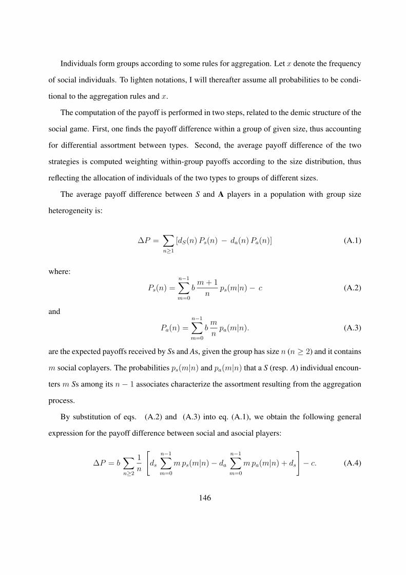
Individuals form groups according to some rules for aggregation. Let x denote the frequency

of social individuals. To lighten notations, I will thereafter assume all probabilities to be condi-

tional to the aggregation rules and x.

The computation of the payoff is performed in two steps, related to the demic structure of the

social game. First, one finds the payoff difference within a group of given size, thus accounting

for differential assortment between types. Second, the average payoff difference of the two

strategies is computed weighting within-group payoffs according to the size distribution, thus

reflecting the allocation of individuals of the two types to groups of different sizes.

The average payoff difference between S and A players in a population with group size

heterogeneity is:

∆P =∑n≥1

[dS(n)Ps(n) − da(n)Pa(n)] (A.1)

where:

Ps(n) =n−1∑m=0

bm+ 1

nps(m|n)− c (A.2)

and

Pa(n) =n−1∑m=0

bm

npa(m|n). (A.3)

are the expected payoffs received by Ss and As, given the group has size n (n ≥ 2) and it contains

m social coplayers. The probabilities ps(m|n) and pa(m|n) that a S (resp. A) individual encoun-

ters m Ss among its n− 1 associates characterize the assortment resulting from the aggregation

process.

By substitution of eqs. (A.2) and (A.3) into eq. (A.1), we obtain the following general

expression for the payoff difference between social and asocial players:

∆P = b∑n≥2

1

n

[ds

n−1∑m=0

mps(m|n)− da

n−1∑m=0

mpa(m|n) + ds

]− c. (A.4)

146

The benefit term in this equation depends on the balance between the average sociality levels in

groups experienced by a S (resp. A) player, weighted by the relative abundance of these groups.

In order to pinpoint the relative role of assortment and group size heterogeneity, I now ex-

plicitly compute this payoff difference for three extreme cases: 1) groups all have the same size;

1) S and A players segregate; in 3), I recover the case described in the manuscript when group

size is distributed and within-group assortment is random. The first two examples are instances

of the case when within-group assortment is made positive by recognition mechanisms amongst

players.

Groups of identical size In the particular case of fixed group size n∗, the payoff difference

writes

∆P (n∗) =b

n∗

[n∗−1∑m=0

m (ps(m)− pa(m)) + 1

]− c (A.5)

If there is no positive assortment within the social type, the condition for sociality to evolve

reduces to b/c > n∗, which is stringent in particular if n∗ is large. Assortative group formation,

however, can lead to a positive payoff difference even for smaller benefit to cost ratios. Since the

probabilities ps(m) and pa(m) both sum up to 1, then if ps(m) > pa(m) for large m (that is, if

social individuals tend to aggregate more with individuals of their type) the quantity m (ps(m)−

pa(m)) is positive and can compensate the cost. Positive assortment has long been reported as

a way to ensure the evolution of cooperative behavior, and has spawned numerous theoretical

studies in the case of fixed group size (see for instance Antal et al. (2009); Eshel and Cavalli-

Sforza (1982); Matessi and Jayakar (1976); Wilson and Dugatkin (1997)).

Perfect segregation An extreme case of group formation is perfect group segregation (through,

for instance, green beard mechanisms; see Jansen and van Baalen (2006); West and Gardner

(2010); Gardner and West (2010)). In this case, assortment is total, i.e. ps(n − 1|n) = 1, thus

147

ps(m 6= n − 1|n) = 0; pa(0|n) = 1, thus pa(m 6= 0|n) = 0. As a consequence, Ps(n) = b − c

and Pa(n) = 0 when n ≥ 2 so that

∆P = b (1− ls) − c (A.6)

where ls = ds(1) is the proportion of social individuals left alone (therefore 1− ls that of social

individuals that are in a group). Here ∆P does not depend on how group size is distributed. In

this favorable setting, sociality may evolve easily as soon as the proportion of lonely Ss is small.

In the limit case when all socials enter one group, that is ls = 0, sociality evolves under the

weakest possible condition b/c > 1.

Heterogeneous group size, no within-group assortment Even in the absence of within-group

assortment (ps = pa), sociality can evolve if Ss and As players are unevenly distributed between

groups, so that sociality corresponds to higher expectations for the size of the group one belongs

to.

This is the case we discuss in the manuscript, where groups are formed via sequential pair-

wise interaction of individuals possensing different attachment probability. Under such group

formation process, no within-group assortment emerges:

ps(m|n) = pa(m|n) =(n− 1

m

)ps(n)

m pa(n)n−1−m ∀m,n (A.7)

The number of social co-members expected, given a size n, is thus the same:

n−1∑n=0

mps(m|n) =n−1∑n=0

mpa(m|n) := m (A.8)

with

m = (n− 1) ps(n) = (n− 1)x ds(n)

x ds(n) + (1− x) da(n)(A.9)

148

The hypothesis of non-assortative aggregation made in the manuscript is conservative: if

positive assortment is further assumed, sociality evolves even more easily. Indeed, under positive

within group assortment∑

mps(m|n) > m (and correspondingly,∑

mpa(m[n) < m), so that

the payoff difference in eq. (A.4) increases.

149

Appendix B

Group size distributions for differential

attachment

Let us first consider social players. We distinguish two cases: 1) the focal social player is

a recruiter (with probability 1/T ); 2) the focal social player is not a recruiter (with probability

(1−1/T )). In what follows, we denote Qs(x) = xπss+(1−x)πas and Qa(x) = xπas+(1−x)πaa

the probabilities that a random player attaches to a social (resp. asocial) recruiter.

Case 1: The focal social player is a recruiter: Its group has size n whenever n−1 individuals

among the T − 1 in its set attach to it, i.e. with a probability

Rs(n, x) =

(T − 1

n− 1

)Qs(x)

n−1(1−Qs(x))T−n

Case 2: The focal social player is not a recruiter: One has to consider whether its recruiter

is social (with probability x) or asocial (with probability (1− x)). The probability to end up in a

151

group of size n if the recruiter is social is:

rs,s(n, x) =

1− πss if n = 1

πss

(T − 2

n− 2

)Qs(x)

n−2(1−Qs(x))T−n if n ≥ 2

Indeed, n ≥ 2 means that the focal player is recruited and that n− 2 among the remaining T − 2

other players also attach to the social recruiter; the case n = 1 means that the interaction with

the social recruiter does not succeed. If the focal player’s recruiter is asocial, one has similarly:

rs,a(n, x) =

1− πas if n = 1

πas

(T − 2

n− 2

)Qa(x)

n−2(1−Qa(x))T−n if n ≥ 2

The group size distribution for social players ds(n, x) is a linear combination of the three

probability distributions Rs(n, x), rs,s(n, x) and rs,a(n, x), weighted by their respective occur-

rence probabilities:

ds(n, x) =1

TRs(n, x) +

(1− 1

T

)[rs,s(n, x) x+ rs,a(n, x) (1− x)] (B.1)

The calculation of the group size distribution for asocial players follows the same lines. In

the end,

da(n, x) =1

TRa(n, x) +

(1− 1

T

)[ra,s(n, x)x+ ra,a(n, x) (1− x)] (B.2)

152

with

Ra(n, x) =

(T − 1

n− 1

)Qa(x)

n−1(1−Qa(x))T−nfor n ≥ 1

ra,s(n, x) =

1− πas if n = 1

πas

(T − 2

n− 2

)Qs(x)

n−2(1−Qs(x))T−n if n ≥ 2

ra,a(n, x) =

1− πaa if n = 1

πaa

(T − 2

n− 2

)Qa(x)

n−2(1−Qa(x))T−n if n ≥ 2

In Fig. B.1, we represent the theoretical distributions da and ds for a given set of parameters

and composition x of the population.

0 20 40 60 80 1000

0.2

0.4

0.6

group size

pdf

social

asocial

1−Qa(x)

1−Qs(x)

TQa(x) TQ

s(x)

Figure B.1: Theoretical group size distributions for social and asocial individuals.

Parameters values: T = 100, πss = 0.8, πaa = 0.3, πas =√πssπaa, x = 0.5.

153

Appendix C

Condition for sociality to be altruistic for

differential attachment

The calculation of the the maximal benefit-cost-ratio rc(x) =(∑

n≥2 dS(n)/n)−1 ensuring that

sociality is altruistic requires the use of the following formulas:

N∑k=0

1

k + 1

(N

k

)Ak BN−k =

(A+B)N+1 −BN+1

A(N + 1)

N∑k=0

1

k + 2

(N

k

)Ak BN−k =

(N + 2)A(A+B)N+1 − (A+B)N+2 +BN+2

A2(N + 1)(N + 2)

Combined with the expressions of the distribution dS , this yields:

rc(x) =

[1

T

(1− (1−Qs)

T

TQs

− (1−Qs)T−1

)+

(1− 1

T

)(xπss

TQs − 1 + (1−Qs)T

T (T − 1)Q2s

+ (1− x)πasTQa − 1 + (1−Qa)

T

T (T − 1)Q2a

)]−1

(C.1)

This critical benefit-to-cost ratio, evaluated at the threshold frequency x∗, is displayed in

155

Fig. 3 of the main text. In the limit T → +∞,

rc(x) ∼T

xπss/Qs + (1− x) πas/Qa

(C.2)

and is thus linear with the maximal group size T .

156

Appendix D

Evolutionary algorithm for chapter 3

The following instructions are repeated at each generation g = 1, . . . , gf until an equilibrium is

reached:

Initialization

The algorithm is initialized with a population of Npop particles ith positions (x, y) chosen at

random on the [0, L] × [0, L] 2D square, and motion directions θ chosen at random between 0

and 2π.

Aggregation process

At each time step t = 1, . . . , tf , all particles’ updated directions and positions are calculated

successively according to the following steps:

1. find the focal particle’s neighbors within a radius r1;

2. calculate the interaction forces they exert on the focal particle according to Equation 1 of

the main text;

3. calculate the focal particle’s new direction according to Equation 2 of the main text;

157

4. update the focal particle’s position according to Equation 3 of the main text.

Payoff allocation

Once time step t = tf is over, each particle’s group (if any) is determined according to the

criterion described in section 3.2.2. If the particle j’s group has nj members, among whom sj

are social, then its payoff is calculated according to a linear PGG, that is:

Pj = bsjnj

if particle j is asocial (D.1)

Pj = bsjnj

− c if particle j is social (D.2)

We assume clonal reproduction. The payoff received by each individual determines its prob-

ability to generate an offspring at the next generation. This probability is linearly determined

by rescaling the payoff between two values fmin and fmax with 0 ≤ fmin < fmax < 1. The

rescaling parameters allow to adjust both the speed of renewal of the population and the strength

of selection.

Social frequency update

Here, we detail how the frequency x(g+1) of the social trait at generation g + 1 is determined

according to its frequency x(g) and the average probabilities f(g)s and f

(g)a of an S (resp. an A)

particle to leave offspring at generation g.

Birth process: Let N (g)s and N

(g)a be the number of S (resp. A) particles in the population at

generation g, so that N (g)s +N

(g)a = Npop. Considering that mutations can arise at a frequency u

and change the strategy of a newborn to the opposite strategy (S → A and A → S), their numbers

N ′s and N ′

a due to the birth process can be expressed as:

158

N ′s = N (g)

s +N (g)s f (g)

s (1− u) +N (g)a f (g)

a u

= Npop

[x(g) + x(g)f (g)

s (1− u) + (1− x(g))f (g)a u

](D.3)

and

N ′a = N (g)

a +N (g)a f (g)

a (1− u) +N (g)s (1 + f (g)

s )u

= Npop

[1− x(g) + (1− x(g))f (g)

a (1− u) + x(g)f (g)s u

](D.4)

Death process: As we want not to take into account demographic effects on the evolutionary

dynamics, we maintain the population constant by means of a death process that applies indis-

criminately to particles of any strategy. Each particle thus dies with a probability d(g) such that at

generation g+1 the population size N (g+1)s +N

(g+1)a = Npop. Hence the survival rate (1−d(g)) is

such that N (g+1)s = N ′

s(1−d(g)) and N(g+1)a = N ′

a(1−d(g)), and combining these two conditions

and Eqs. D.3 and D.4 we find:

1− d(g) =1

1 + x(g)f(g)s + (1− x(g))f

(g)a

(D.5)

Thus,

N (g+1)s = Npop

x(g) + x(g)f(g)s (1− u) + (1− x(g))f

(g)a u

1 + x(g)f(g)s + (1− x(g))f

(g)a

(D.6)

and

x(g+1) = N (g+1)s /Npop (D.7)

159