P49 column mieke loncke ifma_une source d'inspiration pour les architectes
Upload
truongnguyetCategory
view
227download
4
No d’ordre : 596
No attribué par la bibliothèque : __ENSL596
THÈSEen vue d’obtenir le grade de
Docteur de l’Université de Lyon – École Normale Supérieure de Lyon
Spécialité : Mathématiques
Unité de Mathématiques Pures & Appliquées
École Doctorale de Mathématiques & Informatique Fondamentale
présentée et soutenue publiquement le 12 novembre 2010 par
M. Rémi PEYRE
Titre :
Quelques problèmes d’inspiration physique
en théorie des probabilités
Directeur de thèse :
M. Cédric VILLANI
Après avis de :
M. Michel LEDOUX
M. Errico PRESUTTI
Devant la commission d’examen formée de :
Mme Alice GUIONNET, membre
M. Michel LEDOUX, membre/rapporteur
Mme Sylvie MÉLÉARD, membre
M. Errico PRESUTTI, membre/rapporteur
M. Cédric VILLANI, membre


iii
Préambule :Mathématique et physique
le 12 novembre 2010
MATHÉMATIQUE et physique. Deux sciences aux objets d’étude bien distincts, la premières’intéressant aux objets abstraits tandis que la seconde étudie le monde réel. Pourtant, cha-
cun sait confusément que les deux disciplines sont étroitement intriquées. Un grand nombre desavants des siècles passés, d’Archimède à Laplace en passant par Newton, se sont ainsi penchéssimultanément sur ces deux domaines ; et aujourd’hui encore les deux matières sont enseignées deconserve jusqu’en premier cycle universitaire, collectivement qualifiées de « sciences exactes ».
QUELLES sont donc ces intrications entre mathématique et physique ? La plus évidente d’en-tr’elles tient à la notion même d’exactitude physique, en tant que mathématisation du réel :
le physicien a fondamentalement besoin du formalisme mathématique pour exprimer ses résultats.Sans différentiation, pas de dynamique ; sans espaces de Hilbert, pas de mécanique quantique ; sansgéométrie lorentzienne, pas de relativité générale.
MAIS le rôle de la mathématique en physique ne s’arrête pas au simple outillage. La prédictiondu résultat d’une expérience à partir de la théorie, en effet, est un travail cent pour cent
mathématique ! D’où l’exigence, par les écoles d’ingénieur, d’un solide bagage mathématique dela part de leurs élèves. D’où encore la présence, dans les laboratoires de physique, de théoriciensde haute volée mathématique.
BREF, la mathématique est indispensable à la physique ; cela n’est pas un scoop. En revanche, onoublie trop souvent que l’interaction entre mathématique et physique n’est pas à sens unique :
le mathématicien a également beaucoup à gagner à rendre visite à ses confrères physiciens ! Jevoudrais évoquer ici deux exemples de telles influences réciproques.
D’ABORD, il arrive que les problèmes mathématiques rencontrés par les physiciens dans leurtravail soient récupérés par les mathématiciens pour leur intérêt intrinsèque. C’est ainsi que
les équations de Navier – Stokes continuent aujourd’hui de susciter des recherches nombreuses etdifficiles en théorie des équations aux dérivées partielles. Parfois même, les objets suggérés par laphysique engendrent à leur tour de nouveaux développements mathématiques, comme le modèled’Ising du ferromagnétisme qui a conduit de fil en aiguille à la FK-percolation et au processus SLE.
D’AUTRE part, une complémentarité très importante à mes yeux entre physique et mathéma-tique tient à la différence entre les méthodes de travail des scientifiques des deux disciplines.
Quand le physicien rencontre un problème mathématique dans ses travaux, en effet, il essaye del’attaquer en restant guidé malgré tout par la réalité physique des objets étudiés ; en conséquence,son raisonnement visera à une approche intuitive du problème et se rattachera autant que possibleà des notions physiques classiques : énergie, temps, loi des grands nombres, entropie, ... Cela estd’autant plus important en physique que les modèles mathématiques ne sont généralement qu’uneapproximation du monde réel, et que dans cette mesure il compte moins d’avoir une preuve par-faitement rigoureuse que de parvenir à des heuristiques donnant une compréhension suffisammentprofonde du sujet pour en déduire des prédictions valides. L’exemple le plus frappant à cet égardest sans doute la théorie de Yang – Mills, qui sous-tend tout le modèle standard de la physique desparticules, mais dont la démonstration mathématique est toujours mise à prix pour un million dedollars !
iv
SI j’ai choisi d’intituler cette thèse « Quelques problèmes d’inspiration physique en théorie desprobabilités », c’est donc dans les deux sens évoqués ci-dessus. Primo, parce que les questions
abordées seront souvent motivées par des situations physiques, d’où l’emploi récurrent des termes« modèle », « particule », « interaction », « énergie », « temps », « équilibre »... tout au long de cettethèse. Secundo, parce que les arguments de mes démonstrations chercheront en permanence à resteraussi près que possible des motivations initiales : c’est ainsi par exemple que je proposerai desapproches « élémentaires » de certaines inégalités démontrées à coups d’analyse spectrale.
CELA dit, qu’on ne se méprenne pas : cette thèse est bel et bien un travail de pure mathéma-tique, et les théorèmes qu’elle contient y sont démontrés de manière totalement rigoureuse.
Si j’ai cherché malgré tout à m’inspirer des raisonnements des physiciens, c’est pour une raisondouble. Esthétique d’une part, car j’estime que la démonstration d’un théorème compte au moinsautant que son énoncé, et qu’une bonne preuve se doit d’avoir une structure globale naturellementcompréhensible, d’être « morale ». Mais pragmatique également, car derrière cette volonté de co-hérence physique se trouve l’ambition qu’une méthode « naturelle » sera plus fructueuse qu’uneméthode « artificielle » et s’adaptera dans un cadre plus vaste.
Rémi Peyre
v
Remerciements
Au terme des quatre années de travail dont cette thèse marque l’accomplissement, je tiens àremercier tous celles et ceux sans qui ce doctorat aurait été mission impossible.
À tout seigneur, tout honneur ! Merci en premier lieu à Cédric Villani d’avoir accepté de meprendre comme thésard et d’avoir supervisé mon travail. Les thématiques qu’il m’a exposées etsa façon de les envisager ont joué une place importante dans les recherches que ce manuscritprésente. Si j’ai parfois eu du mal avec à la vision de l’encadrement de Cédric, qui se conçoit pluscomme « advisor » que comme « directeur », au final cependant les méthodes de mon patron m’ontbeaucoup apporté en autonomie et en confiance.
Sur le plan scientifique, de nombreux membres de la communauté mathématique m’ont fournià l’occasion une aide précieuse, que ce soit pour m’indiquer des références bibliographiques, ré-soudre certains points techniques, ou suggérer des prolongements à mes recherches. La plupart deces personnes sont remerciées plus en détail dans les chapitres concernés.
Mais une thèse ne saurait être réduite à son aspect scientifique. Ce sont aussi des années de vie,au long desquelles l’amitié humaine fut pour moi un carburant indispensable. À ce point de vue,j’ai particulièrement apprécié l’ambiance au sein de l’UMPA [∗] où j’ai partagé moult momentsconviviaux et conversations passionnantes. En-dehors des murs du laboratoire, j’ai aussi eu le plusgrand plaisir à voir régulièrement mes amis de Lyon et d’ailleurs. Enfin bien sûr, j’ai énormémentapprécié de pouvoir compter sur l’appui moral d’une famille unie et enjouée, notamment mesparents et mes sœurs “Chogosov”, “L@urence” et “Crapatcha”.
La rédaction de ce manuscrit à proprement parler doit un peu à mes grands-parents “Vatti” et“Morfar” dont les maisons de campagne respectives m’ont abrité de la fournaise lyonnaise au coursde mon travail d’écriture. Par ailleurs, je remercie spécialement ma collègue Alice qui a relu toutel’introduction de cette thèse.
*
À l’heure où cette soutenance marque mon entrée définitive dans le monde de la recherchemathématique, il ne faudrait toutefois pas croire que l’histoire a commencé à mon entrée à l’écoledoctorale. Cette vocation trouve en effet sa source auprès d’enseignants qui ont su me passionnerpour les mathématiques, me stimuler dans mes études, et me conseiller dans mes choix : qu’ilsen soient remerciés de tout cœur. Je voudrais également rendre hommage à un homme qui ne meconnaît pas : Olivier Courcelle, dont l’humour m’a convaincu, au moment de choisir ma voie, queles mathématiciens pouvaient décidément être désopilants.
*
Pour finir, je remercie respectueusement mes rapporteurs, MM. Ledoux et Presutti, d’avoir prisle temps de lire ce manuscrit en détail et de lui avoir accordé leur caution scientifique. Je remercieégalement Mmes Méléard et Guionnet d’avoir accepté de siéger à mon jury de soutenance.
***
Arrêter une liste de personnes à remercier nommément est un exercice diplomatiquement déli-
[∗]. Unité de Mathématiques Pures et Appliquées : le laboratoire de mathématiques de l’École Normale Supérieurede Lyon, au sein duquel j’ai travaillé pendant toute la durée de ma thèse.

vi
cat et dont le résultat est nécessairement imparfait. Toutefois, s’il n’en fallait retenir que quarante,je voudrais exprimer ma gratitude particulière aux personnes suivantes :
Alain RAVELLI, Aldéric JOULIN, Alice GUIONNET, Amandine VÉBER, André PEYRE, Auré-lien ALVAREZ, Benoît PEYRE, Cédric VILLANI, Cosma SHALIZI, Emmanuel OPSHTEIN, ErricoPRESUTTI, Étienne GHYS, Fabio MARTINELLI, Jean BAVAY, Jean-Baptiste GUILLON, LaurencePEYRE, Laurent SALOFF-COSTE, Léonie AHRENS, Mathilde PEYRE, Maxime BOURRIGAN, Mi-chel LEDOUX, Odile PEYRE, Olivier BOULAUD, Olivier COURCELLE, Pierre CONNAULT, PierrePETIT, Priscille PEYRE, Raymonde LANGLADE, Richard BRADLEY, Romain TESSERA, SébastienMARTINEAU, Senya SHLOSMAN, Sylvie MÉLÉARD, Thierry BODINEAU, Thomas GALLOUËT,Vincent BEFFARA, Vincent CALVEZ, Wendelin WERNER, Yann OLLIVIER, Yvan VELENIK.

vii
Comment lire cette thèse
Cette thèse de doctorat présente les recherches que j’ai menées à l’École Normale Supérieurede Lyon de novembre 2006 à mai 2010. Elle est constituée de quatre parties indépendantes corres-pondant à autant de travaux différents, que j’ai choisi de présenter dans l’ordre chronologique deleur réalisation :
1. Contrôle des probabilités de transition d’une chaîne de Markov ;2. Limite de champ moyen pour un modèle de Boltzmann ;3. Tensorisation des corrélations maximales ;4. Brisure spontanée de symétrie en dimension infinie.
Afin de permettre au lecteur d’appréhender rapidement la teneur de ces recherches, une intro-duction générale a été rédigée en premier lieu. Cette introduction elle-même est constituée de deuxvolets :
• Je commence par présenter en quelques mots, sans utiliser de formule, les enjeux et lesgrandes lignes de mes travaux ;
• Suivent des version résumées de chacune des parties de la thèse.À noter que, bien que l’introduction traite les quatre parties sur un pied d’égalité, celles-ci sont delongueurs très inégales ; en particulier, la troisième partie représente à elle seule plus de la moitiédu contenu de la thèse.

Table des matières
Introduction générale 2
Présentation de la thèse 2
Résumé des travaux présentés 7
1 Contrôle des probabilités de transition d’une chaîne de Markov . . . . . . . . . . . 7
2 Limite de champ moyen pour un modèle de Boltzmann . . . . . . . . . . . . . . . . 11
3 Tensorisation des corrélations maximales . . . . . . . . . . . . . . . . . . . . . . . . 16
4 Brisure spontanée de symétrie en dimension infinie . . . . . . . . . . . . . . . . . . 20
I Une approche probabiliste de la borne de Carne 28
II Convergence quantitative de modèles à chocs vers la limite de champmoyen 50
III Décorrélations hilbertiennes 76
IV Flambage de Mc Kean – Vlasov 196
Références bibliographiques 219

Introduction générale

Présentation de la thèse
Le premier sujet traité s’intéresse aux chaînes de Markov réversibles dont les transitions suiventles arêtes d’un graphe. En 1985, N. Varopoulos [80] et T. Carne [18] avaient démontré que, pourune telle chaîne de Markov, la probabilité de transition d’un point à un autre en temps fixé estcontrôlée par une borne où intervient un facteur universel gaussien en la distance séparant lesdeux points. J’avais été interpellé par deux collègues sur l’aspect « miraculeux » de la preuve deCarne, où le facteur gaussien apparaissait via des techniques d’analyse spectrale puissantes : cetteapproche était en effet surprenante dans la mesure où les probabilistes sont plus habitués à voir lesgaussiennes émerger de phénomènes de fluctuations (cf. théorème-limite central). Y avait-il uneexplication alternative à la démonstration de Carne ?
Je suis parvenu à montrer que oui, en réinterprétant le résultat de Carne & Varopoulos en termesde fluctuations de martingales. Pour ce faire, j’introduis une fonctionnelle sur l’espace des états quimesure si on est plus proche du point de départ ou de l’arrivée. Bien que cette fonctionnelle nesoit pas une martingale a priori, l’hypothèse de réversibilité permet d’affirmer que sa tendance àcroître lorsqu’on va du départ à l’arrivée sera compensée exactement par sa tendance à croître pourrevenir de l’arrivée au départ. Comme les fluctuations de notre fonctionnelle sont contrôlées du faitque la chaîne de Markov doit suivre les arêtes du graphe, on peut appliquer des résultats de grandesdéviations sur la valeur terminale de cette fonctionnelle pour en déduire la gaussienne — il s’agiten fait d’un analogue discret de la technique de décomposition forward/backward des martingalesinventée par Lyons et Zheng [50].
Il y avait en outre, dans la borne de Carne, un facteur de nature a priori purement spectrale quiraffinait le résultat dans certains cas. Dans la mesure où ces cas correspondaient à une marche« fortement transitoire », j’ai eu l’idée d’interpréter ce facteur probabilistiquement comme unecontrainte de conditionnement. En effet, imposer à la marche d’aller d’un point à un autre luiinterdit en quelque sorte de partir à l’infini, de sorte qu’on peut alors se restreindre à la marche« conditionnée à être récurrente ». Cette marche étant réversible également, la borne simple deCarne s’y applique ; dès lors, le facteur « spectral » est simplement la probabilité que la chaînereste récurrente pendant le temps imparti.
Au-delà de son intérêt esthétique, ma nouvelle démonstration présente surtout une souplessequi lui permet de s’adapter à des distances différentes de la distance du graphe : l’idée est depouvoir ajouter des transitions « exceptionnelles », qui ne suivraient pas les arêtes, sans changerpour autant la borne de façon conséquente — c’est en tout cas ce que l’intuition physique suggère.Alors que les arguments spectraux de Carne semblent impuissants dans de telles situations, mestechniques permettent au contraire d’obtenir une borne proche de la borne initiale. De fait, je donnedes exemples concrets où mes nouvelles bornes améliorent nettement ce qui était connu jusqu’alors.
Le résultat de ces recherches a été publié [65] en 2008 dans la revue Potential Analysis.

Présentation de la thèse
¦
Dans le second volet de cette thèse, on s’intéresse au comportement hors équilibre d’un gazconstitué d’un grand nombre de particules interagissant par des collisions élastiques. On sait heuris-tiquement depuis les travaux de Boltzmann [8] que pour un nombre infini de particules, le systèmeest régi par une équation intégro-différentielle dans laquelle le comportement microscopique descollisions se traduit macroscopiquement par une forme quadratique appelée « noyau de collision ».Je me suis placé plus précisément dans le cadre spatialement homogène, où on omet l’aspect ciné-tique du transport des particules — qui soulève d’importants défis techniques — pour se concentrersur les seules collisions. Le modèle particulaire associé est de nature stochastique.
Quand le nombre de particules tend vers l’infini, on s’attend alors à une convergence versl’équation de Boltzmann spatialement homogène. Chaque particule interagissant avec toutes lesautres avec une intensité comparable, on parle de limite « de champ moyen » (par opposition auxlimites « hydrodynamiques »). Ce type de limite a été étudié par Kac [43] dans un cas d’école, puispar divers autres [77, 56, 36] pour l’équation de Boltzmann.
Les arguments de « propagation du chaos » utilisés dans ces travaux présentaient à mes yeuxl’inconvénient de ne pas dire grand-chose sur l’existence de bornes non asymptotiques ou surla vitesse de cette convergence. Notamment, on donnait un résultat de convergence « différent »pour chaque fonctionnelle du système, plutôt qu’une convergence simultanée de toutes ces fonc-tionnelles — le même distinguo qu’entre le théorème-limite central « ordinaire » et les TLC uni-formes [28]. Or ces enjeux importent dans les situations « appliquées » : à quel point l’équationde Boltzmann est-elle valide pour un nombre d’atomes de l’ordre du nombre d’Avogadro ? Si onlance une simulation informatique, combien d’atomes faut-il pour que le modèle particulaire aitde grandes chances d’être très proche de la limite continue ? Pour toutes ces raisons, j’ai tentéd’établir un résultat de limite de champ moyen dans un cadre aussi « concret que possible » : jevoulais des bornes uniformes (contrôle simultané de toutes les fonctionnelles), quantitatives et nonasymptotiques (résultats applicables numériquement pour un nombre arbitraire de particules).
Plusieurs difficultés ont dû être surmontées. D’abord, les travaux [7, 77] dont je m’inspiraisutilisaient une technique de couplage du système à un ensemble de particules non linéaires, quidevenait inefficace ici à cause de l’évolution du système par chocs. J’ai donc préféré « oublier »l’existence individuelle de chaque particule pour étudier directement la mesure empirique du sys-tème. À partir de là, j’ai établi par des techniques de martingales un résultat « abstrait » susceptibled’être utilisé dans diverses situations, à commencer par celle qui m’intéressait.
Pour mettre en œuvre ce résultat abstrait, il fallait choisir dans quel espace de Banach mesurerla distance entre mesure empirique et mesure limite. Comme le choix classique des distances deWasserstein aurait donné des vitesses de convergence « trop lentes » pour le TLC uniforme en di-mension Ê 2, j’ai préféré prendre des espaces de Sobolev d’exposant négatif
.H−s (pris homogènes
pour des raisons tant physiques que mathématiques), plus grossiers, qui ne présentaient pas cetécueil.
Restait à vérifier les hypothèses du théorème abstrait. Le contrôle des fluctuations (stochas-tiques) du système discret s’obtient naturellement, mais la condition de contractivité sur l’équationlimite (déterministe) est plus délicate. Dans le cas des espaces
.H−s, il s’avère que cette hypothèse
ne peut être vérifiée que pour un modèle maxwellien, c.-à-d. quand la probabilité que deux parti-cules se heurtent ne dépend pas de leur vitesse relative. Cette limitation est assez décevante (carphysiquement non pertinente), mais des choix d’espaces fonctionnels plus subtils permettraientpeut-être de l’éviter. Toujours est-il que dans le cas maxwellien, j’ai pu effectivement démontrer

Quelques problèmes d’inspiration physique en théorie des probabilités
l’hypothèse de contractivité et en déduire des estimations explicites pour la convergence du modèleparticulaire.
Le résultat de ces recherches a été publié [66] en 2009 dans le Journal of Statistical Physics.
¦
Dans la troisième partie de la thèse, on s’intéresse à des systèmes de mécanique statistiqueoù l’état de deux particules distinctes est corrélé, mais où cette corrélation tend vers zéro quandla distance entre les particules augmente — un exemple typique en est le modèle d’Ising sous-critique [61]. Deux particules distantes sont ainsi asymptotiquement décorrélées, mais qu’en est-ilsi on s’intéresse à des groupes de particules ? Par exemple, en dimension 2, y a-t-il décorrélationentre les particules situées sur deux droites parallèles distantes ? Il s’avère que la réponse dépend dela mesure de dépendance employée [11] : ainsi, la corrélation entre ces deux groupes de particulesest maximale au sens du β-mélange ; mais au sens du ρ-mélange, ou corrélation maximale, ily a décroissance exponentielle des corrélations [57]. Cependant, on ne savait jusqu’ici montrercette limitation de la propagation de l’information indépendamment de la taille de l’interface quedans des cas très particuliers, par l’utilisation d’analyse spectrale. Y avait-t-il une explication plusgénérale ?
Reprenons le cas des droites parallèles évoquées ci-dessus et considérons les paires de par-ticules se faisant vis-à-vis. Si ces paires de particules étaient indépendantes entre elles, c’est unrésultat relativement simple [21] que la corrélation maximale se tensorise : la corrélation entreles deux droites serait alors le supremum des corrélations entre deux spins d’une même paire. Enpratique, les paires de particules ne sont certes pas indépendantes, néanmoins elles le deviennentasymptotiquement quand la distance entre deux paires augmente. C’est ainsi que j’ai cherché àtensoriser les corrélations maximales dans un cadre plus général en vue d’obtenir du ρ-mélangeentre groupes de spins.
Le coefficient de ρ-mélange entre deux tribus est le cosinus de l’angle entre les espaces defonctions L2 centrées mesurables par rapport à chacune de ces tribus ; il s’agit donc d’un concepthilbertien. Pour des fonctions dépendant d’un ensemble de spins, une idée naturelle est donc de lesdécomposer en sommes de termes orthogonaux dont chacun exprimera la dépendance par rapport àun spin différent. Cette méthode redonne la tensorisation dans le cas indépendant, et permet d’éva-luer simplement la corrélation entre un groupe de particules et une particule seule (ce que j’appellela tensorisation « en N contre 1 »). Pour la corrélation entre deux groupes de particules (tensorisa-tion « en N contre M »), l’idée de base est la même, mais il faut gérer la décomposition dans deuxbases orthogonales différentes, ce qui donne à surmonter de nombreuses difficultés techniques. Jeborne ainsi la corrélation en N contre M par la norme d’opérateur de la matrice des corrélationsindividuelles. Grâce à cette borne, on peut majorer finement la corrélation entre deux groupes despins distants pour le modèle d’Ising, ainsi que pour des nombreux autres modèles de physiquestatistique, dans des cas beaucoup plus généraux que ce que permettait l’approche spectrale.
Cette partie de la thèse, de très loin la plus volumineuse, a été conçue comme un travail ex-haustif et aborde de ce fait plusieurs questions annexes. Des résultats fins d’optimalité sont ainsi dé-montrés ; on s’intéresse également au ρ-mélange pour des géométries non planes, et pour l’espace-temps (ce qui donne des résultats d’hypocoercivité) ; on montre aussi comment appliquer les cor-rélations hilbertiennes à l’étude du théorème-limite central spatial, et du trou spectral pour la dyna-mique de Glauber. Le plus important de ces résultats secondaires est un nouveau critère pour obtenirle ρ-mélange à partir de conditions de type α-mélange, qui améliore ceux connus jusqu’alors [15]en atteignant la borne optimale.
Présentation de la thèse
Ce travail a été rédigé sous forme de monographie et soumis pour publication.
¦
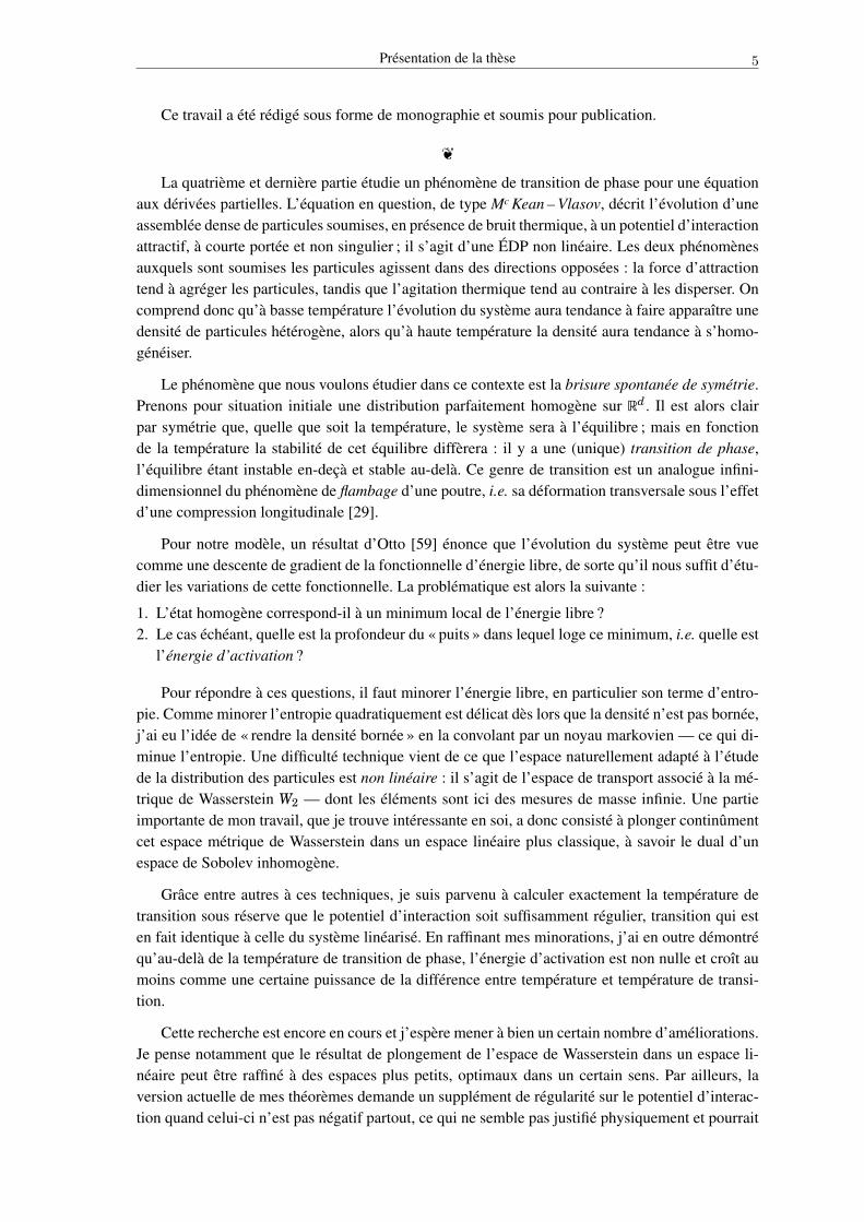
La quatrième et dernière partie étudie un phénomène de transition de phase pour une équationaux dérivées partielles. L’équation en question, de type Mc Kean – Vlasov, décrit l’évolution d’uneassemblée dense de particules soumises, en présence de bruit thermique, à un potentiel d’interactionattractif, à courte portée et non singulier ; il s’agit d’une ÉDP non linéaire. Les deux phénomènesauxquels sont soumises les particules agissent dans des directions opposées : la force d’attractiontend à agréger les particules, tandis que l’agitation thermique tend au contraire à les disperser. Oncomprend donc qu’à basse température l’évolution du système aura tendance à faire apparaître unedensité de particules hétérogène, alors qu’à haute température la densité aura tendance à s’homo-généiser.
Le phénomène que nous voulons étudier dans ce contexte est la brisure spontanée de symétrie.Prenons pour situation initiale une distribution parfaitement homogène sur Rd . Il est alors clairpar symétrie que, quelle que soit la température, le système sera à l’équilibre ; mais en fonctionde la température la stabilité de cet équilibre diffèrera : il y a une (unique) transition de phase,l’équilibre étant instable en-deçà et stable au-delà. Ce genre de transition est un analogue infini-dimensionnel du phénomène de flambage d’une poutre, i.e. sa déformation transversale sous l’effetd’une compression longitudinale [29].
Pour notre modèle, un résultat d’Otto [59] énonce que l’évolution du système peut être vuecomme une descente de gradient de la fonctionnelle d’énergie libre, de sorte qu’il nous suffit d’étu-dier les variations de cette fonctionnelle. La problématique est alors la suivante :
1. L’état homogène correspond-il à un minimum local de l’énergie libre ?2. Le cas échéant, quelle est la profondeur du « puits » dans lequel loge ce minimum, i.e. quelle est
l’énergie d’activation ?
Pour répondre à ces questions, il faut minorer l’énergie libre, en particulier son terme d’entro-pie. Comme minorer l’entropie quadratiquement est délicat dès lors que la densité n’est pas bornée,j’ai eu l’idée de « rendre la densité bornée » en la convolant par un noyau markovien — ce qui di-minue l’entropie. Une difficulté technique vient de ce que l’espace naturellement adapté à l’étudede la distribution des particules est non linéaire : il s’agit de l’espace de transport associé à la mé-trique de Wasserstein W2 — dont les éléments sont ici des mesures de masse infinie. Une partieimportante de mon travail, que je trouve intéressante en soi, a donc consisté à plonger continûmentcet espace métrique de Wasserstein dans un espace linéaire plus classique, à savoir le dual d’unespace de Sobolev inhomogène.
Grâce entre autres à ces techniques, je suis parvenu à calculer exactement la température detransition sous réserve que le potentiel d’interaction soit suffisamment régulier, transition qui esten fait identique à celle du système linéarisé. En raffinant mes minorations, j’ai en outre démontréqu’au-delà de la température de transition de phase, l’énergie d’activation est non nulle et croît aumoins comme une certaine puissance de la différence entre température et température de transi-tion.
Cette recherche est encore en cours et j’espère mener à bien un certain nombre d’améliorations.Je pense notamment que le résultat de plongement de l’espace de Wasserstein dans un espace li-néaire peut être raffiné à des espaces plus petits, optimaux dans un certain sens. Par ailleurs, laversion actuelle de mes théorèmes demande un supplément de régularité sur le potentiel d’interac-tion quand celui-ci n’est pas négatif partout, ce qui ne semble pas justifié physiquement et pourrait

Quelques problèmes d’inspiration physique en théorie des probabilités
être contourné par des outils judicieux d’analyse de Fourier. Enfin, un défi intéressant serait dedéterminer l’exposant critique optimal qui régit l’apparition de l’énergie d’activation quand ondépasse la température de transition.

Résumé des travaux présentés
1 Contrôle des probabilités de transition d’une chaîne de Markov
* Cette section est un résumé du travail présenté en détail dans la partie I de la thèse.
1.a Présentation du problème
Soit V un ensemble de points au plus dénombrable, muni d’une mesure µ (dont la masse totalepeut être infinie) appelée mesure d’équilibre ; nous noterons par commodité µ(x) pour µ(x). Onconsidère une chaîne de Markov homogène (X t)t∈N sur V , décrite par les probabilités de transition
p(x, y) ··=P[X1 = y|X0 = x]. (1A)
Pour t ∈N, on note pt la t-ième puissance de convolution de p, c.-à-d.
pt(x, y)=P[X t = y|X0 = x]. (1B)
La chaîne est supposée réversible, c.-à-d. que pour tous x, y ∈V , on a
µ(x)p(x, y)=µ(y)p(y, x) ; (1C)
en particulier, µ est une mesure invariante de la chaîne.
V peut alors être muni d’une structure canonique de graphe (non orienté), l’ensemble E deses arêtes étant constitué par les paires x, y d’éléments de V tels que p(x, y) > 0 — on supposeraqu’on a ôté de V les points de mesure nulle, de sorte que cette condition est bien symétrique grâceà l’hypothèse de réversibilité. On note d la distance associée à ce graphe.
On définit enfin le noyau de transition P de la chaîne de Markov. Il s’agit d’un opérateur quenous considèrerons ici sur l’espace L2(µ) des fonctions f vérifiant ‖ f ‖2
L2(µ) ··=∑
V f (x)2µ(x)<∞— dans la suite, nous noterons simplement ‖ f ‖ pour ‖ f ‖L2(µ). P est défini par
(P f )(x) ··=E[ f (X1)|X0 = x]= ∑y∈V
µ(x)p(x, y). (1D)
Comme µ est une mesure d’équilibre de la chaîne, l’inégalité de Jensen donne que pour toute f ,‖P f ‖2 É ‖ f ‖2. On peut alors définir la norme d’opérateur de P par
|P| ··= supf ∈L2(µ)à0
‖P f ‖‖ f ‖ , (1E)
qui est un nombre compris entre 0 (strictement) et 1. Notons que dans bon nombre de cas on a enfait |P| = 1, notamment dès que la chaîne est récurrente.
Avec ces notations, Carne [18] a montré en 1985 le
Quelques problèmes d’inspiration physique en théorie des probabilités
1.1 Théorème (Carne). Pour tous x, y ∈V , pour tout t > 0,
pt(x, y)É 2(µ(y)µ(x)
)1/2|P|t exp
(−d(x, y)2
2t
). (1F)
♣
1.b L’argument spectral de Carne
Décrivons en quelques mots le fonctionnement de la preuve de Carne :
1. On commence par réécrire (µ(x)/µ(y))1/2 pt(x, y) comme le produit scalaire
⟨µ(x)−1/2δx,P t(µ(y)−1/2δy)⟩L2(µ), (1G)
où les fonctions µ(x)−1/2δx et µ(y)−1/2δy sont normées dans L2(µ).2. La décomposition du polynôme Z t dans la base (Qk(Z))k∈Z des polynômes de Tchebychev de
première espèce donne
P t = |P|t2t
∑k∈Z
(t
(t+k)/2
)Qk(|P|−1P). (1H)
3. La chaîne de Markov étant réversible, P est autoadjoint dans L2(µ) ; il est donc normal, à valeurspropres réelles, et sa norme est égale à son rayon spectral. Ainsi |P|−1P est un opérateur normalde spectre contenu dans [−1,1], de sorte que Qk(P) est un opérateur normal de spectre contenudans Qk([−1,1]). Mais les polynômes de Tchebychev envoient [−1,1] dans lui-même, donc aufinal la norme d’opérateur de Qk(|P|−1P) est bornée par 1.
4. Comme le polynôme Qk est de degré |k| et que l’opérateur |P|−1P a une portée de 1,⟨δx,Qk(P)δy⟩ est nul dès lors que |k| < d(x, y) ; on peut donc restreindre la somme (1H) aux ktels que |k| Ê d.
5. En interprétant 2−t( t(t+k)/2
)comme la probabilité qu’une marche aléatoire simple sur Z soit en k
au temps t, on montre par des arguments de grandes déviations que pour tout d Ê 0,
12t
∑|k|Êd
(t
(t+k)/2
)É 2e−d2/2t. (1I)
6. Il ne reste plus qu’à mettre bout à bout les étapes 1 à 5 pour obtenir (1F).
1.c Mon argument probabiliste
Passons maintenant à ma preuve probabiliste. On définit la fonction ξ : V → R par ξ(·) ··=d(x,·), de sorte que ξ est 1-lipschitzienne pour la distance d et vérifie ξ(x) = 0,ξ(y) = d(x, y). Ondéfinit pour tout z ∈V
m(z) ··=E[ξ(X1)|X0 = z]−ξ(z), (1J)
et on introduit le processus
Mu ··= ξ(Xu)−ξ(X0)−u−1∑s=0
m(Xs) (1K)
qui est alors une martingale.

Résumé des travaux présentés
Maintenant, sur l’événement “X0 = x et X t = y”, on a
Mt Ê d(x, y)−t−1∑u=0
m(Xu); (1L)
a contrario, sur l’événement “X0 = y et X t = x”, on a
Mt É−d(x, y)−t−1∑u=0
m(Xu). (1M)
Or grâce à l’hypothèse de réversibilité, les points visités par la chaîne de Markov pour aller de xà y en t pas sont les mêmes (dans l’ordre inverse) que pour aller de y à x en t pas, de sorte que lesderniers termes de (1L) et (1M) sont « pratiquement identiques ». Plus précisément, on a que
E[ t−1∑
u=1m(Xu)
∣∣∣X0 = x et X t = y]=E
[ t−1∑u=1
m(Xu)∣∣∣X0 = y et X t = x
]. (1N)
Définissons maintenant un processus (X xu, X y
u)0ÉuÉt de loi notée Px⊗y, où X x est la chaîneissue de x et X y la chaîne issue de y, X x et X y étant indépendants, et introduisons les martingalesMx et M y correspondant respectivement aux processus X x et X y. La combinaison de (1L) et (1M)donne alors, grâce à (1N) :
Ex⊗y [(Mxt −Mx
1)− (M yt −M y
1 )|X xt = y et X y
t = x]Ê 2d(x, y)−2. (1O)
(Les premiers pas de chaque chaîne, qui ne se simplifiaient pas, ont été simplement bornés par 1).
Dans (1O), la variable aléatoire “(Mxt −Mx
1)− (M yt −M y
1 )” peut être vue comme la valeur termi-nale d’une martingale (par rapport à une filtration judicieuse) issue de 0, à (2t−2) pas, où chaquepas, conditionnellement aux précédents, est supporté par un intervalle de longueur 2. Dans de tellesconditions, on sait qu’on peut appliquer des techniques de grandes déviations à une telle variablealéatoire : ainsi, l’inégalité d’Azuma donne que pour tout C Ê 0,
Px⊗y [(Mxt −Mx
1)− (M yt −M y
1 )Ê C]É exp(− C2
2(2t−2)
). (1P)
Ici nous allons utiliser une approche « duale » de ce genre de résultat : sachant que conditionnernotre variable aléatoire par l’événement “X x
t = y et X yt = x” rend son espérance grande, on peut
en déduire que l’événement en question a nécessairement une probabilité petite. On trouve ainsique
Px⊗y [X xt = y et X y
t = x]É exp(− (d(x, y)−1)2+
t−1
). (1Q)
Pour finir, Px⊗y[X xt = y et X y
t = x] se réécrit immédiatement comme pt(x, y)pt(y, x), où, vuque la chaîne de Markov est réversible, on a pt(y, x)= µ(x)
µ(y) pt(x, y). Au bout du compte, (1Q) donne :
pt(x, y)É(µ(y)µ(x)
)1/2exp
(− (d(x, y)−1)2+
2(t−1)
). (1R)
On déduit facilement de cette borne la formule (1F) de Carne (où le préfacteur 2 peut même êtreremplacé par
pe), à l’exclusion du facteur |P|t [voir § 1.d à ce sujet] dont nous avons toutefois fait
remarquer qu’il était souvent égal à 1.
Quelques problèmes d’inspiration physique en théorie des probabilités
1.d Le facteur |P|t
Maintenant nous allons voir qu’on peut en fait récupérer le facteur |P|t de la borne de Carnecomme un corollaire de la « simple » borne gaussienne (1R). Je ne donne que la démarche généralede la preuve, en négligeant tous les aspects techniques : on supposera ainsi que la chaîne de Markovest dans le meilleur cas possible, à savoir que l’espace d’états est fini avec un point absorbant, etque pour le reste la chaîne est irréductible apériodique.
Rappelons que nous cherchons à borner pt(x, y), et que pour cela il suffit de borner pt(x, y)×pt(y, x), qui peut se réécrire comme P[X t = y et X2t = x|X0 = x].
Notons Ru l’événement “la chaîne revient en x après le temps u”. Le rayon spectral |P| peutalors être réinterprété par la propriété :
P[Ru|X0 = x] u→∞∼ c|P|−u pour un certain 0< c <∞. (1S)
Notons A l’événement “X t = y et X2t = x”. La propriété de Markov entraîne que, pour tout uÊ 2t,
P[Ru|X0 = x et A ]=P[Ru−2t|X0 = x], (1T)
d’où par la formule de Bayes :
P[A |X0 = x]= P[A |X0 = x et Ru]P[Ru|X0 = x et A ]
P[Ru|X0 = x]= P[Ru|X0 = x]P[Ru−2t|X0 = x]
P[A |X0 = x et Ru].(1U)
Voyons comment se comporte (1U) quand u → ∞. D’abord, le quotient P[Ru|X0 = x] /P[Ru−2t|X0 = x] tend vers |P|2t d’après la formule (1S), ce qui est précisément le facteur recher-ché.
Il reste à étudier le comportement de P[A |X0 = x et Ru]. En fait, on peut montrer que la chaînede Markov conditionnée à revenir en x au temps u, quand u tend vers l’infini, « tend vers » une nou-velle chaîne de Markov homogène qu’on pourrait appeler « chaîne conditionnée à être récurrente ».Cette chaîne possède pour probabilités de transition les p′(z,v) définis de la manière suivante :
1.2 Définition. Notons τx le temps d’atteinte de x par la chaîne de Markov, c.-à-d. τx ··= infs Ê 0 :Xs = x. Pour tout z ∈V , notons
R(z) ··=E[1τx <∞|P|−τx |X0 = z]; (1V)
on définit alorsp′(z,v) ··= R(v)p(z,v)∑
w,z∈E R(w)p(z,w). (1W)
♦
On montre facilement que la réversibilité de la chaîne de Markov de départ entraîne la réver-sibilité de la chaîne conditionnée à être récurrente (avec une mesure d’équilibre différente). Parconséquent, on peut appliquer la borne (1R) à la chaîne conditionnée pour trouver
limu→∞P[A |X0 = x et Ru]É exp
(− (d(x, y)−1)2+
t−1
), (1X)
ce qui conclut l’argument. Notez bien qu’on utilise ici que la chaîne conditionnée est associée aumême graphe que la chaîne initiale, et que donc la distance intervenant dans la borne de Carne estla même dans les deux cas.
Résumé des travaux présentés
1.e Généralisations
Revenons à notre démonstration de la « simple » borne (1R). Contrairement à la preuve spectralede Carne, les arguments de martingale par lesquels nous sommes passés sont suffisamment souplespour être généralisés à d’autres distances que la distance du graphe. Notre objectif est ainsi depouvoir utiliser dans la borne de Carne des distances pour lesquelles, quand la probabilité de passerd’un point à un autre est non nulle mais très faible, la distance entre ces deux points pourra êtrebeaucoup plus grande que 1, de sorte que l’ajout de transitions très improbables modifiera peu lastructure métrique de V .
Essentiellement, la condition que doit satisfaire une telle distance pour donner une borne deCarne avec notre preuve est de vérifier un analogue de l’inégalité de Hoeffding. Voici un exempleconcret de telle généralisation :
1.3 Théorème (Peyre). Fixons un paramètre β ∈ (0,1] ; pour x ∈V , définissons
Hβ(x) ··=∑y∈V
p(x, y)1−β. (1Y)
Fixons en outre un paramètre α> 0 ; pour x, y ∈V , posons
l(x, y) ··= 1+p
2α(β log(p(x, y)−1)− logHβ(x))1/2+ , (1Z)
et donnons à l’arête x, y de E la longueur minl(x, y), l(y, x), de manière à définir une nouvelledistance
~d sur V . Il existe alors des constantes universelles A(α) et B(α) telles que, pour tous x, y ∈
V , t Ê 0 :
pt(x, y)É(µ(y)µ(x)
)1/2exp
(−(
~d(x, y)−B(α))+
2
2A(α)t
). (1AA)
A(α) et B(α) peuvent en outre être calculées explicitement : ainsi pour α = 1, A = 2312 et B =
1+pπ/2 conviennent. ♣
2 Limite de champ moyen pour un modèle de Boltzmann
* Cette section est un résumé du travail présenté en détail dans la partie II de la thèse.
2.a Les modèles particulaire et continu
On considère un modèle particulaire stochastique pour l’évolution d’un gaz spatialement homo-gène. Dans ce modèle, il y a N particules i ∈ 1, . . . , N, complètement décrites par leurs vitessesvi ∈ Rd . Les collisions entre deux particules de vitesses respectives v et w sont décrites par unemesure positive γv,w, où N−1dγv,w(v′,w′)δt donne la probabilité, pendant un intervalle de tempsinfinitésimal δt, que ces particules subissent un choc élastique et repartent instantanément avecles vitesses émergentes respectives v′ et w′. On fera sur les γv,w les hypothèses physiques habi-tuelles de conservation et d’invariance. Le système particulaire évolue ainsi suivant le processus deMarkov de générateur
L f (v1, . . . ,vN )= 12N
∑0<i, jÉN
∫(Rd)2
(− f (v1, . . . ,vN )+ f (. . . ,v′i, . . . ,v′j, . . .))dγvi ,v j (v
′i,v
′j). (2A)

Quelques problèmes d’inspiration physique en théorie des probabilités
On peut associer à ce modèle particulaire un modèle continu, qui décrit l’évolution de la mesureempirique µN ··= N−1 ∑N
i=1δvi quand on fait tendre formellement N vers l’infini dans (2A). Celui-ciest régi par l’équation différentielle déterministe
dµdt
=Q(µt,µt), (2B)
où le noyau de collision Q(·,·) est la forme quadratique
Q(µ,ν)= 12
∫ (∫(−δv −δw +δv′ +δw′)dγv,w(v′,w′)
)dµ(v)dν(w). (2C)
Notre objectif est de quantifier l’idée que, quand N est grand, l’évolution du système microsco-pique est proche de celle du système macroscopique avec grande probabilité.
2.b Approche abstraite
Dans un premier temps nous raisonnons dans un cadre abstrait. On se place dans un espaceaffine A au-dessus d’un espace hilbertien H, et on considère un processus markovien (X t)tÊ0 àvaleurs dans A évoluant par sauts, dont nous notons L le générateur. À ce processus est associéune équation différentielle de la façon suivante : pour un point-origine o ∈ A arbitraire, on a unopérateur « identité » I : A → H défini par I(x) ··= x−o, et l’opérateur L I : A → H ne dépend pasdu choix de o. [Notez que générateur L est a priori défini pour les fonctions de A dans R, mais onpeut immédiatement le généraliser pour les fonctions de A dans n’importe quel espace de Banach,en l’occurrence pour I]. L’équation différentielle associée au processus Markovien est alors :
dXdt
= (L I)(X t). (2D)
Pour contrôler la distance entre X t et X t, nous nous inspirons de la méthode de Cramér pourles grandes déviaitions, mais dans un cadre infini-dimensionel. On introduit à cette fin une fonctiond’utilité exponentielle sur H :
U (x)= e‖x‖+ e−‖x‖, (2E)
qui est de classe C 2 avec |||∇2U (x)||| ÉU (x).
On peut alors contrôler U (X t − X t) par des arguments de martingale. Le théorème abstrait estle suivant :
2.1 Théorème (Peyre). On se place sous les hypothèses suivantes :
(i) Pour un certain κ ∈ R, le semi-groupe de l’équation différentielle (2D) est « κ-contractif », ausens où pour tous x ∈ A,h ∈ H,
⟨∇[L I](x) ·h,h⟩É−κ‖h‖2. (2F)
(ii) Pour un certain V <∞, les sauts du processus markovien ont le carré de leur longueur bornépar V en espérance. Plus précisément,
∀x ∈ A L (‖·− x‖2)(x)ÉV . (2G)
(iii) Pour un certain L <∞, tous les sauts ont leur longueur bornée par L, presque-sûrement.
Résumé des travaux présentés
Notons X0 la valeur initiale (aléatoire) du processus markovien et X0 la valeur initiale (déter-ministe) de l’équation différentielle associée. Alors pour tout T Ê 0, pour tout λ> 0 :
logE[U (λ(XT − XT ))]É logE[U (λe−κT (X0 − X0))]+λ2e2(λe2κ−T L)e1(−2κT)V T, (2H)
où e1(·) et e2(·) notent les fonctions e1(z) ··= (ez−1)/z, resp. e2(z) ··= (ez−1−z)/z2, prolongées parcontinuité en 0 par e1(0)= 1, resp. e2(0)= 1/2. ♣
Ce théorème montre que pour tout T fixé, XT converge vers XT à vitesse N−1/2 quand lenombre de particules augmente, pour peu qu’initialement X0 soit suffisamment proche de X0.Toutefois, pour κ< 0 les constantes se dégradent très vite dès que T & 1/|κ|.
Sans donner une démonstration complète du théorème, expliquons où se situe son argumentcentral. Il s’agit montrer qu’une fonctionnelle de la forme
F(t)= eh(t)U (λeκ(t−T)(X t − X t)) (2I)
est une surmartingale. Pour cela, on regarde l’espérance de l’évolution de F sur un intervalle detemps infinitésimal [t, t+δt], en supposant X t connu. Par définition d’un générateur, on a alors
E[δX]= (L I)(X t)δt+O(δt2), (2J)
ce qui suggère d’écrire la décomposition suivante, où Yt note (X t − X t) :
F(t+δt)−F(t) = h′(t)F(t)δt (2K)
+ eh(t)λeκ(t−T)∇U (λeκ(t−T)Yt) · (L I(X t)−L I(X t)+κYt)δt (2L)
+ eh(t)[U (λeκ(t−T)Yt+δt)−U (λeκ(t−T)Yt + [L I(X t)−L I(X t)]δt)] (2M)
+ O(δt2).
Dans cette décomposition, chaque ligne est contrôlée de manière à assurer que la somme soittoujours négative :
• La ligne (2K), qui est déterministe, sera contrôlée par un choix judicieux de h.• L’hypothèse (i) du théorème est précisément ce qu’il faut pour assurer que la ligne (2L) soit
toujours négative.• Dans la ligne (2M), réécrivons le terme entre crochets sous la forme U (A + b)−U (A), où
A est déterministe et b est aléatoire. Nous observons alors que E[b] = 0 (à un terme O(δt2)près), de sorte que, par application de la formule de Taylor, on a moralement, sous réserveque les sauts ne soient pas trop grands — c’est là qu’intervient l’hypothèse (iii) — :
E[U (A+b)−U (A)]'E[∇2U (A) · (b,b)]. (2N)
Comme ici b est essentiellement égal au saut effectué par le processus, on voit ainsi quel’espérance de (2M) est contrôlée par l’espérance du carré de la longueur des sauts, que nousmajorons par l’hypothèse (ii).
2.c Mise en œuvre dans le cas maxwellien
Voyons maintenant comment on peut appliquer le théorème 2.1 au modèle de Boltzmann. Pourle choix de l’espace de Hilbert H dans lequel on étudie de processus, j’ai pris l’espace de Sobolevhomogène
.H−s défini par
‖µ‖ .H−s ··=
(∫Rd
|µ(ξ)|2 |ξ|−2s dξ)1/2
, (2O)
Quelques problèmes d’inspiration physique en théorie des probabilités
ou encore, à un facteur constant près :
‖µ‖ .H−s =
∥∥∥µ∗ (|·|−(d−s))∥∥∥
L2(Rd). (2P)
Posant s =·· d/2+ r, on a que pour r ∈ (0,1), la différence de deux mesures de probabilité ayant desmoments polynômiaux de degré r sera dans
.H−s, de sorte que cet espace convient effectivement
pour mesurer la distance entre µt et µNt .
Dans.
H−s, la collisions entre deux particules de vitesse relative v correspond à un saut d’am-plitude proportionnelle à N−1|v|r. Quand le nombre de particules augmente, il est raisonnable desupposer que cela se fait de façon que l’énergie cinétique totale du système croisse en O(N) ; parconséquent on vérifie l’hypothèse (ii) du théorème 2.1 avec V = O(N−1). Pour l’hypothèse (iii),il faut contrôler la vitesse de la plus rapide des particules : par conservation de l’énergie, on peutmontrer que celle-ci est bornée par O(N1/2), de sorte que L = O(N−1+r/2) convient — on s’attendmême à ce que sous des hypothèses raisonnables, on puisse en fait prendre L = O(N−1+η) pourtout η> 0.
L’hypothèse du théorème abstrait la plus délicate à vérifier est (i). Commençons par observerque dans notre cas, (L I)(µ) est la forme quadratique Q(µ,µ), de sorte que ⟨∇[L I](x) · f , f ⟩ =2⟨Q(µ, f ), f ⟩. Comme µ est une mesure de probabilité, en décomposant celle-ci sous la formeµ = ∫
Rd δvdµ(v), on s’aperçoit que pour vérifier l’hypothèse (i) il suffit de démontrer que pourtout v ∈Rd , l’opérateur Q(δv,·) est (−κ/2)-dissipatif, i.e. que pour toute f ∈ H,
⟨Q(δv, f ), f ⟩É−κ2‖ f ‖2. (2Q)
Pour établir (2Q) dans l’espace.
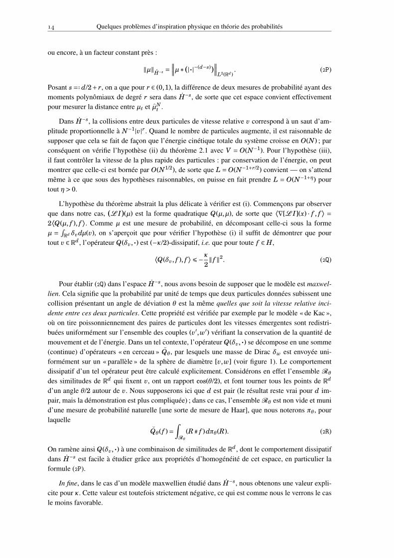
H−s, nous avons besoin de supposer que le modèle est maxwel-lien. Cela signifie que la probabilité par unité de temps que deux particules données subissent unecollision présentant un angle de déviation θ est la même quelles que soit la vitesse relative inci-dente entre ces deux particules. Cette propriété est vérifiée par exemple par le modèle « de Kac »,où on tire poissonniennement des paires de particules dont les vitesses émergentes sont redistri-buées uniformément sur l’ensemble des couples (v′,w′) vérifiant la conservation de la quantité demouvement et de l’énergie. Dans un tel contexte, l’opérateur Q(δv,·) se décompose en une somme(continue) d’opérateurs « en cerceau » Qθ, par lesquels une masse de Dirac δw est envoyée uni-formément sur un « parallèle » de la sphère de diamètre [v,w] (voir figure 1). Le comportementdissipatif d’un tel opérateur peut être calculé explicitement. Considérons en effet l’ensemble Rθ
des similitudes de Rd qui fixent v, ont un rapport cos(θ/2), et font tourner tous les points de Rd
d’un angle θ/2 autour de v. Nous supposerons ici que d est pair (le résultat reste vrai pour d im-pair, mais la démonstration est plus compliquée) ; dans ce cas, l’ensemble Rθ est non vide et munid’une mesure de probabilité naturelle [une sorte de mesure de Haar], que nous noterons πθ, pourlaquelle
Qθ( f )=∫Rθ
(R # f )dπθ(R). (2R)
On ramène ainsi Q(δv,·) à une combinaison de similitudes de Rd , dont le comportement dissipatifdans
.H−s est facile à étudier grâce aux propriétés d’homogénéité de cet espace, en particulier la
formule (2P).
In fine, dans le cas d’un modèle maxwellien étudié dans.
H−s, nous obtenons une valeur expli-cite pour κ. Cette valeur est toutefois strictement négative, ce qui est comme nous le verrons le casle moins favorable.
Résumé des travaux présentés
v
w
θ
FIGURE 1 – L’opérateur « en cerceau » Qθ. Cet opérateur envoie une masse de Dirac en un point w sur lamesure de probabilité uniforme sur le « cerceau » dessiné ci-dessus [ici en dimension 3].
Il nous reste à contrôler l’écart initial entre la mesure limite µ0 et la mesure empirique µN0 .
Nous supposerons que µ0 a un moment r-exponentiel (i.e.∫
ea|v|r dµ0(v) <∞ pour un a > 0), etnous prendrons pour condition initiale sur le modèle stochastique des particules i.i.d. selon la loiµ0. On peut alors contrôler E[U (λe−κT (X0 − X0))] par les mêmes méthodes de martingales quepour la démonstration du théorème 2.1.
En mettant bout-à-bout l’estimation sur la différence initiale, le théorème 2.1 et les estimationssur V , L et κ, nous obtenons alors une majoration explicite de la probabilité d’un événement de laforme P(‖µN
T −µT‖ Ê ε). Cette majoration est assez compliquée à écrire [son expression précise estdonnée dans la partie II de cette thèse, formule (CJ)], mais peut aisément être appliquée numéri-quement. J’ai fait une telle application numérique dans le cas du modèle « de Kac » en dimension 3,avec µ0 = 1
2 (δ−1+δ1) (on part loin de l’équilibre maxwellien) et T = 3 (chaque particule subit troiscollisions en moyenne), le paramètre r de l’espace
.H−s étant pris à 1/2. Je trouve alors que
N Ê 4×10⁵ ⇒ P(‖µNT −µT‖ .
H−s Ê 10−2)É 10−1, (2S)
ce qui montre qu’un nombre de particules assez faible (et largement à portée de simulation) assureavec grande probabilité une très bonne concordance (correspondant à des erreurs de vitesse del’ordre de 10−3) entre modèle particulaire et modèle continu.
D’un point de vue plus qualitatif, ma borne présente les comportements suivants :• Quand on regarde les asymptotiques pour N →∞, on obtient :
limN→∞
P(‖µNT −µT‖ Ê xN−1/2)É 2exp
( −x2
2[e2|κ|Tσ2 + e1(2|κ|T)ωT]
), (2T)
où σ2 est relié aux queues de la distribution initiale et ω à l’énergie du système, ces quan-tités étant calculables explicitement en fonction de µ0. Cette borne montre une convergenceà vitesse N−1/2, avec un contrôle gaussien, ce qui est typique du théorème-limite central(uniforme).
• Quand on s’intéresse au comportement non asymptotique, mes bornes explicites donnent uncontrôle gaussien des fluctuations tant que xN1/2 reste plus petit que O(N−r/2), c.-à-d. jusqu’àun régime intermédiaire entre les déviations standard et les grandes déviations ; au-delà, ongarde encore un contrôle exponentiel des fluctuations.
• Toujours du point de vue non asymptotique, dans le cas κ< 0, mes bornes se dégradent trèsrapidement quand T augmente. En revanche, dans le cas κ > 0, les bornes obtenues restent

Quelques problèmes d’inspiration physique en théorie des probabilités
bonnes quand T devient grand, et on peut même obtenir de bonnes bornes sur la déviationuniforme supt∈[0,T] ‖µN
t −µt‖.
3 Tensorisation des corrélations maximales
* Cette section est un résumé du travail présenté en détail dans la partie III de la thèse.
3.a β-mélange et ρ-mélange
En théorie des probabilités, quand on veut quantifier la dépendance entre deux tribus, deuxméthodes concurrentes sont le β-mélange et le ρ-mélange :
3.1 Définition. Pour X ,Y deux variables aléatoires définies sur un même espace de probabilités, àvaleurs dans deux espaces arbitraires X ,Y , le coefficient de β-mélange entre X et Y est
β(X ,Y ) ··= distVT(LoiX ⊗LoiY , Loi(X ,Y )), (3A)
où distVT désigne la distance en variation totale. En d’autres termes,
β(X ,Y )= 12
∫X×Y
|dP[(X ,Y )= (x, y)]−dP[X = x]dP[Y = y]|. (3B)
♦3.2 Définition. Pour X ,Y deux variables aléatoires définies sur un même espace de probabilités, àvaleurs dans deux espaces arbitraires X ,Y le coefficient de ρ-mélange entre X et Y est
X : Y ··= supf ,g
Cov( f (X ), g(Y ))Sd( f (X ))Sd(g(Y ))
, (3C)
où “Sd( f )” note l’écart-type de f (i.e. Sd( f ) ··=√
Var( f )), f et g étant des fonctions réelles définiesresp. sur X et Y , supposées mesurables et de carrés sommables. Ce coefficient est encore appelécorrélation maximale, ou hilbertienne, entre X et Y . ♦3.3 Proposition.
(i) β(X ,Y ) et X : Y ne dépendent de X et Y que via les tribus que ces variables engendrent ;(ii) Il y a équivalence entre les affirmations suivantes :
1. β(X ,Y )= 0 ;2. X : Y = 0 ;3. X et Y sont indépendantes.
♣
L’étude des corrélations est particulièrement intéressante en mécanique statistique, où l’étatd’une particule peut influencer ses voisines de proche en proche. Un cas d’école est le modèled’Ising des matériaux ferromagnétiques, dont nous rappelons la définition :
3.4 Définition. Dans le modèle d’Ising, l’état du système est décrit par une variable aléatoire→ω ∈ ±1Z
n, ωi ∈ ±1 étant appelé le spin du site i ∈Zn. Deux spins i et j sont dits voisins s’ils sont
adjacents dans le réseau Zn, ce qu’on note “i ∼ j”. →ω suit alors la mesure de Gibbs à paramètre β
définie (formellement) parP(ω)∝ e−βH(ω), (3D)

Résumé des travaux présentés
G D
x
FIGURE 2 – Une réalisation du modèle d’Ising sous-critique. Chaque carré représente un nœud de Z2 ; lesspins +1 sont représentés en clair et les spins −1 en foncé. On voit clairement que les spins proches sontcorrélés mais que cette corrélation décroît avec la distance. La miniature définit les demi-espaces G et D.
où le Hamiltonien du système est (formellement)
H(ω) ··=∑i∼ j
1ωi 6=ω j . (3E)
♦
Dans le cas du modèle d’Ising à petit paramètre, le théorème ci-dessous énonce qu’on a dé-croissance exponentielle des corrélations entre deux spins distants. Notez que la façon de mesurerces corrélations (β- ou ρ-mélange, notamment) importe peu, dans la mesure où la loi jointe d’unepaire de spins vit dans un espace de dimension finie.
3.5 Théorème (Peierls). Pour peu que le paramètre β soit suffisamment petit (régime sous-critique) :
(i) La mesure de Gibbs est uniquement définie, et il n’y a pas d’aimantation globale, i.e.E[ωi]= 0 ∀i.
(ii) Les spins proches présentent une corrélation positive, qui décroît exponentiellement avec ladistance, i.e.
∃ψ> 0,C <∞ ∀i, j ∈Zn 0<E[ωiω j]< C exp(−ψdist(i, j)). (3F)
♣
En revanche, on peut montrer que, dans certains cas au moins, β- et ρ-mélange se comportentdifféremment quand on s’intéresse à des groupes infinis de spins :
3.6 Théorème (Minlos & Sinai). Définissons les ensembles G et D comme sur la figure 2, et notonsresp. →
ωG et →ωD , l’état de l’ensemble des spins de G et de D. Alors :
(i) Quelle que soit la valeur de x, β(→ωG , →
ωD)= 1, ce qui est la valeur maximale pour un coefficientde β-mélange ;
(ii) →ωG : →
ωDÉ e−ψx, où ψ est la constante introduite dans (3F).
♣
La démonstration classique du point (ii) repose toutefois sur des propriétés très particulières,tant du modèle d’Ising [on a besoin que le modèle présente certaines symétries, que la portée desinteractions soit finie et que les corrélations décroissent exponentiellement] que des ensembles Get D [c’est pratiquement la seule forme qui convienne].
Quelques problèmes d’inspiration physique en théorie des probabilités
3.b Tensorisation des corrélations hilbertiennes
Le théorème 3.6 nous montre que les décorrélations hilbertiennes permettent de saisir cer-tains phénomènes intéressants. Nous allons donc tenter d’étudier ces décorrélations « pour elles-mêmes », en espérant qu’on en tirera une démonstration alternative de ce théorème qui soit suscep-tible de généralisations.
Un aspect important des corrélations hilbertiennes est leur capacité à se tensoriser :
3.7 Théorème (Csáki & Fischer). Soit I un ensemble au plus dénombrable, et soient (X i,Yi)i∈I
des couples indépendants de variables aléatoires ; alors :
→X I :
→YI= sup
i∈I
→X i :
→Yi. (3G)
♣
En adaptant certaines techniques de preuve du théorème 3.7, on peut démontrer des théorèmesde tensorisation plus généraux. Je donne ci-dessous un exemple de tel théorème, avec sa démons-tration. On a d’abord besoin d’une définition complémentaire sur les corrélations hilbertiennes :
3.8 Définition. Soient X ,Y et Z trois variables aléatoires. On définit la corrélation subjectiveX : Y Z entre X et Y par rapport à Z comme le supremum (plus précisément, le supremum essen-tiel) des valeurs de X : Y sous les différentes lois conditionnelles P[·|Z = z].
En termes hilbertiens,
X : Y Z = supf ∈L2(σ(X ,Z))g∈L2(σ(Y ,Z))
E[ f |Z],E[g|Z]≡0
|E[ f g]|Sd( f )Sd(g)
. (3H)
♦3.9 Théorème (Peyre). Pour I = 1, . . . , N, soient (X i)i∈I et Y des variables aléatoires. On supposeque pour tout i ∈ I,
X i : Y →X1,...,i−1
É εi; (3I)
alors :X i : Y É
√∑i∈Iε2
i . (3J)
♣
Démonstration. Soient f et g des fonctions L2 centrées resp.→X - et Y -mesurables. L’enjeu est de
borner |E[ f g]|.Définissions, pour tout i ∈ 0, . . . , N,
Fi ··=σ(X1, . . . , X i), (3K)
et pour tout i ∈ 1, . . . , N,f i ··=E[ f |Fi]−E[ f |Fi−1]. (3L)
On a alors f =∑i f i, où les f i sont orthogonales dans L2(P), d’où
|E[ f g]| É ∑i∈I
|E[ f i g]| (3M)
Résumé des travaux présentés
etVar( f )= ∑
i∈IVar( f i). (3N)
Pour borner |E[ f i g]|, on conditionne suivant la valeur de→X1,...,i−1 :
E[ f i g]=∫
E[ f i g|X1 = x1, . . . , X i−1 = xi−1]dP[x1, . . . , xi−1]. (3O)
Or sous la loi dP[·|x1, . . . , xi−1], f i est X i-mesurable et centrée, et g est Y -mesurable, de sortequ’en appliquant l’hypothèse (3I) :
|E[ f i g]|É εi
∫ √E[ f 2
i |x1, . . . , xi−1]√
E[g2|x1, . . . , xi−1]dP[x1, . . . , xi−1]
ÉCSεi
√∫E[ f 2
i |x1, . . . , xi−1]dP[x1, . . . , xi−1]√
idem pour g = εi Sd( f i)Sd(g). (3P)
(“ÉCS
” signifie qu’on a utilisé l’inégalité de Cauchy – Schwarz). En sommant (3P) sur i :
|E[ f g]| ÉN∑
i=1εi Sd( f i)Sd(g) É
CS
√∑iε2
i
√∑i
Var( f i) Sd(g)=√∑
iε2
i Sd( f )Sd(g). (3Q)
(3Q) étant vraie pour toutes f , g, cela démontre le théorème. ♠
Le théorème précédent s’applique à la tensorisation de N spins contre un seul. Pour tensoriserN spins contre M autres, le théorème général est le suivant, qui redonne notamment le théorème 3.7sur la tensorisation indépendante :
3.10 Théorème (Peyre). Soient I et J deux ensembles finis, et (X i)i∈I , (Y j) j∈J des variablesaléatoires. Sur chaque couple (i, j), on fait l’hypothèse suivante : uniformément en I ′ ⊂ I à iet J′ ⊂ J à j, la corrélation subjective entre X i et Y j par rapport à (
→X I ′ ,
→YJ′) est majorée par un
certain εi j — hypothèse qu’on notera de manière synthétique :
X i : Y j∗ É εi j. (3R)
Alors on a :
→X I :
→YJÉε, (3S)
où “ε” désigne la norme d’opérateur de l’opérateur linéaire ε entre espaces euclidiens définipar
ε : L2(J) → L2(I)(a j) j∈J 7→ (∑
j∈J εi ja j)i∈I .(3T)
♣
Grâce à la tensorisation des corrélations hilbertiennes, on peut donner de nouveaux résultats dedécorrélation entre groupes de particules en mécanique statistique. Dans le cas du modèle d’Ising,on obtient ainsi le théorème suivant :
3.11 Théorème (Peyre). Pour le modèle d’Ising sur Zn à paramètre β suffisamment petit, il existedes constantes ψ′ > 0 et k < 1 telles que, pour I, J des ensembles de spins disjoints de tailles et deformes arbitraires, on a, uniformément en I et J :
→ωI : →
ωJÉ (exp[− (ψ′+ o(1))dist(I, J)])∧k. (3U)
♣

Quelques problèmes d’inspiration physique en théorie des probabilités
En fait, Des théorèmes analogues peuvent également être prouvés dans des cadres beaucoupplus généraux que le modèle d’Ising : aucune symétrie n’est requise, la décroissance des corréla-tions peut être polynomiale, l’espace d’états peut être continu, le réseau qui supporte les spins peutavoir de la courbure, etc.
3.c Critère d’α-mélange pour les décorrélations hilbertiennes
J’ai par ailleurs démontré un nouveau critère de décorrélation hilbertienne. Remarquonsd’abord que les corrélations hilbertiennes contrôlent la différence entre mesure produit et mesurejointe sur les rectangles — de telles estimations sont qualifiées d’estimations d’α-mélange :
3.12 Proposition. Si F et G sont deux tribus avec
F : G É ε, (3V)
alors pour tous événements A ∈F ,B ∈G de probabilités respectives p et q,
|P[A∩B]− pq|É ε√p(1− p)q(1− q). (3W)
♣
Démonstration. Appliquer la définition (3C) des corrélations hilbertiennes avec f = 1A et g = 1B.♠
Il était déjà connu que la Propostion 3.12 admet des réciproques partielles, au sens où éta-blir (3W) pour un ε suffisamment petit permet de majorer arbitrairement F : G . La forme optimalede cette réciproque était conjecturée, mais pas connue. C’est elle que je suis parvenu à obtenir :
3.13 Théorème (Peyre). Si F et G sont deux tribus telles que, pour tous événements A ∈F ,B ∈G
de probabilités respectives p et q,
|P[A∩B]− pq|É ε√p(1− p)q(1− q) (3X)
pour un certain ε ∈ (0,1], alors :
F : G É ε(1+| logε|). (3Y)
♣
4 Brisure spontanée de symétrie en dimension infinie
* Cette section est un résumé du travail présenté en détail dans la partie IV de la thèse.
4.a Modèle et problématique
On considère une assemblée dense de particules ponctuelles sur l’espace euclidien affine Rd ,dont la distribution est décrite par une mesure positive µ. Les particules sont soumises à un potentiel
Résumé des travaux présentés
d’interaction v symétrique, ainsi qu’à une agitation brownienne à température T, le tout en présencede forts frottements. La densité m de µ évolue alors selon une équation de Mc Kean – Vlasov :
∂tm =∇·(T∇m+m∇(v∗m)). (4A)
Le potentiel v est supposé vérifier les hypothèses suivantes :
4.1 Hypothèse. La fonction v : Rd → R est dans l’espace de Schwartz (i.e. elle est infinimentdifférentiable et toutes ses dérivées sont intégrables), et est négative sur tout Rd . ♦
Otto [59] a montré que l’équation (4A) pouvait s’interpréter comme une descente de gradientdans une « variété riemannienne ». La fonctionnelle de Lyapounov correspondant à cette descenteest l’énergie libre de la mesure µ :
F (µ) ··=U (µ)+TS (µ), (4B)
où U et S sont respectivement l’énergie interne et l’entropie :
U (µ) ··= 12
∫(Rd)2
v(x− y)dµ(x)dµ(y), (4C)
S (µ) ··=∫Rd
logm(x)dµ(x). (4D)
La « variété riemannienne » dans laquelle a lieu la descente de de gradient est la structure associéeà la métrique de Wasserstein W2, dont nous rappelons la définition :
4.2 Définition. Pour µ,ν deux mesures positives σ-finies sur Rd de même masse totale, un cou-plage entre µ et ν est une mesure γ sur Rd ×Rd dont les deux marginales sont respectivement µet ν. Le coût quadratique de ce couplage est
I[γ] ··=∫
(Rd)2|y− x|2 dγ(x, y). (4E)
Notant Γ(µ,ν) l’ensemble des couplages entre µ et ν, la distance de Wasserstein W2(µ,ν) entre µet ν est alors définie comme
W2(µ,ν) ··= infγ∈Γ(µ,ν)
I[γ]1/2. (4F)
(Nous admettrons ici qu’il s’agit bien d’une distance). ♦
Nous allons étudier la fonctionnelle F pour les perturbations de la mesure uniforme λ sur Rd
définie par dλ(x) ··= Rdx, où R ∈ (0,∞) est un paramètre d’homogénéité fixé. Aussi travaillerons-nous dans l’espace défini ci-dessous :
4.3 Définition. L’espace de Wassertein, noté F, est l’ensemble des mesures µ telles que W2(λ,µ)<∞, muni de la distance de Wasserstein W2. ♦
Pour µ dans F, les formules (4C) et (4D) doivent être renormalisées pour faire sens : notantπ ··=µ−λ et p(x) ··= dπ(x)/dx = m(x)−R, on prendra en fait
U (µ) = 12
∫(Rd)2
v(y− x)(m(x)m(y)−R2)dx dy= 12
∫Rd
(v∗ p)(x)dπ(x) ; (4G)
S (µ) =∫Rd
log(R−1m(x))dµ(x)=∫Rd
((R+ p(x)) log(1+R−1 p(x))− p(x))︸ ︷︷ ︸=··Φ(p(x))
dx, (4H)
de sorte que U (λ),S (λ)= 0 — et donc F (λ)= 0. On notera qu’on a alors S Ê 0 sur tout F.

Quelques problèmes d’inspiration physique en théorie des probabilités
4.4 Définition.
1. Pour une température T donnée, nous dirons que l’équilibre homogène est stable quand la fonc-tionnelle F sur F atteint un minimum local en λ.
2. Quand l’équilibre homogène est stable, son énergie d’activation Ea sera définie comme le su-premum des valeurs E vérifiant la propriété suivante : sur la composante connexe de λ au seindu sous-ensemble de F constitué par les fonctions µ: F (µ)ÉF (λ)+E, F atteint un minimumglobal en λ.
♦
L’énergie d’activation a deux interprétations :
1. Ea est l’énergie minimale qu’il faut fournir au système pour passer de l’état λ à un autre étatplus stable ;
2. Quand on revient au système particulaire dont l’évolution (4A) n’est qu’une approximation, ilpeut arriver, en partant de la distribution homogène, que le système quitte cet état pour pas-ser à un état plus stable sous le seul effet des flucutations. L’énergie d’activation caractérisealors le temps (très long) qu’il faut attendre pour que cela se produise, qui est de l’ordre deexp(N Ea/T), N étant le nombre d’Avogadro.
Notre problématique est la suivante : dans quelles conditions l’équilibre homogène est-il stable,et que vaut alors l’énergie d’activation ?
4.b Stratégie de minoration
Puisque la fonctionnelle d’énergie libre U est quadratique, on voudrait minorer S par uneforme quadratique. Comme la fonction Φ(·) qui intervient dans (4H) est sous-quadratique, on vaconsidérer deux cas selon la valeur de p(x). Introduisons donc un paramètre η ∈ (0,∞) moralementtrès petit, et décomposons p(x) en p2(x)+ p1(x), où
p2(x) ··= 1|p(x)| É η p(x);p1(x) ··= 1|p(x)| > η p(x).
(4I)
On a alors pour tout p que
Φ(p)Ê Φ(η)η2 p2
2 +Φ(η)η
|p1|, (4J)
d’où en intégrant :
S Ê Φ(η)η2 ‖p2‖2
L2 + Φ(η)η
‖p1‖L1 . (4K)
Notons que dans (4K), quand η 0, on a Φ(η)/η2 → 12 R−1 et Φ(η)/η→ 0.
Pour appliquer cela à la minoration de F , posant
V ··=∫Rd
(−v(x))dx, (4L)
Résumé des travaux présentés
on écrit que
F (µ)= 12⟨p,v∗ p⟩L2 +TS (µ)= 1
2⟨p2,v∗ p⟩+ 1
2⟨p1,v∗ p⟩+TS (µ)
Ê−12‖v∗ p‖L2‖p2‖L2 − 1
2‖v∗ p‖L∞‖p1‖L1 +TS
ÊYoung
− 14V
‖v∗ p‖22−
V4‖p2‖2
2 −‖v∗ p‖∞
2‖p1‖1︸ ︷︷ ︸
Ê−(η2V /4Φ(η))Ssi ‖v∗ p‖∞ ÉVη/2
+TS
Ê− 14V
‖v∗ p‖22 +
(T − η2V
4Φ(η)
)S si ‖v∗ p‖∞ ÉVη/2. (4M)
On a donc besoin, d’une part de majorer ‖v∗ p‖∞ au voisinage de λ — ce que nous reportonsau § 4.c —, d’autre part de minorer S par ‖v∗ p‖2
2.
Pour ce dernier point, nous introduisons la marche aléatoire sur Rd dont les pas sont distribuéssuivant la mesure de probabilité K définie par
dK(x) ··= −v(x)V
dx. (4N)
On utilise alors le résultat suivant sur l’entropie :
4.5 Théorème. Si P est le noyau d’une chaîne de Markov sur Rd admettant λ pour mesure in-variante, alors pour toute mesure µ sur Ω, l’entropie de µ est décroissante sous l’action de P :
S (µP)ÉS (µ). (4O)
♣
On en déduit que S (p)ÊS (V−1v∗ p). Sous réserve que ‖v∗ p‖∞ soit suffisamment petit, onpeut alors appliquer la formule (4K) qui donne :
‖v∗ p‖∞ ÉVη ⇒ S Ê Φ(η)η2 V−2‖v∗ p‖2
2. (4P)
Combinant (4M) et (4P), on obtient finalement :
‖v∗ p‖∞ É Vη2
⇒ F Ê(T − η2
Φ(η)V2
)S . (4Q)
4.c Plongement de l’espace de Wasserstein dans un espace linéaire
Nous devons encore borner ‖v∗p‖∞ au voisinage de λ dans F, ce pour quoi nous aurons besoind’un résultat de plongement de l’espace de Wasserstein dans le dual d’un espace de Sobolev. Voiciun tel résultat :
4.6 Théorème (Peyre). Pour f dans l’espace de Schwartz, notant ‖ f ‖1,2 ··= ‖D f ‖L2 , ‖ f ‖2,∞ ··=‖D2 f ‖L∞ , définissons
‖ f ‖W0 ··= ‖ f ‖1,2 ∨ | f ‖2,∞ = (∫Rd
|D f (x)|2 dx)1/2 ∨ supx∈Rd
|D2 f (x)|, (4R)
et notons W0 l’espace obtenu par complétion de cette norme. Alors l’application µ 7→π, considéréede F dans le dual W′
0 de cet espace, est continue en λ. ♣
Quelques problèmes d’inspiration physique en théorie des probabilités
Démonstration. Soit f une fonction de W0 et soit T un plan de transport de λ vers µ ∈ F. Notonsu(x) ··= T(x) / |T(x)| le vecteur unitaire qui indique la direction dans laquelle le point x se déplaceau cours de l’opération de transport.
On a
|⟨ f ,π⟩| = |∫Rd
( f (x+T(x))− f (x))dλ(x)|É R∫
x∈Rd
∫ |T(x)|
r=0|D f (x+ ru(x))|drdx (4S)
et
I[T]=∫Rd
|T(x)|2 dλ(x)= 2R∫
x∈Rd
∫ |T(x)|
r=0r drdx. (4T)
Nous introduisons alors l’espace Ω ··= (x, r) : 0 É r É |T(x)|, et sur Ω nous définissons la mesuredγ ··= 2Rr drdx et la fonction e(x, r) ··= |D f (x+ ru(x))| /2r. Les formules (4T) et (4S) deviennentalors respectivement :
I[T] =∫
(x,r)∈Ωdγ(x, r); (4U)
|⟨ f ,π⟩| É∫
(x,r)∈Ωe(x, r)dγ(x, r). (4V)
Cette position du problème suggère l’utilisation d’un lemme de couplage :
4.7 Lemme (Peyre). Soit γ une mesure (positive) σ-finie sur un espace mesurable Ω, et e : Ω→R+ une fonction mesurable. On suppose qu’il existe une fonction Y∗ : R+ → R+, de classe C 1 etdécroissante avec Y∗(e) e→∞→ 0, telle que pour tout θ ∈R+,∫
e(ω)Êθe(ω)dγ(ω)ÉY∗(θ). (4W)
Définissant à partir de Y∗ la fonction décroissante X∗ : R+ →R+ par
X∗(θ) ··= −∫ ∞
θ
Y ′∗(τ)τ
dτ, (4X)
on a alors : ∫Ω
e(ω)dγ(ω)É (Y∗ X−1∗ )(
∫Ω
dγ(ω)). (4Y)
♣
Pour appliquer le lemme 4.7 à notre situation, il faut majorer∫
e(x,r)Êθ |D f (x+ ru(x))|drdxpour θ > ‖ f ‖2,∞/2 arbitraire. Or “e(x, r) Ê θ” signifie que |D f (x+ ru(x))| Ê 2θr, d’où |D f (x)| Ê(2θ−‖ f ‖2,∞)r, et donc r É (2θ−‖ f ‖2,∞)−1|D f (x)|. On a en outre |D f (x+ ru(x))| É |D f (x)| +r‖ f ‖2,∞, d’où la majoration :∫
e(x,r)Êθ|D f (x+ ru(x))|dx É
∫rÉ |D f (x)|
2θ−‖ f ‖2,∞
(|D f (x)|+ r‖ f ‖2,∞)dx dr
=( 12θ−‖ f ‖2,∞
+ ‖ f ‖2,∞2(2θ−‖ f ‖2,∞)2
)‖ f ‖2
1,2. (4Z)
Le lemme 4.7 donne alors |⟨ f ,π⟩| ÉpR‖ f ‖1,2I[T]1/2+ 1
2‖ f ‖2,∞I[T], et donc en prenant l’infimumsur les plans de transport de λ à µ :
|⟨ f ,π⟩| Ép
R‖ f ‖1,2W2(λ,µ)+ 12‖ f ‖2,∞W2(λ,µ)2, (4AA)
ce qui montre bien que le plongement de F dans W′0 est lipschitzien en λ. ♠
Présentation de la thèse
En raffinant les techniques présentées ci-dessus, on peut même obtenir un résultat de continuitéglobale :
4.8 Théorème (Peyre). Pour α ∈ [0,2/(d+2)), pour f dans l’espace de Schwartz, définissons for-mellement
‖ f ‖Wα ··= ‖D f ‖2 ∨‖D2−α f ‖2/α, (4AB)
et notons Wα l’espace obtenu par complétion de cette norme. Alors l’application µ 7→π, considéréede F dans W′
α, est continue sur tout F. ♣
4.d Quelques résultats
Grâce aux estimations présentées ci-dessus, on obtient le
4.9 Théorème (Peyre). Sous l’hypothèse 4.1, la transition de phase a lieu à la température RV :l’équilibre homogène est instable en-deçà de cette température, et stable au-delà. ♣
Notons que cette température de transition coïncide avec celle du système linéarisé.
Pour minorer l’énergie d’activation, on peut utiliser une minoration de ‖v∗ p‖2 en fonctionde ‖v∗ p‖∞ — l’existence d’une telle minoration est rendue possible par la positivité de µ — :
4.10 Lemme (Peyre). Sous l’hypothèse 4.1, il existe une constante C(v) <∞ telle que pour toutemesure positive µ,
‖v∗ p‖2 Ê C(v)‖v∗m‖−d/4∞ ‖v∗ p‖1+d/4
∞ . (4AC)
♣
4.11 Corollaire (Peyre). Pour T > RV , l’énergie d’activation de l’équilibre uniforme est non nulle,et minorée au voisinage de la température critique par C(T − RV )3+d/2 + o((T −RV )3+d/2) pourun C > 0. ♣
Finissons en évoquant quelques prolongements et conjectures :• Le théorème 4.8 devrait rester valable pour tout α ∈ [0,4/(d+2)), ce qui serait alors l’intervalle
optimal.• Pour v non négatif, on étend la définition de V en posant
V ··= supξ∈Rd
(− v(ξ)). (4AD)
Le théorème 4.9 reste alors valable pour tout v dans l’espace de Schwartz, même non négatif,ainsi que pour tout v ∈ Wα si v est négatif. J’espère pouvoir l’étendre à tout v de Wα. Leshypothèses du théorème 4.11 devraient également pouvoir être affaiblies, mais j’ai plus demal à cerner quelles seraient les conditions minimales.
• Dans le théorème 4.11, j’ignore si l’exposant (3+d/2) est optimal ; une conjecture plausibleest qu’on pourrait abaisser cette valeur à 3.


Première partie
Une approche probabilistede la borne de Carne

Résumé
La borne de Carne est une inégalité fine qui contrôle les probabilités de transition d’une chaînede Markov discrète réversible [§ 1]. Sa preuve habituelle [§ 2] s’appuie sur des techniques spec-trales efficaces mais d’apparence miraculeuse. Je présente ici une nouvelle preuve, dans laquelleon compare la « dérive » entre les chemins « aller » et « retour » pour récupérer la partie gaussiennede la borne [§ 3], et où on utilise une technique de conditionnement pour récupérer le facteur dedissipation [§ 5]. Je montre en outre que cette preuve est plus souple que celle de Carne et peutainsi se généraliser [§ 4].
* Les recherches présentées dans cette partie de la thèse ont été publiées dans [65].
Une approche probabiliste de la borne de Carne
1 Introduction
1.a The Markov chain
Let V be a finite or countable set of points. Let us consider an irreducible Markov chain (X t)t∈Non V , with transition kernel (p(x, y))x,y∈V , and whose law is denoted by Px when starting at x. Thatchain is supposed to be reversible, i.e. we suppose that there exists a measure µ on V such that, forall x ∈V 0<µ(x)<∞, and
∀x, y ∈V µ(x)p(x, y)=µ(y)p(y, x). (A)
By irreducibility, µ is then uniquely determined up to a multiplicative factor; in the sequel, we shallsuppose it fixed. Note that we do not demand µ to be finite.
Then one may associate to the kernel a (non-oriented) graph (V ,E) with vertices set V bydefining the set of edges through
x, y ∈ E ⇔ p(x, y) 6= 0. (B)
(A priori that definition should determine an oriented graph, but actually p(x, y) 6= 0 ⇔ p(y, x) 6= 0by reversibility). As usual, we shall write z ∼ z′ to mean that z, z′ ∈ E [†]. The graph distance,denoted by d, will stand for the length of the shortest path(s) in E joining two points. Speaking interms of probability, one has:
d(x, y)= inft ∈N : pt(x, y) 6= 0, (C)
where pt denotes the t-th convolution power of the kernel p.
This part of the thesis aims at explaining by probabilistic arguments an inequality due to Carneto sharply bound pt(x, y) above when d(x, y)&
pt. Indeed to the best of our knowledge, all the
methods developed so far to get that kind of bounds used spectral analysis techniques [80, 18].We shall also show how our probabilistic approach allows us to generalize Carne–Varopoulos typebounds for more “flexible” distances than the graph distance.
1.b Carne’s bound and its history
In 1985, N. Th. Varopoulos [80] was the first to give a concentration result bounding abovept(x, y) for a reversible Markov chain, whose leading term was exp(−d(x, y)2/Ct), C > 0 being anexplicit constant depending on the transition kernel p. His method introduced a time-continuousMarkov process on the cabled graph associated to (V ,E), and studied the spectral properties of thatprocess in an L2 space. Moreover that proof required extra assumptions about the transition kernel.
The same year, T. K. Carne [18], by a simpler spectral method, got a finer result under thegeneral assumptions stated in § 1.a:
1.1 Theorem (Carne 1985). Suppose the hypotheses of § 1.a are satisfied. Denote by P the L2(µ)-operator associated to the transition kernel p and let |P| stand for its norm, which is always É 1(see a more precise definition in § 2.a). Then:
pt(x, y)É 2(µ(y)µ(x)
)1/2|P|t exp
(−d(x, y)2
2t
). (D)
♣[†]. Look out for the fact that ∼ is not an equivalence relation.
Quelques problèmes d’inspiration physique en théorie des probabilités
My work was motivated by two goals: first, find a proof of Theorem 1.1 which would be morenatural than the original proof of Carne, then, adapt Carne–Varopoulos type bounds to distanceswhich depend continuously on the transition kernel (see § 4.b).
2 Carne’s proof
We give here the proof of [18] as it was exposed in [49, Theorem 13.4].
2.a Norm of the transition kernel
Let us first give a precise definition of P:
2.1 Definition. P is the operator induced by P on L2(µ) through:
P f (x)=Ex[ f (X1)]= ∑y∼x
p(x, y) f (y), (E)
♦
Then we define |P| as the operator norm of P in L2(µ), i.e. |P| = sup‖ f ‖L2(µ)=1 ‖P f ‖L2(µ). Notethat P is self-adjoint by reversibility of µ, and |P| É 1 by Jensen’s inequality.
A more intrinsic defintion of |P| is given by the following classical
2.2 Lemma ([49, Chap. 5-2]). For any x ∈V ,
|P| = limt→∞
(pt(x, x)
)1/t = suptÊ1
(pt(x, x)
)1/t . (F)
♣
2.b Chebychev’s polynomials
Since Pn f (x)=Ex[ f (Xn)], one can write
pt(x, y)=⟨δxµ(x)
,P tδy
⟩L2(µ)
= |P|tµ(x)
⟨δx,
(P|P|
)tδy
⟩L2(µ)
. (G)
The trick then consists in decomposing the polynomial Z t in the basis of Chebychev’s polynomials.The following results are classical:
2.3 Lemma. For any k ∈Z, there exists a unique polynomial Qk(Z) satisfying
∀θ ∈C Qk(cosθ)= cos(kθ), (H)
called the k-th (first type) Chebychev polynomial. It satisfies:
(i) degQk = |k|;(ii) |x| É 1 ⇒ |Q(x)| É 1;
(iii) ∀t ∈N Z t = 12t
∑k∈Z
( t(t+k)/2
)Qk(Z), where by convention
( tp)= 0 whenever p ∉ 0,1, . . . , t.
♣
Une approche probabiliste de la borne de Carne
By property (iii) in Lemma 2.3, formula (G) gives
pt(x, y)= |P|t2tµ(x)
∑k∈Z
(t
(t+k)/2
)⟨δx,Qk
(P|P|
)δy
⟩L2(µ)
. (I)
The linear operator (|P|−1P) on L2(µ) is self-adjoint and its norm is 1 by construction; so itdecomposes onto a countable orthonormal basis of eigenvectors as
P|P|
( ∑λ∈Spec(P/|P|)
aλvλ
)= ∑λ∈Spec(P/|P|)
λaλvλ, (J)
where vλ is the eigenvector associated to the eigenvalue λ, the eigenvalues being counted withmultiplicity. By definition of |P| we have Spec
(|P|−1P)⊂ [−1,1]. So
Qk
(P|P|
)( ∑λ∈Spec(P/|P|)
aλvλ
)= ∑λ∈Spec(P/|P|)
Qk(λ)aλvλ, (K)
where the Qk(λ) are all of absolute value less than or equal to 1 by Lemma 2.3, property (ii). Then,the operator norm of Qk
(|P|−1P)
on L2(µ) is at most 1, so to write:⟨δx,Qk
(P|P|
)δy
⟩L2(µ)
É ‖δx‖L2(µ) · ‖δy‖L2(µ) =√µ(x)µ(y). (L)
Now, we notice that for |k| < d(x, y), Qk(|P|−1P
)δy is a linear combination of the Puδy,0 É
u < d(x, y), by property (i) in Lemma 2.3; then Qk(|P|−1P
)δy is a function supported by the z ∈V
satisfying d(z, y)< d(x, y), in particular⟨δx,Qk
(|P|−1P)δy
⟩L2(µ) = 0. In the end,
pt(x, y)= |P|t2tµ(x)
∑|k|Êd(x,y)
(t
(t+k)/2
)⟨δx,Qk
(P|P|
)δy
⟩L2(µ)
(L)É |P|t2tµ(x)
√µ(x)µ(y)
∑|k|Êd(x,y)
(t
(t+k)/2
)É 2|P|t
(µ(y)µ(x)
)1/2 12t
∑kÊd(x,y)
(t
(t+k)/2
)(M)
(where the last inequality is an equality as soon as d(x, y)> 0).
To conclude, it only remains to prove the relation
12t
∑kÊd(x,y)
(t
(t+k)/2
)É exp(−d(x, y)2/2t). (N)
To do that, we notice that, if X is a random variable equidistributed on −1,1, then, the law of X∗t
(which denotes the t-th convolution power of X ) is 12t
∑k∈Z
( t(t+k)/2
)δk, so
12t
∑kÊd(x,y)
(t
(t+k)/2
)=P
(X∗t Ê d(x, y)
). (O)
Now, we check by direct computation that for all λ> 0, E[eλX ] É eλ
2/2, hence E[eλX∗t
]É etλ2/2,
and then by Chebychev’s inequality:
P(X∗t Ê d(x, y)
)=P(eλX∗t Ê eλd(x,y)
)É etλ2/2
eλd(x,y) , (P)
hence we get (N) by taking λ= d(x, y)/t, which ends the proof.
Quelques problèmes d’inspiration physique en théorie des probabilités
3 The Gaussian factor
As told before, this work presents a new, probabilistic proof of Carne’s bound. In this section,only the Gaussian part of the bound will be considered. The fundamental estimate is the
3.1 Theorem. Let P be a Markov chain as described in § 1.a; let t Ê 2; let x 6= y ∈V ; then
pt(x, y)É(µ(y)µ(x)
)1/2exp
(− (d(x, y)−1)2
2(t−1)
). (Q)
♣
The following immediate corollary yields a more pleasant formula:
3.2 Corollary. For t Ê 1 and x, y ∈V ,
pt(x, y)Épe(µ(y)µ(x)
)1/2exp
(−d(x, y)2
2t
). (R)
♣
3.3 Remark. The first factor in the bound (R) is slightly better than that of (D), but actually onecould replace the 2 by a
pe in the proof of § 2 by refining the bound (N). ♥
Proof. Denote d = d(x, y). First, note that by reversibility of the chain, one has
pt(y, x)= µ(x)µ(y)
pt(x, y); (S)
so to prove (Q) it suffices to show:
pt(x, y) pt(y, x)É exp(− (d−1)2
t−1
). (T)
Now, rather than reasoning on the graph, which is a “complicated” object, we shall introducea function ξ : V → R which measures how much the random walk X is closer to x or to y. ξ mustsatisfy:
3.4 Assumption.• ξ(x)= 0; ξ(y)= d;• ξ is 1-Lipschitz, i.e. for z ∼ v we have |ξ(v)−ξ(z)| É 1.
♦
Such a map ξ always exists since, for instance, the map d(x,·) always satisfies Assumption 3.4.Each point of V tends to make ξ increase or decrease, depending on the values of the transitionkernel. Let us denote by m(z) the expected value for the variation of ξ after the particle havingvisited z, i.e.
m(z)=Ez [ξ(X1)]−ξ(z). (U)
Now, let (Mu)uÊ1 be the process defined by:
Mu = ξ(Xu)−ξ(X1)−u−1∑s=1
m(Xs)=u−1∑s=1
(ξ(Xs+1)−ξ(Xs)−m(Xs)) ; (V)
Une approche probabiliste de la borne de Carne
obviously M is a martingale starting at 0. Let us look at the chain starting at x. On the eventX t = y, one trivially has ξ(X t)−ξ(X1)Ê d−1, hence
Ex [Mt|X t = y]Ê d−1−Ex
[t−1∑u=1
m(Xu)
∣∣∣∣∣X t = y
]. (W)
One may carry out the same reasoning starting at y, which gives:
Ey [Mt|X t = x]É−(d−1)−Ey
[t−1∑u=1
m(Xu)
∣∣∣∣∣X t = x
]. (X)
What can we see? If the terms Ex[∑t−1
u=1 m(Xu)|X t = y], resp. Ey
[∑t−1u=1 m(Xu)|X t = x
]were not present in (W) and (X), these formulae would reduce to Ex [Mt|X t = y] Ê d − 1, resp.Ey [Mt|X t = x]É−(d−1), so that we would observe a large deviation phenomenon on martingales,which would yield a control respectively on pt(x, y) and pt(y, x). Unfortunately, that phenomenonseems to be wiped out because of the terms m(Xs). The key idea then consists in noticing that, byreversibility, these m(Xs) are the same for the “way out” as for the “way back”; subsequently, ifthe m(Xs) tend to make the right hand side of (W) diminish (which would damp the large deviationphenomenon), then they tend to make the right hand side of (X) increase, which this time translatesinto a strengthening of the large deviation phenomenon. So, pt(x, y) and pt(y, x) cannot be largesimultaneously, which will lead us to (T).
So, we consider X x, X y two independent chains with respective laws Px and Py; let Px⊗y
be their joint law. The respective realizations of (Mu)uÊ1 for the paths starting at x and at y aredenoted by (Mx
u)uÊ1 and (M yu)uÊ1. By reversibility,
∀u ∈ 1, . . . , t−1 Ex [m(Xu)|X t = y]=Ey [m(X t−u)|X t = x]. (Y)
Hence by combining (W) and (X),
Ex⊗y [Mxt −M y
t |X xt = y and X y
t = x]Ê 2(d−1). (Z)
It remains to control the deviations of Mxt −M y
t . We remark that this random variable may beinterpreted as the final value of a 2(t−1) steps martingale, to which one can apply the followingvariant of Azuma’s inequality:
3.5 Lemma. Let (Ft)t∈N be a filtration; let (X t)tÊ1 be an adapted real-valued process withE[X t+1|Ft] = 0 [‡]. We suppose that, for all t ∈ N, Law(X t+1|Ft) is supported by an intervalof length 2 almost surely. Then, letting u Ê 0 be a fixed time, we have for all λ ∈R:
E
[exp
(λ
u∑t=1
X t
)]É exp
(uλ2
2
). (AA)
♣
Proof. The proof relies on Hoeffding’s inequality, whose statement is recalled below:
3.6 Lemma (Hoeffding). Let X be a centered real-valued random variable, supported by an inter-val of length 2, then
∀λ ∈R E[eλX
]É eλ
2/2. (AB)
♣[‡]. In other words, the X t’s are the increments of a martingale.

Quelques problèmes d’inspiration physique en théorie des probabilités
That point being taken for granted, we prove Lemma 3.5 by induction on u:• For u = 0 the result is trivial.• Let u Ê 1; suppose the result to be true for u−1. Let λ ∈R; we write
E
[exp
(λ
u∑t=1
X t
)]=E
[exp
(λ
u−1∑t=1
X t
)E
[eλXu
∣∣∣Fu−1
]]
ÉE
[exp
(λ
u−1∑t=1
X t
)]︸ ︷︷ ︸Ée(u−1)λ2/2 by induction
·∥∥∥E
[eλXu
∣∣∣Fu−1
]∥∥∥∞︸ ︷︷ ︸Éeλ2/2 by (AB)
É euλ2/2. (AC)
♠
To conclude, it only remains to us to prove the following measure concentration lemma:
3.7 Lemma. Let X be a centered real-valued random variable satisfying for some k > 0:
∀λ ∈R E[eλX ]É ekλ2/2. (AD)
If A is an event such thatE[X |A ]Ê C (AE)
for some C Ê 0, then
P(A )É exp(−C2
2k
). (AF)
♣
Proof. To lighten notations, let us denote p =P(A ). Let us fix λ> 0, then we have
E[eλX
∣∣∣A ]= E
[1A eλX ]P(A )
(AD)É 1p
ekλ2/2. (AG)
It follows, by Jensen’s inequality, that
E[X |A ]É 1λ
log(
1p
ekλ2/2), (AH)
hence by assumption (AE)1λ
log(
1p
ekλ2/2)Ê C, (AI)
whence finally:p É e−Cλ+kλ2/2. (AJ)
Then it suffices to take λ= C/k to get the announced result. ♠
Now we conclude the proof of Theorem 3.1. Lemma 3.5 permits us to control the Laplacetransform of Mx
t −M yt under Px⊗y:
∀λ ∈R Ex⊗y
[eλ(Mx
t −M yt )
]É e(t−1)λ2
, (AK)
and formula (Z) then gives, via Lemma 3.7:
Px⊗y(X xt = y and X y
t = x)É exp(− (d−1)2
t−1
), (AL)
which is formula (T). ♠

Une approche probabiliste de la borne de Carne
4 Generalization to a larger class of distances
4.a Statement of the generalized theorem
Now we will show that the reasoning made above can in fact adapt to a whole class of distances.So let us consider a new distance on V , which we will also call d —to avoid confusions, the graphdistance that we had defined by (C) will be denoted dG from now on. We have:
4.1 Theorem. Suppose that d is built so that, if ξ : V → R is any 1-Lipschitz function with respectto d, one has, for all x ∈V :
•|Ex [ξ(X1)]−ξ(x)|É B; (AM)
•∀λÊ 0 Ex
[eλξ(X1)−Ex[ξ(X1)]
]É eAλ2/2, (AN)
for some constants A and B independent of ξ. Then, for all x, y ∈V , one has
pt(x, y)É(µ(y)µ(x)
)1/2exp
(− (d(x, y)−B)+2
2At
)É eB/A
(µ(y)µ(x)
)1/2exp
(−d(x, y)2
2At
). (AO)
♣4.2 Remark. We can already point out that, in the case when the distance is dG, it is impossible toget anything better than A = 1 and B = 1. Subsequently, the result will be worsened by a
pe factor
compared to (R)—which remains negligible compared to the exponential part of the bound—: aswe will see later, it is due to the difference in treating the first steps, since the specific argumentthat we have used for dG in the proof of Theorem 3.1 may not generalize. ♥
Proof. We follow again the proof of Theorem 3.1: denote d = d(x, y), let ξ satisfy Assumption 3.4,define m by (U) and let Px⊗y be the joint law of two independent chains of respective laws Px
and Py; we want to bound Px⊗y[X xt = y and X y
t = x] above to conclude by formula (S).
The first difference lies in the definition of M: now, the martingale starts at time 0. So it isdefined by:
Mu = ξ(Xu)−ξ(X0)−u−1∑s=0
m(Xs)=u−1∑s=0
(ξ(Xs+1)−ξ(Xs)−m(Xs)). (AP)
Then we get: Ex [Mt|X t = y]= d−Ex
[∑t−1u=0 m(Xu)
∣∣X t = y],
Ey [Mt|X t = x]=−d−Ey[∑t−1
u=0 m(Xu)∣∣X t = x
] (AQ)
When we want to combine these two formulae as we did in (Z), we observe that all the termsE[m(Xu)] will cancel pairwise, except the terms corresponding to the first steps, i.e. to u = 0 inthe two respective formulae. But we know exactly what these terms are, since under Px, we haveX0 = x a.s. (by definition!), resp. X0 = y a.s. under Py. Thus
Ex⊗y[Mx
t −M yt∣∣X x
t = y and X yt = x
]= 2d−m(x)+m(y)Ê 2d−2B. (AR)
Taking into account assumption (AN)—which plays here the role played before by Hoeffding’sinequality—, we copy off the proof of Lemma 3.5 to get:
∀λÊ 0 Ex⊗y
[eλ(Mx
t +M yt )
]É eAtλ2
, (AS)

Quelques problèmes d’inspiration physique en théorie des probabilités
and it only remains to conclude by Lemma 3.7 [§]. ♠
4.b More flexible distances
Now we will show how one may build distances statisfying Theorem 4.1, such that the metricstructure of V continuously depends on the transition kernel. The method developed below iscertainly neither the best nor the most elegant, but it has the advantage to be of relative pedagogicalsimplicity.
We keep on the principle of putting a length to each edge, but that time all the edges will nothave the same size: indeed we will put a larger length to the edges that are more difficult to visit, inorder to ensure that the metric structure of the graph will not be too much perturbed when we adda very “unlikely” edge.
Let α> 0 be an arbitrary parameter. To each couple (x, y) ∈V ×V , we associate a length l(x, y)such that:
∀a Ê 0 Px (l(x, X1)Ê 1+a)É e−a2/2α2, (AT)
and we define the length of the edge [xy] by |[xy]| =minl(x, y), l(y, x). Then, for any 1-Lipschitzfunction ξ on V , we have:
4.3 Proposition.
∀x ∈V ∀a Ê 0 Px (|ξ(X1)−ξ(x)| Ê 1+a)É e−a2/2α2. (AU)
♣
Now we give a formula for l(x, y) satisfying (AT). First we define what we will call the β-entropy of a probability law:
4.4 Definition. Let β ∈ (0,1]; let p be a probability measure on a discrete space X . We callβ-entropy of p the (possibly infinite) number:
Hβ(p)= ∑x∈X
p(x)1−β [¶]. (AV)
A transition kernel p on V being given, we will also denote, for x ∈V , Hβ(x)= Hβ (p(x,·)). ♦
The β-entropy permits us to control the probability that the observed event is rare:
4.5 Proposition. Let β ∈ (0,1]; let p be a probability measure on a discrete state space X . Wesuppose Hβ(p)<∞. Then under the law p, for all q ∈ (0,1] one has:
P (p(x)É q)É Hβ(p)qβ. (AW)
♣
Proof. Use the identity Hβ(p) = E[p(x)−β] and the fact that the map q 7→ q−β is decreasing, thenapply Markov’s inequality. ♠
[§]. If it occurs that B Ê d, Lemma 3.7 cannot be applied and we may only bound pt(x, y)pt(y, x) above by 1; thisexplains the positive part appearing in (AO).
[¶]. For β= 1 we set by continuity Hβ(p)= #x ∈X : p(x)> 0.
Une approche probabiliste de la borne de Carne
So, one may choose the following expression for l(x, y) to satisfy (AT), where we set that, fora < 0, a1/2 = 0:
l(x, y)= 1+p
2α(β log(p(x, y)−1)− logHβ(x))1/2. (AX)
Now, we want to show that (AU) permits us to get (AM) and (AN) indeed. Let us begin with aneasy observation:
4.6 Proposition. Let ξ be a 1-Lipchitz function on V for a distance d built as above. Then thereexists a random variable Y whose repartition map satisfies ∀a Ê 0 P(Y Ê 1+a) = e−a2/2α2
, i.e. Yhas a law with density
dP(Y = y)= 1yÊ 1y−1α2 e−(y−1)2/2α2
dy, (AY)
such that one has:Px -p.s. |ξ(X1)−ξ(x)| ÉY . (AZ)
♣
So, we easily find that we can take B =E[Y ]= 1+pπ/2α into (AM).
To get a formula for A in (AN), things are a bit more complicated. The tool which we will useis the
4.7 Lemma. Let Y be a positive random variable whose Laplace tranform Y (λ) = E[eλY ]
issupposed to be finite for all λ Ê 0, and let us denote Y = E[Y ]. Let X be a real-valued randomvariable satisfying |X | É Y a.s.; let us denote X = E[X ] and
~X = X −E[X ]. Then the Laplace
transform of~X satisfies:
∀λ ∈R ~X (λ)É e|λ|Y Y (|λ|)−2|λ|Y . (BA)
♣4.8 Remark. The bound (BA) is of quite poor quality close to 0, as it may be particularily striking inthe case Y ≡ 1, where we get the bound e2|λ|−2|λ|, while we know (Hoeffding’s lemma 3.6) thateλ
2/2 would work. In fact, we can compute that in a neighborhood of 0, the right hand side of (BA)takes the form:
1+ (E[Y 2]+3E[Y ]2)λ2
2+ o(λ2), (BB)
while a variance calculation proves that in fact,
~X (λ)É 1+E[Y 2]
λ2
2+ o(λ2). (BC)
♥
Proof. We may restrict ourselves to the case λÊ 0, the case λÉ 0 being then treated by using theresult for −X .We write ~
X (λ)=E[eλ
~X −λ ~
X]
. (BD)
But, since |X | É Y , we have |X | É Y , hence~X ∈ [−Y − Y ,Y + Y ]. And since, on an interval of the
form [−a,a], the map x 7→ eλx −λx takes its maximum at a, it follows that
~X (λ)ÉE
[eλ(Y+Y ) −λ(Y + Y )
]= eλY Y (λ)−2λY . (BE)
♠
Quelques problèmes d’inspiration physique en théorie des probabilités
Now we have the following control on the Laplace transform of the random variable Y definedby (AY):
4.9 Claim. If Y is a random variable whose law is given by (AY), then for λÊ 0 one has:
E[eλY
]É
(1+
√π
2αλ+ α2
2λ2
)eλ+α
2λ2/2. (BF)
Moreover, that bound is sharp close to 0, by which we mean that, if we rewrite (BF) under the formE[eλY ]É f (λ), we have E[Y ]= d
dλ |λ=0 E[eλY ]= f ′(0)= 1+pπ/2α. ♣
Proof. We begin with noticing that we can write Y = 1+αZ, where Z is a random variable withlaw
dP(Z = z)= 1z Ê 0ze−z2/2dz. (BG)
Then it suffices to prove that
∀λÊ 0 E[eλZ
]É
(1+
√π
2λ+ λ2
2
)eλ
2/2. (BH)
To do that, we write:
E[eλZ
]= eλ
2/2∫ ∞
0ze−(z−λ)2
dz t=z−λ= eλ2/2
∫ ∞
−λ(t+λ)e−t2/2dt︸ ︷︷ ︸
I(λ)
, (BI)
where I(0)= 0 and, by the theorem of differenciation under the integral,
I ′(λ)=∫ ∞
−λe−t2/2dt É
√π
2+ λ
2, (BJ)
whence I(λ)É 1+pπ/2λ+λ2/2, and (BF). ♠
From that we deduce the existence of a suitable value for A:
4.10 Claim. For all α> 0, there exists a constant A(α)<∞ such that, if d satisfies condition (AU)for the value α, then (AN) is satisfied for the value A(α). ♣
Proof. For Y with law (AY), denoting Y ··= E[Y ] = 1+pπ/2α, Claim 4.9 shows that 2λ−2 ×
log(eλY E[eλY ]− 2λY ) is bounded for λ Ê→ 0 and λ → ∞. By continuity, this function is thusbounded on the whole half-line [0,+∞). Lemma 4.7 then gives the existence of A. ♠
4.11 Remark. We have not found any simple bound for A(α), but, for a given value of α, it is easyto compute numerically the maximum of the map λ 7→ 2log(eλY E[eλY ]−2λY ) /λ2, which gives asuitable value for A. ♥
4.c A concrete example
I shall illustrate the preceding subsection by showing how Theorem 4.1 can give worthy resultsin cases where the usual Carne bound is irrelevant. [‖]
[‖]. This section has been entirely rewritten for its thesis version: while in [65] I took an example on a hyperbolicgraph, I eventually found it more relevant to take an amenable example.

Une approche probabiliste de la borne de Carne
Let us take for V the discrete Heisenberg group, that is, the set of upper triangular matricesin M3(Z) whose all diagonal entries are 1 —which is a multiplicative group. On V , the naturalgraph structure consists in connecting two matrices M and N by an edge as soon as
NM−1 ∈
1 ±1 0
0 1 00 0 1
,
1 0 00 1 ±10 0 1
; (BK)
we denote by dH the distance associated to that natural graph, which will not be the same as thegraph distance dG. We consider as the Markov chain on V the process which, from point x, jumpson each neighbor of x with probability (1− ε)/4, and, with probability ε, chooses uniformly anarrival point in the (open) ball centered on x with radius L. That chain is clearly reversible, withthe counting measure as invariant measure. So, our process looks much like the simple randomwalk on the Heisenberg group, except that sometimes (with probability ' ε) the mobile may makea larger jump (of length ' L). We would like to say that, even if L is large, it suffices for ε to besmall enough to get a Gaussian bound where L does not appear.
If we naively apply formula (D) to this transition kernel, we will not get anything interesting:indeed, small as ε might be, the graph distance is the same:
∀x, y ∈G dG(x, y)=⌈
dH(x, y)L−1
⌉. (BL)
Then, bounding below dG(·) by dH(·) / (L−1), [∗] Carne’s bound yields
pt(x, y)É 2exp(− dH(x, y)
2t(L−1)2
). (BM)
Concretely, if L = 105 and ε = 1/2226, it will give a bound with a dH(x, y)/21,632t in the expo-
nential, which is strongly worse than the dH(x, y)/2t of the case ε = 0. Yet it is obvious that theinfluence of large jumps should be nearly zero: the bound (BM) thus must be improvable!
So we will apply the techniques exposed in § 4.b. Here we have chosen arbitrarily α = 1 andβ= 1/2. Let us denote by N the cardinality of a ball of radius L, which is easily bounded by 2L4 [†]
For technical reasons we shall assume that L > 2, so that N Ê 17. We have:
H1/2(x)= 4(
1−ε4
+ ε
N
)1/2+ (N −4)
( εN
)1/2 É 2+N1/2ε1/2, (BN)
hence H1/2(x)É 3 for εÉ 1/N. So, if we bound above H1/2(x) by 3, we get that for 1< dH(x, y)< L,one has:
l(x, y)Ê 1+p
2(12 log(N/ε)− log3)1/2, (BO)
whence in particular l(x, y)Ê 1+√
log(ε−1).
Our observation is that, if ε is small enough, d coincides with dH: indeed one has l(x, y) = 1for x ∼ y, l(x, y)=∞ if dH(x, y)Ê L, and l(x, y)Ê L for 2É dH(x, y)< L as soon as:
εÉ e−L2(BP)
—which is however a quite strong condition. (Note that condition (BP) implies automatically thatεÉ 1/N.)
[∗]. Here one has |P| = 1, due to Heisenberg’s group’s being amenable.[†]. Actually it can be shown that when L →∞, N is equivalent to C ·L4 for some explicit C ∈ (0,+∞).
Quelques problèmes d’inspiration physique en théorie des probabilités
Numerical computations for our choice of α give A = 11.6. . ., resp. B = 2.25. . .; so in the endwe have, for εÉ e−L2
,
pt(x, y)É 109
exp(−dH(x, y)2
47t
). (BQ)
Although that bound undoubtedly improves Carne’s bound (BM) in “extreme” cases like thatmentioned above, and even if it is certainly possible to get some better results by a more subtlechoice of α and β, I find that bound rather disappointing in the sense that we still remain far fromCarne’s bound for the smallest values of ε. Anyway, Theorem 4.1 is theoretically interesting andmay have better applications; in particular Lemma 4.7 can certainly be improved.
5 The flight factor
5.a Frame of the proof
The Gaussian bound (R) has got a disadvantage with respect to Carne’s bound (D): in the casewhen |P| < 1, it does not show the exponential decreasing of pt(x, y) in the variable t. In fact,Lemma 2.2 implies pt(x, y)pt(y, x)É p2t(x, x)É |P|2t, whence
pt(x, y)É(µ(y)µ(x)
)1/2|P|t, (BR)
but that is not enough to get again (D). The present section precisely aims at doing this. Here wewill exclusively focus on the case when d = dG, cf. Remark 5.8 below.
Let x, y ∈V . For u a time devised to go to infinity, denote by
Ru ··= ∃s Ê u : Xs = x (BS)
the event which tells that the particle comes back at x at least once after time u. The strategy ofour proof then consists in looking at our Markov chain conditioned to the event Ru. Why this?Well, the fact that |P| < 1 expresses a possibility for the particle to “flee to infinity”. That flight isresponsible for the exponential decay with respect to t of the quantity pt(x, y)pt(y, x) introducedin (T), which measures the probability that the particle, starting at x, goes to y at time t and thencomes back to x at time 2t. Conditioning with respect to Ru then aims, in a way, at preventingthe particle from going to infinity, which will give us a Markov chain for which |P| = 1, where thebound (R) will be relevant. Then it will remain to show that this conditioning selects sufficientlywell the cases when the particle makes a return trip to get back a factor |P|t in (R).
Our proof will use a kind of density argument: in a first step we will add some more assump-tions on our Markov chain to carry out the reasoning, then in a second step we will prove that wecan get rid of these extra assumptions by slightly perturbing the original Markov chain.
5.b Proof under extra assumptions
We will use the following notation:
5.1 Definition. We denote by τx the hitting time of x by a walk on V , i.e. τx ··= inft Ê 0: X t = x.For all z ∈V , we denote
R(z) ··=Ez[1τx <∞|P|−τx
]. (BT)
♦
Une approche probabiliste de la borne de Carne
In this first part of the proof, we add to the assumptions of § 1.a the following conditions:
5.2 Assumption.
(i) V is finite;(ii) There exists a cemetery point ∂ ∈V such that p(∂,·)=δ∂. We will denote
~V for V à ∂;
(iii) The chain P is aperiodic on~V .
♦
5.3 Remark. Under Assumption 5.2, the chain will just be required to be irreducible and reversibleon
~V ; moreover the definition of |P| will be that given by the formula (F) of Lemma 2.2, for
arbitrary x ∈ ~V . ♥
Assumption 5.2 permits to obtain sharp results about the recurrence behaviour of the chain:
5.4 Lemma. Suppose we have an irreducible and reversible Markov chain satisfying Assump-tion 5.2. Then:
(i) There exist two constants 0< c1 É c2 <∞ such that
∀t Ê 0 c1|P|t ÉPx(R t)É c2|P|t. (BU)
(ii) Px(R t+1) /Px(R t)t→∞→ |P|.
(iii) For all z ∈ ~V , R(z)<∞.
♣
The proof of this lemma, which is rather technical, is postponed to Appendix 6.
Now we are armed to prove Carne’s bound for a Markov chain satisfying Assumption 5.2. Letus fix t Ê 0; we have the key proposition:
5.5 Proposition. The law of (Xs)0ÉsÉ2t under Px(·|Ru) converges when u → ∞ (for the totalvariation norm on V 0,...,2t) to the law P′
x of the Markov chain on~V starting at x, with transition
probabilities:
∀z,v ∈ ~V p′(z,v)= R(v)p(z,v)∑
w∼zR(w)p(z,w)
[‡]. (BV)
♣
Proof. It is true in a general framework that P(·|Ru) is a time-inhomogeneous Markov chain with
P(Xs+1 = v|Xs = z and Ru
)= Ss+1,u(v)p(z,v)∑w∼z
Ss+1,u(w)p(z,w), (BW)
where we let Ss+1,u(z) = P(Ru|Xs+1 = z). Our attack will consist in proving that, for all s ∈0, . . . ,2t−1, for all z ∈V , we have Ss+1,u(z)/Px(Ru−(s+1))
u→∞→ R(z).
To begin with, let us notice that Ss+1,u(z) = Pz(Ru−(s+1)), which we shall denote bySu−(s+1)(z); then what we want to prove can be written:
∀z ∈ ~V
Su(z)Px(Ru)
u→∞→ R(z). (BX)
[‡]. That defines a Markov chain on~V indeed because R(∂)= 0.
Quelques problèmes d’inspiration physique en théorie des probabilités
The idea consists in splitting the probability space according to the value of τx, thanks to thestrong Markov property:
Su(z)=u∑
s=0Pz(τx = s)Px(Ru−s)+
∑sÊu+1
Pz(τx = s), (BY)
whenceSu(z)
Px(Ru)=
u∑s=0
Pz(τx = s)Px(Ru−s)Px(Ru)
+ ∑sÊu+1
Pz(τx = s)Px(Ru)
. (BZ)
Let us fix an arbitrarily small ε> 0. Since∑
s Pz(τx = s)|P|−s converges (cf. Lemma 5.4-(iii)), wemay introduce a time u0 for which one has
∑s>u0 Pz(τx = s) É ε. Then, for u Ê u0 one has on the
one hand,u∑
s=u0+1Pz(τx = s)
Px(Ru−s)Px(Ru)
+ ∑s>u
Pz(τx = s)Px(Ru)
5.4-(i)É c2 ∨1c1
∑s>u0
Pz(τx = s)|P|−s = c2 ∨1c1
ε, (CA)
on the other hand,u0∑
s=0Pz(τx = s)
Px(Ru−s)Px(Ru)
5.4-(ii)u→∞→
u0∑s=0
Pz(τx = s)|P|−s. (CB)
It follows thatlim
u→∞
∣∣∣∣R(z)− Su(v)Px(Ru)
∣∣∣∣É (1+ c2 ∨1
c1
)ε, (CC)
hence (BX) by letting ε→ 0. ♠
Now we want to look at the chain P′. First, P′ is clearly irreducible. Then, one has:
5.6 Proposition. The chain P′ is reversible, and its invariant measure is:
∀z ∈ ~V µ′(z)=
R(z)2µ(z) if z 6= x;
R(x)R+(x)µ(x) if z = x [§],(CD)
where R+(x) is defined by Definition 5.7 just below. ♣5.7 Definition. We denote by τ+x the return time to x, i.e.:
τ+x ··= infs Ê 1 : Xs = x. (CE)
Then R+(x) is defined byR+(x)=Ex
[1τ+x <∞|P|−τ+x
]. (CF)
♦
Proof. Let z,v ∈ ~V with z 6= x. We can lighten the expression of p′(z,v), since by Markov’s
property,R(z)= ∑
w∼zp(z,w)Ew
[1τx <∞|P|−(τx+1)
]= |P|−1 ∑
w∼zp(z,w)R(w), (CG)
thus (BV) can be rewritten as
p′(z,v)= p(z,v)R(v)|P|R(z)
. (CH)
In the case when z = x, the same argument leads to
p∗(x,v)= p(x,v)R(v)|P|R+(x)
. (CI)
So, it only remains to use (CH), (CI) and the reversibility of µ under P to get the reversibility of µ′
under P′. ♠[§]. The careful reader may have noticed that R(x)= 1; we let that factor appear for ease of understanding.
Une approche probabiliste de la borne de Carne
Now we are ready to end the proof. We observe that, by Markov’s property, pt(x, y)pt(y, x) =Px(X t = y and X2t = x), which we will denote by Px(A ). For u Ê 2t, Bayes’ formula gives:
Px(A )Px(A |Ru)
= Px(Ru)Px(Ru|A )
Markov= Px(Ru)Px(Ru−2t)
, (CJ)
hence, letting u go to infinity:Px(A )P′
x(A )= |P|2t. (CK)
Now, the Markov chain P′ satisfies the assumptions of Theorem 3.1, hence P′x(A ) É e ·
exp(−d(x, y)2/t
), so Px(A )É e|P|2t exp
(−d(x, y)2/t), and finally we get the desired formula:
pt(x, y)Épe(µ(x)µ(y)
)1/2|P|t exp
(−d(x, y)2
2t
). (CL)
5.8 Remark. The reasoning carried out above cannot apply to other distances than dG: indeed, thedistance which appears in (CL) in fact comes as the distance associated to the process P′. Whenone works with the graph distance, that distance is the same for P and for P′, but this is no moretrue if d depends in a more subtle way on the transition kernel. ♥
5.c The density argument
Now, we want to get rid of Assumption 5.2. We will proceed in two steps: first we will justrelax Assumption 5.2-(iii), then we will deal with the general case.
Relaxing the aperiodicity condition
We consider a finite set V with a transition law (p(x, y))x,y∈V , such that there exists a ceme-tery point ∂ ∈ V satisfying Assumption 5.2-(ii). We suppose that the Markov chain defined by pis irreducible and reversible on
~V = V à ∂, with a reversible measure µ. We denote by n the
cardinality of~V , and by M the matrix ((p(y, x)))x,y∈
~V . The following lemma gives an algebraic
characterization of the value |P| defined in (F):
5.9 Lemma ([49, Chap. 5-2]). |P| is the spectral radius of M. ♣
For ε ∈ [0,1), let pε be the transition kernel defined by:
∀x, y ∈V pε(x, y)=p(x, x)+ε(1− p(x, x)) if y= x;
(1−ε)p(x, y) if y 6= x.(CM)
The Markov chain Pε generated by pε is an irreducible reversible chain whose graph and reversiblemeasure are the same as for p = p0, and which satisfies thye whole of Assumption 5.2 as soon asε> 0. Thus, for x, y ∈ ~
V , t > 0 and ε> 0, we have
ptε(x, y)Ép
e(µ(y)µ(x)
)1/2|Pε|t exp
(−d(x, y)2
2t
). (CN)
To conclude, we just have to notice that ptε(x, y), resp. Pε, are functions of ε continuous at 0.
Indeed, the finite-sized matrix Mε varies continuously with ε, thus its spectral radius |Pε| alsovaries continuously, as well as pt
ε(x, y) which is the coefficient number (y, x) of M tε.

Quelques problèmes d’inspiration physique en théorie des probabilités
Infinite graphs
Now we turn to the general case, i.e. we consider a chain that merely satisfies the assumptionsof § 1.a. Let us give a mark ν(z)> 0 to each vertice z of V , in such a way that for all ε> 0, #z ∈V :ν(z)> 0 is finite.
Let us fix x, y ∈ V , and let us take ε > 0 arbitrarily small (we shall always suppose ε <ν(x),ν(y) to avoid certain problems). We define a finite set Vε equipped with a transition kernel(pε(z,v))z,v∈Vε
through the following way:
5.10 Definition. Vε is obtained by identifying all the points with ν-mass less than ε to a cemeterypoint ∂:
Vε = z ∈V : ν(z)Ê ε∪ ∂. (CO)
From now on we will denote the points of V in the same way as their images on Vε. Then pε is thekernel p projected on Vε, with the requirement that ∂ is a cemetery point:
∀z,v ∈Vε pε(z,v)=
p(z,v) if z,v ∈ ~Vε;
0 if z = ∂ and v ∈ ~Vε;
1 if z = v = ∂;∑ν(w)<ε p(z,w) if z ∈ ~
Vε and w = ∂.
(CP)
♦
Then the chain Pε satisfies points (i) and (ii) of Assumption 5.2, and it is reversible withmeasure µ|~Vε
. This chain may not be irreducible, but we can suppose that such is the case by
keeping only the irreducible component of~Vε containing x.
So the relation (CL) is satisfied for Vε equipped with Pε; it only remains to prove thatptε(x, y) ε→0→ pt(x, y), resp. |Pε| ε→0→ |P|.
Let us deal immediately with the operator norm. The very construction of pε ensures that for allz,v ∈ ~
Vε, we have ptε(z,v) É pt(z,v). Taking z = v = x, the characterization (F) of |P| immediately
gives that |Pε| É |P|, which is enough for us (but convergence when ε→ 0 is also true).
Now, we observe that the law of the t first steps of the chain generated by pε converges to thelaw of the initial chain in the sense of total variation. Indeed, given the way how Vε and pε areconstructed respectively from V and p, we have a canonical map which associates a walk on V(ε) toa walk on V , so that the law Px maps into the law Pε
x. That map is defined as follows: the points ofthe walk on V are sent onto their projections on Vε until the image walk hits ∂, and from that timeon the walk stays at ∂. So if a realization of the original chain stays in
~Vε up to time t, its image by
our map is kept safe on 0, . . . , t, and thus∥∥∥Pεx|V 0,...,t
ε−Px|V 0,...,t
∥∥∥TV
ÉPx
(∃u ∈ 0, . . . , t Xu ∉ ~
Vε)É
t∑u=0
Px (ν(Xu)< ε) ε→0→DCV
0. (CQ)
In particular, ptε(x, y) ε→0→ pt(x, y), and so (CL) is satisfied for V equipped with p, QED.
6 Appendix: Finite sub-Markov chains
This appendix aims at proving Lemma 5.4. Let us recall that in that lemma, we consider asub-Markov chain on a finite graph
~V , given by a kernel p, which is irreducible and aperiodic (the
Une approche probabiliste de la borne de Carne
fact that the chain is reversible is not used in the proof of Lemma 5.4). Denote by n the cardinalityof
~V .
The study of the chain may be expressed into matricial terms: we introduce the matrix
M = ((p(v, z)))z,v∈~V . (CR)
Then the aperiodicity condition translates into the existence of a time t0 such that, for all t Ê t0, M t0
has strictly positive coefficients (actually t0 = n2 would always do). On the other hand, Lemma 5.9above permits us to consider |P| as the spectral radius of M.
So we have in hand all the assumptions to apply the strongest form of the Perron–Frobeniustheorem, whose general statement and proof the reader can find in [75, Chap. 5]:
6.1 Proposition (Perron–Frobenius). |P| is a simple eigenvalue of M, and all the other eigenvaluesof M have an absolute value strictly less than |P|. Moreover, the eigenvector v associated to theeigenvalue |P| has all its entries strictly positive. ♣
Now, let us begin with proving point (i) of Lemma 5.4, and in a first step let us prove the secondinequality. Markov’s strong property gives us the over-muliplicativity relation:
∀t,u Ê 0 Px(R t+u)ÊPx(R t)Px(Ru). (CS)
We deduce that, for all t Ê 1, one has Px(R t)1/t É limu→∞Px(Ru)1/u. Moreover, if |P| < 1, wehave, for all t Ê 1,
P(R t)É∑uÊt
pu(x, x)(F)É ∑
uÊt|P|u = |P|t
1−|P| , (CT)
hence limu→∞Px(Ru)1/u É |P|, that last relation being also trivially true in the case when |P| = 1.Finally, the second inequality of (BU) is satisfied for t Ê 1 with c2 = 1, the case t = 0 being trivial.
For the lower bound, we will only show that there exists a constant c3 > 0 such that one has,for t large enough:
pt(x, x)Ê c3|P|t, (CU)
the first inequality of (BU) then will follow for t large enough, and the case when t is small thenwill be dealt with by finiteness, thanks to noticing that irreducibility ensures that Px(R t)> 0 for allt ∈N. To prove (CU), let us consider the eigenvector v= (vi)i∈
~V associated to the eigenvalue |P|. We
shall keep in mind that, by Proposition 6.1, vx > 0. Denote v = maxi vi; the relation M tv = |P|tvthen gives for all t Ê 0:
|P|tvx =∑z∈
~V
pt(z, x)vz, (CV)
hencemaxz∈
~V
pt(z, x)Ê vx
nv|P|t. (CW)
Let now t0 be such that one has ∀z,v ∈ ~V pt0(z,v) > 0 (such a t0 exists by aperiodicity, as we
noticed supra), and let us denote η= minz,v∈~V pt0(z,v) > 0. For t Ê t0, by (CW) we can fix z1 such
that pt−t0(z1, x)Ê vx|P|t−t0 /nv. It follows that
pt(x, x)Ê ηvx
nv|P|t−t0 , (CX)
hence (CU) with c3 = ηvx/nv|P|t0 .
Quelques problèmes d’inspiration physique en théorie des probabilités
Now, let us look at the fine behaviour of the sequence Px(R t) when t → ∞. By Markov’sproperty,
Px(R t)=∑z∈
~V
pt(x, z)Pz(R0), (CY)
subsequently to prove property (ii) in Lemma 5.4, we just have to show that we havept+1(x, z)/pt(x, z) t→∞→ |P| for all z ∈ ~
V . More precisely, we will show that there exists a constantc4(z)> 0 such that pt(x, z)/|P|t t→∞→ c4(z).
pt(x, z) can be rewritten in matricial terms as δ†zM tδx. Now, by 6.1, if
.M stands for the matrix
of the projection on Rv relatively to the sum of the characteristic spaces for the eigenvalues of Mother than |P|:
1|P|t M t t→∞→ .
M. (CZ)
Subsequently, pt(x, z)/|P|t tends to the value c4(z) = δ†y
.Mδx when t tends to infinity. The non-
nullity of c4(z) then is a consequence of point (i) which we have proved a few lines above: indeed,taking again the notations t0 and η used above, we have by Markov’s property:
∀t Ê t0 pt(x, z)Ê pt−t0(x, x)pt0(x, z)Ê c2|P|t−t0η, (DA)
hence c4 Ê c2 > 0.
Point (iii) may be the most subtle. In fact we will prove that for all z in~V , Pz(τx = t) decreases
exponentially with an exponential decay factor strictly less than |P|. More precisely, we willestimate the decay factor of Pz(τx Ê t and τ∂ Ê t) = Pz ((∀u ∈ 0, . . . , t−1)(Xu 6= x,∂)). In otherwords, we have to look at the decay speed of the sub-Markov chain associated to the transitionkernel p, but restricted to
~V à x. In matricial words, it is the spectral radius of the matrix M∗,
which is the matrix M where the x-th line has been replaced by zeroes. Let us denote by |P∗| itsspectral radius. The weak form of Perron–Frobenius theorem (cf. [75]) claims that there exists a|P∗|-eigenvector v∗ with positive or zero entries for M∗. Each entry of M∗ is less than or equalto the corresponding entry of M, and moreover M∗ 6= M; since M is the matrix of an irreducibleaperiodic chain, it follows that, for t sufficiently large, each entry of (M∗)t is strictly less than thecorreponding entry of M t. So, for t sufficiently large:
|P∗|tv∗ = (M∗)t v∗ < M tv∗, (DB)
which means that each entry of |P∗|tv∗ is strictly less than the corresponding entry of M tv∗. Nowlet us reason by contradiction by supposing that |P∗| Ê |P|, then (DB) shows that we can find t1 > 0and ρ1 > |P| such that M t1v∗ Ê ρt1
1 v∗, hence by iterating:
limt→∞
∣∣M tv∗∣∣1/t Ê ρ1 > |P|. (DC)
But that is absurd, since the spectral radius of M is actually |P|. This implies that |P∗| < |P|, as wewanted.
Further readings and acknowledgements
The use of the martingales introduced in § 3 can actually be seen as a discrete variant of theforward/backward martingale decomposition technique of Lyons and Zheng [50], as was pointedout to me by Laurent Saloff-Coste. In fact, paper [48] gives a bound for continuous diffusionswhose spirit is quite close to that of (Q).

Une approche probabiliste de la borne de Carne
The present work was launched by informal discussions with my colleagues Yann Ollivier andVincent Beffara, who usefully encouraged and helped me when necessary.


Deuxième partie
Convergence quantitativede modèles à chocs
vers la limite de champ moyen

Résumé
Nous considérons un modèle discret à N particules pour l’évolution de Boltzmann spatialementhomogène, et nous prouvons sa convergence vers l’équation différentielle associée quand N →∞avec des estimées non asymptotiques : pour tout temps T > 0, nous majorons la distance, dans unespace de Hilbert adapté, entre la mesure empirique du système particulaire et la mesure préditepar l’équation de Boltzmann spatialement homogène. Le contrôle obtenu est gaussien, c.-à-d. quenous prouvons que la probabilité que cette distance soit plus grande que xN−1/2 décroît en O(e−x2
).Les deux principaux ingrédients de notre preuve sont, d’une part le contrôle des fluctuations duesà la nature discrète des collisions, d’autre part une hypothèse de type Lipschitz sur le noyau deBoltzmann. Nous étudions plus en détail le cas où l’espace de Hilbert est un espace de Sobolevhomogène négatif
.H−s ; dans ce cas nos résultats ne peuvent fonctionner que pour les modèles
maxwelliens, néanmoins les applications numériques semblent indiquer que ces bornes sont utilesen pratique.
* Les recherches présentées dans cette partie de la thèse ont été publiées dans [66].
Convergence quantitative de modèles à chocs vers la limite de champ moyen
Introduction
The Boltzmann equation was written down by L. Boltzmann [8] in 1872, five years afterMaxwell’s seminal paper [55], to describe the behaviour of a large number of gas molecules in-teracting by pairwise collisions. Proving rigorously the heuristic arguments of Boltzmann to getsome convergence of the N-particle model to the continuous Boltzmann equation when N →∞ isan extremely difficult challenge that mathematicians are still dealing with.
Here we are only going to handle the spatially homogeneous Boltzmann equation (also calledmean field Boltzmann equation), in which one forgets the positions of the gas particles to concen-trate only on the collision phenomenon. Then, proving the convergence of the N-particle system tothe continuous equation is a typical mean field limit problem—a particle model is said to be meanfield when each particle interacts with comparable strength with all the other ones. Such a problem,which was first proposed by Kac [43], is far more tractable than the original one, and convergenceresults, mostly qualitative, have already been obtained for it (see § 6.d).
Here however we are interested in a quantitative and non-asymptotic version of these results.We would also like to set our results in an infinite-dimensional setting, that is, to say that notonly any reasonable functional of the particle model converges to the corresponding functionalof the limit system, but moreover that all these functionals converge uniformly. The quantitativeconvergence we are going to prove will even have an N−1/2 speed, typical of the uniform centrallimit theory (see [28] about it).
Concerning concrete Boltzmann models, in the present state of my work I am only able touse my results for Maxwellian systems, and moreover constants in convergence bounds deterioraterapidly with time. However that does not seem to be a fundamental feature of my approach, andfurther improvements might overcome these issues.
0.2 Important Remark. There are two sides in this part of the thesis. The first one, whose climaxis Theorem 3.3, is abstract: it consists in showing how Hilbert spaces can be used to prove a newpowerful type of convergence results for collision models like Boltzmann’s. That work is a priorilikely to be applied to a wide range of situations, but for each of them checking the hypotheses ofthe abstract theorem is a different challenge. The second side, which is more physical, consists instudying one particular case of application of my formulas, namely the Boltzmann model lookedat in the
.H−s space, for which I obtain precise numerical bounds (cf. § 6.c). Though the results
got for that particular choice can be proved to be definitely limited in some way (cf. § 4.a), thatmay be not true any longer for a smarter choice of Hilbert space—which would however be morecomplicated to handle. So this work highlights a way of studying collision models, but remainsat a simple level in the applications, which is the reason why the article [66] I wrote about it wasentitled “Some ideas . . . ”. ♥
Here is some notation which will be used throughout this part of the thesis:• The space Rd is equipped with its Euclidean structure, whose norm is denoted by |·|.• For f : E → F a measurable function and µ a measure on E, the image measure of µ by f
on F will be denoted f #µ.• δx denotes a Dirac mass at x.• S (Rd) is the Schwartz space on Rd , i.e. the set of (complex-valued) C ∞ functions on Rd
which tend to 0 at infinity faster than any |x|−k, as well as all their derivatives.• The Fourier transform of a function f ∈S (Rd) is denoted by f , with the unitary convention
f (ξ)= (2π)−d/2 ∫Rd f (x)e−iξ·xdx.
Quelques problèmes d’inspiration physique en théorie des probabilités
• The notation ‖·‖ will be used to denote Hilbert norms in functional spaces. If Q is a linearoperator between two Hilbert spaces, its operator norm sup‖x‖É1 ‖Qx‖ will be denoted |||Q|||.
• For x, y and z three points of an affine Hilbert space with y, z 6= x, yxz denotes the anglebetween −→xy and −→xz, which is an element of [0,π].
• The identity matrix of size d is denoted by Id .
1 The model
1.a The microscopic model
Let us describe the particle model for the spatially homogeneous Boltzmann evolution. Suchmodels have been first proposed by Kac [43] and later thoroughly studied by Sznitman [78],Spohn [76] and others. There are N identical particles indexed by 1, . . . , N, each particle i be-ing completely described by its velocity vi ∈ Rd . One imposes random collision times, so that themicroscopic evolution is a Markov process. The way two particles with respective velocities vand w hit each other is described by some positive measure γv,w on (Rd)2, N−1dγv,w(v′,w′) beingthe collision rate from state (v,w) to state (v′,w′). In other words, the generator L of the Markovprocess is
L f (v1, . . . ,vN )= 12N
∑0<i, jÉN
∫(Rd)2
(− f (v1, . . . ,vN )+ f (. . . ,v′i, . . . ,v′j, . . .))dγvi ,v j (v
′i,v
′j). (A)
We may add to this model some extra physical conditions. First, we will always suppose thatthe momentum and energy are conserved by collisions, and that the model is invariant by velocitytranslation or rotation, i.e. that for all v,w ∈Rd , for all (positive) isometries J of Rd:
γv,w-a.e. v′+w′ = v+w; (B)
γv,w-a.e. |w′−v′| = |w−v|; (C)
γJv,Jw = (J, J) #γv,w. (D)
When conditions (B) to (D) are satisfied, the model is completely described by the family of mea-sures (γu)u∈(0,∞) on (0,π], where dγu(θ) is the rate of particles with relative speed u which undergoa collision making them deviate by an angle θ in the collision referential.
Moreover, it is often assumed that the γu have a scale invariance property, in the sense thatthere exists a real parameter g such that for any λ ∈ (0,+∞),
γλu =λg γu. (E)
For instance, the hard sphere model is scale-invariant with g = 1. Another very interesting partic-ular case is when g = 0 —then one says that the model is Maxwellian. In this work the concreteresults obtained will actually concern Maxwellian models.
Before turning to the macroscopic model, let us make some remarks on the microscopic one:
1.1 Remark.
(i) The N−1 factor in Equation (A) is essential to get the mean field limit: it morally says that theglobal collision rate of one particle is independent of the total number of particles.
(ii) Strictly speaking, generator (A) allows a particle to collide with itself, which is physicallyabsurd. Yet because of the conservation law (C), the auto-collision term is actually zero, sothere is no problem.
Convergence quantitative de modèles à chocs vers la limite de champ moyen
(iii) The γv,w have to satisfy some integrability conditions for the Markov process to be well-defined. For instance, if conditions (B) to (E) are statisfied, then it suffices that for an arbitrar-ily chosen u ∈ (0,∞),
∫ π0 θ
d−1dγu(θ) is finite, cf. [77].
♥
1.b The macroscopic model
The macroscopic space-homogeneous Boltzmann equation [16] is obtained informally by let-ting N tend to infinity in the microscopic evolution. Then the particles’ velocities are describedby their empirical measure, which is a (non-atomic in general) probability measure µt on Rd . Theevolution of that measure is deterministic and is governed by the equation
Dtµ=Q(µt,µt), (F)
where Q is the Boltzmann collision kernel of the system, formally defined by:
Q(µ,ν)= 12
∫ (∫(−δv −δw +δv′ +δw′)dγv,w(v′,w′)
)dµ(v)dν(w). (G)
Equation (F) is an ordinary differential equation in an infinite-dimensional space; that equationis non-linear because of the quadratic term Q(µ,µ). Unique existence of a solution to it has beenthoroughly studied over the last decades [24, 81]. For our theory to work, we will need to considera setting where that unique existence is achieved in some convenient space—which is quite logicalaltogether. Later we will see concrete examples where (F) behaves well for our purpose.
1.c Conservation laws, convergence to equilibrium
Because of the conservation laws (B) and (C), we get d +1 invariant functions for the micro-scopic system: the first d are synthetised in the momentum P ··= ∑N
i=1 vi, and the last one is theenergy K ··= 1
2∑N
i=1 |vi|2. In the macroscopic model, these invariants become p ··=∫
v dµ(v) andk ··= 1
2∫ |v|2 dµ(v). Moreover, the fact that the macroscopic model derives from the description of
an evolution of particles implies two extra properties for it: first positivity of Equation (F), whichmeans that if µ0 is a positive measure, then so are the µt for t positive; secondly conservation ofmass which gives the (d+2)-nd invariant m ··=
∫dµ(v) for the macroscopic equation.
Concerning equilibrium, if we impose some minimal non-degeneracy condition (see [81]), thenit is a well-known beautiful result due to Boltzmann [8] that Equation (F) is dissipative for positivemeasures and converges to an equilibrium measure µeq depending only on p, k and m: for m = 1and p = 0, it is
dµeq(v)=( d4πk
)d/2e−d|v|2/4kdv, (H)
and it has the invariance properties µeq(p,k,1)= τp#µeq(0,k− p2/2,1), τp being the translation byvector p, and µeq(λp,λk,λm) = λµeq(p,k,m). More recently a beautiful quantitative version ofthat convergence result has been proved by Carlen, Gabetta and Toscani [17].
For the microscopic model, there is also a unique ergodic equilibrium measure for each valueof P and K (N being fixed), which is merely the uniform measure on the (dN−d−1)-dimensional
Quelques problèmes d’inspiration physique en théorie des probabilités
sphere [¶] of (Rd)N made of the N-uples of vectors having these P and K . Note that for N par-ticles with momentum N p and energy Nk, the marginals of that measure tend to the continuousequilibrium measure µeq(p,k,1) when N →∞.
Finally it is worth recalling that the microscopic process is reversible under its equilibriummeasure, while on the contrary the macroscopic equation (F) exhibits a dissipative behaviour—aphenomenon which caused much trouble at Boltzmann’s time, but has been well understood today.
2 Homogeneous Sobolev spaces
2.a Why homogeneous Sobolev spaces?
To be able to speak of quantitative convergence, we will work in some Banach space. Whichone shall we take? As we want to compare the empirical measure of our particle system to its limitevolution, a natural choice would be to take some coupling distance between measures—say, theW1 Wasserstein distance [82, § 7], defined for µ, ν two positive measures with the same mass by
W1(µ,ν) ··= supf 1-Lip.
|∫
f d(ν−µ)|, (I)
where “ f 1-Lip.” means that the supremum is taken over all 1-Lipschitz functions on Rd . How-ever it turns out that it is hopeless to get an N−1/2 rate of convergence in such a space, becausetesting (ν−µ) against so much test functions makes the uniform central limit theory fail: see [28,§ 6.4] for more details. We also give a more intuitive, completely different explanation for that factin § 7.
Thus, the idea is to test (ν−µ) against a smaller space made of more regular functions. Sobolevspaces W s,p, s > 0, are such natural test spaces; then (ν−µ) will be seen as an element of thedual space W−s,p/(p−1). For our theory we will have to work in a Hilbert space, so we take p = 2and work in W−s,2 =·· H−s; then we can take s fractional, which will turn out to be useful in-deed. Yet since defining a norm for H−s spaces requires to choose some aribtrary length, which isphysically annoying, we will rather consider homogeneous
.H−s spaces, which do have a canonical
norm—plus other advantages. Note however, cf. Remark 0.2, that this choice is only one possibil-ity—certainly particularly reasonable—among other ones, and that trickier choices might also berelevant.
2.b Definition and useful properties
Let us define properly the.
H−s spaces.
2.1 Definition. Let s ∈R, and for f ∈S (Rd), set
‖ f ‖ .H−s ··=
(∫Rd
| f (ξ)|2 |ξ|−2s dξ)1/2
. (J)
Then those of the f ∈ S (Rd) for which ‖ f ‖ .H−s <∞, equipped with the norm ‖·‖ .
H−s , constitute apre-Hilbert space with scalar product
⟨ f , g⟩ .H−s =
∫Rd
f (ξ) ¯g(ξ) |ξ|−2s dξ. (K)
[¶]. Possibly of radius 0.
Convergence quantitative de modèles à chocs vers la limite de champ moyen
The Hilbert space obtained by completing it is denoted by.
H−s. ♦
2.2 Remark. For a physicist, f : Rd → C has some homogeneity: say, the elements in Rd aremeasured in x (generally x is a unit of length, say meter) and the elements in C are measured in y(which will often be a density unit, say kg ·m−d). Then ‖ f ‖ .
H−s is measured in y ·xs+d/2 (in ourexample, ‖ f ‖ .
H−s would be measured in kg ·ms−d/2). Equivalently, if µ is a measure on Rd , thephysical dimension of ‖µ‖ .
H−s is z ·xs−d/2, x being the physical dimension of the elements of Rd
and z the physical dimension of µ (which in our example would be kilogram). ♥
As we told in § 2.a, bounding a function or a measure in.
H−s means bounding uniformly itsintegral against some class of regular functions:
2.3 Proposition. Define.
Hs in the same way as.
H−s. Then, for any f for which it makes sense:
‖ f ‖ .H−s = sup
‖g‖ .HsÉ1|∫Rd
f (x) g(x)dx|. (L)
♣
2.4 Proposition. For s ∈ (0,d), let ϕs be the locally integrable function
ϕs(x)= |x|−(d−s), (M)
then one has for all f , g ∈S (Rd):
⟨ f , g⟩ = c(s,d)2⟨ f ∗ϕs, g∗ϕs⟩L2(Rd), (N)
with
c(s,d)= Γ((d− s)/2)(2π)d/2Γ(s/2)
, (O)
Γ(·) being Euler’s Gamma function. ♣
Proof. Use that the Fourier transform of |ξ|−s is (2π)d/2c(s,d)ϕs(x), cf. [74, Exercise V-10]. ♠
2.5 Proposition. Let Jλ be a similarity of Rd with dilation factor λ; then for any map f ∈ .H−s,
‖ f Jλ‖ .H−s =λs+d/2‖ f ‖ .
H−s . (P)
Equivalenty, for any measure µ ∈ .H−s,
‖Jλ #µ‖ .H−s =λs−d/2‖µ‖ .
H−s . (Q)
♣
* From now on, we will always write implicitly s = d/2+ r.
2.6 Proposition. For d Ê 2 [‖], r ∈ (0,1), every signed measure on Rd of total mass zero having anr-th polynomial moment can be seen as an element of
.H−s. ♣
[‖]. The proposition remains valid with d = 1, except that it must be demanded that r < 1/2.
Quelques problèmes d’inspiration physique en théorie des probabilités
Proof. First, we check that ‖µ‖ .H−s is finite for µ of the form (δx −δy), by observing that in this
case the function (µ∗ψs) is L2: indeed it increases like a polynomial of degree −(d − s) > −d/2about its singularities at x and y, and it is bounded by a polynomial of degree −(d− s)−1 <−d/2about infinity. Moreover, changing variables by a similarity shows that ‖δx−δy‖ .
H−s takes the formCr|y− x|r for some absolute constant Cr ∈ (0,∞).
Now, let µ be a signed measure satisfying the general assumptions, and denote µ=··µ+−µ− itsHahn decomposition, µ+ and µ− each having total mass M. Then, since µ has an r-th polynomialmoment, the integral Minkowski inequality gives:
‖µ‖ .H−s É 1
M
∫(Rd)2
‖δx −δy‖ .H−s dµ+(x)dµ−(y)= Cr
M·∫
(Rd)2|x− y|rdµ+(x)dµ−(y)<∞, (R)
which proves the result for the general case. ♠
2.7 Remark. The.
H−s norm allows us to measure the distance between two (sufficiently integrable)probability measures, but speaking of the
.H−s norm of a single probability measure would be
nonsense! Note also that, by Sobolev imbedding, one can bound above ‖ν−µ‖ .H−s , for any two
probability measures µ and ν, by (up to some explicit multiplicative constant)
W1,r(µ,ν)= sup|∫
f dµ−∫
f dν| ; ∀x, y | f (x)− f (y)| É |y− x|r. (S)
♥
3 Dynamic control
3.a Abstract setting
Now let us study the evolution of our particle system along time. We first give our main resultin an abstract setting to alleviate its proof; the reader more comfortable with physical settings mayread Theorem 3.6 instead.
Let H be a Hilbert space, let A be an H-affine space and let (X t)tÊ0 be some jump Markovprocess on A with generator L . Fix o an arbitrary point of A and define
I : A → Hx 7→ −→ox :
(T)
since I is defined up to an additive constant, the operator (L I) : A → H [∗] does not depend on thechoice of o and we can therefore define (X t)tÊ0 as the deterministic process on A following thedifferential equation
DtX = (L I)(X t). (V)
Our goal is to control the distance between X t and X t. Here what is important for us is to havea good control of large deviations for that distance. As Cramér’s method cannot be applied directly
[∗]. Stricto sensu L acts on some space of real functions on A, say the space of continuous bounded functionsCb(A,R). Yet we can straightforwardly extend L to the space Cb(A,E) for any Banach space E by defining theoperator L (E) : Cb(A,E)→Cb(A,E) through:
∀ϕ ∈ E′ ∀ f ∈Cb(A,E) ⟨ϕ,L (E) f ⟩=L (⟨ϕ, f ⟩). (U)
That is what we do here: I is a function from A to H, so L I actually denotes L (H)I.
Convergence quantitative de modèles à chocs vers la limite de champ moyen
because of the infinite-dimensional setting, we introduce an exponential utility function U : H →R
defined by:U (x)= e‖x‖+ e−‖x‖. (W)
The following proposition gathers the properties of U we will use in our work:
3.1 Proposition.
(i) For all x ∈ H, U (x)Ê e‖x‖;(ii) U (0)= 2;
(iii) For all x,h ∈ H, U (x+h)É e‖h‖U (x);(iv) U is of class C ∞ [†];(v) For all x ∈ H, ∇U (x) is positively colinear to x;
(vi) For all x ∈ H, |||∇2U (x)||| ÉU (x).
♣
Then one can state the theorem which will be our central tool. We first need some notation toalleviate our formulas:
3.2 Definition. We denote e1(z) ··= (ez −1)/z, extended by e1(0) = 1, resp. e2(z) ··= (ez −1− z)/z2,extended by e2(0)= 1/2. We also denote by κ− the negative part of κ, i.e. κ− ··=max−κ,0. ♦3.3 Theorem. Suppose that Equation (V) has a κ-contracting semigroup for some κ ∈ R, in thesense that for all x ∈ A,h ∈ H:
⟨Dx(L I) ·h,h⟩É−κ‖h‖2. (X)
Suppose moreover that the Markov process—which we recall to be a jump process—has the ampli-tude of all its jumps bounded above by some L <∞, and satisfies:
∀x ∈ A L (‖·− x‖2)(x)ÉV (Y)
for some V <∞.
Then, denoting by X0 the (random) initial value of the Markov process and by X0 the (de-terministic) initial value of the differential equation (V), one has for any T Ê 0, for any λ > 0:
logE[U (λ(XT − XT ))]É logE[U (λe−κT (X0 − X0))]+λ2e2(λe2κ−T L)e1(−2κT)V T. (Z)
♣
Proof. The principle of the proof is to show that some time-depending functional
Ft(X t) ··= eh(t)U (λeκ(t−T)(X t − X t)), (AA)
for a well-chosen function h, is a supermartingale. To prove this, we will do some Ito calculus forjump processes.
* To make our computations completely rigorous, throughout the proof we will assume thatthe expected number of collisions per unit of time is uniformly bounded, that is, that there is someM <∞ such that |(L 1A′)(x)| É M for all x ∈ A and all Borel subsets A′ ⊂ A. Then the generalresult can be recovered by a standard truncation argument.
[†]. To prove it, note that U (x) = f (‖x‖2), where f = 2cosh(p·) is (the restriction to [0,+∞) of) an analytic function
on R.
Quelques problèmes d’inspiration physique en théorie des probabilités
Let us fix some t ∈ [0,T] and suppose (X t′)t′∈[0,t] is known. Let δt be a small amount oftime devised to tend to 0; O(δtn) will denote any quantity bounded by some Cδtn when δt tendsto 0, where C is deterministic. With this notation, the law of X t+δt depends on (X t′)t′∈[0,t] onlythrough X t, and our goal is to show that E[F(X t+δt)]−F(X t), which is O(δt), is nonpositive—moreprecisely, we only need to prove that E[F(X t+δt)]−F(X t)ÉO(δt2) [‡].
Set Y ··= X − X . Denote δX ··= X t+δt − X t, resp. δX ··= X t+δt − X t, δY ··= Yt+δt − Yt, δF ··=F(X t+δt)−F(X t). The fundamental observation is that
E[δX]= (L I)(X t)δt+O(δt2). (AB)
Now, admitting temporarily that h will be of class C 2, we write:
δF = h′(t)F(t)δt (AC)
+ eh(t)λeκ(t−T)∇U (λeκ(t−T)Yt) · (L I(X t)−L I(X t)+κYt)δt (AD)
+ eh(t)[U (λeκ(t−T)Yt+δt)−U (λeκ(t−T)Yt + [L I(X t)−L I(X t)]δt)] (AE)
+ O(δt2).
In that sum we first see that the term (AD) is nonpositive: (X) implies indeed, for all x ∈ A, y ∈ H,
⟨(L I)(x+ y)− (L I)(x)+κy , y⟩É 0, (AF)
which we apply here with x = X t and y= Yt, using that ∇U (λeκ(t−T)Yt) is positively colinear to Yt
(Proposition 3.1-(v)).
Now let us look at term (AE). Because of (AB), the expectation of the random variable
λeκ(t−T)(Yt+δt − (Yt + [L I(X t)−L I(X t)]δt)) (AG)
is O(δt2). We will use it thanks to the following
3.4 Lemma. Let X ∈ H; let y be an H-valued random variable with zero mean. Then one has:
E[U (X + y)]ÉU (X )(1+E[e2(‖y‖)‖y‖2]). (AH)
♣
Proof of the lemma. Taylor’s formula yields
U (X + y)=U (X )+∇U (X ) · y+(∫ 1
0(1−θ)∇2U (X +θy)dθ
)· (y⊗ y). (AI)
In that sum the third term is bounded above by
‖y‖2∫ 1
0(1−θ)U (X +θy)dθ (AJ)
by Proposition 3.1-(vi), which in turn is bounded by
‖y‖2 U (X )∫ 1
0(1−θ)eθ‖y‖dθ = e2(‖y‖)‖y‖2. (AK)
by Proposition 3.1-(iii). Taking expectation gives the result since the second term in sum (AI) haszero mean by assumption. ♠
[‡]. Beware that “expr.ÉO(δtn)” does not mean “expr.=O(δtn)” but actually “(expr.)+ =O(δtn)”.
Convergence quantitative de modèles à chocs vers la limite de champ moyen
What does it give for us? Let E be the event “some collision occurs between t and t+δt”. E isan event of probability O(δt); on E, the random variable (AG) is O(1), and on Ec it is O(δt). Hence,shorthanding temporarily this quantity into “∗”, E[‖∗‖2e2(‖∗‖)], up to some O(δt2), is merelyλ2e2κ(t−T) E[‖δY ‖2e2(‖λeκ(t−T)δY ‖)], which is bounded above by λ2e2κ(t−T)e2(λe2κ−T L)V uni-formly in t.
Putting all things together, we get
E[δF]É (h′(t)+λ2e2κ(t−T)e2(λe2κ−T L)V)F(t)δt+O(δt2), (AL)
which will be ÉO(δt2) provided
h′(t)É−λ2e2κ(t−T)e2(λe2κ−T L)V . (AM)
To achieve that optimally with h(T)= 0, we choose
h(t)=λ2e2(λe2κ−T L)e1(2κ(t−T))V (T − t), (AN)
which is of class C 2 indeed. Formula (Z) then follows by the supermartingale property. ♠
3.5 Remark. Strictly speaking our proof only shows that F(X t) is a local supermartingale. But thislocal supermartingale is nonnegative, so it is actually a global supermartingale (see [69, § IV-1.5]).
♥
3.b Application to Boltzmann’s model
Translation of Theorem 3.3 Let us see what Theorem 3.3 gives for the Boltzmann model. Forthe time being, according to Remark 0.2 I do not precise what H and A are: all you have to know isthat H is some Hilbert space of measures and A the corresponding affine space, which is assumedto contain all the probability measures having certain moments.
Let N ∈ N∗. The stochastic process (X t)tÊ0 on A will be the empirical measure µNt of our
microscopic process (v1(t), . . . ,vN (t)) on (Rd)N , which is a Markov process indeed; let us denoteits generator by L N . Regardless of N, one has as expected:
∀µ ∈ A (L N I)(µ)=Q(µ,µ), (AO)
so the deterministic process (X t)tÊ0 on A will be our macroscopic process following the Boltzmannequation (F). Finally, for µ ∈ A,ν ∈ H, (Dµ(L I)) ·ν= 2Q(µ,ν) [§]. So Theorem 3.3 becomes:
3.6 Theorem. Let H be a Hilbert space of measures and A the corresponding affine space con-taining probability measures (or a convex subset of that space, cf. Remark 3.7). Consider our mi-croscopic and macroscopic models for some N ∈N∗, with certain initial conditions [¶] (v1, . . . ,vN ),resp. µ0.
Suppose that there exists some constants κ ∈R,L <∞,V <∞ such that:
(i) For all µ ∈ A,ν ∈ H,⟨Q(µ,ν),ν⟩É−κ
2‖ν‖2; (AP)
[§]. Stricto sensu Q(µ,·) is an affine operator from A to H, not a linear operator on H: in fact here Q(µ,ν) de-notes Q(µ,ν), Q(µ,·) being the linear part of Q(µ,·). Identifying notations is relevant because Q, like Q, is formallydefined by (G).
[¶]. The initial condition for the stochastic process can be random.
Quelques problèmes d’inspiration physique en théorie des probabilités
(ii) For all µ ∈ A,E[‖µt+−µt‖2 |µt =µ]ÉV ; (AQ)
(iii) The effect of collisions for the microscopic model in A is always bounded by L, i.e. one hasalmost surely
∀t Ê 0 ||µNt+− µN
t ||É L. (AR)
Then for any T Ê 0, for any λ> 0,
logE[U (λ(µT −µT ))]É logE[U (λe−κT (µ0 −µ0))]+λ2e2(λe2κ−T L)e1(−2κT)V T. (AS)
♣
3.7 Remark. Theorem 3.6 remains valid, with the same proof, if we replace A by any convexsubset
~A ⊂ A such that almost-surely ∀t Ê 0 X t, X N
t ∈~A. An important example is taking for
~A
the subset of the true probability measures of A (which subset is stable because of positivity andconservation of mass for the evolutions, cf. § 1.c), for which the properties of positive measurescan be used. ♥
Constants for the Sobolev setting
* From now on, when dealing with Boltzmann models we work in the space.
H−s(Rd) forsome r ∈ (0,1). We denote by Cr the
.H−s norm of any (δx −δy) for |x− y| = 1, which is some
finite explicit function of d and r.
To apply Theorem 3.6, we have to compute the values of L, V , κ and E[U (λe−κT (X0−X0))].Here let us just look at the first two quantities—the last two ones shall be the objects of separatesections.
Recall that K denotes the energy of the N-particle system, which is conserved along thestochastic evolution—note by the way that up to translating the origin of Rd , we can replace Kby the internal energy
~K = K − |P|2
2N. (AT)
Then at any time no particle has speed greater thanp
2K , so the effect of a collision betweentwo particles on the empirical measure cannot be more than 2 · (8K)r/2CrN−1, which yields anadmissible value for L.
3.8 Remark. To get the bound L É 2 · (8K)r/2CrN−1, we have used that the relative speed be-tween two particles is at most 2
p2K and that the effect of a collision with relative speed u is at
most 2urN−1. Actually one can do slightly better: the relative speed between two particles isat most 2
pK and the effect of a collision with relative speed u is at most 2
p21−r −1CrurN−1
(corresponding to the deviation angle θ =π/2), so we can take
L = 21+r√
21−r −1CrK r/2N−1. (AU)
It is that bound that we will use in the sequel. ♥
Anyway remember that, since K is going to be of order of magnitude O(N), one has L =O(N−1+r/2) when N →∞.
Convergence quantitative de modèles à chocs vers la limite de champ moyen
Now let us compute V : V is defined by (AQ), which is bounded above by
2C2r N−1
∫(Rd)2
|w−v|2rdµ(v)dµ(w)JensenÉ 2C2
r N−1(∫
(Rd)2|w−v|2dµ(v)dµ(w)
)r
= 21+2rC2r N−1
( ~KN
)rÉ 21+2rC2
r K rN−(1+r). (AV)
Taking into account Remark 3.8, we can even take
V = (21−r −1)21+2rC2r K rN−(1+r). (AW)
Anyway remember that V =O(N−1) when N →∞.
3.c Comments on the results
* All the computations in this subsection are heuristic, so we will drop lower order termswithout wondering when we can do so. C1,C2, . . . will denote constants depending only on κ, V , Land T, whose exact expression does not interest us.
In the right-hand side of Formula (AS) there are two terms: the first one, logE[U (λe−κT
(X0 − X0))], merely expresses the difference between the experimental initial condition and itscontinuous limit. There is obviously no surprise in getting such a term, whose study is deferredto § 5: for the time being just notice the presence of the factor e−κT in front of (X0 − X0), whichmeans that the effect of initial fluctuations will be quite large if κ< 0, and conversely quite smallif κ> 0.
The actual dynamic effect in (AS) lies in the term λ2e2(λe2κ−T L)e1(−2κT)V T. Let us studyit in the case of our Sobolev setting. We have noticed that, when N becomes large, one has L =O(Nr/2−1), resp. V =O(N−1), so let us write L ' lNr/2−1, resp. V 'ωN−1. Then the dynamic termof (AS) becomes
λ2e2(λe2κ−T L)e1(−2κT)V T 'λ2N−1e2(λe2κ−T lNr/2−1)e1(−2κT)ωT. (AX)
The λ2N−1 factor hints that the good order of magnitude for λ will be λ = O(N1/2). So writeλ= yN1/2; then (AX) becomes
λ2e2(λe2κ−T L)e1(−2κT)V T ' e2(ye2κ−T lN(r−1)/2)e1(−2κT)ωy2T. (AY)
In our case (r −1)/2 < 0 so, if N is sufficiently large, ye2κ−T lN(r−1)/2 is very close to zero andthe e2(∗) term is very close to e2(0)= 1/2, finally yielding
λ2e2(λe2κ−T L)e1(−2κT)V T ' 12
e1(−2κT)ωy2T. (AZ)
For a fixed T, (AZ) shows that the dynamic term in Formula (AS) is approximately C1 y2. More-over, as we will see in § 5, the static term logE[U (λe−κT (X0 − X0))] is approximately C2 y2 +C3.In the end, one gets
logE[U (yN1/2(X t − X t))].C4 y2 +C3, (BA)
hence by Markov’s inequality and Proposition 3.1-(i), for all x > 0,
P(yN1/2‖XT − XT‖ Ê x). eC4 y2+C3−x. (BB)
Quelques problèmes d’inspiration physique en théorie des probabilités
Optimizing Formula (BB) for fixed x / y ratio, one finally finds:
∀εÊ 0 P(‖XT − XT‖ Ê ε). exp(C3 −C5Nε2). (BC)
So Theorem 3.6 gives a Gaussian control for the fluctuations between XT and XT for any fixedvalue of T —provided the existence of some contractivity constant κ, which for H = .
H−s will beproved in § 4 for the Maxwellian case. Moreover the order of magnitude of the fluctuations we getis N−1/2, the typical deviation size in central limit theorems. So we can say that the bounds wehave got are a kind of explicit dynamic central limit bound for the Boltzmann model.
3.9 Remark. Actually the approximations we made to get (BA) are sensible only if y is not toolarge, otherwise λe2κ−T lNr/2−1 & 1 and then the e2(∗) term in (AX) can no longer be consideredas close to 1/2. It follows that our computations are valid only for λ . N1−r/2/l, i.e. for y .N(1−r)/2/l. Tracking that constraint throughout our reasoning, it finally turns out that (BC) is onlyvalid for ε . ωTN−r/2/l. So our Gaussian control does not hold up to large deviations but onlytill certain intermediate deviations [‖]. Fortunately, (BC) itself tells us that the probability of suchintermediate deviations is bounded above by something like e−C6N1−r
, which goes very fast to 0anyway. Moreover, even for εÀ ωTN−r/2/l one can still use (BB) with y ' N(1−r)/2/l and x =yN1/2ε, which gives an sharp exponential control of the tail of the law of ‖XT − XT‖ (whosehalf-life is O(N−1+r/2)) applicable up to large deviations. ♥
The behaviour of Formula (AZ) as T becomes large depends on the sign of κ: [∗]
• If κ < 0 (the worst case), then the e1(−2κT) factor becomes exponentially large as soon asT & 1/|κ|. Thus the dynamic control given by Theorem 3.6 is relevant only for moderatevalues of T corresponding to durations for which each particle makes only a couple of col-lisions. Moreover, as we noticed in the beginning of that subsection, in that case the termdue to the control of initial fluctuations will become huge as T increases. Note however thatqualitatively we get a Gaussian control for any fixed T, only the constants in that controlbecoming bad.
• If κ= 0 the dynamic term of (AS) increases proportionally to T, so our bound remains goodeven for moderately large values of T, but ultimately becomes uninteresting.
• If κ> 0 (the best case) then Te1(−2κT)→ 1/2κ when T →∞, so the right-hand side of (AS)remains bounded uniformly in T, implying that the N-particle model approximates well itscontinuous limit for any time [†]. Note that κ > 0 is tantamount to having an exponentialconvergence of (F) to equilibrium in A, so in that case our bound rather looks like a result ofconvergence to “equilibrium” for the empirical measure µN
t .
[‖]. Here it is worth noticing that our control (AU) on L was very coarse: in real situations indeed the maximalrelative speed between two particles is ∼√
log N with very large probability (think about the Maxwell distribution), soin most cases L ∼ (log N)r/2N−1. Therefore, provided we could control sharply the probability that L becomes largerthan N−1+η, i.e. that some particle becomes abnormally hot, we could have a Gaussian control of ‖XT − XT‖ up todeviations of order N−η for η < r/2 —but such a control would require another article. . . . Anyway, η could not betaken arbitrarily close to 0, because for η too small the probability of having a hot particle would become larger than theGaussian bound (the threshold for the Maxwellian distribution is η& r / 2(r+1)).
[∗]. In § 4.a we will see that for H = .H−s, κ is actually always negative. Our the discussion is relevant nevertheless,
because it remains valid for other applications of abstract Theorem 3.3, therefore highlighting the interest of choosing aHilbert space better than
.H−s.
[†]. Beware: it does not mean that one random particle system has large probability to stay always close to thecontinuous limit—which is trivially false by ergodicity—but that at any given time, most of the particle systems will beclose to the limit.
Convergence quantitative de modèles à chocs vers la limite de champ moyen
4 Contractivity of the collision kernel
4.a Limitations due to our settings
In this section we are going to look for a suitable constant κ for (X). Unfortunately it turns outthat, for the choices I have made, our results shall unavoidably be limited, as I quickly explain inthis foreword. Let me stress however that all the issues encoutered might be solved by working ina trickier space than the plain
.H−s (cf. Remark 0.2).
First, κ can only be negative, which is the worst case (see page 62). Why that? Well, ifκ were positive, as we said previously it would imply convergence of Equation (F) to a uniqueequilibrium for all measures in A. Yet there are several different equilibrium probability measuresfor the Boltzmann evolution (see Formula (H) and below), whose differences lie in
.H−s, which is
a contradiction. So κ is nonpositive. Then we could prove, using that the model is nondegenerate,that κ cannot be zero and thus is negative. To have a chance to get positive values of κ,
.H−s should
be replaced by a Hilbert space containing only signed measures η such that∫
dη(x),∫
x dη(x),∫ |x|2dη(x)= 0 —but which one?
Secondly, the only chance for κ to be finite is the case of Maxwellian models (recall their def-inition below (E)): this is due to a bad scale invariance property for non-Maxwellian models, cf.Remark 4.2. Though the Maxwellian case is often a useful first step for theoretists, the physicalmodels encountered in real life do not have any reason for being so! To have a chance to get re-sults for non-Maxwellian models,
.H−s should be replaced by some non-homogeneous space—but
non-homogeneous spaces are often less tractable than homogeneous spaces and more difficult tointerpret physically.
4.b Principle for computing κ
To check Hypothesis (AP), according to Remark 3.7 we can consider our Markov processesrestricted to the set of probability measures, and then by positive linearity it suffices to prove (AP)when µ is a Dirac mass:
4.1 Proposition. If, for one arbitrary (then for all) v ∈Rd , the linear operator Q(δv,·) :.
H−s → .H−s
satisfies the “contractivity” property
∀ f ∈ .H−s ⟨Q(δv, f ), f ⟩ É−κ
2‖ f ‖2, (BD)
then the restriction of Q to probability measures satisfies Hypothesis (AP). ♣4.2 Remark. Now we can understand why κ cannot be finite for a non-Maxwellian model. Supposeindeed that the model satisfies (E) with g 6= 0; then, denoting by Iλ the homothety (v 7→λv) for λ∈ (0,+∞), one has
Q(δ0, Iλ #µ)=λgIλ #Q(δ0,µ). (BE)
If assumption (AP) were satisfied for some κ< 0 (which we told to be the only possible case), thenQ(δ0,·) would be κ-contracting, hence also (λgκ)-contracting for all λ by (BE), thus 0-contracting,and thus (AP) would be satisfied with κ= 0 by Proposition 4.1, which is impossible. ♥4.3 Proposition. Recall the definition (M) of ϕs. Denote by (∗ϕs) the convolution operator
(∗ϕs) :.
H−s → L2
f 7→ f ∗ϕs.(BF)

Quelques problèmes d’inspiration physique en théorie des probabilités
Then Q(δv,·) :.
H−s → .H−s satisfies the property (BD) if and only if
(∗ϕs)Q(δv,·) (∗ϕs)−1 : L2 → L2 (BG)
satisfies the same property in the space L2(Rd). ♣
Proof. It follows directly from the isomorphism formula (N). ♠
4.c Effective computation
4.4 Lemma. Let θ ∈ [0,π]; define the linear operator Qθ on measures on Rd such that Qθ(δv)is the uniform probability measure on the (d−2)-dimensional sphere [‡] of velocities v′ such that|v′−v/2| = |v|/2 and v v
2 v′ = θ. Then
(∗ϕs) Qθ = (cos(θ/2))sQθ (∗ϕs). (BH)
♣4.5 Remark. Qθ(δv) respresents the post-collisional distribution of velocity of a particle at initialvelocity v which collided with a particle at initial velocity 0 and underwent an angular deviation θin the collision referential, the precise direction of that deviation being random. ♥
Proof. Let us give first a neat proof working when d is even. Call Rθ the set of the rotations Rof Rd satisfying àv0(Rv)= θ/2 for all v ∈Rd . If d is even, Rθ is non-empty and has some canonicalprobability measure πθ equipping it. Then we notice that
Qθ(µ)=∫Rθ
[cos(θ/2)R] #µ dπθ(R). (BI)
Because of the rotational invariance of ϕs, for any R ∈Rθ,
(∗ϕs) (R#)= (R#) (∗ϕs); (BJ)
similarly, the scale invariance of ϕs makes that for any λ ∈ (0,∞), denoting by Iλ the homothety(v 7→λv),
(∗ϕs) (Iλ#)=λs (Iλ#) (∗ϕs). (BK)
The result then follows by applying Formulas (BJ) and (BK) to the integral (BI).
When d is odd unfortunately I have nothing better than a calculation—which by the way alsoworks when d is even. Fix an arbitrary v > 0; we will prove that (Qθδv)∗ϕs = Qθ(δv∗ϕs), where valso denotes the point (v,0, . . . ,0) ∈ Rd . Since these two functions are obviously invariant by anyrotation around v, we will locate a point in Rd merely by its first coordinate z and its distance ρto the z axis; we will also denote Z =
√z2 +ρ2 its distance to 0. In the following calculations
S denotes the unit sphere in Rd−1, equipped with its Lebesgue probability measure σ, and ρ alsodenotes the point (ρ,0, . . . ,0) ∈ Rd−1; points of S are denoted y = (y0, y1) with y0 ∈ R, y1 ∈ Rd−2.Treating (Qθδv)∗ϕs as a function, we find:
((Qθδv)∗ϕs)(z,ρ)=∫S(cos(θ/2)v−z)2+(sinθ y0v/2−ρ)2+(sinθ)2|y1|2v2/4−(d−s)/2dσ(y0, y1)
=∫SZ2 +cos(θ/2)2v2 −2cos(θ/2)2vz−sinθ vρy0−(d−s)/2dσ(y0, y1). (BL)
[‡]. That sphere degenerates into a point if θ ∈ 0,π.
Convergence quantitative de modèles à chocs vers la limite de champ moyen
For Qθ(δv ∗ϕs) it is more complicated since that case needs computing a expression of type Qθ f ,f being a function. Usually that kind of computation raises no difficulty, but here the operatorQθ has some singularity which makes it less tractable: in Qθ f , the “mass” (in the measure sense)received by the point (z,0, . . . ,0) comes only from a (d−2)-dimensional sphere in Rd —namely, thesphere of points (z,ρ), ρ ∈Rd−1, with |ρ| = tan(θ/2)z. That regularity problem can be overcome byan approximation technique, yielding:
(Qθ f )(z,0, . . . ,0)= 1cos(θ/2)d
∫S
f (z, [tan(θ/2)z]y)dσ(y) (BM)
—this formula also allows to compute Qθ f at points not located on the z axis by rotational invari-ance.
So
(Qθ(δv ∗ϕs))(z,ρ)=cos(θ/2)−d
∫S(z− tan(θ/2)ρy0 −v)2 + (ρ+ tan(θ/2)zy0)2 + tan(θ/2)2Z2|y1|2−(d−s)/2dσ(y0, y1)
= cos(θ/2)−d∫S(1+ tan(θ/2)2)Z2 −2v(z− tan(θ/2)ρy0)+v2−(d−s)/2dσ(y0, y1)
= cos(θ/2)−s((Qθδv)∗ϕs)(z,ρ). (BN)
♠
4.6 Corollary. Let Qθ ··= Qθ+ Qπ−θ− Q0 − Qπ. Then, for all f ∈ .H−s,
⟨Qθ f , f ⟩ É [(cos(θ/2))r + (sin(θ/2))r −1]‖ f ‖2. (BO)
♣
Proof. Observe first that Q0 is the identity and that Qπ = 0, so it suffices to prove that the operatornorm of Qθ in
.H−s is bounded above by (cos(θ/2))r. By isomorphism Formula (N), that is also the
norm of (∗ϕs) Qθ (∗ϕs)−1 in L2, which operator is cos(θ/2)sQθ by Lemma 4.4. So we just haveto bound the norm of Qθ, regarded as an operator in L2, by cos(θ/2)−d/2. Now we note that onecan write
Qθ f = Icos(θ/2) # (~Qθ f ), (BP)
where~Qθ is the kernel of the Markov chain on Rd which sends x uniformly to the (d − 2)-
dimensional sphere of points y such that |y| = |x| and x0y = θ/2. But that Markov chain hasthe Lebesgue measure on Rd as reversible equilibrium measure, so |||
~Qθ|||L2 É 1, thus |||Qθ|||L2 É
cos(θ/2)−d/2, quod erat demonstrandum. ♠
Now we are ready to state the main result of this section:
4.7 Theorem. In a Maxwellian model, calling γ the common value of all the measures γu, thecollision kernel Q, when restricted to the probability measures, satisfies hypothesis (X) with
κ=∫ π
0[1−cos(θ/2)r −sin(θ/2)r]dγ(θ). (BQ)
♣
Quelques problèmes d’inspiration physique en théorie des probabilités
Proof. Note that
Q(δ0,·)= 12
∫ π
0Qθ dγ(θ) (BR)
and apply all the previous work of this section (Lemmas 4.1, 4.3, 4.4 and 4.6). ♠
4.8 Example. The “Kac” model [§] is the case where the measure γv,w always has total mass 1 andis uniform on the sphere supporting it, i.e. it is the Maxwellian model with
dγ(θ)= Γ(d−1)
2d−2Γ((d−1)/2)2 (sinθ)d−2dθ. (BS)
By Theorem 4.7, for this model one has −∞< κ< 0 for any r ∈ (0,1). ♥4.9 Example. The model of Maxwellian potential corresponds to particles having a repulsive forcewith a radially symmetric potential decreasing like ρ−(2d−2) as the distance ρ between two particlesincreases. For that model dγ∼ θ−3/2dθ when θ→ 0 for any d [¶], so by Theorem 4.7 one also has−∞< κ< 0 for any r ∈ (0,1). ♥
5 Initial value
In Formula (AS) given by Theorem 3.6, as we saw, besides the dynamic term there is a term dueto the fluctuations of the initial empirical measure. In this section we will control these fluctuationsin the case of i.i.d. initial particles.
Let µ be a probability measure on Rd and let r ∈ (0,1). We assume that µ has an r-th exponentialmoment, i.e. that there exists some a > 0 such that∫
Rdea|v|r dµ(v)<∞. (BT)
In the sequel we suppose that a fixed.
If v is a random variable in Rd with law µ, then (δv −µ) is a random variable in.
H−s, whoselaw will be denoted by Dµ: Dµ is a centered probability measure on
.H−s. I claim that Dµ has an
exponential moment with parameter a, i.e.∫.
H−sea‖ν‖ dDµ(ν)<∞ : (BU)
to prove it it suffices to note that
‖δv −µ‖ É ‖δv −δ0‖+‖δv0 −µ‖ = Cr|v−v0|r +‖δv0 −µ‖, (BV)
whose a-parameter exponential is integrable because of (BT).
So the law Dµ has a finite exponential moment, hence a fortiori finite variance. Let us denoteit by σ2:
σ2 ··=∫.
H−s‖ν‖2dDµ(ν). (BW)
Now we have all the definitions at hand to state the main result of this section:
[§]. Actually this is not exactly the Kac model of [43], but the spirit is the same.[¶]. Then the measure γ is not finite, however it remains possible to define both the N-particle and the limit models,
cf. Remark 1.1-(iii).

Convergence quantitative de modèles à chocs vers la limite de champ moyen
5.1 Theorem. Let v1, . . . ,vN be N i.i.d. random variables on Rd with law µ, and denote µN =N−1 ∑N
i=1δvi their empirical measure. Then there exists an explicit constant A(µ), which is easyto bound, such that for all λÉ aN:
E[U (λ(µN − µ))]É 2exp(λ2σ2
2N+ λ3 A(µ)
N2a3
). (BX)
♣
Before proving Theorem 5.1, let us examine Formula (BX) further: the term in the exponentialremains bounded when N →∞ if λ increases as N1/2, like in (AX). Thus, writing λ = yN1/2 likein (BA):
E[U (yN1/2(µN −µ))]É 2exp(σ2 y2
2+ A(µ)y3
a3 N−1/2). (BY)
Though we will not use it in the sequel, note the following
5.2 Corollary. For S Êσ2, for all x Ê 0, for all N Ê N0 ··= x2/a2S2:
P(‖µN −µ‖ Ê xN−1/2)É exp(− x2
2S+ log2+ A(µ)N0
1/2N−1/2). (BZ)
♣
5.3 Remark. The condition “N Ê x2/a2S2” is equivalent to “x É aSN1/2”, so the estimate (BZ) isvalid up to the large deviations setting. ♥
Proof of Theorem 5.1. The principle of the proof is the same as for Theorem 3.3, except thathere time will be discrete. Let v1, . . . ,vN be N i.i.d. random variables with law µ. Set Mi =∑i
j=1 N−1(δvi −µ); then (Mi)i is a martingale and a Markov chain, and MN has the same law asµN . So it suffices to prove that for all 0É i < N,
E[U (λMi+1)|Mi]É exp(λ2σ2
2N+ λ3 A(µ)
a3N2
)U (λMi). (CA)
To get (CA), thanks to Lemma 3.4 it suffices to prove that∫(eλN−1‖ν‖−N−1λN−1‖ν‖)dDµ(ν)É exp
(λ2σ2
2N2 + λ3 A(µ)a3N3
). (CB)
We setA(µ)=
∫(ea‖ν‖−a‖ν‖−1)dDµ(ν). (CC)
The function e2(t)= (et −1− t)/t2 is convex on R+, so
∀t Ê 0 ∀θ ∈ [0,1] eθt −θt−1É 12
(1−θ)θ2t2 +θ3(et − t−1). (CD)
Consequently ∫(eN−1λ‖ν‖−N−1λ‖ν‖−1)dDµ(ν)É (1−λaN−1)
λ2σ2
2N2 + λ3 A(µ)a3N3 , (CE)
whence (CB). ♠
Quelques problèmes d’inspiration physique en théorie des probabilités
6 Discussion
6.a Examples of synthetic results
Until now in this part of the thesis I have just given separate results, mainly Theorem 3.6,Formulas (AU) and (AW), Theorem 4.7 and Theorem 5.1. Obviously all these results are to beput together to get synthetic results on the convergence of N-particle dynamic models to theirmean field limit; yet I did not do it in the previous sections. There are several reasons why Ihave postponed the presentation of such synthetic results to the last section. The most obviousone is that these results would have been quite unreadable if put in the beginning of the article.More important, the different “bricks” of results given within the core of the paper are open toimprovements different for each, some of which may work for some cases but not for others, sothat there may be no ideal general result.
Let us however give some examples of formulas got by piling my theorems together—proofswill not be given since they really consist in plain gluing game:
6.1 Theorem. Let d Ê 2, r ∈ (0,1). Let µ0 be a probability measure on Rd with finite r-exponentialmoments for all r < 1. Up to translating the origin of Rd we can suppose that p ··=
∫Rd vdµ0(v)= 0;
then let k ··= 12∫ |v|2dµ0(v). Choose some k1 > k and define
κ ··= 1− Γ(d−1)
2d−3Γ((d−1)/2)2
∫ π
0sin(θ/2)r sin(θ)d−2dθ [‖], (CF)
l ··= 21+r√
21−r −1Crkr/21 , (CG)
ω ··= (21−r −1)21+2rC2r kr
1, (CH)
σ2 ··=∫Rd
‖δv −µ0‖2.H−s dµ0(v). (CI)
Let N Ê 2; let v01, . . . ,v0
N be N i.i.d. random variables with law µ0 and let µN0 be their empirical
measure; denote K N ··= 12∑N
i=1 |v0i |2. Let µN
t be the empirical measure at time t of the Markovprocess with generator (A) for the “Kac” model (BS) and initial condition (v0
1, . . . ,v0N ). Let (µt)tÊ0
be the deterministic evolution (F) for the same model with initial value µ0.
Then for any a > 0, there is a (easily bounded) constant A(a,µ) such that, for any T > 0, assoon as λÉ ae−|κ|T N:
logE[1K N É Nk1U (λ(µN
T −µT ))]É
log2+ e2|κ|Tλ2σ2
2N+ e2|κ|Tλ3 A(a,µ)
N2a3 + λ2ωTN
e1(2|κ|T)e2(λe2|κ|T lNr/2−1). (CJ)
♣
6.2 Corollary. For the same model, for any yÊ 0:
limN→∞
logE[1K N É Nk1U (yN1/2(µN
T −µT ))]É log2+ e2|κ|T σ2 y2
2+ e1(2|κ|T)
ωT y2
2. (CK)
♣[‖]. Warning, κ is negative.

Convergence quantitative de modèles à chocs vers la limite de champ moyen
6.3 Corollary. Still for the same model, for any x Ê 0:
limN→∞
P(‖µNT −µT‖ Ê xN−1/2)É 2exp
( −x2
2[e2|κ|Tσ2 + e1(2|κ|T)ωT]
). (CL)
♣
6.4 Remark. As (CL) is true for any value of k1, we can make k1 approach k in it, which allows toreplace ω by ω0 ··= (21−r −1)21+2rC2
r kr. ♥
6.b Optimality
Theorem 6.1 essentially gives convergence to the continuous limit at rate N−1/2 with Gaussiancontrol. Qualitatively it is the best result one could hope for, because it is the same way of con-vergence as for central limit theorems. Quantitatively however, is the parameter in the Gaussianbound optimal?
Here we will look at what happens for Theorem 5.1 (Theorem 3.3 exhibits the same be-haviour, but it is harder to see). Through Corollary 5.2, Theorem 5.1 gives some Gaussian boundin an infinite-dimensional frame. Yet its proof, whose main ingredient is the use of the utilityfunction U , would work as well in a finite-dimensional setting. So let us imagine that we re-place
.H−s by Rd and Dµ by the centered normal law with variance Id , denoted by N ; then σ2
becomes∫Rd |x|2 dN (x) = d. In that case µN turns into a random variable X N on Rd which is
centered normal with variance N−1Id , and we get
P(|X N | Ê xN−1/2)É exp(− x2
2d+ log2+ AN0
1/2N−1/2)
(CM)
for some A and N0 not depending on N, so making N →∞:
N (|X | Ê x)É 2e−x2/2d, (CN)
whereas the exact result is
N (|X | Ê x)= 21−d/2
Γ(d/2)
∫ ∞
xyd−1e−y2/2dy
x→∞≈ e−x2/2, (CO)
where “≈” means “having equivalent logarithms”.
So, for d > 1 the parameter in the Gaussian bound is underestimeted by a factor d. Why that?Well, the proof of Theorem 5.1 uses the bound on the curvature of U given by Proposition 3.1-(vi).But as soon as x is reasonably large, the Hessian of U at x is much more curved in one directionthan in all the other ones, so that Formula (AH) in Lemma 3.4 becomes strongly suboptimal sincethe factor ‖y‖2 in it should morally be replaced by the sole component of the variance of y in thedirection along which ∇2U (x) is most curved.
That points out that the techniques involving U become poor as soon as the dimension inwhich the random phenomena occur is large. For our particle models we work in
.H−s, whose
dimension is. . . infinite! Does that mean that our results are “infinitely bad”? Obviously not!My explanation for that paradox is the following: in the proof of Theorem 5.1, each incrementof the martingale M is determined by the value of one vi, so that the law of this increment maybe seen as a probability on Rd; that makes the “effective dimension” of
.H−s in our theorems
finite, lying somewhere in (d,∞). More precisely, I tried a heuristic derivation of value of the
Quelques problèmes d’inspiration physique en théorie des probabilités
“effective dimension” of.
H−s, based on studying the curvature of U along a random directionof
.H−s parametrized by Sd−1: my computations suggest that for large d, the effective dimension
of.
H−s would be about 4r−1r−2d, which is actually d for r = 1 and increases to infinity as r 0. [∗]
As a consequence, we had better not choose r too close to 0. On the other hand, the biggers is, the more regular the test functions in the definition of ‖·‖ .
H−s are (see Proposition 2.3), sothe less small-scale details ‖·‖ .
H−s catches [†]. So it should be advised to take medium values of r,e.g. r = 1/2.
6.c A numerical computation
One important side of my work is that it gives non-asymptotic results. The motivation behindthat is that, to understand Boltzmann’s evolution, we will not actually look at N →∞, but rathertake some fixed large N and say that the behaviour of the N-particle system for that N is very closeto the limit evolution with very large probability. In particular, think about the case of numericalsimulation: we cannot afford dealing with 1024 particles on our computers!
Here I will compute numerical values for the following case: the collision kernel is the one of“Kac” model for d = 3, and we take µ0 = 1
2 (δ−1+δ1). Physically speaking, it means that we crashtogether two same-sized sets of frozen particles with relative speed 2. Then the collisions betweenparticles of differents sets will tend to scatter the distribution of velocities of the particles, whichwill morally converge to the law (H) with k = 1/2 in a few units of time—this is the behaviour ofBoltzmann’s equation (F) indeed. The question is, which N will we choose to be almost certainthat the evolution of the particle system shall be fairly close to (F)?
Say we take r = 1/2 and we want to have ‖µNT −µT‖ .
H−s greater than ε= 10−2 (this correspondsto the error made when moving a unit Dirac mass by about 1.3×10⁻³) with probability less thanq = 10−1 for T = 3. As in our case K N É Nk almost surely, we take k1 = k = 1/2. Then onecomputes the following numerical values, which all are rounded above:
−κ ' 0.600; (CP)
l ' 0.432; (CQ)
ω ' 0.0933; (CR)
σ2 ' 0.0398. (CS)
A good choice for a for the measure µ0 we have taken is a = 11; then (CC) gives A(a,µ) ' 5.78.We have to take λ& | log q| /ε, so let us choose λ= 400. Then for N = 4×10⁵ we find by (CJ):
logE[U (λ(µNt −µt))]É 1.620, (CT)
thusP[‖µN
t −µt‖ Ê 10−2]É 10−1 (CU)
by Markov’s inequality.
So, with a discrete system of 4×10⁵ particles one will much probably find a quite good ap-proximation of the Boltzmann mean field limit by running the particle system over 3 units of time.Simulating 4×10⁵ particles is easy for today’s computers, which shows that our bounds can actu-ally be useful in practice. However there is little doubt that the true speed of convergence is muchfaster than what our computations suggest.
[∗]. In my article [66], I used a looser heuristics which suggested rather an effective dimension d / r.[†]. Remember however that homogeneous Sobolev spaces have no inclusion relations between them.
Convergence quantitative de modèles à chocs vers la limite de champ moyen
6.5 Remark. Here we have bypassed the problem of the 1K N É Nk1factor in (CJ) by a specific
argument. How can we do for it in the general case? Well, merely note that, as soon as one wantsto have a result in terms of probability, they will just have to add P(K N > Nk1) to the probabilitythey get by forgetting the indicator. But the event K N > Nk1 is a large deviations event, so assoon as µ0 has some square-exponential moment its probability will decrease exponentially withN and thus cause actually no problem. ♥
6.d Comparison to older results
The usual method to tackle mean field limit problems relies on the concept of propagation ofchaos devised by Kac [43]. Briefly speaking, that method consists in studying the (deterministic)evolution of Law(v1(t), . . . ,vN (t)), which is a probability measure on (Rd)N (the labelling of theparticles will be taken random, so that this law is symmetric by permuting particles). As the statesspace of this law varies with N, the law is studied through its k-dimensional marginals, whichare probability measures on the (Rd)k. One says that there is “chaos” when, for all k, the k-dimensional marginal tends to product law u⊗k when N →∞. The goal is to prove that, if there ischaos at time 0, then this chaos “propagates” for all t.
Propagation of chaos has been proved by Sznitman [77] for spatially homogeneous Boltzmannmodels, and more recently by Graham and Méléard [36] for the more general Povzner equation.Actually, proving propagation of chaos is the same as proving the convergence of empirical dis-tributions of the N-particle system to some deterministic distribution, but propagation of chaosemphasizes the individual behaviour of each particle, which is described by the nonlinear parti-cle [78]. On the other hand, the finite-dimensional setting of that method makes that the quantitativeresults got thanks to it (for instance in [31, 51]) do not translate very well when one tries to controlthe difference between µN and µ in some metric space.
My work was motivated by reading [7], in which Bolley, Guillin and Villani tackle some meanfield limit problems in a quantitative way by working with W1 Wasserstein distances for the em-pirical measures. They get an explicit control of the large deviations of the difference between theempirical measure of the N-particle system and its mean field limit for positive times. Yet thereare two annoying shortcomings in their work:
• First, it seems to be limited to McKean–Vlasov models, that is, systems where the inter-actions between particles are due to forces rather than collisions. The proofs of [7] indeedfundamentally relie on a coupling technique (popularized by Sznitman [77]) in which onedefines a coupling between the real assembly of particles and a virtual assembly of N in-dependent nonlinear particles. Such a technique has little relevance when one deals withcollisions, because these events imply two particles at the same moment each time they oc-cur, so in this case there is no natural way of coupling with independent particles.
• Secondly, the results of [7] are good for large deviations, but the control they give for mediumdeviations is far too poor to get, as we would wish, some N−1/2 convergence rate. As weexplain in § 7, that is actually an intrinsic shortcoming of W1 distances.
After writing my article I discovered some other papers sharing certain features with mine:• The microscopic model exposed in this work is an example of Bird’s direct simulation Monte-
Carlo method [6], whose convergence for the Boltzmann equation was proved in [84, 67],with explicit L1 estimates on the marginals.
• The first having looked at the empirical distribution of the particles in Hilbert spaces to bypass
Quelques problèmes d’inspiration physique en théorie des probabilités
the coupling problems were Fernandez and Méléard [30], who analysed the fluctuations ofthe particle distribution when N →∞ in a spirit close to uniform central limit theory [28].
• Aldéric Joulin pointed out to me that my convergence theorems could be interpreted as resultsof concentration of measure for a Markov process with positive curvature, according to thegeometric notions for Markov chains introduced by Ollivier in [58]. Hypotheses (i), (ii)and (iii) in my Theorem 3.6 indeed correspond resp. to the hypotheses about the discreteRicci curvature κ, the coarse diffusion constant σ(x) and the granularity σ∞ in Theorem 33of [58].
6.e Uniform in time bounds
The results I have given work for some fixed T, i.e. they control ‖µNT −µT‖. It may be more
natural to control supt∈[0,T] ‖µNt −µt‖, i.e. to say that the system is always close to the Boltzmann
mean field limit between times 0 and T, as [7] does for McKean–Vlasov models. We do not do ithere, but note that, as we used martingale techniques, getting results valid for all t ∈ [0,T] couldbe easily achieved from the previous work by using stopping times. Actually for κ É 0 it wouldturn out that uniform in time results are not much different from fixed time results (which is quitelogical because then the control on ‖µN
t −µt‖ is worst for t = T). For κ > 0 yet, when T is largethe maximum of the difference between µN
t and µt is much less well controlled than its terminalvalue, as we already noticed in Footnote [†] on page 62.
7 Appendix: Why Wasserstein distances cannot yield N−1/2 conver-gence
This appendix aims at explaining quickly why, in general situations, the W1 distance cannotyield a N−1/2 rate of convergence for the empirical distribution of an assembly of N particles to itscontinuous limit. As it is not the main matter of this work, I will remain at a heuristic level.
My explanation relies on the transportation interpretation of the W1 distance. Recall that acoupling between two finite measures of same mass µ and ν on respective spaces X and Y is ameasure π on X ×Y whose marginals are resp. µ and ν, i.e. s.t. π(A ×Y ) = µ(A) for all measur-able A ⊂ X , resp. π(X×B)= ν(B). π is also called a transportation plan because it describes a wayto transport a mass distributed according to µ into the mass distribution ν. The set of couplingsbetween µ and ν is always non-void; we denote it by Π(µ,ν). When X = Y = Rd , for π ∈Π(µ,ν)we define the transportation cost
I[π] ··=∫
(Rd)2|y− x|dπ(x, y), (CV)
which represents the total effort you have to put in to transform µ into ν following the plan π. Thenthe optimal transportation cost is merely
W1(µ,ν)= infπ∈Π(µ,ν)
c(π). (CW)
It is a deep result due to Kantorovitch [44] that the definitions (I) and (CW) actually coincide. Formore details on all that, see [82, § 1].
Now, consider a N-particle system whose empirical measure µN is expected to convergeto some density measure µ, say the Lebesgue measure on [0,1]d , and look at the Wasser-stein distance W1(µ, µN ). Let π be a coupling between µN and µ. Write µN = N−1 ∑N
i=1δvi ,
Convergence quantitative de modèles à chocs vers la limite de champ moyen
and call A i⊂Rd the image of N−1δvi by the transportation plan π. A i has Lebesgue mea-sure N−1, so its observable diameter, which is minimal when A i is a ball, is at least ∼ N−1/d ,therefore
∫A i
|v − vi|dµ(v) & N−1N−1/d . Thus the total transportation cost between µ and µN
is I[π] = ∑i∫
A i|v− vi|dµ(v) & N−1/d , and since that is true for any transportation plan, in the
end W1(µ, µN )& N−1/d . And that is always true, however cleverly you might choose the vi —inother words, the phenomenon we describe is not due to fluctuations but to discretization—, so ford > 2 [‡] it is hopeless getting an N−1/2 convergence rate of µN to µ for the Wasserstein distance.
[‡]. For d = 1, the Wasserstein distance does typically yield N−1/2 fluctuations, but this case is physically trivialwhen one studies Boltzmann gases. For the critical dimension d = 2 (for which the phenomena of discretization andfluctuations have the same order of magnitude N−1/2), it turns out that the typical rate of convergence of empiricalmeasures is N−1/2 log N, so in fact there is no uniform central limit theorem either in the Wasserstein space.


Troisième partie
Décorrélations hilbertiennes
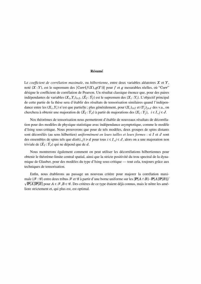
Résumé
Le coefficient de corrélation maximale, ou hilbertienne, entre deux variables aléatoires X et Y ,noté X : Y , est le supremum des |Corr( f (X ), g(Y ))| pour f et g mesurables réelles, où “Corr”désigne le coefficient de corrélation de Pearson. Un résultat classique énonce que, pour des pairesindépendantes de variables (X i,Yi)i∈I ,
→X I :
→YI est le supremum des X i : Yi. L’objectif principal
de cette partie de la thèse sera d’établir des résultats de tensorisation similaires quand l’indépen-dance entre les (X i,Yi) n’est que partielle ; plus généralement, pour (X i)i∈I et (Y j) j∈J des v.a., oncherchera à obtenir une majoration de
→X I :
→YJ à partir de majorations des X i : Y j, i ∈ I, j ∈ J.
Nos théorèmes de tensorisation nous permettront d’établir de nouveaux résultats de décorréla-tion pour des modèles de physique statistique avec indépendance asymptotique, comme le modèled’Ising sous-critique. Nous prouverons que pour de tels modèles, deux groupes de spins distantssont décorrélés (au sens hilbertien) uniformément en leurs tailles et leurs formes : si I et J sontdes ensembles de spins tels que dist(i, j) Ê d pour tous i ∈ I, j ∈ J, alors on a une majoration nontriviale de
→X I :
→YJ qui ne dépend que de d.
Nous montrerons également comment on peut utiliser les décorrélations hilbertiennes pourobtenir le théorème-limite central spatial, ainsi que la stricte positivité du trou spectral de la dyna-mique de Glauber, pour des modèles du type d’Ising sous-critique — tout cela, toujours grâce auxtechniques de tensorisation.
Enfin, nous établirons au passage un nouveau critère pour majorer la corrélation maxi-male F : G entre deux tribus F et G à partir d’une borne uniforme sur les |P[A∩B]−P[A]P[B]|/p
P[A]P[B] pour A ∈F ,B ∈G . Des critères de ce type étaient déjà connus, mais le nôtre les amé-liore strictement et, qui plus est, est optimal.
Contents
Introduction 78
0 Motivation 82
1 A first approach to Hilbertian correlations 89
2 Event sufficient conditions 101
3 Tensorization 117
4 Other applications of tensorization techniques 156
5 Concrete examples 169
Introduction
Overview of this part of the thesis
This part of my thesis is devoted to the study of Hilbertian correlations (also called “maxi-mal correlations” or “ρ-mixing coefficients”), in particular to showing how this concept can be‘tensorized’ to yield new results on systems of statistical mechanics exhibiting asymptotic inde-pendence. I have divided it into six chapters:
• The first chapter, numbered “0”, aims at motivating the study of Hilbertian correlations andtheir tensorization. In this chapter, I will recall some classical results on the subcriticalIsing model, which is a classical model showing asymptotic independence between pairs ofspins. When one gets interested in very large ‘bunches’ of spins, it is known that asymptoticindependence cannot be captured by β-mixing any more, but that, in certain cases at least, itstill holds in terms of ρ-mixing. The techniques used so far to establish ρ-mixing for bunchesof spins are strongly limited by technical assumptions looking somehow artificial, which willmotivate studying ρ-mixing ‘for itself’ and trying to tensorize it.
• In Chapter 1, I shall recall the definition of the Hilbertian correlation coefficient; I shall alsorecall some classical facts about this concept and give some examples. This chapter can beseen as a ‘crash course’ on ρ-mixing for the non-specialist reader: almost nothing in it isnew.
• In Chapter 2, I shall give some new criteria to bound the Hilbertian correlation betweentwo σ-algebras, which criteria assume bounds on the (P[A ∩B]−P[A]P[B]) for events Aand B belonging to these respective σ-algebras. My “strong event sufficient condition”,which improves previous results by several authors, shall even be shown to be optimal.
• Chapter 3 is the core of this work: in it I will handle tensorization of Hilbertian decorrela-tions. This chapter begins with a refined version of the concept of correlation, called “sub-jective correlation”, which is necessary to write the subsequent tensorization results. ThenI shall state and prove my three main tensorization theorems: Theorem 3.2.2 (‘N against 1’theorem) bounds the correlation between a ‘simple’ and a ‘vector’ variable; Theorem 3.3.1(‘N against M’ theorem) deals with correlation between two vector variables, and Theo-rem 3.3.10 (‘Z against Z’ theorem) refines the previous one in the case where certain sym-metries are present. Then, I will discuss some refinement and optimality statements aboutthese theorems; in § 3.9, I will also present a geometric corollary of tensorization resultswhich underlines quite well the Hilbertian aspect of maximal correlations.
• In Chapter 4, I will continue to use the tensorization techniques of Chapter 3, but that timeinstead of proving tensorization results stricto sensu I will turn to different types of results,namely the spatial central limit theorem and the presence of spectral gap for the Glauberdynamics.
• Finally, Chapter 5 will present some concrete applications of the results of this monograph.

Décorrélations hilbertiennes
For instance, I shall prove new results about decorrelation between distant bunches of spinsin Ising’s model (see Theorem 5.1.1); I will also give results of the same type for quitegeneral models of statistical mechanics (see e.g. Theorems 5.2.10 and 5.3.7), also provingspatial CLT and spectral gap for the Glauber dynamics for these models. I will also showhow tensorization of Hilbertian correlations can be used to get ‘hypocoercivity’ results [The-orem 5.4.6].
Conventions and notation
Notation will not always be perfectly rigorous: to make reading easier, it may occur sometimesthat formalism is slightly loose, or that some writing conventions or assumptions are implicit.However this shall only be done in situations where adding the missing information by the readeris (hopefully) obvious.
Here is some notation used throughout this text:
Miscellaneous• The symbol N denotes the set of nonnegative integers, including 0. The set of positive inte-
gers Nà 0 is denoted by N∗.• For a,b real numbers, a∧b denotes mina,b, resp. a∨b denotes maxa,b; a+ denotes the
positive part of a, i.e. a∨0.• For A a set, Ac denotes the complement set of A (the set of reference shall always be clear);
1A denotes the indicator function of A, that is, the function being 1 on A and 0 on Ac.• For A,B sets, A 4 B denotes the symmetric difference of A and B, i.e. (AàB)] (Bà A),
where “]” means the same as “∪”, but with underlining that the union is disjoint.• The identity matrix in dimension n will be denoted by In. The transpose of a matrix A will
be denoted by AT.• If Θ is a set endowed with a metric dist, then for I, J ⊂ Θ, dist(I, J) denotes the distance
between I and J, that is, dist(I, J) ··= infdist(i, j) : i ∈ I, j ∈ J.• As is customary in physical literature, ∝ means “proportional to”.• Whenever I is a set and X a symbol,
→X I will be a shorthand for “(X i)i∈I”.
Probability• We will always work on an implicit probability space (Ω,B) equipped with a probability
measure P. Sub-σ-algebras of B will be merely called “σ-algebras”; I will also often write“variable” for “random variable”. Unless explicitly specified, variables on Ω can be valuedin any set.
• If f is a real random variable, the expectation of f is denoted by E[ f ]; its variance is denotedby Var( f ); its standard deviation is denoted by Sd( f ) ··=
√Var( f ); if g is another real vari-
able, the covariance between f and g is denoted by Cov( f , g) ··=E[ f g]−E[ f ]E[g]. All thatnotation extends to the case where f and g are valued in some vector space RN , except thatin that case it refers to vectors or matrices.
• If B is an event with P[B]> 0, then P[A|B], E[ f |B], Var( f |B), . . . stand resp. for the proba-bility of A, the expectation of f , the variance of f , . . . under the conditional law dP[·|B] ··=1B dP[·]/P[B]. Similarly, if F is a σ-algebra, P[A|F ], E[ f |F ], . . . stand for the conditionalprobability of A, the conditional expectation of f , . . . w.r.t. F .
Quelques problèmes d’inspiration physique en théorie des probabilités
• Concerning conditional expectations, I will actually use two different conventions: for G aσ-algebra, E[ f |G ] can also be denoted by f G . Both conventions can be used inside the sameformula. [§] [¶]
• If X is a variable on Ω, the σ-algebra generated by X (that is, the smallest σ-algebra w.r.t.which X is measurable) is denoted by σ(X ). If F and G are σ-algebras, the σ-algebragenerated by F and G (that is, the smallest σ-algebra containing both F and G ) is denotedby F ∨G , and for an arbitrary number of σ-algebras this notation extends into the ∞-aryoperator
∨.
• An event A ∈B is said to have trivial probability, or to be trivial, if P[A] ∈ 0,1. A σ-algebrais said to be trivial if all its events are trivial. The σ-algebra ;,Ω, which is trivial under anylaw P, will be denoted by O and refered to as “the” trivial sigma-algebra.
• The Lebesgue measure on Rn will be denoted by dx, “x” being the name of the integrationvariable. For a Borel set A ⊂Rn,
∫x∈A dx will sometimes be denoted by |A|.
• For C a positive-semidefinite matrix (possibly of dimension 1, in which case it is identifiedwith σ2 ∈ R+), N (C) denotes the law of the centered Gaussian vector with covariance ma-trix C. I will write N (C)+m to denote the non-centered Gaussian vector with variance Cand mean m.
Functional analysis• Unless otherwise specified, all the functional spaces considered in this monograph shall be
real.• For I an open interval of R and k ∈N∪ ∞, C k
0 (I) denotes the subset of functions of C k(I)with compact support.
• If µ is a nonnegative measure on some measurable space (Ω,B), L2(µ) denotes the set ofmeasurable functions f (up to µ-a.e. equality) such that
∫Ω f (ω)2 dµ(ω)<∞. If I is a count-
able set, L2(I) denotes the set of functions f : I → R such that∑
i∈I f (i)2 < ∞. If F is aσ-algebra, L2(F ) denotes the space of F -measurable functions (up to a.s. equality) whichare square-integrable w.r.t. P. All these spaces are equipped with their natural Hilbertianproduct ⟨·,·⟩ and the associated norm ‖·‖.
• For µ a finite measure, in L2(µ) the constant functions make a line which can be identifiedwith R; then, L2(µ) will denote the quotient L2(µ)/R, equipped with its natural Hilbert struc-ture. In other words, if f ∈ L2(µ) is the projection of f ∈ L2(µ), ‖ f ‖L2 ··= inf‖ f − a‖L2 :a ∈R = (‖ f ‖2
L2 −⟨ f ,1/‖1‖⟩2L2)1/2. L2(µ) can also be seen as the subspace of centered func-tions of L2(µ), i.e. as f ∈ L2(µ) : ⟨ f ,1⟩ = 0; throughout the monograph we will implicitlyswitch between both interpretations.
• If L : H1 → H2 is a linear operator between two Hilbert spaces, then L∗ : H2 → H1 denotesthe adjoint operator of L, characterized by the relationship ⟨L∗y, x⟩H1 = ⟨y,Lx⟩H2 .
• If L : E → F is a linear operator between two Banach spaces (not necessarily Hilbert) withrespective norms ‖·‖E and ‖·‖F , the operator norm of f , denoted by f , is defined assup‖Lx‖F : ‖x‖E = 1.
• If L : E → E is a bounded linear operator on a Banach space, then ρ(L) denotes the spectralradius of f , that is, ρ(L) ··= limk→∞Lk1/k —this limit always exists.
[§]. The use of the first or the second convention will depend on the way we prefer to see the conditional expectationof f w.r.t. G : if it is rather seen as the expectation of f knowing the information of G , notation E[ f |G ] will be chosen,while if it is more seen like the G -measurable function best approximating f , we will use the notation f G .
[¶]. One must not confuse Var( f |G ), which is the variance of f under the law P[·|G ], with Var( f G ) which is the(unconditioned) variance of the random variable f G . One has the well-known identity Var( f )=Var( f G )+E[Var( f |G )],which I shall refer to as associativity of variance.

Décorrélations hilbertiennes
• A column vector (ai)i∈I will automatically be identified with the corresponding elementof L2(I). Likewise, a matrix A = ((ai j))(i, j)∈I×J will be identified with the correspondinglinear operator from L2(J) to L2(I).
• In our computations we will often use the Cauchy - Schwarz inequality and its variants [‖];when using such an inequality, we will indicate it by writing “CS” under the inequality signconcerned. Similarly, “IP” under an equality sign will mean that this equality follows fromintegrating by parts.
Acknowledgements
This work owes to many people’s help. First of all I must mention V. Beffara, who launched meon this topic incidentally. His relevant comments, as well of those of (among others) Y. Ollivier,C. Villani, Y. Velenik, T. Bodineau, C. Shalizi and R. Bradley, have also been the origin for severalimportant improvements of this monograph.
Several colleagues provided me with some help on mathematical topics I was not familiarwith. In particular, Y. Ollivier suggested to me the use of Lipschitz spaces to prove Lemma 2.2.13;S. Martineau pointed out how Gershgorin’s Lemma solved a technical point in the complete proofof Theorem 3.5.2; V. Calvez had the idea of using Laplace transform to prove Lemma 5.5.5. Overthe Internet, F. Martinelli and S. Shlosman also gave me precious bibliographic references on thestate of the art about weak and strong mixing in statistical mechanics.
Most of the drawings in this monograph were made thanks to the excellent LATEX extensionTikZ, combined with computations in C language. The dice of Figure 10 have been kindly drawnfor me by A. Alvarez, using POV-Ray.
[‖]. For instance, the discrete form |∑Ni=1 aibi| É (∑N
i=1 a2i )
1/2(∑Ni=1 b2
i )1/2, the probabilistic form |Cov[ f g]| É
Sd( f )Sd(g), etc..
Chapter 0
Motivation
0.1 Some results on Ising’s model
In this subsection we recall the definition of Ising’s model and give two classical results onit, namely Theorems 0.1.8 and 0.1.9. In § 0.2, considerations on these results will serve as amotivation to the work of this part of the thesis.
0.1.a Ising’s model
Ising’s celebrated model is a basic model of equilibrium thermodynamics, which represents aferromagnetic material:
0.1.1 Definition. For n an integer, consider the lattice Zn endowed with its usual graph structure(each vertex has 2n neighbours), and denote by dist the graph distance. Define Ω = ±1Z
n, and
for →ω ∈Ω, set formally:
H(→ω)=−1
2
∑dist(i, j)=1
ωiω j. (A)
Then, for T Ê 0, the Ising model on Zn at temperature T is, formally, a probability measure P onΩsuch that P[→
ω]∝ exp(−T−1H(→ω)). In rigorous terms, saying that P is an equilibrium measure for
Ising’s model means that for all i ∈Zn, for all→ωic ∈ ±1i
c,
P[ωi = ωi|→ωic =→ωic]∝ exp(T−1 ∑
dist(i, j)=1ωiω j). (B)
♦
Ising’s model and the phase transition it exhibits have been the subject of dozens of works;see [37] for an overview. Here we are interested in the subcritical regime:
0.1.2 Theorem (Subcritical regime, [61]). There is a Tc <∞ (the ‘Curie temperature’) such thatthe solution of (B) is unique for T > Tc . ♣
For T > Tc one says that they are in the subcritical regime. An interesting feature of thisregime is that for distant i and j, the random variables ωi and ω j are ‘almost independent’. Thatphenomenon, called exponential decay of correlations, is stated by the following theorem:
Décorrélations hilbertiennes
0.1.3 Theorem (Exponential decay of correlations, [2]). For Ising’s model on Zn in the subcriticalregime,
(i) For all i ∈Zn, P[ωi =−1]=P[ωi = 1]= 1/2.(ii) There exists ψ> 0 and C <∞ such that for all i, j ∈Zn,
|E[ωiω j]| É C exp(−ψdist(i, j)). (C)
♣
0.1.b Absence of β-mixing
Theorem 0.1.3 states that two distant spins i and j are exponentially decorrelated. However, itdoes not inform us about the dependence between ‘bunches’ of spins. The question is the following:if I and J are two disjoint, distant subsets of Zn, to what extent are →
ωI and →ωJ independent?
To answer such a question, the first thing to do is to define a way of measuring independencebetween ‘complicated’ variables having an arbitrarily large range like →
ωI and →ωJ . The most com-
mon choice is the β-mixing coefficient:
0.1.4 Definition.
1. Recall that for µ, ν two probability measures on the same measurable space (Ω,F ), the totalvariation distance between µ and ν is the total mass of both the positive and the negative partsof the signed measure ν−µ, that is, distTV(µ,ν)= supA⊂F |ν(A)−µ(A)|.
2. If X and Y are two random variables (with arbitrary ranges) defined on the same space, thenone defines the β-mixing coefficient between X and Y as
β(X ,Y ) ··= distTV(LawX ⊗LawY , Law(X ,Y )). (D)
♦
Notice that β(X ,Y ) actually only depends on the σ-algebras σ(X ) and σ(Y ) [11, For-mula (1.5)]. The following proposition is immediate:
0.1.5 Proposition.
(i) One has always β(X ,Y ) ∈ [0,1], and(ii) β(X ,Y )= 0 if and only if X and Y are independent ;
(iii) β(X ,Y )= 1 if and only if LawX ⊗LawY and Law(X ,Y ) are mutually disjoint.(iv) If X ′ is X -measurable and Y ′ is Y -measurable, then β(X ′,Y ′)Éβ(X ,Y ).
♣
So, β(X ,Y ) is a way of measuring ‘how much X and Y are correlated’.
With that tool at hand, decorrelation between bunches of spins in statistical physics modelshas already been thoroughly studied. Concerning Ising’s model, there are two well-known greatresults:
0.1.6 Theorem (Weak mixing property, [52]). For Ising’s model on Zn in the subcritical regime,there exists ψ> 0 and C <∞ (the same as in Theorem 0.1.3) such that for all disjoint I, J ⊂Zn:
β(→ωI , →
ωJ) É C∑
(i, j)∈I×Jexp(−ψdist(i, j)). (E)
♣
Quelques problèmes d’inspiration physique en théorie des probabilités
0.1.7 Theorem (Complete analyticity, [25]). There exists some Tc É T ′c < ∞ [∗] such that for T
> T ′c, Ising’s model is completely analytical, i.e. there exists ψ′ > 0 and C′ > 0 such that the follow-
ing holds: for all K ⊂ Zn, for all ‘boundary’ conditions→ωK ∈ ±1K , denoting P→
ωK··= P[·|→ωK =
→ωK ], Formula (E) holds with Law replaced by Law→
ωKand ψ,C replaced resp. by ψ′ and C′. ♣
Thanks to Theorem 0.1.6, we get an exponential decay of correlation between two bunches ofspins of fixed size when the distance between these bunches increases. However, we cannot saymuch about decorrelation between bunches of variable size which are at fixed distance from eachother. For instance, for n = 2 fix x > 0 and define I l ··= (0, y) : |y| É l, resp. Jl ··= (x, y) : |y| É l.Then Theorem 0.1.6 gives us something like:
β(→ωI l ,
→ωJl ). Cle−ψx. (F)
But recall that a β-mixing coefficient is always bounded by 1; so, for l & eψx/C, (F) tell us abso-lutely nothing about the decorrelation between I l and Jl .
Though the bound (E) is not completely optimal, the previous point is an intrinsic shortcomingof β-mixing coefficients, in the sense that it can be proved that bounds like (F) must become trivialwhen l →∞:
0.1.8 Theorem. For all Tc < T <∞, for all x > 0, denoting I ··= 0×Z and J ··= x×Z, one has
β(→ωI , →
ωJ)= 1. (G)
♣
Proof. Denote i0 ··= (0,0), resp. j0 ··= (x,0). As we told in Theorem 0.1.3-(i), E[ωi0],E[ω j0] = 0.Interpretation of Ising’s model as a random-cluster model [37, § 1.4] shows that P[ωi0 =ω j0]> 1/2,so we define
γ ··=E[ωi0ω j0]> 0. (H)
Now, let N be some large integer, fixed for the time being, let p be some large integer anddefine i1, . . . , iN , resp. j1, . . . , jN , by ik ··= (0,kp), resp. jk ··= (x,kp); denote by PN,p the joint lawof (ωi1 , . . . ,ωiN ,ω j1 , . . . ,ω jN ). By translation invariance, for each k, (ωik ,ω jk ) has the same law as(ωi0 ,ω j0), which law we denote by P1. Then when p →∞, by Theorem 0.1.6, PN,p tends to thelaw PN,∞ ··= P⊗N
1 . [†] In other words, PN,∞ is the law such that all the (ωik ,ω jk ) are independentwith PN,∞[ωik = η and ω jk = θ] = (1+γηθ)/4 for all k. Therefore, the value of β((ωik )k, (ω jk )k)under the law PN,p, which by Proposition 0.1.5-(iv) is a lower bound for β(→
ωI , →ωJ), tends to its
value under PN,∞ when p →∞. This is summed up by the following formula:
β(→ωI , →
ωJ)ÊβPN,∞((ωik )1ÉkÉN , (ω jk )1ÉkÉN). (I)
To end the proof, we will bound the right-hand side of (I) below by a quantity which tends to 1when N →∞. Denote by
~PN,∞ the product of two the marginals of PN,∞ relative resp. to the (ωik )k
and the (ω jk )k, so that βPN,∞((ωik )k, (ω jk )k)= distTV(PN,∞,~PN,∞) by the very definition of the β-
mixing coefficient. Obviously the expression of~PN,∞ is the same as the expression of
~PN,∞, but
[∗]. It is not known whether T′c = Tc today, but in general situations weak mixing does not always imply complete
analyticity. A classical counterexample is Ising’s model with external field [53, § 2].[†]. Note that PN,p takes its values in a space of finite dimension, so there is no ambiguity when speaking of its
convergence.
Décorrélations hilbertiennes
with γ replaced by 0 in the definition of PN,∞. Under PN,∞, (ωikω jk )1ÉkÉN is a sequence of i.i.d.random variables having a certain law with mean γ> γ/2, so that by the law of large numbers,
PN,∞[N−1
N∑k=1
ωikω jk Éγ
2
]N→∞→ 0. (J)
Similarly, since 0< γ/2,
PN,∞[N−1
N∑k=1
ωikω jk Éγ
2
]N→∞→ 1, (K)
so that
distTV(PN,∞,~PN,∞)Ê
∣∣∣ ~PN,∞
[N−1
N∑k=1
ωikω jk Éγ
2
]−PN,∞[the same]
∣∣∣ N→∞→ 1, (L)
which proves our point. ♠
0.1.c Presence of ρ-mixing
So, Theorem 0.1.8 tells us that, for Ising’s model on Z2, there is a ‘full’ correlation between →ωI
and →ωJ in the sense of β-mixing. Yet it is well known too that Theorem 0.1.6 nevertheless implies
a Hilbertian form of decorrelation (called “ρ-mixing”, cf. Remark 1.1.2) between these variables:
0.1.9 Theorem. For Ising’s model on Z2 in the subcritical regime, defining as before I = 0×Zand J = x×Z for some x > 0, one has for all f ∈ L2(→
ωI ) and g ∈ L2(→ωJ):
|E[ f g]| É e−ψx Sd( f )Sd(g), (M)
where ψ is the same as in Theorem 0.1.6. ♣
Proof. Define the operatorP : L2(→
ωI ) → L2(→ωJ)
f 7→ f σ(→ωJ ).(N)
(Recall that f σ(→ωJ ) is an alternative notation for E[ f |→ωJ], insisting on the its being a σ(→ωJ)-
measurable function). Then (M) is equivalent to proving that P É e−ψx (see § 1.1.c). Nowfor all t ∈ 0, . . . , x, denote ω(t) ··= →
ωt×Z, and for all t ∈ 1, . . . , x,
πt : L2(ω(t−1)) → L2(ω(t))f 7→ f σ(ω(t)).
(O)
Due to the fact that the interactions in Ising’s model have only range 1, ω(0) →ω(1) → ···→ω(x) isa Markov chain, and therefore
P =πx · · · π2 π1. (P)
Now, by horizontal translation all the L2(ω(t)) can be identified with a common Hilbert space H.Then all the πt are identified with operators on L2(H), and by the translation invariance of themodel all these operators are actually the same. P is also identified with an operator on L2(H), and(P) becomes:
P =πx. (Q)
But π is self-adjoint because, as the model is invariant by translation and by reflection, the Markovchain ω(0) → ··· → ω(x) is stationary and reversible. In particular π is a normal operator, and thus
Quelques problèmes d’inspiration physique en théorie des probabilités
P = πx. So, proving that P É e−ψx is equivalent to proving that π É e−ψ, which will beour new goal.
Take C <∞ like in Theorem 0.1.6. For l an integer, denote I l and Jl to be resp. 0×−l, . . . , land x×−l, . . . , l. Let f be a bounded [‡] function of L2(→
ωI l ) and denote M ··= ‖ f ‖L∞ . By transla-tion, f can also be identified with a function of L2(→
ωJl ), which is also bounded by M. Now, since
E[ f (→ωI l ) f (→
ωJl )]=Cov( f (→ωI l ) , f (→
ωJl ))=∫
f (→ωI l ) f (→
ωJl )d(Law(→ωI l]Jl )−Law(→
ωI l )⊗Law(→ωJl )),
(R)we can apply (E) to I l and Jl to obtain:
|E[ f (→ωI l ) f (→
ωJl )]| É M2 ·2C(2l+1)2e−ψx. (S)
In terms of operators, (S) means that
|⟨ f ,P f ⟩L2(H)|É 2(2l+1)2M2Ce−ψx. (T)
As the value of x played no particular role to establish (T), that formula can be generalized into
|⟨ f ,πt f ⟩L2(H)|É 2(2l+1)2M2Ce−ψt (U)
for all t ∈N∗. Letting t tend to infinity, we obtain that for all l, for all f ∈ L2(→ωI l )∩L∞,
limt→∞( log |⟨ f ,πt f ⟩|)1/t É e−ψ. (V)
But⋃
l∈N (L2(→ωI l )∩ L∞) is a dense subset of L2(→
ωI ), so by Lemma 0.3.1 set in appendix, weconclude that πL2(H) É e−ψ, which is what we wanted. ♠
0.1.10 Remark. Claim 0.1.8 and Theorem 0.1.9 adapt straighforwardly, with similar proofs, toany n Ê 2, replacing I by 0×Zn−1 and J by x×Zn−1. ♥
0.2 Problematics
Thanks to Theorem 0.1.9, we see that the Hilbertian concept of ρ-mixing can reveal someindependence between infinite bunches of lowly correlated variables in situations where the β-mixing coefficient does not show any independence at all. In the proof we gave, ρ-mixing appearedas a corollary of β-mixing for finite bunches of spins. What additional hypotheses did we need toget our corollary? We used at least the following:
• To introduce the Markov chain ω(0) → ··· →ω(x), we used that the interactions of our modelhad finite range.
• To identify all the spaces L2(ω(t)), we used that I and J had the same shape and that onecould tile up Z2 with a sequence of tiles having that shape (namely, here, tiles of the formt×Z).
• To say that all the πt were the same modulo that identification, we used the translation in-variance of the model.
• To state that the stationary Markov chain ω(0) →···→ω(x) was reversible, we used the reflec-tion invariance of the model.
[‡]. In fact here it is superfluous to impose that f is bounded since →ωI l can only take a finite number of values. I wrote
the proof like this just to underline that the finiteness of the range of the ωi does not play any role in the proof.

Décorrélations hilbertiennes
• To use Lemma 0.3.1, we used the exponential decay of correlations.All these points make the proof of Theorem 0.1.9 we gave in § 0.1 quite difficult to generalize.What, for instance, if we take I and J with arbitrary shapes, just requiring that dist(I, J) Ê x?What if we consider statistical physics models with infinite-range interactions? Etc.. The abovearguments would not work any more! Yet, we do not have the impression that the presence ofρ-mixing fundamentally relies on the peculiar symmetries of the case we treated. . .
So, here will be the goal of this work: establishing ρ-mixing estimates by general methods. Toachieve this goal, I shall try to concentrate on the properties of ρ-mixing ‘for itself’, rather thanon its links with other forms of decorrelation. I will carry out a thorough study of the ρ-mixingcoefficient, in order to get ρ-mixing results for ‘complicated’ variables from decorrelation results ofthe same type for more ‘basic’ variables; in other words, I will tensorize Hilbertian decorrelations.It turns out that tensorization for such correlation coefficients gives results which are quite robustas the size of the bunches of variables increases. Thanks to this method, I shall obtain fairly newdecorrelation theorems for various models of statistical physics.
This part of the thesis is intended to be complete in some sense. I mean, besides the core of thiswork—namely, tensorization results—, I have tried to answer several other questions which ap-peared natural to me concerning Hilbertian decorrelation. This includes studying many examples,finding sharp criteria for maximal decorrelation, looking at the optimality issues in the tensoriza-tion results or showing other applications of the tensorization techniques. Though these topics wereinitially thought as ‘sidework’, some of them may be quite interesting for themselves.
0.3 Appendix: On the norm of self-adjoint operators
In this appendix we prove the following
0.3.1 Lemma. Let L be a self-adjoint operator on a real Hilbert space H, and let C <∞. Then, toprove that LÉ C, it suffices to ensure that
x ∈ H : limk→∞
|⟨Lkx, x⟩|1/k É C (W)
is a dense subset of H. ♣
Proof. Reasoning by contraposition, we have to show that, for L a self-adjoint operator on H, forall C <L, the set of the x ∈ H such that
limk→∞
|⟨Lkx, x⟩|1/k > C (X)
contains a non-empty open subset of H.
Since L is self-adjoint, by the spectral theorem [85, Theorem 7.18], it is unitarily equivalentto the “multiplication by identity” operator M on a space
⊕α∈A L2(ρα), for A some set and ρα
some Radon measures on R, that is [in the following equation, the variable λ is free, so that f (λ) issynonymous with f ]:
M(∑α
fα(λ))=∑α
λ fα(λ). (Y)
So we will assume L is of that form.
Quelques problèmes d’inspiration physique en théorie des probabilités
One has obviously:
L= supλÊ 0 : (∃α ∈ A) (ρα([−λ,λ]c)> 0); (Z)
moreover, for all f ∈ H, f =∑α∈A fα with fα ∈ L2(ρα),
⟨Lk f , f ⟩ = ∑α∈A
∫Rλk| fα(λ)|2 dρα(λ), (AA)
so that (observing that, for k even, λk Ê 0 ∀λ)
limk→∞ |⟨Lk f , f ⟩|1/k = supλÊ 0 : (∃α ∈ A) (
∫[−λ,λ]c
| fα(λ′)|2 dρα(λ′)> 0). (AB)
Now, for C <L, the set
U = f ∈ H : (∃α ∈ A) (∫
[−C,C]c| fα(λ)|2 dρα(λ)> 0) (AC)
is open because∫
[−C,C]c | fα(λ)|2 dρα(λ) is a continuous function of f , and it is non-empty by (Z).But (X) is satisfied for all x ∈U by (AB), so U fulfills our quest. ♠
Chapter 1
A first approach to Hilbertiancorrelations
1.1 Definition and first properties
1.1.a Equivalent definitions
1.1.1 Definition. Let (Ω,B,P) be a probability space. For F ,G two sub-σ-algebras of B, theHilbertian correlation coefficient (or merely “correlation”) between F and G is defined as
F : G ··= supf ∈L2(F )à0g∈L2(G )à0
|E[ f g]|Sd( f )Sd(g)
. (AD)
If the supremum in (AD) is taken over an empty set, that is, if F or G is trivial, we define thissupremum to be 0. ♦1.1.2 Remark. F : G is often called the “maximal correlation coefficient” or “ρ-mixing coeffi-cient” between F and G , and denoted by ρ(F ,G ) (see [11]). ♥1.1.3 Remark. In other words, F : G is the best k ∈ R+ such that the following refined Cauchy–Schwarz inequality holds in the Hilbert space L2(B):
∀ f ∈ L2(F ) ∀g ∈ L2(G ) |⟨ f , g⟩| É k‖ f ‖‖g‖. (AE)
Yet another formulation is that F : G is the cosine of the angle between L2(F ) and L2(G ),seen as subspaces of L2(B) —this angle being defined as the infimum angle between any twonon-zero vectors of these respective subspaces.
If we speak in terms of L2 spaces rather than L2 spaces, F : G is the best k ∈R+ such that forall non-constant square-integrable f , g resp. F and G -measurable,
|Corr( f , g)| É k, (AF)
where Corr( f , g) ··=Cov( f , g) /Sd( f )Sd(g) is the Pearson correlation coefficient between f and g.♥
1.1.4 Definition. We say that F and G are ε-decorrelated, resp. ε-correlated, if F : G É ε, resp.F : G Ê ε. ♦

Quelques problèmes d’inspiration physique en théorie des probabilités
1.1.5 Definition. For X and Y random variables (with arbitrary ranges), we will denote X : Y for σ(X ) :σ(Y ). ♦1.1.6 Remark. One can rewrite Definition 1.1.5 as
X : Y = supf ,g
Cov( f (X ), g(Y ))Sd( f (X ))Sd(g(Y ))
, (AG)
where it is implied that f and g have to be measurable, real, and such that 0< Sd( f (X )),Sd(g(Y ))<∞. ♥
* More generally, all the questions relative to Hilbertian correlations may be handled eitherin terms of σ-algebras or in terms of random variables. In the sequel, we will frequently switchimplicitly between these two paradigms.
It is natural to enquire what happens if one deals with complex L2 spaces. In fact it does notchange anything:
1.1.7 Proposition ([86, Theorem 1.1]). Let F and G be two σ-algebras and let f , g be twocomplex centered L2 variables, measurable w.r.t. resp. F and G . Then, with Sd( f ) meaning√
E[| f −E[ f ]|2], one has:|E[ f g]| É F : G Sd( f )Sd(g). (AH)
♣
Proof. I recall the proof for the sake of completeness. Up to multiplying g by a well-chosen unitcomplex number, we can assume that E[ f g]∈R+. Then we can apply Definition 1.1.1 to the realL2 variables Re f and Re g, resp. Im f and Im g, getting:
|E[ f g]| =ReE[ f g]=E[Re f Re g]−E[Im f Im g]
É F : G (Sd(Re f )Sd(Re g)+Sd(Im f )Sd(Im g))ÉCS
F : G √
Var(Re f )+Var(Im f )√
Var(Re g)+Var(Im g)
= F : G Sd( f )Sd(g). (AI)
♠
Now we turn to a different way of seeing correlation levels.
1.1.8 Definition. For F ,G two σ-algebras, we denote by πGF the ‘projection’ operator
πGF : L2(F ) → L2(G )f 7→ f G .
(AJ)
For F , . . . ,Z σ-algebras, we denote πZ Y X ...GF ··=πZ Y πY X · · · πGF . ♦
With this vocabulary at hand,
1.1.9 Proposition. For F ,G two σ-algebras, F : G =πGF. ♣
Proof. πGF is the orthogonal projection from L2(F ) to L2(G ) in the Hilbert space L2(B), so itsnorm is the cosine of the angle between L2(F ) and L2(G ), i.e. F : G . ♠
1.1.10 Remark. One has πFG = π∗GF
, since ⟨πGF f , g⟩ = E[ f g] = ⟨ f ,πFG g⟩. Therefore the ex-pression πGF in Proposition 1.1.9 can be rewritten into
pπFGF, which is also ρ(πFGF )since πFGF is self-adjoint. ♥
Décorrélations hilbertiennes
1.1.b Immediate properties
Having defined Hilbertian correlations, it is now time to study their behaviour.
The following properties are immediate from Definition 1.1.1:
1.1.11 Proposition. For all σ-algebras F , G and G ′,
(i) G : F = F : G ;(ii) G ⊂G ′ ⇒ F : G É F : G ′;
(iii) F : G ∈ [0,1];(iv) F : G = 0 if and only if F and G are independent;(v) If F is not trivial, then F : F = 1.
♣
When one is concerned by correlation between variables, it often occurs that some of thesevariables are vector-valued. The following proposition means that it suffices to know the behaviourof finite-length vectors to understand the behaviour of all vectors:
1.1.12 Proposition. Let I, J be possibly infinite sets and let→X I ,
→YJ be vector-valued variables.
Then, denoting “I ′b I” to mean that I ′ is a finite subset of I,
→X I :
→YJ= sup
I ′bI,J′bJ
→X I ′ :
→YJ′. (AK)
♣
Proof. This is because⋃
I ′bI L2(→X I ′), resp.
⋃J′bJ L2(
→XJ′), is a dense subset of L2(
→X I ), resp.
L2(→YJ). That property follows by classical approximation arguments like in the proof of [73,
Theorem 3.14]. See [12, Theorem 3.16(II-3)] for a more detailed proof. ♠
1.1.c Operator interpretation
1.1.13 Proposition. If X →Y → Z is a Markov chain, then X : ZÉ X : Y Y : Z. ♣
Proof. The Markov chain property is equivalent to meaning that πZX = πZY X , so the result is aconsequence of the submultiplicativity of operator norms. See also [72, § VII-4]. ♠
There is a refined version of Proposition 1.1.13 which is particularly interesting for reversiblechains:
1.1.14 Proposition. If X →Y → Z is a Markov chain, then X : Z=√ρ(πY ZY πY XY ). ♣
Proof. Because of the Markov chain property, πX Z = πXY πY Z and πZX = πZY πY X . Usingthat for any pair of operators π : H1 → H2 and τ : H2 → H1 one has ρ(π τ) = ρ(τ π), we getthat X : Z2 = ρ(πXY ) = ρ(πXY ZY X ) = ρ(πXY πY ZY X ) = ρ(πY ZY X πXY ) = ρ(πY ZY πY XY ).
♠
1.1.15 Corollary. If · · · → X−1 → X0 → X1 → ··· is a stationary Markov chain so that πX1 X0
and πX0 X1 commute [∗], then for all k ∈Zà 0, X0 : Xk= X0 : X1|k|. ♣[∗]. Reversible chains always satisfy this condition since then πX1 X0 =πX0 X1 .
Quelques problèmes d’inspiration physique en théorie des probabilités
Proof. Since the chain is stationary, all the Xn have the same law and thus all the L2(Xn) can beidentified; then the stationarity property is equivalent to saying that πXn+1 Xn = πX1 X0 for all n ∈Z.Thanks to the commutation hypothesis, one can write for k > 0:
X0 : Xk=√ρ(πX0 Xk X0)=
√ρ(πk
X0 X1πk
X1 X0)=
√ρ(πk
X0 X1 X0)=
√ρ(πX0 X1 X0)k = X0 : X1k.
(AL)For the case k < 0, we use that X0 : Xk= X−k : X0. ♠
1.1.d First criteria for decorrelation
Density sufficient condition
1.1.16 Proposition. Let X and Y be two random variables valued resp. in E and F. Suppose thatLaw(X ,Y ) has a density h w.r.t. the product probability Law(X )⊗Law(Y ). Then:
X : Y É (∫
E×F(h−1)2 dLawX dLawY )1/2. (AM)
♣
1.1.17 Remark. The integral expression in (AM) is nothing but 2 times the bilinearized version ofthe mutual information
I(X ;Y ) ··=∫
E×Fh logh dLawX dLawY . (AN)
Yet Example 1.3.3 will show that one does not have X : Y Ép2(X ;Y )1/2 in general. ♥
Proof. To alleviate notation, denote resp. PX ,PY ,P(X ,Y ) for Law(X ),Law(Y ),Law(X ,Y ). Let fand g be centered L2 functions being resp. X - and Y -measurable. Observe first that∫
E×Ff (x)g(y)dPX [x]dPY [y]= (
∫E
f dPX)(∫
Fg dPY )= 0×0= 0, (AO)
so thatE[ f g]=
∫f g dP(X ,Y ) =
∫hf g dPX dPY =
∫(h−1) f g dPX dPY (AP)
and thus|E[ f g]| É (
∫(h−1)2 dPX dPY )1/2(
∫f 2 g2 dPX dPY )1/2 (AQ)
by the Cauchy–Schwarz inequality. But the last factor in the right-hand side of (AQ) is
(∫
f 2(x)g2(y)dPX [x]dPY [y])1/2 = (∫
f 2dPX)1/2(∫
g2dPY )1/2 =Sd( f )Sd(g), (AR)
so that (AM) is proved.
You may also see [14, Theorem 2.5] for an analogous result. ♠
Event necessary condition
1.1.18 Proposition (event necessary condition). Let F and G be two σ-algebras. If F : G É ε,then for all events A ∈F and B ∈G with respective probabilities p and q,
|P[A∩B]− pq|É ε√p(1− p)q(1− q). (AS)
Décorrélations hilbertiennes
In particular, if there exists two non-trivial events A ∈ F ,B ∈ G which are equivalent (in thesense that P[A 4B]= 0), then F : G = 1. [†] ♣
Proof. It follows from (AF) applied to 1A and 1B. ♠
1.1.e Independent tensorization
Now we are turning to the basic tensorization theorem, which will motivate § 3:
1.1.19 Theorem ([21, Theorem 6.2]). Let I be a set and let→X I ,
→YI be vectorial variables. Suppose
all the pairs (X i,Yi), i ∈ I, are independent, then
→X :
→Y = sup
i∈IX i : Yi. (AT)
♣
Proof. The simplest proof of Theorem 1.1.19 relies on the operator interpretation of correlations,see e.g. the proof of [87, Theorem 1]. Here however I shall give a proof based on decomposingfunctions of several variables into telescopic sums, for this kind of arguments will be used again inthe proofs of the more general tensorization theorems of § 3.
First, observe that the “Ê” inequality of (AT) is trivial, so we only have to prove the “É” in-equality. We denote εi ··= X i : Yi, and to alleviate notation, xi will implicitly stand for an elementin the range of X i, resp. yi for an element in the range of Yi.
By Proposition 1.1.12, we may assume that I is finite, say I = 1, . . . , N for some N ∈N. Let fand g be resp.
→X I-measurable and
→YI-measurable centered L2 real functions; our goal is to bound
above |E[ f g]|.For i ∈ 0, . . . , N, define Fi ··= ∨
jÉiσ(X j,Y j). I claim that, because of the independence hy-pothesis, f Fi only depends on the values of X1, . . . , X i and not on Y1, . . . ,Yi, and similarly that gFi
only depends on the values of Y1, . . . ,Yi: one can write indeed (in the case of f )
f Fi (x1, y1, . . . , xi, yi)=∫
f (x1, . . . , xi, xi+1, . . . , xn)dP[xi+1, . . . , xn|x1, y1, . . . , xi, yi]
=∫
f (x1, . . . , xi, xi+1, . . . , xn)dP[xi+1, . . . , xn]. (AU)
Now, for i ∈ 1, . . . , N, define
f i(x1, . . . , xi) ··= f Fi (x1, . . . , xi)−E[ f |x1, . . . , xi−1], (AV)
with a similar definition for g. One has f =∑i f i, resp. g =∑
i g i, and f i and g i are Fi-measurableand centered w.r.t. Fi−1 (that is, E[ f i|Fi−1],E[g i|Fi−1]≡ 0), so
Var f =∑i
Var f i, (AW)
[†]. The converse is not true: it can occur that F : G = 1 but that no non-trivial events of F and G are equivalent.A counterexample is the following: let (Xn)n∈N be independent Bernoulli(1/2) variables, and define independentlyYn = 1−Xn with probability εn and Yn = Xn otherwise, where (εn)n∈N is a sequence of numbers such that 0< εn É 1/2for all n and εn
n→∞→ 0. Then the vectorial variables→X and
→Y obviously satisfy
→X :
→Y = 1, yet it is not hard to prove
that no→X -measurable non-trivial event is equivalent to a
→Y -measurable one.
Quelques problèmes d’inspiration physique en théorie des probabilités
resp. Var g =∑i Var g i.
We expand:E[ f g]= ∑
(i, j)∈I×IE[ f i g j]. (AX)
In the right-hand side of (AX), if i 6= j then E[ f i g j] = 0 since if, say, i < j, f i is Fi-measurablewhile g j is centered w.r.t. F j−1 ⊃Fi. So (AX) turns into:
E[ f g]= ∑i∈I
E[ f i g i]. (AY)
Writing the law of total expectation,
E[ f i g i]=∫
E[ f i g i|x1, y1, . . . , xi−1, yi−1]dP[x1, y1, . . . , xi−1, yi−1]. (AZ)
But, as we noticed before, under P[·|x1, y1, . . . , xi−1, yi−1], f i only depends on X i and g i onlydepends on Yi. Moreover, because of the independence property, the law of (X i,Yi) is the sameunder P[·|x1, y1, . . . , xi−1, yi−1] as under P, so under P[·|x1, y1, . . . , xi−1, yi−1], f i and g i are cen-tered and εi-independent. Thus
|E[ f i g i]| É εi
∫Sd( f i|x1, y1, . . . , xi−1, yi−1)Sd(g i|x1, y1, . . . , xi−1, yi−1)dP[x1, y1, . . . , xi−1, yi−1]
ÉCSεi
√∫Var( f i|x1, y1, . . . , xi−1, yi−1)dP[x1, y1, . . . , xi−1, yi−1]
√the same for g
É εi Sd( f i)Sd(g i) [‡]. (BA)
Summing over i,
|E[ f g]| É ∑i∈Iεi Sd( f i)Sd(g i)É sup
i∈Iεi ·
∑i∈I
Sd( f i)Sd(g i)
ÉCS
supi∈I
εi ·√∑
i∈IVar( f i)
√∑i∈I
Var(g i)= supi∈I
εi ·Sd( f )Sd(g), (BB)
which is the desired bound. ♠
1.2 Examples
1.2.a Finite-ranged variables
1.2.1 Proposition. Let X and Y be random variables with finite ranges resp. 1, . . . , Nand 1, . . . , M, and denote pa ··= P[X = a], pb ··= P[Y = b], pb
a ··= P[X = a and Y = b]. ThenX : Y =Π, where Π is the N ×M matrix with general entry
Πab =pb
a − pa pb√pa pb
. (BC)
♣[‡]. The last inequality is actually an equality, because f i and g i are centered w.r.t. Fi−1.
Décorrélations hilbertiennes
1.2.2 Remark. In particular, if both X and Y have range 1,2, using the same notation as before,one has
X : Y = |pba − pa pb|√p1 p2 p1 p2
, (BD)
where the right-hand side of (BD) does not depend on the choice of a,b ∈ 1,2. ♥
Proof of Proposition 1.2.1. By Proposition 1.1.9, X : Y is the norm of the operator πXY :L2(Y ) → L2(X ). Here it will be more convenient to work in L2 spaces than in L2 spaces, sowe rather compute the norm of
~π : L2(Y ) → L2(X )
g 7→ gX −E[g],(BE)
which is obviously the same as πXY.
A function g ∈ L2(Y ) can be identified with a M-dimensional vector also denoted by g, andsimilarly ~
πg ∈ L2(X ) can be identified with a N-dimensional vector. Denote P ··= ((pba))a,b ∈RN×M ,
IX ··= ((δaa′ pa))a,a′ ∈ RN×N , IY ··= ((δbb′ pb))b,b′ ∈ RM×M , 1N ··= 11,...,N ∈ RN . Applying Bayes’formula yields that
~πg = I−1
X P g − 1N (1N )T P g. (BF)
Now, ‖g‖L2(Y ) = ‖I1/2Y g‖, resp. ‖~
πg‖L2(X ) = ‖I1/2X (~πg)‖, so:
X : Y = supg 6=0
‖( I−1/2X P − I1/2
X 1N (1N )T P ) g‖‖ I1/2
Y g‖ . (BG)
Performing the change of variables h = I1/2Y g, (BG) becomes X : Y = suph 6=0 ‖Πh‖ / ‖h‖ = Π,
withΠ= I−1/2
X P I−1/2Y − I1/2
X 1N (1N )T P I−1/2Y , (BH)
which is Equation (BC) indeed. ♠
1.2.3 Remark. With the same kind of proof, there is even a similar proposition to calculate X ,Y if either X or Y has finite range, provided you know (in the case it is X which has finite range) allthe P[X = x] and all the ∫
y
dP[Y = y|X = x]dP[Y = y|X = x′]dP[Y = y]
. (BI)
♥1.2.4 Remark. In the case X or Y has range of cardinality 2, applying Proposition (1.2.1) yieldsthat X : Y 2 depends smoothly on Law(X ,Y ). Yet this is not the case in general: in fact, maximalcorrelations are nothing more than a particular case of operator norms (cf. § 1.1.c), and thus theyhave the same behaviour—they are a continuous function of the parameters, but they can have someC 1 singularity. The following example exhibits such a singularity. ♥1.2.5 Example. Suppose both X and Y have range 1,2,3 and
((P[X = a and Y = b]))a,b =
2/9 1/18 1/181/18 2/9+α 1/18−α1/18 1/18−α 2/9+α
(BJ)
Quelques problèmes d’inspiration physique en théorie des probabilités
for a parameter α ∈ [−2/9,1/18]. Then the matrix Π defined by (BC) is
Π=
1/3 −1/6 −1/6−1/6 1/3+3α −1/6−3α−1/6 −1/6−3α 1/3+3α
=U
1/2+6α 0 00 1/2 00 0 0
U−1, (BK)
with
U =
0 −2/p
6 1/p
31/p
2 1/p
6 1/p
3−1/
p2 1/
p6 1/
p3
(BL)
being orthogonal. So by Proposition 1.2.1, X : Y = 1/2+6α+. ♥
1.2.b Gaussian variables
The following theorem, which I will frequently use in the sequel, computes exactly the Hilber-tian correlation between two jointly Gaussian variables:
1.2.6 Theorem ([46, 45]). Let (→X ,
→Y ) be an (N +M)-dimensional Gaussian vector whose covari-
ance matrix writes blockwise
Var(→X ,
→Y )=
(IN CCT IM
), (BM)
then →X :
→Y =C. ♣
1.2.7 Remark. In other words, Theorem 1.2.6 tells that in the Gaussian case, the supremum in (AG)defining
→X :
→Y can be restricted to linear functions f and g. ♥
1.2.8 Remark. By a linear change of variables, Theorem 1.2.6 actually allows us to compute →X :
→Y
for any Gaussian vector (→X ,
→Y ). ♥
Proof of Theorem 1.2.6. I recall a (sketch of) proof for the sake of completeness. By the prop-erties of Gaussian vectors, the law of Y knowing that X = x [I dropped the vector arrows] is thenormal law N (IM −CTC)+CTx, and similarly the law of X knowing that Y = y is the normallaw N (IN −CCT)+Cy. Consequently, the operator πXY X is the generator of the following ran-dom walk on RN (whose equilibrium measure is the standard Gaussian law): when one is at x, theyjump to a point distributed according to the normal law N (IN −CCTCCT)+CCTx. This walkis a multidimensional AR(1)-process (see. [63, § 2.6]), whose properties are perfectly known; inparticular, the eigenvalue f of πXY X responsible for its spectral radius will be a linear function,so we only have to consider linear f in the supremum (AG). For such f , the optimal g will also belinear by the Gaussian nature of the system, so in the end
→X :
→Y is equal to C. ♠
1.2.c Miscellaneous examples
Random conditional laws
1.2.9 Example. Let 0 < p < n be integers. We consider a random variable (X ,Y ) for which Y hasrange Y ··= 1, . . . ,n and X has range X ··=Pp(Y ), Pp(Y ) denoting the set of subsets y⊂Y withcardinality p —so, #X = (n
p)
and #Y = n —, and we take the law of (X ,Y ) uniform on the pairs(x, y) such that y ∈ x: see Figure 3.

Décorrélations hilbertiennes
X
Y
Figure 3: Schematic representation of Example 1.2.9 for n = 5 and p = 2.
When considered as operators on L2 spaces, it is obvious that πXY and πY X are characterizedby (πXY f )(x)= p−1 ∑
y∈x f (y), resp. (πY X g)(y)= (n−1p−1
)−1 ∑y∈x g(x), so that
(πY XY f )(y)= 1p
f (y)+ ∑y′ 6=y
p−1p(n−1)
f (y′). (BN)
Thus, on L2(Y ), πY XY is nothing but the scalar operator n−pp(n−1)I, and therefore
X : Y =√
n− pp(n−1)
(BO)
by Proposition 1.1.9 and Remark 1.1.10. ♥
Weakly coupled particles
1.2.10 Proposition. Let V1 and V2 be potentials on Rn, n Ê 1, i.e. the Vi are real-valued measur-able functions on Rn with
∫Rn e−Vi(x) dx <∞. For i ∈ 1,2, denote by Pi the probability measure
on Rn proportional to e−Vi(x)dx, which is to be thought as the law of the position X i of a particle isubjected to the potential Vi. Denote P⊗ ··= P1⊗P2, which is the joint law of (X1, X2) in absenceof interaction.
Now let W be an interaction potential on (Rn)2 such that e−[V1(x1)+V2(x2)+W(x1, x2)] is inte-grable; denote by P the probability measure on (Rn)2 proportional to e−[V1+V2+W] dx1dx2, whichis the joint law of (X1, X2) in presence of interaction potential W .
Then, under the law P,
X1 : X2É Sd⊗(e−W )E⊗[e−W ]
. (BP)
♣
Proof. The law P has density h = e−W /E⊗[e−W ] w.r.t. P⊗, whence the result by Proposition 1.1.16.♠
1.2.11 Remark. Proposition 1.2.10 gives a rigorous sense to the intuition that two weakly cou-pled particles must have nearly independent positions. This is valid in a quite general setting, inparticular, W does not have to be bounded. ♥
Quelques problèmes d’inspiration physique en théorie des probabilités
Non-reversible Markov chain1.2.12 Example. Here is a example showing that the inequality in Proposition 1.1.13 is strict ingeneral. Consider the stationary Markov chain on 1,2,3 defined by
P = ((P[Xk+1 = a|Xk = b]))ab =
0 1/2 11 0 00 1/2 0
, (BQ)
which has equilibrium measure (2/5,2/5,1/5). Diagonalizing P shows that
P t =
2/5 2/5 2/52/5 2/5 2/51/5 1/5 1/5
+O(2−t/2), (BR)
whence Xk : Xk+t = O(2−t/2) when t →+∞ by Proposition 1.2.1. Yet Xk : Xk+1 = 1, since thenon-trivial events Xk = 1 and Xk+1 = 2 are equivalent (cf. Proposition 1.1.18). ♥
Hyperplanes in Ising’s model As I told in Chapter 0, the initial motivation of this work wasto understand the presence of ρ-mixing in Ising’s model (cf. § 0.1.a); in particular, I intended tore-get a result similar to Theorem 0.1.9 by a more ‘natural’ method. That shall be achieved indeedin § 5.1:
1.2.13 Theorem (Theorem 5.1.1-(i)). For Ising’s model on Zn in the completely analytical regime,for all disjoint I, J ⊂Zn,
→ωI : →
ωJÉ exp[− (ψ′+ o(1))dist(I, J)], (BS)
where ψ′ is the same as in Theorem 0.1.7 and where the “o(1)” (to be understood “as dist(I, J)→∞”) is uniform in I, J. ♣
If we apply that result to the case of parallel ‘hyperplanes’ of Zn (I mean, sets of the formt×Zn−1), Formula (BS) looks far less neat than Formula (M) in Theorem 0.1.9.
That bound can however be improved by using Proposition 1.1.14. Indeed, as we noticed in§ 0.1.c, the states of two parallel hyperplanes are elements of some reversible stationary Markovchain. Therefore, applying Corollary 1.1.15 (in which we let k → ∞), we get a result exactlysimilar to (M), except that we have to replace ψ by ψ′ —recall that it is not known whether ψ′ =ψ.
1.3 Comparing ρ-mixing to other measures of dependence
The material of this section is classical; most of it can be found for instance in [12, §§ 3 & 5].Here we will say that a sequence of pairs of σ-algebras (F n,G n) is ρ-mixing to mean that F n : G nn→∞→ 0.
1.3.a α-mixing
1.3.1 Definition. The α-mixing coefficient of two σ-algebras F and G is
α(F ,G ) ··= supA∈AB∈B
|P[A∩B]−P[A]P[B]|. (BT)
♦
Décorrélations hilbertiennes
Proposition 1.1.18 shows that ‘ρ-mixing implies α-mixing’, in the sense that one has α(F ,G )ÉA(F : G ) for some universal function A : [0,1]→ [0,1] with A(ρ)
ρ→0→ 0.
1.3.2 Remark. Saying that the correlation of two variables tends to 0 means that their joint lawtends in some sense to the product law. When the variables are ranged in Polish spaces, a commonnotion of convergence is weak convergence, that is, convergence against all bounded continuousfunction. [4, Theorem 2.2] states that weak convergence is implied by α-mixing, hence by ρ-mixing. The precise statement is the following: if (X n,Y n)n∈N is a sequence of pairs of randomvariables such that all the Xn (resp. Yn) have the same law Law(X ) (resp. Law(Y )) in some Polishspace E (resp. F), then (α(X n,Y n) n→∞→ 0) ⇒ (Law(X n,Y n) n→∞
* Law(X )⊗Law(Y )). ♥
On the other hand, the following example shows that α-mixing does not imply ρ-mixing:
1.3.3 Example. For ε ∈ (0,1/2], define (X ε,Y ε) in the following way:• With probability ε, one samples X ε and Y ε independently with common law uniform
on [0,ε];• With probability (1−ε), one samples X ε and Y ε independently with common law uniform
on [ε,1].Then for all ε > 0 one has X ε : Y ε = 1, since the non-trivial events X ε É ε and Y ε É ε areequivalent (cf. Proposition 1.1.18). However it is easy to show that α(X ε,Y ε)= ε−ε2 ε→0→ 0. ♥
1.3.b β-mixing
Recall the definition of the β-mixing coefficient from the previous chapter [Definition 0.1.4].
1.3.4 Example. For ε ∈ (0,1), consider two random sequences (X i)i∈N and (Yi)i∈N defined in thefollowing way: (X i)i∈N is a sequence of i.i.d. variables with uniform law on ±1, and for each i ∈N, independently, one sets Yi = X i with probability ε, and with probability (1−ε) one chooses Yi
uniformly on ±1. Then all the (X i,Yi) are i.i.d. with P[X i = η and Yi = θ] = (1+ηθε)/4 forall η,θ ∈ ±1, thus X i : Yi = ε by Remark 1.2.2, whence
→X :
→Y = ε by Theorem 1.1.19. Yet
Law(→X ,
→Y ) and Law(
→X )⊗Law(
→Y ) are mutually singular for all ε> 0.
This shows that ρ-mixing does not imply β-mixing, and a fortiori that there can be no kind ofconverse to Proposition 1.1.16. ♥
1.3.c Mutual information
Recall the definition (AN) of mutual information. [12, Theorem 5.3(III)] states that mutualinformation controls the β-mixing coefficient, so Example 1.3.4, which shows that ρ-mixing doesnot imply β-mixing in general, shows that it does not imply mutual information to tend to 0 either.
Proposition 1.1.16 suggests that, on the other hand, maximal correlation could be controlled bymutual information, but that is not true either: in Example 1.3.3 indeed, X ε : Y ε= 1 for all ε> 0,but
I(X ε;Y ε)= ε log(ε−1)+ (1−ε) log((1−ε)−1) ε→0→ 0. (BU)
Mutual information measures the quantity of information shared by two random variables,which explains intuitively the following property ([20, Theorem 2.5.2]): if X →Y → Z is a Markovchain, then I(Y ; X , Z) É I(X ;Y )+ I(Y ; Z). Does a similar inequality hold for Hilbertian correla-
Quelques problèmes d’inspiration physique en théorie des probabilités
tion? In the Gaussian case, the answer is “yes” thanks to Theorem 1.2.6: one gets that
Y : X , Z2 É (1− Y : Z2) X : Y 2 + (1− X : Y 2) Y : Z2
1− X : Y 2Y : Z2É X : Y 2 + Y : Z2. (BV)
But that property does not hold in general, as the following example shows:
1.3.5 Example. Consider a Markov chain X →Y → Z, where (Y , X ) and (Y , Z) have the same law,which is the joint law described in Example 1.2.9—the role of “Y ” in that example being playedhere by Y in both cases. Fix y ∈Y ; define event A as “Y = y” and event B as “y ∈ X ∩Z”. Thenone computes that P[A]= n−1, while
P[B]= 1n+ (p−1)2
n(n−1). (BW)
Since A ⊂ B, Proposition 1.1.18 then yields that
Y : X , ZÊ√
P[Bc]P[A] /P[Ac]P[B]=(
(n−1)2 − (p−1)2
(n−1)2 + (n−1)(p−1)2
)1/2
. (BX)
Comparing (BO) and (BX), one sees that taking n À 1 and 1 ¿ p ¿ n1/2 makes X : Y and Y : Z arbitrarily close to 0 while Y : X , Z gets arbitrarily close to 1. ♥1.3.6 Remark. There are similar examples with (X ,Y , Z) = (Y−1,Y0,Y1) for a reversible Markovprocess (Yt)t∈R [64]. ♥
Chapter 2
Event sufficient conditions
In § 1.1.d we saw that the maximal correlation coefficient F : G controls the difference be-tween P[A ∩B] and P[A]P[B] for A and B two events resp. F - and G -measurable. A naturalquestion is whether the converse is true, i.e. whether saying that P[A∩B] is always close in somesense to P[A]P[B] implies a control on F : G . We saw in § 1.3.a that α-mixing does not fit, butmaybe stronger conditions of the same type would work.
In § 2.1 I will present a simple such condition (Theorem 2.1.3). This condition demands|P[A∩B]−P[A]P[B]| to be bounded uniformly by ζ(P[A])θ(P[B]) for functions ζ,θ : [0,1]→R+sufficiently well behaved. This result, whose proof is rather simple, is apparently new.
Proposition 1.1.18, however, suggests that the natural condition on events would be a uniformcontrol on |P[A∩B]−P[A]P[B]| /pP[Ac]P[A]
pP[Bc]P[B], which is out of the scope of The-
orem 2.1.3. Bradley [9] proved in 1983 that that condition was indeed sufficient to get ρ-mixing.His result was improved in the next few years (see for instance the bound of [15]), but the optimalbound was remaining unknown, though its value was being conjectured. In § 2.2, I shall prove thisoptimal bound. My method, different from the techniques of [9, 15], relies on the analysis of thespectral properties of an operator linked to a law which I call the “Chogosov law”, whose study isproceeded to in § 2.2.b.
2.1 Weak event sufficient condition
To state our next result we need some functional analysis reminders first:
2.1.1 Definition. On the space C ∞0 (0,1) of compactly supported fuctions of C ∞(0,1), one defines
the scalar product
⟨ϕ,ψ⟩H10=
∫ 1
0ϕ′(x)ψ′(x)dx. (BY)
C ∞0 (0,1) endowed with ⟨·,·⟩H1
0is a pre-Hilbert space; its completion is denoted by H1
0(0,1). ♦
Recall that elements of H10(0,1) may be seen as ordinary functions:
2.1.2 Lemma (Sobolev, [1, Theorem 4.12]). Any element f ∈ H10(0,1) can be identified with a
unique function f ∈ C 00 [0,1], the space of continuous functions on [0,1] with f (0), f (1) = 0. Con-

Quelques problèmes d’inspiration physique en théorie des probabilités
versely, a function f ∈C 00 [0,1] corresponds to an element of H1
0(0,1) if and only if
supg∈C ∞
0 (0,1)
|∫ 10 f (x)g′′(x)dx|√∫ 1
0 g′(x)2dx(BZ)
is finite, and then there is a unique f ∈ H10(0,1) associated to f , whose norm is (BZ). ♣
In accordance with Lemma 2.1.2, we will identify functions of C 00 [0,1] with elements
of H10(0,1) whenever it is possible. If f ∈C 0
0 [0,1] does not correspond to an element of H10(0,1),
then we will set ‖ f ‖H10=+∞.
Now we can state the
2.1.3 Theorem (Weak event sufficient condition). Let F and G be two σ-algebras such that, forall A ∈F and B ∈G with respective probabilities p and q,
P[A∩B]− pq É ζ(p)θ(q) [∗] (CA)
for some ζ,θ ∈C 00 [0,1]. Then:
F : G É ‖ζ‖H10‖θ‖H1
0. (CB)
♣
Proof. We begin with the following formula for covariance:
2.1.4 Lemma. For f and g two real L2 functions,
Cov( f , g)=∫R×R
(P[ f É x and g É y]−P[ f É x]P[g É y])dxdy. (CC)
♣
Proof of Lemma 2.1.4. Suppose in a first time that f and g are nonnegative. A classical Fubiniargument (see [5, Problem 21.6]) shows that
E[ f ]=∫R+
P[ f > x]dx, (CD)
with a similar formula for g. By the same method,
E[ f g]=∫R+×R+
P[ f > x and g > y]dxdy, (CE)
so that, using the computational formula Cov( f , g)=E[ f g]−E[ f ]E[g],
Cov( f , g)=∫R+×R+
(P[ f > x and g > y]−P[ f > x]P[g > y])dxdy. (CF)
Observing that the integrand is also (P[ f É x and g É y]−P[ f É x]P[g É y]) and that it is zerofor (x, y) ∉ R+×R+, we get (CC) in the nonnegative case. By translation invariance, the formularemains true for all f , g bounded below, and then by approximation for all f , g ∈ L2. ♠
[∗]. Note that there is no need to put absolute values in the left-hand side of (CA).
Décorrélations hilbertiennes
Now, let f and g be L2 variables resp. F - and G -mesurable, and denote by F and G therespective distribution functions of f and g. Up to a slight perturbation, F and G may be supposedto be diffeomorphisms from R onto (0,1); denote by α and β their respective inverse maps. Then achange of variables in (CC) yields:
Cov( f , g)=∫
(0,1)2(P[ f Éα(p) and g Éβ(q)]− pq)α′(p)β′(q)dpdq, (CG)
so by assumption (CA):
Cov( f , g)É (∫ 1
0ζ(p)α′(p)dp)×(
∫ 1
0θ(q)β′(q)dq). (CH)
Then our theorem becomes equivalent to the claim stated and proved just below. ♠
2.1.5 Claim. If f is a random variable whose repartition function F is a diffeomorphism of in-verse α, then for ζ ∈C 0
0 [0,1]:
|∫ 1
0ζ(p)α′(p)dp|É ‖ζ‖H1
0Sd( f ). (CI)
♣
Proof. First note that, replacing g by f in (CG), one has:
Var( f )=∫
(0,1)2[p(1− q)∧ q(1− p)]α′(p)α′(q)dpdq. (CJ)
In fact, one can define a scalar product [†] ⟨·,·⟩V on C 0(0,1) by setting
⟨ϕ,ψ⟩V =∫
(0,1)2[p(1− q)∧ q(1− p)]ϕ(p)ψ(q)dpdq, (CK)
so that if α is the inverse distribution fuction of a variable f , Var( f )= ‖α′‖2V .
So, we are considering three scalar products on some subspaces of C 0(0,1): the ordinary L2
product, which we denote by ⟨·,·⟩L2 , the H10(0,1) product ⟨·,·⟩H1
0and the variance product ⟨·,·⟩V .
Our goal is to show that for all ϕ ∈ H10(0,1),ψ ∈C 0(0,1),
|⟨ϕ,ψ⟩L2|É ‖ϕ‖H10‖ψ‖V . (CL)
By approximation we can suppose that ϕ ∈C ∞0 (0,1). A direct computation shows that
⟨ϕ,ψ⟩V = ⟨Lϕ,ψ⟩L2 , (CM)
where the operator L : C ∞0 (0,1)→C 2(0,1) is defined by:
(Lϕ)(x)= x∫ x
0(1− y)ϕ(y)dy+ (1− x)
∫ 1
xyϕ(y)dy. (CN)
But we can make L appear thanks to the following formula: for ϕ ∈C 20 (0,1),
ϕ= L(−ϕ′′), (CO)
as one checks by integrating by parts twice. So,
|⟨ϕ,ψ⟩L2|= |⟨L(−ϕ′′),ψ⟩L2|= |⟨−ϕ′′,ψ⟩V | ÉCS
‖ϕ′′‖V‖ψ‖V , (CP)
where‖ϕ′′‖2
V = ⟨ϕ′′,ϕ′′⟩V = ⟨Lϕ′′,ϕ′′⟩L2 =−⟨ϕ,ϕ′′⟩L2 =IP‖ϕ′‖2
L2 = ‖ϕ‖2H1
0, (CQ)
whence (CL). ♠[†]. The positivity of ⟨·,·⟩V follows from the identity ⟨ϕ,ϕ⟩V = ∫
p<q (∫ q
p ϕ(r)dr)2 dpdq.
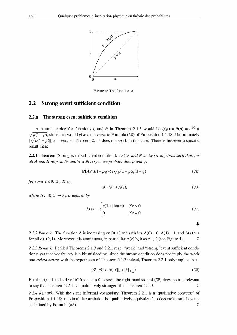
Quelques problèmes d’inspiration physique en théorie des probabilités
0 x 10
y
1
y=Λ(x)
y=x
Figure 4: The function Λ.
2.2 Strong event sufficient condition
2.2.a The strong event sufficient condition
A natural choice for functions ζ and θ in Theorem 2.1.3 would be ζ(p) = θ(p) = ε1/2 ×√p(1− p), since that would give a converse to Formula (AS) of Proposition 1.1.18. Unfortunately
‖√p(1− p)‖H10= +∞, so Theorem 2.1.3 does not work in this case. There is however a specific
result then:
2.2.1 Theorem (Strong event sufficient condition). Let F and G be two σ-algebras such that, forall A and B resp. in F and G with respective probabilities p and q,
P[A∩B]− pq É ε√
p(1− p)q(1− q) (CR)
for some ε ∈ [0,1]. ThenF : G ÉΛ(ε), (CS)
where Λ : [0,1]→R+ is defined by
Λ(ε) ··=ε(1+| logε|) if ε> 0,
0 if ε= 0.(CT)
♣
2.2.2 Remark. The function Λ is increasing on [0,1] and satisfies Λ(0) = 0, Λ(1) = 1, and Λ(ε) > ε
for all ε ∈ (0,1). Moreover it is continuous, in particular Λ(ε) 0 as ε 0 (see Figure 4). ♥
2.2.3 Remark. I called Theorems 2.1.3 and 2.2.1 resp. “weak” and “strong” event sufficient condi-tions; yet that vocabulary is a bit misleading, since the strong condition does not imply the weakone stricto sensu: with the hypotheses of Theorem 2.1.3 indeed, Theorem 2.2.1 only implies that
F : G ÉΛ(‖ζ‖H10‖θ‖H1
0). (CU)
But the right-hand side of (CU) tends to 0 as soon the right-hand side of (CB) does, so it is relevantto say that Theorem 2.2.1 is ‘qualitatively stronger’ than Theorem 2.1.3. ♥2.2.4 Remark. With the same informal vocabulary, Theorem 2.2.1 is a ‘qualitative converse’ ofProposition 1.1.18: maximal decorrelation is ‘qualitatively equivalent’ to decorrelation of eventsas defined by Formula (AS). ♥
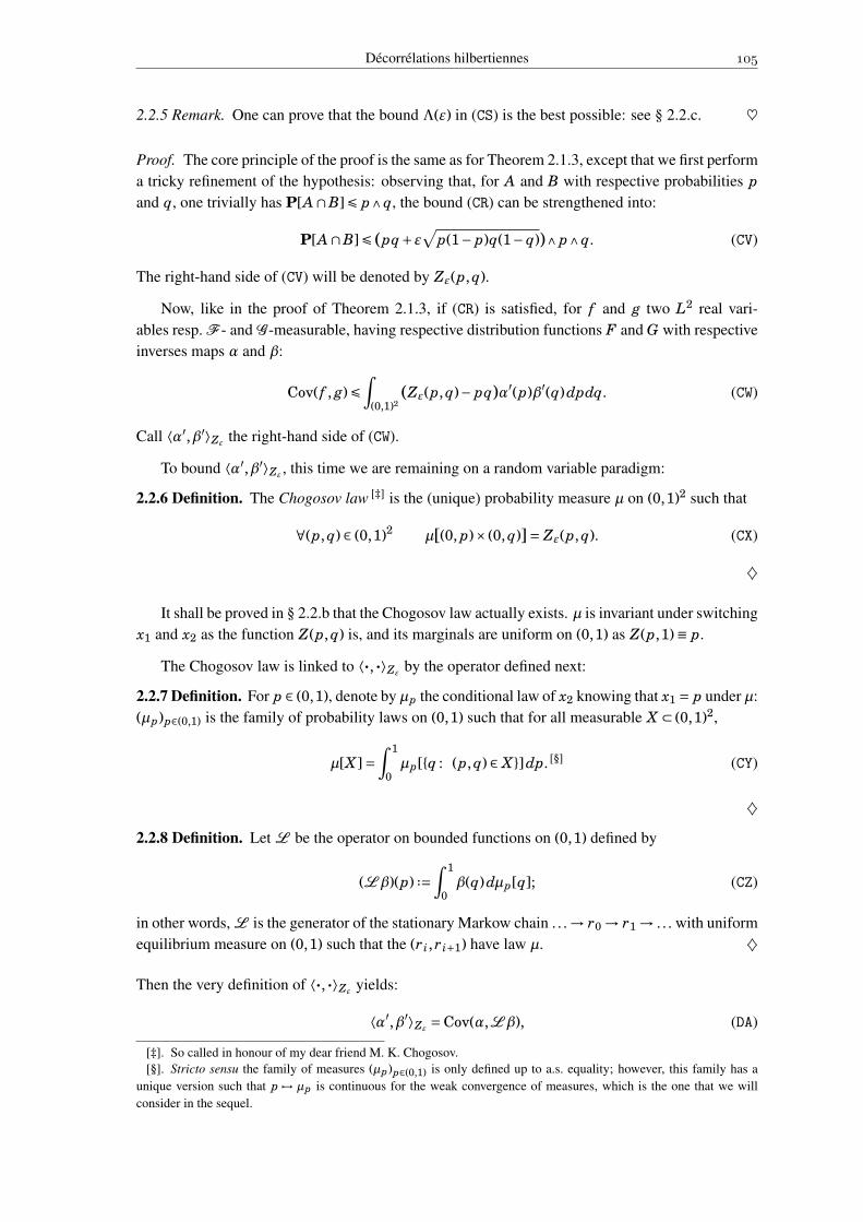
Décorrélations hilbertiennes
2.2.5 Remark. One can prove that the bound Λ(ε) in (CS) is the best possible: see § 2.2.c. ♥
Proof. The core principle of the proof is the same as for Theorem 2.1.3, except that we first performa tricky refinement of the hypothesis: observing that, for A and B with respective probabilities pand q, one trivially has P[A∩B]É p∧ q, the bound (CR) can be strengthened into:
P[A∩B]É (pq+ε√
p(1− p)q(1− q))∧ p∧ q. (CV)
The right-hand side of (CV) will be denoted by Zε(p, q).
Now, like in the proof of Theorem 2.1.3, if (CR) is satisfied, for f and g two L2 real vari-ables resp. F - and G -measurable, having respective distribution functions F and G with respectiveinverses maps α and β:
Cov( f , g)É∫
(0,1)2(Zε(p, q)− pq)α′(p)β′(q)dpdq. (CW)
Call ⟨α′,β′⟩Zεthe right-hand side of (CW).
To bound ⟨α′,β′⟩Zε, this time we are remaining on a random variable paradigm:
2.2.6 Definition. The Chogosov law [‡] is the (unique) probability measure µ on (0,1)2 such that
∀(p, q) ∈ (0,1)2 µ[(0, p)× (0, q)]= Zε(p, q). (CX)
♦
It shall be proved in § 2.2.b that the Chogosov law actually exists. µ is invariant under switchingx1 and x2 as the function Z(p, q) is, and its marginals are uniform on (0,1) as Z(p,1)≡ p.
The Chogosov law is linked to ⟨·,·⟩Zεby the operator defined next:
2.2.7 Definition. For p ∈ (0,1), denote by µp the conditional law of x2 knowing that x1 = p under µ:(µp)p∈(0,1) is the family of probability laws on (0,1) such that for all measurable X ⊂ (0,1)2,
µ[X ]=∫ 1
0µp[q : (p, q) ∈ X ]dp. [§] (CY)
♦2.2.8 Definition. Let L be the operator on bounded functions on (0,1) defined by
(Lβ)(p) ··=∫ 1
0β(q)dµp[q]; (CZ)
in other words, L is the generator of the stationary Markow chain . . .→ r0 → r1 → . . . with uniformequilibrium measure on (0,1) such that the (r i, r i+1) have law µ. ♦
Then the very definition of ⟨·,·⟩Zεyields:
⟨α′,β′⟩Zε=Cov(α,Lβ), (DA)
[‡]. So called in honour of my dear friend M. K. Chogosov.[§]. Stricto sensu the family of measures (µp)p∈(0,1) is only defined up to a.s. equality; however, this family has a
unique version such that p 7→ µp is continuous for the weak convergence of measures, which is the one that we willconsider in the sequel.

Quelques problèmes d’inspiration physique en théorie des probabilités
where by writing “Cov(α,Lβ)” I consider functions α and Lβ as real random variables on theprobability space (0,1) endowed with the uniform measure.
By the Cauchy–Schwarz inequality, it is then enough to prove that Var(Lβ) É Λ(ε)Var(β),i.e. that the operator norm of L on L2(0,1) is bounded above by Λ(ε). That work is achieved byLemma 2.2.13 in next subsection. ♠
2.2.b The Chogosov law
This subsection deals with the “Chogosov law”, which we introduced in the proof of Theo-rem 2.2.1.
* Throughout this subsection we suppose ε ∈ (0,1) fixed and we writeΛ forΛ(ε), resp. Z for Zε.The drawings will be made for ε= 1/2.
Recall Definition 2.2.6 of the Chogosov law. We first have to check that the Chogosov lawactually exists:
2.2.9 Claim. There exists a (unique) probability measure µ on (0,1)2 such that
∀p, q ∈ [0,1] µ[(x1, x2) ∈ (0,1)2 : x1 É p and x2 É q]= Z(p, q), (DB)
where we recall thatZ(p, q) ··= (pq+ε
√p(1− p)q(1− q))∧ p∧ q. (DC)
♣
Proof. (DB) means that the density of µ on (0,1)2 is equal to the distribution ∂2x1x2
Z; the non-trivialpoint consists in proving that that distribution is nonnegative.
* From now on in this subsection elements of (0,1)2 will be automatically denoted by (p, q).Moreover, we will denote p ··= 1− p and ~p ··= p−1/2, resp. q ··= 1− q and ~q ··= q−1/2.
The analytic formula defining Z(p, q) depends on the zone of (0,1)2 in which (p, q) lies (seeFigure 5):
• If pq / qp É ε2, then Z(p, q)= p and we will say that we are in zone ¬;• If ε2 É pq / qp É ε−2, then Z(p, q)= pq+√
ppqq and we will say that we are in zone ;• If ε−2 É pq / qp, then Z(p, q)= q and we will say that we are in zone ®.So the expression of ∂pZ depends on the zone where one lies: in ¬ it is “1”, in it is “q−
ε~p√
qq / pp”, and in ® it is “0”. Anyway it is defined and finite evererywhere, just having jumpsat the borders between the zones, which borders we will denote respectively U for the borderbetween ¬ and , and D for the border between and ® (see Figure 5). To prove that thedistribution ∂2
pqZ is nonnegative, we have to show that ∂pZ is increasing in q at p fixed. Let uscheck it:
• In ¬ and ®, ∂pZ is differentiable with ∂q(∂pZ)= 0Ê 0;• In , ∂pZ is differentiable with ∂q(∂pZ) = 1+ ε~p~q /
√ppqq. Denoting by ρ(p, q) that
expression, let us prove that ρ(p, q) is nonnegative (and even positive) in : either ~p and ~qhave the same sign and then ρ(p, q) is trivially Ê 1, or ~p and ~q have opposite signs. Inthe latter case, say for instance that (~p Ê 0 and ~q É 0). Then p Ê 1/2 and q É 1/2, so|~p| = p−1/2< p and |~q| = 1/2− q < q, which implies that
ε|~p~q|√ppqq
< ε√
pqqp
É ε√ε−2 = 1, (DD)
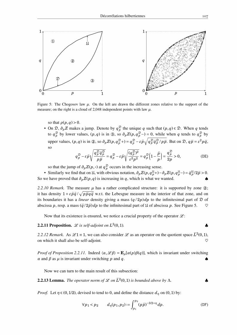
Décorrélations hilbertiennes
0 p 10
q
1
¬
®D
U
0 p 10
q
1
Figure 5: The Chogosov law µ. On the left are drawn the different zones relative to the support of themeasure; on the right is a cloud of 2,048 independent points with law µ.
so that ρ(p, q)> 0.• On D, ∂pZ makes a jump. Denote by qDp the unique q such that (p, q) ∈D. When q tends
to qDp by lower values, (p, q) is in ®, so ∂pZ(p, qDp −) = 0, while when q tends to qDp by
upper values, (p, q) is in , so ∂pZ(p, qDp +) = qDp −ε~p√
qDp qDp / pp. But on D, qp = ε2 pq,so
qDp −ε~p
√qDp qDp
pp= qDp −ε~p
√(qDp )2
ε2 p2 = qDp(1−
~pp
)=
qDp2p
> 0, (DE)
so that the jump of ∂pZ(p,·) at qDp occurs in the increasing sense.• Similarly we find that on U, with obvious notation, ∂pZ(p, qUp+)−∂pZ(p, qUp−)= qUp /2p > 0.
So we have proved that ∂pZ(p, q) is increasing in q, which is what we wanted. ♠
2.2.10 Remark. The measure µ has a rather complicated structure: it is supported by zone ;it has density 1+ ε~p~q /
√ppqq w.r.t. the Lebesgue measure in the interior of that zone, and on
its boundaries it has a linear density giving a mass (q / 2p)dp to the infinitesimal part of D ofabscissa p, resp. a mass (q / 2 p)dp to the infinitesimal part of U of abscissa p. See Figure 5. ♥
Now that its existence is ensured, we notice a crucial property of the operator L :
2.2.11 Proposition. L is self-adjoint on L2(0,1). ♣
2.2.12 Remark. As L 1≡ 1, we can also consider L as an operator on the quotient space L2(0,1),on which it shall also be self-adjoint. ♥
Proof of Proposition 2.2.11. Indeed ⟨α,Lβ⟩ = Eµ[α(p)β(q)], which is invariant under switchingα and β as µ is invariant under switching p and q. ♠
Now we can turn to the main result of this subsection:
2.2.13 Lemma. The operator norm of L on L2(0,1) is bounded above by Λ. ♣
Proof. Let η ∈ (0,1/2), devised to tend to 0, and define the distance dη on (0,1) by:
∀p1 < p2 dη(p1, p2) ··=∫ p2
p1
(pp)−3/2+η dp. (DF)
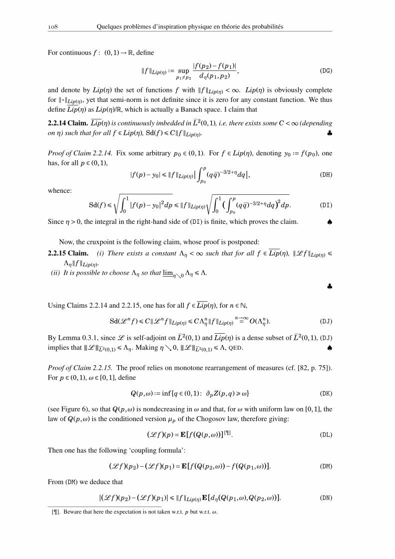
Quelques problèmes d’inspiration physique en théorie des probabilités
For continuous f : (0,1)→R, define
‖ f ‖Lip(η) ··= supp1 6=p2
| f (p2)− f (p1)|dη(p1, p2)
, (DG)
and denote by Lip(η) the set of functions f with ‖ f ‖Lip(η) < ∞. Lip(η) is obviously completefor ‖·‖Lip(η), yet that semi-norm is not definite since it is zero for any constant function. We thusdefine Lip(η) as Lip(η)/R, which is actually a Banach space. I claim that
2.2.14 Claim. Lip(η) is continuously imbedded in L2(0,1), i.e. there exists some C <∞ (dependingon η) such that for all f ∈Lip(η), Sd( f )É C‖ f ‖Lip(η). ♣
Proof of Claim 2.2.14. Fix some arbitrary p0 ∈ (0,1). For f ∈ Lip(η), denoting y0 ··= f (p0), onehas, for all p ∈ (0,1),
| f (p)− y0| É ‖ f ‖Lip(η)|∫ p
p0
(qq)−3/2+ηdq|, (DH)
whence:
Sd( f )É√∫ 1
0| f (p)− y0|2dp É ‖ f ‖Lip(η)
√∫ 1
0(∫ p
p0
(qq)−3/2+ηdq)2dp. (DI)
Since η> 0, the integral in the right-hand side of (DI) is finite, which proves the claim. ♠
Now, the cruxpoint is the following claim, whose proof is postponed:
2.2.15 Claim. (i) There exists a constant Λη < ∞ such that for all f ∈ Lip(η), ‖L f ‖Lip(η) ÉΛη‖ f ‖Lip(η).
(ii) It is possible to choose Λη so that limη0Λη ÉΛ.
♣
Using Claims 2.2.14 and 2.2.15, one has for all f ∈Lip(η), for n ∈N,
Sd(L n f )É C‖L n f ‖Lip(η) É CΛnη‖ f ‖Lip(η)
n→∞= O(Λnη ). (DJ)
By Lemma 0.3.1, since L is self-adjoint on L2(0,1) and Lip(η) is a dense subset of L2(0,1), (DJ)implies that LL2(0,1) ÉΛη. Making η 0, LL2(0,1) ÉΛ, QED. ♠
Proof of Claim 2.2.15. The proof relies on monotone rearrangement of measures (cf. [82, p. 75]).For p ∈ (0,1), ω ∈ [0,1], define
Q(p,ω) ··= infq ∈ (0,1) : ∂pZ(p, q)Êω (DK)
(see Figure 6), so that Q(p,ω) is nondecreasing in ω and that, for ω with uniform law on [0,1], thelaw of Q(p,ω) is the conditioned version µp of the Chogosov law, therefore giving:
(L f )(p)=E[ f (Q(p,ω))] [¶]. (DL)
Then one has the following ‘coupling formula’:
(L f )(p2)− (L f )(p1)=E[ f (Q(p2,ω))− f (Q(p1,ω))]. (DM)
From (DM) we deduce that
|(L f )(p2)− (L f )(p1)|É ‖ f ‖Lip(η) E[dη(Q(p1,ω),Q(p2,ω))]. (DN)
[¶]. Beware that here the expectation is not taken w.r.t. p but w.r.t. ω.
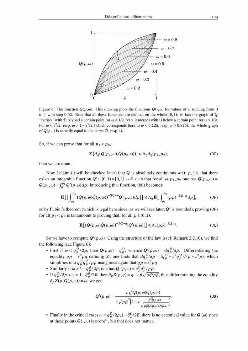
Décorrélations hilbertiennes
0 p 10
Q(p,ω)
1
ω= 0.2
ω= 0.3
ω= 0.4
ω= 0.5
ω= 0.6
ω= 0.7
ω= 0.8
D
U
Figure 6: The function Q(p,ω). This drawing plots the functions Q(·,ω) for values of ω running from 0to 1 with step 0.02. Note that all these functions are defined on the whole (0,1): in fact the graph of Q‘merges’ with D beyond a certain point for ω< 1/2, resp. it merges with U below a certain point for ω> 1/2.For ω < ε2/2, resp. ω > 1− ε2/2 (which corresponds here to ω < 0.125, resp. ω > 0.875), the whole graphof Q(p,·) is actually equal to the curve D, resp. U.
So, if we can prove that for all p1 < p2,
E[dη(Q(p1,ω),Q(p2,ω))]ÉΛηdη(p1, p2), (DO)
then we are done.
Now I claim (it will be checked later) that Q is absolutely continuous w.r.t. p, i.e. that thereexists an integrable function Q′ : (0,1)× [0,1] → R such that for all ω, p1, p2 one has Q(p2,ω) =Q(p1,ω)+∫ p2
p1Q′(p,ω)dp. Introducing that function, (DO) becomes:
E[|∫ p2
p1
(Q(p,ω)Q(p,ω))−3/2+ηQ′(p,ω)dp|]ÉΛηE[∫ p2
p1
(pp)−3/2+η dp], (DP)
so by Fubini’s theorem (which is legal here since, as we will see later, Q′ is bounded), proving (DP)for all p1 < p2 is tantamount to proving that, for all p ∈ (0,1),
E[(Q(p,ω)Q(p,ω))−3/2+η|Q′(p,ω)|]ÉΛη(pp)−3/2+η. (DQ)
So we have to compute Q′(p,ω). Using the structure of the law µ (cf. Remark 2.2.10), we findthe following (see Figure 6):
• First if ω < qDp / 2p, then Q(p,ω) = qDp , whence Q′(p,ω) = dqDp /dp. Differentiating theequality qp = ε2 pq defining D, one finds that dqDp /dp = (qDp + ε2 qDp ) / ( p + ε2 p), whichsimplifies into qDp qDp / pp using once again that qp = ε2 pq.
• Similarly if ω> 1− qUp / 2 p, one has Q′(p,ω)= qUp qUp / pp.• If qDp /2p <ω< 1− qUp /2p, then ∂pZ(p, q)= q−ε~p
√qq/pp, thus differentiating the equality
∂pZ(p,Q(p,ω))=ω, we get:
Q′(p,ω)=ε
√Q(p,ω)Q(p,ω)
4√
pp3(
1+ε~p~Q(p,ω)√
ppQ(p,ω)Q(p,ω)
) . (DR)
• Finally in the critical cases ω= qDp /2p,1− qUp /2p, there is no canonical value for Q′(ω) sinceat these points Q(·,ω) is not C 1, but that does not matter.
Quelques problèmes d’inspiration physique en théorie des probabilités
2.2.16 Remark. Note that one always has Q′(p,ω) > 0, i.e. Q(·,ω) is increasing. In other words,for p1 < p2, µp1 is stochastically smaller than µp2 . ♥
We have computed Q′(p,ω), so now we can tackle (DQ): we have to bound∫ 1
0
( pp
Q(p,ω)Q(p,ω)
)3/2−ηQ′(p,ω)dω, (DS)
uniformly in p. We begin with noticing that
2.2.17 Claim. For all p ∈ (0,1), all q ∈ [qDp , qUp], one has qq/pp É ε−2. ♣
Proof of Claim 2.2.17. The condition q ∈ [qDp , qUp] means that ε2 É pq/qp É ε−2. Then we distin-guish two cases:
• If p É q, then qq/pp = (q/p)2qp/pq É qp/pq = (pq/qp)−1 É ε−2;• If p Ê q, then qq/pp = (q/p)2 pq/qp É pq/qp É ε−2.
♠
Thanks to Claim 2.2.17, we bound (DS) by
ε−2η∫ 1
0
( pp
Q(p,ω)Q(p,ω)
)3/2Q′(p,ω)dω, (DT)
which we shorthand into ε−2ηλ(p). Splitting the integral in (DT) according to the value of ω (resp.for ω ∈ (0, qDp /2p), (qDp /2p,1− qUp/2p) and (1− qUp/2p,1)), one finds:
λ(p) =qDp2p
( ppqDp qDp
)3/2 qDp qDppp
(DU)
+∫ 1−qU
p /2p
qDp /2p
( pp
Q(p,ω)Q(p,ω)
)3/2 ε
√Q(p,ω)Q(p,ω)
4√
pp3(
1+ε~p~Q(p,ω)√
ppQ(p,ω)Q(p,ω)
)dω (DV)
+qUp2p
( ppqUp qUp
)3/2 qUp qUppp
. (DW)
(DU) simplifies into 12
√qDp p/pqDp = 1
2
pε2 = ε/2; similarly (DW) = 1
2
√pqUp/qUp p = ε/2. Concerning
term (DV), we make the change of variables q = Q(p,ω), for which dω = (1+ ε~p~q/√
ppqq)dqbecause of the expression of the density of µ in zone (cf. Remark 2.2.10). One gets:
(DV)= ε
4
∫ qUp
qDp
1qq
dq = ε
4
[log
]qUp
qDp
= ε
4
(log
pε2 p
− logε2 p
p
)= ε
4log
1ε4 = ε| logε|. (DX)
So in the end we have λ(p) = ε/2+ε/2+ε| logε| =Λ for all p, thus Λη É ε−2ηΛ (hence (i)), whichtends to Λ as η 0 (hence (ii)). ♠
2.2.18 Remark. The simplifications in the computation of λ(p) look rather miraculous. . . A priori
I only expected that λ(p)ÉΛ on (0,1) with λ(p)p→0,1→ Λ). That I found the exact quasi-eigenvector
associated to the quasi-eigenvalue Λ (cf. Remark 2.2.19) is purely fortuitous; I have no simpleexplanation for why things work so well. ♥
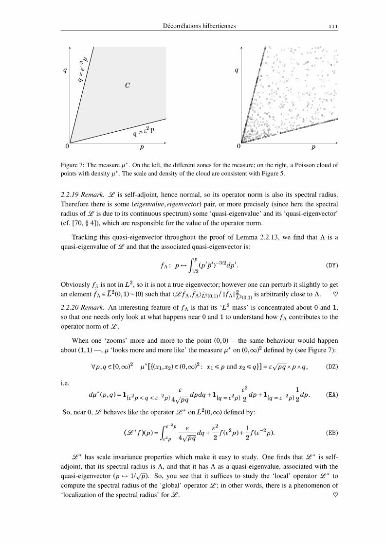
Décorrélations hilbertiennes
q= ε
−2p
q = ε2 p
0 p
q
C
0 p
q
Figure 7: The measure µ∗. On the left, the different zones for the measure; on the right, a Poisson cloud ofpoints with density µ∗. The scale and density of the cloud are consistent with Figure 5.
2.2.19 Remark. L is self-adjoint, hence normal, so its operator norm is also its spectral radius.Therefore there is some (eigenvalue,eigenvector) pair, or more precisely (since here the spectralradius of L is due to its continuous spectrum) some ‘quasi-eigenvalue’ and its ‘quasi-eigenvector’(cf. [70, § 4]), which are responsible for the value of the operator norm.
Tracking this quasi-eigenvector throughout the proof of Lemma 2.2.13, we find that Λ is aquasi-eigenvalue of L and that the associated quasi-eigenvector is:
fΛ : p 7→∫ p
1/2(p′ p′)−3/2dp′. (DY)
Obviously fλ is not in L2, so it is not a true eigenvector; however one can perturb it slightly to getan element
~fΛ ∈ L2(0,1)à 0 such that ⟨L
~fΛ,
~fΛ⟩L2(0,1) /‖
~fΛ‖2
L2(0,1) is arbitrarily close to Λ. ♥2.2.20 Remark. An interesting feature of fΛ is that its ‘L2 mass’ is concentrated about 0 and 1,so that one needs only look at what happens near 0 and 1 to understand how fΛ contributes to theoperator norm of L .
When one ‘zooms’ more and more to the point (0,0) —the same behaviour would happenabout (1,1) —, µ ‘looks more and more like’ the measure µ∗ on (0,∞)2 defined by (see Figure 7):
∀p, q ∈ [0,∞)2 µ∗[(x1, x2) ∈ (0,∞)2 : x1 É p and x2 É q]= εppq∧ p∧ q, (DZ)
i.e.
dµ∗(p, q)= 1ε2 p < q < ε−2 pε
4ppq
dpdq+1q = ε2 pε2
2dp+1q = ε−2 p
12
dp. (EA)
So, near 0, L behaves like the operator L ∗ on L2(0,∞) defined by:
(L ∗ f )(p)=∫ ε−2 p
ε2 p
ε
4ppq
dq+ ε2
2f (ε2 p)+ 1
2f (ε−2 p). (EB)
L ∗ has scale invariance properties which make it easy to study. One finds that L ∗ is self-adjoint, that its spectral radius is Λ, and that it has Λ as a quasi-eigenvalue, associated with thequasi-eigenvector (p 7→ 1/
pp). So, you see that it suffices to study the ‘local’ operator L ∗ tocompute the spectral radius of the ‘global’ operator L ; in other words, there is a phenomenon of‘localization of the spectral radius’ for L . ♥
Quelques problèmes d’inspiration physique en théorie des probabilités
2.2.c Optimality of the strong event sufficient condition
Now I will prove that Theorem 2.2.1 is optimal:
2.2.21 Theorem. The factor Λ(ε) in (CS) cannot be improved. In other words, for all Λ′ <Λ(ε) itis possible to find σ-fields F and G satisfying
∀A ∈F ,B ∈G P[A∩B]−P[A]P[B]É ε√
P[A]P[Ac]P[B]P[Bc], (EC)
but such that F : G ÊΛ′. ♣
2.2.22 Remark. One can automatically add absolutes values in the left-hand side of the condi-tion (EC), since −(P[A∩B]−P[A]P[B])=P[A∩Bc]−P[A]P[Bc]. ♥
Actually I will rather prove the following statement, which is equivalent to the theorem bycontinuity of the function Λ(·):2.2.23 Claim. For all ε′ > ε it is possible to find σ-fields F and G satisfying F : G ÊΛ(ε), butsuch that
∀A ∈F ,B ∈G P[A∩B]−P[A]P[B]É ε′√
P[A]P[Ac]P[B]P[Bc]. (ED)
♣
Proof. According to the proof of Theorem 2.2.1, the ‘natural’ proof would be to take for space(Ω,B,P) the set (0,1)2 equipped with its Borel σ-field and endowed with the Chogosov law µ,and to set F = σ(p) and G = σ(q). Though it seems to be true that that system satisfies (CR), thecomplicated structure of µ makes existence of a short proof for that property unlikely. Therefore Iwill rather adapt the previous idea to the nicer measure µ∗ defined by (DZ), or more precisely to a‘truncation’ of it.
My system is the following: (Ω,B,P) is the set (0,1)2 equipped with its Borel σ-field andendowed with a certain measure ν (specified just after), and I take F = σ(p), resp. G = σ(q). Themeasure ν, which depends on some parameter x ∈ (0,1) morally close to 0, is a measure on (0,1)2
having uniform marginals, which coincides with µ∗ on (0, x]2 and which is ‘as uniform as possible’outside (0, x]2 (see Figure 8). Technically:
ν[A×B]=
µ∗(A×B) if A ⊂ (0, x] and B ⊂ (0, x];
0 if A ⊂ (0,ε2x] and B ⊂ (x,1);
0 if A ⊂ (x,1) and B ⊂ (0,ε2x];
[∫
A (1− ε2
√xp )dp]|B|/(1− x) if A ⊂ (ε2x, x] and B ⊂ (x,1);
|A|[∫B (1− ε
2
√xq )dq]/(1− x) if A ⊂ (x,1) and B ⊂ (ε2x, x];
[1− (2−ε)x]|A||B|/(1− x)2 if A ⊂ (x,1) and B ⊂ (x,1).
(EE)
First step: Proof that F : G Ê Λ. Let Λ′ < Λ. Since Λ is in the spectrum of the self-adjointoperator L ∗ on L2(0,∞) (see (EB) and the lines just below), there exists f ∈ L2(0,∞)à 0 suchthat ⟨L ∗ f , f ⟩/‖ f ‖L2(0,∞) > Λ′. By a standard truncation argument, we can assume that f hasbounded support, say that f is zero outside (0,Y ]. Dividing f by its norm we can also assume that‖ f ‖L2 = 1.
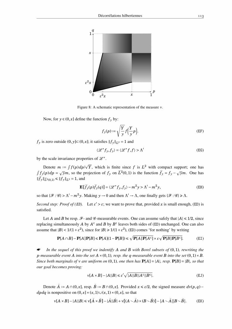
Décorrélations hilbertiennes
0 1p0
1q
ε2x x
ε2x
x
Figure 8: A schematic representation of the measure ν.
Now, for y ∈ (0, x] define the function f y by:
f y(p) ··=√
Yy
f(Y
yp). (EF)
f y is zero outside (0, y]⊂ (0, x]; it satisfies ‖ f y‖L2 = 1 and
⟨L ∗ f y, f y⟩ = ⟨L ∗ f , f ⟩ >Λ′ (EG)
by the scale invariance properties of L ∗.
Denote m ··=∫
f (p)dp/p
Y , which is finite since f is L2 with compact support; one has∫f y(p)dp = pym, so the projection of f y on L2(0,1) is the function f y = f y −pym. One has
‖ f y‖L2(0,1) É ‖ f y‖L2 = 1, and
E[ f y(p) f y(q)]= ⟨L ∗ f y, f y⟩−m2 y>Λ′−m2 y, (EH)
so that F : G >Λ′−m2 y. Making y→ 0 and then Λ′ →Λ, one finally gets F : G ÊΛ.
Second step: Proof of (ED). Let ε′ > ε; we want to prove that, provided x is small enough, (ED) issatisfied.
Let A and B be resp. F - and G -measurable events. One can assume safely that |A| É 1/2, sincereplacing simultaneously A by Ac and B by Bc leaves both sides of (ED) unchanged. One can alsoassume that |B| < 1/(1+ε2), since for |B| Ê 1/(1+ε2), (ED) comes ‘for nothing’ by writing
P[A∩B]−P[A]P[B]ÉP[A](1−P[B])É√
P[A]P[Ac]×ε√
P[B]P[Bc]. (EI)
* In the sequel of this proof we indentify A and B with Borel subsets of (0,1), rewriting thep-measurable event A into the set A× (0,1), resp. the q-measurable event B into the set (0,1)×B.Since both marginals of ν are uniform on (0,1), one then has P[A] = |A|, resp. P[B] = |B|, so thatour goal becomes proving:
ν[A×B]−|A||B| É ε′√
|A||B||Ac||Bc|. (EJ)
Denote A ··= A ∩ (0, x], resp. B ··= B∩ (0, x]. Provided x É ε/2, the signed measure dν(p, q)−dpdq is nonpositive on (0, x]× (x,1)∪ (x,1)× (0, x], so that
ν[A×B]−|A||B| É ν[A× B]−|A||B|+ν[(Aà A)× (Bà B)]− |Aà A||Bà B|. (EK)

Quelques problèmes d’inspiration physique en théorie des probabilités
Now let us bound above the right-hand side of (EK):• The second term is obviously nonpositive.• The third term is [1− (2− ε)x]|A à A||B à B| / (1− x)2, so the sum of the two last terms
is (εx− x2)|Aà A||Bà B| / (1− x)2 É (εx− x2)|A||B|/(1− x)2. Since |A| É 1/2 and |B| É 1/(1+ε2), that quantity is in turn bounded by εx−x2
ε(1−x)2 ×√
|A||B||Ac||Bc|.• For the first term, by Lemma 2.2.24 stated just below, one has ν[A × B] = µ∗[A × B] Éε√
|A||B| É ε√
|A||Ac||B||Bc| / (1− x), in which, provided x É ε2 / (1+ ε2), one has√
|B||Bc| ÉpB|Bc| (because then |B| É |B|∧ x and |B| É 1− x), and similarly
√|A||Ac|É
√A|Ac|, so that
in the end the first term is bounded by ε1−x
√|A||B||Ac||Bc|.
Summing things up, we get:
ν[A×B]−|A||B| É( ε
1− x+ εx− x2
ε(1− x)2
)√|A||B||Ac||Bc|. (EL)
Taking x sufficiently close to 0, the first factor of the right-hand side of (EL) is É ε′, whence thesecond step of the proof. ♠
2.2.24 Lemma. For all A,B ⊂ (0,∞)2 with Lebesgue measures |A|, |B|<∞, µ∗[A×B] Éε√|A||B|. ♣
Proof of Lemma 2.2.24. Recall that µ∗ is the Radon measure on (0,∞)2 having density ε/4ppq
w.r.t. the Lebesgue measure inside the cone C = (p, q) : ε2 p < q < ε−2 p, being zero outside C,and giving to the borders of C a lineic mass defined by µ∗(p,ε2 p) : p ∈ A = ε2|A|/2, resp.µ∗(p,ε−2 p) : p ∈ A = |A|/2 (see Figure 7). µ∗ is invariant under switching p and q, and itsmarginals both are the Lebesgue measure on (0,∞). Let A,B ⊂ (0,∞) be Borel; our goal is to showthat µ∗[A×B]É ε
√|A||B|.
Step 1. If |A| É ε2|B| the result is trivially true, since then µ∗[A×B]ɵ∗[A× (0,∞)]= |A| Éε√
|A||B|. Similarly the result is true if |B| É ε2|A|. Therefore in our proof we will always assumethat ε2|A| < |B| < ε−2|A|.
Step 2. As for the measure µ, decompose the support of µ∗ into three parts U, and D,corresponding resp. to the line “p = ε2q”, the cone C and the line “p = ε−2q” (see Figure 7). Writeµ∗[A×B]= mU +m2 +mD , where mU =µ∗[(A×B)∩U], etc..
Denote by µ∗q the ‘conditioned version’ of µ knowing q, i.e. the probability measure such that
µ∗[X ]=∫ ∞
0µ∗q[p : (p, q) ∈ X ]dq, (EM)
which can be computed explicitly to be:
dµ∗q[p]= 1p = ε2qε2
2+1ε2q < p < ε−2q
ε
4ppq
dp+1p = ε−2q12
. (EN)
The three terms of the right-hand side of (EN) are respectively due to U, and D, so that, integratingthe first one, one finds:
mU =∫
B
ε2
21A 3 ε2qdq É ε2
2|B|. (EO)
Switching the roles of p and q, one has similarly mD É ε2|A|/2. Then it only remains to bound m2.
Step 3. Let us study further the measures µ∗q. If q ∈ ε2 A, then A 3 ε−2q and thus µ∗q[A] ʵ∗[ε−2q] = 1/2, and conversely if q ∉ ε2 A, then A 63 ε−2q and thus µ∗q[A] É 1−µ∗[ε−2q] = 1/2.So, µ∗q[A] is never smaller if q ∈ ε2 A than if q ∉ ε2 A.
Décorrélations hilbertiennes
As a consequence, let us show that we can always assume that ε2 A ⊂ B. Since |B| > ε2|A|,|Bàε2 A| > |ε2 AàB|, so we can fix some B− ⊂ Bàε2 A such that |B−| = |ε2 AàB|. One has:
µ∗[A×B−]=∫
B−µ∗q(A)dq É |B−|
2= |ε2 AàB|
2É
∫ε2 AàB
µ∗q(A)dq =µ∗[A× (ε2 AàB)]. (EP)
Shorthanding “(B à B−) ∪ ε2 A” into “B′”, (EP) implies that replacing B by B′ —which doesnot modify the value of |B| —cannot make µ∗[A ×B] decrease. Consequently, if we prove thatµ∗[A×B′] É ε
√|A||B′|, then we will also have proved that µ∗[A×B] É ε
√|A||B|. As ε2 A ⊂ B′,
we thus have demonstrated the statement at the beginning of this paragraph: one can always assumethat ε2 A ⊂ B.
* Switching the roles of p and q, we will rather impose, instead of ε2 A ⊂ B, that ε2B ⊂ A.
Step 4. Call µ the measure µ∗ restricted to C, i.e. dµ = 1Cdµ∗, so that m2 = µ[A×B]. µ
is absolutely continuous w.r.t. the Lebesgue measure; denote by µq its ‘conditioned version’ forfixed q, i.e. the measure such that
µ[X ]=∫ ∞
0µq[p : (p, q) ∈ X]dq, (EQ)
which has the following explicit density w.r.t. the Lebesgue measure:
dµq[p]= 1ε2q < p < ε−2qε
4ppq
dp. (ER)
We perform a change of variables: for y ∈ (0, |B|), define
β(y)= infq ∈ (0,∞) : |B∩ (0, q)| Ê y; (ES)
so that the push-forward β# dq of the Lebesgue measure on (0, |B|) by the map β is equal to 1Bdq,the Lebesgue measure restricted to B; then
m =∫
Bµq[A]dq =
∫ |B|
0µβ(y)[A]dy. (ET)
Our strategy will consist in bounding µβ(y)[A] for all y.
First, we observe that there is some portion of A which does not contribute to µβ(y)[A]. Denote
indeed A y ··= ε2q: q ∈ B∩(0,β(y)); by the definition of β, |A y| = ε2 y, and one has A y ⊂ ε2B ⊂ A.But A y ⊂ (0,ε2β(y)), so µ
β(y)[A y] = 0, and thus µβ(y)[A] = µ
β(y)[Aà A y], where |Aà A y| = |A|−|A y| = |A|−ε2 y.
Now, for q ∈ (0,∞), the density of µq is zero for p É ε2q and it is nonincreasing for p > ε2q,so an immediate coupling argument shows that the maximal value of µq[X ] under the constraint“|X | = x” is attained for X = (ε2q,ε2q+ x). Applying that result to the conclusion of the previousparagraph, we get that:
µβ(y)[A]ɵβ(y)[(ε2β(y) , ε2β(y)+|A|−ε2 y)]. (EU)
But for x Ê 0, the quantity µq[(ε2q , ε2q+ x)] can be computed explicitly to be
µq[(ε2q , ε2q+ x)]=
(1−ε2)/2 if q É x/(ε−2 −ε2);(ε
√ε2 + x/q−ε2)/2 if q > x/(ε−2 −ε2).
(EV)
Quelques problèmes d’inspiration physique en théorie des probabilités
In particular, that quantity is a nonincreasing function of q. Since, by the definition of β, onealways has β(y)Ê y, it follows that (EU) can be improved into:
µβ(y)[A]ɵy[(ε2 y , |A|)]=
(1−ε2)/2 if yÉ ε2|A|;(ε
√|A|/y−ε2)/2 if y> ε2|A|. (EW)
Integrating, one finds finally:
m2 É∫ ε2|A|
0
1−ε2
2dy+
∫ |B|
ε2|A|
(ε√|A|2py
− ε2
2
)dy
= (1−ε2)ε2|A|2
+[ε√
|A|y− ε2 y2
]|B|
ε2|A|= ε
√|A||B|− ε2
2(|A|+ |B|). (EX)
Step 5. We put our bounds together to get the lemma:
µ∗[A×B]É mD +mU +m2 = ε2
2(|A|+ |B|)+ε
√|A||B|− ε2
2(|A|+ |B|)= ε
√|A||B|. (EY)
♠
2.2.25 Remark. A careful reading of the proof above shows that the maximal value of µ∗[A×B] isattained for A = (0, |A|),B = (0, |B|), in which case, provided ε2|A| É |B| É ε−2|A|, one has equalityin Lemma 2.2.24. ♥
Chapter 3
Tensorization
3.1 Subjective correlation
In this chapter we will need more advanced definitions for decorrelation.
3.1.1 Definition. Let X , Y and Z be random variables. For ε Ê 0, one says that X and Y aresubjectively ε-decorrelated w.r.t. Z (or ε-decorrelated seen from Z) if X and Y are ε-decorrelatedunder the law Law(X ,Y |Z = z) for Law(Z)-almost-all z [∗].
The smallest ε such that X and Y are ε-decorrelated seen from Z will be called the subjectivecorrelation level between X and Y w.r.t. Z (or correlation level between X and Y seen from Z);we denote it X : Y Z . ♦
In § 1.1, we had given the definitions in terms of σ-algebras rather than random variables.Of course there is also a σ-algebra definition for subjective correlation, though I find it harder tounderstand:
3.1.2 Definition. Let F , G and H be σ-algebras. For ε ∈ [0,1], the expression “F : G H É ε”means that for all f ∈ L2(F ∨H ) and all g ∈ L2(G ∨H ) satisfying E[ f |H ]≡ 0, resp. E[g|H ]≡ 0,one has:
|E[ f g]| É εSd( f )Sd(g). (EZ)
♦
We let the reader check that with that definition, for X , Y and Z random variables, X : Y Z =σ(X ) :σ(Y )σ(Z).
3.1.3 Remark. The ordinary correlation can be seen as a particular case of subjective correlation,since F : G = F : G O for O = ;,Ω the trivial σ-field. ♥3.1.4 Remark. Warning! Writing that X : Y Z É ε does not imply that for all subset C of the rangeof Z, X and Y are ε-decorrelated under Law(X ,Y |Z ∈ C): see Examples 3.1.8 and 3.1.9 below. ♥3.1.5 Remark. Warning again! There is no general inequality between X : Y and X : Y Z: seeExamples 3.1.7 and 3.1.8 below. ♥
[∗]. The conditional laws Law(·|Z = z) are only defined up to Law(Z)-a.e. equality, whence the need to specify “forLaw(Z)-almost-all z”.
Quelques problèmes d’inspiration physique en théorie des probabilités
3.1.6 Example. Let f : R → R+ be a nonnegative continuous function with∫R f (x)dx = 1 and
let (X ,Y , Z) be a variable on R3 with density
dP[(X ,Y , Z)= (x, y, z)]= 12π
f (z)exp(sinh z · xy− 12 cosh z · (x2 + y2))dxdydz. (FA)
Then, conditionally to “Z = z”, (X ,Y ) is a Gaussian vector with Var(X ) = Var(Y ) = cosh z andCov(X ,Y ) = sinh z, so by Theorem 1.2.6, under the law P[·|Z = z] one has X : Y = |tanh z|.Consequently X : Y Z = sup|tanh z| : f (z)> 0. ♥
The three following examples show that subjective correlation may behave rather wildly, espe-cially when one changes the σ-field of reference:
3.1.7 Example. Let X and Y be independent variables with uniform law on R/Z and let Z = X +Y ;then X : Y Z = 1: under P[·|Z = z] indeed Y is X -measurable (and not constant), since Y ≡ z−X .
♥3.1.8 Example. Let α,β,γ be three independent random variables uniform on 0,1; defineX = (γ,α),Y = (γ,β) and Z = γ. Then, conditionally to “Z = 0”, X and Y are independent withcommon law uniform on (0,0), (0,1), and similarly X and Y are independent conditionally to“Z = 1”, so X : Y Z = 0. Yet X and Y are not independent since the events “X ∈ (0,0), (0,1)” and“Y ∈ (0,0), (0,1)”, which are non-trivial under P, are equivalent, so that X : Y = 1. ♥3.1.9 Example. Let X = (X1, X2) and Y = (Y1,Y2) be independent with uniform laws on 0,12
and define Z = (X1,Y1); then one easily checks that X : Y Z = 0. Now let Z′ = 1X1 =Y1 , whichis Z-measurable; one has X : Y Z′ = 1 since, for instance, under “Z′ = 1” the events “X1 = 0” and“Y1 = 0” are non-trivial and equivalent. ♥
Now we define a more restrictive concept of subjective correlation.
3.1.10 Definition. A σ-metalgebra M is a set H : H ∈M of σ-algebras which is stable underthe “
∨” operator, i.e. such that for any M ′ ⊂M ,
∨H ∈M ′ H ∈M . ♦
One can speak of the ‘σ-metalgebra spanned by some set of σ-algebras’, as states the followingimmediate proposition:
3.1.11 Proposition. If (Hk)k∈K is a set of σ-algebras, then there is a smallest σ-metalgebra con-taining all the Hk, which is
M = ∨
k∈K ′Hk ; K ′ ⊂ K. (FB)
♣
When one deals with random variables rather than σ-algebras, one has the following variant ofProposition 3.1.11:
3.1.12 Proposition. Let (Zk)k∈K be a set of random variables, then the σ-metalgebra spannedby σ(Zk) : k ∈ K is σ(
→ZK ′) : K ′ ⊂ K. ♣
3.1.13 Definition. Let F and G be σ-algebras and M be a σ-metalgebra. We define the correlationbetween F and G seen from M by:
F : G M = supH ∈M
F : G H . (FC)
♦
Décorrélations hilbertiennes
3.1.14 Remark. Speaking in terms of random variables, if X , Y and (Zk)k∈K are variables, denotingby M the σ-metalgebra spanned by the Zk, then X : Y M is the supremum [†] of the X : Y whentaken under all the laws of kind P[·| →ZK ′ = →zK ′] for K ′ a subset of K and zk,k ∈ K ′ elements of therespective ranges of the Zk. ♥
Finally, the following proposition gathers some easy properties of relative correlation w.r.t. aσ-metalgebra:
3.1.15 Proposition.
(i) Call M; the trivial σ-metalgebra, that is, M; = O ; then for all σ-algebras F and G ,F : G = F : G M; .
(ii) If M ⊂M ′, then F : G M É F : G M ′ .(iii) Let F and G be σ-algebras, let M be a σ-metalgebra, and call
~M the σ-metalgebra spanned
by M , F and G ; then F : G M = F : G ~M
.
♣
3.1.16 Definition. In the sequel, the probabilistic systems which we shall consider will often bemade of some ‘elementary’ variables, say (X i)i∈I . In this case, the so-called natural σ-metalgebraof the system will mean the σ-metalgebra spanned by the X i. ♦
3.2 Simple tensorization
Now we turn to tensorization. First let us deal with ‘simple’ tensorization, by which I meanthat tensorization is performed on only one variable. The main result of this section will be the‘N against 1’ theorem (Theorem 3.2.2).
The problem considered is the following: Let I be a set and (X i)i∈I ,Y be random variables;call M the natural σ-metalgebra of this system, that is, the σ-metalgebra spanned by the X i and Y(cf. Definition 3.1.16). Suppose we have bounds X i : Y M É εi for all i; the question is, can wededuce from them a bound on
→X I : Y ? We shall prove that the answer is “yes”, and moreover the
bound (FM) we will give is optimal in some way (see § 3.5).
For pedagogical purpose, let us first state and prove a weaker but easier proposition:
3.2.1 Proposition. With the notation above,
→X I : Y É
√∑i∈Iε2
i . (FD)
♣
Proof. By Proposition 1.1.12 we may assume I = 1, . . . , N. Let f and g be centered L2 →X -
measurable, resp. Y -measurable, functions; our goal is to bound |E[ f g]|.For all i ∈ 0, . . . , N, denote
Fi =σ(X1, . . . , X i), (FE)
and for all i ∈ 1, . . . , N,f i = f Fi −E[ f |Fi−1]. (FF)
[†]. More precisely it is a true supremum (over K ′) of essential suprema (over →zK ′ ).

Quelques problèmes d’inspiration physique en théorie des probabilités
Then f = ∑i f i, where each f i is Fi-measurable and centered w.r.t. Fi−1 (i.e., E[ f i|Fi−1] ≡ 0).
Consequently, for all i0 < i1 one has E[ f i0 f i1]= 0 (since f i0 is Fi0-measurable while f i1 is centeredw.r.t. Fi1−1 ⊃ Fi0) and thus when one expands Var( f ) = E[(
∑i f i)2] all the non-diagonal terms
vanish, yielding:
Var( f )=N∑
i=1Var( f i). (FG)
Now, the decomposition “ f =∑i f i” yields
E[ f g]=N∑
i=1E[ f i g], (FH)
so let us bound the |E[ f i g]|. The law of total expectation gives:
E[ f i g]=∫
E[ f i g|X1 = x1, . . . , X i−1 = xi−1]dP[x1, . . . , xi−1]. (FI)
But under dP[·|x1, . . . , xi−1], f i is X i-measurable and centered while g is Y -measurable, moreoverunder this law X i : Y É X i : Y Fi−1 É X i : Y M É εi, so:
|E[ f i g|Y1 = y1, . . . ,Yi−1 = yi−1]|É εi Sd( f i|x1, . . . , xi−1)Sd(g|x1, . . . , xi−1). (FJ)
Using the bound Sd(h)É√
E[h2], it follows that:
|E[ f i g]|É εi
∫ √E[ f 2
i |x1, . . . , xi−1]√
E[g2|x1, . . . , xi−1]dP[x1, . . . , xi−1]
ÉCSεi
√∫E[ f 2
i |x1, . . . , xi−1]dP[x1, . . . , xi−1]√
the same for g = εi Sd( f )Sd(g i). (FK)
So, summing (FK) for all i:
|E[ f g]| ÉN∑
i=1εi Sd( f i)Sd(g) É
CS
√∑iε2
i
√∑i
Var( f i) Sd(g)=√∑
iε2
i Sd( f )Sd(g). (FL)
Since (FL) is true for all f , g, (FD) is proved. ♠
It is striking in Proposition 3.2.1 that the right-hand side of (FD) may be greater than 1, which isnever the case for a correlation level. Actually there is some ‘loss of optimality’ in the proof of theproposition when we bound above Var( f i|Fi−1) by E[ f 2
i |Fi−1], since E[ f 2i |Fi−1]−Var( f i|Fi−1)=
E[ f i|Fi−1]2 may be different to 0. We will use a technique for ‘recycling’ that loss to get thefollowing result, which § 3.5 shall prove to be optimal:
3.2.2 Theorem (‘N against 1’ theorem). Take the same hypotheses as in Proposition 3.2.1: ∀i ∈ IX i : Y M É εi, where M is the natural σ-metalgebra of the system. Then:
→X I : Y É
√1−∏
i∈I(1−ε2
i ). (FM)
♣
3.2.3 Remark. The right-hand side of (FM) is the ε ∈ [0,1] characterized by 1− ε2 =∏i(1−εi)2. ♥
3.2.4 Remark. The right-hand side of (FM) is bounded above by√∑
i ε2i , so Theorem 3.2.2 gives
back Proposition 3.2.1 as a corollary. ♥
Décorrélations hilbertiennes
Proof. As in the proof of Proposition 3.2.1, let f and g be centered L2 →X -measurable, resp.
Y -measurable, functions. Assume I = 1, . . . , N; denote Fi ··= σ(X1, . . . , X i) and f i ··= f Fi −E[ f |Fi−1]. Also denote, for i ∈ 0, . . . , N,
gi ··= g−E[g|Fi]. (FN)
As before, one has Var( f )=∑i Var( f i) and E[ f g]=∑N
i=1 E[ f i g]. But f i is centered w.r.t. Fi−1
while (g − gi−1) is Fi−1-measurable, so E[ f i g] = E[ f i gi−1]. Since, conditionally to Fi−1, f i
and gi−1 are both centered and resp. X i- and Y -measurable, the fact that X i : Y M É εi implies,by the same argument as in the previous proof, that
|E[ f i gi−1]| É εi Sd( f i)Sd(gi−1). (FO)
Now, for i ∈ 1, . . . , N, denotegi =E[gi−1|Fi]. (FP)
Since gi−1 = gi + gi, where gi is Fi-measurable while gi is centered w.r.t. Fi, one has:
Var(gi)=Var(gi−1)−Var( gi). (FQ)
Then, the point consists in making the following observation: for Var(gi) to be large (that is, closeto Var(gi−1)), Var( gi) has to be small. But in that case |E[ f i g]| shall be small: one has indeed,since f i is Fi-measurable,
|E[ f i g]| = |E[ f i gi−1]| = |E[ f i(gi−1)Fi]|= |E[ f i gi]| ÉCS
Sd( f i)Sd( gi). (FR)
Let us sum up the relations obtained. One has, for all i ∈ 1, . . . , N:
|E[ f i g]| É εi Sd( f i)Sd(gi−1); (FS)
Sd(gi) =√
Sd(gi−1)2 −Sd( gi)2; (FT)
|E[ f i g]| É Sd( f i)Sd( gi). (FU)
Now define εi ··= |E[ f i g]|/Sd( f i)Sd(gi−1), or εi = 0 if the right-hand side is 0/0. Then (FS) ensuresthat εi É εi, and (FU) means that Sd( gi) Ê εi Sd(gi−1), so that (FT) yields Sd(gi) É
√1− ε2
i ×Sd(gi−1). Since g0 = g, one has therefore by induction Sd(gi) É ∏i−1
i′=1
√1− ε2
i′ Sd(g), so that thedecomposition “E[ f g]=∑
i E[ f i g]” gives:
|E[ f g]| ÉN∑
i=1(εi
i−1∏i′=1
√1− ε2
i′)Sd( f i)Sd(g). (FV)
By the Cauchy–Schwarz inequality, it follows that:
|E[ f g]| É√√√√ N∑
i=1ε2
i
i−1∏i′=1
(1− ε2i′) Sd( f )Sd(g)=
√√√√1−N∏
i=1(1− ε2
i ) Sd( f )Sd(g). (FW)
Obviously the maximal value for the right-hand side of (FW) is when εi = εi for all i, thenyielding (FM). ♠
There is an alternative proof, which is less intuitive but whose reasoning shall be used again inthe proof of Theorem 3.3.1:

Quelques problèmes d’inspiration physique en théorie des probabilités
Alternative proof of Theorem 3.2.2. We use the same notation as in the previous proof. As f isF -measurable, E[ f g]=E[ f gF ], so by the Cauchy–Schwarz inequality:
|E[ f g]| ÉSd( f )Sd(gF ). (FX)
Now, by associativity of variance Sd(gF )=√
Var(g)−Var(g− gF ), so by (FX) it suffices to provethat
Var(g− gF )ÊN∏
i=1(1−ε2
i )Var(g). (FY)
With our notation, g− gF = gN and g = g0; we will prove that for all i ∈ 1, . . . , N,
Var(gi)Ê (1−ε2i )Var(gi−1). (FZ)
Since gi−1 and gi are centered w.r.t. Fi−1, one has
Var(gi−1)=∫
Var(gi−1|x1, . . . , xi−1)dP[x1, . . . , xi−1], (GA)
with a similar decomposition for Var(gi), so that it suffices to prove (FZ) conditionally to Fi−1.
Conditionally to Fi−1, gi−1 is centered and Y -measurable. Moreover, gi = gi−1 − (gi−1)σ(X i),so by associativity of variance Var(gi)=Var(gi−1)−Var((gi−1)σ(X i)), and therefore (FZ) is equiv-alent to
Var((gi−1)σ(X i))Ê ε2i Var(gi−1), (GB)
which follows directly from the assumption “X i : Y Fi−1 É εi”. ♠
3.3 Double tensorization
Simple tensorization as itself is already interesting since it gives an L2-type bound for thecorrelation between X and
→Y , which is better than the L1-type bounds typically obtained by total
variation methods. Yet it does not exhaust the full potential of Hilbertian correlations concerningtensorization, since obviously it does not contain results like independent tensorization (cf. § 1.1.e).
The aim of this section is to get sharp tensorization results where we perform tensorizing onboth sides, without having to assume complete independence like in Theorem 1.1.19. The priceto pay is that the techniques involved, though similar in their spirit, will be much more tricky,moreover the bounds obtained will not be completely optimal (see § 3.5).
3.3.a ‘N against M’ tensorization
The following theorem may be considered as the main result of this part of the thesis. Aswill be explained in § 3.5.b, it ‘contains’ qualitatively all the other tensorization theorems (i.e.Theorems 1.1.19, 3.2.2 and 3.3.10).
3.3.1 Theorem (‘N against M’ theorem). Let I and J be sets, and let (X i)i∈I and (Y j) j∈J berandom variables, the σ-metalgebra they generate being denoted by M . Suppose for any i, j,X i : Y jM É εi j for some εi j Ê 0, and define the operator
ε : L2(J) → L2(I)(a j) j∈J 7→ (
∑j∈J εi ja j)i∈I ,
(GC)
Décorrélations hilbertiennes
then:
→X I :
→YJÉε∧1. (GD)
♣
3.3.2 Remark. On (R+)I×J , ε is a nondecreasing function of each εi j. ♥
* As the proof of Theorem 3.3.1 is rather technical, I found it useful to write down how it goeson a concrete example. This is performed in Appendix 3.7, which I suggest the reader to look at inparallel with the proof as a complement.
To prove Theorem 3.3.1, we will need the following
3.3.3 Lemma. Let X1, X2, . . . , XN and Y be random variables, call M their natural σ-metalgebra,and assume that for all i ∈ 1, . . . , N,
X i : Y M É εi. (GE)
Let f be an L2(→X ) function. For all 0 É i É N, denote Fi ··= σ(X1, . . . , X i), resp. F∗
i ··= σ(X1, . . . ,X i,Y ), and for all 1É i É N, define
f i ··= f Fi −E[ f |Fi−1], (GF)
resp. f ∗i ··= f F∗i −E[ f |F∗
i−1], (GG)
and denote by Vi and V∗i their respective variances. Then, for all 1É i É N,
V∗i Ê (1−ε2
i )Vi −2εi√
Vi(∑i′>i
εi′√
Vi′). (GH)
♣
Proof. For 0É i É N, define ~f i ··= f −E[ f |Fi], (GI)
resp.~f ∗i ··= f −E[ f |F∗
i ], (GJ)
and call~Vi and
~V∗
i their respective variances. One has~f i = ∑
i′>i f i′ , resp.~f ∗i = ∑
i′>i f ∗i′ . More-over, by the same argument as in the proof of Proposition 3.2.1, all the f i are orthogonal (that is,i0 6= i1 ⇒ E[ f i0 f i1]= 0), thus ~
Vi =∑i′>i
Vi′ ; (GK)
similarly, ~V∗
i = ∑i′>i
V∗i′ . (GL)
In a first step, we observe that for all i,~f i −
~f ∗i = ( f − f Fi ) − ( f − f F∗
i ) = f F∗i − f Fi =
f F∗i − ( f Fi )F
∗i = ( f − f Fi )F
∗i = (
~f i)F
∗i , which by associativity of variance yields the following
3.3.4 Claim. ~Vi −
~V∗
i =Var((~f i)F
∗i ). (GM)
♣
Quelques problèmes d’inspiration physique en théorie des probabilités
Now, the following claim will be the main tool for proving the lemma:
3.3.5 Claim. For all 1É i É N,
~Vi−1 −
~V∗
i−1 É (εi√
Vi +√ ~
Vi −~V∗
i )2 [‡]. (GN)
♣
Admit temporarily Claim 3.3.5. Since~VN = ~
V∗N = 0, (GN) applied with i = N gives
~VN−1 −~
V∗N−1 É ε2
NVN , which in turn we can use in (GN) with i = N−1, and so on, to finally prove by finite(decreasing) induction that, for all i,
~Vi −
~V∗
i É (∑i′>i
εi′√
Vi′)2. (GO)
Now to get (GH), we note that Vi =~Vi−1 −
~Vi, resp. V∗
i = ~V∗
i−1 −~V∗
i , so, using successively theinequalities (GN) and (GO),
Vi −V∗i = (
~Vi−1 −
~V∗
i−1)− (~Vi −
~V∗
i )
É (εi√
Vi +√ ~
Vi −~V∗
i )2 − (~Vi −
~V∗
i )= ε2i Vi +2εi
√Vi
√ ~Vi −
~V∗
i
É ε2i Vi +2εi
√Vi(
∑i′>i
εi′√
Vi′), (GP)
which is equivalent to (GH). ♠
Proof of Claim 3.3.5. Thanks to Claim 3.3.4, what we have to prove is:
Var((~f i−1)F
∗i−1)É (εi
√Vi +
√ ~Vi −
~V∗
i )2 . (GQ)
By the definition of conditional expectation and the equality case in the Cauchy–Schwarz inequal-ity, (GQ) is equivalent to saying that for all L2(F∗
i−1) function g,
|E[~f i−1 g]|É (εi
√Vi +
√ ~Vi −
~V∗
i )Sd(g). (GR)
So let g be a centered L2 F∗i−1-measurable real function. Since
~f i−1 = f i +
~f i, E[
~f i−1 g]=E[ f i g]+
E[~f i g], which two terms we shall bound separately.
For the first term, under P[·|Fi−1], f i is centered and only depends on X i, and g only dependson Y . Since X i : Y Fi−1 É X i : Y M É εi, it follows that
|E[ f i g|Fi−1]|É εi Sd( f i|Fi−1) Sd(g|Fi−1), (GS)
which yields upon integrating:
|E[ f i g]| É εi
∫Sd( f i|Fi−1)Sd(g|Fi−1)dP
ÉCSεi
√∫Var( f i|Fi−1)dP
√∫Var(g|Fi−1)dP
= εi√
Vi
√Var(g)−Var(gFi−1)É εi
√Vi Sd(g). (GT)
[‡]. Taking the square root of (~Vi −
~V∗
i ) is allowed, since that quantity is nonnegative by Claim 3.3.4.
Décorrélations hilbertiennes
For the second term, under P[·|Fi], g only depends on Y , and E[~f i|Y ]≡
~f i −
~f ∗i as we noticed
just before Claim 3.3.4, so E[~f i g|Fi]=E[(
~f i −
~f ∗i )g|Fi], which yields upon integrating:
|E[~f i g]| = |E[(
~f i −
~f ∗i )g]| É
CSSd(
~f i −
~f ∗i )Sd(g)=
√ ~Vi −
~V∗
i Sd(g), (GU)
the last equality coming from Claim 3.3.4. Then it just remains to combine (GT) and (GU) to get (GR).♠
Proof of Theorem 3.3.1. First, thanks to a by now classical approximation argument we may as-sume that I = 1, . . . , N and J = 1, . . . , M. Denote F ··= σ(
→X I ), resp. G ··= σ(
→YJ); our goal is to
prove that for all f ∈ L2(F ), all g ∈ L2(G ), one has |E[ f g]| É (ε∧1)Sd( f )Sd(g). We will use thesame trick as in our alternative proof of Theorem 3.2.2: by the definition of conditional expectationand the Cauchy–Schwarz inequality, proving the inequality above is equivalent to showing that forall f ∈ L2(F ),
Var( f G )É (ε2 ∧1)Var( f ), (GV)
which, by associativity of variance, is in turn equivalent to:
Var( f − f G )Ê (1−ε2)+Var( f ). (GW)
For 0 É i É N, resp. 0 É j É M, define Fi = σ(X1, . . . , X i), resp. G j = σ(Y1, . . . ,Y j). Forall 0É j É M, define
f j ··= f −E[ f |G j], (GX)
and for all 1É i É N, define moreover
f ji ··= f G j∨Fi −E[ f |G j ∨Fi−1]. (GY)
Denote V j ··= Var( f j), resp. V ji ··= Var( f j
i ). For fixed j, the f ji are pairwise orthogonal (again by
the argument in the proof of Proposition 3.2.1) and their sum is equal to f j, so:
V j =N∑
i=1V j
i . (GZ)
Thus, with this notation our goal (GW) becomes:
N∑i=1
V Mi Ê (1−ε2)+
N∑i=1
V 0i . (HA)
The main tool to prove (HA) will be Lemma 3.3.3. Actually the rough formula (GH) is quiteimpratical, so we introduce a linearized version of it: for each 1 É i É N take some αi > 0 (whichfor the time being is arbitrary), then by the Cauchy–Schwarz inequality, (GH) implies that:
V∗i Ê (1−ε2
i )Vi − εiVi
αi
∑i′>i
εi′αi′ −εiαi∑i′>i
εi′Vi′
αi′. (HB)
3.3.6 Remark. (HB) is devised so that its right-hand side is exactly the same as in (GH) if Vi ∝ α2i
∀i. ♥

Quelques problèmes d’inspiration physique en théorie des probabilités
Let us reason conditionally to G j−1 for a few lines. Under this conditioning, call.
Fi ··=σ(X1, . . . , X i), resp.
.F∗
i ··=σ(X1, . . . , X i,Y j), and.f ··= f j−1. Then
.f is an L2(
→X ) function, so we are
in situation of applying Lemma 3.3.3 to the functions.f i ··=
.f
.Fi −E[
.f | .
Fi−1] (HC)
and.f ∗i ··=
.f
.F∗
i −E[.f | .
F∗i−1]. (HD)
But in fact we already know these functions: namely,.f i = f j−1
i and.f ∗i = f j
i . Then, applying thelinearized version (HB) of Lemma 3.3.3
Var( f ji |G j−1)Ê
(1−ε2
i j −εi j
αi
∑i′>i
εi′ jαi′)Var( f j−1
i |G j−1)−εi jαi∑i′>i
εi′ j Var( f j−1i′ |G j−1)αi′
, (HE)
whence upon integrating:
V ji Ê (1−ε2
i j)Vj−1
i −(∑i′>i
εi′ jαi′)εi jV
j−1i
αi−εi jαi
∑i′>i
εi′ jVj−1
i′
αi′. (HF)
By Equation (HF), we have transformed our initial problem into a purely abstract operatorproblem, posed in an L1 setting. To handle it, we need a little notation. Call L1(I) the set of realfunctions on I, endowed with the L1 norm
‖(vi)i∈I‖1 ··=∑i∈I
|vi|. (HG)
The dual space of L1(I) is made of the linear forms l : (vi)i∈I 7→ ∑l ivi, equipped with the L∞
norm‖l‖∞ ··= sup
i∈I|l i|. (HH)
We shall write “L1(I) 3 v Ê 0” to mean that all the entries of v are nonnegative, and “(L1(I))′ 3 l Ê0” to mean that (v Ê 0)⇒ (lv Ê 0), which is equivalent to say that all the l i are nonnegative. Now Iclaim the following lemma, whose proof is postponed:
3.3.7 Lemma. Suppose given some nonnegative numbers V ji for (i, j) ∈ 1, . . . , N×0, . . . , M, such
that Equation (HF) is satisfied for all i, j. Call L the nonnegative linear form on L1(I) defined by
L v = ∑j∈J
i,i′∈I
αi′
αiεi jεi′ jvi, (HI)
and assume ‖L ‖∞ É 1, then:
N∑i=1
V Mi Ê
N∑i=1
V 0i −L ((V 0
i )i∈I). (HJ)
♣
Lemma 3.3.7 has the following immediate
3.3.8 Corollary. Suppose given some nonnegative numbers V ji for (i, j) ∈ 1, . . . , N× 0, . . . , M,
such that Equation (HF) is satisfied for all i, j, then:
N∑i=1
V Mi Ê
(1−sup
i∈I
∑j∈Ji′∈I
αi′
αiεi jεi′ j
)+
N∑i=1
V 0i . (HK)
♣
Décorrélations hilbertiennes
Now we finish the proof of Theorem 3.3.1: thanks to Corollary 3.3.8 we have proved that (HK)stands true in our situation for any choice of positive (αi)i∈I . The last step then consists in opti-mizing that choice. Denote “α> 0” to mean that all the αi are positive. One has:
infα>0
supi∈I
∑j∈Ji′∈I
αi′
αiεi jεi′ j = infλÊ 0 : (∃α> 0)(∀i)(
∑j∈Ji′∈I
εi jεi′ jαi′ Éλαi)
= infλÊ 0 : (∃α> 0)(εε∗αÉλα). (HL)
But εε∗ is a nonnegative operator on L2(I) (I mean, when seen as a matrix all its entries arenonnegative), so by Lemma 3.8.1 in appendix:
infλÊ 0 : (∃α> 0)(εε∗αÉλα)= ρ(εε∗)=ε2. (HM)
This ends the proof of Theorem 3.3.1. ♠
Proof of Lemma 3.3.7. We prove Lemma 3.3.7 by induction on M. The case M = 0 is trivial.Suppose M Ê 1 and assume the result is true for (M−1). We generalize the notation L by defining,for • ∈ ,1,∗,
L •v = ∑j∈J•i,i′∈I
αi′
αiεi jεi′ jvi, (HN)
with J1 = 1, resp. J∗ = 2, . . . , M, so that L = L 1 +L ∗. Notice that ‖L ∗‖∞ É 1 since‖L ‖∞ É 1. For all i ∈ I, define
V 1i = (1−ε2
i1)V 0i − εi1V 0
i
αi
∑i′>i
εi′1αi′ −εi1αi∑i′>i
εi′1V 0i′
αi′, (HO)
which is the value that V 1i would take if there were equality in (HF) for j = 1. With that notation,
(HF) writes(V 1
i − V 1i )i∈I Ê 0, (HP)
and by induction hypothesis we have:
N∑i=1
V Mi Ê
N∑i=1
V 1i −L ∗((V 1
i )i∈I). (HQ)
Introducing the V 1i , we have therefore the following chain of inequalities:
N∑i=1
V Mi Ê
(HQ)
N∑i=1
V 1i −L ∗((V 1
i )i∈I)
=(HP)
N∑i=1
V 1i +‖(V 1
i − V 1i )i∈I‖1 −L ∗((V 1
i )i∈I)−L ∗((V 1i − V 1
i )i∈I)
Ê‖L ∗‖∞É1
N∑i=1
V 1i −L ∗((V 1
i )i∈I)=N∑
i=1V 0
i −L 1((V 0i )i∈I)−L ∗((V 1
i )i∈I)
ÊV 1ÉV 0
L ∗Ê0
N∑i=1
V 0i −L 1((V 0
i )i∈I)−L ∗((V 0i )i∈I)=
N∑i=1
V 0i −L ((V 0
i )i∈I), (HR)
so (HJ) is true for M, whence the lemma by induction. ♠
Quelques problèmes d’inspiration physique en théorie des probabilités
3.3.9 Remark. Our proof of Theorem 3.3.1 handled the X i and the Y j in a fully nonsymmetricway, since we began with putting orders on I and J, which orders played a crucial role in thedecomposition of f . Yet the bound (GD) obtained is obviously symmetric by re-labelling the basicvariables—and this is not due to having proceeded to any ‘re-symmetrization’ step. . . To date Ihave no simple explanation for this ‘coincidence’. ♥
3.3.b ‘Z against Z’ tensorization
The proof of the ‘N against M’ theorem was quite more technical than that of the ‘N against 1’theorem; because of that, in order to get tractable computations we had to use suboptimal inequal-ities at two places:
• Claim 3.3.5 is suboptimal: it has indeed the same shortcoming as Proposition 3.2.1 exhibitedcompared to Theorem 3.2.2, namely, it does not ‘recycle the losses’ occurring when onemakes g covariate with both f i and
~f i (cf. the discussion on page 120, just after the proof of
Proposition 3.2.1).• Our linearization technique is suboptimal in general, even after optimizing the αi. In fact,
as we said before, Inequality (HB) is optimal if and only if one has Vi ∝αi; thus, for (HF) tobe always optimal, one has to have V j
i ∝ αi for all j, with the same values for the αi. Thiswould imply that all the sequences (V j
i )0Éi<n are proportional, which is not true in general.So, Theorem 3.3.1 is certainly not optimal [§]—this is confirmed by the example of § 3.7.
Nonetheless, there is one particular case in which an alternative reasoning yields an optimalbound [¶]. This case is when some symmetries in the decorrelation hypotheses allow us to trans-form the original two-parameter problem (indexed by I×J) into a one-parameter problem (indexedby Z). Let us state and prove the corresponding result:
3.3.10 Theorem (‘Z against Z’ theorem). Let I and J be sets isomorphic to Z, and let (X i)i∈I
and (Y j) j∈J be random variables such that, M denoting the σ-metalgebra they generate, one hasfor all i, j ∈Z
X i : Y jM É ε( j− i) (HS)
for some function ε : Z→ [0,1].
Then
→X I :
→YJÉ ε, (HT)
where ε ∈ [0,1] is characterized by:
Arcsin ε= (∑z∈Z
Arcsinε(z))∧ π2
. (HU)
♣
3.3.11 Remark. If we apply Theorem 3.3.1 to the situation above, we find →X I :
→YJÉ (
∑z∈Z ε(z))∧1
(cf. § 3.6.b). The latter expression is always Ê ε because of the concavity of the function sin(·∧ π2 )
on R+, and even > ε if ε 6= 0,1; so, when it is applicable, Theorem 3.3.10 is strictly stronger thanTheorem 3.3.1. ♥
[§]. Though, as we will see in § 3.5.b, it is ‘asymptotically optimal’.[¶]. The bound’s being optimal shall be proved by Theorem 3.5.3.
Décorrélations hilbertiennes
Proof. Let f and g be resp.→X I- and
→YJ-measurable L2 functions. Denote F ··= σ(
→X ), resp. G ··=
σ(→Y ), and for i ∈Z, resp. j ∈Z, denote Fi ··=∨
i′Éiσ(X i′), resp. G j ··=∨j′É jσ(Y j′). For (i, j) ∈Z×Z,
definef j
i ··= f G j∨Fi −E[ f |G j ∨Fi−1] (HV)
and [‖]
gij ··= gG j −E[gG j |G j−1 ∨Fi]. (HW)
Denote V ··=Var( f ), W ··=Var(g), V ji ··=Var( f j
i ), W ij ··=Var(gi
j); also denote
Si j ··=E[ f j−1i gi−1
j ]. (HX)
Our auxiliary functions were devised so that
3.3.12 Claim. Provided the sum in the right-hand side is absolutely convergent,
E[ f g]=∑i, j
Si j. (HY)
♣
Proof of Claim 3.3.12. First define f ··= f G , so that f is G -measurable and E[ f g] = E[ f g]. For j∈Z, define g j ··= gG j −E[g|G j−1], resp. f j ··= f
G j −E[ f |G j−1]: we have g = ∑j g j and f = ∑
j f j,which are the respective decompositions of g and f on the same basis of orthogonal subspacesof L2(G ), so E[ f g] =∑
j E[ f j g j]. The terms of the right-hand side of that formula are unchangedupon replacing f j by f j−1 ··= f −E[ f |G j−1], since E[( f j−1− f j)g j] is zero—the function ( f j−1− f j)is indeed equal to ( f −E[ f |G j]), which is centered conditionally to G j, while g j is G j-measurable.In the end we have:
E[ f g]=∑j
E[ f j−1 g j]. (HZ)
So in a first step we have decomposed E[ f g] into a sum indexed by j. Now we decomposeeach term of that sum into a sum indexed by i. Let us reason conditionally to G j−1. Then f j−1
is an L2(F ) function and g j is in L2(Y j). We compute E[ f j−1 g j] as in the first step of thisproof: first we replace g j by g j ··= (g j)F ; then we decompose f j−1 = ∑
i f j−1i and g j = ∑
i g ji,with f j−1
i ··= ( f j−1)Fi −E[ f j−1|Fi−1] [∗], resp. g ji ··= gFij −E[ g j|Fi−1], and by orthogonal de-
composition we get E[ f j−1 g j] = ∑i E[ f j−1
i g ji]; then we conclude by saying that E[ f j−1i g ji] is
actually equal to E[ f j−1i gi−1
j ], since (gi−1j − g ji) is centered conditionally to Fi while f j−1
i isFi-measurable. In the end we have obtained
E[ f j−1 g j]=∑
iE[ f j−1
i gi−1j ], (IA)
which combined with (HZ) yields (HY). ♠[‖]. Beware: the definition of gi
j is not analogous to the definition of f ji !
[∗]. Notation is consistent: this f j−1i is indeed the same as the f j−1
i defined by (HV), since we are reasoning condi-tionally to G j−1.
Quelques problèmes d’inspiration physique en théorie des probabilités
So we have expressed E[ f g] as a function of the Si j. It is also possible to ‘read’ the valuesof V and W from the V j
i , resp. from the W ij , via the formulas:
V =
limj→−∞(
∑i
V ji ); (IB)
W = ∑j(
lim
i→−∞W i
j ). (IC)
Now we are looking for relations between the V ji , the W i
j and the Si j. The first relation comes
from the decorrelation hypothesis: conditionally to G j−1 ∨Fi−1, f j−1i is in L2(X i), resp. gi−1
j isin L2(Y j), and X i : Y jÉ ε( j− i), so:
|Si j| É ε( j− i)√
V j−1i W i−1
j . (ID)
The second relation means that a large value of |Si j| forces W ij to diminish. To state it, we
observe that, since f j−1i is (G j−1 ∨Fi)-measurable, Si j =E[ f j−1
i (gi−1j )G j−1∨Fi ], so by the Cauchy–
Schwarz inequality |Si j| É Sd( f j−1i )Sd((gi−1
j )G j−1∨Fi). Moreover, since gi−1j − (gi−1
j )G j−1∨Fi = gij,
one has by orthogonality Var((gi−1j )G j−1∨Fi)=Var(gi−1
j )−Var(gij), so our inequality becomes
|Si j| É√
V j−1i
√W i−1
j −W ij (IE)
(where it is understood that W ij ÉW i−1
j ), or more eloquently
W ij ÉW i−1
j − (Si j)2/V j−1i (IF)
provided V j−1i > 0.
The third and last relation means, on the other hand, that a large value of |∑i′>i Si′ j|forces
∑i′>i V j
i to diminish. To state it, we denote
~f j
i ··= f − f G j∨Fi = ∑i′>i
f ji′ , (IG)
whose variance is Var(~f j
i )=∑i′>i Var( f j
i′) since the f ji′ are pairwise orthogonal. One has∑
i′>iSi′ j =
∑i′>i
E[ f j−1i′ gi′−1
j ]= ∑i′>i
E[ f j−1i′ gi
j]=E[~f j−1
i gij]=E[(
~f j−1
i )G j∨Fi gij], (IH)
so by the Cauchy–Schwarz inequality,
|∑i′>i
Si′ j|ÉSd((~f j−1
i )G j∨Fi)Sd(gij). (II)
Since~f j−1
i − (~f j−1
i )G j∨Fi =~f j
i , one has by orthogonality
Var((~f j−1
i )G j∨Fi)=Var(~f j−1
i )−Var(~f j
i ), (IJ)
so our inequality becomes
|∑i′>i
Si′ j|É√∑
i′>iV j−1
i′ − ∑i′>i
V ji′
√W i
j , (IK)
Décorrélations hilbertiennes
or more eloquently: ∑i′>i
V ji′ É
∑i′>i
V j−1i′ −(
∑i′>i
Si′ j)2 /W ij . (IL)
So, we have transformed our initial probabilistic problem into the following analytic one: let Abe an array indexed by Z×Z, each entry (i, j) of which contains three numbers V j
i Ê 0, W ij Ê 0
and Si j, satisfying (ID), (IE) and (IK)—we will say such an array is correct. We define V by (IB)and W by (IC), and we set S =∑
i, j Si j (provided it makes sense); our goal is to get a bound of theform “|S| É εpVW”, with ε only depending on ε(·).
Note that A priori some problems of summability can arise from A’s being infinite, for instanceto check (IL) or to define S. However, in the situations which are of interest to us, we can restrictto cases in which A is of nice particular form. To do this, we first approximate f in L2(
→X ), resp. g
in L2(→Y ), by a function depending only on a finite number of X i, resp. of Y j —say, we assume
f is→X .
I-measurable and g is→Y .
J-measurable for finite.I ⊂ I,
.J ⊂ J. Then, we define a new model
(~X i)i∈Z, (
~Y j) j∈Z by
~X i = X i for i ∈ .
I, resp.~Y j =Y j for j ∈ .
J, and~X i,
~Y j = ∂ for i ∉ .
I, j ∉ .J, ∂ being
some cemetery point. This new model still gives a correct array, for which S/p
VW is arbitrarilyclose to the initial value of E[ f g]/Sd( f )Sd(g); and the new array is of the following form, whichwe will call compact, for which all the quantities of interest are well defined:
• V ji is zero as soon as i ∉ .
I, and it does not depend on j for j <min.J, nor for j Êmax
.J;
• Similarly, W ij is zero as soon as j ∉ .
J, and it does not depend on i for i < min.I, nor for
i Êmax.I;
• Si j is zero as soon as (i, j) ∉ .I × .
J. (This condition automatically follows from the first twoif the array is correct).
We define the following operations on arrays:
3.3.13 Definition.• For z ∈Z, we define the translation operator τz on arrays such that, if the entries of A at (i, j)
are V ji ,W i
j ,Si j, the entries of τzA at (i, j) are V j+zi+z ,W i+z
j+z ,S(i+z)( j+z).
• For A and A two arrays with entries V ji ,W i
j , Si j, resp. V ji ,etc., for α,β two real numbers, we
define the linear combination αA+βA as the array with entries αV ji +βV j
i ,αW ij +βW i
j ,etc..
♦3.3.14 Lemma. Correct arrays are stable by translations and by nonnegative linear combinations,i.e., if A and B are correct arrays, then for all z ∈ Z and α,β Ê 0, τzA and αA+βB are correcttoo. ♣
Proof of Lemma 3.3.14. Recall that being correct means satisfying (ID), (IE) and (IK). These con-ditions are trivially stable by multiplication by a nonnegative constant and by translation [†]. Itremains to see that they are stable by addition. The technique being the same for all three in-equalities, we just treat the case of (IE). Stability of this condition by addition is a consequenceof the following inequality (which is in fact a particuliar case of the Brunn–Minkowski inequality,see [32]):
3.3.15 Lemma. For all a1,b1,a2,b2 Ê 0,√(a1 +a2)(b1 +b2)Ê
√a1b1 +
√a2b2. (IM)
♣[†]. Getting stability of Condition (ID) by translation is actually the only place where the symmetries of the problem
are used.
Quelques problèmes d’inspiration physique en théorie des probabilités
Proof of Lemma 3.3.15. Take squares on both sides of (IM) and notice that (a1 +a2)(b1 +b2)−(√
a1b1 +√
a2b2)2 = a1b2 +a2b1 −2√
a1b1a2b2 = (√
a1b2 −√
a2b1)2 Ê 0. ♠
For A and A two correct arrays satisfying (IE), applying (IM) with a1 = V j−1i ,a2 = V j−1
i ,b1 =W i−1
j −W ij ,b2 = W i−1
j −W ij , we get:
|Si j + Si j|É |Si j|+ |Si j| É√
V j−1i
√W i−1
j −W ij +
√V j−1
i
√W i−1
j −W ij
É√
V j−1i + V j−1
i
√(W i−1
j +W i−1j )− (W i
j +W ij ), (IN)
so (IE) is still valid for (A+ A). ♠
Now, thanks to Lemma 3.3.14 we will reduce our problem on (Z×Z)-arrays into a problemon Z-arrays. Suppose A is a correct array with certain values of V , W and S. Then, for k Ê 0, thearray
Ak =1
2k+1
k∑z=−k
τzA (IO)
is correct too, with the same values of V , W and S as A. Now when k →∞, Ak ‘looks more andmore like a Toeplitz array’, that is, an array whose entries at (i, j) only depend on ( j− i). To stateit rigorously, we need some definitions:
3.3.16 Definition.• Here, a Toeplitz array will mean a Z×Z array whose entries at (i, j) only depend on ( j− i).
For such an array, for z ∈Z we denote by V(z),W(z),S(z) the quantities characterized by V ji =
V( j−i), etc..• Actually we can always assume our Toeplitz array is Toeplitz compact, which means that
there exists some z− É z+ such that:– V(z) does not depend on z for z < z−, nor for z Ê z+;– W(z) does not depend on z for z É z−, nor for z > z+;– S(z) is zero as soon as z < z− or z > z+.
• For a compact Toeplitz array, we define v,w, s as ‘renormalized versions’ of V ,W ,S:
v ··= V(z<z−); (IP)
w ··= W(z>z+); (IQ)
s ··=∑z∈Z
S(z). (IR)
• A Toeplitz array is said to be correct if it is correct when seen as an ordinary array. For aToeplitz array, Equations (ID), (IF) and (IL) become respectively [‡]:
|S(z)| É ε(z)√
V(z−1)W(z+1); (IS)
W(z) É W(z+1) −S2(z) /V(z−1); (IT)
V(z−1) É v−(∑z′<z
S(z′))2 /W(z). (IU)
♦[‡]. Note that the way (IU) follows from (IL) is rather tricky, because it appears a difference between two infinite
quantities, which has to be ‘renormalized’ in the convenient way.
Décorrélations hilbertiennes
With that vocabulary, our informal statement can be made precise: let A be a compact correctarray with entries V j
i ,W ij ,Si j, and associated quantities V ,W ,S, and define the arrays Ak by (IO).
Then when k →∞ one has (2k+1)Ak → A (in the sense that each entry of (2k+1)Ak converges tothe corresponding entry of A), where A is the Toeplitz array with entries V j
i ,W ij , Si j defined by:
V(z) = ∑j−i=z
V ji ; (IV)
W(z) = ∑j−i=z
W ij ; (IW)
S(z) = ∑j−i=z
Si j. (IX)
This array A is Toeplitz compact with z− = min.J −max
.I, resp. z+ = max
.J −min
.I, and the
quantities (IP)–(IR) for A are:
v = V ; (IY)
w = W ; (IZ)
s = S. (JA)
Moreover A is correct, because all the (2k+1)Ak are, and being correct is clearly conserved byarray convergence.
The consequence of this statement is the following claim, which achieves the reduction to a‘Z-indexed’ problem I alluded to a few lines above:
3.3.17 Claim. The supremum of |S|/pVW for correct arrays is not greater than the supremumof |s|/pvw for correct Toeplitz arrays. ♣
So we have to study (compact) correct Toeplitz arrays. Consider such an array. Denote θ(z) ··=Arcsinε(z); then (IS) can be rewritten:
∃θ(z) ∈ [±θ(z)] S(z) = sin θ(z) ·√
V(z−1)W(z+1). (JB)
Now, notice that for fixed values of the V(z), the S(z) and w, if we have values W(z) such that (IS)–(IU) are satisfied, we can modify those W(z) so that (IT) becomes an equality for all z, an operationwhich keeps (IS) and (IU) true since it can only make the W(z) increase. So we can suppose that(IT) actually is an equality, i.e. that for all z ∈Z,
W(z) = w∏z′Êz
cos2 θ(z′). (JC)
Then it remains to integrate (IU). For z ∈Z, denote
Γ(z) ··=∑z′<z
(sin θ(z′) · ∏z′<z′′<z
cos θ(z′′) ·√
V(z′−1)), (JD)
so that (IU) becomes:V(z−1) É v−Γ(z)2. (JE)
Γ(·) satisfies the recursion equation
Γ(z+1)= sin θ(z)√
V(z−1) +cos θ(z)Γ(z), (JF)
so by (JE):|Γ(z+1)| É sin |θ(z)|
√v−Γ(z)2 +cos θ(z)|Γ(z)|. (JG)
Quelques problèmes d’inspiration physique en théorie des probabilités
From (JG), we will now prove that for all z ∈Z:
|Γ(z)| É sin(π2 ∧∑z′<z
θ(z′))pv. (JH)
Indeed, (JH) is equivalent to saying that there exists some η(z) ∈ [0,∑
z′<z θ(z′)] such that |Γ(z)| =sinη(z)
pv, which we prove by induction. First, since our Toeplitz array was supposed compact,
∀z < z− θ(z)= 0, so the formula is true for z É z− with η(z)= 0. Next, if the formula is true for z,then (JG) yields
|Γ(z)| É (sin |θ(z)|cosη(z)+cos |θ(z)|sinη(z))p
v = sin(η(z)+|θ(z)|)pv, (JI)
where η(z)+|θ(z)| É∑z′<z θ(z′)+θ(z)=∑
z′<z+1θ(z′), so the formula is true for (z+1), which endsthe induction.
To conclude, we write that s =∑z S(z) = Γ(z > z+)
pw. But by (JH), |Γ(z > z+)| É sin ε ·pv, so
in the end:|s| É sin ε ·pvw, (JJ)
quod erat demonstrandum. ♠
3.3.18 Corollary (‘Zn against Zn’ theorem). Let n Ê 1; let (Xx)x∈Zn and (Yy)y∈Zn be randomvariables, and assume there exists a function ε : Zn → [0,1] such that for all x, y ∈Zn,
Xx : YyM É ε(y− x), (JK)
M being the natural σ-metalgebra of the system. Then →X :
→Y É ε, where ε the number in [0,1]
such thatArcsin(ε)= (
∑v∈Zn
Arcsinε(v))∧ π2
. (JL)
♣
Proof. To alleviate notation, we define the ‘arcsin-sum’ as the binary operation~+ : [0,1]2 → [0,1]
defined by:a~+b = sin((Arcsina+Arcsinb)∧
π
2 ). (JM)
~+ is associative, commutative and nondecreasing, so it can be extended into an ∞-ary operator~∑
;with this notation, (JL) merely writes ε= ~∑
v∈Znε(v).
Let (e1, . . . ,en) be a Z-basis of Zn. For 1É r É n, we identify Zr with Ze1⊕Ze2⊕·· ·⊕Zer; wealso denote Z⊥
r ··=Zer+1 ⊕·· ·⊕Zen. What we will prove is actually the following
3.3.19 Claim. For all r ∈ 1, . . . ,n, all x, y ∈Z⊥r ,
→Xx+Zr :
→Yy+ZrM É
~∑v∈Zrε(y− x+v). (JN)
♣
The statement of the lemma then corresponds to the claim for r = n.
We prove Claim 3.3.19 by induction on r. The case r = 1 is merely Theorem 3.3.10 [§]. Nowlet us show how to go from the case r−1 to the case r for r > 1:
[§]. More precisely, it is the subjective version of that theorem, cf. § 3.4.b.
Décorrélations hilbertiennes
Take x, y ∈Z⊥r . We notice that
→Xx+Zr = (
→Xx+ier+Zr−1)i∈Z, (JO)
which we shorthand into→Xx+Zr = (Xi)i∈Z; similarly we write, with obvious notation,
→Yy+Zr =··
(Y j) j∈Z. By induction hypothesis one has for all i, j ∈Z:
Xi : Y jM É~∑
v∈Zr−1ε(y− x+ ( j− i)er +v). (JP)
Since the right-hand side of (JP) only depends on ( j− i), we can apply Theorem 3.3.10 to the Xi
and the Y j, which yields
→Xx+Zr :
→Yy+ZrM É
~∑z∈Z(
~∑v∈Zr−1ε(y− x+ zer +v))=
~∑v∈Zrε(y− x+v), (JQ)
i.e. (JN). ♠
3.4 Generalizations of the tensorization results
3.4.a Minimal Hypotheses
When reading the proofs of the tensorization theorems, you may have noticed that taking thedecorrelation hypotheses w.r.t. the whole σ-metalgebra of the system was a needlessly strong as-sumption. Actually each decorrelation hypothesis can be stated relatively to only one σ-algebra, inthe following way:
• For Theorem 3.2.2, one needs only assume that for all i ∈ I, X i and Y are εi-decorrelatedwhen seen from σ((X i′)i′<i);
• For Theorems 3.3.1 and 3.3.10, one needs only assume that X i and Y j are εi j-decorrelated(or ε( j− i)-decorrelated) when seen from σ((X i′)i′<i, (Y j′) j′< j).
In practice it is rare that one can bound above X i : Y →Xi′<i
or X i : Y j(→Xi′<i,
→Y j′< j) more sharply
than X : YiM , resp. X i : Y jM ; yet it is worth remembering that the ‘genuine’ decorrelation hy-potheses are weaker than those we wrote, especially when one gets interested in optimality issues(cf. § 3.5).
3.4.1 Remark. In our tensorization proofs we took I and J finite; yet those proofs, and thereforeeverything in this subsection, remain valid if we take for I or J any (countable) well-ordered set,in particular if I or J is N. ♥
3.4.b Subjective versions of the theorems
In the tensorization theorems I stated, the decorrelation hypotheses were given with regard tothe natural σ-metalgebra M of the system, while the results were given in terms of ‘objective’ (Imean, not subjective) decorrelations. Yet actually it can be shown that our results are still validw.r.t. M —or even w.r.t. any sharper σ-metalgebra N ⊃ M , provided decorrelation hypothesesare stated w.r.t. N . As an example, let us state and prove the subjective result corresponding toTheorem 3.2.2:
3.4.2 Corollary. Let X , (Yi)i∈I and (Zθ)θ∈Θ be random variables, and call N the σ-metalgebrathey span. Suppose we have bounds X : YiN É εi for all i ∈ I; then:
X :→YI N É
√1−∏
i∈I(1−ε2
i ). (JR)
Quelques problèmes d’inspiration physique en théorie des probabilités
♣
Proof. Up to making up copies of I and Θ, we can assume that 0, I and Θ are disjoint, whichallows us to denote Z0 ··= X and Zi ··=Yi for i ∈ I, so that N is the σ-metalgebra spanned by the Zθ
for θ ∈ Θ ··= 0] I ]Θ. Then (JR) means that for all Ξ⊂ Θ, for (almost-)all →zΞ, one must have:
X :→YI É
√1−∏
i∈I(1−ε2
i ) under the law P[·| →ZΞ = →zΞ]. (JS)
So, Corollary 3.4.2 will ensue from Theorem 3.2.2 provided we can prove that, denoting by M theσ-metalgebra spanned by X and the Yi, one has for all i ∈ I:
X : YiM É εi under the law P[·| →ZΞ = →zΞ]. (JT)
But under a law P, saying that X : YiM É εi means that for all Υ⊂ 0] I, for (almost-)all →z ′Υ,
one has X : Yi É εi under the law P[·| →ZΥ = →z ′Υ]. So, for P = P[·| →
ZΞ = →zΞ], (JT) means that, forall →z ′
Υ:X : YiÉ εi under the law P[·| →
ZΞ = →zΞ and→ZΥ = →z ′
Υ]. (JU)
In Formula (JU) we can assume that zθ and z′θ
coincide for all θ ∈Ξ∩Υ, since otherwise the event“
→ZΞ = →zΞ and
→ZΥ = →z ′
Υ” would be empty and there would be nothing to say. Then “→ZΞ = →zΞ and
→ZΥ = →z ′
Υ” is of the form “→ZΞ∪Υ = →zΞ∪Υ”, where Ξ∪Υ⊂ Θ, so that (JU) follows directly from the
hypothesis X : YI N É εi. ♠
3.5 Optimality
3.5.a Exact Optimality
With the minimal hypotheses stated in § 3.4.a, Theorems 3.2.2 and 3.3.10 are optimal:
3.5.1 Theorem. The bound (FM) in Theorem 3.2.2 is optimal, in the following sense: for anyinteger N, for all (εi)1ÉiÉN in [0,1]N , one can find random variables X1, . . . , XN ,Y such that forall i ∈ 1, . . . , N,
X i : Y →Xi′<i
= εi (JV)
and
→X : Y =
√1−∏
i(1−ε2
i ). (JW)
♣3.5.2 Theorem. The bound (HU) in Theorem 3.3.10 is optimal, in the following sense: for anyinteger N, for all (ε(z))−NÉzÉN ∈ [0,1]−N,...,N, one can find random variables (X i)i∈Z and (Y j) j∈Zsuch that for all i, j ∈Z,
X i : Y j(→Xi′<i,
→Y j′< j) =
ε( j− i) if | j− i| É N;0 if | j− i| > N
(JX)
and →X :
→Y = ε, with ε defined by:
Arcsin ε=N∑
z=−NArcsinε(z)∧ π
2. (JY)
♣
Décorrélations hilbertiennes
Actually, as proving Theorem 3.5.2 for all the (ε(z))−NÉzÉN involves some heavy technicali-ties [64], I will only prove the slightly weaker following
3.5.3 Theorem. For any integer N, the exists a neighbourhood U of→0 in [0,1]−N,...,N such
that, for all (ε(z))−NÉzÉN ∈U , one can find random variables (X i)i∈Z and (Y j) j∈Z satisfying (JX)and (JY) [¶]. ♣
3.5.4 Remark. On the other hand, Theorem 3.3.1 is obviously not optimal since, as we pointed out,its bound is strictly weaker than that of Theorem 3.3.10. ♥
The proof of Theorem 3.5.1 relies on the following important result:
3.5.5 Lemma. Let (X1, . . . , XN ,Y ) be an (N +1)-dimensional Gaussian vector. For all 1 É i É N,define
e i ··= X i : Y →Xi′<i
, (JZ)
then one has exactly:
→X : Y =
√1−∏
i(1− e2
i ). (KA)
♣
3.5.6 Remark. Maximal correlation, as I told in § 1, is fundamentally a Hilbertian concept. Whenone deals with Gaussian vectors, the Hilbert spaces involved actually have finite dimensions, sothat Lemma 3.5.5 about decorrelations can also be seen as a result about Euclidian spaces. InAppendix 3.9, I will present an unexpected corollary of this lemma, stating a geometric propertyof the 3-dimensional Euclidian space. ♥
Proof of Lemma 3.5.5. To alleviate notation, we denote Fi−1 ··= σ(→Xi′<i). Since (
→X ,Y ) is Gaus-
sian, the law of (X i,Y ) under P[·|x1, . . . , xi−1] is Gaussian and only depends on (x1, . . . , xi−1)through an additive constant; consequently, we can speak of “the Hilbertian correlation between X i
and Y conditionally to Fi−1”, which is e i, and also of “the conditional variance of X i w.r.t. Fi−1”,resp. “the conditional variance of Y ”, resp. “the conditional covariance of (X i,Y )”, which we de-note resp. Var(X i|Fi−1), Var(Y |Fi−1), Cov(X i,Y |Fi−1). By Theorem 1.2.6, one has:
Cov(X i,Y |Fi−1)=±e i Sd(X i|Fi−1)Sd(Y |Fi−1). (KB)
Now take g(Y ) = Y and f (X ) = ∑Ni=1βi X i, for some βi ∈ R to be chosen later. Then gi−1 is
equal to Y −E[Y |Fi−1] and f i is proportional to X i −E[X i|Fi−1], thus, by (KB) and our model’sbeing Gaussian, all the inequalities until (FU) in the proof of Theorem 3.2.2 actually are equalitiesfor εi = e i. If moreover Cov( f i, gi−1|Fi−1) Ê 0 for all i, then we can drop the absolute values intheir left-hand sides, and thus (FV) will also be an equality. Then, to get an equality in (FW), it justremains to ensure that the final Cauchy–Schwarz equality is an equality, i.e. to ensure that one has,for all i:
Var( f i)∝ e2i
i−1∏i′=1
(1− e2i′). (KC)
If all of that is satisfied, then one will have exactly E[ f g] =√
1−∏i(1− e2
i ) Sd( f )Sd(g), so that
→X : Y Ê
√1−∏
i(1− e2i ). The converse inequality being obviously true by (the minimal version
of) Theorem 3.2.2, the result will follow.
[¶]. Notice that in the neighbourhood of→0, one can drop the “∧π2 ” in the right-hand side of (JY).

Quelques problèmes d’inspiration physique en théorie des probabilités
So, we have to check that the choice of the βi can be performed so that (KC) is satisfied, withCov( f i, gi−1|Fi−1) of the good sign. To do this, we will choose successively relevant values for βN ,βN−1, . . . ,β1.
We observe that, if βN , . . . ,βi+1 have already been fixed, then βi 7→ Cov( f i, gi−1|Fi−1) is anaffine function with slope
±e i Sd(Y |Fi−1)Sd(X i|Fi−1)
Sd(X i). (KD)
Moreover, Var( f i) = Var( f i|Fi−1) as f i is centered w.r.t. Fi−1; so, since f i ∝ X i −E[X i|Fi−1],(KB) implies:
Var( f i)= Cov( f i, gi−1|Fi−1)2
e2i Var(Y |Fi−1)
. (KE)
So, provided all the three quantities e i, Sd(Y |Fi−1) and Sd(X i|Fi−1) are nonzero, there exists a(unique) βi satisfying (KC).
Now if Sd(Y |Fi−1) is zero, this means that Y is Fi−1-measurable; then one of the e i′ hasto be 1 and thus the result is trivial. Next if Sd(X i|Fi−1) is zero, this means that X i is Fi−1-measurable; then e i = 0 and f i ≡ 0, so that (KC) is automatically satisfied. Finally if e i = 0 andVar(X i|Fi−1) > 0, then there exists a (unique) βi such that f i ≡ 0, for which (KC) is satisfied. Soall those particular cases actually work fine too. ♠
Proof of Theorem 3.5.1. For technical reasons, we begin with noticing that the theorem is immedi-ate if some e i is equal to 1, so that we can assume that all the e i are < 1. Thanks to Lemma 3.5.5, itsuffices to prove that for any sequence of εi ∈ [0,1) it is possible to build a Gaussian vector (X ,
→Y )
for which e i = εi ∀i. To do this, let ξ,ζ1, . . . ,ζN be i.i.d. N (1) variables, and take Y = ξ andX i =
p1−αiζi+pαiξ for some parameters αi ∈ [0,1). We want to choose the αi such that →e(→
α)= →ε;
this is always possible, by the following method:• First we compute α1: By Theorem 1.2.6, one can write down the equation linking α1 and e1.
It is clear without knowing the precise form of that equation (actually, e1 =pα1) that e1 is a
continuous increasing function of α1 with e1 = 0 for α1 = 0 and e1 = 1 for α1 = 1. Thereforethere is a unique α1 such that e1 = ε1.
• Then we compute α2: As we already know the value of α1, we can treat it as a con-stant and look for the equation linking α2 and e2, which we compute by Theorem 1.2.6again. That equation, though more complicated than in the previous case (actually, e2 =pα2
p1−α1/
p1−α1α2), exhibits the same behaviour: e2 is a continuous increasing func-
tion of α2 with e2(α2 = 0) = 0 and e2(α2 = 1) = 1. Therefore there is a unique α2 such thate2 = ε2.
• We carry on this process until having determined all the αi.♠
Proof of Theorem 3.5.3. Again, the principle of the proof will consist in showing how the optimalbound can be attained for relevant Gaussian vectors and linear functions of them.
We consider independent N (1) variables (ξ j) j∈Z and (ωi j)(i, j)∈Z×Z. For all i we set:
X i =N∑
z=−Nωi(i+z), (KF)
resp. for all j:
Y j = ξ j +N∑
z=−Nαzω( j−z) j (KG)

Décorrélations hilbertiennes
for some real parameters (αz)−NÉzÉN to be fixed later. This model is obviously invariant by trans-lation of the indexes. For z ∈Z, define
.ez ··= Cov(X i,Yi+z|Fi−1 ∨Gi+z−1)Sd(X i|Fi−1 ∨Gi+z−1) Sd(Yi+z|Fi−1 ∨Gi+z−1)
, (KH)
where the choice of i does not matter. Since our model is Gaussian, by Theorem 1.2.6,
X i : Yi+z(→Xi′<i,
→Y j′<i+z) = | .ez|. (KI)
By the properties of Gaussian vectors, it is possible to write down explicitly the equationslinking the .ez to the αz. Though these equations may be quite horrendous, some of their propertiescan be easily established:
3.5.7 Claim.
(i) For |z| > N, .ez = 0 (for any choice of the αz);(ii) The map (α−N , . . . ,αN ) 7→ ( .e−N , . . . , .eN ) is of class C 1 on the neighbourhood of (0, . . . ,0),
with: (∂.ez
∂αy
)(→0)= 1y= zp
2N +1. (KJ)
♣
By the inverse function theorem, one can therefore find neighbourhoods V and U of→0 in R−N,...,N
such that the map →α 7→ →.e is a C 1-diffeomorphism from V onto U . In particular, for →
ε in such an Uwe can always fix the αz of our model such that ∀z .ez = 1|z| É Nε(z), so that (JX) is satisfied.
Now we have to choose f and g. Morally [‖] we have to take the functions f and g havingmaximal Pearson correlation. Since the model is Gaussian, these functions will be linear, and sincethe model is invariant by translation, they will likely be invariant by translation too. So we wouldlike to take, formally, f (
→X ) = ∑
i∈Z X i and g(→Y ) = ∑
j∈ZY j. As such functions are not properlydefined, we will rather consider f [k](
→X ) = ∑k
i=−k X i, resp. g[k](→Y ) = ∑k
j=−k Y j, and then we willlet k tend to infinity.
For these f [k] and g[k], define the V [k] ji , the W[k]i
j and the S[k]i j as in the proof of Theo-rem 3.3.10, which are gathered into the array A[k]. The following properties of the A[k] followeasily from the structure of our model:
3.5.8 Claim.
(i) All the V [k] ji ,W[k]i
j,S[k]i j are bounded uniformly in i, j,k.
(ii) • V [k] ji is zero as soon as i ∉ −k−2N, . . . ,k;
• W[k]ij is zero as soon as j ∉ −k, . . . ,k.
(iii) S[k]i j is zero as soon as | j− i| > N.(iv) • For −k É i É k−2N, V [k] j
i only depends on ( j− i), even when k varies. We denote its valueby V( j−i).
• For −k É j É k, W[k]ij only depends on ( j− i), even when k varies. We denote its value
by W( j−i).• For −k É i É k−2N and −k É j É k, S[k]i j only depends on ( j− i), even when k varies.
We denote its value by S( j−i).(v) • V(z) has some constant value v for z <−N;
[‖]. I say “morally” because nothing ensures that the supremum (AG) would actually be a maximum here.
Quelques problèmes d’inspiration physique en théorie des probabilités
• W(z) has some constant value w for z > N.
♣
By Claim 3.5.8, A[k] converges pointwise to some compact Toeplitz array A, whose entries arethe V(z),W(z),S(z) introduced at Item (iv) of the claim, whose values v and w are those introducedat Item (v), and whose value s is
∑Nz=−N S(z). All the arrays A[k] are obviously correct since they
correspond to true functions, so by passing to the limit A is correct too.
Since our model is Gaussian, all the inequalities (ID), (IE) and (IK) are actually equalities forthe arrays A[k]; moreover, since the .
εz are nonnegative, the S[k]i j are nonnegative. By letting ktend to infinity, it follows that all the inequalities (IS)–(IU) are actually equalities for the array A,with the S(z) nonnegative. Consequently in (JB) one has θ(z)= θ(z), and all the further inequalitiesare actually equalities, so that in the end (JJ) becomes:
spvw
= ε. (KK)
Now, defining V [k], W[k] and S[k] by resp. (IB), (IC) and (HY) for the arrays A[k], Claim 3.5.8shows that, when k →∞, V [k] ∼ 2kv, resp. W[k] ∼ 2kw, resp. S[k] ∼ 2ks, so (KK) implies thatS[k]/
pV [k]W[k]→ ε. But recall that V [k], W[k] and S[k] are the respective variances and covari-
ance of the functions f [k] ∈ L2(→X ) and g[k] ∈ L2(
→Y ), so by the very definition (AG) of Hilbertian
correlations,
→X :
→Y Ê S[k]p
V [k]W[k]. (KL)
Making k →∞, it follows that →X :
→Y Ê ε; the converse inequality being obviously true by (the
minimal version of) Theorem 3.3.10, this proves Theorem 3.5.3. ♠
3.5.9 Example. In this example we will carry out explicit computations for a Gaussian model closeto the model presented in the proof above. We take independent N (1) variables . . . ,ζ−1,ζ0,ζ1, . . .,. . . ,ξ−1/2,ξ1/2,ξ3/2 . . ., . . . ,ω−1/4,ω1/4,ω3/4, . . ., and we set
X i = ζi +pα(ωi−1/4 +ωi+1/4), (KM)
resp. Y j = ξ j +pα(ω j−1/4 +ω j+1/4) (KN)
for all integer i, resp. all half-integer j, where α is some arbitrary nonnegative parameter. We aregoing to show that for this system (HU) is actually an equality, in accordance with the proof ofTheorem 3.5.3.
For half-integer z denote
ez ··= X i : Yi+z(→Xi′<i,
→Y j′<i+z), (KO)
where the choice of i does not matter by translation invariance. Clearly e−z = ez for all z andez = 0 for |z| > 1/2, so to know all the ez the only nontrivial computation is computing e1/2. Let usperform it.
Since everything is Gaussian, by Theorem 1.2.6, e1/2 is the value, under the law P[·|→Xi<0,
→Y j<1/2 ≡ 0], of
|E[X0Y1/2]| /Sd(X0)Sd(Y1/2). (KP)
Under the law P[·| →Xi<0,
→Y j<1/2 ≡ 0], it is clear that ζ0,ω1/4,ξ1/2,ω3/4, . . . have exactly the same
(joint) law as under P, and that ω−1/4 is still independent of these (joint) variables, though its
Décorrélations hilbertiennes
variance shall have diminished. So we need only compute
v ··=Var(ω−1/4| →Xi<0,
→Y j<1/2 ≡ 0). (KQ)
Denote→Lr ··= (. . . , X−2,Y−3/2, X−1,Y−1/2), resp.
→Ll ··= (. . . , X−2,Y−3/2, X−1). We write that (for-
mally)dP[
→Lr ≡ 0 and ω−1/4 = x]∝ e−x2/2vdx, (KR)
and also dP[→Ll ≡ 0 and ω−3/4 = y]∝ e−y2/2vdy by translation invariance. But under P[·|→Ll ≡ 0 and
ω−3/4 = y], the law of (ξ−1/2,ω1/4) is the same as under P, so one has:
e−x2/2v ∝ dP[→Lr ≡ 0 and ω−1/4 = x]
=∫
ydydP[
→Ll ≡ 0 and ω−3/4 = y]dP[Y−1/2 = 0 and ω−1/4 = x|→Ll ≡ 0 and ω−3/4 = y]
∝∫
ydP[Y−1/2 = 0 and ω−1/4 = x|→Ll ≡ 0 and ω−3/4 = y]e−y2/2v dy
=∫
ydP[ξ−1/2 =−pα(x+ y) and ω−1/4 = x|→Ll ≡ 0 and ω−3/4 = y]e−y2/2v dy
∝∫
ye−α(x+y)2/2e−x2/2e−y2/2v dy∝ exp(1+α− α2
α+1/v) x2
2 , (KS)
so that v must satisfy:
1+α− α2
α+1/v= 1
v, (KT)
whose only nonnegative solution is
v =p
1+4α−12α
. (KU)
So one has Sd(X0|→Ll ≡ 0) = p
1+αv+α = (p
1+4α+ 1)/2, Sd(Y1/2|→Ll ≡ 0) = p
1+2α andE[X0Y1/2|
→Ll ≡ 0]=α, so that in the end (KP) yields:
e1/2 =p
1+4α−1
2p
1+2α. (KV)
With this value, Theorem 3.3.10 states that one has necessarily
→X :
→Y É sin(2Arcsin e1/2) [∗] = 2e1/2
√1− e2
1/2 =2α
1+2α. (KW)
We show that (KW) is actually an equality: take indeed f [k](→X ) ··= ∑k
i=1 Xk, resp. g[k](→Y ) ··=∑k−1/2
j=1/2 Yk, then Var( f [k])=Var(g[k])= k(1+2α) and E[ f g]= (2k−1)α, so that
→X :
→Y Ê (2k−1)α
k(1+2α)k→∞→ 2α
1+2α. (KX)
♥[∗]. As here one always has e1/2 É 1/
p2, we can drop the “∧π2 ” of Formula (HU).

Quelques problèmes d’inspiration physique en théorie des probabilités
3.5.10 Remark. One can formally set α=+∞ in the previous example, which actually means thatone takes X i =ωi−1/4+ωi+1/4, resp. Y j =ω j−1/4+ω j+1/4. In this case, both Formulas (KV) and (KX)‘pass to the limit’, yielding e1/2 = 1/
p2 and
→X :
→Y = 1. This shows that it is possible indeed that
the ez have ‘mild’ values and that yet→X and
→Y are fully correlated. In other words, the “∧π
2 ” in (HU)is not an ‘artifact’ of the proof of Theorem 3.3.10 [†], but the expression of a real ‘phase transition’phenomenon [‡]. Such a phase transition did not occur for the simple tensorization formula (FM),which shows that double tensorization in intrinsically more complicated than simple tensorization.
♥
3.5.b Asymptotic optimality
In the previous subsection we saw that (the minimal versions of) Theorems 3.2.2 and 3.3.10were optimal, while Theorem 3.3.1 was not. However it turns out that that result is nevertheless‘asymptotically optimal’, in the sense that the bound it gives is equivalent to the optimal boundwhen the correlations between the variables become weak. Here is a precise statement:
3.5.11 Theorem. Let I = 1, . . . , N and J = 1, . . . , M be finite sets, and define the function Opt :[0,1]I×J → [0,1] by
Opt(→εI×J) ··= sup→X I :
→YJ ; (∀(i, j) ∈ I × J)(X i : Y j(
→Xi′<i,
→Y j′< j) É εi j); (KY)
then, when →εI×J → →
0, one has:Opt(→ε)∼ε. (KZ)
♣
3.5.12 Remark. In the same way, the simple bound (FD) of Proposition 3.2.1 is asymptoticallyequivalent to the optimal bound (FM) of Theorem 3.2.2. ♥
Proof. Take (M+NM) i.i.d. N (1) variables ξ1, . . . ,ξM ,ω11, . . . ,ωNM . For ((αi j))i, j ∈RN×M , setX i = ∑
jωi j;Y j = ξ j +∑
iαi jωi j.(LA)
Denotee i j ··= X i : Y j(
→Xi′<i,
→Y j′< j), (LB)
and define .e i j as the Pearson correlation coefficient of X i and Y j under the law P[·| →Xi′<i,→
Y j′< j ≡ 0]. Then, as in the proof of Theorem 3.5.3, one has e i j = | .e i j|, and the function →α 7→ →.e is
C 1 around→0, with
→.e = 1pM
→α+O(‖→
α‖2) when →α→ →
0. (LC)
By the inverse function theorem, →α 7→ →.e is therefore a diffeomorphism from some neighbourhood V
of→0 onto some neighbourhood U of
→0, whose inverse function is such that
→α=
pM
→.e+O(‖→.e‖2) when→.e → →
0. (LD)
[†]. On the other hand, it is possible that the “∧1” in (GD) was such an artifact, since Theorem 3.3.1 is not optimal.[‡]. There exist indeed situations going ‘beyond the phase transition’, i.e. for which
∑z∈ZArcsin(ez) > π/2, though
this is not the case for Example 3.5.9.
Décorrélations hilbertiennes
Now let →ε ∈ (R+)N×M ∩U . Take →
α ∈ V such that→.e(→α) = →
ε, so that the condition of (KY) issatisfied. For ϕ ∈RN ,ψ ∈RM with ‖ϕ‖,‖ψ‖ = 1, set
f (→X ) ··= ∑
iϕi X i;g(
→Y ) ··= ∑
jψ jY j.(LE)
One hasVar( f )= M, (LF)
Var(g)= 1+O(‖→α‖2)= 1+O(‖→
ε‖2) (LG)
andE[ f g]=∑
i, jαi jϕiψ j = ⟨ϕ,εψ⟩+O(‖→
ε‖2), (LH)
where the constants implicit in the “O(‖→ε‖2)” are uniform in (ϕ,ψ). So one has
Opt(→ε)Ê →X :
→Y Ê |E[ f g]|
Sd( f )Sd(g)= |⟨ϕ,εψ⟩|+O(‖→
ε‖2), (LI)
whence after taking supremum over (ϕ,ψ):
Opt(→ε)Êε+O(‖→ε‖2)
→ε→→
0∼ ε. (LJ)
Since on the other hand Opt(→ε)Éε by Theorem 3.3.1, the proposition follows. ♠
3.5.13 Remark. If we state decorrelation hypotheses w.r.t. the whole σ-metalgebra of the system(denoted by ∗), no quantity analogous to .e i j shall exist any more; then one can only write, denotinge′i j ··= X i : Y j∗:
e′i j(→α)= |αi j|p
M+O(‖→
α‖2). (LK)
So, to see how the correlations depend on the parameters, we have to study the map →α 7→ →e ′, which
is approximated by a homothety only on the cone RN×M+ —and which moreover is no better thancontinuous here. So we shall replace the inverse function theorem by an alternative technique,which will yield the slightly weaker theorem stated just below. ♥3.5.14 Theorem. Define
Opt′((εi j)(i, j)∈I×J) ··= sup→X I :
→YJ ; (∀(i, j) ∈ I × J)(X i : Y j∗ É εi j); (LL)
then for any closed cone C of RN×M contained in (R∗+)N×M ∪ 0, on C, one has
Opt′(→ε)→ε→→
0∼ ε. (LM)
♣
3.6 Machinery for using the tensorization theorems
Up to now we stated the tensorization theorems in a rather ‘theoretical’ form. To apply theseresults to ‘concrete’ situations, some additional techniques may be needed. This section gives suchtechniques, which we will use later for the applications of Chapter 5.
* In this section, all the probability systems considered will be endowed with their naturalσ-metalgebras, cf. Definition 3.1.16. To alleviate notation, I will give no names to these σ-metalgebras, but will plainly denote X : Y ∗ to mean “the subjective decorrelation between Xand Y seen from the natural σ-metalgebra of the underlying system”.
Quelques problèmes d’inspiration physique en théorie des probabilités
3.6.a The ‘doubling-up’ technique
3.6.1 Definition. For I a set and R a binary relation on I, J1, J2 ⊂ I, we will say that “J2 isR-disjoint to J1” if (i, j) ∈ J1 × J2 ⇒ iR/ j. ♦
3.6.2 Lemma (‘Doubling-up’ lemma). Let I be a (countable) set and let (X i)i∈I be random vari-ables such that for all i, j ∈ I, X i : X j∗ É εi j for a certain family of εi j ∈ [0,1].
Let R be a binary relation on I; for i, j ∈ I, denote εRi j ··= 1iR/ jεi j.
Define I= I1 ] I2 to be a disjoint union of two copies of I; denote by (i1)i∈I , resp. ( j2) j∈I , theelements of I1, resp. I2. Assume that the following holds for a certain ε ∈ [0,1]: “if (Yiκ)iκ∈I arerandom variables such that ∀i, j ∈ I Yi1 : Y j2∗ É εR
i j , then →YI1 :
→YI2É ε”.
Then for all J1, J2 ⊂ I such that J2 is R-disjoint to J1, →XJ1 :
→XJ2∗ É ε. ♣
3.6.3 Remark. The interest of Lemma 3.6.2 is that, by proving one tensorization result on→YI1 :
→YI2, one gets tensorization results on all the
→XJ1 :
→XJ2 for J2 R-disjoint to J1. ♥
3.6.4 Example.
1. If you take for R the equality relation, then Lemma 3.6.2 gives a decorrelation result for alldisjoint J1 and J2.
2. If I is equipped with a distance dist and if you take (iR j) ⇔ (dist(i, j)< d1), then you get adecorrelation result for all J1 and J2 such that dist(J1, J2)Ê d1.
♥
Proof. Assume that the hypotheses of the lemma hold and let J1, J2 ⊂ I with J2 R-disjoint to J1.For iκ ∈ I, define
Yiκ =X i if (κ= 1 and i ∈ J1) or (κ= 2 and i ∈ J2);
∂ otherwise,(LN)
for ∂ some cemetery point in the range of none of the X i. Since a constant variable is al-ways independent of any variable, the hypothesis “X i : X j∗ É εi j” for all i, j ∈ I implies thatYi1 : Y j2∗ É εR
i j , so, by the assumption of the lemma, →YI1 :
→YI2 É ε. But
→XJ1 is
→YI1-measurable,
resp.→XJ2 is
→YI2-measurable, hence
→XJ1 :
→XJ2É ε.
Getting the subjective result w.r.t. ∗ is just a variant of that reasoning, cf. § 3.4.b. ♠
3.6.b A practical result on Zn
In Chapter 5, the situations we will handle shall always be of the following form:
3.6.5 Assumption. For some n ∈ N∗, the system is made of random variables X i, i ∈ Zn, whichsatisfy the condition
∀i, j ∈Zn X i : X j∗ É ε( j− i) (LO)
for some symmetric function ε : Zn → [0,1]. ♦
For systems satisfying Assumption 3.6.5, one has the following practical synthetic result:
Décorrélations hilbertiennes
3.6.6 Lemma. Consider a norm |·| on Rn, the associated distance on the affine Rn being denotedby dist. Then for a system satisfying Assumption 3.6.5, for all J1, J2 ⊂ I:
→XJ1 :
→XJ2É (
∑z∈Zn
|z|Êdist(J1,J2)
ε(z))∧1. (LP)
♣
Proof. To alleviate notation, denote d ··= dist(J1, J2). Applying Lemma 3.6.2, taking for “R” therelation “be at distance < d” (cf. Example 3.6.4-2), our goal becomes the following: supposing(Yiκ)iκ∈Zn
1]Zn2
are random variables such that Yi1 : Y j2∗ É 1| j− i| Ê dε( j − i), we want to boundabove
→YZn
1:
→YZn
2.
To do this we apply Theorem 3.3.1, and we get that →YZn
1:
→YZn
2 is bounded by ε∧1, where ε
is the following operator:
ε : L2(Z) (g( j)) j∈Z 7→ (
∑j∈Z1| j− i| Ê dε( j− i)g( j))i∈Z.
(LQ)
To compute ε, we split ε as∑
z∈Z1|z| Ê dε(z)Mz, where Mz is the operator
Mz : L2(Z) (g( j)) j∈Z 7→ (g(i+ z))i∈Z.
(LR)
Obviously Mz = 1, thus ε É ∑|z|Êd ε(z) —actually there is even equality—, which ends the
proof of Lemma 3.6.6. ♠
3.6.7 Remark. Instead of Theorem 3.3.1, here we could have used Theorem 3.3.18, which wouldyield a better result; yet that would be very specific to Zn (cf. § 3.6.d), and the result would actuallybe almost equivalent to (LP) (cf. § 3.5.b). ♥
3.6.c Avoiding the artificial phase transition
Let us look again at Formula (LP): the “∧1” in it is not really relevant since a correlation level isalways bounded by 1. In fact the situation is dichotomic: denoting d ··= dist(I, J), either
∑|z|Êd ε(z)
is < 1 and then (LP) is a true decorrelation result, or it is Ê 1 and then (LP) tells us actually nothing.In other words, our result has a ‘phase transition’ depending on the relative values of
∑|z|Êd ε(z)
and 1, similar to the phenomenon we discussed in Remark 3.5.10.
However, as I pointed out in Footnote [†] on page 142, it is not clear whether the phase transi-tion we are dealing with is a real phenomenon: maybe it is rather an artifact due to Theorem 3.3.1’sbound’s being non-optimal, which could be avoided by a cleverer reasoning. We are strengthened inthat thought by observing that, if
∑z∈Zn ε(z)<∞, then for d large enough one has
∑|z|Êd ε(d)< 1,
so that there is no phase transition for long distances; why would a transition appear all of a suddenfor short distances?
This subsection will show that, indeed, phase transitions can be avoided in the situations wedeal with.
3.6.8 Lemma. For a system satisfying Assumption 3.6.5 with ε(z) < 1 as soon as z 6= 0 and∑z 6=0 ε(z)<∞, there exists a constant k < 1 such that, for all disjoint J1, J2 ⊂ I, one has
→XJ1 :
→XJ2
É k. ♣
Quelques problèmes d’inspiration physique en théorie des probabilités
Proof. As before, using Lemma 3.6.2 we have to bound above →YZn
1:
→YZn
2 in the relevant doubled-
up model. Our plan to avoid the phase transition will consist in reducing to the ‘long distance’case.
For some l ∈ N∗, we split Zn1 , resp. Zn
2 , into a partition of ln =·· N sublattices Z(1)1 , . . . , Z(N)
1 ,resp. Z(1)
2 , . . . , Z(N)2 , each lattice Z(u)
κ being of the form lZn+ zu for some zu ∈Zn / lZn. I claim twofundamental properties of these sublattices:
3.6.9 Claim. For all u,v ∈ 1, . . . , N,
→YZ(u)
1:
→YZ(v)
2∗ É
∑z≡zv−zu
1z 6= 0 ε(z). (LS)
♣
Proof. It is analogous to the proof of Lemma 3.6.6. ♠
3.6.10 Claim. Provided l is large enough, the right-hand side of (LS) is (strictly) less than 1 forall the possible values of u,v. ♣
Proof. Denote ζ ··= supz 6=0 ε(z); notice that our assumptions imply that ζ < 1. Since∑
z∈Zn ε(z)converges, there exists some d1 <∞ such that
∑|z|>d1 ε(z) < 1−ζ. Now, denoting d0 ··= min|z| :
z ∈Zn à 0, for l > 2d1 / d0, for all u,v there is at most one z congruent to zv − zu [mod. l] suchthat |z| É d1, whence the following uniform bound for the right-hand side of (LS):∑
z≡zv−zu
1z 6= 0 ε(z)É ∑|z|>d1
ε(z)+ ∑|z|Éd1
z≡zv−zuz 6=0
ε(z)
︸ ︷︷ ︸Éζ because
the sum has at mostone term, being É ζ
É ∑|z|>d1
ε(z)︸ ︷︷ ︸<1−ζ
+ζ< 1. (LT)
♠
Now, suppose l large enough so that Claim 3.6.10 works. We apply simple tensorization (The-orem 3.2.2) to the
→YZ(v)
2: writing that
→YZn
2= (
→YZ(1)
2, . . . ,
→YZ(N)
2), we get that, for any u ∈ 1, . . . , N,
→YZ(u)
1:
→YZn
2∗ É
√√√√1−N∏
v=1
(1−
→YZ(u)
1:
→YZ(v)
22∗)< 1. (LU)
Now we write→YZn
1= (
→YZ(1)
1, . . . ,
→YZ(N)
1) and we apply simple tensorization again—this time to
the→YZ(u)
1—to get:
→YZn
1:
→YZn
2É
√√√√1−N∏
u=1
(1−
→YZ(u)
1:
→YZn
22∗)< 1. (LV)
Bound (LV) achieves our goal. ♠
3.6.11 Remark. With that proof, the way k depends on ε(·) is rather complicated; in particular, youcannot express k as a function of only
∑z 6=0 ε(z) and supz 6=0 ε(z). ♥
Décorrélations hilbertiennes
3.6.12 Remark. In the case n = 1, at first sight Lemma 3.6.8 seems to contradict Theorem 3.5.3,in which we told that Theorem 3.3.10, which does have a phase transition, was optimal. The ex-planation for this paradox stands in the slight difference between the assumptions of Lemma 3.6.8and Theorem 3.3.10: while in Lemma 3.6.8 we really imposed that X i : X j∗ É ε(d(i, j)), with “∗”denoting the full natural σ-metalgebra of the system, in Theorem 3.3.10—more precisely, in theversion of Theorem 3.3.10 Theorem 3.5.3 proved to be optimal, which was the minimal versionof this theorem (cf. § 3.4.a)—the conditions on subjective decorrelations were a bit looser. Thatdifference makes all the trick when one performs the steps of simple tensorization in the proof ofLemma 3.6.8, because these steps require subjective decorrelations w.r.t. the
→YI(u)
κ, which the sole
assumptions of Theorem 3.5.3 do not provide. ♥
3.6.d Non-flat geometries
It is natural to ask what we one can do when the basic variables X i are not indexed by Zn, butby the vertices of a more general graph, for instance a tree or a finitely generated group. This shalloccur indeed if the physical space one works in exhibits some curvature—though Chapter 5 willnot handle such situations.
Actually for general graphs there are results analogous to those of §§ 3.6.b and 3.6.c, withsimilar (though more technical) proofs [64]. Here I will only give the statements of these results.
In this subsection the situation will be the following:
3.6.13 Assumption. The system is made of random variables (X i) indexed by a (countable) set I.There is a group G acting transitively on I, and I is endowed with a symmetric map d : I × I →D,called the ‘abstract distance’, which is preserved by the action of G. We assume that one has
∀i, j ∈ I X i : X j∗ É ε(d(i, j)) (LW)
for some function ε : D→ [0,1]. ♦
3.6.14 Definition. For d ∈D, we define val(d) ··= #i ∈ I : d(o, i) = d, where the choice of o ∈ Idoes not matter. ♦
Then the analogous to Lemma 3.6.6 is the
3.6.15 Lemma. For D′ ⊂D, for all J1, J2 ⊂ I such that (i ∈ J1, j ∈ J2) ⇒ d(i, j) ∈D′,
→XJ1 :
→XJ2É (
∑d∈D′
val(d)ε(d))∧1. (LX)
♣
The analogous of Lemma 3.6.8 is the
3.6.16 Lemma. Assume that Assumption 3.6.13 is satisfied; denoting by 0 the (common) valueof the d(i, i), also assume that val(0) = 1 and that ε(d) < 1 as soon as d 6= 0. Assume that∑
d∈Dval(d)ε(d)<∞.
Moreover, assume that the action of G on I is profinite (cf. [41, Definition 1.1]), i.e. that thereis a subset N ⊂N∗ such that for each N ∈N , there is a subgroup GN ÉG such that:
(i) The action of GN splits I into exactly N orbits I(1), . . . , I(N);

Quelques problèmes d’inspiration physique en théorie des probabilités
(ii) GN is normal, so that the partition of I into the I(u) is stable by the action of G;(iii) Any two distinct points of I are ultimately separated by the partitions induced by the GN , i.e.:
limN∈NN→∞
(GN · o)= o. (LY)
Then there exists a constant k < 1 such that, for all disjoint J1, J2 ⊂ I, one has →XJ1 :
→XJ2É k.
♣
3.6.17 Example. For I = Zn on which G = Zn acts by translation, equipped with the abstractdistance d(x, y) = ±(y− x), the assumptions of Lemmas 3.6.15 and 3.6.16 are checked, and theselemmas re-give resp. Lemmas 3.6.6 and 3.6.8. ♥3.6.18 Example. For I the modular group PSL2(Z) acting by left multiplication on itself, equippedwith its natural abstract distance (i.e., d(i, j) = i−1 j, j−1 i), the assumptions of Lemmas 3.6.15and 3.6.16 are also checked—to see that the action of G on I is profinite, take for the GN(l) theprincipal congruence subgroups Γ(l) of the modular group [68]. Notice that PSL2(Z) is an exampleof graph having negative curvature [33]. ♥
3.7 Appendix: Illustration of the proof of Theorem 3.3.1
* This subsection is devised for the readers who would like to understand better the proofof Theorem 3.3.1 by seeing how it works on a concrete example. It only contains pedagogicalmaterial, and thus can be skipped safely.
3.7.a A Gaussian system of variables
In this illustration we take N = 2, M = 1 —since M = 1, Y1 will merely be denoted by Y —,and we take (X1, X2,Y ) Gaussian (and centered), whose law is described through a 3×3 matrixvia writing that, for some standard Gaussian vector (ξ1,ξ2,ξ3) ∈R3,X1
X2
Y
=
α1 α2 α3
β1 β2 β3
ω1 ω2 ω3
ξ1
ξ2
ξ3
. (LZ)
We denote the matrix appearing in (LZ) by M. The rows of M will be denoted by α,β,γ ∈ R3, and(ξ1,ξ2,ξ3) will be denoted by ξ ∈ R3. On R3 we will use the Euclidian scalar product “·” and theassociated norm “‖·‖”.
The advantage of this model is that, by of the general properties of Gaussian vectors (in partic-ular Theorem 1.2.6), all the quantities of interest are computable exactly.
First we compute the correlation levels: by Theorem 1.2.6,
X1 : Y = |α ·ω|‖α‖‖ω‖ , (MA)
similarly X2 : Y = |β ·ω| /‖β‖‖ω‖; and
→X : Y =
√1− |ω · (α→×β)|2
‖ω‖2 ‖α→×β‖2 , (MB)

Décorrélations hilbertiennes
0
α
β
ω
β1
ω1
β∗ ω∗(Rα)⊥
0
α
β
ω
α
~α
β
~β
β
β†
(Rω)⊥
Figure 9: Visual definitions of the vectors derived from α, β and ω: the left drawing shows how to build β1,ω1,β∗,ω∗; the right drawing (with different values for α,β,ω) explains the construction of α, β,
~α,
~β, β,β†.
where “→×” denotes the cross product on R3. Concerning the conditional quantities, denote by β1,resp. ω1, the (orthogonal) projections of β, resp. ω, on Rα, and β∗, resp. ω∗, the projections of thesame vectors on (Rα)⊥, i.e. (assuming that α 6= 0):
β1 ··= (β ·α /‖α‖2)α, ω1 ··= (ω ·α /‖α‖2)α; (MC)
β∗ ··=β−β1, ω∗ ··=ω−ω1 (MD)
(see Figure 9). Then one has E[X2|X1] = β11ξ1 +β1
2ξ2 +β13ξ3 = β1 · ξ, resp. E[Y |X1] = ω1 · ξ,
thus X2 −E[X2|X1] = β∗ · ξ, resp. Y −E[Y |X1] = ω∗ · ξ. As (X1, X2,Y ) is Gaussian, the lawof (X2 −E[X2|X1],Y −E[Y |X1]) under P[·|X1 = x] does not depend on the value of x; thereforewe know all the conditional laws of (X2,Y ) under the P[·|X1 = x], and for all these laws X2 : Y is equal by Theorem 1.2.6 to |β∗ ·ω∗| /‖β∗‖‖ω∗‖, so in the end:
X2 : Y X1 =|β∗ ·ω∗|
‖β∗‖‖ω∗‖ . (ME)
X1 : Y X2 can be computed by a similar formula.
Now let us ‘dissect’ the proof of Theorem 3.3.1 on our example. We take f linear, namely
f (X1, X2) ··= X1 + X2, (MF)
so that all the computations shall again be tractable exactly.
Let us start with computing the quantities linked to f 0: one has
f 0 = f = (α+β) ·ξ; (MG)
f 01 = f σ(X1) = X1 + (X2)σ(X1) = (α+β1) ·ξ; (MH)
f 02 = f − f σ(X1) = β∗ ·ξ, (MI)
whence respectively
V =V 0 = ‖α+β‖2 = ‖α‖2 +‖β‖2 +2α ·β; (MJ)
V 01 = ‖α+β1‖2 = ‖α‖2 +2α ·β+ (α ·β)2
‖α‖2 ; (MK)
V 02 = ‖β∗‖2 = ‖β‖2 − (α ·β)2
‖α‖2 . (ML)
By the way we check that, as claimed by Formula (GZ), V 0 =V 01 +V 0
2 .
Quelques problèmes d’inspiration physique en théorie des probabilités
Now we turn to the quantities linked to f 1. First we have to compute the conditional lawsof (X1, X2) under the events “Y = y”. The technique is the same as for computing X2 : Y X1 afew lines above: denoting by α, resp. by β, the projections of α, resp. β, on Rω, and ~
α, resp.~β, the
projections of the same vectors on (Rω⊥), i.e. (see Figure 9)
α ··= (α ·ω /‖ω‖2)ω, β ··= (β ·ω /‖ω‖2)ω; (MM)
~α ··=α− α,
~β ··=β− β, (MN)
one has E[X1|Y ]= α·ξ, resp. E[X2|Y ]= β·ξ, thus X1−E[X1|Y ]= ~α·ξ, resp. X2−E[X2|Y ]= ~
β·ξ;and (X1 −E[X1|Y ], X2 −E[X2|Y ]) has the same law under all the P[·|Y = y]. So we can computethe quantities linked to f 1 in the same way as we computed those linked to f 0: denoting
β ··=~β · ~α‖~α‖2
~α; (MO)
β† ··=~β− β (MP)
(see Figure 9), one finds
f 1 = (~α+ ~β) ·ξ; (MQ)
f 11 = (~α+ β) ·ξ; (MR)
f 12 = β† ·ξ, (MS)
whence respectively:
V 1 = ‖~α+ ~
β‖2; (MT)
V 11 = ‖~
α+ β‖2; (MU)
V 12 = ‖β†‖2. (MV)
As for f 0, we check that V 1 = V 11 +V 1
2 , since ~α+ ~
β is the orthogonal sum of ~α+ β and β†. More-
over one always has V 1 É V 0, resp. V 12 É V 0
2 : the first inequality follows indeed from (~α+ ~β)’s
being the projection of (α+β) on (Rω)⊥, and the second one from β†’s being the projection of β∗
on (Rω+Rα)⊥. These inequalities are consistent with the following corollary of Claim 3.3.4, ob-tained by applying the claim conditionally to G j−1 with the role of “ f ” played by f j−1 and the roleof “Y ” played by Y j:
3.7.1 Proposition. For all 1É j É M, all 0É i É N,∑i′>i
V ji′ É
∑i′>i
V j−1i′ . (MW)
♣
3.7.b Numerical computations
Now let us see a numerical example. Our parameters will be chosen so that the function fdefined by (MF) is optimal in the supremum (AG) defining the Hilbertian correlation coefficient
→X : Y ; other than that, the behaviour of our example will be generic:
M=
4 1 11 4 11 1 4
. (MX)
For that M the calculations of the previous subsection give:
Décorrélations hilbertiennes
χ α β γ α→×β β1 ω1 β∗ ω∗ α β
~α
~β β β†
χ1 4 1 1 −3 2 2 −1 −1 1/2 1/2 7/2 1/2 7/6 −2/3χ2 1 4 1 −3 1/2 1/2 7/2 1/2 1/2 1/2 1/2 7/2 1/6 10/3χ3 1 1 4 15 1/2 1/2 1/2 7/2 2 2 −1 −1 −1/3 −2/3
whence X1 : Y = 1/2 and X1 : Y X2 = 1/3, thus X1 : Y M = 1/2; and similarly X2 : Y M = 1/2.
Then Theorem 3.2.2 yields:
→X : Y É 1/
p2= 0.707. . . , (MY)
and even, according to the refinements of § 3.4.a:
→X : Y É
p13/6= 0.600. . . ; (MZ)
on the other hand, the true result is:
→X : Y = 1/
p3= 0.577. . . . (NA)
So here the bound (GD) is (fortunately!) correct, and even rather sharp.
Now, as the proof of Theorem 3.3.1 consists in studying the relations between the V ji , let us
see what these quantities look like here. One computes:(V 0
1 V 02
V 11 V 1
2
)=
(401
2 1312
24 12
). (NB)
As a first consequence, we can check the conclusions of Proposition 3.7.1: V 12 = 12 É V 0
2 = 1312 ,
resp. V 11 +V 1
2 = 36ÉV 01 +V 0
2 = 54. Going further, we check the conclusions of Claim 3.3.5, whichforbids the differences V 0
2 −V 12 and (V 0
1 +V 02 )− (V 1
1 +V 12 ) to be too large: for the first difference,
one has V 02 −V 1
2 = 112 É ε2
2V 02 = 33
8[§], and for the second one, (V 0
1 +V 02 )− (V 1
1 +V 12 ) = 18 É
(ε1V 01 +
√V 0
2 −V 12 )2 = 19.419. . . .
3.7.c Some traps to avoid
To finish with this appendix, I would like to comment on what is true or not about the V ji in
general situations. Proposition 3.7.1 pointed out that for all ı ∈ 0, . . . , N,∑
i>ı V ji is a nonincreas-
ing function of j; in particular, when one looks at the table of the V ji , the last term (ı = N −1),
resp. the total (ı = 0) of line j can only decrease. Moreover, if in some line j all the V ji are zero
from some position ı+1, then this property remains true in all the lower lines j′ > j. That can beexplained very simply, since saying that all the V j
i are zero from position ı+1 means indeed that fis (G j ∨F ı)-measurable, hence a fortiori (G j′ ∨F ı)-measurable. The following example, in whichf turns out to be 2X1, illustrates this phenomenon:
M=
1 0 01 0 01 0 1
⇒(V 0
1 V 02
V 11 V 1
2
)=
(4 02 0
). (NC)
[§]. According to § 3.4.a, one can replace ε2 = 1/2 by X2 : Y X1 = 1/3 in this inequality. Then the inequality evenbecomes an equality: this is linked to the optimality of certain tensorization results for Gaussian variables, cf. § 3.5.
Quelques problèmes d’inspiration physique en théorie des probabilités
However, keep careful: almost anything else you would like to say about the table of the V ji
would be false! In particular, for i < N, V ji is not a nonincreasing function of j in general; it is not
even true that V ji = 0 ⇒V j′> j
i = 0, as shown by the following example:
M=
1 0 0−1 1 01 1 1
⇒(V 0
1 V 02
V 11 V 1
2
)=
(0 1
1/6 1/2
). (ND)
It is not true either that, if V j remains unchanged from one line to another (that is, the totalof the V j
i remains unchanged), then all the V ji are unchanged. In fact, that V j+1 is equal to V j
means that, conditionally to G j, f j is centered w.r.t. Y j+1, and then f j+1 = f j. However, the wayf j+1 decomposes into a sum of f j+1
i may be different to the way f j decomposed into a sum of f ji ,
because conditioning w.r.t. Y j+1 may make the law of the X i change! That is what happens in thefollowing example:
M=
1 0 10 1 −10 0 1
⇒(V 0
1 V 02
V 11 V 1
2
)=
(1/2 3/21 1
). (NE)
3.8 Appendix: A corollary of the Perron–Frobenius theorem
In this appendix I handle a lemma used in the proof of Theorem 3.3.1. We are working on thevector space RN for some N > 0; a vector or a matrix is said to be > 0 if all its entries are positive,resp. Ê 0 if all its entries are nonnegative. Then the Perron–Frobenius theorem [39, Theorem 8.3.1]states that if a square matrix A is Ê 0, then A has some Ê 0 eigenvector for the eigenvalue ρ(A).Our goal here is prove the following corollary:
3.8.1 Lemma. Let A Ê 0 be a square matrix, then:
infλÊ 0 : (∃u > 0)(Au Éλu)= ρ(A). (NF)
♣
Proof. We prove separately each way of the equality. Let us begin with way “É”. Let v Ê 0 be someeigenvector of A for the eigenvalue ρ(A). If v > 0, then the value λ = ρ(A) checks the conditionin the infimum and we are done. Otherwise if v ≯ 0, up to a permutation of indices it has theform (0, . . . ,0,v′n+1, . . . ,v′N ) with 0< n < N and all the v′i positive. Reasoning by induction, assumethat we have proved the way “É” of the lemma for all n < N. Then the form of the eigenvector vforces A to write blockwise
A =( ~
A 0∗ ∗
)(NG)
with Rn×n 3~A Ê 0. I claim that ρ(
~A) É ρ(A), since if ~v is an eigenvector of
~A for the eigen-
value ρ(~A), then for t Ê 0
At(~v,0, . . . ,0)= (ρ(~A)t ~v,∗, . . . ,∗), (NH)
solimt→∞ρ(
~A)−t|At(~v,0, . . . ,0)|> 0 [¶] (NI)
Décorrélations hilbertiennes
and consequently ρ(A) Ê ρ(~A). Now let ε > 0. By induction hypothesis there exists some Rn 3 w
> 0 such that~Aw É (ρ(
~A)+ε)w. Thus for η> 0, RN 3 (ηw,v′)> 0 and
A(ηw,v′)= (η~Aw,ρ(A)v′+O(η))É (η(ρ(
~A)+ε)w,ρ(A)v′+O(η))
η0É (ρ(A)+ε)(ηw,v′). (NJ)
So (ρ(A)+ε) checks the condition in the right-hand side of the infimum, which ends the proof ofthe way “É” of (NF).
For the way “Ê”, consider any RN 3 u > 0 and let again v Ê 0 be some eigenvector of A for theeigenvalue ρ(A). Then there exists a (unique) βÊ 0 such that u−βv Ê 0 but u−βv≯ 0. For this β,one of the entries of βv and u is the same, say βvi0 = ui0 . So if λ< ρ(A),
λui0 < ρ(A)ui0 = ρ(A)βvi0 = (A(βv))i0É (A(βv))i0
+ (A(u−βv))i0= (Au)i0 , (NK)
thus Au Ðλu. That relation being true for any u > 0, λ does not check the condition in the infimum,which proves the way “Ê” of (NF). ♠
3.9 Appendix: A geometric consequence of results on correlations
As I pointed out in Remark 3.5.6, for Gaussian vectors Hilbertian correlations can be in-terpreted in terms of Euclidian spaces. In this appendix I will present a funny corollary ofLemma 3.5.5 following from this interpretation. Actually that result itself is more or less a pre-text: the real goal of this appendix is in fact to show in an eloquent way the geometric meaning ofmaximal correlations and the Hilbertian frame that underlies them.
First we need some vocabulary about Euclidian spaces:
3.9.1 Definition.
1. For L1,L2 two vector lines in the Euclidian space R2, or more generally in any Hilbert space,we call geometric angle between L1 and L2, denoted by L1L2, their “angle” in the elementarysense: for arbitrary →a ∈ L1 à 0,
→b ∈ L2 à 0,
L1L2 =Arccos|→a · →
b|‖→a‖‖→
b‖∈ [0,π/2]. (NL)
2. For L1,L2 and L3 6= L1,L2 three vector lines in the Euclidian space R3 (or any Hilbert space),we call apparent angle between L1 and L2 seen from L3 the geometric angle that an observerlocated somewhere on L3 à 0 would have the impression, due to perspective, that L1 and L2
make (see Figure 10): technically, it is the geometric angle L′1L′
2, where L′1 and L′
2 are therespective orthogonal projections of L1 and L2 onto the plane (L3)⊥.
♦
Then one has the following corollary of Lemma 3.5.5:
3.9.2 Theorem. Let L1,L2,L3 be three distinct vector lines of R3. Denote A ··= L2L3, B ··=L3L1,Ω ··= L1L2, and denote by A′ the apparent angle between L2 and L3 seen from L1, resp. B′
the apparent angle between L3 and L1 seen from L2, etc.. Then the relative order of A and A′ isthe same as the relative order of B and B′ and as the relative order of Ω and Ω′, i.e., “A′ < A”(resp. “A′ = A”, resp. “A′ > A”) is equivalent to “B′ < B” (resp. “B′ = B”, resp. “B′ > B”), etc..
♣[¶]. Equation (NI) is meaningless if ρ(
~A)= 0, but in this case there is nothing to prove.
Quelques problèmes d’inspiration physique en théorie des probabilités
3.9.3 Remark. I found Theorem 3.9.2 by chance, one day that I was looking for a situation whereone would have B′ > B but A′ < A, in order to build a ‘nice’ example for § 3.7.b. I thought that sucha situation would be generic, but after having looked for it without success, I realized that it wasactually impossible, and that the explanation had a simple interpretation in terms of correlations. ♥
Proof. Fix three arbitrary nonzero vectors α,β,ω of resp. L1,L2,L3; and consider the Gaussiansystem (LZ) of § 3.7 for these vectors. Then the correlation coefficients between X1, X2 and Y canbe interpreted as angles between L1, L2 and L3; more precisely, one has the following correspon-dance:
3.9.4 Proposition.
(i) X1 : X2 is the cosine of the geometric angle between L1 and L2;(ii) X1 : X2Y is the cosine of the apparent angle between L1 and L2 seen from L3.
♣
Proof. (i) is nothing but the Euclidian interpretation of Theorem 1.2.6. (ii) follows from the factthat, in the vector space spanned by jointly Gaussian real random variables, conditional expectationcorresponds to orthogonal projection and independence corresponds to orthogonality. ♠
By Proprosition 3.9.4, in our situation Lemma 3.5.5 gives:
(X1, X2) : Y =√
1−sin2 B sin2 A′. (NM)
Obviously the roles of X1 and X2 can be interchanged in the above argument, yielding:
(X2, X1) : Y =√
1−sin2 A sin2 B′. (NN)
But (X1, X2) and (X2, X1) generate the same σ-algebra, so (X1, X2) : Y = (X2, X1) : Y , and thus,comparing (NM) and (NN):
sin A′
sin A= sin B′
sin B. (NO)
This implies in particular that sin A,sin A′ and sin B,sin B′ have the same relative order, so also doA, A′ and B, B′. A cyclic permutation of L1, L2 and L3 shows that the result is still valid for Ω,Ω′.
♠
3.9.5 Example. See Figure 10 on page 155. ♥
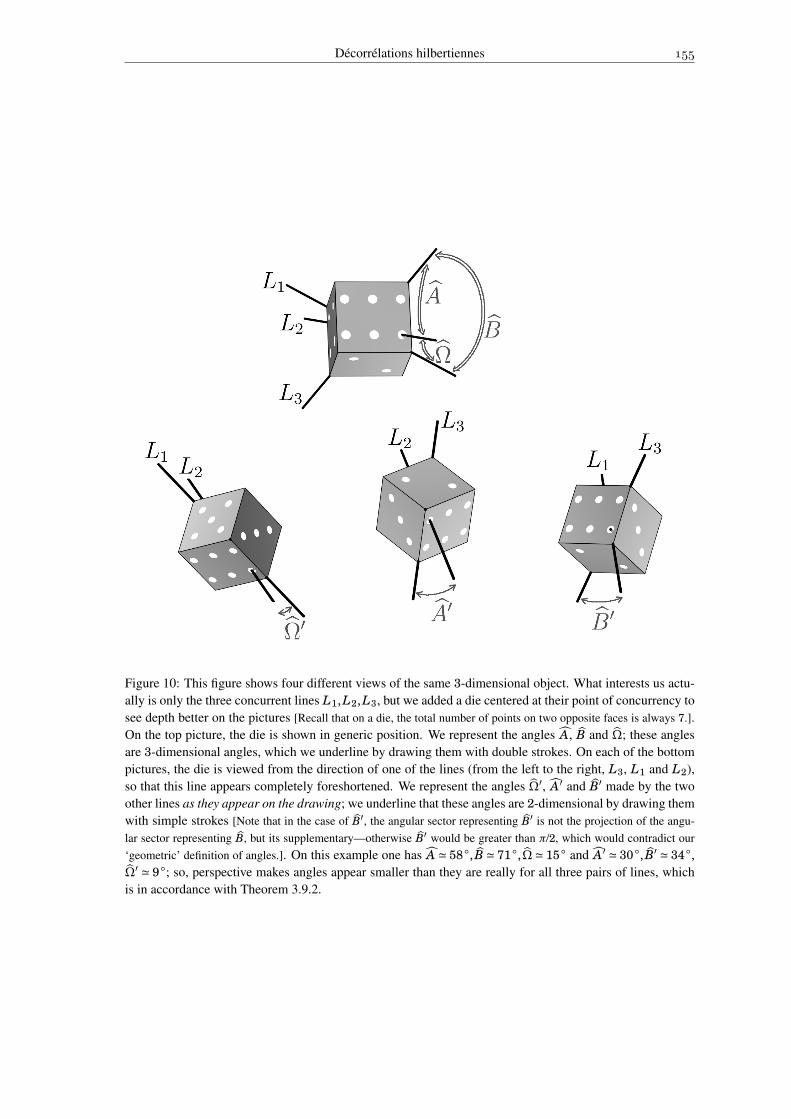
Décorrélations hilbertiennes
Figure 10: This figure shows four different views of the same 3-dimensional object. What interests us actu-ally is only the three concurrent lines L1,L2,L3, but we added a die centered at their point of concurrency tosee depth better on the pictures [Recall that on a die, the total number of points on two opposite faces is always 7.].On the top picture, the die is shown in generic position. We represent the angles A, B and Ω; these anglesare 3-dimensional angles, which we underline by drawing them with double strokes. On each of the bottompictures, the die is viewed from the direction of one of the lines (from the left to the right, L3, L1 and L2),so that this line appears completely foreshortened. We represent the angles Ω′, A′ and B′ made by the twoother lines as they appear on the drawing; we underline that these angles are 2-dimensional by drawing themwith simple strokes [Note that in the case of B′, the angular sector representing B′ is not the projection of the angu-lar sector representing B, but its supplementary—otherwise B′ would be greater than π/2, which would contradict our‘geometric’ definition of angles.]. On this example one has A ' 58, B ' 71,Ω' 15 and A′ ' 30, B′ ' 34,Ω′ ' 9; so, perspective makes angles appear smaller than they are really for all three pairs of lines, whichis in accordance with Theorem 3.9.2.

Chapter 4
Other applications of tensorizationtechniques
In the previous chapter we have been seeing how Hilbertian decorrelation hypotheses betweenpairs of variables could yield ‘global’ results on an arbitrary number of variables, by splittingfunctions of several variables into relevant telescopic sums. I used the word “tensorization” toqualify these results, as the conclusions were of the same nature as the hypotheses.
But the techniques of § 3 can also be applied to get other types of results. In this chapter I amgoing to show how, from Hilbertian decorrelation hypotheses, one can get results on some classicalfeatures of particle systems which are not linked with Hilbertian correlations a priori.
I will deal with two such features. First, I will look at the implications of ρ-mixing on theexistence of a central limit theorem—more precisely, of a spatial central limit theorem, since I ammore interested in random fields than in sequences (variables indexed by Zn rather than by Z).Very sharp results concerning this issue are already known; however, I find interesting to show howit goes with my ‘tensorization-like’ approach: this approach takes indeed a quite different way todo the job, which may be neater by certain sides. Moreover, the results are stated with a slighltydifferent vocabulary—namely, subjective Hilbertian correlations.
Next, I will look at the question of spectral gap for Glauber dynamics. Though this point hasalready been thouroughly studied in a β-mixing paradigm, this work, to the best of my knowledge,is the first to show how ρ-mixing can be used to tackle this issue.
My main goal here is just to show how the techniques of this work may be applied to theproblems of spatial central limit theorem and convergence of the Glauber dynamics. Accordingly,I favoured the simplicity on proofs against the refinement of the results.
4.1 Spatial central limit theorem
4.1.a Introduction
A fundamental result in probability theory is the central limit theorem (CLT), which, in itsstandard statement, requires an assumption of complete independence. It is natural to wonderwhether that assumption can be relaxed into an hypothesis of ‘near independence’. Hilbertian
Décorrélations hilbertiennes
decorrelations are a natural frame for such a generalization, since the CLT already takes place inan L2 setting.
Our point of view is motivated by statistical physics. Let Zn be a lattice, on each vertex i ofwhich there is a random ‘spin’ X i ranged in some space X not depending on i. We assume thatthe law of the system is translation invariant, i.e. that for all z ∈ Zn, (X i+z)i∈Zn has the same lawas
→XZn . Then, for all z ∈Zn, we denote
εz = X i : X i+z∗. (NP)
We are interested in situations where the εz are sufficiently ‘rapidly decreasing’ as |z|→∞ so that∑z∈Zn εz <∞.
Let f : X → R be a function such that f (X0) is square-integrable and centered. The questionis, does one get a CLT when summing f (X i) for i in a large subset of Zn, i.e., does the sum growas the square root of the number of its terms and have asymptotically normal distribution? Forinstance, we would like the law of the variable
1pln
∑i∈Zn
0Éi1,...,in<l
f (X i) (NQ)
to weakly converge, when l →∞, to some Gaussian distribution.
4.1.1 Remark. Note that the limit distribution, if it exists, will have to be centered, but its variancewill not be equal to Var( f (X0)) in general. ♥
In the case n = 1, extremely sharp results for this topic have been known from long; let us cite,among many others, [71, 40, 62, 10]. For n Ê 2, similar results also exist; see e.g. [10, Theorem 5]for such a result, and [12, § 29] for a survey of the topic. All these proofs relie on some ‘coupling’between (bunches of) the spins and other convenient variables which are close to them, but whichare actually independent, so as to deduce the CLT for the former from the CLT for the latter. On theother hand, my proof will mimick Lévy’s proof of the CLT, hence needing no coupling argument.
A priori the results presented here do not improve the state of the art; however, when turning toquantitative versions of these results, it is likely that the difference between the usual method andmine would yield a difference in the corresponding non-asymptotic bounds obtained.
4.1.b Product of weakly coupled variables
My results relie on the following
4.1.2 Lemma. Let N Ê 1 and let.
F1, . . . ,.
FN be σ-algebras with .
Fi :.
F j∗ É εi j[∗], and denote
ε= supi
∑j 6=iεi j. (NR)
Let Φ1, . . . ,ΦN be complex-valued random variables with |Φi| É 1 a.s., such that Φi is.
Fi-measurable for all i, with all the Φi having the same distribution. Then, denoting by ϕ the commonvalue of the E[Φi],
|E[∏
iΦi]−ϕN|É Nε(1+ ε)(1−|ϕ|2). (NS)
♣[∗]. As in § 3.6, “∗” stands for “the natural σ-metalgebra of the system”. Moreover, in the same way as in § 3.4.a, it
is actually possible in the statement of the lemma to replace that σ-metalgebra by smaller ones.
Quelques problèmes d’inspiration physique en théorie des probabilités
Proof. Denote δ ··= Sd(Φ). Since E[|Φ2|] É 1, the definition of (complex) variance ensures thatδÉ
√1−|ϕ|2.
For all i ∈ 0, . . . , N, denote Fi ··=∨i′Éi
.Fi ; denote Ψ(i) ··=∏
i′ÉiΦi′ ; define
Ψ(i)j ··= (Ψ(i))F j −E[Ψ(i)|F j−1] (NT)
and denote ∆(i)j ··=Sd(Ψ(i)
j ). Also denote
Φi, j ··= (Φi)F j −E[Φi|F j−1]. (NU)
Usual manipulation on conditioning shows that, for i Ê 1,
Ψ(i)j =Ψ(i−1)
j (Φi)F j +Ψ(i−1)j−1 Φi, j. (NV)
Since ‖Φi‖L∞ É 1, one has also ‖(Φi)F j‖L∞ É 1, hence
Sd(Ψ(i−1)j (Φi)F j)ÉSd(Ψ(i−1)
j )=∆(i−1)j . (NW)
Similarly, it is obvious that ‖Ψ(i−1)‖L∞ É 1, whence
Sd(Ψ(i−1)j−1 Φi, j)ÉSd(Φi, j). (NX)
Now, I claim that
4.1.3 Claim.Sd(Φi, j)É εi jδ. (NY)
♣
Proof of Claim 4.1.3. Conditionally to F j−1, Φi, j is indeed the projection on.
F j of the centered.Fi-measurable function (Φi −E[Φi|F j−1]), whose standard deviation is less than Sd(Φi) = δ byassociativity of the variance, so that Sd(Φi, j)É
.Fi :
.F jF j−1δÉ εi jδ. ♠
In the end, we got that∆i
j É∆(i−1)j +εi jδ. (NZ)
Since ∆0j = 0, one has therefore:
∀i, j ∆ij É (1+ ε)δ. (OA)
Now, denoting ψ(i) ··=E[Ψ(i)], one has
|ψ(i) −ϕψ(i−1)| = |∑j<i
E[Ψ(i−1)j Φi, j]|É ∑
j<i∆(i−1)
j Sd(Φi, j)É ε(1+ ε)δ2, (OB)
and finally
|ψ(N) −ϕN | =N∑
i=1|ϕ|N−i|ψ(i) −ϕψ(i−1)|É
N∑i=1
|ψ(i) −ϕψ(i−1)|É Nε(1+ ε)δ2, (OC)
which is (NS) if you recall that δ2 É 1−|ϕ|2. ♠
Décorrélations hilbertiennes
4.1.c A spatial CLT
First I state and prove a CLT on cubes:
4.1.4 Theorem. Consider a translation-invariant spin model on a lattice Zn and define εz by (NP).Assume that
∑z∈Zn εz < ∞. Then for any centered square-summable function f : X → R, there
exists a constant σ<∞ such that1pln
∑i∈Zn
0Éi1,...,in<l
f (X i)l→∞* N (σ2), (OD)
where “*” denotes convergence in law. ♣
Proof. Denote by F(l) —or merely F —the left-hand side of (OD).
What will be the value of σ? Clearly we must have
σ2 = liml→∞
Var(F(l)), (OE)
which yieldsσ=
√∑z∈Z
E[ f (X0) f (X z)], (OF)
where the expression under the root sign, which is necessarily nonnegative, is finite because|E[ f (X0) f (X z)]| É εz Sd( f (X0))Sd( f (X z))= εz Var( f ). By the way, we will denote
σ2∗ ··= (
∑zεz)‖ f ‖2
L2 . (OG)
Fix some arbitrary η > 0. The assumption that∑εz < ∞ implies the existence of an l0 < ∞
such that ∑|z|∞>l0
εz É η, (OH)
where |z|∞ denotes max(|z1|, . . . , |zn|). By (OE), we can also fix an l1 <∞ such that
|Var(F(l))−σ2|É η. (OI)
Now we will ‘tile’ the cube of size l into a ‘patchwork’ made of cubes of size l1 which I call“tiles”, each tile being at distance at least l0 from the others, plus some “scrap”. I denote by
~F the
part of F due to the tiles and by F∗ the part of F due to the scrap.
Index the tiles by 1, . . . , N, with N ··= b(l + l0) / (l1 + l0)cn. We write, with obvious notation,~F =·· F1 +·· ·+FN . For λ ∈R, denote
Ψ(λ, l) ··= exp(iλ~F), ψ(λ, l) ··=E[Ψ(λ, l)]; (OJ)
Φ j(λ, l) ··= exp(iλF j), ϕ(λ, l) ··=E[Φ j(λ, l)]. (OK)
Then we are exactly in situation of applying Lemma 4.1.2, which yields:
|ψ(λ, l)−ϕ(λ, l)N |É Nη(1+η)(1−|ϕ(λ, l)|2). (OL)
Let us look at the asymptotics of Formula (OL) when l →∞. We observe that, denoting
Ft ··= 1√ln1
∑i∈ fixed tile
f (X i), (OM)

Quelques problèmes d’inspiration physique en théorie des probabilités
one has
F jlaw=
√ln1p
lnFt. (ON)
Since Ft is centered, its Fourier transform satisfies Ft(0)= 1, F ′t(0)= 0 and F ′′
t =Var(Ft), so that
liml→∞
ln(1−ϕ(λ, l))= λ2
2ln1 Var(Ft), (OO)
where, denoting σ2l1··=Var(Ft), we recall that l1 has been taken sufficiently large so that |σ2
l1−σ2| É
η. Then, since N l→∞∼ ln / (l1 + l0)n, one has the following asymptotics for (OL):
ϕ(λ, l)N l→∞→ exp[−σ2
l1
( l1
l1 + l0
)nλ2
2
]; (OP)
N(1−|ϕ(λ, l)|2) l→∞→ σ2l1
( l1
l1 + l0
)nλ2. (OQ)
It remains to control the contribution of F∗.
4.1.5 Claim. There are at most [1−
( l1
l1 + l0
)n]ln +nl1ln−1 (OR)
scrap spins. ♣
By Claim 4.1.5,
‖F∗‖L1 ÉVar(F∗)É[1−
( l1
l1 + l0
)n+n
l1
l
]σ2∗; (OS)
then the contribution of F∗ is controlled using the following immediate
4.1.6 Lemma. Let X and H be real random variables with ‖H‖L1 <∞. Then, for λ ∈R,
|E[eiλ(X+H)]−E[eiλX ]|É |λ|‖H‖L1 . (OT)
♣
In the end, putting everything together we get:
liml→∞ |ψ(λ, l)− e−σ
2λ2/2|É
|e−(σ2 −η)[l1 / (l1 + l0)]nλ2/2− e−σ2λ2/2|+η(1+η)
( l1
l1 + l0
)n(σ2 +η)λ2 +
√1−
( l1
l1 + l0
)nσ∗. (OU)
Since there were no upper restriction on the value of l1, we can assume that we have taken it suchthat [l1 / (l1 + l0)]n Ê 1−η. Then (OU) becomes:
liml→∞ |ψ(λ, l)− e−σ
2λ2/2|É |e−(σ2 −η)(1−η)λ2/2− e−σ2λ2/2|+η(1+η)(1−η)(σ2+η)λ2+p
ησ∗. (OV)
The right-hand side of (OV) can be made arbitrarily close to 0 by taking η small enough, so we haveproved that
∀λ ∈R E[eiλF(l)] l→∞→ e−σ2λ2/2. (OW)
By Lévy’s theorem on characteristic functions, this is tantamount to saying that F(l) converges inlaw to N (σ2). ♠
Décorrélations hilbertiennes
The CLT should remain valid for other shapes than a cube, since morally the random fieldf (X i) should look like a Gaussian white noise at large scales. Indeed, the same proof as aboveyields a CLT for general shapes, where moreover convergence is uniform in the shape consideredin some way. Let us give a precise statement:
4.1.7 Definition. An open subset U ⊂Rn (not necessarily connected) is said to be C 2 if its bound-ary M is a C 2 submanifold of Rn (of codimension 1). We define the roughness of U , denotedby κ(U), as
κ(U) ··= supx∈M
II(x), (OX)
where II(·) denotes the shape tensor of M [38, Chapter 10], which measures the local deviationof M from being flat. Also, the Lebesgue measure of U will be denoted by vol(U). ♦
4.1.8 Theorem. Consider a translation-invariant spin model on a lattice Zn and define εz by (NP).Assume that
∑z∈Zn εz <∞. Then for any centered square-summable function f : X →R, if (Uk)k∈N
is a sequence of C 2 bounded subsets of Rn with supkκ(Uk) < ∞ and (lk)k∈N is a sequence ofpositive numbers tending to infinity,
1√lnk vol(Uk)
∑i∈lkUk∩Zn
f (X i)k→∞* N (σ2), (OY)
where σ2 is the same as in Theorem 4.1.4. ♣
Proof. Just copy the proof of Theorem 4.1.4. The only difference lies in proving the analoguousof Claim 4.1.5, which is where one needs the κ(Uk) to be bounded. Observe that we use the non-asymptotic form of our intermediate bounds to get a result independent of the precise shape ofthe Uk. ♠
4.1.9 Remark. Another generalization of the CLT, still based on the idea that the field f (X i) lookslike a Gaussian white noise at large scales, is the statement that for ϕ a continuous function withcompact support,
1pln
∑i∈Zn
ϕ(X i / l) f (X i)l→∞* N (σ2∫
Rn ϕ(x)2 dx). (OZ)
This can be proved with the same methods as before. ♥
4.2 Spectral gap for the Glauber dynamics
4.2.a Introduction
In this section we are looking at a probabilistic system made of a large number of ‘elementary’random variables (X i)i∈I — I may be seen as lattice and X i as the state of the particle being atsite i. As is customary by now, theorems will only be stated in the case where I is finite, the infinitecase being got by passing to the limit.
4.2.1 Definition. Denoting by Ω the states space of→X I , let P be a probability measure on Ω.
The Glauber dynamics [35, 26] associated to P is the Markov process on Ω having the followinglaw: on each i ∈ I there is an alarm clock, all the clocks being independent and ringing with lawPoisson(1). When a clock rings, the state of spin X i —and only it—is flipped so that the state of X i
immediately after the flip follows the law P(X i|→X Iài).
Quelques problèmes d’inspiration physique en théorie des probabilités
In formal terms, the Glauber dynamics is the Markov process whose generator L on L∞(Ω) isdefined by:
(L f )(→xI )= ∑i∈I
E[ f (→X I )− f (→xI )| →
X Iài = →xIài]. (PA)
♦
Let us recall some basic facts on the Glauber dynamics (see [47, Chapter IV] for more de-tails). By construction P is a reversible equilibrium measure for the dynamics, so L is self-adjointon L2(P). Since obviously L 1 ≡ 0, one can also define L on L2(P), on which it is self-adjointtoo. This leads to the following definition:
4.2.2 Definition. The energy of f ∈ L2(P) is
E ( f , f )= ⟨Lf , f ⟩ (PB)
♦
The following immediate identity shows that E is always a nonnegative bilinear form:
4.2.3 Proposition.E ( f , f )=
∫Ω
dP[→xI ]∑
iVar( f | →
X Iài = →xIài). (PC)
♣
4.2.4 Definition. For λ > 0, the Glauber dynamics is said to have spectral gap Ê λ if, for all f ∈L2(P),
E ( f , f )ÊλVar( f ). (PD)
♦
What makes spectral gap interesting is that its positiveness is equivalent to exponential conver-gence to 0 of the semigroup (e−tL )tÊ0 on L2(P), the rate of convergence being equal to the widthof the spectral gap. As the Glauber dynamics is one of the easiest ways to simulate the law P forcomplicated models, the stake of having exponential convergence for it is evident.
Many works have been done on the spectral gap of the Glauber dynamics, see for instanceMartinelli’s St-Flour course [52]. Several results state that, the less spins are correlated, the largerthe spectral gap is. Yet the researchers who work on this topic generally express the decorrelationbetween the spins in terms of β-mixing (cf. Definition 0.1.4), while it seems be more natural tolook at them in terms of Hilbertian decorrelations, since the formula (PD) stating the spectral gapproblem takes place in a Hilbertian frame itself. Thus my goal here will be to find a control on thespectral gap expressed in terms of ρ-mixing conditions. Since Hilbertian correlations look to be theminimal frame to study the spectral gap for the Glauber dynamics, hopefully the bounds yieldedby this method will be sharp.
Another noticeable feature of my approach is that it remains at a quite abstract level: no sym-metry property of I or P need be assumed, all the work essentially consisting in manipulatingrelevant quadratic forms.
Décorrélations hilbertiennes
4.2.b A lower bound for the spectral gap
The central theorem of this section is the following:
4.2.5 Theorem. Take I = 1, . . . , N. Suppose that for all distinct i, j ∈ I one has X i : X j∗ É εi j < 1—we will make the costless assumption that ε ji = εi j. For i ∈ I, denote
~1i ··= 1∏
i< jÉN (1−ε2i j)
=~εiN
εiN, (PE)
and for i < j, denote~εi j ··=
εi j∏i< j′É j(1−ε2
i j′). (PF)
Then the Glauber dynamics has spectral gap at least M−2, where M is the (N × N) matrixdefined by
M =
1 −~
ε12 · · · −~ε1N
0. . . . . .
......
. . . . . . −~ε(N−1)N
0 · · · 0 1
−1
~11 0 · · · 0
0. . . . . .
......
. . . . . . 00 · · · 0
~1N
. (PG)
♣
4.2.6 Remark. The form of the first matrix in the right-hand side of (PG) ensures that it is invertible.Since moreover all the εi j were supposed < 1, all the ~
εi j and the~1i are finite; thus, the lower
bound M−2 is strictly positive. ♥
Proof. Let f be a centered square-integrable function on (Ω,P). For I ′ ⊂ I, denote FI ′ ··=σ(→X I ′).
For i ∈ I, I ′ ⊂ I à i, denotef I ′
i ··= f FI′]i −E[ f |FI ′]; (PH)
define moreover
f 6=i ··= f Iàii ; (PI)
f <i ··= f 1,...,i−1i . (PJ)
Then by Proposition 4.2.3, one has
E ( f , f )=∑i
Var( f 6=i ), (PK)
while the usual telescopic argument shows that
Var( f )=∑i
Var( f <i ). (PL)
So to prove the theorem, we have to establish links between the different values Var( f I ′i ). It
will be convenient to introduce the shorthands ∆I ′i =Sd( f I ′
i ). One has the following
4.2.7 Claim. For I ′ ⊂ I and i, j ∈ I à I ′ with j 6= i,
∆I ′i É∆I ′] j
i +εi j∆I ′j . (PM)
♣
Quelques problèmes d’inspiration physique en théorie des probabilités
Proof. Assume in a first time that I ′ =;, and denote f i ··= f ;i , f j ··= f ;j , f ji ··= f j
i and Fi ··= Fi.
Projecting the decomposition “ f i = f ji + ( f i − f j
i )” on L2(Fi), one has f i = ( f ji )Fi + ( f j)Fi , whence
by the Cauchy–Shwarz inequality:
Sd( f i)ÉSd(( f ji )Fi)+Sd(( f j)Fi). (PN)
One has trivially Sd(( f ji )Fi) É Sd( f j
i ); on the other hand, f j is X j-measurable, so Sd(( f j)Fi) Éεi j Sd( f j). In the end, (PN) becomes
Sd( f i)ÉSd( f ji )+εi j Sd( f j), (PO)
which is (PM) for I ′ =;.
In the case I ′ 6= ;, the same reasoning can be performed, except that one have to work condi-tionally to FI ′ . Then, taking f i = f I ′
i , f j = f I ′j , f j
i = f I ′] ji , Fi =FI ′]i, one gets
Sd( f i|FI ′)ÉSd( f ji |FI ′)+εi j Sd( f j|FI ′). (PP)
Now
Sd( f i)=√∫
Sd( f i|→X I ′ = →xI ′)2dP[→xI ′], (PQ)
with similar formulas for f j and f ji , since all these functions are centered w.r.t. FI ′ . Therefore,
integrating (PP) and applying Minkowski’s inequality yields:
Sd( f i)ÉSd( f ji )+εi j Sd( f j), (PR)
i.e. (PM). ♠
For i É j, let us denote∆
[ j]i =∆1,..., jài
i . (PS)
Claim 4.2.7 will be used through the following corollary:
4.2.8 Claim. For all i < j,
∆[ j−1]i É 1
1−ε2i j
(∆[ j]i +εi j∆
<j ). (PT)
♣
Proof. We have to bound ∆[ j−1]i , which here we rather denote ∆[b−1]
a to avoid confusion with thenotation of Claim 4.2.7. Applying Claim 4.2.7 with I ′ = 1, . . . ,b−1à a, i = a and j = b, one has
∆[b−1]a =∆1,...,b−1àa
a É∆1,...,bàaa +εab∆
1,...,b−1àab =∆[b]
a +εab∆1,...,b−1àab . (PU)
But applying again Claim 4.2.7, this time with I ′ = 1, . . . ,b−1à a, i = b and j = a, one has
∆1,...,b−1àab É∆1,...,b−1
b +εab∆1,...,b−1àaa =∆<
b +εab∆[b−1]a . (PV)
Combining (PU) and (PV) then yields (PT). ♠
Décorrélations hilbertiennes
Now let us show how Claim 4.2.8 implies the theorem. To avoid heavy formalism, I will detailthe computations for I = 1,2,3,4 (rather denoted by I = a,b, c,d here to avoid confusions with“1” and “2” taken as numbers), hoping that generalizing is obvious then.
First, note that∆<
d =∆6=d . (PW)
Now, by a direct use of Claim 4.2.8,
∆<c =∆[c]
c É 11−ε2
cd(∆[d]
c +εcd∆<d)=
~1c∆
6=c +~
εcd∆6=d . (PX)
To bound ∆<b , we have to iterate Claim 4.2.8 twice:
∆<b =∆[b]
b É 11−ε2
bc∆[c]
b +~εbc∆
<c
É 1(1−ε2
bc)(1−ε2bd)
(∆[d]b +εcd∆
<d)+~
εbc∆<c =~
1b∆6=b +~
εbd∆6=d +~
εbc∆<c
É(PX)
~1b∆
6=b +~
1c~εbc∆
6=c + (~εbd +~
εbc~εcd)∆6=
d . (PY)
Last, bounding ∆<a requires iterating Claim 4.2.8 three times:
∆<a =∆[a]
a É 11−ε2
ab∆[b]
a +~εab∆
<b
É 1(1−ε2
ab)(1−ε2ac)∆[c]
a +~εac∆
<c +~
εab∆<b É~
1a∆6=a +~
εad∆<d +~
εac∆<c +~
εab∆<b
É(PX,PY)
~1a∆
6=a +~1b
~εab∆
6=b +~
1c(~εac +~εab
~εbc)∆6=
c + (~εad +~εac
~εcd +~
εab~εbd +~
εab~εbc
~εcd)∆6=
d . (PZ)
One can sum up Equations (PW)–(PZ) into the matricial expression∆<
a∆<
b∆<
c∆<
d
É
1 ~
εab~εac +~
εab~εbc
~εad +~
εac~εcd +~
εab~εbd +~
εab~εbc
~εcd
0 1 ~εbc
~εbd +~
εbc~εcd
0 0 1 ~εcd
0 0 0 1
~1a∆
6=a~
1b∆6=b~
1c∆6=c
∆6=d
. (QA)
If we look back at how the square matrix in (QA) has been constructed, we find that
squarematrix
in(QA)
=∞∑
k=0
0 ~
εab~εac
~εad
0 0 ~εbc
~εbd
0 0 0 ~εcd
0 0 0 0
k
=
1 −~
εab −~εac −~
εad
0 1 −~εbc −~
εbd
0 0 1 −~εcd
0 0 0 1
−1
, (QB)
so in the end we obtain that ∆<
a∆<
b∆<
c∆<
d
É M
∆6=
a
∆6=b
∆6=c
∆6=d
, (QC)
where M is given by (PG). Then it is immediate that Var( f ) = ∑i (∆<
i )2 É M2 ∑i (∆6=
i )2 =M2 E ( f , f ), QED. ♠
Quelques problèmes d’inspiration physique en théorie des probabilités
The bound we have obtained for the spectral gap is not symmetric by permutation of the indexesin I. It can however can be bounded by a simpler expression, which is nearly as good as the originalone in concrete situations:
4.2.9 Corollary. In Theorem 4.2.5, M can be replaced by the matrix
M′ =
1 −ε12 · · · −ε1N
−ε12. . . . . .
......
. . . . . . −ε(N−1)N
−ε1N · · · −ε(N−1)N 1
−1
, (QD)
provided ρ(IN −M′)< 1. ♣
Proof. Each entry of M is actually bounded by the corresponding entry of M′. To see it, we‘expand’ the entries of M, resp. M′. First, notice that 1/(1−ε2
i j) can be expanded into 1+εi jε ji +εi jε jiεi jε ji +·· · , so that one has the expansions
~1i =
∑i< j1É···É jk
k∏l=1
εi jlε jl i (QE)
and~εi j =
∑i< j1É···É jkÉ j
(k∏
l=1εi jlε jl i)εi j. (QF)
Then, using the inversion formula (I− A)−1 =∑∞k=0 Ak for triangular arrays, one obtains that
Mi j =∑
(i0,i1,...,ik)first condition
k−1∏l=0
εi l i l+1 , (QG)
where the meaning of “first condition” is given by the following
4.2.10 Definition. A sequence (i0, . . . , ik) is said to satisfy the first condition if:
(i) i0 = i and ik = j;(ii) i l 6= i l+1 for all l;
(iii) i l+1 < i l only if l Ê 1 and i l+1 = i l−1;(iv) If i l+1 < i l and l É k−2, then i l+2 Ê i l .
♦
One has a similar formula for M′:
M′i j =
∑(i0,i1,...,ik)
second condition
k−1∏l=0
εi l i l+1 , (QH)
where
4.2.11 Definition. A sequence (i0, . . . , ik) is said to satisfy the second condition if it satisfies Con-ditions (i) and (ii) of Definition 4.2.10. ♦
Since the second condition is obviously weaker than the first condition, one has Mi j É M′i j.
♠
Décorrélations hilbertiennes
There is a still weaker but even simpler formula:
4.2.12 Corollary. Defining
ε : L2(I) → L2(I)(ai)i∈I 7→ (
∑j 6=i εi ja j)i∈I ,
(QI)
the spectral gap of the Glauber dynamics is at least
(1−ε)2+. (QJ)
♣
Proof. One has M′ = (I−ε)−1, so, provided A< 1,
M′=(I− A)−1= ∞∑k=0
AkÉ∞∑
k=0Ak = (1−A)−1. (QK)
In the case AÊ 1, (QJ) is trivial. ♠
4.2.c Avoiding the articial phase transition
A common situation in which we would like to apply the previous results is when I = Zn andεi j is of the form ε( j− i) for some symmetric function ε : Zn → [0,1]. Then Corollary 4.2.12 tellsthat the Glauber dynamics has a (strictly) positive spectral gap as soon as
∑z 6=0 ε(z)< 1. But like in
§ 3.6.c, we are going to prove that that bound is somehow ‘artificial’ and that it can be relaxed intothe neater condition “
∑z 6=0 ε(z)<∞”:
4.2.13 Theorem. Suppose that I = Zn and that for all i, j ∈ Zn one has X i : X j∗ É ε( j− i) forsome symmetric function ε: Zn → [0,1] such that ε(z)< 1 as soon as z 6= 0. Then if
∑z∈Zn ε(z)<∞,
the spectral gap of the Glauber dynamics is positive. ♣
Proof. The assumption on∑
z ε(z) allows us to take l <∞ large enough so that∑z∈lZnà0
ε(z)< 1. (QL)
We split Zn into a partition of ln =·· N sublattices Z1, . . . , ZN , each lattice Zu being of the formlZn + zu for some zu ∈Zn/lZn. Then we define an auxiliary dynamics:
4.2.14 Definition. The sublattice Glauber dynamics is the Glauber dynamics for→XZn considered
as the finite-dimensional vector (→XZ1 , . . . ,
→XZN ). In other words, on each u ∈ 1, . . . , N there is an
independent Poisson(1) alarm clock, and when clock u rings, the state of the whole→XZu is flipped
in one shot according to P(XZu |→XZnàZu). ♦
Now let f ∈ L2(Ω). In addition to the notation of the proof of Theorem 4.2.5, we introduce thefollowing definition:
4.2.15 Definition. For u ∈ 1, . . . , N, we define
f 6=(u) ··= f −E[ f | →XZnàZu]. (QM)
♦

Quelques problèmes d’inspiration physique en théorie des probabilités
4.2.16 Remark. The f 6=(u) are the equivalent of the f 6=i for the sublattice Glauber dynamics. ♥
Fixing some ‘boundary condition’ →xZnàZu on Zn à Zu, we can apply Corollary 4.2.12 to theGlauber dynamics for
→XZu under the law P[·| →
XZnàZu = →xZnàZu]. After integrating, one gets that
Var( f 6=(u))É (1−ζ)−2 ∑i∈Zu
Var( f 6=i ), (QN)
where ζ is the operator on L2(lZn) defined by
(ζg)(i)=∑
z∈lZnà0ε(z)g(i+ z), (QO)
whose norm is obviously bounded by∑
z∈lZnà0 =·· ζ< 1. Then, summing (QN) for all u:
N∑u=1
Var( f 6=(u))É (1−ζ)−2E ( f , f ). (QP)
Now, let us apply Theorem 4.2.5 to the sublattice Glauber dynamics [Definition 4.2.14]. Ityields that
Var( f )ÉM2N∑
u=1Var( f 6=(u)), (QQ)
where M is some (N × N) matrix depending on the →XZu :
→XZv ∗. But by Theorem 3.6.8,
→XZu :
→XZv ∗ < 1 for all u 6= v, thus M < ∞ by Remark 4.2.6. Combining (QP) and (QQ), we
finally get that the spectral gap of the Glauber dynamics for→XZn is bounded below by M−2 ×
(1−ζ)2 > 0. ♠
4.2.17 Remark. Like Theorem 3.6.8, Theorem 4.2.13 could actually be stated in the general caseof ‘abstract’ metric spaces on which some group acts profinitely. ♥

Chapter 5
Concrete examples
It is now time to see what the results of Chapters 3 and 4 yield for concrete models of statisticalphysics. I will try to give rather different types of examples, so as to illustrate the advantages ofworking with Hilbertian correlations: this frame is indeed quite general, as it requires little structureon the models considered.
In § 5.1 we will look back at Ising’s model, seeing how tensorization of Hilbertian decorrela-tions improves the results of § 0.1, and what other results are given by the theorems of § 4. We willalso consider two kinds of generalizations, namely when the range of interactions becomes infiniteand when the strength of the interactions is random (spin glasses). In the two next sections we willlook at models with continuous states spaces: first a quite general class of linear models [§ 5.2],then a family of nonlinear models [§ 5.3]. Finally in § 5.4 we will see how one can consider timeas a supplementary dimension of the system to get contractivity results for non-reversible Markovchains (hypocoercivity) on an infinite system of particles.
* In this chapter, all the probability systems considered will be endowed with their naturalσ-metalgebras, cf. Definition 3.1.16. To alleviate notation, I will give no names to these σ-metalgebras, but will plainly write “X : Y ∗” to mean “the subjective decorrelation between Xand Y seen from the natural σ-metalgebra of the underlying system”.
5.1 Back to Ising’s model
5.1.a Standard Ising’s model
In all this section, we work on the lattice Zn equipped with its natural distance dist; accordingly|·| will denote the l1 norm on Rn. Recall the definition of Ising’s model and the related notationthat we introduced in § 0.1, and Theorem 0.1.7 on the existence of a completely analytical regime.
The following theroem states that Ising’s model in completely analytical regime is ρ-mixing,i.e. that two distant bunches of spins are little correlated in the sense of maximal correlation:
5.1.1 Theorem. For Ising’s model on Zn in the completely analytical regime,
(i) There exists some ψ′ > 0 (the same as in Theorem 0.1.7) such that for all disjoint I, J ⊂ Zn,one has when dist(I, J)→∞ that
→ωI : →
ωJÉ exp[− (ψ′+ o(1))dist(I, J)], (QR)
Quelques problèmes d’inspiration physique en théorie des probabilités
where the “o(1)” can be easily computed as an explicit function of dist(I, J), n, T, ψ′ andthe C′ appearing in Theorem 0.1.7.
(ii) There exists some k < 1 such that for all disjoint I, J ⊂Zn,
→ωI : →
ωJÉ k. (QS)
(iii) Points (i) and (ii) remain valid uniformly under any law of the form P[·|→ωK = →ωK ], for K ⊂Zn
and→ωK ∈ ±1K a ‘boundary condition’ on K .
♣
5.1.2 Remark. Let us compare Theorem 5.1.1 with Theorem 0.1.7. Both theorems state decorrela-tion between distant bunches of spins above temperature T ′
c; the difference relies in using ρ-mixingrather than β-mixing to quantify dependence between the bunches in Theorem 5.1.1.
Both results give an exponential decay of correlations, with the same exponential constant ψ′,but Theorem 5.1.1 is more powerful in the sense that the bound (QR) is uniform in the size of Iand J while (E) was not. Moreover, thanks to Point (ii) we get a non-trivial result for any choice ofdisjoint I and J, which was not the case beforehand. Recall that the drawbacks of Theorem 0.1.7were inherent to β-mixing, as Theorem 0.1.8 shew.
Both result remain valid under conditioning. However, if one takes a random boundary condi-tion—that is, if one works under the law P[·|→ωK ∈ C] for some non-singleton C ⊂ ±1K —, thenPoint (iii) of Theorem 5.1.1 fails (cf. Remark 3.1.4), while (E) is still valid by convexity of the totalvariation norm. ♥5.1.3 Remark. Let us compare Theorem 5.1.1 with Theorem 0.1.9. The result of Theorem 0.1.9can be rewritten:
→ω0×Zn−1 : →
ωx×Zn−1É e−ψx. (QT)
Theorem 5.1.1 can be seen as a generalization of that result to the case where I and J have arbitraryshapes. [∗] Moreover, Point (iii) also gives the existence of a conditional version, which we did nothave before.
There is however a price to pay for this greater generality, since we had to require completeanalyticity rather than just weak mixing, which can be really more restrictive in some cases (cf.Footnote [∗] on page 84). ♥5.1.4 Remark. Continuing the previous remark, a natural open question is whether one can ten-sorize maximal decorrelation under assumptions of weak mixing type. In the case of Ising’s modelat least, I expect ρ-mixing to remain true—even for arbitrary shapes—as soon as T > Tc, becauseon the one hand Theorem 0.1.9 proves ρ-mixing between parallel hyperplanes, while on the otherhand ρ-mixing seems to hold also in the ‘opposite extreme case’ when I and J make a checkpattern.
By the way, it is likely that the natural condition should not be weak mixing itself but rathersomething like strong mixing for cubes (often called merely strong mixing [†], which means thatwhen a boundary condition is fixed outside a cube of arbitrary edge, changing one spin on the
[∗]. Note that in the case I and J are hyperplanes, we shew on page 98 that (QR) could be improved into
→ω0×Zn−1 : →ωx×Zn−1É e−ψ
′x. (QU)
[†]. Strong mixing stricto sensu is actually the same as complete analyticity, so that mathematicians have got used toundermeaning “for cubes”—but strong mixing for cubes is strictly weaker than complete analyticity! [53, § 2].

Décorrélations hilbertiennes
boundary has an effect in total variation which decreases exponentially with the distance to thespin changed. In fact it has been proved [54] that in dimension 2, weak mixing is equivalent tostrong mixing. ♥
Proof of Theorem 5.1.1. Theorem 5.1.1 will be a direct consequence of the work of Chapter 3 assoon as we show that, denoting by ∗ the natural σ-metalgebra of the system (i.e. the σ-metalgebragenerated by the ωi), for all distinct i, j ∈Zn, one has
ωi :ω j∗ É c0C′e−ψ′dist(i, j) ∧k0 (QV)
for some explicit c0 <∞ and k0 < 1 only depending on n and T. Then indeed, Proposition 3.6.6yields
→ωI : →
ωJÉ ∑δ∈Zn
|δ|Êdist(I,J)
c0C′e−ψ′|δ| = c0C′ ∞∑
d=dist(I,J)#δ ∈Zn : |δ| = de−ψ
′d
dist(I,J)→∞∼ c0C′ ∞∑d=dist(I,J)
2ndn−1
(n−1)!e−ψ
′d ∼ c0C′2n
(n−1)!dist(I, J)n−1e−ψ
′dist(I,J)
= e−(ψ′+o(1))dist(I,J), (QW)
whence Point (i). Moreover, since ∑δ∈Znà0
|δ|Édist(I,J)
c0C′e−ψ′dist(i, j) <∞, (QX)
Point (ii) follows from Lemma 3.6.8, and finally (iii) is a consequence of § 3.4.b about subjectiveresults.
So, we have to prove (QV). Let→ωK ∈ ±1K , K ⊂Zn, be some arbitrary boundary condition, and
denote by Pcon the associated law, that is, Pcon =P[·|→ωK = →ωK ]; our goal is to show that under Pcon,
for all distinct i, j ∈Zn, one has ωi :ω jÉ c0C′e−ψ′dist(i, j) ∧k0.
The result is immediate if i ∈ K , resp. j ∈ K (since then ωi, resp. ω j, is constant and thusindependent of everything), so we assume i, j ∉ K . We begin with observing that if K is theset N(i) of all the neighbours of i, equilibrium at i implies that, whatever the boundary conditionmay be:
Pcon[ωi =−1],Pcon[ωi =+1]Ê (e4n/T +1)−1 (QY)
—the extremal cases being when→ωN(i) ≡ +1, resp.
→ωN(i) ≡ −1. Now in the general case K ⊂
Zn à i, Lawcon[ωi] is an average of laws of the form Law(ωi|→ωN(i) =→ωN(i)), so that (QY) remains
valid. Similarly, equilibrium on i, j gives that for all a,b ∈ ±1,
Pcon[ωi = a and ω j = b]Ê (e8n/T +2e(4n+2)/T +1)−1. (QZ)
Now, recall that the correlation level between two two-ranged variables can be computed byFormula (BD), where |pb
a− pa pb| is also β(X ,Y )/2. Thus the bound “ωi :ω jÉ C0e−ψ′dist(i, j)” is a
direct consequence of Theorem 0.1.7, with
c0 = 1/2(e4n/T +1)−1(1− (e4n/T +1)−1)
= tanh(4n/T)+1. (RA)
It remains to prove the bound “ωi :ω jÉ k0”. We will use the following corollary of (BD):
Quelques problèmes d’inspiration physique en théorie des probabilités
5.1.5 Lemma. With the notation of Remark 1.2.2, there exists a,b in the respective ranges of X ,Ysuch that
X : Y É 1−4pba. (RB)
♣
Proof of Lemma 5.1.5. The difference pba − pa pb gets its sign changed whenever a, resp. b,
changes, so there are some a and b for which this value is nonpositive; moreover, denoting by a,a′and b,b′ the respective ranges of X and Y , pb′
a′ − pa′ pb′is also nonpositive. Now one has
pa pb√pa pa′ pb pb′ ×
pa′ pb′√pa pa′ pb pb′ = 1, (RC)
so that either pa pb or pa′ pb′is É
√pa pa′ pb pb′ . Up to changing notation we can assume that it
is pa pb, and then
X : Y = |pba − pa pb|√
pa pa′ pb pb′ =pa pb − pb
a√pa pa′ pb pb′ É 1− pb
a√pa pa′ pb pb′ É 1−4pb
a. (RD)
♠
Combining Lemma 5.1.5 with (QZ), we then get the desired bound, with
k0 = 1−4(e8n/T +2e(4n+2)/T +1)−1 < 1. (RE)
♠
Formula (QV) is also what we need to apply the results of Chapter 4. Indeed, denoting ε(z) ··=X i : X i+z∗, it gives that
∑z∈Zn ε(z) <∞ with ε(z) < 1 as soon as z 6= 0, so that Theorems 4.1.8
and 4.2.13 yield respectively:
5.1.6 Theorem. In completely analytical regime, the spins Ising’s model satisfies the central limittheorem, in the sense that the conclusions of Theorem 4.1.8 hold for them. ♣
5.1.7 Theorem. In completely analytical regime, the Glauber dynamics for Ising’s model has a(strictly) positive spectral gap, and this remains valid uniformly if one fixes a ‘boundary condition’on the spins of some K ⊂Zn. ♣
5.1.8 Remark. As I told in Chapter 4, results of these kinds have already been studied by othermethods (see e.g. [10, 22] for the CLT and [52] for the spectral gap). For the standard Ising modelin completely analytical regime, which is “very nice”, these previous works apply well, so the twotheorems above are not new. They are interesting however because of the new method used toprove them, which is quite direct and likely to apply to a broader class of models. Such modelswill be presented in the sequel of this chapter. ♥
5.1.b Generalizations of Ising’s model
The previous results can be adapted to several kinds of generalizations of Ising’s model. Let usexpose some of them.
Décorrélations hilbertiennes
Long-range Ising models
A physically important case is the long-range Ising models on Zn. In these models, the statesspace is unchanged, but the Hamiltonian H becomes
H(→ω)=−1
2
∑i 6= j
J( j− i)ωiω j, (RF)
where J : Znà0→R is some symmetric function with non-compact support such that J(z) |z|→∞=O(|z|−(n+α)) for some α> 0.
Let us state a decorrelation result for this class of models. The frame of the proof of thefollowing proposition will work as well for the other generalizations of Ising’s model.
5.1.9 Proposition. There exists an temperature T1 <∞ such that, provided T Ê T1:
(i) Equilibrium for the long-range Ising model is unique;
(ii) Uniformly in i, j, ωi :ω j∗| j−i|→∞= O(| j− i|−(n−α));
(iii) There exists some k0 < 1 such that for all i 6= j, ωi :ω j∗ É k0.
♣
Proof. The principle of the proof consists in coupling two Glauber dynamics with different initialconditions. Recall that the Glauber dynamics is defined as follows: each spin has an independentclock ringing with rate 1, and when the clock of a spin rings, this spin is flipped so that its finalstate is drawn according to its equilibrium measure conditionnally to the state of all other spins.Namely, if the clock of spin i rings at time t, denoting as usual β= T−1,
P[ωi(t+)=+1]= exp(β∑
j 6=i J( j− i)ω j(t))2cosh(β
∑j 6=i J( j− i)ω j(t))
(RG)
and P[ωi(t+)=−1]= 1−P[ωi(t+)=+1].
To couple the Glauber dynamics, we will assume that, rather than just “ringing” at time t, theclock of i is a Poisson process on R+× (0,1), points of which are denoted by (t, y). Then, if attime t the clock of spin i has a point (t, y), spin i flips to +1 if y < P[ωi(t+) = +1], resp. to −1if yÊP[ωi(t+)=+1].
Now, consider two Glauber dynamics →ω− and →
ω+ having the same Poisson process, but startingwith different initial conditions. It will be convenient [‡] to assume that →
ω−(t = 0) É →ω+(t = 0)
almost-surely: then, as we will see, for the coupled dynamics one has (a.s.) →ω−(t) É →
ω+(t) ∀t. Attime t, denote by Θ(t) the set of points where →
ω− and →ω+ differ:
Θ(t)= i ∈Zn : (ω−i (t),ω+
i (t))= (−1,+1). (RH)
When the clock at spin i rings at time t, three cases have to be distinguished:
1. If y < exp(β∑
j 6=i J( j − i)ω−j (t)) / 2cosh(β
∑j 6=i J( j − i)ω−
j (t)), then both ω+i and ω−
i flip intostate +1;
2. If y > exp(β∑
j 6=i J( j − i)ω+j (t)) / 2cosh(β
∑j 6=i J( j − i)ω+
j (t)), then both ω+i and ω−
i flip intostate −1;
[‡]. In the cases where interactions can be antiferromagnetic (J < 0), monotonicity does not stand any more; the proofhowever remains valid with a heavier formalism, replacing “>” by “6=” and putting absolute values at the right places.
Quelques problèmes d’inspiration physique en théorie des probabilités
3. Ifexp(β
∑j 6=i J( j−i)ω−
j (t))2cosh(β
∑j 6=i J( j−i)ω−
j (t)) < y < exp(β∑
j 6=i J( j−i)ω+j (t))
2cosh(β∑
j 6=i J( j−i)ω+j (t)) , then ω+
i flips into state +1 while ω−i flips
into state −1.
DenotingJ ··=
∑z∈Znà0
J(z), (RI)
which is always finite by the assumption on J, the probability of each of the two first cases isbounded below by e−βJ /2cosh(βJ ). The probability of the third case is
sinh(2β∑
j∈Θ(t)ài J( j− i))2cosh(β
∑j 6=i J( j− i)ω−
j (t))cosh(β∑
j 6=i J( j− i)ω+j (t))
, (RJ)
which is bounded above by β∑
j∈Θ(t)ài J( j− i) thanks to the following computational
5.1.10 Lemma. For a É b two real numbers,
sinh(b−a)É (b−a)coshacoshb. (RK)
♣
Proof. Making the change of variables x = (a+ b)/2, t = (b−a)/2, we have to prove that for x ∈R,t Ê 0, one has:
sinh(2t)É 2tcosh(x− t)cosh(x+ t). (RL)
If we consider the right-hand side of (RL) as a function of x, it is symmetric (since cosh is sym-metric) and its logarithm is convex (since logcosh is convex, its derivative being the increasingfunction tanh), so its minimum is attained for x = 0; thus it suffices to prove (RL) in that case, i.e. toprove that sinh(2t)É 2tcosh2 t for all t Ê 0. But sinh(2t)= 2sinh tcosh t, so we can simplify bothsides by 2cosh t, and then it suffices to prove that sinh t É tcosh t, which is true since tanh t É tfor all t Ê 0. ♠
Thanks to these estimates, we can define a process MarkovianΘ∗(t) on P(Zn) such that almost-surely, Θ∗(t)⊃Θ(t) ∀t. This process has the following law:
5.1.11 Definition. The law of Θ∗ is defined thanks to independent Poissonian clocks indexedby (Zn)2. For i 6= j the clock (i, j) has rate βJ( j− i), while the clock (i, i) has rate e−βJ /cosh(βJ ).At t = 0 one has Θ∗(0)=Θ(0). If at time t the clock (i, j) rings, with j 6= i, then:
• Either i ∈Θ∗(t−) and then Θ∗ changes so that Θ∗(t+)=Θ∗(t−)∪ j [§];• Or i ∉Θ∗(t−) and then Θ∗ does not change.
On the other hand, if at time t the clock (i, i) rings, then Θ∗ changes so that Θ∗(t+)=Θ∗(t−)à i.♦
Let λ ··= βJ − (e−βJ /cosh(βJ )). If we take E[#Θ(t = 0)] < ∞ [¶], it is immediate that#Θ∗(t)/eλt is a supermartingale. So, provided T is large enough so that λ< 0, i.e.
βJ < e−βJ
cosh(βJ ), (RM)
[§]. Of course, if j ∈Θ∗(t−) then Θ∗ does actually not change.[¶]. The general case where Θ∗ can be infinite can be got from the finite case by passing to the limit, despite some
technicalities of little interest.
Décorrélations hilbertiennes
the two processes →ω−(t) and →
ω+(t) tend to be equal when t →∞; in particular they have the sameequilibrium. That proves Point (i) of the Lemma, since any initial condition stands between the‘extreme’ conditions →
ω−(t = 0)≡−1 and →ω+(t = 0)≡+1.
Observe that the previous reasoning remains entirely valid if one reasons conditionally to someboundary condition of the form “→
ωK = →ωK ”, with the same condition on T.
Now we are turning to the correlation between two distant spins. Let i ∈Zn and let→ωK be some
boundary condition on some K ⊂Znài. Suppose T satisfies (RM); I want to compare the Glauberdynamics corresponding to the boundary condition “→
ωK]i = (→ωK , (+1)i)”—where (
→ωK , (+1)i)
stands for the function on K ] i which is equal to ω on K and to +1 at i —with the Glauberdynamics corresponding to the boundary condition “→
ωK]i = (→ωK , (−1)i)”. In this frame, one
defines the process Θ∗ as previously, except that one imposes that Θ∗(t)∩K = 0 and i ∈ Θ∗(t)for all t. This time, it is the equilibrium behaviour of Θ∗ which interests us. Denote by Peq theequilibrium law of Θ∗; for j′ ∈ Zn àK , denote θ( j) ··= Peq[ j ∈Θ∗]. Then θ satisfies the followingdiscrete subelliptic equation with Dirichlet boundary conditions: ∀ j ∉ K ] i e−βJ
cosh(βJ )θ( j)Éβ∑i′∈ZnàK
i′ 6= jJ(i′− j)θ(i′);
∀k ∈ K θ(k)= 0; θ(i)= 1.(RN)
Define the convolution kernel a on Zn bya(0)= 1;∀z 6= 0 a(z)=− cosh(βJ )
e−βJ βJ(z),(RO)
so that (RN) writes in the bulk:a∗θ É 0. (RP)
Writing a =·· δ0−~a, Condition (RM) ensures that ‖~a‖l1 < 1. Since l1(Zn) is a Banach algebra for theconvolution operator ∗, with neutral element δ0, it follows that a is invertible with inverse
a−∗ = δ0 + ~a+ ~a∗ ~a+ ~a∗ ~a∗ ~a+·· · . (RQ)
Since ~a Ê 0, a−∗ is nonnegative everywhere with a−∗(0) > 0. Therefore the function F ··=(a−∗(0))−1
δi ∗a−∗ satisfies: ∀ j ∉ K ] i (a∗F)( j)= 0;∀k ∈ K F(k)Ê 0; F(i)= 1.
(RR)
Comparing (RN) with (RR), since (RN) is subelliptic, we can apply a maximum principle to it [‖],which yields that θ É F everywhere. But J(z) = O(|z|−(n+α)), so by Lemma 5.5.7 in appendix,F( j)=O(| j− i|−(n+α)), and therefore
P[ω j =+1|→ωK = →ωK ,ωi = 1]−P[ω j =−1|→ωK = →
ωK ,ωi =−1]=O(| j− i|−(n+α)), (RS)
uniformly in i, j,K ,→ωK .
The end of the proof, namely deducing Point (ii) from (RS) and proving Point (iii), is thenperformed in the same way as to establish (QV) in the proof of Theorem 5.1.1. ♠
[‖]. The maximum principle is generally stated in a PDE context, see for instance [34, § 3.1], but it works exactly thesame for discrete equations.
Quelques problèmes d’inspiration physique en théorie des probabilités
Thanks to Proposition 5.1.9, we can apply the results of Chapters 3 and 4. One gets the follow-ing
5.1.12 Theorem. For the long-range Ising model on Zn at T Ê T1,
(i) For all disjoint I, J ⊂Zn, uniformly in I, J, one has an estimate
→ωI : →
ωJÉO(dist(I, J)−α), (RT)
where the O(·) can be turned into an explicit constant only depending on J and T. Moreover,there exists some k < 1 (still explicit and only depending on J and T) such that for all disjointI, J ⊂Zn,
→ωI : →
ωJÉ k. (RU)
(ii) The spins satisfies the central limit theorem, in the sense that the conclusions of Theorem 4.1.8hold for them.
(iii) The Glauber dynamics has a positive spectral gap.(iv) Points (i) and (iii) remain valid uniformly under any law of the form P[·|→ωK = →
ωK ], for K ⊂Zn
and→ωK ∈ ±1K a ‘boundary condition’ on K .
♣
Proof. The proof is the same as the work done in the previous subsection. The only difference is toprove (RT), which follows from the following computation: denoting D ··= dist(I, J), one has that,when D →∞,
∑z∈Zn
|z|ÊD
1|z|n+α É
∞∑d=D
#z ∈Zn : |z| = ddn+α =
∞∑d=D
O(dn−1)|dn+α| =O(
∞∑d=D
1d1+α )=O(D−α). (RV)
♠
Spin glasses
Spin glasses are another generalization of Ising’s model. In these models, the interaction con-stants are not invariant by translation any longer. The Hamiltonian writes
H(→ω)=−1
2
∑i 6= j
J(i, j)ωiω j (RW)
(with J( j, i) = J(i, j)), where the J(i, j) themselves are random. We make the following assump-tions on the interaction constants:
5.1.13 Assumption. For distinct unordered pairs i, j, all the J(i, j) are independent. Moreover,J(i, j) is distributed according to some law P( j−i)
J only depending on ( j− i) [∗]. We will assumethat all the P(z)
J have bounded support, and we denote by J∞(z) the smallest number such thatP(z)
J [|J| É J∞(z)]= 1. ♦
5.1.14 Remark. Here the J(i, j) can be negative, which corresponds to antiferromagnetic interac-tions. ♥
[∗]. Observe that one has necessarily P(−z)J = P(z)
J for all z; in particular the function J∞ : Zn à 0→R+ shall alwaysbe symmetric.
Décorrélations hilbertiennes
* In spin glass models, there are two levels of randomness: first to fix the J(i, j), next to take →ω
according to the Gibbs measure associated to H. When both levels of randomness are taken intoconsideration, one speaks of annealed law. Here I am only interested in the quenched laws, whichdeal with the second level of randomness for fixed J(i, j). I will write sentences beginning with“for almost-all quenched systems”, which mean that what follows is valid for almost-all Gibbsmeasures when the J(i, j) are taken randomly according to Assumption 5.1.13.
The machinery exposed above still works for spin glass models. We obtain the
5.1.15 Theorem. Suppose that when |z| →∞, J∞(z) decreases at least as fast as O(|z|−(n+α)) forsome α > 0. Then there is a T1 < ∞ such that, for the spin glass model on Zn at T Ê T1, foralmost-all quenched systems,
(i) If J∞(z)=O(|z|−(n+α)), then for all disjoint I, J ⊂Zn, uniformly in I, J, one has an estimate
→ωI : →
ωJÉO(dist(I, J)−α). (RX)
If moreover J∞(z) has exponential decay (see Definition 5.5.4 in the appendix), then theright-hand side of (RX) can even be replaced by “θ(dist(I, J))” for some function θ(·) withexponential decay.In both cases, there exists some k < 1 such that for all disjoint I, J ⊂Zn,
→ωI : →
ωJÉ k. (RY)
(ii) Points (ii)–(iv) of Theorem 5.1.12 hold.
♣
Synthetic vocabulary
For all the models considered in this section, the techniques used and the results stated walkedalong the same lines. First, one establishes a bound X i : X j∗ É ε( j− i)∧k0 for all i 6= j, for somesufficiently rapidly decreasing function ε : Zn → [0,1] and some k0 < 1. Then, one applies theresults of Chapters 3 and 4, which yield maximal decorrelation for distant bunches of spins (whichis sometimes called (interlaced) ρ∗-mixing) with uniformly non-full correlation between any twodisjoint bunches of spins (which is sometimes denoted “ρ∗(1) < 1”), central limit theorem, andspectral gap for the Glauber dynamics.
Since this method will be used again in the following sections, it will be convenient to introducesome synthetic vocabulary:
5.1.16 Definition. If a spin model (spins can have arbitrary range)→X on Zn satisfies some bound
“X i : X j∗ É ε( j− i)∧k0” for all distinct i, j ∈Zn, with∑
z∈Znà0 ε(z)<∞ and k0 < 1, we say thatthis model is well-ρ-mixing. According to our results, for such a model one has ρ∗-mixing withρ∗(1)< 1, CLT and spectral gap.
Moreover,
(i) If ε(z)=O(|z|−(n+α)) when |z| →∞, then we say that the model is α-polynomially ρ-mixing.According to our results, in this case ρ∗-mixing is polynomial with rate α, i.e. Formula (RT)holds.
(ii) If ε(z) has exponential decay (cf. Definition 5.5.4), then we say that the model is exponentiallyρ-mixing. According to our results, in this case ρ∗-mixing has an exponential speed of decay(but not with the same rate as ε(·), cf. Remark 5.5.6), i.e. a formula similar to (QR) holds.
Quelques problèmes d’inspiration physique en théorie des probabilités
♦
5.2 Quadratic models
* In this subsubsection, an arbitrary norm |·| on Zn is fixed.
5.2.1 Definition. In our quadratic model, the states space isΩ=RZnfor some n ∈N∗. For →
ωZn ∈Ω,i ∈Zn, the real number ωi will be called the polarization of particle i. Each particle i is submittedto two types of forces:
• A pinning force, preventing the particle from having a too large polarization, which derivesfrom the quadratic potential ω2
i /2;• Interaction forces: each particle j 6= i exerts a force on i which tends to make the polarizations
of particles i and j equal; this force derives from a quadratic potential γ j−i(ω j −ωi)2/2.In other words, the Hamiltonian of the system is formally defined by
H(→ω)= 1
2
∑i∈Zn
ω2i +
14
∑i 6= j
γ j−i(ω j −ωi)2, (RZ)
where the γz, for z ∈Zn à 0, are nonnegative numbers which we impose to satisfy the symmetrycondition γz = γ−z for all z. Moreover we impose the that the sum of the γz is convergent, and wedenote
Γ ··=∑
z∈Znà0γz <∞. (SA)
♦
The Hamiltonian H is a quadratic function of →ω, so at fixed parameter β the (infinite-
dimensional) random vector →ω will be Gaussian (and centered). Let us compute its covariance:
the probability density of →ω w.r.t. the ‘Lebesgue measure’ on Ω is formally defined by
dPβ[→ω]∏
i∈Zn dωi∝ exp(1
2ωT(βQ)ω), (SB)
where Q is the (infinite-dimensional) symmetric matrix defined byQ i j ··= −γ j−i for i 6= j;Q ii ··= 1+Γ on the diagonal,
(SC)
thus the covariance matrix of →ω is (βQ)−1. So we have to compute Q−1, the inverse matrix of Q.
Since Q is a Toeplitz matrix (with n-dimensional indexes) [†], Q−1 —if it exists—will be of thesame form. Now, knowing that it is a Toeplitz matrix, Q is described by the function aQ : Zn →R
such that for all i, j, Q i j = aQ( j− i). With this notation, (SC) rewrites:
∀z ∈Zn aQ(z)= 1z = 0(1+Γ)−1z 6= 0γz. (SD)
When coded by functions like aQ , the multiplication of Toeplitz matrices becomes the convolutionproduct:
∀M, N Toeplitz aMN = aM ∗aN . (SE)
[†]. Recall that saying that matrix Q is Toeplitz means that its entries Q i j only depend on ( j− i).
Décorrélations hilbertiennes
So, Q−1 will be the Toeplitz matrix whose aQ−1 is the inverse of aQ for the convolution product.Thanks to Condition (SA), such an inverse always exists: indeed we can write aQ = (1+Γ)(δ0−~aQ),where ~aQ is a nonnegative function with ‖~aQ‖l1 =Γ / (1+Γ)< 1, so that aQ is invertible with
a−∗Q = (1+Γ)−1(δ0 + ~aQ + ~aQ ∗ ~aQ + ~aQ ∗ ~aQ ∗ ~aQ +·· ·). (SF)
In the end, at parameter β> 0 the covariance matrix of →ω has entries:
Cov(ωi,ω j)=aQ−1( j− i)
β. (SG)
5.2.2 Remark. All the entries of Cov(→ω) are nonnegative, which reflects the fact that all the inter-
action forces are attractive. ♥5.2.3 Remark. Since Cov(→
ω) depends on β only through a constant factor, the behaviour of thesystem is exactly the same, up to a multiplicative constant, for all β > 0. Hence the study ofcorrelations will not depend on β. ♥
* In the sequel, we fix arbitrarily β= 1 and we denote P for Pβ=1.
Since the model is Gaussian, by (SG) and Theorem 1.2.6 one has for all i 6= j:
ωi :ω j=aQ−1( j− i)
aQ−1(0). (SH)
Now we have the following claim, with an immediate key corollary:
5.2.4 Claim. For all i 6= j, for all K ⊂Zà i, j,
ωi :ω j→ωKÉ ωi :ω j. (SI)
♣
5.2.5 Corollary. Denoting by ∗ the natural σ-metalgebra of the system, for all i 6= j,
ωi :ω j∗ = ωi :ω j=aQ−1( j− i)
aQ−1(0). (SJ)
♣
Proof. The proof of Claim 5.2.4 relies on the following claims:
5.2.6 Claim. Up to an additive constant, Law(→ωZn |→ωK = →
ωK ) is the same for all→ωK ∈ RK , i.e.
there exists a vector-valued function→ωK 7→ offset(
→ωK ) ∈ RZn
such that the law of →ωZn under P[·|
→ωK = →
ωK ] is the same as the law of →ωZn +offset(
→ωK ) under P[·|→ωK ≡ 0]. ♣
5.2.7 Lemma. For (X ,Y ) a two-dimensional centered Gaussian vector with X and Y non-degenerate,
X : Y =√
E[X2]E[Y 2]
|E[Y |X = 1]|. (SK)
♣5.2.8 Claim. For K ⊂Zn, the function offset defined in Claim 5.2.6 is nondecreasing, in the sensethat each of the entries of offset(
→ωK ) is a nondecreasing function of each ωk for k ∈ K . ♣

Quelques problèmes d’inspiration physique en théorie des probabilités
5.2.9 Claim. For i ∈Zn, K ⊂Zn à i:
offset(1i,0K )É offset(1i), (SL)
where (1i,0K ) stands for the function on K ] i which is equal to 1 at i and to 0 on K , resp. 1i
stands for the function on i mapping i to 1. ♣
Admit temporarily the claims. Let i, j be distinct points of Zn, let K ⊂Zn à i, j and let→ωK ∈
RK ; our goal is to compute ωi :ω j under P[·|→ωK = →ωK ]. First, by Claim 5.2.6 we can suppose that
→ωK ≡ 0. Now under P[·|→ωK ≡ 0], (ωi,ω j) is still Gaussian by the properties of Gaussian vectors,and it is centered by symmetry, therefore by Lemma 5.2.7, ωi :ω j is equal to√√√√E[ω2
i |→ωK ≡ 0]
E[ω2j |
→ωK ≡ 0]
|E[ω j|→ωK ≡ 0 and ωi = 1]|=√√√√E[ω2
i |→ωK ≡ 0]
E[ω2j |
→ωK ≡ 0]
(offset(1i,0K ) · j) (SM)
—one has indeed offset(1i,0K ) · j Ê 0, since by Claim 5.2.8, offset(1i,0K )Ê offset(0i]K )≡ 0.
Now, taking K =; in (SM), we find that under the law P:
ωi :ω j=√√√√E[ω2
i ]
E[ω2j ]
(offset(1i) · j), (SN)
which is Ê√
E[ω2i ] /E[ω2
j ](offset(1i,0K ) · j) by Claim 5.2.9. But up to switching the roles of i
and j, we can assume that E[ω2i ] / E[ω2
j ] Ê E[ω2i |
→ωK ≡ 0] / E[ω2
j |→ωK ≡ 0], thus getting the desired
result:
ωi :ω jÊ√√√√E[ω2
i |→ωK ≡ 0]
E[ω2j |
→ωK ≡ 0]
(offset(1i,0K ) · j)= ωi :ω j→ωK. (SO)
♠
Proof of the claims.Claim 5.2.6 – It is a well-known property of Gaussian vectors, which here is stated in an
infinite-dimensional setting.
Claim 5.2.7 – Since (X ,Y ) is centered Gaussian, Yσ(X ) is the orthogonal projection of the L2
variable Y on RX , so E[Y |X = x]∝ x. Thus one has:
E[XY ]=∫
x E[Y |X = x]dP[X = x]=∫
x2 E[Y |X = 1]dP[X = x]=E[Y |X = 1] E[X2]. (SP)
But for such a Gaussian vector, Theorem 1.2.6 gives that
X : Y = |Cov(X ,Y )|Sd(x)Sd(y)
= |E[XY ]|√E[X2]E[Y 2]
, (SQ)
which combined with (SP) gives (SK).
Claim 5.2.8 – First, notice that E[→ωZn |→ωK ≡ 0]= →
0, so that
offset(→ωK )=E[→
ω|→ωK = →ωK ]. (SR)
Now, allowing temporarily β to vary again, by the properties of Gaussian vectors, the vector-valued variable Eβ[→
ωZn |→ωK = →ωK ] is Gaussian with constant expectation and covariance matrix
Décorrélations hilbertiennes
proportional to β. Therefore, the common expectation of all these laws is equal to the constantvalue of →
ωZn for β= 0, which is the →ω minimising H under the constraint “→
ωK = →ωK ”:
offset(→ωK )= argmin
→ωK=
→ωK
H(→ω). (SS)
Since it minimizes energy, the state offset(→ωK ) is at equilibrium outside K . In other words, it is the
solution of the following subelliptic system:∀i ∈Zn àK −ωi +∑
j 6=i γ j−i(ω j −ωi)= 0;∀i ∈ K ωi = ωi.
(ST)
(That system is clearly subelliptic because the pinning and interaction forces all are attractive). Bythe maximum principle, the solution of (ST) is an increasing function of the boundary condition,which was our claim.
Claim 5.2.9 – Denote →ω1Zn = offset(1i). Since offset(0i) = 0Z
n, by Claim 5.2.8 one has
→ω1Zn Ê 0Z
n. Since obviously →
ω1i = 1, one has even →
ω1Zn Ê (1i,0Z
nài). In particular, →ω1
i]K Ê(1i,0K ); therefore, using again Claim 5.2.8,
offset(→ω1
i]K )Ê offset(1i,0K ). (SU)
Now, we defined →ω1Zn as offset(1i), so by Formula (ST) it satisfies
−ω1i′ +
∑j 6=i′
γ j−i′(ω j −ω′i)= 0 (SV)
for all i′ ∈Znài, hence a fortiori for all i′ ∈Znà(i]K). Since moreover →ω1 obviously coincides
with →ω1
i]K on i]K , this implies, by Formula (ST) again, that
offset(→ω1
i]K )= →ω1Zn = offset(1i). (SW)
So, (SU) becomes “offset(1i)Ê offset(1i,0K )”, what we wanted. ♠
Thanks to Corollary 5.2.5 our tensorization theorems give decorrelation results for the quadraticmodel:
5.2.10 Theorem. Provided Condition (SA) holds:
(i) The quadratic model is well-ρ-mixing, cf. Definition 5.1.16. If Γ< 1, one can be more specificabout the property “ρ∗(1)< 1”: for all disjoint I, J ⊂Zn, →
ωI : →ωJÉΓ.
(ii) Moreover, if there is polynomial decay of interactions γz = O(1/|z|n+α), then the model isα-polynomially ρ-mixing, and if γz has exponential decay, then the model is exponentiallyρ-mixing (but not with the same rate as γz in general).
♣
Proof. To prove Point (i), we have to show that
∑z∈Znà0
aQ−1(z)aQ−1(0)
ÉΓ (SX)
—recall that we assumed Γ<∞. We write:∑z∈Znà0
aQ−1(z)aQ−1(0)
=∑
z∈Zn aQ−1(z)aQ−1(0)
−1. (SY)
Quelques problèmes d’inspiration physique en théorie des probabilités
There,∑
z∈Zn aQ−1(z) is equal to 1: indeed, aQ−1 is the convolution inverse of aQ , so by Fubini’stheorem: ∑
z∈ZnaQ−1(z)= (
∑z∈Zn
aQ(z))−1, (SZ)
where ∑z∈Zn
aQ(z)= ∑z∈Znà0
(−γ(z))+ (1+Γ)=−Γ+1+Γ= 1. (TA)
Now, by (SF), aQ−1(0) is obviously bounded below by (1+Γ)−1, so in the end:
∑z∈Znà0
aQ−1(z)aQ−1(0)
É 1(1+Γ)−1 −1=Γ. (TB)
To prove Point (ii), we have to show that polynomial decay of γz implies polynomial decayof aQ−1 with the same exponent, resp. that exponential decay of γz implies exponential decayof aQ−1 . This is achieved resp. by Lemmas 5.5.5 and 5.5.7 in the appendix. ♠
5.3 Nonlinear lattice of particles
In this section we will consider a model with continuous spins, but where interactions are non-linear, so that we cannot use the properties of Gaussian variables. One has a lattice of particlesindexed by Zn (equipped with its l1 graph structure), each particle i being described by its “polar-ization” ωi ∈ R. Each particle is submitted to a pinning force deriving from a potential V , and tointeraction forces with its neighbours, the interactions deriving from a potential W . In other words,the Hamiltonian is formally
H(→ω)= ∑
i∈ZV (ωi)+ 1
2
∑i∼ j
W(ω j −ωi). (TC)
We make the following assumptions:
5.3.1 Assumption. Both V and W are convex; moreover V is uniformly strictly convex and theHessian of W is bounded, i.e. there exist constants v∗ > 0 and w∗ < ∞ such that for all x ∈ R,v∗ ÉV ′′(x) and W ′′(x)É w∗. ♦
We are interested in the equilibrium state of the system at some inverse temperature 0<β<∞.(In the sequel we suppose that β is fixed).
Let i 6= j ∈ Z, K ⊂ Zà i, j and→ωK ∈ RK ; we want to study the law of (ωi,ω j) under the law
P[·|→ωK = →ωK ]. Then, the probability distribution of the system is formally described by
dP(ωi,ω j,→ωKcài, j)∝ exp(−βH(ωi,ω j,
→ωKcài, j,
→ωK )). (TD)
Our assumptions ensure that the function H(·,·,·, →ωK ) is uniformly convex, so that the equilibrium
exists and is unique.
For the sequel, we need to recall the definition of the W∞ Wasserstein distance:
5.3.2 Definition (see also [19]). For µ1,µ2 two measures on some metric space (X ,d),“W∞(µ1,µ2) É ε” means that there exists a probability measure γ on E2 such that the two re-spective marginals of γ are µ1 and µ2 and such that d(x1, x2) É ε γ-a.s.. This defines a (possiblyinfinite) distance on the probability measures on E. ♦
Décorrélations hilbertiennes
The fundamental lemma of this subsection is the following
5.3.3 Claim. For ω j ∈R, denote by µ(ω j) the law of ωi under P[·|→ωK] j = (→ωK ,ω j)]. There exists
a function ε : Z→ [0,1] with ε(d) < 1 as soon as d > 0 and ε(d)d→∞É Ce−ψd for some ψ> 0
and C <∞, such that
∀ω1j ,ω
2j ∈R W∞(µ(ω1
j ),µ(ω2j ))É ε(| j− i|)|ω2
j − ω1j |. (TE)
♣
Proof. The proof relies on the ‘explicit’ construction of a coupling measure γ between µ(ω1j )
and µ(ω2j ). To do that, we will construct P[·|→ωK] j = (
→ωK ,ω j)] thanks to a reversible Fokker–
Planck dynamics, and then couple the dynamics for ω1j and ω2
j .
We define the Fokker–Planck dynamics thanks to independent white noises (dBi′t )t∈R for i′ ∈
Zn à (K ] j). The motion of point i′ is defined by:
dωi′ =−β(V ′(ωi′)+∑
i′′∼i′W ′(ωi′ −ωi′′))+
p2dBi′
t , (TF)
with the boundary condition →ωK] j =
→ωK] j for all times. Coupling then consists in taking the
same noise for the two processes. The initial condition is not very important since it is asymptot-ically forgotten, so we will suppose that the two systems have been coupled for an infinite time,so that at any time both systems follow their equilibrium law. We denote by →
ω1(t) the system cor-reponding to the boundary condition “→
ωK] j = (→ωK ,ω1
j )”, resp. by →ω2(t) the system correponding
to the other boundary condition. We denote ∆i′(t) ··= ω2i′(t)−ω1
i′(t). Then when the dynamics arecoupled,
→∆ evolves according to the following equation:
d(∆i′)=−β[(V ′(ω2i′)−V ′(ω1
i′))+∑
i′′∼i′(W ′(ω2
i′ −ω2i′′)−W ′(ω1
i′ −ω1i′′))]. (TG)
Obviously the right-hand side is not a deterministic function of→∆(t), but it can nonetheless be
written as−β[v(i′, t)∆i′(t)+w(i′, i′′, t)(∆i′(t)−∆i′′(t))], (TH)
for some v(i′, t) and w(i′, i", t) satisfying
v(i′, t) Ê v∗ and (TI)
0É w(i′, i", t) É w∗ (TJ)
by Assumption 5.3.1. Moreover, one has the boundary conditions:
∀t
→∆K ≡ 0;∆ j = ω2
j − ω1j .
(TK)
So,→∆ is the solution of some discrete ‘damped heat equation’, whose coefficients can vary
along time though having to satisfy bounds (TI) and (TJ). Such an equation has no stationarysolution stricto sensu; however there exists some
→∆+ such that
→∆(t)É →
∆+ ⇒ ∀t′ Ê t→∆(t′)É →
∆+; (TL)
Quelques problèmes d’inspiration physique en théorie des probabilités
namely, this→∆+ is defined as the solution of the following system of equations:
→∆+
K ≡ 0, ∆+j =
ω2j − ω1
j , and for all i′ ∉ K ] j,
0=−v∗∆+i′ +
∑i′′∼i′
1∆+i′′ Ê∆+
i′w∗(∆+
i′′ −∆+i′ ). (TM)
One has similarly that→∆(t)Ê →
0 ⇒ ∀t′ Ê t→∆(t′)Ê →
0. (TN)
Consequently, I claim that for all t one has
→0É →
∆(t)É →∆+ : (TO)
indeed if the initial condition of the system satisfies (TO), then that property remains valid for allsubsequent times; now, as I told, initial conditions are asymptomatically forgotten, so in fact (TO)is always satisfied.
One has the following control on→∆+:
5.3.4 Claim. There exists a function ε : Z→ [0,1] with ε(d) < 1 as soon as d > 0 and ε(d)d→∞É
Ce−ψd for some ψ> 0 and C <∞, such that
∀i ∈Zn ∆+i É ε(| j− i|). (TP)
Moreover, the function ε does not depend on K nor on j. ♣
Combining (TO) with Claim 5.3.4 ends the proof of Claim 5.3.3. ♠
Proof of Claim 5.3.4. First, notice that Equation (TM) satisfies a maximum principle, so we knowin advance that ∆+ is uniquely defined with 0É∆+ É 1 everywhere.
For i′ ∼ i′′, denote wi′(i′′) ··= 1∆+i′′ Ê∆+
i′w∗. Then (TM) can be rewritten into:
∆i′ =∑
i′′∼i′
wi′(i′′)v∗+∑
i′′∼i′ wi′(i′′)×∆i′′ + v∗
v∗+∑i′′∼i′ wi′(i′′)
×0. (TQ)
Now I define the following Markov chain on Zn ] ∂, ∂ denoting a cemetery point:
5.3.5 Definition.• If at some time the particle is on some point i′ of Zn à (K ] j), at next time it jumps onto
the neighbour i′′ of i′ with probability wi′(i′′) / (v∗+∑i′′∼i′ wi′(i′′)), and it jumps onto ∂ with
probability v∗ / (v∗+∑i′′∼i′ wi′(i′′));
• If the particle is somewhere in K ] ∂, j at some time, then it does not move any more.♦
Call (X t)t∈N such a Markov chain and denote by L its generator. It is clear that with probabilityone, X t eventually remains at some point of K ] ∂, i. Extend ∆+ to Zn ] ∂ by setting ∆+
∂= 0;
then, (TQ) merely means that ∆+ is L -harmonic, and it follows that
∆+i =E[ f (X∞)|X0 = i]. (TR)
Décorrélations hilbertiennes
Thus, to bound above ∆+i I write that
E[ f (X∞)|X0 = i]=∑
i=i0∼···∼i t= ji1,...,i t−1∉K] j
t−1∏u=0
wiu (iu+1)v∗+∑
i′′∼iu wi′(i′′)
É ∑i=i0∼···∼i t= ji1,...,i t−1 6= j
t−1∏u=0
wiu (iu+1)∑i′′∼iu wi′(i′′)
( 2dw∗
2dw∗+v∗
)t
É( 2dw∗
2dw∗+v∗
)| j−i| ∑i=i0∼···∼i t= ji1,...,i t−1 6= j
t−1∏u=0
wiu (iu+1)∑i′′∼iu wi′(i′′)︸ ︷︷ ︸
É1
É( 2dw∗
2dw∗+v∗
)| j−i|. (TS)
♠
From Claim 5.3.3, we take the following
5.3.6 Corollary. For a Lipschitzian function f : R→R, denote by ‖ f ‖Lip the optimal Lipschitz con-stant for f . On L2(ωi), define the (possibly infinite) norm ‖·‖Lip such that ‖ f (ωi)‖Lip = ‖ f ‖Lip
[‡];denote by Lip(ωi) the corresponding Banach space.
Then under the law P[·|→ωK = →ωK ], the map πω jωi defined by (AJ) is ε(| j− i|)-contracting when
seen as an application from Lip(ωi) into Lip(ω j). ♣
Consequently, the map πωiω jωi : Lip(ωi)→Lip(ωi) is ε(| j− i|)2-contracting. But the canonicalembedding Lip(ωi) 7→ L2(ωi) is continuous as our hypotheses ensure that Law(ωi) is uniformlylog-concave, therefore for all f ∈Lip(ωi) one has
limk→∞ |⟨πk
ωiω jωif , f ⟩L2(ωi)|1/k É ε(| j− i|)2. (TT)
Since πωiω jωi is self-adjoint in L2(ωi) and Lip(ωi) is a dense subset of L2(ωi), it follows byLemma 0.3.1 that πωiω jωi is ε(| j − i|)2-contracting also in L2(ωi). This, by Remark 1.1.10, isequivalent to saying that
ωi :ω j→ωKÉ ε(| j− i|). (TU)
(TU) is what we need to apply Lemma 3.6.8; in the end, we get the
5.3.7 Theorem. The model (TC) is exponentially ρ-mixing. ♣
5.4 A hypocoercive system of interacting particles
For the time being we have only been dealing with spatial decorrelations. Yet I have had theidea that the ability of Hilbertian decorrelations to get tensorized for infinite sets could be welladapted to the study of temporal relaxation of an infinite stochastic system: one can considerindeed time as an extra dimension for the particle system, which leads to a situation analogous tothe parallel hyperplanes of § 0.1.c. In the reversible case, we saw that spectral techniques make
[‡]. This definition can be ambiguous if the support of ωi is not the whole R; in this case, just add an infimum in thedefinition.
Quelques problèmes d’inspiration physique en théorie des probabilités
it possible to get L2 results from L1 results, cf. Theorem 0.1.9. Here I will show how Hilbertiandecorrelations can be used for a non-reversible particle stochastic system.
The system which we will study here as an example is governed by a kinetic Fokker-Planckequation. This equation, which arises naturally in physics, corresponds to a Hamiltonian evolutionperturbed by some noise acting on speeds. The study of such systems is made complicated bythe fact that diffusion is only performed along certain directions of the states space, so that thenon-reversibility of the evolution is essential to ensure convergence to equilibrium. In [83], Villaniproves L2 convergence for such systems in situations where the state of the system lives in a finite-dimensional manifold. Here we will use tensorization of Hilbertian decorrelations in a fundamentalway to get a result valid in an infinite-dimensional setting. Moreover, we will get non-trivial boundsfor arbitrary small times, which is a new feature compared to [83].
5.4.1 Definition. For real parameters m,ω, c,T,λ > 0 [§], we consider a system of particles i in-dexed by Z, each particle being described by its momentum pi ∈ R and its position qi ∈ R. Weconsider the Hamiltonian
H( →p, →q)= m−1 ∑i∈Z
p2i
2+mω2 ∑
i∈Z
q2i
2+mc2 ∑
i∈Z
(qi+1 − qi)2
2. (TV)
Then the system ( →p(u), →q(u)) evolves according to the Hamiltonian H, plus a white noise indepen-dent on each pi, plus a friction force Fi =−λpi on each i which dissipates the energy brought bythe white noise, friction being adjusted to the noise so that their association constitutes a (volumic)thermal bath at temperature T. One computes that this means that the quadratic variation on pi isgiven by d[pi]= 2Tλm du.
In other words, if (Wi(u))i∈Z denotes a family of independent brownian motions, the evolutionof the system is given by
dpi = (−mω2qi +mc2(qi−1 + qi+1 −2qi)−λpi)du+p2Tλm dWi
dqi = m−1 pi du.(TW)
♦5.4.2 Remark. The system of Definition 5.4.1 is to be thought as a toy model for a large class ofsimilar systems obtained by generalizing it in several ways. A first example, which would changealmost nothing but complicating the formalism, is to replace the states space R×R of each particleby Rn ×Rn, or to replace the lattice Z by Zn. A trickier generalization is to consider the case ofnon-harmonic interactions: then I expect the results stated below to remain qualitatively true, butproving them might be far more difficult since one cannot use the properties of Gaussian vectorsany more. Also, if one allows for infinite-ranged interactions, which speed of decay is required toget temporal decorrelations?
All these questions look quite worthwhile to me, though answering them is out of the scope ofthis work. Here I will only show how Hilbertian correlations make everything work fine for the toymodel, hoping that it shall be useful for the general situation. ♥
Let us consider the equilibrium dynamics of our system. We fix an arbitrary time 0 < t <∞.Denote by (pi, qi) the state of particle i at time u = 0, resp. by (p′
i, q′i) the state of particle i at
time u = t. We have to prove the
[§]. m is the mass of each particle, ω is the frequency corresponding to the pinning potential, c is more or less thespeed of sound, expressed in inter-atomic distances by unit of time, T is the temperature and λ is the relaxation constantof the friction. Physical homogeneity of these constants are resp. [M], [T−1], [T−1], [ML2T−2], [T−1].

Décorrélations hilbertiennes
5.4.3 Claim. Provided t is small enough, for all i, j ∈ Z (possibly identical), one has pi : p′j∗,
pi, q′j∗, qi : p′
j∗, qi, q′j∗ < 1, uniformly in i, j. Moreover, still uniformly in i, j, these quantities
are bounded by O(e−γ| j−i|) for some γ> 0. ♣
Proof. We denote by η (resp. η′) ∈ RZ×p,q the global state (pi, qi)i∈Z (resp. (p′i, q′
i)i∈Z) at time 0(resp. t). We also denote by (ϕu)uÊ0 the semigroup of operators on RZ×p,q corresponding to theevolution of the system in absence of noise, but with the friction remaining. Since the system islinear, the ϕu are linear operators.
By the work of § 5.2, we know that η is distributed according to the centered Gaussian law withcovariance matrix T−1C, where C is defined as Q−1, the matrix Q being in turn defined by:
Qpi pi ··= m−1; (TX)
Qqi qi ··= m(ω2 +2c2); (TY)
Qqi qi±1 ··= −mc2, (TZ)
the other entries of Q being zero. Observe that, as the matrix of a quadratic form, Q is bounded(this is obvious from (TX)–(TZ)); moreover, Q−1 (actually exists and) is also bounded: that followsfrom Q’s being bounded below by the matrix having the same expression with c replaced by 0,which we denote by Q, which is a strictly positive ‘scalar’ matrix (modulo some homogeneityconstant).
Because of the linear nature of the system, we have moreover that, conditionally to η, the lawof η′ is some Gaussian vector of the form ϕtη+θ, where θ is a centered Gaussian vector whoselaw does not depend on η. Let us denote by C the covariance matrix of θ, and Q = C−1 —thoughfor the time being it is not clear that Q exists.
Then, we can formally write the covariance matrix C of (η,η′) as C = Q−1, with:
Q(η,η′)= Q(η)+ Q(η′−ϕtη). (UA)
(Note that Q is a quadratic form on RZ×p,q,p′,q′, while Q and Q were defined on RZ×p,q).
5.4.4 Notation. In the sequel, we shorthand “Z× p, q” into “Z]2”, resp. “Z× p, q, p′, q′”into “Z]4”. ♦
Now I claim that there exists constants 0< r É R <∞ such that rIÉ Q É RI. Well, this is mean-ingless stricto sensu, because all the entries of Q do not have the same physical homogeneity, sowe have to ‘convert’ momenta into positions by dividing them by some homogeneity parameter χ,say χ= mω —but other choices may be more relevant.
First, I claim that Q Ê 12 (χ2m−1 ∧ mω2)I. Let indeed (η,η′) = ( →pZ, →qZ,
→p′Z,
→q′Z) ∈ RZ]4
withfinite support. We observe that
‖(η,η′)‖2 = ∑i∈Z
(χ−2 p2i + q2
i +χ−2 p′2i + q′2
i )= ‖η‖2 +‖η′‖2, (UB)
so that either ‖η‖2 Ê 12‖(η,η′)‖2 or ‖η′‖2 Ê 1
2‖(η,η′)‖2. Now, recalling the definition of Q a fewlines above, Q(η)Ê Q(η)Ê (χ2m−1 ∧mω2)‖η‖2, so by (UA), Q(η,η′)Ê (χ2m−1 ∧mω2)‖η‖2. Sincereversing the direction of time yields the same system with the sign of speeds reversed, which doesnot change the norms of η and η′, one has similarly Q(η,η′) Ê (χ2m−1 ∧ mω2)‖η′‖2. The claimfollows.
Quelques problèmes d’inspiration physique en théorie des probabilités
The second point consists in proving that Q is bounded above. On the one hand, by (TX)–(TZ),
Q(η)É (m−1χ2 ∨m(ω2 +4c2))‖η‖2 É (m−1χ2 ∨m(ω2 +4c2))‖(η,η′)‖2. (UC)
Next, the difficult point is to prove that Q(η′−ϕtη) (exists and) can be bounded above by amultiple of ‖(η,η′)‖2. We begin with transforming the original problem of bounding a quadraticform on RZ
]4into a problem on RZ
]2. Indeed, ‖ϕtη‖ is bounded by a multiple of ‖η‖, since
the operator ϕt dissipates the energy H(η), energy which the previous work on Q proved to becontrolled below and above by ‖η‖2; therefore, it suffices to prove that the quadratic form Q(η)on RZ
]2is bounded by a multiple of ‖η‖2 to achieve our goal.
The natural quantity to be computed for θ (recall that θ denotes the total effect of noise betweentimes 0 and t) is its covariance matrix C. Its expression is the following (the notation is explainedjust below):
C = 2Tλm∫ t
0ϕt−uIp(ϕt−u)T du, (UD)
where Ip is the diagonal matrix being 1 on diagonal entries indexed by some pi and 0 on diagonalentries indexed by some qi, and (ϕt−u)T is the transpose of the linear operator ϕt−u seen as a squarematrix indexed by Z]2. This decomposition means that we are summing the contributions of all theelementary noises occuring at times u ∈ [0, t], using that these elementary noises are independent.
Now we need an approximate expression for ϕu, u ∈ [0, t]. Here for the sake of legibility I willremain at a formal level, giving only limited expansions; it is essential nevertheless to keep in mindthat all the “O(∗)” can be made explicit by using Gronwall’s lemma, and that these explicit valuesensure that the O(∗) behave well provided t is small enough. One finds that
ϕuδpi · p j = c2| j−i| u2| j−i|
(2| j− i|)! +O(u2| j−i|+2); (UE)
ϕuδpi · q j = m−1c2| j−i| u2| j−i|+1
(2| j− i|+1)!+O(u2| j−i|+3); (UF)
ϕuδqi · pi = mω2u+O(u3); (UG)
ϕuδqi · p j 6=i = mc2| j−i| u2| j−i|−1
(2| j− i|−1)!+O(u2| j−i|+1); (UH)
ϕuδqi · q j = c2| j−i| u2| j−i|
(2| j− i|)! +O(u2| j−i|+2). (UI)
Injecting Equations (UE)–(UI) into (UD), one finds that: [¶]
Cpi pi = 2Tλmt+O(t3); (UJ)
Cpi qi = Tλt2 +O(t4); (UK)
Cqi qi = 23 Tλm−1t3 +O(t5); (UL)
Cpi p j 6=i = O(t2| j−i|+1); (UM)
Cpi q j 6=i = O(t2| j−i|+2); (UN)
Cqi q j 6=i = O(t2| j−i|+3). (UO)
Consequently, the covariance matrix C can be seen as a perturbation of the matrix C which isdefined by Equations (UJ)–(UO), but with the “O(∗)” terms replaced by 0. Since C is invertible,
[¶]. Recall that C, as a covariance matrix, is symmetric.
Décorrélations hilbertiennes
with an explicitly computable inverse, one finds that C is invertible too with:
Qpi pi = 2T−1λ−1m−1t−1 +O(t); (UP)
Qpi qi = −3T−1λ−1t−2 +O(1); (UQ)
Qqi qi = 6T−1λ−1mt−3 +O(t−1); (UR)
Qpi p j 6=i = O(t2| j−i|−1); (US)
Qpi q j 6=i = O(t2| j−i|−2); (UT)
Qqi q j 6=i = O(t2| j−i|−3). (UU)
In the end, provided that t is small enough, we have proved that Q(η)/‖η‖2 É 6T−1λmt−3 +O(t−1)<∞.
Actually we have proved more than that: not only we have a bound on the operator norm of Q,but we have bounded it entry-wise. More precisely, expanding the O(∗), we find that provided t issmall enough, there exists constants A <∞ and γ> 0 such that for all i, j ∈Z,
Qpi p j ,Qpi q j , . . . ,Qq′i q
′j︸ ︷︷ ︸
all 16 possibilities
É Ae−γ| j−i|. (UV)
5.4.5 Notation. From now on we denote the basic variables pi, qi, p′i, q′
i of our system by X i,i ∈Z]4. ♦
Now the question is: for i 6= j ∈ Z]4, K ⊂ Z]4 à i, j, what is the value of X i : X j→XK
? By
the properties of Gaussian variables [Theorem 1.2.6], the answer is the following. Let Q|Z]4àK
bethe restriction of Q to indexes in (Z]4 àK). Since rI É Q É RI, the same holds for Q|
Z]4àK, so
this matrix is invertible; denote by C|Z]4àKits inverse. This matrix is the covariance matrix of (the
centered version of)→XZ]4àK under some fixed value for
→XK ; thus:
X i : X j→XK
=|C|Z]4àK
i j |√C|Z]4àK
ii C|Z]4àK
j j
. (UW)
It remains to control the entries of C|Z]4àK, uniformly in K . We need two types of control: first
an exponential control when i is far away from j, then a non-trivial control for the values of i and jcorresponding to close (or even identical) atoms.
Let us start with the first one. C|Z]4àK
ii and C|Z]4àK
j j are bounded below by R−1, so we just have
to bound above C|Z]4àK
i j . This is achieved by a direct use of Lemma 5.5.1 in appendix.
Concerning the uniform non-trivial control, since rIÉ Q É RI one has rIÉ Q|Z]4àK
É RI, hence
R−1IÉ C|Z]4àK É r−1I, hence R−1IÉ (C|Z]4àK )|i, j2É r−1I; from this and (UW),
∀i 6= j ∈ I X i : X j∗ É R− rR+ r
< 1. (UX)
♠
From Claim 5.4.3, we get the main result of this subsection:
Quelques problèmes d’inspiration physique en théorie des probabilités
5.4.6 Theorem. For the model of Definition 5.4.1, for all t > 0, η,η′< 1. ♣
Proof. First, if t is small enough so that Claim 5.4.3 holds, direct application of Lemma 3.6.8proves the result, as the X i, X j∗ are summable (since they decrease exponentially) and they allare < 1.
Now for larger t, fix some 0< t1 < t so that Claim 5.4.3 holds for t1. Then we notice that η→η(t1)→ η′ is a Markov chain (with “η(t1)” standing for “( →p(t1), →q(t1))”), so by Proposition 1.1.13,η,η′É η,η(t1)< 1. ♠
5.5 Appendix: Inverses of ‘nearly diagonal’ matrices
The goal of this appendix is to state and prove a few lemmas sharing the same spirit: “if a matrixis ‘nearly diagonal’, then it shall be invertible and its inverse shall also be ‘nearly diagonal’ withthe same type of decay”.
5.5.a Matrices with exponential decay
The goal of this subsection is to prove the following
5.5.1 Lemma. Let I ⊂Z and let ((Mi j))(i, j)∈I2 be a matrix. Assume that, when seen as a quadraticform on L2(I), one has rI É M É RI for 0 < r É R <∞ —in particular, M is invertible. Assumemoreover that there exists constants A <∞ and γ> 0 such that for all i, j ∈ I, |Mi j| É Ae−γ| j−i|.
Then there exist constants A′ <∞ and γ′ > 0 which are explicit functions of r,R,γ, A (so theydo not depend on I), such that one has the following control on the entries of M−1:
∀i, j ∈ I (M−1)i j É A′e−γ′| j−i|. (UY)
♣
Proof. Up to multiplying by a scalar, one can assume that R = 1. Then M writes M = I−H, where0 É H É (1− r)I; since H is symmetric, that inequality means that HÉ 1− r < 1. Therefore, forall k ∈N one has HkÉ (1− r)k, which allows us to write M−1 as a series expansion:
M−1 =∞∑
k=0Hk. (UZ)
Up to replacing A by A+1, we have the same entry-wise control on H as on M. Then one seesby induction that for all k ∈N,
∀i, j ∈ I |(Hk)i j|É Ak1 e−γ1| j−i|, (VA)
where γ1 is an arbitrary parameter in (0,γ) and
A1 ··=∑z∈Z
Ae−γ|z|+γ1z = (1− e−2γ)A(1− e−(γ−γ1))(1− e−(γ+γ1))
(VB)

Décorrélations hilbertiennes
—observe that I does not appear in the expression of A1. Since A1 is greater than 1, (VA) is notenough to get an entry-wise control on M−1. But now observe that the bound Hk É (1− r)k
implies that all the (Hk)i j are bounded by (1− r)k in absolute value; thus:
|(M−1)i j|É∞∑
k=0(e−γ1| j−i|Ak
1 ∧ (1− r)k)É( A1
A1 −1+ 1
r
)exp
(− | log(1− r)|γ1
| log(1− r)|+ log A1| j− i|
), (VC)
from which you read suitable values for A′ and γ′. ♠
5.5.b Convolution inverses of rapidly decreasing functions
* In all this subsection, we work on Zn for some n ∈N∗; Rn is endowed with some fixed norm |·|.5.5.2 Remark. Here I will deal with fonctions on Zn, but the results of this subsection could alsobe tranposed for functions on Rn. ♥
5.5.3 Definition. If a :Zn →R is some integrable function with ‖a‖l1 < 1, we define
B[a]= a+a∗a+a∗a∗a+·· · , (VD)
which is the sum of a convergent series in l1(Zn). B[a] is the function b ∈ l1(Zn) characterized by:
(δ0 −a)∗ (δ0 +b)= δ0. (VE)
♦
5.5.4 Definition. A function a :Zn →R is said to have exponential decay if there exists some β> 0such that, for all β′ < β, a(z)=O(e−β
′|z|) when |z| →∞. The minimal β satisfying that property iscalled the (exponential) rate of decay of a. ♦
5.5.5 Lemma. Let a ∈ l1(Zn) with ‖a‖l1 < 1. If a has exponential decay, then so does B[a]. ♣
Proof. Denoting by |a| the function defined by |a|(z)= |a(z)|, it is clear by (VD) that
∀z ∈Zn |B[a](z)|É B[|a|](z), (VF)
therefore it suffices to prove the case where a is nonnegative. In that case, B[a] will also benonnegative.
Let (Rn)∗ denote the dual space of Rn, endowed with the dual norm
∀λ ∈ (Rn)∗ |λ|∗ = supz∈Rn
|z|=1
|⟨λ, z⟩|. (VG)
For a nonnegative function a, we define its Laplace transform L a : (Rn)∗ →R+∪ +∞ by
L a(λ)= ∑z∈Zn
e⟨λ,z⟩a(z). (VH)
Then, saying that a has exponential decay with rate γ is equivalent to saying that, for all λ ∈ (Rn)∗
with |λ|∗ < γ, L a(λ) is finite.
Since Laplace transform is linear and turns convolution into ordinary product, (VD) yields, forall λ ∈ (Rn)∗:
L B[a](λ)=L a(λ)+L a(λ)2 +L a(λ)3 +·· · , (VI)

Quelques problèmes d’inspiration physique en théorie des probabilités
which converges if and only if L a(λ)< 1.
Now, since a is nonnegative, by (VH) the function L a is convex, so it is continuous on theinterior of the domain where it is finite. By the exponential decay hypothesis, that domain containsa neighbourhood of 0, so L a is continuous at 0. And since L a(0) = ∑
z∈Zn a(z) = ‖a‖l1 < 1,there is a neighbourhood of 0 on which L a < 1 and thus L B[a] <∞. This implies that B[a]has exponential decay. ♠
5.5.6 Remark. This proof also shows that (for nonnegative a) the rate of decay of B[a] will neverbe greater than the rate of decay of a. In general, it is even strictly smaller, since all the valuesof λ for which 1 ÉL a(λ) <∞ yield a finite Laplace tranform for a but an infinite one for B[a].For example, take n = 1 and a = e−1δ1, which has exponential decay with infinite rate since itis compactly supported; then the k-th convolution power of a is a∗k = e−kδk, so that B[a] is thefunction
B[a](z)= 1z > 0e−z, (VJ)
which also has exponential decay, but with rate 1 only. ♥
5.5.7 Lemma. If ‖a‖l1(Zn) < 1 and a(z) = O(1/|z|α) when |z| →∞ for some α > n, then B[a](z)=O(1/|z|α) when |z|→∞. ♣
Proof. Let a satisfy the assumptions of the lemma for some α. Like in the proof of Lemma 5.5.7,we can assume that a is nonnegative. For d > 0, we define the function ϕd : Zn →R by:
ϕd(z) ··= 1/(|z|∧d)α, (VK)
which is in l1(Zn) since α > n. Then the key claim is the following sub-lemma, whose proof ispostponed:
5.5.8 Lemma. Under the assumptions of Lemma 5.5.7, there exists some ρ < 1 and some d ∈ (0,∞)such that, pointwise,
ϕd ∗a É ρϕd. (VL)
♣
Admitting Lemma 5.5.8, take ρ and d such that (VL) is satisfied. The assumption on a impliesthat there exists some C <∞ such that a É Cϕd; therefore by (VL) one also has a∗a É Cϕd ∗a ÉρCϕd , whence by (VL) again a∗a∗a É ρCϕd ∗a É ρ2Cϕd , etc.. In the end,
B[a]É Cϕd +ρCϕd +ρ2Cϕd +·· · É C1−ρϕd, (VM)
which implies that B[a](z)=O(1/|z|α). ♠
Proof of Lemma 5.5.8. Denote S ··= ‖a‖l1 , which by hypothesis is < 1, and fix ε ∈ (0,1/2) such that(1−ε)α > S. Let d ∈ (0,∞), devised to be quite large; our goal is to bound above (ϕd ∗a)(z) forall z ∈Zn. Since ϕd is bounded above by d−α, one has obviously for all z ∈Zn:
(ϕd ∗a)(z)É d−α ∑z∈Zn
a(z)= Sd−α, (VN)
whence (ϕd ∗ a)(z) É Sϕd(z) for all z with |z| É d. Since S < 1, the claim is therefore okay for|z| É d.
Décorrélations hilbertiennes
Now, let z ∈Zn with |z| > d. We have to bound above
(ϕd ∗a)(z)= ∑x,y∈Zn
x+y=z
ϕd(x)a(y). (VO)
We decompose this sum into three pieces:
(ϕd ∗a)(z)= ∑|y|Éε|z|
ϕd(z− y)a(y)+ ∑|x|>ε|z|
|z−x|>ε|z|
ϕd(x)a(z− x)+ ∑|x|Éε|z|
ϕd(x)a(z− x), (VP)
which we shorthand into “¬++®”.
We bound these three terms separately. For ¬, we observe that for |y| É ε|z|, |z− y| Ê (1−ε)|z|by the triangle inequality, thus ϕd(z− y)É ((1−ε)|z|)−α = (1−ε)−αϕd(z), whence by summing:
¬É (1−ε)−αϕd(z)∑
|y|Éε|z|a(y)É (1−ε)−αSϕd(z). (VQ)
Similarly, for |x| É ε|z|, C denoting a constant such that a É Cϕd , one has a(z− x)É C((1−ε)|z|)−α,thus:
®É (1−ε)−αC‖ϕd‖l1 ϕd(z). (VR)
Of course, ‖ϕd‖l1 depends on d; the important point is that, by dominated convergence, ‖ϕd‖l1 → 0when d →∞.
Finally, provided d is large enough, Term will be well approximated by an integral:
É ∑x∈Zn
|x|,|z−x|>ε|z|
1|x|α × C
|z− x|α '∫
x∈Rn
|x|,|z−x|>ε|z|
C(|x| |z− x|)α dx, (VS)
where “'” means that the ratio between the quantites at each side of that symbol can be madearbitrarily close to 1 when d → ∞, uniformly in z. Indeed, the difference between the sum andthe integral is due to two causes: first, approximating the integral on a unit square of Rn by thevalue of the integrand at the center of this square, second, summing (or not summing) terms ofthe discrete sum corresponding to squares that are not entirely in the domain of the integral. Forthe first cause, on the domain of the integral, C/(|x||z− x|)α varies of at most O(1/|z|) in relativevalue on all the unit squares. For the second cause, the border of the domain of the integral ismade of two (n−1)-dimensional spheres of radius ε|z|, so it crosses O(|z|n−1) unit squares. SinceC/(|x||z− x|)α is bounded by C(ε(1−ε))−α|z|−2α on the domain of the integral, the (absolute) errordue to boundary squares is at most O(|z|n−1−2α). As the integral itself is proportional to |z|n−2α
(cf. the change of variables below), the relative error due to boundary squares is at most O(1/|z|)too, and O(1/|z|)= o(1) since |z| > εd.
Making the change of variables x = |z|x′, (VS) becomes:
.C|z|n−2α∫|x′|,|1−x′|>ε
1|x′|α|1− x′|α dx′, (VT)
which I shorthand into “.I C|z|n−2α”. Since |z| > d and α> n, this bound implies:
.I Cdα−n ϕd(z). (VU)
Combining (VQ), (VR) and (VU), one finally gets that when d →∞, for all |z| Ê d,
(ϕd ∗a)(z)É ρ(d)ϕd(z), (VV)

Quelques problèmes d’inspiration physique en théorie des probabilités
withρ(d)= (1−ε)−α(S+C‖a‖l1)+ (1+ o(1))I C/dα−n. (VW)
ρ(d) tends to (1−ε)−αS < 1 when d →∞, so it is < 1 provided d is large enough, which is whatwe wanted. ♠

Quatrième partie
Flambage de Mc Kean – Vlasov
Résumé
On considère une assemblée de particules soumises à un potentiel attractif à courte portée nonsingulier, en présence de bruit. L’assemblée est supposée suffisamment dense pour que le systèmepuisse être décrit par une équation aux dérivées partielles (équation de Vlasov), avec des frotte-ments suffisamment forts pour que l’évolution soit du premier ordre (équation de Mc Kean). Onsait alors que la dynamique du système est équivalente à la descente du gradient de l’énergie libredans la « variété riemannienne de dimension infinie » associée à la métrique de Wasserstein W2. Ons’intéresse au cas où la condition initiale est une densité uniforme sur Rd . Cet état est toujours unéquilibre, mais la stabilité de l’équilibre dépend de la température. Notre objectif est de déterminerà quelle température survient la transition de phase et de minorer l’énergie d’activation dans lerégime stable, ce qui requiert de prendre en compte les non-linéarités du système.
Pour minorer la fonctionnelle d’entropie, on fait agir sur la mesure de répartition des parti-cules un noyau markovien qui rend sa densité bornée. Cet argument passe par l’établissement d’unrésultat nouveau sur la continuité du plongement de la « variété riemannienne » de Wassersteindans un espace linéaire classique. Mes résultats principaux sont présentés au § 5 : sous certaineshypothèses de régularité sur le potentiel d’interaction, je parviens ainsi à déterminer rigoureuse-ment la température de transition de phase, en minorant l’énergie d’activation avec un exposantcritique non-trivial. Quelques améliorations de ces résultats, notamment sur l’affaiblissement deshypothèses, sont en cours d’étude : j’expose brièvement mes projets au § 6.

Flambage de Mc Kean – Vlasov
Conventions et notations
Homogénéité physique
Dans toute cette partie de la thèse, nous travaillerons sur des grandeurs physiques dimension-nées ; on notera x [X] pour dire que la grandeur x a pour homogénéité la dimension X. Nousutiliserons les quatre dimensions de base suivantes :
• Quantité de matière N ;• Longueur L ;• Énergie E ;• Temps T.
On notera N [N−1] le nombre d’Avogadro.
Divers
• Dans toute cette partie de la thèse, « l’espace physique » désignera l’espace affine Rd , d’ho-mogénéité physique L, la dimension d étant un entier fixé. Cet espace est muni de sa structureeuclidienne : pour deux vecteurs v,w ∈ Rd , la norme de v est notée |v| [L] et le produit sca-laire de v et w est noté v ·w [L2]. La mesure de Lebesgue sur Rd est notée dx [Ld].
• Dans ce travail, le caractère π sera utilisé pour noter des mesures de Radon ; quand nousaurons besoin d’invoquer la constante d’Archimède, nous noterons celle-ci
π pour faire ledistinguo.
• Toutes nos fonctions seront sous-entendues réelles, sauf transformation de Fourier où ellespourront être complexes.
• Quand nous dirons d’une fonction f sur Rd qu’elle est gentille, cela signifiera par exemplequ’elle est dans l’espace de Schwartz, i.e. qu’elle est infiniment différentiable et que toutesses dérivées sont intégrables.
• Le crochet de dualité ⟨ f ,µ⟩, pour f [X] une fonction gentille [‖] et µ [N] une mesure deRadon, désigne
∫f (x)dµ(x) [X.N].
• Pour deux fonctions gentilles f [X] et g [Y] sur Rd , on note
⟨ f , g⟩L2 ··=∫Rd
f (x)g(x)dx [X.Y.Ld]. (A)
• La transformée de Fourier d’une fonction gentille f [X] sur Rd est notée f [X.Ld]. Noussuivons la convention usuelle en mathématiques :
f (ξ [L−1]) ··=∫Rd
e−iξ·x f (x)dx. (B)
• La différentielle d’une fonction gentille f [X] est notée D f [X.L−1] (à valeurs vectorielles).• Pour µ [X] une mesure sur un espace mesurable X , Y un autre espace mesurable et f :
X → Y une fonction mesurable, on désigne par f #µ [X] la mesure-image de µ par f , i.e. lamesure sur Y caractérisée par ( f #µ)(B)=µ( f −1(B)).
Espaces fonctionnels
* Attention, certaines conventions utilisées ici ne sont pas standardes !
[‖]. On étendra implicitement la notation au cas de fonctions moins régulières dans la mesure où cela fera sens.
Quelques problèmes d’inspiration physique en théorie des probabilités
0.9 Définition. Pour s ∈ N, p ∈ [1,+∞), f [X] une fonction gentille sur Rd , on définit la norme(homogène)
‖ f ‖s,p ··= (∫Rd|Ds f (x)|pdx)1/p [X.Ld/p−s]. (C)
Pour p =∞, on définit de même ‖ f ‖s,∞ ··= supx∈Rd |Ds f (x)| [X.L−s].
Dans le cas où s ∈ [0,+∞)àN, on étend la définition en posant formellement
|Ds f (x)|p ··=∫Rd
|Dbsc f (y)−Dbsc f (x)|p|y− x|d+p(s−bsc) dy. (D)
L’espace obtenu par complétion de la norme ‖·‖s,p est noté.
W s,p et appelé espace de Sobolevhomogène d’indices (s, p). Pour s = 0,
.W0,p sera simplement noté Lp, et ‖ f ‖0,p sera simplement
noté ‖ f ‖p. ♦
0.10 Définition. Toujours pour f gentille, pour (s1, p1), (s2, p2) ∈ [0,+∞)× [1,+∞], on définit lanorme (inhomogène)
‖ f ‖s1,p1s2,p2
··= ‖ f ‖s1,p1 ∨‖ f ‖s2,p2 , (E)
et on note Wn1,p1n2,p2 l’espace obtenu par complétion de celle-ci. Cet espace sera appelé espace de
Sobolev inhomogène d’indices (s1, p1) et (s2, p2). ♦
* On veillera à ce que ‖ f ‖s,p notera ici une norme homogène, alors que d’habitude cettenotation est utilisée pour ce que nous noterions ici ‖ f ‖s,p
0,p.
0.11 Notation. Le dual d’un espace de Banach W sera noté W ′ ; on le munira de sa topologie forte.♦
1 Objet de l’étude
Introduction : Flambage
En 1952, un travail original d’A. Turing sur la morphogénèse animale [79] expliqua commentles taches d’un léopard (par exemple) pouvaient se former sans avoir à supposer aucun plan d’orga-nisation supérieur : des espèces chimiques de distribution initiale uniforme, dont les concentrationsévoluent sous des équations de réaction-diffusion, font en effet apparaître spontanément, dans cer-taines conditions, des motifs prononcés. À une autre échelle, on sait également que la formationdes grandes structures cosmologiques (galaxies etc.) s’est faite à partir d’un univers primordialessentiellement homogène et isotrope, cette fois-ci via-ci un mécanisme d’effondrement gravita-tionnel régi par une équation de Vlasov – Poisson [60, §§ 4.1 – 5]. On parle de brisure spontanée desymétrie pour désigner cette apparition d’hétérogénéité ex nihilo. Le principe est que, bien que desraisons de symétrie fassent que la situation homogène est un équilibre, cet équilibre est instable etévoluera donc vers des équilibres stables qui, eux, ne seront pas symétriques.
Dans le cas du flambage d’une poutre [29], qui relève de cette famille de phénomènes, lastabilité ou non de l’équilibre symétrique dépend d’un paramètre du système — en l’occurrence,de la force exercée sur la poutre. Il se produit ainsi un phénomène de transition de phase au momentoù cette force dépasse une certaine valeur critique, caractérisé par le retournement de la convexité

Flambage de Mc Kean – Vlasov
de la fonctionnelle d’énergie au point symétrique. En dimension finie, ce genre de transition dephase est bien décrit par la théorie des catastrophes [23].
Dans cette partie de la thèse, nous allons étudier mathématiquement un exemple (relativementsimple) de modèle infini-dimensionnel où une structure spatiale hétérogène apparaît par brisurespontanée de symétrie après une transition de phase. Notre approche visera une rigueur mathé-matique complète ; en particulier, nous considèrerons nos objets d’étude non localement (par quoij’entends « au-delà de leur développement limité »).
1.a Le modèle
Dans l’espace physique Rd [L], on considère un ensemble de particules ponctuelles soumisesà trois types de forces :
• D’une part, un potentiel d’interaction v [E.N−2] ;• D’autre part, un bruit blanc gaussien dû à l’agitation thermique, à température T [E.N−1] ;• Enfin, une force de friction linéaire en la vitesse, dont le coefficient sera noté N −1J, avec
J [E.N−1.L−2.T].
Dans la mesure où cela ne change pas le système physique, nous supposerons toujours v symé-trique. Le cas qui nous intéresse est celui où le potentiel d’interaction est non singulier, à courteportée et attractif. Pour se fixer les idées, le lecteur pourra se représenter v comme C ∞, à supportcompact et négatif ; en fait, pour définir notre modèle, nous aurons simplement besoin de supposerv de classe C 1 et intégrable. On notera informellement L0 la portée de v, c.-à-d. l’échelle typiquesur laquelle se font sentir les forces — dans le cas où v est à support compact, ce pourra être parexemple le diamètre du support de v. Nous définissons
1.1 Notation.V ··= sup
ξ∈Rd(− v(ξ)) [E.N−2.Ld]. (F)
♦1.2 Hypothèse. On supposera qu’on a V > 0 — c’est ainsi qu’on comprendra l’hypothèse selonlaquelle « le potentiel d’interaction est attractif »). ♦1.3 Remarque. Dans la plupart des situations physiques rencontrées, ce seront les phénomènes àgrande échelle qui détermineront la transition de phase, c.-à-d. qu’on aura V =−v(0), i.e. :
V =∫Rd
(−v(x))dx. (G)
Ce sera en particulier le cas si v est négatif, ce que nous supposerons la plupart du temps. ♥
Nous supposons que la répartition des particules est suffisamment dense (à l’échelle de L0) pourqu’on puisse la décrire par une représentation continue : notons ainsi µ [N] la mesure de répartitiondes particules, et m(x) ··= dµ(x)/dx [N.L−d] sa densité au point x. Nous supposons également queles frottements auxquels sont soumis les particules sont suffisamment importants pour qu’on puissedécrire la dynamique du système par une équation du premier ordre [∗]. La densité m évolue alorsselon l’équation de Mc Kean – Vlasov suivante :
∂tm = J−1∇· (T∇m+m∇(v∗m)). (H)
[∗]. Pour donner un sens précis à cette affirmation, il faudrait également tenir compte de la densité typique des parti-cules : si celle-ci est R [N.L−d], pour que la dynamique puisse être décrite au premier ordre, il faut avoir, notant Masse[E.L−2.T2.N−1] la masse molaire des particules, J2 À Masse ·L−2
0 V R.
Quelques problèmes d’inspiration physique en théorie des probabilités
1.4 Remarque. Ce genre d’équation se rencontre dans le modèle de Keller – Segel quasi-station-naire [42], avec dans ce cas un potentiel v singulier et une mesure initiale µ0 de masse finie — alorsqu’ici nous considérons des mesures de masse infinie avec un potentiel régulier — ; la question estalors de savoir si la diffusion va l’emporter ou si, au contraire, les particules vont se regrouper en despoints de mesure non nulle. Dolbeaut & Perthame [27] ont montré que les deux régimes pouvaientexister : en deçà d’une certaine température de transition, les particules forment des singularités entemps fini, tandis qu’au-delà le comportement du système devient diffusif. En outre, la températurede transition de phase dépend uniquement de la masse totale de µ0. ♥
1.b Descente de gradient
Otto [59] a montré que la dynamique de (H) pouvait s’interpréter comme une descente de gra-dient dans une « variété riemannienne ». La fonctionnelle de Lyapounov correspondant à cette des-cente de gradient est l’énergie libre du système :
F ··=U +TS [E], (I)
où U est l’énergie interne :
U ··= 12
∫(Rd)2
v(x− y)dµ(x)dµ(y) [E], (J)
et S est l’entropie [†] (définie à constante additive près) :
S ··=∫Rd
logm(x)dµ(x) [N]. (K)
1.c Espace de Wasserstein
L’espace fonctionnel associé à la descente de gradient d’Otto est, comme nous l’avons dit,une pseudo variété riemannienne (de dimension infinie, avec des singularités) ; seule sa structuremétrique nous importera ici. Cette métrique est celle associé à la distance de Wasserstein W2, dontnous rappelons la définition ci-dessous.
1.5 Définition ([82, définition 7.1.1]). Soient µ,ν [N] deux mesures positives σ-finies sur Rd . Uncouplage entre µ et ν est une mesure γ sur Rd ×Rd dont les deux marginales sont respectivement µet ν. Le coût quadratique de ce couplage est
I[γ] ··=∫
(Rd)2|y− x|2 dγ(x, y) [N.L2]. (L)
Notant Γ(µ,ν) l’ensemble des couplages entre µ et ν [‡], la distance de Wasserstein W2(µ,ν) entreµ et ν est alors définie comme
W2(µ,ν) ··= infγ∈Γ(µ,ν)
I[γ]1/2 [N1/2.L]. (M)
(On montre facilement qu’il s’agit effectivement d’une distance (à valeurs dans [0,+∞]) sur l’en-semble des mesures sur Rd). ♦
[†]. Qu’un physicien appellerait « néguentropie ».[‡]. Éventuellement vide si µ et ν n’ont pas la même masse totale.
Flambage de Mc Kean – Vlasov
Notre objectif étant de regarder ce qui se passe au voisinage d’une distribution uniforme, il estalors naturel de se placer dans un espace que j’appellerai dans la suite espace de Wasserstein, définici-dessous :
1.6 Notation. Dans toute la suite de ce travail, on se fixe une densité non triviale 0 < R < ∞[N.L−d]. Nous appellerons « mesure uniforme », notée λ, la mesure de densité uniforme R parrapport à la mesure de Lebesgue :
dλ(x) ··= Rdx [N]. (N)
Lorsqu’on considèrera une mesure de distribution de particules µ [N], on lui associera impli-citement la mesure signée (de même homogénéité)
π ··=µ−λ; (O)
de même, on associera à la densité m [N.L−d] de la mesure µ la densité p (de même homogénéité)de la mesure π :
p(x) ··= m(x)−R. (P)
♦1.7 Définition (espace de Wasserstein). L’espace de Wassertein, noté F, est l’ensemble des me-sures µ telles que W2(λ,µ)<∞, muni de la distance de Wasserstein W2. ♦1.8 Remarque. L’espace de Wasserstein est foncièrement non linéaire. Ainsi, si deux mesuresµ1,µ2 de F sont associées repectivement à π1,π2, on prendra garde que cela n’a même pas desens de parler de « W2(π1,π2) », vu que les mesures π1 et π2 ne sont pas positives. ♥
F est en fait l’espace naturellement adapté non seulement à l’étude de la dynamique continuedu système, mais aussi à celle des fluctuations de la dynamique réelle du système autour de cetteéquation — car il faut garder à l’esprit qu’en réalité, le modèle est constitué d’un nombre très grandmais fini de particules. Une façon d’exprimer cela est la proposition immédiate suivante :
1.9 Proposition. Soit f : Rd → R [X.N−1] une fonction de classe C 2 ; pour µ [N] une mesuresur Rd , notons
F(µ) ··= ⟨ f ,µ⟩ [X]. (Q)
Considérons N particules X1, . . . , XN ∈ Rd , chacune étant soumise à une agitation brownienne devariation quadratique par unité de temps (dans chaque direction) TJ−1 [L2.T−1], et notons
µ ··=N −1N∑
i=1δX i [N] (R)
leur distribution empirique. Alors la fonctionnelle F(µ) est soumise à des fluctuations dont la va-riation quadratique par unité de temps est égale à N −1TJ−1|∇FF(µ)|2 [X2.T−1], où le gradientde la fonctionnelle F dans F est défini formellement par :
|∇FF(µ)| ··= limε0
|F(ν)−F(µ)|W2(µ,ν)
: 0<W2(µ,ν)É ε
[X.N−1/2.L−1] [§]. (S)
En d’autres termes, les fluctuations de µ sont analogues à celles d’un « mouvement brownien »(de dimension infinie) sur la « variété riemannienne » F, dont la variation quadratique par unitéde temps est N −1J−1T [N.L2.T−1] . ♣
[§]. On calcule que
|∇FF(µ)|= (∫Rd
|∇ f (x)|2 dµ(x))1/2. (T)
Quelques problèmes d’inspiration physique en théorie des probabilités
Cela dit, compte tenu de l’interprétation en descente de gradient, nous oublierons en généralles aspects dynamiques du modèle pour nous concentrer sur la structure statique de F dans F.
1.d Stabilité
Notre but est d’étudier la stabilité du système autour de l’équilibre λ. Commençons par obser-ver que, pour µ une fonction de F, les expressions (J) et (K) sont infinies stricto sensu ; il faut doncles renormaliser (en leur enlevant formellement une constante) afin de leur donner une expressionconvergente. Dans la suite de ce travail, on prendra donc :
U (µ) ··= 12
∫(Rd)2
v(y− x)(m(x)m(y)−R2)dxdy ; (U)
S (µ) ··=∫Rd
log(R−1m(x))dµ(x). (V)
Cette renormalisation, faite de sorte que U (λ),S (λ)= 0, donne également des expressions sympa-thiques en fonction de π : posant, pour p [N.L−d],
Φ(p) ··= (R+ p) log(1+R−1 p)− p [N.L−d], (W)
on a [¶] :
U = 12
∫Rd
(v∗ p)(x)dπ(x); (X)
S =∫RdΦ(p(x))dx. (Y)
1.10 Remarque. On a Φ(p)Ê 0 pour tout p, et Φ(p) p→0∼ 12 R−1 p2. ♥
On définit rigoureusement la stabilité de la façon suivante :
1.11 Définition (stabilité). Pour une température T donnée, nous dirons que l’équilibre homogèneest stable quand la fonctionnelle F sur F atteint un minimum local en λ, i.e. quand il existe unvoisinage de λ dans F sur lequel on a F (µ)ÊF (λ). ♦
1.12 Remarque. À mes yeux, la « bonne » définition de la stabilité [‖] est plutôt la suivante : unéquilibre est stable quand tout chemin Lipschitzien γ : R+ →F issu de λ vérifie F (γ(t))ÊF (λ) auvoisinage de 0 — ce qui est un peu moins contraignant que la définition 1.11.
Le même genre de remarque vaudra pour la définition 1.13. ♥
Quand l’équilibre est stable, la définition suivante nous permet de quantifier la stabilité del’équilibre :
1.13 Définition (énergie d’activation). Quand l’équilibre homogène est stable, son énergie d’ac-tivation Ea [E] est définie comme le supremum des valeurs E vérifiant la propriété suivante :sur la composante connexe de λ au sein du sous-ensemble de F constitué par les fonctions µ :F (µ)ÉF (λ)+E, F atteint un minimum global en λ. ♦
[¶]. Pour obtenir (X) et (Y), on utilise que pour µ ∈F on a formellement∫Rd dπ(x) = 0 — je précise « formellement »,
car∫π n’est pas définie proprement sur F dès que d > 2.
[‖]. Établie d’après des considérations sur des situations similaires en dimension finie.
Flambage de Mc Kean – Vlasov
1.14 Remarque. L’énergie d’activation indique l’énergie minimale qu’il faut fournir au systèmepour passer de l’état λ à un autre état plus stable. Pour Ea = 0, il vaudrait d’ailleurs mieux qualifierl’équilibre λ de métastable, puisque la moindre « pichenette » suffit alors à briser cet équilibre.
On peut aussi interpréter l’énergie d’activation en termes de probabilité de flambage spontané :pour un système initialement homogène, en l’absence d’intervention extérieure il faudra attendre untemps (très long !) de l’ordre de exp(N Ea/T) fois le temps typique de l’évolution (macroscopique)du système [∗] avant d’observer une brisure spontanée de symétrie du seul effet des fluctuations. ♥1.15 Remarque. Pour peu que la formule (G) s’applique, l’état homogène ne correspond jamaisà un minimum absolu de la fonctionnelle F . Considérons en effet la mesure µ† obtenue à partirde la mesure λ ainsi : sur une grande boule (de rayon À L0) de volume noté B [Ld], on portela densité de la mesure à AR pour un certain A À 1 [1], la masse nécessaire à cette opérationayant été prélevée sur une boule encore plus grande de volume (A−1)B. Alors, au premier ordreen B, l’énergie interne (renormalisée) de cette mesure est −1
2 (A −1)AR2V B et son entropie est−(A log A)RB, d’où
F (µ†)∼ AR(− 12 (A−1)RV + (log A)T)B, (Z)
qui est strictement négatif pour peu que A soit choisi suffisamment grand.
À partir de cet exemple, on peut même montrer la propriété un peu plus forte selon laquellel’énergie d’activation de l’équilibre homogène est toujours finie. ♥
Ainsi, nous avons maintenant un objectif mathématique précis : déterminer pour quelles va-leurs de T l’équilibre homogène est stable, et minorer l’énergie d’activation dans les situations destabilité.
2 Minoration de l’énergie libre
* Dans cette section et les suivantes, nous supposons le potentiel v négatif sur tout Rd . (Le casgénéral sera étudié au § 5.c).
Pour montrer que l’énergie libre F atteint un minimum en λ, il nous faut minorer judicieuse-ment cette quantité au voisinage de 0. Nous allons donc chercher des minorations de S et de U .
2.a Entropie
Rappelons que l’entropie du système est S = ∫Rd Φ(p(x))dx, où Φ(p) est défini par (W) ; pour
minorer S , il semble donc naturel de minorer Φ(·). On a vu que Φ(p) était équivalent à 12 R−1 p2
au voisinage de 0, mais il n’y a pas de minoration quadratique globale. On introduit donc unparamètre η ∈ (0,+∞) [N.L−d], et on décompose p en p2 + p1, où
p2 ··= 1|p| É ηp;p1 ··= 1|p| > ηp.
(AA)
L’étude de la fonction Φ donne alors que pour tout p,
Φ(p)Ê Φ(η)η2 p2
2 +Φ(η)η
|p1|. (AB)
[∗]. NdA : Ce temps typique est L20R−1JV−1 [T].
Quelques problèmes d’inspiration physique en théorie des probabilités
Intégrant (AB), on obtient une première minoration de S :
S Ê Φ(η)η2 ‖p2‖2
2 +Φ(η)η
‖p1‖1. (AC)
Remarquez que quand η 0, on a Φ(η)/η2 12 R−1 et Φ(η)/η 0.
Nous allons maintenant établir une seconde minoration de S . L’idée est d’utiliser un résultatclassique sur les chaînes de Markov :
2.1 Théorème ([20, § 4.4.2]). Si P est le noyau d’une chaîne de Markov admettant une mesureinvariante µ sur un espace Ω, alors pour toute mesure ν sur Ω, l’entropie relative [20, § 2.3] de νpar rapport à µ est décroissante sous l’action de P :
DKL(νP‖µ)É DKL(ν‖µ). (AD)
♣
Nous allons appliquer le théorème 2.1 dans le cadre suivant : la chaîne de Markov que nousconsidérons est la marche aléatoire sur Rd dont les pas sont distribués suivant la mesure de proba-bilité K définie par
dK(x) ··= −v(x)V
dx [†], (AE)
et la mesure invariante que nous considérons pour cette chaîne est la mesure uniforme λ. Dans cecas, sous l’action du noyau de la chaîne, la densité m est transformée en V−1v∗m, de sorte que pest transformée en V−1v∗ p. (AD) donne alors :
S (p)ÊS (V−1v∗ p). (AF)
Bien que cette borne n’ait pas l’air très intéressante, il se trouvera que v∗ p peut être contrôlé bienplus facilement que p. Pour l’instant, contentons-nous d’appliquer (AC) à (AF) sous la forme du
2.2 Lemme. Si ‖v∗ p‖∞ ÉVη, alors
S Ê Φ(η)η2 V−2‖v∗ p‖2
2. (AG)
♣
2.b Énergie interne
Nous voulons maintenant minorer U . D’après (X), on a U = 12 ⟨p,v∗ p⟩L2 ; en décomposant p
en p2 + p1 dans le facteur de gauche, on en déduit que
−U É 12
(‖v∗ p‖∞‖p1‖1 +‖p2‖2‖v∗ p‖2), (AH)
d’où par application de l’inégalité de Young :
−U É ‖v∗ p‖∞2
‖p1‖1 + V4‖p2‖2
2 +1
4V‖v∗ p‖2
2. (AI)
[†]. K est bien une mesure de probabilité car nous avons supposé v négatif, ce qui fait que d’une part la mesure K estpositive, d’autre part qu’elle est d’intégrale 1 au vu de la remarque 1.3.
Flambage de Mc Kean – Vlasov
Dans cette formule, sous réserve que ‖v∗ p‖∞ ÉVη, on a par le lemme 2.2 :
14V
‖v∗ p2‖22 É
η2
Φ(η)V4
S , (AJ)
et sous réserve que ‖v∗ p‖∞ ÉVη/2 (condition impliquant la précédente), par (AC) :
‖v∗ p‖∞2
‖p1‖1 + V4‖p2‖2
2 Éη2
Φ(η)V4
S . (AK)
Au final,
‖v∗ p‖∞ É Vη2
[E.N−1] ⇒ −U É η2
Φ(η)V2
S , (AL)
ce qui donne la minoration suivante sur F :
‖v∗ p‖∞ É Vη2
[E.N−1] ⇒ F Ê(T − η2
Φ(η)V2
)S , (AM)
où nous rappelons que S est toujours positive.
3 Plongement de l’espace de Wasserstein dans un espace de Sobolev
Travailler dans l’espace F est délicat, car celui-ci a uniquement une structure métrique et paslinéaire. Dans cette section, nous allons montrer qu’on peut voir F comme une partie d’un espace deBanach classique ; plus précisément, nous allons chercher des espaces de mesures E pour lesquelsle plongement canonique [‡] de F dans E est continu.
3.1 Notation. Pour α ∈ [0,1], nous notons W1,2
2−α,2/α =··Wα. ♦
3.a Un théorème simple
3.2 Théorème. Le plongement canonique de F dans W′0 — plus précisément, l’application µ 7→π
— est continu en λ. ♣
Démonstration. Soit f [X ] une fonction de W0[§] et soit T un plan de transport de λ vers µ ∈ F,
c’est-à-dire que T est une application de Rd (affine) dans Rd (vectoriel) et qu’on considère lamesure de couplage entre λ et µ ··= (Id+T) #λ portée par le graphe de (Id+T). On introduit leraccourci u(x) ··= T(x)/|T(x)| [1], un vecteur unitaire qui indique la direction dans laquelle le pointx se déplace au cours de l’opération de transport.
On écrit :
|⟨ f ,π⟩| = |∫Rd
( f (x+T(x))− f (x))dλ(x)|É R∫
x∈Rd
∫ |T(x)|
r=0|D f (x+ ru(x))|drdx [X.N], (AN)
à comparer au coût de transport qui est
I[T]=∫Rd
|T(x)|2 dλ(x)= 2R∫
x∈Rd
∫ |T(x)|
r=0r drdx [N.L2]. (AO)
[‡]. F et E étant tous les deux des espaces de distributions tempérées, le plongement canonique de F dans E estl’application qui correspond à l’injection canonique quand on la voit dans l’espace des distributions.
[§]. Rappelons que W0 =W1,22,∞, c.-à-d. que les éléments de W0 sont les fonctions dont la dérivée est lipschitzienne et
de carré intégrable.
Quelques problèmes d’inspiration physique en théorie des probabilités
En comparant les deux expressions, on s’aperçoit qu’il est intéressant de considérer la valeurde |D f (x+ ru(x))| / 2r, quantité que nous noterons e(x, r) [X.L−2]. Notant Ω ··= (x ∈ Rd, r [L]) :0É r É |T(x)| et dγ(x, r) ··= 2Rr dxdr [N.L2], on peut alors résumer les lignes précédentes en :
I[T]=∫
(x,r)∈Ωdγ(x, r); (AP)
|⟨ f ,π⟩| É∫
(x,r)∈Ωe(x, r)dγ(x, r). (AQ)
On va maintenant utiliser un lemme de couplage :
3.3 Lemme. Soit γ [X] une mesure (positive) σ-finie sur un espace mesurable Ω, et e : Ω→ R+[Y.X−1] une fonction mesurable. On suppose qu’il existe une fonction Y∗ : R+ [Y.X−1]→R+ [Y],de classe C 1 et décroissante avec Y∗(e) e→∞→ 0, telle que pour tout θ ∈R+,∫
e(ω)Êθe(ω)dγ(ω)ÉY∗(θ). (AR)
Définissons à partir de Y∗ la fonction C 1 décroissante X∗ : R+ [Y.X−1]→R+ [X] par
X∗(θ) ··=∫ ∞
θ
−Y ′∗(τ)τ
dτ; (AS)
on a alors : ∫Ω
e(ω)dγ(ω)É (Y∗ X−1∗ )(
∫Ω
dγ(ω)). (AT)
♣
Démonstration. Pour tout θ ∈R+ [Y.X−1], posons Ωθ ··= ω ∈Ω : e(ω)Ê θ, et définissonsX (θ) ··=
∫Ωθ
dγ(ω) [X];Y (θ) ··=
∫Ωθ
e(ω)dγ(ω) [Y].(AU)
La condition (AR) se réécrit alors “∀θ Y (θ) É Y∗(θ)”. Maintenant, comme X et Y sont des fonc-tions monotones de θ, on peut également exprimer θ et Y en fonction de X , ou θ et X en fonctionde Y . Comme les fonctions θ 7→Y et Y∗ sont décroissantes, en inversant ces fonctions, (AR) devientéquivalente à “∀y θ(y) É Y−1∗ (y)” ; le lemme consiste alors à montrer que, notant x0 ··= X (θ = 0),on a Y (x0)É (Y∗ X−1∗ )(x0). En fait, nous allons carrément prouver cette propriété pour tout x. Eninversant les fonctions (qui, cette fois-ci, sont croissantes), la propriété est équivalente à montrerque pour tout y, on a X (y)Ê (X∗ Y−1∗ )(y).
Dérivant (AU), on adY = θdX , (AV)
d’oùX (y)=
∫ ∞
y
1θ( y)
dyÊ∫ ∞
y
1Y−1∗ ( y)
dy=∫ ∞
y−d(X∗ Y−1
∗ )= (X∗ Y−1∗ )(y), (AW)
ce qui est le résultat annoncé. ♠
Grâce au lemme 3.3, nous devons maintenant majorer∫
(x,r)∈Ωθ|D f (x+ru(x))|dxdr (où Ωθ est
défini comme dans le lemme) pour θ [X.L−2] arbitraire — on supposera juste θ > 12‖ f ‖2,∞.

Flambage de Mc Kean – Vlasov
Or “(x, r) ∈Ωθ” signifie que |D f (x+ ru(x))| Ê 2θr, d’où |D f (x)| Ê (2θ−‖ f ‖2,∞)r, ou encorer É (2θ−‖ f ‖2,∞)−1|D f (x)|. On a en outre |D f (x+ru(x))| É |D f (x)|+r‖ f ‖2,∞, d’où la majoration :∫
(x,r)∈Ωθ
|D f (x+ ru(x))|dx É∫
rÉ |D f (x)|2θ−‖ f ‖2,∞
(|D f (x)|+ r‖ f ‖2,∞)dxdr
=∫Rd
( |D f (x)|22θ−‖ f ‖2,∞
+ ‖ f ‖2,∞|D f (x)|22(2θ−‖ f ‖2,∞)2
)dx
=( 12θ−‖ f ‖2,∞
+ ‖ f ‖2,∞2(2θ−‖ f ‖2,∞)2
)‖ f ‖2
1,2. (AX)
On est alors en mesure d’appliquer le lemme 3.3 avec Y∗(θ) = R‖ f ‖21,2((2θ − ‖ f ‖2,∞)−1 +
12‖ f ‖2,∞(2θ−‖ f ‖2,∞)−2), et on trouve X∗(θ)= R‖ f ‖2
1,2 / (2θ−‖ f ‖2,∞)2, d’où in fine :
|⟨ f ,π⟩| Ép
R‖ f ‖1,2I[T]1/2 + 12‖ f ‖2,∞I[T], (AY)
et donc en prenant l’infimum sur les plans de transport de λ à µ :
|⟨ f ,π⟩| Ép
R‖ f ‖1,2W2(λ,µ)+ 12‖ f ‖2,∞W2(λ,µ)2. (AZ)
On a donc, pour W2(λ,µ) É ε, |⟨ f ,π⟩| É (p
R +ε/2)W2(λ,µ)‖ f ‖W0 [inhomogène]. Dans la mesureoù cela est vrai pour toute f , cela signifie que ‖π‖W′
0É (
pR+ε/2)W2(λ,µ), ce qui montre bien que
le plongement canonique de F dans W′0 est continu (et même lipschitzien) en λ. ♠
3.4 Remarque. L’étude linéarisée de l’espace de Wasserstein [82, § 7.6] montre qu’on a en faitW2(λ,µ) µ→λ∼ p
R‖p‖−1,2, où ‖·‖−1,2 est la norme de Sobolev homogène hilbertienne d’ordre −1. Laformule (AZ) est donc optimale au premier ordre, au sens où le terme dominant
pR‖ f ‖1,2W2(µ,ν)
ne peut être amélioré. ♥
3.b Un théorème plus fin
Nous allons maintenant donner un théorème qui améliore le théorème 3.2 sur les points sui-vants :
• On montre que le plongement de F est continu partout, et plus seulement en λ ;• L’espace d’arrivée E est strictement plus fin que dans le cas précédent ; en outre, il est cette
fois-ci réflexif (pour α> 0).
3.5 Notation. On pose
α ··= 2d+2
. (BA)
♦
3.6 Théorème. Pour α< α, le plongement canonique de F dans W′α est continu (partout). ♣
3.7 Remarque. On retrouve le théorème 3.2 comme corollaire pour α = 0. Pour α É α′, la théoriede l’interpolation [3, Chap. 6] énonce par ailleurs qu’on a un plongement continu W′
α′ → W′α, de
sorte que le théorème 3.6 est d’autant plus fort que α est grand. ♥
Démonstration. Considérons un plan de transport en deux étapes (T1,T2), c’est-à-dire qu’un pointsitué en x est envoyé d’abord en x+T1(x), puis en x+T1(x)+T2(x). Notons µ1,µ2 les images
Quelques problèmes d’inspiration physique en théorie des probabilités
successives de λ par ce plan de transport, i.e. µ1 ··= (Id+T1)#λ, µ2 ··= (Id+T1+T2)#λ ; notons I1
le coût de la première partie du plan de transport, et I2 le coût de la seconde partie, i.e. I1 ··=∫Rd |T1(x)|2 dλ(x), I2 ··=
∫Rd |T2(x)|2 dλ(x) [N.L2]. Notre objectif sera, pour une fonction gentille f
[X], de majorer |⟨ f ,µ2−µ1⟩| par une expression de la forme G(I1, I2)‖ f ‖Wα, où G est croissante en
chacune de ses deux variables avec G(a,b)b0→ 0 pour tout a fixé. Une telle majoration entraînera
le théorème de la même façon que dans la preuve du théorème 3.2, et montrera même que leplongement de F dans W′
α est uniformément continu sur tout borné.
On a
⟨ f ,µ2 −µ1⟩ = R∫Rd
( f (x+T1(x)+T2(x))− f (x+T1(x)))dx [X.N]; (BB)
dans la suite, nous poserons pour alléger les notations
f (x+T1(x)+T2(x))− f (x+T1(x))=··∆2 f (x) [X]. (BC)
Pour 0<βÉ 1 [1] un paramètre que nous ne fixons pas encore, notons
q(x) ··=β|T1(x)|2 +|T2(x)|2 [L2], (BD)
et sur Ω ··=Rd , définissons la mesure
dγ(x) ··= q(x)dλ(x) [N.L2], (BE)
de sorte que∫Rd dγ(x)=βI1 + I2. On définit maintenant
e(x) ··= |∆2 f (x)|q(x)
[X.L−2], (BF)
de sorte que
|⟨ f ,µ2 −µ1⟩| É∫Rd
e(x)dγ(x). (BG)
L’idée est alors, comme dans la preuve précédente, d’appliquer le lemme 3.3 — même si l’espaced’intégration Ω sera différent.
Pour la suite de la preuve, nous avons besoin de « mailler » Rd :
3.8 Définition. Dans la suite du texte, l’espace physique est muni d’un repère orthonormé arbi-traire, et on fixe une longueur de référence arbitraire 0< L0 <∞ [L].
Un cube de Rd désignera un ensemble s’écrivant en coordonnées sous la forme Q = ∏di=1
[xi, xi +a] pour un a ∈ (0,∞) [L] qu’on appellera le côté du cube, noté a(Q).
Un cube Q sera dit dyadique quand a(Q) est de la forme 2vL0 pour un v ∈Z et que les xi/(2vL0)sont tous entiers ou demi-entiers (i.e. tous dans 1
2Z). ♦
On a le lemme suivant :
3.9 Lemme. Toute boule de Rd de rayon r ∈ (0,∞) [L] est contenue dans un cube dyadique Q telque (2r É )a(Q)É 8r. ♣
Démonstration. Si r = L0/4, la boule est contenue dans le cube dyadique de côté L0 dont le centreest le point du réseau 1
2 L0Zd le plus proche du centre de la boule. Par homothétie, si r = 2vL0
pour v entier, la boule est contenue dans un cube dyadique de côté 4r. Enfin dans le cas où r estquelconque, il existe un r′ ∈ [r,2r] de la forme 2vL0, et pour cet r′ la boule de rayon r est contenuedans une boule de rayon r′, elle-même contenue dans un cube dyadique de côté 4r′ É 8r. ♠
Flambage de Mc Kean – Vlasov
Soit θ > 0 [X.L−2]. Pour x ∈Ωθ, notant y1 ··= x+T1(x) et y2 ··= y1+T2(x), on a | f (y2)− f (y1)| Êθ(β|y1 − x|2 + |y2 − y1|2). Or notant r ··= |y1 − x|∨β−1/2|y2 − y1|, on a q(x) Ê βr2, de sorte que x,y1 et y2 sont dans la boule centrée sur y1 de rayon r (rappelons qu’on suppose βÉ 1) et vérifient|y2 − y1| É β1/2r et | f (y2)− f (y1)| Ê βθr2. Par le lemme 3.9, il existe donc un cube dyadiqueQ 3 x, y1, y2 tel que
|y2 − y1| Éβ1/2a(Q)/2;| f (y2)− f (y1)| Êβθa(Q)2/64.
(BH)
3.10 Définition. Pour 0 < β É 1 [1], θ > 0 [X.L−2], un cube dyadique Q sera dit (β,θ)-correctquand il contient deux points x1, x2 à distance Éβ1/2a(Q) tels que | f (x2)− f (x1)| Êβθa(Q)2. Dansla suite, on sous-entendra toujours que les cubes (β,θ)-corrects sont dyadiques. ♦
Avec ce vocabulaire ad hoc, la formule (BH) établit l’
3.11 Avis. Pour tout x ∈Ωθ, il existe un cube (dyadique) (β/4,θ/16)-correct de côté Ê 2β−1/2|T2(x)|qui contient x et ses deux images successives par le plan de transport. ♣3.12 Définition. Un cube (dyadique) Q est dit (β,θ)-maximal quand il est (β,θ)-correct et qu’iln’est contenu dans aucun autre cube (β,θ)-correct. ♦3.13 Remarque. Comme f est supposée gentille, donc bornée, la taille des cubes (β,θ)-corrects estbornée, de sorte que tout cube (β,θ)-correct est contenu dans au moins un cube (β,θ)-maximal. ♥3.14 Lemme. Si Q est un cube dyadique (β,θ)-maximal et x1, x2 ∈ Q avec |x2 − x1| É β1/2a(Q),alors | f (x2)− f (x1)| < 4βθa(Q)2. ♣
Démonstration. Tout cube dyadique est contenu dans un cube dyadique de côté double ; soitdonc Q′ ⊃ Q avec r(Q′) = 2a(Q). L’hypothèse sur (x1, x2) nous assure a fortiori que x1, x2 ∈ Q′
avec |x2 − x1| É β1/2r(Q′) ; par conséquent, si par l’absurde on avait | f (x2)− f (x1)| Ê 4βθa(Q)2 =βθa(Q′)2, Q′ serait (β,θ)-correct, ce qui contredirait l’hypothèse de maximalité. ♠
Dans l’avis 3.11, comme l’hypothèse sur le côté du cube reste trivialement valide quand onpasse à un cube plus grand, on peut appliquer le lemme 3.14 pour obtenir l’
3.15 Avis. Tout point x ∈Ωθ est contenu dans un cube (β/4,θ/16)-maximal Q tel que
|∆2 f (x)| É β
16θa(Q)2. (BI)
♣3.16 Corollaire. Notant Q l’ensemble des cubes (β/4,θ/16)-maximaux,∫
Ωθ
e(x)dγ(x)É β
16Rθ
∑Q∈Q
a(Q)d+2. (BJ)
♣3.17 Lemme. Il existe des constantes (C0,C1) [(1,1)] finies ne dépendant que de (d et) α tellesque, si Q est un cube (β,θ)-correct,∫
Q(C0β
−1θ−2|D f (x)|2 +C1β−1/αθ−2/α|D2−α f (x)|2/α)dx Ê a(Q)d+2. (BK)
♣
Quelques problèmes d’inspiration physique en théorie des probabilités
Démonstration. Dans un premier temps, supposons que Q est le cube centré en 0 et de côté L0.Comme nous avons supposé α < α, l’inégalité de Sobolev [1, théorème 4.12] appliquée à D fsur Q [¶] énonce qu’il existe une constante c <∞ [inhomogène] telle que ‖ f ‖1,∞ É c‖ f ‖Wα
, soiten termes homogènes qu’il existe des constantes (c0, c1) [(L−d/2,L1−(d/2+1)α)] finies telles que
supQ
|D f | É c0(∫
Q|D f (x)|2 dx)1/2 ∨ c1(
∫Q|D2−α f (x)|2/α dx)α/2. (BL)
Comme le cube est (β,θ)-correct, il existe x ∈ Q pour lequel |D f (x)| Ê β1/2θL0, de sorte que (BL)se traduit par∫
Q|D f (x)|2 dx Ê c−2
0 βθ2L20 ou
∫Q|D2−α f (x)|2/α dx Ê c−2/α
1 β1/αθ2/αL2/α0 ; (BM)
dans un cas comme dans l’autre, (BK) est vérifiée avec C0 ··= Ld0 c2
0 et C1 ··= Ld+2−2/α0 c2/α
1 .
Dans le cas général, si Q est centré en 0 et de côté r [L], on transforme la fonction f sur Q enune fonction f sur le cube Q du cas précédent en posant
f (x) ··=(L0
r
)2f( rL0
x). (BN)
Cette transformation conserve la propriété d’être (β,θ)-correct (au sens où Q est (β,θ)-correctpour f ), ainsi que l’inégalité (BK) dont elle multiplie chacun des membres par (L0/r)d+2, de sorteque la validité du lemme sur Q entraîne sa validité sur Q. Enfin si Q n’est pas centré en 0, on s’yramène par une translation, ce qui conserve trivialement la (β,θ)-correction et (BK). ♠
3.18 Lemme. Tout point de Rd (de coordonnées toutes non dyadiques) est contenu dans au plus2d carrés (β,θ)-maximaux différents. ♣
Démonstration. Pour x = (xi)1ÉiÉd ∈ Rd (non dyadique) et Q un cube dyadique centré en c, j’ap-pelle quartier de x dans Q, noté sgnQ(x), le d-uplet (sgn(xi − ci))1ÉiÉd ∈ ±1d . Or pour touts ∈ ±1d , il existe un unique cube dyadique (β,θ)-maximal Q tel que sgnQ(x) = s : en effet, pourtout r de la forme 2vL0, il existe un unique cube dyadique Qv(x, s) de côté r contenant x avecsgnQv(x,s) = s, et la suite des (Qv(x, s))v∈Z est (strictement) croissante pour l’inclusion, de sortequ’un seul des ces cubes peut être (β,θ)-maximal. ♠
Grâce aux lemmes 3.17 et 3.18, l’avis 3.16 donne :∫Ωθ
e(x)dγ(x)É 2dR16
(210C0θ−1‖ f ‖2
1,2 +210αC1β1−1/αθ1−2/α‖ f ‖2/α
2−α,2/α). (BO)
On peut maintenant appliquer le lemme 3.3. Dans les calculs qui suivent, la définition desconstantes C0 et C1 est susceptible de changer à chaque ligne, mais ce seront toujours desconstantes adimensionnées ne dépendant que de α. On trouve :
X∗(θ [X.L−2])= R∫ ∞
θ(C0‖ f ‖2
1,2θ−3 +C1β
1−1/α‖ f ‖2/α2−α,2/αθ
−2/α−1)dθ
Ê (C0R‖ f ‖21,2θ
−2)∨ (C1β1−1/αR‖ f ‖2/α
2−α,2/αθ−2/α) [N.L2]; (BP)
X−1∗ (x [N.L2])Ê C0R1/2‖ f ‖1,2x−1/2 ∨C1β
(α−1)/2Rα/2‖ f ‖2−α,2/αx−α/2 [X.L−2]; (BQ)
[¶]. Le cube vérifie la condition de cône, de sorte qu’on peut bien y appliquer l’inégalité de Sobolev.
Flambage de Mc Kean – Vlasov
(Y∗ X−1∗ )(x [N.L2])É
(C0R1/2‖ f ‖1,2x1/2 ∧C′
0β(1−α)/2R1−α/2 ‖ f ‖1,2
‖ f ‖2−α,2/α‖ f ‖1,2xα/2
)+(
C′1β
1−1/αR3/2−1/α(‖ f ‖2−α,2/α
‖ f ‖1,2
)2/α‖ f ‖1,2x1/α−1/2 ∧C1β
(α−1)/2Rα/2‖ f ‖2−α,2/αx1−α/2)
É C0R1/2‖ f ‖1,2x1/2 +C1β(α−1)/2Rα/2‖ f ‖2−α,2/αx1−α/2. (BR)
Fixant β= (I2/I1)∧1, on trouve enfin :
|⟨ f ,µ2 −µ1⟩| É C0R1/2‖ f ‖1,2(I1 ∧ I2)1/2 +C1Rα/2‖ f ‖2−α,2/αI(1−α)/21 (I1 ∧ I2)1/2, (BS)
qui est bien une expression de la forme désirée — cela montre même que le plongement de Fdans W′
α est lipschitzien sur tout borné. ♠
4 Minoration d’une norme L2 par la norme L∞
Pour minorer l’énergie d’activation, nous aurons besoin de résultats de minoration de ‖v∗ p‖2
en fonction de ‖v∗ p‖∞. A priori cela paraît impossible, mais en fait p n’est pas arbitraire : on saiten effet que la mesure µ est positive, ce qui va nous permettre de nous en sortir.
4.1 Lemme. Supposons que v est (négatif et) gentil ; en particulier, qu’on a ‖D2v‖∞ < ∞ et|D2v(x)| |x|→∞= O(|x|−κ) pour un κ > d. Alors il existe une constante C <∞ [Ld/2] ne dépendantque de v telle que pour toute mesure positive µ,
‖v∗ p‖2 Ê C‖v∗m‖−d/4∞ ‖v∗ p‖1+d/4
∞ . (BT)
♣
4.2 Remarque. Noter l’homogénéité de C, qui ne dépend que de la portée de v et pas de sonintensité. ♥
Démonstration. Commençons par définir la « variance Lp » d’une fonction :
4.3 Définition. Pour f : Rd →R [X] une fonction mesurable, 1É p É∞, on définit la semi-norme
‖ f ‖p ··= infa∈R
‖ f −a‖p [X.Ld/p]. (BU)
♦
Avec cette définition, on a ‖v∗ p‖2 = ‖v∗m‖2 et ‖v∗ p‖∞ = ‖v∗m‖∞, de sorte que (BT) seréécrit :
∀ f Ê 0 ‖ f ∗v‖2 Ê C(‖ f ∗v‖∞‖ f ∗v‖∞
)d/4‖ f ∗v‖∞. (BV)
Pour établir (BV), nous allons montrer l’existence d’une constante c < ∞ [L−2] telle que‖D2( f ∗v)‖∞ É c‖ f ∗ v‖∞ ; la conclusion s’ensuivra, comme nous le montrons ci-dessous, avec
C = (∫
x∈Rd
|x|Ép2
(1−|x|2/2)2dx)1/2c−d/4 [‖]. (BW)
Quelques problèmes d’inspiration physique en théorie des probabilités
Notant f ∗ v =·· g pour alléger les notations, soit en effet a qui minimise ‖g − a‖2, de sorteque ‖g‖2 = ‖g − a‖2. Par définition de ‖g‖∞, ou l’argument minimum ou l’argument maxi-mum de g [∗] vérifie | f (x) − a| Ê ‖ f ‖∞ — mettons ici qu’il s’agit de l’argument maximum,noté x0. On a D g(x0)= 0, d’où par l’inégalité de Taylor – Lagrange, puisqu’on suppose démon-tré ‖D2 g‖∞ É c‖g‖∞, g(x)−a Ê g(x0)− 1
2‖g‖∞|x− x0|2 −a Ê ‖g‖∞− 12 c‖g‖∞|x− x0|2 ∀x ∈ Rd .
En intégrant,
‖g‖22= ‖g−a‖2
2 Ê∫Rd
(g(x)−a)2+ dx
Ê∫Rd
(‖g‖∞− 12 c‖g‖∞|x− x0|2)2
+ dx
= ‖g‖2∞c−d/2
(‖g‖∞‖g‖∞
)d/2 ∫x∈Rd [1]|x|Ép2
(1−|x|2/2)2dx. (BX)
Prouvons donc l’existence de la constante c. On se donne un noyau régularisant K de la forme
K(x [L])= (L−20 |x|2 +1)−κ
′/2 [1], (BY)
pour un paramètre arbitraire κ′ ∈ (d,κ], de sorte que K soit intégrable mais avec des queues poly-nomiales suffisamment lourdes.
D’après les hypothèses faites sur v, il existe alors une constante c1(v) <∞ [E.N−2.L−2] telleque |D2v(x)| É c1K(x) ∀x ∈Rd . D’autre part, vu que (−v) est positive intégrale et globalement nonnulle, il existe une constante c2(v) <∞ [E−1.N2.L−d] telle que (K ∗ (−v))(x) Ê c−1
2 K(x) ∀x ∈ Rd .On peut donc écrire :
‖D2( f ∗v)‖∞ = ‖ f ∗D2v‖∞ ÉfÊ0
‖ f ∗|D2v|‖∞ É c1‖ f ∗K‖∞É c1c2‖ f ∗ (K ∗ (−v))‖∞ = c1c2‖K ∗ ( f ∗v)‖∞ É c1c2‖K‖1‖ f ∗v‖∞, (BZ)
de sorte que c = c1c2‖K‖1 convient. ♠
5 Résultats principaux
* Dans cette section, v n’est plus supposé négatif a priori, sauf mention explicite du contraire.
5.a Température de transition
Commençons par énoncer une minoration de la température de transition qui découle simple-ment de l’étude du système linéarisé :
5.1 Proposition. Pour T < RV , l’équilibre uniforme est instable [†]. ♣
[‖]. On pourrait calculer explicitement le préfacteur de c−d/4, mais cela n’aurait aucun intérêt ; retenons simplementqu’il s’agit d’une constante absolue (ne dépendant que de d).
[∗]. Les extrema de g sont en effet atteints, ou alors on a ‖g‖2 =∞ et (BV) est triviale.[†]. L’instabilité est même valable au sens de la remarque 1.12.
Flambage de Mc Kean – Vlasov
Démonstration. Cette preuve repose sur la linéarisation du système au voisinage de λ ; aussi allons-nous nous placer non pas dans F, mais dans un espace vectoriel topologique qui se plonge continû-ment dans cet espace (au voisinage de λ) — mettons, dans l’espace des fonctions p gentilles tellesque
∫Rd p(x)dx = 0.
Rappelons que l’expression (X) présente l’énergie libre sous forme d’une forme quadratiquede p :
U (µ)= 12⟨v∗ p, p⟩L2 . (CA)
Or l’expression (Y) de l’entropie se bilinéarise formellement au voisinage de λ en
S (µ) p→0∼ 12R
⟨p, p⟩L2 , (CB)
de sorte qu’au final F se bilinéarise en la forme quadratique
F (µ)p→0= 1
2⟨(v+R−1Tδ0)∗ p, p⟩L2 + o(p2), (CC)
où le “o(p2)” est à prendre au sens de Gâteaux, i.e. le long de chaque droite issue de 0. À cause de ladifférentiation au sens de Gâteaux, même si la forme quadratique qui apparaît dans (CC) est (stric-tement) positive, cela ne suffit pas à assurer la stabilité de l’état λ au sens de la définition (1.11) ;en revanche, il suffit de montrer l’existence d’une fonction p telle que ⟨(v+R−1Tδ0)∗ p, p⟩L2 < 0pour démontrer que l’équilibre est instable.
Pour étudier cette forme quadratique, on passe dans le domaine de Fourier, où on a12⟨(v+R−1Tδ0)∗ p, p⟩L2 = 1
4 π⟨(v+R−1T)¯p, p⟩L2 , (CD)
de sorte que la forme quadratique sera positive si et seulement si v(ξ)+R−1T Ê 0 ∀ξ, i.e. si −V +R−1T Ê 0, d’où la proposition. ♠
5.2 Théorème. Si v est négatif avec v ∈ Wα pour un α< α, alors l’équilibre homogène est stabledès que T > RV . ♣
Démonstration. On commence par le
5.3 Lemme. Sous les hypothèses du théorème 5.2, la fonctionnelle µ 7→ ‖v∗ p‖∞ de F dans R+ estcontinue en λ. ♣
Démonstration. D’après le théorème 3.2 (ou 3.6 si α > 0), il suffit de démontrer que la fonction-nelle π 7→ ‖v ∗ p‖∞ est continue en 0 vue comme une fonction sur W′
α. Notant τx l’opérateurde translation par x ∈ Rd (tel que τxv(y) = v(y− x)), on a (v∗ p)(x) = ⟨τxv,π⟩, d’où ‖v∗ p‖∞ =supx∈R |⟨τxv,π⟩| ; or τx est clairement une isométrie de Wα, donc |⟨τxv,π⟩| É ‖τxv‖Wα
‖π‖W′α=
‖v‖Wα‖π‖W′
α, d’où
‖v∗ p‖∞ É ‖v‖Wα‖π‖W′
α, (CE)
ce qui montre la continuité de la fonctionnelle en 0. ♠
D’après le lemme 5.3, pour tout η > 0 [N.L−d] on a donc au voisinage de λ que ‖v∗ p‖∞ ÉVη/2, de sorte qu’on peut appliquer la formule (AM), qui nous donne que l’équilibre uniforme eststable dès que T > η2V /2Φ(η). En faisant tendre η vers 0, η2/Φ(η) tend vers 2R, de sorte qu’enprenant η suffisamment petit on a bien la stabilité de l’équilibre dès que T >V R. ♠
5.4 Corollaire. Si v est négatif avec v ∈ Wα pour α < α, alors la transition de phase du systèmesurvient à la température RV . ♣
Quelques problèmes d’inspiration physique en théorie des probabilités
5.b Énergie d’activation
5.5 Théorème. Si v est négatif et dans W0, avec en outre |D2v(x)| |x|→∞= O(|x|−κ) pour un κ> d,alors pour T > RV l’équilibre homogène a une énergie d’activation non nulle, qui est minorée auvoisinage de la température critique par C(T −RV )3+d/2 pour un C > 0 [N3+d/2.E−(2+d/2)]. ♣
Démonstration. Prenons η suffisamment petit pour que T > η2V /2Φ(η), et notons ici Vη/2 =·· h[E.N−1]. De la même façon que pour le lemme 5.3, mais en remplaçant cette fois le théorème 3.2par le théorème 3.6, nous avons que la fonctionnelle µ 7→ ‖v∗π‖∞ est continue sur F tout entier ;par conséquent, ‖v∗ p‖∞ < h et ‖v∗ p‖∞ > h sont deux ouverts disjoints, qui avec l’ensemble‖v∗ p‖∞ = h partitionnent F.
Supposons que pour un Ea [E], nous sachions démontrer que sur ‖v∗p‖∞ = h on ait F Ê Ea.Alors, pour E < Ea, les ensembles F É E et ‖v∗ p‖∞ < h et F É E et ‖v∗ p‖∞ > h sont deuxouverts de F É E le partitionnant ; par conséquent la composante connexe de λ dans cet ensembleest contenue dans ‖v∗p‖∞ < h. Il s’ensuit que F est positive sur cette composante connexe, doncy atteint son miminum global en λ, ce qui prouve que Ea est un minorant de l’énergie d’activationdu système. Nous voulons donc trouver Ea aussi grand que possible tel que, pour un η bien choisitel que η2V /2Φ(η)< T,
‖v∗ p‖∞ = h ⇒ F (µ)Ê Ea. (CF)
Or pour ‖v∗ p‖∞ = h, on sait en combinant (AM) et (AG) que
F (µ)Ê(Φ(η)Tη2V 2 − 1
2V
)‖v∗ p‖2
2. (CG)
En outre, on peut appliquer le lemme 4.1 en observant que ‖v∗m‖∞ Ê ‖v∗R‖∞ = RV (attenduque m est une perturbation de la fonction constante égale à R), d’où :
‖v∗ p‖2 Ê C′ [Ld/2](RV )d/4 h1+d/4. (CH)
En combinant (CG) et (CH), on obtient alors qu’on peut choisir
Ea = (C′)2V 2
4 · (2R)d/2
(Φ(η)Tη2V 2 − 1
2V
)η2+d/2. (CI)
Développant T = RV+ε, il nous reste à optimiser η en fonction de ε. Un développement à l’ordre 3de la fonction Φ donne
Φ(η)η2
η→0= 12R
− η
6R2 + o(η), (CJ)
de sorte qu’en prenant η = 3d+12d+6 V−1ε, on trouve bien le résultat annoncé, avec C arbitrairement
proche de R(C′)2
d+6
(3d+12
(2d+12)RV
)2+d/2. ♠
5.c Cas où v n’est pas négatif
Les calculs du § 2 recquièrent que v soit négatif afin que le produit de convolution par v puisseêtre vu comme l’action du noyau d’une chaîne de Markov. Cependant on voudrait également pou-voir minorer F quand v est positif par endroits — a priori cela devrait même être encore plusfacile ! Une idée naturelle serait de décomposer v en ses parties négative et positive, mais on auraitdes ennuis du fait que v− et v+ n’ont pas la même régularité que v.
Flambage de Mc Kean – Vlasov
Il s’avère plus fructeux de plutôt chercher un potentiel w négatif qui « minore » v au sens oùl’énergie libre associée à w minore celle associée à v, et pour lequel on ait (presque) la mêmetempérature de transition que pour v.
5.6 Proposition. Soient v et w deux potentiels d’interaction sur Rd , et notons Fv et Fw les fonc-tionnelles d’energie libre respectives associées. Pour toute température, on a Fv ÊFw sur tout Fsi (et seulement si) −v(ξ)É−w(ξ) sur tout Rd [L−1]. ♣
Démonstration. Dans la différence (Fv −Fw), les termes d’entropie s’annulent, de sorte queFv(µ)−Fw(µ) = Uv(µ)−Uw(µ) = 1
2 ⟨(v− w)∗ p, p⟩L2 = 14 π⟨(v− w)¯p, p⟩, dont l’étude du signe
est immédiate. ♠
5.7 Corollaire. Si v est dans l’espace de Schwartz, alors la transition de phase du système survientà la température RV , et l’énergie d’activation est strictement positive dès qu’on est au-delà de cettetempérature. ♣
Démonstration. Pour démontrer le corollaire 5.7, il suffit de prouver que pour tout ε> 0, il existeun potentiel w vérifiant les hypothèses du théorème 5.5 (à savoir, w est négatif et dans W0 avec|D2w(x)| |x|→∞= O(|x|−κ′) pour un κ′ > d) tel que pour tout ξ ∈ Rd [L−1], on ait −v(ξ) É −w(ξ) ÉV +ε. En effet, de la première inégalité on tirera par la proposition 5.6 que Fv ÊFw, et donc qu’àtoute température l’énergie d’activation pour v est plus grande que celle pour w ; et de la secondeinégalité on tirera que le “V” du potentiel w est égal à V + ε, de sorte que Fw et a fortiori Fv
présente une énergie d’activation en λ non nulle dès que T > R(V +ε).Pour un paramètre κ > d + 2 arbitraire, définissons successivement les fonctions g1 et f1 :
Rd [1]→R par
g1(ξ) ··= (1+|ξ|2)−κ/2
(∫Rd (1+|ξ|2)−κ dξ)1/2 ; (CK)
f1 ··= g1 ∗ g1. (CL)
Les propriétés suivantes de f1 sont immédiates :
5.8 Proposition.
(i) f1 est positive, équivalente quand |ξ| →∞ à c|ξ|−κ (pour une constante c > 0 dont la valeurexacte nous importe peu), et atteint sa valeur maximale 1 au point 0.
(ii) La transformée de Fourier f1 est réelle positive, appartient à W0, et sa dérivée secondedécroît plus vite que tout polynôme quand |x|→∞.
♣
Maintenant, la fonction −v est bornée supérieurement par V (par définition de V ) et décroîtplus vite que tout polynôme (puisque v est supposé dans l’espace de Schwartz) ; par conséquentd’après la proposition 5.8-(i), pour L <∞ [L−1] suffisamment grand, définissant
f (ξ [L−1]) ··= (V +ε) f1(ξ/L), (CM)
on a −v(ξ) É f (ξ) É V +ε ∀ξ ∈ Rd . Introduisons alors w comme la transformée de Fourier inversede − f . Comme f se déduit de f1 par des homothéties de rapports positifs sur les espaces de départet d’arrivée, elle hérite de f1 les propriétés de la proposition 5.8-(ii), donc le potentiel w est négatifet dans W0 avec une décroissance plus rapide que tout polynôme, et satisfait ainsi les hypothèsesdu théorème 5.5, ce que nous voulions. ♠
Quelques problèmes d’inspiration physique en théorie des probabilités
6 Travaux en cours
Les travaux que présente cette partie de la thèse sont encore en cours, et j’escompte y appor-ter plusieurs améliorations substantielles dans les mois à venir. Je voudrais évoquer ces pistes derecherche ci-dessous : dans la mesure où une thèse est une forme de période d’essai au travail dechercheur, il me semble en effet naturel que ce manuscrit s’arrête sur un instantané du travail enquestion, avec ses perspectives et ses questions ouvertes. Certaines des pistes présentées ne de-manderont si tout va bien qu’un approfondissement sur certains résultats et techniques d’analyse ;d’autres en revanche sont plus spéculatives.
6.a Sur le plongement optimal de F
Je pense que la condition “α < α” du théorème 3.6 n’est pas optimale. Plus précisément, ilme semble qu’en utilisant des inégalités de type Sobolev plus poussées, le théorème 3.6 devraitpouvoir être adapté pour tout α< 2α.
En effet, dans notre démonstration du lemme 3.17, nous avons utilisé la condition de (β,θ)-correction seulement pour dire que ‖ f ‖1,∞ Ê β1/2θL0. Or la contrainte de (β,θ)-correction est audépart une condition de type L∞ non pas sur D f , mais sur f elle-même, et on perd très vraisem-blablement à omettre cela.
On devrait ainsi avoir le résultat suivant :
6.1 Conjecture. Supposons α < 2α. Alors pour un cube Q fixé, il existe une constante c < ∞[inhomogène] telle que toute fonction f régulière sur Q vérifie
sup f − inf f É c‖ f ‖Wα. (CN)
♣
6.2 Corollaire. Sous la même hypothèse, il existe des constantes C0 et C1 telles que pour tout cube(β,θ)-correct, ∫
Q(C0β
−2θ−2|D f (x)|2 +C1β−2/αθ−2/α|D2−α f (x)|2/α)dx Ê a(Q)d+2. (CO)
♣
La validité de la conjecture 6.1 entraînerait la continuité (lipschitzienne) en λ du plongementde F dans W′
α pour tout α< 2α. Par contre, cela ne suffit pas à avoir la continuité globale.
En poussant plus loin, on pourrait chercher à tirer de l’hypothèse de (β,θ)-correction unecontrainte de type « L∞ sur la dérivée fractionnaire Dη f » pour un η ∈ (0,1]. On devrait alorsobtenir le lemme suivant :
6.3 Conjecture. Pour η ∈ (0,1], α< (2−η)α, il existe des constantes C0 et C1 telles que pour toutcube (β,θ)-correct,∫
Q(C0β
−1θ−2|D f (x)|2 +C1β(η−2)/αθ−2/α|D2−α f (x)|2/α)dx Ê a(Q)d+2. (CP)
♣
Flambage de Mc Kean – Vlasov
La conjecture 6.3 entraîne la continuité du plongement dans W′α dès que α < 2α, mais cette
fois-ci il ne s’agira que d’une continuité ((2−α/α)∧1)-hölderienne [‡]. Comme nous le verrons,cette restriction n’est pas un artefact dû à la preuve mais bien un phénomène incontournable.
6.4 Remarque. En dimension d = 1 on a 2α = 4/3 > 1, de sorte qu’on peut alors prendre α = 1pour obtenir un plongement (continu en λ et 1
2 -hölderien ailleurs) de F dans l’espace homogèneW1 =
.W1,2. ♥
La limite 2α est optimale, car F ne peut pas être plongé dans W2α. En effet, on peut obtenirpour un coût de transport arbitrairement faible à partir de la mesure uniforme une mesure π de laforme nδx0 − f (x)dx (où x0 ∈ Rd , n > 0 [N]) pour f [N.L−d] une fonction gentille, et une tellemesure n’est pas dans W′
2α [1, exemple 4.43].
Par ailleurs, une fois qu’on a créé un atome pour µ, on peut déplacer (dans l’espace physique)cet atome d’une distance r au prix d’un déplacement W2 de la mesure µ qui va en O(r) quand r → 0.Comme la différence entre deux diracs de même masse distants de r a quant à elle une norme dansW′
α qui va en r(2−α/α)∧1 quand r → 0, il s’ensuit que la continuité du plongement de F dans W′α
en une mesure ayant un atome est au mieux ((2−α/α) ∧ 1)-hölderienne. Ainsi les résultats deplongement obtenus si nous parvenons à mener notre programme à bien seront essentiellementoptimaux.
Cela dit, ce n’est pas parce que le théorème 3.2 cesse d’être valide pour α Ê 2α qu’il en estforcément de même pour le théorème 5.2 sur la stabilité de l’équilibre homogène. Il serait doncintéressant de chercher des contre-exemples à ce théorème pour voir à quel point les hypothèses derégularité sur v y sont nécessaires.
6.b Sur l’énergie d’activation
Retour sur le § 4 Pour minorer l’énergie d’activation, j’ai utilisé au § 4 une technique consistant àminorer ‖v∗ p‖2 en fonction de ‖v∗ p‖∞. Malheureusement, le lemme 4.1 sur lequel repose cetteméthode recquiert une hypothèse supplémentaire forte sur v. Cette hypothèse correspond à unecontrainte d’intégrabilité sur D2v ; plus précisément, on a en fait besoin qu’il existe une fonction Aintégrable sur Rd et un rayon r > 0 tels que |y−x| É r ⇒ |D2 f (x)| É A(y). (Cette contrainte est unpeu plus faible que celle du lemme, mais je l’avais éludée car elle n’est guère éclairante et conduità une démonstration plus technique). On peut en tout cas trouver des contre-exemples montrantqu’une hypothèse de ce type est indispensable pour que le lemme 4.1 s’applique. Il est à noter quecette contrainte apparemment surprenante se retrouve également pour démontrer la continuité dela fonctionnelle U sur F, de sorte que son sens est sans doute plus profond qu’il n’y paraît.
Cela dit, peut-être peut-on contourner le lemme 4.1 et minorer quand même l’énergie d’acti-vation pour des potentiels v ne satisfaisant pas l’hypothèse d’intégrabilité sur D2v. Une idée seraitd’essayer d’appliquer à cette situation la technique du § 5.c, à savoir de trouver un potentiel w telque −w majore −v, ayant la même température de transition, et vérifiant pour sa part l’hypothèsesupplémentaire. Dans quelles conditions est-ce possible ?
Je signalerai enfin que le lemme 4.1, qui a été écrit à partir d’hypothèses sur D2v, devraitpouvoir s’adapter sous des hypothèses du même genre sur Dηv pour un η ∈ (0,2]. Ainsi, si v estdans W′
α et vérifie une hypothèse d’intégrabilité supplémentaire appropriée, on devrait pouvoirobtenir une formule du genre de (BT) avec l’exposant d/4 remplacé par 2α−α
2α d/4, et donc au final
[‡]. Plus exactement, pour tout ε> 0 le plongement sera ((2−α/α−ε)∧1)-hölderien (sur les bornés).

Quelques problèmes d’inspiration physique en théorie des probabilités
un exposant de 3+ 2α−α2α d/2 dans la version correspondante du théorème 5.5. Toutefois, compte
tenu des remarques précédente et suivante il est probable que cela n’ait que peu d’intérêt.
Exposant critique pour l’énergie d’activation D’autre part, j’ai établi au théorème 5.5 quel’énergie d’activation apparaissait avec un exposant de (3+d/2) au plus, mais j’ignore quelle est lavaleur optimale de cet exposant. Il s’agit là selon moi d’une question particulièrement importante.Dans le cas d’une brisure spontanée de symétrie en dimension finie en tout cas, la théorie des catas-trophes montre que l’exposant critique générique est 3, ce qui suggère une amélioration possible.Il serait intéressant de déjà mener des calculs et simulations numériques pour se faire une idée dela véritable valeur de l’exposant critique, puis si possible de démontrer le résultat ainsi conjecturé.
6.c Sur les potentiels d’interaction non négatifs
J’ai donné au § 5.c une technique pour établir la température de transition de phase dans le casgénéral où v n’est pas négatif. Nous avons ainsi vu qu’on récupérait la formule du théorème 5.2pour v suffisamment gentille. Peut-on améliorer ce résultat ?
Voici d’abord un point qui pourrait s’avérer intéressant pour les questions d’énergie d’activa-tion. La fonction f1 que j’ai donnée étant strictement inférieure à 1 dès que ξ 6= 0, nous sommesobligés d’augmenter sans cesse la valeur de L à mesure que ε tend vers 0, ce qui entraîne une aug-mentation ennuyeuse de l’exposant du théorème 5.5 (bien que je n’aie pas abordé cette questiontout à l’heure). Pour supprimer cet écueil, il suffirait de remplacer la fonction f1 par une fonctionayant un plateau. J’aimerais donc que la réponse à la question suivante soit positive :
6.5 Question. Existe-t-il un fonction f1 qui satisfasse les propriétés de la proposition 5.8 et qui enoutre soit constante au voisinage de 0 ? ♣
Un défi plus ambitieux est d’affaiblir les hypothèses de régularité sur v dans le théorème 5.7(du moins pour l’aspect « température de transition » de ce théorème). L’idéal serait d’étendre cerésultat pour tout v ∈Wα, ce qui soulève la question suivante :
6.6 Question. Soit α ∈ [0,1]. Pour toute fonction v ∈Wα, existe-t-il une fonction w ∈Wα négativetelle que −w(ξ)Ê−v(ξ) ∀ξ et que
∫(−w) soit arbitrairement proche [§] de V ? ♣
[§]. Voire égal, ce qui répondrait du même coup au premier point de cette sous-section.
Références bibliographiques
[1] ADAMS, R. A., AND FOURNIER, J. J. F. Sobolev spaces, second ed., vol. 140 of Pure andApplied Mathematics (Amsterdam). Elsevier/Academic Press, Amsterdam, 2003.
[2] AIZENMAN, M., BARSKY, D., AND FERNÁNDEZ, R. The phase transition in a general classof Ising-type models is sharp. J. Stat. Phys. 47 (1987), 343–374.
[3] BERGH, J., AND LÖFSTRÖM, J. Interpolation spaces. An introduction, vol. 223 of Grund-lehren der Mathematischen Wissenschaften. Springer-Verlag, 1976.
[4] BILLINGSLEY, P. Convergence of probability measures. John Wiley & Sons Inc., 1968.
[5] BILLINGSLEY, P. Probability and measure, third ed. Wiley Series in Probability and Mathe-matical Statistics. John Wiley & Sons Inc., 1995.
[6] BIRD, G. A. Direct simulation and the Boltzmann equation. Phys. Fluids 13, 10 (1970),2676–2681.
[7] BOLLEY, F., GUILLIN, A., AND VILLANI, C. Quantitative concentration inequalities forempirical measures on non-compact spaces. Prob. Theory and Related Fields 137 (2007),541–593.
[8] BOLTZMANN, L. Weitere Studien über das Wärmegleichgenicht unter Gasmoläkuler. Sit-zungsberichte der Akademie der Wissenschaften 66 (1872), 275–370. See [13] for an Englishtranslation.
[9] BRADLEY, R. C. Equivalent measures of dependence. J. Multivariate Anal. 13, 1 (1983),167–176.
[10] BRADLEY, R. C. On the spectral density and asymptotic normality of weakly dependentrandom fields. J. Theoret. Probab. 5, 2 (1992), 355–373.
[11] BRADLEY, R. C. Basic properties of strong mixing conditions. A survey and some openquestions. Probab. Surv. 2 (2005), 107–144 (electronic). Update of the 1986 original.
[12] BRADLEY, R. C. Introduction to strong mixing conditions. Vol. 1–3. Kendrick Press, HeberCity, UT, 2007.
[13] BRUSH, S. Further studies on the thermal equilibrium of gas molecules. Kinetic theory 2(1966), 88–175.
[14] BRYC, W. Conditional moment representations for dependent random variables. Electron. J.Probab. 1, article no. 7 (1996), 14 pp.
[15] BULINSKII, A. V. Measures of dependence that are close to the maximum correlation coef-ficient. Soviet Math. Dokl. 30, 1 (1984), 249–252.
[16] CARLEMAN, T. Sur la théorie de l’équation intégrodifférentielle de Boltzmann. Acta Math.60, 1 (1933), 91–146.
Quelques problèmes d’inspiration physique en théorie des probabilités
[17] CARLEN, E. A., GABETTA, E., AND TOSCANI, G. Propagation of smoothness and therate of exponential convergence to equilibrium for a spatially homogeneous Maxwellian gas.Comm. Math. Phys. 199, 3 (1999), 521–546.
[18] CARNE, T. K. A transmutation formula for Markov chains. Bul. Sci. Math. (2) 109 (1985),399–405.
[19] CHAMPION, T., DE PASCALE, L., AND JUUTINEN, P. The ∞-Wasserstein distance : localsolutions and existence of optimal transport maps. SIAM J. Math. Anal. 40, 1 (2008), 1–20.
[20] COVER, T. M., AND THOMAS, J. A. Elements of information theory, second ed. Wiley-Interscience [John Wiley & Sons], 2006.
[21] CSÁKI, P., AND FISCHER, J. On the general notion of maximal correlation. Magyar Tud.Akad. Mat. Kutató Int. Közl. 8 (1963), 27–51.
[22] DEDECKER, J. A central limit theorem for stationary random fields. Probab. Theory RelatedFields 110, 3 (1998), 397–426.
[23] DEMAZURE, M. Catastrophes et Bifurcations. Ellipses, 1989.
[24] DESVILLETTES, L. Boltzmann’s kernel and the spatially homogeneous Boltzmann equation.Rivista di Matematica dell’Università di Parma 6, 4* (2001), 1–22.
[25] DOBRUSHIN, R. L., AND SHLOSMAN, S. Completely analytical interactions : constructivedescription. J. Statist. Phys. 46, 5-6 (1987), 983–1014.
[26] DOBRUŠIN, R. L. Markov processes with a large number of locally interacting components :The invertible case and certain generalizations. Problemy Peredaci Informacii 7, 3 (1971),57–66.
[27] DOLBEAULT, J., AND PERTHAME, B. Optimal critical mass in the two-dimensional Keller-Segel model in R2. C. R. Math. Acad. Sci. Paris 339, 9 (2004), 611–616.
[28] DUDLEY, R. M. Uniform central Limit Theorems. No. 63 in Cambridge Studies in avancedmathematics. Cambridge university Press, 1999.
[29] EULER, L. Sur la force des colonnes. Mem. Acad. Sci. Berlin 13 (1759), 252–282.
[30] FERNANDEZ, B., AND MÉLÉARD, S. A Hilbertian approach for fluctuations on the McKean-Vlasov model. Stochastic Process. Appl. 71, 1 (1997), 33–53.
[31] FOURNIER, N., AND MÉLÉARD, S. Monte-Carlo approximations and fluctuations for 2DBoltzmann equations without cutoff. Markov Process. Related Fields 7, 1 (2001), 159–191.
[32] GARDNER, R. J. The Brunn-Minkowski inequality. Bull. Amer. Math. Soc. (N.S.) 39, 3(2002), 355–405.
[33] GHYS, É., AND DE LA HARPE, P. Infinite groups as geometric objects (after Gromov). InErgodic theory, symbolic dynamics, and hyperbolic spaces (Trieste, 1989), Oxford Sci. Publ.Oxford Univ. Press, 1991, pp. 299–314.
[34] GILBARG, D., AND TRUDINGER, N. S. Elliptic partial differential equations of secondorder. Classics in Mathematics. Springer-Verlag, 2001. Reprint of the 1998 edition.
[35] GLAUBER, R. J. Time-dependent statistics of the Ising model. J. Mathematical Phys. 4(1963), 294–307.
[36] GRAHAM, C., AND MÉLÉARD, S. Stochastic particle approximations for generalized Boltz-mann models and convergence estimates. Ann. Probab. 25, 1 (1997), 115–132.
[37] GRIMMETT, G. The random-cluster model, vol. 333 of Grundlehren der MathematischenWissenschaften. Springer-Verlag, 2006.

Bibliographie
[38] GUGGENHEIMER, H. W. Differential geometry. Dover Publications Inc., 1977. Correctedreprint of the 1963 edition.
[39] HORN, R. A., AND JOHNSON, C. R. Matrix analysis. Cambridge University Press, 1990.Corrected reprint of the 1985 original.
[40] IBRAGIMOV, I. A. A note on the central limit theorems for dependent random variables.Theory of Probability and its Applications 20, 1 (1975), 135–141.
[41] IOANA, A. Cocycle superrigidity for profinite actions of property (T) groups. Preprint avai-lable at arXiv:0805.2998v1, 2008.
[42] JÄGER, W., AND LUCKHAUS, S. On explosions of solutions to a system of partial differentialequations modelling chemotaxis. Trans. Amer. Math. Soc. 329, 2 (1992), 819–824.
[43] KAC, M. Foundations of kinetic theory. In Proceedings of the Third Berkeley Symposium onMathematical Statistics and Probability, 1954–1955, vol. III (1956), University of CaliforniaPress, pp. 171–197.
[44] KANTOROVITCH, L. On the translocation of masses. C. R. (Doklady) Acad. Sci. URSS (N.S.)37 (1942), 199–201.
[45] KOLMOGOROV, A. N., AND ROZANOV, Y. A. On strong mixing conditions for stationaryGaussian processes. Theory of Probability and its Applications 5, 2 (1960), 204–208.
[46] LANCASTER, H. O. Some properties of the bivariate normal distribution considered in theform of a contingency table. Biometrika 44 (1957), 289–292.
[47] LIGGETT, T. M. Interacting particle systems, vol. 276 of Grundlehren der MathematischenWissenschaften. Springer-Verlag, 1985.
[48] LUNT, J., LYONS, T. J., AND ZHANG, T. S. Integrability of functionals of Dirichlet pro-cesses, probabilistic representations of semigroups, and estimates of heat kernels. J. Funct.Anal. 153, 2 (1998), 320–342.
[49] LYONS, R. Probabilities on trees and networks. Available at http://mypage.iu.edu/~rdlyons/prbtree/book.pdf.
[50] LYONS, T. J., AND ZHENG, W. A. A crossing estimate for the canonical process on aDirichlet space and a tightness result. In Colloque Paul Lévy sur les Processus Stochastiques(Palaiseau, 1987) (1988), pp. 249–271. Astérisque # 157–158.
[51] MALRIEU, F. Logarithmic Sobolev inequalities for some nonlinear PDE’s. Stochastic Pro-cess. Appl. 95, 1 (2001), 109–132.
[52] MARTINELLI, F. Lectures on Glauber dynamics for discrete spin models. In Lectures onprobability theory and statistics (Saint-Flour, 1997), vol. 1717 of Lecture Notes in Math.Springer, 1999, pp. 93–191.
[53] MARTINELLI, F., AND OLIVIERI, E. Approach to equilibrium of Glauber dynamics in theone phase region. I. The attractive case. Comm. Math. Phys. 161, 3 (1994), 447–486.
[54] MARTINELLI, F., OLIVIERI, E., AND SCHONMANN, R. H. For 2-D lattice spin systemsweak mixing implies strong mixing. Comm. Math. Phys. 165, 1 (1994), 33–47.
[55] MAXWELL, J. On the Dynamical Theory of Gases. Philosophical transactions of the RoyalSociety of London 157 (1867), 49–88.
[56] MÉLÉARD, S. Asymptotic behaviour of some interacting particle systems ; McKean-Vlasovand Boltzmann models. In Probabilistic models for nonlinear partial differential equations(Montecatini Terme, 1995), vol. 1627 of Lecture Notes in Math. Springer, 1996, pp. 42–95.

Quelques problèmes d’inspiration physique en théorie des probabilités
[57] MINLOS, R. A., AND SINAI, J. G. Investigation of the spectra of stochastic operators thatarise in lattice gas models. Teoret. Mat. Fiz. 2, 2 (1970), 230–243.
[58] OLLIVIER, Y. Ricci curvature of Markov chains on metric spaces. J. Funct. Anal. 256, 3(2009), 810–864.
[59] OTTO, F. The geometry of dissipative evolution equations : the porous medium equation.Comm. Partial Differential Equations 26, 1-2 (2001), 101–174.
[60] PADMANABHAN, T. Structure formation in the universe. Cambridge University Press, 1993.
[61] PEIERLS, R. On Ising’s model of ferromagnetism. Proc. Cambridge Philos. Soc. 32 (1936),477–481.
[62] PELIGRAD, M. On the central limit theorem for ρ-mixing sequences of random variables.Ann. Probab. 15, 4 (1987), 1387–1394.
[63] PERCIVAL, D. B., AND WALDEN, A. T. Spectral analysis for physical applications. Cam-bridge University Press, 1993.
[64] PEYRE, R. Compléments sur les corrélations hilbertiennes. Personal notes.
[65] PEYRE, R. A probabilistic approach to Carne’s bound. Potential Anal. 29, 1 (2008), 17–36.
[66] PEYRE, R. Some ideas about quantitative convergence of collision models to their mean fieldlimit. J. Stat. Phys. 136, 6 (2009), 1105–1130.
[67] PULVIRENTI, M., WAGNER, W., AND ZAVELANI ROSSI, M. B. Convergence of particleschemes for the Boltzmann equation. European J. Mech. B Fluids 13, 3 (1994), 339–351.
[68] RANKIN, R. A. The modular group and its subgroups. The Ramanujan Institute, Madras,1969.
[69] REVUZ, D., AND YOR, M. Continuous martingales and Brownian motion, vol. 293 ofGrundlehren der mathematischen Wissenschaften. Springer, 1999.
[70] ROBERT, A. Functional analysis and NSA. In Developments in nonstandard mathematics(Aveiro, 1994), vol. 336 of Pitman Res. Notes Math. Ser. Longman, 1995, pp. 73–90.
[71] ROSENBLATT, M. A central limit theorem and a strong mixing condition. Proc. Nat. Acad.Sci. U. S. A. 42 (1956), 43–47.
[72] ROSENBLATT, M. Markov processes. Structure and asymptotic behavior, vol. 184 of Grund-lehren der mathematischen Wissenschaften. Springer-Verlag, 1971.
[73] RUDIN, W. Real and complex analysis, third ed. McGraw-Hill Book Co., 1987.
[74] SCHWARZ, L. Méthodes mathématiques pour les sciences physiques. Hermann, 1997.
[75] SERRE, D. Les matrices, théorie et pratique. Dunod, 2001.
[76] SPOHN, H. Large scale dynamics of interacting particles. Texts and monographs in physics.Springer, 1991.
[77] SZNITMAN, A.-S. Équations de type de Boltzmann, spatialement homogènes. Z. Wahrsch.Verw. Gebiete 66, 4 (1984), 559–592.
[78] SZNITMAN, A.-S. Topics in propagation of chaos. In École d’Été de Probabilités de Saint-Flour XIX—1989, vol. 1464 of Lecture Notes in Math. Springer, 1991, pp. 165–251.
[79] TURING, A. M. The chemical basis of morphogenesis. Philos. Trans. Roy. Soc. London, B237, 641 (1952), 37–72.
[80] VAROPOULOS, N. TH. Long range estimates for Markov chains. Bul. Sci. Math. (2) 109(1985), 225–252.
Bibliographie
[81] VILLANI, C. A review of mathematical topics in collisional kinetic theory. In Handbook ofmathematical fluid dynamics, Vol. I. North-Holland, 2002, pp. 71–305.
[82] VILLANI, C. Topics in optimal transportation, vol. 58 of Graduate Studies in Mathematics.American Mathematical Society, 2003.
[83] VILLANI, C. Hypocoercivity. Mem. Amer. Math. Soc. 202, 950 (2009), iv+141 pp.
[84] WAGNER, W. A convergence proof for Bird’s direct simulation Monte Carlo method for theBoltzmann equation. J. Statist. Phys. 66, 3-4 (1992), 1011–1044.
[85] WEIDMANN, J. Linear operators in Hilbert spaces, vol. 68 of Graduate Texts in Mathema-tics. Springer-Verlag, 1980. Translated from the German by Joseph Szücs.
[86] WITHERS, C. S. Central limit theorems for dependent variables. I. Z. Wahrsch. Verw. Gebiete57, 4 (1981), 509–534.
[87] WITSENHAUSEN, H. S. On sequences of pairs of dependent random variables. SIAM J. Appl.Math. 28 (1975), 100–113.


Quelques problèmes d’inspiration physiqueen théorie des probabilités
Cette thèse présente quatre travaux de recherche mêlant probabilités et analyse, ayant en communde s’appuyer sur l’intuition physique, tant dans la position des problèmes que dans leur résolution :
1. On borne les probabilités de transition des chaînes de Markov réversibles discrètes, améliorantla borne de Carne grâce à une démonstration alternative.
2. On démontre la convergence vers la limite de champ moyen dans une approche uniforme et nonasymptotique pour un modèle de Boltzmann spatialement homogène.
3. On étudie le coefficient de ρ-mélange entre deux tribus, montrant en particulier comment cettequantité peut être tensorisée dans un cadre général, ce qui implique des résultats de décorrélationentre groupes infinis de spins en physique statistique.
4. On s’intéresse, pour une équation de McKean – Vlasov, à la stabilité de l’équilibre homogèneen fonction de la température, minorant notamment l’énergie d’activation.
Some questions in probability theory viewed with a physical twist
This thesis presents four research themes on probability and analysis, which have in common tostate and solve problems in physically intuitive contexts:
1. I give an upper bound for the transition probabilities of discrete reversible Markov chains, im-proving Carne’s bound by an alternative proof.
2. I prove convergence to the mean field limit in a uniform and non-asymptotic context for aspatially homogeneous Boltzmann model.
3. I study the ρ-mixing coefficient between two σ-algebras, showing in particular how this quantitycan be tensorized in a general framework. This implies decorrelation results between infinitebunches of spins in statistical mechanics.
4. I study stability of the homogeneous equilibrium for a McKean–Vlasov equation as temperaturevaries; among other things, I give a lower bound for the activation energy.