by

Galen McKinley, Miriam Zuk, Morten Hojer,

Monserrat Avalos, Isabel González, Mauricio Hernández, Rodolfo Iniestra, Israel Laguna, Miguel Ángel Martínez, Patri-

cia Osnaya, Luz Miriam Reynales, Raydel Valdés and Julia Martínez

Instituto Nacional de Ecología, México Instituto Nacional de Salud Publica, México

August 2003

Final Report of the Second Phase of the Integrated Environmental Strategies

Program in Mexico

The Local Benefits of Global Air Pollution Control in Mexico City

ii

Table of Contents I. Executive Summary McKinley

II. Project Summary McKinley and Zuk

III. Emission Reductions and Costs

III.1. General Methodology McKinley III.2. Renovation of the taxi fleet Hojer III.3. Extension of the Metro Osnaya III.4. Hybrid buses McKinley III.5. Measures to reduce leaks of Liquefied Petroleum Gas McKinley III.6. Co-generation Laguna

IV. Air quality modeling McKinley and Iniestra

V. Health impacts analysis Zuk with Avalos, Martínez, Hernández, González, Reynales and Valdés

VI. Valuation Zuk with Avalos, Martínez, Hernández,

González, Reynales and Valdés VII. Integration: The Co-Benefits model McKinley and Zuk

VIII. Results McKinley

IX. Conclusions McKinley

Appendix A. Air Quality Modeling McKinley and Iniestra

Appendix B. Capacity Building Zuk and McKinley

Appendix C. Basic User’s Guide for the Co-Benefits Model McKinley and Zuk

Acknowledgements: We thank the U.S. Environmental Protection Agency (EPA) and the U.S.-Mexico Foundation for Science (FUMEC) for their support of the project. We appreciate the input of Dr. Adrián Fernandez of INE. We also thank Dr. Jason West of the US EPA for his attention to the project.

iii

Contact Information: Consultants to Instituto Nacional de Ecología: Galen McKinley galen@alum.mit.edu Miriam Zuk mzuk@alum.mit.edu Morten Hojer mhoejer@hotmail.com Instituto Nacional de Ecología: Julia Martínez jmartine@ine.gob.mx Montserrat Avalos moavalos@ine.gob.mx Isabel González igmerino@ine.gob.mx Rodolfo Iniestra riniestr@ine.gob.mx Miguel Ángel Martínez mmartine@ine.gob.mx Israel Laguna ilaguna@ine.gob.mx Patricia Osnaya posnaya@ine.gob.mx Instituto Nacional de Salud Publica: Mauricio Hernández mhernan@correo.insp.mx Luz Miriam Reynales lreyns@yahoo.com Raydel Valdes rayvs@insp.mx

4

Chapter I. Executive Summary From September 2002 to August 2003, the Second Phase of the Integrated Environmental Strategies Program in Mexico was undertaken at the Instituto Nacional de Ecología (INE; National Institute of Ecology) of Mexico. In this report, activities and findings are summarized. During this project, the following goals have been achieved: • Estimate cost savings due to health improvements related to air pollution reductions

occurring simultaneously with greenhouse gas (GHG) emissions reductions, • Compare costs and benefits for the specific policy measures, • Build capacity in the Mexican government for integrated, quantitative environmental

and economic assessment, and • Provide results and tools with relevance to emission control decision-making process in

Mexico City. We produce estimates of annualized reductions of emissions of local and global air pollutants and program costs for three transportation measures (taxi fleet renovation, metro expansion, and hybrid buses), one residential measure to reduce leaks of liquefied petroleum gas (LPG) from stoves, and one industrial measure for cogeneration for the periods 2003-2010 and 2003-2020 at several discount rates. Using reduced-form air quality modeling techniques, the impacts of changed emissions on exposure are calculated. Then using dose-response methodology, public health improvements due to reduced exposure are estimated. Finally, various valuation metrics are applied to determine the monetized health benefits to society of the control measure. We find that the 5 measures considered in this study could reduce annualized exposure to particulate air pollution by 1% and to maximum daily ozone by 3%, and also reduce greenhouse gas emissions by 2% (more than 300,000 tons C equivalent per year) for both the time periods. We estimate that for both time horizons, over 4400 quality-adjusted life-years (QALYs) per year could be saved, with monetized public health benefits on the order of $200 million USD per year. In contrast, total costs are under $70 million USD per year. The mean cost per QALY is estimated to be under $40,000 for the 5 measures. Of the measures considered, transportation measures are most promising for simultaneous reductions of both local and global pollution in Mexico City. This analysis has been integrated in to an user-friendly modeling tool using Analytica software. The Co-Benefits Model has been made available to decision-makers and their staffs in Mexico City. There is interest from these groups in applying the model to their work and in modifying it for use in other regions of Mexico, particularly the City of Toluca in the State of Mexico. Capacity building has been a major part of this project. A large group of INE staff have actively contributed to the research effort. Regular meetings and training sessions have been held with members of the Metropolitan Environmental Commission (CAM) and other environmental agencies in the Mexico City. These meetings have encouraged active

5

participation in this project and aided the integration of this work with other air pollution control efforts in the region.

6

Chapter II. Project Summary II.1. Introduction Due to complex socio-political, economic and geographical realities, Mexico City suffers from one of the worst air pollution problems in the world. Greenhouse gas emissions from the City are also substantial. In this study, we compare the costs and benefits of a set of politically-relevant air pollution control measures for the City and simultaneously consider the greenhouse gas emission impacts of these measures. We find that with 5 control measures, it would be possible to reduce annualized exposure to particulate air pollution by 1% and to peak ozone by 3%, and also to reduce greenhouse gas emissions by 2% (more than 300,000 tons C equivalent per year) for the time periods 2003-2010 and 2003-2020. We estimate that for both time horizons, over 4400 quality-adjusted life-years (QALYs) per year could be saved, with monetized public health benefits on the order of $200 million USD per year. In contrast, total costs are under $70 million USD per year. The mean cost per QALY is estimated to be under $40,000 for the 5 measures. We find that transportation measures are likely to be the most promising for simultaneous reductions of both local and global pollution in Mexico City. II.2. Motivation With nearly 20 million inhabitants, 3.5 million vehicles, and 35,000 industries, Mexico City consumes more than 40 million liters of fuel each day. It is also located in a closed basin with a mean altitude of 2240m. The combination of these and other factors has led to a serious air quality problem. In 2002, Mexico City air quality exceeded local standards for ozone (110 ppb for 1 hour) on 80% of the days of the year. Particulate 24-hour standards were exceeded on 5% of the days (SMA, 2002). Greenhouse gas (GHG) emissions from Mexico City are also significant. In 1998, Mexico ranked as the 13th largest GHG producing nation. Mexico City emits approximately 13% of the national total (Sheinbaum et al., 2000). Using a 3.3% annual growth rate (West et al., 2003) and a 1996 base year estimate of 45,585,000 tons of CO2 (Sheinbaum et al., 2000), we estimate that the annualized GHG emission of Mexico City for the period 2003-2010 and 2003-2020 will be 17 million tons of C equivalent per year and 20 million tons C equivalent per year, respectively. As emissions of GHG and local air pollutants are often generated from the same sources, there may exist opportunities for their joint control. In this study, we have developed a cost-benefit analysis framework to analyze the trade-offs between costs, public health benefits, and GHG emission reductions for a select set of control measures. In an effort to disseminate the knowledge collected in this work, we have also created a reduced-form analysis tool for use by policy makers. This study fits into an ongoing process of analysis and action regarding Mexico City air quality. At present, Mexico City government is currently in the process of implementing

7

its third air quality management plan. The first plan, PICCA (Programa Integral para el Control de la Contaminación Atmosférica) was initiated in 1990 and had several major accomplishments, including the introduction of two way catalytic converters, the phase out of leaded gasoline, and establishment of vehicle emissions standards. The second program, PROAIRE (Programa para Mejorar la Calidad del Aire en el Valle de México 1995-2000) achieved the introduction of MTBE, restrictions on the aromatic content of fuels and reduction of sulfur content in industrial fuel. While significant improvements in ambient air quality have improved, levels remain dangerously high, therefore the government has recently initiated the third plan, PROAIRE 2002-2010, as an extension of previous plans. PROAIRE 2002-2010 includes 89 control measures targeting emissions reductions from mobile, point and area sources, as well as proposing education and institutional strengthening measures to combat the air pollution that afflicts the city. While some of these measures are slowly being implemented, little quantitative analysis has been done prior to designing this plan. Decision makers are now faced with the difficulty in setting priorities when presented with a such a large range of control options. Several studies are currently quantitatively analyzing these issue (Molina et al., 2002). A recent study by West et al. (2003) aimed to analyze a large number of PROAIRE and climate change control measures to determine the least cost set of options for joint control. This study builds on these works, by simplifying and integrating the analysis to provide real time answers to policy makers. II.3. Methodology Emissions Reductions and Costs for Specific Control Measures We estimate the time profiles of local pollutant (PM10, SO2, CO, NOx, and HC) and global pollutant (CO2, CH4, and N2O) emission reductions, and costs for 5 control measures that address transportation, residential and industrial emission sources. We estimate emissions reductions and costs for each year from 2003 to 2020 such that the different time-profiles of the programs’ costs and impacts can be studied. These two time horizons were chosen to allow us to analyze the short term on the time frame of the plan itself, and a longer term analysis on the scale of the project implementation. For incorporation into the cost – benefit analysis, results are annualized using several discount rates. In this Project Summary, we present results using a 5% discount rate only. Below, key aspects of the control measures analyzed in this study are outlined. In Tables II.1 and II.2, the estimated emissions reductions and costs of these measures are presented. Taxi fleet renovation

• 80% of old taxis are replaced by 2010 • Fuel efficiency increases from 6.7 km/L to 9 km/L • Tier I technology is assumed in 1999 and newer models • Changes in emissions of primary particulate matter are not estimated

8

Metro expansion

• 76 km of new construction by 2020 (5 km between 2003 and 2010, 71 km from 2011 to 2020)

• Riders assumed to come from microbuses and combis • Recuperation value of capital is included, using a 30 year useful life

Hybrid buses

• 1029 hybrid buses are brought into circulation, replacing diesel buses, by 2006

• Emissions factors from detailed study for New York City (MJ Bradley and Associates, 2000)

LPG leaks

• Stove maintenance is performed in 1 million households to eliminate leaks • This is a combination of 4 measures that each address a specific part of LPG

stove systems (TUV, 2000) Cogeneration

• Installation of 160 MW of capacity by 2010 • Recuperation value of capital is included, using a 20 year useful life

Table II.1. Annualized emissions reductions (tons / year)

Control Measure PM10 SO2 CO NOx HC CO2 CH4 N2O

Time horizon 2003-2010

Taxi Renovation 0 64 165,483 5,135 16,863 275,007 64 498

Metro Expansion 1 4 3,518 155 324 19,567 5 1

Hybrid Buses 73 14 566 -119 274 54,063 2 0

LPG Leaks 0 0 0 0 2,480 7,475 0 0

Cogeneration 0 0 9 75 0 590,080 10 1

Time horizon 2003-2020

Taxi Renovation 0 59 146,380 3,060 12,811 257,542 60 466

Metro Expansion 9 65 28,835 1,271 2,653 160,368 39 9 Hybrid Buses 82 16 635 -134 307 60,656 2 0 LPG Leaks 0 0 0 0 1,954 5,888 0 0

Cogeneration 0 0 13 110 0 856,031 15 1

9

Table II.2. Annualized abatement costs (2003 million US$ / year)

Control Measure Public Investment Private Investment Fuel, Operations, Maintenance

Total Cost

Time Horizon 2003-2010 Taxi Renovation 16.10 53.66 -61.16 8.59 Metro Expansion 5.37 0 -0.01 5.37 Hybrid Buses 54.33 0 -9.10 45.24 LPG Leaks 1.31 1.81 -1.39 1.74 Cogeneration 0 4.83 -4.33 0.49

Time Horizon 2003-2020 Taxi Renovation 8.90 29.67 -57.33 -18.76 Metro Expansion 44.05 0 -0.02 44.03 Hybrid Buses 30.04 0 -10.21 19.84 LPG Leaks 0.73 1.00 -0.84 0.89 Cogeneration 0 7.33 -6.40 0.92

Exposure Modeling For the estimation of the impacts of emission reduction on ambient concentrations and population exposures, we have developed a range of reduced-form modeling approaches. Results from a source apportionment study are used to estimate changes in primary and secondary PM10. Ozone isopleths from Salcido et al. (2001) are used to estimate peak O3 changes occurring with changes in hydrocarbon and NOx emissions. In order to account for the spatial relationship of population and pollution concentrations, as well as to account for annual exposures, we use reduced form models to provide a reduction fraction (RF) of pollutant concentration (Cesar et al., 2002; USEPA, 1999). This reduction fraction is then multiplied by projected population-weighted concentrations for the appropriate time horizon. These projected concentrations use as a baseline the mean 1995-1999 observed, population-weighted (1995 census) 24-hour mean PM10 (64.06 ug/m3) or O3 maximum concentration (0.114 ppm), from Cesar et al. (2000). The projection to future population-weighted concentrations is achieved by a linear interpolation of mean concentration results from the Multiscale Climate Chemistry Model (MCCM) model for 1998 and 2010 based on the emissions inventory for 1998 and emissions inventory projection for 2010 of the CAM (PROAIRE, 2002; Salcido et al. 2001). To estimate changes in PM10 concentrations, the chemical species in the observed particulate matter are attributed to primary pollutants based on chemical analyses of the composition of particulate matter in the MCMA (Chow et al. 2002). Fractional changes in the emission inventories of primary pollutants can then be related to fractional reductions in particulate concentrations. Results of chemical analyses of the composition of particulate matter from 6 sampling sites during the IMADA campaign of March 1997 (Chow et al. 2002) are averaged, with weighting based on the total mass of each sample. In order to attribute organic carbon to its primary (combustion) and secondary (hydrocarbon) sources, observed organic carbon is disaggregated into its primary and secondary contributions. Following Turpin et al. (1991), we estimate the primary organic contribution to total organic carbon based on a fixed ratio to elemental carbon mass of 1.9, a mean value for the

10

Los Angeles basin. The mass of secondary organic carbon is then the difference of the total organic carbon mass and the mass of primary organic carbon. Total primary particulate mass from combustion sources (25%) is the sum of primary organic and elemental carbon.

Secondary organic carbon mass (2%) is attributed to hydrocarbon emissions. Additionally, the mass of particles associated with geological sources (45%) is attributed to primary PM10 emissions from geologic sources; the mass of particles associated with total particulate ammonium nitrate (7%) is attributed to NOx emissions; and the mass of particles associated ammonium sulfate (11%) is attributed to SO2 emissions. The peak mean O3 reduction fraction (RO3max) is estimated from the fractional reductions in hydrocarbon (RHC) and NOx (RNOx) by:

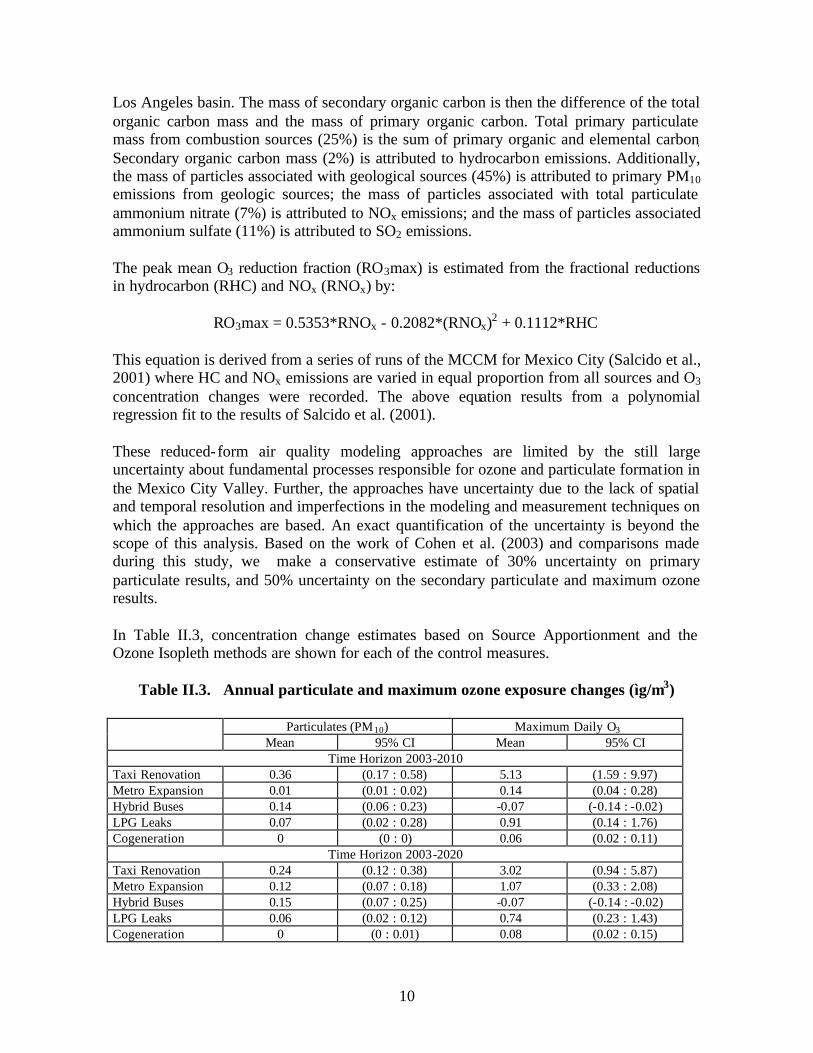
RO3max = 0.5353*RNOx - 0.2082*(RNOx)2 + 0.1112*RHC This equation is derived from a series of runs of the MCCM for Mexico City (Salcido et al., 2001) where HC and NOx emissions are varied in equal proportion from all sources and O3 concentration changes were recorded. The above equation results from a polynomial regression fit to the results of Salcido et al. (2001). These reduced-form air quality modeling approaches are limited by the still large uncertainty about fundamental processes responsible for ozone and particulate formation in the Mexico City Valley. Further, the approaches have uncertainty due to the lack of spatial and temporal resolution and imperfections in the modeling and measurement techniques on which the approaches are based. An exact quantification of the uncertainty is beyond the scope of this analysis. Based on the work of Cohen et al. (2003) and comparisons made during this study, we make a conservative estimate of 30% uncertainty on primary particulate results, and 50% uncertainty on the secondary particulate and maximum ozone results. In Table II.3, concentration change estimates based on Source Apportionment and the Ozone Isopleth methods are shown for each of the control measures.

Table II.3. Annual particulate and maximum ozone exposure changes (ìg/m3)

Particulates (PM10) Maximum Daily O3 Mean 95% CI Mean 95% CI

Time Horizon 2003-2010 Taxi Renovation 0.36 (0.17 : 0.58) 5.13 (1.59 : 9.97) Metro Expansion 0.01 (0.01 : 0.02) 0.14 (0.04 : 0.28) Hybrid Buses 0.14 (0.06 : 0.23) -0.07 (-0.14 : -0.02) LPG Leaks 0.07 (0.02 : 0.28) 0.91 (0.14 : 1.76) Cogeneration 0 (0 : 0) 0.06 (0.02 : 0.11)

Time Horizon 2003-2020 Taxi Renovation 0.24 (0.12 : 0.38) 3.02 (0.94 : 5.87) Metro Expansion 0.12 (0.07 : 0.18) 1.07 (0.33 : 2.08) Hybrid Buses 0.15 (0.07 : 0.25) -0.07 (-0.14 : -0.02) LPG Leaks 0.06 (0.02 : 0.12) 0.74 (0.23 : 1.43) Cogeneration 0 (0 : 0.01) 0.08 (0.02 : 0.15)

11

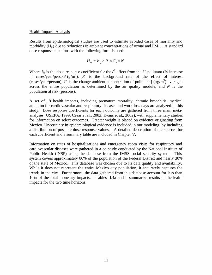
Health Impacts Analysis Results from epidemiological studies are used to estimate avoided cases of mortality and morbidity (Hij) due to reductions in ambient concentrations of ozone and PM10. A standard dose response equations with the following form is used:

NCRH jiijij ×××= β

Where âij is the dose-response coefficient for the ith effect from the jth pollutant (% increase in cases/year/person/ ìg/m3), Ri is the background rate of the effect of interest (cases/year/person), Cj is the change ambient concentration of pollutant j (µg/m3) averaged across the entire population as determined by the air quality module, and N is the population at risk (persons). A set of 19 health impacts, including premature mortality, chronic bronchitis, medical attention for cardiovascular and respiratory disease, and work loss days are analyzed in this study. Dose response coefficients for each outcome are gathered from three main meta-analyses (USEPA, 1999; Cesar et al., 2002; Evans et al., 2002), with supplementary studies for information on select outcomes. Greater weight is placed on evidence originating from Mexico. Uncertainty in epidemiological evidence is included in our modeling, by including a distribution of possible dose response values. A detailed description of the sources for each coefficient and a summary table are included in Chapter V. Information on rates of hospitalizations and emergency room visits for respiratory and cardiovascular diseases were gathered in a co-study conducted by the National Institute of Public Health (INSP) using the database from the IMSS social security system. This system covers approximately 80% of the population of the Federal District and nearly 30% of the state of Mexico. This database was chosen due to its data quality and availability. While it does not represent the entire Mexico city population, it accurately captures the trends in the city. Furthermore, the data gathered from this database account for less than 10% of the total monetary impacts. Tables II.4a and b summarize results of the health impacts for the two time horizons.

12

Table II.4a Annual mean health impacts (cases/year) Time horizon 2003-2010

Taxi

Renovation Metro

Expansion Hybrid Buses LPG Leaks Cogeneration

1.1 Acute Mortality Total mortality 57 2 9 11 1Infant mortality 29 1 11 6 01.2 Chronic Mortality Total 6 0 2 1 0Cardio-respiratory 1 0 0 0 0Lung Cancer 7 0 2 1 01.3 Chronic Bronchitis 448 16 171 89 41.4 Hospital admissions All Respiratory 223 6 1 39 2COPD 38 1 0 7 0All Cardiovascular 1 0 0 0 0Congestive Heart Failure 1 0 0 0 0Ischemic Heart Disease 0 0 0 0 0Pneumonia 49 1 0 9 1Asthma 21 1 1 4 01.5. Emergency room visits (ERVs) Respiratory Causes 1,065 30 17 190 12Asthma 990 28 14 176 111.6. Restricted Activity Days 13,326 476 5,103 2,663 1231.7 Minor Restricted Activity Days 495,076 14,660 44,611 90,682 5,2071.8 School Absenteeism 218,384 6,458 17,303 39,723 2,336

13

Table II.4b Annual mean health impacts (cases/year) Time horizon 2003-2020

Taxi

Renovation Metro

Expansion Hybrid Buses LPG Leaks Cogeneration

1.1 Acute Mortality Total mortality 36 15 10 9 1Infant mortality 19 10 12 5 01.2 Chronic Mortality Total 4 2 3 1 0Cardio-respiratory 0 0 0 0 0Lung Cancer 4 2 3 1 01.3 Chronic Bronchitis 295 152 184 76 61.4 Hospital admissions All Respiratory 134 49 1 33 3COPD 22 8 0 5 1All Cardiovascular 0 0 0 0 0Congestive Heart Failure 0 0 0 0 0Ischemic Heart Disease 0 0 0 0 0Pneumonia 29 10 0 7 1Asthma 12 5 1 3 01.5. Emergency room visits (ERVs) Respiratory Causes 632 232 19 154 16Asthma 583 215 15 144 151.6. Restricted Activity Days 8,908 4,584 5,575 2,320 1761.7 Minor Restricted Activity Days 296,928 119,279 48,591 73,350 7,1901.8 School Absenteeism 132,439 52,346 18,814 32,756 3,174 Valuation Here we evaluate the benefits of reduced health impacts by economic valuation and in terms of the quality-adjusted life-years (QALYs) saved. The economic valuation allows us to compare the costs with the benefits using the same metric. QALYs, on the other hand, allow comparisons of benefits to costs without putting monetary values on public health. This provides us with an alternative means of measuring control effectiveness, and allows us to calculate cost per QALY ratios. For the economic valuation we use three methodologies to determine the total social benefit due to reductions in health impacts: 1. Direct health costs 2. Productivity loss and 3. Willingness to pay (WTP). These three methods are combined to give the total social benefits from reductions in health impacts, removing some impacts to avoid overlap. Direct health costs were derived from an analysis by the Mexican National Institute of Public Health (INSP) of costs of hospitalizations and emergency room visits. Productivity loss is calculated by the salary loss over the duration of an illness or years lost due to premature mortality. Finally, for WTP, we use results from a study conducted in Mexico (Ibarrarán et al., 2002) as well as those from the international body of literature adjusted to Mexican income, placing more weight on the Mexican study.

14

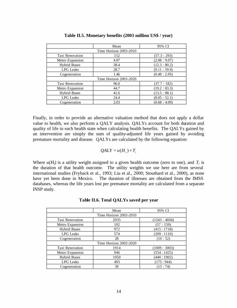
Table II.5. Monetary benefits (2003 million US$ / year)

Mean 95% CI

Time Horizon 2003-2010 Taxi Renovation 152 (57.3 : 293) Metro Expansion 4.97 (2.08 : 9.07)

Hybrid Buses 38.4 (12.3 : 80.2) LPG Leaks 28.7 (9.11 : 59.9)

Cogeneration 1.46 (0.48 : 2.95) Time Horizon 2003-2020

Taxi Renovation 96.0 (37.7 : 182) Metro Expansion 44.7 (19.2 : 83.3)

Hybrid Buses 41.6 (13.5 : 88.1) LPG Leaks 24.4 (8.05 : 52.1)

Cogeneration 2.03 (0.68 : 4.09)

Finally, in order to provide an alternative valuation method that does not apply a dollar value to health, we also perform a QALY analysis. QALYs account for both duration and quality of life in each health state when calculating health benefits. The QALYs gained by an intervention are simply the sum of quality-adjusted life years gained by avoiding premature mortality and disease. QALYs are calculated by the following equation:

ii THuQALY ×= )( Where u(Hi) is a utility weight assigned to a given health outcome (zero to one), and Ti is the duration of that health outcome. The utility weights we use here are from several international studies (Fryback et al., 1993; Liu et al., 2000; Stouthard et al., 2000), as none have yet been done in Mexico. The duration of illnesses are obtained from the IMSS databases, whereas the life years lost per premature mortality are calculated from a separate INSP study.

Table II.6. Total QALYs saved per year

Mean 95% CI Time Horizon 2003-2010

Taxi Renovation 2935 (1543 : 4694) Metro Expansion 102 (57 : 159)

Hybrid Buses 972 (415 : 1718) LPG Leaks 574 (209 : 1110)

Cogeneration 28 (10 : 52) Time Horizon 2003-2020

Taxi Renovation 1914 (1009 : 3003) Metro Expansion 946 (554 : 1425)

Hybrid Buses 1050 (440 : 1902) LPG Leaks 493 (175 : 944)

Cogeneration 39 (15 : 74)

15

II.4. Results We find that the combination of these 5 measures will substantially reduce emissions of local air pollutants, as well as GHG. These measures will reduce PM10 exposure by approximately 1% (0.6 ìg/m3) for both time horizons; and will reduce maximum ozone concentrations by approximately 3% (6.2 ìg/m3 and 4.8 ìg/m3, respectively for 2003-2010 and 2003-2020), while eliminating emissions of more than 300,000 tons C equivalent per year and 400,000 tons C equivalent per year, respectively. Together, these reductions will save more than 4,600 and 4,400 QALYs per year, respectively. Monetized benefits are estimated to be $225 million USD per year and $210 million USD per year, respectively, for the combined 5 controls. Total annualized costs are less than 30% of the estimated benefits: we estimate costs to be $66 million per year for 2003-2010 and $50 million USD per year for 2003-2020. Each measure contributes uniquely to these results. The impact of each individual measure is discussed below. For the 2003-2010 time horizon, the benefits of the Taxi Fleet Renovation are far greater than the costs (Table II.2. and II.5). Costs are small for this measure because of significant fuel efficiency gains realized with newer vehicles. Benefits are high because of large ozone reductions, and also because of significant reductions in secondary particulate concentrations reductions (Table II.3). We estimate that approximately 3,000 QALYs per year could be saved with the measure (Table II.6), at mean cost of approximately $3,000 per QALY. On the longer time horizon, net costs turn into net savings as the fuel cost savings continue to accumulate without additional investment costs. Annualized benefits are still large, though less so, for the long time horizon because there is deterioration in emissions among aging vehicles that gradually increases local emissions, and thus decreases local benefits with time. For 2003-2020, we estimate that approximately 2,000 QALYs per year could be saved (Table II.6) at the same time as cost savings are realized. Consistent with existing government proposals, this analysis assumes that only 5 km of Metro would be built from 2003-2010, and an additional 71 km from 2011-2020. For this reason, it appears as to be a relatively small, inexpensive measure on the short time horizon, but much larger undertaking on the long horizon (Table II.2). Because Metro Expansion involves significant capital investment, the inclusion of the recuperation value for the Metro (30 year useful life) offsets a significant portion of these initial costs. We find that the local emission reduction benefits (Table II.5, II.6) can also be large and compensate for a majority, if not all, of the net costs for both time horizons. For example, for 2003-2020, we estimate that approximately 950 QALYs per year could be saved (Table II.6) at a cost of approximately $50,000 per QALY by the expansion of the Metro. This analysis assumes that the extension of the Metro causes a significant reduction in the use of on-road public bus transportation, which means local emissions are significantly reduced. However, increase in Metro length requires more electricity and increases emissions from power plants that are primarily located outside the valley. Thus, the Metro Expansion causes a net transfer of local emissions from inside to outside the valley. We assume that population density is substantially lower where the electricity is generated than in Mexico City, and for this reason, public health impacts will be negligible from increased power generation. This

16

transfer of local emission helps to make local benefits large enough to offset much, if not all, of the costs for this measure. The Hybrid Buses measure has large upfront investment costs due to the expensive nature of the technology, but also generates significant cost savings on the long term due to greatly enhanced fuel efficiency (Table II.2). Benefits are large for both time horizons primarily because of large reductions in primary particulate emissions. For both time horizons, we find that approximately 1,000 QALYs per year could be saved (Table II.6). This measure is implemented between 2003 and 2006. Annualized costs are, therefore, lower and benefits higher for the long time horizon than for the short time horizon; thus the cost per QALY reduces from approximately $60,000 for 2003-2010 to $20,000 for 2003-2010. The LPG leaks reduction measure, on the other hand, has low costs because of the low unit costs for each stove repair. Benefits are much larger than the costs because of the significant reduction in hydrocarbon emissions that reduces both ozone and secondary organic particulate exposure. For both time horizons, approximately 500 QALYs per year could be saved (Table II.6) at a cost of approximately $50,000 per QALY. For Cogeneration, net costs are low due to the significant gains in fuel efficiency and the inclusion of the recuperation value of the equipment at the end of each time horizon (20 year useful life). Local benefits are not very large for this measure because the gains in efficiency derive from simultaneous on-site production of thermal and electrical energy that replaces off-site electricity generation and on-site thermal energy production. As explained above, only a small portion (3.1%) of the electricity consumed in Mexico City is generated in the valley. Though Cogeneration significantly reduces the total emissions by substantially increasing efficiency, the measure moves emissions of local pollutants into the valley, and thus local benefits are small. QALYs saved are on the order of 30 per year for both time horizons (Table II.6) at a cost of approximately $25,000 per QALY. In Figure II.1, we compare local and global net benefits. The local net benefits are defined as the Monetized Health Benefits (Table II.5) minus Costs (Table II.2), while the global net benefit is the reduction in GHG emission. Figure II.1 illustrates that the Taxi Fleet Renovation measure is clearly the best measure from the joint local – global perspective. The Hybrid Bus measure for 2003-2020 and the LPG Leak measure on both time horizons are the next-most promising for joint local / global control. The Metro Expansion, in large part because of its very high costs, is less promising from the joint perspective. Cogeneration also does not have sufficient local benefits to make it interesting for joint local – global control.

17

Figure II.1: Net Health Benefits vs. C equivalent Reduction

II.5. Discussion and Conclusions Taxi fleet renovation offers the most promising opportunity for the joint control of local and global pollution of the measures studied here. Furthe r, benefits might be found to be significantly larger than estimated here if changes in primary particulate matter emissions could be estimated. The large potential benefits of this measure have already been recognized by decision-makers in Mexico City, and the implementation of this measure has begun as of 2002-2003 with public funding for the replacement of 3,000 taxis. The LPG leak measure also provides benefits than are much larger than the total costs. Emissions reductions and local benefits from this measure are small compared to the taxi fleet renovation, but investment costs are quite small, making implementation of the LPG leak measure relatively feasible from a decision-making standpoint. Cogeneration provides more than 50% of the GHG benefits from this set of measures, but essentially no local benefit because it moves emissions of local pollutants into the valley, and health benefits from the reduced emissions at power plants located outside the valley are assumed to be negligibly small. Were a similar study conducted at the national level, Cogeneration may turn out to be a promising joint local / global option because health benefits derived in populations living near to power plants could be considered. This will depend, of course, on population exposure to emissions generated by electricity production across the country.

18

Metro Expansion has large local benefits, particularly for the long time horizon when the measure has been fully implemented. However, the extremely high initial investment costs required for the measure make its implementation unlikely. Finally, the Hybrid Bus measure may have positive net benefits if the long time horizon is considered. However, the analysis of this measure has large uncertainty because the emission factors used were derived for the altitude, driving conditions, and fuel mix of New York City, not for Mexico City. Altitude has been shown (Yanowitz et al. 2000) to significantly impact emissions behavior from heavy-duty vehicle technology, but these impacts have not been specifically calculated for the technologies under consideration here. We recommend that a better understanding of emissions factors be obtained and also that the cost-effectiveness of other types of advanced technologies (e.g. Cohen et al., 2003) also be considered in order to determine what would be the best advanced bus technology to introduce in Mexico City. This work indicates that measures to improve the efficiency of transportation are key to joint local / global air pollution control in Mexico City. The three measures in this category that are analyzed here all have monetized public health benefits that are larger than their costs when the appropriate time horizon is considered. Global benefits, due to improved fuel efficiency, are also large. In contrast, we find that traditional “no-regrets” electricity efficiency do provide large GHG emission reductions, but do not provide local benefits to Mexico City because the majority of electricity is produced outside of the valley in which Mexico City is located. Further work is needed to analyze more measures that cover a wider range of opportunities for joint local / global air pollution control. Also very important is to quantify the air pollution improvements and cost savings that could be acquired from reduced congestion in the MCMA. Such an analysis may indicate that the benefits from transportation efficiency improvement are, in fact, much larger than estimates here. Improved understanding of emission factors from new and old vehicles under Mexico City driving conditions is also greatly needed, and could significantly impact results. II.6. References CAM, Comisión Ambiental Metropolitana (2002) “Programa para Mejorar la Calidad del Aire de la Zona Metropolitana del Valle de México, 2002-2010” (PROAIRE), Comisión Ambiental Metropolitana, México City. Cesar, H., et al. (2000) “Economic valuation of Improvement of Air Quality in the Metropolitan Area of Mexico City,” Institute for Environmental Studies (IVM)

Cesar, H., et al. (2002) “Air pollution abatement in Mexico City: an economic valuation,” World Bank Report

19

Chow, J.C., J.G. Watson, S.A. Edgerton, and E. Vega (2002) “Chemical composition of PM2.5 and PM10 in Mexico City during winter 1997,” The Science of the Total Environment 287, p.177-201. Cohen, J.T., J.K. Hammitt, and J.I. Levy (2003) Fuels for urban transit buses: A cost-effectiveness analysis. Environ. Sci. Technol 37. 1477-1484. Evans et al. (2002) “Health benefits of air pollution control,” in Air Quality in the Mexico Megacity: An Integrated Assessment, Kluwer Academic Publishers, Boston, 384 pp. Fryback, D., E. Dasbach, R. Klein, B. Klein, N. Dorn, K. Peterson, and P. Martin (1993) "The beaver dam health outcomes study: initial catalog of health-state quality factors," Medical Decision Making, 13: 89-102. Ibarrarán, M., E. Guillomen, Y. Zepeda, and J. Hammit (2002) “Estimate the economic value of reducing health risks by improving air quality in Mexico City,” preliminary results. Liu, J., J. Hammitt, J. Wang, and J. Liu (2000) “Mother’s willingness to pay for her own and her child’s health: a contingent valuation study in Taiwan,” Health Economics, 9: 319-326. M.J. Bradley & Associates, Inc. (2000) “Hybrid-electric drive heavy-duty vehicle testing project: Final emissions report.” http://www.navc.org/Navc9837.pdf Salcido et al. (2001) “MCCM Parametric Studies: Estimation of the NOx, HC and PM10 emission reductions required to produce a 10% reduction in the Ozone and PM10 surface concentrations and compliance with the MCMA air quality standards, with reference to the 2010 MCMA Emission Inventory,” Grupo de Modelación de la Comisión Ambiental Metropolitan (CAM), 42 pp. Sheinbaum P., C., L. Ozawa, O. Vázquez, and G. Robles (2000) “Inventario de emisiones de gases de efecto invernadero asociados a la producción y uso de la energía en la Zona Metropolitana del Valle de México: Informe final.” Grupo de Energía y Ambiente, Instituto de Ingeniería, UNAM, report to the CAM and the World Bank. SMA, Secretaria del Medio Ambiente del Distrito Federal (2002) Red Automática de Monitoreo Atmosférico (RAMA). Stouthard, M., M. Essink-Bot and G. Bonsel (2000) “Disability weights for disease: a modified protocol and results for a western European region,” European Journal of Public Health, 10: 24-30. Turpin, B.J., J.J. Huntzicker, S.M. Larson and G.R. Cass (1991) “Los Angeles summer midday particulate carbon: Primary and secondary aerosol,” Envi. Sci. Technol., 25(10) 1788-1793.

20

TUV Rheinland de Mexico, S. A. de C. V. (2000) “Programa para la reducción y eliminación de fugas de Gas LP, en las instalaciones domésticas de la Zona Metropolitana del Valle de México.” U.S. Environmental Protection Agency (1999) "The Benefits and Costs of the Clean Air Act 1990-2010," Washington, D.C., Office of Air and Radiation, EPA report no. 410/R-99/001. West, J.J., P. Osnaya, I. Laguna, J. Martínez, A. Fernández (2003) “Co-control of urban air pollutants and greenhouse gases in México City.” Final report to US National Renewable Energy Laboratory, subcontract ADC-2-32409-01. Yanowitz, J., R.L. McCormick and M.S. Graboski (2000) “In-use emissions from Heavy-Duty diesel vehicles.” Environ. Sci. Technol. 3, p 729-740.

21

III.1 General Methodology for Estimating Emissions Reductions and Costs III.1.1. Introduction We estimate the time profiles of local pollutant (PM10, SO2, CO, NOX, and HC) and global pollutant (CO2, CH4, and N2O) emission reductions, and direct costs for 5 control measures that address transportation, residential and industrial sources of local and global air pollution emissions. Detailed descriptions of each measure is outlined in sections III.2 through III.6. We also report emission reductions of PM2.5, calculated as a fraction of PM10 emissions (US EPA, 2000) for illustrative purposes, but do not use these estimates of emission reduction in the rest of the analysis. As described below, for each measure an emissions baseline is defined given currently measured or otherwise determined emissions factors and activity levels, combined with reasonable future predictions regarding their behavior without intervention. Control measures cause a change from this baseline by altering future activity levels and / or emissions factors. While emissions factors used in the study are meant to capture current driving conditions, the cost savings and changes in emissions due to reduced congestion could not be calculated because this was far beyond the scope of this study. We encourage the pursuit of improved understanding of congestion impacts in future work since these impact may, in fact, be large. Our objective is to estimate emissions reductions and costs for each year from 2003 to 2020. In this way, the different time-profiles of the programs costs and impacts can be studied. For incorporation into the cost – benefit and ancillary benefits analyses that are the goal of this study, we annualize the results obtained over these time horizons using several different discount rates. Annualized costs and emissions reduction can be considered as a constant annual flux of costs or emission reductions over the time-period that gives an equivalent net present value to the net present value estimated from the actual time-profile of the program. In this way, annualized results allow direct comparisons between measures with different time-profiles. Further, annualized results allow cost-benefit and ancillary benefit calculations to be much simplified since it is only necessary to calculate air quality changes and health impacts based on a single set of emissions reductions that appropriately represent the entire time horizon, as opposed to having to do such calculations for each year. The fact that our reduced-form air quality models (see Chapter IV) are essentially linear facilitates the use of annualized emissions reductions. III.1.2. Choice of Time Horizon We study both a short time horizon (2003 through 2010) that is consistent with Mexico City’s Program for Improved Air Quality in the Valley of Mexico (Programa para Mejorar la Calidad de Aire en el Valle de Mexico, PROAIRE) 2002-2010. We also study a long time horizon (2003 through 2020) that allows consideration of the lasting effects of control

22

measures implemented up to 2010, and also allows consideration of realistic long-term implementation plans for the Metro Expansion control measure. III.1.3. Choice of Discount Rate We calculate costs and emissions reductions using 3 discount rates, 3%, 5% and 7%. We also present results when discounting is ignored, or 0%. Our benchmark scenario, for which results are considered in Chapters IV to IX, uses a discount rate of 5%. III.1.4. Equations used for Discounting and Annualization Discounting to estimate the Net Present Value (NPV) in 2003 (where j is the year from 2003, “value” is the emission reduction or cost in that year, and dr is the discount rate) uses Equation III.1.1.

∑= +

=n

jj

j

dr

valueNPV

1 )1( Equation III.1.1

Annualization (where Nyr is the number of years over which to annualize) uses Equation III.1.2.

[ ] NPVdr

drvalueannualized

Nyr⋅

+−=

−)1(1_ Equation III.1.2

III.1.5. References

U.S. Environmental Protection Agency (2000) "National Air Pollutant Emission Trends: 1900 - 1998," Washington, D.C., EPA report no. 454/R-00-002.

23

III.2. Renovation of the Taxi Fleet III.2.1. Introduction

In 1998 approximately 109,400 taxis were circulating in the Mexico City Metropolitan Area (MCMA); 103,298 in the Federal District and the rest in the State of Mexico. According to official figures, the total number of taxis accounted for 3.4 percent of the entire vehicle fleet in the metropolitan area that year (CAM, 2002a, Table 5.2.2.2). In the Federal District alone, taxis accounted for about 5 percent of the vehicle fleet and about 20 percent of the total vehicle kilometers traveled (CAM, 2002a, Table A.2.6). The emissions from these activities are estimated at 188 tons per year of PM10; 535 tons of SO2; 115,200 tons of CO; 10,366 tons of NOX; and 13,733 tons of HC, respectively (CAM, 2002a, Table 5.2.2.8). By their nature taxis are high-use vehicles. Over time their emission control systems would be expected to deteriorate more rapidly than those of other vehicles used less intensively (however, see Kojima and Bacon, 2001). This is one reason why taxis are sometimes subject to more frequent tests in vehicle inspection and maintenance (I/M) programs. High-use vehicles also consume more fuel, which contributes particularly to emissions of greenhouse gases (GHG), and which makes up an important part of the vehicle operating costs. The problems associated with emissions from taxis are thus similar to the ones of the private car fleet, but they tend to be exacerbated by a more intense use of taxi vehicles. The weighted average age of taxis in the Federal District was 5.7 years in 1998. Four years later, this number had grown considerably and, according to some estimates, 49% of the fleet was more than 10 years old and should have been taken off the road in order to comply with existing regulations (Gonzalez, 2002). However, there are large uncertainties associated with these estimates. A reliable vehicle registration database does not exist, and it is difficult to obtain time-series data. While new vehicle sales are added to the existing population every year, vehicle retirement is often not captured. As a result, large differences have been measured when the official figures are compared with data from extensive field surveys (Kojima and Bacon, 2001). The inconsistencies observed in the official records of the overall fleet size and composition are recognized by the Metropolitan Commission for Transport and Roadways (COMETRAVI, 1999a), and are similar to problems encountered in other parts of Latin America (for a discussion in the context of the MCMA, see Gakkenheimer et al. 2002). Modeling the evolution of the taxi fleet is also complicated by the fact that most taxis are traded on the market for used vehicles, and that an unknown number of vehicles have been turned into taxis illegally. Yet, despite these challenges there seems to be a consensus within the local governments of the MCMA that something needs to be done about the emissions from the existing taxi fleet. High-use vehicles (i.e., taxis and microbuses) are currently required to be renewed after a certain number of years, but the restrictions are not effectively enforced and the age of an increasing number of these vehicles is higher than their age limit.

24

Apart from their impact on air quality and human health, there are also other problems related to the taxis. In particular, 60-70 percent of the taxi owners have only one vehicle as their main source of household income (Gonzalez, 2002). As a consequence, these owners work between 8 and 12 hours a day and typically they do not have any kind of social security. Public policies to reduce emissions from taxis ought to be sensitive to this fact. In the present analysis, however, we shall focus on the total emission reductions and the direct costs of such policies, while ignoring their implications for the distribution across individuals and households. III.2.2. Description of the Measure

In response to growing concerns about the emissions from taxis, an ambitious program has been designed to scrap 80,099 old taxis in the Federal District, and to replace them by vehicles that comply with more stringent emissions standards. The program is being implemented over a four year period, provided sufficient public funds are available. There are four overall goals of the program (Gonzalez, 2002). First, in order to reduce emissions of local air pollutants, such as CO, NOX and HC, old taxi vehicles will be replaced by newer vehicles that comply with at least Tier 1 emission standards. The replacement is facilitated by an incentive for present taxi owners to scrap their old vehicle in exchange for a premium of 1,500 U.S. dollars. In addition, subsidies are given to owners of new taxis in terms of reduced purchase prices from the automobile industry, a special tax relief from the government of the Federal District, interest rate subsidies from credit institutions, and subsidies on spare parts and services. Second, a requirement is included in the program that new vehicle engines must comply with a minimum fuel economy of 12.6 km per liter. Compared with the existing taxi fleet, the requirement would imply not only considerable savings in fuel cost, but also a reduction in GHG emissions. Note, however, that this is based on the assumption of no “rebound effect” from an improvement in the fuel economy of new vehicles (NRC, 2002; Portney, 2002). Third, as emphasized above a number of other problems surround the organization of the taxi fleet. About 90 percent of the vehicles in service are so-called “free” taxis that circulate the streets empty looking for passengers. In contrast with fixed-site taxis, which typically operate from a coordinated taxi stand, free taxis are not formally organized. They produce more emissions per passenger kilometer traveled and are generally considered to be less safe. In the taxi renewal program, provisions are therefore included to increase the share of fixed-site taxis as a means to reduce the emissions and improve the safety of the passengers simultaneously. However, it remains an open question to what extent the operators of free taxis will have sufficient incentives to join a taxi stand, or another form of coordinated operation. Consequently, we shall not consider this element of the program in the analysis. The fourth goal of the program is to improve the income of the taxi owners through public and private subsidies and through increased social security. Financial support is thus provided, not only for the scrappage of old and the purchase of new taxis, but also for

25

recurring expenditures on vehicle operation and maintenance (i.e., interest rate subsidies and subsidies on spare parts and services). In addition, since taxi credits are generally considered by the commercial banks to be a risky asset leading to a prohibitively large risk premium on private commercial loans, a mechanism has been designed between the private financial sector, the government of the Federal District, and the National Development Bank (Nacional Financiera) to provide guaranteed loans at fixed interest rates. An insurance scheme for taxi owners is also being considered jointly with the loan for the purchase of a new vehicle (Gonzalez, 2002; SETRAVI, 2002a). According to the announced plan, the taxi renewal program is being implemented from 2002 to 2006 as part of an overall effort to integrate transport and environmental policies in the Federal Dis trict (CAM, 2002b; SETRAVI, 2002b). However, the financial viability of the program remains insecure. Not only are the financial resources of the Federal District scarce, but there are also large imbalances in the public finances of the transport sector. These imbalances stem in part from a massive underpricing of public transport and infrastructure, such as the metro system and the road network, and in part from the inability of the local Secretariat of Transport and Roadways to raise public revenues. For the fiscal year of 2002, it is estimated that only 37% of the total expenditures in the transport sector are covered by the revenues raised (Gakkenheimer et al., 2002; SETRAVI, 2002b). From the documents available it is difficult to get a clear picture of the current state of the taxi substitution program. In the preliminary Integrated Transport and Roadways Program (Programa Integral de Transporte y Vialidad, PITV) for 2002-2006, a total amount of 10 million US dollars has been designated to a fund for the substitution of 10,000 free taxis (SETRAVI, 2002b). In the Program for Improved Air Quality in the Valley of Mexico (Programa para Mejorar la Calidad de Aire en el Valle de Mexico, PROAIRE) 2002-2010, about 80,000 of the oldest taxis are expected to be gradually replaced at a total cost of 800 million U.S. dollars, of which 80 million dollars would be financed by the public sector and 720 million dollars by the private sector (CAM, 2002b). Finally, in a brief summary of the progress of PROAIRE, Paramo (2003) comments on the availability of funds for the substitution of only 3,000 taxis for the fiscal year 2002. These discrepancies are probably a reflection of the financial insecurity of the program. It is also a fact that the fiscal budget covers expenditures only one year ahead, while the scrappage and replacement of taxis is a multi-year effort that cuts across institutional boundaries within and outside the government of the Federal District. In this respect, the program should be contrasted with the only other known scrappage program of a comparable magnitude, which was considered for almost a decade in California to improve air quality in the greater Los Angeles area, but which was subsequently abandoned by policy makers (Dixon and Garber, 2001a, 2001b; Dixon, Garber, and Porche, 2002). Some taxis in the Federal District have already been scrapped and replaced. Information about these experiences would be useful for the evaluation of the program. Yet, data on the costs and emissions characteristics of both the old taxis that are scrapped and the new vehicles introduced have not been available for the purpose of the analysis. We therefore conduct a prospective analysis of the program, based on our expectations about its likely impacts, and assume a period of implementation from 2003 to 2007.

26

In the analysis, we focus on the real social costs, as opposed to the financial costs, associated with the scrappage and replacement of taxis, the implications for the emissions reductions, and the human health impacts in the Federal District. In particular, we are interested in the question of whether the taxi renewal program is desirable from an overall societal perspective, taking into account only the allocative efficiency of the measure. This means that we include the real resource costs associated with the scrappage and replacement of taxis (i.e., scrappage subsidy, vehicle replacement cost, and fuel cost), while we omit the financial costs associated with a loss to some and a gain to other agents of the economy (i.e., public and private transfers). III.2.3. Data Requirements

For the purpose of the evaluation, a wide range of data is needed to estimate the baseline emissions trajectory for the taxi fleet without the control measure. These data include the base year (1998) emissions inventory for the MCMA, distributed between the Federal District and the State of Mexico (CAM, 2002a). Data is also needed to extend the inventory with estimates of PM2.5 and GHG emissions. For this extension, we introduce a number of simplifying assumptions. In particular, we are interested in an explicit calculation of the average annual fuel consumption of taxis, which at the same time can be used to estimate fuel consumption in the future. Emissions of GHG are then straightforward to calculate on the basis of emissions factors (in grams per kilogram of fuel consumed) reported by the Intergovernmental Panel on Climate Change (IPCC, 1997). Finally, the baseline emissions for the period 1998 to 2020 are estimated on the basis of expectations about the annual rates of change in both the size and composition of the taxi fleet and its emissions characteristics. To the extent possible, these data are obtained from publicly available documents. Where such data are unavailable, alternative assumptions are discussed and justified explicitly. Once the baseline scenario has been specified, it is an easy matter to impose the control measure according to the number of taxis to be replaced and the time period of implementation described above. The annual emissions are then re-calculated in the control scenario for the time period of analysis, and the emissions reductions derived as the difference between the two scenarios. Great care needs to be taken in order to ensure that relevant parameters in the control scenario are correctly adjusted. If, for example, emissions standards are introduced in the control scenario that do not already exist in the baseline scenario, such as more stringent tailpipe emissions or fuel economy standards, this change needs to be reflected in the parameter values (i.e., the emissions factors and the fuel economy of the new vehicles). On the basis of the changes introduced in the control scenario, data are needed on the incremental capital costs and operation and maintenance (O&M) costs of each new taxi. The capital cost include the initial scrappage subsidy (1,500 USD) and the incremental cost to the taxi owner from the purchase of a new vehicle. The O&M costs include the value of

27

changes in fuel consumption, valued at constant real prices over time. We assume that government administration costs of the program are negligible, since no emissions testing is associated with the scrapping of old vehicles. Also, monitoring and enforcement costs are not included. During the first years of the program, when the oldest vehicles are replaced, we believe that these costs can be ignored, because incentives are provided for taxi owners to join the program, in part, through the scrappage subsidies and, in part, through the subsidies for new vehicles. However, during later years of the program, when younger vintages of vehicles are retired, participation in the program will eventually become unattractive as the used car prices of younger vehicles raise above the scrappage subsidy. This is clearly in opposition with the objectives of the program, and requires more careful consideration of the enforcement mechanisms needed to replace almost 80% of the taxi fleet in the Federal District. Yet, there is some confusion in the official perception of how the taxi substitution program is enforced. In the Secretariat of Transport and Roadways (SETRAVI, 2002a), the program is viewed as voluntary. This means that the decision to scrap an old taxi and replace it by a new one is left entirely to the owner. Incentives therefore need to be put in place for the program to take effect (see, for example, Dixon and Garber, 2002a). In the economics literature, these incentives are typically analyzed in models of so-called “rational scrappage”, where the optimal decision of the owner to keep or scrap the vehicle is based on the minimization of the present value of the costs from the two alternatives, with all the relevant costs included (e.g., Hahn, 1995; Alberini et al., 1995, 1998). Vehicle scrappage rates above the natural rate of retirement are then achieved by policies (e.g., scrappage subsidies, emission fees, differentiated ownership taxes, or more stringent inspection and maintenance) that change the relative costs in favor of scrappage. Public policies based on this type of scrappage is also sometimes referred to as “voluntary accelerated vehicle retirement” (VAVR) programs (U.S. EPA, 1998; ESMAP, 2002). In contrast with this viewpoint of the taxi substitution program as voluntary, the Metropolitan Environmental Commission describes it in PROAIRE as mandatory (CAM, 2002b). Since taxi owners in the Federal District are allowed to operate only under a system of public concessions, compliance with the taxi substitution program in ensured in PROAIRE by making the renewal of the concession for each taxi owner dependent on participation in the program. Failure to participate in the program by not scrapping the old taxi means that the license of the owner to own and operate a taxi expires. For convenience, we adopt the latter viewpoint. Estimating a model of rational scrappage is beyond the scope of the present analysis. Given the available time and data, we therefore assume that the incentives provided by the program are sufficient to make the taxi owners comply. If they are not sufficient, we assume that compliance can be enforced through the system of concessions currently in place in the Federal District. This greatly simplifies the analysis. However, the assumption of compliance is questionable given a past history of problems with concessions in the MCMA, particularly with respect to the operation of urban buses (Estache, 2001; Gakkenheimer et al., 2002). One should therefore be cautious in the interpretation of the results from the present analysis.

28

III.2.4. Determining baseline emissions

Following the emissions inventory (CAM, 2002a), a bottom-up approach is used to estimate the total emissions in 1998 by multiplying the level of activities (i.e., the number of taxis and their annual vehicle kilometers traveled) with the level of emissions per unit of activity (i.e., the emissions factors in grams per kilometer). First, we describe the data used in this approach. We then turn to the projection of the activities and the emissions characteristics of the taxi fleet. The base year (1998) emissions A vehicle registration database is not available for the MCMA. In its place, data on the size and composition of the vehicle fleet, as well as its emissions characteristics, can be obtained from the vehicle verification program. The program requires an emissions test to be performed every six months on vehicles circulating in the Federal District and the State of Mexico (see Gakkenheimer et al., 2002). The activity data for the base year emissions inventory are specific to each model year vehicle in 1998 and spans a total of 25 model year vintages. Figure III.2.1. shows the age distribution of taxis and private cars in the Federal District (CAM, 2002a, Table A.2.2). The age distribution of taxis is from the vehicle verification program in the second semester of 1999. The figure illustrates that the taxi fleet is not very old, compared with the private car fleet, and that taxis appear to be retired faster than private cars. This is probably because taxis travel more kilometers every year, and therefore deteriorate more rapidly due to wear and tear. Other interpretations are also possible related to factors external to the vehicles themselves, such as differences in the price of maintenance and repair (Hamilton and Macauley, 1998). Figure III.2.1. Age distribution of taxis and private cars in the Federal District (1998)

0%

5%

10%

15%

20%

25%

30%

0 2 4 6 8 10 12 14 16 18 20 22 24Vehicle age (in years)

% o

f tot

al Taxis

Private cars

29

The taxis are assumed to travel 200 kilometers per day during 6 days a week. This yields a total distance traveled of 62,600 kilometers per year (COMETRAVI, 1999). The estimate represents an upper bound of the annual vehicle kilometers traveled (VKT) per taxi, compared with other estimates of odometer readings taken from the verification program in the period from 1996 to 1999 (Kojima and Bacon, 2001). These estimates indicate that taxis in the Federal District on average travel 30.000 km per year – about half the estimate we use in the present study. Notice that we do not differentiate across model year vehicles in terms of their annual VKT. In agreement with most empirical observations, other studies typically assume that old vehicles travel less than new ones (e.g., Mostashari, 2003). This pattern has also been found in the MCMA, although at a very aggregate level (Kojima and Bacon, 2001). Here we simplify the analysis and leave the quantitative significance of such a variation for further study. Given the total distance traveled for each model year, the emissions of criteria pollutants (CO, NOX, and HC) are calculated with the emissions factors from the emissions inventory shown in Table III.2.1 (CAM, 2002a, Annex A). In the inventory, emissions factors for diesel fueled vehicles and motorcycles are estimated through the MOBILE5-MCMA model. The MOBILE model was originally developed by the U.S. EPA, and has subsequently been adjusted for use in Mexico, including the Mexico City Metropolitan Area (Radian International, 1997; ERG and Radian International, 2000; Burnette et al., 2001). The model is part of a larger, on-going effort to improve the capacity within Mexico for the development of emissions inventories. However, the MOBILE model has been subject to critical scrutiny in the U.S. in recent years, particularly as a means to estimate the expected emissions reductions from mobile source control measures (Harrington et al., 1998; NRC, 2000). A new generation of the model has therefore been developed to address some of its limitations (U.S. EPA, 2001, 2002). For gasoline fueled vehicles in Mexico City, including taxis, emissions data have been obtained from tunnel studies and measurement campaigns conducted, in part, by the Mexican Petroleum Institute (IMP) during the 1990s. Focusing on the emissions of hydrocarbons, two tunnel studies report results on the measurement of exhaust emissions profiles for motor vehicles in operation, as well as hot soak emissions from vehicles in a parking garage (Mugica et al., 1998; Vega et al., 2000). These results were then combined with ambient air quality measurements to develop a source apportionment model, which shows that somewhere between 55% and 64% of the ambient concentrations of non-methane hydrocarbons (NMHC) can be attributed to the emissions from motor vehicles. However, despite these and other efforts, it is a very complicated and time consuming task to develop a comprehensive emissions inventory, which at the same time can be validated through the use of various independent methods (for an excellent discussion, see Molina et al., 2002). Estimating the emissions of taxis in the MCMA is no exception, and it is not clear from the 1998 emissions inventory what are the sources of the emissions factors for taxis (CAM, 2002a, Annex A). The data are shown in Table III.2.1, but measurement results have been obtained only for model years 1991 to 1998. For all the previous model years, the emissions factors of private cars were used instead.

30

Table III.2.1. Emissions factors of local air pollutants from taxis in the MCMA (g/km)

Model year PM10 PM2.5 CO NOx HC

1974 � 0.03 0.02 76.40 2.10 6.26 1975 0.03 0.02 76.40 2.10 6.26 1976 0.03 0.02 76.40 2.10 6.26 1977 0.03 0.02 76.40 2.10 6.26 1978 0.03 0.02 76.40 2.10 6.26 1979 0.03 0.02 76.40 2.10 6.26 1980 0.03 0.02 76.40 2.10 6.26 1981 0.03 0.02 55.60 2.10 5.68 1982 0.03 0.02 55.60 2.10 5.68 1983 0.03 0.02 55.60 2.10 5.68 1984 0.03 0.02 55.60 2.10 5.68 1985 0.03 0.02 55.60 2.10 5.68 1986 0.03 0.02 39.60 2.10 4.55 1987 0.03 0.02 39.60 2.10 4.55 1988 0.03 0.02 39.60 2.10 4.55 1989 0.03 0.02 31.40 2.40 3.59 1990 0.03 0.02 31.40 2.40 3.59 1991 0.03 0.02 15.20 1.48 1.84 1992 0.03 0.02 15.20 1.48 1.84 1993 0.03 0.02 15.20 1.48 1.84 1994 0.03 0.02 15.20 1.48 1.84 1995 0.03 0.02 15.20 1.48 1.84 1996 0.03 0.02 15.20 1.48 1.84 1997 0.03 0.02 15.20 1.48 1.84 1998 0.03 0.02 15.20 1.48 1.84

The emissions factors for PM10 are obtained from a measurement study conducted in the Denver (Colorado) area in the U.S. during 1996 and 1997 (Cadle et al., 1999, 2001). The study offers a useful point of reference for the MCMA, because both locations are at high altitudes, which is known to have an important influence on emissions. Obviously, a number of other factors that are not accounted for might lead to differences in the emissions of PM in the two areas. These factors include differences in temperatures, the urban driving cycles used to test emissions, characteristics of the vehicle fleet and the sample of vehicles in the test. For example, under the driving cycle defined by the Federal Test Procedure (FTP), the Denver study finds considerable differences between the emissions of PM10 from new vehicles (2.82 mg per mile, model years 1991-1996) and the emissions from older vehicles (95.5 mg per mile, model years 1971-1980) during the summer. During the winter, this difference is narrowed somewhat (Cadle et al., 1999, Table 4). In the emissions inventory for the MCMA, no distinction is made between model years with respect to the emissions of PM10. This is unfortunate for the evaluation of the taxi substitution program, because the emissions reductions from this program are obtained precisely from the differences between old and new vehicles. Failure to take these

31

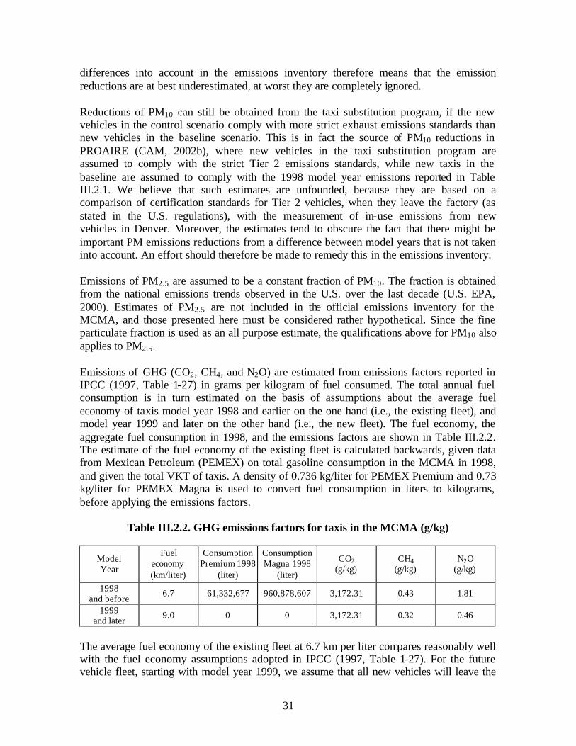
differences into account in the emissions inventory therefore means that the emission reductions are at best underestimated, at worst they are completely ignored. Reductions of PM10 can still be obtained from the taxi substitution program, if the new vehicles in the control scenario comply with more strict exhaust emissions standards than new vehicles in the baseline scenario. This is in fact the source of PM10 reductions in PROAIRE (CAM, 2002b), where new vehicles in the taxi substitution program are assumed to comply with the strict Tier 2 emissions standards, while new taxis in the baseline are assumed to comply with the 1998 model year emissions reported in Table III.2.1. We believe that such estimates are unfounded, because they are based on a comparison of certification standards for Tier 2 vehicles, when they leave the factory (as stated in the U.S. regulations), with the measurement of in-use emissions from new vehicles in Denver. Moreover, the estimates tend to obscure the fact that there might be important PM emissions reductions from a difference between model years that is not taken into account. An effort should therefore be made to remedy this in the emissions inventory. Emissions of PM2.5 are assumed to be a constant fraction of PM10. The fraction is obtained from the national emissions trends observed in the U.S. over the last decade (U.S. EPA, 2000). Estimates of PM2.5 are not included in the official emissions inventory for the MCMA, and those presented here must be considered rather hypothetical. Since the fine particulate fraction is used as an all purpose estimate, the qualifications above for PM10 also applies to PM2.5. Emissions of GHG (CO2, CH4, and N2O) are estimated from emissions factors reported in IPCC (1997, Table 1-27) in grams per kilogram of fuel consumed. The total annual fuel consumption is in turn estimated on the basis of assumptions about the average fuel economy of taxis model year 1998 and earlier on the one hand (i.e., the existing fleet), and model year 1999 and later on the other hand (i.e., the new fleet). The fuel economy, the aggregate fuel consumption in 1998, and the emissions factors are shown in Table III.2.2. The estimate of the fuel economy of the existing fleet is calculated backwards, given data from Mexican Petroleum (PEMEX) on total gasoline consumption in the MCMA in 1998, and given the total VKT of taxis. A density of 0.736 kg/liter for PEMEX Premium and 0.73 kg/liter for PEMEX Magna is used to convert fuel consumption in liters to kilograms, before applying the emissions factors.

Table III.2.2. GHG emissions factors for taxis in the MCMA (g/kg)

Model Year

Fuel economy (km/liter)

Consumption Premium 1998

(liter)

Consumption Magna 1998

(liter)

CO2 (g/kg)

CH4 (g/kg)

N2O (g/kg)

1998 and before

6.7 61,332,677 960,878,607 3,172.31 0.43 1.81

1999 and later

9.0 0 0 3,172.31 0.32 0.46

The average fuel economy of the existing fleet at 6.7 km per liter compares reasonably well with the fuel economy assumptions adopted in IPCC (1997, Table 1-27). For the future vehicle fleet, starting with model year 1999, we assume that all new vehicles will leave the

32

automobile manufacturer with an average fuel economy of 12.6 km per liter. Adjusted for the urban driving cycle and an observed bias in laboratory measurements, this reduces to 9.0 km per liter (U.S. EPA, 2001). The data applied so far in the analysis on vehicle activities and emissions characteristics for the local criteria pollutants coincide with the data used in the 1998 emissions inventory (CAM, 2002a). The total emissions in 1998 are therefore identical, except for a small difference in rounding. For the projection of the baseline activities and emissions, however, there are differences in both the methodology and the data used. For the purpose of comparison, the reader is referred to the calculation of projections and emissions reductions in PROAIRE until 2010 (CAM, 2002b). Vehicle fleet and travel demand projections In the evaluation of measures to control emissions from mobile sources, it is customary to develop models that are able to generate forecasts of future travel demand. These models are based on expectations about the growth in income per capita and other socio-economic characteristics of the population, which may serve as explanatory variables. Some models generate simple estimates of changes in the number and distance of trips, distributed over different modal alternatives (i.e., private cars, taxis, microbuses, etc.). Other models involve more complex econometric estimation. There are also models which include changes in land use among the driving forces behind vehicle ownership and use (Harrington and McConnell, 2003). To some extent, all these different alternatives are relevant to the estimation of the future emissions from taxis in the MCMA, given changes in the number of vehicles, their age distribution, and the total distance traveled (Mostashari, 2003). In the present analysis, however, we side-step the issue of travel demand modeling for two reasons. First, although the taxis in the MCMA are privately owned, the ownership and use of taxis is conditioned on public concessions issued by the government of the Federal District and the State of Mexico. These concessions, if effectively monitored and enforced, act like a constraint on the expansion of the number of taxis. Rather than being a variable in need of explanation, the growth in the taxi fleet thereby becomes a parameter over which the policy makers assume direct control. In the Federal District, no new concessions are currently issued as the result of an explicit political choice (SETRAVI, 2002b). This is seen as a means to reduce the share of taxis in the vehicle fleet over time, since they are generally considered to be in oversupply. In the analysis, we therefore assume a zero percent growth rate of new taxis in the Federal District. Obviously, this parameter can be changed in order to see the implications from the choice of different alternatives. In the State of Mexico, an annual growth rate of 2 percent is expected according to SENER (2000). Second, the demand for vehicles and their use is on occasion seen as a derived demand for transport services with certain characteristics. What is demanded is not the vehicle per se, but rather the mobility it provides under specified conditions, such as size, speed, and

33

safety. But, although taxi owners have preferences over these alternatives, the essential decision with respect to travel seems to be one of supply, not demand. From the viewpoint of the taxi owner, assuming he is also the driver, the problem can therefore be stated as one of choosing how many kilometers to supply, given alternative prices (i.e., the taxi fare), capital and labor costs, and a labor- leisure trade off. In other words, whereas the private car is most easily seen as a durable consumer good, the taxi is more like a producer good. This ought to lead to differences in the modeling strategy of future travel behavior. Vehicle fleet turnover Given the growth rates of new taxis, the total size of the taxi fleet until 2020 is determined. Since we do not discriminate between model years in terms of annual distance traveled, the total VKT of taxis is also determined. If old vehicles are assumed to be driven less than new vehicles, as the evidence seems to indicate, the total VKT depends not only on the total number of vehicles, but also on the age distribution. In order to determine the age distribution of the taxi fleet over time, we develop a simple model of the fleet turnover, which consists of two basic elements; a natural rate of retirement and a rate of replacement. We assume that the two rates are identical each year, so that the old taxis retired are automatically replaced by new ones. This means that the turnover of the taxi fleet is independent of the overall fleet size, a fact which helps us interpret the results. The natural rate of retirement (or the natural scrappage rate) is determined through the specification of age specific “death” probabilities, with the property that old vehicles are more likely to be retired than new vehicles. This property is supported by the empirical literature. The retirement rates of taxis are calculated on the basis of a linear function in 1999, which produces a total retirement of taxis that year equal to 4% of the fleet. This function is kept constant during all the subsequent years. The retirement rates are shown in Figure III.2.2.

Figure III.2.2. Age specific retirement rates for taxis in the MCMA

0.00

0.04

0.08

0.12

0.16

0.20

0 2 4 6 8 10 12 14 16 18 20 22 24Vehicle age (in years)

Ret

irem

ent r

ate

34

From the cumulated retirement rates, a survival function is derived in Figure III.2.3. The figure shows, in percentage terms, how many taxis of each model year would be expected to survive in comparison with the number of taxis in the fleet from the beginning. Given the retirement and survival rates, it is easy to confirm that 17 years is the maximum age all taxis in the MCMA. This is deliberately a conservative estimate.

Figure III.2.3. Age specific survival rates for taxis in the MCMA

0.00

0.20

0.40

0.60

0.80

1.00

0 2 4 6 8 10 12 14 16 18 20 22 24

Vehicle age (in years)

Sur

viva

l rat

e

III.2.5. Estimating emissions reductions and costs for the measure

The previous section has described in considerable detail the development of the baseline scenario and the choice of parameter values for that purpose. In this section, we merge the baseline with the specification of a benchmark control scenario. The benchmark refers to a choice for the analysis of what we believe are moderate parameter values, as well as a control scenario that is not too stringent. The combination for this analysis is shown in Table III.2.3. Table III.2.3 is a “policy analysis matrix” which illustrates the key assumptions and policy variables in the analysis. The policy variables are those over which policy makers and others exercise control in the taxi renewal program, such as the number of old taxis to be replaced, and the standards to be required from new taxis. Although the control scenario is quite ambitious in the number of taxis to be scrapped and replaced, it is not very stringent in the other policy variables. This is easily observed in the table for the tailpipe emissions and the fuel economy standards of new vehicles in the control scenario, which are assumed to be identical with the standards of new vehicles in the baseline scenario. Since there are no additional requirements associated with these standards, they have no incremental costs either.

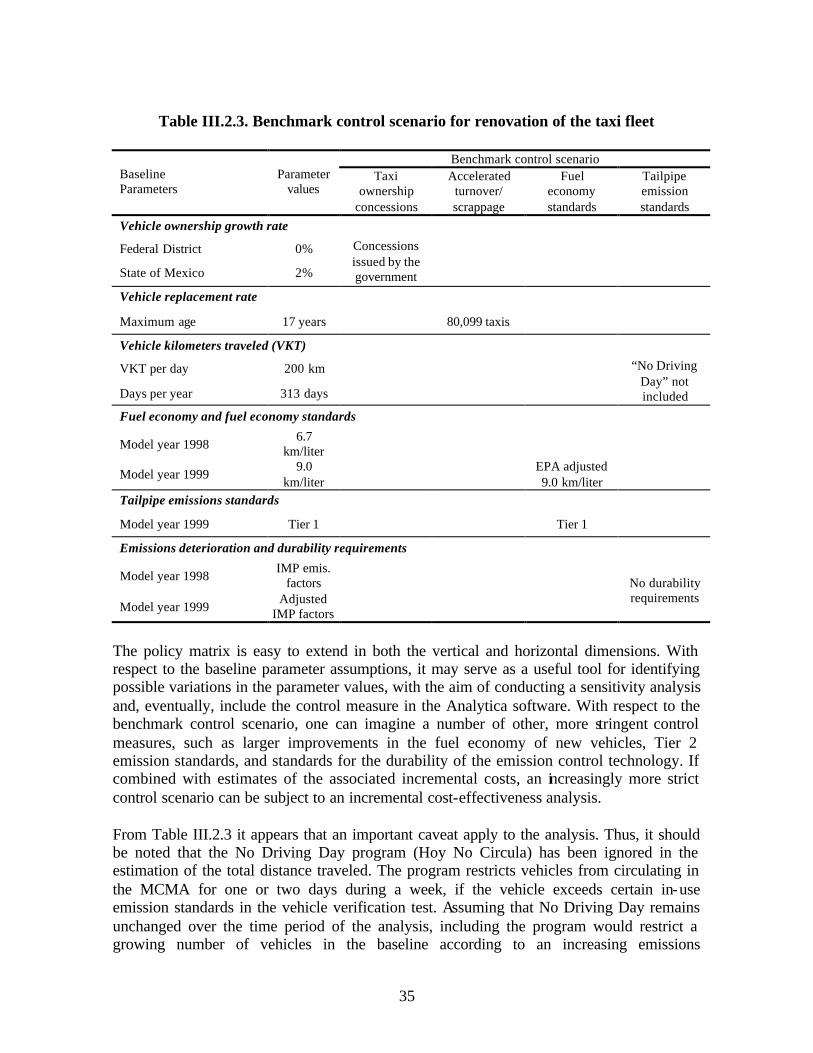
35

Table III.2.3. Benchmark control scenario for renovation of the taxi fleet

Benchmark control scenario

Baseline Parameters

Parameter values

Taxi ownership

concessions

Accelerated turnover/ scrappage

Fuel economy standards

Tailpipe emission standards

Vehicle ownership growth rate

Federal District 0%

State of Mexico 2%

Concessions issued by the government

Vehicle replacement rate

Maximum age 17 years 80,099 taxis

Vehicle kilometers traveled (VKT)

VKT per day 200 km

Days per year 313 days

“No Driving Day” not included

Fuel economy and fuel economy standards

Model year 1998 � 6.7

km/liter

Model year 1999 � 9.0

km/liter

EPA adjusted 9.0 km/liter

Tailpipe emissions standards

Model year 1999 � Tier 1 Tier 1

Emissions deterioration and durability requirements

Model year 1998 � IMP emis.

factors

Model year 1999 � Adjusted

IMP factors

No durability requirements

The policy matrix is easy to extend in both the vertical and horizontal dimensions. With respect to the baseline parameter assumptions, it may serve as a useful tool for identifying possible variations in the parameter values, with the aim of conducting a sensitivity analysis and, eventually, include the control measure in the Analytica software. With respect to the benchmark control scenario, one can imagine a number of other, more stringent control measures, such as larger improvements in the fuel economy of new vehicles, Tier 2 emission standards, and standards for the durability of the emission control technology. If combined with estimates of the associated incremental costs, an increasingly more strict control scenario can be subject to an incremental cost-effectiveness analysis. From Table III.2.3 it appears that an important caveat apply to the analysis. Thus, it should be noted that the No Driving Day program (Hoy No Circula) has been ignored in the estimation of the total distance traveled. The program restricts vehicles from circulating in the MCMA for one or two days during a week, if the vehicle exceeds certain in-use emission standards in the vehicle verification test. Assuming that No Driving Day remains unchanged over the time period of the analysis, including the program would restrict a growing number of vehicles in the baseline according to an increasing emissions

36

deterioration. By contrast, when these vehicles are replaced with new ones, the restrictions from the No Driving Day would be suspended due to the improved emissions control. The net effect of this change would therefore be to reduce the emissions reductions obtained in the present analysis. III.2.6. Costs and Emissions Reductions with the Measure

The undiscounted emissions reductions from the benchmark control scenario are shown in Table III.2.4. As explained above, there are no reductions of PM emissions, since no distinction is made between the emissions factors of old and new vehicles in the emissions inventory. By contrast, the emissions reductions of criteria pollutants and GHG are quite substantial. The time profile shows that the emissions reductions peak in 2007, the last year when taxis are scrapped and replaced through the program. The emissions reductions then start to decline. This observation is a logical consequence of the scrappage program as a measure that produces emissions reductions only temporarily. Since none of the fundamental parameters behind the turnover of the taxi fleet are affected (i.e., growth and retirement rates), the size and composition of the fleet in the control scenario will automatically converge to the original size and composition of the fleet in the baseline scenario. And since no permanent changes are assumed in the emissions characteristics of the new taxis, over and above the new vehicles in the baseline scenario, the total emissions in the control scenario will eventually return to the baseline level.

Table III.2.4. Emission reductions, renovation of the taxi fleet, without discounting (tons/yr)

Year PM10 PM2.5 SO2 CO NOx HC CO2 CH4 N2O

2003 0 0 21 48,819 1,857 5,190 88,969 21 161 2004 0 0 41 98,180 3,698 10,391 177,159 42 321 2005 0 0 61 149,710 5,263 15,702 263,476 62 477 2006 0 0 80 199,910 6,776 20,841 345,917 81 626 2007 0 0 88 224,295 7,649 23,586 377,458 89 683 2008 0 0 83 221,387 6,815 22,901 357,732 84 648 2009 0 0 78 215,184 5,482 21,135 338,532 79 613 2010 0 0 73 216,217 4,386 19,686 319,927 75 579 2011 0 0 69 205,229 2,688 16,951 301,826 71 546 2012 0 0 65 188,932 1,515 14,340 284,296 67 515 2013 0 0 61 161,978 555 11,010 267,350 63 484 2014 0 0 58 138,049 31 8,654 250,998 59 454 2015 0 0 54 114,409 -490 6,294 235,252 55 426 2016 0 0 50 95,596 -254 4,768 218,906 51 396 2017 0 0 47 78,851 -21 3,315 204,468 48 370 2018 0 0 44 68,477 -18 2,594 190,789 45 345 2019 0 0 41 56,915 -15 1,840 177,886 42 322 2020 0 0 38 44,830 -12 1,071 166,711 39 302

37

Table III.2.5. Annualized emissions reductions from the renovation of the taxi fleet (ton/yr)

The annualized emissions reductions are shown in Table III.2.5 for a plausible range of discount rates. The table shows that the results are not very sensitive, neither to changes in the discount rate, nor to changes in the time horizon of the analysis. With the exception of the NOX reductions, the changes are quite small. The larger change in NOX reductions from 2010 to 2020 is due to a sharp decline in NOX emissions reductions, which even become negative from 2015 and onwards. This seeming paradox is explained by the emissions factors for NOX in the emissions inventory, which show a remarkable jump in the emissions for the 1989 and 1990 model year vehicles. However, while this jump had a justification in the past, as a technical artifact of the existing taxi fleet, it is unlikely to be replicated in the future. A more careful modeling of the future emissions of taxis, including the (NOX) emissions deterioration rates, might show a less drastic return to the underlying baseline trend. Such a modeling exercise could be conducted on the MOBILE5 or MOBILE6 models. The time profile of the undiscounted cost estimates and the annualized costs are shown in Table III.2.6 and Table III.2.7. It is clear from the undiscounted costs that although both the public and private costs of capital are substantial, there are also considerable savings in fuel costs due to an improved fuel economy of new vehicles. Note that the fuel savings peak in the year 2007 for the same reasons as the emissions reductions. Similarly, the annual savings will eventually become zero at some point beyond the time horizon of the analysis. Given the time profile of the costs, with large up-front capital costs and fuel savings distributed over the entire time period of analysis, it is expected that the total cost estimates are sensitive to both the choice of discount rate and the choice of time horizon. A lower discount rate leads to much lower total costs, because the future savings are discounted less compared to the initial capital costs. Likewise, when the time horizon of the analysis is extended from 2010 to 2020, the fuel savings are included over a longer period, while the capital costs remain unchanged. This leads to negative total costs for the 2003 to 2020 period, independently of the discount rate applied in the analysis.

Discount rate PM10 PM2.5 SO2 CO NOx HC CO2 CH4 N2O

Time horizon 2003-2010

0% 0 0 66 171,713 5,241 17,429 283,646 67 514

3% 0 0 65 167,970 5,178 17,090 278,478 65 504

5% 0 0 64 165,483 5,135 16,863 275,007 64 498

7% 0 0 63 163,010 5,090 16,636 271,528 64 492

Time horizon 2003-2020

0% 0 0 59 140,387 2,550 11,682 253,758 60 459

3% 0 0 59 144,397 2,866 12,403 256,479 60 464

5% 0 0 59 146,380 3,060 12,811 257,542 60 466

7% 0 0 60 147,818 3,239 13,159 258,018 61 467

38

Table III.2.6. Costs of renovation of the taxi fleet without discounting

(millions US$/yr)

Year Public

Investment Private

Investment O&M Cost

Total Cost

2003 24.03 80.10 -19.74 84.39 2004 24.03 80.10 -39.31 64.82 2005 24.03 80.10 -58.60 45.53 2006 24.03 80.10 -76.93 27.20 2007 24.03 80.10 -83.95 20.18 2008 -79.56 -79.56 2009 -75.29 -75.29 2010 -71.31 -71.31 2011 -67.28 -67.28 2012 -63.37 -63.37 2013 -59.59 -59.59 2014 -55.95 -55.95 2015 -52.44 -52.44 2016 -48.79 -48.79 2017 -45.58 -45.58 2018 -42.53 -42.53 2019 -39.65 -39.65 2020 -37.16 -37.16

Table III.2.7. Annualized costs of renovation of the taxi fleet (millions US$/yr)

Compliance Cost (2003 millons US$/ yr)

Discount rate Public Investment

Private Investment O&M Cost

Total Cost

Time Horizon 2003-2010 0% 15.02 50.06 -63.09 1.99 3% 15.68 52.26 -61.94 6.00 5% 16.10 53.66 -61.16 8.59 7% 16.50 55.00 -60.39 11.12

Time Horizon 2003-2020 0% 6.68 22.25 -56.50 -27.58 3% 8.00 26.67 -57.10 -22.43 5% 8.90 29.67 -57.33 -18.76 7% 9.79 32.65 -57.43 -14.99

III.2.7. Uncertainty

As emphasized already, there are many unquantified uncertainties associated with the wide range of parameter values included in the present analysis. It is therefore recommendable that a careful sensitivity analysis is performed, in order to check to what extent the results obtained are robust. Such an analysis can also be used to identify those parameters that contribute most to the overall uncertainty, and provide a basis for future improvements.

39

Among the parameters in the present analysis, some can be identified as playing a key role for the final results. They include the emissions factors of PM10, the emissions of old high-use vehicles, emissions deterioration rates for the future taxi fleet, and the age specific rate of retirement. These variables, in particular, should be subject to more careful analysis of their quantitative impact on the results. In addition, we have adopted a moderate control scenario in the present analysis. If cost estimates for Tier 2 vehicles can be obtained, it would be interesting to see how large further emissions reductions can be achieved. Since this would imply a permanent shift in the emission rates of new vehicles, the emission reductions would also be more permanent. Considerable uncertainty also exists with respect to the implementation of the taxi substitution program and its expected level of compliance. Since this has been conveniently assumed away in the present analysis, the question of the enforcement of scrappage and replacement does not arise. This is a form of model uncertainty that should be taken seriously. III.2.8. Discussion and Next Steps

On the basis of the present analysis, the scrappage and replacement of taxis seems to be a worthwhile measure to adopt in order to control the large share of emissions from mobile sources in the MCMA. However, this conclusion depends on a number of uncertain factors, whose influence has not been formally analyzed. A careful sensitivity analysis could provide a more firm ground upon which the taxi substitution program is recommended to policy makers and communicated to the public. In this respect, an effort should be made to explain, to what extent the results obtained from the scrappage and replacement of taxis can be expected to carry over to the in-use private car fleet. A fundamental source of conflict exists in the current design of the program. This conflict means that, under the worst circumstances, an over-valued price of the oldest taxis is being used to achieve emissions reductions which are highly uncertain, and which we have been unable to verify and document within the time available for this study. The uncertainty derives from a poor understanding of the average emissions of old taxis, for which there are no directly estimated emissions factors in the emissions inventory. It also derives from a supposedly large distribution over this average, which has been observed in numerous measurement studies of private cars. If these observations hold also for taxis, an improved cost-effectiveness of the taxi substitution program might be achieved by an improved targeting of the program. As a thought experiment, a better targeting is associated with improved knowledge of high-emitting taxis and their costs in the used car market. This calls for an increased testing of the taxis in the program, possibly at the expense of scrapping 80% of the fleet. III.2.9. References Alberini, A., W. Harrington, and V. McConnell (1995), “Determinants of Participation in Accelerated Vehicle Retirement Programs”, The RAND Journal of Economics, 26(1), 93-112.

40

Alberini, A., W. Harrington, and V. McConnell (1998), “Fleet Turnover and Old Car Scrap Policies”, Discussion Paper 98-23, Resources for the Future, Washington, D.C. Burnette, A.D., S. Kishan, and M.E. Wolf (2001), “MOBILE5-Mexico: An Emission Factor Model for On-Road Vehicles in Mexico”, Paper presented at the 10th Annual Emission Inventory Conference, May 2, 2001, Denver, Colorado. Cadle, S.H, P. Mulawa, E.C. Hunsanger, K. Nelson, R.A. Ragazzi, R. Barrett, G. Gallagher, D.R. Lawson, K.T. Knapp, and R. Snow (1999), “Light-Duty Motor Vehicle Exhaust Particulate Matter Measurements in the Denver, Colorado Area”, Journal of the Air and Waste Management Associaction, 49, 164-74. Cadle, S.H., P. Mulawa, P. Groblicki, C. Laroo, R.A. Ragazzi, K. Nelson, G. Gallagher, and B. Zielinska (2001), “In-Use Light-Duty Gasoline Vehicle Particulate Matter Emissions on Three Driving Cycles”, Environmental Science and Technology, 35, 26-32. CAM (Comisión Ambiental Metropolitana) (2002a), Inventario de Emisiones de la Zona Metropolitana del Valle de México, 1998 (Mexico, D.F.: CAM). CAM (Comisión Ambiental Metropolitana) (2002b), Programa para Mejorar la Calidad del Aire de la Zona Metropolitana del Valle de México, 2002-2010 (Mexico, D.F.: CAM). COMETRAVI (Comisión Metropolitana de Transporte y Vialidad) (1999), “Diagnóstico de las Condiciones del Transporte y sus Implicaciones sobre la Calidad del Aire”, in Estudio Integral de Transporte y Calidad del Aire para la Zona Metropolitana del Valle de México, Vol. 1 (Mexico, D.F.: COMETRAVI and CAM). Dixon, L. and S. Garber (2001a), Fighting Air Pollution in Southern California by Scrapping Old Vehicles (Santa Monica, CA.: RAND Institute for Civil Justice). Dixon, L. and S. Garber (2001b), “Scrapping Old Vehicles Would Improve Southern California Air Quality at Reasonable Cost”, Research Brief, RB-9033, RAND Institute for Civil Justice, Santa Monica, CA. Dixon, L., S. Garber, and I. Porche (2002), “Driven Into a Corner”, RAND Review, 26(3), 10-15. ERG (Eastern Research Group) and Radian International (2000), MOBILE5-Mexico: Documentation and User’s Guide (Denver, CO.: Western Governors’ Association and Binational Advisory Committee). ESMAP (UNDP/World Bank Energy Sector Management and Assistance Program) (2002), “Can Vehicle Scrappage Programs Be Successful?”, South Asia Urban Air Quality Management Briefing Note No. 8, World Bank, Washington, D.C. Estache, A. (2001), “Privatization and Regulation of Transport Infrastructure in the 1990s”, The World Bank Research Observer, 16 (1), 85-109.

41

Gakenheimer, R., L.T. Molina, J. Sussman, C. Zegras, A. Howitt, J. Makler, R. Lacy, R. Slott, and A. Villegas, with contributions from M.J. Molina and S. Sanchez (2002), “The MCMA Transportation System: Mobility and Air Pollution”, in L.T. Molina and M.J. Molina, eds. (2002), Air Quality in the Mexico Megacity: An Integrated Assessment (Dordrecht: Kluwer Academic Publishers). Gonzalez, L.E. (2002), “Design of the Taxi Renewal Program”, Presentation at the Fifth Workshop on Mexico City Air Quality, January 21.-24., 2002, Ixtapan de la Sal, State of México (MIT Integrated Program on Urban, Regional and Global Air Pollution). Hahn, R.W. (1995), “An Economic Analysis of Scrappage”, The RAND Journal of Economics, 26(2), 222-42. Hamilton, B.W. and M.K. Macauley (1998), “Competition and Car Longevity”, Discussion Paper 98-20, Resources for the Future, Washington, D.C. Harrington, W., V.D. McConnell, and M. Cannon (1998), “A Behavioural Analysis of EPA’s MOBILE Emission Factor Model”, Discussion Paper 98-47, Resources for the Future, Washington, D.C. Harrington, W. and V.D. McConnell (2003), Motor Vehicles and the Environment (Washington, D.C.: Resources for the Future). IPCC (Intergovernmental Panel on Climate Change) (1997), Revised 1996 IPCC Guidelines for National Greenhouse Gas Inventories, Vols. 1-3 (Bracknell, UK: IPCC). Kojima, M. and R. Bacon (2001), Mexico Energy Environment Review, May 2001 (Washington, D.C.: Joint UNDP/World Bank Energy Sector Management Assistance Programme). Molina, M.J., L.T. Molina, J. West, G. Sosa, and C. Sheinbaum, with contributions from F.C. Martini, M.A. Zavala, and G. McRae (2002), “Air Pollution Science in the MCMA: Understanding Source-Receptor Relationships Through Emissions Inventories, Measurements, and Modeling”, in L.T. Molina and M.J. Molina, eds. (2002), Air Quality in the Mexico Megacity: An Integrated Assessment (Dordrecht: Kluwer Academic Publishers). Mostashari, A. (2003), “Design of Robust Air Quality Measures for the Road-Based Public Transportation Sector in Megacities: The Case of the Mexico City Metropolitan Area (MCMA)”, M.Sc. Dissertation, Massachusetts Institute of Technology, Boston. Mugica, A.V., R.E. Vega, J.L. Arriaga, and M.E. Ruiz (1998), “Determination of Motor Vehicle Profiles for Non-Methane Organic Compounds in the Mexico City Metropolitan Area”, Journal of the Air and Waste Management Association, 48, 1060-68. NRC (National Research Council, Transportation Research Board) (2000), Modeling Mobile Source Emissions (Washington, D.C.: National Academy Press).

42

NRC (National Research Council, Transportation Research Board) (2002), Effectiveness and Impact of Corporate Average Fuel Economy (CAFE) Standards (Washington, D.C.: National Academy Press). Paramo, V.H. (2003), “Mexico City Metropolitan Area Report”, Presentation at Diesel Days, January 16-17, 2003, World Bank Clean Air Initiative and World Resources Institute, Washington, D.C.. Portney, P. (2002), “Penny-Wise and Pound-Fuelish? New Car Mileage Standards in the United States”, Resources, 147, 10-15. Radian International (1997), Mexico Emissions Inventory Program Manuals, Vol. 6: Motor Vehicle Inventory Development (Denver, CO.: Western Governors’ Association and Binational Advisory Committee). SENER (Secretaría de Energía) (2000), Prospectiva de Mercado de Gas Natural Comprimido, 2000-2010 (Mexico, D.F.: SENER) SETRAVI (Secretaría de Transporte y Vialidad) (2002a), Programa de Financiamiento para la Sustitución de Taxis en el Distrito Federal (Mexico, D.F.: SETRAVI). SETRAVI (Secretaría de Transporte y Vialidad) (2002b), Primera Versión del Programa Integral de Transporte y Vialidad, 2002-2006 (Mexico, D.F.: SETRAVI). U.S. EPA (Environmental Protection Agency) (1998), “Transportation Control Measures: Accelerated Vehicle Retirement”, TRAQ Technical Overview, EPA420-S-98-001. U.S. EPA (Environmental Protection Agency) (2000), Guidelines for Preparing Economic Analyses (Washington, D.C.: EPA 240-R-00-003). U.S. EPA (Environmental Protection Agency) (2001a) Light-Duty Automotive Technology and Fuel Economy Trends: 1975 Through 2001 (Washington, D.C.: EPA420-R-01-008) U.S. EPA (Environmental Protection Agency) (2001b), EPA’s New Generation Mobile Source Emissions Model: Initial Proposal and Issues (Washington, D.C.: EPA). U.S. EPA (Environmental Protection Agency) (2002), “Official Release of the MOBILE6 Motor Vehicle Emissions Factor Model”, Federal Register, 67(19), 4254-57. Vega, E., V. Mugica, R. Carmona, and E. Valencia (2000), “Hydrocarbon Source Apportionment in Mexico City Using the Chemical Mass Balance Receptor Model”, Atmospheric Environment, 34, 4121-29.

43

III.3. Expansion of the Metro III.3.1. Introduction

Economic growth is the fundamental force that promotes road congestion and air pollution because it influences rates of motorization, generation of trips and urban growth. The origin-destination (O-D) survey conducted by the National Statistics Institute (INEGI) in 1994, indicates that approximately 29 million vehicle trip segments per day were made in the MCMA. Federal District has 66.5% of these trips, whereas trips of the urbanized municipalities of the State of Mexico represent 33.5%. This is 1.73 trip sections per capita. The projection indicates that in 2020 the trip segments will have grown to 36 million. In terms of overall mode share, using the data on trip segments in 1994, low and medium occupancy modes dominate the landscape. Colectivos account for over 50 percent of trip segments and autos and taxis another 20 percent. Among the high occupancy modes, the metro accounts for roughly 14 percent of all trips, followed by urban and suburban buses with 10 percent. The new Program to Improve the Air Quality in the Valley of Mexico (Programa para Mejorar la Calidad del Aire en el Valle de México 2002-2010 or PROAIRE), also reports a similar tendency in 1998; the capture of passengers of the low occupancy transport continues increasing. On basis to the 1998 emission inventory, near 2.5 million tons of local pollutants were emitted, of which 84% were generated by the mobile sources, principally private autos, taxis, combis and microbuses. For 2010 PROAIRE projects 3.2 million tons of local pollutants, and 5.5 million of vehicles, 80% low occupancy transport. From a modal share perspective, the most worrying trend is the massive shift towards lower capacity modes at the expense of Metro ridership and bus use. This is one of the principal policy challenges facing the city's transportation system. On basis of previous parragraphs, the objective of the Expansion of the Metro is to give a fast, efficient, safe and nonpolluting transport, in agreement with the future demand in the Mexico City Metropolitan Area. III.3.2. Description of the Measure

This control measurement is included in the Integral Strategy of Transport and Air Quality for the MCMA, published by the Metropolitan Commission of Road and Transport (COMETRAVI) in 1999. The Metropolitan Environmental Commission also participated in this strategy. A document that served as base was the “Plan Maestro del Metro y Trenes Ligeros 1996” (Master Plan of Metro and Light Trains, 1996). This Plan proposed the addition of 166 km of new lines of metro, divided between 76 km of urban metro in central city (Federal District) and 68 km of suburban metro or regional train (State of Mexico) for year 2020. In this document the suburban metro was not analyzed. COMETRAVI reports that almost 5 kilometers of metro in the DF will be constructed between 2000 and 2010, and 70 km between 2011 and 2020. PROAIRE also includes the same total installation, but with an implementation plan of 76 kilometros from 2002 to 2010. However, PROAIRE

44

does report the same emission reductions as COMETRAVI. In these documents, economic indicators (Net Present Value) and the emission reductions of carbon dioxide were not considered. In the co-control study, West et al (2003), included both indicators. In our analysis of this measure, we consider that 76 kilometers of metro in the Federal District will be constructed in the period from 2003 to 2020, to have a total network in the DF of 276 km by 2020, in agreement with the COMETRAVI implementation plan. Also in accordance with this plan, implementation is staged with 5 km being constructed between 2003 and 2010, with an additional 71 km between 2011 and 2020. The passengers who travel by metro in 1994 (base year of COMETRAVI analysis) were more than 4 million and for 2020 this number will be increased by 111% due to the Expansion of the metro. III.3.3. Data Requirements

To estimate the impact of the Expansion of Metro, we must have the future growth (2003 to 2020) of population in the MCMA; trips per capita; vehicular fleet and the mode share for vehicle trip segments in the period. To understand current metro use, we need existing metro kilometers, annual and daily round trips, traveled km /day, and transported passengers. For other transport modes, we need occupancy per vehicle, traveled kilometer per day, and the number of days in circulation. Also we need emission factors for local and global pollutants (in g/km and kg/GWh) which are coupled with vehicle kilometers traveled or energy consumption estimates. We need investment, operation and maintenance, and fuel costs. III.3.4. Determining Baseline Emissions

Our benchmark scenario for emissions reductions due to the Expansion of the metro are estimated as a difference from the baseline emissions of the metro and medium occupancy transport (combis and microbuses) that will be substituted or avoided by the metro and those in the control scenario. In other scenarios not considered in detail here, we also estimate the impacts if the substitution were to occur from only microbuses, from private cars and taxis, and from diesel buses. Since a baseline for this measure was not considered in previous studies, we established the baseline. We assume that the capacity of high occupancy transport (metro, trolleybus and light rail) is almost saturated, then the number of passengers who travel in this transport, will remain fixed until 2020. The increase of trips from 2003 to 2020 will be absorbed by other travel modes – low and medium occupancy modes - and that they do not require of investment (buses, microbus, combis, private taxis, cars) in infrastructure. With population growth data in the period of analysis and the number of trips per capita, we considered that almost 29 million of trips were made in 1994 and more than 36 million of trips would be made in 2020.

45

The annual increase of the low and medium capacity vehicular fleet until 2020 was estimated on the basis of the increase trips absorbed from the massive transport and the individual occupancy of each vehicle (bus 350 passengers; microbus 300; combi 7; private auto 1.7). With the annual units of each transport modes and their daily travel kilometers, we estimated the annual kilometers. It was not possible to obtain a distribution of the vehicular fleet per year model, we only estimated the total number of each vehicle in each year. This explanation has importance for the definition of the emission factors that we used. We calculated the baseline emissions with the emission factor and activity level. In the case of the metro , activity level was the electricity consumption (GWh) and the emission factors were taken from the IPCC and PROAIRE. For local pollutants, the emission factors considers the fraction of electrical energy that is generated by the power stations of the ZMVM in relation to the interconnected system (3.1%). The emission factors for global pollutants, consider the total of emissions due to the generation of electricity (global effect). The emission factor for CO2, CH4 and N2O, was weighed according to the primary energy consumption used (fossil fuel) to generate electricity in the interconnected system.

EFG= ∑(Ci/Cn) * EFCO2i i

EFG = the emission factor for CO2, CH4 or N2O (taken from IPCC, 1997). Ci = the consumption of fuel i, used to generate electricity [PJ] in the interconnected

system. Cn = the total consumption of all fuels, used to generate electricity [PJ] in the

interconnected system. Emissions of local pollutants in COMETRAVI (1999) are estimated assuming that the Metro replaces (avoids) diesel buses but the emission factors used appear to be very large (a factor or more than 2 compared with PROAIRE emission factors for urban buses). Obviously, this will tend to overestimate emission reductions, and possibly by a large amount. In our analysis, we considered four scenarios: the expansion of the Metro would replace buses; microbuses and combis; microbuses; private autos and taxis. We assume avoided vehicle use eliminates old vehicles. Due to social realities in Mexico City, we consider the most feasible scenario is the sustitution of microbus and combis, and so this is used as our benchmark. Because we do not have an annual distribution of the vehicular fleet per year model, we also weighed the emission factors for local pollutants reported in the emission inventory 1998 for the MCMA and global pollutants in IPCC.

46

Table III.3.1. Metodology to estimate weighted emission factors

CO2 (g/km) Year Number of microbuses % of total fleet

E.F. x model year EF weighted 1974 555 1.16 601 6.96

: : : : :

1994 199 0.33 3.96 1.31 Total 47,950 100 596

The final emission factors used, can be seen in the next table.

Table III.3.2. Emission Factors

Transport Mode

PM10 PM2.5 SO2 CO NOx HC CO2 CH4 N2O

Metro (kg/GWh)

0.78 0.60 0.09 6.29 53.99 0.27 261,938 3.08 1.44

Colectivos (g/km)

Microbuses 0.03 0.02 0.12 108 4.75 9.86 596 0.13 0.03

Combis 0.03 0.02 0.12 59.4 2.70 5.65 589 0.12 0.04 III.3.5. Estimating Emissions Reductions and Costs for the Measure

In agreement with the COMETRAVI plan for the Expansion of the metro, we estimated the annual consumption of energy (GWh) by the annual additional kilometers of metro until the 2020. With the weighted emission factor in kg/GWh, we estimated the emissions due to the Expansion of the metro. We assumed that the additional passengers who will travel in metro come from microbuses and combis. If each microbus and combi transport 350 and 70 passengers per day respectively, then we have more than 13,000 microbuses and 6,200 combis avoided. Both microbus and combi travelled 200 km per day and circulate 313 days per year, then we know the total kilometers avoided due to the Expansion of the metro and multiplying per the correponding emission factor, we have the emissions of each pollutant in the control scenario. Emission reductions are the difference between the baseline emissions and control scenario. The cost for a kilometer of metro ($35 million USD) from MCMA is taken from a July 2002 article in Reforma Magazine (http://www.reforma.com/ciudaddemexico/articulo/209896/). However, COMETRAVI (1999c) indicates a price of $52 million USD. Regarding to Operations and Maintenance, we estimated the cost due to the incremental energy consumption of the new kilometers of metro. The price of electricity is taken from electronic page of Mexican Energy Ministry. Recuperation value at the end of either time period is included, considering a useful life of 30 years.

47

To consider the saved liters of gasoline by the avoided microbuses and combis, we used the fuel efficiency reported by Sanchez et al, 1999 (2.39 km/lt for microbuses and 3 km/lt for combis). The price of Magna gasoline liter ($5.97) is taken from the website of the Mexican Petroleum Corporation, PEMEX. The 15% value added tax is removed, and conversion to dollars uses an exchange rate of 10. III.3.5. Costs and Emissions Reductions with the Measure

In Tables III.3.3 and III.3.4, it is illustrated that there are significant CO2 reductions due to this measure across the entire time horizon to 2020. On the local side, reductions of HC and NOx will have the most significant impact on air quality.

Table III.3.3. Emissions reductions for expansion of the metro without discounting (tons/yr)

Year PM10 PM2.5 SO2 CO NOx HC CO2 CH4 N2O

2003 0 0 1 829 37 76 4,610 1 0

2004 1 0 2 1,658 73 153 9,220 2 1

2005 1 1 3 2,487 110 229 13,830 3 1

2006 1 1 4 3,316 146 305 18,440 5 1

2007 1 1 5 4,144 183 381 23,050 6 1

2008 2 1 6 4,973 219 458 27,660 7 2

2009 2 1 7 5,802 256 534 32,270 8 2

2010 2 1 8 6,631 292 610 36,880 9 2

2011 5 3 21 17,126 755 1,575 95,245 23 5

2012 9 6 34 27,620 1,217 2,541 153,611 38 9

2013 12 8 47 38,114 1,680 3,506 211,976 52 12

2014 15 10 60 48,609 2,143 4,472 270,342 66 16

2015 18 12 74 59,103 2,605 5,437 328,707 80 19

2016 22 14 87 69,597 3,068 6,403 387,073 95 22 2017 25 16 100 80,092 3,530 7,368 445,438 109 26

2018 28 18 113 90,586 3,993 8,334 503,804 123 29

2019 31 20 126 101,080 4,455 9,299 562,169 137 32 2020 35 23 139 111,575 4,918 10,265 620,535 152 36

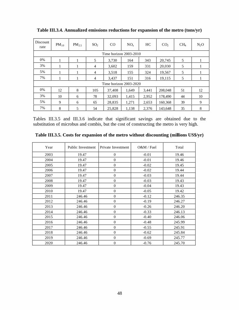
48

Table III.3.4. Annualized emissions reductions for expansion of the metro (tons/yr)

Tables III.3.5 and III.3.6 indicate that significant savings are obtained due to the substitution of microbus and combis, but the cost of constructing the metro is very high. Table III.3.5. Costs for expansion of the metro without discounting (millions US$/yr)

Year Public Investment Private Investment O&M / Fuel Total

2003 19.47 0 -0.01 19.46 2004 19.47 0 -0.01 19.46 2005 19.47 0 -0.02 19.45 2006 19.47 0 -0.02 19.44 2007 19.47 0 -0.03 19.44 2008 19.47 0 -0.03 19.43 2009 19.47 0 -0.04 19.43 2010 19.47 0 -0.05 19.42 2011 246.46 0 -0.12 246.35 2012 246.46 0 -0.19 246.27 2013 246.46 0 -0.26 246.20 2014 246.46 0 -0.33 246.13 2015 246.46 0 -0.40 246.06 2016 246.46 0 -0.48 245.99 2017 246.46 0 -0.55 245.91 2018 246.46 0 -0.62 245.84 2019 246.46 0 -0.69 245.77 2020 246.46 0 -0.76 245.70

Discount rate

PM10 PM2.5 SO2 CO NOx HC CO2 CH4 N2O

Time horizon 2003-2010

0% 1 1 5 3,730 164 343 20,745 5 1 3% 1 1 4 3,602 159 331 20,030 5 1 5% 1 1 4 3,518 155 324 19,567 5 1 7% 1 1 4 3,437 151 316 19,115 5 1

Time horizon 2003-2020

0% 12 8 105 37,408 1,649 3,441 208,048 51 12 3% 10 6 78 32,093 1,415 2,952 178,490 44 10 5% 9 6 65 28,835 1,271 2,653 160,368 39 9 7% 8 5 54 25,828 1,138 2,376 143,648 35 8

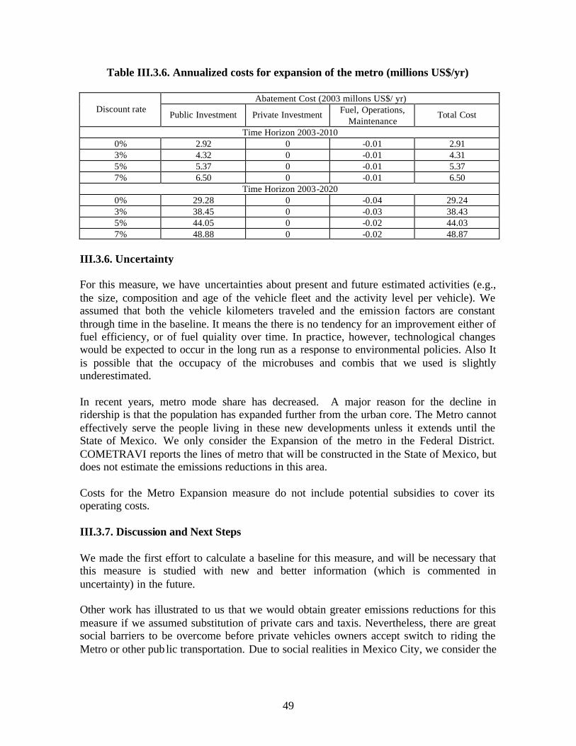
49

Table III.3.6. Annualized costs for expansion of the metro (millions US$/yr)

Abatement Cost (2003 millons US$/ yr) Discount rate

Public Investment Private Investment Fuel, Operations, Maintenance

Total Cost

Time Horizon 2003-2010 0% 2.92 0 -0.01 2.91 3% 4.32 0 -0.01 4.31 5% 5.37 0 -0.01 5.37 7% 6.50 0 -0.01 6.50

Time Horizon 2003-2020 0% 29.28 0 -0.04 29.24 3% 38.45 0 -0.03 38.43 5% 44.05 0 -0.02 44.03 7% 48.88 0 -0.02 48.87

III.3.6. Uncertainty

For this measure, we have uncertainties about present and future estimated activities (e.g., the size, composition and age of the vehicle fleet and the activity level per vehicle). We assumed that both the vehicle kilometers traveled and the emission factors are constant through time in the baseline. It means the there is no tendency for an improvement either of fuel efficiency, or of fuel quiality over time. In practice, however, technological changes would be expected to occur in the long run as a response to environmental policies. Also It is possible that the occupacy of the microbuses and combis that we used is slightly underestimated. In recent years, metro mode share has decreased. A major reason for the decline in ridership is that the population has expanded further from the urban core. The Metro cannot effectively serve the people living in these new developments unless it extends until the State of Mexico. We only consider the Expansion of the metro in the Federal District. COMETRAVI reports the lines of metro that will be constructed in the State of Mexico, but does not estimate the emissions reductions in this area. Costs for the Metro Expansion measure do not include potential subsidies to cover its operating costs. III.3.7. Discussion and Next Steps

We made the first effort to calculate a baseline for this measure, and will be necessary that this measure is studied with new and better information (which is commented in uncertainty) in the future. Other work has illustrated to us that we would obtain greater emissions reductions for this measure if we assumed substitution of private cars and taxis. Nevertheless, there are great social barriers to be overcome before private vehicles owners accept switch to riding the Metro or other pub lic transportation. Due to social realities in Mexico City, we consider the

50

most feasible scenario is the sustitution of microbus and combis, and so this is used as our benchmark. Emissions reductions in this scenario are still very significant. The implementation of this measurement is very expensive, but it has additional benefits since it reduces the colectivos fleet, avoid the vehicular congestion and local pollutant emissions. It will be necessary to review the new Master Plan of Metro in the MCMA, to update this measurement and to review if there is better information regarding the synergies between Expansion of metro and other transport modes. The Expansion of the metro towards the State of Mexico also will have to be analyzed, since this area will have the greater urban growth in the next years. III.3.8. References CAM, Comisión Ambiental Metropolitana (2002a), “Programa para Mejorar la Calidad del Aire de la Zona Metropolitana del Valle de México, 2002-2010” (PROAIRE), Comisión Ambiental Metropolitana. CAM, Comisión Ambiental Metropolitana (2002b), “Inventario de Emisiones de la Zona Metropolitana del Valle de México, 1998”, in http://www.sma.gob.mx/publicaciones/aire/html COMETRAVI, Comisión Metropolitana de Transporte y Vialidad (1999a), “Diagnóstico de las Condiciones del Transporte y sus Implicaciones sobre la Calidad del Aire”, in “Estudio Integral de Transporte y Calidad del Aire para la Zona Metropolitana del Valle de México, Vol. 1” (Mexico City: COMETRAVI and CAM). COMETRAVI, Comisión Metropolitana de Transporte y Vialidad (1999b), “Definición de Políticas para el Metro, Tren Ligero, Trolebús Urbano y Otros Medios de Transporte Masivo en un Nivel Metropolitano”, in Estudio Integral de Transporte y Calidad del Aire para la Zona Metropolitana del Valle de México, Vol. 4 (Mexico City: COMETRAVI and CAM). COMETRAVI, Comisión Metropolitana de Transporte y Vialidad (1999c), “Definición de Políticas para la Infraestructura del Transporte”, in Estudio Integral de Transporte y Calidad del Aire para la Zona Metropolitana del Valle de México, Vol. 6 (Mexico City: COMETRAVI and CAM). Gobierno del Distrito Federal (2003). Información básica del sistema de transporte colectivo Metro in http://www.df.gob.mx/agenda2000/transporte/9_1.html Instituto Nacional de Estadística, Geografía e Informática, INEGI (2003), Principales características del Sistema de Transporte Colectivo Metro, Banco de Información Económica. In http://www.inegi.gob.mx

51

IPCC, Intergovernmental Panel on Climate Change (1997), “Revised 1996 IPCC Guidelines for National Greenhouse Gas Inventories, Vol. 3” (Bracknell, UK: IPCC). Molina, L.T. and M.J. Molina, eds. (2002), Air Quality in the Mexico Megacity: An Integrated Assessment, Kluwer Academic Publishers, Boston, 384 pp. PEMEX Refinación (2002), Anuario Estadístico 2002. México, D.F. In http://www.pemex.gob.mx/index.cfm/action/content/sectionID/1/catID/237/subcatID/246/index.cfm?action=content&sectionID=1&catID=237&subcatID=246 Sánchez Sergio et., al (1999) "Evaluación del Gas Natural", México, D.F. SETRAVI, Secretaría de Transporte y Vialidad (2000), Primera Versión del Programa Integral de Transporte y Vialidad. SENER, Secretaría de Energía (2001), Balance Nacional de Energía 2000. West, J.J., P. Osnaya, I. Laguna, J. Martínez, A. Fernández (2003) Co-control of urban air pollutants and greenhouse gases in México City. Final report to US National Renewable Energy Laboratory, subcontract ADC-2-32409-01.

52

III.4. Hybrid Buses III.4.1. Introduction

The 2000 SETRAVI inventory indicates that the RTP has 985 buses and STP has 168 units (Molina and Molina, 2002). PROAIRE indicates that this is a small part (~10%) of the total diesel vehicle fleet (13,067 vehicles in 2000). The concept of this measure is to replace almost all of these publicly owned diesel transport buses (RTP and STE) with highly efficient, low polluting hybrid buses. III.4.2. Description of the Measure

We follow the implementation plan of PROAIRE measure 22 (introduction of compressed natural gas (CNG) buses), simply changing the technology for this replacement to a hybrid bus as in West et al. (2003). Thus, 1,029 buses from the public RTP and STE systems are to be replaced, almost all of the buses from those systems. We assume 257 buses are replaced each year for 4 years (2003 – 2006), following the implementation schedule from PROAIRE. III.4.3. Data Requirements

To estimate the impact of the introduction of hybrid buses, we must have emission factors for local and global pollutants (in g/km or g/L) and couple these with vehicle kilometers traveled or fuel usage estimates. We need investment, operation and maintenance, and fuel costs. III.4.4. Determining Baseline Emissions – Diesel Buses

Emissions reductions due to the introduction of the hybrid buses are estimated as a difference from the baseline emissions of the diesel buses currently in the system and those that would enter the fleet via fleet growth or natural replacement of old vehicles. Baseline emissions are estimated using emission factors with age and vehicle age distributions used for PROAIRE measure 22 by the Secretariat of the Environment for the Federal District. However, this baseline projection for vehicle age distribution is altered from PROAIRE so that the estimated 2% growth in the fleet each year occurs only in the new vehicles. Additionally, a natural turnover of 2% is assumed in which the oldest buses have the highest likelihood of being removed from the fleet and replaced with a new vehicle, similar to that which is done for the taxi fleet projection. This is a rough model of natural retirement that certainly could be improved, but it provides a mid-ground between a pessimistic baseline in which no natural turnover occurs and the optimistic PROAIRE baseline in which there is no aging of the vehicle fleet. To calculate greenhouse gas emissions from the diesel buses, we need a fuel efficiency which is not reported by PROAIRE since those emissions factors are based on kilometers traveled, not fuel use. We use the M.J. Bradley and Associates (2000) estimate of fuel

53

efficiency for the NovaBUS RTS Diesel Series 50 for the mean of the two city driving cycles (Table III.4.1). We note that this fuel efficiency with PROAIRE kilometers-traveled emissions factors (in g/km) gives very similar fuel-based emissions factors (in g/L) as World Bank fuel efficiency with World Bank kilometers-traveled emissions factors for CO, HC, and PM, and NOx factors agree within a factor of 2. III.4.5. Estimating Emissions Reductions and Costs for the Measure

Previous work on Hybrid vehicles for Mexico City consists of a study by Consultants to the World Bank (2000) in which 4 bus technologies were compared to a diesel option. However, emissions factors in the report have many apparent inconsistencies between the various hybrid technologies; with IPCC emission factors for greenhouse gases; with emission estimates from driving cycle tests in New York City (M.J. Bradley and Associates, 2000); and with PROAIRE emissions factors for diesels. This is likely because the study used manufacturer’s data and information from other third-party sources, not actual driving cycle tests in Mexico City. It is likely that the information compiled in the report came from diverse sources and that the driving cycles on which this information was based was not consistent between technologies, or perhaps even for the same technologies. Further, we have not been able to identify the authors of the study in order to ask methodological questions. Finally, representatives of the World Bank have confirmed that emission factors in this study had many problems and are difficult to interpret (J. A. Lopez Silva, personal communication to J. West). In this light, we decide not to use results from the Consultants to the World Bank study in this work, except to make a rough check for internal consistency on diesel fuel efficiency. We base our estimates on the report of M.J. Bradley and Associates for New York City (NYC). For the Orion-LMCS VI Hybrid Diesel bus, we use the mean local emission factors (Table III.4.2) and fuel efficiency (Table III.4.1) for the mean of two driving cycles in New York City traffic (NYC, Manhattan). For global emissions, we use CO2, CH4, and N20 emissions factors from IPCC 1997 Manual 4, Table 1-32 with diesel density for Mexico in 2001 (Table III.4.3). Finally, since SO2 emissions factors are not available in the M.J. Bradley and Associates results, we calculate by mass balance using a sulfur content of diesel of 400 ppm (G. Stevens, p. communication, Table III.4.4). We assume these emission factors and fuel efficiencies are constant with time.

Table III.4.1. Fuel efficiencies (km/L) for hybrid and diesel, Mean of NYC and Manhattan Cycles (MJB 2000)

Orion LMCS VI – Hybrid Diesel 1.21 NovaBUS RTS Diesel Series 50 0.79

54

Table III.4.2. Local emissions factors (g/km) for hybrids, Mean of NYC and Manhattan Cycles (MJB 2000)

PM CO NOx HC

0.05 1.59 19.72 0.41

Table III.4.3. IPCC 1997 global emissions factors (g/L)

h CH4 N2O

2522 0.1 0.07

Table III.4.4. SO2 emission factor, from mass balance (g/L)

SO2

0.64

The cost for an Orion VI ($385,000 USD) from NYC is taken from a January 2003 news article in Metro Magazine (http://metro-magazine.com/t_featpick.cfm?id=90504764). This article also notes that part of the additional investment cost for a hybrid bus can be offset because the use of regenerative braking means that brake pads need less often replacement, and direct-drive electric motors are less costly to maintain than diesel motors. However, another article (http:/acc6.its.Brooklyn.cuny.edu/~scintech/hybrid/Economical.html) indicates that in the pilot study in NYC with hybrids, maintenance costs increased by 284%, though it notes that these costs should decrease as more buses are introduced and the buses are better engineered. Unfortunately, neither article quantifies maintenance costs in a way that is transferable to this work, so we only include the difference in fuel expenditure under the Fuel, Operations and Maintenance cost category. The price of diesel is that which was charged by PEMEX in February 2003, $4.9 MX / L, from the INEGI website (updated 17 march 2003). The 15% value added tax is removed, and conversion to dollars uses an exchange rate of 10. Recuperation value at the end of either time period is not included.

III.4.6. Costs and Emissions Reductions with the Measure

Tables III.4.5 and III.4.6 illustrate that there are significant CO2 reductions due to this measure across the entire time horizon to 2020. On the local side, NOx emissions increase, while all other local pollutant emissions are reduced.

55

Table III.4.5. Emissions reductions for hybrid buses without discounting (tons/yr)

Year PM10 PM2.5 SO2 CO NOx HC CO2 CH4 N2O

2003 23 21 13 180 -38 87 17,185 1 0 2004 47 41 27 360 -76 174 34,371 1 0 2005 70 62 40 539 -114 261 51,556 2 0 2006 93 82 53 720 -152 348 68,809 3 0 2007 93 82 53 720 -152 348 68,809 3 0 2008 93 82 53 720 -152 348 68,809 3 0 2009 93 82 53 720 -152 348 68,809 3 0 2010 93 82 53 720 -152 348 68,809 3 0 2011 93 82 53 720 -152 348 68,809 3 0 2012 93 82 53 720 -152 348 68,809 3 0 2013 93 82 53 720 -152 348 68,809 3 0 2014 93 82 53 720 -152 348 68,809 3 0 2015 93 82 53 720 -152 348 68,809 3 0 2016 93 82 53 720 -152 348 68,809 3 0 2017 93 82 53 720 -152 348 68,809 3 0 2018 93 82 53 720 -152 348 68,809 3 0 2019 93 82 53 720 -152 348 68,809 3 0 2020 93 82 53 720 -152 348 68,809 3 0

Table III.4.6. Annualized emissions reductions for hybrid buses (tons/yr)

Tables III.4.7 and III.4.8 indicate that while up-front investment costs are large, there are significant savings in terms of reduced fuel expenditure that offset a significant amount of these investments when the full time period is considered.

Discount rate PM10 PM2.5 SO2 CO NOx HC CO2 CH4 N2O

Time horizon 2003-2010

0% 76 67 15 585 -123 283 55,895 2 0 3% 74 65 14 573 -121 277 54,795 2 0 5% 73 65 14 566 -119 274 54,063 2 0 7% 72 64 14 558 -118 270 53,333 2 0

Time horizon 2003-2020

0% 86 75 17 660 -139 319 63,069 3 0 3% 84 74 16 645 -136 312 61,656 2 0 5% 82 72 16 635 -134 307 60,656 2 0 7% 81 71 16 624 -132 302 59,622 2 0

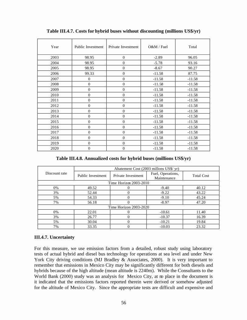
56

Table III.4.7. Costs for hybrid buses without discounting (millions US$/yr)

Year Public Investment Private Investment O&M / Fuel Total

2003 98.95 0 -2.89 96.05 2004 98.95 0 -5.78 93.16 2005 98.95 0 -8.67 90.27 2006 99.33 0 -11.58 87.75 2007 0 0 -11.58 -11.58 2008 0 0 -11.58 -11.58 2009 0 0 -11.58 -11.58 2010 0 0 -11.58 -11.58 2011 0 0 -11.58 -11.58 2012 0 0 -11.58 -11.58 2013 0 0 -11.58 -11.58 2014 0 0 -11.58 -11.58 2015 0 0 -11.58 -11.58 2016 0 0 -11.58 -11.58 2017 0 0 -11.58 -11.58 2018 0 0 -11.58 -11.58 2019 0 0 -11.58 -11.58 2020 0 0 -11.58 -11.58

Table III.4.8. Annualized costs for hybrid buses (millions US$/yr)

Abatement Cost (2003 millons US$/ yr)

Discount rate Public Investment Private Investment Fuel, Operations,

Maintenance Total Cost

Time Horizon 2003-2010 0% 49.52 0 -9.40 40.12 3% 52.44 0 -9.22 43.22 5% 54.33 0 -9.10 45.24 7% 56.18 0 -8.97 47.20

Time Horizon 2003-2020 0% 22.01 0 -10.61 11.40 3% 26.77 0 -10.37 16.39 5% 30.04 0 -10.21 19.84 7% 33.35 0 -10.03 23.32

III.4.7. Uncertainty

For this measure, we use emission factors from a detailed, robust study using laboratory tests of actual hybrid and diesel bus technology for operations at sea level and under New York City driving conditions (MJ Bradley & Associates, 2000). It is very important to remember that emissions in Mexico City may be significantly different for both diesels and hybrids because of the high altitude (mean altitude is 2240m). While the Consultants to the World Bank (2000) study was an analysis for Mexico City, at no place in the document is it indicated that the emissions factors reported therein were derived or somehow adjusted for the altitude of Mexico City. Since the appropriate tests are difficult and expensive and

57

are not normally done in the US and Europe, it is highly unlikely that these emission factors would be for altitudes of >2000m without there being specific mention to this effect in the report. III.4.8. Discussion and Next Steps

Improved understanding of emissions factors for operations at altitude for all technologies is the key next step for improving this analysis. In a current project by World Bank and EMBARQ for the creation of dedicated bus lanes in Mexico City, plans are being made to test a variety of vehicle technology at altitude. Although it is not clear that hybrids will be considered in this study, there should be at a minimum improved understanding of baseline diesel bus emissions from this work. We also note that Cohen et al. (2003) find that emission-controlled diesel buses would be more cost-effective than compressed natural gas (CNG) technology in US cities. Hybrid technologies are likely as expensive or more so than CNG. Thus, before further pursuing the introduction of hybrid buses in Mexico City, it would be sensible to do comparable analyses for other bus technologies. III.4.9. References CAM, Comisión Ambiental Metropolitana (2002), “Programa para Mejorar la Calidad del Aire de la Zona Metropolitana del Valle de México, 2002-2010” (PROAIRE), Comisión Ambiental Metropolitana. Cohen, J.T., J.K. Hammitt, and J.I. Levy (2003) Fuels for urban transit buses: A cost-effectiveness analysis. Environ. Sci. Technol 37. 1477-1484. Consultants to World Bank (2000) Estudio de prefactibilidad para la introducción de autobuses híbridos en las prestación del servicio público de transporte de pasajeros en la ZMVM, report to the World Bank. IPCC, Intergovernmental Panel on Climate Change (1997), “Revised 1996 IPCC Guidelines for National Greenhouse Gas Inventories, Vols. 1-3” (Bracknell, UK: IPCC). M.J. Bradley & Associates, Inc. (2000) “Hybrid-electric drive heavy-duty vehicle testing project: Final emissions report.” Molina, L.T. and M.J. Molina, eds. (2002), Air Quality in the Mexico Megacity: An Integrated Assessment, Kluwer Academic Publishers, Boston, 384 pp. West, J.J., P. Osnaya, I. Laguna, J. Martínez, A. Fernández (2003) Co-control of urban air pollutants and greenhouse gases in México City. Final report to US National Renewable Energy Laboratory, subcontract ADC-2-32409-01.

58

III.5. Measures to reduce leaks of Liquefied Petroleum Gas III.5.1. Introduction A majority of stoves in the residences of Mexico City use Liquefied Petroleum Gas (LPG), supplied in portable or roof-top tanks, as their fuel source. These systems are prone to leaks, in part because LPG is stored under significant pressure. LPG is a hydrocarbon (HC) source that contributes to ozone and also forms CO2 in the atmosphere. The goal of this set of measures is to perform maintenance procedures on the stove systems, replacing worn out parts or permanently closing off stove pilots, in order to eliminate these leaks. We base our calculation of the costs and emissions reduction potential for the four measures based on a detailed study of LPG gas leaks by TUV (2000), as summarized in the calculations of the first phase of the IES study for Mexico (West et al. 2003). III.5.2. Description of the Measures

Pictels, regulators, and connections are specific pieces of the LPG stove / tank system that wear out with time and need replacing. In a service visit to the residence, these pieces are replaced, respectively, in the measures entitled “Change of Pictels (LPG1)”, “Change of Regulators (LPG2)”, “Change of Connections (LPG3)”. Unlit pilots also cause LPG leaks, thus in the “Closure of Pilots (LPG4)” measures, pilots are permanently closed in the service visit and then disposable lighters would be used to light the stove. Since the implementation of these measures requires in-home service visits by stove maintenance professiona ls, it is sensible to consider that all four measures would be implemented simultaneously in order to save on implementation costs. Thus, we also present the sum of these four measures as a single combined LPG leak measure (LPG). Results will be based on the combined LPG measure. III.5.3. Data Requirements

To estimate the emissions reductions and costs to reduce LPG leakage, we need information about rates of LPG loss from current leaks in stove systems and the costs to repair these leaks. Further, we must understand the useful lifetimes of these repairs so that the appropriate schedules for redoing the repairs can be included in the analysis. For this set of measures, all this information is derived from the TUV (2000) study. III.5.4. Determining Baseline Emissions

TUV (2000) estimated the number of household with LPG leaks from pictels, regulators, connections and pilots via random in-home tests of stoves and their connections. Their estimate of the total potential for LPG leak controls from each part of the stove system forms the baselines for these measures.

59

III.5.5. Estimating Emissions Reductions and Costs for the Measures

We base our calculation of the costs and emissions reduction potential for the four measures on the TUV (2000) study. For consistency with other studies recently done in Mexico City (PROAIRE), we retain qualitative assumptions about implementation schedules for the control measures as have been previously made. The repairs to the pictels, regulators and connections in the LPG stove systems have useful lifetimes of between 2 and 5 years. Thus, for the emission reduction benefits of these repairs to be maintained, the repairs must be repeated after the useful lifetimes end. In our estimates, we assume that there is a zero failure rate for these replacements. This is the same assumption that was made by Kellyn Roth in her thesis work on residential measures for air pollution control in Mexico City at MIT (2003). Ms. Roth does believe that some failure rate is likely to be more realistic, however she was not able to find any literature to support a specific choice of a failure rate (K. Roth, personal communication). We use a maximum time horizon to 2020 in this study, in which we aim to estimate the longer-term impacts of policies implemented up to 2010 as outlined in PROAIRE. Thus we assume no maintenance of the repairs after 2010. The local air quality benefit of these measures is a reduction in HC emissions. In atmosphere, HC released through LPG leakage is transformed to CO2. The elimination of the leaks via this measure leads to both a HC and CO2 benefit. LPG is 61% propane (molecular weight = 44) and 39% butane (molecular weight = 58). Thus, as in the co-control work, we estimate CO2 emissions by: (tons HC)*(0.61)*(44/44)*3 + (tons HC)*(0.39)*(44/58)*4 = tons CO2 Equation III.5.1 We assume the initial investment is from the public sector, and then additional investment in replacement occurs from the private sector. Leakages in LPG stove systems results in significant fuel waste, which costs $4.9 MX / kg LPG. Operations and maintenance costs are negative (savings) because this fuel wastage is reduced. Change of Pictels (LPG1) TUV (2000) estimates that there are 1.59 million households with LPG leaks from worn-out pictels, and that from each 0.00533 tons of hydrocarbon (HC) are lost per year. To eliminate these loses, pictel replacements can be performed at a cost of $105 MX ($10.5 US). We assume, as did PROAIRE, that pictels in a total of 1,000,000 households are replaced by 2010. We divide this equally over the period 2003-2010 (8 years), such that there are 125,0000 installations / year. The pictel’s useful life is 2 years, and thus replacements must be redone each 2 years to maintain the HC loss benefit. Change of Regulators (LPG2) We assume, consistent with PROAIRE, that regulators in a total of 336,584 households are replaced by 2010. TUV (2000) estimates that from each regulator, 0.01389 tons of

60

hydrocarbon (HC) is lost per year. Regulator replacements can be performed at a cost of $190 MX ($19 US). We divide this equally over the period 2003-2010 (8 years), such that there are 42,073 installations / year. The regulator’s useful life is 5 years, and thus replacements must be redone each 5 years to maintain the HC loss benefit. Change of Connections (LPG3) We estimate that connections in a total of 961,664 households are replaced by 2010. We divide this equally over the period 2003-2010 (8 years), such that there are 120,208 installations / year. TUV (2000) estimates that from each connection, 0.00926 tons of hydrocarbon (HC) are lost per year. To eliminate these loses, connections could be replaced at a cost of $240 MX ($24 US). The connection’s useful life is 5 years, and thus replacements must be redone each 5 years to maintain the HC loss benefit. Closure of Pilots (LPG4) We assume, as was done in PROAIRE, that pilots in a total of 912,512 households are closed by 2010. We divide this equally over the period 2003-2010 (8 years), such that there are 114,064 closures / year. TUV (2000) estimates that from each pilot, 0.00482 tons of hydrocarbon (HC) is lost per year. Closures cost $75 MX ($7.5 US). We assume this investment comes from the public sector. Additional investment in disposable lighters (3 / year at $64.5 MX / yr) comes from the private sector. Closure of the pilots is a permanent fix for the leaks, so there is no repeat investment necessary. III.5.6. Costs and emissions reductions with the measures

Emission reductions and costs are presented for each ind ividual measure and for a combination of all four measures in Tables III.5.1 to III.5.18.

61

Change of Pictels (LPG1) Table III.5.1. Emissions reductions for change of pictels (LPG1) without discounting

(tons/yr)

Year PM10 PM2.5 SO2 CO NOx HC CO2 CH4 N2O

2003 0 0 0 0 0 666 2,008 0 0 2004 0 0 0 0 0 1,333 4,015 0 0 2005 0 0 0 0 0 1,999 6,023 0 0 2006 0 0 0 0 0 2,665 8,031 0 0 2007 0 0 0 0 0 3,331 10,039 0 0 2008 0 0 0 0 0 3,998 12,046 0 0 2009 0 0 0 0 0 4,664 14,054 0 0 2010 0 0 0 0 0 5,330 16,062 0 0 2011 0 0 0 0 0 2,665 8,031 0 0 2012 0 0 0 0 0 0 0 0 0 2013 0 0 0 0 0 0 0 0 0 2014 0 0 0 0 0 0 0 0 0 2015 0 0 0 0 0 0 0 0 0 2016 0 0 0 0 0 0 0 0 0 2017 0 0 0 0 0 0 0 0 0 2018 0 0 0 0 0 0 0 0 0 2019 0 0 0 0 0 0 0 0 0 2020 0 0 0 0 0 0 0 0 0

Table III.5.2. Annualized emissions reductions for change of pictels (LPG1)

(tons/yr)

Discount rate

PM10 PM2.5 SO2 CO NOx HC CO2 CH4 N2O

Time horizon 2003-2010

0% 0 0 0 0 0 2,998 9,035 0 0 3% 0 0 0 0 0 2,895 8,723 0 0 5% 0 0 0 0 0 2,828 8,522 0 0 7% 0 0 0 0 0 2,763 8,325 0 0

Time horizon 2003-2020

0% 0 0 0 0 0 1,481 4,462 0 0 3% 0 0 0 0 0 1,626 4,900 0 0 5% 0 0 0 0 0 1,711 5,155 0 0 7% 0 0 0 0 0 1,784 5,376 0 0

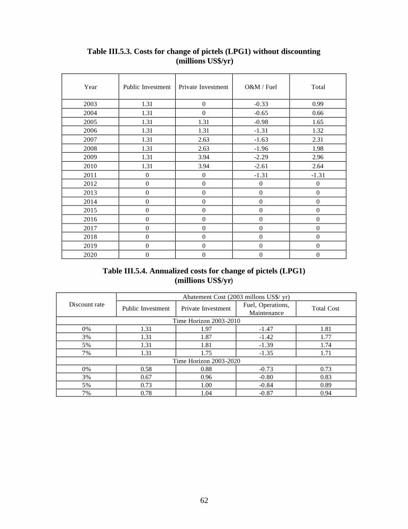
62

Table III.5.3. Costs for change of pictels (LPG1) without discounting (millions US$/yr)

Year Public Investment Private Investment O&M / Fuel Total

2003 1.31 0 -0.33 0.99 2004 1.31 0 -0.65 0.66 2005 1.31 1.31 -0.98 1.65 2006 1.31 1.31 -1.31 1.32 2007 1.31 2.63 -1.63 2.31 2008 1.31 2.63 -1.96 1.98 2009 1.31 3.94 -2.29 2.96 2010 1.31 3.94 -2.61 2.64 2011 0 0 -1.31 -1.31 2012 0 0 0 0 2013 0 0 0 0 2014 0 0 0 0 2015 0 0 0 0 2016 0 0 0 0 2017 0 0 0 0 2018 0 0 0 0 2019 0 0 0 0 2020 0 0 0 0

Table III.5.4. Annualized costs for change of pictels (LPG1)

(millions US$/yr)

Abatement Cost (2003 millons US$/ yr) Discount rate

Public Investment Private Investment Fuel, Operations, Maintenance

Total Cost

Time Horizon 2003-2010 0% 1.31 1.97 -1.47 1.81 3% 1.31 1.87 -1.42 1.77 5% 1.31 1.81 -1.39 1.74 7% 1.31 1.75 -1.35 1.71

Time Horizon 2003-2020 0% 0.58 0.88 -0.73 0.73 3% 0.67 0.96 -0.80 0.83 5% 0.73 1.00 -0.84 0.89 7% 0.78 1.04 -0.87 0.94

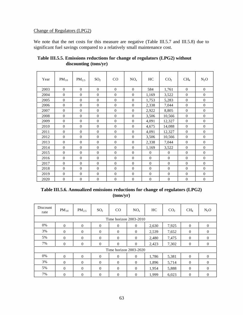
63

Change of Regulators (LPG2) We note that the net costs for this measure are negative (Table III.5.7 and III.5.8) due to significant fuel savings compared to a relatively small maintenance cost.

Table III.5.5. Emissions reductions for change of regulators (LPG2) without discounting (tons/yr)

Year PM10 PM2.5 SO2 CO NOx HC CO2 CH4 N2O

2003 0 0 0 0 0 584 1,761 0 0 2004 0 0 0 0 0 1,169 3,522 0 0 2005 0 0 0 0 0 1,753 5,283 0 0 2006 0 0 0 0 0 2,338 7,044 0 0 2007 0 0 0 0 0 2,922 8,805 0 0 2008 0 0 0 0 0 3,506 10,566 0 0 2009 0 0 0 0 0 4,091 12,327 0 0 2010 0 0 0 0 0 4,675 14,088 0 0 2011 0 0 0 0 0 4,091 12,327 0 0 2012 0 0 0 0 0 3,506 10,566 0 0 2013 0 0 0 0 0 2,338 7,044 0 0 2014 0 0 0 0 0 1,169 3,522 0 0 2015 0 0 0 0 0 0 0 0 0 2016 0 0 0 0 0 0 0 0 0 2017 0 0 0 0 0 0 0 0 0 2018 0 0 0 0 0 0 0 0 0 2019 0 0 0 0 0 0 0 0 0 2020 0 0 0 0 0 0 0 0 0

Table III.5.6. Annualized emissions reductions for change of regulators (LPG2)

(tons/yr)

Discount rate PM10 PM2.5 SO2 CO NOx HC CO2 CH4 N2O

Time horizon 2003-2010

0% 0 0 0 0 0 2,630 7,925 0 0 3% 0 0 0 0 0 2,539 7,652 0 0 5% 0 0 0 0 0 2,480 7,475 0 0 7% 0 0 0 0 0 2,423 7,302 0 0

Time horizon 2003-2020

0% 0 0 0 0 0 1,786 5,381 0 0 3% 0 0 0 0 0 1,896 5,714 0 0 5% 0 0 0 0 0 1,954 5,888 0 0 7% 0 0 0 0 0 1,999 6,023 0 0

64

Table III.5.7. Costs for change of regulators (LPG2) without discounting

(millions US$/yr)

Year Public Investment Private Investment O&M / Fuel Total

2003 0.80 0 -0.29 0.51 2004 0.80 0 -0.57 0.23 2005 0.80 0 -0.86 -0.06 2006 0.80 0 -1.15 -0.35 2007 0.80 0 -1.43 -0.63 2008 0.80 0.80 -1.72 -0.12 2009 0.80 0.80 -2.00 -0.41 2010 0.80 0.80 -2.29 -0.69 2011 0 0 -2.00 -2.00 2012 0 0 -1.72 -1.72 2013 0 0 -1.15 -1.15 2014 0 0 -0.57 -0.57 2015 0 0 0 0 2016 0 0 0 0 2017 0 0 0 0 2018 0 0 0 0 2019 0 0 0 0 2020 0 0 0 0

Table III.5.8. Annualized costs for change of regulators (LPG2)

(millions US$/yr)

Abatement Cost (2003 millons US$/ yr) Discount rate

Public Investment Private Investment

Fuel, Operations, Maintenance

Total Cost

Time Horizon 2003-2010 0% 0.80 0.30 -1.29 -0.19 3% 0.80 0.28 -1.24 -0.17 5% 0.80 0.26 -1.22 -0.15 7% 0.80 0.25 -1.19 -0.14

Time Horizon 2003-2020 0% 0.36 0.13 -0.87 -0.39 3% 0.41 0.14 -0.93 -0.38 5% 0.44 0.15 -0.96 -0.37 7% 0.47 0.15 -0.98 -0.36

65

Change of Connections (LPG3)

Table III.5.9. Emissions reductions for change of connections (LPG3) without discounting (tons/yr)

Year PM10 PM2.5 SO2 CO NOx HC CO2 CH4 N2O

2003 0 0 0 0 0 3,354 3,354 0 0 2004 0 0 0 0 0 6,709 6,709 0 0 2005 0 0 0 0 0 10,063 10,063 0 0 2006 0 0 0 0 0 13,417 13,417 0 0 2007 0 0 0 0 0 16,772 16,772 0 0 2008 0 0 0 0 0 20,126 20,126 0 0 2009 0 0 0 0 0 23,480 23,480 0 0 2010 0 0 0 0 0 26,835 26,835 0 0 2011 0 0 0 0 0 23,480 23,480 0 0 2012 0 0 0 0 0 20,126 20,126 0 0 2013 0 0 0 0 0 13,417 13,417 0 0 2014 0 0 0 0 0 6,709 6,709 0 0 2015 0 0 0 0 0 0 0 0 0 2016 0 0 0 0 0 0 0 0 0 2017 0 0 0 0 0 0 0 0 0 2018 0 0 0 0 0 0 0 0 0 2019 0 0 0 0 0 0 0 0 0 2020 0 0 0 0 0 0 0 0 0

Table III.5.10. Annualized emissions reductions for change of connections (LPG3)

(tons/yr)

Discount rate

PM10 PM2.5 SO2 CO NOx HC CO2 CH4 N2O

Time horizon 2003-2010

0% 0 0 0 0 0 5,009 15,095 0 0 3% 0 0 0 0 0 4,836 14,575 0 0 5% 0 0 0 0 0 4,725 14,238 0 0 7% 0 0 0 0 0 4,616 13,909 0 0

Time horizon 2003-2020

0% 0 0 0 0 0 3,401 10,249 0 0 3% 0 0 0 0 0 3,611 10,883 0 0 5% 0 0 0 0 0 3,721 11,214 0 0 7% 0 0 0 0 0 3,807 11,473 0 0

66

Table III.5.11. Costs for change of connections (LPG3) without discounting (millions US$/yr)

Year Public Investment Private Investment O&M / Fuel Total

2003 2.88 0 -0.55 2.34 2004 2.88 0 -1.09 1.79 2005 2.88 0 -1.64 1.25 2006 2.88 0 -2.18 0.70 2007 2.88 0 -2.73 0.16 2008 2.88 2.88 -3.27 2.50 2009 2.88 2.88 -3.82 1.95 2010 2.88 2.88 -4.36 1.41 2011 0 0 -3.82 -3.82 2012 0 0 -3.27 -3.27 2013 0 0 -2.18 -2.18 2014 0 0 -1.09 -1.09 2015 0 0 0 0 2016 0 0 0 0 2017 0 0 0 0 2018 0 0 0 0 2019 0 0 0 0 2020 0 0 0 0

Table III.5.12. Annualized costs for change of connections (LPG3)

(millions US$/yr)

Abatement Cost (2003 millons US$/ yr) Discount rate

Public Investment Private Investment Fuel, Operations, Maintenance

Total Cost

Time Horizon 2003-2010 0% 2.88 1.08 -2.45 1.51 3% 2.88 1.00 -2.37 1.52 5% 2.88 0.95 -2.32 1.52 7% 2.88 0.90 -2.26 1.53

Time Horizon 2003-2020 0% 1.28 0.48 -1.67 0.10 3% 1.47 0.51 -1.77 0.21 5% 1.60 0.53 -1.82 0.30 7% 1.71 0.54 -1.87 0.38

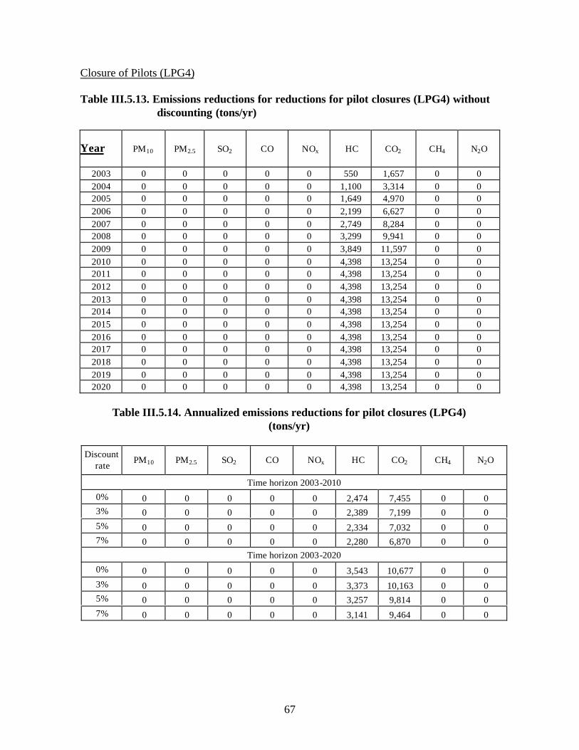
67

Closure of Pilots (LPG4) Table III.5.13. Emissions reductions for reductions for pilot closures (LPG4) without

discounting (tons/yr)

Year PM10 PM2.5 SO2 CO NOx HC CO2 CH4 N2O

2003 0 0 0 0 0 550 1,657 0 0 2004 0 0 0 0 0 1,100 3,314 0 0 2005 0 0 0 0 0 1,649 4,970 0 0 2006 0 0 0 0 0 2,199 6,627 0 0 2007 0 0 0 0 0 2,749 8,284 0 0 2008 0 0 0 0 0 3,299 9,941 0 0 2009 0 0 0 0 0 3,849 11,597 0 0 2010 0 0 0 0 0 4,398 13,254 0 0 2011 0 0 0 0 0 4,398 13,254 0 0 2012 0 0 0 0 0 4,398 13,254 0 0 2013 0 0 0 0 0 4,398 13,254 0 0 2014 0 0 0 0 0 4,398 13,254 0 0 2015 0 0 0 0 0 4,398 13,254 0 0 2016 0 0 0 0 0 4,398 13,254 0 0 2017 0 0 0 0 0 4,398 13,254 0 0 2018 0 0 0 0 0 4,398 13,254 0 0 2019 0 0 0 0 0 4,398 13,254 0 0 2020 0 0 0 0 0 4,398 13,254 0 0

Table III.5.14. Annualized emissions reductions for pilot closures (LPG4)

(tons/yr)

Discount rate

PM10 PM2.5 SO2 CO NOx HC CO2 CH4 N2O

Time horizon 2003-2010

0% 0 0 0 0 0 2,474 7,455 0 0 3% 0 0 0 0 0 2,389 7,199 0 0 5% 0 0 0 0 0 2,334 7,032 0 0 7% 0 0 0 0 0 2,280 6,870 0 0

Time horizon 2003-2020

0% 0 0 0 0 0 3,543 10,677 0 0 3% 0 0 0 0 0 3,373 10,163 0 0 5% 0 0 0 0 0 3,257 9,814 0 0 7% 0 0 0 0 0 3,141 9,464 0 0

68

Table III.5.15. Costs for pilot closures (LPG4) without discounting (millions US$/yr)

Year Public Investment Private Investment O&M / Fuel Total

2003 0.86 0.74 -0.27 1.32 2004 0.86 1.47 -0.54 1.79 2005 0.86 2.21 -0.81 2.25 2006 0.86 2.94 -1.08 2.72 2007 0.86 3.68 -1.35 3.19 2008 0.86 4.41 -1.62 3.65 2009 0.86 5.15 -1.89 4.12 2010 0.86 5.89 -2.16 4.59 2011 0 5.89 -2.16 3.73 2012 0 5.89 -2.16 3.73 2013 0 5.89 -2.16 3.73 2014 0 5.89 -2.16 3.73 2015 0 5.89 -2.16 3.73 2016 0 5.89 -2.16 3.73 2017 0 5.89 -2.16 3.73 2018 0 5.89 -2.16 3.73 2019 0 5.89 -2.16 3.73 2020 0 5.89 -2.16 3.73

Table III.5.16. Annualized costs for pilot closures (LPG4)

(millions US$/yr)

Abatement Cost (2003 millons US$/ yr) Discount rate

Public Investment Private Investment Fuel, Operations, Maintenance

Total Cost

Time Horizon 2003-2010 0% 0.86 3.31 -1.21 2.95 3% 0.86 3.20 -1.17 2.88 5% 0.86 3.12 -1.14 2.83 7% 0.86 3.05 -1.12 2.79

Time Horizon 2003-2020 0% 0.38 4.74 -1.74 3.39 3% 0.44 4.51 -1.65 3.30 5% 0.47 4.36 -1.60 3.24 7% 0.51 4.20 -1.54 3.17

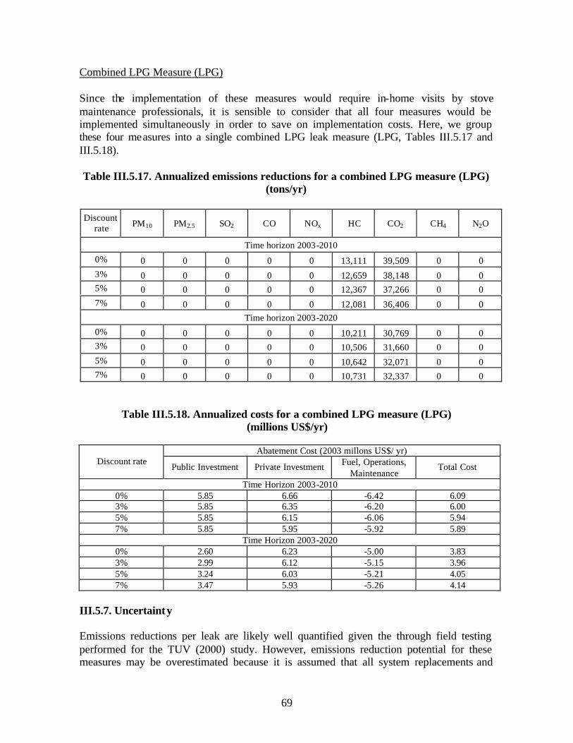
69

Combined LPG Measure (LPG) Since the implementation of these measures would require in-home visits by stove maintenance professionals, it is sensible to consider that all four measures would be implemented simultaneously in order to save on implementation costs. Here, we group these four measures into a single combined LPG leak measure (LPG, Tables III.5.17 and III.5.18). Table III.5.17. Annualized emissions reductions for a combined LPG measure (LPG)

(tons/yr)

Table III.5.18. Annualized costs for a combined LPG measure (LPG) (millions US$/yr)

Abatement Cost (2003 millons US$/ yr)

Discount rate Public Investment Private Investment Fuel, Operations,

Maintenance Total Cost

Time Horizon 2003-2010 0% 5.85 6.66 -6.42 6.09 3% 5.85 6.35 -6.20 6.00 5% 5.85 6.15 -6.06 5.94 7% 5.85 5.95 -5.92 5.89

Time Horizon 2003-2020 0% 2.60 6.23 -5.00 3.83 3% 2.99 6.12 -5.15 3.96 5% 3.24 6.03 -5.21 4.05 7% 3.47 5.93 -5.26 4.14

III.5.7. Uncertainty

Emissions reductions per leak are likely well quantified given the through field testing performed for the TUV (2000) study. However, emissions reduction potential for these measures may be overestimated because it is assumed that all system replacements and

Discount rate PM10 PM2.5 SO2 CO NOx HC CO2 CH4 N2O

Time horizon 2003-2010

0% 0 0 0 0 0 13,111 39,509 0 0 3% 0 0 0 0 0 12,659 38,148 0 0 5% 0 0 0 0 0 12,367 37,266 0 0 7% 0 0 0 0 0 12,081 36,406 0 0

Time horizon 2003-2020

0% 0 0 0 0 0 10,211 30,769 0 0 3% 0 0 0 0 0 10,506 31,660 0 0 5% 0 0 0 0 0 10,642 32,071 0 0 7% 0 0 0 0 0 10,731 32,337 0 0

70

pilot closures occur in systems that are actually leaking. Additional uncertainty arises from the use of a constant baseline of the number of households with leakages in their stove systems. Thus, there is no estimation of improvements in future technology that would reduce leakages in new systems, nor of the deterioration of existing systems that might lead to additional future leaks, nor of the growth in the number of households with LPG stoves in the MCMA. Costs are likely underestimated for these measures because no public investment in enforcement, monitoring or public information is included. III.5.8. Discussion and Next Steps Costs and emission reductions for these LPG leak measures are relatively small in comparison to other measures considered in this study. However, there is the potential for net costs to be negative (e.g. LPG2) due to significant fuel cost savings. Further work should focus on improving cost estimates by understanding the full program costs of these types of measures. Additional understanding of how replacements could be focused only on stove systems that are actually leaking would also improve this set of measures. In the following sections, we consider only the combined LPG leak measure (LPG). We note, however, that it is possible in the Analytica model to consider each of these four measures individually. III.5.9. References CAM, Comisión Ambiental Metropolitana (2002), “Programa para Mejorar la Calidad del Aire de la Zona Metropolitana del Valle de México, 2002-2010” (PROAIRE), Comisión Ambiental Metropolitana. TUV Rheinland de Mexico, S. A. de C. V. (2000) “Programa para la reducción y eliminación de fugas de Gas LP, en las instalaciones domésticas de la Zona Metropolitana del Valle de México.” West, J.J., P. Osnaya, I. Laguna, J. Martínez, A. Fernández (2003) Co-control of urban air pollutants and greenhouse gases in México City. Final report to US National Renewable Energy Laboratory, subcontract ADC-2-32409-01.

71

III.6. Cogeneration III.6.1. Introduction

Cogeneration is defined as the simultaneous generation of heat and power, both of which are used to satisfy the energy requirements of industrial, commercial and/or residential sector. Cogeneration is also known as Combined Heat and Power (CHP) or Total energy. Cogeneration plants are available to provide outputs from 1 kWe to 500 MWe. Plants for industrial applications typically fall into the range from 1 to 50 MWe. Cogeneration is one of the strategies of the Mexican Government to promote energy efficiency. The organism in charge of this effort is the National Commission for Energy Savings (CONAE), a decentralized organism of the Ministry of Energy. CONAE, through its Direction of Cogeneration and non-Conventional Energy Sources, carried out in 1995 the cogeneration potential of the industry & commercial sectors and the petrochemical facilities of the Mexican Oil Company (PEMEX) at a national level. CONAE estimates that Mexico’s cogeneration potential is 7,586 MWe for installations with additional combustion and 14,229 MWe for installations without additional combustion. Around 68% of total cogeneration potential corresponds to industry sector, of which 16% is located at the Federal District & the State of Mexico.

Table III.6.1. National cogeneration potential by sector

Sector Additional combustion (MWe)

Without additional combustion (MWe)

Industry 5,200 9,750 Petrochemical 1,613 3,026 Commercial 773 1,453

Total 7,586 14,229

Table III.6.2. Industrial cogeneration potential by state

X. State Additional combustion (MWe)

Without additional combustion. (MWe)

State of Mexico 324 605 Federal District 530 994 TOTAL 5,200 9,750 MCMA 854 1,599 16.42 % 16.4%

According to the Energy Regulatory Commission (CRE), the office in charge of authorizing cogeneration permits in the State of Mexico, there are two projects currently being installed. These are included in this study.

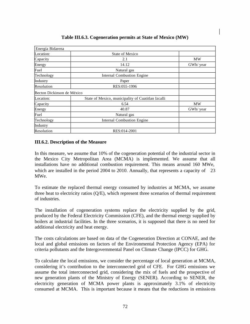
72

Table III.6.3. Cogeneration permits at State of Mexico (MW)

Energía Bidarena Location: State of Mexico Capacity 2.1 MW Energy 14.12 GWh/ year Fuel Natural gas Technology Internal Combustion Engine Industry Paper Resolution RES:055-1996

Becton Dickinson de México Location: State of Mexico, municipality of Cuatitlan Izcalli Capacity 6.54 MW Energy 40.87 GWh/ year Fuel Natural gas Technology Internal Combustion Engine Industry Resolution RES:014-2001 III.6.2. Description of the Measure

In this measure, we assume that 10% of the cogeneration potential of the industrial sector in the Mexico City Metropolitan Area (MCMA) is implemented. We assume that all installations have no additional combustion requirement. This means around 160 MWe, which are installed in the period 2004 to 2010. Annually, that represents a capacity of ∼23 MWe. To estimate the replaced thermal energy consumed by industries at MCMA, we assume three heat to electricity ratios (Q/E), which represent three scenarios of thermal requirement of industries. The installation of cogeneration systems replace the electricity supplied by the grid, produced by the Federal Electricity Commission (CFE), and the thermal energy supplied by boilers at industrial facilities. In the three scenarios, it is supposed that there is no need for additional electricity and heat energy. The costs calculations are based on data of the Cogeneration Direction at CONAE, and the local and global emissions on factors of the Environmental Protection Agency (EPA) for criteria pollutants and the Intergovernmental Panel on Climate Change (IPCC) for GHG. To calculate the local emissions, we consider the percentage of local generation at MCMA, considering it’s contribution to the interconnected grid of CFE. For GHG emissions we assume the total interconnected grid, considering the mix of fuels and the prospective of new generation plants of the Ministry of Energy (SENER). According to SENER, the electricity generation of MCMA power plants is approximately 3.1% of electricity consumed at MCMA. This is important because it means that the reductions in emissions

73

from power plants associated with reductions electricity use have little impact on local air quality in the MCMA. We include the recuperation value of capital for both time horizons, considering the useful life of cogeneration systems of 20 years. III.6.3. Data Requirements

To estimate the impact of the introduction of cogeneration systems, it is necessary to determine the electricity and thermal requirements in terms of energy units for each industry. For our study we assume an average value, due to the lack of specific information, assuming three Q/E scenarios (Low Scenario=0.8, Medium Scenario=3, High Scenario=4). To calculate the fuel consumption, we must know the efficiency of power plants and the structure of interconnected system in order to determine the fuels that cogeneration systems replace. Additionally, the efficiency of industrial boilers is required in order to estimate the replaced fuel consumption. To determine the costs it is required the investment per installed cogeneration capacity (US$ / MWe), the costs of electricity and fuel, and the O&M costs (US$/MWh). III.6.4. Determining Baseline Emissions

Emissions reductions due to the introduction of cogeneration systems are estimated as a difference from the baseline emissions of the electricity produced by CFE and the thermal energy produced by industrial boilers (CFE+ boilers) and those that would be produced if all the electricity and thermal energy were produced by cogeneration systems. Baseline emissions are estimated using emission factors of EPA for criteria pollutants and IPCC’s emission factors for GHG. As stated in the definition of the measure, it is assumed that 160 MWe are replaced from 2004 to 2010. Considering an operation factor of industry process (cogeneration system), we can estimate the total electricity that power plants should supply to industrial devices. The fuel consumption is calculated considering the mix of power plants (fuel-oil, natural gas, coal, nuclear, hydro, etc) of the interconnected grid, the transmission losses and their conversion efficiencies for GHG emissions, and the percentage of local power plants at MCMA related to the interconnected grid for local pollutants. This information is based on the “Energy Balance 2002” and “The Electricity Sector Prospective, 2002-2012”, both edited by the Ministry of Energy. (Secretaría de Energía, http://www.energia.gob.mx).

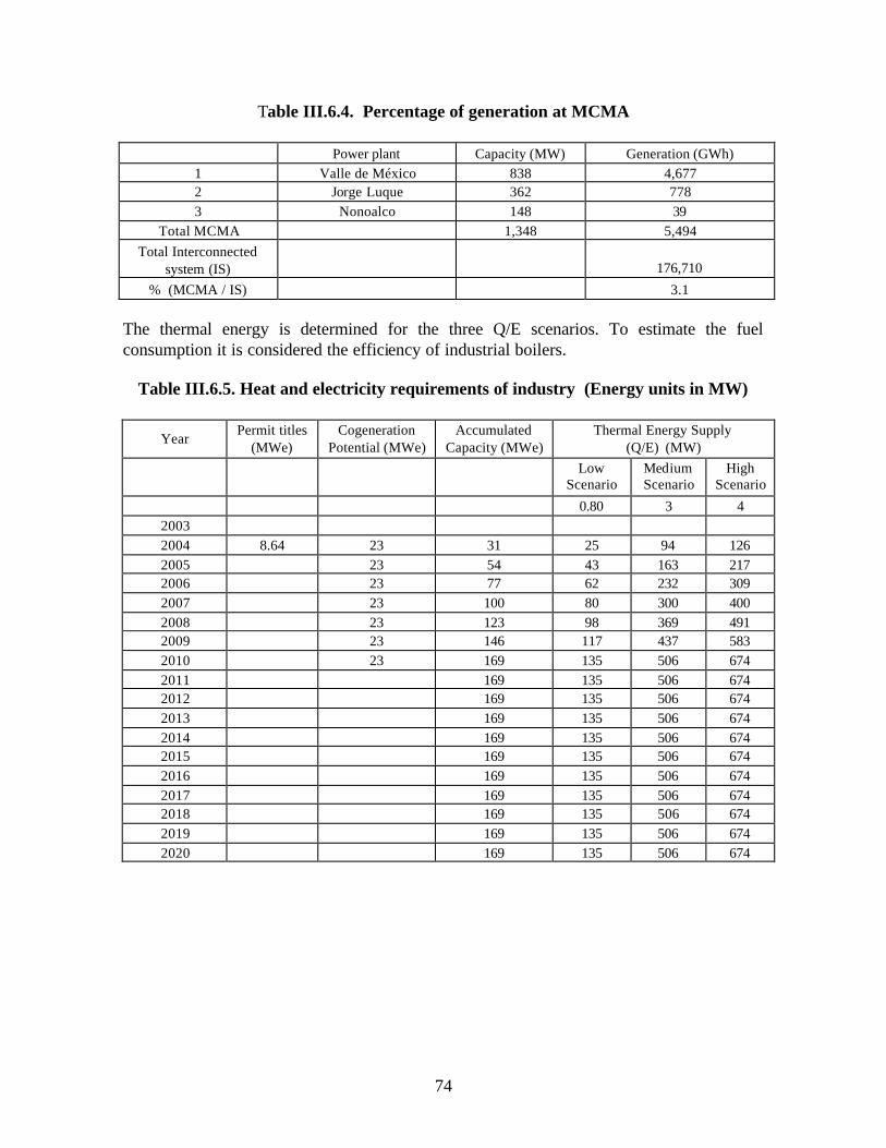
74

Table III.6.4. Percentage of generation at MCMA

Power plant Capacity (MW) Generation (GWh) 1 Valle de México 838 4,677 2 Jorge Luque 362 778 3 Nonoalco 148 39

Total MCMA 1,348 5,494 Total Interconnected

system (IS) 176,710

% (MCMA / IS) 3.1 The thermal energy is determined for the three Q/E scenarios. To estimate the fuel consumption it is considered the efficiency of industrial boilers.

Table III.6.5. Heat and electricity requirements of industry (Energy units in MW)

Year Permit titles

(MWe) Cogeneration

Potential (MWe) Accumulated

Capacity (MWe) Thermal Energy Supply

(Q/E) (MW)

Low

Scenario Medium Scenario

High Scenario

0.80 3 4 2003 2004 8.64 23 31 25 94 126 2005 23 54 43 163 217 2006 23 77 62 232 309 2007 23 100 80 300 400 2008 23 123 98 369 491 2009 23 146 117 437 583 2010 23 169 135 506 674 2011 169 135 506 674 2012 169 135 506 674 2013 169 135 506 674 2014 169 135 506 674 2015 169 135 506 674 2016 169 135 506 674 2017 169 135 506 674 2018 169 135 506 674 2019 169 135 506 674 2020 169 135 506 674

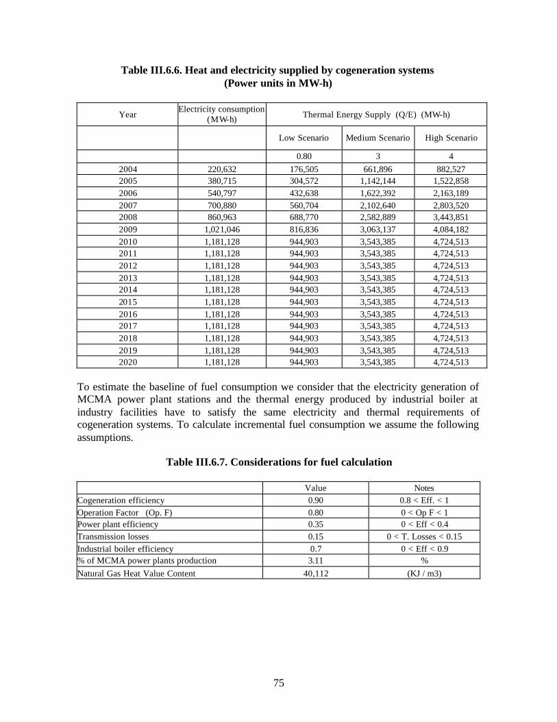
75

Table III.6.6. Heat and electricity supplied by cogeneration systems (Power units in MW-h)

Year Electricity consumption

(MW-h) Thermal Energy Supply (Q/E) (MW-h)

Low Scenario Medium Scenario High Scenario

0.80 3 4 2004 220,632 176,505 661,896 882,527 2005 380,715 304,572 1,142,144 1,522,858 2006 540,797 432,638 1,622,392 2,163,189 2007 700,880 560,704 2,102,640 2,803,520 2008 860,963 688,770 2,582,889 3,443,851 2009 1,021,046 816,836 3,063,137 4,084,182 2010 1,181,128 944,903 3,543,385 4,724,513 2011 1,181,128 944,903 3,543,385 4,724,513 2012 1,181,128 944,903 3,543,385 4,724,513 2013 1,181,128 944,903 3,543,385 4,724,513 2014 1,181,128 944,903 3,543,385 4,724,513 2015 1,181,128 944,903 3,543,385 4,724,513 2016 1,181,128 944,903 3,543,385 4,724,513 2017 1,181,128 944,903 3,543,385 4,724,513 2018 1,181,128 944,903 3,543,385 4,724,513 2019 1,181,128 944,903 3,543,385 4,724,513 2020 1,181,128 944,903 3,543,385 4,724,513

To estimate the baseline of fuel consumption we consider that the electricity generation of MCMA power plant stations and the thermal energy produced by industrial boiler at industry facilities have to satisfy the same electricity and thermal requirements of cogeneration systems. To calculate incremental fuel consumption we assume the following assumptions.

Table III.6.7. Considerations for fuel calculation Value Notes Cogeneration efficiency 0.90 0.8 < Eff. < 1 Operation Factor (Op. F) 0.80 0 < Op F < 1 Power plant efficiency 0.35 0 < Eff < 0.4 Transmission losses 0.15 0 < T. Losses < 0.15 Industrial boiler efficiency 0.7 0 < Eff < 0.9 % of MCMA power plants production 3.11 % Natural Gas Heat Value Content 40,112 (KJ / m3)

76

Table III.6.8. Total fuel consumption baseline at MCMA

CURRENT SYSTEM (CFE + INDUSTRIAL BOILER) Natural Gas Consumption (1,000 m3 / year)

( Q / E ) Year

Low Scenario (0.8) Medium Scenario (3) High Scenario (4) 2004 24,700 86,934 115,222 2005 42,622 150,010 198,822 2006 60,544 213,086 282,423 2007 78,465 276,162 366,024 2008 96,387 339,238 449,625 2009 114,309 402,314 533,225 2010 132,231 465,390 616,826 2011 132,231 465,390 616,826 2012 132,231 465,390 616,826 2013 132,231 465,390 616,826 2014 132,231 465,390 616,826 2015 132,231 465,390 616,826 2016 132,231 465,390 616,826 2017 132,231 465,390 616,826 2018 132,231 465,390 616,826 2019 132,231 465,390 616,826 2020 132,231 465,390 616,826

III.6.5. Estimating emissions reductions and costs for the measure

As stated in the definition of cogeneration, the co-production of electricity and heat is defined by the Heat/Electricity ratio (Q/E), for our analyzes we consider three scenarios for the Q/E ratio. This value could be used to represent the thermal demand of industries according to their energy demand.

77

Table III.6.9. Thermal energy demand (MW)

Year Permit titles

(MWe)

Cogeneration Potential (MWe)

Accumulated Capacity (MWe)

Thermal Energy Supply (Q/ E) (MW)

Low Scenario

(0.8) Medium Scenario

(3) High

Scenario (4)

2004 8.64 23 31 25 94 126 2005 23 54 43 163 217 2006 23 77 62 232 309 2007 23 100 80 300 400 2008 23 123 98 369 491 2009 23 146 117 437 583 2010 23 169 135 506 674 2011 169 135 506 674 2012 169 135 506 674 2013 169 135 506 674 2014 169 135 506 674 2015 169 135 506 674 2016 169 135 506 674 2017 169 135 506 674 2018 169 135 506 674 2019 169 135 506 674 2020 169 135 506 674

TOTAL 169 135 506 674 Fuel consumption

Theoretically, almost any fuel is suitable for cogeneration. In practice, fossil fuels, especially natural gas (for economical as well as for environmental reasons) predominate, but municipal solid waste, certain industrial gases and biomass are also important. For our analyses we consider natural gas as fuel to be consistent to the Fuel Regulation at MCMA. To calculate the fuel consumption, we consider the energy efficiency of cogeneration systems. The energy efficiency of cogeneration systems can reach 90% or more. For our benchmark scenario we assume an efficiency of 90% for cogeneration systems.

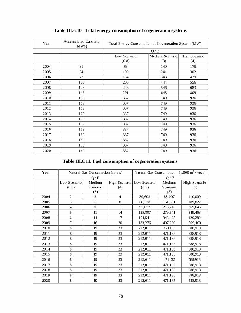
78

Table III.6.10. Total energy consumption of cogeneration systems

Year Accumulated Capacity (MWe)

Total Energy Consumption of Cogeneration System (MW)

Q / E

Low Scenario

(0.8) Medium Scenario

(3) High Scenario

(4) 2004 31 63 140 175 2005 54 109 241 302 2006 77 154 343 429 2007 100 200 444 556 2008 123 246 546 683 2009 146 291 648 809 2010 169 337 749 936 2011 169 337 749 936 2012 169 337 749 936 2013 169 337 749 936 2014 169 337 749 936 2015 169 337 749 936 2016 169 337 749 936 2017 169 337 749 936 2018 169 337 749 936 2019 169 337 749 936 2020 169 337 749 936

Table III.6.11. Fuel consumption of cogeneration systems

Year Natural Gas Consumption (m3 / s) Natural Gas Consumption (1,000 m3 / year)

Q / E Q / E

Low Scenario

(0.8) Medium Scenario

(3)

High Scenario (4)

Low Scenario (0.8)

Medium Scenario

(3)

High Scenario (4)

2004 2 3 4 39,603 88,007 110,009 2005 3 6 8 68,338 151,861 189,827 2006 4 9 11 97,072 215,716 269,645 2007 5 11 14 125,807 279,571 349,463 2008 6 14 17 154,541 343,425 429,282 2009 7 16 20 183,276 407,280 509,100 2010 8 19 23 212,011 471135 588,918 2011 8 19 23 212,011 471,135 588,918 2012 8 19 23 212,011 471,135 588,918 2013 8 19 23 212,011 471,135 588,918 2014 8 19 23 212,011 471,135 588,918 2015 8 19 23 212,011 471,135 588,918 2016 8 19 23 212,011 471135 588918 2017 8 19 23 212,011 471,135 588,918 2018 8 19 23 212,011 471,135 588,918 2019 8 19 23 212,011 471,135 588,918 2020 8 19 23 212,011 471,135 588,918

79

Costs The costs associated to cogeneration installations can be classified into two groups: capital costs & operating costs. The capital costs depend of the main components. Cogeneration plant consists of four basic elements:

1. A prime mover: Steam turbine, reciprocating engine, gas turbine, micro-turbines, stirling engines and fuel cells.

2. An electricity generator. 3. A heat recovery system. 4. A control system.

For our study we consider the average costs reported by CONAE. Tables III.6.12 and 13.

Table III.6.12. Investment costs Prime mover (US$ / KW) Average Costs Gas turbine 850-270 700

Steam turbine 400-150 275 Internal combustion engine (ICE) 650-300 475 Heat recovery equipments (HRU) (US$ / KW) Average costs

Diesel or gas engine 700-600 650

Heat recovery for steam turbines 400-200 300 Heat recovery for exhaust gases 150-75 112.5

Table III.6.13. Operation and Maintenance Cost

Prime mover (US$ / MWh) Internal Combustion Engine (diesel) 7.28

Internal Combustion Engine (natural gas) 5.18 Steam turbine 1.63 Gas turbine (natural gas) 3.08 For the benchmark scenario, we only assume the costs for the Medium Scenario Q/E = 3.

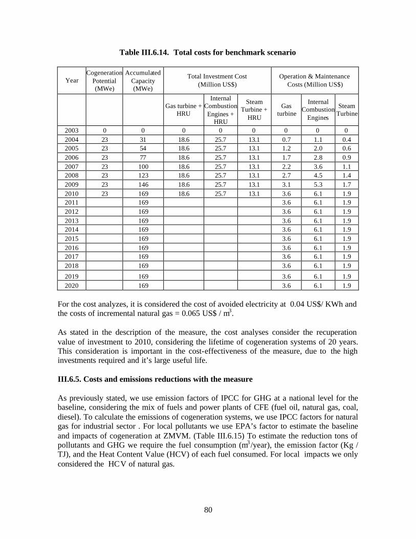
80

Table III.6.14. Total costs for benchmark scenario

Year Cogeneration

Potential (MWe)

Accumulated Capacity (MWe)

Total Investment Cost (Million US$)

Operation & Maintenance Costs (Million US$)

Gas turbine +

HRU

Internal Combustion Engines +

HRU

Steam Turbine +

HRU

Gas turbine

Internal Combustion

Engines

Steam Turbine

2003 0 0 0 0 0 0 0 0 2004 23 31 18.6 25.7 13.1 0.7 1.1 0.4 2005 23 54 18.6 25.7 13.1 1.2 2.0 0.6 2006 23 77 18.6 25.7 13.1 1.7 2.8 0.9 2007 23 100 18.6 25.7 13.1 2.2 3.6 1.1 2008 23 123 18.6 25.7 13.1 2.7 4.5 1.4 2009 23 146 18.6 25.7 13.1 3.1 5.3 1.7 2010 23 169 18.6 25.7 13.1 3.6 6.1 1.9 2011 169 3.6 6.1 1.9 2012 169 3.6 6.1 1.9 2013 169 3.6 6.1 1.9 2014 169 3.6 6.1 1.9 2015 169 3.6 6.1 1.9 2016 169 3.6 6.1 1.9 2017 169 3.6 6.1 1.9 2018 169 3.6 6.1 1.9

2019 169 3.6 6.1 1.9 2020 169 3.6 6.1 1.9

For the cost analyzes, it is considered the cost of avoided electricity at 0.04 US$/ KWh and the costs of incremental natural gas = 0.065 US$ / m3. As stated in the description of the measure, the cost analyses consider the recuperation value of investment to 2010, considering the lifetime of cogeneration systems of 20 years. This consideration is important in the cost-effectiveness of the measure, due to the high investments required and it’s large useful life. III.6.5. Costs and emissions reductions with the measure

As previously stated, we use emission factors of IPCC for GHG at a national level for the baseline, considering the mix of fuels and power plants of CFE (fuel oil, natural gas, coal, diesel). To calculate the emissions of cogeneration systems, we use IPCC factors for natural gas for industrial sector . For local pollutants we use EPA’s factor to estimate the baseline and impacts of cogeneration at ZMVM. (Table III.6.15) To estimate the reduction tons of pollutants and GHG we require the fuel consumption (m3 /year), the emission factor (Kg / TJ), and the Heat Content Value (HCV) of each fuel consumed. For local impacts we only considered the HCV of natural gas.

81

Table III.6.15. Emission factors

IPCC EPA ( AP – 42)

CO2 CO NOx SO2 CH4 NMVOC N2O CO2 CO NOx SO2 CH4 NMVOC N2O

Fuel Kg / TJ Kg / TJ

Electricity Generation

Natural Gas 56,100 18 250 ----- 1 5 0.1 49,716 14.8 116 0.2 1 ----- 0.9

Heavy Fuel Oil

77,367 15 200 995.3 0.9 5 0.3 74,595 14.9 140.2 936.9 0.8 ----- 0.3

Diesel 74,067 16 220 230.8 0.9 5 0.4 16.7 80 236.7 ----- ----- 0.4

Coal 94,600 9 380 1,045.2 0.7 5 1.6 145,137 13.7 316.11045.2 1.1 ----- 0.8

Industrial sector

Natural gas 56,100 16 64 ---- 1.4 5 0.1 49,716 34.8 41.4 0.2 1 ----- 0.9

Sources:Revised IPCC Guidelines for national Greenhouse Gas Inventories, Workbook, volume 2 AP-42 Compilation of Air Pollutant Emissions Factors AP-42, 5th Edition, Volume I, Stationary Point and Area Sources

Natural Gas Emission factor (Kg/106 m3)

PM (total) 121.6 VOC 88 TOC 176 Source: Air Pollution Engineering manual. Second Edition, Air & Waste Management Association Tables III.6.16 and III.6.17, illustrate that there are very large CO2 reductions due to this measure across the entire time horizon to 2020. On the local side, NOx emissions reduce, while there is no effect other local pollutants except for CO. This is because the fuel source considered in both the baseline and control measure is primarily natural gas, which is approximately 90% methane (CH4).

82

Table III.6.16. Emissions reductions for cogeneration systems without discounting (tons/yr)

Year PM10 PM2.5 SO2 CO NOx HC CO2 CH4 N2O

2003 0 0 0 0 0 0 0 0 0 2004 0 0 0 4 29 0 235,481 4 0 2005 0 0 0 6 50 0 405,117 7 0 2006 0 0 0 9 71 0 570,125 10 1 2007 0 0 0 11 92 0 734,075 12 1 2008 0 0 0 14 112 0 884,295 15 1 2009 0 0 0 16 133 0 1,033,945 18 1 2010 0 0 0 19 154 0 1,198,778 21 1 2011 0 0 0 19 154 0 1,218,795 21 1 2012 0 0 0 19 154 0 1,207,823 21 1 2013 0 0 0 19 154 0 1,198,252 21 1 2014 0 0 0 19 154 0 1,189,828 21 1 2015 0 0 0 19 154 0 1,182,358 21 1 2016 0 0 0 19 154 0 1,175,687 21 1 2017 0 0 0 19 154 0 1,169,695 21 1 2018 0 0 0 19 154 0 1,164,283 21 1 2019 0 0 0 19 154 0 1,159,369 21 1 2020 0 0 0 19 154 0 1,154,890 21 1

Table III.6.17. Annualized emissions reductions for cogeneration systems (tons/yr)

Discount rate

PM10 PM2.5 SO2 CO NOx HC CO2 CH4 N2O

Time horizon 2003-2010

0% 0 0 0 10 80 0 632,727 11 1

3% 0 0 0 9 77 0 606,875 10 1

5% 0 0 0 9 75 0 590,080 10 1

7% 0 0 0 9 72 0 573,667 10 1

Time horizon 2003-2020

0% 0 0 0 15 121 0 937,933 16 1

3% 0 0 0 14 115 0 889,344 16 1

5% 0 0 0 13 110 0 856,031 15 1

7% 0 0 0 13 106 0 822,510 14 1

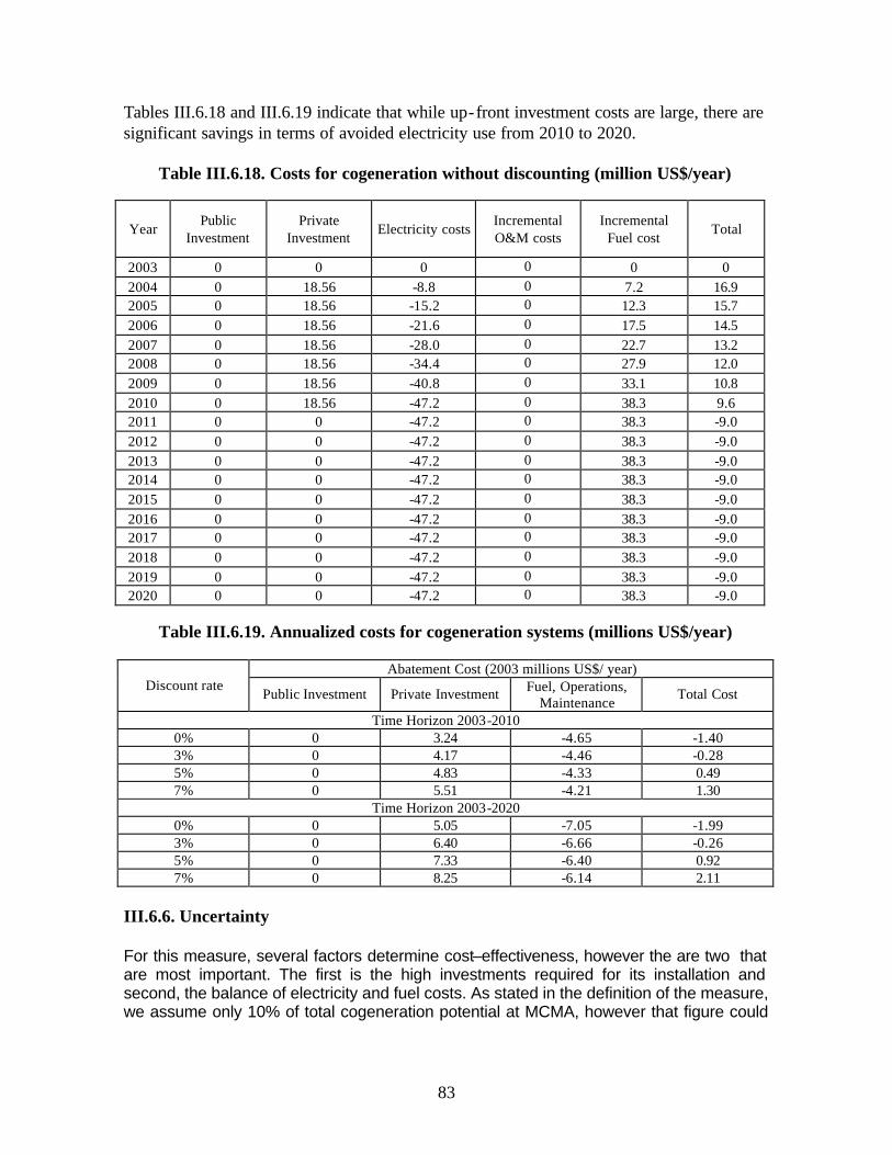
83

Tables III.6.18 and III.6.19 indicate that while up-front investment costs are large, there are significant savings in terms of avoided electricity use from 2010 to 2020.

Table III.6.18. Costs for cogeneration without discounting (million US$/year)

Year Public

Investment Private

Investment Electricity costs

Incremental O&M costs

Incremental Fuel cost

Total

2003 0 0 0 0 0 0 2004 0 18.56 -8.8 0 7.2 16.9 2005 0 18.56 -15.2 0 12.3 15.7 2006 0 18.56 -21.6 0 17.5 14.5 2007 0 18.56 -28.0 0 22.7 13.2 2008 0 18.56 -34.4 0 27.9 12.0 2009 0 18.56 -40.8 0 33.1 10.8 2010 0 18.56 -47.2 0 38.3 9.6 2011 0 0 -47.2 0 38.3 -9.0 2012 0 0 -47.2 0 38.3 -9.0 2013 0 0 -47.2 0 38.3 -9.0 2014 0 0 -47.2 0 38.3 -9.0 2015 0 0 -47.2 0 38.3 -9.0 2016 0 0 -47.2 0 38.3 -9.0 2017 0 0 -47.2 0 38.3 -9.0 2018 0 0 -47.2 0 38.3 -9.0 2019 0 0 -47.2 0 38.3 -9.0 2020 0 0 -47.2 0 38.3 -9.0

Table III.6.19. Annualized costs for cogeneration systems (millions US$/year)

Abatement Cost (2003 millions US$/ year)

Discount rate Public Investment Private Investment Fuel, Operations,

Maintenance Total Cost

Time Horizon 2003-2010 0% 0 3.24 -4.65 -1.40 3% 0 4.17 -4.46 -0.28 5% 0 4.83 -4.33 0.49 7% 0 5.51 -4.21 1.30

Time Horizon 2003-2020 0% 0 5.05 -7.05 -1.99 3% 0 6.40 -6.66 -0.26 5% 0 7.33 -6.40 0.92 7% 0 8.25 -6.14 2.11

III.6.6. Uncertainty

For this measure, several factors determine cost–effectiveness, however the are two that are most important. The first is the high investments required for its installation and second, the balance of electricity and fuel costs. As stated in the definition of the measure, we assume only 10% of total cogeneration potential at MCMA, however that figure could

84

be higher if there were incentives in the next years that promote the use of cogeneration installations. It is important to mention that the size of cogeneration installations depends of the ratio of electricity and fuel consumption of each industry (Q/E ratio). This is an important issue due the required cogeneration scheme (prime mover), is defined by this ratio, and therefore its capital costs. III.6.7. Discussion and Next Steps

As stated in the definition of the measure, the heat demand was carried out according to the Q/E ratio scenarios, nevertheless this value depends on the energy and electricity requirements of each industry, based on it’s production. Future work should be done to determine the Q/E ratio for each industry. It is important to note that the low local benefits of cogeneration at MCMA are due to the small regional generation, which is around 3.1% of interconnected grid. On the other side, the results show that cogeneration is an effective measure to reduce GHG to Mexico. This is due mainly to the high contribution of fossil fuels to national electricity generation. As stated in previous sections, future work should be focused in the cost analyses of each industry. Some of the items that should be included in future works for specific installations are: Installation costs (e.g. materials, labour, etc. ), fuel cost chain (e.g. installation of ducts, labour, prices of alternatives fuels, etc), detailed maintenance costs (e.g. labour, spare parts, etc.) One of the main issues that determine the cost-effectiveness of cogeneration is the recuperation value of investment. As mentioned before, it was considered the useful life of 20 years for all installations; at this point, it is suggested to consider the evolution of cogeneration technology (e.g. efficiency, availability, performance, etc) that will be reflected in the capital and operation and maintenance costs (O&M). Finally, it is important to mention that the introduction of cogeneration systems at MCMA depends on several factors, some of the most important are: Investment cost per KWh installed, O&M cost, availability of natural gas, natural gas cost and electricity cost. Future work should be done considering this issues. III.6.8. References Comisión Nacional para el Ahorro de Energía (2003), Potencial Nacional de Cogeneración 1995, Davis, W., eds. (2000), Air Pollution Engineering Manual. Second Edition, Air & Waste Management Association, Wiley & Sons, US. Fisk, R., VanHousen, R., eds. (1998), Cogeneration Application Considerations, GE Power Systems, Schenectady, NY.

85

IPCC, Intergovernmental Panel on Climate Change (1997), “Revised 1996 IPCC Guidelines for National Greenhouse Gas Inventories, Vols. 1-3” (Bracknell, UK: IPCC). Secretaría de Energía (2002), Balance Nacional de Energía 2001. Secretaría de Energía (2002), Prospectiva del Sector Eléctrico 2002-2011. The European Association for the Promotion of Cogeneration - COGEN Europe, (2001), A Guide to Cogeneration. Guide produced under the auspices of EDUCOGEN, CONTRACT N° XVII/4.1031/P/99-159. West, J.J., P. Osnaya, I. Laguna, J. Martínez, A. Fernández (2003) Co-control of urban air pollutants and greenhouse gases in México City. Final report to US National Renewable Energy Laboratory, subcontract ADC-2-32409-01.

86

Chapter IV. Air Quality Modeling IV.1. Introduction Air quality modeling is an important tool for environmental assessment and is a key in the support decions made by policy makers on air quality issues. A simulation model is a mathematical specification of a system that depicts quantitatively how the system behaves. It is a set of equations, with estimated coefficients and parameters, that depict the relationships among the variables represented in the model. The equations can be solved for values of the variables determined within the model (the endogenous variables) given the values of the other variables determined outside the model (the exogenous variables) and the parameters. Simulation can be used for policy analysis. Alternative policies can be simulated to predict how the system would behave if those policies had been implemented and to estimate their effects. Simulation models have been used to evaluate alternative fiscal, monetary and environmental policies. Models can be classified according to several aspects (including subject matter, objective, structure, degree of aggregation, time horizon and basic approach). A general classification includes two kinds of models: structural models and reduced form models. The equations of a structural model depict what the model builder believes are basic causal relationships. A structural model often depicts the interactions among several endogenous variables of the model. To understand the underlying determinants of a system’s behaviour, one needs a structural model. Often the equations of a structural model can be solved to provide an expression for each endogenous variables in terms of exogenous variables only. These equations are called the reduced form of the model. A reduced form does not depict the actual causal relationships of the system. However, a set of reduced form equations can be used to predict how the endogenous variables respond to the exogenous variables. IV.2. Reduced-Form Atmospheric Modeling Methodology For the estimation of the impacts of emission reduction on ambient concentrations and population exposures, we developed a range of reduced-form modeling approaches. We focused on the estimation of particle concentrations because previous studies have shown that health impacts from particle concentrations overwhelmingly dominate health benefit calculations (Cesar et al, 2000; Cesar et al. 2002; Zuk, 2002; Evans et al. 2002). Our estimate of PM10 is derived from the source apportionment results of Chow et al. (2002). We estimate primary concentrations resulting from direct PM10 emissions, and secondary PM10 concentrations from hydrocarbon, NOx, and SO2 emissions. Ozone isopleths from the Salcido et al. (2001) are used to estimate peak O3 changes occurring with changes in hydrocarbon and NOx emissions.

87

We also developed a box model to estimate primary PM10 concentrations from direct PM10 emissions; and the Marginal PM method of West and San Martini (2001) to estimate secondary sulfate and nitrate particle concentrations (Appendix A). However, following commentary from technical staff of the government agencies attending our regular meetings, we determined that the box model and Marginal PM methods have large uncertainty, and that the use of the source apportionment results is a better way to estimate both primary and secondary concentration changes due to emission changes. Thus, we have eliminated the box model and use Marginal PM as explicit components of the analysis. We use results from our primary reduced-form models, source apportionment and Ozone Isopleths, to give central estimates for the reduction fractions in pollutants derived from emissions changes. Uncertainty is determined for these estimates as described in section IV.6. IV.3. Use of Reduced-Form Models with Observations: Including Spatial and

Temporal Distribution In order to account for the spatial distribution of population and of pollutant concentrations, we use the reduced form models to provide a reduction fraction (RF) of pollutant concentration (Cesar et al. 2002, USEPA, 1999). This reduction fraction is then multiplied by projected future population-weighted concentrations for the appropriate time horizon. These projected concentration are based on the mean 1995-1999 observed, population-weighted (1995 census) 24-hour mean PM (64.06 ug/m3) or O3 maximum concentration (0.114 ppm), from Cesar et al. (2000). The projection to future population-weighted concentrations is achieved by a linear interpolation or extrapolation of mean concentration results from the CAM’s MCCM model for 1998 and 2010 based on the emissions inventory for 1998 and emission inventory projection for 2010 of the CAM (PROAIRE, 2002). This method was described in the first progress report. Projection factors are presented in Table IV.1.

Table IV.1. Projection factors used to scale 1995-1999 observed concentration to future timeframes. 24 hour and maximum O3 concentrations use the same scaling factor

Ratio

2010 / 1998 Ratio

2002-2010 / 1998 Ratio

2002-2020 / 1998 O3 1.075 1.050 1.081

PM10 1.280 1.186 1.303 IV.4. Using Source Apportionment Results for Primary and Secondary PM Source apportionment is a chemical analyses of the composition of particulate matter in the region of interest. To use these results as a reduced-form model, the chemical species in the observed particulate matter are attributed to primary pollutants. Then, fractional changes in the emission of the primary pollutants can be related to fractional reductions in particulate concentrations via the chemical apportionment. The governing equation is:

iiPM RFFRF ⋅= ∑10 Equation IV.1

88

Where RFPM10 is the reduction fraction of the PM concentration, Fi is the fraction of PM mass due to a primary pollutant i and RFi is the reduction fraction of the emission of the primary pollutant. We use the results for chemical composition of PM10 in Mexico City of Chow et al. (2002) to estimate the fractions of PM mass due to each primary pollutant. Chow et al. (2002) present results at 6 sites distributed across Mexico City. We average these results to arrive at a single fractionation estimate for the entire MCMA. The mean mass of PM10 due to each primary pollutant i is estimated by summing the results presented in terms of fractions of PM2.5 and the coarse fraction, and the total mass of PM2.5

and the coarse fraction at each of the six sites.

( )Coarsek

Coarsekikki

ki MFMFM ⋅+⋅= ∑

=,

5.25.2,

6

161

Equation IV.2

In order to attribute organic carbon to its primary (combustion) and secondary (hydrocarbon) sources, we must disaggregate the observed organic carbon into primary and secondary contributions. Following Turpin et al. (1991), we estimate the primary organic contribution to total organic carbon based on a fixed ratio to elemental carbon mass of 1.9, a mean value for the Los Angeles basin (range 1.4-2.4). Thus the mass of primary organic carbon (MOC1) is: MOC1 = MEC*1.9. The mass of secondary organic carbon (MOC2) is then the difference of the total organic carbon mass (MOC_TOT ) and the mass of primary organic carbon: MOC2 = MOC_TOT – MOC1. We then estimate that MOC1 is due to the same primary particle combustion sources that produce elemental carbon. Therefore, total primary particulate mass from combustion sources is MPRI_COMB = MOC1 + MEC. Secondary organic carbon mass (MOC2) is attributed to hydrocarbon emissions (MHC = MOC2). The mass of particles associated with geological sources by Chow et al. (2002) (MPRI_GEO) is attributed to primary PM10 emissions from geologic sources. The mass of particles associated with Total Particulate Ammonium Nitrate (MNO3) is attributed to NOx emissions (MNOx =MNO3); and the mass of particles associated Ammonium Sulfate (MSO4) is attributed to SO2 emissions (MSO2 = MSO4). Fractions are then calculated by dividing the mass of each attributed primary pollutant by the mean mass across the 6 stations. Results are presented in Table IV.2

( )⋅

+=

∑=

6

1

5.2

61

k

Coarsekk

ii

MM

MF Equation IV.3

89

Table IV.2. Apportionment fractions relating primary pollutant emissions to observed PM10

Primary pollutant Fraction FPRI_GEO 0.45 FPRI_COMB 0.25 FHC 0.02 FNOX 0.07 FSO2 0.11 We find that 90% of the particulate mass is accounted for by primary pollutants under considered in this study. Chow et al. (2002) find that, on average for Mexico City, 10% of particle mass is salt, non-crustal and unidentified material; this fraction is implicitly assumed to be constant in this source apportionment analysis. Using the apportionment fractions in Table IV.2, the total reduction fraction for PM10 concentration is then:

iii

PM RFFRF ⋅= ∑=

5

110

Equation IV.4

where: i

ii E

ERF

∆= Equation IV.5

ÄEi is the change in emissions of each primary pollutant due to a control measure. Ei is total emission inventory for each pollutant, from either 2010 (PROAIRE), or 2002-2010 or 2002-2020 depending upon time horizon. 2002-2010 inventory is a simple mean based on a linear interpolation between 1998 and 2010 PROAIRE inventories, and 2002-2020 is a simple mean based on linear interpolation and linear extrapolation to 2020 from the 1998 and 2010 PROAIRE inventories. Once the baseline emissions inventories are prepared for all control measures (see chapter III. Emissions and control strategy costs), as part of the process of estimating emission reductions for each measure, then these inventory estimates will be revised. IV.5. Ozone Isopleths for Peak Ozone The peak mean O3 reduction fraction (RO3max) is estimated from the fractional reductions in hydrocarbon (RHC) and NOx (RNOx) by:

RO3max = 0.5353*RNOx - 0.2082*(RNOx)2 + 0.1112*RHC Equation IV.6 These are estimated from a series of MCCM model runs (Salcido et al., 2001) where HC and NOx emissions are varied in equal proportion from all sources and O3 concentration changes are recorded. The above equation results from multiple linear regression fits to the results of Salcido et al. (2001) using the Analyse-It package for Microsoft Excel.

90

The use of Ozone Isopleths (Chapter IV) to estimate air quality changes due to emission changes requires this analysis to consider all hydrocarbons to be equivalent in terms of their impact on ozone formation. In fact, all hydrocarbons are not equivalently reactive. For example, the hydrocarbons in LPG are of a low reactivity that might mean that the impact on ozone concentration from reductions in LPG leaks may be overestimated using this methodology (Molina et al. 2002). IV.6. Applying Uncertainty Bounds Comparisons using 6 control measures in the version 5.3 of the model (Co-Beneficios-5.3) indicate that the use of source apportionment results (SA) estimates 1/3 the 1o particulate change as does the Box Model. For secondary particulates, SA estimates approximately 20 times the sulfate change and 1.5 times the nitrate change as does the Marginal PM method (Table IV.3). These ratios are the same for all the measures analyzed. Table IV.3. Comparing results of reduced-form air quality models (Co-Beneficios-5.3)

SA / Box SA / Marginal 1º PM10 2º Sulfate PM10 2º Nitrate PM10

0.35 17 1.6 There is large uncertainty in the Box Model – it is generally not considered appropriate in a region of variable wind and complex topography. Further, to get reasonable results in comparison to observations, we have used very low winds. In summary, the Box Model is likely far too simplified to give good quantitative estimates. There is also large uncertainty in the Marginal PM method, in part because of problems of temporal and spatial representativity of the data used in the derivation of the coefficients. SA has more certainty that these two methods, and it also provides a consistent method to estimate both primary and secondary particulate change based on observations of the MCMA. Thus, we use SA as our central estimate in this study. We apply error estimates to these estimates using the results from the other two methods, and also other efforts to quantify uncertainty in the relationship between emissions, concentrations, and population exposure. The application of these uncertainty ranges is described below. Cohen et al. (2003) use intake fractions (Levy et al., 2002) in their cost-effectiveness comparison of public bus technologies in the US. They estimate the ranges of uncertainty as presented in Table IV.4. Ranges are presented as a multiplier of the Central estimate. Table IV.4. Low and high bound multipliers giving intake fraction uncertainty in

Cohen et al. (2003) Low High 1o PM (immediate) 1 5 1 o PM (after transport) ½ 2 NOx to 2 o PM 1/5 6 NOx to O3 1/5 5 SO2 to 2 o PM 1/3 3

91

At the 6th Workshop of the Integrated Program on Urban, Regional and Global Air Pollution, in January 2003, Hammitt et al. (2003) indicated that their study of the benefit and costs of diesel particle filters for the MCMA, they use a multipliers of 1/5 and 5 in a triangular distribution for all PM intake fractions in the MCMA. Given the above evidence, we choose to apply low and high multipliers to the central estimates from the SA. We use 1/3 and 3 for 1o PM because this is both consistent with our comparison between the box model and the source apportionment, and also with a mid-value between those for immediate 1o PM exposure and exposure after transport that were used with intake fractions in Cohen et al. (2003) (Table IV.4) and similar to the value of Hammitt et al. (2003). Our choice for 2o PM is a subjective balance between the large range indicated by the SA / Marginal PM comparison, the fact that the Marginal method is considered very uncertain, and the values used in Cohen et al. (2003) and Hammitt et al. (2003). For uncertainty in the ozone calculation, we also apply multipliers to the Ozone Isopleths, basing our values on Cohen et al. 2003. These changes are implemented in version 5.4 of the model and above. The low and high multipliers used in the model are indicated in Table IV.5.

Table IV.5. Low and high bound uncertainty multipliers Low High 1 o PM 1/3 3 All 2o PM 1/5 5 O3 1/5 5 IV. 7. Results and Uncertainty

In this section, concentration changes, calculated via the above-described methodology, are presented for each measure. We present mean annualized concentration reductions derived from our benchmark scenario, which uses a 5% discount rate, for both the time periods 2003-2010 (Table IV.6) and 2003-2020 (Table IV.7). In Tables IV.6 and Table IV.7, negative values indicate an increase in concentration. Table IV.6. Mean concentration reductions from annualized emissions reductions for

2003-2010 at 5% (ug/m3)

Particulates (PM10) Primary Nitrates Sulfates Organics

Maximum O3

Taxi renovation

0 0.222 0.038 0.096 5.13

Metro expansion

0.002 0.007 0.002 0.002 0.142

Hybrid Buses

0.131 -0.005 0.008 0.002 -0.071

Combined LPG Leak

0 0 0 0.070 0.907

Cogeneration 0 0.003 0 0 0.057

92

Table IV.7. Mean concentration reductions from annualized emissions reductions for

2003-2020 at 5% (ug/m3)

Particulates (PM10) Primary Nitrates Sulfates Organics

Maximum O3

Taxi Renovation

0 0.129 0.033 0.073 3.02

Metro expansion

0.016 0.054 0.036 0.015 1.071

Hybrid Buses

0.142 -0.006 0.009 0.002 -0.073

Combined LPG Leak

0 0 0 0.061 0.737

Cogeneration 0 0.005 0 0 0.077

According to this analysis, the Taxi renovation, Metro expansion (for 2003-2020), and the Combined LPG Leak measure would create significant reductions in maximum ozone concentrations. Primary particulate reductions are substantial only for the Hybrid Bus measure. Reductions in nitrate and organic secondary particulates are large for the Taxi renovation and Metro measures. The Combined LPG measure reduces secondary organic particles. Changes in secondary sulfates are smaller, though not insignificant for the Taxi renovation and Metro measures. In Table IV.8 and IV.9, results for total PM10 and ozone change are presented along with the uncertainty associated with these estimates. Uncertainty is generally large. Table IV.8. Total particulate and maximum ozone change from annualized emissions

reductions for 2003-2010 at 5%, with uncertainty (ug/m3)

Particulates (PM10) Maximum O3 Mean 95% CI Mean 95% CI

Taxi Renovation

0.36 (0.17 : 0.58) 5.13 (1.59 : 9.97)

Metro expansion 0.01 (0.01 : 0.02) 0.14 (0.04 : 0.28) Hybrid Buses

0.14 (0.06 : 0.23) -0.07 (-0.14 : -0.02)

Combined LPG Leak

0.07 (0.02 : 0.28) 0.91 (0.14 : 1.76)

Cogeneration 0 (0 : 0) 0.06 (0.02 : 0.11)

93

Table IV.9. Total particulate and maximum ozone change from annualized emissions reductions for 2003-2020 at 5%, with uncertainty (ug/m3)

Particulates (PM10) Maximum O3

Mean 95% CI Mean 95% CI Taxi Renovation

0.24 (0.12 : 0.38) 3.02 (0.94 : 5.87)

Metro expansion 0.12 (0.07 : 0.18) 1.07 (0.33 : 2.08) Hybrid Buses

0.15 (0.07 : 0.25) -0.07 (-0.14 : -0.02)

Combined LPG Leak

0.06 (0.02 : 0.12) 0.74 (0.23 : 1.43)

Cogeneration 0 (0 : 0.01) 0.08 (0.02 : 0.15)

The inclusion of spatial distribution with Ozone Isopleths and or the application of the source apportionment results should be considered as a way to improve these methodologies. IV.8. References Cesar, H., K. Dorly, X. Olsthoorn, L. Brander, P. V. Beukering, V. Borja-Aburto, V. Torres Meza, A. Rosales Castillo, G. Oliaz Fernandez, R. Muñoz Cruz, G. Soto Montes de Oca, R. Uribe Ceron, E. Vega López, P. Cicero Fernández, A. Cilalic González Martinez, MM Niño Zarazua and MA Niño Zarazua (2000) “Economic valuation of Improvement of Air Quality in the Metropolitan Area of Mexico City,” Institute for Environmental Studies (IVM)

Cesar, H., G. Schadler, M. Hojer, P. Cicero-Fernandez, L. Brander, T. Buhl, A. C. Villagomez, K. Dorland, A. C. G. Martinez, H. Hasselknippe, P. M. Oritz, A. V. Montero, A. Salcido, J. Sarmiento, and P. V. Beukering (2002) “Air pollution abatement in Mexico City: an economic valuation,” World Bank Report

Chow, J.C., J.G. Watson, S.A. Edgerton, and E. Vega (2002) “Chemical composition of PM2.5 and PM10 in Mexico City during winter 1997,” The Science of the Total Environment 287, p.177-201. Cohen, J.T., J.K. Hammitt, and J.I. Levy. 2003. Fuels for urban transit buses: A cost-effectiveness analysis. Environ. Sci. Technol 37. 1477-1484. Evans, J., J. Spengler, J. Levy, J. Hammitt, H. Suh, P. Serrano, L. Rojas-Bracho, C. Santos-Burgoa, H. Rojas-Rodriguez, M. Caballero-Ramirez and M. Castillejos (2000) “Contaminación atmosférica y salud humana en la Ciudad de México,” MIT-IPURGAP Report No. 10.

94

Hammitt, J.K., G. Stevens, and A. Wilson. 2003. Benefit-cost analysis of diesel particulate filters: preliminary results. Presentation at 6th Workshop of the Integrated Program on Urban, Regional and Global Air Pollution, Mexico City, January 2003. Levy, J.I., S.K. Wolff, and J.S. Evans. 2002. A regression-based approach for estimating primary and secondary particulate matter intake fractions. Risk Analysis 22. 895-904. Molina, M.J., L.T. Molina, J. West, G. Sosa, and C. Sheinbaum Pardo (2002) “Air pollution science in the MCMA: Understanding source-receptor relationships through emissions inventories, measurements, and moideling,” in Air Quality in the Mexico Megacity: An Integrated Assessment, Kluwer Academic Pub lishers, Boston, 384 pp. Salcido et al. (2001) “MCCM Parametric Studies: Estimation of the NOx, HC and PM10

emission reductions required to produce a 10% reduction in the Ozone and PM10 surface concentrations and compliance with the MCMA air quality standards, with reference to the 2010 MCMA Emission Inventory,” Grupo de Modelación de la Comisión Ambiental Metropolitan (CAM), 42 pp. Turpin, B.J., J.J. Huntzicker, S.M. Larson and G.R. Cass (1991) “Los Angeles summer midday particulate carbon: Primary and secondary aerosol,” Envi. Sci. Technol., 25(10) 1788-1793. U.S. Environmental Protection Agency (1999) "The Benefits and Costs of the Clean Air Act 1990-2010," Washington, D.C., Office of Air and Radiation, EPA report no. 410/R-99/001. West, J. and I. San Martini (2001) Report of the Fourth Workshop on Mexico City Air Quality, March 8-10, 2001, El Colegio de Mexico, Mexico. MIT-Integrated Program on Urban, Regional and Global Air Pollution Report No. 25, November 2001. Zuk, M (2002) “Evaluating the benefits of reducing uncertainty in air quality management: the case of Mexico City,” Masters thesis, Massachusetts Institute of Technology.

95

Chapter V. Health Impacts Analysis V.1. Introduction It has been well established that exposure to outdoor air pollutants can cause several cardiovascular and respiratory outcome, and even may cause premature mortality. As the primary motivation for air quality management is to reduce the public health burden of pollution, it is important to evaluate how measures aimed at reducing air pollution will affect human health. In this section we expand on the methodology outlined previously to explain some of the basic theory behind our calculations and data sources. In part I, we describe the sources of the dose response coefficients used in the analysis, followed by an explanation of the sources of data on morbidity and mortality rates in Mexico City, concluding with a description of the methodology and results of the Year of Potential Life Lost (YPLL) analysis and final results. Before documenting each part of the analysis, we must first review the basic calculations being made, so that it is clear where the sections fit in. As explained in the main report, we use a general dose response model to estimate the changes in health outcomes due to changes in ambient exposures of ozone and PM10. Equation V.1 describes the general form of this equation.

NCRH jiijij ×××= β Equation V.1 Where âi is the dose-response coefficient for the ith effect from the pollutant of interest (% increase cases/year/person/unit exposure), Ri is the background rate of the effect of interest (cases/year per person), C is the ambient concentration of pollutant (µg/m3) averaged across the entire population, and N is the population at risk (number of people). The dose response coefficients come from epidemiological studies and are described in section 2 and the background rates of disease and mortality in section 3. Concentrations come from the air quality module, and population exposed is the population of Mexico City in the year 2000. Since our analysis of measures finds annualized emissions, the concentration input to this module is annualized concentrations reductions for a stream of 8 or 18 years of emissions. Therefore this value does not represent any single year, but rather an average year in this time period. We therefore use the year 2000 as our base year, although perhaps it would be better to use the projected population in the middle of the period. Table V.1 lists the set of 19 health outcomes analyzed here. These outcomes were chosen based on epidemiological evidence of their association with air pollution. To avoid overlap in the valuation section, we do not include all of these outcomes when calculating total monetary benefits.

96

Table V1. Outcomes evaluated

Mortality due to Acute Exposure

All Causes

Infant Mortality

Mortality due to Chronic Exposure

All Causes

Cardio-respiratory Causes

Lung Cancer

Chronic Bronchitis

Hospital Admissions

All Respitaroty Causes

Asthma

COPD

Pneumonia

All Cardiovascular

Congestive Heart Failure

Ischemic Heart Disease

Emergency Room Visits (ERVs)

All Respiratory Causes

Asthma

Restricted Activity Days

Minor Restricted Activity Days

School Absenteeism

V.2. Dose Response Analysis There is an abundance of literature on the health impacts of air pollution. For certain outcomes there is a plethora of evidence, whereas for others there have been only a few key studies. The purpose of this analysis was to gather information from 3 principal meta-analyses, (USEPA, 1999; Cesar et al. 2002; and Evans et al. 2000), as well as other epidemiological literature to determine the appropriate dose response values to use for our analysis. It was beyond the scope of this study to conduct an original meta-analysis, nor did we find it necessary since there have already been a number of such summary studies conducted for Mexico. The reason for using the 3 meta-analyses is that they include different studies in their analysis and have therefore found different results. Due to the wide range of dose response results from the various studies, we have decided to include a range of possible dose response values, rather than a single number. In this section, we first present the sources of data and the ranges chosen for each health outcome, followed by a summary table. When analyzing various sources of epidemiological studies, it became evident that many different metrics were used. First, it was necessary to ensure that the outcomes of interest were the same as those in the studies. This was guaranteed by comparing ICD codes for the

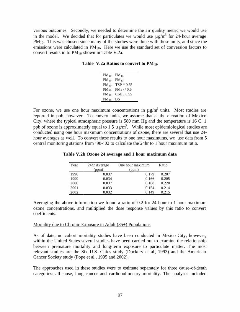
97

various outcomes. Secondly, we needed to determine the air quality metric we would use in the model. We decided that for particulates we would use µg/m3 for 24-hour average PM10. This was chosen since many of the studies were done with these units, and since the emissions were calculated in PM10. Here we use the standard set of conversion factors to convert results in to PM10 shown in Table V.2a.

Table V.2a Ratios to convert to PM 10

PM10 ≅ PM15 PM10 ≅ PM13 PM10 ≅ TSP * 0.55 PM10 ≅ PM2.5 / 0.6 PM10 ≅ CoH / 0.55 PM10 ≅ BS

For ozone, we use one hour maximum concentrations in µg/m3 units. Most studies are reported in ppb, however. To convert units, we assume that at the elevation of Mexico City, where the typical atmospheric pressure is 580 mm Hg and the temperature is 16 C, 1 ppb of ozone is approximately equal to 1.5 µg/m3. While most epidemiological studies are conducted using one hour maximum concentrations of ozone, there are several that use 24-hour averages as well. To convert these results to one hour maximums, we use data from 5 central monitoring stations from ’98-’02 to calculate the 24hr to 1 hour maximum ratio.

Table V.2b Ozone 24 average and 1 hour maximum data

Year 24hr Average

(ppm) One hour maximum

(ppm) Ratio

1998 0.037 0.179 0.207 1999 0.034 0.166 0.205 2000 0.037 0.168 0.220 2001 0.033 0.154 0.214 2002 0.032 0.149 0.215

Averaging the above information we found a ratio of 0.2 for 24-hour to 1 hour maximum ozone concentrations, and multiplied the dose response values by this ratio to convert coefficients. Mortality due to Chronic Exposure in Adult (35+) Populations As of date, no cohort mortality studies have been conducted in Mexico City; however, within the United States several studies have been carried out to examine the relationship between premature mortality and long-term exposure to particulate matter. The most relevant studies are the Six U.S. Cities study (Dockery et al., 1993) and the American Cancer Society study (Pope et al., 1995 and 2002). The approaches used in these studies were to estimate separately for three cause-of-death categories: all-cause, lung cancer and cardiopulmonary mortality. The analyses included

98

controls for several risk factors, including age, gender, race, smoking education, body mass index, alcohol consumption, occupational exposure, diet indices, and others. The Six Cities cohort study, which lasted 16 years, was restricted to 8,111 white subjects who were 25 through 74 years of age. For all cause mortality they found a 14% (4.3% to 25%) increase in mortality per 10 µg/m3 increase in fine particles (PM2.5), for lung cancer 20% (NS to 70%) and for cardiopulmonary mortality 20% (6% to 37%). Translated to PM10 (considering a PM2.5/PM10 ratio of approximately 0.6), this respectively corresponds to 8.4% (2.6% to 15%), 12% (NS to 42%) and 12% (3.6% to 22%). The ACS cohort study of 2002, extended the prior 1995 study until December of 1998. This study associated PM2.5 with all-cause, cardiopulmonary and lung cancer mortality. For all-cause mortality they found a 6% (2% to 11%) increase in mortality per 10 µg/m3

increase in PM2.5, for lung cancer 14% (4% to 23%) and for cardiopulmonary mortality 9% (3% to 16%).Translated to PM10 respectively, 3.6%( 1.2% to 7%), 8.4% (2.4% to 14%) and 5.4% (2% to 10%). From these studies, it can be concluded that there is strong evidence that long-term exposure to fine particulate air pollution is an important risk factor for lung cancer and cardiopulmonary mortality. This holds true even after controlling for cigarette smoking, BMI, diet, occupational exposure, other individual risk factors and after controlling for regional and other spatial differences. Table V.3 compares percent increase in mortality risk obtained in these studies associated with the increase in PM2.5 and PM10 concentration.

Table V.3 Results from 2 Cohort Mortality Studies

Six Cities (Dockery, 1993) ACS (Pope, 2002) PM10 % increased risk (95% CI) associated with a 10 µg/m3 increase

in PM10 All 8.4% (2.6% – 15%) 3.6% (1.2% –7%) Lung cancer 12% (NS – 42%) 8.4% (2.4% – 14%) Cardiopulmonary 12% (3.6% – 22%) 5.4% (2% – 10%)

In the Analytica model, the dose-response coefficients used for mortality considered all-cause mortality. Given that there have been no studies on chronic mortality in Mexico and limited evidence from the U.S., a value of 0 was chosen as a plausible minimum, the ACS 2002 study as a mid-value and the Six Cities study as a maximum to represent the plausible range of dose response values for mortality. Mortality due to Acute Exposure

The evidence from time series studies around the world has been substantially consistent. A recent analysis, the National Morbidity, Mortality and Air Pollution Study (NMMAPS) by Samet et al. (2000), looked at death counts and air pollution levels in 90 cities across the U.S. and attempted to account for differences in methodology, geographic conditions and the effects of gaseous air pollutants in a systematic manner. They found an average

99

increase of 0.5% risk of mortality per 10µg/m3 of PM10, which was greater for mortality due to heart and lung disease than total deaths. A recent meta-analysis by Levy et al. (2000) considered nearly 30 international studies and using a random effects model, found a pooled result of 0.7% increase per 10 µg/m3 increase in PM10 concentrations (95% CI: 0.6%, 0.8%). A number of time series studies have been conducted in Mexico City all of which appear to show a significant relationship between mortality and particulates. An earlier study by Borja Aburto et al. (1997) found the effect of same-day 24-hour average TSP concentrations resulted in a 5% increase in premature mortality (95% CI: 3.0%, 6.7%) for a 100 µg/m3 increase. Three recent studies (Borja-Aburto et al., 1998; Loomis et al., 1999; and Castillejos et al., 2000) considered various particle size fractions and were conducted by a single research team over the same geographic area and time period. The two studies by Borja-Aburto have similar estimates for total mortality (1.1% and 1.2% increase per 10 µg/m3), while the Castillejos study has a higher estimate of 2.5%, potentially associated with the longer exposure window. A number of other time series studies have been conducted analyzing the relationship between pollution exposure and mortality for specific causes. The Harvard risk assessment (Evans et al., 2000) indicated that if the Mexican studies were pooled, the risk of mortality in Mexico City would be around 1.4% increase per 10µg/m3. This seems well within the range of findings from international studies. Given the relatively narrow range of results from these 3 sources, we choose to use the NMMAPS dose response coefficient as the lower bound, the pooled international coefficient from Levy et al. (2000) for the central estimate Mexican value as an upper bound to account for variability in findings across the studies. In the analysis of ozone’s affect on daily mortality, there is some evidence, from both the Mexican and worldwide literature of an association between ozone and premature mortality. Only one of the Mexican studies found a statistically significant association between ozone and cardiovascular mortality (Borja-Aburto et al., 1998). The recent meta-analysis by Levy et al. (2000), found ozone to be a significant predictor of mortality, even when particulate matter was included in the model. Out of 50 studies, only four met their strict inclusion criteria. The pooled estimate from these four studies indicated a 0.4% increase in premature mortality per 10µg/m3 increase in 24-hour average ozone concentrations. In this study we use the estimates of relative risk from Levy et al. (2000), with a lower bound of zero effect and upper bound of 0.7% per 10µg/m3 of 24-hour average ozone concentrations. Translated to 1 hour maximum, this is equivalent to 0, 0.08% and 0.14% per 10µg/m3 of 1-hour maximum ozone levels. Infant Mortality There have been several studies on the association between exposure to air pollution and infant mortality around the world including the Czech republic, Mexico City, Sao Paulo, Beijing and the U.S. The two most relevant studies are the U.S. (Woodruff et al. 1997) and Mexico City (Loomis et al., 1999) studies. The Mexico City study found that a 10 µg/m3

100

increase in PM2.5 was associated with a 6.3% increase in infant mortality (95% CI: NS, 13.2%). Translated to PM10, this corresponds to 3.9% (95% CI: -.3%, 8.2%) per 10µg/m3. The U.S. study by Woodruff et al. (1997) involved an analysis of approximately 4 million infants born between 1989 and 1991. They analyzed all cause and respiratory related post-neonatal mortality and found that exposure to 10 µg/m3 of PM10 corresponded to 1.04% (95% CI: 1.02%, 1.07%) changes in death rates. Given the limited availability of infant mortality studies, we choose to use 0 as a plausible minimum, the U.S. study as a mid-value and the Mexican study as a maximum (0, 1.04%, 3.9%) to represent the plausible range of dose response values. Chronic Bronchitis No large-scale epidemiological studies of chronic bronchitis have been conducted within Mexico; however, there are two smaller studies in Mexico City (Santos-Burgoa et al., 1998; Romano, 2000) which address chronic bronchitis to some extent, nevertheless the evidence linking air pollution to this ailment is relatively weak. Although these studies provide some evidence that chronic bronchitis prevalence may be linked to air pollution in Mexico City, definitive conclusions cannot be reached given the sample size and study population selected, the study design, and lack of direct concentration measures across the entire sample. In the worldwide literature, there are three primary studies that evaluate links between long-term exposure to air pollution and development of bronchitis (Abbey et al., 1993; Schwartz, 1993; Abbey et al., 1995). The Schwartz study in 1993 consisted of a cross sectional analysis of bronchitis prevalence and mean levels of total suspended particles (TSP) in 53 urban area in the U.S. In this study concentration-response relationships were estimated, finding a 7% (95% CI: 2%, 12%) increase in chronic bronchitis rates for a 10 µg/m3 increase in TSP. Both of the Abbey et al. studies were prospective cohort studies of a Seventh Day Adventist population in California. The 1993 study estimated a 36% increase in chronic bronchitis associated with ten years of exposure to a 60 µg/m3 increment of TSP. Therefore an increase in chronic exposure of 10 µg/m3 of TSP would increase chronic bronchitis incidence by 5%. In the 1995 study, PM2.5 was examined. It was estimated that a 45 µg/m3 increase in PM2.5 was associated with a relative risk of 1.81 (95% CI: 0.98%, 3.25%) for chronic bronchitis development, meaning that a 10 µg/m3 increase in PM2.5 would increase chronic bronchitis by 18%. Assuming that PM2.5 comprises 60% of PM10 (PM2.5/PM10 ratio or approximately 0.6 used in Mexico and similar to de default ratio used within the U.S.), and that PM10 comprises 55% of TSP (standard conversion assumptions); the estimates from these three studies correspond to 12% (Schwartz et al. indicate a 7% increase due to TSP), 9% (Abbey et al. (1993) indicate a 5% increase due to TSP) and 8% (Abbey et al. (1995) indicate a 14% increase due to PM2.5) increase of chronic bronchitis for a 10 µg/m3 increase in chronic PM10 exposure.

101

Due to the lack of strong estimates within Mexico City, a chronic bronchitis dose-response coefficient needs to be derived from the U.S. studies. Pooling these three studies (assuming p = 0.05 (Abbey et al. 1993), it can be estimated that chronic bronchitis incidence increases by 10% (95% CI: 5%, 15%) for every 10 µg/m3 increase in long-term exposure to PM10 exposure (Evans et al., 2000). Hospital Admissions for Cardiovascular Disease in Elderly (65+) Populations There have been several studies analyzing the cardiovascular effects of air pollution exposure. Here we consider 2 meta-analyses and the NMMAPS study to synthesize available studies. The Harvard white paper (Evans et al., 2000) summarized findings by pooling four studies on cardiovascular hospital admissions in elderly populations. Their analysis found that a 10 µg/m3 increase in 24-hour average PM10 resulted in a 0.6% (95% CI: 0.4%, 0.8%) increase of hospitalizations due to cardiovascular causes

Results form the World Bank study on the other hand found an increase of 1.22% (95% CI: 0.94%, 1.5%) for every 10 µg/m3 increase in 24-hour average PM10 for cardio and cerebro-vascular admissions The NMMAPS study (unconstrained distributed lag, random effects model) found that for every 10 µg/m3 increase in PM10, there is a 1.07% (CI: .67%, 1.46%) increase in cardiovascular disease in elderly. For the purposes of this study we use the NMMAPS results as the central estimates, with the MIT and World bank estimates as lower and upper bounds respectively (0.6%, 1.07%, 1.22%). Acute Myocardial Infarction Hospital Admissions in Elderly (65+) Populations

There have been a number of studies on hospitalizations for Ischemic Heart Disease, of which Acute Myocardial Infarction (heart attack) is a subset. The Schwartz and Morris (1995) study in Detroit found that a 10µg/m3 change in PM10 resulted in a 0.6% (0.2%, 1%) change in hospitalizations of people 65 and older. The study by Lipmann et al. (2000) also in Detroit found an increase in Ischemic heart disease per 10µg/m3 of PM10 of 1.78% (95% CI: 0.1%,3.6%). Finally a study by Linn et al. (2000) in Loss Angeles found a 0.6% increase (CI: 0.3%, 0.8%). Using these three studies, we estimate a range of 0.2% as the lower bound, 1.78% as the upper bound and 0.6% as the middle for our study. Hospital Admissions for Congestive Heart Failure in Elderly (65+) Populations

There exist several studies on hospitalizations for congestive heart failure, of which we restrict our analysis to those which analyzed PM10 and elderly patients. Under this

102

restriction, we encountered 3 studies including: Schwartz and Morris (1995) which found a 1.0% (95% CI: 0.4, 1.6) increase in hospitalizations, the study by Morris and Naumova (1998) for Chicago found a 0.8% (95% CI: 0.2, 1.4) increase, and finally a study by Lipmann et al. (2000) which estimated a 1.9% (95% CI: 0.0, 3.7) increase in hospitalizations from congestive heart failure per 10 ug/m3 PM10. For our analysis we use the central estimate from these three studies for our range of values. Hospital Admissions for Respiratory Disease

The meta-analysis from the World Bank (Cesar et al. 2002) considered 4 studies for the impact of exposure to ozone on respiratory hospital admissions. The weighted average increase in specific hospitalizations for respiratory diseases 3.76% (CI 95% 0.45 - 7.05) for 10 ppb of ozone. For PM10 they considered 12 studies and found a pooled estimate increase was 1.39 (CI 95% 1.18-1.60) per 10 ug/m3. In the meta-analysis of Levy et al. (1999), they considered 6 studies and found a 1% (95% CI: 0, 1.9%) increase for every 10 ug/m3 PM10, and 0.4% (95% CI: 0, 0.8%) for every 10ug/m3 of ozone. In our analysis, we combine the results from the 2 meta-analyses. For PM10 we use a range of 0%, 1%, and 2%. For ozone, converting units, we find 2.5% from the World Bank and 0.4% for Levy et al. (2000). So we use a range of (0%, 0.4%, 2.5%) increase in respiratory hospital admissions for every 10 ug/m3 ozone. Hospital Admissions for COPD in Elderly (65+) Populations Results from the NMMAPS study (unconstrained distributed lag, random effects model) indicate that for every 10 µg/m3 increase in PM10, there is a 2.88% (CI: 0.19%, 5.64%) increase in COPD admissions in elderly populations. The World bank study pooled 11 studies on COPD admissions and found a pooled result of 2.34% (CI 95% 1.80 - 2.89) for 10 ug/m3 of PM10 of the general population. For the ozone effect they used results from only 2 studies with a pooled effect of 5.5% (0, 7.5%) per 10 ppb of ozone, which when translated to ug/m3 would be (3.6%, CI: 0, 5%). Since the results of the NMMAPS and World Bank are quite similar, here we use the results of the World Bank for ozone and PM10. Hospital Admissions for Pneumonia in Elderly (65+) Populations In the World Bank report, they pooled 4 studies from the U.S. and found a pooled estimated they found was an increase of (1.40% CI 95% 1.05%, 1.75%) in pneumonia hospital admissions for each 10 ug/m3 of PM10. For the ozone effect they again used just 2 studies which found 5.2% and 5.7% increase in pneumonia hospitalizations per 10 ppb of ozone (older than 65). They use a range of 5.2% (2%, 8%) to capture variability in study results. Translated to ug/m3 this would be 3.5% (CI: 1.3%, 5.3%).

103

Results from the NMMAPS study (unconstrained distributed lag, random effects model) indicate that for every 10 µg/m3 increase in PM10, there is a 2.07% (CI: 0.94%, 3.22%) increase in pneumonia admissions in elderly populations. For PM10 we choose to use 1 % as a lower bound, the World Bank estimate (1.4%) as a central estimate and NMMAPS (2.07%) as an upper limit. For ozone we use only the WB results. Hospital Admissions for Asthma The world bank report considered 11 studies on PM10 impact on asthma hospitalizations and found a pooled estimate of 3.02% (CI 95% 2.05 - 4.00) increase in hospitalizations for asthma per every 10 ug/m3 of PM10. For ozone, the World Bank (Cesar et al. 2002) report pooled results from 4 studies. Pooling these results they estimated an increase of 1.47% (CI 95% 0.41 - 2.53) per 10 ppb of ozone and in ug/m3 terms (1% CI: 0, 1.7%) Asthma Emergency Room Visits (AERV) Several studies on relating asthma emergency room visits to pollution exposure have been conducted in Mexico city, including the study by Romieu et al. (1995) in which they measured ozone, SO2, NO2 and PST, and found that a 50ppb increase in peak hour ozone was associated in a 43% (95% CI: 23%,65%) rise in AERVs. This implies that an increase of 10µg/m3 in ozone would raise AERVs by 5% (95% CI:3%, 6%). Another Mexican study is Damokosh et al. (2000) in which they found that a 10 ppb increase in 5 day mean ozone concentrations was associated with a 15% rise in AERVs (95% CI: 0%, 40%), while a 10 ppb rise in 11 day mean concentrations resulted in a 33% (95% CI: 0%, 73%) rise in AERVs. This implies that a 10ug/m3 rise in peak hour ozone is associated with 4.4% (0%, 9.7%) rise in AERVs. In a Canadian study (Stieb et al., 1996) they found that a 10 ppb rise in ozone caused 3.5% (95% CI: 1.7%, 5.3%) rise in AERVs, or 2.3% (95% CI: 1.1%, 3.5) per 10 ug/m3 of ozone. In this study, we use the result of Damokosh et al. (2000) (4.4%) as the central estimate, the Canadian study (2.3%) as the lower limit and results from Romieu et al. (1995) as the upper limit (5%). We consider two studies for AERV association to PM10 exposure. The study by Schwartz et al. (1993) found that an increase of 10µg/m3 in PM10 produced a rise of 4% in AERVs (95% CI: 1%, 7%), with insignificant effects from ozone and SO2. In the study by Lipset et al. (1997) it was found that a rise 10µg/m3 in PM10 was associated with a 4.50% (95% CI: 2.16, 7.0) of AERVs in children. Since these two studies have very similar results, we choose to use those of the Schwartz et al. (1993) study for our analysis.

104

Emergency Room Visits for All Respiratory Causes Two studies from Mexico City exist, in which they have found an association between Respiratory ERVs and pollution exposure. The study by Damokosh et al. (2000), in which they found that a 14 µg/m3 rise in 6 day mean PM2.5 concentrations was associated with a rise of 10% (95% CI: 0%, 30%) in respiratory ERVs. In terms of PM10, this translates to 4% (0, 12%). A study for the same causes by Samet et al., 1981, found a rise of 10µg/m3 of PM10 was associated with an increase of 0.8% (95% CI: 0.2%, 1.4%) in respiratory ERVs. In the World Bank Report, they pooled several studies and found an association of 3.11% (95% CI: 2.35, 3.88) for every 10µg/m3 PM10 and 2% (95% CI: 1%, 3%) for every 10 ug/m3 of ozone. Finally a study by Schwartz et al. (1993) found a 3.4% (95% CI: 1%, 6%) for every10ug/m3 de PM10. In our analysis we use the results from the Samet study (1%) as the lower limit, the World Bank (Cesar et al., 2002) (2%) as the central estimate, and the result from Damokosh et al. (2000) (4%) as the upper limit. For ozone, we simply use the results from the World Bank study. Restricted Activity Days (RAD) and Minor Restricted Activity (MRAD) in Adults (18+) Restricted activity days (RAD) refer to days when individuals are forced to reduce their normal activity due to acute or chronic conditions, including bed days, work- loss days, school loss days and cut down days. This term was coined by the U.S. Health Interview Survey and is an indicator of morbidity outcomes. A related outcome is minor restricted activity days (MRAD), in which individuals neither miss work nor spend the day in bed, but do have some reduction in their daily activities. For the effects of pollution exposure on restricted activity in adults, there have been only two studies, both of which were conducted in the US. Evidence from these studies (Ostro 1987, Ostro and Rothchild, 1989) indicates that there is a 0.5% (95% CI: 0, 2%) increase in risk of minor restricted activity days per 10 µg/m3 in peak hour ozone and a 7% (95% CI: 5%, 9%) increase per 10 µg/m3 of PM2.5. Results from the analysis on RADS from the first study indicated a 5% (95% CI: 3%, 7%) increase in RAD from 10µg/m3 in 24-hour average PM2.5 in the population of 18-65. We use the results from these two studies in the current analysis, adjusting for PM2.5/PM10 ratio (0.62), which gives coefficients for RAD of 0.3% ( 95% CI: 0, 1.3%) and for MRAD of 4.3% (95% CI: 3.1%, 5.6%) for every 10µg/m3 in 24-hour PM10 and 0.5% (95% CI: 0, 2%) for 10µg/m3 peak hour ozone.

105

School Absenteeism

A final parameter, which has been associated directly with high levels of PM10 pollution and indirectly with the toxic effects resulting from exposure, is child absenteeism from school. There has been only one study in Mexico on absenteeism in preschool children (Romieu et al., 1992). This study found a 0.9% increase in elementary school absenteeism per 10 µg/m3 increase in 1-hour maximum ozone concentrations. While this study did control for age, temperature, sex and tobacco exposure, it did not account for PM10 exposures, and it is therefore difficult to draw conclusions from its results. Within the worldwide literature, there are three primary studies addressing school absenteeism, one conducted in recent years (Ransom and Pope, 1992) and two older studies from the 1970s. Neither of the older studies found a significant relationship between air pollution and school absenteeism. The recent study was conducted in Utah between 1985 and 1990, in an area with very little ozone or SO2. Absenteeism was found to be significantly associated with PM10 in regression models controlling for weather and time, with a 10 µg/m3 increase in 28-day average PM10 associated with a 4% increase in absences (95% CI: 2%, 6%). While there isn’t a wealth on information on this outcome, we choose to use the results from these two studies directly to estimate changes in school absenteeism in children from exposure to PM10 and ozone.

Table V.4 Dose Response Coefficients (% /10 ug/m3) used in our analysis

PM10 Ozone Mean1 IC 95% Mean2 IC 95% 1.1 Acute Mortality Total mortality 0.7 0.5 – 1.4 0.08 0 – 0.14 Infant mortality 1.04 0 – 3.9 1.2 Chronic Mortality Total 3.6 0 – 8.4 Cardio-respiratory 5.4 0 – 12 Lung Cancer 8.4 0 – 12 1.3 Chronic Bronchitis 10 5 – 15 1.4 Hospital admissions All Respiratory 1 0 – 2 0.4 0 – 2.5 Asthma 3 2 – 4 1 0 – 1.7 COPD 2.3 1.8 – 2.9 3.6 0 – 5 Pneumonia 1.4 1 – 2.1 3.5 1.3 – 5.3 All Cardiovascular 1.1 0.6 – 1.2 Congestive Heart Failure 1 0.8 – 1.9 Ischemic Heart Disease 0.6 0.2 – 1.8 1.5. Emergency room visits (ERVs) Respiratory Causes 2 1 – 4 2 1 – 3 Asthma 4 1 –7 4 2.3 – 4.5 1.6. Restricted Activity Days 0.3 0 – 1.3 1.7 Minor Restricted Activity Days 4.3 3.1 – 5.6 0.5 0 – 2 1.8 School Absenteeism 4 2 – 6 0.9

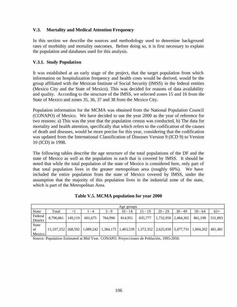
106

V.3. Mortality and Medical Attention Frequency In this section we describe the sources and methodology used to determine background rates of morbidity and mortality outcomes. Before doing so, it is first necessary to explain the population and databases used for this analysis. V.3.1. Study Population It was established at an early stage of the project, that the target population from which information on hospitalization frequency and health costs would be derived, would be the group affiliated with the Mexican Institute of Social Security (IMSS) in the federal entities (Mexico City and the State of Mexico). This was decided for reasons of data availability and quality. According to the structure of the IMSS, we selected zones 15 and 16 from the State of Mexico and zones 35, 36, 37 and 38 from the Mexico City. Population information for the MCMA was obtained from the National Population Council (CONAPO) of Mexico. We have decided to use the year 2000 as the year of reference for two reasons: a) This was the year that the population census was conducted, b) The data for mortality and health attention, specifically that which refers to the codification of the causes of death and diseases, would be more precise for this year, considering that the codification was updated from the International Classification of Diseases Version 9 (ICD 9) to Version 10 (ICD) in 1998. The following tables describe the age structure of the total populations of the DF and the state of Mexico as well as the population in each that is covered by IMSS. It should be noted that while the total population of the state of Mexico is considered here, only part of that total population lives in the greater metropolitan area (roughly 60%). We have included the entire population from the state of Mexico covered by IMSS, under the assumption that the majority of this population lives in the industrial zone of the state, which is part of the Metropolitan Area.

Table V.5. MCMA population for year 2000

Age groups

State Total <1 1 - 4 5 - 9 10 - 14 15 - 19 20 - 29 30 - 49 50 - 64 65+ Federal District

8,796,861 149,119 601,675 784,996 814,951 835,777 1,732,950 2,484,302 861,198 531,893

State of Mexico

13,107,252 268,592 1,089,242 1,384,175 1,403,539 1,372,352 2,625,938 3,477,731 1,004,202 481,481

Source: Population Estimated at Mid Year. CONAPO. Proyecciones de Población, 1995-2050.

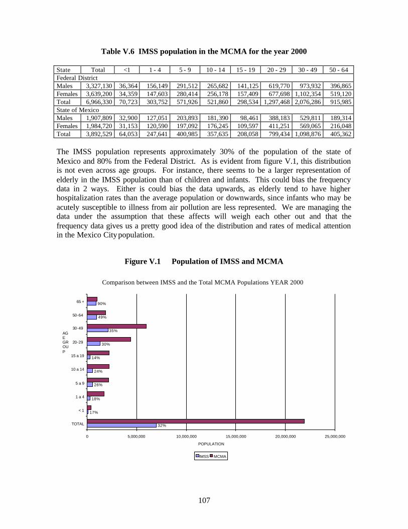
107

Table V.6 IMSS population in the MCMA for the year 2000

State Total <1 1 - 4 5 - 9 10 - 14 15 - 19 20 - 29 30 - 49 50 - 64 Federal District Males 3,327,130 36,364 156,149 291,512 265,682 141,125 619,770 973,932 396,865 Females 3,639,200 34,359 147,603 280,414 256,178 157,409 677,698 1,102,354 519,120 Total 6,966,330 70,723 303,752 571,926 521,860 298,534 1,297,468 2,076,286 915,985 State of Mexico Males 1,907,809 32,900 127,051 203,893 181,390 98,461 388,183 529,811 189,314 Females 1,984,720 31,153 120,590 197,092 176,245 109,597 411,251 569,065 216,048 Total 3,892,529 64,053 247,641 400,985 357,635 208,058 799,434 1,098,876 405,362

The IMSS population represents approximately 30% of the population of the state of Mexico and 80% from the Federal District. As is evident from figure V.1, this distribution is not even across age groups. For instance, there seems to be a larger representation of elderly in the IMSS population than of children and infants. This could bias the frequency data in 2 ways. Either is could bias the data upwards, as elderly tend to have higher hospitalization rates than the average population or downwards, since infants who may be acutely susceptible to illness from air pollution are less represented. We are managing the data under the assumption that these affects will weigh each other out and that the frequency data gives us a pretty good idea of the distribution and rates of medical attention in the Mexico City population.

Figure V.1 Population of IMSS and MCMA

Comparison between IMSS and the Total MCMA Populations YEAR 2000

90%

49%

35%

30%

14%

24%

26%

18%

17%

32% 0 5,000,000 10,000,000 15,000,000 20,000,000 25,000,000

TOTAL

< 1

1 a 4

5 a 9

10 a 14

15 a 19

20-29

30-49

50-64

65 +

AGE GROUP

POPULATION IMSS MCMA

108

While the IMSS by no means represents the entire Mexico City population, we feel that it is sufficient for our calculations. In our final workshop it was suggested that we conduct the analysis for all sectors of the populations (public, private and non-covered). We have considered this option, however given the fact that the information gathered from the IMSS database accounts for less than 10% of the total impact when calculating the monetary value of the health impacts. Therefore, while not perfect, we find it adequate enough for its uses.

V.3.2. Mortality The information on mortality in the year 2000 was obtained from the Mortality Databases published by the National Institute of Statistics, Geography and Informatics and the Ministry of Health of Mexico (INEGI/SSA) in the publication Estadísticas de Mortalidad Año 2000 - 2001. This information was obtained for mortality due to all causes as well as for specific diseases such as:

ICD- 10° Cause CARDIOVASCULAR

I 21 Acute Myocardial Infarction (AMI) I 50 Congestive Heart Failure (CHF)

RESPIRATORY C 33 – C34 Tumor in trachea, bronchioles and lung J 12 – J 18 Pneumonia

J20 Acute bronchitis J 40 – J 44 Bronchitis, Emphysema, (CPOD)

J 45 Asthma Considering the suggestions of the Department of Quality of Information and Evaluation of the Performance of the SSA, a first approximation was done on the behavior of mortality in the year 2000 which involved consulting the previously mentioned databases for the years 2000 and 2001. The former was consulted to identify the deaths that occurred in Mexico in the year 2000, and to thereby eliminate the deaths reported in the year 2000 that actually occurred in other years. The 2001 database was used to include those deaths that occurred in 2000 but that were not reported until 2001. Finally, prorating we estimated the undeclared deaths by sex and age. The sub-registry of deaths greater than 30 years of age was corrected using the methodology proposed by Brass (1975). Figures V.2 and V.3 show the assumptions of required alignment pertaining to the consideration of adults for these ages, by representing the pairs graphically (ny / ny+ ; dy+ / ny+). Using the “least squares” method, we obtained the parameters α and β , the first being an indicator of the implicit rate of growth in this population group and the second being a correction factor of the sub-registry – for men and women.

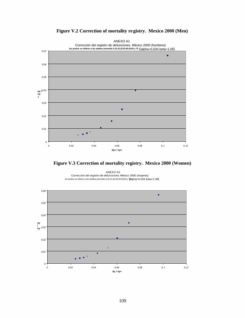
109

Figure V.2 Correction of mortality registry. Mexico 2000 (Men)

ANEXO A1 Corrección del registro de defunciones. México 2000 (hombres)

los puntos se refieren a las edades promedio 5,10,15,20,30,40,50,60 y 70 [alpha=0.034 beta=1.05]

0

0.01

0.02

0.03

0.04

0.05

0.06

0.07

0 0.02 0.04 0.06 0.08 0.1 0.12 dy+ / ny+

ny / ny+

Figure V.3 Correction of mortality registry. Mexico 2000 (Women)

ANEXO A2 Corrección del registro de defunciones. México 2000 (mujeres)

los puntos se refieren a las edades promedio 5,10,15,20,30,40,50,60 y 70 [alpha=0.034 beta=1.09]

0

0.01

0.02

0.03

0.04

0.05

0.06

0 0.02 0.04 0.06 0.08 0.1 0.12 dy / ny+

ny / ny+

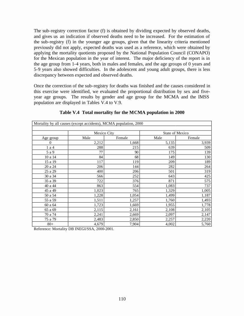
110

The sub-registry correction factor (f) is obtained by dividing expected by observed deaths, and gives us an indication if observed deaths need to be increased. For the estimation of the sub-registry (f) in the younger age groups, given that the linearity criteria mentioned previously did not apply, expected deaths was used as a reference, which were obtained by applying the mortality quotients proposed by the National Population Council (CONAPO) for the Mexican population in the year of interest. The major deficiency of the report is in the age group from 1-4 years, both in males and females, and the age groups of 0 years and 5-9 years also showed difficulties. In the adolescent and young adult groups, there is less discrepancy between expected and observed deaths. Once the correction of the sub-registry for deaths was finished and the causes considered in this exercise were identified, we evaluated the proportional distribution by sex and five-year age groups. The results by gender and age group for the MCMA and the IMSS population are displayed in Tables V.4 to V.9.

Table V.4 Total mortality for the MCMA population in 2000 Mortality by all causes (except accidents), MCMA population, 2000 Mexico City State of Mexico

Age group Male Female Male Female 0 2,212 1,668 5,135 3,939

1 a 4 288 215 639 509 5 a 9 77 90 175 139

10 a 14 84 68 149 130 15 a 19 117 119 209 189 20 a 24 206 144 282 264 25 a 29 400 206 501 319 30 a 34 566 252 643 425 35 a 39 722 376 871 575 40 a 44 863 554 1,083 737 45 a 49 1,023 765 1,329 1,005 50 a 54 1,228 1,054 1,499 1,187 55 a 59 1,511 1,257 1,760 1,493 60 a 64 1,723 1,669 1,955 1,778 65 a 69 2,115 2,161 2,108 2,105 70 a 74 2,241 2,669 2,097 2,147 75 a 79 2,483 2,850 2,257 2,220

80+ 4,679 7,904 4,002 5,760 Reference: Mortality DB INEGI/SSA, 2000-2001.

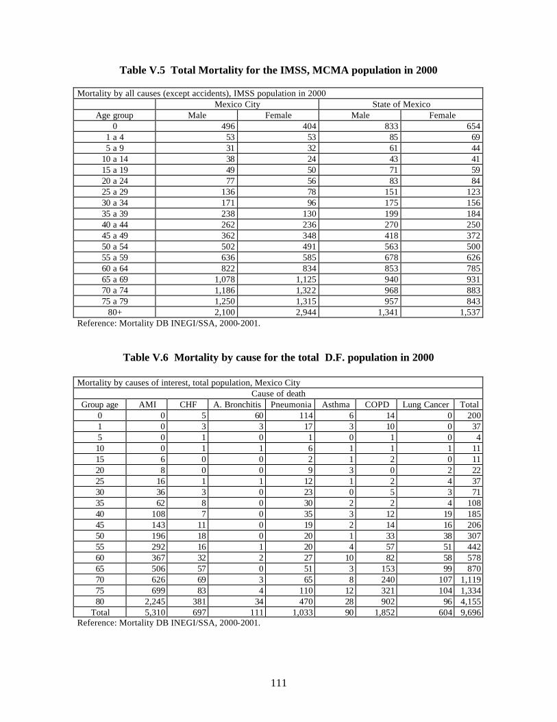
111

Table V.5 Total Mortality for the IMSS, MCMA population in 2000

Mortality by all causes (except accidents), IMSS population in 2000 Mexico City State of Mexico

Age group Male Female Male Female 0 496 404 833 654

1 a 4 53 53 85 69 5 a 9 31 32 61 44

10 a 14 38 24 43 41 15 a 19 49 50 71 59 20 a 24 77 56 83 84 25 a 29 136 78 151 123 30 a 34 171 96 175 156 35 a 39 238 130 199 184 40 a 44 262 236 270 250 45 a 49 362 348 418 372 50 a 54 502 491 563 500 55 a 59 636 585 678 626 60 a 64 822 834 853 785 65 a 69 1,078 1,125 940 931 70 a 74 1,186 1,322 968 883 75 a 79 1,250 1,315 957 843

80+ 2,100 2,944 1,341 1,537 Reference: Mortality DB INEGI/SSA, 2000-2001.

Table V.6 Mortality by cause for the total D.F. population in 2000 Mortality by causes of interest, total population, Mexico City

Cause of death Group age AMI CHF A. Bronchitis Pneumonia Asthma COPD Lung Cancer Total

0 0 5 60 114 6 14 0 200 1 0 3 3 17 3 10 0 37 5 0 1 0 1 0 1 0 4 10 0 1 1 6 1 1 1 11 15 6 0 0 2 1 2 0 11 20 8 0 0 9 3 0 2 22 25 16 1 1 12 1 2 4 37 30 36 3 0 23 0 5 3 71 35 62 8 0 30 2 2 4 108 40 108 7 0 35 3 12 19 185 45 143 11 0 19 2 14 16 206 50 196 18 0 20 1 33 38 307 55 292 16 1 20 4 57 51 442 60 367 32 2 27 10 82 58 578 65 506 57 0 51 3 153 99 870 70 626 69 3 65 8 240 107 1,119 75 699 83 4 110 12 321 104 1,334 80 2,245 381 34 470 28 902 96 4,155

Total 5,310 697 111 1,033 90 1,852 604 9,696 Reference: Mortality DB INEGI/SSA, 2000-2001.

112

Table V.7 Mortality by cause for the total State of Mexico population in 2000

Mortality by causes of interest, total population, State of Mexico, 2000 Cause of death

Group age AMI CHF A. Bronchitis Pneumonia Asthma COPD Lung Cancer Total 0 0 13 261 355 12 27 0 668 1 0 8 24 52 10 5 0 99 5 0 5 7 2 4 0 0 18 10 0 3 1 9 2 2 0 18 15 1 4 2 14 0 4 2 27 20 7 7 3 17 5 1 0 40 25 15 4 0 19 5 7 0 50 30 28 5 0 24 9 5 4 75 35 62 8 3 21 2 13 11 119 40 97 18 2 29 6 20 15 188 45 156 21 3 25 9 32 26 272 50 180 24 3 28 8 39 41 322 55 240 34 5 29 9 76 52 445 60 344 48 4 49 9 118 55 628 65 407 69 1 38 14 220 63 812 70 422 79 8 75 26 294 62 965 75 458 104 12 79 24 377 69 1,123 80 1,311 410 48 321 68 1,011 76 3,246

Total 3,729 862 388 1,187 220 2,252 476 9,115 Reference: Mortality DB INEGI/SSA, 2000-2001.

Table V.8 Mortality by cause for the IMSS population in the D.F. in 2000 Mortality by causes of interest, total population, IMSS, Mexico City, 2000

Cause of death Group age AMI CHF A. Bronchitis Pneumonia Asthma COPD Lung Cancer Total

0 0 0 5 17 0 1 0 23 1 0 2 0 1 0 0 0 3 5 0 0 0 0 0 0 2 2 10 0 0 0 2 1 0 0 3 15 2 0 0 0 0 2 1 5 20 3 0 0 4 2 0 0 9 25 4 1 0 4 0 0 3 13 30 6 0 0 11 0 0 1 18 35 16 2 0 12 0 1 2 33 40 40 3 0 3 0 3 6 56 45 56 4 0 8 1 5 5 79 50 72 6 0 4 0 16 22 121 55 138 7 0 10 0 27 29 212 60 180 15 1 11 4 44 30 285 65 254 24 0 23 2 75 46 424 70 310 27 1 23 3 146 62 572 75 342 42 2 46 6 170 48 657 80 480 75 3 104 2 288 32 982

Total 1,903 210 12 284 21 778 291 3,500 Reference: Mortality DB INEGI/SSA, 2000-2001.

113

Table V.9 Mortality by cause for the IMSS population in the State of Mexico in 2000 Mortality by causes of interest, total population, IMSS, State of Mexico, 2000

Cause of death Group age AMI CHF A. Bronchitis Pneumonia Asthma COPD Lung Cancer Total

0 0 2 22 50 0 4 0 78 1 0 2 2 2 1 1 0 8 5 0 0 2 0 0 0 0 2 10 0 1 0 0 0 1 0 2 15 0 1 0 3 0 1 1 6 20 3 3 0 4 1 1 0 13 25 4 2 0 2 1 0 0 9 30 7 1 0 7 4 1 0 21 35 19 2 0 3 0 2 5 31 40 34 2 0 5 0 8 8 58 45 53 8 0 1 1 13 8 85 50 71 8 2 7 2 20 14 125 55 94 11 1 14 3 41 31 194 60 149 20 0 14 4 52 24 264 65 177 24 0 16 2 100 27 347 70 185 23 1 21 6 135 26 398 75 192 21 2 23 4 151 33 427 80 377 75 8 74 13 349 28 924

Total 1,365 208 40 249 43 881 207 2,994 Reference: Mortality DB INEGI/SSA, 2000-2001.

To include this information in our model, we divided the mortality counts for the entire MCMA (for all cause, cardio-respiratory and lung cancer) by the MCMA population to provide us with the mortality rate. Data on the IMSS population is used in the YPLL analysis described later. Therefore for the mortality analysis we are using city wide rates, and not just the IMSS population. V.3.3. Medical Attention To calculate the frequency of utilization of medical attention for the major diseases associated with environmental air contaminants, we selected a medical attention units databases from the zones of the IMSS that correspond to the MCMA and obtained the frequency of hospitalization admissions, emergency room visits and length-of-stay.This information was collected for each of the federal entities and was grouped into the two categories of pathologies of the study: cardiovascular diseases and respiratory diseases. This data was corrected by a factor of 25%, to account for the observed underutilization by people health care coverage. This underutilization is due to the fact that people receive IMSS coverage from work, but either choose to use private health care or other family providers. Tables V.10 - V.12 describe the results of this analysis.

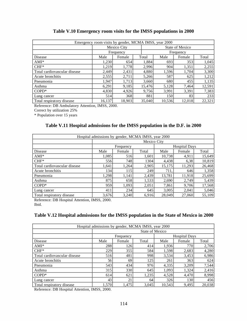
114

Table V.10 Emergency room visits for the IMSS populations in 2000

Emergency room visits by gender, MCMA IMSS, year 2000 Mexico City State of Mexico Frequency Frequency

Disease Male Female Total Male Female Total AMI* 1,230 654 1,884 693 353 1,045 CHF* 1,219 1,778 2,996 904 1,351 2,255 Total cardiovascular disease 2,449 2,431 4,880 1,596 1,704 3,300 Acute bronchitis 2,555 2,711 5,266 587 625 1,212 Pneumonia 1,947 1,713 3,660 680 455 1,135 Asthma 6,291 9,185 15,476 5,128 7,464 12,591 COPD* 4,830 4,926 9,756 3,991 3,391 7,383 Lung cancer 514 368 881 150 83 233 Total respiratory disease 16,137 18,903 35,040 10,536 12,018 22,321 Reference: DB Ambulatory Attention, IMSS, 2000. Correct by utilization 25% * Population over 15 years

Table V.11 Hospital admissions for the IMSS population in the D.F. in 2000

Hospital admissions by gender, MCMA IMSS, year 2000

Mexico City Frequency Hospital Days

Disease Male Female Total Male Female Total AMI* 1,085 516 1,601 10,738 4,911 15,649 CHF* 556 748 1304 4,438 6,38 10,819 Total cardiovascular disease 1,641 1,264 2,905 15,175 11,293 26,468 Acute bronchitis 134 115 249 711, 646 1,358 Pneumonia 1,298 1,141 2,439 13,781 11,918 25,699 Asthma 875 658 1,533 2,690 2,749 5,439 COPD* 959 1,093 2,051 7,861 9,706 17,568 Lung cancer 411 234 645 3,005 2,041 5,046 Total respiratory disease 3,676 3,240 6,916 28,049 27,060 55,109 Reference: DB Hospital Attention, IMSS, 2000. Ibid. Table V.12 Hospital admissions for the IMSS population in the State of Mexico in 2000

Hospital admissions by gender, MCMA IMSS, year 2000 State of Mexico Frequency Hospital Days

Disease Male Female Total Male Female Total AMI* 288 126 414 1,936 770 2,706 CHF* 229 355 584 1,598 2,683 4,280 Total cardiovascular disease 516 481 998 3,534 3,453 6,986 Acute bronchitis 56 69 125 261 363 624 Pneumonia 543 434 976 4,335 3,209 7,544 Asthma 315 330 645 1,093 1,324 2,416 COPD* 614 621 1,235 4,528 4,470 8,998 Lung cancer 43 21 64 326 130 456 Total respiratory disease 1,570 1,475 3,045 10,543 9,495 20,038 Reference: DB Hospital Attention, IMSS, 2000.

115

The admittances to emergency and hospitalization services for cardiovascular diseases are primarily for Congestive Heart Failure (CHF), occurring primarily in women, whereas utilization due to AMI occurs primarily among men. It is important to clarify that the differences observed in the two federal entities is due to the fact that the majority of specialized medical center are geographically located in the Federal District, and they possibly receive patients referred from the State of Mexico and other areas. With regard to respiratory diseases, we observe that the utilization of emergency services is primarily for asthma and then for chronic bronchitis. As for hospitalizations, pneumonia and chronic bronchitis are the causes with the highest frequency. To include this frequency data in our model, we divide the frequency of ERVs and hospitalizations by the IMSS study population as described earlier. This allows us to understand the rate of medical attention , which is used in the dose response calculation. These rates can be multiplied by the total population of Mexico city to determine the total frequency of medical attention and mortality, assuming that the rate for IMSS is generalizable to the entire MCMA population. V.4. Potential Years of Life Lost There has been widespread debate on the issue of the quantity of life lost per premature mortality. This concern arises from the need to value health impacts, and the question about whether we should be putting the same value on saving 1 year of life as saving 10 years of life or more. While the evidence is inconclusive if individuals place more value on saving lives with more life expectancy than less, we choose to quantify the potential life years saved per case of avoided premature mortality here, allowing the user to decide later if it is more appropriate to value life years saved or cases of premature mortality avoided. In order to calculate potential life years saved due to avoided premature mortality, we must first construct life tables using the corrected mortality data from section V.3.2. V.4.1. Life Table Analysis Before reviewing the methodology for constructing life tables, here we define certain variables:

Table V.13. Variable definitions for Life Tables Calculations

x Age interval mx Mortality rates qx Probability of death lx # of Survivors at the beginning of period X dx Decrement Function - # people dying during period x Lx Stationary Population or Person-Years lived at age x Tx Person-Years lived at and over age x ex Life Expectancy at age x ax Fraction of the last year (or period) lived w last age considered (here 85+)

116

To construct life tables, it is first necessary to divide mortality registries in age groups: 0 , 1-4, 5-9,..., 80+. To achieve this, we use the corrected death registry described in Section V.3.2, grouped by 5 year age groups. From this information we can calculate mortality rates (mx), and mortality quotient (qx) to achieve the calculation of life expectancy for the different age groups (ex). The definition of specific mortality rates (mx) in a defined population is expressed as: mx = Dx / Px, where Dx is the number of corrected deaths in an age group and Px is the population of that age group. After calculating the mortality rates (nmx) for each 5 year age group by sex and IMSS delegation, we calculate the corresponding mortality quotient (nqx). To calculate the quotients from the mortality rates, we use the methodology proposed by Chiang (1993), that uses the value ax which is the fraction of the five year period that on average the deceaced lived. For the age group 0 (less than 1 year old) ax, is taken as the desegregation factor k calculated for the deceased less than 1 year old, from the detailed information of age at the time of death in hours, days, weeks and months. For the rest of the age groups, ax is calculated as the weighted mean of the age of death divided by the size of the age interval considered. The general equation to obtain (qx) is: nmx qx = 1 + (1- ax) nmx Once the mortality quotients have been determined from actual data, a fictitious cohort is applied. The series lx is the number of survivors at the beginning of each age group. We apply q0 to a population of 100,000 (l0 = 100,000), and successively reduce the number of survivors in each age group by applying the probability of mortality (qx), until the entire population is extinguished for deaths (dx) after the group 80+. Given that mortality is a demographic phenomenon with a intensity of 1, in other words that everyone is exposed to this risk, for survivors in the last age group (l80) we apply a mortality quotient (q80+) of 1. Where the number of deceased in each age group is found by: d(x,x+n ) = l x – nq,x

With the series of survivors (lx) at each age completed, we can calculate the series of person-years lived by the generation until age x (Lx). The value Lx is interpreted as the total years lived by the survivors until year x+1, in addition to a contribution of ax years for those who died between x and x+1. Continuing with the methodology of Chiang, Lx is obtained by the following equation: nLx = n( l x – dx,x+n) + ax dx, x+n

For the analysis of the group 80+, Lx is calculated by:

117

L 8 0+ = 3.725 * l80+ + 0.000062 5 * (l80+)2

Or if the group were 85+, the calculation would be: L85+ = l85+ * log(l85+)

The log function expresses the notion of the progressive deterioration of human beings, clearly manifested in age groups where the mortality quotient are increasing. This is particularly valid for age groups where the predominant cause of mortality is due to old age. We also calculate the probability of surviving age x and to arrive at the age x+n. The is calculated in the function Sx from Lx, by:

x

nxxx

L

LS += ,

We also calculated the accumulated years lived (Tx ), which is the total number of years left to live by survivors lx from the xth year, until the complete extinction of the fictitious generation. The value T0 is the total number of life years for the generation from birth until death of the last survivor and is calculated by: Tx = Lx + Lx+1 +… + Lù-1 The last calculation of the life table is that of life expectancy (ex), that represents the median number of life years left for survivors at age X. The life expectancy at birth (e0), is the most used indicator of the life table and refers to the median number of years a generation of newborns will live. Life expectancy (ex) is calculated as follows ex = Tx / lx

Tables V.14 and V.15 summarize the results for our life table calculations for the Federal District and the State of Mexico respectively.

118

Table V.14. Abridged IMSS Mexico City Life Table for both sexes from 2000 (Zones IMSS 35, 36, 37 y 38)

Age nmx nqx l(x,x+n) d(x,x+n) nL(x, x+n) nS(x, x+n) nT(x, x+n) ex nA(x,

x+n) 0 0.01296112 0.0128165 100000 1282 98884 0.99738635 7888894 78.9 0.13 1 0.00039102 0.00156259 98718 154 394503 0.99910229 7790009 78.9 0.40 5 0.00012777 0.00063866 98564 63 492686 0.99930844 7395506 75.0 0.57 10 0.00015102 0.00075484 98501 74 492346 0.99839991 6902820 70.1 0.57 15 0.00054142 0.00270391 98427 266 491558 0.99742119 6410474 65.1 0.57 20 0.00042856 0.00214058 98161 210 490290 0.99773309 5918917 60.3 0.51 25 0.00046511 0.00232281 97951 228 489179 0.99752649 5428626 55.4 0.50 30 0.00054364 0.00271459 97723 265 487969 0.99689972 4939448 50.5 0.51 35 0.00076213 0.00380416 97458 371 486456 0.99502012 4451479 45.7 0.55 40 0.00119505 0.00595798 97087 578 484033 0.99234512 3965023 40.8 0.52 45 0.00191936 0.00955276 96509 922 480328 0.98794304 3480990 36.1 0.52 50 0.00306231 0.01520277 95587 1453 474537 0.98189042 3000662 31.4 0.53

55 0.00433285 0.02144681 94133 2019 465943 0.9748184 2526125 26.8 0.53 60 0.00602409 0.02970431 92115 2736 454210 0.96437369 2060182 22.4 0.53 65 0.00839685 0.04115153 89378 3678 438028 0.95008358 1605972 18.0 0.52 70 0.01187124 0.05764708 85700 4940 416163 0.93278537 1167944 13.6 0.50 75 0.0158282 0.07608184 80760 6144 388191 0.93662379 751780 9.3 0.49

80 + 0.01957057 1 74616 74616 363589 363589 4.9 0.12 Table V.15 Abridged IMSS State of Mexico Life Table for both sexes from 2000

(Zones IMSS 15 y 16)

Age nmx nqx l(x,x+n) d(x,x+n) nL(x, x+n) nS(x, x+n) nT(x, x+n) ex nA(x,

x+n) 0 0.02350367 0.02303331 100000 2303 97999 3.97942314 7269330 72.7 0.13 1 0.00084216 0.00336168 97697 328 389979 1.24733762 7171332 73.4 0.39 5 0.00033934 0.00169529 97368 165 486435 0.99827794 6781353 69.6 0.51 10 0.00037086 0.0018527 97203 180 485597 0.9962192 6294918 64.8 0.54 15 0.00119943 0.00598043 97023 580 483762 0.99462836 5809320 59.9 0.53 20 0.0009829 0.0049038 96442 473 481163 0.99458972 5325559 55.2 0.56 25 0.00107853 0.00537813 95969 516 478560 0.99393787 4844396 50.5 0.50 30 0.00138097 0.00688158 95454 657 475659 0.99250186 4365836 45.7 0.51 35 0.00174134 0.00867196 94797 822 472092 0.98920057 3890177 41.0 0.54 40 0.00263988 0.01311851 93975 1233 466994 0.98217086 3418085 36.4 0.53 45 0.0045406 0.02245614 92742 2083 458668 0.97220052 2951091 31.8 0.52 50 0.00716824 0.03525767 90659 3196 445917 0.95612304 2492424 27.5 0.54 55 0.01049464 0.05115774 87463 4474 426351 0.93821178 2046507 23.4 0.51 60 0.01519356 0.07323356 82989 6078 400008 0.91449626 1620155 19.5 0.51 65 0.02111308 0.10041848 76911 7723 365806 0.89335649 1220147 15.9 0.51 70 0.02335173 0.11029742 69188 7631 326795 0.86528861 854342 12.3 0.50 75 0.03410986 0.15669044 61556 9645 282772 0.86562583 527547 8.6 0.48

80 + 0.0351982 1 51911 51911 244775 244775 4.7 0.11

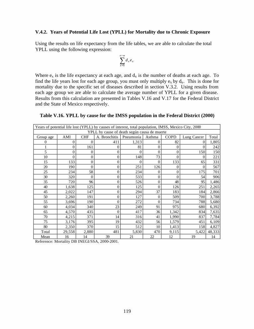
119

V.4.2. Years of Potential Life Lost (YPLL) for Mortality due to Chronic Exposure Using the results on life expectancy from the life tables, we are able to calculate the total YPLL using the following expression:

∑=

=

wx

xxx ed

0

Where ex is the life expectancy at each age, and dx is the number of deaths at each age. To find the life years lost for each age group, you must only multiply ex by dx. This is done for mortality due to the specific set of diseases described in section V.3.2. Using results from each age group we are able to calculate the average number of YPLL for a given disease. Results from this calculation are presented in Tables V.16 and V.17 for the Federal District and the State of Mexico respectively.

Table V.16. YPLL by cause for the IMSS population in the Federal District (2000)

Years of potential life lost (YPLL) by causes of interest, total population, IMSS, Mexico City, 2000 YPLL by cause of death según causa de muerte

Group age AMI CHF A. Bronchitis Pneumonia Asthma COPD Lung Cancer Total 0 0 0 411 1,313 0 82 0 1,805 1 0 161 0 81 0 0 0 242 5 0 0 0 0 0 0 150 150 10 0 0 0 148 73 0 0 221 15 133 0 0 0 0 133 65 331 20 190 0 0 251 126 0 0 567 25 234 58 0 234 0 0 175 701 30 320 0 0 533 0 0 54 906 35 720 96 0 526 0 48 95 1,486 40 1,638 125 0 125 0 126 251 2,265 45 2,022 147 0 294 37 183 184 2,866 50 2,260 191 0 127 0 509 700 3,788 55 3,696 190 0 272 0 734 788 5,680 60 4,034 340 23 249 91 975 680 6,392 65 4,570 435 0 417 36 1,342 834 7,635 70 4,215 371 14 316 41 1,990 837 7,784 75 3,176 395 19 432 56 1,579 451 6,109 80 2,350 370 15 512 10 1,413 158 4,827

Total 29,558 2,880 481 5,830 470 9,115 5,422 48,333 Mean 16 14 39 21 22 12 19 14

Reference: Mortality DB INEGI/SSA, 2000-2001.

120

Table V.16. YPLL by cause for the IMSS population in the State of Mexico (2000)

Years of potential life lost (YPLL) by causes of interest, total population, IMSS, State of Mexico, 2000 YPLL by cause of death según causa de muerte

Group age AMI CHF A. Bronchitis Pneumonia Asthma COPD Lung Cancer Total 0 0 155 1,554 3,550 0 313 0 5,572 1 0 153 151 153 76 76 0 609 5 0 0 165 0 0 0 0 165 10 0 68 0 0 0 67 0 135 15 0 63 0 189 0 63 63 315 20 172 171 0 229 57 57 0 686 25 208 104 0 104 52 0 0 468 30 336 48 0 333 189 48 0 955 35 745 84 0 131 0 87 218 1,047 40 1,206 73 0 189 0 300 298 1,767 45 1,647 256 0 32 32 417 259 2,385 50 1,921 219 55 192 55 548 384 2,989 55 2,153 258 23 328 70 936 702 3,768 60 2,879 392 0 274 78 999 470 4,622 65 2,780 381 0 254 32 1,572 429 5,019 70 2,254 283 12 259 74 1,650 320 4,532 75 1,634 181 17 198 34 1,281 283 3,345 80 1,773 352 38 347 62 1,638 133 4,210

Total 19,705 3,242 2,016 6,760 812 10,053 3,558 42,588 Mean 14 16 50 27 19 11 17 14

Reference: Mortality DB INEGI/SSA, 2000-2001.

We include this information in our analysis by assuming that mortality due to chronic exposure is due to one of the above causes. Without any prior knowledge of the distribution of these deaths, we include a range of life years lost for chronic mortality using the above numbers with a triangular distribution of 10, 15 and 23. V.4.3. Years of Potential Life Lost (YPLL) for Mortality due to Acute Exposure For the case of mortality due to acute exposure, there is little known about the actual number of years that mortality due to air pollution advances death. There is some evidence that only very sick individuals are effected by air pollution episodes, thereby advancing death by only a couple of months (Schwartz, 2000). On the other hand, evidence from the recent cohort studies appears to indicate that air pollution can cause mortality to occur even more prematurely. To determine the number of years lost to premature mortality from short term air pollution fluctuations, the methodology used by Carrothers (2000) was adopted for this analysis. In his study an upper bound was chosen that accounted for the possibility that some persons of average life-expectancy may be affected by air pollution episodes and estimated that four-fifths of those dying from short term exposures to air pollution have life-expectancies equivalent to a patient coronary heart disease, using Kuntz's CHD cohort, and one-fifth have average life expectancy; thus yielding a value of 6.5 years. For a middle estimate, he assumed a life expectancy of people suffering from coronary heart failure, estimated at 2.5

121

years. Finally, since it is possible that people dying from air pollution only had a few months of life left, a plausible lower-bound was estimated at 0.5 years. V.5. Discounting When evaluating the avoided mortality impacts due to reductions in air pollution, itis important to take into account the value of time. In the case of mortality due to chronic exposure to air pollution, it is commonly assumed that there is a latency of the effect, or that mortality will occur a number of years after the exposure. This is not the case, however, with mortality due to acute exposure, as it is assumed that these deaths are occurring within days of exposure. The timing of health benefits is important because people exhibit a non-zero real rate of time preference for both money and health, and would therefore value reduced risk today more than risk reduced a year from now. There are a number of ethical reasons why people would prefer to reduce their risks today rather than in the future beyond the time value of money, including such considerations as uncertainty about the future, ideas of techno logical progress and attitudes towards living in the present (Cropper et al., 1994). Furthermore, when deciding about controls that will have an effect in the future, we typically discount costs incurred in the future to present values. The same must be done with health benefits in order to compare the costs to the benefits, otherwise it will always look more advantageous to save lives in the future rather then today. We must therefore account for this latency in effect by discounting the health effects occurring in the future relative to today. It is important therefore that we account for the fact that the avoided mortalities occur a number of years after exposure. To account for the value of time for future benefits, the number of lives saved in the future were discounted to the present using the following equation:

lrddl −+×= )1( Where dl is the number of discounted lives saved, d is the number of lives saved, l is latency of the mortality effect and r is the social discount rate. Latency of health effects range from 10 to 20 years for risks from smoking and up to 40 years for cancer outcomes. Standard cost effectiveness analysis uses a range of 5 to 15 years, but even longer periods could be plausible, based on the general pattern of chronic diseases such as COPD and heart disease (Carrothers, 2000). For the purposes of this analysis, we adopted the assumptions of Carrothers (2000), where he modeled the average latency period for mortality from chronic exposure as ten years with an upper- and lower-bound of twenty and five years, respectively. V.5. Results Here we present the results for the reductions in health impact for the 5 measures. We are able to distinguish not only the magnitude of the health impacts, but from which pollutant the impacts are derived. In general we find that the Taxi measure has the greatest health

122

impacts and that most of these benefits result from ozone reductions and secondary PM10. The Metro expansion measure results in significant health benefits, also due mostly to ozone and secondary PM, most of which appears in the time horizon 2003-2020 as most of the construction occurs after the year 2010. The measure of Hybrid buses, which reduces mostly primary particulates results in significant mortality and bronchitis benefits. The measure for reducing LPG leaks results in significant ozone reductions and therefore impacts acute mortality and respiratory morbidity. Finally, since the measure of Co-generation reduces electricity generation outside the valley and brings fuel consumption into the city, it does not provide substantial health benefits. The following 10 tables summarize the results of the health impacts analysis and describe the number of cases of morbidity and mortality effects that the controls could prevent described by the expected value and the range of possibilities in the 95% confidence interval. These results are found using a discount rate of 5%.

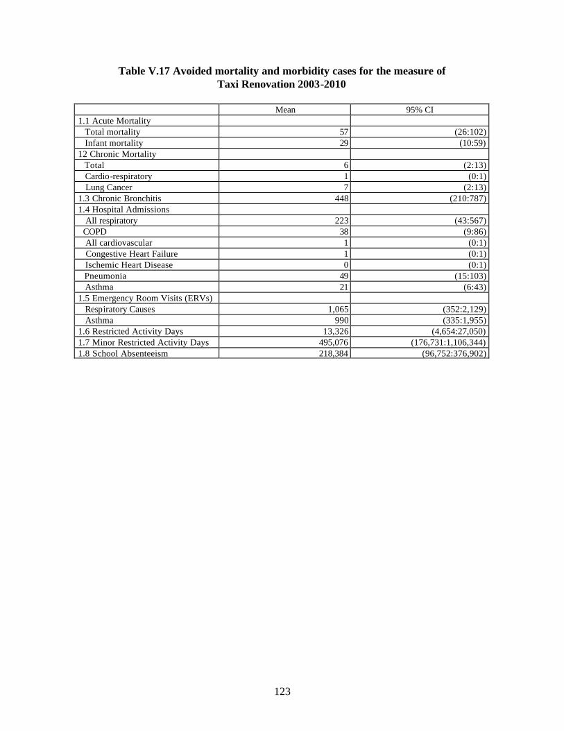
123

Table V.17 Avoided mortality and morbidity cases for the measure of Taxi Renovation 2003-2010

Mean 95% CI

1.1 Acute Mortality Total mortality 57 (26:102) Infant mortality 29 (10:59) 12 Chronic Mortality Total 6 (2:13) Cardio-respiratory 1 (0:1) Lung Cancer 7 (2:13) 1.3 Chronic Bronchitis 448 (210:787) 1.4 Hospital Admissions All respiratory 223 (43:567) COPD 38 (9:86) All cardiovascular 1 (0:1) Congestive Heart Failure 1 (0:1) Ischemic Heart Disease 0 (0:1) Pneumonia 49 (15:103) Asthma 21 (6:43) 1.5 Emergency Room Visits (ERVs) Respiratory Causes 1,065 (352:2,129) Asthma 990 (335:1,955) 1.6 Restricted Activity Days 13,326 (4,654:27,050) 1.7 Minor Restricted Activity Days 495,076 (176,731:1,106,344) 1.8 School Absenteeism 218,384 (96,752:376,902)

124

Table V.18 Avoided mortality and morbidity cases for the measure of

Taxi Renovation 2003-2020

Mean 95% CI 1.1 Acute Mortality Total mortality 36 (16:63) Infant mortality 19 (7:39) 12 Chronic Mortality Total 4 (2:8) Cardio-respiratory 0 (0:1) Lung Cancer 4 (2:9) 1.3 Chronic Bronchitis 295 (147:474) 1.4 Hospital Admissions All respiratory 134 (26:366) COPD 22 (5:49) All cardiovascular 0 (0:1) Congestive Heart Failure 0 (0:1) Ischemic Heart Disease 0 (0:1) Pneumonia 29 (9:59) Asthma 12 (4:27) 1.5 Emergency Room Visits (ERVs) Respiratory Causes 632 (211:1,236) Asthma 583 (203:1,132) 1.6 Restricted Activity Days 8,908 (3,323:17,859) 1.7 Minor Restricted Activity Days 296,928 (113,153:599,831) 1.8 School Absenteeism 132,439 (61,258:227,615)

125

Table V.19 Avoided mortality and morbidity cases for the measure of Metro Expansion 2003-2010

Mean 95% CI

1.1 Acute Mortality Total mortality 2 (1:3) Infant mortality 1 (0:2) 12 Chronic Mortality Total 0 (0:0) Cardio-respiratory 0 (0:0) Lung Cancer 0 (0:0) 1.3 Chronic Bronchitis 16 (9:25) 1.4 Hospital Admissions All respiratory 6 (1:15) COPD 1 (0:2) All cardiovascular 0 (0:0) Congestive Heart Failure 0 (0:0) Ischemic Heart Disease 0 (0:0) Pneumonia 1 (0:3) Asthma 1 (0:1) 1.5 Emergency Room Visits (ERVs) Respiratory Causes 30 (11:59) Asthma 28 (10:54) 1.6 Restricted Activity Days 476 (207:886) 1.7 Minor Restricted Activity Days 14,660 (5,922:30,866) 1.8 School Absenteeism 6,458 (3,150:11,034)

126

Table V.20 Avoided mortality and morbidity cases for the measure of Metro Expansion 2003-2020

Mean 95% CI

1.1 Acute Mortality Total mortality 15 (8:25) Infant mortality 10 (4:18) 12 Chronic Mortality Total 20 (1:4) Cardio-respiratory 0 (0:0) Lung Cancer 2 (1:4) 1.3 Chronic Bronchitis 152 (83:241) 1.4 Hospital Admissions All respiratory 49 (11:125) COPD 8 (2:19) All cardiovascular 0 (0:0) Congestive Heart Failure 0 (0:0) Ischemic Heart Disease 0 (0:0) Pneumonia 10 (3:21) Asthma 5 (2:9) 1.5 Emergency Room Visits (ERVs) Respiratory Causes 232 (86:457) Asthma 215 (77:416) 1.6 Restricted Activity Days 4,584 (1,951:8,459) 1.7 Minor Restricted Activity Days 119,279 (50,667:232,700) 1.8 School Absenteeism 52,346 (26,219:85,139)

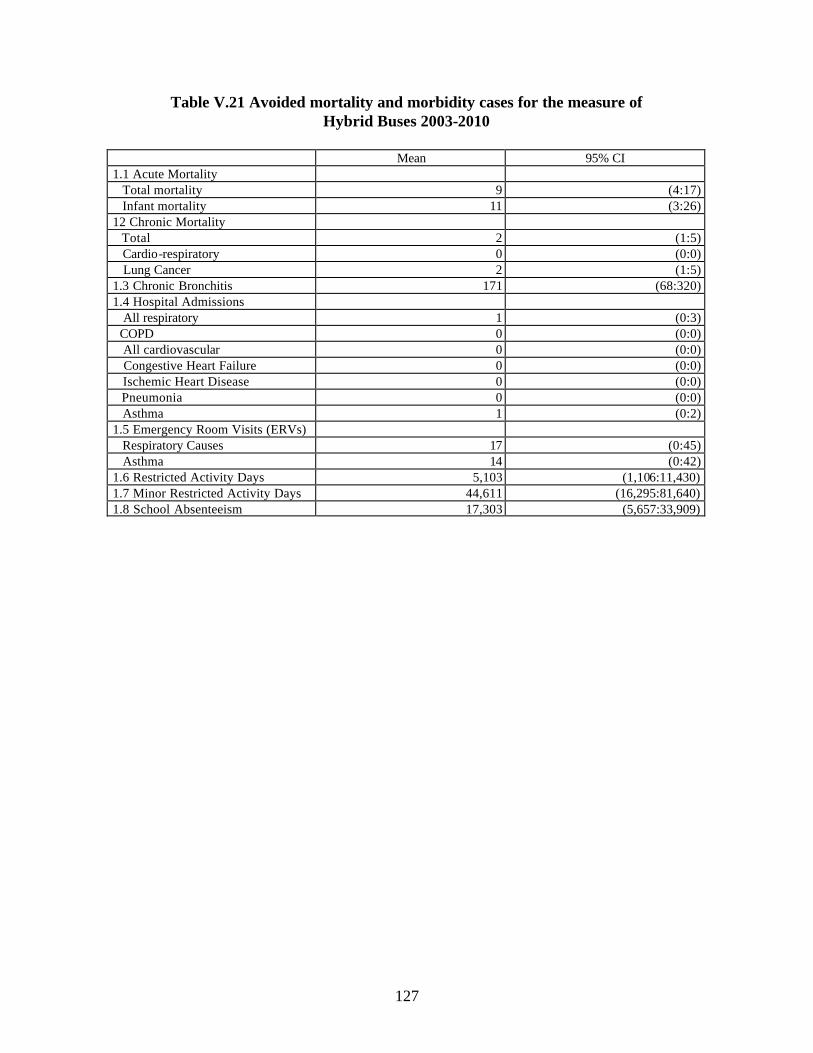
127

Table V.21 Avoided mortality and morbidity cases for the measure of Hybrid Buses 2003-2010

Mean 95% CI

1.1 Acute Mortality Total mortality 9 (4:17) Infant mortality 11 (3:26) 12 Chronic Mortality Total 2 (1:5) Cardio-respiratory 0 (0:0) Lung Cancer 2 (1:5) 1.3 Chronic Bronchitis 171 (68:320) 1.4 Hospital Admissions All respiratory 1 (0:3) COPD 0 (0:0) All cardiovascular 0 (0:0) Congestive Heart Failure 0 (0:0) Ischemic Heart Disease 0 (0:0) Pneumonia 0 (0:0) Asthma 1 (0:2) 1.5 Emergency Room Visits (ERVs) Respiratory Causes 17 (0:45) Asthma 14 (0:42) 1.6 Restricted Activity Days 5,103 (1,106:11,430) 1.7 Minor Restricted Activity Days 44,611 (16,295:81,640) 1.8 School Absenteeism 17,303 (5,657:33,909)

128

Table V.22 Avoided mortality and morbidity cases for the measure of Hybrid Buses 2003-2020

Mean 95% CI

1.1 Acute Mortality Total mortality 10 (4:19) Infant mortality 12 (3:25) 12 Chronic Mortality Total 3 (1:5) Cardio-respiratory 0 (0:0) Lung Cancer 3 (1:6) 1.3 Chronic Bronchitis 184 (75:336) 1.4 Hospital Admissions All respiratory 1 (-1:4) COPD 0 (0:0) All cardiovascular 0 (0:0) Congestive Heart Failure 0 (0:0) Ischemic Heart Disease 0 (0:0) Pneumonia 0 (0:0) Asthma 1 (0:3) 1.5 Emergency Room Visits (ERVs) Respiratory Causes 19 (-4:49) Asthma 15 (-7:43) 1.6 Restricted Activity Days 5,575 (1,182:12,761) 1.7 Minor Restricted Activity Days 48,591 (18,046:88,364) 1.8 School Absenteeism 18,814 (6,527:36,804)

129

Table V.23 Avoided mortality and morbidity cases for the measure of Combined LPG Leakage Reduction 2003-2010

Mean 95% CI

1.1 Acute Mortality Total mortality 11 (4:19) Infant mortality 6 (1:15) 12 Chronic Mortality Total 1 (0:3) Cardio-respiratory 0 (0:0) Lung Cancer 1 (0:3) 1.3 Chronic Bronchitis 89 (26:180) 1.4 Hospital Admissions All respiratory 39 (8:96) COPD 7 (2:15) All cardiovascular 0 (0:0) Congestive Heart Failure 0 (0:0) Ischemic Heart Disease 0 (0:0) Pneumonia 9 (3:18) Asthma 4 (1:7) 1.5 Emergency Room Visits (ERVs) Respiratory Causes 190 (64:388) Asthma 176 (60:344) 1.6 Restricted Activity Days 2,663 (431:7,100) 1.7 Minor Restricted Activity Days 90,682 (27,960:199,169) 1.8 School Absenteeism 39,723 (16,567:69,314)

130

Table V.24 Avoided mortality and morbidity cases for the measure of Combined LPG Leakage Reduction 2003-2020

Mean 95% CI

1.1 Acute Mortality Total mortality 9 (3:16) Infant mortality 5 (1:12) 12 Chronic Mortality Total 1 (0:3) Cardio-respiratory 0 (0:0) Lung Cancer 1 (0:3) 1.3 Chronic Bronchitis 76 (22:155) 1.4 Hospital Admissions All respiratory 33 (7:86) COPD 5 (1:12) All cardiovascular 0 (0:0) Congestive Heart Failure 0 (0:0) Ischemic Heart Disease 0 (0:0) Pneumonia 7 (2:15) Asthma 3 (1:6) 1.5 Emergency Room Visits (ERVs) Respiratory Causes 154 (53:303) Asthma 144 (48:287) 1.6 Restricted Activity Days 2,320 (332:6,312) 1.7 Minor Restricted Activity Days 73,350 (24,530:154,535) 1.8 School Absenteeism 32,756 (3,624:58,811)

131

Table V.25 Avoided mortality and morbidity cases for the measure of Cogeneration 2003-2010

Mean 95% CI

1.1 Acute Mortality Total mortality 1 (0:1) Infant mortality 0 (0:1) 12 Chronic Mortality Total 0 (0:0) Cardio-respiratory 0 (0:0) Lung Cancer 0 (0:0) 1.3 Chronic Bronchitis 4 (1:8) 1.4 Hospital Admissions All respiratory 2 (0:6) COPD 0 (0:1) All cardiovascular 0 (0:0) Congestive Heart Failure 0 (0:0) Ischemic Heart Disease 0 (0:0) Pneumonia 1 (0:1) Asthma 0 (0:0) 1.5 Emergency Room Visits (ERVs) Respiratory Causes 12 (4:24) Asthma 11 (4:21) 1.6 Restricted Activity Days 123 (18:325) 1.7 Minor Restricted Activity Days 5,207 (1,661:11,734) 1.8 School Absenteeism 2,336 (979:4,105)

132

Table V.26 Avoided mortality and morbidity cases for the measure of Cogeneration 2003-2020

Mean 95% CI

1.1 Acute Mortality Total mortality 11 (4:19) Infant mortality 6 (1:15) 12 Chronic Mortality Total 1 (0:3) Cardio-respiratory 0 (0:0) Lung Cancer 1 (0:3) 1.3 Chronic Bronchitis 89 (26:180) 1.4 Hospital Admissions All respiratory 39 (8:96) COPD 7 (2:15) All cardiovascular 0 (0:0) Congestive Heart Failure 0 (0:0) Ischemic Heart Disease 0 (0:0) Pneumonia 9 (3:18) Asthma 4 (1:7) 1.5 Emergency Room Visits (ERVs) Respiratory Causes 190 (64:388) Asthma 176 (60:344) 1.6 Restricted Activity Days 2,663 (431:7,100) 1.7 Minor Restricted Activity Days 90,682 (27,960:199,169) 1.8 School Absenteeism 39,723 (16,567:69,314)

An interesting result from our analysis is that we are able to distinguish the health impacts by the pollutant causing the effect. These results will change depending on the measure and the health outcome of interest. For instance, if a particular measure is specifically targeted at primary PM10 reductions, we can expect that the majority of the health impacts will be from that pollutant. However, the results depend not only on the magnitude of the concentration reduction, but also of the magnitude of the dose response values. With the following graphs, we disaggregate the annualized impacts for 2003-2020 in order to determine, for this set of measures, from where the greatest impact comes. We sum the impacts across the 5 measures and calculate the percentage of cases caused by each pollutant for acute and chronic mortality, cardiovascular and respiratory hospitalizations and emergency room visits and restricted activity. Figure V.4 shows that approximately half of the acute mortality effect for these 5 measures combined is due to reductions in ozone, whereas primary PM accounts for 12% and secondary particulates for the remaining 39%. These results derive from the fact that most of the measures have most significant impacts on ozone concentrations, and we gain the additional benefit from these measures in secondary PM reductions. The effects of primary PM reductions come from the Hybrid Bus measure, whereas the majority of the organic PM effects come from the Taxis and LPG measures. Most of the secondary sulfate and nitrate impact is a result of the Taxi measure as well.

133

Figure V.4 Percentage of mortality due to acute exposure by pollutant, 2003-2020

16%

15%

8%

18%

43%PM10 PrimaryPM10 Secondary OrganicPM10 Secondary SulfatePM10 Secondary NitrateOzone

Figure V.5 shows the results when looking at the effect of mortality due to chronic exposure to pollution. Given that there is only evidence for the effects of particulates, all of the impacts are due to reductions in PM10. We find that 69% of the effect is due to secondary nitrate and organic particulate matter. This is driven primarily by the Taxi and Metro measures. The impact of primary particles is derived from the hybrid bus measure alone. This pattern is repeated with the impacts of cardiovascular hospital admissions as our evidence associates it only with exposure to particulate matter.

134

Figure V.5 Percentage of mortality due to chronic exposure by pollutant, 2003-2020

When conducting the same analysis with respiratory hospital admissions, we find that nearly 90% of the effect results from ozone reductions. In the case for minor restricted activity days, this is reduced to approximately 70%, with the rest distributed nearly equally across secondary sulfates, nitrates and primary particulates. It should be stressed that these results shift between measures. These results may therefo re be biased towards results from the Taxi and Metro measures which primarily reduce ozone, but also have an additional secondary particulate effect and the Hybrid Bus measure which mainly reduces particulates. V.6. References Abbey, D.E., F.F. Petersen, P.K. Mills, and W.L. Beeson (1993) Long-term ambient concentrations of total suspended particulates, ozone, and sulfur dioxide and respiratory symptoms in a non-smoking population. Arch. Environ. Health 48: 33-46 Abbey, D.E., M.D. Lebowithz, P.K. Mills, F.F. Petersen, W.L. Beeson and R.J. Burchette. (1995) Long-term ambient concentrations of particulates and oxidants and development of chronic disease in a cohort of nonsmoking California residents. Inhal. Toxicol. 7: 19-34

28%

27%14%

31%

0%

PM10 Primary

PM10 Secondary Organic

PM10 Secondary Sulfate

PM10 Secondary Nitrate

Ozone

135

Arriaga E (1976) Computers Programs for Demographic Analysis. International Statistical Programs Center. Borja-Aburto VH, M. Castillejos, DR. Gold, S. Bierzwinski, and D. Loomis (1998) Mortality and ambient fine particles in southwest Mexico City, 1993-1995. Environ Health Perspect 106: 849-856. Borja-Aburto VH, D. Loomis, S. Bangdiwala, C. Shy and R. Rascon-Pacheco (1997) Ozone, suspended particulates, and daily mortality in Mexico City. Am J Epidemiol 145: 258-268. Brass W. (1975) Methods for Estimating Fertility and Mortality from Limited and Defective Data. Laboratories for Population Statistics, An Occasional Publication, Chapel Hill, North Carolina. Carrothers, T. (2000) Particulate air pollution policy: Assessing the economic value of further research, PhD Thesis, Harvard School of Public Health. Castillejos M, V. Borja-Aburto, D. Dockery and D. Loomis (2000) Coarse particles and mortality in Mexico City. Inhalation Toxicol 12 (Supp 1): 61-72. Cesar, H., G. Schadler, M. Hojer, P. Cicero-Fernandez, L. Brander, T. Buhl, A. C. Villagomez, K. Dorland, A. C. G. Martinez, H. Hasselknippe, P. M. Oritz, A. V. Montero, A. Salcido, J. Sarmiento, and P. V. Beukering (2002) “Air pollution abatement in Mexico City: an economic valuation,” World Bank Report. Chiang, C. (1993) The Life Table and its Construction. En Rumsey, GW (Ed): Readings in Population Research Methodology. Volume 2 Mortality Research. Published for United Nations Population Fund by Social Development Center Chicago, Illinois, USA, 1993. pp. 7-84 – 7-96. CONAPO. http://www.conapo.gob.mx Cropper, M., S. Ayded, and P. Portney (1994) “Preferences for life saving programs: how the public discounts time and age,” Journal of Risk and Uncertainty, 8: 243-265. Damokosh AI, M. Castillejos, S. Bierzwinski and D. Gold (2000) Acute effects of air pollution on emergency room visits for respiratory disease in children living in southwest Mexico City. Submitted for publication. Dikinson F and E. Welter (1948) What is the leading cuase of death? Two new measures. Bull Bureau Med Econ Am Med Assoc, 64: 1-25. Dockery, D.W., A.A. Pope, III, X. Xu, J.D. Spengler, J.H. Ware, M.E. Fay, B.G. Ferris, Jr. and F.E. Speizer (1993) An association between air pollution and mortality in six. U.S. cities. N. Engl. J. Med. 329:1753-1759.

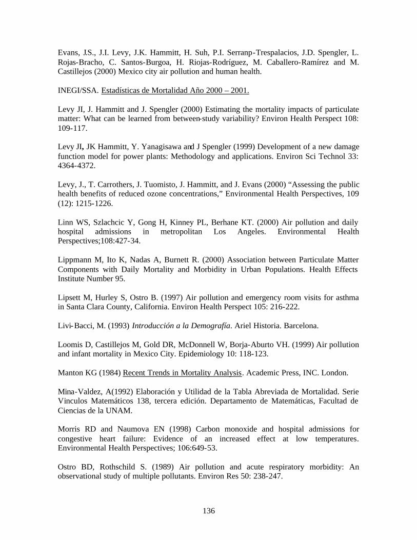
136

Evans, J.S., J.I. Levy, J.K. Hammitt, H. Suh, P.I. Serranp-Trespalacios, J.D. Spengler, L. Rojas-Bracho, C. Santos-Burgoa, H. Riojas-Rodríguez, M. Caballero-Ramírez and M. Castillejos (2000) Mexico city air pollution and human health. INEGI/SSA. Estadísticas de Mortalidad Año 2000 – 2001. Levy JI, J. Hammitt and J. Spengler (2000) Estimating the mortality impacts of particulate matter: What can be learned from between-study variability? Environ Health Perspect 108: 109-117. Levy JI, JK Hammitt, Y. Yanagisawa and J Spengler (1999) Development of a new damage function model for power plants: Methodology and applications. Environ Sci Technol 33: 4364-4372. Levy, J., T. Carrothers, J. Tuomisto, J. Hammitt, and J. Evans (2000) “Assessing the public health benefits of reduced ozone concentrations,” Environmental Health Perspectives, 109 (12): 1215-1226. Linn WS, Szlachcic Y, Gong H, Kinney PL, Berhane KT. (2000) Air pollution and daily hospital admissions in metropolitan Los Angeles. Environmental Health Perspectives;108:427-34. Lippmann M, Ito K, Nadas A, Burnett R. (2000) Association between Particulate Matter Components with Daily Mortality and Morbidity in Urban Populations. Health Effects Institute Number 95. Lipsett M, Hurley S, Ostro B. (1997) Air pollution and emergency room visits for asthma in Santa Clara County, California. Environ Health Perspect 105: 216-222. Livi-Bacci, M. (1993) Introducción a la Demografía. Ariel Historia. Barcelona. Loomis D, Castillejos M, Gold DR, McDonnell W, Borja-Aburto VH. (1999) Air pollution and infant mortality in Mexico City. Epidemiology 10: 118-123. Manton KG (1984) Recent Trends in Mortality Analysis. Academic Press, INC. London. Mina-Valdez, A(1992) Elaboración y Utilidad de la Tabla Abreviada de Mortalidad. Serie Vinculos Matemáticos 138, tercera edición. Departamento de Matemáticas, Facultad de Ciencias de la UNAM. Morris RD and Naumova EN (1998) Carbon monoxide and hospital admissions for congestive heart failure: Evidence of an increased effect at low temperatures. Environmental Health Perspectives; 106:649-53. Ostro BD, Rothschild S. (1989) Air pollution and acute respiratory morbidity: An observational study of multiple pollutants. Environ Res 50: 238-247.

137

Ostro BD (1987) Air pollution and morbidity revisited: A specification test. J Environ Econ Managent 14: 87-98. Pope, C.A. III, M.J. Thun, M.M. Namboodiri, D.W. Dockery, J.S. Evans, F.E. Speizer and C.W. Heath (1995) Particulat air pollution as a predictor of mortality in a prospective study of U.S. adults. Am. J. Respir Crit Care Med. 151:669-674. Pope, C.A. III, R.T. Burnett, M.J. Thun, E.E. Calle, D. Krewski, K. Ito and G.D. Thurston. (2002) Lung cancer, cardiopulmonary Mortality, and long-term exposure to fine particulate air pollution. JAMA. 287:1132-1141. Pressat R (1983) El Análisis Demográfico: Conceptos, métodos, resultados. Fondo de Cultura Económica, México. Ransom, M. Pope III C. (1992). Elementary School Absences and PM10 Pollution in Utah Valley. Environmental Research 58:204-219. Romano Riquer, S.P (2000) Sintomatología respiratoria asociada a partículas menores de 10 µg (PM10) en el centro de la Ciudad de México. Tesis de M.C. Instituto Nacional de Salud Pública. Cuernavaca, Morelos. Romieu I, Cortez-Lugo M, Ruiz-Velasco S, Sanchez S, Meneses F, Hernandez M. (1992) Air pollution and school absenteeism among children in Mexico City. Am J Epidemiol 136: 1524-1531. Romieu I, Meneses F, Sienra-Monge JJL, Huerta J, Velasco SR, White MC, Etzel RA, Hernandez-Avila M (1995) Effects of urban air pollutants on emergency visits for childhood asthma in Mexico City. Am J Epidemiol 141: 546-553. Samet, J., F. Speizer, Y. Bishop, J. Spengler, and B. Ferris (1981) “The Relationship between air pollution and emergency room visits in an industrial community” Journal of Air Pollution Control Association. 31: 236-240. Samet, J.M, S. Zeger, F. Dominici, F. Curriero, I. Coursac, D. Dockery, J. Schwartz, and A. Zanobretti (2000) “The National Morbidity, Mortality and Air Pollution Study Part II: Morbidity and Mortality from Air Pollution in the United States”. Health Effects Institute, Research Report Number 94. Santos Burgoa, C., L. Rojas Bracho, I. Rosas Pérez, A. Ramírez Sánchez, G. Sánchez Rico y S. Mejía Hernández (1998) Modelaje de exposición a partículas en población general y riesgo de enfermedades respiratorias. Gaceta Médica de México 134: 407-418 Schwartz, J. (1993) Particulate air pollution and chronic respiratory disease. Environ. Res. 62: 7-13

138

Schwartz J, Slater D, Larson TV, Pierson WE, Koenig JQ. (1993) Particulate air pollution and hospital emergency room visits for asthma in Seattle. Am Rev Respir Dis 147: 826-831. Schwartz J,. and Morris R. (1995) Air pollution and hospital admissions for cardiovascular disease in Detroit, Michigan. American Journal of Epidemiology;142:23-35. Schwartz, J. (2000) "Harvesting and long-term exposure effects in the relationship between air pollution and mortality," American Journal of Epidemiology, 151: 440-448. Shryock HS, S Siegel et al. (1976) The Methods and Materials of Demography. Academic Press, INC. London. Stieb, D. Burnett, R. Beveridge, R. Brook J. (1996). Association between ozone and asthma emergency department visits in Saint John, New Brunwick, Canada. Enviromental Health Perpectives, 104: 1354-1360. Woodruff TJ, Grillo J, Schoendorf KC (1997) The relationship between selected causes of postneonatal infant mortality and particulate air pollution in the United States. Environ Health Perspect 105: 608-612.

139

Chapter VI. Valuation VI.1. Introduction The comparison of the costs to the benefits of air pollution control strategies requires that a common metric be attached to the health outcomes. This can be accomplished by various means, including economic valuation, medical-based metrics (such as Quality Adjusted Life Years or Disability Adjusted Life Years) or indicator metrics as used in life-cycle impact assessment (Levy and Spengler, 2002). For our analysis we have chosen to evaluate both the economic benefits of the measures we are analyzing and the QALYs to give us an alternative valuation metric. Here, we discuss key concepts for these two methods, as well as the methods used and data necessary to complete the analysis. There exists a considerable amount of uncertainty in the valuation component of this analysis. We discuss some of the sources of uncertainty and how we characterize it.

VI.2. Economic Valuation The economic burden of environmental damage can come in various forms. It can come in the form of damage to human health, biodiversity, visibility etc. To evaluate these damages in economic terms however, one must be able to put a dollar value on each of these goods. There are a number of approaches to valuing environmental damage, which can range from direct costs to society such as cost of illnesses for human health impacts to analyzing the amount an individual would be willing to pay to improve the environment. When evaluating the benefits in terms of risk reduction for morbidity and mortality, there are 3 common methodologies for calculating benefits. These include direct economic costs such as the cost of illness and productivity loss as well as non-marketable costs as represented by willingness-to-pay values. Here, we discuss the main principles behind these three valuation methods and how we quantified them for this study. Monetary benefits are calculated by placing a monetary value on each case and summing the benefits across outcomes in the following form:

))(()/()/($)/($ ∑∑ ×=

j

ij

i

caseiaT acasesHVHB Equation VI.1

Where Hij is the number of cases of the ith health effect (deaths, hospitalizations, incidence of chronic bronchitis etc.) per year due to the jth pollutant and the Vi is the unit social cost of the ith effect. Thus we are summing across pollutants, placing a common dollar metric on the outcome, and then summing across outcomes. The results of this calculation will be the total dollar benefits from reductions in air pollution for a given measure.

140

VI.2.1. Direct Costs The cost of illness (COI) for morbidity outcomes can be understood as direct costs of an illness and can include expenditures on medications, doctors visits, hospitalizations, laboratory tests and human resource costs. This metric aims to include all incurred costs for an illness or medical attention. These costs can be paid directly by the sick individual, through public or private insurance and/or general taxation. In this analysis, we include costs to the health care providers as well as individual costs, as estimated by health experts. Prior to estimating the direct costs per unit of medical attention for each disease, an information collection stage was required in order to know: a) the actions taken by the patients in the three levels of attention for diagnosis and treatment, b) the different services available to people who go to medical attention units, c) human resources (in hours per type of profession), and materials and medications (in physical units) that are utilized at each event. These costs were summed for two events: 1) Emergency Room Attention, and 2) Hospital Attention. The estimation of the total cost of medical attention at the institutional level was determined on the basis of the costs per unit, the integration of costs per event, and the integration of the annual cost per patient for each of the diseases under examination. A cost analysis of disease based on health provider (IMSS) perspective was also conducted. A nominal group technique was utilized to define Therapeutic Diagnostic Guidelines (TDG) and two “Typical Cases” for each disease. The unit costs were estimated taking into account the components of fixed costs and variables that confronted the provider for the year 2001. The costs estimated by event and by disease are shown in Table VI.1. Given that level III medical attention (the highest possible level) was considered, for some diseases, as in the case of AMI and CHF, total costs include the hospital costs, costs for intensive care unit attention, plus the attention in the room.

Table VI.1 COI per case for IMSS health care in 2001

Costs of medical attention by cause, IMSS, year 2001 Type of medical attention

Disease Emergency Visit ICU Hospital Admission AMI* $3,538.00 $65,640.00 $19,172.00 CHF* $3,538.00 $91,896.00 $41,083.00 Acute Bronquitis $2,502.83 - $15,075.00 Pneumonia $2,526.78 - $21,105.00 Asthma $3,173.45 - $6,030.00 COPD* $2,560.00 $132,230.00 $45,238.00 Lung Cancer $2,978.00 - $18,488.00 * Population over 15 years Medical costs were estimated on the level III

141

VI.2.2. Productivity Loss Productivity loss (PL) uses the difference in output (production) due to illnesses as the basis of valuing costs. This value can also be interpreted as the cost of time, or the value of the time an individual loses from being in the hospital, in bed or from premature mortality. While the cost of time would ideally include the opportunity cost of leisure (Cesar et al., 2002), this type of information was not available to us at the time of analysis. Loss of productivity can also be calculated for environmental contingency episodes, when industries must temporarily close their operations due to air pollution levels. This has not been taken into consideration in our calculation of productivity loss, as we are not estimating environmental contingencies in the air quality modeling. It should be noted, therefore, that the productivity loss due to air pollution could be significantly larger than what we are estimating. To calculate the productivity loss per mortality case or medical attention, we multiply the days lost per case by the average daily wage. For medical attention, we obtained average hospital stays from the IMSS database as described in Table VI.2. It should be noted that these are only for days spent in the hospital. It is reasonable to assume that individuals would miss more days of work beyond their stay in the hospital, thereby increasing the productivity loss. This, however, was not estimated here, and therefore we have probably under-estimated work loss days for hospital attention.

Table VI.2 Average length of stay for medical care in IMSS

Average Hospital Stays

Mean ICU Days AMI 5 CHF 7 COPD 10 Mean Hospital Days AMI CHF 7 CHF 15 Acute Bronchitis 5 Pneumonia 7 Asthma 2 COPD 15 Lung Cancer 5

To calculate productivity loss for premature mortality, we use the results from the life years loss analysis for chronic and acute mortality and assume that for each year lost, 260 work days are lost. Data on average daily salaries was obtained from INEGI’s Survey of Household Salaries and Spending (ENIGH). From this information we established 3 income scenarios, as described by Table VI.3.

142

Table VI.3 Average mexican salaries in 2000

Scenario Daily Salary

(Pesos) % of the

population Low 467 6

Medium 2,491 30 High 5,178 64

These salaries are for the year 2000. We do not take into account the growth in salary to our 2003 base-year for valuation, which could increase our estimates of productivity loss. VI.2.3. Willingness-to-Pay One of the most common methods for valuing environmental and health impacts is to determine an individual’s willingness to pay (WTP) for risk reduction. WTP can be determined from contingent valuation and compensating wage studies, which in theory should account for the full cost of disease to an individual including pain and suffering. Contingent valuation studies rely on an individual’s stated preferences through the use of surveys, in which individuals are asked how much they would be willing to pay to reduce their risk of mortality or morbidity. Hedonic wage studies, on the other hand, rely on revealed preferences through the analysis of data on the labor market. Here information on wages and risk levels in certain jobs are obtained and econometric models are used to determine the amount individua ls are compensated for additional risk in the workplace.

These methods for estimating individual preferences rely on the concept of consumer sovereignty and people’s ability to make rational tradeoffs. In theory, values determined from either of these studies would incorporate all the costs to the individual, including medical costs, income loss as well as pain and suffering. We should not, however, expect an individual to incorporate costs he won’t have to pay in his valuation. In theory “external” costs (e.g. publicly provided health care) should be added to WTP. The results from these studies describe the value individuals place on a unit change in risk. The individual WTP divided by the unit risk yields the value of a statistical life (VSL) or morbidity case for the population.

There have been numerous studies on willingness to pay to avoid risk of adverse health outcomes including premature mortality, chronic bronchitis, and respiratory symptoms in the U.S. and a few other countries. Results from these studies could be extrapolated to Mexican conditions by adjusting for income differences. There is, however, concern over the relationship between the value of health and economic and cultural factors between the different countries. These concerns prompted a study to be conducted in Mexico City by Ibarrarán et al. (2002), which involved both contingent valuation and hedonic wage components to estimate WTP for reductions in risks of mortality, chronic bronchitis and a cold. In this study we use results from contingent valuation studies in the U.S. and Mexico. We place greater weight on the evidence from Mexico. Since we cannot base our results on a

143

single study, we have included a range of WTP estimates, using results from the meta-analysis of the EPA’s Benefit and Cost of the Clean Air Act (1999). We have adjusted the central estimates from this report to Mexican income using the following equation:

ε

×=

USA

MexicoUSAMexico GNP

GNPVV Equation VI.2

Where ε is the income elasticity of demand for health. This can be translated as the proportional change in a persons demand for health, as described by their willingness to pay for risk reduction, associated with a proportional change in per capita income. An elasticity between zero and one indicates that demand is relatively insensitive to income, whereas a value greater then one would indicate that health is considered a luxury item. Income elasticities can be derived from hedonic wage or contingent valuation studies, or by comparing values between studies, where populations differ in income, risk and other factors. Additionally, elasticities can be found by analyzing how WTPs change through time as income changes. Findings from WTP studies estimate income elasticities from 0.2 to greater than two (Bowland and Beghin, 2001, Alberini et al., 1997). Comparing results from the Mexican WTP study to the central estimates from the U.S. yields an income elasticity of about 1, indicating that the differences in VSL between Mexico and the U.S. is nearly proportional to income differences. From the hedonic wage study, however, the individual willingness to pay was less then proportional to individual income, with an elasticity of 0.68. In this study we use elasticities of 2 and 0.3 to adjust the U.S. estimates. The results for three outcomes are summarized in Table VI.4.

Table VI.4 WTP estimates for Mexico

Value per Statistical Case (US$)

Health Effect Lower Estimate

(å1 = 2) Central Estimate (Ibarrarán, 2002)

Upper Estimate (å =0 .3)

Mortality $81,120 $506,000 $2,600,000 Chronic bronchitis $4,394 $28,000 $140,980 MRAD 0 $202 $30

1. å is the elasticity of VSL 2. For a minor illness (cold)

For the medical attention outcomes we use the WTP from Cesar et al. (2002) in which they assumed medical attention would be valued as ‘casualty’ in the definition by CSERGE et al. (1999). Using this approach we assumed all hospitalizations to have a WTP of $432 and ERV a value of $223. Table VI.5 summarizes the values we use per each case of mortality or morbidity for the three methods.

144

Table VI.5 Health values for each outcome (US$/case)

COI Productivity

Loss1

WTP (Central estimate)

WTP IC 95%

1.1 Acute Mortality Total mortality - 9,005 506,000 81,120 – 2,600,000 Infant mortality - 212,400 1.2 Chronic Mort ality Total - 45,420 Cardio-respiratory - 45,420 Lung Cancer - 45,420 1.3 Chronic Bronchitis 17,7502 80.9 30,000 4394 – 141,000 1.4 Hospital admissions All Respiratory 2,186 115.6 330 154 – 550 Asthma 603 23.1 330 154 – 550 COPD 17,7503 173.4 330 154 – 550 Pneumonia 2,111 92.5 330 154 – 550 All Cardiovascular 10,890 127.1 330 154 – 550 Congestive Heart Failure 13,3003 173.4 330 154 – 550 Ischemic Heart Disease 8,4813 80.9 330 154 – 550 1.5. Emergency room visits (ERVs) Respiratory Causes 269 57.8 170 79 – 284 Asthma 317 23.1 170 79 – 284 1.6. Restricted Activity Days - 11.64 20 0 – 28 1.7 Minor Restricted Activity Days - 5.84 20 0 – 28 1.8 School Absenteeism - 11.64 20 0 – 28 1 For Average daily salary 2 COPD hospitalization 3 Summation of ICU cost and Hospital Admissions Cost 4 Assume that each case of Restricted Activity Days and School Absenteeim is 1 day, whereas MRAD is ½ day. VI.3. Economic Scenarios Since we use 3 different methods for calculating the unit social cost (Vi) for a given outcome, we combine these methods in 2 different scenarios. It is somewhat unclear how much of an overlap there is between the three methods. In theory, WTP should cover all three, however when medical costs are paid by insurance, or in some studies cost of time lost are specifically not included, WTP may just be considered personal ‘pain and suffering costs’. We are basing our assumptions on the analysis done by Cesar et al. (2002) in which they assume that WTP does not include COI or productivity loss for morbidity. For mortality it can obviously be assumed that there is no cost of illness to the individual (as it is being counted as the event of dying and not the illness preceding a death). However we are assuming that productivity loss is included in WTP estimates for mortality. Using these assumptions we calculate a ‘low scenario’ in which we sum direct costs and productivity loss to calculate the total social benefits. This captures costs that can be observed in the market, but not personal costs such as pain and suffering.

145

Low Scenario = Morbidity (COI + PL) + Mortality (PL) Equation VI.3

For the ‘high scenario’ we include WTP which in theory should include the personal burden of risk. The reason for summing these methods in 2 ways is that there is considerable controversy over WTP values, and which is the appropriate value to use for Mexico. Therefore we have decided to give the users of our model the option on whether or not to take into account WTP in the results. To avoid double counting, we exclude some of the health outcomes in the scenarios.

High Scenario = Morbidity (COI+PL+WTP) + Mortality (WTP) Equation VI.4 Finally, we leave the option for the user to evaluate cases of mortality or years of life saved when evaluating monetary benefits. When years of life lost is analyzed instead of cases, we use an annualized value for the value of a statistical life and multiply it by the years of life saved by the measure. The value of a statistical life is annualized for 35 years, since this is the average life expectancy of an individual responding to contingent valuation studies. Conducting the analysis using years of life saved reduces significantly the value of WTP for mortality risk reduction. Therefore the High scenario when running the model in this manner will reduce significantly, whereas the low scenario will remain the same. VI.4. QALY Analysis It is somewhat unclear whether or not policy analysts should be valuing each life and morbidity case, or if some consideration should be made on the length of lives saved and duration of diseases avoided. If in fact these considerations should be taken into account when designing policy (i.e. if we should be protecting young rather than old, healthy rather than sick individuals) then the economic valuation paradigm may be inappropriate. To account for such discrepancies in health status, the quality adjusted life year (QALY) approach could be applied, which accounts for both duration and quality of life in each health state when calculating health benefits. This analysis is used routinely in the medical and public health fields (Hammitt, 2001). QALY analysis allows us to aggregate mortality and morbidity outcomes in a single unit, and gives us a metric of evaluating health benefits, without necessarily needing to place a monetary value on the outcomes. The QALYs gained by an intervention are simply the sum of quality-adjusted life years gained by avoiding premature mortality and disease. QALYs are calculated by the following equation:

HTHuQALYs ii ××= )( Equation VI.5

Where u(Hi) is a utility weight assigned to a given health outcome which is a number between zero and one, one corresponds to perfect health and zero to death, H is the number of cases and Ti is the duration of that outcome. QALY weights can be estimated by direct elicitation and generic utility scales, such as the Quality of Well Being (QWB) and Health Utilities indices. As none of these surveys have been administered in Mexico, we choose to

146

use QALY weights from studies conducted elsewhere, such as the U.S. (Fryback et al., 1993), Taiwan (Liu et al., 2000) and the Netherlands (Stouthard et al., 2000). Ti is found by two separate analyses: length of hospital stay (from IMSS analysis) and Potential Years of Life Lost analysis, both described earlier in this chapter. Table VI.6 describes the QALY weights and durations used in our analysis for 4 outcomes.

Table VI.6 QALY Weights and Durations of Select Health Outcomes

Outcome QALY Weight Duration (years) Mortality 0.0 see PYLL analysis Chronic Bronchitis 0.81 10 Restricted Activity Day 0.52 1/365 Minor Restricted Activity Day 0.73 1/365 1. Approximate midpoint between results from Viscusi’s (1991) risk-risk tradeoff of chronic bronchitis and mortality finding of 0.68 and Beaver Dam (Fryback et al, 1993) study results of 0.86. Results from the Ibarrarán (2002) study found a risk-risk tradeoff between chronic bronchitis and mortality of approximately 4%, indicating a QALY weight of .96. The weighting depends closely on the severity of the symptoms described in the study. 2. Estimated as ½ ‘dead for a day’ 3. Approximated from Quality of Well Being (QWB) Health State Index results from Liu et al. (2000) study of WTP for minor illness (cold) in Taiwan. The study found the mean QALY weight for women in the study of 0.656 and 0.769 for their children.

For hospital admissions and emergency room visits, we use QALY weights of 0.5, similar to the estimate for a restricted activity day. The durations for these outcomes can be found in Table VI.2. VI.5. Results and Conclusions Results for the high and low economic scenarios for the two time horizons are presented in Tables VI.7 and VI.8. Consistent with the previous results, we find the greatest benefits for the Taxi Fleet Renovation measure. In the shorter time horizon, the Metro Expansion does not have large monetary benefits because less than 10% of the total implementation will have been completed by 2010. However, in the longer time frame the Metro Expansion measure provides relatively large benefits, on the same scale of the Hybrid bus measure. Benefits using the low scenario are significantly lower than the high, by roughly 1 order of magnitude lower, reflecting the fact that we do not use WTP in those results.

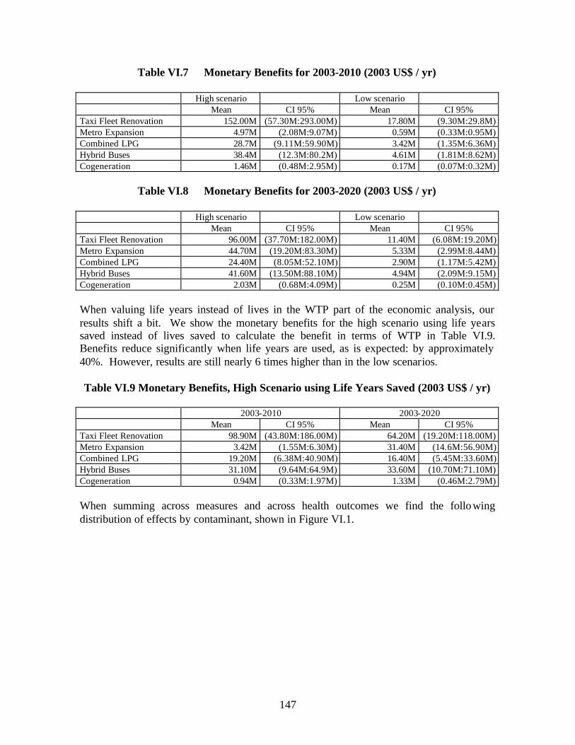
147

Table VI.7 Monetary Benefits for 2003-2010 (2003 US$ / yr)

High scenario Low scenario Mean CI 95% Mean CI 95%

Taxi Fleet Renovation 152.00M (57.30M:293.00M) 17.80M (9.30M:29.8M) Metro Expansion 4.97M (2.08M:9.07M) 0.59M (0.33M:0.95M) Combined LPG 28.7M (9.11M:59.90M) 3.42M (1.35M:6.36M) Hybrid Buses 38.4M (12.3M:80.2M) 4.61M (1.81M:8.62M) Cogeneration 1.46M (0.48M:2.95M) 0.17M (0.07M:0.32M)

Table VI.8 Monetary Benefits for 2003-2020 (2003 US$ / yr)

High scenario Low scenario Mean CI 95% Mean CI 95%

Taxi Fleet Renovation 96.00M (37.70M:182.00M) 11.40M (6.08M:19.20M) Metro Expansion 44.70M (19.20M:83.30M) 5.33M (2.99M:8.44M) Combined LPG 24.40M (8.05M:52.10M) 2.90M (1.17M:5.42M) Hybrid Buses 41.60M (13.50M:88.10M) 4.94M (2.09M:9.15M) Cogeneration 2.03M (0.68M:4.09M) 0.25M (0.10M:0.45M)

When valuing life years instead of lives in the WTP part of the economic analysis, our results shift a bit. We show the monetary benefits for the high scenario using life years saved instead of lives saved to calculate the benefit in terms of WTP in Table VI.9. Benefits reduce significantly when life years are used, as is expected: by approximately 40%. However, results are still nearly 6 times higher than in the low scenarios. Table VI.9 Monetary Benefits, High Scenario using Life Years Saved (2003 US$ / yr)

2003-2010 2003-2020 Mean CI 95% Mean CI 95%

Taxi Fleet Renovation 98.90M (43.80M:186.00M) 64.20M (19.20M:118.00M) Metro Expansion 3.42M (1.55M:6.30M) 31.40M (14.6M:56.90M) Combined LPG 19.20M (6.38M:40.90M) 16.40M (5.45M:33.60M) Hybrid Buses 31.10M (9.64M:64.9M) 33.60M (10.70M:71.10M) Cogeneration 0.94M (0.33M:1.97M) 1.33M (0.46M:2.79M)

When summing across measures and across health outcomes we find the following distribution of effects by contaminant, shown in Figure VI.1.

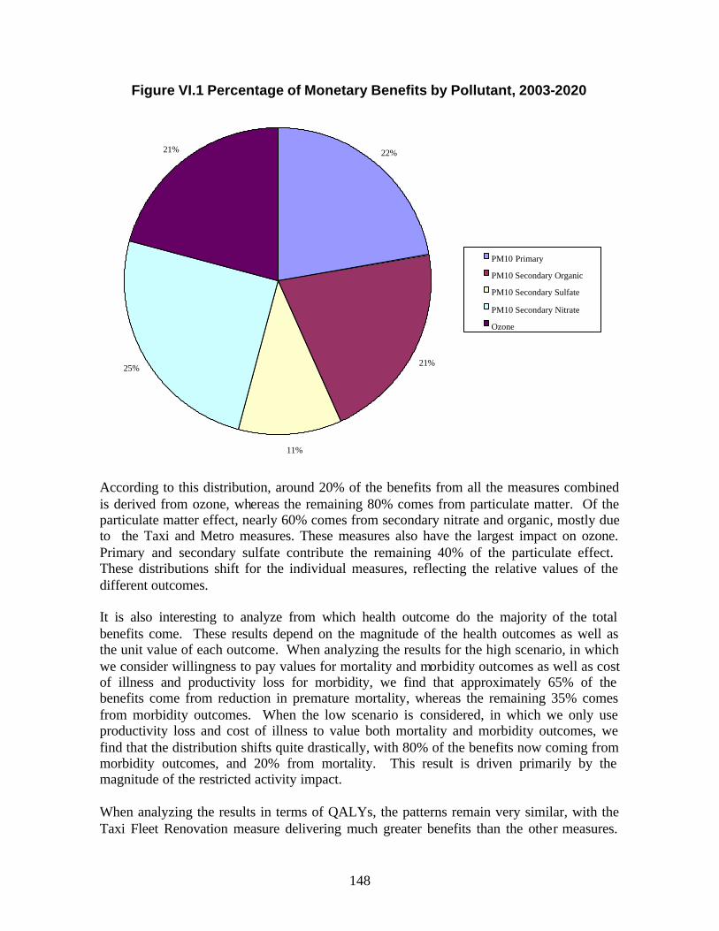
148

Figure VI.1 Percentage of Monetary Benefits by Pollutant, 2003-2020

22%

21%

11%

25%

21%

PM10 Primary

PM10 Secondary Organic

PM10 Secondary Sulfate

PM10 Secondary Nitrate

Ozone

According to this distribution, around 20% of the benefits from all the measures combined is derived from ozone, whereas the remaining 80% comes from particulate matter. Of the particulate matter effect, nearly 60% comes from secondary nitrate and organic, mostly due to the Taxi and Metro measures. These measures also have the largest impact on ozone. Primary and secondary sulfate contribute the remaining 40% of the particulate effect. These distributions shift for the individual measures, reflecting the relative values of the different outcomes. It is also interesting to analyze from which health outcome do the majority of the total benefits come. These results depend on the magnitude of the health outcomes as well as the unit value of each outcome. When analyzing the results for the high scenario, in which we consider willingness to pay values for mortality and morbidity outcomes as well as cost of illness and productivity loss for morbidity, we find that approximately 65% of the benefits come from reduction in premature mortality, whereas the remaining 35% comes from morbidity outcomes. When the low scenario is considered, in which we only use productivity loss and cost of illness to value both mortality and morbidity outcomes, we find that the distribution shifts quite drastically, with 80% of the benefits now coming from morbidity outcomes, and 20% from mortality. This result is driven primarily by the magnitude of the restricted activity impact. When analyzing the results in terms of QALYs, the patterns remain very similar, with the Taxi Fleet Renovation measure delivering much greater benefits than the other measures.

149

In the short time horizon, the Taxi Fleet Renovation has approximately 3 times greater benefits than Hybrid buses, 6 times greater than LPG, 30 times that of Metro Expansion and nearly a hundred times greater than Cogeneration. With the longer time horizon the pattern shifts, with the Taxi measure ranking only 2 times better than Metro Expansion and Hybrid Buses. This comparison contrasts the temporary nature of a vehicle fleet renovation program with the lasting impact of an infrastructure program such as the Metro Expansion.

Table VI.10 Annual QALYs Saved for 2003-2010

Mean CI 95% Taxi Fleet Renovation 2,935 (1,543: 4,694) Metro Expansion 102 (57: 159) Combined LPG 574 (209: 1,110) Hybrid Buses 972 (415: 1,718) Cogeneration 28 (10: 52)

Table VI.11 Annual QALYs Saved for 2003-2020

Mean CI 95% Taxi Fleet Renovation 1,914 (1,009: 3,003) Metro Expansion 946 (554: 1,425) Combined LPG 493 (175: 944) Hybrid Buses 1,050 (440: 1,902) Cogeneration 39 (15: 74)

In future work, population, salaries, and WTP values will be adjusted for changes with time. Projections of these parameters are needed, in a similar manner to that done in Chapter III with costs and emissions. VI.6. References Alberini, A., M. Cropper, T. Fu, A. Krupnick, J. Lui, D. Shaw, W. Harrington (1997) “Valuing health effects of air pollution in developing countries: The case of Taiwan,” Journal of Environmental Economics and Management, 34: 107-126. Bowland, B. and J. Beghin (2001) “Robust estimates of value of a statistical life for developing economies,” Journal of Policy Modeling, 23: 385-396. Cesar, H., G. Schadler, M. Hojer, P. Cicero-Fernandez, L. Brander, T. Buhl, A. C. Villagomez, K. Dorland, A. C. G. Martinez, H. Hasselknippe, P. M. Oritz, A. V. Montero, A. Salcido, J. Sarmiento, and P. V. Beukering (2002) “Air pollution abatement in Mexico City: an economic valuation,” World Bank Report. CSERGE (1999), Benefit Transfer and the Economic Valuation of Environmental Damage in the European Union: With Special Reference to Health, Report to the European Commission under the European Union’s Environmental and Climate Change Research Programme (1994-1998).

150

Fryback, D., E. Dasbach, R. Klein, B. Klein, N. Dorn, K. Peterson, and P. Martin (1993) "The beaver dam health outcomes study: initial catalog of health-state quality factors," Medical Decision Making, 13: 89-102. Hammitt, J. (2002) “QALYs v. WTP”. Risk Analysis 22(5): 985-1001. Ibarrarán, M., E. Guillomen, Y. Zepeda, and J. Hammit (2002) “Estimate the economic value of reducing health risks by improving air quality in Mexico City,” preliminary results. Levy, J and J. Spengler (2002) “Modeling the Benefits of Power Plant Emission Controls in Massachusetts”. J. Air & Waste Manage. Assoc., 52:5-18. Liu, J., J. Hammitt, J. Wang, and J. Liu (2000) “Mother’s willingness to pay for her own and her child’s health: a contingent valuation study in Taiwan,” Health Economics, 9: 319-326. Reynales-Shigematsu L.M. y Cols. “Costos de atención médica de tres enfermedades atribuibles al consumo de tabaco en la Delegación Morelos del Instituto Mexicano del Seguro Social. IMSS.” (In Publication). Stouthard, M., M. Essink-Bot and G. Bonsel (2000) “Disability weights for disease: a modified protocol and results for a western European region,” European Journal of Public Health, 10: 24-30. U.S. Environmental Protection Agency (1999) "The Benefits and Costs of the Clean Air Act 1990-2010," Washington, D.C., Office of Air and Radiation, EPA report no. 410/R-99/001.

151

Chapter VII. Integration: The Co-Benefits Model VII.1. Introduction In the Co-Benefits Model, developed using the Analytica software package, we integrate the calculations described in Chapters III – VI. All air quality (Chapter IV), health impact (Chapter V) and valuation (Chapter VI) calculations are performed within the Model itself. However, emissions and cost calculations (Chapter III) are performed exterior to the Model. Summarized results from the emission and cost calculations (such as Tables III.3.4 and III.3.6 for emission reductions and costs, respectively) are input to the Model. This Model is a user- friendly application that facilitates instruction about and dissemination of our work, and that enhances our analytical work. It allows easy integration of calculations, the inclusion of uncertainty, and rapid propagation of changes in one calculation to all subsequent calculations. VII.2. Analytica We chose to use Analytica as the software for the Co-Benefits Model because it provides a intuitive, graphically-based modeling platform for seamless integration. It allows multiple-dimension matrices to be preserved through the calculations. Additionally, the software has inherent functions that facilitate the inclusion and propagation of explicit uncertainty. Another benefit of Analytica is that a free “Browser” version of the software is available to any interested user. This allows the Co-Benefits Model to be viewed and used without the need to purchase the software. The software should be purchased if users desire to modify the model. Please see Appendix C for information on acquiring Analytica software. VII.3. Co-Benefits Model The User’s Module of the Co-Benefits Model is shown in Figure VII.1. Note that the model is in Spanish, in order to facilitate dissemination to Mexico City decision-makers. From this page, input options for the control measures to be analyzed, the time horizon, the discount rate, and the methodology for valuation of mortality are selected by the user (gray buttons on the left), and essential results can be quickly accessed (pink buttons on the right). Details regarding the use of the model from this page are described in a brief User’s Guide provided in Appendix C.

152

Figure VII.1. The User’s Module of the Co-Benefits Model

Double-clicking on the icon marked “Modelo” in the upper right corner of this page opens the main page of the Co-Benefits Model (Figure VII.2) where calculations occur. This figure illustrates the graphical nature of the inter-relations of variables and modules the Model. The four central modules are those that correspond to Chapters III, IV, V, and VI, respectively. The bottom two modules are where comparisons between GHG emission reductions and benefits are made, and where costs and benefits are rela ted. In the top right, a module for inputs is found.

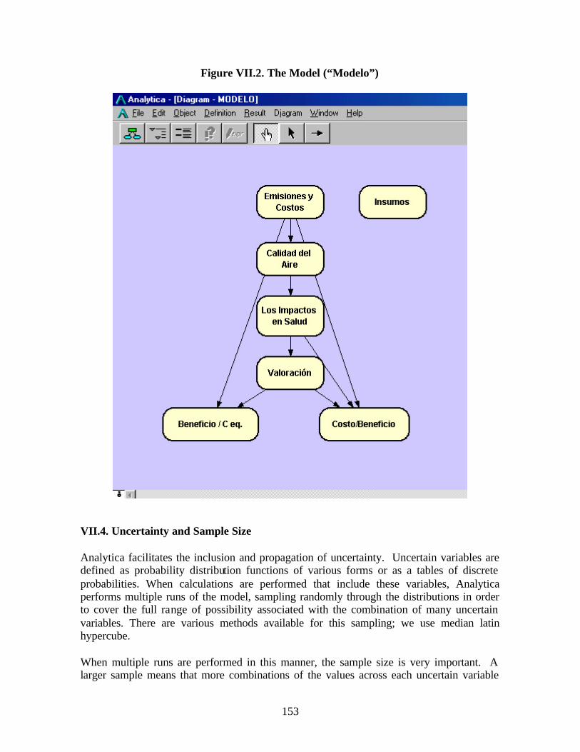
153

Figure VII.2. The Model (“Modelo”)

VII.4. Uncertainty and Sample Size Analytica facilitates the inclusion and propagation of uncertainty. Uncertain variables are defined as probability distribution functions of various forms or as a tables of discrete probabilities. When calculations are performed that include these variables, Analytica performs multiple runs of the model, sampling randomly through the distributions in order to cover the full range of possibility associated with the combination of many uncertain variables. There are various methods available for this sampling; we use median latin hypercube. When multiple runs are performed in this manner, the sample size is very important. A larger sample means that more combinations of the values across each uncertain variable

154

will be made, and thus a more precise result will be achieved. However, a large sample size means that the model will take longer to run. For the Co-Benefits Model, we use a default sample size of 1000. VII.5. Next Steps

Our next steps with the Co-Benefits Model are to include the cost and emissions calculations, with uncertainty, directly in the Model. Additionally, we hope to continually improve the documentation of the Model. The refers to both the documentation within the model of each variable and operation, as well as the external documentation in terms of a more complete User’s Guide. All documentation should be available both in Spanish and in English. The Co-Benefits Model must be maintained and continually improved as improved information becomes available. This job will be undertaken by INE staff.

155

VIII. Results VIII.1. Introduction

In this chapter, we compare the results presented in the previous chapters and discuss the opportunities for joint control of local and global pollution that they illustrate. We present our benchmark results which use a 5% discount rate. VIII.2. Local Impacts

The total cost per QALY saved indicates the net input of funds required for public health improvement in terms of quality adjusted life-years. In Tables VIII.1 and VIII.2, we present these results for the time horizons 2003-2010 and 2003-2020, respectively. For both time horizons, the Taxi Fleet Renovation measure provides the least-cost method per QALYs ($3,000 for 2003-2010). For the longer time horizon, the result is negative because there is a net cost savings. On the short time horizon, Cogeneration is the second-best measure, with a mean of $23,000. For the other measures, the cost per QALY is approximately $60,000. On the longer time horizon, the long-term benefits of the Hybrid Bus measure also become more evident, with the cost dropping to about $23,000.

Table VIII.1. Cost per QALY (2003-2010, 5%)

Mean 95% CI Taxis Fleet Renovation $3,287 $1,774 : $5,551 Metro Expansion $58,090 $34,360 : $91,280 Hybrid Buses $56,600 $25,360 : $114,800 LPG Leaks $58,382 $20,299 : $129,542 Cogeneration $23,220 $9,791 : $48,910

Table VIII.2. Cost per QALY (2003-2020, 5%)

Mean 95% CI Taxis Fleet Renovation -$10,930 -$18,590 : -$6,246 Metro Expansion $50,770 $30,890 : $79,480 Hybrid Buses $23,040 $10,430 : $45,080 LPG Leaks $40,083 $6,622 : $97,332 Cogeneration $30,470 $12,600 : $62,570 These cost per QALY values are low in comparison to the results of Cohen et al. (2003) who find that emission-controlled diesel buses in the US provide health benefits at $270,000 per QALY, while compressed natural gas buses are less cost-effective, at $1.7 -$2.4 million per QALY. This indicates that, in comparison to the technologies study by Cohen et al. (2003), all of the measures studied her are quite cost-effective.

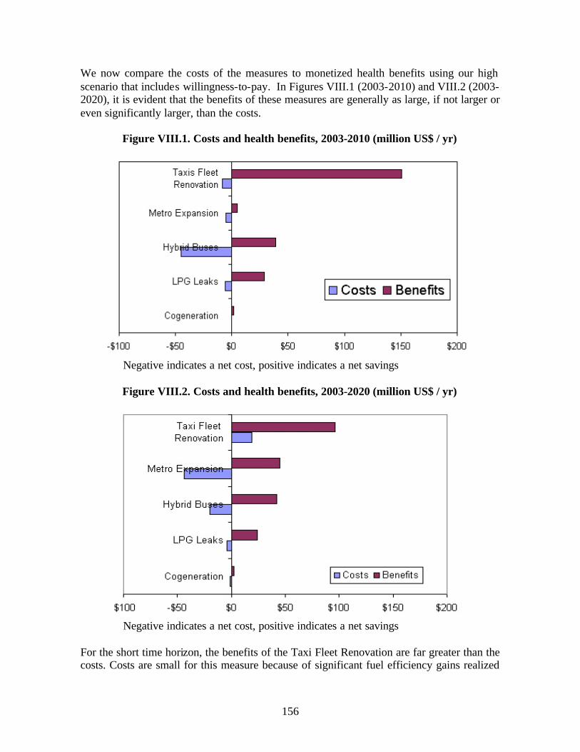
156

We now compare the costs of the measures to monetized health benefits using our high scenario that includes willingness-to-pay. In Figures VIII.1 (2003-2010) and VIII.2 (2003-2020), it is evident that the benefits of these measures are generally as large, if not larger or even significantly larger, than the costs.

Figure VIII.1. Costs and health benefits, 2003-2010 (million US$ / yr)

Negative indicates a net cost, positive indicates a net savings

Figure VIII.2. Costs and health benefits, 2003-2020 (million US$ / yr)

Negative indicates a net cost, positive indicates a net savings

For the short time horizon, the benefits of the Taxi Fleet Renovation are far greater than the costs. Costs are small for this measure because of significant fuel efficiency gains realized

157

with newer vehicles. Benefits are high because of large ozone reductions, and also because of significant reductions in secondary particulate concentrations reductions. On the longer time horizon, net costs turn into net savings as the fuel cost savings continue to accumulate without additional investment costs. Annualized benefits are still la rge, though less so, for the long time horizon because there is deterioration of the fleet of aging vehicles that gradually increases local emissions, and thus decreases local benefits with time. Consistent with existing government proposals, this analysis assumes that only 5 km of Metro would be built from 2003-2010, and an additional 71 km from 2011-2020. For this reason, it appears as to be a relatively inexpensive measure for the short time horizon (Figure VIII.1) and a larger measure for the long horizon (Figure VIII.2). Because Metro Expansion involves significant capital investment, the inclusion of the recuperation value for the Metro (30 year useful life) offsets a significant portion of these initial costs. We find that the local emission reduction benefits can also be large and compensate for a majority, if not all, of the net costs for both time horizons. This analysis assumes that the extension of the Metro causes a significant reduction in the use of on-road public bus transportation, which means local emissions are significantly reduced. However, increase in Metro length requires more electricity and increases emissions from power plants that are primarily located outside the valley. The Metro Expansion causes a net transfer of local emissions from inside to outside the valley. We assume that population density is substantially lower where the electricity is generated than in Mexico City, and for this reason, public health impacts will be negligible from increased power generation. This transfe r of local emission helps to make local benefits large enough to offset much, if not all, of the costs for this measure. The Hybrid Buses measure has large upfront investment costs due to the expensive nature of the technology, but also generates significant cost savings on the long term due to greatly enhanced fuel efficiency. Benefits are large for both time horizons because of reductions in primary particulate emissions. This measure is implemented between 2003 and 2006, and this is why annualized costs are lower and benefits slightly higher for the long time horizon (Figure VIII.2) than for the short time horizon (Figure VIII.1). The LPG leak reduction measure, on the other hand, has low costs because of the low unit costs for each stove repair. Benefits are much larger than the costs because of the significant reduction in hydrocarbon emissions that reduces both ozone and secondary organic particulate exposure. For Cogeneration, net costs are low because of the significant gains in fuel efficiency and the inclusion of the recuperation value of the equipment at the end of each time horizon (20 year useful life). Benefits are not very large for this measure because the gains in efficiency derive from simultaneous on-site production of thermal and electrical energy that replaces off-site electricity generation and on-site thermal energy production. As explained for the Metro measure, only 3.1% of the electricity consumed in Mexico City is generated in the valley. Though Cogeneration significantly reduces the total emissions by substantially increasing efficiency, the measure moves emissions of local pollutants into the valley, and thus local benefits are small.

158

VIII.3. Global impacts Reduction in GHG emissions are presented in Figures VIII.3 (2003-2010) and VIII.4 (2003-2020) in terms of thousand metric tons (=109 g) of C equivalent per year. Due to the large positive impact of the Taxi Fleet Renovation and Cogeneration measures on fuel efficiency, these measures create the largest GHG emission reductions. For the longer time horizon, when much more of the Metro has been built, this measure also begins to cause significant GHG reductions. The LPG Leaks and Hybrid Bus measures create smaller GHG emission reductions for both time horizons.

Figure VIII.3. GHG emission reductions, 2003-2010

159

Figure VIII.4. GHG emission reductions, 2003-2020

VIII.4. Comparing Local and Global Results

In Figure VIII.5, we present the local and global net benefits. The local net benefits are defined as the Health Benefits minus Costs, while the global net benefit is the reduction in GHG emission. Results for both time horizons are presented. Figure VIII.5 illustrates that the Taxi Fleet Renovation measure is clearly the best measure from the joint local – global perspective. The Hybrid Bus measure for 2003-2020 and the LPG Leak measure on both time horizons are the next-most promising for joint local / global control. The Metro Expansion, in large part because of its very high costs, is less promising from the joint perspective. Cogeneration also does not have sufficient local benefits to make it interesting for joint local – global control. However, if only the global perspective is considered, the Cogeneration measure could be of great interest. We also note that were a similar study conducted at the national level, Cogeneration may turn out to be a promising joint local –global option because health benefits derived in populations living near to power plants would be considered. This will depend, of course, on population exposure to emissions generated by electricity production across the country.

160

Figure VIII.5. Local and Global Net Benefits

In Tables VIII.3 and VIII.4, the local health benefits per tons of C equivalent are reported for each measure. Mean values range from $8 / ton C to approximately $2,500 / ton C, with all measures except for the Cogeneration coming in at greater than $800 / ton C. In the IES study in Chile, these values ranged from $60-480 / ton; in Korea the value was $22 / ton. This indicates that, for these measures and with the exception of Cogeneration, local benefits are quite high with respect to the GHG emission reductions. This finding is due in part to the fact that all of these measures, with the exception of Cogeneration, have been designed for the purpose of air quality improvement, as opposed to specifically focused on GHG emission reductions. This analysis indicates the potential for joint control of both local and global pollutant that has large benefits for both, independent of the original intent of the measures. Table VIII.3. Health benefit per ton of GHG reduced, 2003-2010 (US$ / ton C eq.) Mean 95 % CI Taxis Fleet Renovation $1,312 $496 : $2,532 Metro Expansion $912 $382 : $1,665 Hybrid Buses $2,602 $837 : $5,436 LPG Leaks $2,468 $910 : $5,918 Cogeneration $9 $3 : $18

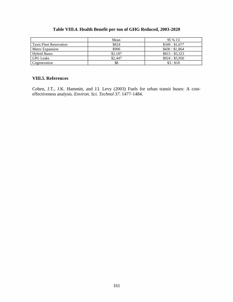
161

Table VIII.4. Health Benefit per ton of GHG Reduced, 2003-2020 Mean 95 % CI Taxis Fleet Renovation $824 $349 : $1,677 Metro Expansion $906 $430 : $1,864 Hybrid Buses $2,187 $815 : $5,323 LPG Leaks $2,447 $924 : $5,950 Cogeneration $8 $3 : $18 VIII.5. References Cohen, J.T., J.K. Hammitt, and J.I. Levy (2003) Fuels for urban transit buses: A cost-effectiveness analysis. Environ. Sci. Technol 37. 1477-1484.

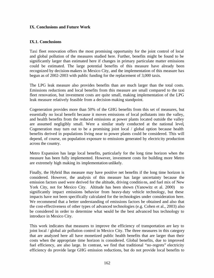
162

IX. Conclusions and Future Work IX.1. Conclusions Taxi fleet renovation offers the most promising opportunity for the joint control of local and global pollution of the measures studied here. Further, benefits might be found to be significantly larger than estimated here if changes in primary particulate matter emissions could be estimated. The large potential benefits of this measure have already been recognized by decision-makers in Mexico City, and the implementation of this measure has begun as of 2002-2003 with public funding for the replacement of 3,000 taxis. The LPG leak measure also provides benefits than are much larger than the total costs. Emissions reductions and local benefits from this measure are small compared to the taxi fleet renovation, but investment costs are quite small, making implementation of the LPG leak measure relatively feasible from a decision-making standpoint. Cogeneration provides more than 50% of the GHG benefits from this set of measures, but essentially no local benefit because it moves emissions of local pollutants into the valley, and health benefits from the reduced emissions at power plants located outside the valley are assumed negligibly small. Were a similar study conducted at the national level, Cogeneration may turn out to be a promising joint local / global option because health benefits derived in populations living near to power plants could be considered. This will depend, of course, on population exposure to emissions generated by electricity production across the country. Metro Expansion has large local benefits, particularly for the long time horizon when the measure has been fully implemented. However, investment costs for building more Metro are extremely high making its implementation unlikely. Finally, the Hybrid Bus measure may have positive net benefits if the long time horizon is considered. However, the analysis of this measure has large uncertainty because the emission factors used were derived for the altitude, driving conditions, and fuel mix of New York City, not for Mexico City. Altitude has been shown (Yanowitz et al. 2000) to significantly impact emissions behavior from heavy-duty vehicle technology, but these impacts have not been specifically calculated for the technologies under consideration here. We recommend that a better understanding of emissions factors be obtained and also that the cost-effectiveness of other types of advanced technologies (e.g. Cohen et al., 2003) also be considered in order to determine what would be the best advanced bus technology to introduce in Mexico City. This work indicates that measures to improve the efficiency of transportation are key to joint local / global air pollution control in Mexico City. The three measures in this category that are analyzed here all have monetized public health benefits that are larger than their costs when the appropriate time horizon is considered. Global benefits, due to improved fuel efficiency, are also large. In contrast, we find that traditional “no-regrets” electricity efficiency do provide large GHG emission reductions, but do not provide local benefits to

163

Mexico City because the majority of electricity is produced away from the valley in which Mexico City is located. IX.2. Future Work Further work is needed to analyze more measures that cover a wider range of opportunities for joint local / global air pollution control. Also very important is to quantify the air pollution improvements and cost savings that could be acquired were congestion reduced in MCMA. Such an analysis may indicate that the benefits from transportation efficiency improvement are, in fact, much larger than estimates here. Improved understanding of emission factors from new and old vehicles under Mexico City driving conditions is also greatly needed, and could significantly impact results. Sensitivity analysis is also needed on the control options studied in this project. The results presented here are, of course, dependent upon assumptions made about baselines, emission factors, implementation plans, etc. Since we are attempting to predict the future, there is much uncertainty. In order to address this uncertainty, sensitivity of results to these basic assumptions needed to be tested. Results that are robust to the gamut of possible futures is the ultimate goal of this kind of analysis, making a complete sensitivity analysis a key next step. Technical working groups among various agencies and institutions in Mexico City are needed in order to more precisely define control measures, and to improve the emissions factors used. Working groups would be mutually beneficial to all parties involved, particularly given the limited resources available for this work in Mexico City, by facilitating interchange of the best-available information. This project has evidenced in many ways the pressing need that decision-makers have for reliable rapid-assessment tools. Reduced form air quality modeling techniques is one example; and the Co-Benefits Model that integrates this analysis is, of course, another. The methods used here should be further studied and improved so that they can give ever-more reliable answers. On the long term, maintenance and technical support must be continued so that the Model and the methodology upon which it is based can remain pertinent to the decision-making process. In the near future, improved documentation and a more complete User’s Guide (ref. Appendix C) is also needed.

164

Appendix A: Air Quality Modeling A.1. Box Model Box models are the simplest of numerical models. The region to be modeled is treated as a simple cell, or box, bounded by the ground on the bottom, the inversion base (or some other upper limit mixing) on the top, and the east-west and north-south boundaries on the sites. The box may enclose an area on the order of several hundred square kilometers. Primary pollutants are emitted into the box by the various sources located within the modeled region, undergoing uniform and instantaneous mixing. The ventilation characteristics of the modeled region are represented by specification of characteristic wind speed and rate of rise of the upper boundary. Fundamental to the box model concept is the assumption that pollutant concentration in a volume of air, a “box”, are spatially homogeneous and instantaneously mixed. Under this assumption, pollutant concentrations can be described by a simple balance among the rates at which they are transported in and out of the air volume, their rates of emission from sources within the volume, the rate at which the volume expands or contracts, the rates at which pollutants flow out the top of the volume, and the rates at which pollutants flow out the top of the volume, and rates at which pollutants react chemically or decay. Because of their formulation, box models can predict, at best, only the temporal variation of the average regional concentration for each pollutant species. Consequently, they are capable of addressing only broad-scale regional questions. The combined effects of local emission patterns and meteorological conditions generally give rise to significant spatial variations in pollutant concentrations. So, clearly box models cannot be used to asses the effectiveness of emission control strategies that lead to spatially inhomogeneous emissions. We have developed a box model for the MCMA that represents emissions, advection and dry deposition of primary PM10. The governing equation is:

−⋅

∆+

∆∆∆+

∆−⋅+

∆−⋅=

∆⋅−

1htv

ood

et

PMzyx

Ey

PMPMv

xPMPM

udt

dPM

Equation A.1 Where u and v are mean zonal and meridional winds, respectively; Äx, Äy and Äz are the horizontal and vertical dimensions of the box; PMo is the concentration of PM on the boundaries of the box; PM is the concentration inside the box; E is the emission of primary particles; Ät is the residence time of a parcel of air in the box (=Äy/v); vd is the dry deposition velocity for particles of 0.1-10ìm ; and h is the height of the deposition layer. Thus, the first two terms represent advection, the third represents emissions into the volume of the box, and the fourth represents dry deposition (Scire et al., 2000).

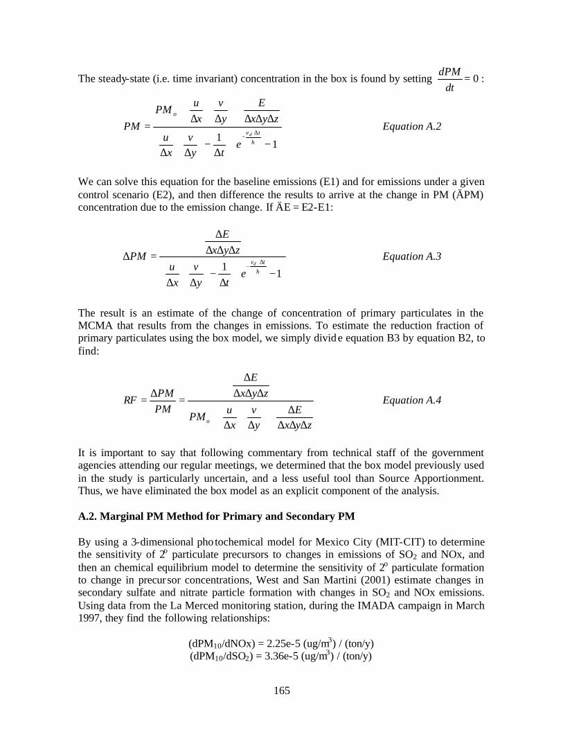
165

The steady-state (i.e. time invariant) concentration in the box is found by setting dt

dPM= 0 :

−⋅

∆−

∆

+∆

∆∆∆+

∆

+∆

⋅=

∆⋅−

11 h

tv

o

d

ety

vx

u

zyxE

yv

xu

PM

PM Equation A.2

We can solve this equation for the baseline emissions (E1) and for emissions under a given control scenario (E2), and then difference the results to arrive at the change in PM (ÄPM) concentration due to the emission change. If ÄE = E2-E1:

−⋅

∆−

∆

+∆

∆∆∆∆

=∆∆⋅

−1

1 h

tvd

ety

vx

u

zyxE

PM Equation A.3

The result is an estimate of the change of concentration of primary particulates in the MCMA that results from the changes in emissions. To estimate the reduction fraction of primary particulates using the box model, we simply divide equation B3 by equation B2, to find:

zyxE

yv

xu

PM

zyxE

PMPM

RF

o ∆∆∆∆+

∆

+∆

⋅

∆∆∆∆

=∆= Equation A.4

It is important to say that following commentary from technical staff of the government agencies attending our regular meetings, we determined that the box model previously used in the study is particularly uncertain, and a less useful tool than Source Apportionment. Thus, we have eliminated the box model as an explicit component of the analysis. A.2. Marginal PM Method for Primary and Secondary PM By using a 3-dimensional pho tochemical model for Mexico City (MIT-CIT) to determine the sensitivity of 2o particulate precursors to changes in emissions of SO2 and NOx, and then an chemical equilibrium model to determine the sensitivity of 2o particulate formation to change in precursor concentrations, West and San Martini (2001) estimate changes in secondary sulfate and nitrate particle formation with changes in SO2 and NOx emissions. Using data from the La Merced monitoring station, during the IMADA campaign in March 1997, they find the following relationships:

(dPM10/dNOx) = 2.25e-5 (ug/m3) / (ton/y) (dPM10/dSO2) = 3.36e-5 (ug/m3) / (ton/y)

166

We apply these relationships to the estimated emissions reductions from the control measures to estimate changes in secondary particle concentrations. A.3 References for Appendix A: Air Quality Modeling Scrire, J.S., D.G .Strimaitis, and R.J. Yamartino (2000), “A User’s Guide for the CALPUFF Dispersion Model (version 5),” Earth Tech, Inc. 521 pp. West, J. and I. San Martini (2001) Report of the Fourth Workshop on Mexico City Air Quality, March 8-10, 2001, El Colegio de Mexico, Mexico. MIT-Integrated Program on Urban, Regional and Global Air Pollution Report No. 25, November 2001.

167

Appendix B. Capacity Building B.1. Introduction A key component of this co-benefits project has been in the building of capacity in the INE team and Mexican policy makers. The main goals of the capacity building have been to:

1) Facilitate the continuation of the project by INE staff once this phase of project is completed

2) Introduce the analysis and the Co-Benefits model to Mexican policy makers, and to

encourage their use of the model

3) Train individuals on Analytica software so that they are able to use this program to conduct integrated analyses for other projects.

Some of the main activities of the capacity building component have been regular meetings with the CAM, a final workshop, several short-courses and close collaboration with INE staff. In this Appendix, we discuss some of our key accomplishments and lessons learned during the project. B.2. Key Accomplishments Throughout the project we have held regular meetings with members of the Metropolitan Environmental Commission (CAM) and other environmental agencies in the MCMA, including the Secretariat of the Environment of the Government of the Federal District (SMA-GDF), the Secretariat of the Environment of the government of the State of Mexico (SEGEM), and the Directorate of Air Quality of the Federal Secretariat of the Environment and Natural Resources (SEMARNAT). These meetings have encouraged active participation in this project and to aid the integration of this work with other efforts in the MCMA, particularly the first revision of PROAIRE. Our close collaboration with INE personnel has also been a fruitful one. From the beginning of the project, INE researchers were encouraged to attend our regular presentations to the CAM and other government agencies. From the beginning of 2003, we have also made efforts to bring multiple INE researchers into active participation on the Co-Benefits team. Following is a list of the major capacity building activities undertaken:

• On November 26, 2002 , we held a meeting with the CAM and other government representatives in which they explained their plans for the first 2-year revision of PROAIRE and we presented the goals for this project. The discussion that followed considered how we can make this work useful to their PROAIRE revision. There was much interest in this analysis from the CAM staff and several members from

168

the State of Mexico asked to be involved closely in the development of the Co-Benefits model.

• On December 16, 2002, we met with Soledad Victoria from the State of Mexico to

introduce her to the Analytica software and an initial version of the model.

• On February 12, 2003, we held a meeting with the CAM and other government representatives to illustrate the Analytica software and to introduce the developing Co-Benefits model. Much valuable feedback was received about the level of detail appropria te for the model if is to be useful to decision-makers.

• On March 6, 2003, we had a productive meeting in which the estimation of costs

and emissions were presented. We focused on the accelerated retirement of taxis as an example.

• Our capacity building with a specific focus on INE researchers began with a short-

course was led by Miriam Zuk on the estimation of health impact and valuation of these impacts (April 1, 2003), and on the Analytica model (April 3, 2003). INE investigators then began to study and work on specific exercises related to each of the modules.

• On April 22 and 24, 2003 intensive working meetings with the entire INE team

were led by Dr. Fernandez and Dr. McKinley to discuss results, uncertainties, priorities for future work, and to begin the planning for the final workshop.

• On April 24, 2003, the air quality models were discussed with CAM and other

governmental representatives. We received valuable feedback during this meeting that led us to eliminate the box model from our final results.

• On April 30, 2003, the health and valuation modules were presented to CAM and

other governmental representatives, and valuable feedback was received.

• On May 20, 2003, the final workshop was held. Policy makers and technical staff were invited and many key figures attended. Consistent with their ever- increasing involvement with the project, INE investigators presented the bulk of the technical details of the project. Interest in the project and the integrated analysis was high, and valuable comments regarding the work were provided by the audience.

• The depth and breadth of the comments during the final workshop led to an

additional meeting for technical comments and discussion that occurred at INE on May 26, 2003. Representatives from the National University of Mexico Center for Atmospheric Science, the Mexican Institute of Petroleum (IMP), the SEGEM, and SEMARNAT attended to share their thoughts and for further discussion of the details of the analysis. It is promising possibility that technical working groups, particularly between INE, IMP and SEGEM, will develop out of this meeting.

169

• On June 4, 2003, we met with Dr. Adrián Berrera of IMP to begin discussions about such collaboration. These kinds of cross- institutional working groups would be highly beneficial to moving forward this type of integrated analysis in Mexico City. We believe that INE is in a very good position to become a focal point for such effort.

• On June 16, 2003, we held a day- long course on the use of Analytica software and

on the use of the Co-Benefits model. The majority of time was spent doing modeling exercises using the software and the model. Eight attendees were from the CAM, SEGEM, and GDF. Another 9 attendees from INE also took the course. The feedback on the course was extremely positive, and there were multiple requests for an advanced course in the near future. This course was a key step in the dissemination of results to the multiple government offices responsible for air quality in Mexico City, and therefore to improving decision-making on local and global pollution control.

B.3. Lessons Learned While capacity building has been a key component of the project since its initiation, we have learned many things over the course of 10 months and our understanding of the best ways to truly achieve capacity building has significantly improved. At the start of the project, our focus was on designing the analysis and determining its scope. Most time was spent in this development phase on detailed technical issues; few INE personnel participated in the planning phase. Later, it was determined that if the analysis was to eventually be transferred completely to INE staff, more people needed to be involved. As such we developed a large work group and had many fruitful meetings on the project as a whole and collaborations in the execution of specific parts of the analysis. Through this process, we have learned that it is essential to involve key INE staff in the project planning and implementation phase from the beginning. It is difficult to encourage participation and re-train staff every time new work groups are determined. We recommend that in the future, a maximum of 4 to 5 staff be selected to work on the project and be asked by their superiors to dedicate a substantial portion of their time to the project. Of this group, one leader would be assigned who understands the broad vision of the project, and is able to integrate the pieces. Depending on the time available of the leader, either they could be responsible for maintaining and updating the model, or perhaps another staff member could be responsible for model maintenance. Additionally, 3 or 4 members should be able to conduct and constantly improve the technical analysis in each of the modules: emissions and costs, air quality modeling, and health benefits assessment. If tasks are not assigned and time is not dedicated, the gains achieved through this project may be lost once this phase is over. We have also learned that in order for people to be truly involved with the project, they not only need to be present at meetings and understand the basics of the analysis, but they must be responsible for a part the project. After key decisions are made, it is difficult to help people understand how the project evolved into its existing form. Though we have made

170

much progress with increasing technical knowledge in the fields touched by this project, capacity building about developing and growing a project is still very much needed at INE. Gathering an interdisciplinary team is difficult, only to be made more difficult when people have little time to devote or have minimal intellectual investment in a project. We therefore recommend that for the continuation of this phase of the project and for future phases (or for other projects), it is very important to: 1) Designate an in-country leader who is responsible for both learning the technical

details of the analysis and for further development and dissemination of the project. 2) Give in-country participants tasks and responsibilities for the work to encourage their

participation and learning. 3) Keep in mind that the capacity building process must be started during the planning

stage of the project. If staff participate from the start of the project, their ownership and intellectua l interest will drive the capacity building process forward. Capacity building in a top-down format is inherently ineffective.

171

Appendix C. Basic User’s Guide for the Co-Benefits Model

C.1. Introduction This appendix is meant to provide the reader with basic instructions on how to access and use the Co-Benefits Model. It indicates where to find the Model and the Analytica software required to run it on the worldwide web. It assumes that the user has access only to the “Browser” version of Analytica software, which is free of charge. This documentation is written based on version 5.7 of the Model. This guide is written on the assumption that the user has read and fully understands the entirety of this Final Report in which the methodology implemented in the Model is discussed at length. We strongly recommend all users to carefully read this Report before beginning to use the Model. It is essential that the user remember that this Co-Benefits Model is designed only for use in Mexico City. It is not applicable to other locations in its current form. It is also key to remember that the emission reductions and costs required as inputs to the Model are:

• Annualized emissions changes at discount rates of 0%, 3%, 5%, 7% for 2003-2010 and 2003-2020.

• Annualized costs 0%, 3%, 5% and 7% for 2003-2010 and 2003-2020. The use of emission changes and / or costs calculated on other bases will cause erroneous results to be derived from the Model. We also note that because our goal is to attract decision-makers in Mexico City to using the Model, the Model’s text is in Spanish. C.2. Accessing the Co-Benefits Model The most recent version of the Model, as well as other information about this project, can be downloaded from:

http://www.ine.gob.mx/dgicurg/cclimatico/benlg.html

C.3. Accessing Analytica It is free to download the “Browser” version of Analytica from the website of Lumina Systems, Inc.

http://www.lumina.com With this version, the Model can be run, but it cannot be modified and input choices cannot be saved. Input choices in the first window can be changed for each run, and new measures can be evaluated under the “Medida Nueva” module. However, such changes cannot be saved and must be re-entered after the Model has been closed and re-opened.

172

We suggest tha t before trying to use the Co-Benefits Model, the prospective user first familiarize herself with Analytica by following the Analytica tutorial guide, which can also be downloaded from Lumina, or by taking an Analytica training course. C.4. The User’s Module of the Co-Benefits Model Upon opening the Model, the user will find the screen shown in Figure C.1.

Figure C.1. The User’s Module of the Co-Benefits Model

All options found in this first window are further defined and implemented under the “MODELO” module that appears in the upper right corner of the window. All technical details required to understand these calculations are described in Chapters IV, V, VI, and VII of this report. C.4.1. Input Options This section describes options that the user can change in order to customize their Model run. All options are found on the left side of the first window of the Co-Benefits Model (Figure C.1). Input buttons are gray in color.

173

Part 1: All Measures or Individual Ones (“Parte I: Todo o Individua l”) With this drop-down button, the user chooses if she will analyze all measures included in the Model (“Todo”) or only a single measure (“Individual”). If “Todo” is selected, results for all measures will be calculated simultaneously, and the Model will take longer to run. Also, if “Todo” is selected, Parte II is deactivated by the Model and can be ignored by the user. Part II: Control Measures (”Parte II: Medidas de Control”) If “Individual” is chosen in Part I, then this button is used to choose which measure to evaluate, or the option “Combination” can be selected. If “Combination” is selected, the user also needs to use the “Tabla para Combinacion” to determine which measures will be summed together before the Model is run. Combination (“Tabla para Combinacion”) Clicking on this button will bring the user to a table with all the control measures listed to the left and a series of 0’s and 1’s in the right column. If the user wants to include a measure in her combination, she should alter the right column in order to have a “1” next to that measure. Excluded control measures should have a “0” beside them. Add a new measure (“Añadir su ‘Medida Nueva’”) If the user wants to define her own set of emission reductions and costs to be evaluated by the Co-Benefits Model, she should use this module. Before doing so, there is likely significant work to be done (see Chapter III) in order to calculate emissions reductions and costs as:

• Annualized emissions changes at discount rates of 0%, 3%, 5%, 7% for 2003-2010 and 2003-2020.

• Annualized costs 0%, 3%, 5% and 7% for 2003-2010 and 2003-2020. Once emissions reductions and costs are calculated in this way, the user should double click on the “Añadir su ‘Medida Nueva’” module. In part 1a, emission changes are entered into a table. Pay careful attention that the measure identified is “Medida Nueva” and that the data are entered under the appropriate time horizon and discount rate. Here, total changes in primary PM10 (PM2.5 is not currently active) should be entered (combustion + geological). In part 1b, changes in geological emissions of primary PM10 (PM2.5 is not currently active) should be entered. The Model accounts for the fact that the total (combustion + geological) was entered in part 1a. In part 2, costs are entered. In each part, it is also possible to alter the values for the 8 control measures inherent to the Model by entering the altered values into the “Medida Nueva” table.

174

Time Horizon and Discount Rate (“Horizonte de tiempo” and “Tasa de Descuento”) With the first button, the user can choose to evaluate either the 2003-2010 time horizon or the 2003-2020 horizon. With the second, the user opts for either not using discounting (0%) or to run the Model using a 3%, 5% or 7% discount rate. Mortality Valuation (“Valoración de Mortalidad”) Here, the user chooses if mortality will be valued based on each case of mortality (”Casos”) or if each year of life lost will be valued (“Años”). Morbidity is always valued based on cases. C.4.2. Output Options Result buttons are pink in color, and are located on the right side of the Model’s first window. “Costos Acutal” returns annualized costs (US$ / yr) for the measure(s), time horizon, and discount rate chosen. “Reducciones actual” gives the emission reductions (ton / yr) for the measure(s), time horizon, and discount rate chosen. “Reduccion C equivalente” gives the change in emissions of greenhouse gases (tons C-equivalent / yr) for the measure(s), time horizon, and discount rate chosen. “Cambio de concentración por medida” returns, for each measure and each contaminant, the change in population-weighted exposure (ug/m3) for the representative annualized year as estimated by the Model. “Impactos totales” gives the number of avoided cases per year (if “Casos” is selected) or QALYs per year (if “Años” is selected) due to the selected control measures. “QALYs totales” returns the total number of QALYs saved each year by the measure, independent of whether “Casos” or “Años” is selected in the input options section. “Beneficios Monetarios” returns the monetary benefits, calculated with each of the three valuation metrics, for each avoided health impact (US$ / yr). “Escenarios de Beneficios” provides the total benefits for the high “Alta” and low “Baja” valuation scenarios (US$ / yr). “Costos / beneficios totales” provides Cost over Benefit ratios for the high “Alta” and low “Baja” scenarios. If costs are negative, a negative ratio will be returned. If benefits are negative, the result will be zero.

175

“Costo / QALY” compares the cost of the control measure(s) to the QALYs it saves (US$ / QALY). “Beneficios Netos” returns the net benefits of the control measure(s), which is the Benefits minus Costs (US$ / year). “Beneficio / ton C eq.” compares the local health benefit and the GHG reduction (US$ / ton C eq.) “Precio de C equivalente” calculates the income per ton of GHG reduction (US$ / ton) that would be needed in order to make the sum of benefits and such “GHG Income” equivalent to the costs of the control measure. If the result is zero, it indicates that either the benefits are already larger than costs without consideration of “GHG Income”, or that there is a net increase in GHG emissions due to the measure. C.5. Citing Results If the results from the Model are used in a report or publication, it should be cited (with the appropriate year and version number) as:

Co-Benefits Model for Mexico City, Version x.x, Instituto Nacional de Ecología, Mexico, 200y.

This report should also be cited:

McKinley et al. (2003) Final Report of the Mexico City Co-Benefits Project, Instituto Nacional de Ecología and the US Environmental Protection

Agency Integrated Strategies Program, August 2003. If a modified version of the Model is used, or new control measures are entered into the existing Model, please cite this report as indicated above. For the Model, please indicate the changes that have been made and by whom:

Co-Benefits Model for Mexico City, Version x.x, Instituto Nacional de Ecología, Mexico, 200y. Modified by (who) of (institution)

in inputs for (costs and emissions of measure X, de dose-response Z, etc.) and in modules (A,B,C) in manner (D,E), etc.