
Solutions Manual to Accompanybayanbox.ir/view/3118992197760472502/James-F... · viii CONTENTS 10 An...
319
Transcript of Solutions Manual to Accompanybayanbox.ir/view/3118992197760472502/James-F... · viii CONTENTS 10 An...


Solutions Manual to Accompany
AN INTRODUCTION TONUMERICAL METHODSAND ANALYSIS
epperson2 solutions-fm_fitzmmaurice-fm.qxd 7/12/2013 1:30 PM Page i

epperson2 solutions-fm_fitzmmaurice-fm.qxd 7/12/2013 1:30 PM Page ii

Solutions Manual to Accompany
AN INTRODUCTION TONUMERICAL METHODSAND ANALYSISSecond Edition
JAMES F. EPPERSON Mathematical Reviews
epperson2 solutions-fm_fitzmmaurice-fm.qxd 7/12/2013 1:30 PM Page iii

Copyright © 2013 by John Wiley & Sons, Inc. All rights reserved.
Published by John Wiley & Sons, Inc., Hoboken, New Jersey.Published simultaneously in Canada.
No part of this publication may be reproduced, stored in a retrieval system or transmitted in any form orby any means, electronic, mechanical, photocopying, recording, scanning or otherwise, except aspermitted under Section 107 or 108 of the 1976 United States Copyright Act, without either the priorwritten permission of the Publisher, or authorization through payment of the appropriate per-copy fee tothe Copyright Clearance Center, Inc., 222 Rosewood Drive, Danvers, MA 01923, (978) 750-8400, fax(978) 750-4470, or on the web at www.copyright.com. Requests to the Publisher for permission shouldbe addressed to the Permissions Department, John Wiley & Sons, Inc., 111 River Street, Hoboken, NJ07030, (201) 748-6011, fax (201) 748-6008, or online at http://www.wiley.com/go/permission.
Limit of Liability/Disclaimer of Warranty: While the publisher and author have used their best efforts inpreparing this book, they make no representation or warranties with respect to the accuracy orcompleteness of the contents of this book and specifically disclaim any implied warranties ofmerchantability or fitness for a particular purpose. No warranty may be created or extended by salesrepresentatives or written sales materials. The advice and strategies contained herein may not be suitablefor your situation. You should consult with a professional where appropriate. Neither the publisher norauthor shall be liable for any loss of profit or any other commercial damages, including but not limitedto special, incidental, consequential, or other damages.
For general information on our other products and services please contact our Customer CareDepartment within the United States at (800) 762-2974, outside the United States at (317) 572-3993 orfax (317) 572-4002.
Wiley also publishes its books in a variety of electronic formats. Some content that appears in print,however, may not be available in electronic formats. For more information about Wiley products, visitour web site at www.wiley.com.
Library of Congress Cataloging-in-Publication Data:
Epperson, James F., author.An introduction to numerical methods and analysis / James F. Epperson, Mathematical Reviews. —
Second edition.pages cm
Includes bibliographical references and index.ISBN 978-1-118-36759-9 (hardback)
1. Numerical analysis. I. Title. QA297.E568 2013518—dc23 2013013979
10 9 8 7 6 5 4 3 2 1
epperson2 solutions-fm_fitzmmaurice-fm.qxd 7/12/2013 1:30 PM Page iv

CONTENTS
1 Introductory Concepts and Calculus Review 1
1.1 Basic Tools of Calculus 11.2 Error, Approximate Equality, and Asymptotic Order Notation 121.3 A Primer on Computer Arithmetic 151.4 A Word on Computer Languages and Software 191.5 Simple Approximations 191.6 Application: Approximating the Natural Logarithm 221.7 A Brief History of Computing 25
2 A Survey of Simple Methods and Tools 27
2.1 Horner’s Rule and Nested Multiplication 272.2 Difference Approximations to the Derivative 302.3 Application: Euler’s Method for Initial Value Problems 402.4 Linear Interpolation 442.5 Application — The Trapezoid Rule 482.6 Solution of Tridiagonal Linear Systems 562.7 Application: Simple Two-Point Boundary Value Problems 61
v

vi CONTENTS
3 Root-Finding 65
3.1 The Bisection Method 653.2 Newton’s Method: Derivation and Examples 693.3 How to Stop Newton’s Method 733.4 Application: Division Using Newton’s Method 773.5 The Newton Error Formula 813.6 Newton’s Method: Theory and Convergence 843.7 Application: Computation of the Square Root 883.8 The Secant Method: Derivation and Examples 923.9 Fixed Point Iteration 963.10 Roots of Polynomials (Part 1) 993.11 Special Topics in Root-finding Methods 1023.12 Very High-order Methods and the Efficiency Index 114
4 Interpolation and Approximation 117
4.1 Lagrange Interpolation 1174.2 Newton Interpolation and Divided Differences 1204.3 Interpolation Error 1324.4 Application: Muller’s Method and Inverse Quadratic
Interpolation 1394.5 Application: More Approximations to the Derivative 1414.6 Hermite Interpolation 1424.7 Piecewise Polynomial Interpolation 1454.8 An Introduction to Splines 1494.9 Application: Solution of Boundary Value Problems 1564.10 Tension Splines 1594.11 Least Squares Concepts in Approximation 1604.12 Advanced Topics in Interpolation Error 166
5 Numerical Integration 171
5.1 A Review of the Definite Integral 1715.2 Improving the Trapezoid Rule 1735.3 Simpson’s Rule and Degree of Precision 1775.4 The Midpoint Rule 1875.5 Application: Stirling’s Formula 1905.6 Gaussian Quadrature 1925.7 Extrapolation Methods 1995.8 Special Topics in Numerical Integration 203

CONTENTS vii
6 Numerical Methods for Ordinary Differential Equations 211
6.1 The Initial Value Problem — Background 2116.2 Euler’s Method 2136.3 Analysis of Euler’s Method 2166.4 Variants of Euler’s Method 2176.5 Single Step Methods — Runge-Kutta 2256.6 Multi-step Methods 2286.7 Stability Issues 2346.8 Application to Systems of Equations 2356.9 Adaptive Solvers 2406.10 Boundary Value Problems 243
7 Numerical Methods for the Solution of Systems of Equations 247
7.1 Linear Algebra Review 2477.2 Linear Systems and Gaussian Elimination 2487.3 Operation Counts 2547.4 The LU Factorization 2567.5 Perturbation, Conditioning and Stability 2627.6 SPD Matrices and the Cholesky Decomposition 2697.7 Iterative Methods for Linear Systems – A Brief Survey 2717.8 Nonlinear Systems: Newton’s Method and Related Ideas 2737.9 Application: Numerical Solution of Nonlinear BVP’s 275
8 Approximate Solution of the Algebraic Eigenvalue Problem 277
8.1 Eigenvalue Review 2778.2 Reduction to Hessenberg Form 2808.3 Power Methods 2818.4 An Overview of the QR Iteration 2848.5 Application: Roots of Polynomials, II 288
9 A Survey of Numerical Methodsfor Partial Differential Equations 289
9.1 Difference Methods for the Diffusion Equation 2899.2 Finite Element Methods for the Diffusion Equation 2939.3 Difference Methods for Poisson Equations 294

viii CONTENTS
10 An Introduction to Spectral Methods 299
10.1 Spectral Methods for Two-Point Boundary Value Problems 29910.2 Spectral Methods for Time-Dependent Problems 30110.3 Clenshaw-Curtis Quadrature 303

Preface to the Solutions Manual
This manual is written for instructors, not students. It includes worked solutions formany (roughly 75%) of the problems in the text. For the computational exercises Ihave given the output generated by my program, or sometimes a program listing. Mostof the programming was done in MATLAB, some in FORTRAN. (The author is wellaware that FORTRAN is archaic, but there is a lot of “legacy code" in FORTRAN,and the author believes there is value in learning a new language, even an archaicone.) When the text has a series of exercises that are obviously similar and havesimilar solutions, then sometimes only one of these problems has a worked solutionincluded. When computational results are asked for a series of similar functions orproblems, only a subset of solutions are reported, largely for the sake of brevity. Someexercises that simply ask the student to perform a straight-forward computation areskipped. Exercises that repeat the same computation but with a different method arealso often skipped, as are exercises that ask the student to “verify” a straight-forwardcomputation.
Some of the exercises were designed to be open-ended and almost “essay-like.”For these exercises, the only solution typically provided is a short hint or brief outlineof the kind of discussion anticipated by the author.
In many exercises the student needs to construct an upper bound on a derivativeof some function in order to determine how small a parameter has to be to achieve a
ix
x
desired level of accuracy. For many of the solutions this was done using a computeralgebra package and the details are not given.
Students who acquire a copy of this manual in order to obtain worked solutions tohomework problems should be aware that none of the solutions are given in enoughdetail to earn full credit from an instructor.
The author freely admits the potential for error in any of these solutions, especiallysince many of the exercises were modified after the final version of the text wassubmitted to the publisher and because the ordering of the exercises was changedfrom the Revised Edition to the Second Edition. While we tried to make all theappropriate corrections, the possibility of error is still present, and undoubtedly theauthor’s responsibility.
Because much of the manual was constructed by doing “copy-and-paste” fromthe files for the text, the enumeration of many tables and figures will be different. Ihave tried to note what the number is in the text, but certainly may have missed someinstances.
Suggestions for new exercises and corrections to these solutions are very welcome.Contact the author at [email protected] or [email protected].
Differences from the text The text itself went through a copy-editing processafter this manual was completed. As was to be expected, the wording of severalproblems was slightly changed. None of these changes should affect the problem interms of what is expected of students; the vast majority of the changes were to replace“previous problem” (a bad habit of mine) with “Problem X.Y” (which I should havedone on my own, in the first place). Some puncuation was also changed. The point ofadding this note is to explain the textual differences which might be noticed betweenthe text and this manual. If something needs clarification, please contact me at theabove email.

CHAPTER 1
INTRODUCTORY CONCEPTS ANDCALCULUS REVIEW
1.1 BASIC TOOLS OF CALCULUS
Exercises:
1. Show that the third order Taylor polynomial for f(x) = (x + 1)−1, aboutx0 = 0, is
p3(x) = 1− x+ x2 − x3.
Solution: We have f(0) = 1 and
f ′(x) = − 1
(x+ 1)2, f ′′(x) =
2
(x+ 1)3, f ′′′(x) = − 6
(x+ 1)4,
so that f ′(0) = −1, f ′′(0) = 2, f ′′′ = −6. Therefore
p3(x) = f(0) + xf ′(0) +1
2x2f ′′(0) +
1
6x3f ′′′(x)
= 1 + x(−1) +1
2x2(2) +
1
6x3(−6)
= 1− x+ x2 − x3.
Solutions Manual to Accompany An Introduction to Numerical Methods and Analysis,Second Edition. By James F. EppersonCopyright c© 2013 John Wiley & Sons, Inc.
1

2 INTRODUCTORY CONCEPTS AND CALCULUS REVIEW
2. What is the third order Taylor polynomial for f(x) =√x+ 1, about x0 = 0?
Solution: We have f(x0) = 1 and
f ′(x) =1
2(x+ 1)1/2, f ′′(x) = − 1
4(x+ 1)3/2, f ′′′(x) =
3
8(x+ 1)5/2,
so that f ′(0) = 1/2, f ′′(0) = −1/4, f ′′′ = 3/8. Therefore
p3(x) = f(0) + xf ′(0) +1
2x2f ′′(0) +
1
6x3f ′′′(x)
= 1 + x(1/2) +1
2x2(−1/4) +
1
6x3(3/8)
= 1− (1/2)x− (1/8)x2 + (1/16)x3.
3. What is the sixth order Taylor polynomial for f(x) =√
1 + x2, using x0 = 0?Hint: Consider the previous problem.
4. Given that
R(x) =|x|6
6!eξ
for x ∈ [−1, 1], where ξ is between x and 0, find an upper bound for |R|, validfor all x ∈ [−1, 1], that is independent of x and ξ.
5. Repeat the above, but this time require that the upper bound be valid only forall x ∈ [− 1
2 ,12 ].
Solution: The only significant difference is the introduction of a factor of 26
in the denominator:
|R(x)| ≤√e
26 × 720= 3.6× 10⁻⁵.
6. Given that
R(x) =|x|4
4!
(−1
1 + ξ
)for x ∈ [− 1
2 ,12 ], where ξ is between x and 0, find an upper bound for |R|, valid
for all x ∈ [− 12 ,
12 ], that is independent of x and ξ.
7. Use a Taylor polynomial to find an approximate value for√e that is accurate
to within 10−3.
Solution: There’s two ways to do this. We can approximate f(x) = ex anduse x = 1/2, or we can approximate g(x) =
√x and use x = e. In addition,
we can be conventional and take x0 = 0, or we can take x0 6= 0 in order tospeed convergence.

BASIC TOOLS OF CALCULUS 3
The most straightforward approach (in my opinion) is to use a Taylor polyno-mial for ex about x0 = 0. The remainder after k terms is
Rk(x) =xk+1
(k + 1)!eξ.
We quickly have that
|Rk(x)| ≤ e1/2
2k+1(k + 1)!
and a little playing with a calculator shows that
|R3(x)| ≤ e1/2
16× 24= 0.0043
but
|R4(x)| ≤ e1/2
32× 120= 4.3× 10⁻⁴.
So we would use
e1/2 ≈ 1 +1
2+
1
2
(1
2
)2
+1
6
(1
2
)3
+1
24
(1
2
)4
= 1.6484375.
To fourteen digits,√e = 1.64872127070013, and the error is 2.84 × 10⁻⁴,
much smaller than required.
8. What is the fourth order Taylor polynomial for f(x) = 1/(x + 1), aboutx0 = 0?
Solution: We have f(0) = 1 and
f ′(x) = − 1
(x+ 1)2, f ′′(x) =
2
(x+ 1)3, f ′′′(x) = − 6
(x+ 1)4, f ′′′′(x) =
24
(x+ 1)5
so that f ′(0) = −1, f ′′(0) = 2, f ′′′ = −6, f ′′′′(0) = 24. Thus
p4(x) = 1+x(−1)+1
2x2(2)+
1
6x3(−6)+
1
24x4(24) = 1−x+x2−x3+x4.
9. What is the fourth order Taylor polynomial for f(x) = 1/x, about x0 = 1?
10. Find the Taylor polynomial of third order for sinx, using:
(a) x0 = π/6.
Solution: We have
f(x0) =1
2, f ′(x0) =
√3
2, f ′′(x0) = −1
2, f ′′′(x0) = −
√3
2,
4 INTRODUCTORY CONCEPTS AND CALCULUS REVIEW
so
p3(x) =1
2+
√3
2
(x− π
6
)− 1
4
(x− π
6
)2−√
3
12
(x− π
6
)3.
(b) x0 = π/4;
(c) x0 = π/2;
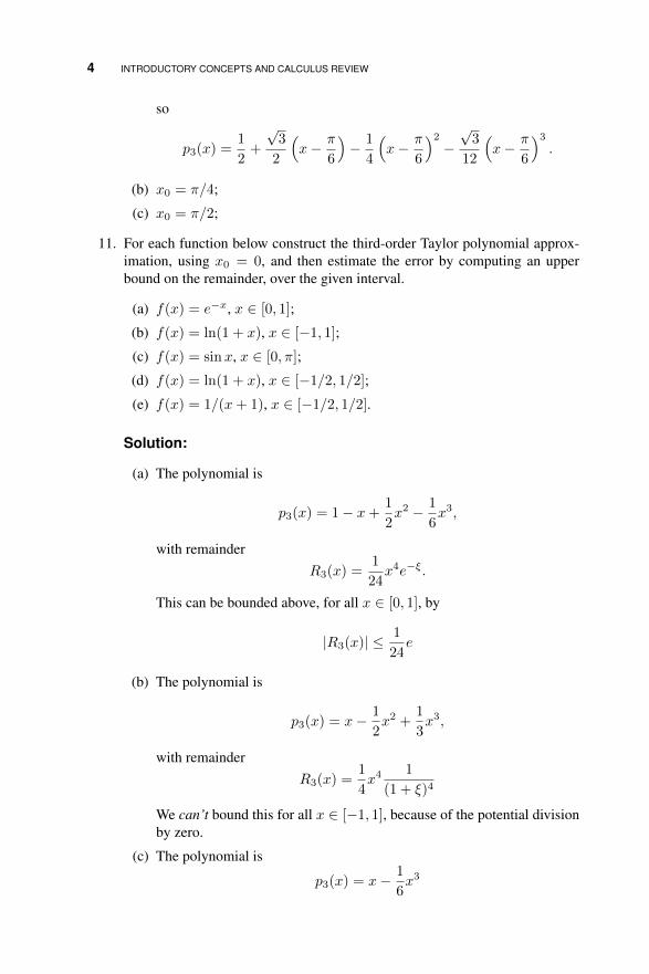
11. For each function below construct the third-order Taylor polynomial approx-imation, using x0 = 0, and then estimate the error by computing an upperbound on the remainder, over the given interval.
(a) f(x) = e−x, x ∈ [0, 1];
(b) f(x) = ln(1 + x), x ∈ [−1, 1];
(c) f(x) = sinx, x ∈ [0, π];
(d) f(x) = ln(1 + x), x ∈ [−1/2, 1/2];
(e) f(x) = 1/(x+ 1), x ∈ [−1/2, 1/2].
Solution:
(a) The polynomial is
p3(x) = 1− x+1
2x2 − 1
6x3,
with remainderR3(x) =
1
24x4e−ξ.
This can be bounded above, for all x ∈ [0, 1], by
|R3(x)| ≤ 1
24e
(b) The polynomial is
p3(x) = x− 1
2x2 +
1
3x3,
with remainderR3(x) =
1
4x4
1
(1 + ξ)4
We can’t bound this for all x ∈ [−1, 1], because of the potential divisionby zero.
(c) The polynomial is
p3(x) = x− 1
6x3

BASIC TOOLS OF CALCULUS 5
with remainder
R3(x) =1
120x5 cos ξ.
This can be bounded above, for all x ∈ [0, π], by
|R3(x)| ≤ π5
120.
(d) The polynomial is the same as in (b), of course,
p3(x) = x− 1
2x2 +
1
3x3,
with remainder
R3(x) =1
4x4
1
(1 + ξ)4
For all x ∈ [−1/2, 1/2] this can be bounded by
R3(x) ≤ 1
4(1/24)
1
(1− (1/2))4=
1
4.
(e) The polynomial is
p3(x) = 1− x+ x2 − x3,
with remainder
R3(x) = x41
(1 + ξ)5
This can be bounded above, for all x ∈ [−1/2, 1/2], by
|R3(x)| ≤ (1/2)41
(1− 1/2)5= 2.
Obviously, this is not an especialy good approximation.
12. Construct a Taylor polynomial approximation that is accurate to within 10−3,over the indicated interval, for each of the following functions, using x0 = 0.
(a) f(x) = sinx, x ∈ [0, π];
(b) f(x) = e−x, x ∈ [0, 1];
(c) f(x) = ln(1 + x), x ∈ [−1/2, 1/2];
(d) f(x) = 1/(x+ 1), x ∈ [−1/2, 1/2];
(e) f(x) = ln(1 + x), x ∈ [−1, 1].

6 INTRODUCTORY CONCEPTS AND CALCULUS REVIEW
Solution:
(a) The remainder here is
Rn(x) =(−1)n+1
(2n+ 1)!x2n+1 cos c,
for c ∈ [0, π]. Therefore, we have
|Rn(x)| ≤ 1
(2n+ 1)!|π|2n+1 ≤ π2n+1
(2n+ 1)!.
Simple manipulations with a calculator then show that
maxx∈[0,π]
|R6(x)| ≤ .4663028067e− 3
butmaxx∈[0,π]
|R5(x)| ≤ .7370430958e− 2.
Therefore the desired Taylor polynomial is
p11(x) = 1− x+1
6x3 − 1
120x5 − 1
7!x7 +
1
9!x9 +
1
11!x11.
(b) The remainder here is
Rn(x) =(−1)n+1
(n+ 1)!xn+1e−c,
for c ∈ [0, 1]. Therefore, we have
|Rn(x)| ≤ 1
(n+ 1)!|x|n+1 ≤ 1
(n+ 1)!.
Simple manipulations with a calculator then show that
maxx∈[0,1]
|R6(x)| ≤ .0001984126984
butmaxx∈[0,1]
|R5(x)| ≤ .1388888889e− 2
Therefore the desired Taylor polynomial is
p6(x) = 1− x+1
2x2 − 1
6x3 +
1
24x4 − 1
120x5 +
1
720x6.
(c) f(x) = ln(1 + x), x ∈ [0, 3/4].

BASIC TOOLS OF CALCULUS 7
Solution: The remainder is now
|Rn(x)| ≤ (1/2)n+1
(n+ 1),
and n = 8 makes the error small enough.(d) f(x) = ln(1 + x), x ∈ [0, 1/2].
13. Repeat the above, this time with a desired accuracy of 10−6.
14. Sinceπ
4= arctan 1,
we can estimate π by estimating arctan 1. How many terms are needed inthe Gregory series for the arctangent to approximate π to 100 decimal places?1,000? Hint: Use the error term in the Gregory series to predict when the errorgets sufficiently small.
Solution: The remainder in the Gregory series approximation is
Rn(x) = (−1)n+1
∫ x
0
t2n+2
1 + t2dt,
so to get 100 decimal places of accuracy for x = 1, we require
|Rn(1)| =∣∣∣∣∫ 1
0
t2n+2
1 + t2dt
∣∣∣∣ ≤ ∫ 1
0
t2n+2dt =1
2n+ 3≤ 10−100,
thus, we have to take n ≥ (10100 − 3)/2 terms. For 1,000 places of accuracywe therefore need n ≥ (101000 − 3)/2 terms.
Obviously this is not the best procedure for computing many digits of π!
15. Elementary trigonometry can be used to show that
arctan(1/239) = 4 arctan(1/5)− arctan(1).
This formula was developed in 1706 by the English astronomer John Machin.Use this to develop a more efficient algorithm for computing π. How manyterms are needed to get 100 digits of accuracy with this form? How manyterms are needed to get 1,000 digits? Historical note: Until 1961 this was thebasis for the most commonly used method for computing π to high accuracy.
Solution: We now have two Gregory series, thus complicating the problem abit. We have
π = 4 arctan(1) = 16 arctan(1/5)− 4 arctan(1/239);
Define pm,n ≈ π as the approximation generated by using an m term Gre-gory series to approximate arctan(1/5) and an n term Gregory series forarctan(1/239). Then we have
pm,n − π = 16Rm(1/5)− 4Rn(1/239),

8 INTRODUCTORY CONCEPTS AND CALCULUS REVIEW
where Rk is the remainder in the Gregory series. Therefore
|pm,n − π| ≤
∣∣∣∣∣16(−1)m+1
∫ 1/5
0
t2m+2
1 + t2dt− 4(−1)n+1
∫ 1/239
0
t2n+2
1 + t2dt
∣∣∣∣∣≤ 16
(2m+ 3)52m+3+
4
(2n+ 3)2392n+3.
To finish the problem we have to apportion the error between the two series,which introduces some arbitrariness into the the problem. If we require thatthey be equally accurate, then we have that
16
(2m+ 3)52m+3≤ ε
and4
(2n+ 3)2392n+3≤ ε.
Using properties of logarithms, these become
log(2m+ 3) + (2m+ 3) log 5 ≥ log 16− log ε
andlog(2n+ 3) + (2n+ 3) log 239 ≥ log 4− log ε.
For ε = (1/2) × 10−100 these are satisfied for m = 70, n = 20. Forε = (1/2)× 10−1000 we get m = 712, n = 209. Changing the apportionmentof the error doesn’t change the results by much at all.
16. In 1896 a variation on Machin’s formula was found:
arctan(1/239) = arctan(1)− 6 arctan(1/8)− 2 arctan(1/57),
and this began to be used in 1961 to compute π to high accuracy. How manyterms are needed when using this expansion to get 100 digits of π? 1,000digits?
Solution: We now have three series to work with, which complicates mattersonly slightly more compared to the previous problem. If we define pk,m,n ≈ πbased on
π = 4 arctan(1) = 24 arctan(1/8) + 8 arctan(1/57) + 4 arctan(1/239),
taking k terms in the series for arctan(1/8), m terms in the series forarctan(1/57), and n terms in the series for arctan(1/239), then we are led tothe inequalities
log(2k + 3) + (2k + 3) log 8 ≥ log 24− log ε,
log(2m+ 3) + (2m+ 3) log 57 ≥ log 8− log ε,

BASIC TOOLS OF CALCULUS 9
andlog(2n+ 3) + (2n+ 3) log 239 ≥ log 4− log ε.
For ε = (1/3) × 10−100 we get k = 54, m = 27, and n = 19; for ε =(1/3)× 10−1000 we get k = 552, m = 283, and n = 209.
Note: In both of these problems a slightly more involved treatment of the errormight lead to fewer terms being required.
17. What is the Taylor polynomial of order 3 for f(x) = x4 + 1, using x0 = 0?
Solution: This is very direct:
f ′(x) = 4x3, f ′′(x) = 12x2, f ′′′(x) = 24x,
so that
p3(x) = 1 + x(0) +1
2x2(0) +
1
6x3(0) = 1.
18. What is the Taylor polynomial of order 4 for f(x) = x4 + 1, using x0 = 0?Simplify as much as possible.
19. What is the Taylor polynomial of order 2 for f(x) = x3 + x, using x0 = 1?
20. What is the Taylor polynomial of order 3 for f(x) = x3 + x, using x0 = 1?Simplify as much as possible.
Solution: We note that f ′′′(1) = 6, so we have (using the solution from theprevious problem)
p4(x) = 3x2 − 2x+ 1 +1
6(x− 1)3(6) = x3 + x.
The polynomial is its own Taylor polynomial.
21. Let p(x) be an arbitrary polynomial of degree less than or equal to n. What isits Taylor polynomial of degree n, about an arbitrary x0?
22. The Fresnel integrals are defined as
C(x) =
∫ x
0
cos(πt2/2)dt
and
S(x) =
∫ x
0
sin(πt2/2)dt.
Use Taylor expansions to find approximations to C(x) and S(x) that are 10−4
accurate for all x with |x| ≤ 12 . Hint: Substitute x = πt2/2 into the Taylor
expansions for the cosine and sine.

10 INTRODUCTORY CONCEPTS AND CALCULUS REVIEW
Solution: We will show the work for the case of S(x), only. We have
S(x) =
∫ x
0
sin(πt2/2)dt =
∫ x
0
pn(t2)dt+
∫ x
0
Rn(t2)dt.
Looking more carefully at the remainder term, we see that it is given by
rn(x) = ±∫ x
0
(t2(2n+3)
(2n+ 3)!cos ξdt.
Therefore,
|rn(x)| ≤∫ 1/2
0
(t2(2n+3)
(2n+ 3)!dt =
(1/2)4n+7
(4n+ 7)(2n+ 3)!.
A little effort with a calculator shows that this is less than 10−4 for n ≥ 1,therefore the polynomial is
p(x) =
∫ x
0
(t2 − (1/6)t6)dt = −x7
42+x3
3.
23. Use the Integral Mean Value Theorem to show that the “pointwise” form (1.3)of the Taylor remainder (usually called the Lagrange form) follows from the“integral” form (1.2) (usually called the Cauchy form).
24. For each function in Problem 11, use the Mean Value Theorem to find a valueM such that
|f(x1)− f(x2)| ≤M |x1 − x2|
is valid for all x1, x2 in the interval used in Problem 11.
Solution: This amounts to finding an upper bound on |f ′| over the intervalgiven. The answers are as given below.
(a) f(x) = e−x, x ∈ [0, 1]; M ≤ 1.
(b) f(x) = ln(1+x), x ∈ [−1, 1];M is unbounded, since f ′(x) = 1/(1+x)and x = −1 is possible.
(c) f(x) = sinx, x ∈ [0, π]; M ≤ 1.
(d) f(x) = ln(1 + x), x ∈ [−1/2, 1/2]; M ≤ 2.
(e) f(x) = 1/(x+ 1), x ∈ [−1/2, 1/2]. M ≤ 4.
25. A function is called monotone on an interval if its derivative is strictly positiveor strictly negative on the interval. Suppose f is continuous and monotoneon the interval [a, b], and f(a)f(b) < 0; prove that there is exactly one valueα ∈ [a, b] such that f(α) = 0.
Solution: Since f is continuous on the interval [a, b] and f(a)f(b) < 0, theIntermediate Value Theorem guarantees that there is a point c where f(c) = 0,

BASIC TOOLS OF CALCULUS 11
i.e., there is at least one root. Suppose now that there exists a second root, γ.Then f(c) = f(γ) = 0. By the Mean Value Theorem, then, there is a point ξbetween c and γ such that
f ′(ξ) =f(γ)− f(c)
γ − c= 0.
But this violates the hypothesis that f is monotone, since a monotone functionmust have a derivative that is strictly positive or strictly negative. Thus wehave a contradiction, thus there cannot exist the second root.
A very acceptable argument can be made by appealing to a graph of thefunction.
26. Finish the proof of the Integral Mean Value Theorem (Theorem 1.5) by writingup the argument in the case that g is negative.
Solution: All that is required is to observe that if g is negative, then we have∫ b
a
g(t)f(t)dt ≤∫ b
a
g(t)fmdt = fm
∫ b
a
g(t)dt
and ∫ b
a
g(t)f(t)dt ≥∫ b
a
g(t)fMdt = fM
∫ b
a
g(t)dt.
The proof is completed as in the text.
27. Prove Theorem 1.6, providing all details.
28. Let ck > 0, be given, 1 ≤ k ≤ n, and let xk ∈ [a, b], 1 ≤ k ≤ n. Then, use theDiscrete Average Value Theorem to prove that, for any function f ∈ C([a, b]),∑n
k=1 ckf(xk)∑nk=1 ck
= f(ξ)
for some ξ ∈ [a, b].
Solution: We can’t apply the Discrete Average Value Theorem to the problemas it is posed originally, so we have to manipulate a bit. Define
γj =cj∑nk=1 ck
;
Thenn∑j=1
γj = 1
and now we can apply the Discrete Average Value Theorem to finish theproblem.

12 INTRODUCTORY CONCEPTS AND CALCULUS REVIEW
29. Discuss, in your own words, whether or not the following statement is true:“The Taylor polynomial of degree n is the best polynomial approximation ofdegree n to the given function near the point x0.”
/ • • • .
1.2 ERROR, APPROXIMATE EQUALITY, AND ASYMPTOTIC ORDERNOTATION
Exercises:
1. Use Taylor’s Theorem to show that ex = 1 + x + O(x2) for x sufficientlysmall.
2. Use Taylor’s Theorem to show that 1−cos xx = 1
2x + O(x3) for x sufficientlysmall.
Solution: We can expand the cosine in a Taylor series as
cosx = 1− 1
2x2 +
1
24x4 cos ξ.
If we substitute this into (1− cosx)/x and simplify, we get
1− cosx
x=
1
2x− 1
24x3 cos ξ,
so that we have∣∣∣∣1− cosx
x− 1
2x
∣∣∣∣ =
∣∣∣∣ 1
24x3 cos ξ
∣∣∣∣ ≤ 1
24|x3| = C|x3|
where C = 1/24. Therefore, 1−cos xx = 1
2x+O(x3).
3. Use Taylor’s Theorem to show that
√1 + x = 1 +
1
2x+O(x2)
for x sufficiently small.
Solution: We have, from Taylor’s Theorem, with x0 = 0,
√1 + x = 1 +
1
2x− 1
8x2(1 + ξ)−3/2,
for some ξ between 0 and x. Since∣∣∣∣18x2(1 + ξ)−3/2∣∣∣∣ ≤ C|x2|

ERROR, APPROXIMATE EQUALITY, AND ASYMPTOTIC ORDER NOTATION 13
for all x sufficiently small, the result follows. For example, we have∣∣∣∣18x2(1 + ξ)−3/2∣∣∣∣ ≤ 1
8× 2√
2|x2|
for all x ∈ [−1/2, 1/2].
4. Use Taylor’s Theorem to show that
(1 + x)−1 = 1− x+ x2 +O(x3)
for x sufficiently small.
Solution: This time, Taylor’s Theorem gives us that
(1 + x)−1 = 1− x+ x2 − x3/(1 + ξ)4
for some ξ between 0 and x. Thus, for all x such that |x| ≤ m,∣∣(1 + x)−1 − (1− x+ x2)∣∣ =
∣∣x3/(1 + ξ)4∣∣ ≤ |x|3/(1−m)4 = C|x|3,
where C = 1/(1−m)4.
5. Show thatsinx = x+O(x3).
6. Recall the summation formula
1 + r + r2 + r3 + · · ·+ rn =n∑k=0
rk =1− rn+1
1− r.
Use this to prove that
n∑k=0
rk =1
1− r+O(rn+1).
Hint: What is the definition of the O notation?
7. Use the above result to show that 10 terms (k = 9) are all that is needed tocompute
S =∞∑k=0
e−k
to within 10−4 absolute accuracy.
Solution: The remainder in the 9 term partial sum is
|R9| =∣∣∣∣ e−10
1− e−1
∣∣∣∣ = 0.000071822 < 10−4.

14 INTRODUCTORY CONCEPTS AND CALCULUS REVIEW
8. Recall the summation formula
n∑k=1
k =n(n+ 1)
2.
Use this to show thatn∑k=1
k =1
2n2 +O(n).
9. State and prove the version of Theorem 1.7 which deals with relationships ofthe form x = xn +O(β(n)).
Solution: The theorem statement might be something like the following:
Theorem: Let x = xn+O(β(n)) and y = yn+O(γ(n)), with bβ(n) > γ(n)for all n sufficiently large. Then
x+ y = xn + yn +O(β(n) + γ(n)),
x+ y = xn + yn +O(β(n)),
Ax = Axn +O(β(n)).
In the last equation, A is an arbitrary constant, independent of n.
The proof parallels the one in the text almost perfectly, and so is omitted.
10. Use the definition of O to show that if y = yh + O(hp), then hy = hyh +O(hp+1).
11. Show that if an = O(np) and bn = O(nq), then anbn = O(np+q).
Solution: We have|an| ≤ Ca|np|
and|bn| ≤ Cb|nq|.
These follow from the definition of the O notation. Therefore
|anbn| ≤ Ca|np||bn| ≤ (Ca|np|)(Cb|nq|) = (CaCb)|np+q|
which implies that anbn = O(np+q).
12. Suppose that y = yh + O(β(h)) and z = zh + O(β(h)), for h sufficientlysmall. Does it follow that y − z = yh − zh (for h sufficiently small)?
13. Show that
f ′′(x) =f(x+ h)− 2f(x) + f(x− h)
h2+O(h2)

A PRIMER ON COMPUTER ARITHMETIC 15
for all h sufficiently small. Hint: Expand f(x ± h) out to the fourth orderterms.
Solution: This is a straight-forward manipulation with the Taylor expansions
f(x+ h) = f(x) + hf ′(x) +1
2h2f ′′(x) +
1
6h3f ′′′(x) +
1
24h4f ′′′′(ξ1)
and
f(x− h) = f(x)− hf ′(x) +1
2h2f ′′(x)− 1
6h3f ′′′(x) +
1
24h4f ′′′′(ξ2).
Add the two expansions to get
f(x+ h) + f(x− h) = 2f(x) + h2f ′′(x) +1
24h4(f ′′′′(ξ1) + f ′′′′(ξ2)).
Now solve for f ′′(x).
14. Explain, in your own words, why it is necessary that the constant C in (1.8) beindependent of h.
/ • • • .
1.3 A PRIMER ON COMPUTER ARITHMETIC
Exercises:
1. In each problem below, A is the exact value, and Ah is an approximation to A.Find the absolute error and the relative error.
(a) A = π, Ah = 22/7;
(b) A = e, Ah = 2.71828;
(c) A = 16 , Ah = 0.1667;
(d) A = 16 , Ah = 0.1666.
Solution:
(a) Abs. error. ≤ 1.265× 10⁻³, rel. error ≤ 4.025× 10⁻⁴;
(b) Abs. error. ≤ 1.828× 10⁻⁶, rel. error ≤ 6.72× 10⁻⁷;
(c) Abs. error. ≤ 3.334× 10⁻⁵, rel. error ≤ 2.000× 10⁻⁴;
(d) Abs. error. ≤ 6.667× 10⁻⁵, rel. error ≤ 4× 10⁻⁴.
2. Perform the indicated computations in each of three ways: (i) Exactly; (ii)Using three-digit decimal arithmetic, with chopping; (iii) Using three-digit

16 INTRODUCTORY CONCEPTS AND CALCULUS REVIEW
decimal arithmetic, with rounding. For both approximations, compute theabsolute error and the relative error.
(a) 16 + 1
10 ;(b) 1
6 ×110 ;
(c) 19 +
(17 + 1
6
);
(d)(17 + 1
6
)+ 1
9 .
3. For each function below explain why a naive construction will be susceptibleto significant rounding error (for x near certain values), and explain how toavoid this error.
(a) f(x) = (√x+ 9− 3)x−1;
(b) f(x) = x−1(1− cosx);(c) f(x) = (1− x)−1(lnx− sinπx);(d) f(x) = (cos(π + x)− cosπ)x−1;(e) f(x) = (e1+x − e1−x)(2x)−1;
Solution: In each case, the function is susceptible to subtractive cancellationwhich will be amplified by division by a small number. The way to avoid theproblem is to use a Taylor expansion to make the subtraction and division bothexplicit operations. For instance, in (a), we would write
f(x) = ((3+(1/6)x−(1/216)x2+O(x3))−3)x−1 = (1/6)−(1/216)x+O(x2).
To get greater accuracy, take more terms in the Taylor expansion.
4. For f(x) = (ex − 1)/x, how many terms in a Taylor expansion are needed toget single precision accuracy (7 decimal digits) for all x ∈ [0, 12 ]? How manyterms are needed for double precision accuracy (14 decimal digits) over thissame range?
5. Using single precision arithmetic, only, carry out each of the following com-putations, using first the form on the left side of the equals sign, then using theform on the right side, and compare the two results. Comment on what youget in light of the material in 1.3.
(a) (x+ ε)3 − 1 = x3 + 3x2ε+ 3xε2 + ε3 − 1, x = 1.0, ε = 0.000001.(b) −b+
√b2 − 2c = 2c(−b−
√b2 − 2c)−1, b = 1, 000, c = π.
Solution: “Single precision” means 6 or 7 decimal digits, so the point of theproblem is to do the computations using 6 or 7 digits.
(a) Using a standard FORTRAN compiler on a low-end UNIX workstation,the author got
(x+ ε)3 − 1 = 0.2861022949218750E − 05

A PRIMER ON COMPUTER ARITHMETIC 17
but
x3 + 3x2ε+ 3xε2 + ε3 − 1 = 0.2980232238769531E − 05.
(b) Using a standard C compiler on a low-end UNIX workstation, the authorgot
−b+√b2 − 2c = −0.003
but2c(−b−
√b2 − 2c)−1 = −0.00314160.
6. Consider the sum
S =m∑k=0
e−14(1−e−0.05k)
where m = 2 × 10⁵. Again using only single precision, compute this twoways: First, by summing in the order indicated in the formula; second, bysumming backwards, i.e., starting with the k = 200, 000 term and ending withthe k = 0 term. Compare your results and comment upon them.
7. Using the computer of your choice, find three values a, b, and c, such that
(a+ b) + c 6= a+ (b+ c).
Repeat for your pocket calculator.
Solution: The key issue is to get an approximation to the machine epsilon,then take a = 1, b = c = (2/3)u or something similar. This will guaranteethat (a + b) + c = a but a + (b + c) > a. Using a standard C compiler ona low-end UNIX workstation, the author was able to determine that a = 1,b = 2 × 10⁻⁷, and c = 3 × 10⁻⁷ will work. On an elderly Sharp calculator,the author found that a = 1, b = 4× 10⁻¹⁰, and c = 4× 10⁻¹⁰ worked.
8. Assume we are using 3-digit decimal arithmetic. For ε = 0.0001, a1 = 5,compute
a2 = a0 +
(1
ε
)a1
for a0 equal to each of 1, 2, and 3. Comment.
9. Let ε ≤ u. Explain, in your own words, why the computation
a2 = a0 +
(1
ε
)a1
is potentially rife with rounding error. (Assume that a0 and a1 are of compa-rable size.) Hint: See previous problem.
Solution: This is just a generalization of the previous problem. If ε is smallenough, then a2 will be independent of a0.

18 INTRODUCTORY CONCEPTS AND CALCULUS REVIEW
10. Using the computer and language of your choice, write a program to estimatethe machine epsilon.
Solution: Using MATLAB on a moderately old personal computer, the authorgot a value of u = 1.1016e− 16. The code is given below.
x = 1.e-10;
for k=1:6000
y = 1 + x;
if y <= 1
disp(’macheps = ’)
disp(x)
break
end
x = x*.99;
end
11. We can compute e−x using Taylor polynomials in two ways, either using
e−x ≈ 1− x+1
2x2 − 1
6x3 + . . .
or using
e−x ≈ 1
1 + x+ 12x
2 + 16x
3 + . . ..
Discuss, in your own words, which approach is more accurate. In particular,which one is more (or less) susceptible to rounding error?
Solution: Because of the alternating signs in the first approach, there is someconcern about subtractive cancellation when it is used.
12. What is the machine epsilon for a computer that uses binary arithmetic, 24 bitsfor the fraction, and rounds? What if it chops?
Solution: Recall that the machine epsilon is the largest number x such thatthe computer returns 1 + x = x. We therefore need to find the largest numberx that can be represented with 24 binary digits such that 1 + x, when roundedto 24 bits, is still equal to 1. This is perhaps best done by explicitly writing outthe addition in binary notation. We have
1 + x = 1.000000000000000000000002
+0.00000000000000000000000dddddddddddddddddddddddd2.
If the machine chops, then we can set all of the d values to 1 and the computerwill still return 1 + x = 1; if the machine rounds, then we need to make thefirst digit a zero. Thus, the desired values are
uround =23∑k=1
2−k−24 = 0.596× 10⁻⁷,

A WORD ON COMPUTER LANGUAGES AND SOFTWARE 19
and
uchop =24∑k=1
2−k−23 = 0.119× 10⁻⁶
13. What is the machine epsilon for a computer that uses octal (base 8) arithmetic,assuming it retains 8 octol digits in the fraction?
/ • • • .
1.4 A WORD ON COMPUTER LANGUAGES AND SOFTWARE
(No exercises in this section.)
1.5 SIMPLE APPROXIMATIONS
Exercises:
1. Consider the error (1.11) in approximating the error function. If we restrictourselves to k ≤ 3, then over what range of values of x is the approximationaccurate to within 10−3?
Solution: We have the inequality
|x8| ≤ 9× 12√π × 10−3
which implies that x ∈ [−.19, .19].
2. If we are interested only in x ∈ [0, 12 ], then how many terms in the errorfunction approximation do we need to take to get an accuracy of 10−4?
3. Repeat the above for x ∈ [0, 1].
Solution: We now have to use k = 6.
4. Assume that x ∈ [0, 1] and write the error in the approximation to the errorfunction using the asymptotic order notation.
5. For
f(x) =
∫ x
0
t−1 sin tdt, x ∈ [−π/4, π/4],
construct a Taylor approximation that is accurate to within 10−4 over theindicated interval.
Solution: Expand the sine function in a Taylor series
sinx = x− 1
6x3 + . . .+
x2n+3
(2n+ 3)!cos ξ

20 INTRODUCTORY CONCEPTS AND CALCULUS REVIEW
and substitute into the integral, then carry out the integration. We concentrateon the remainder term first, in order to find out how many terms we have totake. We have
rn(x) =
∫ x
0
t2n+3
(2n+ 3)!cos ξtdt
so that
|rn(x)| ≤∣∣∣∣∫ x
0
t2n+3
(2n+ 2)!cos ξtdt
∣∣∣∣ ≤ ∫ |x|0
t2n+2
(2n+ 3)!dt =
|x|2n+3
(2n+ 3)(2n+ 3)!.
Since we are interested in x ∈ [−π/4, π/4], we have
Rn = max |rn(x)| ≤ (π/4)2n+3
(2n+ 3)(2n+ 3)!.
Trial and error with a calculator shows that R2 = 0.52 × 10⁻⁵ so n = 2 isgood enough. Thus the polynomial is
p2(x) =
∫ x
0
(1− 1
6t2 +
1
120t4)dt = x− 1
18x3 +
1
600x5.
Note that the way we have done the indexing means that n = 2 is not thesecond order polynomial.
6. Repeat the above for
f(x) =
∫ x
0
e−t2
dt, x ∈[−1
2,
1
2
].
7. Construct a Taylor approximation for
f(x) =
∫ x
0
t−pe−t2
dt, 0 ≤ p < 1, x ∈[0,
1
2
]that is accurate to within 10−3 for all values of p in the indicated range.
8. Does it make a difference in Problem 7 if we restrict p to p ∈ [0, 14 ]?
Solution: It makes a difference because now the error is slightly less, and weare not covering the entire range for p.
9. What is the error in the Taylor polynomial of degree 5 for f(x) = 1/x, usingx0 = 3/4, for x ∈ [ 12 , 1]?
10. How many terms must be taken in the above to get an error of less than 10−2?10−4?
Solution: The remainder, in the general case, is bounded according to
|Rn(x)| ≤ (1/4)n+1 × 2n+2 = (1/2)n.
SIMPLE APPROXIMATIONS 21
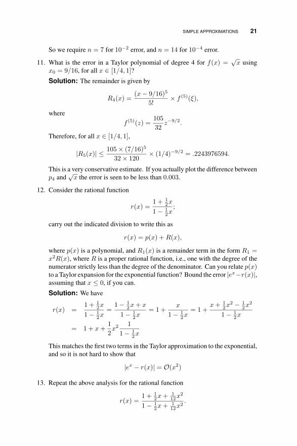
So we require n = 7 for 10−2 error, and n = 14 for 10−4 error.
11. What is the error in a Taylor polynomial of degree 4 for f(x) =√x using
x0 = 9/16, for all x ∈ [1/4, 1]?
Solution: The remainder is given by
R4(x) =(x− 9/16)5
5!× f (5)(ξ),
wheref (5)(z) =
105
32z−9/2.
Therefore, for all x ∈ [1/4, 1],
|R5(x)| ≤ 105× (7/16)5
32× 120× (1/4)−9/2 = .2243976594.
This is a very conservative estimate. If you actually plot the difference betweenp4 and
√x the error is seen to be less than 0.003.
12. Consider the rational function
r(x) =1 + 1
2x
1− 12x
;
carry out the indicated division to write this as
r(x) = p(x) +R(x),
where p(x) is a polynomial, and R1(x) is a remainder term in the form R1 =x2R(x), where R is a proper rational function, i.e., one with the degree of thenumerator strictly less than the degree of the denominator. Can you relate p(x)to a Taylor expansion for the exponential function? Bound the error |ex−r(x)|,assuming that x ≤ 0, if you can.
Solution: We have
r(x) =1 + 1
2x
1− 12x
=1− 1
2x+ x
1− 12x
= 1 +x
1− 12x
= 1 +x+ 1
2x2 − 1
2x2
1− 12x
= 1 + x+1
2x2
1
1− 12x
This matches the first two terms in the Taylor approximation to the exponential,and so it is not hard to show that
|ex − r(x)| = O(x2)
13. Repeat the above analysis for the rational function
r(x) =1 + 1
2x+ 112x
2
1− 12x+ 1
12x2.

22 INTRODUCTORY CONCEPTS AND CALCULUS REVIEW
Can you get a better error in this case?
Solution: A similar computation in both this exercise and the next one showsthe error is now O(x4).
14. Finally, consider the rational function1
r(x) =1 + 1
3x
1− 23x+ 1
6x2.
By dividing out the rational function into a polynomial p(x) plus a remainder,bound the error |ex − r(x)| for all x ≤ 0. Try to get as high an accuracy asyou can in terms of powers of x.
/ • • • .
1.6 APPLICATION: APPROXIMATING THE NATURAL LOGARITHM
Exercises:
1. Write each of the following in the form x = f × 2β for some f ∈ [ 12 , 1].
(a) x = 13;
(b) x = 25;
(c) x = 13 ;
(d) x = 110 .
Solution:
(a) x = 13 = (13/16)× 24;
(b) x = 25 = (25/32)× 25;
(c) x = 13 = (2/3)× 2−1;
(d) x = 110 = (8/10)× 2−3.
2. For each value in the previous problem, compute the logarithm approximationusing the degree 4 Taylor polynomial from (1.12). What is the error comparedto the logarithm on your calculator?
3. Repeat the above for the degree 6 Taylor approximation.
1The functions in these exercises are all examples of what are known as Padé approximations.

APPLICATION: APPROXIMATING THE NATURAL LOGARITHM 23
Solution: The polynomial is
p6(x) = −2.737682073 + 7.999999999x− 13.33333334x2
+15.80246914x3 − 11.85185185x4 + 5.056790124x5
−.9364426155x6.
For each case we get:
(a) p6(25/32) + 5 ln 2 = 3.218875825; ln 25 = 3.218875825;
(b) p6(13/16) + 4 ln 2 = 2.564949354; ln 13 = 2.564949357;
(c) p6(2/3)− ln 2 = −1.098612256; ln 1/3 = −1.098612289;
(d) p6(8/10)− 3 ln 2 = −2.302585094; ln 1/10 = −2.302585093.
4. Repeat the above for the degree 10 Taylor approximation.
5. Implement (as a computer program) the logarithm approximation constructedin this section. Compare it to the intrinsic logarithm function over the interval[ 12 , 1]. What is the maximum observed error?
Solution: A MATLAB script is given, below, which implements the logarithmapproximation. It is not especially efficient. When this is used to computelnx for 1000 values of x uniformly distributed on the interval [1/2, 1], themaximum absolute error observed is about 3.33×10⁻¹⁶. This does not meet thetheoretical standard imposed for the problem, probably because of limitationson the accuracy of MATLAB computations. When the approximation wasimplemented in Maple, taking advantage of the higher precision computationsin Maple, the desired accuracy was observed.
function y = taylog(x)
N = 33;
a = 0.75;
r = log(a);
z = (x - a)/a;
for k=1:N
zL(k) = -(-z)^k;
rL(k) = 1/k;
end
y = sum(zL.*rL) + r;
6. Let’s consider how we might improve on our logarithm approximation fromthis section.
(a) Compute the Taylor expansions, with remainder, for ln(1+x) and ln(1−x) (use the integral of the geometric series, to get the remainder term).
24 INTRODUCTORY CONCEPTS AND CALCULUS REVIEW
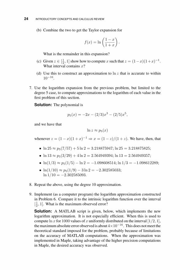
(b) Combine the two to get the Taylor expansion for
f(x) = ln
(1− x1 + x
).
What is the remainder in this expansion?
(c) Given z ∈ [ 12 , 1] show how to compute x such that z = (1−x)(1+x)−1.What interval contains x?
(d) Use this to construct an approximation to ln z that is accurate to within10−16.
7. Use the logarithm expansion from the previous problem, but limited to thedegree 5 case, to compute approximations to the logarithm of each value in thefirst problem of this section.
Solution: The polynomial is
p5(x) = −2x− (2/3)x3 − (2/5)x5,
and we have thatln z ≈ p5(x)
whenever z = (1− x)(1 + x)−1 ⇒ x = (1− z)/(1 + z). We have, then, that
• ln 25 ≈ p5(7/57) + 5 ln 2 = 3.218875947; ln 25 = 3.218875825;
• ln 13 ≈ p5(3/29) + 4 ln 2 = 2.564949394; ln 13 = 2.564949357;
• ln(1/3) ≈ p5(1/5)− ln 2 = −1.098608514; ln 1/3 = −1.098612289;
• ln(1/10) ≈ p5(1/9)− 3 ln 2 = −2.302585033;ln 1/10 = −2.302585093.
8. Repeat the above, using the degree 10 approximation.
9. Implement (as a computer program) the logarithm approximation constructedin Problem 6. Compare it to the intrinsic logarithm function over the interval[ 12 , 1]. What is the maximum observed error?
Solution: A MATLAB script is given, below, which implements the newlogarithm approximation. It is not especially efficient. When this is used tocompute lnx for 1000 values of x uniformly distributed on the interval [1/2, 1],the maximum absolute error observed is about 4×10⁻¹⁶. This does not meet thetheoretical standard imposed for the problem, probably because of limitationson the accuracy of MATLAB computations. When the approximation wasimplemented in Maple, taking advantage of the higher precision computationsin Maple, the desired accuracy was observed.

A BRIEF HISTORY OF COMPUTING 25
function y = taylog2(z)
x = (1-z)/(1+z);
c = [1:(2):33];
a = -2./c;
y = sum(a.*(x.^c));
10. Try to use the ideas from this section to construct an approximation to thereciprocal function, f(x) = x−1, that is accurate to within 10−16 over theinterval [ 1
2 , 1].
/ • • • .
1.7 A BRIEF HISTORY OF COMPUTING
(No exercises in this section.)


CHAPTER 2
A SURVEY OF SIMPLE METHODS ANDTOOLS
2.1 HORNER’S RULE AND NESTED MULTIPLICATION
Exercises:
1. Write each of the following polynomials in nested form.
(a) x3 + 3x+ 2;
(b) x6 + 2x4 + 4x2 + 1;
(c) 5x6 + x5 + 3x4 + 3x3 + x2 + 1;
(d) x2 + 5x+ 6.
Solution:
(a) x3 + 3x+ 2 = 2 + x(3 + x2);
(b) x6 + 2x4 + 4x2 + 1 = 1 + x2(4 + x2(2 + x2));
(c) 5x6 +x5 + 3x4 + 3x3 +x2 + 1 = 1 +x2(1 +x(3 +x(3 +x(1 + 5x))));
Solutions Manual to Accompany An Introduction to Numerical Methods and Analysis,Second Edition. By James F. EppersonCopyright c© 2013 John Wiley & Sons, Inc.
27
28 A SURVEY OF SIMPLE METHODS AND TOOLS
(d) x2 + 5x+ 6 = 6 + x(5 + x).
2. Write each of the following polynomials in nested form, but this time takeadvantage of the fact that they involve only even powers of x to minimize thecomputations.
(a) 1 + x2 + 12x
4 + 16x
6;
(b) 1− 12x
2 + 124x
4.
3. Write each of the following polynomials in nested form.
(a) 1− x+ x2 − x3;
(b) 1− x2 + 12x
4 − 16x
6;
(c) 1− x+ 12x
2 − 13x
3 − 14x
5.
Solution:
(a) 1− x+ x2 − x3 = 1 + x((−1) + x(1− x));
(b) 1− x2 + 12x
4 − 16x
6 = 1 + x2((−1) + x2((1/2)− (1/6)x2));
(c) 1 − x + 12x
2 − 13x
3 − 14x
5 = 1 + x((−1) + x((1/2) + x((−1/3) +x(−1/4)))).
4. Write a computer code that takes a polynomial, defined by its coefficients, andevaluates that polynomial and its first derivative using Horner’s rule. Test thiscode by applying it to each of the polynomials in Problem 1.
Solution: The following is a MATLAB script which does the assigned task,using the less efficient approach to computing the derivative.
function [y, yp] = horner1(a,x)
n = length(a);
y = a(n);
for k=(n-1):(-1):1
y = a(k) + y*x;
end
%
yp = (n-1)*a(n);
for k=(n-1):(-1):2
yp = (k-1)*a(k) + yp*x;
end
5. Repeat the above, using the polynomials in Problem 2 as the test set.
Solution: The same script can be used, of course.
6. Repeat the above, using the polynomials in Problem 3 as the test set.

HORNER’S RULE AND NESTED MULTIPLICATION 29
7. Consider the polynomial
p(x) = 1 + (x− 1) +1
6(x− 1)(x− 2) +
1
7(x− 1)(x− 2)(x− 4).
This can be written in “nested-like” form by factoring out each binomial termas far as it will go, thus:
p(x) = 1 + (x− 1)
(1 + (x− 2)
(1
6+
1
7(x− 4)
)).
Write each of the following polynomials in this kind of nested form.
(a) p(x) = 1 + 13x−
160x(x− 3);
(b) p(x) = −1+ 67 (x−1/2)− 5
21 (x−1/2)(x−4)+ 17 (x−1/2)(x−4)(x−2);
(c) p(x) = 3 + 15 (x− 8)− 1
60 (x− 8)(x− 3).
Solution:
(a) p(x) = 1 + 13x−
160x(x− 3) = 1 + x((1/3)− (1/60)(x− 3));
(b) p(x) = −1+ 67 (x−1/2)− 5
21 (x−1/2)(x−4)+ 17 (x−1/2)(x−4)(x−
2) = −1 + (x− (1/2))((6/7) + (x− 4)((−5/21) + (1/7)(x− 2)));
(c) p(x) = 3 + 15 (x − 8) − 1
60 (x − 8)(x − 3) = 3 + (x − 8)((1/5) −(1/60)(x− 3)).
8. Write a computer code that computes polynomial values using the kind ofnested form used in the previous problem, and test it on each of the polynomialsin that problem.
9. Write a computer code to do Horner’s rule on a polynomial defined by itscoefficients. Test it out by using the polynomials in the previous problems.Verify that the same values are obtained when Horner’s rule is used as when anaive evaluation is done.
10. Write out the Taylor polynomial of degree 5 for approximating the exponentialfunction, using x0 = 0, using the Horner form. Repeat for the degree 5 Taylorapproximation to the sine function. (Be sure to take advantage of the fact thatthe Taylor expansion to the sine uses only odd powers.)
Solution: For the exponential function, we get
p5(x) = 1 + x(1 + x((1/2) + x((1/6) + x((1/24) + (1/120)x))));
for the sine function we get
p5(x) = x(1 + x2((−1/6) + (1/120)x2)).

30 A SURVEY OF SIMPLE METHODS AND TOOLS
11. For each function in Problem 11 of 1.1, write the polynomial approximationin Horner form, and use this as the basis for a computer program that approxi-mates the function. Compare the accuracy you actually achieve (based on thebuilt-in intrinsic functions on your computer) to that which was theoreticallyestablished. Be sure to check that the required accuracy is achieved over theentire interval in question.
12. Repeat the above, except this time compare the accuracy of the derivativeapproximation constructed by taking the derivative of the approximating poly-nomial. Be sure to use the derivative form of Horner’s rule to evaluate thepolynomial.
/ • • • .
2.2 DIFFERENCE APPROXIMATIONS TO THE DERIVATIVE
Exercises:
1. Use the methods of this section to show that
f ′(x) =f(x)− f(x− h)
h+O(h).
Solution: We have, for any a, that
f(x+ a) = f(x) + af ′(x) +1
2a2f ′′(ξ).
Therefore, taking a = −h,
f(x+ a) = f(x− h) = f(x)− hf ′(x) +1
2h2f ′′(ξ)
⇒ f ′(x) =f(x)− f(x− h)
h+
1
2hf ′′(ξ).
2. Compute, by hand, approximations to f ′(1) for each of the following functions,using h = 1/16 and each of the derivative approximations contained in (2.1)and (2.5).
(a) f(x) =√x+ 1;
(b) f(x) = arctanx;
(c) f(x) = sinπx;
(d) f(x) = e−x;

DIFFERENCE APPROXIMATIONS TO THE DERIVATIVE 31
(e) f(x) = lnx;
3. Write a computer program which uses the same derivative approximations asin the previous problem to approximate the first derivative at x = 1 for eachof the following functions, using h−1 = 4, 8, 16, 32. Verify that the predictedtheoretical accuracy is obtained.
(a) f(x) =√x+ 1;
(b) f(x) = arctanx;(c) f(x) = sinπx.(d) f(x) = e−x;(e) f(x) = lnx;
Solution: I wrote a simple FORTRAN program to do this for the single caseof (b). The results I got, using double precision, are in Table 2.1. Note that the
Table 2.1 Derivative Approximations
h−1 D1(h) Error Ratio D2(h) Error Ratio4 0.44262888 0.573711E-01 0.000 0.50510855 0.510855E-02 0.0008 0.47004658 0.299534E-01 1.915 0.50129595 0.129595E-02 3.94216 0.48470016 0.152998E-01 1.958 0.50032514 0.325139E-03 3.98632 0.49226886 0.773114E-02 1.979 0.50008136 0.813564E-04 3.99664 0.49611409 0.388591E-02 1.990 0.50002034 0.203436E-04 3.999
128 0.49805196 0.194804E-02 1.995 0.50000509 0.508617E-05 4.000256 0.49902471 0.975291E-03 1.997 0.50000127 0.127156E-05 4.000512 0.49951204 0.487963E-03 1.999 0.50000032 0.317891E-06 4.0001024 0.49975594 0.244061E-03 1.999 0.50000008 0.794728E-07 4.000
error goes down by a factor of 2 for D1(h), and a factor of 4 for D2(h), thusconfirming the theoretical accuracy.
4. Use the approximations from this section to fill in approximations to the missingvalues in Table 2.2 (Table 2.4 in the text).
5. Use the error estimate (2.5) for the centered difference approximation to thefirst derivative to prove that this approximation will be exact for any quadraticpolynomial.
Solution: We have that
f ′(x)− f(x+ h)− f(x− h)
2h= Ch2f ′′′(ξ),
for some ξ between x−h and x+h. If f is a quadratic, then it has the generalform
f(x) = ax2 + bx+ c,

32 A SURVEY OF SIMPLE METHODS AND TOOLS
Table 2.2 Table for Problem 4.
x f(x) f ′(x)
1.00 1.00000000001.10 0.95135076991.20 0.91816874241.30 0.89747069631.40 0.88726381751.50 0.88622692551.60 0.89351534931.70 0.90863873291.80 0.93138377101.90 0.96176583192.00 1.0000000000
for given constants a, b, and c. But the third derivative of this kind of functionwill always be identically zero.
6. Find coefficients A, B, and C so that
(a) f ′(x) = Af(x) +Bf(x+ h) + Cf(x+ 2h) +O(h2);
(b) f ′(x) = Af(x) +Bf(x− h) + Cf(x− 2h) +O(h2).
Hint: Use Taylor’s theorem.
Solution: Write out Taylor expansions for f(x+ h) and f(x+ 2h), thus:
f(x+ h) = f(x) + hf ′(x) + (h2/2)f ′′(x) +O(h3)
andf(x+ 2h) = f(x) + 2hf ′(x) + 2h2f ′′(x) +O(h3).
Multiply the first one by 4, and subtract the two of them, to get
4f(x+ h)− f(x+ 2h) = 3f(x) + 2hf ′(x) +O(h3);
solve this for f ′ to get
f ′(x) = (−3/2h)f(x) + (2/h)f(x+ h) + (−1/2h)f(x+ 2h) +O(h2)
so that A = −3/2h, B = 2/h, and C = −1/2h. A similar approach worksfor (b), with A = 3/2, B = −2/h, and C = 1/h.
7. Fill in the data from Problem 4 using methods that are O(h2) at each point.Hint: See the previous problem.

DIFFERENCE APPROXIMATIONS TO THE DERIVATIVE 33
8. Use Taylor’s Theorem to show that the approximation
f ′(x) ≈ 8f(x+ h)− 8f(x− h)− f(x+ 2h) + f(x− 2h)
12h
is O(h4).
Solution: We have
f(x+ h) = f(x) + hf ′(x) + (h2/2)f ′′(x) + (h3/6)f ′′′(x)
+(h4/24)f ′′′′(x) +O(h5),
f(x+ 2h) = f(x) + 2hf ′(x) + 2h2f ′′(x) + (4h3/3)f ′′′(x)
+(2h4/3)f ′′′′(x) +O(h5),
f(x− h) = f(x)− hf ′(x) + (h2/2)f ′′(x)− (h3/6)f ′′′(x)
+(h4/24)f ′′′′(x) +O(h5),
and
f(x− 2h) = f(x)− 2hf ′(x) + 2h2f ′′(x)− (4h3/3)f ′′′(x)
+(2h4/3)f ′′′′(x) +O(h5).
Therefore,
8f(x+ h)− 8f(x− h) = 16hf ′(x) + (8h3/3)f ′′′(x) +O(h5)
and
f(x+ 2h)− f(x− 2h) = 4hf ′(x) + (8h3/3)f ′′′(x) +O(h5).
Hence,
8f(x+ h)− 8f(x− h)− f(x+ 2h) + f(x− 2h) = 12hf ′(x) +O(h5),
so that, solving for f ′, we get the desired result.
9. Use the derivative approximation from Problem 8 to approximate f ′(1) for thesame functions as in Problem 3. Verify that the expected rate of decrease isobserved for the error.
10. Use the derivative approximation from Problem 8 to fill in as much as possibleof the table in Problem 4.
Solution: Because this formula uses more points that are farther from thepoint of interest than did the previous formulas, we cannot do as much of the

34 A SURVEY OF SIMPLE METHODS AND TOOLS
table as before. We get:
f ′(1.2) ≈ −.2652536725
f ′(1.3) ≈ −.1517629626
f ′(1.4) ≈ −.05441397741
f ′(1.5) ≈ .03237018117
f ′(1.6) ≈ .1126454212
f ′(1.7) ≈ .1895070563
f ′(1.8) ≈ .2654434511
11. Let f(x) = arctanx. Use the derivative approximation from Problem 8 toapproximate f ′( 1
4π) using h−1 = 2, 4, 8, . . .. Try to take h small enough thatthe rounding error effect begins to dominate the mathematical error. For whatvalue of h does this begin to occur? (You may have to restrict yourself toworking in single precision.)
12. Use Taylor expansions for f(x±h) to derive anO(h2) accurate approximationto f ′′ using f(x) and f(x±h). Provide all the details of the error estimate. Hint:Go out as far as the fourth derivative term, and then add the two expansions.
Solution: We have
f(x+ h) = f(x) + hf ′(x) + (h2/2)f ′′(x) + (h3/6)f ′′′(x) +O(h4),
and
f(x− h) = f(x)− hf ′(x) + (h2/2)f ′′(x)− (h3/6)f ′′′(x) +O(h4),
so thatf(x+ h) + f(x− h) = 2f(x) + h2f ′′(x) +O(h4).
Thus, solving for the second derivative yields
f ′′(x) =f(x+ h)− 2f(x) + f(x− h)
h2+O(h2).
13. Let h > 0 and η > 0 be given, where η = θh, for 0 < θ < 1. Let f be somesmooth function. Use Taylor expansions for f(x + h) and f(x − η) in termsof f and its derivatives at x in order to construct an approximation to f ′(x)that depends on f(x+ h), f(x), and f(x− η), and which is O(h2) accurate.Check your work by verifying that for θ = 1⇒ η = h you get the same resultsas in the text.
Solution: We write the two Taylor expansions
f(x+ h) = f(x) + hf ′(x) +1
2h2f ′′(x) +
1
6h3f ′′′(c1)

DIFFERENCE APPROXIMATIONS TO THE DERIVATIVE 35
andf(x− η) = f(x)− ηf ′(x) +
1
2η2f ′′(x)− 1
6η3f ′′′(c2).
If we simply subtract these, the second derivative terms will not cancel out(because h 6= η), so we have to multiply the first expansion by η2 and thesecond one by h2 to get
η2f(x+ h) = η2f(x) + η2hf ′(x) +1
2η2h2f ′′(x) +
1
6η2h3f ′′′(c1)
and
h2f(x− η) = h2f(x)− h2ηf ′(x) +1
2h2η2f ′′(x)− 1
6h2η3f ′′′(c2).
Now subtract to get
η2f(x+ h)− h2f(x− η) = (η2 − h2)f(x) + (η2h− h2η)f ′(x)
+ +1
6(η2h3f ′′′(c1) + h2η3f ′′′(c2)).
Solve for f ′(x) to get
f ′(x) =η2f(x+ h)− (η2 − h2)f(x)− h2f(x− η)
η2h− h2η
−1
6
η2h3f ′′′(c1) + h2η3f ′′′(c2)
η2h− h2η.
Because we assumed η = θh there is substantial simplification that we can doto get
f ′(x) =θ2f(x+ h)− (θ2 − 1)f(x)− f(x− η)
θ2h− hθ
−1
6
θ2h2f ′′′(c1) + h2θ3f ′′′(c2)
θ2 − θ,
which is sufficient to establish the O(h2) estimate for the error.
14. Write a computer program to test the approximation to the second derivativefrom Problem 12 by applying it to estimate f ′′(1) for each of the followingfunctions, using h−1 = 4, 8, 16, 32. Verify that the predicted theoreticalaccuracy is obtained.
(a) f(x) = e−x;
(b) f(x) = cosπx;
(c) f(x) =√
1 + x;
(d) f(x) = lnx;

36 A SURVEY OF SIMPLE METHODS AND TOOLS
15. Define the following function:
f(x) = ln(e√x2+1 sin(πx) + tanπx).
Compute values of f ′ over the range [0, 14 ] using two methods:
(a) Using the centered-difference formula from (2.5);(b) Using ordinary calculus to find the formula for f ′.
Comment.
Solution: The function f is designed to make direct computation of f ′ adifficult task for the average undergraduate student, thus highlighting thatthere are times when being able to approximate the derivative as was done inthis section might be preferable to doing the exact computation.
16. Let f(x) = ex, and consider the problem of approximating f ′(1), as in thetext. LetD1(h) be the difference approximation in (2.1). Using the appropriatevalues in Table 2.1, compute the new approximations
∆1(h) = 2D1(h)−D1(2h);
and compare these values to the exact derivative value. Are they more orless accurate that the corresponding values of D1? Try to deduce, from yourcalculations, how the error depends on h.
Solution: For the sake of completeness we have reproduced the table fromthe text. Using those values we can compute
∆1(.25) = 2D1(.25)−D1(.5) = 2.649674415
e1 −∆1(.25) = 0.068607413;
∆1(.125) = 2D1(.125)−D1(.25) = 2.702717782
e1 −∆1(.125) = 0.015564046;
∆1(.0625) = 2D1(.0625)−D1(.125) = 2.714572906
e1 −∆1(.0625) = 0.003708922;
∆1(.03125) = 2D1(.03125)−D1(.0625) = 2.717372894
e1 −∆1(.03125) = 0.00090834.
The error appears to be going down by a factor of 4 as h is cut in half.
17. Repeat the above idea for f(x) = arctan(x), x = 1 (but this time you willhave to compute the original D1(h) values).
18. By keeping more terms in the Taylor expansion for f(x + h), show that theerror in the derivative approximation (2.1) can be written as
f ′(x)−(f(x+ h)− f(x)
h
)= −1
2hf ′′(x)− 1
6h2f ′′′(x)− ... (2.1)
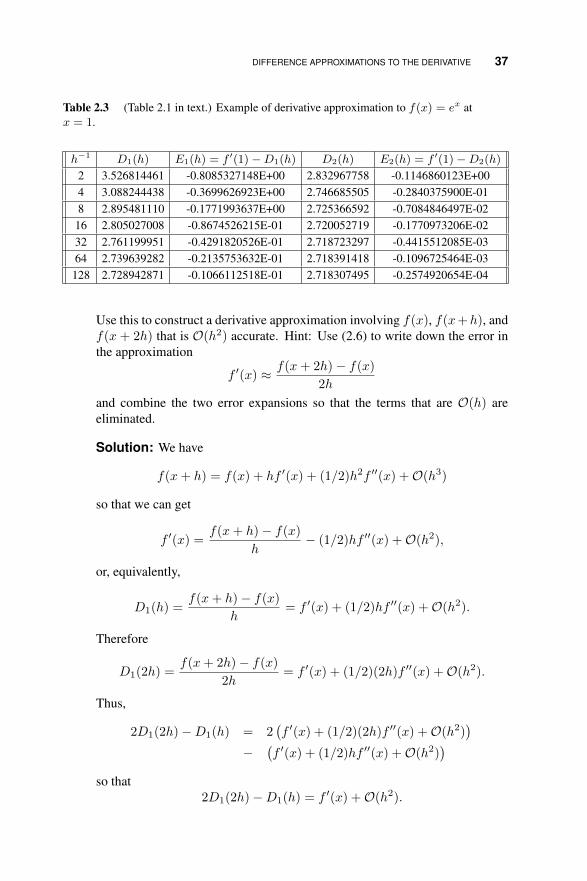
DIFFERENCE APPROXIMATIONS TO THE DERIVATIVE 37
Table 2.3 (Table 2.1 in text.) Example of derivative approximation to f(x) = ex atx = 1.
h−1 D1(h) E1(h) = f ′(1)−D1(h) D2(h) E2(h) = f ′(1)−D2(h)
2 3.526814461 -0.8085327148E+00 2.832967758 -0.1146860123E+004 3.088244438 -0.3699626923E+00 2.746685505 -0.2840375900E-018 2.895481110 -0.1771993637E+00 2.725366592 -0.7084846497E-02
16 2.805027008 -0.8674526215E-01 2.720052719 -0.1770973206E-0232 2.761199951 -0.4291820526E-01 2.718723297 -0.4415512085E-0364 2.739639282 -0.2135753632E-01 2.718391418 -0.1096725464E-03128 2.728942871 -0.1066112518E-01 2.718307495 -0.2574920654E-04
Use this to construct a derivative approximation involving f(x), f(x+h), andf(x + 2h) that is O(h2) accurate. Hint: Use (2.6) to write down the error inthe approximation
f ′(x) ≈ f(x+ 2h)− f(x)
2h
and combine the two error expansions so that the terms that are O(h) areeliminated.
Solution: We have
f(x+ h) = f(x) + hf ′(x) + (1/2)h2f ′′(x) +O(h3)
so that we can get
f ′(x) =f(x+ h)− f(x)
h− (1/2)hf ′′(x) +O(h2),
or, equivalently,
D1(h) =f(x+ h)− f(x)
h= f ′(x) + (1/2)hf ′′(x) +O(h2).
Therefore
D1(2h) =f(x+ 2h)− f(x)
2h= f ′(x) + (1/2)(2h)f ′′(x) +O(h2).
Thus,
2D1(2h)−D1(h) = 2(f ′(x) + (1/2)(2h)f ′′(x) +O(h2)
)−
(f ′(x) + (1/2)hf ′′(x) +O(h2)
)so that
2D1(2h)−D1(h) = f ′(x) +O(h2).

38 A SURVEY OF SIMPLE METHODS AND TOOLS
19. Apply the method derived above to the list of functions in Problem 3, andconfirm that the method is as accurate in practice as is claimed.
20. Let f(x) = ex, and consider the problem of approximating f ′(1), as in thetext. LetD2(h) be the difference approximation in (2.5). Using the appropriatevalues in Table 2.3, compute the new approximations
∆2(h) = (4D2(h)−D2(2h))/3;
and compare these values to the exact derivative value. Are they more orless accurate that the corresponding values of D2? Try to deduce, from yourcalculations, how the error depends on h.
Solution: The D2(h) values are
D2(1/2) = 2.832967758
D2(1/4) = 2.746685505
D2(1/8) = 2.725366592
D2(1/16) = 2.720052719
D2(1/32) = 2.718723297
D2(1/64) = 2.718391418
D2(1/128) = 2.718307495
from which we get that
∆2(1/4) = 2.717924754
∆2(1/8) = 2.718260288
∆2(1/16) = 2.718281428
∆2(1/32) = 2.718280156
∆2(1/64) = 2.718280792
∆2(1/128) = 2.718279521.
These values are, initially, much more accurate thanD2(h), although roundingerror begins to corrupt the computation. It can be shown that this approximationis O(h4).
21. Repeat the above idea for f(x) = arctan(x), x = 1 (but this time you willhave to compute the original D2(h) values).
22. The same ideas as in Problem 18 can be applied to the centered differenceapproximation (2.5). Show that in this case the error satisfies
f ′(x)− f(x+ h)− f(x− h)
2h= −1
6h2f ′′′(x)− 1
120h4f ′′′′′(x)− ... (2.2)
DIFFERENCE APPROXIMATIONS TO THE DERIVATIVE 39
Use this to construct a derivative approximation involving f(x ± h), andf(x± 2h) that is O(h4) accurate.
Solution: Since
f(x+ h) = f(x) + hf ′(x) + (1/2)h2f ′′(x) + (1/6)h3f ′′′(x)
+(1/24)h4f ′′′′(x) +O(h5)
and
f(x− h) = f(x)− hf ′(x) + (1/2)h2f ′′(x)− (1/6)h3f ′′′(x)
+(1/24)h4f ′′′′(x) +O(h5),
we have that
f(x+ h)− f(x− h) = 2hf ′(x) + (1/3)h3f ′′′(x) +O(h5)
or,
f ′(x)− f(x+ h)− f(x− h)
2h= (1/6)h2f ′′′(x) +O(h4).
Therefore,
f ′(x)− f(x+ 2h)− f(x− 2h)
4h= (4/6)h2f ′′′(x) +O(h4),
so that
4
(f ′(x)− f(x+ h)− f(x− h)
2h
)−(f ′(x)− f(x+ 2h)− f(x− 2h)
4h
)= O(h4).
We can manipulate with the left side to get that
3f ′(x)− 8(f(x+ h)− f(x− h))− (f(x+ 2h)− f(x− 2h))
4h= O(h4),
so that finally we have
f ′(x)− 8(f(x+ h)− f(x− h))− (f(x+ 2h)− f(x− 2h))
12h= O(h4).
This is simply an alternate derivation of the method from Exercise 8.
23. Apply the method derived above to the list of functions in Problem 3, andconfirm that the method is as accurate in practice as is claimed.
/ • • • .
40 A SURVEY OF SIMPLE METHODS AND TOOLS
2.3 APPLICATION: EULER’S METHOD FOR INITIAL VALUEPROBLEMS
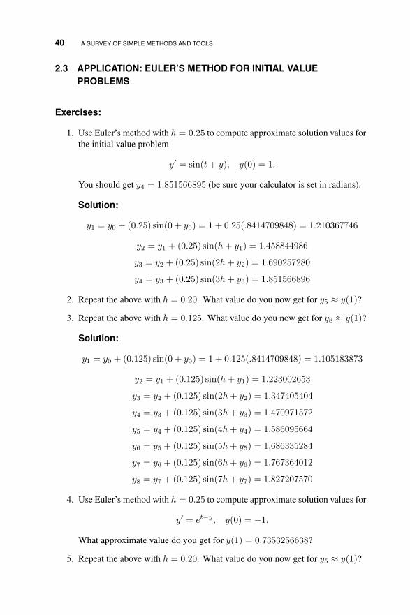
Exercises:
1. Use Euler’s method with h = 0.25 to compute approximate solution values forthe initial value problem
y′ = sin(t+ y), y(0) = 1.
You should get y4 = 1.851566895 (be sure your calculator is set in radians).
Solution:
y1 = y0 + (0.25) sin(0 + y0) = 1 + 0.25(.8414709848) = 1.210367746
y2 = y1 + (0.25) sin(h+ y1) = 1.458844986
y3 = y2 + (0.25) sin(2h+ y2) = 1.690257280
y4 = y3 + (0.25) sin(3h+ y3) = 1.851566896
2. Repeat the above with h = 0.20. What value do you now get for y5 ≈ y(1)?
3. Repeat the above with h = 0.125. What value do you now get for y8 ≈ y(1)?
Solution:
y1 = y0 + (0.125) sin(0 + y0) = 1 + 0.125(.8414709848) = 1.105183873
y2 = y1 + (0.125) sin(h+ y1) = 1.223002653
y3 = y2 + (0.125) sin(2h+ y2) = 1.347405404
y4 = y3 + (0.125) sin(3h+ y3) = 1.470971572
y5 = y4 + (0.125) sin(4h+ y4) = 1.586095664
y6 = y5 + (0.125) sin(5h+ y5) = 1.686335284
y7 = y6 + (0.125) sin(6h+ y6) = 1.767364012
y8 = y7 + (0.125) sin(7h+ y7) = 1.827207570
4. Use Euler’s method with h = 0.25 to compute approximate solution values for
y′ = et−y, y(0) = −1.
What approximate value do you get for y(1) = 0.7353256638?
5. Repeat the above with h = 0.20. What value do you now get for y5 ≈ y(1)?

APPLICATION: EULER’S METHOD FOR INITIAL VALUE PROBLEMS 41
Solution: We have the computation
yn+1 = yn + hetn−yn
where h = 0.2, t0 = 0, and y0 = −1. Hence
y1 = y0 + het0−y0 = −1 + (0.2)e0−(−1) = −0.4563436344,
y2 = y1 + het1−y1 = −0.4563436344 + (0.2)e0.2−(−0.4563436344)
= −0.0707974456,
y3 = y2 + het2−y2 = −0.0707974456 + (0.2)e0.4−(−0.0707974456)
= 0.2494566764,
y4 = y3 + het3−y3 = 0.2494566764 + (0.2)e0.6−(0.2494566764)
= 0.5334244306,
y5 = y4 + het4−y4 = 0.5334244306 + (0.2)e0.8−(0.5334244306)
= 0.7945216786.
6. Repeat the above with h = 0.125. What value do you now get for y8 ≈ y(1)?
7. Use Euler’s method with h = 0.0625 to compute approximate solution valuesover the interval 0 ≤ t ≤ 1 for the initial value problem
y′ = t− y, y(0) = 2,
which has exact solution y(t) = 3e−t + t− 1. Plot your approximate solutionas a function of t, and plot the error as a function of t.
Solution: The plots are given in Figures 2.1 and 2.2.
0 0.1 0.2 0.3 0.4 0.5 0.6 0.7 0.8 0.9 11
1.1
1.2
1.3
1.4
1.5
1.6
1.7
1.8
1.9
2
Figure 2.1 Exact solution forExercise 2.3.7.
0 0.1 0.2 0.3 0.4 0.5 0.6 0.7 0.8 0.9 10
0.005
0.01
0.015
0.02
0.025
0.03
0.035
0.04
Figure 2.2 Error plot forExercise 2.3.7.
8. Repeat the above for the equation
y′ = et−y, y(0) = −1,

42 A SURVEY OF SIMPLE METHODS AND TOOLS
which has exact solution y = ln(et − 1 + e−1).
9. Repeat the above for the equation
y′ + y = sin t, y(0) = −1,
which has exact solution y = (sin t− cos t− e−t)/2.
Solution: The plots are given in Figures 2.3 and 2.4.
0 0.1 0.2 0.3 0.4 0.5 0.6 0.7 0.8 0.9 1−1
−0.9
−0.8
−0.7
−0.6
−0.5
−0.4
−0.3
−0.2
−0.1
0
Figure 2.3 Exact solution forExercise 2.3.9.
0 0.1 0.2 0.3 0.4 0.5 0.6 0.7 0.8 0.9 1−3.5
−3
−2.5
−2
−1.5
−1
−0.5
0x 10−3
Figure 2.4 Error plot for Exercise2.3.9.
10. Use Euler’s method to compute approximate solutions to each of the initialvalue problems below, using h−1 = 2, 4, 8, 16. Compute the maximum errorover the interval [0, 1] for each value of h. Plot your approximate solutions forthe h = 1/16 case. Hint: Verify that your code works by using it to reproducethe results given for the examples in the text.
(a) y′ = t− y, y(0) = 2; y(t) = 3e−t + t− 1.
(b) y′ + 4y = 1, y(0) = 1; y(t) = 14 (3e−4t + 1).
(c) y′ = −y ln y, y(0) = 3; y(t) = e(ln 3)e−t
.
11. Consider the approximate values in Tables 2.5 and 2.6 in the text. Let y8kdenote the approximate values for h = 1/8, and y16k denote the approximatevalues for h = 1/16. Note that
y8k ≈ y(k/8)
andy162k ≈ y(2k/16) = y(k/8) ≈ y8k,
thus y8k and y162k are both approximations to the same value. Compute the setof new approximations
uk = 2y162k − y8k

APPLICATION: EULER’S METHOD FOR INITIAL VALUE PROBLEMS 43
and compare these to the corresponding exact solution values. Are they betteror worse as an approximation?
Solution: Table 2.4 shows the new solution and the error, which is muchsmaller than that obtained using Euler’s method directly.
Table 2.4 Solution values for Exercise 2.3.11.
tk uk y(tk)− uk
0.000 -1.00000000000000 00.125 -0.87500508526970 -0.000004832944650.250 -0.75013901623461 -0.000015606529150.375 -0.62573474516817 -0.000027440640450.500 -0.50230696317037 -0.000036878329040.625 -0.38052202438375 -0.000041613158120.750 -0.26116806849085 -0.000040262304900.875 -0.14512551018440 -0.000032177618501.000 -0.03333809297284 -0.00001728814300
12. Apply the basic idea from the previous problem to the approximation of solu-tions to
y′ = et−y, y(0) = −1,
which has exact solution y = ln(et − 1 + e−1).
13. Assume that the function f satisfies
|f(t, y)− f(t, z)| ≤ K|y − z|
for some constantK. Use this and (2.9)-(2.10) to show that the error |y(tn+1)−yn+1| satisfies the recursion
|y(tn+1)− yn+1| ≤ (1 +Kh)|y(tn)− yn|+1
2h2Y2
whereY2 = max
t|y′′(t)|.
Solution: If we take t = tn and subtract (2.10) from (2.9) we get
y(tn + h)− yn+1 = y(tn)− yn + h(f(tn, y(tn))− f(tn, yn)),
from which we have
|y(tn+1)− yn+1| ≤ |y(tn)− yn|+ hK|y(tn)− yn)|,
and the desired result follows immediately.
/ • • • .

44 A SURVEY OF SIMPLE METHODS AND TOOLS
2.4 LINEAR INTERPOLATION
Exercises:
1. Use linear interpolation to find approximations to the following values of theerror function, using the table in the text. For each case, give an upper boundon the error in the approximation.
(a) erf(0.56);
(b) erf(0.07);
(c) erf(0.34);
(d) erf(0.12);
(e) erf(0.89).
Solution: For Part (a), we have x0 = 0.5 and x1 = 0.6, so
p1(x) =
(x− 0.5
0.6− 0.5
)(0.60385609084793)+
(0.6− x
0.6− 0.5
)(0.52049987781305),
thus
p1(0.56) =
(0.06
0.1
)(0.60385609084793) +
(0.04
0.1
)(0.52049987781305)
= 0.5705136056.
The upper bound on the error comes straight from the error theorem on page59. We have
|erf(x)− p1(x)| ≤ 1
8(0.1)2 max |f ′′(t)|,
where the maximum of the second derivative is computed over the interval[0.5, 0.6]. We have
(erf(x))′′ =−4x√πe−x
2
so that|(erf(x))′′| ≤ 4× 0.6√
πe−0.25 = 1.05...
Hence the error satisfies
|erf(0.56)− p1(0.56)| ≤ 0.01× 1.05...
8= 0.00132...
2. The gamma function, denoted by Γ(x), occurs in a number of applications, mostnotably probability theory and the solution of certain differential equations. Itis basically the generalization of the factorial function to non-integer values,in that Γ(n + 1) = n!. Table 2.5 (Table 2.8 in the text) gives values of Γ(x)

LINEAR INTERPOLATION 45
for x between 1 and 2. Use linear interpolation to approximate values of Γ(x)as given below.
(a) Γ(1.290) = 0.8990415863;
(b) Γ(1.005) = 0.9971385354;
(c) Γ(1.930) = 0.9723969178;
(d) Γ(1.635) = 0.8979334930.
Table 2.5 (Table 2.8 in the text) Table of Γ(x) values.
x Γ(x)
1.00 1.00000000001.10 0.95135076991.20 0.91816874241.30 0.89747069631.40 0.88726381751.50 0.88622692551.60 0.89351534931.70 0.90863873291.80 0.93138377101.90 0.96176583192.00 1.0000000000
3. Theorem 2.1 requires an upper bound on the second derivative of the functionbeing interpolated, and this is not always available as a practical matter. How-ever, if a table of values is available, we can use a difference approximation tothe second derivative to estimate the upper bound on the derivative and hencethe error. Recall, from Problem 12 of 2.2,
f ′′(x) ≈ f(x− h)− 2f(x) + f(x+ h)
h2.
Assume the function values are given at the equally spaced grid points xk =a+ kh for some grid spacing, h. Using the estimate
maxxk≤x≤xk+1
|f ′′(x)| ≈
max
{f(xk−1)− 2f(xk) + f(xk+1)
h2,f(xk)− 2f(xk+1) + f(xk+2)
h2
}to approximate the derivative upper bound, estimate the error made in usinglinear interpolation to approximate each of the following values of Γ(x), basedon the same table as in the previous problem.
(a) Γ(1.290) = 0.8990415863;

46 A SURVEY OF SIMPLE METHODS AND TOOLS
(b) Γ(1.579) = 0.8913230181;(c) Γ(1.456) = 0.8856168100;(d) Γ(1.314) = 0.8954464400;(e) Γ(1.713) = 0.9111663772.
Solution: We do Part (d), only. This is a “two-stage” problem. First, wecompute an approximate value for Γ(1.314) using linear interpolation. Thenwe estimate the error using the suggested device for approximating the secondderivative.
The interpolation is straight-forward:
p1(x) =
(x− 1.3
1.4− 1.3
)(0.8872638175) +
(1.4− x
1.4− 1.3
)(0.8974706963),
so that
Γ(1.314) ≈ p1(1.314) =
(0.014
.1
)(0.8872638175)
+
(0.086
.1
)(0.8974706963)
= 0.8960417333.
Now, the error is bounded according to
|Γ(x)− p1(x)| ≤ 1
8(x1 − x0)2 max |(Γ(t))′′|
where the maximum is taken over the interval [x0, x1]. We don’t have a formulafor Γ(x), so we can’t get one for the second derivative. But we do have theapproximation (for any function)
f ′′(x) ≈ f(x+ h)− 2f(x) + f(x− h)
h2
so we use this to estimate the second derivative of Γ(x):
Γ′′(1.3) ≈ 0.8872638175− 2(0.8974706963) + 0.9181687424
0.01= 1.049...
Γ′′(1.4) ≈ 0.8862269255− 2(0.8872638175) + 0.8974706963
0.01= 0.917...
max |Γ′′(t)| ≈ max{1.049..., 0.917...} = 1.049...
Therefore the estimate on the error is
|Γ(1.314)− p1(1.314)| ≤ 1
8(0.1)2(1.049...) = 0.00131...
According to MATLAB, the exact value (to 15 places) is
Γ(1.314) = 0.89544644002887,

LINEAR INTERPOLATION 47
so our interpolation error is −5.95 × 10⁻⁴, so our estimate is a tad high, butcertainly it is within the range of acceptable estimation.
4. Construct a linear interpolating polynomial to the function f(x) = x−1 usingx0 = 1
2 and x1 = 1 as the nodes. What is the upper bound on the error overthe interval [ 12 , 1], according to the error estimate?
5. Repeat the above for f(x) =√x, using the interval [ 14 , 1].
Solution: The polynomial is
p1(x) =x− 1/4
1− 1/4(1) +
1− x1− 1/4
(1/2) = (2x+ 1)/3.
The error bound is given by
|f(x)− p1(x)| ≤ 1
8(3/4)2 max
t∈[1/4,1]|(−1/4)t−3/2|
= (9/128)× (1/4)× (1/4)−3/2 = 9/64 = 0.140625.
This is again a conservative estimate, since a simple plot of the difference√x− p1(x) shows that the maximum absolute error is about 0.04.
6. Repeat the above for f(x) = x1/3, using the interval [ 18 , 1].
7. If we want to use linear interpolation to the sine function and obtain an accuracyof 10−6, how close together do the entries in the table have to be? What if wechange the error criterion to 10−3?
Solution: This amounts to asking how small does x1−x0 have to be to makethe upper bound in the error estimate less than the specified tolerance. Forconvenience set h = x1 − x0. We have, then, for f(x) = sinx,
|f(x)− p1(x)| ≤ 1
8h2(1)
so that making the error less than 10−6 requires taking h ≤√
8 × 10−3 =.2828427124e−2. For an error less than 10−3 we need h ≤ .8944271912e−1.
8. Repeat the above for f(x) = tanx, for x ∈ [−π/4, π/4].
9. If we try to approximate the logarithm by using a table of logarithm entries,together with linear interpolation, to construct the approximation to ln(1 + x)over the interval [− 1
2 , 0], how many points are required to get an approximationthat is accurate to within 10−14?
Solution: The error estimate is
|f(x)− p1(x)| ≤ 1
8h2 max
t∈[−1/2,1]| − 1/(1 + t)2| = 1
8h2(4) = h2/2.
48 A SURVEY OF SIMPLE METHODS AND TOOLS
So we require h ≤ .1414213562e− 6 for 10−14 accuracy; this means we needn = (1/2)/h ≈ 3.5× 10⁶ points.
10. Construct a piecewise linear approximation to f(x) =√x over the interval
[ 14 , 1] using the nodes 14 ,
916 , 1. What is the maximum error in this approxima-
tion?
11. Repeat the above for f(x) = x1/3 over the interval [ 18 , 1], using the nodes18 ,
2764 , 1.
Solution: The polynomials are
Q1(x) =x− 1/8
27/64− 1/8(3/4) +
27/64− x27/64− 1/8
(1/2) = (32x+ 15)/38,
Q2(x) = (16x+ 21)/37.
The maximum errors are given by
|f(x)−Q1(x)| ≤ 1
8(19/64)2 max
t∈[1/8,27/64]|(−2/9)t−5/3|
=361
32768× 2
9× 32 =
361
4608= .7834201389e− 1
and
|f(x)−Q2(x)| ≤ 1
8(37/64)2 max
t∈[27/64,1]|(−2/9)t−5/3|
=1369
32768× 2
9× 1024
243=
1369
34992= .3912322817e− 1,
so the overall error bound is about 0.078.
/ • • • .
2.5 APPLICATION — THE TRAPEZOID RULE
Exercises:
1. Use the trapezoid rule with h = 14 to approximate the integral
I =
∫ 1
0
x3dx =1
4.
You should get that T4 = 17/64. How small does h have to be to get that theerror is less than 10−3? 10−6?

APPLICATION — THE TRAPEZOID RULE 49
2. Use the trapezoid rule and h = π/4 to approximate the integral
I =
∫ π/2
0
sinxdx = 1.
How small does h have to be to get that the error is less than 10−3? 10−6?
3. Repeat the above with h = π/5.
4. Apply the trapezoid rule with h = 18 , to approximate the integral
I =
∫ 1
0
1√1 + x4
dx = 0.92703733865069.
How small does h have to be to get that the error is less than 10−3? 10−6?
Solution: It’s a fairly direct (if tedious) computation to get
T8 =1/8
2
(1√
1 + 04+
2√1 + (1/8)4
+2√
1 + (2/8)4
+2√
1 + (3/8)4+
2√1 + (4/8)4
+2√
1 + (5/8)4+
2√1 + (6/8)4
+2√
1 + (7/8)4+
1√1 + 14
)
=1
16(1 + 1.99975590406939 + 1.99610515696578
+1.98051315767607 + 1.94028500029066 + 1.86291469895924
+1.74315107424910 + 1.58801110913806 + 0.70710678118655)
= 0.92611518015843
Now, for the accuracy, we have
|I(f)− Tn(f)| = b− a12
h2|f ′′(ξh)|.
The second derivative is
f ′′(x) =6x2(x4 − 1)
(1 + x4)5/2,
and we can bound this (for all x ∈ [0, 1]) as follows
|f ′′(x)| ≤∣∣6(x4 − 1)
∣∣ ≤ 6.
A better upper bound would come from
|f ′′(x)| ≤∣∣6x2(x4 − 1)
∣∣ ≤ 2.31...

50 A SURVEY OF SIMPLE METHODS AND TOOLS
Therefore, to get 10−3 accuracy requires (using the weaker upper bound)
h ≤√
(12/6)× 10−3 = 0.0447...
To get 10−6 accuracy requires
h ≤√
(12/6)× 10−6 = 0.00141...
5. Apply the trapezoid rule with h = 18 , to approximate the integral
I =
∫ 1
0
x(1− x2)dx =1
4.
Feel free to use a computer program or a calculator, as you wish. How smalldoes h have to be to get that the error is less than 10−3? 10−6?
Solution: The approximation is T8(f) = .2460937500. The error boundgives us
|I(f)− Tn(f)| ≤ (1/12)h2 maxt∈[0,1]
| − 6t| = h2/2,
so we requireh ≤ .4472135955e−1 for 10−3 accuracy, andh ≤ .1414213562e−2 for 10−6 accuracy.
6. Apply the trapezoid rule with h = 18 , to approximate the integral
I =
∫ 1
0
ln(1 + x)dx = 2 ln 2− 1.
How small does h have to be to get that the error is less than 10−3? 10−6?
Solution: The approximation is T8(f) = .3856439099. The error boundyields
|I(f)− Tn(f)| ≤ (1/12)h2 maxt∈[0,1]
| − 1/(1 + t)2| = h2/12,
so we need h ≤ .1095445115 to get 10−3 accuracy, and h ≤ .3464101615e−2 to get 10−6 accuracy.
7. Apply the trapezoid rule with h = 18 , to approximate the integral
I =
∫ 1
0
1
1 + x3dx =
1
3ln 2 +
1
9
√3π.
How small does h have to be to get that the error is less than 10−3? 10−6?
8. Apply the trapezoid rule with h = 18 , to approximate the integral
I =
∫ 2
1
e−x2
dx = 0.1352572580.

APPLICATION — THE TRAPEZOID RULE 51
How small does h have to be to get that the error is less than 10−3? 10−6?
Solution: We have
I8 =1/8
2
(e−1 + 2e−(81/64) + 2e−(100/64) + 2e−(121/64) + 2e−(144/64)
+ 2e−(169/64) + 2e−(196/64) + 2e−(225/64) + e−(256/64))
=1
16(0.56412590338763 + 0.41922277430220 + 0.30195483691183
+ 0.21079844912373 + 0.14263336539552 + 0.09354124476792
+ 0.05945843277232)
= 0.13612063042008.
To get the accuracy, we note that
f ′′(x) = (4x2 − 2)e−x2
,
so that, over the interval [1, 2],
|f ′′(x)| ≤ |4x2 − 2|e−1 ≤ (16 + 2)e−1 = 18e−1 = 6.62...
Therefore, to get an error less than 10−3 we take h to satisfy
h ≤√
(12/6.62)× 10−3 = 0.0426...
To get an error less than 10−6 we take h to satisfy
h ≤√
(12/6.62)× 10−6 = 0.00135...
9. Let I8 denote the value you obtained in the previous problem. Repeat thecomputation, this time using h = 1
4 , and call this approximate value I4. Thencompute
IR = (4I8 − I4)/3
and compare this to the given exact value of the integral.
10. Repeat the above for the integral
I =
∫ 1
0
1
1 + x3dx =
1
3ln 2 +
1
9
√3π.
Solution: We getI4 = .8317002443,
I8 = .8346696206,
andIR = .8356594123.

52 A SURVEY OF SIMPLE METHODS AND TOOLS
The exact value is I(f) = .8356488485, so we see that IR is much moreaccurate than either of the trapezoid rule values.
11. For each integral below, write a program to do the trapezoid rule using thesequence of mesh sizes h = 1
2 (b − a), 14 (b − a), 18 (b − a), . . . , 1128 (b − a),
where b− a is the length of the given interval. Verify that the expected rate ofdecrease of the error is obtained.
(a) f(x) = x2e−x, [0, 2],I(f) = 2− 10e−2 = 0.646647168;
(b) f(x) = 1/(1 + 25x2), [0, 1], I(f) = 15 arctan(5);
(c) f(x) =√
1− x2, [−1, 1], I(f) = π/2;
(d) f(x) = lnx, [1, 3], I(f) = 3 ln 3− 2 = 1.295836867;
(e) f(x) = x5/2, [0, 1], I(f) = 2/7;
(f) f(x) = e−x sin(4x), [0, π], I(f) = 417 (1− e−π) = 0.2251261368.
12. For each integral in Problem 11, how small does h have to be to get accuracy,according to the error theory, of at least 10−3? 10−6?
Solution: For the single case of (d), since f(x) = lnx, we have f ′′(x) =−1/x2, so
|f ′′(x)| ≤ 1
for all x on [1, 3]. We therefore have
|I(f)− Tn(f)| ≤ b− a12
h2|f ′′(ξh)| ≤ 1
6h2.
We therefore get 10−3 accuracy by imposing 16h
2 ≤ 10−3 which impliesh ≤ 0.077... For 10−6 accuracy we have h ≤ 0.0024...
13. Apply the trapezoid rule to the integral
I =
∫ 1
0
√xdx =
2
3
using a sequence of uniform grids with h = 12 ,
14 , . . .. Do we get the expected
rate of convergence? Explain.
14. The length of a curve y = g(x), for x between a and b, is given by the integral
L(g) =
∫ b
a
√1 + [g′(x)]
2dx.
Use the trapezoid rule with h = π/4 and h = π/16 to find the length of one“arch” of the sine curve.
Solution: We getL(sin) ≈ 3.819943644

APPLICATION — THE TRAPEZOID RULE 53
(using h = π/4), andL(sin) ≈ 3.820197788
(using h = π/16).
15. Use the trapezoid rule to find the length of the logarithm curve between a = 1and b = e, using n = 4 and n = 16.
16. What should h be to guarantee an accuracy of 10−8 when using the trapezoidrule for each of the following integrals.
(a)
I(f) =
∫ 1
0
e−x2
dx;
Solution: The error bound gives us
|I(f) − Tn(f)| ≤ (1/12)h2 maxt∈[0,1]
|(4t2 − 2)e−t2
| ≤ (h2/12)(2)(1) =
h2/6,
so we require h ≤ .2449489743e− 3.
(b)
I(f) =
∫ 3
1
lnxdx;
Solution: The error bound gives us
|I(f)− Tn(f)| ≤ (2/12)h2 maxt∈[1,3]
| − 1/t2| ≤ (h2/6)(1) = h2/6
so we require h ≤ .2449489743e− 3.
(c)
I(f) =
∫ 5
−5
1
1 + x2dx;
Solution: The error bound gives us
|I(f)− Tn(f)| ≤ (10/12)h2 maxt∈[−5,5]
|(6x2 − 2)/(x2 + 1)3|
≤ (5h2/6)(2) = 5h2/3
so we require h ≤ .7745966692e− 4.
(d)
I(f) =
∫ 1
0
cos(πx/2)dx.
Solution: The error bound gives us
|I(f)− Tn(f)| ≤ (1/12)h2 maxt∈[0,1]
| − (π/2)2 cos(πx/2)| ≤ π2h2/48

54 A SURVEY OF SIMPLE METHODS AND TOOLS
so we require h ≤ .2205315581e− 3.
17. Since the natural logarithm is defined as an integral,
lnx =
∫ x
1
1
tdt (2.3)
it is possible to use the trapezoid rule (or any other numerical integration rule)to construct approximations to lnx.
(a) Show that using the trapezoid rule on the integral (2.3) results in the seriesapproximation (for x ∈ [1, 2])
lnx ≈ x2 − 1
2nx+n−1∑k=1
x− 1
n+ k(x− 1).
Hint: What are a and b in the integral defining the logarithm?
(b) How many terms are needed in this approximation to get an error of lessthan 10−8 for all x ∈ [1, 2]? How many terms are needed for an error ofless than 10−15 over the same interval?
(c) Implement this series for a predicted accuracy of 10−8 and compare itto the intrinsic natural logarithm function on your computer, over theinterval [1, 2]. Is the expected accuracy achieved?
(d) If we were only interested in the interval [1, 3/2], how many terms wouldbe needed for the accuracy specified in (b)?
(e) Is it possible to reduce the computation of lnx for all x > 0 to thecomputation of ln z for z ∈ [1, 3/2]? Explain.
18. How small must h be to compute the error function,
erf(x) =2√π
∫ x
0
e−t2
dt,
using the trapezoid rule, to within 10−8 accuracy for all x ∈ [0, 1]?
Solution: The error estimate implies that
|erf(x)− Tn| ≤ (x/12)h2 maxt∈[0,1]
|(2/√π(4t2 − 2)e−t
2
| ≤ xh2√π
where h = x/n and we have used a very crude upper bound on the secondderivative. Since we want to achieve the specified accuracy for all x ∈ [0, 1],we use x = 1 (since this maximizes the upper bound) and therefore solve theinequality
h2√π≤ 10−8

APPLICATION — THE TRAPEZOID RULE 55
to get h ≤ .1331335364e− 3.
19. Use the data in Table 2.8 to compute
I =
∫ 2
1
Γ(x)dx
using h = 0.2 and h = 0.1.
20. Use the data in Table 2.7 to compute
I =
∫ 1
0
erf(x)dx
using h = 0.2 and h = 0.1.
Solution: Using h = 0.2 we get∫ 1
0
erf(x)dx ≈ .4836804793;
using h = 0.1 we get ∫ 1
0
erf(x)dx ≈ .4854701356.
21. Show that the trapezoid rule is exact for all linear polynomials.
22. Prove Theorem 2.4.
Solution: Let hi = xi − xi−1; then we can apply Theorem 2.2 to get that
I(f)− Tn(f) =n∑i=1
−h3i12
f ′′(ξi),
where ξi ∈ [xi−1, xi]. Therefore,
|I(f)− Tn(f)| ≤
(n∑i=1
h3i12
)maxx∈[a,b]
|f ′′(x)|
=
(n∑i=1
h2i (xi − xi−1)
12
)maxx∈[a,b]
|f ′′(x)|
≤ h2
12
(n∑i=1
(xi − xi−1)
)maxx∈[a,b]
|f ′′(x)|
=h2(b− a)
12maxx∈[a,b]
|f ′′(x)|.

56 A SURVEY OF SIMPLE METHODS AND TOOLS
23. Extend the discussion on stability to include changes in the interval of integra-tion instead of changes in the function. State and prove a theorem that boundsthe change in the trapezoid rule approximation to
I(f) =
∫ b
a
f(x)dx
when the upper limit of integration changes from b to b+ ε, but f remains thesame.
24. Consider a function f(x) which is the floating point representation of f(x); thusf−f is the rounding error in computing f . If we assume that |f(x)−f(x)| ≤ εfor all x, show that
|Tn(f)− Tn(f)| ≤ ε(b− a).
What does this say about the effects of rounding error on the trapezoid rule?
Solution:
Tn(f)− Tn(f) = (h/2)n∑i=1
(f(xi)− f(xi) + f(xi−1)− f(xi−1)
),
so
|Tn(f)− Tn(f)|leq(h/2)n∑i=1
(e(xi) + e(xi−1))) ,
where e(x) = f(x)− f(x). The result follows by simple manipulation.
/ • • • .
2.6 SOLUTION OF TRIDIAGONAL LINEAR SYSTEMS
Exercises:
1. Use the tridiagonal algorithm in this section to compute the solution to thefollowing system of equations:
4 2 0 0
1 4 1 0
0 1 4 1
0 0 2 4
x1x2x3x4
=
π/9√3/2√3/2
−π/9
.Solution: After the elimination step is completed, the triangular system is
4 2 0 0
0 3.5 1 0
0 0 3.7143 1
0 0 0 3.4615
x1x2x3x4
=
0.3491
0.7788
0.6435
−0.6956
.

SOLUTION OF TRIDIAGONAL LINEAR SYSTEMS 57
and the solution is x1x2x3x4
=
0.0085
0.1575
0.2274
−0.2009
.2. Write a computer code to solve the previous problem.
Solution: The following is a MATLAB script that produced the previoussolution
function [delta, f, x] = trisol(l,d,u,b)
n = length(d);
x = zeros(n,1);
for k=2:n
d(k) = d(k) - u(k-1)*l(k)/d(k-1);
b(k) = b(k) - b(k-1)*l(k)/d(k-1);
end
x(n) = b(n)/d(n);
for k=(n-1):(-1):1
x(k) = (b(k) - u(k)*x(k+1))/d(k);
end
delta = d;
f = b;
3. Use the algorithm of this section to solve the following system of equations:6 1 0 0
2 4 1 0
0 1 4 2
0 0 1 6
x1x2x3x4
=
8
13
22
27
.You should get the solution x = (1, 2, 3, 4)T .
4. Write a computer code to solve the previous problem.
5. The diagonal dominance condition is an example of a sufficient but not nec-essary condition. That is, the algorithm will often work for systems that arenot diagonally dominant. Show that the following system is not diagonallydominant, but then use the tridiagonal algorithm in this section to compute thesolution to it:
1 12 0 0
12
13
14 0
0 14
15
16
0 0 16
17
x1x2x3x4
=
2
23/12
53/30
15/14
.You should get the solution x = (1, 2, 3, 4)T .

58 A SURVEY OF SIMPLE METHODS AND TOOLS
Solution: The matrix fails to be diagonally dominant because of the valuesin the second, third, and fourth rows. However, if we apply the algorithm weget the triangular system
1 12 0 0
0 0.0833 14 0
0 0 −0.5500 16
0 0 0 0.1934
x1x2x3x4
=
2.0000
0.9167
−0.9833
0.7734
,and then the correct values for the solution, x.
6. Use the tridiagonal algorithm in this section to compute the solution to thefollowing system of equations:
1 12 0 0
12
13
14 0
0 14
15
16
0 0 16
17
x1x2x3x4
=
2
2
53/30
15/14
.Note that this is a very small change from the previous problem, since the onlydifference is that b2 has changed by only 1/12. How much has the answerchanged?
Solution: The solution is nowx1x2x3x4
=
1.0037
1.9925
3.3358
3.6082
.Considering the small change in the problem, this is a substantial change in thesolution.
7. Write a computer code to do the previous two problems.
8. Verify that the following system is diagonally dominant and use the algorithmof this section to find the solution.
12
1021 0 0
14
13
113 0
0 15
14
121
0 0 16
15
x1x2x3x4
=
61421791565634201310
.9. Use the algorithm of this section to find the solution to this system.
12
1021 0 0
14
13
113 0
0 15
14
121
0 0 16
15
x1x2x3x4
=
61421801565634201310
.

SOLUTION OF TRIDIAGONAL LINEAR SYSTEMS 59
Note that the right side here is different from that in the previous problem byonly a small amount in the b2 component. Comment on your results here ascompared to those in the previous problem.
Solution: The solution is nowx1x2x3x4
=
0.7236
2.2902
2.7240
4.2300
.Again, this is a very large change in the solution for so modest a change in theproblem.
10. Write a computer code to do the previous two problems.
11. Write a code that carries out the tridiagonal solution algorithm, and test it onthe following system of equations:
Tx = b
where T is 10× 10 with
tij =
1, |i− j| = 1;
j + 1, i = j;
0, otherwise.
and bi = 1 for all i. Check your results by computing the residual r = b−Tx.What is the largest component (in absolute value) of r? (You could also checkyour results by using MATLAB’s backslash operator to solve the system.)
12. Extend the tridiagonal algorithm to a pentadiagonal matrix, i.e., one with fivenon-zero diagonals. Write a program to carry out this solution algorithm, andapply it to the system
4 2 1 0
1 4 1 1
1 1 4 1
0 1 2 4
x1x2x3x4
=
1
1
1
1
.Check your results by again computing the residual vector, or by using MAT-LAB’s backslash operation.

60 A SURVEY OF SIMPLE METHODS AND TOOLS
Solution: A MATLAB script for doing this is given below. On the examplein the exercise it returns the (exact) solution x = (1/7, 1/7, 1/7, 1/7)T .
function [delta, f, x] = pentasol(k,l,d,u,v,b)
n = length(d);
x = zeros(n,1);
d(2) = d(2) - l(2)*u(1)/d(1);
u(2) = u(2) - l(2)*v(1)/d(1);
b(2) = b(2) - l(2)*b(1)/d(1);
for j=3:n
l(j) = l(j) - k(3)*u(j-2)/d(j-2);
d(j) = d(j) - k(j)*v(j-2)/d(j-2);
b(j) = b(j) - k(j)*b(j-2)/d(j-2);
d(j) = d(j) - l(j)*u(j-1)/d(j-1);
if j < n
u(j) = u(j) - l(j)*v(j-1)/d(j-1);
end
b(j) = b(j) - l(j)*b(j-1)/d(j-1);
end
delta = d;
f = b;
x = f;
%
x(n) = f(n)/d(n);
x(n-1) = (b(n-1) - u(n-1)*x(n))/d(n-1);
for j=(n-2):(-1):1
x(j) = (b(j) - u(j)*x(j+1) - v(j)*x(j+2))/d(j)
end
13. Consider the family of tridiagonal problems defined by the matrixKn ∈ Rn×n,with
Kn = tridiag(−1, 2,−1)
and a randomly defined right-hand side vector. (Use rand to generate therandom vectors.) Solve the system over the range 4 ≤ n ≤ 100; use the flopscommand to estimate the number of operations required for each case, and plotthe result as a function of n.
Solution: You should get a nearly perfect straight line graph, since the costis linear in the problem size.
/ • • • .

APPLICATION: SIMPLE TWO-POINT BOUNDARY VALUE PROBLEMS 61
2.7 APPLICATION: SIMPLE TWO-POINT BOUNDARY VALUEPROBLEMS
Exercises:
1. Solve, by hand, the two-point BVP (2.28)-(2.29) when f(x) = x, using h = 14 .
Write out the linear system explicitly prior to solution. You should get thefollowing 3× 3 system: 2.0625 −1 0
−1 2.0625 −1
0 −1 2.0625
U1
U2
U3
=
0.015625
0.03125
0.046875
Solution: The approximate solution is U1
U2
U3
=
0.0349
0.0563
0.0500
2. Repeat the above, this time using h = 1
5 . What is the system now?
3. Repeat it again, this time using h = 18 . What is the system now? (For this
problem, you probably will want to use a computer code to actually solve thesystem.)
Solution: The approximate solution is
U1
U2
U3
U4
U5
U6
U7
=
0.0173
0.0331
0.0459
0.0540
0.0556
0.0486
0.0309
4. Write a program which solves the two-point BVP (2.28) - (2.29) where f is as
given below.
(a) f(x) = 4e−x − 4xe−x, u(x) = x(1− x)e−x;
(b) f(x) = (π2 + 1) sinπx, u(x) = sinπx;
(c) f(x) = π(π sinπx+ 2 cosπx)e−x, u(x) = e−x sinπx;
(d) f(x) = 3− 1x − (x2 − x− 2) log x, u(x) = x(1− x) log x.
62 A SURVEY OF SIMPLE METHODS AND TOOLS
The exact solutions are as given. Using h−1 = 4, 8, 16, . . ., do we get the samekind of accuracy as in Table 2.10? Explain why or why not.
Solution: The approximate solutions will display the kind ofO(h2) accuracysuggested in the text, except for (d); in this case the singularity in the logarithmfunction in the solution affects the accuracy of the approximation.
5. Try to apply the ideas of this section to approximating the solution of the twopoint boundary value problem
−u′′ + u′ + u = 1, x ∈ [0, 1]
u(0) = 0, u(1) = 0.
Can we get a tridiagonal system that Algorithm 2.6 can be applied to? Hint:Consider some of the approximations from 2.2; use the most accurate onesthat can be easily used.
Solution: Use the approximation
u′(x) ≈ u(x+ h)− u(x− h)
2h
to construct the approximation. Using the approximation
u′(x) ≈ u(x+ h)− u(x)
h
will result in a loss of accuracy.
6. Solve the two point boundary value problem problem
−u′′ + 64u′ + u = 1, x ∈ [0, 1]
u(0) = 0, u(1) = 0,
using a range of mesh sizes, starting with h = 1/4, 1/8, and going as far ash = 1/256. Comment on your results.
Solution: For larger values of h, the approximate solution is erratic andwildly oscillatory. It isn’t until about h ≤ 32 or so that the solution begins tosettle down.
7. Generalize the solution of the two point boundary value problem to the casewhere u(0) = g0 6= 0 and u(1) = g1 6= 0. Apply this to the solution of theproblem
−u′′ + u = 0, x ∈ [0, 1]
u(0) = 2, u(1) = 1

APPLICATION: SIMPLE TWO-POINT BOUNDARY VALUE PROBLEMS 63
which has exact solution
u(x) =
(e− 2
e2 − 1
)ex +
(2e− 1
e2 − 1
)e−x.
Solve this for a range of values of the mesh. Do we get the expected O(h2)accuracy?
8. Consider the problem of determining the deflection of a thin beam, supportedat both ends, due to a uniform load being placed along the beam. In one simplemodel, the deflection u(x) as a function of position x along the beam satisfiesthe boundary value problem
−u′′ + pu = qx(L− x), 0 < x < L;
u(0) = u(L) = 0.
Here p is a constant that depends on the material properties of the beam, L isthe length of the beam, and q depends on the material properties of the beamas well as the size of the load placed on the beam. For a six foot long beam,with p = 7× 10⁻⁶ and q = 4× 10⁻⁷, what is the maximum deflection of thebeam? Use a fine enough grid that you can be confident of the accuracy ofyour results. Note that this problem is slightly more general than our example(2.28)-(2.29); you will have to adapt our method to this more general case.
Solution: See Figure 2.5.
0 1 2 3 4 5 60
0.2
0.4
0.6
0.8
1
1.2
1.4x 10⁻⁵
Figure 2.5 Exact solution for Exercise 2.7.8.
9. Repeat the above problem, except this time use a three foot long beam. Howmuch does the maximum deflection change, and is it larger or smaller?
10. Repeat the beam problem again, but this time use a 12 foot long beam.
11. Try to apply the ideas of this section to the solution of the nonlinear boundaryvalue problem defined by
−u′′ + eu = 0, 0 < x < 1;
u(0) = u(1) = 0.

64 A SURVEY OF SIMPLE METHODS AND TOOLS
Write out the systems of equations for the specific case of h = 14 . What goes
wrong? Why can’t we proceed with the approximate solution?
Solution: The problem is that the system of equations that is produced by thediscretization process is nonlinear, so our inherently linear algorithm won’twork.
/ • • • .

CHAPTER 3
ROOT-FINDING
3.1 THE BISECTION METHOD
Exercises:
1. Do three iterations (by hand) of the bisection method, applied to f(x) = x3−2,using a = 0 and b = 2.
Solution: We have f(a) = −2, f(b) = 6. The first iteration gives us
c = 1, f(c) = −1,
so the new interval is [a, b] = [1, 2]. The second iteration then gives us
c = 3/2, f(c) = 11/8,
so the new interval is [a, b] = [1, 3/2]. Finally, the third iteration then gives us
c = 5/4, f(c) = −3/64,
so the new interval is [a, b] = [5/4, 3/2].
Solutions Manual to Accompany An Introduction to Numerical Methods and Analysis,Second Edition. By James F. EppersonCopyright c© 2013 John Wiley & Sons, Inc.
65

66 ROOT-FINDING
2. For each of the functions listed below, do a calculation by hand (i.e., with acalculator) to find the root to an accuracy of 0.1. This will take at most 5iterations for all of these, and fewer for several of them.
(a) f(x) = x− e−x2
, [a, b] = [0, 1];
(b) f(x) = lnx+ x, [a, b] = [ 110 , 1];
(c) f(x) = x3 − 3, [a, b] = [0, 3];
(d) f(x) = x6 − x− 1, [a, b] = [0, 2];
(e) f(x) = 3− 2x, [a, b] = [0, 2];
3. Write a program which uses the bisection method to find the root of a givenfunction on a given interval, and apply this program to find the roots of thefunctions below on the indicated intervals. Use the relationship (3.2) to de-termine a priori the number of steps necessary for the root to be accurate towithin 10−6.
(a) f(x) = x3 − 2, [a, b] = [0, 2];
(b) f(x) = ex − 2, [a, b] = [0, 1];
(c) f(x) = x− e−x, [a, b] = [0, 1];
(d) f(x) = x6 − x− 1, [a, b] = [0, 2];
(e) f(x) = x3 − 2x− 5, [a, b] = [0, 3];
(f) f(x) = 1− 2xe−x/2, [a, b] = [0, 2];
(g) f(x) = 5− x−1, [a, b] = [0.1, 0.25];
(h) f(x) = x2 − sinx, [a, b] = [0.1, π].
Solution: The solutions for some of the functions in this list are given in Table3.1. For the sake of brevity we give only the number of iterations required plusthe final answer.
Table 3.1 Solutions to Problem 3.1.3
f(x) n c
ex − 2 20 0.69314670562744x3 − 2x− 5 22 2.09455132484436x2 − sinx 22 0.87672686579500
4. Use the bisection algorithm to solve the nonlinear equation x = cosx. Chooseyour own initial interval by some judicious experimentation with a calculator.
5. Use the bisection algorithm to solve the nonlinear equation x = exp−x. Again,choose your own initial interval by some judicious experimentation with acalculator.

THE BISECTION METHOD 67
6. If you borrow L dollars at an annual interest rate of r, for a period of m years,then the size of the monthly payment, M , is given by the annuity equation
L =12M
r[1− (1 + (r/12)−12m].
The author needs to borrow $150,000 to buy the new house that he wants, andhe can only afford to pay $600 per month. Assuming a 30 year mortgage,use the bisection method to determine what interest rate he can afford to pay.(Should the author perhaps find some rich relatives to help him out here?)
Solution: This amounts to a root-finding problem for
f(r) = L− 12M
r[1− (1 + (r/12)−12m]
where L = 150, M = 0.6, and m = 30. The interest rate turns out to ber = 0.02593381500244, or, about 2.6%. The author is already checking for arich relative.
7. What is the interest rate that the author can afford if he only has to borrow$100,000?
8. Consider the problem of modeling the position of the liquid-solid boundaryin a substance that is melting due to the application of heat at one end. In asimplified model,2 if the initial position of the interface is taken to be x = 0,then the interface moves according to
x = 2β√t
where β satisfies the nonlinear equation
(TM − T0)k
λ√π
e−β2/k = βerf(β/
√k).
Here TM is the melting temperature (absolute scale), T0 < TM is the appliedtemperature, k and λ are parameters dependent on the material properties ofthe substance involved, and erf(z) is the error function defined by
erf(z) =2√π
∫ z
0
e−t2
dt.
MATLAB has an intrinsic error function, erf. If you are not using MATLAB,the error function can be accurately approximated by
E(z) = 1− (a1ξ + a2ξ2 + a3ξ
3)e−z2
2See L.I. Rubinstein, The Stefan Problem, American Mathematical Society, Providence, RI, 1971.

68 ROOT-FINDING
where ξ = 1/(1 + pz) and
p = 0.47047, a1 = 0.3480242, a2 = −0.0958798, a3 = 0.747856.
(a) Show that findingβ is equivalent to finding the rootα of the one-parameterfamily of functions defined by
f(z) = θe−z2
− zerf(z). (3.1)
What is θ? How is α related to β?
(b) Find the value of α corresponding to θ = 0.001, 0.1, 10, 1000. Use thebisection method, and E(z) to approximate the error function.
Solution:
(a) Make the change of variable z = β/√k, θ = (TM − T0)k/λ
√π.
(b) For θ = 0.001, α = 0.0297; for θ = 0.1, α = 0.2895; for θ = 10,α = 1.4149; for θ = 1000, α = 2.4519.
9. A variation on the bisection method is known as regula falsi, or, the methodof false position. Given an interval [a, b], with f(a)f(b) < 0, the new point cis defined by finding where the straight line connecting (a, f(a)) and (b, f(b))crosses the axis. Show that this yields
c = b− f(b)(b− a)/(f(b)− f(a)).
10. Do three iterations (by hand) of regula-falsi (see Problem 9), applied to f(x) =x3 − 2, using a = 0 and b = 2. Compare to your results for Problem 1.
Solution: Regula-falsi produces the results shown in Table 3.2. Note thatafter three iterations, the interval is reduced to [1.0696, 2], whereas bisectionwould have reduced the interval to [1.25, 1.50], which is shorter. Thus bisectionappears to be superior to regula-falsi, at least on this example.
Table 3.2 Solutions to Problem 3.1.10
c f(c) a b
0.5000 -1.8750 0.5000 2.00000.8571 -1.3703 0.8571 2.00001.0696 -0.7763 1.0696 2.0000
11. Modify the bisection algorithm to perform regula falsi (see Problem 9), anduse the new method to find the same roots as in Problem 3. Stop the programwhen the difference between consecutive iterates is less than 10−6, i.e., when|xk+1 − xk| ≤ 10−6, or when the function value satisfies |f(ck)| ≤ 10−6.

NEWTON’S METHOD: DERIVATION AND EXAMPLES 69
12. Repeat Problem 8(b), using your regula-falsi program.
Solution: Regula-falsi finds the same values as bisection, but more slowly.
13. The bisection method will always cut the interval of uncertainty in half, butregula falsi might cut the interval by less, or might cut it by more. Do bothbisection and regula falsi on the function f(x) = e−4x − 1
10 , using the initialinterval [0, 5]. Which one gets to the root the fastest?
14. Apply both bisection and regula-falsi to the following functions on the indicatedintervals. Comment on your results in the light of how the methods aresupposed to behave.
(a) f(x) = 1/(x− 1), [a, b] = [0, 3];
(b) f(x) = 1/(x2 + 1), [a, b] = [0, 5].
Solution: This is kind of a trick question. Neither function has a root on theinterval in question, but both methods will try to find it. Regula falsi lands onthe singularity for f(x) = 1/(x − 1), but bisection doesn’t, so keeps happilycomputing away.
/ • • • .
3.2 NEWTON’S METHOD: DERIVATION AND EXAMPLES
Exercises:
1. Write down Newton’s method as applied to the function f(x) = x3 − 2.Simplify the computation as much as possible. What has been accomplishedif we find the root of this function?
Solution:
xn+1 = xn −f(xn)
f ′(xn)
= xn −(x3n − 2
3x2n
)= (2/3)(xn + (1/x2n)).
When we find the root of this function, we have found 21/3, the cube root of 2.
2. Write down Newton’s method as applied to the function f(x) = x2 − 2.Simplify the computation as much as possible. What has been accomplishedif we find the root of this function?
70 ROOT-FINDING
3. Generalize the preceeding two problems by writing down Newton’s method asapplied to f(x) = xn − a.
Solution:
xn+1 = xn −f(xn)
f ′(xn)
= xn −(xNn − aNxN−1n
)= (1/N)((N − 1)xn + (1/xN−1n )).
When we find the root of this function, we have found a1/N , theN th root of a.
4. Write down Newton’s method as applied to the function f(x) = a − x−1.Simplify the resulting computation as much as possible. What has been ac-complished if we find the root of this function?
5. Do three iterations of Newton’s method (by hand) for each of the followingfunctions:
(a) f(x) = x6 − x− 1, x0 = 1;
Solution: We get:
x1 = 1− f(1)/f ′(1) = 1− −1
5= 1.2;
x2 = 1.2− f(1.2)/f ′(1.2) = 1− 0.785984
13.92992= 1.143575843;
x3 = 1.143575843− f(1.143575843)/f ′(1.143575843)
= 1.143575843− 0.93031963
10.73481139= 1.134909462.
(b) f(x) = x+ tanx, x0 = 3;
(c) f(x) = 1− 2xe−x/2, x0 = 0;
(d) f(x) = 5− x−1, x0 = 12 ;
(e) f(x) = x2 − sinx, x0 = 12 ;
(f) f(x) = x3 − 2x− 5, x0 = 2;
Solution: We get:
x1 = 2− f(2)/f ′(2) = 2.1;
x2 = 2.1− f(2.1)/f ′(2.1) = 2.094568121;
x3 = 2.094568121− f(2.094568121)/f ′(2.094568121)
= 2.094551482;

NEWTON’S METHOD: DERIVATION AND EXAMPLES 71
(g) f(x) = ex − 2, x0 = 1;
Solution: We get:
x1 = 1− f(1)/f ′(1) = .7357588825;
x2 = .7357588825− f(.7357588825)/f ′(1.7357588825)
= .6940422999;
x3 = .6940422999− f(.6940422999)/f ′(.6940422999)
= .6931475811;
(h) f(x) = x3 − 2, x0 = 1;
Solution: We get:
x1 = 1− f(1)/f ′(1) = 1.333333333;
x2 = 1.333333333− f(1.333333333)/f ′(1.333333333)
= 1.263888889;
x3 = 1.263888889− f(1.263888889)/f ′(1.263888889)
= 1.259933493;
(i) f(x) = x− e−x, x0 = 1;
Solution: We get:
x1 = 1− f(1)/f ′(1) = .5378828427;
x2 = .5378828427− f(.5378828427)/f ′(.5378828427)
= .5669869914;
x3 = .5669869914− f(.5669869914)/f ′(.5669869914)
= .5671432860;
(j) f(x) = 2− x−1 lnx, x0 = 13 .
6. Do three iterations of Newton’s method for f(x) = 3 − ex, using x0 = 1.Repeat, using x0 = 2, 4, 8, 16. Comment on your results.
7. Draw the graph of a single function f which satisfies all of the following:
(a) f is defined and differentiable for all x;
(b) There is a unique root α > 0;
(c) Newton’s method will converge for any x0 > α;
(d) Newton’s method will diverge for all x0 < 0.
Note that the requirement here is to find a single function that satisfies all ofthese conditions.

72 ROOT-FINDING
−6 −4 −2 0 2 4 6−5
0
5
10
15
20
25
30
35
40
45
Figure 3.1 Solution for Problem 3.2.7
Solution: Figure 3.1 shows a possible solution.
8. Draw the graph of a single function f which satisfies all of the following:
(a) f is defined and differentiable for all x;
(b) There is a single root α ∈ [a, b], for some interval [a, b];
(c) There is a second root, β < a;
(d) Newton’s method will converge to α for all x0 ∈ [a, b];
(e) Newton’s method will converge to β for all x0 ≤ β.
Note that the requirement here, again, is to find a single function that satisfiesall of these conditions.
9. Write down Newton’s method for finding the root of the arctangent function.From this formulate an equation which must be satisfied by the value x = β,in order to have the Newton iteration cycle back and forth between β and −β.Hint: If xn = β, and Newton’s method is supposed to give us xn+1 = −β,what is an equation satisfied by β?
Solution: Newton’s method applied to the arctangent function is
xn+1 = xn − (x2n + 1)(arctanxn).
What we want to happen is that x0 = β leads to x1 = −β. This means wehave
−β = β − (β2 + 1)(arctanβ),

HOW TO STOP NEWTON’S METHOD 73
or,
2β − (β2 + 1)(arctanβ) = 0.
Graphing this function shows three roots: one at β = 0, and two at β ≈ ±1.39.We want one of these last two.
10. Compute the value of β from the previous problem. Hint: Use bisection tosolve the equation for β.
11. Use Newton’s method on the computer of your choice to compute the rootα = 0 of the arctangent function. Use the value of β from the previousproblem as your x0 and comment on your results. Repeat using x0 = β/2 andx0 = β − ε where ε is O(u).
Solution: Table 3.3 shows the first five iterates using the value of β foundin Problem 10. Note that the iteration is not exactly cycling back and forthbetween β and −β. This is because of rounding error in the computation. Ifwe use x0 = β/2, then the computation converges to the root at x = 0 veryquickly: x3 ≈ 10−7. Taking x0 closer to β only slows down this convergence.For example, taking x0 = (0.999)β yields x5 ≈ 0.36.
Table 3.3 Solution to Problem 3.2.11
k xk
1 -1.391744679089552 1.391743825371683 -1.391741573227774 1.391735631986695 -1.39171995883655
/ • • • .
3.3 HOW TO STOP NEWTON’S METHOD
Exercises:
1. Under the assumption that f ′(α) 6= 0 and xn → α, prove (3.10); be sure toprovide all the details. Hint: Expand f and f ′ in Taylor series about x = α.

74 ROOT-FINDING
Solution: We have
Cn =
(f(xn)
f(xn−1)
)(f ′(xn−1)
f ′(cn)
)=
(f(xn)− f(α)
f(xn−1)− f(α)
)(f ′(α) + (xn−1 − α)f ′′(ξ3)
f ′(α) + (cn − α)f ′′(ξ4)
)
=
f(xn)−f(α)xn−α
f(xn−1)−f(α)xn−1−α
(f ′(α) + (xn−1 − α)f ′′(ξ3)
f ′(α) + (cn − α)f ′′(ξ4)
)
=
(f ′(ηn)
f ′(ηn−1)
)(f ′(α) + (xn−1 − α)f ′′(ξ3)
f ′(α) + (cn − α)f ′′(ξ4)
)
where ηn is between xn and α, ηn−1 is between xn−1 and α, ξ3 is betweenxn−1 and α, and ξ4 is between cn and α. Therefore, as n → ∞, we haveηn → α, ηn−1 → α, ξ3 → α and ξ4 → α. Thus
Cn →(f ′(α)
f ′(α)
)(f ′(α)
f ′(α)
)= 1,
so long as f ′′ is bounded.
2. We could also stop the iteration when |f(xn)| was sufficiently small. Usethe Mean Value Theorem plus the fact that f(α) = 0 to show that, if f ′ iscontinuous and non-zero near α, then there are constants c1 and c2 such that
c1|f(xn)| ≤ |α− xn| ≤ c2|f(xn)|.
Comment on this result.
3. Write a computer program that uses Newton’s method to find the root of a givenfunction, and apply this program to find the root of the following functions,using x0 as given. Stop the iteration when the error as estimated by |xn+1−xn|is less than 10−6. Compare to your results for bisection.
(a) f(x) = 1− 2xe−x/2, x0 = 0;
(b) f(x) = 5− x−1, x0 = 12 ;
(c) f(x) = x3 − 2x− 5, x0 = 2;
(d) f(x) = ex − 2, x0 = 1;
(e) f(x) = x− e−x, x0 = 1;
(f) f(x) = x6 − x− 1, x0 = 1;
(g) f(x) = x2 − sinx, x0 = 12 ;
(h) f(x) = x3 − 2, x0 = 1;
(i) f(x) = x+ tanx, x0 = 3;

HOW TO STOP NEWTON’S METHOD 75
Table 3.4 Solutions to Problem 3.3.3
f(x) n c
x3 − 2x− 5 4 2.0946ex − 2 4 0.6931x6 − x− 1 5 1.1347x2 − sinx 8 0.8767
(j) f(x) = 2− x−1 lnx, x0 = 13 .
Solution: The results, obtained from a mid-range personal computer usingMATLAB, are summarized for some functions in Table 3.4.
4. Figure 3.2 shows the geometry of a planetary orbit3 around the sun. Theposition of the sun is given by S, the position of the planet is given by P . Letx denote the angle defined by P0OA, measured in radians. The dotted line isa circle concentric to the ellipse and having a radius equal to the major axis ofthe ellipse. Let T be the total orbital period of the planet, and let t be the timerequired for the planet to go fromA to P . Then Kepler’s equation from orbitalmechanics, relating x and t, is
x− ε sinx =2πt
T.
Here ε is the eccentricity of the elliptical orbit (the extent to which it deviatesfrom a circle). For an orbit of eccentricity ε = 0.01 (roughly equivalent tothat of the Earth), what is the value of x corresponding to t = T/4? What isthe value of x corresponding to t = T/8? Use Newton’s method to solve therequired equation.
Solution: For t = T/4, Newton’s method yielded x = 1.580795827 in 3iterations; for t = T/8, we get x = .7925194063, also in 3 iterations. Bothcomputations used x0 = 0.
5. Consider now a highly eccentric orbit, such as that of a comet, for which ε = 0.9might be appropriate. What is the value of x corresponding to t = T/4? Whatis the value of x corresponding to t = T/8?
6. Consider the problem of putting water pipes far enough underground to avoidfrozen pipes should the external temperature suddenly drop. Let T0 be theinitial temperature of the ground, and assume that the external air temperature
3For the background material for this and the next problem, the author is indebted to the interesting newcalculus text by Alexander J. Hahn, Basic Calculus; From Archimedes to Newton to its Role in Science,published in 1998 by Springer-Verlag.

76 ROOT-FINDING
S
OA
P0
P
Figure 3.2 Orbital geometry for Problems 4 and 5
suddenly drops to a new value T < T0. Then a simple model of how theunderground temperature responds to the change in external temperature tellsus that
u(x, t)− TT0 − T
= erf
(x
2√at
).
Here u(x, t) is the temperature at a depth x feet and time t seconds after thetemperature change, and a is the thermal conductivity of the soil. Suppose thata = 1.25 × 10⁻⁶ft2/sec and that the initial ground temperature is T0 = 40degrees. How deep must the pipe be buried to guarantee that the temperaturedoes not reach 32 degrees Fahrenheit for 30 days after a temperature shift toT = 0 degrees Fahrenheit? If your computing environment does not have anintrinsic error function, use the approximation presented in Problem 8 of 3.1.
7. In the previous problem, produce a plot of temperature u at depths of 6 feetand 12 feet, as a function of time (days), in response to a temperature shift of40 degrees for the following initial temperatures (in degrees Fahrenheit):
(a) T0 = 40;
(b) T0 = 50;
(c) T0 = 60.
Solution: This really is not a root-finding problem. Simply plot
U(t) = u(6, t) = 40 + (T0 − 40)erf
(6
2√at
)and similarly for u(12, t), over the interval 0 ≤ t ≤ 86, 400. This producesa plot in which time is measured in seconds; it is an easy change of scale toconvert it to days.
APPLICATION: DIVISION USING NEWTON’S METHOD 77
8. Use Newton’s method to solve Problem 6 from 3.1.
9. Repeat the above, assuming that the mortgage is only 15 years in length.
Solution: This amounts to a root finding problem for
f(r) = L− 12M
r[1− (1 + (r/12))−12m]
for L = 150, M = 0.6, and m = 15. Newton’s method finds a negativevalue of r, which implies that there is no interest rate which meets the specifiedconditions.
/ • • • .
3.4 APPLICATION: DIVISION USING NEWTON’S METHOD
Exercises:
1. Test the method derived in this section by using it to approximate 1/0.75 =1.333..., with x0 as suggested in the text. Don’t write a computer program,just use a hand calculator.
Solution: We get the following sequence of values:
x1 = 1.312500
x2 = 1.333007812
x3 = 1.333333254
x4 = 1.333333333
x5 = 1.333333333
2. Repeat the above for a = 2/3.
3. Repeat the above for a = 0.6.
Solution: This time we get:
x1 = 1.656
x2 = 1.6665984
x3 = 1.666666664
x4 = 1.666666667

78 ROOT-FINDING
x5 = 1.666666667
4. Based on the material in this section, write each of the following numbers inthe form
a = b× 2k
where b ∈ [ 12 , 1], and then use Newton’s method to find the reciprocal of b andhence of a.
(a) a = 7;
Solution: We havea = (7/8)× 23,
so b = 7/8. Newton’s method produces b−1 = 1.142857143 in fouriterations, therefore a−1 = b−1 × 0.125 = 0.1428571429.
(b) a = π;
(c) a = 6;
(d) a = 5;
Solution: We have5 = (5/23)× 23 = 5/8× 8,
so b = 5/8 = 0.625. From the text we take
x0 = 3− 2(0.625) = 1.75.
We get the results in Table 3.5. Notice that we converge must faster thanexpected, and that we have
1/5 = 1/1.6× 8 = 0.2,
which is the correct result.
Table 3.5 Newton iteration for Problem 4c, Sec. 3.4.
n xn
1 0.158594E+012 0.159988E+013 0.160000E+014 0.160000E+015 0.160000E+016 0.160000E+01
(e) a = 3.
Solution: We havea = (3/4)× 22,

APPLICATION: DIVISION USING NEWTON’S METHOD 79
so b = 3/4. Newton’s method produces b−1 = 1.333333333 in fouriterations, therefore a−1 = b−1 × 0.25 = 0.333333333.
Be sure to use the initial value as generated in this section and only do as manyiterations as are necessary for 10−16 accuracy. Compare your values to theintrinsic reciprocal function on your computer or calculator. Note this can bedone on computer or hand calculator.
5. Test the method derived in this section by writing a computer program toimplement it. Test the program by having it it compute 1/0.75 = 1.333...,with x0 as suggested in the text, as well as 1/(2/3) = 1.5.
Solution: The following is a MATLAB script that accomplishes the desiredtask.
function r = recip(a)
x = 3 - 2*a;
for k=1:6
x = x*(2 - a*x);
end
r = x;
6. How close an initial guess is needed for the method to converge to within arelative error of 10−14 in only three iterations?
Solution: To get the relative error after 3 iterations less than 10−14, we needto have ∣∣∣e3
α
∣∣∣ =(e0α
)8≤ 10−14.
Therefore, the initial error |e0| must satisfy
|e0| ≤ α10−14/8 = 10−14/8 = 0.0178.
7. Consider the quadratic polynomial
q2(x) = 4.328427157− 6.058874583x+ 2.745166048x2.
What is the error when we use this to generate the initial guess? How manysteps are required to get 10−20 accuracy? How many operations?
8. Repeat Problem 7, this time with the polynomial
q3(x) = 5.742640783− 12.11948252x+ 11.14228488x2 − 3.767968453x3.
Solution: This time we are looking at the difference
g(x) =1
x− q3(x) =
1
x− 5.742640783 + 12.11948252x− 11.14228488x2
+3.767968453x3.

80 ROOT-FINDING
The derivative is therefore
g′(x) = (−1/x2) + 12.11948252− 22.28456976x+ 11.30390x2.
Setting this equal to zero and solving leads us to the polynomial equation
−1 + 12.11948252x2 − 22.28456976x3 + 11.30390x4 = 0.
Plotting this shows there are three roots on the interval [1/2, 1]: α1 ≈ 0.56,α2 ≈ 0.73, and α3 ≈ 0.92. Using Newton’s method to refine each of thesevalues gives us
α1 = .5621750583, α2 = .7285533588, α3 = .9163783254.
These are our critical points, at which we need to evaluate the error g(x) (alongwith the endpoints). We get
g(1/2) = .0025253136
g(1) = .002525310
g(α1) = −.0025253184
g(α2) = .002525312
g(α3) = −.002525321
thus showing that the maximum value of |g(x)|— hence, the maximum valueof the initial error using q3 to compute x0 — is about 0.0025. To get 10−20
accuracy now requires only 3 iterations, and a total of 15 operations, again.
9. Modify your program from Problem 5 to use each of p2, q2, and q3 to compute1/a for a = 0.75 and a = 0.6. Compare to the values produced by ordinarydivision on your computer. (Remember to use Horner’s rule to evaluate thepolynomials!)
10. Modify the numerical method to directly compute the ratio b/a, rather thanjust the reciprocal of a. Is the error analysis affected? (Note: Your algorithmshould approximate the ratio b/a without any divisions at all.)
11. Test your modification by using it to compute the value of the ratio 4/5 = 0.8.
/ • • • .

THE NEWTON ERROR FORMULA 81
3.5 THE NEWTON ERROR FORMULA
Exercises:
1. If f is such that |f ′′(x)| ≤ 3 for all x and |f ′(x)| ≥ 1 for all x, and if the initialerror in Newton’s method is less than 1
2 , what is an upper bound on the errorat each of the first three steps? Hint: Use the Newton error formula from thissection.
Solution: We have, from the Newton error formula,
α− xn+1 = − f ′′(ξn2f ′(xn)
so that, using en = |α− xn|,
e1 ≤ e203
2× 1≤ (1/4)(3/2) = 3/8;
e2 ≤ e213
2× 1≤ (9/64)(3/2) = 27/128;
e3 ≤ e223
2× 1≤ (729/16384)(3/2) = 2187/32768 = 0.0667...
2. If f is now such that |f ′′(x)| ≤ 4 for all x but |f ′(x)| ≥ 2 for all x, and if theinitial error in Newton’s method is less than 1
3 , what is an upper bound on theerror at each of the first three steps?
3. Consider the left-hand column of data in Table 3.6 (Table 3.4 in the text.).Supposedly this comes from applying Newton’s method to a smooth functionwhose derivative does not vanish at the root. Use the limit result (3.14) todetermine whether or not the program is working. Hint: Use α ≈ x7.
Solution: Use α ≈ x7 from the table, and compute values of the ratio
rn =α− xn+1
(α− xn)2
If the method is converging according to the theory, this ratio should approacha constant value. For the data in this table we get
r1 = −0.09523809523810, r2 = −0.16122840690979,
r3 = −0.21215771728295, r4 = −0.22329830363589,
r5 = −0.22031852835393
(Because our approximate α is x7 we can’t use r6.) Since these values aresettling down around −0.22 we are confidant that the program is workingproperly.

82 ROOT-FINDING
Table 3.6 Data for Problems 3 and 4.
n xn (Prob. 3) xn (Prob. 4)0 10.0 0.0000000000001 5.25 0.6266657785732 3.1011904761905 0.8892163186673 2.3567372726442 0.9707680396644 2.2391572227372 0.9925851552125 2.2360701085329 0.9981394156136 2.2360679775008 0.9995344211707 2.2360679774998 0.9998835781978 N/A 0.9999708928529 N/A 0.999992723105
10 N/A 0.999998180783
4. Repeat the previous exercise, using the right-hand column of data in Table 3.6.
5. Apply Newton’s method to find the root of f(x) = 2− ex, for which the exactsolution is α = ln 2. Perform the following experiments:
(a) Compute the ratio
Rn =α− xn+1
(α− xn)2
and observe whether or not it converges to the correct value as n→∞.
(b) Compute the modified ratio
Rn(p) =α− xn+1
(α− xn)p
for various p 6= 2, but near 2. What happens? Comment, in the light ofthe definition of order of convergence.
Solution: For p = 2 the ratio will converge to the theoretical value ofr∞ = −f ′′(α)/2f ′(α) = −0.5 For p > 2, the denominator goes to zero toofast so the ratio will “blow up.” For p < 2, the denominator will not go to zerofast enough, so the ratio will go to zero.
6. Consider applying Newton’s method to find the root of the function f(x) =4x− cosx. Assume we want accuracy to within 10−8. Use the Newton errorestimate (3.12) to show that the iteration will converge for all x0 ∈ [−2, 2].How many iterations will be needed for the iteration to converge? Comparewith the corresponding results for bisection, using an initial interval of [−2, 2].

THE NEWTON ERROR FORMULA 83
7. Verify by actual computation that your results in the previous problem werecorrect, i.e., apply Newton’s method to f(x) = 4x − cosx; do you convergeto the specified accuracy in the correct number of iterations, and does thisconvergence appear to be occurring for all choices of x0?
Solution: What should be done here is to compute the root of f for a varietyof x0 values on the interval [−2, 2] to verify that the convergence does occuras fast as predicted for all x0 ∈ [−2, 2].
8. Consider now the function f(x) = 7x− cos(2πx). Show that a root exists onthe interval [0, 1], and then use the Newton error estimate to determine howclose x0 has to be to the root to guarantee convergence.
9. Investigate your results in the previous problem by applying Newton’s methodto f(x) = 7x−cos(2πx), using several choices of x0 within the interval [0, 1].Comment on your results in light of the theory of the method. Note: This canbe done by a very modest modification of your existing Newton program.
Solution: We first observe that f(0) = −1 and f(1) = 6, so a root existson [0, 1]. To test how close we have to be for convergence, I first used mybisection code to find this root. I then modified my Newton program to cyclethrough different values of x0, printing out the error α − x1 as a fraction ofα − x0, and also recording whether or not the iteration ultimately converged.My output is given in Table 3.7. Note that if the initial guess was far from theactual root of 0.110047 then convergence was certainly delayed. In particular,for x0 ∈ [0.5, 0.9], x1 was not in [0, 1]. While the iteration did eventuallyconverge for most choices of x0, for x0 = 0.6 and x0 = 0.8 the iteration hasnot yet converged after 20 iterations and I would hazard the guess that it isunlikely to converge, ever.
Table 3.7 Newton iteration for f(x) = 7x− cos 2πx.
x0 x1 x5 x20
0.000000E+00 0.142857E+00 0.110047E+00 0.110047E+000.100000E+00 0.110195E+00 0.110047E+00 0.110047E+000.200000E+00 0.115921E+00 0.110047E+00 0.110047E+000.300000E+00 0.114343E+00 0.110047E+00 0.110047E+000.400000E+00 0.624931E-01 0.110047E+00 0.110047E+000.500000E+00 -0.142857E+00 -0.290451E+00 0.110047E+000.600000E+00 -0.914746E+00 -0.145064E+00 -0.159073E+010.700000E+00 -0.438526E+01 0.201481E+00 0.110047E+000.800000E+00 -0.436528E+01 0.378386E+02 0.544820E+030.900000E+00 -0.760494E+00 -0.262859E+00 0.110047E+000.100000E+01 0.142857E+00 0.110047E+00 0.110047E+00

84 ROOT-FINDING
10. Show that if xn is a sequence converging linearly to a value α, then theconstant C in (3.16) must satisfy |C| < 1. Hint: Assume |C| > 1 and prove acontradiction to the convergence assumption.
Solution: If |C| > 1 then, for all n sufficiently large, we have |α− xn+1| >|α− xn|, which means convergence cannot occur.
11. Explain, in your own words, why the assumptions f ′(xn) ≈ f ′(α) andf ′′(ξn) ≈ f ′′(α) are valid if we have xn → α.
Solution: If f ′ and f ′′ are continuous, then we have that
limn→∞
f(xn) = f(
limn→∞
xn
)and similarly for f ′′.
/ • • • .
3.6 NEWTON’S METHOD: THEORY AND CONVERGENCE
Exercises:
1. Consider a function f which satisfies the properties:
(a) There exists a unique root α ∈ [0, 1];
(b) For all real x we have f ′(x) ≥ 2 and 0 ≤ f ′′(x) ≤ 3.
Show that for x0 = 12 , Newton’s Method will converge to within 10−6 of the
actual root in four iterations. How long would bisection take to achieve thisaccuracy?
Solution: The Newton error formula, together with the given bounds on thederivatives, tells us that
|α− xn+1| ≤(
3
4
)|α− xn|2.
Therefore, for x0 = 12 , we have |α− x0| ≤ 1
2 and hence
|α− x1| ≤ (3/4)(1/2)2 = 3/16;
|α− x2| ≤ (3/4)(3/16)2 = 27/1024;
|α− x3| ≤ (3/4)(27/1024)2 = 0.000521421;
|α− x4| ≤ (3/4)(0.000521421)2 = 0.204× 10⁻⁶.

NEWTON’S METHOD: THEORY AND CONVERGENCE 85
Bisection would take 20 iterations to obtain this accuracy, based on the formula(3.2).
2. Consider a function f which satisfies the properties:
(a) There exists a unique root α ∈ [2, 3];
(b) For all real x we have f ′(x) ≥ 3 and 0 ≤ f ′′(x) ≤ 5.
Using x0 = 5/2, will Newton’s method converge, and if so, how many itera-tions are required to get 10−4 accuracy?
Solution: We have
|α− xn+1| ≤(
5
6
)|α− xn|2.
For x0 = 5/2, we have |α− x0| ≤ 12 and hence
|α− x1| ≤ (5/6)(1/2)2 = 5/24;
|α− x2| ≤ (5/6)(5/24)2 = .3616898148e− 1;
|α− x3| ≤ (5/6)(.3616898148e− 1)2 = .1090162684e− 2;
|α− x4| ≤ (5/6)(.1090162684e− 2)2 = .9903788983e− 6.
So the iteration does converge, and four iterations are enough to obtain thedesired accuracy.
3. Repeat the above, this time aiming for 10−20 accuracy.
Solution: Continuing the calculation in the above problem, we see that
|α− x6| ≤ 7.2936e− 028
so that the sixth iterate will have error less than 10−20.
4. Consider a function f which satisfies the properties:
(a) There exists a unique root α ∈ [−1, 3];
(b) For all real x we have f ′(x) ≥ 4 and −6 ≤ f ′′(x) ≤ 3.
Using x0 = 1, will Newton’s method converge, and if so, how many iterationsare required to get 10−4 accuracy?
Solution: The Newton error formula gives us
|α− xn+1| ≤6
2× 4(α− xn)2 =
3
4(α− xn)2.

86 ROOT-FINDING
Since the initial error is bounded above by 2, we have
|α− x1| ≤3
4× 4 = 3 ≥ |α− x0|,
therefore we do not know if convergence follows.
5. Repeat the above, this time aiming for 10−20 accuracy.
Solution: There’s nothing to repeat, since we don’t know if the iterationconverges or not.
6. Consider a function that satisfies the following properties:
(a) f is defined and twice continuously differentiable for all x;
(b) f has a unique root α ∈ [−1, 1];
(c) |f ′(x)| ≥ 2 for all x;
(d) |f ′′(x)| ≤ 5 for all x;
Can we conclude that Newton’s method will converge for all x0 ∈ [−1, 1]?If so, how many iterations are required to get 10−6 accuracy? If not, howmany steps of bisection must we do to get the initial interval small enoughso that Newton’s method will converge? (For any choice of x0.) How manytotal function evaluations (bisection plus Newton) are required to get 10−6
accuracy?
Solution: We have e0 = |α− x0| ≤ 2 and
en+1 ≤ (1/2)e2n(5/2) = (5/4)e2n
Therefore,e1 ≤ (5/4)(22) = 5 > e0,
so we cannot conclude that convergence will occur. If we do a single step ofbisection, the initial Newton error will now be 1, and we will have
e1 ≤ (5/4)(12) = 5/4 > e0,
so we need a second bisection step to get the e0 for Newton less than 1/2. Nowwe have
e1 ≤ (5/4)(1/4) = 5/16
e2 ≤ (5/4)(5/16)2 = 125/1024
and so on. We get 10−6 accuracy after 5 iterations. Thus it takes a total of 12function evaluations.
7. Repeat the above for a function satisfying the properties:
(a) f is defined and twice continuously differentiable for all x;

NEWTON’S METHOD: THEORY AND CONVERGENCE 87
(b) f has a unique root α ∈ [−1, 2];
(c) f ′(x) ≤ −3 for all x;
(d) |f ′′(x)| ≤ 4 for all x;
Solution: We have e0 ≤ 3 and
en+1 ≤1
2e2n(4/3) =
2
3e2n.
Thuse1 ≤
2
3(32) = 6 > e0.
After a single step of bisection we have e0 ≤ 3/2 and
e1 ≤2
3(9/4) = 3/2 ≥ e0.
So we need to take a second bisection step, in which case we have e0 ≤ 3/4and
e1 ≤2
3(9/16) = 3/8.
We converge to 10−6 accuracy in 5 Newton iterations, again using a total of12 function evaluations.
8. Consider the function f(x) = x−a sinx−b, where a and b are positive param-eters, with a < 1. Will the initial guess x0 = b always lead to convergence? Ifnot, what additional condition on a or the initial guess needs to be made?
Solution: The Newton error formula, applied to this function, gives us
|α− xn+1| =1
2(α− xn)2
∣∣∣∣ a sin ξn1− a cosxn
∣∣∣∣ .Since a < 1 this becomes
|α− xn+1| ≤1
2(α− xn)2
a
1− a.
Convergence is implied by
1
2|α− x0|
a
1− a=
1
2|α− b| a
1− a≤ 1,
which obviously will not be satisfied under all circumstances.
9. Write a program using Newton’s method to find the root of f(x) = 1− e−x2
;the exact value is α = 0. Compute the ratio
Rn =α− xn+1
(α− xn)2

88 ROOT-FINDING
as the iteration progresses and comment (carefully!) on your results, in thelight of the material in this section.
Solution: The iteration will converge, but slowly, and the quadratic conver-gence will be lost (thus the value ofRn will not converge). This occurs becausef ′(α) = 0, thus a major condition of our theory does not hold.
10. A monotone function is one whose derivative never changes sign; the function iseither always increasing or always decreasing. Show that a monotone functioncan have at most one root.
Solution: Suppose a monotone function has two roots, α1 and α2. ThenRolle’s Theorem implies that there is a point ξ between the roots where f ′(ξ) =0, and this violates the monotonicity requirement. Thus there cannot be morethan one root.
11. If f is a smooth monotone function with a root x = α, will Newton’s methodalways converge to this root, for any choice of x0? (Either provide a counter-example or a valid proof.)
Solution: The arctangent function discussed earlier in Chapter 3 is a coun-terexample. It is monotone, and there exist values of x0 such that Newton’smethod will not converge to the root α = 0.
/ • • • .
3.7 APPLICATION: COMPUTATION OF THE SQUARE ROOT
Exercises:
1. Based on the material in this section, write each of the following numbers inthe form
a = b× 2k
where b ∈ [ 14 , 1] and k is even, and then use Newton’s method to find the
square root of b and hence of a.
(a) a = π;
(b) a = 5;
(c) a = 7;
(d) a = 3;
(e) a = 6.

APPLICATION: COMPUTATION OF THE SQUARE ROOT 89
Be sure to use the initial value as generated in this section and only do as manyiterations as are necessary for 10−16 accuracy. Compare your values to theintrinsic square root function on your computer or calculator. Note this can bedone on computer or hand calculator.
Solution: For the single case of (c), we have
7 =7
16× 24
so we will be finding the square root of 7/16 = 0.4374. The initial guess isgiven by
x0 = (2(7/16) + 1)/3 = 0.625.
Newton’s method then gives us
x1 = 0.5× (0.625 + 0.4375/0.625) = 0.6625;
x2 = 0.5× (0.6625 + 0.4375/0.6625) = 0.66143867924528;
x3 = 0.5× (0.66143867924528 + 0.4375/0.66143867924528)
= 0.66143782776670;
x4 = 0.5× (0.66143782776670 + 0.4375/0.66143782776670)
= 0.66143782776615;
x5 = 0.5× (0.66143782776615 + 0.4375/0.66143782776615)
= 0.66143782776615.
Thus,√
7 =√
7/16× 22 = 0.66143782776615× 4 = 2.64575131106459.
On my old calculator the value is√
7 = 2.645751311. MATLAB on my PCat home reports a value identical to what we got here.
2. In the example of this section, how many iterations are required for the absoluteerror to be less than 2−48?
Solution: The absolute error satisfies
|√b− xn+1| ≤
1
2√b|√b− xn|2 ≤ |
√b− xn|2.
So it is easy to show that, with an initial error of no more than 9/64, we willconverge to the specified accuracy in 5 iterations.
3. How accurate is the result in only 3 iterations, using the initial guess used here?
Solution: We have∣∣∣∣∣√b− x1√b
∣∣∣∣∣ ≤ 1
2
∣∣∣∣9/64√b
∣∣∣∣2 ≤ 1
2(9/32)2 = 81/2048 ≤ 0.04.

90 ROOT-FINDING
Thus ∣∣∣∣∣√b− x2√b
∣∣∣∣∣ ≤ 1
2(0.04)2 = 0.0008
and ∣∣∣∣∣√b− x3√b
∣∣∣∣∣ ≤ 1
2(0.0008)2 = 0.32× 10⁻⁶.
4. What does the initial error have to be for the relative error after only twoiterations to be less than 10−14?
Solution: We require that
2
(√b− x0√b
)4
≤ 10−14.
Thus the initial relative error has to be less than (2× 10⁻¹⁴)1/4 = 0.0003761.Since the relative error is bounded above by as much as twice the absoluteerror, we have to have |
√b− x0| ≤ 0.0001880.
5. Extend the derivation and analysis of this section to the problem of computingcube roots by solving for the roots of f(x) = x3 − a. Be sure to cover all themajor points that were covered in the text. Is using linear interpolation to getx0 accurate enough to guarantee convergence of the iteration?
Solution The iteration is easily found to be
xn+1 =1
3
(2xn +
a
x2n
)where we now assume that a ∈ [1/8, 1], perhaps by using some more exponentshifting. The Newton error formula gives us that∣∣∣∣α− xn+1
α
∣∣∣∣ ≤ 1
2
∣∣∣∣α− xnα
∣∣∣∣2 ∣∣∣∣6αξn3x2n
∣∣∣∣ =
∣∣∣∣αξnx2n∣∣∣∣ ∣∣∣∣α− xnα
∣∣∣∣2 ,where ξn is between xn and α = a1/3. The same argument as used in the textshows that, for n ≥ 1, xn ≥ α, therefore we have∣∣∣∣α− xn+1
α
∣∣∣∣ ≤ ∣∣∣∣α− xnα
∣∣∣∣2 .The initial guess polynomial is the linear interpolate connecting (1/8, 1/2) and(1, 1), and works out to be
p1(a) = (4a+ 3)/7.

APPLICATION: COMPUTATION OF THE SQUARE ROOT 91
The error in this approximation can be bounded according to
|x0 − p1(a)| ≤ (1/8)(7/8)2 maxt∈[1/8,1]
|(2/9)t−5/3
≤ (1/8)(49/64)(2/9)(8)5/3 = 0.681.
Using this as an upper bound on the initial error, we find that∣∣∣∣α− x1α
∣∣∣∣ ≤ (0.681)2 = .4631558643,
and we get convergence (to 10−14 accuracy) in 7 iterations.
The error estimate for the initial guess is very conservative here. Looking at aplot of x1/3 − p1(x) shows that the largest error is on the order of 0.09; usingthis leads to convergence in 4 iterations.
6. Consider using the polynomial
p2(x) =9
35+
22
21x− 32
105x2
to generate the initial guess. What is the maximum error in |√x− p2(x)| over
the interval [ 14 , 1]? How many iterations (and hence, how many operations) areneeded to get accuracy of 10−16? (Feel free to compute the maximum valueexperimentally, but you must justify the accuracy of your value in this casewith some kind of argument.)
Solution: Experimentally, the error |√x− p2(x)| is bounded above by about
0.006. This can be confirmed using ordinary calculus by finding the extremevalues of the function g(x) =
√x − p2(x). With this as the initial absolute
error, we have that the relative error behaves as follows.∣∣∣∣∣√b− x1√b
∣∣∣∣∣ ≤ 1
2
∣∣∣∣0.006√b
∣∣∣∣2 ≤ 1
2(0.012)2 = 0.0000720,
∣∣∣∣∣√b− x2√b
∣∣∣∣∣ ≤ 2.6e− 8
∣∣∣∣∣√b− x3√b
∣∣∣∣∣ ≤ 0.336e− 17.
∣∣∣∣∣√b− x4√b
∣∣∣∣∣ ≤ 0.564e− 35.
The total number of operations to get this accuracy is 4 to get the initial guessplus 3 in each of 4 iterations, for a total of 16 operations.

92 ROOT-FINDING
7. Repeat the above using
q2(x) = 0.2645796916 + 1.0302824818x− 0.2983646911x2.
Solution: The empirical error is about 0.0036, leading to convergence within10−16 in 4 iterations, for a total of 16 operations, again.
8. Repeat again, using
q1(x) = 0.647941993t+ 0.3667102689.
Solution: The empirical error is about 0.03, leading to convergence within10−16 in 4 iterations, for a total of 15 operations, because computing the initialguess is cheaper this time.
9. Re-implement your program using p2, q2, and q1 to generate the initial guess,applying it to each of the values in Problem 1. Compare your results to thesquare root function on your system.
10. If we use a piecewise linear interpolation to construct x0, using the nodes 14 ,
916 , and 1, what is the initial error and how many iterations are now needed toget 10−16 accuracy? How many operations are involved in this computation?
Solution: This is, to great extent, the same as Exercise 10 of Section 2.4.The maximum initial error is now 0.0244, which leads to convergence in 4iterations, and a total of 15 operations (plus one comparison to decide whichof the two polynomial pieces to use).
/ • • • .
3.8 THE SECANT METHOD: DERIVATION AND EXAMPLES
Exercises:
1. Do three steps of the secant method for f(x) = x3 − 2, using x0 = 0, x1 = 1.
Solution: We get x2 = 2, x3 = 1.142857143, and x4 = 1.209677419.
2. Repeat the above using x0 = 1, x1 = 0. Comment.
Solution: We get x2 = 2, x3 = 0.5, x4 = 0.8571; note that simply switchingx0 and x1 resulted in substantially different results.
3. Apply the secant method to the same functions as in Problem 3 of 3.1, usingx0, x1 equal to the endpoints of the given interval. Stop the iteration when the

THE SECANT METHOD: DERIVATION AND EXAMPLES 93
error as estimated by |xn − xn−1| is less than 10−6. Compare to your resultsfor Newton and bisection in the previous problems.
Solution: For the particular case of (d), Table 3.8 shows the results of myprogram; note that we find a different root than Newton or bisection found.This can happen with root-finding methods. If we reverse x1 and x0 then wefind the same root as the other methods did.
Table 3.8 Secant iteration for f(x) = x6 − x− 1.
n xn |xn − xn−1|0 0.000000000000 N/A1 2.000000000000 2.0000000000002 0.032258064516 0.0322580645163 -1.000000034929 1.0322580994464 -0.492063446441 0.5079365884885 -0.659956919149 0.1678934727086 -0.842841677613 0.1828847584647 -0.762579762950 0.0802619146638 -0.776093797503 0.0135140345539 -0.778152697560 0.002058900057
10 -0.778089343144 0.00006335441611 -0.778089598646 0.000000255502
4. For the secant method, prove that
α− xn+1 = Cn(xn+1 − xn)
where Cn → 1 as n → ∞, so long as the iteration converges. (Hint: followwhat we did in 3.3 for Newton’s Method.)
Solution: We have
α− xn = − f(xn)
f ′(cn),
= − f(xn)
f ′(cn)
f(xn)− f(xn−1)
xn − xn−1xn − xn−1
f(xn)− f(xn−1)
= −f(xn)f ′(ξn)
f(xn)f ′(cn)(xn+1 − xn)
= Cn(xn+1 − xn)
where
Cn = −f′(ξn)
f ′(cn)
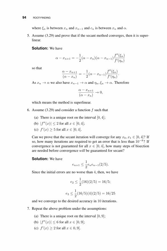
94 ROOT-FINDING
where ξn is between xn and xn−1 and cn is between xn and α.
5. Assume (3.29) and prove that if the secant method converges, then it is super-linear.
Solution: We have
α− xn+1 = −1
2(α− xn)(α− xn−1)
f ′′(ξn)
f ′(ηn)
so thatα− xn+1
(α− xn)= −1
2(α− xn−1)
f ′′(ξn)
f ′(ηn).
As xn → α we also have xn−1 → α and ηn, ξn → α. Therefore
α− xn+1
(α− xn)→ 0,
which means the method is superlinear.
6. Assume (3.29) and consider a function f such that
(a) There is a unique root on the interval [0, 4];
(b) |f ′′(x)| ≤ 2 for all x ∈ [0, 4];
(c) f ′(x) ≥ 5 for all x ∈ [0, 4].
Can we prove that the secant iteration will converge for any x0, x1 ∈ [0, 4]? Ifso, how many iterations are required to get an error that is less than 10−8? Ifconvergence is not guaranteed for all x ∈ [0, 4], how many steps of bisectionare needed before convergence will be guaranteed for secant?
Solution: We haveen+1 ≤
1
2enen−1(2/5).
Since the initial errors are no worse than 4, then, we have
e2 ≤1
2(16)(2/5) = 16/5;
e3 ≤1
2(16/5)(4)(2/5) = 16/25
and we converge to the desired accuracy in 10 iterations.
7. Repeat the above problem under the assumptions:
(a) There is a unique root on the interval [0, 9];
(b) |f ′′(x)| ≤ 6 for all x ∈ [0, 9];
(c) f ′(x) ≥ 2 for all x ∈ 0, 9].

THE SECANT METHOD: DERIVATION AND EXAMPLES 95
Can we prove that the secant iteration will converge for any x0, x1 ∈ [0, 9]? Ifso, how many iterations are required to get an error that is less than 10−8? Ifconvergence is not guaranteed for all x ∈ [0, 9], how many steps of bisectionare needed before convergence will be guaranteed for secant?
Solution: We haveen+1 ≤
1
2enen−1(2/5).
Since the initial errors are no worse than 9, then, we have
e2 ≤1
2(81)(3) = 243/2;
so we will not converge. Doing one step of bisection reduces the originalsecant interval to length 4.5, so we then have
e2 ≤1
2(9/2)2(3) = 243/8,
still too large. Another step of bisection give us
e2 ≤1
2(9/4)2(3) = 243/32,
and a third bisection yields
e2 ≤1
2(9/8)2(3) = 243/128
still not small enough. Finally, a fourth bisection step gives an initial intervalof length 9/16 and a first step error of
e2 ≤1
2(9/16)2(3) = 243/512.
Convergence then occurs in 10 secant iterations.
8. Repeat Problem 8 of 3.1, except this time find α for the set of θ values definedby
θk = 10k/4,
for k ranging from −24 all the way to 24. Construct a plot of α vs. log10 θ.
Solution: For k = −24, α = 0.00094129631308, for k = −23, α =0.00125518056472, for k = 1, α = 0.92775227544590, for k = 2, α =1.09242933874440. The plot is given in Figure 3.3.
9. Comment, in your own words, on the differences between the secant methodand regula-falsi (see Problem 9 of 3.1).
Solution: Regula-falsi chooses the two approximate values in order to guar-antee that the root is “bracketed,” whereas the secant method chooses the most

96 ROOT-FINDING
−6 −4 −2 0 2 4 60
0.5
1
1.5
2
2.5
3
3.5
4
Figure 3.3 Solution for Problem 3.8.10
accurate (i.e., most recent) approximations, regardless of whether or not theybracket the root.
/ • • • .
3.9 FIXED POINT ITERATION
Exercises:
1. Do three steps of each of the following fixed point iterations, using the indicatedx0.
(a) xn+1 = cosxn, x0 = 0 (be sure to set your calculator in radians);
Solution: x1 = 1, x2 = .5403023059, x3 = .8575532158
(b) xn+1 = e−xn , x0 = 0;
(c) xn+1 = ln(1 + xn), x0 = 1/2;
Solution: x1 = 4054651081, x2 = .3403682857, x3 = .2929444165
(d) xn+1 = 12 (xn + 3/xn), x0 = 3.
2. Let Y = 1/2 be fixed, and take h = 18 . Do three steps of the following fixed
point iteration
yn+1 = Y +1
2h (−Y lnY − yn ln yn)
using y0 = Y .
Solution: y1 = .5433216988, y2 = .5423768123, y3 = .5423997893
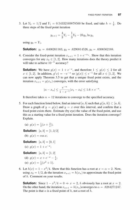
FIXED POINT ITERATION 97
3. Let Y0 = 1/2 and Y1 = 0.54332169878500 be fixed, and take h = 18 . Do
three steps of the fixed point iteration
yn+1 =4
3Y1 −
1
3Y0 − 2hyn ln yn
using y0 = Y1.
Solution: y1 = .6406261163, y2 = .6290814526, y3 = .6306562188.
4. Consider the fixed-point iteration xn+1 = 1 + e−xn . Show that this iterationconverges for any x0 ∈ [1, 2]. How many iterations does the theory predict itwill take to achieve 10−5 accuracy?
Solution: We have g(x) = 1 + e−x, and therefore 1 ≤ g(x) ≤ 2 for allx ∈ [1, 2]. In addition, g(x) = −e−x so |g(x)| ≤ e−1 for all x ∈ [1, 2]. Wecan now apply Theorem 3.5 to get that a unique fixed point exists, and theiteration xn+1 = g(xn) converges, with the error satisfying
|α− xn| ≤e−n
1− e−1|x1 − x0| ≤ 1.6× e−n.
It therefore takes n = 12 iterations to converge to the specified accuracy.
5. For each function listed below, find an interval [a, b] such that g([a, b]) ⊂ [a, b].Draw a graph of y = g(x) and y = x over this interval, and confirm that afixed point exists there. Estimate (by eye) the value of the fixed point, and usethis as a starting value for a fixed point iteration. Does the iteration converge?Explain.
(a) g(x) = 12 (x+ 2
x );
Solution: [a, b] = [1, 3/2]
(b) g(x) = cosx;
Solution: [a, b] = [0, 1]
(c) g(x) = 1 + e−x;
Solution: [a, b] = [1, 2]
(d) g(x) = x+ e−x − 14 ;
(e) g(x) = 12 (x2 + 1).
6. Let h(x) = 1− x2/4. Show that this function has a root at x = α = 2. Now,using x0 = 1/2, do the iteration xn+1 = h(xn) to approximate the fixed pointof h. Comment on your results.
Solution: Since 1 − x2/4 = 0 ⇒ x = 2, h obviously has a root at x = 2.On the other hand, the iteration xn+1 = h(xn)converges to α = .8284271247.The point is that α is a fixed point of h, not a root of h.

98 ROOT-FINDING
7. Let h(x) = 3 − e−x. Using x0 = 2, perform as many iterations of Newton’smethod as are needed to accurately approximate the root of h. Then, usingthe same initial point, do the iteration xn+1 = h(xn) to approximate the fixedpoint of h. Comment on your results.
Solution: This is essentially making the same point as the previous problem.The root is−1.098612289 (approximately), but the fixed point is 2.947530903(approximately).
8. Use fixed point iteration to find a value of x ∈ [1, 2] such that 2 sinπx+x = 0.
9. For a > 0, consider the iteration defined by
xn+1 =x3n + x2n − xna+ a
x2n + 2xn − a
(a) For x0 = 3/2 experiment with this iteration for a = 4 and a = 2. Basedon these results, speculate as to what this iteration does. Try to provethis, and use the theorems of this section to establish a convergence rate.
(b) Now experiment with this iteration using x0 = 2 and a = 5. Compareyour results to Newton’s method.
10. Consider the iteration
xn+1 =(N − 1)xN+1 + ax
NxN
Assume that this converges for integer N and any a > 0. What does itconverge to? Use the theorems of this section to determine a convergence rate.Experiment with this iteration when N = 3 and a = 8, using x0 = 3/2.
11. Consider the iteration defined by
xn+1 = xn − f(xn)
[f(xn)
f(xn + f(xn))− f(xn)
].
This is also sometimes known as Steffenson’s method. Show that it is (locally)quadratically convergent.
Solution: This is a somewhat tricky application of Theorem 3.7. We have
g(x) = x− f(x)
[f(x)
f(x+ f(x))− f(x)
],
so that
g′(x) = 1− f ′(x)
[f(x)
f(x+ f(x))− f(x)
]− f(x)
[f(x)
f(x+ f(x))− f(x)
]′.

ROOTS OF POLYNOMIALS (PART 1) 99
Now, for x = α the last term vanishes (because f(α) = 0), so we can ignoreit. The second term becomes indeterminate (it naively evaluates to 0/0) so wehave to employ L’Hôpital’s rule to get g′(α) = 0. We then have to show thatg′′(α) 6= 0.
12. Apply Steffenson’s method to find the root of f(x) = 2 − ex, using x0 = 0.Compare your convergence results to those in the text for Newton and thesecant method.
Solution: The first 4 iterates are
x1 = .5819767070, x2 = .6876240766,
x3 = .6931320121, x4 = .6931471806
Clearly the iteration is converging to the same root as for Newton and secant,and with comparable speed.
13. Apply Steffenson’s method to f(x) = x2 − a for the computation of√a. For
the following values of a, how does the performance compare to Newton’smethod?
(a) a = 3;
(b) a = 2;
Solution: Usingx0 = 2, the first three Newton iterates arex1 = 1.500000000,x2 = 1.416666667, and x3 = 1.414215686; the first three Steffensoniterates (using the same x0) are x1 = 1.666666667, x2 = 1.477477478,and x3 = 1.419177338.
(c) a = π.
/ • • • .
3.10 ROOTS OF POLYNOMIALS (PART 1)
Exercises:
1. Use the Durand-Kerner algorithm to find all the roots of the polynomial
p(x) = x4 − 10x3 + 35x2 − 50x+ 24.
You should get ζ1,2,3,4 = (1, 2, 3, 4).

100 ROOT-FINDING
Solution: The author’s code (below) converged in 11 iterations; Here arethe ζ values for the first three iterations, using the roots of unity as the initialguesses:
ζ(1)j = −10.0000 + 3.5000i, −2.7694− 4.0214i, 0.5263− 0.6208i,
1.0000− 0.0000i
ζ(2)j = 9.0724 + 11.2615i, 0.9705− 3.5225i, 0.6181− 0.2987i,
1.0000− 0.0000i
ζ(3)j = 6.1229 + 3.0728i, 3.0670− 2.0642i, 1.1368− 0.0148i,
1.0000 + 0.0000i
Using the roots of unity as initial guesses actually simplified the problem a bit,since the initial guess for ζ4 was exact!
The following code is set up as a function which returns the converged valuesof the roots.
Algorithm 3.1 Code for Durand-Kerner
function r = DKroots(p)
np = length(p);
n = np-1;
q = p/p(1);
k = [1:n];
zeta = exp(2*pi*i*k/n);
for j=1:20
old = zeta;
for k=1:n
qp = polyval(q,zeta(k));
denom = 1.0;
for kk=1:n
if k ~= kk
denom = denom*(zeta(k) - zeta(kk));
end
end
zeta(k) = zeta(k) - qp/denom;
end
zeta %Delete this line to avoid excess output
if abs(zeta - old) <= 1.e-14
break
end
end
r = zeta;

ROOTS OF POLYNOMIALS (PART 1) 101
2. Use the Durand-Kerner algorithm to find all the roots of the following polyno-mials (Feel free to use MATLAB’S roots command to check your results):
(a) p(x) = x6 + x5 + x4 + x3 + x2 + x+ 1;
(b) p(x) = x6 − x5 − 1;
(c) p(x) = x9 − x8 − 1;
(d) p(x) = x5 − 1;
Solution: For (a) we get ζ = 0.6235+0.7818i, −0.2225+0.9749i, −0.9010+0.4339i, −0.2225− 0.9749i, 0.6235− 0.7818i, −0.9010− 0.4339i.
3. Use Durand-Kerner to find all the roots of the polynomial
p(x) = x7 − x− 1.
Solution: We get ζ = 0.6171 + 0.9009i, −0.3636 + 0.9526i, −0.8099 +0.2629i, −0.8099−0.2629i, −0.3636−0.9526i, 0.6171−0.9009i, 1.1128+0.0000i.
4. Use Durand-Kerner to find all the roots of the polynomial
p(x) = x8 − x− 1.
5. Consider now the polynomial
p(x) = x6 − ax− 1,
where a is a real parameter. We want to investigate how the roots depend ona. For various values of a ∈ [−2, 2], compute the roots of p and observe howthey change as a changes. Can you plot the real roots as a function of a? Tryto extend the range of values of a. Does anything interesting happen?
Solution: For both a = −2 and a = 2 there are two real roots, as follows:
a = −2 : ζR = −1.2298, 0.4928;
a = 2 : ζR = −0.4928, 1.2298.
Solution: What you need to do is wrap a loop structure around your Durand-Kerner routine, and add some additional code to correctly save the two realroots to make the curves shown in Fig. 3.4.
However, interesting things can indeed happen. If we take 40 points to constructour curves we get the picture in Fig. 3.5. What has happened?
The short answer is that polynomial roots can be very sensitive to changes inthe coefficients. Specifically, in the 40 point case, some of the roots on the

102 ROOT-FINDING
−2 −1.5 −1 −0.5 0 0.5 1 1.5 2−2.5
−2
−1.5
−1
−0.5
0
0.5
1
1.5
Figure 3.4 Solution curves forProblem 5, using 20 points.
−2 −1.5 −1 −0.5 0 0.5 1 1.5 2−2.5
−2
−1.5
−1
−0.5
0
0.5
1
1.5
Figure 3.5 Solution curves forProblem 5, using 40 points.
upper curve were converged to from the initial value used for the lower curve,and vice-versa. A more sophisticated routine for the selection of the rootsmight be able to circumvent this problem.
6. Repeat the above for the polynomial
p(x) = x6 − x− b,
where now b ∈ [−2, 2] is a parameter.
7. Use MATLAB’s rand function to generate a random polynomial of degree 10.(Remember to make it monic!) Use Durand-Kerner to find the roots of thispolynomial, and check your results by using MATLAB’s roots function.
/ • • • .
3.11 SPECIAL TOPICS IN ROOT-FINDING METHODS
Exercises:
1. Consider the fixed-point iteration xn+1 = 1 + e−xn , with x0 = 0. Do foursteps (by hand) and apply both of the Aitken acceleration algorithms to speedup the convergence of the iteration.
Solution: The original iteration produces x1 = 2.0000, x2 = 1.1353, x3 =1.3213, and x4 = 1.2668. The first acceleration method produces y2 =

SPECIAL TOPICS IN ROOT-FINDING METHODS 103
1.3963, y3 = 1.2884, and y4 = 1.2791. The second acceleration methodproduces z1 = 1.3963, z2 = 1.2789, z2 = 1.27854, z4 = 1.2785.
2. Repeat the above for the iteration xn+1 = 12 ln(1 + xn), using x0 = 1/2.
Solution: The basic iteration produces x1 = 0.2027, x2 = 0.09230, x3 =0.04414, and x4 = 0.02160; the first Aitken method produces y2 = 0.02702,y3 = 0.006906, and y4 = 0.001754; the second Aitken method producesz1 = 0.02702, z2 = 0.1720e − 3, z3 = 0.7392e − 8, and z4 = 0.0000; theexact value of the fixed point is α = 0.
3. Consider the iteration xn+1 = e−x. Show (by computational experiment) thatit coverges for x0 = 1/2; then use both Aitken acceleration algorithms to speedup the convergence. What is the gain in terms of function calls to the iterationfunction?
Solution: The second Aitken method converges to 14 digit accuracy in 5iterations, which involves a total of 10 function calls. Neither the originaliteration nor the first Aitken method converge to comparable accuracy in 20iterations (involving 20 function calls in each case), although both are clearlyclose to convergence.
4. Write the second Aitken iteration in the form
xk+1 = G(xk)
Hint: Takex1 = g(x0), x2 = g(x1) = g(g(x0))
and use this to write the updated value of x0 in Algorithm 3.5 entirely in termsof x0, g(x0), and g(g(x0)).
Solution: We have that
xn+1 = g(g(xn)) + γg(g(xn))− g(xn)
1− γ
where
γ =g(g(xn))− g(xn)
g(xn)− xn,
therefore,
xn+1 = g(g(xn)) +
(g(g(xn))−g(xn)g(xn)−xn
)(
1− g(g(xn))−g(xn)g(xn)−xn
) (g(g(xn))− g(xn)).
5. Consider the iterationxk+1 = G(xk),

104 ROOT-FINDING
where
G(x) = g(g(x)) +H(x)
1−H(x)(g(g(x))− g(x))
for
H(x) =g(g(x))− g(x)
g(x)− x.
Assume that α = g(α) is a fixed point for g.
(a) Use L’Hôpital’s Rule to show that
H(α) = g′(α).
Solution: We have
H(α) = limx→α
g(g(x))− g(x)
g(x)− x
= limx→α
g′(g(x))g′(x)− g′(x)
g′(x)− 1
= g′(α) limx→α
g′(g(x))− 1
g′(x)− 1
= g′(α)g′(α)− 1
g′(α)− 1
= g′(alpha)
(b) Use Theorem 3.7 to show that the fixed point iteration for G is quadratic.
Solution: This is a direct consequence of (a) and Exercise 4. Exercise 4implies that we can write the second Aitken algorithm as xn+1 = G(xn),where
G(x) = g(g(x)) +
(g(g(x))−g(x)g(x)−x
)(
1− g(g(x))−g(x)g(x)−x
) (g(g(x))− g(x)).
Writing this in the suggested form
G(x) = g(g(x)) +H(x)
1−H(x)(g(g(x))− g(x)),
where
H(x) =g(g(x))− g(x)
g(x)− x,
we get that G′(α) = 0 if H(α) = g′(α), which is what (a) gives us.

SPECIAL TOPICS IN ROOT-FINDING METHODS 105
6. Apply the chord method to each of the functions in Problem 3 of 3.1, usingthe midpoint of the interval as x0. Compare your results to what you got forbisection, Newton, and/or the secant method.
Solution: Table 3.9 shows results for three of the functions. Note that twoof them appear to be converging nicely, but one is cycling between two values.
Table 3.9 Solutions to Problem 3.10.6
n f(x) = x3 − 2x+ 5 f(x) = ex − 2 f(x) = x2 − sinx
1 2.47368421052632 0.71306131942527 0.996849213938122 1.38118185096799 0.68866210956491 0.932550221184753 2.46066264395747 0.69409059303710 0.904771302259584 1.41273756576147 0.69294563585428 0.891268925284215 2.46661014403290 0.69319009730508 0.884381206417966 1.39839029026513 0.69313803554445 0.880786187037167 2.46412393132776 0.69314912895829 0.878887946242038 1.40440122265335 0.69314676542932 0.877879602201809 2.46521002552796 0.69314726900812 0.8773422750517810 1.40177773347679 0.69314716171506 0.8770554633856611 2.46474386296717 0.69314718457506 0.8769022338665912 1.40290421128725 0.69314717970448 0.8768203317996113 2.46494551887643 0.69314718074221 0.8767765435342314 1.40241699456030 0.69314718052111 0.8767531293165115 2.46485857585776 0.69314718056822 0.8767406084864416 1.40262707133957 0.69314718055818 0.8767339126711417 2.46489611528813 0.69314718056032 0.8767303318483218 1.40253636927138 0.69314718055987 0.8767284168560619 2.46487991697665 0.69314718055996 0.8767273927291020 1.40257550786620 0.69314718055994 0.87672684503010
7. Repeat the above, except this time apply both of the Aitken acceleration algo-rithms to improve the convergence of the iteration. Compute the values of theratio
Rn =α− xn+1
(α− xn)2,
where α is the best value for the root, as found by previous methods. Does thesequence of Rn values appear to be converging to a limit? What does this tellyou?
Solution: Table 3.10 gives the results for the same selection of examples asin the previous problem, using Algorithm 3.5. Note that all three iterationsconverge to 14 digits of accuracy in only 6 iterations. The ratios Rn shouldconverge to a limit since the accelerated methods are quadratic.
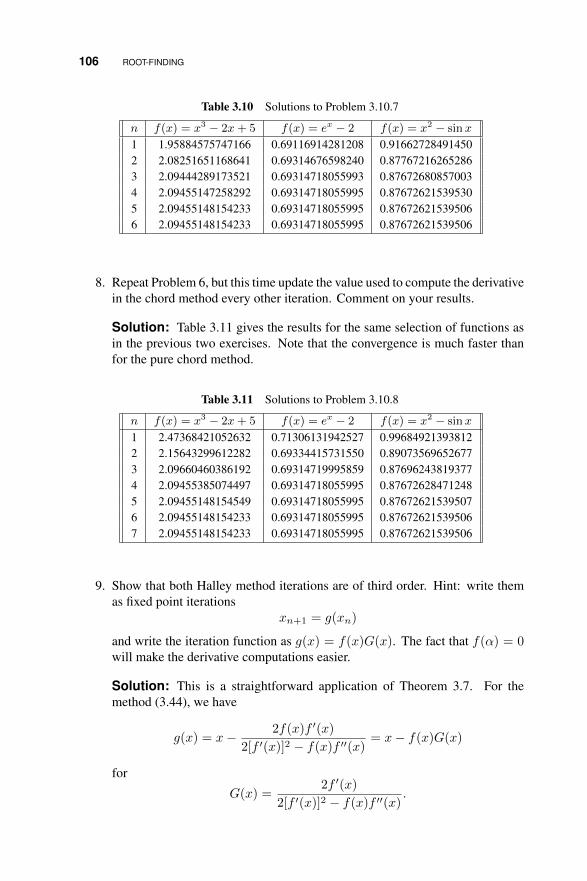
106 ROOT-FINDING
Table 3.10 Solutions to Problem 3.10.7
n f(x) = x3 − 2x+ 5 f(x) = ex − 2 f(x) = x2 − sinx
1 1.95884575747166 0.69116914281208 0.916627284914502 2.08251651168641 0.69314676598240 0.877672162652863 2.09444289173521 0.69314718055993 0.876726808570034 2.09455147258292 0.69314718055995 0.876726215395305 2.09455148154233 0.69314718055995 0.876726215395066 2.09455148154233 0.69314718055995 0.87672621539506
8. Repeat Problem 6, but this time update the value used to compute the derivativein the chord method every other iteration. Comment on your results.
Solution: Table 3.11 gives the results for the same selection of functions asin the previous two exercises. Note that the convergence is much faster thanfor the pure chord method.
Table 3.11 Solutions to Problem 3.10.8
n f(x) = x3 − 2x+ 5 f(x) = ex − 2 f(x) = x2 − sinx
1 2.47368421052632 0.71306131942527 0.996849213938122 2.15643299612282 0.69334415731550 0.890735696526773 2.09660460386192 0.69314719995859 0.876962438193774 2.09455385074497 0.69314718055995 0.876726284712485 2.09455148154549 0.69314718055995 0.876726215395076 2.09455148154233 0.69314718055995 0.876726215395067 2.09455148154233 0.69314718055995 0.87672621539506
9. Show that both Halley method iterations are of third order. Hint: write themas fixed point iterations
xn+1 = g(xn)
and write the iteration function as g(x) = f(x)G(x). The fact that f(α) = 0will make the derivative computations easier.
Solution: This is a straightforward application of Theorem 3.7. For themethod (3.44), we have
g(x) = x− 2f(x)f ′(x)
2[f ′(x)]2 − f(x)f ′′(x)= x− f(x)G(x)
for
G(x) =2f ′(x)
2[f ′(x)]2 − f(x)f ′′(x).

SPECIAL TOPICS IN ROOT-FINDING METHODS 107
Theng′(x) = 1− f ′(x)G(x)− f(x)G′(x).
Hence,
g′(α) = 1− f ′(α)G(α) = 1− f ′(α)2f ′(α)
2[f ′(α)]2= 0.
Further,
g′′(x) = −f ′′(x)G(x)− 2f ′(x)G′(x)− f(x)G′′(x),
so thatg′′(α) = −f ′′(α)G(α)− 2f ′(α)G′(α)
which we can again show is 0.
10. Apply the Halley iteration (3.44) to f(x) = x2 − a, a > 0, to derive a cubicmethod for finding the square root. Test this by using it to find
√5.
Solution: The iteration is
xn+1 =x(x2 + 3a)
3x2 + a.
11. Repeat the above for f(x) = xN−a. Test this out by finding the cubic, quartic,and quintic roots of 2, 3, 4, and 5.
Solution: The iteration for the cube root is
xn+1 =x(x3 + 2a)
2x3 + a.
For the quintic root it is
xn+1 =x(2x5 + 3a)
3x5 + 2a.
12. Apply Halley’s second method to f(x) = a− ex to show that
xn+1 = xn + 2
(ae−xn − 1
ae−xn + 1
)is a cubic convergent iteration for α = log a. Analyze the convergence of thisiteration, under the assumption that a ∈ [ 12 , 1]. Comment on this as a practicalmeans of computing the logarithm of an arbitrary a.
Solution: If a ∈ [1/2, 1], then ln a ∈ [−.7, 0]. One can show that, for anya ∈ [1/2, 1], the iteration function
g(x) = x+ 2
(ae−x − 1
ae−x + 1
)
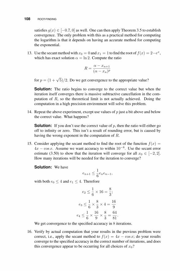
108 ROOT-FINDING
satisfies g(x) ∈ [−0.7, 0] as well. One can then apply Theorem 3.5 to establishconvergence. The only problem with this as a practical method for computingthe logarithm is that it depends on having an accurate method for computingthe exponential.
13. Use the secant method withx0 = 0 andx1 = 1 to find the root of f(x) = 2−ex,which has exact solution α = ln 2. Compute the ratio
R =α− xn+1
(α− xn)p
for p = (1 +√
5)/2. Do we get convergence to the appropriate value?
Solution: The ratio begins to converge to the correct value but when theiteration itself converges there is massive subtractive cancellation in the com-putation of R, so the theoretical limit is not actually achieved. Doing thecomputation in a high precision environment will solve this problem.
14. Repeat the above experiment, except use values of p just a bit above and belowthe correct value. What happens?
Solution: If you don’t use the correct value of p, then the ratio will either gooff to infinity or zero. This isn’t a result of rounding error, but is caused byhaving the wrong exponent in the computation of R.
15. Consider applying the secant method to find the root of the function f(x) =4x − cosx. Assume we want accuracy to within 10−8. Use the secant errorestimate (3.50) to show that the iteration will converge for all x0 ∈ [−2, 2].How many iterations will be needed for the iteration to converge?
Solution: We haveen+1 ≤
1
6enen−1,
with both e0 ≤ 4 and e1 ≤ 4. Therefore
e2 ≤1
6× 16 =
8
3;
e3 ≤1
6× 8
3× 4 =
16
9
e4 ≤1
6× 16
9× 8
3=
64
81.
We get convergence to the specified accuracy in 8 iterations.
16. Verify by actual computation that your results in the previous problem werecorrect, i.e., apply the secant method to f(x) = 4x − cosx; do your resultsconverge to the specified accuracy in the correct number of iterations, and doesthis convergence appear to be occurring for all choices of x0?

SPECIAL TOPICS IN ROOT-FINDING METHODS 109
Solution: Testing the computation for a range of values for x0 and x1, all inthe interval [−2, 2], will confirm the prediction.
17. Prove Lemma 3.1. Hint: Expand f in a Taylor series about α.
Solution: The proof follows directly from the hint.
18. Let f(x) = 1− xe1−x. Write this function in the form (3.57). What is F (x)?Use Taylor’s Theorem or L’Hôpital’s Rule to determine the value of F (α).
Solution: We have
f(x) = (x− 1)2(
1− xe1−x
(x− 1)2
),
so
F (x) =1− xe1−x
(x− 1)2.
Applying L’Hôpital’s Rule to F shows that F (α) = 1/2.
19. For u(x) as defined in (3.60), where f has a k-fold root at x = α, show thatu(α) = 0 but u′(α) 6= 0.
Solution: Since f is assumed to have a multiple root, we can write f(x) =(x− α)kF (x) for some F . Then
u(x) =f ′(x)
f(x)=k(x− α)k−1F (x) + (x− α)kF ′(x)
(x− α)kF (x)=kF (x) + (x− α)F ′(x)
(x− α)F (x)
so that u(α) = 0 but u′(α) won’t.
20. Use the modified Newton method (3.59) to find the root α = 1 for the functionf(x) = 1− xe1−x. Is the quadratic convergence recovered?
Solution: The iteration converges much more quickly than without the mod-ification, but the computed value of the root is not as accurate as we have seenin simple root examples.
21. Let f have a double root at x = α. Show that the Newton iteration function
g(x) = x− f(x)/f ′(x)
is such that g′(α) 6= 0. Provide all details of the calculation.
Solution: Since f has a double root we can write
f(x) = (x− α)2F (x).

110 ROOT-FINDING
Then
g(x) = x− (x− α)2F (x)
2(x− α)F (x) + (x− α)2F ′(x)= x− 2(x− α)F (x)
F (x) + (x− α)F ′(x)
= x− (x− α)
(2F (x)
F (x) + (x− α)F ′(x)
)so that
g(α) = α.
Also
g′(x) = 1−(1)
(2F (x)
F (x) + (x− α)F ′(x)
)−(x−α)
(2F (x)
F (x) + (x− α)F ′(x)
)′.
Therefore
g′(x) = 1− 2F (α)
F (α)− 0 = −1 6= 0.
22. Using a hand calculator, carry out six iterations of the hybrid method for thefunction
f(x) = 2xe−15 − 2e−15x + 1.
You should be able to match the values generated for x2 and x3 in the text. Inaddition, x6 = 0.04146407478711.
Solution: x1 = 0.500000,x2 = 0.250000,x3 = 0.125069,x4 = 0.0625346,x5 = 0.0369239, x6 = 0.0414641
23. Write a computer code to implement the hybrid method described in Section3.10.5. Apply it to each of the functions given below, using the given intervalas the starting interval. On your output, be sure to indicate which iterationmethod was used at each step.
(a) f(x) = x1/19 − 191/19, [1, 100];
(b) f(x) = 2xe−5 − 2e−5x + 1, [0, 1];
(c) f(x) = x2 − (1− x)20, [0, 1];
(d) f(x) = 2xe−20 − 2e−20x + 1, [0, 1];
Solution: Table 3.12 gives the results from my program, applied to the caseof (d). Note that we do cycle back and forth between secant and bisection atthe beginning of the iteration.

SPECIAL TOPICS IN ROOT-FINDING METHODS 111
Table 3.12 Hybrid iteration for f(x) = 2xe−20 − 2e−20x + 1.
n xn f(xn) xn − xn−1 ln |xn − xn−1| an bn Method1 0.39540563 0.99926451 -0.3954056E+00 -0.403 0.010 0.395 S2 0.20270282 0.96529631 0.1927028E+00 -0.715 0.010 0.203 B3 0.08664329 0.64644583 0.1160595E+00 -0.935 0.010 0.087 S4 0.04832164 0.23912462 0.3832164E-01 -1.417 0.010 0.048 B5 0.03786785 0.06219184 0.1045379E-01 -1.981 0.010 0.038 S6 0.03419335 -0.00932344 0.3674505E-02 -2.435 0.034 0.038 S7 0.03467239 0.00030061 -0.4790448E-03 -3.320 0.034 0.035 S8 0.03465743 0.00000139 0.1496305E-04 -4.825 0.034 0.035 S9 0.03465736 0.00000000 0.6965962E-07 -7.157 0.035 0.035 S10 0.03465736 0.00000000 -0.1047069E-10 -10.980 0.035 0.035 S
I have included the Fortran code that I used to get the table.
c
c Code for global root-finding routine
c based on bisection and secant
c
implicit real*8 (a-h,o-z)
character*1 step,bisect,secant
data bisect,secant / ’B’,’S’ /
c
f(x) = 2.0d0*x*dexp(-20.0d0)
* - 2.0d0*dexp(-20.0d0*x) + 1.0d0
c
a = 0.01d0
b = 1.00d0
x0 = a
x1 = b
alpha = 0.0d0
c
fa = f(a)
fb = f(b)
f0 = fa
f1 = fb
c
do 100 n=1,100
xold = x
c
c take secant step
c
dd = f1*(x1 - x0)/(f1 - f0)
x = x1 - f1*(x1 - x0)/(f1 - f0)
c
c if secant prediction is outside bracketing interval,
c do one step of bisection
c
if((x .lt. a) .or. (x .gt. b)) then
x = 0.5d0*(a + b)

112 ROOT-FINDING
fx = f(x)
if(fa*fx .lt. 0.0d0) then
b = x
fb = fx
else
a = x
fa = fx
endif
x0 = a
x1 = b
f0 = fa
f1 = fb
error = xold - x
step = bisect
else
c
c otherwise, update bracketing interval
c
fx = f(x)
if(fa*fx .lt. 0.0d0) then
b = x
fb = fx
else
a = x
fa = fx
endif
error = xold - x
step = secant
x0 = x1
x1 = x
f0 = f1
f1 = fx
endif
e10 = dlog10(dabs(error))
write(6,91) n,x,fx,error,e10,a,b,step
91 format(1h ,i5,’ & ’,2(f12.8,’ & ’),e16.7,’ & ’,
* 3(f8.3,’ & ’),1x,a1 ’\\\\ \\hline’)
if(dabs(error) .le. 1.e-8) stop
100 continue
c
stop
end
24. In Problem 9 of 3.1 we introduced the regula-falsi method. In this problemwe demonstrate how the hybrid method (Algorithm 3.6) is different fromregula-falsi. Let
f(x) = e−4x − 1
10.
(a) Show that f has a root in the interval [0, 5].
Solution: f(0) = 1− (1/10) > 0, and f(5) = e−20 − (1/10) < 0.
(b) Using this interval as the starting interval, compute five iterations ofregula-falsi; be sure to tabulate the new interval in addition to the new

SPECIAL TOPICS IN ROOT-FINDING METHODS 113
approximate root value predicted by the method at each step. A graphshowing the location of each approximate root might be useful.
Solution: Table 3.13 shows five iterations of regula falsi for this function.Note that the value of an remains the same for the entire computation.
Table 3.13 Regula-falsi iteration for f(x) = e−4x − (1/10).
n cn f(cn) an bn
1 4.5000 -0.1000 0 4.50002 4.0500 -0.1000 0 4.05003 3.6450 -0.1000 0 3.64504 3.2805 -0.1000 0 3.28055 2.9525 -0.1000 0 2.9525
(c) Using the same interval as the starting interval, compute five iterationsof the hybrid method given in this section. Again, note the new intervalas well as the new approximate root value at each step. A graphicalillustration might be instructive.
Solution: Table 3.14 shows the results.
Table 3.14 Hybrid iteration for f(x) = e−4x − (1/10).
n cn f(cn) an bn Method1 4.5000 -0.1000 0 4.5000 S2 2.2500 -0.0999 0 2.2500 B3 2.0250 -0.0997 0 2.0250 S4 1.0125 -0.0826 0 1.0125 B5 0.9115 -0.0739 0 0.9115 S6 0.6222 -0.0170 0 0.6222 S
(d) Based on your results, comment on the difference between regula falsiand the hybrid method.
Solution: The obvious difference revealed by this exercise is that the additionof the bisection step speeds up the convergence compared to regula falsi,by cutting the interval in half. A more subtle difference, which is notrevealed well by this example, is that in the hybrid method we use the mostrecent computations to compute the secant approximation, not necessarilythe bracket values. This will serve to speed up the computation.

114 ROOT-FINDING
25. Write a computer program that evaluates the polynomial p(x) = (x−1)5 usingthe following three forms for the computation:
p(x) = (x− 1)5,
p(x) = x5 − 5x4 + 10x3 − 10x2 + 5x− 1,
p(x) = −1 + x(5 + x(−10 + x(10 + x(−5 + x)))).
Use this to evaluate the polynomial at 400 equally spaced points on the interval[0.998, 1.002]. Comment on the results.
Solution: Using the first form will almost surely not produce the “cloudeffect” seen in the text, while the other two probably will (exactly what happensdepends a lot on the platform and language used, and the precision, of course).
/ • • • .
3.12 VERY HIGH-ORDER METHODS AND THE EFFICIENCY INDEX
Exercises:
1. Write a program to employ both Chun-Neta and Super Halley to find the rootof a given function. Test it on the following examples, using the given valuesof x0.
(a) f(x) = sinx − 12x, x∗ = 1.8954942670339809471440357381; x0 =
2, 2.5, 3;
(b) f(x) = ex2+7x−30 − 1, x∗ = 3, x0 = 4, 5, 6;
(c) f(x) = ex sinx+ ln (1 + x2), x∗ = 1, x0 = 0,−1,−2;
Solution: What follows is a MATLAB “code segment” to do 10 iterationsof the two methods; froot is a MATLAB function which returns the functionvalue and its first two derivatives at the argument.
for k=1:10
[fx,fpx,fpxx] = froot(xsuper);
u = fx/fpx;
uL = u*fpxx/fpx;
y = xsuper - 2*u/3;
xsuper = xsuper - (1 + 0.5*uL/(1 - uL))*u;
%
[fx,fpx,fpxx] = froot(xneta);
w = xneta - fx/fpx;

VERY HIGH-ORDER METHODS AND THE EFFICIENCY INDEX 115
[fw,dfw,d2w] = froot(w);
z = w - fw/(fpx*(1 - fw/fx)^2);
[fz,dfz,d2z] = froot(z);
%
xneta = z - fz/(fpx*(1 - (fw/fx) - (fz/fx))^2);
%
end
2. In 3.7 we employed (and analyzed) Newton’s method as an approximator for√a by using it to find the positive root of the function f(x) = x2 − a. In
this and some of the following exercises we will try to apply our high ordermethods to this task.
(a) Apply Halley’s method to finding the root of f(x) = x2 − a. Constructan iteration function, as simplified as possible, so the the iteration isxn+1 = GH(xn). Verify that your construction works by testing it ona = 0.5, for which the exact value is
√0.5 = 0.70710678118655. Note
the number of arithmetic operations required by your function duringeach iteration.
Solution: You should get
gH(x) =x(x2 + 3a)
3x2 + a.
(b) Repeat the above for Super Halley, obtaining the iteration xn+1 =GSH(xn) for as simple a GSH as possible.
Solution: You should get
gSH(x) =6ax2 + 3a2 − x4
8ax.
3. Recall that in 3.7 we were able to restrict our attention to values in the interval[14 , 1], and therefore construct an initial guess by linear interpolation. Modify
your codes from the above problem to reflect this, and use them to approximate√a for a = 0.3, 0.6, and 0.9. In addition, write a code that uses Newton’s
method (or simply use your code from 3.7), and test it on the same values ofa. Which method achieves full accuracy (as measured by MATLAB’s sqrtfunction) in the fewest operations for each a?
4. Modify your codes to step from a = 0.25 to a = 1 in increments of 0.001,finding
√a for each a using each of the three methods. Thus you will first find√
0.25, then√
0.251, etc., all the way to a = 1.00. What is the average numberof operations used by each method to obtain full accuracy, as measured by theflops command?

116 ROOT-FINDING
5. Repeat the above using some of the alternate initial value generators fromProblems 6, 7, and 8 of 3.7.
6. This is more of an essay-type question: As part of your job, you are going tobe given a series of difficult root-finding problems that require highly accuratesolutions. Of all the methods we have studied in this chapter, including the newmethods in this section, which one would you choose? Justify your answer.
7. Think about combining one of these high-order methods with a global methodas we did in 3.11.5. Can you design an algorithm that is better (faster, moreefficient) than the one in that section?
/ • • • .

CHAPTER 4
INTERPOLATION ANDAPPROXIMATION
4.1 LAGRANGE INTERPOLATION
Exercises:
1. Find the polynomial of degree 2 that interpolates at the datapoints x0 = 0,y0 = 1, x1 = 1, y1 = 2, and x2 = 4, y2 = 2. You should get p2(t) =− 1
4 t2 + 5
4 t+ 1.
Solution:
p2(t) = L0(t)y0 + L1(t)y1 + L2(t)y2
=(t− x1)(t− x2)
(0− 1)(0− 4)(1) +
(t− x0)(t− x2)
(1− 0)(1− 4)(2) +
(t− x0)(t− x1)
(4− 0)(4− 1)(2)
=(t− 1)(t− 4)
4− 2(t− 0)(t− 4)
3+
(t− 0)(t− 1)
6
= −1
4t2 +
5
4t+ 1.
Solutions Manual to Accompany An Introduction to Numerical Methods and Analysis,Second Edition. By James F. EppersonCopyright c© 2013 John Wiley & Sons, Inc.
117

118 INTERPOLATION AND APPROXIMATION
2. Find the polynomial of degree 2 that interpolates to y = x3 at the nodes x0 = 0,x1 = 1, and x2 = 2. Plot y = x3 and the interpolating polynomial over theinterval [0, 2].
Solution:
p2(t) = L0(t)y0 + L1(t)y1 + L2(t)y2
=(t− x1)(t− x2)
(0− 1)(0− 2)(1) +
(t− x0)(t− x2)
(1− 0)(1− 2)(4) +
(t− x0)(t− x1)
(2− 0)(2− 1)(8)
= 3t2 − 2t.
3. Construct the quadratic polynomial that interpolates to y = 1/x at the nodesx0 = 1/2, x1 = 3/4, and x2 = 1.
Solution:
p2(t) = L0(t)y0 + L1(t)y1 + L2(t)y2
=(t− 3/4)(t− 1)
(1/2− 3/4)(1/2− 1)(2) +
(t− 1/2)(t− 1)
(3/4− 1)(3/4− 1/2)(4/3)
+(t− 1/2)(t− 3/4)
(1− 1/2)(1− 3/4)(1)
= (8/3)t2 − 6t+ (13/3).
4. Construct the quadratic polynomial that interpolates to y =√x at the nodes
x0 = 1/4, x1 = 9/16, and x2 = 1.
Solution:
p2(t) = L0(t)y0 + L1(t)y1 + L2(t)y2
=(t− x1)(t− x2)
(1/4− 9/16)(1/4− 1)(1/2) +
(t− x0)(t− x2)
(9/16− 1/4)(9/16− 1)(3/4)
+(t− x0)(t− x1)
(1− 1/4)(1− 9/16)(1)
= (−32/105)t2 + (22/21)t+ (9/35).
5. For each function listed below, construct the Lagrange interpolating polynomialfor the set of nodes specified. Plot both the function and the interpolatingpolynomial, and also the error, on the interval defined by the nodes.
(a) f(x) = lnx, xi = 1, 32 , 2;
(b) f(x) =√x, xi = 0, 1, 4;
(c) f(x) = log2 x, xi = 1, 2, 4;
(d) f(x) = sinπx, xi = −1, 0, 1.

LAGRANGE INTERPOLATION 119
Solution:
(a) p2(x) = −.235566072x2 + 1.39984540x− 1.164279325;
(b) p2(x) = (7x− x2)/6;
(c) p2(x) = −(1/6)x2 + (3/2)x− (4/3);
(d) p2(x) = 0.
6. Find the polynomial of degree 3 that interpolates y = x3 at the nodes x0 = 0,x1 = 1, x2 = 2, and x3 = 3. (Simplify your interpolating polynomial asmuch as possible.) Hint: this is easy if you think about the implications of theuniqueness of the interpolating polynomial.
Solution: You should get p3(x) = x3; interpolation to a polynomial repro-duces the polynomial if enough nodes are used.
7. Construct the Lagrange interpolating polynomial to the function f(x) = x2 +2x, using the nodes x0 = 0, x1 = 1, x2 = −2. Repeat, using the nodesx0 = 2, x1 = 1, x2 = −1. (For both sets of nodes, simplify your interpolatingpolynomial as much as possible.) Comment on your results, especially in lightof the uniqueness part of Theorem 4.1, and then write down the interpolatingpolynomial for interpolating to f(x) = x3 +2x2 +3x+1 at the nodes x0 = 0,x1 = 1, x2 = 2, x3 = 3, x4 = 4, and x5 = 5. Hint: You should be able to dothis last part without doing any computations.
Solution: In all three cases the interpolating polynomial will be identical tothe original polynomial.
8. Let f be a polynomial of degree ≤ n, and let pn be a polynomial interpolantto f , at the n + 1 distinct nodes x0, x1, . . . , xn. Prove that pn(x) = f(x) forall x, i.e., that interpolating to a polynomial will reproduce the polynomial, ifyou use enough nodes. Hint: Consider the uniqueness part of Theorem 4.1.
Solution: Let q(x) = f(x) − pn(x). Since both f and pn are polynomialsof degree ≤ n, so is q. But q(xk) = 0 for the n+ 1 nodes xk. The only way apolynomial of degree≤ n can have n+ 1 roots is if it is identically zero, hencef(x) = pn(x) for all x.
9. Let p be a polynomial of degree ≤ n. Use the uniqueness of the interpolatingpolynomial to show that we can write
p(x) =n∑i=0
L(n)i (x)p(xi)
for any distinct set of nodes x0, x1, . . . , xn. Hint: See the previous problem.

120 INTERPOLATION AND APPROXIMATION
Solution: Define
q(x) = p(x)−n∑i=0
L(n)i (x)p(xi).
Since everything on the right side is a polynomial of degree ≤ n, so is q. But,again, q(xk) = 0 for the n + 1 nodes xk, therefore q(x) = 0 for all x, whichproves the desired result.
10. Show thatn∑i=0
L(n)i (x) = 1
for any set of distinct nodes xk, 0 ≤ k ≤ n. Hint: This does not require anycomputation with the sum, but rather a perceptive choice of polynomial p inthe previous problem.
Solution: Let p(x) = 1, and note that this is a polynomial of degree 0. Bythe previous problem, we have that
1 = p(x) =n∑i=0
L(n)i (x)p(xi) =
n∑i=0
L(n)i (x),
and we are done.
/ • • • .
4.2 NEWTON INTERPOLATION AND DIVIDED DIFFERENCES
Exercises:
1. Construct the polynomial of degree 3 that interpolates to the data x0 = 1,y0 = 1, x1 = 2, y1 = 1/2, x2 = 4, y2 = 1/4, and x3 = 3, y3 = 1/3. Youshould get p(t) = (50− 35t+ 10t2 − t3)/24.
Solution: The divided difference coefficients are 1, −1/2, 1/8, and −1/24,so the polynomial is
p(t) = 1−(1/2)(x−1)+(1/8)(x−1)(x−2)−(1/24)(x−1)(x−2)(x−4),
which simplifies as indicated.
2. For each function listed below, use divided difference tables to construct theNewton interpolating polynomial for the set of nodes specified. Plot both the

NEWTON INTERPOLATION AND DIVIDED DIFFERENCES 121
function and the interpolating polynomial, and also the error, on the intervaldefined by the nodes.
(a) f(x) =√x, xi = 0, 1, 4;
Solution: The divided difference coefficients are a0 = 0, a1 = 1, anda2 = −1/6.
(b) f(x) = lnx, xi = 1, 32 , 2;
(c) f(x) = sinπx, xi = 0, 14 ,12 ,
34 , 1;
(d) f(x) = log2 x, xi = 1, 2, 4;
Solution: The divided difference coefficients are a0 = 0, a1 = 1, anda2 = 1/6, so the polynomial is
p(t) = 0 + (1)(x− 1) + (1/6)(x− 1)(x− 2),
which simplifies to
p(t) = (1/6)(x2 + 3x− 4).
(e) f(x) = sinπx, xi = −1, 0, 1.
3. Let f(x) = ex. Define pn(x) to be the Newton interpolating polynomial forf(x), using n + 1 equally spaced nodes on the interval [−1, 1]. Thus we aretaking higher and higher degree polynomial approximations to the exponentialfunction. Write a program that computes pn(x) for n = 2, 4, 8, 16, 32, andwhich samples the error f(x)− pn(x) at 501 equally spaced points on [−1, 1].Record the maximum error as found by the sampling, as a function of n, i.e.,define En as
En = max0≤k≤500
|f(tk)− pn(tk)|
where tk = −1 + 2k/500, and plot En vs. n.
Solution: Using MATLAB on a low-end personal computer, the author got
E2 = 7.8525e− 2, E4 = 1.1244e− 3, E8 = 5.8000e− 8,
E16 = 1.5321e− 14, E32 = 3.6471e− 10.
Note that the error started to actually increase as we added more nodes. Thisis explained, in part, by the material in Section 4.11.1.
4. In 3.7 we used linear interpolation to construct an initial guess for Newton’smethod as a means of approximating
√a. Construct the quadratic polynomial
that interpolates the square root function at the nodes x0 = 14 , x1 = 4
9 , x2 = 1.Plot the error between p2 and
√x over the interval [ 14 , 1] and try to estimate
the worst error. What impact will this have on the use of Newton’s method forfinding
√a?

122 INTERPOLATION AND APPROXIMATION
Solution: The polynomial is
p(t) = −12
35t2 +
23
21t+
26
105.
The worst absolute error, |√t−p(t)|, appears to be, from looking at a plot, about
0.01. This is significantly smaller than the error due to linear interpolation, sothe Newton iteration for computing
√a will converge faster. See some of the
exercises in Section 3.7.
5. Prove Corollary 4.1.
Solution: A straight-forward inductive argument works.
6. Write and test a computer code that takes a given set of nodes, functionvalues, and corresponding divided difference coefficients, and computes newdivided difference coefficients for new nodes and function values. Test it byrecursively computing interpolating polynomials that approximate f(x) = ex
on the interval [0, 1].
Solution: A set of MATLAB scripts that accomplish this are given below.The first script (polyterp) is the“main program.” The second one (divdif)computes divided difference coefficients. The third one (intval) evaluates aninterpolating polynomial from nodal data and divided difference coefficients.
%
n = input(’Initial degree? ’);
m = input(’Maximum degree? ’);
np = n + 1;
mp = m + 1;
%
xn = [0:n]/n
yn = exp(xn);
x = [0:500]/500;
a = divdif(xn,yn);
y = intval(x,xn,a);
figure(1)
plot(x,y)
figure(2)
plot(x,y - exp(x));
max(abs(y - exp(x)))
%
for k=np:mp
xx = input(’New node value? ’);
yy = exp(xx);
pn = intval(xx,xn,a);
w = xx - xn;

NEWTON INTERPOLATION AND DIVIDED DIFFERENCES 123
w = prod(w);
xn = [xn xx];
yn = [yn yy];
aa = (yy - pn)/w;
a = [a aa];
y = intval(x,xn,a);
max(abs(y - exp(x)))
check = sum(abs(yn - intval(xn,xn,a)))
end
%%%%%%%%%%%%%%%%%%%%%%%%%%%%%%%%%%%%%%%
function a = divdif(x,y)
n = length(x)-1;
a = y;
for i=1:n
for j=n:(-1):i
a(j+1) = (a(j+1) - a(j))/(x(j+1) - x(j-i+1));
end
end
%%%%%%%%%%%%%%%%%%%%%%%%%%%%%%%%%%%%%%%
function y = intval(x,xx,d)
%
% evaluates polynomial using divided difference
% coefficients d, and interpolation data xx
%
m = length(x);
n = length(d);
%
y = d(n)*ones(1,m);
for i=(n-1):(-1):1
y = d(i) + (x - xx(i)*ones(1,m)).*y;
end
7. In 1973, the horse Secretariat became the first (and, so far, only) winner ofthe Kentucky Derby to finish the race in less than two minutes, running the1 14 mile distance in 1 : 59.4 seconds4. Remarkably, he ran each quarter mile
faster than the previous one, as the following table of data shows. Here t is theelapsed time (in seconds) since the race began and x is the distance (in miles)that Secretariat has travelled.
4During the final preparation of the First Edition of the text, in May, 2001, the horse Monarchos won theKentucky Derby in a time of 1 : 59.8 seconds, becoming the second winner of the race to finish in lessthan two minutes. Ironically, the only other horse to run the Derby in less than two minutes was Sham,who finished second to Secretariat.

124 INTERPOLATION AND APPROXIMATION
Table 4.1 Data for Problem 7.
x 0.0 0.25 0.50 0.75 1.00 1.25t 0.0 25.0 49.4 73.0 96.4 119.4
(a) Find the cubic polynomial that interpolates this data at x = 0, 1/2,3/4, 5/4.
Solution:
T (x) = p3(x) = 2.986666666x3 − 9.599999999x2 + 102.8533333x
(b) Use this polynomial to estimate Secretariat’s speed at the finish of therace, by finding p′3(5/4).
Solution: We need to use a little calculus here. We have t = P3(x), but thespeed of the horse comes from computing dx/dt, not dt/dx. But weknow that
dx
dt=
1dtdx
,
so the speed of the horse at x = 5/4 is given by
S =1
p′3(5/4)= .1076967261e− 1.
Unfortunately, this is in miles per second and we wanted miles per hour.To convert, we simply multiply by 3600 seconds per hour to get
S = 38.77082140.
(c) Find the quintic polynomial that interpolates the entire dataset.
Solution:
p5(x) = −13.65333333x5 + 42.66666667x4 − 44.80000001x3
+ 13.33333333x2 + 98.85333333x.
(d) Use the quintic polynomial to estimate Secretariat’s speed at the finishline.
Solution: This time we get S = 40.51620641 miles per hour.
8. The data in Table 4.2 (Table 4.7 in the text) gives the actual thermal conductivitydata for the element mercury. Use Newton interpolation and the data for300◦K, 500◦K, and 700◦K to construct a quadratic interpolate for this data.How well does it predict the values at 400K and 600K?

NEWTON INTERPOLATION AND DIVIDED DIFFERENCES 125
Table 4.2 Data for Problem 8.
Temperature (◦K), u 300 400 500 600 700Conductivity (watts/cm ◦K), k 0.084 0.098 0.109 0.12 0.127
Solution: The polynomial is
p2(T ) = −0.0000000875T 2 + 0.000195T + 0.033375.
Since p2(400) = .97375e − 1 and p2(600) = .118875 it is apparent that theinterpolating polynomial does a good job of matching the data.
9. The gamma function, denoted by Γ(x), is an important special function inprobability, combinatorics, and other areas of applied mathematics. Because itcan be shown that Γ(n+ 1) = n!, the gamma function is considered a general-ization of the factorial function to non-integer arguments. Table 4.3 (Table 4.8in the text) gives the values of Γ(x) on the interval [1, 2]. Use these to constructthe fifth degree polynomial based on the nodes x = 1, 1.2, 1.4, 1.6, 1.8, 2.0,and then use this polynomial to estimate the values atx = 1.1, 1.3, 1.5, 1.7, 1.9.Plot your polynomial and compare it to the intrinsic gamma function on yourcomputing system or calculator.
Table 4.3 Table of Γ(x) values.
x Γ(x)
1.00 1.00000000001.10 0.95135076991.20 0.91816874241.30 0.89747069631.40 0.88726381751.50 0.88622692551.60 0.89351534931.70 0.90863873291.80 0.93138377101.90 0.96176583192.00 1.0000000000
Solution: We get
p5 = −.09270377605x5 + .8632574013x4 − 3.199846710x3
+6.287123228x2 − 6.537486675x+ 3.679656532.
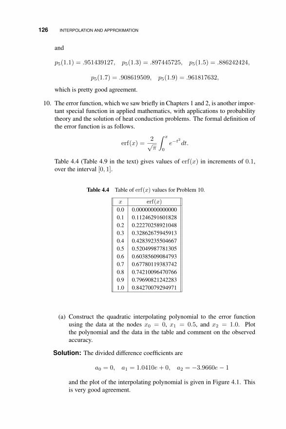
126 INTERPOLATION AND APPROXIMATION
and
p5(1.1) = .951439127, p5(1.3) = .897445725, p5(1.5) = .886242424,
p5(1.7) = .908619509, p5(1.9) = .961817632,
which is pretty good agreement.
10. The error function, which we saw briefly in Chapters 1 and 2, is another impor-tant special function in applied mathematics, with applications to probabilitytheory and the solution of heat conduction problems. The formal definition ofthe error function is as follows.
erf(x) =2√π
∫ x
0
e−t2
dt.
Table 4.4 (Table 4.9 in the text) gives values of erf(x) in increments of 0.1,over the interval [0, 1].
Table 4.4 Table of erf(x) values for Problem 10.
x erf(x)
0.0 0.000000000000000.1 0.112462916018280.2 0.222702589210480.3 0.328626759459130.4 0.428392355046670.5 0.520499877813050.6 0.603856090847930.7 0.677801193837420.8 0.742100964707660.9 0.796908212422831.0 0.84270079294971
(a) Construct the quadratic interpolating polynomial to the error functionusing the data at the nodes x0 = 0, x1 = 0.5, and x2 = 1.0. Plotthe polynomial and the data in the table and comment on the observedaccuracy.
Solution: The divided difference coefficients are
a0 = 0, a1 = 1.0410e+ 0, a2 = −3.9660e− 1
and the plot of the interpolating polynomial is given in Figure 4.1. Thisis very good agreement.

NEWTON INTERPOLATION AND DIVIDED DIFFERENCES 127
0 0.1 0.2 0.3 0.4 0.5 0.6 0.7 0.8 0.9 10
0.1
0.2
0.3
0.4
0.5
0.6
0.7
0.8
0.9
Figure 4.1 Solution plot for Exercise 4.2.11a.
(b) Repeat the above, but this time construct the cubic interpolating polyno-mial using the nodes x0 = 0.0, x2 = 0.3, x2 = 0.7, and x3 = 1.0.
Solution: The divided difference coefficients are
a0 = 0, a1 = 1.0954e+0, a2 = −3.1784e−1, a3 = −1.4398e−1
and the plot of the interpolating polynomial is given in Figure 4.2. Thisis slightly better than in (a).
0 0.1 0.2 0.3 0.4 0.5 0.6 0.7 0.8 0.9 10
0.1
0.2
0.3
0.4
0.5
0.6
0.7
0.8
0.9
Figure 4.2 Solution plot for Exercise 4.2.11b.

128 INTERPOLATION AND APPROXIMATION
11. As steam is heated up, the pressure it generates is increased. Over the temper-ature range [220, 300] (degrees Fahrenheit) the pressure, in pounds per squareinch, is given in Table 4.5.5 (This is Table 4.10 in the text.)
Table 4.5 Temperature-pressure values for steam; Problem 11
T 220 230 240 250 260 270 280 290 300P 17.188 20.78 24.97 29.82 35.42 41.85 49.18 57.53 66.98
(a) Construct the quadratic interpolating polynomial to this data at the nodesT0 = 220, T1 = 260, and T2 = 300. Plot the polynomial and the data inthe table and comment on the observed accuracy.
Solution: The divided difference coefficients are
a0 = 17.1880, a1 = 0.4558, a2 = 0.0042
and the plot of the interpolating polynomial is given in Figure 4.3. Thisis very good agreement.
220 230 240 250 260 270 280 290 30010
20
30
40
50
60
70
Figure 4.3 Solution plot for Exercise 4.2.11a.
(b) Repeat the above, but this time construct the quartic interpolating poly-nomial using the nodes T0 = 220, T1 = 240, T2 = 260, T3 = 280, andT4 = 300.
5Taken from tables in Introduction to Thermodynamics: Classical and Statistical, by Sonntag and VanWylen, John Wiley & Sons, New York, 1971.

NEWTON INTERPOLATION AND DIVIDED DIFFERENCES 129
Solution: The divided difference coefficients are
a0 = 1.7188e+ 1, a1 = 3.8910e− 1, a2 = 3.3350e− 3,
a3 = 1.3375e− 5, a4 = 2.2917e− 8
and the plot of the interpolating polynomial is given in Figure 4.4.
220 230 240 250 260 270 280 290 30010
20
30
40
50
60
70
Figure 4.4 Solution plot for Exercise 4.2.11b.
(c) Which of the two polynomials would you think is best to use to get valuesfor P (T ) that are not on the table?
Solution: Both plots look very good, actually.
12. Similar data for gaseous ammonia is given in Table 4.6 (Table 4.11 in the text).
Table 4.6 Temperature-pressure values for gaseous ammonia; Problem 12
T 0 5 10 15 20 25 30 35 40P 30.42 34.27 38.51 43.14 48.21 53.73 59.74 66.26 73.32
(a) Construct the quadratic interpolating polynomial to this data at the nodesT0 = 0, T1 = 20, and T2 = 40. Plot the polynomial and the data in thetable and comment on the observed accuracy.
Solution: The divided difference coefficients are
a0 = 3.0420e+ 1, a1 = 8.8950e− 1, a2 = 9.1500e− 3.
(b) Repeat the above, but this time construct the quartic interpolating poly-nomial using the nodes T0 = 0, T1 = 10, T2 = 20, T3 = 30, andT4 = 40.

130 INTERPOLATION AND APPROXIMATION
Solution: The divided difference coefficients are
a0 = 3.0420e+ 1, a1 = 8.0900e− 1, a2 = 8.0500e− 3, a3 = 3.6667e− 5,
a4 = 1.7279e− 20
(c) Which of the two polynomials would you think is best to use to get valuesfor P (T ) that are not on the table?
13. In Problem 8 of 3.1 and Problem 8 of 3.8 we looked at the motion ofa liquid/solid interface under a simplified model of the physics involved, inwhich the interface moved according to
x = 2β√t
for β = α/√k. Here k is a material property and α is the root of f(z) =
θe−z2 − zerf(z), where θ also depends on material properties. Figure 4.5
shows a plot of α vs. log10 θ, based on finding the root of f(z). Some of thedata used to create this curve is given in Table 4.7 (Table 4.12 in the text).
−4 −3 −2 −1 0 1 2 3 40
0.5
1
1.5
2
2.5
3
log10θ
α
Figure 4.5 Figure for Problem 13.
(a) Use the data at the nodes {−6,−4,−2, 0, 2, 4, 6} to construct an inter-polating polynomial for this table. Plot the polynomial and compare tothe actual graph in Figure 4.5. Use the polynomial to compute values atlog10 θ = −5,−3, . . . , 3, 5. How do these compare to the actual valuesfrom the table?

NEWTON INTERPOLATION AND DIVIDED DIFFERENCES 131
Table 4.7 Data for Problem 13.
log10 θ α
-6.0000 0.944138E-03-5.0000 0.298500E-02-4.0000 0.941277E-02-3.0000 0.297451E-01-2.0000 0.938511E-01-1.0000 0.289450E+000.0000 0.767736E+001.0000 0.141492E+012.0000 0.198151E+013.0000 0.245183E+014.0000 0.285669E+015.0000 0.321632E+016.0000 0.354269E+01
Solution: The divided difference coefficients are
a0 = 9.4414e−4, a1 = 4.2343e−3, a2 = 9.4962e−3, a3 = 1.0697e−2,
a4 = −1.4662e− 3, a5 = −6.9243e− 5, a6 = 4.6066e− 5
We get p6(x) = .0001600x6 + .00066298x5− .007638x4− .03204x3 +.09548x2 + .5895x+ .7677, for x = log10 θ.
(b) Compute the higher-degree Newton polynomial based on the entire tableof data. Plot this polynomial and compare it to the one generated usingonly part of the data.
Solution: Figure 4.6 shows the nodes and both interpolating polynomials.Note that the interpolations have much more “wiggle” to them than ispresent in the raw data.
14. Write a computer program to construct the Newton interpolating polynomialto f(x) =
√x using equally spaced nodes on the interval [0, 1]. Plot the error
f(x)− pn(x) for n = 4, 8, 16 and comment on what you get.
Solution: Figure 4.7 shows the three error plots. Note the large “spike” in the errornear x = 0. Section 4.3 will explain why this occurs.
/ • • • .

132 INTERPOLATION AND APPROXIMATION
−6 −4 −2 0 2 4 6−0.5
0
0.5
1
1.5
2
2.5
3
3.5
4
Figure 4.6 Solution plot for Exercise 4.2.13.
0 0.5 1−0.05
0
0.05
0.1
0 0.5 1−0.02
0
0.02
0.04
0.06
0 0.5 1−0.01
0
0.01
0.02
0.03
0.04
Figure 4.7 Solution plot for Exercise 4.2.14.
4.3 INTERPOLATION ERROR
Exercises:
1. What is the error in quadratic interpolation to f(x) =√x, using equally spaced
nodes on the interval [ 14 , 1]?

INTERPOLATION ERROR 133
Solution: We have
|f(x)− p2(x)| ≤ 1
9√
3(3/8)3 max
t∈[1/4,1]|(3/8)t−5/2|
=1
9√
3× 81
4096× 45/2 = .4059494081e− 1.
2. Repeat the above for f(x) = x−1 on [ 12 , 1].
Solution: We have
|f(x)− p2(x)| ≤ 1
9√
3(1/4)3 max
t∈[1/2,1]|6x−4|
=1
9√
3× 1
64× 6× 16 = .9622504490e− 1.
3. Repeat the previous two problems, using cubic interpolation.
Solution: This time we have
|√x− p3(x)| ≤ 1
24(1/4)4 max
t∈[1/4,1]|(15/16)x−7/2|
=1
24× 1
256× 15
16× 47/2 = .1953125e− 1
and
|x−1−p3(x)| ≤ 1
24(1/6)4 max
t∈[1/2,1]|24x−5| = 1
24× 1
362×24×32 = .2469135802e−1.
4. Show that the error in third degree polynomial interpolation satisfies
‖f − p3‖∞ ≤1
24h4‖f (4)‖∞,
if the nodes x0, x1, x2, x3 are equally spaced, with xi − xi−1 = h. Hint: Usethe change of variable t = x− x1 − 1
2h.
Solution: We have
f(x)− p4(x) =w4(x)
24f (4)(ξx),
for some value ξx in the interval defined by the nodes and x. Therefore
‖f − p3‖∞ ≤1
24max
x∈[x0,x3]|w4(x)|‖f (4)‖∞,
where we have assumed the nodes are ordered x0 < x1 < x2 < x3. Thechange of variable reduces
W = maxx∈[x0,x3]
|w4(x)|
134 INTERPOLATION AND APPROXIMATION
toW = max
t∈[−3h/2,3h/2]|(t2 − 9h2/4)(t2 − h2/4)|
and ordinary calculus shows that W = h4.
5. Show that the error in polynomial interpolation using six equally spaced points(quintic interpolation) satisfies
‖f − p5‖∞ ≤ Ch6‖f (6)‖∞
where C ≈ 0.0235. Hint: See previous problem.
Solution: The basic outline from the previous exercise shows us that
‖f − p5‖∞ ≤ 1
720max
t∈[−5h/2,5h/2]
|(t2 − 25h2/4)(t2 − 9h2/4)(t2 − h2/4)|‖f (6)‖∞.
Applying ordinary calculus to the problem of finding
W = maxt∈[−5h/2,5h/2]
|(t2 − 25h2/4)(t2 − 9h2/4)(t2 − h2/4)|
shows that W = 16.90089433h6, thus C = 16.90089433/720 = 0.0235.
6. Generalize the derivation of the error bound (4.12) for quadratic interpolationto the case where the nodes are not equally spaced. Take x1 − x0 = h andx2 − x1 = θh for some θ > 0.
Solution: The issue is obtaining an upper bound for
|w2(x)| = |(x− x0)(x− x1)|.
Ordinary calculus, coupled with the same kind of variable shift as used in thetext, can be used to show that
|w2(x)| ≤ (h3/27)g(θ),
where
g(θ) = −(θ − 2 +
√θ2 − θ + 1
)(θ + 1 +
√θ2 − θ + 1
)×(
2 θ − 1−√θ2 − θ + 1
)for θ ∈ [0, 1/2], and
g(θ) = −(θ − 2−
√θ2 − θ + 1
)(θ + 1−
√θ2 − θ + 1
)×(
2 θ − 1 +√θ2 − θ + 1
)

INTERPOLATION ERROR 135
for θ ∈ [1/2, 1].
This looks messy, but the graph of g shows a simple V-shaped curve, rangingfrom 4 at θ = 0 to slightly more than 1 at θ = 1/2, and then back up as θcontinues to increase.
7. Apply your result for the previous problem to the error in quadratic interpolationto f(x) =
√x using the nodes x0 = 1
4 , x1 = 916 , and x2 = 1.
Solution: We have that h = x1 − x0 = 5/16, and θ = 7/5. Thus the erroris bounded according to
|√x− p2(x)| ≤ (h3/27)g(θ) max
t∈[0,1]|(−1/4)t−3/2|
= (5/16)3 × (1/27)× 6.488878750× (1/4)× 43/2
= .1466850846e− 1.
8. If we want to use a table of exponential values to interpolate the exponentialfunction on the interval [−1, 1], how many points are needed to guarantee 10−6
accuracy with linear interpolation? Quadratic interpolation?
Solution: We have, for the linear case,
‖f − pn‖∞ ≤1
8h2‖f ′′‖∞ =
e
8h2.
Therefore we get 10−6 accuracy when h ≤ .1715527770e− 2, which impliesn ≥ 1166 points on the interval [−1, 1].
For the quadratic case, we have
‖f − pn‖∞ ≤1
9√
3h3‖f ′′′‖∞ =
e
9√
3h3.
Therefore we get 10−6 accuracy when h ≤ .1789930706e− 1, which impliesn ≥ 112 points.
9. If we want to use a table of values to interpolate the error function on theinterval [0, 5], how many points are needed to get 10−6 accuracy using linearinterpolation? Quadratic interpolation? Would it make sense to use one gridspacing on, say, [0, 1], and another one on [1, 5]? Explain.
Solution: For the linear case, we have
‖f − pn‖∞ ≤1
8h2‖f ′′‖∞ =
h2
2√pi
(1).
Therefore we get 10−6 accuracy when h ≤ .1882792528e− 2, which impliesn ≥ 2656 points on the interval [0, 5]

136 INTERPOLATION AND APPROXIMATION
For the quadratic case, we have
‖f − pn‖∞ ≤h3
9√
3‖f ′′′‖∞ =
2.256758334h3
9√
3.
Therefore we get 10−6 accuracy when h ≤ .1904463677e− 1, which impliesn ≥ 263 points on the interval [0, 5]
Breaking the table up into two regions [0, 1] and [1, 5] makes sense because theerror function is nearly flat for large arguments, and so we can get away witha much larger h on [1, 5] and probably many fewer overall points.
10. If we want to use a table of values to interpolate the sine function on the interval[0, π], how many points are needed for 10−6 accuracy with linear interpolation?Quadratic interpolation? Cubic interpolation?
Solution: We get n ≥ 1111 for the linear case, n ≥ 144 for the quadraticcase, n ≥ 45 for the cubic case.
11. Let’s return to the computation of the natural logarithm. Consider a computerwhich stores numbers in the form z = f · 2β , where 1
2 ≤ f ≤ 1. We wantto consider using this, in conjunction with interpolation ideas, to compute thenatural logarithm function.
(a) Using piecewise linear interpolation over a grid of equally spaced points,how many table entries would be required to accurately approximate ln zto within 10−14?
(b) Repeat the above, using piecewise quadratic interpolation.
(c) Repeat it again, using piecewise cubic interpolation.
Explain, in a brief essay, the importance here of restricting the domain of z tothe interval [ 12 , 1].
Solution: For the linear case, we have
| lnx− p1(x)| ≤ (1/8)h2 maxt∈[1/2,1]
| − 1/t2| = h2/2,
so we need h ≤ .1414213562e − 6 and hence n ≥ 3535533.907 points. Forthe quadratic case, we have
| lnx− p2(x)| ≤ (1/(9√
3))h3 maxt∈[1/2,1]
|2/t3| = 16h3/(9√
3)
so we need h ≤ .2135802307e − 4 and hence n ≥ 23410.40640 points.Finally, for the cubic case, we have
| lnx− p3(x)| ≤ (1/24)h4 maxt∈[1/2,1]
| − 6/t4| = 96h4/24 = 4h4

INTERPOLATION ERROR 137
so we need h ≤ .2236067977e− 3 and hence n ≥ 2236.067978 points.
12. Assume that, for any real c,
limn→∞
cn
n!= 0.
Use this to prove that, if pn is the polynomial interpolate to f(x) = sinx onthe interval [a, b], using any distribution of distinct nodes xk, 0 ≤ k ≤ n, then‖f − pn‖∞ → 0 as n → ∞. Hint: Can we justify |wn(x)| ≤ cn+1 for somec?
Solution: We have
‖f − pn‖∞ ≤‖wn‖∞(n+ 1)!
‖f (n+1)‖∞ ≤‖wn‖∞(n+ 1)!
,
but
‖wn‖∞ = maxx∈[a,b]
n∏k=0
|x− xn| ≤n∏k=0
|b− a| = (b− a)n+1.
Therefore,
‖f − pn‖∞ ≤(b− a)n+1
(n+ 1)!→ 0,
according to the assumed hypothesis.
13. Can you repeat the above for f(x) = ex? Why/why not?
Solution: A similar argument will work for the exponential function, sincethe derivative term is again bounded by a constant.
14. Define the norms‖f‖∞ = max
x∈[0,1]|f(x)|
and
‖f‖2 =
(∫ 1
0
[f(x)]2dx
)1/2
.
Compute ‖f‖∞ and ‖f‖2 for the following list of functions:
(a) sinnπx, n integer;
(b) e−ax, a > 0;
(c)√xe−ax
2
, a > 0;
Solution: If a > 1/4 then ‖f‖∞ = (√
2/2)e−1/4a−1/4; if a ≤ 1/4, then‖f‖∞ = e−1. ‖f‖2 = (1/2)
√(1− e−2a)/a.
(d) 1/√
1 + x.

138 INTERPOLATION AND APPROXIMATION
Solution: ‖f‖∞ = 1, ‖f‖2 = .9101797207.
15. Define
fn(x) =
{1− nx, 0 ≤ x ≤ 1
n ;
0 1n ≤ x ≤ 1.
Show that
limn→∞
‖fn(x)‖∞ = 1
but
limn→∞
‖fn(x)‖2 = 0.
Hint: Draw a graph of fn(x).
Solution: This can be done by direct computation but a graph of fn isrevealing. It shows that max |fn| = 1 for all n, but the support of |fn| goes tozero, thus forcing the integral norm to vanish while the pointwise norm remainsat 1.
16. Show that
‖f‖1,[a,b] =
∫ b
a
|f(x)|dx
defines a function norm.
Solution: We have, for any constant c,
‖cf‖1,[a,b] =
∫ b
a
|cf(x)|dx = |c|∫ b
a
|f(x)|dx = |c|‖f‖1,[a,b],
and
‖f + g‖1,[a,b] =
∫ b
a
|f(x) + g(x)|dx ≤∫ b
a
|f(x)|dx+
∫ b
a
|g(x)|dx
= ‖f‖1,[a,b] + ‖g‖1,[a,b].
This establishes two of the three conditions. To establish the remaining condi-tion requires an argument to the effect that the integral of the absolute value ofa non-zero function must be greater than zero. Doing this precisely is probablybeyond the analysis skills of most students, but good students ought to be ableto construct a reasonable argument.
/ • • • .

APPLICATION: MULLER’S METHOD AND INVERSE QUADRATIC INTERPOLATION 139
4.4 APPLICATION: MULLER’S METHOD AND INVERSE QUADRATICINTERPOLATION
Exercises:
1. Do three steps of Muller’s method for f(x) = 2 − ex, using the initial points0, 1/2, 1. Make sure you reproduce the values in the table in the text.
2. Repeat the above for inverse quadratic interpolation.
Solution: We get x3 = .7087486790, x4 = .692849951, x5 = .692849951.
3. Let f(x) = x6 − x− 1; show that this has a root on the interval [0, 2] and dothree steps of Muller’s method using the ends of the interval plus the midpointas the initial values.
Solution: f(0) = −1 and f(2) = 61, so a root exists on [0, 2]. We getx3 = 1.0313, x4 = 1.1032, x5 = 1.1258.
4. Repeat the above using inverse quadratic interpolation.
Solution: We getx3 = 1.017357687,x4 = 1.032876088,x5 = 1.174008963.
5. Let f(x) = ex and consider the nodes x0 = −1, x1 = 0, and x2 = 1. Letp2 be the quadratic polynomial that interpolates f at these nodes, and let q2be the quadratic polynomial (in y) that inverse interpolates f at these nodes.Construct p2(x) and q2(y) and plot both, together with f(x).
Solution:
p2(x) = 0.543080635x2 + 1.175201193x+ 1.0
q2(y) = −0.4254590638 y2 + 2.163953414 y − 1.738494350
6. Repeat the above using f(x) = sinπx and the nodes x0 = 0, x1 = 14 , and
x2 = 12 .
Solution: We get p2(x) = −3.31370850x2+3.656854248x, q2(x) = y2/2.
7. Show that the formulas (4.15) and (4.16) for the divided-difference coefficientsin Muller’s Method (4.14) are correct.
Solution: Direct computation.
8. Show that the formulas (4.17) and (4.18) for the coefficients in inverse quadraticinterpolation are correct.
Solution: Direct computation.

140 INTERPOLATION AND APPROXIMATION
9. Apply Muller’s method and inverse quadratic interpolation to the functions inExercise 3 of 3.1, and compare your results to those obtained with Newton’smethod and/or the secant method.
Solution: See Table 4.8 for the Muller’s method results.
Table 4.8 Solutions to Exercise 4.4.9
n f(x) = x3 − 2x+ 5 f(x) = ex − 2 f(x) = x2 − sinx
1 2.00000000000000 0.68725936775341 0.875900565397932 2.09020134845606 0.69308784769077 0.876702266272203 2.09451837842307 0.69314716126932 0.876726214542474 2.09455148276226 0.69314718055995 0.876726215395065 2.09455148154233 0.69314718055995 0.87672621539506
10. Refer back to the discussion of the error estimate for the secant method inSection 3.10.3. Adapt this argument to derive an error estimate for Muller’smethod.
Solution:Muller’s method is based on finding the exact root of a quadratic polyno-mial which interpolates the original function f . Let m be this interpolatingpolynomial, so that we have
m(x) = f(xn) + a1(x− xn) + a2(x− xn)(x− xn−1)
where a1 and a2 are divided difference coefficients and the next iterate isdefined by solving 0 = m(xn+1). Then the quadratic interpolation errorestimate implies that
f(x)−m(x) =1
6(x− xn)(x− xn−1)(x− xn−2)f ′′′(ξn)
for all x; here ξn is in the interval defined by xn, xn−1,xn−2, and α. Set x = αso that we have
f(α)−m(α) =1
6(α− xn)(α− xn−1)(α− xn−2)f ′′′(ξn)
But f(α) = 0 so we have
−m(α) =1
6(α− xn)(α− xn−1)(α− xn−2)f ′′′(ξn)
On the other hand we know that m(xn+1) = 0, so we can substitute this in toget
m(xn+1)−m(α) =1
6(α− xn)(α− xn−1)(α− xn−2)f ′′′(ξn).
APPLICATION: MORE APPROXIMATIONS TO THE DERIVATIVE 141
The Mean Value Theorem then implies that there exists a value ηn between αand xn+1 such that m(xn+1)−m(α) = m′(ηn)(xn+1 − α); therefore,
m′(ηn)(xn+1 − α) =1
6(α− xn)(α− xn−1)(α− xn−2)f ′′′(ξn)
or
xn+1 − α =1
6(α− xn)(α− xn−1)(α− xn−2)
f ′′′(ξn)
m′(ηn).
To really tidy up the final result we need to relate m′(ηn) to f ′.
/ • • • .
4.5 APPLICATION: MORE APPROXIMATIONS TO THE DERIVATIVE
Exercises:
1. Apply the derivative approximations (4.21) and (4.23) to the approximation off ′(x) for f(x) = x3 + 1 for x = 1 and h = 1
8 .
Solution: Using both of (4.21) and (4.23) we get
f ′(x) ≈ 2.968750000
2. Apply the derivative approximations (4.21) and (4.23) to the same set of func-tions as in Exercise 3 of Section 2.2, using a decreasing sequence of meshvalues, h−1 = 2, 4, 8, . . . . Do we achieve the expected rate of accuracy as hdecreases?
3. Derive a version of (4.24) under the assumption that x1−x0 = h, but x2−x1 =η = θh for some real, positive, θ. Be sure to include the error estimate as partof your work, and confirm that when θ = 1 you get the same results as in thetext.
Solution:
f ′(x0) =−θ(2 + θ)f(x0) + (1 + 2θ + θ2)f(x1)− f(x2)
θ(1 + θ)h+
1
6(1+θ)h2f ′′′(ξ)
4. Repeat the above for (4.25).
Solution:
f ′(x1) = (−η/(h(h+ η)))f(x0)− ((h− η)/(hη))f(x1) + (h/(η(h+ η)))f(x2)
− (hη/6)f ′′′(ξ)
142 INTERPOLATION AND APPROXIMATION
5. Repeat the above for (4.26).
Solution:
f ′(x2) =θ2f(x0)− (1 + 2θ + θ2)f(x1) + (2θ + 1)f(x2)
θ(1 + θ)h+
1
6(1+θ)h2f ′′′(ξ)
6. Use the derivative approximations from this section to construct a table ofvalues for the derivative of the gamma function, based on the data in Table 4.3(Table 4.8 in the text).
Solution: Γ′(1) ≈ −.5638283100, Γ′(1.5) ≈ .3125765900e − 1, Γ′(2) ≈.4216022150.
7. Try to extend the ideas of this section to construct an approximation to f ′′(xk).Is it possible? What happens?
Solution: You can’t eliminate all the terms that depend on the derivative withrespect to x of ξx.
/ • • • .
4.6 HERMITE INTERPOLATION
Exercises:
1. Show that H2, as defined in (4.28), is the cubic Hermite interpolate to f at thenodes x = a and x = b.
Solution: Clearly H2(a) = f(a) and H ′2(a) = f ′(a). In addition,
H2(b) = f(a)+f ′(a)(b−a)+(A−f ′(a))(b−a) = f(a)+A(b−a) = f(b),
and
H ′2(b) = f ′(a) + 2B(b− a) +D(b− a)2 = f ′(a) + 2A− 2f ′(a)
+ (C −B)(b− a)
= f ′(a) + 2A− 2f ′(a) + [(f ′(b)−A)− (A− f ′(a))]
= f ′(a)− 2f ′(a) + f ′(a) + 2A− 2A+ f ′(b)
= f ′(b).
H2 is a cubic polynomial and it reproduces the function and derivative valuesat the nodes. Therefore, by the uniqueness part of Theorem 4.4, H2 must bethe Hermite interpolant.

HERMITE INTERPOLATION 143
2. Construct the cubic Hermite interpolate to f(x) = sinx using the nodes a = 0and b = π. Plot the error between the interpolate and the function.
Solution: H2(x) = −(1/π)x2 + x.
3. Construct the cubic Hermite interpolate to f(x) =√
1 + x using the nodesa = 0 and b = 1. Plot the error between the interpolate and the function.
Solution:
H2(x) = 1.0+0.5000000000x−0.085786438x2+0.025126266x2 (x− 1.0)
The maximum absolute error over [0, 1] is about 0.0007.
4. Show that the error in cubic Hermite interpolation at the nodes x = a andx = b is given by
‖f −H2‖∞ ≤(b− a)4
384‖f (4)‖∞.
Solution: This is a direct application of Theorem 4.5, using n = 2.
5. Construct the cubic Hermite interpolate to f(x) =√x on the interval [ 14 , 1].
What is the maximum error on this interval, as predicted by theory? Whatis the maximum error that actually occurs (as determined by observation; noneed to do a complete calculus max/min problem)?
Solution:
H2(x) = 0.2037037037 + 1.388888889x− 0.8888888889x2
+0.2962962963x3
The error theory predicts that the error is bounded according to
|√x−H2(x)| ≤ (3/4)4
384max
x∈[1/4,1]|(15/16)x−7/2|
=81
256× 1
384× 15
16× 47/2
= .9887695312e− 1.
The actual error, looking at a computer plot, is about 0.0065.
6. Construct the cubic Hermite interpolate to f(x) = 1/x on the interval [ 12 , 1].What is the maximum error as predicted by theory? What is the actual (ob-served) maximum error?

144 INTERPOLATION AND APPROXIMATION
Solution: H2(x) = 6− 13x+ 12x2− 4x3, the predicted error is≤ 1/8, theobserved error is ≤ 0.022.
7. Construct the cubic Hermite interpolate to f(x) = x1/3 on the interval [ 18 , 1].
What is the maximum error as predicted by theory? What is the actual (ob-served) maximum error?
Solution:
H2(x) = 0.3090379009 + 1.732750243x− 1.725947522x2
+0.6841593780x3
with maximum observed error about 0.036.
8. Construct the cubic Hermite interpolate to f(x) = lnx on the interval [ 12 , 1].What is the maximum error as predicted by theory? What is the actual (ob-served) maximum error?
Solution: H2(x) = −2.227411278 + 4.364467670x − 3.046701500x2 +.9096451100x3, the predicted error is≤ 1/64, the observed error is≤ 0.0037.
9. Extend the divided difference table for cubic Hermite interpolation to quinticHermite interpolation, using three nodes x = a, x = b, and x = c.
Solution: We get a table like Table 4.9. Here A, B, C, and D are as in thetext, and
α =f(b)− f(c)
b− cβ =
α− f ′(c)b− c
γ =f ′(b)− αb− c
δ =γ − βb− c
E =C − γa− c
F =D − Ea− c
θ =E − δa− c
G =F − θa− c
10. Construct the quintic Hermite interpolate to f(x) = lnx on the interval [ 12 , 1];use x = 3/4 as the third node.
Solution: We get
H2(x) = −2.64516010 + 7.1200353x+ 9.160601x3 − 9.971884x2
−4.659891x4 + 0.9962986x5.
11. What is the error in quintic Hermite interpolation?

PIECEWISE POLYNOMIAL INTERPOLATION 145
Table 4.9 Table for divided differences for quintic Hermite interpolation.
k xk f0(xk) f1(xk) f2(xk) f3(xk) f4(xk) f5(xk)
1 a f(a)
f ′(a)
1 a f(a) B
A D
2 b f(b) C F
f ′(b) E G
2 b f(b) γ θ
α δ
3 c f(c) β
f ′(c)
3 c f(c)
Solution: We get something like
f(x)−H3(x) =1
720ψ3(x)f (6)(ξ)
where ψ3(x) = (x − x1)2(x − x2)2(x − x3)2. This can be bounded aboveaccording to
‖f −H3‖∞ ≤ Ch6‖f (6)‖∞,
where C = .0002057613167, approximately. This value comes from usingordinary calculus to find the extreme values of ψ3.
12. Extend the ideas of Section 4.5 to allow us to compute second derivativeapproximations using Hermite interpolation.
Solution: Becauseψn(x) involves terms of the form (x−xk)2 for each node,the basic idea from Section 4.5 can be used to get derivative approximationformulas for the second derivative, based on Hermite interpolation.
/ • • • .
4.7 PIECEWISE POLYNOMIAL INTERPOLATION
Exercises:
1. Use divided difference tables to construct the separate parts of the piece-wise quadratic polynomial q2(x) that interpolates to f(x) = cos 1
2πx atx = 0, 14 ,
12 ,
34 , 1. Plot the approximation and the error sin 1
2πx− q2(x).

146 INTERPOLATION AND APPROXIMATION
2. Repeat the above using f(x) =√x with the nodes x = 1
5 ,25 ,
35 ,
45 , 1.
Solution: This requires that we construct the two divided difference tables that arerequired here. We have the results in Table 1, thus the piecewise polynomialis given by
q2(x) =
{0.4472 + 0.9262(x− 0.2)− 0.5388(x− 0.2)(x− 0.4) 0.2 ≤ x ≤ 0.6
0.7746 + 0.5992(x− 0.6)− 0.1782(x− 0.6)(x− 0.8) 0.6 ≤ x ≤ 1.
Table 4.10 Divided difference table.
k xk f0(xk) f1(x) f2(x)
0 0.2 0.44720.9262
1 0.4 0.6325 -0.53880.7107
2 0.6 0.7746
k xk f0(xk) f1(x) f2(x)
0 0.6 0.77460.5992
1 0.8 0.8944 -0.17820.5279
2 1.0 1.0000
3. Confirm that (4.30) is the correct piecewise quadratic approximation to f(x) =1/(1 + 25x2) using the nodes x0 = −1, x1 = −2/3, x2 = −1/3, x3 = 0,x4 = 1/3, x5 = 2/3, and x6 = 1.
Solution: Since the each polynomial piece matches the nodal data it must becorrect, because of the uniqueness of polynomial interpolation.
4. Using the data in Table 4.3, construct a piecewise cubic interpolating poly-nomial to the gamma function, using the nodes x = 1.0, 1.2, 1.3, 1.5 for onepiece, and the nodes x = 1.5, 1.7, 1.8, 2.0 for the other piece. Use this approx-imation to estimate Γ(x) for x = 1.1, 1.4, 1.6 and 1.9. How accurate is theapproximation?
Solution:
q3(x) = −.3427614666x3 + 1.873584557x2
− 3.283390574x+ 2.752567484, for 1 ≤ x ≤ 3/2
= (0.1596133333e− 2)x3 + .3766571466x2
− 1.105518098x+ 1.691638542, for 3/2 ≤ x ≤ 2
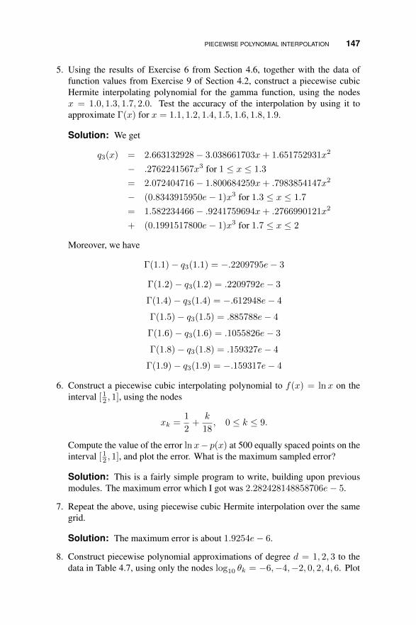
PIECEWISE POLYNOMIAL INTERPOLATION 147
5. Using the results of Exercise 6 from Section 4.6, together with the data offunction values from Exercise 9 of Section 4.2, construct a piecewise cubicHermite interpolating polynomial for the gamma function, using the nodesx = 1.0, 1.3, 1.7, 2.0. Test the accuracy of the interpolation by using it toapproximate Γ(x) for x = 1.1, 1.2, 1.4, 1.5, 1.6, 1.8, 1.9.
Solution: We get
q3(x) = 2.663132928− 3.038661703x+ 1.651752931x2
− .2762241567x3 for 1 ≤ x ≤ 1.3
= 2.072404716− 1.800684259x+ .7983854147x2
− (0.8343915950e− 1)x3 for 1.3 ≤ x ≤ 1.7
= 1.582234466− .9241759694x+ .2766990121x2
+ (0.1991517800e− 1)x3 for 1.7 ≤ x ≤ 2
Moreover, we have
Γ(1.1)− q3(1.1) = −.2209795e− 3
Γ(1.2)− q3(1.2) = .2209792e− 3
Γ(1.4)− q3(1.4) = −.612948e− 4
Γ(1.5)− q3(1.5) = .885788e− 4
Γ(1.6)− q3(1.6) = .1055826e− 3
Γ(1.8)− q3(1.8) = .159327e− 4
Γ(1.9)− q3(1.9) = −.159317e− 4
6. Construct a piecewise cubic interpolating polynomial to f(x) = lnx on theinterval [ 12 , 1], using the nodes
xk =1
2+
k
18, 0 ≤ k ≤ 9.
Compute the value of the error lnx− p(x) at 500 equally spaced points on theinterval [ 12 , 1], and plot the error. What is the maximum sampled error?
Solution: This is a fairly simple program to write, building upon previousmodules. The maximum error which I got was 2.282428148858706e− 5.
7. Repeat the above, using piecewise cubic Hermite interpolation over the samegrid.
Solution: The maximum error is about 1.9254e− 6.
8. Construct piecewise polynomial approximations of degree d = 1, 2, 3 to thedata in Table 4.7, using only the nodes log10 θk = −6,−4,−2, 0, 2, 4, 6. Plot

148 INTERPOLATION AND APPROXIMATION
the resulting curve and compare it to the ordinary interpolating polynomialfound in Problem 13 of 4.2. Test how well this approximation matches thetabulated values at log10 θ = −5,−3,−1, 1, 3, 5.
9. Show that the error in piecewise cubic Hermite interpolation satisfies
‖f −H2‖∞ ≤1
384h4‖f (4)‖∞
where we have assumed uniformly spaced nodes with xk − xk−1 = h.
10. Given a grid of points
a = x0 < x1 < x2 < · · · < xn = b
define the piecewise linear functions φhk , 1 ≤ k ≤ n− 1, according to
φhk(x) =
x−xk−1
xk−xk−1xk−1 ≤ x ≤ xk;
xk+1−xxk+1−xk
xk ≤ x ≤ xk+1;
0 otherwise.
Define the function space
Sh0 = {f ∈ C([a, b]), f(a) = f(b) = 0, f is piecewise linear on the given grid}.
Show that the φhk are a basis for Sh0 , i.e., that every element of the space Sh0can be written as a linear combination of the φhk functions.
11. Implement a routine for approximating the natural logarithm using piecewisepolynomial interpolation, i.e., a table look-up scheme. Assume the table of(known) logarithm values is uniformly distributed on the interval [ 12 , 1]. Chooseenough points in the table to guarantee 10−10 accuracy for any x. Use
(a) Piecewise linear interpolation;
(b) Piecewise cubic Hermite interpolation.
Test your routine against the intrinsic logarithm function on your computerby evaluating the error in your approximation at 5, 000 equally spaced pointson the interval [ 1
10 , 10]. Use the way that the computer stores floating pointnumbers to reduce the logarithm computation to the interval [ 12 , 1], so long asln 2 is known to high accuracy.
/ • • • .

AN INTRODUCTION TO SPLINES 149
4.8 AN INTRODUCTION TO SPLINES
Exercises:
1. Given the set of nodes x0 = 0, x1 = 1/2, x2 = 1, x3 = 3/2, and x4 = 2, weconstruct the cubic spline function
q3(x) = 0.15B−1(x) + 0.17B0(x) + 0.18B1(x) + 0.22B2(x) + 0.30B3(x)
+ 0.31B4(x) + 0.32B5(x),
where each Bk is computed from the exemplar B spline according to (4.39).Compute q3 and its first derivative at each node.
Solution: We have
q3(x0) = 0.15B−1(x0)+0.17B0(x0)+0.18B1(x0) = 0.15+0.17×4+0.18 = 1.01
and
q′3(x0) = 0.15B′−1(x0) + 0.17B′0(x0) + 0.18B′1(x0) = 0.15(−3/h) + 0.17(0)
+ 0.18(3/h) = 0.15(−6) + 0.18(6) = 0.18
The others follow similarly.
2. Is the function
p(x) =
0, x ≤ 0;
x2, 0 ≤ x ≤ 1;
−2x2 + 6x+ 3, 1 ≤ x ≤ 2;
(x− 3)2, 2 ≤ x ≤ 3;
0, x ≥ 3
a spline function? Why/why not?
Solution: No, it is not, because it is not continuous at x = 1.
3. For what value of k is the following a spline function?
q(x) =
{kx2 + (3/2), 0 ≤ x ≤ 1;
x2 + x+ (1/2), 1 ≤ x ≤ 2.
Solution: There is no k that will make this a spline. Taking k = 1 makes thefunction continuous, but the derivative is not continuous.
4. For what value of k is the following a spline function?
q(x) =
{x3 − x2 + kx+ 1 0 ≤ x ≤ 1;
−x3 + (k + 2)x2 − kx+ 3 1 ≤ x ≤ 2.
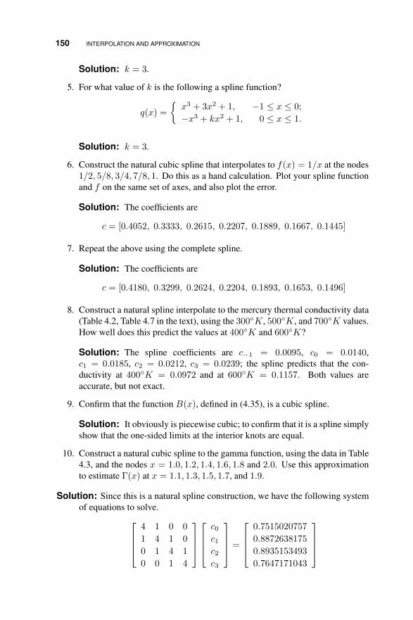
150 INTERPOLATION AND APPROXIMATION
Solution: k = 3.
5. For what value of k is the following a spline function?
q(x) =
{x3 + 3x2 + 1, −1 ≤ x ≤ 0;
−x3 + kx2 + 1, 0 ≤ x ≤ 1.
Solution: k = 3.
6. Construct the natural cubic spline that interpolates to f(x) = 1/x at the nodes1/2, 5/8, 3/4, 7/8, 1. Do this as a hand calculation. Plot your spline functionand f on the same set of axes, and also plot the error.
Solution: The coefficients are
c = [0.4052, 0.3333, 0.2615, 0.2207, 0.1889, 0.1667, 0.1445]
7. Repeat the above using the complete spline.
Solution: The coefficients are
c = [0.4180, 0.3299, 0.2624, 0.2204, 0.1893, 0.1653, 0.1496]
8. Construct a natural spline interpolate to the mercury thermal conductivity data(Table 4.2, Table 4.7 in the text), using the 300◦K, 500◦K, and 700◦K values.How well does this predict the values at 400◦K and 600◦K?
Solution: The spline coefficients are c−1 = 0.0095, c0 = 0.0140,c1 = 0.0185, c2 = 0.0212, c3 = 0.0239; the spline predicts that the con-ductivity at 400◦K = 0.0972 and at 600◦K = 0.1157. Both values areaccurate, but not exact.
9. Confirm that the function B(x), defined in (4.35), is a cubic spline.
Solution: It obviously is piecewise cubic; to confirm that it is a spline simplyshow that the one-sided limits at the interior knots are equal.
10. Construct a natural cubic spline to the gamma function, using the data in Table4.3, and the nodes x = 1.0, 1.2, 1.4, 1.6, 1.8 and 2.0. Use this approximationto estimate Γ(x) at x = 1.1, 1.3, 1.5, 1.7, and 1.9.
Solution: Since this is a natural spline construction, we have the following systemof equations to solve.
4 1 0 0
1 4 1 0
0 1 4 1
0 0 1 4
c0c1c2c3
=
0.7515020757
0.8872638175
0.8935153493
0.7647171043

AN INTRODUCTION TO SPLINES 151
Thus c0c1c2c3
=
0.1511220252
0.1470139748
0.1480858929
0.1541578028
The natural spline construction then tells us the rest of the coefficients:
c0 = Γ(x0)/6 = 1/6, c5 = Γ(x5)/6 = 1/6;
and
c−1 = 2c0−c1 = 0.18221130811994, c6 = 2c5−c4 = 0.17917553048357.
Thus the spline is
q(x) = 0.1822113081B−1(x) + 0.1666666667B0(x)
+0.1511220252B1(x) + 0.1470139748B2(x)
+0.1480858929B3(x) + 0.1541578028B4(x)
= 0.1666666667B5(x) + 0.1791755304B6(x).
We can test this by computing
tk = ck−1 + 4ck + ck+1;
we should get tk = f(xk), and we do. Just for example,
t2 = c1 + 4c2 + c3 = 0.1511220252 + 0.1470139748× 4 + 0.1480858929
= 0.8872638173,
which matches Γ(x2) to nine digits, and probably would match the tenth digitif I had been more careful with my rounding here. Similar results hold at theother points.
We can use this to approximate Γ at the indicated points by computing asfollows.
q(1.1) = 0.1822113081B−1(1.1) + 0.1666666667B0(1.1)
+0.1511220252B1(1.1) + 0.1470139748B2(1.1),
q(1.3) = 0.1666666667B0(1.3) + 0.1511220252B1(1.3)
+0.1470139748B2(1.3) + 0.1480858929B3(1.3)
and so on for the other points.
11. Repeat the above using the complete spline approximation, and use the deriva-tive approximations from Section 4.5 for the required derivative endpoint val-ues.

152 INTERPOLATION AND APPROXIMATION
Solution: The spline coefficients are
c = [0.1872, 0.1653, 0.1515, 0.1469, 0.1481, 0.1544, 0.1658, 0.1824].
Moreover, q3(1.1) = 0.95256719297015, which is a good approximation toΓ(1.1) = 0.95135076986687.
12. Repeat Problem 6 of 4.7, except this time construct the complete cubic splineinterpolate to f(x) = lnx, using the same set of nodes. Plot the approximationand the error. What is the maximum sampled error in this case?
Solution: The spline coefficients are
c = [−0.1345, −0.1153, −0.0977, −0.0819, −0.0674, −0.0541,
−0.0417, −0.0303, −0.0195, −0.0094, 0.0001, 0.0090]
13. Recall Problem 7 from 4.2, in which we constructed polynomial interpolatesto timing data from the 1973 Kentucky Derby, won by the horse Secretariat.For simplicity, we repeat the data in Table 4.11. Here t is the elapsed time (in
Table 4.11 Data for Problem 13.
x 0.0 0.25 0.50 0.75 1.00 1.25t 0.0 25.0 49.4 73.0 96.4 119.4
seconds) since the race began and x is the distance (in miles) that Secretariathas travelled.
(a) Construct a natural cubic spline that interpolates this data.
(b) What is Secretariat’s speed at each quarter-mile increment of the race?(Use miles per hour as your units.)
(c) What is Secretariat’s “initial speed,” according to this model? Does thismake sense?
Note: It is possible to do this problem using a uniform grid. Construct thespline that interpolates t as a function of x, then use your knowledge of calculusto find x′(t) from t′(x).
Solution: (a) Again, the fact that we are asked to do a natural spline tells usthe linear system is
4 1 0 0
1 4 1 0
0 1 4 1
0 0 1 4
c1c2c3c4
=
25.0
49.4
73.0
76.5

AN INTRODUCTION TO SPLINES 153
Thus, the first four spline coefficients arec1c2c3c4
=
4.1842105263
8.2631578947
12.1631578947
16.0842105263
,and the remaining coefficients are
c0 = 0, c−1 = −4.1842105263, c5 = 19.9, c6 = 23.71578947368422
(b) Our spline, as constructed, gives us the time, t (in seconds) as a functionof the distance, x (in miles). But velocity is the derivative of distance withrespect to time. We use the calculus to tell us that
dx
dt=
(dt
dx
)−1.
Thus we can compute q′(1.25) and from that get the horse’s speed. We get
q′(1.25) = (−3/h)(16.0842105263) + (3/h)(23.7157894736) =
sodx
dt= 0.0109195402.
This seems a little low, but then we remember that the units are such that thisis miles per second. Converting to miles per hour we get
dx
dt= 39.3103448279,
which is a much more reasonable speed
(c) The same kind of computation gives us an initial speed of 35.84905660390886.I suspect the horse took a few seconds to get up to full speed, so this is probablya bit high.
14. Show that the complete cubic spline problem can be solved (approximately)without having an explicit expression for f ′ at the endpoints. Hint: Considerthe material from Section 4.5.
Solution: Simply use the approximations
f ′(b) ≈ 3f(b)− 4f(b− h) + f(b− 2h)
2h
and
f ′(a) ≈ −f(a+ 2h) + 4f(a+ h)− 3f(a)
2h.
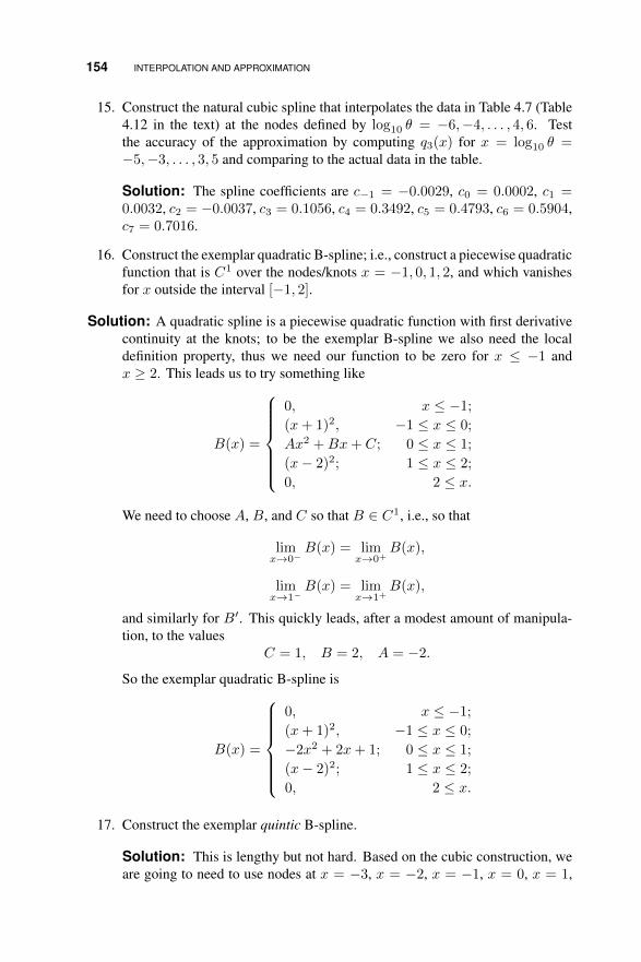
154 INTERPOLATION AND APPROXIMATION
15. Construct the natural cubic spline that interpolates the data in Table 4.7 (Table4.12 in the text) at the nodes defined by log10 θ = −6,−4, . . . , 4, 6. Testthe accuracy of the approximation by computing q3(x) for x = log10 θ =−5,−3, . . . , 3, 5 and comparing to the actual data in the table.
Solution: The spline coefficients are c−1 = −0.0029, c0 = 0.0002, c1 =0.0032, c2 = −0.0037, c3 = 0.1056, c4 = 0.3492, c5 = 0.4793, c6 = 0.5904,c7 = 0.7016.
16. Construct the exemplar quadratic B-spline; i.e., construct a piecewise quadraticfunction that is C1 over the nodes/knots x = −1, 0, 1, 2, and which vanishesfor x outside the interval [−1, 2].
Solution: A quadratic spline is a piecewise quadratic function with first derivativecontinuity at the knots; to be the exemplar B-spline we also need the localdefinition property, thus we need our function to be zero for x ≤ −1 andx ≥ 2. This leads us to try something like
B(x) =
0, x ≤ −1;
(x+ 1)2, −1 ≤ x ≤ 0;
Ax2 +Bx+ C; 0 ≤ x ≤ 1;
(x− 2)2; 1 ≤ x ≤ 2;
0, 2 ≤ x.
We need to choose A, B, and C so that B ∈ C1, i.e., so that
limx→0−
B(x) = limx→0+
B(x),
limx→1−
B(x) = limx→1+
B(x),
and similarly for B′. This quickly leads, after a modest amount of manipula-tion, to the values
C = 1, B = 2, A = −2.
So the exemplar quadratic B-spline is
B(x) =
0, x ≤ −1;
(x+ 1)2, −1 ≤ x ≤ 0;
−2x2 + 2x+ 1; 0 ≤ x ≤ 1;
(x− 2)2; 1 ≤ x ≤ 2;
0, 2 ≤ x.
17. Construct the exemplar quintic B-spline.
Solution: This is lengthy but not hard. Based on the cubic construction, weare going to need to use nodes at x = −3, x = −2, x = −1, x = 0, x = 1,

AN INTRODUCTION TO SPLINES 155
x = 2, and x = 3. In order to get the proper derivative continuity at the nodesx = ±3 we will need the exemplar quintic to have the basic form
B(x) =
0, x < −3
(x+ 3)5, −3 < x ≤ −2
q1(x), −2 < x ≤ −1
q2(x), −1 < x ≤ 0
q3(x), 0 < x ≤ 1
q4(x), 1 < x ≤ 2
(x− 3)5, 2 < x ≤ 3
0, 3 < x
Here we have to choose the individual quintics q1, q2, etc., to maintain conti-nuity and smoothness. For example, we have to have that
q1(−2) = 1, q′1(−2) = 5, q′′1 (−2) = 20, q′′′1 (−2) = 60.
Therefore, we have to have
q1(x) = 1 + 5(x+ 2) + 10(x+ 2)2 + 10(x+ 2)3 +A1(x+ 2)4 +B1(x+ 2)5.
Similarly, we can get that
q4(x) = −1+5(x−2)−10(x−2)2 +10(x−2)3 +A4(x−2)4 +B4(x−2)5.
Corresponding relationships hold for q2 and q3. Algebraic equations for A1,B1, etc., can then be derived by setting q1(−1) = q2(−1) and so forth.
18. For a linear spline function we have d = 1 which forces N = 0. Thus a linearspline has no derivative continuity, only function continuity, and no additionalconditions are required at the endpoints. Show that the exemplar B-spline offirst degree is given by
B(x) =
0, x ≤ −1;
x+ 1, −1 ≤ x ≤ 0;
1− x, 0 ≤ x ≤ 1;
0, 1 ≤ x.
Write out, in your own words, how to construct and evaluate a linear splineinterpolant using this function as the basic B-spline.
Solution: What makes this spline basis so appealing is that the coefficientscan be shown to be the nodal values. That is, we construct the spline approxi-mation to a function f as
q1(x) =n∑i=0
f(xi)Bi(x).

156 INTERPOLATION AND APPROXIMATION
19. Discuss, in your own words, the advantages or disadvantages of spline approx-imation compared to ordinary piecewise polynomial approximation.
Solution: The main difference is the smoothness of the spline approximation,compared to the ordinary piecewise polynomial one.
20. Write an essay which compares and contrasts piecewise cubic Hermite inter-polation with cubic spline interpolation.
Solution: The main point of comparison would be that the Hermite processrequires derivative values.
21. The data below gives the actual thermal conductivity data for the elementnickel. Construct a natural spline interpolate to this data, using only the dataat 200◦K, 400◦K, ..., 1400◦K. How well does this spline predict the valuesat 300◦K, 500◦K, etc.?
Table 4.12 Data for Problem 21.
Temperature (K), u 200 300 400 500 600Conductivity (watts/cm K), k 1.06 0.94 0.905 0.801 0.721
Temperature (K), u 700 800 900 1000Conductivity (watts/cm K), k 0.655 0.653 0.674 0.696
Solution: The spline coefficients are c−1 = 0.2002, c0 = 0.1767, c1 =0.1532, c2 = 0.1156, c3 = 0.1053, c4 = 0.1160, c5 = 0.1267.
22. Construct a natural spline interpolate to the thermal conductivity data in thetable below. Plot the spline and the nodal data.
Temperature (◦K), u 200 300 400 500 600 700Conductivity (watts/cm ◦K), k 0.94 0.803 0.694 0.613 0.547 0.487
/ • • • .
4.9 APPLICATION: SOLUTION OF BOUNDARY VALUE PROBLEMS
Exercises:
1. Set up the linear system for solving the boundary value problem
−u′′ + u = 1, u(0) = 1, u(1) = 0,

APPLICATION: SOLUTION OF BOUNDARY VALUE PROBLEMS 157
using h = 14 . You should get 196 −95 0
−95 196 −95
0 −95 196
c1c2c3
=
101/6
1
671/576
Solution: Since tii = 12h−2 + 4a2 and h = 1/4, a = 1, we quickly have
tii = 12× 16 + 4 = 196.
The off-diagonal elements are
ti,i+1 = −6h−2 + a2 = −6× 16 + 1 = −95.
The values for the right side vector follow in an equally straightforward manner.
2. Solve the system in the previous problem and find the coefficients for the splineexpansion of the approximate solution. The exact solution is
u(x) = 1− e
e2 − 1ex +
e
e2 − 1e−x;
plot your approximation and the error.
Solution: The spline coefficients are c−1 = 0.2021, c0 = 0.1667, c1 =0.1312, c2 = 0.0936, c3 = 0.0513, c4 = 0.0017, c5 = −0.0582.
3. Use the algorithm from this section to approximate the solution to each ofthe following boundary value problems using h−1 = 8, 16, 32. Estimate themaximum error in each case by sampling the difference between the exact andapproximate solutions at 200 equally spaced points on the interval.
(a) −u′′ + u = (π2 + 1) sinπx, u(0) = u(1) = 0; u(x) = sinπx;
(b) −u′′ + u = π(π sinπx + 2 cosπx)e−x, u(0) = u(1) = 0; u(x) =e−x sinπx;
(c) −u′′ + u = 3 − 1x − (x2 − x − 2) log x, u(0) = u(1) = 0; u(x) =
x(1− x) log x.
(d) −u′′ + u = 4e−x − 4xe−x, u(0) = u(1) = 0; u(x) = x(1− x)e−x;
(e) −u′′ + π2u = 2π2 sin(πx), u(0) = 1, u(1) = 0, u(x) = sin(πx)
(f) −u′′ + u = x2+2x−1(1+x)3 , u(0) = 1, u(1) = 1/2, u(x) = (1 + x)−1.
Solution: For (a), with h = 1/8, the spline coefficients are c−1 = −0.0647,c0 = 0, c1 = 0.0647, c2 = 0.1195, c3 = 0.1562, c4 = 0.1690, c5 = 0.1562,c6 = 0.1195, c7 = 0.0647, c8 = 0, c9 = −0.0647. For (e), with h = 1/8, thespline coefficients are c−1 = −0.0650, c0 = 0, c1 = 0.0650, c2 = 0.1201,

158 INTERPOLATION AND APPROXIMATION
c3 = 0.1570, c4 = 0.1699, c5 = 0.1570, c6 = 0.1201, c7 = 0.0650, c8 = 0,c9 = −0.0650.
4. Try to extend the method from this section to the more general two pointboundary value problem defined by
−a(x)u′′ + u = f(x),
u(0) = u(1) = 0
Is the resulting linear system diagonally dominant for all choices of a(x)?
Solution: The components of the linear system now depend on the coefficientfunction a. In particular, we get
tii = 12h−2a(xi) + 4
while the off-diagonal elements are
ti,i+1 = −6h−2a(xi) + 1.
The system is diagonally dominant if tii > |ti,i−1|+ |ti,i+1|. If a is such thatmin a(x) > h2/6, then, for all xi,
|ti,i−1| = 6h−2a(xi)− 1
and similarly for |ti,i+1|. Therefore,
|ti,i−1|+ |ti,i+1| = 12h−2a(xi)− 2 < 12h−2a(xi) + 4 = tii
so the system is diagonally dominant, if min a(x) > h2/6.
5. Try to extend the method from this section to the more general two pointboundary value problem defined by
−u′′ + bu′ + u = f(x),
u(0) = u(1) = 0
Is the resulting linear system diagonally dominant for all values of b?
Solution: The system ceases to be symmetric because of the first derivativeterm in the differential equation, and this impacts the diagonal dominance. Wenow have a diagonally dominant system only if h is “sufficiently small.”
/ • • • .

TENSION SPLINES 159
4.10 TENSION SPLINES
Exercises:
1. Show that the piecewise function defined in (4.56) is, indeed, continuous andhas continuous first and second derivatives.
Solution: This is a straight-forward, if tedious, calculus exercise. Simplyshow that the function values plus the first two derivatives are continuous atthe knots ±2, ±1, 0, i.e., the limits from the left and right are equal. This is agood exercise to use something like Maple or Mathematica on.
2. Fill in the details of the natural spline construction. In particular, confirm theexpressions for δ2,0(p) and δ2,1(p) (and that τ ′′(1) = τ ′′(−1)) as well as theform of the final linear system (4.59).
3. Derive the linear system for construction of a complete taut spline, by followingwhat was done in 4.8.
4. Consider the following dataset:
x 600 650 700 750 800 850 900 950 1000 1050 1100y 0.64 0.65 0.66 0.69 0.91 2.2 1.2 0.62 0.6 0.61 0.61
Plot the data, and construct a (natural) polynomial spline fit to it. Note the“wiggles” to the left of the peak, which appear to be contrary to the sense ofthe data, which is increasing monotonically towards the peak near x = 850.Find the smallest value of p in a taut natural spline fit to this data which yieldsa monotone curve to the left of the peak.
Solution: The plots below show the polynomial spline (on the left) and atension spline with p = 4 (on the right. Note that the wiggles have beensmoothed out.

160 INTERPOLATION AND APPROXIMATION
600 650 700 750 800 850 900 950 1000 1050 11000.4
0.6
0.8
1
1.2
1.4
1.6
1.8
2
2.2
2.4
Figure 4.8 Polynomial (natural) splinefit to the data in Problem 4.
600 650 700 750 800 850 900 950 1000 1050 11000.4
0.6
0.8
1
1.2
1.4
1.6
1.8
2
2.2
2.4
Figure 4.9 Tension spline fit (p = 4) tothe data in Problem 4.
5. Repeat the previous problem using complete splines. Use a simple finitedifference approximation based on the data to get the necessary derivativevalues.
/ • • • .
4.11 LEAST SQUARES CONCEPTS IN APPROXIMATION
Exercises:
1. Modify the methods of Section 4.11.1 to compute the linear function of twovariables that gives the best least-squares fit to the data in Table 4.14.
Solution: We are looking for a linear fit in two variables so the model equationis z = ax+ by + c. Then we want to minimize the function
F (a, b, c) =n∑k=1
(zk − (axk + byk + c))2.
The critical point is defined by the three equations
dF
da= −2
n∑k=1
(zk − (axk + byk + c))(−xk) = 0
dF
db= −2
n∑k=1
(zk − (axk + byk + c))(−yk) = 0

LEAST SQUARES CONCEPTS IN APPROXIMATION 161
dF
dc= −2
n∑k=1
(zk − (axk + byk + c))(1) = 0
from which we get the 3× 3 system
n∑k=1
zkxk =
(n∑k=1
x2k
)a+
(n∑k=1
xkyk
)b+
(n∑k=1
xk
)c
n∑k=1
zkyk =
(n∑k=1
xkyk
)a+
(n∑k=1
y2k
)b+
(n∑k=1
yk
)c
n∑k=1
zk =
(n∑k=1
xk
)a+
(n∑k=1
yk
)b+
(n∑k=1
1
)c
which can be solved to produce the coefficients.
2. The data in Table 4.13 (Table 4.24 in the text) gives the actual thermal con-ductivity data for the element iron. Construct a quadratic least squares fit tothis data and plot both the curve and the raw data. How well does your curverepresent the data? Is the fit improved any by using a cubic polynomial?
Table 4.13 Data for Problem 2.
Temperature (K), u 100 200 300 400 500Conductivity (watts/cm K), k 1.32 0.94 0.835 0.803 0.694
Temperature (K), u 600 700 800 900 1000Conductivity (watts/cm K), k 0.613 0.547 0.487 0.433 0.38
Solution: p2(T ) = 1.3873−0.00186222727273T +0.00000088863636T 2,and p3(T ) = 1.5755 − 0.00353175602176T + 0.00000450850816T 2
−0.00000000219386T 3. While the two curves are close together, the cubicone has a concavity change that appears to be present in the raw data.
3. Repeat Exercise 2, this time using the data for nickel from Exercise 21 in 4.8.
Solution: The quadratic polynomial is
p2(T ) = 1.36016190476191−0.00163075324675T +0.00000095562771T 2
and the cubic polynomial is
p3(T ) = 1.19442857142860− 0.00053271284271T
−0.00000109891775T 2 + 0.00000000114141T 3.
Figure 4.10 shows both curves and the actual data.

162 INTERPOLATION AND APPROXIMATION
200 300 400 500 600 700 800 900 10000.6
0.65
0.7
0.75
0.8
0.85
0.9
0.95
1
1.05
1.1
Figure 4.10 Solution plot for Exercise 4.10.3.
4. Modify the methods of Section 4.11.1 to compute the quadratic polynomialthat gives the best least-squares fit to the data in Table 4.14.
Solution: The general quadratic is y = ax2 + bx + c, so the least squaresfunction that we want to minimize is
F (a, b, c) =n∑k=1
(yk − (ax2k + bxk + c))2.
The critical point is defined by the three equations
dF
da= −2
n∑k=1
(yk − (ax2k + bxk + c))(−x2k) = 0
dF
db= −2
n∑k=1
(yk − (ax2k + bxk + c))(−xk) = 0
dF
dc= −2
n∑k=1
(yk − (ax2k + bxk + c))(1) = 0

LEAST SQUARES CONCEPTS IN APPROXIMATION 163
which simplifies to the 3× 3 system
n∑k=1
ykx2k =
(n∑k=1
x4k
)a+
(n∑k=1
x3k
)b+
(n∑k=1
x2k
)c
n∑k=1
ykxk =
(n∑k=1
x3k
)a+
(n∑k=1
x2k
)b+
(n∑k=1
xk
)c
n∑k=1
yk =
(n∑k=1
x2k
)a+
(n∑k=1
xk
)b+
(n∑k=1
1
)c
which can then be solved to get the coefficients.
Table 4.14 Data for exercises.
Problem 4 Problem 1xn yn xn yn zn
-1 0.9747 0 0 0.95730 0.0483 0 1 2.01321 1.0223 1 0 2.03852 4.0253 1 1 1.97733 9.0152 0.5 0.5 1.9936
5. An astronomical tracking station records data on the position of a newly dis-covered asteroid orbiting the Sun. The data is reduced to measurements of theradial distance from the Sun (measured in millions of kilometers) and angularposition around the orbit (measured in radians), based on knowledge of theEarth’s position relative to the Sun. In theory, these values should fit into thepolar coordinate equation of an ellipse, given by
r =L
2(1 + ε cos θ)
where ε is the eccentricity of the elliptical orbit and L is the width of theellipse (sometimes known as the latus rectum of the ellipse) at the focus. (SeeFigure 4.11.) However, errors in the tracking process and approximations inthe transformation to (r, θ) values perturb the data. For the data in Table 4.15,find the eccentricity of the orbit by doing a least squares fit to the data. Hint:Write the polar equation of the ellipse as
2r(1 + ε cos θ) = L
which can then be written as
2r = ε(−2r cos θ) + L.

164 INTERPOLATION AND APPROXIMATION
Table 4.15 Data for Problem 5.
θn rn
-0.1289 42895-0.1352 42911-0.1088 42851-0.0632 42779-0.0587 42774-0.0484 42764-0.0280 42750-0.0085 427440.0259 427490.0264 427490.1282 42894
S
Figure 4.11 Figure for Problem 5. The closed curve is the elliptical orbit, and the verticalline has length L.
So yk = 2rk and xk = −2rk cos θk.
Solution: b = L = 149670,m = ε = 0.750825, so the polar equation of theorbit is
r =149670
2(1 + 0.750825 cos θ)
6. Prove Theorem 4.8.

LEAST SQUARES CONCEPTS IN APPROXIMATION 165
Solution: All three required properties follow directly from the hypotheses,the properties of the definite integral, and the definition of (·, ·)w.
7. Let w(x) = x on the interval [0, 1]; compute ‖f‖w for each of the followingfunctions:
(a) e−x;
Solution: ‖f‖w = (1/2)√
1− 3e−2 = .3853550799, ‖f‖2 = .6575198540
(b) 1/√x2 + 1;
Solution: ‖f‖w = .5887050110, ‖f‖2 = .8862269255
(c) 1/√x.
Solution: ‖f‖w = 1, ‖f‖2 =undefined.
Compare to the values obtained using the unweighted 2-norm.
8. Derive the linear system (4.61) as the solution to the least squares approxima-tion problem.
Solution: Take the derivative of Rn with respect to each Ck.
9. Provide the missing details to show that the family of polynomials defined in(4.63) is, indeed, orthogonal.
Solution: Directly compute the inner product (φk, φi) for some i < k.
10. Let {φk} be a family of orthogonal polynomials associated with a generalweight function w and an interval [a, b]. Show that the {φk} are independentin the sense that
0 = c1φ1(x) + c2φ2(x) + · · ·+ cnφn(x)
holds for all x ∈ [a, b] if and only if ck = 0 for all k.
Solution: Take the inner product of the given relation with each φk. Theresult is the equation
0 = ck(φk, φk) =⇒ ck = 0
11. Prove the expansion formula (4.64) for a polynomial.
Solution: This is really an exercise in linear algebra more than anything else.Since the {φk} are a basis for polynomials, it follows that we can write anypolynomial as a linear combination of the φk. Thus
qk =k∑i=0
Ckφk

166 INTERPOLATION AND APPROXIMATION
for some coefficientsCk. The precise form of the coefficient comes from usingthe orthogonality of the polynomials.
12. Construct the second degree Legendre least-squares approximation to f(x) =cosπx over the interval [−1, 1].
Solution: p2(x) = −2.279726631x2 + .7599088770; this is not especiallyaccurate.
13. Construct the second degree Laguerre least-squares approximation to f(x) =ex on the interval [0,∞).
14. Construct the third degree Legendre least-squares approximation to f(x) =sin 1
2πx over the interval [−1, 1].
Solution:
p3(x) = 60x(−4π2 + 7x2π2 − 70x2 + 42
)π4
/ • • • .
4.12 ADVANCED TOPICS IN INTERPOLATION ERROR
Exercises:
1. Use your computer’s random number function to generate a set of randomvalues rk, 0 ≤ k ≤ 8, with |rk| ≤ 0.01. Construct the interpolating polynomialto f(x) = sinx on the interval [−1, 1], using 9 equally spaced nodes; call thisp8(x). Then construct the polynomial that interpolates the same function atthe same nodes, except perturb the function values using the rk values; callthis p8(x). How much difference is there between the divided differencecoefficients for the two polynomials? Plot both p8 and p8 and comment onyour results. Note: It is important here that you look at x values between thenodes. Do not produce your plots based simply on the values at the nodes.Repeat using a 16 degree interpolation and 16 random perturbation values.
Solution: The precise results will depend on the random perturbations, but itshould happen that the interpolant to the perturbed data is substantially differentfrom the interpolant to the original data, especially for the higher degree case.
2. Repeat the above, using f(x) = ex.
Solution: The precise results will depend on the random perturbations, but itshould happen that the interpolant to the perturbed data is substantially differentfrom the interpolant to the original data, especially for the higher degree case.

ADVANCED TOPICS IN INTERPOLATION ERROR 167
3. Use the Newton interpolating algorithm to construct interpolating polynomialsof degree 4, 8, 16, and 32 using equally spaced nodes on the interval [−1, 1], tothe function g(x) = (1 + 4x2)−1. Is the sequence of interpolates convergingto g throughout the interval?
Solution: I got that ‖g − pn‖∞ went from 0.1618 (for n = 4) to 0.0671 forn = 32. The sequence of polynomials appears to be converging.
4. Use the Newton interpolating algorithm to construct interpolating polynomialsof degree 4, 8, 16, and 32 using equally spaced nodes on the interval [−1, 1], tothe function g(x) = (1+100x2)−1. Is the sequence of interpolates convergingto g throughout the interval?
Solution: I got that ‖g − pn‖∞ went from 0.6149 (for n = 4) to 2.5× 10⁵
for n = 32. The sequence of polynomials appears to be diverging.
5. Write up a complete proof of Theorem 4.10, providing all the details left outin the text.
Solution: This is straightforward. Simply go through the induction argumentto establish the three-term recurrence, from which everything else follows.
6. Construct interpolating polynomials of degree 4, 8, 16, and 32 on the interval[−1, 1] to f(x) = ex using equidistant and Chebyshev nodes. Sample therespective errors at 500 equally spaced points and compare your results.
Solution: The Lagrange errors go like
e4 = 1.124354920726489e− 003, e8 = 5.799995905775290e− 008
e16 = 1.532107773982716e− 014, e32 = 3.647070978551880e− 010
and the Chebyshev errors go like.
e4 = 6.396994825514923e− 004, e8 = 1.219007073061107e− 008
e16 = 8.881784197001252e− 016, e32 = 8.881784197001252e− 016.
Clearly the Chebyshev errors are smaller.
7. The Chebyshev nodes are defined on the interval [−1, 1]. Show that the changeof variable
tk = a+1
2(b− a)(xk + 1)
will map the Chebyshev nodes to the interval [a, b].
Solution: Since xk are the Chebyshev nodes, they are cosine values and hence|xk| ≤ 1. Therefore
tk ≤ a+1
2(b− a)(2) = b,

168 INTERPOLATION AND APPROXIMATION
andtk ≥ a+
1
2(b− a)(0) = a.
Thus tk ∈ [a, b]. Note that we could have used any transformation that carried[−1, 1] into [a, b], but obviously we want to keep things simple, which is whywe chose the linear transformation that did the job.
8. Use the above to find the Chebyshev nodes for linear interpolation on theinterval [ 14 , 1]. Use them to construct a linear interpolate to f(x) =
√x. Plot
the error in this interpolation. How does it compare to the error estimate usedin 3.7?
Solution: The original Chebyshev nodes for linear interpolation are
x0 =1
2
√2
andx1 = −1
2
√2.
The transformed values for [1/4, 1] become
t0 =1
4+
1
2× 3
4× 2 +
√2
2= 0.890165043
and
t1 =1
4+
1
2× 3
4× 2−
√2
2= 0.359834957.
The linear interpolate is then
p1(x) = 1.7790534738× (x− 0.359834957)
+1.131111480× (0.890165043− x).
9. Repeat the above for f(x) = x−1 on the interval [ 12 , 1].
Solution: The Chebyshev nodes for linear interpolation are
x0 = cos(π/4) =
√2
2,
and
x1 = cos(3π/4) = −√
2
2.
Applying the transformation into the interval [ 12 , 1] results in the new values
t0 =1
2+
1
2× 1
2× (x0 + 1) =
1
2+
1
4
(2 +√
2
2
)= 0.9267766953,

ADVANCED TOPICS IN INTERPOLATION ERROR 169
and
t1 =1
2+
1
2× 1
2× (x1 + 1) =
1
2+
1
4
(2−√
2
2
)= 0.5732233047,
so the interpolate is easily computed as
p1(x) =x− t0t1 − t0
(1/t1) +t1 − xt1 − t0
(1/t0)
= 3.051897118(x− 0.9267766953)
+4.934250059(0.5732233047− x).
This gives a much better approximation than the simple interpolate using theendpoints that we used in Sec. 3.4.
10. What is the error estimate for Chebyshev interpolation on a general interval[a, b]? In other words, how does the change of variable impact the errorestimate?
Solution: Let f(x) be the function on [a, b] that we wish to interpolate. Todo this with the Chebyshev nodes, we construct the new function
F (z) = f(ξ(z))
where ξ(z) = a+ (b− a)(z+ 1)/2. Then the interpolation error is controlledby the derivative (with respect to z) F (n+1). But the chain rule says that
F (n+1)(z) = f (n+1)(ξ(z))[(b− a)/2]n+1.
Therefore, the error goes like
‖f − pn‖∞ ≤(b− a)n+1
4n(n+ 1)!‖f (n+1)‖∞.
The factor of 2−n is replaced by
(b− a)n+1
4n.
/ • • • .

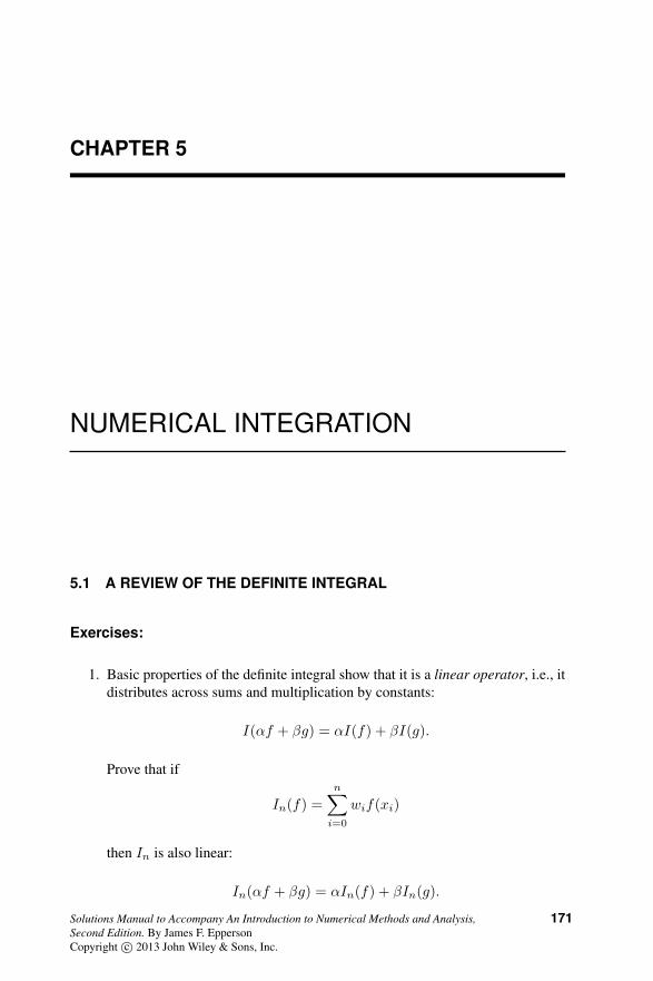
CHAPTER 5
NUMERICAL INTEGRATION
5.1 A REVIEW OF THE DEFINITE INTEGRAL
Exercises:
1. Basic properties of the definite integral show that it is a linear operator, i.e., itdistributes across sums and multiplication by constants:
I(αf + βg) = αI(f) + βI(g).
Prove that if
In(f) =n∑i=0
wif(xi)
then In is also linear:
In(αf + βg) = αIn(f) + βIn(g).
Solutions Manual to Accompany An Introduction to Numerical Methods and Analysis,Second Edition. By James F. EppersonCopyright c© 2013 John Wiley & Sons, Inc.
171

172 NUMERICAL INTEGRATION
Solution: This is a straight-forward computation:
In(αf + βg) =n∑i=0
wi(αf(xi) + βg(xi))
=n∑i=0
wiαf(xi) +n∑i=0
βg(xi)
= αn∑i=0
wif(xi) + βn∑i=0
g(xi)
= αIn(f) + βIn(g).
2. Assume that the quadrature rule In integrates all polynomials of degree lessthan or equal to N exactly:
In(p) = I(p)
for all p ∈ PN . Use this to prove that, for any integrand f , the error I − In isequal to the error in integrating the Taylor remainder:
I(f)− In(f) = I(RN )− In(RN )
where f(x) = pN (x) + RN (x). Does it really matter that we are using theTaylor polynomial and remainder? In other words, will this result hold for anypolynomial approximation and its associated error?
Solution: The previous problem established the linearity of In, which is theimportant issue. We have
I(f)− In(f) = I(pN +RN )− In(IN +RN )
= I(pN ) + I(RN )− In(pN )− In(RN )
= I(RN )− In(RN ).
3. Use Problem 1 to prove the following: If a quadrature rule In is exact for allpowers xk for k ≤ d, then it is exact for all polynomials of degree less than orequal to d.
Solution: Let p be an arbitrary polynomial of degree less than or equal to d,and let ξk(x) = xk. Then we can write
p(x) =d∑k=0
akξk(x).
The linearity that was proved in Problem 1 allows us to write
In(p) = In
(d∑k=0
akξk
)=
d∑k=0
akIn(ξk).

IMPROVING THE TRAPEZOID RULE 173
Therefore, I(p) = In(p) if and only if I(xik) = In(ξk) for all k.
/ • • • .
5.2 IMPROVING THE TRAPEZOID RULE
Exercises:
1. Apply the trapezoid rule and corrected trapezoid rule, with h = 14 , to approxi-
mate the integral
I =
∫ 1
0
x(1− x2)dx =1
4.
Solution: We have
T4(f) = (.25/2)(0 + 2(.234375) + 2(.375) + 2(.328125) + 0) = 0.234375.
We havef ′(x) = 1− 3x2,
so f ′(0) = 1 and f ′(1) = −2. Therefore,
TC4 (f) = T4(f)− (.252/12)(−2− 1) = .25,
which is exact.
2. Apply the trapezoid rule and corrected trapezoid rule, with h = 14 , to approxi-
mate the integral
I =
∫ 1
0
1√1 + x4
dx = 0.92703733865069.
Solution: The trapezoid rule gives us
T4(f) = (0.25/2)(1 + (2/√
1.00390625) + (2/√
1.0625)
+(2/√
1.31640625) + (1/√
2))
= 0.9233310015.
The corrected trapezoid value is then computed from this very simply:
TC4 (f) = 0.9233310015− (0.0625/12)(f ′(1)− f ′(0))
= 0.9233310015− (5.208333333× 10⁻³)(−2/23/2)
= 0.9270138493,

174 NUMERICAL INTEGRATION
which is much more accurate than the original T4 value.
3. Apply the trapezoid rule and corrected trapezoid rule, with h = 14 , to approxi-
mate the integral
I =
∫ 1
0
ln(1 + x)dx = 2 ln 2− 1.
Solution: We have
T4(f) = (.25/2)(0 + 2(.2231435513) + 2(.4054651081)
+2(.5596157879) + .6931471806)
= .3836995094.
We havef ′(x) = 1/(1 + x),
so f ′(0) = 1 and f ′(1) = 1/2. Therefore,
TC4 (f) = T4(f)− (.252/12)(.5− 1)
= .3836995094 + (.0625/24)
= .3863036761.
The exact value is .386294361.
4. Apply the trapezoid rule and corrected trapezoid rule, with h = 14 , to approxi-
mate the integral
I =
∫ 1
0
1
1 + x3dx =
1
3ln 2 +
1
9
√3π.
Solution: We have
T4(f) = (.25/2)(1 + 2(.9846153846) + 2(.8888888889)
+2(.7032967033) + .5)
= .8317002443.
Then we havef ′(x) = −3x2/(1 + x3)2,
so f ′(0) = 0 and f ′(1) = −3/4. Therefore,
TC4 (f) = T4(f)− (.252/12)(−0.75− 0) = .8356064943.
The exact value is .8356488485.
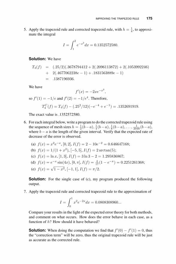
IMPROVING THE TRAPEZOID RULE 175
5. Apply the trapezoid rule and corrected trapezoid rule, with h = 14 , to approxi-
mate the integral
I =
∫ 2
1
e−x2
dx = 0.1352572580.
Solution: We have
T4(f) = (.25/2)(.3678794412 + 2(.2096113872) + 2(.1053992246)
+ 2(.4677062238e− 1) + .1831563889e− 1)
= .1387196936.
We havef ′(x) = −2xe−x
2
,
so f ′(1) = −1/e and f ′(2) = −1/e4. Therefore,
TC4 (f) = T4(f)− (.252/12)(−e−4 + e−1) = .1352691919.
The exact value is .1352572580.
6. For each integral below, write a program to do the corrected trapezoid rule usingthe sequence of mesh sizes h = 1
2 (b−a), 14 (b−a), 18 (b−a), . . . , 12048 (b−a),
where b− a is the length of the given interval. Verify that the expected rate ofdecrease of the error is observed.
(a) f(x) = x2e−x, [0, 2], I(f) = 2− 10e−2 = 0.646647168;
(b) f(x) = 1/(1 + x2), [−5, 5], I(f) = 2 arctan(5);
(c) f(x) = lnx, [1, 3], I(f) = 3 ln 3− 2 = 1.295836867;
(d) f(x) = e−x sin(4x), [0, π], I(f) = 417 (1− e−π) = 0.2251261368;
(e) f(x) =√
1− x2, [−1, 1], I(f) = π/2.
Solution: For the single case of (c), my program produced the followingoutput.
7. Apply the trapezoid rule and corrected trapezoid rule to the approximation of
I =
∫ 1
0
x2e−2xdx = 0.0808308960...
Compare your results in the light of the expected error theory for both methods,and comment on what occurs. How does the error behave in each case, as afunction of h? How should it have behaved?
Solution: When doing the computation we find that f ′(0)− f ′(1) = 0, thusthe “correction term” will be zero, thus the original trapezoid rule will be justas accurate as the corrected rule.
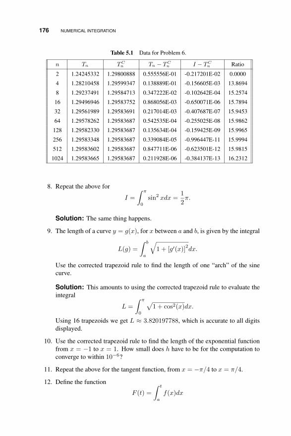
176 NUMERICAL INTEGRATION
Table 5.1 Data for Problem 6.
n Tn TCn Tn − TC
n I − TCn Ratio
2 1.24245332 1.29800888 0.555556E-01 -0.217201E-02 0.0000
4 1.28210458 1.29599347 0.138889E-01 -0.156605E-03 13.8694
8 1.29237491 1.29584713 0.347222E-02 -0.102642E-04 15.2574
16 1.29496946 1.29583752 0.868056E-03 -0.650071E-06 15.7894
32 1.29561989 1.29583691 0.217014E-03 -0.407687E-07 15.9453
64 1.29578262 1.29583687 0.542535E-04 -0.255025E-08 15.9862
128 1.29582330 1.29583687 0.135634E-04 -0.159425E-09 15.9965
256 1.29583348 1.29583687 0.339084E-05 -0.996447E-11 15.9994
512 1.29583602 1.29583687 0.847711E-06 -0.623501E-12 15.9815
1024 1.29583665 1.29583687 0.211928E-06 -0.384137E-13 16.2312
8. Repeat the above for
I =
∫ π
0
sin2 xdx =1
2π.
Solution: The same thing happens.
9. The length of a curve y = g(x), for x between a and b, is given by the integral
L(g) =
∫ b
a
√1 + [g′(x)]
2dx.
Use the corrected trapezoid rule to find the length of one “arch” of the sinecurve.
Solution: This amounts to using the corrected trapezoid rule to evaluate theintegral
L =
∫ π
0
√1 + cos2(x)dx.
Using 16 trapezoids we get L ≈ 3.820197788, which is accurate to all digitsdisplayed.
10. Use the corrected trapezoid rule to find the length of the exponential functionfrom x = −1 to x = 1. How small does h have to be for the computation toconverge to within 10−6?
11. Repeat the above for the tangent function, from x = −π/4 to x = π/4.
12. Define the function
F (t) =
∫ t
a
f(x)dx

SIMPSON’S RULE AND DEGREE OF PRECISION 177
and note that
F (b) = I(f) =
∫ b
a
f(x)dx.
Use Taylor expansions of F and f about x = a to show that
I(f)− 1
2(b− a)(f(b) + f(a))− 1
12(b− a)2(f ′(b)− f ′(a)) = O((b− a)5).
Use this to show that the corrected trapezoid rule is O(h4) when applied overa uniform grid of length h.
13. Construct a version of the “quasi-corrected” trapezoid rule that uses the deriva-tive approximations
f ′(a) ≈ f(a+ h)− f(a)
h, f ′(b) ≈ f(b)− f(b− h)
h.
Explain why we should expect this to be less accurate than the rule using theapproximations (5.2) and (5.3), and demonstrate that this is the case on theintegral
I =
∫ 1
0
x(1− x2)dx =1
4.
Solution: The approximations in (5.2) and (5.3) areO(h2) accurate, whereasthe approximations suggested in this exercise are onlyO(h). We thus expect toget less accuracy when using these approximations in the corrected trapezoidrule, and this is borne out by actual experiment. For the example in thisexercise, the corrected trapezoid rule using the O(h2) formulas is exact, butthe approximation using the less accurate formulas suggested in this exercisestill shows some error for h = (1/2)5.
/ • • • .
5.3 SIMPSON’S RULE AND DEGREE OF PRECISION
Exercises:
1. Apply Simpson’s rule with h = 14 , to approximate the integral
I =
∫ 1
0
x(1− x2)dx =1
4.
Solution: We have
S4(f) = (.25/3)(0 + 4(.2343750000) + 2(.3750000000)
+4(.3281250000) + 0) = 0.25,

178 NUMERICAL INTEGRATION
which is exact.
2. Apply Simpson’s rule with h = 14 , to approximate the integral
I =
∫ 1
0
1√1 + x4
dx = 0.92703733865069.
Solution: We have
S4(f) = (.25/3)(1 + 4(.9980525784) + 2(.9701425000)
+4(.8715755371) + 0.7071067810)
= .9271586870.
3. Apply Simpson’s rule with h = 14 , to approximate the integral
I =
∫ 1
0
ln(1 + x)dx = 2 ln 2− 1.
How small does the error theory say that h has to be to get that the error isless than 10−3? 10−6? How small does h have to be for the trapezoid rule toachieve this accuracy?
Solution: For h = 1/4, we get S4(f) = .3862595628. To get the error lessthan 10−3 we need
h4
180× 6
(1 + 0)4≤ 10−3,
which implies that h ≤ .4161791450. To get 10−6 accuracy, we need h ≤.7400828045e− 1. Using the trapezoid rule, we need to have
h2
12× 1
(1 + 0)2≤ 10−3,
so that we need h ≤ .1095445115 and h ≤ .3464101615e− 2.
4. Apply Simpson’s rule with h = 14 , to approximate the integral
I =
∫ 1
0
1
1 + x3dx =
1
3ln 2 +
1
9
√3π.
Solution: We have
S4(f) = (.25/3)(1 + 4(.9846153846) + 2(.8888888889)
+4(.7032967033) + 0.5)
= .8357855108.

SIMPSON’S RULE AND DEGREE OF PRECISION 179
The exact value is .8356488485.
5. Apply Simpson’s rule with h = 14 , to approximate the integral
I =
∫ 2
1
e−x2
dx = 0.1352572580.
Solution: We have
S4(f) = (.25/3)(.3678794412 + 4(.2096113872) + 2(.1053992246)
+ 4(.4677062238e− 1) + .1831563889e− 1)
= .1352101306.
6. For each function below, write a program to do Simpson’s rule using thesequence of mesh sizes h = 1
2 (b − a), 14 (b − a), 18 (b − a), . . . , 12048 (b − a),
where b − a is the length of the given interval. Verify that the expected rateof decrease of the error is observed. Comment on any anomolies that areobserved.
(a) f(x) = lnx, [1, 3], I(f) = 3 ln 3− 2 = 1.295836867;
(b) f(x) = x2e−x, [0, 2],I(f) = 2− 10e−2 = 0.646647168;
(c) f(x) = 1/(1 + x2), [−5, 5], I(f) = 2 arctan(5);
(d) f(x) =√
1− x2, [−1, 1], I(f) = π/2;
(e) f(x) = e−x sin(4x), [0, π], I(f) = 417 (1− e−π) = 0.2251261368.
Solution: My program produced the output (for (a) - (d), only) in Table5.2. Note that the accuracy is as it should be for all but the single case of(d), for which the error theory does not apply because of the singularity in thederivative at each endpoint.
7. For each integral in the previous problem, how small does h have to be to getaccuracy, according to the error theory, of at least 10−3? 10−6? Compare tothe value of h required by the trapezoid rule for this accuracy. (Feel free to usea computer algebra system to help you with the computation of the derivatives.)
Solution:
(a) For f(x) = lnx we have
|I(f)− Sn(f)| ≤ 2h4
180maxx∈[1,3]
∣∣∣∣−6
x4
∣∣∣∣ ≤ h4
90× 6 =
h4
15.
Therefore we require h ≤ .3499635512 for 10−3 accuracy and h ≤.6223329773e− 1 for 10−6.

180 NUMERICAL INTEGRATION
Table 5.2 Results for Exercise 5.3.6
n (c) (b) (a) (d)
2 6.79487179487180 0.67095296587741 1.29040033696930 1.33333333333333
4 2.65030946065429 0.64863368605631 1.29532166828621 1.48803387171258
8 2.61738281929855 0.64678014940774 1.29579834986087 1.54179757747348
16 2.73331903435335 0.64665562384530 1.29583431135754 1.56059458488771
32 2.74671071699175 0.64664769843876 1.29583670367239 1.56719883449230
64 2.74680148839078 0.64664720084510 1.29583685581508 1.56952610894680
128 2.74680153128328 0.64664716971014 1.29583686536681 1.57034753804027
256 2.74680153372702 0.64664716776365 1.29583686596447 1.57063770946780
512 2.74680153387984 0.64664716764198 1.29583686600184 1.57074025657205
1024 2.74680153388940 0.64664716763438 1.29583686600417 1.57077650465356
2048 2.74680153388999 0.64664716763390 1.29583686600432 1.57078931890607
(b) For f(x) = x2e−x we have
|I(f)− Sn(f)| ≤ 2h4
180maxx∈[0,2]
∣∣(x2 − 8x+ 12)e−x∣∣ ≤ h4
90× 12 =
2h4
15.
Therefore we require h ≤ .2942830956 for 10−3 accuracy and h ≤.5233175697e− 1 for 10−6.
(c) For f(x) = 1/(1 + x2), we have
|I(f)−Sn(f)| ≤ 10h4
180max
x∈[−5,5]
∣∣∣∣24(5x4 − 10x2 + 1)
(1 + x2)5
∣∣∣∣ ≤ 4h4
3×24 = 32h4.
Therefore we require h ≤ .7476743906e − 1 for 10−3 accuracy andh ≤ .1329573974e− 1 for 10−6.
(d) For f(x) =√
1− x2 we have that the fourth derivative is not boundedon [−1, 1] so the error theory does not apply.
(e) For f(x) = e−x sin(4x) we have
|I(f)− Sn(f)| ≤ πh4
180maxx∈[0,π]
∣∣(161 sin 4x+ 240 cos 4x)e−x∣∣
≤ πh4
180× 260 =
13πh4
9.

SIMPSON’S RULE AND DEGREE OF PRECISION 181
Therefore we require h ≤ .1218392792 for 10−3 accuracy and h ≤.2166642816e− 1 for 10−6.
8. Since the area of the unit circle is A = π, it follows that
π
2=
∫ 1
−1
√1− x2dx.
Therefore we can approximateπ by approximating this integral. Use Simpson’srule to compute approximate values of π in this way and comment on yourresults.
Solution: Using the sequence of h values h = 1, 1/2, 1/4, 1/8, . . ., we getfollowing table of approximate values of π. Clearly the values are converging
Estimate of π2.6666666672.9760677443.0835951563.1211891703.1343976703.1390522183.1406950763.1412754193.1414805143.1415530093.1415786383.141587698
to π, but not as rapidly as we would expect from Simpson’s rule. The reason isthat the integrand is not smooth at either endpoint, thus the error estimate forSimpson’s rule does not apply.
9. If we wanted to use Simpson’s rule to approximate the natural logarithmfunction on the interval [ 12 , 1] by approximating
lnx =
∫ x
1
1
tdt
how many points would be needed to obtain an error of less than 10−6? Howmany points for an error of less than 10−16? What are the corresponding valuesfor the trapezoid rule?
Solution: The error using Simpson’s rule is bounded above according to
E ≤ (1/2)h4
180max
x∈(1/2),1
24
x5=
32h4
15.

182 NUMERICAL INTEGRATION
Therefore, to get 10−6 accuracy requires imposing
32h4/15 ≤ 10−6
which implies h ≤ 0.026166, therefore the number of required points isn = 20. To get 10−16 accuracy requires h ≤ .8274377295e−4 and n = 6043.For the trapezoid rule we get h ≤ 0.0049 and n ≥ 103, and h ≤ 0.4899×10⁻⁷
and n ≥ 10206208. Clearly Simpson’s rule is more efficient.
10. Use Simpson’s rule to produce a graph of E(x), defined to be the length of theexponential curve from 0 to x, for 0 ≤ x ≤ 3. See Problem 14 of 2.5.
Solution: If we use a fixed number of points, say n = 128, for any value ofx, then we get the plot shown in Figure 5.1.
0 0.5 1 1.5 2 2.5 30
2
4
6
8
10
12
14
16
18
20
Figure 5.1 Solution for Exercise 5.3.10.
11. Let f(x) = |x|; use the trapezoid rule (with n = 1), corrected trapezoid rule(with n = 1), and Simpson’s rule (with n = 2), to compute
I(f) =
∫ 1
−1f(x)dx
and compare your results to the exact value. Explain what happens in the lightof our error estimates for the trapezoid and Simpson’s rules.
Solution: Because the function is piecewise linear, and one grid point matchesthe “kink” in the graph, the trapezoid rule will produce the exact value of theintegral, but neither Simpson’s rule nor the corrected trapezoid rule will beexact.

SIMPSON’S RULE AND DEGREE OF PRECISION 183
12. Write out the expression for Simpson’s rule when c is not the midpoint of theinterval [a, b]. To simplify matters, take c− a = h, b− c = θh.
Solution: We get
S2(f) = (h/6)(Af(a) + Cf(c) +Bf(b)),
where
A = 2 + θ − θ2, C = (3θ2 + 1 + θ3 + 3θ)/θ, B = (2θ2 + θ − 1)/θ.
13. What is the degree of precision of the corrected trapezoid rule, TC1 ? Whatabout the n subinterval version, TCn ?
Solution: Let ξk(x) = xk, and consider the computation
Ik = TC1 (ξk) =1
2(b− a)
(ak + bk
)− b− a
12
(kbk−1 − kak−1
)=
1
2(b− a)(bk + ak)− 1
12(b− a)2(kb(k − 1)− ka(k − 1)).
When simplified, and compared to the exact values of
I =
∫ b
a
ξk(x)dx
we get that Ik = I for k = 0, 1, 2, 3, but not for k = 4, thus showing thatthe degree of precision is p = 3. The same result holds for the n subintervalversion.
14. Prove that if we want to show that the quadrature rule In(f) has degree ofprecision p, it suffices to show that it will exactly integrate xk, 0 ≤ k ≤ p overthe integral (0, 1).
Solution: Let q(x) be an arbitrary polynomial of degree p. Then
q(x) =
p∑k=0
akxk,
so
I(q) =
p∑k=0
∫ b
a
xkdx.
Therefore, we need only concern ourselves with exactly integrating simplepowers instead of general polynomials. A change of variable can now beemployed to transform the interval of interest to [0, 1] from the more general[a, b].

184 NUMERICAL INTEGRATION
15. Construct the analogue of Simpson’s rule based on exactly integrating a cubicinterpolate at equally spaced points on the interval [a, b].
Solution: This yields what is sometimes known as Simpson’s three-eighthsrule:
I3(f) =3h
8(f(a) + 3f(a+ h) + 3f(a+ 2h) + f(a+ 3h)) .
16. Show that I(q3) = S2(f).
Solution: This is actually a straight-forward (if lengthy) computation withq3(x) as defined here:
q3(x) = f(a) +
(f(c)− f(a)
h
)(x− a)
+
(f ′(c)− f(c)−f(a)
h
h
)(x− a)(x− c) +A(x− a)(x− c)2,
where
A = h−2(f(b)− f(c)
h− 2f ′(c) +
f(c)− f(a)
h
)and
h = c− a = b− c.
17. Consider the quadrature rule defined by exactly integrating a cubic Hermiteinterpolate:
I1(f) = I(H2).
Write down the quadrature formula for both the basic and composite settings,and state and prove an error estimate, using the error results for Hermiteinterpolation from the previous chapter.
Solution: The Hermite cubic interpolant can be written as
H2(x) = ha(x)f(a) + hb(x)f(b) + ha(x)f ′(a) + hb(x)f ′(b),
where the h and h functions are given in Section 4.6 as follows:
ha(x) =
(1− 2
(x− aa− b
))(x− ba− b
)2
hb(x) =
(1− 2
(x− bb− a
))(x− ab− a
)2
ha(x) = (x− a)
(x− ba− b
)2

SIMPSON’S RULE AND DEGREE OF PRECISION 185
hb(x) = (x− b)(x− ab− a
)2
Then the integration rule is
I1(f) = Af(a) +Bf(b) + αf ′(a) + βf ′(b),
where
A =
∫ b
a
ha(x)dx =1
2(b− a)
B =
∫ b
a
hb(x)dx =1
2(b− a)
α =
∫ b
a
ha(x)dx =1
12(b− a)2
β =
∫ b
a
ha(x)dx = − 1
12(b− a)2
The n interval rule is easily derived from the single interval rule. The errorestimate is found as follows:
I(f)− I1(f) =
∫ b
a
(f(x)−H2(x)) dx
=1
24
∫ b
a
(x− a)2(x− b)2f (4)(ξx)dx
=
(1
24
∫ b
a
(x− a)2(x− b)2dx
)f (4)(ξ)
=(b− a)5
720f (4)(ξ)
18. Consider a quadrature rule in the form
In(f) =n∑k=1
akf(xk)
where the coefficients ak > 0 and the grid points xk are all known. Assumethat In integrates the trivial function w(x) = 1 exactly:
In(w) =n∑k=1
ak = I(w) =
∫ b
a
dx = b− a,
and that this holds for all intervals (a, b). Consider now the effects of roundingerror on integrating an arbitrary function f . Let f(x) = f(x) + ε(x) be f

186 NUMERICAL INTEGRATION
polluted by rounding error, with |ε(x)| ≤ Cu for some constant C > 0, for allx ∈ [a, b]. Show that
|In(f)− In(f)| ≤ Cu(b− a).
Comment on this in comparison to the corresponding result for numericaldifferentiation, as given in 2.2.
Solution: The point is that numerical integration is much less affected byrounding error than is numerical differentiation.
19. The normal probability distribution is defined as
p(x) =1
σ√
2πe−(x−µ)
2/2σ2
where µ is the mean, or average, and σ is the variance. This is the famousbell-shaped curve that one hears so much about; the mean gives the center ofthe bell and the variance gives the width of it. If x is distributed in this fashion,then the probability that a ≤ x ≤ b is given by the integral
P (a ≤ x ≤ b) =
∫ b
a
p(x)dx.
(a) Use the change of variable z = (x− µ)/σ to show that
P (−mσ ≤ x ≤ mσ) =1√2π
∫ m
−me−z
2/2dz.
(b) Compute values of P (−mσ ≤ x ≤ mσ) for m = 1, 2, 3, using Simp-son’s rule.
Solution: For m = 1, P (−mσ ≤ x ≤ mσ) ≈ .6826908120; for m = 2,P (−mσ ≤ x ≤ mσ) ≈ .9544947255; and m = 3, P (−mσ ≤ x ≤mσ) ≈ .9972830690.
20. Use Simpson’s rule to solve Problem 9 from 5.2.
21. Use Simpson’s rule to solve Problem 10 from 5.2.
/ • • • .

THE MIDPOINT RULE 187
5.4 THE MIDPOINT RULE
Exercises:
1. Apply the midpoint rule with h = 14 , to approximate the integral
I =
∫ 1
0
x(1− x2)dx =1
4.
How small does h have to be to get that the error is less than 10−3? 10−6?
Solution: We have, for f(x) = x(1− x2),
M4(f) = (1/4)(f(1/8) + f(3/8) + f(5/8) + f(7/8)) = .2578125000.
The error estimate is
|I(f)−Mn(f)| ≤ h2
24maxx∈[0,1]
| − 6x| = h2
4,
so we require h ≤ .6324555320e − 1 for 10−3 accuracy, and h ≤ 0.002 for10−6.
2. Apply the midpoint rule with h = 14 , to approximate the integral
I =
∫ 1
0
1√1 + x4
dx = 0.92703733865069.
How small does h have to be to get that the error is less than 10−3? 10−6?
Solution:M4(f) = .9288993588,
and h ≤ .1312709324 for 10−3 accuracy, h ≤ .4151151371e− 2 for 10−6.
3. Apply the midpoint rule with h = 14 , to approximate the integral
I =
∫ 1
0
ln(1 + x)dx = 2 ln 2− 1.
How small does h have to be to get that the error is less than 10−3? 10−6?
Solution:M4(f) = .3875883105,
and h ≤ .1549193338 for 10−3 accuracy, h ≤ .4898979486e− 2 for 10−6.
4. Apply the midpoint rule with h = 14 , to approximate the integral
I =
∫ 1
0
1
1 + x3dx =
1
3ln 2 +
1
9
√3π.

188 NUMERICAL INTEGRATION
How small does h have to be to get that the error is less than 10−3? 10−6?
Solution:M4(f) = .8376389970,
and h ≤ .1175282713 for 10−3 accuracy, h ≤ .3716570267e− 2 for 10−6.
5. Apply the midpoint rule with h = 14 , to approximate the integral
I =
∫ 2
1
e−x2
dx = 0.1352572580.
How small does h have to be to get that the error is less than 10−3? 10−6?
Solution:M4(f) = .1335215673,
and h ≤ .1095445115 for 10−3 accuracy, h ≤ .3464101615e− 2 for 10−6.
6. Show that the midpoint rule can be derived by integrating, exactly, a polynomialinterpolate of degree zero.
Solution: Take p0(x) = f(c) where c = (a + b)/2 is the midpoint of theinterval. Then
I(p0) =
∫ b
a
p0(x)dx = f(c)(b− a) = M1(f).
7. Apply the midpoint rule to each of the following functions, integrated overthe indicated interval. Use a sequence of grids h = (b − a), (b − a)/2, (b −a)/4, . . . and confirm that the approximations are converging at the correctrate. Comment on any anomolies that you observe.
(a) f(x) = lnx, [1, 3], I(f) = 3 ln 3− 2 = 1.295836867;
(b) f(x) = x2e−x, [0, 2],I(f) = 2− 10e−2 = 0.646647168;
(c) f(x) =√
1− x2, [−1, 1], I(f) = π/2;
(d) f(x) = 1/(1 + x2), [−5, 5], I(f) = 2 arctan(5);
(e) f(x) = e−x sin(4x), [0, π], I(f) = 417 (1− e−π) = 0.2251261368.
Solution: The output is in Table 5.3 ((a) - (d), only). The approximationperformed as expected, with two notable exceptions: For f(x) =
√1− x2,
we did not achieve the expected rate of decrease for the error, because thesecond derivative of f is unbounded on [−1, 1]. For f(x) = x2e−x, weachieved higher accuracy than expected. This occurs because f ′(0) = f ′(2)and there is an effect similar to the corrected trapezoid rule.
8. For each integral in the previous problem, how small does h have to be to getaccuracy, according to the error theory, of at least 10−3? 10−6?
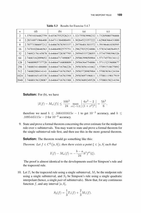
THE MIDPOINT RULE 189
Table 5.3 Results for Exercise 5.4.7
n (d) (b) (a) (c)
2 1.37931034482759 0.65367552526213 1.32175583998232 1.73205080756888
4 2.28316971966400 0.64711384088491 1.30264523357222 1.62968366431800
8 2.70773386697212 0.64667678393337 1.29756401303372 1.59196461030595
16 2.74701026646563 0.64664902575751 1.29627032524886 1.57834346564915
32 2.74692176145878 0.64664728387795 1.29594533728055 1.57347590396326
64 2.74683162099652 0.64664717490087 1.29586399050904 1.57174570134112
128 2.74680905737720 0.64664716808809 1.29584364754886 1.57113233600677
256 2.74680341486880 0.64664716766226 1.29583856141662 1.57091518675892
512 2.74680200414141 0.64664716763565 1.29583728985904 1.57083836124104
1024 2.74680165145330 0.64664716763398 1.29583697196811 1.57081119017919
2048 2.74680156328087 0.64664716763388 1.29583689249528 1.57080158214194
Solution: For (b), we have
|I(f)−Mn(f)| ≤ 10h2
24max
x∈[−5,5]
∣∣∣∣ 6x2 − 2
(1 + x2)3
∣∣∣∣ =5h2
6,
therefore we need h ≤ .3464101615e − 1 to get 10−3 accuracy, and h ≤.1095445115e− 2 for 10−6 accuracy.
9. State and prove a formal theorem concerning the error estimate for the midpointrule over n subintervals. You may want to state and prove a formal theorem forthe single subinterval rule first, and then use this in the more general theorem.
Solution: The theorem would go something like this:
Theorem: Let f ∈ C2([a, b]); then there exists a point ξ ∈ [a, b] such that
I(f)−Mn(f) = −b− a24
h2f ′′(ξ).
The proof is almost identical to the developments used for Simpson’s rule andthe trapezoid rule.
10. Let T1 be the trapezoid rule using a single subinterval,M1 be the midpoint ruleusing a single subinterval, and S2 be Simpson’s rule using a single quadraticinterpolant (hence, a single pair of subintervals). Show that, for any continuousfunction f , and any interval [a, b],
S2(f) =1
3T1(f) +
2
3M1(f).

190 NUMERICAL INTEGRATION
Solution: Let c denote the midpoint of the interval [a, b], so that we have
T1(f) =1
2(b− a)(f(b) + f(a))
S2(f) =(b− a)/2
3(f(a) + 4f(c) + f(b))
M1(f) = (b− a)f(c).
Then a direct computation shows
1
3T1(f) +
2
3M1(f) =
1
6(b− a)(f(b) + f(a)) +
2
3(b− a)f(c)
=(b− a)/2
3(f(a) + 4f(c) + f(b)) = S2(f).
/ • • • .
5.5 APPLICATION: STIRLING’S FORMULA
Exercises:
1. Use Stirling’s formula to show that
limn→∞
(xn
n!
)= 0
for all x.
Solution: We have∣∣∣∣xnn!
∣∣∣∣ ≤ |xn|Cn√n(n/e)n
=
(1
Cn√n
)(|x|en
)n.
Forn sufficiently large, the second factor will be less than one, which completesthe proof.
2. For x = 10 and ε = 10−3, how large does n have to be for∣∣∣∣xnn!
∣∣∣∣ ≤ εto hold? Repeat for ε = 10−6. Use Stirling’s formula here, don’t just plugnumbers into a calculator.

APPLICATION: STIRLING’S FORMULA 191
Solution: We have, for all n ≥ 1,
10n
n!=
10nen
Cn√nnn
≤ 1
2
(10e
n
)n.
For all n ≥ 30, we then have
10n
n!≤ 1
2
(10e
30
)n,
so that taking
n =− ln 10−3
ln 3− 1= 70.05
ought to suffice. For 10−6 we need to have n = 140.1 These are bothconservative estimates, because the ratio 10e/n is of course decreasing as nincreases, and we took it as the fixed value r = 10e/30 ≈ 0.9061. Using aprogram like Maple we can find that the precise values are 32 and 38.
3. Use Stirling’s formula to determine the value of
limn→∞
(n!)p
(pn)!
where p ≥ 2 is an integer.
Solution: We have(n!)p
(pn)!=
[Cn√n(n/e)n]p
Cpn√pn(pn/e)pn
=
(Cpn
Cpn√p
)(√np−1√p
)(1
pp
)n=
(√np−1
Cpn√p
)(Cnpn
)p.
It is a simple exercise with L’Hôpital’s rule to show that the second factor goesto zero much faster than the first one goes to infinity. Thus the limit is zero.
4. Use Stirling’s formula to get an upper bound on the ratio
Rn =1 · 3 · 5 · · · (2n− 1)
2n+1n!
as a function of n.
Solution: The idea is to insert factors of 2 into the numerator and denominatorso that the product of odd terms can be treated as a factorial:
1 · 3 · 5 · · · (2n− 1)
2n+1n!=
1 · 2 · 3 · 4 · 5 · · · (2n− 1) · (2n)
[2 · 4 · 6 · · · (2n)]2n+1n!
=(2n)!
2n(n!)2n+1n!=
(2n)!
2(2nn!)2.
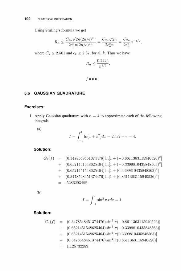
192 NUMERICAL INTEGRATION
Using Stirling’s formula we get
Rn ≤C2n
√2n(2n/e)2n
2c2nn(2n/e)2n=C2n
√2n
2c2nn=C2n
2c2nn−1/2,
where Ck ≤ 2.501 and ck ≥ 2.37, for all k. Thus we have
Rn ≤0.2226
n1/2.
/ • • • .
5.6 GAUSSIAN QUADRATURE
Exercises:
1. Apply Gaussian quadrature with n = 4 to approximate each of the followingintegrals.
(a)
I =
∫ 1
−1ln(1 + x2)dx = 2 ln 2 + π − 4.
Solution:
G4(f) = (0.3478548451374476) ln[1 + (−0.8611363115940526)2]
+ (0.6521451548625464) ln[1 + (−0.3399810435848563)2]
+ (0.6521451548625464) ln[1 + (0.3399810435848563)2]
+ (0.3478548451374476) ln[1 + (0.8611363115940526)2]
= .5286293488
(b)
I =
∫ 1
−1sin2 πxdx = 1.
Solution:
G4(f) = (0.3478548451374476) sin2[π(−0.8611363115940526)]
+ (0.6521451548625464) sin2[π(−0.3399810435848563)]
+ (0.6521451548625464) sin2[π(0.3399810435848563)]
+ (0.3478548451374476) sin2[π(0.8611363115940526)]
= 1.125732289
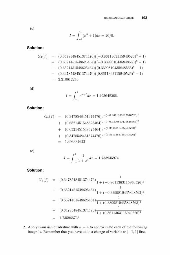
GAUSSIAN QUADRATURE 193
(c)
I =
∫ 1
−1(x8 + 1)dx = 20/9.
Solution:
G4(f) = (0.3478548451374476)((−0.8611363115940526)8 + 1)
+ (0.6521451548625464)((−0.3399810435848563)8 + 1)
+ (0.6521451548625464)((0.3399810435848563)8 + 1)
+ (0.3478548451374476)((0.8611363115940526)8 + 1)
= 2.210612246
(d)
I =
∫ 1
−1e−x
2
dx = 1.493648266.
Solution:
G4(f) = (0.3478548451374476)e−(−0.8611363115940526)2
+ (0.6521451548625464)e−(−0.3399810435848563)2
+ (0.6521451548625464)e−(0.3399810435848563)2
+ (0.3478548451374476)e−(0.8611363115940526)2
= 1.493334622
(e)
I =
∫ 1
−1
1
1 + x4dx = 1.733945974.
Solution:
G4(f) = (0.3478548451374476)1
1 + (−0.8611363115940526)4
+ (0.6521451548625464)1
1 + (−0.3399810435848563)4
+ (0.6521451548625464)1
1 + (0.3399810435848563)4
+ (0.3478548451374476)1
1 + (0.8611363115940526)4
= 1.735966736
2. Apply Gaussian quadrature with n = 4 to approximate each of the followingintegrals. Remember that you have to do a change of variable to [−1, 1] first.

194 NUMERICAL INTEGRATION
(a)
I =
∫ 1
0
ln(1 + x)dx = 2 ln 2− 1.
(b)
I =
∫ 1
0
1√1 + x4
dx = 0.92703733865069.
Solution: G4(f) = .9270388618
(c)
I =
∫ 1
0
x(1− x2)dx =1
4.
(d)
I =
∫ 1
0
1
1 + x3dx =
1
3ln 2 +
1
9
√3π.
Solution: G4(f) = .8356239692
(e)
I =
∫ 2
1
e−x2
dx = 0.1352572580.
3. Show that (5.8) is both necessary and sufficient to make the quadrature exactfor all polynomials of degree less than or equal to 2N − 1.
Solution: Suppose (5.8) holds, and let q(x) be an arbitrary polynomial ofdegree ≤ 2N − 1. Then
q(x) =2N−1∑i=0
aixi
and ∫ 1
−1q(x)dx =
2N−1∑i=0
ai
∫ 1
−1xidx.
Since Gaussian quadrature is exact for this range of degree of polynomials, wethen have
I(q) =2N−1∑i=0
ai
(n∑k=1
w(n)k [x
(n)k ]i
)= Gn(q).
The steps are entirely reversible, so we can easily prove the other direction ofthe implication.
4. Write a program that does Gaussian quadrature, using the weights and Gausspoints given in the text. Apply this to each of the integrals below, and com-pare your results to those for the other quadrature methods in the exercises.

GAUSSIAN QUADRATURE 195
Remember that you will have to do a change of variable if the interval is not[−1, 1]. Be sure to run your program for more than one value of n.
(a) f(x) =√
1− x2, [−1, 1], I(f) = π/2;
(b) f(x) = x2e−x, [0, 2],I(f) = 2− 10e−2 = 0.646647168;
Solution: G4(f) = .6466426358
(c) f(x) = lnx, [1, 3], I(f) = 3 ln 3− 2 = 1.295836867;
(d) f(x) = 1/(1 + x2), [−5, 5], I(f) = 2 arctan(5);
(e) f(x) = e−x sin(4x), [0, π], I(f) = 417 (1− e−π) = 0.2251261368.
5. Let P (x) = 6x3 + 5x2 + x, and let P2(x) = 3x2 − 1 (this is the quadraticLegendre polynomial). Find linear polynomials Q(x) and R(x) such thatP (x) = P2(x)Q(x) +R(x). Verify that I(P ) = I(R).
Solution: Simple division shows that Q(x) = 2x + (5/3) and R(x) =3x+ (5/3). It is then easily verified that
(3x2 − 1)(2x+ (5/3)) + (3x+ (5/3)) = P (x).
6. Let P (x) = x3 + x2 + x− 1, and repeat the above.
Solution: This time Q(x) = (1/3)(x+ 1) and R(x) = (4/3)x− (2/3).
7. Let P (x) = 3x3 + x2 − 6, and repeat the above.
Solution: This time Q(x) = x+ (1/3) and R(x) = x− (17/3).
8. Verify that the weights for the n = 2 Gaussian quadrature rule satisfy theformula (5.9).
Solution: This amounts to showing that∫ 1
−1
x− 0.5773502691896257
−0.5773502691896257− 0.5773502691896257dx = 1
which it does, and similarly for the other Gauss point and weight.
9. Repeat the above for the n = 4 rule.
Solution: This involves the same kind of computation, with the same result.
10. Show, by direct computation, that the n = 2 and n = 4 Gaussian quadraturerules are exact for the correct degree of polynomials.
Solution: Direct computation does the trick.
11. The quadratic Legendre polynomial is P2(x) = (3x2 − 1)/2. Show that it isorthogonal (over [−1, 1]) to all linear polynomials.
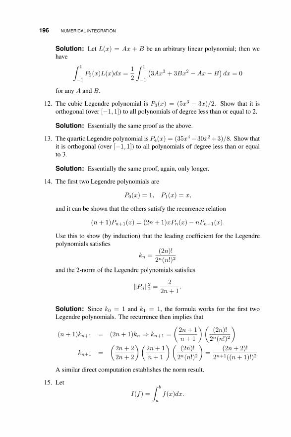
196 NUMERICAL INTEGRATION
Solution: Let L(x) = Ax + B be an arbitrary linear polynomial; then wehave ∫ 1
−1P2(x)L(x)dx =
1
2
∫ 1
−1
(3Ax3 + 3Bx2 −Ax−B
)dx = 0
for any A and B.
12. The cubic Legendre polynomial is P3(x) = (5x3 − 3x)/2. Show that it isorthogonal (over [−1, 1]) to all polynomials of degree less than or equal to 2.
Solution: Essentially the same proof as the above.
13. The quartic Legendre polynomial is P4(x) = (35x4−30x2 +3)/8. Show thatit is orthogonal (over [−1, 1]) to all polynomials of degree less than or equalto 3.
Solution: Essentially the same proof, again, only longer.
14. The first two Legendre polynomials are
P0(x) = 1, P1(x) = x,
and it can be shown that the others satisfy the recurrence relation
(n+ 1)Pn+1(x) = (2n+ 1)xPn(x)− nPn−1(x).
Use this to show (by induction) that the leading coefficient for the Legendrepolynomials satisfies
kn =(2n)!
2n(n!)2
and the 2-norm of the Legendre polynomials satisfies
‖Pn‖22 =2
2n+ 1.
Solution: Since k0 = 1 and k1 = 1, the formula works for the first twoLegendre polynomials. The recurrence then implies that
(n+ 1)kn+1 = (2n+ 1)kn ⇒ kn+1 =
(2n+ 1
n+ 1
)((2n)!
2n(n!)2
)kn+1 =
(2n+ 2
2n+ 2
)(2n+ 1
n+ 1
)((2n)!
2n(n!)2
)=
(2n+ 2)!
2n+1((n+ 1)!)2
A similar direct computation establishes the norm result.
15. Let
I(f) =
∫ b
a
f(x)dx.

GAUSSIAN QUADRATURE 197
Show that the change of variable x = a+ 12 (b− a)(z + 1) gives that
I(f) =
∫ 1
−1F (z)dz
for F (z) = 12 (b− a)f(a+ 1
2 (b− a)(z + 1)).
Solution: Direct computation.
16. Show that the error for Gaussian quadrature applied to
I(f) =
∫ b
a
f(x)dx
is O([(b− a)(e/8n)]2n).
Solution: Apply Stirling’s formula to the error estimate.
17. Prove Theorem 5.5. Hint: Simply generalize what was done in the text for thespecial case of
I(f) =
∫ 1
−1f(x)dx.
Solution: This is a routine adaptation of the exposition in the text to the situ-ation in which the polynomials φk are orthogonal with respect to the weightedinner product defined by w and [a, b].
18. Once again, we want to consider the approximation of the natural logarithmfunction, this time using numerical quadrature. Recall that we have
lnx =
∫ x
1
1
tdt.
Recall also that it suffices to consider x ∈ [ 12 , 1].
(a) How many grid points are required for 10−16 accuracy using the trapezoidrule? Simpson’s rule?
(b) How many grid points are required if Gauss-Legendre quadrature is used?
Solution: Using the formula for the Gaussian quadrature error over a generalinterval, we get (assuming x is near 1 to maximize the b− a factor):
| lnx−Gn| =(1/2)2n+1(n!)4
(2n+ 1)[(2n)!]3× (2n− 1)!
(1/2)2n
=(1/2)
(2n+ 1)(2n)× (n!)4
[(2n)!]2
≤ 1
8n2× (n!)4
[(2n)!]2.

198 NUMERICAL INTEGRATION
We use Stirling’s formula to estimate the factorials. We have
(n!)4 ≤ (2.501)4n2(n/e)4n
and[(2n)!]2 ≥ (2.3)2(2n)(2n/e)4n
Therefore
| lnx−Gn| ≤(2.501)4n2
16(2.3)2n3× (1/2)4n =
(0.46)(1/2)4n
n.
This achieves the desired accuracy for n ≥ 13.
19. Write a computer program that uses Gaussian quadrature for a specified num-ber of points to compute the natural logarithm over the interval [ 12 , 1], to within10−16 accuracy. Compare the accuracy of your routine to the intrinsic loga-rithm function on your system.
Solution: A MATLAB script is given below. The maximum error on [1/2, 1]was about 4 × 10⁻¹⁵. This is larger than the specified accuracy, but this isprobably due to rounding error within MATLAB itself.
function y = loggauss(x)
a = [0.9501250983763744E-01 0.1894506104550685E+00
0.2816035507792589E+00 0.1826034150449236E+00
0.4580167776572274E+00 0.1691565193950024E+00
0.6178762444026438E+00 0.1495959888165733E+00
0.7554044083550030E+00 0.1246289712555339E+00
0.8656312023878318E+00 0.9515851168249290E-01
0.9445750230732326E+00 0.6225352393864778E-01
0.9894009349916499E+00 0.2715245941175185E-01];
xg = a(:,1);
wg = a(:,2);
xg = [-xg; xg];
wg = [wg; wg];
%
xg = 1 + 0.5*(x-1)*(xg + 1);
wg = 0.5*(x-1)*wg;
%
y = sum(wg./xg);
20. Write a brief essay, in your own words, of course, which explains the impor-tance of the linearity of the integral and quadrature rule in the development ofGaussian quadrature.
Solution: The linearity is vital because of the role played by inner productsand orthogonality in the construction and accuracy of the Gaussian quadrature.
/ • • • .
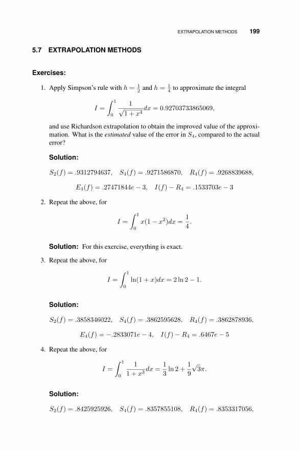
EXTRAPOLATION METHODS 199
5.7 EXTRAPOLATION METHODS
Exercises:
1. Apply Simpson’s rule with h = 12 and h = 1
4 to approximate the integral
I =
∫ 1
0
1√1 + x4
dx = 0.92703733865069,
and use Richardson extrapolation to obtain the improved value of the approxi-mation. What is the estimated value of the error in S4, compared to the actualerror?
Solution:
S2(f) = .9312794637, S4(f) = .9271586870, R4(f) = .9268839688,
E4(f) = .27471844e− 3, I(f)−R4 = .1533703e− 3
2. Repeat the above, for
I =
∫ 1
0
x(1− x2)dx =1
4.
Solution: For this exercise, everything is exact.
3. Repeat the above, for
I =
∫ 1
0
ln(1 + x)dx = 2 ln 2− 1.
Solution:
S2(f) = .3858346022, S4(f) = .3862595628, R4(f) = .3862878936,
E4(f) = −.2833071e− 4, I(f)−R4 = .6467e− 5
4. Repeat the above, for
I =
∫ 1
0
1
1 + x3dx =
1
3ln 2 +
1
9
√3π.
Solution:
S2(f) = .8425925926, S4(f) = .8357855108, R4(f) = .8353317056,

200 NUMERICAL INTEGRATION
E4(f) = .45380545e− 3, I(f)−R4 = .3171429e− 3
5. Repeat the above, for
I =
∫ 2
1
e−x2
dx = 0.1352572580.
Solution:
S2(f) = .1346319964, S4(f) = .1352101306, R4(f) = .1352486730,
E4(f) = −.38542280e− 4, I(f)−R4 = .85850e− 5
6. Write a trapezoid rule program to compute the value of the integral
I =
∫ 1
0
e−x2
dx
Take h small enough to justify a claim of accuracy to within 10−6, and explainhow the claim is justified. (There are several ways of doing this.)
Solution: There are three primary ways of doing this: (1) use the errorestimate to predict how small h must be to theoretically guarantee an error ofless than 10−6; (2) use the correction term from the corrected trapezoid ruleas an error estimator, and stop when that estimate is less than 10−6 in absolutevalue; (3) use the Richardson estimate of the error , and stop when that estimateis less than 10−6 in absolute value. The exercise was written with (3) in mind,but the other two are equally correct.
7. Define
I(f) =
∫ 1
0
exdx
and consider the approximation of this integral using Simpson’s rule togetherwith extrapolation. By computing a sequence of approximate values S2, S4,S8, etc., determine experimentally the accuracy of the extrapolated rule
R2n = (16S2n − Sn)/15.
Solution: You should be able to show that I(f)−R2n = O(h6).
8. Consider the integral
I(f) =
∫ π
0
sin2 xdx =1
2π.
Write a trapezoid rule or Simpson’s rule program to approximate this integral,using Richardson extrapolation to improve the approximations, and comment

EXTRAPOLATION METHODS 201
on your results. In particular, comment upon the rate at which the errordecreases as h decreases, and on the amount of improvement obtained byextrapolation.
Solution: You shouldn’t see much improvement, because you are integratinga periodic function over an integer multiple of the period. We shall see inSection 5.8 that this kind of computation will be super-accurate. For example,for n > 2 Simpson’s rule was exact to 14 digits, so the Richardson processdidn’t really need to be invoked.
9. Repeat the above, this time for the integral
I(f) =
∫ 3π/4
0
sin2 xdx =1
4+
3
8π.
Solution: Since the interval of integration is not an integer multiple of theperiod of the integrand, the super-accuracy is lost, and we see the kind ofbehavior we expect from the usual theory.
10. The following table of values supposedly comes from applying the midpointrule to a smooth, non-periodic function. Can we use this data to determinewhether or not the program is working properly? Explain.
n Mn(f)
4 -0.915951458 -0.9573287516 -0.9785018732 -0.9892102664 -0.99459496128 -0.99729494256 -0.99864683512 -0.99932326
1024 -0.99966159
Solution: If we compute the estimated exponent p, we get that p ≈ 1, butfor the midpoint rule we expect p = 2, so we conclude that the program has anerror.
11. The error function, defined as
erf(x) =2√π
∫ x
0
e−t2
dt
is an important function in probability theory and heat conduction. Use Simp-son’s rule with extrapolation to produce values of the error function that areaccurate to within 10−8 for x ranging from 0 to 5 in increments of 1/4. Check

202 NUMERICAL INTEGRATION
your values against the intrinsic error function on your computer or by lookingat a set of mathematical tables such as Handbook of Mathematical Functions.
Solution: For the range of values of interest, the extrapolated estimate issufficiently accurate with at most n = 64 subintervals.
12. Bessel functions appear in the solution of heat conduction problems in a circularor cylindrical geometry, and can be defined as a definite integral, thus:
Jk(x) =1
π
∫ π
0
cos(x sin t− kt)dt.
Use Simpson’s rule plus extrapolation to produce values of J0 and J1 that areaccurate to within 10−8 over the interval [0, 6] in increments of 1/4. Checkyour values by looking at a set of tables such as Handbook of MathematicalFunctions.
Solution: Again, taking n = 64 yields sufficient accuracy for the extrapo-lated value over this range of arguments. Sometimes we need only n = 16.
13. Apply the trapezoid rule to approximate the integral
I =
∫ π2/4
0
sin√xdx = 2.
Use Richardson extrapolation to estimate how rapidly your approximationsare converging, and comment on your results in the light of the theory for thetrapezoid rule.
Solution: The estimated exponent p goes to 1.5 instead of the expected 2. Inother words, the approximation is not as accurate as it should be. This occursbecause of the square root in the integrand.
14. Show that, for any function f ,
S2(f) = (4T2(f)− T1(f))/3.
Comment on the significance of this result in light of this section.
Solution: The result is proved by a direct computation. We have
T1(f) =b− a
2(f(a) + f(b))
and
T2(f) =(b− a)/2
2(f(a) + 2f((a+ b)/2) + f(b)).
Simply add these up, as indicated, to get S2(f).The significance of this is that it shows that Richardson extrapolation appliedto the trapezoid rule yields Simpson’s rule.
/ • • • .

SPECIAL TOPICS IN NUMERICAL INTEGRATION 203
5.8 SPECIAL TOPICS IN NUMERICAL INTEGRATION
Exercises:
1. Use the Euler-Maclaurin formula to state and prove a formal theorem that thecorrected trapezoid rule, TCn , is O(h4) accurate.
Solution: For N = 1, the Euler-Maclaurin formula says
I(f)− Tn(f) = − 1
12h2(f ′(b)− f ′(a)) +
(b− a)
720h4f (4)(ξ), (5.1)
from whichI(f)− TCn (f) = O(h4)
follows immediately.
2. Using a hand calculator, compute T (0)1 (f), T (0)
2 (f), T (0)4 (f), and T (0)
8 (f) foreach of the following functions, then use Romberg integration to computeΘ3(f). Note: Be sure to use Theorem 5.8 to minimize the work in computingthe first column of the Romberg array.
(a)
I =
∫ 1
0
ln(1 + x)dx = 2 ln 2− 1.
(b)
I =
∫ 1
0
1√1 + x4
dx = 0.92703733865069.
Solution: The Romberg array is
.8535533905
.9118479454 .9312794632
.9233310016 .9271586869 .9268839688
.9261151802 .9270432395 .9270355433 .9270379494
(c)
I =
∫ 1
0
x(1− x2)dx =1
4.
(d)
I =
∫ 1
0
1
1 + x3dx =
1
3ln 2 +
1
9
√3π.
Solution: Θ3(f) = .8356560744

204 NUMERICAL INTEGRATION
(e)
I =
∫ 2
1
e−x2
dx = 0.1352572580.
Solution: Θ3(f) = .1352573547.
3. Write a program to do Romberg integration. Be sure to use Theorem 5.8 inorder to minimize the number of function evaluations. Test your program byapplying it to the following example problems.
(a) f(x) = lnx, [1, 3], I(f) = 3 ln 3− 2 = 1.295836867;
(b) f(x) = x2e−x, [0, 2], I(f) = 2− 10e−2 = 0.646647168;
(c) f(x) =√
1− x2, [−1, 1], I(f) = π/2;
(d) f(x) = 1/(1 + x2), [−5, 5], I(f) = 2 arctan(5).
(e) f(x) = e−x sin(4x), [0, π], I(f) = 417 (1− e−π) = 0.2251261368;
For each example, compute
Nf =Number of function evaluations
− log10 |error|.
This measures the number of function evaluations needed to produce eachcorrect decimal digit in the approximation.
Solution: A MATLAB script for Romberg integration is given below. It iseasily modified to computeNf , which can behave erratically for some of theseexamples.
function r = romberg(m,a,b)
Tnew = zeros(1,m+1);
Told = Tnew;
T0 = 0.5*(b-a)*(romf(b) + romf(a));
Told(1) = T0;
for k=1:m
n = 2^k;
hn = (b-a)/n;
x = a + [1:2:(n-1)]*hn;
y = romf(x);
T0 = Told(1);
T1 = 0.5*T0 + hn*sum(y);
Tnew(1) = T1;
for j=1:k
R = (4^j*Tnew(j) - Told(j))/(4^j - 1);
Tnew(j+1) = R;
end

SPECIAL TOPICS IN NUMERICAL INTEGRATION 205
Told = Tnew;
end
r = Tnew(m+1);
4. Write a computer program that uses Romberg integration for a specified num-ber of points to compute the natural logarithm over the interval [ 12 , 1], to within10−16 accuracy. Compare the accuracy of your routine to the intrinsic loga-rithm function on your system.
Solution: The romberg script can be easily modified to do this. The trickis to use the Richardson error estimate to terminate the computation when thespecified accuracy is achieved.
5. Show that the change of variable x = φ(t), where φ is as given in Section5.8.2, transforms the integral
I(f) =
∫ b
a
f(x)dx
into the integral
I(f) =
∫ 1
−1f(φ(t))φ′(t)dt.
Solution: This is a straight forward calculus exercise.
6. Apply the singular integral technique of Section 5.8.2, with n = 4, to estimatethe value of each of the following integrals. Do this with a hand calculator,using the values in Table 5.14.
(a)
I(f) =
∫ 1
0
lnx
1− x2dx = −π
2
8.
Solution: I4 = −1.28351724985458
(b)
I(f) =
∫ 1
0
lnx
1− xdx = −π
2
6;
Solution: I4 = −1.68916522566720
(c)
I(f) =
∫ 1
0
x ln(1− x)dx = −3
4;
Solution: I4 = −0.79940423863966

206 NUMERICAL INTEGRATION
(d)
I(f) =
∫ 1
0
(ln
1
x
)−1/2dx =
√π;
Solution: I4 = 1.83057018789044
None of these is especially accurate, but recall we are only using n = 4.
7. Repeat the previous problem, except this time use a computer program togetherwith the values in Table 5.14 to compute the n = 16 approximations.
(a)
Solution: I16 = −1.23368545936076
(b)
Solution: I16 = −1.64491714791208
(c)
Solution: I16 = −0.74998668656848
(d)
Solution: I16 = 1.77212889191835
These are substantial improvements over the n = 4 values.
8. We have looked at the gamma function in a number of exercises in previouschapters. The formal definition of Γ(x) is the following:
Γ(x) =
∫ ∞0
e−ttx−1dt.
Use the infinite interval algorithm from Section 5.8.2 to construct a table ofvalues for the gamma function over the interval [1, 2]. Compare your resultsto the values you get for Γ(x) on your computer or from a standard book oftables.
Solution: Using the n = 16 version gives a maximum error of about 10−3.
9. Modify your Romberg integration program to compute values of Ψ(tk)/Ψ(1)for tk ∈ [−1, 1], and use this to extend the values in Table 5.14 to the n = 64case.
Solution: A partial table of Ψ(tk)/Ψ(1) values for n = 64 is in Table 5.4.

SPECIAL TOPICS IN NUMERICAL INTEGRATION 207
Table 5.4 Table of Ψ(tk)/Ψ(1) for −1 ≤ tk ≤ 1.
tk Ψ(tk)/Ψ(1)
-0.250000 0.20043174541744-0.218750 0.23268738852437-0.187500 0.26694920180823-0.156250 0.30298089532632-0.125000 0.34052262810721-0.093750 0.37929519918613-0.062500 0.41900410866588-0.031250 0.45934349927578
0.0 0.500000000000000.031250 0.540656500724220.062500 0.580995891334120.093750 0.620704800813870.125000 0.659477371892790.156250 0.697019104673680.187500 0.733050798191770.218750 0.767312611475630.250000 0.79956825458256
10. Apply the trapezoid rule to each of the following functions, integrated over theindicated intervals, and interpret the results in terms of the Euler-Maclaurinformula.
(a) f(x) = 1 + sinπx, [a, b] = [0, 2];
(b) f(x) = sin2 x, [a, b] = [0, π].
Solution: In both cases, the trapezoid rule produces the exact value forn = 2, which is remarkable accuracy. This is because we are integratingperiodic functions over an interval that is an integer multiple of the period. TheEuler-Maclaurin formula predicts that this will result in exceptional accuracy,and it does.
11. Using a hand calculator and τ as indicated, perform the adaptive quadraturescheme outlined in Section 5.8.3 on each of the following integrals. Be sure topresent your results in an orderly fashion so that the progress of the calculationcan be followed.
(a) τ = 5× 10⁻⁶;
I =
∫ 1
0
ln(1 + x)dx = 2 ln 2− 1.
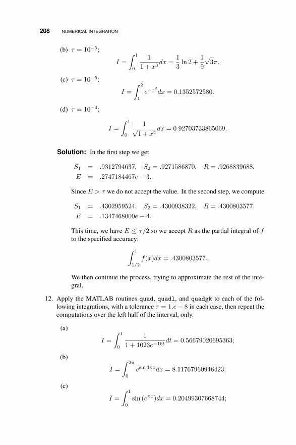
208 NUMERICAL INTEGRATION
(b) τ = 10−5;
I =
∫ 1
0
1
1 + x3dx =
1
3ln 2 +
1
9
√3π.
(c) τ = 10−5;
I =
∫ 2
1
e−x2
dx = 0.1352572580.
(d) τ = 10−4;
I =
∫ 1
0
1√1 + x4
dx = 0.92703733865069.
Solution: In the first step we get
S1 = .9312794637, S2 = .9271586870, R = .9268839688,
E = .2747184467e− 3.
Since E > τ we do not accept the value. In the second step, we compute
S1 = .4302959524, S2 = .4300938322, R = .4300803577,
E = .1347468000e− 4.
This time, we have E ≤ τ/2 so we accept R as the partial integral of fto the specified accuracy:∫ 1
1/2
f(x)dx = .4300803577.
We then continue the process, trying to approximate the rest of the inte-gral.
12. Apply the MATLAB routines quad, quadl, and quadgk to each of the fol-lowing integrations, with a tolerance τ = 1.e− 8 in each case, then repeat thecomputations over the left half of the interval, only.
(a)
I =
∫ 1
0
1
1 + 1023e−16tdt = 0.56679020695363;
(b)
I =
∫ 2π
0
esin 4πxdx = 8.11767960946423;
(c)
I =
∫ 1
0
sin (eπx)dx = 0.20499307668744;
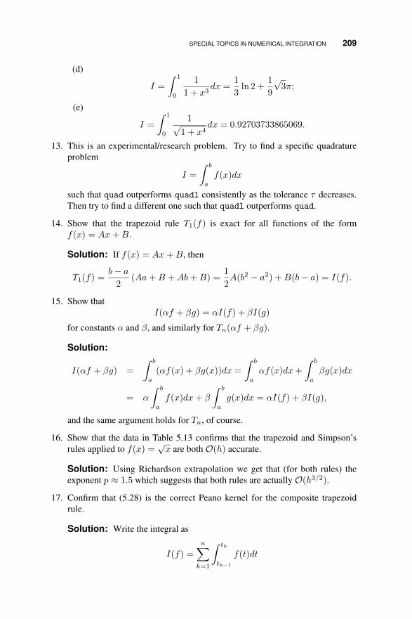
SPECIAL TOPICS IN NUMERICAL INTEGRATION 209
(d)
I =
∫ 1
0
1
1 + x3dx =
1
3ln 2 +
1
9
√3π;
(e)
I =
∫ 1
0
1√1 + x4
dx = 0.92703733865069.
13. This is an experimental/research problem. Try to find a specific quadratureproblem
I =
∫ b
a
f(x)dx
such that quad outperforms quadl consistently as the tolerance τ decreases.Then try to find a different one such that quadl outperforms quad.
14. Show that the trapezoid rule T1(f) is exact for all functions of the formf(x) = Ax+B.
Solution: If f(x) = Ax+B, then
T1(f) =b− a
2(Aa+B +Ab+B) =
1
2A(b2 − a2) +B(b− a) = I(f).
15. Show thatI(αf + βg) = αI(f) + βI(g)
for constants α and β, and similarly for Tn(αf + βg).
Solution:
I(αf + βg) =
∫ b
a
(αf(x) + βg(x))dx =
∫ b
a
αf(x)dx+
∫ b
a
βg(x)dx
= α
∫ b
a
f(x)dx+ β
∫ b
a
g(x)dx = αI(f) + βI(g),
and the same argument holds for Tn, of course.
16. Show that the data in Table 5.13 confirms that the trapezoid and Simpson’srules applied to f(x) =
√x are both O(h) accurate.
Solution: Using Richardson extrapolation we get that (for both rules) theexponent p ≈ 1.5 which suggests that both rules are actually O(h3/2).
17. Confirm that (5.28) is the correct Peano kernel for the composite trapezoidrule.
Solution: Write the integral as
I(f) =n∑k=1
∫ tk
tk−1
f(t)dt

210 NUMERICAL INTEGRATION
and apply the Peano kernel to each integral over [k−1, tk].
18. Show that if f ′ is integrable over [a, b], but f ′′ is not, then the trapezoid rule isO(h) accurate.
Solution: We have
I(f)− Tn(f) =
∫ b
a
K(t)f ′′(t)dt.
Integration by parts can be carefully used to rewrite this as
I(f)− Tn(f) = −∫ b
a
K′(t)f ′(t)dt.
(The additional terms from integration by parts involve K(xi) and thereforevanish.) Hence,
|I(f)− Tn(f)| ≤ maxa≤t≤b
|K ′(t)|∫ b
a
|f ′(t)|dt.
19. Show that the Peano Theorem implies an error estimate for the trapezoid ruleof the form
|I(f)− Tn(f)| ≤ 1
8h2∫ b
a
|f ′′(t)|dt.
Be sure to provide all details missing from the development in the text.
Solution: The only detail left out of the discussion in the text is to show that
maxa≤t≤b
|K(t)| ≤ 1
8h2,
but this is done the same way as the linear interpolation error estimate back inChapter 2.
20. Derive the Peano kernel for Simpson’s rule.
Solution: Following the development in the text, we get
K(t) =
{(b− t)4 − c−a
18 (b− t)3 − b−a9 (c− t)3 a ≤ t ≤ c
124 (b− t)4 − c−a
18 (b− t)3 c ≤ t ≤ b
}
/ • • • .

CHAPTER 6
NUMERICAL METHODS FORORDINARY DIFFERENTIAL EQUATIONS
6.1 THE INITIAL VALUE PROBLEM — BACKGROUND
Exercises:
1. For each initial value problem below, verify (by direct substitution) that thegiven function y solves the problem.
(a) y′ + 4y = 0, y(0) = 3; y(t) = 3e−4t.
(b) y′ = t2/y, y(0) = 1; y(t) =√
1 + 23 t
3.
(c) ty′ − y = t2, y(1) = 4; y(t) = 3t+ t2.
Solution: This is simply a matter of ordinary computation. For (a), we have,for instance,
d
dt
(3e−4t
)+ 4
(3e−4t
)= −12e−4t + 12e−4t = 0,
and y(0) = 3e0 = 3, therefore the given solution is correct.
Solutions Manual to Accompany An Introduction to Numerical Methods and Analysis,Second Edition. By James F. EppersonCopyright c© 2013 John Wiley & Sons, Inc.
211

212 NUMERICAL METHODS FOR ORDINARY DIFFERENTIAL EQUATIONS
2. For each initial value problem in Problem 1, write down the definition of f .
Solution: The function f is simply the right side of the differential equationwhen put into the standard form used in the text. Thus, for (a), f(t, y) = −4y,for (b) f(t, y) = (y + t2)/t, and for (c), f(t, y) = t2/y.
3. For each scalar equation below, write out explicitly the corresponding firstorder system. What is the definition of f?
(a) y′′ + 9y = e−t.
(b) y′′′′ + y = 1.
(c) y′′ + sin y = 0.
Solution: For (a), we have w(t) = (y(t), y′(t))T and the system is
d
dt
(w1(t)
w2(t)
)=
d
dt
(y(t)
y′(t)
)=
(y′(t)
e−t − 9y(t)
)=
(w2(t)
e−t − 9w1(t)
),
therefore
f(t, w) =
(w2(t)
e−t − 9w1(t)
).
Similarly, for (b) we get
d
dt
w1(t)
w2(t)
w3(t)
w4(t)
=d
dt
y(t)
y′(t)
y′′(t)
y′′′(t)
=
y′(t)
y′′(t)
y′′′(t)
1− w1(t)
=
w2(t)
w3(t)
w4(t)
1− w1(t)
,
therefore
f(t, w) =
w2(t)
w3(t)
w4(t)
1− w1(t)
.
Finally, for (c) we get
d
dt
(w1(t)
w2(t)
)=
d
dt
(y(t)
y′(t)
)=
(y′(t)
− sin y(t)
)=
(w2(t)
− sinw1(t)
),
therefore
f(t, w) =
(w2(t)
− sinw1(t)
).
4. For each initial value problem below, verify (by direct substitution) that thegiven function y solves the problem.
(a) y′′ + 4y′ + 4y = 0, y(0) = 0, y′(0) = 1; y(t) = te−2t.

EULER’S METHOD 213
(b) t2y′′ + 6ty′ + 6y = 0, y(1) = 1, y′(1) = −3; y(t) = t−3.(c) y′′ + 5y′ + 6y = 0, y(0) = 1, y′(0) = −2; y(t) = e−2t.
Solution: This is a straight-forward calculus exercise.
5. For each initial value problem below, determine the Lipschitz constant, K, forthe given rectangle.
(a) y′ = 1− 3y, y(0) = 1, R = (−1, 1)× (0, 2);(b) y′ = y(1− y), y(0) = 1
2 , R = (−1, 1)× (0, 2);(c) y′ = y2, y(0) = 1, R = (−1, 1)× (0, 2).
Solution: In general, we get the Lipschitz constant by computing fy andmaximizing it over the rectangle of interest. Therefore,
(a) fy(t, y) = −3 for all (t, y), hence K = 3;(b) fy(t, y) = 1− 2y for all t and all y ∈ (0, 2), hence K = 3;(c) fy(t, y) = 2y, hence K = 4.
6. Are any of the initial value problems in the previous exercise smooth anduniformly monotone decreasing over the given rectangle? If so, determine thevalues of M and m.
Solution: The ODE in (a) is smooth and uniformly monotone decreasingbecause fy < 0 for all (t, y) of interest. In fact, since fy(t, y) = −3 for all(t, y), we have m = M = 3.
/ • • • .
6.2 EULER’S METHOD
Exercises:
1. Use Euler’s method with h = 14 to compute approximate values of y(1) for
each of the following initial value problems. Don’t write a computer program,use a hand calculator to produce an orderly table of (tk, yk) pairs.
(a) y′ = y(1− y), y(0) = 12 ;
Solution:
y1 = y0 + hf(t0, y0) = (1/2) + (1/4)y(1− y) = 0.5625
y2 = y1 + hf(t1, y1) = 0.6240
y3 = y2 + hf(t2, y2) = 0.6827
y4 = y3 + hf(t3, y3) = 0.7368

214 NUMERICAL METHODS FOR ORDINARY DIFFERENTIAL EQUATIONS
(b) ty′ = y(sin t), y(0) = 2.
Solution: We have to use the limiting value of 1 for sin tt at t = 0:
y1 = y0 + hf(t0, y0) = 2 + (1/4)y = 2.5
y2 = y1 + hf(t1, y1) = 3.1185
y3 = y2 + hf(t2, y2) = 3.8661
y4 = y3 + hf(t3, y3) = 4.7445
(c) y′ = y(1 + e2t), y(0) = 1;
Solution:
y1 = y0 + hf(t0, y0) = 1 + (1/4)y(e+ e2t) = 1.5
y2 = y1 + hf(t1, y1) = 2.4933
y3 = y2 + hf(t2, y2) = 4.8109
y4 = y3 + hf(t3, y3) = 11.404
(d) y′ + 2y = 1, y(0) = 2;
Solution:
y1 = y0 + hf(t0, y0) = 2 + (1/4)(1− 2y) = 1.25
y2 = y1 + hf(t1, y1) = 0.875
y3 = y2 + hf(t2, y2) = 0.6875
y4 = y3 + hf(t3, y3) = 0.59375
2. For each initial value problem above, use the differential equation to produceapproximate values of y′ at each of the grid points, tk, k = 0, 1, 2, 3, 4.
Solution:
(a) y′(t0) = f(t0, y0) = 0.25, y′(t1) = 0.2461, y′(t2) = 0.2346, y′(t3) =0.2166, y′(t4) = 0.1939.
(b) y′(t0) = f(t0, y0) = 2, y′(t1) = 2.474, y′(t2) = 2.990, y′(t3) = 3.514,y′(t4) = 3.992.
(c) y′(t0) = f(t0, y0) = 2, y′(t1) = 3.973, y′(t2) = 9.271, y′(t3) = 26.37,y′(t4) = 95.67.
(d) y′(t0) = f(t0, y0) = −3, y′(t1) = −1.5, y′(t2) = −0.75, y′(t3) =−0.375, y′(t4) = −0.1875.
3. Write a computer program that solves each of the initial value problems inProblem 1, using Euler’s method and h = 1/16.
Solution: Below is a MATLAB script that does this for one specific example.

EULER’S METHOD 215
function [tc,yc] = euler1(h,n,y0)
tc = [0];
yc = [y0];
yn = y0;
tn = 0;
for k=1:n
y = yn + h*yn*(1 + exp(2*tn));
t = k*h;
tc = [tc t];
yc = [yc y];
yn = y;
tn = t;
end
tc = tc’;
yc = yc’
exact = exp(-0.5)*exp(tc + 0.5*exp(2*tc));
%
figure(1)
plot(tc,yc)
figure(2)
plot(tc,exact - yc)
4. For each initial value problem below, approximate the solution using Euler’smethod using a sequence of decreasing grids h−1 = 2, 4, 8, . . .. For thoseproblems where an exact solution is given, compare the accuracy achievedover the interval [0, 1] with the theoretical accuracy.
(a) y′ + 4y = 1, y(0) = 1; y(t) = 14 (3e−4t + 1).
(b) y′ = −y ln y, y(0) = 3; y(t) = e(ln 3)e−t
.
(c) y′ + y = sin 4πt, y(0) = 12 .
(d) y′ + sin y = 0, y(0) = 1.
Solution: By making a slight modification to the euler1 script we caneasily solve the two examples for which exact solutions are given, producingthe results shown in Table 6.1.
/ • • • .

216 NUMERICAL METHODS FOR ORDINARY DIFFERENTIAL EQUATIONS
Table 6.1 Solutions to Exercise 6.2.4.
h−1 Max. error for (b) Max. error for (a)2 0.8515 0.59504 0.2759 0.19408 0.0884 0.0846
16 0.0386 0.039932 0.0182 0.019464 0.0089 0.0096128 0.0044 0.0048
6.3 ANALYSIS OF EULER’S METHOD
Exercises:
1. Use Taylor’s Theorem to prove that
(1 + x)n ≤ enx
for all x > −1. Hint: expand ex in a Taylor series, throw away the unnecessaryterms, and then take powers of both sides.
Solution: We have
ex = 1 + x+1
2x2eξ,
therefore1 + x ≤ ex,
therefore(1 + x)n ≤ enx.
2. For each initial value problem below, use the error theorems of this section toestimate the value of
E(h) =maxtk≤1 |y(tk)− yk|
‖y′′‖∞,[0,1]
using h = 1/16, assuming Euler’s method was used to approximate the solu-tion.
(a) y′ + 4y = 1, y(0) = 1;
Solution: E(h) ≤ 6.70h.
(b) y′ = y(1− y), y(0) = 1/2;

VARIANTS OF EULER’S METHOD 217
Solution: We have
E(h) =eK−1
2Kh,
where K is the Lipschitz constant for f(t, y) = y(1 − y). We haveK = max |fy| = max |1 − 2y|, so we need to know the solution toactually complete the estimation. We find y = (1+e−t)−1, soK = 0.46,which implies that
E(h) = 0.635h.
(c) y′ = sin y, y(0) = 12π.
3. Consider the initial value problem
y′ = e−t − 16y, y(0) = 1.
(a) Confirm that this is smooth and uniformly monotone decreasing in y.What is M? What is m?
Solution: Since f(t, y) = e−t − 16y and therefore fy(t, y) = −16 theODE is indeed smooth and uniformly monotone decreasing in y, withM = m = 16.
(b) Approximate the solution using Euler’s method and h = 18 . Do we get
the expected behavior from the approximation? Explain.
Solution: Since this value of h does not satisfy the condition h < M−1 wedo not expect to get the kind of accuracy described in the theorem.
/ • • • .
6.4 VARIANTS OF EULER’S METHOD
Exercises:
1. Using the approximation
y′(tn) ≈ y(tn+1)− y(tn−1)
2h
derive the numerical method (6.20) for solving initial value problems. What isthe residual? What is the truncation error? Is it a consistent method?
Solution: We have
y′(t) =y(t+ h)− y(t− h)
2h− 1
6h2y′′′(θt,h)

218 NUMERICAL METHODS FOR ORDINARY DIFFERENTIAL EQUATIONS
so thaty(t+ h)− y(t− h)
2h− 1
6h2y′′′(θt,h) = f(t, y(t))
ory(t+ h) = y(t− h) + 2hf(t, y(t)) +
1
3h3y′′′(θt,h).
The residual isRn =
1
3h3y′′′(θt,h)
and the truncation error is
Tn =1
3h2y′′′(θt,h).
The method is consistent so long as y′′′ is continuous.
2. Using the approximation
y′(tn−1) ≈ −y(tn+1) + 4y(tn)− 3y(tn−1)
2h
derive the numerical method (6.21) for solving initial value problems. What isthe residual? What is the truncation error? Is it a consistent method?
Solution: The method is consistent, with truncation error (h2/3)y′′′(ξ);
3. Using the approximation
y′(tn+1) ≈ 3y(tn+1)− 4y(tn) + y(tn−1)
2h
derive the numerical method (6.22) for solving initial value problems. What isthe residual? What is the truncation error? Is it a consistent method?
Solution: Using the material in Section 4.5 we have
y′(tn+1) =3y(tn+1)− 4y(tn) + y(tn−1)
2h+
1
3h2y′′′(ξn)
so that the differential equation becomes
3y(tn+1)− 4y(tn) + y(tn−1)
2h+
1
3h2y′′′(ξn) = f(tn+1, y(tn+1)),
or
3y(tn+1)− 4y(tn) + y(tn−1) = 2hf(tn+1, y(tn+1))− 2
3h3y′′′(ξn).
Thus
y(tn+1) =4
3y(tn)− 1
3y(tn−1) +
2
3hf(tn+1, y(tn+1))− 2
9h3y′′′(ξn).

VARIANTS OF EULER’S METHOD 219
The residual isRn = −2
9h3y′′′(ξn)
and the truncation error is
Tn = −2
9h2y′′′(ξn).
The method is consistent so long as y′′′ is continuous.
4. Use the trapezoid rule predictor-corrector with h = 14 to compute approximate
values of y(1) for each of the following initial value problems. Don’t write acomputer program, use a hand calculator to produce an orderly table of (tk, yk)pairs.
(a) y′ = y(1 + e2t), y(0) = 1;
Solution: y(1) ≈ 42.71053582.
(b) y′ + 2y = 1, y(0) = 2;
(c) y′ = y(1− y), y(0) = 12 ;
Solution: y(1) ≈ .7303809855.
(d) ty′ = y(sin t), y(0) = 2.
5. Repeat the above, using the method (6.23) as a predictor-corrector, with Euler’smethod as the predictor. Also use Euler’s method to produce the starting value,y1.
Solution: For (b), y(1) ≈ .7299429169; for (c), y(1) ≈ 42.82307269.
6. Write a computer program that solves each of the initial value problems inProblem 4, using the trapezoid rule predictor-corrector and h = 1/16.
Solution: A MATLAB script which is slightly more general than required isgiven below.
function [tc,yc] = trappc(h,n,y0)
tc = [0];
yc = [y0];
yn = y0;
tn = 0;
for k=1:n
yp = yn + h*yn*(1-yn);
y = yn + 0.5*h*(yp*(1-yp) + yn*(1-yn));
t = k*h;
tc = [tc t];
yc = [yc y];
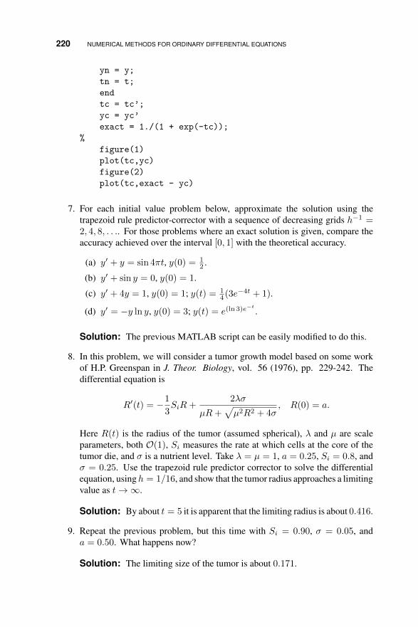
220 NUMERICAL METHODS FOR ORDINARY DIFFERENTIAL EQUATIONS
yn = y;
tn = t;
end
tc = tc’;
yc = yc’
exact = 1./(1 + exp(-tc));
%
figure(1)
plot(tc,yc)
figure(2)
plot(tc,exact - yc)
7. For each initial value problem below, approximate the solution using thetrapezoid rule predictor-corrector with a sequence of decreasing grids h−1 =2, 4, 8, . . .. For those problems where an exact solution is given, compare theaccuracy achieved over the interval [0, 1] with the theoretical accuracy.
(a) y′ + y = sin 4πt, y(0) = 12 .
(b) y′ + sin y = 0, y(0) = 1.
(c) y′ + 4y = 1, y(0) = 1; y(t) = 14 (3e−4t + 1).
(d) y′ = −y ln y, y(0) = 3; y(t) = e(ln 3)e−t
.
Solution: The previous MATLAB script can be easily modified to do this.
8. In this problem, we will consider a tumor growth model based on some workof H.P. Greenspan in J. Theor. Biology, vol. 56 (1976), pp. 229-242. Thedifferential equation is
R′(t) = −1
3SiR+
2λσ
µR+√µ2R2 + 4σ
, R(0) = a.
Here R(t) is the radius of the tumor (assumed spherical), λ and µ are scaleparameters, both O(1), Si measures the rate at which cells at the core of thetumor die, and σ is a nutrient level. Take λ = µ = 1, a = 0.25, Si = 0.8, andσ = 0.25. Use the trapezoid rule predictor corrector to solve the differentialequation, usingh = 1/16, and show that the tumor radius approaches a limitingvalue as t→∞.
Solution: By about t = 5 it is apparent that the limiting radius is about 0.416.
9. Repeat the previous problem, but this time with Si = 0.90, σ = 0.05, anda = 0.50. What happens now?
Solution: The limiting size of the tumor is about 0.171.

VARIANTS OF EULER’S METHOD 221
10. Now solve the differential equation using a variety of Si, σ, and a values (yourchoices). What happens?
Solution: For Si sufficiently small (or σ sufficiently large) the tumor growsin size, instead of shrinking.
11. Now let’s model some treatment for our mathematical tumor. In the previousthree problems, we assumed that the nutrient level was constant. Suppose weare able to decrease the nutrient level according to the model
σ(t) = σ∞ + (σ0 − σ∞)e−qt.
Here σ0 is the initial nutrient level, σ∞ is the asymptotic nutrient level, andq measures the rate at which the nutrient level drops. Investigate the effectof various choices of these parameters on the growth of the tumor, based onyour observations from the previous problems. Again, use the trapezoid rulepredictor corrector with h = 1/16 to solve the differential equation.
Solution: Generally, the same kind of results occur. The faster and fartherthe nutrient level is reduced, the more the tumor shrinks.
12. Verify by direct substitution that (6.43) satisfies the recursion (6.39) for alln ≥ 2.
Solution: Straight forward computation.
13. For the midpoint method (6.21), show that if λ < 0, then 0 < r1 < 1 andr2 < −1.
Solution: The key issues are that√ξ2 + 1 > |ξ| and
√ξ2 + 1
≤√ξ2 + 2|ξ|+ 1 = |ξ|+ 1. Then
r1 > −|ξ|+ |ξ| > 0
andr1 ≤ −|ξ|+ |ξ|+ 1 = 1.
Similarly,
r2 = −|ξ| −√|ξ|2 + 1 < −|ξ| −
√|ξ|2 − 2|ξ|+ 1 = −|ξ| −
√(|ξ| − 1)2
= −|ξ| −√
(1− |ξ|)2 = −|ξ| − (1− |ξ|) = −1.
We assumed at the end that h was small enough that 1 − |ξ| > 0; this shouldhave been an assumption in the problem statement.
14. Show that (6.44) is valid. Hint: First, show that C1 = 1 − C2. Next, useTaylor expansions to write
ξ − eξ√ξ2 + 1
=−1− 1
2ξ2 +O(ξ3)
1 + 12ξ
2 +O(ξ4).

222 NUMERICAL METHODS FOR ORDINARY DIFFERENTIAL EQUATIONS
Solution: Showing C1 = 1− C2 is fairly routine. We then have that
eξ = 1 + ξ +1
2ξ2 +O(ξ3)⇒ ξ − eξ = −1− 1
2ξ2 +O(ξ3),
and √ξ2 + 1 = 1 +
1
2ξ2 +O(ξ4).
Both of these follow from routine Taylor series computations. Finally, we have
−1− 12ξ
2 +O(ξ3)
1 + 12ξ
2 +O(ξ4)=−1− 1
2ξ2 −O(ξ4) +O(ξ4) +O(ξ3)
1 + 12ξ
2 +O(ξ4)
= −1 +O(ξ4) +O(ξ3)
1 + 12ξ
2 +O(ξ4)
= −1 +O(ξ4) +O(ξ3)
= −1 +O(ξ3)
15. Use the midpoint rule predictor-corrector method (6.35)-(6.36) to solve eachof the IVP’s given in Problem 4.
Solution: A MATLAB script that does the job is given below.
function [tc,yc] = midpc(h,n,y0)
tc = [0];
yc = [y0];
yn = y0;
tn = 0;
for k=1:n
yp = yn + 0.5*h*fmid(tn,yn);
y = yn + h*fmid(tn+0.5*h,yp);
t = k*h;
tc = [tc t];
yc = [yc y];
yn = y;
tn = t;
end
tc = tc’;
yc = yc’
exact = 0.5*(1 + 3*exp(-2*tc));
%
figure(1)
plot(tc,yc)
figure(2)
plot(tc,exact - yc)

VARIANTS OF EULER’S METHOD 223
16. Show that the residual for the midpoint rule predictor-corrector is given by
R = y(t+ h)− y(t)− hf(t+ h/2, y(t) + (h/2)f(t, y(t))).
Then use Taylor’s theorem to show thatR = O(h3) and hence that the midpointrule predictor-corrector is a second order method.
Solution: We have
y(t+h)−y(t) = hy′(t)+1
2h2y′′(t)+O(h3) = hf(t, y(t))+
1
2h2y′′(t)+O(h3),
so
R = hf(t, y(t)) +1
2h2y′′(t) +O(h3)−hf(t+h/2, y(t) + (h/2)f(t, y(t))).
For notational simplicity write Y (t) = y(t) + (h/2)f(t, y(t)) so that we have
R = hf(t, y(t)) +1
2h2y′′(t)− hf(t+ h/2, Y (t)) +O(h3).
The problem can be done from this point quite simply using Taylor’s Theoremfor two variable functions, but it can also be done using single variable calculus,carefully. We have
f(t+ h/2, Y (t)) = f(t, Y (t)) + (h/2)ft(t, Y (t)) +O(h2),
so R becomes
R = h(f(t, y(t))− f(t, Y (t))) + (h2/2)(y′′(t)− ft(t, Y (t))) +O(h3).
The first term simplifies as follows:
h(f(t, y(t))− f(t, Y (t))) = hfy(t, ηt)(y(t)− Y (t))
= −(h2/2)fy(t, ηt)f(t, y(t)),
where ηt is a value between y(t) and Y (t). Now, since
y′(t) = f(t, y(t))
it follows that
y′′(t) =d
dtf(t, y(t))
= ft(t, y(t)) + fy(t, y(t))y′(t)
= ft(t, y(t)) + fy(t, y(t))f(t, y(t)).
Therefore,
R = (h2/2)(fy(t, y(t))f(t, y(t))− fy(t, ηt)f(t, y(t))
+ft(t, y(t))− ft(t, Y (t))) +O(h3).
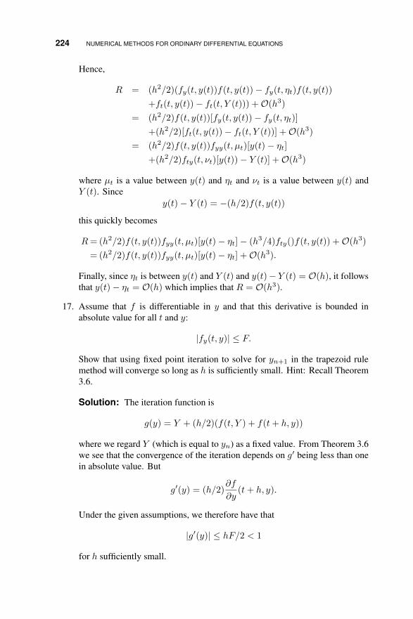
224 NUMERICAL METHODS FOR ORDINARY DIFFERENTIAL EQUATIONS
Hence,
R = (h2/2)(fy(t, y(t))f(t, y(t))− fy(t, ηt)f(t, y(t))
+ft(t, y(t))− ft(t, Y (t))) +O(h3)
= (h2/2)f(t, y(t))[fy(t, y(t))− fy(t, ηt)]
+(h2/2)[ft(t, y(t))− ft(t, Y (t))] +O(h3)
= (h2/2)f(t, y(t))fyy(t, µt)[y(t)− ηt]+(h2/2)fty(t, νt)[y(t))− Y (t)] +O(h3)
where µt is a value between y(t) and ηt and νt is a value between y(t) andY (t). Since
y(t)− Y (t) = −(h/2)f(t, y(t))
this quickly becomes
R= (h2/2)f(t, y(t))fyy(t, µt)[y(t)− ηt]− (h3/4)fty()f(t, y(t)) +O(h3)
= (h2/2)f(t, y(t))fyy(t, µt)[y(t)− ηt] +O(h3).
Finally, since ηt is between y(t) and Y (t) and y(t)− Y (t) = O(h), it followsthat y(t)− ηt = O(h) which implies that R = O(h3).
17. Assume that f is differentiable in y and that this derivative is bounded inabsolute value for all t and y:
|fy(t, y)| ≤ F.
Show that using fixed point iteration to solve for yn+1 in the trapezoid rulemethod will converge so long as h is sufficiently small. Hint: Recall Theorem3.6.
Solution: The iteration function is
g(y) = Y + (h/2)(f(t, Y ) + f(t+ h, y))
where we regard Y (which is equal to yn) as a fixed value. From Theorem 3.6we see that the convergence of the iteration depends on g′ being less than onein absolute value. But
g′(y) = (h/2)∂f
∂y(t+ h, y).
Under the given assumptions, we therefore have that
|g′(y)| ≤ hF/2 < 1
for h sufficiently small.

SINGLE STEP METHODS — RUNGE-KUTTA 225
18. Derive the numerical method based on using Simpson’s rule to approximatethe integral in
y(t+ h) = y(t− h) +
∫ t+h
t−hf(s, y(s))ds.
What is the order of accuracy of this method? What is the truncation error? Isit implicit or explicit? Is it a single step or multistep method?
Solution: We get
y(t+ h) = y(t− h) +h
3(f(t− h, y(t− h)) + 4f(t, y(t))
+f(t+ h, y(t+ h)))− h5
2880y(5)(ξt),
which suggests the numerical method
yn+1 = yn−1 +h
3(f(t− h, yn−1) + 4f(t, yn) + f(t+ h, yn+1)) .
The method is an implicit multistep method, with order of accuracy 4; thetruncation error is
τ(t) = − h4
2880y(5)(ξt).
/ • • • .
6.5 SINGLE STEP METHODS — RUNGE-KUTTA
Exercises:
1. Use the method of Heun with h = 14 to compute approximate values of y(1) for
each of the following initial value problems. Don’t write a computer program,use a hand calculator to produce an orderly table of (tk, yk) pairs.
(a) y′ = y(1− y), y(0) = 12 ;
Solution:
y0 = .5, y1 = .5620117188, y2 = .6221229509,
y3 = .6786683489, y4 = .7303809855
(b) y′ = y(1 + e2t), y(0) = 1;

226 NUMERICAL METHODS FOR ORDINARY DIFFERENTIAL EQUATIONS
Solution:
y0 = 1, y1 = 1.746635238, y2 = 3.674304010,
y3 = 10.24009564, y4 = 42.71053582
(c) y′ + 2y = 1, y(0) = 2;
Solution:
y0 = 2, y1 = 1.4375, y2 = 1.0859375,
y3 = .8662109375, y4 = .7288818360
(d) ty′ = y(sin t), y(0) = 2.
2. Repeat the above, using fourth order Runge-Kutta.
Solution:
(a)
y0 = 2, y1 = 1.410156250, y2 = 1.052256267,
y3 = .8350929950, y4 = .7033246558
(b)
y0 = 1, y1 = 1.775386270, y2 = 3.886047491,
y3 = 11.97099553, y4 = 63.69087556
(c)
y0 = .5, y1 = .5621763730, y2 = .6224590537,
y3 = .6791782275, y4 = .7310578607
3. Write a computer program that solves each of the initial value problems inProblem 1, using the method of Heun, and h = 1/16.
Solution: Below is a MATLAB script that does this task.
function [tc, yc] = heun(y0,h,n)
yc = [y0];
tc = [0];
y = y0;
t = 0;
for k=1:n
k1 = h*fheun(t,y);
k2 = h*fheun(t+2*h/3,y+(2/3)*k1);

SINGLE STEP METHODS — RUNGE-KUTTA 227
yn = y + 0.25*(k1 + 3*k2);
y = yn;
t = t + h;
yc = [yc yn];
tc = [tc t];
end
plot(tc,yc)
4. Write a computer program that solves each of the initial value problems inProblem 1, using fourth order Runge-Kutta, and h = 1/16.
Solution: Below is a MATLAB script that does this task.
function [tc, yc] = rk4(y0,h,n)
yc = [y0];
tc = [0];
y = y0;
t = 0;
for k=1:n
k1 = h*frk(t,y);
k2 = h*frk(t + 0.5*h,y + 0.5*k1);
k3 = h*frk(t + 0.5*h,y + 0.5*k2);
k4 = h*frk(t + h,y + k3);
yn = y + (k1 + 2*k2 + 2*k3 + k4)/6;
y = yn;
t = t + h;
yc = [yc yn];
tc = [tc t];
end
plot(tc,yc)
5. For each initial value problem below, approximate the solution using themethod of Heun with a sequence of decreasing grids h−1 = 2, 4, 8, . . .. Forthose problems where an exact solution is given, compare the accuracy achievedover the interval [0, 1] with the theoretical accuracy.
(a) y′ + sin y = 0, y(0) = 1.
(b) y′ + 4y = 1, y(0) = 1; y(t) = 14 (3e−4t + 1).
(c) y′ + y = sin 4πt, y(0) = 12 .
(d) y′ = −y ln y, y(0) = 3; y(t) = e(ln 3)e−t
.
Solution: The script given above can be used to do this problem.
6. Repeat the above, using fourth order Runge-Kutta as the numerical method.

228 NUMERICAL METHODS FOR ORDINARY DIFFERENTIAL EQUATIONS
Solution: The rk4 script given above can be used to do this problem.
7. Repeat Problem 8 from 6.4, except this time use fourth order Runge Kutta tosolve the differential equation, with h = 1/8.
Solution: The same general results are obtained as previously.
8. Repeat Problem 9 from 6.4, except this time use fourth order Runge Kutta tosolve the differential equation, with h = 1/8.
Solution: The same general results are obtained as previously.
9. Repeat Problem 11 from 6.4, except this time use fourth order Runge Kuttato solve the differential equation, with h = 1/8.
Solution: The same general results are obtained as previously.
10. Repeat Problem 10 from 6.4, except this time use fourth order Runge Kuttato solve the differential equation, with h = 1/8.
Solution: The same general results are obtained as previously.
/ • • • .
6.6 MULTI-STEP METHODS
Exercises:
1. Use second order Adams-Bashforth withh = 14 to compute approximate values
of y(1) for each of the following initial value problems. Don’t write a computerprogram, use a hand calculator to produce an orderly table of (tk, yk) pairs.Use Euler’s method to generate the needed starting value.
(a) y′ + 2y = 1, y(0) = 2;
Solution:
y0 = 2, y1 = 1.25, y2 = 1.0625, y3 = .828125, y4 = .7226562500
(b) y′ = y(1 + e2t), y(0) = 1;
Solution:
y0 = 1, y1 = 1.5, y2 = 2.739905715,
y3 = 6.063673588, y4 = 17.25489584
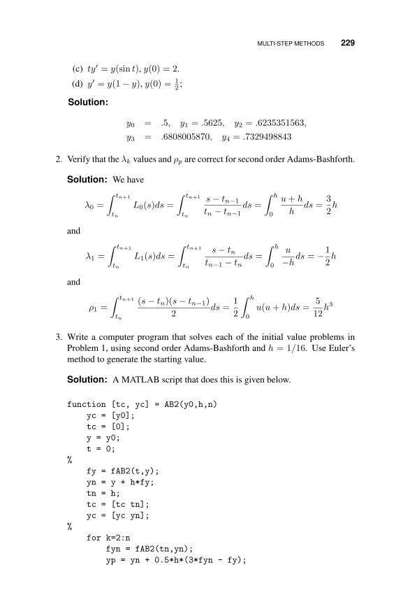
MULTI-STEP METHODS 229
(c) ty′ = y(sin t), y(0) = 2.
(d) y′ = y(1− y), y(0) = 12 ;
Solution:
y0 = .5, y1 = .5625, y2 = .6235351563,
y3 = .6808005870, y4 = .7329498843
2. Verify that the λk values and ρp are correct for second order Adams-Bashforth.
Solution: We have
λ0 =
∫ tn+1
tn
L0(s)ds =
∫ tn+1
tn
s− tn−1tn − tn−1
ds =
∫ h
0
u+ h
hds =
3
2h
and
λ1 =
∫ tn+1
tn
L1(s)ds =
∫ tn+1
tn
s− tntn−1 − tn
ds =
∫ h
0
u
−hds = −1
2h
and
ρ1 =
∫ tn+1
tn
(s− tn)(s− tn−1)
2ds =
1
2
∫ h
0
u(u+ h)ds =5
12h3
3. Write a computer program that solves each of the initial value problems inProblem 1, using second order Adams-Bashforth and h = 1/16. Use Euler’smethod to generate the starting value.
Solution: A MATLAB script that does this is given below.
function [tc, yc] = AB2(y0,h,n)
yc = [y0];
tc = [0];
y = y0;
t = 0;
%
fy = fAB2(t,y);
yn = y + h*fy;
tn = h;
tc = [tc tn];
yc = [yc yn];
%
for k=2:n
fyn = fAB2(tn,yn);
yp = yn + 0.5*h*(3*fyn - fy);

230 NUMERICAL METHODS FOR ORDINARY DIFFERENTIAL EQUATIONS
y = yn;
fy = fyn;
yn = yp;
tn = k*h;
tc = [tc tn];
yc = [yc yp];
end
plot(tc,yc)
4. Write a computer program that solves each of the initial value problems inProblem 1, using fourth order Adams-Bashforth, with fourth order Runge-Kutta to generate the starting values.
Solution: A MATLAB script which does this is given below.
function [t,y] = AB4(y0,h,n)
t0 = 0;
y = [y0];
t = [0];
%
k1 = fAB4(t0,y0);
k2 = fAB4(t0+0.5*h,y0+0.5*h*k1);
k3 = fAB4(t0+0.5*h,y0+0.5*h*k2);
k4 = fAB4(t0+h,y0+h*k3);
ya = y0 + (h/6)*(k1 + 2*k2 + 2*k3 + k4);
ta = t0 + h;
y = [y ya];
t = [t ta];
%
k1 = fAB4(ta,ya);
k2 = fAB4(ta+0.5*h,ya+0.5*h*k1);
k3 = fAB4(ta+0.5*h,ya+0.5*h*k2);
k4 = fAB4(ta+h,ya+h*k3);
yb = ya + (h/6)*(k1 + 2*k2 + 2*k3 + k4);
tb = ta + h;
y = [y yb];
t = [t tb];
%
k1 = fAB4(tb,yb);
k2 = fAB4(tb+0.5*h,yb+0.5*h*k1);
k3 = fAB4(tb+0.5*h,yb+0.5*h*k2);
k4 = fAB4(tb+h,yb+h*k3);
yc = yb + (h/6)*(k1 + 2*k2 + 2*k3 + k4);
tc = tb + h;
y = [y yc];
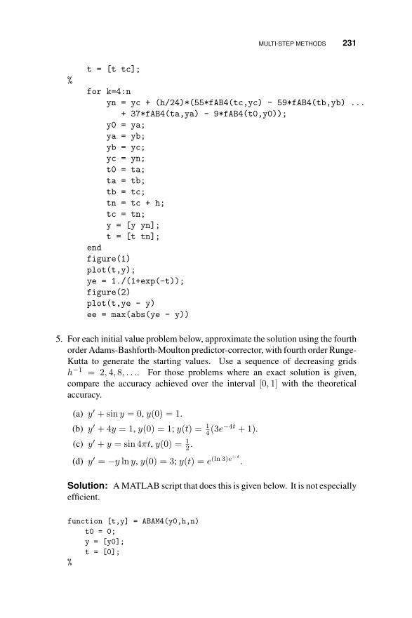
MULTI-STEP METHODS 231
t = [t tc];
%
for k=4:n
yn = yc + (h/24)*(55*fAB4(tc,yc) - 59*fAB4(tb,yb) ...
+ 37*fAB4(ta,ya) - 9*fAB4(t0,y0));
y0 = ya;
ya = yb;
yb = yc;
yc = yn;
t0 = ta;
ta = tb;
tb = tc;
tn = tc + h;
tc = tn;
y = [y yn];
t = [t tn];
end
figure(1)
plot(t,y);
ye = 1./(1+exp(-t));
figure(2)
plot(t,ye - y)
ee = max(abs(ye - y))
5. For each initial value problem below, approximate the solution using the fourthorder Adams-Bashforth-Moulton predictor-corrector, with fourth order Runge-Kutta to generate the starting values. Use a sequence of decreasing gridsh−1 = 2, 4, 8, . . .. For those problems where an exact solution is given,compare the accuracy achieved over the interval [0, 1] with the theoreticalaccuracy.
(a) y′ + sin y = 0, y(0) = 1.
(b) y′ + 4y = 1, y(0) = 1; y(t) = 14 (3e−4t + 1).
(c) y′ + y = sin 4πt, y(0) = 12 .
(d) y′ = −y ln y, y(0) = 3; y(t) = e(ln 3)e−t
.
Solution: A MATLAB script that does this is given below. It is not especiallyefficient.
function [t,y] = ABAM4(y0,h,n)
t0 = 0;
y = [y0];
t = [0];
%

232 NUMERICAL METHODS FOR ORDINARY DIFFERENTIAL EQUATIONS
k1 = fABAM4(t0,y0);
k2 = fABAM4(t0+0.5*h,y0+0.5*h*k1);
k3 = fABAM4(t0+0.5*h,y0+0.5*h*k2);
k4 = fABAM4(t0+h,y0+h*k3);
ya = y0 + (h/6)*(k1 + 2*k2 + 2*k3 + k4);
ta = t0 + h;
y = [y ya];
t = [t ta];
%
k1 = fABAM4(ta,ya);
k2 = fABAM4(ta+0.5*h,ya+0.5*h*k1);
k3 = fABAM4(ta+0.5*h,ya+0.5*h*k2);
k4 = fABAM4(ta+h,ya+h*k3);
yb = ya + (h/6)*(k1 + 2*k2 + 2*k3 + k4);
tb = ta + h;
y = [y yb];
t = [t tb];
%
k1 = fABAM4(tb,yb);
k2 = fABAM4(tb+0.5*h,yb+0.5*h*k1);
k3 = fABAM4(tb+0.5*h,yb+0.5*h*k2);
k4 = fABAM4(tb+h,yb+h*k3);
yc = yb + (h/6)*(k1 + 2*k2 + 2*k3 + k4);
tc = tb + h;
y = [y yc];
t = [t tc];
%
for k=4:n
yp = yc + (h/24)*(55*fABAM4(tc,yc) - 59*fABAM4(tb,yb) ...
+ 37*fABAM4(ta,ya) - 9*fABAM4(t0,y0));
yn = yc + (h/24)*(9*fABAM4(tc+h,yp) + 19*fABAM4(tc,yc) ...
- 5*fABAM4(tb,yb) + fABAM4(ta,ya));
y0 = ya;
ya = yb;
yb = yc;
yc = yn;
t0 = ta;
ta = tb;
tb = tc;
tn = tc + h;
tc = tn;
y = [y yn];
t = [t tn];
end
figure(1)
plot(t,y);
ye = (16*exp(-t)*pi^2-8*pi*cos(4*pi*t)+8*exp(-t)*pi...
+exp(-t)+2*sin(4*pi*t))/(32*pi^2+2);
figure(2)
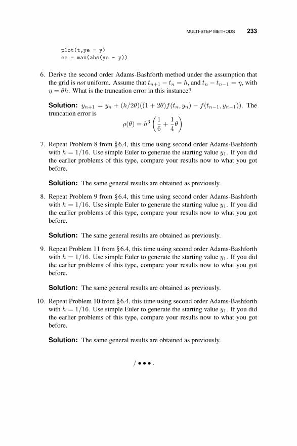
MULTI-STEP METHODS 233
plot(t,ye - y)
ee = max(abs(ye - y))
6. Derive the second order Adams-Bashforth method under the assumption thatthe grid is not uniform. Assume that tn+1 − tn = h, and tn − tn−1 = η, withη = θh. What is the truncation error in this instance?
Solution: yn+1 = yn + (h/2θ)((1 + 2θ)f(tn, yn) − f(tn−1, yn−1)). Thetruncation error is
ρ(θ) = h3(
1
6+
1
4θ
)7. Repeat Problem 8 from 6.4, this time using second order Adams-Bashforth
with h = 1/16. Use simple Euler to generate the starting value y1. If you didthe earlier problems of this type, compare your results now to what you gotbefore.
Solution: The same general results are obtained as previously.
8. Repeat Problem 9 from 6.4, this time using second order Adams-Bashforthwith h = 1/16. Use simple Euler to generate the starting value y1. If you didthe earlier problems of this type, compare your results now to what you gotbefore.
Solution: The same general results are obtained as previously.
9. Repeat Problem 11 from 6.4, this time using second order Adams-Bashforthwith h = 1/16. Use simple Euler to generate the starting value y1. If you didthe earlier problems of this type, compare your results now to what you gotbefore.
Solution: The same general results are obtained as previously.
10. Repeat Problem 10 from 6.4, this time using second order Adams-Bashforthwith h = 1/16. Use simple Euler to generate the starting value y1. If you didthe earlier problems of this type, compare your results now to what you gotbefore.
Solution: The same general results are obtained as previously.
/ • • • .
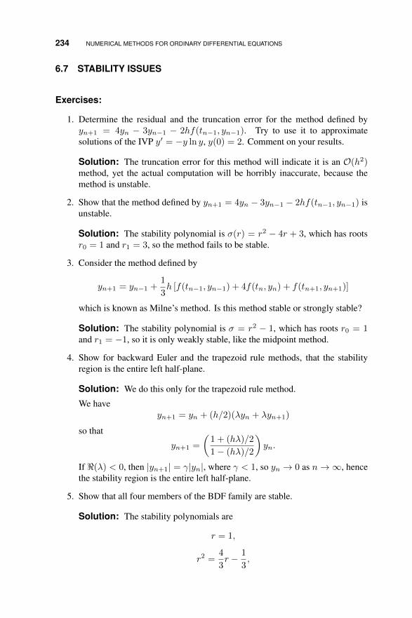
234 NUMERICAL METHODS FOR ORDINARY DIFFERENTIAL EQUATIONS
6.7 STABILITY ISSUES
Exercises:
1. Determine the residual and the truncation error for the method defined byyn+1 = 4yn − 3yn−1 − 2hf(tn−1, yn−1). Try to use it to approximatesolutions of the IVP y′ = −y ln y, y(0) = 2. Comment on your results.
Solution: The truncation error for this method will indicate it is an O(h2)method, yet the actual computation will be horribly inaccurate, because themethod is unstable.
2. Show that the method defined by yn+1 = 4yn − 3yn−1 − 2hf(tn−1, yn−1) isunstable.
Solution: The stability polynomial is σ(r) = r2 − 4r + 3, which has rootsr0 = 1 and r1 = 3, so the method fails to be stable.
3. Consider the method defined by
yn+1 = yn−1 +1
3h [f(tn−1, yn−1) + 4f(tn, yn) + f(tn+1, yn+1)]
which is known as Milne’s method. Is this method stable or strongly stable?
Solution: The stability polynomial is σ = r2 − 1, which has roots r0 = 1and r1 = −1, so it is only weakly stable, like the midpoint method.
4. Show for backward Euler and the trapezoid rule methods, that the stabilityregion is the entire left half-plane.
Solution: We do this only for the trapezoid rule method.
We haveyn+1 = yn + (h/2)(λyn + λyn+1)
so that
yn+1 =
(1 + (hλ)/2
1− (hλ)/2
)yn.
If <(λ) < 0, then |yn+1| = γ|yn|, where γ < 1, so yn → 0 as n→∞, hencethe stability region is the entire left half-plane.
5. Show that all four members of the BDF family are stable.
Solution: The stability polynomials are
r = 1,
r2 =4
3r − 1
3,

APPLICATION TO SYSTEMS OF EQUATIONS 235
r3 =18
11r2 − 9
11+
2
11
andr4 =
48
25r3 − 36
25r2 +
16
25− 3
25.
Simple computations show that all four cases satisfy the root condition, andhence are stable.
6. Show that the stability region for the fourth order BDF method contains theentire negative real axis.
Solution: The stability region is that part of the complex plane for which themethod is relatively stable when applied to the ODE y′ = λy. Thus we lookat the recursion
yn+1 =48
25yn −
36
25yn−1 +
16
25yn−2 −
3
25yn−3 +
12
25hλyn+1
To say that the stability region for the method contains the entire negative realaxis is equivalent to saying that the roots of the polynomial
r4 =48
25r3 − 36
25r2 +
16
25r − 3
25+
12
25hλr4
are less than one in absolute value for all negative real λ. We thus look at thepolynomial equation
(25 + 12ξ)r4 − 48r3 + 36r2 − 16r + 3 = 0,
where ξ = −hλ > 0. For specific values of ξ > 0, we can compute themaximum absolute value of the roots of this polynomial. Since the maximumabsolute value is always less than one, the negative real axis is within thestability region of the method.
/ • • • .
6.8 APPLICATION TO SYSTEMS OF EQUATIONS
Exercises:
1. Using a hand calculator and h = 14 , compute approximate solutions to the
initial value problem
y′1 = −4y1 + y2, y1(0) = 1;
y′2 = y1 − 4y2, y2(0) = −1.
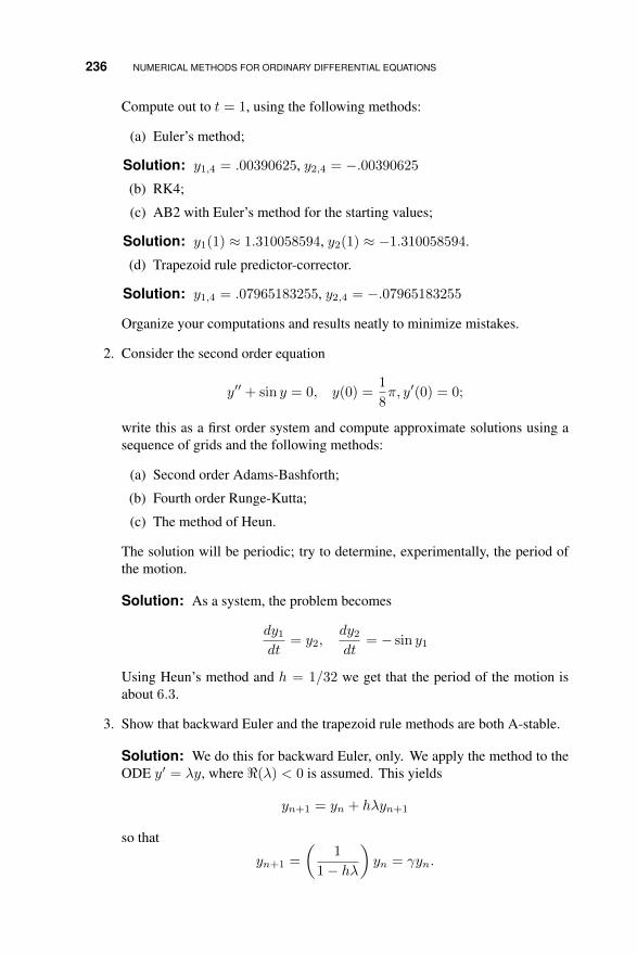
236 NUMERICAL METHODS FOR ORDINARY DIFFERENTIAL EQUATIONS
Compute out to t = 1, using the following methods:
(a) Euler’s method;
Solution: y1,4 = .00390625, y2,4 = −.00390625
(b) RK4;
(c) AB2 with Euler’s method for the starting values;
Solution: y1(1) ≈ 1.310058594, y2(1) ≈ −1.310058594.
(d) Trapezoid rule predictor-corrector.
Solution: y1,4 = .07965183255, y2,4 = −.07965183255
Organize your computations and results neatly to minimize mistakes.
2. Consider the second order equation
y′′ + sin y = 0, y(0) =1
8π, y′(0) = 0;
write this as a first order system and compute approximate solutions using asequence of grids and the following methods:
(a) Second order Adams-Bashforth;
(b) Fourth order Runge-Kutta;
(c) The method of Heun.
The solution will be periodic; try to determine, experimentally, the period ofthe motion.
Solution: As a system, the problem becomes
dy1dt
= y2,dy2dt
= − sin y1
Using Heun’s method and h = 1/32 we get that the period of the motion isabout 6.3.
3. Show that backward Euler and the trapezoid rule methods are both A-stable.
Solution: We do this for backward Euler, only. We apply the method to theODE y′ = λy, where <(λ) < 0 is assumed. This yields
yn+1 = yn + hλyn+1
so that
yn+1 =
(1
1− hλ
)yn = γyn.

APPLICATION TO SYSTEMS OF EQUATIONS 237
Since <(λ) < 0 it follows that γ < 1 so yn → 0, thus the method is A-stable.A similar argument works for the trapezoid rule method.
4. Show that the second-order BDF method is A-stable.
5. Apply the third order BDF method, using the trapezoid method to obtain thestarting values, to the stiff example in the text. Compare your results to theexact solution and those obtained in the text.
Solution: At each step we have to solve the system(I − 6
11hA
)yn+1 =
18
11yn −
9
11yn−1 −
2
11yn−2
where
yn =
(y1,ny2,n
)and
A =
[198 199
−398 −399
]Since we are using a third order method instead of a second order method, weexpect better results and we get them. The maximum error for this method issubstantially smaller than for the trapezoid rule.
6. Consider the following system of differential equations:
y′1(t) = ay1(t)− by2(t)y1(t), y1(0) = y10
y′2(t) = −cy2(t) + dy1(t)y2(t), y2(0) = y20
Solve this system for a sequence of mesh sizes, using the data a = 4, b =1, c = 2, d = 1, with initial values y10 = 3/2 and y20 = 4. Use (a) Secondorder Adams-Bashforth, with Euler’s method providing the starting value; and,(b) Fourth order Runge-Kutta. Plot the solutions in two ways: As a single plotshowing y1 and y2 versus t; and as a phase plot showing y1 versus y2. Note:The solutions should be periodic. Try to determine, experimentally, the period.(Note: This problem is an example of a predator-prey model, in which y1represents the population of a prey species and y2 represents the population ofa predator which uses the prey as its only food source. See Braun [3] for anexcellent discussion of the dynamics of such systems, as well as the historybehind the problem.)
Solution: Using AB2 with h = 1/32 you should get that the period of thesolution is about 2.2.
7. Consider now a situation in which two species, denoted x1 and x2, competefor a common food supply. A standard model for this is
x′1(t) = ax1(t)− (bx1(t) + cx2(t))x1(t)
x′2(t) = Ax2(t)− (Bx1(t) + Cx2(t))x2(t)

238 NUMERICAL METHODS FOR ORDINARY DIFFERENTIAL EQUATIONS
with initial conditions x1(0) = x01, x2(0) = x02. Using any of the methodsin this chapter, solve this system for x01 = x02 = 10, 000, using a = 4, b =0.0003, c = 0.004, A = 2, B = 0.0002, C = 0.0001. Vary the parameters ofthe problem slightly and observe what happens to the solution.
8. An interesting and somewhat unusual application of systems of differentialequations is to combat modeling. Here, we denote the force levels of the twosides at war by x1 and x2, and make various hypotheses about how one side’sforce level affects the losses suffered by the other side. For example, if wehypothesize that losses are proportional to the size of the opposing force, then(in the absence of reinforcements) we get the model
x′1 = −ax2x′2 = −bx1
If we hypothesize that losses are proportional to the square of the opposingforce, we get the model
x′1 = −αx22x′2 = −βx21
The constants α, β, a, b represent the military efficiency of one side’s forces.
Using any of the methods of this section, consider both models with
a = 1, α = 1, x1(0) = 120, x2(0) = 40
and observe how changing b and β affects the long-term trend of the solutions.In particular, can you find values of b and β such that the smaller force anni-hilates the larger one? Combat models such as this are known as Lanchestermodels after the British mathematician F. W. Lanchester who introduced them.
Solution: Using Euler’s method with ∆t = 0.05, the author found that, inthe linear model, the smaller force needed to be have b = 11 to annihilate thelarger force, while for the squared model it required β = 37 for the smallerforce to win. (In the squared model the author used a much smaller time step,∆t = 0.0005, to avoid one side eliminating the other in a single step.)
9. Consider the following system of ODEs:
x′ = σ(y − x),
y′ = x(ρ− z)− y,z′ = xy − βz.
Use two different second order methods (your choice) to approximate solutionsto this system, for σ = 10, β = 8/3, and ρ = 28. Take x(0) = y(0) = z(0) =1 and compute out to t = 5. Plot each component.

APPLICATION TO SYSTEMS OF EQUATIONS 239
10. Consider the second order equation:
x′′ − µ(1− x2)x′ + x = 0, x(0) = 0.5, x′(0) = 0.
First, write this as a system. Then, as in the previous problem, choose twodifferent second order methods and use each to solve the system for µ = 0.1and µ = 10. Compute out to t = 20.
11. One simple but important application of systems of differential equations isto the spread of epidemics. Perhaps the simplest model is the so-called SIRmodel, which models an infectious disease (like measles) that imparts immunityto those who have had it and recovered. We divide the population into threecategories:
• S(t): These are the people who are susceptible, i.e., they are well at timet but might get sick at some future time;
• I(t): These are the people who are infected, i.e., sick;
• R(t): These are the people who have recovered and are therefore pro-tected from getting the disease by being immune.
Under a number of simplifying assumptions6 the SIR model involves thefollowing system, sometimes known as the continuous Kermack-McKendrickmodel.
dS
dt= −rSI,
dI
dt= rSI − aI,
dR
dt= aI,
The parameters r and a measure the rate at which susceptible people becomesick upon contact with infectives, and the rate at which infected people arecured.
(a) For the case I0 = 1, S0 = 762, R0 = 0, a = 0.44, and r = 2.18× 10⁻³,solve the system using the numerical method and step size of your choice,and plot the solutions. This data is taken from a study of an influenzaepidemic at an English boys school; the time scale here is in days.
(b) Now consider the case where S0 = 106, R0 = 0, a = 1.74, r =.3× 10−5. Solve the system (again, using the method of your choice) fora range of values of I0 > 0. Is there a critical value of I0 beyond whichthe disease spreads to almost all of the population? This data is taken,
6See J.D. Murray, Mathematical Biology, Springer-Verlag, Berlin, 1989, pp. 611ff.
240 NUMERICAL METHODS FOR ORDINARY DIFFERENTIAL EQUATIONS
roughly, from a study of a plague epidemic in Bombay; the time scale isweeks.
Solution: Using the trapezoid rule predictor-corrector with h = 1/16,the epidemic dies out in about 5 weeks, regardless of the size of I0, anddoes not spread throughout the population.
(c) In the previous data set, take I0 = 104 and vary the value of r. Try tofind the critical value of r such that, for r < rcrit the number of infecteddrops monotonically, and for r > rcrit the number of infected rises to apeak before falling off.
/ • • • .
6.9 ADAPTIVE SOLVERS
Exercises:
1. Use Algorithm 6.4 to solve the following IVP using the local error toleranceof ε = 0.001:
y′ = y2, y(0) = 1.
Do this as a hand calculation. Compute 4 or 5 steps. Compare the computedsolution to the exact solution y = (1− t)−1.
Solution: The algorithm settles on h1 = h2 = h3 = h4 = h5 = 0.0078125and produces the approximate values
y1 = 1.00785339019122, y2 = 1.01583078044887, y3 = 1.02393512571904,
y4 = 1.03216947546184, y5 = 1.04053697745659
2. Apply one of the MATLAB routines to each of the following ODEs:
(a) y′ + 4y = 1, y(0) = 1;
(b) y′ + sin y = 0, y(0) = 1;
(c) y′ + y = sin 4πt, y(0) = 12 ;
(d) y′ = y−ty+t , y(0) = 4.
Use both τ = 1.e− 3 and τ = 1.e− 6, and compute out to t = 10. Plot yoursolutions. You may need to adjust MaxStep.
Solution: For (b), using an old version of ode45, the author got the graph inFig. 6.1.

ADAPTIVE SOLVERS 241
0 1 2 3 4 5 6 7 8 9 100
0.1
0.2
0.3
0.4
0.5
0.6
0.7
0.8
0.9
1
Figure 6.1 Solution to Problem 2b.
3. The MATLAB ODE routines can be applied to systems. Use each of ode23,ode45, and ode113 to solve the system in Problem 9 of 6.8, using τ = 1.e−3and also τ = 1.e− 6.
Solution: Using an old version of ode23, and plotting each component asa coordinate in 3-space, we get the graph in Fig. 6.2 (computing out toTmax = 65). This system is known as the “Lorenz attractor,” and is one of thefirst examples of a so-called chaotic dynamical system.
4. Apply ode45 to the system in Problem 10 of 6.8, using µ = 10. Computeout to t = 60, and plot both solution components. Comment.
Solution: Using the version of ode45 from the 1994 MATLAB, the authorgot the plot in Figure 6.3. This equation is known as the van der Pol oscillator;it is an example of a nonlinear oscillator. Note to instructors: Advise thestudents to plot the solution components on separate axes; otherwise the largevalues of the derivative will distort the scales.
5. The three routines we used in this section are not designed for stiff ODEs, butthat does not mean we can’t try it! Apply ode23 to the system
y′1 = 198y1 + 199y2, y1(0) = 1;
y′2 = −398y1 − 399y2, y2(0) = −1;
using τ = 10−6. Plot the solution components over the interval (0, 5).
/ • • • .

242 NUMERICAL METHODS FOR ORDINARY DIFFERENTIAL EQUATIONS
−20−10
010
20
−40
−20
0
20
400
10
20
30
40
50
Figure 6.2 Solution to Problem 3.
0 10 20 30 40 50 60−2.5
−2
−1.5
−1
−0.5
0
0.5
1
1.5
2
2.5
Figure 6.3 Solution curve for Problem 10.

BOUNDARY VALUE PROBLEMS 243
6.10 BOUNDARY VALUE PROBLEMS
Exercises:
1. Use a mesh size of h = 14 (n = 4) to solve the boundary value problem
−u′′ + u = sinx, 0 < x < 1;
u(0) = u(1) = 0.
Don’t bother to write a computer program; do this as a hand calculation.
Solution: The system is 33 −16 0
−16 33 −16
0 −16 33
u1u2u3
=
√
2/2
1/2√2/2
which has solution
u1 = 0.05430593375937,
u2 = 0.06781181455454,
u3 = 0.05430593375937.
2. Repeat the above for the BVP
−u′′ + (2− x)u = x, 0 < x < 1;
u(0) = u(1) = 0.
Don’t bother to write a computer program; do this as a hand calculation.
Solution: u(1/4) ≈ 0.0329, u(1/2) ≈ 0.0538, u(3/4) ≈ 0.0484.
3. Repeat the above for the BVP
−u′′ + u = e−x, 0 < x < 1;
u(0) = u(1) = 0.
Solution:u1 = 0.0572, u2 = 0.0694, u3 = 0.0480
4. Consider the linear boundary value problem
−u′′ + (10 cos 2x)u = 1
u(0) = u(π) = 0

244 NUMERICAL METHODS FOR ORDINARY DIFFERENTIAL EQUATIONS
Solve this using finite difference methods and a decreasing sequence of grids,starting with h = π/16, π/32, . . . . Do the approximate solutions appear to beconverging to a solution?
Solution: Using h = π/8, we get
u = (0.0601, 0.0316,−0.1511,−0.3233,−0.1511, 0.0316, 0.0601)T
as the solution vector; the approximate solutions do converge as h→ 0.
5. Consider the nonlinear boundary value problem
−u′′ + eu = 1
u(0) = 0, u(1) = 1
Use shooting methods combined with the trapezoid rule predictor-correctorto construct solutions to this equation, then use a fourth order Runge-Kuttascheme and compare the two approximate solutions. Are they nearly thesame?
Solution: To do this problem we first have to cast it into a first order system:(w1(t)
w2(t)
)′=
(w2(t)
ew1(t) − 1
)We then solve this system using the initial values w1(0) = 0, w2(t) = p, andfind the value of p such that w1(1) = 0. Using the trapezoid rule predictor-corrector we get that p = 0.8172, and a similar value is obtained with thefourth order Runge-Kutta method.
6. Write a program to use the finite element method to solve the BVP
−u′′ + u = e−x, 0 < x < 1;
u(0) = u(1) = 0.
using a sequence of grids, h−1 = 4, 8, 16, . . . , 1024.
Solution: Using n = 256, the author got the plot in Fig. 6.4; the values forn = 16 are marked by the circles.
7. Repeat the above, using the different boundary conditions u(0) = 0, u(1) = 1.
8. No exact solution was provided for either of the previous two exercises (al-though anyone having completed a sophomore ODE course—or with accessto a symbolic algebra program like Maple or Mathematica—ought to be ableto produce a solution). Write an essay addressing the following question: Onwhat basis are you confidant that your codes are producing the correct solution?

BOUNDARY VALUE PROBLEMS 245
0 0.1 0.2 0.3 0.4 0.5 0.6 0.7 0.8 0.9 10
0.02
0.04
0.06
0.08
0.1
0.12
0.14
Figure 6.4 Solution plot for Problem 6.
Solution: If the sequence of solutions are not varying wildly from each other,if the results appear to be converging to a single solution, then we are justifiedin thinking—but by no means certain—that our code is correct. The fact thatour solutions for n = 16 and n = 256 match as well as they do in Problem 6gives us confidence that we are getting good results.
/ • • • .


CHAPTER 7
NUMERICAL METHODS FOR THESOLUTION OF SYSTEMS OFEQUATIONS
7.1 LINEAR ALGEBRA REVIEW
Exercises:
1. Assume Theorem 7.1 and use it to prove Cor. 7.1.
Solution: If A is singular, then Part 2 of the theorem says that the columnsof A are a dependent set. Therefore, there exists a set of constants c1, c2, . . .,cn, not all zero, such that
0 = c1a1 + c2a2 + . . .+ cnan
where the ai are the columns of A written as vectors. But this is equivalent tosaying Ac = 0, where c ∈ Rn has components ck. Therefore there exists atleast one non-zero vector c such that Ac = 0. Now, let β be an arbitrary realnumber; then A(βc) = βAc = 0, so there must be infinitely many non-zerovectors x such that Ax = 0.
2. Use Theorem 7.1 to prove that a triangular matrix is nonsingular if and only ifthe diagonal elements are all non-zero.
Solutions Manual to Accompany An Introduction to Numerical Methods and Analysis,Second Edition. By James F. EppersonCopyright c© 2013 John Wiley & Sons, Inc.
247

248 NUMERICAL METHODS FOR THE SOLUTION OF SYSTEMS OF EQUATIONS
Solution: Let T be the triangular matrix. Then detT =∏tii, so detT is
non-zero if and only if all the diagonal elements are non-zero.
3. Suppose that we can writeA ∈ Rn×n as the product of two triangular matricesL ∈ Rn×n and U ∈ Rn×n where the diagonal elements of L and U are allnon-zero. Prove that A is nonsingular.
Solution: Since L and U are triangular with non-zero diagonal elements,they are non-singular. Therefore
Ax = b⇔ LUx = b⇔ Ux = L−1b⇔ x = U−1L−1b;
thus the system has a unique solution for any b, thus A is non-singular.
/ • • • .
7.2 LINEAR SYSTEMS AND GAUSSIAN ELIMINATION
Exercises:For the sake of simplicity here, we will define at the outset several families of
matrices, parameterized by their dimension. These will be referred to in several ofthe exercises throughout the chapter.
Hn = [hij ], hij =1
i+ j − 1.
Kn = [kij ], ki,j =
2, i = j;
−1, |i− j| = 1;
0, otherwise.
Tn = [tij ], ti,j =
4, i = j;
1, |i− j| = 1;
0, otherwise.
An = [aij ], ai,j =
1, i = j;
4, i− j = 1;
−4, i− j = −1;
0, otherwise.
Even if we do not know the solution to a linear system, we can check the accuracyof a computed solution xc by means of the residual r = b − Axc. If xc is the exactsolution, then each component of r will be zero; in floating point arithmetic, theremight be a small amount of rounding error, unless the matrix is “nearly singular,” aconcept that we will discuss in detail in 7.5.

LINEAR SYSTEMS AND GAUSSIAN ELIMINATION 249
1. Write a naive Gaussian elimination code and use it to solve the system ofequations Ax = b where
A =
14 14 −9 3 −5
14 52 −15 2 −32
−9 −15 36 −5 16
3 2 −5 47 49
−5 −32 16 49 79
and b = [−15,−100, 106, 329, 463]T . The correct answer isx = [0, 1, 2, 3, 4]T .
Solution: A MATLAB script which does this is given below.
function x = naive(a,b)
n = length(b);
x = b;
for i=1:(n-1)
for j=(i+1):n
m = a(j,i)/a(i,i);
for k=(i+1):n
a(j,k) = a(j,k) - m*a(i,k);
end
b(j) = b(j) - m*b(i);
end
end
%
x(n) = b(n)/a(n,n);
for i=(n-1):(-1):1
s = 0;
for j=(i+1):n
s = s + a(i,j)*x(j);
end
x(i) = (b(i) - s)/a(i,i);
end
2. Write a naive Gaussian elimination code and use it to solve the system ofequations
T5x = b
where b = [1, 6, 12, 18, 19]T . The correct answer is x = [0, 1, 2, 3, 4]T .

250 NUMERICAL METHODS FOR THE SOLUTION OF SYSTEMS OF EQUATIONS
Solution: The previous script will work.
3. Write a naive Gaussian elimination code and use it to solve the system ofequations
H5x = b
where b = [5.0, 3.550, 2.81428571428571, 2.34642857142857, 2.01746031746032]T .The correct answer is x = [1, 2, 3, 4, 5]T .
Solution: The same script works, of course.
4. Repeat the above problem, except now use b1 = 5.0001; how much does theanswer change?
Solution: Now we get
x = [1.00249999999970, 1.96999999999926, 3.10500000002115,
3.85999999994903, 5.06300000003183]T .
This is more change in the answer than we perhaps would have expected, giventhe small change in b.
5. Write your own naive Gaussian elimination code, based on the material in thischapter, and test it on the indicated families, over the range of 4 ≤ n ≤ 20.Take b to be the vector of appropriate size, each of whose entries is 1.
(a) Hn;
(b) Kn;
(c) Tn.
For each value of n, compute the value of max1≤i≤n |ri|, where r = b−Ax.
Solution: For the second and third cases, the naive script returns a residualthat is identically zero for all components. For the first case — known asthe Hilbert matrix — the maximum element in the residual is still small, butnon-zero. The author got 2.288243194925598e − 8 as the largest element inthe residual for n = 20.
6. Modify the Gaussian elimination algorithm to handle more than a single righthand side. Test it on a 5× 5 example of your own design, using at least 3 righthand side vectors.
Solution: A MATLAB script which does this is given below. It is a modestchange from the previous one.
function x = naive(a,b)
[n,p] = size(b);
x = b;

LINEAR SYSTEMS AND GAUSSIAN ELIMINATION 251
for i=1:(n-1)
for j=(i+1):n
m = a(j,i)/a(i,i);
for k=(i+1):n
a(j,k) = a(j,k) - m*a(i,k);
end
for k = 1:p
b(j,k) = b(j,k) - m*b(i,k);
end
end
end
%
for ii=1:p
x(n,ii) = b(n,ii)/a(n,n);
for i=(n-1):(-1):1
s = 0;
for j=(i+1):n
s = s + a(i,j)*x(j,ii);
end
x(i,ii) = (b(i,ii) - s)/a(i,i);
end
end
7. Use the naive Gaussian elimination algorithm to solve (by hand) the followingsystem. You should get the same results as in (7.1).[
ε 1
1 1
] [x1x2
]=
[1
2
].
Solution: We have[ε 1 1
1 1 2
]∼[ε 1 1
0 1− (1/ε) 2− (1/ε)
]so that
x2 =2− (1/ε)
1− (1/ε)=
2ε− 1
ε− 1=
1− 2ε
1− ε= 1− ε
1− ε
and
x1 =1
ε(1− x2) =
1
ε
(1− 1 +
ε
1− ε
)=
1
1− ε= 1 +
ε
1− ε

252 NUMERICAL METHODS FOR THE SOLUTION OF SYSTEMS OF EQUATIONS
8. Write a Gaussian elimination code that does partial pivoting and use it to solvethe system of equations Ax = b where
A =
9 3 2 0 7
7 6 9 6 4
2 7 7 8 2
0 9 7 2 2
7 3 6 4 3
and b = [35, 58, 53, 37, 39]T . The correct answer is x = [0, 1, 2, 3, 4]T .
Solution: A MATLAB script that does the assigned task is given below.
function x = naivep(a,b)
n = length(b);
x = b;
for i=1:(n-1)
am = abs(a(i,i));
p = i;
for j=(i+1):n
if abs(a(j,i)) > am
am = abs(a(j,i));
p = j;
end
end
if p > i
for k=i:n
hold = a(i,k);
a(i,k) = a(p,k);
a(p,k) = hold;
end
hold = b(i);
b(i) = b(p);
b(p) = hold;
end
for j=(i+1):n
m = a(j,i)/a(i,i);
for k=(i+1):n
a(j,k) = a(j,k) - m*a(i,k);
end
b(j) = b(j) - m*b(i);
end
end
%
x(n) = b(n)/a(n,n);

LINEAR SYSTEMS AND GAUSSIAN ELIMINATION 253
for i=(n-1):(-1):1
s = 0;
for j=(i+1):n
s = s + a(i,j)*x(j);
end
x(i) = (b(i) - s)/a(i,i);
end
9. Write a naive Gaussian elimination code and use it to solve the system ofequations Ax = b where
A =
1 1/2 1/3
1/2 1/3 1/4
1/3 1/4 1/5
and b = [7/6, 5/6, 13/20]T . The correct answer is x = [0, 1, 2]T .
Solution: The previous script will work.
10. Use the naive Gaussian elimination algorithm to solve (by hand) the follow-ing system, using only 3 digit decimal arithmetic. Repeat, using Gaussianelimination with partial pivoting. Comment on your results.[
0.0001 1
1 1
] [x1x2
] [1
2
]
Solution: This has to be done carefully, and it is important to remember thatthe restriction as to 3 digit arithmetic applies to all the computations. So wecan’t just apply the formulas from the previous problem.
If we don’t pivot, then the elimination goes like this (assuming the machinechops): [
0.0001 1 1
1 1 2
]∼[
0.0001 1 1
0 −9990 −9990
]So, x2 = 1 and x1 = 0, not a very accurate result.
If we do pivot, then the elimination goes like this:[0.0001 1 1
1 1 2
]∼[
1 1 2
0.0001 1 1
]∼[
1 1 2
0 0.999 0.999
]So, x2 = 1 (again) but x1 = 2−x2 = 1, which is a much more accurate result.
11. Write a code to do Gaussian elimination with partial pivoting, and apply it tothe system A5x = b, where b = [−4,−7,−6,−5, 16]T and the solution isx = [0, 1, 2, 3, 4]T .

254 NUMERICAL METHODS FOR THE SOLUTION OF SYSTEMS OF EQUATIONS
Solution: The naivep script will work.
12. Use MATLAB’s rand function to generate A, a random 10 × 10 matrix, anda random vector b ∈ R10; solve the system Ax = b two different ways: (1)By using your own code; (2) By using MATLAB’s backslash command: x =
A\b. Obviously, you should get the same results both times.
Solution: Using the naivep script, the author solved a random system in888 flops. Using the backslash command for the same system produced thesame results but took 1350 flops. The author is amused by this result.
13. Repeat the above, this time using a 20 × 20 random matrix and appropriaterandom right-hand side.
/ • • • .
7.3 OPERATION COUNTS
Exercises:
1. Determine the operation count for the tridiagonal solution algorithm of 2.6.
Solution: About C1 = 4n for the elimination step, and C2 = 2n for thesolution phase, for a total cost of C = 6n.
2. What is the operation count for computing the dot product x ·y of two vectors?
Solution: C = n
3. Create a pair of random vectors in R10 and compute their dot product using theMATLAB command dot. What is the estimated operations count, accordingto flops? Repeat for a pair of vectors in R20 and a pair in R100. Commenton your results, compared to your answer in the previous problem.
4. What is the operation count for computing the matrix-vector product Ax?
Solution: For A ∈ Rm×n and x ∈ Rn, we get C = mn.
5. Repeat the above, assuming that A is tridiagonal.
Solution: C = 3n+O(1)
6. What is the operation count for a matrix-matrix product, AB?
Solution: For A ∈ Rm×n and B ∈ Rn×p we get C = mnp.
7. Repeat the above, assuming that A is tridiagonal.
OPERATION COUNTS 255
Solution: This is easier to figure out by breaking into diagonal parts, so thatwe have A = D1 +D2 +D3 where D2 is the main diagonal and D1 and D3
are the upper and lower diagonals. Then AB = D1B + D2B + D3B, andeach individual product costs roughly np ifB ∈ Rn×p, so the total cost is 3np.
8. Repeat the above, assuming now that both A and B are tridiagonal.
Solution: This time we have
AB = (D1 +D2 +D3)(D4 +D5 +D6),
so the cost is roughly C = 9n+O(1), assuming n is the length of the longestdiagonal.
9. What is the operation count for the outer product xyT ?
Solution: C = n2
10. Determine the operation count for the backward solution algorithm.
Solution:
C =n−1∑i=1
n∑j=i+1
1
=1
2n2 +O(n)
11. Repeat the above for the Gaussian elimination code you wrote in the previoussection.
12. Repeat the above for the tridiagonal solver you wrote back in 2.6.
13. Use the rand command to create a sequence of linear system problems ofincreasing size, say 4 ≤ n ≤ 100. Use the backslash operator to solve eachproblem, and estimate the operations count using flops. Plot the estimatedcost as a function of n.
Solution: The figure below shows a partial solution (for 4 ≤ n ≤ 32) as wellas the discrete values 2n3/3, which is a rough estimate of what flops shouldbe producing. Note that the two curves are rather close in general trend.
14. Use the diag command to form a sequence of tridiagonal systems, similarto what you did in Problem 13, and solve these using the backslash operator.What is the estimated cost of solving these systems, according to flops?
Solution: The backslash command will not take advantage of the tridiagonalstructure of the system, so the result should be a lot like the above.
15. Assume that you are working on a computer that does one operation every10−9 seconds. How long, roughly, would it take such a computer to solve alinear system for n = 100, 000, using the cost estimates derived in this section
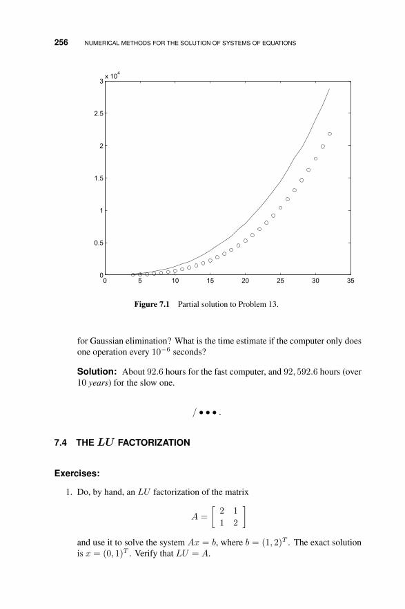
256 NUMERICAL METHODS FOR THE SOLUTION OF SYSTEMS OF EQUATIONS
0 5 10 15 20 25 30 350
0.5
1
1.5
2
2.5
3x 10⁴
Figure 7.1 Partial solution to Problem 13.
for Gaussian elimination? What is the time estimate if the computer only doesone operation every 10−6 seconds?
Solution: About 92.6 hours for the fast computer, and 92, 592.6 hours (over10 years) for the slow one.
/ • • • .
7.4 THE LU FACTORIZATION
Exercises:
1. Do, by hand, an LU factorization of the matrix
A =
[2 1
1 2
]and use it to solve the system Ax = b, where b = (1, 2)T . The exact solutionis x = (0, 1)T . Verify that LU = A.
THE LU FACTORIZATION 257
Solution: We get
A =
[2 1
1 2
]=
[1 0
1/2 1
] [2 1
0 3/2
]so
y =
[1
3/2
]and
x =
[0
1
]as expected.
2. Repeat the above for
A =
[4 1
1 5
]and b = (2, 10)T ; here the exact solution is x = (0, 2)T .
Solution: We get
A =
[4 1
1 5
]=
[1 0
1/4 1
] [4 1
0 15/4
].
Then y = (2, 19/2)T and x = (0, 2)T , as expected.
3. Write an LU factorization code and use it to solve the system of equationsAx = b where
A =
14 14 −9 3 −5
14 52 −15 2 −32
−9 −15 36 −5 16
3 2 −5 47 49
−5 −32 16 49 79
and b = [−15,−100, 106, 329, 463]T . The correct answer isx = [0, 1, 2, 3, 4]T .
Solution: It is an easy modification to the naive script to do this. You get
L =
1.0000 0 0 0 0
1.0000 1.0000 0 0 0
−0.6429 −0.1579 1.0000 0 0
0.2143 −0.0263 −0.1103 0.9140 1.0000
−0.3571 −0.7105 0.2912 1.0000 0

258 NUMERICAL METHODS FOR THE SOLUTION OF SYSTEMS OF EQUATIONS
and
U =
14.0000 14.0000 −9.0000 3.0000 −5.0000
0 38.0000 −6.0000 −1.0000 −27.0000
0 0 29.2669 −3.2293 8.5226
0 0 0 50.3013 55.5483
0 0 0 0 −0.4689
4. Write an LU factorization code and use it to solve the system of equations
T5x = b
where b = [1, 6, 12, 18, 19]T . The correct answer is x = [0, 1, 2, 3, 4]T .
Solution: You getL = 1.0000 0 0 0 0
0.2500 1.0000 0 0 0
0 0.2667 1.0000 0 0
0 0 0.2679 1.0000 0
0 0 0 0.2679 1.0000
and
U = 4.0000 1.0000 0 0 0
0 3.7500 1.0000 0 0
0 0 3.7333 1.0000 0
0 0 0 3.7321 1.0000
0 0 0 0 3.7321
5. Write an LU factorization code and use it to solve the system of equations
H5x = b
where b = [5.0, 3.550, 2.81428571428571, 2.34642857142857,2.01746031746032]T . The correct answer is x = [1, 2, 3, 4, 5]T .
6. Write up your ownLU factorization code, based on the material in this chapter,and test it on the following examples. In each case have your code multiplyout the L and U factors to check that the routine is working.
(a) K5x = b, b = [−1, 0, 0, 0, 5]T ; the solution is x = [0, 1, 2, 3, 4]T ;(b) A5x = b, b = [−4,−7,−6,−5, 16]T ; the solution is x = [0, 1, 2, 3, 4]T .
Solution: For (a) you get
L =
1.0000 0 0 0 0
−0.5000 1.0000 0 0 0
0 −0.6667 1.0000 0 0
0 0 −0.7500 1.0000 0
0 0 0 −0.8000 1.0000
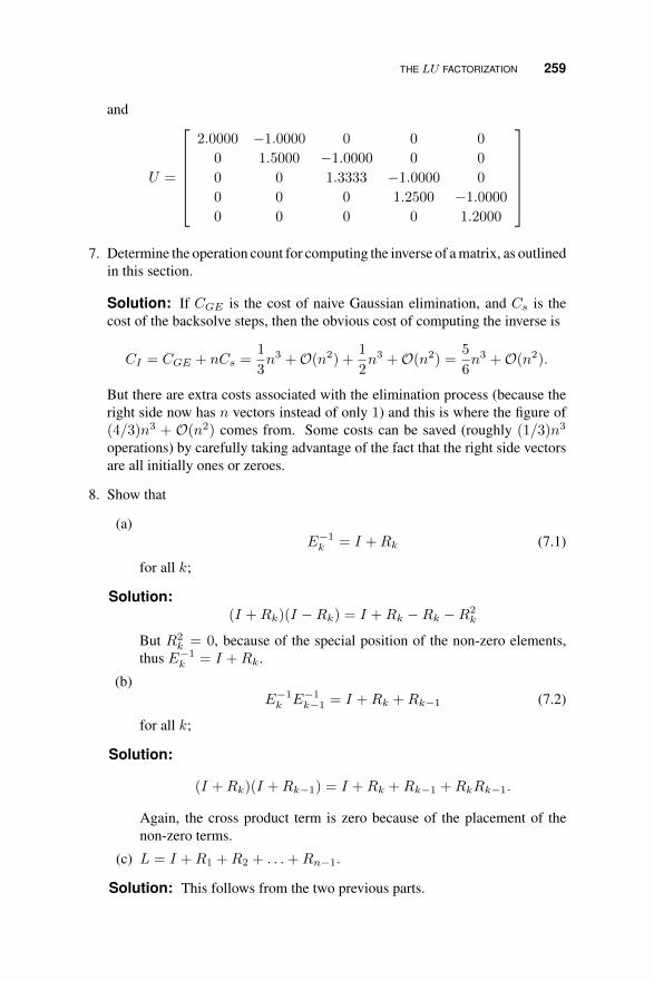
THE LU FACTORIZATION 259
and
U =
2.0000 −1.0000 0 0 0
0 1.5000 −1.0000 0 0
0 0 1.3333 −1.0000 0
0 0 0 1.2500 −1.0000
0 0 0 0 1.2000
7. Determine the operation count for computing the inverse of a matrix, as outlined
in this section.
Solution: If CGE is the cost of naive Gaussian elimination, and Cs is thecost of the backsolve steps, then the obvious cost of computing the inverse is
CI = CGE + nCs =1
3n3 +O(n2) +
1
2n3 +O(n2) =
5
6n3 +O(n2).
But there are extra costs associated with the elimination process (because theright side now has n vectors instead of only 1) and this is where the figure of(4/3)n3 + O(n2) comes from. Some costs can be saved (roughly (1/3)n3
operations) by carefully taking advantage of the fact that the right side vectorsare all initially ones or zeroes.
8. Show that
(a)E−1k = I +Rk (7.1)
for all k;
Solution:(I +Rk)(I −Rk) = I +Rk −Rk −R2
k
But R2k = 0, because of the special position of the non-zero elements,
thus E−1k = I +Rk.
(b)E−1k E−1k−1 = I +Rk +Rk−1 (7.2)
for all k;
Solution:
(I +Rk)(I +Rk−1) = I +Rk +Rk−1 +RkRk−1.
Again, the cross product term is zero because of the placement of thenon-zero terms.
(c) L = I +R1 +R2 + . . .+Rn−1.
Solution: This follows from the two previous parts.
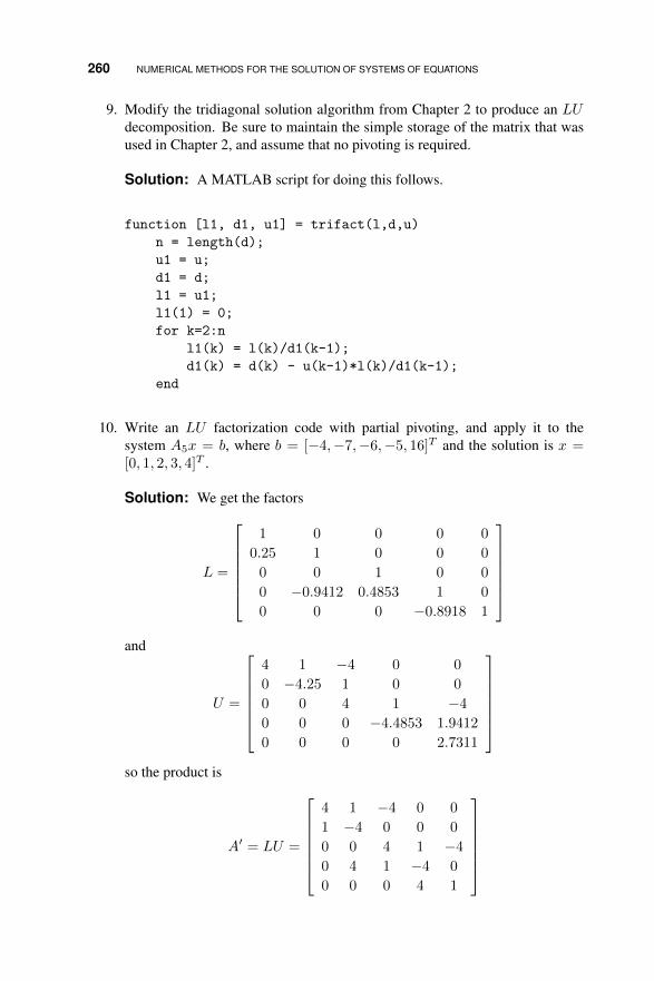
260 NUMERICAL METHODS FOR THE SOLUTION OF SYSTEMS OF EQUATIONS
9. Modify the tridiagonal solution algorithm from Chapter 2 to produce an LUdecomposition. Be sure to maintain the simple storage of the matrix that wasused in Chapter 2, and assume that no pivoting is required.
Solution: A MATLAB script for doing this follows.
function [l1, d1, u1] = trifact(l,d,u)
n = length(d);
u1 = u;
d1 = d;
l1 = u1;
l1(1) = 0;
for k=2:n
l1(k) = l(k)/d1(k-1);
d1(k) = d(k) - u(k-1)*l(k)/d1(k-1);
end
10. Write an LU factorization code with partial pivoting, and apply it to thesystem A5x = b, where b = [−4,−7,−6,−5, 16]T and the solution is x =[0, 1, 2, 3, 4]T .
Solution: We get the factors
L =
1 0 0 0 0
0.25 1 0 0 0
0 0 1 0 0
0 −0.9412 0.4853 1 0
0 0 0 −0.8918 1
and
U =
4 1 −4 0 0
0 −4.25 1 0 0
0 0 4 1 −4
0 0 0 −4.4853 1.9412
0 0 0 0 2.7311
so the product is
A′ = LU =
4 1 −4 0 0
1 −4 0 0 0
0 0 4 1 −4
0 4 1 −4 0
0 0 0 4 1
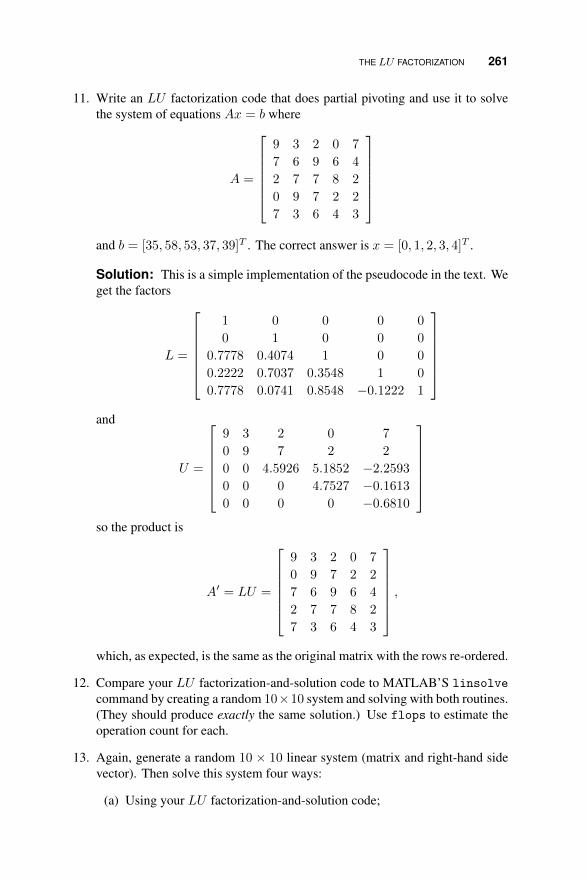
THE LU FACTORIZATION 261
11. Write an LU factorization code that does partial pivoting and use it to solvethe system of equations Ax = b where
A =
9 3 2 0 7
7 6 9 6 4
2 7 7 8 2
0 9 7 2 2
7 3 6 4 3
and b = [35, 58, 53, 37, 39]T . The correct answer is x = [0, 1, 2, 3, 4]T .
Solution: This is a simple implementation of the pseudocode in the text. Weget the factors
L =
1 0 0 0 0
0 1 0 0 0
0.7778 0.4074 1 0 0
0.2222 0.7037 0.3548 1 0
0.7778 0.0741 0.8548 −0.1222 1
and
U =
9 3 2 0 7
0 9 7 2 2
0 0 4.5926 5.1852 −2.2593
0 0 0 4.7527 −0.1613
0 0 0 0 −0.6810
so the product is
A′ = LU =
9 3 2 0 7
0 9 7 2 2
7 6 9 6 4
2 7 7 8 2
7 3 6 4 3
,
which, as expected, is the same as the original matrix with the rows re-ordered.
12. Compare your LU factorization-and-solution code to MATLAB’S linsolve
command by creating a random 10×10 system and solving with both routines.(They should produce exactly the same solution.) Use flops to estimate theoperation count for each.
13. Again, generate a random 10 × 10 linear system (matrix and right-hand sidevector). Then solve this system four ways:
(a) Using your LU factorization-and-solution code;

262 NUMERICAL METHODS FOR THE SOLUTION OF SYSTEMS OF EQUATIONS
(b) Using MATLAB’s linsolve command;
(c) Using the MATLAB backslash operation;
(d) Using MATLAB’s inv command to compute the inverse of the matrix,and then multiply this by the right-hand side vector.
Use flops to estimate the cost of each solution technique, and rank the methodsfor their efficiency in this regard.
14. Repeat the above for the matrixK20 defined at the end of 7.2, using a randomright-hand side vector. Then apply the tridiagonal solver from Chapter 2 tothis problem, and again get the flops estimate. Comment on your results.
/ • • • .
7.5 PERTURBATION, CONDITIONING AND STABILITY
Exercises:
1. Let
A =
1 2 −7
4 −8 0
2 1 0
Compute ‖A‖∞.
Solution: ‖A‖∞ = max{10, 12, 3} = 12.
2. Let
A =
5 6 −9
1 2 3
0 7 2
Compute ‖A‖∞.
Solution: ‖A‖∞ = max{20, 6, 9} = 20.
3. Let
A =
−8 0 −1
3 12 0
1 2 3
Compute ‖A‖∞.
Solution: ‖A‖∞ = max{9, 15, 6} = 15.

PERTURBATION, CONDITIONING AND STABILITY 263
4. Show that‖A‖? = max
i,j|aij |
does not define a matrix norm, according to our defintion. Hint: show that oneof the conditions fails to hold by finding a specific case where it fails.
Solution: Let
A = B =
[1 1
1 1
]Then
AB =
[2 2
2 2
]so ‖AB‖∗ = 2, but ‖A‖∗ = ‖B‖∗ = 1 so the inequality ‖AB‖∗ ≤ ‖A‖∗‖B‖∗doesn’t hold.
5. Let
A =
1 12 0
12
13
14
0 14
15
Compute, directly from the definition, κ∞(A). You should get κ∞(A) = 18.
Solution: We get
A−1 =1
11
−1 24 −30
24 −48 60
−30 60 −20
,so ‖A−1‖∞ = 132/11 = 12. Since ‖A‖∞ = 3/2, we get the expected result.
6. Repeat the above for
A =
4 1 0
1 4 1
0 1 4
for which κ∞(A) = 2.5714.
Solution: We get
A−1 =1
56
15 −4 1
−4 16 −4
1 −4 15
,so ‖A−1‖∞ = 3/7. Since ‖A‖∞ = 6, we get the expected result.

264 NUMERICAL METHODS FOR THE SOLUTION OF SYSTEMS OF EQUATIONS
7. Consider the linear system[1.002 1
1 0.998
] [x1x2
]=
[0.002
0.002
]which has exact solution x = (1,−1)T (verify this). What is the residualb−Axc for the “approximate” solution
xc = (0.29360067817338,−0.29218646673249)T .
Explain.
Solution: We have r = 10−5 × (−0.1413, 0.1416)T . Note that an “approx-imate solution” which is not very close to the actual solution produced a verysmall residual, thus demonstrating that a small residual does not always meanthe computed solution is close to accurate.
8. Consider the linear system problem
Ax = b
where
A =
4 2 0
1 4 1
0 2 4
, b =
8
12
16
,for which the exact solution is x = (1, 2, 3)T . (Check this.) Let xc =x + (0.002, 0.01, 0.001)T be a computed (i.e., approximate) solution to thissystem. Use Theorem 7.8 to find the perturbation matrix E such that xc is theexact solution to Axc = b.
Solution: We get
E =
−0.0020 −0.0040 −0.0060
−0.0031 −0.0062 −0.0092
−0.0017 −0.0034 −0.0051
.9. Compute the growth factor for Gaussian elimination for the matrix in the
previous problem.
Solution: We get
A(1) =
4 2 0
0 3.5 1
0 2 4
A(2) =
4 2 0
0 3.5 1
0 0 3.4286
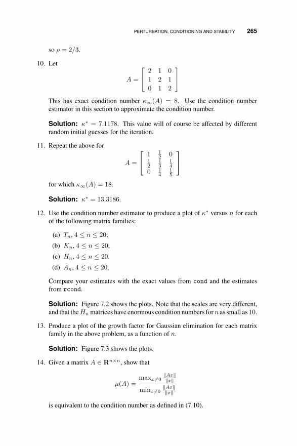
PERTURBATION, CONDITIONING AND STABILITY 265
so ρ = 2/3.
10. Let
A =
2 1 0
1 2 1
0 1 2
This has exact condition number κ∞(A) = 8. Use the condition numberestimator in this section to approximate the condition number.
Solution: κ∗ = 7.1178. This value will of course be affected by differentrandom initial guesses for the iteration.
11. Repeat the above for
A =
1 12 0
12
13
14
0 14
15
for which κ∞(A) = 18.
Solution: κ∗ = 13.3186.
12. Use the condition number estimator to produce a plot of κ∗ versus n for eachof the following matrix families:
(a) Tn, 4 ≤ n ≤ 20;
(b) Kn, 4 ≤ n ≤ 20;
(c) Hn, 4 ≤ n ≤ 20.
(d) An, 4 ≤ n ≤ 20.
Compare your estimates with the exact values from cond and the estimatesfrom rcond.
Solution: Figure 7.2 shows the plots. Note that the scales are very different,and that theHn matrices have enormous condition numbers forn as small as 10.
13. Produce a plot of the growth factor for Gaussian elimination for each matrixfamily in the above problem, as a function of n.
Solution: Figure 7.3 shows the plots.
14. Given a matrix A ∈ Rn×n, show that
µ(A) =maxx6=0
‖Ax‖‖x‖
minx6=0‖Ax‖‖x‖
is equivalent to the condition number as defined in (7.10).

266 NUMERICAL METHODS FOR THE SOLUTION OF SYSTEMS OF EQUATIONS
0 5 10 15 201.8
2
2.2
2.4
2.6
2.8T_n
0 5 10 15 200
50
100
150
200K_n
0 5 10 15 204
6
8
10A_n
0 5 10 15 200
2
4
6
8x 10¹⁷ H_n
Figure 7.2 Solution plot for Exercise 7.5.12.
0 5 10 15 20−0.5
0
0.5
1
1.5
2T_n
0 5 10 15 20−0.5
0
0.5
1
1.5K_n
0 5 10 15 200.5
1
1.5
2
2.5
3A_n
0 5 10 15 200.25
0.3
0.35
0.4
0.45
0.5H_n
Figure 7.3 Solution plot for Exercise 7.5.13.

PERTURBATION, CONDITIONING AND STABILITY 267
Solution: We have
µ(A) =maxx6=0
‖Ax‖‖x‖
minx6=0‖Ax‖‖x‖
=‖A‖
minx6=0‖Ax‖‖x‖
so it remains only to show that the denominator is equivalent to 1/‖A−1‖.Since
1
minX= max
1
X,
we have
1
minx6=0‖Ax‖‖x‖
= maxx6=0
‖x‖‖Ax‖
= maxy 6=0
‖A−1y‖‖y‖
= ‖A−1‖
and we are done.
15. Prove that (7.8) and (7.9) follow from the definition of matrix norm.
Solution: We have that
‖A‖ = maxx 6= 0‖Ax‖‖x‖
so that, for any particular choice of x,
‖A‖ ≥ ‖Ax‖‖x‖
which proves (7.9). To get (7.8), we simply apply (7.9):
‖AB‖ = maxx 6= 0‖ABx‖‖x‖
≤ maxx 6= 0‖A‖‖Bx‖‖x‖
= ‖A‖‖B‖.
16. Prove Theorem 7.10.
Solution: Theorem 7.8 says that there exists a perturbation matrix E suchthat xc is the exact solution to (A + E)xc = b. Theorem 7.6 says that ifκ(A)‖E‖ ≤ ‖A‖, then the relative error is bounded above according to
‖x− xx‖‖x‖
≤ θ
1− θ,
where
θ = κ‖E‖‖A‖
.
The function f(θ) = θ/(1 − θ) is an increasing function, so replacing κ‖E‖‖A‖with something larger preserves the inequality. Returning to Theorem 7.8, wehave that
‖E‖2‖A‖2
≤ ‖r‖2‖A‖2‖xc‖2
≤ ‖r‖2‖Axc‖2
.

268 NUMERICAL METHODS FOR THE SOLUTION OF SYSTEMS OF EQUATIONS
Butb− r = b− (b−Axc) = Axc,
so we are done.
17. Give an argument to support the validity of the “rule of thumb” followingTheorem 7.10.
Solution: Follows by applying the given assumptions to Theorem 7.6. Wehave that
‖x− xx‖‖x‖
≤ θ
1− θ,
where
θ = κ‖E‖‖A‖
,
butθ ≤ (C4 × 10t)(C1C2 × 10−s) = C × 10t−s.
18. Prove Theorem 7.5.
Solution: We have r = b − Axc = Ax − Axc so x − xc = A−1r and theresult follows along the same lines as Theorem 7.4.
19. Consider the linear system problem Ax = b for
A =
[1 1
212
13
], b =
[2
7/6
].
Note that the exact solution is x = (1, 2)T .
(a) Represent the exact factorization ofA using only four decimal digits, andsolve the system.
(b) Do two steps of iterative refinement to improve your solution.
Solution: The factorization is
L =
[1.0000 0
0.5000 1.0000
]
U =
[1.0000 0.5000
0 0.0833
]which multiplies out to
LU =
[1.0000 0.5000
0.5000 0.3333
]

SPD MATRICES AND THE CHOLESKY DECOMPOSITION 269
The uncorrected solution is
xc =
(0.9996
2.0008
)and the refined solution (after two iterations) is
x =
(0.99999999993592
2.00000000012816
)20. Do two more steps of refinement for the problem in Example 7.9.
Solution:
x(3) = (0.99999999999999, 2.00000000000004, 2.99999999999996)T ./ • • • .
7.6 SPD MATRICES AND THE CHOLESKY DECOMPOSITION
Exercises:
1. Show that a matrix with one or more non-positive diagonal elements cannot beSPD. Hint: Try to find a vector x such that xTAx = aii.
Solution: If aii is the non-positive diagonal element, take x = ei. TheneTi Aei = aii.
2. For a 2 × 2 SPD matrix, show that a22 − a221/a11 > 0. Hint: Consider thepositive definite condition with x = (a21,−a11)T .
Solution: For x as suggested, we have
xTAx = a211a22 − a11a221 = a11(a22 − a221/a11
)3. Let A ∈ Rn×n be partitioned as
A =
[A11 A21
A21 A22
]where A11 and A22 are square matrices. Show that both A11 and A22 must beSPD if A ∈ SPD.
Solution: Suppose A11 is not SPD. Then take x = (y, 0)T , partitionedconformably with A, and with y such that yTA11y ≤ 0. Then, since
xTAx = yTA11y,
A cannot be SPD.

270 NUMERICAL METHODS FOR THE SOLUTION OF SYSTEMS OF EQUATIONS
4. In the proof of the Cholesky theorem, show that akk − gT g > 0 must hold, orelse there is a vector x such that xTAx ≤ 0. Hint: Use Problem 2 as a startingpoint.
Solution: Follows from the hint and Exercise 1.
5. Derive the operation count given in the text for the Cholesky decomposition.
Solution: Follows from the formulas in the text and a direct computation.
6. Prove the following: If A ∈ SPD, then there exists a unit lower triangularmatrix L, and a diagonal matrix D with positive elements, such that A =LDLT .
Solution: Let D1 = diag(G), where G is the usual Cholesky factor. DefineL = GD−11 and D = D2
1 . Then
LDLT = (GD−11 )D21(D−11 GT ) = GGT = A.
7. Derive an algorithm for the LDLT factorization that does not require anysquare roots. Hint: Look at the 3 × 3 case, explicitly. Multiply out LDLT
and set the result equal to A, and from this deduce the relationships that arenecessary. In other words, if 1 0 0
l21 1 0
l31 l32 1
d11 0 0
0 d22 0
0 0 d33
1 l21 l310 1 l320 0 1
=
a11 a12 a13a21 a22 a23a31 a32 a33
what is the relationship between the components of L, D, and A? Thengeneralize to a problem of arbitrary size. Don’t forget that A is symmetric!
8. The Tn and Kn families of matrices are all positive definite. Write up a codeto do the Cholesky factorization and test it on these matrices over the range3 ≤ n ≤ 20. Use a right-side vector that is all ones, and confirm that the codeis working by computing ‖r‖∞, where r is the residual vector.
Solution: For both families, the norm of the residual is on the order of 10−12
or smaller, for the entire range of problem sizes given here.
9. If A is tridiagonal and SPD, then the Cholesky factorization can be modifiedto work only with the two distinct non-zero diagonals in the matrix. Constructthis version of the algorithm and test it on the Tn and Kn families, as above.
Solution: A MATLAB script that does this is given below.
function [l,d] = chol3(l,d)
n = length(d);

ITERATIVE METHODS FOR LINEAR SYSTEMS – A BRIEF SURVEY 271
d(1) = sqrt(d(1));
for k=2:n
l(k) = l(k)/d(k-1);
d(k) = sqrt(d(k) - l(k)^2);
end
10. The Hn family of matrices is also SPD, but ill-conditioned. Try to applychol, over the range 4 ≤ n ≤ 20. What happens? Can you explain this?
Solution: For n ≤ 13 everything is fine, but for n = 14 the routine reportsthat the matrix is no longer SPD. In terms of the computation, the argumentto the square root in the computation of gii becomes negative.
/ • • • .
7.7 ITERATIVE METHODS FOR LINEAR SYSTEMS – A BRIEF SURVEY
Exercises:
1. Let
A =
4 −1 0 0
−1 4 −1 0
0 −1 4 −1
−1 0 −1 4
and b = (−4, 2, 4, 10)T .
(a) Verify that the solution to Ax = b is x = (0, 1, 2, 3)T .
(b) Do three iterations (by hand) of the Jacobi iteration for this matrix, usingx(0) = (0, 0, 0, 0)T .
Solution: x(3) = (−0.0781, 0.9062, 1.8438, 2.9062)T
(c) Do three iterations (by hand) of the Gauss-Seidel iteration for this prob-lem, using the same initial guess.
Solution: x(3) = (−0.0645, 0.9500, 1.9702, 2.9764)T
2. Do three iterations of SOR for the previous example, using ω = 1.05.
Solution: x(3) = (−0.0959, 0.9430, 1.6624, 2.9908)T
3. Solve the same system using SOR for a wide set of values of ω ∈ (0, 2). Foreach ω, compute r(ω) = ‖b−Ax(k)‖∞. Graph r(ω) for k = 1, 3, 5, 10.

272 NUMERICAL METHODS FOR THE SOLUTION OF SYSTEMS OF EQUATIONS
0.2 0.4 0.6 0.8 1 1.2 1.4 1.6 1.80
1
2
3
4
5
6
7
8
9
Figure 7.4 Solution plots for Exercise 7.7.3.
Solution: For ω = 0.25, 0.50, 0.75, 1.00, 1.25, 1.50, and 1.75 we get theplots in Figure 7.4. Note that the residual gets very large away from the criticalvalue of ω, which appears to be slightly larger than 1.
4. Write a computer code that does Jacobi for the previous example, for a specifiednumber of iterations. How many iterations does it take to get convergence, inthe sense the consecutive iterates differ by less than 10−6?
Solution: Convergence occurs in 18 iterations.
5. Repeat the above for Gauss-Seidel.
Solution: Convergence occurs in 12 iterations.
6. Repeat the above for SOR. Make sure your code can accept different valuesof ω as an input parameter.
Solution: For ω = 1.25, convergence occurs in 16 iterations; note that thisis better than Jacobi, but worse than Gauss-Seidel. However, for ω = 1.05, weget convergence in 11 iterations, which is better than Gauss-Seidel.
7. Let A be the 16× 16 matrix given at the beginning of this section. Take
b = (5, 11, 18, 21, 29, 40, 48, 48, 57, 72, 80, 76, 69, 87, 94, 85)T .
Write a computer code to do Jacobi, Gauss-Seidel, and SOR on this system ofequations. Write the code to only store the non-zero diagonals ofA, and makethe code as efficient as possible.

NONLINEAR SYSTEMS: NEWTON’S METHOD AND RELATED IDEAS 273
Solution: Jacobi converges in about 80 iterations, Gauss-Seidel in about 43,and SOR (with ω = 1.25) in about 20.
8. Prove that the spectral radius of A, ρ(A), is bounded above by ‖A‖ for anynorm such that ‖Ax‖ ≤ ‖A‖‖x‖.
Solution: Let λ be the eigenvalue which generates the spectral radius. Thenλx = Ax and so
‖λx‖ = ‖Ax‖ ⇒ ρ =‖Ax‖‖x‖
≤ ‖A‖
/ • • • .
7.8 NONLINEAR SYSTEMS: NEWTON’S METHOD AND RELATEDIDEAS
Exercises:
1. Consider the nonlinear system
2x1 − x2 +1
9e−x1 = −1, (7.3)
−x1 + 2x2 +1
9e−x2 = 1. (7.4)
Take x(0) = (1, 1)T and do two iterations of Newton’s method; you should get
x(2) = (−0.48309783661427, 0.21361449746996)T .
Solution: This is fairly straight-forward. As an intermediate check, youshould get
x(1) = (−0.42317280134882, 0.25270278130481)T .
2. Write a computer code to solve the system in the preceding problem, using
(a) Newton’s method;
(b) The chord method;
(c) The chord method, updating every 3 iterations.
Solution: Below is a MATLAB script for the Newton iteration.
function z = newt2(x1,x2,n)

274 NUMERICAL METHODS FOR THE SOLUTION OF SYSTEMS OF EQUATIONS
for k=1:n
y1 = 2*x1 - x2 + (1/9)*exp(-x1) + 1;
y2 = -x1 + 2*x2 + (1/9)*exp(-x2) - 1;
df = [2 - exp(-x1)/9 -1; -1 2 - exp(-x2)/9];
dfi = inv(df);
z = [x1 x2]’ - dfi*[y1 y2]’
x1 = z(1);
x2 = z(2);
end
3. Re-write the system in Problem 1 as
Kx+ φ(x) = b,
where K is the 2× 2 matrix
K =
[2 −1
−1 2
],
φ(x) is defined by
φ(x) =
(19e−x1
19e−x2
),
and b = (−1, 1)T .
(a) Do two iterations (by hand) of the fixed-point iteration
x(k+1) =1
2(b− φ(x(k) −Kx(k) + 2x(k))
for this system, using x(0) = (1, 1)T .
Solution:
x(1) = (−0.02043774673175, 0.97956225326825)T
x(2) = (−0.06692154156532, 0.46892138074399)T
(b) Do two iterations (by hand) of the fixed-point iteration
x(k+1) = K−1(b− φ(x(k))
for this system, using x(0) = (1, 1)T .
(c) Which one do you think is going to converge faster?
4. Write a computer code to implement the fixed point iterations outlined in theprevious problem. Compare the total “cost to convergence” with your resultsfor Newton’s method and the chord iterations.

APPLICATION: NUMERICAL SOLUTION OF NONLINEAR BVP’S 275
Solution: The MATLAB script below converges in 24 iterations to the fixedpoint
α = (−0.48336323789790, 0.21344115515536)T .
function y = fixed2(x)
K = [2 -1; -1 2];
b = [-1 1]’;
for k = 1:100
k
y = 0.5*(b - (1/9)*exp(-x) - K*x + 2*x);
if abs(x - y) < 1.e-6
break
end
x = y;
end
/ • • • .
7.9 APPLICATION: NUMERICAL SOLUTION OF NONLINEAR BVP’S
Exercises:
1. Set up the nonlinear system for the example (7.36)-(7.37), and verify that theresult given in the text (7.38)-(7.40) is correct.
2. Apply Newton’s method and the chord method, to the approximate solutionof the nonlinear BVP (7.36)-(7.37). Compare the number of iterations toconverge and the overall cost of convergence. Use the sequence of gridsh−1 = 4, 8, . . . , 1024.
Solution: For Newton’s method with h = 1/8 and u(0) = 0, we get conver-gence in 10 iterations to
u = (0.1267, 0.2529, 0.3787, 0.5039, 0.6287, 0.7529, 0.8767)T .
3. Consider the nonlinear BVP
−u′′ + e−u = 1,
u(0) = u(1) = 1.
Use finite difference techniques to reduce this (approximately) to a systemof nonlinear algebraic equations, and solve this system using several of themethods discussed in this chapter of the text. Test the program on the sequence
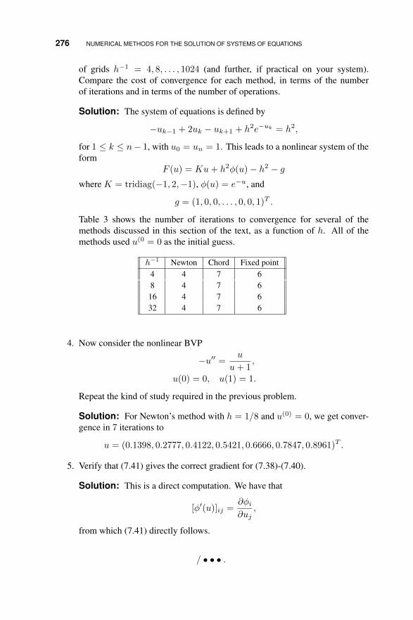
276 NUMERICAL METHODS FOR THE SOLUTION OF SYSTEMS OF EQUATIONS
of grids h−1 = 4, 8, . . . , 1024 (and further, if practical on your system).Compare the cost of convergence for each method, in terms of the numberof iterations and in terms of the number of operations.
Solution: The system of equations is defined by
−uk−1 + 2uk − uk+1 + h2e−uk = h2,
for 1 ≤ k ≤ n− 1, with u0 = un = 1. This leads to a nonlinear system of theform
F (u) = Ku+ h2φ(u)− h2 − gwhere K = tridiag(−1, 2,−1), φ(u) = e−u, and
g = (1, 0, 0, . . . , 0, 0, 1)T .
Table 3 shows the number of iterations to convergence for several of themethods discussed in this section of the text, as a function of h. All of themethods used u(0 = 0 as the initial guess.
h−1 Newton Chord Fixed point4 4 7 68 4 7 616 4 7 632 4 7 6
4. Now consider the nonlinear BVP
−u′′ =u
u+ 1,
u(0) = 0, u(1) = 1.
Repeat the kind of study required in the previous problem.
Solution: For Newton’s method with h = 1/8 and u(0) = 0, we get conver-gence in 7 iterations to
u = (0.1398, 0.2777, 0.4122, 0.5421, 0.6666, 0.7847, 0.8961)T .
5. Verify that (7.41) gives the correct gradient for (7.38)-(7.40).
Solution: This is a direct computation. We have that
[φ′(u)]ij =∂φi∂uj
,
from which (7.41) directly follows.
/ • • • .

CHAPTER 8
APPROXIMATE SOLUTION OF THEALGEBRAIC EIGENVALUE PROBLEM
8.1 EIGENVALUE REVIEW
Exercises:
1. For each matrix below, find the characteristic polynomial and the eigenvaluesby a hand calculation. For some of the exercises, the correct eigenvalues aregiven, to four decimal places, so you can check your work.
(a)
A =
4 1 0
1 4 1
0 1 4
for which σ(A) = {5.4142, 4.0000, 2.5858};
Solution: p(λ) = −λ3 + 12λ2 − 46λ+ 56.
Solutions Manual to Accompany An Introduction to Numerical Methods and Analysis,Second Edition. By James F. EppersonCopyright c© 2013 John Wiley & Sons, Inc.
277

278 APPROXIMATE SOLUTION OF THE ALGEBRAIC EIGENVALUE PROBLEM
(b)
A =
1 2 0
0 4 5
0 5 7
for which σ(A) = {1.0000, 0.2798, 10.7202};
Solution: p(λ) = −λ3 + 12λ2 − 14λ+ 3.
(c)
A =
6 −2 0
2 6 −2
0 2 4
for which σ(A) = {5.5698± 2.6143i, 4.8603};
Solution: p(λ) = −λ3 + 16λ2 − 92λ+ 184.
(d)
A =
4 2 0
1 4 2
0 1 4
for which σ(A) = {2, 4, 6};
Solution: p(λ) = −λ3 + 12λ2 − 44λ+ 48.
(e)
A =
6 −1 0
2 6 −1
0 2 4
;
(f)
A =
0 2 0
2 7 1
0 1 4
.2. Prove that similar matrices have identical eigenvalues and related eigenvectors.
Solution: If A = P−1BP , then we have
Ax = λx⇔ P−1BPx = λx⇔ B(Px) = λ(Px)⇔ By = λy.
3. Apply Gerschgorin’s Theorem to the matrices in Problem 1 and determine theintervals or disks in which the eigenvalues must lie.
Solution: For (a), λ ∈ {z ∈ C | |z − 4| ≤ 3}.

EIGENVALUE REVIEW 279
4. Show that the matrix
A =
3 2 −1
0 2 2
0 −2 7
;
has repeated eigenvalues and is defective, but that the matrix
A =
−1 −1 2
−2 0 2
−4 −2 5
;
which also has repeated eigenvalues, is not defective.
Solution: For the first matrix, we get σ(A) = {3, 3, 6}, but the only eigen-vector for λ = 3 is parallel to x = (1, 0, 0)T ; for the second matrix, we getσ(A) = {2, 1, 1}, and there are two independent eigenvectors for λ = 1.
5. Let A and B be similar matrices of size n× n, with
B =
[λ aT
0 A22
]where λ ∈ R, a ∈ Rn−1, and A22 ∈ Rn−1×n−1.
(a) Prove that λ ∈ σ(A). Hint: What is the product Be1, where e1 is thefirst standard basis vector?
Solution: Since Be1 = λe1, it follows that λ ∈ σ(B), but the similaritythen implies that λ ∈ σ(A).
(b) Prove that each eigenvalue of A22 is also an eigenvalue of A.
Solution: Let µ ∈ σ(A22), with eigenvector y. Then it is easy to show that
x =
[0
y
]is an eigenvector of B, corresponding to the same eigenvalue. Thesimilarity of A and B then proves that µ ∈ σ(A).
6. Generalize the above; let A and B be similar matrices of size n× n, with
B =
[D aT
0 A22
]where D ∈ Rp×p is diagonal, a ∈ Rn−p, and A22 ∈ Rn−p×n−p. Prove thateach diagonal element ofD is an eigenvalue ofA: dii ∈ σ(A), 1 ≤ i ≤ p, andthat each eigenvalue of A22 is also an eigenvalue of A.
Solution: This is an obvious extension of the argument in Problem 5.

280 APPROXIMATE SOLUTION OF THE ALGEBRAIC EIGENVALUE PROBLEM
7. Let A be given by
A =
[2 0
a A22
].
Prove that 2 ∈ σ(A).
8. Let A1 = BC and A2 = CB for given B,C. Show that any non-zeroeigenvalue of A1 is also an eigenvalue of A2, and vice-versa.
Solution: Let µ be an eigenvalue of A1. Then we have A1x = µx for aneigenvector x. Now multiply by C to get
CA1x = µCx⇒ CBCx = µCx⇒ A2Cx = µCx⇒ A2y = µy
for y = Cx. Therefore µ is an eigenvalue of A2. A similar proof works forthe other direction.
/ • • • .
8.2 REDUCTION TO HESSENBERG FORM
Exercises:
1. Show that in the Householder construction, if we use c = −‖x‖2 then we getQx = −‖x‖2e1, and that this will work just as well to construct the Hessenbergmatrix.
2. Compute (by hand) the Hessenberg form of the matrix
A =
6 1 1 1
1 6 1 1
1 1 6 1
1 1 1 6
You should get
AH =
6.0000 1.7321 0 0
1.7321 8.0000 −0.0000 0
0 −0.0000 5.0000 0
0 0 0 5.0000
3. Complete the computation in Example 8.6 by finding the matrix P such thatA = PAHP
T .
4. Use the hess command to compute the Hessenberg form for each of H4, H8,and H10. Verify that the original matrix can be recovered from AH .
/ • • • .

POWER METHODS 281
8.3 POWER METHODS
Exercises:
1. Explain, in your own words, why it is necessary to scale the power iterations.Hint: What happens if we don’t scale the iteration?
Solution: If the iteration is not scaled, then (unless the dominant eigenvaluehas absolute value equal to 1) the vector iterates will either go off to infinity ordown to zero. Either way, the iteration quickly becomes useless.
2. Use an inductive argument to show that, in the basic power method (Theorem8.5) we have
z(k) = ckAkz(0).
What is ck?
Solution: We havez(k) =
1
µkAz(k−1)
soz(k) =
1
µkµk−1Az(k−2)
andz(k) =
1
µkµk−1 . . . µ1Az(0).
Sock =
1
µkµk−1 . . . µ1.
3. Consider the iteration defined by
y(k+1) = Az(k),
z(k+1) = y(k+1)/σk+1
where σk+1 is some scaling parameter. Assume that the iteration converges inthe sense that z(k) → z; prove that σk must also converge, and that therefore(σ, z), where σ is the limit of the σk, must be an eigenpair of A.
Solution: We havez(k+1) =
1
σkAz(k)
so thatAz(k) = σkz
(k+1),
therefore,Az +A
(z(k) − z
)= σkz + σk
(z(k+1) − z
).

282 APPROXIMATE SOLUTION OF THE ALGEBRAIC EIGENVALUE PROBLEM
Since the two differences go to zero, it follows that σk converges to a limit,and we are essentially done.
4. Fill in the details of the eigenvalue error estimate in Theorem 8.5. In particular,show that there is a constant C such that
|λ1 − µk| ≤ C(λ2λ1
)k.
5. Prove Theorem 8.7.
6. Write a program that does the basic power method. Use it to produce a plot ofthe largest eigenvalue of the Tn family of matrices, as a function of n, over therange 2 ≤ n ≤ 20.
7. Write a program that does the inverse power method. Use it to produce a plotof the smallest eigenvalue of the Hn family of matrices, as a function of n,over the range 2 ≤ n ≤ 20.
8. Write a program that does inverse power iteration on a symmetric matrix. As-sume the matrix is tridiagonal, and store only the necessary non-zero elementsof the matrix. Test it on the Tn andKn families, and on your results from find-ing the Hessenberg forms for the Hn matrices. Produce a plot of the smallesteigenvalues of each of these matrices, as a function of n.
9. Add shifts to your inverse power iteration program. Test it on the sameexamples, using a selection of shifts.
10. Let λ and x be an eigenvalue and corresponding eigenvector for A ∈ Rn×n,and let Q be an orthogonal matrix such that Qx = e1. Assume that ‖x‖2 = 1.Show that
B = QAQT =
[λ aT
0 A2
].
Hint: Consider each of the inner products (ei, Bej), using the fact thatQx = e1and that Q is symmetric.
Solution: Following the hint, we have
(ei, Bej) = (ei, QAQT ej) = (QT ei, AQ
T ej).
Now, Qx = e1 implies that x = QT e1, therefore, the (1, 1) element of B is(e1, Be1) = (QT e1, AQ
T e1) = (x,Ax) = λ. The rest follows with a littleattention to detail.
11. An alternate deflation for symmetric matrices is based on the relationship
A′ = A− λ1x1xT1 .

POWER METHODS 283
If A ∈ Rn×n is symmetric, λ1 ∈ σ(A) with corresponding eigenvector x1,and if ‖x1‖2 = 1, show that A′ has the same eigenvalues as A, except that λ1has been replaced by zero. In other words, if
σ(A) = {λ1, λ2, . . . , λn},
thenσ(A′) = {0, λ2, . . . , λn}.
Solution: Since A is symmetric, the eigenvectors can be assumed orthonor-mal, thus
A′xk = Axk − λ1x1xT1 xk = Axk − λδ1k = λk − λδ1k.
which is sufficient.
12. Show how to implement the deflation from the previous problem (known asHotelling’s deflation) without forming the product x1xT1 . Hint: What isA′z forany vector z? Can we write this in terms of the dot product xT1 z? (Accordingto Wilkinson [6], this deflation is prone to excessive rounding error and so isnot of practical value.)
13. What is the operation count for one iteration of the basic power method appliedto a symmetric matrix? Compute two values, one for the matrix in Hessenbergform, one for the full matrix.
Solution: The iteration is
(a) Compute y(k) = Az(k−1);
(b) µk = y(k)i , where ‖y(k)‖∞ = |y(k)i |;
(c) Set z(k) = y(k)/µk.
This amounts to a single matrix-vector multiplication, followed by a scalar-vector multiplication. (We will ignore the cost of determining the maximum.)So the cost of each iteration is
C = n2 + n
multiplications. If the matrix is in Hessenberg form, then the matrix-vectormultiplication only takes 3n operations, for a much cheaper iteration.
14. What is the cost of the basic power method for a symmetric matrix if it runsfor N iterations. Again, compute two values depending on whether or nota Hessenberg reduction is done. Is it always the case that a reduction toHessenberg form is cost-effective?
15. Repeat Problems 13 and 14 for the inverse power method.

284 APPROXIMATE SOLUTION OF THE ALGEBRAIC EIGENVALUE PROBLEM
16. Consider the family of matrices T defined by
tij =
a, i− j = 1
b, i = j
c, i− j = −1
0, otherwise
Thus T is tridiagonal, with constant diagonal elements a, b, and c. It iscommonplace to abbreviate such a matrix definition by saying
T = tridiag(a, b, c).
Write a computer program that uses the power method and inverse powermethod to find the largest and smallest (in absolute value) eigenvalues of sucha matrix, for any user-specified values of a, b, and c. Test the program on thefollowing examples; note that the exact values are given (to four places).
(a) a = c = 4, b = 1, n = 6, λ1 = −6.2708, λ6 = −0.7802;
(b) a = b = c = 6, n = 7, λ1 = 17.0866, λ6 = 1.4078;
(c) a = 2, b = 3, c = 4, n = 5, λ1 = 7.8990, λ6 = 0.1716;
(d) a = c = 1, b = 10, n = 9, λ1 = 11.9021, λ6 = 8.0979;
(e) a = c = 1, b = 4, n = 8, λ1 = 5.8794, λ6 = 2.1206;
17. Modify the program from the previous problem to do the inverse power methodwith shifts. Test it on the same examples by finding the eigenvalue closest toµ = 1.
/ • • • .
8.4 AN OVERVIEW OF THE QR ITERATION
Exercises:
1. Show that the product of two orthogonal matrices, Q1 and Q2, is also orthog-onal.
Solution:
(Q1Q2)T (Q1Q2 = QT2QT1Q1Q2 = QT2 (I)Q2 = I.
2. Let A ∈ Rn×n have the partioned form
A
[A11 a
0 λ
]

AN OVERVIEW OF THE QR ITERATION 285
where A11 ∈ R(n−1)×(n−1) and λ ∈ R. Show that λ must be an eigenvalueof A. How are the eigenvalues of A and A11 related?
Solution: For A as given, let en = (0, 0, 0, . . . , 0, 1)T . Then
Aen = λen
so λ must be an eigenvalue of A. Now let z be an arbitrary eigenvector of A11
and form x = (z, 0)T . Then
Ax =
(A11z
0
)so all the eigenvalues of A11 are also eigenvalues of A.
3. Assume that the iteration in Algorithm 8.5 converges, in the sense that Rk →R∞ which is upper triangular, and Qk → Q∞ which is orthogonal.
(a) Prove that the matrices Ak, defined in (8.5), must also converge to R∞.
Solution: We have
Ak = QTkQk+1QTk+1AQk = QTkQk+1Rk+1
The rest of the proof should be easy.
(b) Prove then that the eigenvalues of A can be recovered from the diagonalelements of Ak, in the limit as k →∞.
Solution: Since Ak → R∞, and Ak is similar to A, it should be easy toconstruct a formal argument.
4. Show that the matrices in the shiftedQR iteration all have the same eigenvalues.
Solution: We haveQkRk = Ak−1 − µk−1I
so thatQkRkQk = Ak−1Qk − µk−1Qk;
thus,Qk(Ak − µk−1I) = Ak−1Qk − µk−1Qk,
or,QkAk = Ak−1Qk
and we are done.
5. Consider the matrix
A =
[0 1
1 0
]

286 APPROXIMATE SOLUTION OF THE ALGEBRAIC EIGENVALUE PROBLEM
(a) Find the exact eigenvalues of A;
(b) Show that
Q =
[0 1
1 0
], R =
[1 0
0 1
]is a valid QR decomposition of A;
(c) Use this to show that the shifted QR iteration for A, using the Rayleighshift, will not converge.
Solution: (a) The eigenvalues are easily shown to be λ1 = 1, λ2 − −1. (b)QR = A, therefore we are done. (c) The Rayleigh shift is a22 = 0, thereforethe first step of QR using this shift simply reproduces the original matrix:A1 = RQ = A. Hence the iteration fails to converge; in fact, it fails to domuch of anything!
6. The QR factorization is usually carried out for the QR iteration by means ofGivens transformations, defined in part (a), below. In this exercise we willintroduce the basic ideas of this kind of matrix operation.
(a) Show that the matrix
G(θ) =
[cos θ − sin θ
sin θ cos θ
]is an orthogonal matrix for any choice of θ.
(b) Show that we can always choose θ so that
G(θ)A =
[cos θ − sin θ
sin θ cos θ
] [a11 a12a21 a22
]=
[r11 r120 r22
]= R
(c) Use a Givens transformation to perform one step of the basicQR iterationfor the matrix [
4 1
1 4
]7. (a) If G(θ) is a Givens transformation, show that
G(θ) =
[1 0
0 G(θ)
]is orthogonal.
(b) Show how to use a sequence of two Givens transformations to do a singleQR step for the matrix 4 1 0
1 4 1
0 1 4

AN OVERVIEW OF THE QR ITERATION 287
8. Write a MATLAB code that automates the kind of computation we did inExamples 8.17 and 8.18: Take an input matrix (square), and perform “naive”QR by executing the commands:
[q, r] = qr(A);
A = r ∗ q;
Stop when A is triangular. Use no shifts. Test your code by forming a randomsymmetric matrix7 and using your routine to find its eigenvalues. Rememberto reduce the matrix to Hessenberg form! Use the flops command to measurethe cost of your routine, and compare this to what MATLAB’s eig commandcosts.
Solution: Here is a MATLAB code that does this on a 6× 6 example:
B = rand(6,6);
A = (B + B’)/2
AH = hess(A);
Asave = AH;
offdiag = 1;
k = 0;
flops(0)
while offdiag > 1.e-6
k = k + 1;
[Q,R] = qr(AH);
AH = R*Q;
AH;
v = diag(AH,-1);
offdiag = norm(v)
pause
end
flops
diag(AH)
flops(0)
lambda = eig(A)
flops
When the author ran this, it took about 37 iterations and 64, 000 flops to findthe eigenvalues, whereas eig found them in about 540 flops. Obviously, agood shifting strategy (and deflation) helps a lot!
9. Repeat the above, this time using the Rayleigh shift. (You should save the ran-dom matrix from the previous problem so a flops comparison is meaningful.
7Recall that S = A+AT is always symmetric.

288 APPROXIMATE SOLUTION OF THE ALGEBRAIC EIGENVALUE PROBLEM
10. Repeat the above, this time using the Wilkinson shift. (Again, use the samematrix and do a flops cost comparison.
/ • • • .
8.5 APPLICATION: ROOTS OF POLYNOMIALS, II
Exercises:
1. For the polynomial p(x) = x3−2x2+5x+1, construct the companion matrix,then use a cofactor expansion to confirm that the characteristic polynomial is,indeed, p(λ).
2. For each polynomial in Problem 2 of 3.10, construct the companion matrixand use MATLAB’s eig to find the roots. Use flops to compare the costswith the Durand-Kerner method from 3.10.
Solution: For (b), the companion matrix is
C =
0 0 0 0 0 1
1 0 0 0 0 0
0 1 0 0 0 0
0 0 1 0 0 0
0 0 0 1 0 0
0 0 0 0 1 1
The author’s Durand-Kerner routine from Chapter 3 found the roots in 6130flops. MATLAB’s eig routine found the same values in 5220 flops, a slightsavings.
3. Consider the polynomial p(x) = x4 − 10x3 + 35x2 − 50x+ 24 and form itscompanion matrix. Using MATLAB’s qr command, do several iterations ofthe unshifted QR iteration. Are the roots being isolated? Is the structure ofthe companion matrix being maintained? Comment.

CHAPTER 9
A SURVEY OF NUMERICAL METHODSFOR PARTIAL DIFFERENTIALEQUATIONS
9.1 DIFFERENCE METHODS FOR THE DIFFUSION EQUATION
Exercises:
1. Write a program to use the explicit method to solve the diffusion equation
ut = uxx, t > 0, 0 < x < 0.1;
u(0, t) = 0;
u(1, t) = 0;
u(x, 0) = sinπx.
which has exact solution
u(x, t) = e−π2t sinπx
(The student should check that this is indeed the exact solution.) Use h−1 =4, 8, . . ., and take ∆t as large as possible for stability. Confirm that theapproximate solution is as accurate as the theory predicts. Compute out tot = 1.
Solutions Manual to Accompany An Introduction to Numerical Methods and Analysis,Second Edition. By James F. EppersonCopyright c© 2013 John Wiley & Sons, Inc.
289

290 A SURVEY OF NUMERICAL METHODSFOR PARTIAL DIFFERENTIAL EQUATIONS
Solution: The following MATLAB script will solve the problem. The authormakes no claims of being the most sophisticated MATLAB programmer.
clear
n = input(’number of points? ’)
h = 1/n;
dt = 0.5*h^2;
%
% Index shift since Matlab doesn’t allow zero subscripts
%
np = n+1;
x = h*[0:n];
uo = sin(pi*x);
nt = floor(0.1/dt);
disp(nt)
disp(’steps’)
r = dt/(h*h);
pause
for k=1:nt
t = k*dt;
u(1) = 0;
ue(1) = 0;
for j=2:n
u(j) = uo(j) + r*(uo(j-1) - 2*uo(j) + uo(j+1));
ue(j) = exp(-pi*pi*t)*sin(pi*(j-1)*h);
error(j) = ue(j) - u(j);
end
u(np) = 0;
ue(np) = 0;
uo = u;
errmax = norm(error,inf);
disp([t,errmax])
if k == 4
figure(1)
plot(x,u)
figure(2)
plot(x,ue)
pause
end
if k == nt
figure(3)
plot(x,u)
figure(4)
plot(x,ue)
pause

DIFFERENCE METHODS FOR THE DIFFUSION EQUATION 291
end
end
2. Repeat the above problem, but this time take ∆t 10% too large to satisfy thestability condition, and attempt to compute solutions out to t = 1. Commenton what happens.
Solution: With ∆t too large, the solution will quickly blow up.
3. Apply Crank-Nicolson to the same PDE as in Problem 1. For each value of h,adjust the choice of ∆t to obtain comparable accuracy in the pointwise normto what was achieved above. Comment on your results. Try to estimate thenumber of operations needed for each computation.
4. Write a program to use the explicit method to solve the diffusion equation
ut = uxx, t > 0, 0 < x < 1;
u(0, t) = 0;
u(1, t) = e−π2t/4;
u(x, 0) = sinπx/2.
which has exact solution
u(x, t) = e−π2t/4 sinπx/2.
(The student should check that this is indeed the exact solution.) Use h−1 =4, 8, . . ., and take ∆t as large as possible for stability. Confirm that theapproximate solution is as accurate as the theory predicts. Compute out tot = 1.
Solution: The previous MATLAB script, appropriately modified to reflectthe changes in boundary and initial conditions, should work.
5. Modify the three algorithms for the diffusion equation to handle non-homogeneousboundary conditions, i.e., to handle problems of the form
ut = uxx + f(x, t), t > 0, 0 < x < 1;
u(0, t) = g0(t);
u(1, t) = g1(t);
u(x, 0) = u0(x);
where g0(t) and g1(t) are not identically zero.
f(x, t) = −2ex−t; g0(t) = e−t; g1(t) = e1−t; u0(x) = ex,
for which the exact solution is u(x, t) = ex−t.

292 A SURVEY OF NUMERICAL METHODSFOR PARTIAL DIFFERENTIAL EQUATIONS
Solution: Using the explicit method, h = 1/16, and ∆t = 90% of themaximum allowed for stability, the author got the graph in Fig. 9.1 for themaximum error at each time step (the horizontal axis is the number of timesteps).
0 100 200 300 400 500 6000
0.5
1
1.5
2
2.5
3
3.5
4
4.5
5x 10⁻⁴
Figure 9.1 Maximum error as a function of time step number for Problem 5.
6. Recall the definition of the matrix 2-norm:
‖A‖2 = maxu 6=0
‖Au‖2‖u‖2
where ‖ · ‖2 is the usual vector 2-norm. If D is an n× n diagonal matrix, usethis definition to show that
‖D‖2 = max1≤k≤n
|dii|,
where dii are the diagonal elements of D.
7. Let Q be an arbitrary n× n orthogonal matrix; show that ‖Q‖2 = 1.
8. Compute the number of operations needed to compute out to t = T using theexplicit method, as a function of n, the number of points in the spatial grid.Assume that the time step is chosen to be as large as possible to satisfy thestability condition.
Solution: Taking the time step as large as possible means
∆t = h2/2a,
where a is the diffusion coefficient. So, to reach t = T requires
NT = T/∆t = 2Ta/h2 = 2Tan2

FINITE ELEMENT METHODS FOR THE DIFFUSION EQUATION 293
time steps. Each time step involves 3n multiplications, so the total cost is
C = 6Tan3.
9. Compute the number of operations needed to compute out to t = T usingCrank-Nicolson, taking ∆t = ch for some constant c > 0, again as a functionof n, the number of points in the spatial grid.
Solution: This time the number of time steps is
NT = T/(ch) = Tn/c.
The cost of each step is the cost of forming, factoring, and solving the tridiag-onal linear system, so the total cost is
C = (6n)(Tn/c) = (6/c)Tn2
10. Consider the nonlinear equation
ut = uxx + V uux
Take u0(x) = sinπx and homogeneous boundary data, and solve this usingethe explicit method, taking ∆t to be 90% of the maximum value allowed forstability. Compute out to t = 1, and plot your solution, for V = 1, 5, 10.
11. Write down the nonlinear system that results from applying the implicit methodto the previous problem, using h = 1
8 . How might you try to solve this system?
12. One way to attack this kind of nonlinear system would be to treat the uxx termas usual in the implicit method, but treat the nonlinear term explicitly, i.e., use(uux)(xi, tn) in the discretization. Write a program to do this approximationand compare your results to the fully explicit method in Problem 10
/ • • • .
9.2 FINITE ELEMENT METHODS FOR THE DIFFUSION EQUATION
Exercises:
1. Use a finite element approach to solve the problem
ut = auxx, 0 ≤ x ≤ 1, t > 0 (9.1)u(0, t) = 0, (9.2)u(1, t) = 0, (9.3)u(x, 0) = u0(x) = sinπx+ sin 4πx; (9.4)

294 A SURVEY OF NUMERICAL METHODSFOR PARTIAL DIFFERENTIAL EQUATIONS
For a = 1/π2, this has exact solution u(x, t) = e−t sinπx + e−16t sin 4πx.(Confirm this8.)
2. Use a finite element approach to solve the problem
ut = auxx + 1, 0 ≤ x ≤ 1, t > 0 (9.5)u(0, t) = 0 (9.6)u(1, t) = 0 (9.7)u(x, 0) = u0(x) = φhM (x), (9.8)
where φhM (x) is the “hat function” centered nearest the middle of the interval.Solve the problem for a range of (positive) values of a, and compute out tot = 1. How does the value of a affect the results?
3. Discuss how you know your code is working in the above problem, given thatwe have no exact solution.
4. Use a finite element approach to solve the problem
ut = uxx, 0 ≤ x ≤ 1, t > 0 (9.9)u(0, t) = 1 (9.10)u(1, t) = 0 (9.11)u(x, 0) = u0(x) = sinπx (9.12)
For various values of h, solve this using the finite element method. Plot yoursolutions for several values of t.
5. Repeat the previous problem, this time using different values of a, the diffusioncoefficient.
/ • • • .
9.3 DIFFERENCE METHODS FOR POISSON EQUATIONS
Exercises:
1. Show that the Jacobi iteration (9.43) is equivalent to the matrix iteration (7.19)from Chapter 7.
8The author is chagrined to admit that several exercises in the Revised Edition had very “inexact exactsolutions.” He would like to try to claim it was all done deliberately, in order to catch unwary studentswho failed to check these things, but that would be a claim of dubious honesty. So, be advised!

DIFFERENCE METHODS FOR POISSON EQUATIONS 295
2. Show that the Gauss-Seidel iteration (9.44) is equivalent to the matrix iteration(7.20) from Chapter 7.
3. Show that the SOR iteration (9.45) is equivalent to the matrix iteration (7.22)from Chapter 7.
4. What is the truncation error in the approximation defined by (9.39)?
Solution: Each derivative approximation is O(h2) so the truncation error isO(h2).
5. Let x1, x2, . . . , xn−1, xn be orthogonal vectors in a vector space V of di-mension n. Show that if z ∈ V is orthogonal to each one of the xk, thenz = 0.
Solution: Let x be an arbitrary vector, and expand it in terms of the xj asfollows:
x =n∑j=1
ξjxj
Then
(z, x) =n∑j=1
ξj(z, xj) = 0.
But the only vector that is orthogonal to all other vectors is the zero vector.
6. For an iteration of the form
u(k+1) = Tu(k) + c,
show that‖u(k+1) − u(k)‖∞‖u(k) − u(k−1)‖∞
≤ ‖T‖∞.
Can we use this to estimate ρJ and therefore ω∗? Hint: Recall Exercise 8 fromSection 7.7.
Solution: We have that
u(k+1 = Tu(k) + c
andu(k = Tu(k−1) + c,
therefore,u(k+1 − u(k) = T (u(k) − u(k−1)).
Hence,‖u(k+1 − u(k)‖∞ ≤ ‖T‖∞‖(u(k) − u(k−1))‖∞,
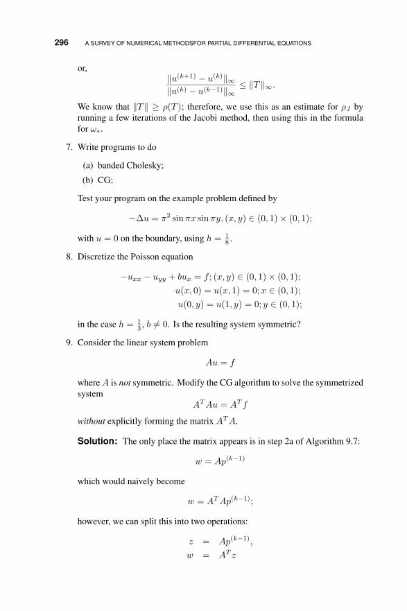
296 A SURVEY OF NUMERICAL METHODSFOR PARTIAL DIFFERENTIAL EQUATIONS
or,‖u(k+1) − u(k)‖∞‖u(k) − u(k−1)‖∞
≤ ‖T‖∞.
We know that ‖T‖ ≥ ρ(T ); therefore, we use this as an estimate for ρJ byrunning a few iterations of the Jacobi method, then using this in the formulafor ω∗.
7. Write programs to do
(a) banded Cholesky;
(b) CG;
Test your program on the example problem defined by
−∆u = π2 sinπx sinπy, (x, y) ∈ (0, 1)× (0, 1);
with u = 0 on the boundary, using h = 18 .
8. Discretize the Poisson equation
−uxx − uyy + bux = f ; (x, y) ∈ (0, 1)× (0, 1);
u(x, 0) = u(x, 1) = 0;x ∈ (0, 1);
u(0, y) = u(1, y) = 0; y ∈ (0, 1);
in the case h = 13 , b 6= 0. Is the resulting system symmetric?
9. Consider the linear system problem
Au = f
whereA is not symmetric. Modify the CG algorithm to solve the symmetrizedsystem
ATAu = AT f
without explicitly forming the matrix ATA.
Solution: The only place the matrix appears is in step 2a of Algorithm 9.7:
w = Ap(k−1)
which would naively become
w = ATAp(k−1);
however, we can split this into two operations:
z = Ap(k−1),
w = AT z

DIFFERENCE METHODS FOR POISSON EQUATIONS 297
so that we never have to compute ATA.
10. Write a code to implement the algorithm you wrote in the previous problem.Test it on the system obtained by discretizing the PDE
−uxx − uyy + ux = π cosπx cosπy + 2π2 sinπx sinπy; (x, y) ∈ (0, 1)× (0, 1);
u(x, 0) = u(x, 1) = 0;x ∈ (0, 1);
u(0, y) = u(1, y) = 0; y ∈ (0, 1);
for h = 14 and h = 1
8 . The exact solution is u(x, y) = sinπx sinπy; use thisto make sure your algorithm is working properly.
11. How does the discretization change when boundary data is non-homogeneous(i.e., non-zero)? Demonstrate by writing down the discrete system for the PDE
−uxx − uyy = −2ex−y; (x, y) ∈ (0, 1)× (0, 1);
u(x, 0) = ex; u(x, 1) = ex−1; x ∈ (0, 1);
u(0, y) = e−y; u(1, y) = e1−y; y ∈ (0, 1);
for h = 14 . Hint: It will help to write the values of the approximate solution
at the grid points in two vectors, one for the interior grid points where theapproximation is unknown; and one at the boundary grid points where thesolution is known.
12. Apply the following solution techniques to the system in the previous example,this time using h = 1
8 . Use the exact solution of u(x, y) = ex−y to verify thatthe code is working properly.
(a) Jacobi iteration;
(b) Gauss-Seidel iteration;
(c) SOR iteration, using ω = 1.4465;
(d) Conjugate gradient iteration.
/ • • • .


CHAPTER 10
AN INTRODUCTION TO SPECTRALMETHODS
10.1 SPECTRAL METHODS FOR TWO-POINT BOUNDARY VALUEPROBLEMS
Exercises:
1. Write a program to solve the boundary value problem (BVP)
−u′′ + 5u′ + u = 1, −1 ≤ x ≤ 1
u(−1) = 0
u(1) = 1
using the spectral method, with either “boundary bordering” or “basis recom-bination.” The exact solution is
u(x) = Aer1x +Ber2x + 1
for r1 = 5.19258, r2 = −0.19258, and
A = 0.003781 B = −0.824844
Solutions Manual to Accompany An Introduction to Numerical Methods and Analysis,Second Edition. By James F. EppersonCopyright c© 2013 John Wiley & Sons, Inc.
299

300 AN INTRODUCTION TO SPECTRAL METHODS
(confirm this); plot the solution and the error, and produce a table of maximumabsolute errors, for 4 ≤ N ≤ 32.
Solution: The author got the solution and error plots in the figures below forN = 8.
−1 −0.8 −0.6 −0.4 −0.2 0 0.2 0.4 0.6 0.8 10
0.1
0.2
0.3
0.4
0.5
0.6
0.7
0.8
0.9
1
Figure 10.1 Solution to Problem 1,N = 8.
−1 −0.8 −0.6 −0.4 −0.2 0 0.2 0.4 0.6 0.8 1−1.5
−1
−0.5
0
0.5
1
1.5
2
2.5x 10⁻³
Figure 10.2 Error for Problem 1,N = 8.
2. Solve the BVP in Example 10.2, for 4 ≤ N ≤ 32, but take advantage of thefact that the solution is even by looking for an approximation that uses onlythe even Chebyshev polynomials.
3. It has been suggested that a better way to do “basis recombination” would beas follows:
C2N (x) = C2N (x)− C2N−2(x)
C2N−1(x) = C2N−1(x)− C2N−3(x)
Repeat Problem 1 using this basis. In addition to the same plots as requestedin Problem 1, plot the condition number of the matrix A as a function of N forboth methods.
4. Extend the work in Theorem 10.1 to include third and fourth derivatives.
Solution: This is a simple exercise in the calculus. You should get
d3Tndx3
=−n3 sin2 t sinnt− 3n2 cos t sin t cosnt+ (3 cos2 t+ sin2 t)n sinnt
sin5 t,
and
d4Tndx4
=n4 sin3 t cosnt− 6n3 cos t sin2 t sinnt− n2A cosnt+ nB sinnt
sin7 t,
whereA = (15 cos2 t sin t+ 4 sin3 t),

SPECTRAL METHODS FOR TIME-DEPENDENT PROBLEMS 301
andB = (9 cos t sin2 t+ 15 cos3 t).
These formulas are taken from page 325 of Boyd’s book [2].
5. Use the formulas from the previous problem to approximate the solution to
u′′′′ = 1
u(−1) = u(1) = 0
u′(−1) = u′(1) = 0
Compute a spectral approximation for 4 ≤ N ≤ 32. Plot your solution forN = 16.
6. Compute the condition number of the matrices in the previous exercise, as afunction of N .
7. As an alternative to the trigonometric formulas from Theorem 10.1, we coulduse the three term recursion (10.2) as a basis for constructing the spectralcoefficient matrix. Show that
T ′n+1(x) = 2Tn(x) + 2xT ′n(x)− T ′n−1(x), T ′0(x) = 0, T ′1(x) = 1,
and similarly for the second derivative. Write a program to solve Problem 1 inthis way. Use MATLAB’s flops command to compare the costs of formingthe spectral coefficient matrix this way, compared to the procedure oulined inthe text.
/ • • • .
10.2 SPECTRAL METHODS FOR TIME-DEPENDENT PROBLEMS
Exercises:
1. Use spectral collocation with Crank-Nicolson time-stepping to solve the fol-lowing PDE:
ut = uxx,
u(−1, t) = 0,
u(1, t) = 0,
u(x, 0) = cosπx/2− sin 4πx.
The exact solution is u(x, t) = e−π2t/4 cosπx/2−e−16π2t sin 4πx. Compute
out to t = 1; use a sequence of values of N ; plot your approximation and theerror for one of them at t = 1.

302 AN INTRODUCTION TO SPECTRAL METHODS
2. Use your spectral code to solve the problem
ut = auxx,
u(−1, t) = 1,
u(1, t) = 1,
u(x, 0) = (x2 − 1)8.
Assume a = 1 and compute out to t = 1, using a sequence of values of N .Plot the solution profile as the computation advances. Now vary a (you mustkeep it positive, of course) and investigate how this affects the solution.
Solution: The initial condition approximates a “pulse” in the center of theinterval. As the system evolves, the pulse will spread out and decay. Highervalues of a (the diffusion coefficient) will speed up this process.
3. Now change the initial condition to u(x, 0) = (x4 − 1)8 and repeat the aboveproblem.
Solution: This is essentially the same as the previous problem, but with amore sharply defined “pulse.”
4. Consider how to implement spectral collocation with variable coefficients.Construct the general linear system that would result from solving the problem
ut = a(x)uxx,
u(−1, t) = 0,
u(1, t) = 0,
u(x, 0) = u0(x).
5. Apply your results from the above problem to approximate solutions to
ut = a(x)uxx,
u(−1, t) = 0,
u(1, t) = 0,
u(x, 0) = cosπx/2,
for the following choices of a:
(a) a(x) = (1 + x2);
(b) a(x) = e−x2
;
(c) a(x) = (1 − x2) (because a vanishes at the boundary, this problem isknown as degenerate but you should be able to compute solutions);

CLENSHAW-CURTIS QUADRATURE 303
6. Consider the nonlinear problem
ut = uxx + V uux
u(−1, t) = 0,
u(1, t) = 0,
u0(x) = sinπx
Use spectral collocation to attack this problem as suggested in Problem 12 of9.1, by treating the nonlinearity explicitly (at time t = tn) and the differential
equation implicitly (at time t = tn+1). Compare your spectral solution to theexplicit solution computed in Problem 10 of 9.1. Comment on your results.
/ • • • .
10.3 CLENSHAW-CURTIS QUADRATURE
Exercises:
1. Use the appropriate change of variable to show how to apply Clenshaw-Curtisquadrature to an integral over an arbitrary interval [a, b].
Solution: The change of variable is the same as obtained in 5.6 for Gaussianquadrature: ∫ b
a
g(x)dx =
∫ 1
−1f(z)dz,
for
f(z) =1
2(b− a)g
(a+
1
2(b− a)(z + 1)
).
2. Write a program to do Clenshaw-Curtis quadrature on each of the integralsin Problem 4 of 5.6. Compare your results to those obtained with Gaussianquadrature. Produce a log-log plot of the error as a function of N for eachintegral.
Solution: We will do (b) and (c). The results are summarized in the Ta-ble 10.1.
3. Looking at the plots in Fig. 10.24, we see that most of them show a very rapiddecrease of the error, and a “rounding error plateau” is reached for most ofthe examples. The exception is the last one, where the integrand is given byf(x) =
√1− x2. Explain why this example is the one that displays this kind
of sub-optimal performance.
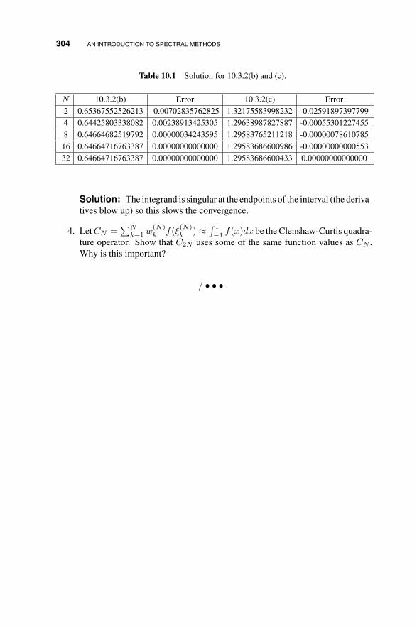
304 AN INTRODUCTION TO SPECTRAL METHODS
Table 10.1 Solution for 10.3.2(b) and (c).
N 10.3.2(b) Error 10.3.2(c) Error2 0.65367552526213 -0.00702835762825 1.32175583998232 -0.025918973977994 0.64425803338082 0.00238913425305 1.29638987827887 -0.000553012274558 0.64664682519792 0.00000034243595 1.29583765211218 -0.0000007861078516 0.64664716763387 0.00000000000000 1.29583686600986 -0.0000000000055332 0.64664716763387 0.00000000000000 1.29583686600433 0.00000000000000
Solution: The integrand is singular at the endpoints of the interval (the deriva-tives blow up) so this slows the convergence.
4. LetCN =∑Nk=1 w
(N)k f(ξ
(N)k ) ≈
∫ 1
−1 f(x)dx be the Clenshaw-Curtis quadra-ture operator. Show that C2N uses some of the same function values as CN .Why is this important?
/ • • • .