
Signal Processing with Scilab - TeoriadeiSegnali.it
205
Transcript of Signal Processing with Scilab - TeoriadeiSegnali.it

Signal
Processing
With
Scilab
Scilab Group
-1
100
101
102
103
10
-160
-150
-140
-130
-120
-110
-100
-90Magnitude
Hz
db
-1
100
101
102
103
10
-180
-90
0Phase
Hz
degrees
4.64 7.44 10.23 13.02 15.82 18.61 21.41 24.20 27.00 29.79 32.58
0.19
1.51
2.84
4.16
5.49
6.81
8.14
9.47
10.79
12.12
13.44
×
×
×
×
×
×
×
××
×
×
⊕
⊕
⊕
⊕
⊕
⊕
⊕⊕
⊕ ⊕⊕
-->a=-2*%pi;b=1;c=18*%pi;d=1;
-->sl=syslin('c',a,b,c,d);
-->bode(sl,.1,100);
-->s=poly(0,'s');
-->S1=s+2*%pi*(15+100*%i);
-->S2=s+2*%pi*(15-100*%i);
-->h1=1/real(S1*S2)
h1 =
1-------------------------
2403666.82 + 188.49556s + s
-->h1=syslin('c',h1);
-->bode(h1,10,1000,.01);
-->h2=ss2tf(sl);
-->bode(h1*h2,.1,1000,.01);

SIGNALPROCESSINGWITHSCILAB
Scilab GroupINRIA Meta2 Project/ENPC Cergrene
INRIA - Unit e de recherche de Rocquencourt - Projet Meta2Domaine de Voluceau - Rocquencourt - B.P. 105 - 78153 Le Chesnay Cedex (France)E-mail : [email protected]

Acknowledgement
This document is an updated version of a primary work by Carey Bunks, Franc¸ois Delebecque, GeorgesLe Vey and Serge Steer

Contents
1 Description of the Basic Tools 11.1 Introduction . . . . . . . . . . . . . . . . . . . . . . . . . . . . . . . . . . . . . . . . . . . 11.2 Signals. . . . . . . . . . . . . . . . . . . . . . . . . . . . . . . . . . . . . . . . . . . . . . 1
1.2.1 Saving, Loading, Reading, and Writing Files. . . . . . . . . . . . . . . . . . . . . 21.2.2 Simulation of Random Signals. . . . . . . . . . . . . . . . . . . . . . . . . . . . . 3
1.3 Polynomials and System Transfer Functions. . . . . . . . . . . . . . . . . . . . . . . . . . 41.3.1 Evaluation of Polynomials. . . . . . . . . . . . . . . . . . . . . . . . . . . . . . . 81.3.2 Representation of Transfer Functions. . . . . . . . . . . . . . . . . . . . . . . . . 9
1.4 State Space Representation. . . . . . . . . . . . . . . . . . . . . . . . . . . . . . . . . . . 91.5 Changing System Representation. . . . . . . . . . . . . . . . . . . . . . . . . . . . . . . . 91.6 Interconnecting systems. . . . . . . . . . . . . . . . . . . . . . . . . . . . . . . . . . . . . 111.7 Discretizing Continuous Systems. . . . . . . . . . . . . . . . . . . . . . . . . . . . . . . . 121.8 Filtering of Signals . . . . . . . . . . . . . . . . . . . . . . . . . . . . . . . . . . . . . . . 141.9 Plotting Signals. . . . . . . . . . . . . . . . . . . . . . . . . . . . . . . . . . . . . . . . . 151.10 Development of Signal Processing Tools. . . . . . . . . . . . . . . . . . . . . . . . . . . . 19
2 Representation of Signals 212.1 Frequency Response. . . . . . . . . . . . . . . . . . . . . . . . . . . . . . . . . . . . . . 21
2.1.1 Bode Plots . . . . . . . . . . . . . . . . . . . . . . . . . . . . . . . . . . . . . . . 212.1.2 Phase and Group Delay. . . . . . . . . . . . . . . . . . . . . . . . . . . . . . . . . 272.1.3 Appendix: Scilab Code Used to Generate Examples. . . . . . . . . . . . . . . . . 35
2.2 Sampling . . . . . . . . . . . . . . . . . . . . . . . . . . . . . . . . . . . . . . . . . . . . 372.3 Decimation and Interpolation. . . . . . . . . . . . . . . . . . . . . . . . . . . . . . . . . . 40
2.3.1 Introduction. . . . . . . . . . . . . . . . . . . . . . . . . . . . . . . . . . . . . . . 422.3.2 Interpolation . . . . . . . . . . . . . . . . . . . . . . . . . . . . . . . . . . . . . . 432.3.3 Decimation. . . . . . . . . . . . . . . . . . . . . . . . . . . . . . . . . . . . . . . 442.3.4 Interpolation and Decimation. . . . . . . . . . . . . . . . . . . . . . . . . . . . . 442.3.5 Examples usingintdec . . . . . . . . . . . . . . . . . . . . . . . . . . . . . . . . 46
2.4 The DFT and the FFT. . . . . . . . . . . . . . . . . . . . . . . . . . . . . . . . . . . . . . 462.4.1 Introduction. . . . . . . . . . . . . . . . . . . . . . . . . . . . . . . . . . . . . . . 462.4.2 Examples Using thefft Primitive . . . . . . . . . . . . . . . . . . . . . . . . . . 51
2.5 Convolution . . . . . . . . . . . . . . . . . . . . . . . . . . . . . . . . . . . . . . . . . . . 542.5.1 Introduction. . . . . . . . . . . . . . . . . . . . . . . . . . . . . . . . . . . . . . . 542.5.2 Use of theconvol function . . . . . . . . . . . . . . . . . . . . . . . . . . . . . . 55
2.6 The Chirp Z-Transform. . . . . . . . . . . . . . . . . . . . . . . . . . . . . . . . . . . . . 562.6.1 Introduction. . . . . . . . . . . . . . . . . . . . . . . . . . . . . . . . . . . . . . . 562.6.2 Calculating the CZT. . . . . . . . . . . . . . . . . . . . . . . . . . . . . . . . . . 582.6.3 Examples. . . . . . . . . . . . . . . . . . . . . . . . . . . . . . . . . . . . . . . . 59
iii

3 FIR Filters 633.1 Windowing Techniques. . . . . . . . . . . . . . . . . . . . . . . . . . . . . . . . . . . . . 63
3.1.1 Filter Types. . . . . . . . . . . . . . . . . . . . . . . . . . . . . . . . . . . . . . . 643.1.2 Choice of Windows. . . . . . . . . . . . . . . . . . . . . . . . . . . . . . . . . . . 66
3.1.3 How to usewfir . . . . . . . . . . . . . . . . . . . . . . . . . . . . . . . . . . . . 693.1.4 Examples. . . . . . . . . . . . . . . . . . . . . . . . . . . . . . . . . . . . . . . . 70
3.2 Frequency Sampling Technique. . . . . . . . . . . . . . . . . . . . . . . . . . . . . . . . . 72
3.3 Optimal filters. . . . . . . . . . . . . . . . . . . . . . . . . . . . . . . . . . . . . . . . . . 743.3.1 Minimax Approximation. . . . . . . . . . . . . . . . . . . . . . . . . . . . . . . . 75
3.3.2 The Remez Algorithm. . . . . . . . . . . . . . . . . . . . . . . . . . . . . . . . . 763.3.3 Functionremezb . . . . . . . . . . . . . . . . . . . . . . . . . . . . . . . . . . . 77
3.3.4 Examples Using the functionremezb . . . . . . . . . . . . . . . . . . . . . . . . . 783.3.5 Scilab functioneqfir . . . . . . . . . . . . . . . . . . . . . . . . . . . . . . . . . 81
4 IIR Filters 854.1 Analog filters . . . . . . . . . . . . . . . . . . . . . . . . . . . . . . . . . . . . . . . . . . 85
4.1.1 Butterworth Filters. . . . . . . . . . . . . . . . . . . . . . . . . . . . . . . . . . . 854.1.2 Chebyshev filters. . . . . . . . . . . . . . . . . . . . . . . . . . . . . . . . . . . . 88
4.1.3 Elliptic filters . . . . . . . . . . . . . . . . . . . . . . . . . . . . . . . . . . . . . . 94
4.2 Design of IIR Filters From Analog Filters. . . . . . . . . . . . . . . . . . . . . . . . . . . 1064.3 Approximation of Analog Filters. . . . . . . . . . . . . . . . . . . . . . . . . . . . . . . . 107
4.3.1 Approximation of the Derivative. . . . . . . . . . . . . . . . . . . . . . . . . . . . 1074.3.2 Approximation of the Integral. . . . . . . . . . . . . . . . . . . . . . . . . . . . . 108
4.4 Design of Low Pass Filters. . . . . . . . . . . . . . . . . . . . . . . . . . . . . . . . . . . 1094.5 Transforming Low Pass Filters. . . . . . . . . . . . . . . . . . . . . . . . . . . . . . . . . 112
4.6 How to Use the Functioniir . . . . . . . . . . . . . . . . . . . . . . . . . . . . . . . . . 1134.7 Examples . . . . . . . . . . . . . . . . . . . . . . . . . . . . . . . . . . . . . . . . . . . . 114
4.8 Another Implementation of Digital IIR Filters. . . . . . . . . . . . . . . . . . . . . . . . . 1154.8.1 Theeqiir function . . . . . . . . . . . . . . . . . . . . . . . . . . . . . . . . . . 115
4.8.2 Examples. . . . . . . . . . . . . . . . . . . . . . . . . . . . . . . . . . . . . . . . 116
5 Spectral Estimation 1215.1 Estimation of Power Spectra. . . . . . . . . . . . . . . . . . . . . . . . . . . . . . . . . . 121
5.2 The Modified Periodogram Method. . . . . . . . . . . . . . . . . . . . . . . . . . . . . . 1225.2.1 Example Using thepspect function . . . . . . . . . . . . . . . . . . . . . . . . . 123
5.3 The Correlation Method . . . . . . . . . . . . . . . . . . . . . . . . . . . . . . . . . . . . 1265.3.1 Example Using the functioncspect . . . . . . . . . . . . . . . . . . . . . . . . . 126
5.4 The Maximum Entropy Method. . . . . . . . . . . . . . . . . . . . . . . . . . . . . . . . 1275.4.1 Introduction. . . . . . . . . . . . . . . . . . . . . . . . . . . . . . . . . . . . . . . 127
5.4.2 The Maximum Entropy Spectral Estimate. . . . . . . . . . . . . . . . . . . . . . . 1285.4.3 The Levinson Algorithm. . . . . . . . . . . . . . . . . . . . . . . . . . . . . . . . 129
5.4.4 How to Usemese . . . . . . . . . . . . . . . . . . . . . . . . . . . . . . . . . . . 1295.4.5 How to Uselev . . . . . . . . . . . . . . . . . . . . . . . . . . . . . . . . . . . . 130
5.4.6 Examples. . . . . . . . . . . . . . . . . . . . . . . . . . . . . . . . . . . . . . . . 130

v
6 Optimal Filtering and Smoothing 1336.1 The Kalman Filter. . . . . . . . . . . . . . . . . . . . . . . . . . . . . . . . . . . . . . . . 133
6.1.1 Conditional Statistics of a Gaussian Random Vector. . . . . . . . . . . . . . . . . 1336.1.2 Linear Systems and Gaussian Random Vectors. . . . . . . . . . . . . . . . . . . . 1346.1.3 Recursive Estimation of Gaussian Random Vectors. . . . . . . . . . . . . . . . . . 1356.1.4 The Kalman Filter Equations. . . . . . . . . . . . . . . . . . . . . . . . . . . . . . 1366.1.5 Asymptotic Properties of the Kalman Filter. . . . . . . . . . . . . . . . . . . . . . 1386.1.6 How to Use the Macrosskf . . . . . . . . . . . . . . . . . . . . . . . . . . . . . . 1396.1.7 An Example Using thesskf Macro . . . . . . . . . . . . . . . . . . . . . . . . . . 1396.1.8 How to Use the Functionkalm . . . . . . . . . . . . . . . . . . . . . . . . . . . . 1406.1.9 Examples Using thekalm Function . . . . . . . . . . . . . . . . . . . . . . . . . . 140
6.2 The Square Root Kalman Filter. . . . . . . . . . . . . . . . . . . . . . . . . . . . . . . . . 1496.2.1 The Householder Transformation. . . . . . . . . . . . . . . . . . . . . . . . . . . 1516.2.2 How to Use the Macrosrkf . . . . . . . . . . . . . . . . . . . . . . . . . . . . . . 152
6.3 The Wiener Filter. . . . . . . . . . . . . . . . . . . . . . . . . . . . . . . . . . . . . . . . 1536.3.1 Problem Formulation. . . . . . . . . . . . . . . . . . . . . . . . . . . . . . . . . . 1536.3.2 How to Use the Functionwiener . . . . . . . . . . . . . . . . . . . . . . . . . . . 1566.3.3 Example . . . . . . . . . . . . . . . . . . . . . . . . . . . . . . . . . . . . . . . . 157
7 Optimization in filter design 1617.1 Optimized IIR filters . . . . . . . . . . . . . . . . . . . . . . . . . . . . . . . . . . . . . . 161
7.1.1 Minimum Lp design . . . . . . . . . . . . . . . . . . . . . . . . . . . . . . . . . . 1617.2 Optimized FIR filters. . . . . . . . . . . . . . . . . . . . . . . . . . . . . . . . . . . . . . 170
8 Stochastic realization 1758.1 Thesfact primitive . . . . . . . . . . . . . . . . . . . . . . . . . . . . . . . . . . . . . . 1768.2 Spectral Factorization via state-space models. . . . . . . . . . . . . . . . . . . . . . . . . 177
8.2.1 Spectral Study. . . . . . . . . . . . . . . . . . . . . . . . . . . . . . . . . . . . . 1778.2.2 The Filter Model . . . . . . . . . . . . . . . . . . . . . . . . . . . . . . . . . . . . 178
8.3 Computing the solution. . . . . . . . . . . . . . . . . . . . . . . . . . . . . . . . . . . . . 1798.3.1 Estimation of the matrices H F G. . . . . . . . . . . . . . . . . . . . . . . . . . . 1798.3.2 computation of the filter. . . . . . . . . . . . . . . . . . . . . . . . . . . . . . . . 180
8.4 Levinson filtering . . . . . . . . . . . . . . . . . . . . . . . . . . . . . . . . . . . . . . . . 1838.4.1 The Levinson algorithm. . . . . . . . . . . . . . . . . . . . . . . . . . . . . . . . 184
9 Time-Frequency representations of signals 1879.1 The Wigner distribution. . . . . . . . . . . . . . . . . . . . . . . . . . . . . . . . . . . . . 1879.2 Time-frequency spectral estimation. . . . . . . . . . . . . . . . . . . . . . . . . . . . . . . 188
Bibliography 191
Chapter 1
Description of the Basic Tools
1.1 Introduction
The purpose of this document is to illustrate the use of the Scilab software package in a signal processingcontext. We have gathered a collection of signal processing algorithms which have been implemented asScilab functions.
This manual is in part a pedagogical tool concerning the study of signal processing and in part a practicalguide to using the signal processing tools available in Scilab. For those who are already well versed in thestudy of signal processing the tutorial parts of the manual will be of less interest.
For each signal processing tool available in the signal processing toolbox there is a tutorial section inthe manual explaining the methodology behind the technique. This section is followed by a section whichdescribes the use of a function designed to accomplish the signal processing described in the preceding sec-tions. At this point the reader is encouraged to launch a Scilab session and to consult the on-line help relatedto the function in order to get the precise and complete description (syntax, description of its functionality,examples and related functions). This section is in turn followed by an examples section demonstrating theuse of the function. In general, the example section illustrates more clearly than the syntax section how touse the different modes of the function.
In this manual thetypewriter-face font is used to indicate either a function name or an exampledialogue which occurs in Scilab.
Each signal processing subject is illustrated by examples and figures which were demonstrated usingScilab. To further assist the user, there exists for each example and figure an executable file which recreatesthe example or figure. To execute an example or figure one uses the following Scilab command
-->exec(’file.name’)
which causes Scilab to execute all the Scilab commands contained in the file calledfile.name .To know what signal processing tools are available in Scilab one would type
-->disp(siglib)
which produces a list of all the signal processing functions available in the signal processing library.
1.2 Signals
For signal processing the first point to know is how to load and save signals or only small portions of lengthysignals that are to be used or are to be generated by Scilab. Finally, the generation of synthetic (random)signals is an important tool in the development in implementation of signal processing tools. This sectionaddresses all of these topics.
1

2 CHAPTER1. DESCRIPTION OF THE BASIC TOOLS
1.2.1 Saving, Loading, Reading, and Writing Files
Signals and variables which have been processed or created in the Scilab environment can be saved in fileswritten directly by Scilab. The syntax for thesave primitive is
-->save(file_name[,var_list])
wherefile name is the file to be written to andvar list is the list of variables to be written. Theinverse to the operationsave is accomplished by the primitiveload which has the syntax
-->load(file_name[,var_list])
where the argument list is identical that used insave .Although the commandssave andload are convenient, one has much more control over the transfer
of data between files and Scilab by using the commandsread andwrite . These two commands worksimilarly to the read and write commands found in Fortran. The syntax of these two commands is as follows.The syntax forwrite is
-->write(file,x[,form])
The second argument,x , is a matrix of values which are to be written to the file.The syntax forread is
-->x=read(file,m,n[,form])
The argumentsmandn are the row and column dimensions of the resulting data matrixx . and form isagain the format specification statement.
In order to illustrate the use of the on-line help for reading this manual we give the result of the Scilabcommand
-->help read
read(1) Scilab Function read(1)
NAMEread - matrices read
CALLING SEQUENCE[x]=read(file-name,m,n,[format])[x]=read(file-name,m,n,k,format)
PARAMETERS
file-name : string or integer (logical unit number)
m, n : integers (dimensions of the matrix x). Set m=-1 if you dontknow the numbers of rows, so the whole file is read.
format : string (fortran format). If format=’(a)’ then read reads a vec-tor of strings n must be equal to 1.
1.2. SIGNALS 3
k : integer
DESCRIPTIONreads row after row the mxn matrix x (n=1 for character chain) in the filefile-name (string or integer).
Two examples for format are : (1x,e10.3,5x,3(f3.0)),(10x,a20) ( the defaultvalue is *).
The type of the result will depend on the specified form. If form isnumeric (d,e,f,g) the matrix will be a scalar matrix and if form containsthe character a the matrix will be a matrix of character strings.
A direct access file can be used if using the parameter k which is is thevector of record numbers to be read (one record per row), thus m must bem=prod(size(k)).
To read on the keyboard use read(%io(1),...).
EXAMPLEA=rand(3,5); write(’foo’,A);B=read(’foo’,3,5)B=read(’foo’,-1,5)read(%io(1),1,1,’(a)’) // waits for user’s input
SEE ALSOfile, readb, write, %io, x_dialog
1.2.2 Simulation of Random Signals
The creation of synthetic signals can be accomplished using the Scilab functionrand which generatesrandom numbers. The user can generate a sequence of random numbers, a random matrix with the uniformor the gaussian probability laws. A seed is possible to re-create the same pseudo-random sequences.
Often it is of interest in signal processing to generate normally distributed random variables with acertain mean and covariance structure. This can be accomplished by using the standard normal randomnumbers generated byrand and subsequently modifying them by performing certain linear numeric oper-ations. For example, to obtain a random vectory which is distributed N(my,�y) from a random vectorxwhich is distributed standard normal (i.e. N(0,I)) one would perform the following operation
y = �1=2y x+my (1.1)
where�1=2y is the matrix square root of�y. A matrix square root can be obtained using thechol primitive
as follows
-->//create normally distributed N(m,L) random vector y
-->m=[-2;1;10];
4 CHAPTER1. DESCRIPTION OF THE BASIC TOOLS
-->L=[3 2 1;2 3 2;1 2 3];
-->L2=chol(L);
-->rand(’seed’);
-->rand(’normal’);
-->x=rand(3,1)x =
! - 0.7616491 !! 1.4739762 !! 0.8529775 !
-->y=L2’*x+my =
! - 3.3192149 !! 2.0234185 !! 12.161519 !
taking note that it is the transpose of the matrix obtained fromchol that is used for the square root ofthe desired covariance matrix. Sequences of random numbers following a specific normally distributedprobability law can also be obtained by filtering. That is, a white standard normal sequence of randomnumbers is passed through a linear filter to obtain a normal sequence with a specific spectrum. For a filterwhich has a discrete Fourier transformH(w) the resulting filtered sequence will have a spectrumS(w) =jH(w)j2. More on filtering is discussed in Section1.8.
1.3 Polynomials and System Transfer Functions
Polynomials, matrix polynomials and transfer matrices are also defined and Scilab permits the definitionand manipulation of these objects in a natural, symbolic fashion. Polynomials are easily created and manip-ulated. Thepoly primitive in Scilab can be used to specify the coefficients of a polynomial or the roots ofa polynomial.
A very useful companion to thepoly primitive is theroots primitive. The roots of a polynomialqare given by :
-->a=roots(q);
The following examples should clarify the use of thepoly androots primitives.
-->//illustrate the roots format of poly
--> q1=poly([1 2],’x’)q1 =

1.3. POLYNOMIALS AND SYSTEM TRANSFER FUNCTIONS 5
22 - 3x + x
--> roots(q1)ans =
! 1. !! 2. !
-->//illustrate the coefficients format of poly
--> q2=poly([1 2],’x’,’c’)q2 =
1 + 2x
--> roots(q2)ans =
- 0.5
-->//illustrate the characteristic polynomial feature
--> a=[1 2;3 4]a =
! 1. 2. !! 3. 4. !
--> q3=poly(a,’x’)q3 =
2- 2 - 5x + x
--> roots(q3)ans =
! - 0.3722813 !! 5.3722813 !
Notice that the first polynomialq1 uses the’roots’ default and, consequently, the polynomial takesthe form (s � 1)(s � 2) = 2 � 3s + s2. The second polynomialq2 is defined by its coefficients givenby the elements of the vector. Finally, the third polynomialq3 calculates the characteristic polynomial ofthe matrixa which is by definition det(sI � a). Here the calculation of theroots primitive yields theeigenvalues of the matrixa.
Scilab can manipulate polynomials in the same manner as other mathematical objects such as scalars,
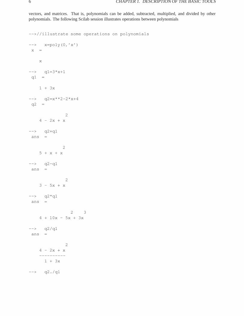
6 CHAPTER1. DESCRIPTION OF THE BASIC TOOLS
vectors, and matrices. That is, polynomials can be added, subtracted, multiplied, and divided by otherpolynomials. The following Scilab session illustrates operations between polynomials
-->//illustrate some operations on polynomials
--> x=poly(0,’x’)x =
x
--> q1=3*x+1q1 =
1 + 3x
--> q2=x**2-2*x+4q2 =
24 - 2x + x
--> q2+q1ans =
25 + x + x
--> q2-q1ans =
23 - 5x + x
--> q2*q1ans =
2 34 + 10x - 5x + 3x
--> q2/q1ans =
24 - 2x + x----------
1 + 3x
--> q2./q1
1.3. POLYNOMIALS AND SYSTEM TRANSFER FUNCTIONS 7
ans =
24 - 2x + x----------
1 + 3x
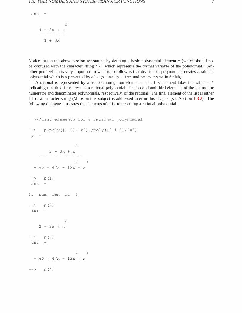
Notice that in the above session we started by defining a basic polynomial elementx (which should notbe confused with the character string’x’ which represents the formal variable of the polynomial). An-other point which is very important in what is to follow is that division of polynomials creates a rationalpolynomial which is represented by a list (seehelp list andhelp type in Scilab).
A rational is represented by a list containing four elements. The first element takes the value’r’indicating that this list represents a rational polynomial. The second and third elements of the list are thenumerator and denominator polynomials, respectively, of the rational. The final element of the list is either[] or a character string (More on this subject is addressed later in this chapter (see Section1.3.2). Thefollowing dialogue illustrates the elements of a list representing a rational polynomial.
-->//list elements for a rational polynomial
--> p=poly([1 2],’x’)./poly([3 4 5],’x’)p =
22 - 3x + x
------------------2 3
- 60 + 47x - 12x + x
--> p(1)ans =
!r num den dt !
--> p(2)ans =
22 - 3x + x
--> p(3)ans =
2 3- 60 + 47x - 12x + x
--> p(4)

8 CHAPTER1. DESCRIPTION OF THE BASIC TOOLS
ans =
[]
1.3.1 Evaluation of Polynomials
A very important operation on polynomials is their evaluation at specific points. For example, perhaps it isdesired to know the value the polynomialx2+3x�5 takes at the pointx = 17:2. Evaluation of polynomialsis accomplished using the primitivefreq . The syntax offreq is as follows
-->pv=freq(num,den,v)
The argumentv is a vector of values at which the evaluation is needed.For signal processing purposes, the evaluation of frequency response of filters and system transfer func-
tions is a common use offreq . For example, a discrete filter can be evaluated on the unit circle in thez-plane as follows
-->//demonstrate evaluation of discrete filter
-->//on the unit circle in the z-plane
--> h=[1:5,4:-1:1];
--> hz=poly(h,’z’,’c’);
--> f=(0:.1:1);
--> hf=freq(hz,1,exp(%pi*%i*f));
--> hf’ans =
! 25. !! 6.3137515 - 19.431729i !! - 8.472136 - 6.1553671i !! - 1.9626105 + 1.42592i !! 1.110D-16 - 4.441D-16i !! 1. - 7.499D-33i !! 0.4721360 - 1.4530851i !! - 0.5095254 - 0.3701919i !! - 5.551D-17i !! 0.1583844 + 0.4874572i !! 1. + 4.899D-16i !
Here,h is an FIR filter of length 9 with a triangular impulse response. The transfer function of the filteris obtained by forming a polynomial which represents thez-transform of the filter. This is followed by
1.4. STATE SPACE REPRESENTATION 9
evaluating the polynomial at the pointsexp(2�in) for n = 0; 1; : : : ; 10 which amounts to evaluating thez-transform on the unit circle at ten equally spaced points in the range of angles[0; �].
1.3.2 Representation of Transfer Functions
Signal processing makes use of rational polynomials to describe signal and system transfer functions. Thesetransfer functions can represent continuous time signals or systems or discrete time signals or systems.Furthermore, discrete signals or systems can be related to continuous signals or systems by sampling.
The function which processes a rational polynomial so that it can be represented as a transfer functionis calledsyslin :
-->sl=syslin(domain,num,den)
Another use for the functionsyslin for state-space descriptions of linear systems is described in thefollowing section.
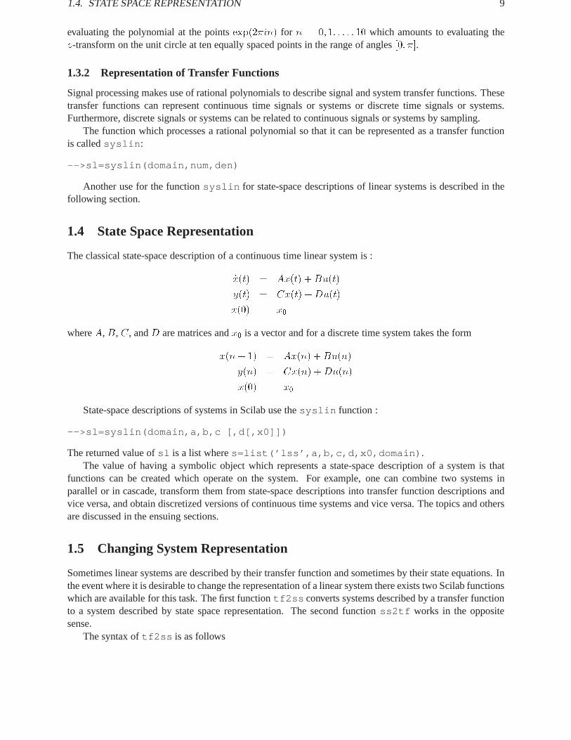
1.4 State Space Representation
The classical state-space description of a continuous time linear system is :
_x(t) = Ax(t) +Bu(t)
y(t) = Cx(t) +Du(t)
x(0) = x0
whereA,B, C, andD are matrices andx0 is a vector and for a discrete time system takes the form
x(n+ 1) = Ax(n) +Bu(n)
y(n) = Cx(n) +Du(n)
x(0) = x0
State-space descriptions of systems in Scilab use thesyslin function :
-->sl=syslin(domain,a,b,c [,d[,x0]])
The returned value ofsl is a list wheres=list(’lss’,a,b,c,d,x0,domain) .The value of having a symbolic object which represents a state-space description of a system is that
functions can be created which operate on the system. For example, one can combine two systems inparallel or in cascade, transform them from state-space descriptions into transfer function descriptions andvice versa, and obtain discretized versions of continuous time systems and vice versa. The topics and othersare discussed in the ensuing sections.
1.5 Changing System Representation
Sometimes linear systems are described by their transfer function and sometimes by their state equations. Inthe event where it is desirable to change the representation of a linear system there exists two Scilab functionswhich are available for this task. The first functiontf2ss converts systems described by a transfer functionto a system described by state space representation. The second functionss2tf works in the oppositesense.
The syntax oftf2ss is as follows

10 CHAPTER1. DESCRIPTION OF THE BASIC TOOLS
-->sl=tf2ss(h)
An important detail is that the transfer functionh must be of minimum phase. That is, the denominatorpolynomial must be of equal or higher order than that of the numerator polynomial.
-->h=ss2tf(sl)
The following example illustrates the use of these two functions.
-->//Illustrate use of ss2tf and tf2ss
-->h1=iir(3,’lp’,’butt’,[.3 0],[0 0])h1 =
2 30.2569156 + 0.7707468z + 0.7707468z + 0.2569156z------------------------------------------------
2 30.0562972 + 0.4217870z + 0.5772405z + z
-->h1=syslin(’d’,h1);
-->s1=tf2ss(h1)s1 =
s1(1) (state-space system:)
!lss A B C D X0 dt !
s1(2) = A matrix =
! 0.0223076 0.5013809 0. !! - 0.3345665 - 0.3797154 - 0.4502218 !! 0.1124639 0.4085596 - 0.2198328 !
s1(3) = B matrix =
! - 2.3149238 !! - 2.1451754 !! 0.2047095 !
s1(4) = C matrix =
! - 0.2688835 0. - 8.327D-17 !
s1(5) = D matrix =
0.2569156
1.6. INTERCONNECTING SYSTEMS 11
s1*s2a - s1 - s2 - a
s1+s2a q
-
-
s2
s1?
6
i+ - a
[s1,s2]
a
a -
-
s2
s1?
6
i+ - a
[s1;s2]a q
-
-
s2
s1
-
-
a
a
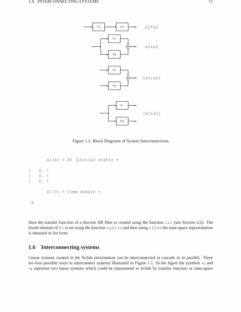
Figure 1.1: Block Diagrams of System Interconnections
s1(6) = X0 (initial state) =
! 0. !! 0. !! 0. !
s1(7) = Time domain =
d
Here the transfer function of a discrete IIR filter is created using the functioniir (see Section4.2). Thefourth element ofh1 is set using the functionsyslin and then usingtf2ss the state-space representationis obtained in list form.
1.6 Interconnecting systems
Linear systems created in the Scilab environment can be interconnected in cascade or in parallel. Thereare four possible ways to interconnect systems illustrated in Figure1.1. In the figure the symbolss1 ands2 represent two linear systems which could be represented in Scilab by transfer function or state-space

12 CHAPTER1. DESCRIPTION OF THE BASIC TOOLS
representations. For each of the four block diagrams in Figure1.1 the Scilab command which makes theillustrated interconnection is shown to the left of the diagram in typewriter-face font format.
1.7 Discretizing Continuous Systems
A continuous-time linear system represented in Scilab by its state-space or transfer function description canbe converted into a discrete-time state-space or transfer function representation by using the functiondscr .
Consider for example an input-output mapping which is given in state space form as:
(C)
�_x(t) = Ax(t) +Bu(t)y(t) = Cx(t) +Du(t)
(1.2)
From the variation of constants formula the value of the statex(t) can be calculated at any timet as
x(t) = eAtx(0) +
Z t
0eA(t��)Bu(�)d� (1.3)
Let h be a time step and consider an inputu which is constant in intervals of lengthh. Then associatedwith (1.2) is the following discrete time model obtained by using the variation of constants formula in (1.3),
(D)
�x(n+ 1) = Ahx(n) +Bhu(n)y(n) = Chx(n) +Dhu(n)
(1.4)
whereAh = exp(Ah)
Bh =
Z h
0eA(h��)Bd�
Ch = C
Dh = D
Since the computation of a matrix exponent can be calculated using the Scilab primitiveexp , it isstraightforward to implement these formulas, although the numerical calculations needed to computeexp(Ah)are rather involved ([30]).
If we take
G =
8>:A B0 0
9>;where the dimensions of the zero matrices are chosen so thatG is square then we obtain
exp(Gh) =
8>:Ah Bh
0 I
9>;WhenA is nonsingular we also have that
Bh = A�1(Ah � I)B:
This is exactly what the functiondscr does to discretize a continuous-time linear system in state-spaceform.
The functiondscr can operate on system matrices, linear system descriptions in state-space form, andlinear system descriptions in transfer function form. The syntax using system matrices is as follows
-->[f,g[,r]]=dscr(syslin(’c’,a,b,[],[]),dt [,m])
1.7. DISCRETIZING CONTINUOUS SYSTEMS 13
wherea andb are the two matrices associated to the continuous-time state-space description
_x(t) = Ax(t) +Bu(t) (1.5)
andf andg are the resulting matrices for a discrete time system
x(n+ 1) = Fx(n) +Gu(n) (1.6)
where the sampling period isdt . In the case where the fourth argumentm is given, the continuous timesystem is assumed to have a stochastic input so that now the continuous-time equation is
_x(t) = Ax(t) +Bu(t) + w(t) (1.7)
wherew(t) is a white, zero-mean, Gaussian random process of covariancemand now the resulting discrete-time equation is
x(n+ 1) = Fx(n) +Gu(n) + q(n) (1.8)
whereq(n) is a white, zero-mean, Gaussian random sequence of covariancer .Thedscr function syntax when the argument is a linear system in state-space form is
-->[sld[,r]]=dscr(sl,dt[,m])
wheresl andsld are lists representing continuous and discrete linear systems representations, respectively.Heremandr are the same as for the first function syntax. In the case where the function argument is a linearsystem in transfer function form the syntax takes the form
-->[hd]=dscr(h,dt)
where nowh andhd are transfer function descriptions of the continuous and discrete systems, respectively.The transfer function syntax does not allow the representation of a stochastic system.
As an example of the use ofdscr consider the following Scilab session.
-->//Demonstrate the dscr function
--> a=[2 1;0 2]a =
! 2. 1. !! 0. 2. !
--> b=[1;1]b =
! 1. !! 1. !
--> [sld]=dscr(syslin(’c’,a,b,eye(2,2)),.1);
--> sld(2)ans =

14 CHAPTER1. DESCRIPTION OF THE BASIC TOOLS
! 1.2214028 0.1221403 !! 0. 1.2214028 !
--> sld(3)ans =
! 0.1164208 !! 0.1107014 !
1.8 Filtering of Signals
Filtering of signals by linear systems (or computing the time response of a system) is done by the functionflts which has two formats . The first format calculates the filter output by recursion and the secondformat calculates the filter output by transform. The function syntaxes are as follows. The syntax offltsis
-->[y[,x]]=flts(u,sl[,x0])
for the case of a linear system represented by its state-space description (see Section1.4) and
-->y=flts(u,h[,past])
for a linear system represented by its transfer function.In general the second format is much faster than the first format. However, the first format also yields
the evolution of the state. An example of the use offlts using the second format is illustrated below.
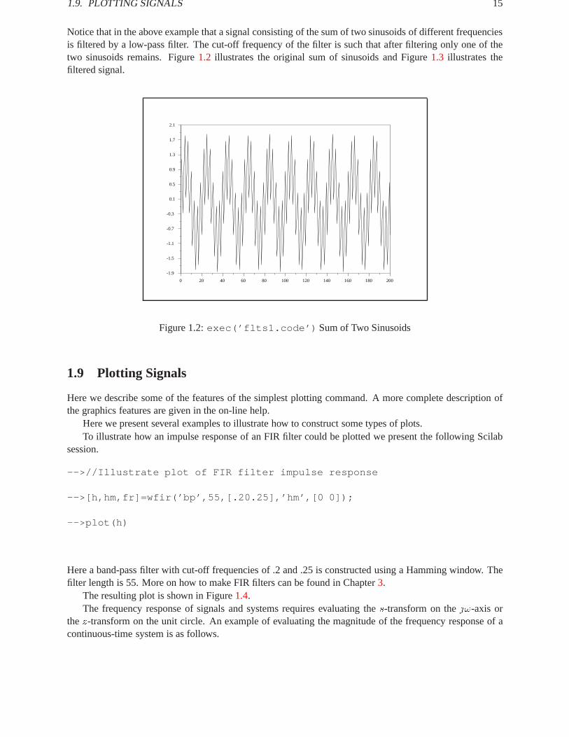
-->//filtering of signals
-->//make signal and filter
-->[h,hm,fr]=wfir(’lp’,33,[.2 0],’hm’,[0 0]);
-->t=1:200;
-->x1=sin(2*%pi*t/20);
-->x2=sin(2*%pi*t/3);
-->x=x1+x2;
-->z=poly(0,’z’);
-->hz=syslin(’d’,poly(h,’z’,’c’)./z**33);
-->yhz=flts(x,hz);
-->plot(yhz);
1.9. PLOTTING SIGNALS 15
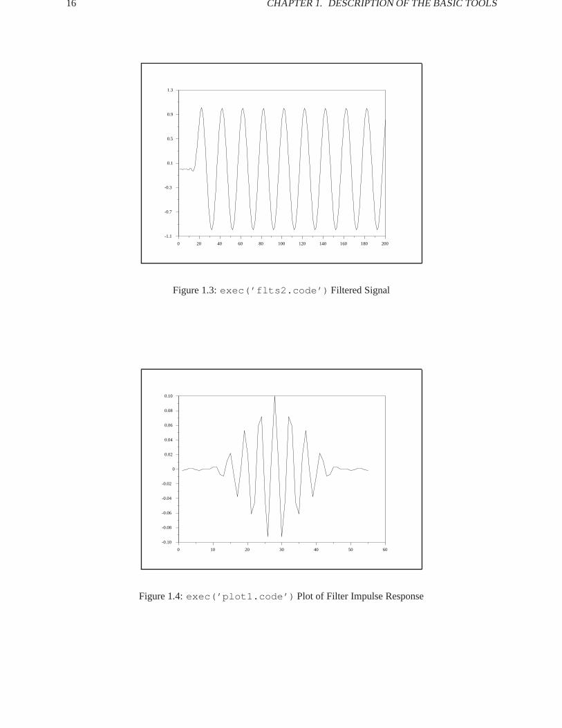
Notice that in the above example that a signal consisting of the sum of two sinusoids of different frequenciesis filtered by a low-pass filter. The cut-off frequency of the filter is such that after filtering only one of thetwo sinusoids remains. Figure1.2 illustrates the original sum of sinusoids and Figure1.3 illustrates thefiltered signal.
0 20 40 60 80 100 120 140 160 180 200
-1.9
-1.5
-1.1
-0.7
-0.3
0.1
0.5
0.9
1.3
1.7
2.1
Figure 1.2:exec(’flts1.code’) Sum of Two Sinusoids
1.9 Plotting Signals
Here we describe some of the features of the simplest plotting command. A more complete description ofthe graphics features are given in the on-line help.
Here we present several examples to illustrate how to construct some types of plots.To illustrate how an impulse response of an FIR filter could be plotted we present the following Scilab
session.
-->//Illustrate plot of FIR filter impulse response
-->[h,hm,fr]=wfir(’bp’,55,[.20.25],’hm’,[0 0]);
-->plot(h)
Here a band-pass filter with cut-off frequencies of .2 and .25 is constructed using a Hamming window. Thefilter length is 55. More on how to make FIR filters can be found in Chapter3.
The resulting plot is shown in Figure1.4.The frequency response of signals and systems requires evaluating thes-transform on thej!-axis or
thez-transform on the unit circle. An example of evaluating the magnitude of the frequency response of acontinuous-time system is as follows.
16 CHAPTER1. DESCRIPTION OF THE BASIC TOOLS
0 20 40 60 80 100 120 140 160 180 200
-1.1
-0.7
-0.3
0.1
0.5
0.9
1.3
Figure 1.3:exec(’flts2.code’) Filtered Signal
0 10 20 30 40 50 60
-0.10
-0.08
-0.06
-0.04
-0.02
0
0.02
0.04
0.06
0.08
0.10
Figure 1.4:exec(’plot1.code’) Plot of Filter Impulse Response

1.9. PLOTTING SIGNALS 17
-->//Evaluate magnitude response of continuous-time system
-->hs=analpf(4,’cheb1’,[.1 0],5)hs =
161.30794---------------------------------------------------
2 3 4179.23104 + 96.905252s + 37.094238s + 4.9181782s + s
-->fr=0:.1:15;
-->hf=freq(hs(2),hs(3),%i*fr);
-->hm=abs(hf);
-->plot(fr,hm),
Here we make an analog low-pass filter using the functionsanalpf (see Chapter4 for more details). Thefilter is a type I Chebyshev of order 4 where the cut-off frequency is 5 Hertz. The primitivefreq (seeSection1.3.1) evaluates the transfer functionhs at the values offr on thej!-axis. The result is shown inFigure1.5
0 2 4 6 8 10 12 14 16
0
0.1
0.2
0.3
0.4
0.5
0.6
0.7
0.8
0.9
1.0
Figure 1.5:exec(’plot2.code’) Plot of Continuous Filter Magnitude Response
A similar type of procedure can be effected to plot the magnitude response of discrete filters where theevaluation of the transfer function is done on the unit circle in thez-plane by using the functionfrmag .
-->[xm,fr]=frmag(num[,den],npts)
18 CHAPTER1. DESCRIPTION OF THE BASIC TOOLS
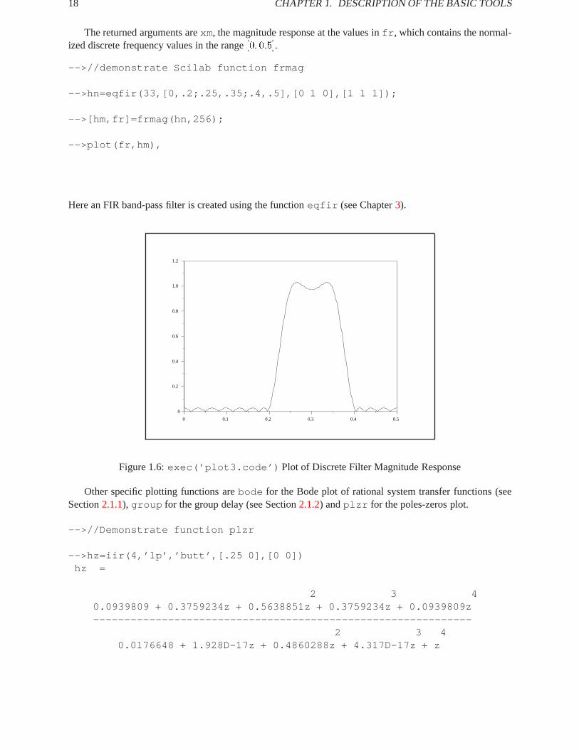
The returned arguments arexm, the magnitude response at the values infr , which contains the normal-ized discrete frequency values in the range[0; 0:5].
-->//demonstrate Scilab function frmag
-->hn=eqfir(33,[0,.2;.25,.35;.4,.5],[0 1 0],[1 1 1]);
-->[hm,fr]=frmag(hn,256);
-->plot(fr,hm),
Here an FIR band-pass filter is created using the functioneqfir (see Chapter3).
0 0.1 0.2 0.3 0.4 0.5
0
0.2
0.4
0.6
0.8
1.0
1.2
Figure 1.6:exec(’plot3.code’) Plot of Discrete Filter Magnitude Response
Other specific plotting functions arebode for the Bode plot of rational system transfer functions (seeSection2.1.1), group for the group delay (see Section2.1.2) andplzr for the poles-zeros plot.
-->//Demonstrate function plzr
-->hz=iir(4,’lp’,’butt’,[.25 0],[0 0])hz =
2 3 40.0939809 + 0.3759234z + 0.5638851z + 0.3759234z + 0.0939809z-------------------------------------------------------------
2 3 40.0176648 + 1.928D-17z + 0.4860288z + 4.317D-17z + z

1.10. DEVELOPMENTOF SIGNAL PROCESSING TOOLS 19
-->plzr(hz)
Here a fourth order, low-pass, IIR filter is created using the functioniir (see Section4.2). The resultingpole-zero plot is illustrated in Figure1.7
-1.562 -1.250 -0.938 -0.626 -0.314 -0.002 0.310 0.622 0.934 1.246 1.558
-1.104
-0.884
-0.664
-0.443
-0.223
-0.002
0.218
0.439
0.659
0.880
1.100
ΟΟΟΟ
ZerosΟ-1.562 -1.250 -0.938 -0.626 -0.314 -0.002 0.310 0.622 0.934 1.246 1.558
-1.104
-0.884
-0.664
-0.443
-0.223
-0.002
0.218
0.439
0.659
0.880
1.100
×
×
×
×
Poles×
imag. axis
real axis
transmission zeros and poles
Figure 1.7:exec(’plot4.code’) Plot of Poles and Zeros of IIR Filter
1.10 Development of Signal Processing Tools
Of course any user can write its own functions like those illustrated in the previous sections. The simplestway is to write a file with a special format . This file is executed with two Scilab primitivesgetf andexec .The complete description of such functionalities is given in the reference manual and the on-line help. Thesefunctionalities correspond to the buttonFile Operations .

20 CHAPTER1. DESCRIPTION OF THE BASIC TOOLS
Chapter 2
Time and Frequency Representation ofSignals
2.1 Frequency Response
2.1.1 Bode Plots
The Bode plot is used to plot the phase and log-magnitude response of functions of a single complex variable.The log-scale characteristics of the Bode plot permitted a rapid, “back-of-the-envelope” calculation of asystem’s magnitude and phase response. In the following discussion of Bode plots we consider only real,causal systems. Consequently, any poles and zeros of the system occur in complex conjugate pairs (or arestrictly real) and the poles are all located in the left-halfs-plane.
ForH(s) a transfer function of the complex variables, the log-magnitude ofH(s) is defined by
M(!) = 20 log10 jH(s)s=j!j (2.1)
and the phase ofH(s) is defined by
�(!) = tan�1[Im(H(s)s=j!)
Re(H(s)s=j!)] (2.2)
The magnitude,M(!), is plotted on a log-linear scale where the independent axis is marked in decades(sometimes in octaves) of degrees or radians and the dependent axis is marked in decibels. The phase,�(!), is also plotted on a log-linear scale where, again, the independent axis is marked as is the magnitudeplot and the dependent axis is marked in degrees (and sometimes radians).
WhenH(s) is a rational polynomial it can be expressed as
H(s) = C
QNn=1(s� an)QMm=1(s� bm)
(2.3)
where thean andbm are real or complex constants representing the zeros and poles, respectively, ofH(s),andC is a real scale factor. For the moment let us assume that thean andbm are strictly real. Evaluating(2.3) on thej!-axis we obtain
H(j!) = C
QNn=1(j! � an)QMm=1(j! � bm)
= C
QNn=1
p!2 + a2ne
j tan�1 !=(�an)QMm=1
p!2 + b2me
j tan�1 !=(�bm)(2.4)
21

22 CHAPTER2. REPRESENTATION OF SIGNALS
and for the log-magnitude and phase response
M(!) = 20(log10 C + (NXn=1
log10p!2 + a2n �
MXm=1
log10p!2 + b2m (2.5)
and
�(!) =
NXn=1
tan�1(!=(�an))�MXm=1
tan�1(!=(�bm)): (2.6)
To see how the Bode plot is constructed assume that both (2.5) and (2.6) consist of single terms corres-ponding to a pole ofH(s). Consequently, the magnitude and phase become
M(!) = �20 logp!2 + a2 (2.7)
and�(!) = �j tan�1(!=(�a)): (2.8)
We plot the magnitude in (2.7) using two straight line approximations. That is, forj!j � jaj we have thatM(!) � �20 log jaj which is a constant (i.e., a straight line with zero slope). Forj!j � jaj we have thatM(!) � �20 log j!j which is a straight line on a log scale which has a slope of -20 db/decade. The inter-section of these two straight lines is atw = a. Figure2.1 illustrates these two straight line approximationsfor a = 10.
0
101
102
10
-40
-25
-10
Log scale
Figure 2.1:exec(’bode1.code’) Log-Magnitude Plot ofH(s) = 1=(s � a)
When! = a we have thatM(!) = �20 logp2a = �20 log a � 20 logp2. Since20 log
p2 = 3:0
we have that at! = a the correction to the straight line approximation is�3db. Figure2.1 illustratesthe true magnitude response ofH(s) = (s � a)�1 for a = 10 and it can be seen that the straight lineapproximations with the 3db correction at! = a yields very satisfactory results. The phase in (2.8) can alsobe approximated. For! � a we have�(!) � 0 and for! � a we have�(!) � �90Æ. At ! = a we have�(!) = �45Æ. Figure2.2 illustrates the straight line approximation to�(!) as well as the actual phaseresponse.
2.1. FREQUENCY RESPONSE 23
0
101
102
103
10
-90
-45
0
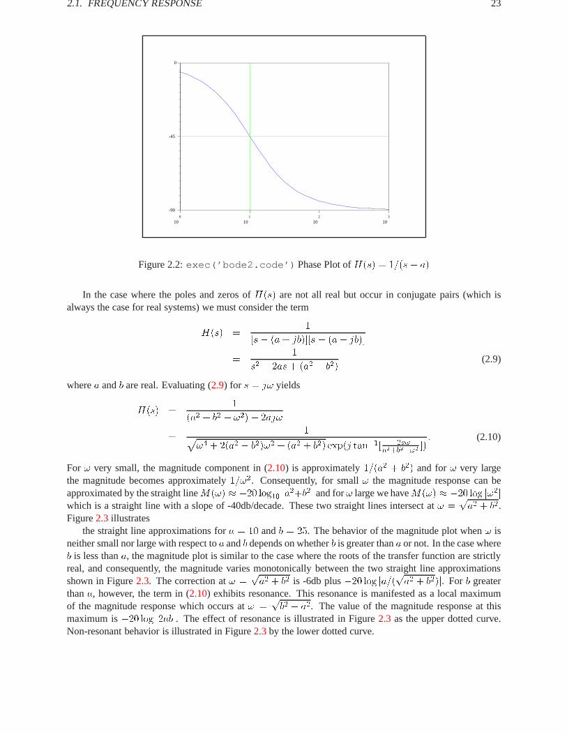
Figure 2.2:exec(’bode2.code’) Phase Plot ofH(s) = 1=(s� a)
In the case where the poles and zeros ofH(s) are not all real but occur in conjugate pairs (which isalways the case for real systems) we must consider the term
H(s) =1
[s� (a+ jb)][s � (a� jb)]
=1
s2 � 2as+ (a2 + b2)(2.9)
wherea andb are real. Evaluating (2.9) for s = j! yields
H(s) =1
(a2 + b2 � !2)� 2aj!
=1p
!4 + 2(a2 � b2)!2 + (a2 + b2) exp(j tan�1[ �2a!a2+b2�!2 ])
: (2.10)
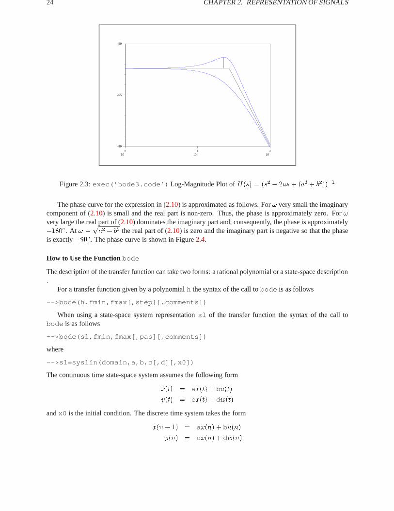
For ! very small, the magnitude component in (2.10) is approximately1=(a2 + b2) and for! very largethe magnitude becomes approximately1=!2. Consequently, for small! the magnitude response can beapproximated by the straight lineM(!) � �20 log10 ja2+b2j and for! large we haveM(!) � �20 log j!2jwhich is a straight line with a slope of -40db/decade. These two straight lines intersect at! =
pa2 + b2.
Figure2.3 illustratesthe straight line approximations fora = 10 andb = 25. The behavior of the magnitude plot when! is
neither small nor large with respect toa andb depends on whetherb is greater thana or not. In the case whereb is less thana, the magnitude plot is similar to the case where the roots of the transfer function are strictlyreal, and consequently, the magnitude varies monotonically between the two straight line approximationsshown in Figure2.3. The correction at! =
pa2 + b2 is -6db plus�20 log ja=(pa2 + b2)j. For b greater
thana, however, the term in (2.10) exhibits resonance. This resonance is manifested as a local maximumof the magnitude response which occurs at! =
pb2 � a2. The value of the magnitude response at this
maximum is�20 log j2abj. The effect of resonance is illustrated in Figure2.3 as the upper dotted curve.Non-resonant behavior is illustrated in Figure2.3by the lower dotted curve.
24 CHAPTER2. REPRESENTATION OF SIGNALS
0
101
102
10
-80
-65
-50
Figure 2.3:exec(’bode3.code’) Log-Magnitude Plot ofH(s) = (s2 � 2as+ (a2 + b2))�1
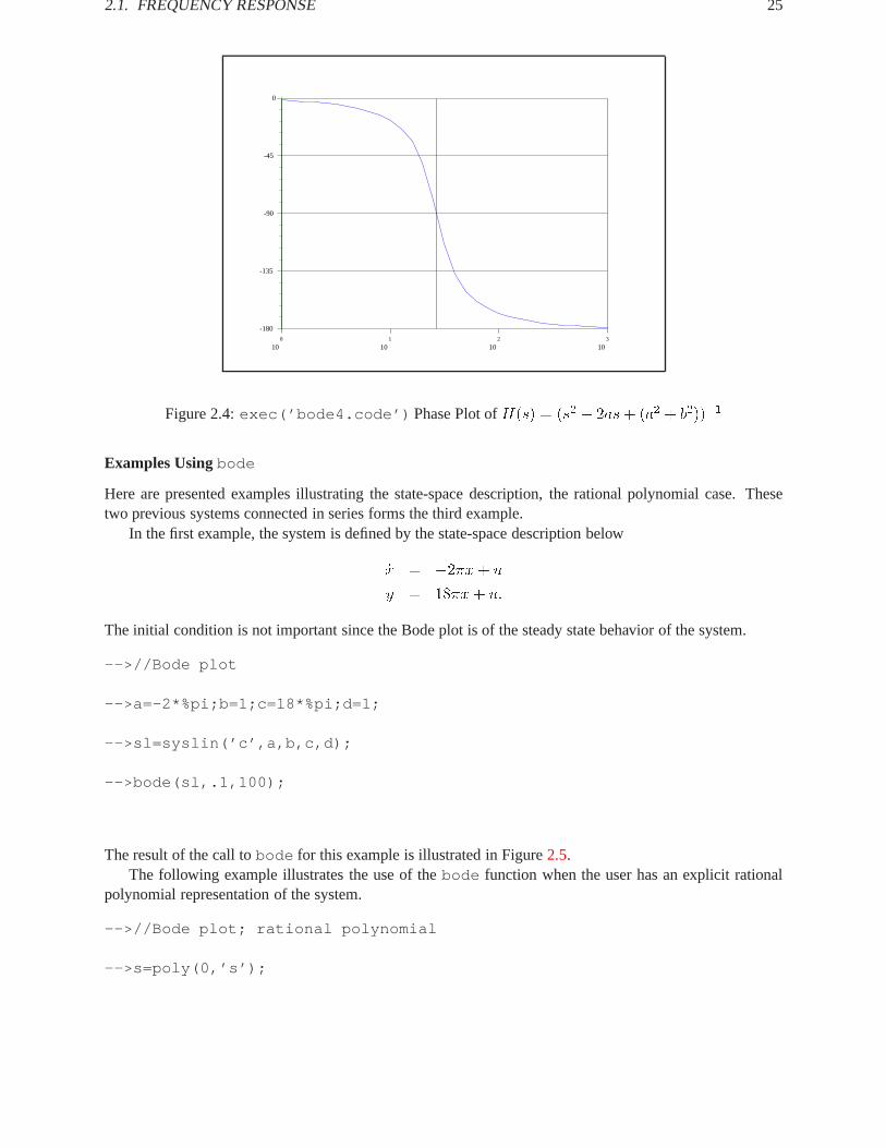
The phase curve for the expression in (2.10) is approximated as follows. For! very small the imaginarycomponent of (2.10) is small and the real part is non-zero. Thus, the phase is approximately zero. For!very large the real part of (2.10) dominates the imaginary part and, consequently, the phase is approximately�180Æ. At ! =
pa2 + b2 the real part of (2.10) is zero and the imaginary part is negative so that the phase
is exactly�90Æ. The phase curve is shown in Figure2.4.
How to Use the Functionbode
The description of the transfer function can take two forms: a rational polynomial or a state-space description.
For a transfer function given by a polynomialh the syntax of the call tobode is as follows
-->bode(h,fmin,fmax[,step][,comments])
When using a state-space system representationsl of the transfer function the syntax of the call tobode is as follows
-->bode(sl,fmin,fmax[,pas][,comments])
where
-->sl=syslin(domain,a,b,c[,d][,x0])
The continuous time state-space system assumes the following form
_x(t) = ax(t) + bu(t)
y(t) = cx(t) + dw(t)
andx0 is the initial condition. The discrete time system takes the form
x(n+ 1) = ax(n) + bu(n)
y(n) = cx(n) + dw(n)
2.1. FREQUENCY RESPONSE 25
0
101
102
103
10
-180
-135
-90
-45
0
Figure 2.4:exec(’bode4.code’) Phase Plot ofH(s) = (s2 � 2as+ (a2 + b2))�1
Examples Usingbode
Here are presented examples illustrating the state-space description, the rational polynomial case. Thesetwo previous systems connected in series forms the third example.
In the first example, the system is defined by the state-space description below
_x = �2�x+ u
y = 18�x+ u:
The initial condition is not important since the Bode plot is of the steady state behavior of the system.
-->//Bode plot
-->a=-2*%pi;b=1;c=18*%pi;d=1;
-->sl=syslin(’c’,a,b,c,d);
-->bode(sl,.1,100);
The result of the call tobode for this example is illustrated in Figure2.5.The following example illustrates the use of thebode function when the user has an explicit rational
polynomial representation of the system.
-->//Bode plot; rational polynomial
-->s=poly(0,’s’);

26 CHAPTER2. REPRESENTATION OF SIGNALS
-1
100
101
102
10
0
2
4
6
8
10
12
14
16
18
20
.
db
Hz
Magnitude
-1
100
101
102
10
-60
-50
-40
-30
-20
-10
0
.
degrees
Hz
Phase
Figure 2.5:exec(’bode5.code’) Bode Plot of State-Space System Representation
-->h1=1/real((s+2*%pi*(15+100*%i))*(s+2*%pi*(15-100*%i)))h1 =
1-------------------------
2403666.82 + 188.49556s + s
-->h1=syslin(’c’,h1);
-->bode(h1,10,1000,.01);
The result of the call tobode for this example is illustrated in Figure2.6.The final example combines the systems used in the two previous examples by attaching them together
in series. The state-space description is converted to a rational polynomial description using thess2tffunction.
-->//Bode plot; two systems in series
-->a=-2*%pi;b=1;c=18*%pi;d=1;
-->sl=syslin(’c’,a,b,c,d);
-->s=poly(0,’s’);
-->h1=1/real((s+2*%pi*(15+100*%i))*(s+2*%pi*(15-100*%i)));
2.1. FREQUENCY RESPONSE 27
1
102
103
10
-160
-150
-140
-130
-120
-110
-100
.
db
Hz
Magnitude
1
102
103
10
-180
-160
-140
-120
-100
-80
-60
-40
-20
0
.
degrees
Hz
Phase
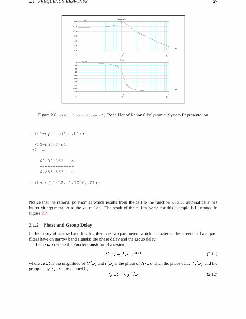
Figure 2.6:exec(’bode6.code’) Bode Plot of Rational Polynomial System Representation
-->h1=syslin(’c’,h1);
-->h2=ss2tf(sl)h2 =
62.831853 + s-------------6.2831853 + s
-->bode(h1*h2,.1,1000,.01);
Notice that the rational polynomial which results from the call to the functionss2tf automatically hasits fourth argument set to the value’c’ . The result of the call tobode for this example is illustrated inFigure2.7.
2.1.2 Phase and Group Delay
In the theory of narrow band filtering there are two parameters which characterize the effect that band passfilters have on narrow band signals: the phase delay and the group delay.
LetH(!) denote the Fourier transform of a system
H(!) = A(!)ej�(!) (2.11)
whereA(!) is the magnitude ofH(!) and�(!) is the phase ofH(!). Then the phase delay,tp(!), and thegroup delay,tg(!), are defined by
tp(!) = �(!)=! (2.12)
28 CHAPTER2. REPRESENTATION OF SIGNALS
-1
100
101
102
103
10
-160
-150
-140
-130
-120
-110
-100
-90
.
db
Hz
Magnitude
-1
100
101
102
103
10
-180
-160
-140
-120
-100
-80
-60
-40
-20
0
.
degrees
Hz
Phase
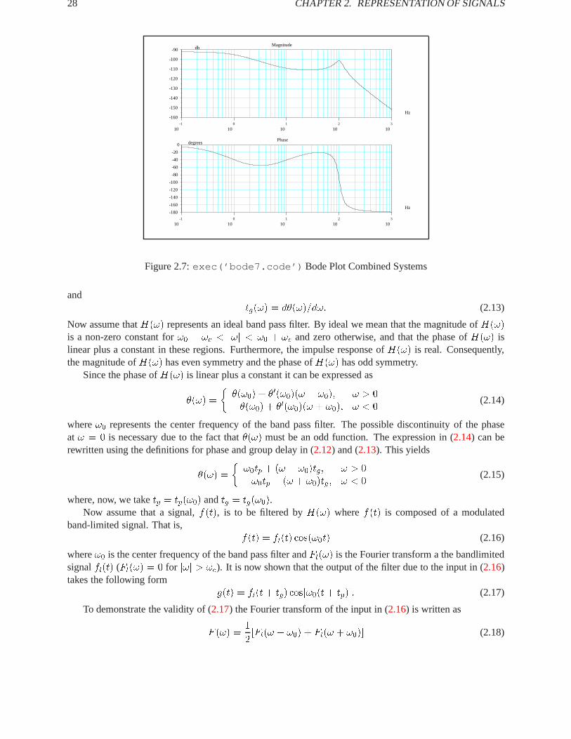
Figure 2.7:exec(’bode7.code’) Bode Plot Combined Systems
andtg(!) = d�(!)=d!: (2.13)
Now assume thatH(!) represents an ideal band pass filter. By ideal we mean that the magnitude ofH(!)is a non-zero constant for!0 � !c < j!j < !0 + !c and zero otherwise, and that the phase ofH(!) islinear plus a constant in these regions. Furthermore, the impulse response ofH(!) is real. Consequently,the magnitude ofH(!) has even symmetry and the phase ofH(!) has odd symmetry.
Since the phase ofH(!) is linear plus a constant it can be expressed as
�(!) =
��(!0) + �0(!0)(! � !0); ! > 0��(!0) + �0(!0)(! + !0); ! < 0
(2.14)
where!0 represents the center frequency of the band pass filter. The possible discontinuity of the phaseat ! = 0 is necessary due to the fact that�(!) must be an odd function. The expression in (2.14) can berewritten using the definitions for phase and group delay in (2.12) and (2.13). This yields
�(!) =
�!0tp + (! � !0)tg; ! > 0�!0tp + (! + !0)tg; ! < 0
(2.15)
where, now, we taketp = tp(!0) andtg = tg(!0).Now assume that a signal,f(t), is to be filtered byH(!) wheref(t) is composed of a modulated
band-limited signal. That is,f(t) = fl(t) cos(!0t) (2.16)
where!0 is the center frequency of the band pass filter andFl(!) is the Fourier transform a the bandlimitedsignalfl(t) (Fl(!) = 0 for j!j > !c). It is now shown that the output of the filter due to the input in (2.16)takes the following form
g(t) = fl(t+ tg) cos[!0(t+ tp)]: (2.17)
To demonstrate the validity of (2.17) the Fourier transform of the input in (2.16) is written as
F (!) =1
2[Fl(! � !0) + Fl(! + !0)] (2.18)

2.1. FREQUENCY RESPONSE 29
where (2.18) represents the convolution ofFl(!) with the Fourier transform ofcos(!0t). The Fouriertransform of the filter,H(!), can be written
H(!) =
8<:
e!0tp+(!�!0)tg ; !0 � !c < ! < !0 + !ce�!0tp+(!+!0)tg ; �!0 � !c < ! < �!0 + !c0; otherwise
(2.19)
Thus, sinceG(!) = F (!)H(!),
G(!) =
�12Fl(! � !0)e
!0tp+(!�!0)tg ; !0 � !c < ! < !0 + !c12Fl(! + !0)e
�!0tp+(!+!0)tg ; �!0 � !c < ! < �!0 + !c(2.20)
Calculatingg(t) using the inverse Fourier transform
g(t) =1
2�
Z 1
�1F (!)H(!)
=1
2
1
2�[
Z !0+!c
!0�!cFl(! � !0)e
j[(!�!0)tg+!0tp]ej!td!
+
Z �!0+!c
�!0�!cFl(! + !0)e
j[(!+!0)tg�!0tp]ej!td!] (2.21)
Making the change in variablesu = ! � !0 andv = ! + !0yields
g(t) =1
2
1
2�[
Z !c
�!cFl(u)e
j[utg+!0tp]ejutej!0tdu
+
Z !c
�!cFl(v)e
j[vtg�!0tp]ejvte�j!0tdv] (2.22)
Combining the integrals and performing some algebra gives
g(t) =1
2
1
2�
Z !c
�!cFl(!)e
j!tgej!t[ej!0tpej!0t + e�j!0tpe�j!0t]d!
=1
2�
Z !c
�!cFl(!) cos[!0(t+ tp)]e
j!(t+tg)d!
= cos[!0(t+ tp)]1
2�
Z !c
�!cFl(!)e
j!(t+tg )d!
= cos[!0(t+ tp)]fl(t+ tg) (2.23)
which is the desired result.The significance of the result in (2.23) is clear. The shape of the signal envelope due tofl(t) is unchanged
and shifted in time bytg. The carrier, however, is shifted in time bytp (which in general is not equal totg). Consequently, the overall appearance of the ouput signal is changed with respect to that of the inputdue to the difference in phase shift between the carrier and the envelope. This phenomenon is illustrated inFigures2.8-2.12. Figure2.8 illustrates
a narrowband signal which consists of a sinusoid modulated by an envelope. The envelope is an decayingexponential and is displayed in the figure as the dotted curve.
Figure2.9shows the band pass filter used to filter the signal in Figure2.8. The filter magnitude is plottedas the solid curve and the filter phase is plotted as the dotted curve.
Notice that since the phase is a constant function thattg = 0. The value of the phase delay istp =�=2. As is expected, the filtered output of the filter consists of the same signal as the input except that the

30 CHAPTER2. REPRESENTATION OF SIGNALS
0 10 20 30 40 50 60
-1.0
-0.8
-0.6
-0.4
-0.2
0
0.2
0.4
0.6
0.8
1.0
Figure 2.8:exec(’group1 5.code’) Modulated Exponential Signal
0 10 20 30 40 50 60
-4
-3
-2
-1
0
1
2
3
4
Figure 2.9:exec(’group1 5.code’) Constant Phase Band Pass Filter
2.1. FREQUENCY RESPONSE 31
0 10 20 30 40 50 60
-1.0
-0.8
-0.6
-0.4
-0.2
0
0.2
0.4
0.6
0.8
1.0
Figure 2.10:exec(’group1 5.code’) Carrier Phase Shift bytp = �=2
0 10 20 30 40 50 60
-15
-11
-7
-3
1
5
9
13
17
Figure 2.11:exec(’group1 5.code’) Linear Phase Band Pass Filter

32 CHAPTER2. REPRESENTATION OF SIGNALS
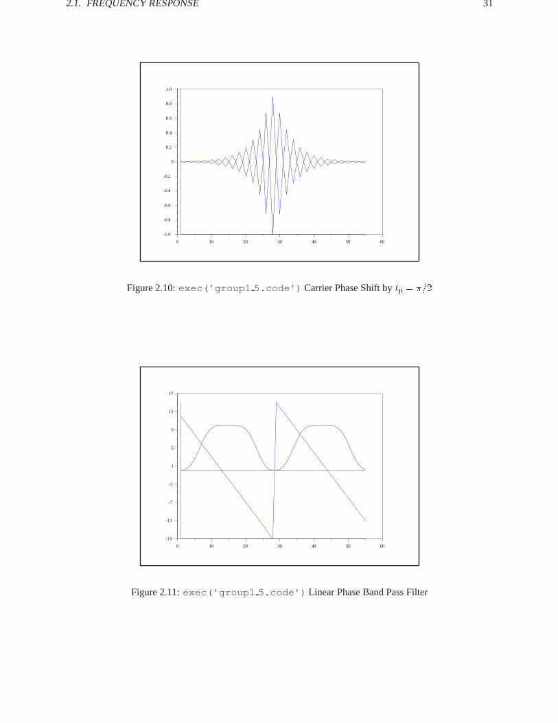
sinusoidal carrier is now phase shifted by�=2. This output signal is displayed in Figure2.10as the solidcurve. For reference the input signal is plotted as the dotted curve.
To illustrate the effect of the group delay on the filtering process a new filter is constructed as is displayedin Figure2.11.
Here the phase is again displayed as the dotted curve. The group delay is the slope of the phase curve asit passes through zero in the pass band region of the filter. Heretg = �1 andtp = 0. The result of filteringwith this phase curve is display in Figure2.12. As expected, the envelope is shifted but the sinusoid is notshifted within the reference frame of the window. The original input signal is again plotted as the dottedcurve for reference.
0 10 20 30 40 50 60
-1.0
-0.8
-0.6
-0.4
-0.2
0
0.2
0.4
0.6
0.8
1.0
Figure 2.12:exec(’group1 5.code’) Envelope Phase Shift bytg = �1
The Function group
As can be seen from the explanation given in this section, it is preferable that the group delay of a filterbe constant. A non-constant group delay tends to cause signal deformation. This is due to the fact that thedifferent frequencies which compose the signal are time shifted by different amounts according to the valueof the group delay at that frequency. Consequently, it is valuable to examine the group delay of filters duringthe design procedure. The functiongroup accepts filter parameters in several formats as input and returnsthe group delay as output. The syntax of the function is as follows:
-->[tg,fr]=group(npts,h)
The group delaytg is evaluated in the interval [0,.5) at equally spaced samples contained infr . Thenumber of samples is governed bynpts . Three formats can be used for the specification of the filter. Thefilter h can be specified by a vector of real numbers, by a rational polynomial representing the z-transformof the filter, or by a matrix polynomial representing a cascade decomposition of the filter. The three casesare illustrated below.
The first example is for a linear-phase filter designed using the functionwfir

2.1. FREQUENCY RESPONSE 33
-->[h w]=wfir(’lp’,7,[.2,0],’hm’,[0.01,-1]);
-->h’ans =
! - 0.0049893 !! 0.0290002 !! 0.2331026 !! 0.4 !! 0.2331026 !! 0.0290002 !! - 0.0049893 !
-->[tg,fr]=group(100,h);
-->plot2d(fr’,tg’,-1,’011’,’ ’,[0,2,0.5,4.])
as can be seen in Figure2.13
0.00 0.05 0.10 0.15 0.20 0.25 0.30 0.35 0.40 0.45 0.50
2.0
2.2
2.4
2.6
2.8
3.0
3.2
3.4
3.6
3.8
4.0
Figure 2.13:exec(’group6 8.code’) Group Delay of Linear-Phase Filter
the group delay is a constant, as is to be expected for a linear phase filter. The second example specifiesa rational polynomial for the filter transfer function:
-->z=poly(0,’z’);
-->h=z/(z-0.5)
34 CHAPTER2. REPRESENTATION OF SIGNALS
h =
z-------
- 0.5 + z
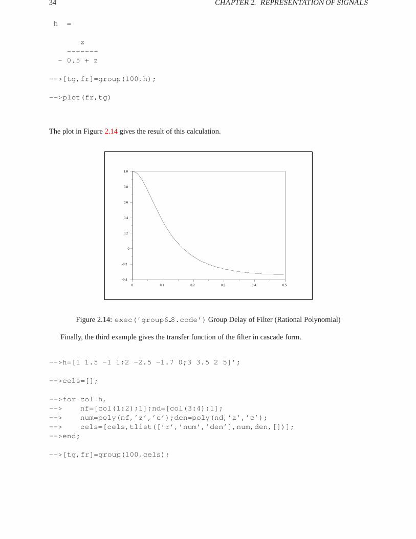
-->[tg,fr]=group(100,h);
-->plot(fr,tg)
The plot in Figure2.14gives the result of this calculation.
0 0.1 0.2 0.3 0.4 0.5
-0.4
-0.2
0
0.2
0.4
0.6
0.8
1.0
Figure 2.14:exec(’group6 8.code’) Group Delay of Filter (Rational Polynomial)
Finally, the third example gives the transfer function of the filter in cascade form.
-->h=[1 1.5 -1 1;2 -2.5 -1.7 0;3 3.5 2 5]’;
-->cels=[];
-->for col=h,--> nf=[col(1:2);1];nd=[col(3:4);1];--> num=poly(nf,’z’,’c’);den=poly(nd,’z’,’c’);--> cels=[cels,tlist([’r’,’num’,’den’],num,den,[])];-->end;
-->[tg,fr]=group(100,cels);

2.1. FREQUENCY RESPONSE 35
-->//plot(fr,tg)
The result is shown in Figure2.15. The cascade realization is known for numerical stability.
0 0.1 0.2 0.3 0.4 0.5
-2
-1
0
1
2
3
4
Figure 2.15:exec(’group6 8.code’) Group Delay of Filter (Cascade Realization)
2.1.3 Appendix: Scilab Code Used to Generate Examples
The following listing of Scilab code was used to generate the examples of the this section.
//exec(’group1_5.code’)//create carrier and narrow band signal
xinit(’group1.ps’);wc=1/4;x=sin(2*%pi*(0:54)*wc);y=exp(-abs(-27:27)/5);f=x.*y;plot([1 1 55],[1 -1 -1]),nn=prod(size(f))plot2d((1:nn)’,f’,[2],"000"),nn=prod(size(y))plot2d((1:nn)’,y’,[3],"000"),plot2d((1:nn)’,-y’,[3],"000"),xend(),xinit(’group2.ps’);
//make band pass filter
[h w]=wfir(’bp’,55,[maxi([wc-.15,0]),mini([wc+.15,.5])],’kr’,60.);

36 CHAPTER2. REPRESENTATION OF SIGNALS
//create new phase function with only phase delay
hf=fft(h,-1);hm=abs(hf);hp=%pi*ones(1:28);//tg is zerohp(29:55)=-hp(28:-1:2);hr=hm.*cos(hp);hi=hm.*sin(hp);hn=hr+%i*hi;plot([1 1 55],[4 -4 -4]),plot2d([1 55]’,[0 0]’,[1],"000"),nn=prod(size(hp))plot2d((1:nn)’,hp’,[2],"000"),nn=prod(size(hm))plot2d((1:nn)’,2.5*hm’,[1],"000"),xend(),xinit(’group3.ps’);
//filter signal with band pass filter
ff=fft(f,-1);gf=hn.*ff;g=fft(gf,1);plot([1 1 55],[1 -1 -1]),nn=prod(size(g))plot2d((1:nn)’,real(g)’,[2],"000"),nn=prod(size(f))plot2d((1:nn)’,f’,[1],"000"),
xend(),
//create new phase function with only group delayxinit(’group4.ps’);tg=-1;hp=tg*(0:27)-tg*12.*ones(1:28)/abs(tg);//tp is zerohp(29:55)=-hp(28:-1:2);hr=hm.*cos(hp);hi=hm.*sin(hp);hn=hr+%i*hi;plot([1 1 55],[15 -15 -15]),plot2d([1 55]’,[0 0]’,[1],"000"),nn=prod(size(hp))plot2d((1:nn)’,hp’,[2],"000"),nn=prod(size(hm))plot2d((1:nn)’,10*hm’,[1],"000"),
xend(),xinit(’group5.ps’);

2.2. SAMPLING 37
//filter signal with band pass filter
ff=fft(f,-1);gf=hn.*ff;g=fft(gf,1);plot([1 1 55],[1 -1 -1]),nn=prod(size(g))plot2d((1:nn)’,real(g)’,[2],"000"),nn=prod(size(f))plot2d((1:nn)’,f’,[1],"000"),xend(),
2.2 Sampling
The remainder of this section explains in detail the relationship between continuous and discrete signals.To begin, it is useful to examine the Fourier transform pairs for continuous and discrete time signals.
Forx(t) andX() a continuous time signal and its Fourier transform, respectively, we have that
X() =
Z 1
�1x(t)e�jtdt (2.24)
x(t) =1
2�
Z 1
�1X()ejtd: (2.25)
Forx(n) andX(!) a discrete time signal and its Fourier transform, respectively, we have that
X(!) =1X
n=�1x(n)e�j!n (2.26)
x(n) =1
2�
Z �
��X(!)ej!nd!: (2.27)
The discrete time signal,x(n), is obtained by sampling the continuous time signal,x(t), at regular intervalsof lengthT called the sampling period. That is,
x(n) = x(t)jt=nT (2.28)
We now derive the relationship between the Fourier transforms of the continuous and discrete time signals.The discussion follows [21].
Using (2.28) in (2.25) we have that
x(n) =1
2�
Z 1
�1X()ejnT d: (2.29)
Rewriting the integral in (2.29) as a sum of integrals over intervals of length2�=T we have that
x(n) =1
2�
1Xr=�1
Z (2�r+�)=T
(2�r��)=TX()ejnTd (2.30)
38 CHAPTER2. REPRESENTATION OF SIGNALS
or, by a change of variables
x(n) =1
2�
1Xr=�1
Z �=T
��=TX( +
2�r
T)ejnT ej2�nrd: (2.31)
Interchanging the sum and the integral in (2.31) and noting thatej2�nr = 1 due to the fact thatn andr arealways integers yields
x(n) =1
2�
Z �=T
��=T[
1Xr=�1
X( +2�r
T)]ejnTd: (2.32)
Finally, the change of variables! = T gives
x(n) =1
2�
Z �
��[1
T
1Xr=�1
X(!
T+
2�r
T)]ej!nd! (2.33)
which is identical in form to (2.27). Consequently, the following relationship exists between the Fouriertransforms of the continuous and discrete time signals:
X(!) =1
T
1Xr=�1
X(!
T+
2�r
T)
=1
T
1Xr=�1
X( +2�r
T): (2.34)
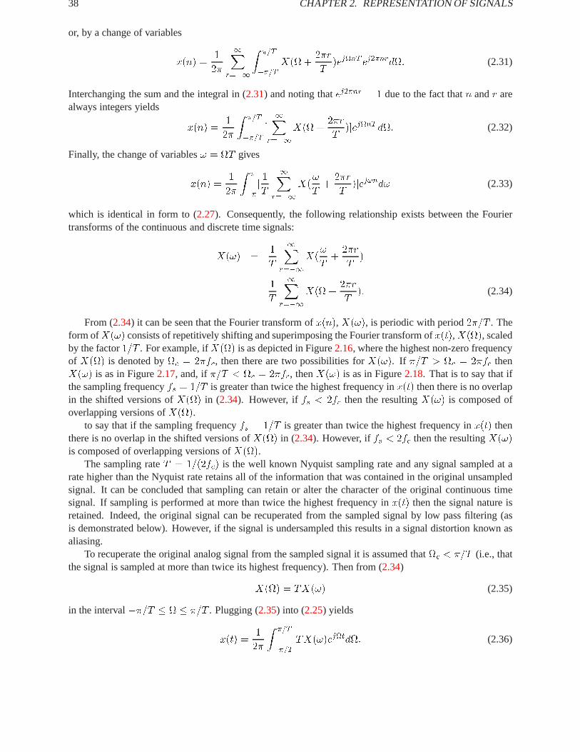
From (2.34) it can be seen that the Fourier transform ofx(n),X(!), is periodic with period2�=T . Theform ofX(!) consists of repetitively shifting and superimposing the Fourier transform ofx(t),X(), scaledby the factor1=T . For example, ifX() is as depicted in Figure2.16, where the highest non-zero frequencyof X() is denoted byc = 2�fc, then there are two possibilities forX(!). If �=T > c = 2�fc thenX(!) is as in Figure2.17, and, if�=T < c = 2�fc, thenX(!) is as in Figure2.18. That is to say that ifthe sampling frequencyfs = 1=T is greater than twice the highest frequency inx(t) then there is no overlapin the shifted versions ofX() in (2.34). However, iffs < 2fc then the resultingX(!) is composed ofoverlapping versions ofX().
to say that if the sampling frequencyfs = 1=T is greater than twice the highest frequency inx(t) thenthere is no overlap in the shifted versions ofX() in (2.34). However, iffs < 2fc then the resultingX(!)is composed of overlapping versions ofX().
The sampling rateT = 1=(2fc) is the well known Nyquist sampling rate and any signal sampled at arate higher than the Nyquist rate retains all of the information that was contained in the original unsampledsignal. It can be concluded that sampling can retain or alter the character of the original continuous timesignal. If sampling is performed at more than twice the highest frequency inx(t) then the signal nature isretained. Indeed, the original signal can be recuperated from the sampled signal by low pass filtering (asis demonstrated below). However, if the signal is undersampled this results in a signal distortion known asaliasing.
To recuperate the original analog signal from the sampled signal it is assumed thatc < �=T (i.e., thatthe signal is sampled at more than twice its highest frequency). Then from (2.34)
X() = TX(!) (2.35)
in the interval��=T � � �=T . Plugging (2.35) into (2.25) yields
x(t) =1
2�
Z �=T
��=TTX(!)ejtd: (2.36)

2.2. SAMPLING 39
-5 -4 -3 -2 -1 0 1 2 3 4 5
-2.0
-1.3
-0.6
0.1
0.8
1.5
2.2
2.9
3.6
4.3
5.0
Wc -Wc
X(W)
W
X(0)
Figure 2.16:exec(’sample1.code’) Frequency ResponseX()
-5 -4 -3 -2 -1 0 1 2 3 4 5
-2.0
-1.3
-0.6
0.1
0.8
1.5
2.2
2.9
3.6
4.3
5.0
pi/T
X(W)
W
X(0)/T
Figure 2.17:exec(’sample2.code’) Frequency Responsex(!) With No Aliasing
40 CHAPTER2. REPRESENTATION OF SIGNALS
-5 -4 -3 -2 -1 0 1 2 3 4 5
-2.0
-1.3
-0.6
0.1
0.8
1.5
2.2
2.9
3.6
4.3
5.0
pi/T
X(W)
W
X(0)/T
Figure 2.18:exec(’sample3.code’) Frequency Responsex(!) With Aliasing
ReplacingX(!) by (2.26) and using (2.28) we have that
x(t) =T
2�
Z �=T
��=T[
1X�1
x(nT )e�jnT ]ejtd: (2.37)
Interchanging the sum and the integral gives
x(t) =
1X�1
x(nT )[T
2�
Z �=T
��=Tej(t�nT )d]: (2.38)
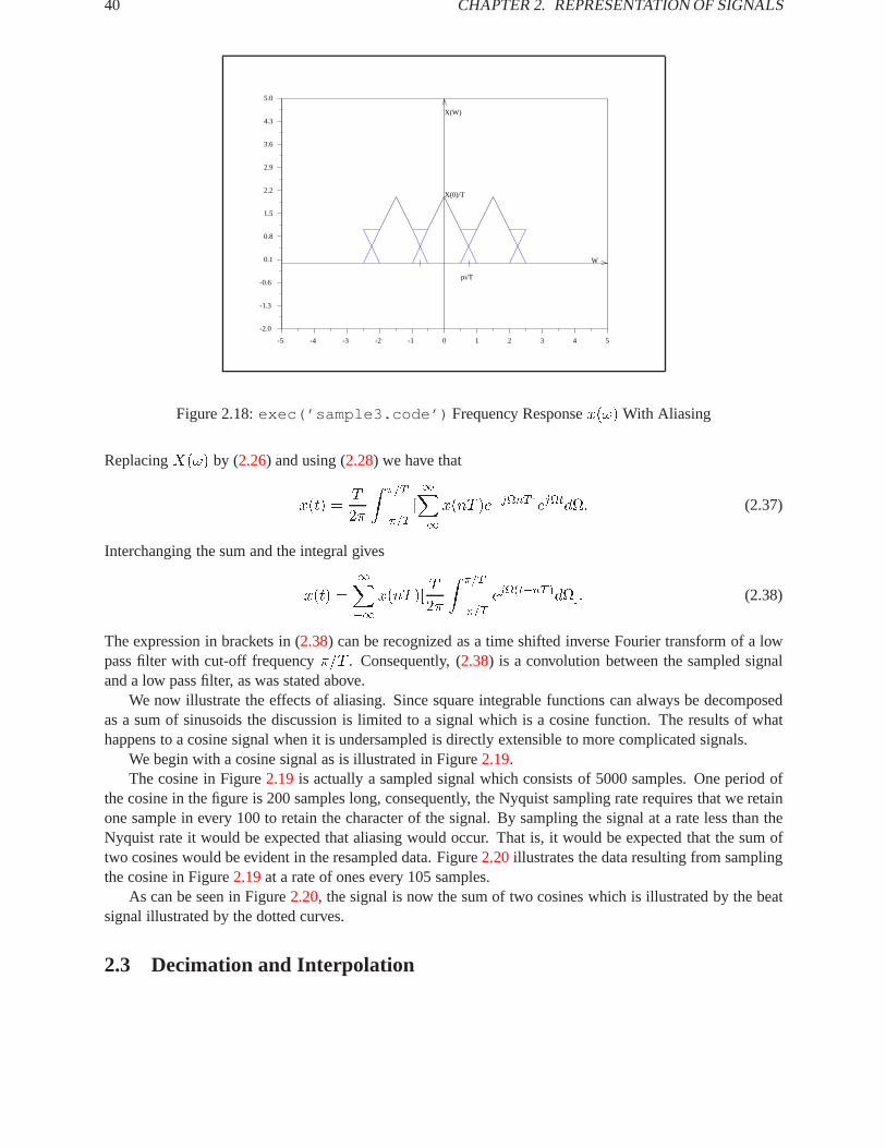
The expression in brackets in (2.38) can be recognized as a time shifted inverse Fourier transform of a lowpass filter with cut-off frequency�=T . Consequently, (2.38) is a convolution between the sampled signaland a low pass filter, as was stated above.
We now illustrate the effects of aliasing. Since square integrable functions can always be decomposedas a sum of sinusoids the discussion is limited to a signal which is a cosine function. The results of whathappens to a cosine signal when it is undersampled is directly extensible to more complicated signals.
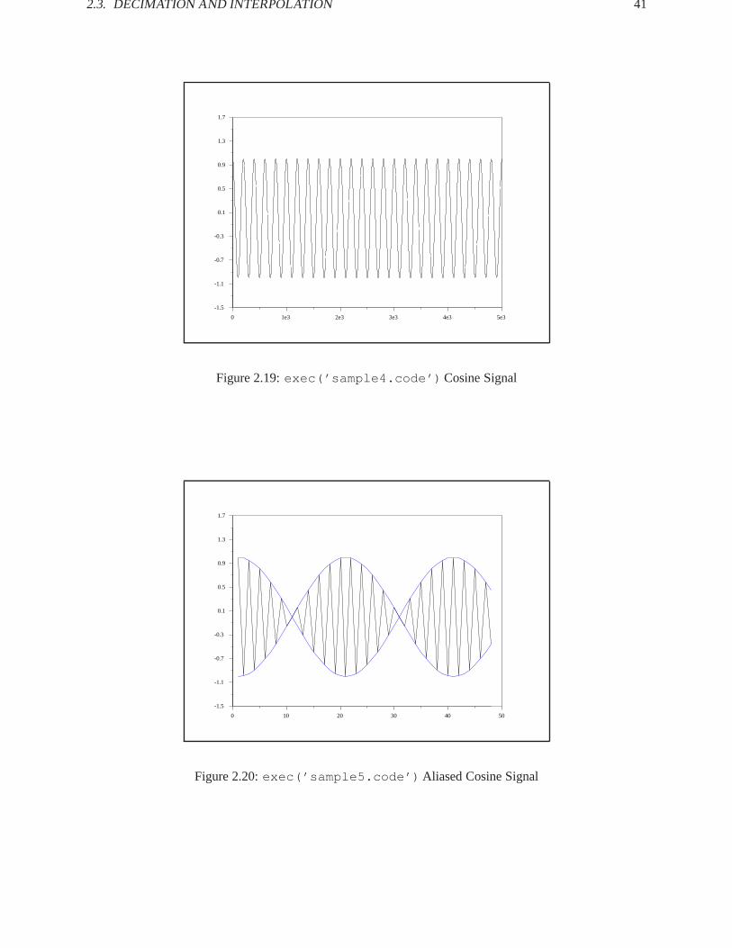
We begin with a cosine signal as is illustrated in Figure2.19.The cosine in Figure2.19is actually a sampled signal which consists of 5000 samples. One period of
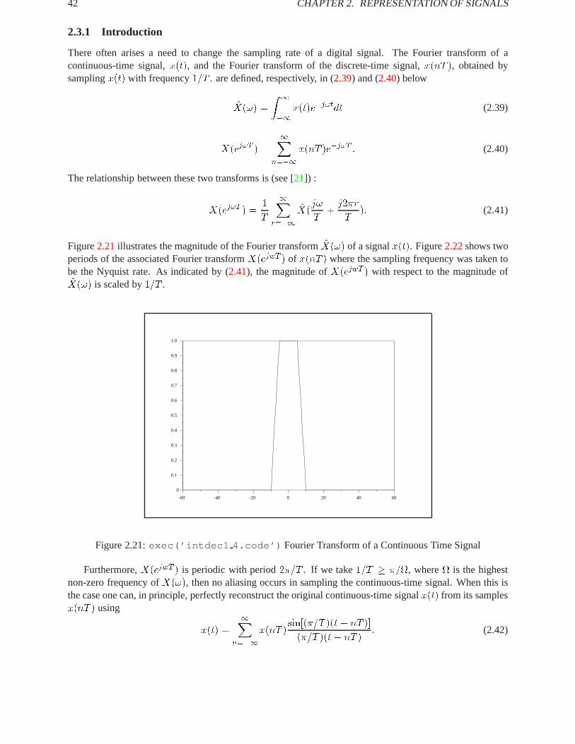
the cosine in the figure is 200 samples long, consequently, the Nyquist sampling rate requires that we retainone sample in every 100 to retain the character of the signal. By sampling the signal at a rate less than theNyquist rate it would be expected that aliasing would occur. That is, it would be expected that the sum oftwo cosines would be evident in the resampled data. Figure2.20illustrates the data resulting from samplingthe cosine in Figure2.19at a rate of ones every 105 samples.
As can be seen in Figure2.20, the signal is now the sum of two cosines which is illustrated by the beatsignal illustrated by the dotted curves.
2.3 Decimation and Interpolation
2.3. DECIMATION AND INTERPOLATION 41
0 1e3 2e3 3e3 4e3 5e3
-1.5
-1.1
-0.7
-0.3
0.1
0.5
0.9
1.3
1.7
Figure 2.19:exec(’sample4.code’) Cosine Signal
0 10 20 30 40 50
-1.5
-1.1
-0.7
-0.3
0.1
0.5
0.9
1.3
1.7
Figure 2.20:exec(’sample5.code’) Aliased Cosine Signal
42 CHAPTER2. REPRESENTATION OF SIGNALS
2.3.1 Introduction
There often arises a need to change the sampling rate of a digital signal. The Fourier transform of acontinuous-time signal,x(t), and the Fourier transform of the discrete-time signal,x(nT ), obtained bysamplingx(t) with frequency1=T . are defined, respectively, in (2.39) and (2.40) below
X(!) =
Z 1
�1x(t)e�j!tdt (2.39)
X(ej!T ) =
1Xn=�1
x(nT )e�j!T : (2.40)
The relationship between these two transforms is (see [21]) :
X(ej!T ) =1
T
1Xr=�1
X(j!
T+j2�r
T): (2.41)
Figure2.21illustrates the magnitude of the Fourier transformX(!) of a signalx(t). Figure2.22shows twoperiods of the associated Fourier transformX(ejwT ) of x(nT ) where the sampling frequency was taken tobe the Nyquist rate. As indicated by (2.41), the magnitude ofX(ejwT ) with respect to the magnitude ofX(!) is scaled by1=T .
-60 -40 -20 0 20 40 60
0
0.1
0.2
0.3
0.4
0.5
0.6
0.7
0.8
0.9
1.0
Figure 2.21:exec(’intdec1 4.code’) Fourier Transform of a Continuous Time Signal
Furthermore,X(ejwT ) is periodic with period2�=T . If we take1=T � �=, where is the highestnon-zero frequency ofX(!), then no aliasing occurs in sampling the continuous-time signal. When this isthe case one can, in principle, perfectly reconstruct the original continuous-time signalx(t) from its samplesx(nT ) using
x(t) =
1Xn=�1
x(nT )sin[(�=T )(t � nT )]
(�=T )(t � nT ): (2.42)

2.3. DECIMATION AND INTERPOLATION 43
-7 -5 -3 -1 1 3 5 7
0
0.1
0.2
0.3
0.4
0.5
0.6
0.7
0.8
0.9
1.0
Figure 2.22:exec(’intdec1 4.code’) Fourier Transform of the Discrete Time Signal
Consequently, one could obtainx(t) sampled at a different sampling rateT 0 from the sampled signalx(nT )by using (2.42) to reconstructx(t) and then resampling. In practice, however, this is impractical. It is muchmore convenient to keep all operations in the digital domain once one already has a discrete-time signal.
The Scilab functionintdec accomplishes a sampling rate change by interpolation and decimation. Theinterpolation takes the input signal and produces an output signal which is sampled at a rateL (an integer)times more frequently than the input. Then decimation takes the input signal and produces an output signalwhich is sampled at a rateM (also an integer) times less frequently than the input.
2.3.2 Interpolation
In interpolating the input signal by the integerL we wish to obtain a new signalx(nT 0) wherex(nT 0)would be the signal obtained if we had originally sampled the continuous-time signalx(t) at the rate1=T 0 =L=T . If the original signal is bandlimited and the sampling ratef = 1=T is greater than twice the highestfrequency ofx(t) then it can be expected that the new sampled signalx(nT 0) (sampled at a rate off 0 =1=T 0 = L=T = Lf ) could be obtained directly from the discrete signalx(nT ).
An interpolation ofx(nT ) to x(nT 0) whereT 0 = T=L can be found by insertingL� 1 zeros betweeneach element of the sequencex(nT ) and then low pass filtering. To see this we construct the new sequencev(nT 0) by puttingL� 1 zeros between the elements ofx(nT )
v(nT 0) =�x(nT=L); n = 0;�L;�2L; : : :0; otherwise:
(2.43)
SinceT 0 = T=L, v(nT 0) is sampledL times more frequently thanx(nT ). The Fourier transform of (2.43)yields
V (ej!T0) =
1Xn=�1
v(nT 0)e�j!nT0
44 CHAPTER2. REPRESENTATION OF SIGNALS
=
1Xn=�1
x(nT )e�j!nLT0
=
1Xn=�1
x(nT )e�j!nT
= X(ej!T ): (2.44)
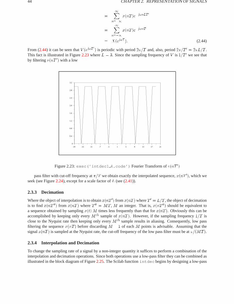
From (2.44) it can be seen thatV (ej!T0) is periodic with period2�=T and, also, period2�=T 0 = 2�L=T .
This fact is illustrated in Figure2.23whereL = 3. Since the sampling frequency ofV is 1=T 0 we see thatby filtering v(nT 0) with a low
-19 -15 -11 -7 -3 1 5 9 13 17 21
0
0.4
0.8
1.2
1.6
2.0
2.4
2.8
3.2
Figure 2.23:exec(’intdec1 4.code’) Fourier Transform ofv(nT 0)
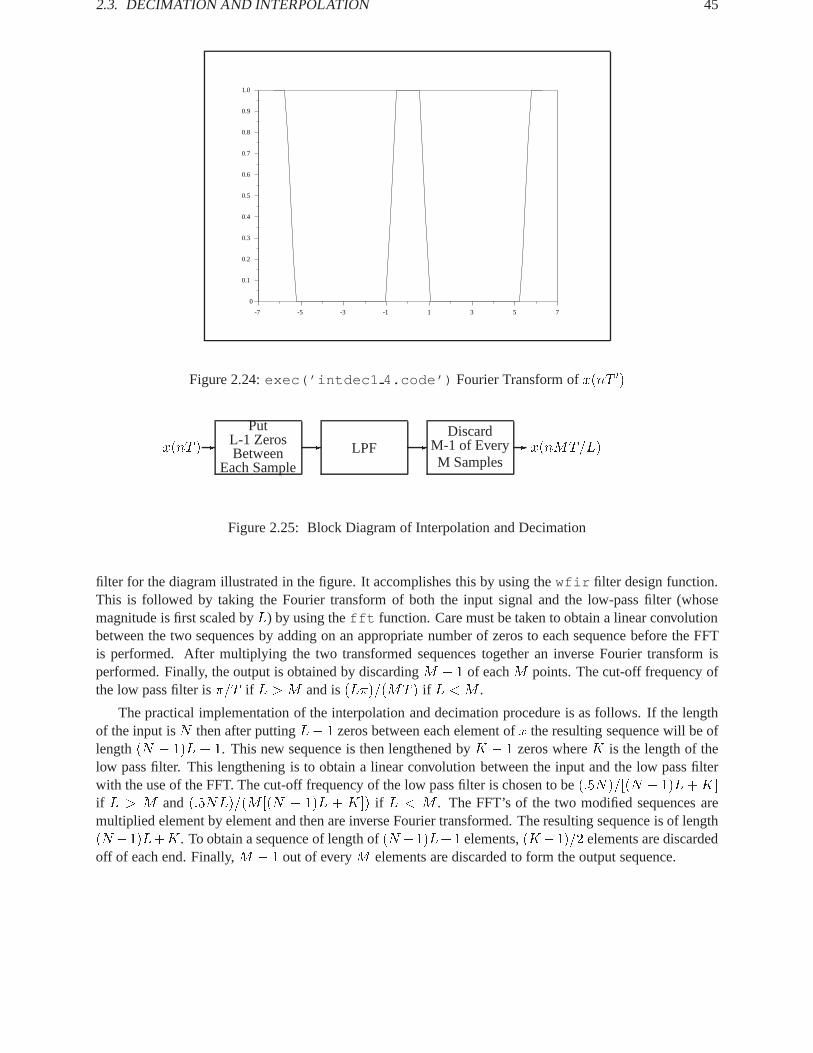
pass filter with cut-off frequency at�=T we obtain exactly the interpolated sequence,x(nT 0), which weseek (see Figure2.24), except for a scale factor ofL (see (2.41)).
2.3.3 Decimation
Where the object of interpolation is to obtainx(nT 0) fromx(nT )whereT 0 = L=T , the object of decimationis to findx(nT 00) from x(nT ) whereT 00 = MT , M an integer. That is,x(nT 00) should be equivalent toa sequence obtained by samplingx(t)M times less frequently than that forx(nT ). Obviously this can beaccomplished by keeping only everyM th sample ofx(nT ). However, if the sampling frequency1=T isclose to the Nyquist rate then keeping only everyM th sample results in aliasing. Consequently, low passfiltering the sequencex(nT ) before discardingM � 1 of eachM points is advisable. Assuming that thesignalx(nT ) is sampled at the Nyquist rate, the cut-off frequency of the low pass filter must be at�=(MT ).
2.3.4 Interpolation and Decimation
To change the sampling rate of a signal by a non-integer quantity it suffices to perform a combination of theinterpolation and decimation operations. Since both operations use a low-pass filter they can be combined asillustrated in the block diagram of Figure2.25. The Scilab functionintdec begins by designing a low-pass
2.3. DECIMATION AND INTERPOLATION 45
-7 -5 -3 -1 1 3 5 7
0
0.1
0.2
0.3
0.4
0.5
0.6
0.7
0.8
0.9
1.0
Figure 2.24:exec(’intdec1 4.code’) Fourier Transform ofx(nT 0)
x(nT )-Put
L-1 ZerosBetween
Each Sample
- LPF -Discard
M-1 of EveryM Samples
- x(nMT=L)
Figure 2.25: Block Diagram of Interpolation and Decimation
filter for the diagram illustrated in the figure. It accomplishes this by using thewfir filter design function.This is followed by taking the Fourier transform of both the input signal and the low-pass filter (whosemagnitude is first scaled byL) by using thefft function. Care must be taken to obtain a linear convolutionbetween the two sequences by adding on an appropriate number of zeros to each sequence before the FFTis performed. After multiplying the two transformed sequences together an inverse Fourier transform isperformed. Finally, the output is obtained by discardingM � 1 of eachM points. The cut-off frequency ofthe low pass filter is�=T if L > M and is(L�)=(MT ) if L < M .
The practical implementation of the interpolation and decimation procedure is as follows. If the lengthof the input isN then after puttingL� 1 zeros between each element ofx the resulting sequence will be oflength(N � 1)L + 1. This new sequence is then lengthened byK � 1 zeros whereK is the length of thelow pass filter. This lengthening is to obtain a linear convolution between the input and the low pass filterwith the use of the FFT. The cut-off frequency of the low pass filter is chosen to be(:5N)=[(N � 1)L+K]if L > M and(:5NL)=(M [(N � 1)L + K]) if L < M . The FFT’s of the two modified sequences aremultiplied element by element and then are inverse Fourier transformed. The resulting sequence is of length(N�1)L+K. To obtain a sequence of length of(N�1)L+1 elements,(K�1)=2 elements are discardedoff of each end. Finally,M � 1 out of everyM elements are discarded to form the output sequence.

46 CHAPTER2. REPRESENTATION OF SIGNALS
2.3.5 Examples usingintdec
Here we take a 50-point sequence assumed to be sampled at a 10kHz rate and change it to a sequencesampled at 16kHz. Under these conditions we takeL = 8 andM = 5. The sequence,x(nT ), is illustratedin Figure2.26. The discrete Fourier transform of x(nT) is shown in
0 10 20 30 40 50
-1
1
3
5
7
9
11
13
Figure 2.26:exec(’intdec5 10.code’) The Sequencex(nT )
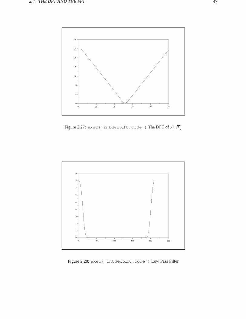
Figure2.27. As can be seen,x(nT ) is a bandlimited sequence. A new sequencev(nT 0) is created byputting 7 zeros between each element ofx(nT ). We use a Hamming windowed lowpass filter of length 33(Figure2.28)
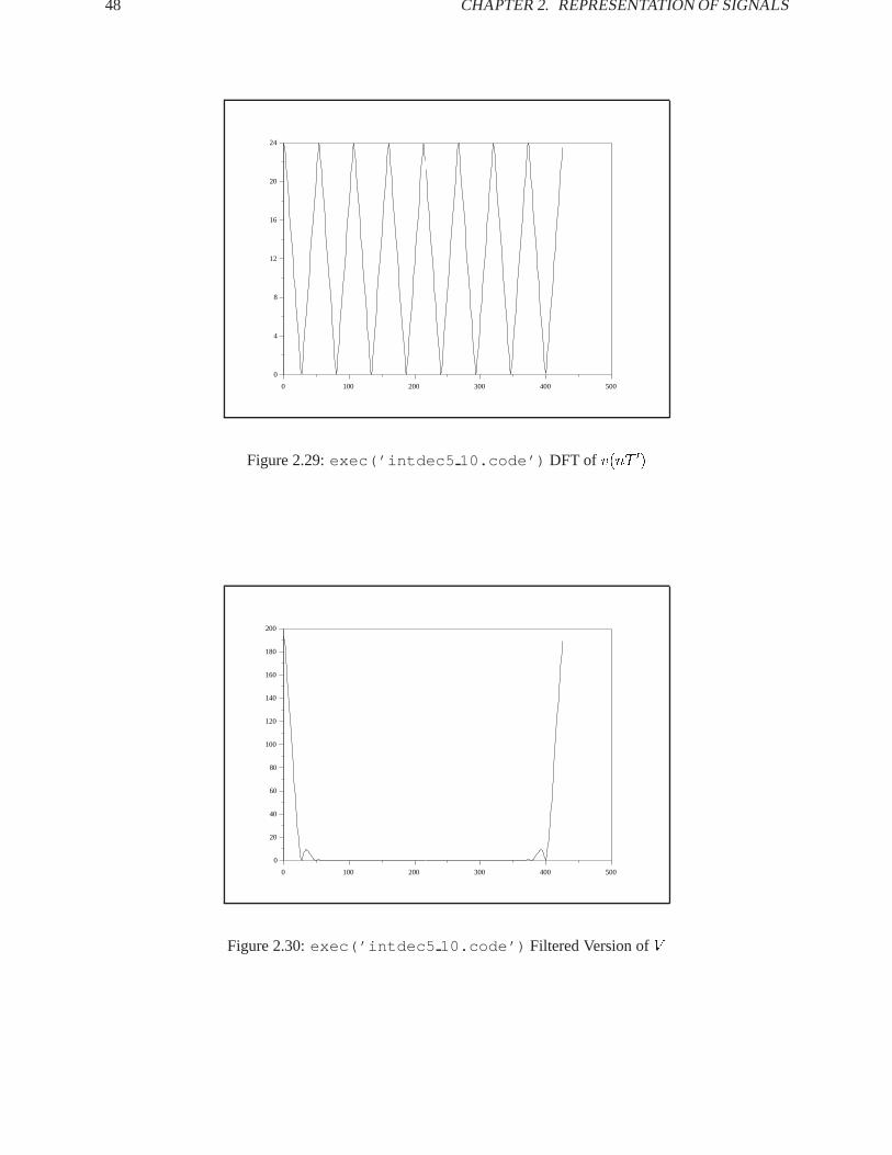
to filter v(nT 0). The discrete Fourier transform ofv(nT 0) is illustrated in Figure2.29. As is to beexpected, the Fourier transform ofv(nT 0) looks like the Fourier transform ofx(nT ) repeated 8 times.
The result of multiplying the magnitude response of the filter with that of the sequencev(nT 0) is shownin Figure2.30. Since the low pass filter is not ideal the resulting filtered sequence has some additional highfrequency energy in it (i.e., the small lobes seen in Figure2.30).
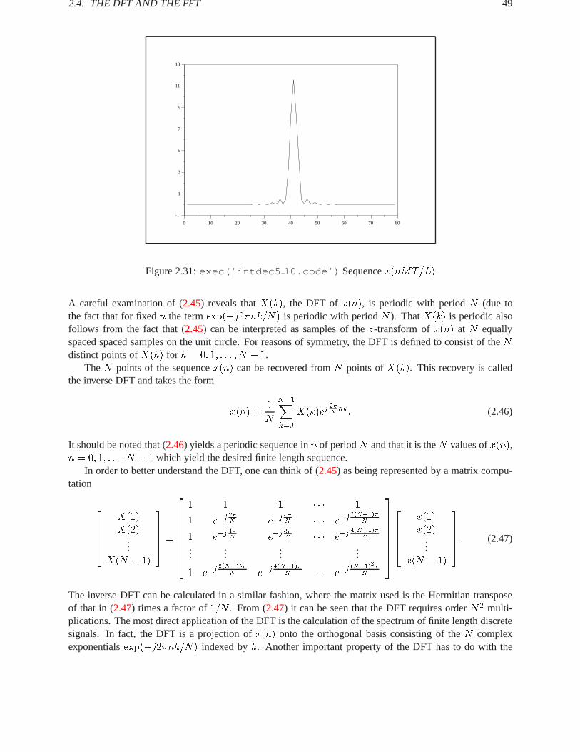
Finally, after taking the inverse discrete Fourier transform and discarding 4 out of every 5 samples weobtain the sequence illustrated in Figure2.31.
2.4 The DFT and the FFT
2.4.1 Introduction
The FFT (“Fast Fourier Transform”) is a computationally efficient algorithm for calculating the DFT (”Dis-crete Fourier Transform”) of finite length discrete time sequences. Calculation of the DFT from its definitionrequires orderN2 multiplications whereas the FFT requires orderN log2N multiplications. In this sectionwe discuss several uses of the DFT and some examples of its calculation using the FFT primitive in Scilab.
We begin with the definition of the DFT for a finite length sequence,x(n), of lengthN ,
X(k) =
N�1Xn=0
x(n)e�j2�Nnk: (2.45)
2.4. THE DFTAND THE FFT 47
0 10 20 30 40 50
0
4
8
12
16
20
24
28
Figure 2.27:exec(’intdec5 10.code’) The DFT ofx(nT )
0 100 200 300 400 500
0
1
2
3
4
5
6
7
8
9
Figure 2.28:exec(’intdec5 10.code’) Low Pass Filter
48 CHAPTER2. REPRESENTATION OF SIGNALS
0 100 200 300 400 500
0
4
8
12
16
20
24
Figure 2.29:exec(’intdec5 10.code’) DFT of v(nT 0)
0 100 200 300 400 500
0
20
40
60
80
100
120
140
160
180
200
Figure 2.30:exec(’intdec5 10.code’) Filtered Version ofV
2.4. THE DFTAND THE FFT 49
0 10 20 30 40 50 60 70 80
-1
1
3
5
7
9
11
13
Figure 2.31:exec(’intdec5 10.code’) Sequencex(nMT=L)
A careful examination of (2.45) reveals thatX(k), the DFT ofx(n), is periodic with periodN (due tothe fact that for fixedn the termexp(�j2�nk=N) is periodic with periodN ). ThatX(k) is periodic alsofollows from the fact that (2.45) can be interpreted as samples of thez-transform ofx(n) at N equallyspaced spaced samples on the unit circle. For reasons of symmetry, the DFT is defined to consist of theNdistinct points ofX(k) for k = 0; 1; : : : ; N � 1.
TheN points of the sequencex(n) can be recovered fromN points ofX(k). This recovery is calledthe inverse DFT and takes the form
x(n) =1
N
N�1Xk=0
X(k)ej2�Nnk: (2.46)
It should be noted that (2.46) yields a periodic sequence inn of periodN and that it is theN values ofx(n),n = 0; 1; : : : ; N � 1 which yield the desired finite length sequence.
In order to better understand the DFT, one can think of (2.45) as being represented by a matrix compu-tation
26664
X(1)X(2)
...X(N � 1)
37775 =
266666664
1 1 1 � � � 1
1 e�j2�N e�j
4�N � � � e�j
2(N�1)�N
1 e�j4�N e�j
8�N � � � e�j
4(N�1)�N
......
......
1 e�j2(N�1)�
N e�j4(N�1)�
N � � � e�j(N�1)2�
N
377777775
26664
x(1)x(2)
...x(N � 1)
37775 : (2.47)
The inverse DFT can be calculated in a similar fashion, where the matrix used is the Hermitian transposeof that in (2.47) times a factor of1=N . From (2.47) it can be seen that the DFT requires orderN2 multi-plications. The most direct application of the DFT is the calculation of the spectrum of finite length discretesignals. In fact, the DFT is a projection ofx(n) onto the orthogonal basis consisting of theN complexexponentialsexp(�j2�nk=N) indexed byk. Another important property of the DFT has to do with the
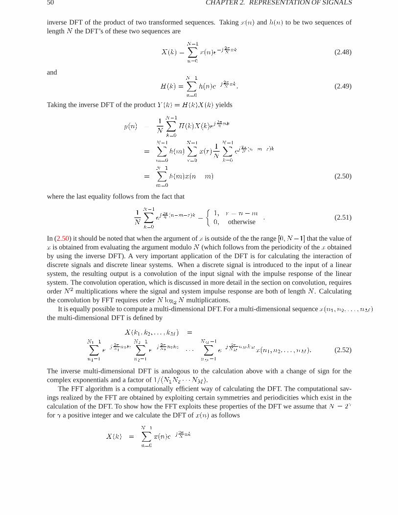
50 CHAPTER2. REPRESENTATION OF SIGNALS
inverse DFT of the product of two transformed sequences. Takingx(n) andh(n) to be two sequences oflengthN the DFT’s of these two sequences are
X(k) =N�1Xn=0
x(n)e�j2�Nnk (2.48)
and
H(k) =N�1Xn=0
h(n)e�j2�Nnk: (2.49)
Taking the inverse DFT of the productY (k) = H(k)X(k) yields
y(n) =1
N
N�1Xk=0
H(k)X(k)ej2�Nnk
=
N�1Xm=0
h(m)
N�1Xr=0
x(r)1
N
N�1Xk=0
ej2�N
(n�m�r)k
=N�1Xm=0
h(m)x(n�m) (2.50)
where the last equality follows from the fact that
1
N
N�1Xk=0
ej2�N
(n�m�r)k =�
1; r = n�m0; otherwise
: (2.51)
In (2.50) it should be noted that when the argument ofx is outside of the the range[0; N�1] that the value ofx is obtained from evaluating the argument moduloN (which follows from the periodicity of thex obtainedby using the inverse DFT). A very important application of the DFT is for calculating the interaction ofdiscrete signals and discrete linear systems. When a discrete signal is introduced to the input of a linearsystem, the resulting output is a convolution of the input signal with the impulse response of the linearsystem. The convolution operation, which is discussed in more detail in the section on convolution, requiresorderN2 multiplications where the signal and system impulse response are both of lengthN . Calculatingthe convolution by FFT requires orderN log2N multiplications.
It is equally possible to compute a multi-dimensional DFT. For a multi-dimensional sequencex(n1; n2; : : : ; nM )the multi-dimensional DFT is defined by
X(k1; k2; : : : ; kM ) =N1�1Xn1=1
e�j 2�
N1n1k1
N2�1Xn2=1
e�j 2�
N2n2k2 � � �
NM�1XnM=1
e�j 2�
NMnMkMx(n1; n2; : : : ; nM ): (2.52)
The inverse multi-dimensional DFT is analogous to the calculation above with a change of sign for thecomplex exponentials and a factor of1=(N1N2 � � �NM ).
The FFT algorithm is a computationally efficient way of calculating the DFT. The computational sav-ings realized by the FFT are obtained by exploiting certain symmetries and periodicities which exist in thecalculation of the DFT. To show how the FFT exploits these properties of the DFT we assume thatN = 2
for a positive integer and we calculate the DFT ofx(n) as follows
X(k) =
N�1Xn=0
x(n)e�j2�Nnk
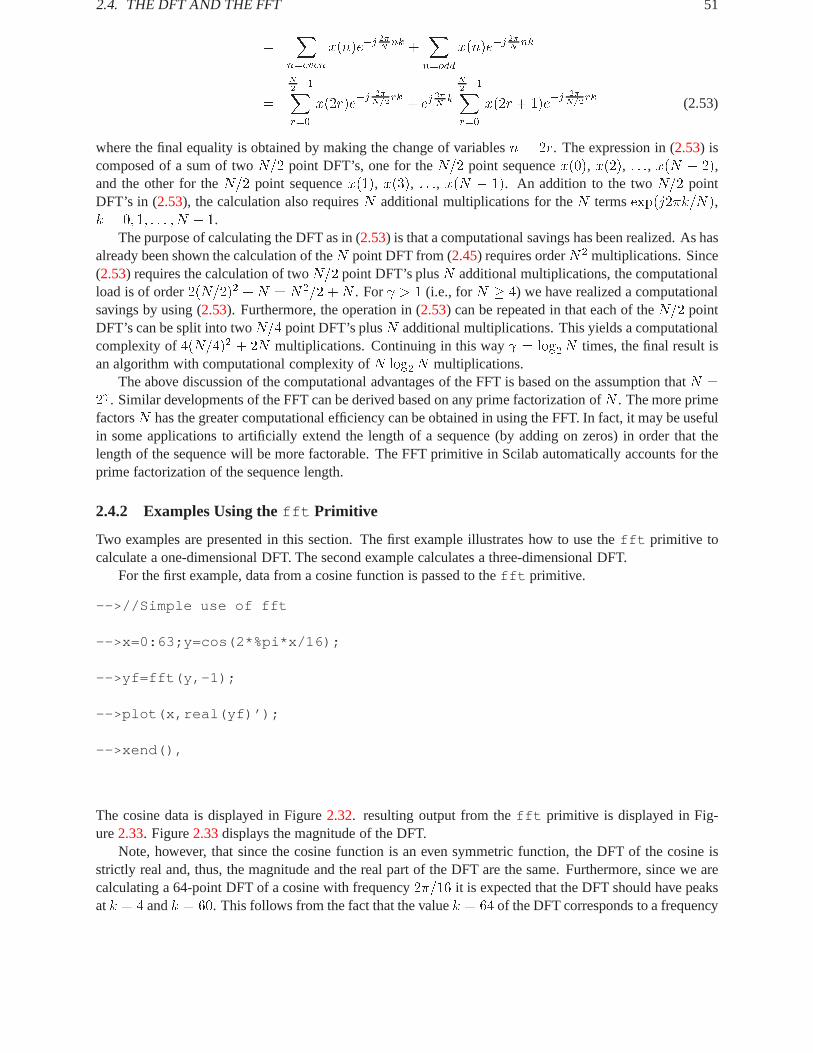
2.4. THE DFTAND THE FFT 51
=X
n=even
x(n)e�j2�Nnk +
Xn=odd
x(n)e�j2�Nnk
=
N2�1X
r=0
x(2r)e�j 2�
N=2rk
+ ej2�Nk
N2�1X
r=0
x(2r + 1)e�j 2�
N=2rk (2.53)
where the final equality is obtained by making the change of variablesn = 2r. The expression in (2.53) iscomposed of a sum of twoN=2 point DFT’s, one for theN=2 point sequencex(0), x(2), : : :, x(N � 2),and the other for theN=2 point sequencex(1), x(3), : : :, x(N � 1). An addition to the twoN=2 pointDFT’s in (2.53), the calculation also requiresN additional multiplications for theN termsexp(j2�k=N),k = 0; 1; : : : ; N � 1.
The purpose of calculating the DFT as in (2.53) is that a computational savings has been realized. As hasalready been shown the calculation of theN point DFT from (2.45) requires orderN2 multiplications. Since(2.53) requires the calculation of twoN=2 point DFT’s plusN additional multiplications, the computationalload is of order2(N=2)2 +N = N2=2 +N . For > 1 (i.e., forN � 4) we have realized a computationalsavings by using (2.53). Furthermore, the operation in (2.53) can be repeated in that each of theN=2 pointDFT’s can be split into twoN=4 point DFT’s plusN additional multiplications. This yields a computationalcomplexity of4(N=4)2 + 2N multiplications. Continuing in this way = log2N times, the final result isan algorithm with computational complexity ofN log2N multiplications.
The above discussion of the computational advantages of the FFT is based on the assumption thatN =2 . Similar developments of the FFT can be derived based on any prime factorization ofN . The more primefactorsN has the greater computational efficiency can be obtained in using the FFT. In fact, it may be usefulin some applications to artificially extend the length of a sequence (by adding on zeros) in order that thelength of the sequence will be more factorable. The FFT primitive in Scilab automatically accounts for theprime factorization of the sequence length.
2.4.2 Examples Using thefft Primitive
Two examples are presented in this section. The first example illustrates how to use thefft primitive tocalculate a one-dimensional DFT. The second example calculates a three-dimensional DFT.
For the first example, data from a cosine function is passed to thefft primitive.
-->//Simple use of fft
-->x=0:63;y=cos(2*%pi*x/16);
-->yf=fft(y,-1);
-->plot(x,real(yf)’);
-->xend(),
The cosine data is displayed in Figure2.32. resulting output from thefft primitive is displayed in Fig-ure2.33. Figure2.33displays the magnitude of the DFT.
Note, however, that since the cosine function is an even symmetric function, the DFT of the cosine isstrictly real and, thus, the magnitude and the real part of the DFT are the same. Furthermore, since we arecalculating a 64-point DFT of a cosine with frequency2�=16 it is expected that the DFT should have peaksatk = 4 andk = 60. This follows from the fact that the valuek = 64 of the DFT corresponds to a frequency

52 CHAPTER2. REPRESENTATION OF SIGNALS
0 10 20 30 40 50 60 70
-1.0
-0.8
-0.6
-0.4
-0.2
0
0.2
0.4
0.6
0.8
1.0
Figure 2.32:exec(’fft1.code’) Cosine Signal
0 10 20 30 40 50 60 70
-1
3
7
11
15
19
23
27
31
35
Figure 2.33:exec(’fft2.code’) DFT of Cosine Signal

2.4. THE DFTAND THE FFT 53
of 2� and, consequently, the valuek = 4 must correspond to the frequency2�=16, which is the frequencyof the signal under examination.
The second example calculates the DFT of a three-dimensional signal. The calculation proceeds asfollows.
-->y1=matrix(1:6,2,3)y1 =
! 1. 3. 5. !! 2. 4. 6. !
-->y2=matrix(7:12,2,3)y2 =
! 7. 9. 11. !! 8. 10. 12. !
-->y=matrix([y1,y2],1,12)y =
column 1 to 11
! 1. 2. 3. 4. 5. 6. 7. 8. 9. 10. 11. !
column 12
! 12. !
-->yf=mfft(y,-1,[2 3 2])yf =
column 1 to 7
! 78. - 6. - 12. + 6.9282032i 0 - 12. - 6.9282032i 0 - 36. !
column 8 to 12
! 0 0 0 0 0 !
-->yf1=matrix(yf(1:6),2,3)yf1 =
! 78. - 12. + 6.9282032i - 12. - 6.9282032i !! - 6. 0 0 !
-->yf2=matrix(yf(7:12),2,3)

54 CHAPTER2. REPRESENTATION OF SIGNALS
x(t) - h(t) -y(t) =Rh(t� u)x(u)du
Figure 2.34: Convolution Performed by Linear System
yf2 =
! - 36. 0 0 !! 0 0 0 !
In the above series of calculations the signaly is three-dimensional and is represented by the two matricesy1 andy2 . The first dimension ofy are the rows of the matrices, the second dimension ofy are the columnsof the matrices, and the third dimension ofy are the sequence of matrices represented byy1 andy2 . Thesignaly is represented by the vectory which is in vector form. The DFT ofy is calculated using the functionmfft whereflag = �1 anddim = [2 3 2]. Naturally, the DFT of the three-dimensional signal is itselfthree-dimensional. The result of the DFT calculation is represented by the two matricesyf1 andyf2 .
2.5 Convolution
2.5.1 Introduction
Given two continuous time functionsx(t) andh(t), a new continuous time function can be obtained byconvolvingx(t) with h(t).
y(t) =
Z 1
�1h(t� u)x(u)du: (2.54)
An analogous convolution operation can be defined for discrete time functions. Lettingx(n) andh(n)represent discrete time functions, by the discrete time convolution givesy(n) is :
y(n) =1X
k=�1h(n� k)x(k): (2.55)
If h(t) represents the impulse response of a linear, time-invariant system and ifx(t) is an input to thissystem then the output of the system,y(t), can be calculated as the convolution betweenx(t) andh(t) (i.e.,as in (2.54). Figure2.34illustrates how convolution is related to linear systems. If the system,h(t) is causal(i.e.,h(t) = 0 for t < 0) and, in addition, the signalx(t) is applied to the system at timet = 0, then (2.54)becomes
y(t) =
Z t
0h(t� u)x(u)du: (2.56)
Similarly, for h(n) a time invariant, causal, discrete linear system with inputx(n) starting at timen = 0,the outputy(n) is the convolution
y(n) =
nXk=0
h(n� k)x(k): (2.57)

2.5. CONVOLUTION 55
An important property of the convolution operation is that the calculation can be effected by usingFourier transforms. This is due to the fact that convolution in the time domain is equivalent to multiplicationin the frequency domain. LetX(!), H(!), andY (!) represent the Fourier transforms ofx(t), h(t), andy(t), respectively, where
Y (!) =
Z 1
�1y(t)e�j!tdt: (2.58)
If the relationship in (2.54) is valid, then it also follows that
Y (!) = H(!)X(!): (2.59)
There is an analogous relationship between the Fourier transform and convolution for discrete time sig-nals. LettingX(ej!),H(ej!), andY (ej!) be the Fourier transforms ofx(n), h(n), andy(n), respectively,where, for example
Y (ej!) =
1Xn=�1
y(n)e�j!n (2.60)
we have that the discrete time convolution operation can be represented in the Fourier domain as
Y (ej!) = H(ej!)X(ej!): (2.61)
The fact that convolution in the time domain is equivalent to multiplication in the frequency domainmeans that the calculations in (2.54) and (2.55) can be calculated (at least approximately) by a computation-ally efficient algorithm, the FFT. This is accomplished by calculating the inverse DFT of the product of theDFT’s of x(n) andh(n). Care must be taken to ensure that the resulting calculation is a linear convolution(see the section on the DFT and the FFT). The linear convolution is accomplished by adding enough zerosonto the two sequences so that the circular convolution accomplished by the DFT is equivalent to a linearconvolution.
The convolution of two finite length sequences can be calculated by the Scilab functionconvol .
2.5.2 Use of theconvol function
Theconvol function can be used following two formats. The first format calculates a convolution based ontwo discrete length sequences which are passed in their entirety to the function. The second format performsupdated convolutions using the overlap-add method described in [21]. It is used when one of the sequencesis very long and, consequently, cannot be passed directly to the function.
The syntax used for the function under the first format is
-->y=convol(h,x)
where bothh andx are finite length vectors andy is a vector representing the resulting convolution of theinputs. An example of the use of the function under the first format is as follows.
-->x=1:3x =
! 1. 2. 3. !
-->h=ones(1,4)h =

56 CHAPTER2. REPRESENTATION OF SIGNALS
! 1. 1. 1. 1. !
-->y=convol(h,x)y =
! 1. 3. 6. 6. 5. 3. !
The syntax used for the function under the second format is
-->[y,y1]=convol(h,x,y0)
wherey0 andy1 are required to update the calculations of the convolution at each iteration and where theuse of the second format requires the following function supplied by the user.
//exec(’convol1.code’)x1=getx(xlen_1,xstart_1);[y,y1]=convol(h,x1);for k=2:nsecs-1,
xk=getx(xlen_k,xstart_k);[y,y1]=convol(h,xk,y1);
end,xn=getx(xlen_n,xstart_n);y=convol(h,xn,y1);
where,nsecs is the number of sections ofx to be used in the convolution calculation and, in addition, theuser must supply a functiongetx which obtains segments of the datax following the format.
function [xv]=getx(xlen,xstart)...
wherexlen is the length of data requested andxstart is the length of the data vector to be used.
2.6 The Chirp Z-Transform
2.6.1 Introduction
The discrete Fourier transform (DFT) of a finite length, discrete time signal,x(n), is defined by
X(k) =N�1Xn=0
x(n)e�j(2�nk)=N (2.62)
k = 0; 1; : : : ; N � 1
and the z-transform ofx(n) is given by
X(z) =
1Xn=�1
x(n)z�n

2.6. THE CHIRP Z-TRANSFORM 57
=
N�1Xn=0
x(n)z�n (2.63)
TheN � 1 points of the DFT ofx(n) are related to the z-transform ofx(n) in that they are samples of thez-transform taken at equally spaced intervals on the unit circle in the z-plane.
There are applications [25] where it is desired to calculate samples of the z-transform at locations eitheroff the unit circle or at unequally spaced angles on the unit circle. The chirp z-transform (CZT) is an efficientalgorithm which can be used for calculating samples of some of these z-transforms. In particular, the CZTcan be used to efficiently calculate the values of the z-transform of a finite-length, discrete-time sequence ifthe z-transform points are of the form
zk = AW�k (2.64)
where
A = A0ej�
W = W0e�j� (2.65)
and whereA0 andW0 are real valued constants and� and� are angles.
◊
◊
◊
◊◊
◊◊◊◊◊
◊◊◊◊◊◊◊
◊◊
◊
Figure 2.35:exec(’czt1.code’) Samples of the z-transform on Spirals
The set of pointsfzkg lie on a spiral wherez0 is at distanceA0 from the origin and at angle� from thex-axis. The remaining points are located at equally spaced angles,�, and approach the origin forW0 > 1,move away from the origin forW0 < 1, and remain on a circle of radiusA0 for W0 = 1. Figure2.35showsthe location of samples of the z-transform forW0 < 1 on the left hand side of the figure and ofW0 < 1on the right hand side of the figure. In both parts of the figure the position ofz0 is indicated by the sampleconnected to the origin by a straight line.
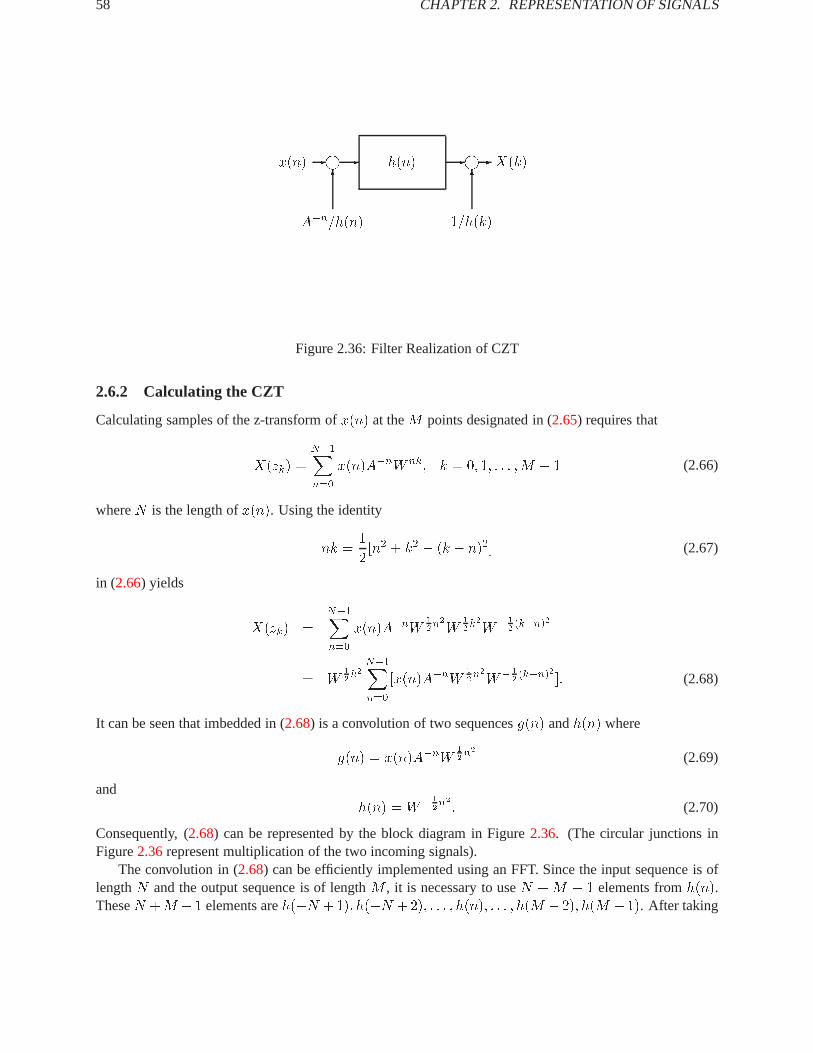
58 CHAPTER2. REPRESENTATION OF SIGNALS
x(n) - i- h(n) - i- X(k)6
1=h(k)
6
A�n=h(n)
Figure 2.36: Filter Realization of CZT
2.6.2 Calculating the CZT
Calculating samples of the z-transform ofx(n) at theM points designated in (2.65) requires that
X(zk) =
N�1Xn=0
x(n)A�nW nk; k = 0; 1; : : : ;M � 1 (2.66)
whereN is the length ofx(n). Using the identity
nk =1
2[n2 + k2 � (k � n)2] (2.67)
in (2.66) yields
X(zk) =N�1Xn=0
x(n)A�nW12n2W
12k2W� 1
2(k�n)2
= W12k2
N�1Xn=0
[x(n)A�nW12n2W� 1
2(k�n)2 ]: (2.68)
It can be seen that imbedded in (2.68) is a convolution of two sequencesg(n) andh(n) where
g(n) = x(n)A�nW12n2 (2.69)
andh(n) =W� 1
2n2 : (2.70)
Consequently, (2.68) can be represented by the block diagram in Figure2.36. (The circular junctions inFigure2.36represent multiplication of the two incoming signals).
The convolution in (2.68) can be efficiently implemented using an FFT. Since the input sequence is oflengthN and the output sequence is of lengthM , it is necessary to useN +M � 1 elements fromh(n).TheseN +M � 1 elements areh(�N +1); h(�N +2); : : : ; h(n); : : : ; h(M � 2); h(M � 1). After taking
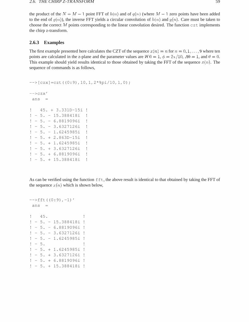
2.6. THE CHIRP Z-TRANSFORM 59
the product of theN +M � 1 point FFT ofh(n) and ofg(n) (whereM � 1 zero points have been addedto the end ofg(n)), the inverse FFT yields a circular convolution ofh(n) andg(n). Care must be taken tochoose the correctM points corresponding to the linear convolution desired. The functionczt implementsthe chirp z-transform.
2.6.3 Examples
The first example presented here calculates the CZT of the sequencex(n) = n for n = 0; 1; : : : ; 9 where tenpoints are calculated in the z-plane and the parameter values areW0 = 1, � = 2�=10, A0 = 1, and� = 0.This example should yield results identical to those obtained by taking the FFT of the sequencex(n). Thesequence of commands is as follows,
-->[czx]=czt((0:9),10,1,2*%pi/10,1,0);
-->czx’ans =
! 45. + 3.331D-15i !! - 5. - 15.388418i !! - 5. - 6.8819096i !! - 5. - 3.6327126i !! - 5. - 1.6245985i !! - 5. + 2.863D-15i !! - 5. + 1.6245985i !! - 5. + 3.6327126i !! - 5. + 6.8819096i !! - 5. + 15.388418i !
As can be verified using the functionfft , the above result is identical to that obtained by taking the FFT ofthe sequencex(n) which is shown below,
-->fft((0:9),-1)’ans =
! 45. !! - 5. - 15.388418i !! - 5. - 6.8819096i !! - 5. - 3.6327126i !! - 5. - 1.6245985i !! - 5. !! - 5. + 1.6245985i !! - 5. + 3.6327126i !! - 5. + 6.8819096i !! - 5. + 15.388418i !

60 CHAPTER2. REPRESENTATION OF SIGNALS
The second example calculates the DFT of the same sequence,x(n), above, however, just at five equallyspaced points in[��=4; �=4] on the unit circle in the z-plane. The spacing between the points is�=8 forfive points in[��=4; �=4]. The result is
-->x=0:9;
-->[czx]=czt(x,5,1,%pi/8,1,-%pi/4);
-->czx’ans =
! 10.363961 + 3.2928932i !! - 25.451987 - 16.665207i !! 45. + 3.553D-14i !! - 25.451987 + 16.665207i !! 10.363961 - 3.2928932i !
Now taking a sixteen point FFT of the sequencex(n) (accomplished by adding six zeros to the end of thesequencex(n)) it can be seen that the CZT computed above yields exactly the desired points on the unitcircle in the z-plane. That is to say that the last three points ofczx correspond to the first three points of theFFT ofx(n) and the first two points ofczx correspond to the last two points of the FFT.
-->y=0*ones(1:16);
-->y(1:10)=0:9;
-->fft(y,-1)’ans =
! 45. !! - 25.451987 + 16.665207i !! 10.363961 - 3.2928932i !! - 9.0640653 - 2.3284927i !! 4. + 5.i !! - 1.2790805 - 5.6422012i !! - 2.363961 + 4.7071068i !! 3.7951327 - 2.6485014i !! - 5. !! 3.7951327 + 2.6485014i !! - 2.363961 - 4.7071068i !! - 1.2790805 + 5.6422012i !! 4. - 5.i !! - 9.0640653 + 2.3284927i !! 10.363961 + 3.2928932i !! - 25.451987 - 16.665207i !

2.6. THE CHIRP Z-TRANSFORM 61

62 CHAPTER2. REPRESENTATION OF SIGNALS

Chapter 3
Design of Finite Impulse Response Filters
3.1 Windowing Techniques
In theory, the design of FIR filters is straightforward. One takes the inverse Fourier transform of the desiredfrequency response and obtains the discrete time impulse response of the filter according to (3.1)
h(n) =1
2�
Z �
��H(!)ej!nd! �1 < n <1 (3.1)
The problem, in practice, is that for many filters of interest the resulting impulse response is infinite andnon-causal. An example of this is the low pass filter which, given its cut-off frequency,!c, is defined by
H(!j!c) =�
1; j!j � !c0; otherwise
(3.2)
The associated impulse response is obtained by applying (3.1) to (3.2) which yields
h(nj!c) = 1
�nsin(!cn) �1 < n <1 (3.3)
A technique for obtaining a finite length implementation to (3.3) is to take the N elements ofh(n) whichare centered aroundn = 0 and to discard all the remaining elements. This operation can be represented bymultiplying the sequence in (3.3) by an appropriately shifted version of a rectangular window of the form
RN (n) =
�1; 0 � n � N � 10; otherwise
(3.4)
The magnitude of the resulting windowed sequence frequency response is depicted in Figure3.1super-imposed on the ideal frequency response (the dotted curve). The filter illustrated in Figure3.1 has lengthN = 33 and a cut-off frequency of!c = :2. As can be seen, the
approximation is marked by a ripple in both the pass and stop bands. This ripple finds its greatestdeviations near the discontinuity at!c. The observed ripple is due to the convolution of the ideal frequencyresponse given by (3.2) with the frequency response of the rectangular window. For many applications theripples in the frequency response of Figure3.1are unacceptable.
It is possible to decrease the amount of rippling by using different types of windows. The performance ofa window is governed by its frequency response. Since the frequency response of the window is convolvedwith the desired frequency response the objective is to find a window which has a frequency response whichis as impulsive as possible. That is, the frequency response should have a narrow main lobe with most ofthe energy in this lobe and side lobes which are as small as possible. The width of the main lobe governs,
63
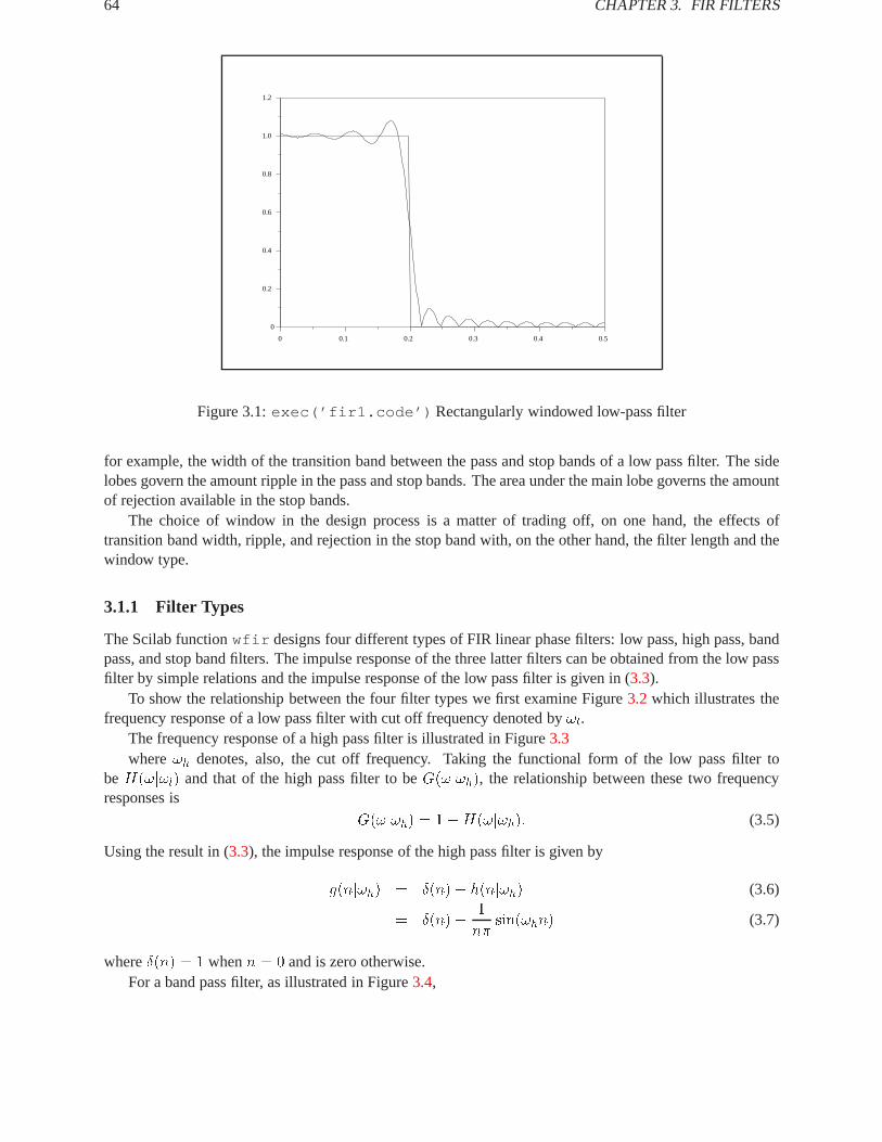
64 CHAPTER3. FIR FILTERS
0 0.1 0.2 0.3 0.4 0.5
0
0.2
0.4
0.6
0.8
1.0
1.2
Figure 3.1:exec(’fir1.code’) Rectangularly windowed low-pass filter
for example, the width of the transition band between the pass and stop bands of a low pass filter. The sidelobes govern the amount ripple in the pass and stop bands. The area under the main lobe governs the amountof rejection available in the stop bands.
The choice of window in the design process is a matter of trading off, on one hand, the effects oftransition band width, ripple, and rejection in the stop band with, on the other hand, the filter length and thewindow type.
3.1.1 Filter Types
The Scilab functionwfir designs four different types of FIR linear phase filters: low pass, high pass, bandpass, and stop band filters. The impulse response of the three latter filters can be obtained from the low passfilter by simple relations and the impulse response of the low pass filter is given in (3.3).
To show the relationship between the four filter types we first examine Figure3.2 which illustrates thefrequency response of a low pass filter with cut off frequency denoted by!l.
The frequency response of a high pass filter is illustrated in Figure3.3where!h denotes, also, the cut off frequency. Taking the functional form of the low pass filter to
beH(!j!l) and that of the high pass filter to beG(!j!h), the relationship between these two frequencyresponses is
G(!j!h) = 1�H(!j!h): (3.5)
Using the result in (3.3), the impulse response of the high pass filter is given by
g(nj!h) = Æ(n)� h(nj!h) (3.6)
= Æ(n)� 1
n�sin(!hn) (3.7)
whereÆ(n) = 1 whenn = 0 and is zero otherwise.For a band pass filter, as illustrated in Figure3.4,
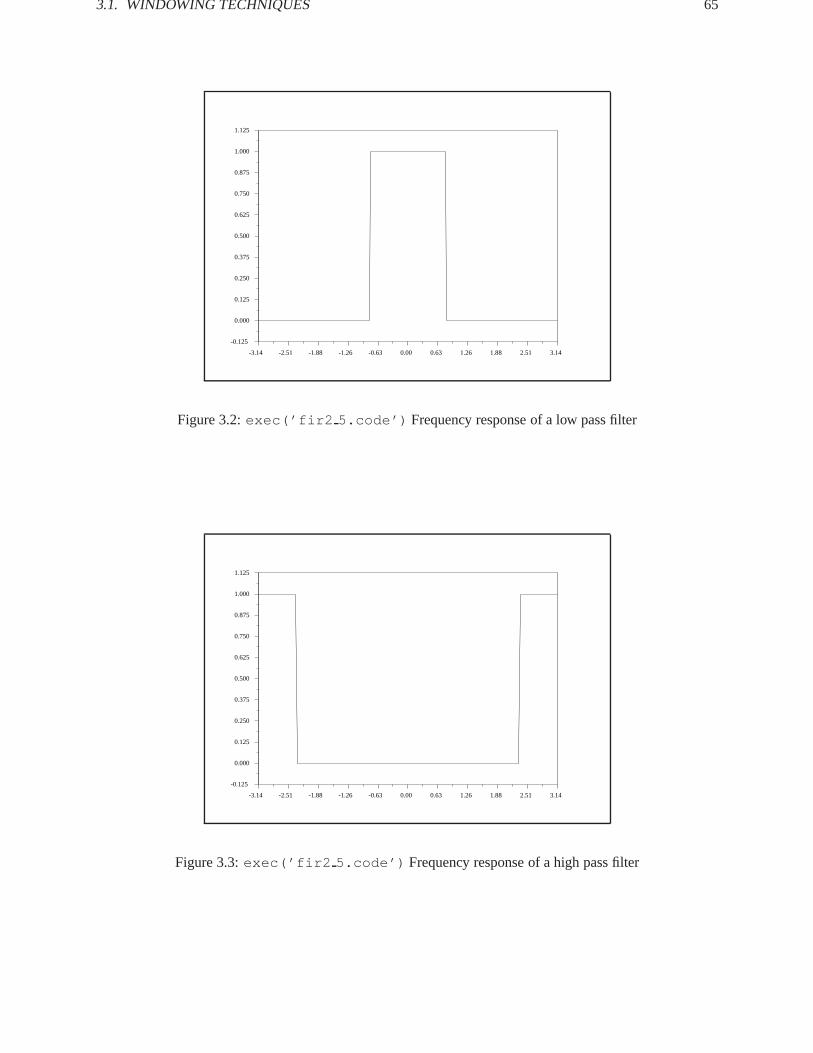
3.1. WINDOWING TECHNIQUES 65
-3.14 -2.51 -1.88 -1.26 -0.63 0.00 0.63 1.26 1.88 2.51 3.14
-0.125
0.000
0.125
0.250
0.375
0.500
0.625
0.750
0.875
1.000
1.125
Figure 3.2:exec(’fir2 5.code’) Frequency response of a low pass filter
-3.14 -2.51 -1.88 -1.26 -0.63 0.00 0.63 1.26 1.88 2.51 3.14
-0.125
0.000
0.125
0.250
0.375
0.500
0.625
0.750
0.875
1.000
1.125
Figure 3.3:exec(’fir2 5.code’) Frequency response of a high pass filter
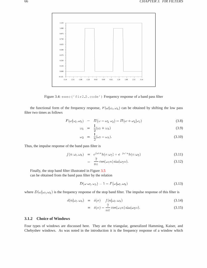
66 CHAPTER3. FIR FILTERS
-3.14 -2.51 -1.88 -1.26 -0.63 0.00 0.63 1.26 1.88 2.51 3.14
-0.125
0.000
0.125
0.250
0.375
0.500
0.625
0.750
0.875
1.000
1.125
Figure 3.4:exec(’fir2 5.code’) Frequency response of a band pass filter
the functional form of the frequency response,F (!j!l; !h) can be obtained by shifting the low passfilter two times as follows
F (!j!l; !h) = H(! � !1j!2) +H(! + !1j!2) (3.8)
!1 =1
2(!l + !h) (3.9)
!2 =1
2(!l � !h): (3.10)
Thus, the impulse response of the band pass filter is
f(nj!l; !h) = ej!1nh(nj!2) + e�j!1nh(nj!2) (3.11)
=2
n�cos(!1n) sin(!2n): (3.12)
Finally, the stop band filter illustrated in Figure3.5can be obtained from the band pass filter by the relation
D(!j!l; !h) = 1� F (!j!l; !h) (3.13)
whereD(!j!l; !h) is the frequency response of the stop band filter. The impulse response of this filter is
d(nj!l; !h) = Æ(n)� f(nj!l; !h) (3.14)
= Æ(n)� 2
n�cos(!1n) sin(!2n): (3.15)
3.1.2 Choice of Windows
Four types of windows are discussed here. They are the triangular, generalized Hamming, Kaiser, andChebyshev windows. As was noted in the introduction it is the frequency response of a window which

3.1. WINDOWING TECHNIQUES 67
-3.14 -2.51 -1.88 -1.26 -0.63 0.00 0.63 1.26 1.88 2.51 3.14
-0.125
0.000
0.125
0.250
0.375
0.500
0.625
0.750
0.875
1.000
1.125
Figure 3.5:exec(’fir2 5.code’) Frequency response of a stop band filter
governs its efficacy in filter design. Consequently, for each window type, we try to give its frequencyresponse and a qualitative analysis of its features with respect to the frequency response of the rectangularwindow.
The frequency response of the rectangular window is obtained by taking the Fourier transform of (3.4)
RN (!) =N�1Xn=0
e�j!n (3.16)
=sin(!N=2)
sin(!=2)e�j(N�1)!=2: (3.17)
The magnitude of (3.17) is plotted as the solid line in Figure3.6. Evaluating (3.17) at! = 0 yields the heightof the main lobe which isRN (0) = N . The zeros ofRN (!) are located at! = �2�n=N , n = 1; 2; : : :,and, consequently, the base of the main lobe has width4�=N . The area under the main lobe can be boundedfrom above by the area of a rectangle (depicted by a dotted curve in Figure3.6) of area4� and from belowby that of a triangle (also shown in Figure3.6) of area2�. Thus, the area under the main lobe is essentiallyindependent of the value ofN and the percentage area under the main lobe decreases with increasingN .This fact is important because it illustrates that the rectangular window is limited in its ability to performlike an impulse.
By comparison the percentage area under the main lobe of the triangular window is approximatelyconstant as the value ofN increases. The impulse response of the triangular window is
T2N�1(n) =
8<:
(n+ 1)=N; 0 � n � N � 1(2N � 1� n)=N; N � n � 2N � 20; otherwise:
(3.18)
Since the impulse response for the triangular window can be obtained by scaling the rectangular window by1=pN and convolving it with itself, the frequency response,T2N�1(!), is the square ofRN (!)=N or
T2N�1(!) =sin2(!N=2)
N sin2(!=2)e�j(N�1)! : (3.19)
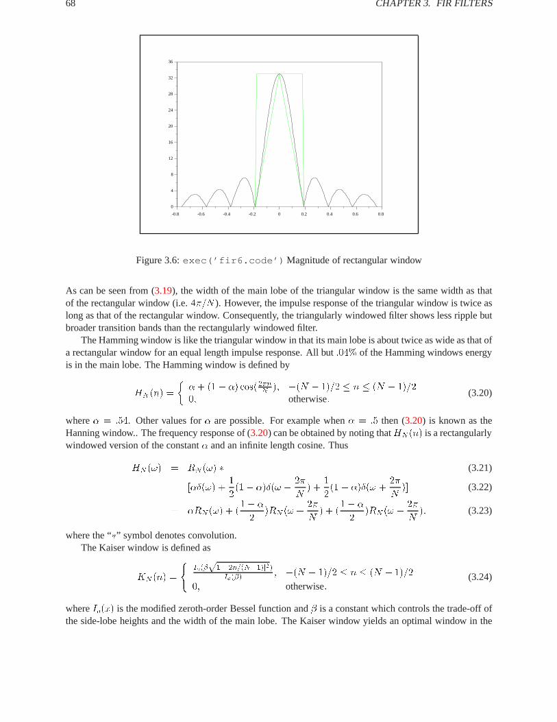
68 CHAPTER3. FIR FILTERS
-0.8 -0.6 -0.4 -0.2 0 0.2 0.4 0.6 0.8
0
4
8
12
16
20
24
28
32
36
Figure 3.6:exec(’fir6.code’) Magnitude of rectangular window
As can be seen from (3.19), the width of the main lobe of the triangular window is the same width as thatof the rectangular window (i.e.4�=N ). However, the impulse response of the triangular window is twice aslong as that of the rectangular window. Consequently, the triangularly windowed filter shows less ripple butbroader transition bands than the rectangularly windowed filter.
The Hamming window is like the triangular window in that its main lobe is about twice as wide as that ofa rectangular window for an equal length impulse response. All but:04% of the Hamming windows energyis in the main lobe. The Hamming window is defined by
HN (n) =
��+ (1� �) cos(2�nN ); �(N � 1)=2 � n � (N � 1)=20; otherwise:
(3.20)
where� = :54. Other values for� are possible. For example when� = :5 then (3.20) is known as theHanning window.. The frequency response of (3.20) can be obtained by noting thatHN (n) is a rectangularlywindowed version of the constant� and an infinite length cosine. Thus
HN (!) = RN (!) � (3.21)
[�Æ(!) +1
2(1� �)Æ(! � 2�
N) +
1
2(1� �)Æ(! +
2�
N)] (3.22)
= �RN (!) + (1� �
2)RN (! +
2�
N) + (
1� �
2)RN (! � 2�
N): (3.23)
where the “�” symbol denotes convolution.The Kaiser window is defined as
KN (n) =
(Io(�
p1�[2n=(N�1)]2)Io(�)
; �(N � 1)=2 � n � (N � 1)=2
0; otherwise:(3.24)
whereIo(x) is the modified zeroth-order Bessel function and� is a constant which controls the trade-off ofthe side-lobe heights and the width of the main lobe. The Kaiser window yields an optimal window in the
3.1. WINDOWING TECHNIQUES 69
sense that the side lobe ripple is minimized in the least squares sense for a certain main lobe width. A closedform for the frequency response of the Kaiser window is not available.
The Chebyshev window is obtained as the inverse DFT of a Chebyshev polynomial evaluated at equallyspaced intervals on the unit circle. The Chebyshev window uniformly minimizes the amount of ripple inthe side lobes for a given main lobe width and filter length. A useful aspect of the design procedure for theChebyshev window is that given any two of the three parameters: the window length,N ; half the main lobewidth, Æf ; the side lobe height,Æp, the third can be determined analytically using the formulas which follow.For Æf andÆp known,N is obtained from
N � 1 +cosh�1((1 + Æp)=(Æp))
cosh�1(1=(cos(�Æf ))): (3.25)
ForN andÆp known,Æf is obtained from
Æf =1
�cos�1(1= cosh(cosh�1((1 + Æp)=Æp)=(N � 1))): (3.26)
Finally, forN andÆf known,Æp is obtained from
Æp = [cosh((N � 1) cosh�1(1= cos(�Æf )))� 1]�1: (3.27)
3.1.3 How to usewfir
The syntax for the functionwfir is as follows can take two formats. The first format is as follows:
--> [wft,wfm,fr]=wfir()
where the parentheses are a required part of the name. This format of the function is interactive and willprompt the user for required input parameters such as the filter type (lp=’low pass’, hp=’high pass’, bp=’bandpass’, sb=’stop band’), filter length (an integern > 2), window type (re=’rectangular’, tr=’triangular’,hm=’hamming’, kr=’kaiser’, ch=’chebyshev’) and other special parameters such as� for the the generalizedHamming window (0 < � < 1) and� for the Kaiser window (� > 0). The three returned arguments are:
� wft: A vector containing the windowed filter coefficients for a filter of length n.
� wfm: A vector of length 256 containing the frequency response of the windowed filter.
� fr: A vector of length 256 containing the frequency axis values (0 � fr� :5) associated to the valuescontained in wfm.
The second format of the function is as follows:
--> [wft,wfm,fr]=wfir(ftype,forder,cfreq,wtype,fpar)
This format of the function is not interactive and, consequently, all the input parameters must be passedas arguments to the function. The first argumentftype indicates the type of filter to be constructed andcan take the values’lp’ , ’hp’ , ’bp’ , andsb’ representing, respectively the filters low-pass, high-pass, band-pass, and stop-band. The argumentforder is a positive integer giving the order of the desiredfilter. The argumentcfreq is a two-vector for which only the first element is used in the case of low-pass and high-pass filters. Under these circumstancescfreq(1) is the cut-off frequency (in normalizedHertz) of the desired filter. For band-pass and stop-band filters both elements ofcfreq are used, thefirst being the low frequency cut-off and the second being the high frequency cut-off of the filter. Bothvalues ofcfreq must be in the range[0; :5) corresponding to the possible values of a discrete frequency

70 CHAPTER3. FIR FILTERS
response. The argumentwtype indicates the type of window desired and can take the values’re’ , ’tr’ ,’hm’ , ’hn’ , ’kr’ , and’ch’ representing, respectively, the windows rectangular, triangular, Hamming,Hanning, Kaiser, and Chebyshev. Finally, the argumentfpar is a two-vector for which only the first elementis used in the case of Kaiser window and for which both elements are used in the case of a Chebyshevwindow. In the case of a Kaiser window the first element offpar indicates the relative trade-off betweenthe main lobe of the window frequency response and the side-lobe height and must be a positive integer. Formore on this parameter see [24]. For the case of the Chebyshev window one can specify either the width ofthe window’s main lobe or the height of the window sidelobes. The first element offpar indicates the side-lobe height and must take a value in the range[0; 1) and the second element gives the main-lobe width andmust take a value in the range[0; :5). The unspecified element of thefpar -vector is indicated by assigningit a negative value. Thus,fpar=[.01,-1] means that the Chebyshev window will have side-lobes ofheight:01 and the main-lobe width is left unspecified.
Note: Because of the properties of FIR linear phase filters it is not possible to design an even length highpass or stop band filter.
3.1.4 Examples
This section gives several examples of windowed filter design. In the first example we choose a low passfilter of lengthn = 33 using a Kaiser window with parameter� = 5:6. The resulting magnitude of thewindowed filter is plotted in Figure3.7where the magnitude axis is given on a log scale.
0 0.1 0.2 0.3 0.4 0.5
-17
-15
-13
-11
-9
-7
-5
-3
-1
1
Figure 3.7:exec(’fir7.code’) Low pass filter with Kaiser window,n = 33, � = 5:6
The second example is a stop band filter of length 127 using a Hamming window with parameter� =:54. The resulting magnitude of the windowed filter is plotted in Figure3.8 where the magnitude is givenon a log scale.
The third example is a band pass filter of length 55 using a Chebyshev window with parameterdp = :001anddf = :0446622. The resulting magnitude of the windowed filter is plotted in Figure3.9 where themagnitude is given on a log scale.

3.1. WINDOWING TECHNIQUES 71
0 0.1 0.2 0.3 0.4 0.5
-13
-11
-9
-7
-5
-3
-1
1
Figure 3.8:exec(’fir8.code’) Stop band filter with Hamming window,n = 127, � = :54
0 0.1 0.2 0.3 0.4 0.5
-8
-7
-6
-5
-4
-3
-2
-1
0
1
Figure 3.9:exec(’fir9.code’) Band pass filter with Chebyshev window,n = 55, dp = :001, df =:0446622
72 CHAPTER3. FIR FILTERS
3.2 Frequency Sampling Technique
This technique is based on specification of a set of samples of the desired frequency response atN uniformlyspaced points around the unit circle, whereN is the filter length. The z-transform of an FIR filter is easilyshown to be :
H(z) =1� z�N
N
N�1Xk=0
H(k)
(1� z�1ej(2�=N)k)(3.28)
This means that one way of approximating any continuous frequency response is tosample in frequency,at N equi-spaced points around the unit circle (the frequency samples), and interpolate between them toobtain the continuous frequency response. Thus, the approximation error will be exactly zero at the samplingfrequencies and finite between them. This fact has to be related to the reconstruction of a continuous functionfrom its samples, as exposed in section2.2for the case of a continuous-time signal.
The interpolation formula for an FIR filter, that is its frequency response, is obtained by evaluating (3.28)on the unit circle:
H(ej!) =e�j!(N�1)=2
N
N�1Xk=0
H(k)e�jk�=N sin(N!=2)
sin(!=2� k�=N)
=e�j!(N�1)=2
N
N�1Xk=0
H(k)S(!; k) (3.29)
where
S(!; k) = e�jk�=Nsin(N!=2)
sin(!=2 � k�=N)
= �e�jk�=N sin(N(!=2) � k�=N)
sin(!=2� k�=N)(3.30)
are the interpolating functions. Thus, the contribution of every frequency sample to the continuous frequencyresponse is proportional to the interpolating functionsin(N!=2)= sin(!=2) shifted byk�=N in frequency.The main drawback of this technique is the lack of flexibility in specifying the transition band width, whichis equal to the number of samples the user decides to put in times�=N , and thus is strongly related toN .Moreover, the specification of frequency samples in transition bands, giving minimum ripple near the bandedges, is not immediate. Nevertheless, it will be seen, in a later chapter on filter optimization techniques,that simple linear programming techniques can be used to drastically reduce the error approximation byoptimizing only those samples located in the transition bands. To illustrate this point, Figure3.10shows theresponse obtained for a type 1 band pass filter with length 65 : first with no sample in the transition bandsand second (dashed curve) with one sample of magnitude .5 in each of these bands. It is worth noting at thispoint that the linear-FIR design problem with arbitrary frequency response specification is more efficientlysolved using a minmax approximation approach, which is exposed in the next section.
Finally, depending on where the initial frequency sample occurs, two distinct sets of frequency samplescan be given, corresponding to the so-called type 1 and type 2 FIR filters :
fk =k
Nk = 0; : : : ; N � 1 for type 1 filters
fk =k + 1=2
Nk = 0; : : : ; N � 1 for type 2 filters

3.2. FREQUENCY SAMPLING TECHNIQUE 73
0 0.1 0.2 0.3 0.4 0.5
-0.2
0
0.2
0.4
0.6
0.8
1.0
1.2
Figure 3.10:exec(’fstyp121.code’) Type 1 band pass filter with no sample or one sample in eachtransition band
The type of design is at user’s will and depends on the application: for example, a band edge may be closerto a type 1 than to a type 2 frequency sampling point. This point is illustrated in Figure3.11for the case ofa low pass filter with length 64 and no sample in the transition band.
The full line (resp. the dashed line) gives the approximated response for the type 1 (resp. type 2) FIRlinear filter. We give now the way the two previous examples have been generated and the code of the func-tion fsfir which calculates the approximated response. Figure3.10was obtained with the following setof instructions :
-->hd=[0*ones(1,15) ones(1,10) 0*ones(1,39)];//desired samples
-->hst1=fsfirlin(hd,1);//filter with no sample in the transition
-->hd(15)=.5;hd(26)=.5;//samples in the transition bands
-->hst2=fsfirlin(hd,1);//corresponding filter
-->pas=1/prod(size(hst1))*.5;
-->fg=0:pas:.5;//normalized frequencies grid
-->n=prod(size(hst1))n =
257.
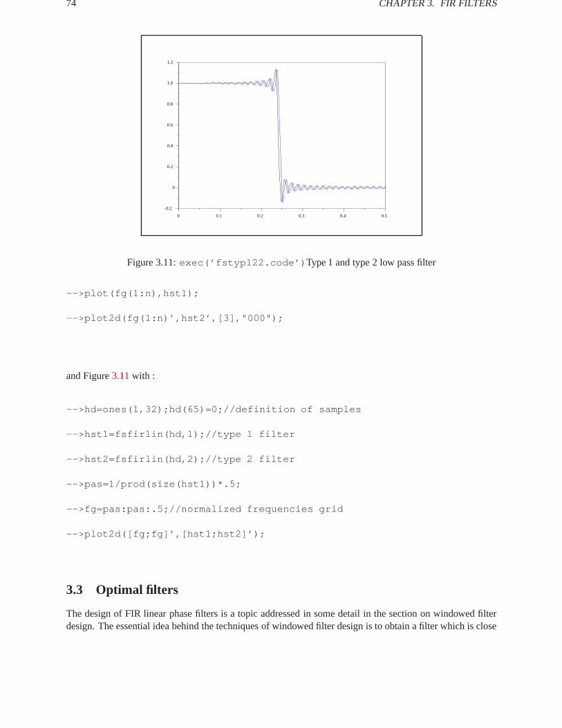
74 CHAPTER3. FIR FILTERS
0 0.1 0.2 0.3 0.4 0.5
-0.2
0
0.2
0.4
0.6
0.8
1.0
1.2
Figure 3.11:exec(’fstyp122.code’) Type 1 and type 2 low pass filter
-->plot(fg(1:n),hst1);
-->plot2d(fg(1:n)’,hst2’,[3],"000");
and Figure3.11with :
-->hd=ones(1,32);hd(65)=0;//definition of samples
-->hst1=fsfirlin(hd,1);//type 1 filter
-->hst2=fsfirlin(hd,2);//type 2 filter
-->pas=1/prod(size(hst1))*.5;
-->fg=pas:pas:.5;//normalized frequencies grid
-->plot2d([fg;fg]’,[hst1;hst2]’);
3.3 Optimal filters
The design of FIR linear phase filters is a topic addressed in some detail in the section on windowed filterdesign. The essential idea behind the techniques of windowed filter design is to obtain a filter which is close
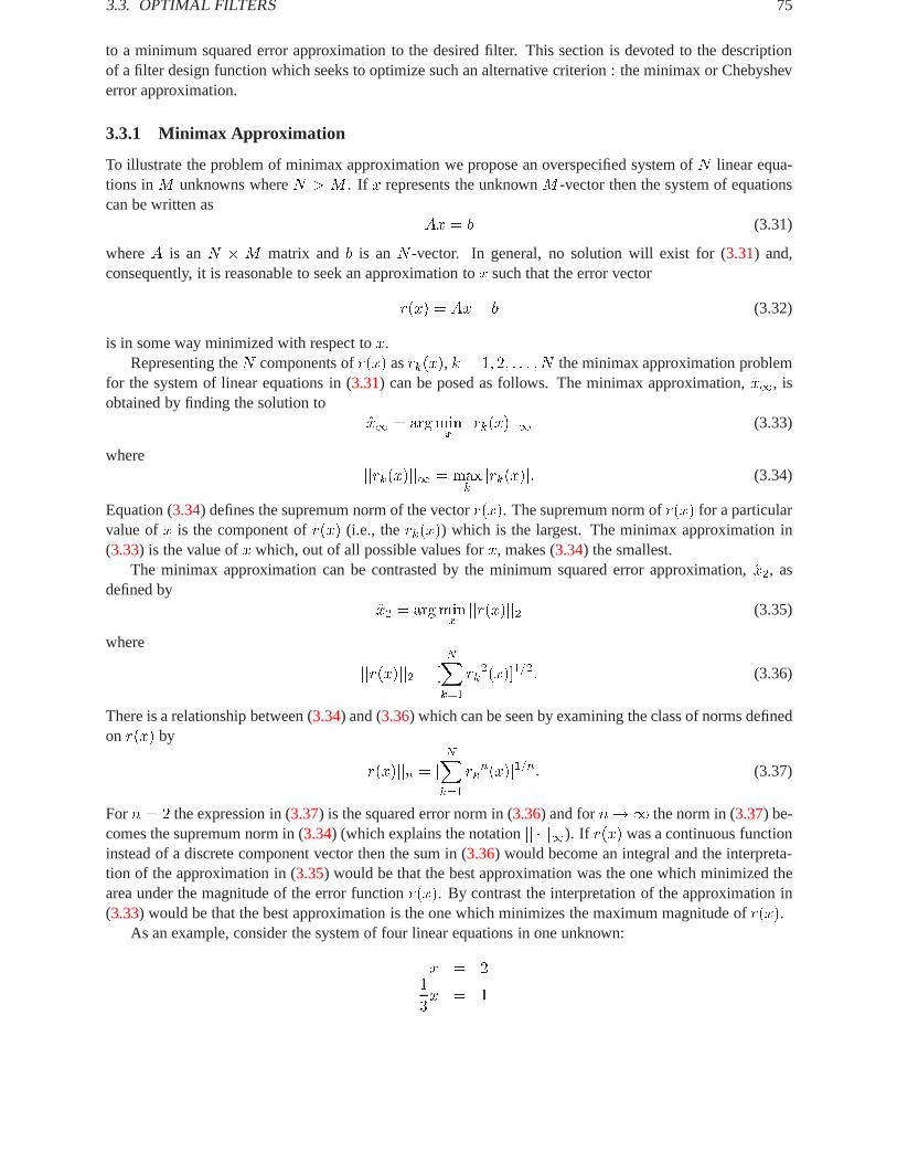
3.3. OPTIMAL FILTERS 75
to a minimum squared error approximation to the desired filter. This section is devoted to the descriptionof a filter design function which seeks to optimize such an alternative criterion : the minimax or Chebysheverror approximation.
3.3.1 Minimax Approximation
To illustrate the problem of minimax approximation we propose an overspecified system ofN linear equa-tions inM unknowns whereN > M . If x represents the unknownM -vector then the system of equationscan be written as
Ax = b (3.31)
whereA is anN � M matrix andb is anN -vector. In general, no solution will exist for (3.31) and,consequently, it is reasonable to seek an approximation tox such that the error vector
r(x) = Ax� b (3.32)
is in some way minimized with respect tox.Representing theN components ofr(x) asrk(x), k = 1; 2; : : : ; N the minimax approximation problem
for the system of linear equations in (3.31) can be posed as follows. The minimax approximation,x1, isobtained by finding the solution to
x1 = argminxjjrk(x)jj1 (3.33)
wherejjrk(x)jj1 = max
kjrk(x)j: (3.34)
Equation (3.34) defines the supremum norm of the vectorr(x). The supremum norm ofr(x) for a particularvalue ofx is the component ofr(x) (i.e., therk(x)) which is the largest. The minimax approximation in(3.33) is the value ofx which, out of all possible values forx, makes (3.34) the smallest.
The minimax approximation can be contrasted by the minimum squared error approximation,x2, asdefined by
x2 = argminxjjr(x)jj2 (3.35)
where
jjr(x)jj2 = [NXk=1
rk2(x)]1=2: (3.36)
There is a relationship between (3.34) and (3.36) which can be seen by examining the class of norms definedon r(x) by
jjr(x)jjn = [
NXk=1
rkn(x)]1=n: (3.37)
Forn = 2 the expression in (3.37) is the squared error norm in (3.36) and forn!1 the norm in (3.37) be-comes the supremum norm in (3.34) (which explains the notationjj � jj1). If r(x) was a continuous functioninstead of a discrete component vector then the sum in (3.36) would become an integral and the interpreta-tion of the approximation in (3.35) would be that the best approximation was the one which minimized thearea under the magnitude of the error functionr(x). By contrast the interpretation of the approximation in(3.33) would be that the best approximation is the one which minimizes the maximum magnitude ofr(x).
As an example, consider the system of four linear equations in one unknown:
x = 21
3x = 1
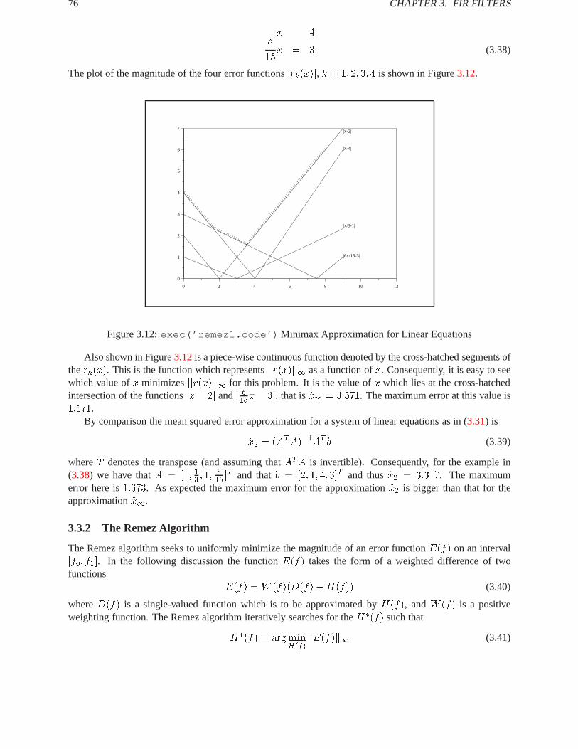
76 CHAPTER3. FIR FILTERS
x = 46
15x = 3 (3.38)
The plot of the magnitude of the four error functionsjrk(x)j, k = 1; 2; 3; 4 is shown in Figure3.12.
0 2 4 6 8 10 12
0
1
2
3
4
5
6
7|x-2|
|x-4|
|x/3-1|
|6x/15-3|
Figure 3.12:exec(’remez1.code’) Minimax Approximation for Linear Equations
Also shown in Figure3.12is a piece-wise continuous function denoted by the cross-hatched segments oftherk(x). This is the function which representsjjr(x)jj1 as a function ofx. Consequently, it is easy to seewhich value ofx minimizesjjr(x)jj1 for this problem. It is the value ofx which lies at the cross-hatchedintersection of the functionsjx� 2j andj 615x� 3j, that isx1 = 3:571. The maximum error at this value is1:571.
By comparison the mean squared error approximation for a system of linear equations as in (3.31) is
x2 = (ATA)�1AT b (3.39)
whereT denotes the transpose (and assuming thatATA is invertible). Consequently, for the example in(3.38) we have thatA = [1; 13 ; 1;
615 ]
T and thatb = [2; 1; 4; 3]T and thusx2 = 3:317. The maximumerror here is1:673. As expected the maximum error for the approximationx2 is bigger than that for theapproximationx1.
3.3.2 The Remez Algorithm
The Remez algorithm seeks to uniformly minimize the magnitude of an error functionE(f) on an interval[f0; f1]. In the following discussion the functionE(f) takes the form of a weighted difference of twofunctions
E(f) =W (f)(D(f)�H(f)) (3.40)
whereD(f) is a single-valued function which is to be approximated byH(f), andW (f) is a positiveweighting function. The Remez algorithm iteratively searches for theH�(f) such that
H�(f) = arg minH(f)
kE(f)k1 (3.41)

3.3. OPTIMAL FILTERS 77
where
kE(f)k1 = maxf0�f�f1
jE(f)j (3.42)
is known as both the Chebyshev and the minimax norm ofE(f). The details of the Remez algorithm can befound in [5].
The functionH(f) is constrained, for our purposes, to the class of functions
H(f) =
NXn=0
an cos(2�fn): (3.43)
Furthermore, we take the interval of approximation to be[0; :5]. Under these conditions the posed problemcorresponds to digital filter design where the functionsH(f) represent the discrete Fourier transform of anFIR, linear phase filter of odd length and even symmetry. Consequently, the functionH(f) can be written
H(f) =
NXn=�N
hne�j2�fn (3.44)
The relationship between the coefficients in (3.43) and (3.44) is an = 2hn for n = 1; 2; : : : ; N anda0 = h0.With respect to the discussion in the previous section the problem posed here can be viewed as an
overspecified system of linear equations in theN + 1 unknowns,an, where the number of equations isuncountably infinite. The Remez algorithm seeks to solve this overspecified system of linear equations inthe minimax sense. The next section describes the Scilab functionremezb and how it can be used to designFIR filters.
3.3.3 Functionremezb
The syntax for the functionremezb is as follows:
--> an=remezb(nc,fg,df,wf)
wheredf andwf are vectors which are sampled values of the functionsD(f) andW (f) (see the previoussection for definition of notation), respectively. The sampled values ofD(f) andW (f) are taken on a gridof points along thef -axis in the interval[0; :5]. The values of the frequency grid are in the vectorfg . Thevalues offg are not obliged to be equi-spaced in the interval[0; :5]. In fact, it is very useful, for certainproblems, to specify anfg which has elements which are equi-spaced in only certain sub-intervals of[0; :5](see the examples in the following section). The value ofnc is the number of cosine functions to be usedin the evaluation of the approximating functionH(f) (see (3.43)). The value of the variablenc must be apositive, odd integer if the problem is to correspond to an FIR filter. Thean are the values of the coefficientsin (3.43) which correspond to the optimalH(f).
To obtain the coefficients of the corresponding FIR filter it suffices to create a vectorhn using the Scilabcommands:
//exec(’remez8.code’)hn(1:nc-1)=an(nc:-1:2)/2;hn(nc)=an(1);hn(nc+1:2*nc-1)=an(2:nc)/2;
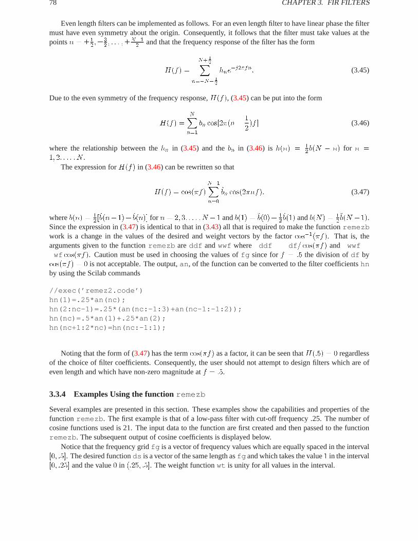
78 CHAPTER3. FIR FILTERS
Even length filters can be implemented as follows. For an even length filter to have linear phase the filtermust have even symmetry about the origin. Consequently, it follows that the filter must take values at thepointsn = �1
2 ;�32 ; : : : ;�N�1
2 and that the frequency response of the filter has the form
H(f) =
N+ 12X
n=�N� 12
hne�j2�fn: (3.45)
Due to the even symmetry of the frequency response,H(f), (3.45) can be put into the form
H(f) =
NXn=1
bn cos[2�(n� 1
2)f ] (3.46)
where the relationship between thehn in (3.45) and thebn in (3.46) is h(n) = 12b(N � n) for n =
1; 2; : : : ; N .The expression forH(f) in (3.46) can be rewritten so that
H(f) = cos(�f)
N�1Xn=0
~bn cos(2�nf): (3.47)
whereb(n) = 12 [~b(n� 1)+~b(n)] for n = 2; 3; : : : ; N � 1 andb(1) = ~b(0)+ 1
2~b(1) andb(N) = 1
2~b(N � 1).
Since the expression in (3.47) is identical to that in (3.43) all that is required to make the functionremezbwork is a change in the values of the desired and weight vectors by the factorcos�1(�f). That is, thearguments given to the functionremezb areddf andwwf where ddf = df = cos(�f) and wwf =
wf cos(�f). Caution must be used in choosing the values offg since forf = :5 the division ofdf bycos(�f) = 0 is not acceptable. The output,an , of the function can be converted to the filter coefficientshnby using the Scilab commands
//exec(’remez2.code’)hn(1)=.25*an(nc);hn(2:nc-1)=.25*(an(nc:-1:3)+an(nc-1:-1:2));hn(nc)=.5*an(1)+.25*an(2);hn(nc+1:2*nc)=hn(nc:-1:1);
Noting that the form of (3.47) has the termcos(�f) as a factor, it can be seen thatH(:5) = 0 regardlessof the choice of filter coefficients. Consequently, the user should not attempt to design filters which are ofeven length and which have non-zero magnitude atf = :5.
3.3.4 Examples Using the functionremezb
Several examples are presented in this section. These examples show the capabilities and properties of thefunction remezb . The first example is that of a low-pass filter with cut-off frequency .25. The number ofcosine functions used is 21. The input data to the function are first created and then passed to the functionremezb . The subsequent output of cosine coefficients is displayed below.
Notice that the frequency gridfg is a vector of frequency values which are equally spaced in the interval[0; :5]. The desired functionds is a vector of the same length asfg and which takes the value1 in the interval[0; :25] and the value0 in (:25; :5]. The weight functionwt is unity for all values in the interval.

3.3. OPTIMAL FILTERS 79
-->nc=21;
-->ngrid=nc*250;
-->fg=.5*(0:(ngrid-1))/(ngrid-1);
-->ds(1:ngrid/2)=ones(1:ngrid/2);
-->ds(ngrid/2+1:ngrid)=0*ones(1:ngrid/2);
-->wt=ones(fg);
-->an=remezb(nc,fg,ds,wt)’an =
! 0.5000000 !! 0.6369345 !! 1.405D-07 !! - 0.2131882 !! - 1.037D-07 !! 0.1289952 !! 6.083D-08 !! - 0.0933182 !! - 2.101D-07 !! 0.0738747 !! 3.184D-07 !! - 0.0618530 !! - 0.0000011 !! 0.0538913 !! 0.0000022 !! - 0.0484436 !! - 0.0000100 !! 0.0447016 !! - 0.0000202 !! - 0.5168409 !! 0.0000417 !! 0. !
As described in the previous section the cosine coefficientsan are converted into the coefficients for a evensymmetry FIR filter which has frequency response as illustrated in Figure3.13.
The error of the solution illustrated in Figure 3.13 is very large; it can become reasonable by leaving atransition band when giving the specification of the frequency grid. The following example shows how thisis done;remezb is specified as follows :
-->nc=21;
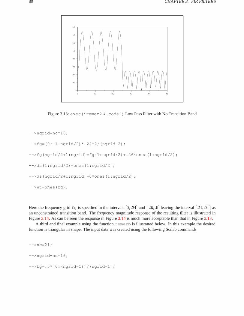
80 CHAPTER3. FIR FILTERS
0 0.1 0.2 0.3 0.4 0.5
0
0.2
0.4
0.6
0.8
1.0
1.2
1.4
1.6
Figure 3.13:exec(’remez2 4.code’) Low Pass Filter with No Transition Band
-->ngrid=nc*16;
-->fg=(0:-1+ngrid/2)*.24*2/(ngrid-2);
-->fg(ngrid/2+1:ngrid)=fg(1:ngrid/2)+.26*ones(1:ngrid/2);
-->ds(1:ngrid/2)=ones(1:ngrid/2);
-->ds(ngrid/2+1:ngrid)=0*ones(1:ngrid/2);
-->wt=ones(fg);
Here the frequency gridfg is specified in the intervals[0; :24] and[:26; :5] leaving the interval[:24; :26] asan unconstrained transition band. The frequency magnitude response of the resulting filter is illustrated inFigure3.14. As can be seen the response in Figure3.14is much more acceptable than that in Figure3.13.
A third and final example using the functionremezb is illustrated below. In this example the desiredfunction is triangular in shape. The input data was created using the following Scilab commands
-->nc=21;
-->ngrid=nc*16;
-->fg=.5*(0:(ngrid-1))/(ngrid-1);
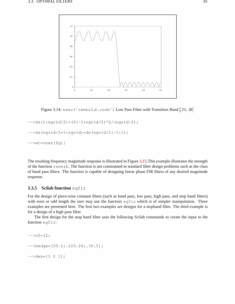
3.3. OPTIMAL FILTERS 81
0 0.1 0.2 0.3 0.4 0.5
0
0.2
0.4
0.6
0.8
1.0
1.2
Figure 3.14:exec(’remez2 4.code’) Low Pass Filter with Transition Band[:24; :26]
-->ds(1:ngrid/2)=(0:-1+ngrid/2)*2/(ngrid-2);
-->ds(ngrid/2+1:ngrid)=ds(ngrid/2:-1:1);
-->wt=ones(fg);
The resulting frequency magnitude response is illustrated in Figure3.15.This example illustrates the strengthof the functionremezb . The function is not constrained to standard filter design problems such as the classof band pass filters. The function is capable of designing linear phase FIR filters of any desired magnituderesponse.
3.3.5 Scilab functioneqfir
For the design of piece-wise constant filters (such as band pass, low pass, high pass, and stop band filters)with even or odd length the user may use the functioneqfir which is of simpler manipulation. Threeexamples are presented here. The first two examples are designs for a stopband filter. The third example isfor a design of a high pass filter.
The first design for the stop band filter uses the following Scilab commands to create the input to thefunctioneqfir :
-->nf=32;
-->bedge=[00.2;.220.28;.30.5];
-->des=[1 0 1];

82 CHAPTER3. FIR FILTERS
0 0.1 0.2 0.3 0.4 0.5
0
0.1
0.2
0.3
0.4
0.5
0.6
0.7
0.8
0.9
1.0
Figure 3.15:exec(’remez2 4.code’) Triangular Shaped Filter
-->wate=[1 1 1];
The resulting magnitude response of the filter coefficients is shown in Figure3.16. As can be seen the designis very bad. This is due to the fact that the design is made with an even length filter and at the same timerequires that the frequency response atf = :5 be non-zero.
The same example withnf = 33 is run with the result shown in Figure3.17.The final example is that of a high pass filter whose input parameters were created as follows:
-->nf=33;
-->bedge=[00.35;.380.5];
-->des=[0 1];
-->wate=[1 1];
The result is displayed in Figure3.18.

3.3. OPTIMAL FILTERS 83
0 0.1 0.2 0.3 0.4 0.5
0.1
0.3
0.5
0.7
0.9
1.1
1.3
1.5
1.7
1.9
Figure 3.16:exec(’remez5 7.code’) Stop Band Filter of Even Length
0 0.1 0.2 0.3 0.4 0.5
0
0.2
0.4
0.6
0.8
1.0
1.2
Figure 3.17:exec(’remez5 7.code’) Stop Band Filter of Odd Length
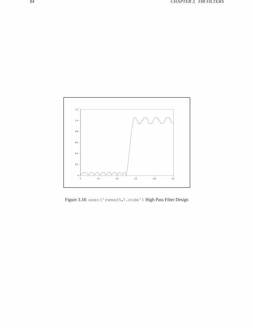
84 CHAPTER3. FIR FILTERS
0 0.1 0.2 0.3 0.4 0.5
0
0.2
0.4
0.6
0.8
1.0
1.2
Figure 3.18:exec(’remez5 7.code’) High Pass Filter Design
Chapter 4
Design of Infinite Impulse Response Filters
4.1 Analog filters
In this section we review some of the most classical analog (or “continuous time”) filters. These are definedin frequency domain as rational transfer functions of the form:
H(s) =
Pmi=0 bis
i
1 +Pn
i=1 aisi
The problem is then to determine theai andbi coefficients or equivalently the zeroszi and polespi of H inorder to meet given specifications of the (squared) magnitude response defined as:
h2(!) = jH(i!)j2 = H(s)H(�s)js=i! (4.1)
Thus,h(!) is the spectrum of the output of a linear filter which admits a white noise as input. We shallconsider in this section only prototype lowpass filters, i.e., ideally we want to obtainh(!) = 0 for ! > !candh(!) = 1 for ! < !c. Highpass, bandpass and stopband filters are then easily constructed by a simplechange of variables.
The construction consists of finding a functionH2 of the complex variables such thatH2(s) = H(s)H(�s)(i.e., is symmetric with respect to the imaginary axis and such thatH2(i!) = h2(!) along the imaginaryaxis). Furthermore, the functionH2(s) will be chosen to be rational and, consequently, defined by its polesand zeros.
The transfer function of the filter,H(s), will then be defined by selecting all the poles and zeros whichlie in the left hand side of the complexs-plane. In this way we obtain a stable and minimum phase filter.
4.1.1 Butterworth Filters
The squared-magnitude response that we want to realize is given by:
h2n(!j!c) =1
1 + (!
!c)2n (4.2)
Here,!c is the cutoff frequency andn the order. A typical response can be plotted with the functionbuttmag (see Figure4.1):
The following code gives an example of the squared magnitude of a Butterworth filter of order 13 (seeFigure4.1).
85

86 CHAPTER4. IIR FILTERS
-->//squared magnitude response of Butterworth filter
-->h=buttmag(13,300,1:1000);
-->mag=20*log(h)’/log(10);
-->plot2d((1:1000)’,mag,[1],"011"," ",[0,-180,1000,20]),
0 100 200 300 400 500 600 700 800 900 1000
-180
-160
-140
-120
-100
-80
-60
-40
-20
0
20
Figure 4.1:exec(’analog1.code’) Magnitude in dB.n = 13; !c = 300
From Figure4.1we see that the magnitude is a decreasing function of the frequency. Also we see that
h2n(!cj!c) =1
2
independently of the ordern.Let us define now the stable transfer functionH(s) (Butterworth filter) by:
H(s) =k0Qn
k=1 (s� pk)
wherepk = ei�[1=2+(2k�1)=2n] k = 1; : : : ; n
This is done by the small functionzpbutt which computes the polespk and the gaink0:For instance, with n=7 and!c = 3, we obtain the following transfer function:
-->n=7;

4.1. ANALOGFILTERS 87
-->omegac=3;
-->[pols,gain]=zpbutt(n,omegac);
-->h=poly(gain,’s’,’coeff’)/real(poly(pols,’s’))h =
2187------------------------------------------------------------------
2 3 42187 + 3276.0963s + 2453.7738s + 1181.9353s + 393.97843s
5 6 7+ 90.880512s + 13.481878s + s
The polespk of H are located on the unit circle and are symmetric with respect to the real axis as isillustrated in Figure4.2. The figure was obtained as follows:
-->//Butterworth filter; 13 poles
-->n=13;
-->angles=ones(1,n)*(%pi/2+%pi/(2*n))+(0:n-1)*%pi/n;
-->s=exp(%i*angles); //Location of the poles
-->xset("mark",0,1);
-->lim=1.2*sqrt(2.);
-->plot2d(real(s)’,imag(s)’,[-3],"012"," ",[-lim,-1.2,lim,1.2]);
-->xarc(-1,1,2,2,0,360*64);
-->xsegs([-lim,0;lim,0],[0,-1.2;0,1.2])
-->xtitle(’Pole positions of Butterworth filter’);
We note the symmetry of the coefficients inH(s) i.e., thatH(s) = ~H(s) = snH(1
s) , which follows
from the fact that for each polepk there corresponds the pole1
pk= pk. Also, we see thatH(�s) is ob-
tained in the same way asH(s) by selecting the (unstable) poles�pk instead of thepk. Since the setf(pk;�pk) k = 1; : : : ; ng is made with the2n roots of the polynomialp(s) = 1 + (�s2)n. Thus, wehave:
H(s)H(�s) = 1
1 + (�s2)n

88 CHAPTER4. IIR FILTERS
⊕⊕
⊕
⊕
⊕
⊕
⊕
⊕
⊕
⊕
⊕⊕
⊕
Pole positions of Butterworth filter
Figure 4.2:exec(’analog2.code’) Butterworth filter: pole positions.n = 13
It follows immediately from (4.1) thatH(s) realizes the response (4.2).We see thatH(s) is obtained by avery simple spectral factorization ofp(s), which here can be done analytically.
Order determination: The filter order,n, completely specifies a Butterworth filter. In generaln is de-termined by giving a desired attenuation1A at a specified “normalized” frequencyf = !r
!c. The filter order,
n, is given by the solution of1A2 = h2n(f). We obtain immediately:
n =log10(A
2 � 1)
2 log10(f)(4.3)
4.1.2 Chebyshev filters
Thenth order Chebyshev polynomialTn(x) is defined recursively by:�Tn+1(x) = 2xTn(x)� Tn�1(x)T0(x) = 1 T1(x) = x
It may be shown thatTn(x) is given more explicitly by:
Tn(x) =
�cos(n cos�1(x)) if jxj < 1
cosh(n cosh�1(x)) otherwise(4.4)
The recursive functionchepol implements this computation: We note that the roots ofTn are real andsymmetric with respect to the imaginary axis. These polynomials are used to analytically define the squared-magnitude of the frequency response for a class of analog filters.
Type 1: Ripple in the passband
For type I Chebyshev filters the squared-magnitude function that we want to realize is:
h21;n(! j !c; �) =1
1 + �2T 2n(
!!c)
(4.5)

4.1. ANALOGFILTERS 89
This function is completely specified once its three parameters(!c; �; n) are given.Usingchepol , it is easy to compute the squared-magnitude response (4.5). The functioncheb1mag
evaluatesh21;n(! j !c; �) for a given sample vector of!0s. Note that for any value ofn one has
h21;n(!c j !c; �) =1
1 + �2
The functionh1 is decreasing for! > !c with “fast” convergence to zero for “large” values of the ordern.The number of oscillations in the passband is also increasing withn. If at ! = !r > !c , h21;n reaches thevalue 1
A2 then the parameters(!c; �; n) and(A;!r) are linked by the equationh21;n(!rj!c; �) = 1A2 which
may be written also as
A2 = 1 + �2T 2n(!r!c
) (4.6)
Using (4.4) this latter equation may be solved more explicitly:n cosh�1(f) = cosh�1(g) with f =!r!c
and
g = A2�1� .
Below is an example of the magnitude plotted in Figure4.3.
-->//Chebyshev; ripple in the passband
-->n=13;epsilon=0.2;omegac=3;sample=0:0.05:10;
-->h=cheb1mag(n,omegac,epsilon,sample);
-->plot(sample,h,’frequencies’,’magnitude’)
0 1 2 3 4 5 6 7 8 9 10
0
0.1
0.2
0.3
0.4
0.5
0.6
0.7
0.8
0.9
1.0magnitude
frequencies
Figure 4.3:exec(’analog3.code’) Magnitude of a Type 1 Chebyshev filter

90 CHAPTER4. IIR FILTERS
Let us now calculate the transfer function of a Type 1 Chebyshev filter. The transfer function is all-poleand the poles lie on an ellipse which can be determined totally by specifying the parameter�, the ordern and
the cutoff frequency!c. The horizontal and vertical raysa andb of this ellipse are given by:a = !c � �1
2
andb = !c + �1
2where
= (1 +
p1 + �2
�)
1=n
The poles(pk = �k + ik; k = 1; 2; : : : ; n) are simple and, in order to have a stable filter, are regularlyspaced over the left hand side of the ellipse. The functionzpch1 computes the poles (and the gain) of aType 1 Chebyshev filter.
With the functionzpch1 we can now calculate the transfer function which realizes the preceding ex-ample and recover the desired magnitude. Compare Figures4.3 and4.4, the latter figure being obtained asfollows:
-->n=13;epsilon=0.2;omegac=3;sample=0:0.05:10;
-->[p,gain]=zpch1(n,epsilon,omegac);
-->//Transfer function computation tr_fct(s)=gain/deno(s)
-->tr_fct=poly(gain,’s’,’coef’)/real(poly(p,’s’))tr_fct =
1946.1951-----------------------------------------------------------------
2 3 41946.1951 + 7652.7444s + 14314.992s + 18875.541s + 17027.684s
5 6 7 8+ 13282.001s + 7398.971s + 3983.2216s + 1452.2192s
9 10 11 12 13+ 574.73496s + 131.30929s + 39.153835s + 4.4505809s + s
-->//Magnitude of the frequency response computed along the
-->//imaginary axis for the values %i*sample...
-->rep=abs(freq(tr_fct(2),tr_fct(3),%i*sample));
-->plot(sample,rep,’frequencies’,’magnitude’)
-->xend()

4.1. ANALOGFILTERS 91
0 1 2 3 4 5 6 7 8 9 10
0
0.1
0.2
0.3
0.4
0.5
0.6
0.7
0.8
0.9
1.0magnitude
frequencies
Figure 4.4:exec(’analog4.code’) Chebyshev filter: frequency response in magnitude
Order determination: We have seen that the parameter� specifies the size of the passband ripple and!cis the passband edge, thus, one has
1
1 + �2� h21;n(! j !c) � 1 for 0 � ! � !c
The ordern is generally determined by specifying a desired attenuation1A at a given “normalized” frequency
f = !r!c
. As in (4.6), n is given by the solution of1A2 = h21;n(f j!c; �):
n =cosh�1(
pA2�1� )
cosh�1(f)=
log(g +p(g2 � 1))
log(f +p(f2 � 1)
whereg =p(A
2�1�2
)
Type 2: Ripple in the stopband
The squared-magnitude response of a Type 2 Chebyshev filter is defined by:
h22;n(! j !r; A) =1
1 + A2�1T 2n(
!r!)
Here!r is the passband edge andA the attenuation at!r. The functioncheb2mag computes the squared-magnitude response. Note that the sample vector must not include the value zero. Also, for any value of theordern one has:
h22;n(!r j !r; A) =1
A2
The function is decreasing for0 < ! < !r and displays ripple for! > !r.Also note that when the equation (4.6) is satisfied both Type 1 and type 2 functionsh1;n andh2;n take
the same values at!c and!r:
h21;n(!rj!c; �) = h22;n(!rj!r; A) =1
A2
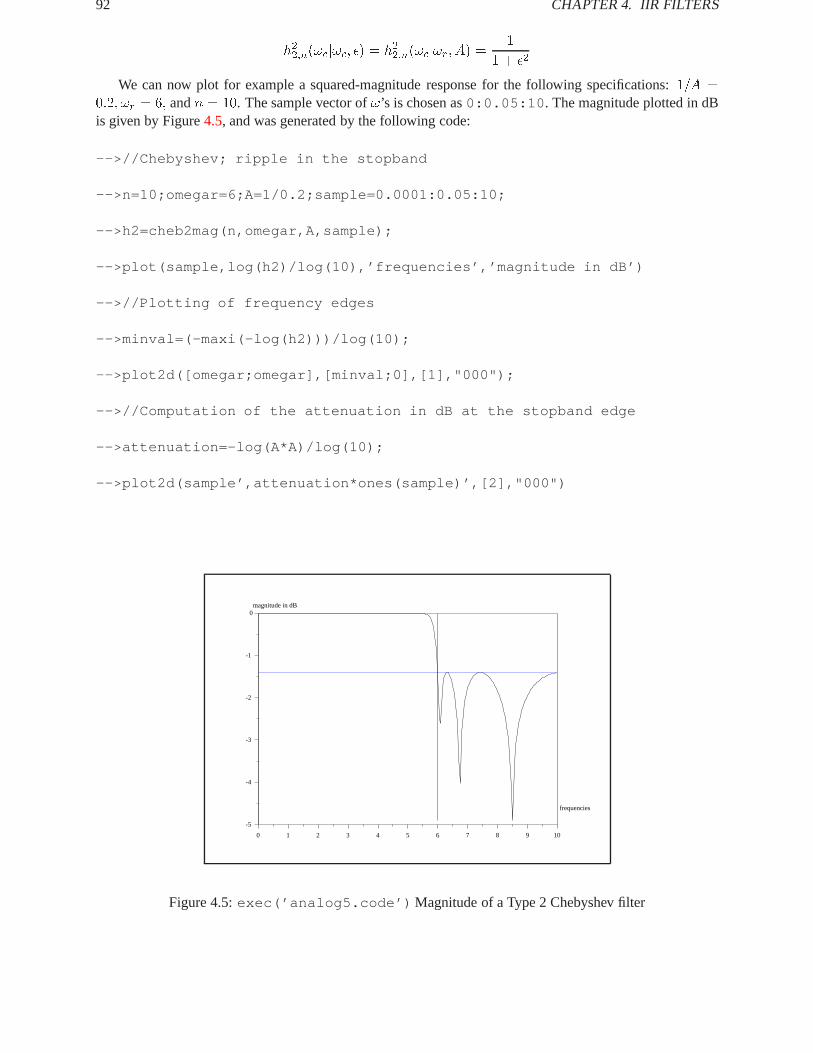
92 CHAPTER4. IIR FILTERS
h22;n(!cj!c; �) = h22;n(!cj!r; A) =1
1 + �2
We can now plot for example a squared-magnitude response for the following specifications:1=A =0:2; !r = 6; andn = 10. The sample vector of!’s is chosen as0:0.05:10 . The magnitude plotted in dBis given by Figure4.5, and was generated by the following code:
-->//Chebyshev; ripple in the stopband
-->n=10;omegar=6;A=1/0.2;sample=0.0001:0.05:10;
-->h2=cheb2mag(n,omegar,A,sample);
-->plot(sample,log(h2)/log(10),’frequencies’,’magnitude in dB’)
-->//Plotting of frequency edges
-->minval=(-maxi(-log(h2)))/log(10);
-->plot2d([omegar;omegar],[minval;0],[1],"000");
-->//Computation of the attenuation in dB at the stopband edge
-->attenuation=-log(A*A)/log(10);
-->plot2d(sample’,attenuation*ones(sample)’,[2],"000")
0 1 2 3 4 5 6 7 8 9 10
-5
-4
-3
-2
-1
0magnitude in dB
frequencies
Figure 4.5:exec(’analog5.code’) Magnitude of a Type 2 Chebyshev filter
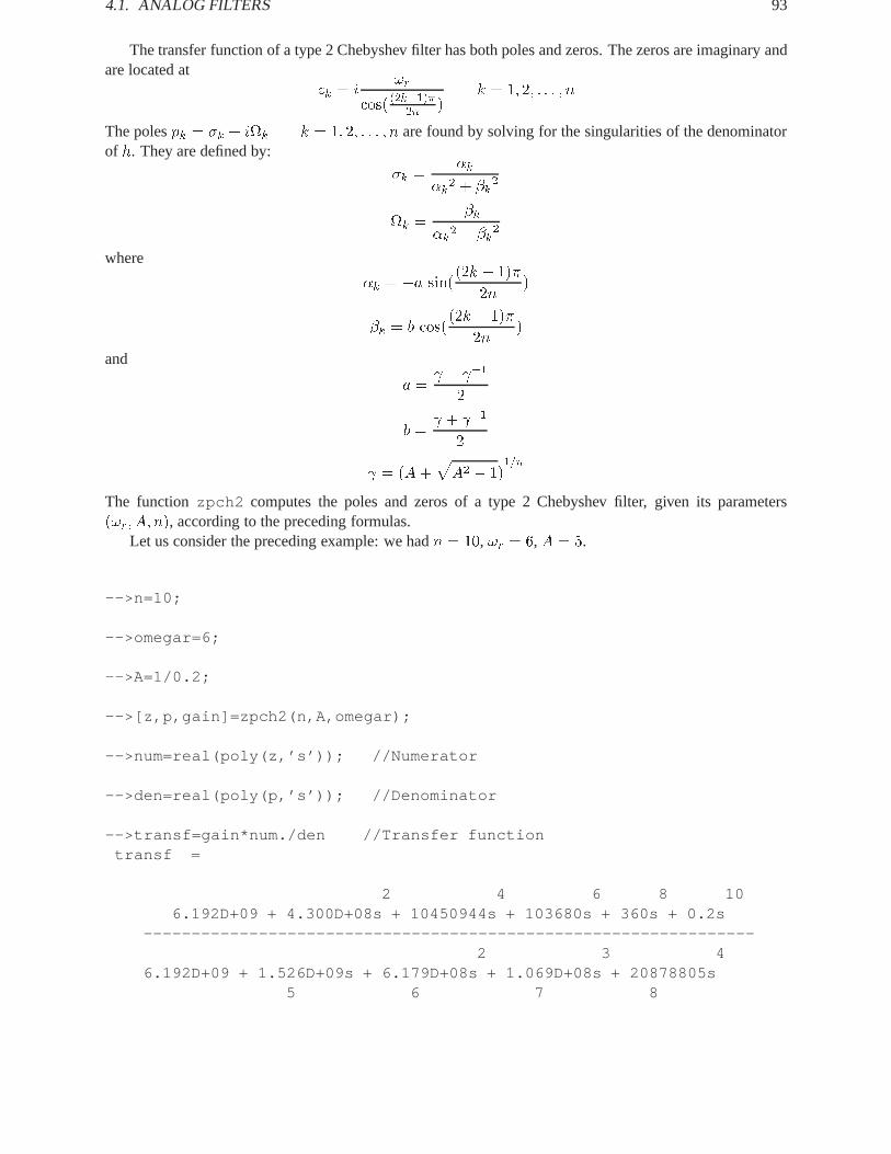
4.1. ANALOGFILTERS 93
The transfer function of a type 2 Chebyshev filter has both poles and zeros. The zeros are imaginary andare located at
zk = i!r
cos( (2k�1)�2n )k = 1; 2; : : : ; n
The polespk = �k + ik k = 1; 2; : : : ; n are found by solving for the singularities of the denominatorof h. They are defined by:
�k =�k
�k2 + �k2
k =��k
�k2 + �k2
where
�k = �a sin((2k � 1)�
2n)
�k = b cos((2k � 1)�
2n)
and
a = � �1
2
b = + �1
2
= (A+pA2 � 1)
1=n
The functionzpch2 computes the poles and zeros of a type 2 Chebyshev filter, given its parameters(!r; A; n), according to the preceding formulas.
Let us consider the preceding example: we hadn = 10, !r = 6, A = 5.
-->n=10;
-->omegar=6;
-->A=1/0.2;
-->[z,p,gain]=zpch2(n,A,omegar);
-->num=real(poly(z,’s’)); //Numerator
-->den=real(poly(p,’s’)); //Denominator
-->transf=gain*num./den //Transfer functiontransf =
2 4 6 8 106.192D+09 + 4.300D+08s + 10450944s + 103680s + 360s + 0.2s
----------------------------------------------------------------2 3 4
6.192D+09 + 1.526D+09s + 6.179D+08s + 1.069D+08s + 20878805s5 6 7 8
94 CHAPTER4. IIR FILTERS
+ 2494608.7s + 282721.94s + 21546.997s + 1329.062s9 10
+ 50.141041s + s
Order determination: We have seen that the parameterA specifies the size of the passband ripple and!ris the stopband edge. Thus, one has
0 � h22;n(! j !r; A) �1
A2for !r � !
The ordern is generally determined by specifying a desired attenuation11+�2
at a given “normalized” fre-quencyf = !r
!c(remember that in order to define a type 2 Chebyshev filter!r must be given). In a similar
way as in (4.6), n is given by the solution of 11+�2
= h22;n(f j!r; A). Because of the symmetry in� andA weobtain the same solution as for type 1 filters:
n =cosh�1(
pA2�1� )
cosh�1(f)=
log(g +p(g2 � 1))
log(f +p(f2 � 1)
whereg =
rA2 � 1
�2
4.1.3 Elliptic filters
The elliptic filter presents ripple in both the passband and stopband. It is based on the properties of theJacobian elliptic function (see [8],[1]) that we briefly introduce now.
Elliptic integral
Let us define forz in the complex plane the function
u(z) =
Z z
0
dt
(1� t2)1=2(1�mt2)1=2(4.7)
wherem is a real constant0 < m < 1. (We will also use the notationu(z;m) when necessary.)
We may assume that the functionsu1 = (1� t2)12 andu2 = (1�mt2)
12 are defined e.g. in the domain
D made of the complex plane cut along the linesfz;Re(z) = �1 andIm(z) < 0g andfz;Re(z) = � 1pm
andIm(z) < 0g. In other words we may choose for these complex functions the determination of the phasebetween��=2 and3�=2. These functions are then completely specified inD by analytic continuation oncewe have fixed their values at0 as being+1.
Let us define now in the above open connected domainD the function
�(t) =1
u1(t)u2(t)=
1
(1� t2)12 (1�mt2)
12
and consider the pathS which encircles the positive right quarter of the complex plane composed of thepositive real axis, the point at infinity and the imaginary axis traversed from1 to zero.
As t increases along the positive real axis the function�(t) first assumes positive real values for0 �t < 1, then for1 < t < 1=
pm, �(t) assumes purely imaginary values and fort > 1=
pm, �(t) assumes

4.1. ANALOGFILTERS 95
real negative values. At1 we have�(t) = 0 and ast decreases from1 to 0 along the imaginary axis�(t)assumes purely imaginary values.
Let us examine now the consequences of these properties on the functionu. Whenz traces the samepathS the functionu(z) traces the border of arectangleR0 with corners at(O;K;K + iK 0; iK 0), eachside being the image of the four parts of the stripS defined above. This follows from the identities:
K(m) =
Z 1
0�(t)dt = �
Z 1
1pm
�(t)dt
and
iK 0(m) =
Z 1pm
1�(t)dt =
Z 1
0�(it)dt
Thus the points(0; 1; 1p(m)
;1) of the real axis are respectively mapped byu into the points(0;K;K +
iK 0; iK 0) of the complex plane and the intervals(0; 1),(1; 1pm),( 1p
m;1) are respectively mapped into the
intervals(0;K),(K;K + iK 0),(K + iK 0; iK 0).It may be shown thatu realizes a conformal mapping of the first quadrant of the complex plane into
the rectangleR0. In particular any pointz with Re(z) � 0 andIm(z) � 0 admits an unique image inthe rectangle. In a similar way we can map, underu, each of the four quadrants of the complex plane intoa rectangleR (called the “fundamental rectangle of periods”) with corners at(�K � iK 0;K � iK 0;K +iK 0;�K + iK 0), made of four smaller rectangles defined asR0 above and having the origin as commonpoint. The functionu defines a one-to-one correspondence of the complex plane intoR.
The functionu has been implemented as the%asn function. This function may receive a real vectorxas argument. The calculation is made componentwise. A specific algorithm [4] is implemented in fortran.We note that it sufficient to be able to computeu(x) for x 2 (0; 1) to haveu(z) for all nonnegative real andpurely imaginary valuesz thanks to the following changes of variable:Z x
1
dt
(t2 � 1)1=2(1�mt2)1=2=
Z y
0
dt
(1� t2)1=2(1�m1t2)1=2
with m1 = 1�m , y2 = 1m1
x2�1x2
andx 2 (1; 1=pm)Z x
1pm
dt
(t2 � 1)1=2(mt2 � 1)1=2=
Z y
0
dt
(1� t2)1=2(1�mt2)1=2
with y2 = 1mx2
andx 2 (1=pm;1)Z x
0
dt
(1 + t2)1=2(1 +mt2)1=2=
Z y
0
dt
(1� t2)1=2(1�m1t2)1=2
with m1 = 1�m andy2 = x2
1+x2 , which givesu for purely imaginary values of its argument.We can now for example use%asn to plot three sides of the rectangleR0 as the image by%asn of
the three associated real intervals (see Figure4.6). Herem = 0:8 and we see that how a linear scale istransformed by%asn (parametric plot). In particular atx = 10 the pointiK 0 is not reached (as expected).
-->//The rectangle R0
-->m=0.8+%eps;
-->z=%asn(1/sqrt(m),m);

96 CHAPTER4. IIR FILTERS
-->K=real(z);KT=imag(z);
-->x2max=1/sqrt(m);
-->x1=0:0.05:1;x2=1:((x2max-1)/20):x2max;x3=x2max:0.05:10;
-->x=[x1,x2,x3];
-->rect=[0,-KT,1.1*K,2*KT]rect =
! 0. - 1.6596236 2.4829259 3.3192472 !
-->y=%asn(x,m);
-->plot2d(real(y)’,imag(y)’,[1],"011"," ",rect);
-->xtitle(’ ’,’real(y)’,’imag(y)’)
-->[n1,n2]=size(x)n2 =
220.n1 =
1.
-->x1=0:0.5:1;x2=1:0.3:x2max;x3=x2max:1:10;
-->x1=[0,0.25,0.5,0.75,1.0,1.1,1.2,1.3,1.4,2,3,4,10]x1 =
column 1 to 10
! 0. 0.25 0.5 0.75 1. 1.1 1.2 1.3 1.4 2. !
column 11 to 13
! 3. 4. 10. !
-->rect=[0,-KT,1.1*K,2*KT]rect =
! 0. - 1.6596236 2.4829259 3.3192472 !
-->y1=%asn(x1,m);
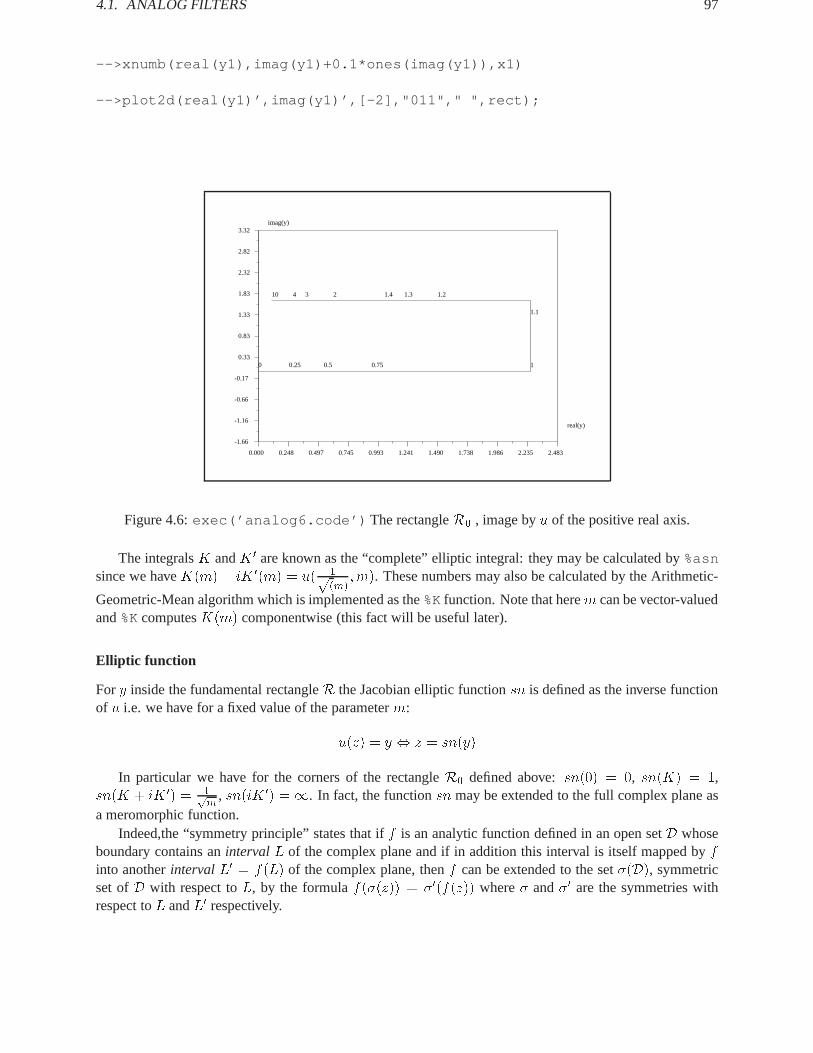
4.1. ANALOGFILTERS 97
-->xnumb(real(y1),imag(y1)+0.1*ones(imag(y1)),x1)
-->plot2d(real(y1)’,imag(y1)’,[-2],"011"," ",rect);
0.000 0.248 0.497 0.745 0.993 1.241 1.490 1.738 1.986 2.235 2.483
-1.66
-1.16
-0.66
-0.17
0.33
0.83
1.33
1.83
2.32
2.82
3.32imag(y)
real(y)
0 0.25 0.5 0.75 1
1.1
1.2 1.3 1.4 2 3 4 10
Figure 4.6:exec(’analog6.code’) The rectangleR0 , image byu of the positive real axis.
The integralsK andK 0 are known as the “complete” elliptic integral: they may be calculated by%asnsince we haveK(m) + iK 0(m) = u( 1p
(m);m). These numbers may also be calculated by the Arithmetic-
Geometric-Mean algorithm which is implemented as the%Kfunction. Note that herem can be vector-valuedand%KcomputesK(m) componentwise (this fact will be useful later).
Elliptic function
Fory inside the fundamental rectangleR the Jacobian elliptic functionsn is defined as the inverse functionof u i.e. we have for a fixed value of the parameterm:
u(z) = y , z = sn(y)
In particular we have for the corners of the rectangleR0 defined above:sn(0) = 0, sn(K) = 1,sn(K + iK 0) = 1p
m, sn(iK 0) =1. In fact, the functionsn may be extended to the full complex plane as
a meromorphic function.Indeed,the “symmetry principle” states that iff is an analytic function defined in an open setD whose
boundary contains anintervalL of the complex plane and if in addition this interval is itself mapped byfinto anotherintervalL0 = f(L) of the complex plane, thenf can be extended to the set�(D), symmetricset ofD with respect toL, by the formulaf(�(z)) = �0(f(z)) where� and�0 are the symmetries withrespect toL andL0 respectively.
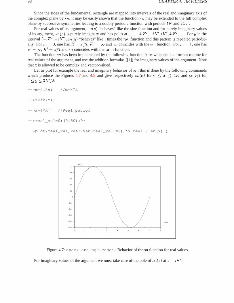
98 CHAPTER4. IIR FILTERS
Since the sides of the fundamental rectangle are mapped into intervals of the real and imaginary axis ofthe complex plane bysn, it may be easily shown that the functionsn may be extended to the full complexplane by successive symmetries leading to a doubly periodic function with periods4K and2iK 0.
For real values of its argument,sn(y) “behaves” like the sine function and for purely imaginary valuesof its argument,sn(y) is purely imaginary and has poles at: : : ;�3iK 0;�iK 0; iK 0; 3iK 0; : : :. Fory in theinterval (�iK 0;+iK 0), sn(y) “behaves” likei times thetan function and this pattern is repeated periodic-ally. Form = 0, one hasK = �=2, K 0 = 1 andsn coincides with thesin function. Form = 1, one hasK =1,K 0 = �=2 andsn coincides with thetanh function.
The functionsn has been implemented by the following function%snwhich calls a fortran routine forreal values of the argument, and use the addition formulas ([1]) for imaginary values of the argument. Notethat x is allowed to be complex and vector-valued.
Let us plot for example the real and imaginary behavior ofsn; this is done by the following commandswhich produce the Figures4.7 and 4.8 and give respectivelysn(x) for 0 � x � 4K and sn(iy) for0 � y � 3K 0=2.
-->m=0.36; //m=kˆ2
-->K=%k(m);
-->P=4*K; //Real period
-->real_val=0:(P/50):P;
-->plot(real_val,real(%sn(real_val,m)),’x real’,’sn(x)’)
0 1 2 3 4 5 6 7 8
-1.0
-0.8
-0.6
-0.4
-0.2
0
0.2
0.4
0.6
0.8
1.0sn(x)
x real
Figure 4.7:exec(’analog7.code’) Behavior of the sn function for real values
For imaginary values of the argument we must take care of the pole ofsn(z) atz = iK 0:

4.1. ANALOGFILTERS 99
-->m=0.36; //m=kˆ2
-->KT=%k(1-m);
-->Ip=2*KT; //Imaginary period
-->ima_val1=[0.:(Ip/50):(KT-0.01)];
-->ima_val2=[(KT+0.01):(Ip/50):(Ip+KT)];
-->z1=%sn(%i*ima_val1,m);z2=%sn(%i*ima_val2,m);
-->rect=[0,-30,Ip+KT,30];
-->plot2d([KT,KT]’,[-30,30]’,[1],"011",’ ’,rect);
-->xtitle(’ ’,’x imaginary’,’sn(x)’) //asymptote
-->plot2d([-30,30]’,[0,0]’,[1],"000");
-->plot2d(ima_val1’,imag(z1)’,[1],"000");
-->plot2d(ima_val2’,imag(z2)’,[1],"000");
0.00 0.60 1.20 1.80 2.39 2.99 3.59 4.19 4.79 5.39 5.99
-30
-24
-18
-12
-6
0
6
12
18
24
30sn(x)
x imaginary
Figure 4.8:exec(’analog8.code’) Behavior of the sn function for imaginary values

100 CHAPTER4. IIR FILTERS
Squared Magnitude Response of Elliptic Filter
The positions of poles and zeros of thesn function will allow to define the squared magnitude response ofa prototype lowpass elliptic filter. The zeros of thesn function are located at2pK + 2qiK 0 ,wherep andqare arbitrary integers and its poles are located at2pK + (2q + 1)K 0.
For a fixed value of the parameterm = m1, let us consider a path�n joining the points(0; nK1; nK1+iK 0
1; iK01) with n anodd integer and denotingK1 = K(m1) andK 0
1 = K(1�m1). From the discussionabove we see that forz 2 (0; nK1) the functionsn(z) oscillates between 0 and 1 periodically as shown inFigure4.7. Forz 2 (nK1; nK+iK 0
1), sn(z) assumes purely imaginary values and increases in magnitude,with (real) limit valuessn(nK1) = 1 andsn(nK1 + iK 0
1) =1pm1
. Finally for z 2 (nK + iK10; iK1
0),sn(z) oscillates periodically betweensn(nK1 + iK1
0) = 1pm1
and1.
For z in the contour�n, let us consider now the function:
v(z) =1
1 + �2sn2(z;m1)(4.8)
Clearly, v(z) oscillates between 1 and11+�2
for z 2 (0; nK1) and between 0 and 1
1+ �2
m1
for z 2 (nK1 +
iK10; iK1
0). Also, clearlyv(z) is a continuous function ofz, which is real-valued forz in the path�n
and if we chose the parameterm1 = �2
A2�1 we can obtain an interesting behavior. The functionell1magcomputesv(z) for a given sample vectorz in the complex plane and for given parameters� andm1.
Now, we define the vectorz = [z1; z2; z3] as a discretization of the path�n, with z1 a dicretization of(0; nK1), z2 a discretization of(nK1; nK1 + ik1
0) andz3 a discretization of(nK1 + iK10; iK1
0). Then wecan produce Figure4.9which clearly shows the behavior ofv(z) for the above three parts ofz.
-->n=9;eps=0.2;A=3;m1=eps*eps/(A*A-1);
-->K1=%k(m1);K1T=%k(1-m1);
-->z1max=n*K1;z2max=K1T;
-->z1=0:(z1max/100):z1max;
-->z2=%i*(0:(z2max/50):z2max);z2=z2+z1max*ones(z2);
-->z3=z1max:-(z1max/100):0;z3=z3+%i*z2max*ones(z3);
-->plot(ell1mag(eps,m1,[z1,z2,z3]));
-->omc=prod(size(z1));
-->omr=prod(size([z1,z2]));
-->plot2d([omc,omc]’,[0,1]’,[2],"000");
-->plot2d([omr,omr]’,[0,1]’,[2],"000");

4.1. ANALOGFILTERS 101
0 40 80 120 160 200 240 280
-0.1
0.1
0.3
0.5
0.7
0.9
1.1
Figure 4.9:exec(’analog9.code’) v(z) for z in�n, with n = 9
Of course, many other paths than�n are possible, giving a large variety of different behaviors. Notethat the number of oscillations in both the passband and stopband isn, an arbitrary odd integer and theamplitudes of the oscillations are entirely specified by the choice of the parameterm1.
Thus, we have obtained a functionv whose behavior seems to correspond to a “good” squared magnitudefor the prototype filter that we want to realize. However, this function is defined along the path�n of thecomplex plane. Since frequencies,!, are given as positive real values we must find a mapping of the positivereal axis onto the path�n. But this is precisely done by the functionu(z) = sn�1(z) given in (4.7) or moregenerally, after scaling by the function�sn�1( z
!c;m) + �. Indeed, as we have seen, such a function maps
the positive real axis into the border of a rectangleR(�; �;m). The size of this rectangle depends on theparameterm and we have to chosem;�; � such thatR(�; �;m) = �n.
To be more specific, we have to choose now the value of the parameterm such that:
�sn(nK1;m) + � = !c (4.9)
�sn(nK1 + iK 01;m) + � = !r (4.10)
Recalling thatsn�1(1;m) = K(m) andsn�1( 1pm;m) = K(m) + iK 0(m) we see that to satisfy these
equations we must chose
� =nK1
K=K1
0
K 0
and
� =
�0 if n is oddK1 if n is even
In particular, we obtain that the parametersn, m1 = �2
A2�1 andm = !c2
!r2of the filter cannot be chosen
independently but that they must satisfy the equation:
n =K 0(m1)
K(m1)
K(m)
K 0(m)=�1�
(4.11)

102 CHAPTER4. IIR FILTERS
(We note�1 =K0(m1)K(m1)
= K(1�m1)K(m1)
and� = K0(m)K(m) = K(1�m)
K(m) ). Usuallym1 is “small” (close to 0) whichyields�1 “large”, andm is “large” (close to 1) which yields� “large”.
In practice very good specifications are obtained with rather low orders. In order to plot the frequencyresponse magnitude of an elliptic prototype lowpass filter we can proceed as follows: first select the ripple
parameters� andA and computem1 = �2
A2�1 and�1 =K01
K1 , then for various integer values ofn computem such that equation (4.11) is satisfied or until the ratio!r!c is acceptable.
See Figure4.10
-->mm1=0:0.01:1;mm1(1)=0.00000001;mm1(101)=0.9999;
-->m=0*mm1;n=3;i=1;
-->anorm=1.-2.*%eps;
-->for m1=mm1,--> y=%asn(anorm/sqrt(m1),m1);--> K1=real(y);--> K12=imag(y);--> chi1=K12/K1;--> m(i)=findm(chi1/n);--> i=i+1;-->end,
-->plot(real(log(mm1)),real(log(m))),
Much flexibility is allowed in the choice of the parameters, provided that equation (4.11) is satisfied.The functionsfind freq andfind ripple may be used to find the stopband edge!r when!c, �, A,andn are given and to find� when the parametersn, !c, !r, andA are given.
The following code shows how to find compatible parameters and produce Figure4.11.
-->deff(’[alpha,beta]=alpha_beta(n,m,m1)’,...-->’if 2*int(n/2)=n then, beta=K1; else, beta=0;end;...-->alpha=%k(1-m1)/%k(1-m);’)
Warning: obsolete use of = instead of ==if 2*int(n/2)=n then, beta=K1; else, beta=0;end;alpha=%k(1-m1)/%k(1-m);
!at line 2 of function alpha_beta called by :beta=0;end;alpha=%k(1-m1)/%k(1-m);’
-->epsilon=0.1;
-->A=10; //ripple parameters

4.1. ANALOGFILTERS 103
-20 -18 -16 -14 -12 -10 -8 -6 -4 -2 0
-5
-4
-3
-2
-1
0
Figure 4.10:exec(’analog10.code’) log(m) versuslog(m1) for ordern fixed
-->m1=(epsilon*epsilon)/(A*A-1);n=5;omegac=6;
-->m=find_freq(epsilon,A,n);
-->omegar = omegac/sqrt(m)omegar =
6.8315017
-->%k(1-m1)*%k(m)/(%k(m1)*%k(1-m))-n //Check...ans =
1.776D-15
-->[alpha,beta]=alpha_beta(n,m,m1)beta =
0.alpha =
3.5754638
-->alpha*%asn(1,m)-n*%k(m1) //Checkans =
3.553D-15

104 CHAPTER4. IIR FILTERS
-->sample=0:0.01:20;
-->//Now we map the positive real axis into the contour...
-->z=alpha*%asn(sample/omegac,m)+beta*ones(sample);
-->plot(sample,ell1mag(epsilon,m1,z))
0 2 4 6 8 10 12 14 16 18 20
0
0.1
0.2
0.3
0.4
0.5
0.6
0.7
0.8
0.9
1.0
Figure 4.11:exec(’analog11.code’) Response of Prototype Elliptic Filter
Construction of the elliptic filter
The design of an elliptic filter is more complex than for the filters that we have defined until now. First theparametersn, m1, andm which characterize the squared magnitude response cannot be chosen independ-ently (see (4.11)). We have seen how to solve this difficulty. Second, the squared magnitude response is nota rational function and moreover it has an infinite number of poles and zeros.
The construction is accomplished in two steps: first a transformation is made in the complex plane whichmaps the real axis to the imaginary axis and transforms the rectangular path�n to a rectangular path�0nin the LHS of the complex plane. Then the elliptic functionsn is used to perform a transformation whichmaps the imaginary axis into�0n. Finally, only poles and zeros which are inside�0n are kept for the transferfunction.
Let us consider the pole-zero pattern of the functionv(z). Clearly, the poles ofsn(z) become doublezeros ofv(z) and the poles ofv(z) are found by solving the equation:
1 + �2 sn2(z) = 0

4.1. ANALOGFILTERS 105
Thus the zeros ofv(z) in �n are located atiK 0; iK 0 + 2K; iK 0 + 4K; : : : ; iK 0 + 2pK and the polesof v(z) in �n are located ati u0; i u0+2K; i u0+4K; : : : ; i u0+2pK with 2p+1 = n and where we havenotedu0 = sn�1( i� ;m1).
Consider now the transformation� = i K0(m)K0(m1)
u = i K(m)nK(m1)
u (n being given in (4.11)). The abovepole-zero pole pattern is mapped inside the LHS of the complex plane and the contour�n is mapped into�0n = (0; iK;�iK 0+K;�K 0), and these points are respectively the image of the points(0; i !c; i !r; i1)of the imaginary axis by the functionz ! i !c sn(�iz;m).
The functionzpell performs these transformations and computes the poles and zeros of a prototypeelliptic filter.
We illustrate the use of this function by the following example which uses the preceding numericalvalues of the parameters�,A, !c, !r. The code produces Figure4.12.
-->//Filter with zpell
-->epsilon=0.1;A=10; //ripple parameters
-->m1=(epsilon*epsilon)/(A*A-1);n=5;omegac=6;
-->m=find_freq(epsilon,A,n);
-->omegar = omegac/sqrt(m)omegar =
6.8315017
-->[z,p,g]=zpell(epsilon,A,omegac,omegar);
-->//Now computes transfer function
-->num=real(poly(z,’s’));den=real(poly(p,’s’));
-->transfer=g*num/dentransfer =
2 410783.501 + 340.56385s + 2.454884s
----------------------------------------------------------------2 3 4 5
10783.501 + 3123.7307s + 773.85348s + 120.79402s + 11.89508s + s
-->//Plot of the response
-->sample=0:0.01:20;
-->rep=freq(g*num,den,%i*sample);
-->plot(sample,abs(rep))
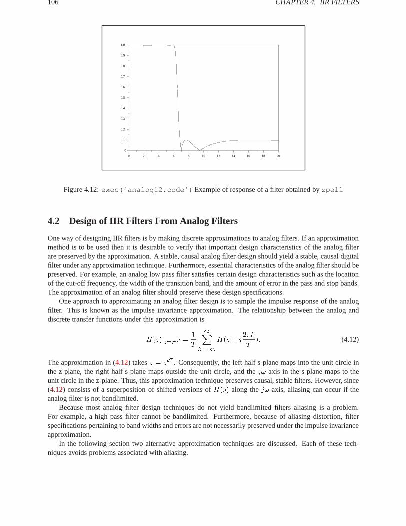
106 CHAPTER4. IIR FILTERS
0 2 4 6 8 10 12 14 16 18 20
0
0.1
0.2
0.3
0.4
0.5
0.6
0.7
0.8
0.9
1.0
Figure 4.12:exec(’analog12.code’) Example of response of a filter obtained byzpell
4.2 Design of IIR Filters From Analog Filters
One way of designing IIR filters is by making discrete approximations to analog filters. If an approximationmethod is to be used then it is desirable to verify that important design characteristics of the analog filterare preserved by the approximation. A stable, causal analog filter design should yield a stable, causal digitalfilter under any approximation technique. Furthermore, essential characteristics of the analog filter should bepreserved. For example, an analog low pass filter satisfies certain design characteristics such as the locationof the cut-off frequency, the width of the transition band, and the amount of error in the pass and stop bands.The approximation of an analog filter should preserve these design specifications.
One approach to approximating an analog filter design is to sample the impulse response of the analogfilter. This is known as the impulse invariance approximation. The relationship between the analog anddiscrete transfer functions under this approximation is
H(z)jz=esT =1
T
1Xk=�1
H(s+ j2�k
T): (4.12)
The approximation in (4.12) takesz = esT . Consequently, the left half s-plane maps into the unit circle inthe z-plane, the right half s-plane maps outside the unit circle, and thej!-axis in the s-plane maps to theunit circle in the z-plane. Thus, this approximation technique preserves causal, stable filters. However, since(4.12) consists of a superposition of shifted versions ofH(s) along thej!-axis, aliasing can occur if theanalog filter is not bandlimited.
Because most analog filter design techniques do not yield bandlimited filters aliasing is a problem.For example, a high pass filter cannot be bandlimited. Furthermore, because of aliasing distortion, filterspecifications pertaining to band widths and errors are not necessarily preserved under the impulse invarianceapproximation.
In the following section two alternative approximation techniques are discussed. Each of these tech-niques avoids problems associated with aliasing.

4.3. APPROXIM ATION OF ANALOGFILTERS 107
4.3 Approximation of Analog Filters
4.3.1 Approximation of the Derivative
Consider an analog filter which can be represented by a rational transfer function,H(s), where
H(s) = B(s)=A(s) (4.13)
andA(s) andB(s) are polynomial functions ofs. The relationship between the input,X(s), and the output,Y (s), of the filter in (4.13) can be expressed as
Y (s) = H(s)X(s) (4.14)
or because of the rational nature ofH(s)
[
NXn=0
ansn]Y (s) = [
MXm=0
bmsm]X(s) (4.15)
where thefang and thefbmg are the coefficients of the polynomial functionsA(s) andB(s), respectively.The relationship between the input and the output in the time domain is directly inferred from (4.15),
NXn=0
andn
dtny(t) =
MXm=0
bmdm
dtmx(t): (4.16)
The differential equation in (4.16) can be approximated by using the Backward Difference Formula approx-imation to the derivative. That is, forT small we take
y0(t)jnT � y(nT )� y(nT � T )
T: (4.17)
Because the operation in (4.17) is linear and time-invariant the approximation can be represented by thez-transform,
Zfy0(n)g = (1� z�1
T)Zfy(n)g (4.18)
whereZf�g represents the z-transform operation andy0(n) andy(n) are sampled sequences of the timefunctionsy0(t) andy(t), respectively.
Higher order derivatives can be approximated by repeated application of (4.17) which in turn can berepresented with the z-transform by repeated multiplication by the factor(1 � z�1)=T . Consequently, theresult in (4.16) can be approximately represented by the z-transform as
[
NXn=0
an(1� z�1
T)n]Y (z) = [
MXm=0
bm(1� z�1
T)m]X(z): (4.19)
Comparing (4.19) to (4.15) allows an identification of a transform from the s-plane to the z-plane,
s =1� z�1
T: (4.20)
Solving (4.20) for z yields
z =1
1� sT: (4.21)
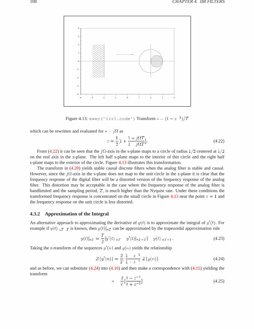
108 CHAPTER4. IIR FILTERS
-4 -3 -2 -1 0 1 2 3 4
-4
-3
-2
-1
0
1
2
3
4
Figure 4.13:exec(’iir1.code’) Transforms = (1� z�1)=T
which can be rewritten and evaluated fors = j as
z =1
2[1 +
1 + jT
1� jT]: (4.22)
From (4.22) it can be seen that thej-axis in the s-plane maps to a circle of radius1=2 centered at1=2on the real axis in the z-plane. The left half s-plane maps to the interior of this circle and the right halfs-plane maps to the exterior of the circle. Figure4.13illustrates this transformation.
The transform in (4.20) yields stable causal discrete filters when the analog filter is stable and causal.However, since thej-axis in the s-plane does not map to the unit circle in the z-plane it is clear that thefrequency response of the digital filter will be a distorted version of the frequency response of the analogfilter. This distortion may be acceptable in the case where the frequency response of the analog filter isbandlimited and the sampling period,T , is much higher than the Nyquist rate. Under these conditions thetransformed frequency response is concentrated on the small circle in Figure4.13near the pointz = 1 andthe frequency response on the unit circle is less distorted.
4.3.2 Approximation of the Integral
An alternative approach to approximating the derivative ofy(t) is to approximate the integral ofy0(t). Forexample ify(t)jnT�T is known, theny(t)jnT can be approximated by the trapezoidal approximation rule
y(t)jnT =T
2[y0(t)jnT � y0(t)jnT�T ] + y(t)jnT�T : (4.23)
Taking the z-transform of the sequencesy0(n) andy(n) yields the relationship
Zfy0(n)g = 2
T[1� z�1
1 + z�1]Zfy(n)g (4.24)
and as before, we can substitute (4.24) into (4.16) and then make a correspondence with (4.15) yielding thetransform
s =2
T[1� z�1
1 + z�1] (4.25)
4.4. DESIGN OF LOW PASSFILTERS 109
between the s-plane and the z-plane. The expression in (4.25) is known as the bilinear transform.Solving (4.25) for z yields
z =1 + (sT=2)
1� (sT=2)(4.26)
and evaluating (4.26) for s = j gives
z =1 + (jT=2)
1� (jT=2): (4.27)
The expression in (4.27) is an all-pass transformation which has unit magnitude and phase which takesvalues from�� to � on the unit circle as goes from�1 to 1. The transformation in (4.26) maps theleft half s-plane into the unit circle in the z-plane and the right half s-plane outside of the unit circle in the z-plane. Consequently, stable causal analog filters yield stable causal digital filters under this transformation.Furthermore, thej-axis in the s-plane maps to the unit circle in the z-plane. The mapping of thej-axisonto the unit circle is not linear and, thus, there is a frequency warping distortion of the analog filter designwhen this transform is used.
Because many filters of interest, such as low pass, band pass, band pass, and stop band filters havemagnitudes which are piece-wise constant, frequency warping distortion is of no consequence. That is, thebilinear transformation maintains the characteristics of the analog filter design. However, if, in addition, thephase of the analog filter is linear, the bilinear transformation will destroy this property when used to obtaina digital filter.
4.4 Design of Low Pass Filters
For piece-wise constant specifications, the bilinear transform is the best of the three possible transformsdiscussed for converting analog filter designs into digital filter designs. Here we discuss how to use thebilinear transform to design a standard digital low pass filter. The next section presents a series of othertransformations which can be used to convert a digital low pass filter into a high pass, band pass, stop band,or another low pass filter.
To effectively use the bilinear transform to design digital filters, it is necessary to transform the digitalfilter constraints into analog filter constraints. Evaluating (4.25) at z = ej! yields
s =2j
Ttan(!=2) = � + j: (4.28)
Thus, a digital filter constraint at! corresponds to an analog filter constraint at
=2
Ttan(!=2): (4.29)
Consequently, to design a digital low pass filter with cut-off frequency!c first requires an analog low passfilter design with cut-off frequency
c = 2 tan(!c=2): (4.30)
(where we have used (4.29) with T = 1).Any of the analog low pass filter design techniques already discussed (such as the Butterworth, Cheby-
shev, and elliptic filter designs) can be used to obtain the digital low pass filter design. The choice of modelorder can be made by specifying additional constraints on the filter design. For example, specification ofa certain amount of attenuation at a specified frequency in the stop band can be used to obtain the modelorder of a Butterworth Filter. Such a specification for a digital filter would be converted to an analog filterspecification using (4.29) before designing the analog filter. More on filter order specification can be foundin the section on analog filter design.

110 CHAPTER4. IIR FILTERS
An example of a typical digital low-pass filter design from a Chebyshev analog filter design of the firsttype is as follows. The digital low-pass filter is to have a cut-off frequency of�=2. This constraint istransformed to an analog constraint using (4.30). The resulting analog constraint takes the cut-off frequencyto be2 tan(�=4) = 2. Now the functionzpch1 is used to design the Chebyshev filter of the first type oforder 3 and passband ripple of .05. Since the ripple of a Chebyshev filter is1=(1 + �2) it follows that for aripple of .05 in the passband that� =
p(1=:95) � 1 = :22942. Thus, the call to the function looks like
-->[pols,gn]=zpch1(3,.22942,2);
-->gngn =
8.7176358
-->pols’ans =
! - 0.7915862 - 2.2090329i !! - 1.5831724 - 1.562D-16i !! - 0.7915862 + 2.2090329i !
-->hs=gn/real(poly(pols,’s’))hs =
8.7176358---------------------------------------
2 38.7176358 + 8.0128698s + 3.1663448s + s
where the transfer functionhs is calculated from the gain and the poles returned from the function. Themagnitude of the the transfer function can be plotted as follows
gn =
8.7176358ans =
! - 0.7915862 - 2.2090329i !! - 1.5831724 - 1.562D-16i !! - 0.7915862 + 2.2090329i !
hs =
8.7176358---------------------------------------
2 38.7176358 + 8.0128698s + 3.1663448s + s
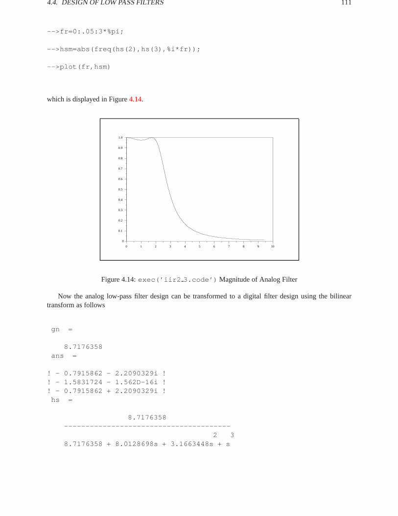
4.4. DESIGN OF LOW PASSFILTERS 111
-->fr=0:.05:3*%pi;
-->hsm=abs(freq(hs(2),hs(3),%i*fr));
-->plot(fr,hsm)
which is displayed in Figure4.14.
0 1 2 3 4 5 6 7 8 9 10
0
0.1
0.2
0.3
0.4
0.5
0.6
0.7
0.8
0.9
1.0
Figure 4.14:exec(’iir2 3.code’) Magnitude of Analog Filter
Now the analog low-pass filter design can be transformed to a digital filter design using the bilineartransform as follows
gn =
8.7176358ans =
! - 0.7915862 - 2.2090329i !! - 1.5831724 - 1.562D-16i !! - 0.7915862 + 2.2090329i !
hs =
8.7176358---------------------------------------
2 38.7176358 + 8.0128698s + 3.1663448s + s
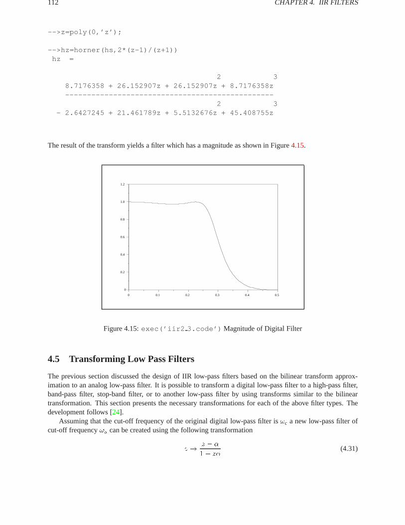
112 CHAPTER4. IIR FILTERS
-->z=poly(0,’z’);
-->hz=horner(hs,2*(z-1)/(z+1))hz =
2 38.7176358 + 26.152907z + 26.152907z + 8.7176358z------------------------------------------------
2 3- 2.6427245 + 21.461789z + 5.5132676z + 45.408755z
The result of the transform yields a filter which has a magnitude as shown in Figure4.15.
0 0.1 0.2 0.3 0.4 0.5
0
0.2
0.4
0.6
0.8
1.0
1.2
Figure 4.15:exec(’iir2 3.code’) Magnitude of Digital Filter
4.5 Transforming Low Pass Filters
The previous section discussed the design of IIR low-pass filters based on the bilinear transform approx-imation to an analog low-pass filter. It is possible to transform a digital low-pass filter to a high-pass filter,band-pass filter, stop-band filter, or to another low-pass filter by using transforms similar to the bilineartransformation. This section presents the necessary transformations for each of the above filter types. Thedevelopment follows [24].
Assuming that the cut-off frequency of the original digital low-pass filter is!c a new low-pass filter ofcut-off frequency!u can be created using the following transformation
z ! z � �
1� z�(4.31)

4.6. HOW TO USE THE FUNCTION IIR 113
where
� =sin[(!c � !u)=2]
sin[(!c + !u)=2]: (4.32)
For a high-pass filter of cut-off frequency!u one can use the transformation
z ! � z + �
1 + z�(4.33)
where
� = �cos[(!c � !u)=2]
cos[(!c + !u)=2]: (4.34)
For a band-pass filter with!u and!l the upper and lower band edges, respectively, one would use thetransformation
z ! � z2 � (2�k=(k + 1))z + ((k � 1)=(k + 1))
1� (2�k=(k + 1))z + ((k � 1)=(k + 1))z2(4.35)
where
� =cos[(!u + !l)=2]
cos[(!u � !l)=2](4.36)
andk = cot[(!u � !l)=2] tan(!c=2): (4.37)
Finally, for a stop-band filter with!u and!l the upper and lower band edges, respectivly, the followingtransformation is used
z ! z2 � (2�=(k + 1))z � ((k � 1)=(k + 1))
1� (2�=(k + 1))z � ((k � 1)=(k + 1))z2(4.38)
where
� =cos[(!u + !l)=2]
cos[(!u � !l)=2](4.39)
andk = tan[(!u � !l)=2] tan(!c=2): (4.40)
4.6 How to Use the Functioniir
The call to the functioniir has the following syntax
--> [hz]=iir(n,ftype,fdesign,frq,delta)
The argumentn is the filter order which must be a positive integer. The argumentftype is the filter typeand can take values’lp’ for a low-pass filter,’hp’ for a high-pass filter,’bp’ for a band-pass filter, or’sb’ for a stop-band filter.
The argumentfdesign indicates the type of analog filter design technique is to be used to design thefilter. The value offdesign can be’butt’ for a Butterworth filter design,’cheb1’ for a Chebyshevfilter design of the first type,’cheb2’ for a Chebyshev filter design of the second type, or’ellip’ foran elliptic filter design.
The argumentfrq is a two-vector which contains cut-off frequencies of the desired filter. For low-passand high-pass filters only the first element of this vector is used. The first element indicates the cut-offfrequency of the desired filter. The second element of this vector is used for band-pass and stop-band filters.This second element is the upper band edge of the band-pass or stop-band filter, whereas the first element ofthe vector is the lower band edge.
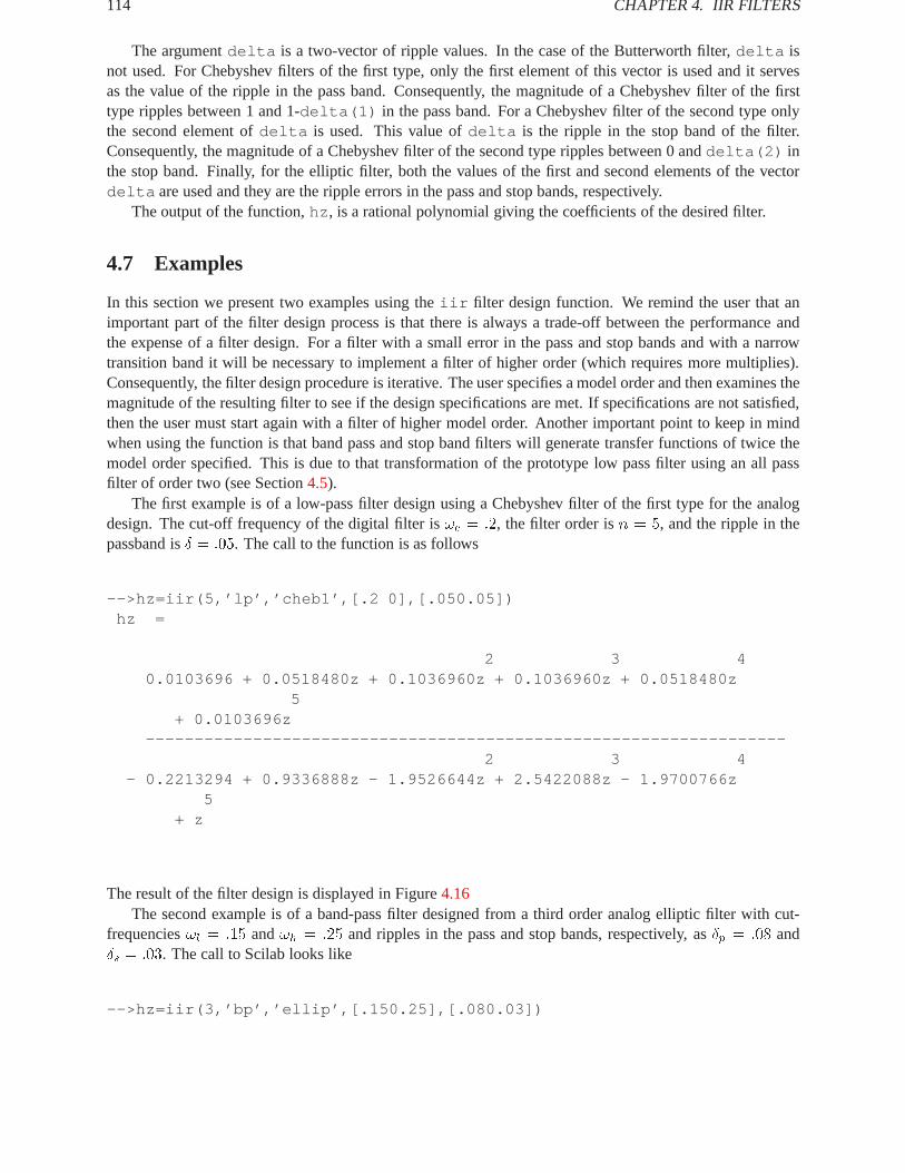
114 CHAPTER4. IIR FILTERS
The argumentdelta is a two-vector of ripple values. In the case of the Butterworth filter,delta isnot used. For Chebyshev filters of the first type, only the first element of this vector is used and it servesas the value of the ripple in the pass band. Consequently, the magnitude of a Chebyshev filter of the firsttype ripples between 1 and 1-delta(1) in the pass band. For a Chebyshev filter of the second type onlythe second element ofdelta is used. This value ofdelta is the ripple in the stop band of the filter.Consequently, the magnitude of a Chebyshev filter of the second type ripples between 0 anddelta(2) inthe stop band. Finally, for the elliptic filter, both the values of the first and second elements of the vectordelta are used and they are the ripple errors in the pass and stop bands, respectively.
The output of the function,hz , is a rational polynomial giving the coefficients of the desired filter.
4.7 Examples
In this section we present two examples using theiir filter design function. We remind the user that animportant part of the filter design process is that there is always a trade-off between the performance andthe expense of a filter design. For a filter with a small error in the pass and stop bands and with a narrowtransition band it will be necessary to implement a filter of higher order (which requires more multiplies).Consequently, the filter design procedure is iterative. The user specifies a model order and then examines themagnitude of the resulting filter to see if the design specifications are met. If specifications are not satisfied,then the user must start again with a filter of higher model order. Another important point to keep in mindwhen using the function is that band pass and stop band filters will generate transfer functions of twice themodel order specified. This is due to that transformation of the prototype low pass filter using an all passfilter of order two (see Section4.5).
The first example is of a low-pass filter design using a Chebyshev filter of the first type for the analogdesign. The cut-off frequency of the digital filter is!c = :2, the filter order isn = 5, and the ripple in thepassband isÆ = :05. The call to the function is as follows
-->hz=iir(5,’lp’,’cheb1’,[.2 0],[.050.05])hz =
2 3 40.0103696 + 0.0518480z + 0.1036960z + 0.1036960z + 0.0518480z
5+ 0.0103696z
------------------------------------------------------------------2 3 4
- 0.2213294 + 0.9336888z - 1.9526644z + 2.5422088z - 1.9700766z5
+ z
The result of the filter design is displayed in Figure4.16The second example is of a band-pass filter designed from a third order analog elliptic filter with cut-
frequencies!l = :15 and!h = :25 and ripples in the pass and stop bands, respectively, asÆp = :08 andÆs = :03. The call to Scilab looks like
-->hz=iir(3,’bp’,’ellip’,[.150.25],[.080.03])
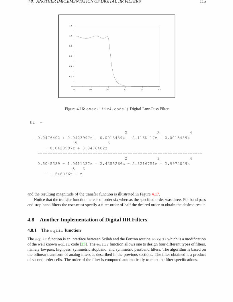
4.8. ANOTHER IMPLEMENTATION OF DIGITAL IIR FILTERS 115
0 0.1 0.2 0.3 0.4 0.5
0
0.2
0.4
0.6
0.8
1.0
1.2
Figure 4.16:exec(’iir4.code’) Digital Low-Pass Filter
hz =
2 3 4- 0.0476402 + 0.0423997z - 0.0013489z - 2.116D-17z + 0.0013489z
5 6- 0.0423997z + 0.0476402z
------------------------------------------------------------------2 3 4
0.5045339 - 1.0411237z + 2.4255266z - 2.6216751z + 2.9974049z5 6
- 1.646036z + z
and the resulting magnitude of the transfer function is illustrated in Figure4.17.Notice that the transfer function here is of order six whereas the specified order was three. For band pass
and stop band filters the user must specify a filter order of half the desired order to obtain the desired result.
4.8 Another Implementation of Digital IIR Filters
4.8.1 Theeqiir function
Theeqiir function is an interface between Scilab and the Fortran routinesyredi which is a modificationof the well knowneqiir code [23]. Theeqiir function allows one to design four different types of filters,namely lowpass, highpass, symmetric stopband, and symmetric passband filters. The algorithm is based onthe bilinear transform of analog filters as described in the previous sections. The filter obtained is a productof second order cells. The order of the filter is computed automatically to meet the filter specifications.

116 CHAPTER4. IIR FILTERS
0 0.1 0.2 0.3 0.4 0.5
0
0.1
0.2
0.3
0.4
0.5
0.6
0.7
0.8
0.9
1.0
Figure 4.17:exec(’iir5.code’) Digital Band-Pass Filter
The filter is given either by the set of its poles and zeros (output variableszpoles andzzeros of theeqiir function) or equivalently by a the representation:
H(z) = factNY1
ni(z)=di(z)
where the rational fractionni(z)=di(z) is the i-th element ofcells .
4.8.2 Examples
Example 1 (Lowpass elliptic filter): Design of a lowpass elliptic filter with maximum ripplesÆp = 0:02,Æs = 0:001 and cutoff frequencies!1 = 2 �
10 and!2 = 4 �10 .
-->[cells,fact,Zeros,Zpoles]=...-->eqiir(’lp’,’ellip’,[2*%pi/10,4*%pi/10],0.02,0.001);
-->Zpoles’ans =
! 0.6906008 - 0.5860065i !! 0.6906008 + 0.5860065i !! 0.6373901 - 0.3437403i !! 0.6373901 + 0.3437403i !! 0.6247028 !
-->Zeros’ans =

4.8. ANOTHER IMPLEMENTATION OF DIGITAL IIR FILTERS 117
! 0.2677115 - 0.9634991i !! 0.2677115 + 0.9634991i !! - 0.1744820 - 0.9846604i !! - 0.1744820 + 0.9846604i !! - 1. !
-->cells’ans =
! 2 !! 1 - 0.5354229z + z !! -------------------------- !! 2 !! 0.8203331 - 1.3812015z + z !! !! 2 !! 1 + 0.3489640z + z !! -------------------------- !! 2 !! 0.5244235 - 1.2747803z + z !! !! 1 + z !! ------------- !! - 0.6247028 + z !
-->transfer=fact*poly(Zeros,’z’)/poly(Zpoles,’z’)transfer =
2 3 40.0059796 + 0.0048646z + 0.0097270z + 0.0097270z + 0.0048646z
5+ 0.0059796z
------------------------------------------------------------------2 3 4
- 0.2687484 + 1.5359753z - 3.7100842z + 4.7646843z - 3.2806846z5
+ z
Example 2 (Lowpass Butterworth filter): Design of a lowpass Butterworth filter with the followingspecifications:- 5dB passband attenuation at the normalized cutoff frequencies:25�=10 and - 120dB attenuation at thestopband edge0:5�=10.
-->om=[.25*%pi/10,4*%pi/10];

118 CHAPTER4. IIR FILTERS
-->pdB=5;
-->sdB=120;
-->deltap=(1.0-10.0**(-0.05*pdB));
-->deltas=10.00**(-0.05*sdB);
-->[cells,fact,zers,pols]=eqiir(’lp’,’butt’,om,deltap,deltas);
-->cellscells =
column 1 to 2
! 2 2 !! 1 + 2z + z 1 + 2z + z !! -------------------------- -------------------------- !! 2 2 !! 0.9450100 - 1.9368524z + z 0.8621663 - 1.8543562z + z !
column 3
! 1 + z !! ------------- !! - 0.9123352 + z !
-->n=prod(cells(2));
-->d=prod(cells(3));
-->tr=n./dtr =
2 3 4 51 + 5z + 10z + 10z + 5z + z
---------------------------------------------------------------2 3 4 5
- 0.7433304 + 3.937017z - 8.3477808z + 8.8576437z - 4.7035438z + z
Example 3 (Lowpass type 1 Chebyshev filter): Design of a lowpass type 1 Chebyshev filter with 2dBripple in the passband and -30 dB attenuation at the stopband edge. The sampling frequency is assumed tobe 3000Hz and the cutoff frequencies at 37.5Hz and 75Hz respectively.
-->sf=3000;

4.8. ANOTHER IMPLEMENTATION OF DIGITAL IIR FILTERS 119
-->f1=37.5;
-->f2=75;
-->as=30;
-->ap=2;
-->om=[f1*(2*%pi)/sf,f2*(2*%pi)/sf];
-->deltas=10.00**(-0.05*as);
-->deltap=(1.0-10.0**(-0.05*ap));
-->[cells,fact,zers,pols]=...-->eqiir(’lp’,’ch1’,om,deltap,deltas);
-->cellscells =
! 2 2 !! 1 - 1.9711824z + z 1 - 1.8376851z + z !! ------------------ ------------------ !! 2 2 !! Nan +Nanz + z Nan +Nanz + z !
Example 4 (Elliptic symmetric bandpass filter): Design of a symmetric bandpass filter with edges at!1 = 0:251463; !2 = �=10; !3 = 2�=10; !4 = 0:773302 and ripples in the passband and stopband givenrespectively byÆp = 0:022763, Æs = 0:01.
-->//Elliptic bandpass filter
-->om=[0.251463,1*%pi/10,2*%pi/10,0.773302];
-->deltap=0.022763;
-->deltas=0.01;
-->[cells,fact,zers,pols]=eqiir(’bp’,’el’,om,deltap,deltas);
-->n=prod(cells(2));d=prod(cells(3));
-->rep=freq(n,d,exp(%i*(0:0.01:%pi)));
-->rep=fact*abs(rep);

120 CHAPTER4. IIR FILTERS
-->n=prod(size(rep))n =
315.
-->plot(20*log(rep(2:n))/log(10))
The preceding example shows how to compute the magnitude response by using thefreq primitive.The example is plotted in Figure4.18.
0 40 80 120 160 200 240 280 320
-100
-90
-80
-70
-60
-50
-40
-30
-20
-10
0
Figure 4.18:exec(’eqiir4.code’) Example of response obtained witheqiir
Chapter 5
Spectral Estimation
5.1 Estimation of Power Spectra
The power spectrum of a deterministic, finite length, discrete-time signal,x(n), is defined to be the mag-nitude squared of the signal’s Fourier transform
Sx(!) =1
NjN�1Xn=0
x(n)e�j!nj2: (5.1)
In an analogous fashion the cross-spectrum of two signalsx(n) andy(n) is defined to be
Sxy(!) =1
N(
N�1Xn=0
x(n)e�j!n)(N�1Xn=0
y(n)e�j!n)�: (5.2)
The power spectra of random, zero-mean, wide sense stationary signals are obtained from the Fourier trans-form of the correlation functions of these signals. Thus, forRx representing the autocorrelation function ofx andRxy representing the cross-correlation function ofx with y we have by definition that
Rx(m) = Efx(n+m)x�(n)g (5.3)
Rxy(m) = Efx(n+m)y�(n)g: (5.4)
Consequently, the power spectrum and cross-power spectrum ofx(n) and ofx(n) with y(n) are, respect-ively,
Sx(!) =1X
m=�1Rx(m)e�j!m (5.5)
Sxy(!) =1X
m=�1Rxy(m)e�j!m: (5.6)
The formulas (5.5) and (5.6) require estimates of the correlation functions. Possible candidates for theestimates of the auto and cross correlation functions of finite length random signals (i.e.,x(n) 6= 0 andy(n) 6= 0 for n = 0; 1; : : : ; N � 1) are
Rx(m) =1
N
N�1�mXn=0
x(n+m)x�(n) (5.7)
Rxy(m) =1
N
N�1�mXn=0
x(n+m)y�(n): (5.8)
121

122 CHAPTER5. SPECTRAL ESTIMATION
The estimates in (5.7) and (5.8) are unbiased, consistent estimators in the limit asN ! 1. Furthermore,in the case where the random signals are jointly Gaussian, these estimators are the maximum likelihoodestimates of the correlation functions. Another interesting property of the estimators in (5.7) and (5.8) isthat when substituted, respectively, into the expressions in (5.5) and (5.6), after some algebraic manipulation,yield exactly the expressions in (5.1) and (5.2).
Unfortunately, there is a serious problem with the above power spectrum estimation scheme. This prob-lem is that the resulting power spectral estimates, in the limit, are not consistent. That is, the error varianceof the estimate does not decrease with increasing data. Consequently, power spectral estimates obtained bytaking the magnitude squared of the Fourier transform are high-variance, low-quality estimates.
In the sections which follow two techniques are discussed which yield improved spectral estimates.These techniques are both based on averaging spectral estimates obtained from the classical approach justdescribed. This averaging, although introducing some biasing, yields greatly improved estimates in that, inthe limit, these estimates become consistent.
The first averaging technique also sections the data into overlapping segments. However, in this casethe magnitude squared of the Fourier transform is calculated from each segment and then these are averagedtogether to yield the spectral estimate. This technique is called the modified periodogram method for spectralestimation.
The second averaging technique sections the data into overlapping segments. For each segment anestimate of the correlation function is calculated. These estimates are then averaged and the estimatedpower spectral density is the Fourier transform of the average. This technique is known as the correlationmethod for spectral estimation.
Both techniques use windows to diminish the effects that finite data has on spectral estimation. Theseeffects are identical to the problems encountered in FIR filter design, and, consequently, the reader is referredto the FIR filter design section for an explanation of the issues involved in the choice of windows. Inthe discussion which follows cross-spectral estimation is not discussed considering that the cross-spectralestimate can be obtained as a simple modification of the auto-spectral estimation techniques.
5.2 The Modified Periodogram Method
The modified periodogram method of spectral estimation repeatedly calculates the periodogram of win-dowed sub-sections of the data. These periodograms are then averaged together and normalized by anappropriate constant to obtain the final spectral estimate. It is the averaging process which reduces thevariance in the estimate.
The periodogram of a finite data sequence is defined by
I(!) =1
UjN�1Xn=0
w(n)x(n)e�j!nj2: (5.9)
wherew(n) is a window function which has energyU . Consequently, ifK sub-segments of lengthN areused to calculate the spectrum of the signal then the modified periodogram spectral estimate,Sx, is just theaverage of theK periodograms
Sx(!) =1
K
K�1Xk=0
Ik (5.10)
where each of theIk is the periodogram (calculated as in (5.9)) of thekth segment of data.Normally, theK segments of data are taken so that there is a regular pattern of overlap in the success-
ive segments. That is, thekth and (k + 1)th segments overlap byD points. Figure5.1 illustrates threeconsecutive overlapping segments of a data sequence.

5.2. THE MODIFIED PERIODOGRAM METHOD 123
1.0 26.5 52.0 77.5 103.0 128.5 154.0 179.5 205.0 230.5 256.0
-2.350
-1.975
-1.600
-1.225
-0.850
-0.475
-0.100
0.275
0.650
1.025
1.400
x1
x2
x3
Figure 5.1:exec(’spect1.code’) Overlapping Data
It can be shown that an overlap of fifty percent in the data segments results in an approximately fiftypercent reduction in the variance of the estimate of the power spectrum [24]. Normally, one chooses thelength of the data segments to reflect thea priori knowledge of the correlation length of the data. Thatis to say that if the correlation between two data samples separated by more thanM points is considerednegligible then the data segment should be of a length on the order ofM . The number of data segmentsused determines the variance of the spectral estimate. The variance decreases proportionally to the numberof independent segments. Of course, with a limited quantity of data the number of data segments must alsobe limited.
The functionpspect calculates an estimate of the power spectrum using the modified periodogrammethod.
5.2.1 Example Using thepspect function
In this section, we demonstrate the use of thepspect macro. The data used is generated by passing zero-mean white noise of unit variance through a low-pass filter. Consequently, the spectrum of the data shouldbe the magnitude square of the filter frequency response. The low-pass filter is an FIR filter of length 33generated using the functioneqfir .
The data was generated using the following Scilab commands,
-->//test modified periodogram method
-->//generate white data
-->rand(’normal’);
-->rand(’seed’,0);

124 CHAPTER5. SPECTRAL ESTIMATION
-->x=rand(1:1024-33+1);
-->//make low-pass filter with eqfir
-->nf=33;
-->bedge=[00.1;.1250.5];
-->des=[1 0];
-->wate=[1 1];
-->hn=eqfir(nf,bedge,des,wate);
-->//filter white data to obtain colored data
-->h1=[hn 0*ones(1:maxi(size(x))-1)];
-->x1=[x 0*ones(1:maxi(size(hn))-1)];
-->hf=fft(h1,-1);
-->xf=fft(x1,-1);
-->yf=hf.*xf;
-->y=real(fft(yf,1));
As can be seen, a total of 1024 data points are available for the estimation of the spectrum. The logarithmof the magnitude squared of the filter frequency response is shown in Figure5.2.
The data obtained above are used to estimate the power spectrum in the following way
-->[sm]=pspect(100,200,’tr’,y);
The log-magnitude of the power spectrum (sm) is plotted in Figure5.3. It should be pointed out here that thevalue of the section lengths was chosen to be 200 in this example to obtain additional resolution in the plotof the Fourier transform of the estimated power spectrum in Figure5.3. However, there is very acceptablebehavior of the spectral estimate when the section length is on the order of twice the filter length. This isdue to the fact that one does not expect correlations in the data that are much longer than the filter length.Normally, the section lengths are chosen to reflect thea priori knowledge of the correlation length in thedata.
As can be seen the estimated spectrum matches the theoretical spectrum (Figure5.2) very well. Inparticular, the peaks of the spectrum in both the pass and stop bands matches well with those of the filtermagnitude response. Furthermore, the normalization of the estimate is accurate with respect to the filterresponse.

5.2. THE MODIFIED PERIODOGRAM METHOD 125
0 0.1 0.2 0.3 0.4 0.5 0.6 0.7 0.8 0.9 1.0
-21
-17
-13
-9
-5
-1
3
Figure 5.2:exec(’spect2 4.code’) Log Magnitude Squared of Filter
0 0.1 0.2 0.3 0.4 0.5 0.6 0.7 0.8 0.9 1.0
-9
-8
-7
-6
-5
-4
-3
-2
-1
0
1
Figure 5.3:exec(’spect2 4.code’) Estimate of Spectrum
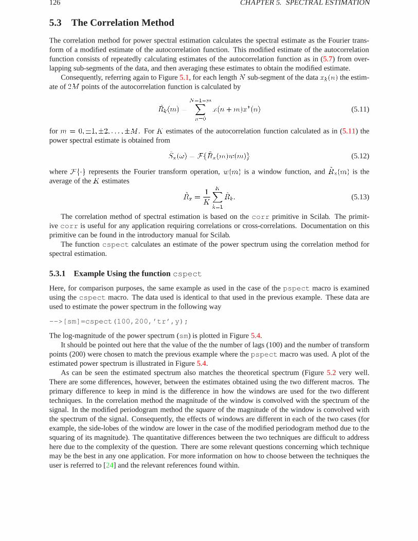
126 CHAPTER5. SPECTRAL ESTIMATION
5.3 The Correlation Method
The correlation method for power spectral estimation calculates the spectral estimate as the Fourier trans-form of a modified estimate of the autocorrelation function. This modified estimate of the autocorrelationfunction consists of repeatedly calculating estimates of the autocorrelation function as in (5.7) from over-lapping sub-segments of the data, and then averaging these estimates to obtain the modified estimate.
Consequently, referring again to Figure5.1, for each lengthN sub-segment of the dataxk(n) the estim-ate of2M points of the autocorrelation function is calculated by
Rk(m) =
N�1�mXn=0
x(n+m)x�(n) (5.11)
for m = 0;�1;�2; : : : ;�M . ForK estimates of the autocorrelation function calculated as in (5.11) thepower spectral estimate is obtained from
Sx(!) = Ff ~Rx(m)w(m)g (5.12)
whereFf�g represents the Fourier transform operation,w(m) is a window function, and~Rx(m) is theaverage of theK estimates
~Rx =1
K
KXk=1
Rk: (5.13)
The correlation method of spectral estimation is based on thecorr primitive in Scilab. The primit-ive corr is useful for any application requiring correlations or cross-correlations. Documentation on thisprimitive can be found in the introductory manual for Scilab.
The functioncspect calculates an estimate of the power spectrum using the correlation method forspectral estimation.
5.3.1 Example Using the functioncspect
Here, for comparison purposes, the same example as used in the case of thepspect macro is examinedusing thecspect macro. The data used is identical to that used in the previous example. These data areused to estimate the power spectrum in the following way
-->[sm]=cspect(100,200,’tr’,y);
The log-magnitude of the power spectrum (sm) is plotted in Figure5.4.It should be pointed out here that the value of the the number of lags (100) and the number of transform
points (200) were chosen to match the previous example where thepspect macro was used. A plot of theestimated power spectrum is illustrated in Figure5.4.
As can be seen the estimated spectrum also matches the theoretical spectrum (Figure5.2 very well.There are some differences, however, between the estimates obtained using the two different macros. Theprimary difference to keep in mind is the difference in how the windows are used for the two differenttechniques. In the correlation method the magnitude of the window is convolved with the spectrum of thesignal. In the modified periodogram method thesquareof the magnitude of the window is convolved withthe spectrum of the signal. Consequently, the effects of windows are different in each of the two cases (forexample, the side-lobes of the window are lower in the case of the modified periodogram method due to thesquaring of its magnitude). The quantitative differences between the two techniques are difficult to addresshere due to the complexity of the question. There are some relevant questions concerning which techniquemay be the best in any one application. For more information on how to choose between the techniques theuser is referred to [24] and the relevant references found within.

5.4. THE MAXIMUM ENTROPY METHOD 127
0 0.1 0.2 0.3 0.4 0.5 0.6 0.7 0.8 0.9 1.0
-7
-6
-5
-4
-3
-2
-1
0
1
Figure 5.4:exec(’spect2 4.code’) Estimate of Spectrum
5.4 The Maximum Entropy Method
5.4.1 Introduction
The power spectrum of a deterministic signal is defined to be the squared magnitude of the signal’s Fouriertransform. That is, forx(n) a discrete time signal, the power spectrum,Sx(!), is
Sx(!) = jX(!)j2 (5.14)
where
X(!) =1X
n=�1xne
�j!n: (5.15)
In many applications it is very useful to know the power spectrum of a signal, however, it is rare that theobtained signal can be characterized as being deterministic. Often the signal is present in a noisy environ-ment and, in addition, is obtained with instrumentation which degrades the signal with measurement noise.Consequently, for a non-deterministic signal one seeks to estimate the power spectrum. It can be shown [21]that taking the Fourier transform of a non-deterministic signal in order to estimate its power spectrum is avery poor approach. The problem is that the resulting power spectrum is a highly variable estimate of thetrue power spectrum and that the variance does not decrease to zero as one increases the data length (i.e.,the estimator is not consistent).
The problem of estimating the power spectrum can be modified as follows. Letx(n) be a zero-mean,stationary signal and letrx(n) be the autocorrelation function of the signal (that is,rx(n) = Efx(k)x�(n+k)g). Then the power spectrumSx(n) of x(n) is taken to be the Fourier transform ofrx(n)
Sx(!) =
1Xn=�1
rx(n)e�j!n: (5.16)
Assuming that statistical averages of the signalx(n) are equal to time averages we can take as an estimate

128 CHAPTER5. SPECTRAL ESTIMATION
for rx(n)
rx(n) = limN!1
1
2N + 1
NXm=�N
x(m)x(m� n): (5.17)
However, after plugging (5.17) into (5.16) and performing some algebraic manipulation it can be seen that(5.16) is just the magnitude squared of the Fourier transform ofx(n). Consequently, (5.16) is not any moreuseful than (5.14) for estimating the power spectrum of a non-deterministic signal.
One can improve the statistical properties of the power spectrum estimate by smoothing the result ob-tained in (5.16) or by breaking the input,x(n), into pieces, performing the calculation in (5.17) and (5.16)for each piece, and then averaging these results together. These approaches are the classical methods ofpower spectral estimation.
These classical methods of power spectral estimation are undesirable for two reasons. The estimateobtained from these methods is based on a finite (i.e., windowed) segment of the autocorrelation function.This means that the resulting estimated power spectrum is a convolution of the true power spectrum and ofthe Fourier transform of the window. Consequently, the resolution of spectral features is diminished and theestimate of the power spectrum at any point is biased by leakage from other parts of the power spectrumthrough the window sidelobes.
The maximum entropy spectral estimate (MESE) of the power spectrum yields an improved spectraldensity estimate. That’s to say that for MESE the resolution is improved and the bias is decreased incomparison with the classical spectral estimation methods. This improvement is due to the fact that theMESE uses a model based estimation procedure.
5.4.2 The Maximum Entropy Spectral Estimate
The maximum entropy spectral estimate (MESE) is designed to produce high-resolution, low-bias spectralestimates from finite length discrete signals. The formulation of the MESE problem is as follows. It isassumed that only a finite number,N , of autocorrelation lags (estimated from a finite length discrete signal)are available. The MESE yields the functionSx(!) which has maximum entropy and whose inverse Fouriertransform exactly matches theN lags,rx(n). This can be expressed by the equation
Sx(!) = maxS(!)
f�Z �
��S(!) log[S(!)]d!g (5.18)
where1
2�
Z �
��Sx(!)e
j!nd! = rx(n); n = 0; 1; : : : ; N � 1: (5.19)
Equation (5.18) expresses the optimality condition of maximizing the entropy ofS(!) subject to theNconstraints posed in (5.19).
Since entropy is a measure of randomness, the MESE is the spectral estimate which is maximally randomgiven the constraints in (5.19). Intuitively, the MESE incorporates no information in the estimated spectrumother than the knowledge of the autocorrelation lags. That is to say that the bias should be eliminated (orat least minimized in some sense) since no non-data related constraints are imposed on the spectrum. Aswas discussed in the introduction, windowed-autocorrelation spectral estimates suffered from bias due tothe leakage from the window sidelobes. The window imposes a non-data related constraint on the powerspectrum estimate in that the autocorrelation function is assumed to be identically zero outside of the supportof the window.
Furthermore, as is discussed in [16], it can be shown that the MESE is equivalent to the Fourier transformof an infinite length autocorrelation sequence which is obtained by extrapolating the sequence of lengthN

5.4. THE MAXIMUM ENTROPY METHOD 129
in (5.19). The extrapolation is accomplished using an auto-regressive, all-pole model of orderN � 1 givenby
rx(n) = �N�1Xk=1
akrn�k; n � N: (5.20)
Any autocorrelation sequence can be modeled by (5.20) given a large enough model order,N . Consequently,in principle, the resolution of the MESE should be much better than that of a windowed spectral estimatesince the MESE uses an infinite length autocorrelation sequence.
The solution to (5.18) and (5.19) can be found by using the calculus of variations [11] and, as demon-strated in [16], the solution takes the form
Sx(!) =�2
j1 +PN�1n=1 an expf�j!ngj2
(5.21)
where the parameter setf�2; a1; a2; : : : ; aN�1g is obtained by solving the system of linear equations26664
rx(0) rx(1) � � � rx(N � 1)rx(1) rx(0) � � � rx(N � 2)
......
...rx(N � 1) rx(N � 2) � � � rx(0)
3777526664
1a1...
aN�1
37775 =
26664�2
0...0
37775 (5.22)
where the Toeplitz matrix in (5.22) is composed of theN estimated correlation lagsrx(n). The system ofN linear equations in (5.22) are known as the Yule-Walker equations and an efficient algorithm for theirsolution is described in the next section.
5.4.3 The Levinson Algorithm
An efficient recursive solution to the Yule-Walker equations in (5.22) exists and is known as the Levinsonalgorithm. The algorithm requiresO(N2) complex multiplications and additions. The solution to thekth
order problem is obtained from the solution to the(k � 1)th order problem using the following equations
akk = �[rx(k) +k�1Xj=1
ak�1;j rx(k � j)]=�2k�1 (5.23)
aki = ak�1;i + akka�k�1;k�i (5.24)
�2k = (1� jakkj2)�2k�1: (5.25)
The solution to the1st order problem is
a11 = �rx(1)=rx(0) (5.26)
�21 = (1� ja11j2)rx(0): (5.27)
5.4.4 How to Usemese
The syntax for the macromese is as follows,
-->[sm,fr]=mese(x)
where one wants to obtain a power spectral estimate ofx , the input data sequence, andsm is the resultingestimate obtained on the normalized frequency axis (0 �fr � :5).

130 CHAPTER5. SPECTRAL ESTIMATION
5.4.5 How to Uselev
The syntax for the macrolev is as follows,
-->[ar,sigma2,rc]=lev(r)
wherer is a vector of auto-correlation coefficients (r(0); r(1); : : : ; r(N�1)), ar is the vector which satisfiesthe Yule-Walker equations,sigma2 is the scalar which satisfies the Yule-Walker equations, andrc is avector of reflection coefficients.
5.4.6 Examples
Here we give an example of estimating the power spectrum of a very short data sequence using the MESEand also using the magnitude squared of the Fourier transform. The data is eleven samples of the sum oftwo sinusoids in additive, uniformly distributed, white noise. The functional form of the data sequence is
x(n) = sin(2�n=20) + sin(3:5�n=20) + :2w(n) (5.28)
wherew(n) is the white noise sequence which takes on values in[�1; 1] andn = 0; 1; :::; 10. Figure5.5shows the input data sequence, x(n). Figures5.6and5.7show the maximum entropy and magnitude squaredestimates of the power spectrum, respectively.
1 2 3 4 5 6 7 8 9 10 11
-2
-1
0
1
2
3
Figure 5.5:exec(’mem1 3.code’) Input Data Sequence,x(n)
As can be seen, the MESE resolves two peaks according to the two sinusoidal frequences inx(n). Thesquared magnitude of the Fourier transform ofx(n) does not have a long enough signal to resolve the twopeaks of the spectrum. Furthermore, the power spectrum estimate in Figure5.7 shows spurious sidelobeswhich have nothing to do with the data.
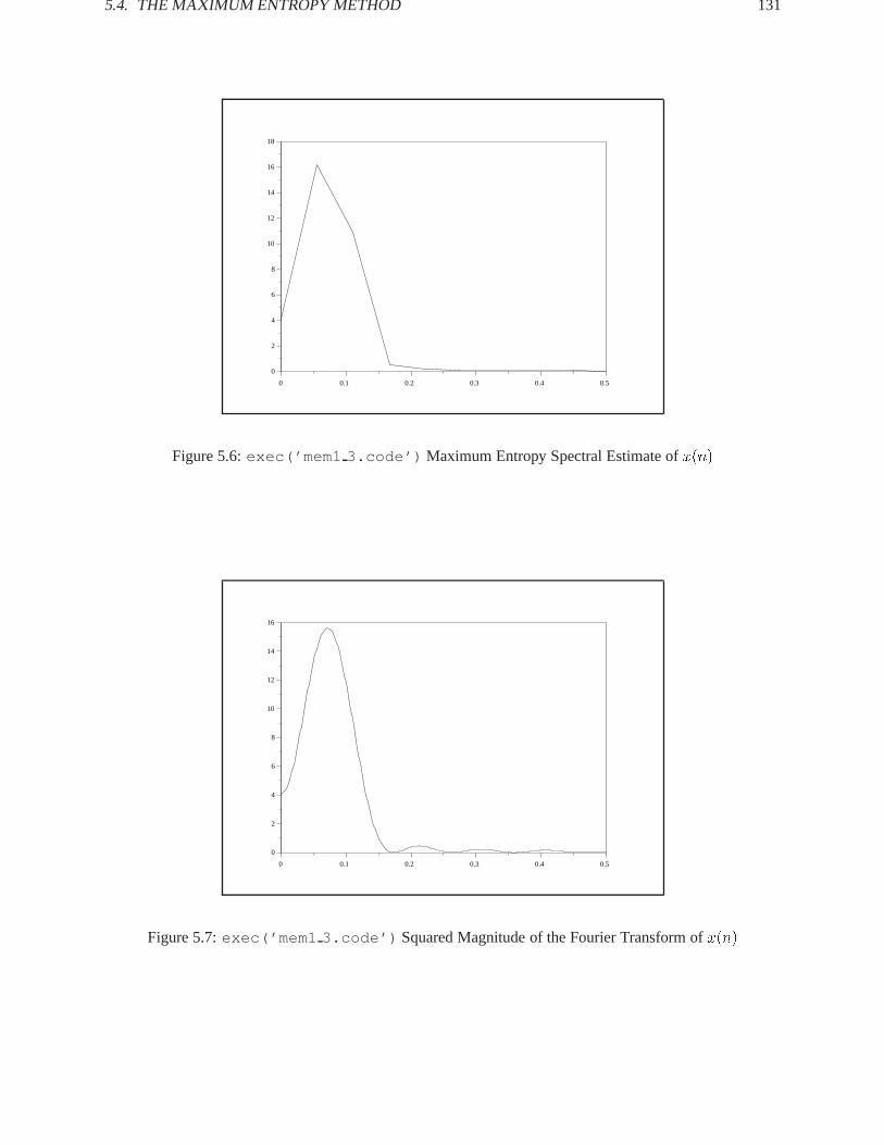
5.4. THE MAXIMUM ENTROPY METHOD 131
0 0.1 0.2 0.3 0.4 0.5
0
2
4
6
8
10
12
14
16
18
Figure 5.6:exec(’mem1 3.code’) Maximum Entropy Spectral Estimate ofx(n)
0 0.1 0.2 0.3 0.4 0.5
0
2
4
6
8
10
12
14
16
Figure 5.7:exec(’mem1 3.code’) Squared Magnitude of the Fourier Transform ofx(n)

132 CHAPTER5. SPECTRAL ESTIMATION
Chapter 6
Optimal Filtering and Smoothing
6.1 The Kalman Filter
Consider the following discrete-time system,
xk+1 = Fkxk +Gkwk
yk = Hkxk + vk (6.1)
where
wk � N(0; Qk)
vk � N(0; Rk)
x0 � N(m0;�0)
(6.2)
andx0, fwkg, andfvkg are independent random vectors. The state vector,xk, has dimensionN and theobservation vector,yk, has dimensionM . Furthermore, it is assumed thatRk > 0.
The problem to be addressed here is the estimation of the state vector,xk, given observations of the vec-torsYk = fy0; y1; : : : ; ykg. Because the collection of variablesfxk; y0; y1; : : : ; ykg are jointly Gaussian onecould estimatexk by maximizing the likelihood of the conditional probability distributionp(xkjYk) giventhe values of the conditional variables. Equivalently, one could search the estimate,xk, which minimized themean square error,�k = xk � xk. In either case it is known that the optimal estimate (maximum likelihoodor least squares) for the jointly Gaussian variables is the conditional mean. The error in the estimate is theconditional covariance.
In what follows, the conditional mean and covariance ofxk givenYk is developed. This is followed by adescription of the Kalman filter, an extremely practical recursive method for calculating the conditional meanand covariance. Several different implementations of the Kalman filter are discussed here: The steady-stateKalman filter which can be used when the system matrices in (6.1) and (6.3) are non-time varying, the non-stationary Kalman filter for use when the system matrices in (6.1) and (6.3) are time-varying, and, finally,the square-root Kalman filter which is used (for time-varying and non-time-varying system matrices) whengreater numerical accuracy is required.
6.1.1 Conditional Statistics of a Gaussian Random Vector
The minimum mean square estimate of a Gaussian random vector given observations of some of its elementsis the conditional mean of the remaining elements. The error covariance of this estimate is the conditional
133
134 CHAPTER6. OPTIMAL FILTERING AND SMOOTHING
covariance. Consequently, assuming thatz is a Gaussian random vector composed of two sub-vectorsx andy, then
z =
�xy
�� N
��mx
my
�;
��x �xy
�yx �y
��(6.3)
wheremx denotes the mean ofx, �xy denotes the covariance ofx with y, and�x is the covariance ofx withitself.
It is known that the marginal and conditional distributions of a Gaussian random vector are also Gaus-sian. In particular, the conditional distribution ofx giveny, p(xjy), is
p(xjy) = N(mxjy;�xjy) (6.4)
wheremxjy denotes the conditional mean and�xjy denotes the conditional covariance. These two quantitiesmay be calculated by
mxjy = mx +�xy��1y (y �my)
�xjy = �x � �xy��1y �yx: (6.5)
(It is useful to note thex andy are not necessarily of the same dimension). Equation (6.5) is very importantin our development of the Kalman filter equations.
With regard to the problem posed in the introduction to this section, the minimum mean square error iscalculated in a straight forward manner. One stacks the individual observation vectors into a single vector,Yk, and then, sincexk andYk are jointly Gaussian , one applies (6.5) to obtain the conditional mean andcovariance ofxk given Yk. The problem with this approach is that for increasingk the vectorYk is ofincreasing dimension, and consequently, the matrix inverse and multiplication operations in (6.5) becomeincreasingly burdensome.
The next few sections are devoted to showing how the linear system of (6.1) and the special propertiesof (6.5) can be used to obtain a recursive update to the estimation ofxk. That is, given the best estimate ofxk based on the observationsYk (we denote this estimate byxkjk) and a new observationyk+1, it is shownhow to obtain the best estimate ofxk+1jk+1 and its error covariance matrixPk+1jk+1.
6.1.2 Linear Systems and Gaussian Random Vectors
Given a random vector,x, with a probability distributionp(x), the minimum mean square error estimate ofx is denoted here byx and consists of the mean ofx. That is,x = mx. The associated error covariance ofthe estimate, denotedPx, is the covariance ofx. Now assume thatx is passed through a linear system andis disturbed by an independent, zero-mean Gaussian vector,v, of covarianceR. This yields an output whichcan be represented by
y = Hx+ v: (6.6)
Since (6.6) is a linear combination of independent Gaussian random vectors,y is also a Gaussian randomvector. The mean and covariance ofy are calculated as follows,
my = Efyg= EfHx+ vg= Hmx (6.7)
and
�y = Ef(y �my)(y �my)T g
= Ef[H(x �mx) + v][H(x�mx) + v]T g= H�xH
T +R: (6.8)
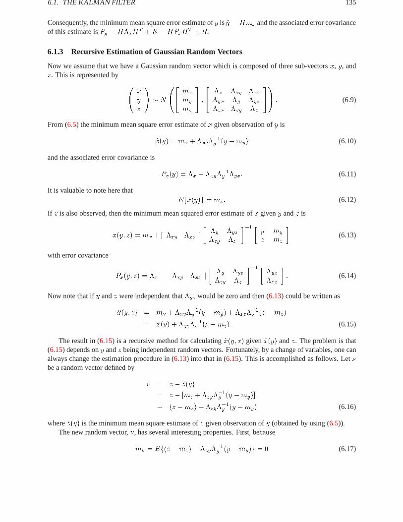
6.1. THE KALMAN FILTER 135
Consequently, the minimum mean square error estimate ofy is y = Hmx and the associated error covarianceof this estimate isPy = H�xH
T +R = HPxHT +R.
6.1.3 Recursive Estimation of Gaussian Random Vectors
Now we assume that we have a Gaussian random vector which is composed of three sub-vectorsx, y, andz. This is represented by0
@ xyz
1A � N
0@24 mx
my
mz
35 ;24 �x �xy �xz
�yx �y �yz
�zx �zy �z
351A : (6.9)
From (6.5) the minimum mean square error estimate ofx given observation ofy is
x(y) = mx +�xy��1y (y �my) (6.10)
and the associated error covariance is
Px(y) = �x � �xy��1y �yx: (6.11)
It is valuable to note here thatEfx(y)g = mx: (6.12)
If z is also observed, then the minimum mean squared error estimate ofx giveny andz is
x(y; z) = mx + [ �xy �xz ]
��y �yz
�zy �z
��1 �y �my
z �mz
�(6.13)
with error covariance
Px(y; z) = �x � [ �xy �xz ]
��y �yz
�zy �z
��1 ��yx
�zx
�: (6.14)
Now note that ify andz were independent that�yz would be zero and then (6.13) could be written as
x(y; z) = mx +�xy��1y (y �my) + �xz�
�1z (z �mz)
= x(y) + �xz��1z (z �mz): (6.15)
The result in (6.15) is a recursive method for calculatingx(y; z) given x(y) andz. The problem is that(6.15) depends ony andz being independent random vectors. Fortunately, by a change of variables, one canalways change the estimation procedure in (6.13) into that in (6.15). This is accomplished as follows. Let�be a random vector defined by
� = z � z(y)
= z � [mz +�zy��1y (y �my)]
= (z �mz)� �zy��1y (y �my) (6.16)
wherez(y) is the minimum mean square estimate ofz given observation ofy (obtained by using (6.5)).The new random vector,�, has several interesting properties. First, because
m� = Ef(z �mz)� �zy��1y (y �my)g = 0 (6.17)
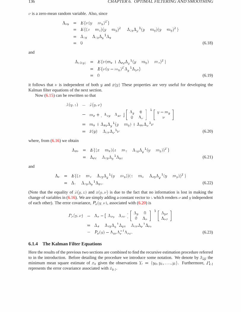
136 CHAPTER6. OPTIMAL FILTERING AND SMOOTHING
� is a zero-mean random variable. Also, since
��y = Ef�(y �my)T g
= Ef(z �mz)(y �my)T � �zy�
�1y (y �my)(y �my)
T g= �zy � �zy�
�1y �y
= 0 (6.18)
and
��x(y) = Ef�(mx +�xy��1y (y �my)�mx)
T g= Ef�(y �my)
T��1y �yxg= 0 (6.19)
it follows that � is independent of bothy and x(y) These properties are very useful for developing theKalman filter equations of the next section.
Now (6.15) can be rewritten so that
x(y; z) = x(y; �)
= mx + [ �xy �x� ]
��y 00 ��
��1 �y �my
�
�= mx +�xy�
�1y (y �my) + �x��
�1� �
= x(y) + �x���1� � (6.20)
where, from (6.16) we obtain
�x� = Ef(x�mx)(z �mz � �zy��1y (y �my))
T g= �xz � �xy�
�1y �yz (6.21)
and
�� = Ef(z �mz � �zy��1y (y �my))(z �mz � �zy�
�1y (y �my))
T g= �z � �zy�
�1y �yz: (6.22)
(Note that the equality ofx(y; z) and x(y; �) is due to the fact that no information is lost in making thechange of variables in (6.16). We are simply adding a constant vector toz which renders� andy independentof each other). The error covariance,Px(y; �), associated with (6.20) is
Px(y; �) = �x � [ �xy �x� ]
��y 00 ��
��1 ��yx
��x
�= �x � �xy�
�1y �yx � �x��
�1� ��x
= Px(y)� �x���1� ��x: (6.23)
6.1.4 The Kalman Filter Equations
Here the results of the previous two sections are combined to find the recursive estimation procedure referredto in the introduction. Before detailing the procedure we introduce some notation. We denote byxkjl theminimum mean square estimate ofxk given the observationsYl = fy0; y1; : : : ; ylg. Furthermore,Pkjlrepresents the error covariance associated withxkjl.

6.1. THE KALMAN FILTER 137
Now, the estimatexkjk can be obtained from the estimatexkjk�1 and the new observationyk in thefollowing manner. From (6.20) and (6.23) we have
xkjk = xkjk�1 +�xk�k��1�k�k
Pkjk = Pkjk�1 � �xk�k��1�k
��kxk (6.24)
where from (6.1), (6.7), and (6.8)�k = yk �Hkxkjk�1: (6.25)
The covariance matrices in (6.24) may be calculated by
��k = Ef�k�Tk g= Ef(yk �Hkxkjk�1)(yk �Hkxkjk�1)T g= Ef[Hk(xk � xkjk�1) + vk][Hk(xk � xkjk�1) + vk]
T g= HkPkjk�1HT
k +Rk (6.26)
(where the final equality follows from the fact thatvk andxk are independent random vectors), and
�xk�k = Ef(xk �Efxkg)�Tk g= Ef(xk �Efxkg+Efxkg � xkjk�1)�Tk g= Ef(xk � xkjk�1)�Tk g= Ef(xk � xkjk�1)(yk �Hkxkjk�1)T g= Ef(xk � xkjk�1)(xk � xkjk�1)THT
k g= Pkjk�1HT
k (6.27)
(where the second equality follows from (6.13) and (6.19)). Substituting (6.25), (6.26), and (6.27) into (6.24)yields
xkjk = xkjk�1 +Kk(yk �Hkxkjk�1)Pkjk = Pkjk�1 �KkHkPkjk�1 (6.28)
whereKk = Pkjk�1HTk [HkPkjk�1HT
k + Rk]�1 is called the Kalman gain of the filter. (Note: Since the
model proposed in the first section of this chapter assumes thatRk > 0 it follows thatKk always exists.However, whenRk is not strictly positive definite there may be problems performing the matrix inversenecessary to calculateKk). Using (6.7) and (6.8) in conjunction with (6.1) gives the two auxiliary equations
xk+1jk = FkxkjkPk+1jk = FkPkjkF T
k +GkQkGTk : (6.29)
Combining the equations in (6.28) and (6.29) yields one set of recursive equations
xk+1jk = Fkxkjk�1 + FkKk(yk �Hkxkjk�1)
Pk+1jk = FkPkjk�1F Tk � FkKkHkPkjk�1F T
k +GkQkGTk : (6.30)
The only remaining detail is to identify the initial conditions of the Kalman filter which are obtained fromthea priori statistics ofx0
x0j�1 = m0
P0j�1 = �0: (6.31)
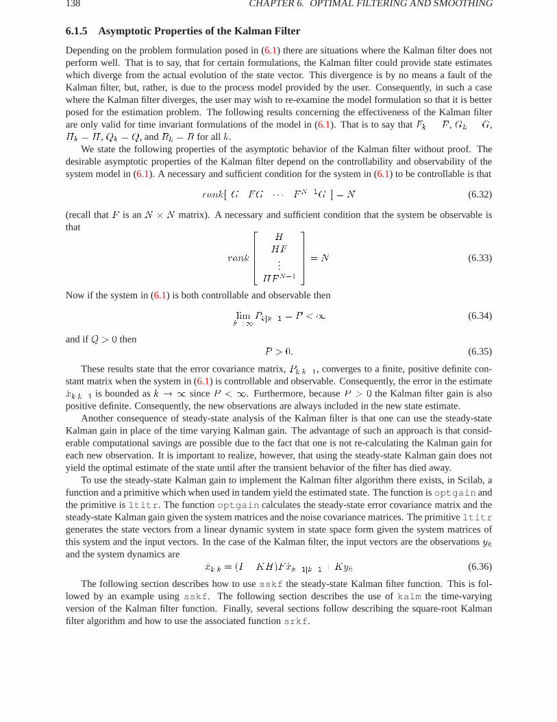
138 CHAPTER6. OPTIMAL FILTERING AND SMOOTHING
6.1.5 Asymptotic Properties of the Kalman Filter
Depending on the problem formulation posed in (6.1) there are situations where the Kalman filter does notperform well. That is to say, that for certain formulations, the Kalman filter could provide state estimateswhich diverge from the actual evolution of the state vector. This divergence is by no means a fault of theKalman filter, but, rather, is due to the process model provided by the user. Consequently, in such a casewhere the Kalman filter diverges, the user may wish to re-examine the model formulation so that it is betterposed for the estimation problem. The following results concerning the effectiveness of the Kalman filterare only valid for time invariant formulations of the model in (6.1). That is to say thatFk = F , Gk = G,Hk = H,Qk = Q, andRk = R for all k.
We state the following properties of the asymptotic behavior of the Kalman filter without proof. Thedesirable asymptotic properties of the Kalman filter depend on the controllability and observability of thesystem model in (6.1). A necessary and sufficient condition for the system in (6.1) to be controllable is that
rank[ G FG � � � FN�1G ] = N (6.32)
(recall thatF is anN � N matrix). A necessary and sufficient condition that the system be observable isthat
rank
26664
HHF
...HFN�1
37775 = N (6.33)
Now if the system in (6.1) is both controllable and observable then
limk!1
Pkjk�1 = P <1 (6.34)
and ifQ > 0 thenP > 0: (6.35)
These results state that the error covariance matrix,Pkjk�1, converges to a finite, positive definite con-stant matrix when the system in (6.1) is controllable and observable. Consequently, the error in the estimatexkjk�1 is bounded ask ! 1 sinceP < 1. Furthermore, becauseP > 0 the Kalman filter gain is alsopositive definite. Consequently, the new observations are always included in the new state estimate.
Another consequence of steady-state analysis of the Kalman filter is that one can use the steady-stateKalman gain in place of the time varying Kalman gain. The advantage of such an approach is that consid-erable computational savings are possible due to the fact that one is not re-calculating the Kalman gain foreach new observation. It is important to realize, however, that using the steady-state Kalman gain does notyield the optimal estimate of the state until after the transient behavior of the filter has died away.
To use the steady-state Kalman gain to implement the Kalman filter algorithm there exists, in Scilab, afunction and a primitive which when used in tandem yield the estimated state. The function isoptgain andthe primitive isltitr . The functionoptgain calculates the steady-state error covariance matrix and thesteady-state Kalman gain given the system matrices and the noise covariance matrices. The primitiveltitrgenerates the state vectors from a linear dynamic system in state space form given the system matrices ofthis system and the input vectors. In the case of the Kalman filter, the input vectors are the observationsykand the system dynamics are
xkjk = (I �KH)F xk�1jk�1 +Kyk (6.36)
The following section describes how to usesskf the steady-state Kalman filter function. This is fol-lowed by an example usingsskf . The following section describes the use ofkalm the time-varyingversion of the Kalman filter function. Finally, several sections follow describing the square-root Kalmanfilter algorithm and how to use the associated functionsrkf .

6.1. THE KALMAN FILTER 139
6.1.6 How to Use the Macrosskf
The syntax of thesskf is as follows
[xe,pe]=sskf(y,f,h,q,r,x0)
where the system is assumed to take the following form
xk+1 = f xk + wk
yk = hxk + vk
where
wk � N(0; q)
vk � N(0; r )
x0 � N( x0 ;�0):
The remaining input, y = [y0; y1; : : : ; yn], is a matrix where the individual observationsyk are containedin the matrix as column vectors.
The outputsxe andpe are the estimated state and the steady-state error covariance matrix. The formof the estimates isxe = [x0j0; x1j1; : : : ; xnjn] where eachxkjk is a column in the matrix. The steady-stateerror covariance matrix is a square matrix of the dimension of the state.
6.1.7 An Example Using thesskf Macro
The example uses the following system model and prior statistics:
xk+1 =
�1:1 :10 :8
�xk +
�1 00 1
�wk
yk =
�1 00 1
�xk + vk
where
EfwkwTk g =
�:03 :01:01 :03
�
EfvkvTk g =
�2 00 2
�
and
Efx0g =
�1010
�
Ef(x0 �m0)(x0 �m0)T g =
�2 00 2
�
Observations from the above system were generated synthetically using the primitiveltitr . The resultsof the steady-state Kalman filter estimates are shown in Figure6.1
where the dotted line marked by stars indicates the actual state path and the solid line marked by circlesmarks the estimated state path.

140 CHAPTER6. OPTIMAL FILTERING AND SMOOTHING
8 12 16 20 24 28 32 36
1
2
3
4
5
6
7
8
9
10
11
⊕
⊕
⊕
⊕
⊕
⊕
⊕
⊕⊕
⊕⊕
Figure 6.1:exec(’kf1.code’) Steady-State Kalman Filter Tracking
6.1.8 How to Use the Functionkalm
The functionkalm takes as input the system description matrices, the statistics of the noise processes, theprior estimate of the state and error covariance matrix, and the new observation. The outputs are the newestimates of the state and error covariance matrix. The call tokalm is as follows:
--> [x1,p1,x,p]=kf(y,x0,p0,f,g,h,q,r)
wherey is the new observation,x0 andp0 are the prior state and error covariance estimates at timet = 0based on observations up to timet = �1, f , g andh are the dynamics, input, and observation matrices,respectively, andq and r are the noise covariance matrices for the dynamics and observations equations,respectively. The outputsx1 andp1 are the new state and error covariance estimates at timet = 1 givenobservations up to timet = 0, respectively, andx andp are the new state and error covariance estimates attime t = 0 given observations up to timet = 0, respectively.
6.1.9 Examples Using thekalm Function
Three examples are illustrated in this section. All three examples are for two-dimensional state vectors.The first example illustrates Kalman tracking for a system model which is controllable and observable. Thesecond and third examples show the results of uncontrollable and unobservable system models, respectively.
The first example uses the following system model and prior statistics:
xk+1 =
�1:1 :10 :8
�xk +
�1 00 1
�wk
yk =
�1 00 1
�xk + vk
where
EfwkwTk g =
�:03 :01:01 :03
�

6.1. THE KALMAN FILTER 141
EfvkvTk g =
�2 00 2
�
and
Efx0g =
�1010
�
Ef(x0 �m0)(x0 �m0)T g =
�2 00 2
�
Observations from the above system were generated synthetically using the system formulation and valuesfrom a random number generator for the dynamics and observations noise. These observations were thenused as input to the Kalman filter. The result of ten observations is illustrated in Figure6.2.
4 8 12 16 20 24 28 32 36
0
2
4
6
8
10
12
14
×
×
×
×
×
×
×
××
×
×
⊕
⊕
⊕
⊕
⊕
⊕
⊕⊕
⊕ ⊕⊕
Figure 6.2:exec(’kf2.code’) Kalman Filter Tracking
The figure shows the actual state path and the Kalman estimate of the state path as a dotted and solidline, respectively. The actual locations of the state and estimated values are indicated by the star and circlesymbols on the respective paths. The ellipses in the figure are centered about the positions of the actualstate path and their borders represent two standard deviations of estimation error calculated from the errorcovariance matrices. The values of the standard deviations for the above example are displayed below:
-->//initialize state statistics (mean and err. variance)
-->m0=[10 10]’;p0=[2 0;0 2];
-->//create system
-->f=[1.10.1;00.8];g=[1 0;0 1];h=[1 0;0 1];
-->//noise statistics
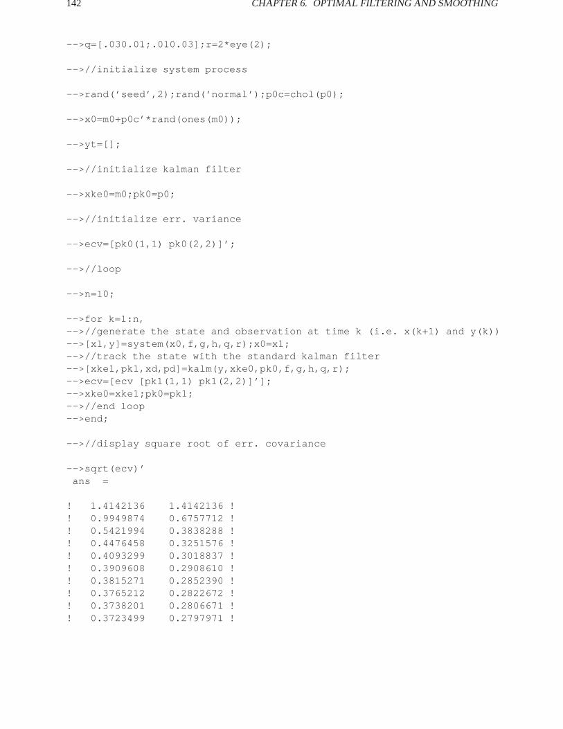
142 CHAPTER6. OPTIMAL FILTERING AND SMOOTHING
-->q=[.030.01;.010.03];r=2*eye(2);
-->//initialize system process
-->rand(’seed’,2);rand(’normal’);p0c=chol(p0);
-->x0=m0+p0c’*rand(ones(m0));
-->yt=[];
-->//initialize kalman filter
-->xke0=m0;pk0=p0;
-->//initialize err. variance
-->ecv=[pk0(1,1) pk0(2,2)]’;
-->//loop
-->n=10;
-->for k=1:n,-->//generate the state and observation at time k (i.e. x(k+1) and y(k))-->[x1,y]=system(x0,f,g,h,q,r);x0=x1;-->//track the state with the standard kalman filter-->[xke1,pk1,xd,pd]=kalm(y,xke0,pk0,f,g,h,q,r);-->ecv=[ecv [pk1(1,1) pk1(2,2)]’];-->xke0=xke1;pk0=pk1;-->//end loop-->end;
-->//display square root of err. covariance
-->sqrt(ecv)’ans =
! 1.4142136 1.4142136 !! 0.9949874 0.6757712 !! 0.5421994 0.3838288 !! 0.4476458 0.3251576 !! 0.4093299 0.3018837 !! 0.3909608 0.2908610 !! 0.3815271 0.2852390 !! 0.3765212 0.2822672 !! 0.3738201 0.2806671 !! 0.3723499 0.2797971 !

6.1. THE KALMAN FILTER 143
! 0.3715458 0.2793216 !
Each row of the above vector represents the standard deviations of the state vector error covariance mat-rix where the first row is the standard deviation of thea priori error in the state vector and the last row isthe standard deviation of the state vector estimate at the last step of the Kalman filter. The above standarddeviation vector is instructive. It should be noted that for both state values, the standard deviation is con-verging to a steady state value. For the first element of the state vector this value is .7800312 and for thesecond element of the state vector the value is .2824549. The convergence is to be expected since the aboveformulation of the system is both controllable and observable.
If we were to change the above system formulation so that the dynamics equation were now
xk+1 =
�1:1 :10 :8
�xk +
�1 00 0
�wk (6.37)
the system would be uncontrollable. Re-running the Kalman filter with this re-formulation yields the fol-lowing sequence of standard deviations:
-->//initialize state statistics (mean and err. variance)
-->m0=[10 10]’;p0=[2 0;0 2];
-->//create system
-->f=[1.10.1;00.8];g=[1 0;0 0];h=[1 0;0 1];
-->//noise statistics
-->q=[.030.01;.010.03];r=2*eye(2);
-->//initialize system process
-->rand(’seed’,2);rand(’normal’);p0c=chol(p0);
-->x0=m0+p0c’*rand(ones(m0));yt=[];
-->//initialize kalman filter
-->xke0=m0;pk0=p0;
-->//initialize err. variance
-->ecv=[pk0(1,1) pk0(2,2)]’;
-->//loop
-->n=10;
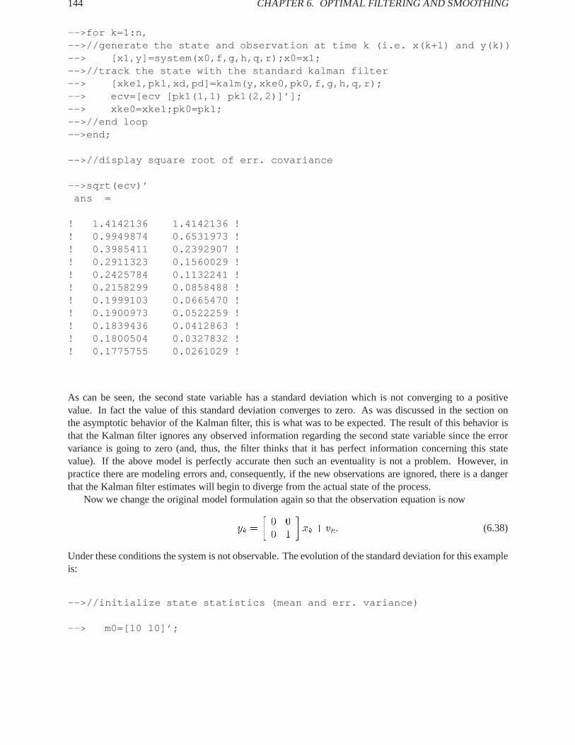
144 CHAPTER6. OPTIMAL FILTERING AND SMOOTHING
-->for k=1:n,-->//generate the state and observation at time k (i.e. x(k+1) and y(k))--> [x1,y]=system(x0,f,g,h,q,r);x0=x1;-->//track the state with the standard kalman filter--> [xke1,pk1,xd,pd]=kalm(y,xke0,pk0,f,g,h,q,r);--> ecv=[ecv [pk1(1,1) pk1(2,2)]’];--> xke0=xke1;pk0=pk1;-->//end loop-->end;
-->//display square root of err. covariance
-->sqrt(ecv)’ans =
! 1.4142136 1.4142136 !! 0.9949874 0.6531973 !! 0.3985411 0.2392907 !! 0.2911323 0.1560029 !! 0.2425784 0.1132241 !! 0.2158299 0.0858488 !! 0.1999103 0.0665470 !! 0.1900973 0.0522259 !! 0.1839436 0.0412863 !! 0.1800504 0.0327832 !! 0.1775755 0.0261029 !
As can be seen, the second state variable has a standard deviation which is not converging to a positivevalue. In fact the value of this standard deviation converges to zero. As was discussed in the section onthe asymptotic behavior of the Kalman filter, this is what was to be expected. The result of this behavior isthat the Kalman filter ignores any observed information regarding the second state variable since the errorvariance is going to zero (and, thus, the filter thinks that it has perfect information concerning this statevalue). If the above model is perfectly accurate then such an eventuality is not a problem. However, inpractice there are modeling errors and, consequently, if the new observations are ignored, there is a dangerthat the Kalman filter estimates will begin to diverge from the actual state of the process.
Now we change the original model formulation again so that the observation equation is now
yk =
�0 00 1
�xk + vk: (6.38)
Under these conditions the system is not observable. The evolution of the standard deviation for this exampleis:
-->//initialize state statistics (mean and err. variance)
--> m0=[10 10]’;

6.1. THE KALMAN FILTER 145
--> p0=[2 0;0 2];
-->//create system
--> f=[1.10.1;00.8];
--> g=[1 0;0 1];
--> h=[0 0;0 1];
-->//noise statistics
--> q=[.030.01;.010.03];
--> r=2*eye(2);
-->//initialize system process
--> rand(’seed’,2),
--> rand(’normal’),
--> p0c=chol(p0);
--> x0=m0+p0c’*rand(ones(m0));
--> yt=[];
-->//initialize kalman filter
--> xke0=m0;
--> pk0=p0;
-->//initialize err. variance
--> ecv=[pk0(1,1) pk0(2,2)]’;
-->//loop
--> n=10;
--> for k=1:n,-->//generate the state and observation at time k (i.e. x(k+1) and y(k))--> [x1,y]=system(x0,f,g,h,q,r);--> x0=x1;-->//track the state with the standard kalman filter--> [xke1,pk1,xd,pd]=kalm(y,xke0,pk0,f,g,h,q,r);
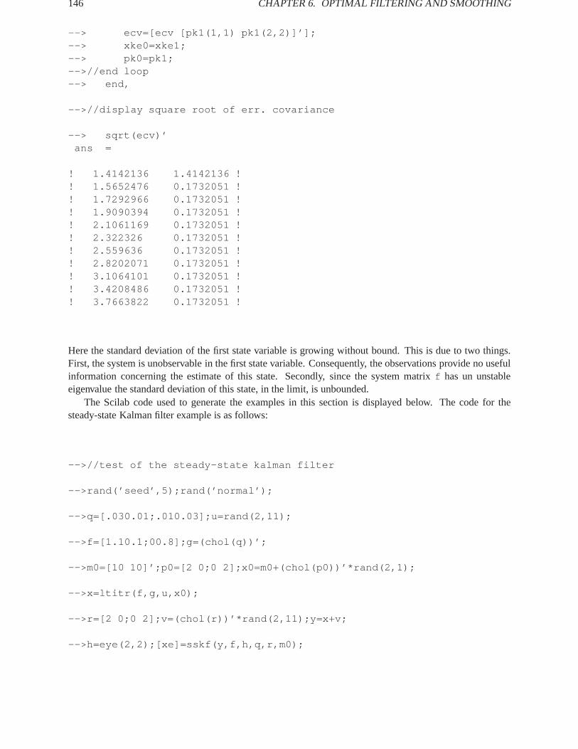
146 CHAPTER6. OPTIMAL FILTERING AND SMOOTHING
--> ecv=[ecv [pk1(1,1) pk1(2,2)]’];--> xke0=xke1;--> pk0=pk1;-->//end loop--> end,
-->//display square root of err. covariance
--> sqrt(ecv)’ans =
! 1.4142136 1.4142136 !! 1.5652476 0.1732051 !! 1.7292966 0.1732051 !! 1.9090394 0.1732051 !! 2.1061169 0.1732051 !! 2.322326 0.1732051 !! 2.559636 0.1732051 !! 2.8202071 0.1732051 !! 3.1064101 0.1732051 !! 3.4208486 0.1732051 !! 3.7663822 0.1732051 !
Here the standard deviation of the first state variable is growing without bound. This is due to two things.First, the system is unobservable in the first state variable. Consequently, the observations provide no usefulinformation concerning the estimate of this state. Secondly, since the system matrixf has un unstableeigenvalue the standard deviation of this state, in the limit, is unbounded.
The Scilab code used to generate the examples in this section is displayed below. The code for thesteady-state Kalman filter example is as follows:
-->//test of the steady-state kalman filter
-->rand(’seed’,5);rand(’normal’);
-->q=[.030.01;.010.03];u=rand(2,11);
-->f=[1.10.1;00.8];g=(chol(q))’;
-->m0=[10 10]’;p0=[2 0;0 2];x0=m0+(chol(p0))’*rand(2,1);
-->x=ltitr(f,g,u,x0);
-->r=[2 0;0 2];v=(chol(r))’*rand(2,11);y=x+v;
-->h=eye(2,2);[xe]=sskf(y,f,h,q,r,m0);

6.1. THE KALMAN FILTER 147
-->//plot result
-->a=mini([x(1,:),xe(1,:)]);a=-0.1*abs(a)+a;
-->b=maxi([x(1,:),xe(1,:)]);b=.1*abs(b)+b;
-->c=mini([x(2,:),xe(2,:)]);c=-0.1*abs(c)+c;
-->d=maxi([x(2,:),xe(2,:)]);d=.1*abs(d)+d;
-->//plot frame, real state (x), and estimate (xke)
-->plot([a a b],[d c c]),
-->plot2d(x(1,:)’,x(2,:)’,[1],’000’,’ ’)
-->plot2d(xe(1,:)’,xe(2,:)’,[2],’000’,’ ’),
-->plot2d(xe(1,:)’,xe(2,:)’,[-3],’000’,’ ’),
-->xend(),
The code used to generate the non-steady-state Kalman filter example is:
-->//generate test process to be sent to kalman filter
-->//initialize state statistics (mean and err. variance)
-->m0=[10 10]’;p0=[2 0;0 2];
-->//create system
-->f=[1.10.1;00.8];g=[1 0;0 1];h=[1 0;0 1];
-->//noise statistics
-->q=[.030.01;.010.03];r=2*eye(2,2);
-->//initialize system process
-->rand(’seed’,2);rand(’normal’);
-->p0c=chol(p0);x0=m0+p0c’*rand(ones(m0));yt=[];

148 CHAPTER6. OPTIMAL FILTERING AND SMOOTHING
-->//initialize kalman filter
-->xke0=m0;pk0=p0;
-->//initialize plotted variables
-->x=x0;xke=m0;
-->ell=[pk0(1,1) pk0(2,2) pk0(1,2)]’;
-->//loop
-->n=10;
--> for k=1:n,-->//generate the state and observation at time k (i.e. x(k+1) and y(k))--> [x1,y]=system(x0,f,g,h,q,r);--> x=[x x1];--> yt=[yt y];--> x0=x1;-->//track the state with the standard kalman filter--> [xke1,pk1,xd,pd]=kalm(y,xke0,pk0,f,g,h,q,r);--> xke=[xke xke1];--> ell=[ell [pk1(1,1) pk1(2,2) pk1(1,2)]’];--> xke0=xke1;--> pk0=pk1;-->//end loop--> end,
-->//define macro which traces an ellipse
-->deff(’[]=ellipse(m1,m2,s1,s2,s12)’,...--> ’t=0:.1:.1+%pi*2;...--> c=2*cos(t);...--> s=2*sin(t);...--> rho=s12/sqrt(s1*s2);...--> cr=sqrt(s1)*c+m1*ones(c);...--> sr=sqrt(s2)*(rho*c+sqrt(1-rho*rho)*s)+m2*ones(s);...--> plot2d(cr’’,sr’’,[1],’"000’"),’)
-->//plot result
-->a=mini([x(1,:)-2*sqrt(ell(1,:)),xke(1,:)]);a=-0.1*abs(a)+a;
-->b=maxi([x(1,:)+2*sqrt(ell(1,:)),xke(1,:)]);b=.1*abs(b)+b;
-->c=mini([x(2,:)-2*sqrt(ell(2,:)),xke(2,:)]);c=-0.1*abs(c)+c;

6.2. THE SQUARE ROOT KALMAN FILTER 149
-->d=maxi([x(2,:)+2*sqrt(ell(2,:)),xke(2,:)]);d=.1*abs(d)+d;
-->//plot frame, real state (x), and estimate (xke)
-->plot([a a b],[d c c]),
-->plot2d(x(1,:)’,x(2,:)’,[2],"000"),
-->plot2d(xke(1,:)’,xke(2,:)’,[1],"000"),
-->//plot ellipses of constant likelihood (2 standard dev’s)
--> for k=1:n+1,--> ellipse(x(1,k),x(2,k),ell(1,k),ell(2,k),ell(3,k)),--> end,
-->//mark data points (* for real data, o for estimates)
-->plot2d(x(1,:)’,x(2,:)’,[-2],"000"),
-->plot2d(xke(1,:)’,xke(2,:)’,[-3],"000")
-->xend(),
6.2 The Square Root Kalman Filter
The Kalman filter is known to have certain numerical instabilities [3]. For example, since the update ofthe error covariance matrix involves taking differences of matrices (see(6.28)) it is possible that machinediscretization error could result in a non positive semi-definite error covariance. Such an event could leadto severe divergence of the Kalman filter because this could render the Kalman gain infinite. Fortunately,there are a class of algorithms which are known collectively as square root Kalman filters which avoid thisproblem.
The square root Kalman filter propagates the state estimate and the square root of the error covariancematrix. (Here,S is defined to be the square root of a matrix,A, if A = SST . The square root,S, is notunique. For example for any other orthogonal matrix,O, such thatOOT = I it follows thatSO is also asquare root ofA. We denote the square root ofA by A1=2). The advantage of propagating the square rootof the error covariance matrix is two-fold. First, the error covariance is always positive semi-definite sinceit is formed by squaring the square root. Second, the dynamic range of the elements in the square root ofthe error covariance is much smaller than that in the error covariance matrix itself. Consequently, the accur-acy of calculations is improved since the machine precision is better adapted to representing the dynamicrange of the square root. The details of a square root Kalman filter algorithm base on using Householdertransformations is detailed below.
Restating the model for the dynamics and observations of the process in (6.1), we have that
yk = Hkxk + vk
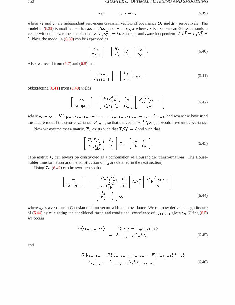
150 CHAPTER6. OPTIMAL FILTERING AND SMOOTHING
xk+1 = Fkxk + wk (6.39)
wherewk andvk are independent zero-mean Gaussian vectors of covarianceQk andRk, respectively. Themodel in (6.39) is modified so thatwk = Gk�k andvk = Lk�k where�k is a zero-mean Gaussian randomvector with unit covariance matrix (i.e.,Ef�k�Tk g = I). Sincewk andvkare independentGkL
Tk = LkG
Tk =
0: Now, the model in (6.39) can be expressed as
�ykxk+1
�=
�Hk LkFk Gk
� �xk�k
�: (6.40)
Also, we recall from (6.7) and (6.8) that
�ykjk�1xk+1jk�1
�=
�Hk
Fk
�xkjk�1: (6.41)
Substracting (6.41) from (6.40) yields
��k
�k+1jk�1
�=
"HkP
1=2kjk�1 Lk
FkP1=2kjk�1 Gk
#"P�1=2kjk�1�kjk�1
�k
#(6.42)
where�k = yk �Hxkjk�1, �k+1jk�1 = xk+1 � xk+1jk�1, �kjk�1 = xk � xkjk�1, and where we have used
the square root of the error covariance,Pkjk�1, so that the vectorP�1=2kjk�1xkjk�1 would have unit covariance.
Now we assume that a matrix,Tk, exists such thatTkT Tk = I and such that
"HkP
1=2kjk�1 Lk
FkP1=2kjk�1 Gk
#Tk =
�Ak 0Bk Ck
�: (6.43)
(The matrixTk can always be constructed as a combination of Householder transformations. The House-holder transformation and the construction ofTk are detailed in the next section).
UsingTk, (6.42) can be rewritten so that
��k
�k+1jk�1
�=
"HkP
1=2kjk�1 Lk
FkP1=2kjk�1 Gk
#TkT
Tk
"P�1=2kjk�1�kjk�1
�k
#
=
�Ak 0Bk Ck
��k (6.44)
where�k is a zero-mean Gaussian random vector with unit covariance. We can now derive the significanceof (6.44) by calculating the conditional mean and conditional covariance of�k+1jk�1 given�k. Using (6.5)we obtain
Ef�k+1jk�1j�kg = Efxk+1 � xk+1jk�1j�kg= ��k+1jk�1�k�
�1�k�k (6.45)
and
Ef[�k+1jk�1 �Ef�k+1jk�1g][�k+1jk�1 �Ef�k+1jk�1g]T j�kg =��k+1jk�1
� ��k+1jk�1�k��1�k��k+1jk�1�k (6.46)
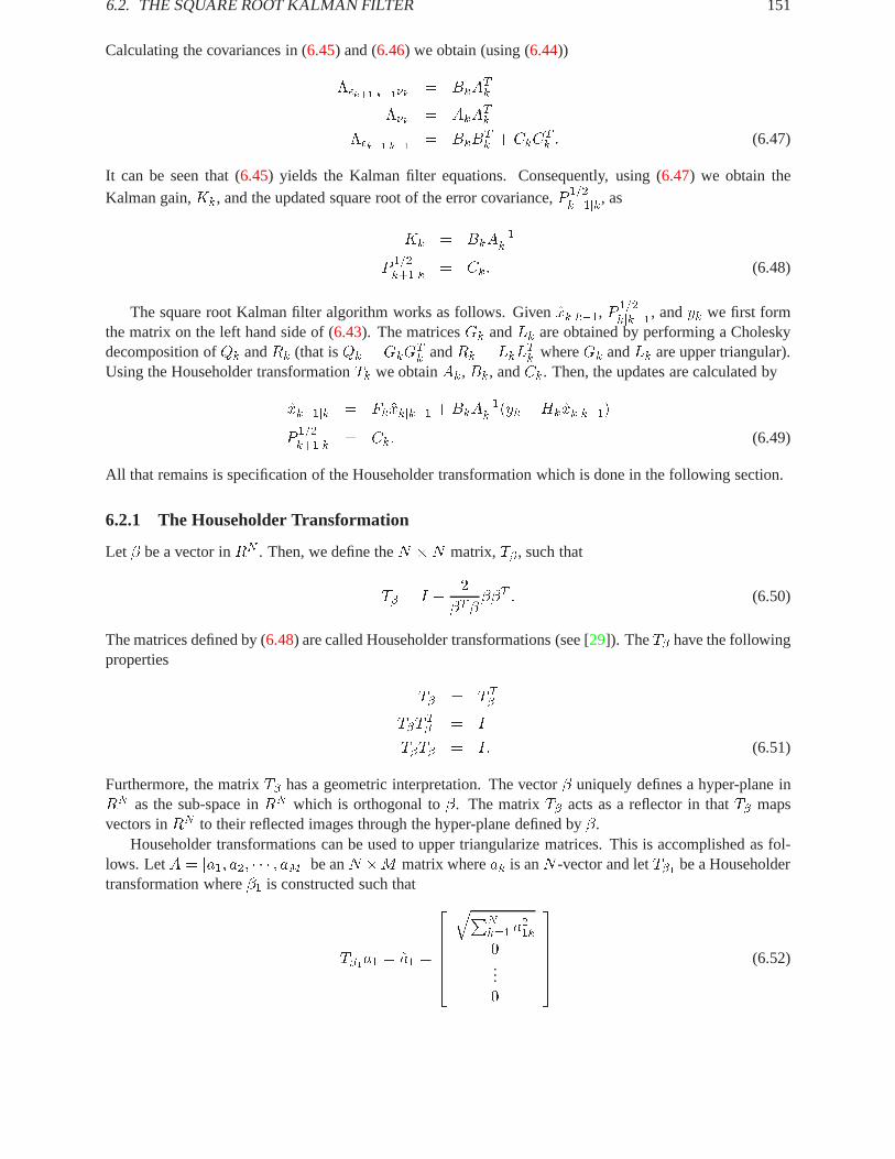
6.2. THE SQUARE ROOT KALMAN FILTER 151
Calculating the covariances in (6.45) and (6.46) we obtain (using (6.44))
��k+1jk�1�k = BkATk
��k = AkATk
��k+1jk�1= BkB
Tk + CkC
Tk : (6.47)
It can be seen that (6.45) yields the Kalman filter equations. Consequently, using (6.47) we obtain theKalman gain,Kk, and the updated square root of the error covariance,P
1=2k+1jk, as
Kk = BkA�1k
P1=2k+1jk = Ck: (6.48)
The square root Kalman filter algorithm works as follows. Givenxkjk�1, P1=2kjk�1, andyk we first form
the matrix on the left hand side of (6.43). The matricesGk andLk are obtained by performing a Choleskydecomposition ofQk andRk (that isQk = GkG
Tk andRk = LkL
Tk whereGk andLk are upper triangular).
Using the Householder transformationTk we obtainAk, Bk, andCk. Then, the updates are calculated by
xk+1jk = Fkxkjk�1 +BkA�1k (yk �Hkxkjk�1)
P1=2k+1jk = Ck: (6.49)
All that remains is specification of the Householder transformation which is done in the following section.
6.2.1 The Householder Transformation
Let � be a vector inRN . Then, we define theN �N matrix,T�, such that
T� = I � 2
�T���T : (6.50)
The matrices defined by (6.48) are called Householder transformations (see [29]). TheT� have the followingproperties
T� = T T�
T�TT� = I
T�T� = I: (6.51)
Furthermore, the matrixT� has a geometric interpretation. The vector� uniquely defines a hyper-plane inRN as the sub-space inRN which is orthogonal to�. The matrixT� acts as a reflector in thatT� mapsvectors inRN to their reflected images through the hyper-plane defined by�.
Householder transformations can be used to upper triangularize matrices. This is accomplished as fol-lows. LetA = [a1; a2; � � � ; aM ] be anN �M matrix whereak is anN -vector and letT�1 be a Householdertransformation where�1 is constructed such that
T�1a1 = ~a1 =
266664
qPNk=1 a
21k
0...0
377775 (6.52)
152 CHAPTER6. OPTIMAL FILTERING AND SMOOTHING
(i.e., we find the�1 such that whena1 is reflected through the hyper-plane defined by�1 its image is asabove). The choice for�1 which accomplishes this goal is
�1 =
266664a11 +
qPNk=1 a
21k
a12...
a1N
377775 (6.53)
wherea1k is thekth element of theN -vectora1.The Householder transformation,T�1 , can be used now to transform the matrixA,
T�1A = [~a1; ~a2; � � � ; ~aM ] (6.54)
where~a1 is as in (6.52) and the remaining columns ofA are transformed to~ak = T�1ak.Now we construct a second Householder transformation,T�2 such that
T�2~a2 =~~a2 =
26666664
~a21qPNk=2 ~a
22k
0...0
37777775
(6.55)
That is, the first element of~a2 is left unchanged, the second element becomes the norm of the rest of theelements and the remaining elements become zero. The choice for�2 which accomplishes this is
�2 =
26666664
0
~a22 +qPN
k=2 ~a22k
~a23...
~a2N
37777775: (6.56)
CalculatingT�2T�1A yieldsT�2T�1A = [~a1; ~~a2; ~~a3; � � � ; ~~aM ] (6.57)
where~a1 is still as in (6.52) and ~~a2 is as in (6.55). Continuing recursively in this way we can uppertriangularize theA matrix.
The Scilab primitiveqr performs a triangularization of a matrix using Householder transformations. Inparticular, it is ther part of the qr-decomposition which yields the desired triangularized matrix.
6.2.2 How to Use the Macrosrkf
The functionsrkf takes as input the system description matrices, the statistics of the noise processes, theprior estimate of the state and error covariance matrix, and the new observation. The outputs are the newestimates of the state and error covariance matrix. The call tokalm is as follows:
--> [x1,p1]=srkf(y,x0,p0,f,h,q,r)
wherey is the new observation,x0 and p0 are the prior state and error covariance estimates,f and hare the dynamics and observation matrices, respectively, andq andr are the noise covariance matrices forthe dynamics and observations equations, respectively. The outputsx1 andp1 are the new state and errorcovariance estimates, respectively.
6.3. THE WIENER FILTER 153
6.3 The Wiener Filter
The generalized Wiener filtering problem [14] can be posed as follows. It is desired to estimate a zero-mean,Gaussian vector process,x(t), in the interval[a; b] from observations of a statistically related, zero-mean,Gaussian vector,y(t). Furthermore, the covariance functionsRyy(t; s) = Efy(t)yT (s)g andRxy(t; s) =Efx(t)yT (s)g are assumed known fort; s 2 [a; b]. Then, the least mean squared error estimate ofx(t)giveny(t) is obtained as a linear operator ony(t) as
x(t) =
Z b
aH(t; s)y(s)ds (6.58)
where x(t) denotes the least mean squared estimate andH(t; s) is anN � M matrix function of twoargumentst ands (i.e., [H(t; s)]ij = hij(t; s) andxi(t) =
R ba
PMj=1 hij(t; s)yj(s)ds).
By the principle of orthogonality the error in the estimate in (6.58), x(t) � x(t), must be orthogonal toy(u) for t; u 2 [a; b]. Thus,
0 = Ef(x(t) � x(t))yT (u)g = Rxy(t; u)�Z b
aH(t; s)Ryy(s; u)ds: (6.59)
Solving the matrix integral equation in (6.59) for H(t; s) yields the optimal estimator forx(t) when used in(6.58). A general solution of (6.59) is not possible, however, for some very important special cases (6.59) isresolvable. For example, if the covariance functionsRxy andRyy are wide sense stationary and with rationalspectral densities then specific solutions techniques are available.
The sections which follow address Wiener filtering for a special formulation of the relationship betweenx(t) andy(t) (albeit, a relationship for which many engineering problems of interest can be formulated) and,consequently, permits a solution to the problem posed by (6.58) and (6.59). This special formulation con-sists of a state space difference equation identical to that used in the development of the Kalman filter. Thisrealization has some advantages in that it allows finite interval estimation of non-stationary processes. Thedisadvantage of this procedure is that sometimes the only knowledge of the processesx andy is their cov-ariance structures. In this case, the construction of a state-space model which has the appropriate covariancecharacteristics may not always be readily evident.
6.3.1 Problem Formulation
In our problem formulation it is assumed that a dynamic model of the processx is known, that the pro-cessy is related to the processx through an observation equation, and that both processes are discrete.Consequently, we have the equations
xk+1 = Fkxk +Gkuk
yk = Hkxk + vk (6.60)
wherex0, uk, andvk are independent and Gaussian random vectors with statistics
uk � N(0; Qk)
vk � N(0; Rk)
x0 � N(m0;�0)
(6.61)
From the formulation in (6.60) and (6.61) one can determine the covariance functionsRxy andRyy and,thus, it is reasonable to try and solve a discrete version of (6.59) to obtain the optimal filter. However, there
154 CHAPTER6. OPTIMAL FILTERING AND SMOOTHING
are certain aspects of the dynamics and observations models which permit a solution to the problem posedin the previous section without explicitly solving for the filter designated by (6.59).
The solution to the discrete version of (6.58) based on the modelization of the underlying processes givenby (6.60) and (6.61) can be achieved by several different Kalman filter formulations. The particular approachused here is known as the Rauch-Tung-Striebel formulation [10]. In this approach a Kalman filter is used onthe data in the usual way to obtain estimatesxkjk�1 andxkjk along with their associated error covariancesPkjk�1 andPkjk. A second recursive filter is then used on the estimates and their error covariances to obtainthe estimatesxkjN and their error covariancesPkjN (that is, the estimate and error covariance ofxk basedon all the data in the interval[0; N ]). This second filter processes the estimates in the backward directionusing xN jN andPN jN to initialize the filter, then usingxN�1jN�1, xN�1jN�2, PN�1jN�1, andPN�1jN�2to obtainxN�1jN andPN�1jN , etc., continuing recursively in this way over the entire interval.
A complete development of the Rauch-Tung-Striebel approach is too involved to recount here. Weoutline a procedure which may be used to obtain the result without discussing all the details. The interestedreader can find a complete and unified development in [20].
The approach we take is based on a constrained maximum likelihood solution to the problem. We form acost function,J(u; v), which we desire to minimize with respect to its arguments. The functionJ is definedby
J(u; v) = uTQ�1u+ vTR�1v (6.62)
where
u =
2666664
m0
u0u1...
uN�1
3777775
v =
26664v0v1...vN
37775
Q =
26664
�0 0 � � � 00 Q0 � � � 0...
......
0 0 � � � QN�1
37775
R =
26664R0 0 � � � 00 R1 � � � 0...
......
0 0 � � � RN
37775 (6.63)
and wherem0 and�0 are thea priori statistics ofx0. The functional in (6.62) is minimized subject to theconstraints
Sx = Gu
y = Hx+ v (6.64)
6.3. THE WIENER FILTER 155
where
x =
26664x0x1...xN
37775
y =
26664y0y1...yN
37775
S =
26664
I 0 � � � 0 0�F0 I � � � 0 0
......
......
0 0 � � � �FN�1 I
37775
G =
26664I 0 � � � 00 G0 � � � 0...
......
0 0 � � � GN�1
37775
H =
26664H0 0 � � � 00 G1 � � � 0...
......
0 0 � � � HN
37775 : (6.65)
Minimizing (6.62) subject to the system constraints in (6.64) yields the estimatexT = [xT0jN ; xT1jN ; : : : ; x
TN jN ]
T .
The optimization can be accomplished using the Lagrange multiplier technique where a new functional~J isformed from (6.62) and (6.64)
~J(u; v) = J(u; v) + �T (Sx�Gu) (6.66)
where�, an unknown vector of the same dimension asx, is called the Lagrange multiplier. After somealgebra and setting the partial derivatives of~J with respect tou and x to zero we obtain the so-calledHamiltonian (see [15]) �
S �GQGT
HTR�1H ST
� �x
�
�=
�0
HTR�1y
�: (6.67)
Solution of (6.67) yields xkjN for k = 0; 1; : : : ; N . It can be seen that (6.67) is a sparse block matrix.In fact, after a re-ordering of the terms in the vectors, the resulting matrix is tri-block-diagonal. Solvingthis tri-block-diagonal system by using Gaussian elimination, first on the lower diagonal, then on the upperdiagonal yields the following equations in matrix form2
6666666666664
��0 I 0 0 0 � � � 0I �0 �F T
0 0 0 � � � 00 �F0 �0 I 0 � � � 00 0 I �1 �F T
1 � � � 0� � � � � � � � � � � � � � �� � � � � � � � � � � � � � �� � � � � � � � � � � � � � �
0 0 � � � 0 �FN�1 �N�1 I0 0 � � � 0 0 I �N
37777777777775
266666666664
�0x0�1x1...�NxN
377777777775=
26666666664
m0
0
0 1
0... N
37777777775
(6.68)
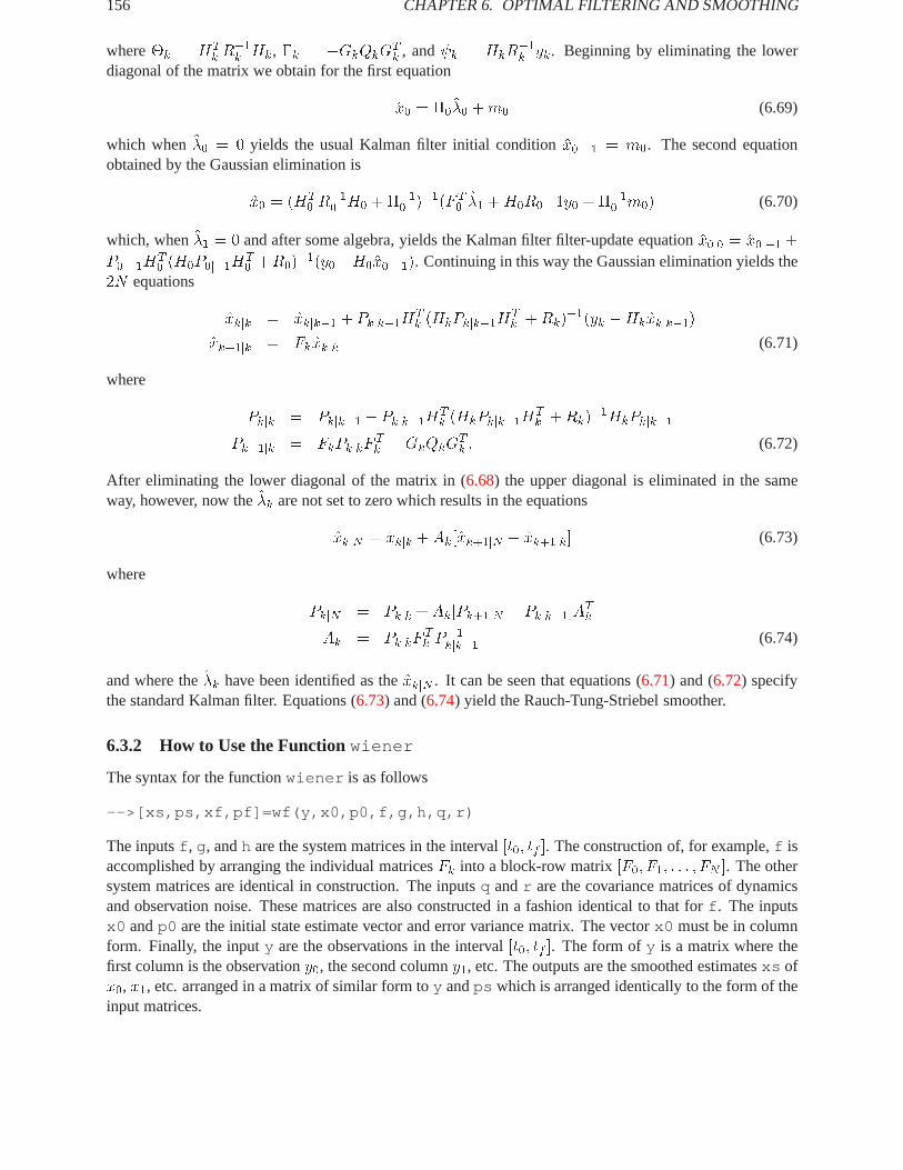
156 CHAPTER6. OPTIMAL FILTERING AND SMOOTHING
where�k = HTk R
�1k Hk, �k = �GkQkG
Tk , and k = HkR
�1k yk. Beginning by eliminating the lower
diagonal of the matrix we obtain for the first equation
x0 = �0�0 +m0 (6.69)
which when�0 = 0 yields the usual Kalman filter initial conditionx0j�1 = m0. The second equationobtained by the Gaussian elimination is
x0 = (HT0 R
�10 H0 +��10 )�1(F T
0 �1 +H0R0�1y0 +��10 m0) (6.70)
which, when�1 = 0 and after some algebra, yields the Kalman filter filter-update equationx0j0 = x0j�1 +P0j�1HT
0 (H0P0j�1HT0 +R0)
�1(y0�H0x0j�1). Continuing in this way the Gaussian elimination yields the2N equations
xkjk = xkjk�1 + Pkjk�1HTk (HkPkjk�1HT
k +Rk)�1(yk �Hkxkjk�1)
xk+1jk = Fkxkjk (6.71)
where
Pkjk = Pkjk�1 � Pkjk�1HTk (HkPkjk�1HT
k +Rk)�1HkPkjk�1
Pk+1jk = FkPkjkF Tk +GkQkG
Tk : (6.72)
After eliminating the lower diagonal of the matrix in (6.68) the upper diagonal is eliminated in the sameway, however, now the�k are not set to zero which results in the equations
xkjN = xkjk +Ak[xk+1jN � xk+1jk] (6.73)
where
PkjN = Pkjk +Ak[Pk+1jN � Pkjk�1]ATk
Ak = PkjkF Tk P
�1kjk�1 (6.74)
and where the�k have been identified as thexkjN . It can be seen that equations (6.71) and (6.72) specifythe standard Kalman filter. Equations (6.73) and (6.74) yield the Rauch-Tung-Striebel smoother.
6.3.2 How to Use the Functionwiener
The syntax for the functionwiener is as follows
-->[xs,ps,xf,pf]=wf(y,x0,p0,f,g,h,q,r)
The inputsf , g, andh are the system matrices in the interval[t0; tf ]. The construction of, for example,f isaccomplished by arranging the individual matricesFk into a block-row matrix[F0; F1; : : : ; FN ]. The othersystem matrices are identical in construction. The inputsq andr are the covariance matrices of dynamicsand observation noise. These matrices are also constructed in a fashion identical to that forf . The inputsx0 andp0 are the initial state estimate vector and error variance matrix. The vectorx0 must be in columnform. Finally, the inputy are the observations in the interval[t0; tf ]. The form ofy is a matrix where thefirst column is the observationy0, the second columny1, etc. The outputs are the smoothed estimatesxs ofx0, x1, etc. arranged in a matrix of similar form toy andps which is arranged identically to the form of theinput matrices.

6.3. THE WIENER FILTER 157
6.3.3 Example
In this section, thewiener function is demonstrated on a two-dimensional problem. The input to the filteris synthetic data obtained using the same system dynamics given to thewiener function. The system usedin the example is as follows.
xk+1 =
�1:15 :10 :8
�xk +
�1 00 1
�wk
yk =
�1 00 1
�xk + vk
where
EfwkwTk g =
�:01 00 :01
�
EfvkvTk g =
�20 00 20
�
and
Efx0g =
�1010
�
Ef(x0 �m0)(x0 �m0)T g =
�100 00 100
�
Figure6.3shows the results of using thewiener function on the synthetic data generated by the modelabove. Here the dotted line indicates the actual state values generated by the system. The circles on thedotted line serve to mark the actual state locations. The solid line marked by circles indicates the Kalmanfilter estimate of the state. The estimate ofx0 is located in the upper left corner of the figure and the estimateof x12 is located in the lower right corner of the figure. As can be seen the initial estimates obtained by theKalman filter are not so good with respect to the final estimates obtained by the filter. This is due to thelarge initial error covariance matrix given for the initial estimate of the state vector. The solid line markedby stars is the smoothed Kalman filter estimate. As can be seen, the final smoothed estimate is identical tothat of the regular Kalman filter. However, as the smoothed Kalman filter estimate works its way back tothe initial state value, the estimate becomes greatly improved, as is to be expected since these states are nowestimated based on all of the observed data.
The Scilab code which generated the example in this section is as follows.
-->//test of the wiener filter function
-->// initialize state statistics (mean and er. variance)
-->m0=[10 10]’;p0=[100 0;0 100];
-->// create system
-->f=[1.150.1;00.8];g=[1 0;0 1];
-->h=[1 0;0 1];[hi,hj]=size(h);
-->// noise statistics
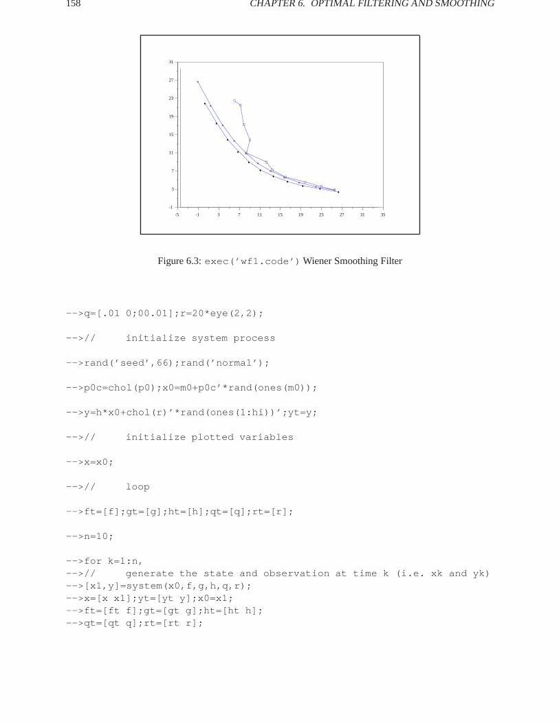
158 CHAPTER6. OPTIMAL FILTERING AND SMOOTHING
-5 -1 3 7 11 15 19 23 27 31 35
-1
3
7
11
15
19
23
27
31
×
×
×
×
×
×
×
××
××
⊕⊕
⊕
⊕
⊕
⊕
⊕
⊕⊕
⊕⊕
♦
♦
♦
♦
♦
♦
♦♦
♦♦
♦
Figure 6.3:exec(’wf1.code’) Wiener Smoothing Filter
-->q=[.01 0;00.01];r=20*eye(2,2);
-->// initialize system process
-->rand(’seed’,66);rand(’normal’);
-->p0c=chol(p0);x0=m0+p0c’*rand(ones(m0));
-->y=h*x0+chol(r)’*rand(ones(1:hi))’;yt=y;
-->// initialize plotted variables
-->x=x0;
-->// loop
-->ft=[f];gt=[g];ht=[h];qt=[q];rt=[r];
-->n=10;
-->for k=1:n,-->// generate the state and observation at time k (i.e. xk and yk)-->[x1,y]=system(x0,f,g,h,q,r);-->x=[x x1];yt=[yt y];x0=x1;-->ft=[ft f];gt=[gt g];ht=[ht h];-->qt=[qt q];rt=[rt r];

6.3. THE WIENER FILTER 159
-->// end loop-->end;
-->// get the wiener filter estimate
-->[xs,ps,xf,pf]=wiener(yt,m0,p0,ft,gt,ht,qt,rt);
-->// plot result
-->a=mini([x(1,:)-2*sqrt(ps(1,1:2:2*(n+1))),xf(1,:),xs(1,:)]);
-->b=maxi([x(1,:)+2*sqrt(ps(1,1:2:2*(n+1))),xf(1,:),xs(1,:)]);
-->c=mini([x(2,:)-2*sqrt(ps(2,2:2:2*(n+1))),xf(2,:),xs(2,:)]);
-->d=maxi([x(2,:)+2*sqrt(ps(2,2:2:2*(n+1))),xf(2,:),xs(2,:)]);
-->xmargin=maxi([abs(a),abs(b)]);
-->ymargin=maxi([abs(c),abs(d)]);
-->a=-0.1*xmargin+a;b=.1*xmargin+b;
-->c=-0.1*ymargin+c;d=.1*ymargin+d;
-->// plot frame, real state (x), and estimates (xf, and xs)
-->plot([a a b],[d c c]);
-->plot2d(x(1,:)’,x(2,:)’,[2],"000"),
-->plot2d(xf(1,:)’,xf(2,:)’,[2],"000"),
-->plot2d(xs(1,:)’,xs(2,:)’,[2],"000"),
-->// mark data points (* for real data, o for estimates)
-->plot2d(xs(1,:)’,xs(2,:)’,[-2],"000"),
-->plot2d(xf(1,:)’,xf(2,:)’,[-3],"000"),
-->plot2d(x(1,:)’,x(2,:)’,[-4],"000"),

160 CHAPTER6. OPTIMAL FILTERING AND SMOOTHING

Chapter 7
Optimization in filter design
In this chapter, some optimization techniques are investigated for the design of IIR as well as FIR filters.Those techniques are particuliarly usefull when non standard responses are desired.
7.1 Optimized IIR filters
In a previous chapter on the design of IIR filters, several methods have been investigated which make use ofclosed-form expressions for this purpose. In this section the desired specifications are achieved with the helpof optimization techniques: the set of convenient filter parameters is computed by minimizing some errorcriterion [24]. This technique has to be used when nonconventional filter specifications are to be achieved.
7.1.1 Minimum Lp design
The criterion that has been retained here is the minimumLp error and the set of parameters to be optimized,the set of poles and zeros the cardinal of which being specified by the user. The reason for such a choiceof parameters is that specifications on the group delay are much more easily written for this set than for theusual filter coefficients - especially the computations of gradients - One may note also that the minimumLp
error criterion admits the well-known minimum mean-square error criterion as a particular case by settingpto two.
Now, letH(z) be the transfer function of the filter given as a cascade ofK second-order sections:
H(z) = A
KYk=1
z2 � 2r0kcos�0kz + r20kz2 � 2rpkcos�pkz + r2pk
(7.1)
The set of parameters to be optimized is then given by the following vector:
� = (r0k; �0k; rpk; �pk; A) k = 1;K (7.2)
where index0 stands for zeros and indexp for poles, no confusion being to be expected with indexp intheLp error criterion. Usually the specifications for a filter are given separately for the magnitudejH(ej!)jand/or the group delay�(!); the corresponding expressions are:
jH(ej!)j , a(�; !) (7.3)
= A
KYk=1
(1� 2r0kcos(! � �0k) + r20k)1=2(1� 2r0kcos(! + �0k) + r20k)
1=2
(1� 2rpkcos(! � �pk) + r2pk)1=2(1� 2rpkcos(! + �pk) + r2pk)
1=2(7.4)
161
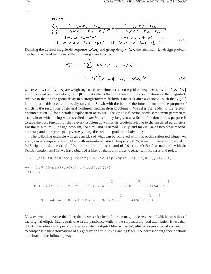
162 CHAPTER 7. OPTIMIZATION IN FILTER DESIGN
and
�(�; !) =KXk=1
f 1� rpkcos(! � �pk)
(1� 2rpkcos(! � �pk) + r2pk)1=2
+1� rpkcos(! + �pk)
(1� 2rpkcos(! + �pk) + r2pk)1=2
� 1� r0kcos(! � �0k)
(1� 2r0kcos(! � �0k) + r20k)1=2
� 1� r0kcos(! + �0k)
(1� 2r0kcos(! + �0k) + r20k)1=2g (7.5)
Defining the desired magnitude responsead(!j) and group delay�d(!), the minimumLp -design problemcan be formulated by mean of the following error function:
E(�) = �
JXj=1
wa(!j)[a(�; !j)� ad(!j)]2p
+ (1� �)
JXj=1
w� (!j)[�(�; !j)� �d(!j)]2p (7.6)
wherewa(!j) andw� (!j) are weighting functions defined on a dense grid of frequenciesf!j=0 � !j � �gand� is a real number belonging to[0; 1] that reflects the importance of the specifications on the magnituderelative to that on the group delay in a straightforward fashion. One seek after a vector�� such thatE(��)is minimum: this problem is easily solved in Scilab with the help of the functionoptim the purpose ofwhich is the resolution of general nonlinear optimization problems . We refer the reader to the relevantdocumentation [7] for a detailed explanation of its use. Theoptim function needs some input parameters,the main of which being what is called asimulator: it may be given as a Scilab function and its purpose isto give the cost function of the relevant problem as well as its gradient relative to the specified parameters.For the minimumLp design problem, the simulator is namediirlp and makes use of two other macros:iirmag andiirgroup ; it givesE(�) together with its gradient relative to�.
The following example will give an idea of what can be achieved with this optimization technique: weare given a low-pass elliptic filter with normalized cut-off frequency 0.25, transition bandwidth equal to0.15, ripple in the passband of 0.1 and ripple in the stopband of 0.01 (i.e. 40dB of attenuation); with theScilab functioneqiir we have obtained a filter of the fourth order together with its zeros and poles.
--> [ce0,f0,ze0,po0]=eqiir(’lp’,’ellip’,%pi*[.5;.65;0;0],.1,.01);
--> hz0=f0*prod(ce0(2))./prod(ce0(3))hz0 =
2 3 40.1164375 + 0.320825z + 0.4377450z + 0.320825z + 0.1164375z-----------------------------------------------------------
2 3 40.1744334 - 0.3436685z + 0.9682733z - 0.4106181z + z
Now we want to inverse this filter, that is we seek after a filter the magnitude reponse of which times that ofthe original elliptic filter equals one in the passband, while in the stopband the total attenuation is less than80dB. This situation appears for example when a digital filter is needed, after analog-to-digital conversion,to compensate the deformations of a signal by an anti-aliasing analog filter. The corresponding specificationsare obtained the following way:

7.1. OPTIMIZED IIR FILTERS 163
-->//design of a low-pass filter with normalized discrete frequency0.25
-->//ripple in the passband 0.1, ripple in the stopband 0.01,
-->//transition bandwidth0.1
-->[ce0,f0,ze0,po0]=eqiir(’lp’,’ellip’,%pi*[.5;.65;0;0],.1,.01);
-->// transfer function of the original filter.
-->hz0=f0*prod(ce0(2))./prod(ce0(3));
-->// initialization of the parameter vector(zeros, poles in polar coord.)
-->//poles and zeros (discarding the conjugates)
-->//of the original filter have been retained as initial values,
-->//leading to a filter with the same degree than the previous.
-->//the last value (10) is the initial value of the gain factor.
-->ze0=ze0(1:2:4);po0=po0(1:2:4);
-->x0=[abs([ze0 po0])’;atan(imag([ze0 po0]),real([ze0 po0]))’;10];
-->x=x0;
-->// grid of frequencies for the analysis
-->omega=%pi*(0.01:0.01:1);
-->// choice of the power for the criterion (mean-square here)
-->p=1;
-->// weighting function (one in the passband, 0.5 in the stopband)
-->wa(1:52)=ones(1,52);
-->wa(53:100)=.5*ones([53:100]);
-->// magnitude response of the original elliptic filter
-->rp0=abs(freq(hz0(2),hz0(3),exp(%i*omega)));
-->//plot(rp0)

164 CHAPTER 7. OPTIMIZATION IN FILTER DESIGN
-->// desired magnitude ad (ad(omega)*rp0(omega)=1 in the
-->//passband, ad having the same attenuation than the original
-->//filter in the stopband)
-->ad(1:49)=ones(1,49)./rp0(1:49);
-->ad(50:100)=rp0(50:100);
-->// starting an unconstrained optimization
-->x=[x0(1:4) x0(5:8)];
-->[cout,xx1,grad,to]=optim(iirmod,x);
-->binf=[0;-2*%pi].*.ones(4,1);
-->bsup=[1;2*%pi].*.ones(4,1);
-->binf=[binf(1:4) binf(5:8)]binf =
! 0. - 6.2831853 !! 0. - 6.2831853 !! 0. - 6.2831853 !! 0. - 6.2831853 !
-->bsup=[bsup(1:4) bsup(5:8)]bsup =
! 1. 6.2831853 !! 1. 6.2831853 !! 1. 6.2831853 !! 1. 6.2831853 !
-->[cout,xx2,grad,to]=optim(iirmod,’b’,binf,bsup,x);
-->z=poly(0,’z’);
-->z1=xx2(1,1)*exp(%i*xx2(1,2));
-->z2=xx2(2,1)*exp(%i*xx2(2,2));
-->num=(z-z1)*(z-z1’)*(z-z2)*(z-z2’)num =

7.1. OPTIMIZED IIR FILTERS 165
real part
2 3 40.2608817 + 0.7621389z + 1.5250529z + 1.4539504z + z
imaginary part
2.776D-17 + 5.551D-17z
-->num=real(num);
-->p1=xx2(3,1)*exp(%i*xx2(3,2));
-->p2=xx2(4,1)*exp(%i*xx2(4,2));
-->den=(z-p1)*(z-p1’)*(z-p2)*(z-p2’);
-->den=real(den);
-->sl=syslin(’c’,num/den);
-->ff=repfreq(sl,0.01,0.5,0.01);
-->rp1=abs(freq(num,den,exp(%i*omega)));
-->plot(rp1);
-->plot(rp0);
-->xbasc();
-->plot(20.*log(rp0.*rp1));
Although the constraints on the parameters can be easily specified, an unconstrained optimization procedurehas been applied because the initial values are unknown (hence may be far away from the optimal solution, ifany) and the order is unknown too. Instead, as indicated in [23], the Scilab functionoptim will be appliedseveral times and when some pole or zero goes outside the unit circle, it will be replaced by the symmetric(with respect to the unit circle) complex number and a new optimization runned. To see the results obtainedwith a constrained optimization, it may be interesting to run the following command, recalling that theconstraints on the poles and zeros are:�
0 � r0k � 1 0 � rpk � 10 � �0k � 2� 0 � �pk � 2�
(7.7)
hz0 =

166 CHAPTER 7. OPTIMIZATION IN FILTER DESIGN
2 3 40.1164375 + 0.320825z + 0.4377450z + 0.320825z + 0.1164375z-----------------------------------------------------------
2 3 40.1744334 - 0.3436685z + 0.9682733z - 0.4106181z + z
-->ze0=ze0(1:2:4);po0=po0(1:2:4);
-->x0=[abs([ze0 po0])’;atan(imag([ze0 po0]),real([ze0 po0]))’;10];
-->x=x0;
-->omega=%pi*(0.01:0.01:1);
-->wa(1:52)=ones(1,52);
-->wa(53:100)=.5*ones([53:100]);
-->rp0=abs(freq(hz0(2),hz0(3),exp(%i*omega)));
-->ad(1:49)=ones(1,49)./rp0(1:49);
-->ad(50:100)=rp0(50:100);
--> x0 = ...--> [ 1.--> 1.--> 0.8750714--> 0.4772780--> 2.0975887--> 2.636041--> 1.6018558--> 1.0620259--> 10. ];
-->x=[x0(1:4) x0(5:8)];
-->binf=[0;-2*%pi].*.ones(4,1);
-->bsup=[1;2*%pi].*.ones(4,1);
-->binf=[binf(1:4) binf(5:8)]binf =
! 0. - 6.2831853 !! 0. - 6.2831853 !! 0. - 6.2831853 !! 0. - 6.2831853 !
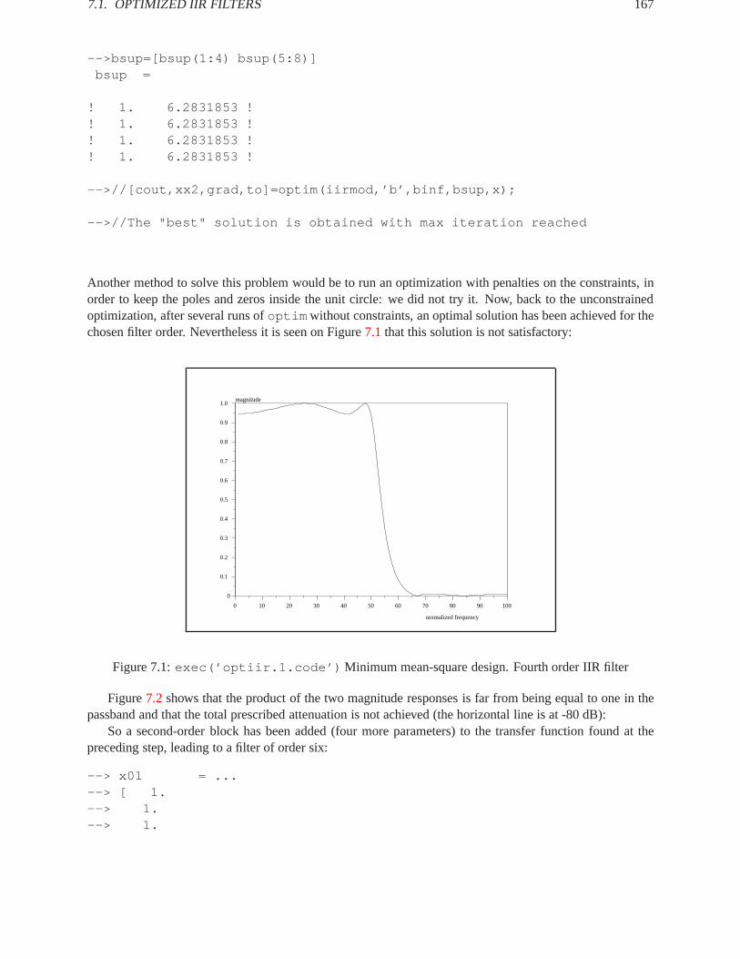
7.1. OPTIMIZED IIR FILTERS 167
-->bsup=[bsup(1:4) bsup(5:8)]bsup =
! 1. 6.2831853 !! 1. 6.2831853 !! 1. 6.2831853 !! 1. 6.2831853 !
-->//[cout,xx2,grad,to]=optim(iirmod,’b’,binf,bsup,x);
-->//The "best" solution is obtained with max iteration reached
Another method to solve this problem would be to run an optimization with penalties on the constraints, inorder to keep the poles and zeros inside the unit circle: we did not try it. Now, back to the unconstrainedoptimization, after several runs ofoptim without constraints, an optimal solution has been achieved for thechosen filter order. Nevertheless it is seen on Figure7.1that this solution is not satisfactory:
0 10 20 30 40 50 60 70 80 90 100
0
0.1
0.2
0.3
0.4
0.5
0.6
0.7
0.8
0.9
1.0magnitude
normalized frequency
Figure 7.1:exec(’optiir.1.code’) Minimum mean-square design. Fourth order IIR filter
Figure7.2 shows that the product of the two magnitude responses is far from being equal to one in thepassband and that the total prescribed attenuation is not achieved (the horizontal line is at -80 dB):
So a second-order block has been added (four more parameters) to the transfer function found at thepreceding step, leading to a filter of order six:
--> x01 = ...--> [ 1.--> 1.--> 1.

168 CHAPTER 7. OPTIMIZATION IN FILTER DESIGN
0 10 20 30 40 50 60 70 80 90 100
-80
-70
-60
-50
-40
-30
-20
-10
0magnitude in dB
normalized frequency
Figure 7.2:exec(’optiir.2.code’) Resulting magnitude response. Log scale
--> 0.8377264--> 0.3147539--> 0.9--> - 3.6886696--> 2.0017663--> 1.7--> 1.605514--> 1.4517773--> 1.3--> 0.1771141 ];
-->omega=%pi*(0.01:0.01:1);
-->z=poly(0,’z’);
-->num=z-x01(1);
-->den=z-x01(7);
-->for i=1:5-->num=num*(z-x01(i+1));-->den=den*(z-x01(i+7));-->end;
-->sl=syslin(’c’,num/den);
-->ff=repfreq(sl,0.01,0.5,0.01);

7.1. OPTIMIZED IIR FILTERS 169
-->hz01=abs(freq(num,den,exp(%i*omega)));
The same optimization procedure has been applied with this initial value, resulting in the following solutionvector:
--> x = ...--> [ 1.--> 1.--> 0.6887491--> 0.8828249--> 0.1052913--> 0.7457737--> - 3.6219555--> 2.1085705--> 1.4768262--> 1.6081331--> - 0.127d-08--> 1.3457622--> 0.1243695 ];
the desired magnitude reponse and the one achieved with that solution appear in Figure7.3, while the productof the log-magnitude responses is in Figure7.4.
0 10 20 30 40 50 60 70 80 90 100
0.7
0.8
0.9
1.0
1.1
1.2
1.3
Figure 7.3:exec(’optiir.3.code’) Minimum mean-square design. Sixth order IIR filter

170 CHAPTER 7. OPTIMIZATION IN FILTER DESIGN
0 10 20 30 40 50 60 70 80 90 100
-190
-170
-150
-130
-110
-90
-70
-50
-30
-10
10
Figure 7.4:exec(’optiir.4.code’) Resulting magnitude response. Log scale
As we are interested in what happens in the passband, focusing on it is needed: this is done in Figure7.5and we see that for! 2 [0; :45] the ripple is equal to 0.07 dB. The reader may convince himself that betterapproximation may be obtained with an increase of the filter order; we mention too that the specification ofad at the beginning of the transition is not likely to be that of a real filter (it has not a monotone decreasingbehaviour in that region !) and that a more realistic desired response could have been best approximatedwith the same number of parameters.
7.2 Optimized FIR filters
As for IIR filters, optimization techniques may be used to achieve particuliar specifications for FIR filters[24] . In this framework, the design problem formulation leads to a simple linear programming problem,which makes this approach attractive, as opposed to nonlinear methods used in the case of optimizationbased, IIR filter design.
As the approach in this section is based on the frequency sampling technique3.1, we first refer to thefrequency response of a linear phase FIR filter as given by formula3.1. In fact, because the linear phaseterm can be ignored for the design purpose, we rather consider the real function:
H�(ej!) =N�1Xk=0
H(k)S(!; k) (7.8)
where
S(!; k) = e�jk�=Nsin(N!=2)
sin(!=2 � k�=N)
= �e�jk�=N sin(N(!=2) � k�=N)
sin(!=2� k�=N)(7.9)
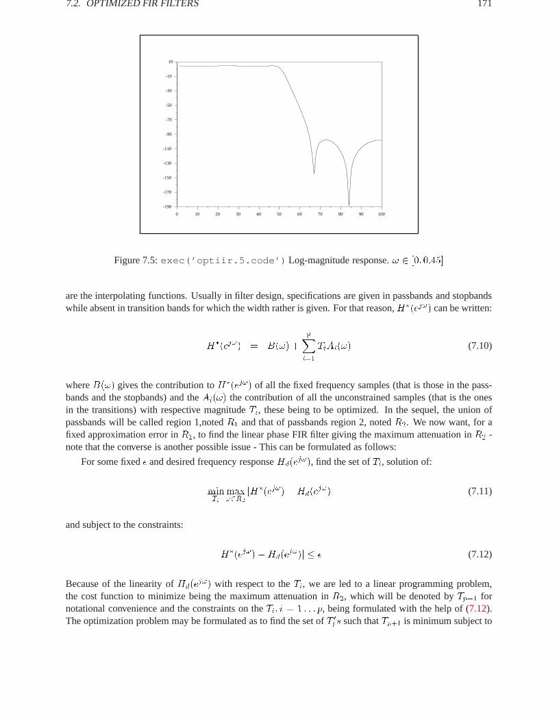
7.2. OPTIMIZED FIR FILTERS 171
0 10 20 30 40 50 60 70 80 90 100
-190
-170
-150
-130
-110
-90
-70
-50
-30
-10
10
Figure 7.5:exec(’optiir.5.code’) Log-magnitude response.! 2 [0; 0:45]
are the interpolating functions. Usually in filter design, specifications are given in passbands and stopbandswhile absent in transition bands for which the width rather is given. For that reason,H�(ej!) can be written:
H�(ej!) = B(!) +
pXi=1
TiAi(!) (7.10)
whereB(!) gives the contribution toH�(ej!) of all the fixed frequency samples (that is those in the pass-bands and the stopbands) and theAi(!) the contribution of all the unconstrained samples (that is the onesin the transitions) with respective magnitudeTi, these being to be optimized. In the sequel, the union ofpassbands will be called region 1,notedR1 and that of passbands region 2, notedR2. We now want, for afixed approximation error inR1, to find the linear phase FIR filter giving the maximum attenuation inR2 -note that the converse is another possible issue - This can be formulated as follows:
For some fixed� and desired frequency responseHd(ej!), find the set ofTi, solution of:
minTi
max!2R2
jH�(ej!)�Hd(ej!)j (7.11)
and subject to the constraints:
jH�(ej!)�Hd(ej!)j � � (7.12)
Because of the linearity ofHd(ej!) with respect to theTi, we are led to a linear programming problem,
the cost function to minimize being the maximum attenuation inR2, which will be denoted byTp+1 fornotational convenience and the constraints on theTi; i = 1 : : : p, being formulated with the help of (7.12).The optimization problem may be formulated as to find the set ofT 0is such thatTp+1 is minimum subject to
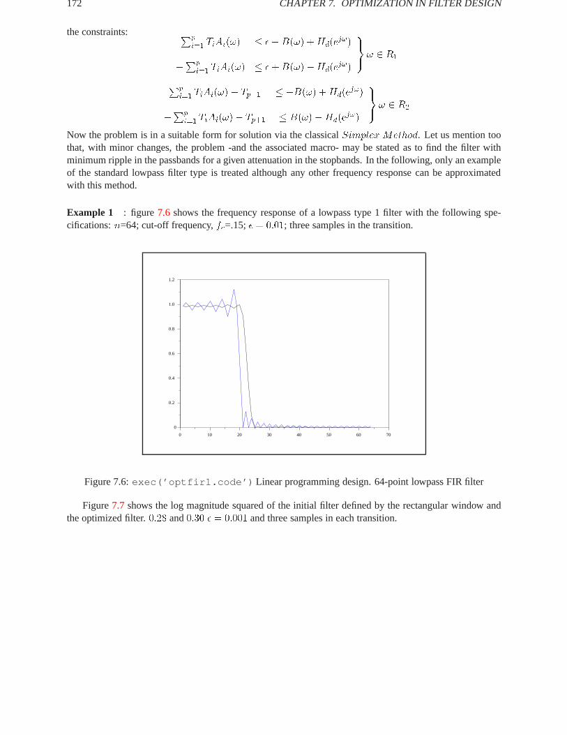
172 CHAPTER 7. OPTIMIZATION IN FILTER DESIGN
the constraints: Ppi=1 TiAi(!) � ��B(!) +Hd(e
j!)
�Ppi=1 TiAi(!) � �+B(!)�Hd(e
j!)
9=;! 2 R1
Ppi=1 TiAi(!)� Tp+1 � �B(!) +Hd(e
j!)
�Ppi=1 TiAi(!)� Tp+1 � B(!)�Hd(e
j!)
9=;! 2 R2
Now the problem is in a suitable form for solution via the classicalSimplex Method. Let us mention toothat, with minor changes, the problem -and the associated macro- may be stated as to find the filter withminimum ripple in the passbands for a given attenuation in the stopbands. In the following, only an exampleof the standard lowpass filter type is treated although any other frequency response can be approximatedwith this method.
Example 1 : figure 7.6 shows the frequency response of a lowpass type 1 filter with the following spe-cifications:n=64; cut-off frequency,fc=.15;� = 0:01; three samples in the transition.
0 10 20 30 40 50 60 70
0
0.2
0.4
0.6
0.8
1.0
1.2
Figure 7.6:exec(’optfir1.code’) Linear programming design. 64-point lowpass FIR filter
Figure7.7 shows the log magnitude squared of the initial filter defined by the rectangular window andthe optimized filter.0:28 and0:30 � = 0:001 and three samples in each transition.

7.2. OPTIMIZED FIR FILTERS 173
0 10 20 30 40 50 60 70
-900
-800
-700
-600
-500
-400
-300
-200
-100
0
100
Figure 7.7:exec(’optfir2.code’) Linear programming design.

174 CHAPTER 7. OPTIMIZATION IN FILTER DESIGN

Chapter 8
Stochastic realization
Let yk be a wide sense stationary gaussian process with covariance functionfRn;n 2 Zg. It is well-knownthatyk may be considered as the output of a filterF with a white noiseet as input. TheStochastic Realizationproblem foryk is the construction of an algorithm givingF ; in addition,F is usually asked to be causaland minimum delay (i.e. with causal inverse), for reasons of realizability. One major consequence of thisadditional constraint is thatF , when it exists, is minimal and unique, up to a transformation of coordinates.The filterF is called theModeling Filter and its inverseF�1 the Whitening Filter . Let us consider thefollowing examples, in which the information onyk is given two different ways. First, let be givenSy(z), thespectrum ofyk. Then, the whitening filter ofyk is the solutionE(z) of theSpectral Factorizationproblemof Sy(z), that is the solution of :
E(z)Sy(z)ET (z�1) = I (8.1)
such thatE(z) andE�1(z) are analytical in the unit disc, that is that the modeling filter ofyk is causaland minimum delay. The stochastic realization problem is then the computation ofE(z), givenSy(ei�).Solutions to this problem will be given in section8.1with direct factorization of matrix polynomials and in8.2via a state-space approach.
Another example is when the covariance functionRn = E(ykyTk�n) of yk is given - the information on
yk is then equivalent to that in the previous example- The whitening filter giving the innovation, or predictionerror, is obtained by minimizing with respect to the coefficientsAk, the mean square prediction error :
E(ketk2) = Efkyk �Xk>0
Akyt�kk2g (8.2)
The stochastic realization problem is then the computation of theAk as the solution of the followingYule-Walker, normal equations :
26664R0 R1 R2 : : :RT1 R0 R1 : : :
RT2 RT
1 R0 : : :...
3777526664A1
A2
A3...
37775 =
26664R1
R2
R3...
37775 (8.3)
This system being To¨eplitz, it may be efficiently solved using a Levinson-type algorithm ,as will be exposedin section8.4.
175

176 CHAPTER8. STOCHASTIC REALIZATION
8.1 Thesfact primitive
Given a matrix polynomialH(z) with sizen�m and rankn, the Scilab functionsfact gives the spectralfactorization ofH(z), that is a matrix polynomialD such that:
H(z) = D(z)D(1=z)zn (8.4)
Consider for example the following2� 2 matrix polynomiala(z), generated from the simulation of a two-dimensional process with three poles followed by a levinson filtering (see section8.4):
-->//Spectral factorization
-->z=poly(0,’z’);
-->a=[ -0.09-0.35z+zˆ2 ,-0.02-0.13z--> -0.03-0.15z , -0.08-0.36z+zˆ2 ]
a =
! 2 !! - 0.44 z + z - 0.15 z !! !! 2 !! - 0.18 z - 0.44 z + z !
-->// We calculate a(z)*a(1/z)*zˆ2
-->sp=a*horner(a,1/z)’;
-->sp=sp*z;
-->sp=sp(2)sp =
! 2 2 !! 1 + 3.2161z + z 1 + 2.1452z + z !! !! 2 2 !! 1 + 2.1452z + z 1 + 3.226z + z !
-->// We get a left spectral factor
-->d=sfact(sp)d =
! 1.6639845 + 0.6009671z 0.2934179z !! !! 1.0204088 + 0.6009671z 1.3181465 + 0.2934179z !
-->// We check the result
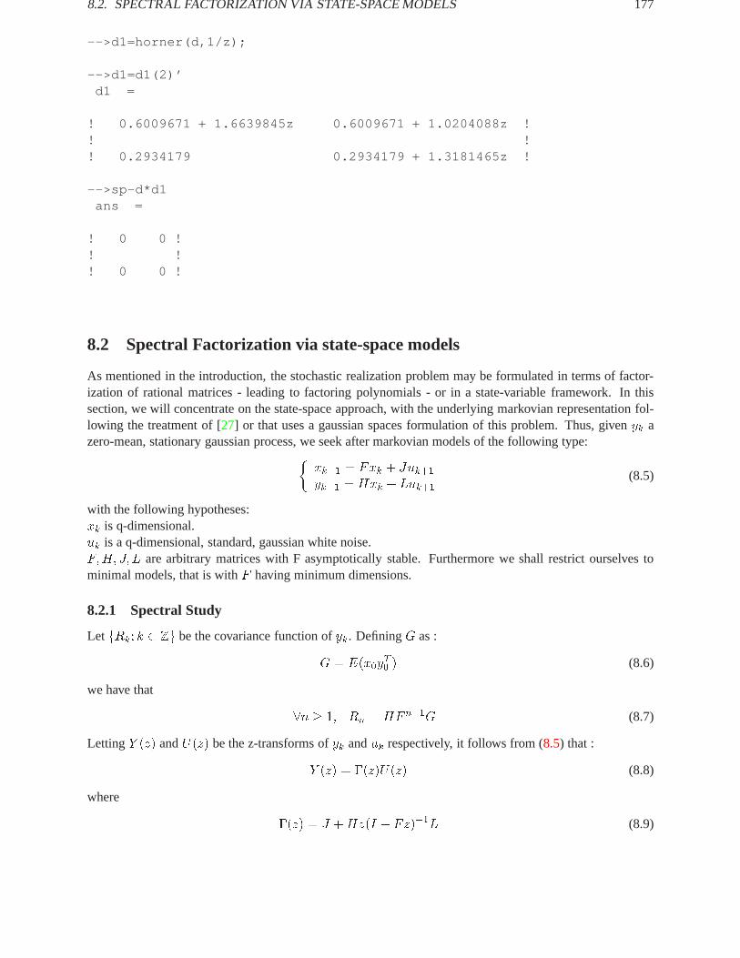
8.2. SPECTRAL FACTORIZATION VIA STATE-SPACE MODELS 177
-->d1=horner(d,1/z);
-->d1=d1(2)’d1 =
! 0.6009671 + 1.6639845z 0.6009671 + 1.0204088z !! !! 0.2934179 0.2934179 + 1.3181465z !
-->sp-d*d1ans =
! 0 0 !! !! 0 0 !
8.2 Spectral Factorization via state-space models
As mentioned in the introduction, the stochastic realization problem may be formulated in terms of factor-ization of rational matrices - leading to factoring polynomials - or in a state-variable framework. In thissection, we will concentrate on the state-space approach, with the underlying markovian representation fol-lowing the treatment of [27] or that uses a gaussian spaces formulation of this problem. Thus, givenyk azero-mean, stationary gaussian process, we seek after markovian models of the following type:�
xk+1 = Fxk + Juk+1
yk+1 = Hxk + Luk+1(8.5)
with the following hypotheses:xk is q-dimensional.uk is a q-dimensional, standard, gaussian white noise.F;H; J; L are arbitrary matrices with F asymptotically stable. Furthermore we shall restrict ourselves tominimal models, that is withF having minimum dimensions.
8.2.1 Spectral Study
Let fRk; k 2 Zg be the covariance function ofyk. DefiningG as :
G = E(x0yT0 ) (8.6)
we have that
8n � 1; Rn = HF n�1G (8.7)
LettingY (z) andU(z) be the z-transforms ofyk anduk respectively, it follows from (8.5) that :
Y (z) = �(z)U(z) (8.8)
where
�(z) = J +Hz(I � Fz)�1L (8.9)
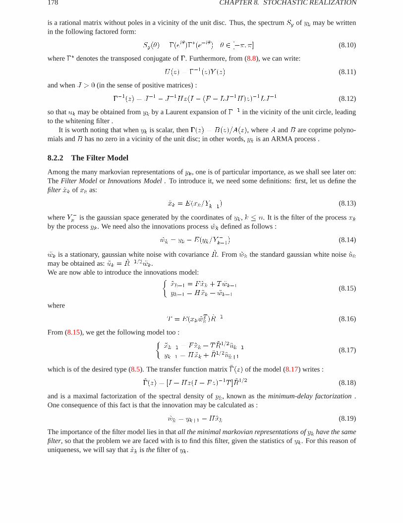
178 CHAPTER8. STOCHASTIC REALIZATION
is a rational matrix without poles in a vicinity of the unit disc. Thus, the spectrumSy of yk may be writtenin the following factored form:
Sy(�) = �(ei�)��(e�i�) � 2 [��; �] (8.10)
where�� denotes the transposed conjugate of�. Furthermore, from (8.8), we can write:
U(z) = ��1(z)Y (z) (8.11)
and whenJ > 0 (in the sense of positive matrices) :
��1(z) = J�1 � J�1Hz(I � (F � LJ�1H)z)�1LJ�1 (8.12)
so thatuk may be obtained fromyk by a Laurent expansion of��1 in the vicinity of the unit circle, leadingto the whitening filter .
It is worth noting that whenyk is scalar, then�(z) = B(z)=A(z), whereA andB are coprime polyno-mials andB has no zero in a vicinity of the unit disc; in other words,yk is an ARMA process .
8.2.2 The Filter Model
Among the many markovian representations ofyk, one is of particular importance, as we shall see later on:TheFilter Model or Innovations Model. To introduce it, we need some definitions: first, let us define thefilter ~xk of xk as:
~xk = E(xk=Y�k�1) (8.13)
whereY �k is the gaussian space generated by the coordinates ofyk, k � n. It is the filter of the processxkby the processyk. We need also the innovations process~wk defined as follows :
~wk = yk �E(yk=Y�k�1) (8.14)
~wk is a stationary, gaussian white noise with covariance~R. From ~wk the standard gaussian white noise~ukmay be obtained as:~uk = ~R�1=2 ~wk.We are now able to introduce the innovations model:�
~xk+1 = F ~xk + T ~wk+1
yk+1 = H~xk + ~wk+1(8.15)
where
T = E(xk ~wTk )
~R�1 (8.16)
From (8.15), we get the following model too :�~xk+1 = F ~xk + T ~R1=2~uk+1
yk+1 = H~xk + ~R1=2~uk+1(8.17)
which is of the desired type (8.5). The transfer function matrix~�(z) of the model (8.17) writes :
~�(z) = [I +Hz(I � Fz)�1T ] ~R1=2 (8.18)
and is a maximal factorization of the spectral density ofyk, known as theminimum-delay factorization.One consequence of this fact is that the innovation may be calculated as :
~wk = yk+1 �H~xk (8.19)
The importance of the filter model lies in thatall the minimal markovian representations ofyk have the samefilter, so that the problem we are faced with is to find this filter, given the statistics ofyk. For this reason ofuniqueness, we will say that~xk is thefilter of yk.

8.3. COMPUTING THE SOLUTION 179
8.3 Computing the solution
We assume now that we could get in some way the covariance sequence of the processyk. The models weconsider being minimal with dimensionq, it is a well-known fact in automatic control that the observabilitymatrix :
O =
26664
HHF
...HF q�1
37775 (8.20)
has its rank equal toq and is defined up to a similarity transformation; thus the pair(H;F ) is unique in thesame sense. For evident reasons G, defined in (8.6), shares the same property. Thus we can conclude thatthe triple(H;F;G) is unique up to a similarity transformation. It may be easily obtained from the empiricalcovariance functionfRkg with algorithms such that Ho’s [12] or Rissanen’s [26]. It is this point that weshall investigate now.
8.3.1 Estimation of the matrices H F G
Numerous algorithms exist for solving this problem and we shall focus on just one of them: the so-calledPrincipal Hankel Component(PHC) [17] approximation method, which is singular value decomposition(SVD) based . It is as follows: from the covariance sequence, form the Hankel matrix:
HM;N =
2666664
R0 R1 R2 : : : RN�1R1 R2 R3 : : : RN
R2 R3 R4 : : : RN+1...
......
...RM�1 RM RM+1 : : : RM+N�2
3777775 (8.21)
The reason for the wide use of this matrix is the Kronecker’s theorem which says that its rank is theoreticallyequal to the order of the associated system, i.e. equal to the dimension of state-vectors of minimal state-spacerealizations. Defining the matrixC as :
C =�G FG : : : F q�1G
�(8.22)
we have that :
HM;N = OC (8.23)
Now, from the observability matrixO, define the two following matrices:
O0=
26664
HHF
...HF q�2
37775 (8.24)
and
O" =
264
HF...
HF q�1
375 (8.25)
It is straightforward that:
O" = O0F (8.26)

180 CHAPTER8. STOCHASTIC REALIZATION
so that the matrixF is obtained as the least-squares solution of (8.26). H is obtained as the first bloc-row ofO andG as the first bloc-column ofC : this is the PHC approximation method.
Numerically, the factorization (8.23) is done via singular-value decomposition:
HM;N = USVT (8.27)
O andC are obtained as :
O = US1=2 C = S1=2V T (8.28)
The phc macro This macro implements the preceding algorithm to find the triple(H;F;G). In the fol-lowing example, a 64-point length covariance sequence has been generated for a two-dimensional process,the first component of which is the sum of two sinusoids with discrete frequencies�=10 and2�=10, whilethe second component is the sum of two sinusoids with frequencies�=10 and1:9�=10, both being in addit-ive, gaussian white noise. This is done as follows:
-->x=%pi/10:%pi/10:102.4*%pi;
-->rand(’seed’);rand(’normal’);
-->y=[.8*sin(x)+.8*sin(2*x)+rand(x);.8*sin(x)+.8*sin(1.99*x)+rand(x)];
-->c=[];
-->for j=1:2,for k=1:2,c=[c;corr(y(k,:),y(j,:),64)];end;end;
-->c=matrix(c,2,128);cov=[];
-->for j=1:64,cov=[cov;c(:,(j-1)*2+1:2*j)];end;
Then the Hankel matrixHM;N is built with the functionhank . Finally, thePsiLab functionphc gives thedesired triple(H;F;G).
8.3.2 computation of the filter
Now, we have obtained the triple(H;F;G) and we shall investigate the matricesT and ~R that have still to becomputed to completely determine the filter model (8.17). From this model, let us compute the convenientcovariances:
R0 = H ~PHT + ~R (8.29)
G = F ~PHT + T ~R (8.30)
~P = F ~PF T + T ~RT T (8.31)
8.3. COMPUTING THE SOLUTION 181
from which the following relations hold:
~R = R0 �H ~PHT (8.32)
T = (G� F ~PHT )(R0 �H ~PHT )�1 (8.33)
Noting that ~R andT depend solely on~P and supposing that~R is positive, we can write after elimination of~R between (8.29), (8.30) and (8.31):
~P = F ~PF T + (G� F ~PHT )(R0 �H ~PHT )�1(GT �H ~PF T ) (8.34)
which is the well-knownalgebraic Riccati equation. A matrix ~P is called a solution of the Riccati equationif it is positive definite, such thatR0�H ~PHT > 0 and satisfies equation (8.34). Although this equation hasseveral solutions, the following result gives an answer to our problem:the covariance~P of the filter is theminimal solution of the algebraic Riccati equation. We shall give now two algorithms giving this minimalsolution : the Faurre algorithm and the Lindquist algorithm .
The Faurre algorithm [9]: in this method, the solution~P is obtained as the growing limit of the sequenceof matricesPN such that:
PN+1 = FPNFT + (G� FPNH
T )(R0 �HPNHT )�1(GT �HPNF
T ) (8.35)
with the initial condition:P0 = GR�10 GT (8.36)
SettingP0 = 0 is allowed too for this leads toP1 = GR�10 GT hence to a simple delay in the iterations. Toconclude, having obtained~P via the recursion (8.35), the matrices~R andT are computed with equations(8.32) and (8.33) respectively. This is done with the macrosrfaur . The recursion forPN is not implemen-ted as in equation (8.35) for it may not converge, especially when the matrixF has poles near the unit circle.To overcome this difficulty, a factored form, Chandrasekhar type recursion has been implemented, leadingto the sought after solution even in the precedent defavourable situation1 . ThePsiLab functionsrfaurimplements this sqare-root algorithm.
Finally, the filter and the corresponding estimated output are calculated with the help of the model (8.17)by using the macroltitr which simulates linear systems. To summarize, the preceding example has beengenerated the following way:
-->// Simulation of a two-dimensional time-series (3 sinusoids)
-->x=%pi/10:%pi/10:102.4*%pi;
-->rand(’seed’,0);rand(’normal’);sx=sin(x);
-->y=[sx+sin(2*x);sx+sin(1.9*x)]+rand(2,1024);
-->// computation of correlations (64 delays)
-->c=[];
-->for j=1:2,for k=1:2,c=[c;corr(y(k,:),y(j,:),64)];end;end;
1A mistake was found in the initialization of the algorithm and could not be corrected in time for the present document

182 CHAPTER8. STOCHASTIC REALIZATION
-->c=matrix(c,2,128);cov=[];r0=c(1:2,1:2);
-->// hankel matrix H20,20 (i.e. square with 20 bloc-rows)
-->hk=hank(20,20,c);
-->// finding H,F,G by the PHC method
-->[h,f,g]=phc(hk,2,6);
-->// solving the algebraic Riccati equation
-->[p,s1,t1,l1,rT,tT]=srfaur(h,f,g,r0,200);
-->r12=sqrt(.5*(rT+rT’));
-->r12=real(r12);f=real(f);tT=real(tT);
-->spec(l1’*l1)ans =
1.0D-17 *
! 0. !! 0. !! 0. !! 0. !! 647184.16 !! 94723947. !
-->// simulation of the filter
-->rand(’seed’,0);rand(’normal’);
-->xest=ltitr(f,tT*r12,rand(2,1024));
-->rand(’seed’,0);rand(’normal’);
-->yest=h*xest+r12*rand(2,1024);
-->// correlations of the filter model output
-->cest=[];
-->for k=1:2,for j=1:2,cest=[cest;corr(yest(j,:),yest(k,:),64)];end;end
-->cest=matrix(cest,2,128);
8.4. LEVINSON FILTERING 183
The Lindquist algorithm [9]: This algorithm makes use of the fact that~R andT may be computed fromK = ~PHT instead of~P itself, leading to substantial computational savings when the observation has a muchlower dimension that the state, the most frequent situation. Refering the reader to [9] for the derivations, wegive now the algorithm itself:8<
:KN+1 = KN +�N ~R�1N �TNH
T
�N+1 = [F � (G� FKN )(R0 �HKN )�1H]�N
~RN+1 = ~RN � �TNHT (R0 �HKN )
�1H�N
(8.37)
with the initial conditions:
K0 = 0 �0 = G ~R0 = R� 0 (8.38)
Then the expression forT is the following:
T = (G� FK)(R0 �HK)�1 (8.39)
andlindquist is the correspondingPsiLab function.
8.4 Levinson filtering
We still consider hereyk, a stationary, vector-valued time-series , from which we have available a sampleyk�1; yk�2; : : : ; yk�N ; the scope here is to estimateyk from this sample, by someyk, say, which may bewritten then as a linear combination of theyk�j, j = 1; : : : ; N : yk =
PNj=1A
Nj yk�j. As mentioned in
the introduction, this problem may be stated as a stochastic realization problem: attempting to minimize themean-square prediction error of orderN at timek:
E(kek(N)k2) = Efkyk �NXj=1
ANj yk�jk2g (8.40)
the filter coefficientsANj , where the superscriptN indicates the dependence on the sample length, are found
to be the solutions of the following To¨eplitz system :2666664
R0 R1 R2 : : : RN�1RT1 R0 R1 : : : RN�2
RT2 RT
1 R0 : : : RN�3...
......
. . ....
RTN�1 RT
N�2 RTN�3 : : : R0
3777775
2666664
A1
A2
A3...AN
3777775 =
2666664
R1
R2
R3...RN
3777775 (8.41)
The mean-square error�N is easily calculated:
�N = E((yk � yk)(yk � yk)T )
(8.42)
= E((yk � yk)yTk )
(8.43)

184 CHAPTER8. STOCHASTIC REALIZATION
= E(ykyTk )�
NXj=1
ANj E(yk�jy
Tk )
= R0 �NXj=1
ANj R�j (8.44)
where the second equality holds from the orthogonality principle between the estimate and the predictionerror. Classically,�N is taken as a measure of the quality of the estimation, since it is a monotone decreas-ing function ofN (the longer the sample, the better the estimation). One may for example compare it toa preassigned mean-square estimation error. So, the problem is to find a procedure which calculates, suc-cessively for eachN , the coefficientsAN
j and�N . An answer is given with Levinson-type algorithms, animportant property of which is their recursivity in the order: one particularity, relative to other input-outputrepresentations such as state-space models or rational matrices, is that in this approach the filter structure -its order for example- is considered as a parameter as well as any other, leading to the idea of lattice filterand to cascade-type realizations of transfer functions. Let us describe now the Levinson algorithm in thecase of a vector-valued time-series, noting that in the scalar case the backward prediction error is no usebecauseR�k = Rk, leading to simpler derivations, albeit similar. For the exposition we shall make use of aHilbert space approach, following the treatment given in5.4.3.
8.4.1 The Levinson algorithm
Suppose we are given the vector-valued time-seriesyk. We begin with some definitions:ek(N) andfk(N) will denote respectively the forward and backward prediction errors of orderN at time k:
ek(N) = yk �NXj=1
ANj yk�j (8.45)
fk(N) = yk�N �NXj=1
BNj yk�N+j (8.46)
with the convention that:ek(0) = fk(0) = yk. We shall need also the following linear space:Y qp =
spanfyp; : : : ; yqg. In the present geometrical approach, the covarianceE(xyT ) of x andy will be noted[x; y] (scalar product) and ifE(xyT ) = 0, we shall writex ? y (x orthogonal to y), as well asA ? B fortwo orthogonal linear spaces. In view of these definitions, the following relations hold:
ek(N) 2 Y kk�N and ek(N) ? Y k�1
k�N (8.47)
fk(N) 2 Y kk�N and fk(N) ? Y k
k�N+1 (8.48)
From (8.45), we get:
ek(N + 1)� ek(N) 2 Y k�1k�N�1 (8.49)
while ek(N + 1) ? Y k�1k�N�1 andek(N) ? Y k�1
k�N imply that:
ek(N + 1)� ek(N) ? Y k�1k�N (8.50)

8.4. LEVINSON FILTERING 185
Recalling (8.48), relations (8.49) and (8.50) caracterize the space spanned byfk�1(N); hence there exists amatrixKN such that:
ek(N + 1)� ek(N) = �KNfk�1(N) (8.51)
KN is determined with the help of the orthogonality condition:
ek(N + 1) ? yk�N�1 (8.52)
this relation implies that:
[ek(N + 1); yk�N�1]= [ek(N); yk�N�1] �KN :[fk�1(N); yk�N�1]= 0
(8.53)
hence giving:
KN = [ek(N); yk�N�1][fk�1(N); yk�N�1]�1 (8.54)
We recognize the second scalar product as the backward mean-square error�N . Relations for the backwardprediction error may be obtained the same way; they are:
fk(N + 1)� fk�1(N) 2 Y kk�N and? Y k�1
k�N (8.55)
which caracterize the space spanned byek(N); thus there exists a matrixK�N such that:
fk(N + 1)� fk�1(N) = �K�Nek(N) (8.56)
and determined by the orthogonality condition:
fk(N + 1) ? yk (8.57)
which leads to:
K�N = [fk�1(N); yk][ek(N); yk]
�1 (8.58)
Here too the second scalar product is seen to be the forward mean-square error�N . Relations (8.51), (8.54),(8.56), (8.58) give the sought after recursions; their lattice structure may be explicited with the help of thefollowing matrix polynomials:
AN (z) = I �NXj=1
ANj z
j (8.59)
BN (z) = zNI �NXj=1
BNj z
N�j (8.60)
and the covariance matrices:Rn = [yk; yk�n], from whichKN andK�N may be expressed:
KN = (RN+1 �NXj=1
ANj RN+1�j)(R0 �
NXj=1
BNj Rj)
�1
= �N��1N (8.61)

186 CHAPTER8. STOCHASTIC REALIZATION
K�N = (R�N�1 �
NXj=1
BNj R�N�1+j)(R0 �
NXj=1
ANj R�j)
�1
= �N��1N (8.62)
with evident definitions. The last recursion to be given is that for�N , for which we will use the expressionsof KN (8.61) andK�
N in (8.62), and the definition of�N :
�N = [ek(N); yk] (8.63)
Then we can compute�N+1 as follows:
�N+1 = [ek(N + 1); yk]
= [ek(N)� �N��1N fk�1(N); yk]
= [ek(N); yk]� �N��1N [fk�1(N); yk]
= �N � �N��1N �N (8.64)
In the same fashion,�N+1 will be written as:
�N+1 = �N � �N��1N �N (8.65)
To summarize,the algorithm is as follows:
8>>>>>>>>>>>>>>>>>>>>>>><>>>>>>>>>>>>>>>>>>>>>>>:
�AN+1(z)BN+1(z)
�=
�I �KN z
�K�N z I
� �AN (z)BN (z)
�
KN = �N��1N
K�N = �N�
�1N
�N+1 = �N � �N��1N �N
�N+1 = �N � �N��1N �N
�N = (R�N�1 �PN
j=1BNj R�N�1+j)
�N = (RN+1 �PN
j=1ANj RN+1�j)
(8.66)
with the initial conditions: ��0 = R�N�1;�0 = RN+1
�0 = �0 = R0;A0(z) = B0(z) = I(8.67)
The corresponding Scilab function islevin .
Chapter 9
Time-Frequency representations of signals
Numerous tools such as DFT, periodogram, maximum entropy method, have been presented in previouschapters for the spectral analysis of stationary processes. But, in many practical situations (speech, acoustics,biomedicine applications, ...), this assumption of stationarity fails to be true. Specific tools are then to beused when the spectral content of a signal under consideration is time dependent. Two such tools will bepresented in this chapter: TheWigner-V ille representation and the classicalShort-T ime periodogram, which are particuliar cases of a more general class of spectral estimators[18]. Nevertheless, due to thesuperiority of the so-calledwigner spectrum, no numerical computation will be done for the short-timeperiodogram.
9.1 The Wigner distribution
Let be given a discrete-time signalf(n) and is Fourier transform:
F (�) =Xn2Z
f(n)e�jn� (9.1)
The Wigner distribution off(n) is given by:
Wf (n; �) = 2Xk2Z
e�j2k�f(n+ k)f�(n� k) (9.2)
Useful in a time-frequency representation framework, a similar expression may be written forF (�):
WF (�; n) =1
�
Z �
��ej2n�F (� + �)F �(� � �)d� (9.3)
so that:
WF (�; n) =Wf (n; �) (9.4)
illustrating the symmetry between the definitions in both time and frequency domains. Among the propertieslisted in [6] are the�-periodicity and the hermitic property, the last leading to the fact that the Wignerdistribution of real signals is real. One more important result is the following:
1
2�
Z �=2
��=2Wf (n; �)d� = jf(n)j2 (9.5)
which means that the integral over a period of the Wigner distribution is equal to the instantaneous signalpower.
187
188 CHAPTER9. TIME-FREQUENCY REPRESENTATIONS OF SIGNALS
9.2 Time-frequency spectral estimation
All the properties stated in [6] for deterministic signals with finite energy are still valid for random processeswith harmonizable covariance, that is those for which the covariance functionK(s; t) has the decomposition:
K(s; t) = E(X(s)X�(t))
=1
4�2
Z �
��
Z �
��ei(�s��t)f(�; �)d�d� (9.6)
The same way an harmonic analysis of stationary random processes with the Fourier transform leads to theclassical spectrum, a mixed time-frequency analysis can be done with the Wigner distribution, leading toa “time-frequency spectrum”, which reduces to the first with the stationary assumption. In [18], a generalclass of spectral estimators is considered:
W (n; �;�) =1
�
Xk2Z
Xm2Z
Z �
��eipm�(p; 2k)X(n +m+ k)X�(n+m� k)e�i2�kdp (9.7)
where�(p; 2k) is the Fourier transform of a data window caracterizing the weighting on the products. Afirst choice of�(p; 2k) is:
�STP (p; 2k) =1
2N � 1
Xj2Z
hN (j + k)h�N (j � k)eipj (9.8)
leading to the well-knownshort time periodogram:
STP (n; �) =1
2N � 1jXj2Z
X(k)hN (k � n)e�i�nj2 (9.9)
which actually is the classical periodogram of the signal to which has been applied a sliding window;smoothed versions may be obtained for this estimator[18] If now �(p; 2k) is chosen to be:
�SPW (p; 2k) = jhN (k)j2Xm2Z
gM (m)e�ipm (9.10)
equation (9.6) particularizes in thesmoothed pseudo-wigner spectral estimator:
PW (n; �) = 2Xk2Z
e�i2�kjhN (k)j2Xm2Z
gM (m)X(n+m� k)X�(n+m� k) (9.11)
wherehN (k) andgM (m) are windows with respective length2N � 1 and2M � 1. One major advantagein chosing�SPW (n; 2k) is that it is a separable function, so that independent smoothing can be applied inthe time and frequency directions, as opposed to�STP (n; 2k) which is governed by “uncertainty relations”between the time and frequency weightings. Thence, the bias, known to be introduced by weighting func-tions in spectral estimation, can be controlled separately for the pseudo-wigner estimator. Morever, in thecase of unsmoothed pseudo-wigner (M = 1), the bias in the time direction vanishes while always presentfor the short time periodogram.
Now, we can compute the wigner spectrum estimator: letx(n) denote the analytical signal of the
sampled realization of the processX(t). SettingM = 1 (unsmoothed estimator) and�ldef= �(l=N),
we can write with the help of (9.10):
PW (n; �l) = 2N�1X
k=�N+1
e�i2k�(l=N)jhN (k)j2x(n+ k)x�(n� k) (9.12)
= 2(2RefN�1Xk=0
e�i2k�(l=N)jhN (k)j2x(n+ k)x�(n� k)g � jx(n)j2)

9.2. TIME-FREQUENCY SPECTRAL ESTIMATION 189
and this expression may be easily computed via the FFT with the Scilab functionwigner .
Example 1 : The following example is taken from [18]: the signal is a finite duration sinusoid modulatedby a parabola:
S(t) =
8<:
p(t) sin(2�16 t+ u(t� 488)�) 408 < t < 568
0 0 � t � 408 ; 567 � t � 951
p(t) is the parabola taking its maximum int = 488, u(t) is the unit step function,hN is the 64-pointrectangular window; the time and frequency increments are respectively equal to12 and�=128; M hasbeen set to one (unsmoothed estimator). The signal generation and wigner spectrum computation are thenas follows:
-->// parabola
-->a=[488ˆ2 488 1;408ˆ2 408 1;568ˆ2 568 1];
-->b=[1.28;0;0];
-->x=a\b;
-->t=408:568;
-->p=x’*[t.*t;t;ones(t)];
-->// unit step function
-->u=[0*ones(408:487) ones(488:568)];
-->// finite duration sinusoid
-->s=p.*sin(2*%pi/16*t+u*%pi);
-->// signal to be analyzed
-->s=[0*ones(0:407) s 0*ones(569:951)];
-->// 64-point rectangular window
-->h=ones(1,64);
-->// wigner spectrum
-->w=wigner(s,h,12,128);
-->plot3d(1:69,1:64,abs(w(1:69,1:64)));
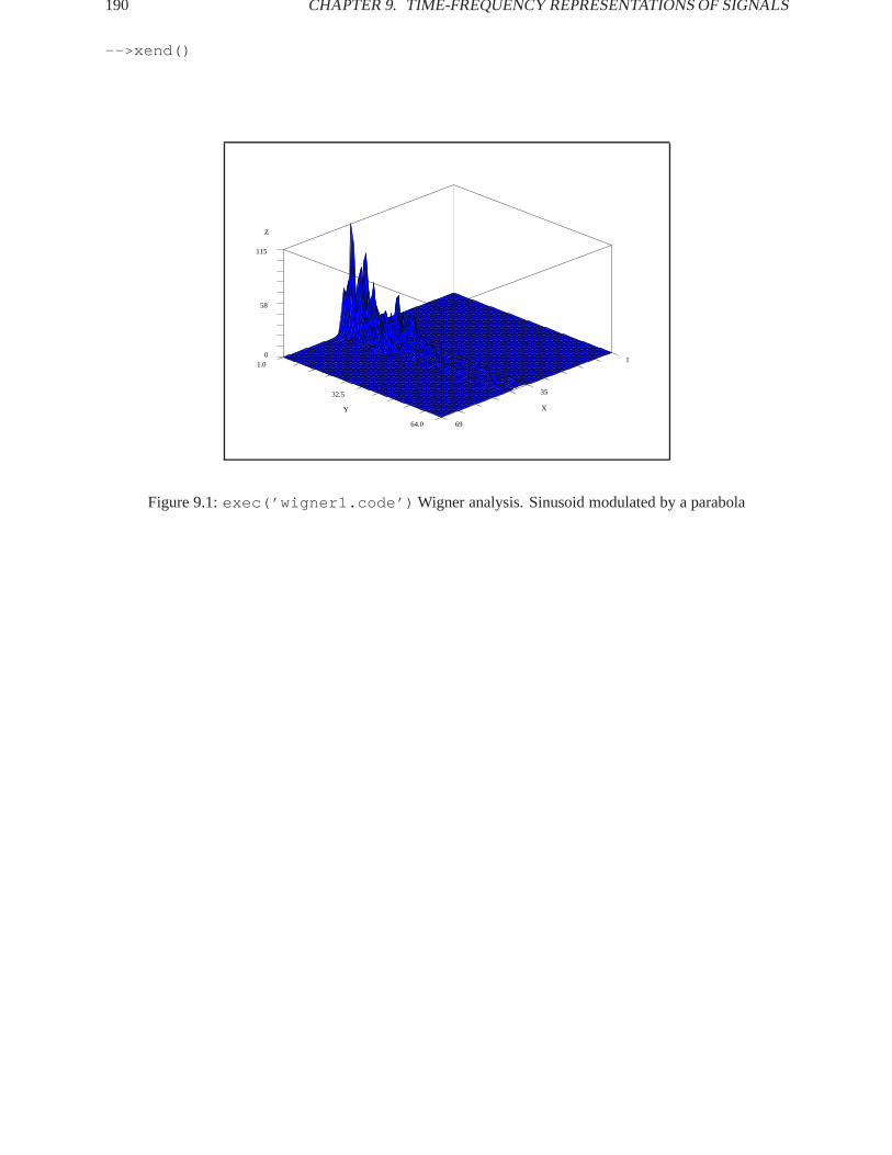
190 CHAPTER9. TIME-FREQUENCY REPRESENTATIONS OF SIGNALS
-->xend()
115
58
0
Z
1.0
32.5
64.0
Y
69
35
1
X
Figure 9.1:exec(’wigner1.code’) Wigner analysis. Sinusoid modulated by a parabola

Bibliography
[1] M. Abramowitz, I.A. Stegun, eds.,Handbook of Mathematical Functions, National Bureau of Stand-ards Applied Mathematics Series, no. 55, Superintendent of Documents, U.S. Goverment PrintingOffice, Washington, D.C., 1964.
[2] B.D.O. Anderson and J.B. Moore,Optimal Filtering, Englewood Cliffs, NJ: Prenctice Hall, 1979.
[3] Gerald J. Bierman,Factorization Methods for Discrete Sequential Estimation, Academic Press, NewYork, 1977.
[4] B.C. Carlson,Special Functions of Applied Mathematics, Academic Press, New York, 1977.
[5] E.W. Cheney,Introduction to Approximation Theory, McGraw-Hill, 1966.
[6] T.A.C.M. Claasen and W.F.G. Mecklenbrauker, “The Wigner distribution: a tool for time frequencysignal analysis”,Phillips J. Res., vol. 35, pp. 217-250, 276-300, 372-389, 1980.
[7] F. Delebecque, C. Klimann and S. Steer,Basile, guide d’utilisation, Internal Report INRIA, 1987.
[8] J. Dieudonn´e,Calcul Infinitesimal, Hermann, Paris, 1980.
[9] P. Faurre,Realisations markoviennes de processus stationnaires, These d’etat, Rapport Laboria n0 13,1973.
[10] A. Gelb, ed.,Applied Optimal Estimation, MIT Press, 1974.
[11] Francis B. Hildebrand,Methods of Applied Mathematics, Prentice Hall, Englewood Cliffs, N.J., 1965.
[12] B.L. Ho and R.E. Kalman, “Effective construction of linear state variable models from Input/Outputdata”,Proc. 3rd Allerton Conference, 1963.
[13] R. Hooke, T.A. Jeeves, “Direct Search solution of numerical and statistical problems”, Journ. Assoc.Comput. Mach., Vol 8 No 2, pp 212-229, April 1961.
[14] T. Kailath,Lectures on Wiener and Kalman Filtering, Springer-Verlag, New York, 1981.
[15] T. Kailath,Linear Systems, Prentice Hall, 1980.
[16] Steven M. Kay and Stanley L. Marple, “Spectrum Analysis - A Modern Perspective”,Proc. IEEE, vol.69, no. 11, pp. 1380-1419, Nov. 1981.
[17] S. Kung, “A new identification and model reduction algorithm via singular value decompositions”,Proc. 12th Asilomar Conf. Circuits, Syst. Comput., Pacific Grove, CA, pp 705-714, Nov 1978.
[18] W. Martin and P. Flandrin, “Wigner-Ville spectral analysis of nonstationary processes”,IEEE Trans.Acoust., Speech, Signal Processing, Vol. ASSP-33, N0 6, Dec. 1985.
191

192 BIBLI OGRAPHY
[19] C. Moler, MATLAB User’s Guide, Tech. Rep. CS81-1, Dept. of Computer Sci., Univ. New Mexico,August, 1982.
[20] R. Nikoukhah,A Deterministic and Stochastic Theory of Two-Point Boundary-Value Descriptor Sys-tems, Ph.D. dissertation, Dept. of Elec. Eng. and Comp. Science, M.I.T., 1988.
[21] A.V. Oppenheim and R.W. Schafer,Digital Signal Processing, Prentice Hall, 1975.
[22] M. Prevosto, A. Benveniste, B. Barnouin, “La m´ethode des variables instrumentales en treillis;application a la modelisation des structures en vibration”, Outils et mod`eles math´ematiques pourl’Automatique, l’Analyse des syst`emes et le Traitement du Signal, Vol 2, pp 639-667, Ed. CNRS,1982.
[23] Programs for Digital Signal Processing, IEEE Press John Wiley and Sons, 1979.
[24] L. Rabiner and B. Gold,Theory and Application of Digital Signal Processing, Prentice Hall, 1975.
[25] L.R. Rabiner, R.W. Schafer, and C.M. Rader, “The Chirp Z-Transform Algorithm and its Applica-tions”, Bell Sys. Tech. J., vol 48, pp. 1249-1292, May 1969.
[26] J. Rissanen, “Recursive identification of linear systems”,SIAM Journal of Control, Vol 9, 1971.
[27] G. Ruckebusch,Representations markoviennes de processus gaussiens stationnaires, These 3eme cylemath. stat., Paris VI, 1975.
[28] K. Steiglitz, “Designing Short-Word recursive digital filters”, Proc. 9th Allerton Conf. on Circuit andSystems Theory, pp 778-788, Oct. 1971.
[29] G.W. Stewart,Introduction to Matrix Computations, Academic Press, New York, 1973.
[30] C.F. Van Loan, “Computing integrals involving matrix exponentials”,IEEE Trans. Autom. Control, volAC-23, pp. 395-404, 1978.

List of Figures
1.1 Block Diagrams of System Interconnections. . . . . . . . . . . . . . . . . . . . . . . . . . 111.2 exec(’flts1.code’) Sum of Two Sinusoids. . . . . . . . . . . . . . . . . . . . . . . 151.3 exec(’flts2.code’) Filtered Signal. . . . . . . . . . . . . . . . . . . . . . . . . . . 161.4 exec(’plot1.code’) Plot of Filter Impulse Response. . . . . . . . . . . . . . . . . . 161.5 exec(’plot2.code’) Plot of Continuous Filter Magnitude Response. . . . . . . . . . 171.6 exec(’plot3.code’) Plot of Discrete Filter Magnitude Response. . . . . . . . . . . . 181.7 exec(’plot4.code’) Plot of Poles and Zeros of IIR Filter. . . . . . . . . . . . . . . 19
2.1 exec(’bode1.code’) Log-Magnitude Plot ofH(s) = 1=(s� a) . . . . . . . . . . . . 222.2 exec(’bode2.code’) Phase Plot ofH(s) = 1=(s� a) . . . . . . . . . . . . . . . . . 232.3 exec(’bode3.code’) Log-Magnitude Plot ofH(s) = (s2 � 2as+ (a2 + b2))�1 . . . 242.4 exec(’bode4.code’) Phase Plot ofH(s) = (s2 � 2as+ (a2 + b2))�1 . . . . . . . . . 252.5 exec(’bode5.code’) Bode Plot of State-Space System Representation. . . . . . . . . 262.6 exec(’bode6.code’) Bode Plot of Rational Polynomial System Representation. . . . 272.7 exec(’bode7.code’) Bode Plot Combined Systems. . . . . . . . . . . . . . . . . . . 282.8 exec(’group1 5.code’) Modulated Exponential Signal. . . . . . . . . . . . . . . . 302.9 exec(’group1 5.code’) Constant Phase Band Pass Filter. . . . . . . . . . . . . . . 302.10 exec(’group1 5.code’) Carrier Phase Shift bytp = �=2 . . . . . . . . . . . . . . . 312.11 exec(’group1 5.code’) Linear Phase Band Pass Filter. . . . . . . . . . . . . . . . . 312.12 exec(’group1 5.code’) Envelope Phase Shift bytg = �1 . . . . . . . . . . . . . . . 322.13 exec(’group6 8.code’) Group Delay of Linear-Phase Filter. . . . . . . . . . . . . . 332.14 exec(’group6 8.code’) Group Delay of Filter (Rational Polynomial). . . . . . . . . 342.15 exec(’group6 8.code’) Group Delay of Filter (Cascade Realization). . . . . . . . . 352.16 exec(’sample1.code’) Frequency ResponseX() . . . . . . . . . . . . . . . . . . . 392.17 exec(’sample2.code’) Frequency Responsex(!) With No Aliasing . . . . . . . . . 392.18 exec(’sample3.code’) Frequency Responsex(!) With Aliasing . . . . . . . . . . . 402.19 exec(’sample4.code’) Cosine Signal. . . . . . . . . . . . . . . . . . . . . . . . . . 412.20 exec(’sample5.code’) Aliased Cosine Signal. . . . . . . . . . . . . . . . . . . . . 412.21 exec(’intdec1 4.code’) Fourier Transform of a Continuous Time Signal. . . . . . 422.22 exec(’intdec1 4.code’) Fourier Transform of the Discrete Time Signal. . . . . . . 432.23 exec(’intdec1 4.code’) Fourier Transform ofv(nT 0) . . . . . . . . . . . . . . . . 442.24 exec(’intdec1 4.code’) Fourier Transform ofx(nT 0) . . . . . . . . . . . . . . . . 452.25 Block Diagram of Interpolation and Decimation. . . . . . . . . . . . . . . . . . . . . . . . 452.26 exec(’intdec5 10.code’) The Sequencex(nT ) . . . . . . . . . . . . . . . . . . . . 462.27 exec(’intdec5 10.code’) The DFT ofx(nT ) . . . . . . . . . . . . . . . . . . . . . 472.28 exec(’intdec5 10.code’) Low Pass Filter. . . . . . . . . . . . . . . . . . . . . . . 472.29 exec(’intdec5 10.code’) DFT of v(nT 0) . . . . . . . . . . . . . . . . . . . . . . . 482.30 exec(’intdec5 10.code’) Filtered Version ofV . . . . . . . . . . . . . . . . . . . . 482.31 exec(’intdec5 10.code’) Sequencex(nMT=L) . . . . . . . . . . . . . . . . . . . 49
193

194 LIST OF FIGURES
2.32 exec(’fft1.code’) Cosine Signal . . . . . . . . . . . . . . . . . . . . . . . . . . . . 522.33 exec(’fft2.code’) DFT of Cosine Signal. . . . . . . . . . . . . . . . . . . . . . . . 522.34 Convolution Performed by Linear System. . . . . . . . . . . . . . . . . . . . . . . . . . . 542.35 exec(’czt1.code’) Samples of the z-transform on Spirals. . . . . . . . . . . . . . . 572.36 Filter Realization of CZT. . . . . . . . . . . . . . . . . . . . . . . . . . . . . . . . . . . . 58
3.1 exec(’fir1.code’) Rectangularly windowed low-pass filter. . . . . . . . . . . . . . 643.2 exec(’fir2 5.code’) Frequency response of a low pass filter. . . . . . . . . . . . . 653.3 exec(’fir2 5.code’) Frequency response of a high pass filter. . . . . . . . . . . . . 653.4 exec(’fir2 5.code’) Frequency response of a band pass filter. . . . . . . . . . . . . 663.5 exec(’fir2 5.code’) Frequency response of a stop band filter. . . . . . . . . . . . . 673.6 exec(’fir6.code’) Magnitude of rectangular window. . . . . . . . . . . . . . . . . 683.7 exec(’fir7.code’) Low pass filter with Kaiser window,n = 33, � = 5:6 . . . . . . . 703.8 exec(’fir8.code’) Stop band filter with Hamming window,n = 127, � = :54 . . . . 713.9 exec(’fir9.code’) Band pass filter with Chebyshev window,n = 55, dp = :001, df = :0446622 713.10 exec(’fstyp121.code’) Type 1 band pass filter with no sample or one sample in each transition band733.11 exec(’fstyp122.code’) Type 1 and type 2 low pass filter. . . . . . . . . . . . . . . 743.12 exec(’remez1.code’) Minimax Approximation for Linear Equations. . . . . . . . . 763.13 exec(’remez2 4.code’) Low Pass Filter with No Transition Band. . . . . . . . . . . 803.14 exec(’remez2 4.code’) Low Pass Filter with Transition Band[:24; :26] . . . . . . . . 813.15 exec(’remez2 4.code’) Triangular Shaped Filter. . . . . . . . . . . . . . . . . . . . 823.16 exec(’remez5 7.code’) Stop Band Filter of Even Length. . . . . . . . . . . . . . . 833.17 exec(’remez5 7.code’) Stop Band Filter of Odd Length. . . . . . . . . . . . . . . . 833.18 exec(’remez5 7.code’) High Pass Filter Design. . . . . . . . . . . . . . . . . . . . 84
4.1 exec(’analog1.code’) Magnitude in dB.n = 13; !c = 300 . . . . . . . . . . . . . . 864.2 exec(’analog2.code’) Butterworth filter: pole positions.n = 13 . . . . . . . . . . . 884.3 exec(’analog3.code’) Magnitude of a Type 1 Chebyshev filter. . . . . . . . . . . . 894.4 exec(’analog4.code’) Chebyshev filter: frequency response in magnitude. . . . . . 914.5 exec(’analog5.code’) Magnitude of a Type 2 Chebyshev filter. . . . . . . . . . . . 924.6 exec(’analog6.code’) The rectangleR0 , image byu of the positive real axis.. . . . 974.7 exec(’analog7.code’) Behavior of the sn function for real values. . . . . . . . . . . 984.8 exec(’analog8.code’) Behavior of the sn function for imaginary values. . . . . . . 994.9 exec(’analog9.code’) v(z) for z in�n, with n = 9 . . . . . . . . . . . . . . . . . . 1014.10 exec(’analog10.code’) log(m) versuslog(m1) for ordern fixed . . . . . . . . . . . 1034.11 exec(’analog11.code’) Response of Prototype Elliptic Filter. . . . . . . . . . . . . 1044.12 exec(’analog12.code’) Example of response of a filter obtained byzpell . . . . . 1064.13 exec(’iir1.code’) Transforms = (1� z�1)=T . . . . . . . . . . . . . . . . . . . . 1084.14 exec(’iir2 3.code’) Magnitude of Analog Filter. . . . . . . . . . . . . . . . . . . . 1114.15 exec(’iir2 3.code’) Magnitude of Digital Filter. . . . . . . . . . . . . . . . . . . . 1124.16 exec(’iir4.code’) Digital Low-Pass Filter . . . . . . . . . . . . . . . . . . . . . . . 1154.17 exec(’iir5.code’) Digital Band-Pass Filter. . . . . . . . . . . . . . . . . . . . . . . 1164.18 exec(’eqiir4.code’) Example of response obtained witheqiir . . . . . . . . . . . 120
5.1 exec(’spect1.code’) Overlapping Data . . . . . . . . . . . . . . . . . . . . . . . . 1235.2 exec(’spect2 4.code’) Log Magnitude Squared of Filter. . . . . . . . . . . . . . . 1255.3 exec(’spect2 4.code’) Estimate of Spectrum. . . . . . . . . . . . . . . . . . . . . 1255.4 exec(’spect2 4.code’) Estimate of Spectrum. . . . . . . . . . . . . . . . . . . . . 1275.5 exec(’mem1 3.code’) Input Data Sequence,x(n) . . . . . . . . . . . . . . . . . . . . 130

LIST OF FIGURES 195
5.6 exec(’mem1 3.code’) Maximum Entropy Spectral Estimate ofx(n) . . . . . . . . . . 1315.7 exec(’mem1 3.code’) Squared Magnitude of the Fourier Transform ofx(n) . . . . . . 131
6.1 exec(’kf1.code’) Steady-State Kalman Filter Tracking. . . . . . . . . . . . . . . . . 1406.2 exec(’kf2.code’) Kalman Filter Tracking. . . . . . . . . . . . . . . . . . . . . . . . 1416.3 exec(’wf1.code’) Wiener Smoothing Filter. . . . . . . . . . . . . . . . . . . . . . . 158
7.1 exec(’optiir.1.code’) Minimum mean-square design. Fourth order IIR filter. . . . 1677.2 exec(’optiir.2.code’) Resulting magnitude response. Log scale. . . . . . . . . . 1687.3 exec(’optiir.3.code’) Minimum mean-square design. Sixth order IIR filter. . . . 1697.4 exec(’optiir.4.code’) Resulting magnitude response. Log scale. . . . . . . . . . 1707.5 exec(’optiir.5.code’) Log-magnitude response.! 2 [0; 0:45] . . . . . . . . . . . 1717.6 exec(’optfir1.code’) Linear programming design. 64-point lowpass FIR filter. . . 1727.7 exec(’optfir2.code’) Linear programming design. . . . . . . . . . . . . . . . . . 173
9.1 exec(’wigner1.code’) Wigner analysis. Sinusoid modulated by a parabola. . . . . . 190

Index
Aanalog filters . . . . . . . . . . . . . . . . . . . . . . . . . . . . . .85
Butterworth . . . . . . . . . . . . . . . . . . . . . . . . . . .85Chebyshev . . . . . . . . . . . . . . . . . . . . . . . . . . . .88
first type . . . . . . . . . . . . . . . . . . . . . . . . . . . .88second type . . . . . . . . . . . . . . . . . . . . . . . . .91
elliptic . . . . . . . . . . . . . . . . . . . . . . . . . . . . . . .94arma process. . . . . . . . . . . . . . . . . . . . . . . . . . . . .178
Bbilinear transform. . . . . . . . . . . . . . . . . . . . . . . .109Bode plot . . . . . . . . . . . . . . . . . . . . . . . . . . . . . . . . .21
examples . . . . . . . . . . . . . . . . . . . . . . . . . . . . .25Bode plot,function syntax . . . . . . . . . . . . . . . . . .24Butterworth filter . . . . . . . . . . . . . . . . . . . . . . . . . .85
CChandrasekhar . . . . . . . . . . . . . . . . . . . . . . . . . . .181changing system representation. . . . . . . . . . . . . .9Chebyshev approximation . . . . . . . . . . . . . . . . . .75Chebyshev filter . . . . . . . . . . . . . . . . . . . . . . . . . . .88
first type . . . . . . . . . . . . . . . . . . . . . . . . . . . . . .91second type . . . . . . . . . . . . . . . . . . . . . . . . . . .88
chirp z-transform. . . . . . . . . . . . . . . . . . . . . . . . . .56examples . . . . . . . . . . . . . . . . . . . . . . . . . . . . .59
convolution . . . . . . . . . . . . . . . . . . . . . . . . . . . . . . .54function syntax . . . . . . . . . . . . . . . . . . . . . . . .55
correlation method . . . . . . . . . . . . . . . . . . . . . . .126example . . . . . . . . . . . . . . . . . . . . . . . . . . . . .126
cost function . . . . . . . . . . . . . . . . . . . . . . . . . . . . .162
Ddecimation . . . . . . . . . . . . . . . . . . . . . . . . . . . .40, 44DFT . . . . . . . . . . . . . . . . . . . . . . . . . . . . . . . . . . . . . .46discretization of continuous systems. . . . . . . . .12
Eelliptic filter . . . . . . . . . . . . . . . . . . . . . . . . . . . . . . .94elliptic function . . . . . . . . . . . . . . . . . . . . . . . . . . .97elliptic integral . . . . . . . . . . . . . . . . . . . . . . . . . . . .94error criterion . . . . . . . . . . . . . . . . . . . . . . . . . . . .161
FFaurre algorithm. . . . . . . . . . . . . . . . . . . . . . . . .181FFT . . . . . . . . . . . . . . . . . . . . . . . . . . . . . . . . . . . . . .46
examples . . . . . . . . . . . . . . . . . . . . . . . . . . . . .51filter
model . . . . . . . . . . . . . . . . . . . . . . . . . . . . . . .178FIR filter design
examples . . . . . . . . . . . . . . . . . . . . . . . . . . . . .70frequency sampling . . . . . . . . . . . . . . . . . . . .72function syntax . . . . . . . . . . . . . . . . . . . . . . . .69minimax optimization . . . . . . . . . . . . . . . . . .74windowing technique . . . . . . . . . . . . . . . . . .63
FIR filters . . . . . . . . . . . . . . . . . . . . . . . . . . . . . . . . .63Fourier transform . . . . . . . . . . . . . . . . . . . . . . . . .187function syntax
bode . . . . . . . . . . . . . . . . . . . . . . . . . . . . . . . .24convol . . . . . . . . . . . . . . . . . . . . . . . . . . . . .55dscr . . . . . . . . . . . . . . . . . . . . . . . . . . . . . . . .13eqfir . . . . . . . . . . . . . . . . . . . . . . . . . . . . . . .81eqiir . . . . . . . . . . . . . . . . . . . . . . . . . . . . . .115flts
for state-space . . . . . . . . . . . . . . . . . . . . . .14for transfer function . . . . . . . . . . . . . . . . .14
frmag . . . . . . . . . . . . . . . . . . . . . . . . . . . . . . .18group . . . . . . . . . . . . . . . . . . . . . . . . . . . . . . .32iir . . . . . . . . . . . . . . . . . . . . . . . . . . . . . . . .113kalm . . . . . . . . . . . . . . . . . . . . . . . . . . . . . . .140load . . . . . . . . . . . . . . . . . . . . . . . . . . . . . . . . .2read . . . . . . . . . . . . . . . . . . . . . . . . . . . . . . . . .2remezb . . . . . . . . . . . . . . . . . . . . . . . . . . . . .77roots . . . . . . . . . . . . . . . . . . . . . . . . . . . . . . . .4save . . . . . . . . . . . . . . . . . . . . . . . . . . . . . . . . .2srkf . . . . . . . . . . . . . . . . . . . . . . . . . . . . . . .152ss2tf . . . . . . . . . . . . . . . . . . . . . . . . . . . . . . .10sskf . . . . . . . . . . . . . . . . . . . . . . . . . . . . . . .139syslin . . . . . . . . . . . . . . . . . . . . . . . . . . . . . . .9tf2ss . . . . . . . . . . . . . . . . . . . . . . . . . . . . . . .10wfir . . . . . . . . . . . . . . . . . . . . . . . . . . . . . . . .69wiener . . . . . . . . . . . . . . . . . . . . . . . . . . . .156write . . . . . . . . . . . . . . . . . . . . . . . . . . . . . . . .2
196

INDEX 197
Ggaussian
process. . . . . . . . . . . . . . . . . . . . . . . . .175, 177space . . . . . . . . . . . . . . . . . . . . . . . . . . .177, 178white noise . . . . . . . . . . . . . . . . . . . . . . . . . .177
Gaussian random vectorsconditional statistics . . . . . . . . . . . . . . . . . .133filtered by linear systems . . . . . . . . . . . . . .134recursive estimation . . . . . . . . . . . . . . . . . .135
group delay . . . . . . . . . . . . . . . . . . . . . .27, 161, 162function syntax . . . . . . . . . . . . . . . . . . . . . . . .32
Hhankel . . . . . . . . . . . . . . . . . . . . . . . . . . . . . . . . . . .179Householder transformation . . . . . . . . . . . . . . .151
IIIR filter design . . . . . . . . . . . . . . . . . . . . . . . . . .106
alternate implementation . . . . . . . . . . . . . .115examples . . . . . . . . . . . . . . . . . . . . . . .114, 116function code . . . . . . . . . . . . . . . . . . . . . . . .115function syntax . . . . . . . . . . . . . . . . . . . . . .113
IIR filters . . . . . . . . . . . . . . . . . . . . . . . . . . . . . . . . .85innovation . . . . . . . . . . . . . . . . . . . . . . . . . .175, 178innovations
model . . . . . . . . . . . . . . . . . . . . . . . . . . . . . . .178process. . . . . . . . . . . . . . . . . . . . . . . . . . . . . .178
interconnecting systems . . . . . . . . . . . . . . . . . . . .11interpolation . . . . . . . . . . . . . . . . . . . . . . . . . . .40, 43interpolation-decimation
example . . . . . . . . . . . . . . . . . . . . . . . . . . . . . .46
KKalman filter . . . . . . . . . . . . . . . . . . . . . . . . . . . . .133
asymptotic properties. . . . . . . . . . . . . . . . .138equations . . . . . . . . . . . . . . . . . . . . . . . . . . . .136examples . . . . . . . . . . . . . . . . . . . . . . . . . . . .140function syntax . . . . . . . . . . . . . . . . . . . . . .140square root . . . . . . . . . . . . . . . . . . . . . . . . . .149
function syntax . . . . . . . . . . . . . . . . . . . .152steady state
example . . . . . . . . . . . . . . . . . . . . . . . . . . .139function syntax . . . . . . . . . . . . . . . . . . . .139
Llevinson . . . . . . . . . . . . . . . . . . . . . . . . . . . .176, 184levinson filters
lattice filters . . . . . . . . . . . . . . . . . . . . . . . . .183Levinson’s algorithm. . . . . . . . . . . . . . . . . . . . .129
macro syntax . . . . . . . . . . . . . . . . . . . . . . . .130
library siglib . . . . . . . . . . . . . . . . . . . . . . . . . . . .1Lindquist algorithm. . . . . . . . . . . . . . . . . . . . . . .181linear programming . . . . . . . . . . . . . . . . . . . . . . .170
Mmacro syntax
lev . . . . . . . . . . . . . . . . . . . . . . . . . . . . . . . .130mese . . . . . . . . . . . . . . . . . . . . . . . . . . . . . . .129
macro,spfact . . . . . . . . . . . . . . . . . . . . . . . . . .176magnitude response. . . . . . . . . . . . . . . . . . . . . . .162markovian
model . . . . . . . . . . . . . . . . . . . . . . . . . . . . . . .177representation. . . . . . . . . . . . . . . . . . . . . . . .178
matrix polynomial . . . . . . . . . . . . . . . . . . . . . . . .175maximum entropy method . . . . . . . . . . . . . . . . .127
examples . . . . . . . . . . . . . . . . . . . . . . . . . . . .130macro syntax . . . . . . . . . . . . . . . . . . . . . . . .129
mean-square error . . . . . . . . . . . . . . . . . . . . . . . .161minimax approximation . . . . . . . . . . . . . . . . . . . .75minimum
delay . . . . . . . . . . . . . . . . . . . . . . . . . . . . . . . .175factorization . . . . . . . . . . . . . . . . . . . . . . .178
Lp error . . . . . . . . . . . . . . . . . . . . . . . . . . . . .161minimum Lp design . . . . . . . . . . . . . . . . . . . . . .161modeling filter . . . . . . . . . . . . . . . . . . . . . . . . . . .175
Oobservability matrix . . . . . . . . . . . . . . . . . . . . . .179optimal filtering and smoothing . . . . . . . . . . . .133optimal FIR filter design . . . . . . . . . . . . . . . . . . .75
examples . . . . . . . . . . . . . . . . . . . . . . . . . . . . .78function syntax . . . . . . . . . . . . . . . . . . . .77, 81
optimization . . . . . . . . . . . . . . . . . . . . . . . . .161, 162optimized
FIR filters . . . . . . . . . . . . . . . . . . . . . . . . . . .170IIR filters . . . . . . . . . . . . . . . . . . . . . . . . . . . .161
Pperiodogram method. . . . . . . . . . . . . . . . . . . . . .122
example . . . . . . . . . . . . . . . . . . . . . . . . . . . . .123phase delay . . . . . . . . . . . . . . . . . . . . . . . . . . . . . . .27plotting . . . . . . . . . . . . . . . . . . . . . . . . . . . . . . . . . . .15
continuous magnitude. . . . . . . . . . . . . . . . . .17discrete magnitude . . . . . . . . . . . . . . . . . . . .18impulse response. . . . . . . . . . . . . . . . . . . . . .15poles and zeros . . . . . . . . . . . . . . . . . . . . . . . .19
poly . . . . . . . . . . . . . . . . . . . . . . . . . . . . . . . . . . . . .4polynomials. . . . . . . . . . . . . . . . . . . . . . . . . . . . . . . .4
evaluation . . . . . . . . . . . . . . . . . . . . . . . . . . . . .8
198 INDEX
representation of transfer functions. . . . . . .9principal hankel component. . . . . . . . . . . . . . .179
Rrandom number generator. . . . . . . . . . . . . . . . . . .3Rauch-Tung-Striebel two filter smoother. . . .154Remez algorithm. . . . . . . . . . . . . . . . . . . . . . . . . .76riccati equation. . . . . . . . . . . . . . . . . . . . . . . . . . .181
Ssampling . . . . . . . . . . . . . . . . . . . . . . . . . . . . . . . . .37short-time periodogram. . . . . . . . . . . . . . . . . . .187signals . . . . . . . . . . . . . . . . . . . . . . . . . . . . . . . . . . . . .1
saving and loading . . . . . . . . . . . . . . . . . . . . . .2simulation of random. . . . . . . . . . . . . . . . . . .3
simplex method . . . . . . . . . . . . . . . . . . . . . . . . . .172simulation of random signals. . . . . . . . . . . . . . . .3singular value decomposition. . . . . . . . . . . . . .179spectral . . . . . . . . . . . . . . . . . . . . . . . . . . . . . . . . . .187
density . . . . . . . . . . . . . . . . . . . . . . . . . . . . . .178factorization . . . . . . . . . . . . . . . . . . . . .175, 176
spectral estimation . . . . . . . . . . . . . . . . . . . . . . . .121correlation method . . . . . . . . . . . . . . . . . . .126maximium entropy method . . . . . . . . . . . .127periodogram method. . . . . . . . . . . . . . . . . .122
spectrum . . . . . . . . . . . . . . . . . . . . . . . . . . . .175, 178square root Kalman filter . . . . . . . . . . . . . . . . . .149state space representation. . . . . . . . . . . . . . . . . . . .9stationary . . . . . . . . . . . . . . . . . . . . . . . . . . . . . . . .175steady state Kalman filter . . . . . . . . . . . . . . . . . .139stochastic
realization . . . . . . . . . . . . . . . . . . . . . . . . . . .175system transfer functions . . . . . . . . . . . . . . . . . . . .4
Ttime series . . . . . . . . . . . . . . . . . . . . . . . . . . . . . . .183time-frequency. . . . . . . . . . . . . . . . . . . . . . . . . . .187toeplitz . . . . . . . . . . . . . . . . . . . . . . . . . . . . .175, 183toolbox library . . . . . . . . . . . . . . . . . . . . . . . . . . . . .1transforming low pass filters . . . . . . . . . . . . . . .112transition . . . . . . . . . . . . . . . . . . . . . . . . . . . . . . . .162
Wwhitening filter . . . . . . . . . . . . . . . . . . . . . . . . . . .175Wiener filter . . . . . . . . . . . . . . . . . . . . . . . . . . . . .153
example . . . . . . . . . . . . . . . . . . . . . . . . . . . . .157function syntax . . . . . . . . . . . . . . . . . . . . . .156
wigner . . . . . . . . . . . . . . . . . . . . . . . . . . . . . . . . . .187windowing
FIR filters . . . . . . . . . . . . . . . . . . . . . . . . . . . .63
spectral estimation . . . . . . . . . . . . . . . . . . .122windows
Chebyshev . . . . . . . . . . . . . . . . . . . . . . . . . . . .69Hamming . . . . . . . . . . . . . . . . . . . . . . . . . . . . .68Kaiser . . . . . . . . . . . . . . . . . . . . . . . . . . . . . . . .68rectangular. . . . . . . . . . . . . . . . . . . . . . . . . . .67triangular . . . . . . . . . . . . . . . . . . . . . . . . . . . . .67
Yyule-walker . . . . . . . . . . . . . . . . . . . . . . . . . . . . . .175