
Présentée en vue d'obtenir le grade de Docteur...
155
+ + Cette thèse est accessible à l'adresse : http://theses.insa-lyon.fr/publication/2014ISAL0038/these.pdf © [M. Jiu], [2014], INSA de Lyon, tous droits réservés
Transcript of Présentée en vue d'obtenir le grade de Docteur...

Numéro d'ordre: Année 2014
Institut National Des Sciences Appliquées de Lyon
Laboratoire d'InfoRmatique en Image et Systèmes
d'information
École Doctorale Informatique et Mathématique de Lyon
Thèse de l'Université de Lyon
Présentée en vue d'obtenir le grade de Docteur,
spécialité Informatique
par
Mingyuan Jiu
Spatial information and end-to-end
learning for visual recognition
Thèse soutenue le 3 Avril 2014 devant le jury composé de:
Mme. Michèle Rombaut Professeur, Université Joseph Fourier Grenoble Rapporteur
M. Matthieu Cord Professeur, UPMC-Sorbonne Universities Rapporteur
Mme. Cordelia Schmid INRIA Research Director Examinateur
M. Alain Trémeau Professeur, Université Jean Monnet Saint Etienne Examinateur
M. Graham Taylor Maître de Conférences, University of Guelph, Canada Examinateur
M. Atilla Baskurt Professeur, INSA Lyon Directeur
M. Christian Wolf Maître de Conférences, HDR, INSA Lyon Co-encadrant
Laboratoire d'InfoRmatique en Image Systèmes d'information
UMR 5205 CNRS - INSA de Lyon - Bât. Jules Verne
69621 Villeurbanne cedex - France
Tel: +33(0)4 72 43 60 97 - Fax: +33(0)4 72 43 71 17
Cette thèse est accessible à l'adresse : http://theses.insa-lyon.fr/publication/2014ISAL0038/these.pdf © [M. Jiu], [2014], INSA de Lyon, tous droits réservés

Cette thèse est accessible à l'adresse : http://theses.insa-lyon.fr/publication/2014ISAL0038/these.pdf © [M. Jiu], [2014], INSA de Lyon, tous droits réservés
Acknowledgments
In this moment, I would like to express my sincere appreciations to numerous
people who have given me helps and supports throughout my study during
the past three and half years.
First of all, my most sincere and deep gratitude is for my supervisors,
Prof. Atilla Baskurt and Dr. Christian Wolf, without whose constant guidance
and assistances this thesis would not be possible.
Secondly, I would like to sincerely acknowledge our collaborators
Prof. Christopher Garcia and Dr. Graham Taylor of University of Guelph,
Canada. I learned too much from discussion with them.
Besides, I would like to sincerely acknowledge Prof. Michèle Rombaut,
Prof. Matthieu Cord, Prof. Cordelia Schmid and Prof. Alain Trémeau for
their kindness to become my thesis reviewers and examiners and for their
time on constructive and meticulous assessment of this thesis work.
I also want to thank all the members I have met/worked with in the
Bâtment Jules Verne, INSA de Lyon, including Guillaume Lavoué, Eric Lom-
bardi, Julien Mille, Stefan Du�ner, Yuyao Zhang, Peng Wang, Oya Celik-
tutan, Louisa Kessi, Thomas Konidaris, Lilei Zheng, Jinjiang Guo, Vincent
Vidal et al. for their kind help, constructive discussions and also the enjoyable
time they have brought to me.
In addition, I would like to thank all my friends, especially Zhenzhong Guo,
Huagui Zhang et al., for sharing their enjoyable time with me during my stay
in Lyon! Certainly, all my family members as well as Wanying Chen deserve
the most important appreciations for their endless loves, their understandings
and supports over all the past years of my study till completing my Ph.D.
Finally, China Scholarship Council (CSC) for providing the scholarship is
gratefully acknowledged.
Cette thèse est accessible à l'adresse : http://theses.insa-lyon.fr/publication/2014ISAL0038/these.pdf © [M. Jiu], [2014], INSA de Lyon, tous droits réservés

ii
Cette thèse est accessible à l'adresse : http://theses.insa-lyon.fr/publication/2014ISAL0038/these.pdf © [M. Jiu], [2014], INSA de Lyon, tous droits réservés
iii
Abstract
In this thesis, we present our research on visual recognition and machine
learning. Two types of visual recognition problems are investigated: action
recognition and human body part segmentation problem. Our objective is to
combine spatial information such as label con�guration in feature space, or
spatial layout of labels into an end-to-end framework to improve recognition
performance.
For human action recognition, we apply the bag-of-words model and re-
formulate it as a neural network for end-to-end learning. We propose two
algorithms to make use of label con�guration in feature space to optimize the
codebook. One is based on classical error backpropagation. The codewords
are adjusted by using gradient descent algorithm. The other is based on clus-
ter reassignments, where the cluster labels are reassigned for all the feature
vectors in a Voronoi diagram. As a result, the codebook is learned in a super-
vised way. We demonstrate the e�ectiveness of the proposed algorithms on
the standard KTH human action dataset.
For human body part segmentation, we treat the segmentation problem
as classi�cation problem, where a classi�er acts on each pixel. Two machine
learning frameworks are adopted: randomized decision forests and convolu-
tional neural networks. We integrate a priori information on the spatial part
layout in terms of pairs of labels or pairs of pixels into both frameworks in
the training procedure to make the classi�er more discriminative, but pixel-
wise classi�cation is still performed in the testing stage. Three algorithms
are proposed: (i) Spatial part layout is integrated into randomized decision
forest training procedure; (ii) Spatial pre-training is proposed for the feature
learning in the ConvNets; (iii) Spatial learning is proposed in the logistical
regression (LR) or multilayer perceptron (MLP) for classi�cation.
Keywords: Spatial learning, end-to-end learning, randomized decision
forest, convolutional neural network, action recognition, human part
segmentation.
Cette thèse est accessible à l'adresse : http://theses.insa-lyon.fr/publication/2014ISAL0038/these.pdf © [M. Jiu], [2014], INSA de Lyon, tous droits réservés

iv
Cette thèse est accessible à l'adresse : http://theses.insa-lyon.fr/publication/2014ISAL0038/these.pdf © [M. Jiu], [2014], INSA de Lyon, tous droits réservés
v
Résumé
Dans cette thèse nous étudions les algorithmes d'apprentissage automa-
tique pour la reconnaissance visuelle. Un accent particulier est mis sur
l'apprentissage automatique de représentations, c.à.d. l'apprentissage au-
tomatique d'extracteurs de caractéristiques; nous insistons également sur
l'apprentissage conjoint de ces dernières avec le modèle de prédiction des prob-
lèmes traités, tels que la reconnaissance d'objets, la reconnaissance d'activités
humaines, ou la segmentation d'objets.
Dans ce contexte, nous proposons plusieurs contributions :
Une première contribution concerne les modèles de type bags of words
(BoW), où le dictionnaire est classiquement appris de manière non super-
visée et de manière autonome. Nous proposons d'apprendre le dictionnaire
de manière supervisée, c.à.d. en intégrant les étiquettes de classes issues de
la base d'apprentissage. Pour cela, l'extraction de caractéristiques et la pré-
diction de la classe sont formulées en un seul modèle global de type réseau de
neurones (end-to-end training). Deux algorithmes d'apprentissage di�érents
sont proposés pour ce modèle : le premier est basé sur la retro-propagation
du gradient de l'erreur, et le second procède par des mises à jour dans le
diagramme de Voronoi calculé dans l'espace des caractéristiques.
Une deuxième contribution concerne l'intégration d'informations
géométriques dans l'apprentissage supervisé et non-supervisé. Elle se
place dans le cadre d'applications nécessitant une segmentation d'un objet en
un ensemble de régions avec des relations de voisinage dé�nies a priori. Un
exemple est la segmentation du corps humain en parties ou la segmentation
d'objets spéci�ques.
Nous proposons une nouvelle approche intégrant les relations spatiales
dans l'algorithme d'apprentissage du modèle de prédication. Contrairement
aux méthodes existantes, les relations spatiales sont uniquement utilisées lors
de la phase d'apprentissage. Les algorithmes de classi�cation restent in-
changés, ce qui permet d'obtenir une amélioration du taux de classi�cation
sans augmentation de la complexité de calcul lors de la phase de test.
Nous proposons trois algorithmes di�érents intégrant ce principe dans trois
modèles :
- l'apprentissage du modèle de prédiction des forêts aléatoires;
- l'apprentissage du modèle de prédiction des réseaux de neurones (et de
la régression logistique);
Cette thèse est accessible à l'adresse : http://theses.insa-lyon.fr/publication/2014ISAL0038/these.pdf © [M. Jiu], [2014], INSA de Lyon, tous droits réservés

vi
- l'apprentissage faiblement supervisé de caractéristiques visuelles à l'aide
de réseaux de neurones convolutionnels.
Mots-clés: L'apprentissage spatiale, forêts aléatoires, réseaux de neurones
convolutionnels, la reconnaissance d'activités humaines, la segmentation du
corps humain en parties.
Cette thèse est accessible à l'adresse : http://theses.insa-lyon.fr/publication/2014ISAL0038/these.pdf © [M. Jiu], [2014], INSA de Lyon, tous droits réservés
Contents
1 General Introduction 1
1.1 Visual recognition problem . . . . . . . . . . . . . . . . . . . . 1
1.2 Scienti�c challenges . . . . . . . . . . . . . . . . . . . . . . . . 5
1.3 Our contributions . . . . . . . . . . . . . . . . . . . . . . . . . 7
1.4 Overview . . . . . . . . . . . . . . . . . . . . . . . . . . . . . . 10
2 State of the art 11
2.1 State of the art . . . . . . . . . . . . . . . . . . . . . . . . . . 11
2.2 Type of features . . . . . . . . . . . . . . . . . . . . . . . . . . 13
2.2.1 Global features . . . . . . . . . . . . . . . . . . . . . . 14
2.2.2 Local sparse features . . . . . . . . . . . . . . . . . . . 19
2.2.3 Local dense features . . . . . . . . . . . . . . . . . . . 26
2.3 Visual recognition: methods . . . . . . . . . . . . . . . . . . . 28
2.3.1 Matching . . . . . . . . . . . . . . . . . . . . . . . . . 28
2.3.2 Sliding windows . . . . . . . . . . . . . . . . . . . . . . 33
2.3.3 Segmentation for visual recognition . . . . . . . . . . . 41
2.4 Feature/Representation learning . . . . . . . . . . . . . . . . . 44
2.4.1 Supervised feature learning . . . . . . . . . . . . . . . . 45
2.4.2 Unsupervised learning . . . . . . . . . . . . . . . . . . 46
2.4.3 Weakly-supervised learning . . . . . . . . . . . . . . . 50
2.5 Conclusion . . . . . . . . . . . . . . . . . . . . . . . . . . . . . 51
3 Supervised end-to-end learning of bag-of-words models 53
3.1 Introduction . . . . . . . . . . . . . . . . . . . . . . . . . . . . 53
3.2 The neural model . . . . . . . . . . . . . . . . . . . . . . . . . 56
3.2.1 The layers of the proposed NN model . . . . . . . . . . 58
3.3 Joint codebook and class label learning . . . . . . . . . . . . . 60
3.3.1 MLP learning . . . . . . . . . . . . . . . . . . . . . . . 60
3.3.2 Supervised codebook learning with error backpropagation 62
3.3.3 Supervised codebook learning through cluster reassign-
ment . . . . . . . . . . . . . . . . . . . . . . . . . . . . 65
3.4 BoW models for human action recognition . . . . . . . . . . . 68
3.5 Experimental Results . . . . . . . . . . . . . . . . . . . . . . . 70
3.6 Conclusion . . . . . . . . . . . . . . . . . . . . . . . . . . . . . 77
Cette thèse est accessible à l'adresse : http://theses.insa-lyon.fr/publication/2014ISAL0038/these.pdf © [M. Jiu], [2014], INSA de Lyon, tous droits réservés

viii Contents
4 Spatial learning 79
4.1 Introduction . . . . . . . . . . . . . . . . . . . . . . . . . . . . 79
4.1.1 Related work . . . . . . . . . . . . . . . . . . . . . . . 85
4.2 Problem formulation . . . . . . . . . . . . . . . . . . . . . . . 86
4.3 Spatial randomized decision forests . . . . . . . . . . . . . . . 87
4.3.1 Spatial learning for randomized decision forests . . . . 88
4.4 Spatial learning in ConvNets . . . . . . . . . . . . . . . . . . . 90
4.4.1 Spatial pre-training . . . . . . . . . . . . . . . . . . . . 91
4.4.2 Supervised spatial LR learning . . . . . . . . . . . . . . 93
4.4.3 The deep learning architecture . . . . . . . . . . . . . . 96
4.5 Conclusion . . . . . . . . . . . . . . . . . . . . . . . . . . . . . 97
5 Human body segmentation 99
5.1 Introduction . . . . . . . . . . . . . . . . . . . . . . . . . . . . 99
5.2 Experiments for spatial randomized decision forest . . . . . . . 101
5.2.1 Depth features . . . . . . . . . . . . . . . . . . . . . . 102
5.2.2 Edge features . . . . . . . . . . . . . . . . . . . . . . . 102
5.2.3 Results . . . . . . . . . . . . . . . . . . . . . . . . . . . 104
5.3 Experiments for spatial ConvNets . . . . . . . . . . . . . . . . 105
5.3.1 Results . . . . . . . . . . . . . . . . . . . . . . . . . . . 107
5.3.2 Spatial distribution of the error . . . . . . . . . . . . . 108
5.4 Discussion and conclusion . . . . . . . . . . . . . . . . . . . . 111
6 General conclusion and discussion 113
6.1 Summary of our contributions . . . . . . . . . . . . . . . . . . 113
6.2 Limitations and Future work . . . . . . . . . . . . . . . . . . . 115
6.3 Other types of spatial information . . . . . . . . . . . . . . . . 117
Bibliography 119
Cette thèse est accessible à l'adresse : http://theses.insa-lyon.fr/publication/2014ISAL0038/these.pdf © [M. Jiu], [2014], INSA de Lyon, tous droits réservés

List of Figures
1.1 The images in PASCAL VOC dataset.
[Everingham and Zisserman, 2010] . . . . . . . . . . . . . . . . 3
1.2 The handshake example in LIRIS HARL dataset.
[Wolf et al., 2012] . . . . . . . . . . . . . . . . . . . . . . . . . 3
1.3 The video of action �Long jump� in the Olympic dataset
[Niebles et al., 2010]. . . . . . . . . . . . . . . . . . . . . . . . 3
1.4 Schematic diagram of Microsoft's Kinect game controller sys-
tem, (taken from www.edition.cnn.com). . . . . . . . . . . . . 5
1.5 Gazing detection system for the disabled person
[Sinhal et al., 2008]. . . . . . . . . . . . . . . . . . . . . . . . 5
1.6 A frequent framework. . . . . . . . . . . . . . . . . . . . . . . 6
1.7 Two frameworks for speci�c recognition problems. (best viewed
in color). . . . . . . . . . . . . . . . . . . . . . . . . . . . . . 7
1.8 Our improved frameworks. (best viewed in color). . . . . . . 8
2.1 The general visual recognition framework. BoW is the abbrev.
for bag-of-words [Csurka et al., 2004] models, and DPM for de-
formable part based models [Felzenszwalb et al., 2010]. . . . . 12
2.2 Feature extraction taxonomy. . . . . . . . . . . . . . . . . . . 14
2.3 Shape context illustration: (a) the shape of letter �A�, (b)
the log-polar coordinate on the shape, (c) the shape con-
text of the given point. This �gure is reproduced from
[Belongie et al., 2002]. . . . . . . . . . . . . . . . . . . . . . . 15
2.4 Space-time shape features. left: space-time saliency, the color
indicates the saliency strength: from red (high) to blue (low);
right: space-time orientations of plates and sticks: the red re-
gions indicate horizontal plates, the blue regions indicate plates
in temporal direction, and the green regions indicate vertical
sticks. This �gure is reproduced from [Gorelick et al., 2007]
(best viewed in color). . . . . . . . . . . . . . . . . . . . . . . 16
2.5 The examples of eigenfaces. (This �gure is reproduced from
[Heseltine et al., 2003].) . . . . . . . . . . . . . . . . . . . . . . 16
2.6 MEI (left) and MHI (right) of a person raising both hands.
This �gure is reproduced from [Bobick and Davis, 2001]. . . . 19
2.7 Illustration of Harris3D interest points of a walking action. This
�gure is reproduced from [Laptev, 2005]. . . . . . . . . . . . . 22
Cette thèse est accessible à l'adresse : http://theses.insa-lyon.fr/publication/2014ISAL0038/these.pdf © [M. Jiu], [2014], INSA de Lyon, tous droits réservés
x List of Figures
2.8 Illustration of interest points of a walking action by Dollar's
detector [Dollar et al., 2005]. This �gure is reproduced from
[Niebles et al., 2008] . . . . . . . . . . . . . . . . . . . . . . . 22
2.9 The SIFT descriptors. This �gure shows a 2*2 subregions
from a 8*8 neighborhood. This �gure is reproduced from
[Lowe, 2004]. . . . . . . . . . . . . . . . . . . . . . . . . . . . 23
2.10 Illustration of the LBP descriptor. The values in the left grid
are gray-scale values, and the values in the right grid is the
binary mask after thresholding by the center gray values. . . 25
2.11 The visualization of the HOG descriptor: (a) an image window
with a person, (b) the HOG feature for each cell; (c) the learned
weights for each feature in HOG. This �gure is reproduced from
[Dalal and Triggs, 2005]. . . . . . . . . . . . . . . . . . . . . 26
2.12 First and second order steerable �lters. (a-b) Gaussian basis,
(c-d) Gaussian oriented �lters. This �gure is reproduced from
[Villamizar et al., 2006]. . . . . . . . . . . . . . . . . . . . . . 27
2.13 The Gabor-like �lters learned by the CNN. This �gure is re-
produced from [Ranzato et al., 2007]. . . . . . . . . . . . . . 27
2.14 A DPM for category �person�: (a) the root �lter, (b) the part
�lters, and (c) the gray scaled deformation cost. . . . . . . . 39
2.15 R-CNN: Regions with convolutional neural network features.
This �gure is reproduced from [Girshick et al., 2013]. . . . . . 42
2.16 Illustration of segmentation in visual recognition. (a) part seg-
mentation for pose estimation; (b) scene full labeling, this �gure
is reproduced from [Gould et al., 2009]. . . . . . . . . . . . . 42
2.17 The feature learning criteria, where �backpropa� means back-
propagation, �Trans� means transformation. . . . . . . . . . . 45
2.18 The convolutional neural network. . . . . . . . . . . . . . . . 46
2.19 Dimensionality reduction. (a): PCA linear embedding;
(b)non-linear embedding, this �gure is reproduced from
[Bengio, 2009]; (c) DrLIM results, this �gure is reproduced
from [Hadsell et al., 2006]. . . . . . . . . . . . . . . . . . . . 46
2.20 The Restricted Boltzmann Machine architecture
[Hinton et al., 2006]. . . . . . . . . . . . . . . . . . . . . . . . 48
3.1 A scheme of the di�erent layers of the neural network. The
left part is stimulated per interest point. The right part is a
classical MLP taking decisions for each video. . . . . . . . . . 57
Cette thèse est accessible à l'adresse : http://theses.insa-lyon.fr/publication/2014ISAL0038/these.pdf © [M. Jiu], [2014], INSA de Lyon, tous droits réservés

List of Figures xi
3.2 Illustration of the notation used for units in this chapter: sym-
bols with bars (e.g. ei) indicate the result of the linear com-
binations performed by each unit. Symbols without bars in-
dicate the output of the unit after the activation function,
e.g. ei = g(ei). The chosen activation function depends on
the layer. . . . . . . . . . . . . . . . . . . . . . . . . . . . . . . 59
3.3 Two di�erent ways to learn the cluster centers illustrated
through a Voronoi diagram of the feature space, for simplic-
ity in 2D. Cluster centers are green and large, training points
are blue and small. Recall that Voronoi cells do not correspond
to decision areas of prediction model for actions. A video is rep-
resented by a bag of multiple points, i.e. a histogram of cluster
indicators/Voronoi cells. (a) The method described in section
3.3.2 directly updates the cluster centers wccij by gradient de-
scent on the loss of the video. The error is equally distributed
over the clusters/Voronoi cells; (b) The method described in
section 3.3.3 indirectly updates the cluster centers by passes
individual feature vectors from one Voronoi to another one ac-
cording to the error in the BoW layer. . . . . . . . . . . . . . 66
3.4 The KTH dataset [Schuldt et al., 2004]. . . . . . . . . . . . . . 71
3.5 A schematic illustration of the early stopping strategy during
MLP learning with 150 codewords . . . . . . . . . . . . . . . . 72
3.6 Supervised learning with error backpropagation (section 3.3.2):
errors on the test set over di�erent iterations. . . . . . . . . . 73
3.7 Supervised learning with cluster reassignment (section 3.3.3):
errors on the test set over di�erent iterations. . . . . . . . . . 74
3.8 Confusion matrix for a codebook with 150 codewords accord-
ing to di�erent learning algorithms and after retraining with
SVMS. The codebook has been learned with: (a) k -means (b)
error backpropagation (section 3.3.2) (c) cluster reassignment
(section 3.3.3). . . . . . . . . . . . . . . . . . . . . . . . . . . . 76
4.1 Di�erent ways to include spatial layout, or not, into learning
parts labels yi from features Zi for pixels i: (a) pixelwise inde-
pendent classi�cation, where spatial layout information is not
taken into account; (b) A Markov random �eld with pairwise
terms coding spatial constraints; (c) our method: pixelwise in-
dependent classi�cation including spatial constraints N . . . . 81
4.2 Part layouts from human body and motorcycle. . . . . . . . . 82
Cette thèse est accessible à l'adresse : http://theses.insa-lyon.fr/publication/2014ISAL0038/these.pdf © [M. Jiu], [2014], INSA de Lyon, tous droits réservés

xii List of Figures
4.3 Spatial relationships are integrated into di�erent models and
training algorithms. (a) RDFs learn all parameters jointly;
(b) CNN + LR/MLP, the feature extractor parameters are
pre-trained by dimensionality reduction and then learned (�ne-
tuned) together with the weights of the prediction model. . . 84
4.4 An example of three parts: (a) part layout; (b) a parent distri-
bution and its two child distributions for a given θ; (c) a second
more favorable case. The entropy gain for the spatial learning
cases are given with λ = 0.3. . . . . . . . . . . . . . . . . . . . 89
4.5 Three spatial relations: (a) shows two pixels from the same
label: i.e. δa,b = 1; (b) shows two pixels from neighboring
labels: i.e. νa,b = 0; (c) shows two pixels from non-neighboring
labels: i.e. νa,b = 1. . . . . . . . . . . . . . . . . . . . . . . . . 92
4.6 The proposed loss function based on di�erences in ranking. . . 93
4.7 Multiscale ConvNets framework [Farabet et al., 2012]. LCN
means local contrast normalization. Each ConvNet contains
several layers of convolutions and pooling described in 4.4.3. . 96
5.1 The depth images (the �rst row) and their groundtruth (the
second row) in CDC4CV Poselets dataset. [Holt et al., 2011]. 100
5.2 A spatial layout for the human body: (a) An illustration of
human upper body model, (b) An adjacency matrix showing
the spatial relationships. 1 indicates the relation of neighbors,
otherwise non-neighbors. . . . . . . . . . . . . . . . . . . . . 101
5.3 Illustration of edge features: (a) an input depth image; (b) an
edge map E; (c) the distance transform DTE. . . . . . . . . . 103
5.4 Examples of the pixelwise classi�cation: each row is an ex-
ample, each column is a kind of classi�cation results, (a) test
depth image; (b) part segmentation; (c) classical classi�cation;
(d) spatial learning with depth features; (e) spatial learning
with depth features and edge features. . . . . . . . . . . . . . 104
5.5 Classi�cation examples from the CDC4CV dataset. (a) in-
put depth image; (b) groundtruth segmentation; (c) appropri-
ate baseline: randomized forest for CDC4CV; (d) DrLIM+LR
without spatial learning; (e) our method (spatial pre-training
and spatial LR learning). . . . . . . . . . . . . . . . . . . . . . 109
Cette thèse est accessible à l'adresse : http://theses.insa-lyon.fr/publication/2014ISAL0038/these.pdf © [M. Jiu], [2014], INSA de Lyon, tous droits réservés
List of Figures xiii
5.6 Histograms over di�erent distances to part boundaries: (a) Hg
� the histogram of all pixels; (b) Hs � the histogram of pixels
for which the proposed method outperforms the baseline; (c)Hb
� the histogram of pixels for which the baseline outperforms
the proposed method; (d) Hd � is the normalized di�erence
histogram. . . . . . . . . . . . . . . . . . . . . . . . . . . . . 110
5.7 The VOIR platform. . . . . . . . . . . . . . . . . . . . . . . . 112
6.1 The motorbike on the right is severely self-occluded, compared
to the one on the left. Most of the spatial part relations are
useless in the energy function. . . . . . . . . . . . . . . . . . 116
6.2 In comparison to the left person, new part spatial layout rela-
tions emerge due to pose changes in the right person, e.g. the
left lower arm and the right lower arm is not taken into account
in the model. . . . . . . . . . . . . . . . . . . . . . . . . . . . 117
6.3 The framework of combination of DPMs and deep feature learn-
ing. . . . . . . . . . . . . . . . . . . . . . . . . . . . . . . . . 118
Cette thèse est accessible à l'adresse : http://theses.insa-lyon.fr/publication/2014ISAL0038/these.pdf © [M. Jiu], [2014], INSA de Lyon, tous droits réservés

Cette thèse est accessible à l'adresse : http://theses.insa-lyon.fr/publication/2014ISAL0038/these.pdf © [M. Jiu], [2014], INSA de Lyon, tous droits réservés

List of Tables
3.1 Errors in(%) on the test by the MLP with classical unsuper-
vised learned codebook : mean and standard deviation over 100
independent runs. . . . . . . . . . . . . . . . . . . . . . . . . . 72
3.2 Error in (%) on the test with di�erent methods, di�erent classi-
�ers and di�erent codebook sizes: mean and standard deviation
over 3 independent runs. . . . . . . . . . . . . . . . . . . . . . 75
3.3 Cost-bene�t table (in %) of the MLP compared to the SVM
with the results of cluster reassignment method. . . . . . . . 75
5.1 Results on body part classi�cation in pixelwise level. . . . . . 105
5.2 Correct rate(%) on pairs of parts for di�erent feature settings
in part level: D=deph features; E=edge features. . . . . . . . 106
5.3 Evaluation of di�erent baselines on the CDC4CV dataset. In
our implementation of [Farabet et al., 2012], only the multi-
scale ConvNets have been used. Purity trees and CRFs have
not been implemented, to make the work comparable to the
rest of this chapter. . . . . . . . . . . . . . . . . . . . . . . . . 108
5.4 Results of di�erent combinations of classical and spatial learn-
ing on the CDC4CV dataset. . . . . . . . . . . . . . . . . . . . 108
5.5 Running times on the CDC4CV dataset of our proposed meth-
ods. For the ConvNets method, training includes pre-training,
LR learning and �ne-tuning, and testing time on one image is
given. The resolution of testing depth image is 320*240. . . . 111
Cette thèse est accessible à l'adresse : http://theses.insa-lyon.fr/publication/2014ISAL0038/these.pdf © [M. Jiu], [2014], INSA de Lyon, tous droits réservés

Cette thèse est accessible à l'adresse : http://theses.insa-lyon.fr/publication/2014ISAL0038/these.pdf © [M. Jiu], [2014], INSA de Lyon, tous droits réservés

Chapter 1
General Introduction
Contents
1.1 Visual recognition problem . . . . . . . . . . . . . . . . 1
1.2 Scienti�c challenges . . . . . . . . . . . . . . . . . . . . 5
1.3 Our contributions . . . . . . . . . . . . . . . . . . . . . 7
1.4 Overview . . . . . . . . . . . . . . . . . . . . . . . . . . 10
1.1 Visual recognition problem
The ultimate goal of arti�cial intelligence (AI), to enable machines to behave
like human being, has driven an enormous amount of research from di�er-
ent communities to advance the frontier since the mid-20th century. Ma-
chine learning, as a core branch of arti�cial intelligence, is a highly active
research direction. A notable de�nition of machine learning from Mitchell
[Mitchell, 1997] is: �A computer program is said to learn from experience
E with respect to some class of tasks T and performance measure P , if its
performance at tasks in T , as measured by P , improves with experience E.�
This de�nition basically outlines the general methodology for machine learn-
ing: The regularities or models are learned from the experience in any way
whatsoever, and then are employed to predict current data or future data. In
the recent decades, remarkable progresses on arti�cial intelligence have been
achieved and it seems that the pace toward the ultimate goal is accelerating.
Humans are able to perform many di�erent tasks, from recognizing objects,
understanding languages to complex logical reasoning and decision making
etc. The common strategy is to learn an e�cient model which is oriented to
one particular task, for example, visual recognition, natural language under-
standing, scene understanding, and migrate them together in the �nal step.
Among the versatile abilities of human beings, the human visual system
is one of the most outstanding ones after millions of years of evolution. The
whole system contains billions of neurons, connecting from the retina to ven-
tral cortical areas, and further to more abstract areas in the brain, which are
Cette thèse est accessible à l'adresse : http://theses.insa-lyon.fr/publication/2014ISAL0038/these.pdf © [M. Jiu], [2014], INSA de Lyon, tous droits réservés
2 Chapter 1. General Introduction
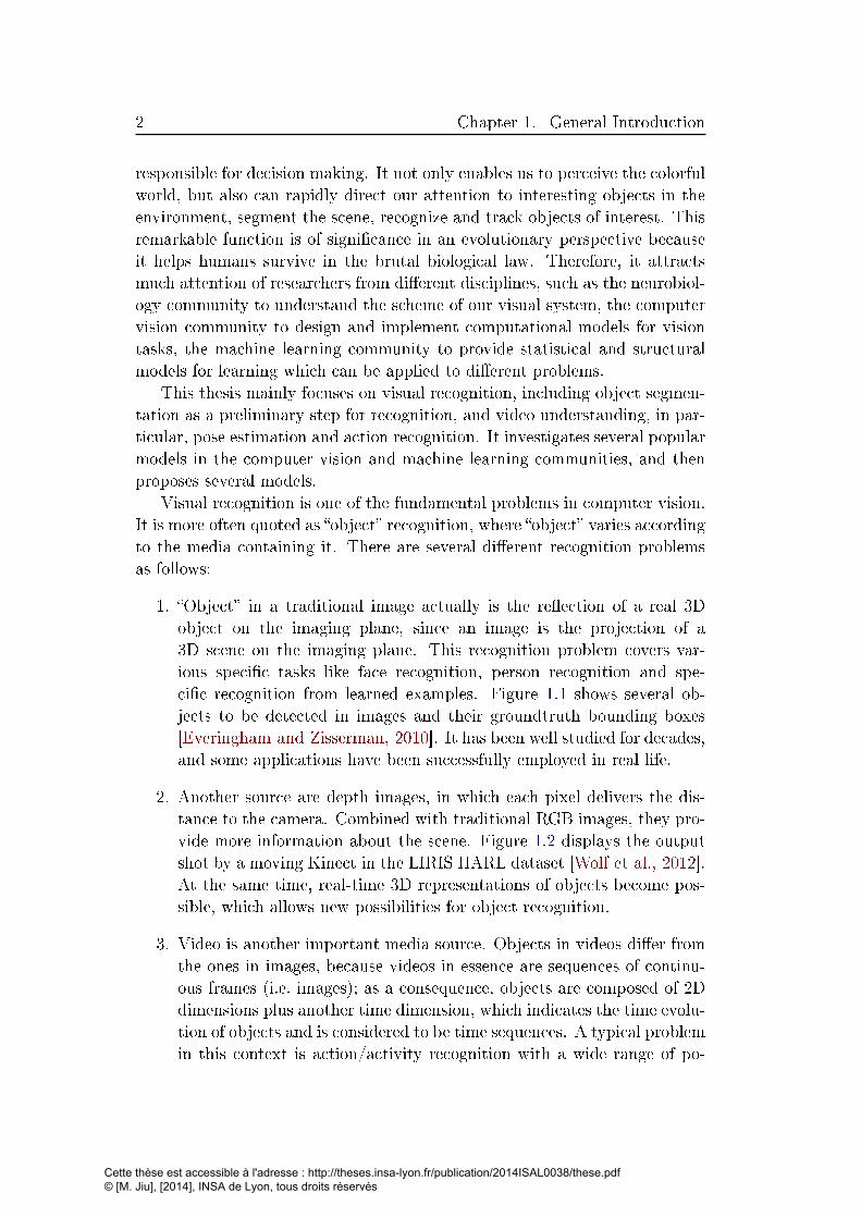
responsible for decision making. It not only enables us to perceive the colorful
world, but also can rapidly direct our attention to interesting objects in the
environment, segment the scene, recognize and track objects of interest. This
remarkable function is of signi�cance in an evolutionary perspective because
it helps humans survive in the brutal biological law. Therefore, it attracts
much attention of researchers from di�erent disciplines, such as the neurobiol-
ogy community to understand the scheme of our visual system, the computer
vision community to design and implement computational models for vision
tasks, the machine learning community to provide statistical and structural
models for learning which can be applied to di�erent problems.
This thesis mainly focuses on visual recognition, including object segmen-
tation as a preliminary step for recognition, and video understanding, in par-
ticular, pose estimation and action recognition. It investigates several popular
models in the computer vision and machine learning communities, and then
proposes several models.
Visual recognition is one of the fundamental problems in computer vision.
It is more often quoted as �object� recognition, where �object� varies according
to the media containing it. There are several di�erent recognition problems
as follows:
1. �Object� in a traditional image actually is the re�ection of a real 3D
object on the imaging plane, since an image is the projection of a
3D scene on the imaging plane. This recognition problem covers var-
ious speci�c tasks like face recognition, person recognition and spe-
ci�c recognition from learned examples. Figure 1.1 shows several ob-
jects to be detected in images and their groundtruth bounding boxes
[Everingham and Zisserman, 2010]. It has been well studied for decades,
and some applications have been successfully employed in real life.
2. Another source are depth images, in which each pixel delivers the dis-
tance to the camera. Combined with traditional RGB images, they pro-
vide more information about the scene. Figure 1.2 displays the output
shot by a moving Kinect in the LIRIS HARL dataset [Wolf et al., 2012].
At the same time, real-time 3D representations of objects become pos-
sible, which allows new possibilities for object recognition.
3. Video is another important media source. Objects in videos di�er from
the ones in images, because videos in essence are sequences of continu-
ous frames (i.e. images); as a consequence, objects are composed of 2D
dimensions plus another time dimension, which indicates the time evolu-
tion of objects and is considered to be time sequences. A typical problem
in this context is action/activity recognition with a wide range of po-
Cette thèse est accessible à l'adresse : http://theses.insa-lyon.fr/publication/2014ISAL0038/these.pdf © [M. Jiu], [2014], INSA de Lyon, tous droits réservés

1.1. Visual recognition problem 3
Horse Motorbike Person
Figure 1.1: The images in PASCAL VOC dataset.
[Everingham and Zisserman, 2010]
(a) Grayscale image (b) depth image (c) colored depth image
Figure 1.2: The handshake example in LIRIS HARL dataset.
[Wolf et al., 2012]
tential applications such as security and surveillance, human-computer
interaction, content-based video analysis, as shown in �gure 1.3.
Visual recognition, as a crucial problem of visual systems, has continued
to attract remarkable interest since its beginning, not only due to the basic
research of seeking a pure interpretation of human vision cognition system,
but also because of promising applications in di�erent domains. Of course, the
development of arti�cial visual recognition system goes along with the demand
of other related industries. The earliest applications of visual recognition
were limited character recognition for o�ce automation tasks, for example,
automated teller machines (ATMs) for banks. Compared to the early very
limited applications to promote production e�ciency, visual recognition is
Figure 1.3: The video of action �Long jump� in the Olympic dataset
[Niebles et al., 2010].
Cette thèse est accessible à l'adresse : http://theses.insa-lyon.fr/publication/2014ISAL0038/these.pdf © [M. Jiu], [2014], INSA de Lyon, tous droits réservés
4 Chapter 1. General Introduction
widely used in numerous applications nowadays, such as military, security,
health care, movies and entertainment, gaming etc. We will describe some
applications in the following:
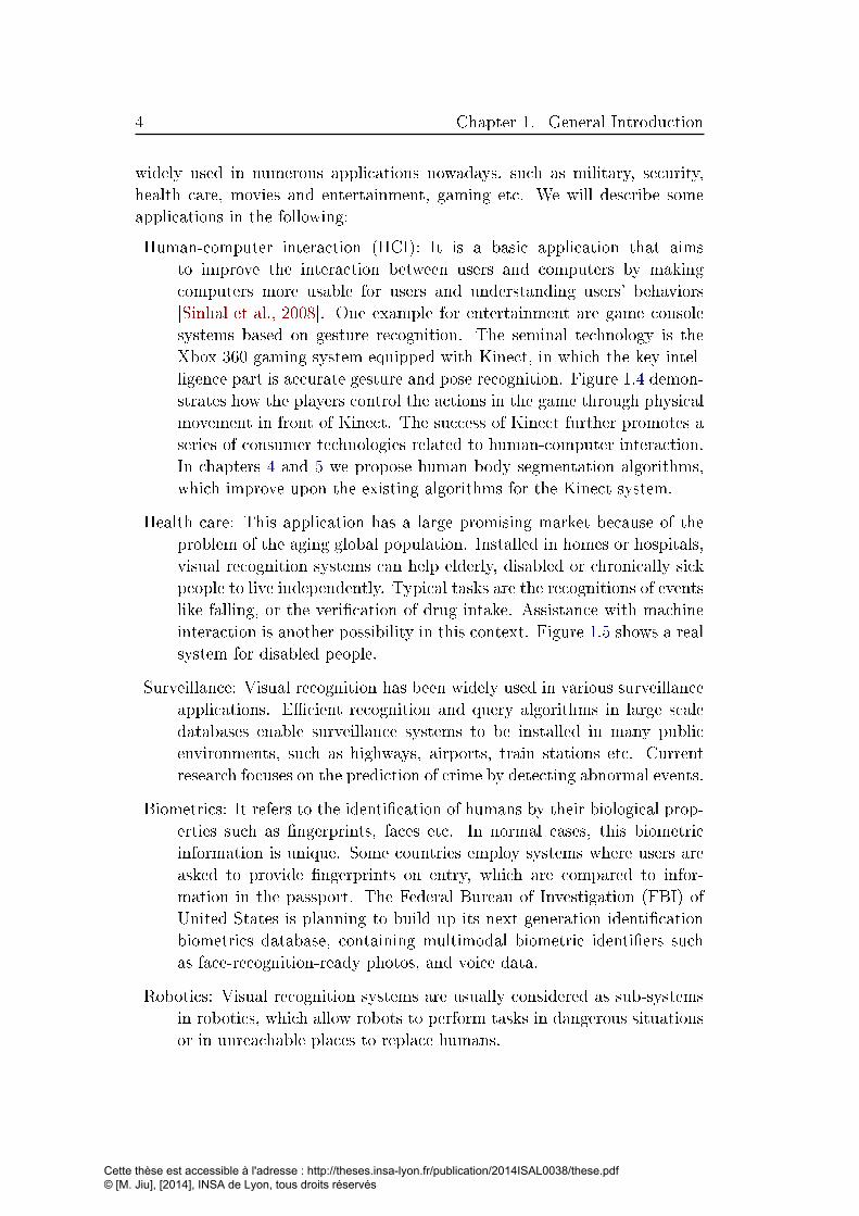
Human-computer interaction (HCI): It is a basic application that aims
to improve the interaction between users and computers by making
computers more usable for users and understanding users' behaviors
[Sinhal et al., 2008]. One example for entertainment are game console
systems based on gesture recognition. The seminal technology is the
Xbox 360 gaming system equipped with Kinect, in which the key intel-
ligence part is accurate gesture and pose recognition. Figure 1.4 demon-
strates how the players control the actions in the game through physical
movement in front of Kinect. The success of Kinect further promotes a
series of consumer technologies related to human-computer interaction.
In chapters 4 and 5 we propose human body segmentation algorithms,
which improve upon the existing algorithms for the Kinect system.
Health care: This application has a large promising market because of the
problem of the aging global population. Installed in homes or hospitals,
visual recognition systems can help elderly, disabled or chronically sick
people to live independently. Typical tasks are the recognitions of events
like falling, or the veri�cation of drug intake. Assistance with machine
interaction is another possibility in this context. Figure 1.5 shows a real
system for disabled people.
Surveillance: Visual recognition has been widely used in various surveillance
applications. E�cient recognition and query algorithms in large scale
databases enable surveillance systems to be installed in many public
environments, such as highways, airports, train stations etc. Current
research focuses on the prediction of crime by detecting abnormal events.
Biometrics: It refers to the identi�cation of humans by their biological prop-
erties such as �ngerprints, faces etc. In normal cases, this biometric
information is unique. Some countries employ systems where users are
asked to provide �ngerprints on entry, which are compared to infor-
mation in the passport. The Federal Bureau of Investigation (FBI) of
United States is planning to build up its next generation identi�cation
biometrics database, containing multimodal biometric identi�ers such
as face-recognition-ready photos, and voice data.
Robotics: Visual recognition systems are usually considered as sub-systems
in robotics, which allow robots to perform tasks in dangerous situations
or in unreachable places to replace humans.
Cette thèse est accessible à l'adresse : http://theses.insa-lyon.fr/publication/2014ISAL0038/these.pdf © [M. Jiu], [2014], INSA de Lyon, tous droits réservés

1.2. Scienti�c challenges 5
Figure 1.4: Schematic diagram of Microsoft's Kinect game controller system,
(taken from www.edition.cnn.com).
Figure 1.5: Gazing detection system for the disabled person
[Sinhal et al., 2008].
1.2 Scienti�c challenges
As mentioned earlier, we introduce contributions to the visual recognition
problem in di�erent domains. Three di�erent types of media (i.e. images,
depth images, videos) associated with visual recognition will be dealt with.
Although each has its speci�c characteristics and also induces particular chal-
lenges for each sub-problem, there are some common challenges for visual
recognition.
Figure 1.6 shows a frequent framework for visual recognition. A test image
is �rst processed by a feature extraction module and represented by features,
which are then classi�ed to give a decision in a classi�cation module. The
parameters are learned in the training stage which is not shown in �gure 1.6.
The use of features instead of raw pixel values is necessary. Compared to the
high-dimensional raw data, low-dimensional features are preferable. Besides,
raw pixel values are sensitive to objects' variation.
Generally, we seek a (learned or handcrafted) discriminative representa-
tion (�features�) which is able to cope with di�erent variations in the data,
depending on intrinsic and extrinsic factors:
Intrinsic factors: They are associated with the inherent properties of the
objects in term of appearance, pose, even gait. For object recognition,
Cette thèse est accessible à l'adresse : http://theses.insa-lyon.fr/publication/2014ISAL0038/these.pdf © [M. Jiu], [2014], INSA de Lyon, tous droits réservés

6 Chapter 1. General Introduction
FeatureClassification Decision
Extraction
Parameters
TestImage
Representation/Features
Parameters(optional)
Figure 1.6: A frequent framework.
the subject can appear di�erently due to di�erent clothes and poses;
similarly, for action recognition, the same actions performed by di�er-
ent subjects look di�erently due to di�erent pace rate, for instance, the
length of hand swing when walking. All of these easily induce large
intra-class variations. At the same time, low inter-class variations can
occur between di�erent categories. So, robust feature extractor algo-
rithms should minimize intra-class variations and simultaneously max-
imize inter-class variations. In addition, the objects we are interested
in are often articulated, rather than rigid. In this case, it is impos-
sible to learn a global rigid model to represent all the possibilities of
distributions of the articulated parts.
Extrinsic factors: They mainly concern the variations due to imaging condi-
tions: viewpoint changes, and changes in scale, rotation, lighting, noise,
occlusions, complex background etc. It is easily seen that even the same
object displays di�erently on the frame if the imaging device changes its
viewpoint. A good representation should be invariant to most of these
transformations.
Besides the above mentioned challenges, real-time processing is often re-
quired in the practical applications of visual recognition. Moreover, some
applications are installed on mobile platforms. Both requirements further
limit the complexity of the algorithm. However, the model with less complex-
ity usually yields more errors, therefore, in a real algorithm design, the cost
between complexities and errors should be seriously considered and the best
trade-o� strategy is adopted according to the needs.
From the above discussion, we can conclude that visual recognition is a
di�cult task, but a large amount of applications encourage the researchers
in computer vision and machine learning communities to seek more e�cient
and e�ective representations and learning algorithms to achieve the level of
the human visual system. In this thesis, we address visual recognition mainly
by using machine learning algorithms, or employing the machine learning
framework to improve the models populated in computer vision community.
Cette thèse est accessible à l'adresse : http://theses.insa-lyon.fr/publication/2014ISAL0038/these.pdf © [M. Jiu], [2014], INSA de Lyon, tous droits réservés
1.3. Our contributions 7
FeatureClassification Decision
Extraction
Parameters
TestImage
Parameters(Dictionary)
Localfeatures
Pooling BoW
TrainingImages
Unsupervisedtraining
Supervisedtraining
Traininglabels
(a): The bag-of-words framework.
Feature ClassificationimageExtraction
Parameters
TestImage
Parameters
Feature
TrainingImages
Traininglabels
MapsSegmented
End-to-end Training
per pixel
(b): The segmentation framework.
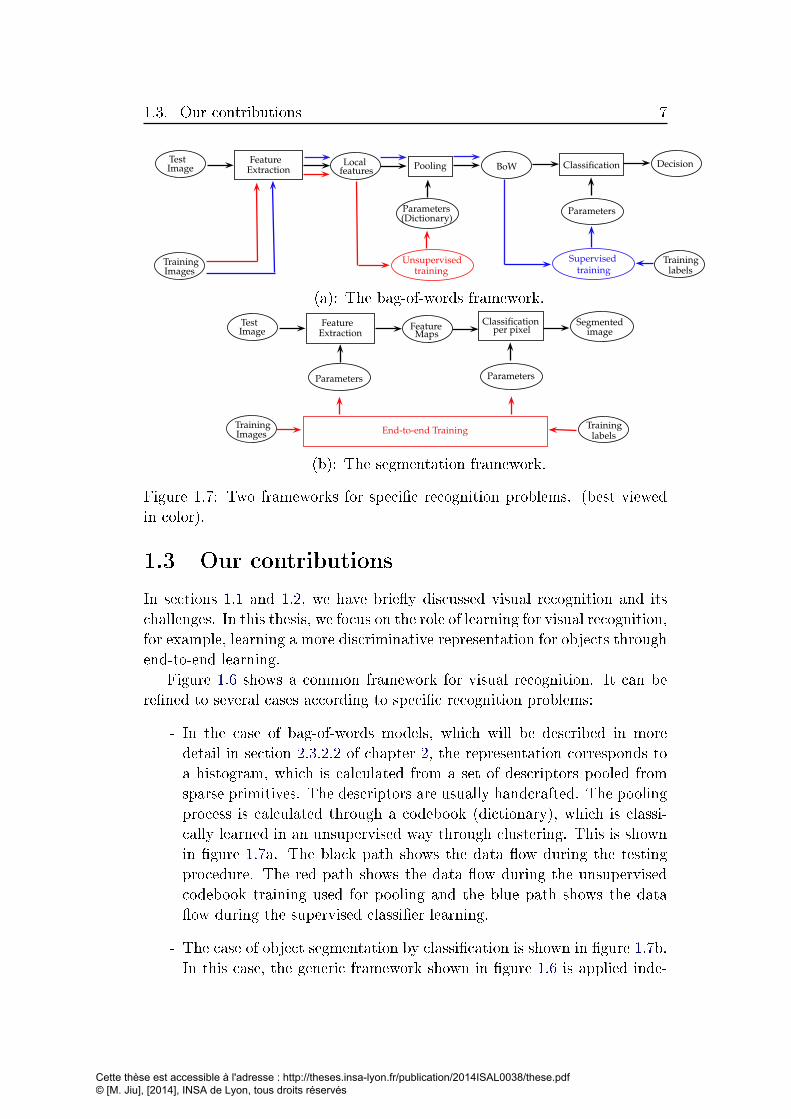
Figure 1.7: Two frameworks for speci�c recognition problems. (best viewed
in color).
1.3 Our contributions
In sections 1.1 and 1.2, we have brie�y discussed visual recognition and its
challenges. In this thesis, we focus on the role of learning for visual recognition,
for example, learning a more discriminative representation for objects through
end-to-end learning.
Figure 1.6 shows a common framework for visual recognition. It can be
re�ned to several cases according to speci�c recognition problems:
- In the case of bag-of-words models, which will be described in more
detail in section 2.3.2.2 of chapter 2, the representation corresponds to
a histogram, which is calculated from a set of descriptors pooled from
sparse primitives. The descriptors are usually handcrafted. The pooling
process is calculated through a codebook (dictionary), which is classi-
cally learned in an unsupervised way through clustering. This is shown
in �gure 1.7a. The black path shows the data �ow during the testing
procedure. The red path shows the data �ow during the unsupervised
codebook training used for pooling and the blue path shows the data
�ow during the supervised classi�er learning.
- The case of object segmentation by classi�cation is shown in �gure 1.7b.
In this case, the generic framework shown in �gure 1.6 is applied inde-
Cette thèse est accessible à l'adresse : http://theses.insa-lyon.fr/publication/2014ISAL0038/these.pdf © [M. Jiu], [2014], INSA de Lyon, tous droits réservés

8 Chapter 1. General Introduction
FeatureClassification Decision
Extraction
Parameters
TestImage
Parameters(Dictionary)
Localfeatures
Pooling BoW
TrainingImages
Traininglabels
End-to-end Training
Spatial constraints on
label configuration in feature space
(a): The bag-of-words framework.
Feature ClassificationimageExtraction
Parameters
TestImage
Parameters
Feature
TrainingImages
Traininglabels
End-to-end Training
MapsSegmented
Spatial constraints on label layout
per pixel
(b): The segmentation framework.
Figure 1.8: Our improved frameworks. (best viewed in color).
pendently to each pixel of an image. Here we do not deal with regu-
larization like it is performed in discrete models (MRF, CRF etc.) or
continuous-discrete formulations (Mumford-Shah functional etc.). The
feature in this case can either be handcrafted (HOG, SIFT etc., see
section 2.2 chapter 2) or learned in an end-to-end training setup (see
section 2.4 of chapter 2). In this case, the features are learned together
with the prediction model (see section 2.3 of chapter 2).
The goal of our work is the integration of as much as information as pos-
sible into the learning process. We proceed by di�erent ways: (i) integrating
additional constraints (related to prior information) into the learning algo-
rithm; (ii) coupling stages which are classically performed separately. A large
emphasis is put on geometric and spatial information. Here our contributions
are given as follows:
• We propose an end-to-end training approach for BoW models. In the
framework shown in �gure 1.8a, the dictionary is learned together with
Cette thèse est accessible à l'adresse : http://theses.insa-lyon.fr/publication/2014ISAL0038/these.pdf © [M. Jiu], [2014], INSA de Lyon, tous droits réservés

1.3. Our contributions 9
the prediction model in a supervised way, i.e. including training labels.
We impose spatial constraints on label con�gurations in feature space. In
this way, the features are directly related to the classi�cation problem,
and they are updated as learning becomes more discriminative. We
experimented this approach on the bag-of-words (BoW) model for action
recognition.
• We integrate prior information in terms of spatial label layout of parts
into di�erent machines, i.e. Randomized Decision Forest (RDF), Con-
volutonal Neural Networks (CNN), and classi�ers such as logistical re-
gression (LR) or multilayer perceptron (MLP). respectively, as shown
in �gure 1.8(b). This concerns applications, where a classi�er takes de-
cisions on labels, which can be spatially interpreted, for instance where
objects are segmented into meaningful parts. Labels here refer to parts,
which are located in the human body. Spatial relationships can sig-
ni�cantly improve performance in this case when the size of available
training instances is very limited.
Traditionally, these constraints are injected using models which require
to solve a combinational problem, e.g. graphical models like MRFs and
CRFs. The additional computational burden makes real-time opera-
tion impossible. We propose to integrate these constraints directly into
the learning algorithm of a traditional classi�er (RDF, CNN, LR or
MLP). Classi�cation still proceeds independently pixel per pixel, which
means that the computational complexity is equivalent to the classical
approaches.
• All the frameworks we propose do end-to-end training as shown in �gures
1.8(a) and 1.8(b). Representations are automatically learned, rather
than hand-engineered 1.
• We employ our spatial learning algorithms on speci�c problems, namely
human body part estimation and segmentation. Visual recognition of
human parts is an important intermediate step, which can be used for
person recognition or human pose estimation. It is necessary to men-
tion that our algorithms can be used for the segmentation of any other
objects, articulated or not.
1In the case of BoW model, the dictionary of the representation is learned, while the
low-level features stay handcrafted.
Cette thèse est accessible à l'adresse : http://theses.insa-lyon.fr/publication/2014ISAL0038/these.pdf © [M. Jiu], [2014], INSA de Lyon, tous droits réservés

10 Chapter 1. General Introduction
1.4 Overview
Here we overview the contents in the following chapters:
Chapter 2 discusses the state-of-the-art on visual recognition. We present
popular feature extraction techniques, and widely used models in computer
vision. We also review common machine learning algorithms for visual recog-
nition with a focus on the ones related to the thesis.
Chapter 3 proposes two algorithms for end-to-end learning of bag-of-words
(BoW) models on action recognition, where the dictionaries are learned in a
supervised way. The codebook for BoW models are updated through error
backpropagation. One algorithm described in section 3.3.2 is based on classical
error backpropagation, the other described in section 3.3.3 is based on cluster
reassignments. We apply both algorithms to the human action recognition
problem, and show that our end-to-end learning technique makes the BoW
model more discriminative.
Chapter 4 proposes spatial learning algorithms for Randomized Decision
Forests in section 4.3 and for Convolutional Neural Networks and LR/MLP
classi�er in section 4.4, respectively. We integrate the spatial layout of object
con�gurations in terms of pairwise relationship of neighbors and non-neighbors
into the learning machines with di�erent architectures. In other words, we
attempt to learn structural machines for recognition. The learned machines
demonstrate better performance on object segmentation problems.
Chapter 5 presents one application for the algorithms proposed in chapter
4, namely segmentation of humans into body parts. Part segmentation is an
important research area in computer vision, which can be regarded as the
bridge between low level image processing to high level scene understanding.
In this work we consider it as a problem of classi�cation, which is addressed
by our algorithms.
Chapter 6 gives general conclusions and describes ongoing and future work.
Cette thèse est accessible à l'adresse : http://theses.insa-lyon.fr/publication/2014ISAL0038/these.pdf © [M. Jiu], [2014], INSA de Lyon, tous droits réservés

Chapter 2
State of the art
Contents
2.1 State of the art . . . . . . . . . . . . . . . . . . . . . . . 11
2.2 Type of features . . . . . . . . . . . . . . . . . . . . . . 13
2.2.1 Global features . . . . . . . . . . . . . . . . . . . . . . 14
2.2.2 Local sparse features . . . . . . . . . . . . . . . . . . . 19
2.2.3 Local dense features . . . . . . . . . . . . . . . . . . . 26
2.3 Visual recognition: methods . . . . . . . . . . . . . . . 28
2.3.1 Matching . . . . . . . . . . . . . . . . . . . . . . . . . 28
2.3.2 Sliding windows . . . . . . . . . . . . . . . . . . . . . . 33
2.3.3 Segmentation for visual recognition . . . . . . . . . . . 41
2.4 Feature/Representation learning . . . . . . . . . . . . 44
2.4.1 Supervised feature learning . . . . . . . . . . . . . . . 45
2.4.2 Unsupervised learning . . . . . . . . . . . . . . . . . . 46
2.4.3 Weakly-supervised learning . . . . . . . . . . . . . . . 50
2.5 Conclusion . . . . . . . . . . . . . . . . . . . . . . . . . . 51
2.1 State of the art
The visual recognition problem is sometimes quoted as the object recognition
problem (the word �object� being interpreted in a very large sense such as
object, activity, gesture etc.), i.e. how to make a machine recognize objects
in an image or in a video without any other assistance. The ultimate goal
is to produce an arti�cial visual system having a performance equivalent to
the human visual system, which is capable of recognizing as many as millions
of objects. However, this powerful and universal visual system has not been
reported until now.
The type of the input depends on the sensing device. It can be a gray or
real colored projection to a 2 dimensional image plane of a common object by
Cette thèse est accessible à l'adresse : http://theses.insa-lyon.fr/publication/2014ISAL0038/these.pdf © [M. Jiu], [2014], INSA de Lyon, tous droits réservés

12 Chapter 2. State of the art
Visual Recognition
Matching Sliding window
Classification
Segmentation
Candidateregions
ClassificationBoW DPM
Global Local
Figure 2.1: The general visual recognition framework. BoW is the abbrev.
for bag-of-words [Csurka et al., 2004] models, and DPM for deformable part
based models [Felzenszwalb et al., 2010].
a traditional camera, a classical problem in computer vision. It can also be a
depth image of an object, where each pixel value corresponds to the distance
to the depth-sensing camera. Moreover, it can be a spatio-temporal �object�
in videos such as an action and an activity associated with one or several
persons.
There is a large amount of literature on visual recognition, and various
methods have been introduced for the �object� recognition problem. A fre-
quently used pipeline can be shown in �gure 1.6 in chapter 1. There are two
modules: given an input (image or video), features are �rstly extracted from
objects, eventually dimension reduction techniques such as Principle Compo-
nent Analysis (PCA), clustering etc. are further applied on the raw features
to get amenable models. Finally, machine learning approaches, for instance,
support vector machines (SVM), randomized decision forests (RDF), etc. are
employed to create a decision for speci�c tasks (e.g. recognition, detection,
localization etc.). Hence, research on visual recognition focuses on two as-
pects: on one hand, much attention is taken to construct and optimize fea-
tures and representations, discriminatively representing the �object�. More
discussions on this can be found in section 2.2. On the other hand, research
in machine learning attempts to seek powerful classi�cation techniques, which
better learn the boundaries between the categories. Beyond simple classi�ca-
tion of vectorial data, other techniques are able to deal with structural data
and spatial, temporal or spatio-temporal relationships. Examples are Struc-
tural SVM, Hidden Markov Models (HMM), Markov Random Fields (MRF),
graph matching, etc.
Visual recognition can be performed through di�erent families of ap-
proaches. Figure 2.1 gives a taxonomy of some frequent ones. They all resolve
Cette thèse est accessible à l'adresse : http://theses.insa-lyon.fr/publication/2014ISAL0038/these.pdf © [M. Jiu], [2014], INSA de Lyon, tous droits réservés

2.2. Type of features 13
the same main problem, which is to identify (detect) the region containing the
object of interest and then to recognize the object itself. This is a chicken-and-
egg problem, since detecting an object theoretically requires its recognition,
whereas recognition requires extracting features from the detected region. We
would not talk more about this, several techniques thus are presented to avoid
this dilemma.
Matching is a prototype based technique, which is performed by searching
for instances of a model (image, point etc.) in the scene through similarity,
and by thresholding the similarity, taking into account structural information.
According to the used features, there are global matching and local match-
ing techniques. Another simple solution is to slide a window over the image
or video, and to recognize the presence of the object by classi�cation. It is
also further divided into local sparse features based (e.g. bag-of-words mod-
els [Csurka et al., 2004]) and local dense features based (e.g. deformable part
based models [Felzenszwalb et al., 2010]). Another possibility is to �rst over-
segment an image into a set of candidate object segments, fuse small regions
together and followed by a classi�cation step.
Existing methods can also be organized by the di�erences in feature types,
where most types of methods require a speci�c type of features, for instance,
local matching requires local features. Figure 2.2 shows a taxonomy of feature
types.
The next three sections are dedicated to these aspects:
- Section 2.2 will describe di�erent feature types, as shown in �gure 2.2.
- Section 2.3 will describe di�erent recognition techniques, as shown in
�gure 2.1.
- Section 2.4 will describe feature learning techniques, where features are
not handcrafted, but learned.
Features and techniques will be presented for both, spatial data and spatio-
temporal data, i.e. for object recognition and for activity recognition.
2.2 Type of features
As mentioned in Chapter 1, features and representations should possibly be as
invariant and as discriminative as possible, to make the subsequent recognition
stage less di�cult.
Figure 2.2 shows a taxonomy of di�erent feature types. They can be
global or local; they can be handcrafted, i.e. designed in all details; or they
can be automatically learned in an unsupervised or a supervised manner.
Cette thèse est accessible à l'adresse : http://theses.insa-lyon.fr/publication/2014ISAL0038/these.pdf © [M. Jiu], [2014], INSA de Lyon, tous droits réservés

14 Chapter 2. State of the art
Feature extraction
Feature
Global Local
Handcraftedfeatures learning
featuresfeaturesUnsupervised
learningSupervisedlearning
1: Shape2: Appearance3: Moments4: Motion
1: Local sparse
2: Local densefeatures
features
Weakly-
learningsupervised
Errorbackpropagation
Neighborhoodrelationshiplearning
1: Auto-encoding2: Transformation
learning
Figure 2.2: Feature extraction taxonomy.
One advantage of this framework is that it can be composed of an end-to-end
framework where features are learned together with the prediction model, as
a result, the features are learned to best suit the classi�cation stage.
In this section, we will present several types of global and local features.
Automatic feature learning will be discussed in its own dedicated section 2.4.
2.2.1 Global features
Global features are extracted on the whole area covered by the object of inter-
est, which is therefore described by a single representation (mostly vectorial).
The research on global representations dominated the beginning of object
recognition.
2.2.1.1 Shape based features
Shape is an important property of an object, it is related to contours for 2 di-
mensional objects and to surfaces for 3 dimensional objects. The earlier shape
features focus on low level information such as edge or texture. Snakes intro-
duced in [Kass et al., 1988] apply energy minimization to contour construc-
tion and the edges are the features. Active Shape Models [Cootes et al., 1995]
integrate global shape constraints into snake constructions to capture the de-
formable shape.
Shape context is a contour based descriptor, which describes a coarse
distribution of all other points with respect to a given point on the shape
[Belongie et al., 2002]. It works well on poorly textural objects, such as let-
ters, sketches, and is widely adopted by the community. The main computa-
tion steps are as follows: an edge image of an object is �rstly obtained and its
Cette thèse est accessible à l'adresse : http://theses.insa-lyon.fr/publication/2014ISAL0038/these.pdf © [M. Jiu], [2014], INSA de Lyon, tous droits réservés

2.2. Type of features 15
(a) (b) (c)
Figure 2.3: Shape context illustration: (a) the shape of letter �A�, (b) the
log-polar coordinate on the shape, (c) the shape context of the given point.
This �gure is reproduced from [Belongie et al., 2002].
shape is discretized into a number of points. A log-polar coordinate system
is put on the shape with its origin at a given point. The shape context for
the given point is a histogram, where each bin in the log-polar coordinate
counts the number of points falling in that bin. Each point's shape context
features are composed of the relative position information of all other points
w.r.t itself; therefore, shape context is very rich and discriminative. It is very
suitable for point-to-point matching problems.
Shape based features can be also used to describe spatio-temporal objects.
Gorelick et al. [Gorelick et al., 2007] propose a global descriptor for space-
time data. They stack 2D object shapes to form a volumetric space-time
shape. Space-time saliency and space-time orientation is extracted from the
space-time shape volume, serving as features. Space-time saliency indicates
which portion of human action has the highest likelihood of action occurrence,
and space-time orientation estimates the local orientation and aspect ratio of
di�erent space-time parts. Figure 2.4 shows the space-time saliency of waving
hands and walking and the space-time orientations of plates and sticks for
walking. Their method does not require prior video alignment and has proper
robustness to partial occlusions, imperfections in the extracted silhouettes.
Another similar space-time volume is extracted from 2D contours for actions
in [Yilmaz and Shah, 2005]. Several geometry properties are computed to
describe the space-time volume, such as peaks, pits, valleys and ridges. These
features are quite invariant because the convex and concave parts of the object
are view invariant.
Cette thèse est accessible à l'adresse : http://theses.insa-lyon.fr/publication/2014ISAL0038/these.pdf © [M. Jiu], [2014], INSA de Lyon, tous droits réservés
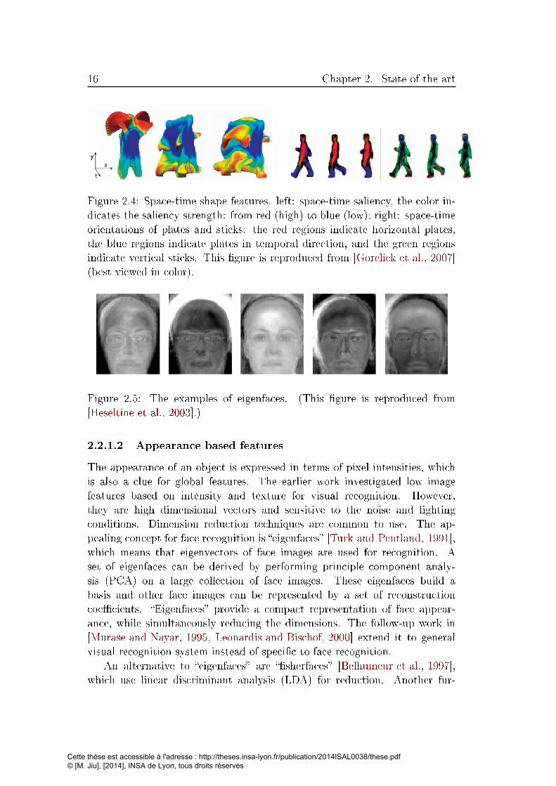
16 Chapter 2. State of the art
Figure 2.4: Space-time shape features. left: space-time saliency, the color in-
dicates the saliency strength: from red (high) to blue (low); right: space-time
orientations of plates and sticks: the red regions indicate horizontal plates,
the blue regions indicate plates in temporal direction, and the green regions
indicate vertical sticks. This �gure is reproduced from [Gorelick et al., 2007]
(best viewed in color).
Figure 2.5: The examples of eigenfaces. (This �gure is reproduced from
[Heseltine et al., 2003].)
2.2.1.2 Appearance based features
The appearance of an object is expressed in terms of pixel intensities, which
is also a clue for global features. The earlier work investigated low image
features based on intensity and texture for visual recognition. However,
they are high dimensional vectors and sensitive to the noise and lighting
conditions. Dimension reduction techniques are common to use. The ap-
pealing concept for face recognition is �eigenfaces� [Turk and Pentland, 1991],
which means that eigenvectors of face images are used for recognition. A
set of eigenfaces can be derived by performing principle component analy-
sis (PCA) on a large collection of face images. These eigenfaces build a
basis and other face images can be represented by a set of reconstruction
coe�cients. �Eigenfaces� provide a compact representation of face appear-
ance, while simultaneously reducing the dimensions. The follow-up work in
[Murase and Nayar, 1995, Leonardis and Bischof, 2000] extend it to general
visual recognition system instead of speci�c to face recognition.
An alternative to �eigenfaces� are ��sherfaces� [Belhumeur et al., 1997],
which use linear discriminant analysis (LDA) for reduction. Another fur-
Cette thèse est accessible à l'adresse : http://theses.insa-lyon.fr/publication/2014ISAL0038/these.pdf © [M. Jiu], [2014], INSA de Lyon, tous droits réservés

2.2. Type of features 17
ther alternative is Active Appearance Models proposed by Cootes et al.
[Cootes et al., 2001], which is a statistical learning method for shapes and
textures of faces. PCA is performed on a set of landmarks on the face to
encapsulate the variation of di�erent faces.
More recently, these kinds of techniques are used in conjunction with deep
learning. The combination is also sometimes called �intelligent dimensionality
reduction� and brie�y described in section 2.4.2.
2.2.1.3 Moment based features
Moments are an extensively used concept in di�erent disciplines. In math-
ematics, a moment is used to measure the characteristics of the shape of a
set of points, such as: mean, variance, and skewness. Moment invariants can
also be applied to two-dimensional images, where they measure the content
of images with respect to di�erent axes.
Hu moments were �rst introduced for visual pattern recognition [Hu, 1962].
They are derived from the theory of algebraic invariants. For a gray image of
size N ∗M , the image intensities in the image coordinate (x, y) are represented
by a function f(x, y), the moment of order (p+ q) is de�ned by:
mpq =M−1∑x=0
N−1∑y=0
xpyqf(x, y), (2.1)
where p, q = 0, 1, 2, 3, · · · .In order to achieve translation invariance, the central moment µpq is given
by:
µpq =M−1∑x=0
N−1∑y=0
(x− x)p(y − y)qf(x, y), (2.2)
where x = m10
m00and y = m10
m00. To be further scale invariant, the central moment
is once again normalized by:
µpq =µpq
µγ00
, γ = 1 + (p+ q)/2. (2.3)
The seven Hu moments are given as:
Cette thèse est accessible à l'adresse : http://theses.insa-lyon.fr/publication/2014ISAL0038/these.pdf © [M. Jiu], [2014], INSA de Lyon, tous droits réservés

18 Chapter 2. State of the art
M1 = µ20 − µ02
M2 = (µ20 − µ02)2 + 4µ2
11
M3 = (µ30 − µ12)2 + (3µ21 − µ03)
2
M4 = (µ30 + µ12)2 + (3µ21 − µ03)
2
M5 = (µ30 − 3µ12)(µ30 + µ12)[(µ30 + µ12)2 − 3(µ21 + µ03)
2]
+(3µ21 − µ03)(µ21 + µ03)[3(µ30 + µ12)2 − (µ21 + µ03)
2]
M6 = (µ20 − µ02)[(µ30 + µ12)2 − (µ12 + µ03)
2] + 4µ11(µ12 + µ30)(µ21 + µ03)]
M7 = (3µ21 − µ03)(µ30 + µ12)[(µ30 + µ12)2 − 3(µ21 + µ03)
2]
+(3µ21 − µ30)(µ21 + µ03)[3(µ30 + µ12)2 − (µ21 + µ03)
2]
Although Hu moments are invariant to scale, translation, and rotation,
one problem is that they are derived from low order moments, whose capacity
of describing a shape is very limited. Another disadvantage is their di�culty
to reconstruct the image. An example of their usage is their application to
action recognition in [Bobick and Davis, 2001].
Zernike moments [Teague, 1980] have been proposed to overcome these
disadvantages. They are computed based on the basis set of orthog-
onal Zernike polynomials. Interesting readers can �nd more details in
[Teh and Chin, 1988]. They have been successfully applied to object recogni-
tion [Revaud et al., 2009, Ta et al., 2008].
2.2.1.4 Motion features
Motion is a special property of objects in video, which is an important clue
for action recognition. Several attempts have been made to construct motion
features. Motion Energy Images (MEI) and Motion History Images (MHI)
introduced by Bobick et al. [Bobick and Davis, 2001] are representative ones.
Background is �rstly subtracted, and then a sequence of silhouettes is aggre-
gated into a single static image, which indicates where the motion occurred
and when w.r.t. the current time instant, respectively. Let I(x, y, t) be the in-
tensity value at time t and location (x, y) in a video; we can obtain the region
of motion by the di�erence of consecutive frames. A binary map D(x, y, t)
is obtained by thresholding the di�erences where there is high likelihood of
motion:
D(x, y, t) =
{1, |I(x, y, t)− I(x, y, t− 1)| > T
0, otherwise(2.4)
Then the MHI function is de�ned by:
hτ =
{τ, if D(x, y, t) = 1
max(0, hτ (x, y, t− 1)), otherwise(2.5)
Cette thèse est accessible à l'adresse : http://theses.insa-lyon.fr/publication/2014ISAL0038/these.pdf © [M. Jiu], [2014], INSA de Lyon, tous droits réservés

2.2. Type of features 19
Figure 2.6: MEI (left) and MHI (right) of a person raising both hands. This
�gure is reproduced from [Bobick and Davis, 2001].
where τ is the total number of frames. MHI are constructed by giving the
sequence frames decaying weights with higher weight given to new frames
and low weight given to older frames. MEI can be obtained through setting
the same value for the pixels above zero in MHI. Figure 2.6 illustrates MEI
and MHI of a person raising both hands. MEI and MHI are not suitable to
complex actions due to over-writing over time. Several extensions on these
features exist in [Weinland et al., 2006, Hu and Boulgouris, 2011]. They also
have been extended to depth videos in [Roh et al., 2010], where they are called
�Volume Motion Template�.
Global features are not restricted to the above mentioned ones. More
types of global features for visual recognition can be found in [Poppe, 2010].
However, global features share a number of common disadvantages: (i) many
of them need pre-segmentation to get rid of the background scenes; (ii) global
features are not robust to noise, a little noise on the boundary may totally
change the orientation of the global features; (iii) they can not cope with
occlusion. Local features described in section 2.2.2 can technically avoid these
disadvantages.
2.2.2 Local sparse features
Local features di�er from their global ones in that they describe the local
content of an object, i.e. the content on a small patch. The object can be
described by the combination of all the local features from the object. Of
course, it is not always practical to use all the possible local primitives, because
most of them fall in non-interesting areas containing little information about
the object, such as the background and visually identical areas.
There is another way to look at local features-based recognition: it is
interpreted as a low-level part-based model. A local primitive can be regarded
as a small part of the object, all the parts therefore are arranged to an object
in a particular spatial con�guration. Much work on building a high level part
Cette thèse est accessible à l'adresse : http://theses.insa-lyon.fr/publication/2014ISAL0038/these.pdf © [M. Jiu], [2014], INSA de Lyon, tous droits réservés
20 Chapter 2. State of the art
as group of local primitives has been reported, rather than based on local
primitives. The readers can �nd more details about part based models in
Section 2.3.
Local features generally describe the properties of the neighborhood of
some local primitive, e.g. a point, an edgel, or a small segmented region.
Interest points are the most widely used local primitives containing much
information, and they are the ones we are interested in. Two questions arise
in this context:
- How can we detect interesting local primitives, e.g. point locations?
Several measure criteria are proposed to constrain the interest points in
image or video.
- How can the area around each point be described locally?
Here we would like to point out that interest points and descriptors are in-
dependent: once interest points are detected, any descriptor techniques can
been applied. In the following, several well-known interest point detectors are
presented as well as descriptors.
2.2.2.1 Interest point detectors
The work on interesting points can be traced back to [Moravec, 1981] on
stereo matching using corner detection. His corners are detected by shift-
ing a local window in the image to determine the average intensity changes.
It was improved by Harris and Stephens to discriminate corners and edges
[Harris and Stephens, 1988]. The basic idea to �nd the point whose value is
above the threshold with Harris measure, which is de�ned on the �rst order
derivatives as follows:
µ = G(x, y) ∗[
L2x LxLy
LxLy L2y
](2.6)
det(µ)− α trace2(µ) > threshold (2.7)
where G(x, y) is two-dimensional Gaussian function, Lx and Ly are the Gaus-
sian derivatives on the image along with x and y direction, α is a parameter
to control the interesting point types, e.g. isotropic points, or edge points.
Harris's detector was �rst employed to image matching problems. The work
in [Schmid and Mohr, 1997] extended Harris's detector to the general recog-
nition problem for image retrieval. It had been widely used in the community
due to the fact that it can produce repeatable corners and for some time
hardware implementations were available.
Cette thèse est accessible à l'adresse : http://theses.insa-lyon.fr/publication/2014ISAL0038/these.pdf © [M. Jiu], [2014], INSA de Lyon, tous droits réservés

2.2. Type of features 21
Arguably, the most widely used interest point detector is the SIFT detec-
tor introduced by Lowe [Lowe, 2004]. He proposes a scale-invariant keypoint
detector by searching over all scales and image locations, implemented as a
di�erence-of-gaussian operation:
D(x, y, σ) = (G(x, y, kσ)−G(x, y, σ)) ∗ I(x, y) (2.8)
where G(x, y, kσ) is a two-dimensional Gaussian function with scale σ, k is a
constant to de�ne its nearby scale, ∗ is the convolution operation. The de-
tected local extrema are further rejected if they have low contrast by equation
(2.9) or are located along an edge by equation (2.10).
D(x) = D +1
2
∂DT
∂xx, (2.9)
Tr(H)
Det(H)<
(r + 1)2
r. (2.10)
Here, x is the o�set of the local extrema, and H is the 2× 2 Hessian matrix
of the local extrema.
Mikolajczyk and Schmid [Mikolajczyk and Schmid, 2002] propose an al-
gorithm to address a�ne invariant interest points. Interest point candidates
are �rst detected by using multi-scale Harris detector, and then for each point
an iterative procedure is performed to simultaneously modify the position,
scale and shape of the point neighborhood, and an a�ne transformation is
estimated to obtain a�ne invariant interest points.
Additional work on 2D interest point detectors includes SURF (Speeded up
robust features) [Bay et al., 2006], FAST (Features from Accelerated Segment
Test) [Rosten and Drummond, 2006] etc.
We temporally turn our attention to present some work on 3D interest
point detector for action/activity recognition. Laptev [Laptev, 2005] extends
the 2D Harris detector to 3D space-time detector. Space-time interest points
(STIP) are those points where the local neighborhood has a signi�cant vari-
ation in both the spatial and the temporal domain. Similarly, the spatio-
temporal second-moment matrix is a 3-by-3 matrix composed of �rst order
spatial and temporal derivatives as following:
µ = G(x, y) ∗
L2x LxLy LxLt
IxIy I2y LyLt
LxLt LyLt L2t
(2.11)
One drawback of this method is that it provides a relatively small number
of stable interest points (see �gure 2.7); it also consumes expensive compu-
tational resources due to a iterative searching procedure in a 5 dimensional
space over (x, y, t, σ, τ).
Cette thèse est accessible à l'adresse : http://theses.insa-lyon.fr/publication/2014ISAL0038/these.pdf © [M. Jiu], [2014], INSA de Lyon, tous droits réservés
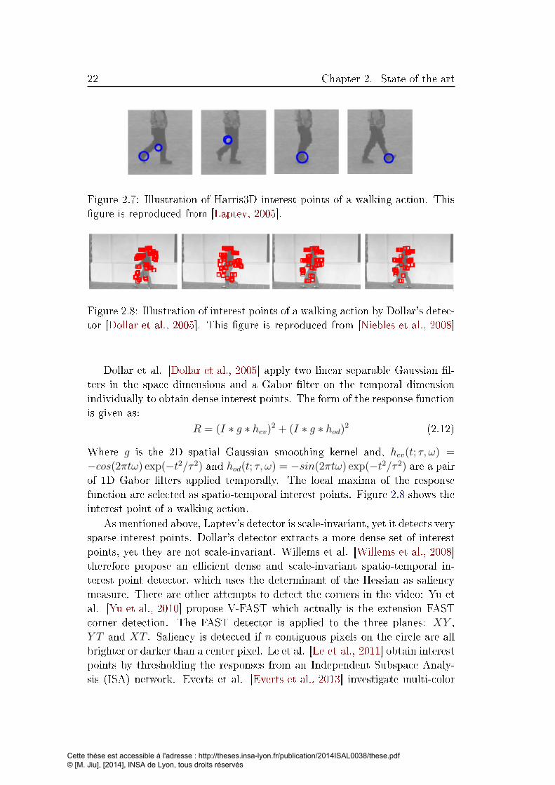
22 Chapter 2. State of the art
Figure 2.7: Illustration of Harris3D interest points of a walking action. This
�gure is reproduced from [Laptev, 2005].
Figure 2.8: Illustration of interest points of a walking action by Dollar's detec-
tor [Dollar et al., 2005]. This �gure is reproduced from [Niebles et al., 2008]
Dollar et al. [Dollar et al., 2005] apply two linear separable Gaussian �l-
ters in the space dimensions and a Gabor �lter on the temporal dimension
individually to obtain dense interest points. The form of the response function
is given as:
R = (I ∗ g ∗ hev)2 + (I ∗ g ∗ hod)2 (2.12)
Where g is the 2D spatial Gaussian smoothing kernel and, hev(t; τ, ω) =
−cos(2πtω) exp(−t2/τ 2) and hod(t; τ, ω) = −sin(2πtω) exp(−t2/τ 2) are a pairof 1D Gabor �lters applied temporally. The local maxima of the response
function are selected as spatio-temporal interest points. Figure 2.8 shows the
interest point of a walking action.
As mentioned above, Laptev's detector is scale-invariant, yet it detects very
sparse interest points. Dollar's detector extracts a more dense set of interest
points, yet they are not scale-invariant. Willems et al. [Willems et al., 2008]
therefore propose an e�cient dense and scale-invariant spatio-temporal in-
terest point detector, which uses the determinant of the Hessian as saliency
measure. There are other attempts to detect the corners in the video: Yu et
al. [Yu et al., 2010] propose V-FAST which actually is the extension FAST
corner detection. The FAST detector is applied to the three planes: XY ,
Y T and XT . Saliency is detected if n contiguous pixels on the circle are all
brighter or darker than a center pixel. Le et al. [Le et al., 2011] obtain interest
points by thresholding the responses from an Independent Subspace Analy-
sis (ISA) network. Everts et al. [Everts et al., 2013] investigate multi-color
Cette thèse est accessible à l'adresse : http://theses.insa-lyon.fr/publication/2014ISAL0038/these.pdf © [M. Jiu], [2014], INSA de Lyon, tous droits réservés

2.2. Type of features 23
Figure 2.9: The SIFT descriptors. This �gure shows a 2*2 subregions from a
8*8 neighborhood. This �gure is reproduced from [Lowe, 2004].
channel spatio-temporal interest points, compared to intensity-based STIP in
[Laptev, 2005]. They are invariant to highlights and shadows and perform
better on action recognition than their intensity-based counterparts.
2.2.2.2 Descriptors
Descriptors are local in an image or video, i.e. in this case, they describe a
local neighborhood around each primitive (e.g. point). We will review some
popular local descriptors in this section.
SIFT and its extensions � SIFT (Scale Invariant Feature Transform)
in [Lowe, 2004] is a very successful local descriptor due to its robustness and
discriminative power. It �rst computes the gradient magnitude and orien-
tation at each pixel in the 16*16 neighborhood centered around an interest
point. They are weighted by a Gaussian window overlaid on this neighbor-
hood, giving more emphasis to the pixels near the center and less emphasis to
the ones far from the center. For each 4*4 subregion, an orientation histogram
of 8 bins is accumulated, resulting in a descriptor of size 4*4*8 for each inter-
est point. The contribution to each bin for each pixel is also weighted by the
gradient magnitude. Figure 2.9 illustrate the scheme of SIFT features.
Ke and Sukthankar [Ke and Sukthankar, 2004] developed a descriptor sim-
ilar to the SIFT descriptor. It applies Principal Components Analysis (PCA)
to the normalized image gradient patches and gives a more distinctive and
more compact descriptor. It performs better than the SIFT descriptor in ac-
curacy or e�ciency. Mikolajczyk and Schmid [Mikolajczyk and Schmid, 2005]
propose Gradient location-orientation histograms (GLOH). They �rst com-
pute SIFT descriptors for a log-polar location grid with 3 bins in radial di-
rection and 8 bins in orientation, and then apply PCA to get a compact
descriptor, which shows better performance than the SIFT descriptor.
Although SIFT and its extensions are very discriminant, it is com-
Cette thèse est accessible à l'adresse : http://theses.insa-lyon.fr/publication/2014ISAL0038/these.pdf © [M. Jiu], [2014], INSA de Lyon, tous droits réservés

24 Chapter 2. State of the art
putationally demanding, and also requires a large amount of memory to
store the descriptors due to its 128-vector. Much work has been done to
improve its e�ciency while preserving its power. The SURF descriptor
[Bay et al., 2006] makes use of integral images to speed up histogram compu-
tation, yielding good approximation to SIFT. However, its descriptor length
is an issue. Binary Robust Independent Elementary Features (also BRIEF)
[Calonder et al., 2010] addresses both issues by building a string of binary
values based on intensity di�erence comparison, but the experiments show
that BRIEF is very sensitive to rotation. ORB (Oriented FAST and Ro-
tated BRIEF) [Rublee and Rabaud, 2011] is proposed to make it rotation in-
variance. SIFT have also been extended to spatio-temporal space for action
recognition [Scovanner et al., 2007].
HOG and HOF � Histograms of oriented gradients (HOG)
[Dalal and Triggs, 2005] are very similar to SIFT. They are implemented by
dividing the neighborhood of an interesting point into small spatial regions
(�cells�), accumulating a local 1-D histogram of gradient orientation for each
cell. All the histogram entries from di�erent cells are aggregated into one
histogram. Contrast normalization is performed on a larger spatial region
(�block�) to make the representation invariance to illumination, etc. Minetto
et al. [Minetto et al., 2013] propose a HOG-based texture descriptor(T-HOG)
for text detection. In [Dalal et al., 2006], Histograms of Flow (HOF) are pro-
posed for videos and are computed from optical �ow instead of gradient direc-
tion, keeping the rule of the technique similar to HOG. HOG and HOF features
are often combined to a single descriptor for activity recognition from videos
[Laptev et al., 2008]. HOG3D descriptor [Klaser et al., 2008] is another ex-
tension of HOG, which computes histograms of 3D gradient orientations for
video.
LBP and its extensions � Local binary patterns (LBP) are a highly
successful descriptor, which has originally been proposed by Ojala et al.
[Ojala et al., 1996] for texture classi�cation, and extended to various appli-
cations, for example, face recognition [Ahonen et al., 2006] and human detec-
tion [Huang, 2008]. Advantages are robustness to illumination changes and
computation e�ciency. LBP is also employed as descriptor for interest points.
LBP describes each pixel by a vector of binary values from its neighbor-
hood. A set of binary values form a binary number, serving as features. N
pixels are sampled on the circle with radius R centered at a given pixel. Each
sampled pixel is compared to the gray value of the center pixel, if the intensity
is higher or equal, the output is set to 1, otherwise to 0. A series of bits from
Cette thèse est accessible à l'adresse : http://theses.insa-lyon.fr/publication/2014ISAL0038/these.pdf © [M. Jiu], [2014], INSA de Lyon, tous droits réservés

2.2. Type of features 25
51
817 90
100
3 7051
30
0 1
1
10
0
0
1
Thresholding
Binary: 01110100
Figure 2.10: Illustration of the LBP descriptor. The values in the left grid
are gray-scale values, and the values in the right grid is the binary mask after
thresholding by the center gray values.
the circle form a binary number:
LBPR,N =N−1∑i=0
s(ni − nc)2i, s(x) =
{1, x ≥ 0,
0, otherwise(2.13)
where nc is the gray-scale value of the center pixel and ni is the gray-scale
value for N pixels equally sampled on the circle with a radius R. Figure 2.10
shows an illustration of LBP features with R = 1 and N = 8. It can be seen
that multi-scale LBPs are easy to extract by changing the radius R.
One extension is uniform LBP, which is a special case of LBP. A local
binary pattern is called uniform LBP if and only if at most two times bitwise
transition between 0 and 1 occurs in the binary pattern, for instance, the
LBP 00011100 has two transitions, whereas 00010110 has four transitions.
The uniform LBPs allow to build a macro representation for texture, because
most of the local binary patterns in natural image are uniform, as observed by
Ojala et al. Each uniform LBP has a separate label and the rest non-uniform
LBP share one label.
Rotation invariant LBP can be achieved by two di�erent ways: one is by
rotation invariant mapping, based on the fact that patch rotation will induce
a circular rotation by the same angles of the LBP codes. In detail, each LBP
binary code is mapped to its minimum value, which is obtained by circular
LBP rotation:
LBP riR,N = min
iROR(LBPR,N , i), (2.14)
where ROR(x, i) is the bit values after bitwise shift version by i steps for
code x. Another way is to perform the Discrete Fourier Transform on the
uniform LBP histogram, where each bin is the number of occurrence of the
uniform LBP in image. More illustration of these features can be found in
[Ahonen et al., 2009].
A spatio-temporal extension of LBPs is introduced
[Zhao and Pietikäinen, 2007]. The LBP codes from three orthogonal
planes: XY, XT and YT are concatenated into one vector. Dominant LBPs
Cette thèse est accessible à l'adresse : http://theses.insa-lyon.fr/publication/2014ISAL0038/these.pdf © [M. Jiu], [2014], INSA de Lyon, tous droits réservés

26 Chapter 2. State of the art
(a) (b) (c)
Figure 2.11: The visualization of the HOG descriptor: (a) an image window
with a person, (b) the HOG feature for each cell; (c) the learned weights for
each feature in HOG. This �gure is reproduced from [Dalal and Triggs, 2005].
have been introduced by Liao [Liao et al., 2009], making use of the dominant
local binary patterns, which frequently occur in the image to capture the
texture information.
Raw data is not suitable to describe the local content. However, recent
work by Song et al. [Song et al., 2013] proposes to learn a�ne transformations
between image space and color space, which are used to construct descriptors
combining color and spatial information. As a result, the descriptors are
invariant to a�ne transformations and photometric changes.
2.2.3 Local dense features
The above descriptors are computed locally on interest point locations, so
their discriminative abilities also rely on the interest point detection. At the
same time, there are some descriptors which are computed densely in the
image without interest point detection.
Local dense features are obtained by computing local features for each
pixel in the image. All descriptors described in section 2.2.2.2 can be adopted.
The common practice is that an image is divided into a batch of grids; for
each grid, a vector of local descriptor is extracted, and all the descriptors are
eventually aggregated into one vector. Figure 2.11 shows an example of dense
HOG features.
Compared to global features and local sparse features, local dense features
are capable of capturing the global character of the object, and also inte-
grating local properties. At the same time, local dense features also combine
information from the context, which seems to be an important supplementary
cue for visual recognition.
Cette thèse est accessible à l'adresse : http://theses.insa-lyon.fr/publication/2014ISAL0038/these.pdf © [M. Jiu], [2014], INSA de Lyon, tous droits réservés

2.2. Type of features 27
Figure 2.12: First and second order steerable �lters. (a-b) Gaussian
basis, (c-d) Gaussian oriented �lters. This �gure is reproduced from
[Villamizar et al., 2006].
Figure 2.13: The Gabor-like �lters learned by the CNN. This �gure is repro-
duced from [Ranzato et al., 2007].
There is another di�erent kind of local dense features based on convolu-
tion/correlation between the input image and a set of �lters. In these ap-
proaches, a stack of feature maps, after convolving the image with the �lters,
is obtained, serving as local dense features. The �lter size usually is much
smaller compared to the image size, allowing to combine the local neighbor-
hood into feature construction. The resulting feature maps are dense because
a descriptor is computed for each pixel, and they are also local due to the re-
ceptive size of �lter, taking the local neighborhood into feature construction.
The used �lters usually describe the content, for example edge orientation and
strength, in the local neighborhood.
The �lters can be Gabor �lters [Kamarainen et al., 2007], steerable �lters
[Yokono and Poggio, 2004], or complex exponential functions, etc. Gabor �l-
ters are discovered to model the behavior of simple cell in the visual cortex of
mammalian brains, therefore they are biologically inspired. Steerable �lters
are Gaussian derivative �lters, which are speci�c to particular orientation and
frequency. Figure 2.12 shows one example of steerable �lters.
The �lters also can be learned in a supervised or an unsupervised way,
e.g. with Convolutional Neural Networks (CNN) [LeCun et al., 1998], where
the �lters are considered as the connections between the layers. The learned
�lters in the CNN can, however, often similar to Gabor-like �lters, as shown
in �gure 2.13. Section 2.4 is devoted to this direction of automatic feature
Cette thèse est accessible à l'adresse : http://theses.insa-lyon.fr/publication/2014ISAL0038/these.pdf © [M. Jiu], [2014], INSA de Lyon, tous droits réservés

28 Chapter 2. State of the art
learning.
2.3 Visual recognition: methods
In section 2.2, we discussed the popular global and local features for visual
recognition in the literature. This section focuses on models and methods.
A large number of approaches have been proposed for the recognition stage.
In this section, we restrict our scope to three families of techniques, which
covers a large part of the state of the art: matching, sliding windows, and
segmentation followed by classi�cation, which are shown in �gure 2.1.
The research on visual recognition is strongly inspired by research in ma-
chine learning, especially learning machines for classi�cation such as support
vector machines (SVMs) and randomized decision forests (RDF) etc. Object
models can be learned e�ciently and e�ectively, if the representation is based
on vectorial global features. However, they are not suited to local represen-
tations based on local features, since local features are inherently structural
and not capable of describing the global characters of the object in a simple
numerical(vectorial) way, unless some grouping techniques are employed on
the local features such as Bag-of-Words (BoW) models. On the other hand,
there are other techniques, for instance, recognition based on matching, which
are capable of directly dealing with structural data.
2.3.1 Matching
Matching is a �exible and powerful technique, which has proved to be e�ective
in many computer vision tasks. The philosophy of matching is that a decision
is made for a new instance according to its similarity to a pattern. The pattern
can be a training instance, or a learned model/prototype. Classi�cation is
frequently done through the KNN classi�er working on distances de�ned on
the matching results. It is able to obtain comparable results on a general
dataset, where machine learning techniques also work well, but it can also
handle with a special case � one-shot learning problem, i.e. only one example
is available in the training set. An important advantage is the possibility of
de�ning distances on non-vectorial/structural data.
2.3.1.1 Global matching
Global matching is one type of matching schemes, where the similarity be-
tween two images is computed globally without local neighborhood correspon-
dence problem. The distance between two images indicates the similarity: the
less distance and the more similarity.
Cette thèse est accessible à l'adresse : http://theses.insa-lyon.fr/publication/2014ISAL0038/these.pdf © [M. Jiu], [2014], INSA de Lyon, tous droits réservés

2.3. Visual recognition: methods 29
Intensity matching � The initial idea is to sum all the gray-scale dif-
ferences of pairs of pixels from the same locations in two images:
D(Ix, Iy) =N∑i=1
|xi − yi|2 = ||X−Y||p (2.15)
where Ix, Iy are two images, xi, yi are gray-scale values for pixel i, X,Y are
vectorized pixel values, p is the norm (e.g. p = 2 is Euclidean distance).
However, matching based on the pixel values rarely works well due to that
the pixel values contain little information about the object. Three distance
metrics are also proposed for object matching in the following.
Feature matching � In principle, most global features described in
section 2.2.1 can also be used for global matching in a straightforward way,
if they are of vectorial nature. In this case a distance can be de�ned, e.g.
through any normed di�erence (e.g. L2-norm).
Chamfer matching � It is widely used for edge based object recog-
nition due to its tolerance to misalignment in scale and position. The
main computation is the chamfer distance, which was �rst introduced by
[Barrow et al., 1977] to compare the shapes of two collections of shape frag-
ments. Given an image I, an edge map E is �rst computed for I. The basic
chamfer distance of a template T at location x in the edge map is calculated
by:
DT,Echam(x) =
1
|T |∑xt∈T
minxe∈E||(xt + x)− xe||2, (2.16)
where ||.||2 is L2 norm and |T | is the number of edge points in the template,
xe is an edge point in the edge map E. Equation 2.16 computes the mean
of the distances between each point on the template to its closest point in
the edge map. Equation 2.16 can be e�ciently computed through a distance
transformation (DT). For the edge map E, the distance transform is �rst
performed to get a distance map, each value on each pixel gives the distance
to its nearest edge:
DTE(x) = minxe∈E||x− xe||2 (2.17)
The distance between the template T and the image is the mean distance
value over the template point locations in the distance map, showing as fol-
lows:
DT,Echam(x) =
1
|T |∑xt∈T
DTE(xt + x). (2.18)
Finally, the matching values usually are truncated to a threshold.
The original chamfer distance needs a good initialization for a tem-
plate. Another drawback is that it su�ers from cluttered background. One
Cette thèse est accessible à l'adresse : http://theses.insa-lyon.fr/publication/2014ISAL0038/these.pdf © [M. Jiu], [2014], INSA de Lyon, tous droits réservés
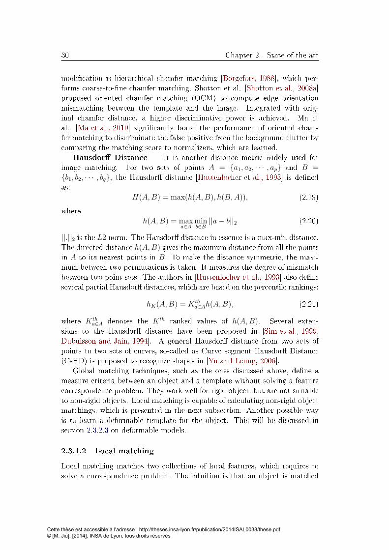
30 Chapter 2. State of the art
modi�cation is hierarchical chamfer matching [Borgefors, 1988], which per-
forms coarse-to-�ne chamfer matching. Shotton et al. [Shotton et al., 2008a]
proposed oriented chamfer matching (OCM) to compute edge orientation
mismatching between the template and the image. Integrated with orig-
inal chamfer distance, a higher discriminative power is achieved. Ma et
al. [Ma et al., 2010] signi�cantly boost the performance of oriented cham-
fer matching to discriminate the false positive from the background clutter by
comparing the matching score to normalizers, which are learned.
Hausdor� Distance � It is another distance metric widely used for
image matching. For two sets of points A = {a1, a2, · · · , ap} and B =
{b1, b2, · · · , bq}, the Hausdor� distance [Huttenlocher et al., 1993] is de�ned
as:
H(A,B) = max(h(A,B), h(B,A)), (2.19)
where
h(A,B) = maxa∈A
minb∈B||a− b||2 (2.20)
||.||2 is the L2 norm. The Hausdor� distance in essence is a max-min distance.
The directed distance h(A,B) gives the maximum distance from all the points
in A to its nearest points in B. To make the distance symmetric, the maxi-
mum between two permutations is taken. It measures the degree of mismatch
between two point sets. The authors in [Huttenlocher et al., 1993] also de�ne
several partial Hausdor� distances, which are based on the percentile rankings:
hK(A,B) = Ktha∈Ah(A,B), (2.21)
where Ktha∈A denotes the Kth ranked values of h(A,B). Several exten-
sions to the Hausdor� distance have been proposed in [Sim et al., 1999,
Dubuisson and Jain, 1994]. A general Hausdor� distance from two sets of
points to two sets of curves, so-called as Curve segment Hausdor� Distance
(CsHD) is proposed to recognize shapes in [Yu and Leung, 2006].
Global matching techniques, such as the ones discussed above, de�ne a
measure criteria between an object and a template without solving a feature
correspondence problem. They work well for rigid object, but are not suitable
to non-rigid objects. Local matching is capable of calculating non-rigid object
matchings, which is presented in the next subsection. Another possible way
is to learn a deformable template for the object. This will be discussed in
section 2.3.2.3 on deformable models.
2.3.1.2 Local matching
Local matching matches two collections of local features, which requires to
solve a correspondence problem. The intuition is that an object is matched
Cette thèse est accessible à l'adresse : http://theses.insa-lyon.fr/publication/2014ISAL0038/these.pdf © [M. Jiu], [2014], INSA de Lyon, tous droits réservés

2.3. Visual recognition: methods 31
to a template, if enough points (or other local primitives) extracted from the
object in the scene are matched well to points on the model. The matching
score of object matching can be related to the matching scores of all the local
points. Another advantage is that local point matching inherently indicates
the object's structure and position, which can also be integrated into the score.
One possible technique for solving the point correspondence problem is
RANSAC (RANdom SAmpling AConsensus). It is an iterative method which
estimates parameters of a global and rigid model from observed data, which
may contain outliers (e.g. a�ne, homography etc.). The parameterized model
can be �tted to the observation through inlier correspondence. However, this
method can not handle non-rigid transformations of an object. Graph match-
ing thus is an alternative method, which is very suitable to non-rigid trans-
formations.
The object can be represented as a graph, which consists of a set of vertices,
and a set of edges between the vertices. Each vertex is often an interest point
(please refer section 2.2.2.1), region of interest, etc. The vertices in the graph
are connected in several ways:
• Full connection: Every pair of nodes in the graph is connected through
an edge. This often is not the optimal choice for large graphs, as the edge
number grows exponentially, and edges do not code any information.
• Proximity: The neighbor nodes are connected according to their distance
in the image or video.
• Adjacency: The edges are estimated from the adjacency relations of the
vertices.
Features can be extracted from each vertex and used to measure the simi-
larity of two nodes. Given two feature vectors Fi and Fj, di�erent metrics are
adopted:
• L−norm: D(Fi, Fj) = ||Fi−Fj||p, amongst Euclidean distance is widely
used.
• χ2 test statistic distance: This distance is a natural choice for two
histogram-type features such as HOG, SIFT:
D(Fi, Fj) =1
2
K∑k=1
[Fi(k)− Fj(k)]2
Fi(k) + Fj(k). (2.22)
Here we brie�y review the philosophy of graph matching. Let Gm =
(Vm, Em, Fm) and Gs = (Vs, Es, F s) be two graphs extracted from the model
Cette thèse est accessible à l'adresse : http://theses.insa-lyon.fr/publication/2014ISAL0038/these.pdf © [M. Jiu], [2014], INSA de Lyon, tous droits réservés
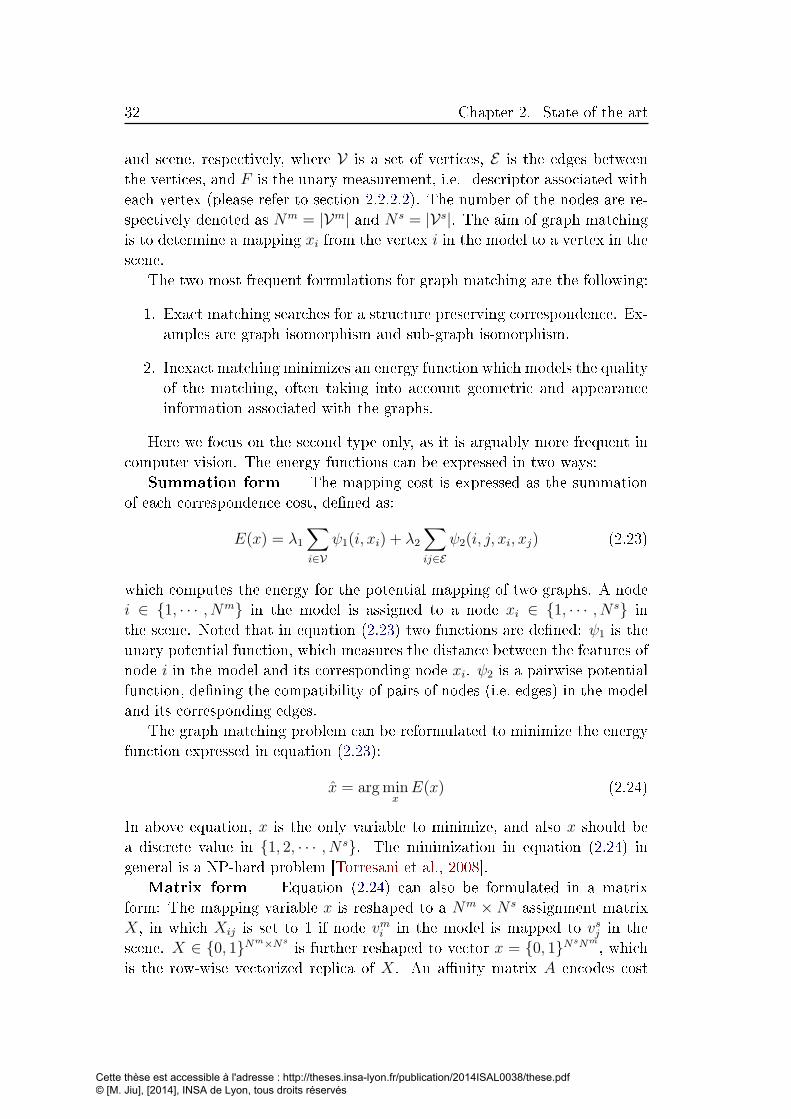
32 Chapter 2. State of the art
and scene, respectively, where V is a set of vertices, E is the edges between
the vertices, and F is the unary measurement, i.e. descriptor associated with
each vertex (please refer to section 2.2.2.2). The number of the nodes are re-
spectively denoted as Nm = |Vm| and N s = |Vs|. The aim of graph matching
is to determine a mapping xi from the vertex i in the model to a vertex in the
scene.
The two most frequent formulations for graph matching are the following:
1. Exact matching searches for a structure preserving correspondence. Ex-
amples are graph isomorphism and sub-graph isomorphism.
2. Inexact matching minimizes an energy function which models the quality
of the matching, often taking into account geometric and appearance
information associated with the graphs.
Here we focus on the second type only, as it is arguably more frequent in
computer vision. The energy functions can be expressed in two ways:
Summation form � The mapping cost is expressed as the summation
of each correspondence cost, de�ned as:
E(x) = λ1∑i∈V
ψ1(i, xi) + λ2∑ij∈E
ψ2(i, j, xi, xj) (2.23)
which computes the energy for the potential mapping of two graphs. A node
i ∈ {1, · · · , Nm} in the model is assigned to a node xi ∈ {1, · · · , N s} in
the scene. Noted that in equation (2.23) two functions are de�ned: ψ1 is the
unary potential function, which measures the distance between the features of
node i in the model and its corresponding node xi. ψ2 is a pairwise potential
function, de�ning the compatibility of pairs of nodes (i.e. edges) in the model
and its corresponding edges.
The graph matching problem can be reformulated to minimize the energy
function expressed in equation (2.23):
x = argminxE(x) (2.24)
In above equation, x is the only variable to minimize, and also x should be
a discrete value in {1, 2, · · · , N s}. The minimization in equation (2.24) in
general is a NP-hard problem [Torresani et al., 2008].
Matrix form � Equation (2.24) can also be formulated in a matrix
form: The mapping variable x is reshaped to a Nm × N s assignment matrix
X, in which Xij is set to 1 if node vmi in the model is mapped to vsj in the
scene. X ∈ {0, 1}Nm×Nsis further reshaped to vector x = {0, 1}NsNm
, which
is the row-wise vectorized replica of X. An a�nity matrix A encodes cost
Cette thèse est accessible à l'adresse : http://theses.insa-lyon.fr/publication/2014ISAL0038/these.pdf © [M. Jiu], [2014], INSA de Lyon, tous droits réservés

2.3. Visual recognition: methods 33
ψ1(i; j) from equation (2.23) in its diagonal elements and cost ψ2(i, j, xi, xj)
from equation (2.23) in its o�-diagonal elements. The optimal solution for
assignment is achieved by minimizing:
E(x) = xTAx, (2.25)
One constraint can be imposed on X to ensure one-to-one correspondences
such that each row contain at most a single 1.
The solutions to solve equation (2.24) and (2.25) are beyond the scope
of this chapter. They are mostly based on discrete optimization (relax-
ation, Lagrangian algorithms, graph cuts, local/tabu search etc.) or a com-
bination of these, or on continuous optimization techniques applied to a re-
laxed version of the problem [Torresani et al., 2008, Duchenne et al., 2009,
Marius et al., 2011, Lee et al., 2011, Lin et al., 2009].
2.3.2 Sliding windows
In section 2.3.1, matching techniques have been discussed for visual recog-
nition. One advantage of these methods is that matching can tell us more
information about an object, not only the presence of the object in the image,
but also its location i.e. where it occurs in the image. However, it su�ers from
heavy computation burden, since it requires to solve a discrete optimization
problem.
In this section, an alternative framework � the sliding window technique,
is discussed. This system slides a window over an image. For each window,
a classi�er determines whether an object is present at this location. The
window's position is assigned to be the object's location. Machine learning
tools can be applied to classi�cation, which can be rapidly executed in the
test stage. Sliding window technique is a trade-o� method, which performs
object detection task in image/video. In the following, bag-of-words models
(BoWs) and deformable part based models (DPMs) are respectively reviewed,
since they can be easily employed in each window.
2.3.2.1 Based on global features
In principle, any global features (described in section 2.2.1) can be combined
with the sliding window technique and any learning machines can be adopted
for object detection and recognition. In particular, appearance and shape
features are widely used. The feature extractor can also be automatically
learned, which is discussed in a dedicated section 2.4.
Cette thèse est accessible à l'adresse : http://theses.insa-lyon.fr/publication/2014ISAL0038/these.pdf © [M. Jiu], [2014], INSA de Lyon, tous droits réservés

34 Chapter 2. State of the art
2.3.2.2 Bag-of-Words models
The bag-of-words (BoW) model has been widely used in computer vision
[Csurka et al., 2004, Dollar et al., 2005] in last decade. This popular model
originates in natural language processing, where it is used to analyze the
content of documents. The model is global in nature, since a single vector de-
scribes the content. However, this content is obtained by pooling descriptors
from local primitives. Each document is expressed as a histogram of frequen-
cies of orderless words, which are taken from a dictionary. Similarly, an image
or video can also be regarded as a document. However, BoW models can
not be directly employed in this case, since dictionaries about objects are not
available. In order to employ the BoW model in computer vision applications,
a dictionary must be built, and each word in the dictionary, named as visual
concept, describes local characteristics of the object.
BoW models have been designed to model whole documents. In principle,
they can also be applied to sliding windows, provided the window contains a
su�ciently large amount of local primitives (e.g. key points) to allow calcu-
lating reliable statistics (histograms). In the video case (activity recognition),
the 3D window can often cover the whole image and several frames, and is
shifted temporally over the video.
Visual concepts traditionally are constructed by extracting features from
the local primitives like interest points, patches, regions, etc (refer to sec-
tion 2.2.2). Each visual primitive can not serve as a codeword due to a large
amount of visual primitives in image/video. Therefore, further special proce-
dure should be performed. The codebook is constructed o�ine. A collection
of feature vectors are extracted from the training set, and a clustering tech-
nique such as k -means is applied on the feature vectors. The obtained cluster
centers are viewed as the codewords. Thus, codewords (visual concepts) are
de�ned as frequently occurring visual patterns. A set of codewords produces
a codebook. The codebook is stored and can be retrieved in the training/test
stage. The procedure of BoW models (refer to �gure 1.7(a) in chapter 1) is
given as follows:
• The training stage comprises two parts:
1. The unsupervised clustering part, which calculates the dictionary.
Clustering techniques are applied on the extracted feature vectors,
and the cluster centers are regarded as codewords.
2. The supervised training part calculates the prediction model. For
each training image, each extracted feature vector is projected to
the codeword with nearest distance in the codebook. A histogram,
where each bin counts frequencies of each codeword occurring in
Cette thèse est accessible à l'adresse : http://theses.insa-lyon.fr/publication/2014ISAL0038/these.pdf © [M. Jiu], [2014], INSA de Lyon, tous droits réservés

2.3. Visual recognition: methods 35
the image, serves as an indicator of the content. Each training
image is represented as a histogram. A set of histograms and their
associated class labels are used to learn the prediction model of a
learning machine such as SVM, NN, etc.
• In the test stage, for a new test image, a similar procedure is performed,
without codebook construction. A histogram is constructed from all the
feature vectors to represent the test image, which is eventually fed into
a learning machine for classi�cation.
BoW models have several advantages: (i) they are very simple and easy
to implement; (ii) they are robust to background clutter and occlusion in the
image; (iii) they are also invariant to viewpoint changes.
1. BoW without structural information
In classical BoW models, an image is represented as a histogram of oc-
currences of codewords, which are independently extracted. The histogram
contains no information of the location of each point of interest, and no infor-
mation about the relationships between the points. Therefore, the classical
BoW model is a model without any structural information. They mainly di�er
from each other in the way how features and codebooks are obtained.
Sivic and Zisserman [Sivic and Zisserman, 2003] and Csurka et al.
[Csurka et al., 2004] �rst introduce �bag-of-features� models into computer
vision community, which have the same meaning as �bag-of-words� models.
They use SIFT features to construct codebooks. They have been success-
fully used for object retrieval problems and visual categorization problems. A
texture vocabulary (i.e. texton) [Leung and Malik, 2001] is learned to recog-
nize the texture objects. Matikainen et al. [Matikainen et al., 2009] learn a
trajectons vocabulary based on trajectory snippets of tracked features. Each
action is represented as a histogram of trajectons. A mid-level sparse visual
vocabulary is learned in [Boureau et al., 2010].
The BoW models have also been extended to the video case for activity
recognition. Visual concepts are detected around space-time interest points
[Laptev, 2005, Dollar et al., 2005]. Semantic visual codebook by using di�u-
sion distance has been proposed for action recognition [Liu et al., 2009].
2. BoW without structural information � optimized models
Traditional codebooks are constructed by classical k -means clustering.
There have been several attempts to optimize the codebook. Jurie and Triggs
[Jurie and Triggs, 2005] show that cluster centers by k -means are exclusively
Cette thèse est accessible à l'adresse : http://theses.insa-lyon.fr/publication/2014ISAL0038/these.pdf © [M. Jiu], [2014], INSA de Lyon, tous droits réservés

36 Chapter 2. State of the art
around dense regions in feature space. They propose scalable acceptance-
radius based clusters to capture non-uniform feature distributions. Ballan et
al. [Ballan et al., 2009] extend this work to human action recognition. Moos-
mann et al. [Moosmann et al., 2007] learn a discriminative visual codebook
by means of randomized clustering forests.
Liu and Shah [Liu and Shah, 2008] learn an optimal codebook by informa-
tion maximization. Considering two random variables X = {x1, x2, . . . , xn}and Y = {y1, y2, . . . , ym}, X indicates codewords and Y indicates videos.
Their goal is to �nd an optimal codebook X with maximum mutual informa-
tion given the initial codebook X :
I(X;Y ) =∑
y∈Y,x∈X
p(x, y) logp(x, y)
p(x)p(y). (2.26)
where p(x, y) is the joint distribution of X and Y , p(x) and p(y) are probability
distributions of X and Y respectively. The function is de�ned as follows:
max(I(X;Y )− λ−1I(X;X)) (2.27)
Here, I(X,X) measures the compactness of the new codebook X compared to
X, which can be computed by a similar equation to (2.26) given the mapping
p(x|x). λ−1 is a Lagrange multiplier.
Equation (2.27) is solved by a greedy bottom-up pairwise merging proce-
dure. The cost of merging two codewords x1 and x2 is expressed as:
4I(x1, x2) = I(Xbef ;Y )− I(Xaft;Y ) (2.28)
where I(Xbef ;Y ) and I(Xaft;Y ) denote the mutual information before and
after merging. Two codewords with minimum loss of equation (2.28) are
merged at each step. The merging operation is continued until 4I(x1, x2) islarger than a prede�ned threshold or numer of clusters is obtained.
The aforementioned approaches of codebook optimization proceed by un-
supervised learning on the feature space, they are not oriented to classi�cation
stage. On the contrast, our codebook optimization by an end-to-end frame-
work introduced in chapter 3 is based on supervised learning, which makes
it possible to use the backpropagated errors from the classi�er to update the
codewords. Goh et al. [Goh et al., 2012] propose to learn a visual codebook
by the framework of Restricted Boltzmann Machines (RBMs) (see section
2.4.2.2) in a supervised way for image category classi�cation.
3. BoW with structural information
Cette thèse est accessible à l'adresse : http://theses.insa-lyon.fr/publication/2014ISAL0038/these.pdf © [M. Jiu], [2014], INSA de Lyon, tous droits réservés

2.3. Visual recognition: methods 37
The BoW model based on interest points usually ignores the spatial (or ge-
ometric) information, i.e. the spatial or spatial-temporal relationships between
the interest points. These relationships contain many important complemen-
tary clues for recognition. The codewords in BoW models are orderless. Other
work attempts to introduce structural information into BoW models.
Grauman and Darrell [Grauman and Darrell, 2005] propose a pyramid
match kernel, which maps unordered features to multi-resolution histograms
and implicitly �nds correspondences on the �nest resolution. Lazebnik and
Schmid [Lazebnik and Schmid, 2006] partition the image into increasingly �ne
sub-regions and compute a BoW model for each sub-region, and use the pyra-
mid kernel in [Grauman and Darrell, 2005] to train a SVM for recognition.
Cao et al. [Cao et al., 2010] encode geometric information of objects into or-
dered BoW models. A histogram transformation is applied to get a spatial
bag-of-features, which is tolerant to variations in translation, rotation, and
scale.
The main distinction between video and image is that the video also con-
tains temporal information, which describes continuous information of the
action. Some work exploits encoding the spatio-temporal relationships into
codewords to improve the BoW models for action recognition.
Oikonomopoulos et al. [Oikonomopoulos et al., 2009] take spatial co-
occurrences of pairs of codewords into account, exploring the relative posi-
tions of codeword pairs with respect to the object's center to create a spatio-
temporal model. Finally they propose a probabilistic spatio-temporal voting
framework for localizing and recognizing human action. Matikainen et al.
[Matikainen et al., 2010] express pairwise relationships with a sequence code
map and estimate the relative location and temporal relationship probabili-
ties from a training dataset. Ryoo and Aggarwal [Ryoo and Aggarwal, 2009]
de�ne the spatio-temporal relationship of pairs of neighboring local features
such as near, far etc, creating a 3D histogram (two codeword dimensions
and one relationship dimension). Ta et al. [Ta et al., 2010b] also propose
pairwise features, which encode both appearance descriptors and spatio-
temporal relationships between spatio-temporal interest points. In contrast to
[Ryoo and Aggarwal, 2009], the structural information is discovered by clus-
tering in a space-time geometric space.
Gaidon et al. [Gaidon et al., 2011] propose a new kernel which addresses
the dynamics and temporal structure of actions on bags of words. They com-
pute the Hilbert-Schmidt distance between two auto-correlations of actions
and provide a kernelized formulation. In contrast to the previous works, their
method does not align two videos to compute their similarity. Bettadapura
et al. [Bettadapura et al., 2013] augment BoW models integrating temporal
structure by quantizing time and de�ning temporal events for activity recogni-
Cette thèse est accessible à l'adresse : http://theses.insa-lyon.fr/publication/2014ISAL0038/these.pdf © [M. Jiu], [2014], INSA de Lyon, tous droits réservés

38 Chapter 2. State of the art
tion. Three n-grams encoding schemes are used to represent BoW models. To
capture global structure, randomly regular expressions are created and treated
as new words, adding into the original BoW models. Li et al. [Li et al., 2013]
represent an activity as short-term segments, which are characterized by the
dynamics of attributes (i.e. the score evolution of attribute detectors along
the activity). They learn a dictionary of attribute dynamics. The activity is
represented as bag of attribute dynamic words.
2.3.2.3 Deformable part based models (DPMs)
DPMs have �rst been proposed in [Fischler and Elschlager, 1973]. A recent
version by Felzenszwalb et al. [Felzenszwalb et al., 2010] has achieved state-
of-the-art results for object localization on many categories in the recently
PASCAL VOC challenges. DPM is a kind of part based models. An object is
represented as a set of meaningful parts and their associated spatial structure.
Compared to low-level feature based models such as bag-of-words models, part
based models, as a middle-level representation, are able to better express the
structural properties of objects.
A large body of work has addressed these models. A part can be regarded
as a constellation of low level features, such as interest points, edges etc. Fer-
gus et al. [Fergus et al., 2003] propose a model of constellations of parts, which
is expressed as a joint probability from all aspects of the object: appearance,
shape, scale and occlusion. They �rst compute the local saliency for each loca-
tion and scale in an image and the regions whose saliency is above a threshold
are considered as parts for recognition. In the process of learning, the param-
eters for the probability are estimated by expectation-maximization. In the
recognition step, a new image is recognized in a Bayesian manner. Fergus et al.
[Fergus et al., 2004] extend their method by integrating curve segments into
the framework: Each part can be either de�ned by a region or curve. Curve
segments are obtained by �rst employing the canny detector and decomposing
the curve into independent segments at bi-tangent points.
Parts also can be learned in a hierarchical structure, where low level fea-
tures in child nodes are merged into a father node, as a part. Mikolajczyk
et al. [Mikolajczyk et al., 2006] propose a hierarchical representation through
codebooks learned from shared appearance features around edge points. A
joint appearance-geometry probability distribution is learned for each cluster
in the hierarchical tree. Recognition is done in a Bayesian way. Zhu et al.
[Zhu et al., 2010] propose Recursive Compositional Models (RCMs) for multi-
view multi-object detection, where each RCM is a probability distribution over
a hierarchical graph corresponding to a speci�c object and viewpoint, which
encodes the root appearance cues, the boundary potential corresponding for
Cette thèse est accessible à l'adresse : http://theses.insa-lyon.fr/publication/2014ISAL0038/these.pdf © [M. Jiu], [2014], INSA de Lyon, tous droits réservés

2.3. Visual recognition: methods 39
(a) (b) (c)
Figure 2.14: A DPM for category �person�: (a) the root �lter, (b) the part
�lters, and (c) the gray scaled deformation cost.
the boundary segments at the leaf nodes, and also pairwise spatial relations
between the parent node and their children nodes.
Pictorial structures [Fischler and Elschlager, 1973,
Felzenszwalb and Huttenlocher, 2005] are another kind of part based models,
where an object is modeled as a set of parts and their structure is captured by
a set of �springs� connections in terms of Gaussian distribution between pairs
of parts. The original pictorial structure [Fischler and Elschlager, 1973] is an
energy based function, which is the sum of the mismatch cost of each part,
and also deformation cost between pairs of parts. The best con�guration of
an object is the one with minimal energy. Felzenszwalb and Huttenlocher
[Felzenszwalb and Huttenlocher, 2005] reformulate the pictorial structure
in a statistical framework. The detection problem transfers to maximum
a posterior (MAP) estimation. The parameters can be learned by using
maximum likelihood estimation. In their star shaped model, only root/part
relationships are included, pairwise part relationships are not modeled. This
allows e�cient inference through dynamic programming.
The aforementioned part based models are learned in a generative way.
Felzenszwalb et al. [Felzenszwalb et al., 2010] attempt to learn deformable
part based models in a discriminative way. Learning and testing are relatively
e�cient. The advantage of DPMs is that the parts are considered as latent
variables in the learning stage and can be inferred e�ciently without part
annotations for each training image. We brie�y review the latter formulation
of DPMs as follows:
A DPM is composed of a root �lter P0 and a set of part �lters Pi, i ∈(1, . . . , n). Each part �lter also de�nes a two-dimensional vector ai = 〈aix, aiy〉specifying the anchor position relative to the root, and four quadratic defor-
mation coe�cients di taking into account the cost of the part relative to its
anchor position. Figure 2.14 shows a learned DPM for category �person�.
Cette thèse est accessible à l'adresse : http://theses.insa-lyon.fr/publication/2014ISAL0038/these.pdf © [M. Jiu], [2014], INSA de Lyon, tous droits réservés

40 Chapter 2. State of the art
The score of a hypothesis in a window is the sum of the scores from the
root �lter and part �lters, minus the deformation cost of each part real (i.e. in-
ferred) location w.r.t the anchor position, and plus a bias b, shown as follows:
f(P0, . . . , Pn) =n∑
i=0
Pi · φ(x, zi)−n∑
i=1
di · ψ(zi) + b. (2.29)
where zi is the inferred part location, and φ(x, zi) are local dense features
extracted from zi, ψ(zi) is the displacement of the inferred position zi w.r.t
the anchor position ai by:
ψ(zi) = [(zix − aix)2, (zix − aix), (ziy − aiy)2, (ziy − aiy)] (2.30)
The real part locations, treated as latent variables, are inferred in the learn-
ing and test stage to maximize the score. Equation (2.29) can be rewritten
as:
f(P0, . . . , Pn) = maxz∈Z(x)
(n∑
i=0
Pi · φ(x, zi)−n∑
i=1
di · ψ(zi) + b). (2.31)
where Z(x) is a collection of all the possible positions for the parts. The
objective function to minimize is the hinge loss, which is expressed by:
L(β) =1
2||β||2 + C
N∑i=1
max(0, 1− yif(xi)) (2.32)
where β is the set of learning parameters containing (P0, P1, · · · , Pn, d, b),
xi and yi is the training example and its groundtruth, f(xi) is its score, C
controls the regularization term, N is the training instance size. Latent SVM
is applied to minimize equation (2.32). The training stage learns part �lters
and deformation costs. In the test stage, part locations are inferred. Note that
the anchor positions are NOT learned in the supervised framework. Instead,
they are set to locations where the root �lter gives high responses. This might
not be optimal, since parts do not necessarily look like the object.
Other follow-up work has be done to further improve DPM models by shar-
ing parts between object classes [Ott and Everingham, 2011], through visual
mixture models [Divvala et al., 2012] where the components for each class are
de�ned by visual similarity instead of height-width ratio of the groundtruth
bounding box, etc. DPMs have also been extended to spatio-temporal data
for activity recognition [Tian et al., 2013]. DPMs are accelerated by replac-
ing the convolution operations by locality-sensitive hashing, which enables
to e�ciently perform the detection of 100000 objects on a single machine
Cette thèse est accessible à l'adresse : http://theses.insa-lyon.fr/publication/2014ISAL0038/these.pdf © [M. Jiu], [2014], INSA de Lyon, tous droits réservés

2.3. Visual recognition: methods 41
[Dean et al., 2013]. Sharma et al. [Sharma et al., 2013] discriminatively learn
a collection of part templates in the images, and each part explains each image
individually. The best set of part templates is chosen for each image. This
is in contrast with other part based models which use all the parts for each
image. At the same time, a large set of part templates also are able to en-
code the variance of humans in the dataset, avoiding highly structured model
learning.
2.3.3 Segmentation for visual recognition
Segmentation is a fundamental problem in the community. It aims to segment
an object into several meaningful parts, which is used to obtain more infor-
mation about object, such as the spatial layout, or object pose. Segmentation
plays several roles in visual recognition, which are addressed in the following.
2.3.3.1 Segmentation for selective candidate regions
The sliding window technique presented in section 2.3.2 is often applied to
object detection in images/videos. However, it has several drawbacks: on one
hand, it works best on objects with a �xed aspect ratio. For general objects,
exhaustive search has to be performed over location, scale, aspect ratio, which
is apparently computationally expensive. DPMs can be e�ciently performed
through generalized distance transformation [Felzenszwalb et al., 2010], but
are still quite expensive.
Recently, an alternate way in favor of a segmentation based pre-precessing
step has been proposed to overcome the drawbacks of sliding window tech-
niques. The core is to �rst over-segment an image into thousands of object seg-
ments (i.e. regions) candidates, which cover most of the objects in the image.
The regions are converted to bounding boxes and the features are extracted
from the bounding box and then fed to a classi�cation machine. Segmentation
as Selective Search [van de Sande et al., 2011] is one of recent algorithms to
generate regions/bounding boxes. They start with oversegmentation, a set of
small regions are obtained. A hierarchical segmentation tree is constructed
through grouping of similar regions in a greedy algorithm. Bounding boxes
containing regions across the tree are considered for the sequent classi�ca-
tion. Selective search enables to use more expensive features for each region
and improves the state-of-the-art for 8 out of 20 classes on Pascal VOC 2007
dataset.
Wang et al. [Wang et al., 2013] apply the selective search approach
[van de Sande et al., 2011] to get a set of small regions (named as �region-
lets�) in the bounding box. Several groups containing regionlets are organized
Cette thèse est accessible à l'adresse : http://theses.insa-lyon.fr/publication/2014ISAL0038/these.pdf © [M. Jiu], [2014], INSA de Lyon, tous droits réservés
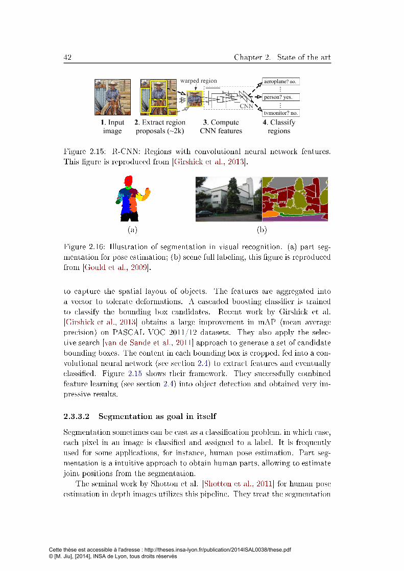
42 Chapter 2. State of the art
Figure 2.15: R-CNN: Regions with convolutional neural network features.
This �gure is reproduced from [Girshick et al., 2013].
(a) (b)
Figure 2.16: Illustration of segmentation in visual recognition. (a) part seg-
mentation for pose estimation; (b) scene full labeling, this �gure is reproduced
from [Gould et al., 2009].
to capture the spatial layout of objects. The features are aggregated into
a vector to tolerate deformations. A cascaded boosting classi�er is trained
to classify the bounding box candidates. Recent work by Girshick et al.
[Girshick et al., 2013] obtains a large improvement in mAP (mean average
precision) on PASCAL VOC 2011/12 datasets. They also apply the selec-
tive search [van de Sande et al., 2011] approach to generate a set of candidate
bounding boxes. The content in each bounding box is cropped, fed into a con-
volutional neural network (see section 2.4) to extract features and eventually
classi�ed. Figure 2.15 shows their framework. They successfully combined
feature learning (see section 2.4) into object detection and obtained very im-
pressive results.
2.3.3.2 Segmentation as goal in itself
Segmentation sometimes can be cast as a classi�cation problem, in which case,
each pixel in an image is classi�ed and assigned to a label. It is frequently
used for some applications, for instance, human pose estimation. Part seg-
mentation is a intuitive approach to obtain human parts, allowing to estimate
joint positions from the segmentation.
The seminal work by Shotton et al. [Shotton et al., 2011] for human pose
estimation in depth images utilizes this pipeline. They treat the segmentation
Cette thèse est accessible à l'adresse : http://theses.insa-lyon.fr/publication/2014ISAL0038/these.pdf © [M. Jiu], [2014], INSA de Lyon, tous droits réservés

2.3. Visual recognition: methods 43
problem as a classi�cation problem. For each image, background is subtracted
and each pixel is annotated to one of N labels (N indicates the part number
of human body). A randomized forest with N labels is learned. Each pixel
in the test image is classi�ed to one of N labels. Mean-shift with a weighted
Gaussian kernel is applied �nally to �nd the joint positions between the parts.
There is another visual recognition task � scene full labeling, where seg-
mentation is needed. It attempts to label each pixel in the image with a
category. This is a very challenging task due to its combination of segmen-
tation and recognition. A common strategy is to pre-segment an image into
super-pixels or other region candidates, and extract features from the can-
didates and �nally make a classi�cation. The di�erence here from selective
search approach [van de Sande et al., 2011] is that we assign a label for each
region, rather than some particular regions with high con�dence to determine
the bounding box of object. Socher et al. [Socher et al., 2011] propose a
max-margin structure prediction based on recursive neural networks to label
the image. The image is �rst over-segmented into small regions. Visual fea-
tures are extracted from the regions. A neural network is trained to output a
higher value when the neighboring region should be merged and also a label
for the region. Farabet et al. [Farabet et al., 2012] adopt the same idea, but
they di�er from [Socher et al., 2011] in that: 1): the features are learned in
the framework of convolutional neural networks, rather than hand-engineered
features; 2) For a hierarchical segmentation tree, a classi�er is learned to �nd
a subset of nodes, which optimally covers the image and also maximizes the
�purity� of the nodes, where purity is de�ned as a quantity that is inversely
proportional to the entropy of the class distribution for each node.
It is also worth mentioning several recent work on scene full labeling. Pin-
heiro and Collobert [Pinheiro and Collobert, 2013] propose to apply recurrent
convolutional neural networks to this task. The output of a ConvNet is fed
to another ConvNet with tied parameters, which allows to model context and
long range dependencies. Kontschieder et al. [Kontschieder et al., 2013] pro-
pose a new geodesic forest, achieving spatially consistent semantic image seg-
mentation by encoding long range, soft connectivity features via generalized
geodesic distance transforms. Shapovalov et al. [Shapovalov et al., 2013] pro-
pose spatial inference machines, taking into account mid-range and long-range
dependencies for semantic segmentation of 3D point clouds. The framework
proposed in [Farabet et al., 2012] has been extended to indoor scene segmen-
tation with RGB-D images [Couprie et al., 2013].
Our work in chapters 4 and 5 focuses on part segmentation as a classi�-
cation problem. We learn a classi�cation machinery targeted to pixels, rather
than regions, and employ it on each pixel in image to estimate parts.
Cette thèse est accessible à l'adresse : http://theses.insa-lyon.fr/publication/2014ISAL0038/these.pdf © [M. Jiu], [2014], INSA de Lyon, tous droits réservés

44 Chapter 2. State of the art
2.4 Feature/Representation learning
In section 2.3, we brie�y reviewed three kinds of recognition techniques. Dif-
ferent features can be adopted in these techniques. Generally speaking, feature
extraction is an independent module compared to the following recognition
module in the dominant pipeline shown in �gure 1.6 in chapter 1. However,
the presented extractors produce hand-crafted features (refer to section 2.2),
which have the following drawbacks:
• Hand-crafted features usually are designed for speci�c properties such
as HOG/HOF for appearance and shape context for shape.
• A certain amount of pre-processing needs to be performed to prepare
for hand-crafted feature calculation. For examples, the gradient is com-
puted �rst for each pixel and aggregated into a histogram of gradient
orientation for a block; others require optical �ow etc. However, pre-
processing is mostly expensive and depends on numerous parameters
which need to be tuned.
• In this classical framework, feature computation is independent from the
following classi�cation stage. Performance can be improved by learning
the features as well as the classi�er together, resulting in an end-to-end
framework.
Given the aforementioned arguments on the hand-crafted features, feature
learning techniques have received much consideration lately. Feature learning
can be operated in di�erent ways as shown in �gure 2.17:
• Supervised learning: The labels of the training examples or the variables
induced from the labels (e.g. sensitivity functions in a neural network)
are directly used in the feature learning stage.
• Unsupervised learning: The labels of the training examples are not used
for feature learning. Other criteria such as reconstruction error, or image
transformations are adopted.
• Weakly-supervised learning: Compared to unsupervised learning, the
labels of the training examples are known in the learning, but they
are not associated with feature learning and no classi�cation error is
calculated. The availability of the labels is often necessary to generate
new training examples (e.g. pairs of examples from the same labels or
di�erent labels).
In the following section, we brie�y present common strategies used for feature
learning.
Cette thèse est accessible à l'adresse : http://theses.insa-lyon.fr/publication/2014ISAL0038/these.pdf © [M. Jiu], [2014], INSA de Lyon, tous droits réservés

2.4. Feature/Representation learning 45
Feature learning
Supervisedlearning
Unsupervisedlearning
Errorbackpropa
Auto- Trans.Neighborhoodrelationship
learning
Weakly-supervisedlearning
Encoding learning
Figure 2.17: The feature learning criteria, where �backpropa� means back-
propagation, �Trans� means transformation.
2.4.1 Supervised feature learning
We aim to learn a more discriminative feature extractor using annotated train-
ing images. An intuitive idea is to calculate classi�cation errors for the training
set and employ them to update the features through minimization, which is
similar to train neural networks(i.e. error backpropagation).
2.4.1.1 Error backpropagation
Earlier work on supervised feature learning is LeCun's work on handwritten
document recognition [LeCun et al., 1998]. They adopted a framework called
Convolutional Neural Networks (CNN or ConvNets) shown in �gure 2.18. The
features are directly computed from the raw data by convolving an image with
a set of �lters, resulting in a set of feature maps. Non-linear transformation
(e.g. hyperbolic tangent function) and spatial reduction/pooling are applied to
the feature maps to make the output robust to noise and slight translations.
Similar operations can be repeated several times by treating the output of
previous layers as the input of next layer. The resulting feature maps are
vectorized into a vector, and then fed to a fully connected logistic regression
layer (or to a MLP) to predict the category of the input. This framework is
an end-to-end framework because the feature extraction module is connected
with the classi�cation module. This means that the error is back propagated
all the way back to the input, updating the weights in the logistic regression
layer as well as the �lters.
The learning procedure is described as follows: The �lters are �rst ran-
domly initialized. Given an input and its associated groundtruth, the network
is stimulated and the output layer delivers an response for each unit. A loss
function (for example sum of errors or cross-entropy loss) is calculated; then
a gradient of the loss function w.r.t each output unit is computed, which is
Cette thèse est accessible à l'adresse : http://theses.insa-lyon.fr/publication/2014ISAL0038/these.pdf © [M. Jiu], [2014], INSA de Lyon, tous droits réservés

46 Chapter 2. State of the art
Full connected
ClassifierFeature learning stage
Convolution
Sampling
Tanh &
Sampling
Convolution
Tanh &
Figure 2.18: The convolutional neural network.
.
(a) (b) (c)
Figure 2.19: Dimensionality reduction. (a): PCA linear embedding; (b)non-
linear embedding, this �gure is reproduced from [Bengio, 2009]; (c) DrLIM
results, this �gure is reproduced from [Hadsell et al., 2006].
used to update the weights in the classi�cation layer. This gradient is again
backpropagated to the previous layer, and the sensitivity is used to update
the �lters. This is the classical error backpropagation, which can be e�ciently
implemented as only inner products are involved in the learning procedure.
After two decades of development, CNN has been used in many applications
[LeCun et al., 2010] and has won important competitions such as ImageNet
2012 [Krizhevsky et al., 2012].
2.4.2 Unsupervised learning
Unsupervised feature learning casts the task as an intelligent dimensionality
reduction problem. The data are passed from a high dimensional input space
(pixel) to a lower dimensional feature space. Classical methods like principle
component analysis (PCA) perform this task. PCA method embeds the input
Cette thèse est accessible à l'adresse : http://theses.insa-lyon.fr/publication/2014ISAL0038/these.pdf © [M. Jiu], [2014], INSA de Lyon, tous droits réservés

2.4. Feature/Representation learning 47
to the eigenspace de�ned by the eigenvector of the input feature matrix. But
it su�ers from its main limitation �linearity, i.e. only linear embedding (see �g-
ure 2.19(a)). Intelligent dimensionality reduction attempts to �nd non-linear
structure in the data and to encode it in a suitable non-linear transformation
(see �gure 2.19(b)).
In this section, we will present two unsupervised feature learning
paradigms: auto-encoding and transformation learning. Auto-encoding tries
to preserve as much as information about the input from the representation,
while the latter tries to learn a transformation between neighboring (or consec-
utive) images, which can be very useful to capture the temporal relationship
between frames in video.
2.4.2.1 Auto-encoding
Auto-encoding is based on the following principle: an encoder encodes the
input data into a compact code, which is smaller than the input data. A
decoder tries to reconstruct the data with minimum error. As the code is
small, the encoder and decoder need to �nd patterns and structures in the
data in order to be e�cient. This structure is postulated to be useful for
recognition.
In more detail, let x be the raw data, an encoder �rst maps x to a represen-
tation code z through a non-linear activation function f , typically a sigmoid
function:
z = Enc(x,We) = f(We ∗ x+ be) (2.33)
whereWe are the parameters of the encoder. A decoder reconstructs the input
to be y from z through another activation function g, typically an identity
function (i.e. linear case) or sigmoid function:
y = Dec(z,Wd) = g(Wd ∗ z + bd) (2.34)
where Wd are the parameters of the decoder. In general, for a set of training
examples, the loss function is expressed by sum of error or cross-entropy:
L =
{ ∑Ni=1 ||xi − yi||2 if linear case∑Ni=1 xi log(yi) + (1− xi) log(1− yi) if sigmoid case
(2.35)
The learning procedure attempts to minimize the loss function over the
parameters We and Wd on the training set. Gradient descent can be applied
to minimize the error. Di�erent training algorithms have been developed ac-
cording to di�erent regularization items added into equation (2.35): regular-
ized auto-encoder with weight decay [Lee et al., 2007], denoising auto-encoder
[Vincent et al., 2010], contractive auto-encoder [Rifai et al., 2011].
Cette thèse est accessible à l'adresse : http://theses.insa-lyon.fr/publication/2014ISAL0038/these.pdf © [M. Jiu], [2014], INSA de Lyon, tous droits réservés
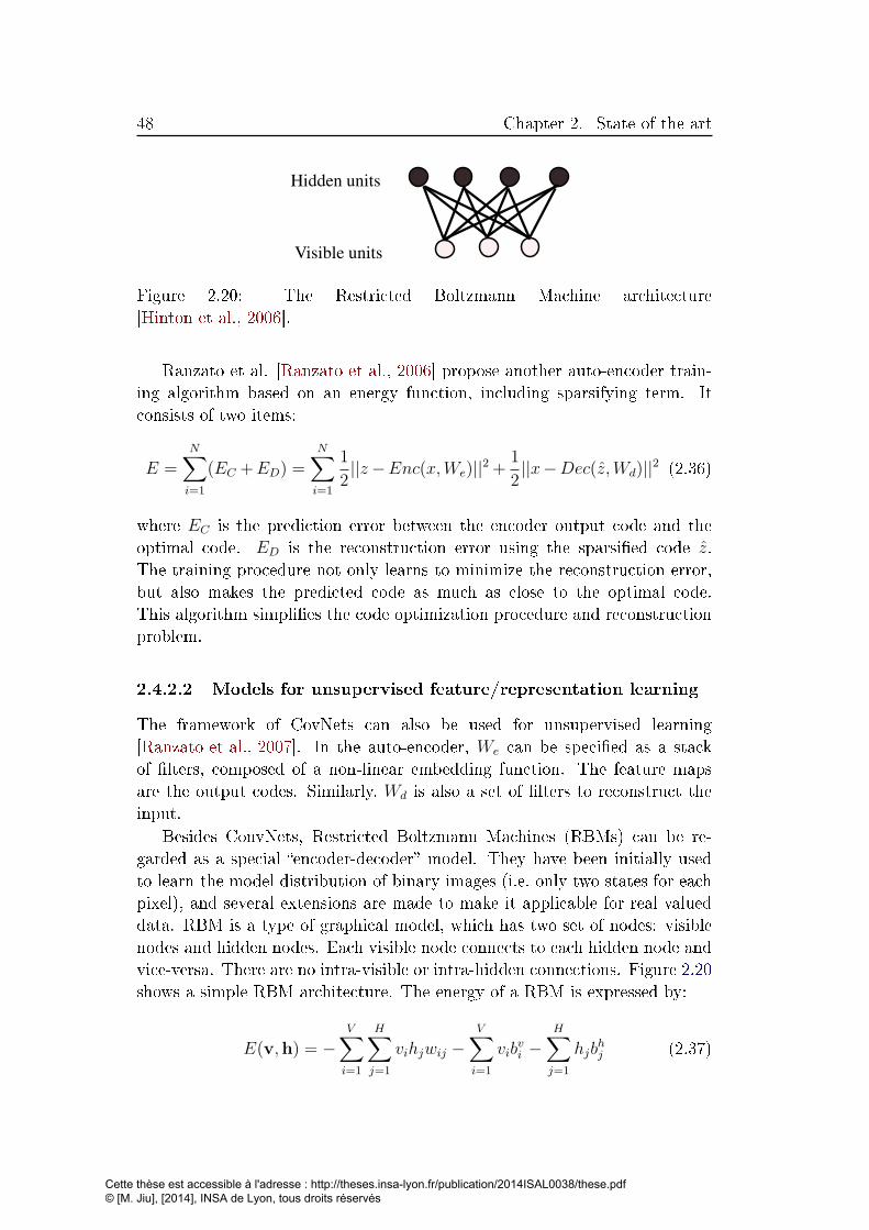
48 Chapter 2. State of the art
Visible units
Hidden units
Figure 2.20: The Restricted Boltzmann Machine architecture
[Hinton et al., 2006].
Ranzato et al. [Ranzato et al., 2006] propose another auto-encoder train-
ing algorithm based on an energy function, including sparsifying term. It
consists of two items:
E =N∑i=1
(EC +ED) =N∑i=1
1
2||z−Enc(x,We)||2 +
1
2||x−Dec(z,Wd)||2 (2.36)
where EC is the prediction error between the encoder output code and the
optimal code. ED is the reconstruction error using the sparsi�ed code z.
The training procedure not only learns to minimize the reconstruction error,
but also makes the predicted code as much as close to the optimal code.
This algorithm simpli�es the code optimization procedure and reconstruction
problem.
2.4.2.2 Models for unsupervised feature/representation learning
The framework of CovNets can also be used for unsupervised learning
[Ranzato et al., 2007]. In the auto-encoder, We can be speci�ed as a stack
of �lters, composed of a non-linear embedding function. The feature maps
are the output codes. Similarly, Wd is also a set of �lters to reconstruct the
input.
Besides ConvNets, Restricted Boltzmann Machines (RBMs) can be re-
garded as a special �encoder-decoder� model. They have been initially used
to learn the model distribution of binary images (i.e. only two states for each
pixel), and several extensions are made to make it applicable for real valued
data. RBM is a type of graphical model, which has two set of nodes: visible
nodes and hidden nodes. Each visible node connects to each hidden node and
vice-versa. There are no intra-visible or intra-hidden connections. Figure 2.20
shows a simple RBM architecture. The energy of a RBM is expressed by:
E(v,h) = −V∑i=1
H∑j=1
vihjwij −V∑i=1
vibvi −
H∑j=1
hjbhj (2.37)
Cette thèse est accessible à l'adresse : http://theses.insa-lyon.fr/publication/2014ISAL0038/these.pdf © [M. Jiu], [2014], INSA de Lyon, tous droits réservés
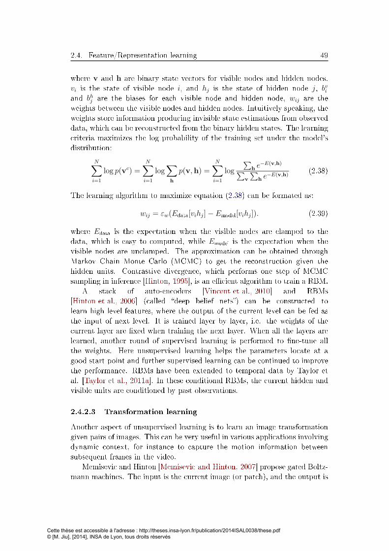
2.4. Feature/Representation learning 49
where v and h are binary state vectors for visible nodes and hidden nodes.
vi is the state of visible node i, and hj is the state of hidden node j, bviand bhj are the biases for each visible node and hidden node, wij are the
weights between the visible nodes and hidden nodes. Intuitively speaking, the
weights store information producing invisible state estimations from observed
data, which can be reconstructed from the binary hidden states. The learning
criteria maximizes the log probability of the training set under the model's
distribution:
N∑i=1
log p(vc) =N∑i=1
log∑h
p(v,h) =N∑i=1
log
∑h e
−E(v,h)∑v
∑h e
−E(v,h)(2.38)
The learning algorithm to maximize equation (2.38) can be formated as:
wij = εw(Edata[vihj]− Emodel[vihj]). (2.39)
where Edata is the expectation when the visible nodes are clamped to the
data, which is easy to computed, while Emodel is the expectation when the
visible nodes are unclamped. The approximation can be obtained through
Markov Chain Monte Carlo (MCMC) to get the reconstruction given the
hidden units. Contrastive divergence, which performs one step of MCMC
sampling in inference [Hinton, 1995], is an e�cient algorithm to train a RBM.
A stack of auto-encoders [Vincent et al., 2010] and RBMs
[Hinton et al., 2006] (called �deep belief nets�) can be constructed to
learn high level features, where the output of the current level can be fed as
the input of next level. It is trained layer by layer, i.e. the weights of the
current layer are �xed when training the next layer. When all the layers are
learned, another round of supervised learning is performed to �ne-tune all
the weights. Here unsupervised learning helps the parameters locate at a
good start-point and further supervised learning can be continued to improve
the performance. RBMs have been extended to temporal data by Taylor et
al. [Taylor et al., 2011a]. In these conditional RBMs, the current hidden and
visible units are conditioned by past observations.
2.4.2.3 Transformation learning
Another aspect of unsupervised learning is to learn an image transformation
given pairs of images. This can be very useful in various applications involving
dynamic context, for instance to capture the motion information between
subsequent frames in the video.
Memisevic and Hinton [Memisevic and Hinton, 2007] propose gated Boltz-
mann machines. The input is the current image (or patch), and the output is
Cette thèse est accessible à l'adresse : http://theses.insa-lyon.fr/publication/2014ISAL0038/these.pdf © [M. Jiu], [2014], INSA de Lyon, tous droits réservés

50 Chapter 2. State of the art
the next image (or patch). In order to capture the relations between the input
and the output, a hidden binary variable is introduced to connect the input
and output. The energy function as shown in equation (2.37) is changed to
associate with the input, output and hidden variable. The weights are also
changed to three-way tensor variables.
Taylor et al. [Taylor et al., 2010] extend this work to convolutional gated
Restricted Boltzmann Machines (convGRBMs) and use them to learn spatio-
temporal features in video. Their method is able to learn the ��ow �elds�
between pairs of input frames. They apply their model for action recognition,
and obtain competitive performance on benchmark datasets.
2.4.3 Weakly-supervised learning
Weakly-supervised learning is a type of learning, which does not use label
information in the feature learning stage in a direct way, i.e. classi�cation error
is not directly minimized. Instead this label information can provide some
other information such as information on neighborhood relationships. We
refer this kind of information as neighborhood relationship, which is de�ned
either by manual labels (i.e. the instances with same label are neighbors) or
the distances between the input data. The neighboring instances from the
same category in the input space should generate the neighboring outputs in
the output space. These methods try to learn a mapping function from high-
dimensional input data to low-dimensional output, at the same time, similar
inputs are mapped to close points and dissimilar inputs to distant points in
the low-dimensional space.
Neighborhood Components Analysis (NCA) [Goldberger et al., 2004] and
its variants [Salakhutdinov and Hinton, 2007] implicitly learn a mapping func-
tion from high dimensional space to low dimensional space while preserving
the neighbourhood relationship. However, NCA is optimized for nearest neigh-
bor classi�cation. Dimensionality Reduction by Learning an Invariant Map-
ping (DrLIM) proposed by Hadsell et al. [Hadsell et al., 2006] is an online,
non-probabilistic energy based method which explicitly learns a non-linear in-
variant embedding function. The framework is a tying siamese architecture.
The training thus works on pairs, embedding the pair of instances with same
label to close outputs and pair of instances with di�erent labels to distant
outputs. But testing still works on single input and gives a feature mapping.
The energy on N pairs of instances is de�ned by:
L(W ) =N∑i=1
L(W, (Y,X1, X2)i), (2.40)
whereW is the learned coe�cients, Y indicates the status of the pair (X1, X2),
Cette thèse est accessible à l'adresse : http://theses.insa-lyon.fr/publication/2014ISAL0038/these.pdf © [M. Jiu], [2014], INSA de Lyon, tous droits réservés
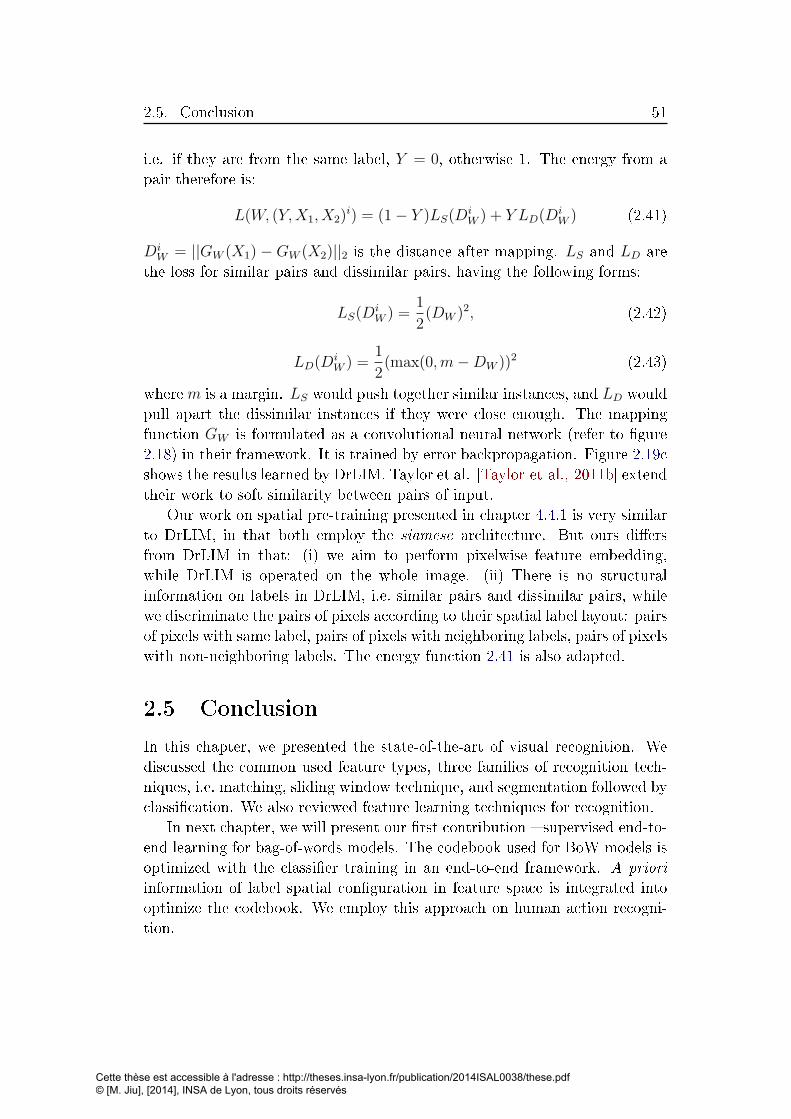
2.5. Conclusion 51
i.e. if they are from the same label, Y = 0, otherwise 1. The energy from a
pair therefore is:
L(W, (Y,X1, X2)i) = (1− Y )LS(D
iW ) + Y LD(D
iW ) (2.41)
DiW = ||GW (X1) − GW (X2)||2 is the distance after mapping. LS and LD are
the loss for similar pairs and dissimilar pairs, having the following forms:
LS(DiW ) =
1
2(DW )2, (2.42)
LD(DiW ) =
1
2(max(0,m−DW ))2 (2.43)
wherem is a margin. LS would push together similar instances, and LD would
pull apart the dissimilar instances if they were close enough. The mapping
function GW is formulated as a convolutional neural network (refer to �gure
2.18) in their framework. It is trained by error backpropagation. Figure 2.19c
shows the results learned by DrLIM. Taylor et al. [Taylor et al., 2011b] extend
their work to soft similarity between pairs of input.
Our work on spatial pre-training presented in chapter 4.4.1 is very similar
to DrLIM, in that both employ the siamese architecture. But ours di�ers
from DrLIM in that: (i) we aim to perform pixelwise feature embedding,
while DrLIM is operated on the whole image. (ii) There is no structural
information on labels in DrLIM, i.e. similar pairs and dissimilar pairs, while
we discriminate the pairs of pixels according to their spatial label layout: pairs
of pixels with same label, pairs of pixels with neighboring labels, pairs of pixels
with non-neighboring labels. The energy function 2.41 is also adapted.
2.5 Conclusion
In this chapter, we presented the state-of-the-art of visual recognition. We
discussed the common used feature types, three families of recognition tech-
niques, i.e. matching, sliding window technique, and segmentation followed by
classi�cation. We also reviewed feature learning techniques for recognition.
In next chapter, we will present our �rst contribution � supervised end-to-
end learning for bag-of-words models. The codebook used for BoW models is
optimized with the classi�er training in an end-to-end framework. A priori
information of label spatial con�guration in feature space is integrated into
optimize the codebook. We employ this approach on human action recogni-
tion.
Cette thèse est accessible à l'adresse : http://theses.insa-lyon.fr/publication/2014ISAL0038/these.pdf © [M. Jiu], [2014], INSA de Lyon, tous droits réservés

Cette thèse est accessible à l'adresse : http://theses.insa-lyon.fr/publication/2014ISAL0038/these.pdf © [M. Jiu], [2014], INSA de Lyon, tous droits réservés

Chapter 3
Supervised end-to-end learning of
bag-of-words models
Contents
3.1 Introduction . . . . . . . . . . . . . . . . . . . . . . . . 53
3.2 The neural model . . . . . . . . . . . . . . . . . . . . . 56
3.2.1 The layers of the proposed NN model . . . . . . . . . 58
3.3 Joint codebook and class label learning . . . . . . . . 60
3.3.1 MLP learning . . . . . . . . . . . . . . . . . . . . . . . 60
3.3.2 Supervised codebook learning with error backpropagation 62
3.3.3 Supervised codebook learning through cluster reassign-
ment . . . . . . . . . . . . . . . . . . . . . . . . . . . . 65
3.4 BoW models for human action recognition . . . . . . 68
3.5 Experimental Results . . . . . . . . . . . . . . . . . . . 70
3.6 Conclusion . . . . . . . . . . . . . . . . . . . . . . . . . . 77
3.1 Introduction
The bag-of-words (BoW) model has been widely used in computer vision appli-
cations such as object class [Csurka et al., 2004, Lowe, 2004] or human action
recognition [Dollar et al., 2005]. In these applications the objective is to rec-
ognize high level information (objects, actions) from a large quantity of low
level data, e.g. image or video pixels. BoW has proved to be an e�cient
representation in this context. This popular model was �rst introduced in
natural language processing, in which each document is expressed as a his-
togram of frequencies of orderless words. In order to employ the BoW model
in computer vision applications, an image or a video is treated as a document,
which can be considered as a collection of interesting local events often called
Cette thèse est accessible à l'adresse : http://theses.insa-lyon.fr/publication/2014ISAL0038/these.pdf © [M. Jiu], [2014], INSA de Lyon, tous droits réservés

54 Chapter 3. Supervised end-to-end learning of bag-of-words models
visual concepts [Csurka et al., 2004]. Information on the presence of these vi-
sual concepts, i.e. whether each one of them is present or not, and with which
frequency, serves as an indicator of the contents.
Visual concepts can be generated in di�erent ways, usually through the
extraction of discriminant and invariant descriptors (features) around local
primitives like interest points, patches, regions, edges etc., followed by clus-
tering in order to identify clusters in feature space of descriptors. The thus
obtained clusters are considered as visual concepts, or visual codewords. A
set of such visual codewords produces a visual codebook.
Traditionally, a visual codebook is learned by unsupervised clustering or
vector quantization of feature vectors extracted from the local primitives in the
image or video, often with algorithms such as k -means [Csurka et al., 2004] or
random forests [Moosmann et al., 2007]. The BoW for a new image or video
is calculated in a similar way: extraction of descriptors on local primitives,
projection of the descriptors on the codebook precalculated on a training
set, calculation of a histogram of the occurrences of each codeword of the
codebook. An image or video is classi�ed passing the BoW model to any
learning machine, for instance a support vector machine (SVM) or a neural
network (NN).
The traditional method of codebook creation through unsupervised clus-
tering ignores the class labels of the feature vectors in the training set. Of
course the labels are used for classi�cation of the BoW models, but not for
the creation of the codebook. As a consequence, the visual codebook is less
discriminative. In section 2.3.2.2 of chapter 2 we gave a short state of the art
on BoW models and their extensions. We here re�ne this state of the art and
brie�y put into the context the work relevant to this chapter.
In order to create a more discriminative codebook, several attempts have
been made to reveal the semantic relations between the codewords of k -means.
In the work of Liu and Shah [Liu and Shah, 2008], they iteratively obtain an
optimal and compact codebook via maximal mutual information. At each it-
eration they merge two clusters which have minimum loss in mutual informa-
tion. The iterative procedure continues until a threshold of maximal mutual
information or minimum cluster number is achieved. The optimal codebook
size is found by unsupervised learning. In [Liu et al., 2009], Liu uses a di�u-
sion map to embed a mid-level codebook into a semantic codebook. However,
it is not appropriate to measure semantic distances using di�usion distances.
In recent work, Sagha� [Sagha� et al., 2010] proposes a concept space to il-
lustrate the semantic relations between the visual codewords. They apply
generative models such as latent semantic analysis (LSA) and probabilistic
latent semantic analysis (pLSA) to discover the latent semantic relations be-
tween the initial codewords. In contrast to the unsupervised pLSA learning
Cette thèse est accessible à l'adresse : http://theses.insa-lyon.fr/publication/2014ISAL0038/these.pdf © [M. Jiu], [2014], INSA de Lyon, tous droits réservés

3.1. Introduction 55
framework in which the number of latent topics is equal to the number of
classes [Niebles et al., 2008], the number of topics is variable in this method.
In all methods mentioned above, the codebooks are created by unsupervised
methods, and the label information of feature vectors is ignored in the code-
book creation. Intuitively, the discriminative power of the codewords could
be increased by learning using the label information.
In contrast to unsupervised codebook learning, we propose a supervised
learning and codebook optimization framework in this chapter. The whole
sequence, codebook creation and class learning, is formulated as an arti�cial
neural network, and the error gradient information is used to update the
codebook cluster centers as well as the classical multilayer perceptron (MLP)
weights for class recognition.
Our work is very close to the recent work by Goh et al. [Goh et al., 2012].
Both adopt an end-to-end framework to learn a discriminative visual code-
book for BoW models in a supervised way. However, unlike our framework
which integrates BoW model construction and codebook learning together,
they instead learn a visual dictionary in an end-to-end framework, and then
train another classi�er (i.e SVM) for classi�cation. In their codebook learning
stage, they resort to RBMs (see 2.4.2.2) to �rst pre-train the codebook in
an unsupervised way, and to �ne-tune the codebook for each input feature
vector associated with the image category label by error backpropagation in
a supervised way. In contrast, we build a BoW model for each input entity in
our framework.
The learning and optimization framework we present in this work is
well suited for any application for which bag of words models can be
successfully used. We restrict ourselves here to human action recogni-
tion in videos, for which BoW models and extensions are widely used
[Csurka et al., 2004, Niebles et al., 2008, Gilbert et al., 2011, Laptev, 2005,
Schuldt et al., 2004]. The improvements we propose make the codebook
more discriminative, and therefore are likely to improve many of the ex-
isting extensions of the basic BoW model, such as, for instance, correlo-
grams [Liu and Shah, 2008], topic models [Niebles et al., 2008], local group-
ing and compound features [Gilbert et al., 2011], spatial co-occurrences of
pairs of features [Oikonomopoulos et al., 2009, Ryoo and Aggarwal, 2009,
Ta et al., 2010b] and parts based models [Mikolajczyk and Uemura, 2011]. To
the best of our knowledge, this is the �rst attempt to combine codebook learn-
ing with action classi�cation in a uni�ed framework.
The chapter is organized as follows. Our formulation of the BoW model
and the subsequent classi�cation phase as a unique global neural model is pre-
sented in section 3.2. Section 3.3 describes the integrated and joint learning
algorithm which updates the cluster centers as well as the MLP weights dis-
Cette thèse est accessible à l'adresse : http://theses.insa-lyon.fr/publication/2014ISAL0038/these.pdf © [M. Jiu], [2014], INSA de Lyon, tous droits réservés
56 Chapter 3. Supervised end-to-end learning of bag-of-words models
criminating between the targeted classes. Two di�erent learning algorithms
are presented, a classical backpropagation algorithm as well as cluster reassign-
ment algorithm speci�c to the BoW model. Section 3.4 brie�y reviews the lit-
erature for human action recognition. In section 3.5 we evaluate the proposed
approach on the public KTH human action dataset [Schuldt et al., 2004]. Sec-
tion 3.6 gives our conclusion.
3.2 The neural model
In our application, visual concepts are de�ned on the local primitives
(i.e. space-time interest points). A large amount of work exits on space-time
interest point detectors using di�erent criteria. We adopted Laptev's method
to obtain space-time interest points and describe them by histogram of gra-
dient (HOG) and histogram of optical �ow (HOF) features (refer to section
2.2.2).
Space-time interest points are calculated on each video and discriminant
and invariant features are calculated on a space-time cuboid around each
interest point location. Initially, a video is therefore described as a collection
of feature vectors. In traditional ways to translate this description into a BoW
model, codebook creation and learning of the BoW models of the training set
are treated as two di�erent phases addressed with two di�erent methods. Here
we present a novel formulation as a single arti�cial neural network.
In classical neural networks, each entity is classi�ed separately by the
learned NN after a stimulation phase. In our proposed model, for each video
multiple feature vectors (one per interest point) are presented sequentially
while the NN integrates this information internally. Classi�cation is done after
all feature vectors have been presented. The scheme in Figure 3.1 illustrates
this concept. The box indicated as �∑� corresponds to the module which
integrates responses over individual interest points for each video. We �rst
give an overview of its purpose before explaining each layer in detail.
The goal of our proposed model is to express several parts into a single
model, which are classically separated: (i) clustering; (ii) feature vector pro-
jection on a codebook; (iii) class prediction. For the bag-of-words model,
a codebook is traditionally constructed by k -means algorithm on the feature
space, where each cluster center is represented by a vector in the feature space
and considered as a codeword. Feature vector projection on the codebook is
completed by computing the distances between the feature vector and di�erent
codewords and selecting the one with minimal distance. Since the procedure
only involves vector inner product, it thus can be reformulated as a neural
model.
Cette thèse est accessible à l'adresse : http://theses.insa-lyon.fr/publication/2014ISAL0038/these.pdf © [M. Jiu], [2014], INSA de Lyon, tous droits réservés

3.2. The neural model 57
Figure 3.1: A scheme of the di�erent layers of the neural network. The left
part is stimulated per interest point. The right part is a classical MLP taking
decisions for each video.
The NN consists of two parts: an initial part at the left which processes
feature vectors and projects them to a codebook. The cluster centers of the
codebook are stored as �weights� of this part of the NN. While passing through
the left part of the network, the feature vector is translated into a binary
vector indicating which cluster it activates, i.e. which cluster center it is closest
to. When several feature vectors are presented, the left part of the NN is
stimulated multiple times, once for each feature vector. The right part of the
NN is a classical MLP, which takes a decision on the action class for each
BoW model.
In this formulation, the cluster centers are coded into the weights of the
network, in particular into the weights between the �rst layer a and the second
layer b : wcc (where "cc" stands for cluster centers). The connections of the
second layer are such that the units of this layer calculate distances between
the input and the di�erent cluster centers. Stimulating the network therefore
is equivalent of projecting a new input to cluster centers (calculating distances
to the di�erent centers). At the same time, changing weights wcc in the neural
model is equivalent to changing cluster center positions in feature space.
In Figure 3.1, there are three kinds of di�erent weights: wccij , w
eij and w
fij.
In the following sections of this chapter, the same subscript index notation
is used unless otherwise speci�ed, i.e. the weight wij denotes the connection
between the unit i in the current layer to the unit j in the previous layer.
Note that subscripts ij are indices which can take integer values. On the
Cette thèse est accessible à l'adresse : http://theses.insa-lyon.fr/publication/2014ISAL0038/these.pdf © [M. Jiu], [2014], INSA de Lyon, tous droits réservés

58 Chapter 3. Supervised end-to-end learning of bag-of-words models
other hand, superscripts are not indices, i.e. they can not take any values. we
merely means the symbol denoting the weights for layer e.
As a summary, the global model can be linked to classical BoW models in
the following way:
- Projecting feature vectors on a learned codebook through the nearest
neighbor criterion corresponds to stimulating our network up to layer c;
- Calculating a single bag-of-words for a video corresponds to integrating
several instances of layer c into a single instance of layer d;
- Learning a prediction model of a classi�er corresponds to updating
weights weij and w
fij for di�erent ij;
- Learning cluster centers (a.k.a. �clustering�) corresponds to updating
weights wccij for di�erent ij.
3.2.1 The layers of the proposed NN model
The input layer consists of a set a of M input nodes a = [a1, . . . aM ]T corre-
sponding to the feature values of lengthM assigned to a single local primitive,
i.e. an interest point.
The N nodes of the second layer b = [b1, . . . bN ]T correspond to the dis-
tances of the input feature vectors to each of N cluster centers. To each node
i and each distance bi is thus assigned a cluster center wcci· , i.e. a vector of
dimensionM , denoted by wcci· = [wcc
i1 , wcci2 , · · · , wcc
iM ]T , which is involved in the
distance computation:
bi = ||a−wcci· || (3.1)
The N nodes of the third layer compute an indicator of the nearest cluster
center. The nearest corresponding node will be assigned 1, the other nodes 0.
The minimum distance will result in the largest value. This is approximated
through a softmin function gb(x), similar to the classical softmax:
ci = gb(bi) =exp (−bi/T )
N∑j=1
exp (−bj/T )(3.2)
where T is a parameter controlling the stability of the softmin function.
The network layers described above propagate the stimulation of a single
feature vector corresponding to a single local primitive. As mentioned before,
in our stimulation strategy, multiple feature vectors of the same entity (a video
in our case) are presented iteratively, resulting in di�erent values for di�erent
Cette thèse est accessible à l'adresse : http://theses.insa-lyon.fr/publication/2014ISAL0038/these.pdf © [M. Jiu], [2014], INSA de Lyon, tous droits réservés
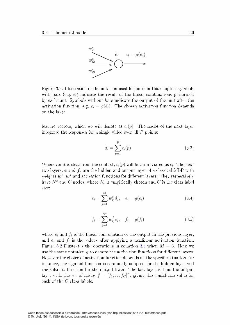
3.2. The neural model 59
Figure 3.2: Illustration of the notation used for units in this chapter: symbols
with bars (e.g. ei) indicate the result of the linear combinations performed
by each unit. Symbols without bars indicate the output of the unit after the
activation function, e.g. ei = g(ei). The chosen activation function depends
on the layer.
feature vectors, which we will denote as ci(p). The nodes of the next layer
integrate the responses for a single video over all P points:
di =P∑
p=1
ci(p) (3.3)
Whenever it is clear from the context, ci(p) will be abbreviated as ci. The next
two layers, e and f , are the hidden and output layer of a classical MLP with
weightswe, wf and activation functions for di�erent layers. They respectively
have N e and C nodes, where Ne is empirically chosen and C is the class label
size:
ei =M∑j=1
weijdj, ei = g(ei) (3.4)
fi =Ne∑j=1
wfijej, fi = g(fi) (3.5)
where ei and fi is the linear combination of the output in the previous layer,
and ei and fi is the values after applying a nonlinear activation function.
Figure 3.2 illustrates the operations in equation 3.4 when M = 3. Here we
use the same notation g to denote the activation functions for di�erent layers.
However the choice of activation function depends on the speci�c situation, for
instance, the sigmoid function is commonly adopted for the hidden layer and
the softmax function for the output layer. The last layer is thus the output
layer with the set of nodes f = [f1, . . . fC ]T , giving the con�dence value for
each of the C class labels.
Cette thèse est accessible à l'adresse : http://theses.insa-lyon.fr/publication/2014ISAL0038/these.pdf © [M. Jiu], [2014], INSA de Lyon, tous droits réservés

60 Chapter 3. Supervised end-to-end learning of bag-of-words models
Algorithm 1: The iterative codebook learning framework
Input: Ftr (training features), Fval (validation features)
Output: wcc (optimal codebook)
wcc ← k-means ;1
repeat2
Btr ← Bags-of-words computation (wcc, Ftr);3
Bval ← Bags-of-words computation (wcc, Fval);4
we,f ← random ;5
we,f ← MLP learning (we,f ,wcc,Btr, Ltr) ;6
wcc ← Cluster center learning (we,f , Ftr, Ltr) { section 3.3.2 or7
3.3.3 } ;
E ← Validation error (we,f ,wcc,Bval, Lval) ;8
until convergence(E) ;9
3.3 Joint codebook and class label learning
Assuming a set of video �les with interest points and their corresponding fea-
ture vectors, as well as a groundtruth action label per video, backpropagation
propagates the error between the stimulated response and the groundtruth
back to the input layers, adjusting weights during the process. Here the
groundtruth of course indicates the action class of a video, and not a cluster
center. In our case, this means adjusting two di�erent types of parameters,
namely the weights of the MLP as well as the cluster centers wcc. The weights
of the MLP are updated with a classical error backpropagation scheme, which
is recalled in section 3.3.1. The cluster centers can be updated by two algo-
rithms, which are respectively addressed in section 3.3.2 and 3.3.3. These two
di�erent types of weights are sequentially and iteratively learned. At any time
the proposed system only learns one type of weights. The former is used to
learn an optimal MLP model and the latter makes use of the backward errors
of the optimal MLP. The pseudo code of the proposed framework is shown in
Algorithm 1.
3.3.1 MLP learning
In the proposed framework, we adopt a MLP network (i.e. layers d, e and f)
with one output unit for each class. No activation functions are used in the
layer d of the MLP. Sigmoid and softmax activation functions are respectively
employed in the hidden layer e and output layer f . An 1-of-c coding scheme
is used to describe the target outputs, which is coded as a binary indicator
Cette thèse est accessible à l'adresse : http://theses.insa-lyon.fr/publication/2014ISAL0038/these.pdf © [M. Jiu], [2014], INSA de Lyon, tous droits réservés

3.3. Joint codebook and class label learning 61
vector of dimension (the number of action classes). The weights we and wf
are adjusted by the classical backpropagation algorithm:
The di�erent input vectors a forward propagate through the network, until
all the input vectors over the whole video are summed in the integration
layer, producing a bag-of-words representation d of the video, and then the
activations of all hidden and output layer units are computed. Given the
desired output (the target) tj from the groundtruth and the response fj for
each unit, the goal is to minimize a loss. Here the classical cross-entropy loss
has been chosen [Bishop, 1994]:
E = −C∑
j=1
tj ln fj (3.6)
We remind the reader, that the target value tj is related to the label of the
video activity class. For instance, if a video is known to be of class 3, then,
according to the classical 1-of-c coding scheme, the ground truth vector t is
set as
t = [0, 0, 1, 0, 0, . . . , 0]T (3.7)
where the size of t is equal to C, the number of activity classes.
The goal is to calculate the derivatives of loss with respect to all di�erent
weights of the model (weij, w
fij and w
ccij ). For this reason, we start by calculating
the derivatives of the loss w.r.t. di�erent intermediate values, starting with
the network outputs fj, which can be given as follows:
∂E
∂fj=−tjfj
(3.8)
Let us recall from the beginning of this subsection that we use a softmax
activation function in the last layer. Therefore, the network output fj is given
as follows from the linear input fj (we recall the notation fj and fj which are
illustrated in Figure 3.2):
fj =exp(fj)∑Ck=1 exp(fk)
(3.9)
The derivative of the loss E w.r.t fj requires the derivative of the softmax func-
tion, which is hard to calculate, and whose derivation is beyond the scope of
this paper. Fortunately it is well known, we refer the reader to [Bishop, 1994].
We can give the derivative of E w.r.t. the linear network outputs fj as follows
(a known result):∂E
∂fj= (fj − tj) (3.10)
Cette thèse est accessible à l'adresse : http://theses.insa-lyon.fr/publication/2014ISAL0038/these.pdf © [M. Jiu], [2014], INSA de Lyon, tous droits réservés

62 Chapter 3. Supervised end-to-end learning of bag-of-words models
In the following, we will abbreviate the derivative of the loss as follows:
δfj =∂E
∂fj∀j = {1, · · · , C} (3.11)
We can now backpropagate the errors in the output layer f into the hidden
layer e, which sequentially pass through linear combinations and activation
function of layer e. The error δej for each unit j in the hidden layer e is
calculated according to the chain rule for partial derivatives:
δej = g′(ej)C∑i=1
wfijδ
fi , ∀j = {1, · · · , N e} (3.12)
where the sum runs over all the C units in the output layer f connecting to
the unit j in the hidden layer e. g′(ej) is the derivative value of activation
function at ej employed in the hidden layer (i.e. sigmoid function), which is
computed as follows:
g′(ej) = g(ej)(1− g(ej)). (3.13)
We next backpropagate the errors in the hidden layer e to the input layer
d of the MLP. The error δdj for each unit j in the layer d is calculated by:
δdj =Ne∑i=1
weijδ
ei , ∀j = {1, · · · ,M} (3.14)
where the chain rule is once again employed. The derivative of the activation
function is not involved, because no activation function is adopted in the layer
d.
Lastly we compute the increments for all the weights of the MLP (i.e. we
and wf ). It can be obtained by multiplying the error at the output end of the
weight (i.e. the unit indicated by the �rst index of the weight) by the value at
the input end of the weight (i.e. the unit indicated by the second index of the
weight). For instance, for the weight wfij connecting the unit i in the layer f
to the unit j in the layer e, the error of its output end is δfi , and the value of
its input end is ej. The increments are calculated by:
∆wfij = ηδfi ej ∆we
ij = ηδei dj, (3.15)
where η is a learning parameter.
3.3.2 Supervised codebook learning with error back-
propagation
The classical error backpropagation algorithm can be adapted to our novel
formulation. In particular, the errors in layer d are continued backpropagating
Cette thèse est accessible à l'adresse : http://theses.insa-lyon.fr/publication/2014ISAL0038/these.pdf © [M. Jiu], [2014], INSA de Lyon, tous droits réservés

3.3. Joint codebook and class label learning 63
into layer c and then into layer b, which can directly act on the cluster centers
wccij . The goal of the derivations in this section is to relate the loss coming
from the right side of the network to the weights wccij . The particularity of our
model allows a geometric interpretation of this update, which corresponds to a
movement of a cluster center, i.e. an M -dimensional vector in M dimensional
feature space.
We therefore �rst recall the goal of the following derivations, namely to
calculate the derivative of the loss E with respect to the parameter wccij :
∂E
∂wccij
(3.16)
A particularity of our model is the integrator between the per-feature-vector
part and the per-video part. As mentioned before, the network output is
calculated over multiple stimulations of the left side of the network, one for
each feature vector. The loss E has been calculated on the right side of the
network for each video. We will denote by p the index of the feature vectors
and for clarity we temporarily add the dependency on the feature vector to
the notation. The feature vector indexed by p is denoted as a(p) with values
a(p) = [a1(p), a2(p), . . . aM(p)]; the value of unit i of layer b obtained when
the network was stimulated with feature vector a(p) is therefore bi(p) etc.
The error δci (p) =∂Eci(p)
of layer c (nearest distance indicator for each feature
point) is supposed to be backpropagated from the succeeding layer d (bag of
words, i.e. the histogram). The hickup here is the unconventionnal structure
of our model, in particular the integrator between the right per-video part and
the left per-feature-vector part. We circumvented this problem by taking the
error on the right layer d and equally distributing it over the corresponding
feature points p:
δci (p) =δdidi∀p = {1, . . . , P} (3.17)
The special case of di = 0 for unit i is a singularity. However it has a mean-
ingful explanation from a model perspective, i.e. di = 0 means that there is
no feature vector belonging to this cluster center for the input, and the unit
i in the layer d can thus be ignored in the classi�cation. We therefore do not
update the weights in this case.
Let us recall that the goal is to update the weights wcc, which correspond
to the encoded cluster centers. We therefore need to backpropagate the error
further to the previous layer b. Let us recall the de�nition of layer b by
reproducing equation (3.1):
bi = ||a−wcci· ||2 =
M∑j=1
(aj − wccij )
2. (3.18)
Cette thèse est accessible à l'adresse : http://theses.insa-lyon.fr/publication/2014ISAL0038/these.pdf © [M. Jiu], [2014], INSA de Lyon, tous droits réservés

64 Chapter 3. Supervised end-to-end learning of bag-of-words models
The equation above can be interpreted as a common neural network layer
with an uncommon activation function. Indeed, in traditional MLPs, the
activation function consists of a non-linearity acting on the linear sum of
the input variables, and the coe�cients are the parameters of the model. In
our case, the activation function acts on a sum of a two-order polynomial of
input variables. Since bi is di�erentiable with respect to wccij , and the softmin
component is also di�erentiable, we thus can resort to gradient descent to
adjust the cluster centers. Calculating the gradient requires the following
derivates :∂E
∂wccij
=P∑
p=1
∂E(p)
∂wccij
=P∑
p=1
∂E(p)
∂bi(p)
∂bi(p)
∂wccij
(3.19)
In the following, only the values for a single feature vector p will be considered.
For clarity we therefore remove (again) the index p from the notation; in
particular E(p) will be noted as E.
According to the chain rule, the derivative of E with respect to bi can be
decomposed of two parts: the derivative of E with respect to the units in the
layer c, and the derivative of the softmin function between layer b and layer
c. We should consider the input node i in the layer b to all the output units
in the layer c. So we have
∂E
∂bi=
N∑k=1
∂E
∂ck
∂ck∂bi
. (3.20)
Let us recall the softmin function in layer c:
ck =exp (−bk/T )N∑i=1
exp (−bi/T )(3.21)
The derivative involves a rather long series of algebra, which we will not
reproduce here. It can be given as:
∂ck∂bi
= − 1
T(ck∆ik − ckci) (3.22)
where ∆ik is the Kronecker delta function with ∆ik = 1 if i = k and 0 else. It
can be seen that the computations of the partial derivatives of ck with respect
to bi are not complex, which only need the current values of layer c.
Substituting equations (3.17) and (3.22) into equation (3.20), we obtain
∂E
∂bi= −
N∑k=1
δckT(ck∆ik − ckci). (3.23)
Cette thèse est accessible à l'adresse : http://theses.insa-lyon.fr/publication/2014ISAL0038/these.pdf © [M. Jiu], [2014], INSA de Lyon, tous droits réservés
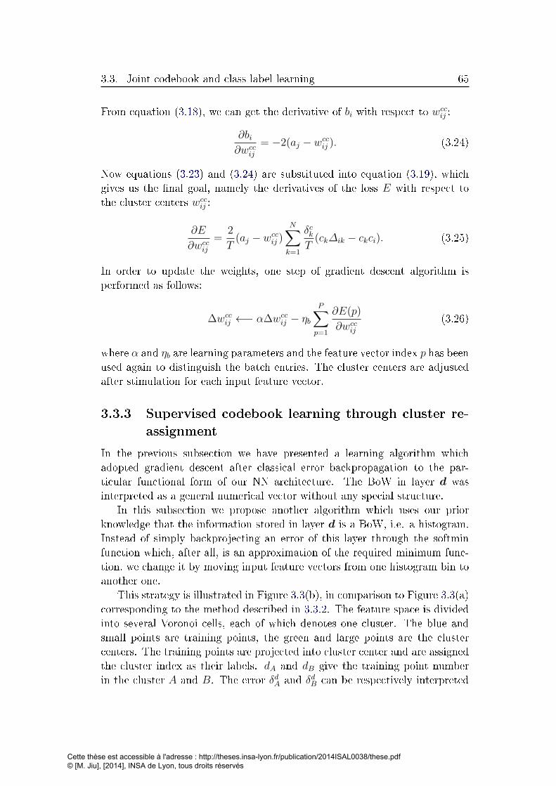
3.3. Joint codebook and class label learning 65
From equation (3.18), we can get the derivative of bi with respect to wccij :
∂bi∂wcc
ij
= −2(aj − wccij ). (3.24)
Now equations (3.23) and (3.24) are substituted into equation (3.19), which
gives us the �nal goal, namely the derivatives of the loss E with respect to
the cluster centers wccij :
∂E
∂wccij
=2
T(aj − wcc
ij )N∑k=1
δckT(ck∆ik − ckci). (3.25)
In order to update the weights, one step of gradient descent algorithm is
performed as follows:
∆wccij ←− α∆wcc
ij − ηbP∑
p=1
∂E(p)
∂wccij
(3.26)
where α and ηb are learning parameters and the feature vector index p has been
used again to distinguish the batch entries. The cluster centers are adjusted
after stimulation for each input feature vector.
3.3.3 Supervised codebook learning through cluster re-
assignment
In the previous subsection we have presented a learning algorithm which
adopted gradient descent after classical error backpropagation to the par-
ticular functional form of our NN architecture. The BoW in layer d was
interpreted as a general numerical vector without any special structure.
In this subsection we propose another algorithm which uses our prior
knowledge that the information stored in layer d is a BoW, i.e. a histogram.
Instead of simply backprojecting an error of this layer through the softmin
function which, after all, is an approximation of the required minimum func-
tion, we change it by moving input feature vectors from one histogram bin to
another one.
This strategy is illustrated in Figure 3.3(b), in comparison to Figure 3.3(a)
corresponding to the method described in 3.3.2. The feature space is divided
into several Voronoi cells, each of which denotes one cluster. The blue and
small points are training points, the green and large points are the cluster
centers. The training points are projected into cluster center and are assigned
the cluster index as their labels. dA and dB give the training point number
in the cluster A and B. The error δdA and δdB can be respectively interpreted
Cette thèse est accessible à l'adresse : http://theses.insa-lyon.fr/publication/2014ISAL0038/these.pdf © [M. Jiu], [2014], INSA de Lyon, tous droits réservés

66 Chapter 3. Supervised end-to-end learning of bag-of-words models
(a)
B
A P
(b)
Figure 3.3: Two di�erent ways to learn the cluster centers illustrated through a
Voronoi diagram of the feature space, for simplicity in 2D. Cluster centers are
green and large, training points are blue and small. Recall that Voronoi cells
do not correspond to decision areas of prediction model for actions. A video
is represented by a bag of multiple points, i.e. a histogram of cluster indica-
tors/Voronoi cells. (a) The method described in section 3.3.2 directly updates
the cluster centers wccij by gradient descent on the loss of the video. The error is
equally distributed over the clusters/Voronoi cells; (b) The method described
in section 3.3.3 indirectly updates the cluster centers by passes individual fea-
ture vectors from one Voronoi to another one according to the error in the
BoW layer.
Cette thèse est accessible à l'adresse : http://theses.insa-lyon.fr/publication/2014ISAL0038/these.pdf © [M. Jiu], [2014], INSA de Lyon, tous droits réservés
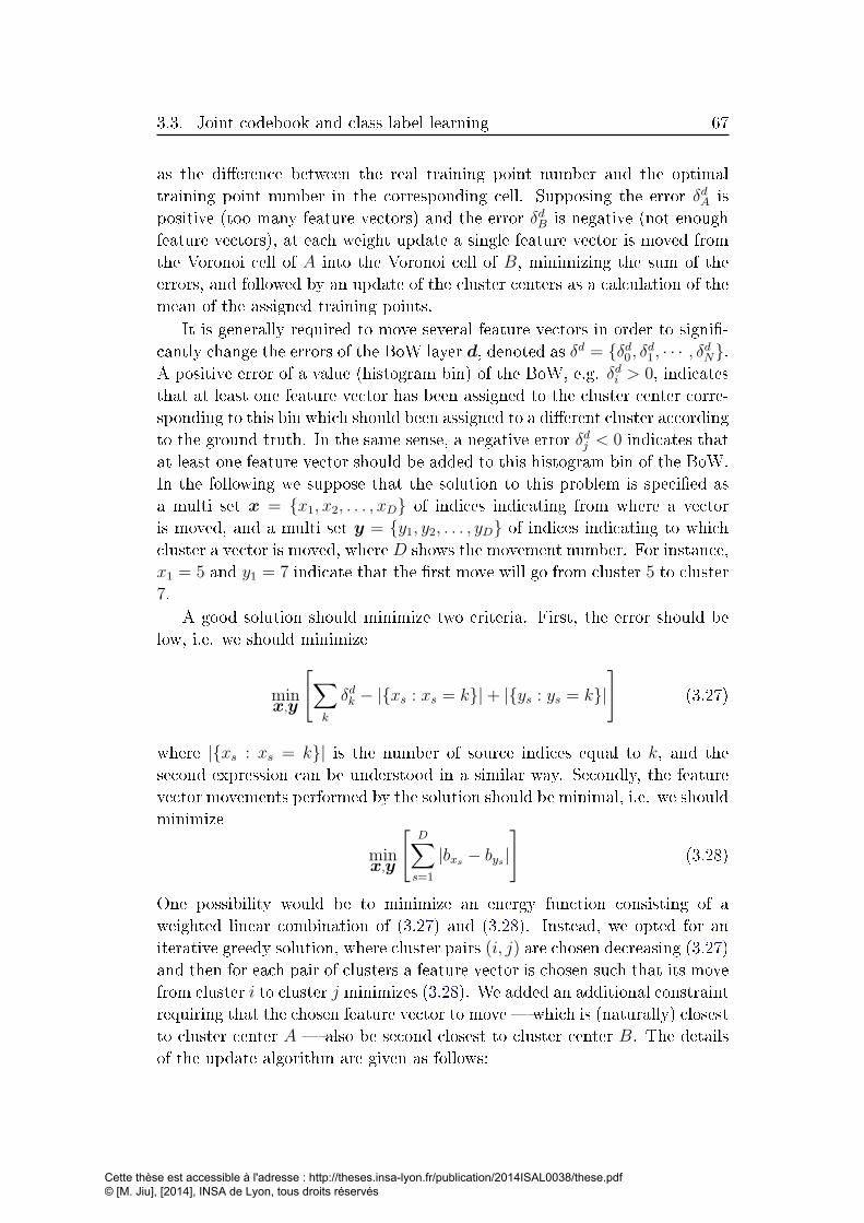
3.3. Joint codebook and class label learning 67
as the di�erence between the real training point number and the optimal
training point number in the corresponding cell. Supposing the error δdA is
positive (too many feature vectors) and the error δdB is negative (not enough
feature vectors), at each weight update a single feature vector is moved from
the Voronoi cell of A into the Voronoi cell of B, minimizing the sum of the
errors, and followed by an update of the cluster centers as a calculation of the
mean of the assigned training points.
It is generally required to move several feature vectors in order to signi�-
cantly change the errors of the BoW layer d, denoted as δd = {δd0 , δd1 , · · · , δdN}.A positive error of a value (histogram bin) of the BoW, e.g. δdi > 0, indicates
that at least one feature vector has been assigned to the cluster center corre-
sponding to this bin which should been assigned to a di�erent cluster according
to the ground truth. In the same sense, a negative error δdj < 0 indicates that
at least one feature vector should be added to this histogram bin of the BoW.
In the following we suppose that the solution to this problem is speci�ed as
a multi set x = {x1, x2, . . . , xD} of indices indicating from where a vector
is moved, and a multi set y = {y1, y2, . . . , yD} of indices indicating to which
cluster a vector is moved, where D shows the movement number. For instance,
x1 = 5 and y1 = 7 indicate that the �rst move will go from cluster 5 to cluster
7.
A good solution should minimize two criteria. First, the error should be
low, i.e. we should minimize
minx,y
[∑k
δdk − |{xs : xs = k}|+ |{ys : ys = k}|
](3.27)
where |{xs : xs = k}| is the number of source indices equal to k, and the
second expression can be understood in a similar way. Secondly, the feature
vector movements performed by the solution should be minimal, i.e. we should
minimize
minx,y
[D∑s=1
|bxs − bys|
](3.28)
One possibility would be to minimize an energy function consisting of a
weighted linear combination of (3.27) and (3.28). Instead, we opted for an
iterative greedy solution, where cluster pairs (i, j) are chosen decreasing (3.27)
and then for each pair of clusters a feature vector is chosen such that its move
from cluster i to cluster j minimizes (3.28). We added an additional constraint
requiring that the chosen feature vector to move � which is (naturally) closest
to cluster center A � also be second closest to cluster center B. The details
of the update algorithm are given as follows:
Cette thèse est accessible à l'adresse : http://theses.insa-lyon.fr/publication/2014ISAL0038/these.pdf © [M. Jiu], [2014], INSA de Lyon, tous droits réservés

68 Chapter 3. Supervised end-to-end learning of bag-of-words models
1. Randomly choose a pair (i, j) of histogram bins (thus of cluster centers),
where the error of one bin is positive and the other is negative, i.e.
δdi > 0 ∧ δdj < 0.
2. Calculate the Voronoi diagram of the cluster centers in feature space
and determine all the feature vectors of the training set falling into the
sets of wcci and wcc
j , respectively.
3. Pick a single feature vector f such that:
• it falls into the Voronoi cell i (distance between f and cluster center
wcci ) is minimum, i.e. nearest).
• its distance to cluster center wccj is second nearest.
• if several vectors satisfy the above two criteria, choose the one
minimizing the distance to the border of the two Voronoi cells, i.e.
the one minimizing |bi − bj|.
4. The chosen feature vector f is reassigned from histogram bin i to his-
togram bin j with the following consequences:
• the two centers wcci and wcc
j are recalculated as the means of the
feature vectors of their respective Voronoi cells.
• the errors of the BoW layer of the corresponding bins are updated:
δd [t+1]i = δ
d [t]i − 1
δd [t+1]j = δ
d [t]j + 1
(3.29)
5. The reassignments are continued (back to step 1) until the error of layer
d is zero or none of the feature vectors satisfy the above conditions.
3.4 BoW models for human action recognition
Along with the wide use of portable imaging devices, a great mass of videos
have been created everyday, thus analyzing so many videos manually frame-
by-frame seems impossible. In order to alleviate human labors, video analysis
automatically by the machine is necessary. Recognizing human actions from
videos is one of such directions, which has become an active research topic in
computer vision community over the past three decades due to a big amount
of potential promising applications, for instance, video surveillance, content-
based video retrieval, human-computer interaction and so on.
Cette thèse est accessible à l'adresse : http://theses.insa-lyon.fr/publication/2014ISAL0038/these.pdf © [M. Jiu], [2014], INSA de Lyon, tous droits réservés

3.4. BoW models for human action recognition 69
An action is typically considered as a simple motion pattern performed
by a single person, usually having a short duration of time, such as walk-
ing, bending, jumping etc. An activity is a more complex motion pattern,
composing of a number of sequential actions performed by several persons.
It is often associated with interactions between several persons or between
humans and objects, of course having a relative longer duration. Examples
of activities include two lovers kissing, a team playing football etc. Activity
recognition to some extent is more challenging than action recognition. Some
researchers also stated the hierarchy relationship between the terms �Action�
and �Activity�. However these two terms are frequently used interchangeably
in most literature. Unless otherwise speci�ed, we ignore their di�erence and
consider the two terms as the same thing in the following.
Action recognition is a challenging problem. Actions in videos present
larger variations than objects in images because of several reasons: (i) videos
also vary in the time dimension; (ii) relevant motion information is mixed with
irrelevant appearance information in the signal; (iii) activities are inherently
and highly articulated.
Due to its huge promising applications in various domains, the amount
of literature on action recognition sky-rocketed in the last years and it
is not possible anymore to give an exhaustive account in this thesis.
We refer the interested reader to some very recently published surveys
[Aggarwal and Ryoo, 2011, Turaga et al., 2008, Weinland et al., 2011].
While early work on modeling human activities focused on articu-
lated motion (e.g. [Goncalves and Perona, 2003]), most recent work
on activity and event recognition does not explicitly model the hu-
man body. Instead, the current state of the art focuses on sparse
local features like interest points and space-time interest points
[Csurka et al., 2004, Lowe, 2004], or on motion segmentation through
background subtraction [Wang and Geng, 2008, Weinland et al., 2007],
dense optical �ow [Sukthankar and Hebert, 2005] or other holistic features
[Mikolajczyk and Uemura, 2008, Zhang et al., 2008], with possible hy-
brid methods [Bregonzio et al., 2009, Liu et al., 2008, Sun et al., 2009]
and classi�cation through dense matching [Seo and Milanfar, 2010,
Shechtman and Irani, 2005]. Fully taking into account spatial relation-
ships through graph matching has recently been proposed [Ta et al., 2010a],
but this requires matching against several graph models per action class.
Pure statistical and unstructured machine learning without feature extrac-
tion is di�cult in this context due to several reasons: (i) the non-rigid nature
of the relevant information and (ii) the mixture of relevant motion information
and irrelevant texture information in the signal (iii) the high dimension of the
feature space in which the data is embedded. For these reasons, machine learn-
Cette thèse est accessible à l'adresse : http://theses.insa-lyon.fr/publication/2014ISAL0038/these.pdf © [M. Jiu], [2014], INSA de Lyon, tous droits réservés
70 Chapter 3. Supervised end-to-end learning of bag-of-words models
ing of human actions has been dominated by methods learning the temporal
evolution of features like HMMs, Semi-Markov models and dynamic belief net-
works [Abdelkader et al., 2010, Boiman and Irani, 2007, Cuntoor et al., 2008,
Shi et al., 2010, Xiang and Gong, 2008a, Xiang and Gong, 2008b,
Zhang and Gatica-Perez, 2005, Zhou and Kimber, 2006]. Typically,
a vectorial description is created frame per frame and its temporal
evolution is modeled and learned, such as Transferable Belief model
[Ramasso et al., 2007, Ramasso et al., 2009]. Other learning-based
methods include biologically-inspired ones [Jhuang et al., 2007], convo-
lutional deep learning [Taylor et al., 2010, Baccouche et al., 2011], methods
based on topic models [Niebles et al., 2008], boosting low-level features
[Fathi and Mori, 2008], trajectory matching [Dyana and Das, 2009], statistics
calculated on the results of tracking [Stau�er and Grimson, 2000], learning
of spatio-temporal predicates and grammars [Ryoo and Aggarwal, 2009,
Ryoo and Aggarwal, 2011, Wang et al., 2010] and other probabilistic graph-
ical models [Niebles and Fei-Fei, 2007]. Among them, the bag-of-words
(BoW) model is one of the most popular models due to its simplicity. The
next section will present experiments applying the proposed model to human
action recognition.
3.5 Experimental Results
The proposed model and learning algorithms have been evaluated on the
publicly available KTH action dataset [Schuldt et al., 2004]. It is one of the
largest available published datasets and contains 6 actions � boxing, hand clap-
ping, hand waving, jogging, running and walking, performed by 25 subjects in
four di�erent scenarios � indoors, outdoors, outdoors with scale variation and
clothes changing. It contains 2391 video sequences and each sequence lasts
four seconds in average. Representative frames of the dataset are shown in
Figure 3.4. For video representation, space-time interest points were detected
by the 3D Harris-corner detector proposed by Laptev [Laptev et al., 2008]. A
space-time cuboid was extracted around each interest point and described by
features of type histogram of gradient (HOG) and histogram of oriented �ow
(HOF) descriptors, which were obtained from the software supplied by Laptev
[Laptev et al., 2008].
As usual, a cross-validation scheme and early stopping strategy are em-
ployed to control the learning phase. The dataset is divided into three inde-
pendent sets: training (12 people), validation (4 people) and test (9 people),
as in [Schuldt et al., 2004]. The MLP is trained on the training set and eval-
uated on the validation set for stopping to avoid over-�tting. Unless said
Cette thèse est accessible à l'adresse : http://theses.insa-lyon.fr/publication/2014ISAL0038/these.pdf © [M. Jiu], [2014], INSA de Lyon, tous droits réservés

3.5. Experimental Results 71
Figure 3.4: The KTH dataset [Schuldt et al., 2004].
otherwise, all errors are reported on the 863 test instances.
Di�erent MLP architectures and learning hyper-parameters were tested,
and the best ones were chosen from the performances on the test set. Val-
ues are given below. Executions times are given for a C++ implementation
running on an Intel Core i7 640 PC under Linux.
Classical unsupervised codebook learning � To demonstrate the
discriminative power of classical codebook and compare with our methods, we
created a baseline with classical unsupervised k -means clustering and MLP
learning of the BoW descriptors. With respect to Figure 3.1, this corresponds
to a scheme where the weights wcc are set without taking into account cluster
labels of the groundtruth, and with supervised MLP learning of the action
class decisions.
In our baseline experiments, the cluster centers were learned by k -means
and then the MLP part was trained given the BoW models. To cope for ran-
dom initialization of the MLP weights, we repeated our baseline experiments
in order to obtain statistically sound results: �rst a codebook is created using
k -means clustering. Then, for each run, the cluster centers were kept �xed
and the MLP weights were randomly initialized between −0.5 and 0.5 and
learned. We ran 100 runs for each codebook in our experiments. Di�erent
MLP architectures were explored with numbers of hidden units of 25, 75, 100
for 50, 150, 300 codewords. Figure 3.5 shows an example using 150 codewords,
where learning stops at the 54th iteration.
Table 3.1 shows error rates (on the test set) of the learned MLP with
di�erent codebooks. A local running mean �lter was applied to the results.
From the table, we can see that the MLP learning is robust. On the other
hand, a larger codebook is more discriminative, resulting in lower error.
Supervised codebook learning with error backpropagation � Re-
Cette thèse est accessible à l'adresse : http://theses.insa-lyon.fr/publication/2014ISAL0038/these.pdf © [M. Jiu], [2014], INSA de Lyon, tous droits réservés
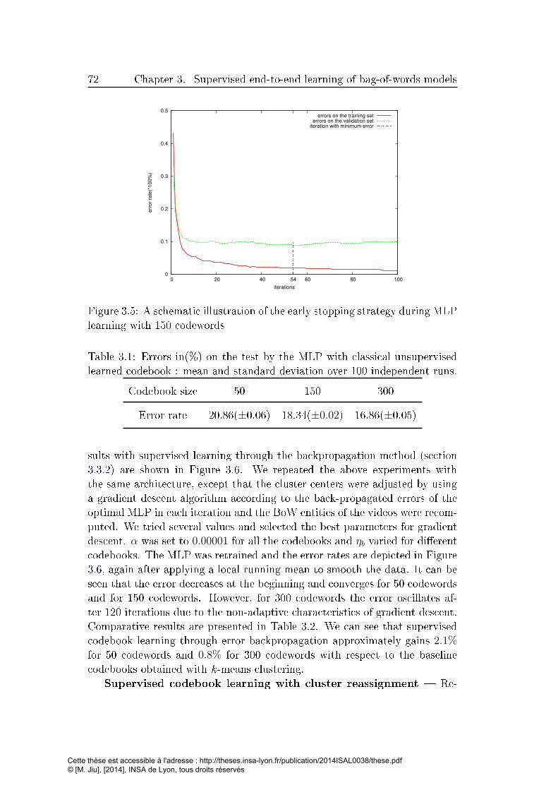
72 Chapter 3. Supervised end-to-end learning of bag-of-words models
0
0.1
0.2
0.3
0.4
0.5
54 0 20 40 60 80 100
err
or
rate
(*1
00
%)
iterations
errors on the training seterrors on the validation set
iteration with minimum error
Figure 3.5: A schematic illustration of the early stopping strategy during MLP
learning with 150 codewords
Table 3.1: Errors in(%) on the test by the MLP with classical unsupervised
learned codebook : mean and standard deviation over 100 independent runs.
Codebook size 50 150 300
Error rate 20.86(±0.06) 18.34(±0.02) 16.86(±0.05)
sults with supervised learning through the backpropagation method (section
3.3.2) are shown in Figure 3.6. We repeated the above experiments with
the same architecture, except that the cluster centers were adjusted by using
a gradient descent algorithm according to the back-propagated errors of the
optimal MLP in each iteration and the BoW entities of the videos were recom-
puted. We tried several values and selected the best parameters for gradient
descent. α was set to 0.00001 for all the codebooks and ηb varied for di�erent
codebooks. The MLP was retrained and the error rates are depicted in Figure
3.6, again after applying a local running mean to smooth the data. It can be
seen that the error decreases at the beginning and converges for 50 codewords
and for 150 codewords. However, for 300 codewords the error oscillates af-
ter 120 iterations due to the non-adaptive characteristics of gradient descent.
Comparative results are presented in Table 3.2. We can see that supervised
codebook learning through error backpropagation approximately gains 2.1%
for 50 codewords and 0.8% for 300 codewords with respect to the baseline
codebooks obtained with k -means clustering.
Supervised codebook learning with cluster reassignment � Re-
Cette thèse est accessible à l'adresse : http://theses.insa-lyon.fr/publication/2014ISAL0038/these.pdf © [M. Jiu], [2014], INSA de Lyon, tous droits réservés

3.5. Experimental Results 73
0.15
0.16
0.17
0.18
0.19
0.2
0.21
0.22
0 20 40 60 80 100 120 140 160 180 200
err
or
rate
(*1
00
%)
iterations
50 codewords150 codewords300 codewords
Figure 3.6: Supervised learning with error backpropagation (section 3.3.2):
errors on the test set over di�erent iterations.
sults with supervised learning through the cluster reassignment method (sec-
tion 3.3.3) are shown in Figure 3.7. We again repeated the above experiments
with the same neural architecture. At each iteration, the cluster centers were
adjusted using the Voronoi cell updates. and then the MLP is retrained.
Figure 3.7 shows the results, which are obtained by applying a local running
mean. As we can see the classi�cation accuracy on the test set increases as the
cluster centers are adjusted. The improvement is higher with smaller code-
book, which is also observed from Figure 3.6. The learned codebooks through
cluster reassignment therefore improve by 1.7% for 50 codewords and 0.8% for
300 codewords with respect to the baseline codebooks obtained with k -means
clustering.
From Table 3.2, we can see that both methods clearly improve the dis-
criminative quality of the codebook when the codebook size is small. This
is an important advantage since larger codebooks signi�cantly increase the
computational complexity of the classi�cation algorithm due to the nearest
neighbor search necessary when the feature vectors are projected on the code-
book. Indexed data-structures like KD-trees are not always helpful in these
situations since visual data is generally embedded in feature spaces of very
high dimensions � 162 dimensions for the HoG/HoF features we employed in
our experiments.
The performance improvement can be explained by the nature of the fea-
tures it creates. The k -means algorithm clusters features based on the ap-
pearance of the cuboids only. When the codebook is small, the intra-cluster
variance is large, which lowers discriminative power. Our methods regroup the
Cette thèse est accessible à l'adresse : http://theses.insa-lyon.fr/publication/2014ISAL0038/these.pdf © [M. Jiu], [2014], INSA de Lyon, tous droits réservés

74 Chapter 3. Supervised end-to-end learning of bag-of-words models
0.15
0.16
0.17
0.18
0.19
0.2
0.21
0.22
0 20 40 60 80 100 120 140 160 180 200
err
or
rate
(*1
00
%)
iterations
50 codewords150 codewords300 codewords
Figure 3.7: Supervised learning with cluster reassignment (section 3.3.3): er-
rors on the test set over di�erent iterations.
feature vectors into di�erent clusters based on class labels of the groundtruth,
thus choosing optimal codewords.
Retraining with SVM classi�ers � The experiments above show that
the combined codebook and MLP learning outperforms the classical sequential
steps k -means clustering followed by MLP learning. However, the question
arises whether the improvement is due to a better codebook or to the integra-
tion of the two methods. We therefore performed an additional experiment
with a two-step learning process:
1. Codebook learning according to one of the three methods (k -means;
supervised codebook learning with error backpropagation; supervised
codebook learning with cluster reassignment).
2. Class label retraining with Support Vector Machines (SVM) on the
learned codebook.
We trained an SVM with a radial basis function kernel on the training set
and validation set, which were the same with the ones used in the above
experiments [Chang and Lin, 2011]. The errors are shown in the lower block
of Table 3.2. Classi�cation time includes the projection of feature vectors on
the codebook and the classi�cation with MLP and SVM classi�ers. The SVM
outperforms the MLP by up to 2% with di�erent codebooks. However, the
recognition of the MLP is faster due to its simple calculations which do not
need inner-products of high dimensional vectors. As shown in Table 3.3, the
MLP gains more bene�ts from computational complexity with respect to the
Cette thèse est accessible à l'adresse : http://theses.insa-lyon.fr/publication/2014ISAL0038/these.pdf © [M. Jiu], [2014], INSA de Lyon, tous droits réservés
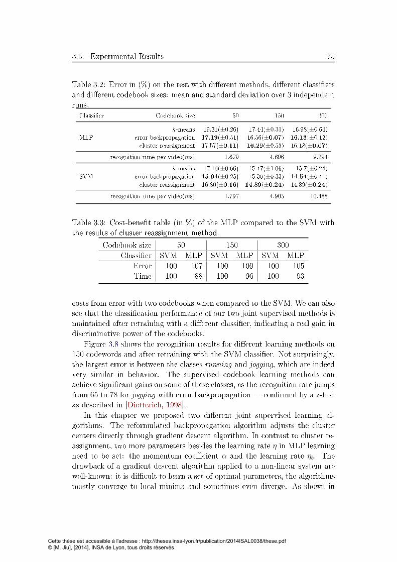
3.5. Experimental Results 75
Table 3.2: Error in (%) on the test with di�erent methods, di�erent classi�ers
and di�erent codebook sizes: mean and standard deviation over 3 independent
runs.
Classi�er Codebook size 50 150 300
k -means 19.31(±0.26) 17.44(±0.31) 16.98(±0.64)MLP error backpropagation 17.19(±0.51) 16.56(±0.07) 16.13(±0.12)
cluster reassignment 17.57(±0.11) 16.29(±0.53) 16.18(±0.07)
recognition time per video(ms) 1.679 4.696 9.294
k -means 17.16(±0.66) 15.47(±1.06) 15.7(±0.24)SVM error backpropagation 15.94(±0.25) 15.30(±0.33) 14.54(±0.41)
cluster reassignment 16.80(±0.16) 14.89(±0.24) 14.89(±0.24)
recognition time per video(ms) 1.797 4.905 10.488
Table 3.3: Cost-bene�t table (in %) of the MLP compared to the SVM with
the results of cluster reassignment method.
Codebook size 50 150 300
Classi�er SVM MLP SVM MLP SVM MLP
Error 100 107 100 109 100 105
Time 100 88 100 96 100 93
costs from error with two codebooks when compared to the SVM. We can also
see that the classi�cation performance of our two joint supervised methods is
maintained after retraining with a di�erent classi�er, indicating a real gain in
discriminative power of the codebooks.
Figure 3.8 shows the recognition results for di�erent learning methods on
150 codewords and after retraining with the SVM classi�er. Not surprisingly,
the largest error is between the classes running and jogging, which are indeed
very similar in behavior. The supervised codebook learning methods can
achieve signi�cant gains on some of these classes, as the recognition rate jumps
from 65 to 78 for jogging with error backpropagation � con�rmed by a z-test
as described in [Dietterich, 1998].
In this chapter we proposed two di�erent joint supervised learning al-
gorithms. The reformulated backpropagation algorithm adjusts the cluster
centers directly through gradient descent algorithm. In contrast to cluster re-
assignment, two more parameters besides the learning rate η in MLP learning
need to be set: the momentum coe�cient α and the learning rate ηb. The
drawback of a gradient descent algorithm applied to a non-linear system are
well-known: it is di�cult to learn a set of optimal parameters, the algorithms
mostly converge to local minima and sometimes even diverge. As shown in
Cette thèse est accessible à l'adresse : http://theses.insa-lyon.fr/publication/2014ISAL0038/these.pdf © [M. Jiu], [2014], INSA de Lyon, tous droits réservés

76 Chapter 3. Supervised end-to-end learning of bag-of-words models
Box Clap Wave Jog Run Walk
Box 95 0 0 0 0 5
Clap 12 88 0 0 0 0
Wave 2 7 91 0 0 0
Jog 0 0 0 65 26 9
Run 0 0 0 23 73 4
Walk 0 0 0 7 2 91
(a)
Box Clap Wave Jog Run Walk
Box 94 0 0 1 0 5
Clap 10 90 0 0 0 0
Wave 3 7 90 0 0 0
Jog 0 0 0 78 14 8
Run 0 0 0 30 66 4
Walk 1 0 0 5 1 93
(b)
Box Clap Wave Jog Run Walk
Box 98 0 0 0 0 2
Clap 13 87 0 0 0 0
Wave 2 6 92 0 0 0
Jog 0 0 1 72 19 8
Run 0 0 0 24 72 4
Walk 0 0 1 6 2 91
(c)
Figure 3.8: Confusion matrix for a codebook with 150 codewords according to
di�erent learning algorithms and after retraining with SVMS. The codebook
has been learned with: (a) k -means (b) error backpropagation (section 3.3.2)
(c) cluster reassignment (section 3.3.3).
Figure 3.6, the error with 300 codewords began to converge after 60 iterations,
but it begin to diverge from 120 iterations.
In comparison, the cluster reassignment algorithm adjusts the cluster cen-
ters indirectly by rearranging the cluster labels for all the feature vectors. It
does not need any more learning parameters except η in MLP learning, and
is easier to control, but needs more iterations to converge, fortunately often
to a better solution. From �gure 3.7 we can see that the errors converge after
100 iterations. This can also be observed for the errors on 300 codewords
� it becomes constant after 140 iterations compared with the errors on 300
codewords in Figure 3.6.
Cette thèse est accessible à l'adresse : http://theses.insa-lyon.fr/publication/2014ISAL0038/these.pdf © [M. Jiu], [2014], INSA de Lyon, tous droits réservés

3.6. Conclusion 77
3.6 Conclusion
In this chapter we proposed a joint supervised codebook learning and opti-
mization framework, which can be applied to any method based on bag of
words models such as object class recognition or human action recognition.
The codebook learning process and the recognition phase are integrated into a
uniform framework. The codebook therefore is created in a goal-directed way
and is more discriminative than classicial ones. We have presented two algo-
rithms to update the cluster centers (codewords) through the back-propagated
errors: one is based on classical error backpropagation, in which the codewords
are adjusted using a gradient descent algorithm. The other is based on cluster
reassignments, in which we reassign the cluster labels for all the feature vec-
tors based on the errors. Our framework has been tested on the public KTH
action dataset, and we have obtained very promising and close results for both
methods. At the same time, they demonstrated that error backpropagation
learned the optimal codebook faster than cluster reassignment. However it
may su�er more from over-�tting, while cluster reassignment is easier to con-
trol. The experiments on the KTH human action dataset have con�rmed that
our framework is able to optimize the codebooks and that it makes them more
discriminative. It is also able to increase the speed of a method by decreasing
the codebook size while keeping its discriminative power.
Cette thèse est accessible à l'adresse : http://theses.insa-lyon.fr/publication/2014ISAL0038/these.pdf © [M. Jiu], [2014], INSA de Lyon, tous droits réservés

Cette thèse est accessible à l'adresse : http://theses.insa-lyon.fr/publication/2014ISAL0038/these.pdf © [M. Jiu], [2014], INSA de Lyon, tous droits réservés

Chapter 4
Spatial learning
Contents
4.1 Introduction . . . . . . . . . . . . . . . . . . . . . . . . 79
4.1.1 Related work . . . . . . . . . . . . . . . . . . . . . . . 85
4.2 Problem formulation . . . . . . . . . . . . . . . . . . . 86
4.3 Spatial randomized decision forests . . . . . . . . . . . 87
4.3.1 Spatial learning for randomized decision forests . . . . 88
4.4 Spatial learning in ConvNets . . . . . . . . . . . . . . 90
4.4.1 Spatial pre-training . . . . . . . . . . . . . . . . . . . . 91
4.4.2 Supervised spatial LR learning . . . . . . . . . . . . . 93
4.4.3 The deep learning architecture . . . . . . . . . . . . . 96
4.5 Conclusion . . . . . . . . . . . . . . . . . . . . . . . . . . 97
4.1 Introduction
Object recognition is one of the fundamental problems in computer vision, as
well as related problems like face detection and recognition, person detection,
and associated pose estimation. Local representations as collections of descrip-
tors extracted from local image patches [Csurka et al., 2004] are very popular.
This representation is robust to occlusions and permits non-rigid matching of
articulated objects, like humans and animals. However, the representation is
inherently structural and is therefore di�cult to use in a statistical learning
framework.
In the literature, many vision recognition problems can be solved in part by
an initial step which segments an image, a video, or their constituent objects
into regions, which are called parts in this context. This general class of prob-
lems corresponds to various applications in computer vision. For example,
pose estimation methods are also often naturally solved through a decompo-
sition into body parts. A preliminary pixel classi�cation step segments the
Cette thèse est accessible à l'adresse : http://theses.insa-lyon.fr/publication/2014ISAL0038/these.pdf © [M. Jiu], [2014], INSA de Lyon, tous droits réservés

80 Chapter 4. Spatial learning
object into body parts, from which joint positions can be estimated in a sec-
ond step. In this case, the subject is each pixel, the recognition techniques
presented in section 2.3 are applied to the pixel and give a label it belongs to.
In this chapter, we will propose new ways of integrating spatial relation-
ships into segmentation algorithms, or more precisely, into training algorithms
of various learning machines. We will �rst brie�y review important work mod-
eling spatial relationships in computer vision.
For object recognition tasks, the known methods in the literature vary
in their degree of usage of spatial relationships, between methods not using
them at all, for instance the bag-of-words model [Sivic and Zisserman, 2003],
and rigid matching methods using all available information, e.g. based on
RANSAC [Fischler and Bolles, 1981]. The former su�ers from low discrim-
inative power, whereas the latter only works for rigid transformations and
cannot be used for articulated objects.
Methods for non-rigid matching exist. Graph-matching and hyper-graph
matching, for instance, restrict the veri�cation of spatial constraints to neigh-
bors in the graph (see section 2.3.1.2 in chapter 2). However, non trivial
formulations require minimizing a complex energy functions and are NP-hard
[Torresani et al., 2008, Duchenne et al., 2009]. Pictorial structures, have been
introduced as early as in 1973 [Fischler and Elschlager, 1973]. The more re-
cent seminal work creates a Bayesian parts based model of the object and
its parts, where the possible relative part locations are modeled as a tree
structured Markov random �eld [Felzenszwalb and Huttenlocher, 2005]. The
absence of cycles makes minimization of the underlying energy function rela-
tively fast � of course much slower than a model without pairwise terms. In
[Felzenszwalb and Zabih, 2011] the Bayesian model is replaced with a more
powerful discriminative model, where scale and relative position of each part
are treated as latent variables and searched by Latent SVM.
The most existing segmentation algorithms typically consider local appear-
ance information, and frequently also model the spatial relationships between
di�erent pixels or di�erent parts. Unfortunately, considering these relation-
ships within the segmentation process mostly amounts to solving constraint
satisfaction problems or performing inference in a graphical model with cy-
cles and a non sub-modular energy function, both of which are intractable
in the general case. We address the problem of e�ciently modeling spatial
relationships without the need for solving complex combinatorial problems.
A similar problem occurs in tasks where joint object recognition and
segmentation is required. Layout CRFs and extensions model the object
as a collection of local parts (patches or even individual pixels), which are
related through an energy function [Winn and Shotton, 2006]. However,
unlike pictorial structures, the energy function here contains cycles which
Cette thèse est accessible à l'adresse : http://theses.insa-lyon.fr/publication/2014ISAL0038/these.pdf © [M. Jiu], [2014], INSA de Lyon, tous droits réservés

4.1. Introduction 81
Z3
i i
N
yi y1y3
y2
y4
Z2
Z4
Z1Zi Zi
yi
(a) (b) (c)
Figure 4.1: Di�erent ways to include spatial layout, or not, into learning parts
labels yi from features Zi for pixels i: (a) pixelwise independent classi�cation,
where spatial layout information is not taken into account; (b) A Markov
random �eld with pairwise terms coding spatial constraints; (c) our method:
pixelwise independent classi�cation including spatial constraints N .
makes minimization more complex, for instance through graph cuts tech-
niques. Furthermore, the large number of labels makes the expansion move
algorithms ine�cient [Kolmogorov and Zabih, 2004]. In the original paper
[Winn and Shotton, 2006], and as in one of several contributions in this chap-
ter, the unary terms are based on randomized decision forests. Another related
application which could bene�t from this contribution is full scene labeling
[Farabet et al., 2012].
In all cases, the underlying discrete optimization problem is very similar:
an energy function encoding the spatial relationships in pairwise terms needs
to be minimized. A typical dependency graph for this kind of problem is
shown in Figure 4.1(b): unary terms relate each label yi to a feature vector
Zi, and pairwise terms encode prior knowledge on the possible con�gurations
of neighboring labels yi and yj.
Classical learning machines working on data embedded in a vector space,
like neural networks, SVM, randomized decision trees, Adaboost etc., are in
principal capable of learning arbitrary complex decision functions, if the un-
deryling prediction model (architecture) is complex enough. The well-known
system described in [Shotton et al., 2011], installed on millions of gaming con-
soles and taking as input images from consumer depth cameras, completely
ignores spatial relationships between the object parts and puts all of the clas-
si�cation burden on the pixel-wise random forest classi�er. To achieve its
state-of-the-art level of performance, it required training on an extremely large
training set of 2 · 109 training vectors. These simple systems consist of unary
terms only and do not model spatial relationships, i.e. interactions between
neighboring labels. In graphical model notation, this situation is shown in
Cette thèse est accessible à l'adresse : http://theses.insa-lyon.fr/publication/2014ISAL0038/these.pdf © [M. Jiu], [2014], INSA de Lyon, tous droits réservés

82 Chapter 4. Spatial learning
1
2
3 45
6
78
9 10
11
(a) human body (b) motorcycle
Figure 4.2: Part layouts from human body and motorcycle.
�gure 4.1(a).
In reality the available amount of training data and computational com-
plexity limit the complexity which can be learned. In most cases only few data
are available with respect to the complexity of the problem. It is therefore of-
ten useful to impose some structure on the model, or process which is re�ned
to as structural risk minimization in machine learning. In this chapter we
propose to use prior knowledge in the form of the spatial layout of the labels
to add structure to the decision function learned by the learning machinery,
which is evalutated on an application of human part estimation in the depth
image.
In this chapter, we propose two methods which segment an image or an
object into parts through pixelwise classi�cation, integrating the spatial lay-
out of the part labels on two di�erent learning machineries (i.e. Randomized
decision forests and Convolutional neural networks), as shown in �gure 4.1(c).
Like methods which ignore the spatial layout, they are extremely fast as no
additional step needs to be added to pixelwise classi�cation and no energy min-
imization is necessary during testing. The (slight) additional computational
load only concerns learning at an o�ine stage. The goal is not to compete with
methods based on energy minimization, which is impossible through pixelwise
classi�cation only. Instead, we aim to improve the performance of pixelwise
classi�cation by using all of the available information during learning.
In each of the problems that we consider, the labels we aim to predict
have spatial structure. Figure 4.2 illustrates the kind of spatial information
we would like to integrate into the classi�cation and learning process. We
suppose that class labels correspond to parts of an object or of a human,
and that these class labels/parts have neighborhood/adjacency relationships
between them. In �gure 4.2a, for instance, we can see that the part �head� is
a neighbor of part �neck�, but not of part �shoulder�.
In �gure 1.8b in chapter 1, we showed the end-to-end framework for the
segmentation problems considered here. Figure 4.3 shows the two di�erent
learning frameworks into which we integrate these spatial constraints. Ran-
Cette thèse est accessible à l'adresse : http://theses.insa-lyon.fr/publication/2014ISAL0038/these.pdf © [M. Jiu], [2014], INSA de Lyon, tous droits réservés

4.1. Introduction 83
dom decision forests learn the whole set of parameters (parameters related to
the feature extractor and parameters of the prediction model) jointly through
maximization of entropy gain [Shotton et al., 2011]. In section 4.3 we propose
a way how the spatial information can be introduced into these criteria. An-
other popular framework is based on the combination of Convolutional Neural
Networks (CNN) for feature learning and logistical regression (LR) or MLPs
for classi�cation. In section 4.4 we present contributions for the integration of
spatial information into two di�erent training algorithms: (i) Weakly super-
vised dimensionality reduction for feature pre-training [Hadsell et al., 2006];
(ii) Error backpropagation for joint LR/MLP weight learning and �ne-tuning
of CNN parameters (end-to-end training).
Our proposed methods use di�erent energy functions to enforce a spatial
consistency in learned features which re�ects the spatial layout of labels. Un-
like combinatorial methods, our energy function is minimized during training
(i.e. while learning features) but is unused at test time. It is based on two main
assumptions. First, di�erent high-dimensional features with the same label
are embedded into a lower-dimensional manifold which preserves the original
semantic meaning. Second is our belief that greater loss should be incurred
when misclassi�cation occurs between features coming from non-neighbor la-
bels than features coming from the same or neighboring labels. In other words,
the geometry of learned features, to some extent, re�ects the spatial layout
of labels. We will show that this new loss function increases the classi�cation
performance of the learned prediction model.
Another way of looking at our contributions is to interpret it as a way of
structuring the prediction model of a learning machine. Although classical
techniques working on data represented in a vector space are capable of learn-
ing arbitrary complex decision functions if enough training data and computa-
tional resources are available, these strict conditions are not easily achieved.
It is therefore often useful to impose some structure on the model. We al-
ready mentioned structured models based on energy minimization and their
computational disadvantages. Manifold learning is another technique which
assumes that the data, although represented in a high dimensional space, is
distributed according to a lower dimensional manifold in that space. Semi-
supervised learning uses a large amount of additional training data, which is
unlabeled, to help the learning machine better infer the structure of the de-
cision function. In this work, we propose to use prior knowledge in the form
of the spatial layout of the labels to add structure to the task of learning the
decision function.
Cette thèse est accessible à l'adresse : http://theses.insa-lyon.fr/publication/2014ISAL0038/these.pdf © [M. Jiu], [2014], INSA de Lyon, tous droits réservés

84 Chapter 4. Spatial learning
(a)
(b)
Figure 4.3: Spatial relationships are integrated into di�erent models and train-
ing algorithms. (a) RDFs learn all parameters jointly; (b) CNN + LR/MLP,
the feature extractor parameters are pre-trained by dimensionality reduction
and then learned (�ne-tuned) together with the weights of the prediction
model.
Cette thèse est accessible à l'adresse : http://theses.insa-lyon.fr/publication/2014ISAL0038/these.pdf © [M. Jiu], [2014], INSA de Lyon, tous droits réservés
4.1. Introduction 85
4.1.1 Related work
Our work takes into account the prior information of object spatial layouts
into classi�cation learning. It is partially related to these segmentation prob-
lems involving parts, like semantic full scene labeling, and it is related to
context based models. There is a general consensus that context plays an im-
portant role in the recognition procedure. It provides additional information
capable of resolving ambiguity. Several recent work study the role of context
in di�erent recognition tasks. Shotton et al. [Shotton et al., 2008b] use bag of
semantic textons and region priors in the segmentation, which allows to exploit
both texture and semantic context. Heitz and Koller [Heitz and Koller, 2008]
propose to combine the objects in the spatial context (e.g. tree, sky) to im-
prove the detection. Divvala and Hoiem [Divvala and Hoiem, 2009] investi-
gate di�erent sources of context and the ways to utilize them to leverage the
recognition. However, our methods di�er from them in the ways how we treat
context in the learning procedure, most existing work extracts features from
the context and the object respectively and learns them together, whereas we
explicitly model the spatial relationships between labels, not features.
One of our contributions based on ConvNets (see �gure 4.3b) also learns
a feature extractor from raw data combining the spatial layout of labels, in
order to produce a better decision function for segmentation. It is equivalent to
learning a mapping function from high dimensional space to a low-dimensional
manifold space, which is related to dimensionality reduction.
Unsupervised approaches for learning a mapping capturing global struc-
ture are well-known; most notably Principal Component Analysis (PCA)
[Jolli�e, 1986] and Multi-Dimensional Scaling [Cox and Cox, 1994]. However,
our aim is to embed based on the spatial layout of part labels, so we restrict
our discussion to supervised methods. Neighborhood Components Analy-
sis (NCA) [Goldberger et al., 2004] implicitly learn a mapping function from
high dimensional space to low dimensional space while preserving the neigh-
borhood relationship de�ned by class labels. However, NCA is optimized for
nearest neighbor classi�cation and does not take into account structure within
the labels, only their identity. DrLIM [Hadsell et al., 2006] is an online, non-
probabilistic method which explicitly learns a non-linear invariant embedding
function. In particular, pairwise distance in feature space are, respectively,
minimized or maximized according to label information. More details can be
found in section 2.4.3 of chapter 2 . Similarly, we parameterize our embedding
with a convolutional neural network (ConvNet) [LeCun et al., 1998], however,
like NCA, DrLIM does not consider structure in the labels. Our method dif-
fers from NCA and DrLIM by incorporating the spatial layout of labels into
an energy function, rather than a binary notion of neighbors de�ned by data
Cette thèse est accessible à l'adresse : http://theses.insa-lyon.fr/publication/2014ISAL0038/these.pdf © [M. Jiu], [2014], INSA de Lyon, tous droits réservés

86 Chapter 4. Spatial learning
points with the same label.
Farabet et al. [Farabet et al., 2012] have recently introduced multi-scale
ConvNets and applied them successfuly to Full Scene Labeling. Our work is
similar in its motivation and the fact that we adopt their multi-scale approach
to learn scale-invariant features. However, the way in which we approach
the problem is very di�erent. They apply sophisticated machinery based on
optimal purity cover to search the best spatial grouping of feature vectors from
which to predict a label. Our model has no such notion of adaptive pooling.
Instead, we use weakly-supervised learning to introduce spatial context into
the features. We believe the two approaches are complimentary, and although
beyond the scope of this thesis, could be applied together.
This chapter is organized as following: Section 4.2 introduces the problem
formulation. We propose in section 4.3 an algorithm which enforces spa-
tial con�guration information of object to one classical learning machine �
Randomized Decision Forest. Section 4.4 further introduces another two al-
gorithms having similar spirit into a classical deep network � Convolutional
Neural Networks. Section 4.5 gives our partial conclusion on this aspect of
work.
4.2 Problem formulation
We consider problems where the pixels i of an image are classi�ed as be-
longing to one of L target labels by a learning machine whose alphabet is
L = {1 . . . L}. To this end, descriptors Zi are extracted on each pixel i and
a local patch around it, and the learning machine takes a decision yi ∈ Lfor each pixel. A powerful prior can be de�ned over the set of possible la-
bellings for a spatial object. Beyond the classical Potts model known from
image restoration [Geman and Geman, 1984], which favors equal labels for
neighboring pixels over unequal labels, additional (soft) constraints can be
imposed. Labels of neighboring pixels can be supposed to be equal, or at
least compatible, i.e. belonging to parts which are neighbors in the spatial
layout of the object. If the constraints are supposed to be hard, the resulting
problem is a constraint satisfaction problem. In computer vision this kind
of constraints is often modeled soft through the energy potentials of a global
energy function:
E(l1, . . . , lN) =∑i
U(yi, Zi) + µ∑i∼j
D(yi, yj) (4.1)
where the unary terms U(·) integrate con�dence of a pixelwise employed learn-
ing machine and the pairwise terms D(·, ·) are over couples of neighbors i ∼ j.
Cette thèse est accessible à l'adresse : http://theses.insa-lyon.fr/publication/2014ISAL0038/these.pdf © [M. Jiu], [2014], INSA de Lyon, tous droits réservés

4.3. Spatial randomized decision forests 87
In the case of certain simple models like the Potts model, the energy function
is submodular and the exact solution can be calculated in polynomial time
using graph cuts [Kolmogorov and Zabih, 2004]. Taking the spatial layout
of the object parts into account results in non-submodular energy functions
which are di�cult to solve. Let's note that even the complexity of the sub-
modular problem (quadratic on the number of pixels in the worst case) is far
beyond the complexity of pixelwise classi�cation with unary terms only.
The goal of our work is to improve the learning machine in the case where
it is the only source of information, i.e. no pairwise terms are used for clas-
si�cation. Traditional learning algorithm in this context are supervised and
use as only input the training feature vectors Zi as well as the training la-
bels yi, where i is over the pixels of the training set. We propose to provide
the learning machine with additional information, namely the spatial layout
of the labels of the alphabet L. Some pairs of labels are closer than other
pairs in that they correspond to neighboring parts. The risk associated for
misclassifying a label with a neighboring label should therefore be lower than
the risk of misclassifying a label with a not neighboring label.
4.3 Spatial randomized decision forests
In this section we focus on randomized decision forests (RDF) as learning
machines, because they have shown to outperform other learning machines in
this kind of problem and they have become very popular in computer vision
lately [Shotton et al., 2011]. Decision trees, as simple tree structured classi-
�ers with decision and terminal nodes, su�er from over-�tting. Randomized
decision forests, on the other hand, overcome this drawback by integrating
distributions over several trees.
One of the classical learning algorithm for RDFs [Lepetit et al., 2004]
trains each tree separately, layer by layer, which allows the training of deep
trees with a complex prediction model. The drawback of this approach is the
absence of any gradient on the error during training. Instead, training maxi-
mizes the gain in information based on Shannon entropy. In the following we
give a short description of the classical training procedure.
We describe the version of the learning algorithm from
[Shotton et al., 2011] which jointly learns features and the parameters
of the tree, i.e. the thresholds for each decision node. We denote by θ the set
of all learned parameters (features and thresholds) for each decision node. We
will not explain the speci�c nature of the features here, the reader is referred
to section 5.2.2 in chapter 5 conceiving these details. We only suppose that
the features are vectorial, and that one value is used per node of each tree
Cette thèse est accessible à l'adresse : http://theses.insa-lyon.fr/publication/2014ISAL0038/these.pdf © [M. Jiu], [2014], INSA de Lyon, tous droits réservés

88 Chapter 4. Spatial learning
� a classical assumption in this context. For each tree, a subset of training
instances is randomly sampled with replacement.
1. Randomly sample a set of candidates θ for each node. This includes
candidates for the threshold τ , and candidates for parameters related to
the feature values used for this node.
2. Partition the set of input vectors into two sets, one for the left child and
one for the right child according to the threshold τ ∈ θ. Denote by Q
the label distribution of the parent and by Ql(θ) and Qr(θ) the label
distributions of the left and the right child node, respectively.
3. Choose θ with the largest gain in information:
θ∗ = argmaxθ
G(θ)
= argmaxθ
H(Q)−∑
s∈{l,r}
|Qs(θ)||Q|
H(Qs(θ))(4.2)
where H(Q) is the Shannon entropy from class distribution of set Q.
4. Recurse the left and right child until the prede�ned level or largest gain
is arrived.
4.3.1 Spatial learning for randomized decision forests
In what follows we will integrate the additional information on the spatial
layout of the object parts into the training algorithm, which will be done
without using any information on the training error. Let us �rst recall that
the target alphabet of the learning machine is L = {1 . . . L}, and then imag-
ine that we create groups of pairs of two labels, giving rise to a new alphabet
L′ = {11, 12, . . . 1L, 21, 22, . . . 2L, . . . , LL}. Each of the new labels is a com-
bination of two original labels. Assuming independent and identically dis-
tributed (i.i.d.) original labels, the probability of a new label ij consisting of
the pair of original labels i and j is the product of the original probabilities,
i.e. p(ij) = p(i)p(j). The Shannon entropy of a distribution Q′ over the new
alphabet is therefore
H(Q′) =∑k
−p(k) log p(k) (4.3)
where k is over the new alphabet. This can be expressed in terms of the
original distribution over the original alphabet:
H(Q′) =∑i,j
−p(i)p(j) log[p(i)p(j)] (4.4)
Cette thèse est accessible à l'adresse : http://theses.insa-lyon.fr/publication/2014ISAL0038/these.pdf © [M. Jiu], [2014], INSA de Lyon, tous droits réservés

4.3. Spatial randomized decision forests 89
Classical: G(θ)=0.37 Classical: G(θ)=0.37
Spatial: G′(θ)=0.22 Spatial: G′(θ)=0.31
(a) (b) (c)
Figure 4.4: An example of three parts: (a) part layout; (b) a parent distribu-
tion and its two child distributions for a given θ; (c) a second more favorable
case. The entropy gain for the spatial learning cases are given with λ = 0.3.
We can now separate the new pairwise labels into two di�erent subsets, the
set of neighboring labels L′1, and the set of not neighboring labels L′2, with
L′ = L′1 ∪ L′2 and L′1 ∩ L′2 = ∅. We suppose that each original label is
neighbor of itself. In the same way, a distribution Q′ over the new alphabet
can be split into two di�erent distributions Q′1 and Q′2 from these two subsets.
Then a learning criterion can be de�ned using the gain in information
obtained by parameters θ as a sum over two parts of the histogram Q′, each
part being calculated over one subset of the labels:
G′(θ) = λ G′1(θ) + (1− λ) G′2(θ) (4.5)
where
G′i(θ) = H(Q′i)−∑
s∈{l,r}
|Q′is (θ)||Q′i|
H(Q′is (θ)) (4.6)
Here, λ is a weight, and λ < 0.5 in order to give separation of non neighboring
labels a higher priority.
To be better explain the motivation of this choice, let's consider a simple
parts based model with three parts numbered from 1 to 3 shown in �gure
4.4a. We suppose that part 1 is a neighbor of 2, that 2 is a neighbor of 3,
but that 1 is not a neighbor of 3. Let's also consider two cases where a set of
tree parameters θ splits a label distribution Q into two distributions, the left
distribution Ql(θ) and the right one Qr(θ).
Cette thèse est accessible à l'adresse : http://theses.insa-lyon.fr/publication/2014ISAL0038/these.pdf © [M. Jiu], [2014], INSA de Lyon, tous droits réservés

90 Chapter 4. Spatial learning
The distributions for the two di�erent cases are given in �gure 4.4b and
4.4c, respectively. We can see that the child distributions for the second case
are permuted versions of the child distributions of the �rst case. Here, we
did not compare the the individual values for Shannon entropy gain between
classical measure and spatial measure, as the former is calculated from the
unary distribution and the latter on a pairwise distribution. However, the
di�erence between two cases can be observed using the same measure. It
can been seen that the classical measure is equal for both cases: the entropy
gains are both 0.37. If we take into account the spatial layout of the di�erent
parts, we can see that the entropy gain is actually higher in the second case
(G′(θ)=0.31) than the �rst case (G′(θ)=0.22) when setting λ=0.3. In the �rst
case, the highest gain in information is obtained for parts 2 and 3, which are
equally probable in the parent distribution Q, whereas a high di�erence in
probability is obtained for the child distributions Ql(θ) and Qr(θ). However,
the highest gain comes from parts 1 and 3 which are not neighbors in the
second case. This is consistent with what we advocate above that a higher
priority is set to non-neighbor labels.
4.4 Spatial learning in ConvNets
We have proposed an algorithm for integrating spatial information into Ran-
domized Decision Forest in section 4.3. In the recent years, deep neu-
ral learning has gained momentum, especially due to some major suc-
cesses [Krizhevsky et al., 2012]. ConvNets are a successful deep architec-
ture widely studied in various applications, such as object recognition
[LeCun et al., 1998, Jarrett and Kavukcuoglu, 2009, Krizhevsky et al., 2012],
scene parsing [Grangier et al., 2009, Farabet et al., 2012] and connectomics
[Turaga et al., 2010]. By parameter tying and feature pooling, ConvNets
can automatically learn shift-invariant, discriminative low- and mid-level fea-
tures from the raw pixels, avoiding the problem of generalization with hand-
engineered features.
Apart the structure classi�er learning of the ConvNets, another key as-
pect of our technique is end-to-end feature learning. The dominant method-
ology in computer vision, though changing in light of recent successes
[Krizhevsky et al., 2012], is to extract engineered features such as SIFT
[Lowe, 2004] or HOG [Dalal and Triggs, 2005], pool responses, and learn a
classi�er from this �xed representation. Our objective is to apply learning at
all stages of the pipeline, from pixels to labels. However, compared to contem-
porary Deep Learning approaches, we learn representations that are informed
by the spatial structure of the part labels instead of simply their identity.
Cette thèse est accessible à l'adresse : http://theses.insa-lyon.fr/publication/2014ISAL0038/these.pdf © [M. Jiu], [2014], INSA de Lyon, tous droits réservés
4.4. Spatial learning in ConvNets 91
We are given a set ofM images {X1, . . . , XM} and their associated labeledgroundtruths. In our notation, the pixels of an image are indexed by a linear
index: Xm = {Xm(i)}. We seek to learn a segmentation model consisting of
two parts:
• A parametric mapping function Z = f(X|θf ) which embeds each image
X to a feature representation. This representation consists of Q maps,
each of which have the same dimensions as X, and therefore can be in-
dexed linearly: Z(i) ∈ RQ. The parameters θf are learned from training
data, taking into account Euclidean distances of pairs of features in the
embedding space: d(i, j) = ||Z(i)− Z(j)||2 (see Section 4.4.1).
• A classi�er y(i) = g(Z(i)|θg) which classi�es the features Z(i) given
trained parameters θg giving an estimate y(i) of the part label (see Sec-
tion 4.4.2).
These two parts are illustrated in �gure 4.3b. As is common in
the Deep Learning literature, the embedding can be pre-trained
in an unsupervised [Hinton and Salakhutdinov, 2006] or supervised
[Salakhutdinov and Hinton, 2007] manner based on auto-encoding or some
other kind of inductive principle. Then, the classi�er and the embedding are
jointly learned in a supervised way by minimizing some classi�cation-based
loss1. Our method proceeds in a similar way. We assume that the spatial
part layout remains consistent across the di�erent images of a corpus. In
particular, adjacency information of parts is assumed not to vary across
images. In body part estimation, for example, we suppose that the upper
arm and the forearm are always adjacent. The next two subsections will
describe how spatial constraints can be integrated into, respectively, the
training procedure for the embedding f(·), as well as the training procedure
for the classi�er g(·). The two contributions can be applied independently,
or combined. The result is a method proceeding as illustrated in Figure
4.1c: the information on the neighborhood layout is injected into a classi�er
working independently for each pixel i.
4.4.1 Spatial pre-training
Common ways of learning the embedding function f(·) are to min-
imize reconstruction error in an unsupervised auto-encoding setting
[Hinton and Salakhutdinov, 2006], or in a supervised setting, map pixels with
the same labels to close-by points in feature space and pixels with di�erent
1If pre-training is supervised, the common setting is to perform classi�cation by k-nearest
neighbor search in embedded space, requiring no additional learning step.
Cette thèse est accessible à l'adresse : http://theses.insa-lyon.fr/publication/2014ISAL0038/these.pdf © [M. Jiu], [2014], INSA de Lyon, tous droits réservés

92 Chapter 4. Spatial learning
(a) (b) (c)
Figure 4.5: Three spatial relations: (a) shows two pixels from the same label:
i.e. δa,b = 1; (b) shows two pixels from neighboring labels: i.e. νa,b = 0; (c)
shows two pixels from non-neighboring labels: i.e. νa,b = 1.
labels to distant points [Salakhutdinov and Hinton, 2007, Hadsell et al., 2006,
Taylor et al., 2011b].
Given the availability of ground-truth data (i.e. the part labels), we
advocate its use in the pre-training step as supervised or semi-supervised
training has been shown to produce a more discriminative embedding
[Salakhutdinov and Hinton, 2007]. However, instead of using classi�cation
loss as a training criteria, we aim to bene�t from the knowledge of the neigh-
borhood layout of the parts in the corpus. We introduce a new energy function
which exploits the spatial layout of di�erent parts:
E =∑i,j
δy(i),y(j)LS(i, j) +∑i,j
νy(i),y(j)LD(i, j) (4.7)
where y(i) and y(j) are the ground truth labels for pixels indexed by i and
j, respectively; δa,b is the Kronecker delta de�ned as δa,b=1 if a=b and 0
otherwise; νa,b is de�ned as νa,b=1 if parts a and b are not neighbors in the
corpus, and 0 otherwise. Figure 4.5 shows three spatial relations for pairwise
pixels. LS and LD are measured between pairs of features indexed by i and
j in the feature space, which is embedded from raw data X through the em-
bedding function. Note that we simply ignore contributions from pairs which
have di�erent labels but whose respective parts are neighbors in the corpus.
As the exact boundaries between neighbors (given a human annotator) are
somewhat arbitrary and often noisy, we choose to remain agnostic toward the
relationship between features across a single boundary. We have chosen this
scheme for simplicity, though we admit there are many other ways to design
an energy function based on preserving spatial relationships. For example,
if we could quantify the distance between labels (e.g. mean distance between
body parts), such a �soft� neighbour criterion could be incorporated into the
energy function. This is reserved for future work.
Cette thèse est accessible à l'adresse : http://theses.insa-lyon.fr/publication/2014ISAL0038/these.pdf © [M. Jiu], [2014], INSA de Lyon, tous droits réservés

4.4. Spatial learning in ConvNets 93
6
1
3
5
6
4
2Neighbors
labelGroundtruth
neighborsNot
Ranked network output Target ranking
3
1
5
2
4
Figure 4.6: The proposed loss function based on di�erences in ranking.
LS is the loss component for a pair of pixels having the same label, which
has the e�ect of pushing their associated embeddings together. LD is a con-
trastive loss component for a pair having di�erent labels which pulls their
embeddings apart. Similar to [Hadsell et al., 2006], LS and LD are set to
LS(i, j) =1
2(d(i, j))2, (4.8)
LD(i, j) =1
2[max(0, α− d(i, j)]2, (4.9)
where α > 0 is a margin. It controls the contrastive scope such that only
dissimilar inputs which lie close-by in the embedded space contribute to the
energy.
The gradient of Equation (4.7) with respect to the parameters can be
computed via the chain rule (backpropagation):
∂E
∂θf=
∂E
∂Z(i)
∂Z(i)
∂θf+
∂E
∂Z(j)
∂Z(j)
∂θf(4.10)
where ∂E∂Z(i)
and ∂E∂Z(j)
can be obtained from (4.8) and (4.9). ∂Z(i)∂θf
and ∂Z(j)∂θf
depend on the particular architecture of the embedding function f(·) whichis described in Section 4.4.3.
We �nally want to point out that, although the energy function is de�ned
on pairwise pixel terms, testing is done pixelwise, so testing does not require
solving a combinatorial problem.
4.4.2 Supervised spatial LR learning
In Section 4.4.1, we introduced spatial constraints into unsupervised pre-
training of deep learning architectures, which are ConvNets in our setting
Cette thèse est accessible à l'adresse : http://theses.insa-lyon.fr/publication/2014ISAL0038/these.pdf © [M. Jiu], [2014], INSA de Lyon, tous droits réservés

94 Chapter 4. Spatial learning
(see Section 4.4.3). In this section we show that a similar principle can also
be applied to supervised learning of classi�ers. In our work, we choose a
ConvNet with a single fully-connected classi�cation layer (i.e. the top layer
is equivalent to logistic regression) which are trained end-to-end. The same
principle, introducing spatial relationships into pixelwise classi�cation, can
also be applied to other classi�ers, although the method may di�er if the clas-
si�er is not learned to minimize classi�cation error (or something akin to it,
such as cross-entropy). In particular, our method includes spatial constraints
into learning randomized decision forests by adapting the training algorithm
based on maximizing gain in entropy (see section 4.3).
Classi�cation-based neural nets are typically trained to minimize cross-
entropy. When the normalized outputs of the net are viewed as probabilities,
this is equivalent to maximizing the log probability the net assigns to the true
class. In the multi-class setting, this involves normalizing the outputs of the
network via a softmax function and comparing them to the groundtruth label.
However, minimizing cross-entropy does not take into account the layout of
the part labels.
We propose the following new loss function, which is based on the ranking
of class labels according to network output. For each input vector, a forward
pass gives a network response for each class label, which can be used to rank
the class labels in decreasing order. A loss can be de�ned based on the di�er-
ence between this ranking and a desired target ranking, which is de�ned by
the following properties:
• The highest ranked class label should be the target groundtruth label.
This constraint is related to the entropy loss in traditional neural net-
work learning;
• The next highest-ranked class labels should be neighbors of the
groundtruth label in the class neighborhood de�nition of the corpus.
We advocate that better generalization to unseen data can be achieved
by forcing the net to learn these constraints.
An example for this is given in Figure 4.6, where the groundtruth label for
the pixel is 1. The actual output ranks the groundtruth label at second place.
The target ranking ranks groundtruth label 1 at �rst place, followed by labels
3 and 2 which, in this example, are neighbors of label 1.
Learning to rank is a classical problem in machine learning which has
been addressed in the literature [Burges et al., 2005, Freund et al., 2003,
Dekel et al., 2004]. We adopt a loss function similar in spirit to RankNet
[Burges et al., 2005], de�ned on pairwise constraints. Given a pair of labels
(u, v), we denote by gu(Z(i)) and gv(Z(i)) the respective topmost (i.e. classi-
�cation) layer outputs for location i and by ouv(i) = gu(Z(i))− gv(Z(i)) their
Cette thèse est accessible à l'adresse : http://theses.insa-lyon.fr/publication/2014ISAL0038/these.pdf © [M. Jiu], [2014], INSA de Lyon, tous droits réservés

4.4. Spatial learning in ConvNets 95
di�erence. The probability of label u being ranked higher than v is mapped
through a logistic function:
Puv(i) =eouv(i)
1 + eouv(i)(4.11)
Given a target probability Puv(i), the loss function Cuv(i) is the cross entropy
loss [Burges et al., 2005]:
Cuv(i) = −Puv(i) logPuv(i)−(1− Puv (i)
)log (1− Puv (i)) (4.12)
The target probability Puv(i) is set to λ>0.5 if class u is ranked higher in the
desired ranking, and to 1−λ otherwise.
Given the properties of the desired ranking described above, the following
two sets of pairwise constraints have been derived:
1. A set of L − 1 constraints, where each constraint speci�es that the
groundtruth label is to be ranked higher than one of the other labels;
2. A set of constraints each one specifying that a label u, which is a neigh-
bor of the groundtruth label, should be ranked higher than another label
v, which is not a neighbor of the groundtruth label.
The loss function E for a single pixel is the sum over the pairwise con-
straints of the pairwise loss Cuv:
E(i; l) =∑u6=l
Clu(i) +∑
(u,v):νu,l=0,νv,l=1
Cuv(i) (4.13)
where i is the index of the pixel, and we use the shortform l = y(i) as its
ground truth label.
This loss function based on rankings provides a principled way of combin-
ing classi�cation loss and spatial layout. Two types of constraints can be set
through the λ parameter controlling the target probability Puv. Varying this
parameter, di�erent priorities could be given to di�erent constraints.
It is important to note that this formulation allows one to include unlabeled
data into the learning procedure in a semi-supervised setting. In this case, la-
beled images will be presented to the network with the loss function described
above, whereas the loss function for unlabeled data does not contain the pair-
wise constraints including the groundtruth label - we consider neighbours of
the network's strongest output instead of the ground truth neighbours.
As in Section 4.4.1, we would like to avoid confusion created by the term
�pairwise", which here involves pairs of labels selected during training, which
typically are of low cardinality compared to pixels. Testing proceeds indepen-
dently for each pixel, conforming to the objectives of our work.
Cette thèse est accessible à l'adresse : http://theses.insa-lyon.fr/publication/2014ISAL0038/these.pdf © [M. Jiu], [2014], INSA de Lyon, tous droits réservés

96 Chapter 4. Spatial learning
ClassifiermapsFeature
convNetsMultiscale Input Preprocessing Pyramid
LCN
Upsampling
LaplacianLR
ConvNet
ConvNet
ConvNet
Tied
Tied
Figure 4.7: Multiscale ConvNets framework [Farabet et al., 2012]. LCN
means local contrast normalization. Each ConvNet contains several layers
of convolutions and pooling described in 4.4.3.
4.4.3 The deep learning architecture
While our mapping f(·) can be any di�erentiable architecture, we adopt a two-stage ConvNet [LeCun et al., 1998]. Each stage consists of a convolutional
layer with a bank of �lters, an element-wise non-linear squashing mapping
(i.e. tanh function), followed by a spatial pooling and subsampling opera-
tor. A bank of feature maps are produced after convolving with the �lters.
The output of the �rst stage is fed as input to the convolutional layer at the
second stage, where each feature map is connected to several maps in the pre-
vious stage. Connectivity is chosen uniform randomly before learning begins.
The gradient of the energy function is computed with respect to the network
output, and backpropagation is applied to update the parameters θf . The pa-
rameters θf consist of the �lters and element-wise additive and multiplicative
biases at the feature maps.
Many visual recognition problems require a large context due to complex
interactions of di�erent parts. However, the contextual size of ConvNets is
limited by the �lter size and sampling rate. Simply selecting larger �lters
does not address the fact that important cues may be observed at di�erent
scales. To overcome this dilemma, multiscale ConvNets [Farabet et al., 2012]
are employed in our architecture, as shown in Figure 4.7. We use the notation
f s(θsf ), ∀s ∈ {1, . . . , N} to denote the output produced by each scale ConvNet
where s indexes the scales and N is the total number of scales. By employing
the weight sharing across scales, ConvNets can learn scale-invariant features.
A multiscale Laplacian pyramid Xs,∀s ∈ {1, . . . , N} is constructed for
each image X in the pre-processing stage, where X1 has the same size as
the original image. Local contrast normalization is applied to the Laplacian
images to ensure that the local neighborhood has zero mean and standard
Cette thèse est accessible à l'adresse : http://theses.insa-lyon.fr/publication/2014ISAL0038/these.pdf © [M. Jiu], [2014], INSA de Lyon, tous droits réservés

4.5. Conclusion 97
deviation. A batch consisting of pairs of patches2 is randomly extracted from
each scale imageXs. The patches are processed by the corresponding ConvNet
f s, where the learned parameters θsf are shared across the scales.
The training procedure of the above architecture contains two steps. The
�rst step is the spatial deep learning described in section 4.4.1, where the
labels are only used to de�ne spatial layout. We therefore call this stage
weakly supervised pre-training. At this stage, the ConvNet parameters are
initialized such that the features are consistent with the spatial arrangement
of the labels. The second step is supervised spatial learning in section 4.4.2.
A logistic regression layer parameterized with θg is connected to the topmost
feature maps of the ConvNet to predict the labels. We also apply a �ne-tuning
scheme in which the gradients from the LR are back-propagated to update
the ConvNet parameters θf .
4.5 Conclusion
In this chapter, we discussed the integration of spatial information on part
layout into machine learning. We proposed three di�erent algorithms, one for
randomized decision forest and two for a deep architecture. Here we surmise
that a learning machine can be improved when it is given a priori information
on the object structure.
In next chapter, we will demonstrate one application of human body part
estimation by employing the proposed algorithms. It is worth noting that our
algorithms can not only be used for human body part estimation, moreover,
they could be applied to any object segmentation problem with an apparent
spatial con�guration.
2Since our loss function operates on pairs of features, i.e. particular locations i and j in
the feature maps, we do not perform a full convolution while training. Instead, we extract
patches corresponding to the receptive �elds at locations i and j and map these patches to
their respective feature vectors.
Cette thèse est accessible à l'adresse : http://theses.insa-lyon.fr/publication/2014ISAL0038/these.pdf © [M. Jiu], [2014], INSA de Lyon, tous droits réservés

Cette thèse est accessible à l'adresse : http://theses.insa-lyon.fr/publication/2014ISAL0038/these.pdf © [M. Jiu], [2014], INSA de Lyon, tous droits réservés

Chapter 5
Human body segmentation
Contents
5.1 Introduction . . . . . . . . . . . . . . . . . . . . . . . . 99
5.2 Experiments for spatial randomized decision forest . 101
5.2.1 Depth features . . . . . . . . . . . . . . . . . . . . . . 102
5.2.2 Edge features . . . . . . . . . . . . . . . . . . . . . . . 102
5.2.3 Results . . . . . . . . . . . . . . . . . . . . . . . . . . 104
5.3 Experiments for spatial ConvNets . . . . . . . . . . . 105
5.3.1 Results . . . . . . . . . . . . . . . . . . . . . . . . . . 107
5.3.2 Spatial distribution of the error . . . . . . . . . . . . . 108
5.4 Discussion and conclusion . . . . . . . . . . . . . . . . 111
5.1 Introduction
This chapter discusses one application of the algorithms introduced in chapter
4 to human body estimation for depth images. This kind of technique is
frequently employed as a preliminary step of human pose estimation. Many
applications associated with human-computer interaction depend on human
pose estimation.
The proposed algorithm has been evaluated on the CDC4CV Poselets
dataset [Holt et al., 2011]. Our goal is not to beat the state of the art in
pose estimation, but to show that spatial learning is able to improve pixel-
wise classi�cation of parts based models. The dataset contains upper body
poses taken with Kinect and consists of 345 training and 347 test depth im-
ages. The authors also supplied corresponding annotation �les which contain
the locations of 10 articulated parts: head(H), neck(N), left shoulder(LS),
right shoulder(RS), left elbow(LE), left hand(LHA), right elbow(RE), right
hand(RHA), left hip(LH), right hip(RH). We created groundtruth segmenta-
tions through nearest neighbor labeling. In our experiments, the left/right
Cette thèse est accessible à l'adresse : http://theses.insa-lyon.fr/publication/2014ISAL0038/these.pdf © [M. Jiu], [2014], INSA de Lyon, tous droits réservés

100 Chapter 5. Human body segmentation
Figure 5.1: The depth images (the �rst row) and their groundtruth (the second
row) in CDC4CV Poselets dataset. [Holt et al., 2011].
elbow (LE,RE) and hand (LHA,RHA) parts were extended to left/right up-
per arm (LUA,RUA) and forearm (LFA, RFA) parts, we also de�ned the
part below the waist as other. Figure 5.1 shows several examples and their
groundtruth.
We de�ne a spatial layout of 28 neighborhood relations among the 11 parts
calculated from a canonical pose where a subject stretches his or her arms.
The spatial layout of human body and part adjacency matrix are shown in
�gure 5.2. It is worth noting that the spatial relationship matrix is symmet-
rical. Our spatial relationships are very simple, they are expressed as binary
values. Soft relationships may be one possible extension, which could take
into account part occlusion in real images. Further research can go to this di-
rection. We adopt the same spatial relationships in the following experiments,
unless otherwise speci�ed.
This chapter will discuss two sets of experiments:
- Section 5.2 presents experiments using spatial learning for randomized
decision forest, introduced in section 4.3 of chapter 4. This part is com-
pleted by an additional contribution, namely edge features which com-
plement existing depth features, and whose parameters can be learned
easily as the latter ones.
- Section 5.3 describes experiments using spatial learning with ConvNets,
as introduced in section 4.4 of chapter 4.
- Section 5.4 gives our discussion and conclusion.
Cette thèse est accessible à l'adresse : http://theses.insa-lyon.fr/publication/2014ISAL0038/these.pdf © [M. Jiu], [2014], INSA de Lyon, tous droits réservés

5.2. Experiments for spatial randomized decision forest 101
Head1
Neck2
Left shoulder3
Right shoulder
4
Left hip
9
Right hip
10
Left upper
5
arm
Left forearm
6 Others
11
Right upper
7
arm
Right forearm
8
(a)PPPPPPPPPPLabel
Label1 2 3 4 5 6 7 8 9 10 11
1 1 1 0 0 0 0 0 0 0 0 0
2 1 1 1 1 0 0 0 0 0 0 0
3 0 1 1 1 1 0 0 0 1 1 0
4 0 1 1 1 0 0 1 0 1 1 0
5 0 0 1 0 1 1 0 0 1 0 0
6 0 0 0 0 1 1 0 0 0 0 0
7 0 0 0 1 0 0 1 1 0 1 0
8 0 0 0 0 0 0 1 1 0 0 0
9 0 0 1 1 1 0 0 0 1 1 1
10 0 0 1 1 0 0 1 0 1 1 1
11 0 0 0 0 0 0 0 0 1 1 1
(b)
Figure 5.2: A spatial layout for the human body: (a) An illustration of human
upper body model, (b) An adjacency matrix showing the spatial relationships.
1 indicates the relation of neighbors, otherwise non-neighbors.
5.2 Experiments for spatial randomized deci-
sion forest
Depth images are di�erent from RGB images with di�erent properties. There
is no texture, which makes it easier to extract shape information. On the
other hand, classical appearance features such as HOG/HOF, SIFT etc. are
not optimal for this kind of images. Shotton et al. [Shotton et al., 2011]
Cette thèse est accessible à l'adresse : http://theses.insa-lyon.fr/publication/2014ISAL0038/these.pdf © [M. Jiu], [2014], INSA de Lyon, tous droits réservés

102 Chapter 5. Human body segmentation
propose a depth comparison feature, which uses a set of depth di�erences
around the given pixel as features. At the same time, they take advantage
of randomized decision forest to learn the best o�sets for nodes, which are
involved in feature selection. We �rst present depth comparison features in
section 5.2.1 and then introduce our complementary edge features in section
5.2.2.
5.2.1 Depth features
In [Shotton et al., 2011], depth features have been proposed for pose estima-
tion from Kinect depth images. One of their main advantages is their simplic-
ity and their computational e�ciency. Brie�y, at a given pixel x, the depth
di�erence between two o�sets centered at x is computed:
fθ(I,x) = dI(x+u
dI(x))− dI(x+
v
dI(x)) (5.1)
where dI(x) is the depth at pixel x in image I, parameters θ = (u,v) are two
o�sets which are normalized by the current depth for depth-invariance. A
single feature vector contains several di�erences, each comparison value being
calculated from a di�erent pair of o�sets u and v. These o�sets are learned
during training together with the prediction model, as described in section 4.3
of chapter 4.
5.2.2 Edge features
The depth comparison features described above capture simple di�erences be-
tween pairs of neighboring pixels. One weakness is their inability to capture
richer shape information. Here we extend this concept further by introduc-
ing edge comparison features extracted from edges. We propose two di�erent
types of features based on edges, the �rst using edge magnitude, and the
second using edge orientation. Our features capture slightly richer informa-
tion, such as di�erences in distances to part borders, and di�erences in part
orientation.
In principle, these features can be extracted from grayscale, RGB or depth
images, where an extraction from grayscale or RGB requires to solve a corre-
spondence problem between RGB and depth coordinate systems, if the edge
features are to be combined with the existing depth features. This can be
done easily with calibrated Kinect sensors. In our experiments we calculated
edges from the depth images, mainly because the used dataset did not pro-
vide RGB data. As will can be seen, even edge information from depth images
signi�cantly improves performance.
Cette thèse est accessible à l'adresse : http://theses.insa-lyon.fr/publication/2014ISAL0038/these.pdf © [M. Jiu], [2014], INSA de Lyon, tous droits réservés
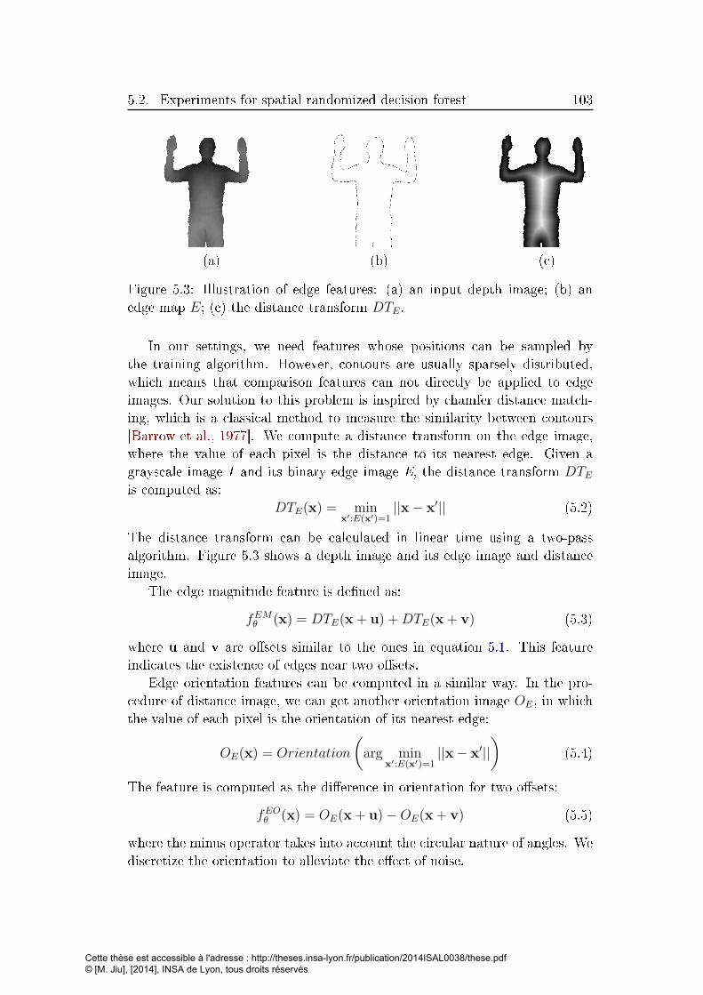
5.2. Experiments for spatial randomized decision forest 103
(a) (b) (c)
Figure 5.3: Illustration of edge features: (a) an input depth image; (b) an
edge map E; (c) the distance transform DTE.
In our settings, we need features whose positions can be sampled by
the training algorithm. However, contours are usually sparsely distributed,
which means that comparison features can not directly be applied to edge
images. Our solution to this problem is inspired by chamfer distance match-
ing, which is a classical method to measure the similarity between contours
[Barrow et al., 1977]. We compute a distance transform on the edge image,
where the value of each pixel is the distance to its nearest edge. Given a
grayscale image I and its binary edge image E, the distance transform DTEis computed as:
DTE(x) = minx′:E(x′)=1
||x− x′|| (5.2)
The distance transform can be calculated in linear time using a two-pass
algorithm. Figure 5.3 shows a depth image and its edge image and distance
image.
The edge magnitude feature is de�ned as:
fEMθ (x) = DTE(x+ u) +DTE(x+ v) (5.3)
where u and v are o�sets similar to the ones in equation 5.1. This feature
indicates the existence of edges near two o�sets.
Edge orientation features can be computed in a similar way. In the pro-
cedure of distance image, we can get another orientation image OE, in which
the value of each pixel is the orientation of its nearest edge:
OE(x) = Orientation
(arg min
x′:E(x′)=1||x− x′||
)(5.4)
The feature is computed as the di�erence in orientation for two o�sets:
fEOθ (x) = OE(x+ u)−OE(x+ v) (5.5)
where the minus operator takes into account the circular nature of angles. We
discretize the orientation to alleviate the e�ect of noise.
Cette thèse est accessible à l'adresse : http://theses.insa-lyon.fr/publication/2014ISAL0038/these.pdf © [M. Jiu], [2014], INSA de Lyon, tous droits réservés

104 Chapter 5. Human body segmentation
(a) (b) (c) (d) (e)
Figure 5.4: Examples of the pixelwise classi�cation: each row is an exam-
ple, each column is a kind of classi�cation results, (a) test depth image; (b)
part segmentation; (c) classical classi�cation; (d) spatial learning with depth
features; (e) spatial learning with depth features and edge features.
The objective of both features is to capture the edge distribution at speci�c
locations in the image, which will be learned by the RDF.
5.2.3 Results
Unless otherwise speci�ed, the following parameters have been used for RDF
learning: 3 trees each with a depth of 9; 2000 randomly selected pixels per
image, randomly distributed over the body; 4000 candidate pairs of o�sets; 22
candidate thresholds; o�sets and thresholds have been learned separately for
each node in the forest. For spatial learning, 28 pairs of neighbors have been
identi�ed between the 11 parts based on a pose where the subject stretches
his arms. The parameter λ was set to 0.4.
During learning, depth features are mixed with edge features. More pre-
cisely, for each tree node, the learning algorithm selects one of the two features.
This choice is integrated into the learning algorithm described in section 4.3 of
chapter 4 in the same way as training of all other parameters (o�sets u and v
and threshold τ): it is learned to maximize the gain in entropy, i.e. maximizing
equation 4.6.
We evaluate our method at two levels: pixelwise classi�cation error and
part recognition and localization. Pixelwise decisions are directly provided
by the random forest. Part localizations are obtained from the pixelwise re-
sults through pixel pooling. We create a posterior probability map for each
part from the classi�cation results: After non-maximum suppression and low
pass �ltering, the location with largest response is used as an estimate of
Cette thèse est accessible à l'adresse : http://theses.insa-lyon.fr/publication/2014ISAL0038/these.pdf © [M. Jiu], [2014], INSA de Lyon, tous droits réservés

5.3. Experiments for spatial ConvNets 105
Table 5.1: Results on body part classi�cation in pixelwise level.
Accuracy
Classical RDF with Depth features [Shotton et al., 2011] 60.30%
Spatial RDF with Depth features λ = 0.4 61.05%
Spatial RDF with Depth + Edge features λ = 0.4 67.66%
the part. Then the positions of pairs of detected parts are calculated, which
approximately correspond to joints and serve as an intermediate pose indi-
cator [Ferrari et al., 2008]. In the following, we denote them by the pair of
neighboring parts.
Table 5.1 shows classi�cation accuracies of three di�erent settings. A base-
line has been created with classical RDF learning and depth features. Spatial
learning with depth features only and with depth and edge features together
are also shown in table 5.1. We can see that that spatial learning can obtain a
performance gain, although no pairwise terms have been used during testing.
Figure 5.4 shows some classi�cation examples, which demonstrate that spatial
learning makes the randomized forest more discriminative. The segmentation
output is cleaner, especially at the borders.
At part level, we report our results of pairs of parts according to the esti-
mation metric by [Ferrari et al., 2008]: a pair of groundtruth parts is matched
to a detected pair if and only if the endpoints of the detected pairs lie within
a circle of radius r=50% of the length of the groundtruth pair and centered
on it. Table 5.2 shows our results on part level using several settings. It
demonstrates that spatial learning improves recognition performance for most
of the parts.
The experiments at both pixelwise and part level demonstrate that spatial
learning makes randomized decision forests more discriminative by integrating
the spatial layout into its prediction model. This proposition is very simple
and fast to implement, as the standard pipeline can be still used. Only the
learning method has been changed, the testing code is unchanged.
5.3 Experiments for spatial ConvNets
In this section, we present experiments on the same dataset using a com-
bination of ConvNets for feature learning and logistical regression (LR) for
classi�cation.
Unless otherwise speci�ed, we use a 2-stage ConvNet in all of the exper-
iments below. The �rst convolutional layer consists of 8 �lters of size 9 × 9,
followed by an element-wise tanh function and a 2×2 non-overlapping average
Cette thèse est accessible à l'adresse : http://theses.insa-lyon.fr/publication/2014ISAL0038/these.pdf © [M. Jiu], [2014], INSA de Lyon, tous droits réservés
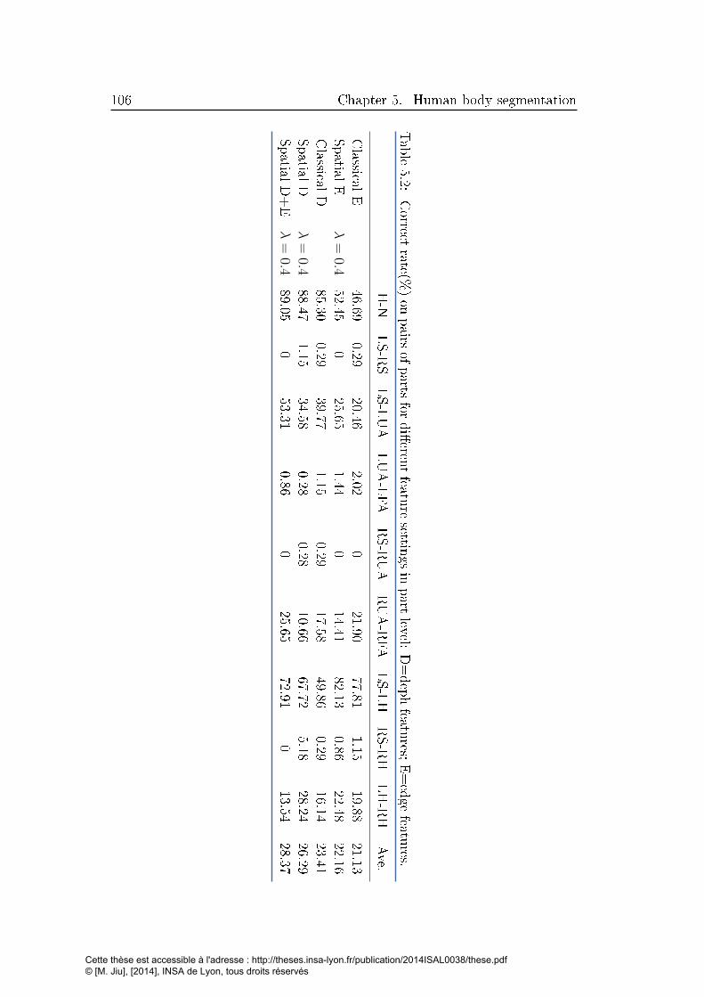
106 Chapter 5. Human body segmentation
Table5.2:
Correct
rate(%)on
pairs
ofparts
fordi�eren
tfeatu
resettin
gsin
part
level:D=dephfeatu
res;E=edge
features.
H-N
LS-RS
LS-LUA
LUA-LFA
RS-RUA
RUA-RFA
LS-LH
RS-RH
LH-RH
Ave.
Classical
E46.69
0.2920.46
2.020
21.9077.81
1.1519.88
21.13
Spatial
Eλ=
0.452.45
025.65
1.440
14.4182.13
0.8622.48
22.16
Classical
D85.30
0.2939.77
1.150.29
17.5849.86
0.2916.14
23.41
Spatial
Dλ=
0.488.47
1.1534.58
0.280.28
10.6667.72
5.1828.24
26.29
Spatial
D+E
λ=
0.489.05
053.31
0.860
25.6572.91
013.54
28.37
Cette thèse est accessible à l'adresse : http://theses.insa-lyon.fr/publication/2014ISAL0038/these.pdf © [M. Jiu], [2014], INSA de Lyon, tous droits réservés

5.3. Experiments for spatial ConvNets 107
pooling operator. The second convolutional layer consists of 32 �lters of size
9× 9, each of which combines 4 feature maps of the previous layer, with the
same activation and pooling operator. The output is a set of 32 feature maps.
The receptive �eld for a single ConvNet on a single scale is 28×28. We resort
to a multiscale setting with a pyramid of 3 scales, with each scale consisting
of 2 convolutional layers [Farabet et al., 2012]. The total receptive �eld is of
size 112 × 112, thus a large spatial context is used to learn better features,
comparable to a best probe distance of 120× 120 of the randomized decision
forest described earlier.
Local contrast normalization is applied to the inputs of the ConvNet, and
the pixels from the background or the context are set to an arbitrary high
value (in our case, 4) to distinguish from the zero-distributed pixels of the ob-
ject. The margin α for pre-training was set to 1.25 [Hadsell et al., 2006], and
λ was set constant to 1 for all constraints in all experiments, i.e. Puv = 1 if u
is ranked higher than v, otherwise 0. Weakly-supervised feature learning and
supervised learning each used 30 epochs through the entire dataset, where
mini-batch gradient descent is adopted. End-to-end �ne-tuning, if applied,
used another 30 epochs. Di�erent learning hyper-parameters (such as learn-
ing rates for di�erent layers) were chosen empirically, e.g. ε1 is set to 10−6
for the �rst convolutional layer and ε2 to 10−5 for the second convolutional
layer. When performing classi�cation, we consider each pixel in isolation,
applying its corresponding 32-dimensional feature vector as input to an LR.
The parameters of the LR are shared at each pixel location. In the following
experiments, we report mean pixel-wise accuracy.
5.3.1 Results
For the application of part estimation from depth images, our baselines are
the algorithms based on randomized decision forests described in the last sec-
tion, as well as single- and multi-scale ConvNets with supervised end-to-end
training without any spatial context. From table 5.3, which gives performance
results on 4 di�erent baseline algorithms, it is clear that the large receptive
�eld of the multiscale architecture is necessary to reliably estimate body part
labels, and also that the Deep Learning-based architecture outperforms ran-
dom forests on the CDC4CV dataset.
We investigate the performance of di�erent combinations of our frame-
work based on spatial pre-training of the purely convolutional layers (which
we call ConvNet) and the classi�cation layer (which we call LR). As a
non-spatial baseline, we also implemented a �pixel-wise� version of DrLIM
[Hadsell et al., 2006], a similar pre-training strategy in which spatial layout
is not taken into consideration, i.e. δa,b=1 if a=b and 0 otherwise; νa,b=1 if
Cette thèse est accessible à l'adresse : http://theses.insa-lyon.fr/publication/2014ISAL0038/these.pdf © [M. Jiu], [2014], INSA de Lyon, tous droits réservés

108 Chapter 5. Human body segmentation
Table 5.3: Evaluation of di�erent baselines on the CDC4CV dataset. In our
implementation of [Farabet et al., 2012], only the multiscale ConvNets have
been used. Purity trees and CRFs have not been implemented, to make the
work comparable to the rest of this chapter.
Methods Accuracy
Randomized forest [Shotton et al., 2011] 60.30%
Spatial RDF (Section 4.3 of chapter 4) 61.05%
Single-scale (vanilla) ConvNet [LeCun et al., 1998] 47.17%
Multi-scale ConvNet [Farabet et al., 2012] 62.54%
a 6= b and 0 otherwise in equation 4.7. The results are shown in Table 5.4. For
each setting (�ne-tuning or no �ne-tuning), spatial training outperforms non
spatial training, and in many cases, the gains are high. Fine-tuning means
end-to-end training of the LR (top two layers) and ConvNet (remaining layers)
with the same objective used to train the LR.
Table 5.4: Results of di�erent combinations of classical and spatial learning
on the CDC4CV dataset.
Convolutional layers LR Fine-tuning Accuracy
DrLIM [Hadsell et al., 2006] classical no 35.10%
DrLIM [Hadsell et al., 2006] spatial no 41.05%
spatial classical no 38.60%
spatial spatial no 41.65%
DrLIM [Hadsell et al., 2006] classical yes 64.39%
DrLIM [Hadsell et al., 2006] spatial yes 65.12%
spatial classical yes 65.18%
spatial spatial yes 66.92%
Examples of segmentation results are shown in Figure 5.5. From visual
inspection we can see that the segmentation results produced by spatial learn-
ing are better than the ones by the non spatial methods. In particular, the
segmentation produced by spatial learning is more consistent (less noisy), es-
pecially for the arms.
5.3.2 Spatial distribution of the error
The proposed method injects neighborhood relationships into the training
algorithm. The question arises, whether the bene�t of the proposed method
Cette thèse est accessible à l'adresse : http://theses.insa-lyon.fr/publication/2014ISAL0038/these.pdf © [M. Jiu], [2014], INSA de Lyon, tous droits réservés

5.3. Experiments for spatial ConvNets 109
(a) (b) (c) (d) (e)
Figure 5.5: Classi�cation examples from the CDC4CV dataset. (a) input
depth image; (b) groundtruth segmentation; (c) appropriate baseline: ran-
domized forest for CDC4CV; (d) DrLIM+LR without spatial learning; (e)
our method (spatial pre-training and spatial LR learning).
only applies to pixels at the boundaries, which would imply a rather trivial
improvement. To rule this out, an in-depth analysis has been performed
to verify that the proposed methods generally improve classi�cation error
independent of the pixels' positions in the part.
For each pixel in the test images the distance to the nearest part bound-
ary was calculated using a distance transform, which allowed us to calculate
histograms over these distances, where each bin corresponds to a range of
distances. Distribution Hg gives the number of pixels of the test images over
distances, shown in Figure 5.6(a). This histogram largely depends on the sizes
of the di�erent body parts, and we can see that the pixel count decreases with
distance. Distributions Hs and Hb are over pixels which are better classi�ed
by the baseline or by the proposed method, respectively:
• Distribution Hs, shown in Figure 5.6(b), is the distribution of pixels
which have been correctly classi�ed by the proposed method but wrongly
classi�ed by the baseline method (DrLIM and classical LR with �ne-
tuning);
• Distribution Hb, shown in Figure 5.6(c), is the distribution of pixels
which have been correctly classi�ed by the baseline method (DrLIM
and classical LR with �ne-tuning) but wrongly classi�ed by the proposed
method.
The normalized histogram Hd, shown in Figure 5.6(d), illustrates the contri-
bution of the proposed spatial learning method as a function of the the pixels'
Cette thèse est accessible à l'adresse : http://theses.insa-lyon.fr/publication/2014ISAL0038/these.pdf © [M. Jiu], [2014], INSA de Lyon, tous droits réservés
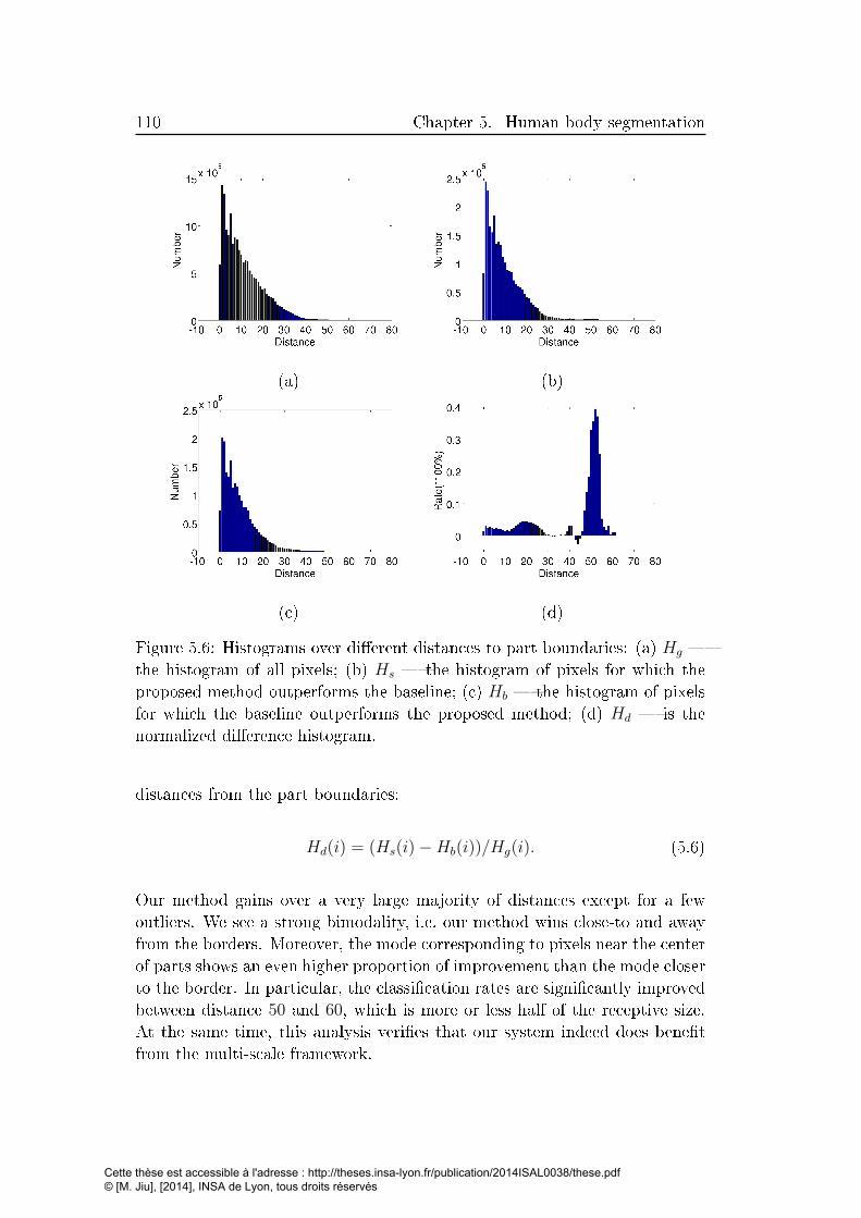
110 Chapter 5. Human body segmentation
(a) (b)
(c) (d)
Figure 5.6: Histograms over di�erent distances to part boundaries: (a) Hg �
the histogram of all pixels; (b) Hs � the histogram of pixels for which the
proposed method outperforms the baseline; (c) Hb � the histogram of pixels
for which the baseline outperforms the proposed method; (d) Hd � is the
normalized di�erence histogram.
distances from the part boundaries:
Hd(i) = (Hs(i)−Hb(i))/Hg(i). (5.6)
Our method gains over a very large majority of distances except for a few
outliers. We see a strong bimodality, i.e. our method wins close-to and away
from the borders. Moreover, the mode corresponding to pixels near the center
of parts shows an even higher proportion of improvement than the mode closer
to the border. In particular, the classi�cation rates are signi�cantly improved
between distance 50 and 60, which is more or less half of the receptive size.
At the same time, this analysis veri�es that our system indeed does bene�t
from the multi-scale framework.
Cette thèse est accessible à l'adresse : http://theses.insa-lyon.fr/publication/2014ISAL0038/these.pdf © [M. Jiu], [2014], INSA de Lyon, tous droits réservés

5.4. Discussion and conclusion 111
Table 5.5: Running times on the CDC4CV dataset of our proposed methods.
For the ConvNets method, training includes pre-training, LR learning and
�ne-tuning, and testing time on one image is given. The resolution of testing
depth image is 320*240.
Task Method Machine Architecture Time
Testing spatial ConvNet Xeon E56620, 8 cores, 2.4GHz MATLAB+IPP 00.41 sec
Testing spatial ConvNet Xeon E56620, 8 cores, 2.4GHz MATLAB+GPU 00.31 sec
Testing spatial RDF Xeon E56620, 8 cores, 2.4GHz C++ / CPU only 00.18 sec
Testing classical RDF Xeon E56620, 8 cores, 2.4GHz C++ / CPU only 00.18 sec
Training spatial ConvNet Xeon E56620, 8 cores, 2.4GHz MATLAB+GPU 36.00 h
Training spatial RDF Xeon E56620, 8 cores, 2.4GHz C++ / CPU only 15.8 h
5.4 Discussion and conclusion
The experiments above demonstrate that even pixelwise independent classi�-
cation indeed bene�ts from the a priori additional information contained in
the spatial part layout.
The quantitative evaluation measures presented in the di�erent tables re-
port pixelwise classi�cation accuracy. This proves that the proposed learning
algorithms improve pixelwise classi�cation, although the injected additional
information does not speci�cally state this. An additional advantage of our
methods are not captured by this evaluation: if a pixel is wrongly classi�ed,
then spatial learning will increase the probability that the wrong part label
is a neighbor of the correct part label. In some applications this can be an
advantage, for instance if the segmentation is post-processed to estimate joint
positions, as in [Shotton et al., 2011].
Currently, we demonstrated a single application of the proposed methods
to human part estimation in depth images. The approach is, however, not
speci�c to pose estimation, and can be applied to other problems, as for in-
stance object segmentation from RGB images, or semantic full scene labeling.
In these cases, the context may be dynamic and the spatial layout might be
more di�cult to extract from the corpus, requiring learning techniques. This
is reserved for future work.
Two di�erent methods have seen introduced: one based on randomized
decision forests, and a second one based on a combination of convolutional
neural networks and logistical regression (or MLPs). The latter deep learning
method achieves better results than the RDF based method, which is mostly
explained by the more powerful features learned by the ConvNets. However,
this classi�cation performance comes at a cost, as the method is computation-
ally more complex.
Cette thèse est accessible à l'adresse : http://theses.insa-lyon.fr/publication/2014ISAL0038/these.pdf © [M. Jiu], [2014], INSA de Lyon, tous droits réservés
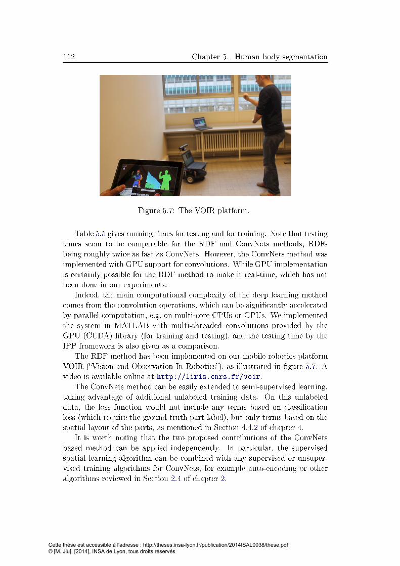
112 Chapter 5. Human body segmentation
Figure 5.7: The VOIR platform.
Table 5.5 gives running times for testing and for training. Note that testing
times seem to be comparable for the RDF and ConvNets methods, RDFs
being roughly twice as fast as ConvNets. However, the ConvNets method was
implemented with GPU support for convolutions. While GPU implementation
is certainly possible for the RDF method to make it real-time, which has not
been done in our experiments.
Indeed, the main computational complexity of the deep learning method
comes from the convolution operations, which can be signi�cantly accelerated
by parallel computation, e.g. on multi-core CPUs or GPUs. We implemented
the system in MATLAB with multi-threaded convolutions provided by the
GPU (CUDA) library (for training and testing), and the testing time by the
IPP framework is also given as a comparison.
The RDF method has been implemented on our mobile robotics platform
VOIR (�Vision and Observation In Robotics�), as illustrated in �gure 5.7. A
video is available online at http://liris.cnrs.fr/voir.
The ConvNets method can be easily extended to semi-supervised learning,
taking advantage of additional unlabeled training data. On this unlabeled
data, the loss function would not include any terms based on classi�cation
loss (which require the ground truth part label), but only terms based on the
spatial layout of the parts, as mentioned in Section 4.4.2 of chapter 4.
It is worth noting that the two proposed contributions of the ConvNets
based method can be applied independently. In particular, the supervised
spatial learning algorithm can be combined with any supervised or unsuper-
vised training algorithms for ConvNets, for example auto-encoding or other
algorithms reviewed in Section 2.4 of chapter 2.
Cette thèse est accessible à l'adresse : http://theses.insa-lyon.fr/publication/2014ISAL0038/these.pdf © [M. Jiu], [2014], INSA de Lyon, tous droits réservés

Chapter 6
General conclusion and discussion
Contents
6.1 Summary of our contributions . . . . . . . . . . . . . . 113
6.2 Limitations and Future work . . . . . . . . . . . . . . . 115
6.3 Other types of spatial information . . . . . . . . . . . 117
In this chapter, we �rst conclude our work and review the di�erent contri-
butions. We then discuss some limitations, and �nally introduce perspectives
and future work.
6.1 Summary of our contributions
In this thesis, we have presented several contributions on visual recognition.
Our objective was to combine the available information, such as spatial con-
�gurations of labels in feature space, or spatial layouts of objects, to improve
the performance of recognition algorithms. Two types of visual recognition
problems have been investigated: action recognition and human body part
segmentation. These two problems di�er from each other in nature. However,
they are actually related to each other: human body part segmentation can
be treated as a preliminary step for action recognition, due to its relation to
human pose.
We resolve the two visual recognition problems by machine learning ap-
proaches, which is a common choice in computer vision. Features are �rst
extracted from the input image/video and then machine learning techniques
are employed to learn a classi�er for classi�cation. Our contributions provide
more available information in the learning stage, resulting in a better repre-
sentation of the object, or a better classi�er. We brie�y summarize them in
the following:
Supervised end-to-end learning for BoW models: We applied BoW
models to action recognition. Each video is represented as a histogram
of occurrence of codewords in a pre-learned codebook. We reformulated
Cette thèse est accessible à l'adresse : http://theses.insa-lyon.fr/publication/2014ISAL0038/these.pdf © [M. Jiu], [2014], INSA de Lyon, tous droits réservés

114 Chapter 6. General conclusion and discussion
the BoW model as a neural network in an end-to-end training frame-
work with two modules (see �gure 3.1). The �rst module creates and
learns BoW models, and the second module is a two-layer Multi-Layer
Perceptron(MLP), which assigns a label to each input video. The gradi-
ent information computed from the MLP module is back-propagated to
the BoW module and used to learn the codebook. However, this kind of
backpropagation is not straight forward in the network architecture due
to the pooling process over interest points. We proposed two algorithms
to make use of the gradient information to optimize the codebook. One
is based on classical error backpropagation, and the other is based on
cluster reassignments, in which we reassign the cluster labels for all the
feature vectors based on the errors in a Voronoi diagram. In this way,
the codebook is learned in a supervised way according to the gradient
information from the MLP. We demonstrated the e�ectiveness of the
proposed algorithms on the standard KTH human action dataset.
Spatial learning for randomized decision forest: The randomized de-
cision forest (RDF) is a simple method for classi�cation. The feature
vector of each entity (object/pixel etc.) is passed down the tree through
a comparison between each feature value with a threshold. The thresh-
old for each node (as well as feature parameters) are chosen maximizing
the entropy gain from the parent to children nodes. RDFs work well
when a large amount of training data is available. However, when the
training data is very limited, the performance drops. We proposed to
integrate the spatial layout of objects into RDF learning. The origi-
nal label set is split into two sets of label pairs: neighboring labels and
non-neighboring labels. The gain in entropy is adopted to each set.
We applied our algorithm to the human part estimation problem and
demonstrated that our algorithm is more discriminative than classical
RDF learning. A by-product are edge features, similar to the existing
depth comparison features, which are capable of improving classi�cation
performance.
Spatial learning for convolutional neural networks: Compared to fea-
ture threshold learning in RDFs, convolutional neural networks can learn
features through end-to-end training even in the existing literature. We
proposed spatial learning for the feature learning module and for the
classi�cation module, respectively. For the feature learning module, our
algorithm operates on pairs of pixels. The pairs are divided into three
sets: the same label, neighboring labels, non-neighboring labels. A loss
function is minimized in order to make the mapped feature vectors close
for pairs of pixels with the same label and distant for pairs of pixels
Cette thèse est accessible à l'adresse : http://theses.insa-lyon.fr/publication/2014ISAL0038/these.pdf © [M. Jiu], [2014], INSA de Lyon, tous droits réservés

6.2. Limitations and Future work 115
with non-neighboring labels. For the classi�cation stage, we structured
the outputs by a ranking technique. We aim to rank the response from
the groundtruth label highest, to rank the responses from the labels
which are neighbors of the groundtruth label next, and �nally to rank
which are not neighbors last. Weakly-supervised learning and super-
vised learning have been combined to further improve the recognition
performance. Experiments on human part estimation in depth images
demonstrated the e�ectiveness of our algorithms.
General conclusion
From the results we have obtained, we can conclude that visual recognition
can be improved by adding information and constraints such as labels, and
spatial layout into di�erent learning stages i.e. into the feature learning stage,
into the classi�cation stage or into both. An end-to-end framework is very
interesting for feature learning because it connects the path from the raw
input data to recognition results. It is goal-oriented, since classi�cation error
is directly used for learning all of di�erent parameters of the system. We draw
the following conclusions:
- Our algorithms work better in the case of small and medium amount
of training data. A large amount of training data allows the classi�er
to better generalize and produce optimal performance. On the other
hand, a priori information is additionally provided to the small/medium
training data to help to generalize the learned machine, playing a similar
role as regularization terms.
- In the training procedure, pairs of entities are fed into the learning.
However, testing is still performed on the single entity (pixel), therefore
there is no additional computation cost.
- End-to-end learning can be useful, but sometimes should be completed
by pre-training (unsupervised learning or weakly supervised learning).
- It is not always clear when end-to-end is better, which thus depends
on the complexity of the problems (i.e. the function to minimize), the
amount of available data, the amount of available training time etc.
6.2 Limitations and Future work
Limitations of supervised end-to-end learning for bag-of-words mod-
els
Cette thèse est accessible à l'adresse : http://theses.insa-lyon.fr/publication/2014ISAL0038/these.pdf © [M. Jiu], [2014], INSA de Lyon, tous droits réservés

116 Chapter 6. General conclusion and discussion
Figure 6.1: The motorbike on the right is severely self-occluded, compared to
the one on the left. Most of the spatial part relations are useless in the energy
function.
In the current work, the input is comprised of extracted features, and
the BoW model construction is formulated as a neural network. The dictio-
nary is coded into the weights between the layers. Low level features like
HOG/HOF are chosen, rather than learned. A feature learning module could
be added at the beginning, e.g. a convolutional layer as described in section
4.4.1. The error backpropagation scheme can be applied to learn the �lters
in the convolutional layer. The advantage would be to learn the features and
the dictionary together in a longer end-to-end learning scheme.
Limitations of spatial learning
In this thesis, we also proposed three spatial learning algorithms for two
di�erent frameworks: spatial learning for randomized decision forests, spatial
learning for pre-training ConvNets, and spatial learning for supervised learn-
ing of LR and MLP classi�ers. They di�er from each other, but they share
a minor common limitation: constant spatial part layout structure, as shown
in �gure 5.2 for human upper body part segmentation. The reason is that
the spatial layout depends on inherent object properties, even for a non-rigid
object. The spatial layout is correct for all the objects in the same category.
However, in reality, due to occlusions induced by di�erent object poses, some
parts may be not visible in the image, their spatial relations to other parts
still occur in the energy function. At the same time, some new spatial rela-
tions emerge due to dynamic poses, on the contrary, which are ignored in the
energy function. Figure 6.1 and 6.2 show two limitation cases, respectively.
A possible solution to deal with occlusion and dynamic pose is to adopt a
dynamic spatial layout for each image. In principle, the spatial layout could
been detected for each image by neighborhood search algorithms. But energy
divergence might be a problem in this context.
Limitations of spatial ConvNets learning
We proposed a ranking technique in the spatial supervised learning of LR
Cette thèse est accessible à l'adresse : http://theses.insa-lyon.fr/publication/2014ISAL0038/these.pdf © [M. Jiu], [2014], INSA de Lyon, tous droits réservés

6.3. Other types of spatial information 117
Figure 6.2: In comparison to the left person, new part spatial layout relations
emerge due to pose changes in the right person, e.g. the left lower arm and
the right lower arm is not taken into account in the model.
and MLP classi�ers. The response of the groundtruth label is ranked �rst,
followed by the neighboring labels of the groundtruth, and last by the non-
neighboring labels of the groundtruth. The desired probabilities we used in
the current version are rigid, i.e. the desired probability is set to 1 for all
the correct rankings, otherwise 0. However, it is intuitive that the desired
probabilities should be �soft�, i.e. values in [0, 1], keeping certain constraints.
The exact probabilities are hyperparameters, which could be learned over
the validation data. Additional constraints will be required to ensure that
the learned ranking measure is valid, as suggested in [Burges et al., 2005] in
a di�erent context.
6.3 Other types of spatial information
The current pipeline presented in chapter 4 is used to classify pixels for human
part estimation. It works for simple parts and for rigid objects (faces etc.).
The variance in pose and occlusion is not large. The parts and their a priori
information of spatial layout are given as groundtruth.
If we aim to recognize non-rigid objects (and not just their parts), in
this context, a possible solution is �rst to detect parts, and then to treat
constellation of the features from di�erent parts as the object features, which
are fed into a classi�er. The features also can be learned in an end-to-end way.
This framework is a combination of DPMs (see section 2.3.2.3 of chapter 2)
and deep feature learning (see section 2.4 of chapter 2). However, it requires to
solve a combinational problem over part positions, which makes it di�cult to
calculate gradients used for feature learning. Figure 6.3 shows this framework.
This is our ongoing work.
Cette thèse est accessible à l'adresse : http://theses.insa-lyon.fr/publication/2014ISAL0038/these.pdf © [M. Jiu], [2014], INSA de Lyon, tous droits réservés
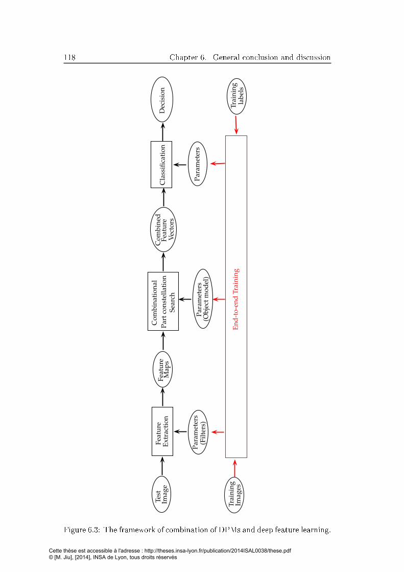
118 Chapter 6. General conclusion and discussion
Fea
ture
Cla
ssifi
cati
on
Ex
trac
tio
n
Par
amet
ers
Tes
tIm
age
Par
amet
ers
Fea
ture
Tra
inin
gIm
ages
Tra
inin
gla
bel
s
Map
sD
ecis
ion
En
d-t
o-e
nd
Tra
inin
g
Co
mb
inat
ion
al
Par
tco
nst
ella
tio
nS
earc
h
Co
mb
ined
Fea
ture
Vec
tors
(Fil
ters
)P
aram
eter
s(O
bje
ctm
od
el)
Figure 6.3: The framework of combination of DPMs and deep feature learning.
Cette thèse est accessible à l'adresse : http://theses.insa-lyon.fr/publication/2014ISAL0038/these.pdf © [M. Jiu], [2014], INSA de Lyon, tous droits réservés

Bibliography
[Abdelkader et al., 2010] Abdelkader, M. F., Abd-Almageed, W., Srivastava,
A., and Chellappa, R. (2010). Silhouette-based Gesture and Action Recog-
nition via Modeling Trajectories on Riemannian shape manifolds. Computer
Vision and Image Understanding, 115(3):439�455. (Cited on page 70.)
[Aggarwal and Ryoo, 2011] Aggarwal, J. and Ryoo, M. (2011). Human activ-
ity analysis: A review. ACM Computing Surveys (CSUR), 43(3). (Cited
on page 69.)
[Ahonen et al., 2006] Ahonen, T., Hadid, A., and Pietikäinen, M. (2006).
Face description with local binary patterns: application to face recog-
nition. IEEE transactions on pattern analysis and machine intelligence,
28(12):2037�41. (Cited on page 24.)
[Ahonen et al., 2009] Ahonen, T., Matas, J., He, C., and Pietikäinen, M.
(2009). Rotation invariant image description with local binary pattern
histogram fourier features. Scandinavian Conference on Image Analysis,
Lecture Notes in Computer Science., pages 61�70. (Cited on page 25.)
[Baccouche et al., 2011] Baccouche, M., Mamalet, F., Wolf, C., Garcia, C.,
and Baskurt, A. (2011). Sequential Deep Learning for Human Action Recog-
nition. 2nd International Workshop on Human Behavior Understanding,
pages 1�11. (Cited on page 70.)
[Ballan et al., 2009] Ballan, L., Bertini, M., and Bimbo, A. D. (2009). E�ec-
tive codebooks for human action categorization. in Proc. of ICCV Work-
shop on Video-oriented Object and Event Classi�cation (VOEC). (Cited on
page 36.)
[Barrow et al., 1977] Barrow, H. G., Tenenbaum, J. M., Bolles, R. C., and
Wolf, H. C. (1977). Parametric correspondence and chamfer matching:
two new techniques for image matching. In Proc. 5th International joint
conference Arti�cial Intelligence. (Cited on pages 29 and 103.)
[Bay et al., 2006] Bay, H., Tuytelaars, T., and Van Gool, L. (2006). Surf:
Speeded up robust features. ECCV, pages 404�417. (Cited on pages 21
and 24.)
Cette thèse est accessible à l'adresse : http://theses.insa-lyon.fr/publication/2014ISAL0038/these.pdf © [M. Jiu], [2014], INSA de Lyon, tous droits réservés
120 Bibliography
[Belhumeur et al., 1997] Belhumeur, P., Hespanha, João, P., and Kriegman,
D. J. (1997). Eigenfaces vs. �sherfaces: Recognition using class speci�c lin-
ear projection. IEEE Trans. on Pattern Analysis and Machine Intelligence,
19(7):711�720. (Cited on page 16.)
[Belongie et al., 2002] Belongie, S., Malik, J., and Puzicha, J. (2002). Shape
matching and object recognition using shape contexts. IEEE Transactions
on Pattern Analysis and Machine Intelligence, 24(4):509�522. (Cited on
pages ix, 14 and 15.)
[Bengio, 2009] Bengio, Y. (2009). Learning Deep Architectures for AI. Foun-
dations and Trends in Machine Learning, 2(1):1�127. (Cited on pages x
and 46.)
[Bettadapura et al., 2013] Bettadapura, V., Schindler, G., Plötz, T., and
Essa, I. (2013). Augmenting bag-of-words: Data-driven discovery of tem-
poral and structural information for activity recognition. CVPR. (Cited on
page 37.)
[Bishop, 1994] Bishop, C. (1994). Neural networks for pattern recognition.
pages 140�145. (Cited on page 61.)
[Bobick and Davis, 2001] Bobick, A. F. and Davis, J. W. (2001). The recog-
nition of human movement using temporal templates. IEEE Transactions
on PAMI, 23(3):257267. (Cited on pages ix, 18 and 19.)
[Boiman and Irani, 2007] Boiman, O. and Irani, M. (2007). Detecting Irregu-
larities in Images and in Video. International Journal of Computer Vision,
74(1):17�31. (Cited on page 70.)
[Borgefors, 1988] Borgefors, G. (1988). Hierarchical chamfer matching: A
parametric edge matching algorithm. IEEE Transcations on PAMI,
10(6):849�865. (Cited on page 30.)
[Boureau et al., 2010] Boureau, Y.-l., Bach, F., LeCun, Y., and Ponce, J.
(2010). Learning mid-level features for recognition. CVPR. (Cited on
page 35.)
[Bregonzio et al., 2009] Bregonzio, M., Gong, S., and Xiang, T. (2009).
Recognising Action as Clouds of Space-Time Interest Points. In CVPR.
(Cited on page 69.)
[Burges et al., 2005] Burges, C., Shaked, T., Renshaw, E., Lazier, A., Deeds,
M., Hamilton, N., and Hullender, G. (2005). Learning to rank using gradient
descent. In ICML. (Cited on pages 94, 95 and 117.)
Cette thèse est accessible à l'adresse : http://theses.insa-lyon.fr/publication/2014ISAL0038/these.pdf © [M. Jiu], [2014], INSA de Lyon, tous droits réservés

Bibliography 121
[Calonder et al., 2010] Calonder, M., Lepetit, V., Strecha, C., and Fua, P.
(2010). Brief: Binary robust independent elementary features. ECCV.
(Cited on page 24.)
[Cao et al., 2010] Cao, Y., Wang, C., Li, Z., Zhang, L., and Zhang, L. (2010).
Spatial-bag-of-features. CVPR. (Cited on page 37.)
[Chang and Lin, 2011] Chang, C.-C. and Lin, C.-J. (2011). LIBSVM: A li-
brary for support vector machines. ACM Transactions on Intelligent Sys-
tems and Technology, 2(3):1�27. (Cited on page 74.)
[Cootes et al., 2001] Cootes, T., Edwards, G. J., and Taylor, C. J. (2001).
Active appearance models. PAMI, 23(6):681685. (Cited on page 17.)
[Cootes et al., 1995] Cootes, T., Taylor, C., Cooper, D., and Graham, J.
(1995). Active shape models-their training and application. Computer Vi-
sion and Image Understanding. (Cited on page 14.)
[Couprie et al., 2013] Couprie, C., Farabet, C., Najman, L., and LeCun, Y.
(2013). Indoor semantic segmentation using depth information. arXiv,
pages 1�8. (Cited on page 43.)
[Cox and Cox, 1994] Cox, T. and Cox, M. (1994). Multidimensional scaling.
Chapman and Hill. (Cited on page 85.)
[Csurka et al., 2004] Csurka, G., Dance, C., and Fan, L. (2004). Visual cate-
gorization with bags of keypoints. ECCV International Workshop on Sta-
tistical Learning in Computer Vision. (Cited on pages ix, 12, 13, 34, 35,
53, 54, 55, 69 and 79.)
[Cuntoor et al., 2008] Cuntoor, N. P., Yegnanarayana, B., and Chellappa, R.
(2008). Activity modeling using event probability sequences. IEEE trans-
actions on image processing, 17(4):594�607. (Cited on page 70.)
[Dalal and Triggs, 2005] Dalal, N. and Triggs, B. (2005). Histograms of ori-
ented gradients for human detection. In CVPR. (Cited on pages x, 24, 26
and 90.)
[Dalal et al., 2006] Dalal, N., Triggs, B., and Schmid, C. (2006). Human
detection using oriented histograms of �ow and appearance. ECCV, pages
428�441. (Cited on page 24.)
[Dean et al., 2013] Dean, T., Ruzon, M. A., and View, M. (2013). Fast ,
accurate detection of 100 , 000 object classes on a single machine. CVPR.
(Cited on page 41.)
Cette thèse est accessible à l'adresse : http://theses.insa-lyon.fr/publication/2014ISAL0038/these.pdf © [M. Jiu], [2014], INSA de Lyon, tous droits réservés
122 Bibliography
[Dekel et al., 2004] Dekel, O., Manning, C., and Singer, Y. (2004). Log-linear
models for label-ranking. In NIPS. (Cited on page 94.)
[Dietterich, 1998] Dietterich, T. G. (1998). Approximate Statistical Tests for
Comparing Supervised Classi cation Learning Algorithms 1 Introduction.
Neural Computation, 10(7):1895�1923. (Cited on page 75.)
[Divvala et al., 2012] Divvala, S., Efros, A., and Hebert, M. (2012). How
important are "deformable parts" in the deformable parts model? ECCV
Workshops. (Cited on page 40.)
[Divvala and Hoiem, 2009] Divvala, S. and Hoiem, D. (2009). An empirical
study of context in object detection. CVPR, pages 1271�1278. (Cited on
page 85.)
[Dollar et al., 2005] Dollar, P., Rabaud, V., Cottrell, G., and Belongie, S.
(2005). Behavior Recognition via Sparse Spatio-Temporal Features. IEEE
International Workshop on Visual Surveillance and Performance Evalua-
tion of Tracking and Surveillance, pages 65�72. (Cited on pages x, 22, 34,
35 and 53.)
[Dubuisson and Jain, 1994] Dubuisson, M. and Jain, A. (1994). A modi�ed
hausdor� distance for object matching. International Conference on Pat-
tern Recognition, pages 566�568. (Cited on page 30.)
[Duchenne et al., 2009] Duchenne, O., Bach, F., Kweon, I., and Ponce, J.
(2009). A tensor-based algorithm for high-order graph matching. (Cited on
pages 33 and 80.)
[Dyana and Das, 2009] Dyana, a. and Das, S. (2009). Trajectory representa-
tion using Gabor features for motion-based video retrieval. Pattern Recog-
nition Letters, 30(10):877�892. (Cited on page 70.)
[Everingham and Zisserman, 2010] Everingham, M., V. G. L. W. C. K. I.
W. J. and Zisserman, A. (2010). The pascal visual object classes (voc)
challenge. International Journal of Computer Vision, 88(2):303�338. (Cited
on pages ix, 2 and 3.)
[Everts et al., 2013] Everts, I., van Gemert, J., and Gevers, T. (2013). Evalu-
ation of color stips for human action recognition. pages 2850�2857. (Cited
on page 22.)
[Farabet et al., 2012] Farabet, C., Couprie, C., Najman, L., and LeCun, Y.
(2012). Scene parsing with multiscale feature learning, purity trees, and
Cette thèse est accessible à l'adresse : http://theses.insa-lyon.fr/publication/2014ISAL0038/these.pdf © [M. Jiu], [2014], INSA de Lyon, tous droits réservés

Bibliography 123
optimal covers. NIPS. (Cited on pages xii, xv, 43, 81, 86, 90, 96, 107
and 108.)
[Fathi and Mori, 2008] Fathi, A. and Mori, G. (2008). Action recognition
by learning mid-level motion features. In Computer Vision and Pattern
Recognition, 2008. CVPR 2008. IEEE Conference on, pages 1�8. IEEE.
(Cited on page 70.)
[Felzenszwalb et al., 2010] Felzenszwalb, P., Girshick, R., McAllester, D., and
Ramanan, D. (2010). Object detection with discriminatively trained part
based models. IEEE Tr on PAMI, 32(9):1627�1645. (Cited on pages ix, 12,
13, 38, 39 and 41.)
[Felzenszwalb and Huttenlocher, 2005] Felzenszwalb, P. F. and Huttenlocher,
D. P. (2005). Pictorial Structures for Object Recognition. IJCV, 61(1):55�
79. (Cited on pages 39 and 80.)
[Felzenszwalb and Zabih, 2011] Felzenszwalb, P. F. and Zabih, R. (2011). Dy-
namic programming and graph algorithms in computer vision. IEEE trans-
actions on pattern analysis and machine intelligence, 33(4):721�40. (Cited
on page 80.)
[Fergus et al., 2003] Fergus, R., Perona, P., and Zisserman, A. (2003). Object
class recognition by unsupervised scale-invariant learning. In IEEE, editor,
CVPR, volume 2, pages 264�271. (Cited on page 38.)
[Fergus et al., 2004] Fergus, R., Perona, P., and Zisserman, A. (2004). A
visual category �lter for google images. ECCV, pages 1�14. (Cited on
page 38.)
[Ferrari et al., 2008] Ferrari, V., Marin-Jimenez, M., and Zisserman, A.
(2008). Progressive search space reduction for human pose estimation. In
CVPR, pages 1�8. (Cited on page 105.)
[Fischler and Bolles, 1981] Fischler, M. and Bolles, R. (1981). Random sam-
ple consensus: A paradigm for model �tting with applications to image anal-
ysis and automated cartography. Communcations of the ACM, 24:381â395.
(Cited on page 80.)
[Fischler and Elschlager, 1973] Fischler, M. and Elschlager, R. (1973). The
representation and matching of pictorial structures. Computers, IEEE
Transactions on, c(1):67�92. (Cited on pages 38, 39 and 80.)
Cette thèse est accessible à l'adresse : http://theses.insa-lyon.fr/publication/2014ISAL0038/these.pdf © [M. Jiu], [2014], INSA de Lyon, tous droits réservés
124 Bibliography
[Freund et al., 2003] Freund, Y., Iyer, R., Schapire, R., and Singer, Y. (2003).
An e�cient boosting algorithm for combining preferences. Journal of Ma-
chine Learning Research, 4:933�969. (Cited on page 94.)
[Gaidon et al., 2011] Gaidon, A., Harchoui, Z., and Schmid, C. (2011). A
time series kernel for action recognition. Procedings of the British Machine
Vision Conference 2011, pages 63.1�63.11. (Cited on page 37.)
[Geman and Geman, 1984] Geman, S. and Geman, D. (1984). Stochastic Re-
laxation, Gibbs Distributions, and the Bayesian Restoration of Images.
IEEE Transactions on PAMI, 6(6):721�741. (Cited on page 86.)
[Gilbert et al., 2011] Gilbert, A., Illingworth, J., and Bowden, R. (2011).
Mined Hierarchical Compound Features. International Journal of Com-
puter Vision, 33(5):883�897. (Cited on page 55.)
[Girshick et al., 2013] Girshick, R., Donahue, J., Darrell, T., and Malik, J.
(2013). Rich feature hierarchies for accurate object detection and semantic
segmentation. (Cited on pages x and 42.)
[Goh et al., 2012] Goh, H., Thome, N., Cord, M., and Lim, J. (2012). Unsu-
pervised and supervised visual codes with restricted boltzmann machines.
ECCV. (Cited on pages 36 and 55.)
[Goldberger et al., 2004] Goldberger, J., Roweis, S., Hinton, G., and
Salakhutdinov, R. (2004). Neighbourhood component analysis. In NIPS.
(Cited on pages 50 and 85.)
[Goncalves and Perona, 2003] Goncalves, L. and Perona, P. (2003). Unsuper-
vised learning of human motion. IEEE Transactions on Pattern Analysis
and Machine Intelligence, 25(7):814�827. (Cited on page 69.)
[Gorelick et al., 2007] Gorelick, L., Blank, M., Shechtman, E., Irani, M., and
Basri, R. (2007). Actions as space-time shapes. IEEE transactions on
PAMI, 29(12):22472253. (Cited on pages ix, 15 and 16.)
[Gould et al., 2009] Gould, S., Fulton, R., and Koller, D. (2009). Decompos-
ing a scene into geometric and semantically consistent regions. ICCV, pages
1�8. (Cited on pages x and 42.)
[Grangier et al., 2009] Grangier, G., Bottou, L., and R.Collobert (2009).
Deep convolutional networks for scene parsing. In ICML Deep Learning
Workshop. (Cited on page 90.)
Cette thèse est accessible à l'adresse : http://theses.insa-lyon.fr/publication/2014ISAL0038/these.pdf © [M. Jiu], [2014], INSA de Lyon, tous droits réservés

Bibliography 125
[Grauman and Darrell, 2005] Grauman, K. and Darrell, T. (2005). The pyra-
mid match kernel: discriminative classi�cation with sets of image features.
ICCV, pages 1458�1465. (Cited on page 37.)
[Hadsell et al., 2006] Hadsell, R., Chopra, S., and LeCun, Y. (2006). Dimen-
sionality reduction by learning an invariant mapping. In CVPR, pages
1735�1742. (Cited on pages x, 46, 50, 83, 85, 92, 93, 107 and 108.)
[Harris and Stephens, 1988] Harris, C. and Stephens, M. (1988). A combined
corner and edge detector. In In Proc. of Fourth Alvey Vision Conference,
pages 147�151. (Cited on page 20.)
[Heitz and Koller, 2008] Heitz, G. and Koller, D. (2008). Learning spatial
context: Using stu� to �nd things. ECCV, pages 1�14. (Cited on page 85.)
[Heseltine et al., 2003] Heseltine, T., Pears, N., Austin, J., and Chen, Z.
(2003). Face Recognition : A Comparison of Appearance-Based Approaches
2 The Direct Correlation Method. Proc. VIIth Digital Image Computing:
Techniques and Applications, pages 59�68. (Cited on pages ix and 16.)
[Hinton et al., 2006] Hinton, G., Osindero, S., and Teh, Y.-W. (2006). A fast
learning algorithm for deep belief nets. Neural Computation. (Cited on
pages x, 48 and 49.)
[Hinton and Salakhutdinov, 2006] Hinton, G. and Salakhutdinov, R. (2006).
Reducing the dimensionality of data with neural networks. Science,
313(5786):504�507. (Cited on page 91.)
[Hinton, 1995] Hinton, G. E. (1995). The wake-sleep algorithm for unsuper-
vised neural networks. Science. (Cited on page 49.)
[Holt et al., 2011] Holt, B., Ong, E.-J., Cooper, H., and Bowden, R. (2011).
Putting the pieces together: Connected poselets for human pose estimation.
In ICCV Workshop on Consumer Depth Cameras for Computer Vision.
(Cited on pages xii, 99 and 100.)
[Hu and Boulgouris, 2011] Hu, J. and Boulgouris, N. V. (2011). Fast human
activity recognition based on structure and motion. Pattern Recognition
Letters, 32(14):1814�1821. (Cited on page 19.)
[Hu, 1962] Hu, M.-K. (1962). Visual Pattern Recognition by Moment. IRE
Transactions on Information Theory, pages 66�70. (Cited on page 17.)
[Huang, 2008] Huang, T. (2008). Discriminative local binary patterns for
human detection in personal album. CVPR, pages 1�8. (Cited on page 24.)
Cette thèse est accessible à l'adresse : http://theses.insa-lyon.fr/publication/2014ISAL0038/these.pdf © [M. Jiu], [2014], INSA de Lyon, tous droits réservés

126 Bibliography
[Huttenlocher et al., 1993] Huttenlocher, D., Klanderman, G. A., and Ruck-
lidge, W. J. (1993). Comparing images using the hausdor� distance. IEEE
Transcations on PAMI, 15(9):850�863. (Cited on page 30.)
[Jarrett and Kavukcuoglu, 2009] Jarrett, K. and Kavukcuoglu, K. (2009).
What is the best multi-stage architecture for object recognition? In ICCV.
(Cited on page 90.)
[Jhuang et al., 2007] Jhuang, H., Serre, T., and Wolf, L. (2007). A Biologi-
cally Inspired System for Action Recognition. ICCV. (Cited on page 70.)
[Jolli�e, 1986] Jolli�e, T. I. (1986). Principal component analysis. In New
York: Springer-Verlag. (Cited on page 85.)
[Jurie and Triggs, 2005] Jurie, F. and Triggs, B. (2005). Creating e�cient
codebooks for visual recognition. ICCV. (Cited on page 35.)
[Kamarainen et al., 2007] Kamarainen, J. K., Kyrki, V., and Kälviäinen, H.
(2007). Local and global Gabor features for object recognition. Pattern
Recognition and Image Analysis, 17(1):93�105. (Cited on page 27.)
[Kass et al., 1988] Kass, M., Witkin, A., and Terzopoulos, D. (1988). Snakes:
Active contour models. International journal of computer vision. (Cited on
page 14.)
[Ke and Sukthankar, 2004] Ke, Y. and Sukthankar, R. (2004). PCA-SIFT: A
more distinctive representation for local image descriptors. CVPR, 2:506�
513. (Cited on page 23.)
[Klaser et al., 2008] Klaser, A., Marszalek, M., and Schmid, C. (2008). A
spatio-temporal descriptor based on 3d-gradients. BMVC. (Cited on
page 24.)
[Kolmogorov and Zabih, 2004] Kolmogorov, V. and Zabih, R. (2004). What
energy functions can be minimized via graph cuts? IEEE Transactions on
PAMI, 26(2):147�159. (Cited on pages 81 and 87.)
[Kontschieder et al., 2013] Kontschieder, P., Kohli, P., Shotton, J., and Cri-
minisi, A. (2013). Geof: Geodesic forests for learning coupled predictors.
2013 IEEE Conference on Computer Vision and Pattern Recognition, pages
65�72. (Cited on page 43.)
[Krizhevsky et al., 2012] Krizhevsky, A., Sutskever, I., and Hinton, G. E.
(2012). Imagenet classi�cation with deep convolutional neural networks.
In NIPS. (Cited on pages 46 and 90.)
Cette thèse est accessible à l'adresse : http://theses.insa-lyon.fr/publication/2014ISAL0038/these.pdf © [M. Jiu], [2014], INSA de Lyon, tous droits réservés

Bibliography 127
[Laptev, 2005] Laptev, I. (2005). On Space-Time Interest Points. Interna-
tional Journal of Computer Vision, 64:107�123. (Cited on pages ix, 21, 22,
23, 35 and 55.)
[Laptev et al., 2008] Laptev, I., Marszalek, M., Schmid, C., and Rozenfeld,
B. (2008). Learning realistic human actions from movies. In CVPR, pages
1�8. IEEE. (Cited on pages 24 and 70.)
[Lazebnik and Schmid, 2006] Lazebnik, S. and Schmid, C. (2006). Beyond
bags of features : Spatial pyramid matching for recognizing natural scene
categories. In CVPR. (Cited on page 37.)
[Le et al., 2011] Le, Q., Zou, W., Yeung, S., and Ng, A. (2011). Learning hi-
erarchical invariant spatio-temporal features for action recognition with in-
dependent subspace analysis. CVPR, pages 3361�3368. (Cited on page 22.)
[LeCun et al., 1998] LeCun, Y., Botto, L., Bengio, Y., and Ha�ner, P. (1998).
Gradient-based learning applied to document recognition. Proceedings of
IEEE, 86(11):2278�2324. (Cited on pages 27, 45, 85, 90, 96 and 108.)
[LeCun et al., 2010] LeCun, Y., Kavukcuoglu, K., and Farabet, C. (2010).
Convolutional networks and applications in vision. Proceedings of 2010
IEEE International Symposium on Circuits and Systems, pages 253�256.
(Cited on page 46.)
[Lee et al., 2007] Lee, H., Ekanadham, C., and Ng, A. (2007). Sparse deep
belief net model for visual area v2. NIPS, pages 1�8. (Cited on page 47.)
[Lee et al., 2011] Lee, J., Cho, M., and Lee, K. M. (2011). Hyper-graph
matching via reweighted random walks. In CVPR. (Cited on page 33.)
[Leonardis and Bischof, 2000] Leonardis, A. and Bischof, H. (2000). Robust
recognition using eigenimages. Computer Vision and Image Understanding,
78(1):99118. (Cited on page 16.)
[Lepetit et al., 2004] Lepetit, V., Pilet, J., and Fua, P. (2004). Point matching
as a classi�cation problem for fast and robust object pose estimation. In
CVPR, pages 244�250. (Cited on page 87.)
[Leung and Malik, 2001] Leung, T. and Malik, J. (2001). Representing and
recognizing the visual appearance of materials using three-dimensional tex-
tons. International Journal of Computer Vision, 43(1):29�44. (Cited on
page 35.)
Cette thèse est accessible à l'adresse : http://theses.insa-lyon.fr/publication/2014ISAL0038/these.pdf © [M. Jiu], [2014], INSA de Lyon, tous droits réservés

128 Bibliography
[Li et al., 2013] Li, W., Yu, Q., Sawhney, H., and Vasconcelos, N. (2013).
Recognizing activities via bag of words for attribute dynamics. 2013 IEEE
Conference on Computer Vision and Pattern Recognition, pages 2587�2594.
(Cited on page 38.)
[Liao et al., 2009] Liao, S., Law, M., and Chung, A. (2009). Dominant local
binary patterns for texture classi�cation. IEEE Transactions on Image
Processing, 18(5):1107�1118. (Cited on page 26.)
[Lin et al., 2009] Lin, L., Zeng, K., Liu, X., and Zhu, S.-C. (2009). Layered
graph matching by composite cluster sampling with collaborative and com-
petitive interactions. CVPR, pages 1351�1358. (Cited on page 33.)
[Liu et al., 2008] Liu, J., Ali, S., and Shah, M. (2008). Recognizing human
actions using multiple features. In CVPR. (Cited on page 69.)
[Liu and Shah, 2008] Liu, J. and Shah, M. (2008). Learning human actions
via information maximization. CVPR, pages 1�8. (Cited on pages 36, 54
and 55.)
[Liu et al., 2009] Liu, J., Yang, Y., and Shah, M. (2009). Learning seman-
tic visual vocabularies using di�usion distance. 2009 IEEE Conference
on Computer Vision and Pattern Recognition, pages 461�468. (Cited on
pages 35 and 54.)
[Lowe, 2004] Lowe, D. G. (2004). Distinctive Image Features from Scale-
Invariant Keypoints. International Journal of Computer Vision, 60(2):91�
110. (Cited on pages x, 21, 23, 53, 69 and 90.)
[Ma et al., 2010] Ma, T., Yang, X., and Latecki, L. (2010). Boosting chamfer
matching by learning chamfer distance normalization. ECCV, (1). (Cited
on page 30.)
[Marius et al., 2011] Marius, L., Andrei, Z., and Cristian, S. (2011). Semi-
supervised learning and optimization for hypergraph matching. In ICCV,
pages 2274�2281. (Cited on page 33.)
[Matikainen et al., 2009] Matikainen, P., Hebert, M., and Sukthankar, R.
(2009). Trajectons: Action recognition through the motion analysis of
tracked features. 2009 IEEE 12th International Conference on Computer
Vision Workshops, pages 514�521. (Cited on page 35.)
[Matikainen et al., 2010] Matikainen, P., Hebert, M., and Sukthankar, R.
(2010). Representing pairwise spatial and temporal relations for action
recognition. ECCV, pages 508�521. (Cited on page 37.)
Cette thèse est accessible à l'adresse : http://theses.insa-lyon.fr/publication/2014ISAL0038/these.pdf © [M. Jiu], [2014], INSA de Lyon, tous droits réservés
Bibliography 129
[Memisevic and Hinton, 2007] Memisevic, R. and Hinton, G. (2007). Unsu-
pervised learning of image transformations. 2007 IEEE Conference on Com-
puter Vision and Pattern Recognition, pages 1�8. (Cited on page 49.)
[Mikolajczyk et al., 2006] Mikolajczyk, K., Leibe, B., and Schiele, B. (2006).
Multiple object class detection with a generative model. CVPR, 1:26�36.
(Cited on page 38.)
[Mikolajczyk and Schmid, 2002] Mikolajczyk, K. and Schmid, C. (2002). An
a�ne invariant interest point detector. ECCV. (Cited on page 21.)
[Mikolajczyk and Schmid, 2005] Mikolajczyk, K. and Schmid, C. (2005). Per-
formance evaluation of local descriptors. IEEE transactions on PAMI,
27(10):1615�30. (Cited on page 23.)
[Mikolajczyk and Uemura, 2008] Mikolajczyk, K. and Uemura, H. (2008). Ac-
tion recognition with motion-appearance vocabulary forest. CVPR. (Cited
on page 69.)
[Mikolajczyk and Uemura, 2011] Mikolajczyk, K. and Uemura, H. (2011). Ac-
tion recognition with appearancemotion features and fast search trees. Com-
puter Vision and Image Understanding, 115(3):426�438. (Cited on page 55.)
[Minetto et al., 2013] Minetto, R., Thome, N., Cord, M., Leite, N. J., and
Stol�, J. (2013). T-HOG: An e�ective gradient-based descriptor for single
line text regions. Pattern Recognition, 46(3):1078�1090. (Cited on page 24.)
[Mitchell, 1997] Mitchell, T. M. (1997). Machine Learning. page 2. (Cited on
page 1.)
[Moosmann et al., 2007] Moosmann, F., Triggs, B., and Jurie, F. (2007). Fast
discriminative visual codebooks using randomized clustering forests. In
Advances in neural information processing systems, volume 19, page 985.
Citeseer. (Cited on pages 36 and 54.)
[Moravec, 1981] Moravec, H. (1981). Rover Visual Obstacle Avoidance. IJ-
CAI. (Cited on page 20.)
[Murase and Nayar, 1995] Murase, H. and Nayar, S. K. (1995). Visual learn-
ing and recognition of 3-d objects from appearance. International Journal
of Computer Vision, 14(1):524. (Cited on page 16.)
[Niebles and Fei-Fei, 2007] Niebles, J. C. and Fei-Fei, L. (2007). A hierarchical
model of shape and appearance for human action classi�cation. CVPR.
(Cited on page 70.)
Cette thèse est accessible à l'adresse : http://theses.insa-lyon.fr/publication/2014ISAL0038/these.pdf © [M. Jiu], [2014], INSA de Lyon, tous droits réservés

130 Bibliography
[Niebles et al., 2010] Niebles, J. C., W, C. C., and Fei-Fei, L. (2010). Modeling
temporal structure of decomposable motion segments for activity classi�-
cation. page 392405. (Cited on pages ix and 3.)
[Niebles et al., 2008] Niebles, J. C., Wang, H., and Fei-Fei, L. (2008). Un-
supervised Learning of Human Action Categories Using Spatial-Temporal
Words. International Journal of Computer Vision, 79(3):299�318. (Cited
on pages x, 22, 55 and 70.)
[Oikonomopoulos et al., 2009] Oikonomopoulos, A., Patras, I., and Pantic,
M. (2009). An implicit spatiotemporal shape model for human activity
localization and recognition. In CVPR, pages 27�33. (Cited on pages 37
and 55.)
[Ojala et al., 1996] Ojala, T., Pietikäinen, M., and Harwood, D. (1996). A
comparative study of texture measures with classi�cation based on featured
distributions. Pattern recognition, 29. (Cited on page 24.)
[Ott and Everingham, 2011] Ott, P. and Everingham, M. (2011). Shared
parts for deformable part-based models. CVPR. (Cited on page 40.)
[Pinheiro and Collobert, 2013] Pinheiro, P. and Collobert, R. (2013). Recur-
rent convolutional neural networks for scene parsing. arXiv. (Cited on
page 43.)
[Poppe, 2010] Poppe, R. (2010). A survey on vision-based human action
recognition. Image and Vision Computing, 28(6):976990. (Cited on
page 19.)
[Ramasso et al., 2007] Ramasso, E., Panagiotakis, C., Pellerin, D., and Rom-
baut, M. (2007). Human action recognition in videos based on the trans-
ferable belief model. Pattern Analysis and Applications, 11(1):1�19. (Cited
on page 70.)
[Ramasso et al., 2009] Ramasso, E., Panagiotakis, C., Rombaut, M., Pellerin,
D., and Tziritas, G. (2009). Human shape-motion analysis in athletics
videos for coarse to �ne action/activity recognition using transferable belief
model. Electronic Letters on Computer Vision and Image Analysis, 7(4):32�
50. (Cited on page 70.)
[Ranzato et al., 2007] Ranzato, M., Huang, F. J., Boureau, Y.-L., and Le-
Cun, Y. (2007). Unsupervised learning of invariant feature hierarchies with
applications to object recognition. 2007 IEEE Conference on Computer
Vision and Pattern Recognition, pages 1�8. (Cited on pages x, 27 and 48.)
Cette thèse est accessible à l'adresse : http://theses.insa-lyon.fr/publication/2014ISAL0038/these.pdf © [M. Jiu], [2014], INSA de Lyon, tous droits réservés
Bibliography 131
[Ranzato et al., 2006] Ranzato, M., Poultney, C., Chopra, S., and LeCun, Y.
(2006). E�cient learning of sparse representations with an energy-based
model. NIPS. (Cited on page 48.)
[Revaud et al., 2009] Revaud, J., Lavoué, G., and Baskurt, A. (2009). Im-
proving zernike moments comparison for optimal similarity and rotation
angle retrieval. IEEE transactions on pattern analysis and machine intelli-
gence, 31(4):627�36. (Cited on page 18.)
[Rifai et al., 2011] Rifai, S., Vincent, P., Muller, X., Glorot, X., and Bengio,
Y. (2011). Contractive auto-encoders: Explicit invariance during feature
extraction. ICML. (Cited on page 47.)
[Roh et al., 2010] Roh, M.-C., Shin, H.-K., and Lee, S.-W. (2010). View-
independent human action recognition with volume motion template on
single stereo camera. Pattern Recognition Letters, 31(7):639�647. (Cited on
page 19.)
[Rosten and Drummond, 2006] Rosten, E. and Drummond, T. (2006). Ma-
chine learning for high-speed corner detection. ECCV, pages 1�14. (Cited
on page 21.)
[Rublee and Rabaud, 2011] Rublee, E. and Rabaud, V. (2011). ORB: an ef-
�cient alternative to SIFT or SURF. ICCV, pages 2564�2571. (Cited on
page 24.)
[Ryoo and Aggarwal, 2011] Ryoo, M. and Aggarwal, J. (2011). Stochastic
representation and recognition of high-level group activities. International
journal of computer vision. (Cited on page 70.)
[Ryoo and Aggarwal, 2009] Ryoo, M. S. and Aggarwal, J. K. (2009). Spatio-
temporal relationship match: Video structure comparison for recognition
of complex human activities. 2009 IEEE 12th International Conference on
Computer Vision, pages 1593�1600. (Cited on pages 37, 55 and 70.)
[Sagha� et al., 2010] Sagha�, B., Farahzadeh, E., Rajan, D., and Sluzek, A.
(2010). Embedding visual words into concept space for action and scene
recognition. Procedings of the British Machine Vision Conference 2010.
(Cited on page 54.)
[Salakhutdinov and Hinton, 2007] Salakhutdinov, R. and Hinton, G. (2007).
Learning a nonlinear embedding by preserving class neighbourhood struc-
ture. In AISTATS, volume 11. (Cited on pages 50, 91 and 92.)
Cette thèse est accessible à l'adresse : http://theses.insa-lyon.fr/publication/2014ISAL0038/these.pdf © [M. Jiu], [2014], INSA de Lyon, tous droits réservés

132 Bibliography
[Schmid and Mohr, 1997] Schmid, C. and Mohr, R. (1997). Local Greyvalue
Invariants for Image Retrieval. IEEE Transcations on PAMI, 5:530�534.
(Cited on page 20.)
[Schuldt et al., 2004] Schuldt, C., Laptev, I., and Caputo, B. (2004). Recog-
nizing human actions: a local SVM approach. Proceedings of the 17th In-
ternational Conference on Pattern Recognition, pages 32�36 Vol.3. (Cited
on pages xi, 55, 56, 70 and 71.)
[Scovanner et al., 2007] Scovanner, P., Ali, S., and Shah, M. (2007). A 3-
dimensional sift descriptor and its application to action recognition. Pro-
ceedings of the 15th international conference on Multimedia - MULTIME-
DIA '07, page 357. (Cited on page 24.)
[Seo and Milanfar, 2010] Seo, H. J. and Milanfar, P. (2010). Action Recogni-
tion from One Example. IEEE transactions on pattern analysis and machine
intelligence, pages 1�16. (Cited on page 69.)
[Shapovalov et al., 2013] Shapovalov, R., Vetrov, D., and Kohli, P. (2013).
Spatial inference machines. CVPR, pages 2985�2992. (Cited on page 43.)
[Sharma et al., 2013] Sharma, G., Jurie, F., and Schmid, C. (2013). Expanded
parts model for human attribute and action recognition in still images.
CVPR. (Cited on page 41.)
[Shechtman and Irani, 2005] Shechtman, E. and Irani, M. (2005). Space-time
behavior based correlation. CVPR. (Cited on page 69.)
[Shi et al., 2010] Shi, Q., Cheng, L., Wang, L., and Smola, A. (2010). Human
Action Segmentation and Recognition Using Discriminative Semi-Markov
Models. International Journal of Computer Vision, 93(1):22�32. (Cited on
page 70.)
[Shotton et al., 2008a] Shotton, J., Blake, A., and Cipolla, R. (2008a). Mul-
tiscale categorical object recognition using contour fragments. IEEE trans-
actions on PAMI, 30(7):1270�81. (Cited on page 30.)
[Shotton et al., 2011] Shotton, J., Fitzgibbon, A., Cook, M., Sharp, T.,
Finocchio, M., Moore, R., Kipman, A., and Blake, A. (2011). Real-time hu-
man pose recognition in parts from single depth images. In CVPR. (Cited
on pages 42, 81, 83, 87, 101, 102, 105, 108 and 111.)
[Shotton et al., 2008b] Shotton, J., Johnson, M., and Cipolla, R. (2008b).
Semantic texton forests for image categorization and segmentation. 2008
Cette thèse est accessible à l'adresse : http://theses.insa-lyon.fr/publication/2014ISAL0038/these.pdf © [M. Jiu], [2014], INSA de Lyon, tous droits réservés

Bibliography 133
IEEE Conference on Computer Vision and Pattern Recognition, pages 1�8.
(Cited on page 85.)
[Sim et al., 1999] Sim, D., Kwon, O., and Park, R. (1999). Object matching
algorithms using robust hausdor� distance measures. IEEE Transactions
on Image Processing, 8(3):425�429. (Cited on page 30.)
[Sinhal et al., 2008] Sinhal, A., Chaturvedi, A., and Khan, V. (2008). Human
Computer Interaction: Overview on State of the Art. Internatinal Journal
on Smart Sensing and Intelligent System, 1(1):137�159. (Cited on pages ix,
4 and 5.)
[Sivic and Zisserman, 2003] Sivic, J. and Zisserman, A. (2003). Video Google:
A text retrieval approach to object matching in videos. In Proceedings of
the International conference on computer vision (ICCV), volume 2, pages
1470�1477. (Cited on pages 35 and 80.)
[Socher et al., 2011] Socher, R., Lin, C., Andrew, N., and DM, C. (2011).
Parsing natural scenes and natural language with recursive neural networks.
NIPS. (Cited on page 43.)
[Song et al., 2013] Song, X., Muselet, D., and Trémeau, A. (2013). A�ne
transforms between image space and color space for invariant local descrip-
tors. Pattern Recognition, 46(8):23762389. (Cited on page 26.)
[Stau�er and Grimson, 2000] Stau�er, C. and Grimson, W. (2000). Learning
patterns of activity using real-time tracking. Pattern Analysis and Machine
. . . . (Cited on page 70.)
[Sukthankar and Hebert, 2005] Sukthankar, R. and Hebert, M. (2005). Ef-
�cient Visual Event Detection Using Volumetric Features. ICCV, pages
166�173. (Cited on page 69.)
[Sun et al., 2009] Sun, X., Chen, M., and Hauptmann, A. (2009). Action
recognition via local descriptors and holistic features. CVPR Workshops on
human communicative behavior analysis, pages 58�65. (Cited on page 69.)
[Ta et al., 2010a] Ta, A., Wolf, C., Lavoué, G., and Baskurt, A. (2010a). Rec-
ognizing and localizing individual activities through graph matching. In
2010 Seventh IEEE International Conference on Advanced Video and Sig-
nal Based Surveillance, pages 196�203. IEEE. (Cited on page 69.)
[Ta et al., 2010b] Ta, A. P., Wolf, C., Lavoué, G., Baskurt, A., and Jolion,
J. M. (2010b). Pairwise features for human action recognition. In 2010
Cette thèse est accessible à l'adresse : http://theses.insa-lyon.fr/publication/2014ISAL0038/these.pdf © [M. Jiu], [2014], INSA de Lyon, tous droits réservés

134 Bibliography
International Conference on Pattern Recognition, pages 3224�3227. IEEE.
(Cited on pages 37 and 55.)
[Ta et al., 2008] Ta, A. P., Wolf, C., Lavoué, G., and Baskurt, A. (2008).
3D object detection and viewpoint selection in sketch images using local
patch-based zernike moments. In International workshop on content-based
multimedia indexing (CBMI). (Cited on page 18.)
[Taylor et al., 2010] Taylor, G., Fergus, R., Lecun, Y., and Bregler, C. (2010).
Convolutional learning of spatio-temporal features. In European conference
on Computer vision. (Cited on pages 50 and 70.)
[Taylor et al., 2011a] Taylor, G., Hinton, G., and Roweis, S. (2011a). Two
distributed-state models for generating high-dimensional time series. Jour-
nal of Machine Learning Research, 12:1025�1068. (Cited on page 49.)
[Taylor et al., 2011b] Taylor, G., Spiro, I., Bregler, C., and Fergus, R.
(2011b). Learning invariance through imitation. In CVPR, pages 2729�
2736. (Cited on pages 51 and 92.)
[Teague, 1980] Teague, M. R. (1980). Image analysis via the general theory
of moments∗. J. Opt. Soc. Am., 70(8):920�930. (Cited on page 18.)
[Teh and Chin, 1988] Teh, C. H. and Chin, R. T. (1988). On Image Analysis
by the Methods of Moments. IEEE Trans. on Pattern Analysis and Machine
Intelligence, 10(4):496�512. (Cited on page 18.)
[Tian et al., 2013] Tian, Y., Sukthankar, R., and Shah, M. (2013). Spatiotem-
poral deformable part models for action detection. 2013 IEEE Conference
on Computer Vision and Pattern Recognition, pages 2642�2649. (Cited on
page 40.)
[Torresani et al., 2008] Torresani, L., Kolmogorov, V., and Rother, C. (2008).
Feature correspondence via graph matching: Models and global optimiza-
tion. ECCV. (Cited on pages 32, 33 and 80.)
[Turaga et al., 2008] Turaga, P., Chellappa, R., Subrahmanian, V. S., and
Udrea, O. (2008). Machine Recognition of Human Activities: A Sur-
vey. IEEE Transactions on Circuits and Systems for Video Technology,
18(11):1473�1488. (Cited on page 69.)
[Turaga et al., 2010] Turaga, S. C., Murray, J. F., Jain, V., Roth, F., Helm-
staedter, M., Briggman, K., Denk, W., and Seung, H. S. (2010). Convolu-
tional networks can learn to generate a�nity graphs for image segmentation.
Neural Computation, 22:511�538. (Cited on page 90.)
Cette thèse est accessible à l'adresse : http://theses.insa-lyon.fr/publication/2014ISAL0038/these.pdf © [M. Jiu], [2014], INSA de Lyon, tous droits réservés

Bibliography 135
[Turk and Pentland, 1991] Turk, M. and Pentland, A. (1991). Face recogni-
tion using eigenfaces. CVPR. (Cited on page 16.)
[van de Sande et al., 2011] van de Sande, K. E. a., Uijlings, J. R. R., Gevers,
T., and Smeulders, A. W. M. (2011). Segmentation as selective search for
object recognition. 2011 International Conference on Computer Vision,
pages 1879�1886. (Cited on pages 41, 42 and 43.)
[Villamizar et al., 2006] Villamizar, M., Sanfeliu, A., and Andrade-Cetto, J.
(2006). Orientation invariant features for multiclass object recognition. 11th
Iberoamerican Congress on Pattern Recognition. (Cited on pages x and 27.)
[Vincent et al., 2010] Vincent, P., Larochelle, H., and Lajoie, I. (2010).
Stacked denoising autoencoders: Learning useful representations in a deep
network with a local denoising criterion. Journal of Machine Learning Re-
search, 11:3371�3408. (Cited on pages 47 and 49.)
[Wang and Geng, 2008] Wang, L. and Geng, X. (2008). Moving shape dy-
namics: A signal processing perspective. Computer Vision and . . . , pages
0�7. (Cited on page 69.)
[Wang et al., 2010] Wang, L., Wang, Y., and Gao, W. (2010). Mining Layered
Grammar Rules for Action Recognition. International Journal of Computer
Vision, 93(2):162�182. (Cited on page 70.)
[Wang et al., 2013] Wang, X., Yang, M., Zhu, S., and Lin, Y. (2013). Region-
lets for generic object detection. (Cited on page 41.)
[Weinland et al., 2007] Weinland, D., Boyer, E., and Ronfard, R. (2007). Ac-
tion Recognition from Arbitrary Views using 3D Exemplars. 2007 IEEE
11th International Conference on Computer Vision, pages 1�7. (Cited on
page 69.)
[Weinland et al., 2006] Weinland, D., Ronfard, R., and Boyer, E. (2006). Free
viewpoint action recognition using motion history volumes. Comput. Vis.
Image Underst., 104(2):249�257. (Cited on page 19.)
[Weinland et al., 2011] Weinland, D., Ronfard, R., and Boyer, E. (2011). A
survey of vision-based methods for action representation, segmentation and
recognition. Computer Vision and Image Understanding, 115(2):224�241.
(Cited on page 69.)
[Willems et al., 2008] Willems, G., Tuytelaars, T., and Gool, L. V. (2008). An
e�cient dense and scale-invariant spatio-temporal interest point detector.
ECCV. (Cited on page 22.)
Cette thèse est accessible à l'adresse : http://theses.insa-lyon.fr/publication/2014ISAL0038/these.pdf © [M. Jiu], [2014], INSA de Lyon, tous droits réservés

136 Bibliography
[Winn and Shotton, 2006] Winn, J. and Shotton, J. (2006). The layout con-
sistent random �eld for recognizing and segmenting partially occluded ob-
jects. In CVPR, volume 1, pages 37�44. (Cited on pages 80 and 81.)
[Wolf et al., 2012] Wolf, C., Mille, J., Lombardi, E., Celiktutan, O., Jiu, M.,
Baccouche, M., Dellandrea, E., Bichot, C.-E., Garcia, C., and Sankur, B.
(2012). The liris human activities dataset and the icpr 2012 human activities
recognition and localization competition. Technical Report RR-LIRIS-2012-
004, LIRIS Laboratory. (Cited on pages ix, 2 and 3.)
[Xiang and Gong, 2008a] Xiang, T. and Gong, S. (2008a). Activity based
surveillance video content modelling. Pattern Recognition, 41:2309 � 2326.
(Cited on page 70.)
[Xiang and Gong, 2008b] Xiang, T. and Gong, S. (2008b). Incremental and
adaptive abnormal behaviour detection. Computer Vision and Image Un-
derstanding, 111(1):59�73. (Cited on page 70.)
[Yilmaz and Shah, 2005] Yilmaz, A. and Shah, M. (2005). Actions as objects:
A novel action representation. CVPR. (Cited on page 15.)
[Yokono and Poggio, 2004] Yokono, J. and Poggio, T. (2004). Oriented �l-
ters for object recognition: an empirical study. Proceedings of 6th IEEE
interational conference on Automatic Face and Gesture Recognition, pages
755�760. (Cited on page 27.)
[Yu et al., 2010] Yu, T.-H., Kim, T.-K., and Cipolla, R. (2010). Real-time
Action Recognition by Spatiotemporal Semantic and Structural Forests.
Procedings of the British Machine Vision Conference 2010, pages 52.1�
52.12. (Cited on page 22.)
[Yu and Leung, 2006] Yu, X. and Leung, M. (2006). Shape recognition using
curve segment hausdor� distance. International Conference on Pattern
Recognition, pages 441�444. (Cited on page 30.)
[Zhang and Gatica-Perez, 2005] Zhang, D. and Gatica-Perez, D. (2005).
Semi-supervised adapted hmms for unusual event detection. CVPR,
00(c):0�7. (Cited on page 70.)
[Zhang et al., 2008] Zhang, Z., Hu, Y., Chan, S., and Chia, L. T. (2008). Mo-
tion context: A new representation for human action recognition. ECCV,
(Mc):817�829. (Cited on page 69.)
Cette thèse est accessible à l'adresse : http://theses.insa-lyon.fr/publication/2014ISAL0038/these.pdf © [M. Jiu], [2014], INSA de Lyon, tous droits réservés

Bibliography 137
[Zhao and Pietikäinen, 2007] Zhao, G. and Pietikäinen, M. (2007). Dynamic
texture recognition using local binary patterns with an application to facial
expressions. IEEE Trans. on Pattern Analysis and Machine Intelligence,
29(6):915 � 928. (Cited on page 25.)
[Zhou and Kimber, 2006] Zhou, H. and Kimber, D. (2006). Unusual event de-
tection via multi-camera video mining. ICPR, 00(c):0�5. (Cited on page 70.)
[Zhu et al., 2010] Zhu, L., Chen, Y., Torralba, A., Freeman, W., and Yuille,
A. (2010). Part and appearance sharing: Recursive compositional models
for multi-view multi-object detection. CVPR. (Cited on page 38.)
Cette thèse est accessible à l'adresse : http://theses.insa-lyon.fr/publication/2014ISAL0038/these.pdf © [M. Jiu], [2014], INSA de Lyon, tous droits réservés