Modeling of heavy metals transfer in the …...HUSSEIN, Ali mohammad AJORLOO, Mohanad AL-FACH, Ahmed...
136
UNIVERSITE DES SCIENCES ET TECHNOLOGIES DE LILLE Année : 2007 N° d’ordre : 4006 THESE DE DOCTORAT Préparée au Laboratoire de Mécanique de Lille (UMR 8107) Ecole Polytechnique Universitaire de Lille Spécialité Génie civil Titre Modélisation du transfert de métaux lourds dans les sols non saturés (modèle fractionnaire hydrogéochimique) Par Ihssan Sadoon DAWOOD Soutenue le 13 juillet 2007 devant le jury composé de : Eric CARLIER Président-Professeur, Université d’Artois, Lens Shang-Hong CHEN Rapporteur-Professeur, Wuhan University, Wuhan Azzedine HANI Rapporteur- Professeur, Université Badji Mokhtar, Annaba Jacky MANIA Examinateur-Professeur Emérite, USTL, Polytech’Lille, Lille Isam SHAHROUR Directeur de thèse- Professeur, USTL, Polytech’Lille, Lille Laurent LANCELOT Co-directeur de thèse- Mdc, USTL, Polytech’Lille, Lille
Transcript of Modeling of heavy metals transfer in the …...HUSSEIN, Ali mohammad AJORLOO, Mohanad AL-FACH, Ahmed...
UNIVERSITE DES SCIENCES ET TECHNOLOGIES DE LILLE
Année : 2007 N° d’ordre : 4006
THESE DE DOCTORAT
Préparée au Laboratoire de Mécanique de Lille (UMR 8107)
Ecole Polytechnique Universitaire de Lille
Spécialité Génie civil
Titre
Modélisation du transfert de métaux lourds dans les sols non saturés
(modèle fractionnaire hydrogéochimique)
Par
Ihssan Sadoon DAWOOD
Soutenue le 13 juillet 2007 devant le jury composé de :
Eric CARLIER Président-Professeur, Université d’Artois, Lens Shang-Hong CHEN Rapporteur-Professeur, Wuhan University, Wuhan Azzedine HANI Rapporteur- Professeur, Université Badji Mokhtar, Annaba Jacky MANIA Examinateur-Professeur Emérite, USTL, Polytech’Lille, Lille Isam SHAHROUR Directeur de thèse- Professeur, USTL, Polytech’Lille, Lille Laurent LANCELOT Co-directeur de thèse- Mdc, USTL, Polytech’Lille, Lille
Modeling of heavy metals transfer in the
unsaturated soil zone (Fractional hydro-geochemical model)
A THESIS SUBMITTED TO THE UNIVERSITY OF LILLE FOR SCIENCE AND TECHNOLOGY, LABORATORY OF MECHANICS FOR THE DEGREE OF DOCTOR OF
PHILOSOPHY IN THE FACULTY OF CIVIL ENGINEERING
By
Ihssan Sadoon DAWOOD Department of civil engineering
July 2007
ACKNOWLEDGEMENT
Great appreciation goes to my professors, Prof. Isam SHAHROUR (vice
president of the University of Lille1) and Dr. Laurent LENCELOT (director of
the civil engineering department). I could not complete this research without
their guidance, expertise and patience. Meanwhile, I would like to say thanks to
the other members of the jury: Prof. CARLIER, Prof. MANIA, Prof. CHEN, and
Prof. HANI for their advice and suggestions.
I wish to thank the Department of Civil Engineering for the wonderful
experience I have during my study at the University of Lille1. I especially
appreciate the assistance of the staff of the Department of Civil Engineering: Ali
ZAWI, Marwan SADEK, Hussein MROUEH, Zohra BAKRI, Jean-philippe
CARLIER, Fabrice CORMERY, Eric PRUCHNICKI, Zoubeir LAFHAJ, and
Jian-fu SHAO.
I am thankful to all friends I met at the USTL. All of themes were very
supportive, friendly and helpful during my study. Special thanks go to Issa
Mussa , Bassem ALI , Ammar ALJR, Eddy ELTABACH, Hasan ALJR, Samir
AZOUZ, Louay KHALIL, Jewan ISMAIL, Bassel NAJIB, Ayied AYOUB,
Ahmed ARAB, Fathi BAALI, Ibrahim BENAZOUZ, Assef MOHAMAD
HUSSEIN, Ali mohammad AJORLOO, Mohanad AL-FACH, Ahmed AL-
QADAD, Ahmed ASNAASHARI, Abid BERGHOUT, Alia HATEM,
Mohammed KARAKHALID, Moustafa MASRI, Youssef PARISH, Fahmi
ZAIRI and Lila TATAIE.
Finally, I would like to thanks my parents, brothers, sisters and all my
family and friends in Baghdad.
DEDICATION DEDICATION DEDICATION DEDICATION
To my beloved wife
HIBA
II
Résumé Beaucoup d’études ont montré que l’équation d’advection-dispersion classique ne
permet pas de simuler correctement le transport de solutés dans les sols hétérogènes, ni de
prendre en considération la spéciation des solutés dans les systèmes géochimiques que
constituent les sols.
Dans ce travail, un modèle fractionnaire hydrogéochimique a été proposé pour simuler
le transport et la spéciation des métaux lourds dans la zone non saturée des sols, que ce soit en
régime permanent ou transitoire. Ce modèle a été proposé pour remédier aux limitations du
modèle classique d’advection dispersion.
En régime permanent, la solution analytique de l’équation fractionnaire d’advection-
dispersion a été couplée sous MATLAB au modèle de réactions géochimiques, et ce nouveau
modèle a été validé à l’aide de résultats expérimentaux.
En régime non permanent, une nouvelle solution numérique de l’équation fractionnaire
d’advection-dispersion est proposée, et couplée avec un modèle d’écoulement et un modèle
géochimique. Le modèle résultant, programmé sous MATLAB, a été testé en le comparant à
des simulations obtenues avec les codes HYDRUS-1D et HP1.
Les résultats de validation ont montré que le nouveau modèle fractionnaire reproduit
bien le transfert de solutés dans la zone non saturée des sols et qu’il est capable de donner
plus de détails sur les espèces chimiques présentes dans le sol, sur leur migration et leur
interaction.
Le nouveau modèle a été utilisé pour étudier le transfert de zinc dans la région de
Kempen (à la frontière entre la Belgique et les Pays Bas). Il s’agit d’un site fortement pollué
par les métaux lourds rejetés par les fonderies de zinc existant dans la région. Une étude
paramétrique a été conduite pour déterminer la sensibilité du modèle à une variation de ses
paramètres hydrologiques ou géochimiques. La conductivité hydraulique du sol (Ks), la teneur
en eau à saturation (θs) et la teneur en eau initiale du sol (θini) sont les paramètres les plus
influents pour le modèle d’écoulement d’eau. Le modèle fractionnaire de transport de soluté
est sensible à la variation de l’ordre fractionnaire de dérivation (α) et à celle du coefficient de
dispersion (D). Le pH est le facteur déterminant pour le modèle géochimique, suivi par la
concentration en SO42- et en CO3
2-. L’effet des cations Al3+, Mn2+ et Fe2+ n’est pas significatif.
Mots-clés : Fractionnaire, FADE, ADE, transport, géochimie, zinc, spéciation
III
Abstract
Many previous studies showed that the classical advection-dispersion equation (ADE)
is not capable to well simulating solutes transport in the heterogeneous field soil and it does
not take into consideration the speciation of the solutes in the geochemical soil system.
In this thesis, new fractional hydro-geochemical model was proposed for simulating
the transport and speciation of heavy metals in the unsaturated soil zone at the steady-
unsteady state. This model was proposed for overcoming the limitations of the classical
advection dispersion model (ADE).
At the steady state, the analytical solution of the fractional advection dispersion model
(FADE) was coupled by MATLAB code with the geochemical reactions model and the new
model was validated with experimental data.
At the unsteady state, new numerical solution of FADE was proposed and coupled
with the water flow model and the geochemical model. MATLAB code was written for the
new model and the well known transport models HYDRUS-1D and HP1 were used for testing
the applicability of the new model.
The validation results showed that the new fractional hydro-geochemical model well
simulates the transfer of solutes in the unsaturated soil zone and it is capable to giving more
details about the forms (species) of the solutes in the geochemical soil system.
The new model was used for studying the transfer of zinc in the Kempen region (in the
border between Belgium and the Netherlands); this region is heavily polluted by heavy metals
emitted from the zinc smelters existing in the region. Then, a sensitivity analysis was made
for determining the sensitivity of the new model for the hydrological and geochemical
parameters. Soil hydraulic conductivity (Ks), saturated soil water content (θs) and initial soil
water content (θini) are the most affecting factor for the water flow model. The fractional
solute transport model was sensitive to the values of the fractional order (α) and the dispersion
coefficient (D). pH value is the most affecting geochemical factors followed by the
concentration of 24 ,SO Cl− − and 2
3CO − . There was no significant effect of the other cations
( 3 2 2, ,Al Mn Fe+ + + ).
Key words: Fractional, FADE, ADE, Transport, Geochemical, Zinc, Speciation.
IV
Table of Contents
Résumé……………………………………………………………………………. II Abstract……………………………………………………………………………. III Table of contents…………………………………………………………………... IV List of tables………………………………………………………………………. VI List of figures……………………………………………………………………… VII Symbols and abbreviations………………………………………………………... IX General Introduction………………………………………………………………. 1
Chapter One
Literature Review
1.1 Introduction………………………………………………………………......... 3 1.2 Literature review about zinc…………………………………………………. 3 1.2.1 Origin of zinc……………………………………………………………………... 3 1.2.2 Production and utilization…………………………………………………….. 6 1.2.3 Toxicity of zinc and zinc compounds……………………………………………. 7 1.2.4 Zinc releases to the environment in France……………………………………... 8 1.3 Geochemical reactions modeling……………………………………………... 11 1.3.1 Introduction………………………………………………………………… 11 1.3.2 Chemical equilibria………………………………………………………….. 11 1.3.3 Chemical reaction codes……………………………………………………… 16 1.3.4 Speciation of zinc in the soil solution…………………………………………… 18 1.4 Water flow model in the vadose zone…………………………………………. 22 1.4.1 Formulation………………………………………………………………… 22 1.4.2 Water flow model codes………………………………………………………. 23 1.5 Fractional advection dispersion equation……………………………………... 25 1.5.1 Preliminaries: Fractional calculus……………………………………………... 25 1.5.2 Classical advection dispersion equation………………………………………… 26 1.5.3 Fractional advection dispersion equation………………………………………... 27 1.5.4 Governing equation of FADE………………………………………………….. 28 1.5.5 Comparison between fractional and classical ADE……………………………………… 29 1.6 Conclusion……………………………………………………………………. 34
Chapter two
Simulation of solute transport in soils at steady state
2.1 Introduction……………………………………………………………………. 35 2.2 STEFAD model……………………………………………………………….. 35 2.2.1 Validation of the STEFAD model………………………………………………... 36 2.3 Geo-STEFAD model………………………………………………………….. 40 2.3.1 Solution strategy of the geochemical model………………………………………... 42 2.3.2 Solution strategy of the Geo-STEFAD model………………………………………. 46 2.3.3 Validating the Geo-STEFAD model………………………………………………. 48 2.4 Conclusion……………………………………………………………………. 50
V
Chapter three
Simulation of solute transport in soils at unsteady state 3.1 Introduction……………………………………………………………………. 51 3.2 Fractional derivatives………………………………………………………….. 51 3.2.1 Exponentials………………………………………………………………….. 52 3.2.2 Power………………………………………………………………………... 52 3.2.3 Binomial Formula……………………………………………………………... 52 3.2.4 Grünwald-Letnikov Derivative………………………………………………….. 53 3.2.5 Riemann-Liouville Derivative…………………………………………………… 53 3.3 Water Flow Model…………………………………………………………….. 54 3.3.1 Soil Hydraulic Properties Equations……………………………………………... 54 3.4 UNSTEFAD model…………………………………………………………… 60 3.4.1 Solution strategy………………………………………………………………. 62 3.4.2 Validating the UNSTEFAD model……………………………………………….. 63 3.5 Geo-UNSTEFAD model……………………………………………………… 63 3.5.1 Solution strategy………………………………………………………………. 64 3.5.2 Validating the Geo-UNSTEFAD model…………………………………………... 65 3.6 Conclusion……………………………………………………………………. 69
Chapter four
Models application and sensitivity analysis
4.1 Introduction……………………………………………………………………. 70 4.2 Steady area description………………………………………………………... 70 4.2.1 Historical background…………………………………………………………. 70 4.2.2 Soil characteristics…………………………………………………………….. 72 4.2.3 Topography and climate………………………………………………………... 76 4.3 Parameters estimation…………………………………………………………. 76 4.3.1 Water flow parameters estimation……………………………………………….. 76 4.3.2 Solute transport parameters estimation…………………………………………... 76 4.3.3 Geochemical reactions parameters estimation…………………………………….. 78 4.4 Models sensitivity analysis……………………………………………………. 80 4.4.1 Sensitivity analysis of the soil water flow model…………………………………… 80 4.4.2 Sensitivity analysis of the fractional solute transport model…………………………. 93 4.4.3 Sensitivity analysis of the geochemical reactions model…………………………….. 98 4.5 Conclusion……………………………………………………………………. 104
General conclusions and recommendations…………………… 105
References…………………………………………………………………….. 107

VI
List of Tables
Table Title Page
1.1 Natural sources of zinc in the environment…………………………………… 4 1.2 Anthropogenic Input of zinc to the environment (different references)………. 5 1.3 Natural zinc levels (total zinc) in the environment (Van Assche et. al.1996)… 6 1.4 Zinc releases to the atmosphere in France (tones/year) (CITEPA, 2004)…….. 9 1.5 Average zinc content by horizon (mg/kg dry soil) (Perrono, 2002)…………... 10 1.6 Chemical reaction models described in the literature…………………………. 17 1.7 Some alternative forms of Richards’ equation (Warrick, 2003)………………. 23 1.8 Water transport model Summery (Williams, 2005)…………………………... 25 1.9 Parameters for Cd transport (Huang et al., 2005)……………………………... 30 1.10 Parameters for NH4
+-N transport (Huang et al., 2005)………………………... 30 2.1 Estimated parameters for the FADE applied to data on Cl- BTCs (Pachepesky
et.al, 2000)…………………………………………………………………….. 37 2.2 Estimated parameters for the FADE applied to data on Cl- BTCs from soil
column (Pachepesky et.al. 2000)……………………………………………… 39 2.3 Parameters for cadmium transport (Huang et al 2005)……………………… 48 4.1 Basic statistics of the soil major components (WILKENS and LOCH, 1995) 73 4.2 Grain size distribution of a representative soil samples (WILKENS and
LOCH, 1995)………………………………………………………………….. 73 4.3 Soil water retention parameters for Kempen soil (Seunjens et al. 2002)……... 76 4.4 Values of van Genuchten parameters used for the sensitivity analysis……….. 80 4.5 Soil hydraulic properties at 5 cm soil depth…………………………………... 81 4.6 Difference in time needed to reach the saturation state……………………... 92 4.7 Third scenario for testing the sensitivity of FADE; procedure A……………... 93 4.8 Third scenario for testing the sensitivity of FADE; procedure B……………... 93 4.9 The baseline concentration of each component in the geochemical soil
system…………………………………………………………………………. 98
VII
List of figures
Figure
Title Page
1.1 Chemical equilibria between zinc and soil components (Kiekens, 1995)……... 19 1.2 Statistically significant relationship between zinc and soil parameters in
mineral soils. Soil parameters: CF- clay fraction (<0.02mm), CEC-cation exchange capacity, BS-base saturation, SOM-soil organic matter……………. 20
1.3 reparation of zinc in soil solution of the whole dataset (n=66)………………... 21 1.4 a) plot of 0.2 .4, 0.6, 0.8, and 1st derivatives of(x) = x2 , b) Plot of the 1st, 1.2,
1.4, 1.6, 1.8, and 2nd derivatives of f(x) = x2…………………………………... 26 1.5 Longitudinal distribution of an injected tracer in a heterogeneous aquifer, at
six points in time. (Adam and Gelhar, 1992)………………………………….. 28 1.6 Comparison of Cd concentration calculated with FADE and ADE and the
measured data at 27 cm below the soil surface: (a) linear axes and (b) semi-log axes………………………………………………………………………… 31
1.7 Comparison of NH4+-N concentration calculated with FADE and ADE and
the measured data at 22.5 cm below the soil surface of the soil column: (c) linear axes, (d) semi-log axis…………………………………………………... 31
1.8 Linear plots of the MADE–2 normalized longitudinal tritium mass distribution at four intervals. Analytic solutions of the ADE and the fractional ADE were gained by numerical integration………………………………….... 33
1.9 Semi–log plots of the MADE–2 tritium plume. Analytic solutions of the ADE and the fractional ADE were gained by numerical integration………………... 33
1.10 Log–log plots of the MADE–2 tritium plume. Analytic solutions of the ADE and the fractional ADE were gained by numerical integration………………... 34
2.1 Comparison between measured and calculated (with STEFAD model) chloride breakthrough curves in unsaturated sand…………………………….. 37
2.2 Comparison between measured and calculated (with STEFAD model) chloride breakthrough curves in saturated sand……………………………..… 37
2.3 Chloride transport simulation in 11 cm soil column by STEFAD model with different values of α…………………………………………………………… 38
2.4 Comparison between measured and calculated (by STEFAD model) chloride transport in the clayey soil with different α value and constant q = 0.28 cm/hr. 39
2.5 Comparison between measured and calculated (by STEFAD model) chloride transport in the clayey soil with different α value and constant q = 2.75 cm/hr. 40
2.6 Flow diagram of the speciation sub-model……………………………………. 46 2.7 Flow diagram of GEO-STEFAD model solution……………………………… 47 2.8 Comparison between STEFAD, ADE and data from Huang et. al (2005) at
27 cm soil depth…………………………………………………….................. 49 2.9 Cadmium aqueous species breakthrough at 27 cm soil depth and pH=5……… 49 2.10 Cadmium aqueous species breakthrough at 27 cm soil depth after 300 hours
of simulation beginning and at different pH value…………………………….. 50 3.1 Soil water content profile for Yolo Light clay (comparison between results
obtained by Warrick 2003 and those from MATLAB code)………………….. 59 3.2 Flowchart of UNSTEFAD solution procedure………………………………… 62 3.3 Chloride breakthrough curves at different soil depths………………………… 63 3.4 Flowchart of UNSTEFAD solution procedure………………………………… 65
VIII
3.5 Comparison of total aqueous lead breakthrough curve simulated by UNSTEFADE and HP1 models……………………………………………….. 68
3.6 Lead aqueous species breakthrough at 50 cm soil depth and pH = 5………….. 68 3.7 Lead aqueous species at 50 cm soil depth after 1 hour of simulation beginning
and at different pH values……………………………………………………... 69 4.1 Map showing the location of the Kempen area near the Dutch-Belgian border
(Google Earth)…………………………………………………………………. 71 4.2 Zn production (106 kg /year) since 1800, for Belgium, Germany, Australia
and The Congo (Schmitz, 1979)………………………………………………. 72 4.3 Belgian smelter and refinery production for Zn, Cu and Pb (106 kg/ year)
from 1837 to 1976 (Schmitz, 1979)…………………………………………… 72 4.4 Field profiles of the average content of organic matter, H3O
+ and aluminum oxide…………………………………………………………………………… 74
4.5 Field profiles of the average iron oxide content, manganese oxide content and zinc concentration……………………………………………………………... 75
4.6 Basic soil profiles at different times, A: soil water head profile, B: soil water content profile, C: soil hydraulic conductivity profile, and D: pore water velocity profile………………………………………………………………… 82
4.7 Saturated soil hydraulic conductivity effects on A: soil water content, B: soil water head and C: pores water velocity at 100 cm of soil depth………………. 84
4.8 Saturated soil water content effects on A: soil water content, B: soil water head and C: pores water velocity at 100 cm of soil depth……………………... 85
4.9 Residual soil water content effects on A: soil water content, B: soil water head and C: pores water velocity at 100 cm of soil depth……………………... 87
4.10 Initial soil water content effects on A: soil water content, B: soil water head and C: pores water velocity at 100 cm of soil depth 88
4.11 van Genuchten αv parameter effects on A: soil water content, B: soil water head and C: pores water velocity at 100 cm of soil depth……………………... 90
4.12 van Genuchten n parameter effects on A: soil water content, B: soil water head and C: pores water velocity at 100 cm of soil depth……………………... 92
4.13 effect of fractional order (α) values on zinc breakthrough curves at 100 cm of Overpelt sand soil……………………………………………………………… 94
4.14 Effect of dispersivity (λ) values on zinc breakthrough curves at 100 cm of Overpelt sand soil (lam=λ)…………………………………………………….. 95
4.15 Effect of both α and λ values (according table 4.21) on zinc breakthrough curves at 100 cm of Overpelt sand soil………………………………………... 96
4.16 Effect of both α and λ values (according table 4.22) on zinc breakthrough curves at 100 cm of Overpelt sand soil………………………………………... 97
4.17 Effect of pH on the speciation of zinc…………………………………………. 99 4.18 The effects of Cl − concentration (in mol/l) on the speciation of zinc…………. 100 4.19 The effects of 2
4SO − concentration (in mol/l) on the speciation of zinc……...... 101 4.20 The effects of 2
3CO − concentration (in mol/l) on the speciation of zinc……...... 102 4.21 The effects of 3Al + concentration (in mol/l) on the speciation of zinc………... 103 4.22 The effects of 2Mn + concentration (in mol/l) on the speciation of zinc……...... 103 4.23 The effects of 2Fe + concentration (in mol/l) on the speciation of zinc………... 103
IX
Symbols and Abbreviation
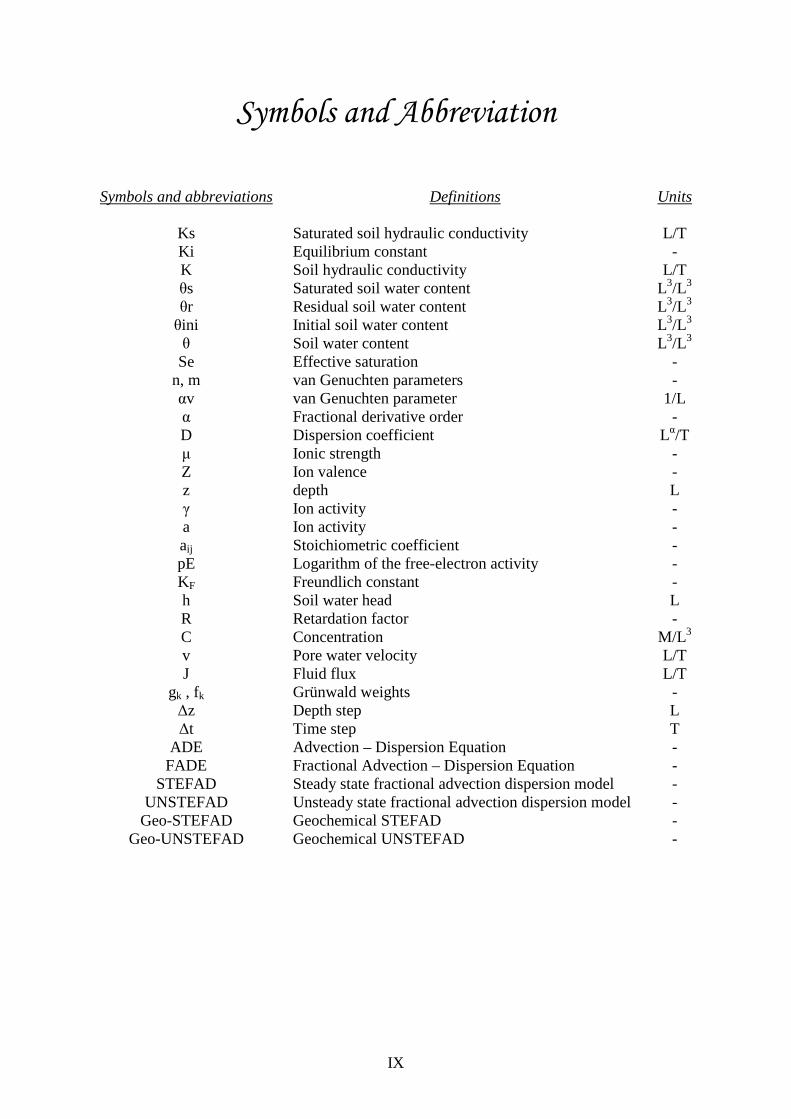
Symbols and abbreviations Definitions Units
Ks Saturated soil hydraulic conductivity L/T Ki Equilibrium constant - K Soil hydraulic conductivity L/T θs Saturated soil water content L3/L3 θr Residual soil water content L3/L3 θini Initial soil water content L3/L3 θ Soil water content L3/L3 Se Effective saturation -
n, m van Genuchten parameters - αv van Genuchten parameter 1/L α Fractional derivative order - D Dispersion coefficient Lα/T µ Ionic strength - Z Ion valence - z depth L γ Ion activity - a Ion activity - aij Stoichiometric coefficient - pE Logarithm of the free-electron activity - KF Freundlich constant - h Soil water head L R Retardation factor - C Concentration M/L3 v Pore water velocity L/T J Fluid flux L/T
gk , fk Grünwald weights - ∆z Depth step L ∆t Time step T
ADE Advection – Dispersion Equation - FADE Fractional Advection – Dispersion Equation -
STEFAD Steady state fractional advection dispersion model - UNSTEFAD Unsteady state fractional advection dispersion model -
Geo-STEFAD Geochemical STEFAD - Geo-UNSTEFAD Geochemical UNSTEFAD -
General IntroductionGeneral IntroductionGeneral IntroductionGeneral Introduction
. General introduction
1
Heavy metals are by-product of many industrial processes. They are one of the
contaminant groups of concern to the environment due to their toxic effects on human health.
Adequate techniques are needed to provide good estimates of the movement of contaminants
after they are released into the subsurface system to asses their environmental effects.
Achievement of this objective requires careful prediction of the physico-chemical interaction
of the heavy metals solution with soil. This, of course, requires an appreciation of the
mechanisms of contaminant transport through soils.
The advection – dispersion equation (ADE) is one of the most commonly used
equations for describing the contaminant transport in the porous media. Many studies
indicated that good results can be obtained with ADE to simulate the contaminant transport in
homogeneous media. However, natural porous media and aquifers usually are heterogeneous.
Accumulated researches showed that the traditional ADE associated with Fickian diffusion is
no longer applicable to the anomalous diffusion in heterogeneous media. Therefore, fractional
advection-dispersion equation (FADE) was derived and used to simulate the non-Fickian
transport process. The basic idea of the FADE is that the dispersion flux is proportional to the
fractional derivative gradient of the contaminant concentration, and the effect of the
heterogeneity of the porous media on contaminants transport is reflected by the exponent of
the fractional derivative.
Furthermore, the existing transport models have many limitations such as: (1)
dissolved concentration of each component is predicted, regardless of the speciation effects of
the other contaminants along the flow path, (2) physico-chemical interactions among the
heavy metals solutions, other contaminants and soil surface properties (cation exchange
capacity, surface area) cannot be simulated, and (3) profile of the heavy metals partitioning (
dissolved in aqueous phase and adsorbed or precipitated on the soil surface) cannot be
predicted. On the other hand, the geochemical models consider all chemical reactions
including aqueous complex, reduction/oxidation, acid/base reactions, sorption via surface
reactions and precipitation/dissolution. It does not provide the partitioning of heavy metals
with time and space unless coupled to a suitable transport model.
This study aims to developing a coupled fractional solute transport and chemical
equilibrium speciation model which accounts for most of the hydro-geochemical interactions
of heavy metals with the homogeneous and heterogeneous soils. Also, to predict long term
migration and retention of a heavy metals solution into the soils through the proposed model,
suitably calibrated with the experimental data.

. General introduction
2
To achieve these objectives and goals, various tasks will be performed. These include:
(1) reviewing the existing geochemical/transport models, (2) formulating the coupled
fractional hydro-geochemical model, (3) programming the solution of the proposed model by
using MATLAB programming language, (4) validating the model by using experimental
results, and (5) application of the proposed fractional hydro-geochemical transport model for
simulating heavy metals transport in the unsaturated soil zone.
In this study, zinc will be selected as a sample of heavy metals depending on its
mobility and its wide uses and production.
The thesis consists of four chapters: Chapter one summarizes theoretical basics and
literature review. This chapter consists of four sections: zinc contamination; geochemical
reaction models; water flow models; and fractional advection dispersion model. Chapter two
shows the formulation of the fractional model coupled with the geochemical model at the
steady state. It contains also the analytical solutions of each model with the coupling
procedure. These models are validated with the experimental data. Chapter three shows the
formulation of the soil water flow model, fractional solute transport model and the
geochemical model at the unsteady state. It contains the numerical solution procedures at its
validations. Chapter four represents the application of the fractional hydro-geochemical
model for predicting zinc migration in the unsaturated soil zone. This chapter consists of three
sections: site description, parameters estimation, sensitivity analysis (for the water flow
model, fractional solute transport model and the geochemical reactions model). In the end,
general conclusions and recommendations for further studies will be proposed.
. General introduction
ChapterChapterChapterChapter One One One One
Theoretical Basics and Literature ReviewTheoretical Basics and Literature ReviewTheoretical Basics and Literature ReviewTheoretical Basics and Literature Review
Chapter one Theoretical basics and literature review
-3-
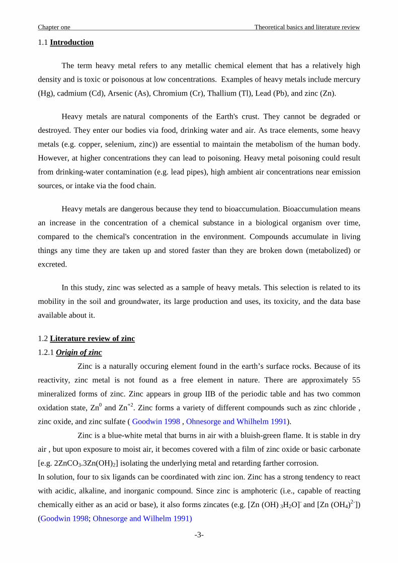
1.1 Introduction
The term heavy metal refers to any metallic chemical element that has a relatively high
density and is toxic or poisonous at low concentrations. Examples of heavy metals include mercury
(Hg), cadmium (Cd), Arsenic (As), Chromium (Cr), Thallium (Tl), Lead (Pb), and zinc (Zn).
Heavy metals are natural components of the Earth's crust. They cannot be degraded or
destroyed. They enter our bodies via food, drinking water and air. As trace elements, some heavy
metals (e.g. copper, selenium, zinc)) are essential to maintain the metabolism of the human body.
However, at higher concentrations they can lead to poisoning. Heavy metal poisoning could result
from drinking-water contamination (e.g. lead pipes), high ambient air concentrations near emission
sources, or intake via the food chain.
Heavy metals are dangerous because they tend to bioaccumulation. Bioaccumulation means
an increase in the concentration of a chemical substance in a biological organism over time,
compared to the chemical's concentration in the environment. Compounds accumulate in living
things any time they are taken up and stored faster than they are broken down (metabolized) or
excreted.
In this study, zinc was selected as a sample of heavy metals. This selection is related to its
mobility in the soil and groundwater, its large production and uses, its toxicity, and the data base
available about it.
1.2 Literature review of zinc
1.2.1 Origin of zinc
Zinc is a naturally occuring element found in the earth’s surface rocks. Because of its
reactivity, zinc metal is not found as a free element in nature. There are approximately 55
mineralized forms of zinc. Zinc appears in group IIB of the periodic table and has two common
oxidation state, Zn0 and Zn+2. Zinc forms a variety of different compounds such as zinc chloride ,
zinc oxide, and zinc sulfate ( Goodwin 1998 , Ohnesorge and Whilhelm 1991).
Zinc is a blue-white metal that burns in air with a bluish-green flame. It is stable in dry
air , but upon exposure to moist air, it becomes covered with a film of zinc oxide or basic carbonate
[e.g. 2ZnCO3.3Zn(OH)2] isolating the underlying metal and retarding farther corrosion.
In solution, four to six ligands can be coordinated with zinc ion. Zinc has a strong tendency to react
with acidic, alkaline, and inorganic compound. Since zinc is amphoteric (i.e., capable of reacting
chemically either as an acid or base), it also forms zincates (e.g. [Zn (OH) 3H2O]- and [Zn (OH4)2-])
(Goodwin 1998; Ohnesorge and Wilhelm 1991)
Chapter one Theoretical basics and literature review
-4-
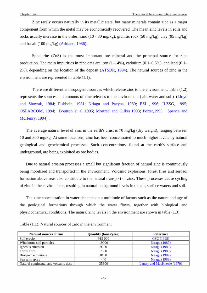
Zinc rarely occurs naturally in its metallic state, but many minerals contain zinc as a major
component from which the metal may be economically recovered. The mean zinc levels in soils and
rocks usually increase in the order: sand (10 - 30 mg/kg), granitic rock (50 mg/kg), clay (95 mg/kg)
and basalt (100 mg/kg) (Adriano, 1986).
Sphalerite (ZnS) is the most important ore mineral and the principal source for zinc
production. The main impurities in zinc ores are iron (1–14%), cadmium (0.1–0.6%), and lead (0.1–
2%), depending on the location of the deposit (ATSDR, 1994). The natural sources of zinc in the
environment are represented in table (1.1).
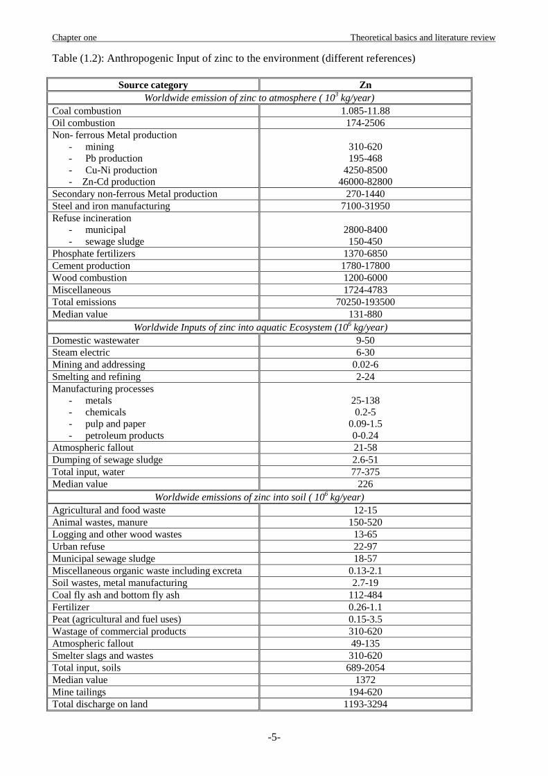
There are different anthropogenic sources which release zinc to the environment. Table (1.2)
represents the sources and amounts of zinc releases to the environment ( air, water and soil) (Lioyd
and Showak, 1984; Fishbein, 1981; Nriagu and Pacyna, 1989; EZI ,1996; ILZSG, 1995;
OSPARCOM, 1994; Boutron et al.,1995; Mortred and Gilkes,1993; Porter,1995; Spence and
McHenry, 1994) .
The average natural level of zinc in the earth's crust is 70 mg/kg (dry weight), ranging between
10 and 300 mg/kg. At some locations, zinc has been concentrated to much higher levels by natural
geological and geochemical processes. Such concentrations, found at the earth's surface and
underground, are being exploited as ore bodies.
Due to natural erosion processes a small but significant fraction of natural zinc is continuously
being mobilized and transported in the environment. Volcanic explosions, forest fires and aerosol
formation above seas also contribute to the natural transport of zinc. These processes cause cycling
of zinc in the environment, resulting in natural background levels in the air, surface waters and soil.
The zinc concentration in water depends on a multitude of factors such as the nature and age of
the geological formations through which the water flows, together with biological and
physicochemical conditions. The natural zinc levels in the environment are shown in table (1.3).
Table (1.1): Natural sources of zinc in the environment
Natural sources of zinc Quantity (tones/year) Reference Soil erosion 915 000 GSC (1995) Windborne soil particles 19000 Niragu (1989) Igneous emission 9600 Niragu (1989) Forest fires 7600 Niragu (1989) Biogenic emissions 8100 Niragu (1989) Sea salts spray 440 Niragu (1989) Natural continental and volcanic dust 35800 Lantzy and MacKnezie (1979)
Chapter one Theoretical basics and literature review
-5-
Table (1.2): Anthropogenic Input of zinc to the environment (different references)
Source category Zn Worldwide emission of zinc to atmosphere ( 103 kg/year)
Coal combustion 1.085-11.88 Oil combustion 174-2506 Non- ferrous Metal production
- mining - Pb production - Cu-Ni production - Zn-Cd production
310-620 195-468
4250-8500 46000-82800
Secondary non-ferrous Metal production 270-1440 Steel and iron manufacturing 7100-31950 Refuse incineration
- municipal - sewage sludge
2800-8400 150-450
Phosphate fertilizers 1370-6850 Cement production 1780-17800 Wood combustion 1200-6000 Miscellaneous 1724-4783 Total emissions 70250-193500 Median value 131-880
Worldwide Inputs of zinc into aquatic Ecosystem (106 kg/year) Domestic wastewater 9-50 Steam electric 6-30 Mining and addressing 0.02-6 Smelting and refining 2-24 Manufacturing processes
- metals - chemicals - pulp and paper - petroleum products
25-138 0.2-5
0.09-1.5 0-0.24
Atmospheric fallout 21-58 Dumping of sewage sludge 2.6-51 Total input, water 77-375 Median value 226
Worldwide emissions of zinc into soil ( 106 kg/year) Agricultural and food waste 12-15 Animal wastes, manure 150-520 Logging and other wood wastes 13-65 Urban refuse 22-97 Municipal sewage sludge 18-57 Miscellaneous organic waste including excreta 0.13-2.1 Soil wastes, metal manufacturing 2.7-19 Coal fly ash and bottom fly ash 112-484 Fertilizer 0.26-1.1 Peat (agricultural and fuel uses) 0.15-3.5 Wastage of commercial products 310-620 Atmospheric fallout 49-135 Smelter slags and wastes 310-620 Total input, soils 689-2054 Median value 1372 Mine tailings 194-620 Total discharge on land 1193-3294
Chapter one Theoretical basics and literature review
-6-
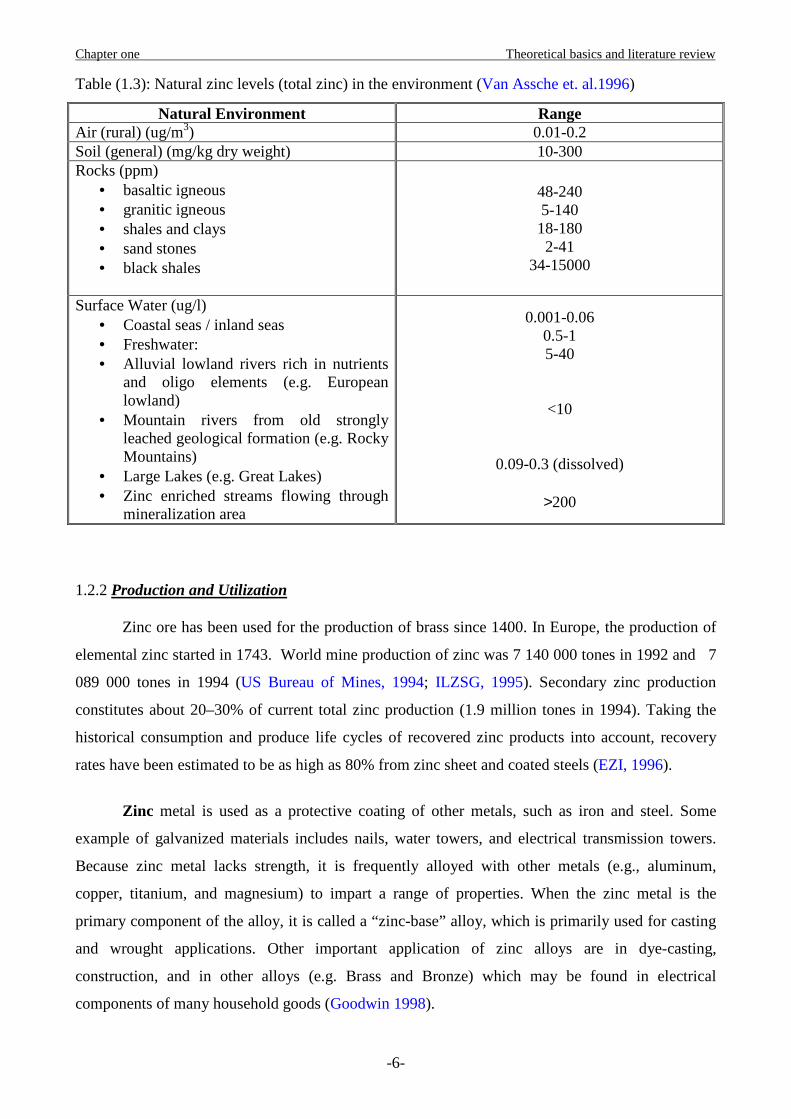
Table (1.3): Natural zinc levels (total zinc) in the environment (Van Assche et. al.1996)
Natural Environment Range Air (rural) (ug/m3) 0.01-0.2 Soil (general) (mg/kg dry weight) 10-300 Rocks (ppm)
• basaltic igneous • granitic igneous • shales and clays • sand stones • black shales
48-240 5-140 18-180 2-41
34-15000
Surface Water (ug/l) • Coastal seas / inland seas • Freshwater: • Alluvial lowland rivers rich in nutrients
and oligo elements (e.g. European lowland)
• Mountain rivers from old strongly leached geological formation (e.g. Rocky Mountains)
• Large Lakes (e.g. Great Lakes) • Zinc enriched streams flowing through
mineralization area
0.001-0.06 0.5-1 5-40
<10
0.09-0.3 (dissolved)
>200
1.2.2 Production and Utilization
Zinc ore has been used for the production of brass since 1400. In Europe, the production of
elemental zinc started in 1743. World mine production of zinc was 7 140 000 tones in 1992 and 7
089 000 tones in 1994 (US Bureau of Mines, 1994; ILZSG, 1995). Secondary zinc production
constitutes about 20–30% of current total zinc production (1.9 million tones in 1994). Taking the
historical consumption and produce life cycles of recovered zinc products into account, recovery
rates have been estimated to be as high as 80% from zinc sheet and coated steels (EZI, 1996).
Zinc metal is used as a protective coating of other metals, such as iron and steel. Some
example of galvanized materials includes nails, water towers, and electrical transmission towers.
Because zinc metal lacks strength, it is frequently alloyed with other metals (e.g., aluminum,
copper, titanium, and magnesium) to impart a range of properties. When the zinc metal is the
primary component of the alloy, it is called a “zinc-base” alloy, which is primarily used for casting
and wrought applications. Other important application of zinc alloys are in dye-casting,
construction, and in other alloys (e.g. Brass and Bronze) which may be found in electrical
components of many household goods (Goodwin 1998).
Chapter one Theoretical basics and literature review
-7-
Zinc chloride is used in wood preservation, solder fluxes, and batteries. Solution of zinc
chloride is widely used in mercerizing cotton and as a mordant in dying. In medicine, zinc chloride
is used as an antiseptic, disinfectant, deodorant and in dental cement, in rubber vulcanization, and
oil refining (Goodwin 1998). Zinc chloride is a primary ingredient in smoke bombs used for crowd
dispersal, in fire-fighting exercises (by both military and civilian communities).
Zinc oxide accounts for the largest use of zinc compounds, and is used primarily by the
rubber industry as a vulcanization activator and accelerator and to slow rubber aging by neutralizing
sulfur and organic acids formed by oxidation. It is also acts in rubber as a reinforcing agent, a heat
conductor, a white pigment, and an absorber of UV light. In paints, zinc oxides serve as a mild
waste, acid buffer, and a pigment. It is used in animal feed as a zinc supplement and as fertilizer-
additive for zinc- deficient soils. Zinc oxide is used in cosmetics and drugs primarily for its
fungicide properties, and in dentistry in dental cements. It is also used in ceramics, in glass
manufacture, as a catalyst in organic synthesis, and in coated photocopy paper (Goodwin 1998).
Zinc sulfate is used in fertilizers, sprays, and animal feed as a trace element and disease-
control agent. It is used in the manufacture of rayon, in textile dying and printing, in flotation
reagents, for electro galvanizing, in paper bleaching, and in glue (Goodwin 1998).
1.2.3 Toxicity of Zinc and Zinc Compounds
Zinc is an essential element. The recommended daily allowance is 15 mg for adult males, 12
mg for adult females, 15 mg for pregnant women, 19 mg for nursing mothers during the first six
months and 16 mg during the second six months, 10 mg for children older than 1 year, and 5 mg for
infants 0-12 months old (NRC, 1989).
Oral Exposures
Gastrointestinal distress is a common symptom of acute oral exposure to zinc compounds
(ATSDR, 1994), particularly when zinc salts of strong mineral acids are ingested (Stokinger, 1981).
Accidental poisonings have occurred as a result of the therapeutic use of zinc supplements and from
food contamination caused by the use of zinc galvanized containers. Symptoms include nausea,
vomiting, diarrhea, and abdominal cramps (Stokinger, 1981; Elinder, 1986). The concentration in
drinking water that can cause an emetic effect ranges from 675 to 2,280 ppm (Stokinger, 1981).
Severe toxic effects have also been reported in cases of ingestion of zinc chloride. A single dose
(amount not reported) caused burning in the mouth and throat, vomiting, pharyngitis, esophagitis,
hypocalcaemia (Chobanian, 1981). One of the most toxic inorganic zinc compounds is the
Chapter one Theoretical basics and literature review
-8-
rodenticide zinc phosphide, which releases phosphine gas under acidic conditions in the stomach.
Poisonings with this substance can result in vomiting, anorexia, abdominal pain, lethargy,
hypotension, cardiac arrhythmias, circulatory collapse, pulmonary edema, seizures, renal damage,
leukopenia, and coma and death in days to weeks (Mack, 1989). The estimated fatal dose is 40
mg/kg.
Inhalation Exposures
Inhalation exposure to high concentrations of some zinc compounds can result in toxic effects
to the respiratory system (ATSDR, 1994). Inhalation of zinc oxide fumes has been associated with
"metal fume fever" (Bertholf, 1988) characterized by nasal passage irritation, cough, rales, headache,
altered taste, fever, weakness, hyperpnoea, sweating, pains in the legs and chest, reduced lung
volume, and decreased diffusing capacity of carbon monoxide. Hives and angioedema were also
reported in one case (Farrell, 1987). General symptoms can appear at concentrations as low as 15
mg/m3. A concentration as high as 600 mg Zn/m3 for only a few minutes can cause effects in several
hours. Leukocytosis is a secondary effect that has been reported in cases of "metal fume fever"
(Sturgis et al., 1927; Malo et al., 1990).
Inhalation of zinc chloride can cause nose and throat irritation, dyspnea, cough, chest pain,
headache, fever, nausea and vomiting, pneumothorax, and acute pneumonitis (ITII, 1988; ATSDR,
1994; Nemery, 1990). More severe effects include ulcerative and edematous changes in mucous
membranes, subpleural hemorrhage, advanced pulmonary fibrosis, and respiratory distress syndrome.
Fatalities have occurred in some accidental exposures (Elinder, 1986; Hjortso et al, 1988), a 4,800
mg/m3 for a 30-min exposure has been reported for zinc chloride (Stokinger, 1981).
Other Source of Exposure
Exposure to zinc-chromium compounds from galvanized steel was considered to be partially
responsible for an outbreak of irritant hand dermatitis, which affected 24 of 41 employees working on
a new assembly line of an electronics factory (Bruynzeel et al, 1988).
When administered parenterally, zinc depresses the central nervous system, causing tremors
and paralysis of the extremities (Stokinger, 1981).
1.2.4 Zinc releases to the environment in France
Air (CITEPA, 2004)
Zinc emissions decrease since 1990: 2031 tones in 1990 versus 1339 tones in 2002 (-34%). The
main source of zinc emissions is the manufacturing industry (80% of total emissions in 2002) and,
Chapter one Theoretical basics and literature review
-9-
to a lesser extent, energy conversion (15% of total emissions generated by household waste
incineration plants with energy recovery) and residential/tertiary (6%). Produced by the combustion
of coal and residual oil, zinc emissions are also generated by industrial processes in the iron and
steel industry (86%), non-ferrous metallurgy (8%) and waste incineration (2%). Significant
improvements have been carried out in the iron and steel industry since 1990. The amount of zinc
releases to atmosphere in France is described in table (1.4).
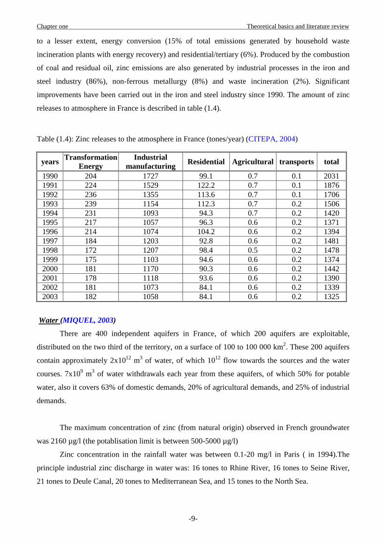
Table (1.4): Zinc releases to the atmosphere in France (tones/year) (CITEPA, 2004)
years Transformation Energy
Industrial manufacturing
Residential Agricultural transports total
1990 204 1727 99.1 0.7 0.1 2031 1991 224 1529 122.2 0.7 0.1 1876 1992 236 1355 113.6 0.7 0.1 1706 1993 239 1154 112.3 0.7 0.2 1506 1994 231 1093 94.3 0.7 0.2 1420 1995 217 1057 96.3 0.6 0.2 1371 1996 214 1074 104.2 0.6 0.2 1394 1997 184 1203 92.8 0.6 0.2 1481 1998 172 1207 98.4 0.5 0.2 1478 1999 175 1103 94.6 0.6 0.2 1374 2000 181 1170 90.3 0.6 0.2 1442 2001 178 1118 93.6 0.6 0.2 1390 2002 181 1073 84.1 0.6 0.2 1339 2003 182 1058 84.1 0.6 0.2 1325
Water (MIQUEL, 2003)
There are 400 independent aquifers in France, of which 200 aquifers are exploitable,
distributed on the two third of the territory, on a surface of 100 to 100 000 km2. These 200 aquifers
contain approximately 2x10¹² m3 of water, of which 1012 flow towards the sources and the water
courses. 7x10⁹ m3 of water withdrawals each year from these aquifers, of which 50% for potable
water, also it covers 63% of domestic demands, 20% of agricultural demands, and 25% of industrial
demands.
The maximum concentration of zinc (from natural origin) observed in French groundwater
was 2160 µg/l (the potablisation limit is between 500-5000 µg/l)
Zinc concentration in the rainfall water was between 0.1-20 mg/l in Paris ( in 1994).The
principle industrial zinc discharge in water was: 16 tones to Rhine River, 16 tones to Seine River,
21 tones to Deule Canal, 20 tones to Mediterranean Sea, and 15 tones to the North Sea.
Chapter one Theoretical basics and literature review
-10-
Soil
Baize (2000) reported the median zinc contents of soils of different textural classes: sandy
soils 17 mg/kg, silty soils (<20% clay) 40mg/kg, loams (20-30% clay) 63.5 mg/kg, clayey soils (30-
50% clay) 98 mg/kg and very clayey soils (>50% clay) 132 mg/kg.
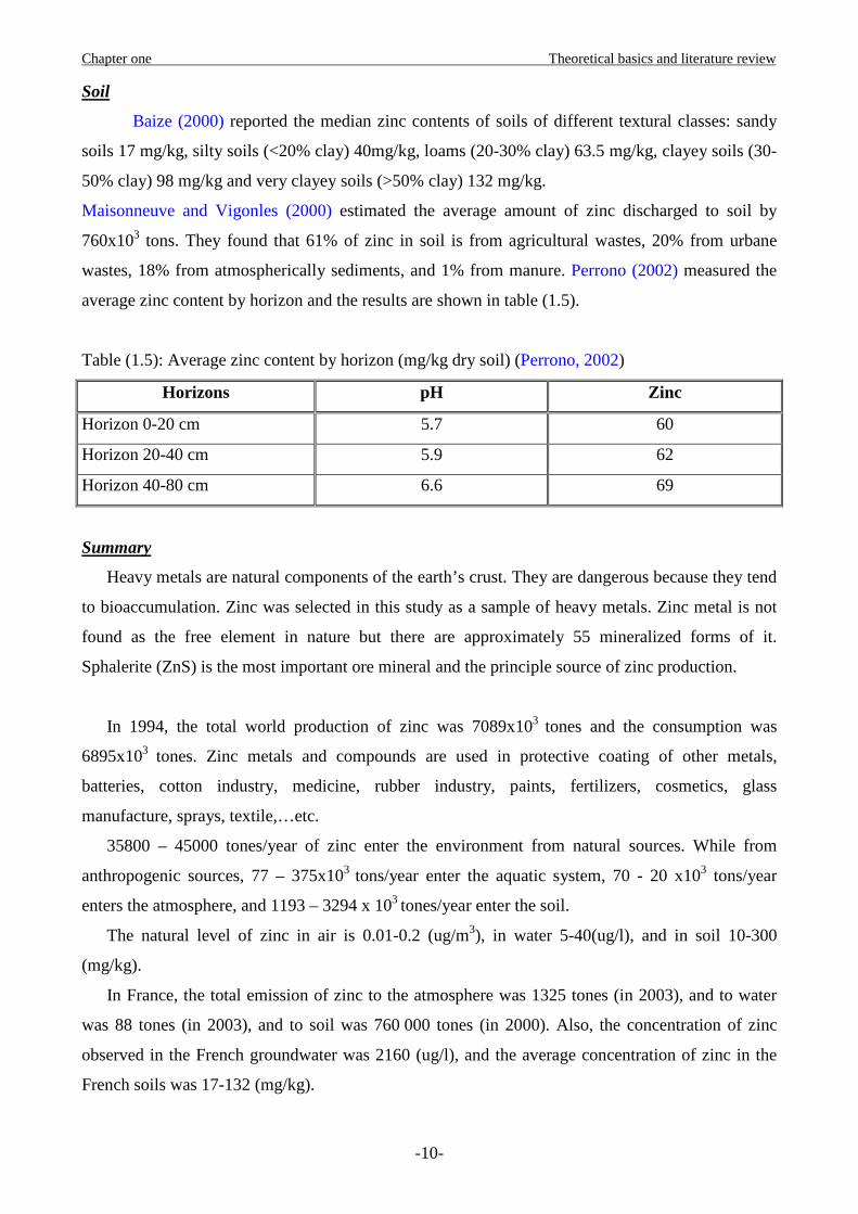
Maisonneuve and Vigonles (2000) estimated the average amount of zinc discharged to soil by
760x103 tons. They found that 61% of zinc in soil is from agricultural wastes, 20% from urbane
wastes, 18% from atmospherically sediments, and 1% from manure. Perrono (2002) measured the
average zinc content by horizon and the results are shown in table (1.5).
Table (1.5): Average zinc content by horizon (mg/kg dry soil) (Perrono, 2002)
Horizons pH Zinc
Horizon 0-20 cm 5.7 60
Horizon 20-40 cm 5.9 62
Horizon 40-80 cm 6.6 69
Summary
Heavy metals are natural components of the earth’s crust. They are dangerous because they tend
to bioaccumulation. Zinc was selected in this study as a sample of heavy metals. Zinc metal is not
found as the free element in nature but there are approximately 55 mineralized forms of it.
Sphalerite (ZnS) is the most important ore mineral and the principle source of zinc production.
In 1994, the total world production of zinc was 7089x103 tones and the consumption was
6895x103 tones. Zinc metals and compounds are used in protective coating of other metals,
batteries, cotton industry, medicine, rubber industry, paints, fertilizers, cosmetics, glass
manufacture, sprays, textile,…etc.
35800 – 45000 tones/year of zinc enter the environment from natural sources. While from
anthropogenic sources, 77 – 375x103 tons/year enter the aquatic system, 70 - 20 x103 tons/year
enters the atmosphere, and 1193 – 3294 x 103 tones/year enter the soil.
The natural level of zinc in air is 0.01-0.2 (ug/m3), in water 5-40(ug/l), and in soil 10-300
(mg/kg).
In France, the total emission of zinc to the atmosphere was 1325 tones (in 2003), and to water
was 88 tones (in 2003), and to soil was 760 000 tones (in 2000). Also, the concentration of zinc
observed in the French groundwater was 2160 (ug/l), and the average concentration of zinc in the
French soils was 17-132 (mg/kg).
Chapter one Theoretical basics and literature review
-11-
1.3 Geochemical Reactions Modeling
1.3.1 Introduction
To predict contaminant transport through the subsurface accurately, it is essential to
developing a mathematical model for the geochemical processes affecting the contaminant
transport. Dissolution/precipitation and adsorption/desorption are the most important processes
affecting contaminant interaction with soils. Dissolution/precipitation is more likely to be a key
process where chemical non-equilibrium exists. Adsorption/desorption will likely be the key
process controlling contaminant migration in area where chemical equilibrium exists.
Solute transport modelers are commonly provided with the total concentration of a dissolved
substance in a contaminant plume. They give little insight into the forms in which the metals are
present in the plume or their mobility and bioavailability. Contaminants can occur in a plume as
soluble-free, soluble-complexed, adsorbed, organically complexed, precipitated, or co-precipitated
species (Sposito, 1989). Before discussing the geochemical processes that contribute to the
formation of these species and their potential effect on contaminant transport, a brief review of the
methods of handling chemical equilibrium is discussed below.
1.3.2 Chemical Equilibria
Some chemical reactions in soils proceed with sufficient speed that equilibrium relationships
are immediately attained. Other reactions proceed so slowly that final equilibrium is probably never
attained. Regardless of the rate at which equilibrium is attained, equilibrium relationships are useful
for predicting chemical changes that can or cannot occur. Equilibrium provides a reference point for
predicting which chemical reactions can take place regardless of the rate at which they occur
(Lindsay, 2001). Equilibrium constant for the reaction:
2 24 4ZnSO Zn SO+ −+��⇀↽�� …………. 1.1
can be expressed as:
[ ]4
2 24
ZnSOK
Zn SO+ −=
� …………. 1.2
In general, for the following reaction:
aA bB cC dD+ +��⇀↽�� ………… 1.3
Chapter one Theoretical basics and literature review
-12-
The equilibrium constant can be expressed as:
[ ] [ ][ ] [ ]
a b
c d
A BK
C D=� ……… 1.4
The ionic strength is defined as:
21
2 i ic Zµ = ∑ ………. 1.5
where µ is the ionic strength, ci is the concentration in moles/liter of ion i, Zi is the valency of that
ion, and ∑ indicates that the product of each ion and its valency squared is summed for all ions
solution. The ratio of the activity of an ion ai, to its concentration, ci is called the activity coefficient
γi:
ii
i
a
cγ = ……….. 1.6
Knowing γi, we are able to convert from concentration to activities, and vice versa.
The Debye-Hückel theory of estimating activity coefficients is based on laws of
electrostatics and thermodynamics. In essence, it assumes that ions behave like point charges in a
continuous medium with a dielectric constant equal to that of the solvent. The resulting equation for
calculating activity coefficients of simple ions in aqueous solutions is
2 1/ 2log i iAZγ µ= − ……… 1.7
where A=0.509 for water at 250C. By extending the Debye-Hückel theory to account for the
effective size of hydrated ions, a more precise equation is obtained, that is,
1/ 22
1/2log
1i ii
AZBd
µγµ
= −+
……… 1.8
where B = 0.328 x 10⁸ for water at 250C, di value for Zn2+ is 6. Davis (1962) proposed the following
equation:
1/ 22
1/ 2log 0.3
1i iAZµγ µ
µ
= − − + …….. 1.9
The latter equation is often used in preference to the extended Debye-Hückel equation because the
single variable is more adopted to simplify calculations.
Chapter one Theoretical basics and literature review
-13-
I. Aqueous complexation
The soil solution is defined as the aqueous liquid phase of the soil and its solutes. The
majority of solutes in the soil solution are ions, which occur either as free hydrated ions, or as
various complexes with organic or inorganic ligands. The equilibrium constant can describe the
distribution of a given constituent among its possible chemical forms if complex formation and
dissociation reactions are at equilibrium. The constant is affected by the ionic strength of the
aqueous phase and temperature.
The most common complexing anions present in groundwater are HCO3-, CO3
2-, Cl-, SO42-, and
humic substances (i.e., organic materials). Possible outcomes of lowering the activity of the free
species of the metal include lowering the potential for adsorption and increasing its solubility, both
of which can enhance migration potential. On the other hand, some complexants (e.g., humic acids)
readily bond to soils and thus retard the migration of the complexed metals.
II. Redox Reactions
An oxidation reduction (Redox) reaction is a chemical reaction in which electrons are
transferred completely from one species to another. The chemical species that loses electrons in this
charge transfer process is described as oxidized, and the species receiving electrons is described as
reducer.
The electron activity is a useful conceptual device for describing the redox status of aqueous
systems, just as the aqueous proton activity is so useful for describing the acid – base status of soils.
Similar to pH, the propensity of a system to be oxidized can be expressed by the negative common
logarithm of the free-electron activity, pE:
pE = -log (e-) ………1.10
the range of pE in the natural environment varies between approximately 7 and 17 in the vadose
zone (Sposito, 1989). The most important chemical elements affected by redox reactions in ambient
groundwater are carbon, nitrogen, oxygen, sulfur, manganese, and iron.
III. Adsorption
Adsorption reactions of zinc in soils are important to understand the solid and liquid phase
interaction determining the release and fixation of applied zinc and thereby the efficiency of
fertilization. The physico-chemical properties play a key role in influencing the process. Because of
the heterogeneity of soils, adsorption isotherms are typically different for different soils and
Chapter one Theoretical basics and literature review
-14-
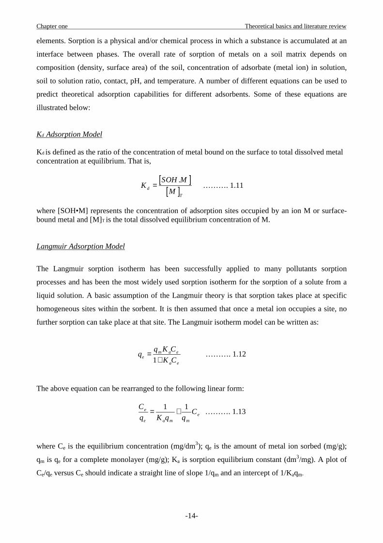
elements. Sorption is a physical and/or chemical process in which a substance is accumulated at an
interface between phases. The overall rate of sorption of metals on a soil matrix depends on
composition (density, surface area) of the soil, concentration of adsorbate (metal ion) in solution,
soil to solution ratio, contact, pH, and temperature. A number of different equations can be used to
predict theoretical adsorption capabilities for different adsorbents. Some of these equations are
illustrated below:
Kd Adsorption Model Kd is defined as the ratio of the concentration of metal bound on the surface to total dissolved metal concentration at equilibrium. That is,
[ ][ ]
.d
T
SOH MK
M= ………. 1.11
where [SOH•M] represents the concentration of adsorption sites occupied by an ion M or surface-bound metal and [M]T is the total dissolved equilibrium concentration of M. Langmuir Adsorption Model
The Langmuir sorption isotherm has been successfully applied to many pollutants sorption
processes and has been the most widely used sorption isotherm for the sorption of a solute from a
liquid solution. A basic assumption of the Langmuir theory is that sorption takes place at specific
homogeneous sites within the sorbent. It is then assumed that once a metal ion occupies a site, no
further sorption can take place at that site. The Langmuir isotherm model can be written as:
1m a e
ea e
q K Cq
K C=
+ ………. 1.12
The above equation can be rearranged to the following linear form:
1 1ee
e a m m
CC
q K q q= + ………. 1.13
where Ce is the equilibrium concentration (mg/dm3); qe is the amount of metal ion sorbed (mg/g);
qm is qe for a complete monolayer (mg/g); Ka is sorption equilibrium constant (dm3/mg). A plot of
Ce/qe versus Ce should indicate a straight line of slope 1/qm and an intercept of 1/Kaqm.
Chapter one Theoretical basics and literature review
-15-
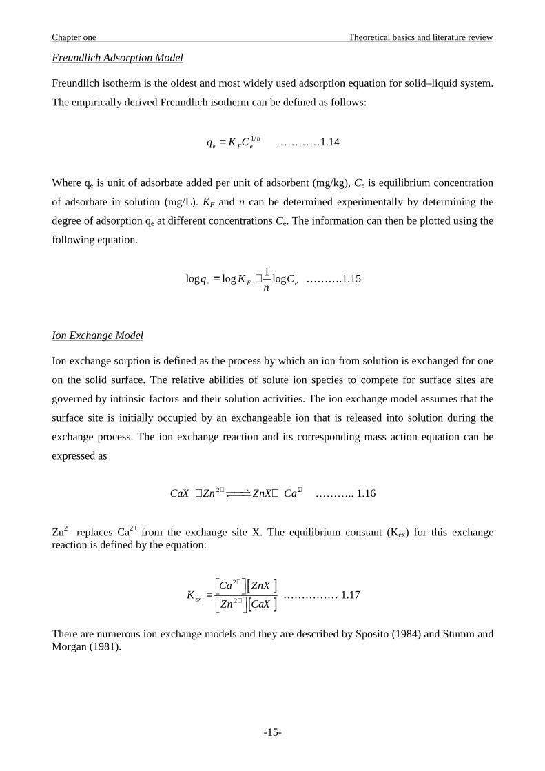
Freundlich Adsorption Model Freundlich isotherm is the oldest and most widely used adsorption equation for solid–liquid system.
The empirically derived Freundlich isotherm can be defined as follows:
1/ne F eq K C= …………1.14
Where qe is unit of adsorbate added per unit of adsorbent (mg/kg), Ce is equilibrium concentration
of adsorbate in solution (mg/L). KF and n can be determined experimentally by determining the
degree of adsorption qe at different concentrations Ce. The information can then be plotted using the
following equation.
1
log log loge F eq K Cn
= + ……….1.15
Ion Exchange Model Ion exchange sorption is defined as the process by which an ion from solution is exchanged for one
on the solid surface. The relative abilities of solute ion species to compete for surface sites are
governed by intrinsic factors and their solution activities. The ion exchange model assumes that the
surface site is initially occupied by an exchangeable ion that is released into solution during the
exchange process. The ion exchange reaction and its corresponding mass action equation can be
expressed as
2 2CaX Zn ZnX Ca+ ++ +��⇀↽�� ……….. 1.16
Zn2+ replaces Ca2+ from the exchange site X. The equilibrium constant (Kex) for this exchange reaction is defined by the equation:
[ ][ ]
2
2ex
Ca ZnXK
Zn CaX
+
+
=
…………… 1.17
There are numerous ion exchange models and they are described by Sposito (1984) and Stumm and Morgan (1981).

Chapter one Theoretical basics and literature review
-16-
IV. Precipitation . The precipitation reaction of dissolved species is a special case of the complexation reaction in
which the complex formed by two or more aqueous species is a solid. Precipitation is particularly
important to the behavior of heavy metals in soil-groundwater systems. As an example, consider the
formation of a sulfide precipitate with a bivalent cation (M2+):
222 ( ) ( )M HS M HS s+ −+ = ………. 1.18
The equilibrium constant Keq, is:
2( )
2 22 2
( ) 1s
eq
M HSK
M HS M HS+ − + −
= =
..…….. 1.19
By convention, the concentration of pure solid phase is set equal to unity (Stumm and Morgan,
1996). Therefore, the solubility product is:
22spK M HS+ − = ………. 1.20
Precipitation and co-precipitation is more likely to occur in the high salts concentration and large
pH gradient environment. Solubility models are thermodynamic equilibrium models and typically
do not consider the time (i.e. kinetics) required to dissolved or completely precipitate. When
identification of the likely controlling solid is difficult or when kinetic constraints are suspected,
empirical solubility experiments are often performed to gather data that can be used to generate an
empirical solubility release model.
1.3.3 Chemical Reactions Codes
A chemical reaction model is defined as the integration of mathematical expressions
describing theoretical concepts and thermodynamic relationships on which the aqueous speciation,
oxidation/reduction, precipitation/dissolution, and adsorption/desorption calculations are based. A
chemical reaction code refers to the translation of a chemical reaction model into a sequence of
statements in a particular computer language. Most chemical reaction models are based on
equilibrium conditions, and contain limited or no kinetic equations in any of their sub-models.
Chapter one Theoretical basics and literature review
-17-
Numerous reviews of chemical reaction codes have been published. Some of the more extensive
reviews include those by Jenne 1981; Kincaid et al. 1984; Mercer et al. 1981; Nordstrom et al.
1979; Nordstrom and Ball 1984; Nordstrom and Munoz 1985; Potter 1979; and others. These
reviews have been briefly described in Serne et al., 1990. The reviews discuss issues such as: (1)
Basic mathematical and thermodynamic approaches that are required to formulate the problem of
solving geochemical equilibria in aqueous solutions, (2)Applications for which these codes have
been developed and used, such as the modeling of adsorption equilibria, complexation and
solubility of trace metals, equilibria in brine solutions and high-temperature geothermal fluids, mass
transfer, fluid flow and mass transport, and redox balance of aqueous solutions,(3) Selection of
thermodynamic data and development of thermodynamic databases, (4)Limitations of chemical
reaction codes, such as the testing of the equilibrium assumption, application of these models to
high-ionic strength aqueous solutions, the reliability of thermodynamic databases, and the use of
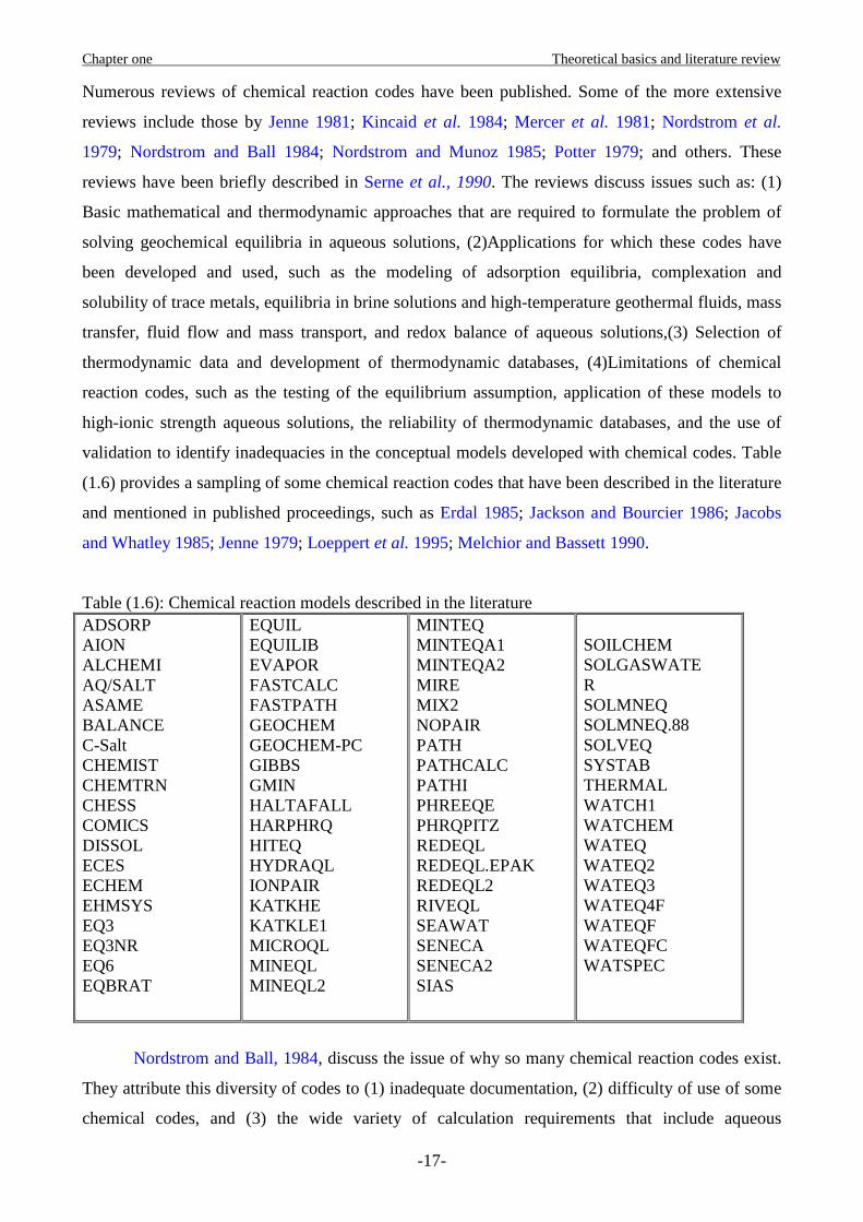
validation to identify inadequacies in the conceptual models developed with chemical codes. Table
(1.6) provides a sampling of some chemical reaction codes that have been described in the literature
and mentioned in published proceedings, such as Erdal 1985; Jackson and Bourcier 1986; Jacobs
and Whatley 1985; Jenne 1979; Loeppert et al. 1995; Melchior and Bassett 1990.
Table (1.6): Chemical reaction models described in the literature ADSORP AION ALCHEMI AQ/SALT ASAME BALANCE C-Salt CHEMIST CHEMTRN CHESS COMICS DISSOL ECES ECHEM EHMSYS EQ3 EQ3NR EQ6 EQBRAT
EQUIL EQUILIB EVAPOR FASTCALC FASTPATH GEOCHEM GEOCHEM-PC GIBBS GMIN HALTAFALL HARPHRQ HITEQ HYDRAQL IONPAIR KATKHE KATKLE1 MICROQL MINEQL MINEQL2
MINTEQ MINTEQA1 MINTEQA2 MIRE MIX2 NOPAIR PATH PATHCALC PATHI PHREEQE PHRQPITZ REDEQL REDEQL.EPAK REDEQL2 RIVEQL SEAWAT SENECA SENECA2 SIAS
SOILCHEM SOLGASWATE R SOLMNEQ SOLMNEQ.88 SOLVEQ SYSTAB THERMAL WATCH1 WATCHEM WATEQ WATEQ2 WATEQ3 WATEQ4F WATEQF WATEQFC WATSPEC
Nordstrom and Ball, 1984, discuss the issue of why so many chemical reaction codes exist.
They attribute this diversity of codes to (1) inadequate documentation, (2) difficulty of use of some
chemical codes, and (3) the wide variety of calculation requirements that include aqueous
Chapter one Theoretical basics and literature review
-18-
speciation, solubility, and/or adsorption (calculations for aqueous systems that range from simple,
chemical systems associated with laboratory experiments to complex, multi-component systems
associated with natural environments). No single code can do all of the desired calculations in a
perfectly general way.
Jenne, 1981, divides chemical reaction codes into 2 general categories: aqueous speciation-
solubility codes and reaction path codes. All of the aqueous speciation-solubility codes may be used
to calculate aqueous speciation/complexation, and the degree of saturation of the speciated
composition of the aqueous. Chemical reaction codes, such as WATEQ, REDEQL, GEOCHEM,
MINEQL, MINTEQ, and their later versions, are examples of codes of this type.
Reaction path codes include the capabilities to calculate aqueous speciation and the degree of
saturation of aqueous solutions, but also permit the simulation of mass transfer due to mineral
precipitation/dissolution or adsorption onto adsorbents as a function of reaction progress. Examples
of reaction path codes include the PHREEQE, PATHCALC, and the EQ3/EQ6 series of codes.
Adsorption models incorporated into chemical reaction codes include non-electrostatic, empirical
models as well as the more mechanistic and data intensive, electrostatic, surface complexation
models. Examples of non-electrostatic models include the partition (or distribution) coefficient (Kd),
Langmuir isotherm, Freundlich isotherm, and ion exchange models. The electrostatic, surface
complexation models (SCMs) incorporated into chemical reaction codes include the diffuse layer
model (DLM) [or diffuse double layer model (DDLM)], constant capacitance model (CCM), Basic
Stern model, and triple layer model (TLM). Some of the chemical reaction codes identified in the
reviews by Goldberg, 1995, and Davis and Kent, 1990, as having adsorption models include
HARPHRE (Brown et al., 1991), HYDRAQL (Papelis et al., 1988), SOILCHEM (Sposito and
Coves, 1988), and the MINTEQ series of chemical reaction codes.
1.3.4 Speciation of zinc in the soil solution
The mobility and the bioavailability of a trace metal depend not only on his total
concentration but also on his speciation in a soil solution. The total amount of zinc in soils is
distributed over five fractions. These comprise: (1) the water soluble fraction which is present in the
soil solution, (2) exchangeable fraction in which ions bound to soil particles by electrical charges,
(3) organically bound fraction: ions adsorbed or complexed with organic ligands, (4) fraction of
zinc sorbed (non-exchangeable) onto clay minerals and insoluble metallic oxides, (5) fraction of
weathering primary minerals (Alloway,2004).
It is only the zinc in the soluble fractions and those from which ions can be desorbed which
are available to plants and which are also potentially leachable in water percolating down through
the soil profile. The distribution of zinc between these forms is governed by the equilibrium
Chapter one Theoretical basics and literature review
-19-
constants of the corresponding reactions in which zinc is involved. These reactions include
precipitation and dissolution, complexation and decomplexation, adsorption and desorption.
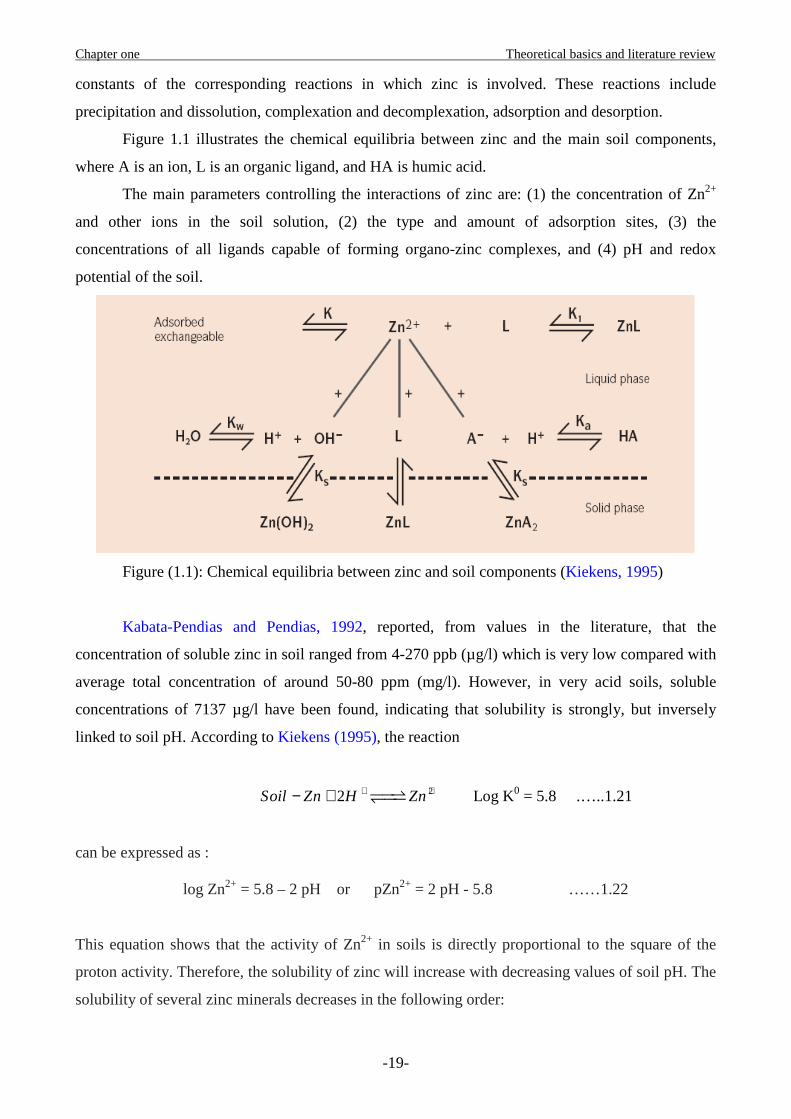
Figure 1.1 illustrates the chemical equilibria between zinc and the main soil components,
where A is an ion, L is an organic ligand, and HA is humic acid.
The main parameters controlling the interactions of zinc are: (1) the concentration of Zn2+
and other ions in the soil solution, (2) the type and amount of adsorption sites, (3) the
concentrations of all ligands capable of forming organo-zinc complexes, and (4) pH and redox
potential of the soil.
Figure (1.1): Chemical equilibria between zinc and soil components (Kiekens, 1995)
Kabata-Pendias and Pendias, 1992, reported, from values in the literature, that the
concentration of soluble zinc in soil ranged from 4-270 ppb (µg/l) which is very low compared with
average total concentration of around 50-80 ppm (mg/l). However, in very acid soils, soluble
concentrations of 7137 µg/l have been found, indicating that solubility is strongly, but inversely
linked to soil pH. According to Kiekens (1995), the reaction
22Soil Zn H Zn+ +− + ��⇀↽�� Log K0 = 5.8 .…..1.21 can be expressed as :
log Zn2+ = 5.8 – 2 pH or pZn2+ = 2 pH - 5.8 ……1.22
This equation shows that the activity of Zn2+ in soils is directly proportional to the square of the
proton activity. Therefore, the solubility of zinc will increase with decreasing values of soil pH. The
solubility of several zinc minerals decreases in the following order:
Chapter one Theoretical basics and literature review
-20-
Zn(OH) > α-Zn(OH)2 > β-Zn(OH)2 > γ-Zn(OH)2 > ε-Zn(OH)2 > ZnCO3 > ZnO > Zn(PO4)2.4H2O >
soil Zn > ZnFe2O4 .
Soil pH governs the speciation of zinc in solution. At pH values below 7.7, Zn2+ predominates but
above pH 7.7, ZnOH+ is the main species, and above pH 9.11 the neutral species Zn(OH)2 is
dominant. At pH 5 the activity of Zn2+ is 10–4 M (6.5 mg/L) but at pH 8 it decreases to 10–10 M
(0.007 µg/L) (Kiekens, 1995).
Zinc forms soluble complexes with chloride, phosphate, nitrate and sulphate ions, but the neutral
sulphate (ZnSO40) and phosphate (ZnHPO4
0) species are the most important and contribute to the
total concentration of zinc in solution. The ZnSO40 complex may increase the solubility of Zn2+ in
soils and accounts for the increased availability of zinc when acidifying fertilizers are used.
Low molecular weight organic acids also form soluble complexes with zinc and contribute to the
total soluble concentration in a soil. The often observed improvement in the available zinc status of
some deficient soils after heavy applications of manure is probably the result of an increase in
soluble, organically complexed forms of zinc. Barrow, 1993, reported work which showed that
organic ligands reduced the amounts of zinc adsorbed onto an oxisol soil and that the effect was
most pronounced with those ligands, including humic acids, that complexed zinc most strongly.
Soluble forms of organically complexed zinc can result in zinc becoming increasingly mobile and
plant available in soils. In many cases, complexation of organic zinc with organic ligands will result
in decreased adsorption onto mineral surfaces (Harter, 1991).
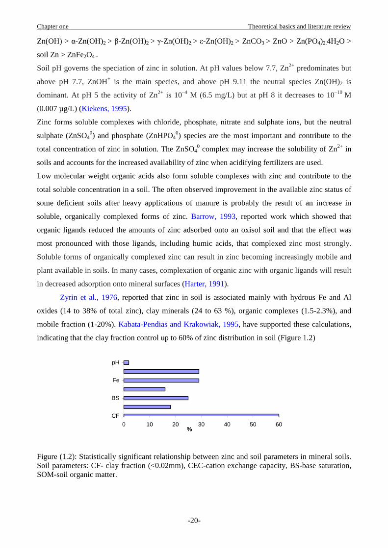
Zyrin et al., 1976, reported that zinc in soil is associated mainly with hydrous Fe and Al
oxides (14 to 38% of total zinc), clay minerals (24 to 63 %), organic complexes (1.5-2.3%), and
mobile fraction (1-20%). Kabata-Pendias and Krakowiak, 1995, have supported these calculations,
indicating that the clay fraction control up to 60% of zinc distribution in soil (Figure 1.2)
0 10 20 30 40 50 60
CF
BS
Fe
pH
%
Figure (1.2): Statistically significant relationship between zinc and soil parameters in mineral soils. Soil parameters: CF- clay fraction (<0.02mm), CEC-cation exchange capacity, BS-base saturation, SOM-soil organic matter.
Chapter one Theoretical basics and literature review
-21-
Abd-Elfatah and Wada, 1981, found that the clay minerals, hydrous oxides, and pH are
likely to be the most important factors controlling zinc speciation in soil, while organic complexing
and precipitation of Zn as hydroxides, carbonate, and sulfide compounds appear to be of much
lesser importance.
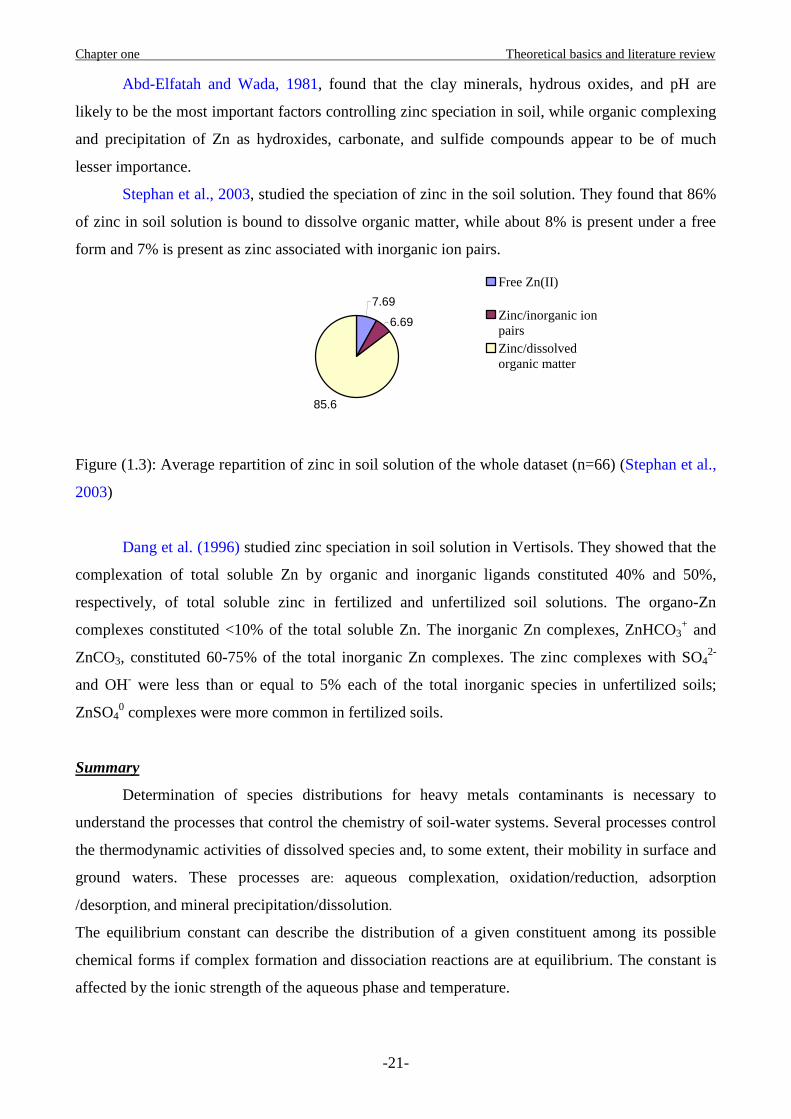
Stephan et al., 2003, studied the speciation of zinc in the soil solution. They found that 86%
of zinc in soil solution is bound to dissolve organic matter, while about 8% is present under a free
form and 7% is present as zinc associated with inorganic ion pairs.
7.69
6.69
85.6
Free Zn(II)
Zinc/inorganic ionpairsZinc/dissolvedorganic matter
Figure (1.3): Average repartition of zinc in soil solution of the whole dataset (n=66) (Stephan et al.,
2003)
Dang et al. (1996) studied zinc speciation in soil solution in Vertisols. They showed that the
complexation of total soluble Zn by organic and inorganic ligands constituted 40% and 50%,
respectively, of total soluble zinc in fertilized and unfertilized soil solutions. The organo-Zn
complexes constituted <10% of the total soluble Zn. The inorganic Zn complexes, ZnHCO3+ and
ZnCO3, constituted 60-75% of the total inorganic Zn complexes. The zinc complexes with SO42-
and OH- were less than or equal to 5% each of the total inorganic species in unfertilized soils;
ZnSO40 complexes were more common in fertilized soils.
Summary
Determination of species distributions for heavy metals contaminants is necessary to
understand the processes that control the chemistry of soil-water systems. Several processes control
the thermodynamic activities of dissolved species and, to some extent, their mobility in surface and
ground waters. These processes are: aqueous complexation, oxidation/reduction, adsorption
/desorption, and mineral precipitation/dissolution.
The equilibrium constant can describe the distribution of a given constituent among its possible
chemical forms if complex formation and dissociation reactions are at equilibrium. The constant is
affected by the ionic strength of the aqueous phase and temperature.
Chapter one Theoretical basics and literature review
-22-
Adsorption reactions of zinc in soils are important to understand the solid and liquid phase
interaction determining the release and fixation of applied zinc. The physico-chemical properties
play a key role in influencing the process. The overall rate of zinc adsorption on a soil matrix
depends on composition (density, surface area) of the soil, concentration of adsorbate (zinc ion) in
solution, soil to solution ratio, contact, pH, and temperature. A number of different equations can be
used to predict theoretical adsorption capabilities for different adsorbents. Some of these equations
are: Kd model, Langmuir model, Freundlich model, and Ion exchange model.
There are so many chemical reaction codes (most of them are based on equilibrium conditions).
This diversity of codes is caused by the inadequate documentation, difficulty of use of some
chemical codes, and the wide varity of calculation requirements.
Zinc in soil is associated mainly with hydrous Fe and Al oxides (14 to 38% of total zinc), clay
minerals (24 to 63 %), organic complexes (1.5-2.3%), and mobile fraction (1-20%).
Soil pH governs the speciation of zinc in solution; the solubility of zinc increases with decreasing
values of soil pH. Zinc forms soluble complexes with chloride, phosphate, nitrate and sulphate ions,
but the neutral sulphate (ZnSO40) and phosphate (ZnHPO4
0) species are the most important and
contribute to the total concentration of zinc in solution.
1.4. Water Flow in the Vadose Zone
1.4.1 Formulation
Soil water flux in the vadose zone has a great influence on the contaminant transport in the soil.
Water flow in the vadose zone is predominantly vertical, and can generally be simulated as one-
dimensional flow (Romano et al., 1998). Richards’ equation (1.23) can be used for simulating water
flow in the unsaturated soil zone because it has a clear physical basis (van Dam, 2000).
JS
t x
θ∂ ∂= − +∂ ∂
………………1.23
Where θ is the volumetric water content, t is time, J is water flux, x is the special coordinate, and S
is the sink term. According to Richards’ approximation, the vertical unsaturated soil water flow is
traditionally simulated by combining Darcy’s law with the mass conservation equation, yielding the
well known equation shown in table (1.7).
Chapter one Theoretical basics and literature review
-23-
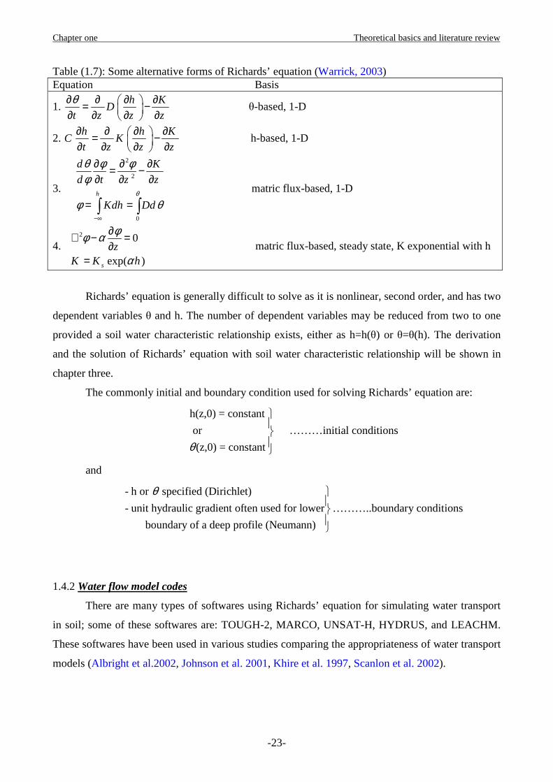
Table (1.7): Some alternative forms of Richards’ equation (Warrick, 2003) Equation Basis
1. h K
Dt z z z
θ∂ ∂ ∂ ∂ = − ∂ ∂ ∂ ∂ θ-based, 1-D
2. h h K
C Kt z z z
∂ ∂ ∂ ∂ = − ∂ ∂ ∂ ∂ h-based, 1-D
3.
2
2
0
h
d K
d t z z
Kdh Ddθ
θ φ φφ
φ θ−∞
∂ ∂ ∂= −∂ ∂ ∂
= =∫ ∫ matric flux-based, 1-D
4. 2 0
exp( )s
zK K h
φφ α
α
∂∇ − =∂
= matric flux-based, steady state, K exponential with h
Richards’ equation is generally difficult to solve as it is nonlinear, second order, and has two
dependent variables θ and h. The number of dependent variables may be reduced from two to one
provided a soil water characteristic relationship exists, either as h=h(θ) or θ=θ(h). The derivation
and the solution of Richards’ equation with soil water characteristic relationship will be shown in
chapter three.
The commonly initial and boundary condition used for solving Richards’ equation are:
h(z,0) = constant
or
(z,0) = constantθ
………initial conditions
and
- h or specified (Dirichlet)
- unit hydraulic gradient often used for lower
boundary of a deep profile (Neumann)
θ
………..boundary conditions
1.4.2 Water flow model codes
There are many types of softwares using Richards’ equation for simulating water transport
in soil; some of these softwares are: TOUGH-2, MARCO, UNSAT-H, HYDRUS, and LEACHM.
These softwares have been used in various studies comparing the appropriateness of water transport
models (Albright et al.2002, Johnson et al. 2001, Khire et al. 1997, Scanlon et al. 2002).
Chapter one Theoretical basics and literature review
-24-
TOUGH-2
Transport Of Unsaturated Groundwater and Heat, or TOUGH-2, is s finite-difference model
solving Richards’ equation for multi-dimensional transport. TOUGH-2 was designed for use in
nuclear waste isolation studies and variably saturated water transport (Pruess et al. 1999). TOUGH-
2 does not have any plant growth considerations, although it allows evapotranspiration input data.
MACRO
MACRO is based on Richards’ equation and includes an additional term to account for
preferential flow through macro pore and micro pore water movement (Johnson et al. 2001).
MACRO may be used to model saturated or unsaturated media. MACRO can account for plant
water uptake and calculates solute transport as well as water transport. Johnson compared MACRO
with HYDRUS, and he found that preferential flow was significant and should be included in a
model.
UNSAT-H
UNSAT-H, developed at Pacific Northwest Laboratory (PNL), solves Richards’ equation for
one-dimensional flow in the unsaturated media by the finite difference method. UNSAT-H accounts
for plant transpiration, and allows user input about the soil media properties. A study by Khire et al.
1997, found that UNSAT-H was more accurate than the water balance solver HELP.
HYDRUS-1D
HYDRUS-1D is a finite element solution of Richards’ equation for one dimensional flow in
variability saturated media. The HYDRUS-1D software includes plant growth and plant root water
uptake options. In addition to the modeling of water flux, HYDRUS can simulate contaminant
transport through the media and contaminant root uptake. A soil catalogue is contained within the
software, but user input data of soil hydraulic properties is also allowed (Simunek et al. 1998).
HYDRUS-2D
HYDRUS-2D includes all the function of HYDRUS-1D and includes the modeling software
SWMS_2D for two-dimensional water movement. The two-dimensional solution is useful when
lateral flow modeling is required.
Chapter one Theoretical basics and literature review
-25-
LEACHM
The Leaching Estimation And CHemistry model, LEACHM, is a one dimensional transport
model solving Richards’ equation with a finite difference approach. The code was created for use in
agricultural applications and solves only for unsaturated media. Although it was developed for
agricultural use, it is limited by its lack of plant considerations and does not account for water
runoff (Albright et al. 2002). LEACHM does account for chemical transport in addition to water
flow. A summary of the above models is presented in table (1.8).
Table (1.8): Water transport model Summery (Williams, 2005)
Model name Plant growth Solute transport Variably saturated media TOUGH-2 No Yes No MACRO Yes Yes Yes
UNSAT-H Yes No No HYDRUS Yes Yes Yes LEACHM Yes Yes No
Summary
Richards’ equation is used for simulating water flow in the vadose zone. There are different
forms of Richards’ equation and the numerical solution of this equation need the analytical solution
of the soil water characteristics functions. The derivation and solution of Richards’ equation will be
discussed in chapter three.
1.5. Fractional Advection Dispersion Equation 1.5.1 Preliminaries: Fractional Calculus
Fractional calculus is concerned with fractional-order, rather than strictly integer-order,
derivatives and integrals. The majority of fractional calculus theory was developed in the 19th
century (Oldham and Spanier, 1974). The mathematics of fractional calculus is a natural extension
of integer-order calculus. Fractional calculus is now used in many scientific and engineering fields,
including fluid flow, electrical networks, electro-magnetic theory, and probability and statistics
(e.g., Miller and Ross, 1993; Oldham and Spanier, 1974; Zaslavsky, 1994; Gorenflo and Mainardi,
1998). Fig 1.4 shows an example of fractional–order derivatives of the function f(x) = x2. In the
classical calculus we can find the first and the second derivatives of f(x) as ( )' 2f x x= and ( )" 2f x =
but we could not find the 1.2 derivative of f(x). In the fractional calculus, the 1.2 derivative of f(x)
is equal to 0.82.147x . This result is found by using the fractional derivative rule: ( )( )
1
1a aa
D x xa
α α
α−Γ +
=Γ − +

Chapter one Theoretical basics and literature review
-26-
Benson et al. (2000) and Gorenflo and Mainardi (1998) provide an introduction to fractional
calculus for the diffusion problems while Oldham and Spanier (1974), Miller and Ross (1993), or
Samko et al. (1993) present complete treatises on the subject. For the purposes of this discussion, it
is necessary to understand the differences in the behavior of integer-order and fractional-order
derivatives. Some of fractional calculus properties will be shown in chapter three.
a
0
10
20
30
40
0 1 2 3 4 5X
f(X)
0.2
0.4
0.6
0.8
1
b
0
1
2
3
4
5
6
7
8
0 1 2 3 4 5
X
f(X)
1.21.41.6
1.82
Figure (1.4): a) plot of 0.2 .4, 0.6, 0.8, and 1st derivatives of(x) = x2 , b) Plot of the 1st, 1.2, 1.4, 1.6, 1.8, and 2nd derivatives of f(x) = x2. 1.5.2 Classical Advection Dispersion Equation
The hydrodynamic dispersion theory is one of the most commonly used theories for
describing the contaminant transport in porous media. The advection-dispersion equation for non-
reactive contaminant transport can be expressed as (Bear, 1972):
……… 1.24
where C is the concentration of the contaminant, D is the hydrodynamic dispersion coefficient, and
v is the average pore velocity of contaminant transport.
Most of the present studies related to solute dispersion are still based on the Fickian-type ADE, with
temporally or spatially changing dispersion coefficients. Yates (1990, 1992) obtained the analytical
( )vCC CD
t x x x
∂∂ ∂ ∂ = − ∂ ∂ ∂ ∂
Chapter one Theoretical basics and literature review
-27-
solutions for one-dimensional ADE with linearly or exponentially increasing dispersion coefficient.
Zhang et al. (1994) obtained a travel time probability density function based on the analytical
solution with distance-dependent dispersion coefficient. Aral and Liao (1996) developed analytical
solutions for the two-dimensional ADE with a time-dependent dispersion coefficient. Hunt (1998)
discussed analytical solutions for the one-, two- and three-dimensional ADE with scale-dependent
dispersion coefficients for unsteady flow with an instantaneous source and for steady flow with a
continuous source. Pang and Hunt (2001) provided analytical solutions for a one-dimensional ADE
with scale-dependent dispersion and linear equilibrium sorption and first-order degradation.
Numerical solutions of ADE with scale-dependent dispersion coefficients have also been
investigated. Pickens and Grisak (1981) developed a finite element model that allows the
dispersivity to vary temporally as a function of the mean travel distance.
1.5.3 Fractional Advection Dispersion Equation
The use of the conventional ADE based on Fickian-type dispersion has been questioned in
recent years and alternative non-Fickian dispersion models have been proposed. Berkowitz et al.
(2000), Lévy and Berkowitz (2003) and Cortis and Berkowitz (2004) have found that the
anomalous transport in a sand box might be explained by the continuous time random walk
(CTRW) theory. Based on the Lévy motion theory, Benson (1998) derived the fractional advection–
dispersion equation (FADE) to describe the non-Fickian transport. The long tail of breakthrough
curves (BTCs) can be better modeled by FADE with respect to ADE (Pachepsky et al., 2000,
Benson et al., 2000a, b). Pachepsky et al. (2000) used FADE to interpret transport in short columns
and found that a constant dispersion coefficient can be used. In a large-scale field study carried out
in a heterogeneous alluvial aquifer at the Columbus Air Force Base (Mississippi), bromide was
injected as a pulse and traced over a 20 month period (Boggs et. al, 1992, Adam and Gelhar, 1992).
The tracer plume that evolved was remarkably asymmetric (Fig.1.5), and cannot be described by
classical ADE models (Berkowitz and Scher, 1997). As a consequent, the classical ADE can not
always describe the solute transport in the soil with a good precision; therefore, a new general
model capable to cover the most of field cases is needed.
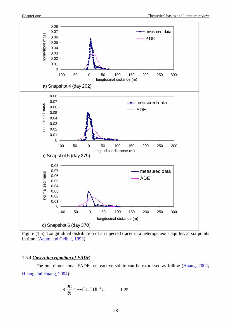
Chapter one Theoretical basics and literature review
-28-
a) Snapshot 4 (day 202)
00.01
0.020.030.04
0.050.06
0.070.08
-100 -50 0 50 100 150 200 250 300longitudinal distance (m)
norm
aliz
ed m
ass measured data
ADE
b) Snapshot 5 (day 279)
0
0.01
0.02
0.03
0.04
0.05
0.06
0.07
0.08
-100 -50 0 50 100 150 200 250 300longitudinal distance (m)
norm
aliz
ed m
ass measured data
ADE
c) Snapshot 6 (day 370)
00.010.020.030.040.050.060.070.08
-100 -50 0 50 100 150 200 250 300
longitudinal distance (m)
norm
aliz
ed m
ass measured data
ADE
Figure (1.5): Longitudinal distribution of an injected tracer in a heterogeneous aquifer, at six points in time. (Adam and Gelhar, 1992)
1.5.4 Governing equation of FADE
The one-dimensional FADE for reactive solute can be expressed as follow (Huang, 2002;
Huang and Huang, 2004):
…….. 1.25
CR v C D C
tα∂ = − ∇ + ∇
∂
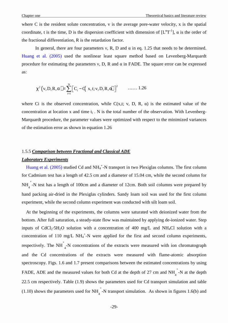
Chapter one Theoretical basics and literature review
-29-
where C is the resident solute concentration, v is the average pore-water velocity, x is the spatial
coordinate, t is the time, D is the dispersion coefficient with dimension of [LαT-1], α is the order of
the fractional differentiation, R is the retardation factor.
In general, there are four parameters ν, R, D and α in eq. 1.25 that needs to be determined.
Huang et al. (2005) used the nonlinear least square method based on Levenberg-Marquardt
procedure for estimating the parameters ν, D, R and α in FADE. The square error can be expressed
as:
…… 1.26
where Ci is the observed concentration, while C(x,t; v, D, R, α) is the estimated value of the
concentration at location x and time ti . N is the total number of the observation. With Levenberg-
Marquardt procedure, the parameter values were optimized with respect to the minimized variances
of the estimation error as shown in equation 1.26
1.5.5 Comparison between Fractional and Classical ADE
Laboratory Experiments
Huang et al. (2005) studied Cd and NH4+-N transport in two Plexiglas columns. The first column
for Cadmium test has a length of 42.5 cm and a diameter of 15.04 cm, while the second column for
NH4
+-N test has a length of 100cm and a diameter of 12cm. Both soil columns were prepared by
hand packing air-dried in the Plexiglas cylinders. Sandy loam soil was used for the first column
experiment, while the second column experiment was conducted with silt loam soil.
At the beginning of the experiments, the columns were saturated with deionized water from the
bottom. After full saturation, a steady-state flow was maintained by applying de-ionized water. Step
inputs of CdCl2·5H2O solution with a concentration of 400 mg/L and NH4Cl solution with a
concentration of 110 mg/L NH4+-N were applied for the first and second column experiments,
respectively. The NH+
4-N concentrations of the extracts were measured with ion chromatograph
and the Cd concentrations of the extracts were measured with flame-atomic absorption
spectroscopy. Figs. 1.6 and 1.7 present comparisons between the estimated concentrations by using
FADE, ADE and the measured values for both Cd at the depth of 27 cm and NH4
+-N at the depth
22.5 cm respectively. Table (1.9) shows the parameters used for Cd transport simulation and table
(1.10) shows the parameters used for NH4
+-N transport simulation. As shown in figures 1.6(b) and
( ) ( )N
22i
i 1
v,D,R, C C x, t;v,D,R,=
χ α = − α ∑

Chapter one Theoretical basics and literature review
-30-
1.7(b), the measured concentration values were larger than zero at breakthrough curves for Cd at the
depth of 27 cm before 100 h and NH4+-N at the depth of 22.5 cm before 50 h. Comparing to ADE,
FADE can give a better fitting to the measured data at the early part of the breakthrough curves. A
slightly better fitting to the late part of the breakthrough curve can also be obtained by using FADE
as shown in Fig. 1.7(a). The results may be attributed to the heterogeneity of the soil columns,
which may be caused by both heterogeneity of the soil particles and the non-uniformity packing
process of the soil columns. The contaminant transport behavior in heterogeneous media usually
exhibits anomalous or non-Fickian behavior (Berkowitz et al., 2000, Dentz et al., 2004), therefore
the transport process can not be well described by using ADE, which is based on Fickian diffusion
law.
Table (1.9): parameters for Cd transport (Huang et al., 2005)
ADE FADE Depth
cm D cm2/hr
v cm/hr
R
α D
cmα/hr v
cm/hr R
2 10.72 5.92 73.99 1.54 7.44 5.95 37.06 7 9.25 5.97 48.53 1.22 6.72 5.97 48.53 17 8.69 5.95 40.20 1.94 7.75 5.96 41.12 27 6.10 5.93 57.55 1.98 6.33 5.96 58.46
average 8.69 5.94 55.07 1.67 7.29 5.96 46.29 Table (1.10): parameters for NH4
+-N transport (Huang et al., 2005) ADE FADE
Depth cm D
cm2/hr v
cm/hr R
α D
cmα/hr v
cm/hr R
2.5 0.602 1.509 8.246 1.45 0.553 1.887 9.219 12.5 0.904 1.688 7.526 1.22 0.775 1.688 7.486 22.5 0.744 1.685 6.879 1.94 0.519 1.688 6.890 32.5 0.886 1.688 7.204 1.98 0.650 1.689 7.220
average 0.784 1.643 7.464 1.65 0.624 1.738 7.704
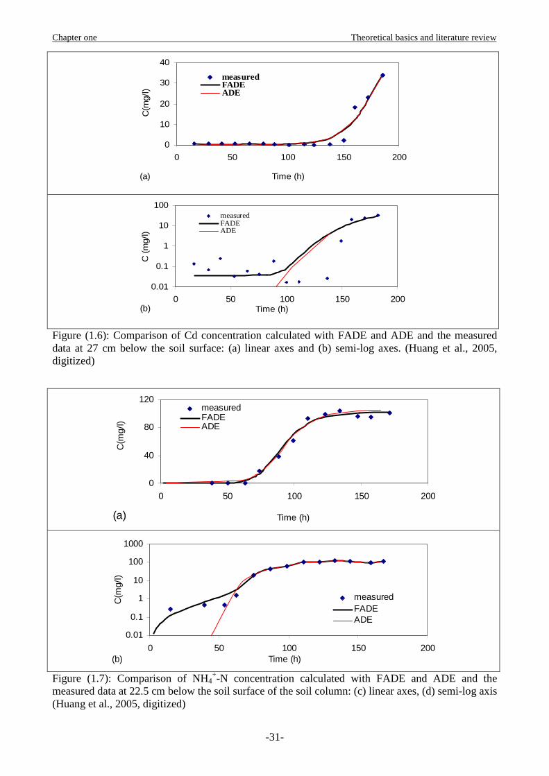
Chapter one Theoretical basics and literature review
-31-
(a)
0
10
20
30
40
0 50 100 150 200
Time (h)
C(m
g/l)
measuredFADEADE
(b)
0.01
0.1
1
10
100
0 50 100 150 200Time (h)
C (
mg/
l)
measuredFADEADE
Figure (1.6): Comparison of Cd concentration calculated with FADE and ADE and the measured data at 27 cm below the soil surface: (a) linear axes and (b) semi-log axes. (Huang et al., 2005, digitized)
(a)
0
40
80
120
0 50 100 150 200
Time (h)
C(m
g/l)
measuredFADEADE
(b)
0.01
0.1
1
10
100
1000
0 50 100 150 200Time (h)
C(m
g/l)
measuredFADEADE
Figure (1.7): Comparison of NH4
+-N concentration calculated with FADE and ADE and the measured data at 22.5 cm below the soil surface of the soil column: (c) linear axes, (d) semi-log axis (Huang et al., 2005, digitized)
Chapter one Theoretical basics and literature review
-32-
Field Experiments
Benson et al. (2001) used the results of the macro-dispersion experiments (MADE) to make
comparison between FADE and ADE. The Macro-Dispersion Experiment (MADE) site is located
on the Columbus Air Force Base in northeastern Mississippi. The two large–scales, natural–gradient
tracer tests performed there differ from other large–scale tracer experiments such as the Borden site
in Ontario, Canada (e.g., Sudicky, 1986) or the Cape Cod site in Massachusetts (e.g., LeBlanc et al.,
1991) because of the strong heterogeneity of the aquifer (Rehfeldt et al. 1992; Boggs et al., 1993).
The unconfined, alluvial aquifer consists of generally unconsolidated sands and gravels with
smaller clay and silt components. Irregular lenses and horizontal layers were observed in an aquifer
exposure near the site (Rehfeldt et al., 1992). Detailed studies characterizing the spatial variability
of the aquifer and the spreading of the conservative tracer plume for the experiment conducted
between October 1986 and June 1988 (MADE–1) are summarized by Boggs and Adams (1992),
Adams and Gelhar (1992), and Rehfeldt et al. (1992). A synopsis of the second experiment
(MADE–2), conducted between June 1990 and September 1991, is given by Boggs et al. (1993).
Approximately 104 L of water containing 2,500 mg/L of Bromide were injected into the
MADE aquifer for the first test. Over the next 20 months, seven sampling events using an extensive
array of multi–level samplers (MLS) were performed. They use the parameters estimated from the
aquifer K statistics (supported by Adams and Gelhar’s analysis of the MADE–1 bromide plume) to
predict the MADE–2 tritium plume. During the MADE–2 experiment, 9.7 m3 of titrated water and
four organic compounds were injected into the shallow alluvial aquifer at the test site. Over the next
15 months, five snapshots of the tracer concentration distributions were collected. They compare
the solutions of the traditional ADE (α = 2) and the fractional ADE (α = 1.1) and they concluded
that the fractional ADE gave better predictions with a very low information’s required (as illustrated
in the following figures).
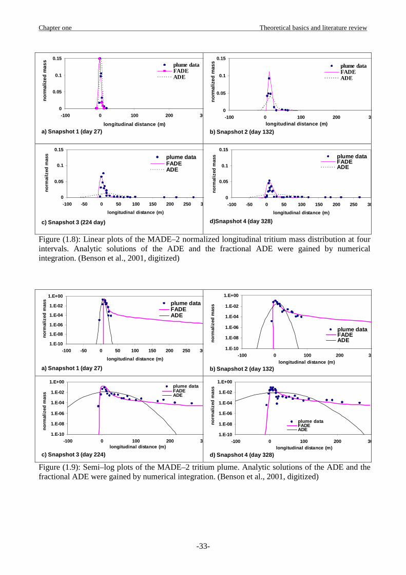
Chapter one Theoretical basics and literature review
-33-
a) Snapshot 1 (day 27)
0
0.05
0.1
0.15
-100 0 100 200 300
longitudinal distance (m)
no
rmal
ized
mas
s
plume dataFADEADE
b) Snapshot 2 (day 132)
0
0.05
0.1
0.15
-100 0 100 200 300longitudinal distance (m)
no
rmal
ized
mas
s
plume dataFADEADE
c) Snapshot 3 (224 day)
0
0.05
0.1
0.15
-100 -50 0 50 100 150 200 250 300
longitudinal distance (m)
no
rmai
lzed
mas
s plume dataFADEADE
d)Snapshot 4 (day 328)
0
0.05
0.1
0.15
-100 -50 0 50 100 150 200 250 300
longitudinal distance (m)n
orm
aliz
ed m
ass plume data
FADEADE
Figure (1.8): Linear plots of the MADE–2 normalized longitudinal tritium mass distribution at four intervals. Analytic solutions of the ADE and the fractional ADE were gained by numerical integration. (Benson et al., 2001, digitized)
a) Snapshot 1 (day 27)
1.E-10
1.E-08
1.E-06
1.E-04
1.E-02
1.E+00
-100 -50 0 50 100 150 200 250 300
longitudinal distance (m)
no
rmal
ized
mas
s plume dataFADEADE
b) Snapshot 2 (day 132)
1.E-10
1.E-08
1.E-06
1.E-04
1.E-02
1.E+00
-100 0 100 200 300longitudinal distance (m)
no
rmal
ized
mas
s
plume dataFADEADE
c) Snapshot 3 (day 224)
1.E-10
1.E-08
1.E-06
1.E-04
1.E-02
1.E+00
-100 0 100 200 300longitudinal distance (m)
no
rmal
ized
mas
s
plume dataFADEADE
d) Snapshot 4 (day 328)
1.E-10
1.E-08
1.E-06
1.E-04
1.E-02
1.E+00
-100 0 100 200 300longitudinal distance (m)
no
rmal
ized
mas
s
plume dataFADEADE
Figure (1.9): Semi–log plots of the MADE–2 tritium plume. Analytic solutions of the ADE and the fractional ADE were gained by numerical integration. (Benson et al., 2001, digitized)
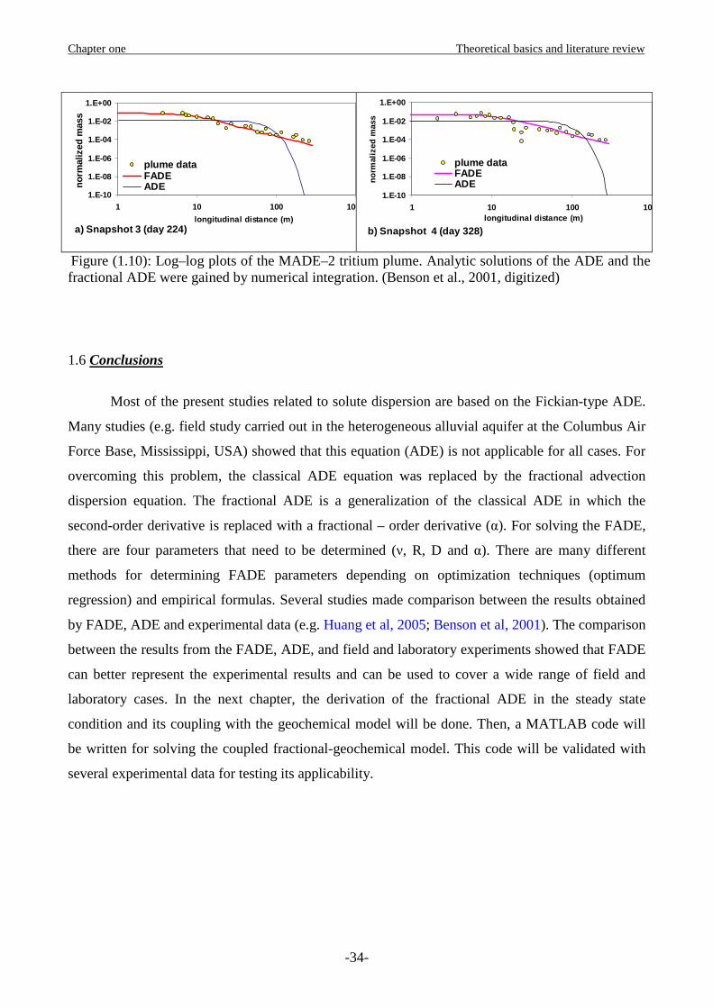
Chapter one Theoretical basics and literature review
-34-
a) Snapshot 3 (day 224)
1.E-10
1.E-08
1.E-06
1.E-04
1.E-02
1.E+00
1 10 100 1000
longitudinal distance (m)
norm
aliz
ed m
ass
plume dataFADEADE
b) Snapshot 4 (day 328)
1.E-10
1.E-08
1.E-06
1.E-04
1.E-02
1.E+00
1 10 100 1000longitudinal distance (m)
no
rmal
ized
mas
s
plume dataFADEADE
Figure (1.10): Log–log plots of the MADE–2 tritium plume. Analytic solutions of the ADE and the fractional ADE were gained by numerical integration. (Benson et al., 2001, digitized)
1.6 Conclusions
Most of the present studies related to solute dispersion are based on the Fickian-type ADE.
Many studies (e.g. field study carried out in the heterogeneous alluvial aquifer at the Columbus Air
Force Base, Mississippi, USA) showed that this equation (ADE) is not applicable for all cases. For
overcoming this problem, the classical ADE equation was replaced by the fractional advection
dispersion equation. The fractional ADE is a generalization of the classical ADE in which the
second-order derivative is replaced with a fractional – order derivative (α). For solving the FADE,
there are four parameters that need to be determined (ν, R, D and α). There are many different
methods for determining FADE parameters depending on optimization techniques (optimum
regression) and empirical formulas. Several studies made comparison between the results obtained
by FADE, ADE and experimental data (e.g. Huang et al, 2005; Benson et al, 2001). The comparison
between the results from the FADE, ADE, and field and laboratory experiments showed that FADE
can better represent the experimental results and can be used to cover a wide range of field and
laboratory cases. In the next chapter, the derivation of the fractional ADE in the steady state
condition and its coupling with the geochemical model will be done. Then, a MATLAB code will
be written for solving the coupled fractional-geochemical model. This code will be validated with
several experimental data for testing its applicability.

Chapter Two Chapter Two Chapter Two Chapter Two
Simulation of solutes transport in soils at steady stateSimulation of solutes transport in soils at steady stateSimulation of solutes transport in soils at steady stateSimulation of solutes transport in soils at steady state
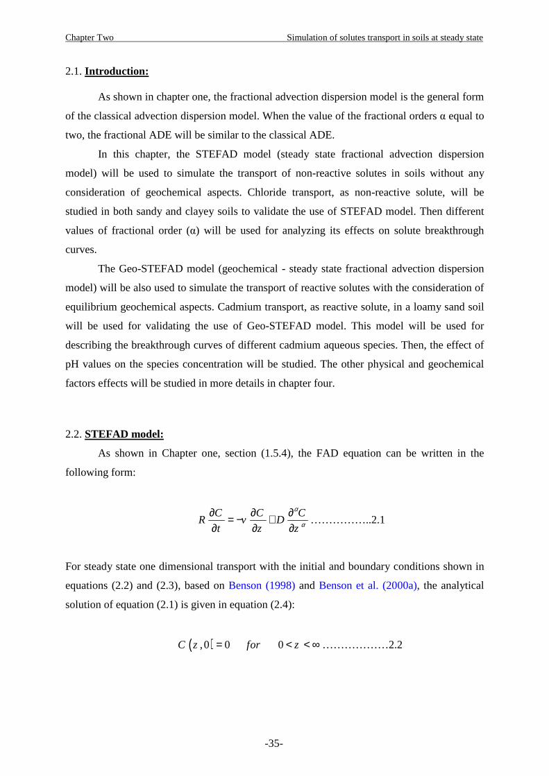
Chapter Two Simulation of solutes transport in soils at steady state
-35-
2.1. Introduction:
As shown in chapter one, the fractional advection dispersion model is the general form
of the classical advection dispersion model. When the value of the fractional orders α equal to
two, the fractional ADE will be similar to the classical ADE.
In this chapter, the STEFAD model (steady state fractional advection dispersion
model) will be used to simulate the transport of non-reactive solutes in soils without any
consideration of geochemical aspects. Chloride transport, as non-reactive solute, will be
studied in both sandy and clayey soils to validate the use of STEFAD model. Then different
values of fractional order (α) will be used for analyzing its effects on solute breakthrough
curves.
The Geo-STEFAD model (geochemical - steady state fractional advection dispersion
model) will be also used to simulate the transport of reactive solutes with the consideration of
equilibrium geochemical aspects. Cadmium transport, as reactive solute, in a loamy sand soil
will be used for validating the use of Geo-STEFAD model. This model will be used for
describing the breakthrough curves of different cadmium aqueous species. Then, the effect of
pH values on the species concentration will be studied. The other physical and geochemical
factors effects will be studied in more details in chapter four.
2.2. STEFAD model:
As shown in Chapter one, section (1.5.4), the FAD equation can be written in the
following form:
C C CR v D
t z z
α
α∂ ∂ ∂= − +∂ ∂ ∂
……………..2.1
For steady state one dimensional transport with the initial and boundary conditions shown in
equations (2.2) and (2.3), based on Benson (1998) and Benson et al. (2000a), the analytical
solution of equation (2.1) is given in equation (2.4):
( ),0 0 0C z for z= < < ∞ ………………2.2
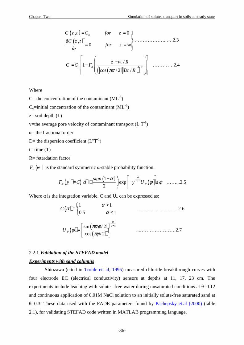
Chapter Two Simulation of solutes transport in soils at steady state
-36-
( )
( ), 0
,0
oC z t C for z
C z tfor z
z
= = ∂
= = ∞∂
………………..….2.3
( )( )1/
/1
cos / 2 /
z vt RC C F
Dt Rα α
πα
− = −
� ………….2.4
Where
C= the concentration of the contaminant (ML-3)
Co=initial concentration of the contaminant (ML-3)
z= soil depth (L)
v=the average pore velocity of contaminant transport (L T-1)
α= the fractional order
D= the dispersion coefficient (LαT-1)
t= time (T)
R= retardation factor
( )F wα is the standard symmetric α-stable probability function.
( ) ( ) ( ) ( )1
1
0
1exp
2−
−= + −
∫
signF y C y U d
αα
α αα
α φ φ ……...2.5
Where α is the integration variable, C and Uα can be expressed as:
( ) 1 1
0.5 1C
αα
α>
= < ……………….……..2.6
( ) ( )( )
1sin / 2
cos / 2
− =
U
αα
απαφ
φπφ
...………………….2.7
2.2.1 Validation of the STEFAD model
Experiments with sand columns
Shiozawa (cited in Troide et. al, 1995) measured chloride breakthrough curves with
four electrode EC (electrical conductivity) sensors at depths at 11, 17, 23 cm. The
experiments include leaching with solute –free water during unsaturated conditions at θ=0.12
and continuous application of 0.01M NaCl solution to an initially solute-free saturated sand at
θ=0.3. These data used with the FADE parameters found by Pachepsky et.al (2000) (table
2.1), for validating STEFAD code written in MATLAB programming language.
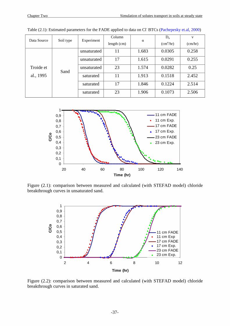
Chapter Two Simulation of solutes transport in soils at steady state
-37-
Table (2.1): Estimated parameters for the FADE applied to data on Cl- BTCs (Pachepesky et.al, 2000)
Data Source Soil type Experiment Column
length (cm) α
Dα
(cmα/hr)
v
(cm/hr)
unsaturated 11 1.683 0.0305 0.258
unsaturated 17 1.615 0.0291 0.255
unsaturated 23 1.574 0.0282 0.25
saturated 11 1.913 0.1518 2.452
saturated 17 1.846 0.1224 2.514
Troide et
al., 1995 Sand
saturated 23 1.906 0.1073 2.506
00,1
0,20,3
0,40,5
0,60,7
0,80,9
1
20 40 60 80 100 120 140
Time (hr)
C/C
o
11 cm FADE
11 cm Exp.
17 cm FADE
17 cm Exp.
23 cm FADE
23 cm Exp.
Figure (2.1): comparison between measured and calculated (with STEFAD model) chloride breakthrough curves in unsaturated sand.
00,10,20,30,40,50,60,70,80,9
1
2 4 6 8 10 12
Time (hr)
C/C
o
11 cm FADE11 cm Exp17 cm FADE17 cm Exp.23 cm FADE23 cm Exp.
Figure (2.2): comparison between measured and calculated (with STEFAD model) chloride breakthrough curves in saturated sand.
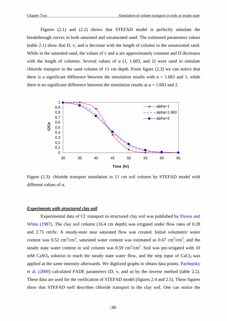
Chapter Two Simulation of solutes transport in soils at steady state
-38-
Figures (2.1) and (2.2) shows that STEFAD model is perfectly simulate the
breakthrough curves in both saturated and unsaturated sand. The estimated parameters values
(table 2.1) show that D, v, and α decrease with the length of column in the unsaturated sand.
While in the saturated sand, the values of v and α are approximately constant and D decreases
with the length of columns. Several values of α (1, 1.683, and 2) were used to simulate
chloride transport in the sand column of 11 cm depth. From figure (2.3) we can notice that
there is a significant difference between the simulation results with α = 1.683 and 1, while
there is no significant difference between the simulation results at α = 1.683 and 2.
00,10,20,30,40,50,60,70,80,9
1
30 35 40 45 50 55 60 65
Time (hr)
C/C
o
alpha=1
alpha=1.683
alpha=2
Figure (2.3): chloride transport simulation in 11 cm soil column by STEFAD model with
different values of α.
Experiments with structured clay soil
Experimental data of Cl- transport in structured clay soil was published by Dyson and
White (1987). The clay soil column (16.4 cm depth) was irrigated under flow rates of 0.28
and 2.75 cm/hr. A steady-state near saturated flow was created. Initial volumetric water
content was 0.52 cm3/cm3, saturated water content was estimated as 0.67 cm3/cm3, and the
steady state water content in soil column was 0.59 cm3/cm3. Soil was pre-irrigated with 10
mM CaSO4 solution to reach the steady state water flow, and the step input of CaCl2 was
applied at the same intensity afterwards. We digitized graphs to obtain data points. Pachepsky
et al. (2000) calculated FADE parameters (D, v, and α) by the inverse method (table 2.2).
These data are used for the verification of STEFAD model (figures 2.4 and 2.5). These figures
show that STEFAD well describes chloride transport in the clay soil. One can notice the

Chapter Two Simulation of solutes transport in soils at steady state
-39-
significant influence of the numerical results. When α value decreases from 1.642 to 1, the
normalized concentration (C/Co) decreases by approximately 50%. The estimated
concentration increases by approximately 20% when α value increases from 1.642 to 2. The
estimated values of α don’t differ significantly for the two flow rates and are similar to those
in the unsaturated sand. The dispersion coefficient (D) increases approximately 37 times as
the flow rate increases 10 times.
Table (2.2): Estimated parameters for the FADE applied to data on Cl- BTCs from soil column (Pachepesky et.al. 2000)
Data Source Soil type Experiment
Column
length
(cm)
α Dα
(cmα/hr)
V
(cm/hr)
q= 0.28 cm/hr 16.4 1.642 1.209 0.756 Dyson and
White, 1987 Clay
q= 2.75 cm/hr 16.4 1.695 44.69 12.89
00,10,20,30,40,50,60,70,80,9
1
0 10 20 30 40 50 60 70 80
Time (hr)
C/C
o
alpha =1
alpha = 1.642
alpha = 2
Measured
Figure (2.4): comparison between measured and calculated (by STEFAD model) chloride transport in the clayey soil with different α values and constant q = 0.28 cm/hr
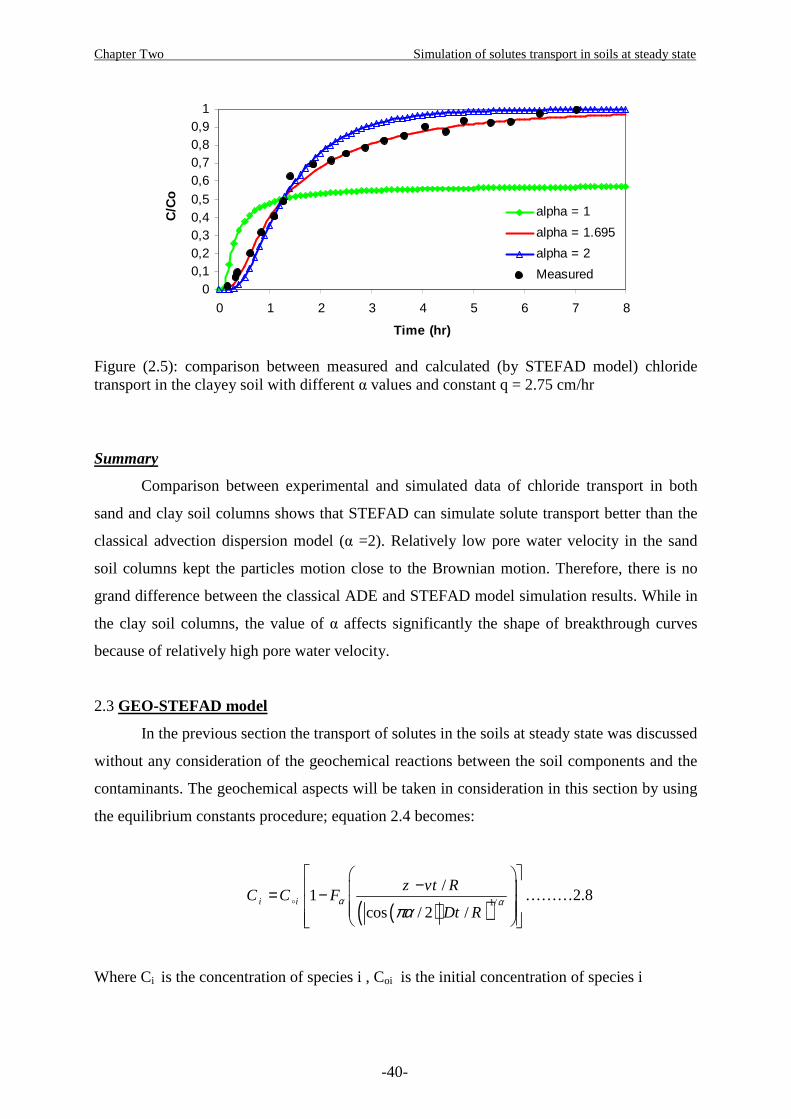
Chapter Two Simulation of solutes transport in soils at steady state
-40-
00,10,20,30,40,5
0,60,70,80,9
1
0 1 2 3 4 5 6 7 8
Time (hr)
C/C
o
alpha = 1
alpha = 1.695
alpha = 2
Measured
Figure (2.5): comparison between measured and calculated (by STEFAD model) chloride transport in the clayey soil with different α values and constant q = 2.75 cm/hr
Summary
Comparison between experimental and simulated data of chloride transport in both
sand and clay soil columns shows that STEFAD can simulate solute transport better than the
classical advection dispersion model (α =2). Relatively low pore water velocity in the sand
soil columns kept the particles motion close to the Brownian motion. Therefore, there is no
grand difference between the classical ADE and STEFAD model simulation results. While in
the clay soil columns, the value of α affects significantly the shape of breakthrough curves
because of relatively high pore water velocity.
2.3 GEO-STEFAD model
In the previous section the transport of solutes in the soils at steady state was discussed
without any consideration of the geochemical reactions between the soil components and the
contaminants. The geochemical aspects will be taken in consideration in this section by using
the equilibrium constants procedure; equation 2.4 becomes:
( )( )1/
/1
cos / 2 /i i
z vt RC C F
Dt Rα α
πα
− = −
�………2.8
Where Ci is the concentration of species i , Coi is the initial concentration of species i
Chapter Two Simulation of solutes transport in soils at steady state
-41-
In order to describe the chemical reactions mathematically, a subset of the species
must be chosen as components. All other ions, complexes, sorbed species, and minerals can
be formed from these components. It is assumed that all chemical interactions between
soluble components in the aqueous phase and soil constitutes in the solid phase are controlled
by local equilibrium and that local equilibrium exists at every point of the system considered.
In the local equilibrium controlled transport system, the reaction rates are much faster than the
rates of physical transport. This assumption may be the most restrictive relative to conditions
that may pertain to the total system. The equilibrium chemistry must contain all of the phase-
exchange and/or mass-equations necessary to describe the chemical processes affecting the
transport, i.e. sorption, complexation, dissociation, and ion exchange. A system of n
independent components that can be combining to form m species is represented by a set of
mass action expressions of the form:
{ } ija
i i jj
K S X−= ∏ ………2.9
Where:
Ki = equilibrium constant for the formation of species i
{Si} = activity species i
aij = stoichiometric coefficient of component j in species i
Π = indicates the product over all components in species i
The concentration of species i, [Si], is related to the activity {Si} by the activity coefficients γi.
{ } [ ]i i iS Sγ= …………..2.10
Substituting this expression for {Si} in equation 2.3 and rearranging gives:
[ ] ijaii j
ji
KS X
γ= ∏ ………..2.11
Now if we define 'iK such that
' /i i iK K γ= ………………2.12
Then
Chapter Two Simulation of solutes transport in soils at steady state
-42-
[ ] ' ija
i i i jj
C S K X= = ∏ ………….2.13
In the logarithmic form, equation 2.7 becomes:
'log log logi i ij jj
C K a X= +∑ ………..2.14
In addition to the mass action expressions, the set of n independent components is governed
by n mass balance equation of the form:
j ij i ji
Y a C T= −∑ …………..2.15
Where
Tj = total dissolved concentration of component j (known measured input parameter)
Y j = the differences between the calculated total dissolved concentration of component j and
the known analytical total dissolved concentration of component j.
2.3.1 Solution strategy of the geochemical model
The solution (in the mathematical sense) is that set of component activities X (using
matrix notation for brevity) which results in the set of concentrations C such that each
individual of the set of mass balance differences Y is equal to zero. In practice, it is only
necessary to find X such that each individual of Y is made less than some tolerance value.
The general procedure is to first guess X (makes this guess and puts it in the input file), then
calculate C and Y. If any individual of Y exceeds (in absolute terms) its prescribed tolerance
value, a new guess is made for X, C and Y are recalculated, and the test is repeated. This
iterative procedure is continued until all the individuals of Y are less than the tolerance value.
The Newton-Raphson approximation method is used to estimate the new X at each iteration.
The tolerance value or convergence a criterion is 10-4 times Tj for each component j.
We will use Cd2+ speciation as example to illustrate the generalized mathematical formalisms
used to solve chemical equilibrium problems. The system consists of 2 2 24 3, , ,Cd Cl SO CO+ − − −
and the chemical equilibrium model was applied to this system using the equilibrium
formation constants procedure. The major species for the previous defined applications are
24 3, , ,Cd CdCl CdSO CdCO+ + and adsorbed cadmium. The sorption sites will be denoted as
Q2-, and cadmium adsorbed to the soil will be denoted as QCd. As shown in chapter one
Chapter Two Simulation of solutes transport in soils at steady state
-43-
(equation 1.7), Activity coefficients can be estimated by using the extended Debye-Huckel
equation:
2
log1
ii
i
Az I
Bd Iγ− =
+………..2.16
Where i is the ionic strength of the solution (mol/L), z is valence of ion i in solution, A and B
are constants and equal to 0.51 mol/l, and 0.33 Å (mol-0.5/L0.5) respectively, di is the diameter
of ions Å. The extended Deybe-Hückel equation (2.16) will be used for those species that
have the necessary parameters in the database. For any species lacking the necessary
parameters, the Davies equation (2.17) will be used to estimate the activity coefficient for that
species:
2log 0.241
i i
IAZ I
Iγ = − −
+……………..2.17
In which the variable are defined as in equation (2.10).
The partial CO2 pressure (pCO2) and the pH in the soil are boundary conditions of the model.
pH and pCO2 are linked by the dissolution of CO2 in water:
22 2 32CO H O H CO+ −+ +��⇀↽�� ,
{ } { }2 2
2
23.
, log 18.14co cop p
CO
H COK K
p
+ −
= = − ……..2.18
and the considered complexation equilibria are
2Cd Cl CdCl+ − ++ ��⇀↽�� ,{ }
{ } { }2, log 1.98
.CdCl CdCl
CdClK K
Cd Cl+ +
+
+ −= = …………..2.19
2 24 4Cd SO CdSO+ −+ ��⇀↽�� ,
{ }{ } { }4 4
4
2 24
, log 2.45.
CdSO CdSO
CdSOK K
Cd SO+ −= = ………….2.20
2 23 3Cd CO CdCO+ −+ ��⇀↽��
{ }{ } { }3 3
3
2 23
, log 5.4.
CdCO CdCO
CdCOK K
Cd CO+ −= = …………2.21
Adsorption of cadmium to the soil is described with an extended Freundlich equation:
Chapter Two Simulation of solutes transport in soils at steady state
-44-
[ ] { } { }2 n m
effQCd K Cd H+ += ……………………2.22
This mass action equation can be interpreted as a virtual exchange equation:
2 2 2 2m nn mnCd Q mH QCd H+ − + − −+ + ��⇀↽�� ………………..2.23
The parameter Keff is a function of the bulk density, the water content, and the organic matter
content of the soil. For convenient usage of the model, the constant K* is introduced. K* is
independent of soil moisture content and bulk density. The following conversion is applied:
( )
1
*33
.1. .
.1010 .
n
seff
m
ocK K
M
ρθ
− =
…………………2.24
in which K* (mg1-n Ln kg-1) is the scaled Freundlich sorption constant, Mx (g/ mol) is the
molecular weight of metal x , sρ (kg/m3) is the bulk density of dry soil , θ is volumetric water
content (m3/m3), and oc (% by mass) organic carbon content. For each component, a mass
balance can be calculated:
[ ] [ ] [ ]2 22
4 3Cd CdY Cd CdCl CdSO CdCO QCd T+ +
+ + = + + + + − ……………………2.25
Cl ClY Cl CdCl T− −
− + = + − …………………………………………………………2.26
[ ]2 24 4
24 4SO SO
Y SO CdSO T− −− = + − ……………………………………………………..2.27
Note that the balance for carbon-oxide species is not considered because the system is
considered to be open with respect to CO2. By applying equation 2.4 and the mass action
equations (2.25 – 2.27) we have:
( )
( ) ( )
2 2 24 4
23 3
2 2
2 ' ' 24
'
2
1 CdSO CdSOCd Cd Cl CdCl Cd
CdCO pCOCd H
n m
eff Cd H Cd
Y Cd K Cl K SO
K K H
K Cd H T
γ γ γ γ
γ γ
γ γ
+ + − + +
+ +
+ + +
+ − −
+
+ +
= + +
+
+ −
……………………..2.28

Chapter Two Simulation of solutes transport in soils at steady state
-45-
( )2
2
' 2
' 2
1
1
Cl Cd Cl CdCl Cl
Cl Cl
Cd Cl CdCl
Y Cl K Cd T
Y TCl
K Cd
γ γ
γ γ
− + − + −
− −
+ − +
− +
−+
= + −
+ ⇒ = +
……………………………………………2.29
( )2 2 24 44 4
2 24 4
24 4
2 ' 24
24 ' 2
1
1
CdSO CdSOSO Cd SO
SO SO
CdSO CdSOCd
Y SO K Cd T
Y TSO
K Cd
γ γ
γ γ
− + −
− −
+
− +
−+
= + −
+ ⇒ = +
……………………………………2.30
By substituting Cl
Y − and 24SO
Y − in 2CdY + we have:
( ) ( )
2 2
2
24
24 4
24 4
23 3
2 2
2 '
' 2
'
' 2
'
2
11
1
ClCd Cd Cl CdCl
Cd Cl CdCl
SOCdSO CdSOCd
CdSO CdSOCd
CdCO pCOCd H
n m
eff Cd H Cd
TY Cd K
K Cd
TK
K Cd
K K H
K Cd H T
γ γγ γ
γ γγ γ
γ γ
γ γ
−
+ + − +
+ − +
−
+
+
+ +
+ +
++
+
+
+ +
= + +
+
+
+
+ − +
……………………..2.31
Equation (2.31) can be solved for Cd2+ by using Newton-Raphson method and all the other
species can be calculated from the obtained value of Cd2+ concentration. The solution
procedure for the geochemical speciation model by the equilibrium method is shown in figure
(2.6)

Chapter Two Simulation of solutes transport in soils at steady state
-46-
Fig. (2.6) Flow diagram of the speciation sub-model 2.3.2 Solution Strategy of the Geo-STEFAD model
The fractional advection- dispersion equation describing aqueous phase transport are
spanning over spatial and temporal domains only, and the geochemical equations describing
the transformation of heavy metals into different species are spanning over the chemical
domain only. In other words, the fractional ADE and geochemical equations are decoupled
and solved separately. The advantage of this method of solution is that the highly non-linear
behavior of geochemical equilibrium is confined to the model describing the geochemistry.
Thus, the overall solution system consists of two steps: a physical step in which the fractional
advection dispersion equation is solved, as transport term, and a chemical step in which the
Get provisional total concentration of each component
Read input data and soil adsorption properties
Calculate ionic strength
Calculate activity coefficients and Keff
Start
Calculate mass distribution for each species through formation constants
End
Yes
Mass balance
No

Chapter Two Simulation of solutes transport in soils at steady state
-47-
chemical equilibrium equations are solved for the aqueous and solid phase components for
each nodal point in the spatial domain. A sequential coupling strategy of the physical and
chemical steps has been adopted. The physical and chemical coupling is external. The
disadvantage of this method is that chemical equilibrium is allowed to occur only at the end of
time step. This dose not causes significant errors if small time steps are chosen.
The master model first reads the physical and chemical input parameters. These
parameters includes: fractional order (α), pore water velocity (v), dispersion coefficient (D),
time (to, ∆t, tfinal), depth (z, ∆z), the considered aqueous species, the formation constants, pH,
pCO2, temperature, soil adsorption properties, and provisional total concentration of each
component. At each time step, the master program calls the Fractional transport model. This
model furnishes the convected concentrations at each node for each component under
consideration. The convected concentrations of the components are taken as inputs by the
geochemical model. This model equilibrates the chemical system using the appropriate
reactions and returns the modified component concentrations which are further convected by
the fractional transport model at the next time step. The flowchart depicting this methodology
is shown in figure (2.7).
Fig (2.7) Flow diagram of GEO-STEFAD model solution
t+1
Equilibrated concentration
Input parameters
Fractional solute transport model
Geochemistry
t
t
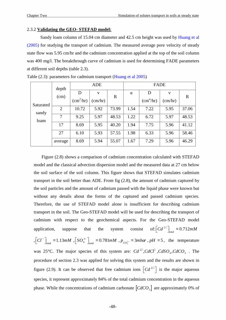
Chapter Two Simulation of solutes transport in soils at steady state
-48-
2.3.2 Validating the GEO- STEFAD model:
Sandy loam column of 15.04 cm diameter and 42.5 cm height was used by Huang et al
(2005) for studying the transport of cadmium. The measured average pore velocity of steady
state flow was 5.95 cm/hr and the cadmium concentration applied at the top of the soil column
was 400 mg/l. The breakthrough curve of cadmium is used for determining FADE parameters
at different soil depths (table 2.3).
Table (2.3): parameters for cadmium transport (Huang et al 2005)
ADE FADE depth
(cm) D
(cm2/hr)
v
(cm/hr) R
α D
(cmα/hr)
v
(cm/hr) R
2 10.72 5.92 73.99 1.54 7.22 5.95 37.06
7 9.25 5.97 48.53 1.22 6.72 5.97 48.53
17 8.69 5.95 40.20 1.94 7.75 5.96 41.12
27 6.10 5.93 57.55 1.98 6.33 5.96 58.46
Saturated
sandy
loam
average 8.69 5.94 55.07 1.67 7.29 5.96 46.29
Figure (2.8) shows a comparison of cadmium concentration calculated with STEFAD
model and the classical advection dispersion model and the measured data at 27 cm below
the soil surface of the soil column. This figure shows that STEFAD simulates cadmium
transport in the soil better than ADE. From fig (2.8), the amount of cadmium captured by
the soil particles and the amount of cadmium passed with the liquid phase were known but
without any details about the forms of the captured and passed cadmium species.
Therefore, the use of STEFAD model alone is insufficient for describing cadmium
transport in the soil. The Geo-STEFAD model will be used for describing the transport of
cadmium with respect to the geochemical aspects. For the Geo-STEFAD model
application, suppose that the system consist of:2 0.712total
Cd mM+ =
, 1.13total
Cl mM− = , 24 0.781
totalSO mM− = , 2
33
COp mbar− = , 5pH = , the temperature
was 25°C. The major species of this system are: 2 4 3, , ,Cd CdCl CdSO CdCO+ + . The
procedure of section 2.3 was applied for solving this system and the results are shown in
figure (2.9). It can be observed that free cadmium ions 2Cd + is the major aqueous
species, it represent approximately 84% of the total cadmium concentration in the aqueous
phase. While the concentrations of cadmium carbonate [ ]3CdCO are approximately 0% of
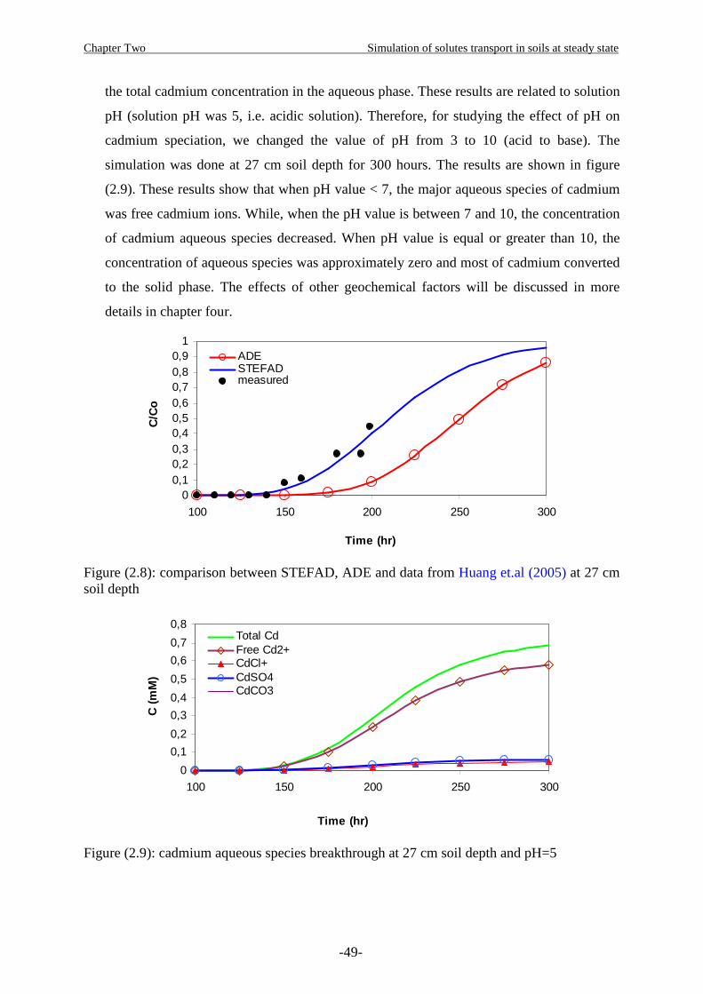
Chapter Two Simulation of solutes transport in soils at steady state
-49-
the total cadmium concentration in the aqueous phase. These results are related to solution
pH (solution pH was 5, i.e. acidic solution). Therefore, for studying the effect of pH on
cadmium speciation, we changed the value of pH from 3 to 10 (acid to base). The
simulation was done at 27 cm soil depth for 300 hours. The results are shown in figure
(2.9). These results show that when pH value < 7, the major aqueous species of cadmium
was free cadmium ions. While, when the pH value is between 7 and 10, the concentration
of cadmium aqueous species decreased. When pH value is equal or greater than 10, the
concentration of aqueous species was approximately zero and most of cadmium converted
to the solid phase. The effects of other geochemical factors will be discussed in more
details in chapter four.
00,10,20,30,40,50,60,70,80,9
1
100 150 200 250 300
Time (hr)
C/C
o
ADESTEFADmeasured
Figure (2.8): comparison between STEFAD, ADE and data from Huang et.al (2005) at 27 cm soil depth
0
0,1
0,2
0,3
0,4
0,5
0,6
0,7
0,8
100 150 200 250 300
Time (hr)
C (
mM
)
Total CdFree Cd2+CdCl+CdSO4CdCO3
Figure (2.9): cadmium aqueous species breakthrough at 27 cm soil depth and pH=5
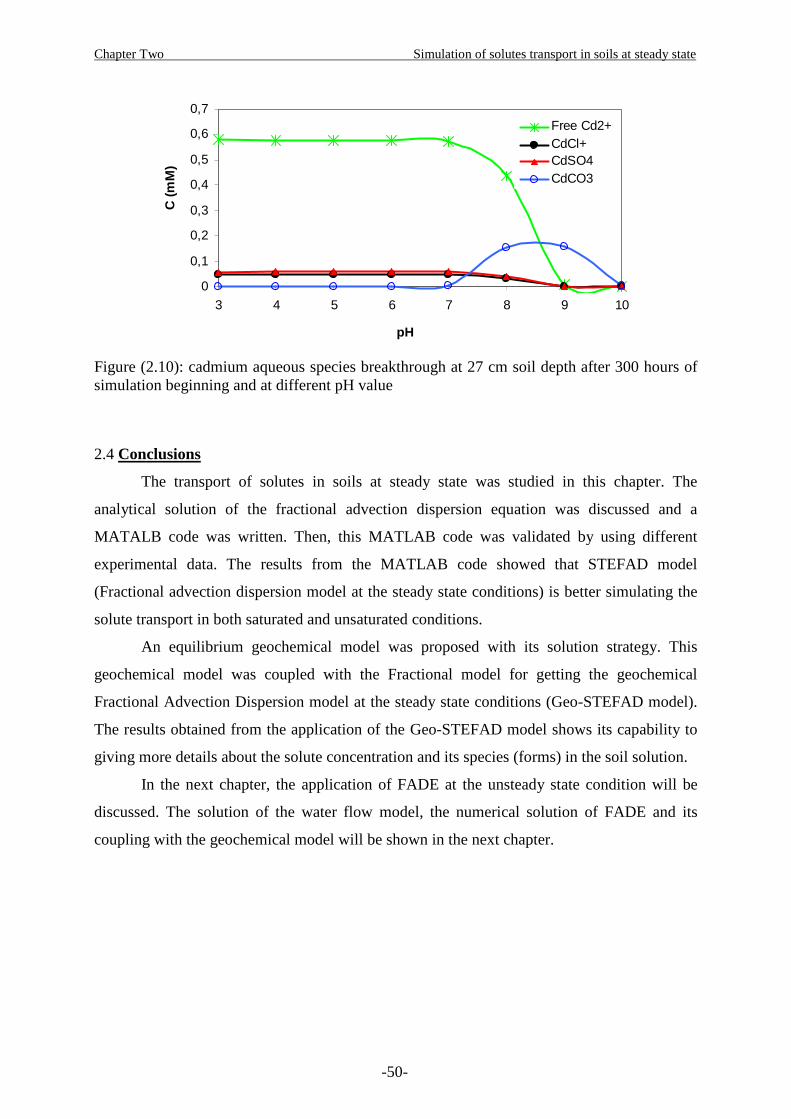
Chapter Two Simulation of solutes transport in soils at steady state
-50-
0
0,1
0,2
0,3
0,4
0,5
0,6
0,7
3 4 5 6 7 8 9 10
pH
C (
mM
)
Free Cd2+CdCl+CdSO4CdCO3
Figure (2.10): cadmium aqueous species breakthrough at 27 cm soil depth after 300 hours of simulation beginning and at different pH value
2.4 Conclusions
The transport of solutes in soils at steady state was studied in this chapter. The
analytical solution of the fractional advection dispersion equation was discussed and a
MATALB code was written. Then, this MATLAB code was validated by using different
experimental data. The results from the MATLAB code showed that STEFAD model
(Fractional advection dispersion model at the steady state conditions) is better simulating the
solute transport in both saturated and unsaturated conditions.
An equilibrium geochemical model was proposed with its solution strategy. This
geochemical model was coupled with the Fractional model for getting the geochemical
Fractional Advection Dispersion model at the steady state conditions (Geo-STEFAD model).
The results obtained from the application of the Geo-STEFAD model shows its capability to
giving more details about the solute concentration and its species (forms) in the soil solution.
In the next chapter, the application of FADE at the unsteady state condition will be
discussed. The solution of the water flow model, the numerical solution of FADE and its
coupling with the geochemical model will be shown in the next chapter.
Chapter Three Simulation of solute transport in soils at unsteady state
Chapter ThreeChapter ThreeChapter ThreeChapter Three
Simulation of solute transSimulation of solute transSimulation of solute transSimulation of solute transport in soils at unsteady state port in soils at unsteady state port in soils at unsteady state port in soils at unsteady state
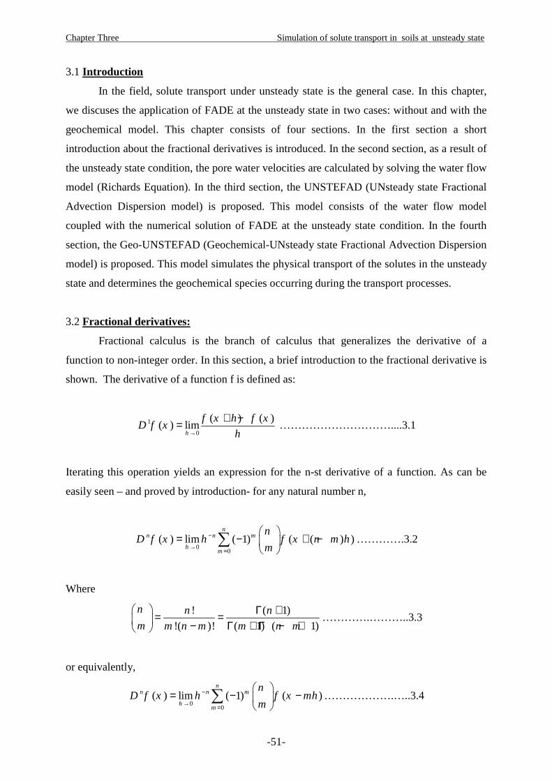
Chapter Three Simulation of solute transport in soils at unsteady state
-51-
3.1 Introduction
In the field, solute transport under unsteady state is the general case. In this chapter,
we discuses the application of FADE at the unsteady state in two cases: without and with the
geochemical model. This chapter consists of four sections. In the first section a short
introduction about the fractional derivatives is introduced. In the second section, as a result of
the unsteady state condition, the pore water velocities are calculated by solving the water flow
model (Richards Equation). In the third section, the UNSTEFAD (UNsteady state Fractional
Advection Dispersion model) is proposed. This model consists of the water flow model
coupled with the numerical solution of FADE at the unsteady state condition. In the fourth
section, the Geo-UNSTEFAD (Geochemical-UNsteady state Fractional Advection Dispersion
model) is proposed. This model simulates the physical transport of the solutes in the unsteady
state and determines the geochemical species occurring during the transport processes.
3.2 Fractional derivatives:
Fractional calculus is the branch of calculus that generalizes the derivative of a
function to non-integer order. In this section, a brief introduction to the fractional derivative is
shown. The derivative of a function f is defined as:
1
0
( ) ( )( ) lim
h
f x h f xD f x
h→
+ −= …………………………....3.1
Iterating this operation yields an expression for the n-st derivative of a function. As can be
easily seen – and proved by introduction- for any natural number n,
00
( ) lim ( 1) ( ( ) )n
n n m
hm
nD f x h f x n m h
m−
→ =
= − + −
∑ ………….3.2
Where
! ( 1)
!( )! ( 1) ( 1)
n n n
m m n m m n m
Γ += = − Γ + Γ − + ………….………..3.3
or equivalently,
00
( ) lim ( 1) ( )n
n n m
hm
nD f x h f x mh
m−
→ =
= − −
∑ ……………….…..3.4
Chapter Three Simulation of solute transport in soils at unsteady state
-52-
3.2.1 Exponentials:
The case of the exponential function is especially simple and gives some indications
about the generalization of the derivatives:
( ( ) )
00
lim ( 1)ax n a x n h
hn
D e h en
αα α αα− + −
→ =
= − =
∑
00
lim ( 1) ( )ax n ah n
hn
e h en
αα αα− −
→ =
= − =
∑
( )0
lim 1ax ah
he h e
αα−
→= − =
axa eα= ………………………………..3.5
3.2.2 Power:
The case of powers of x also has some simplicity that allows its generalization. The
case of integer order derivatives
1
1 1
0
!( )
( )!
na a n a a n a n
m
aD x ax D x x a m x
a n
−− − −
=
= ⇒ = − =−∏ …………3.6
can be easily generalized to non-integer order derivatives
( 1)
( 1)a aa
D x xa
α α
α−Γ +=
Γ − + …………………………………….…..3.7
Which can be applied to any function that can be expanded in powers x
( ) ( )( )
1( )
1n n n
n n nn n n
nf x a x D f x a D x a x
nα α α
α
∞ ∞ ∞−
=−∞ =−∞ =−∞
Γ += ⇒ = =
Γ − +∑ ∑ ∑ ………….……..3.8
3.2.3 Binomial Formula
Let ( ) ( )hd f x f x h= + whose iteration yields:
( ) ( )hd f x f x hα α= + ………………………………………………..3.9
Chapter Three Simulation of solute transport in soils at unsteady state
-53-
Therefore
00
( ) lim ( 1) ( ( ) )n
n n m
hm
nD f x h f x n m h
m−
→ =
= − + − =
∑
00
lim ( 1) ( )n
n m n mh
hm
nh d f x
m− −
→ =
= − =
∑
0
1lim ( )h
h
df x
h→
− =
…………………………………....3.10
For non-integer numbers,
0
1( ) lim ( )h
h
dD f x f x
h
αα
→
− = =
0
0
( 1)lim ( 1) ( )
!( 1)n n
hh
n
h d f xn n
α ααα
∞− −
→ =
Γ += − =− +∑
0
0
( 1)lim ( 1) ( ( ) )
!( 1)n n
hh
n
h d f x n hn n
α αα αα
∞− −
→ =
Γ += − + −− +∑ ……….3.11
Finally, it is obvious that as h goes to 0 the last equation is equivalent to the following
( )( ) ( )
00
1( ) lim ( 1)
! 1n
hn
D f x h f x nhn n
α α αα
∞−
→ =
Γ += − −
Γ − +∑ …………….3.12
3.2.4 Grünwald-Letnikov Derivative
Grünwald-Letnikov derivative is a generalization of the derivative analogous to the
generalization by the binomial formula (3.12), but it is based on the direct generalization of
the equation (3.4):
( ) ( ) ( )( ) ( )
00
1lim 1
! 1
x a
hm
hm
D f x h f x mhm m
α α αα
−
−
→ =
Γ += − −
Γ − +∑ …………..3.13
3.2.5 Riemann-Liouville Derivative
Riemann-Liouville derivative is the most used generalization of the derivative. The
Riemann-Liouville derivative is:
10
1 ( )( )
( ) ( )
x f tD f x dt
x tα
αα +=Γ − −∫ ……………..3.14

Chapter Three Simulation of solute transport in soils at unsteady state
-54-
3.3 Water Flow Model:
Darcy’s equation for one dimensional saturated flow is:
s
HJ K
z
∂ = − ∂ ………..…………3.15
Where J is fluid flux, K is the saturated hydraulic conductivity; z is the spatial coordinate
(Simunek et al. 1998, Warrick 2003). The Darcy equation modified for the unsaturated flow
and becomes Buckingham-Darcy equation:
1u
hJ K
z
∂ = − + ∂ ……..……………3.16
Which is derived by defining the total head H as pressure head h and vertical spatial
coordinate z. The unsaturated hydraulic conductivity Ku is a function of pressure head and/or
of water content. Richards’ equation for transient water flow is:
J
t z
θ∂ ∂= −∂ ∂
………………………….…..3.17
Where θ is the volumetric water content, t is time. The Buckingham equation coupled with
Richards’ equation, we have:
1h
Kt z z
θ∂ ∂ ∂ = + ∂ ∂ ∂ ……………………3.18
This equation for one-dimensional flow contains two dependent variables, pressure head h
and water content θ (Warrick 2003). Equation (3.18) can be written in the following form
(van Dam et al. 2000):
1h h
C Kt t z z
θ∂ ∂ ∂ ∂ = = + ∂ ∂ ∂ ∂ ……………………3.19
Where C is the differential water capacity (dθ/dh) (cm-1).
3.3.1 Soil Hydraulic Properties Equations
The hydraulic conductivity K in equation (3.19) is given by
( ) ( ) ( ), ,s rK h z K z K h z= ………………….3.20
Chapter Three Simulation of solute transport in soils at unsteady state
-55-
Where Ks is the saturated hydraulic conductivity and Kr is the relative hydraulic conductivity
(Simunlek et al. 1998). Mualem gives the relative hydraulic conductivity Kr as:
r es
KK S
K= = ……………..3.21
The effective saturation (Se) is:
re
s r
Sθ θθ θ
−=−
………………..3.22
Where θ is the water content, θr is the residual water content, and θs is the saturated water
content (Mualem 1976). The van Genuchten model for solving hydraulic conductivity as a
function of water content is:
( ) ( )2
1/ 2 1/1 1mm
r e eK h S S = − − ………………….3.23
11 1m n
n= − > ……………………………3.24
Multiplying this equation by Ks gives (Simunek et al.1998, van Genuchten 1980):
( ) ( )2
1/ 2 1/1 1mm
s e eK h K S S = − − ……………………..3.25
Soil water content as a function of pressure head is given by van Genuchten as:
( )( )1
s rr mn
v
hh
θ θθ θα
−= + +
……………………………3.26
Equation (3.26) is highly non-linear due to the non-linear physical relationships
between θ-h-K. Therefore, this equation can be solved analytically only for a very limited
cases. Numerical techniques used for solving this equation have been described by Yeh, 1986.
The results of the numerical soil water flow models may be seriously affected by the way they
average the hydraulic conductivity K between nodes. Haverkamp and Vauclin ,1979;
Chapter Three Simulation of solute transport in soils at unsteady state
-56-
Belmans, Wesseling and Feddes ,1983; and Hornung and Messing ,1983; proposed to use the
geometric mean, which increased the accuracy of calculated fluxes and caused the fluxes to be
less sensitive to changes in nodal distance. However, the geometric mean has serious
disadvantages too. When simulating infiltration in dry soils or high evaporation from wet
soils, the geometric mean severely underestimates the water fluxes and may cause
convergence problems (Zaidel and Russo 1992). Other researchers proposed the use of a
harmonic mean (Warrick 1991; Zaidel and Russo 1992; Desbarats 1995; Baker 1995;
Romano, Brunone and Santini 1998). The different approaches may have a significant effect
on the calculated soil water fluxes.
Van Dam and Feddes, 2000, investigated the effect of nodal distance and averaging of
hydraulic conductivity with SWAP (Soil–Water–Atmosphere–Plant). This model has been
developed at Wageningen UR from 1978 onwards (Feddes, Kowalik and Zaradny 1978;
Belmans, Wesseling and Feddes 1983; Kabat, Van den Broek and Feddes 1992; Van Dam et
al. 1997) and simulates one-dimensional (1D), variably saturated, water flow, solute transport
and heat flow in relation to crop development . One of the investigated cases concerned an
intensive rain shower on a dry sandy soil. Van Dam and Feddes, 2000, varied the nodal
distance from 0.1 to 5 cm and applied both arithmetic and geometric averaging of K. At small
nodal distances the hydraulic gradient and the average K converge to the same value,
whatever method of K-averaging was used. They support the use of arithmetic averages in
commonly applied finite difference numerical schemes.
Both finite difference and finite element methods have been used to solve Richards’
equation for variability saturated soil (Feddes et al., 1988; Celia et al., 1990; Pan et al., 1996).
In two and three dimensional flow domains, finite elements are advantageous at irregular
geometries. In one dimension finite difference is advantageous because it needs no mass
lumping to prevent oscillation (Van Genuchten, 1982; Pan et al., 1996), and is easier to
conceive and to implement in numerical routines.
A Dirichlet boundary condition is taken at the soil surface:
θ(0,t) = θs ………………..3.27
A unit hydraulic gradient (free drainage) is taken at zmax
Chapter Three Simulation of solute transport in soils at unsteady state
-57-
max
0z zz
θ=
∂ =∂
…….……….3.28
and an initial condition of
θ (z,0) = θini …………………3.29
A popular method to solve Richards’ equation is the implicit, finite difference scheme
with explicit linearization of hydraulic conductivity K, and water capacity C, as described by
Warrick (2003):
Consider the h-based Richards’ equation in the following form:
h h KC K
t z z z
∂ ∂ ∂ ∂ − = − ∂ ∂ ∂ ∂ ………………………………….………3.30
An approximation at z=zi and tn+1= t+∆t is:
( ) ( )( )
( )( )
( )* * * * *, , 0.5, 1 0.5, 1 0.5, 0.5,
2 2
i n i i n i n i i i n i i i n i nC h h K h h K h h K K
t zz z
+ + − − + −− − − −− + = −
∆ ∆∆ ∆……….3.31
In (3.31), the specific water content and conductivities are at the “old” time tn and the h*
values correspond to the new time tn+1. The ∆z is assumed constant.
1 1
2i iz z
z + −−∆ = ……………………………………………….3.32
1 10.5 0.5,
2 2i i i i
i i
K K K KK K+ −
+ −+ += = …………………..3.33
Application of equation 3.31 results in a tridiagonal matrix:
* * *1 1i i i i i i iA h B h C h D− ++ + = i=1... nz ……………..….3.34
Chapter Three Simulation of solute transport in soils at unsteady state
-58-
*10 0 1
*21 1 1 2
*33
*2 2 2 11
*1 1
0 ... 0
0 .
0 .
. .
. 0
.
0 0N N N nn
N N nn
DB C h
DA B C h
Dh
A B C Dh
A B Dh− − − −−
− −
=
………………….3.35
Internal nodes (i=2… nz-1)
( )
0.5,2
i ni
KA
z
−= −∆
……………..………………..…3.36
( )
, 0.5, 0.5,2
i n i n i ni
C K KB
t z
+ −+= +
∆ ∆……........................3.37
( )
0.5,2
i ni
KC
z
−= −∆
……….………………………....3.38
( )0.5, 0.5,, , i n i ni n i n
i
K KC hD
t z+ −−
= −∆ ∆
………………3.39
Upper node, θ (0, t) or h (0, t) given
1 0A = …………………..…….. ………………3.40
B1 as above with i=1…………….………………….3.41
C1 as above with i=1 ………………………..…..3.42
( )( )
1.5, 0.5,1, 1, 0.5,1 2
(0, )n nn n nK KC h K h t
Dt z z
−= − +
∆ ∆ ∆……….3.43
[K0.5,n based on h(0,t) and K1,n]
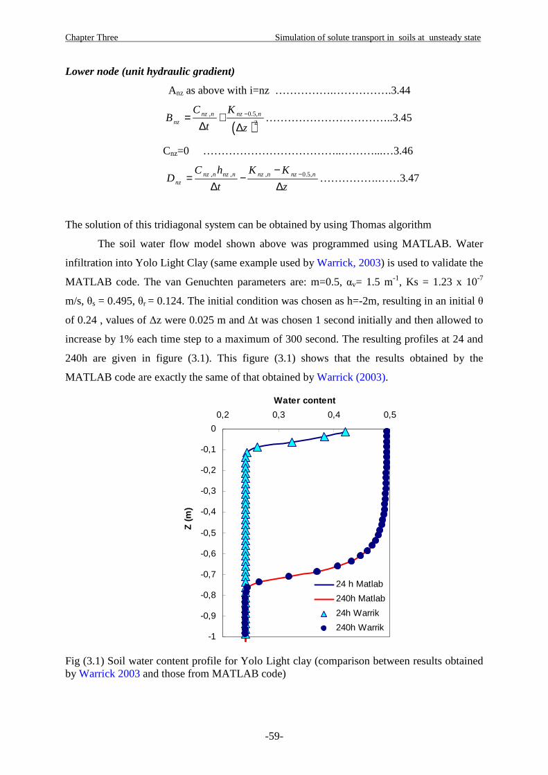
Chapter Three Simulation of solute transport in soils at unsteady state
-59-
Lower node (unit hydraulic gradient)
Anz as above with i=nz …………….…………….3.44
( )
, 0.5,2
nz n nz nnz
C KB
t z
−= +∆ ∆
……………………………..3.45
Cnz=0 ………………………………..………...…3.46
, , , 0.5,nz n nz n nz n nz nnz
C h K KD
t z−−
= −∆ ∆
…………….……3.47
The solution of this tridiagonal system can be obtained by using Thomas algorithm
The soil water flow model shown above was programmed using MATLAB. Water
infiltration into Yolo Light Clay (same example used by Warrick, 2003) is used to validate the
MATLAB code. The van Genuchten parameters are: m=0.5, αv= 1.5 m-1, Ks = 1.23 x 10⁻⁷
m/s, θs = 0.495, θr = 0.124. The initial condition was chosen as h=-2m, resulting in an initial θ
of 0.24 , values of ∆z were 0.025 m and ∆t was chosen 1 second initially and then allowed to
increase by 1% each time step to a maximum of 300 second. The resulting profiles at 24 and
240h are given in figure (3.1). This figure (3.1) shows that the results obtained by the
MATLAB code are exactly the same of that obtained by Warrick (2003).
-1
-0,9
-0,8
-0,7
-0,6
-0,5
-0,4
-0,3
-0,2
-0,1
0
0,2 0,3 0,4 0,5
Water content
Z (
m)
24 h Matlab
240h Matlab
24h Warrik
240h Warrik
Fig (3.1) Soil water content profile for Yolo Light clay (comparison between results obtained by Warrick 2003 and those from MATLAB code)

Chapter Three Simulation of solute transport in soils at unsteady state
-60-
3.4 UNSTEFAD model
FADE at unsteady state can be written as (Zhang et al. 2006):
[ ]1
1.......................3.48
C CD VC
t z z z
α
α
−
−
∂ ∂ ∂ ∂= − ∂ ∂ ∂ ∂
When V and D are constants, equation (3.48) reduces directly to FADE at steady state
condition used by Benson et al. (2000a, 2001). The same reduction is also shown by Cushman
and Ginn (2000).
We first expand the variation of dispersive flux in (3.48) as:
1 1
1 1..............3.49
C C D CD D
z z z z z
α α α
α α α
− −
− −
∂ ∂ ∂ ∂ ∂= + ∂ ∂ ∂ ∂ ∂
and then we approximate the α and α-1 order fractional derivative with a one-shift and zero-
shift Grünwald formula, respectively (Meerschaert and Tadjeran, 2004)
( ) ( )0
, 1, ..................3.50
N
kk
C z tg C z k z z t
z z
α
α α=
∂≈ − ∆ + ∆
∂ ∆ ∑
( ) ( )1 1
1 10
, 1, ........................3.51
N
kk
C z tf C z k z t
z z
α
α α
− −
− −=
∂≈ − ∆
∂∆ ∆ ∑
Where ∆z is the space step size, N is a sufficiently large number of grid points, and gk , fk are
the Grünwald weights
( )( ) ( ) .........................................3.52
1k
kg
k
αα
Γ −=
Γ − Γ +
( )( ) ( )
( )1..............3.53
1 1k k
k kf g
k
α ααα
Γ − − − = =−Γ − − Γ +
To solve equation (3.48), we use a zero- and one-shift Grünwald estimate to approximate the
(α-1)- order and the α-order fractional derivative (as shown in 3.50 and 3.51), respectively,
and the resulting difference equation:
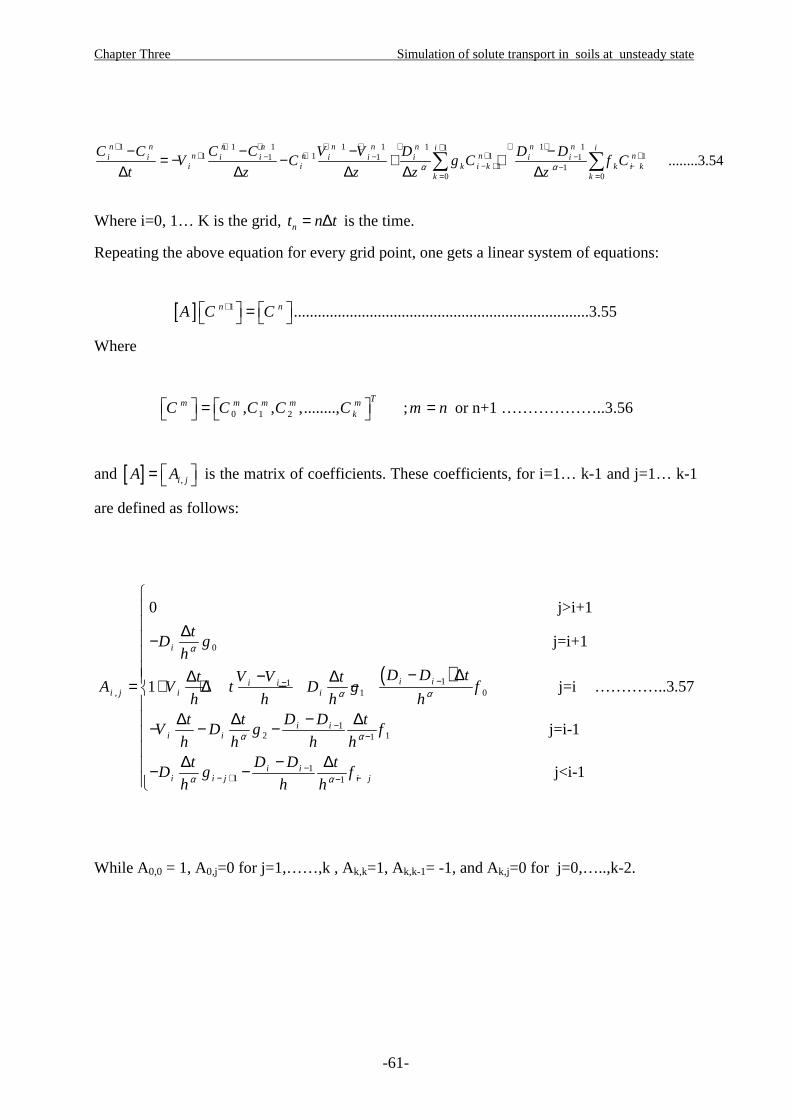
Chapter Three Simulation of solute transport in soils at unsteady state
-61-
1 1 1 1 1 1 1 111 1 1 11 1 1
1 10 0
........3.54n n n n n n n n ni i
n n n ni i i i i i i i ii i k i k k i k
k k
C C C C V V D D DV C g C f C
t z z z zα α
+ + + + + + + +++ + + +− − −
− + −−= =
− − − −= − − + +∆ ∆ ∆ ∆ ∆∑ ∑
Where i=0, 1… K is the grid, nt n t= ∆ is the time.
Repeating the above equation for every grid point, one gets a linear system of equations:
[ ] 1 ..........................................................................3.55n nA C C+ =
Where
0 1 2, , ,........, ;Tm m m m m
kC C C C C m n = = or n+1 ………………..3.56
and [ ] ,i jA A = is the matrix of coefficients. These coefficients, for i=1… k-1 and j=1… k-1
are defined as follows:
( )0
11, 1 0
12 11
11 1
0 j>i+1
j=i+1
1 j=i
j=i-1
j<i-1
i
i ii ii j i i
i ii i
i ii i j i j
tD g
hD D tV Vt t
A V t D g fh h h h
D Dt t tV D g f
h h h hD Dt t
D g fh h h
α
α α
α α
α α
−−
−−
−− + −−
∆− − ∆−∆ ∆= + + ∆ − −
−∆ ∆ ∆− − −
−∆ ∆− −
…………..3.57
While A0,0 = 1, A0,j=0 for j=1,……,k , Ak,k=1, Ak,k-1= -1, and Ak,j=0 for j=0,…..,k-2.
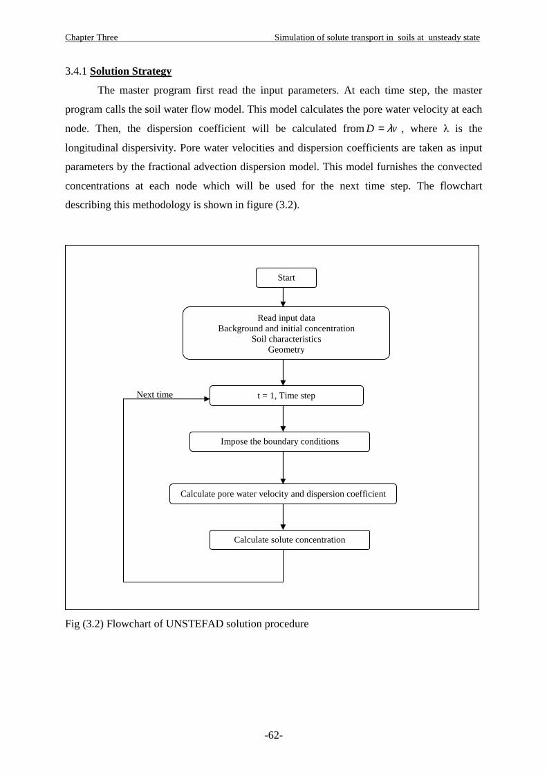
Chapter Three Simulation of solute transport in soils at unsteady state
-62-
3.4.1 Solution Strategy
The master program first read the input parameters. At each time step, the master
program calls the soil water flow model. This model calculates the pore water velocity at each
node. Then, the dispersion coefficient will be calculated fromD vλ= , where λ is the
longitudinal dispersivity. Pore water velocities and dispersion coefficients are taken as input
parameters by the fractional advection dispersion model. This model furnishes the convected
concentrations at each node which will be used for the next time step. The flowchart
describing this methodology is shown in figure (3.2).
Fig (3.2) Flowchart of UNSTEFAD solution procedure
Start
Read input data Background and initial concentration
Soil characteristics Geometry
t = 1, Time step
Impose the boundary conditions
Calculate pore water velocity and dispersion coefficient
Calculate solute concentration
Next time step

Chapter Three Simulation of solute transport in soils at unsteady state
-63-
3.4.2 Validating the UNSTEFAD model
Chloride transport through 50 cm sandy soil column is used for validating
UNSTEFAD MATLAB code. UNSTEFAD is used with α = 2 (when α = 2, the fractional
ADE will converted to the classical ADE). The hydraulic properties of the soil column were:
θr = 0.044, θs=0.413, αv=0.027 /cm, n = 2.897, Ks = 21.37 cm/hr, θin = 0.2 and the longitudinal
dispersivity = 0.2 cm. Chloride concentration is 400 mg/l.
The results from UNSTEFAD are compared with those from HYDRUS-1D (Software
Package for Simulating the One-Dimensional Movement of Water, Heat, and Multiple Solutes
in Variably-Saturated Media). Figure (3.3) shows the comparison between results from
HYDRUS-1D and UNSTEFAD. This figure shows that the codes (HYDRUS-1D and
UNSTEFAD) give the same results when the value of α = 2. Also, this figure shows that
influent chloride concentration equal to effluent chloride concentration after 7,17,32,43, and
60 minutes at 10, 20, 30, 40, and 50 cm soil depth, respectively.
0
50
100
150
200
250
300
350
400
0 0,2 0,4 0,6 0,8 1
Time (hr)
C (
mg
/l)
H-10 cmUN-10 cmH-20 cmUN-20 cmH-30 cmUN-30 cmH-40 cmUN-40 cmH-50 cmUN-50 cm
Figure (3.3): chloride breakthrough curves at different soil depths (H= HYDRUS and UN = UNSTEFAD)
3.5 Geo-UNSTEFAD model
In Geo-UNSTEFAD model (Geochemical unsteady state fractional advection
dispersion model), three models are coupled together: water flow model, solute transport
model and the geochemical model. As shown in the previous section, the flow model (section
3.2) consists of equations for water content distribution, and velocity field. The partial
differential equations are discretized in time and space using finite differences. At each time
step, a set of non-linear algebraic equations are formulated. These equations are solved using
Thomas algorithm for the tridiagonal matrix to obtain the pore water velocity along the length
Chapter Three Simulation of solute transport in soils at unsteady state
-64-
of column. The fractional transport model (section 3.3) computes the concentrations of solutes
along the soil column. This model describe the physical transport of the total aqueous
concentration. The geochemical model (chapter two, section 2.3) will be used for studying the
speciation of solutes (i.e. studying the transport of each component independently). These
models are coupled and solved following the procedure shown in the section 3.4.1.
3.5.1 Solution Strategy
For Geo-UNSTEFAD model solution, we adopted the same procedure used for
solving UNSTEFAD (section 3.3.1) and adding the geochemical model after the fractional
transport model. Therefore, at each time step; the master program read the input parameters.
Then it calls the water flow model for calculating the pore water velocity at each node of the
soil depth. After this, the master program calculates the dispersion coefficient for each node
depending on the pore water velocity. The pore water velocities and the dispersion
coefficients will be used as input parameters by the fractional transport model. This model
will calculate the advected concentration of solutes at each node. Then, the master program
calls the geochemical model. This model will equilibrates the chemical system using the
appropriate reactions and returns the modified component concentrations which will be
further convected by the fractional transport model in the next time step. Figure (3.4) shows
the flowchart of this procedure.
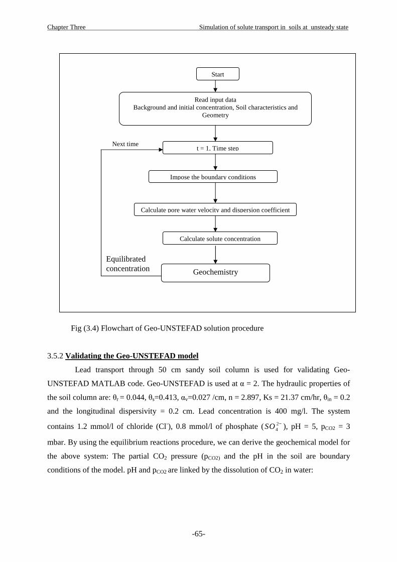
Chapter Three Simulation of solute transport in soils at unsteady state
-65-
Fig (3.4) Flowchart of Geo-UNSTEFAD solution procedure
3.5.2 Validating the Geo-UNSTEFAD model
Lead transport through 50 cm sandy soil column is used for validating Geo-
UNSTEFAD MATLAB code. Geo-UNSTEFAD is used at α = 2. The hydraulic properties of
the soil column are: θr = 0.044, θs=0.413, αv=0.027 /cm, n = 2.897, Ks = 21.37 cm/hr, θin = 0.2
and the longitudinal dispersivity = 0.2 cm. Lead concentration is 400 mg/l. The system
contains 1.2 mmol/l of chloride (Cl-), 0.8 mmol/l of phosphate ( 24SO − ), pH = 5, pCO2 = 3
mbar. By using the equilibrium reactions procedure, we can derive the geochemical model for
the above system: The partial CO2 pressure (pCO2) and the pH in the soil are boundary
conditions of the model. pH and pCO2 are linked by the dissolution of CO2 in water:
Start
Read input data Background and initial concentration, Soil characteristics and
Geometry
t = 1, Time step
Impose the boundary conditions
Calculate pore water velocity and dispersion coefficient
Calculate solute concentration
Next time
Geochemistry
Equilibrated concentration
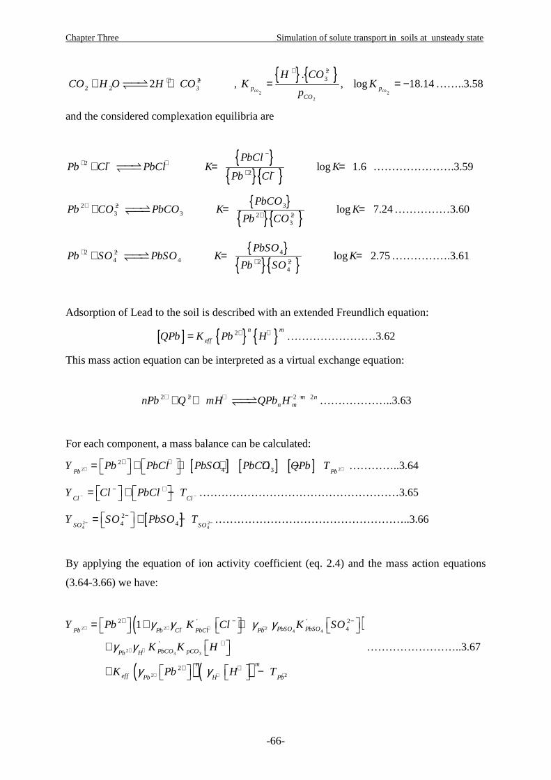
Chapter Three Simulation of solute transport in soils at unsteady state
-66-
22 2 32CO H O H CO+ −+ +��⇀↽�� ,
{ } { }2 2
2
23.
, log 18.14co cop p
CO
H COK K
p
+ −
= = − ……..3.58
and the considered complexation equilibria are
{ }{ }{ }
2
2log 1.6
PbClPb Cl PbCl K K
Pb Cl
−+ − +
+ −+ = =��⇀↽�� ………………….3.59
{ }{ }{ }
32 23 3 2 2
3
log 7.24PbCO
Pb CO PbCO K KPb CO
+ −+ −
+ = =��⇀↽�� ……………3.60
{ }{ }{ }
42 24 4 2 2
4
log 2.75PbSO
Pb SO PbSO K KPb SO
+ −+ −
+ = =��⇀↽�� …………….3.61
Adsorption of Lead to the soil is described with an extended Freundlich equation:
[ ] { } { }2 n m
effQPb K Pb H+ += ……………………3.62
This mass action equation can be interpreted as a virtual exchange equation:
2 2 2 2m nn mnPb Q mH QPb H+ − + − −+ + ��⇀↽�� ………………..3.63
For each component, a mass balance can be calculated:
[ ] [ ] [ ]2 22
4 3Pb PbY Pb PbCl PbSO PbCO QPb T+ +
+ + = + + + + − …………..3.64
Cl ClY Cl PbCl T− −
− + = + − ………………………………………………3.65
[ ]2 24 4
24 4SO SO
Y SO PbSO T− −− = + − ……………………………………………..3.66
By applying the equation of ion activity coefficient (eq. 2.4) and the mass action equations
(3.64-3.66) we have:
( )
( ) ( )
2 2 24 4
23 3
2 2
2 ' ' 24
'
2
1 PbSO PbSOPb Pb Cl PbCl Pb
PbCO pCOPb H
n m
eff Pb H Pb
Y Pb K Cl K SO
K K H
K Pb H T
γ γ γ γ
γ γ
γ γ
+ + − + +
+ +
+ + +
+ − −
+
+ +
= + +
+
+ −
……………………..3.67
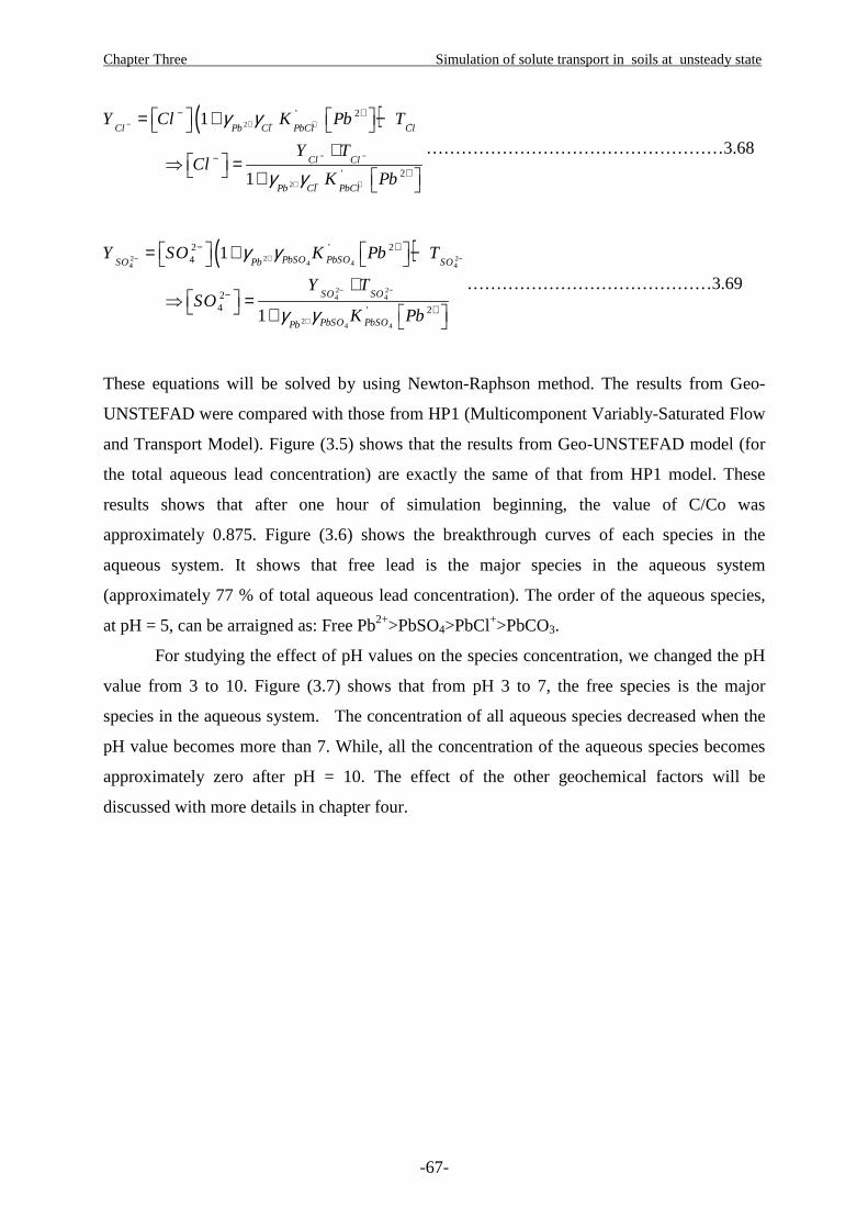
Chapter Three Simulation of solute transport in soils at unsteady state
-67-
( )2
2
' 2
' 2
1
1
Cl Pb Cl PbCl Cl
Cl Cl
Pb Cl PbCl
Y Cl K Pb T
Y TCl
K Pb
γ γ
γ γ
− + − + −
− −
+ − +
− +
−+
= + −
+ ⇒ = +
……………………………………………3.68
( )2 2 24 44 4
2 24 4
24 4
2 ' 24
24 ' 2
1
1
PbSO PbSOSO Pb SO
SO SO
PbSO PbSOPb
Y SO K Pb T
Y TSO
K Pb
γ γ
γ γ
− + −
− −
+
− +
−+
= + −
+ ⇒ = +
……………………………………3.69
These equations will be solved by using Newton-Raphson method. The results from Geo-
UNSTEFAD were compared with those from HP1 (Multicomponent Variably-Saturated Flow
and Transport Model). Figure (3.5) shows that the results from Geo-UNSTEFAD model (for
the total aqueous lead concentration) are exactly the same of that from HP1 model. These
results shows that after one hour of simulation beginning, the value of C/Co was
approximately 0.875. Figure (3.6) shows the breakthrough curves of each species in the
aqueous system. It shows that free lead is the major species in the aqueous system
(approximately 77 % of total aqueous lead concentration). The order of the aqueous species,
at pH = 5, can be arraigned as: Free Pb2+>PbSO4>PbCl+>PbCO3.
For studying the effect of pH values on the species concentration, we changed the pH
value from 3 to 10. Figure (3.7) shows that from pH 3 to 7, the free species is the major
species in the aqueous system. The concentration of all aqueous species decreased when the
pH value becomes more than 7. While, all the concentration of the aqueous species becomes
approximately zero after pH = 10. The effect of the other geochemical factors will be
discussed with more details in chapter four.
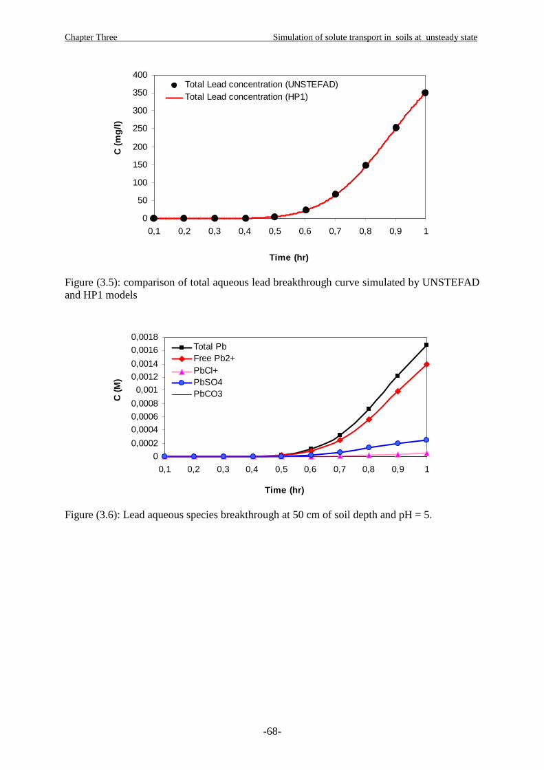
Chapter Three Simulation of solute transport in soils at unsteady state
-68-
0
50
100
150
200
250
300
350
400
0,1 0,2 0,3 0,4 0,5 0,6 0,7 0,8 0,9 1
Time (hr)
C (
mg
/l)
Total Lead concentration (UNSTEFAD)Total Lead concentration (HP1)
Figure (3.5): comparison of total aqueous lead breakthrough curve simulated by UNSTEFAD and HP1 models
0
0,0002
0,0004
0,0006
0,0008
0,001
0,0012
0,0014
0,0016
0,0018
0,1 0,2 0,3 0,4 0,5 0,6 0,7 0,8 0,9 1
Time (hr)
C (
M)
Total PbFree Pb2+PbCl+PbSO4PbCO3
Figure (3.6): Lead aqueous species breakthrough at 50 cm of soil depth and pH = 5.
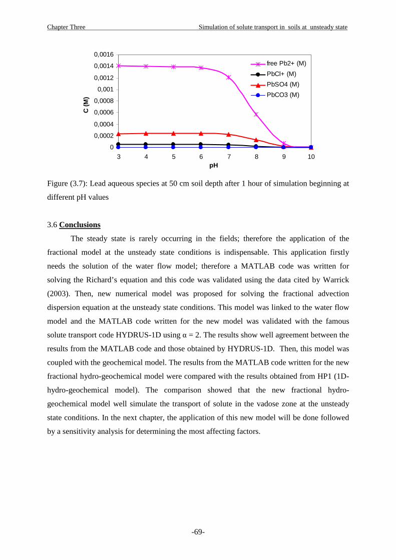
Chapter Three Simulation of solute transport in soils at unsteady state
-69-
0
0,0002
0,0004
0,0006
0,0008
0,001
0,0012
0,0014
0,0016
3 4 5 6 7 8 9 10pH
C (
M)
free Pb2+ (M)
PbCl+ (M)
PbSO4 (M)
PbCO3 (M)
Figure (3.7): Lead aqueous species at 50 cm soil depth after 1 hour of simulation beginning at
different pH values
3.6 Conclusions
The steady state is rarely occurring in the fields; therefore the application of the
fractional model at the unsteady state conditions is indispensable. This application firstly
needs the solution of the water flow model; therefore a MATLAB code was written for
solving the Richard’s equation and this code was validated using the data cited by Warrick
(2003). Then, new numerical model was proposed for solving the fractional advection
dispersion equation at the unsteady state conditions. This model was linked to the water flow
model and the MATLAB code written for the new model was validated with the famous
solute transport code HYDRUS-1D using α = 2. The results show well agreement between the
results from the MATLAB code and those obtained by HYDRUS-1D. Then, this model was
coupled with the geochemical model. The results from the MATLAB code written for the new
fractional hydro-geochemical model were compared with the results obtained from HP1 (1D-
hydro-geochemical model). The comparison showed that the new fractional hydro-
geochemical model well simulate the transport of solute in the vadose zone at the unsteady
state conditions. In the next chapter, the application of this new model will be done followed
by a sensitivity analysis for determining the most affecting factors.
Chapter FourChapter FourChapter FourChapter Four
Model Application and sensitivity analysisModel Application and sensitivity analysisModel Application and sensitivity analysisModel Application and sensitivity analysis
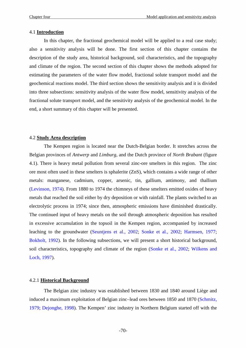
Chapter four Model application and sensitivity analysis
-70-
4.1 Introduction
In this chapter, the fractional geochemical model will be applied to a real case study;
also a sensitivity analysis will be done. The first section of this chapter contains the
description of the study area, historical background, soil characteristics, and the topography
and climate of the region. The second section of this chapter shows the methods adopted for
estimating the parameters of the water flow model, fractional solute transport model and the
geochemical reactions model. The third section shows the sensitivity analysis and it is divided
into three subsections: sensitivity analysis of the water flow model, sensitivity analysis of the
fractional solute transport model, and the sensitivity analysis of the geochemical model. In the
end, a short summary of this chapter will be presented.
4.2 Study Area description
The Kempen region is located near the Dutch-Belgian border. It stretches across the
Belgian provinces of Antwerp and Limburg, and the Dutch province of North Brabant (figure
4.1). There is heavy metal pollution from several zinc-ore smelters in this region. The zinc
ore most often used in these smelters is sphalerite (ZnS), which contains a wide range of other
metals: manganese, cadmium, copper, arsenic, tin, gallium, antimony, and thallium
(Levinson, 1974). From 1880 to 1974 the chimneys of these smelters emitted oxides of heavy
metals that reached the soil either by dry deposition or with rainfall. The plants switched to an
electrolytic process in 1974; since then, atmospheric emissions have diminished drastically.
The continued input of heavy metals on the soil through atmospheric deposition has resulted
in excessive accumulation in the topsoil in the Kempen region, accompanied by increased
leaching to the groundwater (Seuntjens et al., 2002; Sonke et al., 2002; Harmsen, 1977;
Bokholt, 1992). In the following subsections, we will present a short historical background,
soil characteristics, topography and climate of the region (Sonke et al., 2002; Wilkens and
Loch, 1997).
4.2.1 Historical Background
The Belgian zinc industry was established between 1830 and 1840 around Liège and
induced a maximum exploitation of Belgian zinc–lead ores between 1850 and 1870 (Schmitz,
1979; Dejonghe, 1998). The Kempen’ zinc industry in Northern Belgium started off with the
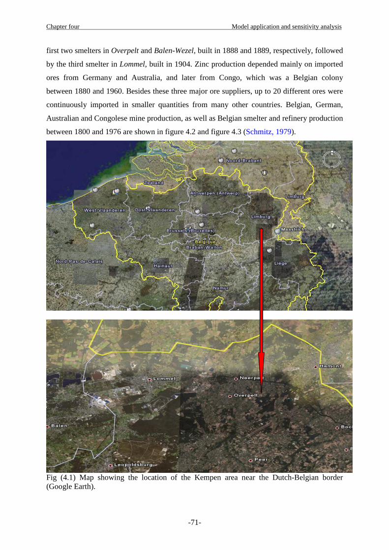
Chapter four Model application and sensitivity analysis
-71-
first two smelters in Overpelt and Balen-Wezel, built in 1888 and 1889, respectively, followed
by the third smelter in Lommel, built in 1904. Zinc production depended mainly on imported
ores from Germany and Australia, and later from Congo, which was a Belgian colony
between 1880 and 1960. Besides these three major ore suppliers, up to 20 different ores were
continuously imported in smaller quantities from many other countries. Belgian, German,
Australian and Congolese mine production, as well as Belgian smelter and refinery production
between 1800 and 1976 are shown in figure 4.2 and figure 4.3 (Schmitz, 1979).
Fig (4.1) Map showing the location of the Kempen area near the Dutch-Belgian border (Google Earth).
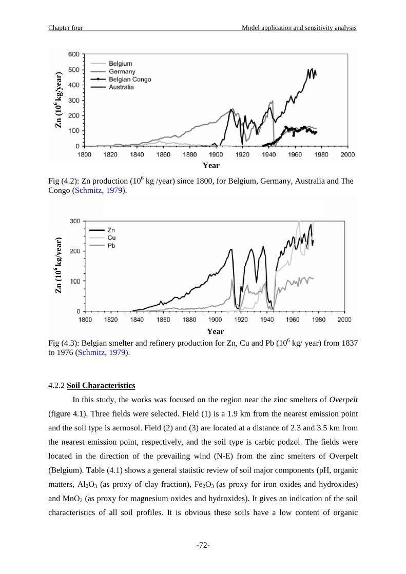
Chapter four Model application and sensitivity analysis
-72-
Fig (4.2): Zn production (106 kg /year) since 1800, for Belgium, Germany, Australia and The Congo (Schmitz, 1979).
Fig (4.3): Belgian smelter and refinery production for Zn, Cu and Pb (106 kg/ year) from 1837 to 1976 (Schmitz, 1979).
4.2.2 Soil Characteristics
In this study, the works was focused on the region near the zinc smelters of Overpelt
(figure 4.1). Three fields were selected. Field (1) is a 1.9 km from the nearest emission point
and the soil type is aernosol. Field (2) and (3) are located at a distance of 2.3 and 3.5 km from
the nearest emission point, respectively, and the soil type is carbic podzol. The fields were
located in the direction of the prevailing wind (N-E) from the zinc smelters of Overpelt
(Belgium). Table (4.1) shows a general statistic review of soil major components (pH, organic
matters, Al2O3 (as proxy of clay fraction), Fe2O3 (as proxy for iron oxides and hydroxides)
and MnO2 (as proxy for magnesium oxides and hydroxides). It gives an indication of the soil
characteristics of all soil profiles. It is obvious these soils have a low content of organic
Year
Year
Zn
(106
kg/y
ear)
Z
n (1
06 kg
/yea
r)
Chapter four Model application and sensitivity analysis
-73-
matter, low pH and low contents of oxides. The soil samples contain less than 0.5% of the
fraction below 2 µm. Consequently the amount of clay minerals is negligible. Most soil
particles are in the fraction 125 to 250 µm (Table 4.2).
Figures 4.4 and 4.5 present depth profiles of organic matter content, H3O+
concentration, the contents of aluminum oxide, iron oxide, manganese oxide, and zinc
concentration of the sampled fields. These figures show that at field 1, there are very low
content of organic matters (about 1.5%). While for field 2 and 3, the amount of organic
matters is about 7% at the top of soil and about 2% until 25 cm of soil depth. After 25 cm of
soil depth, there is approximately no organic matters content. Soils at the three fields are
acidic (pH ≈ 4). Iron and aluminum are partially removed from the topsoil probably due to a
decrease in pH. In general, the content of aluminum, iron and manganese are low and increase
with the depth, which may be a result of acidification (WILKENS and LOCH, 1997). There is
a clear enrichment of zinc in the topsoil. This is due to the accumulation of zinc from the
atmospheric emissions. The average content of zinc in the topsoil of the three fields is about
80 to 300 µg/g. The natural background zinc content of the Kempen region in the topsoil (0-6
cm) is 5-15 µg/g. In general, the content of zinc decreases with depth for the three fields.
Table (4.1): Basic statistics of the soil major components (WILKENS and LOCH, 1997)
Mean SD Min Max n
OM 1.89 2.59 0.03 20.75 369
pH 4.15 3.46 5.53 369
Al 2O3 1.68 0.8 0.23 6.32 401
Fe2O3 0.42 0.24 0.05 1.63 401
MnO 2 0.0064 0.004 0.0014 0.0287 401
Mean = arithmetic average; S.D. = standard deviation; Min = minimum value; Max = maximum value; n = number of observations.
Table (4.2) Grain size distribution of a representative soil samples (WILKENS and LOCH, 1997)
Fraction µm [%] Fraction µm [%]
1000 – 2000 0.3 50 – 105 12.8
500 – 1000 1.7 16 – 50 2.2
250 – 500 14.1 2 – 16 0.8
125 – 250 48.3 < 2 0.5
105 - 125 19.5
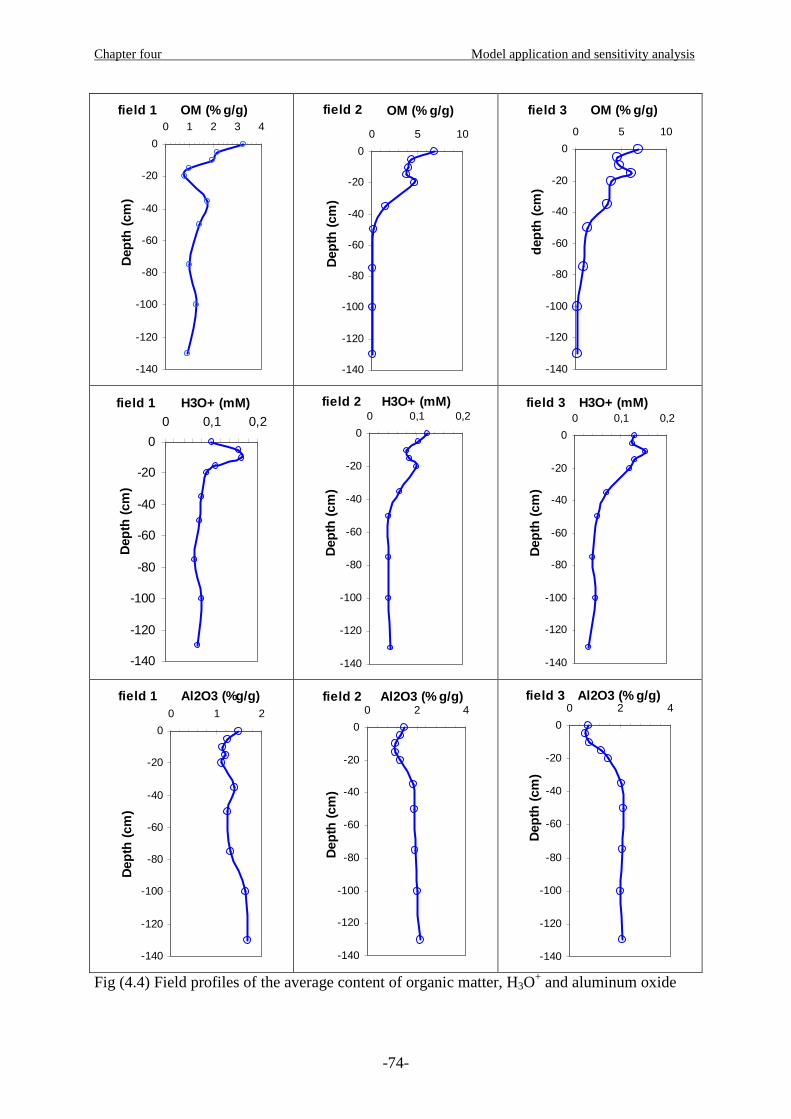
Chapter four Model application and sensitivity analysis
-74-
field 1
-140
-120
-100
-80
-60
-40
-20
0
0 1 2 3 4OM (% g/g)
Dep
th (
cm)
field 2
-140
-120
-100
-80
-60
-40
-20
0
0 5 10
OM (% g/g)
Dep
th (
cm)
field 3
-140
-120
-100
-80
-60
-40
-20
0
0 5 10
OM (% g/g)
dep
th (
cm)
field 1
-140
-120
-100
-80
-60
-40
-20
0
0 0,1 0,2H3O+ (mM)
Dep
th (
cm)
field 2
-140
-120
-100
-80
-60
-40
-20
0
0 0,1 0,2H3O+ (mM)
Dep
th (
cm)
field 3
-140
-120
-100
-80
-60
-40
-20
0
0 0,1 0,2H3O+ (mM)
Dep
th (
cm)
field 1
-140
-120
-100
-80
-60
-40
-20
0
0 1 2
Al2O3 (%g/g)
Dep
th (
cm)
field 2
-140
-120
-100
-80
-60
-40
-20
0
0 2 4Al2O3 (% g/g)
Dep
th (
cm)
field 3
-140
-120
-100
-80
-60
-40
-20
0
0 2 4Al2O3 (% g/g)
Dep
th (
cm)
Fig (4.4) Field profiles of the average content of organic matter, H3O
+ and aluminum oxide
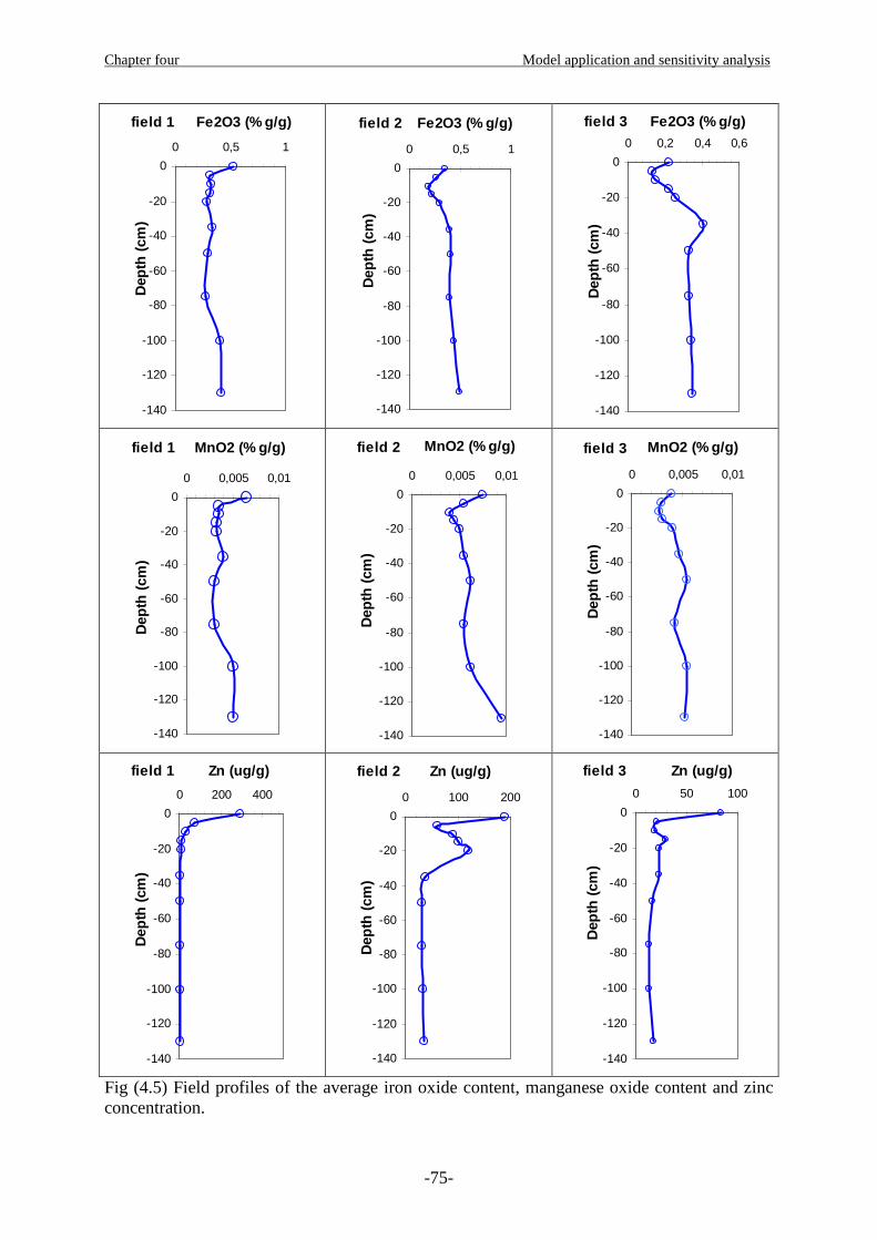
Chapter four Model application and sensitivity analysis
-75-
field 1
-140
-120
-100
-80
-60
-40
-20
0
0 0,5 1
Fe2O3 (% g/g)D
epth
(cm
)
field 2
-140
-120
-100
-80
-60
-40
-20
0
0 0,5 1
Fe2O3 (% g/g)
Dep
th (
cm)
field 3
-140
-120
-100
-80
-60
-40
-20
0
0 0,2 0,4 0,6
Fe2O3 (% g/g)
Dep
th (
cm)
field 1
-140
-120
-100
-80
-60
-40
-20
0
0 0,005 0,01
MnO2 (% g/g)
Dep
th (
cm)
field 2
-140
-120
-100
-80
-60
-40
-20
0
0 0,005 0,01
MnO2 (% g/g)
Dep
th (
cm)
field 3
-140
-120
-100
-80
-60
-40
-20
0
0 0,005 0,01
MnO2 (% g/g)
Dep
th (
cm)
field 1
-140
-120
-100
-80
-60
-40
-20
0
0 200 400
Zn (ug/g)
Dep
th (
cm)
field 2
-140
-120
-100
-80
-60
-40
-20
0
0 100 200
Zn (ug/g)
Dep
th (
cm)
field 3
-140
-120
-100
-80
-60
-40
-20
0
0 50 100
Zn (ug/g)
Dep
th (
cm)
Fig (4.5) Field profiles of the average iron oxide content, manganese oxide content and zinc concentration.
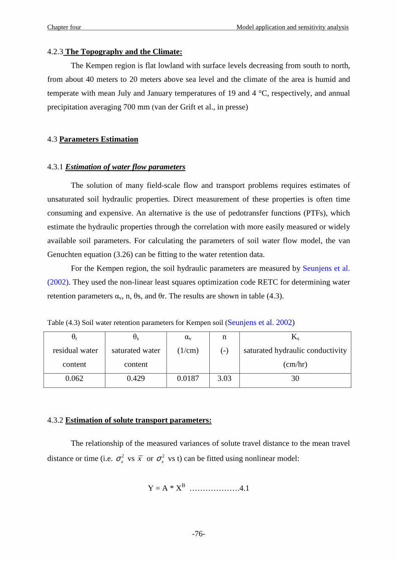
Chapter four Model application and sensitivity analysis
-76-
4.2.3 The Topography and the Climate:
The Kempen region is flat lowland with surface levels decreasing from south to north,
from about 40 meters to 20 meters above sea level and the climate of the area is humid and
temperate with mean July and January temperatures of 19 and 4 °C, respectively, and annual
precipitation averaging 700 mm (van der Grift et al., in presse)
4.3 Parameters Estimation 4.3.1 Estimation of water flow parameters The solution of many field-scale flow and transport problems requires estimates of
unsaturated soil hydraulic properties. Direct measurement of these properties is often time
consuming and expensive. An alternative is the use of pedotransfer functions (PTFs), which
estimate the hydraulic properties through the correlation with more easily measured or widely
available soil parameters. For calculating the parameters of soil water flow model, the van
Genuchten equation (3.26) can be fitting to the water retention data.
For the Kempen region, the soil hydraulic parameters are measured by Seunjens et al.
(2002). They used the non-linear least squares optimization code RETC for determining water
retention parameters αv, n, θs, and θr. The results are shown in table (4.3).
Table (4.3) Soil water retention parameters for Kempen soil (Seunjens et al. 2002)
θr
residual water
content
θs
saturated water
content
αv
(1/cm)
n
(-)
Ks
saturated hydraulic conductivity
(cm/hr)
0.062 0.429 0.0187 3.03 30
4.3.2 Estimation of solute transport parameters:
The relationship of the measured variances of solute travel distance to the mean travel
distance or time (i.e. 2xσ vs x or 2
xσ vs t) can be fitted using nonlinear model:
Y = A * X B ……………….4.1
Chapter four Model application and sensitivity analysis
-77-
Where Y is the variance of travel distance (2xσ ), X is the mean travel distance (x ) or time (t),
A and B are regression coefficients that can be used to determine transport parameters.
Because ADE predicts a linear increase of travel distance 2xσ , the measured relationship
between 2xσ and time t or mean travel distancex is often used to estimate the dispersion
coefficient or dispersivity (Zhou and Selim, 2003). Similarly, this method is also applicable to
the parameters estimation of FADE. According to Benson et al. (2000a):
2/
2 2 cos2x Dt
απασ =
…………..4.2
Where σ is the measured plume variance, D is the fractional dispersion coefficient (Lα/T); t is
time (T) and α is the fractional order. For α = 2 both sides of Eq. (4.2) are exactly equal for
the classical ADE. Comparing eq. (4.1) and eq. (4.2), one can find a relationship between
regression coefficients and fractional parameters (Zhou and Selim, 2003):
2 /Bα = ………………4.3
( )( )
1// 2
cos /
BA
DBπ
= ……….4.4
In addition, if one assumes that the molecular diffusion can be ignored (Zhou and Selim,
2003), the fractional dispersion coefficient can be expressed as,
D λν= ……………….4.5
Where v is the pore water velocity (LT-1) and λ is the fractional dispersivity (Lα-1).
Accordingly, Eq. (4.2) becomes, (Zhou and Selim, 2003)
2/
2 2 cos2x x
απασ λ ≈
……………4.6
Where x is mean travel distance, In this case, we may also estimate λ according to the
measured relationship between 2xσ andx . The fractional dispersivity is thus given by,
Chapter four Model application and sensitivity analysis
-78-
( )( )
1// 2
cos /
BA
Bλ
π= ………4.7
The inverse method is also used to determine the parameters for given BTCs involving
several derivatives of concentration versus the parameters. Benson (1998) has adopted a finite
difference (FD) method to approximate those first-order derivatives for parameters estimation.
Huang et al. (2006) adopted a semi-analytical approach to deal with those first-order
derivatives. Instead of using the finite difference method from the beginning, the first-order
derivatives can be analytically evaluated then implement the necessary integrations
numerically. The Levenberg-Marquart procedure (Press et al. 1989) can be used to minimize
the variance of the estimation error.
Soil dispersivity for the soil of Kempen region was measured by Seunjens et al. (2002)
using experiments with a non-sorbing tracer (chloride) in two undisturbed 1m-long and 0.8 m-
diameter soil columns. They found that the dispersivity is equal to 2cm. As a result of data
missing, several values of the fractional order value (1≤α≤2) will be taken to test its effects on
zinc transfer in the unsaturated soil zone of Overpelt soil (which is a part of Kempen region).
4.3.3 Geochemical Reactions Parameters Estimation:
The same procedure of chapter two and three is used for simulating the geochemical reactions
of zinc in the soil of Kempen region. The considered equilibrium geochemical reactions with
their formation constants are shown below (database of Cheaqs, 2005):
( )2Zn OH Zn OH++ −+ ⇌ Log K = 5 ……………………………. 4.8
( )2
(2)( )2
aqZn OH Zn OH+ −+ ⇌ Log K = 11.1 ……………………………. 4.9
( )2
33Zn OH Zn OH
−+ −+ ⇌ Log K = 13.6 ……………………………. 4.10
2Zn Cl ZnCl+ − ++ ⇌ Log K = 0.46 ……………………………. 4.11 ( )2
(2)( )2
aqZn Cl Zn Cl+ −+ ⇌ Log K = 0.62 ……………………………. 4.12
( )2
33Zn Cl Zn Cl
++ −+ ⇌ Log K = 0.51 ……………………………. 4.13
( )22
44Zn Cl Zn Cl
++ −+ ⇌ Log K = 0.2 ……………………………. 4.14
2 24 4( )aqZn SO ZnSO+ −+ ⇌ Log K = 2.3 ……………………………. 4.15
( )22 24 4 2
2Zn SO Zn SO−+ −+ ⇌ Log K = 3.6 ……………………………. 4.16

Chapter four Model application and sensitivity analysis
-79-
( )42 24 4 3
3Zn SO Zn SO−+ −+ ⇌ Log K = 2.7 ……………………………. 4.17
2 2
3 3( )aqZn CO ZnCO+ −+ ⇌ Log K = 4.76 ……………………………. 4.18 2 2
3 3Zn H CO ZnHCO+ + − ++ + ⇌ Log K = 11.8 3 ……………………………. 4.19
( )22 23 3 2
2Zn CO Zn CO−+ −+ ⇌ Log K = 7.3 ……………………………. 4.20
( )23Al OH Al OH++ −+ ⇌ Log K = 9 ……………………………. 4.21
3 23 3Al CO AlCO+ − ++ ⇌ Log K = 8.43 ……………………………. 4.22
24 4Al SO AlSO+ − ++ ⇌ Log K = 3.89 ……………………………. 4.23
3 2Al Cl AlCl+ − ++ ⇌ Log K = -0.391 ……………………………. 4.24
2Mn OH MnOH+ − ++ ⇌ Log K = 3.4 ……………………………. 4.25 23 3( )aqMn CO MnCO+ −+ ⇌ Log K = 4.7 ……………………………. 4.26
2 24 4( )aqMn SO MnSO+ ++ ⇌ Log K = 2.27 ……………………………. 4.27
2Fe OH FeOH+ − ++ ⇌ Log K = 4.6 ……………………………. 4.28 2
3 3( )aqFe CO FeCO+ ++ ⇌ Log K = 4.73 ……………………………. 4.29 3 2
4 4( )aqFe SO FeSO+ −+ ⇌ Log K = 2.39 ……………………………. 4.30 2Fe Cl FeCl+ − ++ ⇌ Log K = -0.3 ……………………………. 4.31

Chapter four Model application and sensitivity analysis
-80-
4.4 Model Sensitivity Analysis: The sensitivity analysis of the parameters of the fractional hydro-geo-chemical model
is conducted to examine the effects of these parameters on the simulation output. Small
changes in a parameter resulting relatively large output changes are indicative of parameters
sensitivity. The objectives of the sensitivity analysis are to find the parameters of great
importance affecting the transport of zinc and its forms in the unsaturated soil zone. This
section contains three sub-sections: 1) sensitivity analysis of the soil water flow model, 2)
sensitivity analysis of the fractional transport model, and 3) sensitivity analysis of the
geochemical model.
4.4.1 Sensitivity analysis of the soil water flow model The parameters considered in the sensitivity analysis of the soil water flow model are:
saturated hydraulic conductivity Ks, saturated soil water content θs, residual soil water
content θr, initial soil water content θi, and van Genuchten αv and n parameters.
Several scenarios are designed for the sensitivity analysis represents the soil of
Overpelt region. A single soil type of sand with a depth of 100 cm is considered. The values
of soil water retention parameters are shown in table (4.3). Runoff, evaporation, and plants
uptake processes are not considered in this study. The simulations are run for 8 hours. Table
(4.4) shows the values of the soil water flow parameters used in the sensitivity analysis. The
values of these parameters are changed by ±10% and ±25%.
Table (4.4) values of van Genuchten parameters used for the sensitivity analysis
parameters
Ks
(cm/hr)
θs
(-)
θr
(-)
θini
(-)
αv
(1/cm)
n
(-)
-25 % 22.5 0.322 0.047 0.15 0.014 2.273
-10 % 27 0.386 0.056 0.18 0.0168 2.727
Baseline 30 0.429 0.062 0.2 0.0187 3.03
+10 % 33 0.472 0.068 0.22 0.0206 3.333
+25 % 37.5 0.536 0.078 0.25 0.0234 3.788
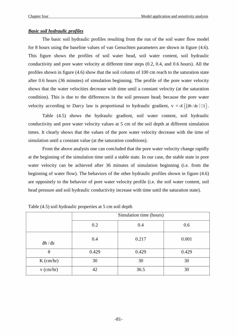
Chapter four Model application and sensitivity analysis
-81-
Basic soil hydraulic profiles
The basic soil hydraulic profiles resulting from the run of the soil water flow model
for 8 hours using the baseline values of van Genuchten parameters are shown in figure (4.6).
This figure shows the profiles of soil water head, soil water content, soil hydraulic
conductivity and pore water velocity at different time steps (0.2, 0.4, and 0.6 hours). All the
profiles shown in figure (4.6) show that the soil column of 100 cm reach to the saturation state
after 0.6 hours (36 minutes) of simulation beginning. The profile of the pore water velocity
shows that the water velocities decrease with time until a constant velocity (at the saturation
condition). This is due to the differences in the soil pressure head; because the pore water
velocity according to Darcy law is proportional to hydraulic gradient, v = ( )- / 1K h z∂ ∂ + .
Table (4.5) shows the hydraulic gradient, soil water content, soil hydraulic
conductivity and pore water velocity values at 5 cm of the soil depth at different simulation
times. It clearly shows that the values of the pore water velocity decrease with the time of
simulation until a constant value (at the saturation conditions).
From the above analysis one can concluded that the pore water velocity change rapidly
at the beginning of the simulation time until a stable state. In our case, the stable state in pore
water velocity can be achieved after 36 minutes of simulation beginning (i.e. from the
beginning of water flow). The behaviors of the other hydraulic profiles shown in figure (4.6)
are oppositely to the behavior of pore water velocity profile (i.e. the soil water content, soil
head pressure and soil hydraulic conductivity increase with time until the saturation state).
Table (4.5) soil hydraulic properties at 5 cm soil depth
Simulation time (hours)
0.2 0.4 0.6
/h z∂ ∂ 0.4 0.217 0.001
θ 0.429 0.429 0.429
K (cm/hr) 30 30 30
v (cm/hr) 42 36.5 30

Chapter four Model application and sensitivity analysis
-82-
A
-100
-90
-80
-70
-60
-50
-40
-30
-20
-10
0
-80 -40 0soil water head (cm)
soil
dep
th (
cm)
time = 0.2 h
time = 0.4 h
time = 0.6 h
B
-100
-90
-80
-70
-60
-50
-40
-30
-20
-10
0
0,2 0,3 0,4 0,5soil water content
soil
dep
th (
cm)
time = 0.2 htime = 0.4 htime = 0.6 h
C
-100
-90
-80
-70
-60
-50
-40
-30
-20
-10
0
0 20 40
soil hydraulic conductivity (cm/hr)
soil
dep
th (
cm)
time = 0.2 htime = 0.4 htime = 0.6 h
D
-100
-90
-80
-70
-60
-50
-40
-30
-20
-10
0
0 20 40 60
pore water velocity (cm/hr)
soil
dep
th (
cm)
time =0.2 htime =0.4 htime =0.6 h
Fig (4.6) basic soil profiles at different times, A: soil water head profile, B: soil water content profile, C: soil hydraulic conductivity profile, and D: pore water velocity profile
Chapter four Model application and sensitivity analysis
-83-
Scenario A: Effect of saturated soil hydraulic conductivity (Ks)
In scenario A, the values of saturated soil hydraulic conductivity change by ±10% and
±25%. The other parameters are fixed at the baseline values. The results are shown in figure
(4.7). It shows the variation of soil water content, soil water head, and pore water velocity
with respect to time at 100 cm of soil depth. This figure shows that there are adversely
relationship between the value of saturated soil hydraulic conductivity and the time needed to
reach the saturation state. When the value of soil hydraulic conductivity increases by 25%, the
time needed to make θ = θs is 29 minutes. In the other hand, when the value of soil hydraulic
conductivity decreases by 25%, the time needed to make θ = θs is 46 minutes. The effect of
saturated soil hydraulic conductivity appears more clearly on pore water velocity. When the
values of the saturated soil hydraulic conductivity change by ±10% and ±25%, the values of
pore water velocity will be changed by the same percentages, respectively. As a consequent,
one can concluded that the saturated soil hydraulic conductivity is a sensitive parameter in the
soil water flow model.
Scenario B: Effect of saturated soil water content (θs)
In scenario B, the values of saturated soil water content change by ±10% and ±25%.
The other parameters are fixed at the baseline values. The results are shown in figures (4.8)
Figure (4.8) shows the effect of saturated soil water content on the values of the soil
water content, soil water head, soil hydraulic conductivity and pore velocity. It shows that
there are direct relationships between the time needed to reach the saturation state and the
other parameters (soil water content, soil hydraulic head and pore water velocity). In other
word, the time needed to reach the saturation state decrease when the value of the saturated
soil water content decrease and vice versa. From figure 4.8-A and 4.8-B, the times needed to
reach the saturation state are 52 minutes at 25% increasing in θs value and 22 minutes at 25%
decreasing in θs value. The pore water velocity reaches the velocity at the saturation state
lately by 18 minutes when the value of θs increase by 25% and early by 12 minutes when θs
decrease by 25%. As a consequent, one can concluded that the saturated soil water content is
also a sensitive parameter in the soil water flow model.
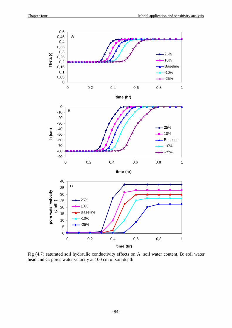
Chapter four Model application and sensitivity analysis
-84-
A
00,050,1
0,150,2
0,250,3
0,350,4
0,450,5
0 0,2 0,4 0,6 0,8 1
time (hr)
Th
eta
(-) 25%
10%
Baseline
-10%
-25%
B
-90
-80
-70
-60
-50
-40
-30
-20
-10
0
0 0,2 0,4 0,6 0,8 1
time (hr)
h (
cm) 25%
10%
Baseline
-10%
-25%
C
0
5
10
15
20
25
30
35
40
0 0,2 0,4 0,6 0,8 1
time (hr)
po
re w
ater
vel
oci
ty
(cm
/hr) 25%
10%
Baseline
-10%
-25%
Fig (4.7) saturated soil hydraulic conductivity effects on A: soil water content, B: soil water head and C: pores water velocity at 100 cm of soil depth
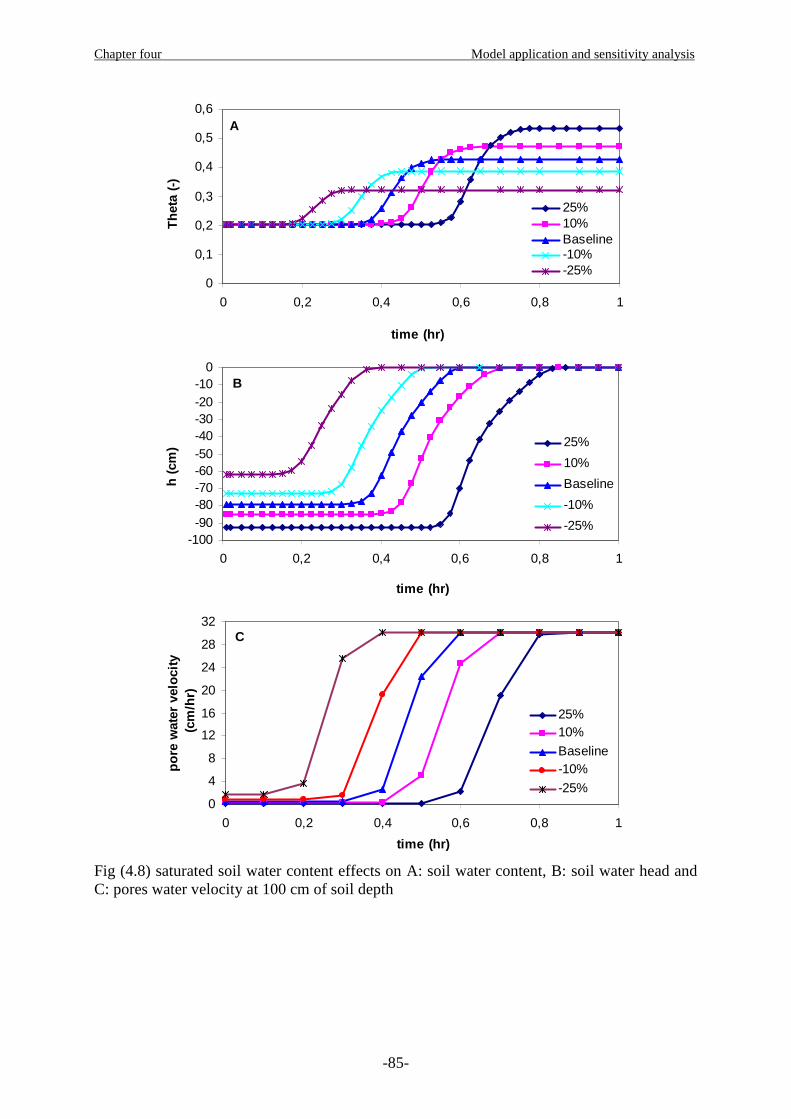
Chapter four Model application and sensitivity analysis
-85-
A
0
0,1
0,2
0,3
0,4
0,5
0,6
0 0,2 0,4 0,6 0,8 1
time (hr)
Th
eta
(-)
25%10%Baseline-10%-25%
B
-100-90-80-70-60-50-40-30-20-10
0
0 0,2 0,4 0,6 0,8 1
time (hr)
h (
cm) 25%
10%
Baseline
-10%
-25%
C
0
4
8
12
16
20
24
28
32
0 0,2 0,4 0,6 0,8 1
time (hr)
po
re w
ater
vel
oci
ty
(cm
/hr)
25%10%
Baseline-10%
-25%
Fig (4.8) saturated soil water content effects on A: soil water content, B: soil water head and C: pores water velocity at 100 cm of soil depth
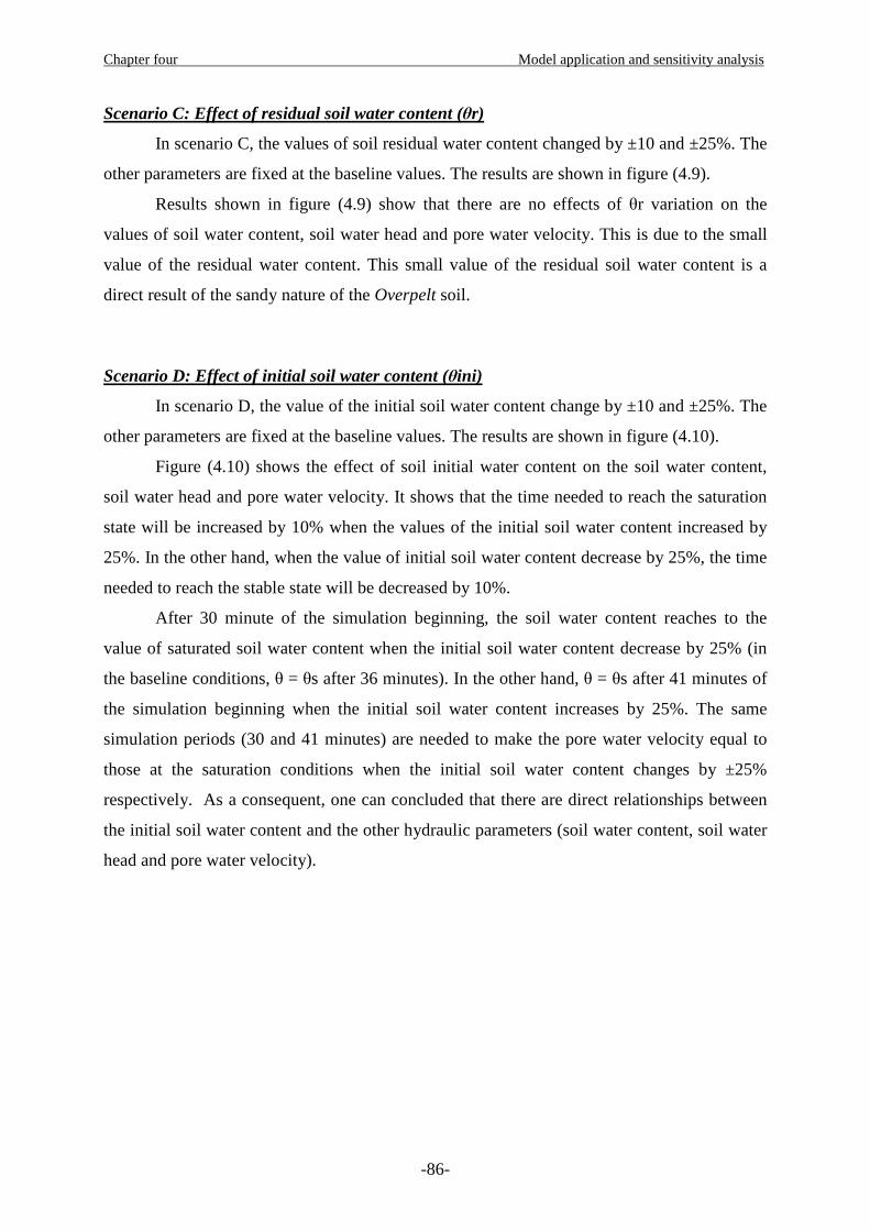
Chapter four Model application and sensitivity analysis
-86-
Scenario C: Effect of residual soil water content (θr)
In scenario C, the values of soil residual water content changed by ±10 and ±25%. The
other parameters are fixed at the baseline values. The results are shown in figure (4.9).
Results shown in figure (4.9) show that there are no effects of θr variation on the
values of soil water content, soil water head and pore water velocity. This is due to the small
value of the residual water content. This small value of the residual soil water content is a
direct result of the sandy nature of the Overpelt soil.
Scenario D: Effect of initial soil water content (θini)
In scenario D, the value of the initial soil water content change by ±10 and ±25%. The
other parameters are fixed at the baseline values. The results are shown in figure (4.10).
Figure (4.10) shows the effect of soil initial water content on the soil water content,
soil water head and pore water velocity. It shows that the time needed to reach the saturation
state will be increased by 10% when the values of the initial soil water content increased by
25%. In the other hand, when the value of initial soil water content decrease by 25%, the time
needed to reach the stable state will be decreased by 10%.
After 30 minute of the simulation beginning, the soil water content reaches to the
value of saturated soil water content when the initial soil water content decrease by 25% (in
the baseline conditions, θ = θs after 36 minutes). In the other hand, θ = θs after 41 minutes of
the simulation beginning when the initial soil water content increases by 25%. The same
simulation periods (30 and 41 minutes) are needed to make the pore water velocity equal to
those at the saturation conditions when the initial soil water content changes by ±25%
respectively. As a consequent, one can concluded that there are direct relationships between
the initial soil water content and the other hydraulic parameters (soil water content, soil water
head and pore water velocity).

Chapter four Model application and sensitivity analysis
-87-
A
00,050,1
0,150,2
0,250,3
0,350,4
0,450,5
0 0,2 0,4 0,6 0,8 1
time (hr)
Th
eta
(-)
25%
10%
Baseline
-10%
-25%
B
-90
-80
-70
-60
-50
-40
-30
-20
-10
0
0 0,2 0,4 0,6 0,8 1
time (hr)
h (
cm)
25%
10%
Baseline
-10%
-25%
C
0
5
10
15
20
25
30
35
0 0,2 0,4 0,6 0,8 1
time (hr)
po
re w
ater
vel
oci
ty
(cm
/hr) 25%
10%
baseline
-10%
-25%
Fig (4.9) Residual soil water content effects on A: soil water content, B: soil water head and C: pores water velocity at 100 cm of soil depth
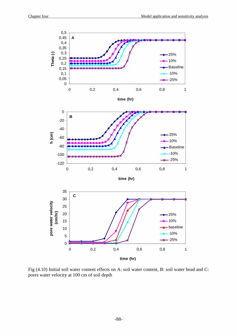
Chapter four Model application and sensitivity analysis
-88-
A
00,050,1
0,150,2
0,250,3
0,350,4
0,450,5
0 0,2 0,4 0,6 0,8 1
time (hr)
Th
eta
(-)
25%
10%
Baseline
-10%
-25%
B
-120
-100
-80
-60
-40
-20
0
0 0,2 0,4 0,6 0,8 1
time (hr)
h (
cm)
25%
10%
Baseline
-10%
-25%
C
0
5
10
15
20
25
30
35
0 0,2 0,4 0,6 0,8 1
time (hr)
po
re w
ater
vel
oci
ty
(cm
/hr) 25%
10%
baseline
-10%
-25%
Fig (4.10) Initial soil water content effects on A: soil water content, B: soil water head and C: pores water velocity at 100 cm of soil depth
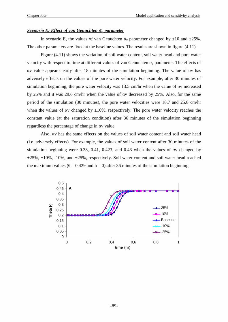
Chapter four Model application and sensitivity analysis
-89-
Scenario E: Effect of van Genuchten αv parameter
In scenario E, the values of van Genuchten αv parameter changed by ±10 and ±25%.
The other parameters are fixed at the baseline values. The results are shown in figure (4.11).
Figure (4.11) shows the variation of soil water content, soil water head and pore water
velocity with respect to time at different values of van Genuchten αv parameter. The effects of
αv value appear clearly after 18 minutes of the simulation beginning. The value of αv has
adversely effects on the values of the pore water velocity. For example, after 30 minutes of
simulation beginning, the pore water velocity was 13.5 cm/hr when the value of αv increased
by 25% and it was 29.6 cm/hr when the value of αv decreased by 25%. Also, for the same
period of the simulation (30 minutes), the pore water velocities were 18.7 and 25.8 cm/hr
when the values of αv changed by ±10%, respectively. The pore water velocity reaches the
constant value (at the saturation condition) after 36 minutes of the simulation beginning
regardless the percentage of change in αv value.
Also, αv has the same effects on the values of soil water content and soil water head
(i.e. adversely effects). For example, the values of soil water content after 30 minutes of the
simulation beginning were 0.38, 0.41, 0.423, and 0.43 when the values of αv changed by
+25%, +10%, -10%, and +25%, respectively. Soil water content and soil water head reached
the maximum values (θ = 0.429 and h = 0) after 36 minutes of the simulation beginning.
A
0
0,050,1
0,15
0,20,25
0,3
0,35
0,40,45
0,5
0 0,2 0,4 0,6 0,8 1time (hr)
Th
eta
(-)
25%
10%
Baseline
-10%
-25%
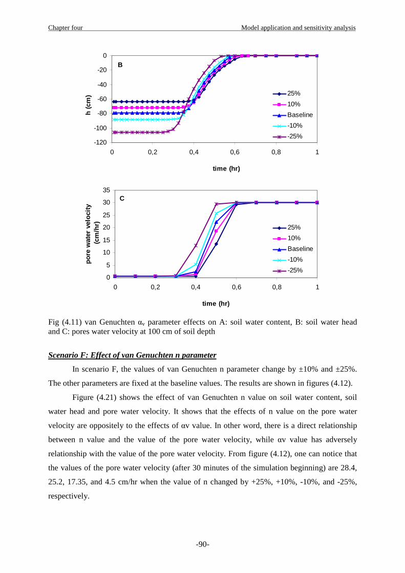
Chapter four Model application and sensitivity analysis
-90-
B
-120
-100
-80
-60
-40
-20
0
0 0,2 0,4 0,6 0,8 1
time (hr)
h (
cm) 25%
10%
Baseline
-10%
-25%
C
0
5
10
15
20
25
30
35
0 0,2 0,4 0,6 0,8 1
time (hr)
po
re w
ater
vel
oci
ty
(cm
/hr) 25%
10%
Baseline
-10%
-25%
Fig (4.11) van Genuchten αv parameter effects on A: soil water content, B: soil water head and C: pores water velocity at 100 cm of soil depth
Scenario F: Effect of van Genuchten n parameter
In scenario F, the values of van Genuchten n parameter change by ±10% and ±25%.
The other parameters are fixed at the baseline values. The results are shown in figures (4.12).
Figure (4.21) shows the effect of van Genuchten n value on soil water content, soil
water head and pore water velocity. It shows that the effects of n value on the pore water
velocity are oppositely to the effects of αv value. In other word, there is a direct relationship
between n value and the value of the pore water velocity, while αv value has adversely
relationship with the value of the pore water velocity. From figure (4.12), one can notice that
the values of the pore water velocity (after 30 minutes of the simulation beginning) are 28.4,
25.2, 17.35, and 4.5 cm/hr when the value of n changed by +25%, +10%, -10%, and -25%,
respectively.

Chapter four Model application and sensitivity analysis
-91-
The soil water content and soil water head has been affected in the same manner by
the value of n (i.e. their values increase with the increases in n value and vice versa). For
example, the soil water content values (after 30 minutes of the simulation beginning) were
0.427, 0.4216, 0.404, and 0.3224 when the values of n changed by +25%, +10%, -10%, and -
25%, respectively. The same thing for the soil water head, it values were -14.8, -18.6, -24.4,
and -49.8 cm when the values of n changed by +25%, +10%, -10%, and -25%, respectively.
The pore water velocity, the soil water content and the soil water head reach the
maximum value ( at the saturation conditions) at the same time (36 minutes) for all cases
except in the case where the value of n decrease by 25% ( it need 42 minutes to reach the
maximum value).
A
00,05
0,10,150,2
0,25
0,30,350,4
0,450,5
0 0,2 0,4 0,6 0,8 1
time (hr)
Th
eta
(-)
25%
10%
Baseline
-10%
-25%
B
-120
-100
-80
-60
-40
-20
0
0 0,2 0,4 0,6 0,8 1
time (hr)
h (
cm)
25%
10%
Baseline
-10%
-25%

Chapter four Model application and sensitivity analysis
-92-
C
0
5
10
15
20
25
30
35
0 0,2 0,4 0,6 0,8 1
time (hr)
po
re w
ater
vel
oci
ty
(cm
/hr) 25%
10%
Baseline
-10%
-25%
Fig (4.12) van Genuchten n parameter effects on A: soil water content, B: soil water head and C: pores water velocity at 100 cm of soil depth Summery
The soil water flow model was applied for calculating the pore water velocity and the
other hydraulic parameters at 100 cm of the soil depth at different simulation times. Then, a
sensitivity analysis is made for determining the most effective hydraulic parameters that
affecting the pore water velocity. The adopted analysis procedure depends on the parameters
of van Genuchten model (Ks, θs, θr, n, and αv) and the initial soil water content (θini). For
testing the sensitivity of each parameter, its value is changed by ±10% and ±25%.
The results show that the values of pore water velocity are sensitive to the change in
the values of soil hydraulic properties; except in the case of θr variation. The effects of the
hydraulic parameters on the pore water velocity can be arranged by the following order: Ks >
θs > θini > n > αv > θr. The time needed to reach the pore water velocity to those at the
saturation state is more sensitive to the saturated soil water content as shown in table (4.6)
which shows the differences in the time needed to reach the saturation state (dt) at a specific
parameter values and at the baseline values. Due to its small value, the residual soil water
content has no effects on the values of the pore water velocity or on the time needed to reach
the saturation state.
Table (4.6) difference in time needed to reach the saturation state.
parameter dt (%) parameter dt (%) parameter dt (%) +25% -16.7 +25% +50 +25% 0 +10% 0 +10% +16.7 +10% 0 -10% +16.7 -10% -16.7 -10% 0
Ks
-25% +20
θs
-25% -33
θr
-25% 0 +25% -16.7 +25% +16.7 +25% 0 +10% 0 +10% +16.7 +10% 0 -10% +16.7 -10% 0 -10% 16.7
θini
-25% +16.7
αv
-25% 0
n
-25% 16.7
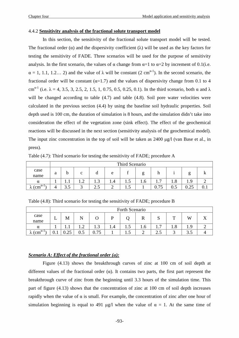
Chapter four Model application and sensitivity analysis
-93-
4.4.2 Sensitivity analysis of the fractional solute transport model
In this section, the sensitivity of the fractional solute transport model will be tested.
The fractional order (α) and the dispersivity coefficient (λ) will be used as the key factors for
testing the sensitivity of FADE. Three scenarios will be used for the purpose of sensitivity
analysis. In the first scenario, the values of α change from α=1 to α=2 by increment of 0.1(i.e.
α = 1, 1.1, 1.2… 2) and the value of λ will be constant (2 cmα-1). In the second scenario, the
fractional order will be constant (α=1.7) and the values of dispersivity change from 0.1 to 4
cmα-1 (i.e. λ = 4, 3.5, 3, 2.5, 2, 1.5, 1, 0.75, 0.5, 0.25, 0.1). In the third scenario, both α and λ
will be changed according to table (4.7) and table (4.8). Soil pore water velocities were
calculated in the previous section (4.4) by using the baseline soil hydraulic properties. Soil
depth used is 100 cm, the duration of simulation is 8 hours, and the simulation didn’t take into
consideration the effect of the vegetation zone (sink effect). The effect of the geochemical
reactions will be discussed in the next section (sensitivity analysis of the geochemical model).
The input zinc concentration in the top of soil will be taken as 2400 µg/l (van Base et al., in
press).
Table (4.7): Third scenario for testing the sensitivity of FADE; procedure A
Third Scenario case name
a b c d e f g h i g k
α 1 1.1 1.2 1.3 1.4 1.5 1.6 1.7 1.8 1.9 2 λ (cmα-1) 4 3.5 3 2.5 2 1.5 1 0.75 0.5 0.25 0.1
Table (4.8): Third scenario for testing the sensitivity of FADE; procedure B
Forth Scenario case name
L M N O P Q R S T W X
α 1 1.1 1.2 1.3 1.4 1.5 1.6 1.7 1.8 1.9 2 λ (cmα-1) 0.1 0.25 0.5 0.75 1 1.5 2 2.5 3 3.5 4
Scenario A: Effect of the fractional order (α):
Figure (4.13) shows the breakthrough curves of zinc at 100 cm of soil depth at
different values of the fractional order (α). It contains two parts, the first part represent the
breakthrough curve of zinc from the beginning until 3.3 hours of the simulation time. This
part of figure (4.13) shows that the concentration of zinc at 100 cm of soil depth increases
rapidly when the value of α is small. For example, the concentration of zinc after one hour of
simulation beginning is equal to 491 µg/l when the value of α = 1. At the same time of
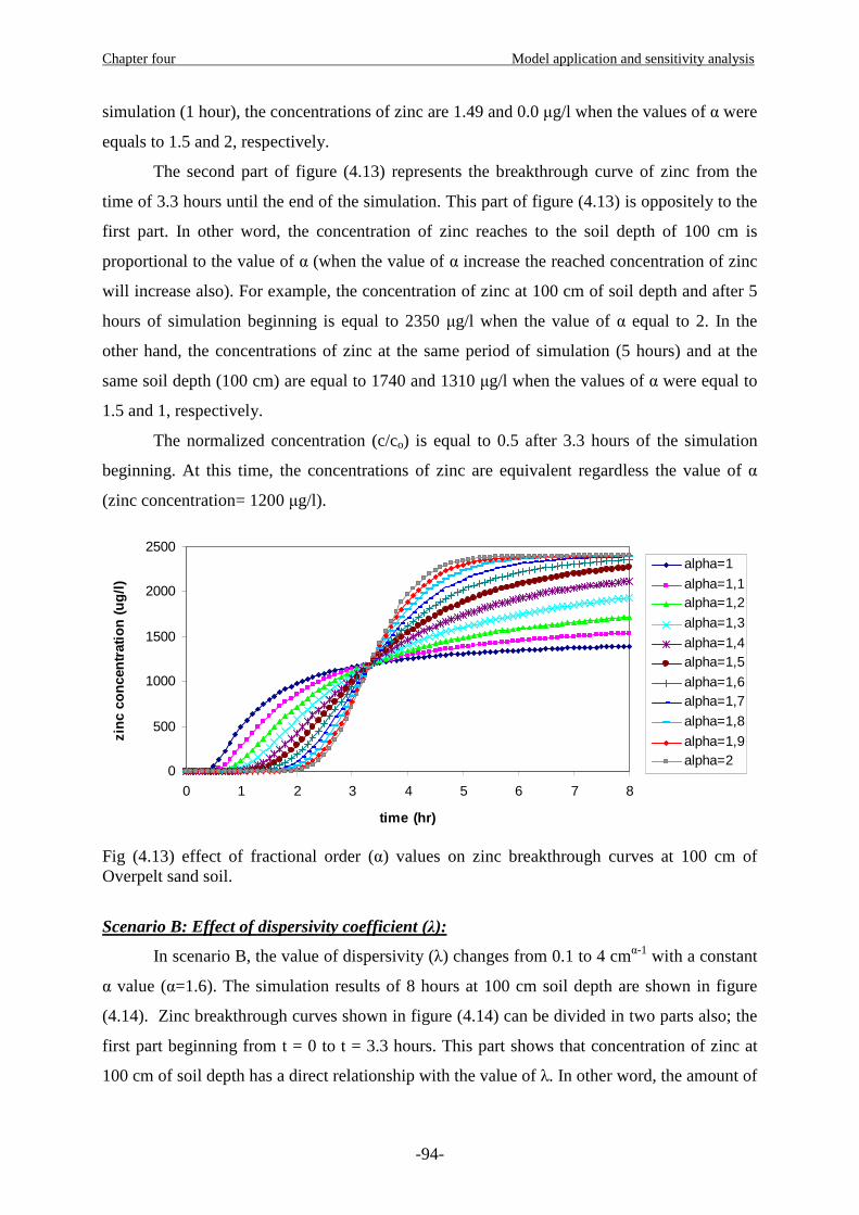
Chapter four Model application and sensitivity analysis
-94-
simulation (1 hour), the concentrations of zinc are 1.49 and 0.0 µg/l when the values of α were
equals to 1.5 and 2, respectively.
The second part of figure (4.13) represents the breakthrough curve of zinc from the
time of 3.3 hours until the end of the simulation. This part of figure (4.13) is oppositely to the
first part. In other word, the concentration of zinc reaches to the soil depth of 100 cm is
proportional to the value of α (when the value of α increase the reached concentration of zinc
will increase also). For example, the concentration of zinc at 100 cm of soil depth and after 5
hours of simulation beginning is equal to 2350 µg/l when the value of α equal to 2. In the
other hand, the concentrations of zinc at the same period of simulation (5 hours) and at the
same soil depth (100 cm) are equal to 1740 and 1310 µg/l when the values of α were equal to
1.5 and 1, respectively.
The normalized concentration (c/co) is equal to 0.5 after 3.3 hours of the simulation
beginning. At this time, the concentrations of zinc are equivalent regardless the value of α
(zinc concentration= 1200 µg/l).
0
500
1000
1500
2000
2500
0 1 2 3 4 5 6 7 8
time (hr)
zin
c co
nce
ntr
atio
n (
ug
/l)
alpha=1
alpha=1,1alpha=1,2
alpha=1,3
alpha=1,4alpha=1,5
alpha=1,6alpha=1,7
alpha=1,8
alpha=1,9alpha=2
Fig (4.13) effect of fractional order (α) values on zinc breakthrough curves at 100 cm of Overpelt sand soil.
Scenario B: Effect of dispersivity coefficient (λ):
In scenario B, the value of dispersivity (λ) changes from 0.1 to 4 cmα-1 with a constant
α value (α=1.6). The simulation results of 8 hours at 100 cm soil depth are shown in figure
(4.14). Zinc breakthrough curves shown in figure (4.14) can be divided in two parts also; the
first part beginning from t = 0 to t = 3.3 hours. This part shows that concentration of zinc at
100 cm of soil depth has a direct relationship with the value of λ. In other word, the amount of
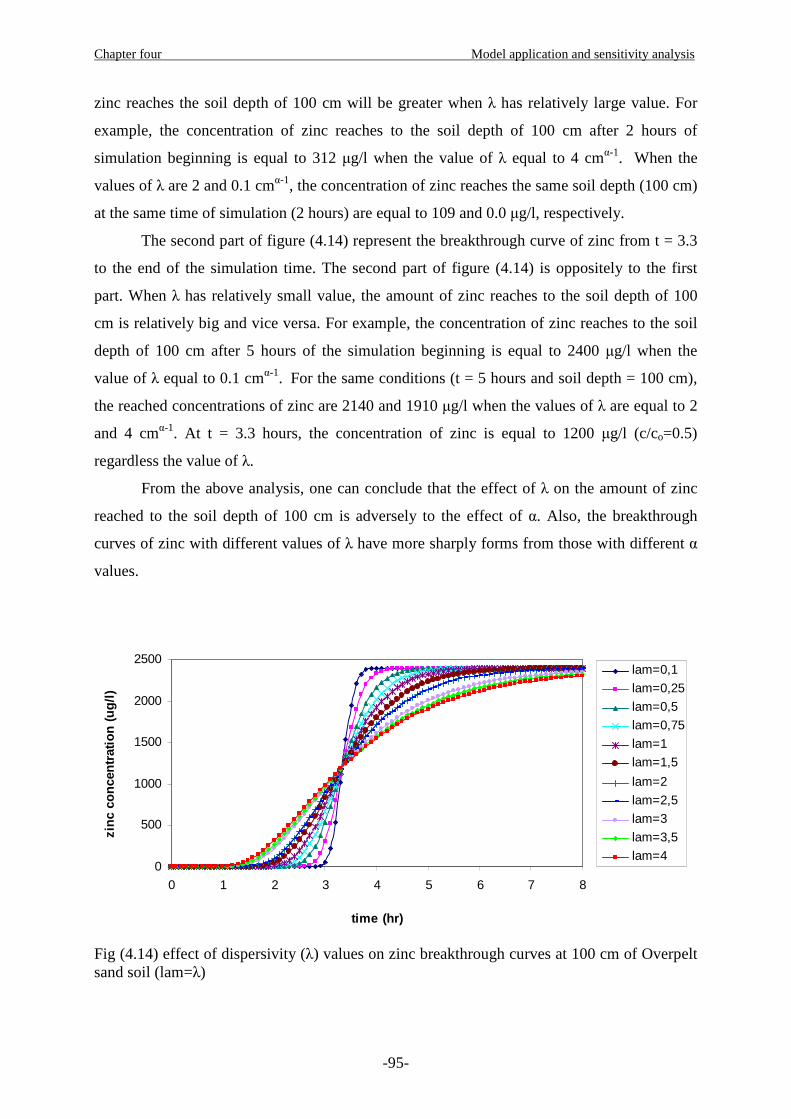
Chapter four Model application and sensitivity analysis
-95-
zinc reaches the soil depth of 100 cm will be greater when λ has relatively large value. For
example, the concentration of zinc reaches to the soil depth of 100 cm after 2 hours of
simulation beginning is equal to 312 µg/l when the value of λ equal to 4 cmα-1. When the
values of λ are 2 and 0.1 cmα-1, the concentration of zinc reaches the same soil depth (100 cm)
at the same time of simulation (2 hours) are equal to 109 and 0.0 µg/l, respectively.
The second part of figure (4.14) represent the breakthrough curve of zinc from t = 3.3
to the end of the simulation time. The second part of figure (4.14) is oppositely to the first
part. When λ has relatively small value, the amount of zinc reaches to the soil depth of 100
cm is relatively big and vice versa. For example, the concentration of zinc reaches to the soil
depth of 100 cm after 5 hours of the simulation beginning is equal to 2400 µg/l when the
value of λ equal to 0.1 cmα-1. For the same conditions (t = 5 hours and soil depth = 100 cm),
the reached concentrations of zinc are 2140 and 1910 µg/l when the values of λ are equal to 2
and 4 cmα-1. At t = 3.3 hours, the concentration of zinc is equal to 1200 µg/l (c/co=0.5)
regardless the value of λ.
From the above analysis, one can conclude that the effect of λ on the amount of zinc
reached to the soil depth of 100 cm is adversely to the effect of α. Also, the breakthrough
curves of zinc with different values of λ have more sharply forms from those with different α
values.
0
500
1000
1500
2000
2500
0 1 2 3 4 5 6 7 8
time (hr)
zin
c co
nce
ntr
atio
n (
ug
/l)
lam=0,1
lam=0,25
lam=0,5
lam=0,75
lam=1
lam=1,5
lam=2
lam=2,5
lam=3
lam=3,5
lam=4
Fig (4.14) effect of dispersivity (λ) values on zinc breakthrough curves at 100 cm of Overpelt sand soil (lam=λ)

Chapter four Model application and sensitivity analysis
-96-
Scenario C: Effect of Both (α) and (λ): In scenario A and B, the effects of α and λ on the amount of zinc reached to the soil
depth of 100 cm were studied separately (by changing one parameter and fixing the other). In
scenario C, both α and λ values will be changed together for studying its effect on zinc
transfer in the soil. The values of α and λ are shown in tables (4.7) and (4.8). The simulation
results are shown in figure (4.15) for the values of table (4.7). The breakthrough curves shown
in figure (4.15) shows that the fractional order (α) has more effect than the dispersivity (λ)
because its shapes and values are nearest to those in figure (4.13). The breakthrough curves in
figure (4.15) are more sharply from those in figure (4.13) and this is due to the effects of λ
values.
Figure (4.16) shows the results of zinc transport simulation with the values of α and λ
shown in table (4.8). The breakthrough curves in figure (4.16) shows that the effect of α
values can be approximately equilibrated by the effect of λ values. This result is due to the
oppositely effects of α and λ on the zinc transport breakthrough curves. The oppositely
effects of α and λ are shown in the previous section (II).
0
500
1000
1500
2000
2500
0 1 2 3 4 5 6 7 8
time (hr)
zin
c co
nce
ntr
atio
n (
ug
/l)
a
b
c
d
e
f
g
h
i
j
k
Fig (4.15) effect of both α and λ values (according table 4.7) on zinc breakthrough curves at 100 cm of Overpelt sand soil.
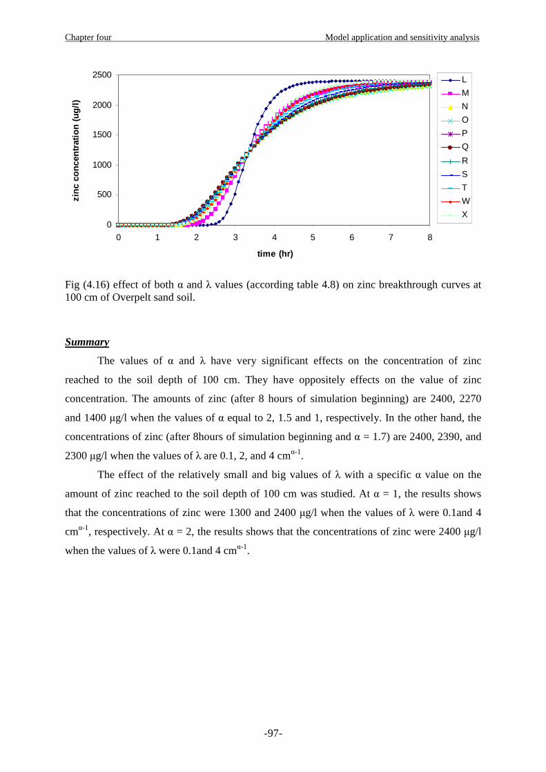
Chapter four Model application and sensitivity analysis
-97-
0
500
1000
1500
2000
2500
0 1 2 3 4 5 6 7 8
time (hr)
zin
c co
nce
ntr
atio
n (
ug
/l)
L
M
N
O
P
Q
R
S
T
W
X
Fig (4.16) effect of both α and λ values (according table 4.8) on zinc breakthrough curves at 100 cm of Overpelt sand soil.
Summary
The values of α and λ have very significant effects on the concentration of zinc
reached to the soil depth of 100 cm. They have oppositely effects on the value of zinc
concentration. The amounts of zinc (after 8 hours of simulation beginning) are 2400, 2270
and 1400 µg/l when the values of α equal to 2, 1.5 and 1, respectively. In the other hand, the
concentrations of zinc (after 8hours of simulation beginning and α = 1.7) are 2400, 2390, and
2300 µg/l when the values of λ are 0.1, 2, and 4 cmα-1.
The effect of the relatively small and big values of λ with a specific α value on the
amount of zinc reached to the soil depth of 100 cm was studied. At α = 1, the results shows
that the concentrations of zinc were 1300 and 2400 µg/l when the values of λ were 0.1and 4
cmα-1, respectively. At α = 2, the results shows that the concentrations of zinc were 2400 µg/l
when the values of λ were 0.1and 4 cmα-1.

Chapter four Model application and sensitivity analysis
-98-
4.4.3 Sensitivity Analysis of geochemical reactions model
The sandy soil of Kempen region is acidic (pH ≈ 4) and it has low content of organic
matter and metals oxides as shown in section (4.2.2). As a consequent, there are no
considerable geochemical reactions can be occurring in this conditions and the free ion of zinc
(Zn2+) is the major species in the aqueous solution.
As shown in section (4.3.3), the geochemical soil system in the Kempen region
consists of: 2+ - 2-4Zn , Cl , SO ,OH − and 2
3CO − . Several scenarios are proposed for studying the
sensitivity of the geochemical model. In the first scenario, the effect of pH value on the
speciation of zinc will be studied by considering the concentration of zinc reached to the soil
depth of 100 cm after 8 hours of simulation beginning equal to 2400 µg/l (the output from the
fractional transport model will be used as input data in the geochemical model). The other
scenarios test the sensitivity of the other components ( 2 2 3 24 3, , , ,Cl SO CO Al Mn− − − + + , and 3Fe + )
on the speciation of zinc using different concentrations of each component and fixing the
concentration of the others. The baseline concentrations of these components shown in table
(4.9) are collected from different references.
Table (4.9): The baseline concentration of each component in the geochemical soil system
component H+ Zn2+ Cl- SO42- CO3
2- Al3+ Mn2+ Fe2+
concentration
(morality) 10-4 3.67x10⁻⁵ 1.2x10⁻³ 8x10⁻⁴ 0 5x10⁻⁴ 1.165x10⁻³ 0.15
Scenario A: pH effects
A wide range of pH values (pH = 3, 4, 5, 6, 7, 8, 9, and 10) are used for illustrating the
effects of the pH on the speciation of zinc. The results shown in figure (4.17) indicate that the
free zinc (Zn2+) is the major species when the pH is in the acidic zone and Zn(OH)2 is the
major species when the pH is in the basic zone. Free Zn2+ represents about 90% of the total
zinc concentration when the pH = 7. The concentration of free Zn2+ decreases with the acidity
of the soil solution (pH >7). The concentration of Zn(OH)2 species increases when the
alkalinity of the soil solution increases. At pH = 9 and 10, the concentration of Zn(OH)2
represent 84% and 96% of the total zinc concentration, respectively. The percentages of the
other species of zinc are shown in figure (4.17).
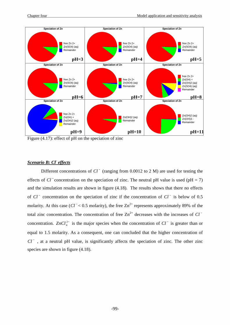
Chapter four Model application and sensitivity analysis
-99-
Speciation of Zn
free Zn 2+Zn(SO4) (aq)Remainder
Speciation of Zn
free Zn 2+Zn(SO4) (aq)Remainder
Speciation of Zn
free Zn 2+Zn(SO4) (aq)Remainder
Speciation of Zn
free Zn 2+Zn(SO4) (aq)Remainder
Speciation of Zn
free Zn 2+Zn(SO4) (aq)Remainder
Speciation of Zn
free Zn 2+Zn(OH) +Zn(OH)2 (aq)Zn(SO4) (aq)Remainder
Speciation of Zn
free Zn 2+Zn(OH) +Zn(OH)2 (aq)Remainder
Speciation of Zn
Zn(OH)2 (aq)Remainder
Speciation of Zn
Zn(OH)2 (aq)Zn(OH)3 -Remainder
Figure (4.17): effect of pH on the speciation of zinc
Scenario B: Cl- effects
Different concentrations of Cl − (ranging from 0.0012 to 2 M) are used for testing the
effects of Cl − concentration on the speciation of zinc. The neutral pH value is used (pH = 7)
and the simulation results are shown in figure (4.18). The results shows that there no effects
of Cl − concentration on the speciation of zinc if the concentration of Cl − is below of 0.5
molarity. At this case (Cl − < 0.5 molarity), the free Zn2+ represents approximately 89% of the
total zinc concentration. The concentration of free Zn2+ decreases with the increases of Cl −
concentration. 24ZnCl − is the major species when the concentration of Cl − is greater than or
equal to 1.5 molarity. As a consequent, one can concluded that the higher concentration of
Cl − , at a neutral pH value, is significantly affects the speciation of zinc. The other zinc
species are shown in figure (4.18).
pH=3 pH=4 pH=5
pH=6 pH=7 pH=8
pH=9 pH=10 pH=11
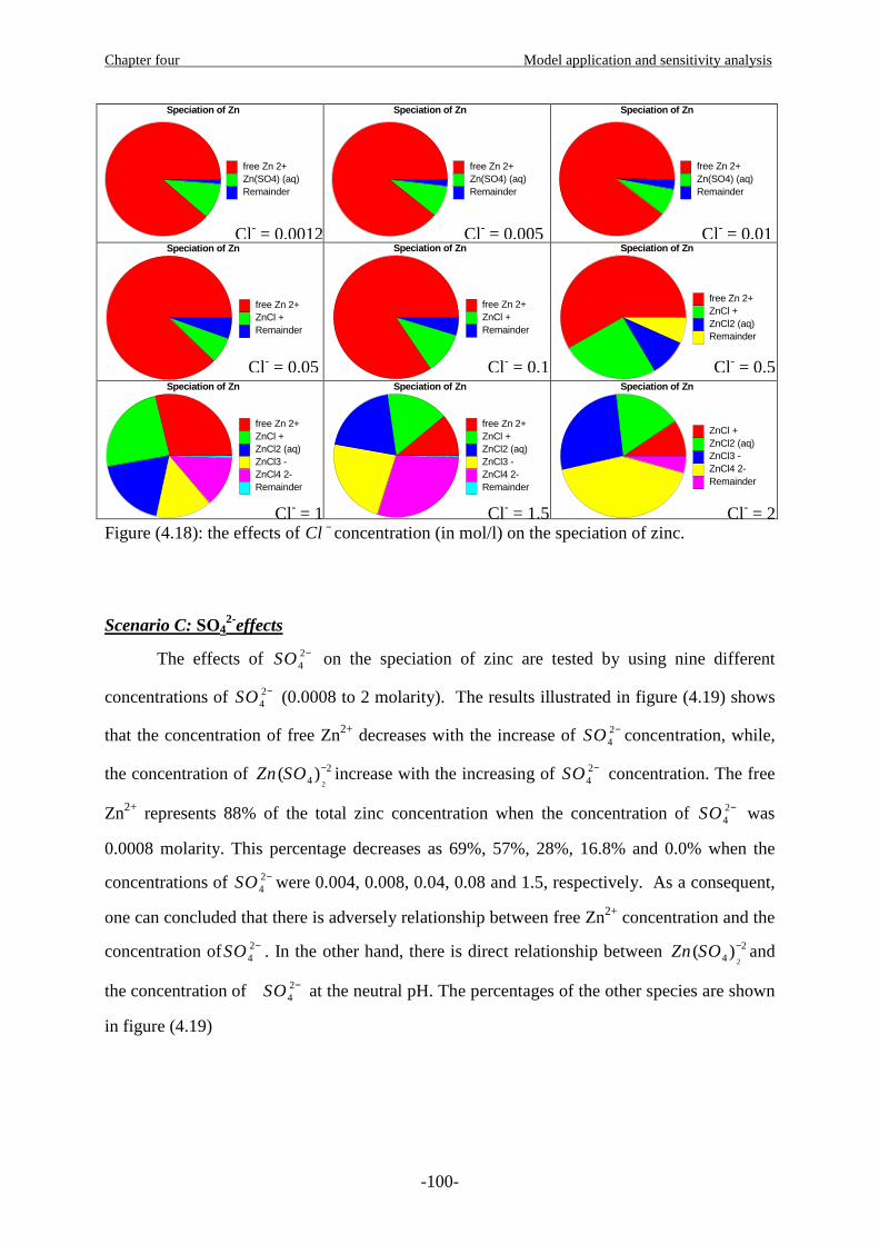
Chapter four Model application and sensitivity analysis
-100-
Speciation of Zn
free Zn 2+Zn(SO4) (aq)Remainder
Speciation of Zn
free Zn 2+Zn(SO4) (aq)Remainder
Speciation of Zn
free Zn 2+Zn(SO4) (aq)Remainder
Speciation of Zn
free Zn 2+ZnCl +Remainder
Speciation of Zn
free Zn 2+ZnCl +Remainder
Speciation of Zn
free Zn 2+ZnCl +ZnCl2 (aq)Remainder
Speciation of Zn
free Zn 2+ZnCl +ZnCl2 (aq)ZnCl3 -ZnCl4 2-Remainder
Speciation of Zn
free Zn 2+ZnCl +ZnCl2 (aq)ZnCl3 -ZnCl4 2-Remainder
Speciation of Zn
ZnCl +ZnCl2 (aq)ZnCl3 -ZnCl4 2-Remainder
Figure (4.18): the effects of Cl − concentration (in mol/l) on the speciation of zinc.
Scenario C: SO42-effects
The effects of 24SO − on the speciation of zinc are tested by using nine different
concentrations of 24SO − (0.0008 to 2 molarity). The results illustrated in figure (4.19) shows
that the concentration of free Zn2+ decreases with the increase of 24SO − concentration, while,
the concentration of 2
24( )Zn SO − increase with the increasing of 2
4SO − concentration. The free
Zn2+ represents 88% of the total zinc concentration when the concentration of 24SO − was
0.0008 molarity. This percentage decreases as 69%, 57%, 28%, 16.8% and 0.0% when the
concentrations of 24SO − were 0.004, 0.008, 0.04, 0.08 and 1.5, respectively. As a consequent,
one can concluded that there is adversely relationship between free Zn2+ concentration and the
concentration of 24SO − . In the other hand, there is direct relationship between
2
24( )Zn SO − and
the concentration of 24SO − at the neutral pH. The percentages of the other species are shown
in figure (4.19)
Cl- = 0.0012 Cl- = 0.005 Cl- = 0.01
Cl- = 0.05 Cl- = 0.1 Cl- = 0.5
Cl- = 1 Cl- = 1.5 Cl- = 2

Chapter four Model application and sensitivity analysis
-101-
Speciation of Zn
free Zn 2+Zn(SO4) (aq)Remainder
Speciation of Zn
free Zn 2+Zn(SO4) (aq)Remainder
Speciation of Zn
free Zn 2+Zn(SO4) (aq)Zn(SO4)2 2-Remainder
Speciation of Zn
free Zn 2+Zn(SO4) (aq)Zn(SO4)2 2-Remainder
Speciation of Zn
free Zn 2+Zn(SO4) (aq)Zn(SO4)2 2-Remainder
Speciation of Zn
Zn(SO4) (aq)Zn(SO4)2 2-Zn(SO4)3 4-Remainder
Speciation of Zn
Zn(SO4)2 2-Zn(SO4)3 4-Remainder
Speciation of Zn
Zn(SO4)2 2-Remainder
Speciation of Zn
Zn(SO4)2 2-Remainder
Figure (4.19): the effects of 2
4SO − concentration (in mol/l) on the speciation of zinc.
Scenario D: CO32-effects
In this scenario, the concentrations of 23CO − are changed from 0 to 3 molarity for
examining its effects on the speciation of zinc in the geochemical soil system. The results
shown in figure (4.20) shows that the concentration of 23CO − is significantly affects the
speciation of zinc. The free Zn2+ is the major species (89%) when the concentration of 23CO −
was 0 molarity. This percentage is severely changed from 89% to 14% when the
concentration of 23CO − increased from 0 to 0.4 molarity. At this concentration of 2
3CO − (0.4
molarity), 3( )ZnH CO + is the major species which represent 50% of the total concentration of
zinc. When the concentration of 23CO − equal to 1.6 molarity, the concentration of free Zn2+ is
approximately zero and the major zinc species are those associated with the 23CO − . The
percentages of all species in the geochemical soil system at different 23CO − concentrations are
shown in figure (4.20).
SO42-=0.0008 SO4
2-=0.004 SO42-=0.008
SO42-=0.04 SO4
2-=0.08 SO42-=0.4
SO42-=1 SO4
2-=1.5 SO42-=2

Chapter four Model application and sensitivity analysis
-102-
Speciation of Zn
free Zn 2+Zn(SO4) (aq)Remainder
Speciation of Zn
free Zn 2+Zn(CO3) (aq)ZnH(CO3) +Remainder
Speciation of Zn
free Zn 2+Zn(CO3) (aq)ZnH(CO3) +Zn(CO3)2 2-Remainder
Speciation of Zn
free Zn 2+Zn(CO3) (aq)ZnH(CO3) +Zn(CO3)2 2-Remainder
Speciation of Zn
Zn(CO3) (aq)ZnH(CO3) +Zn(CO3)2 2-Remainder
Speciation of Zn
Zn(CO3) (aq)ZnH(CO3) +Zn(CO3)2 2-Remainder
Speciation of Zn
Zn(CO3) (aq)ZnH(CO3) +Zn(CO3)2 2-Remainder
Speciation of Zn
Zn(CO3) (aq)ZnH(CO3) +Zn(CO3)2 2-Remainder
Speciation of Zn
Zn(CO3) (aq)ZnH(CO3) +Zn(CO3)2 2-Remainder
Figure (4.20): the effects of 23CO − concentration (in mol/l) on the speciation of zinc.
Scenario E: Al 3+, Mn2+ and Fe2+ effects
The effects of Al3+, Mn2+ and Fe2+ on the speciation of zinc are studied by changing
their concentrations. The results are shown in figures (4.21), (4.22) and (4.23), respectively.
Figure (4.21) shows that the concentration of Al3+ (ranging between 0 – 0.05 molarity) dose
not affect significantly the speciation of zinc in the geochemical soil system. The free Zn2+ is
the major species of zinc. It represents approximately 88% of the total concentration of zinc.
The effects of Mn2+ concentration on the speciation of zinc are shown in figure (5.22).
As in the case of Al3+, the variation in Mn2+ concentration has no grand effects on the
speciation of zinc in the geochemical soil system. The concentration of free Zn2+ represents
88% of the total concentration of zinc when the concentration of Mn2+ was zero molarity and
it represent (86 %) when the concentration of Mn2+ was 5 molarity.
Figure (4.23) shows that Fe2+ concentration effects on the speciation of zinc don’t
differ from those of Mn2+ and Al3+. The results show that the change in the Fe2+ from 0 to 1.5
molarity will decrease the percentage of free Zn2+ by 5% only. The concentration of the free
Zn2+ represents 98% of the total concentration of zinc.
CO32- = 0 CO3
2- = 0.4 CO32- = 0.8
CO32- = 1.2 CO3
2- = 1.6 CO32- = 2
CO32- = 2.4 CO3
2- = 2.8 CO32- = 3
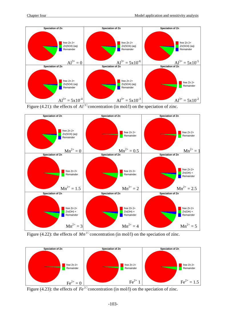
Chapter four Model application and sensitivity analysis
-103-
Speciation of Zn
free Zn 2+Zn(SO4) (aq)Remainder
Speciation of Zn
free Zn 2+Zn(SO4) (aq)Remainder
Speciation of Zn
free Zn 2+Zn(SO4) (aq)Remainder
Speciation of Zn
free Zn 2+Zn(SO4) (aq)Remainder
Speciation of Zn
free Zn 2+Zn(SO4) (aq)Remainder
Speciation of Zn
free Zn 2+Remainder
Figure (4.21): the effects of 3Al + concentration (in mol/l) on the speciation of zinc.
Speciation of Zn
free Zn 2+Zn(SO4) (aq)Remainder
Speciation of Zn
free Zn 2+Remainder
Speciation of Zn
free Zn 2+Remainder
Speciation of Zn
free Zn 2+Remainder
Speciation of Zn
free Zn 2+Remainder
Speciation of Zn
free Zn 2+Zn(OH) +Remainder
Speciation of Zn
free Zn 2+Zn(OH) +Remainder
Speciation of Zn
free Zn 2+Zn(OH) +Remainder
Speciation of Zn
free Zn 2+Zn(OH) +Remainder
Figure (4.22): the effects of 2Mn + concentration (in mol/l) on the speciation of zinc.
Speciation of Zn
free Zn 2+Remainder
Speciation of Zn
free Zn 2+Remainder
Speciation of Zn
free Zn 2+Remainder
Figure (4.23): the effects of 2Fe + concentration (in mol/l) on the speciation of zinc.
Al 3+ = 0 Al3+ = 5x10⁻⁶ Al3+ = 5x10⁻⁵
Al 3+ = 5x10⁻⁴ Al3+ = 5x10⁻³ Al3+ = 5x10⁻²
Mn2+ = 0 Mn2+ = 0.5 Mn2+ = 1
Mn2+ = 1.5 Mn2+ = 2 Mn2+ = 2.5
Mn2+ = 3 Mn2+ = 4 Mn2+ = 5
Fe2+ = 0 Fe2+ = 1.5 Fe2+ 1

Chapter four Model application and sensitivity analysis
-104-
Summary
The pH value is the only factors that affecting the speciation of zinc in the soil of
Overpelt (in the Kempen region). At pH less than 8, the free Zn2+ is the major species in the
geochemical soil solution (it represent approximately 89% of the total zinc concentration). At
pH ≥ 8, Zn(OH)2 is the major species (85% of the total zinc concentration). Cl − has no effect
on zinc concentration when its concentration below 0.5 molarity and the major species is the
free Zn2+ .The concentration of the free Zn2+ decreases when the concentration of Cl − above
0.5 molarity. When the concentration of Cl −≥ 1.5, the major species is 24ZnCl − .
The concentration of Zn2+ decreases with the increasing in 24SO − concentration. As a
consequent, the concentration of 2
24( )Zn SO − will be increased. The free Zn2+ represent 88%
and 0.0% when the concentrations of 24SO − were 0.0008 and 1.5 molarity, respectively.
The percentage of the free Zn2+ concentration changed from 89% to 14% when the
concentration of 23CO − increased from 0 to 0.4 molarity. At 2
3CO − concentration of 1.6
molarity, all zinc forms in the aqueous system converted to carbonate forms. The other
metals (Al3+, Mn2+ and Fe2+) have no significant effects on the zinc speciation in the
geochemical soil system and the major species is the free Zn2+.
4.5 Conclusion
The soil of Kempen region is heavily polluted by the heavy metals. This pollution is
due to the pollutant emission from the zinc smelters located in the region from 1880. Due to
the acidic sandy prosperities of the soil, there are low content of organic matter.
The Geo-UNSTEFAD model was applied for this region and a sensitivity analysis was
done. The results show that the values of pore water velocity are sensitive to the change in the
values of soil hydraulic properties; except in the case of θr variation. The effects of the
hydraulic parameters on the pore water velocity can be arranged by the following order: Ks >
θs > θini > n > αv > θr. The values of α and λ have very significant effects on the
concentration of zinc. They have oppositely effects on the value of zinc concentration. pH
value is the key parameter for the speciation of zinc. In the acidic media, free zinc is the major
species, while in the basic media; Zn(OH)2 is the major species. The concentration of free
Zn2+ has adversely relationship with the concentrations of 24SO − ,Cl − and 2
3CO − . The other
metals (Al3+, Mn2+ and Fe2+) have no significant effects on the zinc speciation.

General Conclusions and RecommendationsGeneral Conclusions and RecommendationsGeneral Conclusions and RecommendationsGeneral Conclusions and Recommendations
. General conclusions and recommendations
-105-
The main objective of this study was to develop a mathematical model which
simulates flow and transport processes within unsaturated soil zone taking into consideration
the geochemical reactions occurring during the transport processes. This thesis contains four
parts.
The first part deals with the bibliographical analysis. It consists of four sections: the
zinc (origin, production-utilization, and toxicity), the geochemical reactions model (chemical
equilibria, chemical reactions codes, and speciation of zinc), water flow model (formulations
and water flow codes), and fractional advection-dispersion model (ADE, FADE and
comparison between them). This part shows that the classical ADE has some limitations in the
simulation of solutes transport in the heterogeneous field soils and the fractional ADE
replaces the classical ADE for overcoming these limitations. Also, the solutes transport
models don’t take into considerations the geochemical reactions processes; therefore the
fractional ADE should be coupled with the geochemical model for overcoming this problem.
The second part deals with the application of FADE at the steady state and its coupling
with the geochemical reactions model. It consists of two sections: STEFADE (analytical
solution of FADE at the steady state and model validation) and Geo-STEFADE (coupling the
geochemical model with the analytical solution of FADE at the steady state and model
validation). The results obtained from the application of these models showed their capability
to giving more details about the solute concentration and its species (forms) in the soil
solution.
The third part deals with the application of FADE at the unsteady state and its
coupling with the geochemical reactions model. It consists of four sections: fractional
derivatives (general introduction of the fractional derivatives), water flow model (Richards
equation solution and model validation), UNSTEFADE model (numerical solution of FADE
and model validation), and Geo-UNSTEFADE (coupling the geochemical model with the
numerical solution of FADE at the unsteady state and model validation). The results from
these models were compared with those obtained from HYDRUS-1D and HP1 software. This
comparison showed that UNSTEFAD and Geo-UNSTEFAD models well simulates the
transport of solutes in the unsaturated soil zone at the unsteady state.

. General conclusions and recommendations
-106-
The fourth part concerns the application of the new model and the sensitivity analysis.
It consists of three sections: steady area description (historical background, soil
characteristics, and topography and climate), parameters estimation (water flow parameters,
FADE parameters, and geochemical parameters). Saturated soil hydraulic conductivity (Ks)
has adversely effects on the time needed to reach the saturation state. The value of pore water
velocity changes by the same percentage of the change in the value of Ks. Saturated soil water
content (θs) has a direct relationship with the time needed to reach the saturation state.
Residual soil water content hasn’t any effects on the water flow model and this is due to its
relatively small value.
The fractional order (α) has two oppositely effects on the concentration of zinc. The
first effect started from the beginning of simulation time until the time where c/co = 0.5. At
this period, α value has adversely effect on the reached zinc concentration. After this point
(c/co = 0.5), α value has a direct effect on the value of reached zinc concentration. The effect
of the dispersivity value (λ) is oppositely to those of the fractional order (α). The effect of α
value is greater than the effect of λ value.
pH is the most affecting geochemical factor. Free Zn2+ is the major species in the
aqueous geochemical system when pH < 8; while Zn(OH)2 is the major species when pH >8.
The concentration of free Zn2+ has adversely relationship with the concentrations of 24 ,SO Cl− − and 2
3CO − . The concentrations of the other cations (3 2 2, ,Al Mn Fe+ + + ) have no
significant effects on the speciation of zinc in the aqueous solution.
Several aspects in this study needs more research from these: the estimation method
of the fractional order (α) and the fractional dispersion coefficient (D), the effects of the
vegetation zone, the effect of contaminant type, and the use of FADE in two and three
dimensions.

References References References References

. References
-107-
1 Abd-Elfattah A. and Wada K., “Adsorption of lead, copper, zinc, cobalt and cadmium by soils that differs in cation-exchange material”, J. Soil Sci., 32,271, 1981
2 Adams E. E., and Gelhar L. W., “Field study of dispersion in a heterogeneous aquifer, 2, Spatial moments analysis”, Water Resource. Res., 28(12), 3293–3307, 1992
3 Adriano D.C.,” Trace Elements in the Terrestrial Environment”, Springer-Verlag, New York, 1986
4 Albright W.H., Gee G.W., Wilson G.V., and Fayer M.J.,” Alternative cover assessment project phase1”, Report 41183, 2002, Desert Research Institute.
5 Alloway B. J., “Heavy metals in soils”, Blackie Acad., London, 2004
6 Aral M.M. and Liao B.,”Analytical solutions for two-dimensional transport equation with time-dependent dispersion coefficients” J. Hydrol. Eng. 1 (1), 20– 32, 1996
7 ATSDR, “Toxicological profile for zinc” Agency for Toxic Substances and Disease Registry ,Atlanta, US Public Health Service, pp1–230, 1994
8 Baize D., “Teneurs totale en métaux lourds dans les sols français” Le courier de l’environnement de l’INRA. No. 39: 39-54, 2000
9 Baker D.L.”Darcian weighted interblock conductivity means for vertical unsaturated flow”. Ground Water, 33: 385-390, 1995
10 Barrow N.J. “Mechanisms of Reaction of Zinc with Soil and Soil Components” Chapter 2 in Robson A.D. “Zinc in Soils and Plants” Kluwer Academic Publishers, Dordrecht. pp 15 – 32, 1993
11 Bear J.” Dynamics of Fluids in Porous Media” Elsevier, New York, 1972
12 Belmans C., Wesseling J.G. and Feddes R.A. “Simulation of the water balance of a cropped soil: SWATRE” J. Hydrol., 63: 271-286, 1983
13 Benson D. A., Schumer R., Meerschaert M. M. and Wheatcraft S. W. “Fractional dispersion, Lévy motion, and the MADE tracer tests”, Transp. Porous Media, 42(1/2), 211-240, 2001
14 Benson D.A. “The Fractional Advection–Dispersion Equation: Development and Application” PhD dissertation, University of Nevada, Reno, USA, 1998
15 Benson D.A., Wheatcraft S.W., Meerschaert M.M. “The fractional-order governing equation of Lévy motion”. Water Resour. Res. 36 (6), 1413– 1423, 2000a
. References
-108-
16 Benson D.A., Wheatcraft S.W., Meerschaert M.M. “Application of a fractional advective–dispersion equation” Water Resour. Res. 36 (6), 1403– 1412, 2000b
17 Berkowitz B. and Scher H. “Anomalous transport in random fracture networks” Physical Review Letters, 79(20), 4038-4041, 1997
18 Berkowitz B., Scher H., Silliman S. E. “Anomalous transport in laboratory-scale, heterogeneous porous media” Water Resour. Res., 36(1): 149-158, 2000
19 Bertholf R.L. “Zinc” in “ Handbook on Toxicity of Inorganic Compounds”, Sigel H. and. Seiler H.G, Marcel Dekker, Inc., New York. pp. 787-800, 1988
20 Boekhold A.E. “Field scale behavior of cadmium in soil”, Thesis, Agricultural University of Wageningen, the Netherlands, 1992
21 Boggs J. M., Beard L. M, Long S. E. and McGee M. P. “Database for the second macrodispersion experiment (MADE–2)” EPRI report TR–102072, Electric Power Res. Inst., Palo Alto, CA, 1993
22 Boggs J.M. and Adams E. E. “Field study of dispersion in a heterogeneous aquifer, 4; Investigation of adsorption and sampling bias” Water Resour. Res., 28(12),3325–3336, 1992
23 Boggs J.M., Young S.C., Beard L.M., Gelhar L.W., Rehfeldt K.R., Adams E.E. “Field study of dispersion in a heterogeneous aquifer: 1. Overview and site description” Water Resour. Res. 28 (12), 3281– 3291, 1992
24 Boutron CF, Candelone J-P, & Hong S “Greenland snow and ice cores unique archives of large-scale pollution of the troposphere of the northern hemisphere by lead and other heavy metals” Science of the Total Environment, 160-161: 233-241, 1995.
25 Brown P. L., Haworth A., Sharland S. M., and Tweed C. J. “HARPHRQ: A Geochemical Speciation Program Based on PHREEQE”. Report NSS/R188, Harwell Laboratory, Harwell Laboratory, Oxford shire, United Kingdom, 1991.
26 Bruynzeel D.P., Hennipman G.,van Ketel W.G. “Irritant contact dermatitis and chrome-passivated metal” Contact Dermatitis 19:175-179, 1988.
27 Celia M.A., Bouloutas E.T. and Zarba R.L. “A general mass-conservative numerical solution for the unsaturated flow equation” Water Resour. Res., 26: 1483-1496, 1990.
28 Chobanian S.J. “Accidental ingestion of liquid zinc chloride: local and systemic effects” Ann. Emerg. Med. 10:91-93. (Cited in ATSDR, 1989), 1981.
29 CITEPA, Centre Interprofessionnel d’Etude de la Pollution Atmosphérique, www.citepa..org , 2004

. References
-109-
30 Cortis A., Berkowitz B. “Anomalous transport in classical soil and sand columns”. Soil Sci. Soc. Am. J. 68 (5), 1539–1548, 2004.
31 Cushman J. H. and Ginn T. R. “Fractional advection-dispersion equation: A classical mass balance with convolution-Fickian flux” Water Resour. Res., 36(12), 3763-3766, 2000
32 Dam van J.C., and Feddes R.A. “Numerical simulation of infiltration, evaporation and shallow groundwater levels with the Richards’ equation” J. Hydro. 2000.
33 Dam van J.C., Huygen J., Wesseling J.G., Feddes R.A., Kabat P., Walsum van P.E.V., Groenendijk P. and Diepen van C.A. “Theory of SWAP version 2.0. Simulation of water flow, solute transport and plant growth in the Soil-Water-Atmosphere-Plant environment” Report 71, dep. Water Resources, Wageningen University, Technical document 45, Alterra Green World Research, Wageningen,1997
34 Dam van J.C. “Field-scale water flow and solute transport: SWAP model concepts, parameter estimation and case studies”; Doctoral Thesis, Wageningen University, 2000
35 Dang Y.P., Tiller K.G., Dalal R.C., and Edwards D.G. “Zinc speciation in soil solution of Vertisols” Aust. J. Soil Res. 34:369–383, 1996.
36 Davis, J. A., and Kent D. B. “Surface Complexation Modeling in Aqueous Geochemistry” In Mineral-Water Interface Geochemistry, M. F. Hochella, Jr. And A. F. White (eds.), pp. 177-260, Reviews in Mineralogy, Volume 23, Mineralogical Society of America, Washington, D.C., 1990
37 Dejonghe L. “Zinc-lead deposits of Belgium” Ore Geol Rev,12(5):329 –354, 1998
38 Dentz M., Cortis A., Scher H. et al. “Time behavior of contaminant transport in heterogeneous media: transition from anomalous to normal transport” Adv. Water Res., 2004, 27: 155-173.
39 Desbarats A.J. “An interblock conductivity scheme for finite difference models of steady unsaturated flow in heterogeneous media” Water Resource. Res., 31: 2883-2889, 1995
40 Dyson J.S., White R.E. “A comparison of the convective–dispersive equation and transfer function model for predicting chloride leaching through an undisturbed structured clay soil” J. Soil Sci.;38:157-172, 1987
41 Elinder C.-G. “Zinc. In: Handbook on the Toxicology of Metals” 2nd ed., vol. II: Specific Metals, L. Friberg, G.F. Nordberg and V.B. Vouk, V.B., eds. Elsevier, New York, 1986.

. References
-110-
42 Erdal B., Chairman R. “Workshop on Fundamental Geochemistry Needs for Nuclear Waste Isolation” US DOE CONF8406134, National Technical Information Service, Springfield, Virginia, 1985.
43 EZI “Zinc recycling: history, present position and prospects” Brussels, European Zinc Institute, 1996.
44 Farrell F.J. “Angioedema and urticaria as acute and late phase reactions to zinc fume exposure, with associated metal fume fever-like symptoms” Am. J. Ind. Med. 12:331-337. (Cited in ATSDR, 1989), 1987.
45 Feddes R.A., Kabat P., Bakel van P.J.T., Bronswijk J.J.B. and Halbertsma J. “Modeling soil water dynamics in the unsaturated zone - state of the art” J. Hydrol., 100: 69-111, 1988.
46 Feddes R.A., Kowalik P.J. and Zaradny H. “Simulation of field water use and crop yield” .Simulation Monographs, Pudoc, Wageningen, 189 p., 1978.
47 Fishbein L. “Sources, transport and alterations of metal compounds: an overview. I. Arsenic, beryllium, cadmium, chromium, and nickel”. Environ Health Perspect, 40: 43–64, 1981.
48 Genuchten M.Th. van “A comparison of numerical solutions of the one-dimensional unsaturated-saturated flow and transport equations” Adv. Water Resour., 5: 47-55, 1982.
49 Genuchten M.Th. van “ A closed – forum for predicting the hydraulic conductivity of unsaturated soil” SSSAJ, 44,892-898, 1980
50 Goldberg S. “Adsorption Models Incorporated into Chemical Equilibrium Models” In Chemical Equilibrium and Reaction Models, R. H. Loeppert, A. P. Schwab, and S. Goldberg (eds.), pp. 75-95, Special Publication Number 42, Soil Science Society of America, Inc., Madison, Wisconsin, 1995.
51 Goodwin FE. “Zinc compounds” In: Kroschwitz J, Howe-Grant M, eds. Krik-Othmer encyclopedia of chemical technology. New York, NY, John Wiley & Sons, Inc., 840-853 , 1998
52 Gorenflo R., and Mainardi F. “Fractional calculus and stable probability distributions” Arch. Mech., 50(3), 377–388, 1998.
53 GSC, “Geological Survey of Canada. National geochemical reconnaissance data” Ottawa, Natural Resources Canada, Government of Canada. (1995)
54 Harmsen K. “Behavior of heavy metals in soils” Thesis, Agricultural University Wageningen, the Netherlands, 1977.
55 Harter R.D. “Micronutrient Adsorption - Desorption Reactions in Soils” Chap 3 in Mortvedt, J.J., F.R. Cox, L.M. Schuman and R.M. Welch (eds) Micronutrients in
. References
-111-
Agriculture (2nd edition), Book Series No.4, Soil Science Society of America, Madison, Wisc. pp 59 – 88, 1991.
56 Haverkamp R. and Vauclin M. “A note on estimating finite difference interblock hydraulic conductivity values for transient unsaturated flow problems” Water Resour. Res., 15: 181-187, 1979
57 Hjortso E., Qvist J. and Bud M.I. “ARDS after accidental inhalation of zinc chloride smoke” Intensive Care Med. 14:17-24. (Cited in ATSDR, 1989), 1988.
58 Hornung U. and Messing W. “Truncation errors in the numerical solution of horizontal diffusion in saturated/unsaturated media” Adv. Water Resource, 6: 165-168, 1983.
59 Huang G., Huang Q., Zhan H., Chen J., Xiong Y. & Feng S.” Modeling
contaminant transport in homogeneous porous media with fractional advection-dispersion equation” Science in China Ser. D Earth Sciences 2005 Vol.48 Supp. II 295-302, 2005
60 Huang Q. and Huang G. “Modeling adsorbing solute transport with fractional advection dispersion equation” In: Huang, G., Pereira, L.S. (Eds.), Land and Water Management: Decision Tools and Practice Proceedings of 2004 International Commission of Agricultural Engineering Conference, Beijing, China, Oct. 11–14, China Agricultural. , 2004
61 Huang Q “Modeling adsorbing solute transport with fractional advection dispersion equation”, M.Sc. thesis China agricultural university, 2002
62 Huang G., Huang Q. and Hongbin Z.”evidence of one-dimensional scale-dependent fractional advection – dispersion” J. of contaminant hydrology, 2006
63 Hunt B. “Contaminant source solutions with scale-dependent dispersivity” J. Hydro. Eng. 3 (4), 268– 275. , 1998. Jayawardena A.A., Lui P.H. “Numerical solution of the dispersion equation using a variable dispersion coefficient: method and applications” Hydrol. Sci. J. 29 (3), 293– 309., 1984
64 ILZSG “Lead and zinc statistics. Monthly bulletin of the International Lead and Zinc Study Group” La Tribune du Cebedeau, 35: 37, 39–41, 54, 67, 1995.
65 ITII (International Technical Information Institute) “Toxic and Hazardous Industrial Chemicals Safety Manual for Handling and Disposal, with Toxicity and Hazard Data” Tokyo, Japan. pp. 562-564, 1988.
66 Jackson K. J. and Bourcier W. L (technical organizers) “Proceedings of the Workshop on Geochemical Modeling” CONF-8609134, National Technical information Service, Springfield, Virginia, 1986.
67 Jacobs G. K. and Whatley S. K. “Proceedings of the Conference on the Application of Geochemical Models to High-level Nuclear Waste Repository
. References
-112-
Assessment” NUREG/CR-0062 (ORNL/TM-9585), Oak Ridge National Laboratory, Oak Ridge, Tennessee, 1985
68 Jenne E. A. “Chemical Modeling in Aqueous Systems. Speciation, Sorption, Solubility, and Kinetics” Symposium Series 93, American Chemical Society, Washington, D.C., 1979
69 Jenne E. A. “Geochemical Modeling: A Review” PNL-3574, Pacific Northwest Laboratory, Richland, Washington, 1981.
70 Johnson C.A., Schaap M.G., and Abbaspour K.C. ”Model comparison of flow through a municipal solid waste incinerator ash landfill ” Journal of Hydrology, 243; 55-72, 2001
71 Kabat P., Broek B.J. van den and Feddes R.A. “SWACROP: A water management and crop production simulation model” ICID Bulletin 92, vol. 41, no. 2: 61-84, 1992.
72 Kabata - Pendias A. and Pendias H. “Trace Elements in Soils and Plants” 2nd edition, CRC Press, Boca Raton.365 pp, 1992
73 Kabat-Pendias A. and Karkowiak A. “Soils parameters as a base for the calculation of background heavy metals status” Int. Conf. Heavy metals in the environment, Wilkens, R.-D, Fôrstner, U., and Knôchel, A., Eds., 1, 398, 1995
74 Khire M.V., Benson C.H. and Bosscher P.J., ”Water Balance Modeling of Earthen Final cover” Journal of Geotechnical and Geoenvironmental Engineering ,744-754, 1997
75 Kiekens L “Zinc, in Alloway”, Blackie Academic and Professional, London, pp 284 – 305, 1995
76 Kincaid C. T., Morrey J. R. and Rogers J. E. “Geohydrochemical Models for Solute Migration” Volume 1: Process Description and Computer Code Selection. EPRI EA-3417, Volume 1, Battelle, Pacific Northwest Laboratories, Richland, Washington, 1984.
77 Lantzy RJ & Mackenzie FT “Atmospheric trace metals: global cycles and assessment of man’s impact” Geochim Cosmochim Acta, 43: 511–525, 1979
78 LeBlanc D. R., Garabedian S. P., Hess K. M., Gelhar L. W., Quadri R. D., Stollenwerk K. G. and Wood W. W. “Large–scale natural gradient tracer test in sand and gravel, Cape Cod, Massachusetts, 1, Experimental design and observed tracer movement” Water Resour. Res., 27(5), 895–910, 1991
79 Levinson A. A. “Introduction to Exploration Geochemistry” Applied Publishing Ltd, 1974
. References
-113-
80 Lévy M., Berkowitz B. “Measurement and analysis of non-Fickian dispersion in heterogeneous porous media” J. Contam. Hydrol. 64, 203– 226, 2003
81 Lindsay W. L.” Chemical equilibria in soils” Book, Blackburn press, 2001
82 Lioyd TB. & Showak W. “Zinc and zinc alloys” In: Grayson M ed. Encyclopedia of chemical technology 3rd ed. Vol. 24: Vitamins to zone refining. New York, John Wiley & Sons, pp 835–836, 1984.
83 Loeppert R. H., Schwab A. P., and Goldberg S. “Chemical Equilibrium and Reaction Models” Special Publication Number 42, Soil Science Society of America, Inc., Madison, Wisconsin, 1995
84 Mack R.B. “A hard day's knight, zinc phosphate poisoning” N.C. Med. J. 50: 17-18, 1989
85 Maisonneuve V. and Vignoles M. “Etude de transfer des ETM ver les sols et les plantes” , INRA, 2000
86 Malo J-L., Malo J., Cartier A., Dolovich J. “Acute lung reaction due to zinc inhalation” Eur. Respir. J. 3:111-114, 1990
87 Meerschaert M. M. and Tadjeran C. “Finite difference approximations for fractional advection-dispersion flow equations” J. of Comp. and Appl. Math., 172, 65-77, 2004
88 Melchior D. C. and Bassett R. L. “Chemical Modeling in Aqueous Systems II” Symposium Series 416, American Chemical Society, Washington, D.C, 1990
89 Mercer J. W., Faust C. R., Miller W. J. and Pearson F. J. “Review of Simulation Techniques for Aquifer Thermal Energy Storage (ATES)” PNL-3769, Pacific Northwest Laboratory, Richland, Washington, 1981.
90 Miller K. S., and Ross B. “An Introduction to the Fractional Calculus and Fractional Differential Equations” John Wiley, New York, 1993.
91 MIQUEL M. G.”La qualité de l’eau et de l’assainissement en France”, N° 705, Assemblée Nationale, France, 2003.
92 Mortred JJ. and Gilkes RJ. “Zinc fertilizers” In: Robson AD ed. Developments in plant and soil sciences, vol. 55. Zinc in soils and plants. Dordrecht, Klewer, pp 33–44, 1993.
93 Mualem Y. “A new model for predicting the hydraulic conductivity of unsaturated porous media” Water Resour. Res., 12: 513-522, 1976.
94 Nemery B. “Metal toxicity and the respiratory tract” Eur. Respir. J. 3:202-219, 1990.
. References
-114-
95 Nordstrom D. K. and Munoz J. L. “Geochemical Thermodynamics” The Benjamin/Cummings Publishing Co., Inc., Menlo Park, California, 1985.
96 Nordstrom D. K. and Ball. J. W. “Chemical Models, Computer Programs and Metal Complexation in Natural Waters” In Complexation of Trace Metals in Natural Waters, C. J. M. Kramer and J. C. Duinker (eds.), pp. 149-169, Martinus Nijhoff/Dr. J. W. Junk Publishing Co., Netherlands, 1984.
97 Nordstrom D. K., Plummer L. N., Wigley T. M. L., Woley T. J., Ball J. W., Jenne E. A., Bassett R. L., Crerar D. A., Florence T. M., Fritz B., Hoffman M., Holdren G. R., Lafon G. M., Mattigod S. V., McDuff R. E., Morel F., Reddy M. M., Sposito G., and Thrailkill J. “Comparison of Computerized Chemical Models for Equilibrium Calculations in Aqueous Systems” In Chemical Modeling in Aqueous Systems. Speciation, Sorption, Solubility, and Kinetics, E. A. Jenne (ed.), pp. 857-892, American Chemical Society Symposium Series 93, Washington, D.C., 1979.
98 NRC (National Research Council). “Recommended Dietary Allowances” 10th ed. National Academy Press, Washington, DC, 1989.
99 Nriagu JO & Pacyna JM “Quantitative assessment of worldwide contamination of air, water and soils by trace metals” Nature, 333: 134–139, 1989.
100 Ohnesorge FK, and Whilhelm M. “Zinc: Metals and their compounds in the environment” Weihiem, NY: VCH, 1309-1333, 1991
101 Oldham K. B. and Spanier J. “The Fractional Calculus” Academic, New York, 1974.
102 OSPARCOM “Draft description of best available techniques for the primary production of non-ferrous metals (zinc, copper, lead and nickel works)” 1994.
103 Pachepsky Y., Benson D.A., Rawls W. “Simulating scale-dependent solute transport in soils with the fractional advection–dispersive equation” Soil Sci. Soc. Am. J. 64, 1234– 1243, 2000
104 Pan L., Warrick A.W. and Wierenga P.J. “Finite elements methods for modeling water flow in variably saturated porous media: Numerical oscillation and mass distributed schemes” Water Resour. Res., 32: 1883-1889, 1996.
105 Pang L. and Hunt B. “Solutions and verification of a scale-dependent dispersion model” J. Contam. Hydrol. 53, 21–39,2001
106 Papelis C., Hayes K. F., and Leckie J. O. “HYDRAQL: A Program for the Computation of Chemical Equilibrium Composition of Aqueous Batch Systems Including Surface-Complexation Modeling of Ion Adsorption at the Oxide/Solution Interface” Technical Report No. 306, Department of Civil Engineering, Stanford University, Stanford, California, 1988.
. References
-115-
107 Pickens J.F., Grisak G.E. “Scale-dependent dispersion in a stratified granular aquifer” Water Resour. Res. 17 (4), 1191– 1211, 1981.
108 Porter FC. “Corrosion resistance of zinc and zinc alloys” New York, Basel, Hong Kong, Marcel Dekker, 1995.
109 Potter R. W. “Computer Modeling in Low Temperature Geochemistry” Reviews of Geophysics and Space Physics, 17:850-860, 1979.
110 Press W.H., Flannery B.P., Teukolsky S.A., Vetterling W.T. “Numerical Recipes, the Art of Scientific Computing” Cambridge Univ. Press, New York, USA, 1989
111 Pruess K., Oldenburg C., and Moridis G.” TOUGH2 User’s guide, Version 2” Lawrence Berkeley National Laboratory Report LBNL-43134, University of California, Berkeley.
112 Rehfeldt K.R., Boggs J. M., and Gelhar L. W. “Field study of dispersion in a heterogeneous aquifer. 3: Geostatistical analysis of hydraulic conductivity” Water Resour. Res., 28(12), 3309–3324, 1992
113 Romano N., Brunone B., and Santini A. “Numerical analysis of one-dimensional unsaturated flow in layered soils” Journal of Advances in water resources, 21; 313-324, 1998
114 Rosenberg von D. U.” Methods for the numerical solution of partial differential equations”, Elsevier. New York, 1969
115 Samko S. G., Kilbas A. A., and Marichev O. I. “Fractional Integrals and Derivatives: Theory and Applications” Gordon and Breach, Newark, N. J., 1993.
116 Scanlon B.R., Christman M., Reedy R.C., Porro I., Simunek J., and Flerchinga G.N. ”Intercode comparisons for simulating water balance of surficial sediments in semiarid region” Journal of Water Resources Research, 38 , 12, 2002
117 Schmitz CJ. “World Non-Ferrous Metal Production and Prices” 1700–1976. London: Frank Cass and Co. Ltd, 1979
118 Serne R. J., Arthur R. C., and Krupka K. M. “Review of Geochemical Processes and Codes for Assessment of Radionuclide Migration Potential at Commercial LLW Sites” NUREG/CR-5548 (PNL-7285), Pacific Northwest Laboratory, Richland, Washington, 1990
119 Seuntjenus P., Maltants D., Simunek J., Patyn J., and Jacques D. “Sensitivity analysis of physical and chemical properties affecting field-scale cadmium transport in a heterogeneous soil profile” J. of hydrology, 264,185-200, 2002.
120 Simunek J., Sejna M., and van Genuchten M.T. “The HYDRUS-1D software package for simulating the one-dimensional movement of water, heat, and
. References
-116-
multiple solutes in variably-saturated media” U.S. Salinity Laboratory, Riverside, California, 1998
121 Sonke J.E., Hoogewerff J.A., van der Laan S.R., and Vangonsveld A. “Chemical and mineralogical reconstruction of Zn-smelter emissions in the Kempen region (Belgium), based on organic pool sediment cores” The Science of the Total Environment, 292, 101-119, 2002.
122 Spence JW. & McHenry JN. “Development of regional corrosion maps for galvanizing steel by linking the RADM engineering model with an atmospheric corrosion model” Atoms Environ, 28(13), 3033-3046, 1994.
123 SPOSITO G.” The chemistry of soils” Book, Oxford University press, Nueva York- Oxford, 1989
124 Sposito G. and Coves J. “SOILCHEM: A Computer Program for the Calculation of Chemical Speciation in Soils” Kearny Foundation for Soil Science, University of California, Riverside, California, 1988
125 Stephan C, Courchesne F, Hendershot W, Sauvé S. “Speciation of zinc in soil solutions” 7ème Conférence internationale sur la biogéochimie des éléments traces. 15-19 juin 2003, Uppsala, Suède, 2003
126 Stokinger H.E. “Zinc. In: Patty's Industrial Hygiene and Toxicology” 3rd rev. ed., vol. 2A. G.D. Clayton and E. Clayton, eds., John Wiley and Sons, New York. pp. 2033-2049, 1981.
127 Stumm W. and Morgan J.,” Aquatic chemistry: Chemical equilibria and rates in natural water” John Wiley and Sons, Inc., 1996.
128 Sturgis C.C., Drinker P., Sinclair A.J. “Metal fume fever: I. Clinical observations on the effect of the experimental inhalation of zinc oxide by two apparently normal persons” J. Ind. Hyg. 9:88-97, 1927, (Cited in ATSDR, 1989).
129 Sudicky E. A. “A natural gradient experiment on solute transport in a sandy aquifer: Spatial variability of hydraulic conductivity and its role in the dispersion process” Water Resour. Res.,22(13), 2069–2082, 1986.
130 Toride N., Leij F. and van Genuchten M.Th. “The CXTFIT code for estimating transport parameters from laboratory or field tracer experiments: Version 2.0” Research Rep. 137. U.S. Salinity Lab., Riverside, CA., 1995
131 US Bureau of Mines “Mineral commodity summaries: Zinc” pp 194–195, 1994.
132 Van Assche F, van Tilborg W. and Waeterschoot H. “Environmental Risk Assessment for Essential Elements - Case Study Zinc” in ”Report of the International Workshop on Risk Assessment of Metals and their Inorganic Compounds”. ICME, Ottawa, Publ. P. 171-180, 1996.
. References
-117-
133 Warrick A.W. “Soil Water Dynamics” Book, Oxford university press, 2003
134 Warrick A.W. “Numerical approximations of Darcian flow through unsaturated soil” Water Resour. Res., 27: 1215-1222, 1991.
135 Wilkens B.J., and Loch J.P.G. “Accumulation of cadmium and zinc from diffuse emission on acid sandy soils, as a function of soil composition” Water Air Soil Pollution 96(1-4), 1-16, 1997
136 Williams L. L. “effect of plant root intrusion on the water balance of landfill cover systems” M.Sc. thesis, Vanderbilt University, 2005
137 Yates S.R. “An analytical solution for one-dimension transport in heterogeneous porous media” Water Resour. Res. 26 (10), 2331– 2338, 1990
138 Yates S.R. “An analytical solution for one-dimension transport in porous media with an exponential dispersion function” Water Resour. Res. 28 (8), 2149–2154, 1992
139 Yeh W.W.G. “Review of parameter identification procedures in groundwater hydrology: the inverse problem” Water Resour. Res., 22: 95-108, 1986
140 Zaidel J. and Russo D. “Estimation of finite difference interblock conductivities for simulation of infiltration into initially dry soils” Water Resour. Res., 28: 2285-2295, 1992
141 Zaslavsky G. M. “Fractional kinetic equation for Hamiltonian chaos” Physica D, 76, 110–122, 1994b.
142 Zhang R., Huang K., Xiang J. “Solute movement through homogeneous and heterogeneous soil columns” Adv. Water Resour. 17 (5), 317– 324, 1994.
143 Zhang Y., Benson D. A., Meerschaert M. M. and Scheper H. P. “On using random walks to solve the space- fractional advection-dispersion equations” J. Stat. Phy., 123(1), 89-110, 2006
144 Zhou L. and Selim H. M. “Application of the Fractional Advection-Dispersion Equation in Porous Media” Soil Sci. Soc. Am. J. 67:1079-1084, 2003
145 Zyrin N. G., Rerich W.J. and Tikhomirov F.A. “Forms of zinc compounds in soils and its supply to plants” Aagrokhimiya, 5, 124, 1976