L’U P A (INSTITUT DES SCIENCES ET INDUSTRIES DU … · 2 lesquels je partage, je pense, un...

NNT : 2016SACLA021

THESE DE DOCTORAT DE

L’UNIVERSITE PARIS-SACLAY

PREPAREE A

AGROPARISTECH (INSTITUT DES SCIENCES ET INDUSTRIES DU

VIVANT ET DE L'ENVIRONNEMENT)

ECOLE DOCTORALE N°581

Agriculture, alimentation, biologie, environnement, santé (ABIES)

Spécialité de doctorat : Sciences Economiques

Par

Mr Benjamin Dequiedt

Le coût de l’atténuation des émissions de gaz à effet de serre liées

à la fertilisation des cultures

Thèse présentée et soutenue à AgroParisTech, le 7 décembre 2016 :

Composition du Jury : Mme Etner Johanna Professeur, Université Paris Ouest-Nanterre la Défense Président

M. Couture Stéphane Chargé de recherche, INRA - MIA Rapporteur

M. Pellerin Sylvain Directeur de recherche INRA - ISPA Rapporteur

M. Delacote Philippe Chargé de recherche INRA – LEF Co-directeur de thèse

M. De Cara Stéphane Directeur de recherche INRA – Economie Publique Directeur de thèse

1

Remerciements

Après ces quelques années passées à travailler sur ma thématique de recherche, j’ai le sentiment qu’il

faudrait sans doute l’équivalent d’une thèse pour décrire les raisons de ma reconnaissance envers

toutes les personnes qui mon accompagné au cours de ce trajet. Ceci n’étant pas l’objectif ici, je vais

donc tenter l’exercice difficile de décrire ces raisons de la manière la plus succincte possible en

espérant que les angles morts de mes remerciements ne seront pas interprétés comme une forme

d’ingratitude de ma part mais bien comme la nécessité de répondre aux contraintes de cet exercice

diabolique. Il est à noter également que cet exercice exige une certaine retenue. Par conséquent, le

lecteur devra garder en tête que les lignes suivantes ont été rédigées à travers le filtre de l’euphémisme

afin d’éviter toute envolée lyrique se rapprochant sans doute mieux des sentiments réels que j’éprouve

pour chacune des personnes rencontrées pendant ma thèse.

En premier lieu, je pense à mes directeurs de thèse qui m’ont fait l’honneur de m’accompagner tout au

long de mon parcours. Je remercie ainsi Stéphane De Cara pour son suivi et ses conseils tout au long

de mon doctorat. L’estime que j’ai pour lui, sa force de travail et ses nombreuses contributions

académiques ont été pour moi une source de mobilisation au cours de ces derniers mois. Je remercie

aussi chaleureusement Philippe Delacote, sa patience et sa capacité à avoir habilement intégré dans

son exigence pour mes travaux de recherches de nombreux moments de convivialité.

Je pense à Christian de Perthuis sans qui tout cela n’aurait pas été possible. Les quelques minutes que

nous avons eu pendant mon entretien d’embauche au tout début de cette aventure resteront longtemps

encrées dans ma mémoire avec notamment la découverte de notre intérêt commun pour la Nièvre.

Grâce à lui, j’ai pu entrer à la Chaire Economie du Climat et contribuer, à mon niveau, à son

développement. J’ai été heureux de faire partie de cette aventure et notamment de la jeune équipe de

l’initiative Agriculture-Alimentation-Forêt. Celle-ci m’a permis d’entrer en contact avec de nombreux

professionnels du secteur agricole, et pas seulement des chercheurs, mais aussi des stagiaires,

doctorants pour qui je conserve une amitié solide. Mon passage à la Chaire m’a donné également

l’opportunité de partir en Ecosse à Edimbourg au Scotland Rural College pendant trois mois. Elle m’a

permis également par son intermédiaire la possibilité de découvrir d’enseignement de travaux dirigés à

l’université de Nanterre. Pour tout cela, merci. Je souhaite le meilleur pour la suite à ce centre de

recherche.

Ce travail n’aurait pas également été possible sans le concours d’InVivo-Agrosolutions financeur de

ma thèse via la Chaire Economie du Climat. J’ai été heureux des échanges et des retours réguliers sur

mon travail que j’ai pu avoir avec un certain nombre de leurs experts tels qu’Antoine Poupart, avec

2

lesquels je partage, je pense, un intérêt et une vision commune des problématiques liées au secteur

agricole.

Enfin, je tiens à remercier particulièrement mes amis de la Chaire Economie du Climat, doctorants et,

pour certains d’entre eux, déjà docteurs avec qui j’ai partagé cette aventure : Bénédicte, Jill, Hugo,

Gabriela et Julien. Je pense aussi à ma famille, mes amis non-chercheurs (et qui conservent malgré

cela toute mon estime) et mes colocataires qui m’ont soutenu et accompagné et auxquels j’adresse un

très grand

5

Résumé

La forte contribution de l’agriculture au réchauffement climatique nécessite la mise en œuvre d’outils

de régulation visant à atténuer ses émissions au coût le plus faible possible. L’étude du coût marginal

d’abattement permet d’analyser l’impact d’un prix affectant les émissions de gaz à effet de serre

(GES) permettant d’identifier des trajectoires efficaces de réduction d’émissions. L’objectif de cette

thèse est d’estimer ce potentiel au niveau de la fertilisation des cultures qui représente en Europe et en

France respectivement 38% et 44% des émissions de GES de l’agriculture.

L’étude du coût et du potentiel d’abattement est effectuée sur deux mesures clés dans l’atténuation des

émissions à savoir la mise en place de plantes fixatrices d’azote (i.e. légumineuses) et la réduction de

la fertilisation par hectare. Les plantes légumineuses ont la capacité naturelle à fixer l’azote

atmosphérique pour leur croissance à la différence des cultures conventionnelles telles que le maïs, le

blé, le colza, l’orge ou l’avoine. Cette caractéristique leur permet d’être moins dépendantes des

apports en azote synthétique ce qui leur permet d’être envisagées comme une mesure pertinente

d’atténuation des émissions agricoles. Dans le premier chapitre, nous étudions leur potentiel

d’atténuation en simulant leur augmentation dans les assolements agricoles français. Dans le deuxième

chapitre, ce potentiel est étudié à l’échelle de rotations de cultures pouvant durer jusqu’à six ans. Nous

exploitons pour cela, dans ce deuxième chapitre, des données issues d’enquêtes réalisées par le

Leibniz-Centre for Agricultural Landscape Research (ZALF) offrant des données économiques et

agronomiques détaillées sur la construction des rotations de cultures et intégrant leurs contraintes

associées. Cette base de données porte sur cinq régions européennes reflétant l’hétérogénéité des

conditions bio-physiques pouvant exister en Europe.

La méthode employée pour la conception de ces deux études est hybride entre deux grandes tendances

existant dans la littérature sur l’estimation des coûts d’abattements agricoles : l’approche type

ingénieur et l’approche par modèle d’offre. L’hypothèse retenue est celui d’une rationalité

économique se traduisant par la minimisation du coût d’abattement. Je me démarque de l’approche

type ingénieur en affinant l’estimation du coût par obtention de courbes croissantes de coût marginal,

et me rapproche ainsi davantage des approches reposant sur des modèles d’offre. Cependant, je me

différencie de cette dernière en reposant mes analyses dans les deux premiers articles sur des situations

baseline correspondant aux chiffres réels de mes bases de données exploitées. L’intérêt principal de

cette combinaison est d’obtenir une vision plus précise du coût et de permettre potentiellement

l’identification de coûts d’abattement négatifs.

Les résultats du premier chapitre révèlent que des réductions importantes d’émissions de GES sont

possibles, tout en augmentant le profit des agriculteurs. Ce résultat est robuste aux analyses de

6

sensibilité effectuées. De telles augmentations de profit apparaissent également lorsque la pratique

d’atténuation consiste à modifier les rotations des agriculteurs dans le chapitre 2. La mise en évidence

de telles opportunités économiques conduit naturellement à la question suivante : pourquoi les

agriculteurs ne modifient pas leurs pratiques alors qu’il apparaît que ceux-ci peuvent augmenter leur

profit tout en réduisant leurs émissions de GES ? Une réponse possible à cette interrogation est sans

doute l’existence d’autres coûts pouvant être liés aux coûts de mise en œuvre de politiques

d’atténuation, aux interactions complexes pouvant exister entre différents postes de production

agricoles ou bien à l’aspect comportemental des agriculteurs. Le troisième article de cette thèse se

focalise sur l’un des aspects de la dimension comportementale à savoir le rôle de l’aversion pour le

risque dans la définition des quantités d’azote à apporter par hectare.

Dans ce troisième chapitre, la réduction de la fertilisation des cultures par hectare est analysée comme

mesure d’atténuation du changement climatique. L’objectif est ici d’étudier l’impact de l’aversion

pour le risque sur l’atténuation des émissions en focalisant l’analyse sur trois aspects : (i) l’impact de

l’aversion sur les émissions liées à la fertilisation, (ii) l’impact de l’aversion sur la réduction des

émissions suscitée par un signal prix du carbone et (iii) la proposition et l’étude d’un outil innovant sur

la réduction des émissions à savoir une assurance permettant l’atténuation des émissions de GES. Il est

montré premièrement les conditions analytiques pour lesquelles l’aversion à une influence sur les

émissions. Celle-ci conduit à un apport additionnel d’engrais par hectare si la variance du rendement

diminue en fonction des quantités d’engrais apportés. Dans ces conditions, apporter une dose

supplémentaire par hectare constitue pour l’agriculteur averse au risque une manière de se protéger

contre le risque de perte de rendement. Dans un second temps, nous montrons empiriquement que ces

conditions sont réunies pour de nombreuses cultures dans le périmètre géographique retenu (les

départements de l’Orne, de la Seine-Maritime et des Deux-Sèvres). Les simulations numériques ne

permettent toutefois pas d’identifier un frein important de l’aversion pour le risque dans la réduction

des émissions en réponse à un signal prix du carbone. Cependant, les simulations effectuées

spécifiquement sur les agriculteurs averses au risque démontrent qu’une assurance d’atténuation des

émissions peut potentiellement déclencher des réductions importantes d’émissions de gaz à effet de

serre.

9

Contents

Remerciements ...................................................................................................................................... 1

Résumé ................................................................................................................................................... 5

Contents .................................................................................................................................................. 9

List of figures ....................................................................................................................................... 13

List of tables ......................................................................................................................................... 15

Introduction générale .......................................................................................................................... 17

1.1 Contexte : l’importance des émissions de GES liées à la fertilisation ........................................ 19

1.1.1. La fertilisation : une pratique fondamentale pour la sécurité alimentaire mondiale associée

à des impacts environnementaux conséquents.............................................................................. 19

1.1.2. Une source importante d’émissions en Europe et en France .............................................. 21

1.1.3. Des réductions d’émissions à poursuivre pour atteindre les objectifs d’attenuation en

matière de changement climatique ............................................................................................... 23

1.2. Des instruments réglementaires à l’idée de l’inclusion d’un prix sur les émissions de GES ..... 26

1.3. Revue de la littérature sur l’estimation des coûts d’abattement en agriculture. ......................... 30

1.3.1. Les différentes approaches pour estimer le coût d’atténuation ........................................... 30

1.3.2. Le traitement de la fertilisation dans les différentes approches .......................................... 31

1.4. Apports de la thèse ..................................................................................................................... 36

1.5. References .................................................................................................................................. 39

1.6 Appendix ..................................................................................................................................... 44

Chapter 1 .............................................................................................................................................. 47

2.1. Introduction ................................................................................................................................ 48

2.2. Context ....................................................................................................................................... 49

2.3. Cost-effectiveness analysis in the literature ............................................................................... 50

2.4. Method ....................................................................................................................................... 52

2.4.1. Defining emissions and gross margin ................................................................................. 52

2.4.2. Baseline .............................................................................................................................. 53

2.4.3. Introduction of legumes onto croplands ............................................................................. 53

2.5. Results ........................................................................................................................................ 56

10

2.5.1. Abatement potentials and cost ............................................................................................ 56

2.5.2. Heterogeneity of abatement cost between French geographical areas ............................... 58

2.5.3. Sensitivity analysis ............................................................................................................. 59

2.6. Discussion .................................................................................................................................. 62

2.7. Conclusion ................................................................................................................................. 64

2.8. References .................................................................................................................................. 66

2.9. Appendix .................................................................................................................................... 71

2.9.1. Area, emissions and gross margin for the main crops in France at the national level in the

baseline situation .......................................................................................................................... 71

2.9.2. Impact on legume introduction on other cereals area (for a carbon price of 80 euros/tCO2eq

with a limit of 50%) ...................................................................................................................... 71

Chapter 2 .............................................................................................................................................. 73

3.1. Introduction ................................................................................................................................ 74

3.2. Method ....................................................................................................................................... 77

3.2.1. Data description .................................................................................................................. 77

3.2.2. Legume preceding crop effect ............................................................................................ 77

3.2.3. Rotation Data ...................................................................................................................... 79

3.2.4. Baseline rotations ............................................................................................................... 80

3.2.5. Building Abatement Cost Curve ......................................................................................... 81

3.2.6. Aggregating the 5 regions results following abatement cost efficiency ranking ................ 83

3.2.7. Economically efficient abatement ...................................................................................... 84

3.3. Results ........................................................................................................................................ 85

3.4. Discussion .................................................................................................................................. 90

3.5. Conclusion ................................................................................................................................. 92

3.6. References .................................................................................................................................. 93

3.7. Appendix .................................................................................................................................... 96

3.7.1. Site class descriptions ......................................................................................................... 96

3.7.2. GM and GHG calculations ................................................................................................. 97

3.7.3. Pre-crop effect .................................................................................................................. 100

11

3.7.4. Rotation Selection according to the mitigation cost efficiency (in the B N-Decrease

Scenario) ..................................................................................................................................... 101

3.7.5. Aggregated crop areas in the 5 NUTS 2 regions in “Yield” scenarios ............................. 106

3.7.6. GM and GHG emissions for each rotation in each site class (“Fertilisation” scenario). .. 107

3.7.7. Abbreviation of crops ....................................................................................................... 111

3.7.8. Comparison of the results with results on legumes from European MACC studies......... 112

3.7.9. Crop-frequency in the rotations (for crop abbreviations see Appendix 3.7.7) ................. 113

Chapter 3 ............................................................................................................................................ 115

4.1. Introduction .............................................................................................................................. 116

4.2. Literature review on risk and fertilisation ................................................................................ 118

4.3. Modelling fertilisation application and risk ............................................................................. 120

4.3.1. Economic decision model ................................................................................................. 120

4.3.2. Policy instruments ............................................................................................................ 122

4.4. Empirical Application .............................................................................................................. 124

4.4.1. Data ................................................................................................................................... 124

4.4.2. Estimation methodology and functional forms ................................................................. 126

4.4.3. Estimation methodology for risk aversion ........................................................................ 127

4.5. Results ...................................................................................................................................... 128

4.5.1. Regression ........................................................................................................................ 128

4.5.2. Aversion ............................................................................................................................ 130

4.5.3. Impact of a price on N2O emissions ................................................................................. 132

4.5.4. Insurance ........................................................................................................................... 134

4.6. Discussion and conclusion ....................................................................................................... 135

4.7. References ................................................................................................................................ 138

4.8. Appendix .................................................................................................................................. 143

4.8.1. CARA (Constant absolute risk aversion).......................................................................... 143

4.8.2. CRRA (Constant relative risk aversion) ........................................................................... 146

4.8.3. Illustration of rish aversion impact on fertilizer spreading ............................................... 148

4.8.4. Implicit function theorem ................................................................................................. 153

12

4.8.5. Illustration of the impact of insurance program on nitrogen amounts for one crop ......... 155

4.8.6. Data base treatment........................................................................................................... 156

4.8.7. Accuracy of risk aversion scenario with observed emissions. .......................................... 158

4.8.8. Impact of risk aversion on crops associated to convex variance functions ...................... 159

4.8.9. Insurance impact on emissions in the CRRA 4 scenario. ................................................. 160

Conclusion Générale ......................................................................................................................... 162

13

List of figures

Figure 1 - Place de l’agriculture dans les émissions européennes (UE-28) en 2014 (émissions en

ktCO2eq). Données : UNFCCC ............................................................................................................ 22

Figure 2 - Variation des émissions par rapport à 1990 (en poucentage) – données : UNFCCC ........... 25

Figure 3 - Illustration of legume area increase in farmlands at the departmental scale ........................ 55

Figure 4 - Illustrative marginal and overall abatement cost curves linked to increasing legume area on

farmland ................................................................................................................................................ 55

Figure 5 - Sensitivity of the abatement cost to variable limit (results per year) .................................... 57

Figure 6 - Departmental share of the mitigation potential (in percentage) for a marginal abatement cost

of 80 euros/t to reach an overall abatement of 0,9 MtCO2eq/year (limit : 50%) .................................. 58

Figure 7 - Examples of marginal abatement cost curves for three geographical areas for one year

(limit: 50%) ........................................................................................................................................... 59

Figure 8 - Sensitivity of the abatement cost to variation in grain prices (other than legumes) (results

per year) ................................................................................................................................................. 60

Figure 9 - Sensitivity of the abatement cost to agricultural input prices (results per year) ................... 61

Figure 10 – Characterization of the pre-crop effect between the two scenarios. .................................. 78

Figure 11 – Selection of rotations to reduce GHG emissions - Example in site class ”Clay-Soil” region

Västsverige (under the “Fertilisation” data) .......................................................................................... 82

Figure 12 – Selected rotations in “Clay Soil” represented through an abatement cost curve ............... 83

Figure 13 – Aggregated Carbon Switching Price for the five regions .................................................. 85

Figure 14 - Total profit in the five regions ............................................................................................ 85

Figure 15 - Aggregated total crop production in the five regions ......................................................... 86

Figure 16 - Aggregated fodder legumes production in the five regions ................................................ 86

Figure 17 - Aggregated grain legumes production in the five regions .................................................. 87

Figure 18 - Crops areas aggregated for the five regions, scenario “Fertilisation” (pre-crop effect

decreases the nitrogen rate) ................................................................................................................... 87

Figure 19 - Risk aversion distribution of farmers (including risk averse, risk seeking and risk neutral

attitudes) - scenario CARA 1 .............................................................................................................. 131

Figure 20 - Impact of a tax on emissions from fertilisation ................................................................ 133

15

List of tables

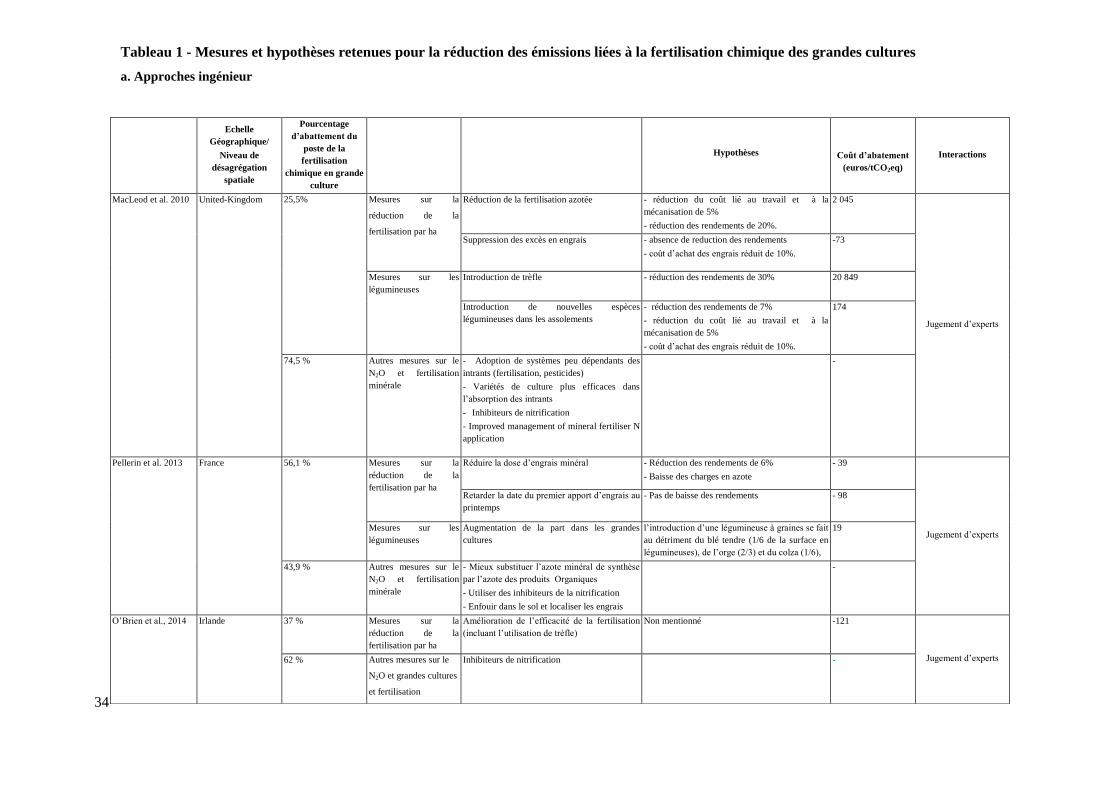
Tableau 1 - Mesures et hypothèses retenues pour la réduction des émissions liées à la fertilisation

chimique des grandes cultures ............................................................................................................... 34

Table 2 - Comparison between the two policy approaches for the same target of abatement .............. 64

Table 3 – Comparison of rotations data between the five European regions ........................................ 79

Table 4 - Baseline rotations for the 13 site classes (for crop abbreviations see Appendix 3.7.7) ......... 81

Table 5 - Regional results for the baseline and for a cost-effectiveness of €45 /t CO2eq, scenario

Fertilisation (all rotations per site class; pre-crop effect decreases the nitrogen rate)........................... 89

Table 6 - Description of the sample used in the regression (step 2 of the data base treatment) .......... 125

Table 7 – Aversion coefficient taken in the literature for sensitivity analysis .................................... 128

Table 8 – Forms of variance and yield functions detected from the regression .................................. 129

Table 9 - Impact of insurance on fertilizer application (in kgN/ha) and abatement (only on risk averse

agents) – scenario CARA 1 ................................................................................................................. 134

Table 10 - Fertilisation reduction per type of crop (insurance premium 25 euros/ha and triggering

threshold : 0,9) ..................................................................................................................................... 135

17

Introduction générale

L’augmentation de la concentration atmosphérique des gaz à effet de serre (GES) conduit à une

altération de la capacité de l’atmosphère à maintenir sa température moyenne à son niveau actuel. Elle

induit dès lors un risque d’affaiblissement, voire même de disparition de certains écosystèmes sur

lesquels reposent les sociétés humaines. Par conséquent, il apparaît nécessaire de mettre en place des

actions afin d’infléchir cette tendance.

Depuis l’identification par Arrhenius en 1896 de l’impact de la concentration de CO2 sur la

température moyenne, l’augmentation continue du réchauffement climatique et la responsabilité des

activités anthropiques ont été étayées par de nombreux travaux scientifiques. Le dernier rapport

d’évaluation sur le changement climatique réalisé par le GIEC en 2014 fait état d’une situation

préoccupante. D’après les scénarios de projection de l’évolution du climat explorés, l’absence d’effort

destiné à limiter les émissions conduirait à des trajectoires d’augmentation de la température moyenne

à la surface du globe se situant dans une gamme de 2 à 4°C par rapport à 1985-2005 à l’horizon 21001.

L’attentisme se traduirait ainsi par un « risque de conséquences graves, généralisées et irréversibles à

l’échelle du globe » engendrant des dommages « plus grands pour les populations et les communautés

défavorisées de tous les pays, quel que soit leur niveau de développement » (IPCC, 2014). Ce constat

issu de la communauté des experts du climat, accompagné par une prise de conscience de plus en plus

forte des opinions publiques des pays industrialisés, a conduit au cours des deux dernières décennies à

l’émergence d’une gouvernance du climat à l’échelle mondiale. Celle-ci s’est notamment traduite dans

certaines régions par la mise en place d’instruments de régulation sur les émissions de CO2 issues de la

combustion de produits fossiles associés à la production d’énergie et aux activités industrielles. Le

marché d’échange de quotas de carbone en Europe fait ainsi figure de système pionnier dans le monde

et a été accompagné par la suite d’une série de systèmes analogues dans d’autres régions du globe

(Goubet et Nikov, 2015). A l’échelle nationale, certains Etats ont par ailleurs choisi la mise en place

de taxes carbone en Europe (Kossoy et al., 2015).

Cela étant, les mesures prises sur la limitation des émissions de CO2 n’ont pour le moment pas été

associées à une volonté tout aussi nette de régulation des cycles biogéochimiques du méthane et de

l’azote en dépit de leur rôle tout aussi important dans le fonctionnement du climat. Engendrés pour

l’essentiel par des processus biologiques, ces deux gaz, au potentiel de réchauffement global

important, ont également connu une forte augmentation de leur concentration atmosphérique au cours

des dernières décennies (IPCC, 2014) et sont principalement émis par les activités agricoles. En 2010,

1 D’après les scénarios RCP6,0 et RCP8,5 qui n’intègrent aucun effort d’atténuation des émissions

18

sur les 49 GtCO2eq (±4.5) de gaz à effet de serre émis par les activités humaines, les activités

agricoles2 représentaient 5,4 GtCO2eq (±0.5) (IPCC – WG3, 2014) soit une part des émissions

mondiales de 11% (±0.2) en raison des émissions de protoxyde d’azote (N2O) et de méthane (CH4)

liées à la fertilisation et à l’élevage.

Si les conséquences de l’agriculture sur le réchauffement climatique font l’objet d’une littérature

scientifique de plus en plus fournie, il n’en demeure pas moins que l’ampleur de la mise en place

d’instruments de régulation appliqués à ce secteur apparait encore faible au regard de l’enjeu

climatique. Les initiatives lancées dans la foulée de la ratification du protocole de Kyoto telles que les

mécanismes de développement propres ou la mise en œuvre conjointe ont pu aboutir à la réalisation de

projets innovants dans les agricultures des pays industrialisés et des pays en voie de développement.

Elles ont jusqu’à présent permis l’identification de mesures novatrices de réduction d’émissions tant

du point de vue des techniques alternatives employées que celui du mode de financement. Néanmoins,

l’ampleur de leur déploiement et de leur diffusion n’est encore pas suffisante pour infléchir

significativement et durablement les trajectoires d’émissions des agricultures dans le monde.

Il convient par conséquent d’amplifier la réduction des émissions par des politiques publiques visant à

inciter à réduire des émissions de gaz à effet de serre agricoles. La mise en place d’un prix du carbone

(que ce soit par le biais d’une taxe, ou d’un marché d’échange de quotas de carbone) ou la mise en

place de normes peuvent être envisagées comme instruments de régulation. La nécessité de développer

la connaissance sur le coût de réduction (ou coût d’abattement) des émissions apparaît toutefois être

un préalable afin (i) d’apprécier la pertinence des outils les uns par rapport aux autres, (ii) d’anticiper

les réductions d’émissions attendues par ces différents instruments et (iii) de discuter l’efficacité

économique des mesures qui peuvent être envisagées dans ce secteur.

Cette thématique est l’objet de cette thèse qui se focalise sur la question du coût lié à la réduction des

émissions de gaz à effet de serre afin de comprendre quels peuvent être les potentiels de réduction

ainsi que les éventuels freins associés à certaines mesures d’atténuation. Je me concentre sur les

émissions de protoxyde d’azote (N2O) liées à la fertilisation qui, nous le verrons, constituent un poste

majeur d’émissions. Le cadre retenu est celui de l’agriculture européenne conventionnelle qui sera

abordée à travers trois niveaux géographiques différents. Le premier chapitre porte sur le niveau

français, le deuxième se concentre sur cinq régions européennes tandis que le troisième porte sur trois

départements français. Chaque chapitre analyse une mesure d’atténuation des émissions spécifique.

L’instrument de régulation des émissions étudié de manière privilégié sera celui d’une taxe carbone,

2 Catégorie n’intégrant pas les émissions liées à l’utilisation et au changement des sols

19

traduisant la mise en place d’un prix du carbone3, et constituera le fil rouge de ce travail mais sera

complétée, dans le troisième chapitre, par l’étude d’un autre outil pouvant être envisagé pour

l’atténuation des émissions, à savoir la mise en place d’une assurance.

L’objectif de ce chapitre introductif est de présenter, premièrement, le contexte général des émissions

de gaz à effet de serre dans l’agriculture européenne et française et, deuxièmenent, la place de ce

travail par rapport à ce contexte et à la littérature disponible. Après avoir identifié l’importance des

émissions liées à la fertilisation dans la première partie, les bases théoriques de la mise en place d’un

prix du carbone sont abordées dans la partie 2. Ces observations nous révèlent l’importance de l’étude

du coût d’atténuation afin d’anticiper les réductions engendrées par ce mécanisme incitatif. Les

différentes approches retenues dans la littérature économique agricole sur les coûts marginaux

d’atténuation sont exposées dans la partie 3. Puis, en partie 4, les apports, les approches retenues et les

problématiques abordées dans la thèse sont présentées.

1.1 Contexte : l’importance des émissions de GES liées à la fertilisation

1.1.1. La fertilisation : une pratique fondamentale pour la sécurité alimentaire mondiale associée à

des impacts environnementaux conséquents

La consommation européenne d’azote en Europe a été estimée dans les années 2000 à 20 millions de

tonnes par an (Sutton et al., 2011). Elément chimique fondamental pour la croissance des plantes et

donc pour l’alimentation humaine, sa maîtrise est à la croisée d’enjeux liés au commerce international,

à la préservation de l’environnement et à la sécurité alimentaire.

L’azote est présent de manière abondante dans l’atmosphère. Cependant, sa forme chimique N2 est peu

réactive et donc très peu assimilable par la plupart des organismes vivants. Par constrate, l’azote

présent sur terre revet des formes chimiques plus réactives (ammonium, nitrate, acides aminés,

proteines etc.) mais disponibles en quantités beaucoup plus réduites. La capacité à déplacer une partie

du stock de l’atmosphère vers le sol a donc historiquement constitué un défi majeur pour les

agriculteurs et agronomes afin de répondre à la demande alimentaire.

3 Le terme « taxe carbone » est utilisé ici de manière générique, même si en l’occurrence elle s’applique pour la

thèse aux émissions de protoxyde d’azote exprimées en équivalent CO2. La valeur du pouvoir de réchauffement

global (PRG) du N2O reprend celle retenue dans les inventaires d’émissions et correspond aux valeurs définies

par la CCNUCC, c’est à dire celle indiquée dans le 4ème rapport du GIEC (IPCC, 2007). Cette valeur est de 298,

autrement dit une tonne émise de N2O est équivalent à l’émission de 298 tonnes de CO2.

20

Avant la révolution de la fixation de l’azote par le procédé Haber-Bosch, la fertilisation des cultures

était principalement assurée par des sources naturelles telles que les déjections d’élevage et la fixation

symbiotique des plantes légumineuses (pois, luzerne, lentilles, fève etc.) ou bien par des sources

« fossiles » telles que le guano péruvien, le salpêtre chilien ou le sel d’ammonium extrait du charbon

(Erisman et al., 2008 ; Hager, 2008). Ce système a cependant été bouleversé par la découverte de Fritz

Haber en 1908 de la fixation atmosphèrique permettant d’obtenir de l’azote réactif à partir d’oxygène

et de diazote atmosphériques et de méthane placés à très haute température et à haute pression. Cette

innovation industrielle a ainsi permis de lever l’une des principales limites portant sur l’augmentation

de la production agricole mondiale. Pour Sutton l’ampleur avec laquelle elle s’est déployée au cours

du vingtième siècle, après avoir été découverte, fait de cette dernière « la plus importante expérience

de géo-ingénierie que l’humanité ait jamais réalisée » (Sutton et al., 2011). Elle a permis notamment

la réalisation de sauts en matière de potentiel de production des cultures après la seconde guerre

mondiale4 rendant les échanges internationaux de gouano et d’os, qui s’étaient constitués jusqu’alors,

obsolètes. Enfin, elle a permis d’accompagner le mouvement d’augmentation de la population portée

par la révolution verte agricole qui est passée de 3,5 à 7,35 milliards d’habitants dans le monde entre

1950 et 2015. Ainsi, Erisman et al. (2008) estiment que la fertilisation azotée chimique contribue à

nourrir 48% de la population mondiale.

L’importation massive d’azote sous forme minérale dans les agro-systèmes a eu pour conséquence, en

particulier, une moindre nécessité pour les agriculteurs d’avoir recours à des formes d’azote

organiques (déjections d’élevage, fixation symbiotique via les plantes légumineuses). Le service de

fertilisation apporté par les déjections d’élevage et les légumineuses, s’est vu fortement concurrencé

par l’efficacité de l’azote fourni par les engrais minéraux. Les régions agricoles ont pu, par ailleurs,

accélérer leur mouvement de spécialisation (Johnstone, 1995), et les secteurs de l’élevage et des

cultures ont pu être davantage dissociés favorisant la différenciation entre zones de cultures et

d’élevage. Enfin, la transformation du cycle global de l’azote engendrée par les activités humaines,

s’est accompagnée de conséquences néfastes pour l’environnement (Sutton et al,. 2011). En Europe, le

lessivage des nitrates s’est notamment traduit par des concentrations importantes dans les eaux

potables dans certaines régions (notamment en Belgique, en Bulgarie et en Bretagne) et par

l’eutrophisation des écosystèmes aquatiques. L’apport d’azote sur les terres agricoles engendre

également des émissions de NOx avec des conséquences importantes sur la qualité de l’air et la santé.

Enfin, la fertilisation azotée est responsable d’une partie substantielle des émissions de gaz à effet de

serre que nous abordons plus en détail dans le paragraphe suivant.

4 Stewart et al., 2005 concluent, d’après des expériences de long terme effectuées aux Etats-Unis, au Royaume-

Uni et dans différentes zones tropicales, que 30 à 50% du rendements des cultures est due à l’épandage d’engrais

synthétiques.

21

1.1.2. Une source importante d’émissions en Europe et en France

Les émissions de l’agriculture peuvent être approximées grâce aux règles de calcul développées par le

GIEC (Houghton et al., 1997 ; IPCC, 2000). Celles-ci permettent une comptabilité des émissions de

gaz à effet de serre dans le système commun d’inventaire encadré par l’UNFCCC afin, d’une part, de

suivre l’évolution des émissions des différents pays signataires sur la base d’une métrique et d’une

méthode communes et, d’autre part, d’apprécier le respect des engagements des différents Etats en

matière d’atténuation des émissions.

Les émissions liées à la fertilisation sont représentées dans la catégorie ‘Agricultural Soils’. Celles-ci

rassemblent les émissions liées à la fertilisation azotée des champs cultivés et des prairies. On

distingue les émissions de N2O directes et indirectes. Les émissions directes sont produites à l’endroit

de l’épandage des engrais, que ces engrais soient synthétiques (engrais chimiques) ou organiques

(résidus de culture, lisiers d’animaux, ou des déjections animales effectuées en pâture). Les émissions

de N2O indirectes sont produites sur une surface différente du lieu de la fertilisation. Elles résultent du

transport des composés azotés en dehors de la parcelle sous l’effet du lessivage, du ruissellement ou de

la déposition atmosphérique. La déposition atmosphérique commence par la volatilisation de l’azote

sous forme de NH3 ou de NOx, suivie de sa redéposition sur le sol sous forme d’ammonium ou de

nitrate. Dans un second temps, ce dépôt engendre des émissions de N2O par les mêmes processus de

nitrification et de dénitrification que les émissions directes. Le lessivage est le flux d’eau qui s’infiltre

depuis la surface jusqu’aux profondeurs des racines pour ensuite rejoindre les eaux souterraines.

Enfin, le ruisselement correspond aux flux d’eau en surface des terres.

En 2014, la fertilisation est responsable en Europe (UE-28) de l’émission de 164 MtCO2eq (voir figure

1) soit 37,9% des émissions agricoles ou encore 4,2% de l’ensemble des émissions nettes5. Si le poids

de la fertilisation est élevé en Europe, il l’est encore plus en France. Elle représente ainsi la première

source de gaz à effet de serre de l’agriculture de ce pays avec 35 MtCO2eq (voir annexe 1.6) soit

43,8% des émissions de l’agriculture et 8,5% de l’ensemble des émissions nettes françaises. Le poids

de la fertilisation dans les émissions françaises et la part que représente la France dans les émissions

agricoles européennes6 s’expliquent principalement par le fait que la France dispose de la plus grande

surface agricoles utile (SAU) des pays de l’Union. L’explication de ce poids dans son propre périmètre

est aussi liée à l’importance du nucléaire dans le mix énergétique français, conduisant à des émissions

relativement plus basses dans le secteur de la production d’énergie et donc une part plus importante

pour celles provenant de l’agriculture.

5 En prenant en compte le puits net de gaz à effet de serre lié aux usages des sols et à la forêt.

6 La fertilisation française représente en effet 21% des émissions de la fertilisation de l’UE-28.

22

-100 0 100 200

UTCF Agricole

Energie de l'agriculture

Fermentation entérique

Gestion des effluents

Sols Agricoles

Autres

Emissions (en MtCO2eq)

Méthane et protoxyde d'azote

Terres cultivées restant Terres Cultivées (CO2)

Terres converties en terres cultivées (CO2)

Prairies restant prairies (CO2)

Terres converties en prairies (CO2)

Terres cultivées et prairies converties en forêts

(CO2)

Terres cultivées et prairies converties en zones

urbanisées (CO2)

Carburants (CO2)

-1 000

-

1 000

2 000

3 000

4 000

5 000

Em

issi

on

s (e

n M

tCO

2eq

)

Industries de l'énergie

Transport

Secteur commercial et résidentiel

Manufactures et construction

Agriculture

Procédés industriels

Déchets

Emissions fugitives issues des

carburantsEnergie des autres secteurs

Autres

UTCF

Note : UTCF signifie Utilisation des Terres, leurs Changements et la Forêt

Légende 1-a :

a. Répartition des émissions

européennes par secteur

b. Répartition des émissions

agricoles par sources

Légende 1-b :

Figure 1 - Place de l’agriculture dans les émissions européennes de GES (UE-28) en 2014. Données :

UNFCCC

23

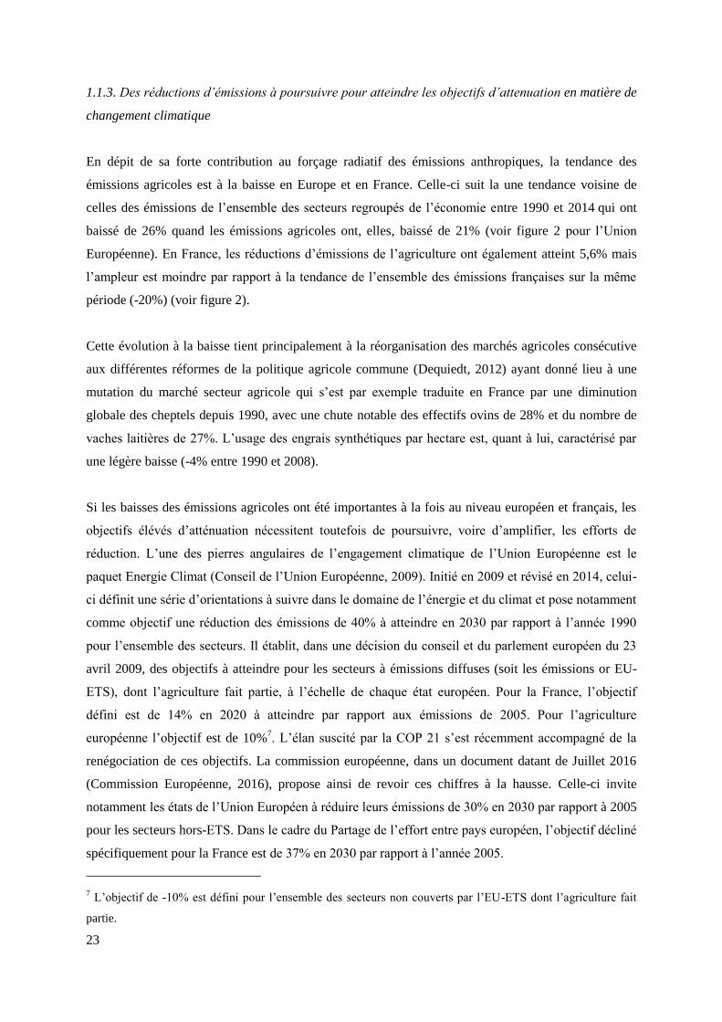
1.1.3. Des réductions d’émissions à poursuivre pour atteindre les objectifs d’attenuation en matière de

changement climatique

En dépit de sa forte contribution au forçage radiatif des émissions anthropiques, la tendance des

émissions agricoles est à la baisse en Europe et en France. Celle-ci suit la une tendance voisine de

celles des émissions de l’ensemble des secteurs regroupés de l’économie entre 1990 et 2014 qui ont

baissé de 26% quand les émissions agricoles ont, elles, baissé de 21% (voir figure 2 pour l’Union

Européenne). En France, les réductions d’émissions de l’agriculture ont également atteint 5,6% mais

l’ampleur est moindre par rapport à la tendance de l’ensemble des émissions françaises sur la même

période (-20%) (voir figure 2).

Cette évolution à la baisse tient principalement à la réorganisation des marchés agricoles consécutive

aux différentes réformes de la politique agricole commune (Dequiedt, 2012) ayant donné lieu à une

mutation du marché secteur agricole qui s’est par exemple traduite en France par une diminution

globale des cheptels depuis 1990, avec une chute notable des effectifs ovins de 28% et du nombre de

vaches laitières de 27%. L’usage des engrais synthétiques par hectare est, quant à lui, caractérisé par

une légère baisse (-4% entre 1990 et 2008).

Si les baisses des émissions agricoles ont été importantes à la fois au niveau européen et français, les

objectifs élévés d’atténuation nécessitent toutefois de poursuivre, voire d’amplifier, les efforts de

réduction. L’une des pierres angulaires de l’engagement climatique de l’Union Européenne est le

paquet Energie Climat (Conseil de l’Union Européenne, 2009). Initié en 2009 et révisé en 2014, celui-

ci définit une série d’orientations à suivre dans le domaine de l’énergie et du climat et pose notamment

comme objectif une réduction des émissions de 40% à atteindre en 2030 par rapport à l’année 1990

pour l’ensemble des secteurs. Il établit, dans une décision du conseil et du parlement européen du 23

avril 2009, des objectifs à atteindre pour les secteurs à émissions diffuses (soit les émissions or EU-

ETS), dont l’agriculture fait partie, à l’échelle de chaque état européen. Pour la France, l’objectif

défini est de 14% en 2020 à atteindre par rapport aux émissions de 2005. Pour l’agriculture

européenne l’objectif est de 10%7. L’élan suscité par la COP 21 s’est récemment accompagné de la

renégociation de ces objectifs. La commission européenne, dans un document datant de Juillet 2016

(Commission Européenne, 2016), propose ainsi de revoir ces chiffres à la hausse. Celle-ci invite

notamment les états de l’Union Européen à réduire leurs émissions de 30% en 2030 par rapport à 2005

pour les secteurs hors-ETS. Dans le cadre du Partage de l’effort entre pays européen, l’objectif décliné

spécifiquement pour la France est de 37% en 2030 par rapport à l’année 2005.

7 L’objectif de -10% est défini pour l’ensemble des secteurs non couverts par l’EU-ETS dont l’agriculture fait

partie.

24

Ces objectifs ambitieux appelent une nouvelle inflexion des trajectoires actuelles d’émissions. La

figure 2 permet de rendre compte de l’écart persistant entre la baisse réelle des émissions et les baisses

telles qu’elles devraient être en vue de l’atteinte des différents objectifs d’atténuation à l’échelle

européenne et française8. Entre 1990 et 2014, les réductions annuelles d’émissions agricoles ont été en

moyenne de 0,2% et de 0,9% respectivement au niveau français et européen. Le simple respect des

objectifs fixés par le paquet énergie-climat en 2009 impliquerait de rehausser les efforts annuels de

réduction à 2,4%, soit une multiplication par 11 des efforts engagés actuellement au niveau français, et

de 1,5%, soit une multiplication par 1,8 des efforts actuels au niveau de l’Union Européenne.

Par conséquent, pour encourager de nouvelles baisses d’émissions et atteindre les objectifs liés à la

limitation du changement climatique, il convient d’identifier le potentiel de mesures additionnelles

d’atténuation et d’envisager la mise en place d'outils de régulation.

8 En supposant une déclinaison annuelle des différents objectifs climatiques à atteindre.

25

a. Union Européenne (UE-28)

b. France

Figure 2 – Illustration de l’écart entre l’évolution des émissions de GES et les différents objectifs d’atténuation (en

pourcentage) – données : UNFCCC

-40.00

-35.00

-30.00

-25.00

-20.00

-15.00

-10.00

-5.00

0.00

1990 1995 2000 2005 2010 2015

Evolu

tion

des

ém

issi

on

s d

an

s l'

Un

ion

Eu

rop

éen

ne

(en

%

par

rap

port

à 1

99

0)

Ensemble des secteurs (emissions

nettes)

Agriculture (CH4+N2O)

Sols Agricoles

Commission Européenne, 2014

Facteur 4

Paquet Energie-Climat, 2009

Paquet Energie climat, 2016

Trajecto

ires d’ém

ission

s

nécessaires p

ou

r atteind

re les

différen

ts ob

jectifs

d’attén

uatio

n

Notes : les différents objectifs de réduction d’émissions de gaz à effet de serre :

- « Commission européenne, 2014 »: correspond à un objectif de réduction de 40% des émissions en 2030 par

rapport à 1990 pour l’ensemble des secteurs de l’économie.

- « Facteur 4 » : correspond à une baisse des émissions de 75% en 2050 par rapport à 1990 pour l’ensemble des

secteurs de l’économie. En France, il est intégré dans la loi programme fixant les orientations de la politique

énergétique datant du 13 juillet 2005. En Europe, il correspond à la recommendation du parlement établie dans la

décision du 23 avril 2009.

- « Paquet Energie-Climat, 2009 » : objectif de réduction de 10% pour les secteurs à émissions diffuses en 2020

par rapport à 2005 dans l’UE-28. L’objectif en France est de 14%.

- « Paquet Energie-Climat, 2016 » : objectif de réduction de 30% proposé par la Commision Européenne pour les

secteurs à émissions diffuses (hors-ETS) en 2030 par rapport à 2005 dans l’UE-28. L’objectif proposé en France

est de 37%.

-40.00

-35.00

-30.00

-25.00

-20.00

-15.00

-10.00

-5.00

0.00

5.00

10.00

1990 1995 2000 2005 2010 2015

Evolu

tion

des

ém

issi

on

s en

Fra

nce

(en

%

par

rap

port

à 1

99

0)

26

1.2. Des instruments réglementaires à l’idée de l’inclusion d’un prix sur les émissions de GES

En dépit d’une prise de conscience du problème climatique encore relativement faible chez les

agriculteurs9, l’intégration du climat dans l’agriculture reste une ambition affichée par les autorités

publiques. Si l’accord de la COP21 à Paris (UNFCCC, 2015) en décembre dernier ne mentionne pas le

rôle de l’agriculture dans l’atténuation des émissions, au niveau européen, la communication de la DG

Agriculture (European Commission, 2010) mentionne la nécessité pour l’agriculture de « poursuivre

les actions d’atténuation des changements climatiques et d'adaptation à ces changements afin de

permettre à l'agriculture d'y faire face ».

Pour que l’atténuation des émissions de GES soit efficace, les instruments des politiques de

l’environnement ont pour objectif de fournir les incitations permettant de trouver un point d’équilibre

entre les deux extrêmes que constituent d’un côté la réduction complète des niveaux de pollution et, de

l’autre, le laissez-faire engendrant des dommages considérables pour l’environnement. En d’autres

termes, la réduction des externalités, en l’occurrence des émissions de gaz à effet de serre, ne doit pas

induire davantage de coûts pour la société que le coût des dommages créés par ces externalités elles-

mêmes (Pigou, 1932 ; Barde, 1995). Ce point d’équilibre, appelé également optimum social, doit

correspondre au niveau d’émissions où le coût marginal d’atténuation (ou coût marginal d’abattement)

des émissions égalise la valeur marginale des dommages induits par ces pollutions.

On distingue généralement deux grandes catégories d'instruments permettant de trouver cet équilibre:

les instruments réglementaires et les instruments économiques. Les instruments réglementaires sont

mesures institutionnelles visant à contraindre le comportement des pollueurs sous peine de sanctions

administratives ou judiciaires. Ceux-ci comportent principalement les normes d’émissions, définissant

des intensités maximales d'émissions de polluant dans le milieu de production, ou de normes

techniques, qui obligent les firmes à utiliser une technologie particulière de réduction de la pollution.

Les instruments économiques sont des mesures institutionnelles visant à modifier l'environnement

économique du pollueur (i.e. les bénéfices et les coûts) via des signaux "prix", tels que les taxes

environnementales ou les marchés de droits à polluer, pour l'inciter à l'adoption volontaire de

comportements moins polluants.

L’un des avantages des instruments par les prix est qu’ils permettent de différencier les efforts de

dépollution entre les firmes sans que cette répartition efficace de l’effort ne soit déterminée par une

autorité de régulation (Pigou, 1932). En effet, sous l'effet d'une taxe, les firmes ayant un coût de

9 dont seulement 20% sont convaincus, par exemple en France, de l’existence du lien entre les activités humaines et le

réchauffement climatique (Boy, 2014)

27

dépollution plus faible, iront plus loin dans la dépollution que les firmes les moins efficaces. Ce

faisant, la taxe permet de minimiser le coût global de l’atténuation des firmes d’un même secteur

économique. A l’inverse, une norme uniforme qui imposerait à chaque pollueur le respect d'un même

niveau maximal d'émissions ne permet pas d’atténuer les émissions au coût global le plus faible

puisque les firmes aux coûts de dépollution le plus faible sont amenées, dans cette configuration, aux

mêmes niveaux que celles aux coûts de dépollution le plus élevée. Il est possible toutefois, en théorie,

d’envisager la mise en place de normes d'émission plus efficaces qui différencieraient les niveaux de

pollution prescrits à chaque firme. Ainsi, une norme différenciée qui prescrirait différentes quantités

maximales d’émissions ajustées en fonction de leur capacité d’abattement, permettrait, comme la taxe

pigouvienne, d'atteindre l’optimum social. Il est à noter cependant, que ce dispositif nécessite que les

autorités de régulation puissent disposer des informations suffisantes, notamment le coût d’atténuation

de chaque entreprise, pour déterminer ces niveaux de pollution différenciées.

Jusqu’à présent, les instruments environnementaux de la Politique Agricole Commune (PAC) ont été

principalement de nature réglementaire. Apparue au moment de la réforme Fischler en 2003, l’éco-

conditionnalité renforce, par exemple, les dispositions que doivent prendre les agriculteurs en matière

d’environnement en échange des aides du premier pilier. Celle-ci comprennent le maintien des prairies

permanentes, la préservation des surface d’intérêt écologique ou encore la diversification des cultures

(Commission Européenne, 2013)10

. Initiée en 1991, la Directive Nitrate fixe également des limites sur

les quantités d’azote épandues sur les terres agricoles et a eu par conséquent un impact indirect sur les

émissions de N2O (Velthof et al., 2014). L’impact sur les émissions de GES agricoles reste toutefois

un objectif secondaire de ce dispositif. La réforme de la PAC en 2014 adosse aux mesures agro-

environnementales, dans le cadre du deuxième pilier, une composante climatique mais il n’est pas

encore possible d’estimer leur impact concret sur les pratiques des agriculteurs et sur la réduction des

émissions.

La PAC offre donc un cadre pour l’inclusion et le renforcement de la dimension climatique dans les

pratiques agricoles. Il convient toutefois d’apporter les remarques suivantes:

Tout d’abord, le principe de rétribution en échange de services environnementaux (c’est par

exemple le cas des mesures agro-environnementales) est opposé au principe pollueur-payeur

adopté par les pays de l'OCDE qui implique que le coût des mesures économiques engagées

doit être supporté par les agents responsables de la pollution (OCDE, 1989; Henry, 1989).

10 http://ec.europa.eu/agriculture/policy-perspectives/policy-briefs/05_fr.pdf

http://ec.europa.eu/agriculture/policy-perspectives/policy-briefs/05_fr.pdf

28

Ensuite, selon Dupraz (2007), les mesures agro-environnementales sont intrinsèquement

sous-optimales au regard de la théorie économique d’internalisation des externalités, qui

préconise une rémunération tenant compte de la demande sociale, c’est-à-dire de la valeur

accordée par la collectivité aux externalités négatives. Ce n’est pas le cas ici puisque seules

les pertes de profit pour les agriculteurs, et non le coût pour la société de manière globale,

sont prises en compte dans le calcul des aides que reçoivent les agriculteurs, ce qui peut

aboutir à une situtation sous-optimale pour le bien-être global de la société.

Concernant les normes limitant les externalités, s’il y a un progrès technique permettant de

réduire le coût de pollution, l’agriculteur ne sera pas incité à changer ses pratiques en deça de

ce que définissent les normes actuelles. En effet, le pollueur sera d’autant moins incité à faire

spontanément mieux que la norme qu’il craindra un « effet de cliquet » de la part des

pouvoirs publics qui seront tentés d’entériner le progrès technique par un renforcement

général des normes (Barde, 1995). Par conséquent, la norme constituerait davantage une

invitation à se cantonner dans le système actuel.

Par ailleurs, le fait que la mise en place de normes différenciées optimales suppose que

l’autorité de régulation puisse au préalable déterminer l’optimum de pollution en estimant la

fonction de dommage, d’un coté, et les fonctions de coût d’atténuation pour chacun des

acteurs du secteur (Weitzman, 1974 ; Baumol and Oates, 1971, Segerson, 1988) représente un

problème pratique pour le secteur agricole. Si cela implique un coût de relativement faible de

collecte de l’information dans des secteurs tels que celui de la production d’énergie, où les

émissions de GES sont concentrées en quelques unités de production, le problème est tout

autre dans le secteur agricole qui comprend de nombreuses exploitations réparties sur le

territoire et présentant des conditions de production très hétérogènes et donc une forte

disparité du coût d’abattement.

A la différence des normes, la régulation par les prix permet d’éviter les principaux écueils énoncés ci-

dessus. Sans nécessiter le calcul du coût d’atténuation pour chaque exploitation agricole, elle permet

notamment de s’adapter à l’hétérogénéité des conditions du secteur agricole (Shortle et Dunn, 1986)

sans besoin de déterminer les quantités de polluants par exploitations. Elle revet l’avantage de fournir

une incitation continue à la réduction des émissions permettant de favoriser l’intégration du progrès

technique dans la production (Barde, 1995) et respecte le principe pollueur-payeur des pays de

l’OCDE.

29

Une partie de la littérature propose que cette régulation par les prix soit mise en œuvre dans

l’agriculture via la mise en place d’un marché d’échange de quotas de carbone (Pérez-Dominguez et

al., 2009 ; Mac Carl and Schneider, 2000). Cette proposition repose sur l’approche de Coase (1960)

proposant d’attribuer à chaque agent des quotas ou permis d’émissions puis à permettre l’échange de

ces droits par ventes ou achat, générant ainsi un prix des droits à polluer. D’un point de vue théorique,

ce système permettrait d’être tout aussi efficace pour atteindre le niveau d’émissions de GES optimal

et ne diffère pas ainsi d’une taxe pigouvienne par la minimisation du coût global d’atténuation (Barde,

1995). De Cara et Vermont (2011) soulignent par ailleurs que l’élargissement du système d’échange

de quotas de carbone européen (EU-ETS) à l’agriculture aurait l’avantage de réduire le coût

d’abattement global d’atténuation notamment en réalisant des économies du côté des secteurs couverts

par l’ETS. L’économie globale réalisée par cet élargissement serait, selon ces mêmes auteurs,

supérieure aux coûts de transaction (associés à la mesure, le reporting et la verification des émissions

de gaz à effet de serre dans le secteur agricole) inhérents à un tel système.

Si la discussion sur la mise en place d’un prix du carbone dans l’agriculture reste jusqu’à présent

principalement théorique, certaines initiatives initiées au moment du protocole de Kyoto suivent le

principe d’attribution d’un prix des émissions de GES dans les différents secteurs de l’économie y

compris celui de l’agriculture. C’est le cas des Mécanismes de Développement Propre (MDP) pour les

pays en voie de développement (hors-annexe B) et de la Mise en Œuvre Conjointe (MOC) pour les

pays développés (annexe-B). La valeur de la tonne de CO2eq résulte ici des contraintes d’émissions

des pays engagés dans le protocole de Kyoto qui peuvent se mettre en conformité par rapport à leur

objectif en achetant des tonnes de réduction d’émissions générées par différents projets11

. Tronquet et

Foucherot (2015) recensent, dans les MDP, quelques 954 projets liés à l’agriculture (enregistrés au 1er

décembre 2014) soit 13% de l’ensemble des projets MDP. Ces mêmes auteurs rapportent que les

projets agricoles de la MOC, sur la période 2008-2012, représentent 70 projets sur les 648 projets

MOC (soit 9% des projets). Cependant, la plupart d’entre eux ne concernent que la filière en amont et

aval de l’agriculture sans se concentrer sur les émissions de l’exploitation12

. Ceux-ci portent en effet,

en majorité, sur la réduction des émissions de N2O lors de la fabrication d’engrais ou l’utilisation de la

biomasse en substitution de combustibles fossiles pour la production énergétique et laissent ainsi la

portion congrue au changement des pratiques des agriculteurs.

11 Certified emission reduction units (CERs) pour les mécanismes de développement propre et Emission Reduction Units

(ERUs) pour la mise en œuvre conjointe.

12 Les projets ne concernant que les émissions au sein de l’exploitation ne concernent en effet que 213 projets MDP et 12

projet MOC (Tronquet et Foucherrot, 2015)

30

Enfin, la Nouvelle-Zélande a créé en 2008 le New Zealand Emission Trading System (NZ-ETS),

couvrant une grande partie des secteurs de l’économie néo-zélandaise13

et devant s’élargir

progressivement à celui de l’agriculture. Des obligations de reporting ont ainsi été imposées aux

transformateurs agricoles depuis le 1er janvier 2012 et il a également été prévu d’intégrer les

émissions agricoles en 2015 dans ce marché d’échange de quotas carbone, en plaçant la contrainte sur

les producteurs d’engrais azotés pour les émissions de N2O et sur les industries de transformation de la

viande pour les émissions liées à l’élevage. Cependant, l’entrée du secteur agricole dans le système de

quotas n’est plus à l’ordre du jour suite aux pressions du secteur agricole.

En dépit de la portée relativement faible de ces initiatives, la mise en place d’un prix sur les émissions

agricoles reste d’intérêt à une échelle plus globale pour le secteur agricole. L’évaluation du coût

d’abattement permet d’évaluer l’impact de la mise en place d’un prix du carbone en termes de

potentiel de réduction de gaz à effet de serre, ce que se propose de faire une partie de la littérature sur

le coût d’abattement.

1.3. Revue de la littérature sur l’estimation des coûts d’abattement en agriculture.

1.3.1. Les différentes approaches pour estimer le coût d’atténuation

Vermont et De Cara (2010) identifient trois grandes approches pour estimer le coût marginal

d’abattement : i) les approches de type ingénieur, ii) les approches reposant sur des modèles

économiques d’offre ; iii) les approches par construction de modèles d’équilibre partiel ou général.

L’approche type ingénieur se concentre sur le potentiel de mesures individuelles et s’attache

à produire leur abattement cumulé et les coûts associés. Les données employées pour estimer

leur potentiel sont généralement issues de fermes modèles (ou représentatives) et permettent

ainsi de réduire les incertitudes sur l’estimation du coût d’atténuation des émissions à l’échelle

de chaque mesure (MacLeod et al. 2010, Pellerin et al. 2013, O’Brien et al., 2014).

L’approche regroupant des modèles économiques d’offre décrit le comportement

d’exploitations types représentant différentes régions géographiques (De Cara and Jayet,

2011; Hediger, 2006). La fonction objectif est typiquement le profit de ces exploitations

auxquelles sont ajoutées différentes contraintes que constituent par exemple la disponibilité

des terres ou encore des éléments de politique agricole. L’intégration d’un prix du carbone

13 Production d’énergie, industrie, déchets et forêt

31

dans ces modèles, par la mise en place d’une taxe sur les émissions de GES, permet au modèle

de décrire la réponse efficace en termes de reconfiguration des productions au sein de

l’exploitation pour réduire les émissions.

L’approche fondée sur des modèles d’équilibre général ou partiel partage avec l’approche

ci-dessus l’hypothèse de maximisation du profit des agents. Celle-ci inclue cependant une

description de la demande des produits agricoles ainsi qu’une représentation des ajustements

des prix et de l’équilibre sur les marchés. Les modèles de cette catégorie représentent ainsi les

effets retour des prix sur les coûts marginaux d’atténuation (Pérez-Dominguez et al., 2012;

Schneider et al., 2007; Golub et al., 2009).

1.3.2. Le traitement de la fertilisation dans les différentes approches

Ces trois approches ont été mobilisées pour estimer le potentiel d’atténuation de l’agriculture dont

celui de la fertilisation. Les tableaux 1-A et 1-B présentent la prise en compte de différentes mesures

d’atténuation liées à la fertilisation chimique des grandes cultures dans les différentes études. De

manière générale, elles se distinguent sur la base des éléments suivants :

Premièrement, une différence importante entre les approches repose sur le nombre de mesures

étudiées. Généralement les approches ingénieur abordent un éventail plus large de mesures.

Ainsi, sur le poste d’émissions liées à la fertilisation, Mac Leod et al. (2010) retiennent au

total neuf mesures et Pellerin et al. (2014) six mesures. Elles peuvent, par conséquent, donner

l’impression d’être plus fines en termes de possibilités de production examinées, mais elles

sont souvent plus rigides sur les hypothèses de niveaux de fertilisation retenues. A l’inverse,

les approches microéconomiques se concentrent sur un nombre plus restreint de mesures (de

trois à quatre mesures selon les études). Par ailleurs, les approches reposant sur des modèles

d’offre ne permettent généralement pas une aussi bonne lecture de la contribution de chaque

mesure individuelle puisque généralement celle-ci ne rendent compte uniquement que de la

réduction globale du poste sol agricole sans préciser le coût et le potentiel de chaque mesure.

Ensuite, une différence notable entre les approches concerne le niveau de désagrégation

spatiale (Vermont et De Cara, 2010). Les approches ingénieur se concentrent sur l’estimation

d’un potentiel à l’échelle d’un pays (au niveau de la France pour Pellerin et al., 2014 ; au

niveau du Royaume-Uni pour MacLeod et al., 2010 ; au niveau de l’Irlande pour O’Brien et

al., 2014) sans toutefois identifier la variabilité spatiale du coût et du potentiel de chaque

mesure au sein du périmètre géographique retenu. Ainsi, chaque mesure est associée à un coût

32

marginal constant suggérant que le coût d’abattement est le même quelles que soient les

conditions agronomiques de l’ensemble géographique retenu. A l’inverse, l’un des avantages

des études micro-économiques construites sur des modèles d’offre est de présenter une

meilleure désagrégation spatiale permettant d’identifier les potentiels de rendement et les

pratiques au niveau de chaque échelon géographique.

Les différentes approches se distinguent également par leur prise en compte des interactions

pouvant avoir lieu entre les différentes techniques retenues. Certaines approches type

ingénieur les prennent peu en considération puisqu’elles estiment le coût individuel de chaque

mesure sans considérer leur caractère potentiellement exclusif (Pellerin et al., 2014) quand

d’autres estiment leurs interactions à partir de jugements d’experts (Mac Leod et al., 2010 ;

O’Brien et al., 2014). Les approches micro-économiques les prennent, elles, davantage en

considération par l’arbitrage de la maximisation du profit et par la mise en place de contraintes

dans les modèles. Ceci a pour avantage de mieux représenter les interactions pouvant exister

entre le secteur des grandes cultures et de l’élevage. Enfin, les approches par modèle

d’équilibre permettent de représenter l’impact de la baisse de la fertilisation sur les prix des

intrants et des produits agricoles.

Enfin, une différence importante entre ces approches se situe au niveau de la définition des

émissions de la baseline. L’approche type ingénieur construit ses trajectoires d’atténuation à

partir de références de profits et d’émissions associées à des comportements économiques non

optimisés. Ainsi, si une pratique d’atténuation est plus profitable que les pratiques de

référence alors le coût d’atténuation évalué est négatif. Autrement dit, celle-ci permet

potentiellement l’identification de possibilités de réduction des émissions associées à

l’augmentation du profit des agriculteurs. Pour prendre un exemple, la mesure consistant à

éviter les excès d’apport en fertilisant sur les parcelles impliquerait un coût de -73

euros/tCO2eq au Royaume-Uni (Macleod et al., 2010) quand Pellerin et al., 2013 indiquent,

sur des mesures similaires, en France un coût de -39 euros/tCO2eq14

à -98 euros/tCO2eq15

.

L’obtention de tels abattements « gagnant-gagnant » est par construction impossible dans les

approches par modèle d’offre ou par modèles d’équilibre. Ces dernières, fondées sur une

hypothèse de rationalité des agents, supposent que les individus optimisent initialement leur

profit en ayant parfaitement connaissance des possibilités de production. Les émissions de

référence correspondent ainsi au point où les variables d’activité agricoles sont ajustées de

telle sorte que le profit des agriculteurs est maximisé. Par conséquent, toute trajectoire de

14 Mesure consistant à réduire de la dose d’engrais minéral par hectare

15 Mesure consistant à retarder la date du premier apport d’engrais au printemps

33

réduction d’émissions construite à partir de ce point se traduit nécessairement par une perte de

profit pour les agriculteurs.

Parmi les critiques émises dans la littérature sur la construction des courbes de coût marginal

d’abattement, Kesicki et Ekins (2012) indiquent que ces modes d’estimation, quelle que soit

l’approche employée, ne permettent pas de représenter complétement certains coûts cachés relatifs à

différents types de frein liés 1) à la capacité des agriculteurs à pouvoir réagir aux signaux

économiques, 2) aux coûts de transaction des différents types de politiques mises en œuvre et 3) aux

effets de blocage pouvant exister dans la filière amont et aval de l’exploitation. Par conséquent, les

coûts négatifs révélés dans l’approche ingénieur peuvent être davantage lus comme une quantification

de ces coûts cachés que l’identification de réelles opportunités économiques.

Parmi les freins cités à l’échelle de l’agriculteur16

, et non pris en compte dans les différentes études,

l’aversion pour le risque constitue une des dimensions de la prise de décision des agriculteurs pouvant

influer sur l’adoption d’innovation et en l’occurrence sur la réduction des émissions. S’il s’avère que

les changements de pratiques sont associés à un risque plus élevé en dépit de gains espérés plus

importants (Feder, 1980), les agriculteurs averses au risque ne changeront pas nécessairement leurs

pratiques. Les coûts négatifs ainsi identifiées sur l’évitement du surdosage d’engrais par hectare par

Macleod et al. (2010) et Pellerin et al. (2013) pourraient, en réalité être associés à une prise de risque

plus importante sur les rendements. Autrement dit, la réduction pourrait en moyenne se traduire par un

une augmentation de profit mais par une prise de risque plus importante. Stuart et al., 2014 ont par

exemple montré, dans une étude portant sur un programme de réduction de la fertilisation azotée aux

Etat-Unis, que les agriculteurs américains utilisent ces intrants pour minimiser leur risque de

production. Par conséquent, les incitations ou les coûts d’abattement présentés dans les différentes

études devraient pouvoir être capables de représenter cette dimension.

16 Le lecteur intéressé par cette thématique pourra se rapporter aux travaux de la littérature sur

l’adoption d’innovation tels que Trujillo-Barrera et al. (2016) ou Roussy (2016).

34

Echelle

Géographique/

Niveau de

désagrégation

spatiale

Pourcentage

d’abattement du

poste de la

fertilisation

chimique en grande

culture

Hypothèses

Coût d’abatement

(euros/tCO2eq)

Interactions

MacLeod et al. 2010 United-Kingdom 25,5% Mesures sur la

réduction de la

fertilisation par ha

Réduction de la fertilisation azotée - réduction du coût lié au travail et à la

mécanisation de 5%

- réduction des rendements de 20%.

2 045

Jugement d’experts

Suppression des excès en engrais - absence de reduction des rendements

- coût d’achat des engrais réduit de 10%.

-73

Mesures sur les

légumineuses

Introduction de trèfle - réduction des rendements de 30% 20 849

Introduction de nouvelles espèces

légumineuses dans les assolements

- réduction des rendements de 7%

- réduction du coût lié au travail et à la

mécanisation de 5%

- coût d’achat des engrais réduit de 10%.

174

74,5 % Autres mesures sur le

N2O et fertilisation

minérale

- Adoption de systèmes peu dépendants des

intrants (fertilisation, pesticides)

- Variétés de culture plus efficaces dans

l’absorption des intrants

- Inhibiteurs de nitrification

- Improved management of mineral fertiliser N

application

-

Pellerin et al. 2013 France 56,1 % Mesures sur la

réduction de la


Réduire la dose d’engrais minéral - Réduction des rendements de 6%

- Baisse des charges en azote

- 39

Jugement d’experts

Retarder la date du premier apport d’engrais au

printemps

- Pas de baisse des rendements - 98

Mesures sur les

légumineuses

Augmentation de la part dans les grandes

cultures

l’introduction d’une légumineuse à graines se fait

au détriment du blé tendre (1/6 de la surface en

légumineuses), de l’orge (2/3) et du colza (1/6),

19

43,9 % Autres mesures sur le

N2O et fertilisation

minérale

- Mieux substituer l’azote minéral de synthèse

par l’azote des produits Organiques

- Utiliser des inhibiteurs de la nitrification

- Enfouir dans le sol et localiser les engrais

-

O’Brien et al., 2014 Irlande 37 % Mesures sur la

réduction de la


Amélioration de l’efficacité de la fertilisation

(incluant l’utilisation de trèfle)

Non mentionné -121

Jugement d’experts 62 % Autres mesures sur le

N2O et grandes cultures

et fertilisation

Inhibiteurs de nitrification

-

Tableau 1 - Mesures et hypothèses retenues pour la réduction des émissions liées à la fertilisation chimique des grandes cultures

a. Approches ingénieur

35

Echelle Géographique/

Niveau de désagrégation

spatiale

Abattement (sols agricoles)

par rapport à l’ensemble

du potentiel Agricole (tout

gaz confondus)

Hypothèses Interaction

Approche fondée sur

des modèles d’offre

De Cara and

Jayet., 2011

UE-24 /niveaux infra-regional

(fermes types) et regional

(régions du RICA).

~ 25% (pour une taxe

comprise entre 0 et 50

euros/tCO2eq)

Mesures sur la

réduction de la


Apport global en fertilisants

déterminé par les surfaces

entre cultures

- Apports en azote et les rendements constants

- Contraintes de rotation intégrées par un

maximum de la part des cultures individuelles

(ou groupe de cultures)

- Avec le secteur de l’élevage

par intégration de

l’alimentation animale

- Substitution engrais minéral

et engrais organique Mesures sur les

légumineuses

Fixation biologique de l’azote

déterminée par la part des

cultures de légumineuses

Autres mesures sur

le N2O et

fertilisation

minérale

2 :

- réutilisation des résidus de

culture

- Substitution engrais minéral /

engrais organique

Hediger,

2006

Suisse - Mesures sur la

réduction de la


Réduction de l’intensité de

l’application en engrais

Mesures sur les

légumineuses

Fixation biologique de l’azote

déterminée par la part des

cultures de légumineuses

Autres mesures sur

le N2O et la

fertilisation

Substitution engrais minéral /

engrais organique

Modèles d’équilibre

général ou partiel

Pérez-

Dominguez et

al., 2012

UE-27 / Régions européennes

NUTS2

~ 77% (année 2020)

Mesures sur la

réduction de la


Réduction de l’intensité de

l’application en engrais

Rendements maintenus - Avec le secteur de l’élevage

par intégration de

l’alimentation animale

Mesures sur les

légumineuses



entre cultures (y compris

légumineuses)

-

Schneider et

al., 2007

United States/ 63 régions

américaines

~ de 3,3 à 1,9 % (pour une

taxe comprise entre 0 et 50

euros/tCO2eq)

Mesures sur la

réduction de la




entre cultures (y compris

légumineuses)

- Inclut une description de la

demande des produits

agricoles ainsi qu’une

représentation des ajustements

des prix et de l’équilibre sur

les marchés. Réduction de la fertilisation 2 alternatives possibles de fertilisation:

- Réduction de 15% de la quantité d’azote

- Réduction de 30% de la quantité d’azote

Golub et al.,

2009

3 grandes regions mondiales

(USA, Chine, Reste du monde)

~ 3% (pour une taxe

mondiale de 100 €/tCO2eq)

Mesure sur la

fertilisation

Reduce N fertilizer Intègre l’impact de la

reduction de l’azote sur les

rendements et les prix des

intrants

b. Approches par modèles d’offre ou modèles d’équilibre

36

1.4. Apports de la thèse

Compte-tenu, d’une part, de la forte contribution de la fertilisation aux émissions de GES agricoles

françaises et européennes, d’autre part, de la représentation du coût d’abattement par moyenne dans les

approches type ingénieur et de l’absence d’identification précise de la contribution des principales

mesures portant sur la réduction des émissions liées à la fertilisation dans les modèles d’offre, l’objectif de

cette thèse est de se concentrer sur la question suivante :

Quelles informations peuvent apporter des méthodes hybrides sur l’estimation du coût de réduction

des émissions de GES ?

Pour répondre à cette problématique, je me concentre sur l’étude du coût et du potentiel d’abattement de

deux mesures clés dans l’atténuation des émissions à savoir la mise en place de plantes fixatrices d’azote

(i.e. légumineuses) et la réduction de la fertilisation par hectare. Chacun des articles de cette thèse se

concentre sur l’une ou l’autre de ces pratiques spécifiquement. L’approche retenue est hybride entre

l’approche type ingénieur et l’approche par modèle d’offre. Située dans leurs deux filiations, l’hypothèse

retenue est celle d’une rationalité économique se traduisant par la minimisation du coût d’abatement. Je

me démarque cependant de l’approche type ingénieur en affinant l’estimation du coût par obtention de

courbes croissantes de coût marginal d’atténuation, et me rapproche, sur ce point, davantage des

approches reposant sur des modèles d’offre. Cependant, je me différencie de cette dernière en faisant

reposer l’analyse, dans les deux premiers articles, sur des baselines correspondant aux chiffres réels des

bases de données exploitées, autrement dit sur des situations non optimisées initialement par les modèles

employés. Ceci a pour avantage principal de faire apparaître des coûts d’abattement négatifs qui pourront,

c’est mon interprétation, donner une estimation des barrières autres que celle du coût d’opportunité dans la

réduction des émissions de gaz à effet de serre. Enfin, le troisième article a pour intérêt d’ajouter dans la

prise de décision des agriculteurs une dimension supplémentaire à la minisation du coût, à savoir

l’aversion pour le risque.

Nous l’avons vu en partie 2 de ce chapitre introductif, la littérature apporte des arguments favorables à la

mise en place d’un prix du carbone comme outil efficace de réduction des émissions. Les résultats des

différents chapitres de cette thèse permettront d’indiquer les réductions induites par un tel dispositif si

celui-ci était plus largement introduit dans l’agriculture à travers par exemple la mise en place d’une taxe

sur les émissions du N2O.

37

L’inconvénient principal de l’approche retenue est qu’il ne sera pas tenu compte des interactions avec

d’autres postes de production de l’exploitation agricole tels que l’élevage et dont il a été montré dans la

littérature qu’elles pouvaient influencer l’estimation du coût d’atténuation. Il ne sera pas non plus tenu

compte de l’évolution du prix des marchés agricoles en réaction aux changements des pratiques des

exploitations que l’atténuation des émissions induit. Cet aspect est, nous l’avons vu en partie 1.3, mieux

mis en en évidence par les modèles d’équilibre général. Néanmoins, en apportant d’une part un niveau de

résolution géographique sur l’estimation du coût d’abattement élevé, compte-tenu des bases de données

exploitées, en prenant en compte d’autre part les bénéfices agronomiques que peuvent apporter les

légumineuses dans les rotations de cultures et en considérant enfin de manière précise la relation entre le

rendement et l’apport en fertilisants azotés, les différents articles de cette thèse apportent un éclairage sur

certains des points aveugles de la littérature sur le potentiel d’atténuation agricole.

L’organisation de la thèse est la suivante :

Dans le premier article, nous étudions le coût associé à l’introduction progressive de légumineuses

dans les assolements français. A la différence de Pellerin et al. 2014 qui estiment un coût global

pour la France de 19 euros/tCO2eq, l’objectif est de déterminer la variabilité spatiale du coût

d’abatement estimé par département français et d’estimer ce coût en fonction des atténuations

générées. Nous conduisons par ailleurs une analyse de sensibilité de ce coût d’abattement en

fonction de différentes hypothèses sur la capacité des agriculteurs à exploiter des coûts

d’abattement faibles, reflétant à la fois les contraintes possibles techniques et comportementales

des agriculteurs. Je souhaite ainsi répondre à la question suivante :

- Quelle est la sensibilité du coût d’atténuation liée à la mise en place de plantes

légumineuses dans les assolements agricoles français relative aux contraintes

techniques et comportementales des agriculteurs ?

Dans le second article, nous étudions le potentiel d’abattement à une échelle pluri-annuelle en

nous concentrant sur des rotations de cultures couvrant une période de 3 à 6 ans. L’objectif ici est

de permettre une meilleure représentation de la séquence de cultures, et la prise en compte d’une

dimension temporelle plus longue que ce que retiennent les études actuelles sur le coût

d’abattement agricole. Nous exploitons pour cela la base de données de Reckling et al (2014)

permettant d’identifier de manière fine le rôle joué par les légumineuses dans les rotations. Celle-

ci nous donne accès à cinq régions européennes avec un niveau de désagrégation comprenant

différents types de contextes agricoles (« site class »). Le coût d’abattement estimé n’est pas ici

marginal mais correspond à un changement complet du système de production. La question

explorée est ainsi la suivante :

38

- Quel est le coût d’abattement lié au changement des rotations des agriculteurs?

Enfin, dans le dernier article, j’étudie le rôle potentiel que joue la gestion du risque dans l’apport

en fertilisants des agriculteurs. J’exploite pour cela la base de données Epiclès donnant des

informations précises de fertilisation à l’échelle des agriculteurs au sein de trois départements

français (Orne, Deux-Sèvres, Seine Maritime). Premièrement, j’examine économétriquement le

lien entre les apports en fertilisants et la variance du rendement de différentes cultures.

Deuxièmement, à partir de ce lien et des apports réels en fertilisants des agriculteurs, je propose

une estimation de leur aversion pour le risque. Troisièmement, j’étudie le potentiel frein que

représente l’aversion pour le risque en réponse à un signal-prix du carbone. Enfin, la mise en place

d’une assurance est également étudiée comme outil d’incitation à l’atténuation de ces émissions.

Cet article final aborde ainsi les questions suivantes :

- Comment l’aversion au risque peut expliquer une partie des quantités d’azote chimique

que les agriculteurs épandent sur leurs parcelles?

- En quoi l’aversion au risque peut limiter le signal d’un prix du carbone sur la

réduction des émissions?

- Si les fertilisants sont employés comme auto-assurance, quels peuvent être les

réductions d’émissions induites par une assurance ayant pour objectif d’atténuer le

changement climatique ?

39

1.5. References

Ambec, S., & Coria, J. (2013). Prices vs quantities with multiple pollutants. Journal of Environmental

Economics and Management, 66, 123-140.

Barde, J.-P. (1995). Environmental policy and policy instruments. Principles of Environmental and

Resource Economics, 157.

Baumol, W. J., & Oates, W. E. (1971). The use of standards and prices for protection of the environment.

The economics of environment, 53-65.

Boy, D. (2014). Les représentations sociales de l'effet de serre et du réchauffement climatique. Étude

réalisée pour le compte de l’ADEME.

Commission Européenne (2014). Communication de la commission au parlement européen, au conseil, au

comité économique et social européen et au comité des régions. Un cadre d'action en matière de

climat et d’énergie pour la période comprise entre 2020 et 2030.

Commission Européenne (2016). Energy Union and Climate Action: Driving Europe’s transition to a low-

carbon economy. European Commission - Press release. Brussels, 20 July 2016

Conseil de l’Union Européenne (2009). Conclusion de la présidence du 13 février 2009. Décision du

Conseil et du Parlement Européen du 23 avril 2009.

Coase, R. H. (1960). The problem of social cost. Springer. 87-137.

Dequiedt , B. (2012). Emissions de gaz à effet de serre et politique agricole commune : quel ticket

gagnant? Les cahiers de la Chaire Economie du Climat.

De Cara, S. & Jayet, P.-A. (2011). Marginal abatement costs of greenhouse gas emissions from European

agriculture, cost effectiveness, and the EU non-ETS burden sharing agreement. Ecological

Economics, 70, 1680-1690.

De Cara, S. & Vermont, B. (2011). Policy considerations for mandating agriculture in a greenhouse gas

emissions trading scheme: a comment. Applied economic perspectives and policy, 33, 661-667.

40

Dupraz P., Pech M., 2007. Effets des mesures agri-environnementales. INRA-Sciences Sociales. N° 2-3 –

Septembre 2007.

Erisman, J. W., Sutton, M. A., Galloway, J., Klimont, Z., & Winiwarter, W. (2008). How a century of

ammonia synthesis changed the world. Nature Geoscience, 1, 636-639.

European Commission, 2010. Communication de la commission au parlement européen, au conseil, au

comité économique et social européen et au comité des régions. « La PAC à l’horizon 2020 ».

Bruxelles, le 18 novembre 2010

European Parliament and the council. Decision no 406/2009/ec of the european parliament and of the

council of 23 April 2009.

Feder, G. (1980). Farm size, risk aversion and the adoption of new technology under uncertainty. Oxford

Economic Papers, 32, 263-283.

Golub, A., Hertel, T., Lee, H.-L., Rose, S., & Sohngen, B. (2009). The opportunity cost of land use and

the global potential for greenhouse gas mitigation in agriculture and forestry. Resource and

Energy Economics, 31, 299-319.

Hager, T. (2008). The alchemy of air. Harmony Books, New York.

Hediger, W. (2006). Modeling GHG emissions and carbon sequestration in Swiss agriculture: An

integrated economic approach. International Congress Series. 1293, 86-95.

Henry C. (1989). Microeconomics for Public Policy, Clarendon Press, Oxford.

Houghton, J. T., Filho, L. M., Lim, B., Treanton, K., Mamaty, I., & others. (1997). Revised 1996 IPCC

guidelines for national greenhouse gas inventories. v. 1: Greenhouse gas inventory reporting

instructions.-v. 2: Greenhouse gas inventory workbook.-v. 3: Greenhouse gas inventory reference

manual.

IPCC, 2014. Climate Change 2014: Synthesis Report. Contribution of Working Groups I, II and III to the

Fifth Assessment Report of the Intergovernmental Panel on Climate Change [Core Writing Team,

R.K. Pachauri and L.A. Meyer (eds.)]. IPCC, Geneva, Switzerland, 151 pp.

41

IPCC, 2007 : Bilan 2007 des changements climatiques. Contribution des Groupes de travail I, II et III au

quatrième Rapport d’évaluation du Groupe d’experts intergouvernemental sur l’évolution du

climat. GIEC, Genève, Suisse

Johnstone, N. (1995). Trade liberalization, economic specialization and the environment. Ecological

Economics, 14, 165-173.

Kesicki, F., & Ekins, P. (2012). Marginal abatement cost curves: a call for caution. Climate Policy, 12,

219-236.

Kossoy, A., Peszko, G., Oppermann, K., Prytz, N., Klein, N., Blok, K., et al. (2015). State and trends of

carbon pricing 2015. The World Bank.

MacLeod, M., Moran, D., Eory, V., Rees, R., Barnes, A., Topp, C. F., et al. (2010). Developing

greenhouse gas marginal abatement cost curves for agricultural emissions from crops and soils in

the UK. Agricultural Systems, 103, 198-209.

McCarl, B. A., & Schneider, U. A. (2000). US agriculture's role in a greenhouse gas emission mitigation

world: An economic perspective. Review of Agricultural economics, 22, 134-159.

O’Brien, D., Shalloo, L., Crosson, P., Donnellan, T., Farrelly, N., Finnan, J., et al. (2014). An evaluation

of the effect of greenhouse gas accounting methods on a marginal abatement cost curve for Irish

agricultural greenhouse gas emissions. Environmental Science & Policy, 39, 107-118.

OCDE (1989), Politiques de l'agriculture et de l'environnement : possibilités d'intégration, Organisation de

Coopération et de Développement Économique, Paris.

IPCC, 2000. Good Practice Guidance and Uncertainty Management in National Greenhouse Gas

Inventories, Chapter 5, pages 5-14,5-15,5-16

Pérez-Domínguez I., Fellmann T, Witzke H-P., Jansson T., Oudendag D., Gocht A. and Verhoog D.,

2012. Agricultural GHG emissions in the EU: an exploratory economic assessment of mitigation

policy options. JRC Scientific and Policy Reports.

Pérez-Domínguez I., Britz, W., Holm-Müller, K., & others. (2009). Trading schemes for greenhouse gas

emissions from European agriculture: A comparative analysis based on different implementation

options. Review of Agricultural and Environmental Studies, 90, 287-308.

42

Pellerin, S., Bamière, L., Angers, D., Béline, F., Benoît, M., Butault, J., et al. (2013). Quelle contribution

de l'agriculture française à la réduction des émissions de gaz à effet de serre ? Potentiel

d'atténuation et coût de dix actions techniques.

Pigou, A. (1932), The Economics of WeIfare, Fourth Edition, MacMillan and Co.

Goubet C., Nikov D.. 2015. Les marchés carbone européen et mondiaux. Les marchés carbone européen

et mondiaux n°12.

Segerson, K. (1988). Uncertainty and incentives for nonpoint pollution control. Journal of environmental

economics and management, 15, 87-98.

Shortle, J. S., Dunn, J. W. (1986). The relative efficiency of agricultural source water pollution control

policies. American Journal of Agricultural Economics, 68, 668-677.

Schneider, U., McCarl, B., & Schmid, E. (2007). Agricultural sector analysis on greenhouse gas

mitigation in US agriculture and forestry. Agricultural Systems, 94, 128-140.

Stewart, W., Dibb, D., Johnston, A., & Smyth, T. (2005). The contribution of commercial fertilizer

nutrients to food production. Agronomy Journal, 97, 1-6.

Stuart, D., Schewe, R., & McDermott, M. (2014). Reducing nitrogen fertilizer application as a climate

change mitigation strategy: Understanding farmer decision-making and potential barriers to

change in the US. Land Use Policy, 36, 210-218.

Sutton, M. A., Howard, C. M., Erisman, J. W., Billen, G., Bleeker, A., Grennfelt, P., et al. (2011). The

European nitrogen assessment: sources, effects and policy perspectives. Cambridge University

Press.

Roussy C. (2016). Systèmes de culture innovants : déterminants de l'adoption et rôle du risque. Thèse

Agrocampus Ouest Rennes.

Tronquet C., Foucherot C., 2015. Développement et perspectives de l’agriculture dans les negociations

climatiques internationales. Etude Climat n°48 Février 2015.

43

Trujillo-Barrera A., Pennings J.M.E., Hofenk D. (2016). Understanding producers' motives for adopting

sustainable practices : the role of expected rewards, rik perception and risk tolerance. European

Review of Agricultural Economics 43(3) : 359-382.

UNFCCC, 2015. Accord de Paris. Conférence des Parties Vingt et unième session Paris, 30 novembre-11

décembre 2015.

Victor D.G., D. Zhou, E.H.M. Ahmed, P.K. Dadhich, J.G.J. Olivier, H-H. Rogner, K. Sheikho, and M.

Yamaguchi, 2014: Introductory Chapter. In: Climate Change 2014: Mitigation of Climate Change.

Contribution of Working Group III to the Fifth Assessment Report of the Intergovernmental Panel

on Climate Change [Edenhofer, O., R. Pichs-Madruga, Y. Sokona, E. Farahani, S. Kadner, K.

Seyboth, A. Adler, I. Baum, S. Brunner, P. Eickemeier, B. Kriemann, J. Savolainen, S. Schlömer,

C. von Stechow, T. Zwickel and J.C. Minx (eds.)]. Cambridge University Press, Cambridge,

United Kingdom and New York, NY, USA

Velthof, GL and Lesschen, JP and Webb, J and Pietrzak, S and Miatkowski, Z and Pinto, M and Kros, J

and Oenema, O (2014). The impact of the Nitrates Directive on nitrogen emissions from

agriculture in the EU-27 during 2000--2008. Science of the Total Environment, 468, 1225--1233

Vermont, B., De Cara, S. (2010). How costly is mitigation of non-CO2 greenhouse gas emissions from

agriculture?: A meta-analysis. Ecological Economics, 69, 1373-1386.

Weitzman, M. L. (1974). Prices vs. quantities. The review of economic studies, 41, 477-491.

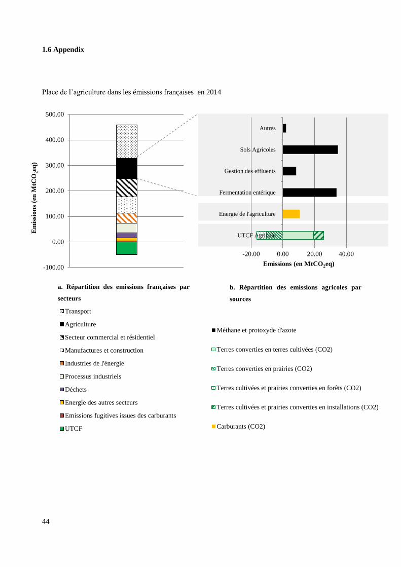
44

1.6 Appendix

Place de l’agriculture dans les émissions françaises en 2014

-100.00

0.00

100.00

200.00

300.00

400.00

500.00

Em

issi

on

s (e

n M

tCO

2eq

)

Transport

Agriculture

Secteur commercial et résidentiel

Manufactures et construction

Industries de l'énergie

Processus industriels

Déchets

Energie des autres secteurs

Emissions fugitives issues des carburants

UTCF

-20.00 0.00 20.00 40.00

UTCF Agricole

Energie de l'agriculture

Fermentation entérique

Gestion des effluents

Sols Agricoles

Autres

Emissions (en MtCO2eq)

Méthane et protoxyde d'azote

Terres converties en terres cultivées (CO2)

Terres converties en prairies (CO2)

Terres cultivées et prairies converties en forêts (CO2)

Terres cultivées et prairies converties en installations (CO2)

Carburants (CO2)

b. Répartition des emissions agricoles par

sources

a. Répartition des emissions françaises par

secteurs

47

Chapter 1

The cost of emission mitigation by legume crops in

French agriculture

This chapter considers the cost of greenhouse gas mitigation potential of legume crops in French

arable systems. We construct marginal abatement cost curves to represent this mitigation or

abatement potential for each department of France and provide a spatial representation of its extent.

Despite some uncertainty, the measure appears to offer a significant low-cost mitigation potential.

We estimate that the measure could abate half of the emission reduction sought by a national plan

for the reduction of chemical fertilizer emissions by 2020. This would be achieved at a loss of

farmland profit of 1.2%. Considering the geographical heterogeneity of cost, it suggests that a

policy implementing carbon pricing in agriculture would be more efficient than a uniform

regulatory requirement for including the crop in arable systems.

Ce chapitre a été co-écrit avec Dominic Moran17

et reprend l’article suivant:

Dequiedt, B., & Moran, D. (2015). The cost of emission mitigation by legume crops in French

agriculture. Ecological Economics, 110, 51-60. doi:10.1016/j.ecolecon.2014.12.006

17 Land Economy and Environment Research Group, Scotland's Rural College (SRUC), Edinburgh EH9 3JG, Scotland, United

Kingdom

48

2.1. Introduction

Agriculture accounts for a significant proportion of total greenhouse gas (GHG) emissions both in France

and at the European level. In 2014, European Union agriculture accounted for 435 million tCO2eq, while

in France the amount was 79 million tCO2eq (respectively 10,9 and 19,1% of European and French GHG

emissions including land use, land use change and forestry according to UNFCCC18

National Inventory

Report, 2016). A recent European Commission communication (European Commission, 2014) on the

policy framework for climate and energy indicated that emissions from sectors outside the EU Emission

Trading Scheme (EU-ETS) would need to be cut by 30% below the 2005 level by 2030. At the same time,

within the framework of the 'energy-climate' package France has committed to reduce emissions of its

sectors not covered by the EU-ETS by 14% by 2020 compared to 2005 emissions levels (European Union,

2009).

Given these ambitions, there is increasing scrutiny of the mitigation measures and specifically their cost

relative to other options available within agriculture and in other sectors. This paper considers the

abatement of emissions from crop fertilisation, which represents a major source of emissions from French

agriculture (a fifth of French agricultural emissions19

). This comprises emissions of nitrous oxide mainly

emitted during the process of denitrification of nitrogenous fertilizers spread on arable land. The paper

assesses the overall abatement potential of a key measure, the introduction of leguminous crops, and the

associated costs and co-benefits in farm systems.

Legumes (fabaceae), commonly known in France as alfalfa, pea, or bean family, have the ability to

naturally fix atmospheric nitrogen and can reduce N2O emissions compared with conventional crops

(maize, wheat, barley, oilseed, rape). This function is conferred by rhizobium bacteria that live in

symbiosis at the level of their roots in little organs called nodules. As a consequence, they need far less

fertilizer thanks to the fixing effect allowing nitrogen to stay in the ground for up to two years after

planting. This contributes additional amounts of nitrogen to subsequent crop in rotations. Studying

alternative crop emissions, Jeuffroy et al. (2013) demonstrated that legume crops emit around five to

seven times less GHG per unit area compared with other crops. Measuring N2O fluxes from different

crops they show that peas emitted 43 gN2O/ha; far less than winter wheat (434 gN2O/ha) and rape

emissions (864 gN2O/ha). Moreover, compared to the emissions from cattle meat production, human

consumption of peas instead of meat leads to 85 to 210 times less N2O emissions for the same content of

18 United Nations Framework Convention on Climate Change.

19 Calculated by dividing the 20,29 MtCO2eq emissions from crops (see appendix 2.9.1) by the 94,3 MtCO2eq

French agricultural emissions (CITEPA, 2012).

49

protein ingested20

. Despite this mitigation benefit, N-fixing crops have low agronomic performance (see

appendix 2.9.1) and consequently their introduction in arable systems will, in most regions, incur a penalty

in terms of farm revenue.

Recent research (Pellerin et al. 2013) has suggested the cost of GHG mitigation via grain legumes at

around 19 euros/tCO2eq. This paper scrutinises this assessment by proposing three improvements: (1)

determining the spatial variation of cost across French Departments; (2) studying how cost varies

according to reduction targets; and (3) analyzing the sensitivity of the abatement cost with respect to

agricultural seed prices and farmers’ ability to exploit low abatement cost.

Here, abatement cost assessment is linked to the substitution of other arable crops by legume crops in

farmlands simulating two consecutive years, so as to integrate the fixing effect of the preceding period.

This methodology allows the derivation of a marginal abatement cost curve for each French metropolitan

geographical area21

. The results are then subject to a sensitivity analysis to examine growers’ responses to

low cost abatement, crops prices and agricultural input prices.

The paper is structured as follows. The next section presents the context of N-fixing crops cultivation in

France and in Europe and section 3 analyses abatement cost assessment in the scientific literature. Section

4 describes the methodology. Section 5 analyses the results and compares them with the previous INRA

(National Institute of Agronomic Research) study (Pellerin et al., 2013). Finally, a discussion considers the

policy relevance of carbon pricing to promote N-fixing crops.

2.2. Context

Despite their beneficial properties, the area planted to legumes in France has been on a steady downward

trend. For fodder legumes the fall started in the 1960’s from a high of 17% of the French arable land. The

area then decreased steadily, reaching 2% in 2010 (Duc et al. 2010). For grain legumes, the fall began later

at the end of the 1980’s after years of political effort to develop them through the common agricultural

policy (CAP) (Cavaillès, 2009).

20 20-37 gN2O/kg protein for meat and 0,17-0,23 gN2O/kg protein for peas. The amount of emissions for meat is obtained using

the N2O content from feed fertilisation and manure management included in cattle meat from Dollé et al. (2011) of 3,026

kgCO2eq and 1,615 kgCO2eq per kg of meat. The amount of emissions for pea is obtained using the yield of 25-34 q/ha from

Agreste data..The protein content of meat (27,6g/100g) and peas (8,8 g/100g) required for the calculation are from Ciqual (2012).

21 Each geographical area corresponds to a department. In the administrative divisions of France, the department (French:

département) is one of the three levels of government below the national level. It is situated between the region and the commune.

50

This decline is due to several factors. First an increasingly meat-based diet incorporating less vegetable

proteins led to lower consumption of legumes by humans. The General Commission for Sustainable

Development reports that in France between 1920 and 1985 human seed legume consumption fell from

7,3 kg/person/year to 1,4 kg/person/year (Cavaillès, 2009). This trend coincided with a change in livestock

feeding regimes, with legume-based rations being increasingly replaced by maize silage, grass plants and

imported soybean meal. The loss of agricultural nitrogen due to this switch in farmlands was compensated

by chemical fertilizers, which had become increasingly price-competitive since the 1960’s.

Simultaneously, trade agreements on the abolition of customs tariffs between Europe and the United

States favored American soybean imports. Finally, a lack of agronomic research dedicated to legumes

compared with common crops, led to a relative decrease of their agronomic performance (Cavaillès,

2009).

In France, as in the rest of the European Union (EU) these factors have led to a strong dependency on soya

imported from America to feed livestock. In 2009, soya was the largest feed commodity imported into the

EU (12,5 million tons) ahead of palm oil and bananas (FAO22

). These imports come mainly from South

America (49% from Brazil and 31% from Argentina (European Commission, 2011)), and at a significant

cost : the average annual trade balance, calculated over the period 2004-2008, represented a loss

equivalent to 1 billion euros (Cavaillès, 2009) for France and up to 10,9 billion euros for the EU. It

follows that increasing legume areas in French agriculture can both mitigate GHG emissions and limit

dependency on feed imports. This is all the more so given the trend of increasing chemical fertilizer

prices. In 2010, the price of fertilizers and soil conditioners spread on farmland in France were some 65%

higher than 1990; this increase being largely related to higher global energy prices. Thus, the increasing

scarcity of fossil fuels provides another reason to explore the potential development of legume crops.

2.3. Cost-effectiveness analysis in the literature

For cost-effectiveness analysis Vermont and De Cara (2010) identify three broad approaches for the

derivation of marginal abatement cost curves (MACCs), the device typically used to evaluate pollution

abatement costs and benefits. These are: i) a bottom-up or engineering approach; ii) an economic approach

consisting of modeling the economic optimization of a set of (in this case) farm operations; iii) a partial or

general equilibrium approach that extends and relaxes some of the assumptions about wider price effects

induced by mitigation activity.

22 http://faostat.fao.org/

51

The engineering approach focuses on the potential emission reduction of individual measures and

observes their cumulated abatement and associated costs. The required data to appraise abatement costs

are ideally collected from measures applied on test farms, thereby reducing some uncertainty the estimated

cost and mitigation potential for each mitigation measure. It is normally the case that more measures are

assessed using the engineering approach relative to the economic approach (MacLeod et al. 2010, Moran

et al. 2010, Pellerin et al. 2013).

The economic approach consists of modeling the economic optimization of a set of farm operations

located within a given geographical scale. The objective function is typically to maximize profit of these

farms under given constraints such as available arable land or even lay fallow land as imposed by

agricultural policies. The introduction of a carbon tax as a new constraint, allows the model to reconfigure

farm activities to accommodate the necessary GHG emissions reductions. The resulting loss in profit

(opportunity cost) and GHG reduction provide the relevant abatement cost information.

Equilibrium models relax some of the cost assumptions made in the economic approach and include a

description of the demand for agricultural products thereby allowing a price feedback into the cost of

mitigation (Vermont and De Cara, 2014). Their level of spatial disaggregation is generally lower than that

of bottom-up models and their geographic scope and coverage are generally wider. This approach has

been used to assess abatement cost at the level of the USA (Schneider and McCarl, 2006; Schneider et al.,

2007; McCarl and Schneider, 2001).

A noteworthy difference between the approaches is the frequent observation of negative cost options in

the engineer approach for some options (Moran et al., 2010; MacKinsey & Company, 2009). These are

obviated in any optimization approach and are in any case questioned by some authors. Kesicki and Ekins

(2012) for example suggest that they more likely imply a failure to assess some hidden costs (diffusion of

the information, administration barriers) than any real opportunity to reduce emissions while increasing

farm gross margins. Another observation is that each mitigation measure in the engineering approach is

associated with a constant marginal cost – creating a stepwise marginal abatement curve (each step

corresponding to an option). This observation suggests that the economic potential per ton CO2 equivalent

mitigation is the same for each specific option irrespective of spatial scale or in terms of the overall

volume of emission reduction, which would seem unlikely. Indeed, due to regional variability in soils,

farm systems, climate and yields, abatement cost would also vary for any individual mitigation measure.

Results from studies employing the economic approach are depicted by continuous increasing abatement

cost curves, with no negative cost. An advantage of these studies is optimization of fewer mitigation

measures over a large number of farm types. For example De Cara and Jayet (2011) modeled around 1300

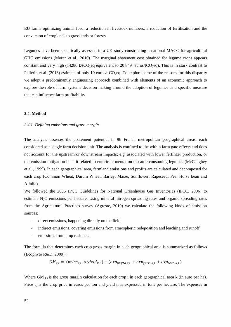
52

EU farms optimizing animal feed, a reduction in livestock numbers, a reduction of fertilisation and the

conversion of croplands to grasslands or forests.

Legumes have been specifically assessed in a UK study constructing a national MACC for agricultural

GHG emissions (Moran et al., 2010). The marginal abatement cost obtained for legume crops appears

constant and very high (14280 £/tCO2eq equivalent to 20 849 euros/tCO2eq). This is in stark contrast to

Pellerin et al. (2013) estimate of only 19 euros/t CO2eq. To explore some of the reasons for this disparity

we adopt a predominantly engineering approach combined with elements of an economic approach to

explore the role of farm systems decision-making around the adoption of legumes as a specific measure

that can influence farm profitability.

2.4. Method

2.4.1. Defining emissions and gross margin

The analysis assesses the abatement potential in 96 French metropolitan geographical areas, each

considered as a single farm decision unit. The analysis is confined to the within farm gate effects and does

not account for the upstream or downstream impacts; e.g. associated with lower fertilizer production, or

the emission mitigation benefit related to enteric fermentation of cattle consuming legumes (McCaughey

et al., 1999). In each geographical area, farmland emissions and profits are calculated and decomposed for

each crop (Common Wheat, Durum Wheat, Barley, Maize, Sunflower, Rapeseed, Pea, Horse bean and

Alfalfa).

We followed the 2006 IPCC Guidelines for National Greenhouse Gas Inventories (IPCC, 2006) to

estimate N2O emissions per hectare. Using mineral nitrogen spreading rates and organic spreading rates

from the Agricultural Practices survey (Agreste, 2010) we calculate the following kinds of emission

sources:

- direct emissions, happening directly on the field,

- indirect emissions, covering emissions from atmospheric redeposition and leaching and runoff,

- emissions from crop residues.

The formula that determines each crop gross margin in each geographical area is summarized as follows

(Ecophyto R&D, 2009) :

𝐺𝑀𝑘,𝑖 = (𝑝𝑟𝑖𝑐𝑒𝑘,𝑖 × 𝑦𝑖𝑒𝑙𝑑𝑘,𝑖 ) − (𝑒𝑥𝑝𝑝ℎ𝑦𝑡𝑜,𝑘,𝑖 + 𝑒𝑥𝑝𝑓𝑒𝑟𝑡𝑖,𝑘,𝑖 + 𝑒𝑥𝑝𝑠𝑒𝑒𝑑,𝑘,𝑖 )

Where GM k,i is the gross margin calculation for each crop i in each geographical area k (in euro per ha).

Price k,i is the crop price in euros per ton and yield k,i is expressed in tons per hectare. The expenses in

53

phytosanytary products (expphyto,k,i ), in fertilizers spread (expferti,k,i ) and in seed (expseed,k,i) are all measured

in euros per hectare.

2.4.2. Baseline

Appendix 2.9.1 shows the results for the main crops cultivated in France and gives the baseline for overall

farmland gross margin (6,4 billion euros) and for emissions (20,4 MtCO2eq). When comparing these

emissions with those of the national inventory report, we observe that the amount represents less than half

of the category ‘Agricultural Soils’ (46,7 MtCO2eq (CITEPA, 2012)). This category represents all N2O

emissions linked to soil fertilisation both from cropland and grassland soils. Hence the baseline emissions

assessed here is quite coherent since we only focus here on emissions from croplands which represent less

than half of the French Utilized Land Area23

.

2.4.3. Introduction of legumes onto croplands

Legume crops have low emissions per hectare and a low gross margin compared with other crops.

Consequently, in most geographical areas, as the overall utilized land area remains constant, increasing the

share of in N-fixing crops induces a reduction of both profit and emissions.

Additional legume crop areas are introduced in each geographical area by 10% increments to the initial

legumes area. The loss of profit (dCost) divided by the reduction of emission (dEmissions) linked to these

additional areas represents the marginal abatement cost. The marginal cost and marginal emissions also

integrate the preceding fixing effect, which induces higher gross margin and lower emission for following

year crops that have been preceded by legumes.

𝑀𝑎𝑟𝑔𝑖𝑛𝑎𝑙 𝐴𝑏𝑎𝑡𝑒𝑚𝑒𝑛𝑡 𝐶𝑜𝑠𝑡 = 𝑑𝐶𝑜𝑠𝑡

𝑑𝐸𝑚𝑖𝑠𝑠𝑖𝑜𝑛𝑠

Legume substitution continues until a marginal abatement cost of 125 euros/tCO2eq has been exceeded per

geographical area. This upper abatement cost threshold has been arbitrarily chosen, considering the

relative abatement cost in other sectors (Vermont and De Cara, 2014)24

.

23 According to Agreste, the Utilized Land Area represents 28 million hectare in France. In appendix 2.9.1, we observe that

cropland area covers less than half of this area: 13,6 million hectares.

24 Vermont and De Cara, 2014 assesses for instance a marginal abatement cost curve for European farms until a maximum level

of 100 euros/tCO2eq

54

In seeking the lowest abatement cost in terms of foregone gross margin per unit emissions, we assume that

legume crops displace conventional (non N fixing) crops according to a schedule of progressively

increasing gross margin. Thus areas yielding lowest gross margin are converted first. But to avoid

complete displacement of conventional crops, a cap is placed on the extent of this displacement. The logic

here is that it is difficult to foresee that farmers would be entirely motivated by an abatement cost goal to

cultivate legumes to the exclusion of other crops. In reality most farmers would seek to minimize risk by

maintaining a level of diversity on their land, which often means that they maintain less profitable crops.

For instance, on livestock farms, some less profitable crops are used for feed. In other cases a lack of

training and information can also retard the adoption of new practices such as legumes. We consider

scenarios in which the limit, termed the variable limit, is assumed to take alternative values of 10%, 30%,

90% and 100%. When the variable limit is 100%, farmers can potentially replace all the crop area,

meaning that they are looking for a complete minimization of abatement cost and are strongly sensitive to

economic signals for mitigation. On the other hand, a 10% limit means that farmers cannot replace more

than 10% of the least profitable crops area. Moreover, we account for the fact that the variable limit is the

same for every crop in every geographical area. Allowing for agronomic differences, different national

abatement cost curves are therefore presented for the different variable limits: from the 10% scenario

corresponding to a low exploitation of minimal abatement cost to a complete use of low abatement cost in

the 100% scenario.

As legume crops are introduced onto farmland the cumulated cost corresponds to the sum of dCost and the

cumulated abatement corresponds to the sum of dEmissions generated at each additional area introduction.

These cumulated cost and abatement are obtained both at the regional and national levels. The average

mitigation cost is the ratio between cumulated cost and cumulated abatement. Figure 3 illustrates a sample

geographical area in which legumes area is increased with a 50% limit. Agricultural land is allocated with

only 5 crops, each characterized by a specific emissions rate per hectare and gross margin. Assume the

rank of crops considering their ratios of gross margin per emissions is : crop i, crop j, crop l and crop m.

Thus, the additional area of legumes first replaces crops i. Once crop i has lost 50% of its area, legumes

replace crop j, and so on until the introduction reaches crop m. At this stage, the 125 euros/tCO2eq is

achieved, which consequently stops further legume introduction.

55

Figure 3 - Illustration of legume area increase in farmlands at the departmental scale

The marginal abatement cost of successive areas increments is depicted in figure 4. Each point of the

curve corresponds to an additional increase in legume area. For a given crop, the marginal abatement cost

is the same whatever the replaced area, which explains the different steps of the curve. The values

comprising the overall abatement cost curve is derived from the integral of the marginal abatement cost

curve.

Figure 4 - Illustrative marginal and overall abatement cost curves linked to increasing legume area on farmland

56

2.5. Results

2.5.1. Abatement potentials and cost

At the national level and assuming the variable limit of 100%, the maximum technical abatement of 2,5

million tCO2eq/year is possible for an overall cost of 118 million euros/year (see figure 5. c). This

corresponds to an increase of 1,6 Mha of legumes and an average abatement cost of 43 euros/tCO2eq.

The overall cost depends on the volume of emissions reduction. Since displaced crops in each

geographical area are ordered by their ratio of gross margin per emission, the lower the abatement targets

the lower the overall cost. For example, if the target of emission reduction is reduced by 30%, to 1,7

MtCO2eq, the average abatement cost is reduced by 80% to 14 euros/tCO2eq. If the target is lower than 1,4

MtCO2eq, we find a negative abatement cost, implying that legumes are actually now more profitable than

the crop that is displaced .

Reducing the variable limit also reduces the overall abatement potential while increasing the abatement

cost. Fixing the limit to either 10% or 90% induces a reduction in the maximum abatement potential of

84% and 8% respectively. We thus observe that results are highly sensitive to this variable. But even if the

variable is low, we still observe opportunities to reduce emissions while increasing farm gross margins

(see figure 5).

Pellerin et al. (2013) suggests that legume introduction could provide an overall abatement potential of 0,9

MtCO2eq, at a cost of 17 million euros. This implies an average mitigation cost of 19 euros/tCO2eq. That

study did not consider how cost varies with area and hence the potential for negative costs. By illustrating

those results (the blue curve in Figures 5b and 5c) alongside those derived in this study, it is possible to

see that defining a variable limit of 50%, which is the average scenario, and the most realistic, for the

same amount of emission abated, we obtain the same overall cost and the same average abatement cost

(reached for a marginal abatement cost of 80 euros/tCO2eq).

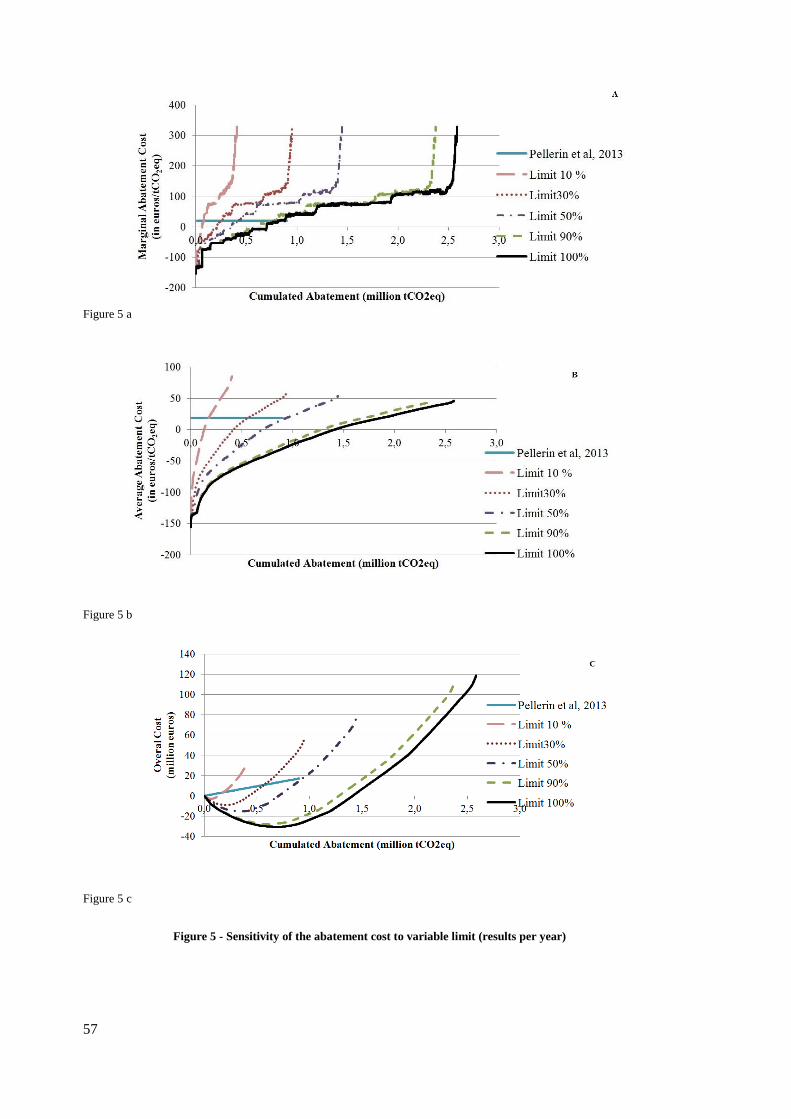
57

Figure 5 a

Figure 5 b

Figure 5 c

Figure 5 - Sensitivity of the abatement cost to variable limit (results per year)

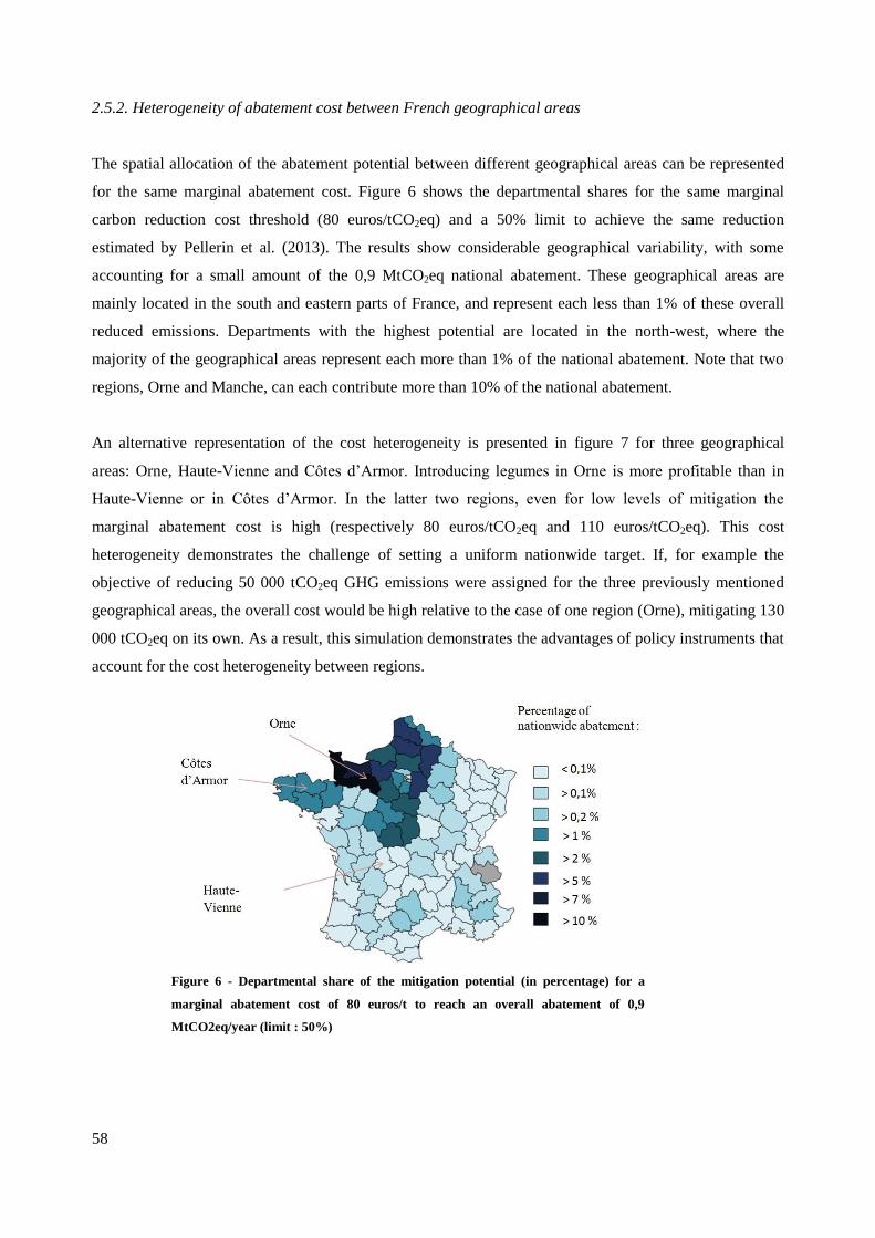
58

2.5.2. Heterogeneity of abatement cost between French geographical areas

The spatial allocation of the abatement potential between different geographical areas can be represented

for the same marginal abatement cost. Figure 6 shows the departmental shares for the same marginal

carbon reduction cost threshold (80 euros/tCO2eq) and a 50% limit to achieve the same reduction

estimated by Pellerin et al. (2013). The results show considerable geographical variability, with some

accounting for a small amount of the 0,9 MtCO2eq national abatement. These geographical areas are

mainly located in the south and eastern parts of France, and represent each less than 1% of these overall

reduced emissions. Departments with the highest potential are located in the north-west, where the

majority of the geographical areas represent each more than 1% of the national abatement. Note that two

regions, Orne and Manche, can each contribute more than 10% of the national abatement.

An alternative representation of the cost heterogeneity is presented in figure 7 for three geographical

areas: Orne, Haute-Vienne and Côtes d’Armor. Introducing legumes in Orne is more profitable than in

Haute-Vienne or in Côtes d’Armor. In the latter two regions, even for low levels of mitigation the

marginal abatement cost is high (respectively 80 euros/tCO2eq and 110 euros/tCO2eq). This cost

heterogeneity demonstrates the challenge of setting a uniform nationwide target. If, for example the

objective of reducing 50 000 tCO2eq GHG emissions were assigned for the three previously mentioned

geographical areas, the overall cost would be high relative to the case of one region (Orne), mitigating 130

000 tCO2eq on its own. As a result, this simulation demonstrates the advantages of policy instruments that

account for the cost heterogeneity between regions.

Figure 6 - Departmental share of the mitigation potential (in percentage) for a

marginal abatement cost of 80 euros/t to reach an overall abatement of 0,9

MtCO2eq/year (limit : 50%)

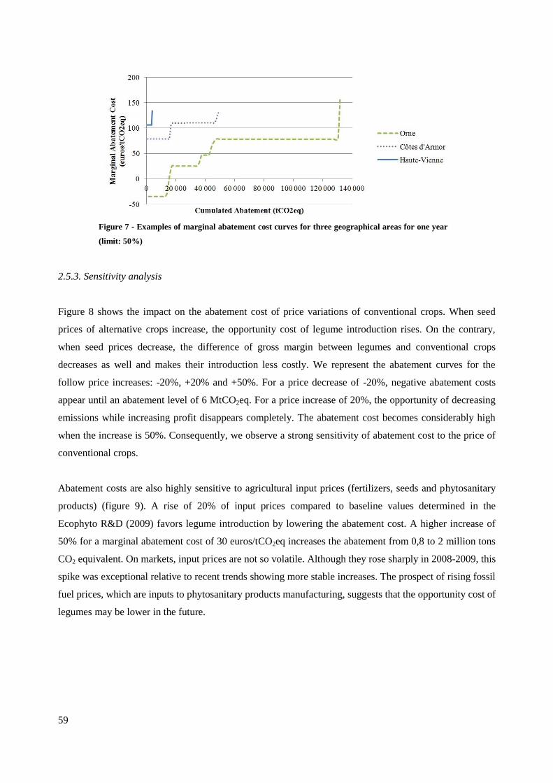
59

2.5.3. Sensitivity analysis

Figure 8 shows the impact on the abatement cost of price variations of conventional crops. When seed

prices of alternative crops increase, the opportunity cost of legume introduction rises. On the contrary,

when seed prices decrease, the difference of gross margin between legumes and conventional crops

decreases as well and makes their introduction less costly. We represent the abatement curves for the

follow price increases: -20%, +20% and +50%. For a price decrease of -20%, negative abatement costs

appear until an abatement level of 6 MtCO2eq. For a price increase of 20%, the opportunity of decreasing

emissions while increasing profit disappears completely. The abatement cost becomes considerably high

when the increase is 50%. Consequently, we observe a strong sensitivity of abatement cost to the price of

conventional crops.

Abatement costs are also highly sensitive to agricultural input prices (fertilizers, seeds and phytosanitary

products) (figure 9). A rise of 20% of input prices compared to baseline values determined in the

Ecophyto R&D (2009) favors legume introduction by lowering the abatement cost. A higher increase of

50% for a marginal abatement cost of 30 euros/tCO2eq increases the abatement from 0,8 to 2 million tons

CO2 equivalent. On markets, input prices are not so volatile. Although they rose sharply in 2008-2009, this

spike was exceptional relative to recent trends showing more stable increases. The prospect of rising fossil

fuel prices, which are inputs to phytosanitary products manufacturing, suggests that the opportunity cost of

legumes may be lower in the future.

Figure 7 - Examples of marginal abatement cost curves for three geographical areas for one year

(limit: 50%)

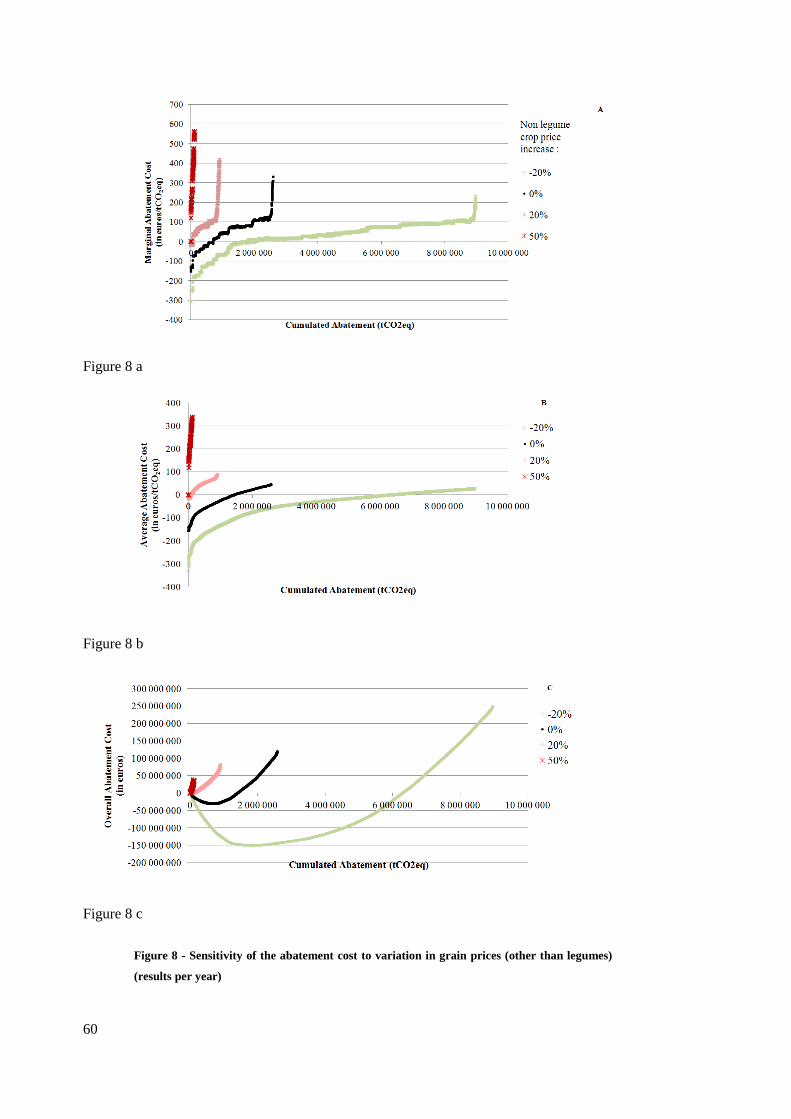
60

Figure 8 a

Figure 8 b

Figure 8 c

Figure 8 - Sensitivity of the abatement cost to variation in grain prices (other than legumes)

(results per year)

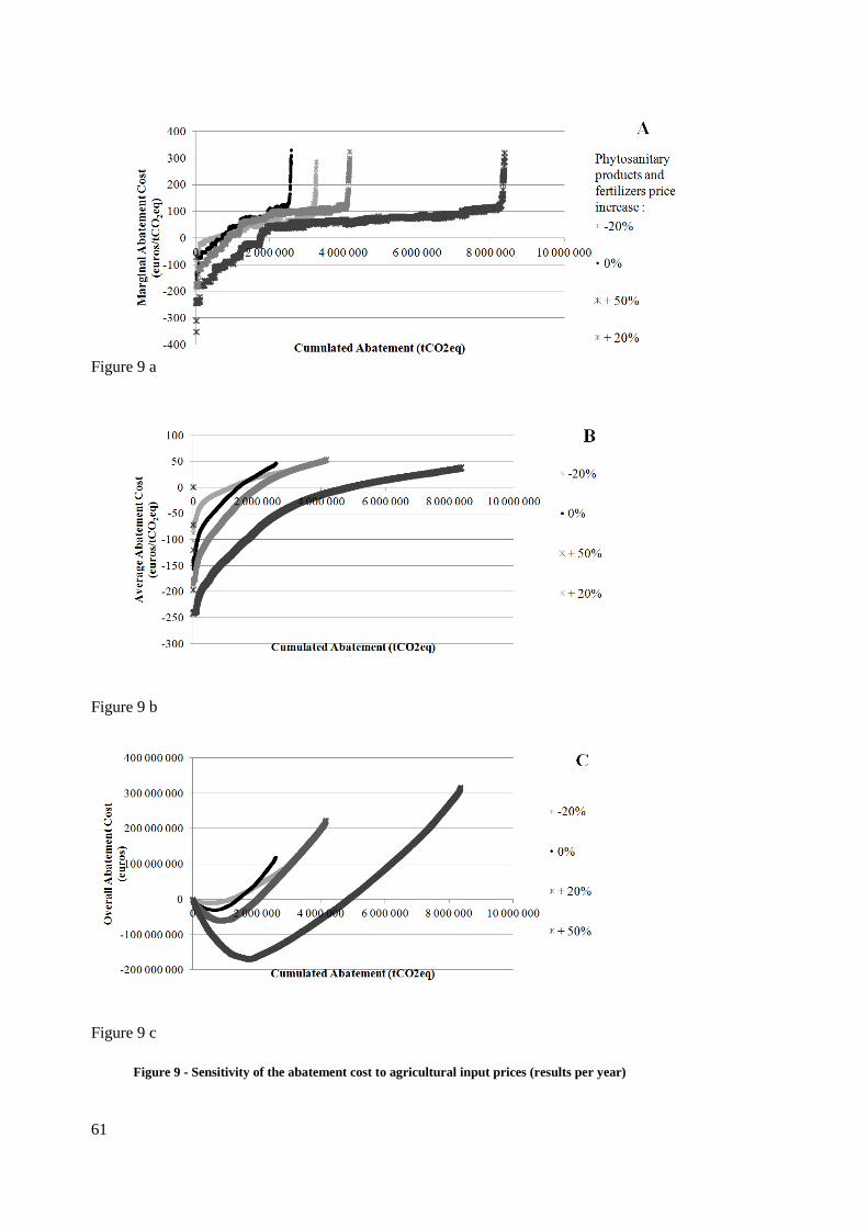
61

Figure 9 a

Figure 9 b

Figure 9 c

Figure 9 - Sensitivity of the abatement cost to agricultural input prices (results per year)

62

2.6. Discussion

A problematic observation in the analysis is the presence of negative abatement costs, which raises

questions about their veracity. Specifically, it is unclear why farmers would not automatically adopt such

profitable measures (and provide associated mitigation) unless it is the case that there are other

unaccounted for costs driving decision-making, which are not captured in this analysis. These hidden

costs can be attributed to a variety of barriers within and beyond the farm. Some barriers are intrinsic to

individual behaviors and imply internal factors (cognition and habit) and social factors (norms and roles)

(Moran et al. 2013). Moreover, farmers may be exhibiting risk aversion behavior in response to legume

yield variation. In this study, the average legume gross margin is relatively high in some regions, making

the crop in rotations more profitable than some of the conventional crops. However, the annual yield of

legume disguises significant annual variation that is not represented here. Consequently some farmers,

actually grow crops with a lower gross margin to be sure that the yield of the crop will be high enough and

to avoid any risk of significant loss associated to legumes. This risk aversion is also linked to the volatility

of other crop prices, which has a strong impact on abatement cost as shown in figure 8. Furthermore, as

noted by Gouldson (2008), some factors are external to the farm. These include a necessity to adapt the

organization of agricultural cooperatives to collect the output of legumes. For instance, legumes need

adapted silos that are not currently established in all regions in France. The role of cooperatives is also

important in the diffusion of information, training and advice in the agricultural sector (Meynard et al.,

2013).

Beyond the apparent paradox of non adoption of negative cost measures, a broader challenge relates to the

available policy options available for agricultural mitigation. The CAP reform framework for the 2014-

2020 period elevates emissions mitigation as a significant challenges for agriculture (European

Commission, 2014). But ongoing debate about the reform is notable for the limited scope of explicit GHG

mitigation objectives that are nevertheless being analyzed at national level in several countries (e.g. UK,

Ireland, and Netherlands). In France, the Court of Auditors has indicated that climate policy should not

only focus on the energy and industry sectors through the EU-ETS, but also on sectors with small and

diffuse emissions sources, in particular agriculture (Cour des Comptes, 2014). A similar situation can be

observed in the UK, where abatement cost analysis has helped to define an economic abatement potential

that is initially being targeted through voluntary agreement with the agricultural sector (AHDB, 2011).

The point now at issue is the relevant policy instrument to motivate these emissions reductions at least

cost.

The fact that abatement costs vary strongly from one geographical area to another suggests that these

instruments should rely more on market-based approaches, rather than a regulatory approach aimed at

increasing legumes area directly. Such approaches (e.g. a tax or forms of emissions permits) offer the

63

flexibility of response, thereby increasing the likelihood of realizing the abatement potential identified by

marginal abatement cost curves. Specifically, when a carbon price is implemented in a specific sector,

agents should reduce their emission until the marginal abatement cost reaches the carbon price (de

Perthuis et al., 2010).

In the case of domestic projects, a carbon price can compensate the costs due to the introduction of

additional legume area. In this way, agents will continue to reduce their emissions as long as marginal

abatement costs are lower than the benefit of the carbon annuity. Thus, legumes areas rise while

minimizing overall abatement cost; in contrast to a blanket regulatory requirement that specifies the area

to be planted.

For illustration, we compare the two approaches for the same target for increasing legumes (doubling the

current area at national level). This target is chosen since it corresponds to an area that should be

cultivated in France to reduce dependence on soya imports (Cavaillès, 2009). In the carbon pricing

approach, a doubling of legumes at national level happens at a carbon price of 80 euros/tCO2eq. In the

uniform regulatory approach, each geographical area is required to double its legumes area. On the face of

it, the latter approach appears logical if we consider that each region increases area in proportion of the

initial area. Yet, we observe in table 2 that for the same target, the overall abatement cost is far lower

under a carbon price (18 million euros) than under a uniform target (127 million euros).

An experimental initiative with offset payments for legume cultivation is currently being piloted on a

voluntary basis by some regional cooperatives (InVivo, 2011). Farmers willing to increase the share of

legumes on their land receive a carbon annuity, determined by the level of carbon price on the EU ETS25

.

However, few cooperatives have been part of this initiative. Indeed, the carbon price being relatively low

at 5 euros/tCO2eq (CDC Climat, 2014) the offer is not attractive for farmers. An advantage of the MACC

analysis presented here is to assess the impact on abatement if this initiative were to become more

widespread, subsequently to higher carbon price level.

25 This project is led under the framework of the Joint Implementation

(http://unfccc.int/kyoto_protocol/mechanisms/joint_implementation/items/1674.php).

http://unfccc.int/kyoto_protocol/mechanisms/joint_implementation/items/1674.php

64

Table 2 - Comparison between the two policy approaches for the same target of abatement

Uniform doubling across all

geographical areas Carbon Pricing

Final legumes area Million ha

1,5

(12% of French overall agricultural land)

Overall Cost Million euros/year 127 18

Marginal Abatement Cost Euros/tCO2eq - 80 euros/tCO2eq

Overall Abatement Million tCO2eq 1,03 0,9

Average Abatement Cost Euros/tCO2eq 123 19,5

2.7. Conclusion

Combining both economic and engineering approaches to the development of abatement cost curves, this

study offers a national assessment of the cost-effectiveness of GHG mitigation using legumes in arable

systems. This intermediate MACC approach allows for the possibility of negative abatement costs that are

typically excluded in economic approaches to MACC construction. It also reveals more granularity in cost

information that is usually disguised in the average cost assumptions made in engineering approaches.

This is particularly advantageous for illustrating uncertainties linked to agricultural price variation

(agricultural input and seed prices volatility) and some hypotheses about the reaction of farmers to

economic signals. Finally the approach is useful to display regional variability in costs and hence to

illuminate the efficiently of policy alternatives for the introduction of the measure.

In a realistic scenario, legumes could abate a maximum 7% of chemical fertilizer emissions at a cost of 77

million euros corresponding to a loss of 1,2% of overall profit in France. Win-win abatement could be 3%

of chemical fertilizer emissions. Hence, although showing that this mitigation option could offer low

abatement cost, N-fixing crop would need to be combined with other measures to tackle the 14%

emissions reduction target of diffuse emissions sectors by 2020 (European Union, 2009). To increase

adoption the suggested option of carbon pricing would appear to be more economically efficient than a

policy focusing on increasing areas in each geographical area directly.

65

An interesting addition to this work would be to investigate the upstream and downstream impact of

legume on greenhouse gases and their consequences on abatement cost. The production of chemical

fertilizers is responsible for significant CO2 emissions in industries. Hence, the associated decrease of

emissions due to chemical fertilizers substitution should decrease abatement cost. Further, the

displacement of imported soybean by fodder legumes such as alfalfa would have a positive impact on

enteric fermentation, responsible for methane emissions in livestock feeding regimes (Martin et al., 2006).

It would also via indirect land use change (Searchinger et al., 2008; De Cara et al., 2012) impact land use

emissions of countries where soybean is currently produced. Accordingly, studying impacts beyond the

farm gate would be a useful extension.

Finally, further research should seek a more disaggregated level with several farms inside the geographical

area scope. Currently, the decision unit is at the level of the department. Providing a more disaggregated

level of analysis below the focus would be worthwhile especially by distinguishing different groups of

farms below this level. In the different scenarios concerning the impact of the variable limit, we assume

that all farmers have the same response toward economic signals, but reality shows that farmer

behaviours are diverse (Dury, 2011; Glenk et al., 2014). In this regard characterizing groups of farmers

with specific variable limits would be of interest.

66

2.8. References

Agreste. Data base : http://agreste.agriculture.gouv.fr/page-d-accueil/article/donnees-en-ligne. Data

Extracted January 2013.

Agreste (2010). Pratiques Culturales 2006. Agreste Les Dossiers. N°8.

http://agreste.agriculture.gouv.fr/IMG/pdf/dossier8_integral.pdf

AHDB (2011). Meeting the Challenge: Agriculture Industry GHG Action Plan Delivery of Phase I: 2010 –

2012 04 April 2011; http://www.ahdb.org.uk/projects/GreenhouseGasActionPlan.aspx

Cavaillès, E. (2009). « La relance des légumineuses dans le cadre d’un plan légumineuses ». Commissariat

Général au Développement Durable. Etudes & Documents.

CDC Climat (2014). Tendance Carbone. Bulletin mensuel du marché européen du CO2. N°92. Juin 2014.

Ciqual (2012). ANSES (French Agency for Food, Environmental and Occupational Health & Safety)

database. Data Extracted October 24th 2014. http://www.afssa.fr/TableCIQUAL/index.htm

CITEPA (2012). Rapport national d’inventaire pour la France au titre de la convention cadre des Nations-

Unies sur les changements climatiques et du protocole de Kyoto. Technical report, CITEPA.

Cour des Comptes (2014), 'La mise en œuvre par la France du Paquet énergie-climat', Technical report,

Cour des Comptes.

De Cara, S., Goussebaïle, A., Grateau, R., Levert, F., Quemener, J., Vermont, B., et al. (2012). Revue

critique des études évaluant l’effet des changements d’affectation des sols sur les bilans

environnementaux des biocarburants. rapport de l’ADEME.

De Cara, S. & Jayet, P.-A. (2011). Marginal abatement costs of greenhouse gas emissions from European

agriculture, cost-effectiveness, and the EU non-ETS burden sharing agreement. Ecological

Economics, 70(9), 1680–1690.

de Perthuis, C., Suzanne, S., & Stephen, L. (2010). Normes, écotaxes, marchés de permis : quelle

combinaison optimale face au changement climatique ? Technical report, La Chaire Economie du

Climat.

http://agreste.agriculture.gouv.fr/page-d-accueil/article/donnees-en-ligne

http://agreste.agriculture.gouv.fr/IMG/pdf/dossier8_integral.pdf

http://www.afssa.fr/TableCIQUAL/index.htm

67

Dolle, JB and Agabriel, J and Peyraud, JL and Faverdin, P and Manneville, V and Raison, C and Gac, A

and Le Gall, A. (2011). Les gaz à effet de serre en élevage bovin: évaluation et leviers d'action.

Productions Animales. 24 (2011), 415.

Duc, G., Mignolet, C., Carrouée, B., & Huyghe, C. (2010). Importance économique passée et présente des

légumineuses : Rôle historique dans les assolements et les facteurs d’évolution. Innovations

Agronomiques, (pp. 11, 11–24.).

Dury, J. (2011). The cropping-plan decision-making: A farm level modelling and simulation approach.

Institut National Polytechnique de Toulouse (INP Toulouse). PHDThesis.

Ecophyto R&D, Nicolas, B., Philippe, D., Marc, D., Olivier, G., Laurence, G., Loic, G., Pierre, M.,

Nicolas, M.-J., Bertrand, O., Bernard, R., Philippe, V., & Antoine, V. (2009). Ecophyto R&D.

Vers des systèmes de production économes en produits phytosanitaires? Technical report, INRA.

European Commission (2014). Communication from the commission to the European Parliament, the

council, the European Economic and Social Committee and the Committee of the regions. “A

policy framework for climate and energy in the period from 2020 to 2030”. http://eur-

lex.europa.eu/legal-content/EN/TXT/PDF/?uri=CELEX:52014DC0015&from=EN

European Commission (2013). 'Overview of CAP Reform 2014-2020', Technical report, European

Commission.

European Commission (2011). Monitoring Agri-Trade Policy. Technical report, Directorate-General for

Agriculture and Rural Development.

European Commission (2001). European Climate Change Programme. Technical report, Commission

Européenne.

European Union (2009). 'Decision Number 406/2009/EC of the european parliament and of the council of

23 April 2009 on the effort of Member States to reduce their greenhouse gas emissions to meet the

Community’s greenhouse gas emission reduction commitments up to 2020', Technical report,

Official Journal of the European Union.

Glenk, K., Eory, V., Colombo, S., Barnes, A. (2014). Adoption of greenhouse gas mitigation in

agriculture: An analysis of dairy farmers' perceptions and adoption behavior. Ecological

Economics,108, 49-58.

http://eur-lex.europa.eu/legal-content/EN/TXT/PDF/?uri=CELEX:52014DC0015&from=EN

http://eur-lex.europa.eu/legal-content/EN/TXT/PDF/?uri=CELEX:52014DC0015&from=EN

68

Gouldson, A. (2008). Understanding business decision making on the environment. Energy Policy (36)

pp.4618-4620.

InVivo (2011). Méthodologie spécifique aux projets de réduction des émissions de N2O dues à la

dénitrification des sols agricoles par l’insertion de légumineuses dans les rotations agricoles?

Technical report.

IPCC (2006). Guidelines for National Greenhouse Gas Inventories, Volume 4, Agriculture, Forestry and

Other Land Use. Intergovernmental Panel on Climate Change.

Jeuffroy, M., Baranger, E., Carrouée, B., Chezelles, E. d., Gosme, M., Hénault,C., Schneider, A., &

Cellier, P. (2013). Nitrous oxide emissions from crop rotations including wheat, rapeseed and dry

pea. Biogeosciences Discussions, 9(7), 9289.

Kesicki, F., & Ekins, P. (2012). Marginal abatement cost curves: a call for caution. Climate Policy, 12(2),

219-236.

MacCarl, B. & Schneider, U. (2001). Greenhouse gas mitigation in US agriculture and forestry. Science,

294 (5551), 2481–2482. 23.

McCaughey, W. P., Wittenberg, K. and Corrigan, D. (1999). Impact of pasture type on methane

production by lactating beef cows. Canadian Journal of Animal Science. 79: 221–226.

MacKinsey & Company (2009). Pathways to a low-carbon economy:Version 2 of the global greenhouse

gas abatement cost curve. Technical report.

MacLeod, M., Moran, D., Eory, V., Rees, R., Barnes, A., Topp, C. F., Ball, B., Hoad, S., Wall, E.,

McVittie, A., et al. (2010). Developing greenhouse gas marginal abatement cost curves for

agricultural emissions from crops and soils in the UK. Agricultural Systems, 103(4), 198–209.

Martin, C., Morgavi, D., Doreau, M., Jouany, J.P., (2006) : Comment réduire la production de méthane

chez les ruminants? Fourrages, 187, p 283 – 300.

Meynard, J.M., Messéan, A., Charlier, A., Charrier, F., Fares, M., Le Bail, M., Magrini, M.B., Savini, I.,

(2013). Freins et leviers à la diversification des cultures. Etude au niveau des exploitations

agricoles et des filières. Synthèse du rapport d'étude, INRA, 52 p.

69

Moran, D., A. Lucas and A. Barnes (2013) Mitigation win-win, Nature Climate Change, July 2013

Volume 3 Number 7 pp 611-613, doi:10.1038/nclimate1922

Moran, D., MacLeod, M., Wall, E., Eory, V., McVittie, A., Barnes, A., Rees, R., Topp, C. F., Pajot, G.,

Matthews, R., et al. (2010). Developing carbon budgets for UK agriculture, land-use, land-use

change and forestry out to 2022. Climatic change, 105(3-4), 529–553.

Pellerin S., Bamière L., Angers D., Béline F., Benoît M., Butault J.P., Chenu C., Colnenne-David C., De

Cara S., Delame N., Doreau M., Dupraz P., Faverdin P., Garcia-Launay F., Hassouna M., Hénault

C., Jeuffroy M.H., Klumpp K., Metay A., Moran D., Recous S., Samson E., Savini I., Pardon L.,

2013. Quelle contribution de l’agriculture française à la réduction des émissions de gaz à effet de

serre ? Potentiel d'atténuation et coût de dix actions techniques. Synthèse du rapport d'étude,

INRA (France), 92 p.

Schneider, U. & McCarl, B. (2006). Appraising agricultural greenhouse gas mitigation potentials: effects

of alternative assumptions. Agricultural Economics, 35(3), 277–287.

Schneider, U., McCarl, B., & Schmid, E. (2007). Agricultural sector analysis on greenhouse gas

mitigation in us agriculture and forestry. Agricultural Systems, 94(2), 128–140.

Searchinger, T., Heimlich, R., Houghton, R. A., Dong, F., Elobeid, A., Fabiosa, J., et al. (2008). Use of

US croplands for biofuels increases greenhouse gases through emissions from land-use change.

Science, 319, 1238-1240.

UNFCCC (2013). France National Inventory Report. Source CITEPA / rapport CCNUCC – édition de

mars 2013.

http://unfccc.int/national_reports/annex_i_ghg_inventories/national_inventories_submissions/item

s/7383.php

Vermont, B. & De Cara, S. (2014). Atténuation de l’effet de serre d’origine agricole: efficacité en coûts et

instruments de régulation. Actes de la journée du 4 juin 2014, Centre INRA Versailles-Grignon.

Atténuation des gaz à effet de serre par l’agriculture.

Vermont, B. & De Cara, S. (2010). How costly is mitigation of non-CO2 greenhouse gas emissions from

agriculture? A meta-analysis. Ecological Economics, 69(7), 1373–1386.24

http://unfccc.int/national_reports/annex_i_ghg_inventories/national_inventories_submissions/items/7383.php

http://unfccc.int/national_reports/annex_i_ghg_inventories/national_inventories_submissions/items/7383.php

71

2.9. Appendix

2.9.1. Area, emissions and gross margin for the main crops in France at the national level in the baseline

situation

Area

Average

Emissions

Overall

Emissions

Average

GM

Profit

ha kgCO2eq/ha MtCO2eq euros/ha Meuros

Common Wheat 4 961 435 1 323 6,56 546 2 709

Durum Wheat 519 852 1 512 0,79 377 196

Barley 1 581 969 1 222 1,93 365 577

Maize 3 051 075 2 230 6,81 588 1 794

Sunflower 671 075 1 356 0,91 293 197

Rapeseed 1 452 744 1 528 2,22 360 523

Other 672 539 1 552 1,04 422 284

Legumes (pea, alfalfa, horse

bean)

763 049 35,4 0,03 122 93

All Crops 13 673 738 - 20,29 - 6 372,90

2.9.2. Impact on legume introduction on other cereals area (for a carbon price of 80 euros/tCO2eq with a

limit of 50%)

0

1 000 000

2 000 000

3 000 000

4 000 000

5 000 000

6 000 000

ha

Area in the reference scenario

Area in the seed legumes

introduction scenario

73

Chapter 2

Mitigation costs through alternative crop rotations in

agriculture: an assessment for five European regions

To develop a better understanding of the agriculture sector in the context of climate change and the

corresponding issue of cutting greenhouse gas (GHG) emissions, this paper aims at assessing

regional mitigation potential and cost due to changing crops rotations at farm-scale in five European

regions. For this purpose, we use rotation database from Reckling et al (2014) bringing accurate and

exhaustive data about crop management in these areas. First, we complete the database with nitrous-

oxide (N2O) emissions calculations and bring an additional hypothesis on pre-crop effect so as to

capture the diversity of knowledge outlined in the agronomic literature. Then, GHG abatement cost

is assessed using a bottom-up approach and assuming that farmers are maximizing their profit. In

the literature on mitigation cost assessment, the abatement effort is generally considered as marginal

and hence is added to previous cumulated efforts of reduction. In contrast, this study analyses

rotation switch which implies a complete switch of cropland systems on several years (up to 6

years). Results show that aggregated “win-win” abatement potential in the five European regions

could reach a maximum of 35% of the baseline soil N2O emissions of arable areas. The total dry

matter production is increasing, while the area under cereal production is decreasing to this level of

GHG abatement. Consequently, these findings tend to indicate that variations in agricultural

production linked to a mitigation policy, while generating important changes in cropping systems,

would not necessarily endanger food security.

Ce chapitre reprend un article réalisé en collaboration avec Vera Eory26

, Juliette Maire2, Cairstiona

F. E. Topp2, Robert M. Rees

2, Peter Zander

27, Moritz Reckling

3 et Nicole Schlaefke

3.

26 Scotland’s Rural College, Research Division, West Mains Road, Edinburgh EH9 3JG, UK

27 Leibniz Centre for Agricultural Landscape Research (ZALF), EberswalderStraße 84, 15374 Müncheberg, Germany

74

3.1. Introduction

In its last communication on climate policy framework, the European Commission set an ambitious target

of greenhouse gas (GHG) emissions reduction of 40% compared to the 1990 level by 2030 (European

Commission, 2014). This effort follows the recommendations of scientists of the Intergovernmental

Experts Group on the Climate Change (IPCC) to contain the average temperature increase below 2°C

globally by the end of the century. According to the Annual European Union Greenhouse Gas Inventory,

the EU-27 emitted 3 976 million ton CO2 equivalents28

(MtCO2eq) in 2014, with the agricultural sector

being the second largest emitter, with 435 MtCO2eq emissions (11.1 %)(UNFCCC, 2016).

Among the numerous practices suggested to mitigate GHG emissions, one is to modulate the area of crops

implanted in cropland. Since crops do not have the same needs in nitrogen application, favouring those

requiring less fertilisation could bring significant abatement of GHG emissions. At the forefront,

increasing the cultivation of legumes in crop rotations and on grasslands has been highlighted by many

studies (Dequiedt and Moran, 2015; Cavaillès, 2009). These crops are able to fix nitrogen from the

atmosphere. Therefore, not only they need no or very little nitrogen fertiliser for their own growth but also

provide substantial amount to the subsequent crop in rotation (Charles et al, 2001; Köpke and Nemecek,

2010). Additionally, legumes provide a range of other potential rotational benefits that are not directly

related to nitrogen such as increasing phosphorus availability (Hassan et al, 2010), reducing soil strength

that contributes to the development of better root systems (Rochester et al, 2001) or reducing diseases or

pest (Jensen et al, 2010). These properties allow higher yields from succeeding crops at the same fertiliser

rate or a reduced fertiliser use for the same yield or a combination of both. Grain and forage legumes are

currently grown on 180 million hectares worldwide and their extent is expected to increase as the demand

for legume production for dietary protein increases. However, the European context is less promising; the

cultivation of legumes as grains and forage has declined throughout the EU from 11.3 million ha in 1961

to about 3.4 million ha in 200529

. Having said that, the interesting properties of legumes should not hide

the potential of other crops with low nitrogen need and which could participate as well in carbon

mitigation. Rapeseed (Justes et al, 1999), some kinds of grass and leaf crops are also well known to limit

nitrogen leaching and hence restrict resulting greenhouse gases.

To assess GHG abatement cost in European agriculture via increasing low GHG emitting rotations, an

abatement cost curve analysis is carried out. The latter shows the cost of one additional abatement option

for different levels of total emission reduction. Abatement cost curves have been developed in several

other studies to illustrate the economics of climate change mitigation in croplands. De Cara and Jayet

28 Total CO2 equivalent emissions with land use, land-use change and forestry

29 FAOSTAT 2011 data, accessed: January 2014 for the year 2011.

75

(2011) assess the marginal abatement cost of agriculture in Europe and focus mainly on fertilisation

reduction regarding N2O emissions abatement. The UK government has used marginal abatement cost

curves (MACCs) to evaluate climate policy in all sectors of the economy (MacLeod et al, 2010) and an

agricultural abatement cost assessment was also developed for France (Pellerin et al, 2013). They both

appraise the potential of crops requiring few nitrogen fertilisations (legumes, forage plant varieties,

intermediate and cover crops) and estimate the associated cost of mitigation per ton CO2 equivalent unit.

According to the latter, legumes could reduce GHG emissions by 1.4 MtCO2eq, with a mean abatement

cost of -52 €/tCO2eq30 and estimate intermediate crops introduction potential to be 115 to 260 €/tCO2eq.

In the UK, MacLeod et al. (2010) assess an abatement potential of 20 849 €/tCO2eq for legume.

Nationwide MACCs (Pellerin et al, 2013 ; MacLeod et al, 2010 and Wang et al, 2013), assessing different

mitigation options, estimate a national average mitigation cost. Although these studies bring useful

insights of the most effective options in term of abatement cost, there is still a need to investigate the cost

at a more detailed area so as to observe the variability hidden behind the average national cost.

Accordingly, following a bottom-up approach, we focus on disaggregated regional levels and within these

levels on different site class characteristics. A classification of low emitting rotations is obtained for each

of them which allows creating abatement cost curve for individual geographical area unit. Consequently,

we obtain an increasing abatement cost curve and not a single average abatement cost for the overall level.

Dequiedt and Moran (2015) also reach a more disaggregated geographic level in France and obtain

increasing MACCs. However, they strictly focus on legume introduction in cropland up to two years

without taking into account, first, the potential of other crops and, second, the sequence of crops on a

longer period. Here, following rotations database generated by Reckling et al (2014), we hope to match

the potential of a mix of crops, and not specifically legumes, following agronomic rotation planning up to

6 years. Lastly, a noteworthy difference between the present assessment and the above-mentioned studies

is that, here, the abatement cost is not marginal but implies a complete change of rotation on several years.

Thereby, we do not use the term “marginal abatement cost” but rather “abatement cost” since at each site

class level the last mitigation option, i.e. the most cost-efficient rotation regarding a specific abatement

objective, substitutes the potential of the previous rotation potential.

This report assesses five regions in Europe, representing a diversity of land types and agroecological

zones: Eastern Scotland (UK); Västsverige (Sweden); Brandenburg (Germany); South-Muntenia

(Romania); Calabria (Italy). These regions are depicted by 13 representative site classes with different soil

features, agricultural practices and crops. Information related to crops like production costs, yield, or crop

prices has been collected in an agronomic survey by Reckling et al (2014). Based on agronomic practices

30 These figures reprent two measures assessed by Pellerin et al., 2013 : one measure which consists in increasing legumes in

cropland and the other increasing legumes in grasslands.

76

and rules, the authors used the survey data to generate possible rotations for the 13 site classes and

obtained in total 79,340 potential rotations. The current article uses the information of fertilisation and

yield data of the above mentioned survey and completes the database by calculating soil-based nitrous-

oxide (N2O) emissions from crop cultivation. Two agronomic scenarios are examined to tackle the

diversity of pre-crop effect from legumes depicted in the agronomic literature. In the ‘Yield’ scenario, we

assume that the pre-crop effect causes an increase in the following crop’s yield with no change in the

fertilisation practice. The ‘Fertilisation’ scenario assumes that chemical fertilisation is reduced by 20% for

the following crops with no change in their yield.

Constructing the abatement cost curve follows two steps. First, using mixed integer programming, we

generate an abatement classification of the different available rotations for each site class. The purpose

here is to select for successive abatement goals the rotations that reduce emissions at the least cost.

Second, results are aggregated at the level of the five European regions, using the cost-effectiveness

ranking of rotations, so as to draw the overall abatement cost curve.

The rest of this paper is structured as follow. The next part describes the methodology used to calculate

data and to generate abatement cost curves. Section 3 presents the results of the assessment with the

abatement cost curve, crop production and crop area evolution. Section 4 discusses the accuracy of the

abatement cost assessment regarding the frame of the methods and is followed by conclusion in Section 5.

77

3.2. Method

3.2.1. Data description

The database generated by Reckling et al (2014) captures the bio-physical and socio-economic variability

of different regions across Europe: five contrasting regions were selected as case study regions. Within the

case study regions, a local typology of site classes was formulated. On total, 13 site classes were defined:

5 for Brandenburg, 1 for Sud-Muntenia, 3 for Calabria, 3 for Eastern Scotland and 1 for Västsverige (see

Appendix 3.7.1 for more details on the site class characteristics).

The database includes 544 agricultural activities. Each agricultural activity concerns the cultivation of one

crop grown for one year and is characterized by a site class location, a preceding crop type, and specific

agro-economic data (yield, dry matter content, synthetic and organic fertilizer amount and the production

cost of fertilisation, pesticides products and labour). Based on these data, gross margins were calculated by

Reckling et al (2014). The gross margin is the difference between the revenue and costs per hectare for

each crop (see Appendix 3.7.2 for more details), not considering subsidies received.

In addition to gross margin data in Reckling et al (2014), N2O emissions are calculated in this present

paper, using the IPCC Tier 1 methodology (IPCC 2006). The emissions include direct and indirect N2O

emissions from synthetic fertilizers applied, manure and from crop residues.

3.2.2. Legume preceding crop effect

Among the 544 agricultural activities, 317 are characterized by a so-called pre-crop effect. This pre-crop

effect results from the additional nitrogen amount left in the soil from residues from the crop grown the

year before. This effect is triggered by legumes but also by potato, rape, leaf crops and some kinds of

grass and mainly consists in changes of fertilisation, yield and agro-chemical applications.

In the “Yield” scenario, the pre-crop effect is assumed to increase the following crop’s yield, while

keeping the fertilisation rate constant. We follow here the assumption made by Reckling et al (2014) in

their database. On average, crops that benefit from the so-called pre-crop effect have a 17.8% higher yield

than the same crops without pre-crop effect.

In the “Fertilisation” scenario, we assume that the pre-crop effect induces a 20% decrease in nitrogen

fertilisation while keeping the yield constant. We follow here a part of the agronomic literature

considering, conversely, that N-fixing crops cannot trigger an increase of yield in reason of cropland over-

fertilisation (Martin and Meynard, 1997). The rate of 20% decrease of nitrogen application is based on the

78

UK’s Fertiliser Manual (Defra, 2011), which assumes that the soil nitrogen supply is 30 kg N/ha higher

after peas and beans than after cereals and suggests reducing the nitrogen applied accordingly. Organic

fertiliser application is assumed to be reduced in practice by 20% as well, but the resulting organic

nitrogen surplus is considered to be used on other fields where it substitutes the application of other

synthetic nitrogen. Therefore, assuming a replacement rate of 33% (a value in the lower range used in the

different European countries according to Webb et al 2010), the total nitrogen reduction effect from

organic fertilisation is estimated to be 6.66%.

Figure 10 shows the differences of data between the two different scenarios for pre-crop effect. We

observe that the “Yield” hypothesis induces higher gross margin but also higher emissions than in the

“Fertilisation” one.

Figure 10 – Characterization of the pre-crop effect between the two scenarios.

These two graphs represent 317 of 544 agricultural activities characterized by a pre-crop effect. The abscissa

axis shows the different agricultural activities ranked according to emissions (left-hand chart) or gross margin

(the right-hand chart)

-1000

-500

0

500

1000

1500

2000

2500

3000

1

15

29

43

57

71

85

99

11

3

12

7

14

1

15

5

16

9

18

3

19

7

21

1

22

5

23

9

25

3

26

7

28

1

29

5

30

9

Eu

ro

s/h

a/Y

r

Agricultural Activities

Gross Margin

Fertilization Yield

0

500

1000

1500

2000

2500

3000

3500

4000

4500

1

17

33

49

65

81

97

11

3

12

9

14

5

16

1

17

7

19

3

20

9

22

5

24

1

25

7

27

3

28

9

30

5

kg

CO

2eq

/ha

/Yr

Agricultural Activities

Emissions

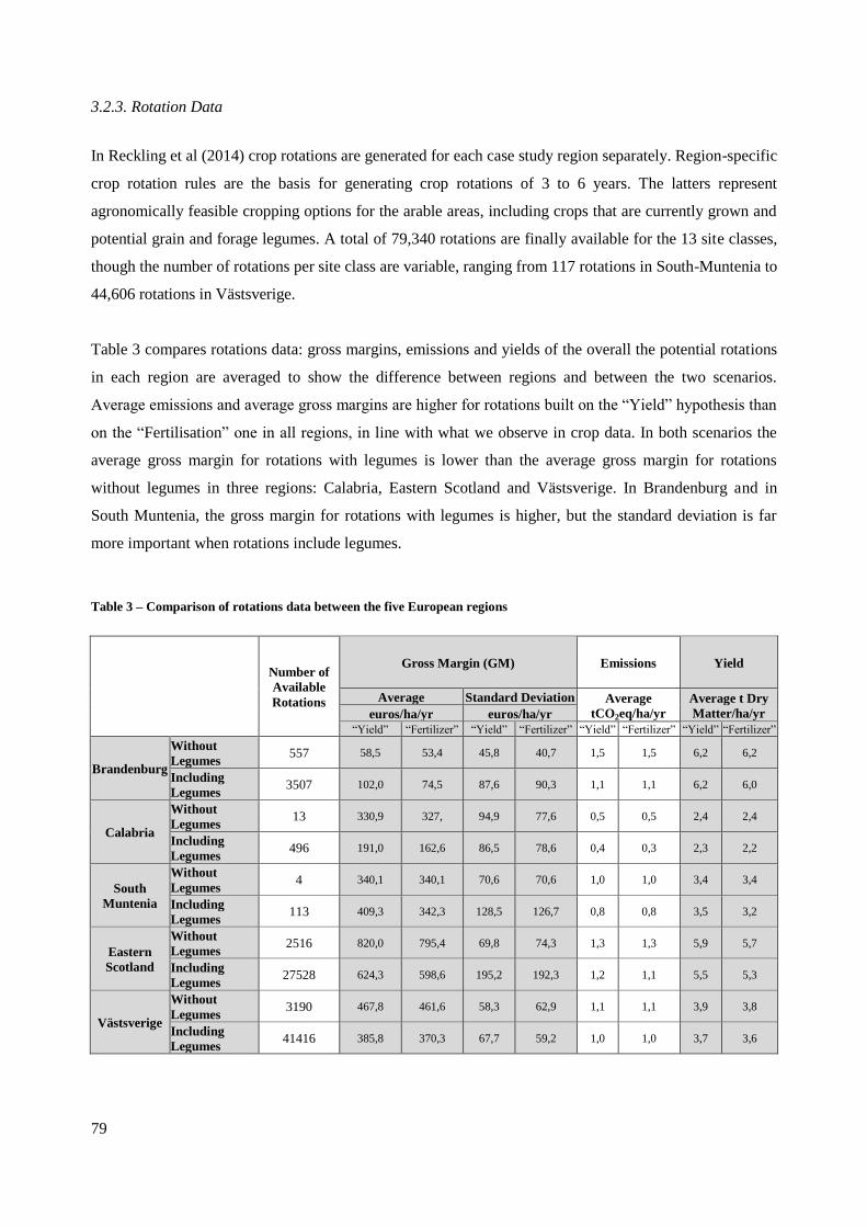
79

3.2.3. Rotation Data

In Reckling et al (2014) crop rotations are generated for each case study region separately. Region-specific

crop rotation rules are the basis for generating crop rotations of 3 to 6 years. The latters represent

agronomically feasible cropping options for the arable areas, including crops that are currently grown and

potential grain and forage legumes. A total of 79,340 rotations are finally available for the 13 site classes,

though the number of rotations per site class are variable, ranging from 117 rotations in South-Muntenia to

44,606 rotations in Västsverige.

Table 3 compares rotations data: gross margins, emissions and yields of the overall the potential rotations

in each region are averaged to show the difference between regions and between the two scenarios.

Average emissions and average gross margins are higher for rotations built on the “Yield” hypothesis than

on the “Fertilisation” one in all regions, in line with what we observe in crop data. In both scenarios the

average gross margin for rotations with legumes is lower than the average gross margin for rotations

without legumes in three regions: Calabria, Eastern Scotland and Västsverige. In Brandenburg and in

South Muntenia, the gross margin for rotations with legumes is higher, but the standard deviation is far

more important when rotations include legumes.

Table 3 – Comparison of rotations data between the five European regions

Number of

Available

Rotations

Gross Margin (GM) Emissions Yield

Average Standard Deviation Average

tCO2eq/ha/yr

Average t Dry

Matter/ha/yr euros/ha/yr euros/ha/yr

“Yield” “Fertilizer” “Yield” “Fertilizer” “Yield” “Fertilizer” “Yield” “Fertilizer”

Brandenburg

Without

Legumes 557 58,5 53,4 45,8 40,7 1,5 1,5 6,2 6,2

Including

Legumes 3507 102,0 74,5 87,6 90,3 1,1 1,1 6,2 6,0

Calabria

Without

Legumes 13 330,9 327, 94,9 77,6 0,5 0,5 2,4 2,4

Including

Legumes 496 191,0 162,6 86,5 78,6 0,4 0,3 2,3 2,2

South

Muntenia

Without

Legumes 4 340,1 340,1 70,6 70,6 1,0 1,0 3,4 3,4

Including

Legumes 113 409,3 342,3 128,5 126,7 0,8 0,8 3,5 3,2

Eastern

Scotland

Without

Legumes 2516 820,0 795,4 69,8 74,3 1,3 1,3 5,9 5,7

Including

Legumes 27528 624,3 598,6 195,2 192,3 1,2 1,1 5,5 5,3

Västsverige

Without

Legumes 3190 467,8 461,6 58,3 62,9 1,1 1,1 3,9 3,8

Including

Legumes 41416 385,8 370,3 67,7 59,2 1,0 1,0 3,7 3,6

80

3.2.4. Baseline rotations

For each site class, a baseline rotation is identified to represent common and regional specific cropping

practices. The baseline rotation is selected on the basis of three main criteria: (1) crop sequence

constraints, (2) crop composition and (3) gross margin. On the first point, rules on crop type frequency

constraints are applied to help to control soil-borne pests and diseases that are relevant for crops of the

same type e.g., cereal nematodes. Timing restrictions implementation ensures that the cropping periods of

subsequent crops do not overlap and allow sufficient time for seedbed preparation in order to produce no

rotations that are at risk of failing due to risky combination. Regarding crop composition, the purpose is to

match the crops composition of the rotation with region-specific agricultural statistics of crops areas31

.

Hence, in Brandenbourg, crops in baseline rotations are the 5 most widespread in current croplands. In

Calabria, crops in baseline rotations take over 7 of the first 12 crops established in the region. In

Västeverige, chosen crops correspond to 2 of the first 3 grown crops. In South Muntenia, baseline crops

are the first 4 cereals cultivated in the region. Lastly, in Eastern Scotland, crops composing baseline

correspond to the first 5 crops of the region. Since in all the five case study regions the proportions of area

covered by legumes is below 6%32

, and the smallest possible legume proportion is 16.6% in the modelled

rotations (as the longest rotation in each site class lasts 6 years), only rotations without legumes were

selected as baselines. Thirdly, at the level of one site-class, when several potential baseline rotations have

the same crop composition and sequence, the rotation with the highest gross margin is defined as the

baseline rotation. The baseline rotations are presented in Table 4 which displays the average annual gross

margin, emissions and yield. Appendix 3.7.6, shows the relative position among all the possible rotations

in the different site classes.

31 To check the correspondence with the crop composition, we use Eurostat Data (2012). Accessed: January 2015.

32 Data for winter rye, rape, barley, maize, wheat, sunflower and soybean from Eurostat (2010), data for faba bean, lupin, oat, pea

from FAOSTAT (2011).Accessed: January2014

81

Table 4 - Baseline rotations for the 13 site classes (for crop abbreviations see Appendix 3.7.7)

Region Site Class CropSequence GM Emissions Yield

Year 1 Year 2 Year 3 Year 4 Year 5 Year 6 €/year/ha tCO2eq/year/ha tDM/year/ha

Brandenburg LBG1 Winter

Rape

Winter

Wheat

Winter

Barley 225 1,43 5,14


Rape

Winter

Wheat

Winter

Barley 109 1,32 4,31


Rape

Winter

Rye Maize S

Winter

Rye

Spring

Barley 35 1,21 4,81


Rye

Winter

Rye

Winter

Rye

Winter

Rye

Spring

Barley 273 0,99 6,28


Rye

Winter

Rye

Winter

Rye

Winter

Rye

Spring

Barley 242 0,96 5,88

Calabria Rainfed Winter

Rape woat

Winter

Rape

Winter

Barley 286 0,49 2,33

Calabria Irrigated highland potato Winter

Rape

Winter

wheat

Winter

Rape

Winter

Wheat 551 0,67 2,54

Calabria Irrigated lowland maize_s Winter

Barley 503 1,21 7,53

South-

Muntenia chernozem

Sun

flower

Winter

Wheat

Winter

Wheat

Winter

Rape

Winter

Barley 314 1,03 3,30

Eastern

Scotland Grade 1&2 potato

Winter

Wheat

Winter

Wheat

Winter

Wheat

Winter

Wheat

Winter

Rape 986 1,87 7,12

Eastern

Scotland Grade 3 potato

Winter

Wheat

Winter

Wheat

Winter

Wheat

Winter

Barley

Winter

Rape 724 1,99 6,15

Eastern

Scotland Grade4 grass grass grass

Spring

Barley 518 2,56 9,00

Västsverige Clay Soil Winter

Wheat

Winter

Wheat

Winter

Wheat

Winter

Wheat

Spring

Oat 562 1,31 3,70

3.2.5. Building Abatement Cost Curve

After the generation of the different possible rotations in each site class, a mixed integer programming

model is used to define the rotations that maximize gross margin (GM) for different CO2 reduction levels.

In its most general form, the generic model can be written as follows:

Max 𝐺𝑀𝑘,𝑟𝑜𝑡𝑎𝑡𝑖𝑜𝑛

s.t.(𝐸𝑚̅̅ ̅̅ 𝑘 − 𝐸𝑚𝑘,𝑟𝑜𝑡𝑎𝑡𝑖𝑜𝑛) ≥ 𝐴𝑏𝑎𝑡𝑒𝑚𝑒𝑛𝑡𝐺𝑜𝑎𝑙𝑘

where GMk,rotation is the rotation gross marging maximizing the profit in euros per hectare in of one site

class k, 𝐸𝑚𝑘,𝑟𝑜𝑡𝑎𝑡𝑖𝑜𝑛 the emissions of the rotation in ton CO2 equivalent per hectare and 𝐸𝑚̅̅̅̅̅ the emissions

of the baseline rotation. Successive abatement goals of 5% are computed in the model through equality

constraints. The abatement goal ranges from 0 to 50% for each site class.

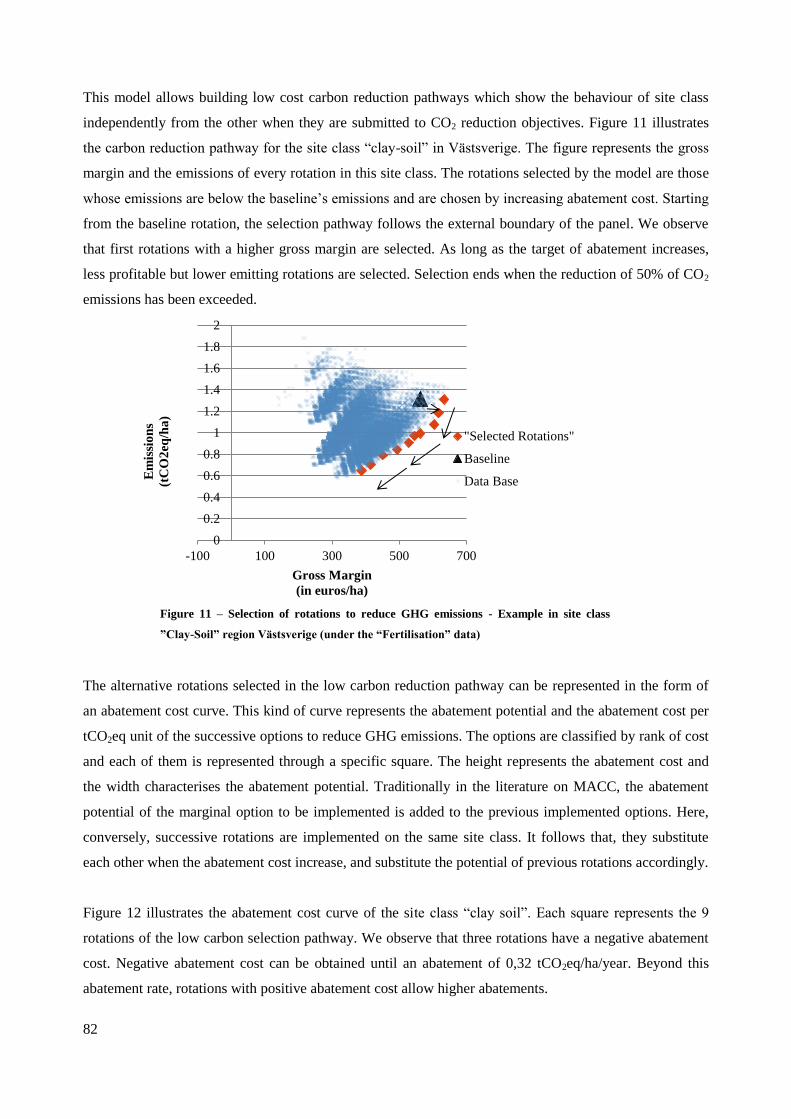
82

This model allows building low cost carbon reduction pathways which show the behaviour of site class

independently from the other when they are submitted to CO2 reduction objectives. Figure 11 illustrates

the carbon reduction pathway for the site class “clay-soil” in Västsverige. The figure represents the gross

margin and the emissions of every rotation in this site class. The rotations selected by the model are those

whose emissions are below the baseline’s emissions and are chosen by increasing abatement cost. Starting

from the baseline rotation, the selection pathway follows the external boundary of the panel. We observe

that first rotations with a higher gross margin are selected. As long as the target of abatement increases,

less profitable but lower emitting rotations are selected. Selection ends when the reduction of 50% of CO2

emissions has been exceeded.

The alternative rotations selected in the low carbon reduction pathway can be represented in the form of

an abatement cost curve. This kind of curve represents the abatement potential and the abatement cost per

tCO2eq unit of the successive options to reduce GHG emissions. The options are classified by rank of cost

and each of them is represented through a specific square. The height represents the abatement cost and

the width characterises the abatement potential. Traditionally in the literature on MACC, the abatement

potential of the marginal option to be implemented is added to the previous implemented options. Here,

conversely, successive rotations are implemented on the same site class. It follows that, they substitute

each other when the abatement cost increase, and substitute the potential of previous rotations accordingly.

Figure 12 illustrates the abatement cost curve of the site class “clay soil”. Each square represents the 9

rotations of the low carbon selection pathway. We observe that three rotations have a negative abatement

cost. Negative abatement cost can be obtained until an abatement of 0,32 tCO2eq/ha/year. Beyond this

abatement rate, rotations with positive abatement cost allow higher abatements.

0

0.2

0.4

0.6

0.8

1

1.2

1.4

1.6

1.8

2

-100 100 300 500 700

Em

issi

on

s

(tC

O2

eq/h

a)

Gross Margin

(in euros/ha)

"Selected Rotations"

Baseline

Data Base

Figure 11 – Selection of rotations to reduce GHG emissions - Example in site class

”Clay-Soil” region Västsverige (under the “Fertilisation” data)

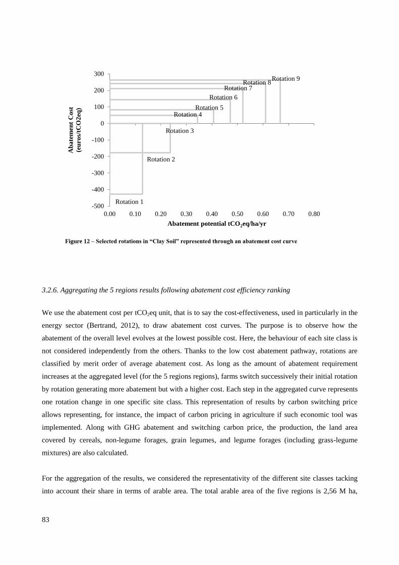
83

3.2.6. Aggregating the 5 regions results following abatement cost efficiency ranking

We use the abatement cost per tCO2eq unit, that is to say the cost-effectiveness, used in particularly in the

energy sector (Bertrand, 2012), to draw abatement cost curves. The purpose is to observe how the

abatement of the overall level evolves at the lowest possible cost. Here, the behaviour of each site class is

not considered independently from the others. Thanks to the low cost abatement pathway, rotations are

classified by merit order of average abatement cost. As long as the amount of abatement requirement

increases at the aggregated level (for the 5 regions regions), farms switch successively their initial rotation

by rotation generating more abatement but with a higher cost. Each step in the aggregated curve represents

one rotation change in one specific site class. This representation of results by carbon switching price

allows representing, for instance, the impact of carbon pricing in agriculture if such economic tool was

implemented. Along with GHG abatement and switching carbon price, the production, the land area

covered by cereals, non-legume forages, grain legumes, and legume forages (including grass-legume

mixtures) are also calculated.

For the aggregation of the results, we considered the representativity of the different site classes tacking

into account their share in terms of arable area. The total arable area of the five regions is 2,56 M ha,

Rotation 1

Rotation 2

Rotation 3

Rotation 4 Rotation 5

Rotation 6

Rotation 7 Rotation 8

Rotation 9

-500

-400

-300

-200

-100

0

100

200

300

0.00 0.10 0.20 0.30 0.40 0.50 0.60 0.70 0.80

Ab

ate

men

t C

ost

(eu

ros/

tCO

2eq

)

Abatement potential tCO2eq/ha/yr

Figure 12 – Selected rotations in “Clay Soil” represented through an abatement cost curve

84

representing 2.7% of the arable land in the EU-2733

. For the aggregated results, the profit for each region

are calculated based on the GM (see Appendix 3.7.2).

3.2.7. Economically efficient abatement

The economically efficient GHG abatement can be defined as the abatement up to a carbon price

threshold. Here, this threshold is approximated by the carbon value used by the UK Government, which is

€45 /tCO2eq (£52 /tCO2eq) in the non-traded sector in 2010 (central value) (DECC, 2009).

33Eurostat, 2010 data; Accessed: February 2014

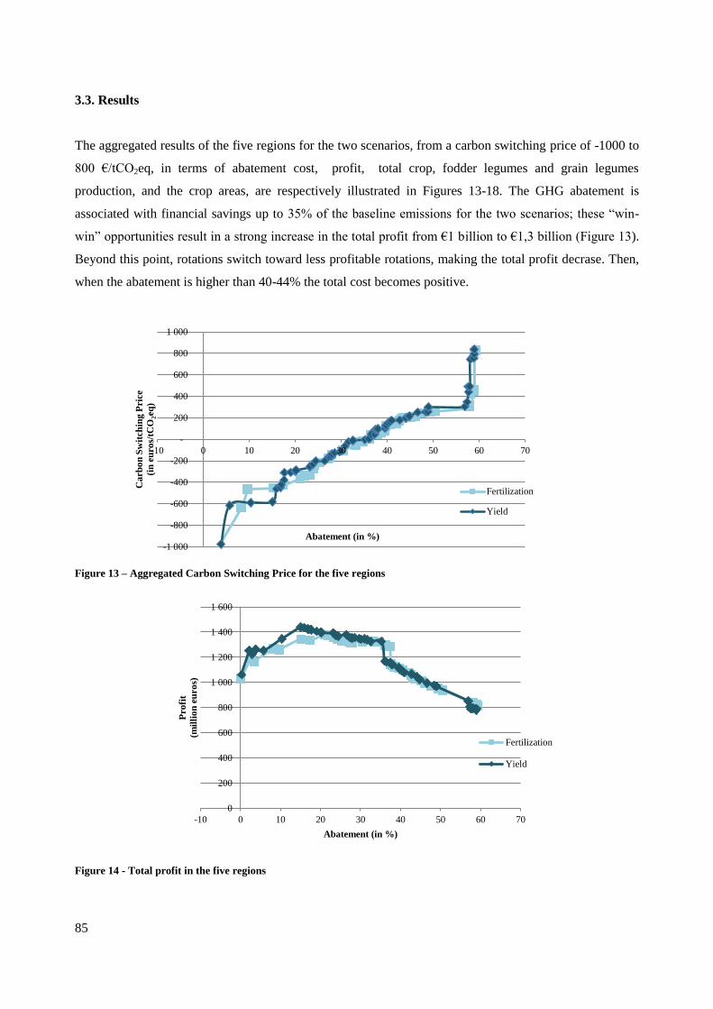
85

3.3. Results

The aggregated results of the five regions for the two scenarios, from a carbon switching price of -1000 to

800 €/tCO2eq, in terms of abatement cost, profit, total crop, fodder legumes and grain legumes

production, and the crop areas, are respectively illustrated in Figures 13-18. The GHG abatement is

associated with financial savings up to 35% of the baseline emissions for the two scenarios; these “win-

win” opportunities result in a strong increase in the total profit from €1 billion to €1,3 billion (Figure 13).

Beyond this point, rotations switch toward less profitable rotations, making the total profit decrase. Then,

when the abatement is higher than 40-44% the total cost becomes positive.

Figure 13 – Aggregated Carbon Switching Price for the five regions

Figure 14 - Total profit in the five regions

-1 000

-800

-600

-400

-200

-

200

400

600

800

1 000

-10 0 10 20 30 40 50 60 70

Ca

rb

on

Sw

itch

ing

Pric

e

(in

eu

ro

s/tC

O2eq

)

Abatement (in %)

Fertilization

Yield

0

200

400

600

800

1 000

1 200

1 400

1 600

-10 0 10 20 30 40 50 60 70

Pro

fit

(mil

lio

n e

uro

s)

Abatement (in %)

Fertilization

Yield

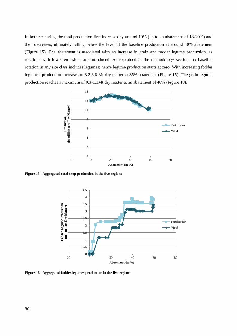
86

In both scenarios, the total production first increases by around 10% (up to an abatement of 18-20%) and

then decreases, ultimately falling below the level of the baseline production at around 40% abatement

(Figure 15). The abatement is associated with an increase in grain and fodder legume production, as

rotations with lower emissions are introduced. As explained in the methodology section, no baseline

rotation in any site class includes legumes; hence legume production starts at zero. With increasing fodder

legumes, production increases to 3.2-3.8 Mt dry matter at 35% abatement (Figure 15). The grain legume

production reaches a maximum of 0.3-1.1Mt dry matter at an abatement of 40% (Figure 18).

Figure 15 - Aggregated total crop production in the five regions

Figure 16 - Aggregated fodder legumes production in the five regions

0

2

4

6

8

10

12

14

-20 0 20 40 60 80

Pro

du

cti

on

(in

mil

lio

n t

on

s D

ry M

att

er)

Abatement (in %)

Fertilization

Yield

0

0.5

1

1.5

2

2.5

3

3.5

4

4.5

-20 0 20 40 60 80

Fo

dd

er L

eg

um

e P

ro

du

cti

on

(mil

ion

to

ns

Dry

Ma

tter)

Abatement (in %)

Fertilisation

Yield

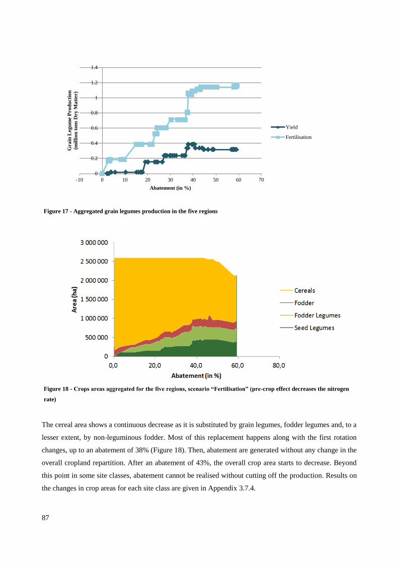
87

The cereal area shows a continuous decrease as it is substituted by grain legumes, fodder legumes and, to a

lesser extent, by non-leguminous fodder. Most of this replacement happens along with the first rotation

changes, up to an abatement of 38% (Figure 18). Then, abatement are generated without any change in the

overall cropland repartition. After an abatement of 43%, the overall crop area starts to decrease. Beyond

this point in some site classes, abatement cannot be realised without cutting off the production. Results on

the changes in crop areas for each site class are given in Appendix 3.7.4.

0

0.2

0.4

0.6

0.8

1

1.2

1.4

-10 0 10 20 30 40 50 60 70

Gra

in L

eg

um

e P

ro

du

cti

on

(mil

lio

n t

on

s D

ry

Ma

tter)

Abatement (in %)

Yield

Fertilisation

Figure 17 - Aggregated grain legumes production in the five regions

Figure 18 - Crops areas aggregated for the five regions, scenario “Fertilisation” (pre-crop effect decreases the nitrogen

rate)

88

Regional results for the economically efficient abatement (up to 45 €/t CO2eq) for the “Fertilisation”

scenario are summarized in Table 5 and highlights important disparity between regions. Brandenburg and

Eastern Scotland offer the highest abatement: respectively 46% and 44% reduction of the baseline soil

N2O emissions.. Västsverige and South Muntenia’s cost-effective abatement potentials are respectively

24% and 30%, while the potential abatement is lowest in Calabria (Italy), with only 2% of the baseline.

Moreover, at the economically efficient abatement, the GHG abatement is associated with an increase in

profit in every region (Table 5) except in South-Muntenia. The region with the highest relative increase in

profit is Brandenburg, where average profit is augmented by 75.7%. Eastern-Scotland and Calabria benefit

from a moderate profit increase (13.9% and 11.2%, respectively), while the profit increase in Västsverige

is only 0.2%.

At the same abatement level, all regions, apart from Västsverige, present an increase in the share of

legumes, and cereal areas decline in three regions (Sud-Muntenia, Eastern Scotland and Brandenburg). In

Calabria, non-leguminous fodder are substituted by both grain legumes and cereals, while in Västsverige,

non-leguminous fodder are replaced by cereals, with no area increase for legumes. In Eastern Scotland, the

non-leguminous fodder area also increased alongside the legumes area. Rotations providing both GHG

abatement and financial savings at the same time include both fodder and grain legumes in Brandenburg

(grass-clover mix, alfalfa, lupin and pea), and in Eastern Scotland (grass-clover mix and pea), whereas in

South-Muntenia and Calabria only grain legumes (common bean for South-Muntenia) or fodder legumes

(alfalfa for Calabria) appear in these rotations. In Västsverige, there are no legumes in the ‘win-win’

rotations. More detailed results for the scenario “Fertilisation” on the composition of the rotations selected

by the model are presented in Appendix 3.7.4.

89

Table 5 - Regional results for the baseline and for a cost-effectiveness of €45 /t CO2eq, scenario Fertilisation (all rotations per site class; pre-crop effect decreases the nitrogen rate)

Area

Cereals

Area

Fodder

Crops

Area

Fodder

Legumes

Area Grain

Legumes Cost Production Emissions Abatement

Gross

Margin

% % % % euros/ha

kg Dry

Matter/ha tCO2eq/ha tCO2eq/ha Euros/ha

South-

Muntenia

Baseline 100,0 0,0 0,0 0,0 0 3296 1,03 0 314

45 euros/tCO2eq 75,0 25,0 14,03 2962 0,72 0,31 300

Västsverige

Baseline 80,0 20,0 0,0 0,0 0 3703 1,31 0 562

45 euros/tCO2eq 100,0 0,0 0,0 -0,56 3105 0,99 0,32 563

Eastern-

Scotland

Baseline 94,3 5,7 0,0 0,0 0 6676 2,00 0 792

45 euros/tCO2eq 40,9 32,3 11,4 15,4 -111,26 6495 1,11 0,89 903

Calabria

Baseline 71,7 28,3 0,0 0,0 0 3706 0,70 0 376

45 euros/tCO2eq 81,8 13,0 0,0 5,1 -41,59 3881 0,68 0,02 418

Brandenburg

Baseline 92,7 7,3 0,0 0,0 0 5187 1,18 0 144

45 euros/tCO2eq 54,4 0,0 31,3 14,4 -109,74 6136 0,63 0,55 253

Overall

Baseline 89,9 10,1 0,0 0,0 0 4735 1,29 0 384

45 euros/tCO2eq 67,1 7,1 14,5 12,3 -63,27 4914 0,81 0,49 447

90

3.4. Discussion

Abatement cost in the five regions can be compared with results of other studies focussing the comparison

specifically on legumes to stay at the same scope. Pellerin et al (2013) considered using fodder and grain

legumes as two options to mitigate agriculture emissions in France. Legumes abatement cost potential was

estimated in according to a change in France farmlands and not according to rotation changes. The

abatement potential was 1.4 MtCO2eq for a total cost of -72 M€, which induces an average cost of -52

€/tCO2eq34. Macleod et al (2010) assessment on legumes gave a high average abatement cost of 20 849

€/tCO2eq (with cost of implementation of 33 €/ha), while accounting for interactions with other mitigation

options which reduce the abatement potential of this option considerably. The present analysis find the

average abatement cost to be -130€/tCO2eq at a carbon switch price of 45 €/tCO2eq, which is the lowest

average abatement cost from legumes among the three studies (see Appendix 3.7.8 for a further detailed

comparison). Most of this increase in the profit is due to the initial changes from the baseline rotations to

other more profitable rotations. We remind that these more profitable rotations cannot be considered as

baseline due to their high legume content.

Consequently, results suggest that there is significant potential win-win abatement in all five regions, i.e. a

potential decrease in GHG emissions with a simultaneous increase in GM. These win-win mitigation

opportunities (i.e. negative cost-effectiveness) will always raise further questions about the assumptions in

the calculations. Indeed, a quite intuitive interrogation is: why farmers would currently refuse to reduce

their GHG emissions whereas it would raise their profit? The most common explanations for the negative

cost are the following: either simulation’s estimates are robust but farmers do not have information about

these opportunities and the assumption about their profit-maximising behaviour does not capture other

barriers, either the model does not capture some important cost elements due to production system

changes.

On this latter point, the 13 site classes are not farms. Consequently their production system (e.g. livestock

or cereals) is not specified. Yet, in reality, farmers are constrained by their production system, for example

farms with ruminant animals tend to utilise their land area for home-grown fodder, rather than producing

crops for export and importing the feed. On the other hand, farms without ruminants have very limited

ability to sell fodder, mostly due to the high transportation costs. Moreover, beyond the farm gate,

structural barriers might be hidden in the supply chain of legumes contributing to the existence of

seemingly win-win opportunities. For instance, legumes need adapted silos that are not currently

34 These figures reprent two measures assessed by Pellerin et al., 2013 : one measure which consists in increasing legumes in

cropland and the other increasing legumes in grasslands.

91

established in all regions in Europe. Besides, the effect of an increased legume production and a decreased

cereal production on the European crop market is not taken into account in this study, while in the

meantime these feedbacks have the potential to increase the costs.

Barriers also exist in the diffusion of information in the agricultural sector. Farmers’ decision making,

including internal factors (cognition and habit) and social factors (norms and roles), can also explain the

non-current exploitation of these negative costs. Besides, farmers may be exhibiting risk aversion

behaviour in response to a potentially higher variation in the yield of legumes (Jensen et al, 2010) and

their action on the pre-crop effect (as suggested in Table 3 in the standard deviation figure).

Lastly, assumptions about the baseline practices would also affect both the abatement and the cost of win-

win opportunities. In the case of the current assessment, the choice of the baseline rotations and the fact

that many low-emission leguminous crops are associated with a relatively high GM in the crop database is

partly responsible for the win-win opportunities.

Consequently, given the fact that the scope of our research does not capture the aforementioned barriers

and thus is underestimating costs, results should not be interpreted as actual estimation but rather as a

maximum optimistic potential. The estimation of the weight of these implementation barriers is left aside

for further research work.

92

3.5. Conclusion

The results emphasize the importance of rotation switch in European agriculture and underpin that a shift

for rotational schemes implying lower nitrogen requirement is not only beneficial to the climate, but can

be made without significant losses for the farmers and without a reduction in agricultural production. A

significant part of the abatement potential can be achieved without the implementation of legumes in some

area such as Västverige, but most of this abatement potential is fulfilled thanks to the cultivating of grain

and fodder legumes. Over around 15% of the arable land areas, replacing non-leguminous fodder and

cereal areas induces a maximum farm revenue increase at an abatement of 0.7 MtCO2eq (35% of the soil

N2O emissions from these land areas).

Though the increased cultivation of legumes would reduce cereal production, it would provide additional

proteins both for animal and human consumption, reducing the need for feed protein imports (the

additionnal grain legume production is 0.3-1.1 Mt DM at the five regions level, this accounts to 1.2-3.2%

of the current 34.4 Mt DM/y soybean import in the EU-25). The reduced cereal production would have

implications on cereal production elsewhere, potentially resulting in a GHG leakage. Investigating the

overall impact of such a shift in the place of production needs a life cycle analysis approach.

Increasing the switch toward less nitrogen consuming cropland systems in European could be promoted

through providing better information on the agronomic issues (e.g. agronomic characteristics of clover

varieties, nutritional values of legume fodder for animals) via existing advisory schemes, information

tools, or through compulsory schemes, especially given that monitoring and enforcement is relatively

straightforward. One opportunity is already implemented within the new Common Agricultural Policy

(CAP): farmers can chose to comply with Ecological Focus Areas requirements by cultivating legumes.

The demand for grain legumes can increase if it becomes practical for livestock farmers and feed

producers to replace part of the soybean in the feed with peas and beans, and also if consumers become

more willing to give up part of their livestock-protein consumption for plant-proteins (this aligns well with

efforts promoting a shift in consumption towards a more sustainable pattern). A broad incentive that

targets not only farmers producing crops, but also consumers and the agricultural supply chain as well,

could be the implementation of a carbon price in the economy covering nitrous oxide emissions.

93

3.6. References

Cavaillès, E., 2009. La relance des légumineuses dans le cadre d'un plan légumineuses. Commissariat

Général au Développement DurableEtudes & Documents.

Charles, R., Vullioud, P., 2001. Pois protéagineux et azote dans la rotation. Revue Suisse d’Agriculture 33

(6), 265–270.

Dequiedt, B., & Moran, D. (2015). The cost of emission mitigation by legume crops in French agriculture.

Ecological Economics, 110, 51-60.

Bertrand, 2012. Understanding fuel switching under the EU ETS.Global Energy Issues.Vol. 35, No. 6,

2012.

De Cara & Jayet, 2011. Marginal abatement costs of greenhouse gas emissions from European agriculture,

cost-effectiveness, and the EU Non-ETS burden sharing agreement. Ecological Economics, 70(9),

1680–1690.

Department of Energy and Climate Change (2009) Carbon Valuation in UK Policy Appraisal: a revised

Approach’

Defra, 2011.Fertiliser Manual RB209.Updated 22 April 2013. Tables A-C, p. 91-93. and p. 105-112

European Commission, 2014.Communication from the commission to the European parliament, the

council, the European economic and social committee and the committee of the regions.A policy

framework for climate and energy in the period from 2020 to 2030. Brussels 22.1.2014.

European Commission, 2010. Commission staff working document on implementation of Council

Directive 91/676/EEC concerning the protection of waters against pollution caused by nitrates

from agricultural sources based on Member State reports for the period 2004-2007 (map on page

18), ec.europa.eu/environment/water/water-nitrates/pdf/swd.pdf

FAOSTAT 2011. Data processed: January2014 for the year 2011.

Graham PH, Vance CP (2003) Legumes: importance and constraints to greater use. Plant Physiol 131:872

– 877

94

Hassan, H. M., Marschner, P., McNeill, A., & Tang, C. (2012). Grain legume pre-crops and their residues

affect the growth, P uptake and size of P pools in the rhizosphere of the following wheat. Biology

and Fertility of Soils, 48, 775-785.

IPCC (2006) IPCC Guidelines for National Greenhouse Gas Inventories, Prepared by the National

Greenhouse Gas Inventories Programme , Volume 4: Agriculture, forestry and other land use.

Eggleston, H. S., Buendia, L., Miwa, K., Ngara, T., and Tanabe, K. Japan, IGES.

Jensen, E. S., Peoples, M. B., & Hauggaard-Nielsen, H. (2010). Faba bean in cropping systems. Field

Crops Research, 115, 203-216.

Justes, E., Mary, B., & Nicolardot, B. (1999). Comparing the effectiveness of radish cover crop, oilseed

rape volunteers and oilseed rape residues incorporation for reducing nitrate leaching. Nutrient

cycling in Agroecosystems, 55, 207-220.

Köpke, U., & Nemecek, T. (2010). Ecological services of faba bean. Field Crops Research, 115, 217-233.

MacLeod, M., Moran, D., Eory, V., Rees, R., Barnes, A., Topp, C. F., Ball, B., Hoad, S., Wall, E.,

McVittie, A., et al. (2010). Developing greenhouse gas marginal abatement cost curves for

agricultural emissions from crops and soils in the UK. Agricultural Systems, 103(4), 198–209.

Martin P., Meynard JM., 1997. Systèmes de culture, érosion et pollution par l’ion nitrate. in L’eau dans

l’espace rural, production végétale et qualité de l'eau. Collection “ Mieux comprendre ”,

Universités francophones, INRA ed. pp. 303-322.

Moran, D., MacLeod, M., Wall, E., Eory, V., McVittie, A., Barnes, A., et al. (2010). Developing carbon

budgets for UK agriculture, land-use, land-use change and forestry out to 2022. Climatic Change.

Pellerin S., Bamière L., Angers D., Béline F., Benoît M., Butault J.P., Chenu C., Colnenne-David C., De

Cara S., Delame N., Doreau M., Dupraz P., Faverdin P., Garcia-Launay F., Hassouna M., Hénault

C., Jeuffroy M.H., Klumpp K., Metay A., Moran D., Recous S., Samson E., Savini I., Pardon L.,

2013. Quelle contribution de l’agriculture française à la réduction des émissions de gaz à effet de

serre? Potentiel d'atténuation et coût de dix actions techniques. Synthèse du rapport d'étude, INRA

(France), 92p.

Reckling M., N. Schläfke, J.-M.Hecker, J. Bachinger, P. Zander (2014a) Survey structure on farm and

crop data.LegumeFutures Report D4.1.

95

Reckling M., N. Schläfke, J.-M.Hecker, J. Bachinger, P. Zander (2014b) Generation and evaluation of

crop rotations.LegumeFutures Report D4.2.

Rochester, I., Peoples, M., Hulugalle, N., Gault, R., & Constable, G. (2001). Using legumes to enhance

nitrogen fertility and improve soil condition in cotton cropping systems. Field Crops Research, 70,

27-41.

UNFCCC, 2013. UNFCCC National Inventory Report, 2013

Webb, J., Sorensen, P., Velthof, G.L., Amon, B., Pinto, M., Rodhe, L., Salomon, E., Hutchings, N.,

Burczyk, P. and Reid, J. (2010) Study on variation of manure N efficiency throughout Europe -

Final report. Report no: ENV.B.1/ETU/2010/0008, DG Environment

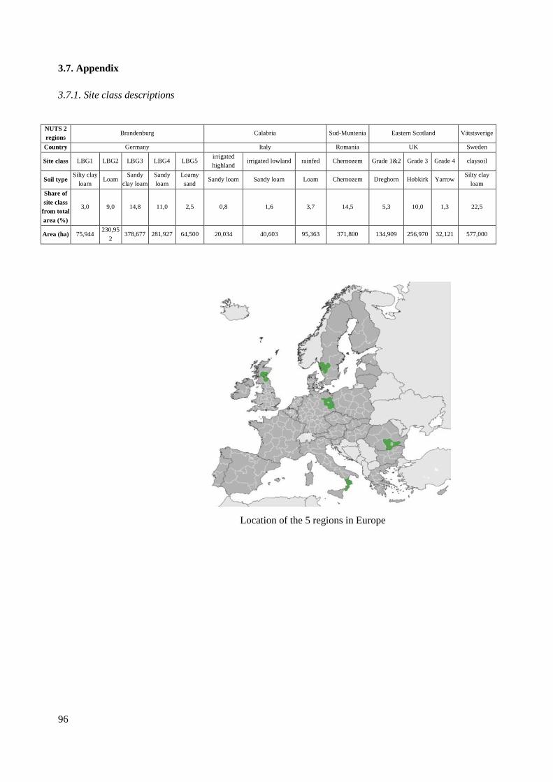
96

3.7. Appendix

3.7.1. Site class descriptions

NUTS 2

regions Brandenburg Calabria Sud-Muntenia Eastern Scotland Vätstsverige

Country Germany Italy Romania UK Sweden

Site class LBG1 LBG2 LBG3 LBG4 LBG5 irrigated

highland irrigated lowland rainfed Chernozem Grade 1&2 Grade 3 Grade 4 claysoil

Soil type Silty clay

loam Loam

Sandy

clay loam

Sandy

loam

Loamy

sand Sandy loam Sandy loam Loam Chernozem Dreghorn Hobkirk Yarrow

Silty clay

loam

Share of

site class

from total

area (%)

3,0 9,0 14,8 11,0 2,5 0,8 1,6 3,7 14,5 5,3 10,0 1,3 22,5

Area (ha) 75,944 230,95

2 378,677 281,927 64,500 20,034 40,603 95,363 371,800 134,909 256,970 32,121 577,000

Location of the 5 regions in Europe

97

3.7.2. GM and GHG calculations

Gross margin (GM) calculation (source : Reckling et al. (2014) database)

𝐺𝑀𝑐𝑟𝑜𝑝 = (Yield * PA + YieldB * PB + YieldByProd * PByProd)– (Production Cost + Other)

Yield: main production yield (kg DM/ha/year) for instance the grain of wheat

Yield_B: second production yield if it is exist (kg DM/ha/year) for instance the wheat straw

YieldByProd: third production yield if it exist (kg DM/ha/year)

PA: main production price (€/t)

PB: second production price (€/t)

PByProd: third production price (€/t)

Production Cost: cost of fungicides, pesticides, fertilisers, insecticides, harvest, irrigation, drying

and cleaning, machinery and harvesting cost.

Other : Services including contraction costs.

𝐺𝑀𝑟𝑜𝑡𝑎𝑡𝑖𝑜𝑛 = ∑𝐺𝑀𝑐𝑟𝑜𝑝

(1 + 𝑟)𝑡

𝑚

𝑡=1

m : overall length of the rotation from two to six years

𝐺𝑀𝑐𝑟𝑜𝑝 : crop gross margin.

r : discount Rate of 3% per year

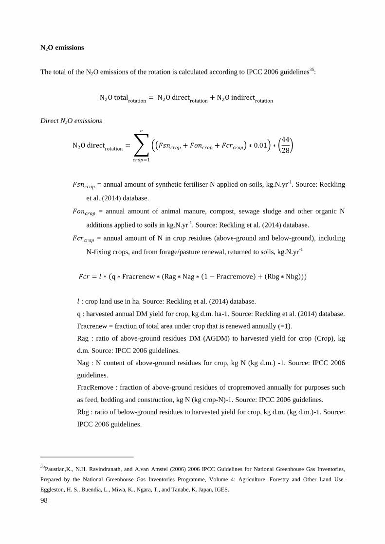
98

N2O emissions

The total of the N2O emissions of the rotation is calculated according to IPCC 2006 guidelines35

:

N2O totalrotation

= N2O directrotation

+ N2O indirectrotation

Direct N2O emissions

N2O directrotation

= ∑ ((𝐹𝑠𝑛𝑐𝑟𝑜𝑝 + 𝐹𝑜𝑛𝑐𝑟𝑜𝑝 + 𝐹𝑐𝑟𝑐𝑟𝑜𝑝) ∗ 0.01) ∗ (44

28)

𝑛

𝑐𝑟𝑜𝑝=1

𝐹𝑠𝑛𝑐𝑟𝑜𝑝 = annual amount of synthetic fertiliser N applied on soils, kg.N.yr-1

. Source: Reckling

et al. (2014) database.

𝐹𝑜𝑛𝑐𝑟𝑜𝑝 = annual amount of animal manure, compost, sewage sludge and other organic N

additions applied to soils in kg.N.yr-1

. Source: Reckling et al. (2014) database.

𝐹𝑐𝑟𝑐𝑟𝑜𝑝 = annual amount of N in crop residues (above-ground and below-ground), including

N-fixing crops, and from forage/pasture renewal, returned to soils, kg.N.yr-1

𝐹𝑐𝑟 = 𝑙 ∗ (q ∗ Fracrenew ∗ (Rag ∗ Nag ∗ (1 − Fracremove) + (Rbg ∗ Nbg)))

𝑙 : crop land use in ha. Source: Reckling et al. (2014) database.

q : harvested annual DM yield for crop, kg d.m. ha-1. Source: Reckling et al. (2014) database.

Fracrenew = fraction of total area under crop that is renewed annually (=1).

Rag : ratio of above-ground residues DM (AGDM) to harvested yield for crop (Crop), kg

d.m. Source: IPCC 2006 guidelines.

Nag : N content of above-ground residues for crop, kg N (kg d.m.) -1. Source: IPCC 2006

guidelines.

FracRemove : fraction of above-ground residues of cropremoved annually for purposes such

as feed, bedding and construction, kg N (kg crop-N)-1. Source: IPCC 2006 guidelines.

Rbg : ratio of below-ground residues to harvested yield for crop, kg d.m. (kg d.m.)-1. Source:

IPCC 2006 guidelines.

35Paustian,K., N.H. Ravindranath, and A.van Amstel (2006) 2006 IPCC Guidelines for National Greenhouse Gas Inventories,

Prepared by the National Greenhouse Gas Inventories Programme, Volume 4: Agriculture, Forestry and Other Land Use.

Eggleston, H. S., Buendia, L., Miwa, K., Ngara, T., and Tanabe, K. Japan, IGES.

99

Nbg : N content of below-ground residues for crop, kg N (kg d.m.)-1. Source: IPCC 2006

guidelines.

Indirect N2O emissions

N2O indirectrotation = ∑ N2Oadtcrop

𝑛

𝑐𝑟𝑜𝑝=1

+ N2O𝐿𝑐𝑟𝑜𝑝

N2Oadt : N2O from atmospheric deposition of N volatilised from managed soils

N2Oadtcrop = ((𝐹𝑠𝑛 ∗ 0.1 + 𝐹𝑜𝑛 ∗ 0.2) ∗ 0.01) ∗ (44

28)

N2OL : N2O from N leaching and runoff from managed soils in regions where leaching and

runoff occur

N2OLcrop = ((𝐹𝑠𝑛 + 𝐹𝑜𝑛) ∗ 0.3) ∗ 0.0075 ∗ (44

28)

100

3.7.3. Pre-crop effect

Change in yield in the “Yield” scenario

Change in fertiliser costs in the “Fertilisation” scenario

Tons Dry Matter M/ha % Euros/ha %

Average +1.33 +17.8 -31.0 -14.1 Standard deviation +1.17 +10.7 -13.5 -4.7

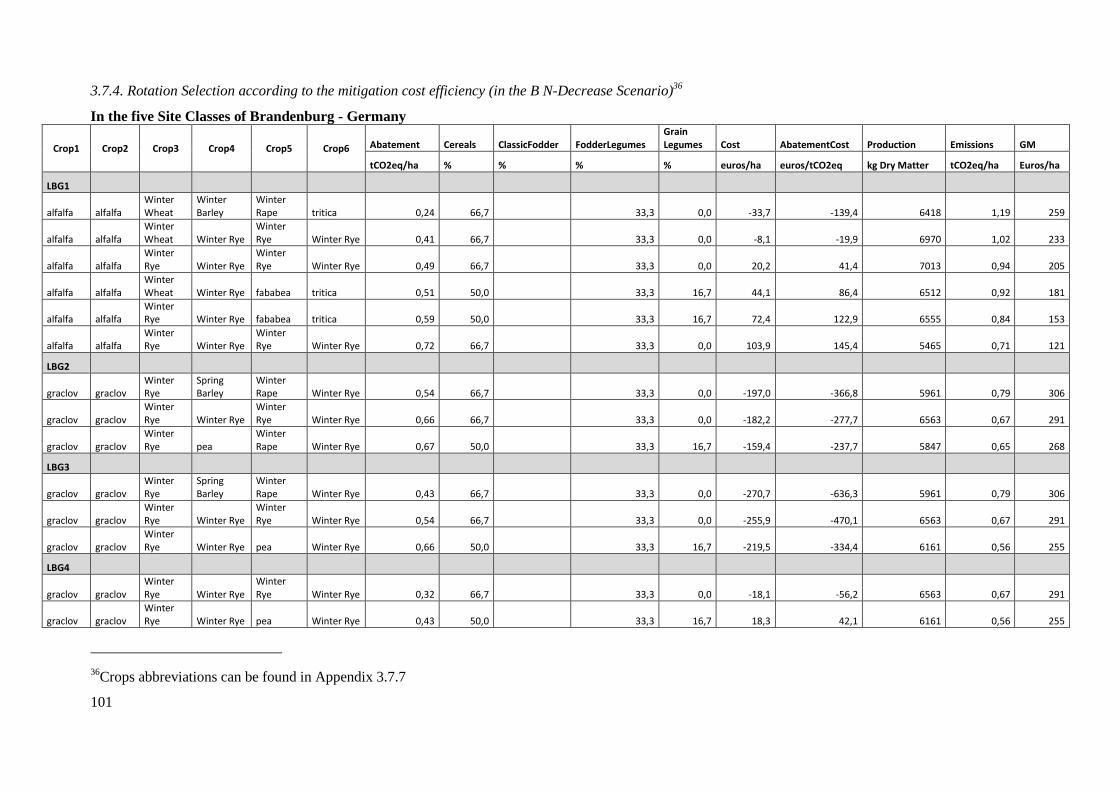
101

3.7.4. Rotation Selection according to the mitigation cost efficiency (in the B N-Decrease Scenario)36

In the five Site Classes of Brandenburg - Germany

Crop1 Crop2 Crop3 Crop4 Crop5 Crop6 Abatement Cereals ClassicFodder FodderLegumes Grain Legumes Cost AbatementCost Production Emissions GM

tCO2eq/ha % % % % euros/ha euros/tCO2eq kg Dry Matter tCO2eq/ha Euros/ha

LBG1

alfalfa alfalfa Winter Wheat

Winter Barley

Winter Rape tritica 0,24 66,7

33,3 0,0 -33,7 -139,4 6418 1,19 259

alfalfa alfalfa Winter Wheat Winter Rye

Winter Rye Winter Rye 0,41 66,7

33,3 0,0 -8,1 -19,9 6970 1,02 233

alfalfa alfalfa Winter Rye Winter Rye


33,3 0,0 20,2 41,4 7013 0,94 205

alfalfa alfalfa Winter Wheat Winter Rye fababea tritica 0,51 50,0

33,3 16,7 44,1 86,4 6512 0,92 181

alfalfa alfalfa Winter Rye Winter Rye fababea tritica 0,59 50,0

33,3 16,7 72,4 122,9 6555 0,84 153

alfalfa alfalfa Winter Rye Winter Rye


33,3 0,0 103,9 145,4 5465 0,71 121

LBG2

graclov graclov Winter Rye

Spring Barley

Winter Rape Winter Rye 0,54 66,7 33,3 0,0 -197,0 -366,8 5961 0,79 306

graclov graclov Winter Rye Winter Rye


33,3 0,0 -182,2 -277,7 6563 0,67 291

graclov graclov Winter Rye pea

Winter Rape Winter Rye 0,67 50,0 33,3 16,7 -159,4 -237,7 5847 0,65 268

LBG3

graclov graclov Winter Rye

Spring Barley

Winter Rape Winter Rye 0,43 66,7

33,3 0,0 -270,7 -636,3 5961 0,79 306



33,3 0,0 -255,9 -470,1 6563 0,67 291

graclov graclov Winter Rye Winter Rye pea Winter Rye 0,66 50,0

33,3 16,7 -219,5 -334,4 6161 0,56 255

LBG4



33,3 0,0 -18,1 -56,2 6563 0,67 291


33,3 16,7 18,3 42,1 6161 0,56 255

36Crops abbreviations can be found in Appendix 3.7.7

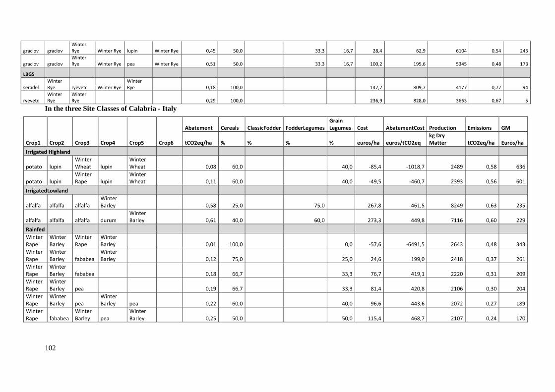
102

graclov graclov Winter Rye Winter Rye lupin Winter Rye 0,45 50,0

33,3 16,7 28,4 62,9 6104 0,54 245


33,3 16,7 100,2 195,6 5345 0,48 173

LBG5

seradel Winter Rye ryevetc Winter Rye

Winter Rye 0,18 100,0

147,7 809,7 4177 0,77 94

ryevetc Winter Rye

Winter Rye 0,29 100,0

236,9 828,0 3663 0,67 5

In the three Site Classes of Calabria - Italy

Crop1 Crop2 Crop3 Crop4 Crop5 Crop6

Abatement Cereals ClassicFodder FodderLegumes Grain Legumes Cost AbatementCost Production Emissions GM

tCO2eq/ha % % % % euros/ha euros/tCO2eq kg Dry Matter tCO2eq/ha Euros/ha

Irrigated Highland

potato lupin Winter Wheat lupin

Winter Wheat 0,08 60,0 40,0 -85,4 -1018,7 2489 0,58 636

potato lupin Winter Rape lupin

Winter Wheat 0,11 60,0

40,0 -49,5 -460,7 2393 0,56 601

IrrigatedLowland

alfalfa alfalfa alfalfa Winter Barley 0,58 25,0

75,0

267,8 461,5 8249 0,63 235

alfalfa alfalfa alfalfa durum Winter Barley 0,61 40,0

60,0

273,3 449,8 7116 0,60 229

Rainfed

Winter Rape

Winter Barley

Winter Rape

Winter Barley 0,01 100,0

0,0 -57,6 -6491,5 2643 0,48 343

Winter Rape

Winter Barley fababea


25,0 24,6 199,0 2418 0,37 261

Winter Rape

Winter Barley fababea 0,18 66,7

33,3 76,7 419,1 2220 0,31 209

Winter Rape

Winter Barley pea 0,19 66,7

33,3 81,4 420,8 2106 0,30 204

Winter Rape

Winter Barley pea

Winter Barley pea 0,22 60,0

40,0 96,6 443,6 2072 0,27 189

Winter Rape fababea

Winter Barley pea


50,0 115,4 468,7 2107 0,24 170

103

In the Site Classe of Muntenia - Romania


Abatement

Cereals

ClassicFodder

FodderLegumes

Grain Legumes Cost

AbatementCost Production Emissions GM

tCO2eq/ha % % % %

euros/ha euros/tCO2eq

kg Dry Matter

tCO2eq/ha

Euros/ha

chernozem

Combean

Winter Wheat

Winter Rape

maize_g 0,23 75,0 25,0 -431,6 -1873,7 3192 0,80 746

combean

Winter Wheat

Winter Rape


25,0 -355,7 -1213,0 2977 0,74 670

soybean

Winter Wheat

Winter Rape


25,0 14,0 44,8 2962 0,72 300

soybean

Winter Barley sunfl

Winter Wheat

Winter Rape 0,36 80,0

20,0 62,4 172,1 2540 0,67 252

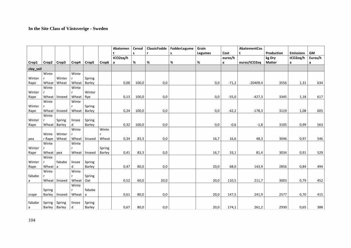
104

In the Site Class of Västsverige - Sweden


Abatement

Cereals

ClassicFodder

FodderLegumes

Grain Legumes Cost


tCO2eq/ha % % % %

euros/ha euros/tCO2eq

kg Dry Matter

tCO2eq/ha

Euros/ha

clay_soil

Winter Rape

Winter Wheat

Winter Wheat

Winter Wheat

Spring Barley 0,00 100,0 0,0 0,0 -71,2 -20409,4 3556 1,31 634

Winter Rape

Winter Wheat linseed

Winter Wheat

Winter Rye 0,13 100,0 0,0

0,0 -55,0 -427,3 3345 1,18 617

Winter Rape


Winter Wheat

Spring Barley 0,24 100,0 0,0

0,0 -42,2 -178,3 3119 1,08 605

Winter Rape

Winter Wheat

Spring Barley

linseed


0,0 -0,6 -1,8 3105 0,99 563

pea Winter Rape

Winter Wheat


Winter Wheat 0,34 83,3 0,0

16,7 16,6 48,3 3046 0,97 546

Winter Rape

Winter Wheat pea



16,7 33,1 81,4 3034 0,91 529

Winter Rape

Winter Wheat

fababea

linseed

Spring Barley 0,47 80,0 0,0 20,0 68,0 143,9 2856 0,84 494

fababea


Winter Wheat

Spring Oat 0,52 60,0 20,0

20,0 110,5 211,7 3003 0,79 452

srape Spring Barley linseed

Winter Wheat

fababea 0,61 80,0 0,0

20,0 147,5 241,9 2577 0,70 415

fababea

Spring Barley

Spring Barley

linseed


20,0 174,1 261,2 2930 0,65 388

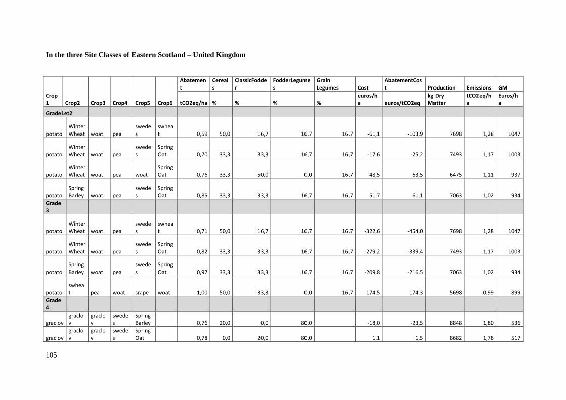
105

In the three Site Classes of Eastern Scotland – United Kingdom


Abatement

Cereals

ClassicFodder

FodderLegumes

Grain Legumes Cost


tCO2eq/ha % % % % euros/ha euros/tCO2eq

kg Dry Matter

tCO2eq/ha

Euros/ha

Grade1et2

potato Winter Wheat woat pea

swedes

swheat 0,59 50,0 16,7 16,7 16,7 -61,1 -103,9 7698 1,28 1047


swedes

Spring Oat 0,70 33,3 33,3 16,7 16,7 -17,6 -25,2 7493 1,17 1003

potato Winter Wheat woat pea woat

Spring Oat 0,76 33,3 50,0 0,0 16,7 48,5 63,5 6475 1,11 937

potato Spring Barley woat pea

swedes

Spring Oat 0,85 33,3 33,3 16,7 16,7 51,7 61,1 7063 1,02 934

Grade3


swedes

swheat 0,71 50,0 16,7 16,7 16,7 -322,6 -454,0 7698 1,28 1047


swedes

Spring Oat 0,82 33,3 33,3 16,7 16,7 -279,2 -339,4 7493 1,17 1003

potato Spring Barley woat pea

swedes

Spring Oat 0,97 33,3 33,3 16,7 16,7 -209,8 -216,5 7063 1,02 934

potato swheat pea woat srape woat 1,00 50,0 33,3 0,0 16,7 -174,5 -174,3 5698 0,99 899

Grade4

graclov graclov

graclov

swedes

Spring Barley 0,76 20,0 0,0 80,0 -18,0 -23,5 8848 1,80 536

graclov graclov

graclov

swedes

Spring Oat 0,78 0,0 20,0 80,0

1,1 1,5 8682 1,78 517

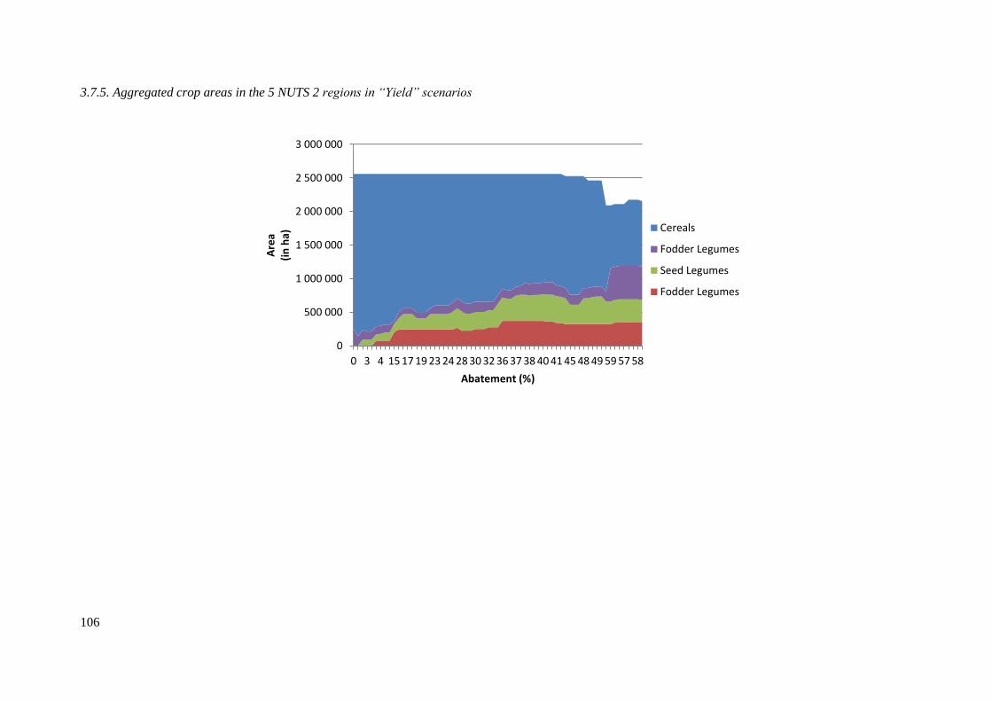
106

3.7.5. Aggregated crop areas in the 5 NUTS 2 regions in “Yield” scenarios

0

500 000

1 000 000

1 500 000

2 000 000

2 500 000

3 000 000

0 3 4 15 17 19 23 24 28 30 32 36 37 38 40 41 45 48 49 59 57 58

Are

a

(in

ha)

Abatement (%)

Cereals

Fodder Legumes

Seed Legumes

Fodder Legumes

107

3.7.6. GM and GHG emissions for each rotation in each site class (“Fertilisation” scenario).

0

0.5

1

1.5

2

2.5

3

0 500 1000 1500

Em

issi

on

s

(tC

O2

eq

/ha

)

Gross Margin

(in euros/ha)

Grade 3

0

0.5

1

1.5

2

2.5

3

0 200 400 600

Em

issi

on

s

(tC

O2

eq

/ha

)

Gross Margin

(in euros/ha)

Grade 4

0

0.2

0.4

0.6

0.8

1

1.2

1.4

1.6

1.8

2

0 500 1000 1500

Em

issi

on

s

(tC

O2

eq/h

a)

Gross Margin

(in euros/ha)

Grade 1&2

0

0.1

0.2

0.3

0.4

0.5

0.6

0 100 200 300 400

Em

issi

on

s

(tC

O2

eq/h

a)

Gross Margin

(in euros/ha)

Rainfed

Selected Rotations

Baseline

Data Base

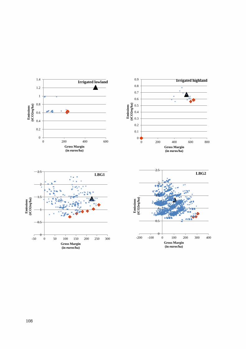
108

0

0.2

0.4

0.6

0.8

1

1.2

1.4

0 200 400 600

Em

issi

on

s

(tC

O2

eq

/ha

)

Gross Margin

(in euros/ha)

Irrigated lowland

0

0.1

0.2

0.3

0.4

0.5

0.6

0.7

0.8

0.9

0 200 400 600 800

Em

issi

on

s

(tC

O2

eq

/ha

)

Gross Margin

(in euros/ha)

Irrigated highland

0

0.5

1

1.5

2

2.5

-50 0 50 100 150 200 250 300

Em

issi

on

s

(tC

O2

eq

/ha

)

Gross Margin

(in euros/ha)

LBG1

0

0.5

1

1.5

2

2.5

-200 -100 0 100 200 300 400

Em

issi

on

s

(tC

O2

eq

/ha

)

Gross Margin

(in euros/ha)

LBG2

109

0

0.5

1

1.5

2

2.5

-200 -100 0 100 200 300 400

Em

issi

on

s

(tC

O2

eq

/ha

)

Gross Margin

(in euros/ha)

LBG3

0

0.2

0.4

0.6

0.8

1

1.2

1.4

1.6

1.8

-400 -200 0 200 400

Em

issi

on

s

(tC

O2

eq

/ha

)

Gross Margin

(in euros/ha)

LBG4

0

0.2

0.4

0.6

0.8

1

1.2

-300 -200 -100 0 100 200 300

Em

issi

on

s

(tC

O2

eq

/ha

)

Gross Margin

(in euros/ha)

LBG5

0

0.2

0.4

0.6

0.8

1

1.2

1.4

1.6

1.8

2

0 200 400 600 800

Em

issi

on

s

(tC

O2

eq

/ha

)

Gross Margin

(in euros/ha)

Clay Soil

110

0

0.2

0.4

0.6

0.8

1

1.2

0 200 400 600 800

Em

issi

on

s

(tC

O2

eq

/ha

)

Gross Margin

(in euros/ha)

Chernozem

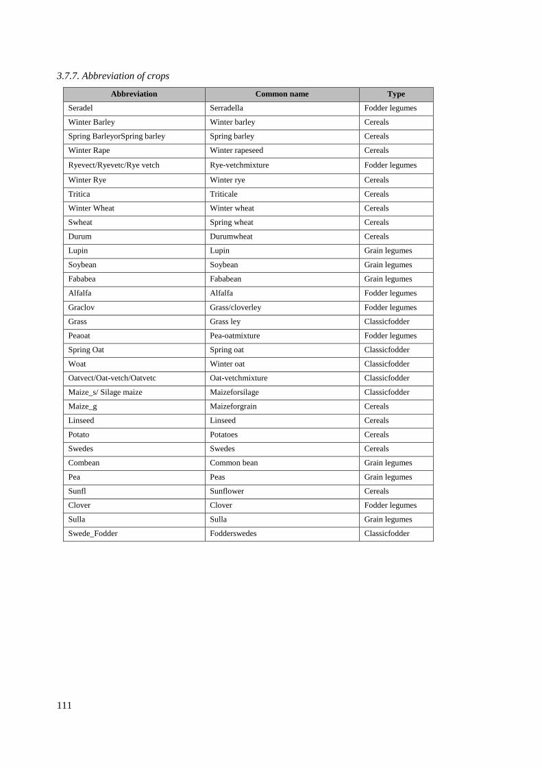
111

3.7.7. Abbreviation of crops

Abbreviation Common name Type

Seradel Serradella Fodder legumes

Winter Barley Winter barley Cereals

Spring BarleyorSpring barley Spring barley Cereals

Winter Rape Winter rapeseed Cereals

Ryevect/Ryevetc/Rye vetch Rye-vetchmixture Fodder legumes

Winter Rye Winter rye Cereals

Tritica Triticale Cereals

Winter Wheat Winter wheat Cereals

Swheat Spring wheat Cereals

Durum Durumwheat Cereals

Lupin Lupin Grain legumes

Soybean Soybean Grain legumes

Fababea Fababean Grain legumes

Alfalfa Alfalfa Fodder legumes

Graclov Grass/cloverley Fodder legumes

Grass Grass ley Classicfodder

Peaoat Pea-oatmixture Fodder legumes

Spring Oat Spring oat Classicfodder

Woat Winter oat Classicfodder

Oatvect/Oat-vetch/Oatvetc Oat-vetchmixture Classicfodder

Maize_s/ Silage maize Maizeforsilage Classicfodder

Maize_g Maizeforgrain Cereals

Linseed Linseed Cereals

Potato Potatoes Cereals

Swedes Swedes Cereals

Combean Common bean Grain legumes

Pea Peas Grain legumes

Sunfl Sunflower Cereals

Clover Clover Fodder legumes

Sulla Sulla Grain legumes

Swede_Fodder Fodderswedes Classicfodder

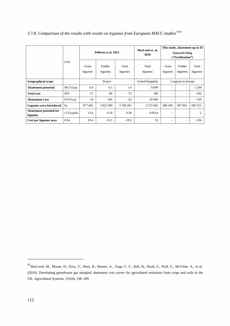
112

3.7.8. Comparison of the results with results on legumes from European MACC studies3738

Unit

Pellerin et al, 2013 MacLeod et. al,

2010

This study, abatement up to 45

Euros/tCO2eq

(“Fertilisation”)

Grain

legumes

Fodder

legumes

Total

legumes

Total

legumes

Grain

legumes

Fodder

legumes

Total

legumes

Geographical scope

France United Kingdom 5 regions in Europe

Abatement potential Mt CO2eq 0.9 0.5 1.4 0.009 - - 1.244

Total cost M € 17 -89 -72 188 - - -162

Abatement Cost €/tCO2eq 19 -185 -52 20 849 - - -130

Legumes area introduced ha 877 681 2 822 500 3 700 181 5 572 683 388 196 597 965 685 551

Abatement potential for

legumes t CO2eq/ha 1.03 0.18 0.38 0.0014 - - 2

Cost per legumes area €/ha 19.4 -31.5 -19.5 33 - - -236

37MacLeod, M., Moran, D., Eory, V., Rees, R., Barnes, A., Topp, C. F., Ball, B., Hoad, S., Wall, E., McVittie, A., et al.

(2010). Developing greenhouse gas marginal abatement cost curves for agricultural emissions from crops and soils in the

UK. Agricultural Systems, 103(4), 198–209.

113

3.7.9. Crop-frequency in the rotations (for crop abbreviations see Appendix 3.7.7)

Region Brandenburg Calabria

S-

Munt

enia

Eastern Scotland

Västs

verig

e

Site class

LB

G 1

LB

G2

LB

G3

LB

G4

LB

G5

irri

gat

ed

hig

hla

nd

irri

gat

ed

low

lan

d

rain

fed

cher

no

zem

Gra

de

1&

2

Gra

de

3

Gra

de

4

clay

No. of

rot. 345 2724 902 78 9 14 28 905 137 33852 33890 18 44607

alfalfa 215 1203 443 0 0 3 5 0 0 0 0 0 0

clover 0 0 0 0 0 3 0 13 0 0 0 0 0

combean 0 0 0 0 0 0 0 0 35 0 0 0 0

durum 0 0 0 0 0 0 6 227 0 0 0 0 0

fababea 202 729 0 0 0 0 17 440 0 15345 15345 0 2016

graclov 0 126 109 48 0 0 0 0 0 0 20 10 100

grass 0 0 0 0 0 0 0 0 0 0 18 8 100

linseed 0 0 0 0 0 0 0 0 0 0 0 0 22733

lupin 0 0 248 31 3 9 0 0 0 0 0 0 0

maize_g 0 0 0 0 0 0 0 0 90 0 0 0 0

maize_s 277 1839 637 66 0 0 24 0 0 0

0 9629

oatvetc 0 0 0 0 0 0 0 440 0 0 0 0 0

pea 0 909 262 31 0 0 17 440 63 13872 13872 0 19666

peaoat 0 0 0 0 0 0 0 0 0 0 0 0 19667

potato 0 0 0 0 0 14 0 0 0 25098 25098 0 0

ryevetc 0 0 0 0 7 0 0 0 0 0 0 0 0

Spring

Barley 0 1172 440 0 0 0 0 0 0 22648 22669 11 21164

seradel 0 0 0 0 3 0 0 0 0 0 0 0 0

Spring

Oat 0 1385 480 0 0 0 0 0 0 17261 17282 11 26308

soybean 0 0 0 0 0 0 0 0 35 0 0 0 0

srape 0 0 0 0 0 0 0 0 0 20007 20011 0 14718

sunfl 0 0 0 0 0 0 0 0 28 0 0 0 0

swedes 0 0 0 0 0 0 0 0 0 3141 3143 2 0

swheat 0 0 0 0 0 0 0 0 0 11584 11588 0 18225

tritica 130 986 0 0 0 0 4 307 0 0 0 0 19805

Winter

Barley 125 689 0 0 0 0 6 329 79 14117 14121 0 0

woat 0 0 0 0 0 0 4 307 0 11032 11036 4 0

Winter

Rape 30 313 80 0 0 9 0 784 131 3414 3418 0 5646

Winter

Rye 228 1607 790 78 9 0 0 0 0 0 0 0 19805

Winter

Wheat 157 825 115 0 0 14 5 310 115 15587 15591 0 22623

The frequency of crops presented in rotations in the different site classes does not reflect the statistical

crop proportions of the site class, as the possible rotations are generated to represent all agronomically

feasible rotations, rather than a representative set of rotations used in the site classes. However, it

gives an overview of the crops appearing at different site classes, and gives an indication of the

composition of the rotations. For instance, grass appears in 8 out of 18 rotations in Grade 4 (Eastern

114

Scotland) – the high GHG emissions and low gross margin of this crop influences these eight rotations

and subsequently the MAC curve.

115

Chapter 3

Risk as a limit or an opportunity to climate change

mitigation? The case of fertilisation

In this chapter, we investigate how risk and risk aversion influence the fertilisation behavior of

farmers. We show analytically that a decreasing variance of yield along with nitrogen inputs

encourages risk averse farmers to apply larger quantities of fertilizers compared with risk neutral

behavior. Then, we use data concerning three departments in France (Deux-Sèvres, Seine-

Maritime and Eure-et-Loir) to determine (i) crop yield response function to N fertilizers and (ii)

risk aversion behavior of farmers on the basis of their actual fertilizers applications. We find that

risk averse farmers represent 29,7% of farmers while risk seeking ones represent 35,5%. Risk

aversion behavior is associated with an additional application of 29 kg/ha compared with risk

neutral behavior which represents an average loss of 76 euros/ha. We show that the reduction of

abatement linked to risk aversion behavior should appear only when crop yield variance is convex

with respect to N fertilizers. Lastly, our results show that an insurance covering yield variability

could be foreseen as an interesting tool to mitigate emissions.

Ce chapitre reprend un article réalisé en collaboration avec Emmanuel Servonnat39

.

Acknowledgment

Warm thanks go to Stéphane De Cara, Philipe Delacote, Shahbano Soomro, Marielle Brunette and

Caroline Orset for their reading and advice.

JEL codes : Q15, Q18, F64, H23, N53

39 InVivo-Agrosolution.

116

4.1. Introduction

Nitrogen pollution is a significant environmental issue around the world and in Europe (Galloway et

al, 2008 ; European Commission, 2013). The carbon cycle usually receives more attention than the

nitrogen cycle, due to the central role of CO2 in global warming. However, the nitrogen cycle is also

deeply disordered by human activities especially through fertilisation of agricultural soils. This

disruption brings a range of impacts, from accelerating climate change to participating in water

pollution and generates high external costs (Von Blottnitz et al, 2006). In the European Union,

fertilisation from farm activities accounts for 38% of agricultural greenhouse gas (GHG) emissions

and represents 4% of the overall European emissions (in 2014 according to the UNFCCC, 2016)40

.

France constitutes also a good example of the nitrogen over-application issue due to the importance of

the agricultural sector in French economy and since air and water pollution by nitrogen has been

highlighted by many studies (Dalmas, 2010).

In response to these environmental consequences, important regulations on fertilisation have been

undertaken. In the forefront, the Nitrate Directive limits nitrogen application on specific areas and

affects indirectly farming externalities, including GHG emission, but the ambitious national and

international commitments to cut global emissions41

strengthen the necessity to mitigate emissions in a

cost-efficient way.

To tackle the pressing problem of climate mitigation it is generally argued that the most efficient

instrument is emission pricing (Lamhauge and Cox, 2013; Ellerman et al., 2010). Many papers have

investigated the potential impact of setting up this instrument in agriculture even though this sector has

been set aside from European and national climate policies. To name a few, De Cara and Jayet (2011)

evaluated the impact of a tax on fertilisation and induced reductions of greenhouse gases. Bourgeois et

al. (2014) also simulated the impact of a tax on fertilizer application coupled with subsidies on

perennial crops such as miscanthus. Likewise, Dequiedt and Moran (2015) assessed the impact on

legume crops and the resulting impact on GHG emissions. These papers are all based on the

assumption of profit maximization or cost minimization but little attention has been paid to other

essential elements of the decision-making process of farmers. Among those elements, risk

management appears as a determining dimension in the production choice of farmers (Chavas and

Holt, 1990; Cook et al., 2013; Menapace et al., 2013) and could constitute a potential barrier to

40 In France, nitrogen fertilisation accounts for 44% of greenhouse emissions (GHG) from French agriculture and alone

represents 8 % of national emissions in 2014 (UNFCCC, 2016)

41 See for instance the European Council agreement in October 2014 aiming to reduce European greenhouse gas emissions by

40% by 2030 relative to 1990 levels

117

mitigate emissions. Indeed, in a survey conducted on the behavior of farmers, Dury (2011) reveals for

instance that less than 1% of farmers cite profit maximization as the sole decision criterion. 71% of

them seek instead a "good" profit associated with minimal risk. Besides, Berentsen et al. (2012) show

that the risks associated with organic dairy farms are more important than the risk of conventional

agriculture (both on the size of the production and agricultural prices) and therefore limits the change

of practices. Interested in the barriers associated with a fertilisation reduction program in the United

States, Stuart et al. (2014) have shown that the yield loss associated with reduced fertilisation is

considered as an important and immediate risk. For most of the interviewed farmers, applying an

additional amount of fertilizer is perceived as a way to reduce exposure to production risks. Therefore,

it is appropriate to study the impact of risk on the incentive effect of a emission price and also to

consider the potential role of insurance as a tool to reduce emissions from fertilisation.

This paper contributes to the literature on GHG mitigation cost assessment in agriculture by providing

some analytical and quantitative insights into the following three main questions:

- How risk aversion can explain all (or a part of) nitrogen over-application?

- To what extent risk aversion can limit the mitigation incentive created by a emission price on

GHG emissions?

- If farmers use fertilizers as self-insurance, what would be the emissions reduction triggered by

an insurance program to mitigate emissions?

For these purposes, we use an original data base, completed by InVivo-Agrosolution farming

cooperative, which allows us obtaining a large sample of farmers’data located in three departments in

France. We first use feasible generalized least square (FGLS) regression to determine the link between

yield variability and nitrogen application at the plot level. In a second step, we use these results to

derive risk aversion coefficient consistent with actual farmers’ fertilizers spreading. Then, these

coefficients are used to simulate the impact of emission price and also to simulate the impact of an

insurance system on emissions.

The next section presents the literature on risk and fertilisation. Section 3 details the model of farmers’

decision-making on nitrogen application. Data and econometric method are presented in Section 4.

Section 5 presents the results. Discussion is given in section 6.

118

4.2. Literature review on risk and fertilisation

Can nitrogen be used by farmers to reduce their exposure to risk? The answer to this question depends

on the link between inputs and yield variability (Lambert, 1990; Leather and Quiggin, 1991).

Although this topic has been widely studied in the literature, there is no clear consensus on this link.

First, an important stream of empirical studies concludes that fertilizers are a risk-increasing factor as

they have variance-increasing effect on yield (Just and Pope, 1979; Rajsic et al., 2009; Montjardino et

al., 2015). This statement depends on weather uncertainty, which implies high level of yield in good

growing years and low in bad growing years. This uncertainty has two possible effects depending on

the consideration of farmers risk aversion. On one hand, according to Babcock (1992), who takes into

account solely the expected profit in the farmer objective function, farmers should be tempted to apply

larger amount of nitrogen compared to the case where yield variability is not considered. Since

farmers do not know what the growing conditions will be before nitrogen application, it is optimal for

them to anticipate good conditions so that nitrogen will not limit potential profits in those years. On

the other hand, other studies concludes that in reason of their risk aversion, farmers tend to spread less

fertilizers so as to limit the probability of bad events (Montjardino et al., 2015; Broun, 2007; Finger,

2012). Second, an alternate stream concludes that fertilizers could conversely be a risk reducing factor.

Because unobservable processes (such as leaching, denitrification or nitrogen up-take in previous crop

in rotation) influence the availability of nitrogen in the soil this could results in reducing the variability

of yields as nitrogen amount increases (Gandorfer et al., 2011 ; Comifer, 2011) and then could favor

the over-application of fertilizers. This corresponds to studies focusing on risk perception of farmers,

who consider nitrogen as a risk-decreasing input (SriRamaratnam, 1987; Stuart et al, 2014). Third,

some studies argue that the link between fertilisation and variability can not be clearly established.

Regev and al. (1997) show no conclusive evidence to assert if nitrogen is either risk-reducing or risk-

increasing. Then, according to Antle (2010) empirical study on potato production, the conclusion on

this link depends on utility framework implemented: a risk-value model based on partial moments

implies that fertilizer is risk increasing, whereas an expected utility model based on full moments has

the opposite implications. One explanation for these seemingly contradictory conclusions is the

diverse climate and agricultural contexts of studies. Going forward, it seems necessary to assess the

role of nitrogen at each geographical level to see whether it is a risk-reducing factor or a risk-

increasing factor.

Some papers have addressed the question of the impact of insurance on chemical input use.

Theoretically, two different effects have been identified (Bougherara, 2011). The first effect is linked

to the above-discussed risk-reduction effect. As insurance increases income in bad states of nature,

while decreasing income in good states of nature by charging a premium, it thereby cause farmer to act

more like risk-neutral farmer (Sheriff, 2005). Hence, the impact on input use relies on the relationship

119

between fertilizer and risk. If chemical inputs are risk-reducing then they will reduce the amount

spread, with the opposite effect if they are risk increasing. The effect one is the moral hazard effect. It

occurs when producers take actions to increase the probability and size of losses, and provide

incentives for less intensive cultivation practices that result in reduction of inputs and average yields

(Coble et al., 1993). Which effect dominates has been examined by empirical papers. In a study

conducted on corn farmers, Horowitz and Lichtenberg (1993) conclude that insured farmers applied

significantly more nitrogen per acre (+19%) than uninsured one, thus supporting the view that

chemical inputs are a risk-increasing input. However these results were latter contradicted by Smith

and Goodwin (1996) who confirm the view that moral hazard incentivizes insured farmers to use

fewer chemical inputs.

As global warming is expected to cause an increase in the frequency of extreme climate events,

insurance is mainly foreseen as a tool to favor adaptation to climate change (Smit and Skinner, 2002).

However, as chemical input have been highlighted to play the role of a self-insurance when their risk-

reducing ability have been elicited (see for instance Bougherara, 2011 for pesticides), insurance could

also be considered as a possible tool to support the implementation of environmental measures42

. This

potential is for instance developed by Huang et al. (2001) who, in a study of US agriculture,

analytically and empirically show that an insurance system can help to reduce the amounts of nitrogen

applied by the farmer. So far, to our knowledge it has not been used as a tool to limit agricultural

environmental externalities. Yet, an interesting example of the possible forthcoming role of

instruments that support the adoption of environmental measures , by tackling uncertainty and risk, is

provided by the 2015 framework convention between the Loire-Bretagne Water Agency and local

farming cooperatives (Agence de l’Eau – Loire Bretagne, 2015). The objective of this convention is to

favor the implication of farmers in improving the quality of water. Among the different incentives, the

convention plans to establish the reimbursement of losses due to the implementation of innovation

only in case of failure.

42 In France, the current agricultural insurance system is characterized by public and private intervention that help to cover

damages caused by frost, hail or drought. The public intervention is under the responsibility of the FNGRA (Le Fonds

national de gestion des risques en agriculture) and aims to cover farmers against uninsurable risk. Insurable risks are covered

by the private market, alongside government intervention: farmers receive a grant representing at most 65% of the insurance

premium.

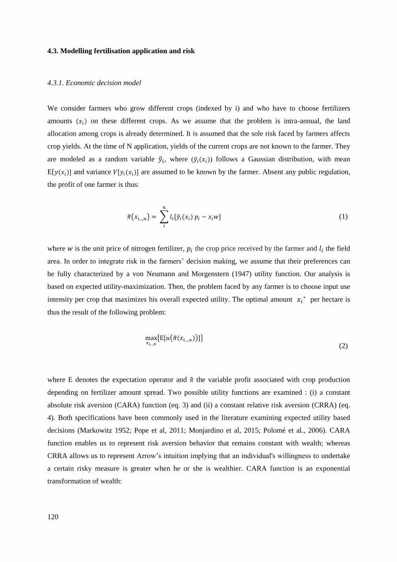
120

4.3. Modelling fertilisation application and risk

4.3.1. Economic decision model

We consider farmers who grow different crops (indexed by i) and who have to choose fertilizers

amounts (𝑥𝑖) on these different crops. As we assume that the problem is intra-annual, the land

allocation among crops is already determined. It is assumed that the sole risk faced by farmers affects

crop yields. At the time of N application, yields of the current crops are not known to the farmer. They

are modeled as a random variable �̃�𝑖, where (�̃�𝑖(𝑥𝑖)) follows a Gaussian distribution, with mean

E[𝑦(𝑥𝑖)] and variance 𝑉[𝑦𝑖(𝑥𝑖)] are assumed to be known by the farmer. Absent any public regulation,

the profit of one farmer is thus:

�̃�(𝑥𝑖,..,𝑛) = ∑ 𝑙𝑖[�̃�𝑖(𝑥𝑖) 𝑝𝑖 − 𝑥𝑖𝑤]

𝑛

𝑖

(1)

where 𝑤 is the unit price of nitrogen fertilizer, 𝑝𝑖 the crop price received by the farmer and 𝑙𝑖 the field

area. In order to integrate risk in the farmers’ decision making, we assume that their preferences can

be fully characterized by a von Neumann and Morgenstern (1947) utility function. Our analysis is

based on expected utility-maximization. Then, the problem faced by any farmer is to choose input use

intensity per crop that maximizes his overall expected utility. The optimal amount 𝑥𝑖∗ per hectare is

thus the result of the following problem:

max𝑥𝑖,..,𝑛

{E[𝑢(�̃�(𝑥𝑖,..,𝑛))]}

(2)

where E denotes the expectation operator and �̃� the variable profit associated with crop production

depending on fertilizer amount spread. Two possible utility functions are examined : (i) a constant

absolute risk aversion (CARA) function (eq. 3) and (ii) a constant relative risk aversion (CRRA) (eq.

4). Both specifications have been commonly used in the literature examining expected utility based

decisions (Markowitz 1952; Pope et al, 2011; Monjardino et al, 2015; Polomé et al., 2006). CARA

function enables us to represent risk aversion behavior that remains constant with wealth; whereas

CRRA allows us to represent Arrow’s intuition implying that an individual's willingness to undertake

a certain risky measure is greater when he or she is wealthier. CARA function is an exponential

transformation of wealth:

121

𝑢(�̃�) = −𝑒−𝛼�̃�

(3)

where 𝛼 is the absolute risk aversion parameter (𝛼 > 0 for a risk averse agent; 𝛼 < 0 for a risk loving

agent). CRRA is a power function and is represented as follow:

𝑢(�̃�) =

�̃�(1−𝑟)

1 − 𝑟

(4)

Where r is the relative risk aversion coefficient. Relative risk aversion and relative risk loving

preferences are obtained respectively for r > 0 and 𝑟 < 0. As yields are assumed to follow a Gaussian

distribution, in both cases (CARA and CRRA), the expected utility can be written in function of the

expected profit and the variance profit (V) (see appendix 4.8.1 and 4.8.2 for details) as follow:

max𝑥𝑖,..,𝑛

{𝐸[𝑢(𝜋(̃𝑥𝑖,..,𝑛))] = 𝑎 + 𝑏. 𝐸 [∑ �̃�𝑖(𝑥𝑖)

𝑛

𝑖

] − 𝑐. 𝑉 [∑ �̃�𝑖(𝑥𝑖)

𝑛

𝑖

]} (5)

With a=𝜋0 for CARA preferences and a=𝑢(2𝜋0) + 𝑢′(2𝜋0)𝜋0 for CRRA preferences, 𝜋0 being the

initial wealth of a farmer. b=1 for CARA preferences and b= 𝑢′(2𝜋0) for CRRA preferences.

c=−𝑢′′(2𝜋0)

2=

𝑟(2𝜋0)−1−𝑟

2 for CRRA preferences and c=

𝛼

2 for CARA preferences.

We found no covariance between the different yield functions43

. Then, the solutions of the overall

maximization program are equivalent to the solutions of individual field maximization program:

max𝑥𝑖

{𝐸[𝑢(�̃�𝑖(𝑥𝑖))] = 𝑏. 𝐸[�̃�𝑖(𝑥𝑖)] − 𝑐. 𝑉[�̃�𝑖(𝑥𝑖)]} (6)

This form of equation allows us to represent in the objective function both expected income and profit

variability, both of which are determined by nutrient input. The optimal input 𝑥𝑖∗ must satisfy the first

order condition given by:

𝑑𝐸[𝑢(𝜋�̃�(𝑥𝑖∗))]

𝑑𝑥𝑖

=𝑑𝐸[𝜋�̃�(𝑥𝑖

∗)]

𝑑𝑥𝑖

− 𝑘 𝑑𝑉[𝜋�̃�(𝑥𝑖

∗)]

𝑑𝑥𝑖

= 0

(7)

43 This finding is consistent for instance with Polomé et al. (2006) study on acreage allocation under

risk where no covariance was found between crops after examination of panels of yields.

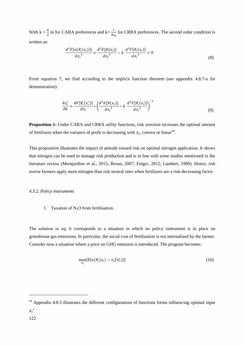
122

With k = 𝛼

2 in for CARA preferences and k=

𝑟

4𝜋0 for CRRA preferences. The second order condition is

written as:

𝑑2𝐸[𝑢(𝜋�̃�(𝑥𝑖))]

𝑑𝑥𝑖2 =

𝑑2𝐸[�̃�(𝑥𝑖)]

𝑑𝑥𝑖2 − 𝑘

𝑑2𝑉[𝜋�̃�(𝑥𝑖)]

𝑑𝑥𝑖2 < 0

(8)

From equation 7, we find according to the implicit function theorem (see appendix 4.8.7-a for

demonstration):

𝜕𝑥𝑖∗

𝜕𝑘=

𝑑𝑉[𝜋�̃�(𝑥𝑖∗)]

𝑑𝑥𝑖

∗ (𝑑2𝐸[�̃�(𝑥𝑖)]


𝑑2𝑉[𝜋�̃�(𝑥𝑖)]

𝑑𝑥𝑖2 )

−1

(9)

Proposition 1: Under CARA and CRRA utility functions, risk aversion increases the optimal amount

of fertilizers when the variance of profit is decreasing with 𝑥𝑖, convex or linear44

.

This proposition illustrates the impact of attitude toward risk on optimal nitrogen application. It shows

that nitrogen can be used to manage risk production and is in line with some studies mentioned in the

literature review (Montjardino et al., 2015; Broun, 2007; Finger, 2012; Lambert, 1990). Hence, risk

averse farmers apply more nitrogen than risk neutral ones when fertilizers are a risk-decreasing factor.

4.3.2. Policy instruments

1. Taxation of N2O from fertilisation.

The solution to eq. 6 corresponds to a situation in which no policy instrument is in place on

greenhouse gas emissions. In particular, the social cost of fertilisation is not internalized by the farmer.

Consider now a situation where a price on GHG emission is introduced. The program becomes:

max𝑥𝑖

{E[𝑢(𝜋�̃�(𝑥𝑖) − 𝑥𝑖𝑓𝑡𝑙𝑖)]}

(10)

44 Appendix 4.8.3 illustrates the different configurations of functions forms influencing optimal input

𝑥𝑖∗

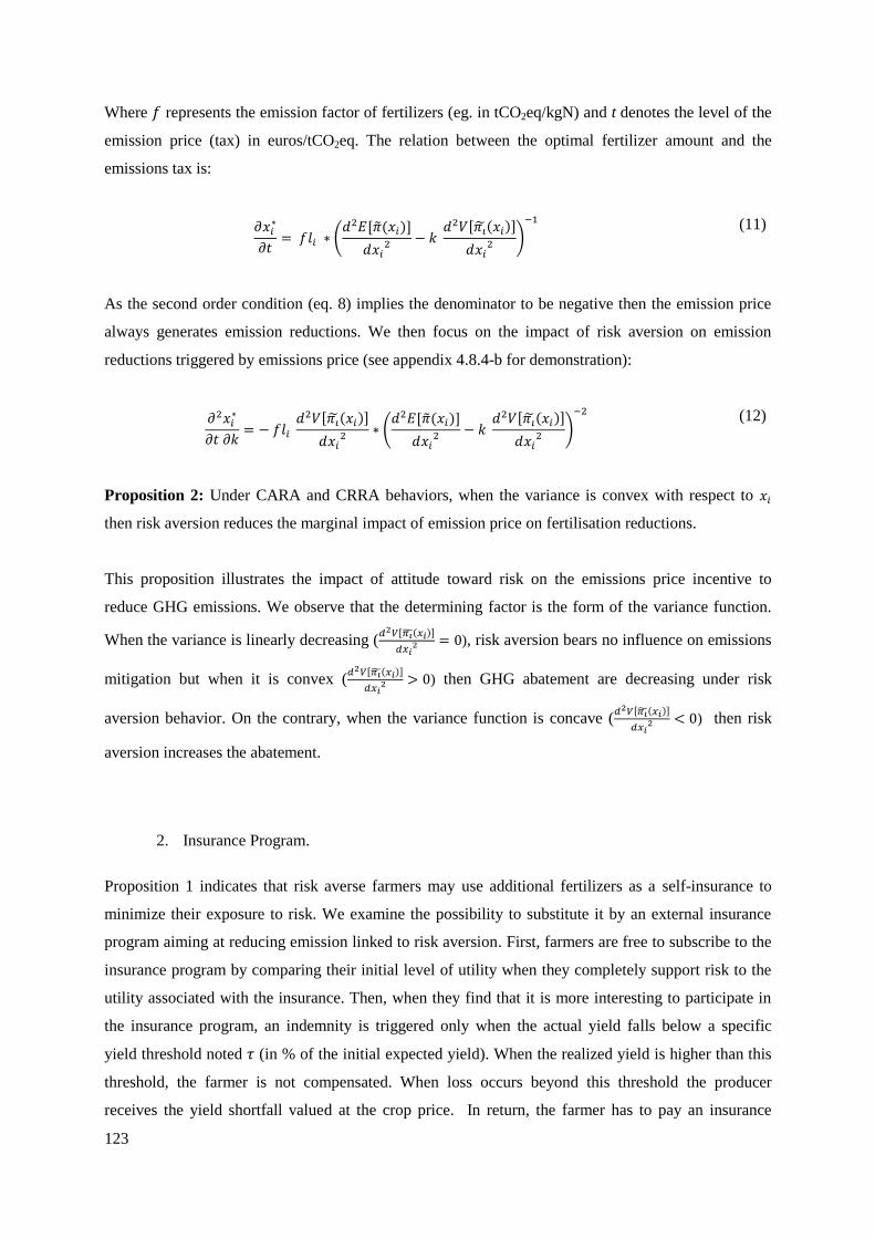
123

Where 𝑓 represents the emission factor of fertilizers (eg. in tCO2eq/kgN) and t denotes the level of the

emission price (tax) in euros/tCO2eq. The relation between the optimal fertilizer amount and the

emissions tax is:

𝜕𝑥𝑖∗

𝜕𝑡= 𝑓𝑙𝑖 ∗ (

𝑑2𝐸[�̃�(𝑥𝑖)]


𝑑2𝑉[𝜋�̃�(𝑥𝑖)]

𝑑𝑥𝑖2 )

−1

(11)

As the second order condition (eq. 8) implies the denominator to be negative then the emission price

always generates emission reductions. We then focus on the impact of risk aversion on emission

reductions triggered by emissions price (see appendix 4.8.4-b for demonstration):

𝜕2𝑥𝑖∗

𝜕𝑡 𝜕𝑘= − 𝑓𝑙𝑖

𝑑2𝑉[𝜋�̃�(𝑥𝑖)]

𝑑𝑥𝑖2 ∗ (

𝑑2𝐸[�̃�(𝑥𝑖)]


𝑑2𝑉[𝜋�̃�(𝑥𝑖)]

𝑑𝑥𝑖2 )

−2

(12)

Proposition 2: Under CARA and CRRA behaviors, when the variance is convex with respect to 𝑥𝑖

then risk aversion reduces the marginal impact of emission price on fertilisation reductions.

This proposition illustrates the impact of attitude toward risk on the emissions price incentive to

reduce GHG emissions. We observe that the determining factor is the form of the variance function.

When the variance is linearly decreasing (𝑑2𝑉[𝜋�̃�(𝑥𝑖)]

𝑑𝑥𝑖2 = 0), risk aversion bears no influence on emissions

mitigation but when it is convex (𝑑2𝑉[𝜋�̃�(𝑥𝑖)]

𝑑𝑥𝑖2 > 0) then GHG abatement are decreasing under risk

aversion behavior. On the contrary, when the variance function is concave (𝑑2𝑉[𝜋�̃�(𝑥𝑖)]

𝑑𝑥𝑖2 < 0) then risk

aversion increases the abatement.

2. Insurance Program.

Proposition 1 indicates that risk averse farmers may use additional fertilizers as a self-insurance to

minimize their exposure to risk. We examine the possibility to substitute it by an external insurance

program aiming at reducing emission linked to risk aversion. First, farmers are free to subscribe to the

insurance program by comparing their initial level of utility when they completely support risk to the

utility associated with the insurance. Then, when they find that it is more interesting to participate in

the insurance program, an indemnity is triggered only when the actual yield falls below a specific

yield threshold noted 𝜏 (in % of the initial expected yield). When the realized yield is higher than this

threshold, the farmer is not compensated. When loss occurs beyond this threshold the producer

receives the yield shortfall valued at the crop price. In return, the farmer has to pay an insurance

124

premium 𝐼 in (euros/ha) whatever the amount of the realized yield. As we want to find the optimal

nitrogen application amount, the expected utility maximization program under insurance participation

can be written as:

max�̅�𝑖

{E[𝑢(𝜋�̃�(�̅�𝑖) − 𝐼)]} (13)

s.t 𝑥𝑖∗ ≥ �̅�𝑖 > 0

With �̅�𝑖 being the amount of nitrogen application under insurance. In a more detailed form eq.14

becomes :

E[𝑢(𝜋�̃�(𝑥_𝑖𝑛𝑠) − 𝐼)] = ∫ 𝑔 (�̃�𝑖(�̃�𝑖(𝑥_𝑖𝑛𝑠))) 𝑢(𝜋𝑖(𝜏) − 𝐼)𝑑𝑦

𝜏

0

+ ∫ 𝑔 (�̃�𝑖(�̃�𝑖(𝑥_𝑖𝑛𝑠))) 𝑢(𝜋𝑖(𝑦) − 𝐼)𝑑𝑦

+∞

𝜏

(14)

With 𝑔(�̃�𝑖) being the probability density function of a normal distribution. Participation in the

insurance program occurs when E[𝑢(𝜋�̃�(𝑥_𝑖𝑛𝑠𝑖∗) − 𝐼)] > E[𝑢(𝜋�̃�(𝑥𝑖

∗))] and emissions reductions occur

when the optimal �̅�𝑖∗ with insurance is lower than 𝑥i

∗ maximizing the initial expected utility with no

insurance. Appendix 4.8.5 illustrates 3 different cases of the impact of insurance on emission

reductions.

4.4. Empirical Application

4.4.1. Data

The data used in this paper come from Epicles, a database compiled by InVivo-Agrosolution, a French

farming cooperative. It comprises the fertilisation practices of farmers who are members of the

cooperative, in particular the amount of nitrogen spread for each farmer, the amount prescribed by the

cooperative, the resulting crop yield, the soil type and the preceding crop in the rotation. This

information is available at the field level and is highly detailled in comparison to other data bases used

in the literature45

.

We chose to restrict our attention to three departments (Deux-Sèvres, Seine-Maritime et Eure-et-Loir).

Foremost this is because those departments are well represented in Epicles database and, also because,

they represent a diversity of farming conditions. Deux-Sèvres department is mostly composed by

45 The European FADN (Farm accountancy Data Network) database, for instance, gathers data from representative farms of

a given territory but not the data of all farms. Besides, it does not give information on the amount of fertilizers but the cost

linked to fertilization.

125

livestock and cropping systems and is characterized by relative low yield, Seine-Maritime comprises

also livestock and cropping systems, but with higher yields, and Eure-et-Loir which covers a part of

the Beauce region, is mainly characterized by the presence of cropping farms with high yields and

relatively low diversity in the crops composition. The Epicles database covers 22,5% of the Deux-

Sèvres cereals land use, 10,7% of Seine-Maritime land use and 20,0 % of Eure-et-Loir land use.

We focus on 10 main crops : common wheat, oat, rape seed, durum wheat, fodder maize, grain maize,

spring barley, winter barley, sunflower and triticale. We use data for four harvest campaigns (2010,

2011, 2012 and 2013) to assess the parameters of the yield and variance functions. We remove from

the data set crop categories (characterized by a department location, a soil type, and a preceding crop

type) whose number is inferior to 30. To isolate the effect of nitrogen on yield we do not examine

plots having received any mineral element (K, S, P etc.) other than nitrogen. In addition, farmers who

do not report their nitrogen application are also eliminated from the study. In some cases, the

declaration is systematically the same as the amount advised by the cooperative or when the amount of

nitrogen applied is 0. These cases are also left out. Finally, a total of 24 729 observations are used in

the regressions (see table 6). The impact of a tax on GHG emissions and the implementation of an

insurance program are assessed using the initial fertilisation levels of the 2013 campaign which

represents 2 774 plots (appendix 4.8.6 gives a detailed overview of the different steps in the data base

treatment).

Table 6 - Description of the sample used in the regression (step 2 of the data base treatment)

Source Unit

Deux-Sèvres

(79)

Seine-

Maritime

(76)

Eure-et-Loir

(28) Overall

Number of

observations Epicles 16 007 4 691 4 031 24 729

Land Area

(year 2013) Epicles ha 14 607 8 434 7 323 23 041

Number of Farms

concerned Epicles

1065 581 655 2 301

Average Chemical

Fertilizer

application for

wheat

(year : 2011)

Epicles kg.ha-1 137 183 163 -

Agreste Crop

Survey

(Agreste,

2014)

kg.ha-1 138 158 160 -

Average Yield for

wheat

(year : 2011)

Epicles q/ha 68 85 79 -

Agreste Crop

Survey

(Agreste,

2014)

q/ha 60 62 78 -

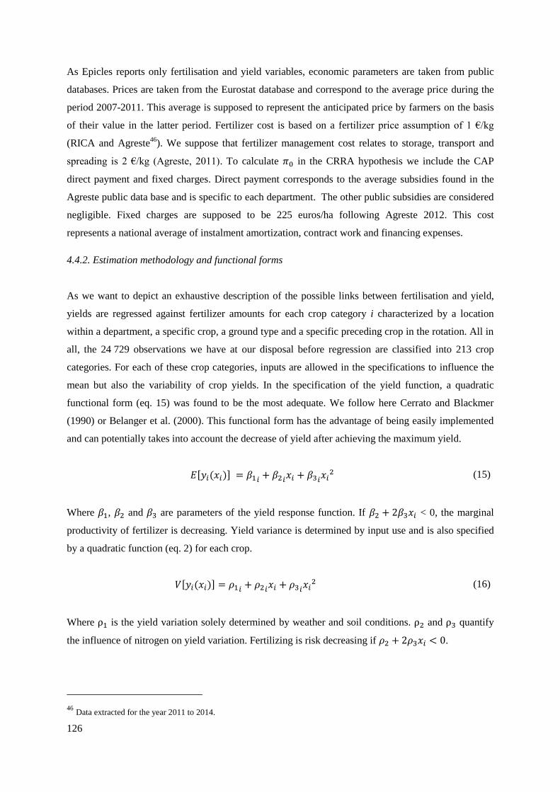
126

As Epicles reports only fertilisation and yield variables, economic parameters are taken from public

databases. Prices are taken from the Eurostat database and correspond to the average price during the

period 2007-2011. This average is supposed to represent the anticipated price by farmers on the basis

of their value in the latter period. Fertilizer cost is based on a fertilizer price assumption of 1 €/kg

(RICA and Agreste46

). We suppose that fertilizer management cost relates to storage, transport and

spreading is 2 €/kg (Agreste, 2011). To calculate 𝜋0 in the CRRA hypothesis we include the CAP

direct payment and fixed charges. Direct payment corresponds to the average subsidies found in the

Agreste public data base and is specific to each department. The other public subsidies are considered

negligible. Fixed charges are supposed to be 225 euros/ha following Agreste 2012. This cost

represents a national average of instalment amortization, contract work and financing expenses.

4.4.2. Estimation methodology and functional forms

As we want to depict an exhaustive description of the possible links between fertilisation and yield,

yields are regressed against fertilizer amounts for each crop category i characterized by a location

within a department, a specific crop, a ground type and a specific preceding crop in the rotation. All in

all, the 24 729 observations we have at our disposal before regression are classified into 213 crop

categories. For each of these crop categories, inputs are allowed in the specifications to influence the

mean but also the variability of crop yields. In the specification of the yield function, a quadratic

functional form (eq. 15) was found to be the most adequate. We follow here Cerrato and Blackmer

(1990) or Belanger et al. (2000). This functional form has the advantage of being easily implemented

and can potentially takes into account the decrease of yield after achieving the maximum yield.

𝐸[𝑦𝑖(𝑥𝑖)] = 𝛽1𝑖 + 𝛽2𝑖𝑥𝑖 + 𝛽3𝑖𝑥𝑖

2 (15)

Where 𝛽1, 𝛽2 and 𝛽3 are parameters of the yield response function. If 𝛽2 + 2𝛽3𝑥𝑖 < 0, the marginal

productivity of fertilizer is decreasing. Yield variance is determined by input use and is also specified

by a quadratic function (eq. 2) for each crop.

𝑉[𝑦𝑖(𝑥𝑖)] = 𝜌1𝑖 + 𝜌2𝑖𝑥𝑖 + 𝜌3𝑖𝑥𝑖

2 (16)

Where ρ1 is the yield variation solely determined by weather and soil conditions. ρ2 and ρ3 quantify

the influence of nitrogen on yield variation. Fertilizing is risk decreasing if 𝜌2 + 2𝜌3𝑥𝑖 < 0.

46 Data extracted for the year 2011 to 2014.

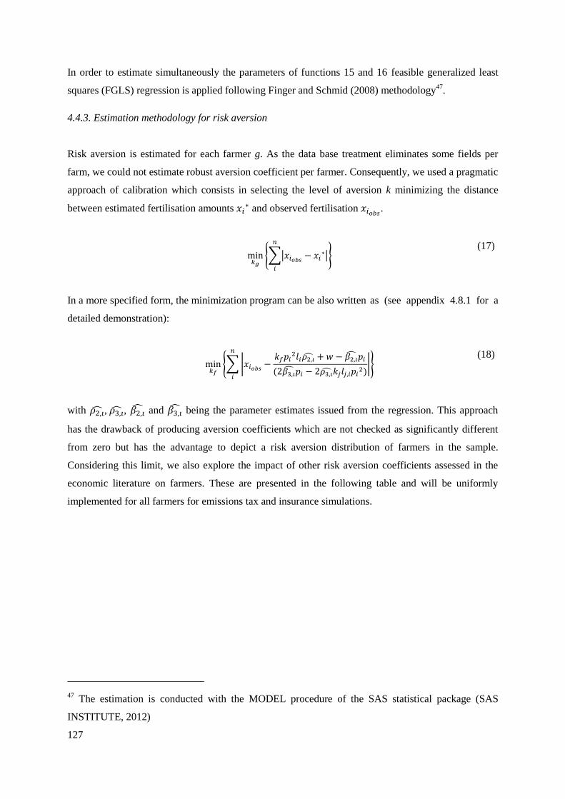
127

In order to estimate simultaneously the parameters of functions 15 and 16 feasible generalized least

squares (FGLS) regression is applied following Finger and Schmid (2008) methodology47

.

4.4.3. Estimation methodology for risk aversion

Risk aversion is estimated for each farmer g. As the data base treatment eliminates some fields per

farm, we could not estimate robust aversion coefficient per farmer. Consequently, we used a pragmatic

approach of calibration which consists in selecting the level of aversion k minimizing the distance

between estimated fertilisation amounts 𝑥𝑖∗ and observed fertilisation 𝑥𝑖𝑜𝑏𝑠

.

min

𝑘𝑔

{∑|𝑥𝑖𝑜𝑏𝑠− 𝑥𝑖

∗|

𝑛

𝑖

}

(17)

In a more specified form, the minimization program can be also written as (see appendix 4.8.1 for a

detailed demonstration):

min

𝑘𝑓

{∑ |𝑥𝑖𝑜𝑏𝑠−

𝑘𝑓𝑝𝑖2𝑙𝑖𝜌2,�̂� + 𝑤 − 𝛽2,�̂�𝑝𝑖

(2𝛽3,�̂�𝑝𝑖 − 2𝜌3,�̂�𝑘𝑗𝑙𝑗,𝑖𝑝𝑖2)

|

𝑛

𝑖

} (18)

with 𝜌2,�̂�, 𝜌3,�̂�, 𝛽2,�̂� and 𝛽3,�̂� being the parameter estimates issued from the regression. This approach

has the drawback of producing aversion coefficients which are not checked as significantly different

from zero but has the advantage to depict a risk aversion distribution of farmers in the sample.

Considering this limit, we also explore the impact of other risk aversion coefficients assessed in the

economic literature on farmers. These are presented in the following table and will be uniformly

implemented for all farmers for emissions tax and insurance simulations.

47 The estimation is conducted with the MODEL procedure of the SAS statistical package (SAS

INSTITUTE, 2012)

128

Table 7 – Aversion coefficient taken in the literature for sensitivity analysis

Scenarii Aversion Coefficient Type of aversion

coefficient

Source

« CARA 1 » Estimation Absolute Eq. 16

« CARA 2 » Uniform* : 7,5.10-7 Absolute Pope et al, 2011

« CARA 3 » Uniform* : 0,0075 Absolute Saha et al., 1994

« CARA 4 » Uniform* : 0,04 Absolute Brunette et al, 2015

« CRRA 2 » Uniform* : 0,25 Relative Lansink., 1999

“Value in the range [0,31-0,2]”

« CRRA 3 » Uniform* : 1,12 Relative Brunette et al, 2015

« CRRA 4 » Uniform* : 5,4 Relative Saha et al., 1994

* The same aversion coefficient for every farmer.

4.5. Results

4.5.1. Regression

We keep all of the estimates of the yield function (eq.15) and variance function (eq.16) associated with

a p-value inferior to 5% and only in cases where heteroscedasticity is not detected48

. Table presenting

the exhaustive results of the parameter estimates per crop type is available upon request or through the

link in the footnote49

. Over the 213 different crop categories, 160 have been consistently estimated and

53 have not been estimated, either because of failure in the convergence of the model, simultaneous

lack of significance in the parameter estimates or because of heteroscedasticity.

Table 8 presents a summary of the forms of the yield and variance functions derived from the

parameter estimates. Over the 160 crop types whose functions have been successfully estimated, 97 of

them follow a constant variance. For the others, the yield variance is influenced by nitrogen

application. Within the latter category, the majority of crops have a linear decreasing variance

function. Convex variance functions and concave variance functions come respectively second and

third. From these results we observe that cases where there is risk-decreasing significance of fertilizer

are relatively consistent and should not be neglected when assessing the emission tax impact.

48 Using the White and Breusch-Pagan tests.

49 The following link gives access to the table presenting the results of the regression :

https://docs.google.com/spreadsheets/d/1qmaiz7boFxlZOJmesc7r9rDtYnIZ8hXJJMUpCzFLUSg/edit?

usp=sharing

https://docs.google.com/spreadsheets/d/1qmaiz7boFxlZOJmesc7r9rDtYnIZ8hXJJMUpCzFLUSg/edit?usp=sharing

https://docs.google.com/spreadsheets/d/1qmaiz7boFxlZOJmesc7r9rDtYnIZ8hXJJMUpCzFLUSg/edit?usp=sharing

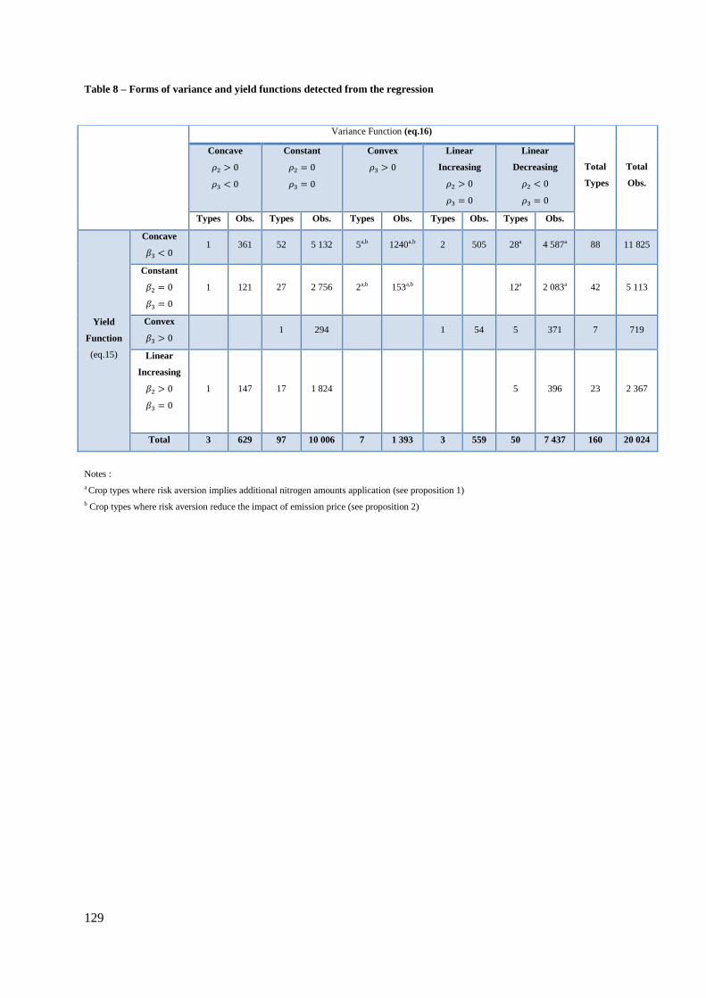
129

Table 8 – Forms of variance and yield functions detected from the regression

Notes :

a Crop types where risk aversion implies additional nitrogen amounts application (see proposition 1)

b Crop types where risk aversion reduce the impact of emission price (see proposition 2)

Variance Function (eq.16)

Total

Types

Total

Obs.

𝜌2 > 0

𝜌3 < 0

Concave

𝜌2 = 0

𝜌3 = 0

Constant

𝜌3 > 0

Convex

𝜌2 > 0

𝜌3 = 0

Linear

Increasing

𝜌2 < 0

𝜌3 = 0

Linear

Decreasing

Types Obs. Types Obs. Types Obs. Types Obs. Types Obs.

Yield

Function

(eq.15)

𝛽3 < 0

Concave 1 361 52 5 132 5a,b 1240a,b 2 505 28a 4 587a 88 11 825

𝛽2 = 0

𝛽3 = 0

Constant

1 121 27 2 756 2a,b 153a,b

12a 2 083a 42 5 113

𝛽3 > 0

Convex

1 294

1 54 5 371 7 719

𝛽2 > 0

𝛽3 = 0

Linear

Increasing

1 147 17 1 824

5 396 23 2 367

Total 3 629 97 10 006 7 1 393 3 559 50 7 437 160 20 024

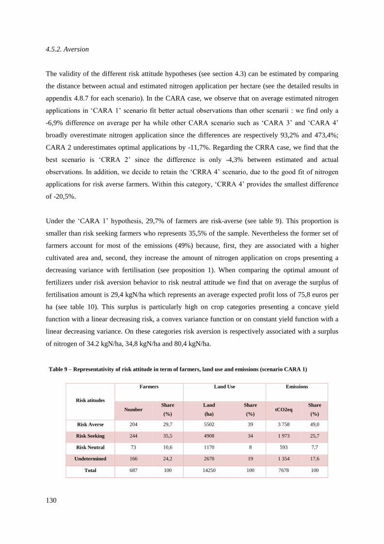
130

4.5.2. Aversion

The validity of the different risk attitude hypotheses (see section 4.3) can be estimated by comparing

the distance between actual and estimated nitrogen application per hectare (see the detailed results in

appendix 4.8.7 for each scenario). In the CARA case, we observe that on average estimated nitrogen

applications in ‘CARA 1’ scenario fit better actual observations than other scenarii : we find only a

-6,9% difference on average per ha while other CARA scenario such as ‘CARA 3’ and ‘CARA 4’

broadly overestimate nitrogen application since the differences are respectively 93,2% and 473,4%;

CARA 2 underestimates optimal applications by -11,7%. Regarding the CRRA case, we find that the

best scenario is ‘CRRA 2’ since the difference is only -4,3% between estimated and actual

observations. In addition, we decide to retain the ‘CRRA 4’ scenario, due to the good fit of nitrogen

applications for risk averse farmers. Within this category, ‘CRRA 4’ provides the smallest difference

of -20,5%.

Under the ‘CARA 1’ hypothesis, 29,7% of farmers are risk-averse (see table 9). This proportion is

smaller than risk seeking farmers who represents 35,5% of the sample. Nevertheless the former set of

farmers account for most of the emissions (49%) because, first, they are associated with a higher

cultivated area and, second, they increase the amount of nitrogen application on crops presenting a

decreasing variance with fertilisation (see proposition 1). When comparing the optimal amount of

fertilizers under risk aversion behavior to risk neutral attitude we find that on average the surplus of

fertilisation amount is 29,4 kgN/ha which represents an average expected profit loss of 75,8 euros per

ha (see table 10). This surplus is particularly high on crop categories presenting a concave yield

function with a linear decreasing risk, a convex variance function or on constant yield function with a

linear decreasing variance. On these categories risk aversion is respectively associated with a surplus

of nitrogen of 34.2 kgN/ha, 34,8 kgN/ha and 80,4 kgN/ha.

Risk atitudes

Farmers

Land Use

Emissions

Number Share

(%)

Land

(ha)

Share

(%) tCO2eq

Share

(%)

Risk Averse 204 29,7 5502 39 3 758 49,0

Risk Seeking 244 35,5 4908 34 1 973 25,7

Risk Neutral 73 10,6 1170 8 593 7,7

Undetermined 166 24,2 2670 19 1 354 17,6

Total 687 100 14250 100 7678 100

Table 9 – Representativity of risk attitude in term of farmers, land use and emissions (scenario CARA 1)

131

Table 10 - Impact of risk aversion on nitrogen application and expected profit (scenario “CARA 1”)

a Difference of profit between risk averse behavior and risk neutral behavior

Form of

Expected

Yield

Form of

Variance

function

X*

X*

under risk neutral

behavior

Nitrogen

Application

linked to risk

aversion

Expected

Profit

Expected Profit

under risk neutral

behavior

Loss

linked to

risk

aversiona

kgN/ha kgN/ha kgN/ha euros/ha euros/ha euros/ha

Concave

Constant 161 161,0 0,0 841 841 0,0

Convexe 153 118,2 34,8 366 553,5 187,4

LinInc 25 43,8 -18,3 691 752,4 61,5

LinDecr 169 134,7 34,2 641 703,3 62,7

Constant Constan

LinDecr 80 0,0 80,4 577 818,4 241,1

Linear

Inc.

Constant 109 109,1 0,0 1008 1007,9 0,1

LinDecr 115 114,7 0,0 336 335,6 0,4

Overall 146 116,7 29,4 684 759,9 75,8

0

5

10

15

20

25

30

35

40

45

Freq

uen

cy

(%)

Risk Aversion Coefficient (k) - 0,001 Rounded

CARA 1

Figure 19 - Risk aversion distribution of farmers (including risk averse, risk seeking

and risk neutral attitudes) - scenario CARA 1

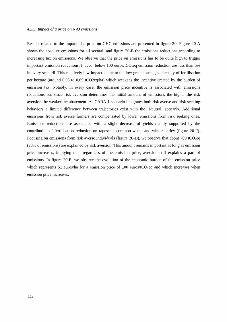
132

4.5.3. Impact of a price on N2O emissions

Results related to the impact of a price on GHG emissions are presented in figure 20. Figure 20-A

shows the absolute emissions for all scenarii and figure 20-B the emissions reductions according to

increasing tax on emissions. We observe that the price on emissions has to be quite high to trigger

important emission reductions. Indeed, below 100 euros/tCO2eq emission reduction are less than 5%

in every scenarii. This relatively low impact is due to the low greenhouse gas intensity of fertilisation

per hectare (around 0,05 to 0,65 tCO2eq/ha) which weakens the incentive created by the burden of

emission tax. Notably, in every case, the emission price incentive is associated with emissions

reductions but since risk aversion determines the initial amount of emissions the higher the risk

aversion the weaker the abatement. As CARA 1 scenario integrates both risk averse and risk seeking

behaviors a limited difference between trajectories exist with the ‘Neutral’ scenario. Additional

emissions from risk averse farmers are compensated by lower emissions from risk seeking ones.

Emissions reductions are associated with a slight decrease of yields mainly supported by the

contribution of fertilisation reduction on rapeseed, common wheat and winter barley (figure 20-F).

Focusing on emissions from risk averse individuals (figure 20-D), we observe that about 700 tCO2eq

(23% of emissions) are explained by risk aversion. This amount remains important as long as emission

price increases, implying that, regardless of the emission price, aversion still explains a part of

emissions. In figure 20-E, we observe the evolution of the economic burden of the emission price

which represents 51 euros/ha for a emission price of 100 euros/tCO2eq and which increases when

emission price increases.

133

A. Evolution of emissions under different risk scenarii B. Marginal abatement cost curves under different risk scenarii

C. Evolution of emissions according to risk attitude (scenario CARA 1) D. Impact of risk aversion of emissions (scenario CARA 1)

E. Economic Impact of Emissione Price (CARA 1) F. Yield evolution according to emissions reduction

(scenario CARA 1)

0

5 000

10 000

15 000

20 000

25 000

30 000

35 000

40 000

45 000

50 000

0 100 200 300 400 500

Em

issi

on

s (t

CO

2eq

)

Emission Price (euros/tCO2eq)

CARA1 CARA 3 CARA 4

CARA 2 CRRA 4 CRRA_3

CRRA 2 Neutral

0

50

100

150

200

250

300

350

400

450

0 5 10 15 20 25

Em

issi

on

s P

ric

e

(eu

ro

s/tC

O2

eq

)

Emissions Reduction (in %)

0

1000

2000

3000

4000

5000

6000

7000

8000

9000

0 100 200 300 400

Em

issi

on

s (t

CO

2eq

)


Averse Neutral Risk Seeking Undetermined

0

500

1000

1500

2000

2500

3000

3500

4000

0 100 200 300 400 500

Em

issi

on

s (t

CO

2eq

)


Risk Averse

(CARA_1)Neutral

0

100

200

300

400

500

600

700

0 100 200 300 400

Eu

ro

s/h

a


Profit Carbon Burden

80

85

90

95

100

105

0 0.2 0.4 0.6 0.8

Yie

ld

(Em

issi

on

e P

ric

e -

Ba

se 1

00

)

Emissions (tCO2eq/ha)

Oats Durum Wheat

Common Wheat Rapeseed

Seed Maize Spring Barley

Winter Barley Sunflower

Tritical

Figure 20 - Impact of a tax on emissions from fertilisation

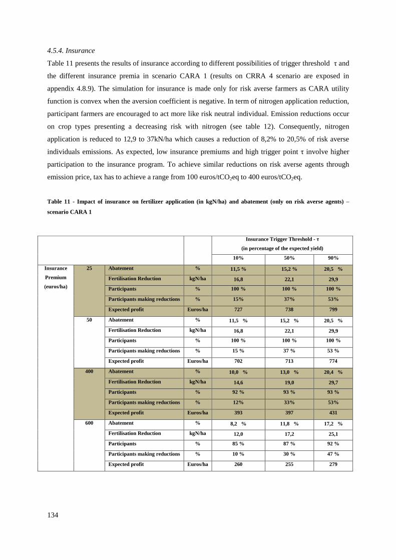
134

4.5.4. Insurance

Table 11 presents the results of insurance according to different possibilities of trigger threshold τ and

the different insurance premia in scenario CARA 1 (results on CRRA 4 scenario are exposed in

appendix 4.8.9). The simulation for insurance is made only for risk averse farmers as CARA utility

function is convex when the aversion coefficient is negative. In term of nitrogen application reduction,

participant farmers are encouraged to act more like risk neutral individual. Emission reductions occur

on crop types presenting a decreasing risk with nitrogen (see table 12). Consequently, nitrogen

application is reduced to 12,9 to 37kN/ha which causes a reduction of 8,2% to 20,5% of risk averse

individuals emissions. As expected, low insurance premiums and high trigger point τ involve higher

participation to the insurance program. To achieve similar reductions on risk averse agents through

emission price, tax has to achieve a range from 100 euros/tCO2eq to 400 euros/tCO2eq.

Table 11 - Impact of insurance on fertilizer application (in kgN/ha) and abatement (only on risk averse agents) –

scenario CARA 1

Insurance Trigger Threshold - τ

(in percentage of the expected yield)

10% 50% 90%

Insurance

Premium

(euros/ha)

25

Abatement % 11,5 % 15,2 % 20,5 %

Fertilisation Reduction kgN/ha 16,8 22,1 29,9

Participants % 100 % 100 % 100 %

Participants making reductions % 15% 37% 53%

Expected profit Euros/ha 727 738 799

50

Abatement % 11,5 % 15,2 % 20,5 %


Participants % 100 % 100 % 100 %

Participants making reductions % 15 % 37 % 53 %


400

Abatement % 10,0 % 13,0 % 20,4 %


Participants % 92 % 93 % 93 %

Participants making reductions % 12% 33% 53%


600

Abatement % 8,2 % 11,8 % 17,2 %


Participants % 85 % 87 % 92 %

Participants making reductions % 10 % 30 % 47 %


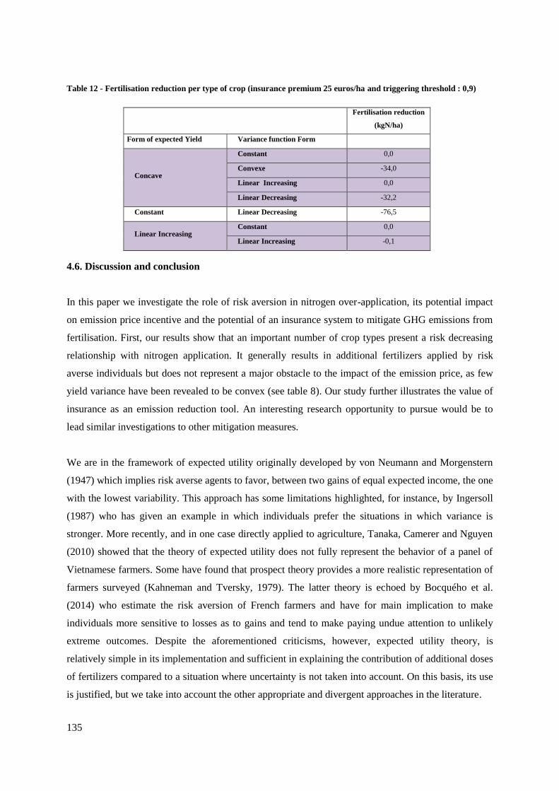
135

Table 12 - Fertilisation reduction per type of crop (insurance premium 25 euros/ha and triggering threshold : 0,9)

Fertilisation reduction

(kgN/ha)

Form of expected Yield Variance function Form

Concave

Constant 0,0

Convexe -34,0

Linear Increasing 0,0

Linear Decreasing -32,2

Constant Linear Decreasing -76,5

Linear Increasing Constant 0,0

Linear Increasing -0,1

4.6. Discussion and conclusion

In this paper we investigate the role of risk aversion in nitrogen over-application, its potential impact

on emission price incentive and the potential of an insurance system to mitigate GHG emissions from

fertilisation. First, our results show that an important number of crop types present a risk decreasing

relationship with nitrogen application. It generally results in additional fertilizers applied by risk

averse individuals but does not represent a major obstacle to the impact of the emission price, as few

yield variance have been revealed to be convex (see table 8). Our study further illustrates the value of

insurance as an emission reduction tool. An interesting research opportunity to pursue would be to

lead similar investigations to other mitigation measures.

We are in the framework of expected utility originally developed by von Neumann and Morgenstern

(1947) which implies risk averse agents to favor, between two gains of equal expected income, the one

with the lowest variability. This approach has some limitations highlighted, for instance, by Ingersoll

(1987) who has given an example in which individuals prefer the situations in which variance is

stronger. More recently, and in one case directly applied to agriculture, Tanaka, Camerer and Nguyen

(2010) showed that the theory of expected utility does not fully represent the behavior of a panel of

Vietnamese farmers. Some have found that prospect theory provides a more realistic representation of

farmers surveyed (Kahneman and Tversky, 1979). The latter theory is echoed by Bocquého et al.

(2014) who estimate the risk aversion of French farmers and have for main implication to make

individuals more sensitive to losses as to gains and tend to make paying undue attention to unlikely

extreme outcomes. Despite the aforementioned criticisms, however, expected utility theory, is

relatively simple in its implementation and sufficient in explaining the contribution of additional doses

of fertilizers compared to a situation where uncertainty is not taken into account. On this basis, its use

is justified, but we take into account the other appropriate and divergent approaches in the literature.

136

Besides, we explore in this article risk aversion as a mean to explain the surplus of nitrogen

application but in three scenarii (CARA 1, CARA 2, CRRA 2) we find that risk aversion does not fully

explain all observed nitrogen amount (see appendix 4.8.7). This should attract our attention to

additional reasons for over-application nitrogen found within other articles of the literature. For

instance, these factors may include lack of trust in farm advisors or models (Stuart et al, 2014). The

fact that we elicited here the links between fertilisation and yield variability for different crop types in

3 departments does not mean that crop yield will follow these relationships at each individual farm

level. That lack of access to appropriate information or technological tools may inhibit the adoption of

practices to increase nitrogen use efficiency. Moreover, recent private-sector developments in

contracting have the potential to impact farming behavior as well. These contracts generally offer

higher levels of profitability compared to commercial crops. Most seed contracts also have a

competitive component: growers receive financial penalties or rewards based on how their production

compares to other growers of the same variety (Dubois, 2006; Stuart et al, 2014). Consequently

farmers concerned by contracts also act to achieve the optimal nitrogen to fit the best quality. All these

elements, explain why a large share of farmers prioritizes yields above economic return (Stuart et al,

2013).

Moreover, our findings suggest that insurance, as it is made on a voluntary basis, would be preferable

to a emission price. It is important to note however that, we only consider one option to mitigate

emission. If other alternatives to mitigate emissions, like changing crop allocation, were represented in

modelling, then we expect, from other results in the literature (De Cara and Jayet, 2011) that the

abatement cost would be lower. Moreover, we implicitly assume that the insurance program is

unaffected by the moral hazard effect. This effect is observed when farmers change their behavior

when they know that a part of their risk is covered, thus potentially leading to some fraudulent,

intentional losses. Among the conditions for the development of insurance, the insurer must be able to

estimate accurately both expected frequency and severity of loss (Barnett et al., 1999). Current

developments in insurance and farm advisement show that this latter point is bound to be improved.

Pacifica insurance company initiated for instance in 2015 an insurance contract dedicated one

grasslands implying surveillance by satellite to observe losses compared with a baseline built on an

historical production data (Crédit Agricole Assurance – Airbus Défense & Space, 2015). Morevover,

as farmers increasingly collect and report their economic gain and their production amount, used and

shared with farm Cooperatives, this could constitute a lever to identify and control loss at the farm

gate. Besides, if the implementation of insurance is conditioned by GHG mitigation, other techniques,

involved in precision farming, can help to improve measurement like static chambers measuring gas

fluxes between the soil ant the atmosphere (Collier et al., 2016) or organic emission assessment by

drone teledetection (Gilliot et al, 2014).

137

Together, these findings highlight further avenues for research, which ought to be pursued in future

works.

138

4.7. References

ADEME, 2012. Les émissions agricoles de particules dans l’air : état des lieux et levier d’action.

Agreste, 2014. Pratiques culturales sur les grandes cultures et prairies portant sur l’année 2011.

http://agreste.agriculture.gouv.fr/enquetes/pratiques-culturales/grandes-cultures-prairies/

Agreste, 2012. Charges de mécanisation et structure d’exploitation. Document de travail n°7 – Juillet

2012.

Agreste, 2011. Les Dossiers N° 12 - Juillet 2011

Agence de l’eau Loire-Bretagne, 2016. 10ième

programme de l’agence de l’eau Loire-Bretagne – 2016-

2018. Fiche 10. http://www.eau-loire-

bretagne.fr/nos_missions/programme_2013_2018/10prog_fiches-action111214.pdf

Antle, J. M. (2010). Asymmetry, partial moments, and production risk. American Journal of

Agricultural Economics, 92, 1294-1309.

Babcock, B. A. (1992). The effects of uncertainty on optimal nitrogen applications. Review of

Agricultural Economics, 271-280.

Barnett, B. J., Coble, K. H., & others. (1999). Understanding crop insurance principles: A primer for

farm leaders.

Bélanger, G., Walsh, J. R., Richards, J. E., Milburn, P. H., & Ziadi, N. (2000). Comparison of three

statistical models describing potato yield response to nitrogen fertilizer. Agronomy Journal,

92, 902-908.

Berentsen, P., Kovacs, K., & Asseldonk, M. V. (2012). Comparing risk in conventional and organic

dairy farming in the Netherlands: an empirical analysis. Journal of dairy science, 95, 3803-

3811.

Blottnitz, H. V., Rabl, A., Boiadjiev, D., Taylor, T., & Arnold, S. (2006). Damage costs of nitrogen

fertilizer in Europe and their internalization. Journal of environmental planning and

management, 49, 413-433.

Bocquého, G., Jacquet, F., & Reynaud, A. (2014). Expected utility or prospect theory maximisers?

Assessing farmers' risk behaviour from field-experiment data. European Review of


Bougherara, D. (2011). Rôle de l’aversion au risque des agriculteurs dans l’utilisation de pesticides et

implications pour la régulation.

Bourgeois, C., Fradj, N. B., & Jayet, P.-A. (2014). How Cost-Effective is a Mixed Policy Targeting

the Management of Three Agricultural N-pollutants? Environmental Modeling and

Assessment, 19, 389-405.

Broun, A. (2007). Assessing nitrogen application strategies for wheat production: a case study.

http://agreste.agriculture.gouv.fr/enquetes/pratiques-culturales/grandes-cultures-prairies/

http://www.eau-loire-bretagne.fr/nos_missions/programme_2013_2018/10prog_fiches-action111214.pdf

http://www.eau-loire-bretagne.fr/nos_missions/programme_2013_2018/10prog_fiches-action111214.pdf

139

Brunette, M., Choumert, J., Couture, S., Montagne-Huck, C., & others. (2015). A Meta-analysis of the

Risk Aversion Coefficients of Natural Resource Managers Evaluated by Stated Preference

Methods.

Cayatte, J.-L. (2004). Introduction à l'économie de l'incertitude. De Boeck Supérieur.

Cerrato, M., & Blackmer, A. (1990). Comparison of models for describing; corn yield response to

nitrogen fertilizer. Agronomy Journal, 82, 138-143.

Chavas, J.-P., & Holt, M. T. (1996). Economic behavior under uncertainty: A joint analysis of risk

preferences and technology. The review of economics and statistics, 329-335.

Coble, K. H., Knight, T. O., Pope, R. D., & Williams, J. R. (1993). An empirical-test for moral hazard

and averse selection in multiple peril crop insurance. 75, 1296-1296.

Collier, S. M., Ruark, M. D., Oates, L. G., Jokela, W. E., & Dell, C. J. (2014). Measurement of

greenhouse gas flux from agricultural soils using static chambers. JoVE (Journal of Visualized

Experiments), e52110--e52110.

COMIFER. (2011). Calcul de la fertilisation azotée. Comifer.

Cooke, I. R., Mattison, E. H., Audsley, E., Bailey, A. P., Freckleton, R. P., Graves, A. R., et al. (2013).

Empirical Test of an Agricultural Landscape Model: the importance of farmer preference for

risk aversion and crop complexity. Sage Open, 3, 2158244013486491.

Dalmas, D., Moreau, R., Quévrremont, P., & Frey, V. (2010). Elaboration d'un plan de lutte contre les

algues vertes. Ministère de l'Ecologie, Ministère de l'Intérieur, Ministère de la Santé et des

Sports, Ministère de l'Agriculture.

De Cara, S., Jacquet, F., Reynaud, A., Goulevant, G., Jeuffroy, M.-H., Montfort, F., et al. (2011).

Economic Analysis of Summer Fallow Management to Reduce Take-All Disease and N

Leaching in a Wheat Crop Rotation. Environmental modeling \& assessment, 16, 91-105.

Dequiedt, B., & Moran, D. (2015). The cost of emission mitigation by legume crops in French

agriculture. Ecological Economics, 110, 51-60.

Dubois, P., & others. (2006). Efficacité des contrats agricoles: le cas de la production de blé en Midi-

Pyrénées. INRA Sciences Sociales.

Dury, J. (2011). The cropping-plan decision-making: a farm level modelling and simulation approach.

Institut National Polytechnique de Toulouse (INP Toulouse). INPT.

Ellerman, A. D., Convery, F. J., & Perthuis, C. D. (2010). Pricing emission: the European Union

emissions trading scheme. Cambridge University Press.

European Commission (2013). Rapport de la commission au conseil et au parlement européen relatif

à la mise en œuvre de la directive 91/676/CEE du Conseil concernant la protection des eaux

contre la pollution par les nitrates à partir de sources agricoles, sur la base des rapports

établis par les États membres pour la période 2008-2011. COM(2013) 683 final, European

Commission.

European Commission (2013). Nitrogen Pollution and the European Environment. In depth report.

140

European Union. (2009). Decision Number 406/2009/EC of the european parliament and of the

council of 23 April 2009 on the effort of Member States to reduce their greenhouse gas

emissions to meet the Community's greenhouse gas emission reduction commitments up

to 2020. Decision Number 406/2009/EC of the european parliament and of the council of

23 April 2009 on the effort of Member States to reduce their greenhouse gas emissions to

meet the Community's greenhouse gas emission reduction commitments up to 2020.

Finger, R. (2012). Nitrogen use and the effects of nitrogen taxation under consideration of production

and price risks. Agricultural Systems, 107, 13-20.

Finger, R., & Schmid, S. (2008). Modeling agricultural production risk and the adaptation to climate

change. Agricultural Finance Review, 68, 25-41.

Galloway, J. N., Townsend, A. R., Erisman, J. W., Bekunda, M., Cai, Z., Freney, J. R., et al. (2008).

Transformation of the nitrogen cycle: recent trends, questions, and potential solutions.

Science, 320, 889-892.

Gandorfer, M., Pannell, D., & Meyer-Aurich, A. (2011). Analyzing the effects of risk and uncertainty

on optimal tillage and nitrogen fertilizer intensity for field crops in Germany. Agricultural

Systems, 104, 615-622.

Gilliot, J.-M., Vaudour, E., Michelin, J., & Houot, S. (2014). Estimation des teneurs en emissione

organique des sols agricoles par télédétection par drone. 2--p.

Horowitz, J. K., & Lichtenberg, E. (1993). Insurance, moral hazard, and chemical use in agriculture.

American Journal of Agricultural Economics, 75, 926-935.

Huang, W.-Y., Heifner, R. G., Taylor, H., & Uri, N. D. (2001). Using insurance to enhance nitrogen

fertilizer application to reduce nitrogen losses to the environment. Environmental monitoring

and assessment, 68, 209-233.

Ingersoll, J. E. (1987). Theory of financial decision making (Vol. 3). Rowman \& Littlefield.

Just, R. E., & Pope, R. D. (1979). Production function estimation and related risk considerations.

American Journal of Agricultural Economics, 276-284.

Kahneman, D., & Tversky, A. (1979). Prospect theory: An analysis of decision under risk.

Econometrica: Journal of the Econometric Society, 263-291.

Lambert, D. K. (1990). Risk considerations in the reduction of nitrogen fertilizer use in agricultural

production. Western Journal of Agricultural Economics, 234-244.

Lansink, A. O. (1999). Area allocation under price uncertainty on Dutch arable farms. Journal of


Leathers, H. D., & Quiggin, J. C. (1991). Interactions between agricultural and resource policy: the

importance of attitudes toward risk. American Journal of Agricultural Economics, 73, 757-

764.

Markowitz, H. (1952). Harry M. Markowitz. Portfolio selection, Journal of Finance, 7, 77-91.

141

Menapace, L., Colson, G., & Raffaelli, R. (2013). Risk aversion, subjective beliefs, and farmer risk

management strategies. American Journal of Agricultural Economics, 95, 384-389.

Monjardino, M., McBeath, T., Ouzman, J., Llewellyn, R., & Jones, B. (2015). Farmer risk-aversion

limits closure of yield and profit gaps: A study of nitrogen management in the southern

Australian wheatbelt. Agricultural Systems, 137, 108-118.

Neumann, L. J., & Morgenstern, O. (1947). Theory of games and economic behavior. Princeton

University Press Princeton, NJ.

Polomé, P., Harmignie, O., & Frahan, B. d. (2006). Farm-level acreage allocation under risk.

Pope, R. D., LaFrance, J. T., & Just, R. E. (2011). Agricultural arbitrage and risk preferences. Journal

of econometrics, 162, 35-43.

Rajsic, P., Weersink, A., & Gandorfer, M. (2009). Risk and nitrogen application levels. Canadian

Journal of Agricultural Economics/Revue canadienne d'agroeconomie, 57, 223-239.

Regev, U., Gotsch, N., & Rieder, P. (1997). Are fungicides, nitrogen and plant growth regulators risk-

reducing? empirical evidence from swiss wheat production. Journal of Agricultural

Economics, 48, 167-178.

RICA. Réseau d'information agricole. http://agreste.agriculture.gouv.fr/page-d-accueil/article/donnees-

en-ligne

Saha, A., Shumway, C. R., & Talpaz, H. (1994). Joint estimation of risk preference structure and

technology using expo-power utility. American Journal of Agricultural Economics, 76, 173-

184.

Sheriff, G. (2005). Efficient waste? Why farmers over-apply nutrients and the implications for policy

design. Applied Economic Perspectives and Policy, 27, 542-557.

Smit, B., & Skinner, M. W. (2002). Adaptation options in agriculture to climate change: a typology.

Mitigation and adaptation strategies for global change, 7, 85-114.

Smith, V. H., & Goodwin, B. K. (1996). Crop insurance, moral hazard, and agricultural chemical use.

American Journal of Agricultural Economics, 78, 428-438.

SriRamaratnam, S., Bessler, D. A., Rister, M. E., Matocha, J. E., & Novak, J. (1987). Fertilisation

under uncertainty: an analysis based on producer yield expectations. American Journal of


Stuart, D., Schewe, R., & McDermott, M. (2014). Reducing nitrogen fertilizer application as a climate

change mitigation strategy: Understanding farmer decision-making and potential barriers to

change in the US. Land Use Policy, 36, 210-218.

Tanaka, T., Camerer, C. F., & Nguyen, Q. (2010). Risk and time preferences: linking experimental

and household survey data from Vietnam. The American Economic Review, 100, 557-571.

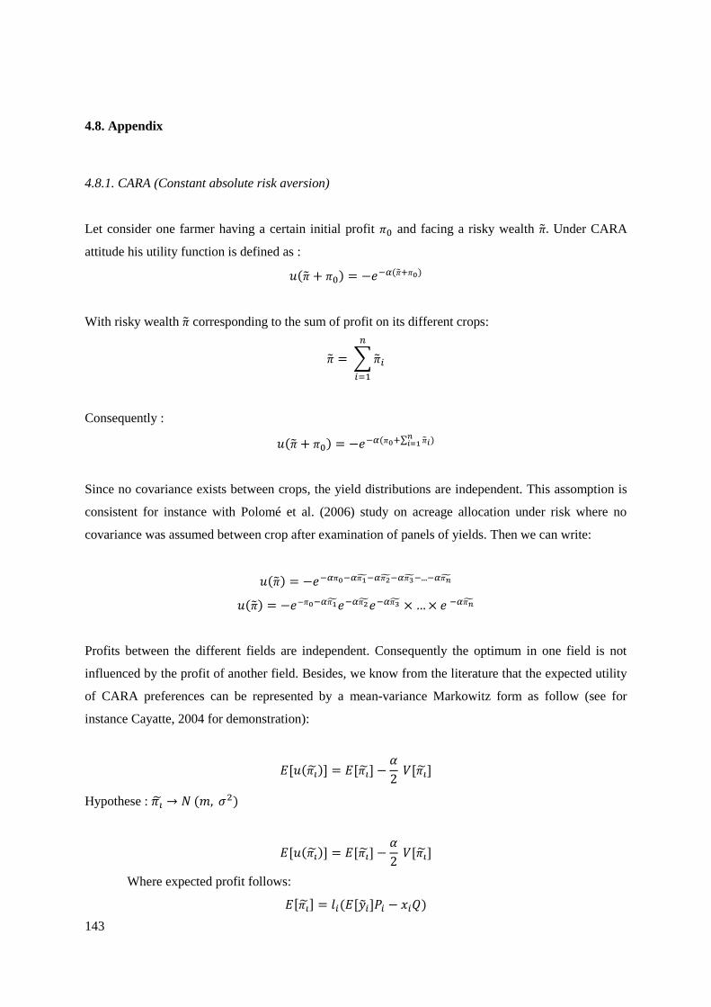
143

4.8. Appendix

4.8.1. CARA (Constant absolute risk aversion)

Let consider one farmer having a certain initial profit 𝜋0 and facing a risky wealth �̃�. Under CARA

attitude his utility function is defined as :

𝑢(�̃� + 𝜋0) = −𝑒−𝛼(�̃�+𝜋0)

With risky wealth �̃� corresponding to the sum of profit on its different crops:

�̃� = ∑ �̃�𝑖

𝑛

𝑖=1

Consequently :

𝑢(�̃� + 𝜋0) = −𝑒−𝛼(𝜋0+∑ �̃�𝑖𝑛𝑖=1 )

Since no covariance exists between crops, the yield distributions are independent. This assomption is

consistent for instance with Polomé et al. (2006) study on acreage allocation under risk where no

covariance was assumed between crop after examination of panels of yields. Then we can write:

𝑢(�̃�) = −𝑒−𝛼𝜋0−𝛼𝜋1̃−𝛼𝜋2̃−𝛼𝜋3̃−...−𝛼𝜋�̃�

𝑢(�̃�) = −𝑒−𝜋0−𝛼𝜋1̃𝑒−𝛼𝜋2̃𝑒−𝛼𝜋3̃ × … × 𝑒 −𝛼𝜋�̃�

Profits between the different fields are independent. Consequently the optimum in one field is not

influenced by the profit of another field. Besides, we know from the literature that the expected utility

of CARA preferences can be represented by a mean-variance Markowitz form as follow (see for

instance Cayatte, 2004 for demonstration):

𝐸[𝑢(𝜋�̃�)] = 𝐸[𝜋�̃�] −𝛼

2 𝑉[𝜋�̃�]

Hypothese : 𝜋�̃� → 𝑁 (𝑚, 𝜎2)

𝐸[𝑢(𝜋�̃�)] = 𝐸[𝜋�̃�] −𝛼

2 𝑉[𝜋�̃�]

Where expected profit follows:

𝐸[𝜋�̃�] = 𝑙𝑖(𝐸[�̃�𝑖]𝑃𝑖 − 𝑥𝑖𝑄)

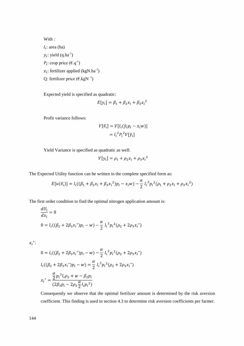
144

With :

𝑙𝑖: area (ha)

𝑦𝑖: yield (q.ha-1

)

𝑃𝑖: crop price (€.q-1

)

𝑥𝑖: fertilizer applied (kgN.ha-1

)

Q: fertilizer price (€.kgN -1

)

Expected yield is specified as quadratic:

𝐸[𝑦𝑖] = 𝛽1 + 𝛽2𝑥𝑖 + 𝛽3𝑥𝑖2

Profit variance follows:

𝑉[𝜋�̃�] = 𝑉[𝑙𝑖(�̃�𝑖𝑝𝑖 − 𝑥𝑖𝑤)]

= 𝑙𝑖2𝑃𝑖

2𝑉[�̃�𝑖]

Yield Variance is specified as quadratic as well:

𝑉[𝑦𝑖] = 𝜌1 + 𝜌2𝑥𝑖 + 𝜌3𝑥𝑖2

The Expected Utility function can be written in the complete specified form as:

𝐸[𝑢(𝜋�̃�)] = 𝑙𝑖((𝛽1 + 𝛽2𝑥𝑖 + 𝛽3𝑥𝑖2)𝑝𝑖 − 𝑥𝑖𝑤) −

𝛼

2 𝑙𝑖

2𝑝𝑖2(𝜌1 + 𝜌2𝑥𝑖 + 𝜌3𝑥𝑖

2)

The first order condition to find the optimal nitrogen application amount is:

𝑑𝑈𝑖

𝑑𝑥𝑖= 0

0 = 𝑙𝑖((𝛽2 + 2𝛽3𝑥𝑖∗)𝑝𝑖 − 𝑤) −

𝛼

2 𝑙𝑖

2𝑝𝑖2(𝜌2 + 2𝜌3𝑥𝑖

∗)

𝑥𝑖∗:

0 = 𝑙𝑖((𝛽2 + 2𝛽3𝑥𝑖∗)𝑝𝑖 − 𝑤) −

𝛼

2 𝑙𝑖


∗)

𝑙𝑖((𝛽2 + 2𝛽3𝑥𝑖∗)𝑝𝑖 − 𝑤) =

𝛼

2 𝑙𝑖


∗)

𝑥𝑖∗ =

𝛼2 𝑝𝑖

2𝑙𝑖𝜌2 + 𝑤 − 𝛽2𝑝𝑖

(2𝛽3𝑝𝑖 − 2𝜌3𝛼2 𝑙𝑖𝑝𝑖

2)

Consequently we observe that the optimal fertilizer amount is determined by the risk aversion

coefficient. This finding is used in section 4.3 to determine risk aversion coefficients per farmer.

145

Let now study the impact of an emission price on the optimal amount of fertilizers:

Expected utility with a tax on emissions:

𝑈𝑖 = 𝑙𝑖((𝛽1 + 𝛽2𝑥𝑖 + 𝛽3𝑥𝑖2)𝑝𝑖 − 𝑥𝑖𝑤 − 𝑥𝑖𝑓𝑡) −

𝛼

2 𝑙𝑖

2𝑝𝑖2(𝜌1 + 𝜌2𝑥𝑖 + 𝜌3𝑥𝑖

2)

Where t is the emissions price and f the emission factor.

The First order condition becomes:

𝑑𝑈𝑖

𝑑𝑥𝑖= 𝑙𝑖((𝛽2 + 2𝛽3𝑥𝑖

∗)𝑝𝑖 − 𝑤 − 𝑓𝑡) −𝛼

2 𝑙𝑖


∗) = 0

𝑥𝑖∗ =

𝛼2

𝑝𝑖2𝑙𝑖𝜌2 + 𝑤 + 𝑓𝑡 − 𝛽2𝑝𝑖

(2𝛽3𝑃𝑖 − 2𝜌3𝛼2

𝑙𝑖𝑃𝑖2)

The Second order condition being:

𝑑𝑈𝑖2

𝑑2𝑥𝑖= 2𝑙𝑖𝛽3𝑝𝑖 − 𝛼𝑙𝑖

2𝑝𝑖2𝜌3 < 0

Impact of a emission price on fertilizer reduction:

𝑑𝑥𝑖∗

𝑑𝑡=

𝑓

2𝛽3𝑝𝑖 −2𝜌3𝛼

2𝑙𝑖𝑝𝑖

2 <=>

𝑑𝑥𝑖∗

𝑑𝑡=

𝑙𝑖𝑓

𝑑2𝐸[�̃�]

𝑑𝑥𝑖2 −𝑘

𝑑2𝑉[𝑤�̃�]

𝑑𝑥𝑖2

If 𝜌3 ≠ 0 then the emission reduction will be influenced by the risk aversion coefficient.

146

4.8.2. CRRA (Constant relative risk aversion)

Let consider consider now the problem with a CRRA function :

𝑢(𝜋0 + �̃�) =(𝜋0 + �̃�)(1−𝑟)

1 − 𝑟

With :

𝑢′(�̃�+𝜋0) = (𝜋0 + �̃�)−𝑟

𝑢′′(�̃� + 𝜋0) = −𝑟(�̃� + 𝜋0)−𝑟−1

Where r is the relative risk aversion.

By definition the absolute risk aversion coefficient is :

𝑎 = − 𝑢′′(�̃� + 𝜋0)

𝑢′(�̃� + 𝜋0)

𝑎 = 𝑟

(�̃� + 𝜋0)

According to the Taylor series:

𝑢(2𝜋0 + 𝜀̃) = 𝑢(2𝜋0) + 𝜀̃𝑢′(2𝜋0) + �̃�2

2𝑢′′(2𝜋0)

𝐸[𝑢(2𝜋0 + 𝜀̃)] = 𝑢(2𝜋0) + 𝑢′(2𝜋0)𝐸[𝜀]̃ + 𝑢′′(2𝜋0) 𝐸[�̃�2]

2

With

𝜀̃ = �̃� − 𝜋0

If we consider that 𝐸[𝜀̃2] ≈ V[𝜀̃], and no covariance then per field the first order condition is:

𝑑𝑈𝑖

𝑑𝑥𝑖= 𝑢′(2𝜋0)𝑙𝑖((𝛽2 + 2𝛽3𝑥𝑖

∗)𝑝𝑖 − 𝑤) +𝑢′′(2𝜋0)

2 𝑙𝑖


∗) = 0

Then 𝑥𝑖∗:

𝑥𝑖∗ =

𝑟4𝜋0

𝑝𝑖2𝑙𝑖𝜌2 + 𝑤 − 𝛽2𝑝𝑖

(2𝛽3𝑝𝑖 −𝑟

2𝜋0𝑙𝑖𝑝𝑖

2𝜌3)

Impact of a price on emissions:

The First order condition:

147

𝑑𝑈𝑖

𝑑𝑥𝑖= 𝑢′(2𝜋0)𝑙𝑖((𝛽2 + 2𝛽3𝑥𝑖

∗)𝑝𝑖 − 𝑤𝑖 − 𝑓𝑡) +𝑢′′(2𝜋0)

2 𝑙𝑖


∗) = 0

𝑥𝑖∗ =

𝑟4𝜋0

𝑝𝑖2𝑙𝑖𝜌2 + 𝑤 + 𝑓𝑡 − 𝛽2𝑝𝑖

(2𝛽3𝑝𝑖 −𝑟

2𝜋0𝑙𝑖𝑝𝑖

2𝜌3)

The Second order condition:

𝑑𝑈𝑖2

𝑑2𝑥𝑖= 2𝑙𝑖𝛽3𝑃𝑖 −

𝑟

2𝜋0𝑙𝑖

2𝑃𝑖2𝜌3 < 0

Impact of a emission price on fertilizer reduction:

𝑑𝑥𝑖∗

𝑑𝐶𝑝=

𝑓

2𝛽3𝑃𝑖 − 𝜌3𝑟

2𝜋0𝑙𝑖𝑃𝑖

2

If 𝜌3 ≠ 0 then the emission reduction will be influenced by the risk aversion coefficient.

148

4.8.3. Illustration of rish aversion impact on fertilizer spreading

Legend :

𝑑𝐸[𝜋�̃�(𝑥𝑖)]

𝑑𝑥𝑖

Optimal fertilizer amount for risk neutral farmers

𝑘 𝑑𝑉[𝜋�̃�(𝑥𝑖)]

𝑑𝑥𝑖 with k>0

Optimal fertilizer amount for risk averse farmers (k>0)

𝑘 𝑑𝑉[𝜋�̃�(𝑥𝑖)]

𝑑𝑥𝑖 with k<0

Optimal fertilizer amount for risk loving farmers (k<0)

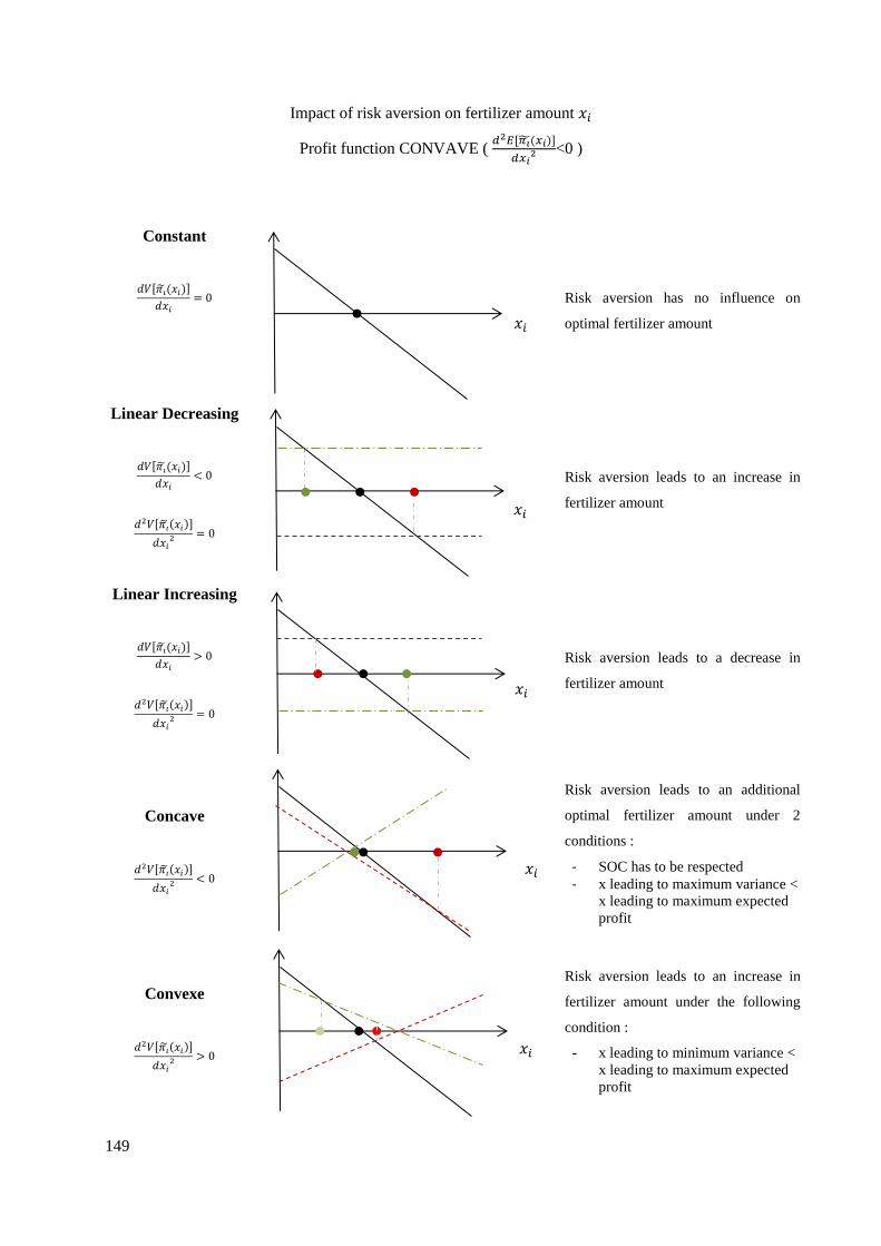
149

Impact of risk aversion on fertilizer amount 𝑥𝑖

Profit function CONVAVE ( 𝑑2𝐸[𝜋�̃�(𝑥𝑖)]

𝑑𝑥𝑖2 <0 )

𝑑𝑉[𝜋�̃�(𝑥𝑖)]

𝑑𝑥𝑖

= 0

Constant

Risk aversion has no influence on

optimal fertilizer amount


𝑑𝑥𝑖

< 0

𝑑2𝑉[𝜋�̃�(𝑥𝑖)]

𝑑𝑥𝑖2 = 0

Linear Decreasing

Risk aversion leads to an increase in

fertilizer amount


𝑑𝑥𝑖

> 0

𝑑2𝑉[𝜋�̃�(𝑥𝑖)]

𝑑𝑥𝑖2 = 0

Linear Increasing

Risk aversion leads to a decrease in

fertilizer amount

𝑑2𝑉[𝜋�̃�(𝑥𝑖)]

𝑑𝑥𝑖2 < 0

Concave

Risk aversion leads to an additional

optimal fertilizer amount under 2

conditions :

- SOC has to be respected

- x leading to maximum variance <

x leading to maximum expected

profit

𝑑2𝑉[𝜋�̃�(𝑥𝑖)]

𝑑𝑥𝑖2 > 0

Convexe

Risk aversion leads to an increase in

fertilizer amount under the following

condition :

- x leading to minimum variance <

x leading to maximum expected

profit

𝑥𝑖

𝑥𝑖

𝑥𝑖

𝑥𝑖

𝑥𝑖

150


Profit function Linear Decreasing ( 𝑑2𝐸[𝜋�̃�(𝑥𝑖)]

𝑑𝑥𝑖2 <0 )


𝑑𝑥𝑖

= 0

Constant

SOC not respected


𝑑𝑥𝑖

< 0

𝑑2𝑉[𝜋�̃�(𝑥𝑖)]

𝑑𝑥𝑖2 = 0

Linear Decreasing

SOC not respected


𝑑𝑥𝑖

> 0

𝑑2𝑉[𝜋�̃�(𝑥𝑖)]

𝑑𝑥𝑖2 = 0

Linear Increasing

SOC not respected

𝑑2𝑉[𝜋�̃�(𝑥𝑖)]

𝑑𝑥𝑖2 < 0

Concave

SOC is not respected for risk averse

agents.

Risk loving preference leads to

fertilisation.

𝑑2𝑉[𝜋�̃�(𝑥𝑖)]

𝑑𝑥𝑖2 > 0

Convexe

SOC is not respected for risk loving

agents.

Risk avers preference leads to

fertilisation.

𝑥𝑖

𝑥𝑖

𝑥𝑖

𝑥𝑖

𝑥𝑖

151


Profit function Linear Increasing ( 𝑑2𝐸[𝜋�̃�(𝑥𝑖)]

𝑑𝑥𝑖2 =0 )


𝑑𝑥𝑖

= 0

Constant

SOC not respected


𝑑𝑥𝑖

< 0

𝑑2𝑉[𝜋�̃�(𝑥𝑖)]

𝑑𝑥𝑖2 = 0

Linear Decreasing

SOC not respected


𝑑𝑥𝑖

> 0

𝑑2𝑉[𝜋�̃�(𝑥𝑖)]

𝑑𝑥𝑖2 = 0

Linear Increasing

SOC not respected

𝑑2𝑉[𝜋�̃�(𝑥𝑖)]

𝑑𝑥𝑖2 < 0

Concave


agents.

Risk loving preference leads to

fertilisation.

𝑑2𝑉[𝜋�̃�(𝑥𝑖)]

𝑑𝑥𝑖2 > 0

Convexe


averse agents.

Risk avers preference leads to

fertilisation.

𝑥𝑖

𝑥𝑖 𝑥𝑚𝑎𝑥




152


Profit function Convex ( 𝑑2𝐸[𝜋�̃�(𝑥𝑖)]

𝑑𝑥𝑖2 >0 )


𝑑𝑥𝑖

= 0

Constant

SOC not respected


𝑑𝑥𝑖

< 0

𝑑2𝑉[�̃�(𝑥𝑖)]

𝑑𝑥𝑖2 = 0

Linear Decreasing

SOC not respected


𝑑𝑥𝑖

> 0

𝑑2𝑉[𝜋�̃�(𝑥𝑖)]

𝑑𝑥𝑖2 = 0

Linear Increasing

SOC not respected

𝑑2𝑉[𝑤�̃�(𝑥𝑖)]

𝑑𝑥𝑖2 < 0

Concave

𝑑2𝐸[�̃�(𝑥𝑖)]

𝑑𝑥𝑖2 < 𝑘

𝑑2𝑉[𝑤�̃�(𝑥𝑖)]

𝑑𝑥𝑖2


agents.

For risk loving preferences, the

condition for solutions is:

𝑑2𝑉[𝑤�̃�(𝑥𝑖)]

𝑑𝑥𝑖2 > 0

Convexe

𝑑2𝐸[�̃�(𝑥𝑖)]

𝑑𝑥𝑖2 < 𝑘

𝑑2𝑉[𝑤�̃�(𝑥𝑖)]

𝑑𝑥𝑖2


agents.

For risk loving preferences, the

condition for solutions is:

𝑥𝑖

𝑥𝑖

𝑥𝑖

𝑥𝑖

𝑥𝑖

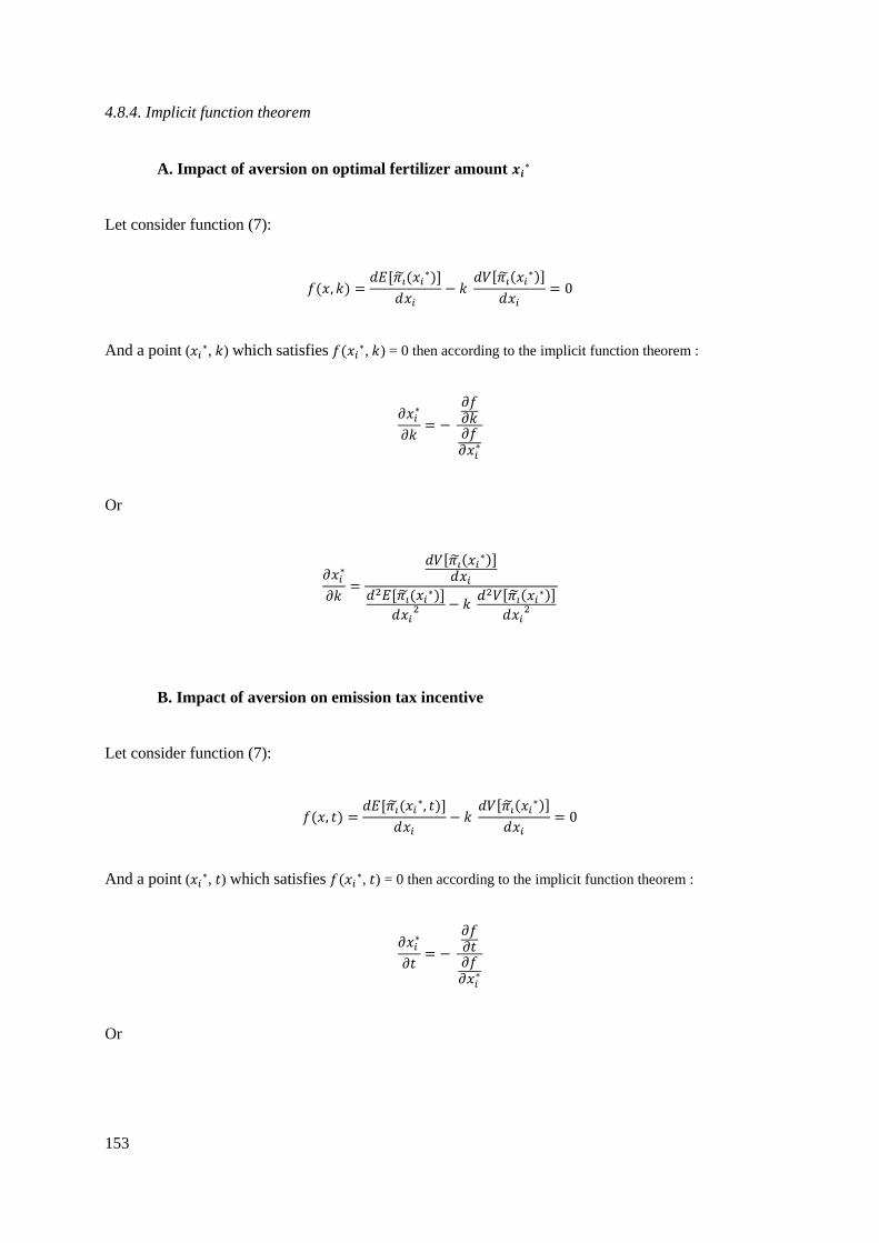
153

4.8.4. Implicit function theorem

A. Impact of aversion on optimal fertilizer amount 𝒙𝒊∗

Let consider function (7):

𝑓(𝑥, 𝑘) =𝑑𝐸[𝜋�̃�(𝑥𝑖

∗)]

𝑑𝑥𝑖


∗)]

𝑑𝑥𝑖

= 0

And a point (𝑥𝑖∗, 𝑘) which satisfies 𝑓(𝑥𝑖

∗, 𝑘) = 0 then according to the implicit function theorem :

𝜕𝑥𝑖∗

𝜕𝑘= −

𝜕𝑓𝜕𝑘𝜕𝑓𝜕𝑥𝑖

∗

Or

𝜕𝑥𝑖∗

𝜕𝑘=

𝑑𝑉[𝜋�̃�(𝑥𝑖∗)]

𝑑𝑥𝑖

𝑑2𝐸[𝜋�̃�(𝑥𝑖∗)]


𝑑2𝑉[𝜋�̃�(𝑥𝑖∗)]

𝑑𝑥𝑖2

B. Impact of aversion on emission tax incentive

Let consider function (7):

𝑓(𝑥, 𝑡) =𝑑𝐸[𝜋�̃�(𝑥𝑖

∗, 𝑡)]

𝑑𝑥𝑖


∗)]

𝑑𝑥𝑖

= 0

And a point (𝑥𝑖∗, 𝑡) which satisfies 𝑓(𝑥𝑖

∗, 𝑡) = 0 then according to the implicit function theorem :

𝜕𝑥𝑖∗

𝜕𝑡= −

𝜕𝑓𝜕𝑡𝜕𝑓𝜕𝑥𝑖

∗

Or

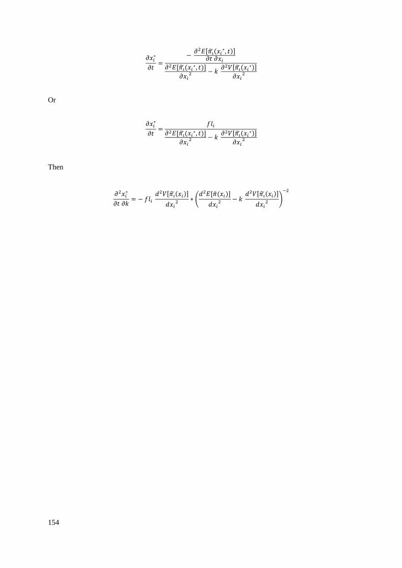
154

𝜕𝑥𝑖∗

𝜕𝑡=

− 𝜕2𝐸[𝜋�̃�(𝑥𝑖

∗, 𝑡)]𝜕𝑡 𝜕𝑥𝑖

𝜕2𝐸[𝜋�̃�(𝑥𝑖∗, 𝑡)]

𝜕𝑥𝑖2 − 𝑘

𝜕2𝑉[𝜋�̃�(𝑥𝑖∗)]

𝜕𝑥𝑖2

Or

𝜕𝑥𝑖∗

𝜕𝑡=

𝑓𝑙𝑖

𝜕2𝐸[𝜋�̃�(𝑥𝑖∗, 𝑡)]

𝜕𝑥𝑖2 − 𝑘

𝜕2𝑉[𝜋�̃�(𝑥𝑖∗)]

𝜕𝑥𝑖2

Then

𝜕2𝑥𝑖∗

𝜕𝑡 𝜕𝑘= − 𝑓𝑙𝑖

𝑑2𝑉[𝜋�̃�(𝑥𝑖)]

𝑑𝑥𝑖2 ∗ (

𝑑2𝐸[�̃�(𝑥𝑖)]


𝑑2𝑉[𝜋�̃�(𝑥𝑖)]

𝑑𝑥𝑖2 )

−2

155

4.8.5. Illustration of the impact of insurance program on nitrogen amounts for one crop

-80

-70

-60

-50

-40

-30

-20

-10

0

0 50 100 150 200

Ex

pec

ted

uti

lity

(*1

0-3

)

x - Fertilisation (kgN/ha)

Participation and fertilisation reduction

�̅� maximizing

insurance utility

-80

-70

-60

-50

-40

-30

-20

-10

0

0 50 100 150 200

Ex

pec

ted

uti

lity

(*

10

-3)


Participation and

no fertilisation reduction

�̅� maximizing

insurance utility

= x maximizing utility

with no insurance

-80

-70

-60

-50

-40

-30

-20

-10

0

0 50 100 150 200

Ex

pec

ted

uti

lity

(*

10

-3)


No participation in insurance program

No Insurance

Insurance

�̅� maximizing

insurance utility

x

maximizing utility

with no insurance

x maximizing utility

with no insurance

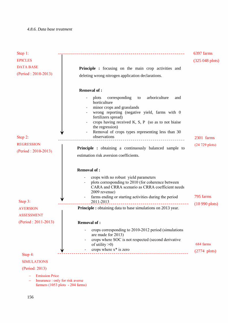
156

4.8.6. Data base treatment

Step 1:

EPICLES

DATA BASE

(Period : 2010-2013)

Principle : focusing on the main crop activities and

deleting wrong nitrogen application declarations.

Removal of :

- plots corresponding to arboriculture and

horticulture

- minor crops and grasslands

- wrong reporting (negative yield, farms with 0

fertilizers spread)

- crops having received K, S, P (so as to not biaise

the regression)

- Removal of crops types representing less than 30

observations

6397 farms

(325 048 plots)

Step 2:

REGRESSION

(Period : 2010-2013)

2301 farms

(24 729 plots)

Principle : obtaining a continuously balanced sample to

estimation risk aversion coefficients.

Removal of :

- crops with no robust yield parameters

- plots corresponding to 2010 (for coherence between

CARA and CRRA scenario as CRRA coefficient needs

2009 revenue)

- farms ending or starting activities during the period

2011-2013

795 farms

(10 990 plots) Step 3:

AVERSION

ASSESSMENT

(Period : 2011-2013)

Principle : obtaining data to base simulations on 2013 year.

Removal of :

- crops corresponding to 2010-2012 period (simulations

are made for 2013)

- crops where SOC is not respected (second derivative

of utility >0)

- crops where x* is zero

684 farms

(2774 plots) Step 4:

SIMULATIONS

(Period: 2013)

Emission Price

Insurance : only for risk averse

farmers (1053 plots - 204 farms)

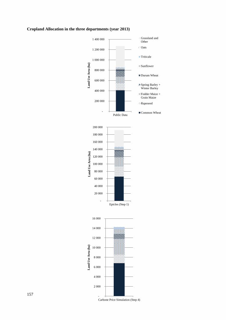
157

Cropland Allocation in the three departments (year 2013)

-

200 000

400 000

600 000

800 000

1 000 000

1 200 000

1 400 000

Public Data

La

nd

Use

Area

(h

a)

Grassland and

Other

Oats

Triticale

Sunflower

Durum Wheat

Spring Barley +

Winter Barley

Fodder Maize +

Grain Maize

Rapeseed

Common Wheat

-

20 000

40 000

60 000

80 000

100 000

120 000

140 000

160 000

180 000

200 000

Epicles (Step 1)

La

nd

Use

Area

(h

a)

-

2 000

4 000

6 000

8 000

10 000

12 000

14 000

16 000

Carbone Price Simulation (Step 4)

La

nd

Use

Area

(h

a)

158

4.8.7. Accuracy of risk aversion scenario with observed emissions.

Aversion

Coefficient

Type of

aversion

coefficient

Risk

Averse Neutral Risk Seeking Undetermined

All risk

attitudes

CARA 1 Distribution Absolute -7,0 -12,4 -6,9 1,3 -6,9

CARA 2 Uniform :

7,5.10-7

Absolute -25,9 -12,4 10,3 1,3 -11,7

CARA 3 Uniform :

0,0075

Absolute 93,4 85,9 129,3 14,3 93,2

CARA 4 Uniform :

0,04

Absolute 528,3 459,5 565,3 15,3 473,4

CRRA 2 Uniform :

0,25

Relative -25,7 -12,2 37,4 2,7 -4,3

CRRA 3 Uniform :

1,12

Relative -24,9 -11,5 130,8 2,7 20,6

CRRA 4 Uniform :

5,4

Relative -20,5 -5,5 589,9 5,8 144,5

Neutral Uniform :0 Relative -25,9 -12,4 10,3 1,3 -11,7

Average distance in % per ha between observed and estimated nitrogen application (The categorization of attitude toward risk is

based on scenario CARA 1)

159

4.8.8. Impact of risk aversion on crops associated to convex variance functions

Slopes

demissions

/

dEmissionprice

« CARA 1 » -0,061

« CRRA 4 » -0,062

« Neutral » -0,067

Note : This figure is an illustration of proposition 2 which shows the impact of risk aversion on

emissions reduction triggered by a tax on emissions. We focus here on crops having a convex variance

function. We observe that the reduction rate is lower when considering risk aversion. Focusing on

CARA 1 scenario, the reduction rate (-61 kgCO2eq/dtax) is by 8% lower than the reduction rate (-67

kgCO2eq/dtax) under Neutral behavior.

0

50

100

150

200

250

0 500 1000

emis

sion

s (t

CO

2eq

)

Emission price (euros/tCO2eq)

CARA_1

Neutral

CRRA_2

Emission reductions from risk averse farmers on crops

having a convex variance function

160

4.8.9. Insurance impact on emissions in the CRRA 4 scenario.

Emission Reduction for risk averse farmers in CRR4 4 scenario (in %)

Insurance Trigger Threshold - τ

(in percentage of the expected yield)

0,1 0,5 0,9

Insurance Premium

(euros/ha) 25 - 3,4 - 5,0 -8,2

50 - 3,3 - 5,0 - 8,2

400 - 2,2 - 4,4 - 8,1

600 - 2,1 - 3,9 - 8,0

163

Conclusion Générale

La forte contribution de l’agriculture au réchauffement climatique nécessite la mise en œuvre d’outils

de régulation qui visent à atténuer ses émissions au coût le plus faible possible. L’étude du coût

marginal d’abattement offre un éclairage quantitatif permettant d’analyser l’impact d’un prix sur les

pratiques agricoles et les émissions de GES. L’objectif de cette thèse est d’analyser ce potentiel à

l’échelle de plusieurs mesures associées aux pratiques de fertilisation des agriculteurs.

En étudiant le coût d’opportunité associé à la mise en place de plantes légumineuses dans les

assolements, et en comparant ce coût par rapport aux données réelles, les résultats du premier chapitre

révèlent que des réductions importantes d’émissions sont possibles, tout en augmentant le profit des

agriculteurs. Ce résultat est robuste aux analyses de sensibilité effectuées. De telles augmentations de

profit apparaissent également lorsque la pratique d’atténuation consiste à modifier les rotations des

agriculteurs dans le chapitre 2.

Nous l’avons vu au cours des différentes discussions menées dans les chapitres 1 et 2, la mise en

évidence de telles opportunités économiques conduit naturellement à la question suivante : pourquoi

les agriculteurs ne modifient pas leurs pratiques alors qu’il apparaît que ceux-ci peuvent augmenter

leur profit tout en réduisant leurs émissions de GES ? Une réponse possible à cette interrogation est

sans doute l’existence d’autres coûts, liés à trois grands niveaux. Le premier est associé à l’aspect

comportemental des agriculteurs. S’il est généralement admis que les individus prennent leur décision

sur la base de la maximisation de leur profit, c’est une hypothèse que retiennent notamment les deux

premiers articles de cette thèse, la prise de décision réelle des individus repose cependant sur un

éventail plus large d’éléments d’ordre psychologique et social. Ceci, par conséquent, induit un écart

entre les comportements des individus observés et le comportement attendu lorsque les modèles

reposent sur la seule hypothèse de minimisation des coûts. Par conséquent, la représentation de la

maximisation de l’utilité, intégrant ces autres éléments apparaît plus réaliste que celle de la seule

minimisation du coût. Le deuxième niveau est celui des coûts de mise en œuvre de politiques

d’atténuation. La mise en place d’instruments de régulation des émissions de gaz à effet de serre

implique un coût administratif dont l’estimation est d’autant plus déterminante que l’agriculture

présente la caractéristique d’une forte dispersion des émissions attribuées à un nombre important

d’acteurs établis sur le territoire. Ce coût dépendra par ailleurs de la nature de l’instrument retenu. Une

taxe aura l’avantage de ne pas impliquer la gestion des quotas que suppose la mise en place d’un

marché d’échange d’émissions et dont les coûts de transaction peuvent s’avérer potentiellement

élevés. Enfin, le troisième niveau est celui des interactions existant entre les pratiques des agriculteurs

et la filière en amont et en aval de l’exploitation agricole.

164

Si certains articles de la littérature représentent les interactions entre pratiques au sein de l’exploitation

ou bien sur les coûts de mise en œuvre, le troisième article de cette thèse se focalise sur l’un des

aspects de la dimension comportementale à savoir le rôle de l’aversion pour le risque dans la définition

des quantités d’azote à apporter par hectare.

Nous avons pu voir dans ce troisème chapitre, qu’en retenant l’hypothèse de fonctions d’utilité type

CARA ou CRRA, à l’échelle d’un individu, l’aversion pour le risque se traduit par des apports

supplémentaires d’engrais par rapport à un comportement de type neutre au risque en raison de la

réduction de la variabilité des rendements en fonction de la quantité d’engrais apportée. A l’échelle de

notre échantillon d’agriculteurs français comportant à la fois des individus neutres, riscophiles et

averses pour le risques, dans trois départements français, les simulations numériques effectuées ne

donnent pas de différences importantes entre les apports d’engrais appliqués par les agriculteurs après

avoir identifié leur aversion pour le risque et les apports lorsque que ceux-ci sont tous considérés

comme neutres au risque. Ceci est lié au fait que l’apport additionnel d’engrais des agriculteurs

averses au risque est compensé par l’apport moindre d’engrais par les agriculteurs ayant du goût pour

le risque. Nous avons également identifié les conditions dans lesquelles l’aversion au risque constitue

un frein par rapport à un signal prix appliqué sur les émissions de N2O. Les simulations numériques ne

permettent pas d’identifier un frein important de l’aversion pour le risque dans la réduction des

émissions puisque ces conditions50

sont présentes dans une minorité de cas. Enfin, la prise en compte

de l’aversion pour le risque dans la prise de décision suggère l’intérêt d’une assurance en termes

d’atténuation des émissions comme un outil efficace d’atténuation pour les agriculteurs averses au

risque.

Ce travail ouvre la voie à de futures extensions, invitant à poursuivre les efforts de modélisation dans

le but d’intégrer les différents niveaux interagissant avec les pratiques des agriculteurs décrits

précédemment. Ainsi, je propose l’exploration des voies suivantes :

Elargir le modèle d’intégration des légumineuses, présenté dans le chapitre 1, en modèle

d’optimisation de l’ensemble des cultures composant les assolements agricoles et le combiner

ensuite avec l’optimisation de la fertilisation par hectare étudiée en chapitre 3. Ce modèle

devra tenir compte de l’interaction avec le poste de l’élevage et pourrait être construit en

envisageant les liens avec les postes d’activités en amont et aval de l’exploitation.

50 Une variance du rendement des cultures convexe

165

Le modèle d’assurance à l’atténuation des émissions de gaz à effet de serre présenté dans le

chapitre 3 devra aborder la question de l’offre d’assurance dans l’optique de savoir si ce type

de couverture de risque peut être proposé par une agence privée ou publique.

Ces deux points pourraient être traités de manière innovante en abordant davantage la compréhension

des phénomènes de verrous (lock-in) bloquant le changement des pratiques et responsables d’inertie

dans l’organisation de la filière agricole. Une attention particulière pourrait être accordée à l’impact

des coûts fixes, tels que l’endettement, sur la capacité des différents maillons de la filière à pouvoir

changer leurs pratiques. A l’échelle de l’agriculteur spécifiquement, une étude sur leur capacité à

accepter de nouveaux dispositifs fiscaux pourrait être menée en abordant particulièrement le lien entre

leur compréhension de l’enjeu climatique et la capacité à accepter les dispositifs économiques

environnementaux nouveaux.

Titre : Le coût de l’atténuation des émissions de gaz à effet de serre liées à la fertilisation des cultures.

Mots clés : atténuation du changement climatique, légumineuses, fertilisation, prix du carbone, aversion pour le risque, assurance à l’atténuation

Résumé : L’objectif de cette thèse est d’estimer le coût de mesures d’atténuation des émissions de gaz à effet de serre (GES) liée à la fertilisation des cultures qui représente en Europe et en France respectivement 38% et 44% des émissions de GES de l’agriculture. L’étude du coût et du potentiel d’abattement est effectuée sur deux mesures clés dans l’atténuation des émissions à savoir la mise en place de plantes fixatrices d’azote (i.e. légumineuses) et la réduction de la fertilisation par hectare. Le potentiel d’atténuation des légumineuses est étudié en simulant leur augmentation dans les assolements agricoles français et dans un deuxième temps à l’échelle de rotations de cultures pouvant durer jusqu’à six ans dans cinq régions européennes. Les

résultats obtenus révèlent que des réductions importantes d’émissions sont possibles, tout en augmentant le profit des agriculteurs. Le rôle de l’aversion pour le risque est aussi étudié concernant la réduction de la fertilisation des cultures par hectare. Nous montrons analytiquement les conditions conduisant à une sur-application d’engrais par hectare permettant aux agriculteurs averses au risque de minimiser le risque de perte de rendement. Les simulations numériques effectuées spécifiquement sur les agriculteurs averses au risque démontrent qu’une assurance d’atténuation des émissions peut potentiellement déclencher des réductions importantes d’émissions de gaz à effet de serre.

Title : Mitigation cost of greenhouse gas emissions from fertilization in agriculture

Keywords : mitigation cost, legume crops, fertilization, carbon price, risk aversion, mitigation insurance

Abstract : In this thesis, we assess the mitigation cost of greenhouse gas (GHG) from fertilization which represents 38% and 44% of agricultural GHG emissions in Europe and in France. This assessment is conducted for two key measures in climate mitigation which are the implementation of legumes crops and the reduction of fertilization per hectare. The abatement potential of legume crops is computed by simulating their increase in French croplands and also by a switch of crop rotations on several years (up to 6 years) in five European regions. Results show that significant mitigation amounts can be obtained by increasing farms revenues.

The role of risk aversion is studied through the reduction of fertilisation per hectare. We analytically shows the conditions leading to nitrogen over-applications on crops which allows farmers to minimize their risk of loss on crop yields. The simulations lead on risk averse farmers show that an insurance covering yield variability could be foreseen as an interesting tool to mitigate emissions.

L’U P A (INSTITUT DES SCIENCES ET INDUSTRIES DU … · 2 lesquels je partage, je pense, un...

Documents

Transcript of L’U P A (INSTITUT DES SCIENCES ET INDUSTRIES DU … · 2 lesquels je partage, je pense, un...