PRINCIPAL COMPONENTS ANALYSIS

S. Daultrey

ISBN 0 902246 56 9

ISSN 0306 - 6142

© Stu Daultrey 1976

CONCEPTS AND TECHNIQUES IN MODERN GEOGRAPHY No. 8

CATMOG (Concepts and Techniques in Modern Geography)

CATMOG has been created to fill a teaching need in the field of quantitativemethods in undergraduate geography courses. These texts are admirable guidesfor the teachers, yet cheap enough for student purchase as the basis of class-work. Each book is written by an author currently working with the techniqueor concept he describes.

PRINCIPAL COMPONENTS ANALYSIS

by

Stu Daultrey

(University College Dublin)

CONTENTS

This series, Concepts and Techniques in Modern Geographyis produced by the Study Group in Quantitative Methods, ofthe Institute of British Geographers.For details of membership of the Study Group, write tothe Institute of British Geographers, 1 Kensington Gore,London, S.W.7.The series is published by Geo Abstracts Ltd., Universityof East Anglia, Norwich, NR4 7TJ, to whom all otherenquiries should be addressed.

Page

I THE TECHNIQUE DESCRIBED

(i) Introduction 3

(ii) Prior knowledge assumed 4

(iii) Conventions and notations 4

(iv) Correlation 5

II THE TECHNIQUE EXPLAINED (i) The transformation of one co-ordinate system to another 10

(ii) The derivation of the principal components 15

(iii) Principal component loadings 17

(iv) Principal component scores 18

(v) Further reading 18

(vi) A worked example 19

(vii) The significance of principal components 24

III THE TECHNIQUE APPLIED (i) Introduction 26

(ii) The data 27

(iii) The first analysis 30

(iv) The second analysis 35

IV THE TECHNIQUE ELABORATED (i) The normal distribution and the principal components

of correlation matrices 41

(ii) Principal components analysis of dispersion matrices 42

(iii) Discarding variables 42

(iv) Rotation of principal components 44

1. An introduction to Markov chain analysis - L. Collins

2. Distance decay in spatial interactions - P.J. Taylor

3. Understanding canonical correlation analysis - D. Clark

4. Some theoretical and applied aspects of spatial interactionshopping models - S. Openshaw

5. An introduction to trend surface analysis - D. Unwin

6. Classification in geography - R.J. Johnston

7. An introduction to factor analysis - J. Goddard & A. Kirby

8. Principal components analysis - S. Daultrey

Other titles in preparation

(v) The analysis of component scores 44

(vi) Sampling properties of principal components 46

(vii) Conclusions 47

BIBLIOGRAPHY 48

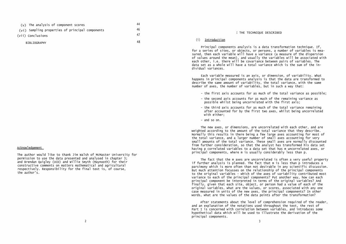
Acknowledgement

The author would like to thank Jim Walsh of McMaster University forpermission to use the data presented and analysed in chapter 3;and Brendan Quigley (UCD) and Willie Smyth (Maynooth) for theirconstructive comments on matters mathematical and agriculturalrespectively. Responsibility for the final text is, of course,the author's.

2

I THE TECHNIQUE DESCRIBED

(i) Introduction

Principal components analysis is a data transformation technique. If,for a series of sites, or objects, or persons, a number of variables is mea-sured, then each variable will have a variance (a measure of the dispersionof values around the mean), and usually the variables will be associated witheach other, i.e. there will be covariance between pairs of variables. Thedata set as a whole will have a total variance which is the sum of the in-dividual variances.

Each variable measured is an axis, or dimension, of variability. Whathappens in principal components analysis is that the data are transformed todescribe the same amount of variability, the total variance, with the samenumber of axes, the number of variables, but in such a way that:

- the first axis accounts for as much of the total variance as possible;

- the second axis accounts for as much of the remaining variance aspossible whilst being uncorrelated with the first axis;

- the third axis accounts for as much of the total variance remainingafter accounted for by the first two axes, whilst being uncorrelatedwith either;

- and so on.

The new axes, or dimensions, are uncorrelated with each other, and areweighted according to the amount of the total variance that they describe.Normally this results in there being a few large axes accounting for most ofthe total variance, and a larger number of small axes accounting for verysmall amounts of the total variance. These small axes are normally discountedfrom further consideration, so that the analyst has transformed his data sethaving p correlated variables to a data set that has m uncorrelated axes, orprincipal components, where m is usually considerably less than p.

The fact that the m axes are uncorrelated is often a very useful propertyif further analysis is planned. The fact that m is less than p introduces aparsimony which is more often than not desirable in any scientific discussion.But much attention focusses on the relationship of the principal componentsto the original variables - which of the axes of variability contributed mostvariance to each of the principal components? Put another way, how can eachprincipal component be interpreted in terms of the original variables? Andfinally, given that each site, object, or person had a value of each of theoriginal variables, what are the values, or scores, associated with any onecase measured in units of the new axes, the principal components? In otherwords, what are the values of the data points after the transformation?

After statements about the level of comprehension required of the reader,and an explanation of the notations used throughout the text, the rest ofPart I is concerned with correlation between variables, and introduces somehypothetical data which will be used to illustrate the derivation of theprincipal components.

3

C is used to denote the sample variance-covariance matrix in preference

Working with sample data, r, an unbiassed estimate of the population

(11)

(1)

Part II is concerned with the derivation of the magnitudes and direc-tions of the principal components of a data set, which, once obtained, allowthe description of the relation between the original variables and the prin-cipal components, and thence the definition of the data points in terms ofthe principal components.

Part III demonstrates the application of principal components analysisto an actual data set, in this case information on post-War changes in agri-culture in the Republic of Ireland.

Some of the problems arising from the analysis in Part III are dealtwith in Part IV, together with a more general discussion of principal com-ponents analysis in geographical studies.

(ii) Prior knowledge assumed

It is assumed that the reader:

1. can add, subtract, multiply and divide;

2. has taken a course in elementary statistical methods, and is familiarwith the descriptive statistics mean, variance, covariance, withprobability distributions e.g. the normal distribution, and withhypothesis testing.

3. is acquainted with the rudiments of matrix algebra.

If assumption 3. does not hold then the reader is referred to the ex-cellent synopses and bibliographies in Krumbein & Graybill (1965; chapter 11)and King (1969; appendix A4), Morrison (1967; chapter 2).

(iii) Conventions and notations

As far as possible standard notations have been adhered to. The Greeksymbols represent population statistics, whilst ordinary letters represent

whether or not they are derived from sample data; the Greek symbol is usedbecause a typewritten lower case 1 is easily confused with the number 1 orthe letter i. L is used instead to denote the matrix of component loadings.

4

(iv) Correlation

Principal components analysis depends upon the fact that at least someof the variables in the data set are intercorrelated. If none of the p vari-ables is correlated with any other, there exists already a set of uncorrelatedaxes, and there is no point in performing a principal components analysis.

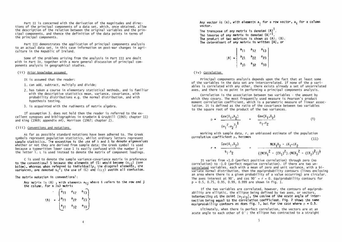
Correlation is the association between two variables - the amount bywhich they covary. The most frequently used measure is Pearson's productmoment correlation coefficient, which is a parametric measure of linear assoc-iation. It is defined as the ratio of the covariance between two variablesto the square root of the product of the two variances.

It varies from +1.0 (perfect positive correlation) through zero (nocorrelation) to -1.0 (perfect negative correlation). If there are two un-correlated variables, each with a mean of zero and unit variance, with a bi-variate normal distribution, then the equiprobability contours (lines enclosingan area where there is a given probability of a value occurring) are circular.

The axes interest at 90°, and cos 90° = r = 0. Equiprobability contours forp = 0.5, 0.75, 0.95, 0.99, 0.999 are shown in fig. 1.

If the two variables are correlated, however, the contours of equiprob-ability are elliptic, the ellipse being defined by two axes, or vectors,

Ultimately, when there is perfect correlation, the vectors are at anacute angle to each other of 0 0 ; the ellipse has contracted to a straight

5

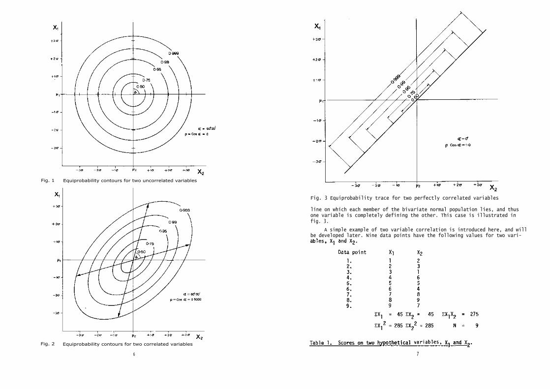
Fig. 1 Equiprobability contours for two uncorrelated variables

Fig. 2 Equiprobability contours for two correlated variables

6

Fig. 3 Equiprobability trace for two perfectly correlated variables

line on which each member of the bivariate normal population lies, and thusone variable is completely defining the other. This case is illustrated infig. 3.

A simple example of two variable correlation is introduced here, and willbe developed later. Nine data points have the following values for two vari-

7

Fig. 4 Plot of hypothetical data for two variables

Fig. 4 shows the data points; and fig 5 shows for the same data oneelliptical equiprobability contour defined by two vectors intersecting at330 34' (cos 33° 34' = 0.8333 - r). Fig. 6 shows two orthogonal axes super-imposed on the ellipse such that the long axis is as long as possible, andthe other axis is as long as possible whilst being at right angles to thefirst. These axes are the principal components; the long axis is the firstcomponent, accounting for as much of the total variance (the area of theellipse) as possible, and the other axis is the second component, in thiscase accounting for the remainder of the total variance.

Describing the principal components of two variables is instructive, butsubstantively trivial; normally, many more than two variables are analysed.It is impossible to draw more than three dimensions, thus in this section andin section II(vi) much of the description will focus on a three variableexample.

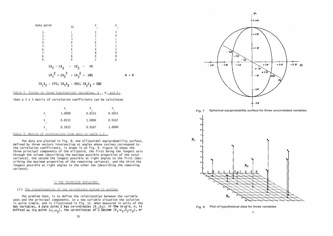
Just as two uncorrelated variables have circular contours of equiprob-ability, three uncorrelated variables have spherical equiprobability surfaces(see fig. 7, which shows the p = 0.99 surface). Three correlated variableshave ellipsoidal equiprobability surfaces. If a third variable is added tothe two in table 1.

8

Fig. 5 Hypothetical data with two variables and equiprobability contour

Fig. 6 Hypothetical data with two principal components andequiprobability contour

9

Data pointX1

X2

X3

1. 1 2 32. 2 3 43. 3 1 14. 4 6 75. 5 5 56. 6 4 27. 7 8 98. 8 9 89. 9 7 6

Table 2. Scores on three hypothetical variables, X i , X 2 and X 3 .

then a 3 x 3 matrix of correlation coefficients can be calculated.

X1

X2

X3

X1

1.0000 0.8333 0.5833

X2

0.8333 1.0000 0.9167

X3

0.5833 0.9167 1.0000

Table 3. Matrix of correlations from data in table 1.2.

The data are plotted in fig. 8; one ellipsoidal equiprobability surface,defined by three vectors intersecting at angles whose cosines correspond tothe correlation coefficients, is drawn in on fig. 9. Figure 10 shows thethree principal components of the ellipsoid, the first being the longest axisthrough the volume (describing the maximum possible proportion of the totalvariance), the second the longest possible at right angles to the first (des-cribing the maximum proportion of the remaining variance), and the third thelongest possible at right angles to the other two (describing the remainingvariance).

II THE TECHNIQUE EXPLAINED

(i) The transformation of one co-ordinate system to another

The problem then, is to define the relationships between the variableaxes and the principal components. In a two variable situation the solutionis quite simple, and is illustrated in fig. 11. When measured in units of the

Fig. 7 Spherical equiprobability surface for three uncorrelated variables

Fig. 8 Plot of hypothetical data for three variables

1110

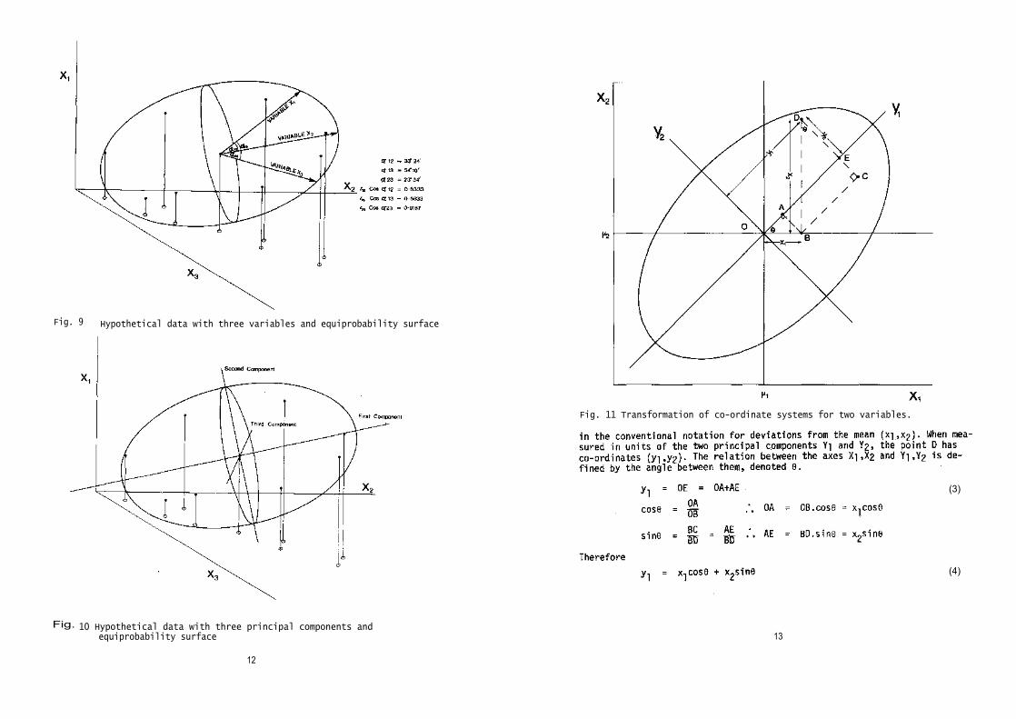
Fig. 9 Hypothetical data with three variables and equiprobability surface

Fig. 11 Transformation of co-ordinate systems for two variables.

(3)

(4)

Fig. 10 Hypothetical data with three principal components andequiprobability surface 13

12

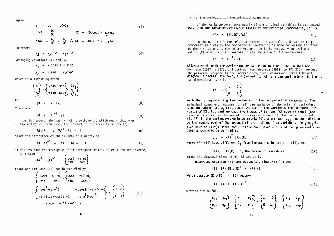
Again

which is a matrix equation

Arranging equations (4) and (6)

(8)

(9)

(5)

(6)

( 7 )

As it happens, the matrix {A} is orthogonal, which means that whenmultiplied by its transpose, the product is the identity matrix {I}.

Equations (10) and (11) can be verified by

(12)

or

Therefore

Therefore

Since the definition of the inverse of a matrix is

(10)

(11)

it follows that the transpose of an orthogonal matrix is equal to its inverse,in this case

since the diagonal elements of {R} are unit.

(15)

(16)

(17)

(18)

(ii) The derivation of the principal components

If the variance-covariance matrix of the original variables is designated

(13)

In the matrix {A} the relation between the variables and each principalcomponent is given by the row vectors. However it is more convenient to referto these relations by the column vectors, so it is necessary to define amatrix {E} which is the transpose of {A}. Equation (13) then becomes

(14)

Morrison (1967, p.223), and derived from Anderson (1958, pp 272-279). Becausethe principal components are uncorrelated, their covariance terms (the off-

two-dimensional case it is

principal Components account for all the variance of the original variables,

trace of a matrix is the sum of the diagonal elements). The correlation mat-

written out in full

15

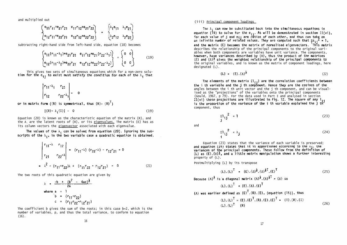
and multiplied out(iii) Principal component loadings

subtracting right-hand side from left-hand side, equation (18) becomes

This gives two sets of simultaneous equations which for a non-zero solu-

(19)

(19)

and

(23)

(24)

Equation (20) is known as the characteristic equation of the matrix {R}, andthe A i are the latent roots of {R}, or its eigenvalues. The matrix {E} has as

its column vectors the eigenvector associated with each eigenvalue.

(21)

The two roots of this quadratic equation are given by

The coefficient b gives the sum of the roots; in this case b=2, which is thenumber of variables, p, and thus the total variance, to conform to equation(16).

16

describes the relationship of the principal components to the original vari-ables when both components are variables have unit variance. The components,

the original variables, and is known as the matrix of component loadings, heredesignated (L).

(22)

angles between the i th unit vector and the j th component, and can be visual-ised as the "projections" of the variables onto the principal components(Gould, 1967, p 79). For the data used in Part I and analysed in section

component, thus

Equation (23) states that the variance of each variable is preserved;

property of {L}.

Postmultiplying {L} by its transpose

(25)

(26)

17

(29)

(30)

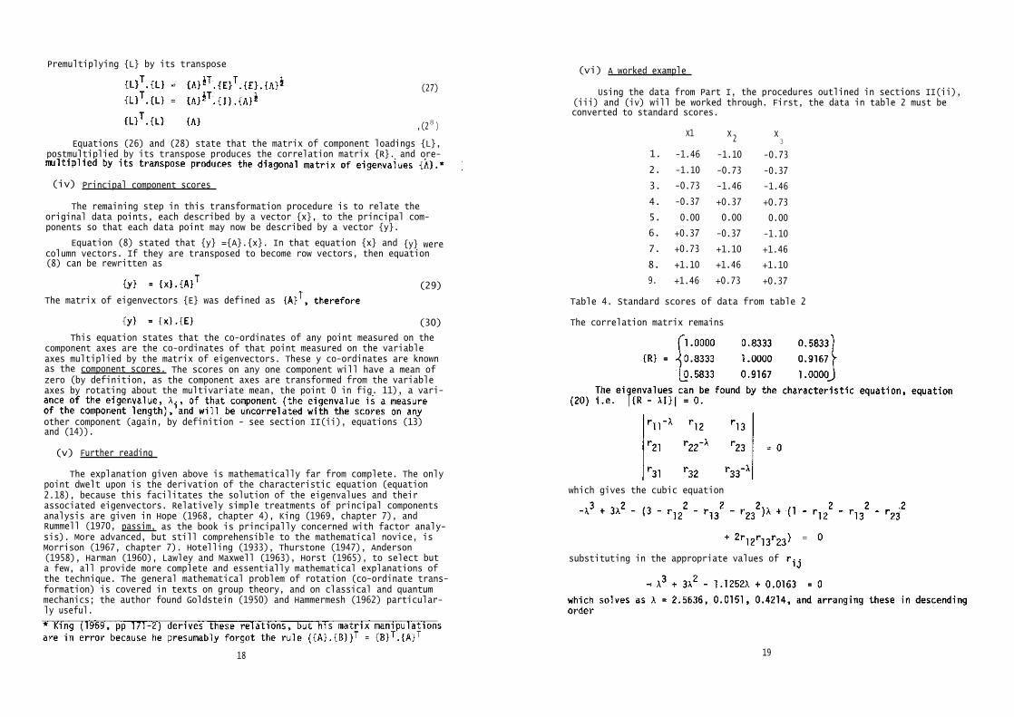
(vi) A worked example

Using the data from Part I, the procedures outlined in sections II(ii),(iii) and (iv) will be worked through. First, the data in table 2 must beconverted to standard scores.

XX12

X3

1. -1.46 -1.10 -0.73

2. -1.10 -0.73 -0.37

3. -0.73 -1.46 -1.46

4. -0.37 +0.37 +0.73

5. 0.00 0.00 0.00

6. +0.37 -0.37 -1.10

7. +0.73 +1.10 +1.46

8. +1.10 +1.46 +1.10

9. +1.46 +0.73 +0.37

Table 4. Standard scores of data from table 2

The correlation matrix remains

which gives the cubic equation

substituting in the appropriate values of

18 19

Premultiplying {L} by its transpose

(27)

,(28

)

Equations (26) and (28) state that the matrix of component loadings {L},postmultiplied by its transpose produces the correlation matrix {R}. and ore-

(iv) Principal component scores

The remaining step in this transformation procedure is to relate theoriginal data points, each described by a vector {x}, to the principal com-ponents so that each data point may now be described by a vector {y}.

Equation (8) stated that {y} ={A}.{x}. In that equation {x} and {y} werecolumn vectors. If they are transposed to become row vectors, then equation(8) can be rewritten as

The matrix of eigenvectors {E} was defined as

This equation states that the co-ordinates of any point measured on thecomponent axes are the co-ordinates of that point measured on the variableaxes multiplied by the matrix of eigenvectors. These y co-ordinates are knownas the component scores. The scores on any one component will have a mean ofzero (by definition, as the component axes are transformed from the variableaxes by rotating about the multivariate mean, the point 0 in fig. 11), a vari-

other component (again, by definition - see section II(ii), equations (13)and (14)).

(v) Further reading

The explanation given above is mathematically far from complete. The onlypoint dwelt upon is the derivation of the characteristic equation (equation2.18), because this facilitates the solution of the eigenvalues and theirassociated eigenvectors. Relatively simple treatments of principal componentsanalysis are given in Hope (1968, chapter 4), King (1969, chapter 7), andRummell (1970, passim, as the book is principally concerned with factor analy-sis). More advanced, but still comprehensible to the mathematical novice, isMorrison (1967, chapter 7). Hotelling (1933), Thurstone (1947), Anderson(1958), Harman (1960), Lawley and Maxwell (1963), Horst (1965), to select buta few, all provide more complete and essentially mathematical explanations ofthe technique. The general mathematical problem of rotation (co-ordinate trans-formation) is covered in texts on group theory, and on classical and quantummechanics; the author found Goldstein (1950) and Hammermesh (1962) particular-ly useful.

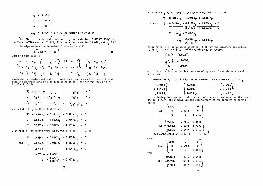
These ratios will be obtained no matter which way the equations are solved,

which is normalised by setting the sums of squares of the elements equal tounity, viz.

The eigenvectors can be solved from equation (18)

which in this case is

which when multiplied out and with right-hand side subtracted from left-handside yields three sets of simultaneous equations , one set for each of the

and substituting in the actual values

20

Allowing the computer to do the rest of the work, and to alter the fourthdecimal places, the eigenvalues and eigenvectors of the correlation matrixbecome

where

then

21

(30)

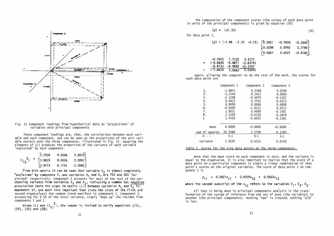
Table 5. Scores for the nine data points on the three components.

Note that the mean score on each component is zero, and the variance isequal to the eigenvalue. It is also important to realise that the score of adata point on a particular component is simply a linear combination of thatpoint's scores on the original variables. The score of data point 1 on com-ponent 1 is

Fig. 12 Component loadings from hypothetical data as "projections" ofvariables onto principal components

These component loadings are, then, the correlations between each vari-able and each component, and can be seen as the projections of the unit vari-able vectors onto the three components, illustrated in fig. 12. Squaring theelements of {L} produces the proportion of the variance of each variable"explained" by each component.

plained" respectively. Component 2 accounts for most of the rest of the out-

second eigenvalues) the common trend manifest in component 1. Component 3,accounting for 0.5% of the total variance, simply "mops up" the residue fromcomponents 1 and 2.

22

The computation of the component scores (the values of each data pointin units of the principal components) is given by equation (30)

for data point 1,

Again, allowing the computer to do the rest of the work, the scores foreach data point are

Component 1 Component 2 Component 3

1. -1.8855 0.5568 0.03992. -1.2540 0.5422 0.00693. -2.1298 -0.4979 -0.12674. 0.4423 0.7765 0.03725. 0.0000 0.0000 0.00006. -0.6490 -1.0112 0.05127. 1.9031 0.4690 -0.15818. 2.1209 -0.0150 0.18599. 1.4520 -0.8205 -0.1362

mean 0.0000 -0.0000 +0.0000

sum of squares 20.5088 3.3708 0.1200N - 1

variance

9-1

2.5636

9-1

0.4214

9-1

0.0150

All that is being done in principal components analysis is the trans-formation of the system of reference from one set of axes (the variables) toanother (the principal components). Nothing "new" is created; nothing "old"is lost.

23

(31)

where k is the number of eigenvalues not under consideration (k=p-t).Q can

arithmetic mean of the t eigenvalues.

(32)

(33)

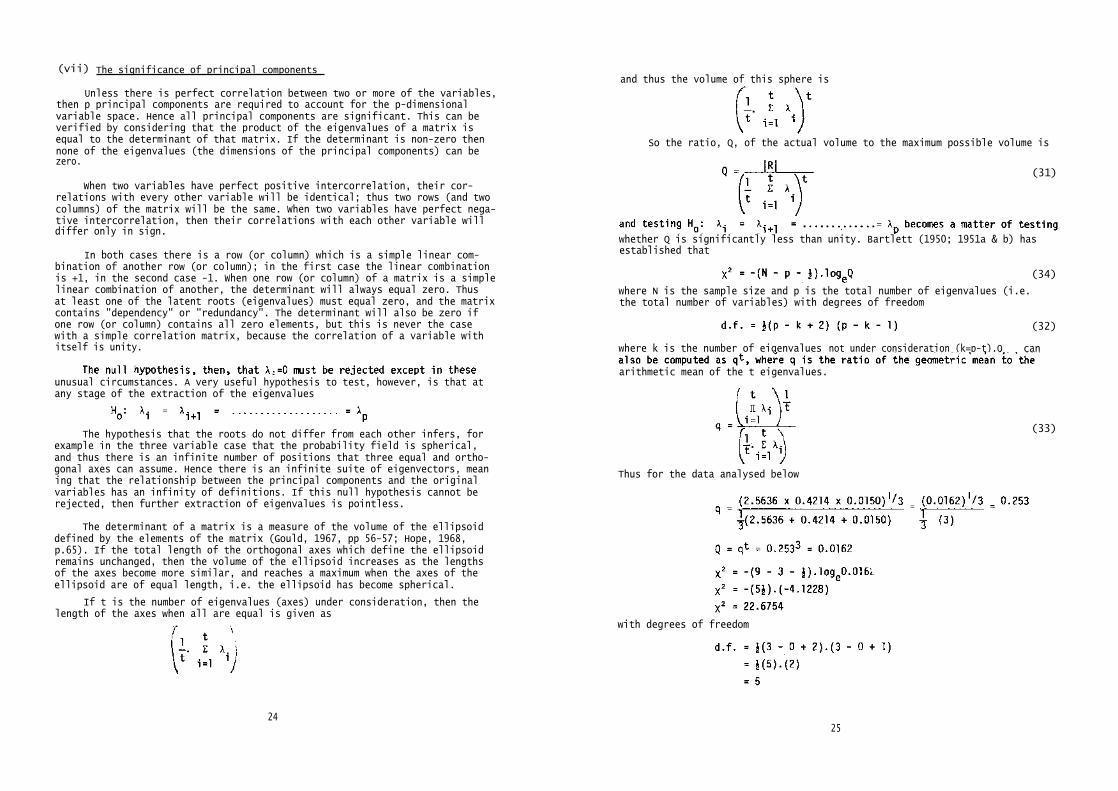
(vii) The significance of principal components

Unless there is perfect correlation between two or more of the variables,then p principal components are required to account for the p-dimensionalvariable space. Hence all principal components are significant. This can beverified by considering that the product of the eigenvalues of a matrix isequal to the determinant of that matrix. If the determinant is non-zero thennone of the eigenvalues (the dimensions of the principal components) can bezero.

When two variables have perfect positive intercorrelation, their cor-relations with every other variable will be identical; thus two rows (and twocolumns) of the matrix will be the same. When two variables have perfect nega-tive intercorrelation, then their correlations with each other variable willdiffer only in sign.

In both cases there is a row (or column) which is a simple linear com-bination of another row (or column); in the first case the linear combinationis +1, in the second case -1. When one row (or column) of a matrix is a simplelinear combination of another, the determinant will always equal zero. Thusat least one of the latent roots (eigenvalues) must equal zero, and the matrixcontains "dependency" or "redundancy". The determinant will also be zero ifone row (or column) contains all zero elements, but this is never the casewith a simple correlation matrix, because the correlation of a variable withitself is unity.

unusual circumstances. A very useful hypothesis to test, however, is that atany stage of the extraction of the eigenvalues

The hypothesis that the roots do not differ from each other infers, forexample in the three variable case that the probability field is spherical,and thus there is an infinite number of positions that three equal and ortho-gonal axes can assume. Hence there is an infinite suite of eigenvectors, meaning that the relationship between the principal components and the originalvariables has an infinity of definitions. If this null hypothesis cannot berejected, then further extraction of eigenvalues is pointless.

The determinant of a matrix is a measure of the volume of the ellipsoiddefined by the elements of the matrix (Gould, 1967, pp 56-57; Hope, 1968,p.65). If the total length of the orthogonal axes which define the ellipsoidremains unchanged, then the volume of the ellipsoid increases as the lengthsof the axes become more similar, and reaches a maximum when the axes of theellipsoid are of equal length, i.e. the ellipsoid has become spherical.

If t is the number of eigenvalues (axes) under consideration, then thelength of the axes when all are equal is given as

and thus the volume of this sphere is

So the ratio, Q, of the actual volume to the maximum possible volume is

whether Q is significantly less than unity. Bartlett (1950; 1951a & b) hasestablished that

(34)

where N is the sample size and p is the total number of eigenvalues (i.e.the total number of variables) with degrees of freedom

Thus for the data analysed below

with degrees of freedom

2425

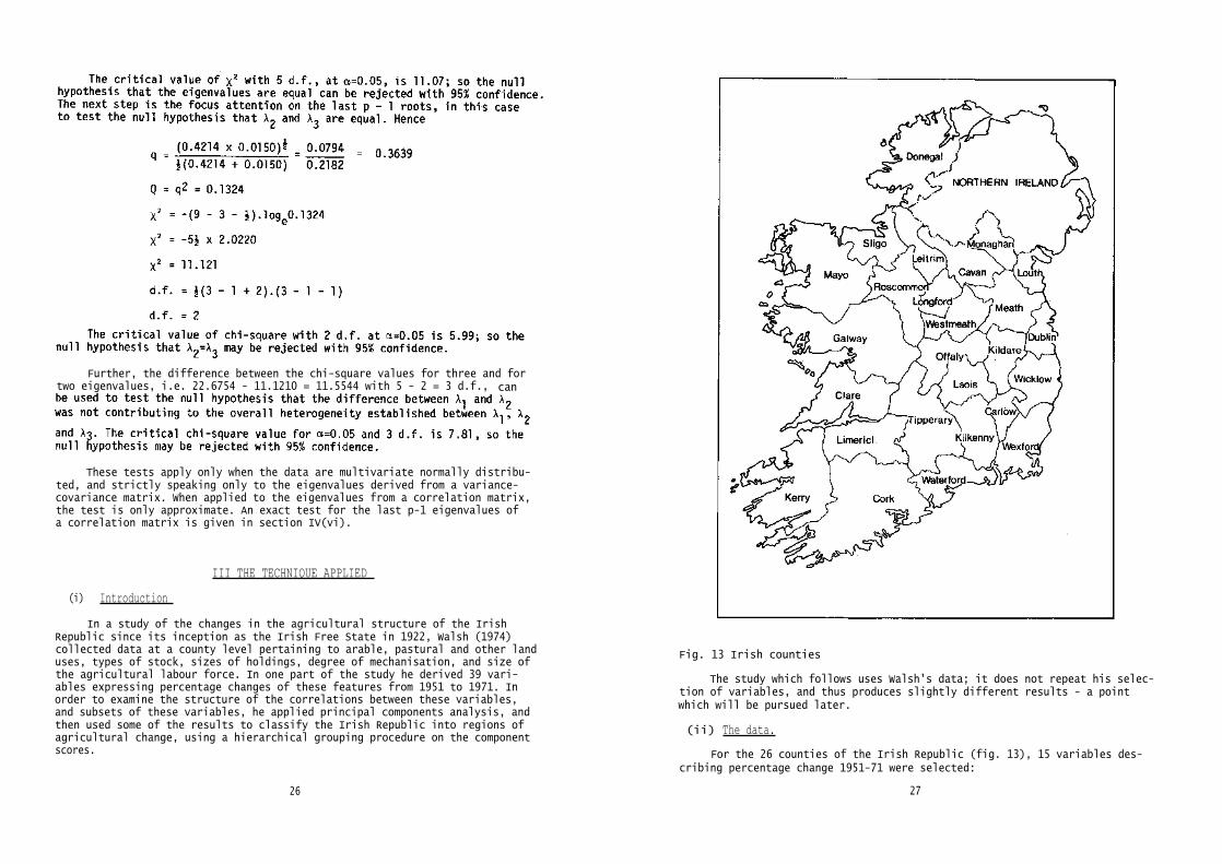
Fig. 13 Irish counties

The study which follows uses Walsh's data; it does not repeat his selec-tion of variables, and thus produces slightly different results - a pointwhich will be pursued later.

(ii) The data.

For the 26 counties of the Irish Republic (fig. 13), 15 variables des-cribing percentage change 1951-71 were selected:

27

Further, the difference between the chi-square values for three and fortwo eigenvalues, i.e. 22.6754 - 11.1210 = 11.5544 with 5 - 2 = 3 d.f., can

These tests apply only when the data are multivariate normally distribu-ted, and strictly speaking only to the eigenvalues derived from a variance-covariance matrix. When applied to the eigenvalues from a correlation matrix,the test is only approximate. An exact test for the last p-1 eigenvalues ofa correlation matrix is given in section IV(vi).

III THE TECHNIQUE APPLIED

(i) Introduction

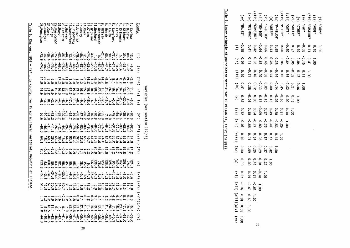
In a study of the changes in the agricultural structure of the IrishRepublic since its inception as the Irish Free State in 1922, Walsh (1974)collected data at a county level pertaining to arable, pastural and other landuses, types of stock, sizes of holdings, degree of mechanisation, and size ofthe agricultural labour force. In one part of the study he derived 39 vari-ables expressing percentage changes of these features from 1951 to 1971. Inorder to examine the structure of the correlations between these variables,and subsets of these variables, he applied principal components analysis, andthen used some of the results to classify the Irish Republic into regions ofagricultural change, using a hierarchical grouping procedure on the componentscores.

26

2928

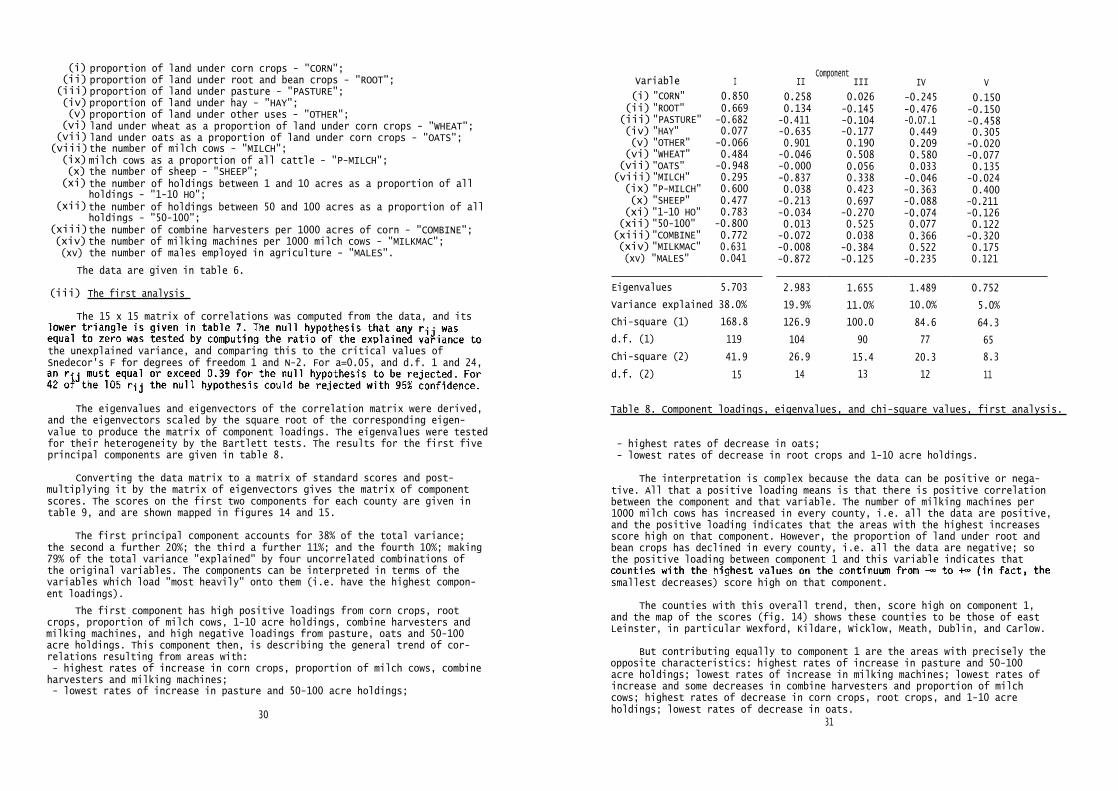
(i) proportion of land under corn crops - "CORN";(ii) proportion of land under root and bean crops - "ROOT";(iii)proportion of land under pasture - "PASTURE";(iv) proportion of land under hay - "HAY";(v) proportion of land under other uses - "OTHER";(vi) land under wheat as a proportion of land under corn crops - "WHEAT";(vii) land under oats as a proportion of land under corn crops - "OATS";(viii)the number of milch cows - "MILCH";(ix)milch cows as a proportion of all cattle - "P-MILCH";(x) the number of sheep - "SHEEP";(xi) the number of holdings between 1 and 10 acres as a proportion of all

holdings - "1-10 HO";(xii)the number of holdings between 50 and 100 acres as a proportion of all

holdings - "50-100";(xiii)the number of combine harvesters per 1000 acres of corn - "COMBINE";(xiv)the number of milking machines per 1000 milch cows - "MILKMAC";(xv) the number of males employed in agriculture - "MALES".

The data are given in table 6.

(iii) The first analysis

The 15 x 15 matrix of correlations was computed from the data, and its

the unexplained variance, and comparing this to the critical values ofSnedecor's F for degrees of freedom 1 and N-2. For a=0.05, and d.f. 1 and 24,

Variable I

(i) "CORN" 0.850(ii) "ROOT" 0.669(iii)"PASTURE" -0.682(iv) "HAY" 0.077(v) "OTHER" -0.066(vi) "WHEAT" 0.484(vii)"OATS" -0.948(viii)"MILCH" 0.295(ix) "P-MILCH" 0.600(x) "SHEEP" 0.477(xi) "1-10 HO" 0.783(xii)"50-100" -0.800(xiii)"COMBINE" 0.772(xiv) "MILKMAC" 0.631(xv) "MALES" 0.041

Eigenvalues 5.703

Variance explained 38.0%

Chi-square (1) 168.8

d.f. (1) 119

Chi-square (2) 41.9

d.f. (2) 15

ComponentII III IV V

0.258 0.026 -0.245 0.1500.134 -0.145 -0.476 -0.150

-0.411 -0.104 -0.07.1 -0.458-0.635 -0.177 0.449 0.3050.901 0.190 0.209 -0.020-0.046 0.508 0.580 -0.077-0.000 0.056 0.033 0.135-0.837 0.338 -0.046 -0.0240.038 0.423 -0.363 0.400-0.213 0.697 -0.088 -0.211-0.034 -0.270 -0.074 -0.1260.013 0.525 0.077 0.122-0.072 0.038 0.366 -0.320-0.008 -0.384 0.522 0.175-0.872 -0.125 -0.235 0.121

2.983 1.655 1.489 0.752

19.9% 11.0% 10.0% 5.0%

126.9 100.0 84.6 64.3

104 90 77 65

26.9 15.4 20.3 8.3

14 13 12 11

The eigenvalues and eigenvectors of the correlation matrix were derived,and the eigenvectors scaled by the square root of the corresponding eigen-value to produce the matrix of component loadings. The eigenvalues were testedfor their heterogeneity by the Bartlett tests. The results for the first fiveprincipal components are given in table 8.

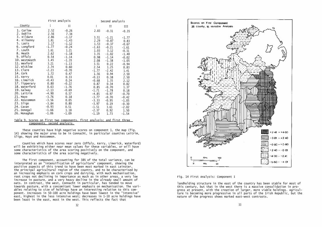
Converting the data matrix to a matrix of standard scores and post-multiplying it by the matrix of eigenvectors gives the matrix of componentscores. The scores on the first two components for each county are given intable 9, and are shown mapped in figures 14 and 15.

The first principal component accounts for 38% of the total variance;the second a further 20%; the third a further 11%; and the fourth 10%; making79% of the total variance "explained" by four uncorrelated combinations ofthe original variables. The components can be interpreted in terms of thevariables which load "most heavily" onto them (i.e. have the highest compon-ent loadings).

The first component has high positive loadings from corn crops, rootcrops, proportion of milch cows, 1-10 acre holdings, combine harvesters andmilking machines, and high negative loadings from pasture, oats and 50-100acre holdings. This component then, is describing the general trend of cor-relations resulting from areas with:- highest rates of increase in corn crops, proportion of milch cows, combineharvesters and milking machines;- lowest rates of increase in pasture and 50-100 acre holdings;

30

Table 8. Component loadings, eigenvalues, and chi-square values, first analysis.

- highest rates of decrease in oats;- lowest rates of decrease in root crops and 1-10 acre holdings.

The interpretation is complex because the data can be positive or nega-tive. All that a positive loading means is that there is positive correlationbetween the component and that variable. The number of milking machines per1000 milch cows has increased in every county, i.e. all the data are positive,and the positive loading indicates that the areas with the highest increasesscore high on that component. However, the proportion of land under root andbean crops has declined in every county, i.e. all the data are negative; sothe positive loading between component 1 and this variable indicates that

smallest decreases) score high on that component.

The counties with this overall trend, then, score high on component 1,and the map of the scores (fig. 14) shows these counties to be those of eastLeinster, in particular Wexford, Kildare, Wicklow, Meath, Dublin, and Carlow.

But contributing equally to component 1 are the areas with precisely theopposite characteristics: highest rates of increase in pasture and 50-100acre holdings; lowest rates of increase in milking machines; lowest rates ofincrease and some decreases in combine harvesters and proportion of milchcows; highest rates of decrease in corn crops, root crops, and 1-10 acreholdings; lowest rates of decrease in oats.

31

County

First analysis

I II I

Second analysis

II III

1. Carlow 2.52 -0.26 2.83 -0.31 -0.352. Dublin 2.56 7.343. Kildare 2.86 -1.17 3.51 -1.21 -1.774. Kilkenny 1.81 -1.43 2.29 -0.87 0.835. Laois 1.17 -1.12 1.53 -0.37 -0.676. Longford -1.77 -0.24 -1.63 -0.21 -1.617. Louth 1.61 1.21 1.03 3.12 -0.318. Meath 2.62 -1.18 3.35 -1.02 -1.409. Offaly 0.54 -1.14 0.98 -1.14 -0.0210. Westmeath 1.45 -1.35 2.08 -1.38 -1.0511. Wexford 3.21 -1.13 3.51 0.22 -0.9412. Wicklow 2.74 0.60 2.54 1.25 0.8313. Clare -2.23 -0.70 -1.77 -2.42 1.4114. Cork 1.72 0.47 1.56 0.94 2.5015. Kerry 0.01 0.33 -0.13 0.38 2.5016. Limerick -0.43 0.24 -0.68 1.35 2.1217. Tipperary 0.80 -0.22 0.87 0.34 0.8218. Waterford 0.63 -1.76 0.85 -0.70 1.3719. Galway -2.13 -0.69 -1.71 -1.78 0.1820. Leitrim -4.90 0.57 -4.85 -0.97 -0.7021. Mayo -3.76 0.18 -3.77 -0.70 -0.4222. Roscommon -3.56 0.05 -3.33 -0.95 -1.0523. Sligo -3.84 0.80 -3.97 0.19 -0.3024. Cavan -0.93 0.51 -1.51 3.61 -2.0225. Donegal -1.66 1.18 -2.37 0.92 1.5026. Monaghan -1.06 -1.09 -1.19 1.73 -1.54

Table 9. Scores on first two components, first analysis; and first three components, second analysis.

These counties have high negative scores on component 1, the map (fig.14) showing the major area to be in Connacht, in particular counties Leitrim,Sligo, Mayo and Roscommon.

Counties which have scores near zero (Offaly, Kerry, Limerick, Waterford)will be exhibiting either near mean values for these variables, or will havesome characteristics of the area scoring positively on the component, andsome characteristics of the area scoring negatively.

The first component, accounting for 38% of the total variance, can beinterpreted as an "intensification of agriculture" component, showing thepositive aspects of this trend to have been most marked in east Leinster,the principal agricultural region of the country, and to be characterised byan increasing emphasis on corn crops and dairying, with much mechanisation,root crops not declining in importance as much as in other areas, a very lowincrease in pasture, and a very heavy decline in the already small amount ofoats. In contrast, the west, Connacht in particular, has tended to movetowards pasture, with a concomitant lower emphasis on mechanisation. The vari-ables relating to size of holdings have an interesting relation to this com-ponent. Increases in 50-100 acre holdings have been lowest in the "intensive"east, highest in the less intensive west; decreases in 1-10 acre holdings havebeen least in the east, most in the west. This reflects the fact that

32

Fig. 14 First Analysis: Component I

landholding structure in the east of the country has been stable for most ofthis century, but that in the west there is a massive consolidation in pro-gress at present, with the creation of larger, more viable holdings. Agricul-ture is becoming more progressive in all parts of the Irish Republic, but thenature of the progress shows marked east-west contrasts.

33

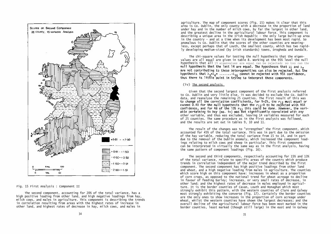
Fig. 15 First Analysis : Component II

The second component, accounting for 20% of the total variance, has ahigh positive loading from other land, and high negative loadings from hay,milch cows, and males in agriculture. This component is describing the trendsin correlation resulting from areas with the highest rates of increase inother land, and highest rates of decrease in hay, milch cows, and males in

34

agriculture. The map of component scores (fig. 15) makes it clear that thisarea is Co. Dublin, the only county with a decrease in the proportion of landunder hay and in the number of milch cows, by far the largest in other land,and the greatest decline in the agricultural labour force. This component isdescribing a unique area in the Irish Republic - the only large built-up areain the country - and at a time when its development has been most rapid. Soanomalous is Co. Dublin that the scores of the other counties are meaning-less, except perhaps that of Louth, the smallest county, which has two rapid-ly developing medium-sized (by Irish standards) towns, Drogheda and Dundalk.

The chi-square values for testing the null hypothesis that the eigen-values are all equal are given in table 8. Working at the 95% level the nullhypothesis that all 15 eigenvalues are equal can be rejected; so too can the

(iv) The second analysis

Given that the second largest component of the first analysis referredto Co. Dublin and very little else, it was decided to exclude the Co. Dublindata, and reanalyse the remaining 25 counties. The first result of this was

other variable, and thus was excluded, leaving 14 variables measured for eachof 25 counties. The same procedure as in the first analysis was followed,and the results are set out in tables 9, 10 and 11.

The result of the changes was to "strengthen" the first component, whichaccounted for 45% of the total variance. This was in part due to the omissionof the hay variable, reducing the total variance from 15 to 14, and in partdue to the removal of the Dublin anomaly, which increased the component load-ings relating to milch cows and sheep in particular. This first componentcan be interpreted in virtually the same way as in the first analysis, havingthe same pattern of component loadings (fig. 16).

The second and third components, respectively accounting for 15% and 13%of the total variance, relate to specific areas of the country which producetrends in correlation independent of the major trend described by the firstcomponent. The second component has high positive loadings from other landand wheat, and a high negative loading from males in agriculture. The countieswhich score high on this component have: increases in wheat as a proportionof corn crops, as opposed to the national trend for wheat acreage to declinein favour of feeding barley; increases, or very small rates of decrease, inother land; and the highest rates of decrease in males employed in agricul-ture. It is the border counties of Cavan, Louth and Monaghan which moststrongly exhibit this pattern, with the western counties of Clare and Galwaymost strongly exhibiting the converse (fig. 17). Certainly the border countiesare the only ones to show increases in the proportion of corn acreage underwheat, whilst the western counties have shown the largest decreases; and theoverall decline of the agricultural labour force has been most marked in theborder counties, least marked (though still large) in the east and in Galway

35

36

(i)(ii)

(iii)(v)(vi)(vii)(viii)(ix)(x)(xi)(xii)(xiii)(xiv)(xv)

"CORN""ROOT""PASTURE""OTHER""WHEAT""OATS""MILCH""P-MILCH""SHEEP""1-10 HO""50-100""COMBINE""MILKMAC""MALES"

0.8660.686

-0.672-0.4560.440

-0.9320.6580.6410.5240.762

-0.7740.7370.5800.429

-0.044-0.352-0.2150.6870.583

-0.125-0.228-0.3070.0470.146-0.0080.4690.417-0.716

0.0500.1850.053-0.152-0.472-0.101-0.580-0.471-0.6440.325-0.5500.0030.4110.037

0.1400.3210.5160.072

-0.059-0.140-0.022-0.1330.2630.223

-0.1560.022-0.427-0.381

0.217-0.413-0.028-0.209-0.0860.009-0.1370.3510.0070.3180.020-0.2930.013-0.299

Eigenvalues

Variance explained

Chi-square (1)

d.f. (1)

Chi-square (2)

d.f. (2)

6.305

45.0%

151.1

104

52.3

14

2.076

14.9%

98.8

90

16.3

13

1.847

13.2%

82.5

77

21.6

12

0.908

6.5%

60.9

65

8.7

11

0.689

4.9%

52.2

54

6.8

10

Table 11. Component loadings, eigenvalues, and chi-square values, second analysis

and Clare. The category "other land" covers a multitude of land uses, and itsprecise meaning in this context is not clear. Generally, the second componentseems to be describing separate trends which happen to be occuring in thesame areas.

The third component is somewhat easier to interpret. The highest load-ings are all negative, and are from the numbers of milch cows, the numbersof sheep, and the proportion of 50-100 acre holdings. Thus the areas whichscore high on this component will have the lowest rates of increase in milchcows, sheep and 50-100 acre holdings. These turn out to be Kerry, Cork andLimerick, where the dairying industry was already well-established by the1950's, and thus the rapid increase shown over the rest of the country is notrepeated there (fig. 18). It would seem that the pattern of increase in sheepnumbers coincides with the dairying pattern, rather than being part of thesame process.

A major factor in the lack of clarity of the second and third componentsbecomes immediately apparent when the chi-square values from the Bartlett

remaining 13 eigenvalues cannot be rejected with 95% confidence. Thus afterthe first principal component has accounted for 45% of the total variance,the 13-dimensional ellipsoid defining the remaining 55% is not significantlydifferent from a 13-dimensional sphere, meaning that the values of the

37

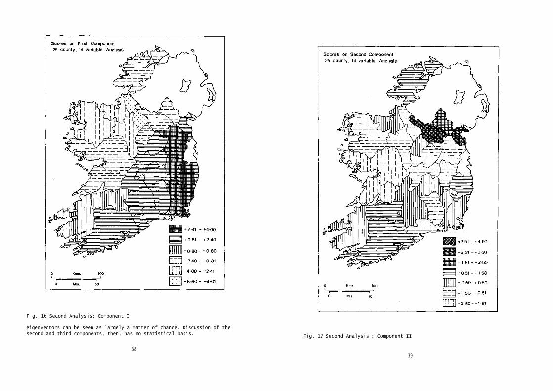
Fig. 17 Second Analysis : Component II

Fig. 16 Second Analysis: Component I

eigenvectors can be seen as largely a matter of chance. Discussion of thesecond and third components, then, has no statistical basis.

3839

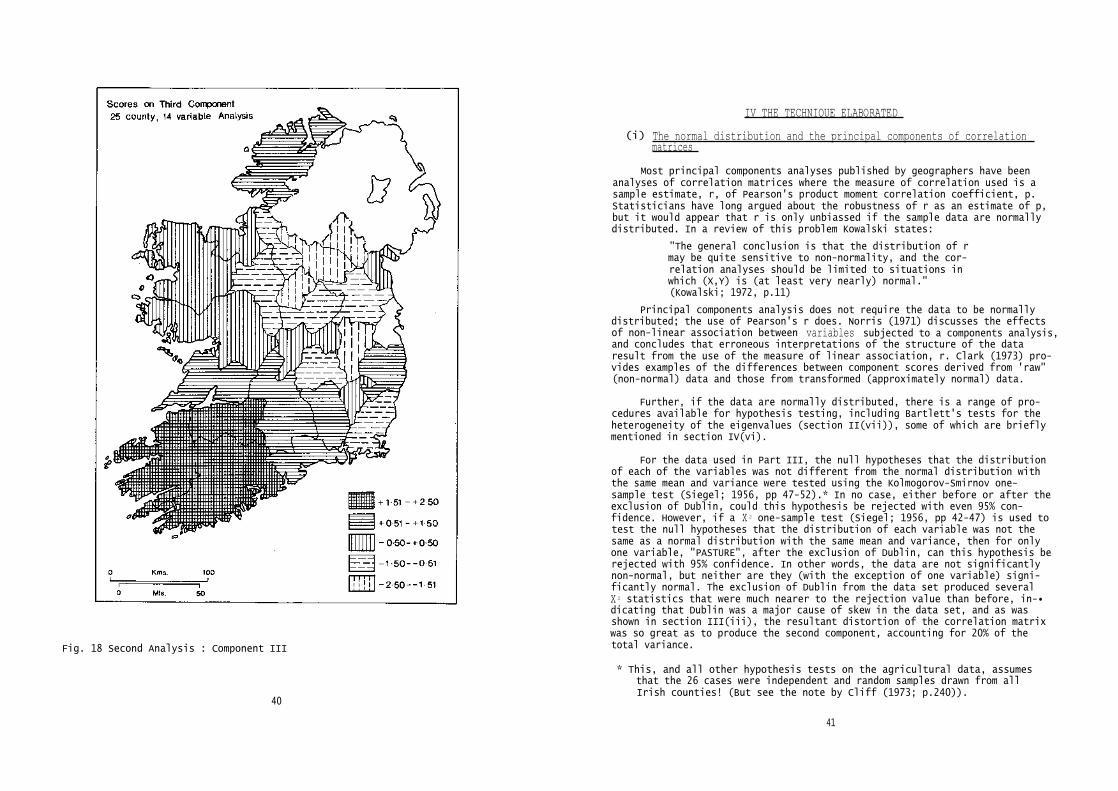
Fig. 18 Second Analysis : Component III

40

IV THE TECHNIQUE ELABORATED

(i) The normal distribution and the principal components of correlation matrices

Most principal components analyses published by geographers have beenanalyses of correlation matrices where the measure of correlation used is asample estimate, r, of Pearson's product moment correlation coefficient, p.Statisticians have long argued about the robustness of r as an estimate of p,but it would appear that r is only unbiassed if the sample data are normallydistributed. In a review of this problem Kowalski states:

"The general conclusion is that the distribution of rmay be quite sensitive to non-normality, and the cor-relation analyses should be limited to situations inwhich (X,Y) is (at least very nearly) normal."(Kowalski; 1972, p.11)

Principal components analysis does not require the data to be normallydistributed; the use of Pearson's r does. Norris (1971) discusses the effectsof non-linear association between variables subjected to a components analysis,and concludes that erroneous interpretations of the structure of the dataresult from the use of the measure of linear association, r. Clark (1973) pro-vides examples of the differences between component scores derived from 'raw"(non-normal) data and those from transformed (approximately normal) data.

Further, if the data are normally distributed, there is a range of pro-cedures available for hypothesis testing, including Bartlett's tests for theheterogeneity of the eigenvalues (section II(vii)), some of which are brieflymentioned in section IV(vi).

For the data used in Part III, the null hypotheses that the distributionof each of the variables was not different from the normal distribution withthe same mean and variance were tested using the Kolmogorov-Smirnov one-sample test (Siegel; 1956, pp 47-52).* In no case, either before or after theexclusion of Dublin, could this hypothesis be rejected with even 95% con-fidence. However, if a x 2 one-sample test (Siegel; 1956, pp 42-47) is used totest the null hypotheses that the distribution of each variable was not thesame as a normal distribution with the same mean and variance, then for onlyone variable, "PASTURE", after the exclusion of Dublin, can this hypothesis berejected with 95% confidence. In other words, the data are not significantlynon-normal, but neither are they (with the exception of one variable) signi-ficantly normal. The exclusion of Dublin from the data set produced severalx 2 statistics that were much nearer to the rejection value than before, in-•dicating that Dublin was a major cause of skew in the data set, and as wasshown in section III(iii), the resultant distortion of the correlation matrixwas so great as to produce the second component, accounting for 20% of thetotal variance.

* This, and all other hypothesis tests on the agricultural data, assumesthat the 26 cases were independent and random samples drawn from allIrish counties! (But see the note by Cliff (1973; p.240)).

41

As Clark (1973, p.113) notes, most published analyses display a certainreticence about discussing the distribution of values for each variable. Ifit is not possible to transform skewed data to a normal distribution, thenthe use of either Spearman's rank correlation coefficient or Kendall's Tcoefficent, both of which have up to 91% power efficiency (Siegel; 1956,p.223), is preferable to the use of Pearson's r. The use of rank correlationcoefficients has largely been confined to the mental mappers, e.g. Gould andWhite (1974), whose data are usually obtained in ordinal form in the firstplace.

(ii) Principal components analysis of dispersion matrices

The principal components analysis of the variance-covariance matrix {C}is preferable to the analysis of the corresponding correlation matrix {R} fortwo reasons:

1. the sampling theory of the eigenvalues of dispersion matrices is moresimple than that of correlation matrices, better understood, and thus thereare more, and more exact, tests for the eigenvalues and eigenvectors ofvariance-covariance matrices;2. the fact that the principal components are linear combinations of theoriginal variables given by the general equation

b coefficients in a regression analysis.

However, the measurement scales used in many geographical studies areso diverse that the disadvantages of not weighting each variable equally (bythe conversion of the data to standard scores, and thus {C} to {R}) far ex-ceed the advantages mentioned above. Although Walsh's data are all measuredon the same scale, i.e. percentage change, the dispersion matrix was notanalysed because of the large differences in variance between the variables,and also because, as percentage changes are dimensionless ratios, it wasdoubted if much physical interpretation would have been possible.

It would appear that the analysis of dispersion matrices is more suitedto, and more commonly used on, problems in biology, psychology and economics.

(iii) Discarding variables

This section discusses two different, but related, problems. They are:

1. the choice of the variables determines the results of the principal com-ponents analysis - which variables should be chosen for analysis?2. the principal components are one interpretation of the structure of inter-correlations between the variables - which variables best describe this struc-ture, and thus could be most profitably monitored for further analysis?

42

An illustration of the first problem is the author's preliminary analy-sis of the soil moisture, topography and vegetation system of a savanna areain Brasil (Daultrey; 1970). Six of his twelve variables were direct measuresof soil moisture, so it was hardly surprising that the first component, ex-plaining 55% of the total variance, was interpreted on the basis of the com-ponent loadings as a "wet-dry" component. In a later analysis, three of thesix soil moisture variables were discarded giving what the author consideredto be a better description of the system, in that it was less biassed towardwet-dry contrasts (Daultrey; 1973). This was an entirely subjective decision,based on field knowledge of the system.

The selection of the 15 variables for analysis in Part III from the 39derived by Walsh was again subjective, being based on an examination of the39x39 correlation matrix, discarding those variables with very similar cor-relation patterns (i.e. those repeating the same information), and those withvery weak correlations (i.e. those with very little information). Walsh'sselections were different, and influenced by his far deeper knowledge of Irishagriculture than the author's. The results were similar - a first componentrelating to intensification and consolidation, and second and subsequent com-ponents produced by smaller, regional trends.

But generally speaking there is no solution to the first problem. If aset of highly intercorrelated variables is analysed, then a first componentexplaining a very large proportion of the total variance will be produced,which may be very pleasing but usually neither surprising nor edifying. Ifhowever, the variables are only weakly intercorrelated, the proportion of thevariance explained by the first component will be very low, and it is quitelikely that a large number of the other components will not be significantlydifferent from each other in the proportion of the variance explained. (Seealso section IV(vi)).

A study of the second problem was recently carried out by Jolliffe(1972; 1973). He was concerned with methods of selection of a few indicatorvariables from a whole series so that these indicator variables adequatelydescribed the structure and variability of the system concerned. This hasobvious practical advantages, for after a pilot study in which a large numberof variables are examined, just the few indicator variables decided on couldbe monitored, giving a considerable saving in time and money spent on samp-ling and measurement.

He used three basic methods: multiple correlation: principal componentsanalysis; and clustering of variables. In the first method, the variable withthe highest multiple correlation coefficient, R, with all the others was dis-carded, and then the variable with the largest multiple correlation with theremaining variables, and so on until the largest R was less than a criticalvalue, found to be 0.15. This would select those variables which were mostnearly independent of each other.

The third method involves clustering the variables into groups on thebasis of their similarity to each other, and then selecting one variable fromeach group. These three methods all produced similar results, both with arti-ficial and with real data.

One of the real data sets was that compiled by Moser and Scott (1961).They used a principal components analysis on 57 variables for 157 towns, andclassified the towns according to the scores on the first four components(see section IV(v)). Jolliffe used the clustering method to reduce the 57variables to 26, and produced a classification of towns similar to that ofMoser and Scott. Jolliffe's analysis was obviously the cheaper in terms ofcomputer time, but which of the two classifications was the better is stilla matter for personal judgement.

Principal components analysis, then, can be used to study the correlationstructure of multivariate observations by providing clues through the compon-ent loadings as to which of the variables best describe the independent trendsin correlation. But no a priori assumptions as to the nature of the principalcomponents can be made. Choosing variables to load onto components is a taskfor factor analysis.

(iv) Rotation of principal components

Factor analysts often rotate their factors so that loadings on certainvariables are increased, and on others decreased, thus making more clear theinterpretation of the factors. The principal components of a data set providea unique orthogonal solution, maximising the variance explained by eachsuccessive component until the total variance has been accounted for. Often,factor analyses do not produce unique solutions, and never account for thetotal variance in a data set; hence the need for rotation. In principal com-ponents analysis there is little point in using an orthogonal rotation, be-cause it eliminates the property of maximum variance; and little point inusing a non-orthogonal rotation, because it eliminates the property of ortho-gonality. So there is neither the need for rotation, nor the justification.A debate on this issue, among several others, was conducted between Davies(1971a; 1971b; 1972a) and Mather (1971; 1972), and is well worth reading.

(v) The analysis of component scores

Having stressed the fact that principal components analysis is primarilya transformation procedure, it follows that the most useful application of thetechnique is not the interpretation of the components, but the further analy-sis of the component scores - the transformed data themselves. Before dis-cussing this, it is necessary to examine one problem raised initially insection I(i). A few of the p components will account for most of the totalvariance. But how many components (and their scores) should be considered?

There is no easy answer, or one that is satisfactory to everyone. Oneobvious criterion is to eliminate all those components for which the null

small but large relative to p, only the smallest components, if any, will notbe heterogenous, leaving m acceptable components, m being not much less thanp. A criterion used quite commonly is to eliminate all components whoseeigenvalues are less than 1.0, on the grounds that these components areaccounting for less of the total variance than any one variable (H.F. Kaiser,

44

referenced in Pocock and Wishart; 1969, p.76). But when p is small, this maylead to the elimination of important dimensions of variability in the dataset.

Most analyses report the cumulative proportion of the total varianceaccounted for by successive components. From this information, the number ofcomponents to be eliminated can be decided: either by retaining those thataccount for a previously determined proportion of the total variance, e.g.80%, 90% (D.F. Morrison, referenced in Pocock and Wishart; 1969, p.77); orby discarding those components whose individual contribution to the proportionof total variance falls below a previously determined level, e.g. 10%, 5%.The advice given to the author as a student was to retain only those componentswhich could be interpreted, on the grounds that to analyse scores on a com-ponent whose physical "meaning" was unclear was less than logical. However,as stated above, it is not the primary purpose of the technique to interpretthe components, and anyway, analysis of the scores often gives a clue as tothe "meaning" of the component.

In the author's experience, it doesn't really matter where the cut-offpoint is, provided the heterogeneity of the eigenvalues of the components canbe demonstrated. The scores on the smaller components have smaller variances,thus their effect on the analysis is usually minimal. Again, the problem comesdown to a subjective decision on the part of the analyst.

Because the scores are uncorrelated, they can be used as the m indepen-dent variables in a multiple regression on one dependent variable. Thisapproach obviates the need to use stepwise multiple regression, with its oftenunsatisfactory criterion that the independent variable having the largest cor-relation with the dependent variable is the most "important" predictor of thedependent variable. But to interpret the regression coefficients, the prin-cipal components must be interpretable, otherwise the meaning of a linear com-bination of a linear combination of variables will be somewhat obscure. Lewisand Williams (1970), forecasting flood discharges; and Veitch (1970), fore-casting maximum temperatures, have used principal component scores in thisway, and Cox (1968) and Romsa et al. (1969) have likewise regressed scoresderived from factor analyses.

Apart from simply mapping the scores, as in Part III, the most commontype of analysis of scores is for them to be used in a hierarchical groupingprocedure to produce a classification of the N cases based on m uncorrelatedattributes rather than on p correlated attributes. The fact that the scoresare uncorrelated allows very simple similarity coefficients (e.g. Euclideandistance) to be used in the grouping procedures (see, for example, Pocockand Wishart; 1969). The significance of the variation between the classes pro-duced by the grouping procedure is usually tested by discriminant analysis oran analysis of variance (for a review, see Spence and Taylor; 1970).

In geographical studies the cases are more often than not areal units,thus the grouping of the cases produces areal aggregates, sometimes calledregions. There is a vast literature on the quantitative approach to regional-isation, in which both principal components analysis and factor analytic tech-niques are used, and often confused. This general approach in human geographyis summarised by Berry (1961; 1964; 1968) and more recently by Clark, Daviesand Johnston (1974), and Mather and Openshaw (1974). Applied to urban areasthe approach is often used as a part of "factorial ecology", or "social areaanalysis" and is discussed by Johnston (1971) and Rees (1971).

45

In physical geography the areal units of study are less often amenableto regionalisation by aggregation, although Mather and Doornkamp (1970) applyfactor analysis, hierarchical grouping and discriminant analysis to classifya series of drainage basins. More often the classification of scores is usedto locate boundaries in a continuum. For example McBoyle (1971) and Morgan(1971) have produced climatic classifications of Australia and West Malaysiarespectively, and McCammon (1966) has distinguished depositional sub-environments in this way.

Clark, Davies and Johnston (1974, p.272) make the point that most analy-ses, in order to classify the cases, transform the variable space and thengroup the scores - this is an R-mode analysis. It may be more appropriate totransform the case space and group the cases by their loadings on the re-sultant components - i.e. a Q-mode analysis. Davies (1972b) provides an ex-ample of this approach in a study of journey patterns in the Swansea area.Conversely, botanists have traditionally used Q-mode principal componentsanalysis to locate stands in species-dimensional space (e.g. Greig-Smithet al.; 1967), and more recently have used R-mode analysis to locate speciesin stand-dimensional space (e.g. Goff and Cottam; 1967). (Beals (1973) strong-ly criticises both uses of principal components analysis on the grounds thatthe botanical data do not meet the assumptions of the principal componentmodel).

Q-mode analysis often produces the situation where there are more dimen-sions to be transformed than there are points in that space. Theoretically,this is not meaningful because, for example, a 3-dimensional plane cannot bedefined uniquely by less than 3 points. Practically, this makes no difference,because the transformation is performed using individual estimates of thevariances and covariances of the dimensions which are valid. However, nosignificance tests can be performed on the principal components so produced.

(vi) Sampling properties of principal components

Morrison (1967; section 7.7) provides a very comprehensible review ofthe more useful sampling properties of principal components, discussing con-fidence intervals for eigenvalues and eigenvectors derived from both thesample dispersion matrix and the sample correlation matrix, as well as tests

the Bartlett tests are not exact for the eigenvalues of correlation matrices.However, an exact test is available for the last p-1 roots of a correlationmatrix, based on some general properties of the matrix.

It can be shown that the largest eigenvalue of a positive semidefinitecovariance (or correlation) matrix cannot exceed the largest row sum of theabsolute values (i.e. the sum of the values irrespective of sign).

(36)

This property is extremely useful, because an investigator can veryquickly determine the largest proportion of the total variance that can beexplained by any component.

If the correlation matrix {11} is such that all the off-diagonal cor-relations are equal (an equicorrelation matrix), then the largest eigenvaluewill equal the row sum

(37)

and the remaining eigenvalues are all equal to (1 - r).

relating to the heterogeneity of the original correlations.

This test is exact if the population is multivariate normal, and N is large.

(vii) Conclusions

Because it is simple, easily accessible through package computer pro-grams, and was introduced into geography early in the "quantitative revolu-tion", principal components analysis has been much used, and often abused, bygeographers. Only when used on carefully selected data (i.e. random, indepen-dent, and normally distributed) has it any "explanatory" power. The inter-pretation put on the results of the analyses in Part III was stretching thetechnique about as far as it can go. Principal components analysis is a trans-formation procedure, and should be used as such, or as a preliminary searchprocedure to identify variables(or cases) for further monitoring and analysis.

(38)

(39)

if the matrix

(40)

(41)

(42)

46 47

BIBLIOGRAPHY

A. Some Basic Textbooks

Anderson, T.W. (1958), Introduction to multivariate statisticalanalysis. (New York: John Wiley & Sons).

Goldstein, H. (1950), classical mechanics. (Reading: Addison-Wesley Publ.Co).

Hammermesh, M. (1962), Group theory and its application to physicalproblems. (Oxford: Pergamon Press).

Harman, H. (1960), Modern factor analysis. (Chicago: University ofChicago Press).

Hope, K. (1968), Methods of multivariate analysis. (London: Universityof London Press).

Horst, P. (1965), Factor analysis of data matrices. (New York: Holt,Rinehart and Winston).

King, L.J. (1969), Statistical analysis in geography. (Englewood Cliffs,N.J.: Prentice-Hall).

Krumbein, W.C. & F.A. Graybill, (1965), An introduction to statisticalmodels in geology. (New York: McGraw-Hill).

Lawley, D.N. & A.E. Maxwell, (1963), Factor analysis as a statisticalmethod. (London: Butterworth).

Morrison, D.F. (1967), Multivariate statistical methods. (New York:McGraw-Hill).

Rummel, R.J. (1970), Applied factor analysis. (Evanston, Ill.: North-western University Press).

Siegel, S. (1956), Nonparametric statistics for the behaviouralsciences. (New York: McGraw-Hill).

Thurstone, L.L. (1947), Multiple-factor analysis. (Chicago: Universityof Chicago Press).

B. Technical Considerations

Bartlett, M.S. (1950), Tests of significance in factor analysis . BritishJournal of Statistical Psychology, 3, 77-85.

Bartlett, M.S. (1951a), The effect of standardisation on a approximation infactor analysis . Biometrika, 38, 337-344.

Bartlett, M.S. (1951b), A further note on tests of significance in factoranalysis:. British Journal of Statistical Psychology, 4, 1-2.

Beals, E.W. (1973), Ordination: mathematical elegance and ecological naivete'.Journal of Ecology, 61, 23-35.

Clark, D. (1973), Normality, transformation, and the principal componentssolution: an empirical note . Area, 5, 110-113.

Cliff, A.D. (1973), A note on statistical hypothesis testing . Area, 5, 240.

Daultrey, S. (1973), Some problems in the use of principal components analy-sis . IBG Quantitative Methods Study Group, working Papers, 1,13-18.

48

Davies, W.K.D. (1971a), Varimax and the destruction of generality: a methodolo-gical note . Area, 3, 112-118.

Davies, W.K.D. (1971b), Varimax and generality: a reply . Area, 3, 254-259.

Davies, W.K.D. (1972a), Varimax and generality: a second reply . Area, 4,207-208.

Goff, F.G. & G. Cottam, (1967), Gradient analysis: the use of species andsynthetic indices . Ecology, 48, 783-806.

Hotelling, H. (1933), Analysis of a complex of statistical variables intoprincipal components . Journal of Educational Psychology, 24,417-441, 498-520.

Johnston, R.J. (1971), Some limitations on factorial ecologies and socialarea analysis . Economic Geography, 47, 314-323.

Jolliffe, I.J. (1972), Discarding variables in a principal component analysis.I: Artificial data . Applied Statistics, 21, 160-173.

Jolliffe, I.J. (1973), Discarding variables in a principal component analysis.II: Real data•. Applied Statistics, 22, 21-31.

Kowalski, C.J. (1972), On the effects of non-normality on the distributionof the sample product-moment correlation-coefficient . AppliedStatistics, 21, 1-12.

Mather, P.M. (1971), Varimax and generality: a comment . Area, 3, 252-254.

Mather, P.M. (1972), Varimax and generality: a second comment . Area, 4,27-30.

Mather, P.M. & S. Openshaw, (1974), Multivariate methods and geographicaldata . The Statistician, 23, 283-308.

Norris, J.M. (1971), Functional relationships in the interpretation of prin-cipal components analyses . Area, 3, 217-220.

C. Applications

Berry, B.J.L. (1961), 'A method for deriving multi-factor uniform regions .Przeglad Geograficzne, 33, 263-279.

Berry, B.J.L. (1964), Approaches to regional analysis: a synthesis . Annals,Association of American Geographers, 54 , 2-11.

Berry, B.J.L. (1968), A synthesis of formal and functional regions using ageneral field theory of spatial behaviour'. in B.J.L. Berry andD.F. Marble, eds, Spatial analysis: a reader in statisticalgeography. (Englewood Cliffs, N.J.: Prentice-Hall).

Clark, D., W.K.D. Davies & R.J. Johnston, (1974), The application of factoranalysis in human geography . The Statistician, 23, 259-281.

Cox, K.R. (1968), 'Suburbia and voting behaviour in the London metropolitanarea . Annals, Association of American Geographers, 58,

111-127.

Daultrey, S. (1970), An analysis of the relation between soil moisture,topography, and vegetation types in a savanna area•. Geographical

Journal, 136, 399-406.

49

Davies, W.K.D. (1972b), Conurbation and city region in an administrativeborderland: a case study of the greater Swansea area RegionalStudies, 6, 217-236.

Gould, P.R. (1967), On the geographical interpretation of eigenvalues .Transactions Institute of British Geographers, 42, 53-86.

Gould, P.R. & R. White, (1974), Mental maps, (Harmondsworth: Penguin).

Greig-Smith, P., M.P. Austin & T.C. Whitmore, (1967), The applications ofquantitative methods to vegetation survey. I: Association analysisand principal component ordinations of rain forest . Journal ofEcology, 55, 483-503.

Lewis, G.L. & T.T. Williams, (1970), Selected multivariate statistical methodsapplied to runoff data from Montana watersheds . state HighwayCommission and U.S. Bureau of Roads, Publ. P3 183705.

McBoyle, G. (1971), Climatic classification of Australia by computer*.Australian Geographical Studies, 9, 1-14.

McCamman, R.B. (1966), Principal components analysis and its application inlarge-scale correlation studies . Journal of Geology,74, 721-733.

Mather, P.M. & J.C. Doornkamp, (1970), Multivariate analysis in geographywith particular reference to drainage-basin morphology . Trans-actions Institute of British Geographers, 51, 163-187.

Morgan, R.P.C. (1971), Rainfall of West Malaysia - a preliminary regional-isation using principal components analysis . Area, 3, 222-227.

Moser, C.A. & W. Scott, (1961), British towns. Edinburgh: Oliver and Boyd.

Pocock, D.C.D. & D. Wishart, (1969), 'Methods of deriving multi-factor uni-form regions . Transactions Institute of British Geographers,47, 73-98.

Rees, P.H. (1971), Factorial ecology: an extended definition, survey, andcritique . Economic Geography, 47, 220-233.

Romsa, G.H., W.L. Hoffman, S.T. Gladin & S.D. Brunn, (1969), An example ofthe factor analytic - regression model in geographic research .Professional Geographer, 21, 344-346.

Spence, N.A. & P.J. Taylor, (1970), Quantitative methods in regional taxonomy .in C. Board et. al (eds) Progress in Geography, Volume 2, 1-63(London: Arnold).

Veitch, L.G. (1970), Forecasting Adelaide's maximum temperature using prin-cipal components and multiple linear regression . AustralianMeteorological Magazine, 18, 1-21.

Walsh, J. (1974), Changes in Irish agriculture. unpublished B.A.dissertation, Dept. of Geography, University College Dublin.

50

NOTES

51