Habilitation a diriger des recherches · M. Andrei Okounkov Columbia University, New-York....

Universite Pierre et Marie Curie

Ecole doctorale de sciences mathematiques de Paris centre

Habilitation a diriger des recherchesDiscipline : Mathematiques

presentee par

Cedric Boutillier

Around planar dimer models:

Schur processes and integrable statistical

mechanics on isoradial graphs

Soutenue le 1er decembre 2016 devant le jury compose de :

M. Vincent Beffara CNRS & Universite Grenoble AlpesM. Philippe Biane CNRS & Universite de Paris-Est

M. Dmitry Chelkak Ecole Normale Superieure, ParisM. Philippe Di Francesco CEA, Saclay

M. Nathanael Enriquez Universite de Paris-OuestM. Thierry Levy Universite Pierre et Marie Curie

M. Fabio Toninelli CNRS & Universite de Lyon 1

apres avis des rapporteurs :

M. Vincent Beffara CNRS & Universite Grenoble AlpesM. Kurt Johansson KTH, Stockholm

M. Andrei Okounkov Columbia University, New-York

Laboratoire de Probabiliteset Modeles AleatoiresUMR 7599Boıte courrier 1884 place Jussieu75252 Paris Cedex 05

Universite Pierre et Marie CurieEcole doctorale de sciencesmathematiques de Paris centreBoıte courrier 2904 place Jussieu75252 Paris Cedex 05

Around planar dimer models:Schur processes and integrable statistical

mechanics on isoradial graphsMemoire d’habilitation a diriger des recherches

Cedric Boutillier

شدیم استاد به کودکی به چند یکشدیم شاد خود استادی به چند یکرسید چه را ما که شنو سخن پایان

شدیم باد بر و درآمدیم خاک از

J’avais un maıtre alors que j’etais un enfant.Puis je devins un maıtre et, par la, triomphant.Mais ecoute la fin : tout cela fut en sommeUn amas de poussiere emporte par le vent.

(Omar Khayyam, 1048–1131)

Abstract

The dimer model is a probability measure on perfect matchings (or dimer configurations)on a graph. Dimer models on some subgraphs of the honeycomb and square lattices, whichby duality, correspond to tilings with rhombi and dominos, are directly related to Schurprocesses, probability measures on sequences of interlacing partitions. Via bijectionsand other combinatorial correspondences, other integrable models of two-dimensionalstatistical mechanics can be mapped to planar dimer models: spanning trees, the Isingmodel. . .

This manuscript presents an overview of the results obtained by the author and hiscoauthors on questions around planar dimer models, with a strong emphasis, on onehand, on the relation with Schur processes, and on the other hand, on these models fromstatistical mechanics related to dimers, defined on isoradial graphs, a particular class ofembedded planar graphs with interesting properties.

Resume

Le modele de dimeres est une mesure de probabilite sur les couplages parfaits (ouconfigurations de dimeres) d’un graphe. Les modeles de dimeres sur certains sous-graphesdu reseau hexagonal ou du reseau carre, qui par dualite, correspondent a des pavagespar losanges ou par dominos, sont directement relies aux processus de Schur, mesures deprobabilites sur les suites de partitions entrelacees. Par le moyen de bijections et autrescorrespondances combinatoires, d’autres modeles integrables de mecanique statistiqueen dimension deux peuvent etre etudies au moyen de modeles de dimeres : les arbrescouvrants, le modele d’Ising. . .

Ce document presente un survol des resultats obtenus par l’auteur et ses collaborateurssur des questions autour du modele de dimeres sur les graphes planaires, avec un accentd’une part sur la relation avec les processus de Schur, et d’autre part sur ces modelesde mecanique statistique lies aux dimeres, definis sur les graphes isoradiaux, une classeparticuliere de graphes planaires plonges aux proprietes interessantes.

Remerciements

Je tiens a remercier tout d’abord les trois rapporteurs de ce manuscript, Vincent Beffara,Kurt Johansson et Andrei Okounkov, d’avoir bien voulu consacrer de leur temps precieuxpour lire et evaluer ce texte.

Vincent, Philippe, Dima, Philippe, Thierry, Nathanael, Fabio, je suis tres heureux ethonore que vous ayez accepte de faire partie de ce jury d’habilitation. Merci pour votrepresence.

Je remercie Richard Kenyon, dont les idees et les travaux restent pour moi une sourced’admiration et d’inspiration. Merci aussi a Kirone Mallick, qui a guide mes premiers pasdans le monde de la recherche.

Je remercie aussi mes collaborateurs avec qui j’apprends beaucoup et ai un grandplaisir a travailler. J’ai partage de formidables moments de recherche avec vous. Unmerci particulier a Beatrice, ma grande sœur mathematique, qui a accepte de meneravec moi une partie importante des projets presentes ici. D’autres aventures scientifiquespassionnantes nous attendent ! Un deuxieme merci a Sylvie pour avoir ete un elementmoteur determinant pour le lancement de redaction de ce memoire.

Je remercie le LPMA dans son ensemble. Tout d’abord l’institution et ses tutelles,pour les excellentes conditions de travail qui y sont offertes, mais surtout son personnel :en premier lieu les membres de son equipe d’administration et de gestion, en particulierFlorence, Josette et Serena, pour leur efficacite et leur bonne humeur. Merci aussi auxcollegues cotoyes au quotidien : Daphne, Nathalie, Damien, Thomas, Thierry, Omer,Vincent, Lorenzo, Gilles et tous les autres. . . Nos conversations mathematiques, et surtoutnon-mathematiques, sont autant de bonnes raisons pour venir au bureau.

Merci a mes parents. Une pensee aussi a ma mamy Anny qui vient de feter ses 90 ans,et qui a deja ete exposee aux pavages et aux dimeres lors de ma soutenance de these il ya maintenant un petit moment.

Merci a mes enfants Marie et Alexandre, et ma femme Olya, pour m’avoir supporte,soutenu et encourage, chacun a votre maniere, pendant la redaction de ce memoire.

Merci aussi a ces personnes qui ont partage des moments de mon existence, pendantdes annees, quelques jours, ou juste quelques minutes, et qui ont marque positivement etdurablement ma vie.

7

Contents

Introduction 13

1. The dimer model . . . . . . . . . . . . . . . . . . . . . . . . . . . . . . . . 13

2. Dimers, interlacing particles and Schur processes . . . . . . . . . . . . . . 14

3. Dimers and other related models on Isoradial graphs . . . . . . . . . . . . 16

4. Notes on the manuscript . . . . . . . . . . . . . . . . . . . . . . . . . . . . 18

I. Dimers and Schur processes 19

1. The Schur process 20

1.1. Partitions, Young and Maya diagrams, symmetric functions . . . . . . . . 20

1.1.1. Partitions and their Young diagrams . . . . . . . . . . . . . . . . . 20

1.1.2. Maya diagrams . . . . . . . . . . . . . . . . . . . . . . . . . . . . . 21

1.1.3. Semi-standard Young tableaux and Schur functions . . . . . . . . . 22

1.2. Interlacement, dual interlacement . . . . . . . . . . . . . . . . . . . . . . . 23

1.3. Schur processes . . . . . . . . . . . . . . . . . . . . . . . . . . . . . . . . . 24

1.4. Vertex operator formalism . . . . . . . . . . . . . . . . . . . . . . . . . . . 24

1.4.1. Bosonic operators . . . . . . . . . . . . . . . . . . . . . . . . . . . 25

1.4.2. Fermionic operators . . . . . . . . . . . . . . . . . . . . . . . . . . 26

2. Plane partitions as Schur processes 27

2.1. Plane partitions and skew plane partitions . . . . . . . . . . . . . . . . . . 27

2.2. Partition function and particle statistics via vertex operators . . . . . . . 29

2.3. Geometry of large plane partitions . . . . . . . . . . . . . . . . . . . . . . 31

2.4. Steep domino tilings . . . . . . . . . . . . . . . . . . . . . . . . . . . . . . 34

3. Dimers on Rail Yard Graphs 36

3.1. Rail Yard Graphs . . . . . . . . . . . . . . . . . . . . . . . . . . . . . . . . 36

3.2. Dimer models on rail yard graphs . . . . . . . . . . . . . . . . . . . . . . . 37

3.3. Dimer correlations . . . . . . . . . . . . . . . . . . . . . . . . . . . . . . . 39

3.4. Applications to the case of the Aztec diamond . . . . . . . . . . . . . . . 42

3.4.1. Creation rate and edge probability generating function . . . . . . . 43

3.4.2. The inverse Kasteleyn matrix . . . . . . . . . . . . . . . . . . . . . 45

3.4.3. The arctic circle theorem . . . . . . . . . . . . . . . . . . . . . . . 45

9

4. Perfect simulations of Schur processes 474.1. Bijective atomic steps . . . . . . . . . . . . . . . . . . . . . . . . . . . . . 48

4.1.1. The Cauchy case . . . . . . . . . . . . . . . . . . . . . . . . . . . . 49

4.1.2. Dual Cauchy case . . . . . . . . . . . . . . . . . . . . . . . . . . . 50

4.2. Sampling algorithm . . . . . . . . . . . . . . . . . . . . . . . . . . . . . . . 51

4.3. Markov chains intertwiners . . . . . . . . . . . . . . . . . . . . . . . . . . 52

4.4. Application to random tilings and extensions . . . . . . . . . . . . . . . . 52

4.4.1. Connection with Robinson-Schensted-Knuth correspondence andthe domino shuffling . . . . . . . . . . . . . . . . . . . . . . . . . . 52

4.4.2. Extension to the symmetric case . . . . . . . . . . . . . . . . . . . 53

4.4.3. Schur processes with infinitely many parameters . . . . . . . . . . 54

II. Statistical mechanics on isoradial graphs 55

5. Isoradial graphs 565.1. Planar graphs, surface graphs and associated notions . . . . . . . . . . . . 56

5.2. Isoradial graphs . . . . . . . . . . . . . . . . . . . . . . . . . . . . . . . . . 56

5.3. Rombic flips and integrable statistical mechanics on isoradial graphs . . . 58

5.3.1. Rhombic flips . . . . . . . . . . . . . . . . . . . . . . . . . . . . . . 59

5.3.2. The Yang–Baxter equation and Z-invariant models . . . . . . . . . 59

5.4. Laplacian on isoradial graphs . . . . . . . . . . . . . . . . . . . . . . . . . 60

5.4.1. Conductances and their star-triangle relation . . . . . . . . . . . . 60

5.4.2. Discrete exponential functions and harmonicity . . . . . . . . . . . 61

5.5. The Ising Model and its star-triangle relation . . . . . . . . . . . . . . . . 62

5.6. Periodic isoradial graphs and spectral curves . . . . . . . . . . . . . . . . 63

5.A. Graphical methods for the Ising model on surface graphs . . . . . . . . . . 64

5.A.1. Low temperature expansion . . . . . . . . . . . . . . . . . . . . . . 64

5.A.2. High temperature expansion . . . . . . . . . . . . . . . . . . . . . . 65

5.A.3. Duality . . . . . . . . . . . . . . . . . . . . . . . . . . . . . . . . . 65

5.A.4. Higher genus and boundary . . . . . . . . . . . . . . . . . . . . . . 66

6. The critical Ising model on isoradial graphs via dimers 676.1. Fisher’s correspondence . . . . . . . . . . . . . . . . . . . . . . . . . . . . 67

6.2. Spectral curve and Kasteleyn inverse matrix . . . . . . . . . . . . . . . . . 69

6.3. The inverse Kasteleyn matrix for non periodic GD . . . . . . . . . . . . . 69

6.4. Construction of a Gibbs measure for the critical Ising model on nonperiodic isoradial graphs . . . . . . . . . . . . . . . . . . . . . . . . . . . . 70

6.5. From criticality to non-criticality . . . . . . . . . . . . . . . . . . . . . . . 72

7. Massive Laplacian on isoradial graphs 737.1. Definitions . . . . . . . . . . . . . . . . . . . . . . . . . . . . . . . . . . . . 73

7.2. Statistical mechanics . . . . . . . . . . . . . . . . . . . . . . . . . . . . . . 73

7.3. Massive Laplacians on isoradial graphs . . . . . . . . . . . . . . . . . . . . 74

10

7.4. Massive exponential functions . . . . . . . . . . . . . . . . . . . . . . . . . 757.5. The massive Green function . . . . . . . . . . . . . . . . . . . . . . . . . . 767.6. Integrability . . . . . . . . . . . . . . . . . . . . . . . . . . . . . . . . . . . 787.7. Construction of Gibbs measures for Z-invariant spanning forests . . . . . 797.8. Spectral curves of massive Laplacians . . . . . . . . . . . . . . . . . . . . 79

8. The XOR Ising model 828.1. Setting and definitions . . . . . . . . . . . . . . . . . . . . . . . . . . . . . 828.2. Mixed contour expansion for the double Ising model . . . . . . . . . . . . 838.3. From mixed contours to bipartite dimer models . . . . . . . . . . . . . . . 84

8.3.1. From mixed contours to the 6-vertex model . . . . . . . . . . . . . 848.3.2. From the 6-vertex model to a bipartite dimer model . . . . . . . . 85

8.4. The critical XOR Ising model on isoradial graphs . . . . . . . . . . . . . . 86

III. Other works and possible developments 89

9. Other works 909.1. Winding of the toroidal honeycomb dimer model . . . . . . . . . . . . . . 909.2. Limit shape and fluctuations of boxed partitions . . . . . . . . . . . . . . 91

10.Some perspectives 95

Publications 100

Bibliography 102

11

Introduction

The dimer model is introduced in statistical mechanics to describe the chemical process ofadsorption of diatomic molecules (dimers) on the surface of a crystal [FR37]. On planargraphs, it turns out that the model is completely solvable, meaning that one can, forexample, compute exactly the number of configurations, or correlations between dimers,with algebraic tools. This property and the fact that this model is connected to severalother combinatorial objects via bijections put this model at the intersection of severalbranches of mathematics (probability, combinatorics, real algebraic geometry), but alsocomputer sciences and theoretical physics.

Dimer models have been the main topic of our research, presented in this manuscript,either directly, or as a tool to study related models. In this introduction, we first brieflypresent in Section 1 the dimer model and some of its properties. For a more completetreatment, we refer the reader to some lectures notes on this model [Ken04, Ken09, dT15,Cim14]. In Section 2, we discuss the link between the geometric constraints betweendimers and the interlacing properties of partitions in Schur processes, which are the topicof the first part of this document. Then, in Section 3, we present the connection betweendimer models and other models of statistical mechanics. On a special family of planargraphs, the isoradial graphs, these models have rich and interesting properties. They arediscussed at length in the second part of the manuscript.

The documents ends with a third part, containing a summary of other works [10, 7],and some perspectives on ongoing or future research projects. The three parts are mostlyindependent from one another.

1. The dimer model

A dimer configuration of a graph G = (V,E) is a subset of edges M ⊂ E such that inthe subgraph (V,M), all vertices have degree 1: all vertices of G are incident to exactlyone edge of M . In graph theory, dimer configurations are also called perfect matchings:a dimer configuration pairs every vertex of the graph with one of its neighbors.

If G is a finite graph (which admits at least a dimer configuration) and positive weights(νe)e∈E are assigned to edges, the dimer model on G is the Boltzmann probability measureon dimer configurations of G, where the probability of a configuration M is proportionalto the product of the weights it contains. The proportionality factor

Z(G, ν) =∑

M : dimerconfiguration

∏

e∈Mνe

is called the dimer partition function.

13

In the 1960’s, it has been proven [TF61, Kas61] that the partition function of the dimermodel on a finite planar graph can be expressed as the Pfaffian of a weighted orientedadjacency matrix of the graph, the Kasteleyn matrix. The orientation should satisfy theclockwise odd condition: around every face, the number of edges oriented clockwise isodd. When the graph is bipartite, the Kasteleyn matrix has a 2 × 2 block structure,reflecting the two classes of vertices, with zero blocks on the diagonal. The Pfaffianof the whole matrix can be reduced to the determinant of one of these blocks [Per69].When the graph is not planar, but can be drawn on a surface with g handles, Kasteleyn’sapproach can be extended to compute the dimer partition function with 22g Pfaffians ordeterminants [GL99, Tes00, CR07, CR08].

Dimer configurations on planar graphs can be seen by duality as tilings of the plane, orregions of the plane. For example, on the square lattice, dimer configurations correspondto tilings with dominos, which are the union of two adjacent (dual) square faces. Similarly,dimer configurations on the hexagonal lattice correspond to tilings with rhombi, whichare the union of two adjacent faces of the dual triangular lattice.

For a periodic infinite planar weighted graph G, the notion of Boltzmann measures isreplaced by that of Gibbs measures, which are measures such that, when we conditionon the configuration in some annular region:

- the configurations inside and outside of the annulus are independent- the distribution on configurations in the finite region inside is the Boltzmann

measure.

Gibbs measures are usually constructed as weak limits of Boltzmann measures onsequences of finite graphs approximating G, for example by taking quotients of G bylattices with a larger and larger mesh (toroidal graphs).

Correlations for the weak limit of uniform measures for domino tilings and rhombustilings were obtained by Kenyon [Ken97]. The edges in a random dimer configuration fora determinantal point process, with a kernel given by the inverse of the infinite Kasteleynmatrix. This result has been extended to any two-dimensional bipartite lattices, anda full classification of ergodic Gibbs measures for dimer models on planar biperiodicgraphs has been obtained in [KOS06], with very interesting connections to real algebraicgeometry. See also [KO06].

2. Dimers, interlacing particles and Schur processes

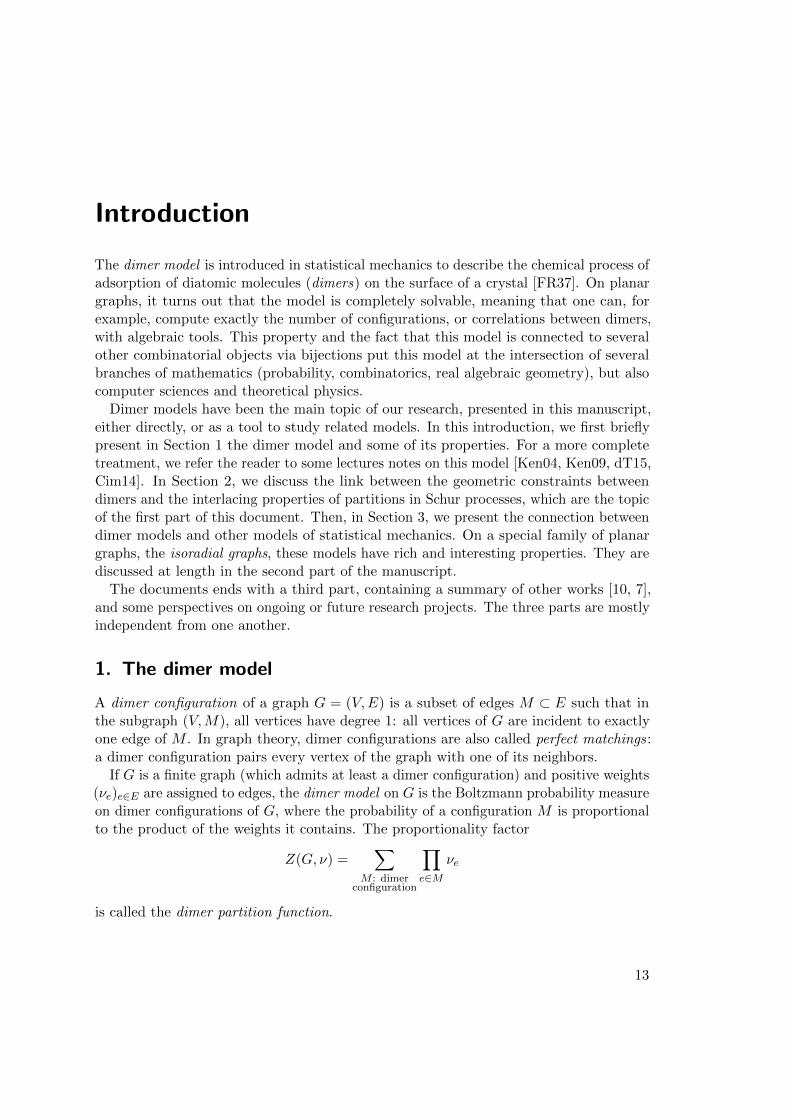
A uniform tiling of a hexagon with rhombi, is represented on Figure 0.1, with differentcolors (yellow, red, blue) for tiles depending on their orientation. One sees that due tothe geometric constraints, between two successive blue horizontal rhombi, there is exactlyone blue rhombus on their left, and one on their right. They form what is called aninterlacing particle process. This interlacing property has been used in [CLP98, Joh02]to study this model and obtain the asymptotic typical behaviour of these objects. Thisinterlacing property is in fact true for any tiling with rhombi of simply connected regionsof the plane, like the ones obtained as the projection of plane partitions (See Figure 4.3a,page 53 for an example).

14

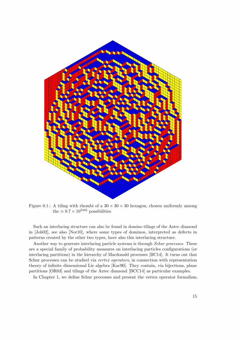
Figure 0.1.: A tiling with rhombi of a 30 × 30 × 30 hexagon, chosen uniformly amongthe ' 8.7× 105442 possibilities

Such an interlacing structure can also be found in domino tilings of the Aztec diamondin [Joh02], see also [Nor10], where some types of dominos, interpreted as defects inpatterns created by the other two types, have also this interlacing structure.

Another way to generate interlacing particle systems is through Schur processes. Theseare a special family of probability measures on interlacing particles configurations (orinterlacing partitions) in the hierarchy of Macdonald processes [BC14]. It turns out thatSchur processes can be studied via vertex operators, in connection with representationtheory of infinite dimensional Lie algebra [Kac90]. They contain, via bijections, planepartitions [OR03] and tilings of the Aztec diamond [BCC14] as particular examples.

In Chapter 1, we define Schur processes and present the vertex operator formalism.

15

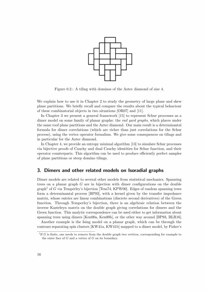
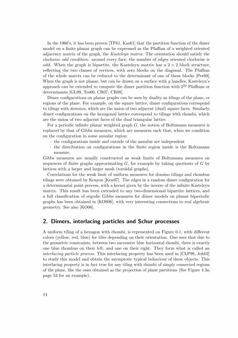
Figure 0.2.: A tiling with dominos of the Aztec diamond of size 4.

We explain how to use it in Chapter 2 to study the geometry of large plane and skewplane partitions. We briefly recall and compare the results about the typical behaviourof these combinatorial objects in two situations [OR07] and [11].

In Chapter 3 we present a general framework [15] to represent Schur processes as adimer model on some family of planar graphs: the rail yard graphs, which places underthe same roof plane partitions and the Aztec diamond. Our main result is a determinantalformula for dimer correlations (which are richer than just correlations for the Schurprocess), using the vertex operator formalism. We give some consequences on tilings andin particular for the Aztec diamond.

In Chapter 4, we provide an entropy minimal algorithm [13] to simulate Schur processesvia bijective proofs of Cauchy and dual Cauchy identities for Schur function, and theiroperator counterparts. This algorithm can be used to produce efficiently perfect samplesof plane partitions or steep domino tilings.

3. Dimers and other related models on Isoradial graphs

Dimer models are related to several other models from statistical mechanics. Spanningtrees on a planar graph G are in bijection with dimer configurations on the doublegraph1 of G via Temperley’s bijection [Tem74, KPW00]. Edges of random spanning treesform a determinantal process [BP93], with a kernel given by the transfer impedancematrix, whose entries are linear combinations (discrete second derivatives) of the Greenfunction. Through Temperley’s bijection, there is an algebraic relation between theinverse Kasteleyn matrix on the double graph giving correlations for dimers and theGreen function. This analytic correspondence can be used either to get information aboutspanning trees using dimers [Ken00a, Ken00b], or the other way around [BP93, BLR16].

Another example is the Ising model on a planar graph, which can be through thecontours separating spin clusters [KW41a, KW41b] mapped to a dimer model, by Fisher’s

1If G is finite, one needs to remove from the double graph two vertices, corresponding for example tothe outer face of G and a vertex of G on its boundary.

16

bijection [Fis66]. See also [Kas67, DZM+96]. Via dimer computations, many results onthe Ising model can be derived. See e.g., [MW73, Dub11b, CCK15]

In [Ken02], Kenyon introduces a Laplacian and a Kasteleyn operator on a family ofplanar graphs with a special embedding, called the isoradial graphs, where conductancesand dimer weights are trigonometric functions. He gives an explicit formula for theassociated Green function and the inverse Kasteleyn operator which have the localityproperty: their entries indexed by two vertices depends only on the geometry of theembedding of the graph along a path between these two vertices. The key tool is theexistence of a family of harmonic functions, the discrete exponential functions [Mer04],computed at a vertex as the product of local terms on a path from a base point to thatvertex.

In Chapter 5, we introduce the notion of isoradial graphs. We discuss the rhombic flipoperation, in connection with the Yang-Baxter equation and the star-triangle transfor-mation for the Ising model and electric networks, and the implication for the criticalLaplacian [Ken02] and its Green function.

The study of critical Ising model on isoradial graphs [8, 9] is presented in Chapter 6.The main results are an explicit and local expression for the inverse Kasteleyn operatoron the Fisher graph for an arbitrary infinite isoradial graph (without hypothesis ofperiodicity), which allows us to construct a Gibbs measure on spin configurations for thecritical Ising model on isoradial graphs.

In Chapter 7, we summarize the results of [16], recently accepted for publication inInvent. Math. We construct a family of massive Laplacians, with masses and conductancesexpressed in terms of elliptic functions, which reduces to Kenyon’s Laplacian when themass goes to zero. We define a family of massive harmonic function with a product (zerocurvature) structure which reduce to exponential. We give an explicit integral formulafor the Green function, which has the locality property. As for the critical Ising model ofChapter 6, we explore the implications for an underlying model of statistical mechanics:the rooted spanning forests, which are the massive analogues of spanning trees. We alsocharacterize completely the algebraic curves which can arise as spectral curves of thesemassive Laplacians on periodic isoradial curves, in the same spirit as what has been donefor bipartite periodic planar dimer models [KOS06]: these are Harnack curve of genus 1,with an additional symmetry.

Using duality in the high/low temperature contour expansion of the Ising model, weexhibit in Chapter 8 a coupling between the double Ising model on a finite graph Gdrawn on a surface, and a bipartite dimer model on a decorated version GQ of its medialgraph, in such a way that the contours separating clusters where the spins of the twoconfigurations agree and disagree (XOR contours) are the level line of the restriction ofthe height function of the dimer model on GQ to a subset of vertices. When G is aninfinite isoradial graph, so is GQ, and the coupling extends to this situation for the Gibbsmeasures for the critical Ising model [9] and the bipartite dimer model on GQ [dT07b].This gives some insights on Wilson’s conjecture about the scaling limit of the criticalXOR contours [Wil11].

17

4. Notes on the manuscript

This document contains two bibliography indexes: the first one, on page 100, lists ourpublications, labeled with numbers like [16]. These publications can be downloaded from:

http://www.lpma-paris.fr/pageperso/boutil/publications/.

The other one, page 102, lists external references, and uses alphanumeric code from thename of the authors and year of publication, like [Bor11].

18

http://www.lpma-paris.fr/pageperso/boutil/publications/

Part I.

Dimers and Schur processes

Abstract

After introducing Schur processes as a random process on sequences of integer partitions,and the formalism of vertex operators in Chapter 1, we explain how to compute variousprobabilistic quantities for Schur processes, and to derive the typical behaviour of largeplane partitions [OR07][11] as an application in Chapter 2. In Chapter 3, we presenta family of planar graphs, the rail yard graphs [15], on which a version of the dimermodel is equivalent to Schur processes, with arbitrary parameters, extending the knowncorrespondence for (skew) plane partitions [OR03] and steep domino tilings [BCC14].Chapter 4 is dedicated to the description of an entropy optimal and efficient algorithmto perfectly simulate Schur processes and which thus can be used to produce efficientlysamples of random tilings [13].

1. The Schur process

In this chapter, we give some notions and notation for Schur processes, which areprobability measures on sequences of partitions. Although there are several ways to studythem, we use here the formalism of vertex operators, following [OR03, OR07]. We referthe reader to these articles, as well as to [BR05] for more details about the Eynard-Mehtaapproach, and [Bor11].

Our study of Schur processes will be motivated by examples in connection with randomtilings. So our definitions may not be the most general ones. However, they will beenough for us here, and the more complete ones can be obtained by taking suitable limits.

1.1. Partitions, Young and Maya diagrams, symmetricfunctions

1.1.1. Partitions and their Young diagrams

Definition 1. A partition of a non negative integer n is a non increasing sequence ofnon negative integers λ = (λ1, λ2, . . . , ) whose sum is equal to n. The integer n = |λ| =∑∞

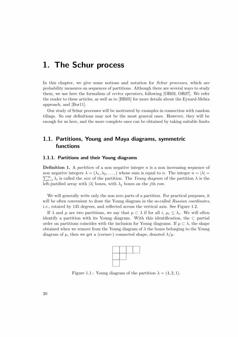
i=1 λi is called the size of the partition. The Young diagram of the partition λ is theleft-justified array with |λ| boxes, with λj boxes on the jth row.

We will generally write only the non zero parts of a partition. For practical purposes, itwill be often convenient to draw the Young diagram in the so-called Russian coordinates,i.e., rotated by 135 degrees, and reflected across the vertical axis. See Figure 1.2.

If λ and µ are two partitions, we say that µ ⊂ λ if for all i, µi ≤ λi. We will oftenidentify a partition with its Young diagram. With this identification, the ⊂ partialorder on partitions coincides with the inclusion for Young diagrams. If µ ⊂ λ, the shapeobtained when we remove from the Young diagram of λ the boxes belonging to the Youngdiagram of µ, then we get a (corner-) connected shape, denoted λ/µ.

Figure 1.1.: Young diagram of the partition λ = (4, 2, 1).

20

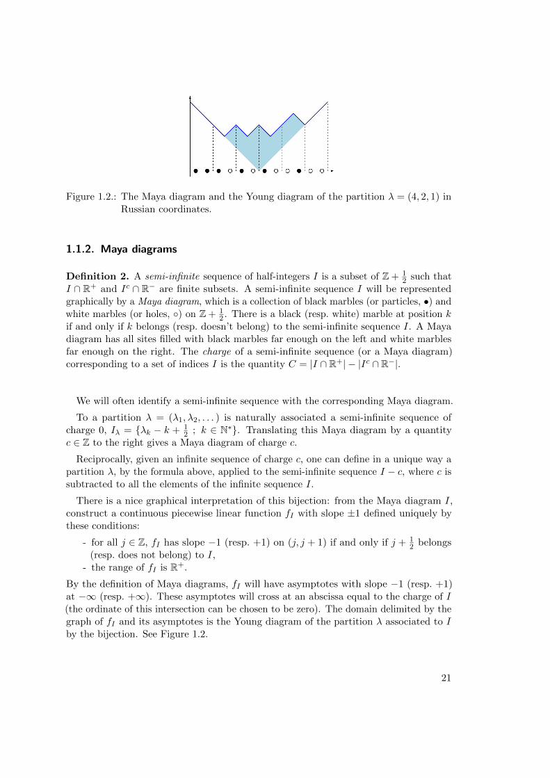
Figure 1.2.: The Maya diagram and the Young diagram of the partition λ = (4, 2, 1) inRussian coordinates.

1.1.2. Maya diagrams

Definition 2. A semi-infinite sequence of half-integers I is a subset of Z + 12 such that

I ∩ R+ and Ic ∩ R− are finite subsets. A semi-infinite sequence I will be representedgraphically by a Maya diagram, which is a collection of black marbles (or particles, •) andwhite marbles (or holes, ◦) on Z + 1

2 . There is a black (resp. white) marble at position kif and only if k belongs (resp. doesn’t belong) to the semi-infinite sequence I. A Mayadiagram has all sites filled with black marbles far enough on the left and white marblesfar enough on the right. The charge of a semi-infinite sequence (or a Maya diagram)corresponding to a set of indices I is the quantity C = |I ∩ R+| − |Ic ∩ R−|.

We will often identify a semi-infinite sequence with the corresponding Maya diagram.

To a partition λ = (λ1, λ2, . . . ) is naturally associated a semi-infinite sequence ofcharge 0, Iλ = {λk − k + 1

2 ; k ∈ N∗}. Translating this Maya diagram by a quantityc ∈ Z to the right gives a Maya diagram of charge c.

Reciprocally, given an infinite sequence of charge c, one can define in a unique way apartition λ, by the formula above, applied to the semi-infinite sequence I − c, where c issubtracted to all the elements of the infinite sequence I.

There is a nice graphical interpretation of this bijection: from the Maya diagram I,construct a continuous piecewise linear function fI with slope ±1 defined uniquely bythese conditions:

- for all j ∈ Z, fI has slope −1 (resp. +1) on (j, j + 1) if and only if j + 12 belongs

(resp. does not belong) to I,- the range of fI is R+.

By the definition of Maya diagrams, fI will have asymptotes with slope −1 (resp. +1)at −∞ (resp. +∞). These asymptotes will cross at an abscissa equal to the charge of I(the ordinate of this intersection can be chosen to be zero). The domain delimited by thegraph of fI and its asymptotes is the Young diagram of the partition λ associated to Iby the bijection. See Figure 1.2.

21

1.1.3. Semi-standard Young tableaux and Schur functions

Partitions are basic blocks to construct more involved combinatorial objects, such assemi-standard Young tableaux, defined below:

Definition 3. Let λ be a partition. A semi-standard Young tableau (SSYT) of shape λis a filling of the Young diagram of λ with positive integers which is

- weakly increasing along rows, from left to right,- strictly increasing along columns, from top to bottom.

If T is a SSYT, and x = (x1, x2, . . . ) a sequence of formal variables, we denote by xT

the monomialxT = xnumber of 1’s in T

1 xnumber of 2’s2 · · · .

Definition 4. The Schur function sλ associated to a partition λ is the function in aninfinite number of variables x = (x1, x2, . . . ) defined by

sλ(x) =∑

T : SSYTof shape λ

xT .

Although it is not completely obvious from this combinatorial definition, sλ is asymmetric function. In fact, the collection (sλ)λ indexed by all partitions is a basis for thealgebra of symmetric variables, which is orthonormal for the standard scalar product 〈·, ·〉on the space of symmetric function, defined by requiring that monomial and completesymmetric functions are dual bases for this scalar product.

This combinatorial definition for Schur functions can be extended to skew shapes todefine semi-standard skew Young tableaux, and obtain the so-called skew Schur functions:

Definition 5. Let λ ⊃ µ two partitions. A skew semi-standard Young tableau of shapeλ/µ is a filling of the skew shape of λ/µ with positive integers which is

- weakly increasing along rows, from left to right,- strictly increasing along columns, from top to bottom.

The skew Schur function sλ/µ is the symmetric function in an infinite number of variablesx = (x1, x2, . . . ) defined by

sλ/µ(x) =∑

T : skew SSTYof shape λ/µ

xT .

When we write that a symmetric function depends only on a finite number of variables,it means that all the other formal variables have been set to 0.

Schur and skew Schur functions satisfy two algebraic relations which will play ancrucial role in the properties of Schur processes:

Proposition 1 (Cauchy identity).

∑

λ

sλ(x) sλ(y) =∏

i,j

1

1− xiyj. (1.1)

22

Proposition 2 (branching rule). For any partitions λ and ν,

sλ/ν(x,y) =∑

µ

sλ/µ(x) sµ/ν(y). (1.2)

For more details about the combinatorial definition of Schur functions, the connectionwith their classical definition in terms of ratio of Vandermonde like determinant, andrelations with other classical families of symmetric functions, we refer the reader to [Sta99,Chapter 7] and [Mac15].

1.2. Interlacement, dual interlacement

Definition 6. Let λ and µ be two partitions. We write λ � µ if for all i ≥ 1, λi ≥ µi ≥λi+1. We say that that λ and µ interlace, or or differ by a horizontal strip if either λ � µor λ � µ.

If T is a SSYT of shape λ, define (λ(i))i as the sequence of partitions included in λ,such that λ(i) is the union of boxes with a content in T less or equal to i. Then:

λ(0) = ∅ � λ(1) � · · ·

The skew Schur function sλ/µ in one variable x has a very simple expression:

sλ/µ(x) = x|λ|−|µ|1λ�µ. (1.3)

There is a natural involution on the set of partitions, called transposition, and denotedby ω.

Definition 7. The transposed λ′ = ω · λ of a partition λ is a partition with parts(λ′1, λ

′2, . . . ) defined by:

∀i ∈ N∗, λ′i = Card{j ∈ N∗ : λj ≥ i}.

For example, if λ = (4, 2, 2), then λ′ = (3, 3, 1, 1) In terms of Young diagrams thisinvolution corresponds to exchanging rows and columns. In terms of Maya diagram, itcorresponds to a reflection with respect to 0 followed by an inversion of colors.

This naturally yields the relation of dual interlacement, denoted by �′.Definition 8. Two partitions λ and µ dually interlace if and only if λ′ and µ′ interlace:

λ �′ µ⇔ λ′ � µ′.

We say then also that λ and µ differ by a vertical strip.

The branching rule (1.2) and Cauchy identity (1.1) are completed with the dual Cauchyidentity:

Proposition 3 (dual Cauchy identity).∑

λ

sλ(x) sλ′(y) =∏

i,j

(1 + xiyj). (1.4)

23

1.3. Schur processes

Definition 9. Let ` < r be two integers. A Schur process is a probability measure onsequences of partitions (λ(`), . . . , λ(r+1)), characterised by three sequences:

- The LR sequence a = (a`, . . . , ar) ∈ {L,R}[`..r],- The sign sequence b = (b`, . . . , br) ∈ {+,−}[`..r],- The parameter sequence x = (x`, . . . , xr) ∈ (R∗+)[`..r],

such that the probability of a given sequence of partitions is proportional to:

r∏

j=`

Saj ,bj (λ(j), λ(j+1);xj) (1.5)

where λ(`) and λ(r+1) are the empty partitions and

Sa,b(λ, µ;x) =

sλ/µ(x) if a = L and b = −,

sµ/λ(x) if a = L and b = +,

sλ′/µ′(x) if a = R and b = −,

sµ′/λ′(x) if a = R and b = +.

Remark 1. A few comments about this definition:

- With probability one, for all j, λ(j) and λ(j+1) interlace (resp. dually interlace) ifaj = L (resp. aj = R), the direction of the inclusion being given by the sign of bj .

- When λ and µ satisfy the correct interlacing relation, Sa,b(λ, µ;x) is just x||λ|−|µ||.- Here, the transition between λ(j) and λ(j+1) is given by a specialisation of skew

Schur functions in only one variable, taking a positive real value. More generalspecialisations can be used, if they give positive results. The characterisation ofSchur-positive specialisations of symmetric functions is the content of Thoma’stheorem [Tho64]. See also [VK81, Oko00, KOO98, BG15] for statement and proofsof this result. They can all be obtained from the definition here, by “forgetting”some of the intermediate partitions, and possibly taking suitable limits.

By Jacobi-Trudi identities expressing skew Schur function as determinants of completesymmetric functions, the weight (1.5) of a configuration can be written as a product ofdeterminants. It follows from (an extended version of) Eynard-Metha’s theorem [BR05]that the statistics of the particles form a determinantal process. However, we will see thatin this context, the vertex operators together with the fermionic localisation operatorscan readily lead to determinantal formulas with an explicit kernel for the correlations.

1.4. Vertex operator formalism

There is an algebraic way to construct symmetric functions as the action of some operatorson a vector space. These operators will act as transfer matrices to construct consecutiveelements of the random sequence of partitions from the Schur process.

24

1.4.1. Bosonic operators

Definition 10. The bosonic Fock space is an infinite dimensional Hilbert space B witha countable orthonormal basis indexed by partitions (|λ〉)λ.

On this space we define various vertex operators: the operator Γ+(x) acts on B asfollows:

Γ+(x)|λ〉 =∑

µ�λx|λ\µ||µ〉.

Its adjoint Γ−(x) acts on a basis vector as follows:

Γ−(x)|λ〉 =∑

µ�λx|µ\λ||µ〉.

Note that even if the result is not a finite linear combination, all the coefficients are finite.They satisfy the following commutation relations: for all x and y,

Γ+(x)Γ+(y) = Γ+(y)Γ+(x),

Γ−(x)Γ−(y) = Γ−(y)Γ−(x),

Γ+(x)Γ−(y) =1

1− xyΓ−(y)Γ+(x).

(1.6)

One can construct the skew Schur functions specialised in n variables as a matrixelement of a product of n operators Γ+(x1),. . . ,Γ+(xn).

〈µ|Γ+(x1) · · ·Γ+(xn)|λ〉 = sλ/µ(x1, . . . , xn).

The transposition on partitions and the notion of dual interlacement allow also one todefine two new vertex operators Γ′+(x) and Γ′−(x), which are conjugates of the previousΓ+(x) and Γ−(y) by the involution ω:

Γ′+(x) = ωΓ+(x)ω = Γ+(−x)−1, Γ′−(y) = ωΓ−(y)ω = Γ−(−y)−1,

which corresponds in terms of action on partitions to:

Γ′+(x)|λ〉 =∑

µ�′λx|λ\µ||µ〉, Γ′−(x)|λ〉 =

∑

µ�′λx|µ\λ||µ〉.

In the next chapters, instead of putting or not a prime to distinguish between inter-lacement and dual interlacement, we may use more symmetric notation, with symbolsfrom the sequences a and b.

ΓL±(x) = Γ±(x), ΓR±(x) = Γ′±(x).

25

1.4.2. Fermionic operators

Let V a Hilbert space with an infinite countable basis (ek)k∈Z+ 12.

Definition 11. The fermionic Fock space F =∧∞

2 V is the linear space generatedby the external product of vectors of the basis (ek)k∈Z+ 1

2indexed by a semi-infinite

sequence I = {i1 > i2 > . . .}. It is naturally Z-graded by the charge. The basis vectorcorresponding to the semi-infinite sequence I is denoted

|I〉 = ei1 ∧ ei2 ∧ · · ·

There are natural operators acting on∧∞

2 V :- creation operators ψk, k ∈ Z + 1

2 acting by external product:

ψk|I〉 = ek ∧(ei1 ∧ ei2 ∧ · · ·

)=

{(−1)#{n:in>k}|I ∪ {k}〉 if k 6∈ I,

0 if k ∈ I

- annihilation operators ψ∗k, k ∈ Z + 12 acting by internal product:

ψ∗k|I〉 = ιek(ei1 ∧ ei2 ∧ · · ·

)=

{(−1)#{n:in>k}|I \ {k}〉 if k ∈ I,

0 if k 6∈ IThe action of these operators in term of Maya diagram is easy to describe: the operator

ψk (resp. ψ∗k) tries to add (resp. remove) a particle at site k to a Maya diagram, andgives 0 if a particle is present (resp. absent) at that site.

These operators satisfy the canonical anticommutation relations:

∀ k, l ∈ Z +1

2, ψkψ

∗l + ψ∗l ψk = 1k=l.

Whereas ψk and ψ∗k separately do not preserve the charge, their products do, and havein fact a very simple interpretation: ψkψ

∗k (resp. ψ∗kψk) is the projector on the subspace

of F generated by Maya diagrams with a particle (resp. a hole) at position k.The operators Γ+(x) and Γ−(y) can also act on F . They preserve the charge, and

satisfy commutation relations, that are nicely written if we introduced the generatingfunctions for ψk’s and ψ∗k:

ψ(z) =∑

k∈Z+ 12

zkψk, ψ∗(w) =∑

k∈Z+ 12

w−kψ∗k,

For example,

Γ+(x)ψ(z) =1

1− zxψ(z)Γ+(x). (1.7)

The complete list of commutation relations between Γab(x) and ψ(z) or ψ∗(w) can befound in [15, Proposition 11], and can be obtained from the relation above by takingduals, inverse and conjugates by ω. For a combinatorial proof, see [15, Appendix A]. Foralgebraic proofs, see for instance [Kac90, Chapter 14], [MJD00], [Oko01, Appendix A],[OR07], [Tin11] and [AZ13].

26

2. Plane partitions as Schur processes

Plane partitions are the two dimensional analogues of integer partitions, which can beseen as some tilings with rhombi with special steep boundary conditions. We explainin Section 2.1 how these objects, together with one of their generalizations, the skewplane partitions, can be encoded as sequences of interlacing partitions. Then we describein Section 2.2 how to compute generating functions for these objects and correlationsunder the associated Boltzmann measure, following [ORV06, OR03, OR07], using theformalism of vertex operators. In Section 2.3 we describe briefly the implication onthe shape of large skew plane partitions, comparing the results of [OR07] and [11] fordifferent setups. The chapter ends with a description of steep domino tilings [BCC14],which are the domino counterpart of the steep rhombi tiling coming from skew planepartitions, and comprise as special examples the Aztec diamond and pyramid partitions.

2.1. Plane partitions and skew plane partitions

A plane partition is the two-dimensional analog of a partition:

Definition 12. A plane partition is a sequence π = (πi,j)(i,j)∈N∗2 of non negative integerswhich is weakly decreasing in i and j and has a finite number of nonzero coefficients.The size |π| of the plane partition π is the sum of its coefficients: |π| = ∑i,j πi,j . Whenwritten like a matrix, the support of π (i.e., the set of indices with positive coefficients)is a Young diagram, called the shape of π.

As for partitions, we usually just write down the non zero coefficients of a planepartition. Similarly, one can define skew plane partitions, where the sequence is nowindexed by N∗2 deprived from the Young diagram of a partition. Plane partitions canbe represented graphically by 3D Young diagrams, which are piles of cubes. Projectedin the plane x+ y + z = 0, orthogonal to the great diagonal of the cubes, these piles ofcubes give tilings of some regions of the plane with rhombi, which are the projection ofthe visible faces of the cubes.

A plane partition π can be decomposed as a sequence of diagonal slices (λ(i))i∈Z. Theseslices are partitions satisfying interlacing relations

· · · � λ(−2) � λ(−1) � λ(0) � λ(1) � λ(2) � · · ·

27

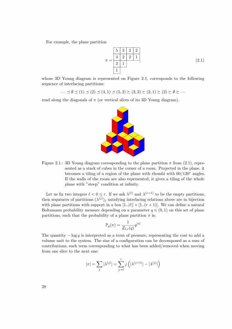
For example, the plane partition

π =

5 3 2 2

4 2 2 1

2 1

1

, (2.1)

whose 3D Young diagram is represented on Figure 2.1, corresponds to the followingsequence of interlacing partitions:

· · · � ∅ � (1) � (2) � (4, 1) � (5, 2) � (3, 2) � (2, 1) � (2) � ∅ � · · ·read along the diagonals of π (or vertical slices of its 3D Young diagram).

Figure 2.1.: 3D Young diagram corresponding to the plane partition π from (2.1), repre-sented as a stack of cubes in the corner of a room. Projected in the plane, itbecomes a tiling of a region of the plane with rhombi with 60/120◦ angles.If the walls of the room are also represented, it gives a tiling of the wholeplane with ”steep” condition at infinity.

Let us fix two integers ` < 0 ≤ r. If we ask λ(`) and λ(r+1) to be the empty partitions,then sequences of partitions (λ(j))j satisfying interlacing relations above are in bijectionwith plane partitions with support in a box [1..|`|]× [1..(r + 1)]. We can define a naturalBoltzmann probability measure depending on a parameter q ∈ (0, 1) on this set of planepartitions, such that the probability of a plane partition π is:

Pq(π) =1

Z`,r(q)q|π|

The quantity − log q is interpreted as a term of pressure, representing the cost to add avolume unit to the system. The size of a configuration can be decomposed as a sum ofcontributions, each term corresponding to what has been added/removed when movingfrom one slice to the next one:

|π| =∑

j

|λ(j)| =r∑

j=`

j(|λ(j+1)| − |λ(j)|

)

28

Using the expression for skew Schur functions in one variable, (1.3) we write the weightof π as:

q|π| =r∏

`

qj(|λ(j+1)|−|λ(j)|) =

−1∏

j=`

sλ(j+1)/λ(j)(q|j|)

r∏

j=0

sλ(j)/λ(j+1)(qj) =

−1∏

j=`

〈λ(j)|Γ+(q|j|)|λ(j+1)〉r∏

j=0

〈λ(j)|Γ−(qj)|λ(j+1)〉 (2.2)

This Boltzmann measure on bounded width plane partitions is thus a particular caseof a Schur process, defined in Section 1.3, with the sequences

a = (L, . . . , L︸︷︷︸r−`+1

), b = (+, . . . ,+︸︷︷︸−`

,−, . . . ,−︸︷︷︸r+1

) and x = (q|`|, q|`+1|, . . . , q︸︷︷︸−`

, 1, q, . . . , qr−1, qr︸︷︷︸r+1

).

2.2. Partition function and particle statistics via vertexoperators

The vertex operator formalism is very useful to study plane and skew plane partitions.Let us illustrate this with a very simple case: the computation with this formalism of thegenerating function (also called the partition function) Z`,r(q) of plane partitions with ashape fitting into a |`| × (r + 1) rectangle, with a weight q to the number of cubes.

Z`,r(q) =∑

π: plane partitionshape(π)⊂[1..|`|]×[1..(r+1)]

q|π| = 〈∅|Γ+(q|`|) · · ·Γ+(q1)Γ−(q0) · · ·Γ−(qr)|∅〉,

just by summing (2.2) over the intermediate partitions λ(`+1), . . . , λ(r), using the factthat the boundary partitions λ(`) and λ(r+1) are empty, and that the vectors |λ〉 form anorthonormal basis. Applying several times the commutation relations (1.6), one gets:

Z`,r(q) =

|`|−1∏

i=0

r∏

j=0

1

1− qi+j+1,

from which in the limit when |`| and r go to infinity, we recover the MacMahon formulafor the generating function of plane partitions:

∑

π: plane partition

q|π| =∞∏

k=1

1

(1− qk)k , (2.3)

which is a two-dimensional analogue of the well-known Euler generating function forpartitions1

∑

λ: partition

q|λ| =

∞∏

k=1

1

1− qk . (2.4)

1This partition generation function can also be derived in the vertex operator formalism, as the limit ofZ`,r(q) when r goes to infinity and |`| is kept equal to 1.

29

This construction is straightforwardly extended to skew plane partitions, giving asequence of interlacing partitions, with arbitrary sequence of interlacement relation. Onealso can play with the parameters of the vertex operators Γ+(·) and Γ−(·) to have aprobability measure on these objects giving different weights for cubes on every verticalslice.

Using also the fermionic operators allows one to compute correlations: to measure thepresence of a particle in the Maya diagram at position ` in the jth partition of the Schurprocess, it suffices to insert the operator ψ`ψ

∗` after the jth operator Γ±(x). Suppose

that the partition function for our skew plane partitions is

Z = 〈∅|r∏

m=`

Γ±(xm)|∅〉.

If (j1, k1), . . . (jp, kp) is such that j1 ≤ · · · ≤ jp, the probability of seeing a particle inpartition number ji at position ki for every i ∈ [1..p].

ρ(j1,k1),...,(jp,kp) =1

Z〈∅|∏

m1≤j1

Γ±(xm1)ψk1ψ∗k1

∏

j1<m2≤j2

Γ±(xm2) . . . ψkpψ∗kp

∏

mp+1>jp

Γ±(xmp)|∅〉

(2.5)Applying again commutation relations (1.6) both in the numerator and the denominator,

one can get rid of the denominator and obtain

ρ(j1,k1),...,(jp,kp) = 〈∅|Ψk1(j1)Ψ∗k1(j1) · · ·Ψkp(jp)Ψkp(jp)|∅〉 (2.6)

where Ψk(j) (resp. Ψ∗k(j) is the operator ψk (resp. ψ∗k) conjugated by a product of Γ−and Γ−1

+ . Since, as one can see from (1.7), conjugating ψk (resp. ψ∗k) by vertex operatorsgives a linear combination of ψs (resp. ψ∗s), one can use the following Wick’s lemma2 tocompute (2.6):

Lemma 1 (Wick’s lemma). Let b1, . . . , bn (resp. c1, . . . , cn) be linear combinations ofcreation operators ψk (resp. annihilation operators ψ∗k). Then

〈∅|b1c1 · · · bncn|∅〉 = det1≤i,j≤n

(Ai,j

),

where

Ai,j =

{〈∅|bicj |∅〉 if i ≤ j,−〈∅|cjbi|∅〉 if i > j.

Since commuting operators Γ+(x), Γ−(y) and the generating functions for ψs andψ∗s involve rational fractions, the quantities 〈|∅|Ψ`(j)Ψ

∗`′(j′)|∅〉 can be expressed as

coefficients of a series expansion of a rational fraction in some domain, which in turn, foranalytic purposes is conveniently rewritten as a double contour integral. See [OR03] for

2This Wick’s lemma is the fermionic version of the usual Wick’s lemma computing moments of Gaussianfields. The fact that creation and annihilation operators satisfy anticommutation relations in thefermionic case is at the origin of the signs in the determinant.

30

details. In particular, this shows that positions of the particles in the Maya diagram forma determinantal process, whose kernel has an integral form, suitable either for explicitevaluation via Cauchy residue theorem, or for asymptotic analysis.

These computations can be easily adapted for skew plane partitions. Particles statisticsfor Maya diagrams give statistics for the position of horizontal tiles in the randomrhombus tilings obtained by the projection of the 3D Young diagrams of the randomskew plane partitions, sampled according to such a Boltzmann measure.

2.3. Geometry of large plane partitions

The formalism of vertex operators is extremely useful to study the geometry of largerandom plane partitions or skew plane partitions. Large random (skew) plane partitionsare obtained when the parameter q of the partition function

∑π q|π| goes to 1 from

below, so that the expected size diverges. In order to have a non degenerate limit, theboundaries ` and r also go to infinity in the following way: let ε > 0 be a small parameterwhich will eventually tend to zero.

- Set q = qε = e−ε.- Let `ε and rε such that ε`ε and εrε have a positive (possibly infinite) limit when ε

goes to zero.- Define partitions λε such that the boundary of the Young diagram (in Russian

coordinates), rescaled by a factor ε converges to some Lipschitz function f .

In a series of papers [OR03, OR06, OR07], Andrei Okounkov and Nikolai Reshetikhin,studied the case when the graph of the limiting function f is a polygonal line withslope ±1. They proved:

- a limit shape phenomenon: the expected boundary of the 3D young diagram,rescaled by ε, seen as a graph above the plane x+ y + z = 0, converges for the supnorm to a some Lipschitz function, which has an explicit description. Convergencein probability and a variational principle can be obtained by either manuallycontrolling the exponential decay of some probabilities for statistics of particlesusing complex analysis, or adapting the variational principle for tilings derivedby Cohn, Kenyon and Propp [CKP01] to this situation. See also [CK01] for avariational principle for (non restricted) large 3D Young diagrams.

- The liquid region is connected, and is tangent to the boundary. The upper boundaryof the liquid region is almost everywhere at finite height. The number of pointswhere the arctic curve goes to infinity is the number of outer corners of the polygonalline. The arctic curve has as many cusps as inner corners.

- The fluctuations are described by the extended incomplete Beta kernel in the bulkof the liquid region, by the GUE corner process close to the turning points, at thevertical boundaries, by the Airy process at a generic point of the arctic curve, andby the Pearcy process at non symmetric cusps.

These results are obtained by looking at the kernel of the determinantal process forthe particles in its contour integral form, and performing steepest descent analysis.

31

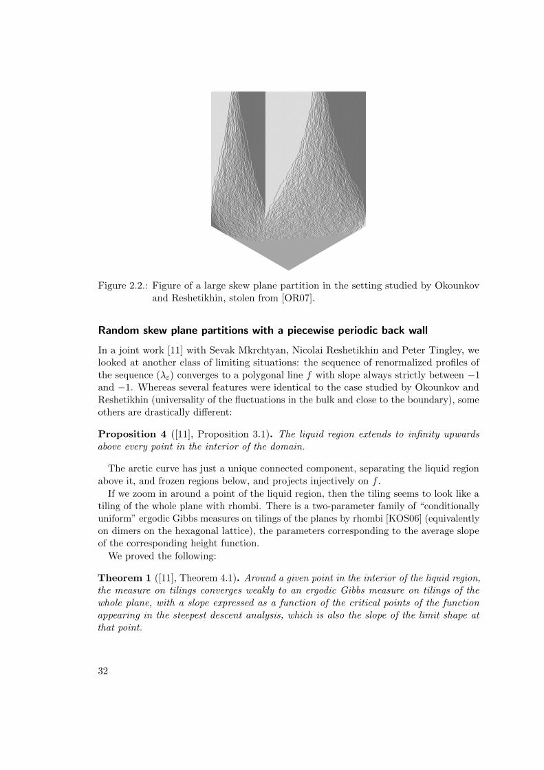
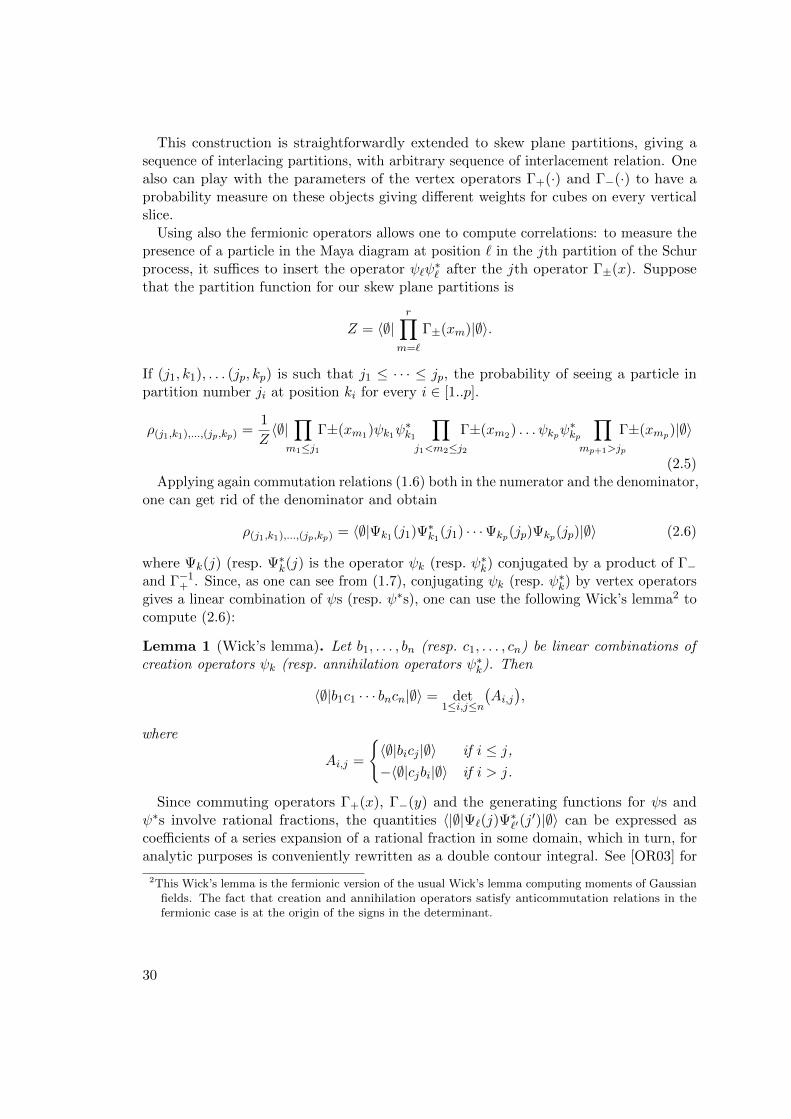
Figure 2.2.: Figure of a large skew plane partition in the setting studied by Okounkovand Reshetikhin, stolen from [OR07].

Random skew plane partitions with a piecewise periodic back wall

In a joint work [11] with Sevak Mkrchtyan, Nicolai Reshetikhin and Peter Tingley, welooked at another class of limiting situations: the sequence of renormalized profiles ofthe sequence (λε) converges to a polygonal line f with slope always strictly between −1and −1. Whereas several features were identical to the case studied by Okounkov andReshetikhin (universality of the fluctuations in the bulk and close to the boundary), someothers are drastically different:

Proposition 4 ([11], Proposition 3.1). The liquid region extends to infinity upwardsabove every point in the interior of the domain.

The arctic curve has just a unique connected component, separating the liquid regionabove it, and frozen regions below, and projects injectively on f .

If we zoom in around a point of the liquid region, then the tiling seems to look like atiling of the whole plane with rhombi. There is a two-parameter family of “conditionallyuniform” ergodic Gibbs measures on tilings of the planes by rhombi [KOS06] (equivalentlyon dimers on the hexagonal lattice), the parameters corresponding to the average slopeof the corresponding height function.

We proved the following:

Theorem 1 ([11], Theorem 4.1). Around a given point in the interior of the liquid region,the measure on tilings converges weakly to an ergodic Gibbs measure on tilings of thewhole plane, with a slope expressed as a function of the critical points of the functionappearing in the steepest descent analysis, which is also the slope of the limit shape atthat point.

32

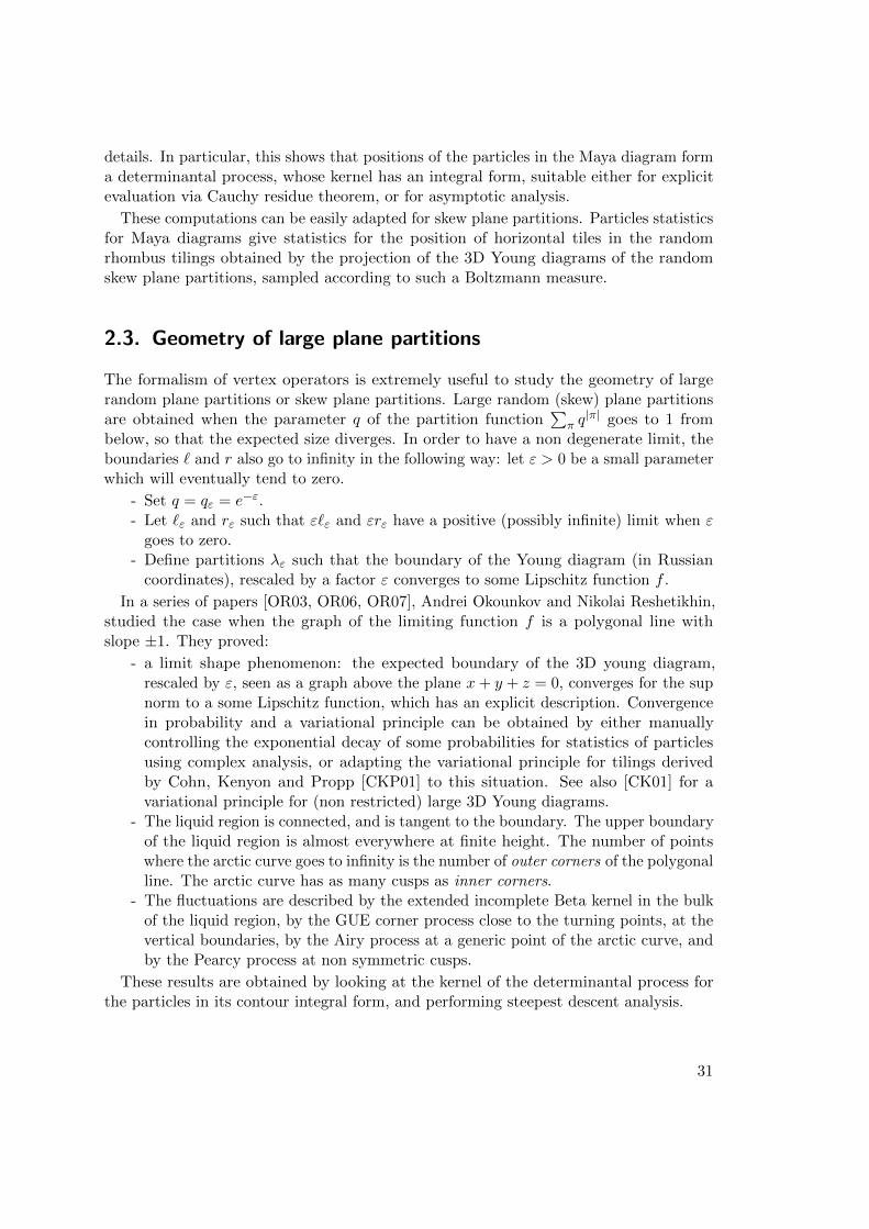
(a)

A = 8−8, −7, 0, 4, 6, 7<, α = 8−0.1, 0.4, −0.45, 0.4, −0.25<

(b)

Figure 2.3.: (a) Setup for large skew plane partitions with limiting f with slope strictlybetween −1 and 1 from [11]. (b) The limiting arctic curve in one example ofthis setup.

The fact that local correlations near a point in a large domain should behave like theergodic measure with a slope given by the tangent plane to the limit shape is very naturalstatement for general dimer models of large domains, but is still a conjecture, except forspecific cases where it has been proven (see for example [Ken08, Pet15]).

The idea of the proof is very simple in this case and consists in noticing that an ergodicGibbs measure on dimers of the hexagonal lattice is, as the correlations for rhombi in theliquid region, like in [OR07], given by the extended incomplete Beta kernel, and relatingthe corresponding parameters to the slope of the height function.

When going up, the density of horizontal rhombi in a random configuration stayspositive but decreases and converges to zero. A natural question is to study the statisticsof the horizontal tiles, using a different scaling in both directions.

Theorem 2 ([11], Theorem 4.3). When going up, the distribution of horizontal rhombi,once the vertical direction is rescaled by a factor ε, converges to an ergodic Gibbs measureof the bead process.

The bead process [6] is a determinantal point process on Z×R, where configurations areinterlacing point configuration: between two successive points on {n}×R, there is exactlyone point on {n− 1} × R and {n+ 1} × R. It is a natural object to describe the limitof dimer models on the hexagonal lattice and more generally on any periodic bipartitegraph, when the weight of one type of edge goes to zero. There is a two-parameterfamily of ergodic Gibbs measures for the bead process, whose corresponding kernels areextended sine kernels: the two parameters are the density (the average number of beadsper unit interval) and the tilt, describing the tendency of a bead to prefer being closer toits north-east neighbor rather than to it south-east neighbour.

In the case of skew plane partitions, the expression for the density and the tilt is anexplicit expression of the abscissa, and the limiting polygonal contour for the partitions(λε), in terms of lengths of linear pieces and angles at corners.

These results have been generalised by Sevak Mkrtchyan [Mkr11] to the situation wherethe limiting function f for the boundary of the removed partition is piecewise linear with

33

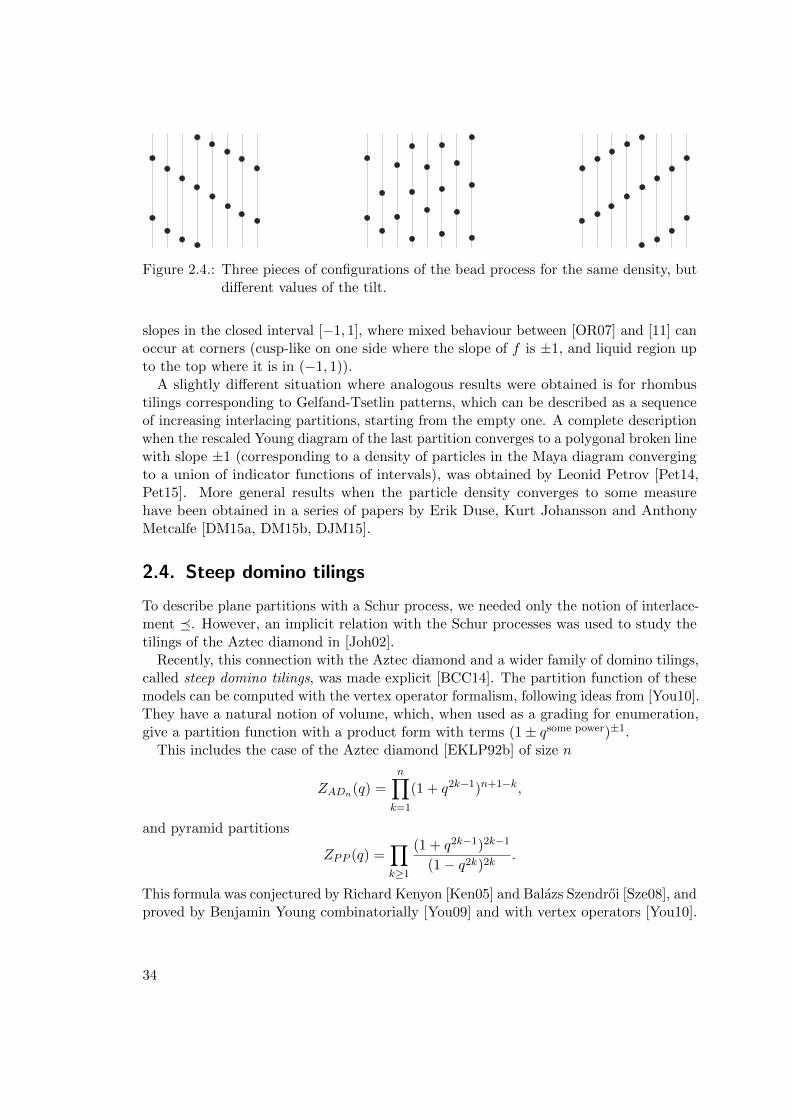
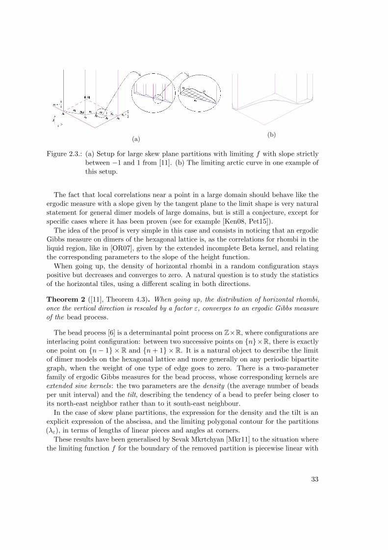
Figure 2.4.: Three pieces of configurations of the bead process for the same density, butdifferent values of the tilt.

slopes in the closed interval [−1, 1], where mixed behaviour between [OR07] and [11] canoccur at corners (cusp-like on one side where the slope of f is ±1, and liquid region upto the top where it is in (−1, 1)).

A slightly different situation where analogous results were obtained is for rhombustilings corresponding to Gelfand-Tsetlin patterns, which can be described as a sequenceof increasing interlacing partitions, starting from the empty one. A complete descriptionwhen the rescaled Young diagram of the last partition converges to a polygonal broken linewith slope ±1 (corresponding to a density of particles in the Maya diagram convergingto a union of indicator functions of intervals), was obtained by Leonid Petrov [Pet14,Pet15]. More general results when the particle density converges to some measurehave been obtained in a series of papers by Erik Duse, Kurt Johansson and AnthonyMetcalfe [DM15a, DM15b, DJM15].

2.4. Steep domino tilings

To describe plane partitions with a Schur process, we needed only the notion of interlace-ment �. However, an implicit relation with the Schur processes was used to study thetilings of the Aztec diamond in [Joh02].

Recently, this connection with the Aztec diamond and a wider family of domino tilings,called steep domino tilings, was made explicit [BCC14]. The partition function of thesemodels can be computed with the vertex operator formalism, following ideas from [You10].They have a natural notion of volume, which, when used as a grading for enumeration,give a partition function with a product form with terms (1± qsome power)±1.

This includes the case of the Aztec diamond [EKLP92b] of size n

ZADn(q) =n∏

k=1

(1 + q2k−1)n+1−k,

and pyramid partitions

ZPP (q) =∏

k≥1

(1 + q2k−1)2k−1

(1− q2k)2k.

This formula was conjectured by Richard Kenyon [Ken05] and Balazs Szendroi [Sze08], andproved by Benjamin Young combinatorially [You09] and with vertex operators [You10].

34

They are obtained as Schur processes where now the a sequence is not constant equalto L, but alternates between L and R. The b sequence for the Aztec diamond is (+−)n,whereas for pyramid partitions, it is · · ·+ + − − · · · . Combinatorial and enumerativefacts about these steep tilings are given in [BCC14], in particular the way to compute thepartition function as a result of the commutation relations between the vertex operators.

Sunil Chhita and Benjamin Young [CY14] gave an explicit expression for the inverseKasteleyn matrix of the Aztec diamond, which is, up to minor details, the kernel ofthe determinantal process describing the position of the dominos. Their proof is usinginduction via the urban renewal transformation and explicit residue computation, butthe formula has the same flavor as the one obtained by Okounkov and Reshetikhin withvertex operators. Can we derive the formula of Chhita and Young via vertex operators?What is the meaning of the presence of a domino in a steep tiling in terms of particles inthe Maya diagram? Can this be extended to a general framework which would containother Schur processes? In particular, it is remarkable that both skew plane partitions(giving rhombus tilings) and steep domino tilings were examples of dimer models. It isthen natural to ask whether other Schur processes can be expressed as a dimer model.All those questions were answered in of [15], the main results of which are exposed inChapter 3.

35

3. Dimers on Rail Yard Graphs

In a joint work [15] with Jeremie Bouttier, Guillaume Chapuy, Sylvie Corteel and SanjayRamassamy, we introduce a family of planar graphs, called rail yard graphs. They areperiodic in the vertical direction, obtained by concatenating from left to right four kindsof elementary graphs. From dimer models on these rail yard graphs, with suitableboundary conditions, we can recover the Schur processes described in Chapter 1. Thedimer statistics (and not only those corresponding to particles in the Schur process)can be computed using vertex operators, creating a bridge between this formalism andKasteleyn approach.

3.1. Rail Yard Graphs

Rail yard graphs form a family of planar graphs, indexed by the following data (`, r, a, b),with two integers ` < r, the LR sequence a = (a`, . . . , ar) = {L,R}[`..r] and the signsequence b = (b`, . . . , br) = {+,−}[`..r]. Note that this is exactly the same data used todescribed Schur processes in Chapter 1, except the weight sequence x, which will beintroduced later when we talk about dimers.

Definition 13. The rail yard graph associated with the integers ` and r, the LR sequencea and the sign sequence b, and denoted by RYG(`, r, a, b), is the bipartite plane graphdefined as follows. Its vertex set is [2`− 1..2r + 1]× (Z + 1/2), and we say that a vertexis even (resp. odd) if its abscissa is an even (resp. odd) integer. Each even vertex (2m, y),m ∈ [`..r], is then incident to three edges: two horizontal edges connecting it to the oddvertices (2m− 1, y) and (2m+ 1, y), and one diagonal edge connecting it to

- the odd vertex (2m− 1, y + 1) if am = L and bm = +,- the odd vertex (2m− 1, y − 1) if am = L and bm = −,- the odd vertex (2m+ 1, y + 1) if am = R and bm = +,- the odd vertex (2m+ 1, y − 1) if am = R and bm = −.

A rail yard graph is infinite and 1-periodic in the vertical direction. When ` = r, theLR and sign sequences both consist of a single element, and the corresponding rail yardgraph, which is said elementary, is of one of four possible types, see Figure 3.1. Giventwo rail yard graphs RYG(`, r, a, b) and RYG(`′, r′, a′, b′) such that `′ = r + 1, we definetheir concatenation by taking the union of their vertex and edge sets. It is nothing butthe rail yard graph RYG(`, r′, aa′, bb′) where aa′ and bb′ denote the concatenations of theLR and sign sequences. Clearly, a general rail yard graph is obtained by concatenatingelementary ones.

36

...

... R+

...

... ...

... R−...

... ...

... L+

...

... ...

... L−...

...

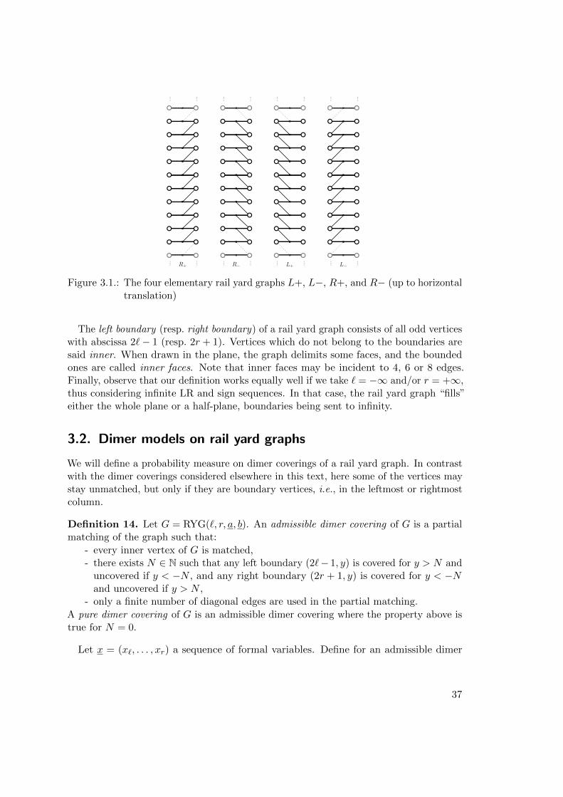
Figure 3.1.: The four elementary rail yard graphs L+, L−, R+, and R− (up to horizontaltranslation)

The left boundary (resp. right boundary) of a rail yard graph consists of all odd verticeswith abscissa 2`− 1 (resp. 2r + 1). Vertices which do not belong to the boundaries aresaid inner. When drawn in the plane, the graph delimits some faces, and the boundedones are called inner faces. Note that inner faces may be incident to 4, 6 or 8 edges.Finally, observe that our definition works equally well if we take ` = −∞ and/or r = +∞,thus considering infinite LR and sign sequences. In that case, the rail yard graph “fills”either the whole plane or a half-plane, boundaries being sent to infinity.

3.2. Dimer models on rail yard graphs

We will define a probability measure on dimer coverings of a rail yard graph. In contrastwith the dimer coverings considered elsewhere in this text, here some of the vertices maystay unmatched, but only if they are boundary vertices, i.e., in the leftmost or rightmostcolumn.

Definition 14. Let G = RYG(`, r, a, b). An admissible dimer covering of G is a partialmatching of the graph such that:

- every inner vertex of G is matched,- there exists N ∈ N such that any left boundary (2`− 1, y) is covered for y > N and

uncovered if y < −N , and any right boundary (2r + 1, y) is covered for y < −Nand uncovered if y > N ,

- only a finite number of diagonal edges are used in the partial matching.

A pure dimer covering of G is an admissible dimer covering where the property above istrue for N = 0.

Let x = (x`, . . . , xr) a sequence of formal variables. Define for an admissible dimer

37

...

y = 0

} allcovered

} nonecovered

}all

covered }none

covered

y = 0

2`− 1 2r+1

...

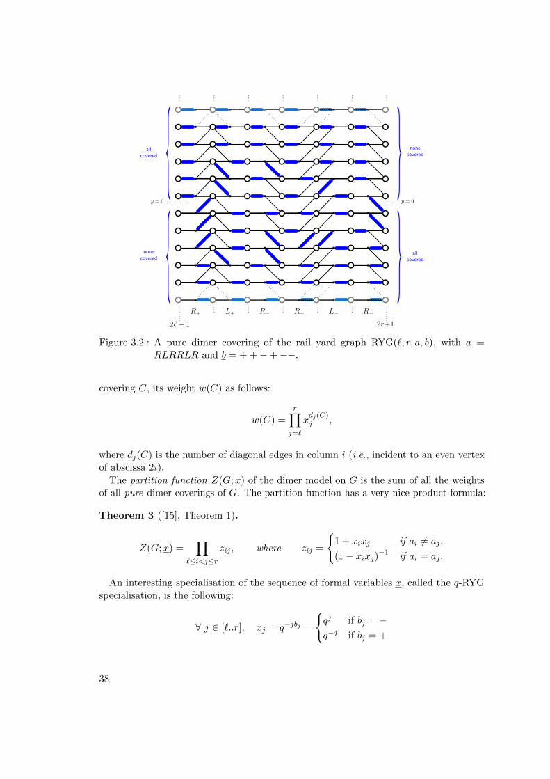
...... R+ L+ R− R+ L− R−... ... ... ... ...

... ... ... ... ...

......

Figure 3.2.: A pure dimer covering of the rail yard graph RYG(`, r, a, b), with a =RLRRLR and b = + +−+−−.

covering C, its weight w(C) as follows:

w(C) =

r∏

j=`

xdj(C)j ,

where dj(C) is the number of diagonal edges in column i (i.e., incident to an even vertexof abscissa 2i).

The partition function Z(G;x) of the dimer model on G is the sum of all the weightsof all pure dimer coverings of G. The partition function has a very nice product formula:

Theorem 3 ([15], Theorem 1).

Z(G;x) =∏

`≤i<j≤rzij , where zij =

{1 + xixj if ai 6= aj ,

(1− xixj)−1 if ai = aj .

An interesting specialisation of the sequence of formal variables x, called the q-RYGspecialisation, is the following:

∀ j ∈ [`..r], xj = q−jbj =

{qj if bj = −q−j if bj = +

38

The exponent of q in the weight of C is equal to the minimal number of flips of dimersaround a face to perform to get C from the fundamental dimer covering, where all thedimers are horizontal1. This is the one we used for plane partitions in the previouschapter, when the LR sequence a is constant equal to L: in that case, the rail yard graphsare strips of the honeycomb lattice, and their dimer coverings correspond by duality torhombus tilings, which are projections of piles of a finite number of cubes.

3.3. Dimer correlations

We now suppose that the variables xj are specialised in such a way that the weights ofpure dimer configurations are positive and the partition function is finite, in order tohave a probabilistic (or statistical physics) interpretation of the model. This means thatxj > 0 for all j, and xixj < 1 if bi = +, bj = −, ai = aj and i < j.

The probability PG;x(C) of a pure dimer configuration C is the ratio w(C)/Z(G;x).Given a finite subset E of edges of the graph G, we denote also by PG;x(E) the probabilitythat the edges of E are present in the random dimer covering of G.

We get a general formula for the probability of such a set of edges as a determinant ofa matrix with explicit entries in terms of the geometry of the graphs and the edges in E.

Define for any integer k the following rational fraction:

Fk(z) =

∏

i:(ai,bi)=(R,+)2i<k

(1 + xiz)∏

j:(aj ,bj)=(L,−)2j>k

(1− xjz

)

∏

i:(ai,bi)=(L,+)2i≤k

(1− xiz)∏

j:(aj ,bj)=(R,−)2j≥k

(1 +xjz

)

For α = (αx, αy), β = (βx, βy) two vertices of G such that αx is even and βx is odd,define

Cα,β =

∮

Cz

∮

Cw

Fαx(z)

Fβx(w)

wβy

zαy

√zw

z − wdz

2iπz

dw

2iπw. (3.1)

where the simple positively oriented contours Cz and Cw should satisfy the followingconditions:

- Cz should encircle 0 and all negative poles of Fαx(z), but not the positive ones- Cw should encircle 0 and the positive zeros of Fβx(w), but not the negative ones- Cz and Cw should not intersect and Cz should surround Cw if and only is αx < βx

It corresponds to the extraction of the coefficient of zαyw−β

yin a series expansion in z

and w of the rational fraction Fαx (z)√zw

Fβx (w)(z−w) in a particular domain of convergence.

Theorem 4 ([15], Theorem 5). Let E = {e1, . . . , es} be a finite set of edges of G =RYG(`, r, a, b), with ei = (αi, βi). Then:

PG;x(E) = (−1)H(E)xn det1≤i,j≤s

(Cαi,βj ),

1It is easy to check that such a pure dimer covering with only horizontal dimers exists for any rail yardgraph and is unique.

39

with H(E) the number of horizontal edges in E whose right endpoint is at an evenabscissa, xn = xn`` · · ·xnrr , with nk the number of diagonal edges in column k.

The fact that this probability is a determinant is not surprising: since the graph G isplanar and bipartite, the Kasteleyn theory of dimer models tells us that this probabilitycan be computed via a minor of the inverse of a Kasteleyn matrix associated to thegraph2 G. We prove [15, Theorem17] that indeed, the matrix C whose entries are definedby Equation (3.1) is indeed the inverse of such a Kasteley matrix.

From a pure dimer covering C of a rail yard graph G, one can construct a sequenceof Maya diagrams, which describe the state of edges at the juncture of two successiveelementary graph which compose G.

For j ∈ [`..r + 1], the jth Maya diagram mk(C) ∈ {◦, •}Z+ 12 is constructed as follows:

mj(C)k =

{◦ if (2j − 1, k) is not connected to a dimer on its left in C,

• if (2j − 1, k) is not connected to a dimer on its right in C.

This construction gives in particular the following:

Lemma 2. Under the measure PG;x, the sequence of Maya diagrams follows a Schurprocess with parameters given by the sequences a, b and x.

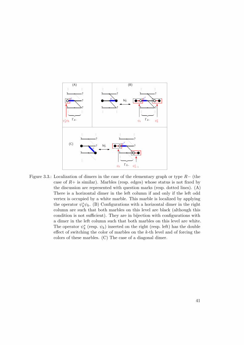
On some of the edges in G, those in simple columns3, the presence or absence is directlyrelated to the presence of a white or a black marble in the closest Maya diagram to theseedges. See Figure 3.3 (A). The statistics for those edges can be computed directly fromstatistics for Schur processes, either by the vertex operator formalism as presented in theprevious chapter, or by Eynard-Mehta theorem (see e.g.,[BR05]). In particular, if thesequence a is constant equal to L and the edges in E are all horizontal edges in simplecolumns, Theorem 4 reduces to correlations for plane partitions of [OR03].

For edges in double columns, there is no direct direct correspondence between dimersand marbles in Maya diagrams. However, there is a bijection between configurations withgiven dimers on double columns and dimer coverings with defects. The partition functionof the configurations with defects can be written down in terms of vertex operatorsand creation/annihilation operators appearing in more complicated combination thanjust projectors, see Figure 3.3 (B) and (C). Although these quantities do not havedirectly a direct probabilist interpretation on Maya diagrams, they allow one to computecorrelations of dimers, with the kind of formula as (2.6).

One of the interesting features of Theorem 4 is that we have an explicit formula forthe kernel of the determinantal process, with a double contour integral which can beevaluated explicitly if needed. As in the case of Okounkov and Reshethin, this integralform is particularly suitable for asymptotic analysis via the steepest descent analysis,and allows to get results for large rail yard graphs.

2once we have removed the unmatched vertices on the boundary.3The simple column of elementary graph of type L (resp. R) is the rightmost (resp. leftmost), which

contains only horizontal edges.

40

... ...

... ...

... ...

...

e e

ΓR−ψ∗kψk

︸︷︷︸

?

? ?

...

... ...

...

e′bij.

?

? ?

?

? ?

ΓR−

︸︷︷︸

...

?

? ?

ψk ψ∗k

?

(A) (B)

...

...

...

e

...

...

...

e′bij.

?

? ?

?

? ?

ΓR−

︸︷︷︸

?

ψk ψ∗k−1

?(C)

Figure 3.3.: Localization of dimers in the case of the elementary graph or type R− (thecase of R+ is similar). Marbles (resp. edges) whose status is not fixed bythe discussion are represented with question marks (resp. dotted lines). (A)There is a horizontal dimer in the left column if and only if the left oddvertex is occupied by a white marble. This marble is localized by applyingthe operator ψ∗kψk. (B) Configurations with a horizontal dimer in the rightcolumn are such that both marbles on this level are black (although thiscondition is not sufficient). They are in bijection with configurations witha dimer in the left column such that both marbles on this level are white.The operator ψ∗k (resp. ψk) inserted on the right (resp. left) has the doubleeffect of switching the color of marbles on the k-th level and of forcing thecolors of these marbles. (C) The case of a diagonal dimer.

41

L+ R−... ...

... ...

L+ R−... ...

... ...

L+ R−... ...

... ...

L+ R−... ...

... ...

y = 0y = 0

x = 0

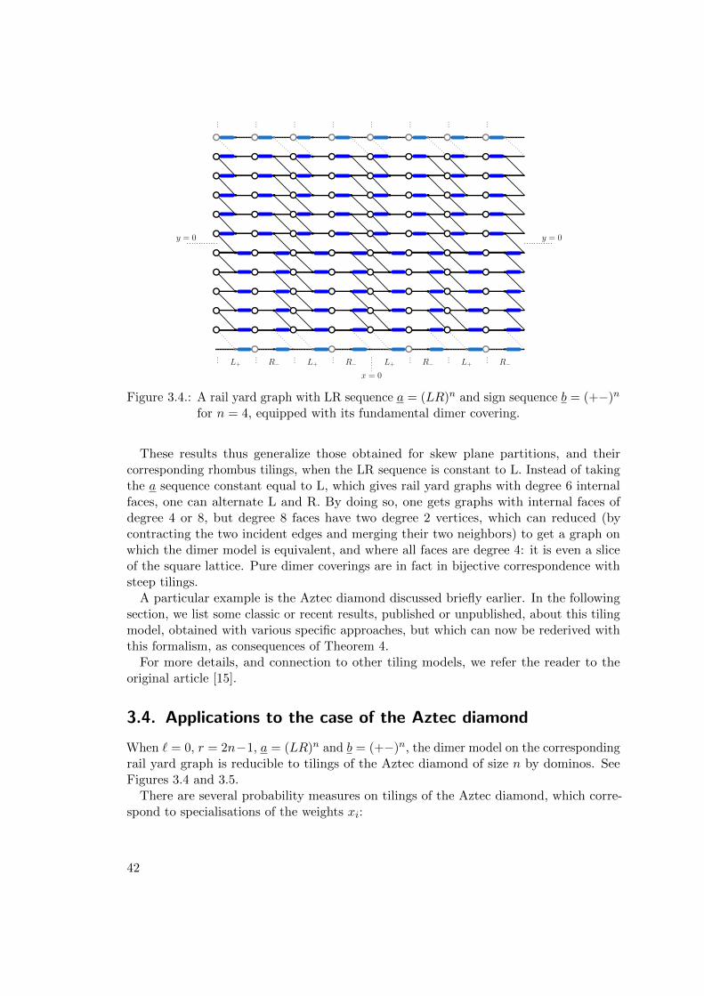
Figure 3.4.: A rail yard graph with LR sequence a = (LR)n and sign sequence b = (+−)n

for n = 4, equipped with its fundamental dimer covering.

These results thus generalize those obtained for skew plane partitions, and theircorresponding rhombus tilings, when the LR sequence is constant to L. Instead of takingthe a sequence constant equal to L, which gives rail yard graphs with degree 6 internalfaces, one can alternate L and R. By doing so, one gets graphs with internal faces ofdegree 4 or 8, but degree 8 faces have two degree 2 vertices, which can reduced (bycontracting the two incident edges and merging their two neighbors) to get a graph onwhich the dimer model is equivalent, and where all faces are degree 4: it is even a sliceof the square lattice. Pure dimer coverings are in fact in bijective correspondence withsteep tilings.

A particular example is the Aztec diamond discussed briefly earlier. In the followingsection, we list some classic or recent results, published or unpublished, about this tilingmodel, obtained with various specific approaches, but which can now be rederived withthis formalism, as consequences of Theorem 4.

For more details, and connection to other tiling models, we refer the reader to theoriginal article [15].

3.4. Applications to the case of the Aztec diamond

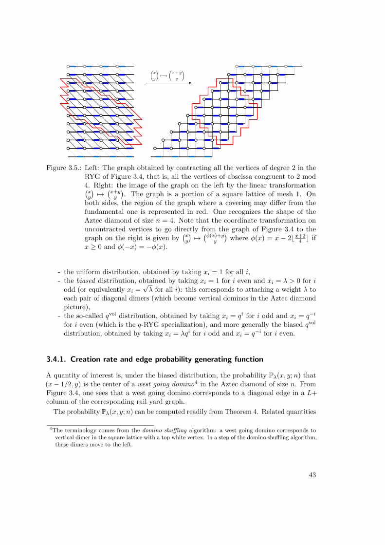
When ` = 0, r = 2n−1, a = (LR)n and b = (+−)n, the dimer model on the correspondingrail yard graph is reducible to tilings of the Aztec diamond of size n by dominos. SeeFigures 3.4 and 3.5.

There are several probability measures on tilings of the Aztec diamond, which corre-spond to specialisations of the weights xi:

42

(x

y

)7−→

(x + y

y

)

Figure 3.5.: Left: The graph obtained by contracting all the vertices of degree 2 in theRYG of Figure 3.4, that is, all the vertices of abscissa congruent to 2 mod4. Right: the image of the graph on the left by the linear transformation(xy

)7→(x+yy

). The graph is a portion of a square lattice of mesh 1. On

both sides, the region of the graph where a covering may differ from thefundamental one is represented in red. One recognizes the shape of theAztec diamond of size n = 4. Note that the coordinate transformation onuncontracted vertices to go directly from the graph of Figure 3.4 to thegraph on the right is given by

(xy

)7→(φ(x)+y

y

)where φ(x) = x − 2bx+2

4 c ifx ≥ 0 and φ(−x) = −φ(x).

- the uniform distribution, obtained by taking xi = 1 for all i,- the biased distribution, obtained by taking xi = 1 for i even and xi = λ > 0 for i

odd (or equivalently xi =√λ for all i): this corresponds to attaching a weight λ to

each pair of diagonal dimers (which become vertical dominos in the Aztec diamondpicture),

- the so-called qvol distribution, obtained by taking xi = qi for i odd and xi = q−i

for i even (which is the q-RYG specialization), and more generally the biased qvol

distribution, obtained by taking xi = λqi for i odd and xi = q−i for i even.

3.4.1. Creation rate and edge probability generating function

A quantity of interest is, under the biased distribution, the probability Pλ(x, y;n) that(x− 1/2, y) is the center of a west going domino4 in the Aztec diamond of size n. FromFigure 3.4, one sees that a west going domino corresponds to a diagonal edge in a L+column of the corresponding rail yard graph.

The probability Pλ(x, y;n) can be computed readily from Theorem 4. Related quantities

4The terminology comes from the domino shuffling algorithm: a west going domino corresponds tovertical dimer in the square lattice with a top white vertex. In a step of the domino shuffling algorithm,these dimers move to the left.

43

of interest are the so-called biased creation rate

Crλ(x, y;n) =λ+ 1

λ

(Pλ(x, y;n)− Pλ(x+ 1, y;n− 1)

),

and the edge probability generating function

Πλ(u, v, t) =∑

x,y,n

Pλ(x, y;n)uxvytn.

Proposition 5 ([15], Proposition 21). The biased creation rate equals

Crλ(x, y;n) =

(λ

λ+ 1

)n−1

cλ(A,B, n− 1)cλ(B,A, n− 1)

where A = n−m− y = (x− 1−x− y)/2, B = m− 1 = (n− 1 +x− y)/2, and cλ(A,B, n)

is the coefficient of zA in (1− z)B(1 + λ−1z)n−B

.

Remark 2. The quantities cλ(A,B, n) are Krawtchouk polynomials, which play a greatrole in the analysis of the Aztec diamond, see [Joh02].

The idea of the proof is that taking the difference of two Pλ makes appear in thenumerator of the rational fraction a factor (z − w), which cancels the same factor in thedenominator. After this cancellation, the rational fraction decouples, and the result canbe rewritten as a product of two single contour integrals, which can both be transformedinto integral representations of the Krawtchouk polynomials.

Proposition 6 ([15], Proposition 21). The biased edge probability generating functionequals

Πλ(u, v, t) =λt

(1− t/u)((1 + λ)(1 + t2)− t(u+ u−1)− λt(v + v−1)). (3.2)

To prove this formula, one plugs the integral formula of Pλ(x, y;n) in the definition ofΠ(u, v, t). The sums over x and n can be performed explicitly as geometric series. Thesum over y acts as a Dirac distribution, and allows one to remove one of the contourintegrals. Computing explicitly the remaining integral by Cauchy theorem yields theresult.

These results were used for example in [CEP96] as a way to prove the arctic circletheorem, and its generalization for arbitrary λ. However, the formula appeared withoutproofs, supposed to appear in an article by Gessel, Ionescu and Propp, that has notbeen published so far. Formula (3.2) for λ = 1 appears in [Hel00] and [Du11], and usedin [BP11] as yet another route to the arctic circle. See [15], Section 6.1, for more detailsabout these quantities.

44

3.4.2. The inverse Kasteleyn matrix

In [CY14], Sunil Chhita and Ben Young give an explicit expression for the inverse ofthe Kasteleyn matrix for the biased qvol distribution. They write down an expressionby extrapolating the expression of the kernel of the determinantal process for a particlesystem encoded in the Aztec diamond [Hel00] in the uniform case. To prove thatthe expression they give is indeed the inverse Kasteleyn matrix, they do an ad-hoccomputation, based on induction, which is long and tedious.

We prove [15, Section 6.2] that up to a simple change of variables that the entries oftheir inverse Kasteleyn matrix are equal (up to multiplicative factors cancelling in thedeterminant) to the coefficients Cα,β. The interpretation in terms of rail yard graphsgives thus a constructive proof of that formula, and an explanation of the double contourintegral representation.

The formula for the inverse Kasteleyn matrix from [CJY15] for the biased distributionon Aztec diamond can be also obtained from the formula for Cα,β.

The technique used by Chhita and Young in [CY14] also applies to more generalweights on the Aztec diamond, like the double weighting, which yields in that case to aquadruple integral representation for the entries of the inverse Kasteleyn matrix, andtwo of them can be performed explicitly [CJ16]. To our knowledge, this weighting doesnot fit in the rail yard graph framework.

3.4.3. The arctic circle theorem

Yet another proof of the arctic circle [JPS98] can be given, by following the ideas ofOkounkov and Reshetikhin in the case of skew plane partitions. To prove convergence inexpectation of the limit shape, it is enough to look at the probability that at a givenpoint even vertex α = (2m, y − 1

2) is connected to a diagonal dimer. When n is large,m = τn and y = χn, this probability can be written as

pα =

∮

Cz

∮

Cw

en(S(χ,τ ;z)−S(χ,τ ;w)+o(1)) 1

z − wdzdw

(2iπ)2,

where

S(τ, χ; z) = −τ log(1− z)− (1− τ) log(1 +1

z)− χ log z.

We now proceed as in [OR03] to obtain the asymptotics of this probability. For fixed(τ, χ), the function z 7→ S(τ, χ; z) has two critical points.

- If the two critical points are real, the integral goes to 0 or 1 exponentially fast withn by the saddle point method. The point (τ, χ) is in the frozen region.

- If the two critical points are complex conjugate, one can move the contours so thatthey cross transversally at the complex critical points to apply again the saddlepoint method. By doing so, we pick the contribution of the residue at z = w, whichgives the main contribution of the integral, giving a result strictly between 0 and 1.

The transition between those two regimes correspond to the value of (τ, χ) for whichthe two critical points merge. This happens when the discriminant of the numerator of

45

∂S(τ, χ; z)/∂z is equal to zero. This gives

(2τ − 1)2 − 4(τ + χ)(1− χ− τ) = 0, (3.3)

which under the change of variables

{u = 2τ + χ

v = χ(3.4)

corresponds to the circle 2(u− 1)2 + 2v2 = 1 inscribed in the limiting square of the Aztecdiamond, given by |u− 1|+ |v| ≤ 1.

46

4. Perfect simulations of Schur processes

In a joint work [13] with Dan Betea, Jeremie Bouttier, Guillaume Chapuy, Sylvie Corteel,and Mirjana Vuletic, we describe a simple sampling algorithm for Schur processes Thisalgorithm is a sequence of atomic steps, which are based on bijective proofs of the Cauchyidentities (1.1) and (1.4). Since some Schur processes correspond bijectively to rhombusor domino tilings, this algorithm can be used to efficiently generate random tilings.

Exact sampling algorithms for classes of tilings have been proposed before, includingthe case of plane and skew plane partitions [Bor11] and the Aztec diamond [EKLP92b].See also [BF14] for a general approach, and [BF15] for an application of this approachto a restricted class of graphs including, but not limited to the Aztec diamond. Ouralgorithm described below, different from but somewhat similar to that of [Bor11] allowsone to sample general Schur processes, which under appropriate specialisation, give planeand skew plane partitions, tilings of the Aztec diamond by dominos, pyramid partitionsand more generally steep tilings.

Moreover, the algorithm we propose is entropy optimal (if we suppose that we cangenerate Bernoulli and geometric random variables optimally), in the sense that therandom input of the algorithm can be reconstructed completely from the output. See [13],Proposition 3.8.

Following the notation of the previous chapters, our Schur processes will be definedby the sequences a = (a`, . . . , ar) and b = (b`, . . . , br), and parameters x = (x`, . . . , xr),and will generate random sequences of interlacing/dually interlacing partitions Λ =(λ(`), . . . , λ(r+1)), such that λ(`) = λ(r+1) = ∅. The measure on sequences of partitions issuch that, according to (1.5),

P(Λ) ∝r∏

j=`

x||λ(j+1)|−|λ(j)||j .

For notation convenience, we will suppose here that ` = 0 and r = n− 1, so that thenon trivial partitions are labelled from 1 to n − 1, and the sequences a, b and x havelength n.

The encoded shape of the Schur process is the Young diagram whose boundary is thelattice path of length n+ 1 constructed by the sequence b as follows: + corresponds to ahorizontal step to the right, and − corresponds to a vertical up step1. See Figure 4.1.

The edges of the path encoded by b are decorated with the elements of the sequencesa and x. The different partitions of the realisation of the Schur process Λ are attachedto vertices visited by this path.

1In [13], the encoded shape is represented as a Young diagram in French coordinates, so the notion ofvertical up and down steps are exchanged.

47

� �′

�

��′

�′

�′

�

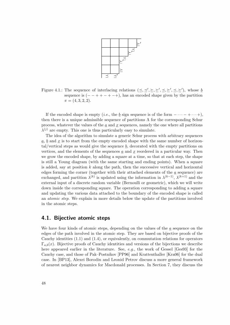
Figure 4.1.: The sequence of interlacing relations (�,�′,�,�′,�,�′,�,�′), whose bsequence is (−−+ +−+−+), has an encoded shape given by the partitionπ = (4, 3, 2, 2).

If the encoded shape is empty (i.e., the b sign sequence is of the form − · · · −+ · · ·+),then there is a unique admissible sequence of partitions Λ for the corresponding Schurprocess, whatever the values of the a and x sequences, namely the one where all partitionsλ(j) are empty. This one is thus particularly easy to simulate.

The idea of the algorithm to simulate a generic Schur process with arbitrary sequencesa, b and x is to start from the empty encoded shape with the same number of horizon-tal/vertical steps as would give the sequence b, decorated with the empty partitions onvertices, and the elements of the sequences a and x reordered in a particular way. Thenwe grow the encoded shape, by adding a square at a time, so that at each step, the shapeis still a Young diagram (with the same starting and ending points). When a squareis added, say at position k along the path, then the successive vertical and horizontaledges forming the corner (together with their attached elements of the a sequence) areexchanged, and partition λ(k) is updated using the information in λ(k−1), λ(k+1) and theexternal input of a discrete random variable (Bernoulli or geometric), which we will writedown inside the corresponding square. The operation corresponding to adding a squareand updating the various data attached to the boundary of the encoded shape is calledan atomic step. We explain in more details below the update of the partitions involvedin the atomic steps.

4.1. Bijective atomic steps

We have four kinds of atomic steps, depending on the values of the a sequence on theedges of the path involved in the atomic step. They are based on bijective proofs of theCauchy identities (1.1) and (1.4), or equivalently, on commutation relations for operatorsΓa,b(x). Bijective proofs of Cauchy identities and versions of the bijections we describehere appeared earlier in the literature. See, e.g., the work of Gessel [Ges93] for theCauchy case, and those of Pak–Postnikov [PP96] and Krattenthaller [Kra06] for the dualcase. In [BP13], Alexei Borodin and Leonid Petrov discuss a more general frameworkof nearest neighbor dynamics for Macdonald processes. In Section 7, they discuss the

48

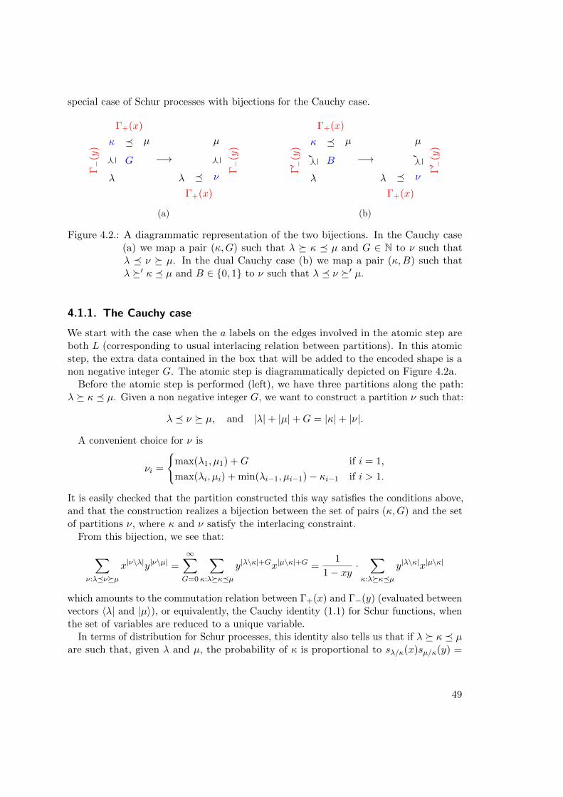
special case of Schur processes with bijections for the Cauchy case.

κ µ�Γ+(x)

�Γ−

(y)

λ

G −→λ ν

µ

�Γ+(x)

�Γ−

(y)

(a)

κ µ�Γ+(x)

�′

Γ′ −

(y)

λ

B −→λ ν

µ

�Γ+(x)

�′

Γ′ −

(y)

(b)

Figure 4.2.: A diagrammatic representation of the two bijections. In the Cauchy case(a) we map a pair (κ,G) such that λ � κ � µ and G ∈ N to ν such thatλ � ν � µ. In the dual Cauchy case (b) we map a pair (κ,B) such thatλ �′ κ � µ and B ∈ {0, 1} to ν such that λ � ν �′ µ.

4.1.1. The Cauchy case

We start with the case when the a labels on the edges involved in the atomic step areboth L (corresponding to usual interlacing relation between partitions). In this atomicstep, the extra data contained in the box that will be added to the encoded shape is anon negative integer G. The atomic step is diagrammatically depicted on Figure 4.2a.

Before the atomic step is performed (left), we have three partitions along the path:λ � κ � µ. Given a non negative integer G, we want to construct a partition ν such that:

λ � ν � µ, and |λ|+ |µ|+G = |κ|+ |ν|.

A convenient choice for ν is

νi =

{max(λ1, µ1) +G if i = 1,

max(λi, µi) + min(λi−1, µi−1)− κi−1 if i > 1.

It is easily checked that the partition constructed this way satisfies the conditions above,and that the construction realizes a bijection between the set of pairs (κ,G) and the setof partitions ν, where κ and ν satisfy the interlacing constraint.

From this bijection, we see that:

∑

ν:λ�ν�µx|ν\λ|y|ν\µ| =

∞∑

G=0

∑

κ:λ�κ�µy|λ\κ|+Gx|µ\κ|+G =

1

1− xy ·∑

κ:λ�κ�µy|λ\κ|x|µ\κ|

which amounts to the commutation relation between Γ+(x) and Γ−(y) (evaluated betweenvectors 〈λ| and |µ〉), or equivalently, the Cauchy identity (1.1) for Schur functions, whenthe set of variables are reduced to a unique variable.

In terms of distribution for Schur processes, this identity also tells us that if λ � κ � µare such that, given λ and µ, the probability of κ is proportional to sλ/κ(x)sµ/κ(y) =

49

x|λ\κ|y|µ\κ|, and if G is distributed as a geometric random variable with parameter xy,then the conditional probability of the partition ν constructed above is proportional tosν/λ(x)sν/µ(y). In particular, if λ � κ � µ is a piece of a sample of a Schur process withsequences

a = · · ·LL · · · , b = · · · −+ · · · , x = · · ·xy · · · ,

(the indicated terms of the sequences correspond to transitions λ → κ → µ), then thesame sequence of partitions, where κ is replaced by ν is sampled according to a Schurprocess with new sequences:

a = · · ·LL · · · , b = · · ·+− · · · , x = · · · yx · · · ,

where all the parameters for the two transitions are exchanged.

The construction above can also be used to perform atomic steps when all the partitionsdually interlace. First, transpose λ, κ, and µ; then perform the previous atomic stepto produce ν ′ from λ′, κ′, µ′ and a geometric random variable G, then transpose again,to get a new partition ν, such that λ �′ ν �′ µ, distributed according to the correctmarginal. This operation is equivalent to the commutation relation satisfied by theoperators Γ′+(x) and Γ′−(y).

4.1.2. Dual Cauchy case

In order to recover the commutation relation between Γ+(x) and Γ′−(y), a differentconstruction is needed: by looking at the commutation relation, we see that the factor

11−xy , which was interpreted before as the generating function of a geometric randomvariable is replaced by (1 + xy) which the generating function for a variable B takingvalues 0 or 1. This will be the extra data contained in the box to be added to the encodedshape. See the diagram on Figure 4.2b.

Let λ, κ, µ such that λ �′ κ ≺ µ. Given a integer B ∈ {0, 1}, we now want to constructa partition ν such that

λ � ν �′ µ and|λ|+ |µ|+B = |κ|+ |ν|.

The bijection is concisely presented in the following pseudo-code, which provides therandom update from κ to ν, from λ and µ, by generating the Bernoulli variable B withparameter ξ = xy:

def sampleHV(λ, µ, κ, ξ)sample B ∼ Bernoulli( ξ

1+ξ )for i = 1 . . .max(`(λ), `(µ)) + 1

if λi ≤ µi < λi−1 then νi = max(λi, µi) +Belse νi = max(λi, µi)if µi+1 < λi ≤ µi then B = min(λi, µi)− κi

return ν

50

This bijection implies that

∑

ν:λ�ν�′µx|ν\λ|y|ν\µ| =

1∑

B=0

∑

κ:λ�′κ�µy|λ\κ|+Bx|µ\κ|+B = (1 + xy) ·

∑

κ:λ�′κ�µy|λ\κ|x|µ\κ|,

which is equivalent to the commutation relation between Γ+(x) and Γ′−(y).

As in the Cauchy case, the structure of Schur process is preserved: given λ and µ, if κ(subject to the previous interlacing conditions) is sampled with a probability proportionalto

x|λ\κ|y|µ\κ| = sλ′/κ′(x)sµ/κ(y),

and B is a Bernoulli random variable with parameter xy1+xy , then ν has the marginal

distribution of a Schur process, where the parameters of the three sequences a, b, and xcorresponding to the transitions involved are exchanged.

The fourth case (corresponding to the commutation between Γ′+(x) and Γ−(y) is readilyobtained from the bijection above by transposing partitions before and after the bijectiveconstruction, as above.

4.2. Sampling algorithm

The sampling algorithm to simulate a Schur process of length n encoded by the sequencesa, b and weight x is now being explained: first compute the encoded shape π of theSchur process. For each i ∈ [0..n− 1], the (i+ 1)th edge of the lattice path describingthe boundary of π is labeled by (ai, bi, xi). If this edge e is vertical (resp. horizontal),this label is propagated on all vertical (resp. horizontal) edges on the left (resp. above) euntil the coordinate axis. This gives a consistent labelling of the edges in the smallestrectangle2 of size p× q containing the encoded shape π, such that all monotone pathsfrom the top left corner to the bottom right corner collect the same labels, but in adifferent order.

This gives a partition of the sequence of weights x into two subsequences X =(X1, X2, . . . , Xp) and Y = (Y1, Y2, . . . , Yq) attached respectively to the horizontal andvertical edges. Similarly, the a sequence can be split into two subsequences A =(A1, . . . , Ap) and A = (A1, . . . , Aq).

Fill every box (i, j) of the Young diagram of π with a geometric variable of parameter

XiYj (resp. a Bernoulli variable of parameterXiYj

1+XiYj) if the values Ai and Aj are the

same (resp. different).

If N = |π| is the size of π, choose an increasing sequence (π(0) = ∅, . . . , π(N) = π)of partitions starting from the empty partition and ending at π, where at each step, aunique box is added in the Young diagram3. This gives an order to add the boxes toconstruct the encoded shape π. All the choices yield the same the result.

2The quantities p and q are respectively the number of + and − in the sequence b and satisfy p+ q = n.3Such a sequence is given by a standard Young tableau of shape π.

51

For the Schur process with encoded shape π(0) = ∅, with the sequence of a parametersand weights read along the path, there is a unique sequence of partitions with non zeroprobability, because of the order of the interlacing conditions along the path, given by(∅, . . . , ∅).

For every k between 1 and N , the transition from π(k−1) to π(k) is done by addinga box (ik, jk) at an inner corner of π(k−1), at a position `k, along the path forming theboundary of the encoded shape.

At the vertices of the box (ik, jk), three partitions are known. When adding the boxto the encoded shape, generate the fourth one (north-east corner) by using one of thefour corresponding atomic step, depending on the value of Aik and Ajk , and using theinput of the three other partitions, and the random variable in the box.

Once all the boxes have been added to the encoded shape π, the sequence of partitionsread along the boundary of π is a sample of the Schur process with sequences (a, b) andweights x.

4.3. Markov chains intertwiners

In fact, the sequence of partitions read along any monotone path from (0, q) to (p, 0) isa sample of a Schur process with some a, b sequences and weights obtained from theoriginal sequences by a common permutation. This is an example of intertwined Markovprocess, see [BF15] and references therein for more details. The same mechanism ofintertwined Markov chains is used in [BG09] to generate tilings of hexagons with rhombi.

4.4. Application to random tilings and extensions

We present below some pictures of random plane partitions, and tilings of the Aztecdiamond with dominos, generated by the algorithm described above. For more examples,we refer the reader to [13].

4.4.1. Connection with Robinson-Schensted-Knuth correspondence and thedomino shuffling

For plane partitions inside a p×q rectangle, our algorithm is equivalent Fomin’s descriptionof Robinson-Schensted-Knuth correspondence, between integer values matrices andsequences of integers [Sta99, Chapter 7, Appendix].

Another tiling example fitting this framework is, as explained in Section 2.4, tilings bydominos of the Aztec diamond, corresponding to sequences a = (LR)n and b = (+−)n.The so called domino shuffling algorithm [EKLP92a] is a random algorithm which allowsto grow a random tiling from an Aztec diamond of size n to one of size n + 1. Thisalgorithm has three steps: two deterministic ones (suppression of “bad” 2 × 2 blocks,migration of dominos) and random one (filling of the empty spaces left by dominos aftermigration by good blocks). Following carefully the shuffling algorithm in terms of Maya

52

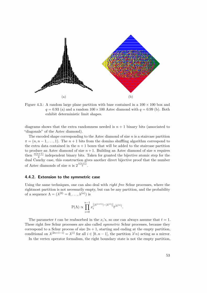
(a) (b)

Figure 4.3.: A random large plane partition with base contained in a 100× 100 box andq = 0.93 (a) and a random 100×100 Aztec diamond with q = 0.99 (b). Bothexhibit deterministic limit shapes.

diagrams shows that the extra randomness needed is n + 1 binary bits (associated to“diagonals” of the Aztec diamond).

The encoded shape corresponding to the Aztec diamond of size n is a staircase partitionπ = (n, n− 1, . . . , 1). The n+ 1 bits from the domino shuffling algorithm correspond tothe extra data contained in the n+ 1 boxes that will be added to the staircase partitionto produce an Aztec diamond of size n+ 1. Building an Aztec diamond of size n requiresthen n(n+1)

2 independent binary bits. Taken for granted the bijective atomic step for thedual Cauchy case, this construction gives another direct bijective proof that the number

of Aztec diamonds of size n is 2n(n+1)

2 .

4.4.2. Extension to the symmetric case

Using the same techniques, one can also deal with right free Schur processes, where therightmost partition is not necessarily empty, but can be any partition, and the probabilityof a sequence Λ = (λ(0) = ∅, . . . , λ(n)) is

P(Λ) ∝n−1∏

i=0

x||λ(i+1)|−|λ(i)||i t|λ

(n)|.

The parameter t can be reabsorbed in the xi’s, so one can always assume that t = 1.These right free Schur processes are also called symmetric Schur processes, because theycorrespond to a Schur process of size 2n+ 1, starting and ending at the empty partition,conditional on λ(2n+1−i) = λ(i) for all i ∈ [0..n− 1], the partition λ(n) acting as a mirror.

In the vertex operator formalism, the right boundary state is not the empty partition,

53

but a sum over all partitions, possibly weighted by their size:

|t〉 =∑

ν

t|ν||ν〉.

The additional ingredient is the Littlewood identity [Mac15, p. 93]

∑

ν

sν/µ(x) =∏

i

1

1− xi∏

i<j

1

1− xixj∑

κ

sµ/κ(x),

or equivalently, the reflection identity for vertex operators:

Γ+(x)|t〉 =1

1− xtΓ−(xt2)|t〉.

which corresponds to a new atomic step for the generation of the rightmost partition.See [13, Section 4] for more details.

There is also modified versions of the Littlewood identity where the sums over ν andκ are restricted to partitions with only even (resp. odd) parts. This corresponds torestricting the sum in the definition of the right boundary state |t〉 to partitions withonly even (resp. odd) parts.

4.4.3. Schur processes with infinitely many parameters

The definition of a Schur process we used involves only a finite number of partitions. Butin some situations (e.g. for plane partitions or pyramid partitions), one wants to considerunbounded Schur processes where the sequence of partition is (bi)infinite.

The condition on the weights xi for the weight of a configuration to be normalizableinto a probability is exactly the condition that among the infinite number of geometricand Bernoulli random variables one would need to use to generate the process using theprevious atomic steps, only a finite number of them are non zero. One can even writedown explicitly the distribution4 of the index of the first non-zero such variable.

After having simulated the index of the last non-zero random input, and value of thatrandom input according to a biased distribution, one is then back to a finite situation,where the non-zero partitions are generated from a (random) finite number of externalrandom variables. See [13, Section 5] for the details of the implementation.

4As it is given as an infinite product, it is delicate to use it in practice for simulations, because ofnumerical instabilities.

54

Part II.

Statistical mechanics on isoradialgraphs

Abstract

We define isoradial graphs in Chapter 5, as well as some of their properties, in connectionwith integrability of electric networks and the Ising model. We then summarize resultsobtained on integrable models of statistical mechanics on planar isoradial graphs. Theseinclude the critical Ising model [8, 9] (Chapter 6), the XOR Ising model [14] (Chapter 8),and spanning rooted forests [16] (Chapter 7). They are all intimately related to dimermodels, either via bijections or combinatorial correspondences, or more indirectly throughtheir spectral curve.

5. Isoradial graphs

After some generalities and definitions, on graphs drawn on surfaces in Section 5.1, weintroduce a special class of embedded planar graphs, the so-called isoradial graphs [Duf68,Mer01, Ken02]. We discuss their properties in Section 5.2, and motivate why they forma natural support for statistical mechanics in dimension 2, in connection with the Yang-Baxter equation for integrable models (Section 5.3). Two examples are thus discussedwhich will serve as reference and motivation for the following chapters: the Laplacianon isoradial graphs (Section 5.4) and the Ising model (Section 5.5). This chapter endswith some considerations about spectral curves of operators on periodic graphs and theformulation of the Ising model as a measure on contours.

5.1. Planar graphs, surface graphs and associated notions

We first give some terminology associated to graphs drawn on surfaces and particularlyplanar graphs. Let G be a connected graph drawn on a boundaryless connected orientedsurface Σ, in such a way that no two edges cross each other in their interior, andthat cutting Σ along the edges of G, one gets only pieces that are homeomorphic todisks. These pieces are the faces of G. In other words, G is the 1-skeleton of a cellulardecomposition of Σ. Then one can define the dual graph G∗, where vertices of G∗ arethe faces of G and two dual vertices are connected by a dual edge if the correspondingfaces share an edge in G.

From G and G∗, one can construct the diamond graph, G�. The vertices of G� arevertices and faces of G. A vertex v and face f of G are connected by an edge in G� if andonly if v is on the boundary of f . The graphs G and G∗ have the same diamond graph,and the faces of G� are quadrilaterals. The dual (G�)

∗ of G� is a regular degree-4 graph,called the medial graph, and denoted GM . An edge path on GM which goes straight atevery intersection is called a train-track.

These definitions extend to the case when the surface Σ has a boundary, by takingspecial care of what happens at the boundary. Several choices are possible. However, wewill mainly be interested in the boundaryless case.

5.2. Isoradial graphs

We consider a family of planar graphs, with an embedding on the plane, i.e., a specialplacement of the vertices and the edges in the plane.

Definition 15. A planar embedded graph G is said to be isoradial if all the boundedfaces are inscribed in a circle of radius 1.

56

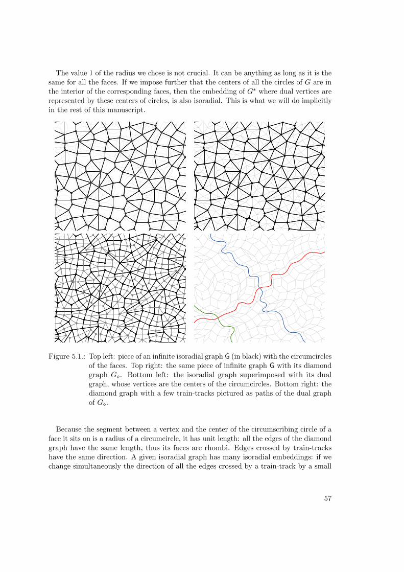
The value 1 of the radius we chose is not crucial. It can be anything as long as it is thesame for all the faces. If we impose further that the centers of all the circles of G are inthe interior of the corresponding faces, then the embedding of G∗ where dual vertices arerepresented by these centers of circles, is also isoradial. This is what we will do implicitlyin the rest of this manuscript.

Figure 5.1.: Top left: piece of an infinite isoradial graph G (in black) with the circumcirclesof the faces. Top right: the same piece of infinite graph G with its diamondgraph G�. Bottom left: the isoradial graph superimposed with its dualgraph, whose vertices are the centers of the circumcircles. Bottom right: thediamond graph with a few train-tracks pictured as paths of the dual graphof G�.

Because the segment between a vertex and the center of the circumscribing circle of aface it sits on is a radius of a circumcircle, it has unit length: all the edges of the diamondgraph have the same length, thus its faces are rhombi. Edges crossed by train-trackshave the same direction. A given isoradial graph has many isoradial embeddings: if wechange simultaneously the direction of all the edges crossed by a train-track by a small

57

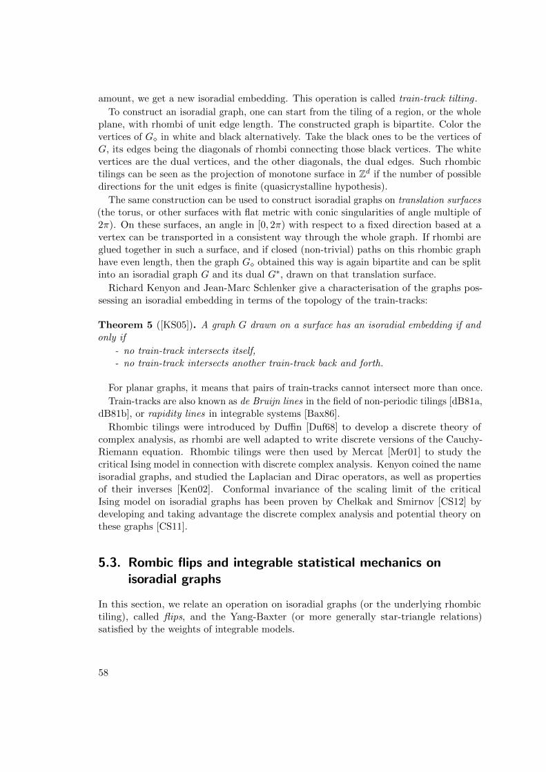
amount, we get a new isoradial embedding. This operation is called train-track tilting .

To construct an isoradial graph, one can start from the tiling of a region, or the wholeplane, with rhombi of unit edge length. The constructed graph is bipartite. Color thevertices of G� in white and black alternatively. Take the black ones to be the vertices ofG, its edges being the diagonals of rhombi connecting those black vertices. The whitevertices are the dual vertices, and the other diagonals, the dual edges. Such rhombictilings can be seen as the projection of monotone surface in Zd if the number of possibledirections for the unit edges is finite (quasicrystalline hypothesis).

The same construction can be used to construct isoradial graphs on translation surfaces(the torus, or other surfaces with flat metric with conic singularities of angle multiple of2π). On these surfaces, an angle in [0, 2π) with respect to a fixed direction based at avertex can be transported in a consistent way through the whole graph. If rhombi areglued together in such a surface, and if closed (non-trivial) paths on this rhombic graphhave even length, then the graph G� obtained this way is again bipartite and can be splitinto an isoradial graph G and its dual G∗, drawn on that translation surface.

Richard Kenyon and Jean-Marc Schlenker give a characterisation of the graphs pos-sessing an isoradial embedding in terms of the topology of the train-tracks:

Theorem 5 ([KS05]). A graph G drawn on a surface has an isoradial embedding if andonly if

- no train-track intersects itself,- no train-track intersects another train-track back and forth.

For planar graphs, it means that pairs of train-tracks cannot intersect more than once.

Train-tracks are also known as de Bruijn lines in the field of non-periodic tilings [dB81a,dB81b], or rapidity lines in integrable systems [Bax86].

Rhombic tilings were introduced by Duffin [Duf68] to develop a discrete theory ofcomplex analysis, as rhombi are well adapted to write discrete versions of the Cauchy-Riemann equation. Rhombic tilings were then used by Mercat [Mer01] to study thecritical Ising model in connection with discrete complex analysis. Kenyon coined the nameisoradial graphs, and studied the Laplacian and Dirac operators, as well as propertiesof their inverses [Ken02]. Conformal invariance of the scaling limit of the criticalIsing model on isoradial graphs has been proven by Chelkak and Smirnov [CS12] bydeveloping and taking advantage the discrete complex analysis and potential theory onthese graphs [CS11].

5.3. Rombic flips and integrable statistical mechanics onisoradial graphs

In this section, we relate an operation on isoradial graphs (or the underlying rhombictiling), called flips, and the Yang-Baxter (or more generally star-triangle relations)satisfied by the weights of integrable models.

58

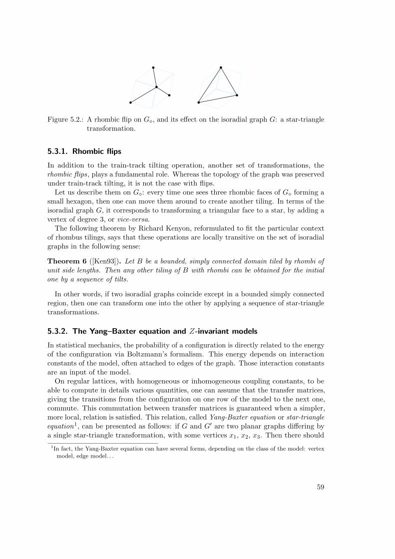
Figure 5.2.: A rhombic flip on G�, and its effect on the isoradial graph G: a star-triangletransformation.

5.3.1. Rhombic flips

In addition to the train-track tilting operation, another set of transformations, therhombic flips , plays a fundamental role. Whereas the topology of the graph was preservedunder train-track tilting, it is not the case with flips.

Let us describe them on G�: every time one sees three rhombic faces of G� forming asmall hexagon, then one can move them around to create another tiling. In terms of theisoradial graph G, it corresponds to transforming a triangular face to a star, by adding avertex of degree 3, or vice-versa.

The following theorem by Richard Kenyon, reformulated to fit the particular contextof rhombus tilings, says that these operations are locally transitive on the set of isoradialgraphs in the following sense:

Theorem 6 ([Ken93]). Let B be a bounded, simply connected domain tiled by rhombi ofunit side lengths. Then any other tiling of B with rhombi can be obtained for the initialone by a sequence of tilts.

In other words, if two isoradial graphs coincide except in a bounded simply connectedregion, then one can transform one into the other by applying a sequence of star-triangletransformations.

5.3.2. The Yang–Baxter equation and Z-invariant models

In statistical mechanics, the probability of a configuration is directly related to the energyof the configuration via Boltzmann’s formalism. This energy depends on interactionconstants of the model, often attached to edges of the graph. Those interaction constantsare an input of the model.

On regular lattices, with homogeneous or inhomogeneous coupling constants, to beable to compute in details various quantities, one can assume that the transfer matrices,giving the transitions from the configuration on one row of the model to the next one,commute. This commutation between transfer matrices is guaranteed when a simpler,more local, relation is satisfied. This relation, called Yang-Baxter equation or star-triangleequation1, can be presented as follows: if G and G′ are two planar graphs differing bya single star-triangle transformation, with some vertices x1, x2, x3. Then there should

1In fact, the Yang-Baxter equation can have several forms, depending on the class of the model: vertexmodel, edge model. . .

59

exist a positive constant C such that for every configuration outside the locus of thestar-triangle transformation connecting G and G′, the sum of all statistical weights forconfigurations inside this locus compatible with the outside configuration on G and G′

are proportional with the constant C.

When solving these relations, we find that the weights associated to edges connectedto x1, x2 and x3 satisfy some algebraic relation. Sometimes, the weights satisfying thisrelation can be parameterized by a parameter u describing a curve, in such a way thatthe algebraic relation satisfied by the curve corresponds to a simple relation on theparameters u (like an addition formula).

Taking advantage of the fact that every edge e on an isoradial graph has also a naturalparameter, the half-angle θe of the rhombus containing it, we can identify the unit circlewith a component of the real locus of this curve, and assign to edges the weights givenby the particular parameter corresponding to its half-angle. This way, we have a naturalway to define integrable statistical models on isoradial graphs. When a model has suchweights, it is said to be Z-invariant [Bax86].

We will see examples of this in the next two sections, for conductances of electricnetworks, and coupling constants for the Ising model.

5.4. Laplacian on isoradial graphs

5.4.1. Conductances and their star-triangle relation

In [Ken02], Kenyon introduces conductances on edges of an isoradial graph as functionof their half-angle: if an edge e is a diagonal of a rhombus with half-angle θ, then itsconductance ρ(e) = ρ(θ) is equal to tan(θ). A Laplacian ∆ is then defined on functionson vertices of the isoradial graph by:

∀ f ∈ CG, ∀ v ∈ G, ∆f(v) =∑

w∼vρ(e)

(f(v)− f(w)

).

These conductances have the property that the associated random walk is a martingalewith steps which have a scalar covariance matrix [CS11, Bef08].

It has also the property that when doing a rhombic flip in the underlying diamondgraph, the new conductances give an equivalent electric network. Indeed, the star-trianglerelation which should be satisfied by conductances for equivalent electric networks [Ken99]yields the following equation for the three conductances a, b, c adjacent to a trivalentvertex:

a+ b+ c = abc

which is parameterized by the tan function through the triple tangent identity:

tan(θ) + tan(φ) + tan(ψ) = tan(θ) tan(φ) tan(ψ) (5.1)

under the condition that θ+φ+ψ = π, which is exactly the relation satisfied by half-anglesaround a trivalent vertex.

60

5.4.2. Discrete exponential functions and harmonicity

A 1-parameter family of functions on pairs of vertices of G�, found in the work of ChristianMercat [Mer04], indexed by λ ∈ C = C ∪ {∞} are defined as follows: to any orientededge ε of G� identified with the unit vector eiα(ε) = eiα, we attach a rational factor:

Expε(λ) =λ− eiαλ+ eiα

.

Note that, if ε represents the same edge but with the reverse orientation, then

Expε(λ) =λ− ei(α+π)

λ+ ei(α+π)= Expε(λ)−1. (5.2)

Given two vertices v and w in G�, and a path of edges ε1 = eiα1 , . . . , εn = eiαn from vto w, the discrete exponential function from v to w is defined as

Expv,w(λ) =n∏

j=1

Expεj (λ) =n∏

j=1

(λ− eiαjλ+ eiαj

)(5.3)

These functions are called discrete exponential functions. Because of (5.2), Expv,w(λ)does not depend on the edge path connecting v and w, Expv,v(λ) = 1 and Expw,v(λ) =

Expv,w(λ)−1. When λ is of the form eiu, then Expε(λ) = i tan(u−α2 ). One can thereforewrite for two neighboring vertices v and w on the diagonal of a rhombus such thatw − v = eiα + eiβ, and λ = eiu:

tan

(β − α

2

)(Expv,w(λ)− Expv,v(λ)

)=

− tan

(β − α

2

)[tan

(u− α

2

)tan

(u− β

2

)+ 1

]= tan

(u− β

2

)− tan

(u− α

2

)

which is a telescopic quantity when summing over all the neighboring vertices w ofv. This proves that restriction of these discrete exponential functions to vertices ofG are harmonic2. Because of their product structure, they form what is called a zerocurvature representation3 of the solution of the discrete Laplace equation ∆f = 0, andtheir existence is related the integrability of the discrete Laplace equation. See [BS08,Chapter 6]. Harmonicity of exponential functions and integrability of the Laplaceequation is thus a consequence of (5.1) when the angles can take complex values (bytaking θ = β−α

2 , φ = u−β2 and −ψ = u−α

2 ).Richard Kenyon used these exponential functions to build an exact expression for the

Green function on any isoradial graph, as an integral of the discrete exponential functionagainst a singular measure in the λ-space:

2More, the restriction to G∗ is also harmonic for the Laplacian on the isoradial graph G∗, and is thenatural dual harmonic of the restriction on G.

3In this language, the (exponential of the) curvature of a domain is the product along the boundary ofthe domain of the connection defined on edges by the local factors.

61

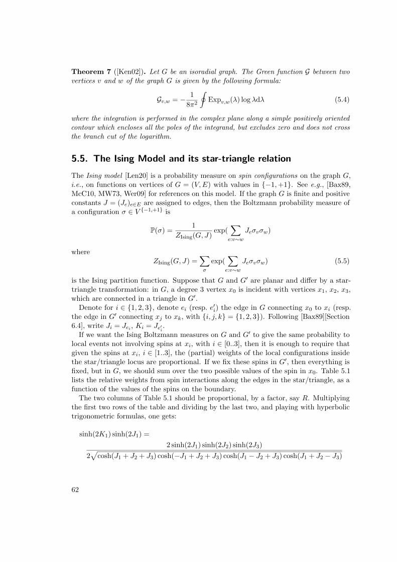
Theorem 7 ([Ken02]). Let G be an isoradial graph. The Green function G between twovertices v and w of the graph G is given by the following formula:

Gv,w = − 1

8π2

∮Expv,w(λ) log λdλ (5.4)

where the integration is performed in the complex plane along a simple positively orientedcontour which encloses all the poles of the integrand, but excludes zero and does not crossthe branch cut of the logarithm.

5.5. The Ising Model and its star-triangle relation

The Ising model [Len20] is a probability measure on spin configurations on the graph G,i.e., on functions on vertices of G = (V,E) with values in {−1,+1}. See e.g., [Bax89,McC10, MW73, Wer09] for references on this model. If the graph G is finite and positiveconstants J = (Je)e∈E are assigned to edges, then the Boltzmann probability measure ofa configuration σ ∈ V {−1,+1} is

P(σ) =1

ZIsing(G, J)exp(

∑

e:v∼wJeσvσw)

whereZIsing(G, J) =

∑

σ

exp(∑

e:v∼wJeσvσw) (5.5)

is the Ising partition function. Suppose that G and G′ are planar and differ by a star-triangle transformation: in G, a degree 3 vertex x0 is incident with vertices x1, x2, x3,which are connected in a triangle in G′.

Denote for i ∈ {1, 2, 3}, denote ei (resp. e′i) the edge in G connecting x0 to xi (resp.the edge in G′ connecting xj to xk, with {i, j, k} = {1, 2, 3}). Following [Bax89][Section6.4], write Ji = Jei , Ki = Je′i .

If we want the Ising Boltzmann measures on G and G′ to give the same probability tolocal events not involving spins at xi, with i ∈ [0..3], then it is enough to require thatgiven the spins at xi, i ∈ [1..3], the (partial) weights of the local configurations insidethe star/triangle locus are proportional. If we fix these spins in G′, then everything isfixed, but in G, we should sum over the two possible values of the spin in x0. Table 5.1lists the relative weights from spin interactions along the edges in the star/triangle, as afunction of the values of the spins on the boundary.

The two columns of Table 5.1 should be proportional, by a factor, say R. Multiplyingthe first two rows of the table and dividing by the last two, and playing with hyperbolictrigonometric formulas, one gets:

sinh(2K1) sinh(2J1) =

2 sinh(2J1) sinh(2J2) sinh(2J3)

2√

cosh(J1 + J2 + J3) cosh(−J1 + J2 + J3) cosh(J1 − J2 + J3) cosh(J1 + J2 − J3)

62

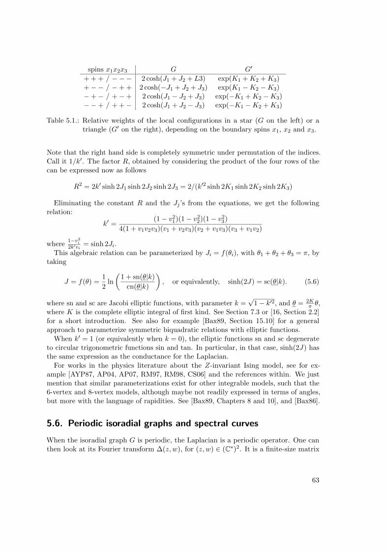
spins x1x2x3 G G′

+ + + / −−− 2 cosh(J1 + J2 + L3) exp(K1 +K2 +K3)+−− / −+ + 2 cosh(−J1 + J2 + J3) exp(K1 −K2 −K3)−+− / +−+ 2 cosh(J1 − J2 + J3) exp(−K1 +K2 −K3)−−+ / + +− 2 cosh(J1 + J2 − J3) exp(−K1 −K2 +K3)

Table 5.1.: Relative weights of the local configurations in a star (G on the left) or atriangle (G′ on the right), depending on the boundary spins x1, x2 and x3.

Note that the right hand side is completely symmetric under permutation of the indices.Call it 1/k′. The factor R, obtained by considering the product of the four rows of thecan be expressed now as follows

R2 = 2k′ sinh 2J1 sinh 2J2 sinh 2J3 = 2/(k′2 sinh 2K1 sinh 2K2 sinh 2K3)

Eliminating the constant R and the Jj ’s from the equations, we get the followingrelation:

k′ =(1− v2

1)(1− v22)(1− v2

3)

4(1 + v1v2v3)(v1 + v2v3)(v2 + v1v3)(v3 + v1v2)

where1−v2i2k′vi

= sinh 2Ji.

This algebraic relation can be parameterized by Ji = f(θi), with θ1 + θ2 + θ3 = π, bytaking

J = f(θ) =1

2ln

(1 + sn(θ|k)

cn(θ|k)

), or equivalently, sinh(2J) = sc(θ|k). (5.6)

where sn and sc are Jacobi elliptic functions, with parameter k =√

1− k′2, and θ = 2Kπ θ,

where K is the complete elliptic integral of first kind. See Section 7.3 or [16, Section 2.2]for a short introduction. See also for example [Bax89, Section 15.10] for a generalapproach to parameterize symmetric biquadratic relations with elliptic functions.

When k′ = 1 (or equivalently when k = 0), the elliptic functions sn and sc degenerateto circular trigonometric functions sin and tan. In particular, in that case, sinh(2J) hasthe same expression as the conductance for the Laplacian.

For works in the physics literature about the Z-invariant Ising model, see for ex-ample [AYP87, AP04, AP07, RM97, RM98, CS06] and the references within. We justmention that similar parameterizations exist for other integrable models, such that the6-vertex and 8-vertex models, although maybe not readily expressed in terms of angles,but more with the language of rapidities. See [Bax89, Chapters 8 and 10], and [Bax86].

5.6. Periodic isoradial graphs and spectral curves

When the isoradial graph G is periodic, the Laplacian is a periodic operator. One canthen look at its Fourier transform ∆(z, w), for (z, w) ∈ (C∗)2. It is a finite-size matrix

63

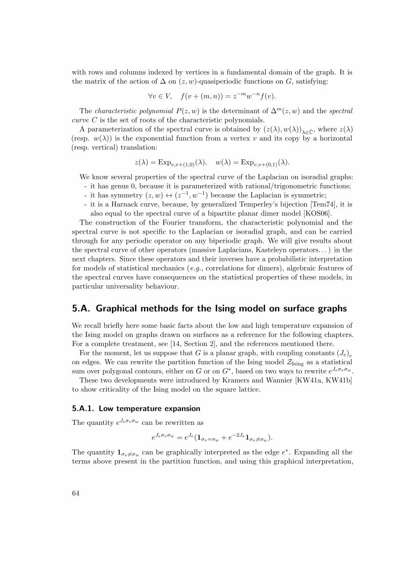
with rows and columns indexed by vertices in a fundamental domain of the graph. It isthe matrix of the action of ∆ on (z, w)-quasiperiodic functions on G, satisfying:

∀v ∈ V, f(v + (m,n)) = z−mw−nf(v).

The characteristic polynomial P (z, w) is the determinant of ∆m(z, w) and the spectralcurve C is the set of roots of the characteristic polynomials.

A parameterization of the spectral curve is obtained by (z(λ), w(λ))λ∈C, where z(λ)(resp. w(λ)) is the exponential function from a vertex v and its copy by a horizontal(resp. vertical) translation:

z(λ) = Expv,v+(1,0)(λ), w(λ) = Expv,v+(0,1)(λ).

We know several properties of the spectral curve of the Laplacian on isoradial graphs:- it has genus 0, because it is parameterized with rational/trigonometric functions;- it has symmetry (z, w)↔ (z−1, w−1) because the Laplacian is symmetric;- it is a Harnack curve, because, by generalized Temperley’s bijection [Tem74], it is

also equal to the spectral curve of a bipartite planar dimer model [KOS06].The construction of the Fourier transform, the characteristic polynomial and the

spectral curve is not specific to the Laplacian or isoradial graph, and can be carriedthrough for any periodic operator on any biperiodic graph. We will give results aboutthe spectral curve of other operators (massive Laplacians, Kasteleyn operators. . . ) in thenext chapters. Since these operators and their inverses have a probabilistic interpretationfor models of statistical mechanics (e.g., correlations for dimers), algebraic features ofthe spectral curves have consequences on the statistical properties of these models, inparticular universality behaviour.

5.A. Graphical methods for the Ising model on surface graphs

We recall briefly here some basic facts about the low and high temperature expansion ofthe Ising model on graphs drawn on surfaces as a reference for the following chapters.For a complete treatment, see [14, Section 2], and the references mentioned there.

For the moment, let us suppose that G is a planar graph, with coupling constants (Je)eon edges. We can rewrite the partition function of the Ising model ZIsing as a statisticalsum over polygonal contours, either on G or on G∗, based on two ways to rewrite eJeσvσw .

These two developments were introduced by Kramers and Wannier [KW41a, KW41b]to show criticality of the Ising model on the square lattice.

5.A.1. Low temperature expansion

The quantity eJeσvσw can be rewritten as

eJeσvσw = eJe(1σv=σw + e−2Je1σv 6=σw).

The quantity 1σv 6=σw can be graphically interpreted as the edge e∗. Expanding all theterms above present in the partition function, and using this graphical interpretation,

64

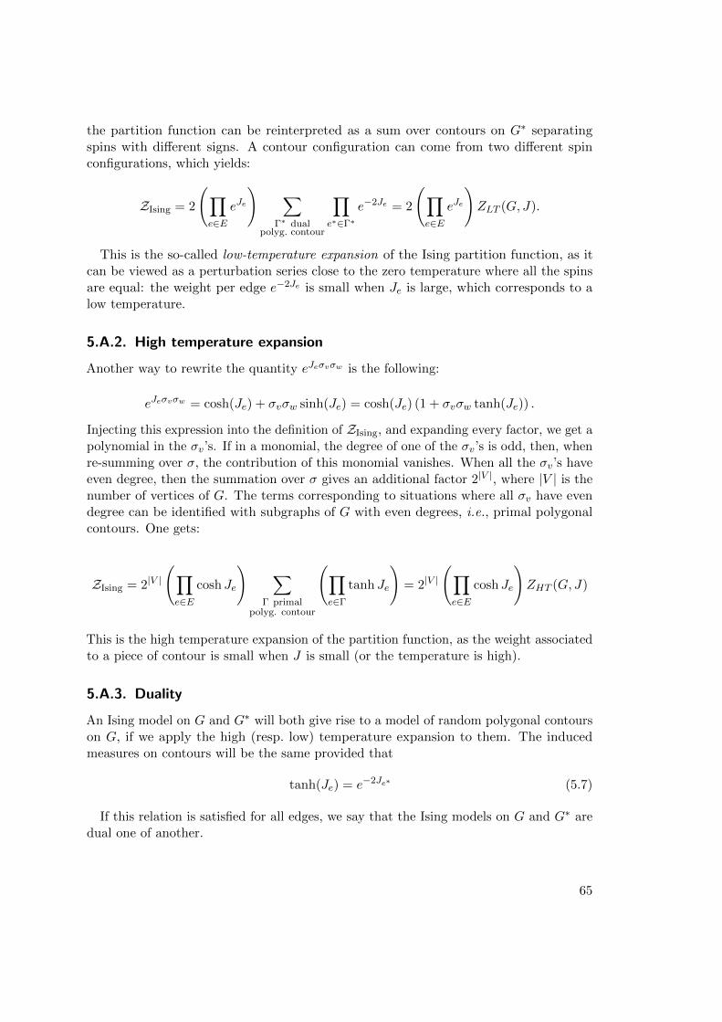
the partition function can be reinterpreted as a sum over contours on G∗ separatingspins with different signs. A contour configuration can come from two different spinconfigurations, which yields:

ZIsing = 2

(∏

e∈EeJe

) ∑

Γ∗ dualpolyg. contour

∏

e∗∈Γ∗

e−2Je = 2

(∏

e∈EeJe

)ZLT (G, J).

This is the so-called low-temperature expansion of the Ising partition function, as itcan be viewed as a perturbation series close to the zero temperature where all the spinsare equal: the weight per edge e−2Je is small when Je is large, which corresponds to alow temperature.

5.A.2. High temperature expansion

Another way to rewrite the quantity eJeσvσw is the following:

eJeσvσw = cosh(Je) + σvσw sinh(Je) = cosh(Je) (1 + σvσw tanh(Je)) .

Injecting this expression into the definition of ZIsing, and expanding every factor, we get apolynomial in the σv’s. If in a monomial, the degree of one of the σv’s is odd, then, whenre-summing over σ, the contribution of this monomial vanishes. When all the σv’s haveeven degree, then the summation over σ gives an additional factor 2|V |, where |V | is thenumber of vertices of G. The terms corresponding to situations where all σv have evendegree can be identified with subgraphs of G with even degrees, i.e., primal polygonalcontours. One gets:

ZIsing = 2|V |

(∏

e∈Ecosh Je

) ∑

Γ primalpolyg. contour

(∏

e∈Γ

tanh Je

)= 2|V |

(∏

e∈Ecosh Je

)ZHT (G, J)

This is the high temperature expansion of the partition function, as the weight associatedto a piece of contour is small when J is small (or the temperature is high).

5.A.3. Duality

An Ising model on G and G∗ will both give rise to a model of random polygonal contourson G, if we apply the high (resp. low) temperature expansion to them. The inducedmeasures on contours will be the same provided that

tanh(Je) = e−2Je∗ (5.7)

If this relation is satisfied for all edges, we say that the Ising models on G and G∗ aredual one of another.

65

The square lattice is isomorphic to its dual. If all the coupling constants are chosen tobe the same and equal to β (which is in physics is interpreted as the inverse temperature)on G, and to β∗ on G∗, then relation (5.7) becomes

tanh(β) = e−2β∗

which is equivalent to sinh(2β) sinh(2β∗) = 1. Taking β = β∗, this equation has a uniquesolution

βc = log

(√2 +√

2

).

which turns out to be the critical temperature for the square lattice.On an isoradial graph, the half-angles θ and θ∗ associated to an edge e and its dual e∗

sum to π2 . The duality described above translates to the following identity on the weights

for the Z-invariant Ising model (5.6)

J(θ|k) =1

2ln

(1 + sn(θ|k)

cn(θ|k)

)=

1

2ln

(1 + sn(θ∗|k∗)

cn(θ∗|k∗)

)= J(θ∗|k∗)

with (1− (k∗)2)(1− k2) = 1. If we impose that the model is self-dual to have J(θ|k) =J(θ|k∗) for all θ, we find that k = 0 and obtain the following expression

J(θ|k) =1

2ln

(1 + sin(θ)

cos(θ)

)(5.8)

for the Z-invariant self-dual Ising model which is indeed critical [Li10, Li12, CDC13].

5.A.4. Higher genus and boundary

If G is not planar, but instead drawn on a surface Σ with a boundary, then the dualitydescribed above is not valid anymore: for example, when going around a handle, wecome back to our starting point, and thus observe the same spin. As a consequence, thenumber of low temperature contours we cross is even. On the contrary, there is no parityconstraint for the high temperature expansion.

A possible way is to introduce variants of the Ising model with defect lines, whichcorrespond to possible relative homology classes in H1(Σ, ∂Σ;Z/2Z). The duality relationthen extends. See [14, Equation (5)].

66

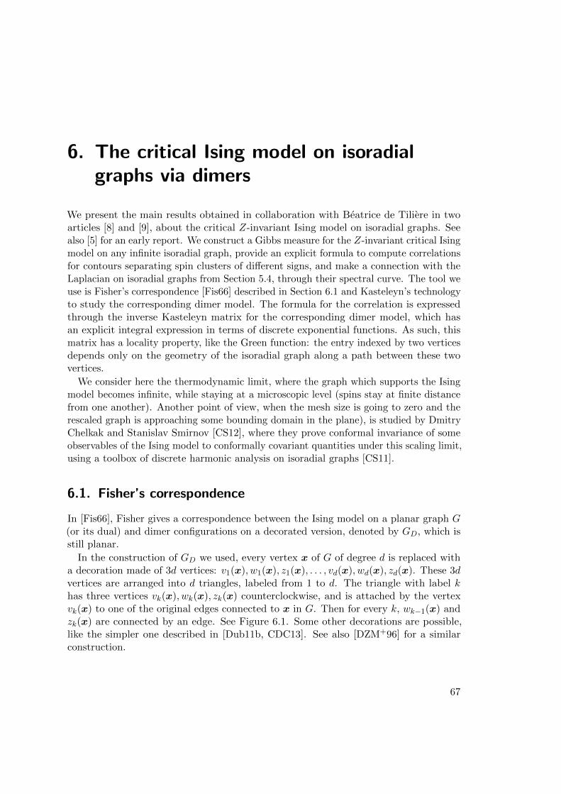
6. The critical Ising model on isoradialgraphs via dimers

We present the main results obtained in collaboration with Beatrice de Tiliere in twoarticles [8] and [9], about the critical Z-invariant Ising model on isoradial graphs. Seealso [5] for an early report. We construct a Gibbs measure for the Z-invariant critical Isingmodel on any infinite isoradial graph, provide an explicit formula to compute correlationsfor contours separating spin clusters of different signs, and make a connection with theLaplacian on isoradial graphs from Section 5.4, through their spectral curve. The tool weuse is Fisher’s correspondence [Fis66] described in Section 6.1 and Kasteleyn’s technologyto study the corresponding dimer model. The formula for the correlation is expressedthrough the inverse Kasteleyn matrix for the corresponding dimer model, which hasan explicit integral expression in terms of discrete exponential functions. As such, thismatrix has a locality property, like the Green function: the entry indexed by two verticesdepends only on the geometry of the isoradial graph along a path between these twovertices.

We consider here the thermodynamic limit, where the graph which supports the Isingmodel becomes infinite, while staying at a microscopic level (spins stay at finite distancefrom one another). Another point of view, when the mesh size is going to zero and therescaled graph is approaching some bounding domain in the plane), is studied by DmitryChelkak and Stanislav Smirnov [CS12], where they prove conformal invariance of someobservables of the Ising model to conformally covariant quantities under this scaling limit,using a toolbox of discrete harmonic analysis on isoradial graphs [CS11].

6.1. Fisher’s correspondence

In [Fis66], Fisher gives a correspondence between the Ising model on a planar graph G(or its dual) and dimer configurations on a decorated version, denoted by GD, which isstill planar.

In the construction of GD we used, every vertex x of G of degree d is replaced witha decoration made of 3d vertices: v1(x), w1(x), z1(x), . . . , vd(x), wd(x), zd(x). These 3dvertices are arranged into d triangles, labeled from 1 to d. The triangle with label khas three vertices vk(x), wk(x), zk(x) counterclockwise, and is attached by the vertexvk(x) to one of the original edges connected to x in G. Then for every k, wk−1(x) andzk(x) are connected by an edge. See Figure 6.1. Some other decorations are possible,like the simpler one described in [Dub11b, CDC13]. See also [DZM+96] for a similarconstruction.

67

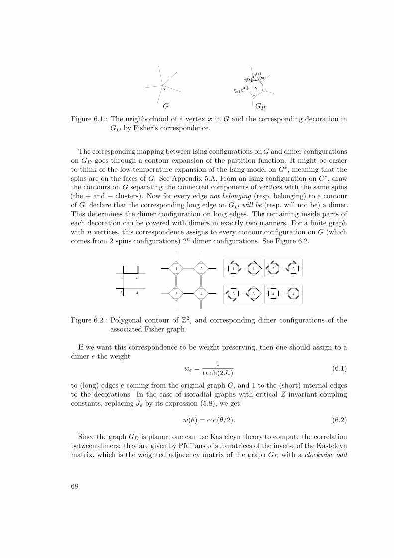
zk( )( )x

kw

vk( )

x

x

x vk+1 x( )

x

G GD

Figure 6.1.: The neighborhood of a vertex x in G and the corresponding decoration inGD by Fisher’s correspondence.

The corresponding mapping between Ising configurations on G and dimer configurationson GD goes through a contour expansion of the partition function. It might be easierto think of the low-temperature expansion of the Ising model on G∗, meaning that thespins are on the faces of G. See Appendix 5.A. From an Ising configuration on G∗, drawthe contours on G separating the connected components of vertices with the same spins(the + and − clusters). Now for every edge not belonging (resp. belonging) to a contourof G, declare that the corresponding long edge on GD will be (resp. will not be) a dimer.This determines the dimer configuration on long edges. The remaining inside parts ofeach decoration can be covered with dimers in exactly two manners. For a finite graphwith n vertices, this correspondence assigns to every contour configuration on G (whichcomes from 2 spins configurations) 2n dimer configurations. See Figure 6.2.

21

3 4

1 2

3 4

1 1 2 2

3 3 4 4

Figure 6.2.: Polygonal contour of Z2, and corresponding dimer configurations of theassociated Fisher graph.

If we want this correspondence to be weight preserving, then one should assign to adimer e the weight:

we =1

tanh(2Je)(6.1)

to (long) edges e coming from the original graph G, and 1 to the (short) internal edgesto the decorations. In the case of isoradial graphs with critical Z-invariant couplingconstants, replacing Je by its expression (5.8), we get:

w(θ) = cot(θ/2). (6.2)

Since the graph GD is planar, one can use Kasteleyn theory to compute the correlationbetween dimers: they are given by Pfaffians of submatrices of the inverse of the Kasteleynmatrix, which is the weighted adjacency matrix of the graph GD with a clockwise odd

68

orientation. However, since the graph GD is not bipartite, the results from [KOS06]cannot be used in this context.

6.2. Spectral curve and Kasteleyn inverse matrix

We suppose in this section that the isoradial graph G is periodic. Since the Kasteleynoperator K on GD is now a periodic operator, one can define according to Section 5.6 itscharacteristic polynomial PK(z, w) and the corresponding spectral curve CK .

We proved the following result about the spectral curve:

Theorem 8 ([8], Theorem 8). The spectral curve of the dimer model corresponding tothe critical isoradial Ising model on G is the same as the spectral curve of the Laplacianon G. In other words, the characteristic polynomials are equal, up to a multiplicativeconstant.

The spectral curve CK has the properties described for the spectral curve of theLaplacian (See Section 5.6).

Proof. Our proof is indirect. We first show that the characteristic polynomial of theLaplacian is a divisor of PK(z, w): for every (z, w) on the spectral curve of the Laplacianon G, parameterized by discrete exponential functions, we construct a (z, w)-quasiperiodicfunction on GD in the kernel of the Kasteleyn matrix, also using the discrete exponentialfunctions. Therefore, the spectral curve of the Laplacian is included in CK . Then,interpreting combinatorially the monomials of both polynomials, and comparing theterms corresponding to extremal monomials, we prove that the degree of PK is not largerthan that of P∆.

Beatrice de Tiliere proved [dT16] a combinatorial correspondence between configura-tions counted by P∆(z, w) (rooted spanning forests) and the configurations counted byPK(z, w), providing an alternative, more constructive, proof of this identity.

Knowing the singularities the inverse of the Fourier transform of the Kasteleyn matrixK on the unit torus allowed us to prove existence of a unique inverse A for the operatorK, with entries Ax,y going to zero when the distance between x and y tends to infinity.It is possible to compute its entries using Fourier transform, as the extraction of a certaincoefficient of a certain rational fraction whose denominator is PK .

Knowing also in generality the possible singularities of PK on the unit torus, we provedthat the sequence of Boltzmann measures on dimer configurations of larger and largerquotients of GD converge to a Pfaffian process, with a kernel given by this inverse A ofthe Kasteleyn matrix.

6.3. The inverse Kasteleyn matrix for non periodic GD

Even when G is not periodic, it is possible to give an explicit expression for the inverseA. The formula is built on the same model as the Green function: let x and y be two

69

vertices of GD belonging to decorations decorations, coming from vertices x and y of theisoradial graph G, respectively. Construct a function gx,y(λ) as

gx,y(λ) = fx(λ) Expxy(λ)fy(−λ),

where Exp is the discrete exponential function on G introduced in Section 5.4.2, and fxdepends only on the type (v, w, z) of x:

fx(λ) =

eiαx/2

eiαx−λ if x = wk(x),

− eiαx/2

eiαx−λ if x = zk(x),

fwk(x)(λ) + fzk(x)(λ) if x = vk(x),

where αx is an angle modulo 4π associated to x, corresponding to the direction of theunit length edge in G� the closest to x. See [8, Section 4.2.2] for details.

Theorem 9 ([9], Theorem 5). The entry of the inverse Kasteleyn matrix for two verticesx and y is equal to:

Ax,y =

∮

Cx,ygx,y(λ) log λ

dλ

(2π)2 + cx,y (6.3)

where Cx,y is a simple closed curve oriented counterclockwise, which contains in its interiorthe poles of gx,y, but avoids a cone with vertex at the origin, and containing a certain raydx,y.

When x and y are not too close to each other, the ray dx,y is the geometric ray fromx to y, which are vertices of G� at distance at most 2 from x and y respectively. Theconstant cx,y is equal to ±1

4 if x and y are interior vertices of the same decoration, oftype w or z (the sign depends on the clockwise odd orientation in the decoration), and iszero otherwise.

Remark 3. The explicit expression for Ax,y given in (6.3) has the very interesting featureof being local, just like the Green function from Section 5.4, i.e., it only depends on thegeometry of the embedding of the isoradial graph G on a path between x and y.

A nice consequence of this property is the following. For i = 1, 2, let Gi be an isoradialgraph with corresponding Fisher graph (Gi)D. Let Ki be the Kasteleyn matrix of thegraph (Gi)D, whose edges are assigned the dimer critical weight function. Let Ai bethe inverse of Ki given by Theorem 9. If G1 and G2 coincide on a ball B, and if theKasteleyn orientations on (G1)D and (G2)D are chosen to be the same in that ball, thenfor every couple of vertices (x, y) in B at distance at least 2 from the boundary, we have

(A1)x,y = (A2)x,y.

6.4. Construction of a Gibbs measure for the critical Isingmodel on non periodic isoradial graphs

The locality property described above allows one to define a Gibbs measure on the setof dimer configurations of GD, by mimicking the expression given by the Boltzmannmeasure on finite planar graphs, and using the inverse A defined in Theorem 9.

70

Theorem 10 ([9], Theorem 9). There is a unique probability measure P on dimer con-figurations of GD, such that for every finite collection of edges E = {e1 = x1y1, · · · , ek =xkyk} ⊂ E(GD), the probability that these edges covered by dimers is

P(edges of E are covered) =

(k∏

i=1

Kxi,yi

)Pfaff

((A{x1,y1,··· ,xk,yk})

T), (6.4)

where A is given by Theorem 9, and A{x1,y1,··· ,xk,yk} is the submatrix of A whose rowsand columns are indexed by vertices {x1, y1, · · · , xk, yk}.

Moreover, P is a Gibbs measure. When GD is Z2-periodic, P is the Gibbs mea-sure obtained as weak limit of the Boltzmann measures Pn on the toroidal exhaustion{GD/(nZ2)}n≥1 of GD.

Proof. The proof of this theorem is done in several steps:First, we prove that if GD is periodic, then the Boltzmann measure on dimers configu-

rations on GD/nZ2 converges as n to infinity to a measure of the form (6.4), where A isthe unique inverse of the Kasteleyn matrix with entries decaying to zero, given by theFourier transform. This is done by writing explicitly the finite dimensional distributionsof the Boltzmann measure, as a linear combination of 4 Pfaffians, and taking explicitlythe limit, taking advantage of the symmetries of the graph to block diagonalize theKasteleyn matrices, and the fact that we know explicitly the singularity of the rationalfraction in the inverse Fourier transform.

When G is not periodic, it is not clear from the definition of A that (6.4) is a realquantity, between 0 and 1. But if B is a ball of the graph G containing in its interior allthe vertices corresponding to the decorations hosting these vertices, then there exists aperiodic isoradial graph G with a fundamental domain containing G [dT07a]. Since theexpression of A is local, the entries of the matrix in (6.4) depend only on the geometry ofthe isoradial graph in the ball B. Therefore, this formula is the same for G and G. Butbecause of the uniqueness result for the inverse Kasteleyn matrix in the periodic case, weknow that the local formula coincides with the inverse Fourier formula, and thus (6.4) onG is the limit of Boltzmann measure on periodic graphs.

This ensures that this expression defines on G a family of compatible finite-dimensionalprobability distributions. By Kolmogorov’s extension theorem, there is a unique proba-bility measures on the set of edge configurations for which those distributions are thefinite-dimensional marginals.

This probability measure on dimer configurations can now be lifted via Fisher’scorrespondence to a Gibbs measure on contours separating spin clusters. Then choosethe sign of a given spin at random with a fair coin, independently from the contours.The values of all the other spins are completely determined.

Corrolary 11. Let G be an isoradial graph. Then there exists a Gibbs measure for theIsing model on G∗ for which the law of contours separating clusters of same spins is aPfaffian process1with a kernel given by the inverse Kasteleyn matrix (6.3).

1In fact, this is not entirely exact: in our version of Fisher’s correspondence, what corresponds to

71

In the low temperature expansion picture, the computation of correlations betweenspins amounts to computing the parity of the number of pieces of contour one sees alonga path connecting these spins. Since statistics of pieces of low-temperature contoursare directly related to dimer statistics on GD which in turn depend only on the localgeometry of the graph, because of the local property of the inverse Kasteleyn matrix,the spin correlations are themselves local, i.e., they depend only on the geometry of thegraph trough a neighborhood of a path connecting those two spins.

6.5. From criticality to non-criticality

An open question after this work was whether a similar study could be carried overfor the Z-invariant non-critical Ising model, where now the elliptic parameter k couldbe nonzero. Although we knew explicitly the weights to put on the dimers by (5.6)and (6.1), the first step already could not be performed directly, because no analogue ofthe Laplacian and discrete exponential functions for noncriticality were known.

Since correlations should decay exponentially fast out of criticality, we have beenlooking for a massive Laplacian, for which the Green function would decay exponentiallyfast. Connections between noncritical Ising models and massive Laplacians or killedrandom walks were known [Mes06, BDC12], but these were specific to the square lattice.

This led Beatrice de Tiliere, Kilian Raschel and myself to search and define a family ofZ-invariant massive Laplacian on isoradial graphs, described in Chapter 7, which turnedout to be very rich and interesting objects by themselves, which postponed a little bitthe initial goal about the non critical Z-invariant Ising model.

the presence of a dimer on a long edge is the absence of that edge in the contours. This can besolved by either considering the complement of the contour configuration, changing the kernel to its“complement”, or by changing slightly the version of the Fisher correspondence to a simpler versionwhere dimers correspond directly to contours.

72

7. Massive Laplacian on isoradial graphs

In [16], in collaboration with Beatrice de Tiliere, and Kilian Raschel, we define a oneparameter family of integrable massive Laplace operators on isoradial graphs. Weintroduce a family of zero-curvature massive harmonic functions, the so called massiveexponential functions, depending on a parameter u living on a torus, and give an explicitrepresentation representation of the associated Green function as an integral along acontour in the u-space of massive exponential functions. We discuss implications on amodel from statistical mechanics, the rooted spanning forests, where configurations are“counted” by the determinant of this massive Laplacian. In the periodic case, we alsocharacterize the set of algebraic curves which can arise as spectral curve of these massiveLaplacians.

7.1. Definitions

Let G = (V,E) be a graph. Every edge e (resp. every vertex v) is associated a positive(resp. nonnegative) number ρe (resp. mv). ρe is called the conductance of the edge e andmv the (squared) mass at the vertex v.

The massive Laplacian ∆m on G (for these conductances and masses) is defined byits action on functions on vertices of G: for every function f on vertices of G, and anyvertex v,

(∆mf)(v) =∑

e:v∼wρe(f(v)− f(w)) +mvf(v).

See for example [LJ11, Chapter 1], for some more definitions and properties of thisoperator.

7.2. Statistical mechanics

The massive Laplacian is naturally connected to various systems from statistical mechanics.The first example is the killed random walk: the massive Laplacian can be interpretedas the generator of a Markov process in continuous time describing the evolution of aparticle which, at a vertex v, either jumps to one of the neighbouring vertices after anexponential random time, or gets absorbed at that vertex forever.

The second example is the random rooted spanning forest model. A rooted tree is acycle-free connected subgraph with a distinguished vertex, called the root of the tree.A rooted spanning forest is a spanning subgraph whose all connected components are

73

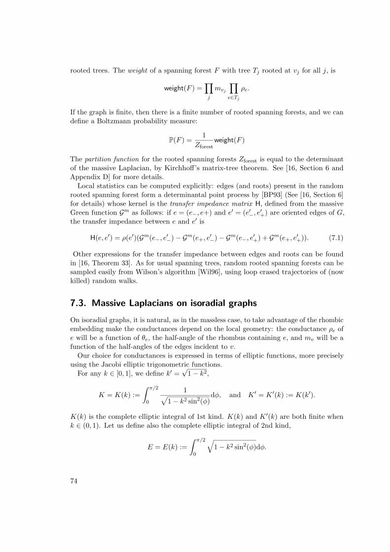
rooted trees. The weight of a spanning forest F with tree Tj rooted at vj for all j, is

weight(F ) =∏

j

mvj

∏

e∈Tj

ρe.

If the graph is finite, then there is a finite number of rooted spanning forests, and we candefine a Boltzmann probability measure:

P(F ) =1

Zforestweight(F )

The partition function for the rooted spanning forests Zforest is equal to the determinantof the massive Laplacian, by Kirchhoff’s matrix-tree theorem. See [16, Section 6 andAppendix D] for more details.

Local statistics can be computed explicitly: edges (and roots) present in the randomrooted spanning forest form a determinantal point process by [BP93] (See [16, Section 6]for details) whose kernel is the transfer impedance matrix H, defined from the massiveGreen function Gm as follows: if e = (e−, e+) and e′ = (e′−, e

′+) are oriented edges of G,

the transfer impedance between e and e′ is

H(e, e′) = ρ(e′)(Gm(e−, e′−)− Gm(e+, e

′−)− Gm(e−, e

′+) + Gm(e+, e

′+)). (7.1)

Other expressions for the transfer impedance between edges and roots can be foundin [16, Theorem 33]. As for usual spanning trees, random rooted spanning forests can besampled easily from Wilson’s algorithm [Wil96], using loop erased trajectories of (nowkilled) random walks.

7.3. Massive Laplacians on isoradial graphs

On isoradial graphs, it is natural, as in the massless case, to take advantage of the rhombicembedding make the conductances depend on the local geometry: the conductance ρe ofe will be a function of θe, the half-angle of the rhombus containing e, and mv will be afunction of the half-angles of the edges incident to v.

Our choice for conductances is expressed in terms of elliptic functions, more preciselyusing the Jacobi elliptic trigonometric functions.

For any k ∈ [0, 1], we define k′ =√

1− k2,

K = K(k) :=

∫ π/2

0

1√1− k2 sin2(φ)

dφ, and K ′ = K ′(k) := K(k′).

K(k) is the complete elliptic integral of 1st kind. K(k) and K ′(k) are both finite whenk ∈ (0, 1). Let us define also the complete elliptic integral of 2nd kind,

E = E(k) :=

∫ π/2

0

√1− k2 sin2(φ)dφ.

74

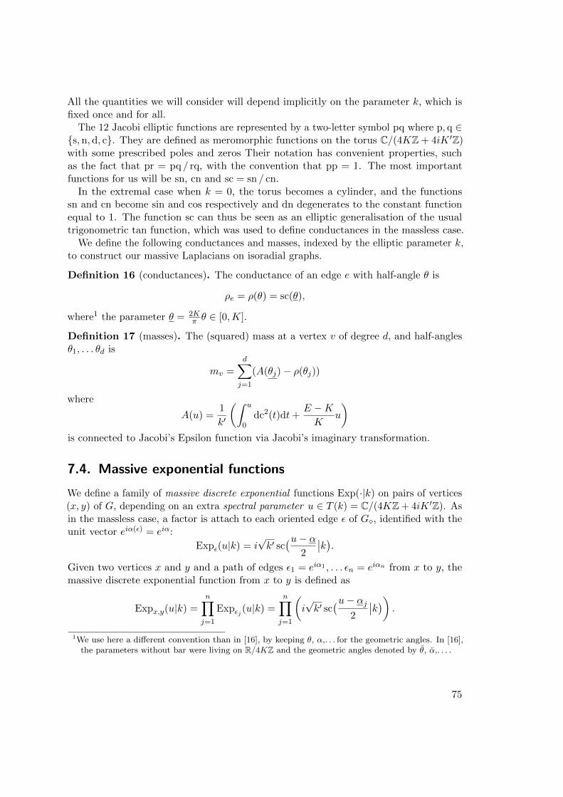
All the quantities we will consider will depend implicitly on the parameter k, which isfixed once and for all.

The 12 Jacobi elliptic functions are represented by a two-letter symbol pq where p, q ∈{s,n,d, c}. They are defined as meromorphic functions on the torus C/(4KZ + 4iK ′Z)with some prescribed poles and zeros Their notation has convenient properties, suchas the fact that pr = pq / rq, with the convention that pp = 1. The most importantfunctions for us will be sn, cn and sc = sn / cn.

In the extremal case when k = 0, the torus becomes a cylinder, and the functionssn and cn become sin and cos respectively and dn degenerates to the constant functionequal to 1. The function sc can thus be seen as an elliptic generalisation of the usualtrigonometric tan function, which was used to define conductances in the massless case.

We define the following conductances and masses, indexed by the elliptic parameter k,to construct our massive Laplacians on isoradial graphs.

Definition 16 (conductances). The conductance of an edge e with half-angle θ is

ρe = ρ(θ) = sc(θ),

where1 the parameter θ = 2Kπ θ ∈ [0,K].

Definition 17 (masses). The (squared) mass at a vertex v of degree d, and half-anglesθ1, . . . θd is

mv =

d∑

j=1

(A(θj)− ρ(θj))

where

A(u) =1

k′

(∫ u

0dc2(t)dt+

E −KK

u

)

is connected to Jacobi’s Epsilon function via Jacobi’s imaginary transformation.

7.4. Massive exponential functions

We define a family of massive discrete exponential functions Exp(·|k) on pairs of vertices(x, y) of G, depending on an extra spectral parameter u ∈ T (k) = C/(4KZ + 4iK ′Z). Asin the massless case, a factor is attach to each oriented edge ε of G�, identified with theunit vector eiα(ε) = eiα:

Expε(u|k) = i√k′ sc

(u− α2

∣∣k).

Given two vertices x and y and a path of edges ε1 = eiα1 , . . . εn = eiαn from x to y, themassive discrete exponential function from x to y is defined as

Expx,y(u|k) =n∏

j=1

Expεj (u|k) =n∏

j=1

(i√k′ sc

(u− αj2

∣∣k))

.

1We use here a different convention than in [16], by keeping θ, α,. . . for the geometric angles. In [16],the parameters without bar were living on R/4KZ and the geometric angles denoted by θ, α,. . . .

75

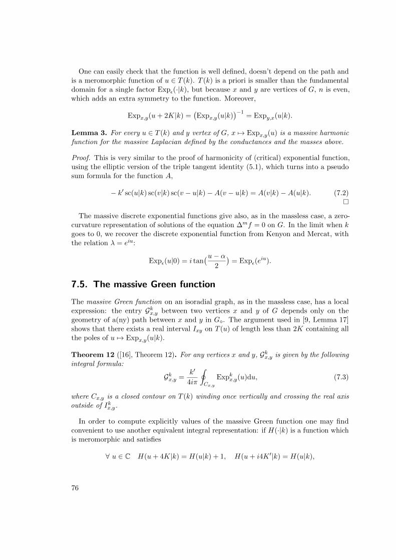
One can easily check that the function is well defined, doesn’t depend on the path andis a meromorphic function of u ∈ T (k). T (k) is a priori is smaller than the fundamentaldomain for a single factor Expε(·|k), but because x and y are vertices of G, n is even,which adds an extra symmetry to the function. Moreover,

Expx,y(u+ 2K|k) =(Expx,y(u|k)

)−1= Expy,x(u|k).

Lemma 3. For every u ∈ T (k) and y vertex of G, x 7→ Expx,y(u) is a massive harmonicfunction for the massive Laplacian defined by the conductances and the masses above.

Proof. This is very similar to the proof of harmonicity of (critical) exponential function,using the elliptic version of the triple tangent identity (5.1), which turns into a pseudosum formula for the function A,

− k′ sc(u|k) sc(v|k) sc(v − u|k)−A(v − u|k) = A(v|k)−A(u|k). (7.2)

The massive discrete exponential functions give also, as in the massless case, a zero-curvature representation of solutions of the equation ∆mf = 0 on G. In the limit when kgoes to 0, we recover the discrete exponential function from Kenyon and Mercat, withthe relation λ = eiu:

Expε(u|0) = i tan(u− α

2

)= Expε(e

iu).

7.5. The massive Green function

The massive Green function on an isoradial graph, as in the massless case, has a localexpression: the entry Gkx,y between two vertices x and y of G depends only on thegeometry of a(ny) path between x and y in G�. The argument used in [9, Lemma 17]shows that there exists a real interval Ixy on T (u) of length less than 2K containing allthe poles of u 7→ Expx,y(u|k).

Theorem 12 ([16], Theorem 12). For any vertices x and y, Gkx,y is given by the followingintegral formula:

Gkx,y =k′

4iπ

∮

Cx,y

Expkx,y(u)du, (7.3)

where Cx,y is a closed contour on T (k) winding once vertically and crossing the real axisoutside of Ikx,y.

In order to compute explicitly values of the massive Green function one may findconvenient to use another equivalent integral representation: if H(·|k) is a function whichis meromorphic and satisfies

∀ u ∈ C H(u+ 4K|k) = H(u|k) + 1, H(u+ i4K ′|k) = H(u|k),

76

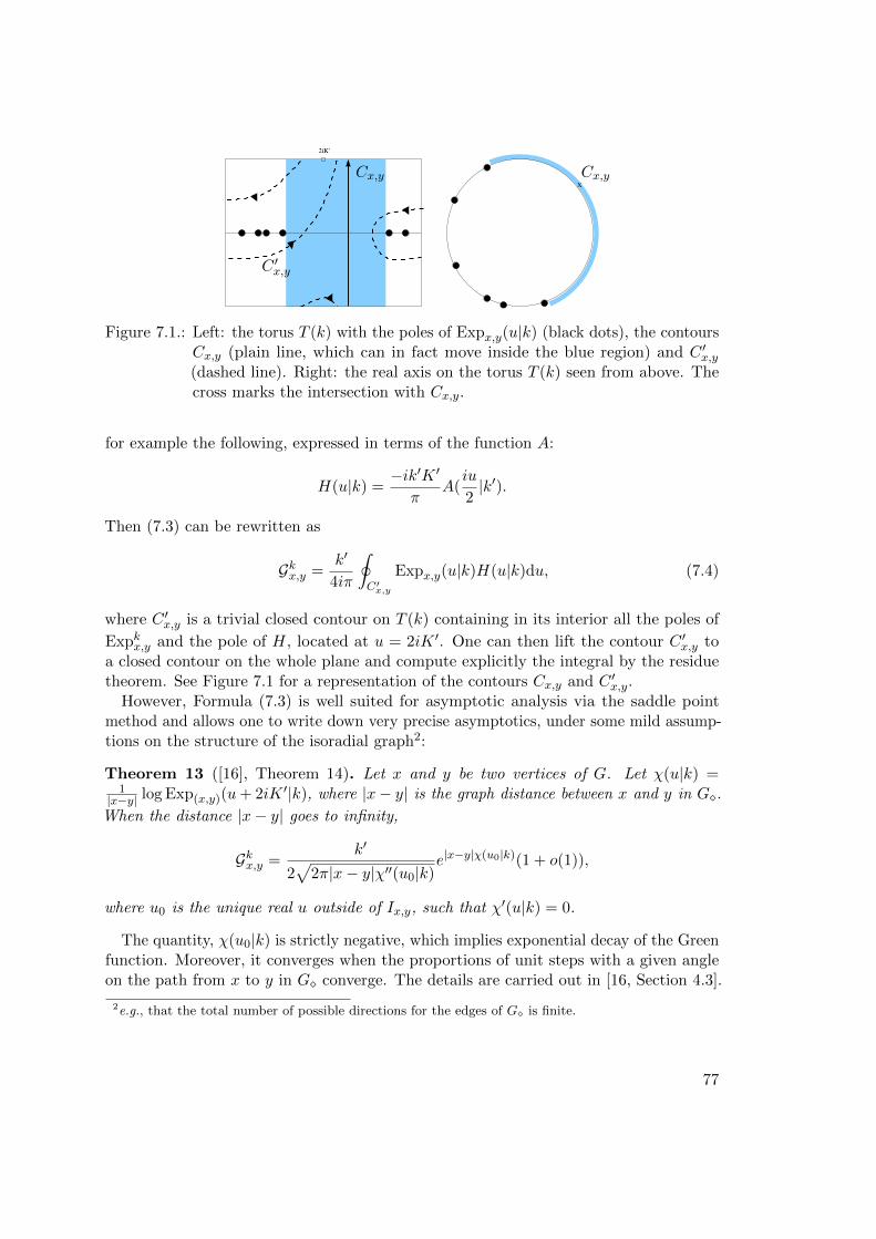
2iK’

X

Cx,y Cx,y

C ′x,y

Figure 7.1.: Left: the torus T (k) with the poles of Expx,y(u|k) (black dots), the contoursCx,y (plain line, which can in fact move inside the blue region) and C ′x,y(dashed line). Right: the real axis on the torus T (k) seen from above. Thecross marks the intersection with Cx,y.

for example the following, expressed in terms of the function A:

H(u|k) =−ik′K ′π

A(iu

2|k′).

Then (7.3) can be rewritten as

Gkx,y =k′

4iπ

∮

C′x,y

Expx,y(u|k)H(u|k)du, (7.4)

where C ′x,y is a trivial closed contour on T (k) containing in its interior all the poles of

Expkx,y and the pole of H, located at u = 2iK ′. One can then lift the contour C ′x,y toa closed contour on the whole plane and compute explicitly the integral by the residuetheorem. See Figure 7.1 for a representation of the contours Cx,y and C ′x,y.

However, Formula (7.3) is well suited for asymptotic analysis via the saddle pointmethod and allows one to write down very precise asymptotics, under some mild assump-tions on the structure of the isoradial graph2:

Theorem 13 ([16], Theorem 14). Let x and y be two vertices of G. Let χ(u|k) =1|x−y| log Exp(x,y)(u+ 2iK ′|k), where |x− y| is the graph distance between x and y in G�.

When the distance |x− y| goes to infinity,

Gkx,y =k′

2√

2π|x− y|χ′′(u0|k)e|x−y|χ(u0|k)(1 + o(1)),

where u0 is the unique real u outside of Ix,y, such that χ′(u|k) = 0.

The quantity, χ(u0|k) is strictly negative, which implies exponential decay of the Greenfunction. Moreover, it converges when the proportions of unit steps with a given angleon the path from x to y in G� converge. The details are carried out in [16, Section 4.3].

2e.g., that the total number of possible directions for the edges of G� is finite.

77

7.6. Integrability

The fact that we have a zero curvature representation for a family of massive harmonicfunctions is an evidence of integrability of the massive Laplacian, understood as a nicebehaviour of this operator under star-triangle transformations of the isoradial graphs.This is indeed the case, as we can see from the following statements Let G and G′ betwo infinite isoradial graphs differing by a star-triangle transformation, as in Figure 5.2.G has the star, and thus has an extra vertex x0.

Lemma 4 ([16], Proposition 8). There is a bijection between harmonic functions on Gand G′ as follows:

- If f is massive harmonic on G, then its restriction to vertices of G′ is massiveharmonic on G′.

- If g is massive harmonic on G′, then there exists a unique way to extend g to x0 ina massive harmonic function f on G.

This lemma implies in particular that there is a unique and well-defined way totransport a massive harmonic function along a flow of isoradial graphs differing bystar-triangle transformations, or equivalently, of monotone hypersurface in Zd differing byadding/removing a 3-cube. This property is called in [BS08] 3-dimensional consistency.In fact this property does not require f or g to be massive harmonic at every verticesof the graph, but just that f is, at the vertex in the center x0 of the star. The massiveLaplacians of f and g will coincide on other vertices.

This lemma has a counterpart in statistical mechanics, in the context of rooted spanningforests:

Proposition 7 ([16], Theorem 41). The rooted spanning forest models with the (noncrit-ical) conductances and masses is Z-invariant: the measure of a local event is unchangedif star-triangle transformations are performed outside of the locus of the event.

A direct proof is given in [16, Section 6.4], in the same spirit as what we sketched forthe Ising model in Section 5.5, by checking proportionality of local configurations in thegraphs differing by a star-triangle transformation, given conditions on the boundary ofthe location of this transformation, which involves quite long and tedious computations.It is not the case that the identities the weights have to satisfy for Z-invariance reducedirectly to the (elliptic version of) the triple tangent identity, as for spanning trees in thecritical case.

A shorter but indirect proof is to say that the probability of a local event is given by adeterminant of the transfer impedance matrix, which is a linear combination of entriesof the Green function. Since the Green function is massive harmonic (expect on thediagonal), we can apply Lemma 4 and get that the entries of the Green function, andthus the probability of the event does not change.

78

7.7. Construction of Gibbs measures for Z-invariant spanningforests

Given the local property of the massive Green function, one can define, as what has beendone for the critical Z-invariant model, a Gibbs measure on rooted spanning forest onany infinite isoradial graph, by mimicking writing a determinant formula involving thetransfer impedance matrix (7.1), as in the finite case.

Theorem 14 ([16], Theorem 34). Let k ∈ (0, 1). There exists a unique measure Pkforest onrooted spanning forests of G such that for any distinct edges e1, . . . , ej, and any distinctvertices x1, . . . , xk of G, the probability of seeing these edges and roots in the randomrooted spanning forest is:

Pkforest({e1, . . . , ej , x1, . . . , xk}) = det

( (Hk(ei, e`)

) (Hk(ei, x`)

)(Hk(xi, e`)

) (Hk(xi, x`)

))

where Hk is the transfer impedance on G.

The measure Pkforest is the weak limit of the sequence (Pk,(n)forest) on rooted spanning forests

of any exhaustion (Gn)n≥1 of G by finite graphs. Under Pkforest, the connected componentsof the random rooted spanning forests are finite almost surely.

The proof follows the same lines as the proof of the construction of the Gibbs measurefor the critical Z-invariant Ising model from Theorem 10. It is even easier since we havethe convergence of the massive Green functions for any exhaustion of G, and not only fortoroidal exhaustions. See [16, Section D.4].

When the graph G is periodic, we compute explicitly the free energy F (k) of rootedspanning forests, associated with the measure Pkforest, as a function of the half-anglesof edges in a fundamental domain. It is obtained by a deformation argument usingtrain-track tilting, as in [Ken02].

When k = 0, the probability measure is the measure on spanning trees from Burtonand Pemantle [BP93]. We can study the phase transition from rooted spanning foreststo spanning trees, and obtain the following phase transition of order 2 [16, Theorem 38]

F (k) = Ftrees − k2 log k−1|V1|+O(k2),

where |V1| is the number of vertices in a fundamental domain of G.

7.8. Spectral curves of massive Laplacians

We suppose in this section that G is periodic. One can define then as in Section 5.6 thecharacteristic polynomial P and the spectral curve C of the massive Laplacian on G fora given fixed k ∈ (0, 1).

In the same spirit as the work by Kenyon, Okounkov and Sheffield [KOS06, KO06, KS04]for bipartite periodic planar dimer models, we investigated algebraic properties of thespectral curve.

79

Theorem 15 ([16],Theorems 25 and 26). The following properties hold:- The spectral curve is a Harnack curve of (geometric) genus 1 with a symmetry

(z, w)↔ (z−1, w−1).- Every genus 1 Harnack curve with the (z, w)↔ (z−1, w−1) is the spectral curve of

a Z-invariant massive Laplacian on a periodic isoradial graph.

Proof. The proof of the first statement is based on the fact that the exponential functionsfrom a vertex to its translates by a basis of the lattice

z(u) = Expv,v+(1,0)(u), w(u) = Expv,v+(0,1)(u),

provide a complete parameterization ψ : u ∈ T (k) 7→ (z(u), w(u)) of the spectral curve.This parameterization is birational, and T (k) is a torus, thus the geometric genus ofC is 1. The symmetry (z, w) ↔ (z−1, w−1) can be seen as a consequence of the factthat ∆m is a Hermitian operator, or directly, from the fact that z(u + 2K) = z(u)−1

and w(u+ 2K) = w(u)−1. We then notice that C has two real connected components(i.e., invariant under complex conjugation), which are the image by ψ of two horizontalcontours at height 0 and 2iK ′ on T (k): C is thus a maximal curve. One of thesecomponents is bounded in (C∗)2 whereas the other one is unbounded and will intersectthe coordinate axes. To prove that C is Harnack, it is then enough to show [Bru14] thatthis unbounded real component of C intersects the axes cyclically. But this property is aconsequence of the compatibility between the cyclic order of the values of u correspondingto such an intersection with the axes (i.e., when z(u) or w(u) become 0 or infinite), whichare by definition of the exponential function, parameters associated to train-tracks, andthe homology class in H1(T,Z) of the train-tracks.

For the second statement, given a Harnack curve C of genus 1, one can construct asuitable periodic isoradial graph as follows. Since the curve is maximal (because Harnack)and has genus 1, and has the symmetry (z, w)↔ (z−1, w−1), it has a parametrization ofthe form ψ : u 7→ (z(u), w(u)), where u belongs to T (k) for some k ∈ (0, 1), and

z(u) =

n∏

j=1

(i√k′ sc

(u− αj2

))−bj, w(u) =

n∏

j=1

(i√k′ sc

(u− αj2

))−aj,

where α1, . . . , αn are ordered cyclically, (aj , bj) 6= 0 and both∑

j aj and∑

j bj are even.Several (consecutive) αj can be equal, and aj and bj are coprime.

For any j ∈ [1..n], draw on a torus T a simple loops Lj with homology class H1(T,Z)given by {(aj , bj)}, and arrange these loops such there are only pairwise intersectionsand total number of intersections is minimal. This gives a graph with 4-valent verticeson the torus, which is the dual of a diamond graph on the torus. Now, since the curve Cis Harnack, the cyclic order of the homology classes (aj , bj) in Z2 \ {(0, 0)} coincides withthe cyclic order of the αj ’s (see above). As a consequence one can put at an intersectionbetween Lj and Lk a rhombus spanned by eiαj and eiαk to obtain the diamond graphof an isoradial graph on the torus, which can then be lifted to the plane. The spectralcurve of the Laplacian on this isoradial graph will be exactly C.

80

One can construct also the unique (up to a multiplicative constant) holomorphic formon C from ∆m: define Q(z, w) to be any principal minor of ∆m(z, w) (they are all equal).Then

η =Q(z, w)

zw ∂P∂w

dz

is a holomorphic differential form on C. With the help of η, it is possible to show that inthe periodic case, the Fourier expression for the Green function, as a double integral overthe unit torus,

Gk(x, y + (m,n)) =

∫∫

|z|=|w|=1

Qx,y(z, w)

P (z, w)z−mw−n

dz

2iπz

dw

2iπw

with Q(z, w) the comatrix of ∆m(z, w), reduces to the expression (7.3), by computingexplicitly one integral, say that over z by the residue theorem, and performing a change ofvariable from the remaining variable w to u. Taking the limit when k goes to zero extendsthis connection between the Fourier formula and the local one to the massless case. Thisconnection was not understood in the previous articles [Ken02, dT07a] and [9].

81

8. The XOR Ising model

We present another aspect of the connection between the Ising model and dimer models,studied in [14] in collaboration with Beatrice de Tiliere, namely the correspondencebetween the XOR Ising model on a graph G and a bipartite dimer model on a decoratedversion of its medial graph, denoted by GQ.

A configuration of the XOR Ising model is simply obtained by taking the pointwiseproduct of two independent Ising configurations on the same graph1. In [14], we areinterested in describing the contours separating the spins of different signs in a randomXOR configuration as contours of the height function of a bipartite dimer model.

This work was motivated by a conjecture formulated by Wilson, supported by numericsimulations on the hexagonal lattice. At the critical temperature, the interfaces betweenXOR clusters seemed to behave like conformal invariant curves. More precisely,

Conjecture 1. [Wil11] The scaling limit of the family of loops separating clusters in thecritical XOR Ising model are the level lines of the Gaussian Free field, corresponding to

levels that are odd multiples of√π

2 .

The result we proved can be seen as a discrete version of that conjecture, which isvalid for any coupling constant of the Ising model, and not just at criticality:

Theorem 16 ([14], Theorem 1.3). The XOR contours have the same law as the levellines of the restriction of the height function of the bipartite dimer model on the graphGQ.

We explain at the end of this chapter the connection between these two statements.Although most of this work is valid in the general context of the Ising model on a

finite graph drawn on a surface, the extension to infinite planar graph can be carriedout for isoradial graphs, since by locality properties, Gibbs measures for both XORIsing configurations and dimer configurations can be constructed, by Theorem 10 and itsanalogue for dimers [dT07a], as limits of probability measures on finite graphs, whichguarantees that this identity in law is still true in the limit.

8.1. Setting and definitions

To simplify the exposition, we will suppose here that G is a planar graph, althougheverything is valid for a graph G drawn on a compact surface Σ with no boundary, andgenus g.

1The name XOR comes from the fact that if instead of ±1, one uses 0 and 1 to represent the spins,then the product of two spins is mapped to the XOR logic operation, giving 1 if and only if the twospins are the same.

82

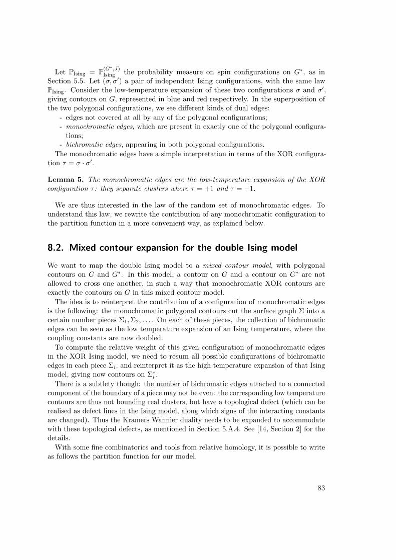
Let PIsing = P(G∗,J)Ising the probability measure on spin configurations on G∗, as in

Section 5.5. Let (σ, σ′) a pair of independent Ising configurations, with the same lawPIsing. Consider the low-temperature expansion of these two configurations σ and σ′,giving contours on G, represented in blue and red respectively. In the superposition ofthe two polygonal configurations, we see different kinds of dual edges:

- edges not covered at all by any of the polygonal configurations;- monochromatic edges, which are present in exactly one of the polygonal configura-

tions;- bichromatic edges, appearing in both polygonal configurations.

The monochromatic edges have a simple interpretation in terms of the XOR configura-tion τ = σ · σ′.

Lemma 5. The monochromatic edges are the low-temperature expansion of the XORconfiguration τ : they separate clusters where τ = +1 and τ = −1.

We are thus interested in the law of the random set of monochromatic edges. Tounderstand this law, we rewrite the contribution of any monochromatic configuration tothe partition function in a more convenient way, as explained below.

8.2. Mixed contour expansion for the double Ising model

We want to map the double Ising model to a mixed contour model, with polygonalcontours on G and G∗. In this model, a contour on G and a contour on G∗ are notallowed to cross one another, in such a way that monochromatic XOR contours areexactly the contours on G in this mixed contour model.

The idea is to reinterpret the contribution of a configuration of monochromatic edgesis the following: the monochromatic polygonal contours cut the surface graph Σ into acertain number pieces Σ1,Σ2, . . . . On each of these pieces, the collection of bichromaticedges can be seen as the low temperature expansion of an Ising temperature, where thecoupling constants are now doubled.

To compute the relative weight of this given configuration of monochromatic edgesin the XOR Ising model, we need to resum all possible configurations of bichromaticedges in each piece Σi, and reinterpret it as the high temperature expansion of that Isingmodel, giving now contours on Σ∗i .

There is a subtlety though: the number of bichromatic edges attached to a connectedcomponent of the boundary of a piece may not be even: the corresponding low temperaturecontours are thus not bounding real clusters, but have a topological defect (which can berealised as defect lines in the Ising model, along which signs of the interacting constantsare changed). Thus the Kramers Wannier duality needs to be expanded to accommodatewith these topological defects, as mentioned in Section 5.A.4. See [14, Section 2] for thedetails.

With some fine combinatorics and tools from relative homology, it is possible to writeas follows the partition function for our model.

83

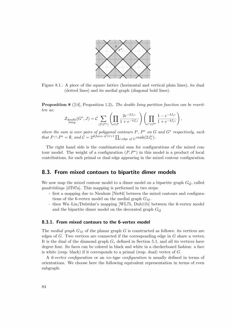
e

e*

Figure 8.1.: A piece of the square lattice (horizontal and vertical plain lines), its dual(dotted lines) and its medial graph (diagonal bold lines).

Proposition 8 ([14], Proposition 1.2). The double Ising partition function can be rewrit-ten as:

ZdoubleIsing

(G∗, J) = C∑

(P,P ∗)

(∏

e∈P

2e−2Je∗

1 + e−4Je∗

)( ∏

e∗∈P ∗

1− e−4Je∗

1 + e−4Je∗

),

where the sum is over pairs of polygonal contours P , P ∗ on G and G∗ respectively, suchthat P ∩ P ∗ = ∅, and C = 2#faces of G+1

∏e:edge of G cosh(2J∗e ).

The right hand side is the combinatorial sum for configurations of the mixed con-tour model. The weight of a configuration (P, P ∗) in this model is a product of localcontributions, for each primal or dual edge appearing in the mixed contour configuration.

8.3. From mixed contours to bipartite dimer models

We now map the mixed contour model to a dimer model on a bipartite graph GQ, calledquadritilings [dT07a]. This mapping is performed in two steps:

- first a mapping due to Nienhuis [Nie84] between the mixed contours and configura-tions of the 6-vertex model on the medial graph GM .

- then Wu–Lin/Dubedat’s mapping [WL75, Dub11b] between the 6-vertex modeland the bipartite dimer model on the decorated graph GQ

8.3.1. From mixed contours to the 6-vertex model

The medial graph GM of the planar graph G is constructed as follows: its vertices areedges of G. Two vertices are connected if the corresponding edge in G share a vertex.It is the dual of the diamond graph G� defined in Section 5.1, and all its vertices havedegree four. Its faces can be colored in black and white in a checkerboard fashion: a faceis white (resp. black) if it corresponds to a primal (resp. dual) vertex of G.

A 6-vertex configuration or an ice-type configuration is usually defined in terms oforientations. We choose here the following equivalent representation in terms of evensubgraph:

84

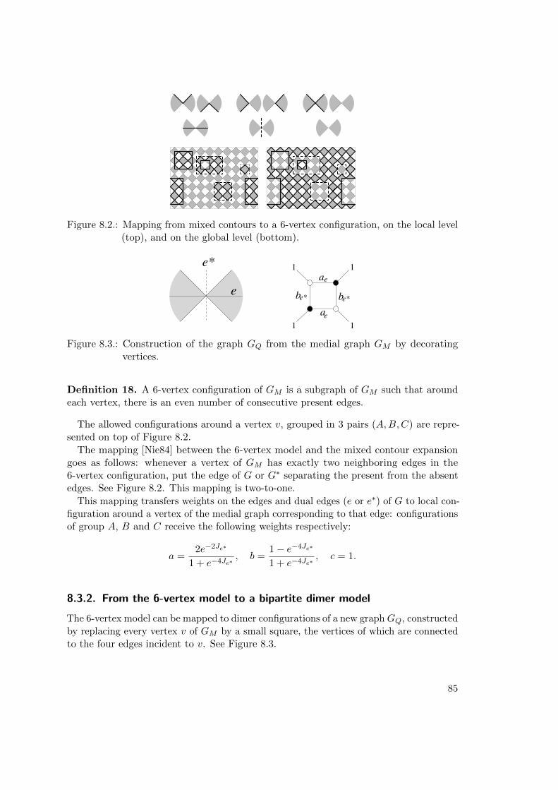
Figure 8.2.: Mapping from mixed contours to a 6-vertex configuration, on the local level(top), and on the global level (bottom).

be*

ae

be*

ae

e*

e

1

11

1

Figure 8.3.: Construction of the graph GQ from the medial graph GM by decoratingvertices.

Definition 18. A 6-vertex configuration of GM is a subgraph of GM such that aroundeach vertex, there is an even number of consecutive present edges.

The allowed configurations around a vertex v, grouped in 3 pairs (A,B,C) are repre-sented on top of Figure 8.2.

The mapping [Nie84] between the 6-vertex model and the mixed contour expansiongoes as follows: whenever a vertex of GM has exactly two neighboring edges in the6-vertex configuration, put the edge of G or G∗ separating the present from the absentedges. See Figure 8.2. This mapping is two-to-one.

This mapping transfers weights on the edges and dual edges (e or e∗) of G to local con-figuration around a vertex of the medial graph corresponding to that edge: configurationsof group A, B and C receive the following weights respectively:

a =2e−2Je∗

1 + e−4Je∗, b =

1− e−4Je∗

1 + e−4Je∗, c = 1.

8.3.2. From the 6-vertex model to a bipartite dimer model

The 6-vertex model can be mapped to dimer configurations of a new graphGQ, constructedby replacing every vertex v of GM by a small square, the vertices of which are connectedto the four edges incident to v. See Figure 8.3.

85

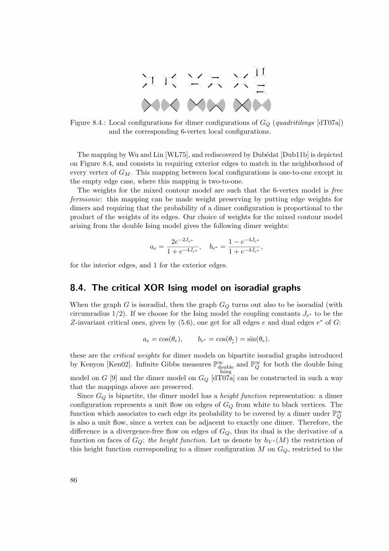
Figure 8.4.: Local configurations for dimer configurations of GQ (quadritilings [dT07a])and the corresponding 6-vertex local configurations.

The mapping by Wu and Lin [WL75], and rediscovered by Dubedat [Dub11b] is depictedon Figure 8.4, and consists in requiring exterior edges to match in the neighborhood ofevery vertex of GM . This mapping between local configurations is one-to-one except inthe empty edge case, where this mapping is two-to-one.

The weights for the mixed contour model are such that the 6-vertex model is freefermionic: this mapping can be made weight preserving by putting edge weights fordimers and requiring that the probability of a dimer configuration is proportional to theproduct of the weights of its edges. Our choice of weights for the mixed contour modelarising from the double Ising model gives the following dimer weights:

ae =2e−2Je∗

1 + e−4Je∗, be∗ =

1− e−4Je∗

1 + e−4Je∗,

for the interior edges, and 1 for the exterior edges.

8.4. The critical XOR Ising model on isoradial graphs

When the graph G is isoradial, then the graph GQ turns out also to be isoradial (withcircumradius 1/2). If we choose for the Ising model the coupling constants Je∗ to be theZ-invariant critical ones, given by (5.6), one get for all edges e and dual edges e∗ of G:

ae = cos(θe), be∗ = cos(θ∗e) = sin(θe).

these are the critical weights for dimer models on bipartite isoradial graphs introducedby Kenyon [Ken02]. Infinite Gibbs measures P∞double

Ising

and P∞Q for both the double Ising

model on G [9] and the dimer model on GQ [dT07a] can be constructed in such a waythat the mappings above are preserved.

Since GQ is bipartite, the dimer model has a height function representation: a dimerconfiguration represents a unit flow on edges of GQ from white to black vertices. Thefunction which associates to each edge its probability to be covered by a dimer under P∞Qis also a unit flow, since a vertex can be adjacent to exactly one dimer. Therefore, thedifference is a divergence-free flow on edges of GQ, thus its dual is the derivative of afunction on faces of GQ: the height function. Let us denote by hV ∗(M) the restriction ofthis height function corresponding to a dimer configuration M on GQ, restricted to the

86

faces of GQ corresponding to a primal vertex of G. It is determined once we know itsvalue at a given dual vertex v∗, which we take to be zero.

Lemma 6 ([14], Lemma 7.1). The restricted height function hV ∗ has the followingproperties

- hV ∗ takes only values in Z.- The increments of hV ∗ are nonzero if and only if the two dual vertices are separated

by a primal edge of G in the corresponding mixed contour model

Since primal edges in the mixed contour model and monochromatic edges (or edges ofcontour separating clusters) in the XOR Ising model have the same law by Proposition 8,we get the following:

Theorem 17 ([14], Theorem 7.5). Monochromatic polygon configurations of the criticalXOR-Ising model have the same distribution as level lines of the restriction to dualvertices of the height function of dimer configurations of GQ.

Theorem 17 can be interpreted as a proof of a version of Wilson’s conjecture in adiscrete setting, before passing to the scaling limit, and brings some elements for acomplete proof of this conjecture. In particular, it explains the link with the Gaussianfree field and the factor

√2, as we will now show.

The contours on G separating distinct integer values of hV ∗ can be understood asdiscrete level lines corresponding to half-integer values.

On infinite isoradial graphs, the dimer height function hV ∗ , seen as a distribution onthe graph GQ with circumradius ε, is known to converge, as ε goes to zero (in a weaksense, unfortunately), to the Gaussian massless free field times 1√

π, like the unrestricted

height function [dT07b].

Therefore, it is natural to expect that these contour lines converge to the contour linesof the limiting object, i.e., to level lines for the Gaussian free field with levels (k + 1

2)√π,

k ∈ Z. Unfortunately, the result for the convergence result of the height function to theGaussian free field is too weak to ensure convergence of contour lines.

The Gaussian free field is a wild object: it is a random generalized function, and not afunction, and as such, there is no direct way to define what its level lines are. The levellines of the Gaussian free field are understood here as the scaling limit when the meshgoes to zero of the level lines of the discrete Gaussian free field on a triangulation of thedomain, which separate domains where the field is above or below a certain level [SS09].

The level lines of the Gaussian free field corresponding to levels that are odd multiplesof λ =

√π8 form a CLE4 [SS09, MS]. It is conjectured to be the full scaling limit for

the critical double dimer loops, which can be seen as discrete half integer level lines ofthe difference of the two height functions. This difference, by independence, converges(in a weak sense) to

√2/π times the Gaussian free field, which would give a consistent

spacing.

The contour lines of the XOR Ising models are conjectured by Wilson to have the samelimiting behavior as the CLE4, except that there are a factor of

√2 times fewer loops in

87

the XOR Ising picture. This conjecture is in agreement with predictions of conformalfield theory [IR11, PS11].

Therefore, the extra factor√

2 compared to the CLE4 spacing in Wilson’s conjecturecorresponds to the fact that contours in the XOR Ising model have to do with contourlines of only one dimer height function, as opposed to two for dimer loops.

88

Part III.

Other works and possibledevelopments

89

9. Other works

In this chapter, we briefly describe the results of two other papers related to dimermodels and random partitions. In Section 9.1, we present the results of a joint work [7]with Beatrice de Tiliere, about the asymptotic distribution of the winding of dimerconfigurations on the honeycomb lattice wrapped on a large torus. In Section 9.2, wegive the main results of [10] obtained with Dan Beltoft and Nathanael Enriquez aboutthe limit shape of a random Young diagram constrained in a large rectangular box, andthe fluctuations around this limit shape.

9.1. Winding of the toroidal honeycomb dimer model

We consider the dimer model on a family of graphs Gm,n obtained as the quotient of thebiperiodic honeycomb graph by a two dimensional lattice.

A dimer configuration C can be interpreted as a function αC on edges with definitedivergence at each vertex. The difference with a fixed function on edges α0 with the samedivergence (and which may or not come from a dimer configuration) is a divergence-freeflow, whose dual is a closed form on dual edges.

If the graph is planar, then this closed form is exact, and is the differential of a functionon faces: the height function. But as in classical differential topology, if the graph isdrawn on a surface of higher surface, the height function is not well defined, and hasperiods.

In a joint work with Beatrice de Tiliere [7], we determine the limit of the law of theperiods of the height function of a uniform dimer configuration on Gm,n, as m and n goto infinity, with an aspect ratio ρ = n

m√

3kept fixed.

We prove the following theorem:

Theorem 18 ([7], Theorem 1). When n and m go to infinity, in such a way thatlim n

m√

3= ρ ∈ (0,∞), the pair of horizontal and vertical periods converges in law to a

two-dimensional random variable windρ, with a discrete Gaussian distribution:

P(windρ = (k, l)) ∝ exp

(−π

2(ρk2 +

l2

ρ)

).

The proof of this result is based on a very precise asymptotic analysis of the partitionfunction of the dimer model on the torus, with slightly perturbed weights on edges,depending on their orientation. We use then the combinatorial fact that the number ofedges of each orientation is a linear function of the period to conclude. The partitionfunction is a linear combination of four determinants, by Kasteleyn’s theorem, each of

90

these being written as a double product over roots of unity, using periodicity of theunderlying graph.

The asymptotic analysis is performed in this particular case for simplicity, but lookingat the proof, one sees that the following ingredients are essential:

- the spectral curve of the corresponding dimer model is a Harnack curve, and thedimer model is in a liquid phase. As a consequence, the curve will intersect twicethe unit torus.

- whereas the contributions of unit roots far from those points will contribute to thefree energy (the global exponential growth of the partition function), the termsclose to the intersection points with the spectral curve will give rise to terms lookinglike Jacobi’s triple product formula, thus elliptic theta functions.

- The generating function for the discrete Gaussian distribution is also expressedin terms of theta functions, which are obtained as recombination of the variouscontributions of neighborhoods of the intersection points in the four determinants.

The program to extend this computation to all toroidal bipartite dimer models, andmuch more has been finalized in a work by Richard Kenyon, Nike Sun and DavidWilson [KSW13]. This result is in agreement with predictions of the conformal fieldtheory. On isoradial graphs on the torus, the height function converges to a compactifiedGaussian massless free field [Dub11a]. The result above should thus be true for a moregeneral class of graphs. Mathematical results in that direction can be found in a recentwork by Julien Dubedat and Reza Gheissari [DG15], for the wide class of Temperleyangraphs, without assumption on periodicity, but with instead an assumption about thelimiting behaviour of the simple random walk on the underlying graph. For other robustresults about dimers using connection with the behaviour of the loop erased randomwalk, see [BLR16].

9.2. Limit shape and fluctuations of boxed partitions

In [10] in collaboration with Dan Beltoft and Nathanael Enriquez, we considered aprobability measure Pqa,b on partitions contained in an a× b rectangle, i.e., with at mosta parts, each of length at most b. The probability of a partition λ fitting in this rectangleis

Pqa,b(λ) =1

Za,b(q)q|λ|,

where Za,b(q), the partition function, is the sum of q|µ| over all the partitions µ in thea× b rectangle.

We were interested in the large scale behavior of a typical partition when the dimensionsof the box become very large. More precisely, we consider sequences of positive integers(an)n≥1 and (bn)n≥1 satisfying

∀ n ≥ 1, an + bn = 2n, and limn→∞

anbn

=ρ

1− ρfor some fixed parameter ρ ∈ (0, 1). In order to have a nontrivial limit, the parameter qneeds to be scaled, and go to 1 when n goes to infinity. We set q = e−

cn . Note that c = 0

91

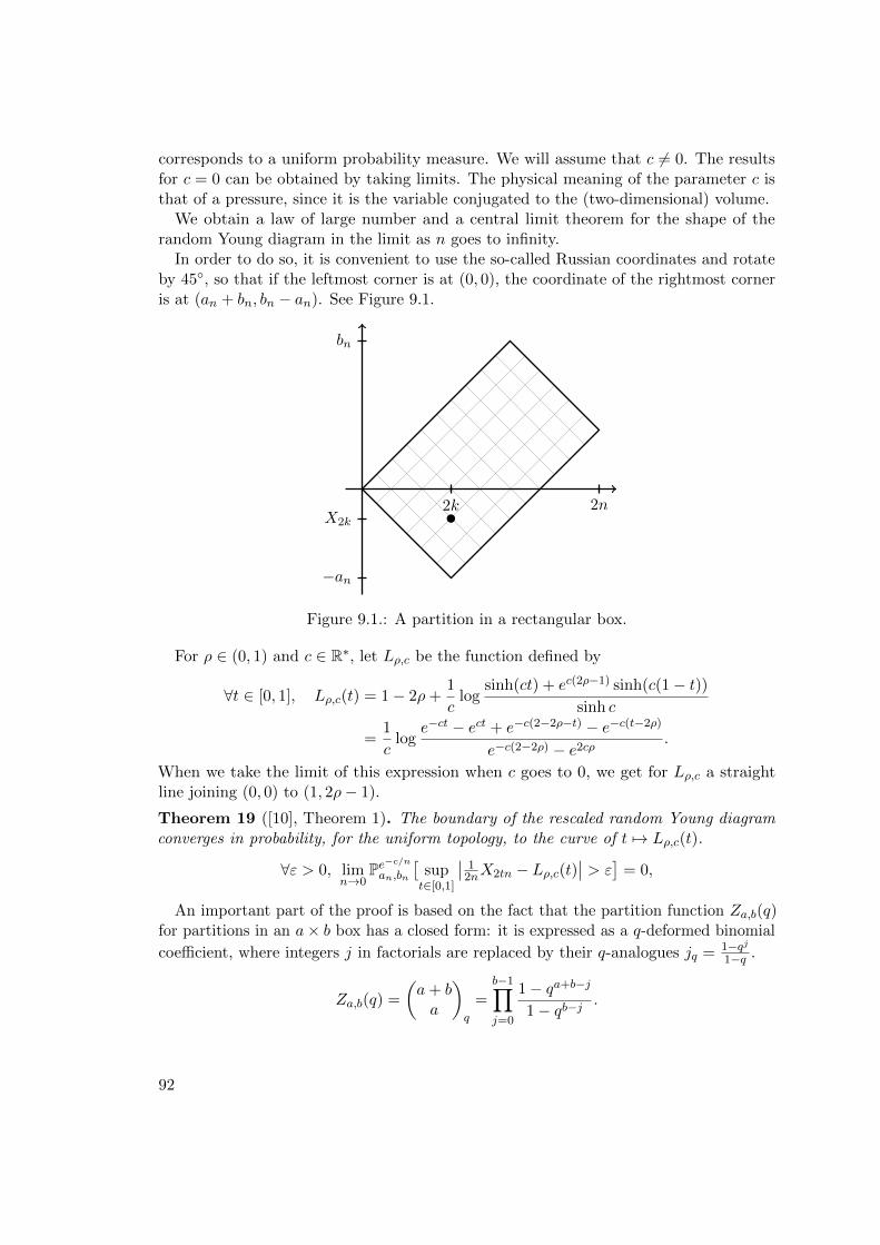
corresponds to a uniform probability measure. We will assume that c 6= 0. The resultsfor c = 0 can be obtained by taking limits. The physical meaning of the parameter c isthat of a pressure, since it is the variable conjugated to the (two-dimensional) volume.

We obtain a law of large number and a central limit theorem for the shape of therandom Young diagram in the limit as n goes to infinity.

In order to do so, it is convenient to use the so-called Russian coordinates and rotateby 45◦, so that if the leftmost corner is at (0, 0), the coordinate of the rightmost corneris at (an + bn, bn − an). See Figure 9.1.

2n

−an

bn

2kX2k

Figure 9.1.: A partition in a rectangular box.

For ρ ∈ (0, 1) and c ∈ R∗, let Lρ,c be the function defined by

∀t ∈ [0, 1], Lρ,c(t) = 1− 2ρ+1

clog

sinh(ct) + ec(2ρ−1) sinh(c(1− t))sinh c

=1

clog

e−ct − ect + e−c(2−2ρ−t) − e−c(t−2ρ)

e−c(2−2ρ) − e2cρ.

When we take the limit of this expression when c goes to 0, we get for Lρ,c a straightline joining (0, 0) to (1, 2ρ− 1).

Theorem 19 ([10], Theorem 1). The boundary of the rescaled random Young diagramconverges in probability, for the uniform topology, to the curve of t 7→ Lρ,c(t).

∀ε > 0, limn→0

Pe−c/nan,bn

[supt∈[0,1]

∣∣ 12nX2tn − Lρ,c(t)

∣∣ > ε]

= 0,

An important part of the proof is based on the fact that the partition function Za,b(q)for partitions in an a× b box has a closed form: it is expressed as a q-deformed binomial

coefficient, where integers j in factorials are replaced by their q-analogues jq = 1−qj1−q .

Za,b(q) =

(a+ ba

)

q

=b−1∏

j=0

1− qa+b−j

1− qb−j .

92

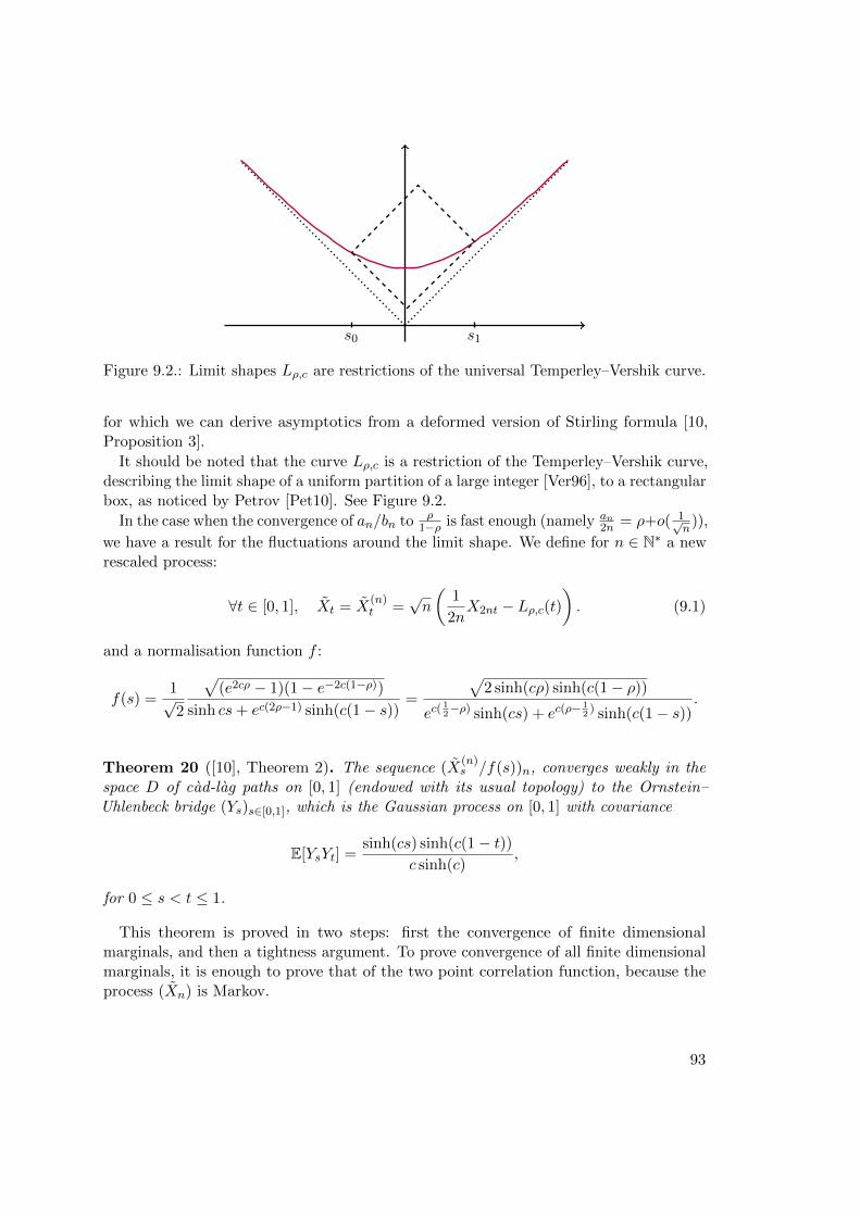
s0 s1

Figure 9.2.: Limit shapes Lρ,c are restrictions of the universal Temperley–Vershik curve.

for which we can derive asymptotics from a deformed version of Stirling formula [10,Proposition 3].

It should be noted that the curve Lρ,c is a restriction of the Temperley–Vershik curve,describing the limit shape of a uniform partition of a large integer [Ver96], to a rectangularbox, as noticed by Petrov [Pet10]. See Figure 9.2.

In the case when the convergence of an/bn to ρ1−ρ is fast enough (namely an

2n = ρ+o( 1√n

)),

we have a result for the fluctuations around the limit shape. We define for n ∈ N∗ a newrescaled process:

∀t ∈ [0, 1], Xt = X(n)t =

√n

(1

2nX2nt − Lρ,c(t)

). (9.1)

and a normalisation function f :

f(s) =1√2

√(e2cρ − 1)(1− e−2c(1−ρ))

sinh cs+ ec(2ρ−1) sinh(c(1− s)) =

√2 sinh(cρ) sinh(c(1− ρ))

ec(12−ρ) sinh(cs) + ec(ρ−

12

) sinh(c(1− s)).

Theorem 20 ([10], Theorem 2). The sequence (X(n)s /f(s))n, converges weakly in the

space D of cad-lag paths on [0, 1] (endowed with its usual topology) to the Ornstein–Uhlenbeck bridge (Ys)s∈[0,1], which is the Gaussian process on [0, 1] with covariance

E[YsYt] =sinh(cs) sinh(c(1− t))

c sinh(c),

for 0 ≤ s < t ≤ 1.

This theorem is proved in two steps: first the convergence of finite dimensionalmarginals, and then a tightness argument. To prove convergence of all finite dimensionalmarginals, it is enough to prove that of the two point correlation function, because theprocess (Xn) is Markov.

93

An analogue of Theorem 20 can also be written down for fluctuations around Temperley–Vershik’s curve for the unconstrained case: it is described by a stationary Ornstein–Uhlenbeck process on R, modulated by a cosh function. See [10, Theorem 4]. When wecondition this process to have zero integral over R, we obtain a new centered Gaussianprocess with covariance between time s and t is given by

e−|t−s|

2 cosh s cosh t− π2

6h(s)h(t),

where h(t) = 6π2 t tanh t− log(2 cosh t). Expressed in the original coordinates (by rotating

by 45◦), this covariance is the one obtained by Pittel [Pit97], who deals with themicrocanonical ensemble of partitions (with a fixed area |λ| = n→∞). The fluctuationsin that case are thus given by this Gaussian, but non-Markov process.

94

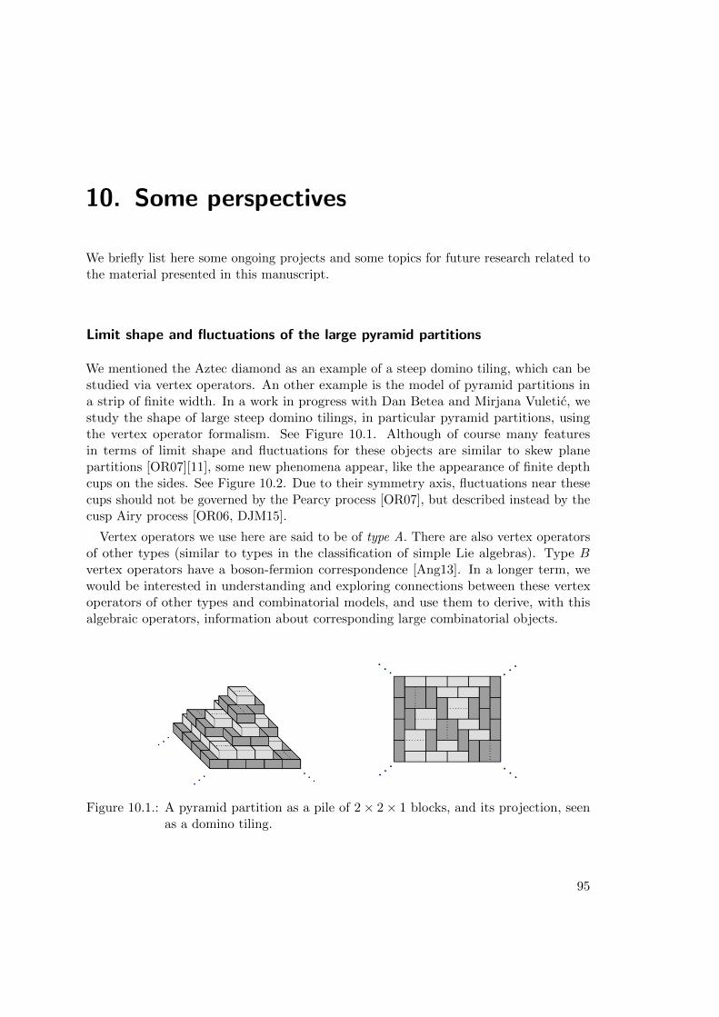
10. Some perspectives

We briefly list here some ongoing projects and some topics for future research related tothe material presented in this manuscript.

Limit shape and fluctuations of the large pyramid partitions

We mentioned the Aztec diamond as an example of a steep domino tiling, which can bestudied via vertex operators. An other example is the model of pyramid partitions ina strip of finite width. In a work in progress with Dan Betea and Mirjana Vuletic, westudy the shape of large steep domino tilings, in particular pyramid partitions, usingthe vertex operator formalism. See Figure 10.1. Although of course many featuresin terms of limit shape and fluctuations for these objects are similar to skew planepartitions [OR07][11], some new phenomena appear, like the appearance of finite depthcups on the sides. See Figure 10.2. Due to their symmetry axis, fluctuations near thesecups should not be governed by the Pearcy process [OR07], but described instead by thecusp Airy process [OR06, DJM15].

Vertex operators we use here are said to be of type A. There are also vertex operatorsof other types (similar to types in the classification of simple Lie algebras). Type Bvertex operators have a boson-fermion correspondence [Ang13]. In a longer term, wewould be interested in understanding and exploring connections between these vertexoperators of other types and combinatorial models, and use them to derive, with thisalgebraic operators, information about corresponding large combinatorial objects.

Figure 10.1.: A pyramid partition as a pile of 2× 2× 1 blocks, and its projection, seenas a domino tiling.

95

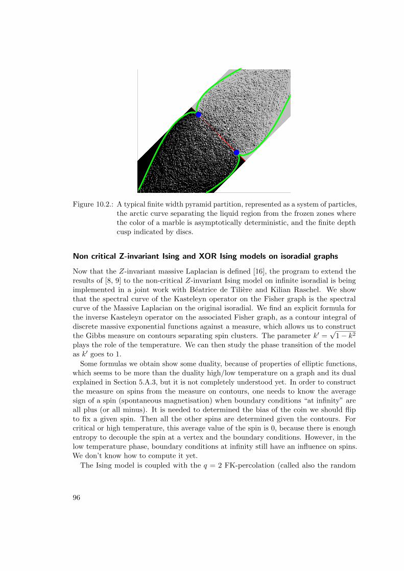
Figure 10.2.: A typical finite width pyramid partition, represented as a system of particles,the arctic curve separating the liquid region from the frozen zones wherethe color of a marble is asymptotically deterministic, and the finite depthcusp indicated by discs.

Non critical Z-invariant Ising and XOR Ising models on isoradial graphs

Now that the Z-invariant massive Laplacian is defined [16], the program to extend theresults of [8, 9] to the non-critical Z-invariant Ising model on infinite isoradial is beingimplemented in a joint work with Beatrice de Tiliere and Kilian Raschel. We showthat the spectral curve of the Kasteleyn operator on the Fisher graph is the spectralcurve of the Massive Laplacian on the original isoradial. We find an explicit formula forthe inverse Kasteleyn operator on the associated Fisher graph, as a contour integral ofdiscrete massive exponential functions against a measure, which allows us to constructthe Gibbs measure on contours separating spin clusters. The parameter k′ =

√1− k2

plays the role of the temperature. We can then study the phase transition of the modelas k′ goes to 1.

Some formulas we obtain show some duality, because of properties of elliptic functions,which seems to be more than the duality high/low temperature on a graph and its dualexplained in Section 5.A.3, but it is not completely understood yet. In order to constructthe measure on spins from the measure on contours, one needs to know the averagesign of a spin (spontaneous magnetisation) when boundary conditions “at infinity” areall plus (or all minus). It is needed to determined the bias of the coin we should flipto fix a given spin. Then all the other spins are determined given the contours. Forcritical or high temperature, this average value of the spin is 0, because there is enoughentropy to decouple the spin at a vertex and the boundary conditions. However, in thelow temperature phase, boundary conditions at infinity still have an influence on spins.We don’t know how to compute it yet.

The Ising model is coupled with the q = 2 FK-percolation (called also the random

96

cluster model) [FK72, Gri06]. In [Ken04], Kenyon recalls the weights for the self-dual(critical) FK percolation on isoradial graphs. It would be interesting to see what couldbe said in the case q = 2 about this model out of criticality. For example, is there a link,like for the decay of dimer correlations, between the exponential tail for quantities likethe size of the finite clusters and the geometry of the isoradial embedding?

In this project on the non-critical Ising model, we also extend the correspondencebetween the XOR Ising model and a bipartite dimer model on GQ. This is the firstexample of bipartite dimer model with elliptic weights and with a local formula for theinverse Kasteleyn operator.

Integrable dimer weights out of criticality

Kenyon introduced [Ken02] critical dimer weights on bipartite isoradial graphs, in relationwith the conductances of the Laplacian from Section 5.4. Dimer models on periodicisoradial graphs with these weights are in correspondence with Harnack curves of genuszero [KO06].

With Beatrice de Tiliere and David Cimasoni, we are investigating if such a corre-spondence exists for Harnack curves of genus one. More precisely, does there exist aparameterization for integrable dimer models with elliptic functions? Integrability forbipartite dimer models does not mean directly invariance under star-triangle transforma-tion, simply because this transformation already breaks bipartiteness. It is replaced bythe more elementary spider move [GK13], a variant of the urban renewal.

For isoradial graphs of the form GQ, the study above for the non-critical Z-invariantIsing model provides a positive answer, but it is very specific to the structure of thegraph where all vertices have degree 3, and it gives only Harnack curves with a (z, w)↔(z−1, w−1). Preliminary results seem to show that in general, such parameterizations ofthe spider move transformation can only be rational, and it may be that the only dimerweights on edges as a function of their half-angle are the critical ones on isoradial graphs,and their generalization, where we allow circumcenters to lie outside of the face (andthus some rhombi in G� are upside-down). We plan to continue the investigations onthis problem.

Massive Laplacians and fermionic observable for the non critical Ising model

In [CS12], strong discrete holomorphy of the fermionic observable [Smi10] is used in afundamental way so that the scaling limit of a related quantity is almost harmonic for theLaplacian of Section 5.4. From the corresponding harmonic analysis toolbox [CS11] andconvergence results from discrete harmonic functions to their continuous counterparts,conformal invariance of the critical Z-invariant Ising model on isoradial graphs is proved.

This fermionic observable can be defined out of criticality. On the square lattice, outof criticality, this observable is harmonic for a certain massive Laplacian [BDC12]. Thisstudy is however specific to the square lattice since it is used in a non trivial way thefact that the graph on which the fermionic observable is defined has the same structureas the graph where the spins live, and the Laplacian acts.

97

It would be interesting to see if this connection between massive Laplacian and noncritical Ising model can be established for the Z-invariant models on isoradial graphs.This would yield a combinatorial link between the Ising model and the massive Laplacian,which would be more concrete than the equality of their spectral curves. More generally,is it possible to construct discrete massive Dirac operator, which would be a “squareroot” of the massive Laplacian, which would extend out of criticality the connectionbetween the Laplacian and the Kasteleyn operator on the double graph with criticalweights which gives a version of the discrete Cauchy–Riemann equations?

A natural but naıve candidate would be to just perturb the (full) Kasteleyn matrix byadding nonzero coefficients on the diagonal, as we did to add a mass for the Laplacian.Expanding the determinant would give a sum of configurations with dimers and monomers,but the signs are not compensated any more by the clockwise odd orientation.

The Green function on finite isoradial graphs and branched coverings

Explicit and local formulas for the Z-invariant Green [Ken02] and massive Green [16]functions are known, as integral of discrete exponential functions (or their massiveanalogues) against a singular measure along a contour.

There exists a representation theorem for discrete harmonic functions on finite isoradialgraphs as a (generalized) linear combination of discrete exponential functions [BMS05,BS08]. Using the same arguments, we can formulate the analogue representation resultfor massive harmonic functions.

The problem is that the coefficients in this linear combination are not very explicit.We are wondering if an explicit formula for the Poisson kernel of a simply connected finiteisoradial graph could be written down. It may be complicated due to all the flexibilitythese graphs can have on their boundary. Maybe a simpler problem would be already togive formulas for Green functions on isoradial graphs which are branch covers of the plane.In particular, can we understand the mechanism linking the branching structure, and thesingular measure used to integrate the (massive) exponential functions? Can we do italso for the Green function associated to Laplacian with connexions along edges [Ken11]?These exotic Green functions can then be used for the purposes of statistical mechanics:for example, in [KW15], such a Green function is used to compute the probability that aloop erased random walk passes through a given edge.

98

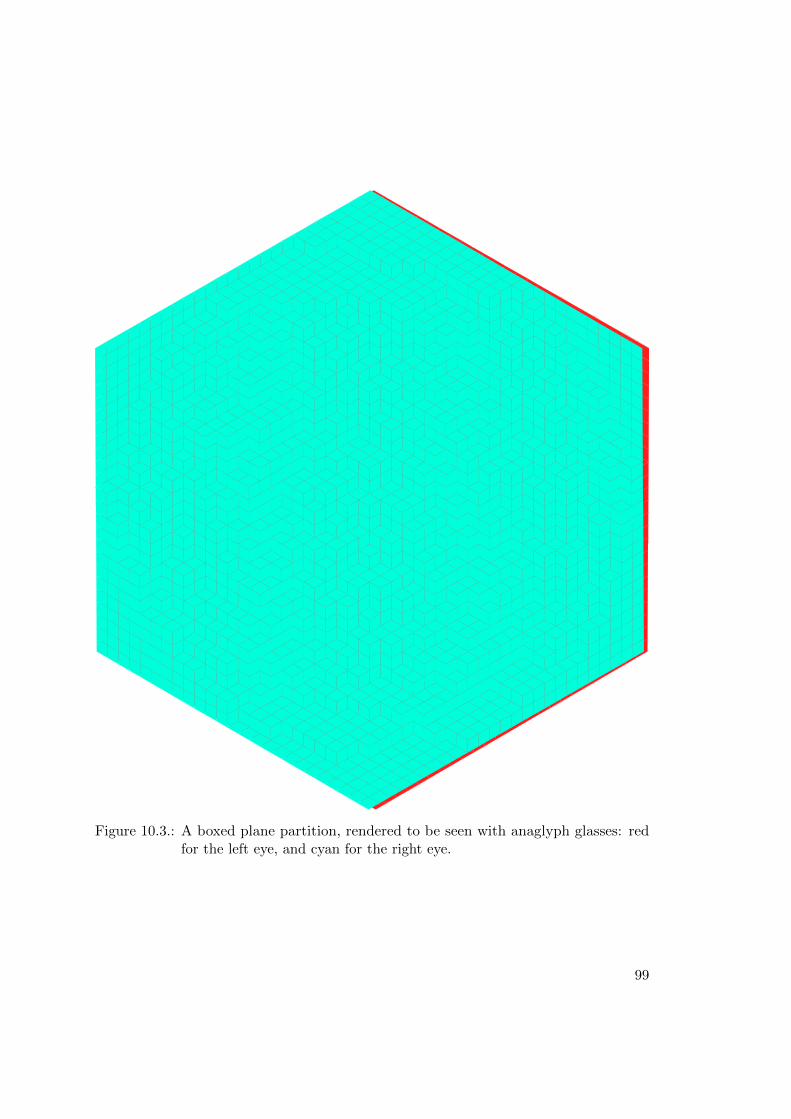
Figure 10.3.: A boxed plane partition, rendered to be seen with anaglyph glasses: redfor the left eye, and cyan for the right eye.

99

Publications

[1] Cedric Boutillier, Paul Francois, Kirone Mallick, and Shamlal Mallick. A matrixansatz for the diffusion of an impurity in the asymmetric exclusion process. J. Phys.A, 35(46):9703–9730, 2002.

[2] Cedric Boutillier. Modeles de Dimeres : comportements limites. PhD thesis, Univer-site Paris 11 – Orsay, 2005.

[3] Cedric Boutillier. Non-colliding paths in the honeycomb dimer model and the Dysonprocess. J. Stat. Phys., 129(5-6):1117–1135, 2007.

[4] Cedric Boutillier. Pattern densities in non-frozen planar dimer models. Comm.Math. Phys., 271(1):55–91, 2007.

[5] Cedric Boutillier. The critical Ising model on infinite isoradial graphs via dimers.Oberwolfach Reports (Stochastic Analysis Workshop), (25/2008), 2008.

[6] Cedric Boutillier. The bead model and limit behaviors of dimer models. Ann.Probab., 37(1):107–142, 2009.

[7] Cedric Boutillier and Beatrice de Tiliere. Loops statistics in the toroidal honeycombdimer model. Ann. Probab., 37(5):1747–1777, 2009.

[8] Cedric Boutillier and Beatrice de Tiliere. The critical Z-invariant Ising model viadimers: the periodic case. Probab. Theory Related Fields, 147(3-4):379–413, 2010.

[9] Cedric Boutillier and Beatrice de Tiliere. The critical Z-invariant Ising model viadimers: locality property. Comm. Math. Phys., 301(2):473–516, 2011.

[10] Dan Beltoft, Cedric Boutillier, and Nathanael Enriquez. Random partitions in arectangular box. Moscow Mathematical Journal, 12(4):719–745, 2012.

[11] Cedric Boutillier, Sevak Mkrtchyan, Nicolai Reshetikhin, and Peter Tingley. Randomskew plane partitions with a piecewise periodic back wall. Ann. Henri Poincare,13(2):271–296, 2012.

[12] Cedric Boutillier and Beatrice Tiliere. Statistical Mechanics on Isoradial Graphs.In Jean-Dominique Deuschel, Barbara Gentz, Wolfgang Konig, Max von Renesse,Michael Scheutzow, and Uwe Schmock, editors, Probability in Complex PhysicalSystems, volume 11 of Springer Proceedings in Mathematics, pages 491–512. SpringerBerlin Heidelberg, 2012.

100

[13] Dan Betea, Cedric Boutillier, Jeremy Bouttier, Guillaume Chapuy, Sylvie Cor-teel, and Mirjana Vuletic. Perfect sampling algorithms for Schur processes.arxiv:1407.3764, Markov Processes and Related Fields (accepted), proceedings ofInhomogenous Random Systems 2015, 2014.

[14] Cedric Boutillier and Beatrice de Tiliere. Height representation of XOR-Ising loopsvia bipartite dimers. Electron. J. Probab., 19:no. 80, 33, 2014.

[15] Cedric Boutillier, Jeremy Bouttier, Guillaume Chapuy, Sylvie Corteel, and SanjayRamassamy. Dimers on rail yard graphs. arXiv:1504.05176, Annals of IHP D (toappear), 2015.

[16] Cedric Boutillier, Beatrice de Tiliere, and Kilian Raschel. The Z-invariant massiveLaplacian on isoradial graphs. Invent. Math., pages 1–81, 2016.

The publication listed here can be downloaded from:

http://www.lpma-paris.fr/pageperso/boutil/publications/.

101

http://www.lpma-paris.fr/pageperso/boutil/publications/

Bibliography

[Ang13] Iana I. Anguelova. Boson-Fermion Correspondence of Type B and TwistedVertex Algebras, pages 399–410. Springer Japan, Tokyo, 2013.

[AP04] H. Au-Yang and J. H. H. Perk. Q-dependent susceptibility in Z-invariantpentagrid ising model. ArXiv Condensed Matter e-prints, September 2004.

[AP07] H. Au-Yang and J. H. H. Perk. Q-dependent susceptibilities in ferromagneticquasiperiodic Z-invariant ising models. J. Stat. Phys., 127:265–286, April 2007.

[AYP87] Helen Au-Yang and Jacques H. H. Perk. Critical correlations in a Z-invariantinhomogeneous Ising model. Phys. A, 144(1):44–104, 1987.

[AZ13] Alexander Alexandrov and Anton Zabrodin. Free fermions and tau-functions.Journal of Geometry and Physics, 67(0):37–80, 2013.

[Bax86] Rodney J. Baxter. Free-fermion, checkerboard and Z-invariant lattice modelsin statistical mechanics. Proc. Roy. Soc. London Ser. A, 404(1826):1–33, 1986.

[Bax89] Rodney J. Baxter. Exactly solved models in statistical mechanics. AcademicPress Inc. [Harcourt Brace Jovanovich Publishers], London, 1989. Reprint ofthe 1982 original.

[BC14] Alexei Borodin and Ivan Corwin. Macdonald processes. Probab. Theory RelatedFields, 158(1-2):225–400, 2014.

[BCC14] Jeremie Bouttier, Guillaume Chapuy, and Sylvie Corteel. From Aztec diamondsto pyramids: steep tilings. 2014.

[BDC12] V. Beffara and H. Duminil-Copin. Smirnov’s fermionic observable away fromcriticality. Ann. Probab., 40(6):2667–2689, 2012.

[Bef08] Vincent Beffara. Is critical 2D percolation universal? In In and out ofequilibrium. 2, volume 60 of Progr. Probab., pages 31–58. Birkhauser, Basel,2008.

[BF14] A. Borodin and P. L. Ferrari. Anisotropic growth of random surfaces in 2 + 1dimensions. Comm. Math. Phys., 325(2):603–684, 2014.

[BF15] A. Borodin and P. Ferrari. Random tilings and Markov chains for interlacingparticles. arXiv:1506.03910, 2015.

102

[BG09] Alexei Borodin and Vadim Gorin. Shuffling algorithm for boxed plane partitions.Adv. Math., 220(6):1739–1770, 2009.

[BG15] Alexey Bufetov and Vadim Gorin. Stochastic monotonicity in Young graphand Thoma theorem. Int. Math. Res. Not. IMRN, (23):12920–12940, 2015.

[BLR16] Nathanael Berestycki, Benoit Laslier, and Gourab Ray. Universality of fluctu-tations in the dimer model. 2016.

[BMS05] A. I. Bobenko, C. Mercat, and Y. B. Suris. Linear and nonlinear theories ofdiscrete analytic functions. Integrable structure and isomonodromic Green’sfunction. J. Reine Angew. Math., 583:117–161, 2005.

[Bor11] A. Borodin. Schur dynamics of the Schur processes. Adv. Math., 228(4):2268–2291, 2011.

[BP93] R. Burton and R. Pemantle. Local characteristics, entropy and limit theoremsfor spanning trees and domino tilings via transfer-impedances. Ann. Probab.,21(3):1329–1371, 1993.

[BP11] Yuliy Baryshnikov and Robin Pemantle. Asymptotics of multivariate sequences,part III: Quadratic points. Adv. Math., 228(6):3127–3206, 2011.

[BP13] A. Borodin and L. Petrov. Nearest neighbor Markov dynamics on Macdonaldprocesses. arXiv:1305.5501, 2013.

[BR05] Alexei Borodin and Eric M. Rains. Eynard-Mehta theorem, Schur process,and their Pfaffian analogs. J. Stat. Phys., 121(3-4):291–317, 2005.

[Bru14] Erwan Brugalle. Pseudoholomorphic simple Harnack curves. Enseign. Math.,2014. to appear.

[BS08] Alexander I. Bobenko and Yuri B. Suris. Discrete differential geometry, vol-ume 98 of Graduate Studies in Mathematics. American Mathematical Society,Providence, RI, 2008. Integrable structure.

[CCK15] Dmitry Chelkak, David Cimasoni, and Adrien Kassel. Revisiting the combina-torics of the 2d Ising model. 2015.

[CDC13] David Cimasoni and Hugo Duminil-Copin. The critical temperature for theIsing model on planar doubly periodic graphs. Electron. J. Probab., 18:no. 44,18, 2013.

[CEP96] Henry Cohn, Noam Elkies, and James Propp. Local statistics for randomdomino tilings of the Aztec diamond. Duke Math. J., 85(1):117–166, 1996.

[Cim14] David Cimasoni. The geometry of dimer models. 2014.

103

[CJ16] Sunil Chhita and Kurt Johansson. Domino statistics of the two-periodic Aztecdiamond. Adv. Math., 294:37–149, 2016.

[CJY15] Sunil Chhita, Kurt Johansson, and Benjamin Young. Asymptotic dominostatistics in the Aztec diamond. Ann. Appl. Probab., 25(3):1232–1278, 2015.

[CK01] Raphael Cerf and Richard Kenyon. The low-temperature expansion of theWulff crystal in the 3D Ising model. Comm. Math. Phys., 222(1):147–179,2001.

[CKP01] Henry Cohn, Richard Kenyon, and James Propp. A variational principle fordomino tilings. J. Amer. Math. Soc., 14(2):297–346 (electronic), 2001.

[CLP98] Henry Cohn, Michael Larsen, and James Propp. The shape of a typical boxedplane partition. New York J. Math., 4:137–165 (electronic), 1998.

[CR07] David Cimasoni and Nicolai Reshetikhin. Dimers on surface graphs and spinstructures. I. Comm. Math. Phys., 275(1):187–208, 2007.

[CR08] David Cimasoni and Nicolai Reshetikhin. Dimers on surface graphs and spinstructures. II. Comm. Math. Phys., 281(2):445–468, 2008.

[CS06] Ruben Costa-Santos. Geometrical aspects of the Z-invariant ising model. Eur.Phys. J. B, 53(1):85–90, 2006.

[CS11] D. Chelkak and S. Smirnov. Discrete complex analysis on isoradial graphs.Adv. in Math., 228(3):1590–1630, 2011.

[CS12] D. Chelkak and S. Smirnov. Universality in the 2D Ising model and conformalinvariance of fermionic observables. Inv. Math., 189:515–580, 2012.

[CY14] Sunil Chhita and Benjamin Young. Coupling functions for domino tilings ofAztec diamonds. Adv. Math., 259:173–251, 2014.

[dB81a] Nicolaas G. de Bruijn. Algebraic theory of Penrose’s non-periodic tilings ofthe plane. I. Indagationes Mathematicae (Proceedings), 84(1):39–52, 1981.

[dB81b] Nicolaas G. de Bruijn. Algebraic theory of Penrose’s non-periodic tilings ofthe plane. II. Indagationes Mathematicae (Proceedings), 84(1):53 – 66, 1981.

[DG15] Julien Dubedat and Reza Gheissari. Asymptotics of height change on toroidalTemperleyan dimer models. J. Stat. Phys., 159(1):75–100, 2015.

[DJM15] Erik Duse, Kurt Johansson, and Anthony Metcalfe. The Cusp-Airy Process.arXiv:1510.02057, 2015.

[DM15a] Erik Duse and Anthony Metcalfe. Asymptotic geometry of discrete interlacedpatterns: Part I. Internat. J. Math., 26(11):1550093, 66, 2015.

104

[DM15b] Erik Duse and Anthony Metcalfe. Asymptotic geometry of discrete interlacedpatterns: Part II. arXiv:1507.00467, 2015.

[dT07a] Beatrice de Tiliere. Quadri-tilings of the plane. Probab. Theory Related Fields,137(3-4):487–518, 2007.

[dT07b] Beatrice de Tiliere. Scaling limit of isoradial dimer models and the case oftriangular quadri-tilings. Ann.I. H. Poincare B, 43(6):729–750, 2007.

[dT15] Beatrice de Tiliere. The dimer model in statistical mechanics. In Dimer modelsand random tilings, volume 45 of Panor. Syntheses, pages 1–45. Soc. Math.France, Paris, 2015.

[dT16] Beatrice de Tiliere. Critical Ising model and spanning trees partition functions.Ann. Inst. Henri Poincare Probab. Stat., 52(3):1382–1405, 2016.

[Du11] Peng Du. The Aztec Diamond Edge-Probability Generating Function, 2011.Master Thesis, University of Pennsylvania.

[Dub11a] J. Dubedat. Dimers and analytic torsion I. ArXiv e-prints, October 2011.

[Dub11b] J. Dubedat. Exact bosonization of the Ising model. ArXiv: 1112.4399, 2011.

[Duf68] Richard J. Duffin. Potential theory on a rhombic lattice. J. CombinatorialTheory, 5:258–272, 1968.

[DZM+96] N. P. Dolbilin, Yu. M. Zinov′ev, A. S. Mishchenko, M. A. Shtan′ko, and M. I.Shtogrin. Homological properties of two-dimensional coverings of lattices onsurfaces. Funktsional. Anal. i Prilozhen., 30(3):19–33, 95, 1996.

[EKLP92a] N. Elkies, G. Kuperberg, M. Larsen, and J. Propp. Alternating-sign matricesand domino tilings. I. J. Algebraic Combin., 1(2):111–132, 1992.

[EKLP92b] N. Elkies, G. Kuperberg, M. Larsen, and J. Propp. Alternating-sign matricesand domino tilings. II. J. Algebraic Combin., 1(3):219–234, 1992.

[Fis66] M. E. Fisher. On the dimer solution of planar Ising models. J. Math, Phys.,7:1776–1781, 1966.

[FK72] Cornelius Marius Fortuin and Piet W Kasteleyn. On the random-cluster model:I. Introduction and relation to other models. Physica, 57(4):536–564, 1972.

[FR37] R. H. Fowler and G. S. Rushbrooke. An attempt to extend the statisticaltheory of perfect solutions. Transactions of the Faraday Society, 33:1272–1294,1937.

[Ges93] I. M. Gessel. Counting paths in Young’s lattice. J. Statist. Plann. Inference,34(1):125–134, 1993.

105

[GK13] Alexander B. Goncharov and Richard Kenyon. Dimers and cluster integrablesystems. Ann. Sci. Ec. Norm. Super. (4), 46(5):747–813, 2013.

[GL99] A. Galluccio and M. Loebl. On the theory of Pfaffian orientations. I. Perfectmatchings and permanents. Electron. J. Combin., 6:Research Paper 6, 18 pp.(electronic), 1999.

[Gri06] Geoffrey Grimmett. The random-cluster model, volume 333 of Grundlehrender Mathematischen Wissenschaften [Fundamental Principles of MathematicalSciences]. Springer-Verlag, Berlin, 2006.

[Hel00] H. Helfgott. Edge Effects on Local Statistics in Lattice Dimers: A Study ofthe Aztec Diamond (Finite Case). ArXiv Mathematics e-prints, July 2000.

[IR11] Y. Ikhlef and M. A. Rajabpour. Discrete holomorphic parafermions in theAshkin–Teller model and SLE. Journal of Physics A: Mathematical andTheoretical, 44(4):042001, 2011.

[Joh02] Kurt Johansson. Non-intersecting paths, random tilings and random matrices.Probab. Theory Related Fields, 123(2):225–280, 2002.

[JPS98] William Jokusch, James Propp, and Peter Shor. Random Domino Tilings andthe Arctic Circle Theorem. arXiv:math/9801068 [math.CO], 1998.

[Kac90] Victor G. Kac. Infinite-dimensional Lie algebras. Cambridge University Press,Cambridge, third edition, 1990.

[Kas61] P. W. Kasteleyn. The statistics of dimers on a lattice : I. the number of dimerarrangements on a quadratic lattice. Physica, 27:1209–1225, December 1961.

[Kas67] P. W. Kasteleyn. Graph theory and crystal physics. In Graph Theory andTheoretical Physics, pages 43–110. Academic Press, London, 1967.

[Ken99] Arthur E. Kennelly. The equivalence of triangles and three-pointed stars inconducting networks. Electrical World and Engineer, 34:413–414, 1899.

[Ken93] Richard Kenyon. Tiling a polygon with parallelograms. Algorithmica, 9(4):382–397, 1993.

[Ken97] R. Kenyon. Local statistics of lattice dimers. Ann. Inst. H. Poincare Probab.Statist., 33(5):591–618, 1997.

[Ken00a] Richard Kenyon. The asymptotic determinant of the discrete Laplacian. ActaMath., 185(2):239–286, 2000.

[Ken00b] Richard Kenyon. Long-range properties of spanning trees. J. Math. Phys.,41(3):1338–1363, 2000. Probabilistic techniques in equilibrium and nonequilib-rium statistical physics.

106

[Ken02] Richard Kenyon. The Laplacian and Dirac operators on critical planar graphs.Invent. Math., 150(2):409–439, 2002.

[Ken04] R. Kenyon. An introduction to the dimer model. pages 267–304. ICTP Lect.Notes, XVII, Abdus Salam Int. Cent. Theoret. Phys., Trieste, 2004.

[Ken05] Richard Kenyon. Talk given at the workshop on Random partitions andCalabi–Yau crystals, Amsterdam, 2005. Slides available at http://www.math.brown.edu/~rkenyon/talks/pyramids.pdf.

[Ken08] Richard Kenyon. Height fluctuations in the honeycomb dimer model. Comm.Math. Phys., 281(3):675–709, 2008.

[Ken09] Richard Kenyon. Lectures on dimers. In Statistical mechanics, volume 16 ofIAS/Park City Math. Ser., pages 191–230. Amer. Math. Soc., Providence, RI,2009.

[Ken11] Richard Kenyon. Spanning forests and the vector bundle Laplacian. Ann.Probab., 39(5):1983–2017, 2011.

[KO06] Richard Kenyon and Andrei Okounkov. Planar dimers and Harnack curves.Duke Math. J., 131(3):499–524, 2006.

[KOO98] Sergei Kerov, Andrei Okounkov, and Grigori Olshanski. The boundary ofthe Young graph with Jack edge multiplicities. Internat. Math. Res. Notices,(4):173–199, 1998.

[KOS06] Richard Kenyon, Andrei Okounkov, and Scott Sheffield. Dimers and amoebae.Ann. of Math. (2), 163(3):1019–1056, 2006.

[KPW00] Richard Kenyon, James Propp, and David Wilson. Trees and matchings.Electron. J. Combin., 7:Research Paper 25, 34 pp. (electronic), 2000.

[Kra06] C. Krattenthaler. Growth diagrams, and increasing and decreasing chains infillings of Ferrers shapes. Adv. in Appl. Math., 37(3):404–431, 2006.

[KS04] Richard Kenyon and Scott Sheffield. Dimers, tilings and trees. J. Combin.Theory Ser. B, 92(2):295–317, 2004.

[KS05] Richard Kenyon and Jean-Marc Schlenker. Rhombic embeddings of planarquad-graphs. Trans. Amer. Math. Soc., 357(9):3443–3458 (electronic), 2005.

[KSW13] Richard W. Kenyon, Nike Sun, and David B. Wilson. On the asymptotics ofdimers on tori. arXiv:1310.2603, 2013.

[KW41a] H. A. Kramers and G. H. Wannier. Statistics of the two-dimensional ferromag-net. part I. Phys. Rev., 60(3):252–262, Aug 1941.

107

http://www.math.brown.edu/~rkenyon/ talks/pyramids.pdf

http://www.math.brown.edu/~rkenyon/ talks/pyramids.pdf

[KW41b] H. A. Kramers and G. H. Wannier. Statistics of the two-dimensional ferromag-net. part II. Phys. Rev., 60(3):263–276, Aug 1941.

[KW15] Richard W. Kenyon and David B. Wilson. Spanning trees of graphs on surfacesand the intensity of loop-erased random walk on planar graphs. J. Amer. Math.Soc., 28(4):985–1030, 2015.

[Len20] W Lenz. Beitrag zum Verstandnis der magnetischen Erscheinungen in festenKorpern. Physikalische Zeitschrift, 21:613–615, 1920.

[Li10] Z. Li. Spectral Curve of Periodic Fisher Graphs. ArXiv e-prints, August 2010.

[Li12] Z. Li. Critical temperature of periodic Ising models. Comm. Math. Phys.,315:337–381, 2012.

[LJ11] Yves Le Jan. Markov paths, loops and fields, volume 2026 of Lecture Notes inMathematics. Springer, Heidelberg, 2011. Lectures from the 38th ProbabilitySummer School held in Saint-Flour, 2008, Ecole d’Ete de Probabilites deSaint-Flour. [Saint-Flour Probability Summer School].

[Mac15] I. G. Macdonald. Symmetric functions and Hall polynomials. Oxford ClassicTexts in the Physical Sciences. The Clarendon Press, Oxford University Press,New York, second edition, 2015. With contribution by A. V. Zelevinskyand a foreword by Richard Stanley, Reprint of the 2008 paperback edition [MR1354144].

[McC10] Barry M. McCoy. Advanced statistical mechanics, volume 146 of InternationalSeries of Monographs on Physics. Oxford University Press, Oxford, 2010.

[Mer01] Christian Mercat. Discrete Riemann surfaces and the Ising model. Comm.Math. Phys., 218(1):177–216, 2001.

[Mer04] Christian Mercat. Exponentials form a basis of discrete holomorphic functionson a compact. Bull. Soc. Math. France, 132(2):305–326, 2004.

[Mes06] RJ Messikh. The surface tension near criticality of the 2d-ising model. Arxiv:0610636, 2006.

[MJD00] T. Miwa, M. Jimbo, and E. Date. Solitons, volume 135 of Cambridge Tractsin Mathematics. Cambridge University Press, Cambridge, 2000. Differentialequations, symmetries and infinite-dimensional algebras, Translated from the1993 Japanese original by Miles Reid.

[Mkr11] Sevak Mkrtchyan. Scaling limits of random skew plane partitions with arbi-trarily sloped back walls. Comm. Math. Phys., 305(3):711–739, 2011.

[MS] J. Miller and S. Sheffield. CLE(4) and the Gaussian Free Field. (in preparation).

108

[MW73] B. McCoy and F. Wu. The two-dimensional Ising model. Harvard Univ. Press,1973.

[Nie84] B. Nienhuis. Critical behavior of two-dimensional spin models and chargeasymmetry in the Coulomb gas. J. Statist. Phys., 34(5-6):731–761, 1984.

[Nor10] Eric Nordenstam. On the shuffling algorithm for domino tilings. Electron. J.Probab., 15:no. 3, 75–95, 2010.

[Oko00] Andrei Okounkov. Random matrices and random permutations. Internat.Math. Res. Notices, (20):1043–1095, 2000.

[Oko01] Andrei Okounkov. Infinite wedge and random partitions. Selecta Math. (N.S.),7(1):57–81, 2001.

[OR03] Andrei Okounkov and Nikolai Reshetikhin. Correlation function of Schurprocess with application to local geometry of a random 3-dimensional Youngdiagram. J. Amer. Math. Soc., 16(3):581–603 (electronic), 2003.

[OR06] Andrei Okounkov and Nicolai Reshetikhin. The birth of a random matrix.Mosc. Math. J., 6(3):553–566, 588, 2006.

[OR07] Andrei Okounkov and Nicolai Reshetikhin. Random skew plane partitions andthe Pearcey process. Comm. Math. Phys., 269(3):571–609, 2007.

[ORV06] Andrei Okounkov, Nikolai Reshetikhin, and Cumrun Vafa. Quantum Calabi-Yau and classical crystals. In The unity of mathematics, volume 244 of Progr.Math., pages 597–618. Birkhauser Boston, Boston, MA, 2006.

[Per69] J. K. Percus. One more technique for the dimer problem. J. Math. Phys.,10:1881, 1969.

[Pet10] F Petrov. Limit shapes of Young diagrams. Two elementary approaches.Journal of Mathematical Sciences, 166(1), 2010.

[Pet14] Leonid Petrov. Asymptotics of random lozenge tilings via Gelfand-Tsetlinschemes. Probab. Theory Related Fields, 160(3-4):429–487, 2014.

[Pet15] Leonid Petrov. Asymptotics of uniformly random lozenge tilings of polygons.Gaussian free field. Ann. Probab., 43(1):1–43, 2015.

[Pit97] Boris Pittel. On a likely shape of the random Ferrers diagram. Adv. in Appl.Math., 18(4):432–488, 1997.

[PP96] I. Pak and A. Postnikov. Oscillating tableaux, (Sp×Sp)-modules, and Robinson-Schensted-Knuth correspondence. In Proceedings of FPSAC ’96, Minneapolis,MN, 1996.

109

[PS11] M. Picco and R. Santachiara. Critical interfaces and duality in the Ashkin-Teller model. Phys. Rev. E, 83:061124, Jun 2011.

[RM97] J. R. Reyes Martınez. Correlation functions for the Z-invariant Ising model.Phys. Lett. A, 227(3-4):203–208, 1997.

[RM98] J. R. Reyes Martınez. Multi-spin correlation functions for the Z-invariant Isingmodel. Phys. A, 256(3-4):463–484, 1998.

[Smi10] Stanislav Smirnov. Conformal invariance in random cluster models. I. Holo-morphic fermions in the Ising model. Ann. of Math. (2), 172(2):1435–1467,2010.

[SS09] O. Schramm and S. Sheffield. Contour lines of the two-dimensional discreteGaussian free field. Acta Math., 202(1):21–137, 2009.

[Sta99] R. P. Stanley. Enumerative combinatorics. Vol. 2, volume 62 of CambridgeStudies in Advanced Mathematics. Cambridge University Press, Cambridge,1999. With a foreword by Gian-Carlo Rota and appendix 1 by Sergey Fomin.

[Sze08] Balazs Szendroi. Non-commutative Donaldson-Thomas invariants and theconifold. Geom. Topol., 12(2):1171–1202, 2008.

[Tem74] H. N. V. Temperley. In Combinatorics: Proceedings of the British combinatorialconference 1973. page 202–204, 1974.

[Tes00] Glenn Tesler. Matchings in graphs on non-orientable surfaces. J. Combin.Theory Ser. B, 78(2):198–231, 2000.

[TF61] Harold N. V. Temperley and Michael E. Fisher. Dimer problem in statisticalmechanics-an exact result. Philos. Mag., 6(68):1061–1063, 1961.

[Tho64] Elmar Thoma. Die unzerlegbaren, positiv-definiten Klassenfunktionen derabzahlbar unendlichen, symmetrischen Gruppe. Math. Z., 85:40–61, 1964.

[Tin11] Peter Tingley. Notes on Fock space, 2011. http://webpages.math.luc.edu/

~ptingley/lecturenotes/Fock_space-2010.pdf.

[Ver96] A. M. Vershik. Statistical mechanics of combinatorial partitions, and theirlimit configurations. Funktsional. Anal. i Prilozhen., 30(2):19–39, 96, 1996.

[VK81] A. M. Vershik and S. V. Kerov. Asymptotic theory of the characters of asymmetric group. Funktsional. Anal. i Prilozhen., 15(4):15–27, 96, 1981.

[Wer09] Wendelin Werner. Percolation et modele d’Ising, volume 16 of Cours Specialises[Specialized Courses]. Societe Mathematique de France, Paris, 2009.

110

http://webpages.math.luc.edu/~ptingley/lecturenotes/Fock_space-2010.pdf

http://webpages.math.luc.edu/~ptingley/lecturenotes/Fock_space-2010.pdf

[Wil96] David Bruce Wilson. Generating random spanning trees more quickly thanthe cover time. In Proceedings of the Twenty-eighth Annual ACM Symposiumon the Theory of Computing (Philadelphia, PA, 1996), pages 296–303. ACM,New York, 1996.

[Wil11] D. B. Wilson. XOR-Ising loops and the Gaussian free field. ArXiv: 1102.3782,2011.

[WL75] F. Y. Wu and K. Y. Lin. Staggered ice-rule vertex model — the Pfaffiansolution. Phys. Rev. B, 12:419–428, Jul 1975.

[You09] Ben Young. Computing a pyramid partition generating function with dimershuffling. J. Combin. Theory Ser. A, 116(2):334–350, 2009.

[You10] Benjamin Young. Generating functions for colored 3D Young diagrams andthe Donaldson-Thomas invariants of orbifolds. Duke Math. J., 152(1):115–153,2010. With an appendix by Jim Bryan.

111

Index

3-dimensional consistency, 786-vertex, 84

arctic circle, 45

CauchyCauchy identity, 22dual Cauchy identity, 23

characteristic polynomial, 64conductances, 60, 75

diagramMaya diagram, 21Young diagram, 20

diamond graph, 56dimer covering

admissible, 37pure, 37

exponential function (discrete)massive, 75massless, 61

Fisher’s correspondence, 67flip, 59Fock space

bosonic, 25fermionic, 26

graphdiamond graph, 56dual graph, 56isoradial graph, 56medial graph, 56rail yard graph, 36

Green function, 61, 76

Harnack curve, 64, 79

integrability, 78interlacement, 23

dual, 23Ising model, 62

contour expansionhigh temperature, 65low-temperature, 65

duality, 65XOR Ising model, 82

isoradiality, 56

Jacobi elliptic functions, 75

MacMahon formula, 29medial graph, 56

operatorannihilation operator, 26creation operator, 26vertex operator, 25

Ornstein–Uhlenbeck, 93

partition, 20plane partition, 27skew plane partition, 27

rhombic flip, 59rooted spanning forest, 73

SchurSchur functions, 22Schur process, 24skew Schur functions, 22

spectral curve, 64, 79star-triangle transformation, 59steep domino tilings, 34

train-track, 56

113

tilting, 58transfer impedance matrix, 74

Wick’s lemma, 30winding, 90

XOR Ising model, 82

Yang-Baxter equation, 59Young

diagram, 20semi-standard tableau, 22skew semi-standard tableau, 22

114

Habilitation a diriger des recherches · M. Andrei Okounkov Columbia University, New-York....

Documents

Transcript of Habilitation a diriger des recherches · M. Andrei Okounkov Columbia University, New-York....