Formulation of the Dutch Atmospheric Large-Eddy Simulation
30
Geosci. Model Dev., 3, 415–444, 2010 www.geosci-model-dev.net/3/415/2010/ doi:10.5194/gmd-3-415-2010 © Author(s) 2010. CC Attribution 3.0 License. Geoscientific Model Development Formulation of the Dutch Atmospheric Large-Eddy Simulation (DALES) and overview of its applications T. Heus 1,6 , C. C. van Heerwaarden 2 , H. J. J. Jonker 3 , A. Pier Siebesma 1,3 , S. Axelsen 4 , K. van den Dries 2 , O. Geoffroy 1 , A. F. Moene 2 , D. Pino 5 , S. R. de Roode 3 , and J. Vil` a-Guerau de Arellano 2 1 Royal Netherlands Meteorological Institute, De Bilt, The Netherlands 2 Meteorology and Air Quality Section, Wageningen University, Wageningen, The Netherlands 3 Department of Multi-Scale Physics, Delft University of Technology, Delft, The Netherlands 4 Institute for Marine and Atmospheric Research Utrecht, Utrecht University, Utrecht, The Netherlands 5 Applied Physics Department, Technical University of Catalonia, and Institute for Space Studies of Catalonia (IEEC), Barcelona, Spain 6 Max Planck Institute for Meteorology, Bundesstraße 53, 20146 Hamburg, Germany Received: 8 January 2010 – Published in Geosci. Model Dev. Discuss.: 16 February 2010 Revised: 7 September 2010 – Accepted: 15 September 2010 – Published: 30 September 2010 Abstract. The current version of the Dutch Atmospheric Large-Eddy Simulation (DALES) is presented. DALES is a large-eddy simulation code designed for studies of the physics of the atmospheric boundary layer, including con- vective and stable boundary layers as well as cloudy bound- ary layers. In addition, DALES can be used for studies of more specific cases, such as flow over sloping or heteroge- neous terrain, and dispersion of inert and chemically active species. This paper contains an extensive description of the physical and numerical formulation of the code, and gives an overview of its applications and accomplishments in recent years. 1 Introduction Modern atmospheric research relies on a spectrum of ob- servational and modeling tools. Among the numerical tools that are commonly used for the most detailed studies of at- mospheric flow, an important spot is taken by Large-Eddy Simulations (LES). This type of modeling is widely used for atmospheric boundary layer (ABL) studies and provides, in combination with observations, the basis for many cloud and boundary layer parameterizations in models on the other side of the spectrum, such as General Circulation Models. Correspondence to: T. Heus ([email protected]) The principle of LES is to resolve the turbulent scales larger than a certain filter width, and to parameterize the smaller, less energetic scales. This filter width, in practical applications often a function of the grid size of the LES, and ranges typically between 1 m for stably stratified boundary layers, to 50 m for simulations of the cloud-topped ABL. In such a typical LES setup, up to 90% of the turbulence energy resides in the resolved scales. For applications of LES like the ones presented in this paper, LES has the advantage over larger-scale models that it relies less on parameterizations. In comparison with observational studies, LES has the advan- tage of providing a complete data set, in terms of time and space, and in terms of variables that can be diagnosed. Espe- cially the combined use of LES and observations is a popular methodology in process studies of the ABL. In comparison with the yet finer Direct Numerical Simulations (DNS) that aim to resolve all turbulence scales, LES has the advantage of being able to cover larger domains than a few meters. LES modeling of the ABL started in the late sixties (e.g., Lilly, 1967; Deardorff, 1972); cloudy boundary lay- ers were first simulated by Sommeria (1976). From Nieuw- stadt and Brost (1986) onward, several cycles of intercom- parison studies compare state-of-the-art LES codes with ob- servational studies and with each other. The aim of these studies was not so much to determine which LES code per- forms best in which situation, but more to determine the strengths and weaknesses of LES. Two particularly active cy- cles are organized under the umbrella of the Global Energy Published by Copernicus Publications on behalf of the European Geosciences Union.
Transcript of Formulation of the Dutch Atmospheric Large-Eddy Simulation
Geosci. Model Dev., 3, 415–444, 2010www.geosci-model-dev.net/3/415/2010/doi:10.5194/gmd-3-415-2010© Author(s) 2010. CC Attribution 3.0 License.
GeoscientificModel Development
Formulation of the Dutch Atmospheric Large-Eddy Simulation(DALES) and overview of its applications
T. Heus1,6, C. C. van Heerwaarden2, H. J. J. Jonker3, A. Pier Siebesma1,3, S. Axelsen4, K. van den Dries2,O. Geoffroy1, A. F. Moene2, D. Pino5, S. R. de Roode3, and J. Vila-Guerau de Arellano2
1Royal Netherlands Meteorological Institute, De Bilt, The Netherlands2Meteorology and Air Quality Section, Wageningen University, Wageningen, The Netherlands3Department of Multi-Scale Physics, Delft University of Technology, Delft, The Netherlands4Institute for Marine and Atmospheric Research Utrecht, Utrecht University, Utrecht, The Netherlands5Applied Physics Department, Technical University of Catalonia, and Institute for Space Studies of Catalonia (IEEC),Barcelona, Spain6Max Planck Institute for Meteorology, Bundesstraße 53, 20146 Hamburg, Germany
Received: 8 January 2010 – Published in Geosci. Model Dev. Discuss.: 16 February 2010Revised: 7 September 2010 – Accepted: 15 September 2010 – Published: 30 September 2010
Abstract. The current version of the Dutch AtmosphericLarge-Eddy Simulation (DALES) is presented. DALES isa large-eddy simulation code designed for studies of thephysics of the atmospheric boundary layer, including con-vective and stable boundary layers as well as cloudy bound-ary layers. In addition, DALES can be used for studies ofmore specific cases, such as flow over sloping or heteroge-neous terrain, and dispersion of inert and chemically activespecies. This paper contains an extensive description of thephysical and numerical formulation of the code, and gives anoverview of its applications and accomplishments in recentyears.
1 Introduction
Modern atmospheric research relies on a spectrum of ob-servational and modeling tools. Among the numerical toolsthat are commonly used for the most detailed studies of at-mospheric flow, an important spot is taken by Large-EddySimulations (LES). This type of modeling is widely used foratmospheric boundary layer (ABL) studies and provides, incombination with observations, the basis for many cloud andboundary layer parameterizations in models on the other sideof the spectrum, such as General Circulation Models.
Correspondence to:T. Heus([email protected])
The principle of LES is to resolve the turbulent scaleslarger than a certain filter width, and to parameterize thesmaller, less energetic scales. This filter width, in practicalapplications often a function of the grid size of the LES, andranges typically between 1 m for stably stratified boundarylayers, to 50 m for simulations of the cloud-topped ABL. Insuch a typical LES setup, up to 90% of the turbulence energyresides in the resolved scales. For applications of LES likethe ones presented in this paper, LES has the advantage overlarger-scale models that it relies less on parameterizations. Incomparison with observational studies, LES has the advan-tage of providing a complete data set, in terms of time andspace, and in terms of variables that can be diagnosed. Espe-cially the combined use of LES and observations is a popularmethodology in process studies of the ABL. In comparisonwith the yet finer Direct Numerical Simulations (DNS) thataim to resolve all turbulence scales, LES has the advantageof being able to cover larger domains than a few meters.
LES modeling of the ABL started in the late sixties(e.g., Lilly , 1967; Deardorff, 1972); cloudy boundary lay-ers were first simulated bySommeria(1976). FromNieuw-stadt and Brost(1986) onward, several cycles of intercom-parison studies compare state-of-the-art LES codes with ob-servational studies and with each other. The aim of thesestudies was not so much to determine which LES code per-forms best in which situation, but more to determine thestrengths and weaknesses of LES. Two particularly active cy-cles are organized under the umbrella of the Global Energy
Published by Copernicus Publications on behalf of the European Geosciences Union.
416 T. Heus et al.: The Dutch Atmospheric LES
and Water Cycle Experiment (GEWEX): the GEWEX Atmo-spheric Boundary Layers Study (GABLS), and the GEWEXCloud System Study (GCSS) Boundary Layer Cloud Work-ing Group. The GABLS focuses on the clear boundary layer,mainly on stable and transitional situations (Holtslag, 2006;Beare et al., 2006; Basu et al., 2008). The GCSS looks at dif-ferent aspects of boundary layer clouds, mainly shallow cu-mulus and stratocumulus clouds (Bretherton et al., 1999a,b;Duynkerke et al., 1999, 2004; Brown et al., 2002; Siebesmaet al., 2003; Stevens et al., 2001, 2005; Ackerman et al.,2009; van Zanten et al., 2010). Other useful intercompari-son studies on the clear convective boundary layer were per-formed byNieuwstadt and de Valk(1987) and byFedorovichet al.(2004b).
The Dutch Atmospheric Large-Eddy Simulation (DALES)has joined virtually all of the intercomparisons mentioned inthe previous paragraph. Beyond these intercomparison stud-ies, that discuss convective, stable and cloud-topped bound-ary layers, DALES has been used on a wide range of topics,such as for studies of shear driven flow, of heterogeneoussurfaces, of dispersion and of turbulent reacting flows in theABL, and of flow over sloped terrain. Whenever appropriate,results from DALES have been compared to observationaldata to provide additional validation for the less standard usecases. In a recent effort, DALES is being used in the KNMIParameterization Testbed (Neggers et al., 2010), which al-lows for a day-by-day comparison between observationaldata, LES, and large-scale model results. As such, DALESis one of the most all-round tested available LES codes forstudies of the ABL. In this paper, we aim to describe andvalidate DALES 3.2, the current version of DALES.
In the remainder of this paper, we first give a thoroughdescription of the code in Sect.2. In Sect.3, an overview ofstudies conducted with DALES is given, both as a validationof the code as well as an overview of the capabilities of anLES like DALES. In Sect.4, an outlook is given on futurestudies that are planned to be done with DALES, as well asan outlook on future improvements.
2 Description of the code
2.1 Generalities
DALES is rooted in the LES code ofNieuwstadt and Brost(1986). Cuijpers and Duynkerke(1993) first used DALESfor moist convection, and provided a general description ofan older version of DALES. Large parts of the code havebeen changed ever since and contributions of many peopleover a number of years have resulted in the current ver-sion 3.2 of DALES. Currently, DALES is maintained by re-searchers from Delft University, the Royal Netherlands Me-teorological Institute (KNMI), Wageningen University andthe Max Planck Institute for Meteorology.
Notable changes in comparison with the version that hasbeen described byCuijpers and Duynkerke(1993) include:different time integration and advection schemes, revisedsubfilter-scale, surface and radiation schemes, addition ofa cloud-microphysical scheme, capabilities for chemical re-active scalar transport and for Lagrangian particle dispersion,for flow over heterogeneous and for flow over sloping ter-rain. These revisions in DALES result in faster simulationsand higher stability, and in an easier and more extendableuser interface. Due to the modular setup of the code, newlywritten code for specific applications of DALES can easilyimprove the code as a whole. This makes DALES suitableas a community model; besides the actively developing coreusers, the code is currently used in several other institutesacross the world.
DALES 3.2 is released under the GPLv3 license. It isavailable atdales.ablresearch.org. Documentation is alsoavailable there. Although the code is completely free to use,to modify and to redistribute, it is regarded courtesy to sharebug fixes and extensions that can be of general interest, andto keep in contact with the core developers. Given the exper-imental character of the code, it is also appreciated to discussco-authorship in case of publications coming out of researchconducted with DALES.
To improve compatibility and portability of the code, wemake an effort to stay as close as possible to standard For-tran 95. To create makefiles and compile the code, Kitware’sCmake (www.cmake.org) is being used. This system is in-stalled on most modern systems (and is usually installablewith user permissions if that is not the case). Cmake facili-tates flexible handling of compiler options, various platformsand library locations. It also automatically keeps track whichsource code needs to be (re)build. For the communicationbetween multiple processes, DALES relies on the MessagePassing Interface (MPI). For purposes of input and output,the Network Common Data Form (NetCDF) version 3 orhigher is an optional dependency. Code for Fourier trans-formations is part of the DALES package, leaving the codeas portable as possible. To the best knowledge of the au-thors, DALES runs on all common combinations of platformarchitecture, compiler, and MPI implementation. Currently,an effort is being made to port DALES to Compute UnifiedDevice Architecture (CUDA), to be able to run simulationson graphical processors as a fast and cost efficient solution.
The prognostic variables of DALES are the three velocitycomponentsui (i = 1,2,3), the liquid water potential temper-atureθl , the total water specific humidityqt, the rain waterspecific humidityqr, the rain droplet number concentrationNr, and up to 100 passive or reactive scalars. The subfilter-scale turbulence kinetic energy (SFS-TKE,e) is an additionalprognostic variable, and is being used in the parameterizationof the sub-filter scale dynamics. To decrease simulation time,only calculations ofui , e, andθl are obligatory; all the addi-tional scalars need not to be calculated when these variablesare not used.
Geosci. Model Dev., 3, 415–444, 2010 www.geosci-model-dev.net/3/415/2010/
T. Heus et al.: The Dutch Atmospheric LES 417
Given that ice is not currently implemented in the model,the total water specific humidity is defined as the sum of thewater vapor specific humidityqv and the cloud liquid waterspecific humidityqc:
qt = qv +qc. (1)
Note that this definition ofqt does not include the rain waterspecific humidityqr. Any conversion between rain water onthe one hand, and cloud water or water vapor on the otherhand, will therefore enter the equations forqt and forθl asan addition source term. We use the close approximationexplained byEmanuel(1994):
θl ≈ θ −L
cpd5qc, (2)
with θ being the potential temperature (related to the absolutetemperatureT following T = θ5), L = 2.5×10⁶ J kg−1 thelatent heat of vaporization,cpd = 1004 J kg−1 K−1 the heatcapacity of dry air, and5 being the exner function:
5 =
(p
p0
) Rdcpd
, (3)
in which Rd = 287.0 J kg−1 K−1 is the gas constant for dryair andp0=105 Pa is a reference pressure.
In the absence of precipitation and other explicit sources,θl andqt are conserved variables. The liquid water virtualpotential temperatureθv is in good approximation defined as(Emanuel, 1994):
θv ≈
(θl +
L
cpd5qc
)(1−
(1−
Rv
Rd
)qt −
Rv
Rdqc
), (4)
with Rv = 461.5 J kg−1 K−1 being the gas constant for watervapor. The most important thermodynamical constants thatare used throughout this paper are summarized in Table1.
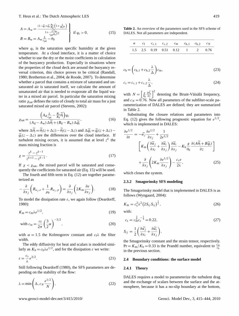
DALES is run on an Arakawa C-grid (see Fig.2). Thepressure, the SFS-TKE, and the scalars are defined at gridcell center, the three velocity components are defined at theWest side, the South side, and the bottom side of the grid cell,respectively.
Hereafter, quantities that are averaged over the LES filterwidth are denoted with a tilde·, time averages with a over-bar · , and averages over the two horizontal directions ofthe domain with angular brackets〈·〉 (slab average). Theprognosed scalars can often be treated in an identical man-ner as the generic scalar fieldϕ∈{θl,qt,qr,Nr,sn}. Primesdenote the subfilter-scale fluctuations with respect to the fil-tered value. Double primes indicate local deviations from thehorizontal slab average. To remain consistent with notationalconventions used in literature and also in the source code ofDALES, some symbols can have different meaning betweendifferent subsections. In such cases, the immediate contextshould always make it clear what each symbol stands for ina particular section. Vertical velocities and fluxes are in gen-eral positive when directed upward; only the radiative and
Table 1. The main thermodynamical constants used throughout thispaper.
Rv Gas constant for water vapor 461.5 J kg−1 K−1
Rd Gas constant for dry air 287.0 J kg−1 K−1
L Latent heat release for vaporization 2.5×10⁶ J kg−1
cpd Heat capacity for dry air 1004 J kg−1 K−1
sedimentation fluxes are positive when pointing downward,following conventions.
In the following sections, different components of the codeare described one by one. Sections2.2–2.7describe the phys-ical and numerical components that are necessary to conducta minimal experiment with DALES. After that, Sects.2.8–2.12describe various forcings and source terms that extendthe core of DALES for use in more specific applications. Fi-nally, Sect.2.13 describes the most relevant statistical rou-tines in DALES.
2.2 The governing equations
DALES assumes the Boussinesq approximation, with the ref-erence stateθ0,ρ0,p0 equal to the surface values of liquidwater potential temperature, density and pressure, respec-tively. For an extended treatment see for exampleWyngaard(2004).
Within the Boussinesq approximation the equations of mo-tion, after application of the LES filter, are given by
∂ui
∂xi
= 0, (5)
∂ui
∂t= −
∂ui uj
∂xj
−∂π
∂xi
+g
θ0θvδi3+Fi −
∂τij
∂xj
, (6)
∂ϕ
∂t= −
∂uj ϕ
∂xj
−∂Ruj ,ϕ
∂xj
+Sϕ, (7)
where the tildes denote the filtered mean variables. Molec-ular transport terms have been neglected. The z-direction(x3) is taken to be normal to the surface,π =
pρ0
+23e is the
modified pressure,δij the Kronecker delta, andFi representsother forcings, including large scale forcings and the Coriolisacceleration
Fcori = −2εijk�j uk, (8)
where� is the Earth’s angular velocity. Source terms forscalarϕ are denoted bySϕ , and may include of microphys-ical (Smcr), radiative (Srad), chemical (Schem), large-scale(S ls), and relaxation (Srel) terms. The subfilter-scale (SFS),or residual, scalar fluxes are denoted byRuj ,ϕ≡ujϕ−uj ϕ,i.e., the contribution to the resolved motion from all scales
www.geosci-model-dev.net/3/415/2010/ Geosci. Model Dev., 3, 415–444, 2010
418 T. Heus et al.: The Dutch Atmospheric LES
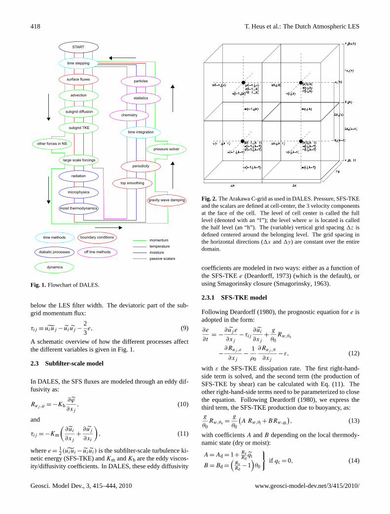
Fig. 1. Flowchart of DALES.
below the LES filter width. The deviatoric part of the sub-grid momentum flux:
τij ≡ uiuj − ui uj −2
3e, (9)
A schematic overview of how the different processes affectthe different variables is given in Fig.1.
2.3 Subfilter-scale model
In DALES, the SFS fluxes are modeled through an eddy dif-fusivity as:
Ruj ,ϕ = −Kh∂ϕ
∂xj
, (10)
and
τij = −Km
(∂ui
∂xj
+∂uj
∂xi
), (11)
wheree =12(uiui − ui ui) is the subfilter-scale turbulence ki-
netic energy (SFS-TKE) andKm andKh are the eddy viscos-ity/diffusivity coefficients. In DALES, these eddy diffusivity
Fig. 2. The Arakawa C-grid as used in DALES. Pressure, SFS-TKEand the scalars are defined at cell-center, the 3 velocity componentsat the face of the cell. The level of cell center is called the fulllevel (denoted with an “f”); the level wherew is located is calledthe half level (an “h”). The (variable) vertical grid spacing1z isdefined centered around the belonging level. The grid spacing inthe horizontal directions (1x and1y) are constant over the entiredomain.
coefficients are modeled in two ways: either as a function ofthe SFS-TKEe (Deardorff, 1973) (which is the default), orusing Smagorinsky closure (Smagorinsky, 1963).
2.3.1 SFS-TKE model
Following Deardorff(1980), the prognostic equation fore isadopted in the form:
∂e
∂t= −
∂uj e
∂xj
−τij
∂ui
∂xj
+g
θ0Rw,θv
−∂Ruj ,e
∂xj
−1
ρ0
∂Ruj ,π
∂xj
−ε, (12)
with ε the SFS-TKE dissipation rate. The first right-hand-side term is solved, and the second term (the production ofSFS-TKE by shear) can be calculated with Eq. (11). Theother right-hand-side terms need to be parameterized to closethe equation. FollowingDeardorff (1980), we express thethird term, the SFS-TKE production due to buoyancy, as:g
θ0Rw,θv =
g
θ0
(A Rw,θl +BRw,qt
), (13)
with coefficientsA andB depending on the local thermody-namic state (dry or moist):
A = Ad = 1+RvRd
qt
B = Bd =
(RvRd
−1)θ0
}if qc = 0, (14)
Geosci. Model Dev., 3, 415–444, 2010 www.geosci-model-dev.net/3/415/2010/
T. Heus et al.: The Dutch Atmospheric LES 419
A = Aw =(1−qt+qs
RvRd
(1+
LRvT
)1+
L2qscpdRvT 2
B = Bw = AwLcpd
−θ0
if qc > 0, (15)
where qs is the saturation specific humidity at the giventemperature. At a cloud interface, it is a matter of choicewhether to use the dry or the moist coefficients in calculationof the buoyancy production. Especially in situations wherethe properties of the cloud deck are around the buoyancy re-versal criterion, this choice proves to be critical (Randall,1980; Bretherton et al., 2004; de Roode, 2007). To determinewhether a parcel that contains a mixture of saturated and un-saturated air is saturated itself, we calculate the amount ofunsaturated air that is needed to evaporate all the liquid wa-ter in a mixed air parcel. In particular the saturation mixingratioχsatdefines the ratio of cloudy to total air mass for a justsaturated mixed air parcel (Stevens, 2002):
χsat=
(Ad
Lcpd
−RvRd
θl
)qc
(Ad−Aw)1θl +(Bd−Bw)1qt, (16)
where1θl = θl(z+1z)− θl(z−1z) and1qt = qt(z+1z)−
qt(z −1z) are the differences over the cloud interface. Ifturbulent mixing occurs, it is assumed that at levelzk themass mixing fraction is
χ =zk
−zk−1
zk+1−zk−1. (17)
If χ < χsat, the mixed parcel will be saturated and conse-quently the coefficients for saturated air (Eq.15) will be used.
The fourth and fifth term in Eq. (12) are together parame-terized as
−∂
∂xj
(Ruj ,e +
1
ρ0Ruj ,p
)=
∂
∂xj
(2Km
∂e
∂xj
). (18)
To model the dissipation rateε, we again follow (Deardorff,1980):
Km = cmλe1/2, (19)
with cm =cf
2π
(3
2α
)−3/2
, (20)
with α = 1.5 the Kolmogorov constant andcfλ the filterwidth.
The eddy diffusivity for heat and scalars is modeled simi-larly asKh = chλe1/2, and for the dissipationε we write:
ε =cε
λe3/2. (21)
Still following Deardorff(1980), the SFS parameters are de-pending on the stability of the flow:
λ = min
(1,cN
e1/2
N
), (22)
Table 2. An overview of the parameters used in the SFS scheme ofDALES. Not all parameters are independent.
α cf cε,1 cε,2 cm ch,1 ch,2 cN
1.5 2.5 0.19 0.51 0.12 1 2 0.76
ch =
(ch,1+ch,2
λ
1
)cm, (23)
cε = cε,1+cε,2λ
1, (24)
with N =
[gθ0
∂θv∂z
]2denoting the Brunt-Vaisala frequency,
andcN = 0.76. Now all parameters of the subfilter-scale pa-rameterization of DALES are defined; they are summarizedin Table2.
Substituting the closure relations and parameters intoEq. (12) gives the following prognostic equation fore1/2,which is implemented in DALES:
∂e1/2
∂t= −uj
∂e1/2
∂xj
+1
2e1/2[Km
(∂uj
∂xi
+∂ui
∂xj
)∂ui
∂xj
−Khg
θ0
∂(Aθl +Bqt)
∂z
]
+∂
∂xj
(2Km
∂e1/2
∂xj
)−
cεe
2λ, (25)
which closes the system.
2.3.2 Smagorinsky SFS modeling
The Smagorinsky model that is implemented in DALES is asfollows (Wyngaard, 2004):
Km = c2sλ
2(2SijSij
) 12 , (26)
with:
cs = c34mc
−14
ε = 0.22, (27)
Sij =1
2
(∂uj
∂xi
+∂ui
∂xj
),
the Smagorinsky constant and the strain tensor, respectively.Pr= Km/Kh = 0.33 is the Prandtl number, equivalent tocm
chin the previous section.
2.4 Boundary conditions: the surface model
2.4.1 Theory
DALES requires a model to parameterize the turbulent dragand the exchange of scalars between the surface and the at-mosphere, because it has a no-slip boundary at the bottom,
www.geosci-model-dev.net/3/415/2010/ Geosci. Model Dev., 3, 415–444, 2010
420 T. Heus et al.: The Dutch Atmospheric LES
but does not resolve the flow up to the surface-roughnessscale. The surface fluxes enter the domain at subfilter-scale,since by definition the resolved fluctuations in the verticalvelocity at the surface are equal to zero. In the remainder ofthis section we define an arbitrary surface flux of variableφ
asFs,φ = wφ− wφ.We followed the common way of parameterizing turbu-
lent fluxes in atmospheric models by applying the transferlaws of Louis (1979). In DALES we assume that the firstmodel level is in the atmospheric surface layer. We applyMonin-Obukhov similarity theory for the computation of thespatially averaged fluxes
⟨Fs,φ
⟩and gradients at the bottom
boundary of the model.The procedure for determining the bottom boundary con-
ditions starts with the evaluation of the Obukhov length. Thisvalue is approximated using a Newton-Rhapson method forsolving the implicit equation that relates the bulk Richardsonnumber to the Obukhov length (see Eq.28).
RiB =z1
L
[ln(
z1z0h
)−9H
(z1L
)+9H
(z0hL
)][ln(
z1z0m
)−9M
(z1L
)+9M
(z0mL
)]2, (28)
with
RiB =g
θ0
z1(⟨θv1⟩−⟨θv0⟩)
〈U1〉2
, (29)
and
L = −u3
∗0
κg
〈θv0〉
⟨Fs,θv
⟩ , (30)
whereRiB is the averaged bulk Richardson number of thelayer between the surface and the first full levelz1, L is theObukhov length,z0m andz0h are the roughness lengths formomentum and heat,9H and9M are the integrated stabil-ity functions as provided byBeljaars(1991) for the stableatmosphere andWilson (2001) for the unstable atmosphere,⟨θv0⟩
is the spatially averaged filtered surface virtual poten-tial temperature,
⟨θv1⟩is the spatially averaged filtered virtual
potential temperature at the first model level,〈U1〉 is the mag-nitude of the horizontal wind vector at the first model level,defined as〈U1〉 =
√〈u1〉
2+〈v1〉
2, κ is the Von Karman con-
stant and⟨w′θ ′
v0
⟩is the horizontally averaged surface virtual
temperature flux.Subsequently, the calculated Obukhov length is used in the
computation of the slab averaged friction velocityu∗0 and
scalar scalesϕ∗0 = −〈Fs,φ〉
u∗0, based on the scaling arguments
of Businger et al.(1971); Yaglom(1977).Now, we can calculate the drag coefficientsCM andCϕ :
CM =u2
∗0
〈U1〉2, (31)
Cϕ =u∗0ϕ∗0
〈U1〉〈ϕ1−ϕ0〉. (32)
Although all locations in the horizontal use the same dragcoefficient, we calculate local fluxes and gradients that aver-age to the values computed in our evaluation of the Obukhovlength. The subfilter-scale momentum fluxes are calculatedby decomposingu2
∗0 along the two components of the hori-zontal wind vector (Eqs.33, 34), whereas Eq. (35) gives thescalar flux. This results in
Fs,u = −CM 〈U1〉u1, (33)
Fs,v = −CM 〈U1〉v1, (34)
Fs,ϕ = −Cϕ 〈U1〉(ϕ1−ϕ0). (35)
For land surfaces where moisture is not freely available, suchas a vegetated land surface or a bare soil, an additional stephas to be made before the similarity relation as in Eq. (35)can be applied to the specific humidity. Here, we definethe aerodynamic resistancera as
(Cϕ 〈U1〉
)−1 and introducethe surface resistancers that takes into account the limitedwater supply at the land surface. The value forrs is ei-ther prescribed or calculated using the Jarvis-Stewart model(Jarvis, 1976), where the correction functions for radiation,soil moisture and vapor pressure deficit are taken from theECMWF Integrated Forcast System (cycle 31R1), and thecorrection function for temperature fromNoilhan and Plan-ton (1989). A urface value can be computed:
〈q0〉 =ra
ra+rs〈qs(T0)〉+
rs
ra+rs〈q1〉. (36)
Note that the drag coefficients and resistances are based onslab averaged values, to assure that the spatially averagedfluxes and gradients are consistent with Monin-Obukhovsimilarity theory. In DALES there is also the option availableto work with locally computed values. We are aware that thismethod overpredicts gradients at the first model level (Bou-Zeid, 2005). We, however, use this method for exploratoryexperiments over heterogeneous land surfaces, because herea universal surface model formulation is still lacking (Bou-Zeid, 2005).
2.4.2 Overview of surface boundary options in DALES
DALES has four options to provide the surface momentumand scalar fluxes and surface scalar values to the model, withdifferent degrees of complexity.
1. Parameterized surface scalar and momentum fluxes, pa-rameterized surfaces values. Here, a Land SurfaceModel (LSM, see Sect.2.4.3) calculates the surfacetemperature and the stomatal resistance which enters inthe evaporation equation based on the vegetation typethat is assigned to the grid cell. The variablesu∗0, L
andϕ∗0 are determined iteratively to get the drag coeffi-cients. This is the method that represents a fully interac-tive land surface. Combined with the radiation model,this options allows for the simulation of full diurnal cy-cles, in which both the surface fluxes and the surfacetemperature are free variables.
Geosci. Model Dev., 3, 415–444, 2010 www.geosci-model-dev.net/3/415/2010/
T. Heus et al.: The Dutch Atmospheric LES 421
2. Parameterized surface scalar and momentum fluxes,prescribed scalar values at the surface. In this optionu∗0, L andϕ∗0 are solved iteratively to get the drag co-efficients. The surface momentum and scalar fluxes arecomputed using the prescribed scalar values at the sur-face and the acquired drag coefficients. This option iscommonly used as the surface boundary condition forsimulations of marine boundary-layers. It is also ap-plied in the simulation of stable boundary layers. Forsimulations over land, a fixed surface resistancers canbe prescribed.
3. Prescribed surface scalar fluxes, prescribedu∗0. In thisoption no iterations are necessary and the scalar surfacevaluesϕ0 are calculated diagnostically. This is an op-tion that is used in idealized simulations in which thesurface drag is preferred to be controlled, thereby ne-glecting thatu∗0 is an internal parameter of the flow.
4. Prescribed surface scalar fluxes, parameterizedu∗0.Hereu∗0 andL are calculated iteratively, whereasϕ∗ isdiagnostically calculated as a function of the prescribedscalar fluxes and the calculatedu∗0. This is the mostcommonly used option for simulation of daytime con-vection over land.
Prescribed fluxes or surface values may depend on time; lin-ear interpolation is then performed between the given “an-chor” points.
In addition to the previous description which assumed ho-mogeneous surfaces, DALES is also able to simulate hetero-geneously forced ABLs. Under such conditions, only theprescribed scalar fluxes boundary conditions are available.Scalar fluxes are defined per grid cell, whereas the momen-tum flux is dynamically computed. In these conditions, localvalues ofu∗0, L andϕ∗0 are used.
2.4.3 Land surface model
DALES has the option to use a land surface model (LSM).The LSM has two components, namely a solver for the sur-face energy balance and a four layer soil scheme which cal-culates the soil temperature profile for each grid cell. Thefollowing surface energy balance equation is solved:
CskdT0
dt= Q∗ −ρcpFs,θl
−ρLvFs,qt −G, (37)
in which Csk is the heat capacity per unit of area of the skinlayer (seeDuynkerke, 1999), T0 is the surface temperature,Q∗ is the net radiation andG is the ground heat flux. Ifthe LSM is used, the surface resistancers in Eq. (36) iscalculated using the Jarvis-Stewart parameterization (Jarvis,1976).
The ground heat flux is parameterized as:
G = 3(T0−Tsoil1), (38)
in which 3 is a bulk conductivity for the stagnant air in theskin layer (Duynkerke, 1999) depending on the type of sur-face, andTsoil1 is the temperature of the top soil layer.
The soil consists of four layers in which the heat transportis solved using a simple diffusion equation in which both theconductivity and the heat capacity are functions of the prop-erties of the soil material and of the soil moisture content.The temperature at the bottom of the lowest soil layer is pre-scribed.
2.5 Boundary conditions: the sides and top
In comparison with the boundary conditions at the bottomboundary, the boundary conditions at the top and the sides ofthe domain are relatively straightforward. In the horizontaldirections, periodic boundary conditions are applied for allfields. At the top of the domain, we take:
∂u
∂z=
∂v
∂z= 0; w = 0;
∂ϕ
∂z= constant in time. (39)
Fluctuations of velocity and scalars at the top of the do-main (for instance due to gravity waves) are damped outby a sponge layer through additional forcing/source terms(added to the right-hand-side of the transport equations):
Fspi (z) =
1
t sp(〈ui〉− ui), (40)
Sspϕ (z) =
1
t sp(〈ϕ〉− ϕ), (41)
with t sp a relaxation time scale that goes fromt
sp0 =1/(2.75×10−3) s≈6 min at the top of the domain
to infinity at the bottom of the sponge layer, which is bydefault a quarter of the number of levels, with a minimum of15 levels.
2.6 Pressure solver
To solve for the modified pressureπ , the divergence ∂∂xi
of Eq. (6) is taken. Subsequently, the continuity equation(Eq. 5) is applied (both divergence and continuity equationare applied in their discrete form). As a result, the left handside of the equation is equal to zero. Rearranging the termsleads to a Poisson equation for the modified pressure:
∂2π
∂x2i
=∂
∂xi
(−
∂ui uj
∂xj
+g
θ0θvδi3+Fi −
∂τij
∂xj
). (42)
Since computations are performed in a domain that is pe-riodic in both horizontal directions, the Poisson equation issolved by applying a Fast Fourier Transform in the lateral di-rections followed by solving a tri-diagonal linear system inthe z-direction using Gaussian elimination. In the latter, thepressure gradients at the upper and lower boundary are set tozero. An inverse Fast Fourier Transform in both lateral di-rections is applied to the result of the Gaussian eliminationto obtain the modified pressure.
www.geosci-model-dev.net/3/415/2010/ Geosci. Model Dev., 3, 415–444, 2010
422 T. Heus et al.: The Dutch Atmospheric LES
2.7 Numerical scheme
A Cartesian grid is used, with optional grid stretching in thez-direction. For clarity, an equidistant grid is assumed in thediscussion of the advection scheme. The grid is staggeredin space as an Arakawa C-grid; the pressure, the SFS-TKEand the scalars are defined atx+
12(1x,1y,1z), theu is de-
fined atx+12(0,1y,1z), and similar forv andw. The level
of cell center is called the full level (denoted with an “f”);the level wherew is located is called the half level (an “h”).The (variable) vertical grid spacing1z is defined centeredaround the belonging level (see Fig.2). The grid spacing inthe horizontal directions (1x and1y) is constant over theentire domain.
To be able to use multiple computational processes, thusdecreasing the wall clock time of experiments, DALES 3.2has been parallelized by dividing the domain in separatestripes in the y-direction. Tests show that this method is com-putationally efficient as long as the amount of processes issmaller than a quarter of the number of grid points in they-direction. In the near future, we plan to also divide the do-main in the x-direction, leaving narrow columns to be calcu-lated by each process, and ensuring that the maximum num-ber of processes would scale with the total number of gridpoints in each slab, thus allowing for much larger experi-ments.
Time integration is performed by a third order Runge-Kutta scheme followingWicker and Skamarock(2002).With f (φn) the right-hand side of the appropriate equation ofEqs. (6–7) for variableφ = {u,v,w,e1/2,ϕ}, φn+1 at t +1t
is calculated in three steps:
φ∗= φn
+1t
3f (φn),
φ∗∗= φn
+1t
2f (φ∗),
φn+1= φn
+1tf (φ∗∗), (43)
with the asterisks denoting intermediate time steps. The sizeof the time step1t is determined adaptively, and is limitedby both the Courant-Friedrichs-Lewy criterion ( CFL)
CFL= max
(∣∣∣∣ ui1t
1xi
∣∣∣∣), (44)
and the diffusion numberd (seeWesseling, 1996).
d = max
(3∑
i=1
Km1t
1x2i
). (45)
The numerical stability and accuracy depends on the spatialscheme that is used. Furthermore, additional terms, such aschemical or microphysical source, may require more strin-gent time stepping. Therefore, the limiting CFL andd
numbers can be manually adjusted to further optimize thetimestep. By default CFL andd are set well below the
stability levels known from the literature of the respectivecombinations of spatial and temporal integration scheme (seeWicker and Skamarock, 2002).
Depending on the desired properties (like high accuracyor monotonicity), several advection schemes are available.With advection in the x-direction discretized as
∂uiφi
∂x=
Fi+ 1
2−F
i− 12
1x, (46)
with Fi− 1
2the convective flux of variableφ through thei− 1
2
plane; thei− 12 plane is the plane through the location of ve-
locity ui(i), perpendicular on the direction of velocityui(i).Since we are using a staggered grid, the velocity is availableat i− 1
2 without interpolation (see Fig.2). Second order cen-tral differencing can be used for variables where neither veryhigh accuracy nor strict monotonicity is necessary:
F 2ndi− 1
2= u
i− 12
φi +φi−1
2, (47)
and similar forF 2ndi− 1
2. A higher-order accuracy in the calcu-
lation of the advection is reached with a sixth order centraldifferencing scheme (seeWicker and Skamarock, 2002):
F 6thi− 1
2=
ui− 1
2
60
[37(φi+φi−1)−8(φi+1+φi−2)+(φi+2+φi−3)
].
(48)
Starting with this sixth order scheme, a nearlymonotonous fifth order scheme can be constructed byadding a dissipative term toF 6th
i− 12,
F 5thi− 1
2= F 6th
i− 12−
∣∣∣∣∣ ui− 12
60
∣∣∣∣∣ (49)[10(φi −φi−1)−5(φi+1−φi−2)+(φi+2−φi−3)
].
For advection of scalars that need to be strictly monotone (forexample chemically reacting species) theκ scheme (Hunds-dorfer et al., 1995) has been implemented:
F κ
i− 12
= ui− 1
2
[φi−1+
1
2κi− 1
2(φi−1−φi−2)
], (50)
in caseu > 0. Following Hundsdorfer et al.(1995), κi−1/2serves as a switch between third order upwind advection incase of small upwind gradients ofφ, and a first order upwindscheme in case of stronger gradients. This makes the schememonotone, but also more dissipative, effectively taking overthe role of the SFS-scheme in regions of strong gradients.
2.8 Cloud microphysics
The cloud-microphysical scheme implemented in DALES isa bulk scheme for precipitating liquid-phase clouds. The hy-drometeor spectrum is divided in a cloud droplet and raindrop category. The cloud liquid water specific humidityqc is
Geosci. Model Dev., 3, 415–444, 2010 www.geosci-model-dev.net/3/415/2010/
T. Heus et al.: The Dutch Atmospheric LES 423
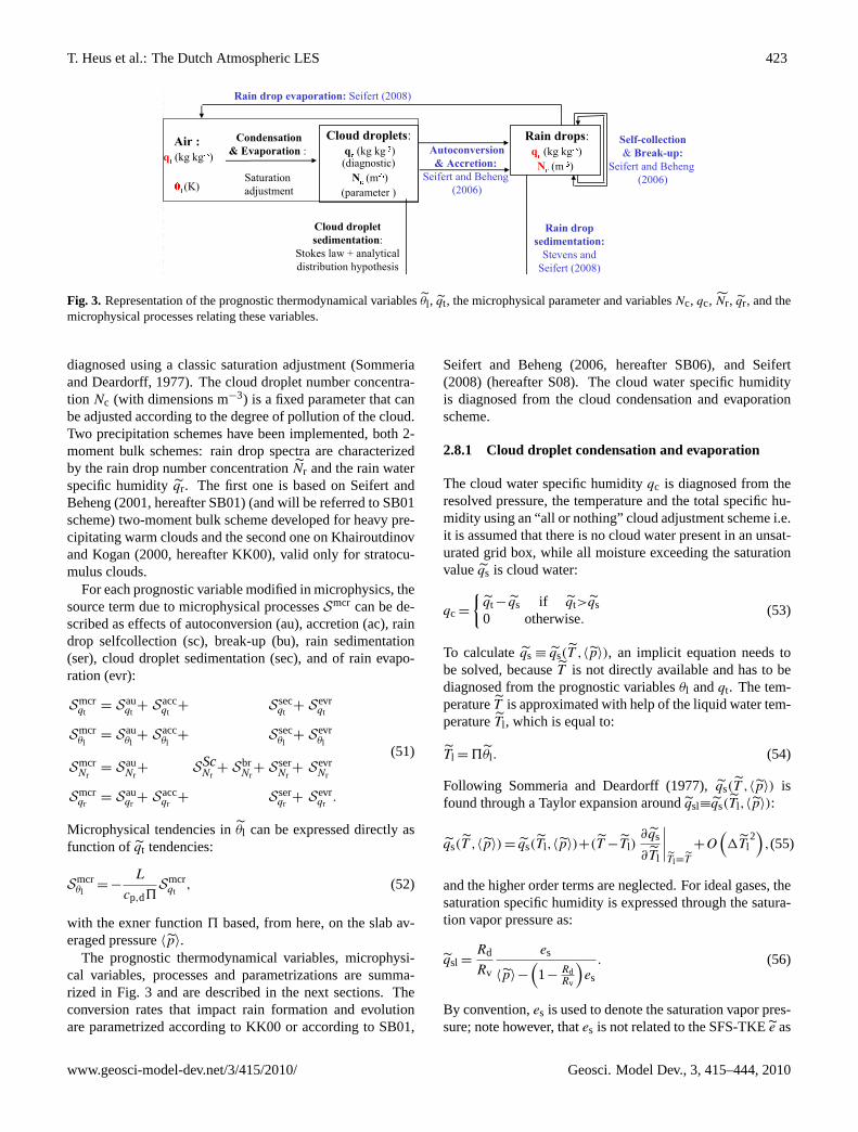
Fig. 3. Representation of the prognostic thermodynamical variablesθl , qt, the microphysical parameter and variablesNc, qc, Nr, qr, and themicrophysical processes relating these variables.
diagnosed using a classic saturation adjustment (Sommeriaand Deardorff, 1977). The cloud droplet number concentra-tion Nc (with dimensions m−3) is a fixed parameter that canbe adjusted according to the degree of pollution of the cloud.Two precipitation schemes have been implemented, both 2-moment bulk schemes: rain drop spectra are characterizedby the rain drop number concentrationNr and the rain waterspecific humidityqr. The first one is based onSeifert andBeheng(2001, hereafter SB01) (and will be referred to SB01scheme) two-moment bulk scheme developed for heavy pre-cipitating warm clouds and the second one onKhairoutdinovand Kogan(2000, hereafter KK00), valid only for stratocu-mulus clouds.
For each prognostic variable modified in microphysics, thesource term due to microphysical processesSmcr can be de-scribed as effects of autoconversion (au), accretion (ac), raindrop selfcollection (sc), break-up (bu), rain sedimentation(ser), cloud droplet sedimentation (sec), and of rain evapo-ration (evr):
Smcrqt
= Sauqt
+ Saccqt
+ Ssecqt
+ Sevrqt
Smcrθl
= Sauθl
+ Saccθl
+ Ssecθl
+ Sevrθl
SmcrNr
= SauNr
+ SScNr
+ SbrNr
+ SserNr
+ SevrNr
Smcrqr
= Sauqr
+ Saccqr
+ Sserqr
+ Sevrqr
.
(51)
Microphysical tendencies inθl can be expressed directly asfunction of qt tendencies:
Smcrθl
= −L
cp,d5Smcr
qt, (52)
with the exner function5 based, from here, on the slab av-eraged pressure〈p〉.
The prognostic thermodynamical variables, microphysi-cal variables, processes and parametrizations are summa-rized in Fig.3 and are described in the next sections. Theconversion rates that impact rain formation and evolutionare parametrized according to KK00 or according to SB01,
Seifert and Beheng(2006, hereafter SB06), andSeifert(2008) (hereafter S08). The cloud water specific humidityis diagnosed from the cloud condensation and evaporationscheme.
2.8.1 Cloud droplet condensation and evaporation
The cloud water specific humidityqc is diagnosed from theresolved pressure, the temperature and the total specific hu-midity using an “all or nothing” cloud adjustment scheme i.e.it is assumed that there is no cloud water present in an unsat-urated grid box, while all moisture exceeding the saturationvalueqs is cloud water:
qc =
{qt − qs if qt>qs0 otherwise.
(53)
To calculateqs ≡ qs(T ,〈p〉), an implicit equation needs tobe solved, becauseT is not directly available and has to bediagnosed from the prognostic variablesθl andqt. The tem-peratureT is approximated with help of the liquid water tem-peratureTl , which is equal to:
Tl = 5θl . (54)
Following Sommeria and Deardorff(1977), qs(T ,〈p〉) isfound through a Taylor expansion aroundqsl≡qs(Tl,〈p〉):
qs(T ,〈p〉) = qs(Tl,〈p〉)+(T −Tl)∂qs
∂Tl
∣∣∣∣Tl=T
+O(1Tl
2),(55)
and the higher order terms are neglected. For ideal gases, thesaturation specific humidity is expressed through the satura-tion vapor pressure as:
qsl =Rd
Rv
es
〈p〉−
(1−
RdRv
)es
. (56)
By convention,es is used to denote the saturation vapor pres-sure; note however, thates is not related to the SFS-TKEe as
www.geosci-model-dev.net/3/415/2010/ Geosci. Model Dev., 3, 415–444, 2010
424 T. Heus et al.: The Dutch Atmospheric LES
defined in Sect.2.3. The Clausius-Clapeyron relation relateses to the temperature:
des
dT=
Les
RvT 2, (57)
with Rv = 461.5 J kg−1 K−1 denoting the gas constant forwater vapor. It can be solved in very good approximationas:
es(Tl) = es0exp
[aTl −T trip
Tl −b
], (58)
with constantses0= 610.78 Pa,T trip = 273.16 K, a = 17.27andb = 35.86 K. After having substituted in Eqs. (56–58)into the truncated Taylor expansion Eq. (55) we obtain forthe saturated specific humidity:
qs= qsl
(1+
L2
Rvcp,dTl2qt
)(1+
L2
Rvcp,dTl2qsl
)−1
, (59)
and finally the cloud water specific humidity can be calcu-lated with Eq. (53). When higher accuracy is necessary, theprocedure can be applied iteratively.
2.8.2 Cloud droplet sedimentation
The cloud droplet sedimentation process has an impact oncloud evolution by reducing entrainment at stratocumuluscloud top (Ackerman et al., 2004; Bretherton et al., 2007).Its cloud water specific humidity source term can be ex-pressed as the derivative of a sedimentation flux. The latteris parametrized by assuming a Stokes law to calculate thecloud droplets terminal velocity and a log-normal distribu-tion to represent the cloud droplet spectrum (Ackerman et al.,2009), which lead to the following expression:
F secqc
= kSt4
3πρw N
−2/3c q
5/3c exp(5ln(σgc)
2), (60)
with ρw = 1000 kg m−3, kSt= 1.2×10⁸ m−1 s−1 and the log-normal geometric standard deviation parameterσgc is set to1.3 (Geoffroy et al., 2010).
2.8.3 Rain drop processes
The precipitation processes are parameterized as functionsof the local thermodynamical state. Thus they are valid onlyfor simulations where microphysical fields are explicitly re-solved, as is the case in LES. To be able to neglect subfilter-scale fluctuations, resolution must not be more than 200 mhorizontally and a few ten of meters vertically.
In slightly precipitating clouds, most of the falling massis contained in particles smaller than 50 µm in radius, alsoreferred to as drizzle. InKhairoutdinov and Kogan(2000)scheme, the limit between the cloud category and the raincategory is set at the radius value of 25 µm which permits
consideration of drizzle in the precipitating category, whichcan have significant impact on the evolution of the boundarylayer. This scheme is empirically based: it has been tunedwith spectra derived from 3-D simulations of stratocumulusclouds using a coupled LES-bin microphysics model. Thus itis valid only for stratocumulus clouds. Because a descriptionof that scheme is fully given inKhairoutdinov and Kogan(2000), it is not described here.
The SB01 scheme assumes the limit at the separating massvaluex0 of 2.6×10⁻¹⁰ kg which corresponds to a separatingradiusr0 of the order of 40 µm. Thus the SB01 scheme ismore suitable for heavily precipitating clouds, in which mostof the falling mass is contained in millimeter size particles.The parametrized collection rates are expressed in functionof the microphysical variables by analytical integration of thestochastic collection equation (SCE) and assuming analyticaldistributions to represent the hydrometeor spectra. A correc-tion function is added to the autoconversion and accretionrate, that take in account the evolution of the cloud dropletspectra due to conversion of cloud water in rain water.
The rain drop size distribution (RDSD) is assumed to bea Gamma distribution:
nr(r) = N0λµr+1r rµre−λrr , (61)
wherer is the rain drop radius.N0 and the slope parameterλr can be expressed as a function of the prognostic variablesand µr. In autoconversion and accretion parametrizations,µr has been set to theMarshall and Palmer(1948) value (i.e.0) and is fixed because the parametrizations have been tunedwith such a value using spectra derived from 1-D simulationsusing a coupled LES-bin microphysics model. The value ofthe shape parameterµr is parametrized in function of the rainwater content (Geoffroy et al., 2010):
µr = 0.5/(1000ρqr)0.7
−1, (62)
2.8.4 Autoconversion from cloud droplets to rain drops
Autoconversion is the process that initializes the rain dropspectra. After analytical integration of the SCE andadding of correction function, SB06 obtained the followingparametrized expressions:
Sauqr
=kau
20x0
(νc+2)(νc+4)
(νc+1)2q2
cx2c
(1+
ζau(χl)
(1−χl)2
)ρ0, (63)
Sauqt
= −Sauqr
, (64)
with:
χl = qr/(qc+ qr), (65)
ζau(χl) = 400χ0.7l
(1−χ0.7
l
)3, (66)
andkau= 10.58×10⁹ m3 kg−2 s−1 (Pinsky and Khain, 2002,SB06) andxc is the mean mass of the cloud droplet distribu-tion. νc is parametrized according toGeoffroy et al.(2010):
νc = 1580ρqc−0.28, (67)
Geosci. Model Dev., 3, 415–444, 2010 www.geosci-model-dev.net/3/415/2010/
T. Heus et al.: The Dutch Atmospheric LES 425
New drizzle drops are assumed to have a radius equal to theseparating radiusr0. Thus the rain number concentrationsource term due to autoconversion is:
SauNr
=Sau
qr
4πρw3ρ
r30
, (68)
2.8.5 Accretion of cloud droplets
The growth rate of rain drops by collecting cloud droplets istaken to be a function of the cloud and rain water contents(SB06):
Saccqr
= kaccqcqrζacc,(ρ0ρ)12 (69)
Saccqt
= −Saccqr
, (70)
with:
ζacc(χl) =
(χl
χl +5×10⁻⁵
)4
, (71)
andkacc=5.25 m3 kg−1 s−1.
2.8.6 Rain drop selfcollection
The rain number concentration decreases because of the self-collection process, i.e. interaction between rain drops to-gether to form larger rain drops. Its parametrization is ex-pressed as the following (SB06):
SscNr
= −kscNrqr
(1+
κsc
λr(4
3πρw)1/3
)−9
(ρ0ρ)12 , (72)
with ksc= 7.12 m3 kg−1 s−1 andκsc= 60.7 kg−1/3.
2.8.7 Break-up of rain drops
The break-up of rain drops into smaller rain drops is appliedfor spectra with a mean volume radiusrvr larger than 150 µmfollowing (SB06):
SbrNr
= −SscNr
(kbr(rvr −req)+1
), (73)
with kbr = 2000 m−1 andreq= 550 µm. Whenrvr becomeslarger thanreq the break-up process becomes predominantover the selfcollection process. The strong increase of thebreak-up process for large mean volume radius is not takenin account.
2.8.8 Rain drop sedimentation
Assuming theRogers et al.(1993) dependence of rain dropterminal velocity in function of the drop radius, the flux ofthe rain number concentration and the flux of the rain waterspecific humidity are (Stevens and Seifert, 2008):
F serNr
=
(a−b(1+c/λr)
µr+1)Nr, (74)
F serqr
=
(a−b(1+c/λr)
µr+4)qr, (75)
with a = 9.65 m s−1, b=9.8 m s−1, c = 1200 m−1 (see S08).
2.8.9 Rain drop evaporation
The tendency of the rain water specific humidity due to evap-oration is expressed by integration of the drop growth rate byvapor diffusion formulation (S08):
Sevrqr
≈ 4πρw
ρG(T ,P )
qt − qs
qs
(Nrλr)µr+1
0(µr +1)
×
[av0(µr +2)λ−(µr+2)
r +bvSc13
(a
νa
)1/2
0
(µr +
5
2
)
× λ
(−µr+
52
)r
1−1
2
b
a
(λr
c+λr
)(µr+52
), (76)
where0(x) is the gamma distribution,
G(T ,P ) =1
ρw
[RvT
es(T )Dv+
L
kaT
(L
RvT−1
)]−1
, (77)
Sc, the Schmidt number,av andbv are ventilation factor co-efficients with the following values:Sc= 0.71,av = 0.78 andbv = 0.308 (Pruppacher and Klett, 1997).
The tendency of the rain drop number concentration dueto evaporation is assumed to be (S08):
SevrNr
= γNr
qrSevr
qr, (78)
with γ = 0.7 (A. Seifert, personal communication, 2008).Note that a 0 value ofγ means that no rain drop disappearduring evaporation. A value larger than 1 would be possi-ble if a large number of little rain drops totally evaporate inpresence of large drops.
2.9 Radiation schemes
The net radiative heating is equal to the (downward pointing)radiative flux divergence (per unit wave length) integratedover all wavelengthsν:
Sradθl
=
∫∞
0ρ0cpd
∂F rad(ν)
∂zdν, (79)
DALES includes a multi-waveband radiative transfer model.It needs information of the vertical profiles of temperature,humidity and ozone up to the top of the atmosphere. To re-duce the computational cost of the radiative transfer calcu-lation, DALES has implemented the Monte Carlo SpectralIntegration (Pincus and Stevens, 2008), where at each gridpoint and at each time step the radiative flux is approximatedby the radiative flux of one randomly chosen waveband, or arandomly chosen part of that waveband where all absorptioncoefficients are similar. A complete discussion of the radia-tive transfer model can be found inFu and Liou(1992); Fuet al.(1997).
DALES also includes a simple parameterization for thevertical component of the longwave radiation and of the
www.geosci-model-dev.net/3/415/2010/ Geosci. Model Dev., 3, 415–444, 2010
426 T. Heus et al.: The Dutch Atmospheric LES
shortwave radiation through computationally cheap analyticapproximations of the Mie theory, that maintain sufficientaccuracy for most purposes. In the parameterized radiationscheme, radiative transfer is computed at every single col-umn of the LES, neglecting horizontal radiative transfer.
2.9.1 The GCSS parameterization for longwave radia-tion
The absorptivity of longwave radiation is controled by theliquid water path (LWP),
LWP(x,y,z1,z2) = ρair
∫ z2
z1
qc(x,y,z)dz. (80)
The net longwave radiative fluxF radL is linked to the liquid
water path through an analytic formula,
F radL (x,y,z) = FL(ztop)e
−kLWP(x,y,z,ztop)
+FL(0)e−kLWP(x,y,0,z), (81)
wherek is the absorption coefficient, andFL(ztop) andFL(0)
represent the total net longwave radiative flux at the top of thecloud and the cloud base, respectively.Larson et al.(2007)discuss the validity of this parameterization in detail. Theyconclude that when the parameterization constants are opti-mized for individual stratocumulus cases like the ones set upby Duynkerke et al.(1999, 2004), andStevens et al.(2005),the formula yields remarkably accurate fluxes and heatingrates for low clouds.
To study the effect of longwave radiative on the generationof turbulence, but in the absence of latent heat release effectsthat occur in a real liquid water cloud, one can substitute theliquid water path by the vertical integral of a passive scalar.This so-called “smoke” cloud has an initial concentration setto unity in the boundary layer and zero above (Brethertonet al., 1999b). The liquid water path in the longwave radia-tion Eq. (81) is then replaced by the smoke path, which canbe computed by substitutingqc by the smoke concentrationsin Eq. (80). For a smoke absorptivityk = 0.02 m2 kg−1 oneobtains similar cooling rates as in stratocumulus (Brethertonet al., 1999b). It should be noted that unlike liquid water,smoke is a conserved quantity. This means that if smokeis transported by turbulence into the inversion layer, it willcause a local cooling tendency in this layer.
2.9.2 The delta-Eddington model for shortwave radia-tive transfer
In the shortwave band the cloud optical depthτ is themost important parameter defining the radiative properties ofclouds,
τ(x,y,z) =3
2
LWP(x,y,z,zt)
reρw. (82)
Herere defines the cloud droplet effective radius, i.e. the ratioof the third moment to the second moment of the droplet size
distribution (Stephens, 1984). A constant value forre is used,and for marine boundary layer clouds isre = 10 µm, whichwas observed for stratocumulus over the Pacific Ocean offthe coast of California during FIRE I (Duda et al., 1991).
Cloud droplets scatter most of the incident radiation intothe forward direction. This asymmetry in the distribution ofthe scattering angle is measured by the first moment of thephase function, and is commonly refered to as the asymme-try factor g which is takeng = 0.85. The radiative transferfor shortwave radiation in clouds is modeled by the delta-Eddington approximation, in which the highly asymmetricphase function is approximated by a Dirac delta function anda two term expansion of the phase function (Joseph et al.,1976). The physical interpretation of this approach is thatforward scattered radiation is treated as direct solar radiation.
The ratio of the scattering coefficientQs to the extinc-tion coefficient Qe is called the single scattering albedoω0 = Qs/Qe, and is unity for a non-absorbing medium. Fol-lowing Fouquart(1985),
ω0 = 1−9×10⁻⁴−2.75×10⁻³(µ0+1)e−0.09τt , (83)
with τt the total optical depth in a subcloud column. Dueto multiple scattering this small deviation ofω0 from unityleads to a non-negligible absorption of shortwave radiation.
The delta-Eddington equations are exactly the same as theEddington equations (Joseph et al., 1976) with transformedasymmetry factorg, single-scattering albedoω0 and opticaldepthτ substituted by primed quantities:
g′=
g
1+g, (84)
ω′
0 =(1−g2)ω0
1−ω0g2, (85)
τ ′= (1−ω0g
2)τ, (86)
For constantω0 and g the delta-Eddington equation canbe solved analytically (Shettle and Weinman, 1970; Josephet al., 1976):
F rads (x,y,z) = F0
4
3[p(C1e
−kτ ′(x,y,z)−C2e
kτ ′(x,y,z))−βe−
τ ′(x,y,z)µ0
]+µ0F0e
−τ ′(x,y,z)
µ0 , (87)
with:
k = [3(1−ω′
0)(1−ω′
0g′)]1/2, (88)
p =
(3(1−ω′
0)
1−ω′
0g′
)1/2
, (89)
β = 3ω′
0µ01+3g′(1−ω′
0)µ20
4(1−k2µ20)
, (90)
andµ0 = cosα0 for a solar zenith angleα0. The values ofthe constantsC1 andC2 in Eq. (87) are calculated from the
Geosci. Model Dev., 3, 415–444, 2010 www.geosci-model-dev.net/3/415/2010/
T. Heus et al.: The Dutch Atmospheric LES 427
boundary conditions. A prescribed value for the total down-ward solar radiation (parallel to the beam) determines the up-per boundary condition at the top of the cloudF0. In addi-tion, it is assumed that at the ground surface a fraction ofthe downward radiation reaching is reflected back by a Lam-bertian ground surface with albedoAg. See for further de-tails Shettle and Weinman(1970) andJoseph et al.(1976).The delta-Eddington solution is applied in every column us-ing the local cloud optical depth. A study byde Roode andLos (2008) of the cloud albedo bias effect showed a goodagreement between results obtained with the delta-Eddingtonapproach and from the I3RC Monte-Carlo model (Cahalanet al., 2005) that utilizes the full three-dimensional structureof the cloud field.
2.10 Other forcings and sources
Large-scale forcings and sources, such as the meangeostrophic windug, the large-scale subsidencews, and thehorizontal advective scalar transport may depend on heightand time. The effects of large-scale subsidence are calcu-lated using the slab-averaged scalar profiles and a prescribedsubsidence velocityws(z,t) (see, e.g.Siebesma et al., 2003):
Ssubsϕ = −ws
∂ 〈ϕ〉
∂z, (91)
Optionally, the slab-averaged prognostic variables can benudged with a relaxation time scalet rel to a prescribed (timedepending) valueϕrel:
Srelϕ = −
1
t rel
(〈ϕ〉−ϕrel
), (92)
analogous to large-scale forcings in single column models(seeNeggers et al., 2010). The application ofSrel
ϕ to the hor-izontal mean〈ϕ〉, instead of to the individual values ofϕ,ensures that room for variability within the LES domain re-mains, and the small-scale turbulence will not be disturbedby the nudging.
2.11 Flow over tilted surfaces
To simulate flow over a sloped surface under an angleα
(> 0), a coordinate transformation is performed; computa-tions are then done in a system(s,y,n) , with s andn arethe coordinates in the down slope direction and perpendicu-lar to the slope, respectively. Under the assumption that theflow can be considered homogeneous along the slope (seeSect.3.5), only the buoyancy force is directly dependent ons. The original gravitational forcingg
θ0θvδi3 needs to cor-
rected. The reformulated gravitational forcing is equal to:
Fslopeus
= −g
θ0θvsinα, (93)
Fslopeun
=g
θ0θvcosα. (94)
As of yet, the SFS model is not adjusted, which limits theaccuracy of the simulations, especially for bigger slope an-gles and very stable conditions. To accommodate the peri-odic horizontal boundary conditions for slope flow, we fol-low Schumann(1990) in splitting each scalar fieldϕ in anambient componentϕa that incorporates thez dependency ofthe mean state, and a deviationϕd with respect toϕa.
ϕ(s,y,n) = ϕa(s,y,n)+ϕd(s,y,n). (95)
The ambient profileϕa(s,y,n) is equal to slab averaged valueof the scalar〈ϕ〉(z), where the brackets still stand for anaverage over the x- and y-directions. Definingz = 0 ats,n = {0,0}, the ambient value of the scalar is equal to:
ϕa(s,z) = 〈ϕ〉(ncosα−ssinα). (96)
The deviationϕd is now homogeneous along the slope sur-face direction, and periodic boundary conditions can be ap-plied on it. Currently, this splitting procedure is not imple-mented for the total specific humidity, focusing slope flowstudies exclusively on the dry boundary layer for now.
2.12 Chemically reactive scalars
DALES is equipped with the necessary tools to study the dis-persion of atmospheric compounds using the Eulerian andLagrangian framework and their chemical transformation.The Lagrangian framework is explained in Sect.2.13.2. Inthe Eulerian approach, a line or surface source of a scalaror a reactant is included to mimic the emission of an atmo-spheric constituent in the ABL flow allowing the calcula-tion and analysis of the diagnostic scalar fields (Nieuwstadtand de Valk, 1987). If the atmospheric compounds react, thesource or sink term in Eq. (7) needs to be included in the nu-merical calculation. For a generic compoundϕl , this reactionterm reads:
Sϕl =P(t,ϕm)−L(t,ϕm)ϕl m = 1,...,n. (97)
The respective termsP(t,ϕm) andL(t,ϕm) are nonnegativeand represent production and loss terms for atmospheric con-stituentϕl reacting on timet with then number of speciesϕmit is reacting with.
In DALES, we compute the chemical source termSϕl us-ing the chemical solver TWOSTEP extensively describedand tested byVerwer (1994) and Verwer and Simpson(1995). In short, this chemical solver uses an implicitsecond-order accurate method based on the two-step back-ward differentiation formula. Since in atmospheric chemistrywe are dealing with chemical system characterized by a widerange of chemical time scales, i.e., stiff system of ordinarydifferential equations, the time step is adjusted depending onthe chemical reaction rate.
A simple chemical mechanism serves us as an introductionof the specific form ofP(t,ϕk) andL(t,ϕk). Atmospheric
www.geosci-model-dev.net/3/415/2010/ Geosci. Model Dev., 3, 415–444, 2010
428 T. Heus et al.: The Dutch Atmospheric LES
chemistry mechanism are composed of first- and second-order reactions. Third-order reactions normally involve wa-ter vapor or an air molecule, for instance nitrogen or oxygen.Due to the much larger concentration of these compoundsthan the reactant concentration, third-order reaction rates arenormally expressed as a pseudo second-order reaction, i.e.,k2nd= k3rd[M] where[M] is a molecule of H2O or air. There-fore, the generic atmospheric chemical system consisting ofa first- and a second-order reaction reads:
aj
→ b+c, (R1)
b+ck
→ a, (R2)
wherea, b andc are atmospheric compound concentrations,j and k are the first- and second-order reaction rate. Forreactanta theL andP are, respectively:
L = −j, (98)
P = kbc. (99)
The photodissociation ratej depends on the ultraviolet ac-tinic flux and specific photodissociation properties of the at-mospheric compound. Therefore, in DALESj is a functionon the diurnal variability (latitude, day of the year) and thepresence of clouds. Thej -values are updated every time step.The cloud influence on the actinic flux is implemented usinga function that depends on the cloud optical depth (Eq.82)(Vil a-Guerau de Arellano et al., 2005). The reaction ratek depends on the absolute temperature, on the water vaporcontent and the pressure. Depending on the reaction, sev-eral reaction rate expressions can be specified at DALES.Moreover, the generally very low concentrations of chemi-cal species in the atmosphere allows us to neglect the heat-ing contribution of the reactions on the liquid water potentialtemperatureθl , or on the water contentqt andqr.
For the chemical solver, it is essential that the concentra-tion of the species is non-negative. Therefore, the entire nu-merical discretization for the reactants, spatial and temporalintegration of advection and diffusion and temporal integra-tion of the chemistry, has to satisfy the following three nu-merical properties: it has to be conservative, monotone andpositive definite. Of the advection schemes that are imple-mented in DALES, the kappa scheme (see Sect.2.7) fulfillsthese properties.
The chemistry module is designed to be flexible in or-der to allow study of different chemical mechanisms. Re-quired input parameters include the number of inert scalars,and of chemical species, their initial vertical profiles and sur-face fluxes, and a list of chemical reactions, together with thereaction rate functions. More information on the chemistrymodule can be found atVil a-Guerau de Arellano et al.(2005)andVil a-Guerau de Arellano et al.(2009).
2.13 Statistics
In DALES, standard output includes time series and slab-averaged profiles of the main variables, the (co-) variances,and of the resolved and SFS-modeled fluxes. The modularset-up of the code facilitates inclusion of many other statisti-cal routines, specifically aimed at the purposes of a particularresearch question. Sharing such code with the communityleaves the code base with a rich palette of statistics, includ-ing specific routines that focus on the details of, for example,radiation, cloud microphysics, or the surface layer. A fewexamples of the statistical capabilities of DALES are givenbelow.
2.13.1 Conditional sampling
Conditionally averaged profiles can be found by defininga maskM, which is equal to 1 or 0, depending on whethera set condition is true or false, respectively. Frequently usedsampling conditions are, for instance, clouds (ql > 0), areasof updrafts (w > 0), areas of positive buoyancy (θv > 〈θv〉),and any combination of these conditions. New definitions ofthe maskM are possible with small adjustments of the code.
2.13.2 Lagrangian statistics
While the Eulerian formulation of the LES favors a Eulerianframe of reference for statistics, many problems can greatlybenefit from a Lagrangian approach. This holds in particu-lar for studies of entrainment and detrainment, since theseproblems can often be stated as a study on the evolution intime of a parcel of air. To this end a Lagrangian Particle Dis-persion Model (LPDM) has been implemented into DALES.Within this model, massless particles move along with theflow. Since each of the particles is uniquely identifiable, theorigins and headings of the particles (and of the air) can becaptured.
The position of a particlexp is determined using:
dxi,p
dt= ui(xp;t)+u′
i(xp;t), (100)
where u is the LES-resolved velocity linearly interpolatedto the particle position, andu′ is an additional random termthat represents the SFS-velocity contribution. This term isespecially important in regions where the SFS-TKE is rela-tively large, such as near the surface or in the inversion zone.The calculation ofu′ follows Weil et al.(2004), and was tai-lored for use in LES with TKE-closure. It is implemented inDALES as follows:
du′
i = −3fsC0εu
′
i
4edt +
1
2
(u′
i
e
de
dt+
2
3
∂e
∂xi
)dt
+(fsC0ε)1/2dξi, (101)
whereC0 is the Langevin-model constant (Thomson, 1987)that has been set to 6;fs is the slab-averaged ratio between
Geosci. Model Dev., 3, 415–444, 2010 www.geosci-model-dev.net/3/415/2010/
T. Heus et al.: The Dutch Atmospheric LES 429
SFS-TKE and total TKE.dξ is a Gaussian noise to mimicthe velocity field associated with the subfilter turbulence.
Boundary conditions are periodic in the horizontal di-rections, and emulate the LES boundary conditions at thetop and bottom of the domain. Particles are reflected (wpchanges sign) should they hit the top or bottom. For time in-tegration, the third order Runge Kutta scheme is again used.The LPDM was validated byHeus et al.(2008) for a cumu-lus topped boundary layer and additionally byVerzijlberghet al. (2009) for a scalar point source emission in differentclear and cloud-topped boundary layer flows.
2.13.3 Transport, tendencies and turbulence
To study the mechanisms driving the development of theABL, tendency statistics are included that diagnose slab av-erage profiles of every forcing and source term in Eqs. (6)and (7). Where necessary, the individual terms of the un-derlying equations can also be diagnosed, such as for theSFS-TKE, radiation or microphysical components. Fluxesand co-variances of the main variables are also calculated.
To understand the turbulence in the boundary layer it isinteresting to analyze the resolved turbulence kinetic energybudgetE, which, under horizontal homogeneous conditionsand neglecting subsidence, can be based on the turbulencekinetic energy budget as given by e.g. (Stull, 1988):⟨∂E
∂t
⟩≡
⟨∂
∂t
[1
2
(u
′′2+ v
′′2+ w
′′2)]⟩
= −
[⟨u′′w′′
⟩ ∂ 〈u〉
∂z+⟨v′′w′′
⟩ ∂ 〈v〉
∂z
]+
g
θ0
⟨wθv
⟩−
∂⟨w′′E
⟩∂z
−
∂⟨w′′π ′′
⟩∂z
−〈εr〉, (102)
where the double prime indicates a deviation from the slab-average,θ0 is a reference virtual potential temperature. Theleft-hand side term represents the total tendency of turbulentkinetic energy. The right-hand side terms are, respectively,the shear production, the buoyancy production, the turbulenttransport, the pressure correlation, and the viscous dissipa-tion term:
εr = u′′
j
∂
∂xj
(Km
[∂u′′
i
∂xj
+∂u′′
j
∂xi
]),
whereKm is the SFS eddy diffusivity.Due to the staggered grid used in DALES each variable
entering in the budget terms is evaluated at a different posi-tion. In order to correctly build up the different terms, severalinterpolations have to be performed, which have to be consis-tent with the spatial discretization of the model. Due to thesenumerical issues, the budget is not fully closed, although theresidual is small compared to the physical terms (see Fig.4
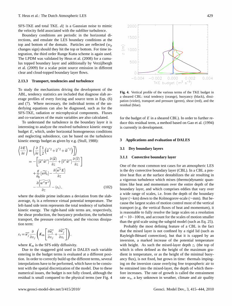
Fig. 4. Vertical profile of the various terms of the TKE budget ina sheared CBL: total tendency (orange), buoyancy (black), dissi-pation (violet), transport and pressure (green), shear (red), and theresidual (blue).
for the budget ofE in a sheared CBL). In order to further re-duce this residual term, a method based onGao et al.(1994)is currently in development.
3 Applications and evaluation of DALES
3.1 Dry boundary layers
3.1.1 Convective boundary layer
One of the most common test cases for an atmospheric LESis the dry convective boundary layer (CBL). In a CBL a pos-itive heat flux at the surface destabilizes the air resulting ina vigorous turbulence which mixes (thermo)dynamic quan-tities like heat and momentum over the entire depth of theboundary layer, and which comprises eddies that vary overa wide range of scales, i.e. from the depth of the boundarylayer (∼km) down to the Kolmogorov-scale (∼mm). But be-cause the largest scales of motion control most of the verticaltransport (e.g. the vertical fluxes of heat and momentum), itis reasonable to fully resolve the large scales on a resolutionof ∼ 10−100 m, and account for the scales of motion smallerthan the grid scale using the subgrid model (such as Eq.25).
Probably the most defining feature of a CBL is the factthat the mixed layer is not confined by a rigid lid (such asRayleigh-Benard convection), but that it is capped by aninversion, a marked increase of the potential temperaturewith height. As such the mixed-layer depthzi (the top ofwhich is often defined as the height of the maximum gra-dient in temperature, or as the height of the minimal buoy-ancy flux), is not fixed, but grows in time: thermals imping-ing on the inversion cause overlying free tropospheric air tobe entrained into the mixed-layer, the depth of which there-fore increases. The rate of growth is called the entrainmentratewe, a key unknown in weather, climate and air quality
www.geosci-model-dev.net/3/415/2010/ Geosci. Model Dev., 3, 415–444, 2010
430 T. Heus et al.: The Dutch Atmospheric LES
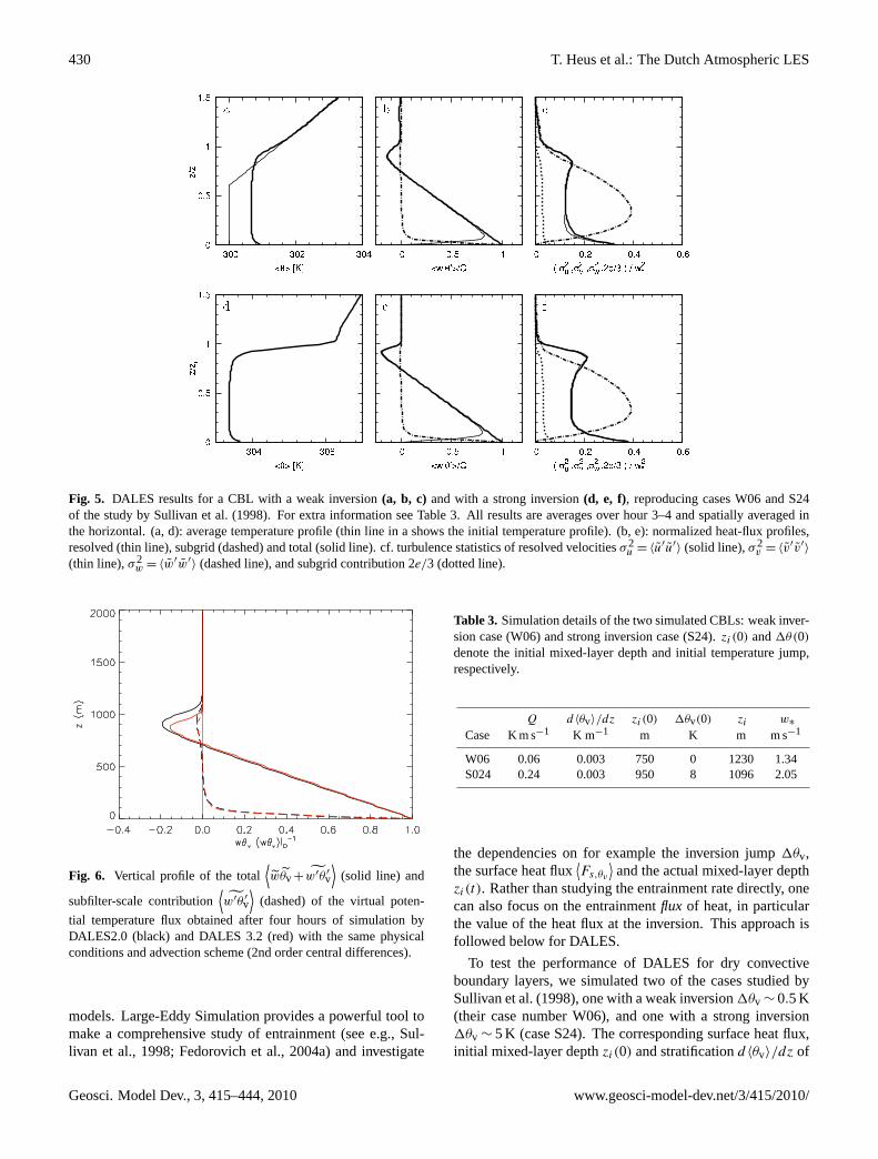
Fig. 5. DALES results for a CBL with a weak inversion(a, b, c) and with a strong inversion(d, e, f), reproducing cases W06 and S24of the study bySullivan et al.(1998). For extra information see Table3. All results are averages over hour 3–4 and spatially averaged inthe horizontal. (a, d): average temperature profile (thin line in a shows the initial temperature profile). (b, e): normalized heat-flux profiles,resolved (thin line), subgrid (dashed) and total (solid line). cf. turbulence statistics of resolved velocitiesσ2
u = 〈u′u′〉 (solid line),σ2
v = 〈v′v′〉
(thin line),σ2w = 〈w′w′
〉 (dashed line), and subgrid contribution 2e/3 (dotted line).
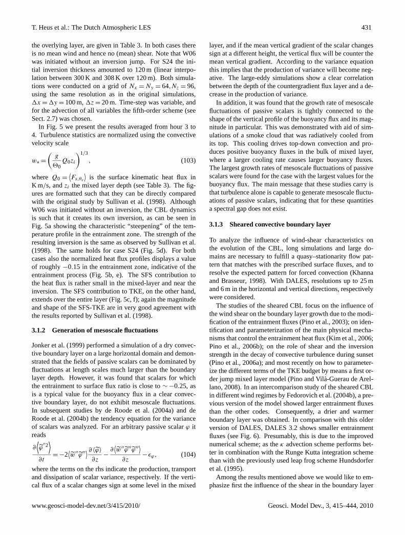
Fig. 6. Vertical profile of the total⟨wθv + w′θ ′
v
⟩(solid line) and
subfilter-scale contribution⟨w′θ ′
v
⟩(dashed) of the virtual poten-
tial temperature flux obtained after four hours of simulation byDALES2.0 (black) and DALES 3.2 (red) with the same physicalconditions and advection scheme (2nd order central differences).
models. Large-Eddy Simulation provides a powerful tool tomake a comprehensive study of entrainment (see e.g.,Sul-livan et al., 1998; Fedorovich et al., 2004a) and investigate
Table 3. Simulation details of the two simulated CBLs: weak inver-sion case (W06) and strong inversion case (S24).zi(0) and1θ(0)
denote the initial mixed-layer depth and initial temperature jump,respectively.
Q d 〈θv〉/dz zi(0) 1θv(0) zi w∗
Case K m s−1 K m−1 m K m m s−1
W06 0.06 0.003 750 0 1230 1.34S024 0.24 0.003 950 8 1096 2.05
the dependencies on for example the inversion jump1θv,the surface heat flux
⟨Fs,θv
⟩and the actual mixed-layer depth
zi(t). Rather than studying the entrainment rate directly, onecan also focus on the entrainmentflux of heat, in particularthe value of the heat flux at the inversion. This approach isfollowed below for DALES.
To test the performance of DALES for dry convectiveboundary layers, we simulated two of the cases studied bySullivan et al.(1998), one with a weak inversion1θv ∼ 0.5 K(their case number W06), and one with a strong inversion1θv ∼ 5 K (case S24). The corresponding surface heat flux,initial mixed-layer depthzi(0) and stratificationd 〈θv〉/dz of
Geosci. Model Dev., 3, 415–444, 2010 www.geosci-model-dev.net/3/415/2010/
T. Heus et al.: The Dutch Atmospheric LES 431
the overlying layer, are given in Table3. In both cases thereis no mean wind and hence no (mean) shear. Note that W06was initiated without an inversion jump. For S24 the ini-tial inversion thickness amounted to 120 m (linear interpo-lation between 300 K and 308 K over 120 m). Both simula-tions were conducted on a grid ofNx = Ny = 64,Nz = 96,using the same resolution as in the original simulations,1x = 1y = 100 m,1z = 20 m. Time-step was variable, andfor the advection of all variables the fifth-order scheme (seeSect.2.7) was chosen.
In Fig. 5 we present the results averaged from hour 3 to4. Turbulence statistics are normalized using the convectivevelocity scale
w∗ =
(g
20Q0zi
)1/3
, (103)
where Q0 =⟨Fs,θv
⟩is the surface kinematic heat flux in
K m/s, andzi the mixed layer depth (see Table3). The fig-ures are formatted such that they can be directly comparedwith the original study bySullivan et al.(1998). AlthoughW06 was initiated without an inversion, the CBL dynamicsis such that it creates its own inversion, as can be seen inFig. 5a showing the characteristic “steepening” of the tem-perature profile in the entrainment zone. The strength of theresulting inversion is the same as observed bySullivan et al.(1998). The same holds for case S24 (Fig.5d). For bothcases also the normalized heat flux profiles displays a valueof roughly−0.15 in the entrainment zone, indicative of theentrainment process (Fig.5b, e). The SFS contribution tothe heat flux is rather small in the mixed-layer and near theinversion. The SFS contribution to TKE, on the other hand,extends over the entire layer (Fig.5c, f); again the magnitudeand shape of the SFS-TKE are in very good agreement withthe results reported bySullivan et al.(1998).
3.1.2 Generation of mesoscale fluctuations
Jonker et al.(1999) performed a simulation of a dry convec-tive boundary layer on a large horizontal domain and demon-strated that the fields of passive scalars can be dominated byfluctuations at length scales much larger than the boundarylayer depth. However, it was found that scalars for whichthe entrainment to surface flux ratio is close to∼ −0.25, asis a typical value for the buoyancy flux in a clear convec-tive boundary layer, do not exhibit mesoscale fluctuations.In subsequent studies byde Roode et al.(2004a) and deRoode et al.(2004b) the tendency equation for the varianceof scalars was analyzed. For an arbitrary passive scalarϕ itreads
∂⟨ϕ
′′2⟩
∂t= −2
⟨w′′ϕ′′
⟩ ∂ 〈ϕ〉
∂z−
∂⟨w′′ϕ′′ϕ′′
⟩∂z
−εϕ, (104)
where the terms on the rhs indicate the production, transportand dissipation of scalar variance, respectively. If the verti-cal flux of a scalar changes sign at some level in the mixed
layer, and if the mean vertical gradient of the scalar changessign at a different height, the vertical flux will be counter themean vertical gradient. According to the variance equationthis implies that the production of variance will become neg-ative. The large-eddy simulations show a clear correlationbetween the depth of the countergradient flux layer and a de-crease in the production of variance.
In addition, it was found that the growth rate of mesoscalefluctuations of passive scalars is tightly connected to theshape of the vertical profile of the buoyancy flux and its mag-nitude in particular. This was demonstrated with aid of sim-ulations of a smoke cloud that was radiatively cooled fromits top. This cooling drives top-down convection and pro-duces positive buoyancy fluxes in the bulk of mixed layer,where a larger cooling rate causes larger buoyancy fluxes.The largest growth rates of mesoscale fluctuations of passivescalars were found for the case with the largest values for thebuoyancy flux. The main message that these studies carry isthat turbulence alone is capable to generate mesoscale fluctu-ations of passive scalars, indicating that for these quantitiesa spectral gap does not exist.
3.1.3 Sheared convective boundary layer
To analyze the influence of wind-shear characteristics onthe evolution of the CBL, long simulations and large do-mains are necessary to fulfill a quasy–stationarity flow pat-tern that matches with the prescribed surface fluxes, and toresolve the expected pattern for forced convection (Khannaand Brasseur, 1998). With DALES, resolutions up to 25 mand 6 m in the horizontal and vertical directions, respectivelywere considered.
The studies of the sheared CBL focus on the influence ofthe wind shear on the boundary layer growth due to the modi-fication of the entrainment fluxes (Pino et al., 2003); on iden-tification and parameterization of the main physical mecha-nisms that control the entrainment heat flux (Kim et al., 2006;Pino et al., 2006b); on the role of shear and the inversionstrength in the decay of convective turbulence during sunset(Pino et al., 2006a); and most recently on how to parameter-ize the different terms of the TKE budget by means a first or-der jump mixed layer model (Pino and Vila-Guerau de Arel-lano, 2008). In an intercomparison study of the sheared CBLin different wind regimes byFedorovich et al.(2004b), a pre-vious version of the model showed larger entrainment fluxesthan the other codes. Consequently, a drier and warmerboundary layer was obtained. In comparison with this olderversion of DALES, DALES 3.2 shows smaller entrainmentfluxes (see Fig.6). Presumably, this is due to the improvednumerical scheme; as theκ advection scheme performs bet-ter in combination with the Runge Kutta integration schemethan with the previously used leap frog schemeHundsdorferet al.(1995).
Among the results mentioned above we would like to em-phasize first the influence of the shear in the boundary layer
www.geosci-model-dev.net/3/415/2010/ Geosci. Model Dev., 3, 415–444, 2010
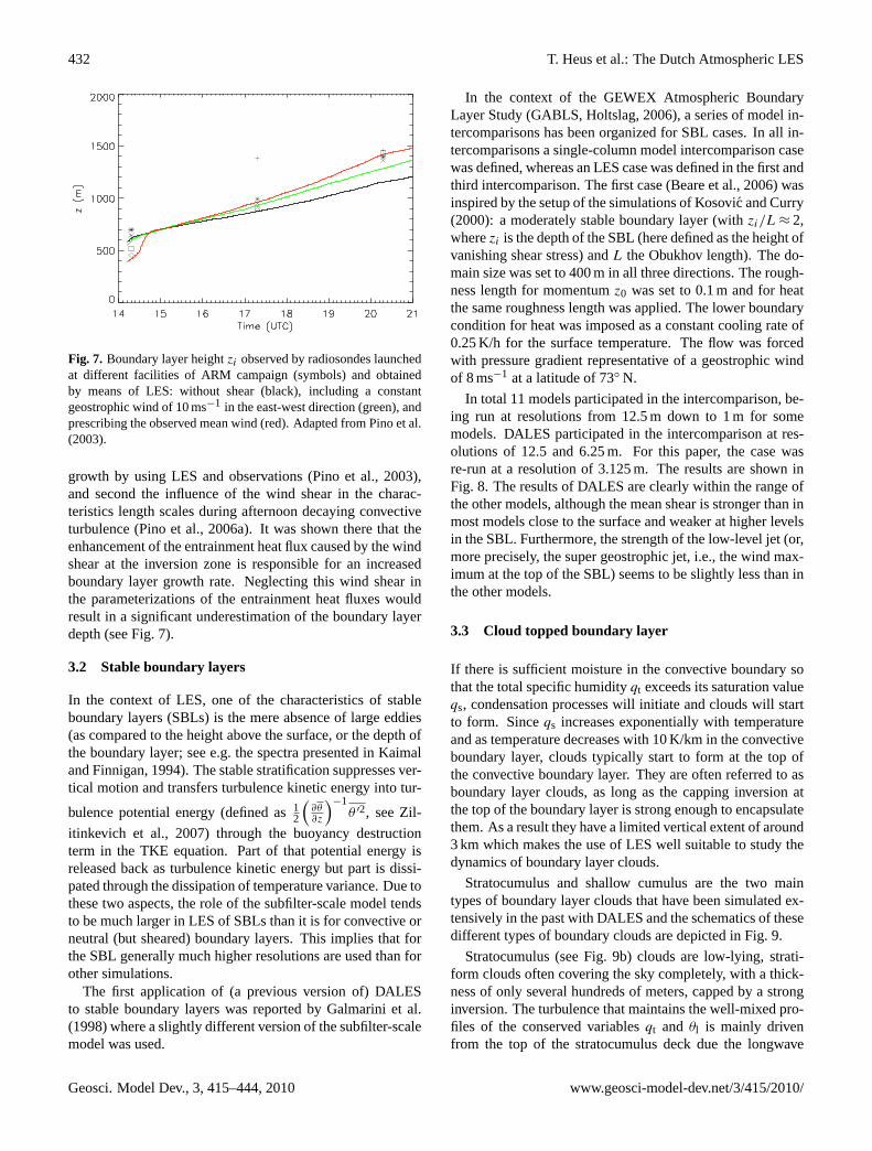
432 T. Heus et al.: The Dutch Atmospheric LES
Fig. 7. Boundary layer heightzi observed by radiosondes launchedat different facilities of ARM campaign (symbols) and obtainedby means of LES: without shear (black), including a constantgeostrophic wind of 10 ms−1 in the east-west direction (green), andprescribing the observed mean wind (red). Adapted fromPino et al.(2003).
growth by using LES and observations (Pino et al., 2003),and second the influence of the wind shear in the charac-teristics length scales during afternoon decaying convectiveturbulence (Pino et al., 2006a). It was shown there that theenhancement of the entrainment heat flux caused by the windshear at the inversion zone is responsible for an increasedboundary layer growth rate. Neglecting this wind shear inthe parameterizations of the entrainment heat fluxes wouldresult in a significant underestimation of the boundary layerdepth (see Fig.7).
3.2 Stable boundary layers
In the context of LES, one of the characteristics of stableboundary layers (SBLs) is the mere absence of large eddies(as compared to the height above the surface, or the depth ofthe boundary layer; see e.g. the spectra presented inKaimaland Finnigan, 1994). The stable stratification suppresses ver-tical motion and transfers turbulence kinetic energy into tur-
bulence potential energy (defined as12
(∂θ∂z
)−1θ ′2, seeZil-
itinkevich et al., 2007) through the buoyancy destructionterm in the TKE equation. Part of that potential energy isreleased back as turbulence kinetic energy but part is dissi-pated through the dissipation of temperature variance. Due tothese two aspects, the role of the subfilter-scale model tendsto be much larger in LES of SBLs than it is for convective orneutral (but sheared) boundary layers. This implies that forthe SBL generally much higher resolutions are used than forother simulations.
The first application of (a previous version of) DALESto stable boundary layers was reported byGalmarini et al.(1998) where a slightly different version of the subfilter-scalemodel was used.
In the context of the GEWEX Atmospheric BoundaryLayer Study (GABLS,Holtslag, 2006), a series of model in-tercomparisons has been organized for SBL cases. In all in-tercomparisons a single-column model intercomparison casewas defined, whereas an LES case was defined in the first andthird intercomparison. The first case (Beare et al., 2006) wasinspired by the setup of the simulations ofKosovic and Curry(2000): a moderately stable boundary layer (withzi/L ≈ 2,wherezi is the depth of the SBL (here defined as the height ofvanishing shear stress) andL the Obukhov length). The do-main size was set to 400 m in all three directions. The rough-ness length for momentumz0 was set to 0.1 m and for heatthe same roughness length was applied. The lower boundarycondition for heat was imposed as a constant cooling rate of0.25 K/h for the surface temperature. The flow was forcedwith pressure gradient representative of a geostrophic windof 8 ms−1 at a latitude of 73◦ N.
In total 11 models participated in the intercomparison, be-ing run at resolutions from 12.5 m down to 1 m for somemodels. DALES participated in the intercomparison at res-olutions of 12.5 and 6.25 m. For this paper, the case wasre-run at a resolution of 3.125 m. The results are shown inFig. 8. The results of DALES are clearly within the range ofthe other models, although the mean shear is stronger than inmost models close to the surface and weaker at higher levelsin the SBL. Furthermore, the strength of the low-level jet (or,more precisely, the super geostrophic jet, i.e., the wind max-imum at the top of the SBL) seems to be slightly less than inthe other models.
3.3 Cloud topped boundary layer
If there is sufficient moisture in the convective boundary sothat the total specific humidityqt exceeds its saturation valueqs, condensation processes will initiate and clouds will startto form. Sinceqs increases exponentially with temperatureand as temperature decreases with 10 K/km in the convectiveboundary layer, clouds typically start to form at the top ofthe convective boundary layer. They are often referred to asboundary layer clouds, as long as the capping inversion atthe top of the boundary layer is strong enough to encapsulatethem. As a result they have a limited vertical extent of around3 km which makes the use of LES well suitable to study thedynamics of boundary layer clouds.
Stratocumulus and shallow cumulus are the two maintypes of boundary layer clouds that have been simulated ex-tensively in the past with DALES and the schematics of thesedifferent types of boundary clouds are depicted in Fig.9.
Stratocumulus (see Fig. 9b) clouds are low-lying, strati-form clouds often covering the sky completely, with a thick-ness of only several hundreds of meters, capped by a stronginversion. The turbulence that maintains the well-mixed pro-files of the conserved variablesqt and θl is mainly drivenfrom the top of the stratocumulus deck due the longwave
Geosci. Model Dev., 3, 415–444, 2010 www.geosci-model-dev.net/3/415/2010/
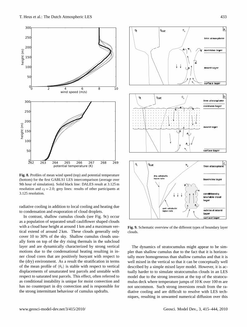
T. Heus et al.: The Dutch Atmospheric LES 433
0 2 4 6 8 10wind speed (m/s)
0
50
100
150
200
250
300
heig
ht
(m)
262 263 264 265 266 267 268 269potential temperature (K)
0
50
100
150
200
250
300
heig
ht
(m)
Fig. 8. Profiles of mean wind speed (top) and potential temperature(bottom) for the first GABLS1 LES intercomparison (average over9th hour of simulation). Solid black line: DALES result at 3.125 mresolution andcf = 2.0; grey lines: results of other participants at3.125 resolution.
radiative cooling in addition to local cooling and heating dueto condensation and evaporation of cloud droplets.
In contrast, shallow cumulus clouds (see Fig. 9c) occuras a population of separated small cauliflower shaped cloudswith a cloud base height at around 1 km and a maximum ver-tical extend of around 2 km. These clouds generally onlycover 10 to 30% of the sky. Shallow cumulus clouds usu-ally form on top of the dry rising thermals in the subcloudlayer and are dynamically characterized by strong verticalmotions due to the condensational heating resulting in in-ner cloud cores that are positively buoyant with respect tothe (dry) environment. As a result the stratification in termsof the mean profile of〈θv〉 is stable with respect to verticaldisplacements of unsaturated test parcels and unstable withrespect to saturated test parcels. This effect, often referred toas conditional instability is unique for moist convection andhas no counterpart in dry convection and is responsible forthe strong intermittant behaviour of cumulus updrafts.
Fig. 9. Schematic overview of the different types of boundary layerclouds.
The dynamics of stratocumulus might appear to be sim-pler than shallow cumulus due to the fact that it is horizon-tally more homogeneous than shallow cumulus and that it iswell mixed in the vertical so that it can be conceptually welldescribed by a simple mixed layer model. However, it is ac-tually harder to to simulate stratocumulus clouds in an LESmodel due to the strong inversion at the top of the stratocu-mulus deck where temperature jumps of 10 K over 100 m arenot uncommon. Such strong inversions result from the ra-diative cooling and are difficult to resolve with LES tech-niques, resulting in unwanted numerical diffusion over this
www.geosci-model-dev.net/3/415/2010/ Geosci. Model Dev., 3, 415–444, 2010
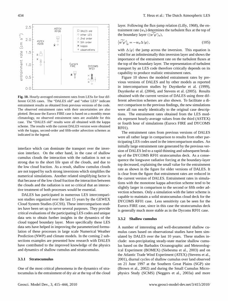
434 T. Heus et al.: The Dutch Atmospheric LES
Fig. 10.Hourly-averaged entrainment rates from LESs for four dif-ferent GCSS cases. The “DALES old” and “other LES” indicateentrainment results as obtained from previous versions of the code.The observed entrainment rates with their uncertainties are alsoplotted. Because the Eurocs FIRE case is based on a monthly meanclimatology, no observed entrainment rates are available for thiscase. The “DALES old” results were all obtained with the kappascheme. The results with the current DALES version were obtainedwith the kappa, second-order and fifth-order advection schemes asindicated in the legend.
interface which can dominate the transport over the inver-sion interface. On the other hand, in the case of shallowcumulus clouds the interaction with the radiation is not sostrong due to the short life span of the clouds, and due tothe low cloud fraction. As a result, shallow cumulus cloudsare not topped by such strong inversions which simplifies thenumerical simulations. Another related simplifying factor isthat because of the low cloud fraction the interaction betweenthe clouds and the radiation is not so critical that an interac-tive treatment of both processes would be essential.
DALES has participated in numerous LES intercompari-son studies organized over the last 15 years by the GEWEXCloud System Studies (GCSS). These intercomparison stud-ies have been set up to serve several purposes. They providecritical evaluations of the participating LES codes and uniquedata sets to obtain further insights in the dynamics of thecloud topped boundary layer. More specifically these LESdata sets have helped in improving the parameterized formu-lation of these processes in large scale Numerical WeatherPrediction (NWP) and climate models. In the coming 2 sub-sections examples are presented how research with DALEShave contributed to the improved knowledge of the physicsand dynamics of shallow cumulus and stratocumulus.
3.3.1 Stratocumulus
One of the most critical phenomena in the dynamics of stra-tocumulus is the entrainment of dry air at the top of the cloud
layer. Following the flux-jump relation (Lilly , 1968), the en-trainment rate (we) determines the turbulent flux at the top ofthe boundary layer(〈w′ϕ′〉e),⟨w′ϕ′
⟩e= −we1〈ϕ〉, (105)
with 1〈ϕ〉 the jump across the inversion. This equation isvalid for an infinitesimally thin inversion layer and shows theimportance of the entrainment rate on the turbulent fluxes atthe top of the boundary layer. The representation of turbulenttransport by an LES code therefore critically depends on itscapability to produce realistic entrainment rates.
Figure 10 shows the modeled entrainment rates by pre-vious versions of DALES and by other models as reportedin intercomparison studies byDuynkerke et al.(1999),Duynkerke et al.(2004), andStevens et al.(2005). Resultsobtained with the current version of DALES using three dif-ferent advection schemes are also shown. To facilitate a di-rect comparison to the previous findings, the new simulationswere all run nearly identically to the original case descrip-tions. The entrainment rates obtained from the LES mod-els represent hourly-average values from the third (ASTEX)or fourth hour of simulations (Eurocs FIRE and DYCOMSRF01).
The entrainment rates from previous versions of DALESwere all rather large in comparison to results from other par-ticipating LES codes used in the intercomparison studies. Aninitially large entrainment rate generated by the previous ver-sion of DALES led to a rapid thinning and subsequent break-up of the DYCOMS RF01 stratocumulus deck. As a conse-quence the longwave radiative forcing at the boundary-layertop decreased, explaining the small value for the entrainmentrate as shown in the figure for older versions of DALES. Itis clear from the figure that entrainment rates are reduced inthe current version of DALES. Entrainment rates in simula-tions with the monotone kappa advection scheme tend to beslightly larger in comparison to the second or fifth order ad-vection schemes. Only a simulation with the latter scheme iscapable to maintain a solid stratocumulus cloud deck for theDYCOMS RF01 case. Less sensitivity can be seen for theEurocs FIRE case, since in this case the stratocumulus deckis generally much more stable as in the Dycoms RF01 case.
3.3.2 Shallow cumulus
A number of interesting and well-documented shallow cu-mulus cases based on observational studies have been sim-ulated by DALES over the last 10 years. These studies in-clude: non-precipitating steady-state marine shallow cumu-lus based on the Barbados Oceanographic and Meteorolog-ical Experiment (BOMEX) (Siebesma et al., 2003) and onthe Atlantic Trade Wind Experiment (ATEX) (Stevens et al.,2001), diurnal cycles of shallow cumulus over land observedon 21 June 1997 at the Southern Great Plains (SGP) site(Brown et al., 2002) and during the Small Cumulus Micro-physics Study (SCMS) (Neggers et al., 2003a) and more
Geosci. Model Dev., 3, 415–444, 2010 www.geosci-model-dev.net/3/415/2010/
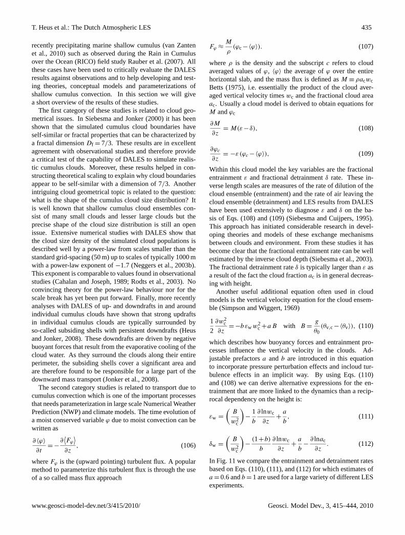
T. Heus et al.: The Dutch Atmospheric LES 435
recently precipitating marine shallow cumulus (van Zantenet al., 2010) such as observed during the Rain in Cumulusover the Ocean (RICO) field studyRauber et al.(2007). Allthese cases have been used to critically evaluate the DALESresults against observations and to help developing and test-ing theories, conceptual models and parameterizations ofshallow cumulus convection. In this section we will givea short overview of the results of these studies.
The first category of these studies is related to cloud geo-metrical issues. InSiebesma and Jonker(2000) it has beenshown that the simulated cumulus cloud boundaries haveself-similar or fractal properties that can be characterized bya fractal dimensionDf = 7/3. These results are in excellentagreement with observational studies and therefore providea critical test of the capability of DALES to simulate realis-tic cumulus clouds. Moreover, these results helped in con-structing theoretical scaling to explain why cloud boundariesappear to be self-similar with a dimension of 7/3. Anotherintriguing cloud geometrical topic is related to the question:what is the shape of the cumulus cloud size distribution? Itis well known that shallow cumulus cloud ensembles con-sist of many small clouds and lesser large clouds but theprecise shape of the cloud size distribution is still an openissue. Extensive numerical studies with DALES show thatthe cloud size density of the simulated cloud populations isdescribed well by a power-law from scales smaller than thestandard grid-spacing (50 m) up to scales of typically 1000 mwith a power-law exponent of−1.7 (Neggers et al., 2003b).This exponent is comparable to values found in observationalstudies (Cahalan and Joseph, 1989; Rodts et al., 2003). Noconvincing theory for the power-law behaviour nor for thescale break has yet been put forward. Finally, more recentlyanalyses with DALES of up- and downdrafts in and aroundindividual cumulus clouds have shown that strong updraftsin individual cumulus clouds are typically surrounded byso-called subsiding shells with persistent downdrafts (Heusand Jonker, 2008). These downdrafts are driven by negativebuoyant forces that result from the evaporative cooling of thecloud water. As they surround the clouds along their entireperimeter, the subsiding shells cover a significant area andare therefore found to be responsible for a large part of thedownward mass transport (Jonker et al., 2008).
The second category studies is related to transport due tocumulus convection which is one of the important processesthat needs parameterization in large scale Numerical WeatherPrediction (NWP) and climate models. The time evolution ofa moist conserved variableϕ due to moist convection can bewritten as
∂ 〈ϕ〉
∂t= −
∂⟨Fϕ
⟩∂z
, (106)
whereFϕ is the (upward pointing) turbulent flux. A popularmethod to parameterize this turbulent flux is through the useof a so called mass flux approach
Fϕ ≈M
ρ(ϕc−〈ϕ〉). (107)
whereρ is the density and the subscriptc refers to cloudaveraged values ofϕ, 〈ϕ〉 the average ofϕ over the entirehorizontal slab, and the mass flux is defined asM ≡ ρacwcBetts (1975), i.e. essentially the product of the cloud aver-aged vertical velocity timeswc and the fractional cloud areaac. Usually a cloud model is derived to obtain equations forM andϕc
∂M
∂z= M(ε−δ), (108)
∂ϕc
∂z= −ε (ϕc −〈ϕ〉), (109)
Within this cloud model the key variables are the fractionalentrainmentε and fractional detrainmentδ rate. These in-verse length scales are measures of the rate of dilution of thecloud ensemble (entrainment) and the rate of air leaving thecloud ensemble (detrainment) and LES results from DALEShave been used extensively to diagnoseε andδ on the ba-sis of Eqs. (108) and (109) (Siebesma and Cuijpers, 1995).This approach has initiated considerable research in devel-oping theories and models of these exchange mechanismsbetween clouds and environment. From these studies it hasbecome clear that the fractional entrainment rate can be wellestimated by the inverse cloud depth (Siebesma et al., 2003).The fractional detrainment rateδ is typically larger thanε asa result of the fact the cloud fractionac is in general decreas-ing with height.
Another useful additional equation often used in cloudmodels is the vertical velocity equation for the cloud ensem-ble (Simpson and Wiggert, 1969)
1
2
∂w2c
∂z= −bεw w2
c +aB with B =g
θ0(θv,c−〈θv〉), (110)
which describes how buoyancy forces and entrainment pro-cesses influence the vertical velocity in the clouds. Ad-justable prefactorsa and b are introduced in this equationto incorporate pressure perturbation effects and incloud tur-bulence effects in an implicit way. By using Eqs. (110)and (108) we can derive alternative expressions for the en-trainment that are more linked to the dynamics than a recip-rocal dependency on the height is:
εw =
(B
w2c
)−
1
b
∂ lnwc
∂z+
a
b, (111)
δw =
(B
w2c
)−
(1+b)
b
∂ lnwc
∂z+
a
b−
∂ lnac
∂z. (112)
In Fig. 11we compare the entrainment and detrainment ratesbased on Eqs. (110), (111), and (112) for which estimates ofa = 0.6 andb = 1 are used for a large variety of different LESexperiments.
www.geosci-model-dev.net/3/415/2010/ Geosci. Model Dev., 3, 415–444, 2010
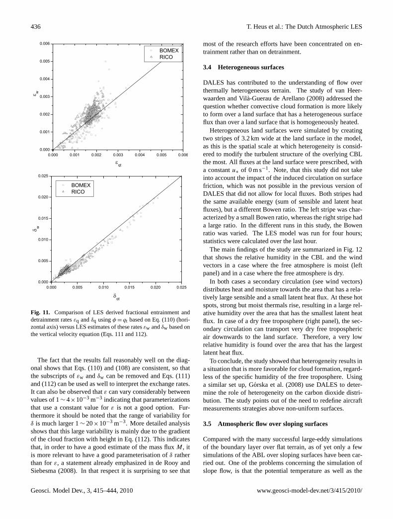
436 T. Heus et al.: The Dutch Atmospheric LES
0.000 0.001 0.002 0.003 0.004 0.005 0.006
0.000
0.001
0.002
0.003
0.004
0.005
0.006
εw
εqt
BOMEX
RICO
0.000 0.005 0.010 0.015 0.020 0.025
0.000
0.005
0.010
0.015
0.020
0.025
δw
δqt
BOMEX
RICO
Fig. 11. Comparison of LES derived fractional entrainment anddetrainment ratesεq andδq usingφ = qt based on Eq. (110) (hori-zontal axis) versus LES estimates of these ratesεw andδw based onthe vertical velocity equation (Eqs.111and112).
The fact that the results fall reasonably well on the diag-onal shows that Eqs. (110) and (108) are consistent, so thatthe subscripts ofεw andδw can be removed and Eqs. (111)and (112) can be used as well to interpret the exchange rates.It can also be observed thatε can vary considerably betweenvalues of 1∼ 4×10⁻³ m−3 indicating that parameterizationsthat use a constant value forε is not a good option. Fur-thermore it should be noted that the range of variability forδ is much larger 1∼ 20×10−3 m−3. More detailed analysisshows that this large variability is mainly due to the gradientof the cloud fraction with height in Eq. (112). This indicatesthat, in order to have a good estimate of the mass fluxM, itis more relevant to have a good parameterisation ofδ ratherthan forε, a statement already emphasized inde Rooy andSiebesma(2008). In that respect it is surprising to see that
most of the research efforts have been concentrated on en-trainment rather than on detrainment.
3.4 Heterogeneous surfaces
DALES has contributed to the understanding of flow overthermally heterogeneous terrain. The study ofvan Heer-waarden and Vila-Guerau de Arellano(2008) addressed thequestion whether convective cloud formation is more likelyto form over a land surface that has a heterogeneous surfaceflux than over a land surface that is homogeneously heated.
Heterogeneous land surfaces were simulated by creatingtwo stripes of 3.2 km wide at the land surface in the model,as this is the spatial scale at which heterogeneity is consid-ered to modify the turbulent structure of the overlying CBLthe most. All fluxes at the land surface were prescribed, witha constantu∗ of 0 m s−1. Note, that this study did not takeinto account the impact of the induced circulation on surfacefriction, which was not possible in the previous version ofDALES that did not allow for local fluxes. Both stripes hadthe same available energy (sum of sensible and latent heatfluxes), but a different Bowen ratio. The left stripe was char-acterized by a small Bowen ratio, whereas the right stripe hada large ratio. In the different runs in this study, the Bowenratio was varied. The LES model was run for four hours;statistics were calculated over the last hour.
The main findings of the study are summarized in Fig.12that shows the relative humidity in the CBL and the windvectors in a case where the free atmosphere is moist (leftpanel) and in a case where the free atmosphere is dry.
In both cases a secondary circulation (see wind vectors)distributes heat and moisture towards the area that has a rela-tively large sensible and a small latent heat flux. At these hotspots, strong but moist thermals rise, resulting in a large rel-ative humidity over the area that has the smallest latent heatflux. In case of a dry free troposphere (right panel), the sec-ondary circulation can transport very dry free troposphericair downwards to the land surface. Therefore, a very lowrelative humidity is found over the area that has the largestlatent heat flux.
To conclude, the study showed that heterogeneity results ina situation that is more favorable for cloud formation, regard-less of the specific humidity of the free troposphere. Usinga similar set up,Gorska et al.(2008) use DALES to deter-mine the role of heterogeneity on the carbon dioxide distri-bution. The study points out of the need to redefine aircraftmeasurements strategies above non-uniform surfaces.
3.5 Atmospheric flow over sloping surfaces
Compared with the many successful large-eddy simulationsof the boundary layer over flat terrain, as of yet only a fewsimulations of the ABL over sloping surfaces have been car-ried out. One of the problems concerning the simulation ofslope flow, is that the potential temperature as well as the
Geosci. Model Dev., 3, 415–444, 2010 www.geosci-model-dev.net/3/415/2010/
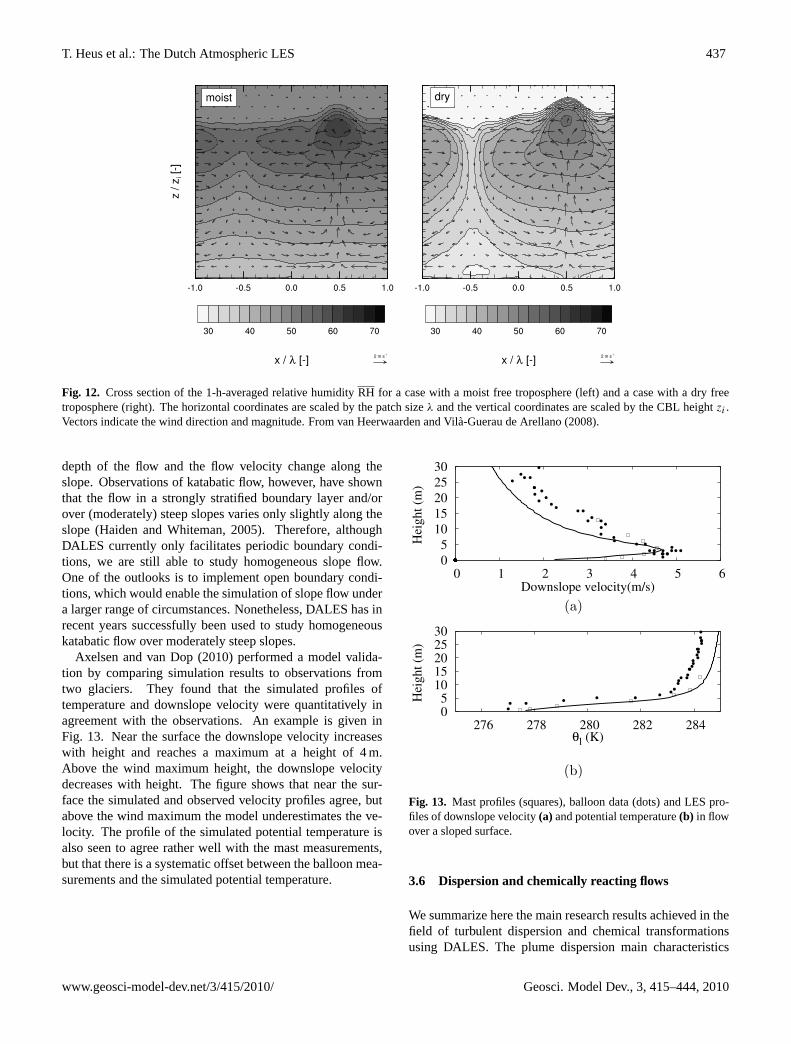
T. Heus et al.: The Dutch Atmospheric LES 437
Fig. 12. Cross section of the 1-h-averaged relative humidityRH for a case with a moist free troposphere (left) and a case with a dry freetroposphere (right). The horizontal coordinates are scaled by the patch sizeλ and the vertical coordinates are scaled by the CBL heightzi .Vectors indicate the wind direction and magnitude. Fromvan Heerwaarden and Vila-Guerau de Arellano(2008).
depth of the flow and the flow velocity change along theslope. Observations of katabatic flow, however, have shownthat the flow in a strongly stratified boundary layer and/orover (moderately) steep slopes varies only slightly along theslope (Haiden and Whiteman, 2005). Therefore, althoughDALES currently only facilitates periodic boundary condi-tions, we are still able to study homogeneous slope flow.One of the outlooks is to implement open boundary condi-tions, which would enable the simulation of slope flow undera larger range of circumstances. Nonetheless, DALES has inrecent years successfully been used to study homogeneouskatabatic flow over moderately steep slopes.
Axelsen and van Dop(2010) performed a model valida-tion by comparing simulation results to observations fromtwo glaciers. They found that the simulated profiles oftemperature and downslope velocity were quantitatively inagreement with the observations. An example is given inFig. 13. Near the surface the downslope velocity increaseswith height and reaches a maximum at a height of 4 m.Above the wind maximum height, the downslope velocitydecreases with height. The figure shows that near the sur-face the simulated and observed velocity profiles agree, butabove the wind maximum the model underestimates the ve-locity. The profile of the simulated potential temperature isalso seen to agree rather well with the mast measurements,but that there is a systematic offset between the balloon mea-surements and the simulated potential temperature.
0
5
10
15
20
25
30
0 1 2 3 4 5 6
Hei
gh
t (m
)
Downslope velocity(m/s)
(a)
0 5
10 15 20 25 30
276 278 280 282 284
Hei
gh
t (m
)
θl (K)
(b)
Fig. 13. Mast profiles (squares), balloon data (dots) and LES pro-files of downslope velocity(a) and potential temperature(b) in flowover a sloped surface.
3.6 Dispersion and chemically reacting flows
We summarize here the main research results achieved in thefield of turbulent dispersion and chemical transformationsusing DALES. The plume dispersion main characteristics
www.geosci-model-dev.net/3/415/2010/ Geosci. Model Dev., 3, 415–444, 2010
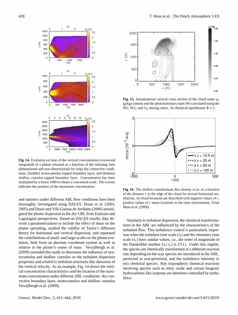
438 T. Heus et al.: The Dutch Atmospheric LES
Cz(z,t)
0
200
400
600
800
1000
1200
z (
m)
0
0.5
1
1.5
2
2.5
0 500 1000 1500
0 1 2
t (s)
t/t*
Cz(z,t)
0
200
400
600
800
1000
z (
m)
0
0.5
1
1.5
2
2.5
0 500 1000 1500 2000
0 1 2
t (s)
t/t*
Cz(z,t)
0
500
1000
1500
2000
2500
3000
z (
m)
0
0.5
1
1.5
2
2.5
0 3600 7200 10800 14400 18000
0 2 4 6 8 10 12
t (s)
t/t*
Fig. 14. Evolution on time of the vertical concentration (crosswindintegrated) of a plume released as a function of the releasing time(dimensional and non-dimensional) for (top) dry convective condi-tions, (middle) stratocumulus topped boundary layer, and (bottom)shallow cumulus topped boundary layer. Concentration has beenmultiplied by a factor 1000 to obtain a convenient scale. The crossesindicates the position of the maximum concentration.
and statistics under different ABL flow conditions have beenthoroughly investigated using DALES.Dosio et al.(2003,2005) andDosio and Vila-Guerau de Arellano(2006) investi-gated the plume dispersion in the dry CBL from Eulerian andLagrangian perspectives. Based on DALES results, they de-rived a parameterization to include the effect of shear on theplume spreading, studied the validity of Taylor’s diffusiontheory for horizontal and vertical dispersion, and separatedthe contributions of small- and large-scales on the plume evo-lution, both from an absolute coordinate system as well asrelative to the plume’s center of mass.Verzijlbergh et al.(2009) extended this study to determine the influence of stra-tocumulus and shallow cumulus on the turbulent dispersionproperties and related to turbulent structures like skewness ofthe vertical velocity. As an example, Fig.14shows the verti-cal concentration characteristics and the location of the maxi-mum concentration under different ABL conditions: dry con-vective boundary layer, stratocumulus and shallow cumulusVerzijlbergh et al.(2009).
Fig. 15. Instantaneous vertical cross section of the cloud waterqc(g/kg) content and the photostationary state (8) calculated using theNO, NO2 and O3 mixing ratios. At chemical equilibrium8 = 1.
r [m]
m(r
)∆r
[10
−3 m
/s]
−500 0 500−5
0
5
∆ x = 12.5 m
∆ x = 25 m
∆ x = 50 m
∆ x = 100 m
Fig. 16. The shallow cumulusmass flux densitym1r as a functionof the distancer to the edge of the cloud for several horizontal res-olutions. In-cloud locations are described with negative values ofr,positive values ofr mean locations in the clear environment. FromHeus et al.(2009).
Similarly to turbulent dispersion, the chemical transforma-tions in the ABL are influenced by the characteristics of theturbulent flow. This turbulence control is particularly impor-tant when the turbulent time scale (τt) and the chemistry timescale (τc) have similar values, i.e., the order of magnitude ofthe Damkohler number (τt/τc) is O(1). Under this regime,the species are chemically transformed at a different reactionrate depending on the way species are introduced in the ABL,premixed or non-premixed, and the turbulence intensity tomix chemical species. Key tropospheric chemical reactionsinvolving species such as nitric oxide and certain biogenichydrocarbons like isoprene are therefore controlled by turbu-lence.
Geosci. Model Dev., 3, 415–444, 2010 www.geosci-model-dev.net/3/415/2010/
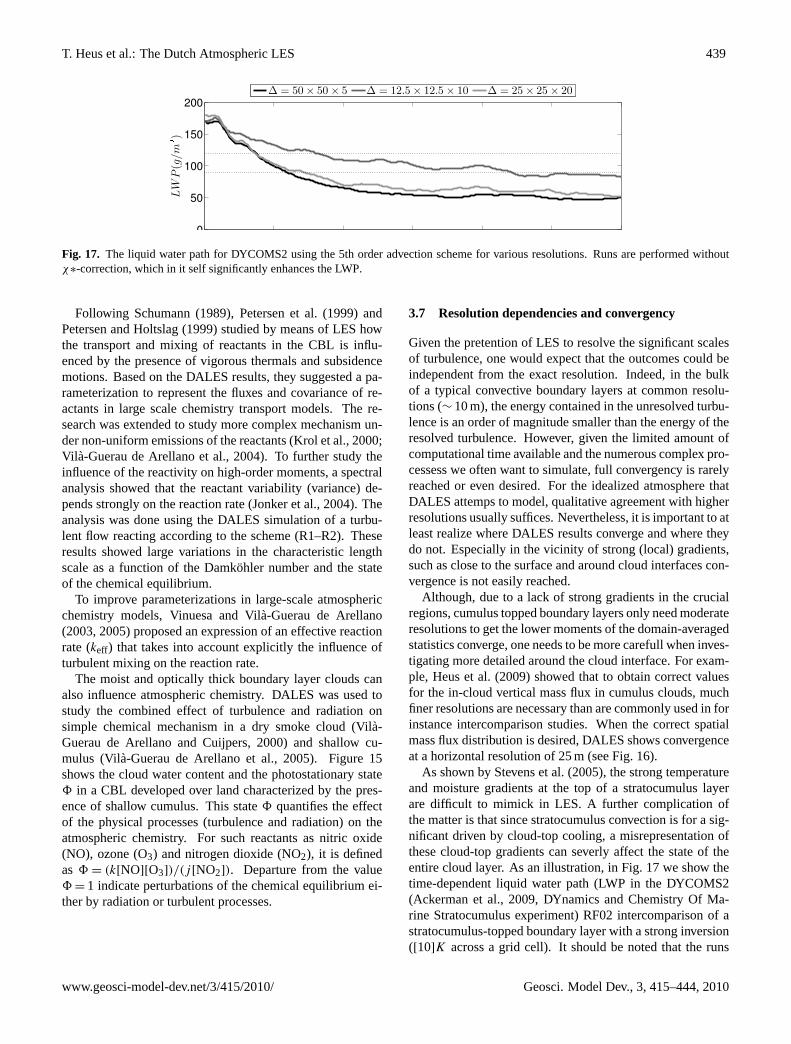
T. Heus et al.: The Dutch Atmospheric LES 439
Fig. 17. The liquid water path for DYCOMS2 using the 5th order advection scheme for various resolutions. Runs are performed withoutχ∗-correction, which in it self significantly enhances the LWP.
Following Schumann(1989), Petersen et al.(1999) andPetersen and Holtslag(1999) studied by means of LES howthe transport and mixing of reactants in the CBL is influ-enced by the presence of vigorous thermals and subsidencemotions. Based on the DALES results, they suggested a pa-rameterization to represent the fluxes and covariance of re-actants in large scale chemistry transport models. The re-search was extended to study more complex mechanism un-der non-uniform emissions of the reactants (Krol et al., 2000;Vil a-Guerau de Arellano et al., 2004). To further study theinfluence of the reactivity on high-order moments, a spectralanalysis showed that the reactant variability (variance) de-pends strongly on the reaction rate (Jonker et al., 2004). Theanalysis was done using the DALES simulation of a turbu-lent flow reacting according to the scheme (R1–R2). Theseresults showed large variations in the characteristic lengthscale as a function of the Damkohler number and the stateof the chemical equilibrium.
To improve parameterizations in large-scale atmosphericchemistry models,Vinuesa and Vila-Guerau de Arellano(2003, 2005) proposed an expression of an effective reactionrate (keff) that takes into account explicitly the influence ofturbulent mixing on the reaction rate.
The moist and optically thick boundary layer clouds canalso influence atmospheric chemistry. DALES was used tostudy the combined effect of turbulence and radiation onsimple chemical mechanism in a dry smoke cloud (Vil a-Guerau de Arellano and Cuijpers, 2000) and shallow cu-mulus (Vil a-Guerau de Arellano et al., 2005). Figure 15shows the cloud water content and the photostationary state8 in a CBL developed over land characterized by the pres-ence of shallow cumulus. This state8 quantifies the effectof the physical processes (turbulence and radiation) on theatmospheric chemistry. For such reactants as nitric oxide(NO), ozone (O3) and nitrogen dioxide (NO2), it is definedas 8 = (k[NO][O3])/(j [NO2]). Departure from the value8 = 1 indicate perturbations of the chemical equilibrium ei-ther by radiation or turbulent processes.
3.7 Resolution dependencies and convergency
Given the pretention of LES to resolve the significant scalesof turbulence, one would expect that the outcomes could beindependent from the exact resolution. Indeed, in the bulkof a typical convective boundary layers at common resolu-tions (∼ 10 m), the energy contained in the unresolved turbu-lence is an order of magnitude smaller than the energy of theresolved turbulence. However, given the limited amount ofcomputational time available and the numerous complex pro-cessess we often want to simulate, full convergency is rarelyreached or even desired. For the idealized atmosphere thatDALES attemps to model, qualitative agreement with higherresolutions usually suffices. Nevertheless, it is important to atleast realize where DALES results converge and where theydo not. Especially in the vicinity of strong (local) gradients,such as close to the surface and around cloud interfaces con-vergence is not easily reached.
Although, due to a lack of strong gradients in the crucialregions, cumulus topped boundary layers only need moderateresolutions to get the lower moments of the domain-averagedstatistics converge, one needs to be more carefull when inves-tigating more detailed around the cloud interface. For exam-ple, Heus et al.(2009) showed that to obtain correct valuesfor the in-cloud vertical mass flux in cumulus clouds, muchfiner resolutions are necessary than are commonly used in forinstance intercomparison studies. When the correct spatialmass flux distribution is desired, DALES shows convergenceat a horizontal resolution of 25 m (see Fig.16).
As shown byStevens et al.(2005), the strong temperatureand moisture gradients at the top of a stratocumulus layerare difficult to mimick in LES. A further complication ofthe matter is that since stratocumulus convection is for a sig-nificant driven by cloud-top cooling, a misrepresentation ofthese cloud-top gradients can severly affect the state of theentire cloud layer. As an illustration, in Fig.17 we show thetime-dependent liquid water path (LWP in the DYCOMS2(Ackerman et al., 2009, DYnamics and Chemistry Of Ma-rine Stratocumulus experiment) RF02 intercomparison of astratocumulus-topped boundary layer with a strong inversion([10]K across a grid cell). It should be noted that the runs
www.geosci-model-dev.net/3/415/2010/ Geosci. Model Dev., 3, 415–444, 2010
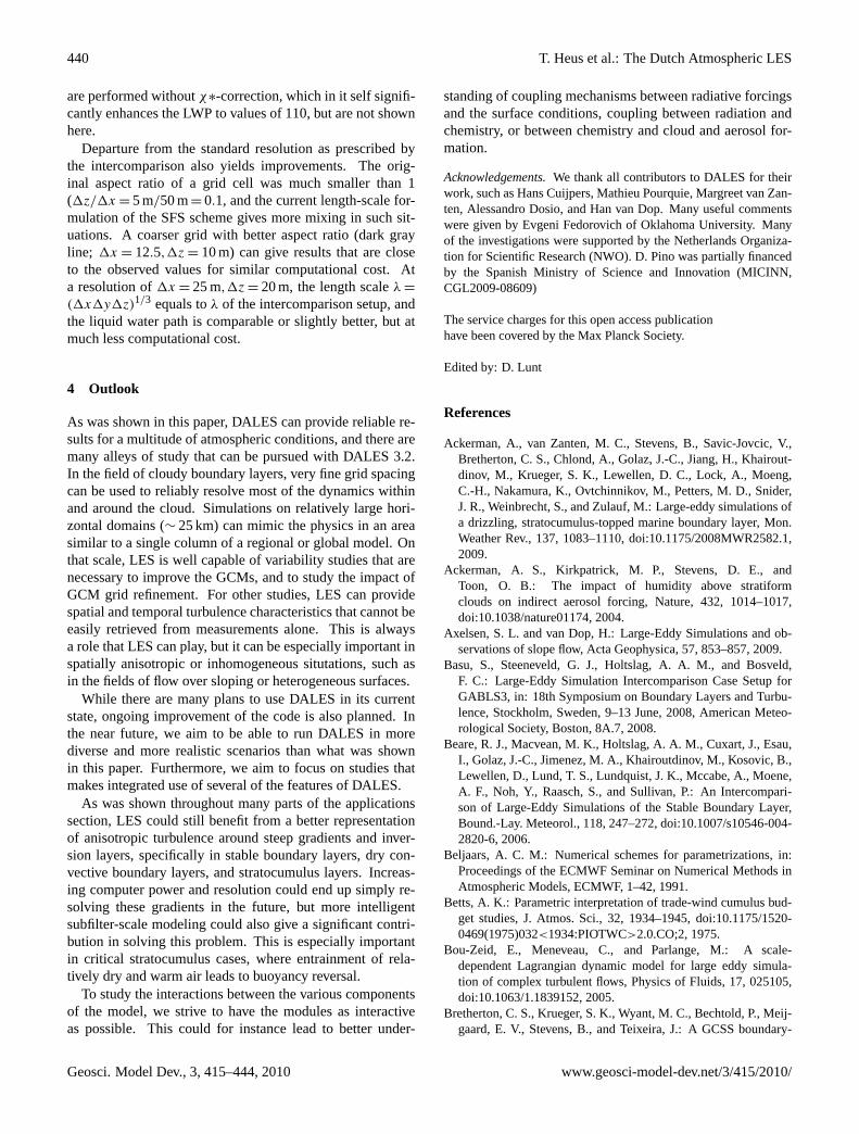
440 T. Heus et al.: The Dutch Atmospheric LES
are performed withoutχ∗-correction, which in it self signifi-cantly enhances the LWP to values of 110, but are not shownhere.
Departure from the standard resolution as prescribed bythe intercomparison also yields improvements. The orig-inal aspect ratio of a grid cell was much smaller than 1(1z/1x = 5 m/50 m= 0.1, and the current length-scale for-mulation of the SFS scheme gives more mixing in such sit-uations. A coarser grid with better aspect ratio (dark grayline; 1x = 12.5,1z = 10 m) can give results that are closeto the observed values for similar computational cost. Ata resolution of1x = 25 m,1z = 20 m, the length scaleλ =
(1x1y1z)1/3 equals toλ of the intercomparison setup, andthe liquid water path is comparable or slightly better, but atmuch less computational cost.
4 Outlook
As was shown in this paper, DALES can provide reliable re-sults for a multitude of atmospheric conditions, and there aremany alleys of study that can be pursued with DALES 3.2.In the field of cloudy boundary layers, very fine grid spacingcan be used to reliably resolve most of the dynamics withinand around the cloud. Simulations on relatively large hori-zontal domains (∼ 25 km) can mimic the physics in an areasimilar to a single column of a regional or global model. Onthat scale, LES is well capable of variability studies that arenecessary to improve the GCMs, and to study the impact ofGCM grid refinement. For other studies, LES can providespatial and temporal turbulence characteristics that cannot beeasily retrieved from measurements alone. This is alwaysa role that LES can play, but it can be especially important inspatially anisotropic or inhomogeneous situtations, such asin the fields of flow over sloping or heterogeneous surfaces.
While there are many plans to use DALES in its currentstate, ongoing improvement of the code is also planned. Inthe near future, we aim to be able to run DALES in morediverse and more realistic scenarios than what was shownin this paper. Furthermore, we aim to focus on studies thatmakes integrated use of several of the features of DALES.
As was shown throughout many parts of the applicationssection, LES could still benefit from a better representationof anisotropic turbulence around steep gradients and inver-sion layers, specifically in stable boundary layers, dry con-vective boundary layers, and stratocumulus layers. Increas-ing computer power and resolution could end up simply re-solving these gradients in the future, but more intelligentsubfilter-scale modeling could also give a significant contri-bution in solving this problem. This is especially importantin critical stratocumulus cases, where entrainment of rela-tively dry and warm air leads to buoyancy reversal.
To study the interactions between the various componentsof the model, we strive to have the modules as interactiveas possible. This could for instance lead to better under-
standing of coupling mechanisms between radiative forcingsand the surface conditions, coupling between radiation andchemistry, or between chemistry and cloud and aerosol for-mation.
Acknowledgements.We thank all contributors to DALES for theirwork, such as Hans Cuijpers, Mathieu Pourquie, Margreet van Zan-ten, Alessandro Dosio, and Han van Dop. Many useful commentswere given by Evgeni Fedorovich of Oklahoma University. Manyof the investigations were supported by the Netherlands Organiza-tion for Scientific Research (NWO). D. Pino was partially financedby the Spanish Ministry of Science and Innovation (MICINN,CGL2009-08609)
The service charges for this open access publicationhave been covered by the Max Planck Society.
Edited by: D. Lunt
References
Ackerman, A., van Zanten, M. C., Stevens, B., Savic-Jovcic, V.,Bretherton, C. S., Chlond, A., Golaz, J.-C., Jiang, H., Khairout-dinov, M., Krueger, S. K., Lewellen, D. C., Lock, A., Moeng,C.-H., Nakamura, K., Ovtchinnikov, M., Petters, M. D., Snider,J. R., Weinbrecht, S., and Zulauf, M.: Large-eddy simulations ofa drizzling, stratocumulus-topped marine boundary layer, Mon.Weather Rev., 137, 1083–1110, doi:10.1175/2008MWR2582.1,2009.
Ackerman, A. S., Kirkpatrick, M. P., Stevens, D. E., andToon, O. B.: The impact of humidity above stratiformclouds on indirect aerosol forcing, Nature, 432, 1014–1017,doi:10.1038/nature01174, 2004.
Axelsen, S. L. and van Dop, H.: Large-Eddy Simulations and ob-servations of slope flow, Acta Geophysica, 57, 853–857, 2009.
Basu, S., Steeneveld, G. J., Holtslag, A. A. M., and Bosveld,F. C.: Large-Eddy Simulation Intercomparison Case Setup forGABLS3, in: 18th Symposium on Boundary Layers and Turbu-lence, Stockholm, Sweden, 9–13 June, 2008, American Meteo-rological Society, Boston, 8A.7, 2008.
Beare, R. J., Macvean, M. K., Holtslag, A. A. M., Cuxart, J., Esau,I., Golaz, J.-C., Jimenez, M. A., Khairoutdinov, M., Kosovic, B.,Lewellen, D., Lund, T. S., Lundquist, J. K., Mccabe, A., Moene,A. F., Noh, Y., Raasch, S., and Sullivan, P.: An Intercompari-son of Large-Eddy Simulations of the Stable Boundary Layer,Bound.-Lay. Meteorol., 118, 247–272, doi:10.1007/s10546-004-2820-6, 2006.
Beljaars, A. C. M.: Numerical schemes for parametrizations, in:Proceedings of the ECMWF Seminar on Numerical Methods inAtmospheric Models, ECMWF, 1–42, 1991.
Betts, A. K.: Parametric interpretation of trade-wind cumulus bud-get studies, J. Atmos. Sci., 32, 1934–1945, doi:10.1175/1520-0469(1975)032<1934:PIOTWC>2.0.CO;2, 1975.
Bou-Zeid, E., Meneveau, C., and Parlange, M.: A scale-dependent Lagrangian dynamic model for large eddy simula-tion of complex turbulent flows, Physics of Fluids, 17, 025105,doi:10.1063/1.1839152, 2005.
Bretherton, C. S., Krueger, S. K., Wyant, M. C., Bechtold, P., Meij-gaard, E. V., Stevens, B., and Teixeira, J.: A GCSS boundary-
Geosci. Model Dev., 3, 415–444, 2010 www.geosci-model-dev.net/3/415/2010/
T. Heus et al.: The Dutch Atmospheric LES 441
layer cloud model intercomparison study of the first ASTEXLagrangian experiment, Bound.-Lay. Meteorol., 93, 341–380,doi:10.1023/A:1002005429969, 1999a.
Bretherton, C. S., MacVean, M. K., Bechtold, P., Chlond, A.,Cuxart, J., Khairoutdinov, M., Kosovic, B., Lewellen, D. C., Mo-eng, C.-H., Siebesma, A. P., Stevens, B., Stevens, D. E., I.Sykes,and Wyant, M. C.: An intercomparison radiatively-driven en-trainment and turbulence in a smoke cloud, as simulated by dif-ferent numerical models, Q. J. Roy. Meteor. Soc., 125, 391–423,doi:10.1002/qj.49712555402, 1999b.
Bretherton, C. S., McCaa, J. R., and Grenier, H.: A new param-eterization for shallow cumulus convection and its applicationto marine subtropical cloud-topped boundary layers. Part I:Description and 1D results, Mon. Weather Rev., 132, 864–882,doi:10.1175/1520-0493(2004)132<0864:ANPFSC>2.0.CO;2,2004.
Bretherton, C. S., Blossey, P. N., and Uchida, J.: Clouddroplet sedimentation, entrainment efficiency, and subtropi-cal stratocumulus albedo, Geophys. Res. Lett., 34, 3307,doi:10.1029/2006GL027648, 2007.
Brown, A. R., Cederwall, R. T., Chlond, A., Duynkerke, P. G.,Golaz, J. C., Khairoutdinov, M., Lewellen, D. C., Lock, A. P.,MacVean, M. K., Moeng, C.-H., Neggers, R. A. J., Siebesma,A. P., and Stevens, B.: Large-eddy simulation of the diurnal cy-cle of shallow cumulus convection over land, Q. J. Roy. Mete-orol. Soc., 128, 1075–1093, doi:10.1256/003590002320373210,2002.
Businger, J. A., Wyngaard, J. C., Izumi, Y., and Bradley,E. F.: Flux-profile relationships in the atmospheric sur-face layer, J. Atmos. Sci., 28, 181–189, doi:10.1175/1520-0469(1971)028<0181:FPRITA>2.0.CO;2, 1971.
Cahalan, R. and Joseph, J.: Fractal statistics of cloudfields, Mon. Weather Rev., 117, 261–272, doi:10.1175/1520-0493(1989)117<0261:FSOCF>2.0.CO;2, 1989.
Cahalan, R. F., Oreopoulos, L., Marshak, A., Evans, K. F., Davis,A. B., Pincus, R., Yetzer, K. H., Mayer, B., Davies, R., Ack-erman, T. P., Barker, H. W., Clothiaux, E. E., Ellingson, R. G.,Garay, M. J., Kassianov, E., Kinne, S., Macke, A., O’Hirok, W.,Partain, P. T., Prigarin, S. M., Rublev, A. N., Stephens, G. L.,Szczap, F., Takara, E. E., Varnai, T., Wen, G., and Zhuravleva,T. B.: The I3RC: Bringing together the most advanced radiativetransfer tools for cloudy atmospheres, B. Am. Meteorol. Soc.,86, 1275–1293, doi:10.1175/BAMS-86-9-1275, 2005.
Cuijpers, J. W. M.: Subgrid Parameterization in a large-eddy sim-ulation model, in: Ninth Symp. on Turbulence and Diffusion,Amer. Meteor. Soc., Roskilde, Denmark, 176–179, 1990.
Cuijpers, J. W. M. and Duynkerke, P. G.: Large-eddy simulationof trade-wind cumulus clouds, J. Atmos. Sci., 55, 151–162,doi:10.1175/1520-0469(1998)055<0151:IOSANE>2.0.CO;2,1993.
de Roode, S. R., Duynkerke, P. G., and Jonker, H.J. J.: Large-eddy simulation: How large is largeenough?, J. Atmos. Sci., 61, 403–421, doi:10.1175/1520-0469(2004)061¡0403:LSHLIL¿2.0.CO;2, 2004a.
de Roode, S. R., Jonker, H. J. J., Duynkerke, P. G., and Stevens,B.: Countergradient fluxes of conserved variables in the clearconvective and stratocumulus-topped boundary layer: The roleof the entrainment flux, Bound.-Layer Meteor., 112, 179–196,doi:10.1023/B:BOUN.0000020167.25780.16, 2004b.
de Roode, S. R.: The role of eddy diffusivity profiles on stratocu-mulus liquid water path biases, Mon. Weather Rev., 135, 2786–2793, doi:10.1175/MWR3426.1, 2007.
de Roode, S. R. and Los, A.: The effect of temperature and hu-midity fluctuations on the liquid water path of non-precipitatingclosed-cell stratocumulus, Q. J. Roy. Meteorol. Soc., 134, 403–416, doi:10.1002/qj.222, 2008.
de Rooy, W. C. and Siebesma, A. P.: A simple parameterization fordetrainment in shallow cumulus, Mon. Weather Rev., 136, 560–576, doi:10.1175/2007MWR2201.1, 2008.
Deardorff, J. W.: Theoretical expression for the counter-gradient vertical heat flux, J. Geophys. Res., 77, 5900–5904,doi:10.1029/JC077i030p05900, 1972.
Deardorff, J. W.: Three-dimensional numerical modeling of theplanetary boundary layer, in: Workshop on Meteorology, editedby: Haugen, D. A., American Meteorological Society, 271–311,1973.
Deardorff, J. W.: Stratocumulus-capped mixed layers derived froma three dimensional model, Bound.-Lay. Meteorol., 18, 495–527,doi:10.1007/BF00119502, 1980.
Dosio, A. and Vila-Guerau de Arellano, J.: Statistics of absolute andrelative dispersion in the atmospheric convective boundary layer:a Large-Eddy Simulation study, J. Atmos. Sci., 63, 1253–1272,doi:10.1175/JAS3689.1, 2006.
Dosio, A., Vila-Guerau de Arellano, J., Holtslag, A. A. M., andBuiltjes, P. J. H.: Dispersion of a passive tracer in buoyancy- andshear-driven boundary layers., J. Appl. Meteor., 42, 1116–1130,doi:10.1175/1520-0450(2003)042<1116:DOAPTI>2.0.CO;2,2003.
Dosio, A., Vila-Guerau de Arellano, J., Holtslag, A. A. M., andBuiltjes, P. J. H.: Relating Eulerian and Lagrangian statistics forthe turbulent dispersion in the atmospheric convective boundarylayer, J. Atmos. Sci., 62, 1175–1191, doi:10.1175/JAS3393.1,2005.
Duda, D. P., Stephens, G. L., and Cox, S. K.: Mi-crophysical and radiative properties of marine stra-tocumulus from tethered balloon measurements,J. Appl. Meteor., 30, 170–186, doi:10.1175/1520-0450(1991)030<0170:MARPOM>2.0.CO;2, 1991.
Duynkerke, P., Jonker, P., Chlond, A., van Zanten, M., Cuxart, J.,Clark, P., Sanchez, E., Martin, G., Lenderink, G., and Teixeira,J.: Intercomparison of three- and one-dimensional model simu-lations and aircraft observations of stratocumulus, Bound.-Lay.Meteorol., 92, 453–487, doi:10.1023/A:1002006919256, 1999.
Duynkerke, P. G.: Turbulence, radiation and fog in Dutch Sta-ble Boundary Layers, Bound.-Lay. Meteorol., 90, 447–477,doi:10.1023/A:1026441904734, 1999.
Duynkerke, P. G., de Roode, S. R., Van Zanten, M. C., et al.: Obser-vations and numerical simulation of the diurnal cycle of the EU-ROCS stratocumulus case, Q. J. Roy. Meteor. Soc., 140, 3269–3296, doi:10.1256/qj.03.139, 2004.
Emanuel, K. A.: Atmospheric Convection, Oxford UniversityPress, New York, 1994.
Fedorovich, E., Conzemius, R., and Mironov, D.: Convec-tive entrainment into a shear-free, linearly stratified atmo-sphere: bulk models reevaluated through large-eddy sim-ulations, J. Atmos. Sci., 61, 281–295, doi:10.1175/1520-0469(2004)061<0281:CEIASL>2.0.CO;2, 2004a.
Fedorovich, E., R.Conzemius, Esau, I., Chow, F. K., Lewellen, D.,
www.geosci-model-dev.net/3/415/2010/ Geosci. Model Dev., 3, 415–444, 2010
442 T. Heus et al.: The Dutch Atmospheric LES
Moeng, C.-H., Sullivan, P., Pino, D., and Vila-Guerau de Arel-lano, J.: Entrainment Into Sheared Convective Boundary LayersAs Predicted By Different Large Eddy Simulation Codes, in: The16th Symposium on Boundary-Layers and Turbulence, 2004b.
Fouquart, Y.: Radiation in boundary layer clouds, in: Report,JSC/CAS Workshop on Modelling of Cloud-Topped BoundaryLayer, Fort Collins, CO, WMO/TD 75, Appendix D, 40 pp, 1985.
Fu, Q. and Liou, K.: On the Correlated k-DistributionMethod for Radiative Transfer in Nonhomogenecous Atmo-spheres, J. Atmos. Sci., 49, 2139–2156, doi:10.1175/1520-0469(1992)049<2139:OTCDMF>2.0.CO;2, 1992.
Fu, Q., Liou, K. N., Cribb, M. C., Charlock, T. P., and Gross-man, A.: Multiple Scattering Parameterization in ThermalInfrared Radiative Transfer, J. Atmos. Sci., 54, 2799–2812,doi:10.1175/1520-0469(1997)054<2799:MSPITI%>2.0.CO;2,1997.
Galmarini, S., Beets, C., Duynkerke, P., and Vila-Guerau de Arel-lano, J.: Stable Nocturnal Boundary Layers: A Comparison ofOne-Dimensional and Large-Eddy Simulation Models, Bound.-Lay. Meteorol., 88, 181–210, doi:10.1023/A:1001158702252,1998.
Gao, S., Gao, Z., and Voke, P.: Balance Equatios in Finite-VolumeLarge-Eddy Simulations, Tech. rep., Department of MechanicalEngineering, Surrey University, England, 1994.
Geoffroy, O., Brenguier, J.-L., and Burnet, F.: Parametric rep-resentation of the cloud droplet spectra for LES warm bulkmicrophysical schemes, Atmos. Chem. Phys., 10, 4835–4848,doi:10.5194/acp-10-4835-2010, 2010.
Geoffroy, O., Siebesma, A. P, and Burnet, F.: Parametric represen-tation of the rain drop spectra for bulk microphysics, in prepara-tion, 2010.
Gorska, M., Vila-Guerau de Arellano, J., LeMone, M., and vanHeerwaarden, C.: Mean and Flux Horizontal Variability of Vir-tual Potential Temperature, Moisture, and Carbon Dioxide: Air-craft Observations and LES Study, Mon. Weather Rev., 136,4435–4451, doi:10.1175/2008MWR2230.1, 2008.
Haiden, T. and Whiteman, C. D.: Katabatic Flow Mecha-nisms on a Low-Angle Slope, J. Appl. Metor., 44, 113–126.,doi:10.1175/JAM-2182.1, 2005.
Heus, T. and Jonker, H. J. J.: Subsiding shells aroundshallow cumulus clouds, J. Atmos. Sci., 65, 1003–1018,doi:10.1175/2007JAS2322.1, 2008.
Heus, T., van Dijk, G., Jonker, H. J. J., and van den Akker,H. E. A.: Mixing in shallow cumulus clouds studied by La-grangian particle tracking, J. Atmos. Sci., 65, 2581–2597,doi:10.1175/2008JAS2572.1, 2008.
Heus, T., Pols, C. F. J., Jonker, H. J. J., van den Akker, H. E. A. andLenschow, D. H.: Observational validation of the compensatingmass flux through the shell around cumulus clouds, Q. J. Roy.Meteorol. Soc., 134, 101–112 2009.
Holtslag, B.: Preface: GEWEX Atmospheric Boundary-layer Study(GABLS) on Stable Boundary Layers, Bound.-Lay. Meteorol.,118, 243–246, doi:10.1007/s10546-005-9008-6, 2006.
Hundsdorfer, W., Koren, B., Vanloon, M., and Verwer, J. G.: A pos-itive finite-difference advection scheme, J. Comput. Phys., 117,35–46, doi:10.1006/jcph.1995.1042, 1995.
Jarvis, P. G.: The interpretation of the variations in leaf water po-tential and stomatal conductance found in canopies in the field,Philos. T. Roy. Soc. Lon., 273B, 593–610, 1976.
Jonker, H. J. J., Duynkerke, P. G., and Cuijpers, J. W. M.:Mesoscale fluctuations in scalars generated by boundary layerconvection, J. Atmos. Sci., 56, 801–808, doi:10.1175/1520-0469(1999)056¡0801:MFISGB¿2.0.CO;2, 1999.
Jonker, H. J. J., Vila-Guerau de Arellano, J., and Duynkerke, P. G.:Characteristic length scales of reactive species in a convectiveboundary layer, J. Atmos. Sci., 61, 41–56, doi:10.1175/1520-0469(2004)061<0041:CLSORS>2.0.CO;2, 2004.
Jonker, H. J. J., Heus, T., and Sullivan, P. P.: A refined view ofvertical transport by cumulus convection, Geophys. Res. Lett.,35, L07810, doi:10.1029/2007GL032606, 2008.
Joseph, J. H., Wiscombe, W. J., and Weinman, J. A.:The delta-Eddington approximation for radiative flux trans-fer, J. Atmos. Sci., 33, 2452–2459, doi:10.1175/1520-0469(1976)033<2452:TDEAFR>2.0.CO;2, 1976.
Kaimal, J. and Finnigan, J.: Atmospheric Boundary Layer Flows:Their Structure and Measurement, Oxford University Press,USA, 1994.
Khairoutdinov, M. and Kogan, Y.: A new cloud physics parame-terization in a large-eddy simulation model of marine stratocu-mulus, Mon. Weather Rev., 128, 229–243, doi:10.1175/1520-0493(2000)128<0229:ANCPPI>2.0.CO;2, 2000.
Khanna, S. and Brasseur, J. G.: Three-dimensional buoyancyand shear-induced local structure of the atmospheric bound-ary layer, J. Atmos. Sci., 55, 710–743, doi:10.1175/1520-0469(1998)055<0710:TDBASI>2.0.CO;2, 1998.
Kim, S. W., Park, S. U., Pino, D., and Vila-Guerau de Arellano, J.:Parameterization of entrainment in a sheared convec boundarylayer using a first-order jump model, J. Atmos. Sci., 120, 455–475, 2006.
Kosovic, B. and Curry, J.: A Large Eddy Simulation Studyof a Quasi-Steady, Stably Stratified Atmospheric BoundaryLayer, J. Atmos. Sci., 57, 1052–1068, doi:10.1175/1520-0469(2000)057<1052:ALESSO>2.0.CO;2, 2000.
Krol, M. C., Molemaker, M. J., and Vila-Guerau de Arellano, J.: Ef-fects of turbulence and heterogeneous emissions on photochemi-cally active species in the convective boundary layer, J. Geophys.Res., 105, 6871–6884, doi:10.1029/1999JD900958, 2000.
Larson, V. E., Kotenberg, K. E., and Wood, N. B.: An analytic long-wave radiation formula for liquid layer clouds, Mon. WeatherRev., 135, 689–699, doi:10.1175/MWR3315.1, 2007.
Lilly, D.: Models of cloud-topped mixed layers under a strong in-version, Q. J. Roy. Meteorol. Soc., 94, 292–309, 1968.
Lilly, D. K.: The representation of small-scale turbulence in numer-ical simulation experiments, in: Proc. IBM Scientific Comput-ing symp. on Environmental Sciences, edited by: Goldstine, H.,195–210, 1967.
Louis, J. F.: A parametric model of vertical fluxes inthe atmosphere, Bound.-Lay. Meteorol., 17, 187–202,doi:10.1007/BF00117978, 1979.
Marshall, J. and Palmer, W.: The distribution of raindrops with size,J. Meteorol., 5, 165–166, 1948.
Neggers, R. A. J., Duynkerke, P. G., and Rodts, S. M. A.: Shal-low cumulus convection: A validation of large-eddy simulationagainst aircraft and Landsat observations, Q. J. Roy. Meteorol.Soc., 129, 2671–2696, doi:10.1256/qj.02.93, 2003a.
Neggers, R. A. J., Jonker, H. J. J., and Siebesma, A. P.: Sizestatistics of cumulus cloud populations in large-eddy simu-lations, J. Atmos. Sci., 60, 1060–1074, doi:10.1175/1520-
Geosci. Model Dev., 3, 415–444, 2010 www.geosci-model-dev.net/3/415/2010/
T. Heus et al.: The Dutch Atmospheric LES 443
0469(2003)60<1060:SSOCCP>2.0.CO;2, 2003b.Neggers, R. A. J., Siebesma, A. P., and Heus, T.: The KNMI Pa-
rameterization Testbed, B. Am. Meteorol. Soc., submitted, 2010.Nieuwstadt, F. T. M. and Brost, R. A.: The decay of convec-
tive turbulence, J. Atmos. Sci., 43, 532–546, doi:10.1175/1520-0469(1986)043<0532:TDOCT>2.0.CO;2, 1986.
Nieuwstadt, F. T. M. and de Valk, J. P. J. M. M.: A Large eddysimulation of buoyant and non-buoyant plume dispersion in theatmospheric boundary layer, Atmos. Environ., 21, 2573–2587,doi:10.1016/0004-6981(87)90189-2, 1987.
Noilhan, J. and Planton, S.: A simple parameterization of land sur-face processes for meteorological models, Mon. Weather Rev., 3,536–549,1989.
Petersen, A. and Holtslag, A. A. M.: A first-order closure for co-variances and fluxes of reactive species in the convective bound-ary layer, J. Appl. Meteor., 38, 1758–1776, doi:10.1175/1520-0450(1999)038<1758:AFOCFC>2.0.CO;2, 1999.
Petersen, A. C., Beets, C., van Dop, H., Duynkerke, P. G., andSiebesma, A. P.: Mass-flux characteristics of reactive scalarsin the convective boundary layer, J. Atmos. Sci., 56, 37–56,doi:10.1175/1520-0469(1999)056<0037:MFCORS>2.0.CO;2,1999.
Pincus, R. and Stevens, B.: Monte Carlo Spectral Integration:a Consistent Approximation for Radiative Transfer in LargeEddy Simulations, J. Adv. Model. Earth Syst., 1, 1, 9 pp.,doi:10.3894/JAMES.2009.1.1, 2009.
Pino, D. and Vila-Guerau de Arellano, J.: Effects of the shearin the convective boundary layer: Analysis of the turbu-lent kinetic energy budget, Acta Geophysica, 56, 167–193,doi:10.2478/s11600-007-0037-z, 2008.
Pino, D., Vila-Guerau de Arellano, J., and Duynkerke, P. G.: Thecontribution of shear to the evolution of a convective bound-ary layer, J. Atmos. Sci., 60, 1913–1926, doi:10.1175/1520-0469(2003)060<1913:TCOSTT>2.0.CO;2, 2003.
Pino, D., Jonker, H. J. J., Vila-Guerau de Arellano, J., and Do-sio, A.: Role of the shear and inversion strength during sun-set turbulence over land, Bound.-Lay. Meteorol., 121, 537–556,doi:10.1007/s10546-006-9080-6, 2006a.
Pino, D., Vila-Guerau de Arellano, J., and Kim, S. W.: Repre-senting sheared convective boundary layer by zeroth- and first-order jump mixed layer models: large-eddy simulation veri-fication, J. Appl. Meteor., 45, 1224–1243, doi:10.1175/1520-0469(2003)060<1913:TCOSTT>2.0.CO;2, 2006b.
Pinsky, M. B. and Khain, A. P.: Effects of in-cloud nucle-ation and turbulence on droplet spectrum formation in cu-mulus clouds, Q. J. Roy. Meteorol. Soc., 128, 501–533,doi:10.1256/003590002321042072, 2002.
Randall, D.: Conditional instability of the fist kind up-side down, J. Atmos. Sci., 37, 125–150, doi:10.1175/1520-0469(1980)037<0125:CIOTFK>2.0.CO;2, 1980.
Rauber, R. M., Stevens, B., Ochs, H. T., Knight, C. A., Albrecht,B. A., Blyth, A. M., Fairall, C. W., Jensen, J. B., Lasher-Trapp,S. G., Mayol-Bracero, O. L., Vali, G., Anderson, J. R., Baker,B. A., Bandy, A. R., F., B., Brenguier, J.-L., Brewer, W. A.,Brown, P. R. A., Chuang, P., Cotton, W. R., Di Girolamo, L.,Geerts, B., Gerber, H., Goke, S., Gomes, L., Heikes, B. G., Hud-son, J. G., Kollias, P., P., L. R., Krueger, S., Lenschow, D. H.,Nuijens, L., O’Sullican, D. W. O., Rilling, R. A., Rogers, D. C.,Siebesma, A. P., Snodgrass, E., Stith, J. L., Thornton, D. C.,
Tucker, S., Twohy, C. H., and Zuidema, P.: Rain in (shallow) cu-mulus over the ocean – The RICO campaign, B. Am. Meteorol.Soc., 88, 1912–1928, doi:10.1175/BAMS-88-12-1912, 2007.
Rodts, S. M. A., Duynkerke, P. G., and Jonker, H. J. J.:Size distributions and dynamical properties of shallowcumulus clouds from aircraft observations and satellitedata, J. Atmos. Sci., 60, 1895–1912, doi:10.1175/1520-0469(2003)060<1895:SDADPO>2.0.CO;2, 2003.
Rogers, R. R., Baumgardner, R. M., Ethier, S. A., Carter,D. A., and Ecklund, W. L.: Comparison of raindrop sizedistributions measured by radar wind profiler and by air-plane, J. Appl. Meteor., 32, 694–699, doi:10.1175/1520-0450(1993)032<0694:CORSDM>2.0.CO;2, 1993.
Schumann, U.: Large-eddy simulation of turbulent diffusion withchemical reactions in the convective boundary layer, Atmos.Environ., 23, 1713–1729, doi:10.1016/0004-6981(89)90056-5,1989.
Schumann, U.: Large-eddy simulation of the up-slope bound-ary layer, Q. J. Roy. Meteorol. Soc, 116, 637–670,doi:10.1256/smsqj.49306, 1990.
Seifert, A.: On the parameterization of evaporation of raindrops assimulated by a one-dimensional rainshaft model, J. Atmos. Sci.,65, 3608–3619, doi:10.1175/2008JAS2586.1, 2008.
Seifert, A. and Beheng, K. D.: A double-moment parameterizationfor simulating autoconversion, accretion and selfcollection, At-mos. Res., 59, 265–281, doi:10.1016/S0169-8095(01)00126-0,2001.
Seifert, A. and Beheng, K. D.: A two-moment cloud microphysicsparameterization for mixed-phase clouds. Part 1: Model descrip-tion, Meteorol. Atmos. Phys., 92, 45–66, doi:10.1007/s00703-005-0112-4, 2006.
Shettle, E. P. and Weinman, J. A.: The transfer of solar irradi-ance through inhomogeneous turbid atmospheres evaluatedby Eddingtons approximation, J. Atmos. Sci., 27, 1048–1055,doi:10.1175/1520-0469(1970)027<1048:TTOSIT>2.0.CO;2,1970.
Siebesma, A. P. and Cuijpers, J. W. M.: Evaluation ofparametric assumptions for shallow cumulus convec-tion, J. Atmos. Sci., 52, 650–666, doi:10.1175/1520-0469(1995)052<0650:EOPAFS>2.0.CO;2, 1995.
Siebesma, A. P. and Jonker, H. J. J.: Anomalous scaling ofcumulus cloud boundaries, Phys. Rev. Lett., 85, 214–217,doi:10.1103/PhysRevLett.85.214, 2000.
Siebesma, A. P., Bretherton, C. S., Brown, A., Chlond, A., Cuxart,J., Duynkerke, P. G., Jiang, H. L., Khairoutdinov, M., Lewellen,D., Moeng, C. H., Sanchez, E., Stevens, B., and Stevens, D. E.: Alarge eddy simulation intercomparison study of shallow cumulusconvection, J. Atmos. Sci., 60, 1201–1219, doi:10.1175/1520-0469(2003)60<1201:ALESIS>2.0.CO;2, 2003.
Simpson, J. and Wiggert, V.: Models of precipitating cumulustowers, Mon. Weather Rev., 97, 471–489, doi:10.1175/1520-0493(1969)097<0471:MOPCT>2.3.CO;2, 1969.
Smagorinsky, J.: General circulation experiments withthe primitive equations: I. The basic equations,Mon. Weather Rev., 91, 99–164, doi:10.1175/1520-0493(1963)091<0099:GCEWTP>2.3.CO;2, 1963.
Sommeria, G.: Three-dimensional simulation of turbu-lent processes in an undisturbed trade-wind boundarylayer, J. Atmos. Sci., 33, 216–241, doi:10.1175/1520-
www.geosci-model-dev.net/3/415/2010/ Geosci. Model Dev., 3, 415–444, 2010
444 T. Heus et al.: The Dutch Atmospheric LES
0469(1976)033<0216:TDSOTP>2.0.CO;2, 1976.Sommeria, G. and Deardorff, J. W.: Subgrid-scale condensation in
models of non-precipitating clouds, J. Atmos. Sci., 34, 344–355,doi:10.1175/1520-0469(1977)034<0344:SSCIMO>2.0.CO;2,1977.
Stephens, G. L.: The parameterization of radiation fornumerical weather prediction and climate models,Mon. Weather Rev., 112, 826–867, doi:10.1175/1520-0493(1984)112<0826:TPORFN>2.0.CO;2, 1984.
Stevens, B.: Entrainment in stratocumulus-topped mixed layers, Q.J. Roy. Meteor. Soc., 128, 2663–2690, doi:10.1256/qj.01.202,2002.
Stevens, B. and Seifert, A.: Understanding macrophysical out-comes of microphysical choices in simulations of shallowcumulus convection, J. Meteor. Soc. Japan, 86a, 143–162,doi:10.2151/jmsj.86A.143, 2008.
Stevens, B., Ackerman, A. S., Albrecht, B. A., Brown, A. R.,Chlond, A., Cuxart, J., Duynkerke, P. G., Lewellen, D. C.,MacVean, M. K., Neggers, R. A. J., Sanchez, E., Siebesma,A. P., and Stevens, D. E.: Simulations of trade wind cumuliunder a strong inversion, J. Atmos. Sci., 58, 1870–1891,doi:10.1175/1520-0469(2001)058<1870:SOTWCU>2.0.CO;2,2001.
Stevens, B., Moeng, C. H., Ackerman, A. S., Bretherton, C. S.,Chlond, A., De Roode, S., Edwards, J., Golaz, J. C., Jiang,H. L., Khairoutdinov, M., Kirkpatrick, M. P., Lewellen, D. C.,Lock, A., Muller, F., Stevens, D. E., Whelan, E., and Zhu, P.:Evaluation of large-Eddy simulations via observations of noctur-nal marine stratocumulus, Mon. Weather Rev., 133, 1443–1462,doi:10.1175/MWR2930.1, 2005.
Stull, R. B.: An Introduction to Boundary Layer Meteorology,Springer, USA, 1988.
Sullivan, P. P., Moeng, C.-H., Stevens, B., Lenschow,D. H., and Mayor, S. D.: Structure of the entrain-mentzone capping the convective atmospheric boundarylayer, J. Atmos. Sci., 55, 3042–3064, doi:10.1175/1520-0469(1998)055<3042:SOTEZC>2.0.CO;2, 1998.
Thomson, D. J.: Criteria for the selection of stochastic models ofparticle trajectories in turbulent flows, J. Fluid Mech., 180, 529–556, doi:10.1017/S0022112087001940, 1987.
van Heerwaarden, C. C. and Vila-Guerau de Arellano, J.: Rel-ative humidity as an indicator for cloud formation over het-erogeneous land surfaces, J. Atmos. Sci., 65, 3263–3277,doi:10.1175/2008JAS2591.1, 2008.
vanZanten, M. C., Stevens, B., Nuijens, L., Siebesma, A. P., Ack-erman, A., Burnet, F., Cheng, A., Couvreux, F., Jiang, H.,Khairoutdinov, M., Kogan, Y., Lewellen, D. C., Mechem, D.,Nakamura, K., Noda, A., Shipway, B., Slawinska, J., Wang, S.,and Wyszogrodzki, A.: Controls on precipitation and cloudinessin simulations of trade-wind cumulus as observed during RICO,J. Adv. Model. Earth Syst., submitted, 2010.
Verwer, J. G.: Gauss seidel iterations for stiff nodes from chemicalkinetics, J. Sci. Comput., 15, 1243–1250, 1994.
Verwer, J. G. and Simpson, D.: Explicit methods for stiff ODEsfrom atmosperic chemistry, Applied Numerical Mathematics, 18,413–430, doi:10.1016/0168-9274(95)00068-6, 1995.
Verzijlbergh, R. A., Jonker, H. J. J., Heus, T., and Vila-Gueraude Arellano, J.: Turbulent dispersion in cloud-topped boundarylayers, Atmos. Chem. Phys., 9, 1289–1302, doi:10.5194/acp-9-1289-2009, 2009.
Vil a-Guerau de Arellano, J. and Cuijpers, J. W. M.: Thechemistry of a dry cloud: the effects of radiation and tur-bulence, J. Atmos. Sci., 57, 1573–1584, doi:10.1175/1520-0469(2000)057<1573:TCOADC>2.0.CO;2, 2000.
Vil a-Guerau de Arellano, J., Dosio, A., Vinuesa, J. F., Holtslag, A.A. M., and Galmarini, S.: The dispersion of chemically reactivespecies in the atmospheric boundary layer, Meteor. Atmos. Phys.,87, 23–38, doi:10.1007/s00703-003-0059-2, 2004.
Vil a-Guerau de Arellano, J., Kim, S.-W., Barth, M. C., and Pat-ton, E. G.: Transport and chemical transformations influenced byshallow cumulus over land, Atmos. Chem. Phys., 5, 3219–3231,doi:10.5194/acp-5-3219-2005, 2005.
Vil a-Guerau de Arellano, J., van den Dries, K., and Pino, D.: On in-ferring isoprene emission surface flux from atmospheric bound-ary layer concentration measurements, Atmos. Chem. Phys., 9,3629–3640, doi:10.5194/acp-9-3629-2009, 2009.
Vinuesa, J. F. and Vila-Guerau de Arellano, J.: Fluxes and (co-)variances of reacting scalars in the convective boundary layer,Tellus B, 55, 935–949, doi:10.1046/j.1435-6935.2003.00073.x,2003.
Vinuesa, J. F. and Vila-Guerau de Arellano, J.: Introducing ef-fective reaction rates to account for the inefficient mixing inthe convective boundary layer, Atmos. Environ., 39, 445–461,doi:10.1016/j.atmosenv.2004.10.003, 2005.
Weil, J. C., Sullivan, P. P., and Moeng, C. H.: The use of large-eddysimulations in Lagrangian particle dispersion models, J. Atmos.Sci., 61, 2877–2887, doi:10.1175/JAS-3302.1, 2004.
Wesseling, P.: Von Neumann stability conditions for theconvection-diffusion equation, IMA J. Num. Anal., 16, 583–598,doi:10.1093/imanum/16.4.583, 1996.
Wicker, L. J. and Skamarock, W. C.: Time-splitting meth-ods for elastic models using forward time schemes,Mon. Weather Rev., 130, 2088–2097, doi:10.1175/1520-0493(2002)130<2088:TSMFEM>2.0.CO;2, 2002.
Wilson, D. K.: An alternative function for the wind and temperaturegradients in unstable surface layers, Bound.-Lay. Meteorol., 99,151–158, doi:10.1023/A:1018718707419, 2001.
Wyngaard, J. C.: Toward numerical modeling in the “TerraIncognita”, J. Atmos. Sci., 61, 1816–1826, doi:10.1175/1520-0469(2004)061¡1816:TNMITT¿2.0.CO;2,2004.
Yaglom, A. M.: Comments on wind and temperature flux-profile relationships, Bound.-Lay. Meteorol., 11, 89–102,doi:10.1007/BF00221826, 1977.
Zilitinkevich, S. S., Elperin, T., Kleeorin, N., and Rogachevskii,I.: Energy- and flux-budget (EFB) turbulence closure model forstably stratified flows. Part I: steady-state, homogeneous regimes,Bound.-Lay. Meteorol., 125, 167–191, doi:10.1007/s10546-007-9189-2, 2007.
Geosci. Model Dev., 3, 415–444, 2010 www.geosci-model-dev.net/3/415/2010/