Thèseen vue de l’obtention du

Doctorat de l’Université Blaise PascalDélivré par l’Université Clermont-Ferrand II – Blaise Pascal

Spécialité : Informatique

Présentée par :

Charles ROUGÉ

Titre :

Résilience et vulnérabilitédans le cadre de la théorie de la viabilité

et des systèmes dynamiquesstochastiques contrôlés

JuryM. Guillaume DEFFUANT Directeur de thèseM. Luc DOYEN RapporteurM. Maurice LEMAIRE ExaminateurM. Jean-Denis MATHIAS Co-directeur de thèseM. Daniel SCHERTZER ExaminateurM. Eric SERVAT Rapporteur

Ecole doctorale : Sciences pour l’IngénieurUnité de recherche : Laboratoire d’Ingénierie pour les Systèmes Complexes

Directeurs de thèse : Guillaume DEFFUANT et Jean-Denis MATHIAS

Resilience and vulnerability in the framework of viability theoryand stochastic controlled dynamical systems

Thesis defended by Charles ROUGÉ on December 17th, 2013, in the UniversitéBlaise Pascal. Work directed by Guillaume DEFFUANT et Jean-Denis MATHIAS.

Abstract: This thesis proposes mathematical definitions of the resilience and vulnera-bility concepts, in the framework of stochastic controlled dynamical system, and par-ticularly that of discrete time stochastic viability theory. It relies on previous worksdefining resilience in the framework of deterministic viability theory.

The proposed definitions stem from the hypothesis that it is possible to distin-guish usual uncertainty, included in the dynamics, from extreme or surprising events.Stochastic viability and reliability only deal with the first kind of uncertainty, and bothevaluate the probability of exiting a subset of the state space in which the system’sproperties are verified. Stochastic viability thus appears to be a branch of reliabilitytheory. One of its central objects is the stochastic viability kernel, which contains allthe states that are controllable so their probability of keeping the properties over agiven time horizon is greater than a threshold value. We propose to define resilienceas the probability of getting back to the stochastic viability kernel after an extremeor surprising event. We use stochastic dynamic programming to maximize both theprobability of being viable and the probability of resilience at a given time horizon.

We propose to then define vulnerability from a harm function defined on everypossible trajectory of the system. The trajectories’ probability distribution implies thatof the harm values and we define vulnerability as a statistic over this latter distribu-tion. This definition is applicable with both the aforementioned uncertainty sources.On one hand, considering usual uncertainty, we define sets such that vulnerability isbelow a threshold, which generalizes the notion of stochastic viability kernel. On theother hand, after an extreme or surprising event, vulnerability proposes indicators todescribe recovery trajectories (assuming that only usual uncertainty comes into playthen). Vulnerability indicators related to a cost or to the crossing of a threshold canbe minimized thanks to stochastic dynamic programming.

We illustrate the concepts and tools developed in the thesis through an applica-tion to preexisting indicators of reliability and vulnerability that are used to evaluatethe performance of a water supply system. We focus on proposing a stochastic dy-namic programming algorithm to minimize a criterion that combines criteria of costand of exit from the constraint set. The concepts are then articulated to describe theperformance of a reservoir.

Keywords : resilience, vulnerability, stochastic viability theory, reliability, stochasticdynamic programming.

Résilience et vulnérabilité dans le cadre de la théorie de laviabilité et des systèmes dynamiques stochastiques contrôlés

Thèse soutenue par Charles ROUGÉ le 17 décembre 2013 à l’Université Blaise Pas-cal. Travaux encadrés par Guillaume DEFFUANT et Jean-Denis MATHIAS.

Résumé : Cette thèse propose des définitions mathématiques des concepts de rési-lience et de vulnérabilité dans le cadre des systèmes dynamiques stochastiques contrô-lés, et en particulier celui de la viabilité stochastique en temps discret. Elle s’appuiesur les travaux antérieurs définissant la résilience dans le cadre de la viabilité pour desdynamiques déterministes.

Les définitions proposées font l’hypothèse qu’il est possible de distinguer des aléasusuels, inclus dans la dynamique, et des événements extrêmes ou surprenants donton étudie spécifiquement l’impact. La viabilité stochastique et la fiabilité ne mettenten jeu que le premier type d’aléa, et s’intéressent à l’évaluation de la probabilité desortir d’un sous-ensemble de l’espace d’état dans lequel les propriétés d’intérêt du sys-tème sont satisfaites. La viabilité stochastique apparaît ainsi comme une branche dela fiabilité. Un objet central en est le noyau de viabilité stochastique, qui regroupe lesétats contrôlables pour que leur probabilité de garder les propriétés sur un horizontemporel défini soit supérieure à un seuil donné. Nous proposons de définir la rési-lience comme la probabilité de revenir dans le noyau de viabilité stochastique aprèsun événement extrême ou surprenant. Nous utilisons la programmation dynamiquestochastique pour maximiser la probabilité d’être viable ainsi que pour optimiser laprobabilité de résilience à un horizon temporel donné.

Nous proposons de définir ensuite la vulnérabilité à partir d’une fonction de dom-mage définie sur toutes les trajectoires possibles du système. La distribution des trajec-toires définit donc une distribution de probabilité des dommages et nous définissons lavulnérabilité comme une statistique sur cette distribution. Cette définition s’appliqueaux deux types d’aléas définis précédemment. D’une part, en considérant les aléas dupremier type, nous définissons des ensembles tels que la vulnérabilité soit inférieureà un seuil, ce qui généralise la notion de noyau de viabilité stochastique. D’autre part,après un aléa du deuxième type, la vulnérabilité fournit des indicateurs qui aident àdécrire les trajectoires de retour (en considérant que seul l’aléa de premier type inter-vient). Des indicateurs de vulnérabilité lié à un coût ou au franchissement d’un seuilpeuvent être minimisés par la programmation dynamique stochastique.

Nous illustrons les concepts et outils développés dans la thèse en les appliquantaux indicateurs pré-existants de fiabilité et de vulnérabilité, utilisés pour évaluer laperformance d’un système d’approvisionnement en eau. En particulier, nous proposonsun algorithme de programmation dynamique stochastique pour minimiser un critèrequi combine des critères de coût et de sortie de l’ensemble de contraintes. Les conceptssont ensuite articulés pour décrire la performance d’un réservoir.

Mots-clefs : résilience, vulnérabilité, viabilité stochastique, fiabilité, programmationdynamique stochastique.

Remerciements

A tout seigneur tout honneur, il convient d’abord de remercier les financeurs de mathèse. Ma bourse provient pour moitié d’Irstea et pour moitié de la région Auvergne,qui ont a ce titre tout ma gratitude.

Mais ce financement aurait été inaccessible sans l’implication de mon directeur dethèse, Guillaume Deffuant, que je remercie donc tout particulièrement. L’encadrementde ma thèse par lui et par Jean-Denis Mathias a été excellent. Au cours de ces trois ans,tous deux se sont avérés très disponibles pour discuter en détail avec moi sur le sujetde mon travail de thèse. Une dynamique très positive s’est enclenchée entre nous trois,et cela est dû en grande partie au qualités autant humaines que scientifiques de mesdeux encadrants, que je remercie donc du fond du coeur. L’encadrement de la thèse aété également complété par deux comités de thèse, et je remercie Luc Doyen, PatrickSaint-Pierre, Olivier Barreteau et Sophie Martin pour leur participation. Pour conclureces remerciements scientifiques, je remercie de tout coeur mon jury de thèse, constitué(par ordre alphabétique) de Guillaume Deffuant, Luc Doyen, Maurice Lemaire, Jean-Denis Mathias, Daniel Schertzer et Eric Servat.

La thèse est également une aventure humaine dans un cadre de travail. Le LISCconstitue un cadre assez exceptionnel car il est constitué de personnes toutes plusattachantes les unes que les autres, et je parle ici tant de ceux qui sont partis que deceux qui resteront après moi. Ils ont contribué à rendre ces trois années très agréables.Mention spéciale aussi au joueurs de foot du jeudi, tant ceux du premier étage que ceux“du deuxième” !

Enfin, mes pensées vont à toutes celles et à tous ceux qui ont rendu belles ces troisannées à Clermont-Ferrand, et mémorables les escapades et autres voyages hors de laville. Il s’agit bien sûr de ma famille, qui a toujours su m’entourer de beaucoup d’amouravant et pendant mon doctorat. Il s’agit aussi de mes amis, ceux que j’ai rencontrésà Clermont comme ceux que j’ai connus avant. Last but not least, mes pensées vont àBlandine, dont la présence a illuminé la dernière année de thèse, pourtant supposéeêtre la plus dure.

v

Table des matières

1 Introduction 1

1.1 Démarche et objectifs . . . . . . . . . . . . . . . . . . . . . . . . . . . . . . . . 11.1.1 Le cadre viabiliste pour la résilience . . . . . . . . . . . . . . . . . . 11.1.2 Démarche de la thèse . . . . . . . . . . . . . . . . . . . . . . . . . . . 21.1.3 Démarche de l’introduction . . . . . . . . . . . . . . . . . . . . . . . 4

1.2 Thème (A) : Description du système . . . . . . . . . . . . . . . . . . . . . . 51.2.1 Formulation de système dynamique stochastique contrôlé . . . . 51.2.2 Une typologie des aléas . . . . . . . . . . . . . . . . . . . . . . . . . . 81.2.3 Clarification des aspects descriptif et normatif . . . . . . . . . . . . 9

1.3 Thème (B) : Des concepts aux indicateurs et à leur calcul . . . . . . . . . 111.3.1 Une typologie des indicateurs . . . . . . . . . . . . . . . . . . . . . . 111.3.2 Utilisation de la programmation dynamique stochastique . . . . . 12

1.4 Thème (C) : Complémentarité de résilience et vulnérabilité . . . . . . . . 141.4.1 Liens entre concepts et aspects normatifs du système . . . . . . . 141.4.2 Rapport à la persistance de propriétés . . . . . . . . . . . . . . . . . 151.4.3 Description des trajectoires de restauration . . . . . . . . . . . . . . 16

2 Resilience : a stochastic viability framework 17

2.1 Introduction . . . . . . . . . . . . . . . . . . . . . . . . . . . . . . . . . . . . . 182.2 Background : resilience in the deterministic case . . . . . . . . . . . . . . . 21

2.2.1 Problem statement . . . . . . . . . . . . . . . . . . . . . . . . . . . . . 212.2.2 The viability kernel . . . . . . . . . . . . . . . . . . . . . . . . . . . . 232.2.3 Viability-based definition of resilience . . . . . . . . . . . . . . . . . 24

2.3 Resilience computations in uncertain discrete-time systems . . . . . . . . 252.3.1 Incorporating uncertainty . . . . . . . . . . . . . . . . . . . . . . . . 272.3.2 Robustness to uncertainty . . . . . . . . . . . . . . . . . . . . . . . . 282.3.3 Probability of resilience . . . . . . . . . . . . . . . . . . . . . . . . . . 292.3.4 Resilience-related indicators . . . . . . . . . . . . . . . . . . . . . . . 32

2.4 Application to an uncertain lake model . . . . . . . . . . . . . . . . . . . . . 332.4.1 The problem of lake eutrophication . . . . . . . . . . . . . . . . . . 342.4.2 Resilience for a given strategy . . . . . . . . . . . . . . . . . . . . . . 372.4.3 Resilience with an optimal management strategy . . . . . . . . . . 43

2.5 Discussion . . . . . . . . . . . . . . . . . . . . . . . . . . . . . . . . . . . . . . 512.6 Conclusions . . . . . . . . . . . . . . . . . . . . . . . . . . . . . . . . . . . . . . 522.7 Appendix : Relationship between Vd , Vs and resilience . . . . . . . . . . . 532.8 Appendix : Dimensional analysis of the lake problem . . . . . . . . . . . . 55

vii

2.9 Appendix : Derivation of the discrete time equation (2.27) . . . . . . . . . 562.9.1 Uncertainty . . . . . . . . . . . . . . . . . . . . . . . . . . . . . . . . . 562.9.2 Controls . . . . . . . . . . . . . . . . . . . . . . . . . . . . . . . . . . . 562.9.3 Derivation of the discrete-time evolution equation . . . . . . . . . 56

3 Stochastic viability and reliability 59

3.1 Introduction . . . . . . . . . . . . . . . . . . . . . . . . . . . . . . . . . . . . . 603.2 The controlled time-variant reliability problem . . . . . . . . . . . . . . . . 62

3.2.1 Time-invariant reliability . . . . . . . . . . . . . . . . . . . . . . . . . 623.2.2 Time-variant reliability . . . . . . . . . . . . . . . . . . . . . . . . . . 633.2.3 The controlled time-variant reliability problem . . . . . . . . . . . 65

3.3 Stochastic viability as controlled time-variant reliability . . . . . . . . . . 663.3.1 Deterministic viability . . . . . . . . . . . . . . . . . . . . . . . . . . . 663.3.2 The stochastic viability problem . . . . . . . . . . . . . . . . . . . . . 683.3.3 A dynamic programming solution . . . . . . . . . . . . . . . . . . . 693.3.4 Approximating the date of first out-crossing . . . . . . . . . . . . . 70

3.4 Application . . . . . . . . . . . . . . . . . . . . . . . . . . . . . . . . . . . . . . 713.4.1 A simple population model . . . . . . . . . . . . . . . . . . . . . . . . 713.4.2 Constant carrying capacity . . . . . . . . . . . . . . . . . . . . . . . . 723.4.3 Decreasing carrying capacity . . . . . . . . . . . . . . . . . . . . . . . 76

3.5 Discussion . . . . . . . . . . . . . . . . . . . . . . . . . . . . . . . . . . . . . . 773.6 Conclusion . . . . . . . . . . . . . . . . . . . . . . . . . . . . . . . . . . . . . . 793.7 Appendix : Equation (3.22) as a time-invariant problem . . . . . . . . . . 813.8 Appendix : Computation of p f (t , x0, u(.)) for t < T . . . . . . . . . . . . . 82

3.8.1 Forward . . . . . . . . . . . . . . . . . . . . . . . . . . . . . . . . . . . 823.8.2 Backward . . . . . . . . . . . . . . . . . . . . . . . . . . . . . . . . . . 82

4 Vulnerability 85

4.1 Introduction . . . . . . . . . . . . . . . . . . . . . . . . . . . . . . . . . . . . . 864.2 The dynamical system framework for vulnerability . . . . . . . . . . . . . 88

4.2.1 System dynamics . . . . . . . . . . . . . . . . . . . . . . . . . . . . . . 894.2.2 Harm . . . . . . . . . . . . . . . . . . . . . . . . . . . . . . . . . . . . . 904.2.3 Vulnerability to computable uncertainty . . . . . . . . . . . . . . . . 914.2.4 Specific vulnerability . . . . . . . . . . . . . . . . . . . . . . . . . . . 914.2.5 Low-vulnerability kernels (LVKs) . . . . . . . . . . . . . . . . . . . . 92

4.3 Examples of vulnerability indicators . . . . . . . . . . . . . . . . . . . . . . . 934.3.1 Example of harm functions . . . . . . . . . . . . . . . . . . . . . . . . 934.3.2 Examples of vulnerability indicators . . . . . . . . . . . . . . . . . . 944.3.3 Searching for the optimal action strategy . . . . . . . . . . . . . . . 954.3.4 Consequences for vulnerability computations . . . . . . . . . . . . 97

4.4 Application . . . . . . . . . . . . . . . . . . . . . . . . . . . . . . . . . . . . . . 974.4.1 A simple lake eutrophication problem . . . . . . . . . . . . . . . . . 974.4.2 Vulnerability to computable uncertainty . . . . . . . . . . . . . . . . 994.4.3 Specific vulnerability to a change in b . . . . . . . . . . . . . . . . . 103

4.5 Discussion . . . . . . . . . . . . . . . . . . . . . . . . . . . . . . . . . . . . . . 1094.5.1 Adaptation and adaptive capacity indicators . . . . . . . . . . . . . 109

4.5.2 Vulnerability and risk . . . . . . . . . . . . . . . . . . . . . . . . . . . 1124.5.3 Components of vulnerability . . . . . . . . . . . . . . . . . . . . . . . 112

4.6 Conclusions and perspectives . . . . . . . . . . . . . . . . . . . . . . . . . . . 1134.7 Appendix : Stochastic viability kernels as LVKs . . . . . . . . . . . . . . . . 116

4.7.1 Proof of equation (4.19) . . . . . . . . . . . . . . . . . . . . . . . . . 1164.7.2 LV K(V

β

M ; v,τ) as a stochastic viability kernel . . . . . . . . . . . . . 1164.8 Appendix : Stochastic dynamic programming algorithms . . . . . . . . . . 117

4.8.1 Viability maximization . . . . . . . . . . . . . . . . . . . . . . . . . . 1174.8.2 Cost minimization . . . . . . . . . . . . . . . . . . . . . . . . . . . . . 117

5 Water resources application 119

5.1 Introduction . . . . . . . . . . . . . . . . . . . . . . . . . . . . . . . . . . . . . 1205.2 Computing the composite vulnerability index . . . . . . . . . . . . . . . . . 121

5.2.1 System dynamics . . . . . . . . . . . . . . . . . . . . . . . . . . . . . . 1215.2.2 Harm criteria . . . . . . . . . . . . . . . . . . . . . . . . . . . . . . . . 1225.2.3 Change in state variables . . . . . . . . . . . . . . . . . . . . . . . . . 1245.2.4 Composite vulnerability index . . . . . . . . . . . . . . . . . . . . . . 125

5.3 Application to reliability and vulnerability indicators . . . . . . . . . . . . 1265.3.1 Description of the static criteria of satisfaction . . . . . . . . . . . . 1265.3.2 Trajectory-based reliability and vulnerability . . . . . . . . . . . . . 1265.3.3 The composite R-V indicator . . . . . . . . . . . . . . . . . . . . . . . 1285.3.4 The performance kernel . . . . . . . . . . . . . . . . . . . . . . . . . 128

5.4 Application . . . . . . . . . . . . . . . . . . . . . . . . . . . . . . . . . . . . . . 1295.4.1 Model formulation . . . . . . . . . . . . . . . . . . . . . . . . . . . . . 1295.4.2 Performance criteria . . . . . . . . . . . . . . . . . . . . . . . . . . . . 1305.4.3 Operating policies . . . . . . . . . . . . . . . . . . . . . . . . . . . . . 1315.4.4 Performance indicators . . . . . . . . . . . . . . . . . . . . . . . . . . 134

5.5 Discussion . . . . . . . . . . . . . . . . . . . . . . . . . . . . . . . . . . . . . . 1365.6 Appendix : Proof of equation (5.12) . . . . . . . . . . . . . . . . . . . . . . . 139

Bibliographie 141

Table des figures

1.1 Présentation de la thèse . . . . . . . . . . . . . . . . . . . . . . . . . . . . . . 61.2 Typologie des indicateurs . . . . . . . . . . . . . . . . . . . . . . . . . . . . . 12

2.1 Notions of strategy and time horizon . . . . . . . . . . . . . . . . . . . . . . 232.2 The original viability framework of resilience . . . . . . . . . . . . . . . . . 262.3 The stochastic viability framework for resilience . . . . . . . . . . . . . . . 312.4 Attractors for the lake eutrophication problem . . . . . . . . . . . . . . . . 372.5 Two trajectories in the (L, P) plane . . . . . . . . . . . . . . . . . . . . . . . 392.6 Possible positions of the attractors and system state . . . . . . . . . . . . . 402.7 Stochastic viability kernels in the lake case . . . . . . . . . . . . . . . . . . 412.8 Probability of resilience at T = 30 and entry time tα for strategy f (1) . . 422.9 Probability of resilience at T = 30 and entry time tα for strategy f (2) . . 432.10 Six trajectories of the managed lake system . . . . . . . . . . . . . . . . . . 442.11 Time evolution of the probability of resilience . . . . . . . . . . . . . . . . 452.12 Expected return time under the optimal strategy at T = 30 . . . . . . . . 462.13 99th percentile of the return time under the optimal strategy at T = 30 . 472.14 Perturbation amplitude and resilience of a hysteretic lake . . . . . . . . . 482.15 Probability of resilience (T = 30) for an irreversible lake . . . . . . . . . . 492.16 Perturbation amplitude and resilience of an irreversible lake . . . . . . . 50

3.1 Viability and reliability in the deterministic controlled case . . . . . . . . 673.2 Viability and reliability in the stochastic controlled case . . . . . . . . . . 693.3 Reliability at T = 100 with the performance function g1 . . . . . . . . . . 733.4 Reliability kernel depending on the horizon under g1 . . . . . . . . . . . . 743.5 Optimal controls under g1 . . . . . . . . . . . . . . . . . . . . . . . . . . . . . 753.6 Reliability kernel depending on the horizon, under g2 . . . . . . . . . . . . 763.7 Evolution of the out-crossing rate under the performance function g2 . . 773.8 Evolution of the probability of failure under g2. . . . . . . . . . . . . . . . 78

4.1 Static harm in the lake eutrophication problem . . . . . . . . . . . . . . . . 1004.2 Vulnerability V 1(x0,τ) : expected value of total harm . . . . . . . . . . . . 1014.3 Examples of trajectories using the strategy σ∗1 . . . . . . . . . . . . . . . . 1024.4 Vulnerability as the probability of leaving K(0.25) . . . . . . . . . . . . . . 1034.5 Probability of leaving K(0.25) using the strategy σ∗1 . . . . . . . . . . . . . 1044.6 Influence of U on V 1(x0,τ) . . . . . . . . . . . . . . . . . . . . . . . . . . . . 1054.7 Vulnerability V 1(x0,τ; Z) to a 15% decrease in b . . . . . . . . . . . . . . . 1074.8 Vulnerability V 2(x0,σ∗1,σ+1 ,τ; Z) to a 15% decrease in b . . . . . . . . . . 1084.9 Vulnerability to a 15% decrease in b depending on U . . . . . . . . . . . . 109

xi

4.10 Summary of the dynamical system framework for vulnerability . . . . . . 114

5.1 Optimal policies for κ∗1(λ, x0) and different values of λ. . . . . . . . . . . 1325.2 Optimal policies for κ∗2(λ, x0) and different values of λ. . . . . . . . . . . 1335.3 Optimal policies for κ∗1(λ, x0) and T = 50. . . . . . . . . . . . . . . . . . . . 1355.4 Reliability-vulnerability trade-off for D0 = 0.5, I0 = 0.5 and η= 0.3 . . . 1355.5 Reliability-vulnerability trade-off for D0 = 0.5, I0 = 0.5 and η= 0.4 . . . 1365.6 Overall system performance for RV (x0,λ) = κ∗1(x0,λ), and D0 = 0.5. . . 137

Liste des tableaux

4.1 Summary of static notions and their dynamic conceptual equivalents . . 934.2 Some possible vulnerability indicators. . . . . . . . . . . . . . . . . . . . . . 95

xiii

– 1 –

Introduction

1.1 Démarche et objectifs

Cette thèse sur articles s’appuie sur le cadre viabiliste pour la résilience, proposé par

Martin (2004) puis adopté par Deffuant et Gilbert (2011). Il dérive de la notion de

temps de crise avancée par Doyen et Saint-Pierre (1997). Il est rappelé dans la Section

1.1.1. Ensuite la démarche de la thèse, exposée dans la Section 1.1.2, repose sur la

constatation de certaines limites de ce cadre, et sur l’exploitation de résultats liant

la programmation dynamique et la viabilité stochastique (Doyen et De Lara, 2010). A

partir de là, la Section 1.1.3 énonce les thèmes transverses aux articles que la thèse

contient, et qui seront discutés dans la suite de ce chapitre introductif.

1.1.1 Le cadre viabiliste pour la résilience

Ce cadre repose sur la théorie de la viabilité (Aubin, 1991; Aubin et al., 2011), qui

a pour but de contrôler des systèmes dynamiques pour qu’ils respectent indéfiniment

des contraintes. Elle repose sur une formulation de système dynamique déterministe

contrôlé, qui s’écrit en temps discret comme suit :

∀t > 0, x(t + 1) = f (t , x(t), u(t)) (1.1)

où 0 représente la date initiale. x est l’état du système. Il regroupe toutes les variables

que la dynamique f influence. Une telle définition s’applique à n’importe quel système

évoluant dans le temps. S’il y a p variables d’état, l’espace d’état X est en général un

sous-ensemble de Rp (p ∈ N). Des décisions u(t) sont prises pour influencer l’état

x(t + 1), l’espace des contrôles possibles étant défini pour chaque x et t : U(t , x), un

sous-ensemble de Rq (q ∈ N).

1

2 1. Introduction

Cette formulation a été la première à donner à la résilience un cadre mathéma-

tique dans lequel les politiques d’action qui l’influencent sont prises en compte. Un

autre apport majeur du cadre est l’idée que parler de la résilience revient à parler de

la résilience de propriétés du système, ces dernières étant définies comme un sous-

ensemble de l’espace d’état. La définition de propriétés est à rapprocher de celle du

noyau de viabilité, un objet mathématique central dans la théorie de la viabilité comme

dans la définition de la résilience par Martin (2004). Il se définit comme l’ensemble des

états initiaux pour lesquels il existe une série de contrôles qui permettent de respecter

indéfiniment les contraintes :

Viab = x0 ∈ X|∃(u(0), u(1), . . . ),∀t > 0, x(t) ∈ K(t) (1.2)

où K(t) définit les contraintes à chaque instant. Si l’état du système ne se situe pas

dans le noyau de viabilité, il est certain qu’il est en-dehors de l’espace des contraintes,

ou qu’il va s’y trouver. La question est alors de savoir s’il peut revenir dans le noyau.

L’ensemble des états tels qu’il existe une politique d’action ramenant l’état du système

dans le noyau de viabilité est appelé le bassin de capture du noyau de viabilité. Dans le

cadre viabilsite pour la résilience, il définit l’ensemble des états résilients du système.

Le cadre reflète la définition classique de la résilience en écologie. Elle y est définie

comme la capacité d’un système à garder ses propriétés et fonctions à la suite d’un

aléa, ou de les récupérer s’il les a perdues (Holling, 1973, 1996). Les propriétés sont

définies, le noyau de viabilité est l’ensemble où les propriétés sont conservées, et son

bassin de capture est celui où elles sont récupérées après un aléa.

1.1.2 Démarche de la thèse

Le cadre viabiliste pour la résilience fait le choix de travailler sur l’état du système

après un aléa. On suppose que l’aléa est une transformation de l’espace d’état, et l’on

s’intéresse à la trajectoire post-aléa. Les études de cas variées que l’on trouve dans

Deffuant et Gilbert (2011) découplent effectivement la modélisation du système étu-

dié et celle des aléas potentiels. Le cadre permet alors d’éluder cette dernière, sous

l’argument que, quel que soit l’aléa, il est possible d’évaluer la résilience des proprié-

tés en se basant sur l’état post-aléa.

Or dans cette démarche, il faut que tous les aléas que l’on puisse imaginer n’af-

fectent que l’état du système. Il faut donc définir les aléas possibles avant l’espace

d’état lui-même. Le point de départ de cette thèse a consisté en une clarification du

rôle et de la modélisation de l’aléa dans le cadre viabiliste pour la résilience.

C’est pourquoi le Chapitre 2 est l’extension du cadre dans le cas stochas-

1.1. Démarche et objectifs 3

tique en se servant de travaux effectués en temps discret (De Lara et Doyen, 2008;

Doyen et De Lara, 2010). L’équation (1.1) est alors remplacée par une représentation

de système dynamique stochastique contrôlé. D’autre part, la prise en compte les incer-

titudes remplace l’idée d’une trajectoire unique par la réalité de multiples trajectoires

possibles, ce qui justifie le choix effectué de fixer un horizon fini T > 0 à la représen-

tation. Elle est donnée en temps discret par :

∀t ∈ [0, T ], x(t + 1) = f (t , x(t), u(t), w(t)) (1.3)

où 0 représente toujours la date initiale et w(t) est le vecteur des incertitudes, ap-

partenant à W, un sous-ensemble de Rs (s ∈ N). La résilience se définit alors comme

la probabilité de retour vers le noyau de viabilité stochastique à un horizon donné.

Elle peut être calculée par programmation dynamique stochastique (PDS) en utilisant

les travaux de Doyen et De Lara (2010) en viabilité stochastique. Des indicateurs de

résilience sont définis à partir de la distribution de probabilité des temps de retour.

Le noyau de viabilité stochastique, quant à lui, est l’ensemble des états tels que la

probabilité de garder sans interruption les propriétés pendant une période donnée est

supérieure à un seuil. Contrairement à son pendant déterministe, le noyau de viabilité

stochastique est donc un objet qui dépend de deux paramètres. Cette constatation

conduit à préciser le lien intuitif entre noyau de viabilité stochastique et persistance des

propriétés, cette dernière étant communément associée à la résilience (Walker et al.,

2004). Ce lien apparaît dans le cas déterministe (Doyen et Saint-Pierre, 1997; Martin,

2004), et constitue un élément central dans le cadre viabiliste pour la résilience, en

particulier parce que ce cadre entend refléter le sens conceptuel du terme.

Explorer le lien entre noyau de viabilité stochastique et persistance des proprié-

tés peut passer par la confrontation de la viabilité stochastique avec d’autres cadres

mathématiques. C’est pourquoi le Chapitre 3 compare la viabilité stochastique avec la

théorie de la fiabilité, qui s’intéresse à la probabilité de défaillance de propriétés, et

utilise pour cela un vocabulaire et des méthodes qui lui sont propres. Il met en évi-

dence que la viabilité stochastique correspond à une branche de la fiabilité. Ce travail

permet à la fois d’introduire la PDS en fiabilité, et d’ouvrir la porte à des applications

d’outils fiabilistes dans des problèmes dans lesquels la viabilité est utilisée.

Explorer le lien entre noyau de viabilité stochastique et persistance des propriétés

peut aussi passer par l’exploration d’un concept voisin de celui de résilience, et dont

l’usage s’est développé en parallèle (Miller et al., 2010) : la vulnérabilité. Il se définit

de la manière très générale comme une mesure des dommages futurs (Hinkel, 2011).

Le Chaptire 4 opérationnalise ce concept dans le cadre des systèmes dynamiques sto-

chastiques contrôlés, à partir de l’hypothèse que l’on peut estimer les dommages subis

4 1. Introduction

par le système sur chacune de ses trajectoires possibles. La vulnérabilité se définit

alors comme une statistique sur la distribution des dommages. Cela conduit à propo-

ser un certains nombre d’indicateurs de vulnérabilité, et comme corollaire, définir des

ensembles de faible vulnérabilité. Les noyaux de viabilité stochastiques sont un cas

particulier de tels ensembles.

Enfin, le Chaptire 5 propose une application dans le domaine de la gestion des res-

sources en eau, où des indicateurs de fiabilité et de vulnérabilité sont définis dans la

littérature. Un indicateur composite agrégeant des critères de coût et de viabilité est

proposé, tel que son optimisation par PDS est réalisable. Cet indicateur composite est

un indicateur de vulnérabilité tel que défini dans le Chapitre 4. Il représente également

n’importe quelle combinaison linéaire d’indicateurs de fiabilité et de vulnérabilité tels

que définis dans le domaine de la gestion des ressources en eau. La zone dans laquelle

la valeur de l’indicateur composite est en-dessous de seuil est un noyau de faible vul-

nérabilité comme défini dans le Chapire 4. Une application simple à un réservoir qui

sert de source d’approvisionnement en eau illustre le cadre.

1.1.3 Démarche de l’introduction

J’ai choisi de décliner le reste de ce chapitre d’introduction en fonction de thèmes

transverses aux différents chapitre. En effet, à partir d’un point de départ clairement

identifié dans la Section 1.1.1, l’ensemble du travail constitue une progression vers un

cadre commun pour la résilience et la vulnérabilité, deux concepts communément uti-

lisés pour décrire l’impact d’aléas sur un système socio-écologique (SSE). Ces thèmes

transverses correspondent à des objectifs à poursuivre pour édifier ce cadre commun,

qui est la suite logique de cette thèse. Aucun des chapitres ne prétend donc apporter de

réponse ferme et définitive à ces objectifs. Ils constituent plutôt un prolongement de la

réflexion. De plus, il m’a semblé que dégager des thèmes récurrents aide à prendre du

recul, et ainsi à faciliter la continuation de ce travail, que ce soit par mes encadrants,

moi-même, ou toute autre personne.

Les thèmes transverses se déclinent comme suit :

(A) Baser les définitions proposées sur une représentation générale du système étudié.

(B) Définir et calculer des indicateurs opérationnels qui restent fidèles aux concepts

originels dont ils découlent ;

(C) Mettre en évidence et exploiter la complémentarité des concepts, en particulier

résilience et vulnérabilité.

1.2. Thème (A) : Description du système 5

Le cadre vers lequel la thèse entend progresser est résumé par la Figure 1.1, qui

annonce également la suite de cette introduction. La description d’un SSE correspond

au thème (A), et sera discutée dans la Section 1.2. La généralité et la clarté concep-

tuelle de la représentation entraînent celles des indicateurs opérationnels. Sa typologie

sera donc effectuée dans la Section 1.3, en même temps que les méthodes de calcul

et notamment la programmation dynamique stochastique (PDS) qui est la méthode

employée tout au long de la thèse. Ainsi sera introduit le thème (B). La Section 1.4

propose quelques perspectives ouvertes par le travail de thèse, en citant des points de

convergence et de complémentarité des concepts : c’est le thème (C).

1.2 Thème (A) : Description du système

Dans les trois sous-sections qui détaillent ce thème, il s’agira d’énoncer et justifier la

formulation de système dynamique contrôlé (Section 1.2.1), une typologie des des

aléas (Section 1.2.2), et la nécessité de clarifier les aspects normatifs de la description

(Section 1.2.3).

1.2.1 Formulation de système dynamique stochastique contrôlé

Cette section a pour but de justifier la formulation de système dynamique stochastique

contrôlé de l’équation (1.3), en particulier vis-à-vis de la formulation déterministe

(1.1). La différence tient à l’intégration d’incertitudes dans la dynamique. On peut

classifier les sources d’incertitudes qui affectent un SSE en quatre catégories qui sont

(Williams, 2011) :

(i) Les aléas extérieurs au système. C’est souvent la source d’incertitude la plus large,

et elle n’est pas toujours bien anticipée ;

(ii) L’observabilité partielle de l’état du système. Les erreurs de mesure notamment,

rentrent dans cette catégorie ;

(iii) La contrôlabilité partielle, qui traduit l’écart entre les conséquences prévues de

décisions et leur impact véritable ;

(iv) L’incertitude structurelle liée au fait que le modèle n’est pas une représentation

exacte du système.

Pour rendre compte de ces incertitudes dans le cadre de la théorie de la viabilité,

cette thèse choisit d’utiliser la formulation de l’équation (1.3), qui est plus générale

6 1. Introduction

FIGURE 1.1 – La thèse propose des définitions mathématiques des concepts de rési-lience et vulnérabilité qui sont à l’interface entre un système et sa gestion.

1.2. Thème (A) : Description du système 7

que son pendant déterministe de l’équation (1.2). Comme on le verra dans le Cha-

pitre 2, elle est également plus complexe à cause de la multiplicité des trajectoires à

considérer. Elle donne donc lieu à des changements dans la définition mathématique

de la résilience et à ce titre-là, la représentation mathématique du système influe sur

la manière dont un concept est rendu opérationnel.

Cela est patent dans le cas de la résilience, où le cadre de Martin (2004) repré-

sente une amélioration conceptuelle par rapport à une représentation basée sur des

systèmes dynamiques non contrôlés (par exemple Anderies et al., 2002). La métaphore

du système comme une boule roulant dans des puits de potentiels au fond duquel sont

des points d’équilibres de la dynamique est adossée à cette vision non contrôlée, et a

été reprise pour définir la résilience (Walker et al., 2004). Si elle ne permet pas de

trouver les politiques d’action pour lesquelles les propriétés d’intérêt du système sont

résilientes, une telle métaphore a tout de même prouvé son utilité. Elle a par exemple

eu l’avantage de populariser l’idée que les SSE pouvaient être non-linéaires, et que des

effets de seuils pouvaient favoriser des transitions rapides, catastrophiques et diffici-

lement réversibles d’un mode de fonctionnement vers un autre (Scheffer et al., 2001;

Scheffer et Carpenter, 2003). Ceci est par ailleurs une preuve que la représentation

mathématique d’un système a un impact sur la façon de le voir.

A cet égard, il est possible de s’interroger sur la pertinence du terme de contrôle.

Certes, il est mathématiquement juste puisque l’équation (1.1) vient de la théorie de la

viabilité. Mais il est également difficilement dissociable de l’idée de contrôle optimal

pour qui n’est pas familier avec ce cadre mathématique. Or cette idée, ou plutôt son

usage généralisé, a été critiquée à juste titre dans la communauté qui s’intéresse aux

SSE sous l’angle de la résilience (Folke et al., 2002a; Walker et al., 2002). Cela contri-

bue à expliquer que la métaphore de la boule et du puits soit toujours dominante,

alors même que le cadre initial de Martin a presque dix ans. Car paradoxalement, le

concept de résilience est étroitement lié à l’idée que des décisions sont prises à diffé-

rentes échelles d’espace et de temps pour que le système s’adapte ou même se trans-

forme (Walker et al., 2004; Folke, 2006; Folke et al., 2010). De plus, le cadre de la

viabilité lui-même a été créé pour ne contrôler le système que pour éviter que celui-ci

franchisse des seuils dommageables, sinon irréversibles. Il s’adosse donc à une philo-

sophie beaucoup moins éloignée de l’approche “résilience” que de l’optimisation d’un

objectif.

Malgré l’existence de représentations concurrentes, au moins la formalisation de

la résilience est-elle plus avancée que celle de la vulnérabilité. Venant de plusieurs

branches des sciences sociales, alors que le concept de résilience tel qu’utilisé dans

cette thèse est influencé par son utilisation en écologie (Miller et al., 2010), le concept

8 1. Introduction

de vulnérabilité est très peu formalisé. De fait, les cadres mathématiques préexistant

à cette thèse sont rares, récents et correspondent à des formulations de système dyna-

mique de portée générale relativement faible (Ionescu et al., 2009; Wolf et al., 2013).

Cela est à mettre en relation avec l’idée que les indicateurs de vulnérabilité n’atteignent

pas toujours leurs buts avoués (Hinkel, 2011), ou avec la constatation que la dimen-

sion temporelle de la vulnérabilité est souvent négligée (Liu et al., 2008).

En résumé de cette sous-section, l’existence d’une formalisation mathématique a

un impact sur la manière dont ce concept est représenté, et cela même dans des cas

où des équations explicites ne peuvent être écrites. Ce constat conduit à rechercher

une représentation à la fois simple et générale. La formulation de système dynamique

stochastique contrôlé de l’équation (1.3) est celle choisie dans cette thèse.

1.2.2 Une typologie des aléas

Dans sa version déterministe, le cadre viabiliste pour la résilience ne fait aucune hy-

pothèse sur les aléas. Cette thèse introduit un aléa récurrent dans la formulation de

système dynamique stochastique contrôlé. La thèse fait donc l’hypothèse d’une typo-

logie simple des aléas. La typologie choisie repose sur l’information disponible sur

cet aléa, par le biais d’une distinction opérée par Carpenter et al. (2008) entre aléas

calculables et aléas incalculables. Un aléa calculable peut être exprimé par une distri-

bution de probabilité. C’est la quantification de ce type d’aléa qui permet de calculer

et d’élaborer des indicateurs. Dans le cas contraire, l’aléa est dit incalculable. Cette

sous-section vise à décrire de manière plus précise ce dernier type d’aléa.

La terminologie d’aléa incalculable qualifie notamment des aléas dont la nature est

connue, mais dont les observations passées ne permettent pas de tirer de conclusions

sur l’avenir. De tels aléas sont résumés par ce qu’en hydrologie, Mandelbrot et Wallis

(1968) ont appelé respectivement “l’effet Noé” et “l’effet Joseph”. L’effet Noé prévoit

que les événements extrêmes, par exemple une inondation, sont parfois plus extrêmes

qu’anticipés. L’effet Joseph dit littéralement que les périodes anormalement humides

– ou sèches – sont parfois très longues. Il traduit le fait que les tendances dans les

changements des variables environnementales ne sont pas extrapolables dans le futur

en l’absence d’un mécanisme explicatif adéquat (Koutsoyiannis, 2006).

Les interférences humaines, notamment par le biais des changements environne-

mentaux en cours, rendent plus prégnante cette non-extrapolabilité des données histo-

riques au futur. En supposant qu’un extrême climatique soit un aléa calculable lorsque

le climat est stationnaire, Felici et al. (2007b) ont démontré que cela pouvait ne plus

être du tout le cas lorsque l’hypothèse de stationnarité disparaît.

La dénomination d’aléa incalculable s’applique aussi à des aléas qui sont soit im-

1.2. Thème (A) : Description du système 9

prévus dans un modèle, soit imprévus tout court. Dans les deux cas, la survenue de

l’événement peut être considérée comme une surprise (Folke et al., 2002b; Janssen,

2002; Folke et al., 2004), d’où son caractère incalculable. Le caractère surprenant de

l’événement dans des cas où il est seulement imprévu dans le modèle a de quoi éton-

ner, mais Carpenter et al. (2008) expliquent que par exemple, les mécanismes que les

modèles ne savent pas reproduire sont parfois laissés de côté. Cela est le cas en hy-

drologie où Koutsoyiannis (2002) constate que les modèles statistiques n’intègrent pas

l’effet Joseph à cause de sa difficulté conceptuelle et opérationnelle. De tels modèles

ne sont pas capables de prévoir une sécheresse longue, qui arrive alors comme une

surprise.

Partant de ces constatations sur la nature de l’aléa en fonction de l’information que

l’on a sur lui, cette thèse distingue l’aléa usuel et l’aléa spécifique. L’aléa usuel modélise

à chaque pas de temps l’aléa et l’inclut dans la dynamique. Un aléa spécifique se définit

comme un aléa qui est considéré comme certain dans un scénario donné. Considérer

un aléa incalculable comme aléa spécifique est le seul moyen d’évaluer et de quantifier

son impact potentiel par des indicateurs, mais un aléa spécifique peut faire partie des

aléas calculables. Par exemple, considérons une crue centennale : c’est par définition

un aléa calculable puisque sa probabilité d’ocurrence est supposée connue. Mais on

peut la prendre comme aléa spécifique pour évaluer son impact.

1.2.3 Clarification des aspects descriptif et normatif

Les deux premières parties de la Section 1.2 se sont focalisées surtout sur les aspects

descriptifs de la représentation d’un SSE. Celle-ci s’intéresse au contraire aux aspects

normatifs, en mettant en perspective les apports respectifs des recherches antérieures

sur la résilience et sur la vulnérabilité.

En écologie, et aussi longtemps que l’on s’intéresse à un système dont on n’a pas

à prendre en compte la dimension humaine, la résilience peut être vue comme un

concept essentiellement descriptif. Le formalisme des attracteurs et des bassins d’at-

traction qui y est associé permet de parler de manière totalement neutre de la rési-

lience d’un régime de fonctionnement, dont la frontière coïncide avec celle d’un bassin

d’attraction (par exemple Anderies et al., 2002; López et al., 2013; Perz et al., 2013).

Cette neutralité est plus difficile à observer lorsque l’on considère un SSE, puisqu’en

général, la composante humaine du système ne juge pas tous les états d’un bassin

d’attraction de la même manière. La prise en compte de l’intérêt social dans la com-

préhension de la résilience a débouché sur une multiplicité de points de vue, et conduit

Brand et Jax (2007) à constater qu’une dimension normative s’était introduite dans le

concept. Cette thèse soutient l’idée que la dimension normative de la résilience doit

10 1. Introduction

être clarifiée et formalisée pour que l’aspect normatif soit contenu dans la description

des propriétés du systèmes, et non dans les concepts.

A cet égard, la définition d’un sous-ensemble de l’espace d’état comme propriété

d’intérêt est donc l’un des apports majeurs du cadre viabiliste pour la résilience

(Martin, 2004; Deffuant et Gilbert, 2011). D’une part, il intègre le point de vue norma-

tif dans la description des propriétés du SSE. Mais d’autre part, il permet à la résilience

de rester un concept descriptif : la capacité à garder ou récupérer des propriétés après

une perturbation. Mieux, l’aspect descriptif est renforcé par le fait que la possibilité de

calculer la résilience est décorrélée de la présence d’attracteurs, grâce justement à la

définition de propriétés.

Il convient ici de remarquer que le caractère normatif réfère seulement à la dé-

claration d’un intérêt pour des propriétés données. Cela ne signifie pas qu’un juge-

ment de valeur leur soit porté, car il est tout à fait possible d’étudier la résilience

de propriétés que l’on trouve indésirables. Par exemple, certaines structures insti-

tutionnelles qui favorisent une gestion catastrophique des ressources ont un mode

de fonctionnement qui peut être vu comme une propriété résiliente (Young, 2010;

Schlüter et Herrfahrdt-Pähle, 2011).

De son côté, la vulnérabilité, de par son origine, est explicitement rattachée aux

aspects normatifs du système. Par exemple, elle a été reliée à des seuils de pauvreté

(Adger, 2006), dont la fixation suppose une part d’objectivité. Néanmoins, le rapport

exact des aspects normatifs au concept est longtemps resté flou. Il n’a été éclairé que

récemment par la définition de la vulnérabilité de Hinkel (2011) comme une mesure

des dommages futurs. Les dommages sont alors définis comme un jugement normatif

associé à un état. Dans la thèse, cette idée sera utilisée en tandem avec la formulation

de l’équation (1.3) qui permet de réfléchir sur un horizon donné, pour définir les dom-

mages de manière plus générale comme associés plutôt à une trajectoire, c’est-à-dire

une séquence d’états.

La vulnérabilité a aussi été définie par rapport à des seuils de dommages

(Luers et al., 2003; Luers, 2005; Béné et al., 2011). Le rapport entre les notions de

seuil et de dommages est ambigüe, et elle est un moyen de relier résilience et vulnéra-

bilité. Elle sera donc explorée plus avant dans la Section 1.4 où les complémentarités

entre les deux concepts seront explicitées.

1.3. Thème (B) : Des concepts aux indicateurs et à leur calcul 11

1.3 Thème (B) : Des concepts aux indicateurs et à leur

calcul

Les différents indicateurs sont liés aux différents types d’aléas et à leur impact. Une

typologie en sera donc donnée (Section 1.3.1), avant de se pencher plus précisément

sur le calcul des indicateurs par la PDS (Section 1.3.2).

1.3.1 Une typologie des indicateurs

La résilience étant la capacité à garder ou récupérer des propriétés, c’est un concept

biface. D’un côté, la résilience est liée à la persistance des propriétés (Walker et al.,

2004). C’est une évolution depuis la notion de stabilité, qui définit la résilience à partir

d’attracteurs. En écologie, de nombreux termes ont été utilisés dans un sens proche

de ceux résilience et de stabilité (Grimm et Wissel, 1997). D’un autre côté, comme le

cadre viabiliste le met en relief, la résilience est liée à la restauration des propriétés.

Martin (2004) montre que le cadre viabiliste prend en compte les deux faces de

la résilience, et ce pour le même système. Si le système est encore dans le noyau de

viabilité (équation (1.2)) après l’aléa, les propriétés persistent. S’il n’y est plus, se pose

la question de la restauration. Tout dépend donc de l’état du système après un aléa ou

une séquence d’aléas.

La viabilité stochastique s’intéresse au fait de contrôler le système pour que les pro-

priétés ne soient pas perdues. Elle s’intéresse exclusivement aux aléas usuels, car il est

nécessaire de pouvoir définir une densité de probabilité dans l’espace des séquences

d’aléas aussi appelé espace des scénarios (De Lara et Doyen, 2008; Doyen et De Lara,

2010). Un indicateur de viabilité est attaché à l’état, mais aussi donné par un ensemble

d’états. C’est ainsi que l’on parle, pour une formulation stochastique comme l’équation

(1.3), de noyau de viabilité stochastique. Ce dernier terme renvoit par ailleurs à un

objet, le noyau de viabilité, qui perd dans le cas stochastique certaines propriétés im-

portantes pour son calcul (pour une revue de ces propriétés, voir Aubin et al., 2011).

Une recherche est donc effectuée au fil de la thèse pour proposer une terminologie

plus représentative. En particulier, la fiabilité (voir la revue de Rackwitz, 2001) a pour

objet d’évaluer la probabilité de défaillance d’un système, ce qui n’est pas sans rap-

peler la viabilité stochastique. La confrontation des deux théories dans le Chapitre 3

conduira ainsi à proposer le nom alternatif de noyau de fiabilité.

En revanche, lorsque l’on est en présence d’un aléa spécifique, ou d’aléas usuels

qui entraînent néanmoins la perte des propriétés, il s’agit de comprendre comment

en limiter l’impact. L’enjeu est de connaître les conséquences de l’occurrence de l’aléa

12 1. Introduction

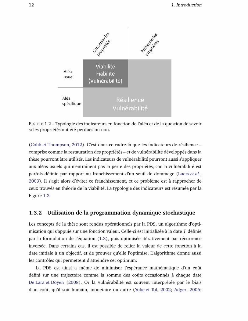
FIGURE 1.2 – Typologie des indicateurs en fonction de l’aléa et de la question de savoirsi les propriétés ont été perdues ou non.

(Cobb et Thompson, 2012). C’est dans ce cadre-là que les indicateurs de résilience –

comprise comme la restauration des propriétés – et de vulnérabilité développés dans la

thèse pourront être utilisés. Les indicateurs de vulnérabilité pourront aussi s’appliquer

aux aléas usuels qui n’entraînent pas la perte des propriétés, car la vulnérabilité est

parfois définie par rapport au franchissement d’un seuil de dommage (Luers et al.,

2003). Il s’agit alors d’éviter ce franchissement, et ce problème est à rapprocher de

ceux trouvés en théorie de la viabilité. La typologie des indicateurs est résumée par la

Figure 1.2.

1.3.2 Utilisation de la programmation dynamique stochastique

Les concepts de la thèse sont rendus opérationnels par la PDS, un algorithme d’opti-

misation qui s’appuie sur une fonction valeur. Celle-ci est initialisée à la date T définie

par la formulation de l’équation (1.3), puis optimisée itérativement par récurrence

inversée. Dans certains cas, il est possible de relier la valeur de cette fonction à la

date initiale à un objectif, et de prouver qu’elle l’optimise. L’algorithme donne aussi

les contrôles qui permettent d’atteindre cet optimum.

La PDS est ainsi a même de minimiser l’espérance mathématique d’un coût

défini sur une trajectoire comme la somme des coûts occasionnés à chaque date

De Lara et Doyen (2008). Or la vulnérabilité est souvent interprétée par le biais

d’un coût, qu’il soit humain, monétaire ou autre (Yohe et Tol, 2002; Adger, 2006;

1.3. Thème (B) : Des concepts aux indicateurs et à leur calcul 13

Peduzzi et al., 2009). La minimisation d’un coût peut donc être comprise comme un

calcul de vulnérabilité. Dans les régions de l’espace d’état où ce coût est faible, il est

possible de se retrouver dans une configuration de contrôle optimal dans certains cas.

Récemment, Doyen et De Lara (2010) ont montré que la PDS pouvait maximiser

la probabilité pour un système d’être viable en respectant des contraintes sans inter-

ruption jusqu’à la date T . Cela mène à la définition et au calcul du noyau de viabilité

dans le cas stochastique. Un tel algorithme était nécessaire car les propriétés du noyau

de viabilité, utilisées pour le calcul de noyau (Saint-Pierre, 1994; Bonneuil, 2006;

Deffuant et al., 2007) ne sont en général plus vérifiées dans le cas stochastique. La

maximisation de viabilité est omniprésente dans cette thèse. Par ailleurs, l’algorithme

de Doyen et De Lara s’applique à ce que l’on appelle un problème de cible, dans lequel

la contrainte est d’atteindre une zone donnée de l’espace d’état à une date donnée. Ce

type de problème a été utilisé dans le cas déterministe pour définir la notion de temps

de crise (Doyen et Saint-Pierre, 1997) qui entretient des liens étroits avec le concept

de résilience (Martin, 2004; Hardy, 2013).

La vulnérabilité est parfois définie par rapport à un seuil. Un noyau de viabilité

stochastique est un cas particulier d’ensemble pour lequel la vulnérabilité, comprise

comme probabilité de franchissement du seuil, est faible. Ainsi, la vulnérabilité peut

être – parfois simultanément – reliée aux deux algorithmes de PDS sus-mentionnés.

On connaît alors les décisions qui maximisent une probabilité d’être viable ou de mini-

miser un coût. Celles-ci sont généralement différentes, indiquant alors qu’il existe un

compromis à trouver entre les deux objectifs. Toutefois, aucun des deux algorithmes ne

permet de trouver ce compromis. C’est pourquoi le Chapitre 5 s’intéresse au problème

d’utiliser la PDS sur un indicateur qui agrège ces deux types d’objectifs.

Toutefois la PDS, comme les algorithmes de viabilité utilisés dans le cas détermi-

niste, sont sujets à ce que l’on appelle la malédiction de la dimension. Cela signifie que

le temps de calcul comme la mémoire requise augmentent exponentiellement avec le

nombre de dimensions de l’espace d’état, rendant le calcul impossible. C’est dans cette

optique-là qu’il convient de ne pas négliger l’apport potentiel d’autres disciplines. Par

exemple, la fiabilité (Rackwitz, 2001) a développé des algorithmes de calcul de proba-

bilité de défaillance dans des cas où l’espace à explorer est de dimension très élevée,

grâce par exemple à des méthodes d’approximation de surfaces de réponse. Certaines

de ces méthodes, comme FORM (First Order Reliability Method) ou SORM (Second

Order Reliability Method) sont statiques, donc a priori loin de cas décrits par l’équa-

tion (1.3). Mais il est intéressant de noter qu’une étude récente a porté sur la viabilité

de pêcheries côtière guyanaises en considérant treize espèces simultanément, et une

évolution sur un seul pas de temps (Cissé et al., 2013). Un tel problème ressemble à

14 1. Introduction

ceux que l’on peut traiter par FORM ou SORM.

1.4 Thème (C) : Complémentarité de résilience et vul-

nérabilité

Cette section constitue une mise en perspective des concepts de résilience et vulnéra-

bilité, dans la démarche de la thèse qui est de progresser vers un cadre commun aux

deux concepts.

La résilience et la vulnérabilité ont souvent été employées comme contraires l’un

de l’autre, et la vulnérabilité a même été définie comme le “revers de la médaille” de la

résilience (Folke et al., 2002b). Cependant, une revue comparative des deux concepts

a conclu qu’il existait des aires de convergence et de complémentarité entre les deux

concepts (Miller et al., 2010), et suggéré que des travaux supplémentaires étaient né-

cessaire pour réellement les mettre en lumière. Cela correspond au thème (C) de cette

thèse : la mise en évidence de complémentarités entre ces deux concepts. Cette section

a pour but de donner quelques perspectives.

1.4.1 Liens entre concepts et aspects normatifs du système

Une première piste concerne la manière dont les deux concepts sont reliés aux aspects

normatifs du système. Par exemple, dans leur revue de la littérature de la vulnérabilité,

Eakin et Luers (2006) évoquent “l’identification de seuils de dommages significatifs”,

ce qui implique que les dommages potentiels sont évalués pour chaque état ou tra-

jectoire avant de fixer un seuil. Mais ils dépeignent aussi un seuil comme “un point

de référence à partir duquel mesurer” la vulnérabilité. Le dommage n’est alors défini

qu’au-delà du seuil, et une fois que celui-ci est fixé.

En réalité, ce dernier cas correspond à définir une zone de dommage nul et à consi-

dérer que le “seuil de dommage significatif” délimite cette zone. Il est donc plus gé-

néral d’estimer les dommages et de définir ensuite des seuils. Emergent alors deux

manières alternatives de définir les propriétés selon que l’on définit ou non un seuil,

et qui restent à explorer.

En définissant un seuil, on définit les propriétés du système par un sous-ensemble

de l’espace d’état qui n’est autre que le noyau de faible vulnérabilité. Cela pose des

problèmes évidents de définition, puisqu’un tel objet n’est défini qu’à la date initiale,

alors que les contraintes sont définies pour chaque date de l’horizon temporel consi-

déré. Toutefois, c’est une piste à explorer afin de définir des propriétés pour le calcul

1.4. Thème (C) : Complémentarité de résilience et vulnérabilité 15

de résilience en s’appuyant sur la description normative du système donnée par l’as-

sociation d’une fonction de dommage à l’espace des trajectoires.

Les propriétés d’un SSE ont systématiquement été modélisées par un prédicat dans

le cadre viabiliste de la résilience. Par exemple dans le cas, abondamment repris dans

la thèse, de l’eutrophisation d’un lac, l’approche viabiliste fait le choix de supposer

que le lac est eutrophe quand sa concentration en phoshpore est supérieure à un seuil.

L’eutrophisation se traduit par une flore essentiellement algale, qui se développe au

détriment du reste des espèces initialement présentes dans le lac, et peut conduire à

rendre l’eau impropre à la baignade ou à la consommation. Toutefois, on peut aussi

faire correspondre à la propriété “lac oligotrophe” (le contraire d’eutrophe) plusieurs

seuils dans l’espace d’état, selon le niveau d’eutrophisation et les désagréments asso-

ciés. Le respect de la propriété “lac oligotrophe” peut alors être évalué pour chaque

trajectoire à travers les dommages liés au franchissement de chaque seuil, et le temps

passé au-delà de ces seuils. Si l’on se réfère à la terminologie du Chapitre 4, elle peut

dans ce cas précis être évaluée à travers une fonction de dommage telle qu’établie pour

calculer la vulnérabilité.

La question est alors de savoir si le noyau de faible vulnérabilité traduit alors la

persistance de la propriété “lac oligotrophe”. En effet, le fait que l’état se trouve dans le

noyau traduit le fait que les chances de franchir durablement un ou plusieurs des seuils

d’eutrophisation à un horizon donné sont limitées. Toutefois, une telle notion de per-

sistance est plus équivoque que celle proposée par le noyau de viabilité stochastique.

Sa pertinence reste à explorer et le cas échéant, à démontrer.

1.4.2 Rapport à la persistance de propriétés

Dans le cadre viabiliste, la résilience est caractérisée par le retour dans le noyau de

viabilité. Cet ensemble caractérise de manière non équivoque la persistance des pro-

priétés, car aussi longtemps qu’aucun aléa ne vient perturber le système, celui-ci va

toujours pouvoir être contrôlé de manière à ce que ses propriétés soient respectées.

En particulier, il sera possible de garder l’état dans le noyau de viabilité.

Une telle stabilité des trajectoires dans le noyau n’est plus garantie dans le cas

stochastique. En effet, seule la stabilité dans l’ensemble des contraintes est garantie

avec un niveau de confiance et pour une période donnés. Une question pratique est

de savoir comment traiter le cas (*) où l’état quitte le noyau de viabilité stochastique,

mais que les propriétés sont conservées. L’idée du cadre de la résilience du Chapitre 2

est de restaurer la persistance des propriétés en optimisant la vitesse de retour dans

le noyau de viabilité stochastique. La stratégie qui optimise la vitesse de restauration

des propriétés et celle qui optimise la viabilité ne sont pas forcément les mêmes. Il

16 1. Introduction

peut donc exister dans le cas (*) un dilemne entre la probabilité d’être viable et la

probabilité de résilience à certains horizons temporels. Si la non-viabilité est reliée à

la vulnérabilité comme dans le Chapitre 4, cela peut se traduire par un dilemne entre

résilience et vulnérabilité. Dans ce cas précis, les rôles des deux concepts de résilience

et de vulnérabilité dans un cadre commun restent donc à établir.

Une autre question est la possibilité de décrire la persistance des propriétés en

utilisant un noyau de faible vulnérabilité autre que le noyau de viabilité stochastique.

A priori, utiliser un critère de viabilité traduit mieux la persistance qu’un critère de

coût. Toutefois, la question mérite d’être posée, surtout à la lumière des noyaux de

faible vulnérabilité basés sur des critères composite de coût et de viabilité définis dans

le Chapitre 5. De tels noyaux sont peut-être à même de résoudre le dilemne exposé au

paragraphe précédent.

1.4.3 Description des trajectoires de restauration

En définissant la résilience comme l’inverse d’un coût de restauration, Martin (2004)

accrédite l’idée que la vulnérabilité et la résilience sont des contraires. Toutefois, cette

idée a ensuite été nuancée (Deffuant et Gilbert, 2011) en dissociant la résilience –

le fait de restaurer les propriétés – du coût associé. La vulnérabilité et la résilience

donnent alors une information complémentaire.

Dans un cadre stochastique, le fait de rentrer n’est plus seulement certain ou impos-

sible. Il devient en général une probabilité. Cela s’applique aussi au fait de rentrer dans

un horizon temporel donné. Dans ces conditions, il existe de nombreuses statistiques

associées à la distribution de probabilité de dates de rentrée. Si de nombreuses mé-

triques peuvent décrire la résilience du système, alors la vulnérabilité devient d’autant

plus nécessaire pour décrire les dommages occasionnés par la perte des propriétés.

Cependant, il faut garder à l’esprit que les politiques d’action qui maximisent une

probabilité de résilience et celles qui minimisent une fonction de dommage ne sont pas

en général les mêmes. Là encore, les indicateurs composites définis dans le Chapitre

5 semblent en mesure d’expliciter les compromis éventuels à faire entre résilience et

vulnérabilité.

– 2 –

Extending the viability theory framework of

resilience to uncertain dynamics, and

application to lake eutrophication

Publié dans Ecological Indicators, Volume 29, pages 429-433, 2013.

Auteurs : Charles ROUGÉ, Jean-Denis MATHIAS et Guillaume DEFFUANT

Resilience, the capacity for a system to recover from a perturbation so as to

keep its properties and functions, is of growing concern to a wide range of en-

vironmental systems. The challenge is often to render this concept operational

without betraying it, nor diluting its content. The focus here is on building on

the viability theory framework of resilience to extend it to discrete-time sto-

chastic dynamical systems. The viability framework describes properties of

the system as a subset of its state space. This property is resilient to a per-

turbation if it can be recovered and kept by the system after a perturbation :

its trajectory can come back and stay in the subset. This is shown to reflect a

general definition of resilience. With stochastic dynamics, the stochastic via-

bility kernel describes the robust states, in which the system has a high pro-

bability of staying in the subset for a long time. Then, probability of resilience

is defined as the maximal probability that the system reaches a robust state

within a time horizon. Management strategies that maximize the probability

of resilience can be found through dynamic programming. It is then possible

to compute a range of statistics on the time for restoring the property. The

approach is illustrated on the example of lake eutrophication and shown to

foster the use of different indicators that are adapted to distinct situations. Its

relevance for the management of ecological systems is also discussed.

17

18 2. Resilience : a stochastic viability framework

2.1 Introduction

Resilience has growingly been regarded as a central concept for many ecological sys-

tems, as well as for many human systems relying on ecosystem services. Indeed, resi-

lience is related to the continued existence and sustainability of these systems in an

era of upcoming widespread changes (e.g. Folke et al., 2002b; Walker et al., 2004).

Since the original definition of resilience in ecology by Holling (1973), there has been

a flurry of definitions of the concept in related fields (Brand et Jax, 2007), while it can

be tackled at different levels of abstraction (Carpenter et al., 2001). In this context,

and in order not to lose what is meant by resilience, one central challenge is to intro-

duce generic computational frameworks that can at the same time accurately reflect

the concept and produce case-specific indicators.

This paper aims at tackling this issue for discrete-time stochastic dynamical sys-

tems. It builds on the viability theory framework of resilience, initially introduced in

Martin (2004) for deterministic systems, and to which a book has recently been de-

voted (Deffuant et Gilbert, 2011). It focuses on extending this framework to the sto-

chastic case through the use of computational techniques based on dynamic program-

ming. The viability framework generalizes the current mathematical definitions of the

concept of resilience without betraying its intuitive sense. In this respect, we consider

that the viability approach responds to the call from Brand et Jax (2007) for a clear

descriptive definition of the term of resilience, to avoid an eventual loss of its concep-

tual content as its use as a boundary object is spread around different research com-

munities, for instance ecology and social sciences (Adger, 2000; Folke et al., 2002b;

Adger et al., 2005). Besides, one major advantage of the viability approach is to pro-

vide with ways of computing relevant courses of action to ensure the resilience of the

system. The extension presented here preserves this aspect.

The viability framework of resilience starts with the idea that it is essential to define

the resilience of “what” to “what” (Carpenter et al., 2001). It assumes that we are

interested in the resilience of a property of the dynamical system, this property being

called resilient to a perturbation if the system is able to restore it if it is lost, then

keep it. In mathematical terms, a property can be described as a subset of the system

state space, delimited by constraints. Resilience is related to the ability to come back

and stay in this subset. Hence, this approach particularly emphasizes the possibility for

restoring the property after losing it, which in our view is what distinguishes resilience

from the concept of stability (Grimm et Wissel, 1997).

In this respect, the viability framework is distinct from the initial definition of re-

silience in ecology by Holling (1973) as the amount of perturbation a system can

2.1. Introduction 19

withstand while keeping its properties and functions. A direct implication of such a

definition is the emphasis put on the considered properties and functions. The reason

is that the considered resilience is of the system itself, hence of the properties and func-

tions that define its identity. When considering the resilience of any property, possibly

a minor one, we open the possibility for the system to lose the property for a while,

and then to restore it. We claim that focusing on the aspects of recovery and restora-

tion, which is put forward in the viability based framework, is pivotal to the resilience

concept. There is indeed a variety of studies that relates resilience to measures of

the recovery capacity of a system (e.g. Hashimoto et al., 1982; MacGillivray et Grime,

1995; Johnson et al., 1996; Lesnoff et al., 2012).

As explained in Deffuant et Gilbert (2011), the viability framework generalizes

the mathematical attractor-based definitions of resilience (e.g. Anderies et al., 2002)

which focus on regime shifts. Indeed, in these latter definitions, the property of inter-

est is identified as a set of states located around selected attractors which represent

a desirable regime. Resilience indicators are related to the size of the attractor basins

of these attractors, namely the part of space where the system avoids to fall into bad

attractor basins. If one defines the property of interest as a subset around the good

attractors, then the viability framework provides similar results to the ones of the at-

tractor based definition. However, the property of interest can be defined as any subset

of the state space and therefore offers wider possibilities, especially in cases where no

attractor would exist.

Moreover, the viability framework of resilience provides operational tools for com-

puting policies of actions (or feedback rules) to keep or restore a property of interest,

namely by driving the system back to the desirable subset and keeping it there. Alter-

native mathematical frameworks for computing resilience at best suppose that a policy

of action is already defined. This is a very important practical advantage of the viabi-

lity framework, as illustrated in several case studies in (Deffuant et Gilbert, 2011). As

any other framework, viability has its limits and drawbacks, namely :

1) The current numerical approaches for computing the resilient states and the

restoration policies are very demanding computationally because they require

to discretize the state space (and also the action space). Therefore, in practice

only the dynamical models with very few degrees of freedom are tractable (see

Deffuant et Gilbert (2011) for further information).

2) The current viability framework only considers one-time perturbations in otherwise

deterministic dynamical systems, thus not taking into account the potential impact

of other uncertainty sources while computing resilience to these events.

20 2. Resilience : a stochastic viability framework

This paper aims at overcoming the latter limit and proposes an extension of the via-

bility framework of resilience to stochastic dynamical systems. It is based on the key

assumption that uncertainty, whatever its source, can be mathematically described in

two different ways. On the one hand, some of the uncertainty can be described by

stochastic processes, which can be assessed under the form of probability distribution

functions (pdf) and reduced by experience (Allen et al., 2011; Williams, 2011). Since

this part of the uncertainty can be embedded into the dynamics, the system can be ma-

naged so as to be made robust to it. On the other hand, there is invariably a part of un-

predictability that escapes such assessments (Gunderson, 2000; Walker et al., 2002),

as emphasized by the expression “uncertainty and surprise” found in the literature

(Folke et al., 2002b, 2004; Adger et al., 2005). This second uncertainty source gene-

rally refers to events that initiate potentially major disturbances, and to which the

resilience of the system must be assessed.

From a technical point of view, the present work uses the stochastic extensions to

viability theory in the discrete-time case (De Lara et Doyen, 2008; Doyen et De Lara,

2010) and builds on the robust and stochastic viability frameworks, both based

on dynamic programming, and which have been successfully applied to fisheries

management (Doyen et Béné, 2003; De Lara et Martinet, 2009; Doyen et al., 2012;

Péreau et al., 2012). One can expect three main differences between the deterministic

and stochastic viability frameworks :

1) The viability kernel is a subset of the state space of a deterministic system in which

the system can keep the property if it remains undisturbed. Stochastic viability ker-

nels only guarantee that the system will keep the property with a given probability

by a given time horizon, but this is also a guarantee that the system is robust to the

uncertainty sources described by the stochasticity of its dynamics.

2) The single optimal trajectory for reaching the deterministic viability kernel is re-

placed by a set of trajectories. This fosters the definition a probability of resilience,

the probability of reaching the stochastic viability kernel by a given time horizon.

Besides, the single resilience indicator that prevails in the deterministic case (e.g.

the inverse of the restoration cost as in Martin (2004)) is replaced by a pdf for the

times or costs of restoration. Resilience indicators are derived from statistics on

this pdf.

3) Contrary to what happens with deterministic viability, the time horizon considered

for the management of the system becomes of paramount importance for policy

design. Policies become specifically designed to maximize the probability of being

2.2. Background : resilience in the deterministic case 21

resilient by the time horizon, but are not in general meant to maximize this proba-

bility at any shorter horizon.

The paper is organized as follows. First, we recall the main concepts of the viability-

based framework of resilience in the deterministic case, and illustrate it on a simple

lake eutrophication model (Section 2.2). In section 2.3, we introduce the extension

of the viability based framework of resilience to stochastic dynamics, defining the

concepts of probability of resilience and different measures of restoration time and

cost. Section 2.4 illustrates the approaches on the lake model, first for a given control

strategy, then when controls are being optimized as resilience is computed. The rele-

vance for the study of ecological systems is discussed in Section 2.5, before conclusions

are drawn in Section 2.6.

2.2 Background : resilience in the deterministic case

The general problem of achieving resilience in limited time after a perturbations, consi-

dering constrained dynamics and controlled strategies, is laid out in discrete time in

the deterministic case. The viability framework of resilience from Martin (2004) and

Deffuant et Gilbert (2011) is then put into perspective.

2.2.1 Problem statement

Controlled dynamics

In the viability framework for resilience presented by Martin (2004), an important

innovation is to introduce controls to explicitly account for the possibility to act on

the system. In this framework, the policy is not fixed beforehand. Instead, the goal is

to find policies that will make the system resilient. In discrete time, this means that

at each time step, there is a set of possible actions that one must choose from, and

a known transition equation between two consecutive dates. Let us note X the state

space and x t the state of the system at date t. Noting also U(x t, t) the set of available

controls and ut the chosen control value, a typical controlled discrete-time dynamical

system can be written as :

x t+1 = g (x t , ut) (2.1)

Resilience to “what” ?

In this framework we focus on resilience to a given perturbation. There is no assump-

tion on the nature or amplitude of the perturbation. Indeed, we place ourselves in the

22 2. Resilience : a stochastic viability framework

post-perturbation state of the system. Resilience of any state to any perturbation can

then be assessed by looking at the new state of the system after the perturbation.

Management objectives and constraints

The system has some properties that are deemed desirable. We assume that these

properties can be mathematically translated into state constraints, which define a set

of desirable states noted K . The general goal then becomes to control the system so it

stays within K .

After a perturbation, the goal becomes to ensure that the system gets back to a

state where its dynamics are going to keep it within K for as long as it is not disturbed

again. Management also has a time frame, or time scale of interest, which we will note

T . This is the time by which the system’s properties ought to be restored.

Management strategies

The objectives are achieved through management strategies. A strategy can be repre-

sented by a function which associates a control to any date 0 ≤ t ≤ T − 1 and to any

state x . A strategy can be described at each time step by a feedback map, an applica-

tion from X into U(x , t) (or from K if we only want to see whether the system leaves

K). In this work, strategies will be determined depending on the time horizon. Conse-

quently, we choose to reference a feedback maps are referenced by their time distance

to the horizon. A strategy is given, in chronological order, by the following succession

of feedback maps :

f = ( fT , fT−1, . . . , f1) (2.2)

Controls at any date t ≤ T are deduced from equation (2.3) :

¨

ut = fT−t(x)

ut ∈ U(x , t)(2.3)

We can also introduce the notation F(T ) for the set of all strategies f with a time

horizon T . For a given f , it is possible to recursively compute all the states from the

initial state x0 to the final state xT . Indeed, equation (2.1) can be written anew using

equation (2.3) through :

x t+1 = g(x t, fT−t(x t)) (2.4)

Thus, we can define the trajectory g f starting from the initial state x0 and using the

strategy f as :

∀t ∈ [0, T ], x t = g f (t , x0) (2.5)

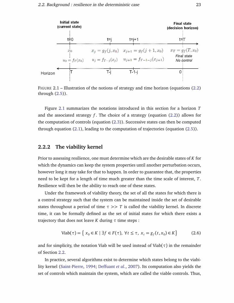
2.2. Background : resilience in the deterministic case 23

FIGURE 2.1 – Illustration of the notions of strategy and time horizon (equations (2.2)through (2.5)).

Figure 2.1 summarizes the notations introduced in this section for a horizon T

and the associated strategy f . The choice of a strategy (equation (2.2)) allows for

the computation of controls (equation (2.3)). Successive states can then be computed

through equation (2.1), leading to the computation of trajectories (equation (2.5)).

2.2.2 The viability kernel

Prior to assessing resilience, one must determine which are the desirable states of K for

which the dynamics can keep the system properties until another perturbation occurs,

however long it may take for that to happen. In order to guarantee that, the properties

need to be kept for a length of time much greater than the time scale of interest, T .

Resilience will then be the ability to reach one of these states.

Under the framework of viability theory, the set of all the states for which there is

a control strategy such that the system can be maintained inside the set of desirable

states throughout a period of time τ >> T is called the viability kernel. In discrete

time, it can be formally defined as the set of initial states for which there exists a

trajectory that does not leave K during τ time steps :

Viab(τ) =

x0 ∈ K | ∃ f ∈ F(τ), ∀t ≤ τ, x t = g f (t , x0) ∈ K

(2.6)

and for simplicity, the notation Viab will be used instead of Viab(τ) in the remainder

of Section 2.2.

In practice, several algorithms exist to determine which states belong to the viabi-

lity kernel (Saint-Pierre, 1994; Deffuant et al., 2007). Its computation also yields the

set of controls which maintain the system, which are called the viable controls. Thus,

24 2. Resilience : a stochastic viability framework

it incorporates the impacts of management policies, and implicitly optimizes them.

2.2.3 Viability-based definition of resilience

This section puts into perspective the results from Martin (2004) and

Deffuant et Gilbert (2011) about resilience to a single perturbation in an other-

wise deterministic system. Resilience is associated to the possibility of getting back to

the viability kernel in a relevant time frame, denoted by the horizon T .

Let us first consider a given strategy f at horizon T , with the only constraint that

at any date and for any state within the viability kernel fT−t(x) is a viable control. One

can then define what is called a resilience basin in Deffuant et Gilbert (2011) : the set

of states for which the system is brought back to the viability kernel in a horizon t ≤ T .

This notion can first be written for a given strategy :

Bres( f , t) =

x ∈ X | g f (t , x) ∈ Viab

(2.7)

For t1 < t2, since any trajectories that reaches the viability kernel by t1 can also reach

it if given a greater time horizon, we have Bres( f , t1) ⊂ Bres( f , t2). The union of all

the resilience basins is Bres( f , T ), and it is the set of resilient states for the strategy

f , from which the system can recover by getting back to the viability kernel in T time

steps or less.

Yet, one has many strategies at her disposal, and may want to find the set of all

the states for which it is possible to bring the system back to the viability kernel in a

horizon t ≤ T . This brings about a different definition of a resilience basin :

Bres(t) =

x ∈ Rn | ∃ f ∈ F(t), g f (t , x) ∈ Viab

(2.8)

The implicit difference between equations (2.7) and (2.8) is that in the latter, controls

have been optimized to find trajectories that ensure the resilience of the system by the

chosen time horizon. In this work, we choose to use dynamic programming to carry

out this optimization. Dynamic programming is a recursive algorithm which enables to

optimize a value function, noted Vd(t , x) in this deterministic case, at each horizon t . It

progresses backwards from date T (horizon 0) to the initial date (horizon T). It yields

the same results in the deterministic case as algorithms like KAVIAR (Deffuant et al.,

2007) used by Deffuant et Gilbert (2011), but will be extended to the uncertain case

in Section 2.3. Like any recursive algorithm, it works based on an initial equation and

a transition equation. Here, initialization comes from the fact that resilience at a time

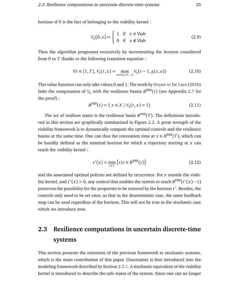
2.3. Resilience computations in uncertain discrete-time systems 25

horizon of 0 is the fact of belonging to the viability kernel :

Vd(0, x) =

¨

1 if x ∈ Viab

0 if x /∈ Viab(2.9)

Then the algorithm progresses recursively by incrementing the horizon considered

from 0 to T thanks to the following transition equation :

∀t ∈ [1, T ], Vd(t , x) = maxu∈U(x ,T−t)

Vd(t − 1, g(x , u)) (2.10)

This value function can only take values 0 and 1. The work by Doyen et De Lara (2010)

links the computation of Vd with the resilience basins Bres(t) (see Appendix 2.7 for

the proof) :

Bres(t) = x ∈ X | Vd(t , x) = 1 (2.11)

The set of resilient states is the resilience basin Bres(T ). The definitions introdu-

ced in this section are graphically summarized in Figure 2.2. A great strength of the

viability framework is to dynamically compute the optimal controls and the resilience

basins at the same time. One can thus the restoration time at x ∈ Bres(T ), which can

be handily defined as the minimal horizon for which a trajectory starting at x can

reach the viability kernel :

t∗(x) =mint≤T

t |x ∈ Bres(t)

(2.12)

and the associated optimal policies are defined by recurrence. For x outside the viabi-

lity kernel, and t∗(x)> 0, any control that enables the system to reach Bres(t∗(x)−1)

preserves the possibility for the properties to be restored by the horizon t∗. Besides, the

controls only need to be set once, so that in the deterministic case, the same feedback

map can be used regardless of the horizon. This will not be true in the stochastic case

which we introduce now.

2.3 Resilience computations in uncertain discrete-time

systems

This section presents the extension of the previous framework to stochastic systems,

which is the main contribution of this paper. Uncertainty is first introduced into the

modeling framework described by Section 2.2.1. A stochastic equivalent of the viability

kernel is introduced to describe the safe states of the system. Since one can no longer

26 2. Resilience : a stochastic viability framework

FIGURE 2.2 – Constraint set, viability kernel and some resilience basins in the originalviability framework of Martin (2004) and Deffuant et Gilbert (2011). There is onepossible trajectory for a given control strategy : post-perturbation states A and B areresilient while C is not.

2.3. Resilience computations in uncertain discrete-time systems 27

guarantee that a set can be reached with probability one after a minimal amount of

time, we choose to focus on maximizing the probability of being resilient by reaching

the stochastic viability kernel. We thus introduce the notion of probability of resilience,

before showing how quantities that can be related to a variety of possible resilience

indicators can be handily computed thanks to this notion.

2.3.1 Incorporating uncertainty

Uncertainty in a modeling framework such as that of Section 2.2.1 can arise from nu-

merous sources (Williams, 2011). Yet, here we are concerned with how uncertainty

can be modeled, rather than where it comes from. Knowledge about uncertainty can

be imperfect (Walker et al., 2002), so that no pdf can capture all of the uncertainty,

especially that related to large events. As mentioned in the introduction, the key as-

sumption used here is to consider that aside from large uncertain perturbations which

might happen from to time to time, the rest of the uncertainty can be modeled at each

time step using random variables for which a pdf can be defined. Then, we compute

resilience to a given large, unknown event while taking into account the sequential

effects of smaller events which may be described in stochastic terms at each time step.

When considering uncertainty, the dynamic g of equation (2.1) has to be modified.

Following Doyen et De Lara (2010), let us assume the existence of a known dynamic

g which incorporates a vector ε of all uncertainties, whether they concern the dynamic

itself or the state, control or parameter variables. We get :

x t+1 = g(x t , ut ,εt) (2.13)

Let us now suppose that the state space X has been discretized, which is the case

in practice. Discretization methods are not within the scope of this paper. We note X

the points of the discrete grid.

The rest of Section 2.2.1 is kept unchanged. In particular, the notion of strategy

f ∈ F(T ) is kept ; unlike what happens in deterministic viability, one should not expect

the feedback map to be the same for two different values of the horizon T . We also

keep the notion of trajectory associated to a strategy, but we are now faced with a

set of trajectories which depends on the events ε0, ε1, etc. . .Thus, g f (t , x0) becomes a

random variable.

The use of dynamic programming as an essential tool of stochastic viability theory

(Doyen et De Lara, 2010) imposes the pdfs εt to be uncorrelated with one another.

This is because dynamic programming essentially requires to travel backwards in time.

What is more, in this framework, feedback optimization is only guaranteed when the

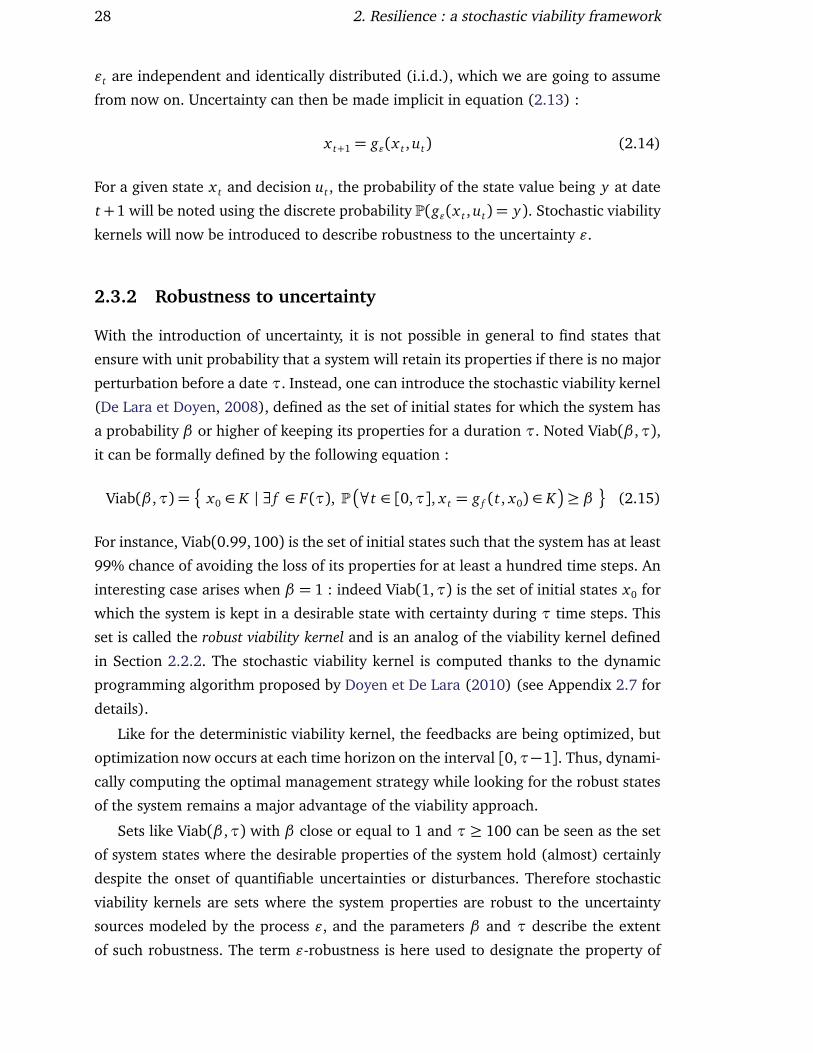
28 2. Resilience : a stochastic viability framework

εt are independent and identically distributed (i.i.d.), which we are going to assume

from now on. Uncertainty can then be made implicit in equation (2.13) :

x t+1 = gε(x t , ut) (2.14)

For a given state x t and decision ut , the probability of the state value being y at date

t+1 will be noted using the discrete probability P(gε(x t , ut) = y). Stochastic viability

kernels will now be introduced to describe robustness to the uncertainty ε.

2.3.2 Robustness to uncertainty

With the introduction of uncertainty, it is not possible in general to find states that

ensure with unit probability that a system will retain its properties if there is no major

perturbation before a date τ. Instead, one can introduce the stochastic viability kernel

(De Lara et Doyen, 2008), defined as the set of initial states for which the system has

a probability β or higher of keeping its properties for a duration τ. Noted Viab(β ,τ),

it can be formally defined by the following equation :

Viab(β ,τ) =

x0 ∈ K | ∃ f ∈ F(τ), P

∀t ∈ [0,τ], x t = g f (t , x0) ∈ K

≥ β

(2.15)

For instance, Viab(0.99, 100) is the set of initial states such that the system has at least

99% chance of avoiding the loss of its properties for at least a hundred time steps. An

interesting case arises when β = 1 : indeed Viab(1,τ) is the set of initial states x0 for

which the system is kept in a desirable state with certainty during τ time steps. This

set is called the robust viability kernel and is an analog of the viability kernel defined

in Section 2.2.2. The stochastic viability kernel is computed thanks to the dynamic

programming algorithm proposed by Doyen et De Lara (2010) (see Appendix 2.7 for

details).

Like for the deterministic viability kernel, the feedbacks are being optimized, but

optimization now occurs at each time horizon on the interval [0,τ−1]. Thus, dynami-

cally computing the optimal management strategy while looking for the robust states

of the system remains a major advantage of the viability approach.

Sets like Viab(β ,τ) with β close or equal to 1 and τ ≥ 100 can be seen as the set

of system states where the desirable properties of the system hold (almost) certainly

despite the onset of quantifiable uncertainties or disturbances. Therefore stochastic

viability kernels are sets where the system properties are robust to the uncertainty

sources modeled by the process ε, and the parameters β and τ describe the extent

of such robustness. The term ε-robustness is here used to designate the property of

2.3. Resilience computations in uncertain discrete-time systems 29

state within a stochastic viability kernel. However, the focus of this work is to compute

resilience to a large unexpected perturbation, and a new notion is needed to extend

to the stochastic case the viability framework, which precisely dealt with resilience to

such events in the deterministic case.

2.3.3 Probability of resilience

Let us now assume that one has computed a stochastic (or robust) viability kernel

Viab(β ,τ), the set of states for which the system’s properties are guaranteed to be

ε-robust. The conceptual notion of resilience can then be operationalized through the

possibility of reaching this set in a given time frame T . This is very similar to what

is done in the deterministic case, except that reaching Viab(β ,τ) now guarantees ε-

robustness to quantifiable uncertainty. Besides, the considered horizon T has to be

small compared to the time scale τ during which the system can be maintained with

a high probability, so that the condition T << τ holds, like in Section 2.2.

For a given strategy f ∈ F(T ), the probability of getting into a given Viab(β ,τ) by

a date t ≤ T is the capacity to recover from a perturbation under this strategy. It is

noted PRes( f , t , x) :

PRes( f , t , x) = P

∃ j ∈ [0, t], g f ( j, x) ∈ Viab(β ,τ)

(2.16)

and from equation (2.2), the controls that are applied between dates 1 and t are those

of the successive feedback maps ( fT , fT−1, . . . , fT−t).

Like in the deterministic case, the objective of viability is to find the feedbacks

that maximize the probability of resilience, but now specifically as the probability of

reaching Viab(β ,τ) by date T . This probability of resilience, noted PRes(T, x), is thus

given by the value of PRes( f , T, x) when the strategy is optimal :

PRes(T, x) = maxf ∈F(T)PRes( f , T, x)

= PRes( f∗, T, x)

(2.17)

where the optimal strategy f ∗ is not necessarily unique. The probability of resilience

PRes(T, x) represents the probability of being resilient within the considered time

frame. If PRes(T, x) = 1, the system can always be made ε-robust, and it is resilient.

To compute the probability of resilience in this stochastic case, we use a value

function Vs depending on the horizon t and state x , which is the exact analog of the

30 2. Resilience : a stochastic viability framework

deterministic Vd :

Vs(0, x) =

¨

1 if x ∈ Viab(β ,τ)

0 if x /∈ Viab(β ,τ)

∀t ∈ [1, T ],

Vs(t , x) =

maxf t(x)∈U(x ,T−t)

∑

y∈X

P(gε(x , ft(x)) = y) Vs(t − 1, y)

!

if x /∈ Viab(β ,τ)

1 if x ∈ Viab(β ,τ)

(2.18)

and the value function Vs yields the maximal value of the probability of resilience

(proof to be found in Appendix 2.7) :

PRes(T, x) = Vs(T, x) (2.19)

and the associated optimal strategy f ∗ is given by the feedback maps f ∗T−t

:

x → ut , computed through equation (2.18) at each time step. This strategy f ∗ =

( f ∗T, f ∗

T−1, . . . , f ∗1 ) yields the maximal probability for the system to be resilient at the

horizon T . It can then used to compute the probabilities PRes( f∗, t , x) of recovering

the ε-robustness of the system’s properties by a date t ≤ T .

The feedback one has to apply to a given state at a given date depend on the

distance to the horizon T , and thus, on the horizon itself. Indeed, the probabilities

PRes( f∗, t , x) are not necessarily the maximal probability of reaching the stochastic

viability kernel by t . For that, one should use the optimized feedbacks ( f ∗t, f ∗

t−1, . . . , f ∗1 )

for the respective dates (0, 1, . . . , t). These feedbacks would yield PRes(t , x) which

the maximal probability of being resilient with a time horizon t . Yet, one should

keep in mind that between the initial date and t , the strategies ( f ∗t, f ∗

t−1, . . . , f ∗1 ) and

( f ∗T, f ∗

T−1, . . . , f ∗T+1−t

) are in general different, and that only the latter maximizes the

probability of being resilient at date t .

The definitions introduced in this section are graphically summarized in Figure

2.3. One can notice differences with the resilience basins one can compute in the

deterministic case (Section 2.2.3 and Figure 2.2). Due to the many possible trajectories

for the optimal feedback strategy, resilience is not in general a certain property any

more. As a consequence, minimizing the time to get back to the viability kernel does

not make obvious sense like it does in the deterministic case. Instead, we choose to

maximize the probability of getting back at a given horizon instead.

Besides, the probability of resilience is highly dependent on the prior choice of the

β and τ. Indeed, the larger β and τ, the smaller the stochastic viability kernel, and the

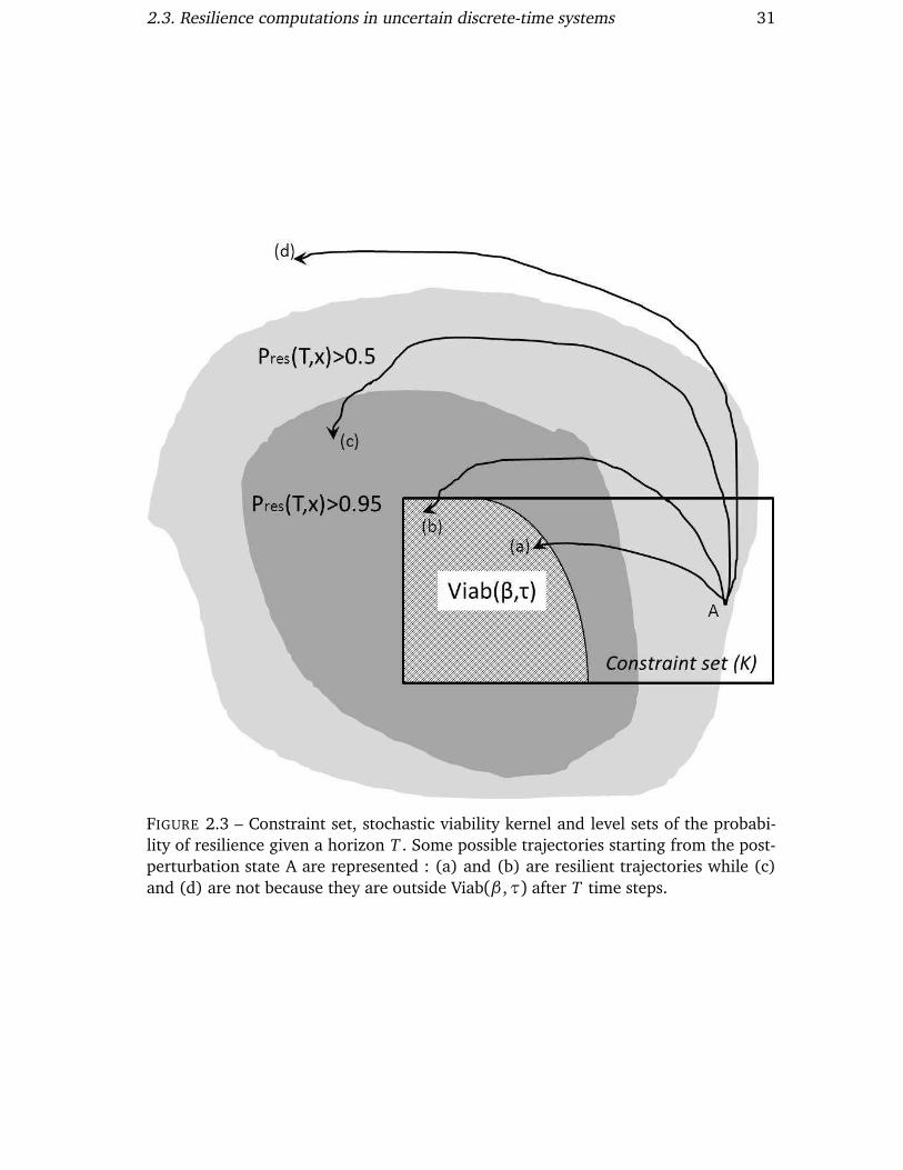
2.3. Resilience computations in uncertain discrete-time systems 31

FIGURE 2.3 – Constraint set, stochastic viability kernel and level sets of the probabi-lity of resilience given a horizon T . Some possible trajectories starting from the post-perturbation state A are represented : (a) and (b) are resilient trajectories while (c)and (d) are not because they are outside Viab(β ,τ) after T time steps.

32 2. Resilience : a stochastic viability framework

longer it takes to reach it. Yet, the more draconian the robustness criteria, the better

the robustness of the system when it reaches that set, and the more meaningful it is to

see resilience as the probability of reaching it. Thus when setting the parameters β and

τ, one has to consider a tradeoff between the quality of the resilience and robustness of

the properties of the system, and how costly these are to achieve. This means resilience

to a large, unpredictable perturbation is defined in tandem with ε-robustness.

Eventually, the optimal feedbacks used to compute the ε-robust states and the re-

silient ones are not the same in general. They correspond to two distinct problems :

the first is to guarantee the properties of the system against “usual” uncertainty, while

the second is to make the system robust again following a perturbation. In both cases,

the feedbacks are dependent on the time horizon considered.

2.3.4 Resilience-related indicators

Computed for a given T , the quantities PRes( f∗, t , x) form a set of indicators that

gives the cumulative distribution function of the time needed to get to a set where

the desirable properties of the system are guaranteed to a comfortable extent against

uncertainty. Yet, measures of resilience are often given through a single performance

indicator. Thus, while they represent well what resilience is at the conceptual level,

these quantities are not necessarily relevant operational indicators. However, they are

a basis for computing virtually any indicator that represents resilience based on the

time taken to reach a situation that keeps the properties of interest of a system. Indeed,

the pdf of the time taken to reach an ε-robust set Viab(β ,τ) is given by the difference

PRes( f∗, t , x)− PRes( f

∗, t − 1, x)

, which is the probability to reach this set exactly

at date t .

Index computation depends on whether or not the loss of ε-robustness is reversible

with unit probability by the date T . If there are states such that PRes(T, x) < 1, one

can directly relate this quantity to the resilience of the system. Yet further relevant in-

dicators related to resilience exist, especially (but not only) when PRes(T, x) = 1. One

such indicator can be the expected value of the time needed to acquire the resilience

property using the strategy f ∗ :

E(t | f ∗, x) =

T∑

t=0

(t + 1)

PRes( f∗, t + 1, x)− PRes( f

∗, t , x)

(2.20)

It should be noted that f ∗ is not necessarily the strategy that optimizes the expected

entry time, and it is no equivalent to the entry time defined in the deterministic case

by equation (2.12). Such an equivalent could be provided by tailoring the considered

2.4. Application to an uncertain lake model 33

horizon to the state of the system, still keeping in mind that it means the feedback

maps used will then change. For x , one would pick the shortest horizon tα such that

the probability of resilience PRes(t , x) guarantees that the ε-robustness of the system

at the horizon tα with a confidence level α. When it exists, tα can be defined by :

tα(x) = min0≤t≤T

t |PRes(t , x)≥ α

(2.21)

and because of equation (2.19), it can be computed using yet again the value function

Vs :

tα(x) = min0≤t≤Tt |Vs(t , x)≥ α (2.22)

Both indicators E(t | f ∗, x) and tα(x) can be used in association with the notion of re-

silience, and a resilience indicator can even be defined as a decreasing function of one

of them. Then, this decreasing function is often the inverse function (Hashimoto et al.,

1982; Martin, 2004). In a more general way, when resilience can be achieved with a

nonzero probability, a useful indicator is the cost incurred while driving the system

back to the viability kernel. One can choose whether to associate it to the notion of re-

silience or to define resilience as a decreasing function of this cost much like in Martin

(2004) (e.g. its inverse).

The equations proposed here provide one with various ways to compute resilience

and related indicators while explicitly incorporating the potential effects of uncer-

tainty. They are also an illustration of the power of dynamic programming tools when

it comes to carrying out resilience computations.

2.4 Application to an uncertain lake model

The lake eutrophication problem can be tackled through simple nonlinear dynamics,

and has been well-studied (Carpenter et al., 1999, 2001; Ludwig et al., 2003). Here we

choose, for illustrative purposes, to use the deterministic model from Martin (2004)

and add uncertainty to it. Resilience computations introduced by Martin (2004) and

Deffuant et Gilbert (2011) are outlined, and the added value of considering uncer-

tainty is highlighted. The dynamics and resilience problem are laid out first, before

being solved for a given strategy. Then, the interest of using stochastic viability to

optimize the control strategy is emphasized.

34 2. Resilience : a stochastic viability framework

2.4.1 The problem of lake eutrophication

Using the publications cited above, this section introduces the case of lake eutrophi-

cation under its simplest formulation, that is, not considering the mud dynamics. The

problem is formulated much like in Section 2.2.1, but introduces uncertainty while

introducing the system’s dynamic.

Uncertain controlled dynamics

The state variables are the phosphorus concentration p in the lake, and the phosphorus

input rate l. In continuous time θ , the evolution of phosphorus concentration reads as

follows Martin (2004) :

dp

dθ= −bp+ l + r

pq

pq +mq(2.23)

where the parameter b is the phosphorus sink rate (e.g. the quantity that flows out

of the lake), r is the maximal recycling rate by algae, m is the value of p for which

the recycling term (rpq)/(pq +mq) is half its maximal value, and q is a dimensionless

parameter, set at q = 8 in several studies (e.g. Martin, 2004; Guttal et Jayaprakash,

2007).

Through dimensional analysis, the parameters b and m can be eliminated while p,

l and r are turned into their respective dimensionless equivalents : the state variables

P and L, and the only remaining parameter is R (see Appendix 2.8 for details). θ is also

replaced by the dimensionless time t , and we get the new continuous-time equation :

dP

d t= −P + L + R

P8

P8 + 1(2.24)

Let us now tackle uncertainty. For the sake of simplicity, only phosphorus input

uncertainty will be considered in this example. It represents, for instance, the uncer-

tainty that is due to the soil storage of phosphorus. A discrete-time decomposition (for

which the continuous-time equivalent is given in Appendix 2.9.1) between the mean

input rate L∗ and a deviation is introduced :

L t = L∗t+σεt (2.25)

Here ε is considered i.i.d., and it is modeled by a standard normal distributionN (0, 1),

due to the common use of such distributions. σ represents the standard deviation of

the noise. Since the phosphorus input L is not updated by the dynamic of equation

(2.23), choosing L∗ instead of L as a state variable enables the modeler to project the

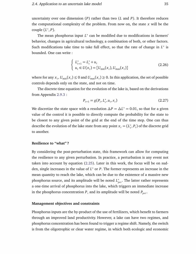
2.4. Application to an uncertain lake model 35

uncertainty over one dimension (P) rather than two (L and P). It therefore reduces

the computational complexity of the problem. From now on, the state x will be the

couple (L∗, P).

The mean phosphorus input L∗ can be modified due to modifications in farmers’

behavior, changes in agricultural technology, a combination of both, or other factors.

Such modifications take time to take full effect, so that the rate of change in L∗ is

bounded. One can write :

¨

L∗t+1 = L∗

t+ ut

ut ∈ U(x t) = [Umin(x t), Umax(x t)](2.26)

where for any x t , Umin(x t) ≤ 0 and Umax(x t) ≥ 0. In this application, the set of possible

controls depends only on the state, and not on time.

The discrete time equation for the evolution of the lake is, based on the derivations

from Appendix 2.9.3 :

Pt+1 = g(Pt , L∗t, ut ,εt) (2.27)

We discretize the state space with a resolution ∆P = ∆L∗ = 0.01, so that for a given

value of the control it is possible to directly compute the probability for the state to

be closest to any given point of the grid at the end of the time step. One can thus

describe the evolution of the lake state from any point x t = (L∗t, Pt) of the discrete grid

to another.

Resilience to “what” ?

By considering the post-perturbation state, this framework can allow for computing

the resilience to any given perturbation. In practice, a perturbation is any event not

taken into account by equation (2.25). Later in this work, the focus will be on sud-

den, single increases in the value of L∗ or P. The former represents an increase in the

mean quantity to reach the lake, which can be due to the existence of a massive new

phosphorus source, and its amplitude will be noted L∗per

. The latter rather represents

a one-time arrival of phosphorus into the lake, which triggers an immediate increase

in the phosphorus concentration P, and its amplitude will be noted Pper.

Management objectives and constraints

Phosphorus inputs are the by-product of the use of fertilizers, which benefit to farmers

through an improved land productivity. However, a lake can have two regimes, and

phosphorus concentration has been found to trigger a regime shift. Namely, the switch

is from the oligotrophic or clear water regime, in which both ecologic and economic

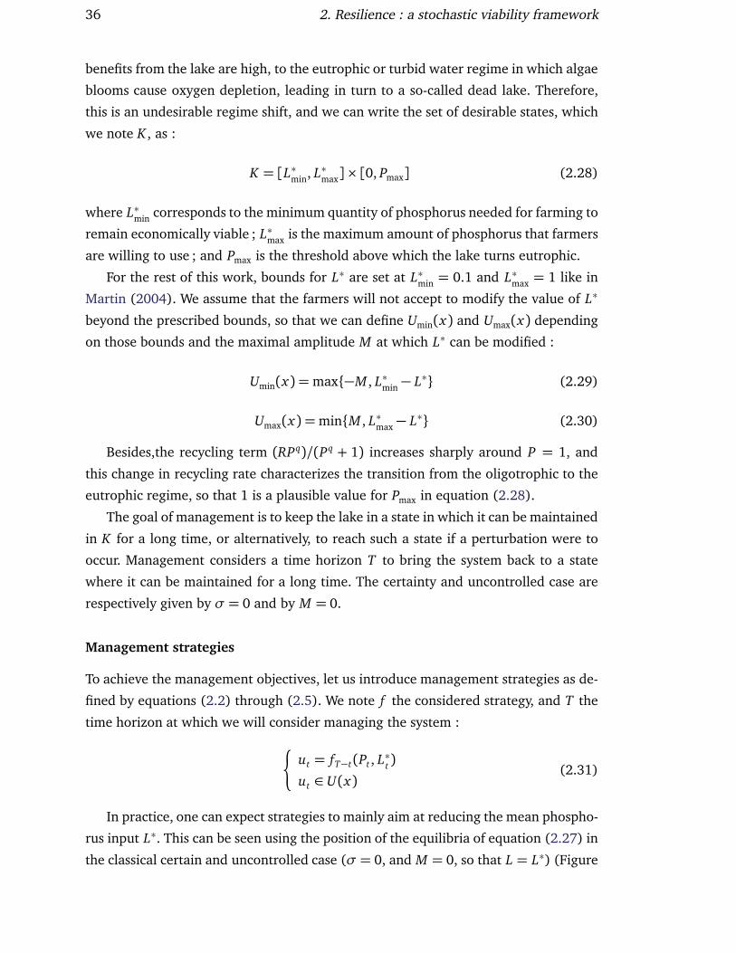
36 2. Resilience : a stochastic viability framework

benefits from the lake are high, to the eutrophic or turbid water regime in which algae

blooms cause oxygen depletion, leading in turn to a so-called dead lake. Therefore,

this is an undesirable regime shift, and we can write the set of desirable states, which

we note K , as :

K = [L∗min, L∗max]× [0, Pmax] (2.28)

where L∗min corresponds to the minimum quantity of phosphorus needed for farming to

remain economically viable ; L∗max is the maximum amount of phosphorus that farmers

are willing to use ; and Pmax is the threshold above which the lake turns eutrophic.

For the rest of this work, bounds for L∗ are set at L∗min = 0.1 and L∗max = 1 like in

Martin (2004). We assume that the farmers will not accept to modify the value of L∗

beyond the prescribed bounds, so that we can define Umin(x) and Umax(x) depending

on those bounds and the maximal amplitude M at which L∗ can be modified :

Umin(x) =max−M , L∗min − L∗ (2.29)

Umax(x) =minM , L∗max − L∗ (2.30)

Besides,the recycling term (RPq)/(Pq + 1) increases sharply around P = 1, and

this change in recycling rate characterizes the transition from the oligotrophic to the

eutrophic regime, so that 1 is a plausible value for Pmax in equation (2.28).

The goal of management is to keep the lake in a state in which it can be maintained

in K for a long time, or alternatively, to reach such a state if a perturbation were to

occur. Management considers a time horizon T to bring the system back to a state

where it can be maintained for a long time. The certainty and uncontrolled case are

respectively given by σ = 0 and by M = 0.

Management strategies

To achieve the management objectives, let us introduce management strategies as de-

fined by equations (2.2) through (2.5). We note f the considered strategy, and T the

time horizon at which we will consider managing the system :

¨

ut = fT−t(Pt , L∗t)

ut ∈ U(x)(2.31)

In practice, one can expect strategies to mainly aim at reducing the mean phospho-

rus input L∗. This can be seen using the position of the equilibria of equation (2.27) in

the classical certain and uncontrolled case (σ = 0, and M = 0, so that L = L∗) (Figure

2.4. Application to an uncertain lake model 37

0 0.2 0.4 0.6 0.8 1 1.2 1.4 1.60

0.5

1

1.5

2

2.5

3

L (input rate)

P (

conc

entr

atio

n)

Reversible (R=0.4)Hysteretic (R=1.2)Irreversible (R=2)Desirable states (K)

FIGURE 2.4 – Stable (continuous line) and unstable (dashed line) attractors for thelake eutrophication problem.

2.4). Depending on the value of the parameter R, there can be three types of behavior

for the lake. These have been well studied in the literature. When R is low, for instance

R = 0.4, there is only one value of P which is an equilibrium for each value of L, and

the lake is called reversible. For higher values, such as R= 1.2, there can be alternate

state states for the same value of L, making a regime shift much more difficult to re-

verse. The lake is then called hysteretic. Finally when R is even higher, for instance

at 2, the lake can be called irreversible, because any transition towards the eutrophic

regime cannot be reversed. The reversible case is only weakly nonlinear, so that the

remainder of this paper will focus exclusively on the hysteretic and irreversible cases,

with the same respective values of R (1.2 and 2) as in Figure 2.4.

2.4.2 Resilience for a given strategy

In this section, resilience is explored using predefined strategy. The focus will be on

1) strategy f (1) ≡ 0 where no management strategy is implemented, and 2) a purely

reactive strategy f (2) where an effort is made once the lake has become eutrophic, by

38 2. Resilience : a stochastic viability framework

reducing the mean phosphorus input as long as the constraint L∗ ≥ L∗min is respected :

∀t ∈ [0, T ], f(2)

T−t(x) =

¨

0 if x ∈ K

Umin(x) if x /∈ K(2.32)

where we set M = 0.05. In this paragraph, we also set R = 1.2. We will first explore

the advantage of using viability kernels rather than attractors to describe the states

that are robust to uncertainty (still using the term of ε-uncertainty), then we will give

resilience indicators as introduced in Section 2.3 for these two strategies.

Stochastic viability kernels and their advantages

The search for ε-robust states considers the trajectory of the system only as long as it

does not exit the set K of desirable states. Since both the strategies considered here

yield f ≡ 0 within K , we only need to consider strategy f (1) ≡ 0, and f (2) will give

exactly the same results.

Figure 2.5 shows how a system set at a stable desirable attractor of the (L, P)

plane can switch towards an undesirable state in a short time span when uncertainty

is present. That had already been noted by Guttal et Jayaprakash (2007). Thus, uncer-

tainty causes a description of the dynamics of the system using stable equilibria and

their basins of attraction to become precarious. Switching variables to (L∗, P) does

not change this fundamental fact, even though they do allow for the projection of

uncertainty over a single state variable instead of two (Figure 2.6). Indeed, while un-

certainty does not influence the value of L∗, it does interfere strongly with the position

of the equilibria in the (L∗, P) plane. For a system in the same initial state as in Figure

2.5, the 95% confidence interval (CI) associated with its state after 5 time steps (Fi-

gure 2.6) shows that the oligotrophic attractor only describes the dynamic very poorly.

Using equilibria that change at every time step is very unpractical, and moreover, one

can perceive that the system is very unlikely to be on a stable equilibrium at any date.

Since it situates a system with respect to a set rather than with respect to a point,

viability theory is well-suited to describe out-of-equilibrium situations (Martin, 2004;

Deffuant et Gilbert, 2011). One can easily represent different degrees of ε-robustness

of the system by computing stochastic viability kernels Viab(β ,τ) for different values

of β and τ (Figure 2.7). Equilibria for the mean case εt = 0 are still shown for an

easier understanding. The limit case σ = 0 is also represented : it corresponds to the

deterministic viability kernel.

As expected, for a given value of β and σ, the higher τ, the smaller the size of the

kernel. Likewise, for (β ,τ), the higher the scale σ of the uncertainty, the smaller the

2.4. Application to an uncertain lake model 39

0.1 0.2 0.3 0.4 0.5 0.6 0.7 0.8 0.9 10

0.5

1

1.5

2

2.5

L (input rate)

P (

conc

entr

atio

n)

TrajectoryTrajectoryP=1L for ε

t=0

95% CI for L

FIGURE 2.5 – Two trajectories simulated in the (L, P) plane using σ = 0.1 and with aconstant value of L∗ = 0.63. Both start at x0 = (0.6, 0.63), which is an oligotrophicstable equilibrium. The dates are t = 0, . . . , 15, and the final date is signaled with across.

40 2. Resilience : a stochastic viability framework

FIGURE 2.6 – The 95% confidence interval (CI) for the position of the attractors isrepresented in grey in the case σ = 0.1, as well as the 95% CI for the state x5 after 5times steps, if the initial state is x0 = (0.6, 0.63).

2.4. Application to an uncertain lake model 41

FIGURE 2.7 – Stochastic viability kernels for β = 0.99 and different values of σ andτ, reminding that for τ1 < τ2, Viab(β ,τ2) is a subset of Viab(β ,τ1). For reference theviability kernel (σ = 0) is on the left side of the grey line.

size of Viab(β ,τ). The same result holds when β increases for given values of β and σ.

Besides, the size decrease caused by an increase in τ is magnified by higher values of

σ. Figure 2.7 shows that for a hysteretic lake, one can get nonempty stochastic viability

kernels Viab(β ,τ) with β close to one, e.g. β = 0.99, and a time horizon much more

important than that of decision-making, e.g. τ = 103. The set Viab(0.99, 103) will be

used from now on to describe the ε-robust states. We also set σ = 0.1.

Resilience

Let us now assume a management horizon T = 30 (T << 103) and look at the possi-

bility to reach a ε-robust state after a perturbation with either strategy f (1) or f (2). We

solely look at the post-perturbation state of the system. The null strategy f (1) lets L∗

stay constant over time, so that reaching Viab(0.99, 103) is only possible if for a given

L∗, there are values of P which are ε-robust. Hence, outside the stochastic viability

kernel, resilience is only possible for a small portion of the state space (Figure 2.8).

For strategy f (2) however, there is a possibility to control the system when the

constraints are violated, and a possibility for the system to get to a ε-robust state once

L∗ gets very low. Hence, with M = 0.05, most post-perturbations states are resilient

with unit probability at the horizon T = 30 (Figure 2.9), highlighting the importance

of management actions. The only exception concerns states which are not ε-robust if

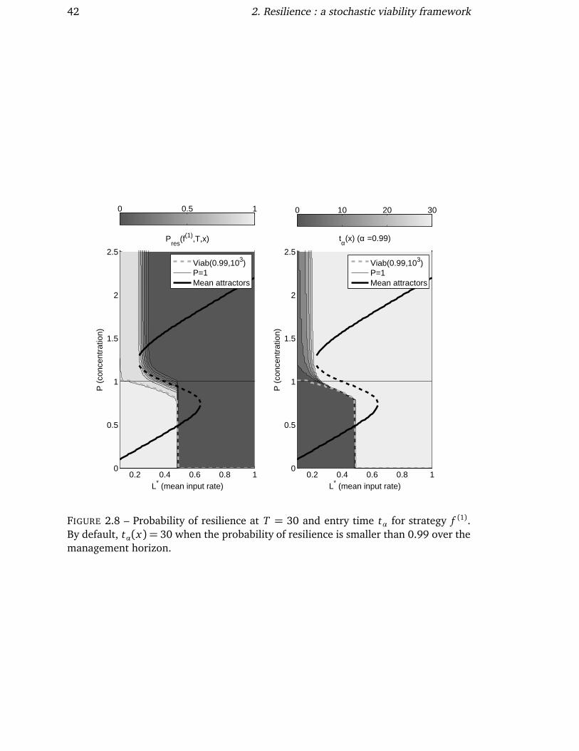
42 2. Resilience : a stochastic viability framework

0.2 0.4 0.6 0.8 10

0.5

1

1.5

2

2.5

L* (mean input rate)

P (

conc

entr

atio

n)

Pres

(f(1),T,x)

Viab(0.99,103)P=1Mean attractors

0 0.5 1

0.2 0.4 0.6 0.8 10

0.5

1

1.5

2

2.5

L* (mean input rate)

P (

conc

entr

atio

n)

tα(x) (α =0.99)

Viab(0.99,103)P=1Mean attractors

0 10 20 30

FIGURE 2.8 – Probability of resilience at T = 30 and entry time tα for strategy f (1).By default, tα(x) = 30 when the probability of resilience is smaller than 0.99 over themanagement horizon.

2.4. Application to an uncertain lake model 43

0.2 0.4 0.6 0.8 10

0.5

1

1.5

2

2.5

L* (mean input rate)

P (

conc

entr

atio

n)

Pres

(f(2),T,x)

Viab(0.99,103)P=1Mean attractors

0.2 0.4 0.6 0.8 1

0.2 0.4 0.6 0.8 10

0.5

1

1.5

2

2.5

L* (mean input rate)

P (

conc

entr

atio

n)

tα(x) (α =0.99)

Viab(0.99,103)P=1Mean attractors

0 10 20 30

FIGURE 2.9 – Probability of resilience at T = 30 and entry time tα for strategy f (2).By default, tα(x) = 30 when the probability of resilience is smaller than 0.99 over themanagement horizon.

we consider β = 0.99 and τ = 103, but for which the probability of a switch towards

a eutrophic lake is relatively slim. Strategy f (2) then leaves the system in a precarious

state until that switch happens. One can intuitively sense that in such cases, a strategy

that would take action and reduce L∗ before the lake becomes eutrophic would be

more environmentally efficient. In fact, as described in Section 2.3, viability theory

allows for searching the best strategy available.

2.4.3 Resilience with an optimal management strategy

Let us now fully exploit a major advantage of viability theory : the possibility to select

the policy choices that maximize the probability of resilience at the horizon T . Through

this whole section, we will haveσ = 0.1 and M = 0.05, and the lake will be considered

hysteretic R= 1.2 unless mentioned otherwise.

44 2. Resilience : a stochastic viability framework

0.1 0.2 0.3 0.4 0.5 0.6 0.7 0.8 0.9 10

0.5

1

1.5

2

L* (mean input rate)

P (

conc

entr

atio

n)

Viab(0.99,103)TrajectoriesLimit of KMean attractors

FIGURE 2.10 – Six trajectories towards the ε-robust set in the (L∗, P) plane, simulatedwith σ = 0.1, M = 0.05 and a post-perturbation state (0.8, 0.5).

Implications for stochastic viability kernels

Thanks to the work by Doyen et De Lara (2010), feedbacks inside K can be computed

by dynamic programming so as to maximize the probability of keeping the lake in a

desirable state. Whatever the value of τ and for all three values of R considered, the

method yields the same optimal feedback map at all dates, and it is noted f ∗ :

f ∗(x) = Umin(x) (2.33)

Yet again, we choose to describe ε-robustness using (β ,τ) = (0.99, 103). As expec-

ted, the associated viability kernel is much bigger than with strategies f (1) or f (2), as

evidenced on Figure 2.10. It in fact encompasses states that we deemed “precarious”

when using strategy f (2), so that the optimal strategy makes them “robust” to measu-

rable uncertainty.

2.4. Application to an uncertain lake model 45

0 5 10 15 20 25 300

0.1

0.2

0.3

0.4

0.5

0.6

0.7

0.8

0.9

1

Time t

Pre

s(f* ,t,

x)

L*=0.7

L*=0.75

L*=0.8

L*=0.85

FIGURE 2.11 – Cumulative probability of reaching an ε-stable state in t time steps, fordifferent post-perturbation values of the mean phosphorus input L∗, and a phosphorusconcentration P = 0.5.

Implications for indicator computation

Now that we got the stochastic viability kernel Viab(β ,τ) for the optimal strategy of

2.33, dynamic programming is used a second time to get the probability of resilience.

This time it is carried out over a set that includes all the states trajectories can visit

before getting back to Viab(β ,τ), and a satisfactory set is (L∗, P) = [0.1, 1] × [0, 4].

The proof from Appendix 2.7 ensures that we find the strategy that maximizes the

probability of resilience, and yet again, the solution described through equation (2.33)

is found to apply for all the considered states, and whatever the date and time horizon.

Nevertheless, through this section, recall that only T = 30 will be used.

If the lake is a hysteretic one, its state is eventually going to become ε-robust after

L∗ has been brought down to L∗min. This is suggested by Figure 2.10, which showcases

two possibilities for a system that has been deprived of its ε-robustness by a perturba-

tion. It can enter the stochastic viability kernel after a few time steps, or be attracted

towards the eutrophic regime. In the latter case, the lake will remain eutrophic for

several time steps, so that ε-robustness can only be restored after a much longer time.

Thus, the cumulative probability of reaching Viab(0.99, 103) shifts from 0 to 1 in two

distinct phases, the first one taking place in the first few time steps and five to six time

steps before the second starts (Figure 2.11). Besides, this figure showcases how the

probability of reaching that set in a few time steps dramatically decreases when the

post-perturbation state gets farther from its boundary.

Yet for all the considered states, ε-robustness is achieved with unit probability by

the horizon T = 30, so that the system is resilient when this horizon is considered. One

can then choose to use indicators such as those defined in Section 2.3.4. They can be

46 2. Resilience : a stochastic viability framework

0.1 0.2 0.3 0.4 0.5 0.6 0.7 0.8 0.9 10

0.5

1

1.5

2

2.5

2

2

4

4

6

6

8

8

10

10

12

12

14

16

18 20

L* (mean input rate)

P (

conc

entr

atio

n)E(t|f*,x)

Viab(0.99,103)P=1Mean attractors

0 2 4 6 8 10 12 14 16 18 20

FIGURE 2.12 – The resilience-related indicator E(t | f ∗, x) for a hysteretic lake (R= 1.2)with M = 0.05, σ = 0.1 and T = 30.

for instance the mean duration as computed in (2.20) (Figure 2.12), or if a worst-case

approach is taken, the maximal time needed to become ε-robust with 99% confidence

like in equation (2.21) (Figure 2.13). Unsurprisingly, both indicators quickly increase

as the starting state gets further from the boundary of the stochastic viability kernel,

but the increase of the mean time E(t | f ∗, x) is less abrupt than that of the maximal

tα(x). This shows that the maximal time needed to get back to a ε-robust set can

top 20 time steps when the trajectory involves leaving the set of desirable states and

getting into the eutrophic regime. Thus, integrating potential management actions and

uncertainty into the model confirms the fact that restoration of the lake’s robustness

can be a long and costly process in the hysteretic case.

From the maps of Figures 2.12 and 2.13, which give the values of indicators for

post-perturbation states, one can deduce the impact of different perturbations for a

given initial state. In this case study, the perturbation is applied to the system as a

one-time jump in the value of one of its state variables. The impact of perturbation

2.4. Application to an uncertain lake model 47

0.1 0.2 0.3 0.4 0.5 0.6 0.7 0.8 0.9 10

0.5

1

1.5

2

2.5

3

3

6

6

9

912

1215

15

18 21 24

L* (mean input rate)

P (

conc

entr

atio

n)

tα(x) (α =0.99)

Viab(0.99,103)P=1Mean attractors

0 5 10 15 20

FIGURE 2.13 – The resilience-related indicator tα(x) (α = 0.99) for a hysteretic lake(R= 1.2) with M = 0.05, σ = 0.1 and T = 30.

48 2. Resilience : a stochastic viability framework

0 0.05 0.1 0.15 0.2 0.25 0.3 0.35 0.4 0.45 0.50

5

10

15

20

25

30

L*per

(amplitude of the mean input rate increase)

Tim

e

E(t|f*,x)tα(x) (α=0.99)

Limit of Viab(0.99,103)

0 0.1 0.2 0.3 0.4 0.5 0.6 0.7 0.8 0.9 10

5

10

15

20

Pper

(amplitude of the perturbation increase)

Tim

e

E(t|f*,x)tα(x) (α=0.99)

Limit of Viab(0.99,103)

FIGURE 2.14 – Impact of the amplitude of a perturbation on resilience-related indica-tors for a hysteretic lake, if the system is at (0.5, 0.5) before the perturbation.

amplitude on different indicators can then be observed through curves such as Figure

2.14, drawn for a system at (0.5, 0.5) before the perturbation. The boundary of the

stochastic viability kernel is a threshold beyond which the perturbation can affect the

recovery time of the system, which illustrates the interest of keeping its state as far

inside this boundary as possible.

Resilience for the irreversible case (R= 2) is worth investigating, all other variables

keeping the same values. By definition, the system may get stuck in a eutrophic state

with no possibility of switching back to the oligotrophic state. Recovery, and therefore

resilience, can not guaranteed at any T , which hampers the relevance of using the same

indicators as in the hysteretic case. Yet, the probability of resilience Pmax keeps being

relevant, and can be computed for T = 30 (Figure 2.15). The feedback map keeps

being f ∗ at each time step, and the horizon is long enough for the system to either

recover or switch for good towards an undesirable regime. Like in Figure 2.14, one

can evaluate the impact of a given perturbation at any given pre-perturbation state,

using this time the probability of resilience (Figure 2.16). This illustrates how the

proposed framework can foster the use of different yet relevant indicators in distinct

situations.

2.4. Application to an uncertain lake model 49

0.1 0.2 0.3 0.4 0.5 0.6 0.7 0.8 0.9 10

0.5

1

1.5

2

2.5

3

L* (mean input rate)

P (

conc

entr

atio

n)

Pres

(T,x) (T=30)

Viab(0.99,103)P=1Mean attractors

0 0.2 0.4 0.6 0.8 1

FIGURE 2.15 – PRes(T, x) for an irreversible lake (R= 2), and T = 30.

50 2. Resilience : a stochastic viability framework

0 0.1 0.2 0.3 0.4 0.50

0.2

0.4

0.6

0.8

1

Perturbation amplitude

Pro

babi

lity

of r

esili

ence

L*

per

Pper

FIGURE 2.16 – For an irreversible lake which state is (0.5, 0.5) before the perturbation,possible impacts of a perturbation on the probability of resilience.

2.5. Discussion 51

2.5 Discussion

In the stochastic viability framework, the policy is only optimal with respect to the ho-

rizon T . When the feedbacks f ∗ are computed for a given horizon T , the probabilities

of resilience computed with f ∗ for t < T are not necessarily the maximum probability

of reaching Viab(β ,τ) after t time steps. The policy is also only optimal for the objec-

tive of maximizing the probability of resilience. In the work by Martin (2004), the most

resilient trajectory is the one that besides reaching the viability kernel in due time, also

minimizes a cost function. In the stochastic case, there are many possible trajectories,

some of which may not reach the viability kernel. Thus, minimizing the cost on the tra-

jectory may sometimes conflict with maximizing the probability to reach the viability

kernel, and one should define a trade-off between these objectives. Viability theory al-

lows for the exploration of trade-offs in the latter case under the so-called framework

of co-viability (Doyen et al., 2012), but without addressing the issue of resilience. Ex-

ploring the integration of resilience computations in a co-viability framework could be

a natural and useful continuation of this work.

However, in the case of lake eutrophication, the controls are independent on the

horizon, so that the feedback map is the same at every date. This means that changing

the management horizon will not affect the immediate decisions to be taken. Besides,

the map is the same whether ones aims at optimizing the resilience of the system or

its ε-robustness. Such a simplification is due to the fact that one always has interest

in reducing L∗. Many other systems studied through viability theory in the determi-

nistic case have the same characteristic : controls allow for changing a state variable

which increase, or decrease, always leads to enhancing the resilience of the system

(see examples throughout Deffuant et Gilbert (2011)). Ecological systems where the

same feedback map applies whatever the horizon might in fact be common.

Yet, one should keep in mind that the model exposed in this paper is only a theo-

retical toy. It is a well-known benchmark model of a nonlinear ecological system, and

can be used to explore some aspects of such systems. One of its advantages is that

of being two-dimensional, which makes its dynamic easier to understand (Figures 2.5

and 2.10) and thus to showcase concepts and methodological developments. However,

this model is not meant to be used for assessing resilience of actual lakes, for a num-

ber of reasons, some of which can be briefly described here. First, it accounts for mud

dynamics only implicitly, through the recycling term Pq/(1+ Pq) of equation (2.24).

This term governs the transition from an oligotrophic to a eutrophic state, so that

mud dynamics should be explicitly accounted for in any model aimed at being used

for decision-making. Second, available policies generally have an unknown impact, so

52 2. Resilience : a stochastic viability framework

that uncertainty on the control should be included in the model, and they are also not

constant in time. For instance, one can expect a policy response to not have imme-

diate effects, and such delays are not taken into account in our hypothetical model.

Third, the economic interests of farmers are only reflected by the existence of a bound

L∗min > 0 to K , and the optimal policy involves reducing L∗ until it reaches that value.

Under such a formulation, L∗min becomes the quantity of phosphorus farmers usually

discharge into the lake, even though it may not be acceptable for them to maintain

their use at that level for a prolonged period of time.

Last but not least, dynamic programming algorithms work in theory for any system

described by equation (2.14), which would make this method very general. Its area

of application, however, is limited in practice by the curse of dimensionality, which

causes both the required computational time and memory to increase exponentially

with the dimension of the state space. Yet, the notion of stochastic viability kernel, and

that of resilience of a system based on a policy, are not defined through dynamic pro-

gramming, which is merely a good way to compute them. It could be very interesting

to explore in future work how they can be generalized to systems of higher dimensio-

nality, even if such developments may render the computations more approximate.

2.6 Conclusions

This work presented a framework for defining and computing resilience of stochas-

tic controlled dynamical systems, using stochastic viability kernels and dynamic pro-

gramming. This allows for the incorporation of uncertainty so that computations can

explicitly account for the capacity of a system to cope with adverse events. The two

main advantages of the viability framework of resilience prove all their utility in the

uncertain case. On the one hand, attractors cease to be fixed points when the dynamics

is stochastic, yet viability tools such as stochastic viability kernels can still be defined.

On the other hand, the possibility to use this framework to dynamically optimize the

management policies while computing the resilience remains in the stochastic case.

The presented framework does not claim to give a single, standard formula for

computing resilience, because what can be computed in practice is only a resilience

indicator. Rather, it proposes a set of possibilities for deriving general indicators that

can fit different applicative contexts. The case of the lake illustrates how this frame-

work allows for the computation of different indicators for resilience depending on

the value of the lake parameter R. In the end, the indicators given in this work are

generic examples : they may not be the most relevant one in a given case, but they can

be built upon to define such a relevant indicator.

2.7. Appendix : Relationship between Vd , Vs and resilience 53

2.7 Appendix : Relationship between Vd , Vs and resi-

lience

In the work by Doyen et De Lara (2010), given a time horizon T , one is interested

in keeping a system described by uncertain dynamics such as g of equation (2.14)

in a constraint set A(t) for all dates t < T . For simplicity, we also suppose that A(t)

represents a discretezed set of points. A dynamic programming algorithm is proposed

and uses the following value function :

V (T, x) =

¨

1 if x ∈ A(T )

0 if x /∈ A(T )

∀t ∈ [0, T − 1], V (t , x) = maxut∈U(x)

∑

y∈A(t)

P(gε(x , ut) = y) V (t + 1, y)

! (2.34)

The main result of their work is that this value function allows for finding the feedbacks

that maximizes the odds of the system to remain in A(t) at all dates t < T . In particular,

setting T = τ and A(t) = K at all dates yields the value function used to compute

stochastic viability kernels. x ∈Viab(β ,τ) is then equivalent to V (0, x)> β .

Equation (2.34) can equivalently be written by considering the horizon T − t ins-

tead of the date t :

V (0, x) =

¨

1 if x ∈ A(0)

0 if x /∈ A(0)

∀t ∈ [1, T ], V (t , x) = maxf t(x)∈U(x ,T−t)

∑

y∈A(t)

P(gε(x , ft(x)) = y) V (t − 1, y)

!

(2.35)

Setting A(0) as the viability kernel and A(t) as the entire state space for any horizon

t > 0, and placing ourselves in the case where no uncertainty is present, V becomes

the value function Vd . Then Vd is the optimal probability of the problem of reaching

the viability kernel by T , and the set of states x such that Vd(T, x) = 1 is the set of

states which are solution to this problem, which corresponds to the definition of the

resilience basin Res(T ). The same applies for any t ≤ T .

Likewise for Vs, one can set A(0) = Viab(β ,τ) and A(t) as the entire state space

for t < T in equation (2.35). Furthermore, to express that we are not interested in

this computation by what might happen after the recovery is complete and the system

reaches the viability kernel, we need to apply the results from Doyen et De Lara (2010)

to modified dynamic in which all the points within Viab(β ,τ) are fixed whatever the

control and uncertainty (∀u,ε, g(x , u,ε) = x). Then, Vs is the optimal probability of

54 2. Resilience : a stochastic viability framework

the problem of being in Viab(β ,τ) at date T under the modified dynamics, or to reach

it before T under the original dynamics. Hence, for any state x , PRes(T, x) = Vs(T, x)

because both entail optimizing the same probability over the same time frame.

2.8. Appendix : Dimensional analysis of the lake problem 55

2.8 Appendix : Dimensional analysis of the lake pro-

blem

Recall the continuous time equation (2.23) :

dp

dθ= −b p+ l + r

p8

p8 +m8(2.36)

We want to reduce the number of parameters by introducing the following dimension-

less variables and parameters :

P =p

mL =

l

b mR=

r

b mdt = b dθ (2.37)

so that dividing equation (2.36) by (b m) yields equation (2.24), effectively reducing

the number of parameters from three to one.

56 2. Resilience : a stochastic viability framework

2.9 Appendix : Derivation of the discrete time equation

(2.27)

We start from the continuous time equation (2.24), integrate uncertainty and controls

before deriving the discrete time equivalent. The amount of time between dates t and

t + 1 is noted ∆t , and is supposed constant between any pair of consecutive dates.

2.9.1 Uncertainty

The continuous time equivalent for equation (2.25) is :

L(t) = L∗(t) +ω(t) (2.38)

where ω is a brownian motion such that its pdf after a time interval ∆t is N (0,σ).

2.9.2 Controls

In the continuous time formulation of Martin (2004), the introduction of a limited

capacity of action in equation (2.26) is mathematically translated into the possibility

to choose the temporal derivative of L∗ within a bounded range, noted Uc in continuous

time. This can be written as :

(

d L∗

d t= L∗ + u

u ∈ Uc(x) =

h

Uminc (x)

∆t,

Umaxc (x)

∆t

i (2.39)

2.9.3 Derivation of the discrete-time evolution equation

Integrating uncertainty, equation (2.24) becomes :

dP

d t= −P + L∗ +ω+ R

P8

p8 +m8(2.40)

Let us introduce δt such that ∆t = jδt with j ∈ N, and use the smaller δt for the

Euler approximation of equation (2.24) so as to minimize the computational error. For

any k ∈ [0, j − 1] and a given value of u, we get :

Pt+(k+1)δt = Pt+kδt +δt

−Pt+kδt + L∗t+kδt

+σ

∆tεt + R

P8t+kδt

P8t+kδt

+ 1

L∗t+(k+1)δt

= L∗t+kδt

+ uδt

∆t

(2.41)

2.9. Appendix : Derivation of the discrete time equation (2.27) 57

and the latter equation can be iterated j times over to get equation 2.27 :

Pt+1 = g(Pt , L∗t, ut ,εt) (2.42)

where the parameters R and σ are made implicit. Throughout this paper we used

j = 10.

– 3 –

Stochastic viability concepts and dynamic

programming methods for controlled

time-variant reliability problems

Soumis dans Reliability Engineering and System Safety.

Auteurs : Charles ROUGÉ, Jean-Denis MATHIAS et Guillaume DEFFUANT

The goal of this paper is twofold : (1) to show that stochastic viability and

time-variant reliability address similar problems with different points of view,

and (2) to demonstrate the relevance of concepts and methods from stochastic

viability in reliability problems. On the one hand, reliability aims at evaluating

the probability of failure of a system subjected to uncertainty and stochasticity.

Most research done in the development of reliability concepts has been related

to find good approximations of this probability in increasingly complex cases.

On the other hand, viability aims at maintaining a controlled dynamical sys-

tem within a survival set. When the dynamical system is stochastic, a viability

problem is a controlled time-variant reliability problem. We show that dyna-

mic programming, which is used for solving stochastic viability problems, can

thus yield the control strategy which guarantees reliability at a significance

level α and the set of states for which there exists such a strategy. Besides, it

leads to a straightforward computation of the date of the first out-crossing,

informing on when the system is most likely to fail. We illustrate this approach

with a simple example of population dynamics, including a case where load

increases with time.

59

60 3. Stochastic viability and reliability

3.1 Introduction

This paper connects two lines of research, viability and reliability, that have ignored

each other up to now despite strong similarities. Both frameworks study whether a sys-

tem will retain desirable properties over a given amount of time. They were developed

in different contexts and sometimes tackle different specific technical or conceptual

issues in relation with the same type of problems, which makes their confrontation

promising. In particular, this work focuses on showing how concepts and methods co-

ming from the stochastic viability framework can be applied to time-variant reliability

so as to extend its applicability to a class of problems where reliability is dynamically

dependent on the decisions taken over time to influence system performance. The rest

of this introduction presents in more detail how both frameworks deal with systems

that are either in a survival state (noted S(t)) or in a failure state (noted F(t)).

The viability approach (Aubin, 1991) deals with controlled dynamic systems under

state constraints, which can still be noted S(t). An emphasis is put on finding the via-

bility kernel, the set of all states which can be controlled so that their trajectory stays

in S(t) at all times. This theory has first been developed in controlled deterministic

systems and the algorithms generally yield both the viability kernel and the associated

viable controls at once (e.g. Saint-Pierre, 1994). Viability tools have been successfully

applied to a variety of fields such as finance, robotics, or ecology (Deffuant et Gilbert,

2011). Recent work has extended the framework of viability theory in discrete time by

considering uncertainties in the dynamics, leading to the definition of the stochastic

viability kernel (De Lara et Doyen, 2008), a set of states for which the respect of the

constraints can be guaranteed with a desired minimal probability and for a desired

time frame. Dynamic programming can compute stochastic viability kernels and de-

termine the control strategy that maximizes the probability to stay in S(t) during that

period, as demonstrated in Doyen et De Lara (2010). This is the specific development

which applicability to reliability we propose to demonstrate throughout this work.

Reliability theory initially comes from the field of mechanical and structural engi-

neering (Rackwitz, 2001) and has a wide range of applications, from material science

(Mathias et Lemaire, 2012) and industrial maintenance (Rausand, 1998) to ecology

(Naeem, 1998), environmental management (Aliev et Kartvelishvili, 1993) and hydro-

logy (Melching, 1992). In these applications, different numerical methods enable the

estimation of the response surface and the associated probability of a system to reach

the failure set F(t). A large body of research has been done to provide ever-improving

approximations of this probability in cases of growing complexity. For instance, while

the Monte Carlo method is used when the complexity of the model does not lead to

3.1. Introduction 61

disproportionate computation times, methods such as the First (respectively Second)

Order Reliability Method (FORM, respectively SORM) can be used in the case of more

computationally demanding systems. These methods have been perfected and tailo-

red to an increasing number of applications (Rackwitz, 2001). They approximate the

failure surface, which separates S(t) from F(t). However, most of these studies deal

with time-invariant systems, since they are carried out under a single definite period

of time or while taking time at a parameter. When the system under consideration

evolves in time, the reliability problem is referred to as time-variant.

Yet, even for explicitly time-variant systems, there exist many cases where the

problem is treated exactly as if it were time-invariant. This is the case for ins-

tance when system performance decays monotonously in time (Andrieu-Renaud et al.,

2004), or if time is used as yet another random variable in a time-invariant pro-

blem when reliability is used to estimate pollutant transport in a heterogeneous aqui-

fer (Skaggs et Barry, 1997). Other applications decompose a time-variant problem

into a series of related time-invariant ones, by using bayesian analysis to update re-

liability estimates (Hsiao et al., 2008) or by considering the different time steps as

parts of a component reliability problem (Oviedo-Salcedo, 2012). In other problems

where the above solutions are not suitable, methods are based on the computation

and time integration of the out-crossing rate, i.e. the rate at which the state may go

through the limit state surface (e.g. Li et Der Kiureghian, 1995). Even then, some al-

gorithms exist that follow a decomposition of the time-variant problem into a series of

time-invariant ones (Hagen et Tvedt, 1991), leading to methodologies such as PHI2

(Andrieu-Renaud et al., 2004; Sudret, 2008). The challenge is then to propagate these

time-invariant approximations through time. This work shall show how another de-

composition into simpler problems, fostered by stochastic viability and dynamic pro-

gramming, can help meet these challenges. Furthermore, it will be demonstrated to

dynamically find the decisions which can optimize system reliability during its lifetime.

In fact, both reliability and stochastic viability deal with the question of whether

the system performance is satisfactory, i.e. whether the reliability is guaranteed at a si-

gnificance level α. It should be noted that these two methods, tackling very similar per-

formance problems, have both been used in fields concerned with environmental and

resources management. Thus, reliability theory has been used for more than three de-

cades for water resources systems, following the pioneering work by Hashimoto et al.

(1982) later completed by Moy et al. (1986) and Kundzewicz et Laski (1995). In eco-

logy, the definition of ecosystem failure by Naeem (1998) has fostered discussions on

the link between species redundancy and ecosystem reliability (Naeem et Li, 1997;

Rastetter et al., 1999). In both fields, the goal is to assess whether the performance of

62 3. Stochastic viability and reliability

the system is consistent or satisfactory over a given time frame, which can be expressed

in terms of whether and how reliability may reach or best a threshold value. The sto-

chastic viability framework, which uses the word of viability instead of reliability, has

tackled the same type of performance problem for fishery management (Doyen et al.,

2007; De Lara et Martinet, 2009; Doyen et al., 2012), the latter publication using the

concept of stochastic viability kernel which explicitly addresses the issue of whether

staying in the survival set can be guaranteed with a desired probability.

The paper is organized as follows. In Section 3.2, the controlled time-variant re-

liability problem is introduced and its identity with a stochastic viability problem is

discussed. Then in Section 3.3, the main concepts of reliability and viability are ex-

posed and confronted so as to highlight what stochastic viability methods bring to

time-variant reliability. An application is proposed in Section 3.4 in order to illustrate

how dynamic programming can be applied to a reliability problem. These findings are

further discussed in Section 3.5, and summarized in the concluding Section 3.6.

3.2 The controlled time-variant reliability problem

This section introduces the controlled time-variant reliability problem through classic

reliability problems. Besides, it shows the challenges posed by this problem, which

cannot be resolved by existing reliability methods.

3.2.1 Time-invariant reliability

Let us consider a system S and a vector of random variables W which represents the

uncertainty and stochasticity of this system. The realizations of W are noted w and

belong to Rq. The state of the system depends on the vector W, so that it is a random

vector X :

X= f (W,π) (3.1)

where π is a vector describing the known deterministic parameters of the system. The

parameter space is Rp and π is chosen in a subset which we note Π. The state space

is noted A and is a subset of Rn. A realization of X is x and there exists a realization

w of W such that x = f (w,π). Assuming that the performance of the system can be

expressed in terms of its load l (demand) and resistance r (capacity), the performance

function g(X) is commonly written as :

g(X) = r(X)− l(X). (3.2)

3.2. The controlled time-variant reliability problem 63

The failure (or limit state) surface, g(X) = 0, separates the states that lie in the failure

domain F (where g(X) < 0) from those in the survival domain S (where g(X) ≥ 0).

The object of reliability is to determine the probability of failure p f of the system :

p f = P(X ∈ F) = P(g(X) < 0)). (3.3)

A diversity of methods such that FORM or SORM have been developed in that

purpose. Such computations prompt the use of an iso-probabilistic transformation of

the random variable X into Y in the standard normal space, thus making the state

space centered around a mean state equal to zero. The limit surface from Equation

(3.2) is defined in accordance with this geometric transformation of the state space,

and becomes g(Y) = 0.

A classic problem is to find values of the parameter vector π that make the system

reliable with a significance level α (i.e. a confidence level 1−α). From now on in this

work we call reliable at the significance level α a system such that there exists such

a value of the parameters, and we call a reliable parameter such a value. This kind

of problem is close to reliability-based design optimization, often abbreviated RBDO,

which balances the design and maintenance cost of a system with the expected cost

of a failure (Rackwitz, 2001). Then, one wishes to achieve a certain reliability using a

design that is under a given cost, and we can assume Π to give the possible options.

3.2.2 Time-variant reliability

We now place ourselves between an initial date t0 = 0 and final date T , so that

the problem is studied in discrete time within an interval [0, T ] called the planning

period. Uncertainty and stochasticity are represented at each date by the random

vector W(t). Following a convention from De Lara et Doyen (2008), the sequence

W = (W(0),W(1), . . . ,W(T − 1)) is called a scenario, and it is an element from the

set of all scenarios S. Instead of a representation of the time evolution of a system

through its temporal correlation structure, usual within reliability theory, in this work

time dependence is expressed explicitly using a dynamical system formulation. In dis-

crete time this can be described using the following transition equation between two

consecutive dates :

X(t + 1) = f (t ,X(t),π,W(t)) (3.4)

In the latter, the state X(t) can in fact be formulated as a function of the date t , scenario

W, initial state x0 = x(0) and parameter vector π :

X(t) = f (t , x0,π,W) (3.5)

64 3. Stochastic viability and reliability

The performance of the system described by equation (3.2) now evolves to take

into account its possible time evolution :

g(t ,X(t)) = r(t ,X(t))− l(t ,X(t)) (3.6)

Likewise, the limit state surface g(t ,X(t)) = 0 is also dependent on time, and so are

the failure domain F(t) (where g(t ,X(t)) < 0) and the survival domain S(t) (where

g(t ,X(t))≥ 0). The probability of failure p f (T, x0,π) is the probability for a trajectory

(x0,X(1), . . . ,X(T )) to leave the survival set over the planning period :

p f (T, x0,π) = P(∃t ∈ [0, T ],X(t) ∈ F(t)) (3.7)

where the dependence of p f on x0 and π is explicit through equation (3.5).

Existing time-variant reliability methods aim at finding the value of the probability

of failure given the initial state x0 and the parameter vector π. Yet, the dynamics and

uncertainty now have to be propagated through T time steps, making the computa-

tion of the failure probability p f (T, x0,π) more expensive than in the time-invariant

case. This is the case for instance for out-crossing (or out-crossing-based) methods

(Rackwitz, 2001; Andrieu-Renaud et al., 2004). These methods are based on the out-

crossing rate ν+(t) defined in continuous time as the instantaneous rate at which the

system leaves the survival set, providing an upper bound for the probability of failure :

p f (T, x0,π)≤

∫ T

0

ν+(t)d t (3.8)

and this inequality becomes an equality under the assumption that failure occurs only

once. The aim is then to determine when the time-dependent system crosses the limit

state. Like in the time-invariant state, the state space is transformed into the standard

normal space at each time step so that the state vector is centered around its mean.

The time evolution of limit state surface G(t ,X(t)) = 0 also needs to be accounted for

as a result. Different methods are available in the literature enabling the estimation of

the failure probability p f (T, x0,π) from the out-crossing rate such as the PHI2 method

(Andrieu-Renaud et al., 2004) or the EOLE method (Li et Der Kiureghian, 1995).

Much like in the time-invariant case, existing methods can deal with the problem

of finding values for the initial state x0 and parameter vector π such that the system

is reliable over the planning period with a significance level α. A very similar problem

consists in finding a reliable π for a given initial state x0, which is then called reliable

as well. We call reliability kernel the set of all the reliable initial states at a significance

3.2. The controlled time-variant reliability problem 65

level α, and note :

Rel(α, T ) =

x0 ∈ S(0)|∃π ∈ Π, p f (T, x0,π)≤ α

(3.9)

Let us now explore the consequences of modifying this problem so that the para-

meters value can be changed to a certain extent at each time step, rather than just fixed

beforehand. This is what we shall call the controlled time-variant reliability problem.

3.2.3 The controlled time-variant reliability problem

Still on a planning period [0, T ], let us now consider the possibility to decide the

value of some parameters at each date t , depending on the state of the system. These

parameters are now called controls and u(t , x) = (u1(t , x), u2(t , x), . . . , up(t , x)) is the

vector of the control variables that are applied at date t if the system is at state x .

Controls are chosen among the set U(t , x) of admissible controls and in particular, the

set of available options at the initial date, noted Π previously in this work, can also

be noted U(0, x). A function u(t , .) which associates a control to all states at date t is

called a feedback map. The sequence of feedback maps between an initial date 0 and

a final date T is called a strategy and noted u(.). The set of all strategies that can be

implemented during the time frame [0, T ] is notedU (T ). Equation (3.4) can now be

updated into :

X(t + 1) = f (t ,X(t), u(t),W(t)) (3.10)

or alternatively, like in equation (3.5), X(t) can be now expressed as a function of t ,

x0, u(.) and W :

X(t) = f (t , x0, u(.),W) (3.11)

Trough the latter equation, the probability of failure within the planning period [0, T ]

becomes a function of T , x0 and u(.) :

p f (T, x0, u(.)) = P(∃t ∈ [0, T ],X(t) ∈ F(t)) (3.12)

and this definition can also be extended to anterior dates :

p f (t , x0, u(.)) = P(∃τ ∈ [0, t],X(τ) ∈ F(τ)) (3.13)

The controlled time-variant reliability problem is to find, given an initial state x0,

the control strategy u(.) such that the system is reliable at the significance level α

during the planning period. Its reliability kernel, analogous to equation (3.9), is the

66 3. Stochastic viability and reliability

following set :

Rel(α, T ) =

x0 ∈ S(0)|∃u(.) ∈ U (T ), p f (T, x0, u(.))≤ α

(3.14)

We can call reliable at the significance level α a state of the reliability kernel Rel(α, T ).

To call x0 reliable, one needs to find an associated reliable strategy, but the search for

its existence is very challenging because a strategy is described by one variable for

each state and for each time step. Searching a strategy inU (T ) thus means searching

a space of very high dimensionality. Besides, for each state and time step, one must

potentially consider many possible controls.

Reliability methods are not meant to tackle this problem of searching U (T ). Yet,

viability methods and concepts have been devised to search for suitable controls.

3.3 Stochastic viability as controlled time-variant relia-

bility

The identity between the stochastic viability and controlled time-variant reliability

problems is demonstrated in this section. The relevance of stochastic viability concepts

and methods to reliability is a consequence of this, and is detailed henceforth. Before

that, however, the original deterministic version of viability is exposed to elicit how the

reliability and viability framework deal with the same type of problems with different

point of view.

3.3.1 Deterministic viability

In its original deterministic version (Aubin, 1991), viability theory deals with control-

led systems such that W(t)≡ 0. Equation (3.10) can be simplified into :

x(t + 1) = f (t , x(t), u(t)) (3.15)

where the random variable X has been replaced by a deterministic variable x , all else

being the same. f is called the dynamic of the system. In this framework, for a gi-

ven initial state x0 and strategy u(.), there is only one trajectory, so the state can be

noted x(t , x0, u(.)). The central question of viability is whether that trajectory leaves

S(t), given by equation (3.6) as previously, at any given date within the time frame

[0, T ]. An answer to this question is brought about by a central object, the viability

kernel, which is the set of all initial states for which the system can be controlled so

3.3. Stochastic viability as controlled time-variant reliability 67

its trajectory does not leave the survival set. We can write :

Viab(T ) = x0 ∈ S(0)|∃u(.) ∈ U (T ),∀t ∈ [0, T ], x(t , x0, u(.)) ∈ S(t) (3.16)

Thus, an initial state can either be viable or not, which we can translate into reliability

terms by stating that in a deterministic context, the probability of failure is either 0

or 1. Figure 3.1 summarizes this. Properties of the viability kernel have provided the

foundation of viability algorithms. This is for instance the case for algorithms that

use the binary nature of a state under deterministic viability (e.g. Saint-Pierre, 1994;

Deffuant et al., 2007), or the fact that viable trajectories are tangent to the surface of

the viability kernel (Bonneuil, 2006). An interest of these algorithms is that they find

both the viable initial states and the associated viable controls, notions from which we

derived those of reliable states and controls for the controlled time-variant reliability

problem.

FIGURE 3.1 – Link between the viability kernel Viab(T ) and the probability of failurep f (T, x0, u(.)) with deterministic controlled dynamics. All sets are represented at theinitial date t = 0.

68 3. Stochastic viability and reliability

3.3.2 The stochastic viability problem

In the discrete time stochastic viability framework of De Lara et Doyen (2008), un-

certainty is introduced into viability problems using the same concepts and nota-

tions as in Section 3.2.3. The dynamic becomes, still following the notations from

De Lara et Doyen :

x(t + 1) = f (t , x(t), u(t), w(t)) (3.17)

where one can recognize equation (3.17) where the stochastic process X is replaced

at all dates by its realization. Notations nonwithstanding, both equations are thus the

same. Thus, equation (3.11) to describe the state X(t) still applies.

In fact, the goal is also the same : reliability focuses on the probability of failure

which is the probability of reaching the failure set during a given time frame, while

the concern of stochastic viability is the probability of staying in the survival set during

that time frame. Much like in the original viability framework, a central concept is the

stochastic viability kernel, defined as the set of all states for which the system has a

probability ρ or higher of staying in the survival set S(t) for a given time horizon T .

It can be formally defined by the following equation in which it is noted Viab(ρ, T ) :

Viab(ρ, T ) = x0 ∈ S(0)|∃u(.) ∈ U (T ),P(∀t ∈ [0, T ],X(t) ∈ S(t))≥ ρ (3.18)

For instance, Viab(0.99, 100) is the set of initial states such that the system has a

99% chance of staying in the survival set S(t) for at least a hundred time steps. The

stochastic viability problem can be related to the controlled time-variant reliability

problem by the remark that :

p f (T, x0, u(.)) = 1−P(∀t ∈ [0, T ],X(t) ∈ S(t)) (3.19)

and thus, using equations (3.14) and (3.18) we have :

Rel(α, T ) = Viab(1−α, T ) (3.20)

and both concepts are interchangeable. One can argue that the concept of reliability

kernel is more intuitive because the analogy between the stochastic viability kernel

and its deterministic counterpart defined in equation (3.16) is limited. It is adapted

for states inside the stochastic viability kernel, for which the property of being viable

is replaced by one of being viable with probability 1− α. However, all the properties

of the viability kernel which were used for its computations are lost when uncertainty

is introduced. For instance, a initial state x0 which is not in Viab(0.95, T ) may have a

3.3. Stochastic viability as controlled time-variant reliability 69

94% chance of staying in the survival set under the right strategy, while its reliability is

zero if it is outside the viability kernel Viab (T ). Viability and reliability in the stochastic

case are summarized by Figure 3.2.

FIGURE 3.2 – Reliability kernels Rel(α, T ) and Rel(0.9×α, T )with stochastic controlleddynamics. All sets are represented at the initial date t = 0.

Yet, equation (3.20) does not allow for the computation of the reliability kernel.

Its interest comes from the fact that there exists a dynamic programming to compute

the stochastic viability kernel.

3.3.3 A dynamic programming solution

Provided that at all dates, the w(t) are independent from each other, Doyen et De Lara

(2010) establish that the problem of finding the stochastic viability kernel can be sol-

ved by dynamic programming, a widespread category of recursive algorithms, desi-

gned to solve the problem backwards from date T to the initial date. Let us assume

that the continuous bounded sets that form the state and control spaces have been

discretized, as is the case in practice. The state is then represented by a finite set of

points x i of the discrete space Ad , of which the survival set S(t) is a subset. Likewise,

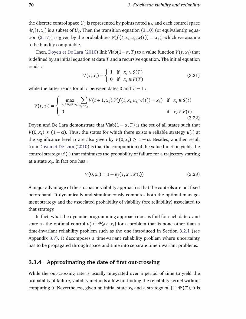
70 3. Stochastic viability and reliability

the discrete control space Ud is represented by points noted u j, and each control space

Ud(t , x i) is a subset of Ud . Then the transition equation (3.10) (or equivalently, equa-

tion (3.17)) is given by the probabilities P( f (t , x i, u j, w(t)) = xk), which we assume

to be handily computable.

Then, Doyen et De Lara (2010) link Viab(1−α, T ) to a value function V (t , x i) that

is defined by an initial equation at date T and a recursive equation. The initial equation

reads :

V (T, x i) =

¨

1 if x i ∈ S(T )

0 if x i ∈ F(T )(3.21)

while the latter reads for all t between dates 0 and T − 1 :

V (t , x i) =

maxu j∈Ud (t,xi)

∑

xk∈Ad

V (t + 1, xk).P( f (t , x i, u j, w(t)) = xk) if x i ∈ S(t)

0 if x i ∈ F(t)

(3.22)

Doyen and De Lara demonstrate that Viab(1 − α, T ) is the set of all states such that

V (0, x i) ≥ (1 − α). Thus, the states for which there exists a reliable strategy u(.) at

the significance level α are also given by V (0, x i) ≥ 1 − α. Besides, another result

from Doyen et De Lara (2010) is that the computation of the value function yields the

control strategy u∗(.) that minimizes the probability of failure for a trajectory starting

at a state x0. In fact one has :

V (0, x0) = 1− p f (T, x0, u∗(.)) (3.23)

A major advantage of the stochastic viability approach is that the controls are not fixed

beforehand. It dynamically and simultaneously computes both the optimal manage-

ment strategy and the associated probability of viability (ore reliability) associated to

that strategy.

In fact, what the dynamic programming approach does is find for each date t and

state x i the optimal control u∗j∈ Ud(t , x i) for a problem that is none other than a

time-invariant reliability problem such as the one introduced in Section 3.2.1 (see

Appendix 3.7). It decomposes a time-variant reliability problem where uncertainty

has to be propagated through space and time into separate time-invariant problems.

3.3.4 Approximating the date of first out-crossing

While the out-crossing rate is usually integrated over a period of time to yield the

probability of failure, viability methods allow for finding the reliability kernel without

computing it. Nevertheless, given an initial state x0 and a strategy u(.) ∈ U (T ), it is

3.4. Application 71

useful to know around which dates the system is most likely to leave the survival set.

Noting tout the date at which the system first leaves the survival set for the first time,

we have :

P(tout = t) = P ([X(t) ∈ F(t)]∩ [∀τ < t , X(τ) ∈ S(τ)])

= P ([X(t) ∈ F(t)] | [∀τ < t , X(τ) ∈ S(τ)]) .

1− p f (t , x0, u(.))

(3.24)

where p f (t , x0, u(.)) is defined in equation (3.13), and using the identity

P (∀τ < t , X(τ) ∈ S(τ)) = 1− p f (t , x0, u(.)). Besides, P(tout = t)/∆t is an approxima-

tion of the rate of the first out-crossing. Contrary to what happens in usual out-crossing

approaches (equation (3.8)), we no longer need to assume that the system crosses the

failure surface only once. The probability P(tout = t) can be computed by noting that :

P(tout ≤ t) = p f (t , x0, u(.)) (3.25)

so that the probability distribution for the date of the first crossing tout is given by :

P(tout = t) = p f (t , x0, u(.))− p f (t − 1, x0, u(.)) (3.26)

Computation of the probability of failure p f (t , x0, u(.)) for t < T can be achieved both

by backward and forward programming, and both methods are presented in Appendix

3.8.

3.4 Application

In this section we apply the stochastic viability techniques from Section 3.3 to a simple

dynamical model of controlled population growth. Despite the apparent simplicity of

the equations, complex control strategies can and may have to be devised. Then we

consider a performance function that decreases with time, like in a number of relia-

bility applications, and use the results from stochastic viability to compute the out-

crossing rate.

3.4.1 A simple population model

We consider a modified version of a simple model of population growth introduced

by Aubin et Saint-Pierre (2002). It is discretized and uncertainty is integrated as an

additive term to the population variable at each time step. The evolution of the state

72 3. Stochastic viability and reliability

x = (a, b) reads :

¨

a(t + 1) = a(t) + (a(t)b(t) +w(t))∆t

b(t + 1) = b(t) + u(t)(3.27)

where the state variables are the population a(t) and its growth coefficient b(t) ; this

coefficient is controlled by u(t). The control is bounded by [Umin, Umax], which repre-

sents the inertia in the evolution of the population. These bounds are taken to be

Umin = −0.5 and Umax = 0.5. Besides, throughout this section ∆t = 1 and the uncer-

tainty term w(t) is a realization of W (t)∼N (0, 0.25). In what follows, all quantities

are assumed to be non dimensional for simplicity.

The size of the population is constrained, so that the survival set is represented by

the following performance function :

g(t , x(t)) = g(t , a(t), b(t)) = (a(t)− 0.2)(c(t)− a(t)) (3.28)

so that the survival set is defined by a(t) ∈ [0.2, c(t)] where c(t) is the carrying ca-

pacity of the system and is assumed to be greater than 0.2. In ecology, the carrying

capacity is the maximal size of the population that can be sustained by the environ-

ment it lives in.

In this study, the state space has been discretized, with resolutions ∆a = 0.01 and

∆b = 0.05, and the control space is likewise discretized with a resolution ∆u= 0.05.

In this discrete space, the transition function between two time steps was obtained by

interpolating from equation (3.27). The goal is to assess reliability at a time horizon T

for a given initial state x0 = (a0, b0), first with a constant carrying capacity, then with a

decreasing one. In what follows the relevant range for y was found to be [−1.5, 2.5].

3.4.2 Constant carrying capacity

Let us assume that the carrying capacity is constant c = 3. Then, the performance

function from equation (3.28) is under the following form g1 :

g1(t , x(t)) = (a(t)− 0.2)(3− a(t)) (3.29)

Dynamic programming leads to the strategy u(.) that optimizes reliability at any ho-

rizon, and the only approximation is that of the discretization. This is showcased for

T = 100 by Figure 3.3, which shows that only initial states grouped around b0 = 0

have a good reliability. There is, however, a sizable reliability kernel Rel(0.95, 100).

Such reliability kernels can also be computed at any horizon, so that one can for ins-

3.4. Application 73

tance observe the evolution of Rel(0.95, T ) as T increases, and observe that its size

decreases very little until it abruptly ceases to exist when T tops 254 (Figure 3.4).

Population a

Gro

wth

coe

ffici

ent b

0.5 1 1.5 2 2.5 3−1.5

−1

−0.5

0

0.5

1

1.5

2

2.5

0

0.1

0.2

0.3

0.4

0.5

0.6

0.7

0.8

0.9p

f(100,x

0,u*(.))

Limit of Rel(0.95,100)

FIGURE 3.3 – Reliability with the performance function g1 and a time horizon of ahundred time steps.

This stability of the reliability kernel Rel(0.95, T ) as the horizon increases is mat-

ched by that of the optimal strategy. Whatever the horizon, the backward sequence of

feedback maps u(t , .) from the final date T to the initial date is the same, and what is

more, the map u(t , .) becomes constant for t ≤ T − 10. It is noted u∗ and represented

on Figure 3.5. One can see that for a given value of a, the value of u∗ increases as b

increases, but the relationship between u∗ and b is different for each single value of a,

making the map is very complex.

Out-crossing rates as approximated by P(tout = t)/∆t can be estimated using this

feedback map. Since ∆t = 1, using equation (3.24) the out-crossing rate takes the

approximate value of (λ(1− p f (t , x0, u∗(.))) after less than 10 time steps, where λ ≈

2 × 10−4 is probability of leaving at t conditional on staying in the survival set up

to t − 1. It is independent on the initial states, so that the differences in reliability

displayed in Figure 3.3 account for the probability of leaving the survival set within

these first ten time steps. After t = 10, the probability of failure only increases very

74 3. Stochastic viability and reliability

0.5

1

1.5

2

2.5

3

−1.5−1

−0.50

0.51

1.52

2.5

0

50

100

150

200

250

300

Growth coefficient bPopulation a

Tim

e ho

rizon

T

FIGURE 3.4 – Initial states x0 belonging to Rel(0.95, T ), for different values of thehorizon T and the performance function g1.

3.4. Application 75

Population a

Gro

wth

coe

ffici

ent b

0.5 1 1.5 2 2.5 3−1.5

−1

−0.5

0

0.5

1

1.5

2

2.5

−0.5

−0.4

−0.3

−0.2

−0.1

0

0.1

0.2

0.3

0.4

0.5

FIGURE 3.5 – Map of the optimal controls u∗(x) for the performance function g1, 10time steps or more from the horizon.

76 3. Stochastic viability and reliability

slowly.

3.4.3 Decreasing carrying capacity

Let us now suppose that the system performance decreases linearly over time, with a

diminishing adaptive capacity c(t) = 3− 0.01t . Let us note this function g2, equation

(3.28) becomes :

g2(t , x(t)) = (a(t)− 0.2)(3− 0.01t − a(t)) (3.30)

As expected, this linear decrease in performance affects reliability, so that

Rel(0.95, T ), even though it assumes a similar shape as for g1, vanishes for T > 54

(Figure 3.6). Besides, unlike for the case of a constant carrying capacity, the optimal

control maps change at each time step. This would make them very difficult to find if

it were not for dynamic programming.

0.5

1

1.5

2

2.5

3

−1.5−1

−0.50

0.51

1.52

2.5

0

10

20

30

40

50

60

Growth coefficient bPopulation a

Tim

e ho

rizon

T

FIGURE 3.6 – Initial states x0 belonging to Rel(0.95, T ), for different values of thehorizon T and the performance function G2.

Yet, for t ≤ T − 10 it seems that the map u∗(t , .) does not depend on the horizon

T . Thus, the maps for T = 100 and T = 200 are identical until the date t = 92,

while those for T = 150 and T = 200 are identical until t = 145. This makes the

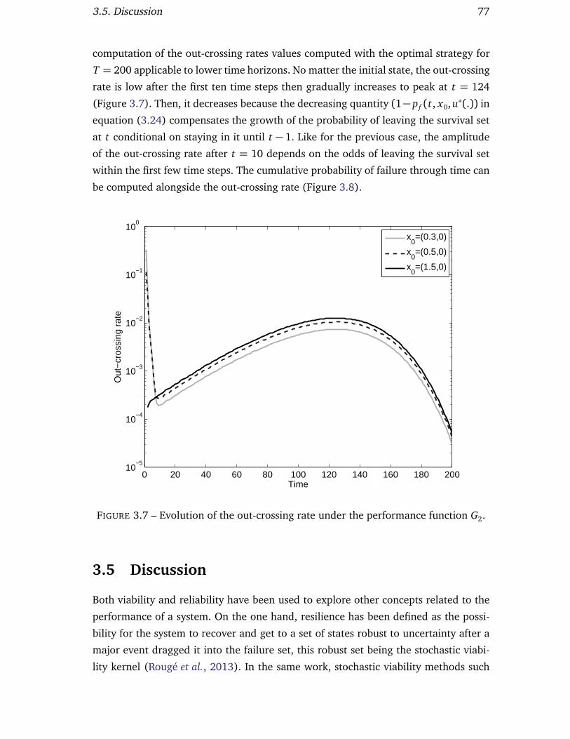
3.5. Discussion 77

computation of the out-crossing rates values computed with the optimal strategy for

T = 200 applicable to lower time horizons. No matter the initial state, the out-crossing

rate is low after the first ten time steps then gradually increases to peak at t = 124

(Figure 3.7). Then, it decreases because the decreasing quantity (1− p f (t , x0, u∗(.)) in

equation (3.24) compensates the growth of the probability of leaving the survival set

at t conditional on staying in it until t − 1. Like for the previous case, the amplitude

of the out-crossing rate after t = 10 depends on the odds of leaving the survival set

within the first few time steps. The cumulative probability of failure through time can

be computed alongside the out-crossing rate (Figure 3.8).

0 20 40 60 80 100 120 140 160 180 20010

−5

10−4

10−3

10−2

10−1

100

Time

Out

−cr

ossi

ng r

ate

x

0=(0.3,0)

x0=(0.5,0)

x0=(1.5,0)

FIGURE 3.7 – Evolution of the out-crossing rate under the performance function G2.

3.5 Discussion

Both viability and reliability have been used to explore other concepts related to the

performance of a system. On the one hand, resilience has been defined as the possi-

bility for the system to recover and get to a set of states robust to uncertainty after a

major event dragged it into the failure set, this robust set being the stochastic viabi-

lity kernel (Rougé et al., 2013). In the same work, stochastic viability methods such

78 3. Stochastic viability and reliability

0 20 40 60 80 100 120 140 160 180 2000

0.1

0.2

0.3

0.4

0.5

0.6

0.7

0.8

0.9

1

Time

Fai

lure

pro

babi

lity

p f(t,x

0,u*(

.))

x

0=(0.3,0)

x0=(0.5,0)

x0=(1.5,0)

FIGURE 3.8 – Evolution of the probability of failure under g2.

3.6. Conclusion 79

as dynamic programming are used to compute the probability of reaching a given sto-

chastic viability kernel within a given time frame after an event. On the other hand,

resilience but also vulnerability have been defined alongside reliability as performance

indicators for water resources systems (Hashimoto et al., 1982) and further, a method

computing all three concepts using FORM also exists (Maier et al., 2001). Thus, one

can hope that bringing viability and reliability methods together may improve the de-

finition and computation of other related concepts such as resilience and vulnerability.

As mentioned in Section 3.3, dynamic programming decomposes a time-variant

reliability problem into many simpler time-invariant reliability problems. Thus, while

this work focused on showing how stochastic viability methods could foster a better

computation of reliability in time-variant cases, it is possible to have time-invariant

reliability methods help solve stochastic viability problems. For instance, if the transi-

tions from the state x t to the state x t+1 along a trajectory are difficult to compute, then

equation (3.22) may be approximated through methods such as FORM or SORM.

Further, one must keep in mind the limitations of dynamic programming algo-

rithms. They only work for systems where the state space has a low dimension. Too

high a dimension leads to the so-called “curse of dimensionality” which designates

the exponential increase of the needed computational time and memory. This leads to

problems that are unpractical to solve. Besides, this method requires that the random

variables W(t) be independent with each other. In practice, temporal dependence can

be solved at a given date t by artificially adding as state variable the values of the

uncertain vectors that are needed to compute W(t). However, such a strategy leads to

an explosion of the dimension of the problem. There exist decomposition algorithms

that have been used to deal with the dimension problem in dynamic programming,

such as the Benders decomposition (Perreira et Pinto, 1985), but their applicability is

outside the scope of this work.

3.6 Conclusion

Stochastic viability and reliability have the same broad goal of computing the probabi-

lity for a system to not violate its constraints. Thus, the search for feedback strategies

that guarantee the reliability of a system with a probability 1 − α can be addressed

through the dynamic programming methods introduced in stochastic viability theory.

The set of states for which such feedbacks exist is the stochastic viability kernel, which

can also appropriately be named reliability kernel. The proposed alternative name is

also motivated by the fact that the properties of the viability kernel in the original

deterministic framework of viability theory no longer hold when stochasticity and un-

80 3. Stochastic viability and reliability

certainty are introduced. For a given adequate strategy, one can then also compute the

out-crossing rate to understand when failure may occur.

Application to a simple system shows that this method is well-suited to tackle cases

where the performance function decreases over time. Further, it showcases how the

optimal strategy that dynamic programming finds to avoid failure may be very complex

and have hundreds of degrees of freedom, even in seemingly simple cases. There is to

our knowledge no other case of a method that can yield the most reliable policies in

an uncertain dynamical system.

Acknowledgements

This work would not have been possible without funding from Région Auvergne.

3.7. Appendix : Equation (3.22) as a time-invariant problem 81

3.7 Appendix : Equation (3.22) as a time-invariant pro-

blem

We are in a situation where the date t and discrete state x i are fixed parameters, and

we set the parameter vector π = (t , x i, u j). Then equation (3.10) can be written over

as X(t + 1) = f (W(t),π), where one can recognize a time-invariant problem since

time is a parameter. Let us introduce the Bernoulli variable B dependent on the value

of the realization of X(t + 1) defined by :

P(B= 1|X(t + 1) = xk) = V (t + 1, xk) (3.31)

We can also introduce the random variable Z defined by :

Z= (X(t + 1),B(X(t + 1))) (3.32)

The latter equation corresponds to Z = g(W(t),π) where g(W(t),π) =

( f (W(t),π),B( f (W(t),π)), and one can have a time-invariant type problem by setting

the survival set S = (Ad ×1) for Z, where Ad represents the discrete state space of X.

Then, a design problem is to find the value of u j that maximizes reliability. The law of

total probability yields :

P(Z ∈ S) =∑

k

P(B= 1|X(t + 1) = xk).P(X(t + 1) = xk) (3.33)

and replacing with equations (3.31) and (3.17) leads to :

P(Z ∈ S) =∑

k

V (t + 1, xk).P( f (π, w(t)) = xk) (3.34)

The value of u j, hence that of π, that maximizes the latter probability is exactly the

one yielded by the maximization problem of equation (3.22).

82 3. Stochastic viability and reliability

3.8 Appendix : Computation of p f (t, x0,u(.)) for t < T

3.8.1 Forward

This is done through the direct computation of the possible trajectories, as long as they

do not leave the survival set. We recursively compute V1(1, x0, u(.), xk) = P(X(t) =

xk|∀τ < t ,X(τ) ∈ S(τ)). Initialization reads :

V1(1, x0, u(.), xk) =

¨

P( f (0, x0, u(0, x0), w(0)) = xk) if xk ∈ S(0)

0 if xk ∈ F(0)(3.35)

then the function V1 recursively updated at each date 1≤ t ≤ T :

V1(t , x0, u(.), xk) =∑

xi∈S(t−1)

V1(t − 1, x0, u(.), x i).P( f (t − 1, x i, u(t − 1, x i), w(t − 1)) = xk)

(3.36)

Then we have :

p f (t , x0, u(.)) =∑

xk∈S(t)

V1(t , x0, u(.), xk) (3.37)

The advantage of using the above approach is that it yields the failure probabilities

at all dates recursively, in a single run. The inconvenient lies with the large amount

of computational memory it requires, since it connects all the points of the successive

survival sets with each other.

3.8.2 Backward

One uses a value function V2 which is initialized through :

V2(t , x i) =

¨

1 if x i ∈ S

0 if x i ∈ F(3.38)

and then progresses backward from t to 0 :

V2(τ, x i) =

∑

xk∈Ad

P( f (t , x i, u(τ, x i), w(τ)) = xk).V2(τ+ 1, xk) if x i ∈ S

0 if x i ∈ F

(3.39)

These equations are exact analogous to equations (3.21) and (3.22) for the value

function V , where there is only one possible control u(τ, x i) at each date τ and state

x i. Thus, equation (3.23) becomes V2(0, x i) = 1− p f (t , x0, u(.)). This is less expensive

than the algorithm for V since there is no need to solve an optimization problem at

3.8. Appendix : Computation of p f (t , x0, u(.)) for t < T 83

each date and state to get the feedbacks. However, one will need to run this algorithm

for each date separately so as to get the probability of failure at multiple dates.

– 4 –

Vulnerability : from the conceptual to the

operational using a dynamical system

perspective

Soumis dans Environmental Modelling & Software

Auteurs : Charles ROUGÉ, Jean-Denis MATHIAS et Guillaume DEFFUANT

This work proposes to address a lack of conceptual consensus surrounding the

term vulnerability, by using a minimal definition of vulnerability as a measure

of potential future harm, and by basing this definition on a stochastic control-

led dynamical system framework. Harm is defined as a normative judgment

on the undesirability of a trajectory, the sequence of the system states bet-

ween two dates. Given an initial state, action policy and time horizon, consi-

dering all possible trajectories leads to obtaining the probability distribution

of harm values. Vulnerability is then defined as a statistic derived from this

distribution. This framework (1) promotes a dynamic view of vulnerability

by highlighting its temporal dimension and (2) fosters the development of

operational indicators in a context which clarifies the descriptive and norma-

tive aspects in the system’s representation. An object of interest is the low-

vulnerability kernel, which regroups all the system states such that vulnera-

bility is kept below a threshold value pending enforcement of an appropriate

policy. For some indicators, this set can be found using the mathematical fra-

mework of stochastic viability theory, and its associated stochastic dynamic

programming tools. Regarding the hazards that may affect the system, we

propose to distinguish between the computable uncertainty, embedded in the

stochastic dynamics, and extreme or surprising events whose impacts can be

explored through specific scenarios. The relevance of this work to situations

where a dynamical formulation is not available is stressed. A simple nonlinear

model of lake eutrophication illustrates the framework, and showcases its link

with concepts related to coping and adaptation, which it allows to effectively

discuss.

85

86 4. Vulnerability

4.1 Introduction

This work proposes an operational definition of vulnerability, based on a stochastic

dynamical system framework which accounts for its uncertain evolution and for the

decisions that can be taken to impact it. Vulnerability is defined in a most general

way as a measure of potential future harm. It is an oft-used concept in the literature

dealing with the potential negative impacts of natural hazards and social and envi-

ronmental change. However, vulnerability concepts and tools originate from several

different communities (Adger, 2006; Eakin et Luers, 2006; Miller et al., 2010). Conse-

quently, there is a lack of consensus about the conceptual definitions of the term and

this breeds vagueness (Hinkel, 2011). Thus, despite the existence of similar opera-

tional protocols, unified frameworks in or across research fields are largely missing

(Costa et Kropp, 2012).

The minimal definition we propose to use comes from a formal analysis of the term

(Wolf et al., 2013), and it is the lowest common denominator in most vulnerability

definitions in the literature (Hinkel, 2011). To our knowledge, our framework consti-

tutes the second attempt at mathematically formalizing the concept of vulnerability

after that by Ionescu et al. (2009), who argue that such a formalization is warranted

for several reasons, namely making vulnerability assessments systematic, clarifying

the concepts and their communication, avoiding analytical inconsistencies and prac-

tical omissions, and enabling the development of computational approaches. These

reasons stress that formalization is useful regardless of the presence of a dynamical

system formulation in a given case.

We propose to start with the most general possible conceptual and mathematical

formulation, and then to interpret elements of the framework that are relevant to the

vulnerability literature. We argue that this approach provides both a formal basis and

a great flexibility for the discussion of vulnerability concepts. Indeed, the mathematics

remain a non ambiguous reference for the discussion of the concepts, for which several

interpretations may be possible and relevant depending on their application. In that

sense, flexibility appears as a prerequisite to bridging the gap between conceptual

definitions and their many possible operational translations.

Besides, we propose to explicitly consider evolutions over several time steps, exten-

ding the work by Ionescu et al. (2009) who mainly base their vulnerability discussions

on evolutions over a single time step. The fact that the vulnerability of an entity de-

pends on uncertain dynamics over time (Wolf et al., 2013) is often overlooked or kept

implicit (Liu et al., 2008) because such dynamics often cannot be expressed explicitly

by a relevant model. Hence the need for a framework centered on the notion of pos-

4.1. Introduction 87

sible future trajectories to which harm values are associated. Uncertainty in the value

of future harm is considered through the occurrence probabilities of these possible tra-

jectories, leading to obtaining a probability distribution function (pdf) of these harm

values. Then, a relevant statistic derived from this pdf is a measure of potential future

harm, in other words vulnerability.

This necessity for taking temporal dynamics into account has been highlighted

in the literature (Liu et al., 2008), and illustrated through the concept of path depen-

dence (Preston, 2013), and through the idea that a natural hazard can impact a system

long after hitting it (Menoni et al., 2002; Lesnoff et al., 2012). Moreover, a dynamic

vision of a system, that includes normative judgments on its state and the underlying

notions of trajectories and thresholds, can be successful in a participatory assessment

of vulnerability (Béné et al., 2011), with no need for the system to be modeled by ex-

plicit equations. Thus, regardless of the existence of a dynamical system formulation, a

dynamic vulnerability framework can be helpful both for understanding and assessing

the concepts, and for communicating with stakeholders.

However conceptually general, the proposed framework also aims at participating

in a clarification of the operational meaning of the term by helping to specify vulne-

rability of “what” to “what”. The former – what is the focus of vulnerability – is to be

rendered explicit through a dual representation of the studied system. On one hand,

the stochastic controlled dynamical system formulation describes the possible trajecto-

ries. On the other hand, the normative side of the assessment is clarified by associating

a harm value to each trajectory.

When it comes to the to “what” part of vulnerability, i.e. the knowledge of the

future events that may affect the system, the candidates abound. This is true for ins-

tance in the climate change literature (see e.g. Turner II et al., 2003; Adger, 2006;

Parry et al., 2007) and in the natural hazards literature (e.g. Birkmann, 2006; Fuchs,

2009; Peduzzi et al., 2009). We propose a simpler typology of events, using the notions

of computable and uncomputable uncertainty from Carpenter et al. (2008). Compu-

table uncertainty encompasses the known hazards events to which the system is expo-

sed on a regular basis, and can be integrated in the stochastic dynamics. In contrast,

uncomputable uncertainty generally refers to extreme or unexpected events, a change

in the system, or a combination of the above. Vulnerability is then assessed with respect

to one specific hazard, and both types of vulnerability assessments shall be distingui-

shed in our framework.

Also of interest is the identification of the initial system configurations and asso-

ciated action policies that lead to a low vulnerability. The set of all initial states such

that vulnerability is below a threshold value will be introduced as the low-vulnerability

88 4. Vulnerability

kernel (to be noted LVK thereafter). This object also explicitly makes a connection bet-

ween harm and the notion of threshold that is present in the vulnerability literature

(e.g. Luers et al., 2003; Luers, 2005; Béné et al., 2011).

In particular, quoting Eakin et Luers (2006), the focus can be on “the identifica-

tion of critical thresholds of significant damage”, and the objective is then to find

initial states which may respect a safety criterion if the system is properly mana-

ged. This is also the aim of viability theory (Aubin, 1991), a mathematical frame-

work where a central object is the viability kernel, the set of initial states such

that the system can be controlled so as to not cross thresholds of harms. This

theory has been extended to uncertain controlled dynamics under the name of

stochastic viability theory (De Lara et Doyen, 2008), and has been used to design

sustainable policies under uncertainty in social-ecological systems such as fisheries

(Doyen et Béné, 2003; De Lara et Martinet, 2009; Doyen et al., 2012) or grassland

agro-ecosystems (Sabatier et al., 2010). It has been related to stochastic dynamic pro-

gramming (SDP), an algorithm that helps compute the stochastic version of viability

kernel (Doyen et De Lara, 2010). Drawing from this analogy, we shall show how SDP

can help compute the LVK in some cases, and point out in which cases it coincides with

a stochastic viability kernel.

A controlled stochastic dynamical system perspective also provides a connection,

often explicit in definitions, between vulnerability and the capacity to act. The relation-

ship between ability to act and vulnerability is often highlighted (Turner II et al., 2003;

Gallopín, 2006; Smit et Wandel, 2006), and the latter is often associated with limita-

tions of the former (McCarthy et al., 2001; Adger, 2006; Parry et al., 2007). As shall

be highlighted through the application to a simple model in which human activities

lead to environmental degradation, the case of lake eutrophication (Carpenter et al.,

1999), this framework is relevant to discussions around coping and adaptation.

The rest of this work is organized as follows. Section 4.2 presents the dynamical

system framework for vulnerability. Section 4.3 then proposes examples of vulnerabi-

lity indicators, along with a practical computation of the LVK for some of them. Section

4.4 illustrates these concepts using a simple dynamical system model of lake eutrophi-

cation, while Section 4.5 discusses them. Section 4.6 provides concluding remarks.

4.2 The dynamical system framework for vulnerability

This section presents a general discrete-time stochastic controlled dynamical system

formulation. We introduce, in this order, the dynamics, harm along a trajectory, vul-

nerability to computable uncertainty, vulnerability to a specific hazard, and the notion

4.2. The dynamical system framework for vulnerability 89

of LVK.

4.2.1 System dynamics

We consider a system and its uncertain and controlled dynamics. This system can for

instance be a social-ecological system (SES), but the framework is applicable to any

system that evolves with time. We are interested in this evolution during a given period

spanning from an initial date 0 and a final date τ. In discrete time, the transition

between two consecutive dates is given by (De Lara et Doyen, 2008) :

x t+1 = ft(x t, ut , wt) (4.1)

The time-dependent dynamic ft is the transition function between two dates. x t is the

vector of state variables describing the system at a date t . Meanwhile, ut is the vector

representing the decisions that are taken at date t by stakeholders to influence the

state. The set of decisions that are available depends both on the date and the state,

and this decision space is noted Ut(x). wt is the vector representing the uncertainty

and variability that affect the system at date t .

A possible sequence of events can be called a scenario (De Lara et Doyen, 2008),

and be noted ω = (w0, w1, . . . , wτ−1). The space of all the scenarios is noted Ω, and

for the computation of vulnerability indicators, one needs to assume the existence of

a probability P defined over Ω1. One should keep in mind that any dynamic represen-

tation of a system may not take into account all the possible scenarios, nor evaluate

correctly their probability of occurrence, so that such a probability is only partly com-

putable (Carpenter et al., 2008).

A strategy σ associates to any date t and state x a decision ut(x) chosen among

the set of possible decisions Ut(x). The set of all the strategies σ available within a

horizon of τ is noted Σ(τ). In a way, σ and ω are the respective dynamic equivalents

of u and w.

The initial state x0 at t = 0, the strategy σ and the scenario ω define only one

possible sequence of states according to equation (4.1). This is what we call a trajec-

tory and note θ (x0,σ,ω,τ). Each successive state x t belonging to a given trajectory

may also be noted θt(x0,σ,ω), hence equation (4.1) leads to the following recursive

1In mathematical terms, the probability P is in reality defined over P (Ω), the set of all the subsetsof Ω, and the triplet (Ω,P (Ω),P) is called a probability space. We omit to mention P (Ω) in the maintext so as not to overload it with mathematical notions.

90 4. Vulnerability

sequence :

¨

θ0(x0,σ,ω) = x0

∀t ∈ [0,τ− 1], x t+1 = θt+1(x0,σ,ω) = ft(x t , ut(x t), wt)(4.2)

so that a trajectory can be seen as the dynamic equivalent of a state.

4.2.2 Harm

According to Wolf et al. (2013), harm is defined by associating a harm value to an

evolution. Therefore, noting H(x0,σ,ω,τ) the harm value which corresponds to a

trajectory θ (x0,σ,ω,τ), and F the function that associates them, we have :

H(x0,σ,ω,τ) =F (θ (x0,σ,ω,τ)) (4.3)

This notion of harm contains the idea that two trajectories can be compared, and it is

intrinsically a subjective notion (Ionescu et al., 2009; Wolf et al., 2013). Importantly,

the set of harm values is not necessarily continuous. For instance, one can simply

distinguish between “harmed” and (comparatively) “unharmed” trajectories : harm

is then a boolean and takes respective values 1 and 0, a binary classification some-

times used to define vulnerability (e.g. Mendoza et al., 1997; Rockström et al., 2012;

Kasprzyk et al., 2013).

In practice, harm H(x0,σ,ω,τ) along a trajectory is often a very abstract notion.

It can be made more practical thanks to a two-step process in which harm is first

introduced as a normative judgment on the “badness” of a state (Hinkel, 2011). A

value ht(x), static equivalent of harm H(x0,σ,ω,τ) and called static harm to avoid

any confusion, is given to each state x and date t . We note :

ht (θt(x0,σ,ω)) = ht(x0,σ,ω) (4.4)

Although it is not a general necessity, it may often be convenient to assume that static

harm is a quantity that is never negative, but can be equal to zero if the state is deemed

harmless. Naturally, like harm along a whole trajectory, static harm values ht(x0,σ,ω)

can take discrete values.

Then, we can define harm H(x0,σ,ω,τ) along a trajectory directly as a function

of the τ + 1 static harm values ht(x0,σ,ω) associated to the successive states. One

can imagine a virtually infinite number of ways to build the function H. Yet, it seems

natural to assume that this harm value H(x0,σ,ω,τ) is a growing function of each

of the τ+ 1 static harms. A few straightforward and common examples are given in

4.2. The dynamical system framework for vulnerability 91

Section 4.3.1.

4.2.3 Vulnerability to computable uncertainty

Assessing vulnerability supposes the aggregation into one value of the harm values H

associated to different scenarios. Given the density function p(ω) for the probability P

defined overΩ, a vulnerability indicator can be defined as a statistic on the distribution

of harm values. It is only dependent on the initial state x0, the strategy σ and the

horizon τ. It is a measure of possible future harm inflicted during the time frame

[0,τ].

The most straightforward of these statistics is vulnerability as the expected value

of future harm, expected vulnerability V E :

V E(x0,σ,τ) =

∫

ω∈Ω

H(x0,σ,ω,τ)p(ω)dω (4.5)

Another approach to vulnerability is to take into account the worst case scenario,

and vulnerability is then expressed through high quantiles of the distribution of harm

values. This can be equated with finding the harm value that is not exceeded with a

confidence level β such as 90%, 95%, 99% or even higher. This is also called the the

value-at-risk V β for harm, it is the minimal value that future harm will not exceed with

a probability of at least β :

V β(x0,σ,τ) =min

η ∈ R+|P (H(x0,σ,ω,τ) ≤ η) ≥ β

(4.6)

One can certainly think about many other vulnerability indicators, but enumerating

them is both virtually impossible and outside the scope of this work. Practical examples

of vulnerability indicators using V E and V β are given in Section 4.3.2.

4.2.4 Specific vulnerability

Specific vulnerability is defined relative to a well-identified hazard Z , which can be

any event which impact upon occurrence is investigated, whether it is uncomputable

or not. It can in general be modeled by a modification of the pdf defined for the sce-

nario space Ω. The density p(ω) becomes pZ(ω), and this affects the vulnerability

function V (x0,σ,τ) which becomes VZ (x0,σ,τ). For instance let us assume we want

to investigate the consequences of an extreme rainfall event at the initial date, so as to

know whether it can lead to a flood and which impacts this flood may cause. Then, a

scenario will be run in the hydrological model of the floodplain using a modified pro-

92 4. Vulnerability

bability distribution of the rainfall amount, so that it is extreme with unit probability.

Another example can an environmental change leading to a shift in the expected value

of a parameter, which can be reflected by a shift in its pdf, expressed in wt , between

the initial date and the final date.

Since VZ(x0,σ,τ) represents the vulnerability to computable uncertainty condi-

tional on the occurrence of the hazard Z , it represents vulnerability to both Z and

computable uncertainty sources. Instead, specific vulnerability to the hazard Z at the

state x0 is given by the difference between vulnerability VZ and vulnerability V which

is the vulnerability to all the known hazards in its absence. For any two strategies σ1

and σ2 chosen among the set Σ(τ) of available strategies we get :

V (x0,σ1,σ2,τ; Z) = VZ(x0,σ2,τ)− V (x0,σ1,τ) (4.7)

where the result is more relevant if these two strategies are efficient, or better yet, if

σ1 and σ2 respectively minimize V and VZ .

4.2.5 Low-vulnerability kernels (LVKs)

From a static point of view, low-harm states are defined as states such that static harm

is below a threshold value :

Kt(l) = x |ht(x)≤ l (4.8)

This delimits a constraint set, that generalizes the notion of threshold because it can

have any shape. In a way, by separating the state space between two zones – low harm

or not – it provides a coarser judgment on the system states than the original harm

function does. A particular case of constraint set is Kt(0), which corresponds to the

limit case where no harm at all is incurred to the system (assuming harm is never

negative).

Yet, one can imagine that the dynamics of system in a currently desirable state may

drag it into a much less desirable one. This is the case for a healthy-looking economy

or ecosystem right before it crashes, when the “healthy” property defined by a low

unemployment rate or a high biodiversity still holds. Thus, the vulnerability of the

properties is not only related to the states for which these properties are met, but also

to the possible evolutions of the system.

The equivalent of the constraint set when considering a dynamic harm – related to

a trajectory – is the LVK, noted LV K(V ; v,τ). This is the set of initial states such that

there exists an action strategy σ such that the value of the vulnerability indicator V

4.3. Examples of vulnerability indicators 93

Static Dynamic(at date t) (over the period [0,τ])

Name Notation Name NotationDecision ut (Action) Strategy σ

Uncertainty wt Scenario ω

State x t Trajectory θ(x0,σ,ω,τ)Static harm ht(x) Harm H(x0,σ,ω,τ)

Constraint set Kt(l) Low-vulnerability kernel LV K(V ; v,τ)

TABLE 4.1 – Summary of static notions, taken at date t , and their dynamic conceptualequivalents, spanning the entire period [0,τ].

remains below a threshold value v with the time horizon τ :

LV K(V ; v,τ) = x0 ∈ X,∃σ ∈ Σ(τ), V (x0,σ,τ) ≤ v (4.9)

Some trajectories originating from a state belonging to a LVK may have very high

harm values, yet vulnerability, understood as a relevant statistic over the distribution

of harm values, is low under an appropriate strategy. Equation (4.9) effectively defines

the states for which future harm is low : LV K(V ; v,τ) is a dynamic equivalent to Kt(l).

Static notions and their dynamic equivalents are summarized in Table 4.1.

4.3 Examples of vulnerability indicators

We give a few examples of harm and vulnerability functions, then focus on how SDP

can help find action strategies that minimize vulnerability in some situations, on how

this impacts the computation vulnerability, whether specific to a hazard or not. From

now on we assume the existence of static harm functions ht(x)which associate a harm

value to each state and date, from the initial date to the final date τ.

4.3.1 Example of harm functions

The harm indicators given in this Section are common in the field of water resources

planning and management. This is to our knowledge the only field where vulnerability

statistics have been systematically evaluated from values taken along a trajectory, since

the original definition of vulnerability for a water supply system by Hashimoto et al.

(1982). Consequently, their relevance has been illustrated by over thirty years of prac-

tice (Moy et al., 1986; Loucks, 1997; Kjeldsen et Rosbjerg, 2004; Sandoval-Solis et al.,

2011), the main difference being that vulnerability indicators are evaluated over a so-

called failure period in the water resources literature, while we consider a fixed time

94 4. Vulnerability

frame [0,τ].

Maybe the most basic way to assess harm along a trajectory is by using a boolean

Hl which value depends on whether static harm is kept below a threshold level at all

times :

Hl(x0,σ,ω,τ) =

¨

1 if ∃t ∈ [0,τ], ht(x0,σ,ω) > l

0 if ∀t ∈ [0,τ], ht(x0,σ,ω) ≤ l(4.10)

so that Hl is in fact a binary (or Bernoulli) random variable. Then, another straight-

forward measure of harm is HS, the sum of the static harm values ht :

HS(x0,σ,ω,τ) =τ∑

t=0

ht(x0,σ,ω)) (4.11)

while an alternative may be to measure harm severity as the maximal value of static

harm (Hashimoto et al., 1982) along the trajectory, thus defining HM :

HM (x0,σ,ω,τ) = maxt∈[0,τ]

ht(x0,σ,ω) (4.12)

4.3.2 Examples of vulnerability indicators

Sandoval-Solis et al. (2011) enumerate possible vulnerability indicators as the expec-

ted value of the three above harm indicators. Using equation (4.5) we can set the

expected vulnerabilities V ES

and V EM

:

V ES(x0,σ,τ) =

∫

ω∈Ω

HS(x0,σ,ω,τ)p(ω)dω (4.13)

V EM(x0,σ,τ) =

∫

ω∈Ω

HM (x0,σ,ω,τ)p(ω)dω (4.14)

while V El

is the expected value of the binary variable Hl . Thus, it is also the probability

that Hl(x0,σ,ω,τ) = 1 :

V El(x0,σ,τ) = P (Hl(x0,σ,ω,τ) = 1) (4.15)

In this work V El

is called probability of being harmed, and it is sufficient to fully des-

cribe the distribution of the harm values Hl(x0,σ,ω) along all the trajectories. Vulne-

rability as the probability for the system to evolve into a less desirable state has also

been used outside of the field of water resources (e.g. Peterson, 2002).

Besides, Loucks (1997) gives two more formulas to evaluate worst-case scenarios,

using the value-at-risk vulnerability indicator V β from equation (4.6) with the harm

4.3. Examples of vulnerability indicators 95

Type of vulnerability Binary harm Hl : Sum of harm Harm severitystatistic crossing of a threshold values HS HM

Expected value V E V El

V ES V E

M

Value-at-risk V β – Vβ

SVβM

TABLE 4.2 – Some possible vulnerability indicators.

functions HS and HM , so we can set Vβ

S and Vβ

M :

Vβ

S (x0,σ,τ) =min

η ∈ R+|P (HS(x0,σ,ω,τ) ≤ η) ≥ β

(4.16)

Vβ

M (x0,σ,τ) =min

η ∈ R+|P (HM (x0,σ,ω,τ) ≤ η) ≥ β

(4.17)

These possible indicators are summarized in Table 4.2. We are now to explore how

in the cases of the vulnerability statistics V El

, Vβ

M and V ES

, SDP may be used to find the

optimal strategy.

4.3.3 Searching for the optimal action strategy

SDP can be a way to determine the strategy that minimizes V for all the initial states, if

it exists. Then, all the x0 for which V < v belong to the LVK. SDP needs the assumption,

made from now on, that for any couple of different dates t1 and t2, the uncertainty

vectors wt1and wt2

are statistically independent from each other. SDP is a recursive

algorithm carried out backwards from a final date to an initial date. Yet, only some of

the vulnerability statistics introduced in Section 4.3.2 can be minimized, namely the

probability V El

of being harmed, the value-at-risk Vβ

M of the harm severity function HM ,

and the expected value V ET

of the sum HS of harm values along a trajectory.

Probability V El

of being harmed

For a given initial state x0, we are concerned with finding strategies that keep V El

defined by equation (4.15) below a threshold level. In other words, we are concerned

with finding the initial states such that there exists strategies that allow for maintaining

a low level of static harm during [0,τ] with a confidence level β . Such a set is the

stochastic viability kernel (Doyen et De Lara, 2010) defined as :

Viab(β ,τ) = x0 ∈ K0(l)|∃σ ∈ Σ(τ),P [∀t ∈ [0,τ],θt (x0,σ,ω) ∈ Kt(l)]≥ β

(4.18)

96 4. Vulnerability

where τ is the decision horizon. Using equations (4.8), (4.10) and (4.15), the stochas-

tic viability kernel can also be written as (see Appendix 4.7.1) :

Viab(β ,τ) =

x0 ∈ K0(l)|∃σ ∈ Σ(τ), V El(x0,σ,τ) ≤ 1− β

(4.19)

so that using equation (4.9) we have :

LV K(V El

; 1− β ,τ) = Viab(β ,τ) (4.20)

Thus, the LVK can be interpreted as a stochastic viability kernel, and stochastic viability

methods can be used to find it.

From a computational perspective, Doyen et De Lara (2010) establish the link bet-

ween stochastic viability and SDP. They propose a SDP algorithm that finds the strategy

that maximizes the probability of keeping the properties of a system (see Appendix

4.8.1 for details). Therefore, this strategy σ∗ can therefore minimize V El

through the

same algorithm. One can then use σ∗ to define the probability V El

of being harmed as

a function of the initial state x0 and final date τ alone :

V El(x0,τ) = V E

l(x0,σ∗,τ) (4.21)

Value-at-risk Vβ

M of harm severity

Here we are concerned with finding the kernel LV K(Vβ

M ; v,τ) for given v and τ. In fact,

like for the probability V El

of being harmed, one can show (see Appendix 4.7.2) that

the computation of this LVK is that of the stochastic viability kernel using the constraint

sets Kt(v) instead of Kt(l) at each date t . In other words, the initial states x0 such that

there exists σ such that Vβ

M (x0,σ,τ) ≤ v are those for which such a strategy makes

the system viable, or lowly vulnerable (in the sense of V El

) if one uses Kt(v) instead of

Kt(l).

Therefore, LV K(Vβ

M ; v,τ) can also be computed through SDP (see Appendix 4.8.1),

and the algorithm will both yield the lowly vulnerable state in the sense of Vβ

M and the

strategy σ∗ which minimizes vulnerability. Like for equation (4.21), the value-at-risk

Vβ

M of the harm severity function HM can be defined as a function of x0 alone :

Vβ

M (x0,τ) = Vβ

M (x0,σ∗,τ) (4.22)

4.4. Application 97

Expected value V ES

of the sum of static harm values

LV K(V ES

; v,τ) is the set of initial states x0 such that there is a strategy σ that can

maintain the expected sum of the damage below a threshold value v. Contrary to the

previous LVKs, this one cannot be expressed as a stochastic viability kernel, yet it can be

easily computed through SDP. This amounts to a classical example of cost minimization

(e.g. Loucks et van Beek, 2005; De Lara et Doyen, 2008), detailed in Appendix 4.8.2,

and we can yet again define :

V ET(x0,τ) = V E

T(x0,σ∗,τ) (4.23)

4.3.4 Consequences for vulnerability computations

As illustrated through examples in Section 4.3.3, any vulnerability indicator V can

be expressed as a function of the initial state alone when the action strategy σ∗ that

minimizes V is known :

V (x0,τ) = V (x0;σ∗,τ) (4.24)

This also has consequences for expressing vulnerability to a specific hazard Z . If

the strategies σ∗1 and σ∗2 that respectively minimize V and VZ are known, then using

equation (4.24) one can write equation (4.7) to express specific vulnerability as a

function of the initial state and hazard alone :

V (x0,τ; Z) = VZ(x0,τ)− V (x0,τ) (4.25)

Arguably, having vulnerability to a hazard not depending on two distinct action stra-

tegies makes the computation of indicators more relevant and less prone to debate.

4.4 Application

4.4.1 A simple lake eutrophication problem

We illustrate the proposed framework with the discrete-time lake eutrophication mo-

del by Carpenter et al. (1999) (C99 thereafter), and we use the following discrete-time

system, where all the variables are dimensionless :

Pt+1 = Pt + (Lt + ut)eWt − bt Pt +

Pqt

1+ Pqt

Lt+1 = L t + ut

(4.26)

98 4. Vulnerability

This corresponds to the formulation x t+1 = ft(x t , ut , wt) from equation (4.1), where

the state is x t = (Pt , L t), the control is ut and the uncertainty vector is w(t) = (Wt , bt).

The first part of equation (4.26) is the same as Equation (8) from C99 and describes

the dynamical evolution of the state variable P which is the quantity of phosphorus

(Ph) in the lake. Its second part describes the evolution of the other state variable L,

the excess Ph from human activities. L is bounded by Lmax, a value for which all the

needs in Ph of these activities are met. It is controlled by ut chosen within the set Ut(x)

of available decisions. Since the presence of lags in the decision-making is common

and can result in a slow evolution of L t (C99), Martin Martin (2004) uses a bound

U > 0 on the value of ut , so we have Ut(x) = [−U , U].

The Ph input into the lake is LteWt , it is stochastic because the soil stores Ph and

acts as a buffer. The random variable Wt has a Student distribution with standard

deviation σd and d f degrees of freedom. bt determines how fast Ph is eliminated in

from the lake, for example as outflow.

Ph has been proved to be the main inducer of lake eutrophication (Schindler, 2006;

Schindler et al., 2008), so that Ph inputs must be controlled to avoid the ecological de-

gradation of lakes (Carpenter, 2008). Eutrophication lowers water quality in the lakes

and leads to ecosystem changes that tend to lower the value of ecosystem services

from the lake, such as fishing or recreation. Thus, one has to balance Ph-producing

economic activities with the ecological preservation of the lake. Vulnerability is asses-

sed from harm over the period [0,τ].

Harm values can be associated to 1) being limited in the quantity of Ph that can be

used for economic activities and 2) the presence of Ph in the lake. We choose to reuse

the utility functions from Equations (4) and (5) from C99, since harm functions can

be seen as the opposite of utility functions. Static harm can be expressed as the sum of

1) economic and 2) ecological static harm functions. Since these are stationary, static

harm is noted h(x) and under its simplest form, it is given by :

h(x) = αP2 + (Lmax − L) (4.27)

so that α compares the ecological harm, which increases with Pt , and the econo-

mic harm, which decreases as L t increases. Using static harm functions, sets K0(l) =

K1(l) = · · · = Kτ(l) = K(l) can be defined in the same way as in equation (4.8). We

also derive the sum of static harm values HS(x0,σ,ω,τ) (equation (4.11)) and the

binary harm H0.25(x0,σ,ω,τ) (equation (4.10)), which assesses whether the boun-

dary of K(0.25) is crossed. Both harm functions are computed for trajectories that are

defined over [0,τ], with τ = 100 time steps. A time step can be thought of as a year

in the model.

4.4. Application 99

In what follows, the parameter values are from Figures 11 and 12 from C99, with

q = 2, α = 0.2, d f = 10 and σd = 0.25, while bt is picked to be certain and constant

in a given case. We will use b = 0.60 and b = 0.51. P and L are discretized over a grid,

with resolutions ∆P = 0.01 and ∆L = 0.001. The range for L is [0, Lmax] where we

set Lmax = 0.2, a reasonable value according to the results from C99 (see for instance

Figures 11 and 14 from that publication). For such values of L, P ranging over [0, 3]

enables to cover all the dynamics from equation (4.26).

Static harm is pictured in Figure 4.1. The lines of constant harm are almost parallel

with the horizontal, which could suggest this choice of α leads to valuing ecological

harm over economic harm. Yet, the attractors of the dynamic that are in the zone of

lowest harm (for b = 0.60) correspond to low ecological health and some restrictions

on excess Ph input L t . Lowering the value of α, for instance to 0.05, would make Lt =

Lmax the attractor with lowest static harm, which is the best-case scenario for economic

actors using Ph and the worst-case scenario for the lake ecology and the ecosystem

services attached to it. In that respect α = 0.2 better illustrates a compromise between

ecological and economic requirements. h(x) = 0.25 is chosen as a threshold of harm.

4.4.2 Vulnerability to computable uncertainty

In this section we assume that b = 0.60 and τ= 100, and we assess vulnerability to the

variable input of Ph into the lake under this assumption. Unless stated otherwise, we

use U = 5×10−3. We note V 1 = V ES

the expected value of future harm, and V 2 = V E0.25

the probability of crossing the threshold h(x) = 0.25.

One can compute (Figure 4.2) V 1(x0,τ) using the strategy that minimizes the ex-

pected value of total harm along a trajectory, which we get using SDP and note σ∗1.

V 1(x0,τ) ranges from 12.3 to 22.7, which reflects the fact that there is no way to simul-

taneously minimize ecological and economic harm at the same time. Hence, the LVK

can be taken to be the starting states for which V 1(x0) is within a certain percentage

of its minimal value in the state space. In Figure 4.2, LV K(V 1; 13.5,τ) is represented :

it is the zone for which V 1(x0) is within 10% of its minimal value. One can notice the

extension of the LVK in the state space. In reality trajectories are converging towards

an approximately rectangular zone, with L comprised between 0.08 and 0.1, and P

between 0.1 and 0.6, as illustrated by two of the trajectories of Figure 4.3. This is were

the attractors of the system where static harm is the lowest are situated.

One can also compute V 2(x0,τ) with SDP, and thus minimize the probability

of crossing the threshold h(x) = 0.25 (Figure 4.4). The strategy which minimizes

V 2(x0,σ,τ) is not the same as σ∗1, so that it is relevant to understand how σ∗1 fares

with respect of the objective of not crossing the threshold h(x) = 0.25. Results show

100 4. Vulnerability

0 0.02 0.04 0.06 0.08 0.1 0.12 0.14 0.16 0.18 0.20

0.2

0.4

0.6

0.8

1

1.2

1.4

1.6

1.8

2

0.125

0.25

0.25

0.375

0.375

0.5

0.5

0.625

0.625

0.75

0.75

0.875

Static harm h(xt)

Lt

Pt

0 0.1 0.2 0.3 0.4 0.5 0.6 0.7 0.8

Attractors for b=0.60Attractors for b=0.51Upper limit of K(0.25)

FIGURE 4.1 – Static harm, set K(0.25) and attractors of the dynamic for b = 0.60 andb = 0.51. They represent the states Pt oscillates around for a given constant value ofLt .

4.4. Application 101

0 0.05 0.1 0.15 0.20

0.2

0.4

0.6

0.8

1

1.2

1.4

1.6

1.8

2

13

13

14

14

15

15

16

1616

17

17

18

18

19

19

20

21

22

Vulnerability V1(x0)

L0

P0

13 14 15 16 17 18 19 20 21 22

Upper boundary of LVK(V1;13.5,τ)Attractors for b=0.60

FIGURE 4.2 – Vulnerability as the expected value of total harm, V 1(x0,τ) = V ET(x0,τ).

Here τ = 100.

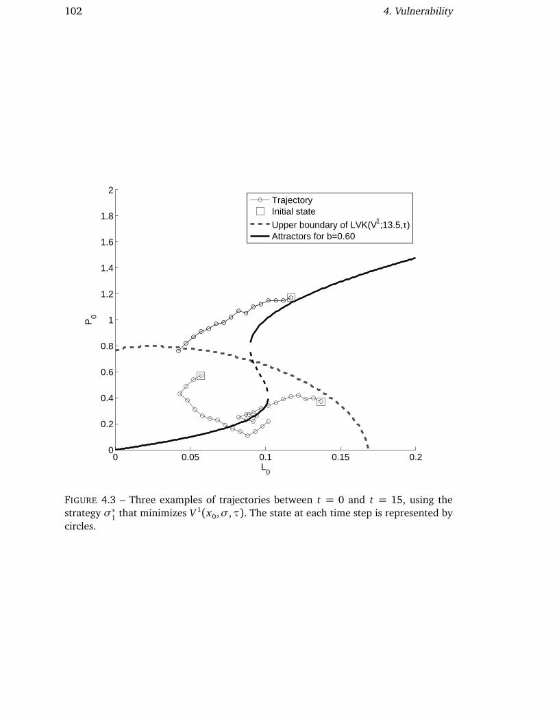
102 4. Vulnerability

0 0.05 0.1 0.15 0.20

0.2

0.4

0.6

0.8

1

1.2

1.4

1.6

1.8

2

L0

P0

TrajectoryInitial state

Upper boundary of LVK(V1;13.5,τ)Attractors for b=0.60

FIGURE 4.3 – Three examples of trajectories between t = 0 and t = 15, using thestrategy σ∗1 that minimizes V 1(x0,σ,τ). The state at each time step is represented bycircles.

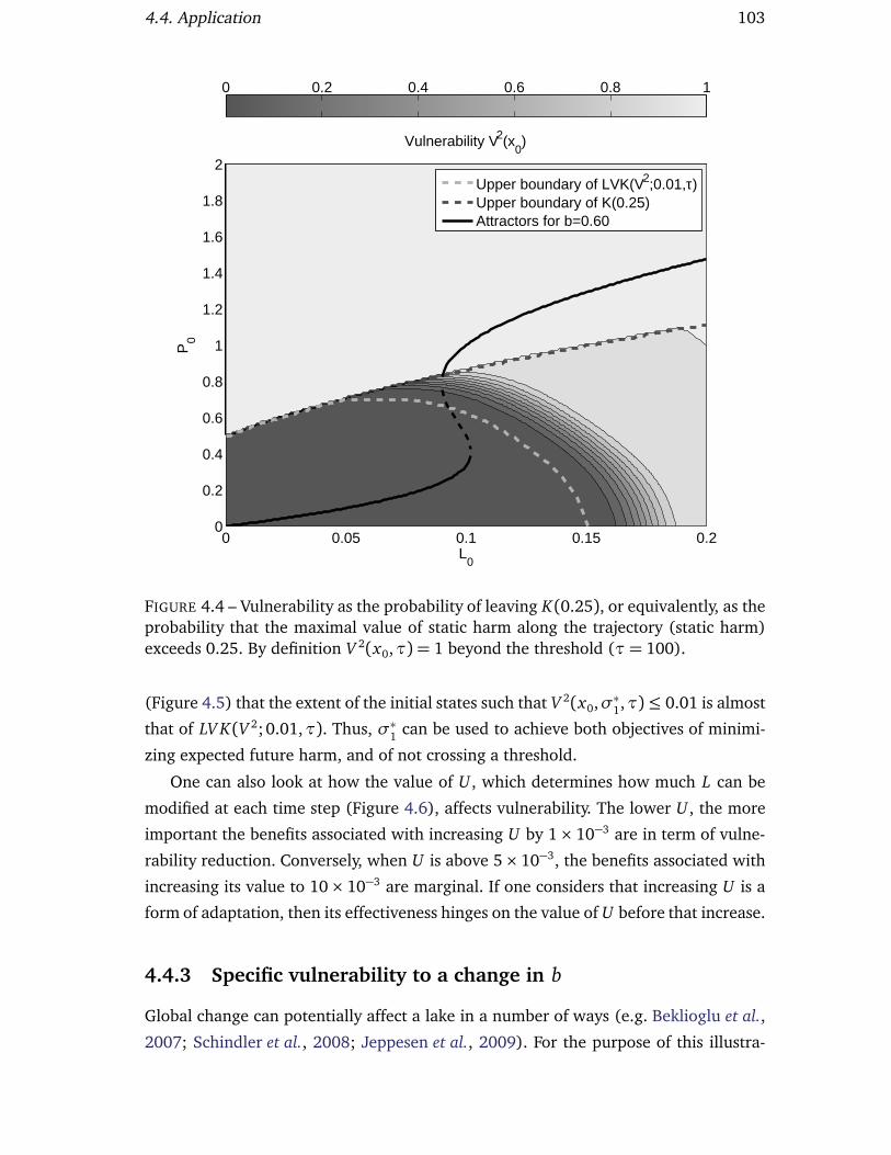
4.4. Application 103

0 0.05 0.1 0.15 0.20

0.2

0.4

0.6

0.8

1

1.2

1.4

1.6

1.8

2

Vulnerability V2(x0)

L0

P0

0 0.2 0.4 0.6 0.8 1

Upper boundary of LVK(V2;0.01,τ)Upper boundary of K(0.25)Attractors for b=0.60

FIGURE 4.4 – Vulnerability as the probability of leaving K(0.25), or equivalently, as theprobability that the maximal value of static harm along the trajectory (static harm)exceeds 0.25. By definition V 2(x0,τ) = 1 beyond the threshold (τ= 100).

(Figure 4.5) that the extent of the initial states such that V 2(x0,σ∗1,τ)≤ 0.01 is almost

that of LV K(V 2; 0.01,τ). Thus, σ∗1 can be used to achieve both objectives of minimi-

zing expected future harm, and of not crossing a threshold.

One can also look at how the value of U , which determines how much L can be

modified at each time step (Figure 4.6), affects vulnerability. The lower U , the more

important the benefits associated with increasing U by 1× 10−3 are in term of vulne-

rability reduction. Conversely, when U is above 5× 10−3, the benefits associated with

increasing its value to 10× 10−3 are marginal. If one considers that increasing U is a

form of adaptation, then its effectiveness hinges on the value of U before that increase.

4.4.3 Specific vulnerability to a change in b

Global change can potentially affect a lake in a number of ways (e.g. Beklioglu et al.,

2007; Schindler et al., 2008; Jeppesen et al., 2009). For the purpose of this illustra-

104 4. Vulnerability

0 0.05 0.1 0.15 0.20

0.2

0.4

0.6

0.8

1

1.2

1.4

1.6

1.8

2

Vulnerability V2(x0,σ*

1)

L0

P0

0.1 0.2 0.3 0.4 0.5 0.6 0.7 0.8 0.9 1

V2(x0,σ*

1) ≤ 0.01 below this line

Upper boundary of LVK(V2;0.01,τ)

Upper boundary of LVK(V1;13.5,τ)Upper boundary of K(0.25)Attractors for b=0.60

FIGURE 4.5 – Probability of leaving K(0.25) if σ∗1, the strategy which minimizesV 1(x0,σ,τ), is being used (τ= 100).

4.4. Application 105

0 0.5 1 1.5 212

14

16

18

20

a) L0=0.006

P0

V1 (x

0)

0 0.5 1 1.5 210

15

20

25

30

35

b) L0=0.009

P0

V1 (x

0)

0 0.5 1 1.5 210

15

20

25

30

35

40

c) L0=0.012

P0

V1 (x

0)

0 0.5 1 1.5 210

15

20

25

30

35

40

45

d) L0=0.015

P0

V1 (x

0)

U=0

U=0.001

U=0.002

U=0.003

U=0.004

U=0.005

U=0.01

FIGURE 4.6 – Influence of U on V 1(x0,τ) for different values of x0 = (P0, L0), withτ= 100.

106 4. Vulnerability

tion of vulnerability concepts on an very simple model, we focus on the impacts of

possible modifications of the rainfall regime. Lower precipitation may affect the out-

flow from the lake, which lowers b, but also the Ph inputs if it is accompanied of

rainfall events of lower intensity (Schindler et al., 2008). However, Ph is disproportio-

nately released from the soil into the lake by important runoff events (Sharpley et al.,

2008; Rodríguez-Blanco et al., 2013), and more extreme precipitation is expected

Jeppesen et al. (2009), so that more extreme events may balance the lower quantity of

total precipitation when it comes to releasing Ph into the lake. As a result, we simply

explore the consequences of a shift Z in b, namely a 15% decrease. This changes the

uncertainty vector wt = (Wt , 0.60) into (Wt , 0.51). Again, τ= 100, and U = 5× 10−3

unless stated otherwise.

Because of Z , the dynamic of the system is modified, and therefore the indicators

V 1 and V 2 respectively become V 1Z

and V 2Z

. The strategy that minimizes the expected

value of total harm V 1Z

is noted u+1 . The vulnerability to the shift Z can be given by

V 1(x0,τ; Z) = V 1Z(x0,τ)− V 1(x0,τ) (Figure 4.7). It is always positive and takes very

high values if L0 is high at the time of the shift. This is true in particular in some

regions of LV K(V 1; 13.5,τ). V 1Z(x0) has a minimum of 14.48, which is why we derive

a new LVK, namely LV K(V 1Z

; 14.9,τ), which represents the zone in which vulnerability

to computable uncertainty after the change is within 10% of its new minimal value. In

fact, the least-harm strategy brings the state of the system towards the new attractors

for which P is low. This supposes a decrease in L, and an economic vulnerability to Z

– provided a policy that balances ecological and economic harm is applied.

As for u∗1 in the case b = 0.60, one can test the impact of u+1 on the probability of

crossing the threshold h(x) = 0.25. The strategy u+1 is found to be near optimal for

minimizing V 2Z

so it can be used for both purposes of minimizing the expected value of

harm within the long run, as well as the probability of crossing the threshold. However,

vulnerability as the added probability of crossing after Z occurs is high in a zone of

the state space which was safe as long as b = 0.60 (Figure 4.8).

Finally, one can assess vulnerability to Z for different values of U (Figure 4.9). This

supposes to know, for each value of U , the strategies u∗1 and u+1 that respectively mi-

nimize V 1(x0,σ,τ) and V 1Z(x0,σ,τ). Figure 4.9 shows the impact of U on the specific

vulnerability to Z for states in which the lake may well be after having been mana-

ged for a long time under b = 0.60 using u∗1. It shows that the effect of increasing

U , which was almost null for U ≥ 5× 10−3 before the shift Z , can become important

when the shift occurs. This is the case for V 1 for P0 = 0.45 and 0.60, and for V 2 if

P0 = 0.45. However, it is interesting to note that even U = 0.01 cannot prevent the

system from crossing the threshold if x0 = (0.6, 0.09). Thus, adapting by anticipating

4.4. Application 107

0 0.05 0.1 0.15 0.20

0.2

0.4

0.6

0.8

1

1.2

1.4

1.6

1.8

2

2

4

4

6

6

8

8

10

10

12

12

14

14

16 18

20

22

L0

P0

V1(x0;Z)

5 10 15 20

Upper boundary of LVK(V1Z;14.9,τ)

Attractors for b=0.51

Upper boundary of LVK(V1;13.5,τ)Attractors for b=0.60

FIGURE 4.7 – Vulnerability V 1(x0,τ; Z) = V 1Z(x0,τ)− V 1(x0,τ) to a 15% decrease in

b, and incidence on the LVK (τ= 100).

108 4. Vulnerability

0 0.05 0.1 0.15 0.20

0.2

0.4

0.6

0.8

1

1.2

1.4

1.6

1.8

2

L0

P0

V2(x0,σ*

1,σ+

1;Z)

0.1 0.2 0.3 0.4 0.5 0.6 0.7 0.8 0.9

V2Z(x

0,σ+

1) ≤ 0.01 below this line

Upper boundary of LVK(V2Z;0.01,τ)

Upper boundary of K(0.25)Attractors for b=0.51Attractors for b=0.60

FIGURE 4.8 – Vulnerability to a 15% decrease in b as the added probability of cros-sing the threshold h(x) = 0.25, assuming the strategies used are σ∗1 and σ+1 whichrespectively minimize V 1(x0,τ) and V 1

Z(x0,τ), with τ= 100.

4.5. Discussion 109

0 0.002 0.004 0.006 0.008 0.010

5

10

15

20

25

30

35

40

45

U

V1 (x

0;Z)

P0=0.3

P0=0.45

P0=0.6

0 0.002 0.004 0.006 0.008 0.010

0.2

0.4

0.6

0.8

1

U

V2 (x

0,σ* co

st,σ

+ cost

;Z)

P

0=0.3

P0=0.45

P0=0.6

FIGURE 4.9 – Vulnerability to a 15% decrease in b for different initial states (P0, L0)

such that L0 = 0.09, and for different values of U . For each U , the strategies used arethose which respectively minimize V 1(x0,τ) and V 1

Z(x0,τ), with τ = 100.

on Z by increasing U can sometimes be very beneficial, but this also depends on the

chosen indicator.

4.5 Discussion

This discussion is articulated around the concepts vulnerability is related to. The res-

pective links of vulnerability with adaptation and with risk shall be discussed, before

tackling the relationship between vulnerability and its so-called components.

4.5.1 Adaptation and adaptive capacity indicators

The ability to act is described through the ability of these actions to have beneficial

consequences, and this has been designated in many different ways : coping capacity,

ability to cope, ability to adjust, adaptation, transformation, adaptive capacity. . .Even

though there is to date no comprehensive framework precisely defining these terms

together, a few guidelines can be extracted from the literature. Thus, adaptation refers

to an answer to potential future harm, be it anticipatory adaptation to circumstances

that have not yet been met, or reactive adaptation undertaken so that past harmful

events may not happen again (Fankhauser et al., 1999). The notion of success in at

least alleviating harm is implicit. Adaptation can be interpreted as a proof that the

system has adaptive capacity (Smit et Wandel, 2006), the latter being measurable as

the vulnerability reduction achieved through a modification of the system (Luers et al.,

2003; Sandoval-Solis et al., 2011).

110 4. Vulnerability

Besides, this framework can foster a discussion on the distinction between adapta-

tion and coping, made for instance by the 2012 IPCC report (Field et al., 2012, pp. 51

and 72). This distinction is implicit in concept such as that of coping range, the range

of perturbations a system can cope with, and which can be dynamically influenced by

climatic changes but also by adaptation (Smit et al., 2000; Smit et Pilifosova, 2003;

Smit et Wandel, 2006) Thus, coping is described as being the immediate reaction to a

hazard, while adaptation can also refer to action undertaken before the hazard hits.

The aim of adaptation is to increase the capacity to cope to a particular event or change

(Smit et al., 2000; Yohe et Tol, 2002), and it takes place over longer time scales than

coping (Smit et Wandel, 2006). Even though this distinction can be ambiguous, since

coping can be seen as a form of emergency adaptation (Turner II et al., 2003), coping

can be related to control strategies in the dynamical system framework we propose.

Indeed the strategy used to cope with computable uncertainty – or with a specific

hazards – is chosen among a set of already available strategies, and implementing it

supposes no change in the system, nor in the available strategy or in the definition

of harm. By contrast, adaptation can be thought of as through such modifications.

For instance, in Section 4.4 one can relate an increase in U with adaptation, and this

changes the way the system can cope with both computable events, and a specific

event Z .

Adaptation can either be planned or autonomous (Fankhauser et al., 1999). Plan-

ned adaptation is instigated with the purpose of lowering vulnerability, and it can

result in a change in any of the system’s parameters, or in a change of the set Σ(τ)

of available action strategies, in a reduction of the uncertainty (affecting ω), or in

a change in the shape or size of the constraint set. Autonomous adaptation can also

result in any of the above, and may also arise from the dynamic itself. It is then a

phenomenon that is not captured by equation (4.1), which generally implies that the

dynamical system representation should be updated. Such surprises are unexpected

phenomena that can arise either from the environment, the public or the institutions

(Janssen, 2002) and while the literature is most concerned with the negative ones

(and rightly so), they can also be positive.

Since adaptation is a manifestation of adaptive capacity, adaptive capacity can be

demonstrated when vulnerability is reduced as the result of an adaptation A, which

can be any of the changes described in the previous paragraph. Similar to the case

of specific vulnerability, the merits of adaptation are best judged when vulnerability

statistic V is chosen to measure it. The consequences of the adaptation A modify the

vulnerability function V (x0,σ,τ) into a new function VA(x0,σ,τ). Following up on

the analogy with specific vulnerability, for any two strategies σ1 and σ2, the adaptive

4.5. Discussion 111

capacity CA demonstrated by the adaptation A can be measured at the initial state x0 :

CA(x0,σ1,σ2,τ; A) = V (x0,σ1,τ)− VA(x0,σ2,τ) (4.28)

so that adaptive capacity is positive, provided adaptation did lower vulnerability. This

definition is analogous to that of Luers et al. (2003), yet more precise since it connects

adaptive capacity with the implementation of definite coping strategies both before

and after adaptation. The proposed adaptive capacity indicator judges adaptive ca-

pacity on its efficiency in lowering a given vulnerability indicator. Other frameworks

define instead adaptive capacity based on its determinants (Yohe et Tol, 2002), or as

the inventory of the resources that can be allocated to adaptation (Nelson et al., 2007;

McDowell et Hess, 2012). These evaluation criteria are complimentary, since the for-

mer focuses on potential results while the latter emphasizes the causes that make

adaptations possible.

Section 4.3.3 has shown that there are cases in which SDP techniques can find the

action strategy that minimizes the vulnerability indicator. If σ1 and σ2 in equation

(4.28) are the strategies that respectively minimize V and VA then we can omit the

strategies in the expression of the capacity CA demonstrated by the adaptation A :

CA(x0,τ; A) = V (x0,τ)− VA(x0,τ) (4.29)

One could use these formulas to assess adaptive capacity associated to an increase of

U in the case of the lake : it is null when vulnerability does not decrease, but it can be

very high in other cases, for instance when U is doubled from 10−3 to 2× 10−3. Yet,

some management policies are called maladaptative since they increase vulnerability

(Burton, 1997; Smit et al., 2000). This leads to a negative adaptive capacity, one can

state instead that there is a vulnerability to these policies, and use equation (4.7) to

quantify it.

Some frameworks (e.g. Turner II et al., 2003) rather use the concept of resilience

to describe the capacity of a system to cope and adapt. In reality, resilience in its

own is a long-standing concept (Holling, 1973), which has given way to a large body

of literature in many fields (Brand et Jax, 2007). Vulnerability and resilience, due to

their distinct disciplinary origins, conceptual center of interests, and methodological

approaches, seem to be strongly complementary concepts (Miller et al., 2010). This

complementarity is yet to be fully explored and lies outside the scope of this work, but

it could be achieved through the integration of both vulnerability and resilience in the

same dynamical system framework. Indeed, a dynamical system formulation that uses

concepts and tools from viability theory have also been used in the resilience literature

112 4. Vulnerability

(Martin, 2004; Deffuant et Gilbert, 2011; Rougé et al., 2013).

4.5.2 Vulnerability and risk

Besides all of its so-called components, vulnerability is often associated to the notion

of risk. Risk is commonly defined as the convolution of the cost and pdf. It has long

been related to vulnerability (Turner II et al., 2003), even though there does not seem

to be a clear consensus on how exactly the two notions are situated with respect to

one another. It is common to consider that risk arises from the interplay of a hazard

and of a system’s vulnerability (Wamsler et al., 2012). Indeed a hazard, in itself, does

not cause harm or damage, and it is rather its interplay with vulnerable properties of

a system that causes harm.

Arguably, the difference between risk and vulnerability is that computing a risk

requires the knowledge of the probability of occurrence of a hazard. This can prove

challenging since major hazard events are by definition extreme and rare, so that the

estimation of their return period can be very uncertain and heavily dependent on the

pdf used to approximate them (Esteves, 2013) ; and it has been shown that providing

such estimates is far more perilous in the context of a changing climate (Felici et al.,

2007a,b). Vulnerability, by contrast, only requires the knowledge of computable un-

certainty, represented by ω(t) in equation 4.1, as opposed to uncomputable uncer-

tainty, be it extreme events or mechanisms designated by the expression “uncertainty

and surprise” (Folke et al., 2002b, 2004; Adger et al., 2005) because their impact on

the system is not anticipated. Specific vulnerability assessments allow for exploring

the impacts of such uncertainties as scenarii, without requiring that return periods be

calculated. Scenario planning has been proved to be a fitting tool to explore large un-

certainties associated to climate change (Allen et al., 2011; Cobb et Thompson, 2012)

and the proposed framework for vulnerability may result useful in evaluating scenario

outcomes.

4.5.3 Components of vulnerability

Vulnerability has often been expressed as a function of its three perceived main com-

ponents, most notably exposure, sensitivity, and adaptive capacity or resilience, (e.g.

Luers et al., 2003; Turner II et al., 2003; Luers, 2005; Parry et al., 2007). However, it

has been argued that the use of vulnerability-related concepts is largely a matter of

which disciplinary point of view is taken on a problem (Miller et al., 2010), but also

that confronting different viewpoints on vulnerability could be warranted in order to

have a comprehensive vision of a given situation (Fuchs, 2009). For instance, Li et al.

4.6. Conclusions and perspectives 113

(2013) mention a total of five ways to describe vulnerability to floods as a function

of three components. Hence the choice made in this work not to write vulnerability

explicitly as a function of related concepts, in order to keep the proposed framework

general.

Nevertheless, links between vulnerability and related concepts can sometimes be

inferred from this framework. For instance, sensitivity can be measured as the im-

pact of a perturbation on the state of the system (e.g. Luers, 2005). Yet, even though

this impact may be immediate in the case of an extreme event, one may want to ins-

tead consider sensitivity based on how the whole trajectory of the system is modified

following the hazard’s occurrence. The necessity of considering many possible future

trajectories may be a challenge in measuring sensitivity, and our framework shows that

in fact, it is not a prerequisite to measuring vulnerability.

As for exposure, it is defined based on the inventory of elements that may be ad-

versely impacted by an event or change (Cardona et al., 2012). Thus, an element is

exposed when it there is both a value judgment on the adverse impacts associated

to its possible states, and when hazards or uncertainties may affect its evolution. In

that respect, defining harm functions is closely related to determining a system’s ex-

posure, and only the sensitivity of the system following a hazard event may determine

if the exposed elements can truly be harmed. In that sense our framework illustrates

the common notion (Luers, 2005; Smit et Wandel, 2006) that exposure and sensitivity

only work in tandem.

4.6 Conclusions and perspectives

Hinkel (2011) contends that vulnerability indicators are mainly fit for identifying who

may be vulnerable and where. A dynamic systems perspective on the matter may trans-

cend this grim diagnosis by fostering the development of fully dynamic indicators at

the interface between the representation of social-ecological system and its manage-

ment (Figure 4.10). The benefits of explicitly considering the temporal dimension of

vulnerability are enumerated hereafter.

1) Vulnerability becomes a descriptive concept based on a system representation,

which comprises both a description of the system’s dynamics and the normative choices

which were made when assigning a harm value to each possible trajectory. This cla-

rification of the normative and descriptive aspects is arguably a clarification of the

science-policy interface as well.

2) The choice of the indicator itself is normative. For instance, choosing between an

expected value of future harm, or a value-at-risk – related to the probability of crossing

114 4. Vulnerability

FIGURE 4.10 – Schematic representation of the proposed framework, which replacesvulnerability indicators at the interface between a social-ecological system and its ma-nagement.

4.6. Conclusions and perspectives 115

a threshold of harm – is motivated by different policy objectives. This difference is hard

to make explicit unless trajectories are used.

3) An indicator becomes associated to a given combination of computable events

and of specific extreme hazards. This clarifies which events the assessment, and the-

refore the vulnerability indicators, do not take into account. This link between consi-

dered hazards and indicator values is crucial when it comes to make policy decisions.

4) A fully dynamic framework is a prerequisite to integrating the impact of stra-

tegies in the assessment of vulnerability indicators, so as to understand how to best

cope with a given situation. Even though a closed set of equations, let alone a way to

optimize the implemented strategy, may not be available often in practice, it should

be kept in mind that strategies dynamically influence vulnerability.

5) Eventually, using a stochastic controlled dynamical system perspective is a way

to understand under which conditions a proposed adaptation measure may prove ef-

fective, since its success is shown to be related to the dynamic, the considered events,

and the already available coping strategies.

Acknowledgements

This work would not have been possible without funding from Région Auvergne.

116 4. Vulnerability

4.7 Appendix : Stochastic viability kernels as LVKs

4.7.1 Proof of equation (4.19)

Recall the definition of the stochastic viability kernel for a decision horizon τ and a

threshold confidence level β :

Viab(β ,τ) = x0 ∈ K0(l)|∃σ ∈ Σ(τ),P [∀t ∈ [0,τ],θt (x0,σ,ω) ∈ Kt(l)]≥ β

(4.30)

From equation (4.8) we have the following equivalence between the situation within

the constraint set and the value of the static harm function :

[∀t ∈ [0,τ],θt (x0,σ,ω) ∈ Kt(l)]⇔ [∀t ∈ [0,τ], ht(x0,σ,ω) ≤ l] (4.31)

and this equation, taken along with the definition of Hl(x0,σ,ω) in equation (4.10),

yields :

[∀t ∈ [0,τ],θt (x0,σ,ω) ∈ Kt(l)]⇔ [Hl(x0,σ,ω) ≤ l] (4.32)

Then, injecting this latter result into equation (4.30) and using the definition of the

probability of vulnerability (equation (4.15)) directly leads to equation (4.19).

4.7.2 LV K(Vβ

M ; v,τ) as a stochastic viability kernel

By definitions of LV K(Vβ

M ; v,τ) in equation (4.9) and Vβ

M in equation (4.17) :

LV K(Vβ

M ; v,τ) = x0 ∈ X|∃σ ∈ Σ(τ),P (HM (x0,σ,ω) ≤ v) ≥ β (4.33)

Then, using the definition of HM (x0,σ,ω) from equation (4.12), equation (4.33) be-

comes :

LV K(Vβ

M ; v,τ) = x0 ∈ X|∃σ ∈ Σ(τ),P [∀t ∈ [0,τ], ht(x0,σ,ω) ≤ v] ≥ β (4.34)

so that introducing the set of states Kt(v) = x ∈ X|ht(x)≤ v such that the static

harm function is below the threshold value v leads to :

LV K(Vβ

M ; v,τ) = x0 ∈ X|∃σ ∈ Σ(τ),P [∀t ∈ [0,τ],θt(x0,σ,ω) ∈ Kt(v)]≥ β

(4.35)

which corresponds to the definition of the stochastic viability kernel given by equation

(4.18), solely replacing Kt(l) with Kt(v).

4.8. Appendix : Stochastic dynamic programming algorithms 117

4.8 Appendix : Stochastic dynamic programming algo-

rithms

4.8.1 Viability maximization

In what follows we use for simplicity a discretization of the state space into a discrete

set which we note X . Thus, we can define the transition probability from any state x

to any state y given the decision u. We note this function p(x , y|u).

Let us have Kt(l) as defined in equation (4.8), SDP works using a value function

G which is initialized at the final date τ, then recursively updated backwards from τ

to the initial date 0. Initialization reads :

G(T, x) =

¨

1 if x ∈ KT (l)

0 if x /∈ KT (l)(4.36)

and the recursive transition equation is :

∀t ∈ [0,τ− 1], G(t , x) = maxu∈U(t,x)

∑

y∈Kt (l)

p(x , y|u) G(t + 1, y)

!

(4.37)

Doyen et De Lara (2010) prove that G(0, x) was the maximal probability for the sys-

tem to remain within Kt(l) at all dates during [0,τ], and that therefore, the stochastic

viability kernel is the set of states such that G(0, x)≥ β .

4.8.2 Cost minimization

We use the same discretization as in Appendix 4.8.1, as well as the notation p(x , y|u).

However, the value function G changes so that initialization now reads :

G(τ, x) = hτ(x) (4.38)

and the recursive transition equation is :

∀t ∈ [0,τ− 1], G(t , x) = ht(x) + minu∈U(t,x)

∑

y∈X

p(x , y|u) G(t + 1, y)

(4.39)

The reunion of equations (4.38) and (4.39) constitutes the well-known Bellman equa-

tion, and the associated optimality principle ensures that G(0, x) is the lowest possible

value for the expected vulnerability indicator V ES

(for a proof, see for instance Section

A.3 of De Lara et Doyen (2008)).

– 5 –

Performance indicators in water resources : a

joint stochastic dynamic programming

algorithm for reliability and vulnerability

En préparation.

Auteurs : Charles ROUGÉ, Jean-Denis MATHIAS et Guillaume DEFFUANT

Three indicators, called reliability, resilience and vulnerability, are commonly

used to describe the performance of a water supply system. This work focuses

on reliability and vulnerability and proposes a novel way to optimize the ex-

pected value of an indicator which uses stochastic dynamic programming to

combine both. Reliability is a measure of how often the system is in a sa-

tisfactory state. Vulnerability measures how severe or damaging a failure is,

and several different indicators can be used. A composite index is then the

sum of individual indicators, each of which can be optimized separately using

stochastic dynamic programming, whether they express a cost or the proba-

bility of crossing a threshold. A change of variable enables the optimization

of the composite index. An application to a single reservoir storing water for

consumption illustrates the method, highlighting how it makes the trade-off

between the two types of indicators explicit.

119

120 5. Water resources application

5.1 Introduction

It is common in the field of water resources management to describe the performance

of a static property of interest – e.g. the minimal satisfactory value of water supply

from a reservoir system – through a set of three indicators called reliability, resilience

and vulnerability (Hashimoto et al., 1982). This work aims at developing a composite

indicator of reliability and vulnerability, and at proposing a stochastic dynamic pro-

gramming (SDP) algorithm to optimize this composite indicator. It does not represent

the third indicator, namely resilience. Indeed, resilience has been found to be redun-

dant with vulnerability in some cases (Kundzewicz et Laski, 1995; McMahon et al.,

2006), so that it has been recommended to use only vulnerability and reliability

(Kjeldsen et Rosbjerg, 2004), a recommendation followed by Jain (2010) when pro-

posing a sustainability index. Hence our focus solely on reliability and vulnerability

indicators.

SDP is a backward induction algorithm that is well-suited to optimize the expected

value of a criterion defined for a trajectory of a system (De Lara et Doyen, 2008). It has

for instance proved effective for cost minimization problems (e.g. Loucks et van Beek,

2005), and more recently, for the maximization of the probability of respecting state

constraints during a given time horizon (Doyen et De Lara, 2010). The latter is also

called a viability criterion, a term springing from a branch of control mathematics cal-

led viability theory (Aubin, 1991). SDP also yields the control decisions that maximize

each type of criterion.

However, the decisions that minimize cost may not maximize viability, and vice

versa. This is an important limitation, because then, using these two types of criteria

together is only marginally useful : one is just warned about the existence of a trade-

off between them, without having real means to quantify it. Besides, while minimi-

zing cost is a common endeavor in many fields, avoiding the crossing of a threshold is

an issue that is focused upon in various domains such as that of vulnerability assess-

ments (e.g. Luers et al., 2003; Eakin et Luers, 2006), or those studied through viability

theory. The latter has been applied to diverse fields such as economics (Aubin, 2003),

the management of harvested ecosystems (Béné et al., 2001; Sabatier et al., 2010),

social sciences and material sciences (Deffuant et Gilbert, 2011). We show in Section

5.2 that SDP can be used to remove this hurdle, by minimizing a composite vulnerabi-

lity indicator that is a linear combination of a cost criterion along with one or several

viability criteria.

Such a composite indicator can then be related to reliability and vulnerability

(Section 5.3), indirectly fostering their computation using SDP. Previous studies have

5.2. Computing the composite vulnerability index 121

only used SDP on one of these indicators, e.g. vulnerability understood as a cost

(Raje et Mujumdar, 2010), or reliability (Nalbantis et Koutsoyiannis, 1997). Others

have used the three performance indicators in parallel with optimization of ano-

ther objective via SDP (e.g. Onta et al., 1991). In general, these indicators have

not been used by researchers and practitioners as an objective to optimize, but ra-

ther as a descriptive tool that helps understand trade-offs between different alterna-

tives (e.g. Vogel et Bolognese, 1995; Maier et al., 2001; Kjeldsen et Rosbjerg, 2004;

Jain et Bhunya, 2008). The exception (Moy et al., 1986) concerns cases were linear

programming is applicable, and where uncertainty is not accounted for. The proposed

composite indicator, which we shall call R-V indicator, is to be high when reliability is

low and vulnerability is high.

Once such R-V indicators have been defined, Section 5.4 applies them to a simple

case of reservoir operation, assuming the only objective is to deliver a target water

supply each year. It shows the pertinence of the proposed algorithm and of the indi-

cators which computation it enables. Finally, Section 5.5 discusses both the algorithm

and its application.

5.2 Computing the composite vulnerability index

5.2.1 System dynamics

We consider a system and its uncertain and controlled dynamics. We are interested in

its evolution during a given period spanning between an initial date 0 and a final date

T . In discrete time, the transition between two consecutive dates is given by :

x(t + 1) = f (t , x(t), u(t), w(t)) (5.1)

In equation (5.1), the dynamic f is the transition function between two dates, and

it is in general dependent on time. The state space is X ⊂ Rn and the vector x(t)

is the state of the system at a date t . The vector u(t) is the decision vector. The set

of decisions that are available depends both on the date and on the state, and this

decision space is noted U(t , x)⊂ Rq. A strategy σ associates to any date t and state x

a decision u(t , x) chosen among the set of possible decisions U(t , x). The set of all the

strategiesσ available within a horizon T is noted Σ(T ). w(t) is the vector representing

the uncertainty and variability that affect the system at date t .

A possible sequence of events can be called a scenario (De Lara et Doyen, 2008),

and be noted ω = (w(0), w(1), . . . , w(T − 1)). The space of all the scenarios is noted

Ω, and for the computation of vulnerability indicators, one needs to assume the exis-

122 5. Water resources application

tence of a probability P defined over P (Ω), the set of all the subsets of Ω. The triplet

(Ω,P (Ω),P) is a probability space. In this section, the uncertainty vectors w(t) from

equation (5.1) are assumed to be i.i.d (independent and identically distributed) at all

dates. We also note EP[.] expected value in the scenario space.

An initial state x0 at t = 0, a strategy σ and a scenario ω define only one possible

trajectory, which we note θ (x0,σ,ω). Each successive state x(t) belonging to a given

trajectory may also be noted θ (t , x ,σ,ω), so that equation (5.1) leads to the following

recursive sequence :

¨

θ (0, x0,σ,ω) = x0

∀t ∈ [1,τ], x(t) = θ (t , x0,σ,ω)(5.2)

and to designate the states along a trajectory that goes through x at date t , one can

also use x(τ) = θ (τ, x(t),σ,ω) when τ≥ t .

5.2.2 Harm criteria

We extract a composite criterion from two types of harm functions from Chapter 4.

These respectively correspond to cost and viability criteria. The exit criterion is the

opposite of a viability criterion.

Viability criterion

The viability criterion assesses whether a trajectory constantly respects constraints

during [0, T ]. Contrary to Doyen et De Lara (2010) who define this criterion, we as-

sume that there is no uncertainty on the constraints. Noting K(t) the constraint set

at each date, the viability criterion is defined for a trajectory, hence the notation

γ(t , x0,σ,ω) = γ(θ (t , x0,σ,ω)). The criterion reads :

γ(t , x0,σ,ω) =T∏

τ=t

1K(τ) [θ (τ, x0,σ,ω)] (5.3)

where 1K(t) is the indicator function of the set K(t), defined by :

1K(t)(x) =

¨

1 if x ∈ K(t)

0 if x /∈ K(t)(5.4)

Here we are interested in aggregating several such viability criteria, designed by

5.2. Computing the composite vulnerability index 123

an integer i ∈ [1, J]. Each is represented by a set Ki(t), and we assume that :

∀i, j ∈ [1, J], i ≤ j⇒ Ki(t) ⊂ K j(t) (5.5)

so that when i < j, the viability criterion “ j” is respected when the viability criterion “i”

is. Thus, the sets Ki(t) define degrees of undesirability. We note 1Ki(t)(x) the indicator

functions of these ensembles, and γi(t , x0,σ,ω) the associated viability criteria.

Since we are interested in an exit criterion βi rather than in a viability criterion,

we can define for each Ki(t) :

βi(t , x0,σ,ω) = αi (1− γi(t , x0,σ,ω)) (5.6)

where each exit criterion is weighted by αi > 0.

Cost criterion

The cost criterion is based on associating a cost C(t , x) to each state at each date.

These costs are summed up along a trajectory, leading to the criterion χ(t , x0,σ,ω) =

χ(θ (t , x0,σ,ω)) :

χ(t , x0,σ,ω) =T∑

τ=t

C(τ,θ (τ, x0,σ,ω)) (5.7)

Contrary to the viability or exit criteria, a linear combination of cost criteria is still a

cost criterion.

Composite harm criterion

A linear combination of a cost criterion and of several cost criteria leads to a composite

criterion which weighs the two sources of harm along the trajectory. This new criterion

κ(t , x0,σ,ω) = κ(θ (t , x0,σ,ω)) reads :

κ(t , x0,σ,ω) = χ(t , x0,σ,ω) +J∑

i=1

βi(t , x0,σ,ω) (5.8)

The goal is to minimize the value on the criterion on the whole trajectory :

κ(0, x0,σ,ω) = χ(0, x0,σ,ω) +J∑

i=1

βi(0, x0,σ,ω) (5.9)

Due to the multiplicity of potential trajectories, this minimization can only be done in

a probabilistic sense.

124 5. Water resources application

5.2.3 Change in state variables

The issue with the criterion of equation (5.9) is that its expected value cannot be

minimized using SDP. Indeed, for this minimization to be possible, the criterion κmust

be in a so-called Whittle form (Whittle, 1982; De Lara et Doyen, 2008), a recursive

relationship between κ(t , x0,σ,ω) and κ(t + 1, x0,σ,ω). Therefore, we are looking

for a transition function ψ such that κ can be written as follows :

¨

∀t ∈ [0, T − 1],κ(t , x0,σ,ω) =ψ (t , x(t),σ(t , x(t)), w(t),κ(t+ 1, x0,σ,ω))

κ(T, x0,σ,ω) = M (θ (T, x0,σ,ω))(5.10)

where the function M enables the initialization of the backward induction. For SDP

to be used to optimize the expected value of the criterion, ψ must be under the

form ψ(t , x , u, w, C) = g(t , x , u, w) + h(t , x , u, w)C . This is the case for a cost cri-

terion (ψ(t , x , u, w, C) = g(t , x , u, w) + C) or a viability criterion (ψ(t , x , u, w, C) =

h(t , x , u, w)C), but the composite harm criterion κ falls in neither category.

This is why we make a change of variables by replacing the state x by y = (x , j)

where j has integer values comprised between 0 and J . The new state y(t) is given

by the system (S’) :

x(t + 1) = f (t , x(t), u(t), w(t))

j(t + 1) =max

¨

j(t),J∑

i=1

1− 1Ki(t)(x(t + 1))

«

(S’)

so that j is the count of the sets Ki(t) that the trajectory left at some point during

the trajectory, and a variable that can only increase along the trajectory. The set Y of

feasible states is :

Y=

(x , j) ∈ X× [0, J]|x ∈ K j+1(t)

(5.11)

where we set the convention KJ+1(t) = X. The harm criterion can now be written as

follows (proof in Appendix 5.6) :

κ(t , y0,σ,ω) = χ(t , x0,σ,ω) +j(T)∑

i=1

αi (5.12)

and by definition of the cost criterion χ (equation (5.7)) we can write :

κ(t , y0,σ,ω) =T∑

τ=t

C(τ,θ (τ, x0,σ,ω)) +j(T)∑

i=1

αi (5.13)

5.2. Computing the composite vulnerability index 125

so we can introduce the cost C ′(t , y) by :

∀t < T, C ′(t , y) = C(t , x)

C ′(T, y) = C(T, x)+

j∑

i=1

αi

(5.14)

and we can then rewrite κ as a cost criterion :

κ(t , y0,σ,ω) =T∑

τ=t

C ′(τ,θ (τ, y0,σ,ω)) (5.15)

As stated at the beginning of the section, a cost criterion can be put in Whittle form

with ψ under the form ψ(t , x , u, w) = g(t , x , u, w) + C :

¨

∀t ∈ [0, T − 1],κ(t , y0,σ,ω) = C ′(t , y) + κ(t + 1, y0,σ,ω)

κ(T, y0,σ,ω) = C ′(T, y)(5.16)

and we now minimize its expected value.

5.2.4 Composite vulnerability index

We define the composite vulnerability index as the expected value of the κ :

κE(t , y0,σ) = EP [κ(t , y0,σ,ω)] (5.17)

Since κ is a cost criterion, κE is related to the following value function :

(

V (T, y) = C ′(T, y)

∀t ∈ [0, T − 1], V (t , y) = C ′(t , y) + minu∈U(t,x)

EP [V (t + 1, f (t , y, u, w))](5.18)

In particular, one can prove (see e.g. De Lara et Doyen, 2008, Appendix A.4) that :

V (0, y0) = minσ∈Σ(T)

κE(0, y0,σ) (5.19)

and we can define this minimal value κ∗E

as a function of the initial state and date

alone :

V (0, y) = κ∗E(0, y) (5.20)

so that any composite indicator made of a linear combination cost and exit criteria can

be computed through equation (5.18), provided the exit criteria are based on sets that

verify equation (5.5).

126 5. Water resources application

Eventually, if we set :

j(x) = argmin j ∈ N, (x , j) ∈ Y (5.21)

then we write the mimimal value of κE for the initial state x0 :

κ∗E(x0) = κ

∗E(0, x0, j(x0)) (5.22)

5.3 Application to reliability and vulnerability indica-

tors

The results from Section 5.2 are applied to the reliability and vulnerability indicators,

as they are known in the field of water resources planning and management. In what

follows, we assume that the state space is discretized in a set Xd .

5.3.1 Description of the static criteria of satisfaction

R-R-V performance indicators are based on static notions of satisfactory and unsatis-

factory performance, which they translate into dynamic indicators. Satisfactory per-

formance is described by a subset of the state space, K1(t). When performance is unsa-

tisfactory, the degree of dissatisfaction can be given by a sequence of other sets K j(t),

growing in the sense of equation (5.5). This sequence is finite because the state space

is discrete.

One can also define performance at a state x and date t based on a cost, c(t , x).

The cost is positive and is null when the performance is satisfactory, so that we have

the following relationship between this cost and K1(t) :

K1(t) = x |c(t , x) = 0 (5.23)

and one can also relate all the sets Ki(t) with a cost level :

∀i ∈ [2, J], Ki(t) = x |c(t , x)≤ ci (5.24)

5.3.2 Trajectory-based reliability and vulnerability

Let x0, σ andω : they define a unique trajectory, and this section deals with reliability

and vulnerability indicators defined along it, and how they relate to the viability and

cost criteria defined in Section (5.2.2).

5.3. Application to reliability and vulnerability indicators 127

The definition of reliability as a trajectory-based criterion can be made in two ways

(Hashimoto et al., 1982). On one hand, it is the fraction of the time when the system

is in a satisfactory state :

Rl1(x0,σ,ω) =1

T + 1

T∑

t=0

1K1(t)[θ (t , x0,σ,ω)] (5.25)

Maximizing Rl1 amounts to minimizing a cost (1−Rl1) so that this first reliability cri-

terion is essentially a cost criterion. On the other hand, reliability is the fact of not

reaching an unsatisfactory state during [0, T ] :

Rl2(x0,σ,ω) =T∏

t=0

10t[θ (t , x0,σ,ω)] (5.26)

where one can recognize the viability criterion γ of equation (5.3). This equivalence

between this reliability criterion and a viability criterion was also the focus of Chapter

3.

As for vulnerability criteria, they are defined in a variety of ways on a given tra-

jectory (Loucks, 1997; Sandoval-Solis et al., 2011). One can distinguish between two

broad families, one being vulnerability as a cost along a trajectory :

Vu1(x0,σ,ω) =T∑

t=0

c(t ,θ (t , x0,σ,ω)) (5.27)

while the other emphasizes the worst state along the trajectory :

Vu2(x0,σ,ω) = max0≤t≤T

c(t ,θ (t , x0,σ,ω)) (5.28)

This definition is related to the sets Ki(t) as defined in equation (5.24). If a set is

defined for each cost level, Vu2 can be written as a function of all the thresholds that

are crossed :

Vu2(x0,σ,ω) =J∑

i=1

αi

1−T∏

t=0

1it[θ (t , x0,σ,ω)]

∀i ∈ [2, I],αi = ci − ci−1

(5.29)

where the ci are defined by equation (5.24). A particular case arises when cost is defi-

ned as a distance to the property of interest which defines satisfactory performance :

then, αi = 1 for all i.

To summarize, both Vu1 and Rl1 are related to a cost, while Rl2 is a viability criterion

128 5. Water resources application

and Vu2 can be interpreted as linear combination of exit criteria. Therefore, any linear

combination of reliability and vulnerability criteria can be expressed by a composite

harm criterion κ under the form of equation (5.9).

5.3.3 The composite R-V indicator

Since the expected value of κ can be minimized thanks to SDP (equations (5.18) to

(5.22), one can get a composite reliability-vulnerability indicator along with the deci-

sion strategy σ that minimizes it. Noting it RV we have :

RV (x0) = κ∗E(x0) (5.30)

This indicator depends on the weights of the different reliability and vulnerability

criteria that are considered while computing κ. As such, it enables the elicitation of

trade-offs between reliability and vulnerability. In particular, the knowledge of κ∗E

at

a given initial state and for different values of the weights leads to approximating the

Pareto front for these indicators.

Besides, the computation of RV (x0) also yields the strategy σ∗ that minimizes it.

This gives in particular the decision to be taken at the initial date of the assessment,

which can for instance be the current date in the physical world. RV (x0) is a vulnera-

bility indicator in the sense of Chapter 4 : a low-vulnerability kernel can be associated

to it.

5.3.4 The performance kernel

A low value of RV (x0) corresponds to a high reliability and a low vulnerability of the

property of interest. In other words, failures are expected to be a rare occurrence,

and when they happen, they are expected to be of mild severity. Since reliability and

vulnerability indicators are usually called performance indicators in the field of wa-

ter resources management, a low value of RV (x0) arguably measures a high system

performance. The set of initial system configurations x0 such that RV (x0) is below the

threshold value ρ is defined as the performance kernel P (RV ;ρ, T ) defined as :

P (RV ;ρ, T ) = x0 ∈ X|RV (x0) ≤ ρ (5.31)

and we propose an overall indicator of the performance of the system with respect to

the property of interest, namely the size of the performance kernel relative to that of

5.4. Application 129

the state space :

Φ(RV ;ρ, T ) =1

∑

x∈Xdλ(x i)

∑

x∈Xd

1R(RV ;ρ,T)(x i)λ(x i) (5.32)

5.4 Application

This application is inspired from You et Cai (2008c), except that we consider a horizon

T instead of a rolling two-period scheme.

5.4.1 Model formulation

We are interested in the operation of a single reservoir for water supply. The state

variables are reservoir storage S and the delivery D of water for consumption. The

decision is the release R from the reservoir, and the inflow I is stochastic. The state

transition reads :¨

S(t + 1) = S(t) + I(t)− R(t)

D(t + 1) =minR(t), D0(5.33)

where the first equation is the water balance, and the second expresses that D matches

the water demand D0 whenever possible. We set a yearly time step, and the demand

D0 is assumed to be known and constant for every year. D(t + 1) is the water delivery

at year t , and the date t + 1 is artificially given so as to respect the formulation of

equation (5.1). By convention we set D(0) = D0. We also have the hard constraints :

0 ≤ S(t)≤ C (5.34)

0≤ R(t)≤ S(t) + I(t) (5.35)

where C is the maximum capacity of the reservoir. Finally, the inflow I(t) is assumed

to be log-normal with mean I0 and scale parameter η, and to be i.i.d.

The static criterion expresses whether the demand is met, so the set of satisfactory

states K1, constant through time, is :

K1 = (S, D)|D = D0 (5.36)

In other words, satisfaction amounts to having release equal or greater than D0.

All the quantities introduced above are made non-dimensional by scaling them by

the reservoir capacity C . Consequently, at any date, S(t) ∈ [0, 1], and in what follows,

a resolution of 0.01 is taken for all the variables.

130 5. Water resources application

5.4.2 Performance criteria

Three criteria are used in this case-study. First, Rl1 from equation (5.25) translates

into :

Rl1(x0,σ,ω) =1T

T∑

t=1

1D=D0[θ (t , x0,σ,ω)] (5.37)

since there are only T release decisions over [0, T ]. Then, Vu1 from equation (5.27)

represents the sum of water deficits D0 − D(t) over [0, T ], normalized on [0, 1] :

Vu1(x0,σ,ω) =1T

T∑

t=1

1−D(t)

D0

(5.38)

and we also keep track of the highest deficit along the trajectory, so Vu2 from equation

(5.28) becomes Vu2 :

Vu2(x0,σ,ω) = max1≤t≤T

1−D(t)

D0

3

(5.39)

where Vu2 is like the other two criteria. The exponent 3 was chosen as a good com-

promise between the need for skewing the criterion against the more severe failures,

and that for . Noting Di the discrete points between 0 and D0, with a resolution of

∆S = 0.01, one can rewrite Vu2 as a sum of exit criteria like in equation 5.29. The

change of variables y = (x , j) of Section 5.2.3 leads to rewriting Vu2 as follows :

Vu2(y0,σ,ω) =

1−∆S × j(T )

D0

k

(5.40)

Then, one can define two composite criteria. The first composite criterion weighs

Vu1 with Vu2 :

κ1(λ, y0,σ,ω) = λVu1(x0,σ,ω) + (1−λ)Vu2(y0,σ,ω) (5.41)

The second weighs (1−Re1) and Vu2, which mirror the reliability and vulnerability

indicators initially proposed by Hashimoto et al. (1982) to describe the performance

of a water supply system with respect to a delivery target :

κ2(λ, y0,σ,ω) = λ(1−Rl1(x0,σ,ω)) + (1−λ)Vu2(y0,σ,ω) (5.42)

and the objective is to minimize the expected value of these criteria. For i = [1, 2] the

5.4. Application 131

objective is :

κ∗i(λ, y0) = min

σ∈Σ(T)EP [κi(λ, y0,σ,ω)] (5.43)

and, using equation (5.22), we can write, still for i = [1, 2] :

κ∗i(λ, x0) = κ

∗i(λ, x0, j(x0)) (5.44)

5.4.3 Operating policies

SDP is used to minimize the two objectives given above, with T = 20. Due to a

yearly time step, this value of the decision horizon is deemed sufficient in practice,

because the past behavior of the statistical distribution of water inflows cannot be ex-

trapolated into the future (Koutsoyiannis, 2006), especially not in a stationary way

(Milly et al., 2008). Besides, the decision horizon should not exceed the forecast hori-

zon (You et Cai, 2008a).

In particular, SDP yields the optimal release decision at the initial (current) date.

This policy assumes that past releases have no influence on j(T ), which is only a mean

to keep track of the thresholds that will be crossed until T . The release decision at year

t is assumed to be done only once the total amount of water available, S+ I , is known.

Of course, there may be uncertainty within year t regarding the release rate depending

on future inflow during the same year. Such decisions would be captured by intra-year

dynamics which are not captured by equations (5.33) and (5.35), so we choose to

ignore intra-year uncertainty.

Respective release decisions at the date t = 0 depending on total available water

are displayed in Figure 5.1 for κ∗1(x0), and Figure 5.2 for κ∗2(x0). On both figures,

intermediate values of λ lead to policies that compromise between those chosen for

λ= 0 or λ = 1. Though they both are for given values of the parameters, the behavior

they display is generic across all parameter values.

On Figure 5.1, λ = 1 corresponds to the policy that minimizes the expected value

of the sum of the future shortages, known as the standard operating policy or SOP

(Hashimoto et al., 1982). It consists in (A) releasing all the available water when the

demand is not met, (B) filling the reservoir when there is enough water to meet the

demand, and (C) releasing the surplus. Alternatively, λ= 0 is the case where only Vu2

is considered. As a result, the corresponding policy is a hedging policy, defined as a

policy where the current demand is purposefully not met so as to store more water in

the reservoir and make possible future shortages less severe (Draper et Lund, 2004).

Through economic analysis over a current and a future period, You et Cai (2008b)

132 5. Water resources application

FIGURE 5.1 – Optimal policies for κ∗1(λ, x0) and different values of λ. Known casescorrespond to λ = 0 (hedging) and λ = 1 (Standard Operating Policy or SOP). D0 =

0.8, I0 = 0.8 and η = 0.8.

5.4. Application 133

FIGURE 5.2 – Optimal policies for κ∗2(λ, x0) and different values of λ. A known casecorresponds to λ= 0 (hedging). D0 = 0.8, I0 = 0.8 and η = 0.8.

134 5. Water resources application

find a concave hedging curve between the part (A) of the curve where the reservoir is

empty, and the part (C) where it is full. Through a minimization of the expected value

of the maximum failure, we also find a concave hedging curve. In between those two

cases, the compromise between hedging and SOP yields mixed policies that amount

to hedging for low values of S+ I , so the reservoir gets partially filled even though the

demand is not met. Then when the reservoir is filled at 41% (in the case λ = 0.5) or

72% (for λ = 0.75), the additionnal water is released until the demand is met : this

amounts to switching back to SOP. Such mixed rules do not appear in the literature,

and it is the proposed composite indicator that enables to show their relevance.

On Figure 5.2, λ = 1 corresponds to (A) storing all the water when S + I < D0,

then (B) meeting the demand and filling the reservoir with the remaining water, and

(C) releasing all the excess water. This difference apart, the results are the same as for

Figure 5.1, and intermediate values of λ again give rise to new policies where hedging

is prioritized until a threshold value of S+ I where the optimal release decision is that

given by the case λ= 1.

Both these policies are optimal at the initial date and for T = 20. It should be

noted that the optimal policy at a given date changes with the time horizon conside-

red. As T grows, so does the possibility of a severe shortage, which means that the

expected value of j(T ) increases. To hedge against this risk, the operating policy gets

more conservative, and leads to storing less water. However, the optimal policy re-

mains qualitatively unchanged with respect to the horizon, as illustrated in Figure 5.3

which represents the operating rule in the same conditions as for Figure 5.1, except

for the decision horizon. The comparison between both figures also reveals that the

quantitative difference between the decisions at T = 20 and T = 50 is relatively small,

as it never goes over 0.06.

5.4.4 Performance indicators

In this section, we keep only one R-V indicator, so RV (x0,λ) = κ∗2(x0,λ). This choice

enables us to examine the trade-offs between reliability and vulnerability (Figures

5.4 and 5.5) using for each λ the optimal strategy σ∗(λ). One can thus get a Pareto

front, where λ close to 0 corresponds to hedging more water in order to avoid more

severe future water shortages, and λ close to 1 corresponds to maximizing reliability.

It is interesting to note the sensitivity of reliability and vulnerability to a change in

inflow standard deviation between the two figures, which highlights the importance

of climate variability. Initial water storage is also crucial, especially when it comes to

the expected maximal deficit.

Besides having an in-depth look at the indicators that compose RV , one can de-

5.4. Application 135

FIGURE 5.3 – Same as Figure 5.1, but with T = 50.

0 0.2 0.4 0.6 0.8 10

0.1

0.2

0.3

0.4

0.5

0.6

0.7

0.8

0.9

1

Probability of failure

Exp

ecte

d va

lue

of V

u 2

S(0)=0.2S(0)=0.4S(0)=0.6S(0)=0.8S(0)=1

0 0.2 0.4 0.6 0.8 10

0.1

0.2

0.3

0.4

0.5

0.6

0.7

0.8

0.9

1

Probability of failure

Exp

ecte

d m

axim

al d

efic

it

S(0)=0.2S(0)=0.4S(0)=0.6S(0)=0.8S(0)=1

FIGURE 5.4 – Trade-off of the probability of failure EP[1 − Rl1(x0,σ∗(λ),ω)] withEP[Vu2(x0,σ∗(λ),ω)] (left) and the expected maximal deficit (right). D0 = 0.5,I0 = 0.5 and η = 0.3. S(0) is the initial storage.

136 5. Water resources application

0 0.2 0.4 0.6 0.8 10

0.1

0.2

0.3

0.4

0.5

0.6

0.7

0.8

0.9

1

Probability of failure

Exp

ecte

d va

lue

of V

u 2

S(0)=0.2S(0)=0.4S(0)=0.6S(0)=0.8S(0)=1

0 0.2 0.4 0.6 0.8 10

0.1

0.2

0.3

0.4

0.5

0.6

0.7

0.8

0.9

1

Probability of failure

Exp

ecte

d m

axim

al d

efic

it

S(0)=0.2S(0)=0.4S(0)=0.6S(0)=0.8S(0)=1

FIGURE 5.5 – Same as for Figure 5.4, but now with η= 0.4.

termine the performance kernel P (RV ;ρ, T ) so as to infer the overall performance of

the system. We choose ρ = 0.1, and plot the performance Φ for D0 = 0.5 and different

values of the inflow mean I0 and variance η (Figure 5.6). For all three values of λ (0,

0.5 and 1) there is a range of combinations of I0 and η for which the water inflow is

too scarce and too variable. The performance kernel is empty, which highlights that the

reservoir cannot be in a state where RV is low. In contrast, most other combinations

of these parameters yield a performance of 0.7 when λ = 0, 0.79 when λ = 0.5 and 1

when λ= 1. This means that even for a low initial storage, the reservoir can function

in a satisfactory way. When λ 6= 1, large water deficits D0− D(t) are penalized, so the

system cannot be expected to have a very low RV (x0) when the initial storage is very

low. Indeed, if the first inflow is low, then the water deficit of the first year can be very

high. For λ = 1 however, only reliability is taken into account, so even if initial water

storage is low, what matters is whether the reservoir can quickly be filled, which is the

case when the annual mean inflow is greater than the annual demand.

5.5 Discussion

This paper presents an SDP algorithm which computes the expected value of a criterion

which is a linear combination of cost and exit criteria. Even though it is presented to

cases where the viability criteria are delimited by certain constraints, this hypothesis

is no longer needed when the state space is discretized. Indeed, it is then possible

to compute, at each point within the state space, the sum of αi coefficients weighted

by the probability that the state is outside Ki(t). Then, all the states can be ranked

5.5. Discussion 137

00.5

1

00.5

10

0.5

1

Inflow variance η

a) λ=0

Inflow mean I0

Per

form

ance

Φ(R

V;0

.1,2

0)

00.5

1

00.5

10

0.5

1

Inflow variance η

b) λ=0.5

Inflow mean I0

Per

form

ance

Φ(R

V;0

.1,2

0)

00.5

1

00.5

10

0.5

1

Inflow variance η

c) λ=1

Inflow mean I0

Per

form

ance

Φ(R

V;0

.1,2

0)

FIGURE 5.6 – Overall system performance for RV (x0,λ) = κ∗1(x0,λ), and D0 = 0.5.For instance, a value of 0.74 means that the top 74% of the initial storage values arewithin the performance kernel P (RV ; 0.1, 20).

138 5. Water resources application

according to the value of this sum, and be put into newly defined sets K ′m(t) which

reflect this ranking. Their boundaries are not uncertain so one gets back to the case in

which the algorithm is proposed.

It is also possible to use the same kind of scheme to optimize a compromise between

the expected value a harm function as defined in Chapter 4, and the probability of

reaching a set at a certain horizon. If this set is a stochastic viability kernel, then this

probability is a probability of resilience (Chapter 2), and the algorithm can be used to

find a compromise between resilience and vulnerability.

The application to a simple case of reservoir operation showcases how the algo-

rithm can be used to compute trade-offs between indicators, and to propose operating

policies. However, a limitation of the proposed method appears to be its dependence

on the time horizon, which can be illustrated through the application.

5.6. Appendix : Proof of equation (5.12) 139

5.6 Appendix : Proof of equation (5.12)

Let us define the sets Yi = X× [0, i − 1]. The viability criterion γi(0, y0,σ,ω) is equal

to 1 if the trajectory did not cross the boundary of i of the constraint sets and to 0

otherwise. :

γi(0, y0,σ,ω) = 1Yi(θ (T, y0,σ,ω))

= 1[0,i−1]( j(T ))

As a consequence we can write the weighted sum of exit criteria :

J∑

i=1

βi(0, y0,σ,ω) =J∑

i=1

αi

1− 1[0,i−1]( j(T ))

=

j(T)∑

i=1

αi

1− 1[0,i−1]( j(T ))

+

J∑

i= j(T)+1

αi

1− 1[0,i−1]( j(T ))

on the other hand, by definition of the indicator function :

1[0,i−1]( j(T )) =

¨

0 if j(T )≥ i

1 if j(T )< i

so that we finally get :J∑

i=1

βi(0, y0,σ,ω) =j(T)∑

i=1

αi (5.45)

Bibliographie

ADGER, W. N. (2000). Social and ecological resilience : are they related ? Progress in

Human Geography, 24(3):347–364.

ADGER, W. N. (2006). Vulnerability. Global Environmental Change, 16:268–281.

ADGER, W. N., HUGUES, T. P., FOLKE, C., CARPENTER, S. R. et ROCKSTRÖM, J. (2005).

Social-ecological resilience to coastal disasters. Science, 309:1036–1039.

ALIEV, T. A. et KARTVELISHVILI, L. N. (1993). Principles of evaluating the ecological

reliability of irrigation systems. Hydrotechnical Construction, 27(5):297–304.

ALLEN, C. R., FONTAINE, J. J., POPE, K. L. et GARMESTANI, A. S. (2011). Adaptive

management for a turbulent future. Journal of Environmental Management, 92:

1339–1345.

ANDERIES, J. M., JANSSEN, M. A. et WALKER, B. H. (2002). Grazing management,

resilience, and the dynamics of a fire-driven rangeland system. Ecosystems, 5:23–

44.

ANDRIEU-RENAUD, C., SUDRET, B. et LEMAIRE, M. (2004). The phi2 method : A way to

compute time-variant reliability. Reliability Engineering and System Safety, 84:75–

86.

AUBIN, J.-P. (1991). Viability Theory. Birkhäuser.

AUBIN, J.-P. (2003). Regulation of the evolution of the architecture of a network by

tensors operatingon coalitions of actors. Journal of Evolutionary Economics, 13:95–

124.

AUBIN, J.-P., BAYEN, A. et SAINT-PIERRE, P. (2011). Viability Theory. Regulation of Un-

certain Systems. Springer-Verlag.

AUBIN, J.-P. et SAINT-PIERRE, P. (2002). An introduction to viability theory and ma-

nagement of renewable resources. Dans Coupling Climate and Economic Dynamics,

pages 55–96. Springer.

141

142 Bibliographie

BEKLIOGLU, M., ROMO, S., KAGALOU, I., QUINTANA, X. et BÉCARES, E. (2007). State of

the art in the functioning of shallow mediterranean lakes : workshop conclusions.

Hydrobiologia, 584:317–326.

BÉNÉ, C., DOYEN, L. et GABAY, D. (2001). A viability analysis for a bio-economic model.

Ecological Economics, 36:385–396.

BÉNÉ, C., EVANS, L., MILLS, D., OVIE, S., RAJI, S., TAFIDA, A., KODIO, A., SINABA, F.,

MORAND, P., LEMOALLE, J. et ANDREW, N. (2011). Testing resilience thinking in

a poverty context : Experience from the niger river basin. Global Environmental

Change, 21:1173–1184.

BIRKMANN, J., éditeur (2006). Measuring vulnerability to natural hazards. United

Nations University Press, Tokyo.

BONNEUIL, N. (2006). Computing the viability kernel in large state dimension. Journal

of Mathematical Analysis and Applications, 323:1444–1454.

BRAND, F. S. et JAX, K. (2007). Focusing on the meaning(s) of resilience : Resilience

as a descriptive concept and a boundary object. Ecology and Society, 12(1).

BURTON, I. (1997). Vulnerability and adaptive response in the context of climate and

climate change. Climatic Change, 36:185–196.

CARDONA, O., van AALST, M., BIRKMANN, J., FORDHAM, M., MCGREGOR, G., PEREZ,

R., PULWARTY, R., SCHIPPER, E. et SINH, B. (2012). Determinants of risk : exposure

and vulnerability. Dans FIELD, C., BARROS, V., STOCKER, T., QIN, D., DOKKEN, D.,

EBI, K., MASTRANDREA, M., MACH, K., PLATTNER, G.-K., ALLEN, S., TIGNOR, M. et

MIDGLEY, P., éditeurs : Managing the Risks of Extreme Events and Disasters to Advance

Climate Change Adaptation, pages 65–108. Cambridge University Press, Cambridge,

UK, and New York, NY, USA. A Special Report of Working Groups I and II of the

Intergovernmental Panel on Climate Change (IPCC).

CARPENTER, S., WALKER, B., ANDERIES, J. M. et ABEL, N. (2001). From metaphor to

measurement : Resilience of what to what ? Ecosystems, 4:765–781.

CARPENTER, S. R. (2008). Phosphorus control is critical to mitigating eutrophication.

Proceedings of the National Academy of Science, 105(32):11039–11040.

CARPENTER, S. R., FOLKE, C., SCHEFFER, M. et WESTLEY, F. (2008). Resilience : Ac-

counting for the noncomputable. Ecology and Society, 14(1):13.

Bibliographie 143

CARPENTER, S. R., LUDWIG, D. et BROCK, W. A. (1999). Management of eutrophication

for lakes subject to potentially irreversible change. Ecological Applications, 9(3):751–

771.

CISSÉ, A. A., GOURGUET, S., DOYEN, L., BLANCHARD, F. et PÉREAU, J.-C. (2013). A bio-

economic model for the viable management of the coastal fishery in french guyana.

Environmental and Development Economics, pages 1–25.

COBB, A. N. et THOMPSON, J. L. (2012). Climate change scenario planning : A model

for the integration of science and management in environmental decision-making.

Environmental Modelling & Software, 38:296–305.

COSTA, L. et KROPP, J. P. (2012). Linking components of vulnerability in theoretic

frameworks and case studies. Sustainability Science, 8(1):1–9.

DE LARA, M. et DOYEN, L. (2008). Sustainable Management of Natural Resources.

Springer-Verlag, Berlin.

DE LARA, M. et MARTINET, V. (2009). Multi-criteria dynamic decision under uncer-

tainty : A stochastic viability analysis and an application to sustainable fishery ma-

nagement. Mathematical Biosciences, 217:118–124.

DEFFUANT, G., CHAPEL, L. et MARTIN, S. (2007). Approximating viability kernel with

support vector machines. IEEE Transactions on Automatic Control, 52(5):933–937.

DEFFUANT, G. et GILBERT, N., éditeurs (2011). Viability and resilience of complex sys-

tems. Kluwer Academic Publishers, London.

DOYEN, L. et BÉNÉ, C. (2003). Sustainability of fisheries through marine reserves : a

robust modeling analysis. Journal of Environmental Management, 69:1–13.

DOYEN, L. et DE LARA, M. (2010). Stochastic viability and dynamic programming.

Systems and Control Letters, 59:629–634.

DOYEN, L., LARA, M. D., FERRARIS, J. et PELLETIER, D. (2007). Sustainability of exploi-

ted marine ecosystems through protected areas : A viability model and a coral reef

case study. Ecological Modelling, 208:353–366.

DOYEN, L. et SAINT-PIERRE, P. (1997). Scale of viability and minimal time of crisis.

Set-Valued Analysis, 5:227–246.

DOYEN, L., THÉBAUD, O., BÉNÉ, C., MARTINET, V., GOURGUET, S., BERTIGNAC, M., FIFAS,

S. et BLANCHARD, F. (2012). A stochastic viability approach to ecosystem-based

fisheries management. Ecological Economics, 75:32–42.

144 Bibliographie

DRAPER, A. J. et LUND, J. R. (2004). Optimal hedging and carryover storage value.

Journal of Water Resources Planning and Management, 130(1):83–87.

EAKIN, H. et LUERS, A. L. (2006). Assessing the vulnerability of social-environmental

systems. Annual Review of Environment and Resources, 31:365–394.

ESTEVES, L. S. (2013). Consequences to flood management of using different proba-

bility distributions to estimate extreme rainfall. Journal of Environmental Manage-

ment, 115:98–105.

FANKHAUSER, S., SMITH, J. B. et TOL, R. S. J. (1999). Weathering climate change :

some simple rules to guide adaptation decisions. Ecological Economics, 30:67–78.

FELICI, M., LUCARINI, V., SPERANZA, A. et VITOLO, R. (2007). Extreme value statistics of

the total energy in an intermediate-complexity model of the midlatitude atmosphe-

ric jet. part i : Stationary case. Journal of the Atmospheric Sciences, 64:2137–2158.

FELICI, M., LUCARINI, V., SPERANZA, A. et VITOLO, R. (2007). Extreme value statistics of

the total energy in an intermediate-complexity model of the midlatitude atmosphe-

ric jet. part ii : Trend detection and assessment. Journal of the Atmospheric Sciences,

64:2159–2175.

FIELD, C., BARROS, V., STOCKER, T., QIN, D., DOKKEN, D., EBI, K., MASTRANDREA, M.,

MACH, K., PLATTNER, G.-K., ALLEN, S., TIGNOR, M. et MIDGLEY, P., éditeurs (2012).

IPCC, 2012 : Managing the Risks of Extreme Events and Disasters to Advance Climate

Change Adaptation. Cambridge University Press, Cambridge, UK, and New York, NY,

USA. A Special Report of Working Groups I and II of the Intergovernmental Panel

on Climate Change.

FOLKE, C. (2006). Resilience : The emergence of a perspective for social-ecological

systems analyses. Global Environmental Change, 16:253–267.

FOLKE, C., CARPENTER, S., ELMQVIST, T., GUNDERSON, L., HOLLING, C. S. et WALKER,

B. (2002). Resilience and sustainable development : Building adaptive capacity in

a world of transformations. Ambio, 31(5):437–440.

FOLKE, C., CARPENTER, S., ELMQVIST, T., GUNDERSON, L., HOLLING, C. S., WALKER, B.,

BENGTSSON, J., BERKES, F., COLDING, J., DANELL, K., FALKENMARK, M., GORDON, L.,

KASPERSON, R., KAUTSKY, N., KINZIG, A., LEVIN, S., MÄLER, K.-G., F.MOBERG, OHLS-

SON, L., OLSSON, P., OSTROM, E., REID, W., ROCKSTRÖM, J., SAVENIJE, H. et SVEDIN,

U. (2002). Resilience and sustainable development : Building adaptive capacity in a

Bibliographie 145

world of transformations. Rapport technique, Scientific Background Paper on Resi-

lience for the process of The World Summit on Sustainable Development on behalf

of The Environmental Advisory Council to the Swedish Government.

FOLKE, C., CARPENTER, S. R., WALKER, B., SCHEFFER, M., CHAPIN, T. et ROCKSTRÖM, J.

(2010). Resilience thinking : Integrating resilience, adaptability and transformabi-

lity. Ecology and Society, 15(4):20.

FOLKE, C. S., CARPENTER, S., WALKER, B., SCHEFFER, M., ELMQVIST, T., GUNDERSON,

L. et HOLLING, C. S. (2004). Regime shifts, resilience, and biodiversity in ecosystem

management. Annual Review of Ecology, Evolution, and Systematics, 35:557–581.

FUCHS, S. (2009). Susceptibility versus resilience to mountain hazards in austria -

paradigms of vulnerability revisited. Natural Hazards and Earth System Sciences,

9:337–352.

GALLOPÍN, G. C. (2006). Linkages between vulnerability, resilience, and adaptive ca-

pacity. Global Environmental Change, 16:293–303.

GRIMM, V. et WISSEL, C. (1997). Babel, or the ecological stability discussions : an

inventory and analysis of terminology and a guide for avoiding confusion. Oecologia,

109:323–334.

GUNDERSON, L. H. (2000). Ecological resilience – in theory and application. Annual

Review of Ecology and Systematics, 31:425–439.

GUTTAL, V. et JAYAPRAKASH, C. (2007). Impact of noise on bistable ecological systems.

Ecological Modelling, 201(3-4):420–428.

HAGEN, O. et TVEDT, L. (1991). Vector process out-crossing as parallel system sensiti-

vity measure. Journal of Engineering Mechanics, 117(10):2201–2220.

HARDY, P.-Y. (2013). Gestion viable et résilience de la petite pêche côtière des îles coral-

liennes. Thèse de doctorat, Museum National d’Histoire Naturelle.

HASHIMOTO, T., STEDINGER, J. R. et LOUCKS, D. P. (1982). Reliability, resiliency, and

vulnerability criteria for water resource system performance evaluation. Water Re-

sources Research, 18(1):14–20.

HINKEL, J. (2011). “indicators of vulnerability and adaptive capacity” : Towards a

clarification of the science-policy interface. Global Environmental Change, 21:198–

208.

146 Bibliographie

HOLLING, C. S. (1973). Resilience and stability of ecological systems. Annual Review

of Ecology, Evolution, and Systematics, 4:1–23.

HOLLING, C. S. (1996). Engineering resilience versus ecological resilience. Dans Engi-

neering within ecological constraints. National Academy Press, D.C., USA.

HSIAO, E., SCHUSTER, M., JUANG, C. et KUNG, G. (2008). Reliability analysis and upda-

ting of excavation-induced ground settlement for building serviceability assessment.

Journal of Geotechnical and Geoenvironmental Engineering, 134(10):1448–1458.

IONESCU, C., KLEIN, R., HINKEL, J., KUMAR, K. K. et KLEIN, R. (2009). Towards a

formal framework of vulnerability to climate change. Environmental Modelling and

Assessment, 14(1):1–16.

JAIN, S. K. (2010). Investigating the behavior of statistical indices for performance

assessment of a reservoir. Journal of Hydrology, 391:90–96.

JAIN, S. K. et BHUNYA, P. K. (2008). Reliability, resilience and vulnerability of a multi-

purpose storage reservoir. Hydrological Sciences Journal, 53(2):434–447.

JANSSEN, M. A. (2002). A future of surprises. Dans GUNDERSSON, L. H. et HOLLING,

C. S., éditeurs : Panarchy : understanding transformations in human and natural

systems, chapitre 9, pages 241–260. Island Press, Washington, D.C., USA.

JEPPESEN, E., KRONVANG, B., MEERHOFF, M., SØNDERGAARD, M., HANSEN, K. M., AN-

DERSEN, H. E., LAURIDSEN, T. L., LIBORIUSSEN, L., BEKLIOGLU, M., ÖZEN, A. et OLE-

SEN, J. E. (2009). Climate change effects on runoff , catchment phosphorus loading

and lake ecological state, and potential adaptations. Journal of Environmental Qua-

lity, 38(5):1930–1941.

JOHNSON, K. H., VOGT, K. A., CLARK, H. J., SCHMITZ, O. J. et VOGT, D. J. (1996).

Biodiversity and the productivity and stability of ecosystems. Trends in Ecology and

Evolution, 11(9):372–377.

KASPRZYK, J. R., NATARAJ, S., REED, P. M. et LEMPERT, R. J. (2013). Many objective

robust decision making for complex environmental systems undergoing change. En-

vironmental Modelling & Software, 42:55–71.

KJELDSEN, T. R. et ROSBJERG, D. (2004). Choice of reliability, resilience and vulnerabi-

lity estimators for risk assessments of water resources systems. Hydrological Sciences

Journal, 49(5):755–767.

Bibliographie 147

KOUTSOYIANNIS, D. (2002). The hurst phenomenon and fractional gaussian noise

made easy. Hydrological Sciences Journal, 47(4):573–595.

KOUTSOYIANNIS, D. (2006). Nonstationarity versus scaling in hydrology. Journal of

Hydrology, 324:239–254.

KUNDZEWICZ, Z. et LASKI, A. (1995). Reliability-related criteria in water supply stu-

dies. In : New Uncertainties Concepts in Hydrology and Water Resources. Cambridge

University Press, Cambridge, UK.

LESNOFF, M., CORNIAUX, C. et HIERNAUX, P. (2012). Sensitivity analysis of the recovery

dynamics of a cattle population following drought in the sahel region. Ecological

Modelling, 232:28–39.

LI, C. et DER KIUREGHIAN, A. (1995). Mean out-crossing rate of nonlinear response to

stochastic input. Dans MÉBARKI A, B., éditeur : Proceedings of the Internationational

Conference on the Application of Statistics and Probability (ICASP7), volume Volume

1, pages 295–302.

LI, C.-H., LI, N., WU, L.-C. et HU, A.-J. (2013). A relative vulnerability estimation of

flood disaster using data envelopment analysis in the dongting lake region of hunan.

Natural Hazards and Earth System Sciences, 13:1723–1734.

LIU, C., GOLDING, D. et GONG, G. (2008). Farmers´ coping response to the low flows in

the lower yellow river : A case study of temporal dimensions of vulnerability. Global

Environmental Change, 18:543–553.

LÓPEZ, D. R., BRIZUELA, M. A., WILLEMS, P., AGUIAR, M. R., SIFFREDI, G. et BRAN, D.

(2013). Linking ecosystem resistance, resilience, and stability in steppes of north

patagonia. Ecological Indicators, 24:1–11.

LOUCKS, D. P. (1997). Quantifying trends in system sustainability. Hydrological Sciences

Journal, 42(4):513–530.

LOUCKS, D. P. et van BEEK, E. (2005). Water Resources Systems Planning and Manage-

ment. UNESCO.

LUDWIG, D., CARPENTER, S. et BROCK, W. (2003). Optimal phosphorus loading for a

potentially eutrophic lake. Ecological Applications, 13(4):1135–1152.

LUERS, A. L. (2005). The surface of vulnerability : An analytical framework for exa-

mining environmental change. Global Environmental Change, 15:214–233.

148 Bibliographie

LUERS, A. L., LOBELL, D. B., SKLAR, L. S., ADDAMS, C. L. et MATSON, P. A. (2003). A

method for quantifying vulnerability, applied to the agricultural system of the yaqui

valley, mexico. Global Environmental Change, 13:255–267.

MACGILLIVRAY, C. W. et GRIME, J. P. (1995). Testing predictions of the resistance and

resilience of vegetation subjected to extreme events. Functional Ecology, 9:640–649.

MAIER, H. R., LENCE, B. J., TOLSON, B. A. et FOSCHI, R. O. (2001). First-order reliabi-

lity method for estimating reliability, vulnerability, and resilience. Water Resources

Research, 37(3):779–790.

MANDELBROT, B. et WALLIS, J. R. (1968). Noah, joseph, and operational hydrology.

Water Resources Research, 4(5):909–918.

MARTIN, S. (2004). The cost of restoration as a way of defining resilience : a viability

approach applied to a model of lake eutrophication. Ecology and Society, 9(2).

MATHIAS, J.-D. et LEMAIRE, L. (2012). Reliability analysis of bonded joints with va-

riations in adhesive thickness. Journal of Adhesion Science and Technology, pages

1–11.

MCCARTHY, J. J., CANZIANI, O. F., LEARY, N. A., DOKKEN, D. J. et WHITE, K. S., éditeurs

(2001). Climate Change 2001 : Impacts, Adaptation and Vulnerability. Cambridge

University Press, Cambridge.

MCDOWELL, J. Z. et HESS, J. J. (2012). Accessing adaptation : Multiple stressors on li-

velihoods in the bolivian highlands under a changing climate. Global Environmental

Change, 22:342–352.

MCMAHON, T. A., ADELOYE, A. J. et ZHOU, S.-L. (2006). Understanding performance

measures of reservoirs. Journal of Hydrology, 324:359–382.

MELCHING, C. S. (1992). An improved first-order reliability approach for assessing

uncertainties in hydrologic modeling. Journal of Hydrology, 132:157–177.

MENDOZA, V. M., VILLANUEVA, E. E. et ADEM, J. (1997). Vulnerability of basins and

watersheds in mexico to global climate change. Climate Research, 9:139–145.

MENONI, S., PERGALANI, F., BONI, M. P. et PETRINI, V. (2002). Lifelines earthquake

vulnerability assessment : a systemic approach. Soil Dynamics and Earthquake En-

gineering, 22:1199–1208.

Bibliographie 149

MILLER, F., OSBAHR, H., BOYD, E., THOMALLA, F., BHARWANI, S., ZIERVOGEL, G., WAL-

KER, B., BIRKMANN, J., van der LEEUW, S., ROCKSTRÖM, J., HINKEL, J., DOWNING, T.,

FOLKE, C. et NELSON, D. (2010). Resilience and vulnerability : Complementary or

conflicting concepts ? Ecology and Society, 15(3):11.

MILLY, P. C. D., BETANCOURT, J., FALKENMARK, M., HIRSCH, R. M., KUNDZEWICZ, Z. W.,

LETTENMAIER, D. P. et STOUFFER, R. J. (2008). Stationarity is dead : Whither water

management ? Science, 319(5863):573–574.

MOY, W., COHON, J. et REVELLE, C. (1986). A programming model for analysis of the

reliability, resilience, and vulnerability of a water supply reservoir. Water Resources

Research, 22(4):489–498.

NAEEM, S. (1998). Species redundancy and ecosystem reliability. Conservation Biology,

12(1):39–45.

NAEEM, S. et LI, S. (1997). Biodiversity enhances ecosystem reliability. Nature, 390:

507–509.

NALBANTIS, I. et KOUTSOYIANNIS, D. (1997). A parametric rule for planning and mana-

gement of multiple-reservoir systems. Water Resources Research, 33(9):2165–2177.

NELSON, D. R., ADGER, W. N. et BROWN, K. (2007). Adaptation to environmental

change : contributions of a resilience framework. Annual Review of Environment

and Resources, 32:395–419.

ONTA, P. R., GUPTA, A. D. et HARBOE, R. (1991). Multistep planning model for conjunc-

tive use of surface- and ground-water resources. Journal of Wate, 117:662–678.

OVIEDO-SALCEDO, D. M. (2012). Accounting for parameter uncertainty and temporal

variability in coupled groundwater-surface water models using component and systems

reliability analysis. Thèse de doctorat, University of Illinois at Urbana-Champaign.

PARRY, M., CANZIANI, O., PALUTIKOF, J., van der LINDEN, P. et HANSON, C., éditeurs

(2007). Climate Change 2007 : Impacts, Adaptation and Vulnerability. Contribution

of Working Group II to the Fourth Assessment Report of the Intergovernmental Panel

on Climate Change. Cambridge University Press, Cambridge, United Kingdom and

New York, NY, USA.

PEDUZZI, P., DAO, H., HEROLD, C. et MOUTON, F. (2009). Assessing global exposure

and vulnerability towards natural hazards : the disaster risk index. Natural Hazards

and Earth System Sciences, 9:1149–1159.

150 Bibliographie

PÉREAU, J.-C., DOYEN, L., LITTLE, L. R. et THÉBAUD, O. (2012). The triple bottom line :

Meeting ecological, economic and social goals with individual transferable quotas.

Journal of Environmental Economics and Management, 63:419–434.

PERREIRA, M. V. F. et PINTO, L. M. V. G. (1985). Stochastic optimization of a multire-

servoir hydroelectric system : a decomposition approach. Water Resources Research,

21(6):779–792.

PERZ, S. G., noz CARPENA, R. M., KIKER, G. et HOLT, R. D. (2013). Evaluating ecological

resilience with global sensitivity and uncertainty analysis. Ecological Modelling, 263:

174–186.

PETERSON, G. D. (2002). Estimating resilience across landscapes. Ecology & Society,

6(1):17.

PRESTON, B. L. (2013). Local path dependence of u.s. socioeconomic exposure to

climate extremes and the vulnerability commitment. Global Environmental Change,

23:719–732.

RACKWITZ, R. (2001). Reliability analysis – a review and some perspectives. Structural

Safety, 23:365–395.

RAJE, D. et MUJUMDAR, P. P. (2010). Reservoir performance under uncertainty in hy-

drologic impacts of climate change. Advances in Water Resources, 33:312–326.

RASTETTER, E. B., GOUGH, L., HARTLEY, A. E., HERBERT, D. A., NADELHOFFER, K. J. et

WILLIAMS, M. (1999). A revised assessment of species redundancy and ecosystem

reliabilityauthor. Conservation Biology, 13(2):440–443.

RAUSAND, M. (1998). Reliability centered maintenance. Reliability Engineering and

System Safety, 60(2):121–132.

ROCKSTRÖM, J., FALKENMARK, M., LANNERSTAD, M. et KARLBERG, L. (2012). The pla-

netary water drama : Dual task of feeding humanity and curbing climate change.

Geophysical Research Letters, 39.

RODRÍGUEZ-BLANCO, M., TABOADA-CASTRO, M. et TABOADA-CASTRO, M. (2013). Phos-

phorus transport into a stream draining from a mixed land use catchment in galicia

(nw spain) : Significance of runoff events. Journal of Hydrology, 481:12–21.

ROUGÉ, C., MATHIAS, J.-D. et DEFFUANT, G. (2013). Extending the viability theory fra-

mework of resilience to uncertain dynamics, and application to lake eutrophication.

Ecological Indicators, 29:420–433.

Bibliographie 151

SABATIER, R., DOYEN, L. et TICHIT, M. (2010). Modelling trade-offs between livestock

grazing and wader conservation in a grassland agroecosystem. Ecological Modelling,

221:1292–1300.

SAINT-PIERRE, P. (1994). Approximation of the viability kernel. Applied Mathematics

and Optimization, 29:187–209.

SANDOVAL-SOLIS, S., MCKINNEY, D. C. et LOUCKS, D. P. (2011). Sustainability index

for water resources planning and management. Journal of Water Resources Planning

and Management, 137(5):381–390.

SCHEFFER, M., CARPENTER, S., FOLEY, J. A., FOLKE, C. et WALKER, B. (2001). Catas-

trophic shifts in ecosystems. Nature, 413(6856):591–596.

SCHEFFER, M. et CARPENTER, S. R. (2003). Catastrophic regime shifts in ecosystems :

linking theory to observation. Trends in Ecology and Evolution, 18(12):648–656.

SCHINDLER, D. W. (2006). Recent advances in the understanding and management of

eutrophication. Limnology and Oceanography, 51(1):356–363.

SCHINDLER, D. W., HECKY, R. E., FINDLAY, D. L., STAINTON, M. P., PARKER, B. R., PA-

TERSON, M. J., BEATY, K. G., LYNG, M. et KASIAN, S. E. M. (2008). Eutrophica-

tion of lakes cannot be controlled by reducing nitrogen input : Results of a 37-

year whole-ecosystem experiment. Proceedings of the National Academy of Science,

105(32):11254–11258.

SCHLÜTER, M. et HERRFAHRDT-PÄHLE, E. (2011). Exploring resilience and transforma-

bility of a river basin in the face of socioeconomic and ecological crisis : an example

from the amudarya river basin, central asia. Ecology and Society, 16(1):32.

SHARPLEY, A. N., KLEINMAN, P. J. A., HEATHWAITE, A. L., GBUREK, W. J., FOLMAR, G. J. et

SCHMIDT, J. P. (2008). Phosphorus loss from an agricultural watershed as a function

of storm size. Journal of Environmental Quality, 37:362–368.

SKAGGS, T. H. et BARRY, D. A. (1997). The first-order reliability method of predicting

cumulative mass flux in heterogeneous porous formations. Water Resources Research,

33(6):1485–1494.

SMIT, B., BURTON, I., KLEIN, R. et WANDEL, J. (2000). An anatomy of adaptation to

climate change and variability. Climatic Change, 45(1):223–251.

152 Bibliographie

SMIT, B. et PILIFOSOVA, O. (2003). From adaptation to adaptive capacity and vulne-

rability reduction. Dans SMITH, J., KLEIN, R. et HUQ, S., éditeurs : Climate Change,

Adaptive Capacity and Development, pages 9–28. Imperial College Press, London.

SMIT, B. et WANDEL, J. (2006). Adaptation, adaptive capacity and vulnerability. Global

Environmental Change, 16:282–292.

SUDRET, B. (2008). Analytical derivation of the outcrossing rate in time-variant relia-

bility problems. Structure and Infrastructure Engineering, 4(5):353–362.

TURNER II, B. L., KASPERSON, R. E., MATSON, P. A., MCCARTHY, J. J., CORELL, R. W.,

CHRISTENSEN, L., ECKLEY, N., KASPERSON, J. X., LUERS, A., MARTELLO, M. L., POLSKY,

C., PULSIPHER, A. et SCHILLER, A. (2003). A framework for vulnerability analysis

in sustainability science. Proceedings of the National Academy of Science, 100(14):

8074–8079.

VOGEL, R. M. et BOLOGNESE, R. A. (1995). Storage-reliability-resilience-yield relations

for over-year water supply systems. Water Resources Research, 31(3):645–654.

WALKER, B., CARPENTER, S., ANDERIES, J., ABEL, N., CUMMING, G., JANSSEN, M., LEBEL,

L., NORBERG, J., PETERSON, G. D. et PRITCHARD, R. (2002). Resilience management

in social-ecological systems : a working hypothesis for a participatory approach.

Conservation Ecology, 6(1):14.

WALKER, B., HOLLING, C. S., CARPENTER, S. R. et KINZIG, A. (2004). Resilience, adapta-

bility and transformability in social-ecological systems. Ecology and Society, 9(2):5.

WAMSLER, C., BRINK, E. et RENTALA, O. (2012). Climate change, adaptation, and for-

mal education : the role of schooling for increasing societies’ adaptive capacities in

el salvador and brazil. Ecology and Society, 17(2):2.

WHITTLE, P. (1982). Optimization over Time : Dynamic Programming and Stochastic

Control, volume 1. John Wiley & Sons, New York.

WILLIAMS, B. K. (2011). Adaptive management of natural resources – framework and

issues. Journal of Environmental Management, 92:1346–1353.

WOLF, S., HINKEL, J., HALLIER, M., BISARO, A., LINCKE, D., IONESCUO, C. et KLEIN, R.

J. T. (2013). Clarifying vulnerability definitions and assessments using formalisa-

tion. International Journal of Climate Change Strategies and Management, 5(1):54–

70.

Bibliographie 153

YOHE, G. et TOL, R. (2002). Indicators for social and economic coping capacity -

moving toward a working definition of adaptive capacity. Global Environmental

Change, 12(1):25–40. cited By (since 1996)236.

YOU, J.-Y. et CAI, X. (2008). Determining forecast and decision horizons for reservoir

operations under hedging policies. Water Resources Research, 44.

YOU, J.-Y. et CAI, X. (2008). Hedging rule for reservoir operations : 1. a theoretical

analysis. Water Resources Research, 44.

YOU, J.-Y. et CAI, X. (2008). Hedging rule for reservoir operations : 2. a numerical

model. Water Resources Research, 44.

YOUNG, O. R. (2010). Institutional dynamics : Resilience, vulnerability and adaptation

in environmental and resource regimes. Global Environmental Change, 20:378–385.