ÉCOLE DE TECHNOLOGIE SUPÉRIEURE UNIVERSITÉ DU QUÉBEC

INTELLIGENT DISTRIBUTION VOLTAGE CONTROL WITH DISTRIBUTED GENERATION

BY Jose CASTRO MENDIETA

MANUSCRIPT – BASED THESIS PRESENTED TO ÉCOLE DE TECHNOLOGIE SUPÉRIEURE

IN PARTIAL FULFILLMENT FOR THE DEGREE OF DOCTOR OF PHILOSOPHY

Ph.D.

MONTREAL, OCTOBER 17, 2016

© Copyright Jose CASTRO MENDIETA, 2016 All rights reserved

© Copyright

Reproduction, saving or sharing of the content of this document, in whole or in part, is prohibited. A reader

who wishes to print this document or save it on any medium must first obtain the author’s permission.

BOARD OF EXAMINERS (THESIS PH.D.)

THIS THESIS HAS BEEN EVALUATED

BY THE FOLLOWING BOARD OF EXAMINERS Mr. Maarouf Saad, Thesis Supervisor Department of Electrical Engineering, École de technologie supérieure Mr. Serge Lefebvre, Thesis Co-supervisor Hydro-Quebec research institute IREQ Ms. Sylvie Ratté, Chair, Board of Examiners Department of Mechanical Engineering, École de technologie supérieure Mr. Pierre-Jean Lagacé, Member of the jury Department of Electrical Engineering, École de technologie supérieure Ms. Dalal Asber, External jury Research Institute of Hydro-Québec (IREQ) Mr. Innocent Kamwa, Independent external jury Research Institute of Hydro-Québec (IREQ)

THIS THESIS WAS PRENSENTED AND DEFENDED

IN THE PRESENCE OF A BOARD OF EXAMINERS AND THE PUBLIC

ON SEPTEMBER 9, 2016

AT ÉCOLE DE TECHNOLOGIE SUPÉRIEURE

ACKNOWLEDGMENTS

I would like to express deepest appreciation to my advisor Professor Maarouf Saad for

trusting me to come up with this project and to be an outstanding role model. I am very

grateful for having had an opportunity to work with Dr. Serge Lefebvre, Dr. Dalal Asber and

Dr. Laurent Lenoir. Thank for allowing me to be part of GREPCI and teaching me the

importance of collaborative work.

I also want to thank all the members of the committee to take the time to read and evaluated

this thesis, many thanks to the president Professor Sylvie Ratté, to Professor Pierre-Jean

Lagacé and the external member Dr. Innocent Kamwa.

I would have not been able to complete my work if it had not been for the constant support of

my wife Betty. She has always inspired me to be optimist and encouraged me to excel and

achieve beyond what I think I am capable of. Finally, I want to thank my kids Josue, Mariela,

and Isabela.

INTELLIGENT DISTRIBUTION VOLTAGE CONTROL WITH DISTRIBUTED GENERATION

Jose CASTRO MENDIETA

ABSTRACT

In this thesis, three methods for the optimal participation of the reactive power of distributed generations (DGs) in unbalanced distributed network have been proposed, developed, and tested. These new methods were developed with the objectives of maintain voltage within permissible limits and reduce losses. The first method proposes an optimal participation of reactive power of all devices available in the network. The propose approach is validated by comparing the results with other methods reported in the literature. The proposed method was implemented using Simulink of Matlab and OpenDSS. Optimization techniques and the presentation of results are from Matlab. The co-simulation of Electric Power Research Institute’s (EPRI) OpenDSS program solves a three-phase optimal power flow problem in the unbalanced IEEE 13 and 34-node test feeders. The results from this work showed a better loss reduction compared to the Coordinated Voltage Control (CVC) method. The second method aims to minimize the voltage variation on the pilot bus on distribution network using DGs. It uses Pareto and Fuzzy-PID logic to reduce the voltage variation. Results indicate that the proposed method reduces the voltage variation more than the other methods. Simulink of Matlab and OpenDSS is used in the development of the proposed approach. The performance of the method is evaluated on IEEE 13-node test feeder with one and three DGs. Variables and unbalanced loads are used, based on real consumption data, over a time window of 48 hours. The third method aims to minimize the reactive losses using DGs on distribution networks. This method analyzes the problem using the IEEE 13-node test feeder with three different loads and the IEEE 123-node test feeder with four DGs. The DGs can be fixed or variables. Results indicate that integration of DGs to optimize the reactive power of the network helps to maintain the voltage within the allowed limits and to reduce the reactive power losses. The thesis is presented in the form of the three articles. The first article is published in the journal Electrical Power and Energy System, the second is published in the international journal Energies and the third was submitted to the journal Electrical Power and Energy System. Two other articles have been published in conferences with reviewing committee. This work is based on six chapters, which are detailed in the various sections of the thesis. Keywords: Distribution network; coordinated voltage control; distributed generation; multi-objective optimization.

CONTRÔLE DE TENSION INTELLIGENT DES RÉSEAUX DE DISTRIBUTION AVEC GÉNÉRATION DISTRIBUÉE

Jose CASTRO MENDIETA

RÉSUMÉ

Dans cette thèse, trois méthodes pour la participation optimale de la puissance réactive de la génération distribuée (DG) des réseaux de distribution déséquilibrés ont été proposées, développées et testées. Ces nouvelles méthodes ont été développées avec les objectifs de maintenir la tension dans les limites admissibles et de réduire les pertes. La première méthode propose une participation optimale de la puissance réactive de tous les dispositifs disponibles sur le réseau. La méthode proposée est validée en comparant les résultats obtenus avec d'autres méthodes décrites dans la littérature. Les méthodes ont été simulées dans Simulink de Matlab et OpenDSS. Les techniques d'optimisation et la présentation des résultats sont faites dans Matlab. Le logiciel développé par Electric Power Research Institute’s (EPRI) résout le problème d'écoulement de puissance triphasé déséquilibré dans les réseaux tests utilisés, IEEE 13 et 34 barres. Les résultats de cette étude montrent une meilleure réduction des pertes en comparaison avec la méthode de contrôle coordonnée de tension (CVC). La deuxième méthode minimise la variation de tension dans la barre pilote sur le réseau de distribution en utilisant la génération distribuée (DG). Cette méthode utilise la technique de Pareto et la logique floue (Fuzzy-PID) pour réduire la variation de tension. Les résultats indiquent que la méthode proposée permet de réduire la variation de la tension plus que les autres méthodes. Simulink de Matlab et OpenDSS sont utilisées dans le développement de la méthode proposée. La performance de cette méthode est évaluée sur le réseau IEEE 13 barres avec une et trois DGs. Des charges variables et déséquilibrée sont utilisées en se basant, sur la consommation réelle d’une période de 48 heures. La troisième méthode minimise les pertes de puissance réactive en utilisant les DGs dans les réseaux de distribution. Cette méthode analyse le problème en utilisant le réseau IEEE 13 barres avec trois différentes charges variables et le réseau IEEE 123 barres avec quatre DGs. Les DGs peuvent être fixes ou variables. Les résultats indiquent que l'intégration des DGs optimise la puissance réactive du réseau et aide à maintenir la tension dans les limites permises et de réduire les pertes de puissance réactive. La thèse est présentée sous la forme de trois articles. Le premier article est publié dans la revue Electrical Power and Energy System, le second est publié dans International Journal Energies et le troisième a été soumis à la revue Electrical Power and Energy System. Deux autres articles ont été publiés dans des conférences avec comité de lecture. Mots clés : Réseau de distribution; contrôle de la tension coordonnée; génération distribuée; optimisation multi-objectifs.

TABLE OF CONTENTS

Page INTRODUCTION .....................................................................................................................1 CHAPTER 1 LITERATURE REVIEW ............................................................................7 1.1 Introduction ....................................................................................................................7 1.2 Impacts of Distributed Generators .................................................................................7

1.2.1 Voltage stability .......................................................................................... 8 1.2.2 Reactive Power ............................................................................................ 9 1.2.3 Distribution Losses .................................................................................... 11

1.3 Optimization techniques ..............................................................................................13 CHAPTER 2 BACKGROUND CONCEPTS ..................................................................15 2.1 Introduction ..................................................................................................................15 2.2 Optimization Techniques .............................................................................................15

2.2.1 Pareto optimization ................................................................................... 15 2.2.1.1 Pareto frontier ............................................................................ 16 2.2.1.2 Decision Maker (DM) ................................................................ 19

2.2.2 Fuzzy logic ................................................................................................ 20 2.2.3 Fuzzy-PI Controller ................................................................................... 21

2.3 OpenDSS program .......................................................................................................22 2.3.1 OPenDSS structure .................................................................................... 23 2.3.2 Modeling in OpenDSS on distribution networks ...................................... 24 2.3.3 OpenDSS access from Matlab .................................................................. 25

CHAPTER 3 OPTIMAL VOLTAGE CONTROL IN DISTRIBUTION NETWORK IN THE PRESENCE OF DGs ...................................................................27 3.1 Introduction ..................................................................................................................28 3.2 Coordinated Voltage Control in Distribution Network ................................................30

3.2.1 Problem formulation ................................................................................. 31 3.2.1.1 Voltage at pilot bus .................................................................... 31 3.2.1.2 Reactive power production ........................................................ 31 3.2.1.3 Voltage at generators ................................................................. 32

3.2.2 Optimization constraints ........................................................................... 32 3.2.2.1 Voltage Constraints .................................................................... 33 3.2.2.2 Reactive power constraint .......................................................... 33 3.2.2.3 Weights constraints .................................................................... 33

3.2.3 Pilot Bus .................................................................................................... 34 3.2.4 The On-load taps Changer (OLTC) .......................................................... 35

3.3 Pareto Optimization .....................................................................................................36 3.4 Optimal Coordinated Voltage Control (OCVC) ..........................................................38

3.4.1 Flowchart programming of OCVC ........................................................... 38 3.5 Case study ....................................................................................................................40

XII

3.5.1 Implementation ......................................................................................... 41 3.5.2 IEEE 13 Node Test Feeder ........................................................................ 41

3.5.2.1 OLTC: reference case ................................................................ 43 3.5.2.2 Coordination Voltage Control (Fixed weight) ........................... 43 3.5.2.3 Optimal Coordination Voltage Control (OCVC) ....................... 43

3.5.3 IEEE 34 Node Test Feeder ........................................................................ 46 3.6 Conclusions ..................................................................................................................48 CHAPTER 4 COORDINATED VOLTAGE CONTROL IN DISTRIBUTION NETWORK WITH THE PRESENCE OF DGs AND VARIABLE LOAD USING PARETO AND FUZZY LOGIC ......................................53 4.1 Introduction ..................................................................................................................52 4.2 Coordinated Voltage Control (CVC) ...........................................................................55

4.2.1 Objectives Function .................................................................................. 55 4.2.1.1 Voltage at Pilot Bus ................................................................... 55 4.2.1.2 Reactive Power .......................................................................... 56 4.2.1.3 Voltage at Generators ................................................................ 56

4.2.2 Constraints ................................................................................................. 57 4.2.2.1 Reactive Power Constraint ......................................................... 57 4.2.2.2 Technical Compliance Voltage .................................................. 57 4.2.2.3 Weights Constraints ................................................................... 57

4.3 Coordinated Voltage Control Using Pareto and Fuzzy Logic (CVCPF) .....................58 4.3.1 Pareto Optimization .................................................................................. 58 4.3.2 Fuzzy Logic ............................................................................................... 59 4.3.3 Design of Reactive Power of DG .............................................................. 62 4.3.4 Solution Algorithm .................................................................................... 62 4.3.5 Case Study ................................................................................................. 65

4.4 Simulation Results .......................................................................................................67 4.5 Conclusions ..................................................................................................................74 CHAPTER 5 POWER FACTOR COMPUTATION OF DISTRIBUTED GENERATION USING MULTI-OBJECTIVE OPTIMIZATION...........79 5.1 Introduction ..................................................................................................................76 5.2 Problem formulation and optimization ........................................................................79

5.2.1 Multi-Objective Problem (MOP) .............................................................. 79 5.2.1.1 Coordinated Voltage Control (CVC) ......................................... 80 5.2.1.2 Active and reactive power of the DGs ....................................... 80

5.2.2 Main Constraints ....................................................................................... 82 5.2.2.1 Power factor constraints ............................................................. 82 5.2.2.2 Voltage constraints..................................................................... 82 5.2.2.3 Weight constraints ..................................................................... 82

5.2.3 Optimization techniques ............................................................................ 83 5.2.3.1 Pareto optimization .................................................................... 83 5.2.3.2 Fuzzy-PI controller .................................................................... 84

5.3 Proposed Solution ........................................................................................................87

XIII

5.4 Case Study ....................................................................................................................90 5.4.1 IEEE 13-node test feeder .......................................................................... 90

5.4.1.1 Simulations results ..................................................................... 91 5.4.1.2 Variable load 1 ........................................................................... 91 5.4.1.3 Variable load 2 ........................................................................... 94 5.4.1.4 Comparison of results ................................................................ 95 5.4.1.5 Variable load 3 ........................................................................... 96

5.4.2 IEEE 123-node test feeder ........................................................................ 98 5.4.3 Implementation ....................................................................................... 101 5.4.4 Analysis of Results and Discussions ....................................................... 102

5.5 Conclusions ................................................................................................................102 CHAPTER 6 SUMMARY AND CONCLUSIONS ......................................................109 6.1 Summary ....................................................................................................................105 6.2 Conclusions ................................................................................................................107 6.3 Recommendations for future work ............................................................................108 APPENDIX I IEEE NODE TEST FEEDER .................................................................111 APPENDIX II OPENDSS CODES ................................................................................123 ANNEXE I REFERENCES OF ARTICLES PUBLISHED .....................................129 BIBLIOGRAPHY ..................................................................................................................131

LIST OF TABLES

Page Table 1.1 Summary of the reviewed studies on the impact on voltage stability ..........9

Table 1.2 Summary of the reviewed studies on the impact on Reactive Power .........11

Table 1.3 Summary of the reviewed studies on the impact on losses .........................12

Table 2.1 Genetic Algorithm (Default values) ...........................................................17

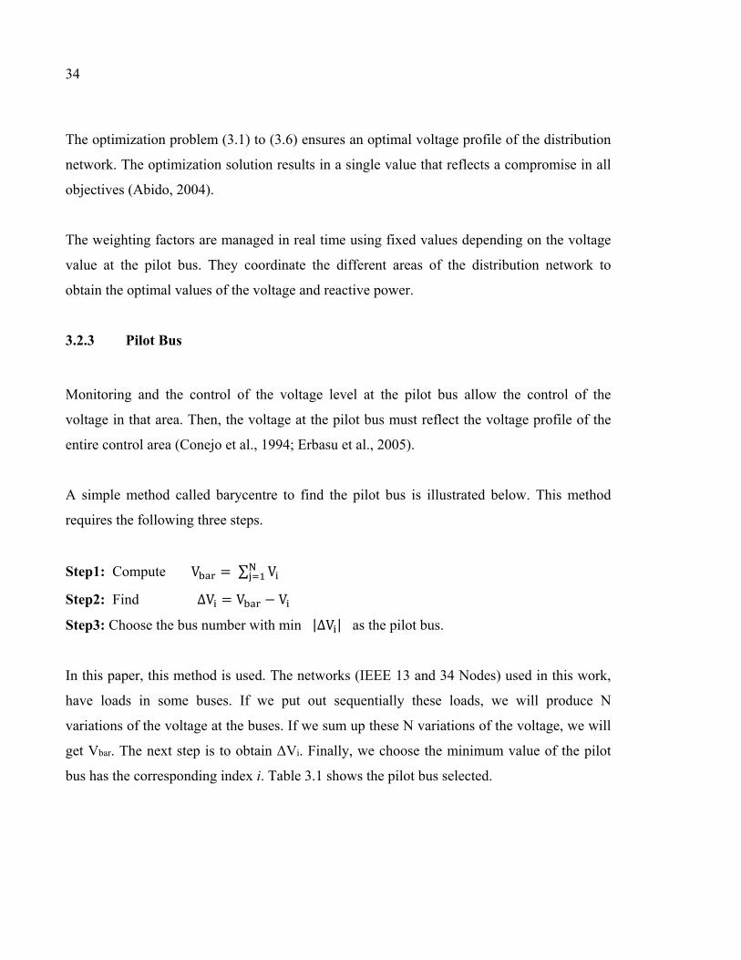
Table 2.2 Interface between Matlab and OpenDSS program ....................................26

Table 3.1 Pilot bus for IEEE 13 and IEEE 34 buses ...................................................35

Table 3.2 Weight variation: Comparison between CVC and OCVC .........................44

Table 4.1 Spot Load Data for IEEE 13 .......................................................................66

Table 4.2 Cable line configuration for IEEE 13 node test feeder ...............................66

Table 4.3 Maximum load variation in Case 1, 2 and 3 ...............................................67

Table 4.4 Maximum load variation in Case 1, 2 and 3 ...............................................71

Table 5.1 Spot Load Data for IEEE 13 ......................................................................90

Table 5.2 Cable lines configuration for IEEE 13-node test feeder .............................92

Table 5.3 Transformer data for IEEE 13-node test feeder .........................................92

Table 5.4 Voltage deviation. OCVC, CVCPF, and VPF methods .............................96

Table 5.5 Computation Performance; OCVC, CVCPF, and VPF methods ..............102

LIST OF FIGURES

Page

Figure 2.1 Illustration of Pareto frontier for two objectives .......................................17

Figure 2.2 Input fuzzy membership functions ...........................................................20

Figure 2.3 Fuzzy-PI controller ....................................................................................22

Figure 2.4 OpenDSS structure ...................................................................................24

Figure 2.4 Block diagram of the implemented procedure ..........................................25

Figure 3.1 Pareto Optimization scheme for multi-objective function ........................37

Figure 3.2 Flow chart of the proposed algorithm .......................................................39

Figure 3.3 Case study distribution network IEEE 13 Node Test Feeder ....................42

Figure 3.4 Voltage profile of the IEEE 13 Node Test Feeder on the pilot bus ...........44

Figure 3.5 Active power losses in the IEEE 13 Node Test Feeder .............................45

Figure 3.6 Reactive power losses in the IEEE 13 Node Test Feeder .........................45

Figure 3.7 Case study distribution network. IEEE 34 Node Test Feeder ....................46

Figure 3.8 Voltage profile of the IEEE 34 Node Test Feeder on the pilot bus ............47

Figure 3.9 Active power losses in the IEEE 34 Node Test Feeder ..............................47

Figure 3.10 Reactive power losses in the IEEE 34 Node Test Feeder .........................48

Figure 4.1 Pareto optimization scheme for a multi-objective problem ......................59

Figure 4.2 Fuzzy logic reactive power factor controller .............................................61

Figure 4.3 Input fuzzy membership functions ............................................................61

Figure 4.4 Flow chart of the proposed algorithm .......................................................64

Figure 4.5 IEEE 13 Node Test Feeder ........................................................................65

Figure 4.6 Variation of the load in kW at bus 671 ......................................................66

Figure 4.7 Voltage at bus 671(phase a) with respect to reactive power input. Case 1 .68

XVIII

Figure 4.8 Voltage at bus 671(phase a) with respect to reactive power input. Case 2 .68

Figure 4.9 Voltage at bus 671(phase a) with respect to reactive power input. Case 3 .69

Figure 4.10 Losses. Active and reactive power for Case 2 ............................................72

Figure 4.11 Reactive power generated by the DG for Case 3 with CVCPF and OCVC methods ......................................................................................................72

Figure 4.12 Voltage at pilot bus with respect to reactive power input. Case 4 ..............73

Figure 5.1 Pareto optimization scheme for MOP .........................................................85

Figure 5.2 Scheme of a Fuzzy-PI controller .................................................................85

Figure 5.3 a) Fuzzy set for input voltage deviation; b) Fuzzy set for input voltage deviation change ........................................................................................87

Figure 5.4 Flow chart of the proposed algorithm ........................................................89

Figure 5.5 IEEE 13-node test feeder with variable and unbalanced load ...................91

Figure 5.6 Total variable load (VL1, VL2, VL3) .........................................................93

Figure 5.7 a) Active power input; b) Reactive power losses. Variable load 1 .............93

Figure 5.8 a) Reactive power of DG; b) Voltage on pilot bus 671 with VL1 ..............94

Figure 5.9 a) Reactive power of the DG; b) Voltage on pilot bus 671 with VL2 .........95

Figure 5.10 a) Active power input b) Reactive power losses. Variable load 3 ...............97

Figure 5.11 a) Reactive power of the DG; b) Voltage on pilot bus 671 with VL3 .........97

Figure 5.12 Size of the active power of the DG (Variable loads VL1,VL2 and VL3) ..98

Figure 5.13 IEEE 123-node test feeder with variable and unbalanced load .................99

Figure 5.14 a) Total variable load; b) Variable load on bus 99 ....................................100

Figure 5.15 a) Active power input; b) Reactive power losses for IEEE 123 ................100

Figure 5.16 a) Reactive power of the DGs; b) Reactive power of the fixed DG; c) Voltage on pilot bus .............................................................................101

LIST OF ABREVIATIONS DG Distributed generation OLTC On-load tap changer CVC Coordinated voltage control MO Multi-objective SO Single-objective PVC Primary voltage control AVR Automatic voltage regulators SVC Secondary voltage control TVC Tertiary voltage control ΔV Voltage regulation OCVC Optimal coordinated voltage control IEEE Institute of electrical and electronics engineers PID Proportional integral derivative GA Genetic algorithm DM Decision maker CVCPF Coordinated voltage control using Pareto and Fuzzy logic SISO Single-input and single-output PF Power factor VPF Variable power factor

LIST OF SYMBOLS AND UNITS OF MEASUREMENTS Ci,k Sensitivity matrix coefficient fj Objective j of the MO function G Generator PDG Active power of DG (kW) PL Reactive power load (kW) PF Power factor QDG Reactive power of DG (kVAR) qref Reactive power constraint Qi Reactive power generation (kVAR) Ql Reactive power load (kVAR) Qloss Reactive power loss (kVAR) RL Line resistance Vi Voltage at bus i Vpref Reference voltage of pilot bus VpOptimo Optimal voltage of pilot bus

Regulator gain XL Line reactance Greek letters λ Weighting factor ԝi Output membership μi Value of the output member

XXII

θ angle Symbols W Active power (W) Q Reactive power (VAR) V Voltage (p.u) t Time (s) Measurement units W watt kW kilowatt VAR volt-ampere reactive kVAR kilo volt-ampere reactive t seconds/hours Index abs Absolute value sign Sign max Maximum min Minimum

INTRODUCTION

Background

The electric power industry is continually growing due to increased demand. Previously,

most power systems were operated with large centers of generation and transmission systems

of energy. In these power systems, the voltage is stepped up to high voltage (HV) levels to be

transmitted over long distances.

Many countries are building their economies based on renewable energy. Power Research

Institute (EPRI) estimates that DG will be about 25% of the new generation by 2020.

National Gas Foundation shows that this estimate could be even higher, account for nearly

30% (Duong et al., 2010) (Ahmidi et al., 2012).

Technological development, evolving energy policies, constraints on the construction,

increasing demand on highly reliable electricity supply, the changes in power market,

regulatory mandates and reduction of the usage of fossil fuel resources are influencing in the

use of small-scale generation, and many of them will be directly connected to the distribution

network, which is commonly called Distributed Generation (DG) (Ochoa et al., 2010; Zidan

et El-Saadany, 2012). DG can come from renewable (solar photovoltaic, wind power,

biomass, small geothermal plants, etc.) or non-renewable (internal combustion engines,

combustion turbines and full cells) energy resources (Gao et al., 2014). As these DGs

become increasingly integrated with the grid, they will impact the distribution network

operation and control (Gong et al., 2016). Many studies have been performed to determine

the optimal size and location of the DGs (Rios et Rubio, 2007; Sedighi et al., 2010; Shaaban

et al., 2013). Therefore the impact of the DG in distribution networks must be studied (Kaabi

et al., 2014).

2

Problem Statement

Normally, voltage control devices in distribution networks are operated with the criterion that

the voltage decreases along the feeder. The presence of the DGs makes this feature no longer

valid and the DG has not been designed to control voltage (Song et al., 2013). These are

some questions that may arise in distribution networks with the presence of DGs. Some

impacts of the DGs in the network and several questions arise (Richardot et al., 2006) (Liu et

al., 2016; Viawan et Karlsson, 2008):

• impact on protection: The change of power transits and short-circuit currents;

• impact on the voltage and the operation of on-load tap-changers (OLTC);

• impact on network stability and elimination of faults;

• How to include the DGs in the distribution network in order to ensure adequate

voltage regulation?

• How to design a control algorithm to find a voltage and reactive power optimal using

DGs?

Due to these impacts and questions, it is necessary to perform an adaptation of the system

supervision and control of the network to improve the quality and reliability with the help of

the DGs.

Authors in (Anwar et Pota, 2011; Kolenc et al., 2012; Ochoa et al., 2011; Ochoa et Harrison,

2011; Viawan et Karlsson, 2008) have demonstrated the reduction of power loss by optimally

sizing and placing DGs in distribution networks. However, most of the studies have been

performed on balanced distribution network.

Many researchers (Ahmidi et al., 2012; Barin et al., 2008; Calderaro et al., 2005; Duong et

al., 2010; Gao et al., 2014; Maciel et Padilha-Feltrin, 2009; Masters, 2002) have studied the

impact of DG in distribution networks, but there are no studies that calculate the reactive

power values of DG in distribution networks with variable and unbalanced loads.

3

During the planning phase of DG integration in distribution networks, the goals that allow a

reliable, secure and lower cost energy supply must be considered. To obtain this optimal

situation, it is necessary to consider the creation of a model that includes the identified goals.

These goals may include reduction in distribution loss, the reduction of the voltage variation

and improvement in the reliability (Muttaqi et al., 2014; Tomoiaga et al., 2013).

Authors in (Kang et al., 2015; Richardot et al., 2006; Soroudi et al., 2011) use Coordinated

Voltage Control (CVC) to analyze the impact of DG on distribution network. CVC needs the

multi-objective (MO) function to minimize the voltage variation at the pilot bus located in

the controlled area. Several methods have been proposed to solve the MO optimization

voltage control problem (Griffin et al., 2000; Khalesi et Haghifam, 2009; Nara et al., 2001;

Ngatchou et al., 2005).

This research provides the framework for planning and solves the problems of the DGs in

distribution networks.

Research Objectives

The main contribution of this thesis is to propose new methods capable of coordinating

optimally the reactive power of the different areas of the distribution network to maintain the

voltage within the limits and reducing losses using DGs. In addition, these new techniques

were conducted in distribution networks with unbalanced and variable loads.

The primary objective of this work is the optimal participation of reactive power of a DG at

variable and unbalanced distribution network.

The optimal reactive power of a DG that would result in:

• minimum of the losses;

• improvement in feeder voltage profile;

4

• optimal injection of active and reactive power of a DG.

To accomplish the primary objective, the following secondary objectives are necessary:

1) investigate the impact of DG on losses and voltage profile;

2) improve and minimize the voltage variation in distribution network using DGs;

3) investigate the impact of variable and fixed DGs in distribution network.

Methodology

Objective 1 has been accomplished by developing a technique based on Pareto optimization

to compute the different objectives of the MO function separately (Richardot et al., 2006).

The proposed technique has been tested on the IEEE 13 and 34-node test feeders with

unbalanced load and the results are compared using Coordinate Voltage Control (CVC) and

OLTC method. Some disturbances are investigated and the results show the effectiveness of

the proposed technique.

Objective 2 has been accomplished through the implementation of two techniques (Pareto

optimization and Fuzzy-PID Logic) to find the optimal value of the reactive power of the DG

that minimizes voltage variation on the buses. The first part uses Pareto optimization for

solving the MO voltage control problem while the second part uses the reactive power of DG

as a control variable to minimize the voltage variation. The effectiveness of the proposed

technique is verified by testing on IEEE 13-node test feeder using variables and unbalanced

loads. The results are compared using CVC and OLTC technique.

Objective 3 has been accomplished through the implementation of MO control problems with

2 objective functions. The first objective function represents the control of voltage deviation

at the pilot buses and the second objective function is the management of the loss reduction.

This new technique analyzes the problem from three perspectives: 1) the adoption of a fixed

DG with variable power factor in real time and variable loads, 2) the implementation of a

5

variable DG with variable power factor in real time and variable loads, and 3) analysis of

losses and voltage using only OLTC (On-Load Tap Changer). The new technique is tested on

the IEEE 13 and 123-node test feeders using variables and unbalanced loads. The results

show that optimal integration of the DGs in distribution network helps to maintain stable

voltage and to reduce the reactive power loss.

The programs used in Objectives 1, 2 and d 3 are: OpenDSS program to solve three phase

power flow (Dugan et McDermott, 2011) and Matlab program is used for optimization.

This thesis includes six chapters. Chapters 3 through 5 are based on papers that have been

written by the author and have been published or submitted for publication. Chapter 1

analyzes the DGs and their impact on voltage profile and distribution power losses in

distribution network.

Chapter 2 discusses the techniques optimization techniques used in this thesis. The program

OPenDSS used in this thesis is analyzed. In this chapter, we analyze its performance and

demonstrate the advantages of the program with an example.

Chapter 3 presents the first paper: “Optimal Voltage Control in Distribution Network in the

presence of DGs”. This paper published in the “International Journal of Electrical Power and

Energy Systems” (Elsevier) describes the methodology to find the optimal value of the

voltage at pilot bus with optimal participation of the reactive power of all devices available in

the network. The integration of DGs is analyzed in two different distribution networks and

some disturbances are analyzed. The proposed method is compared with the classical method

of Coordinated Voltage Control and the typical method of OLTC for distribution network

(Castro et al., 2016a).

Chapter 4 presents the second paper: “Coordinated Voltage Control in Distribution Network

with the presence of DGs and Variable Loads using Pareto and Fuzzy Logic”. This paper

was published in the International Journal Energies. This paper proposes a new approach for

6

finding the optimal reactive power of the DG, which minimizes the voltage variation. This

work is formulated using Pareto optimization and Fuzzy-PID logic. This paper is tested on

the IEEE 13-node test feeder with one and three DGs (Castro et al., 2016b).

Chapter 5 presents the third paper: “Power factor computation of distributed generation

using multi-objective optimization”. It is submitted to the International Journal of Electrical

Power and Energy Systems. This paper demonstrates the benefits of the reactive power of the

DGs. The problem is formulated as the minimization of the reactive power losses and the

minimization of the voltage deviation at the pilot bus. Three case studies with different

variables and unbalanced loads are presented in this chapter.

Chapter 6 is a summary and conclusions of the main results obtained in this thesis. Also, this

chapter presents the recommendations a future research direction.

CHAPTER 1

LITERATURE REVIEW 1.1 Introduction

The typical power system design is radial with large centers of generation and the consumers

are usually located several hundred kilometers. However, this typical power system is slowly

changing. The transmission and distribution network will be bolstered to transmit power

generated from wind farm, geothermal and solar generations, etc. These are called distributed

generators (DGs). DGs will increase substantially over the next few decades and their

integration disturbs the radial nature of power flow through feeders.

1.2 Impacts of Distributed Generators

Traditionally, the distribution networks were designed for a unidirectional power in which

the primary substation was the only source of power. Then, voltage decreases towards the

end of the radial feeder, and the load provokes a voltage drop. The integration of the DGs

into the distribution network creates a reverse power flow which can degrade the protection

system and cause problems with the voltage drop specifically on a network equipment used

to control voltage (Dahal et Salehfar, 2013; Ren et al., 2010). Thus, despite the fact that the

DGs were not intended for inclusion, the distribution network can still handle some amount

of DGs as long as the appropriate protection functions are used. Some researchers (Castro et

al., 2016a; Duong et al., 2010; Esmaili, 2013; Ochoa et Harrison, 2011) have shown that

when DGs are added in appropriate quantities and operated at the right time and locations,

they can actually improve the performance of the distribution network. Authors in (Song et

al., 2013) proposed that the penetration level of DGs for a particular voltage level should be

limited to maintain admissible power quality and reliability. The following sections examine

the significant impacts of the DGs on the distribution network.

8

1.2.1 Voltage Stability

The voltage stability at the buses of the network is heavily dependent on the stability of the

power system in the distribution network. The connection of DG can cause significant

voltage rise in the network unless it absorbs reactive power. The change of reactive power

may cause problems in voltage profile of the network requiring a review of voltage control.

According to American national standard institute (ANSI) standard C84.1, the range of

acceptable customer service voltage at distribution network is ± 5% of the nominal level.

Moreover, if the capacity of the DGs is small compared to the total system capacity, the

voltage at the connection point will change and will not affect the frequency (Dahal et

Salehfar, 2013).

Many studies have been performed to better understand the impact of the DGs on voltage

variation. Authors in (Barin et al., 2008; Dahal et Salehfar, 2013) have investigated the

impact of the location and size of DGs on the voltage profile of a distribution network.

Effects of the DGs on distribution losses and voltage variation have been presented in

(Anwar et Pota, 2011; Ochoa et Harrison, 2011; Poornazaryan et al., 2016).

(Gao et Redfern, 2011; Gao et al., 2014) have proposed a method to control and improve the

voltage profile by integrating DGs and daily load sequences into the distribution network. In

(Hong et al., 2015) proposed the investment cost (installation, unit and maintenance cost) of

the DG to improve the voltage profile. Three alternative analytical expressions to determine

the best location and adequate power factor of the DG units whose active and reactive power

were constrained by the voltage profile and reduced losses is present in (Hung. et al., 2013).

The authors of (Babu et al., 2015; Kolenc et al., 2012) proposed the development of the

control strategy to minimize the distribution line losses with respect to the voltage profile. A

coordinated voltage control (CVC) scheme using fuzzy logic based power factor controller

with multiple DGs for the voltage regulation of the distribution network is presented in

(Gaonkar et Pillai, 2010).

9

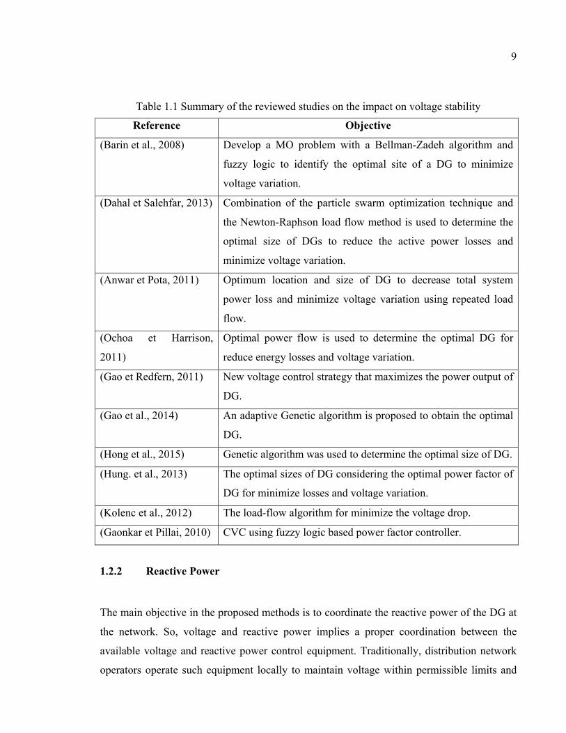
Table 1.1 Summary of the reviewed studies on the impact on voltage stability

Reference Objective

(Barin et al., 2008) Develop a MO problem with a Bellman-Zadeh algorithm and

fuzzy logic to identify the optimal site of a DG to minimize

voltage variation.

(Dahal et Salehfar, 2013) Combination of the particle swarm optimization technique and

the Newton-Raphson load flow method is used to determine the

optimal size of DGs to reduce the active power losses and

minimize voltage variation.

(Anwar et Pota, 2011) Optimum location and size of DG to decrease total system

power loss and minimize voltage variation using repeated load

flow.

(Ochoa et Harrison,

2011)

Optimal power flow is used to determine the optimal DG for

reduce energy losses and voltage variation.

(Gao et Redfern, 2011) New voltage control strategy that maximizes the power output of

DG.

(Gao et al., 2014) An adaptive Genetic algorithm is proposed to obtain the optimal

DG.

(Hong et al., 2015) Genetic algorithm was used to determine the optimal size of DG.

(Hung. et al., 2013) The optimal sizes of DG considering the optimal power factor of

DG for minimize losses and voltage variation.

(Kolenc et al., 2012) The load-flow algorithm for minimize the voltage drop.

(Gaonkar et Pillai, 2010) CVC using fuzzy logic based power factor controller.

1.2.2 Reactive Power

The main objective in the proposed methods is to coordinate the reactive power of the DG at

the network. So, voltage and reactive power implies a proper coordination between the

available voltage and reactive power control equipment. Traditionally, distribution network

operators operate such equipment locally to maintain voltage within permissible limits and

10

minimize reactive power losses (Ahmidi et al., 2012). In the operation stage, the distribution

network operators have different methods to coordinate the voltage and reactive power

control. Properly location and sizing shunt capacitors will decrease losses; the capacitor is

based on the load size (Vu et al., 1996). Voltage and reactive power control has been used to

evaluate the impact of DG inclusion in a distribution network (Duong et al., 2010; Ochoa et

Harrison, 2011). These indices play a critical role on renewable energy, power quality,

system stability and security. Authors in (Zhang. et al., 2015) have investigated the problem

of voltage and reactive power control as the economics operations, the roles of DGs in the

future retail electricity market.

To achieve a better voltage-VAr in distribution network an uncoordinated and coordinated

voltage control have been presented in (Viawan et Karlsson, 2008). The voltage and reactive

power control are operating locally in uncoordinated voltage control. The coordinated

voltage control (CVC) means that the voltage and reactive power control equipment will be

adjusted remotely and locally, based on wide area coordination, in order to obtain an

optimum voltage profile and reactive power with the presence of DGs. Similarly, (Richardot

et al., 2006) have demonstrated that DGs reduce the losses, the number of OLTC operations

and the voltage fluctuation in distribution network. The contribution of DGs as ancillary

services is significant with local control variable such as voltage regulation or power

reduction is presented in (Thong et al., 2007). In system contingencies (Chi et al., 2014;

Kojovic, 2002; Sheng et al., 2009a), the CVC in distribution network with DGs is presented

for enhancing the ability of fast and coordinated voltage and reactive power control.

Numerous studies use different objectives functions and operating constraints in voltage and

reactive power control. Authors in (Dehghani-Arani et Maddahi, 2013; Gao et al., 2014) still

consider losses minimization and keeping the voltages within permissible limits as the main

objectives and constraints in the voltage and reactive power control. Another objective is the

flattering the voltage on the pilot bus (Richardot et al., 2006). Other references, such as

(Anwar et Pota, 2011) consider the minimization of the reactive power losses as the main

objective.

11

Table 1.2 Summary of the reviewed studies on the impact on Reactive Power

Reference Method Used DGs

(Ahmidi et al., 2012) Probabilistic method Multiple

(Duong et al., 2010) Improving the analytical (IA) Four types

(Ochoa et Harrison, 2011) Optimal power flow Multiple

(Zhang. et al., 2015) Game theoretic Multiple

(Viawan et Karlsson, 2008) Coordinated voltage control Single

(Richardot et al., 2006) Genetic algorithm Multiple

(Kojovic, 2002) Alternative Transient Program Single

(Chi et al., 2014) Control strategy in DIgSILENT Single

(Dehghani-Arani et

Maddahi, 2013)

Pareto optimization Single

(Gao et al., 2014) Genetic algorithm Multi-type

(Anwar et Pota, 2011) Repeated load flow Single

1.2.3 Distribution Losses

The transmission and distribution networks have an estimated 8-10 percent total loss and

almost 70% of these losses occur in distribution network (Federico, Gonzalez et Lyra, 2005).

The optimal location and size of DGs can significantly reduce the losses in distribution

network. The DGs must be located at correct points on the network operated at the optimal

output real and reactive power levels (Abu-Mouti et El-Hawary, 2011). Authors in (Anwar et

Pota, 2011; Dahal et Salehfar, 2013; Hung et Mithulananthan, 2014; Sattarpour et al., 2015)

have demonstrated the reduction in power losses by optimally sizing and placing DGs in

distribution networks. A multi-objective function that includes minimizing the number of

DGs and power losses as well as maximizing voltage stability is presented in (Esmaili, 2013).

(Fu et al., 2015), the optimal allocation is formulated as a multi-objective function with

support vector machines to find the Pareto front consisting of a set of possible solutions for

loss reductions.

12

Introducing multi-objective function for minimizing voltage unbalanced factor and real

power loss, improving of voltage profile and increasing of economical profit is presented in

(Dehghani-Arani et Maddahi, 2013). (Hung et Mithulananthan, 2014) presents a new multi-

objective index to determine the optimal size and power factor of DG for reducing power

losses and enhancing loadability. The influence of DG on distribution line losses with respect

to voltage profile is presented in (Kolenc et al., 2012). The proposed model by (Li et al.,

2013) integrates costs, losses, and voltage index to achieve optimal size and site of DG in

distribution networks.

The problem of minimizing losses in distribution networks using fixed and variable DGs, and

the trade-off between energy losses and more generation is presented in (Ochoa et Harrison,

2011). (Young-Jin et al., 2013) proposes a method to decrease the number of switching

devices operations, as well as to reduce the power losses in distribution networks, while

maintaining the grid voltage within the allowed ranges.

Table 1.3 Summary of the reviewed studies on the impact on losses

Reference Method Used DGs

(Abu-Mouti et El-Hawary, 2011) Artificial bee colony Single

(Dahal et Salehfar, 2013) Particle Swarm Optimization and

Newton-Raphson

Single

(Hung et Mithulananthan, 2014) Exhaustive load flow Multiple

(Esmaili, 2013) Fuzzy logic Different type

(Fu et al., 2015) Adaptive reactive control Photovoltaic

(Dehghani-Arani et Maddahi,

2013)

Pareto optimization Single

(Kolenc et al., 2012) Load flow algorithm Multiple

(Li et al., 2013) Game theory Single

(Ochoa et Harrison, 2011) Optimal power flow Multiple

(Young-Jin et al., 2013) Dynamic programming algorithm Single

13

1.3 Optimization techniques

Several optimization techniques are used by researchers for an optimal integration of DGs in

distribution network. (Abu-Mouti et El-Hawary, 2011) presents an optimization approach

that employs an artificial bee colony algorithm to determine the optimal DG size, power

factor and location in order to minimize the real power loss. The appropriate selection and

the optimal DG location are determined using the fuzzy logic and the Bellman-Zadeh

algorithm in (Barin et al., 2008). (Ahmidi et al., 2012) use a multilevel control system, and a

probabilistic method is used to predict the available reactive power reserve. A repeated load

flow is used to find an appropriate size and location of DG to reduce significantly the total

power loss in distribution network (Anwar et Pota, 2011). A novel algorithm combining the

MO particle swarm optimization (MOPSO) with support vector machine is proposed to find

the optimal allocation of DG in distribution network (Fu et al., 2015). (Kiprakis et Wallace,

2004) analyze the implications of the DGs in distribution networks, they use a deterministic

system and fuzzy logic to adjust the power factor in response to the terminal voltage. (Li et

al., 2013; Zhang. et al., 2015) work with Game Theory and MO optimization problems that

allow minimizing total system power losses and maximizing voltage improvement. DGs can

reduce distribution losses if they are placed appropriately in distribution network with the

implementation method of tabu search as demonstrated in (Nara et al., 2001). In (Ochoa et

Harrison, 2011) a multi-period AC optimal power flow (OPF) is used to determine the

optimal accommodation of DGs in a way that minimizes the system energy losses.

All of the reviewed works have shown that with proper allocation of DGs, the reliability of

distribution system can be enhanced significantly while reducing the distribution network

losses and maintains voltage within permissible limits.

CHAPTER 2

BACKGROUND CONCEPTS 2.1 Introduction

This chapter presents the basic theoretical concepts used in this thesis. First, we present the

optimization techniques. Then, a brief description of Pareto and fuzzy logic is given.

Secondly, the OpenDSS program is analyzed. At this point, we explained how a distribution

network can be included in OpenDSS. Finally, we show how Simulink of Matlab and

OpenDSS work together.

2.2 Optimization Techniques

Optimization techniques play an important role in the success of DG integration activities.

Multi-Objective problems on distribution networks are usually handled in two ways. A

simple method is to convert the MO problem into a Single-objective (SO) problem by

constraint, weighting, or membership (Li et Qiu, 2015; Moradi et al., 2014). Although this

method has proven its effectiveness, it is difficult to describe or obtain precisely the weights

of different objectives. Another disadvantage is that the calculation procedure has to be

restarted when the weights are changed (Wu et al., 2011). Pareto optimization uses the

concept of non-dominated solutions. MO problem can be optimized simultaneously and a set

of optimum solutions is obtained using a decision maker. The MO problem can be

formulated as a non-linear model (Kumar, Samantaray et Kamwa, 2015). In this thesis, we

use Pareto optimization to resolve the MO problem.

2.2.1 Pareto Optimization

MO problem is different than single-objective (SO) problem as there is a vector of objective

functions (two or more), which must be optimized simultaneously and subject to a set of

equality and inequality constraints. To compare candidate solutions to the Multi-Objective

(MO) problem, the concepts of Pareto front and Pareto solutions are commonly used and can

16

be viewed as a simple baseline technique for MO optimization (Gatter et al., 2016). This

allows us to calculate a set of optimal solutions from the Pareto frontier. Thus, the set of

optimal solutions constitute an interesting trade-off (Ke-yan et al., 2015; Muller-Hannemann

et al., 2001).

2.2.1.1 Pareto Frontier

A multi-objective (MO) problem involves multiple objective functions. In mathematical

terms, a MO problem can be formulated as:

min( ( ), ( ), … , ( )) (2.1)

where k ≥ 2 is the number of objectives and x is the feasible set of decision vectors with

some constraint functions.

Figure 2.1 illustrates a simple case of minimizing two objectives simultaneously (F1, F2),

with the solid line indicating the Pareto frontier. Each point of the frontier represents a

unique model parameterization, so Pareto identifies multiple Pareto optimal solutions and all

solutions in a Pareto set are equally optimal. Point C is not on the Pareto Frontier because it

is dominated by both point A and point B. So, point C is a Dominated solution and the point

A and point B are Non-dominated solutions.

In this thesis, Matlab function (gamultiobj) finds the Pareto frontier of the objectives defined

subject to the linear inequalities constraints using genetic algorithm (MathWorks, 2014).

Genetic Algorithm is an evolutionary computing that emulates the biological process. A

population of individuals representing different solutions is evolving to find the optimal

solutions. The fittest individuals are chosen, mutation and crossover operations applied, thus

yielding a new generation (Ngatchou et al., 2005).

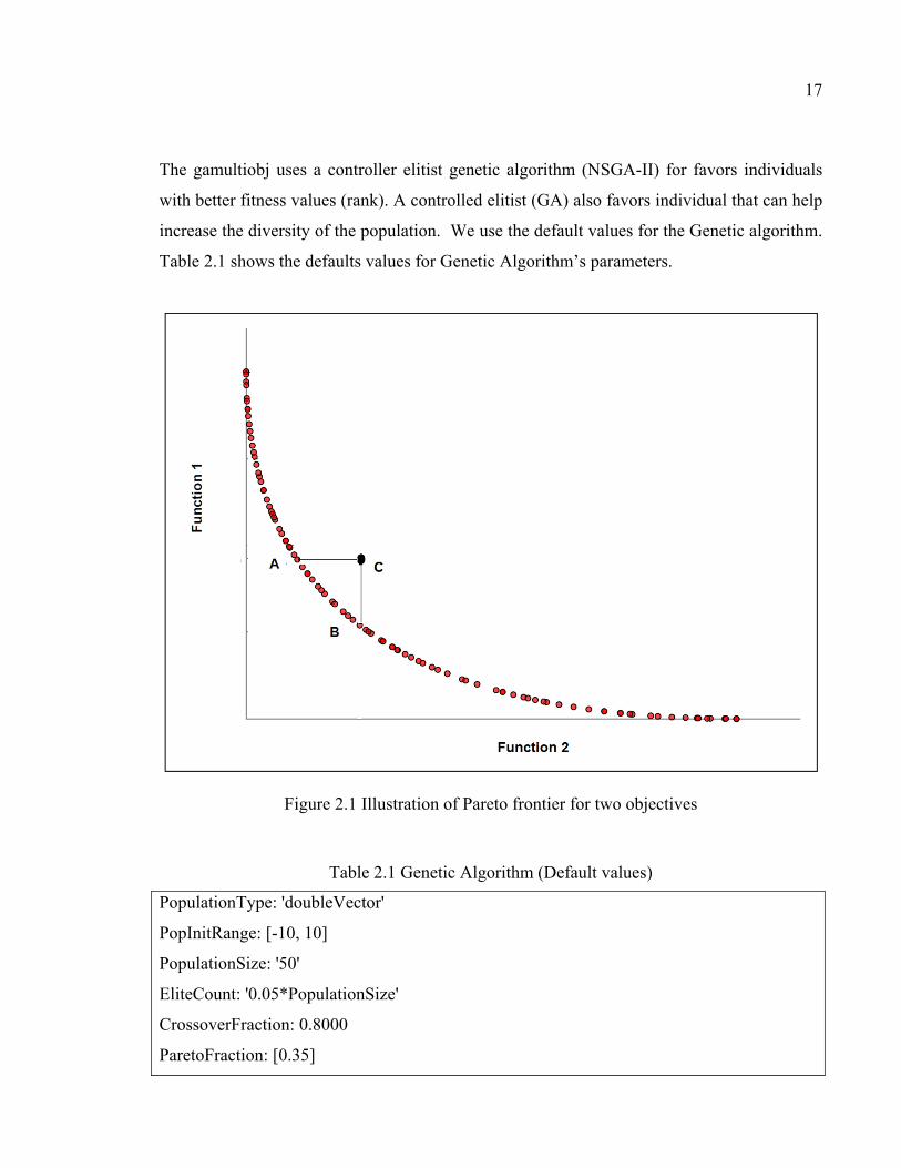
17

The gamultiobj uses a controller elitist genetic algorithm (NSGA-II) for favors individuals

with better fitness values (rank). A controlled elitist (GA) also favors individual that can help

increase the diversity of the population. We use the default values for the Genetic algorithm.

Table 2.1 shows the defaults values for Genetic Algorithm’s parameters.

Figure 2.1 Illustration of Pareto frontier for two objectives

Table 2.1 Genetic Algorithm (Default values)

PopulationType: 'doubleVector'

PopInitRange: [-10, 10]

PopulationSize: '50'

EliteCount: '0.05*PopulationSize'

CrossoverFraction: 0.8000

ParetoFraction: [0.35]

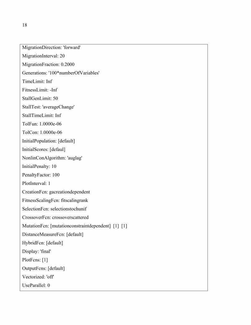
18

MigrationDirection: 'forward'

MigrationInterval: 20

MigrationFraction: 0.2000

Generations: '100*numberOfVariables'

TimeLimit: Inf

FitnessLimit: -Inf

StallGenLimit: 50

StallTest: 'averageChange'

StallTimeLimit: Inf

TolFun: 1.0000e-06

TolCon: 1.0000e-06

InitialPopulation: [default]

InitialScores: [defaul]

NonlinConAlgorithm: 'auglag'

InitialPenalty: 10

PenaltyFactor: 100

PlotInterval: 1

CreationFcn: gacreationdependent

FitnessScalingFcn: fitscalingrank

SelectionFcn: selectionstochunif

CrossoverFcn: crossoverscattered

MutationFcn: [mutationconstraintdependent] [1] [1]

DistanceMeasureFcn: [default]

HybridFcn: [default]

Display: 'final'

PlotFcns: [1]

OutputFcns: [default]

Vectorized: 'off'

UseParallel: 0

19

In terms of speed, Pareto seems to perform consistently well, despite being essentially a

simple algorithm. The primary reason for this is its ability to find multiple Pareto-optimal

solutions in one single simulation run (Knowles et Corne, 1999). Some researchers (Habibi et

al., 2013; Maciel et Padilha-Feltrin, 2009; Richardot et al., 2006; Soroudi et al., 2011) use

Pareto to minimize the MO problem and determine the optimal DGs size and location

minimizing the power losses. Many researchers use Pareto distribution networks to solve

optimization problems.

2.2.1.2 Decision Maker (DM)

The set of non-dominated solutions representing the Pareto frontier are optimal solutions.

DM finds the only optimal solution to this optimization problem. Hence, some additional

constraints are required to single out a solution. In this thesis, the objective is to minimize

losses and to maintain voltage within permissible limits. So, mathematically it can be

formulated as:

= (2.2)

= ∈−( − )

(2.3)

Equations (2.2 and 2.3) represent the DM used in the thesis. The set of solutions that

minimizes losses is chosen using Equation (2.2). Equation (2.3) chooses the set of optimal

solutions that minimizes a single objective of MO problem. In addition, the set of solutions

may be chosen developing equations to new DMs by applying different settings at the

decision stage, according to specific circumstances.

20

2.2.2 Fuzzy Logic

In recent years, the number and variety of applications of fuzzy logic have increased

significantly. Fuzzy logic is not a control strategy in itself, this is a method of combining

several control rules which may have conflicting objectives and arriving at a decision. Fuzzy

logic may be viewed as a methodology for computing with words rather than numbers.

Furthermore, computing with words exploits the tolerance for imprecision and thereby

lowers the cost of solutions (MathWorks, 2014). Fuzzy logic is a generalization in which the

true values of variables may be any real number between 0 and 1. Fuzzy logic is useful for

dealing with vagueness and ambiguity; this is based on the fuzzy sets theory, where

uncertainties are handled in a direct way without many realizations (Ni et al., 2016). In

distribution networks problems, the membership grades of fuzzy logic sets are uncertain

(Figueroa-Garcia et al., 2012). Advantages of the fuzzy logic are:

1. Rules can be described in natural language and easily translated into fuzzy logic

2. Many rules can be combined to produce complex behaviour.

In fuzzy logic, the calculus of fuzzy rules provides this mechanism. The inputs and outputs

parameters of the system are “somehow” related (Loetamonphong et al., 2002; Takagi et

Sugeno, 1985). The authors (Esmaili, 2013; Gaonkar et Pillai, 2010; Ghatee et Hashemi,

2009) propose Fuzzy logic for optimal placement and sizing of DGs.

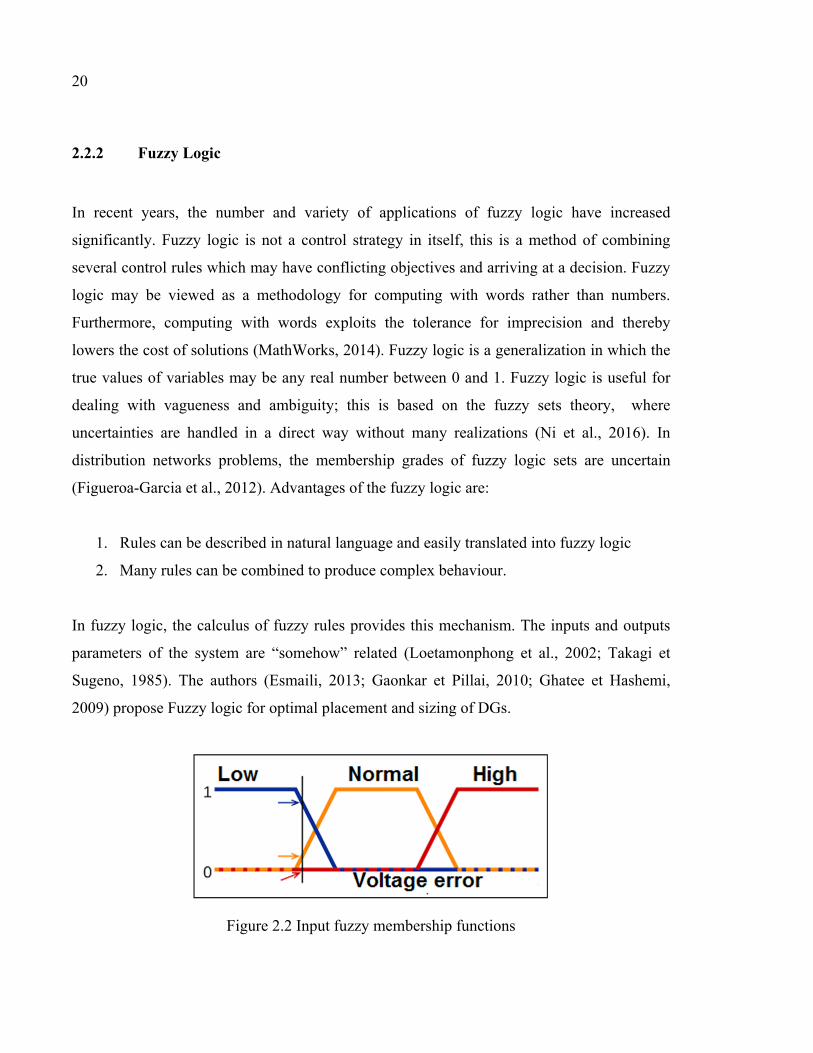
Figure 2.2 Input fuzzy membership functions

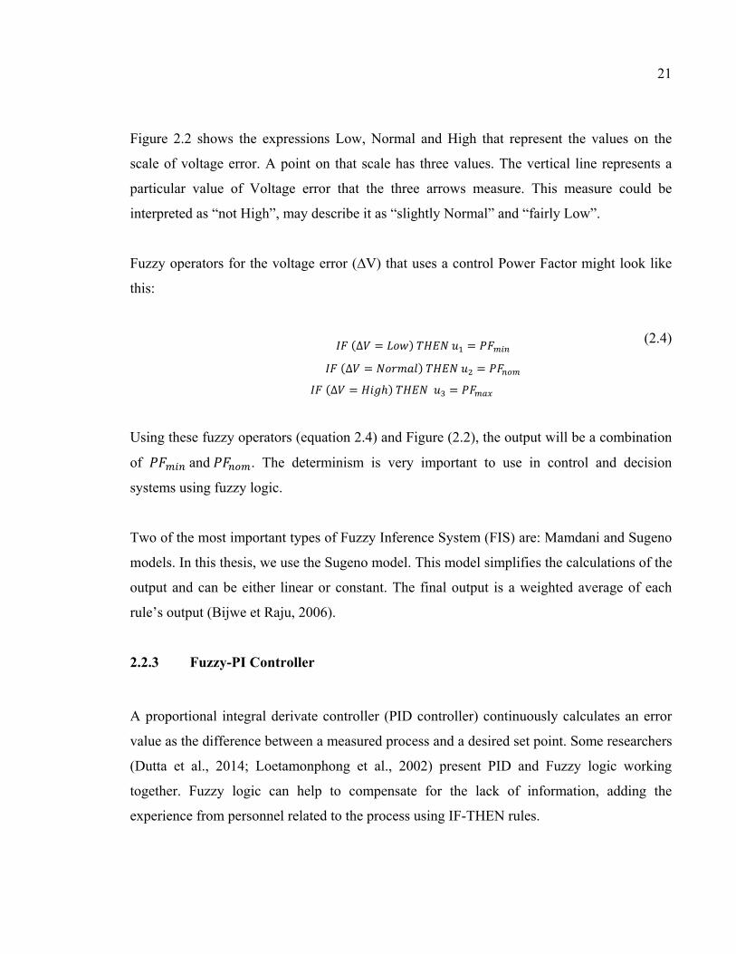
21

Figure 2.2 shows the expressions Low, Normal and High that represent the values on the

scale of voltage error. A point on that scale has three values. The vertical line represents a

particular value of Voltage error that the three arrows measure. This measure could be

interpreted as “not High”, may describe it as “slightly Normal” and “fairly Low”.

Fuzzy operators for the voltage error (∆V) that uses a control Power Factor might look like

this:

(∆ = ) = (∆ = ) = (∆ = ℎ) =

(2.4)

Using these fuzzy operators (equation 2.4) and Figure (2.2), the output will be a combination

of and . The determinism is very important to use in control and decision

systems using fuzzy logic.

Two of the most important types of Fuzzy Inference System (FIS) are: Mamdani and Sugeno

models. In this thesis, we use the Sugeno model. This model simplifies the calculations of the

output and can be either linear or constant. The final output is a weighted average of each

rule’s output (Bijwe et Raju, 2006).

2.2.3 Fuzzy-PI Controller

A proportional integral derivate controller (PID controller) continuously calculates an error

value as the difference between a measured process and a desired set point. Some researchers

(Dutta et al., 2014; Loetamonphong et al., 2002) present PID and Fuzzy logic working

together. Fuzzy logic can help to compensate for the lack of information, adding the

experience from personnel related to the process using IF-THEN rules.

22

A proportional integral (PI) is a special case of the classical PID controller. A PI controller is

a controller that produces proportional plus integral control action. A fuzzy-PI controller is a

generalization of the conventional PI controller that uses an error signal and its derivative as

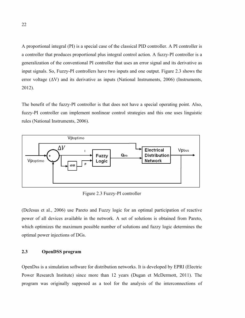
input signals. So, Fuzzy-PI controllers have two inputs and one output. Figure 2.3 shows the

error voltage (ΔV) and its derivative as inputs (National Instruments, 2006) (Instruments,

2012).

The benefit of the fuzzy-PI controller is that does not have a special operating point. Also,

fuzzy-PI controller can implement nonlinear control strategies and this one uses linguistic

rules (National Instruments, 2006).

Figure 2.3 Fuzzy-PI controller

(DeJesus et al., 2006) use Pareto and Fuzzy logic for an optimal participation of reactive

power of all devices available in the network. A set of solutions is obtained from Pareto,

which optimizes the maximum possible number of solutions and fuzzy logic determines the

optimal power injections of DGs.

2.3 OpenDSS program

OpenDss is a simulation software for distribution networks. It is developed by EPRI (Electric

Power Research Institute) since more than 12 years (Dugan et McDermott, 2011). The

program was originally supposed as a tool for the analysis of the interconnections of

23

distributed generation, but its continued evolution has led to the development of the other

features as the studies of efficiency in the provision of energy and harmonic studies.

2.3.1 OPenDSS structure

OpenDSS software has been used to:

• planning and analysis of distribution networks;

• poly-phase AC circuit analysis;

• analysis of interconnection of distributed generation;

• simulations windmills plant;

• improving distribution network efficiency;

• studies of harmonics and inter harmonics.

The program includes several modes of solutions, such as:

• power flow (snapshot mode, time mode);

• harmonic Analysis;

• dynamic Analysis;

• calculation shorted.

OpenDss is designed to receive instructions in text form allowing greater flexibility for users.

Figure 2.4 (Dugan et McDermott, 2011) shows how the various modules interact within

OpenDSS structure.

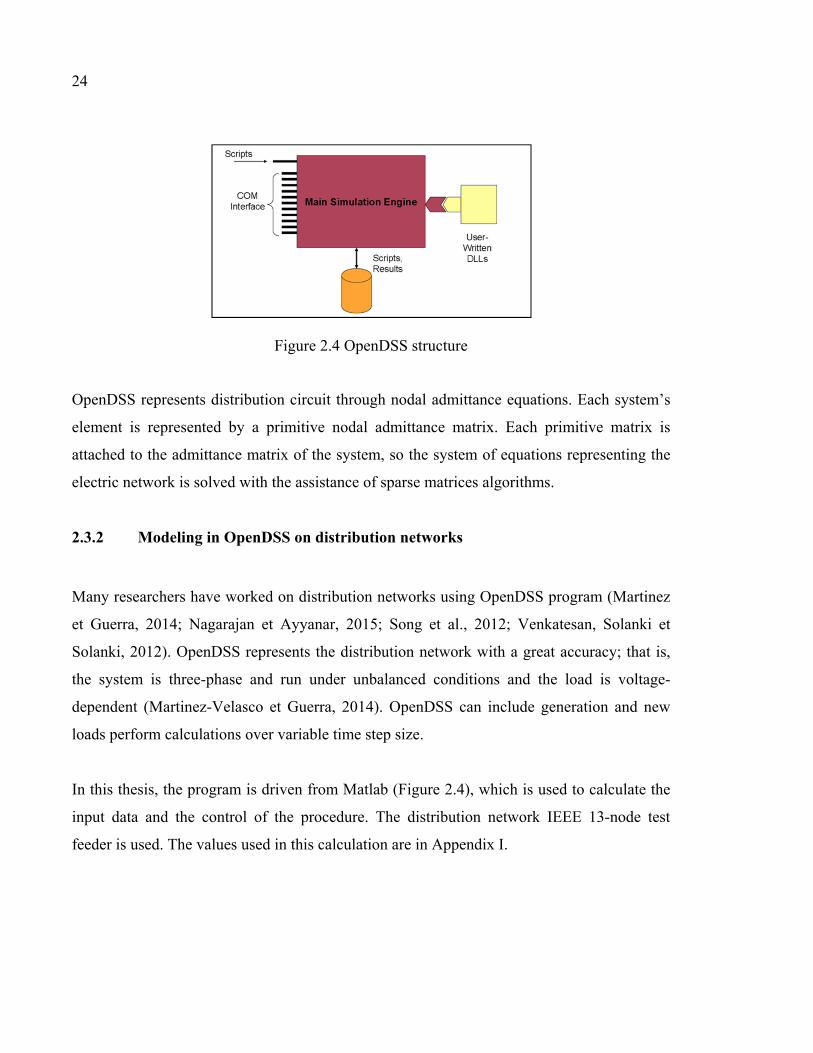
24

Figure 2.4 OpenDSS structure

OpenDSS represents distribution circuit through nodal admittance equations. Each system’s

element is represented by a primitive nodal admittance matrix. Each primitive matrix is

attached to the admittance matrix of the system, so the system of equations representing the

electric network is solved with the assistance of sparse matrices algorithms.

2.3.2 Modeling in OpenDSS on distribution networks

Many researchers have worked on distribution networks using OpenDSS program (Martinez

et Guerra, 2014; Nagarajan et Ayyanar, 2015; Song et al., 2012; Venkatesan, Solanki et

Solanki, 2012). OpenDSS represents the distribution network with a great accuracy; that is,

the system is three-phase and run under unbalanced conditions and the load is voltage-

dependent (Martinez-Velasco et Guerra, 2014). OpenDSS can include generation and new

loads perform calculations over variable time step size.

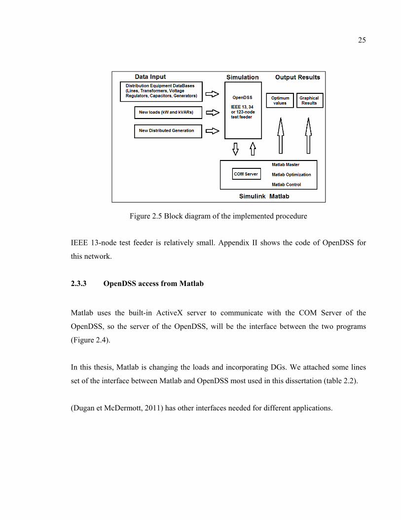
In this thesis, the program is driven from Matlab (Figure 2.4), which is used to calculate the

input data and the control of the procedure. The distribution network IEEE 13-node test

feeder is used. The values used in this calculation are in Appendix I.

25

Figure 2.5 Block diagram of the implemented procedure

IEEE 13-node test feeder is relatively small. Appendix II shows the code of OpenDSS for

this network.

2.3.3 OpenDSS access from Matlab

Matlab uses the built-in ActiveX server to communicate with the COM Server of the

OpenDSS, so the server of the OpenDSS, will be the interface between the two programs

(Figure 2.4).

In this thesis, Matlab is changing the loads and incorporating DGs. We attached some lines

set of the interface between Matlab and OpenDSS most used in this dissertation (table 2.2).

(Dugan et McDermott, 2011) has other interfaces needed for different applications.

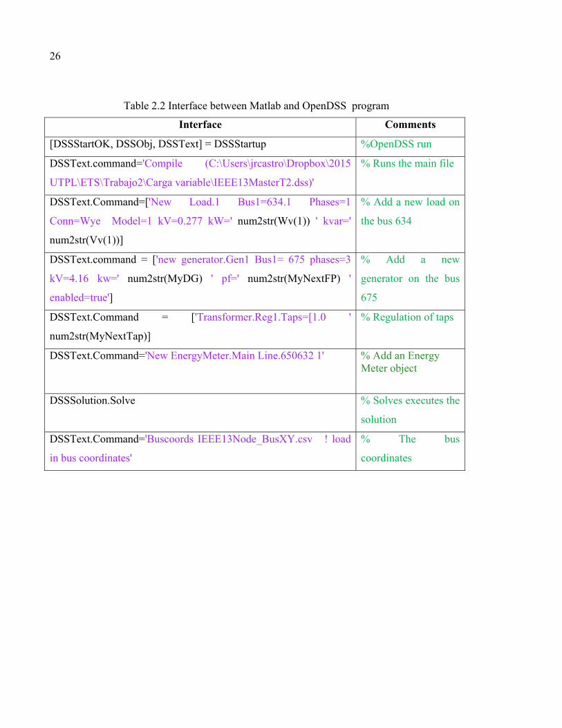
26

Table 2.2 Interface between Matlab and OpenDSS program

Interface Comments

[DSSStartOK, DSSObj, DSSText] = DSSStartup %OpenDSS run

DSSText.command='Compile (C:\Users\jrcastro\Dropbox\2015

UTPL\ETS\Trabajo2\Carga variable\IEEE13MasterT2.dss)'

% Runs the main file

DSSText.Command=['New Load.1 Bus1=634.1 Phases=1

Conn=Wye Model=1 kV=0.277 kW=' num2str(Wv(1)) ' kvar='

num2str(Vv(1))]

% Add a new load on

the bus 634

DSSText.command = ['new generator.Gen1 Bus1= 675 phases=3

kV=4.16 kw=' num2str(MyDG) ' pf=' num2str(MyNextFP) '

enabled=true']

% Add a new

generator on the bus

675

DSSText.Command = ['Transformer.Reg1.Taps=[1.0 '

num2str(MyNextTap)]

% Regulation of taps

DSSText.Command='New EnergyMeter.Main Line.650632 1' % Add an Energy Meter object

DSSSolution.Solve % Solves executes the

solution

DSSText.Command='Buscoords IEEE13Node_BusXY.csv ! load

in bus coordinates'

% The bus

coordinates

CHAPTER 3

OPTIMAL VOLTAGE CONTROL IN DISTRIBUTION NETWORK IN THE PRESENCE OF DGs.

Jose Raul Castro 1, 2, Maarouf Saad 2, Serge Lefebvre 3, Dalal Asber 3, Laurent Lenoir 3

1 Universidad Técnica Particular de Loja, Loja, Ecuador 2 Department of Electrical Engineering, École de Technologie Supériure,

1100 Notre-Dame St. West, Montreal, Quebec, Canada H3C1K3 3 Hydro-Québec’s Research Institute, Varennes, Québec, Canada J3X1S3

This paper has been published in Electrical Power and Energy System Volume 78, January 2016, pages 239-247

Abstract

Nowadays, integration of new devices like Distributed Generation, small energy storage and

smart meter, to distribution networks introduced new challenges that require more

sophisticated control strategies. This paper proposes a new technique called Optimal

Coordinated Voltage Control (OCVC) to solve a multi-objective optimization problem with

the objective to minimize the voltage error at pilot buses, the reactive power deviation and

the voltage error at the generators. OCVC uses Pareto optimization to find the optimal values

of voltage of the generators and OLTC. It proposes an optimal participation of reactive

power of all devices available in the network.

OCVC is compared with the classical method of Coordinated Voltage Control and is tested

on the IEEE 13 and 34 Node test feeders with unbalanced load. Some disturbances are

investigated and the results show the effectiveness of the proposed technique.

28

Keywords: distribution network; Coordinated Voltage Control (CVC); Distributed

Generation (DG); Multi-Objective Optimization; Power Loss; On Load Tap Changer

(OLTC).

3.1 Introduction

The climate changes and the new technologies have led to major changes in electricity

generation and consumption patterns. The equipment connected to the distribution network is

becoming more diversified including renewable energy that is known as Distributed

Generation (DG), small energy storage, and smart meter. It consequently requires more

advanced algorithms for voltage and VAR control.

The DGs may trigger variation of voltage and change the direction of power flow in the

distribution network. The voltage rise depends on the amount of active and reactive power

injected by the DGs. Some researches (Ahmidi et al., 2012; Anwar et Pota, 2011; Habibi et

al., 2013) have studied the impact on the voltage, the reduction of losses, and the

determination the optimum size and location of the DGs. Also, improper DG size and

inappropriate location may cause high power loss and problems in the voltage profile (Anwar

et Pota, 2011; Kiprakis et Wallace, 2004; Maciel et Padilha-Feltrin, 2009).

Other researches (Sheng et al., 2009a; Vu et al., 1996) represent the variation voltage in each

control area by the variations at some selected buses called “pilot buses”. Then, the aim is to

keep the voltages at pilot buses within a fixed range around set point values.

On the other hand, it is common to use the on-load tap-changer (OLTC) and switch shunt

capacitors to control voltage in distributed network (Larsson et Karlsson, 2003). In some

networks, these devices are operated locally without wide coordination with the others. In

(Biserica et al., 2011; Richardot et al., 2006), the authors presents an approach using the DGs

and OLTCs for voltage regulation and losses reduction.

29

Coordinated Voltage Control (CVC) in distribution network adjusts the voltage in pilot

buses. CVC uses the multi-objective (MO) function to minimize the voltage variation at the

pilot buses(Richardot et al., 2006). CVC in distribution networks adjusts the voltage on pilot

buses located in the controlled area. To do so, it minimizes the MO optimization problem

using a deterministic method. So, the problem to solve is to minimize the following

objectives (Biserica et al., 2011; Richardot et al., 2006): Objective 1: voltage deviation at

pilot buses; Objective 2: reactive power production ratio deviation; and Objective 3:

generators voltage deviation (OLTC + DGs).

In (Viawan et Karlsson, 2008), the authors have made a comparison in distribution networks,

between uncoordinated and coordinated voltage control, without and with DGs involved in

the voltage control. The result indicates that using DG in the voltage control will reduce the

losses, the number of OLTC operations and will decrease the voltage fluctuation in

distribution network.

The authors in (Ngatchou et al., 2005; Richardot et al., 2006; Soroudi et al., 2011) solve the

MO function converting the objectives into a single objective (SO) function; in this case, the

objective is to find the solution that minimizes the single objective. The optimization solution

results in a single value that represents a compromise among all the objectives.

Previous researches adequately solved the problem of MO function using DG in distribution

network. There is no research that is able to adequately coordinate the different areas of the

distribution network and focus on the benefits that a better use of reactive power of DG can

provide to the distribution systems with unbalanced load.

To overcome the problem cited above, this paper proposes a new technique called optimal

coordinated voltage control (OCVC). OCVC is capable of coordinating different areas of the

distribution network including all sources of active and reactive power present in the

distribution network. OCVC uses Pareto optimization to solve all the different objectives of

the Multi-Objective function separately and finds the optimal values so that the network gets

30

lower losses. OCVC will also have a good performance with various disturbances that occur

in the distribution network.

The original contributions of this paper are described as follows:

a) disturbances in distribution network are investigated;

b) optimal participation of reactive power of a DG at unbalanced distribution network; c) the minimization of the losses;

d) the objectives of the MO function are resolved separately.

This paper is organized as follows. Section 3.2 presents the coordinated voltage control in

distribution network. The Pareto Multi-Objective optimization is explained in section 3.3.

The proposed approach on optimal coordinated voltage control is explained in section 3.4.

Section 3.5 presents a case study and some results using the proposed approach. Finally, a

conclusion is given in section 3.6.

3.2 Coordinated Voltage Control in Distribution Network

Nowadays, a hierarchical voltage regulation strategy with three levels has been developed by

some electric utilities to prevent voltage deterioration and to allow a better use of existing

reactive power resources. Each level acts with a different time constant: Primary voltage

control (PVC) is locally performed by automatic voltage regulators (AVR), secondary

voltage control (SVC) makes reactive power production-consumption balance and tertiary

voltage control (TVC) is based on optimization methods taking into account economical and

technical aspects of power system operation (Richardot et al., 2006).

SVC is an important level for improving power-system voltage dynamic performance, where

voltage deviation at pilot buses is minimized. This problem can be generalized to integrate

voltage deviation at generators and reactive power generation. In this case, we talk about

Coordinated Voltage Control (CVC) (Richardot et al., 2006).

31

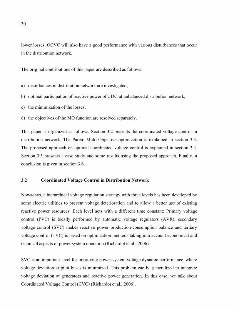
3.2.1 Problem formulation

The voltage in a distribution network at some selected buses (pilot buses), the reactive power

production and the generator’s voltage deviation are tied together. Any increase or decrease

in voltage at pilot buses will increase or decrease the reactive power production and

generator voltage respectively. Therefore, this problem can be formulated as an optimization

problem as explained below:

3.2.1.1 Voltage at pilot bus

CVC in distribution networks adjust the voltage at pilot buses. In a mathematical form, the

problem can be written as follows:

F = λ∈ κ V − V − C , · ∆V∈ (3.1)

Where: P and G are the sets of pilot and generator buses indices; V , V and ∆V are set-

point voltage, actual voltage and voltage deviation at bus i, i.e. the difference of voltage

values between two computing steps; C , is the sensitivity matrix coefficient linking the

voltage variation at bus i and bus k respectively; λ and are weighting factor and regulator

gain respectively.

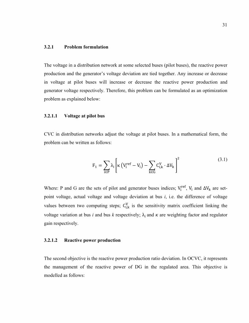
3.2.1.2 Reactive power production

The second objective is the reactive power production ratio deviation. In OCVC, it represents

the management of the reactive power of DG in the regulated area. This objective is

modelled as follows:

32

F = λ κ q − QQ − C , · ∆V∈ (3.2)

Where: is the set of generator buses indices; Q and Q are actual and maximum reactive

power generations at bus i; q = ∑ Q /∑ Q∈∈ is the uniform set-point reactive

power value within the regulated area; C , is sensitivity matrix coefficients linking

respectively voltage variation at bus i and bus k; λ andκ are weighting factor and regulator

gain respectively.

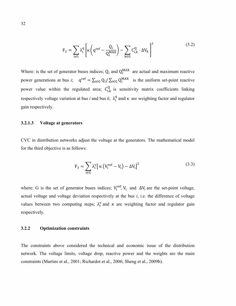
3.2.1.3 Voltage at generators

CVC in distribution networks adjust the voltage at the generators. The mathematical model

for the third objective is as follows:

F = λ κ V − V − ΔV∈ (3.3)

where: G is the set of generator buses indices; V , V and ∆V are the set-point voltage,

actual voltage and voltage deviation respectively at the bus i, i.e. the difference of voltage

values between two computing steps; λ and are weighting factor and regulator gain

respectively.

3.2.2 Optimization constraints

The constraints above considered the technical and economic issue of the distribution

network. The voltage limits, voltage drop, reactive power and the weights are the main

constraints (Martins et al., 2001; Richardot et al., 2006; Sheng et al., 2009b).

33

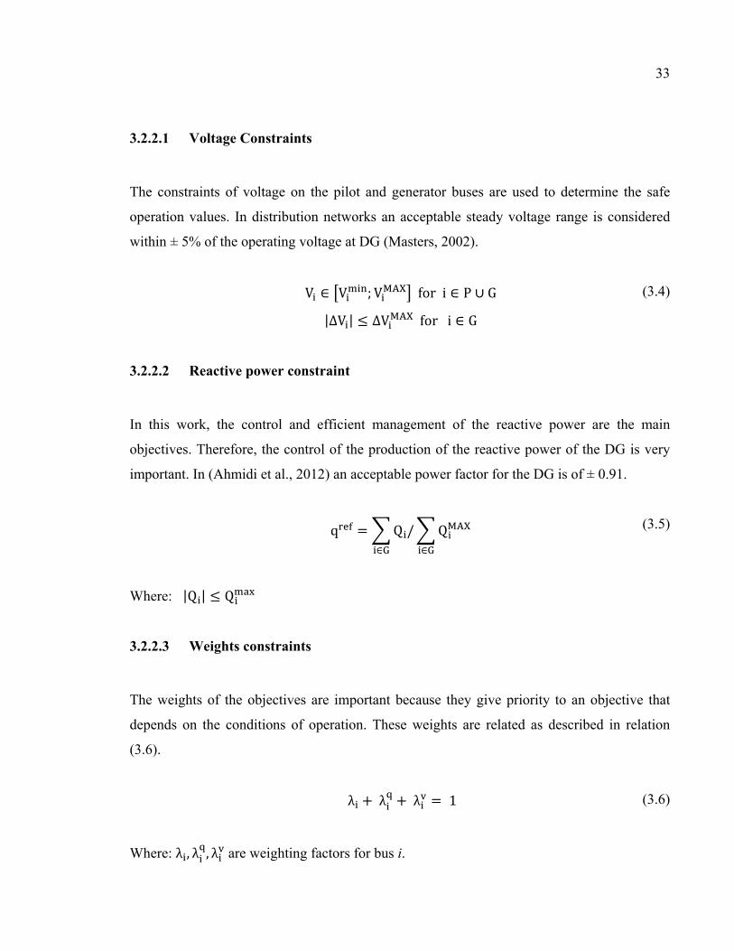
3.2.2.1 Voltage Constraints

The constraints of voltage on the pilot and generator buses are used to determine the safe

operation values. In distribution networks an acceptable steady voltage range is considered

within ± 5% of the operating voltage at DG (Masters, 2002).

V ∈ V ; V for i ∈ P ∪ G |∆V | ≤ ∆V for i ∈ G

(3.4)

3.2.2.2 Reactive power constraint

In this work, the control and efficient management of the reactive power are the main

objectives. Therefore, the control of the production of the reactive power of the DG is very

important. In (Ahmidi et al., 2012) an acceptable power factor for the DG is of ± 0.91.

q = Q / Q∈∈ (3.5)

Where: |Q | ≤ Q

3.2.2.3 Weights constraints

The weights of the objectives are important because they give priority to an objective that

depends on the conditions of operation. These weights are related as described in relation

(3.6).

λ + λ + λ = 1 (3.6)

Where: λ , λ , λ are weighting factors for bus i.

34

The optimization problem (3.1) to (3.6) ensures an optimal voltage profile of the distribution

network. The optimization solution results in a single value that reflects a compromise in all

objectives (Abido, 2004).

The weighting factors are managed in real time using fixed values depending on the voltage

value at the pilot bus. They coordinate the different areas of the distribution network to

obtain the optimal values of the voltage and reactive power.

3.2.3 Pilot Bus

Monitoring and the control of the voltage level at the pilot bus allow the control of the

voltage in that area. Then, the voltage at the pilot bus must reflect the voltage profile of the

entire control area (Conejo et al., 1994; Erbasu et al., 2005).

A simple method called barycentre to find the pilot bus is illustrated below. This method

requires the following three steps.

Step1: Compute V = ∑ V

Step2: Find ∆V = V − V

Step3: Choose the bus number with min |∆V | as the pilot bus.

In this paper, this method is used. The networks (IEEE 13 and 34 Nodes) used in this work,

have loads in some buses. If we put out sequentially these loads, we will produce N

variations of the voltage at the buses. If we sum up these N variations of the voltage, we will

get Vbar. The next step is to obtain ΔVi. Finally, we choose the minimum value of the pilot

bus has the corresponding index i. Table 3.1 shows the pilot bus selected.

35

Table 3.1 Pilot bus for IEEE 13 and IEEE 34 buses

IEEE 13 IEEE 34

Pilot bus Bus 671 Bus 888

3.2.4 The On-load taps Changer (OLTC)

OLTC are normally located in the transformer between transmission and distribution network

and they are quite common to maintain the voltage in medium voltage network (Leisse et al.,

2010). Normally, the highest voltage point of the network is the sending-end bus bar and the

voltage is decreased along the feeder due to line impedance and loads. The typical

mathematical model of the voltage drop is as follows (Gao et Redfern, 2011):

∆ = − +

(3.7)

Where , are the active and reactive power of load; , are respectively the line

resistance and reactance; , are the sending-end voltage and load bus voltage

respectively.

Due to the structure and properties of the distribution networks the most effective way of

regulating the voltage is OLTC. The OLTC changes the voltage by alternating the turns ratio

of the primary side and secondary transformers. When a DG is connected to the distribution

network, the voltage drop is approximated as follows (Gao et Redfern, 2011):

∆ = − ( − ) + ( − ( ))

(3.8)

Where and are the active and reactive power of DG.

36

The extent of voltage regulation (ΔV) is limited by the number of positions and the step size

between positions. In (Kersting, 2001) the characteristics of our OLTCs are displayed.

3.3 Pareto Optimization

Conversion of the multi-objective function into a single-objective function has several

limitations (Abido, 2004; Ngatchou et al., 2005):

1) it takes a priori knowledge of the objectives;

2) single-objective function leads to only one solution;

3) trade-offs between objectives cannot be easily evaluated; 4) the solution may not be obtained unless the search space is convex.

Pareto optimization solves the problem of multi-objective functions separately. It aims to

find and to compare the set of acceptable solutions and present them to the decision maker

(DM) who will choose among them the final solution (Figure 3.1). Nowadays and due to the

computational advances, it is possible to use techniques based on metaheuristic algorithms to

determine the Pareto frontier by optimizing all the objectives separately(Smith, 2002). These

methods include genetic algorithms (GA), evolutionary algorithms (EA) and evolutionary

strategies (ES) which only differ in the way the fitness selection, mutation and crossover

operations are performed.

In this work, we use Matlab (gamultiobj function) to find minimum of multiple functions

using genetic algorithm and obtain the Pareto frontier. For each set of solutions, Decision

Maker (DM) calculates the minimum of the sum of the three objectives (minimum of losses);

the set of solutions that have the minimum is selected (Dehghani-Arani et Maddahi, 2013).

= (3.9)

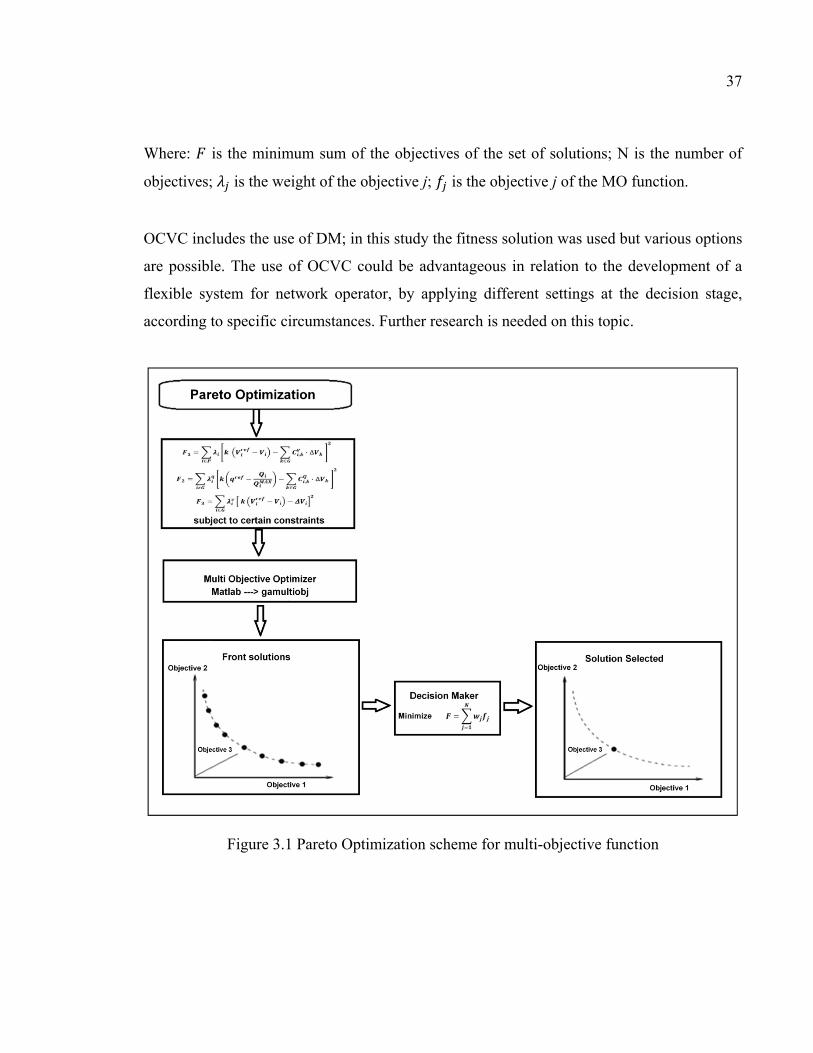
37

Where: is the minimum sum of the objectives of the set of solutions; N is the number of

objectives; is the weight of the objective j; is the objective j of the MO function.

OCVC includes the use of DM; in this study the fitness solution was used but various options

are possible. The use of OCVC could be advantageous in relation to the development of a

flexible system for network operator, by applying different settings at the decision stage,

according to specific circumstances. Further research is needed on this topic.

Figure 3.1 Pareto Optimization scheme for multi-objective function

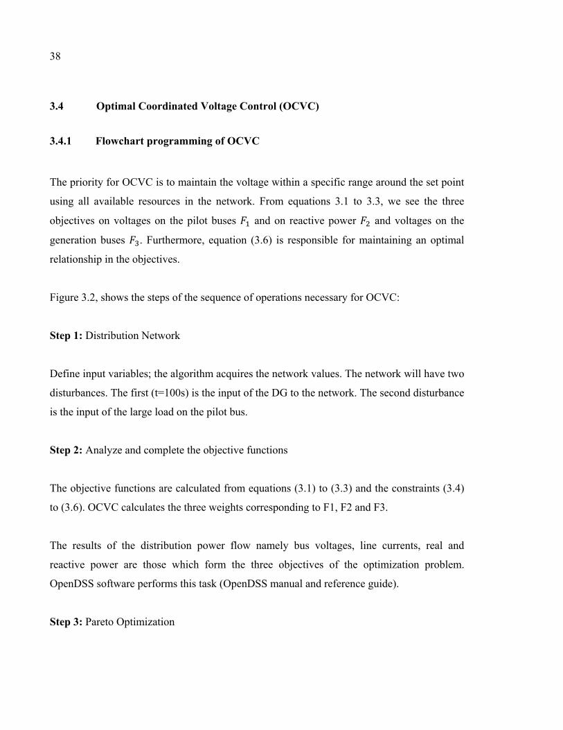
38

3.4 Optimal Coordinated Voltage Control (OCVC)

3.4.1 Flowchart programming of OCVC

The priority for OCVC is to maintain the voltage within a specific range around the set point

using all available resources in the network. From equations 3.1 to 3.3, we see the three

objectives on voltages on the pilot buses and on reactive power and voltages on the

generation buses . Furthermore, equation (3.6) is responsible for maintaining an optimal

relationship in the objectives.

Figure 3.2, shows the steps of the sequence of operations necessary for OCVC:

Step 1: Distribution Network

Define input variables; the algorithm acquires the network values. The network will have two

disturbances. The first (t=100s) is the input of the DG to the network. The second disturbance

is the input of the large load on the pilot bus.

Step 2: Analyze and complete the objective functions

The objective functions are calculated from equations (3.1) to (3.3) and the constraints (3.4)

to (3.6). OCVC calculates the three weights corresponding to F1, F2 and F3.

The results of the distribution power flow namely bus voltages, line currents, real and

reactive power are those which form the three objectives of the optimization problem.

OpenDSS software performs this task (OpenDSS manual and reference guide).

Step 3: Pareto Optimization

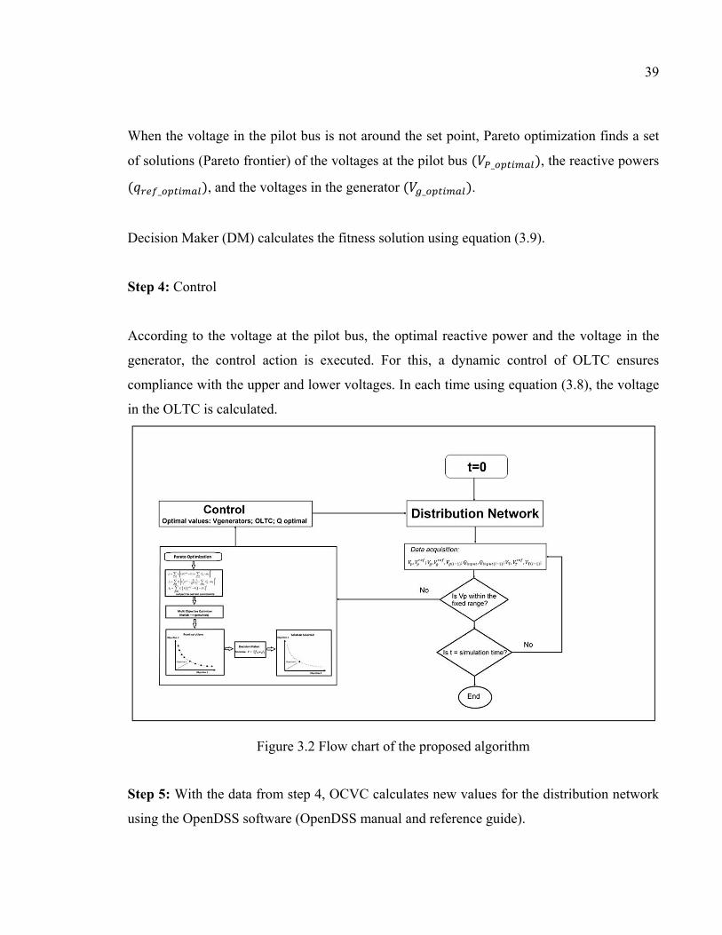
39

When the voltage in the pilot bus is not around the set point, Pareto optimization finds a set

of solutions (Pareto frontier) of the voltages at the pilot bus ( _ ), the reactive powers ( _ ), and the voltages in the generator ( _ ).

Decision Maker (DM) calculates the fitness solution using equation (3.9).

Step 4: Control

According to the voltage at the pilot bus, the optimal reactive power and the voltage in the

generator, the control action is executed. For this, a dynamic control of OLTC ensures

compliance with the upper and lower voltages. In each time using equation (3.8), the voltage

in the OLTC is calculated.

Figure 3.2 Flow chart of the proposed algorithm

Step 5: With the data from step 4, OCVC calculates new values for the distribution network

using the OpenDSS software (OpenDSS manual and reference guide).

40

Step 6: If the voltage values at the pilot bus is within the limits go to 7, if not, return to step1.

Step 7: If the time reaches the limit of simulation go to 8, if not, return to step 2.

Step 8: End.

In OCVC, the three objectives are always competing. When the voltage in pilot bus is within

the fixed range, the objective 1 decreases its value. Therefore, the objective 2 (reactive

power) becomes more important. The weights are related to the optimization process and will

be responsible to maintain this priority.

Conversely, when the voltage in pilot bus is outside the acceptable range, objective 1 and

objective 3 increase the value and become the most important objectives. In this case, OCVC

optimizes the voltage of the generators and OLTC available on the network.

When the voltage begins to be within the limits defined, OCVC changes the priority. The

new objective is to reduce the losses. OCVC has the advantage of using all the available

sources of reactive power in the network and calculates the optimum value and reduce the

losses, so λ increases its value in MO function.

The difference between the methods (CVC) proposed by (Biserica et al., 2011; Richardot et

al., 2006) and the proposed method is that OCVC solves all the different objectives of the

optimization problem separately and that OCVC changes the weights all the time to achieve

the objectives of the minimization of losses and maximization of all the reactive power

sources.

3.5 Case study

Our analysis method has been implemented on two IEEE distribution test systems with

unbalanced load. These are IEEE 13 node test feeder and 34 node test feeder. The first one,

41

IEEE 13 node test feeder is small but good for test case. The second one, IEEE 34 node test

feeder is an actual feeder located in Arizona (IEEE.org).

3.5.1 Implementation

OCVC was coded in Simulink of Matlab (R2014a) and OpenDSS (64 bits) software.

Simulations carried out on a PC (Intel Core i7 2.9 GHz, 8 GB RAM) were delivered in

around 30 s for the IEEE 13 Node, 50 to 60 s for the IEEE 34 Node Test Feeder.

The OpenDSS is an electrical power Distribution System Simulator (DSS) for supporting

distributed resource integration and grid modernization efforts (OpenDSS manual and

reference guide). It can solve a very large distribution system in a very small CPU time. In

addition, it is freely distributed by EPRI.

3.5.2 IEEE 13 Node Test Feeder

The diagram of the IEEE 13 node test feeder used as a test system is given in figure 3.3. It

corresponds to a simple primary distribution system. The values obtained for the voltages,

currents, and power flows are very accurate compared with the values reported by the IEEE

Distribution system analysis subcommittee (IEEE.org). The network has an OLTC.

The work performed by Anwar (Anwar et Pota, 2011) determines the appropriate size and

proper allocation of the DG to reduce electric power losses. Then, one DG of 1200 kW in

the 675 bus has been added in the network.

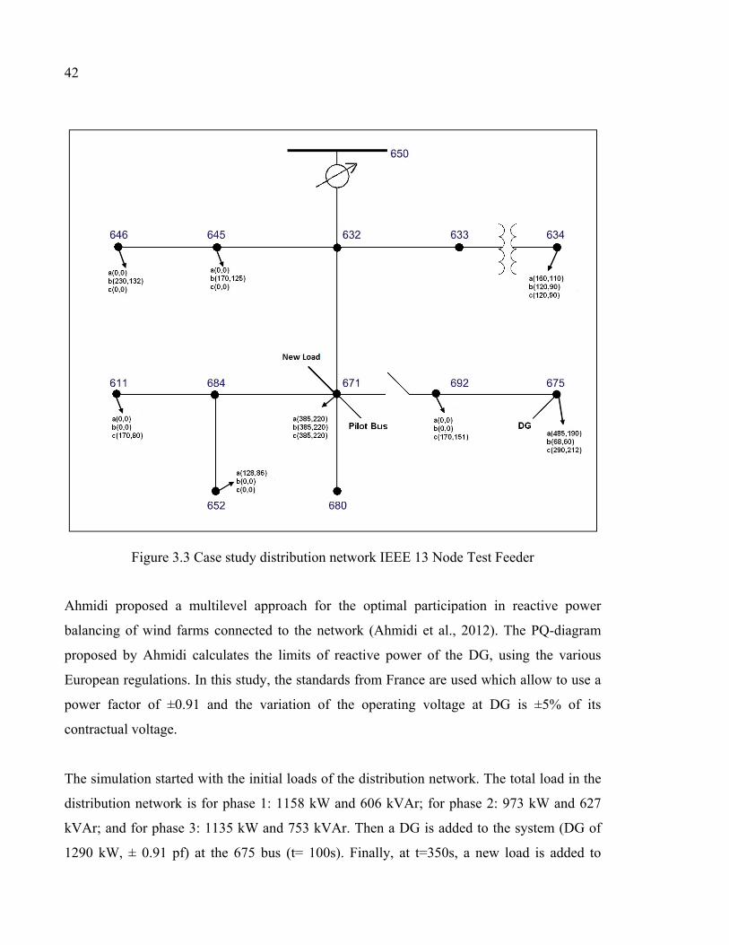
42

Figure 3.3 Case study distribution network IEEE 13 Node Test Feeder

Ahmidi proposed a multilevel approach for the optimal participation in reactive power

balancing of wind farms connected to the network (Ahmidi et al., 2012). The PQ-diagram

proposed by Ahmidi calculates the limits of reactive power of the DG, using the various

European regulations. In this study, the standards from France are used which allow to use a

power factor of ±0.91 and the variation of the operating voltage at DG is ±5% of its

contractual voltage.

The simulation started with the initial loads of the distribution network. The total load in the

distribution network is for phase 1: 1158 kW and 606 kVAr; for phase 2: 973 kW and 627

kVAr; and for phase 3: 1135 kW and 753 kVAr. Then a DG is added to the system (DG of

1290 kW, ± 0.91 pf) at the 675 bus (t= 100s). Finally, at t=350s, a new load is added to

43

simulate a disturbance (New three phase balanced load in the 671 bus of 1200 kW and 800

kVAr). The simulation lasts 500 seconds.

3.5.2.1 OLTC: reference case

In this case, the only equipment used for the voltage control is the OLTC. This is the typical

case of a distribution network currently. The DG and the new load in the network may appear

like an overvoltage which OLTC will correct. The reactive power injected from the DG is

zero in this case. Furthermore, the DG does not participate in the regulation of the voltage.

3.5.2.2 Coordination Voltage Control (Fixed weight)

The OLTC and DG are considered to control the voltage. In CVC, the weights factor of the

MO function response to voltage deviation at the pilot bus.

When the pilot bus voltage is within the limits, the reactive power control is the priority. So,

the weight factors are: λ = 0.3;λ = 0.6λ = 0.1 . If the voltage in pilot bus is close to

the limits, the reactive power is managed globally. The weight factors in this case are: λ =0.5;λ = 0.4λ = 0.1. Finally, when the voltage in pilot bus has exceeded the limits, the

priority of CVC is to bring the voltage within the allowable limits. The weight factors are: λ = 0.8;λ = 0.1λ = 0.1 (Richardot et al., 2006).

3.5.2.3 Optimal Coordination Voltage Control (OCVC)

OCVC proposes a multilevel approach for optimal participation in reactive power balancing

of DG connected to the distribution network. The weighting factors vary dynamically

depending on: 1) the value of the voltage at the pilot bus, 2) the value of the voltage at the

generator bus and 3) the value of reactive power available.

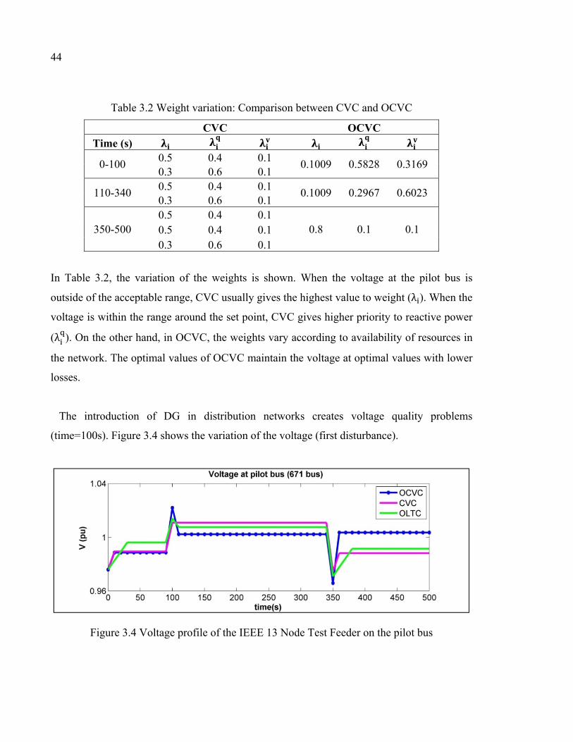
44

Table 3.2 Weight variation: Comparison between CVC and OCVC

CVC OCVC Time (s)

0-100 0.5 0.4 0.1

0.1009 0.5828 0.3169 0.3 0.6 0.1

110-340 0.5 0.4 0.1

0.1009 0.2967 0.6023 0.3 0.6 0.1

350-500 0.5 0.4 0.1

0.8 0.1 0.1 0.5 0.4 0.1 0.3 0.6 0.1

In Table 3.2, the variation of the weights is shown. When the voltage at the pilot bus is

outside of the acceptable range, CVC usually gives the highest value to weight (λ ). When the

voltage is within the range around the set point, CVC gives higher priority to reactive power

(λ ). On the other hand, in OCVC, the weights vary according to availability of resources in

the network. The optimal values of OCVC maintain the voltage at optimal values with lower

losses.

The introduction of DG in distribution networks creates voltage quality problems

(time=100s). Figure 3.4 shows the variation of the voltage (first disturbance).

Figure 3.4 Voltage profile of the IEEE 13 Node Test Feeder on the pilot bus

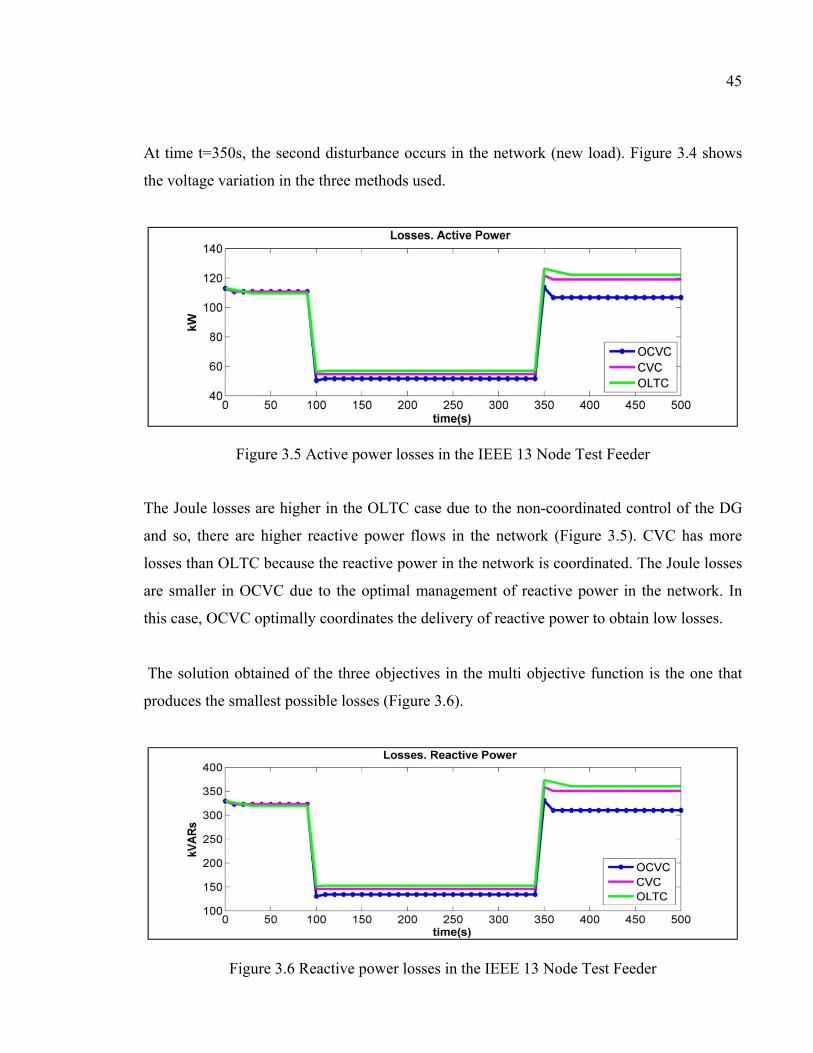
45

At time t=350s, the second disturbance occurs in the network (new load). Figure 3.4 shows

the voltage variation in the three methods used.

Figure 3.5 Active power losses in the IEEE 13 Node Test Feeder

The Joule losses are higher in the OLTC case due to the non-coordinated control of the DG

and so, there are higher reactive power flows in the network (Figure 3.5). CVC has more

losses than OLTC because the reactive power in the network is coordinated. The Joule losses

are smaller in OCVC due to the optimal management of reactive power in the network. In

this case, OCVC optimally coordinates the delivery of reactive power to obtain low losses.

The solution obtained of the three objectives in the multi objective function is the one that

produces the smallest possible losses (Figure 3.6).

Figure 3.6 Reactive power losses in the IEEE 13 Node Test Feeder

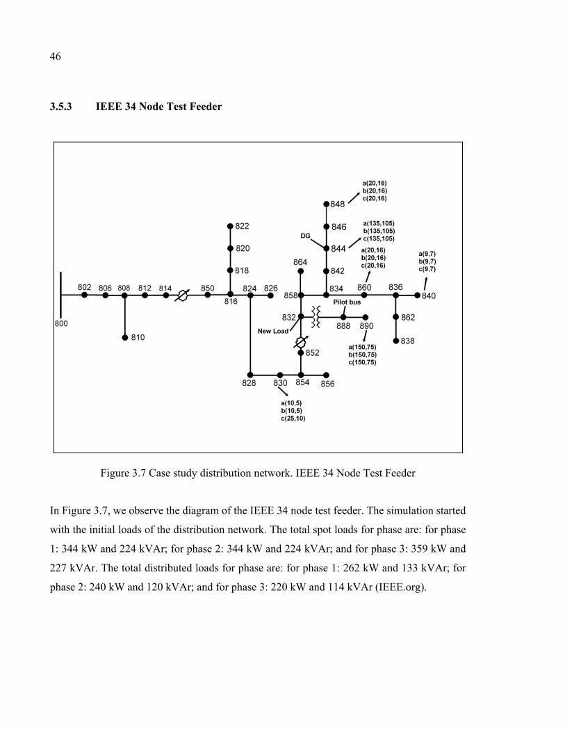
46

3.5.3 IEEE 34 Node Test Feeder

Figure 3.7 Case study distribution network. IEEE 34 Node Test Feeder

In Figure 3.7, we observe the diagram of the IEEE 34 node test feeder. The simulation started

with the initial loads of the distribution network. The total spot loads for phase are: for phase

1: 344 kW and 224 kVAr; for phase 2: 344 kW and 224 kVAr; and for phase 3: 359 kW and

227 kVAr. The total distributed loads for phase are: for phase 1: 262 kW and 133 kVAr; for

phase 2: 240 kW and 120 kVAr; and for phase 3: 220 kW and 114 kVAr (IEEE.org).

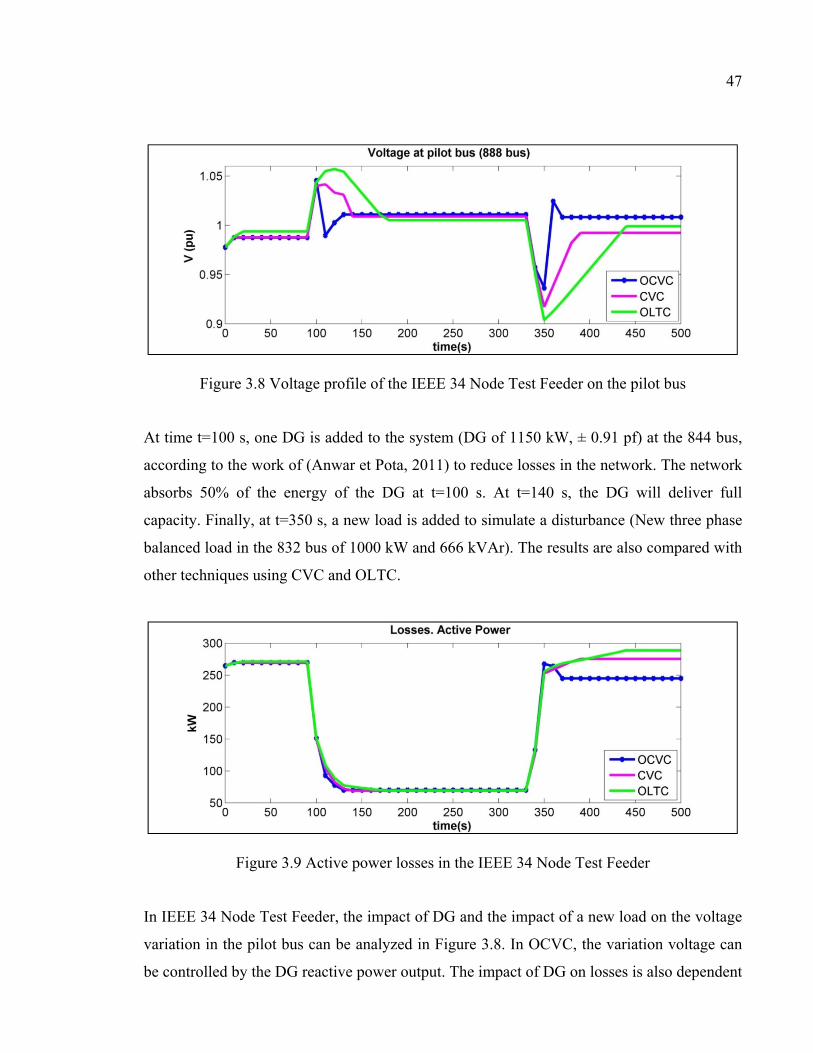
47

Figure 3.8 Voltage profile of the IEEE 34 Node Test Feeder on the pilot bus

At time t=100 s, one DG is added to the system (DG of 1150 kW, ± 0.91 pf) at the 844 bus,

according to the work of (Anwar et Pota, 2011) to reduce losses in the network. The network

absorbs 50% of the energy of the DG at t=100 s. At t=140 s, the DG will deliver full

capacity. Finally, at t=350 s, a new load is added to simulate a disturbance (New three phase

balanced load in the 832 bus of 1000 kW and 666 kVAr). The results are also compared with

other techniques using CVC and OLTC.

Figure 3.9 Active power losses in the IEEE 34 Node Test Feeder

In IEEE 34 Node Test Feeder, the impact of DG and the impact of a new load on the voltage

variation in the pilot bus can be analyzed in Figure 3.8. In OCVC, the variation voltage can

be controlled by the DG reactive power output. The impact of DG on losses is also dependent

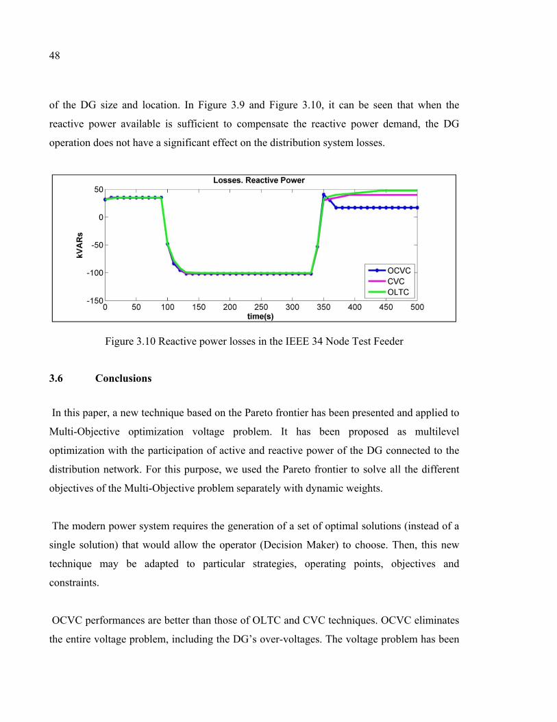
48

of the DG size and location. In Figure 3.9 and Figure 3.10, it can be seen that when the

reactive power available is sufficient to compensate the reactive power demand, the DG

operation does not have a significant effect on the distribution system losses.

Figure 3.10 Reactive power losses in the IEEE 34 Node Test Feeder

3.6 Conclusions

In this paper, a new technique based on the Pareto frontier has been presented and applied to

Multi-Objective optimization voltage problem. It has been proposed as multilevel

optimization with the participation of active and reactive power of the DG connected to the

distribution network. For this purpose, we used the Pareto frontier to solve all the different

objectives of the Multi-Objective problem separately with dynamic weights.

The modern power system requires the generation of a set of optimal solutions (instead of a

single solution) that would allow the operator (Decision Maker) to choose. Then, this new

technique may be adapted to particular strategies, operating points, objectives and

constraints.

OCVC performances are better than those of OLTC and CVC techniques. OCVC eliminates

the entire voltage problem, including the DG’s over-voltages. The voltage problem has been

49

solved; the distribution network voltage profile stays in a fixed range around the set point

values.

OCVC could be an interesting way to reduce or eliminate future investments in classical

voltage and reactive power regulation.

This paper shows that the optimal integration of DG in distribution network can help to

maintain the voltage within the limits and reduce losses.

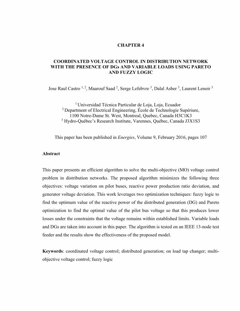
CHAPTER 4

COORDINATED VOLTAGE CONTROL IN DISTRIBUTION NETWORK WITH THE PRESENCE OF DGs AND VARIABLE LOADS USING PARETO

AND FUZZY LOGIC

Jose Raul Castro 1, 2, Maarouf Saad 2, Serge Lefebvre 3, Dalal Asber 3, Laurent Lenoir 3

1 Universidad Técnica Particular de Loja, Loja, Ecuador 2 Department of Electrical Engineering, École de Technologie Supériure,

1100 Notre-Dame St. West, Montreal, Quebec, Canada H3C1K3 3 Hydro-Québec’s Research Institute, Varennes, Québec, Canada J3X1S3

This paper has been published in Energies, Volume 9, February 2016, pages 107

Abstract

This paper presents an efficient algorithm to solve the multi-objective (MO) voltage control

problem in distribution networks. The proposed algorithm minimizes the following three

objectives: voltage variation on pilot buses, reactive power production ratio deviation, and

generator voltage deviation. This work leverages two optimization techniques: fuzzy logic to

find the optimum value of the reactive power of the distributed generation (DG) and Pareto

optimization to find the optimal value of the pilot bus voltage so that this produces lower

losses under the constraints that the voltage remains within established limits. Variable loads

and DGs are taken into account in this paper. The algorithm is tested on an IEEE 13-node test

feeder and the results show the effectiveness of the proposed model.

Keywords: coordinated voltage control; distributed generation; on load tap changer; multi-

objective voltage control; fuzzy logic

52

4.1 Introduction

Due to rapid industrialization and growth of residential and commercial sectors, the electrical

energy requirements have increased significantly over the last decades. In this situation,

renewable energy becomes a very important factor in the electrical distribution system. This

type of generating unit is known as distributed generation (DG), and these generators will

supply a large portion of demand and many of them will be directly connected to the

distribution network. The DGs may trigger variations in voltage and can cause a change of

direction in the power flow. The voltage rise depends on the amount of energy injected by

the DG and, therefore, it is a limiting factor for the DG capacity. Many researchers have

studied DGs and their impact on the voltage, the reduction of the losses in the active and

reactive power, and the maximization of the DG capacity (Ahmidi et al., 2012; DeJesus et al.,

2006; Habibi et al., 2013). In (Anwar et Pota, 2011) a minimization of loss was used to

determine the optimum size and location of DG.

On the other hand, a review of the literature shows that many works have been done

assuming that the loads in the electrical network are fixed. There are only a few works that

use variable loads (Dehghani-Arani et Maddahi, 2013; Hong et al., 2015; Lopez et al., 2004;

Queiroz et Lyra, 2009; Zidan et El-Saadany, 2012). In this paper, all the loads of the

analyzed networks are varying in time to better reflect system operation. Three different

models of load variation are utilized. Each model represents the measurements of the change

in consumption of customers for 48 h (data provided by Hydro-Québec).

Coordinated voltage control (CVC) in distribution network adjusts the voltage in pilot buses.

CVC uses the multi-objective problem to minimize the voltage variation at the pilot buses

(Richardot et al., 2006). Several methods have been proposed to solve the optimization of the

multi-objective (MO) voltage control problem. In (Richardot et al., 2006) a genetic algorithm

(GA) was used to determine an optimal weighted solution of the MO problem. In (Knowles

et Corne, 1999) a simpler evolution scheme for MO problems is proposed; this algorithm

uses the local search for the generation of new candidate solutions.

53

Some researchers (Ngatchou et al., 2005; Richardot et al., 2006; Soroudi et al., 2011) solve

the MO voltage control problem converting the objectives into a single objective (SO)

function; in this case, the objective is to find the solution that minimizes or maximizes this

single objective. The optimization solution results in a single value that represents a

compromise among all the objectives (Ngatchou et al., 2005).

Other researchers (Deb et al., 2002; Ngatchou et al., 2005; Xiyi et al., 2013) work with the

objectives of the MO problem separately, resulting in a set of solutions called the Pareto

frontier. This causes the difficulty to find an optimal solution since there is no a single

solution. Therefore, a decision-maker (DM) is necessary to choose the most appropriate

solution. This feature is useful because it provides a better understanding of the system

because all the objectives are explored. This method leads to find the weighted minimum of

the objectives. Thus, the constraints and criteria specified of each objective are important to

find the Pareto frontier.

Electrical power systems are very difficult to control with traditional methods due to highly

complex and nonlinear behaviors. Fuzzy logic can overcome these difficulties. In (Barin et

al., 2008; Loetamonphong et al., 2002) a fuzzy logic technique was introduced to solve the

optimal values of MO voltage control problem. The solution set is usually not a singleton set.

The problem requires the objectives functions to be linear and it also requires the value of the

minimal solutions of the system. To solve this problem, fuzzy logic can be used closely with

other optimization technique (Gao et al., 2014).

Previous methods adequately solved the problem of MO voltage control problem using DGs

in distribution networks obtaining optimum values of voltage and reactive power (Ahmidi et

al., 2012; Anwar et Pota, 2011; Barin et al., 2008; Gaonkar et Pillai, 2010; Ghatee et

Hashemi, 2009; Kiprakis et Wallace, 2004; Maciel et Padilha-Feltrin, 2009; Richardot et al.,

2006; Viawan et Karlsson, 2008). There is no research that calculates the value of the

reactive power of the DG using the optimal values of the MO voltage control problem in

distribution network with variable and unbalanced loads.

54

To overcome the problems cited above, this paper proposes a new method called coordinated

voltage control using Pareto and fuzzy logic (CVCPF). This technique finds the optimal

values of the MO voltage control problem and finds the optimal value of reactive power of

the DG. CVCPF maintains the voltage of the buses into the established limits, minimize the

losses of the network, and minimizes the voltage variation in the pilot bus. This new method

is tested on an IEEE 13-node test feeder using variables and unbalanced loads.

CVCPF uses Pareto optimization for solving the MO voltage control problem; the objectives

of the MO problem are resolved separately. This paper uses fuzzy logic to find the optimal

reactive power of DG to inject in distribution system. Fuzzy logic analyzes the voltage

difference (ΔV) between the reference voltage (Vpref) and the optimal voltage of pilot bus

(VpOptimo) to find the reactive power of DG that minimizes voltage error.

The original contributions of this paper consist basically in combining the following:

1) variables and unbalanced loads with DGs in distribution network are investigated;

2) CVCPF uses two optimization techniques. Pareto Optimization to find the optimal voltage and fuzzy logic to calculate the optimal value of reactive power of DG;

3) CVCPF uses the reactive power of DG as a control variable to minimize the voltage variation;

4) the objectives of the MO voltage control problem are resolved separately.

The rest of this paper is organized as follows: Section 4.2 presents the classical CVC. Section

4.3 presents coordinated voltage control using Pareto and fuzzy approach (CVCPF).

Simulation results are presented in Section 4.4 and, finally, in Section 4.5 the conclusions are

given.

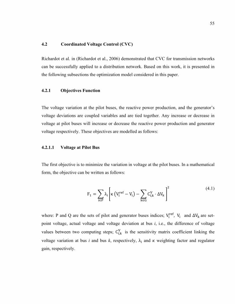
55

4.2 Coordinated Voltage Control (CVC)

Richardot et al. in (Richardot et al., 2006) demonstrated that CVC for transmission networks

can be successfully applied to a distribution network. Based on this work, it is presented in

the following subsections the optimization model considered in this paper.

4.2.1 Objectives Function

The voltage variation at the pilot buses, the reactive power production, and the generator’s

voltage deviations are coupled variables and are tied together. Any increase or decrease in

voltage at pilot buses will increase or decrease the reactive power production and generator

voltage respectively. These objectives are modelled as follows:

4.2.1.1 Voltage at Pilot Bus

The first objective is to minimize the variation in voltage at the pilot buses. In a mathematical

form, the objective can be written as follows:

F = λ∈ κ V − V − C , · ∆V∈ (4.1)

where: P and Q are the sets of pilot and generator buses indices; V , V and ∆V are set-

point voltage, actual voltage and voltage deviation at bus i, i.e., the difference of voltage

values between two computing steps; C , is the sensitivity matrix coefficient linking the

voltage variation at bus i and bus k, respectively, λ and weighting factor and regulator

gain, respectively.

56

4.2.1.2 Reactive Power

The second objective is the management of the reactive power. This objective is modelled

as follows:

= − − , · ∆∈ (4.2)

where: G is the set of generator buses indices; Q and Q are actual and maximum reactive

power generations at bus i; q = ∑ Q /∑ Q∈∈ is the uniform set-point reactive

power value within the regulated area; C , is sensitivity matrix coefficients linking,

respectively, voltage variation at bus i and bus k. λ and are weighting factor and

regulator gain, respectively.

4.2.1.3 Voltage at Generators

The third objective is the minimization of the generator’s voltage deviations. The

mathematical model is as follows:

= − −∈ (4.3)

where: G is the set of generator buses indices; V , V and ∆V are the set-point voltage,

actual voltage and voltage deviation, respectively, at the bus i, i.e., the difference of voltage

values between two computing steps. λ and are weighting factor and regulator gain,

respectively.

57

4.2.2 Constraints

The constraints are presented as follows:

4.2.2.1 Reactive Power Constraint

In this work, one of the main objectives is to control the production of the reactive power of

the DG. In (Ahmidi et al., 2012) an acceptable power factor is of ±0.91.

= / ∈∈ (4.4)

where: |Q | ≤ Q .

4.2.2.2 Technical Compliance Voltage

The compliance of constraints of voltage on the pilot and generator buses is used to

determine the safe operation values. In distribution networks an acceptable steady voltage

range is considered within ±3% of the operating voltage at DG (Masters, 2002):

∈ ; ∈ ∪ |∆ | ≤ ∆ ∈

(4.5)

4.2.2.3 Weights Constraints

The weights of the objectives are important because they give priority to an objective that

depends on the conditions of operation. For example, if the voltage on the pilot bus is outside

of the limits, the weight for this objective will be higher than the other two; however, these

weights are related as described in relation Equation (4.6):

58

+ + = 1 (4.6)

λ , λ , λ are weighting factors for bus i.

4.3 Coordinated Voltage Control Using Pareto and Fuzzy Logic (CVCPF)

This section presents the Pareto optimization to find the optimal voltage on the pilot bus and

the determination of reactive power of DG using a fuzzy approach.

4.3.1 Pareto Optimization

The classical methods consist of converting the MO problem into a single objective (SO)

problem. The solution of this SO problem yield a single result that depend of the selection of

the weights. On the other hand, Pareto optimization optimizes all objectives separately.

Figure 4.1 shows that Pareto optimization calculates a set of solutions called the Pareto

frontier, which can optimize the maximum possible number of objectives. In this work, we

use Matlab to find the minimum of multiple functions using a genetic algorithm and obtain

the Pareto frontier subject to the linear equalities Aeq × x = beq. All objectives and

constraints are changing in the real-time set considering the actual needs and capabilities.

This Pareto frontier is obtained by using the dominance relationship among different

solutions.

59

Figure 4.1 Pareto optimization scheme for a multi-objective problem

The algorithm needs to choose only one solution to this set of solutions using a new

condition decision-maker (DM) (Dehghani-Arani et Maddahi, 2013).

For each set of solutions, the decision-maker (DM) calculates the minimum of the sum of the

three objectives; the set of solutions that have the minimum is selected:

= (4.7)

where: is the minimum sum of the objectives of the set of solutions. N is the number of

objectives. is the weight of the objective j. is the objective j of the MO voltage control

problem.

4.3.2 Fuzzy Logic

Fuzzy logic is an extension of traditional Boolean relations where the system is not

characterized by simple binary values but a range of truths from 0 to 1. The input and output

60

of the system are “somehow” related (Ghatee et Hashemi, 2009). Fuzzy logic is increasingly

utilized in distribution networks.

Two of the most important types of fuzzy control are: the Mamdani and Sugeno models. The

Mamdani model allows expressing the available prior knowledge of the system, whereas the

Sugeno model simplifies the calculations of the output. The Sugeno output can be either

linear or constant and the final output is a weighted average of each rule’s output; so, its

process does not require defuzzification. It works well with optimization and adaptive

techniques and has a guaranteed continuity of output surface. Finally, the Sugeno model is

well suited to mathematical analysis (Takagi et Sugeno, 1985).

In this work, the Sugeno model will be used and its mathematical model has the following

form:

1 = , ℎ ℎ = (4.8)

In a zero-order model, the output level z is a constant (a=0). Each output zi of each rule has

a weight wi (Soroudi et al., 2011):

= ( ) (4.9)

Where F1(x) are the membership functions for input 1 (Takagi et Sugeno, 1985). The average

estimate is then given by the equation:

= ∑∑ (4.10)

61

CVCPF uses fuzzy logic to calculate the optimal reactive power of DG. Figure 4.2 shows the

fuzzy logic reactive power controller. The input signal is the error (ΔV). This error (ΔV) is

varying over the range ∆V , Zeroand∆V where

∆V = -0.05 (p.u.) and ∆V = +0.05 (p.u.)

The output of the fuzzy logic is the variation of the reactive power. The output of the

controller is the voltage variation. The PID generates an output based on the difference

between the power factor calculated by fuzzy logic and output power factor of the network.

The three linguistic labels define voltage: Low, Normal, and High. The input membership

(Gaussian) functions are shown in Figure 4.3.

Figure 4.2 Fuzzy logic reactive power factor controller

Figure 4.3 Input fuzzy membership functions

62

4.3.3 Design of Reactive Power of DG

In this work, this model is a single-input and single output (SISO) controller (Figure 4.2).

Using relation Equation (4.8):

1 = ∆ , ℎ = (4.11)

The set of fuzzy rules are as follows:

(∆ = ) = (∆ = ) = (∆ = ℎ) =

(4.12)

The advantage of the Sugeno model is that the output can be found using the average

estimate formula (Takagi et Sugeno, 1985).

= ∑∑ (4.13)

where: , , are the outputs of the respective fuzzy rules. = min ( ) when ( )is the membership function for input 1.

4.3.4 Solution Algorithm

The algorithm flow chart is illustrated in Figure 4.4. The steps followed to solve the MO

voltage control problem are as follows:

Step 1: System Data: Define input variables; the algorithm acquires the network values.

63

Step 2: Analyze and complete the objective functions. The objective functions are calculated

from Equations (4.1) to (4.3) and the constraints Equations (4.4) to (4.6). CVCPF calculates

the three weights corresponding to F1, F2, and F3 and finds a set of solutions (Pareto

frontier).

Step 3: Decision-maker (DM) calculates the fitness solution.

Step 4: Fuzzy logic

Figure 4 shows the step 4. The error (ΔV) is calculated:

∆ = − (4.14)

Determination of the rules: Equation (4.12) shows the rules.

Determination of the output stage: The final output is computed according to Equation

(4.13). Finally, the reactive power of DG is:

= acos( ) = ( ) × tan( ) (4.15)

Determination of the optimal reactive power reference: The reactive power is computed

using Equation (4.4):

= / ∈∈ (4.16)

Finally, the PID removes the error of the power factor.

64

Step 5: Control: According to the voltage at the pilot bus and the optimal reactive power

reference, the control action is calculated on the OLTC and the PF of the DG.

Step 6: With the data from step 5, CVCPF calculates new values for the distribution network

using the OpenDSS program (OpenDSS manual and reference guide).

Step 7: If voltage values at the pilot buses, reactive power reference, and voltage at

generators are within the limits go to step 8; if not, return to step 1.

Step 8: End.

Figure 4.4 Flow chart of the proposed algorithm

65

4.3.5 Case Study

The proposed method is tested on IEEE13 Node Test Feeder shown in Figure 4.5, 4.16 kV

distribution network. The technical data of the network is given in (Kersting, 2001). In this

work, for Case 1, 2, and 3 only a DG with 1.290 kW connected at the 675 bus is considered

(Anwar et Pota, 2011). For Case 4, this work uses three DGs.

Figure 4.5 IEEE 13 Node Test Feeder

Table 4.1 shows the default unbalanced loads values for the network IEEE 13 (fixed values).

In the second column of the Table 4.1, the three basic loads are displayed. (1) Constant

Impedance Load Model (Constant Z); (2) Constant Current Load Model (Constant I); and (3)

Constant Power Load Model (Constant PQ). In this study, three different cases are analyzed

where variable loads are added to the fixed network loads; each case represents the

measurements of typical change in consumption of customers in a 48 h horizon (data

provided by Hydro-Québec). Table 4.2 shows the cable line configuration for an IEEE 13

node test feeder. Figure 4.6 shows these three cases on the pilot bus in active power (bus

671).

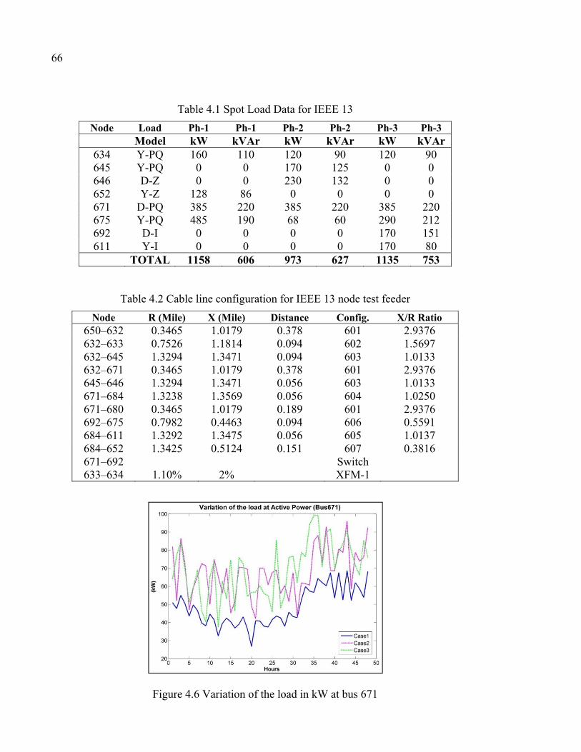
66

Table 4.1 Spot Load Data for IEEE 13

Node Load Ph-1 Ph-1 Ph-2 Ph-2 Ph-3 Ph-3 Model kW kVAr kW kVAr kW kVAr

634 Y-PQ 160 110 120 90 120 90 645 Y-PQ 0 0 170 125 0 0 646 D-Z 0 0 230 132 0 0 652 Y-Z 128 86 0 0 0 0 671 D-PQ 385 220 385 220 385 220 675 Y-PQ 485 190 68 60 290 212 692 D-I 0 0 0 0 170 151 611 Y-I 0 0 0 0 170 80

TOTAL 1158 606 973 627 1135 753

Table 4.2 Cable line configuration for IEEE 13 node test feeder

Node R (Mile) X (Mile) Distance Config. X/R Ratio 650–632 0.3465 1.0179 0.378 601 2.9376 632–633 0.7526 1.1814 0.094 602 1.5697 632–645 1.3294 1.3471 0.094 603 1.0133 632–671 0.3465 1.0179 0.378 601 2.9376 645–646 1.3294 1.3471 0.056 603 1.0133 671–684 1.3238 1.3569 0.056 604 1.0250 671–680 0.3465 1.0179 0.189 601 2.9376 692–675 0.7982 0.4463 0.094 606 0.5591 684–611 1.3292 1.3475 0.056 605 1.0137 684–652 1.3425 0.5124 0.151 607 0.3816 671–692 Switch 633–634 1.10% 2% XFM-1

Figure 4.6 Variation of the load in kW at bus 671

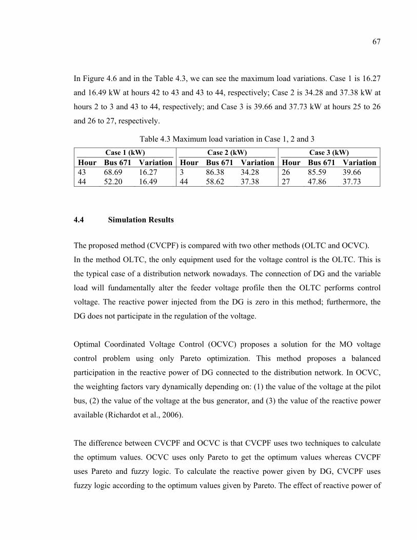
67

In Figure 4.6 and in the Table 4.3, we can see the maximum load variations. Case 1 is 16.27

and 16.49 kW at hours 42 to 43 and 43 to 44, respectively; Case 2 is 34.28 and 37.38 kW at

hours 2 to 3 and 43 to 44, respectively; and Case 3 is 39.66 and 37.73 kW at hours 25 to 26

and 26 to 27, respectively.

Table 4.3 Maximum load variation in Case 1, 2 and 3

Case 1 (kW) Case 2 (kW) Case 3 (kW) Hour Bus 671 Variation Hour Bus 671 Variation Hour Bus 671 Variation43 68.69 16.27 3 86.38 34.28 26 85.59 39.66 44 52.20 16.49 44 58.62 37.38 27 47.86 37.73

4.4 Simulation Results

The proposed method (CVCPF) is compared with two other methods (OLTC and OCVC).

In the method OLTC, the only equipment used for the voltage control is the OLTC. This is

the typical case of a distribution network nowadays. The connection of DG and the variable

load will fundamentally alter the feeder voltage profile then the OLTC performs control

voltage. The reactive power injected from the DG is zero in this method; furthermore, the

DG does not participate in the regulation of the voltage.

Optimal Coordinated Voltage Control (OCVC) proposes a solution for the MO voltage

control problem using only Pareto optimization. This method proposes a balanced

participation in the reactive power of DG connected to the distribution network. In OCVC,

the weighting factors vary dynamically depending on: (1) the value of the voltage at the pilot

bus, (2) the value of the voltage at the bus generator, and (3) the value of the reactive power

available (Richardot et al., 2006).

The difference between CVCPF and OCVC is that CVCPF uses two techniques to calculate

the optimum values. OCVC uses only Pareto to get the optimum values whereas CVCPF

uses Pareto and fuzzy logic. To calculate the reactive power given by DG, CVCPF uses

fuzzy logic according to the optimum values given by Pareto. The effect of reactive power of

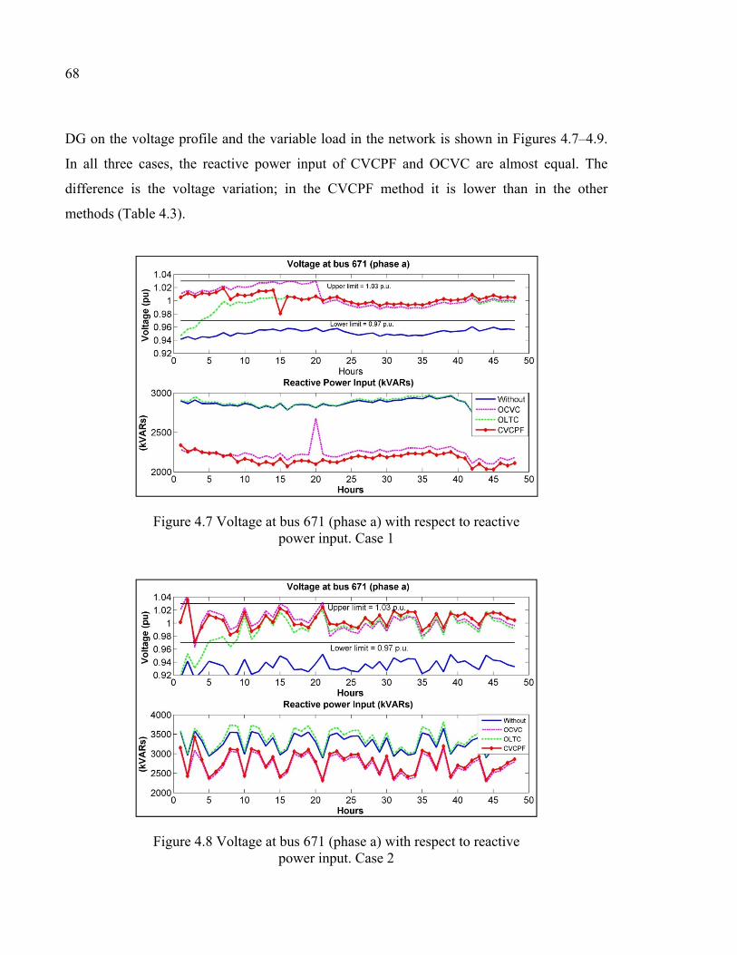
68

DG on the voltage profile and the variable load in the network is shown in Figures 4.7–4.9.

In all three cases, the reactive power input of CVCPF and OCVC are almost equal. The

difference is the voltage variation; in the CVCPF method it is lower than in the other

methods (Table 4.3).

Figure 4.7 Voltage at bus 671 (phase a) with respect to reactive power input. Case 1

Figure 4.8 Voltage at bus 671 (phase a) with respect to reactive power input. Case 2

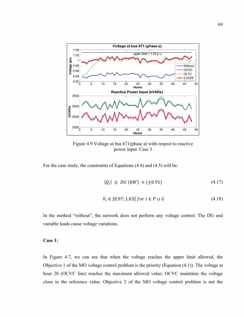
69

Figure 4.9 Voltage at bus 671(phase a) with respect to reactive power input. Case 3

For the case study, the constraints of Equations (4.4) and (4.5) will be:

| | ≤ ( ) × ( 0.91) (4.17)

∈ 0.97; 1.03 ∈ ∪ (4.18)

In the method “without”, the network does not perform any voltage control. The DG and

variable loads cause voltage variations.

Case 1:

In Figure 4.7, we can see that when the voltage reaches the upper limit allowed, the

Objective 1 of the MO voltage control problem is the priority (Equation (4.1)). The voltage at

hour 20 (OCVC line) reaches the maximum allowed value; OCVC maintains the voltage

close to the reference value. Objective 2 of the MO voltage control problem is not the

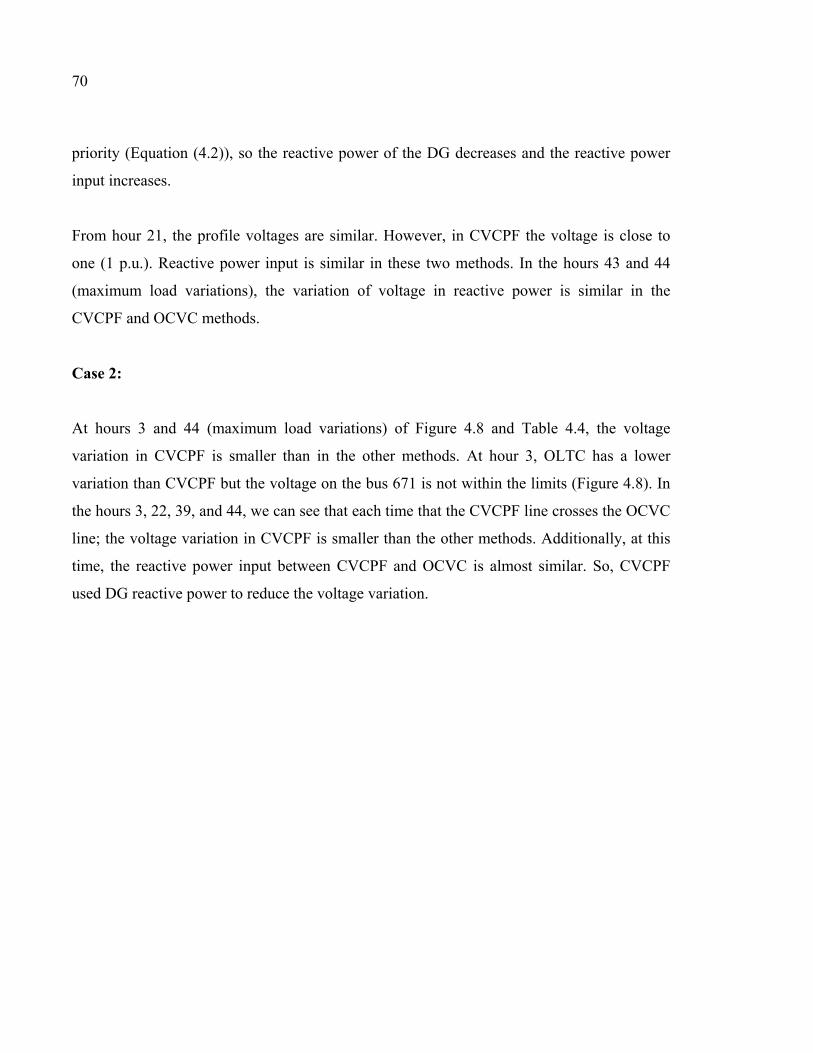
70

priority (Equation (4.2)), so the reactive power of the DG decreases and the reactive power

input increases.

From hour 21, the profile voltages are similar. However, in CVCPF the voltage is close to

one (1 p.u.). Reactive power input is similar in these two methods. In the hours 43 and 44

(maximum load variations), the variation of voltage in reactive power is similar in the

CVCPF and OCVC methods.

Case 2:

At hours 3 and 44 (maximum load variations) of Figure 4.8 and Table 4.4, the voltage

variation in CVCPF is smaller than in the other methods. At hour 3, OLTC has a lower

variation than CVCPF but the voltage on the bus 671 is not within the limits (Figure 4.8). In

the hours 3, 22, 39, and 44, we can see that each time that the CVCPF line crosses the OCVC

line; the voltage variation in CVCPF is smaller than the other methods. Additionally, at this

time, the reactive power input between CVCPF and OCVC is almost similar. So, CVCPF

used DG reactive power to reduce the voltage variation.

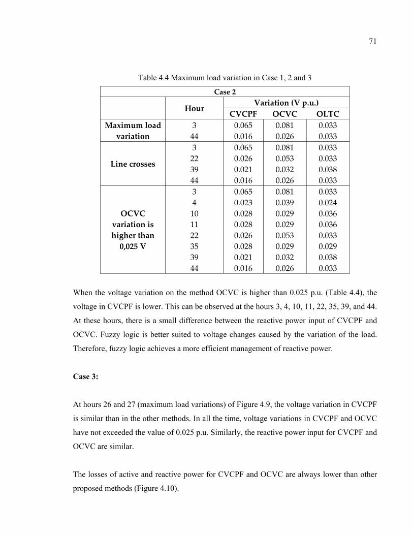
71

Table 4.4 Maximum load variation in Case 1, 2 and 3

Case 2

Hour Variation (V p.u.)

CVCPF OCVC OLTCMaximum load

variation 3 0.065 0.081 0.033 44 0.016 0.026 0.033

Line crosses

3 0.065 0.081 0.033 22 0.026 0.053 0.033 39 0.021 0.032 0.038 44 0.016 0.026 0.033

OCVC variation is higher than

0,025 V

3 0.065 0.081 0.033 4 0.023 0.039 0.024 10 0.028 0.029 0.036 11 0.028 0.029 0.036 22 0.026 0.053 0.033 35 0.028 0.029 0.029 39 0.021 0.032 0.038 44 0.016 0.026 0.033

When the voltage variation on the method OCVC is higher than 0.025 p.u. (Table 4.4), the

voltage in CVCPF is lower. This can be observed at the hours 3, 4, 10, 11, 22, 35, 39, and 44.

At these hours, there is a small difference between the reactive power input of CVCPF and

OCVC. Fuzzy logic is better suited to voltage changes caused by the variation of the load.

Therefore, fuzzy logic achieves a more efficient management of reactive power.

Case 3:

At hours 26 and 27 (maximum load variations) of Figure 4.9, the voltage variation in CVCPF

is similar than in the other methods. In all the time, voltage variations in CVCPF and OCVC

have not exceeded the value of 0.025 p.u. Similarly, the reactive power input for CVCPF and

OCVC are similar.

The losses of active and reactive power for CVCPF and OCVC are always lower than other

proposed methods (Figure 4.10).

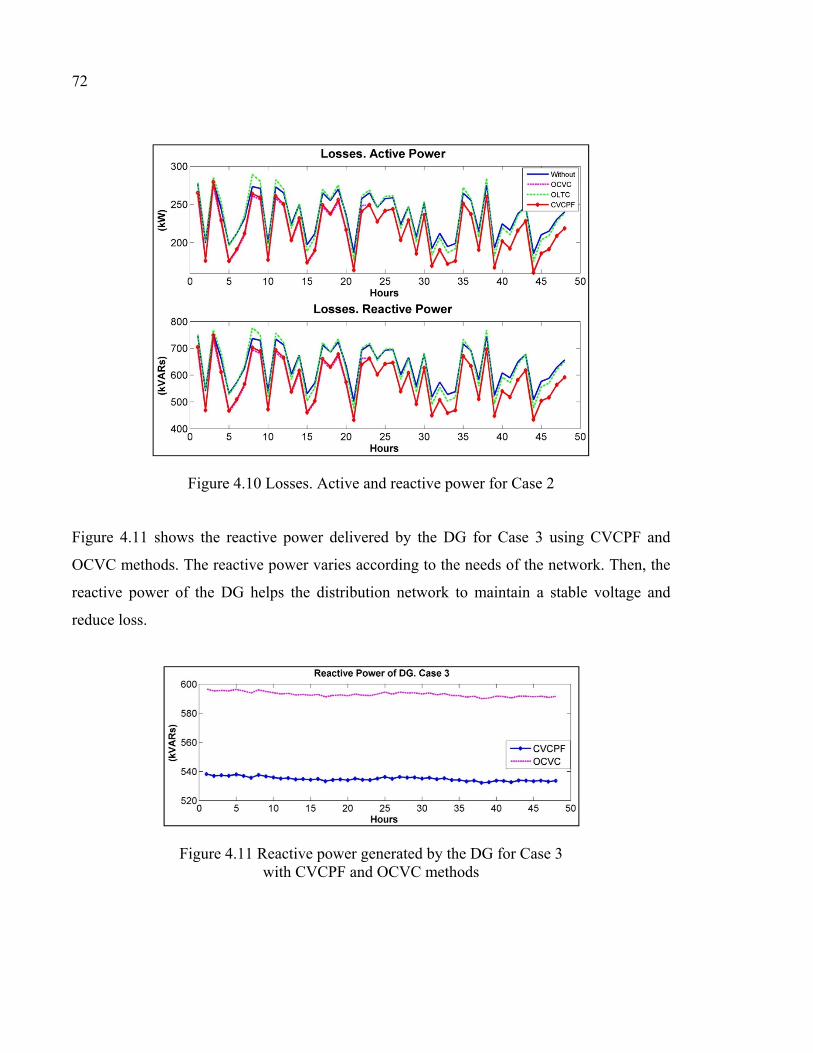
72

Figure 4.10 Losses. Active and reactive power for Case 2

Figure 4.11 shows the reactive power delivered by the DG for Case 3 using CVCPF and

OCVC methods. The reactive power varies according to the needs of the network. Then, the

reactive power of the DG helps the distribution network to maintain a stable voltage and

reduce loss.

Figure 4.11 Reactive power generated by the DG for Case 3 with CVCPF and OCVC methods

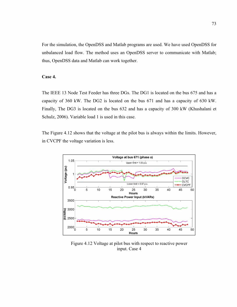
73

For the simulation, the OpenDSS and Matlab programs are used. We have used OpenDSS for

unbalanced load flow. The method uses an OpenDSS server to communicate with Matlab;

thus, OpenDSS data and Matlab can work together.

Case 4.

The IEEE 13 Node Test Feeder has three DGs. The DG1 is located on the bus 675 and has a

capacity of 360 kW. The DG2 is located on the bus 671 and has a capacity of 630 kW.

Finally, The DG3 is located on the bus 632 and has a capacity of 300 kW (Khushalani et

Schulz, 2006). Variable load 1 is used in this case.

The Figure 4.12 shows that the voltage at the pilot bus is always within the limits. However,

in CVCPF the voltage variation is less.

Figure 4.12 Voltage at pilot bus with respect to reactive power input. Case 4

74

4.5 Conclusions

A new algorithm, called CVCPF, for resolving the MO voltage control problem in

distribution networks is presented. The three objectives considered in this paper are: voltage

at pilot bus, management of the reactive power and voltage in generators. CVCPF uses a

combination of optimization techniques (Pareto optimization and fuzzy logic) to find the

optimal values for the MO voltage control problem.

The performance of the CVCPF is evaluated on an IEEE 13 node test feeder. Variables and

unbalanced loads are used, based on real consumption data, over a time window of 48 h.

Three such profiles are used in the study, varying in the amount of the load. The results are

compared with those obtained from the methods OCVC and OLTC as well as from the case

of no voltage control.

This work demonstrates that CVCPF reduces the voltage variation more than the other

methods.

This work shows also that optimal integration of the DGs in the distribution network helps to

maintain stable voltage and to reduce loss.

CVCPF includes the use of decision-maker; in this study the fitness solution was used but

various options are possible. The use of CVCPF could be advantageous with respect to the

development of a flexible system for network operators, by applying different settings at the

decision stage, according to specific circumstances. Further research is needed on this topic.

Acknowledgments

Thanks to Ecole de technologie supérieure and Hydro Québec for the support given in

this work.

CHAPTER 5

POWER FACTOR COMPUTATION OF DISTRIBUTED GENERATION USING MULTI-OBJECTIVE OPTIMIZATION

Jose Raul Castro 1, 2, Maarouf Saad 2, Serge Lefebvre 3, Dalal Asber 3, Laurent Lenoir 3

1 Universidad Técnica Particular de Loja, Loja, Ecuador 2 Department of Electrical Engineering, École de Technologie Supériure,

1100 Notre-Dame St. West, Montreal, Quebec, Canada H3C1K3 3 Hydro-Québec’s Research Institute, Varennes, Québec, Canada J3X1S3

This paper has been submitted for publication in Electrical Power and Energy System

Abstract

Increased Distributed Generation (DG) conventional distribution networks with unbalanced

loads require new control strategies to optimize the use of available resource assets. This

paper presents a new technique to demonstrate the benefits of using the reactive power of the

DGs in distribution networks with variable and unbalanced loads. The problem is formulated

as a multi-objective optimization model that minimizes reactive power losses with the

minimization of the variations of the voltage on the pilot bus using : Pareto Optimality, used

to find the optimal value of the pilot bus voltage, and Fuzzy-PI controller, used to find the

optimal power factor of the DGs. The proposed technique is applied to the IEEE 13 and 123-

node test feeders with different and real cases of variable loads. The results demonstrate the

efficiency of the proposed approach and its significant impact on loss minimization.

Keywords: Distributed generation (DG); Multi-objective optimization; distribution network;

energy loss; optimal power factor; optimal size.

76

5.1 Introduction

Demand for electricity is growing rapidly. To satisfy this demand, the electrical networks has

become highly complex due to the large number of buses present, as well as the large variety

of production systems in use; these include those related to renewable energy in general,

which today, play a very important role in electrical distribution systems.

The generating units connected to the distribution network are known as Distributed

Generations (DGs), and they can meet a large proportion of demand. However, DGs may

trigger voltage deviation and changes in the power flow direction. Voltage deviation is

function of the energy injected by the DGs, and therefore constitutes a limiting factor for

their capacity. Traditionally, DGs have been integrated into the distribution network as

passive circuits; their power factor (PF) depends on technical decisions made at certain given

times, and may lead to undesirable levels of absorption of reactive power from the

transmission network, as well as to voltage problems (Ochoa et al., 2011). Knowledge of the

characteristics of the distribution network, of load variation and of the DG type is required to

specify the capacity of the reactive power (or voltage support) (Kolenc et al., 2012; Li et al.,

2013). In most European countries, the permissible power factor (PF) range for DGs is ±0.95.

However, countries such as Spain allow the reactive power of DGs to be delivered according

to network requirements (Grid, 2010). Moreover, DGs can yield several additional benefits,

such as loss reduction, voltage enhancement, reliability improvement and network upgrade

deferral. The DGs are integrated into the network, act as spinning reserves, and provide

reactive power support, loss compensation, frequency control, and other rapid response

services (Anwar et Pota, 2011; Barin et al., 2008; Dehghani-Arani et Maddahi, 2013; Hung et

Mithulananthan, 2014; Hung. et al., 2013; Kiprakis et Wallace, 2004; Maciel et Padilha-

Feltrin, 2009).

As the volumes of DGs increases, however, so do some associated problems. One of these is

the disequilibrium between energy supply and demand. Generally, in a distribution network,

loads usually change with time, while the network uses available resources to attempt to

77

maintain the voltage within permissible limits (Hung et Mithulananthan, 2014; Ren et al.,

2010; Zhang. et al., 2015). The direct and indirect cost of power supply quality, reliability,

and energy losses of the DGs is presented by (Muttaqi et al., 2016). Many researchers

(Aghaei et al., 2014; Esmaili, 2013; Griffin et al., 2000; Khalesi et Haghifam, 2009; Li et al.,

2013; Nara et al., 2001; Ren et al., 2010; Richardot et al., 2006) usually employ a multi-

objective optimization problem (MOP) in dealing with the latter problem. (Niknam et al.,

2011) presents an efficient new MO fuzzy self-adaptive particle swarm optimization

(MNFSAPSO) to solve the MOP, considering the minimization of power loss and voltage

deviations. In (Richardot et al., 2006), the three objectives of the MOP are: 1) minimization

of the voltage deviation on pilot buses; 2) minimization of reactive power production ratio

deviation; and 3) minimization of generators’ voltage deviation. The authors convert MOP

models into a simple objective problem (SOP). The optimal solution gives a single value,

which represents a compromise between all objectives, and requires a priori knowledge about

the relative importance of the objectives and the limits of the constraints under consideration.

The MOP allows precise reactive power management to maintain the voltage within

permissible limits.

The importance of working with DGs that are capable of delivering both active and reactive

power in a distribution network is illustrated in (Ahmidi et al., 2012; Duong et al., 2010;

Moghimi et al., 2013; Thong et al., 2007). In (Ahmidi et al., 2012; Thong et al., 2007), the

DGs are considered as negative loads that play an active role in the power system’s control

and operation.

Previous methods adequately solved the problem of finding an optimum location and size for

DGs in a distribution network. However, the majority of existing works convert the MOP

into SOPs. Furthermore, there is no solution that considers reactive power losses as an

objective of the MOP.

To overcome the above problems, our paper proposes a new technique called “DG with

optimal variable power factor” (VPF). In our previous works (Castro et al., 2016a; Castro et

78

al., 2016b), the MOP had three objectives; in the first work, we proposed Pareto optimization

for solving the MOP separately, and in the second paper, we proposed Pareto optimization

and Fuzzy-PID for solving the MOP. In this paper, and based on these previous works, we

consider the MOP with only two objectives, where the reactive power of the DGs minimizes

the voltage deviation on the pilot bus and the losses in the network. Three cases are

evaluated: 1) the adoption of fixed values of the DGs with a variable power factor in real

time and variable loads, 2) the implementation of variable values of the DGs with a variable

power factor in real time and variable loads, and 3) analysis of losses and voltage using only

OLTC (On-Load Tap Changer). The VPF is tested on 1) the IEEE 13-node test feeder using a

DG with variable and unbalanced loads, and 2) the IEEE 123-node test feeder using four

DGs with variable and unbalanced loads.

Pareto Optimality and Fuzzy-PI are used in VPF for solving the MOP problem and for

defining the optimal active and reactive powers values of the DGs. The two objectives of the

multi-objective optimization problem are solved separately. The original contributions of this

paper consist essentially in combining the following:

1) it presents a new MO function, where the reactive power losses and voltage regulation have been incorporated as objective functions considering DGs;

2) it proposes a new multi-objective algorithm based on Pareto optimality and Fuzzy-PI; 3) it applies real and variable loads and illustrates the impact of variable and fixed DGs on

distribution networks.

The rest of this paper is organized as follows: Section 5.2 presents the mathematical

formulation of the problem using MOP and Optimization techniques. Section 5.3 presents the

proposed solution approach. In section 5.4, the case studies used are given and simulation

results are presented. Finally, in section 5.5, the conclusions are presented.

79

5.2 Problem formulation and optimization

In this work, different variable loads are analyzed. The variable loads are added to the fixed

network loads of the IEEE 13 and 123-node test feeders, and load represents a typical change

in consumption by customers in a 48-hour horizon (Data provided by Hydro-Québec).

In order to investigate the impact of the DGs on the voltage on a pilot bus and the losses in

distribution networks with variable and unbalanced loads, three cases are evaluated:

Case 1: Variable Demand and Variable DGs (VDGs+VL): The active and reactive powers of

the DG need to be optimized.

Case 2: Variable Demand (DGs+VL): The reactive power of the fixed DG is optimized.

Case 3: OLTC: Analysis of losses and voltage using only OLTC (On-Load Tap Changer).

Conventional (passive) networks operate DGs with fixed PF values over all load conditions.

Conversely, VPF may vary the OLTC or the PF of the DGs (active network). To facilitate

understanding of how the control system reduces losses, a number of variables and

constraints are incorporated into the VPF. Here, the Coordinated Voltage Control (CVC) and

the minimization of reactive power losses are implemented with the main objective of

finding the optimal size of the DGs allowing loss reduction while maintaining the voltage

within acceptable limits.

5.2.1 Multi-Objective Problem (MOP)

The MOP model aims to support the decisions of planners respecting the selection of the

levels of operation of the DGs throughout the planning period (Ren et al., 2010). The

objectives are modelled as follows:

80

5.2.1.1 Coordinated Voltage Control (CVC)

The first objective is to minimize the variation in voltage on the pilot buses. In mathematical

form, the objective can be written as follows (Richardot et al., 2006):

= ∈ − − , · ∆∈ (5.1)

Where P and Q are the sets of pilot and generator bus indices; V , V are the set point

voltage, and the measured voltage on bus i respectively, and ∆ , is the voltage deviation on

generator bus k, i.e., the difference in voltage values between two iterations; C , is the

sensitivity matrix coefficient linking the voltage deviation on buses i and k, respectively, and

is a desired weighting coefficient.

5.2.1.2 Active and reactive power of the DGs

The second objective is loss reduction management. (Abu-Mouti et El-Hawary, 2011; Anwar

et Pota, 2011; Esmaili, 2013; Young-Jin et al., 2013) present an optimized algorithm using

sensitivity factors. If the DG size varies from QDGi1 to QDGi2 to then the reactive power loss

varies from Qli1 to Qli2, respectively. The sensitivity factor is stated as follows:

= = ∈−−

(5.2)

where − corresponds to the change in reactive power loss; − is the

change in DG reactive power from time 1 to 2; and λ is a weighting coefficient.

The power factor (PF) of the DGs is given by (5.3)

81

= + (5.3)

where and are the active and reactive power of , and is the power factor

of DG.

Assuming

= ( ) tan( ( )) (5.4)

The reactive power output of the DGs is expressed by (5.5)

= (5.5)

in which sign = +1DG injecting reactive power; sign = −1 DG consuming reactive power;

From (5.2), (5.3), (5.4), and (5.5), the reactive power loss can be rewritten as:

= = ∈−( − )

(5.6)

where P ≤ P and − is the variation of the DG size.

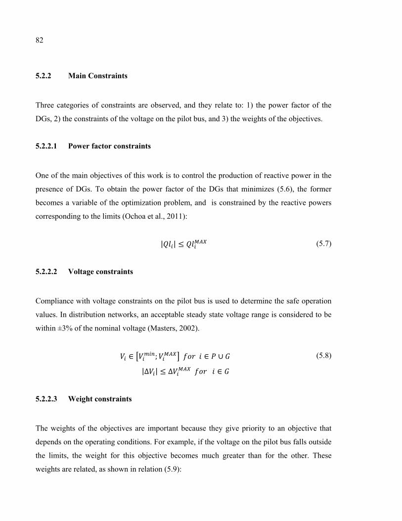
82

5.2.2 Main Constraints

Three categories of constraints are observed, and they relate to: 1) the power factor of the

DGs, 2) the constraints of the voltage on the pilot bus, and 3) the weights of the objectives.

5.2.2.1 Power factor constraints

One of the main objectives of this work is to control the production of reactive power in the

presence of DGs. To obtain the power factor of the DGs that minimizes (5.6), the former

becomes a variable of the optimization problem, and is constrained by the reactive powers

corresponding to the limits (Ochoa et al., 2011):

| | ≤ (5.7)

5.2.2.2 Voltage constraints

Compliance with voltage constraints on the pilot bus is used to determine the safe operation

values. In distribution networks, an acceptable steady state voltage range is considered to be

within ±3% of the nominal voltage (Masters, 2002).

∈ ; ∈ ∪ |∆ | ≤ ∆ ∈

(5.8)

5.2.2.3 Weight constraints

The weights of the objectives are important because they give priority to an objective that

depends on the operating conditions. For example, if the voltage on the pilot bus falls outside

the limits, the weight for this objective becomes much greater than for the other. These

weights are related, as shown in relation (5.9):

83

λ + λ = 1 (5.9)

where λ , λ are weighting coefficients for bus i.

5.2.3 Optimization techniques

This section presents the Pareto optimization and Fuzzy-PI approach used to find the optimal

size and power factor of the DGs.

5.2.3.1 Pareto optimization

The Pareto optimization finds a set of solutions constituting what is known as the Pareto

frontier, which can optimize the two objectives (figure 5.1). The Genetic algorithm (GA), a

global optimization technique, is used to find the optimal solution.

GA emulates the biological evolution process. An initial population of individuals

representing different solutions is evolving to find optimal solutions. The fittest individuals

are evaluated and selected from the current population. These are the values that solve the

optimization problem of the objective function. Each individual is mutated to form a new

generation using crossover operations (Ouyang et Pano, 2015). It is important to maintain

population diversity to ensure convergence to an optimal Pareto frontier (Deb et al., 2002).

The Pareto frontier is obtained by using the dominance relationship between different

solutions (Fu et al., 2015).

The algorithm needs to choose only one solution among the set of solutions, using a Decision

Maker (DM) (Dehghani-Arani et Maddahi, 2013; Ngatchou et al., 2005). For each set of

solutions, the DM calculates the minimum of the reactive power losses. The set of solutions

having the minimum DM is selected:

84

= ∈ −( − ) (5.10)

where is the minimum of the second objective of the set of solutions; −

corresponds to the change in reactive power loss; − is the change in active power

of DG from time 1 to time 2; and λ is a weighting factor.

5.2.3.2 Fuzzy-PI controller

The Fuzzy-PI controller uses the Pareto optimal values to find the appropriate reactive power

values that can deliver the DGs.

The controller, as shown in Figure 5.2, has two inputs and one single output. The voltage

deviation (ΔV) and its derivate are the inputs. The input membership functions are Low,

Normal, and High (Figure 5.3) (Pitalúa-Díaz et al., 2015). The output signal Fuzzy-PI

controller is the optimal reactive power of the DGs.

The Fuzzy-PI controller has the advantage of not having a specific operating point. The rules

evaluate the tendency of the error signals to determine whether to increase or decrease the

control variable.

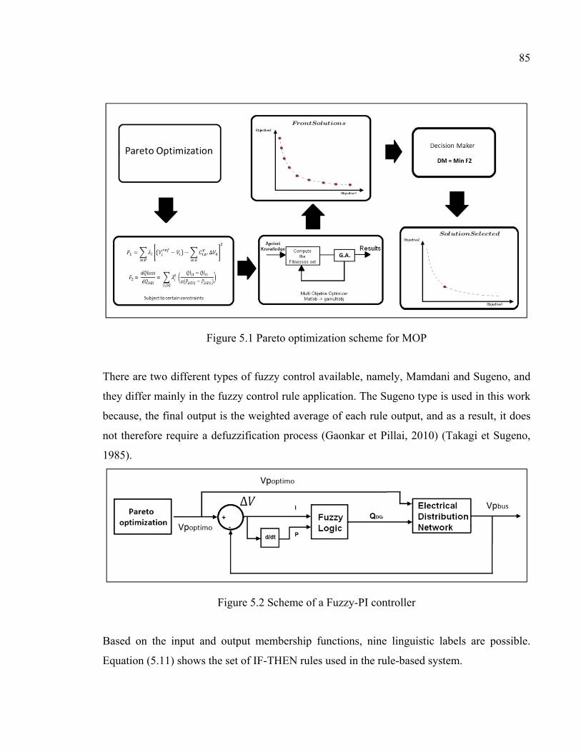
85

Figure 5.1 Pareto optimization scheme for MOP

There are two different types of fuzzy control available, namely, Mamdani and Sugeno, and

they differ mainly in the fuzzy control rule application. The Sugeno type is used in this work

because, the final output is the weighted average of each rule output, and as a result, it does

not therefore require a defuzzification process (Gaonkar et Pillai, 2010) (Takagi et Sugeno,

1985).

Figure 5.2 Scheme of a Fuzzy-PI controller

Based on the input and output membership functions, nine linguistic labels are possible.

Equation (5.11) shows the set of IF-THEN rules used in the rule-based system.

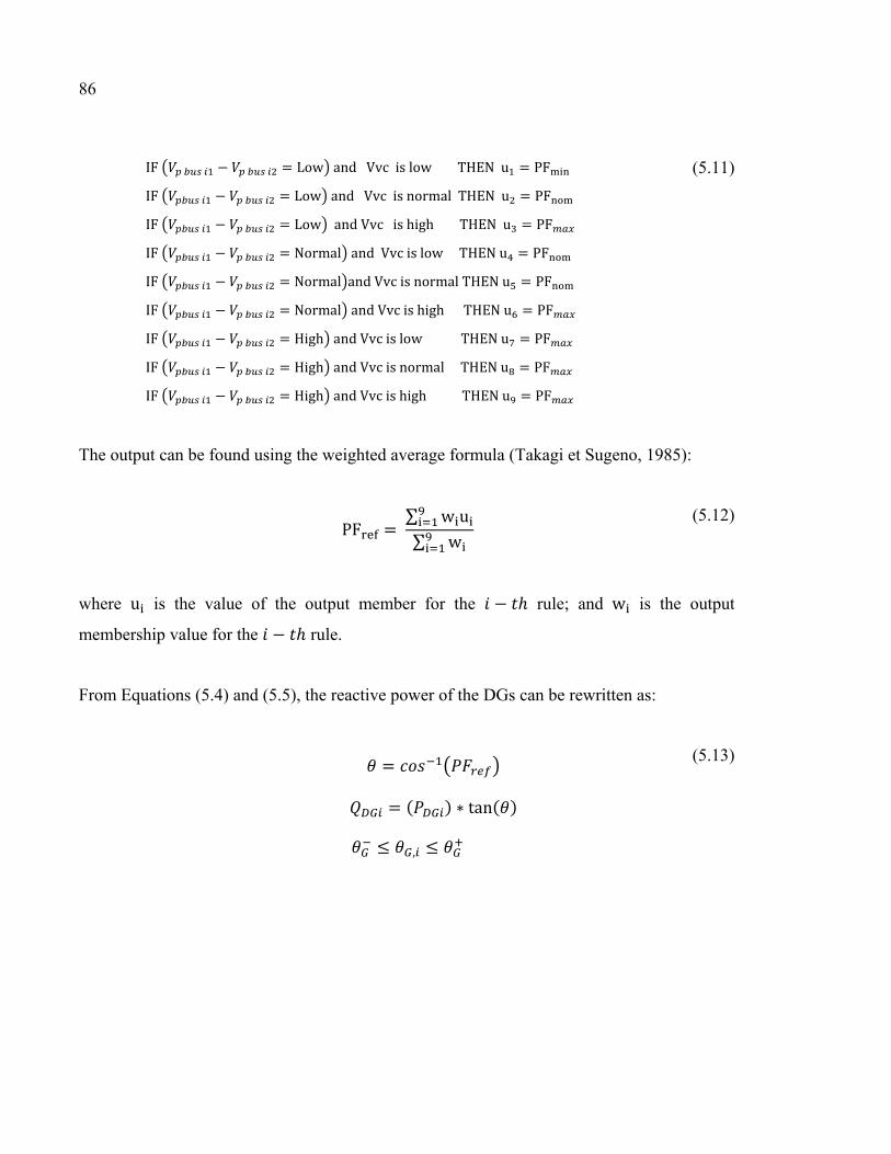
86

IF − = Low and Vvc is low THEN u = PFIF − = Low and Vvc is normal THEN u = PFIF − = Low andVvcishighTHENu = PF IF − = Normal andVvcislowTHENu = PF IF − = Normal andVvcisnormalTHENu = PF IF − = Normal andVvcishighTHENu = PF IF − = High andVvcislowTHENu = PF IF − = High andVvcisnormalTHENu = PF IF − = High andVvc is high THEN u = PF

(5.11)

The output can be found using the weighted average formula (Takagi et Sugeno, 1985):

PF = ∑ w u∑ w (5.12)

where u is the value of the output member for the − ℎ rule; and w is the output

membership value for the − ℎ rule.

From Equations (5.4) and (5.5), the reactive power of the DGs can be rewritten as:

= = ( ) ∗ tan( ) ≤ , ≤

(5.13)

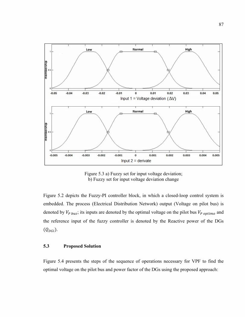
87

Figure 5.3 a) Fuzzy set for input voltage deviation; b) Fuzzy set for input voltage deviation change

Figure 5.2 depicts the Fuzzy-PI controller block, in which a closed-loop control system is

embedded. The process (Electrical Distribution Network) output (Voltage on pilot bus) is

denoted by ; its inputs are denoted by the optimal voltage on the pilot bus and

the reference input of the fuzzy controller is denoted by the Reactive power of the DGs ( ).

5.3 Proposed Solution

Figure 5.4 presents the steps of the sequence of operations necessary for VPF to find the

optimal voltage on the pilot bus and power factor of the DGs using the proposed approach:

88

Step 1: Input Data: The input of the variables to Equations (5.1) and (5.6) of the optimization

problem are defined. The data network is provided using OpenDSS software (OpenDSS

manual and reference guide).

Step 2: Pareto optimization: Matlab is used to solve Equations (5.1) and (5.6) with

constraints (5.7) to (5.9). The algorithm calculates the two weights (λ andλ )

corresponding to the functions F1 and F2, and finds a set of solutions (Pareto frontier).

(Figure 5.1)

Step 3: The Decision Maker (DM) finds the solution set that minimizes the second function.

The set of solutions selected gives the optimal values of the two functions. So, the optimal

voltage for the pilot bus is selected. While the variation of the load has an impact on the pilot

bus voltage, the reactive powers of the DGs can however help reduce this voltage deviation.

Step 4: Fuzzy-PI Controller: Equation (5.11) determines the rules. The final output is

computed according to Equation (5.12). Finally, the reactive powers of the DGs are

calculated using Equation (5.13)

Step 5: Control: The control action is executed according to the voltage on the pilot bus and

the optimal reactive and active powers of the DGs.

OLTC should adjust its tap to reach the optimal voltage value found in Step 3. At each time

step, the voltage in the OLTC is treated as a variable. The upper and lower voltages and the

maximum and minimum variations of active and reactive power are respected.

Step 6: With the data from Step 5 and the new values of the load (variable load), the

OpenDSS program calculates the power flow of the distribution network (OpenDSS manual

and reference guide).

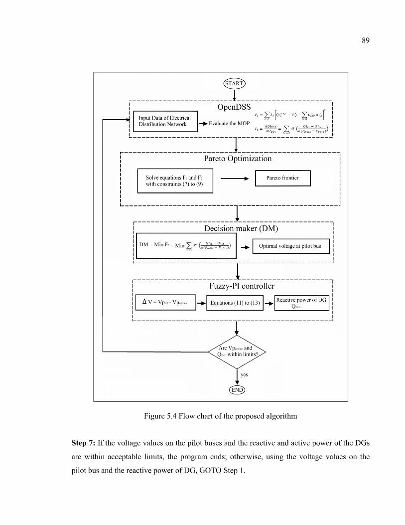
89

Figure 5.4 Flow chart of the proposed algorithm

Step 7: If the voltage values on the pilot buses and the reactive and active power of the DGs

are within acceptable limits, the program ends; otherwise, using the voltage values on the

pilot bus and the reactive power of DG, GOTO Step 1.

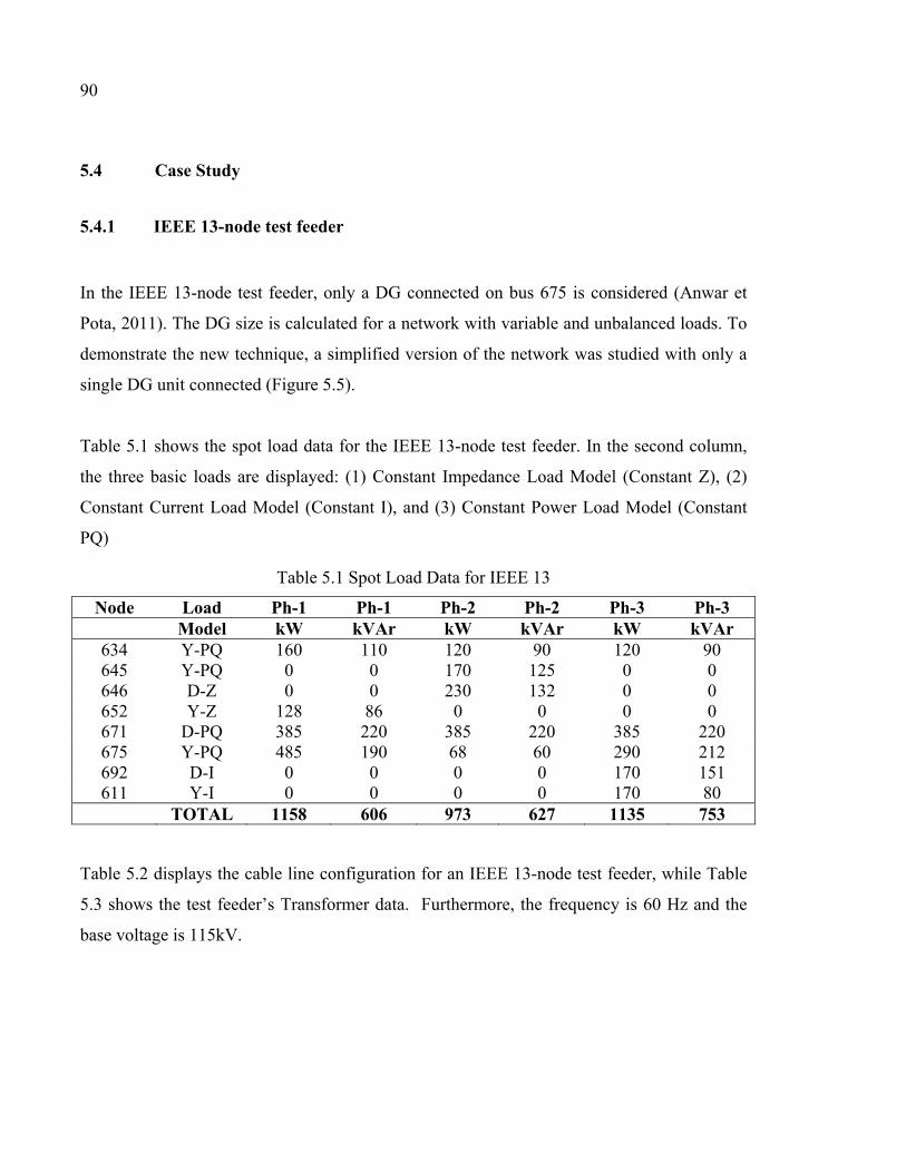
90

5.4 Case Study

5.4.1 IEEE 13-node test feeder

In the IEEE 13-node test feeder, only a DG connected on bus 675 is considered (Anwar et

Pota, 2011). The DG size is calculated for a network with variable and unbalanced loads. To

demonstrate the new technique, a simplified version of the network was studied with only a

single DG unit connected (Figure 5.5).

Table 5.1 shows the spot load data for the IEEE 13-node test feeder. In the second column,

the three basic loads are displayed: (1) Constant Impedance Load Model (Constant Z), (2)

Constant Current Load Model (Constant I), and (3) Constant Power Load Model (Constant

PQ)

Table 5.1 Spot Load Data for IEEE 13

Node Load Ph-1 Ph-1 Ph-2 Ph-2 Ph-3 Ph-3 Model kW kVAr kW kVAr kW kVAr

634 Y-PQ 160 110 120 90 120 90 645 Y-PQ 0 0 170 125 0 0 646 D-Z 0 0 230 132 0 0 652 Y-Z 128 86 0 0 0 0 671 D-PQ 385 220 385 220 385 220 675 Y-PQ 485 190 68 60 290 212 692 D-I 0 0 0 0 170 151 611 Y-I 0 0 0 0 170 80

TOTAL 1158 606 973 627 1135 753

Table 5.2 displays the cable line configuration for an IEEE 13-node test feeder, while Table

5.3 shows the test feeder’s Transformer data. Furthermore, the frequency is 60 Hz and the

base voltage is 115kV.

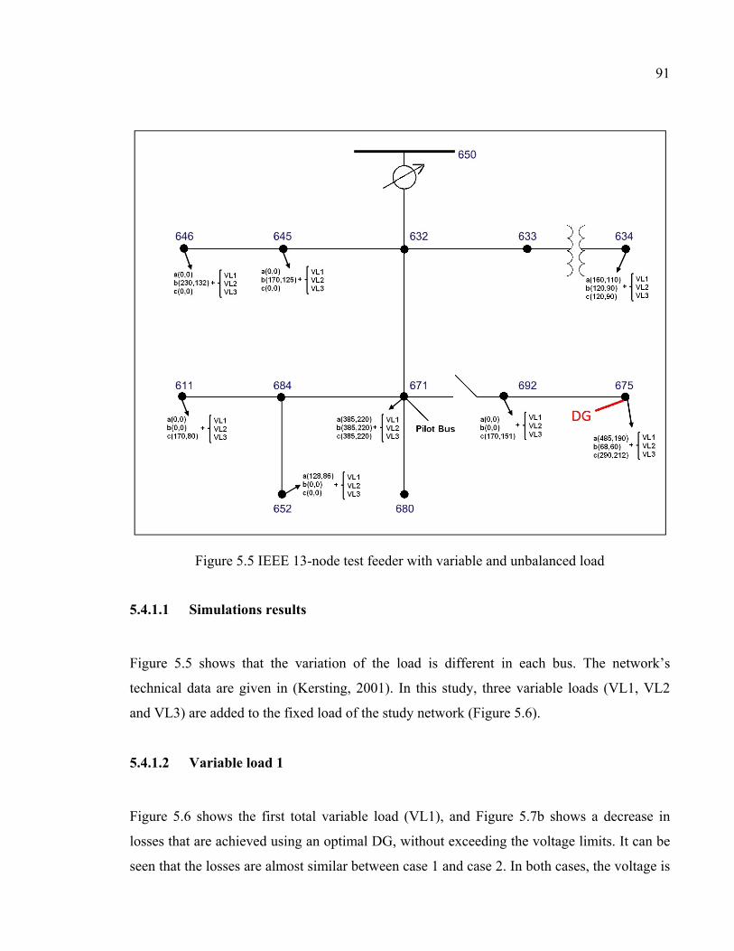
91

Figure 5.5 IEEE 13-node test feeder with variable and unbalanced load

5.4.1.1 Simulations results

Figure 5.5 shows that the variation of the load is different in each bus. The network’s

technical data are given in (Kersting, 2001). In this study, three variable loads (VL1, VL2

and VL3) are added to the fixed load of the study network (Figure 5.6).

5.4.1.2 Variable load 1

Figure 5.6 shows the first total variable load (VL1), and Figure 5.7b shows a decrease in

losses that are achieved using an optimal DG, without exceeding the voltage limits. It can be

seen that the losses are almost similar between case 1 and case 2. In both cases, the voltage is

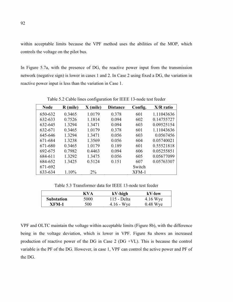
92

within acceptable limits because the VPF method uses the abilities of the MOP, which

controls the voltage on the pilot bus.

In Figure 5.7a, with the presence of DG, the reactive power input from the transmission

network (negative sign) is lower in cases 1 and 2. In Case 2 using fixed a DG, the variation in

reactive power input is less than the variation in Case 1.

Table 5.2 Cable lines configuration for IEEE 13-node test feeder

Node R (mile) X (mile) Distance Config. X/R ratio

650-632 0.3465 1.0179 0.378 601 1.11043636 632-633 0.7526 1.1814 0.094 602 0.14755727 632-645 1.3294 1.3471 0.094 603 0.09525154 632-671 0.3465 1.0179 0.378 601 1.11043636 645-646 1.3294 1.3471 0.056 603 0.0567456 671-684 1.3238 1.3569 0.056 604 0.05740021 671-680 0.3465 1.0179 0.189 601 0.55521818 692-675 0.7982 0.4463 0.094 606 0.05255851 684-611 1.3292 1.3475 0.056 605 0.05677099 684-652 1.3425 0.5124 0.151 607 0.05763307 671-692 Switch 633-634 1.10% 2% XFM-1

Table 5.3 Transformer data for IEEE 13-node test feeder

KVA kV-high kV-low Substation 5000 115 - Delta 4.16 Wye

XFM-1 500 4.16 - Wye 0.48 Wye

VPF and OLTC maintain the voltage within acceptable limits (Figure 8b), with the difference

being in the voltage deviation, which is lower in VPF. Figure 8a shows an increased

production of reactive power of the DG in Case 2 (DG +VL). This is because the control

variable is the PF of the DG. However, in case 1, VPF can control the active power and PF of

the DG.

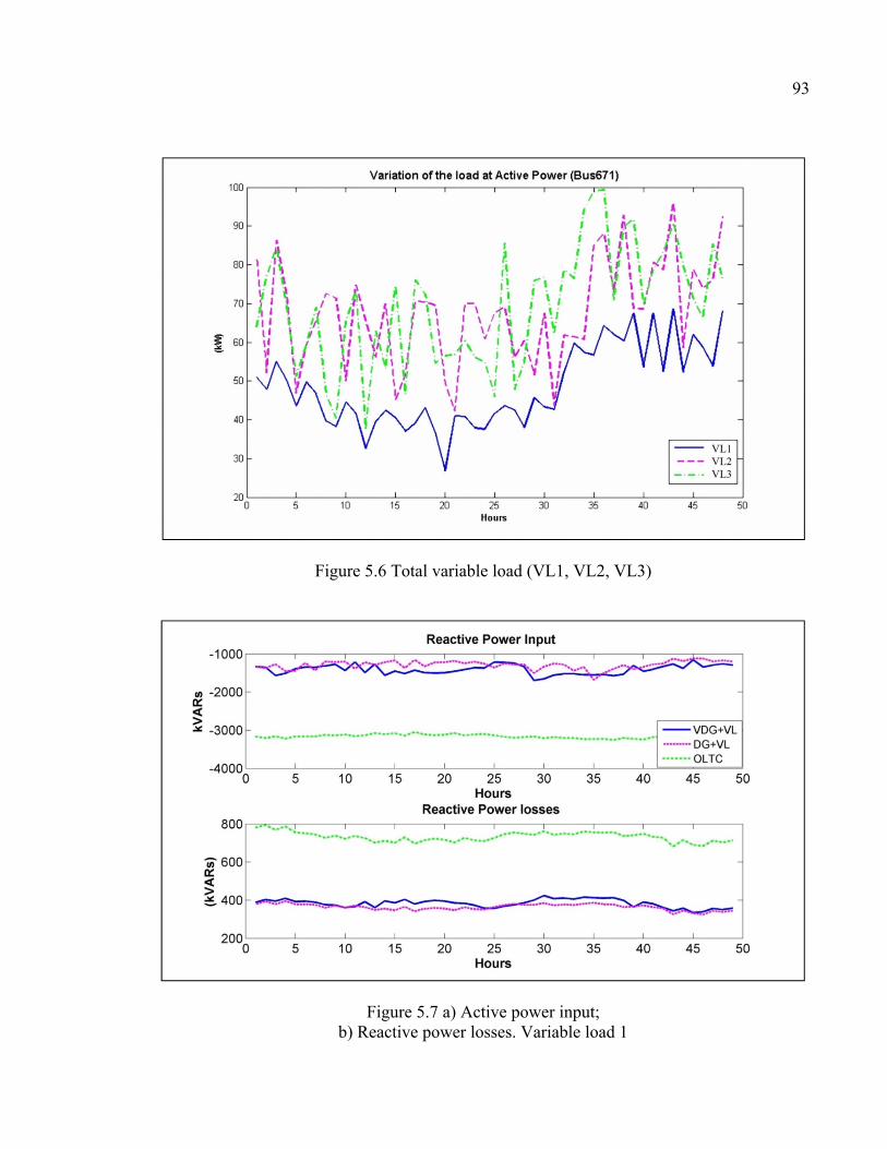
93

Figure 5.6 Total variable load (VL1, VL2, VL3)

Figure 5.7 a) Active power input; b) Reactive power losses. Variable load 1

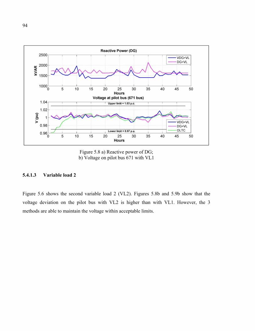
94

Figure 5.8 a) Reactive power of DG; b) Voltage on pilot bus 671 with VL1

5.4.1.3 Variable load 2

Figure 5.6 shows the second variable load 2 (VL2). Figures 5.8b and 5.9b show that the

voltage deviation on the pilot bus with VL2 is higher than with VL1. However, the 3

methods are able to maintain the voltage within acceptable limits.

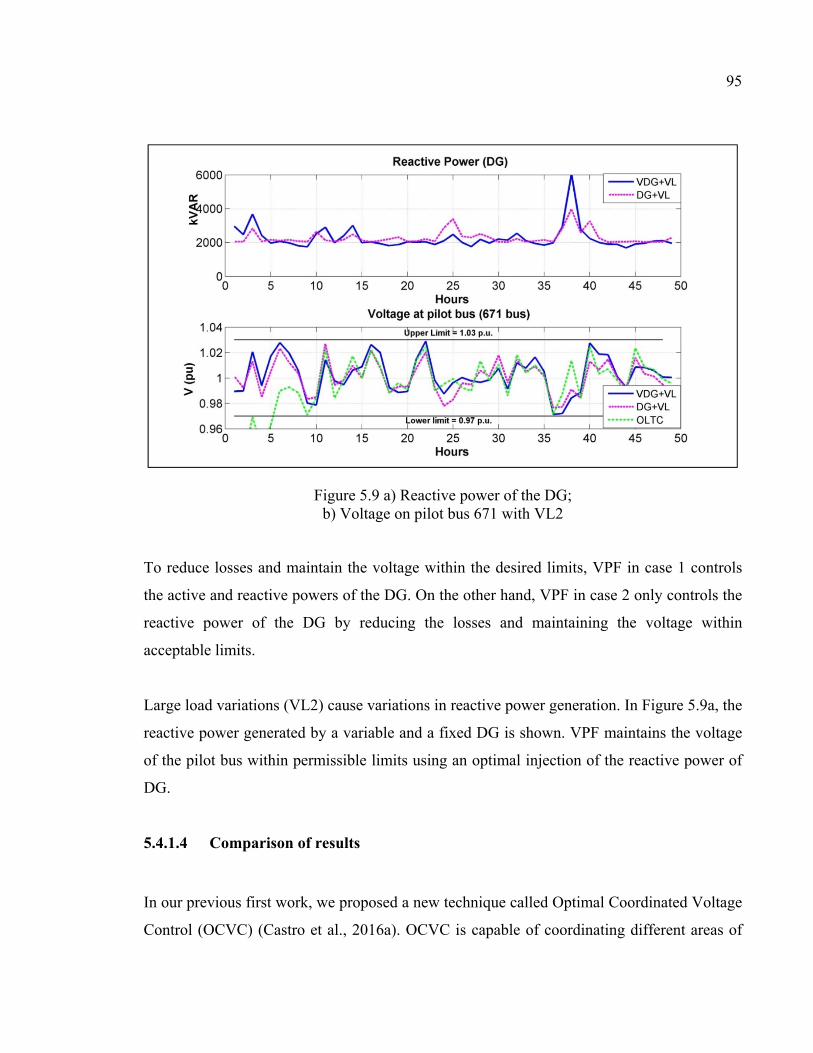
95

Figure 5.9 a) Reactive power of the DG; b) Voltage on pilot bus 671 with VL2

To reduce losses and maintain the voltage within the desired limits, VPF in case 1 controls

the active and reactive powers of the DG. On the other hand, VPF in case 2 only controls the

reactive power of the DG by reducing the losses and maintaining the voltage within

acceptable limits.

Large load variations (VL2) cause variations in reactive power generation. In Figure 5.9a, the

reactive power generated by a variable and a fixed DG is shown. VPF maintains the voltage

of the pilot bus within permissible limits using an optimal injection of the reactive power of

DG.

5.4.1.4 Comparison of results

In our previous first work, we proposed a new technique called Optimal Coordinated Voltage

Control (OCVC) (Castro et al., 2016a). OCVC is capable of coordinating different areas of

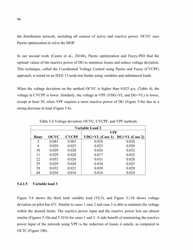
96

the distribution network, including all sources of active and reactive power. OCVC uses

Pareto optimization to solve the MOP.

In our second work (Castro et al., 2016b), Pareto optimization and Fuzzy-PID find the

optimal values of the reactive power of DG to minimize losses and reduce voltage deviation.

This technique, called the Coordinated Voltage Control using Pareto and Fuzzy (CVCPF)

approach, is tested on an IEEE 13-node test feeder using variables and unbalanced loads.

When the voltage deviation on the method OCVC is higher than 0.025 p.u. (Table 4), the

voltage in CVCPF is lower. Similarly, the voltage in VPF (VDG+VL and DG+VL) is lower,

except at hour 39, when VPF requires a more reactive power of DG (Figure 5.9a) due to a

strong decrease in load (Figure 5.6).

Table 5.4 Voltage deviation. OCVC, CVCPF, and VPF methods

Variable Load 2 VPF

Hour OCVC CVCPF VDG+VL (Case 1) DG+VL (Case 2) 3 0.081 0.065 0.028 0.0284 0.039 0.023 0.023 0.020 10 0.029 0.028 0.026 0.032 11 0.029 0.028 0.017 0.032 22 0.053 0.026 0.031 0.028 35 0.029 0.028 0.034 0.025 39 0.032 0.021 0.039 0.029 44 0.026 0.016 0.016 0.024

5.4.1.5 Variable load 3

Figure 5.6 shows the third total variable load (VL3), and Figure 5.11b shows voltage

deviation on pilot bus 671. Similar to cases 1 case 2 and case 3 is able to maintain the voltage

within the desired limits. The reactive power input and the reactive power loss are almost

similar (Figures 5.10a and 5.10 b) for cases 1 and 2. A side benefit of minimizing the reactive

power input of the network using VPF is the reduction of losses it entails, as compared to

OLTC (Figure 10b).

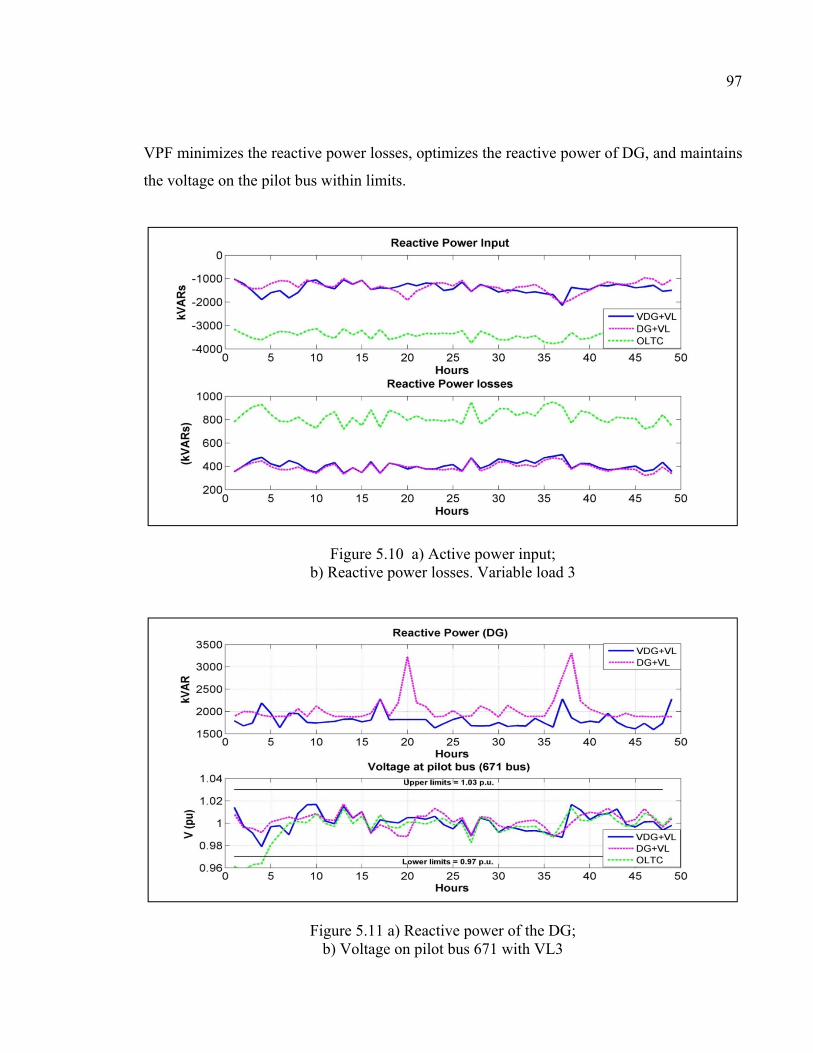
97

VPF minimizes the reactive power losses, optimizes the reactive power of DG, and maintains

the voltage on the pilot bus within limits.

Figure 5.10 a) Active power input; b) Reactive power losses. Variable load 3

Figure 5.11 a) Reactive power of the DG; b) Voltage on pilot bus 671 with VL3

98

Figure 5.12 Size of the active power of the DG (Variable loads VL1, VL2 and VL3)

Figure 5.12 shows the sizes of the DGs (fixed and variable) for each variable load.

5.4.2 IEEE 123-node test feeder

In the IEEE 123-node test feeder, four DGs are connected at buses 76, 67, 57 and 98 (Dahal

et Salehfar, 2013). The DGs’ sizes are calculated using VPF for a network with variable and

unbalanced loads. Figure 5.13 shows the location of the four DGs.

Figure 5.14a shows the total variation load (VL) added to the fixed load of the network.

Figure 5.14b shows the variation load on the pilot bus (bus 99). The variation load is on the

91 spot loads of the IEEE 123-node test feeder.

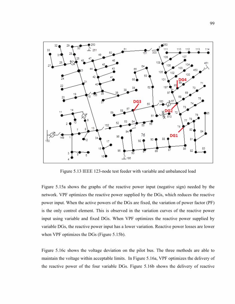
99

Figure 5.13 IEEE 123-node test feeder with variable and unbalanced load

Figure 5.15a shows the graphs of the reactive power input (negative sign) needed by the

network. VPF optimizes the reactive power supplied by the DGs, which reduces the reactive

power input. When the active powers of the DGs are fixed, the variation of power factor (PF)

is the only control element. This is observed in the variation curves of the reactive power

input using variable and fixed DGs. When VPF optimizes the reactive power supplied by

variable DGs, the reactive power input has a lower variation. Reactive power losses are lower

when VPF optimizes the DGs (Figure 5.15b).

Figure 5.16c shows the voltage deviation on the pilot bus. The three methods are able to

maintain the voltage within acceptable limits. In Figure 5.16a, VPF optimizes the delivery of

the reactive power of the four variable DGs. Figure 5.16b shows the delivery of reactive

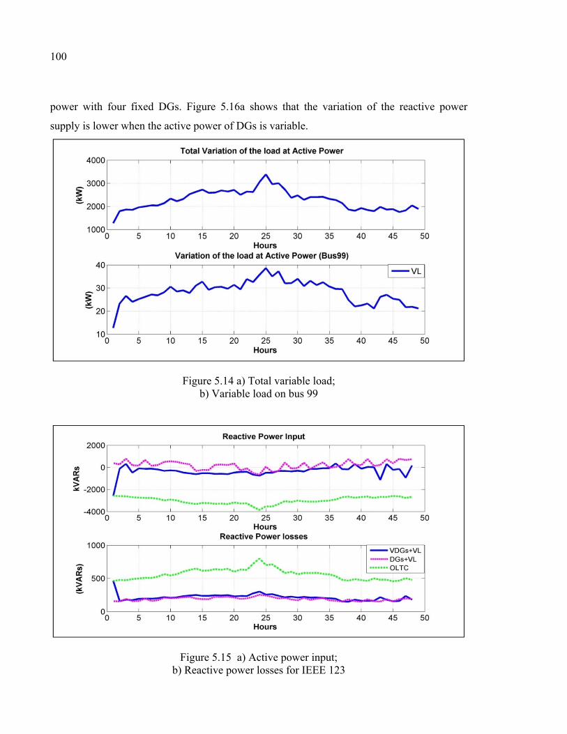
100

power with four fixed DGs. Figure 5.16a shows that the variation of the reactive power

supply is lower when the active power of DGs is variable.

Figure 5.14 a) Total variable load; b) Variable load on bus 99

Figure 5.15 a) Active power input; b) Reactive power losses for IEEE 123

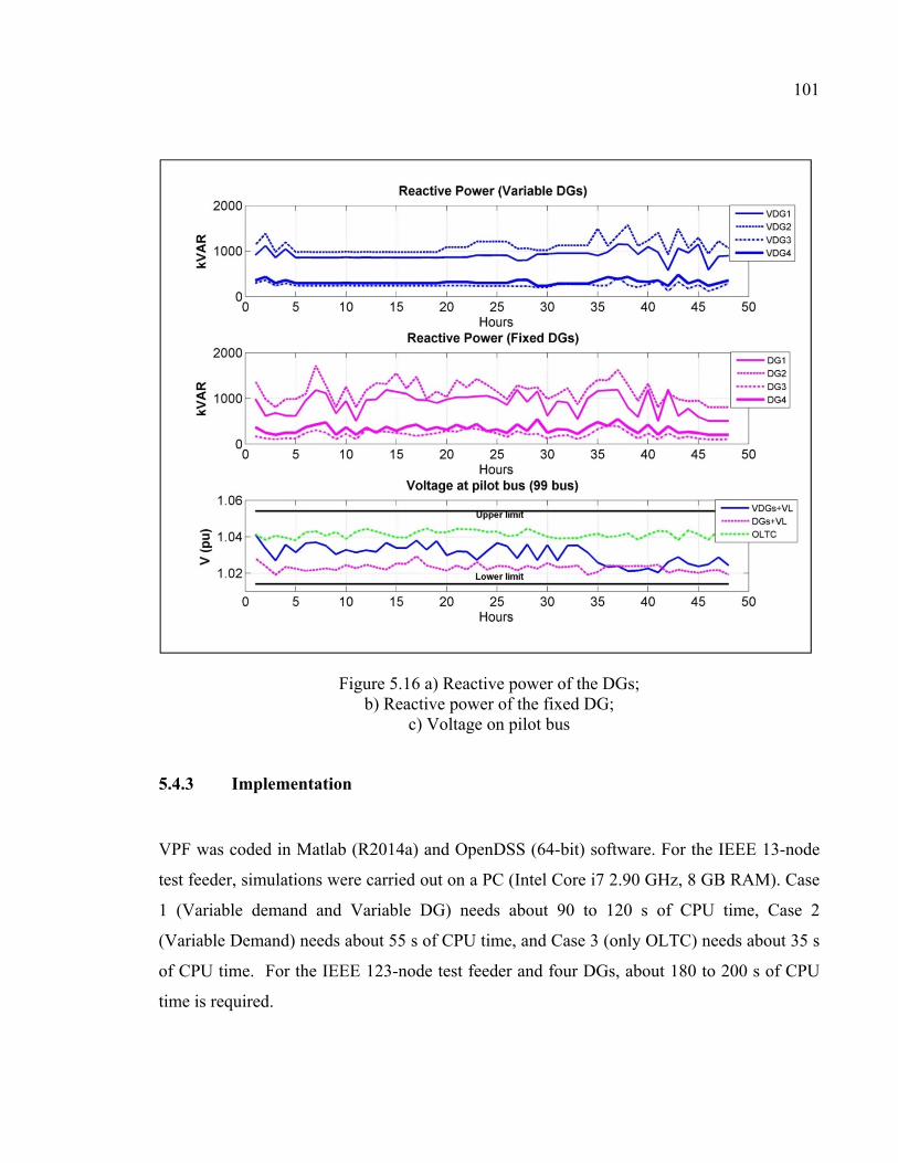
101

Figure 5.16 a) Reactive power of the DGs; b) Reactive power of the fixed DG;

c) Voltage on pilot bus

5.4.3 Implementation

VPF was coded in Matlab (R2014a) and OpenDSS (64-bit) software. For the IEEE 13-node

test feeder, simulations were carried out on a PC (Intel Core i7 2.90 GHz, 8 GB RAM). Case

1 (Variable demand and Variable DG) needs about 90 to 120 s of CPU time, Case 2

(Variable Demand) needs about 55 s of CPU time, and Case 3 (only OLTC) needs about 35 s

of CPU time. For the IEEE 123-node test feeder and four DGs, about 180 to 200 s of CPU

time is required.

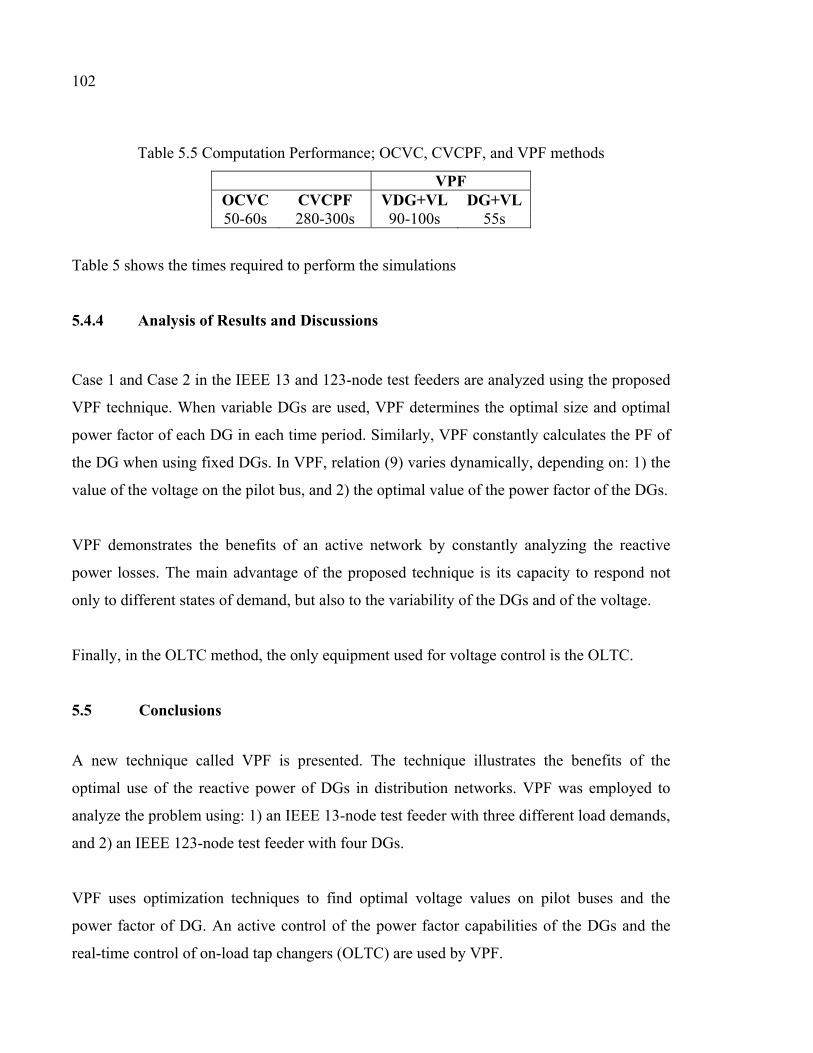
102

Table 5.5 Computation Performance; OCVC, CVCPF, and VPF methods

VPF OCVC CVCPF VDG+VL DG+VL50-60s 280-300s 90-100s 55s

Table 5 shows the times required to perform the simulations

5.4.4 Analysis of Results and Discussions

Case 1 and Case 2 in the IEEE 13 and 123-node test feeders are analyzed using the proposed

VPF technique. When variable DGs are used, VPF determines the optimal size and optimal

power factor of each DG in each time period. Similarly, VPF constantly calculates the PF of

the DG when using fixed DGs. In VPF, relation (9) varies dynamically, depending on: 1) the

value of the voltage on the pilot bus, and 2) the optimal value of the power factor of the DGs.

VPF demonstrates the benefits of an active network by constantly analyzing the reactive

power losses. The main advantage of the proposed technique is its capacity to respond not

only to different states of demand, but also to the variability of the DGs and of the voltage.

Finally, in the OLTC method, the only equipment used for voltage control is the OLTC.

5.5 Conclusions

A new technique called VPF is presented. The technique illustrates the benefits of the

optimal use of the reactive power of DGs in distribution networks. VPF was employed to

analyze the problem using: 1) an IEEE 13-node test feeder with three different load demands,

and 2) an IEEE 123-node test feeder with four DGs.

VPF uses optimization techniques to find optimal voltage values on pilot buses and the

power factor of DG. An active control of the power factor capabilities of the DGs and the

real-time control of on-load tap changers (OLTC) are used by VPF.

103

Acknowledgments

The authors would like to thank École de technologie supérieure and Hydro-Québec for the

support provided for this work.

CHAPTER 6

SUMMARY AND CONCLUSIONS 6.1 Summary

In the coming years, distributed generation (DG) will be a challenge in the distribution

network. In this problematic, our interest in this thesis is related to: the voltage on the buses,

the reactive power injection and power losses. This dissertation proposes through new

techniques the optimal coordination of the reactive power in the different areas of the

distribution network to improve voltage regulation, and reduce losses using DGs on

distribution networks with variable and unbalanced loads.

In this thesis, the primary objective of this work is the intelligent distribution voltage control

using the optimal participation of reactive power of a DG at variable and unbalanced

distribution network. The secondary objectives are as follows:

1) Investigate the impact of DG on losses and voltage profile

This objective was accomplished using a new technique called Optimal Coordinated Voltage

Control (OCVC). OCVC uses Pareto optimization to find an optimal participation of reactive

power of all devices available in the network. After validating effectiveness of the proposed

method on IEEE 13-node test feeder and IEEE 34-node test feeder with the initial loads, it

was then validated adding a DG in the network. Finally, the proposed method was also

validated adding a new load to simulate a disturbance. Pareto optimization was implemented

in simulink of Matlab and the distribution power flow was simulated using open source

software called OpenDSS. Results from the proposed method shows that the optimal

integration of DG in distribution networks can help to maintain the voltage within the limits

and reduce losses.

106

2) Improve and minimize the voltage variation in distribution network using DGs

This objective was accomplished by two optimization techniques: PID-Fuzzy Logic to find

the optimum value of the reactive power of the DG and Pareto optimization to find the

optimal value of the pilot bus voltage so that minimize the voltage variation in distribution

network. Coordinated Voltage Control using Pareto and Fuzzy logic (CVCPF) was proposed

by combining the optimization techniques. The proposed method was validated on IEEE 13-

node test feeder. Variables and unbalanced are used, based on real consumption, over a time

window of 48 hours. The results are compared with those obtained from the methods OCVC

and OLTC as well as from the case of no voltage control. The robustness of the proposed

method was demonstrated using three DGs simultaneously. Results from the proposed

method show that the optimal integration of DG in distribution network can help to minimize

the voltage variation and reduce losses.

3) Investigate the impact of variable and fixed DGs in distribution network

This objective was accomplished by implementation a new multi-objective model that

minimizes reactive power losses with the minimization of the variation of the voltage on the

pilot bus. DG with variable power factor (VPF) uses Fuzzy-PI controller according to the

optimal values given by Pareto, and calculates the power factor of the DGs. The proposed

method (VPF) was validated on IEEE 13 and 123-node test feeder with different and real

cases of variables loads and four DGs. These networks were analyzed from two perspectives;

the first with variable DGs, changing according to demand variations, and the second with

fixed DGs. The results are compared with those obtained from the method OLTC as well as

from the case of fixed and variable DGs. Result from the proposed method shows that VPF

allows to optimize the DGs of the distribution network to maintain the voltage within

permissible limits and reduce reactive power losses.

107

6.2 Conclusions

The work of this thesis is to study the impact of DGs in distribution networks. The new

methods, a MO problem focusing on voltage profile improvement, power loss reduction and

voltage stability was formulated to find the optimal participation of DG.

Firstly, the methodology used is a comparative analysis. We have proposed a new method for

solving the MO problem. The results of this method have been verified with others two

methods used in distribution networks.

The results have resulted in the following conclusions:

• The optimal participation of active and reactive power of DGs connected to the

distribution network.

• Solve all the different objectives of the multi-objective problem separately with dynamic

weights.

• Eliminate the entire voltage problem, including the DG’s over-voltages.

• The method OCVC could be interesting way to reduce or eliminate future investments in

voltage control and reactive power regulation.

Secondly, an efficient algorithm to solve the multi-objective voltage control problem is

presented. Fuzzy logic to calculate the optimal reactive power of DG and the PID generates a

solution based on the difference between the power factor calculated by fuzzy logic and the

output power factor of the network. The results of Pareto and PID-Fuzzy Logic with DGs

have resulted in the following conclusions:

• The reduction of the voltage variation more than other methods is demonstrated.

• The optimal integration of DGs in distribution networks helps to maintain stable voltage

and to reduce losses.

108

• CVCPF could be advantageous for network operators by the development of flexible

systems.

Thirdly, an experimental design methodology was used to demonstrate the benefits of using

the reactive power of the variables and fixed DGs in distribution network. The problem was

formulated as multi-objective problem with two objectives. The first objective was to

minimize the variation voltage and the second objective was the management of the loss

reduction. The results of Pareto and Fuzzy-PI controller have resulted in the following

conclusions:

• The reduction of the voltage variation and the losses on distribution networks using DGs

is demonstrated.

• The benefits that the better use of reactive power of DGs on distribution network.

• The advantages of optimizing the multi-objective problem with Pareto and Fuzzy-PI

controller.

• The use of fixed and variable DGs on distribution network.

6.3 Recommendations for future work

Although the work presented in this thesis provides methods and results for DGs integration

on distribution network, it can be extended in the following research directions.

• Variable Decision Maker (DM) to choose a set of solutions according to distribution

network conditions.

• The impact of DGs on economic resources. One objective of the multi-objective problem

should be the cost of implementation, the maintenance costs and the cost of connection.

• The impact of DGs on the frequency, voltage stabilization and reactive power regulations

should be addressed carefully.

• Reactive power compensation in single-phase.

109

• To use the methods proposed to determine the best location of the DG in distribution

network.

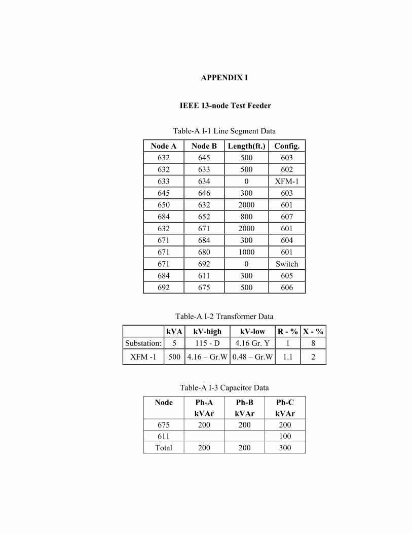
APPENDIX I

IEEE 13-node Test Feeder

Table-A I-1 Line Segment Data

Node A Node B Length(ft.) Config.

632 645 500 603

632 633 500 602

633 634 0 XFM-1

645 646 300 603

650 632 2000 601

684 652 800 607

632 671 2000 601

671 684 300 604

671 680 1000 601

671 692 0 Switch

684 611 300 605

692 675 500 606

Table-A I-2 Transformer Data

kVA kV-high kV-low R - % X - %

Substation: 5 115 - D 4.16 Gr. Y 1 8

XFM -1 500 4.16 – Gr.W 0.48 – Gr.W 1.1 2

Table-A I-3 Capacitor Data

Node Ph-A Ph-B Ph-C kVAr kVAr kVAr

675 200 200 200

611 100

Total 200 200 300

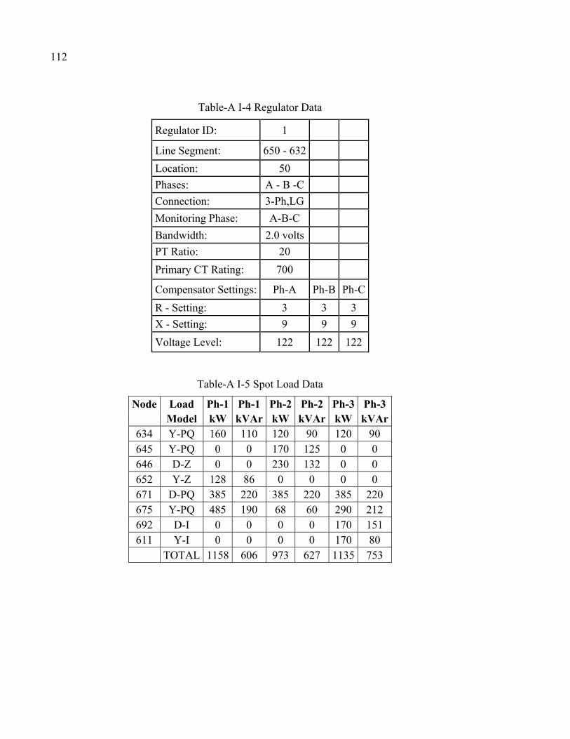
112

Table-A I-4 Regulator Data

Regulator ID: 1

Line Segment: 650 - 632

Location: 50

Phases: A - B -C

Connection: 3-Ph,LG

Monitoring Phase: A-B-C

Bandwidth: 2.0 volts

PT Ratio: 20

Primary CT Rating: 700

Compensator Settings: Ph-A Ph-B Ph-C

R - Setting: 3 3 3

X - Setting: 9 9 9

Voltage Level: 122 122 122

Table-A I-5 Spot Load Data

Node Load Ph-1 Ph-1 Ph-2 Ph-2 Ph-3 Ph-3 Model kW kVAr kW kVAr kW kVAr

634 Y-PQ 160 110 120 90 120 90 645 Y-PQ 0 0 170 125 0 0 646 D-Z 0 0 230 132 0 0 652 Y-Z 128 86 0 0 0 0 671 D-PQ 385 220 385 220 385 220 675 Y-PQ 485 190 68 60 290 212 692 D-I 0 0 0 0 170 151 611 Y-I 0 0 0 0 170 80

TOTAL 1158 606 973 627 1135 753

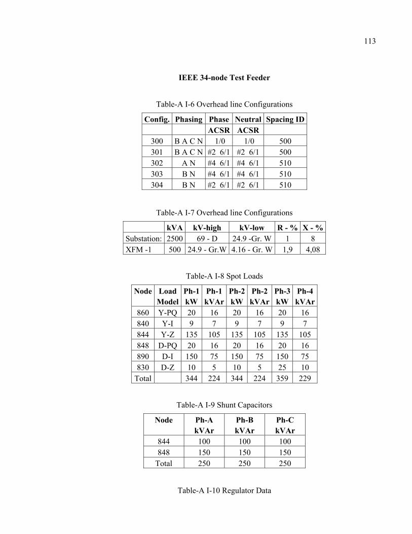
113

IEEE 34-node Test Feeder

Table-A I-6 Overhead line Configurations

Config. Phasing Phase Neutral Spacing ID ACSR ACSR

300 B A C N 1/0 1/0 500 301 B A C N #2 6/1 #2 6/1 500 302 A N #4 6/1 #4 6/1 510 303 B N #4 6/1 #4 6/1 510 304 B N #2 6/1 #2 6/1 510

Table-A I-7 Overhead line Configurations

kVA kV-high kV-low R - % X - % Substation: 2500 69 - D 24.9 -Gr. W 1 8 XFM -1 500 24.9 - Gr.W 4.16 - Gr. W 1,9 4,08

Table-A I-8 Spot Loads

Node Load Ph-1 Ph-1 Ph-2 Ph-2 Ph-3 Ph-4 Model kW kVAr kW kVAr kW kVAr

860 Y-PQ 20 16 20 16 20 16 840 Y-I 9 7 9 7 9 7 844 Y-Z 135 105 135 105 135 105 848 D-PQ 20 16 20 16 20 16 890 D-I 150 75 150 75 150 75 830 D-Z 10 5 10 5 25 10

Total 344 224 344 224 359 229

Table-A I-9 Shunt Capacitors

Node Ph-A Ph-B Ph-C kVAr kVAr kVAr

844 100 100 100 848 150 150 150

Total 250 250 250

Table-A I-10 Regulator Data

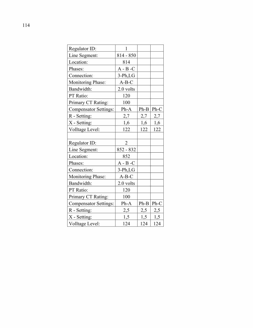
114

Regulator ID: 1 Line Segment: 814 - 850 Location: 814 Phases: A - B -C Connection: 3-Ph,LG Monitoring Phase: A-B-C Bandwidth: 2.0 volts PT Ratio: 120 Primary CT Rating: 100 Compensator Settings: Ph-A Ph-B Ph-CR - Setting: 2,7 2,7 2,7 X - Setting: 1,6 1,6 1,6 Volltage Level: 122 122 122 Regulator ID: 2 Line Segment: 852 - 832 Location: 852 Phases: A - B -C Connection: 3-Ph,LG Monitoring Phase: A-B-C Bandwidth: 2.0 volts PT Ratio: 120 Primary CT Rating: 100 Compensator Settings: Ph-A Ph-B Ph-CR - Setting: 2,5 2,5 2,5 X - Setting: 1,5 1,5 1,5 Volltage Level: 124 124 124

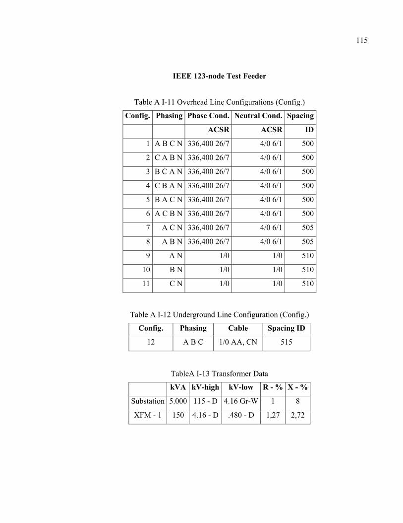
115

IEEE 123-node Test Feeder

Table A I-11 Overhead Line Configurations (Config.)

Config. Phasing Phase Cond. Neutral Cond. Spacing

ACSR ACSR ID

1 A B C N 336,400 26/7 4/0 6/1 500

2 C A B N 336,400 26/7 4/0 6/1 500

3 B C A N 336,400 26/7 4/0 6/1 500

4 C B A N 336,400 26/7 4/0 6/1 500

5 B A C N 336,400 26/7 4/0 6/1 500

6 A C B N 336,400 26/7 4/0 6/1 500

7 A C N 336,400 26/7 4/0 6/1 505

8 A B N 336,400 26/7 4/0 6/1 505

9 A N 1/0 1/0 510

10 B N 1/0 1/0 510

11 C N 1/0 1/0 510

Table A I-12 Underground Line Configuration (Config.)

Config. Phasing Cable Spacing ID

12 A B C 1/0 AA, CN 515

TableA I-13 Transformer Data

kVA kV-high kV-low R - % X - %

Substation 5.000 115 - D 4.16 Gr-W 1 8

XFM - 1 150 4.16 - D .480 - D 1,27 2,72

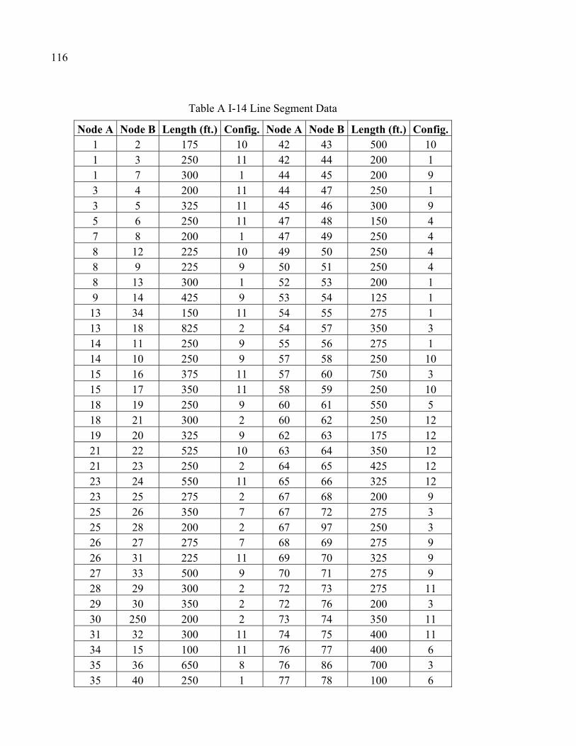
116

Table A I-14 Line Segment Data

Node A Node B Length (ft.) Config. Node A Node B Length (ft.) Config. 1 2 175 10 42 43 500 10 1 3 250 11 42 44 200 1 1 7 300 1 44 45 200 9 3 4 200 11 44 47 250 1 3 5 325 11 45 46 300 9 5 6 250 11 47 48 150 4 7 8 200 1 47 49 250 4 8 12 225 10 49 50 250 4 8 9 225 9 50 51 250 4 8 13 300 1 52 53 200 1 9 14 425 9 53 54 125 1 13 34 150 11 54 55 275 1 13 18 825 2 54 57 350 3 14 11 250 9 55 56 275 1 14 10 250 9 57 58 250 10 15 16 375 11 57 60 750 3 15 17 350 11 58 59 250 10 18 19 250 9 60 61 550 5 18 21 300 2 60 62 250 12 19 20 325 9 62 63 175 12 21 22 525 10 63 64 350 12 21 23 250 2 64 65 425 12 23 24 550 11 65 66 325 12 23 25 275 2 67 68 200 9 25 26 350 7 67 72 275 3 25 28 200 2 67 97 250 3 26 27 275 7 68 69 275 9 26 31 225 11 69 70 325 9 27 33 500 9 70 71 275 9 28 29 300 2 72 73 275 11 29 30 350 2 72 76 200 3 30 250 200 2 73 74 350 11 31 32 300 11 74 75 400 11 34 15 100 11 76 77 400 6 35 36 650 8 76 86 700 3 35 40 250 1 77 78 100 6

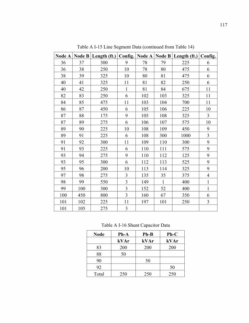
117

Table A I-15 Line Segment Data (continued from Table 14)

Node A Node B Length (ft.) Config. Node A Node B Length (ft.) Config.36 37 300 9 78 79 225 6 36 38 250 10 78 80 475 6 38 39 325 10 80 81 475 6 40 41 325 11 81 82 250 6 40 42 250 1 81 84 675 11 82 83 250 6 102 103 325 11 84 85 475 11 103 104 700 11 86 87 450 6 105 106 225 10 87 88 175 9 105 108 325 3 87 89 275 6 106 107 575 10 89 90 225 10 108 109 450 9 89 91 225 6 108 300 1000 3 91 92 300 11 109 110 300 9 91 93 225 6 110 111 575 9 93 94 275 9 110 112 125 9 93 95 300 6 112 113 525 9 95 96 200 10 113 114 325 9 97 98 275 3 135 35 375 4 98 99 550 3 149 1 400 1 99 100 300 3 152 52 400 1 100 450 800 3 160 67 350 6 101 102 225 11 197 101 250 3 101 105 275 3

Table A I-16 Shunt Capacitor Data

Node Ph-A Ph-B Ph-C kVAr kVAr kVAr

83 200 200 200 88 50 90 50 92 50

Total 250 250 250

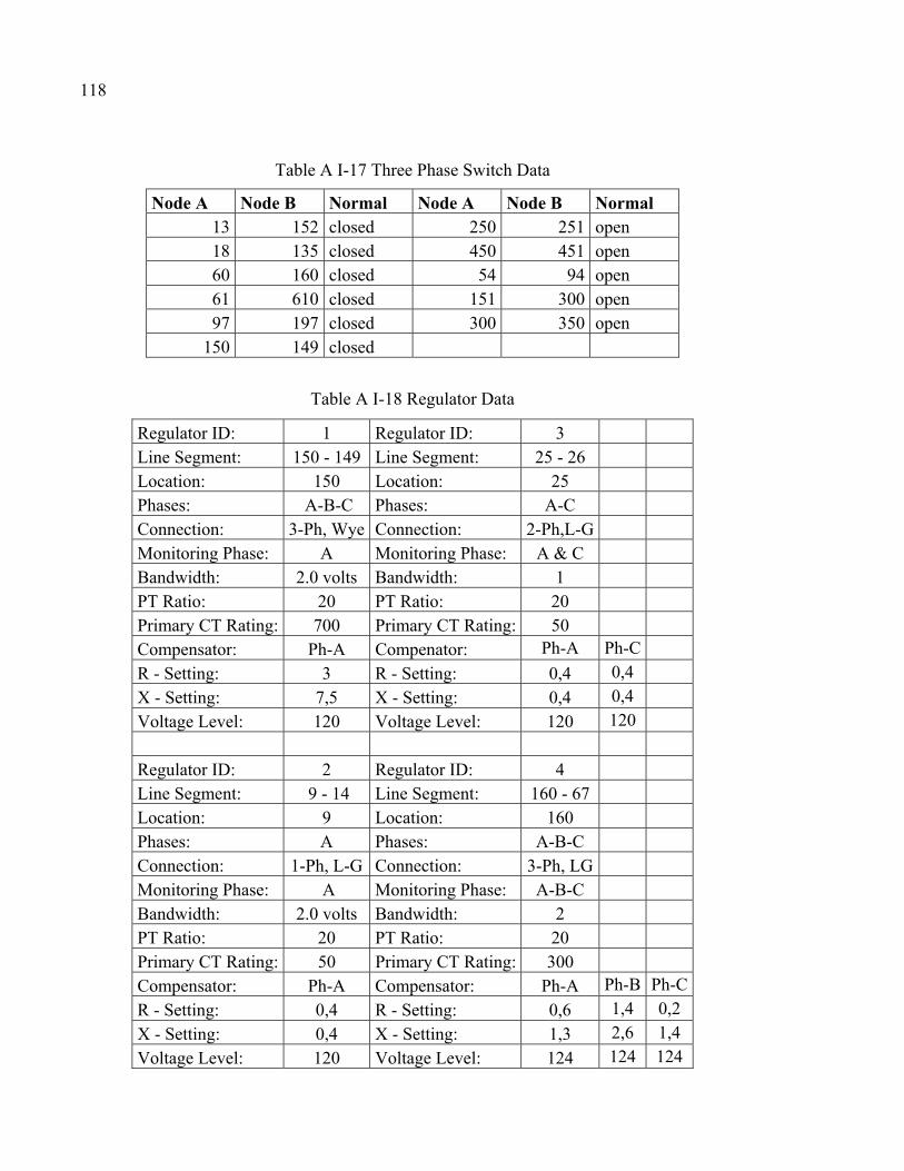
118

Table A I-17 Three Phase Switch Data

Node A Node B Normal Node A Node B Normal 13 152 closed 250 251 open 18 135 closed 450 451 open 60 160 closed 54 94 open 61 610 closed 151 300 open 97 197 closed 300 350 open

150 149 closed

Table A I-18 Regulator Data

Regulator ID: 1 Regulator ID: 3 Line Segment: 150 - 149 Line Segment: 25 - 26 Location: 150 Location: 25 Phases: A-B-C Phases: A-C Connection: 3-Ph, Wye Connection: 2-Ph,L-G Monitoring Phase: A Monitoring Phase: A & C Bandwidth: 2.0 volts Bandwidth: 1 PT Ratio: 20 PT Ratio: 20 Primary CT Rating: 700 Primary CT Rating: 50 Compensator: Ph-A Compenator: Ph-A Ph-C

R - Setting: 3 R - Setting: 0,4 0,4

X - Setting: 7,5 X - Setting: 0,4 0,4

Voltage Level: 120 Voltage Level: 120 120

Regulator ID: 2 Regulator ID: 4

Line Segment: 9 - 14 Line Segment: 160 - 67

Location: 9 Location: 160

Phases: A Phases: A-B-C

Connection: 1-Ph, L-G Connection: 3-Ph, LG

Monitoring Phase: A Monitoring Phase: A-B-C

Bandwidth: 2.0 volts Bandwidth: 2

PT Ratio: 20 PT Ratio: 20

Primary CT Rating: 50 Primary CT Rating: 300

Compensator: Ph-A Compensator: Ph-A Ph-B Ph-C

R - Setting: 0,4 R - Setting: 0,6 1,4 0,2

X - Setting: 0,4 X - Setting: 1,3 2,6 1,4

Voltage Level: 120 Voltage Level: 124 124 124

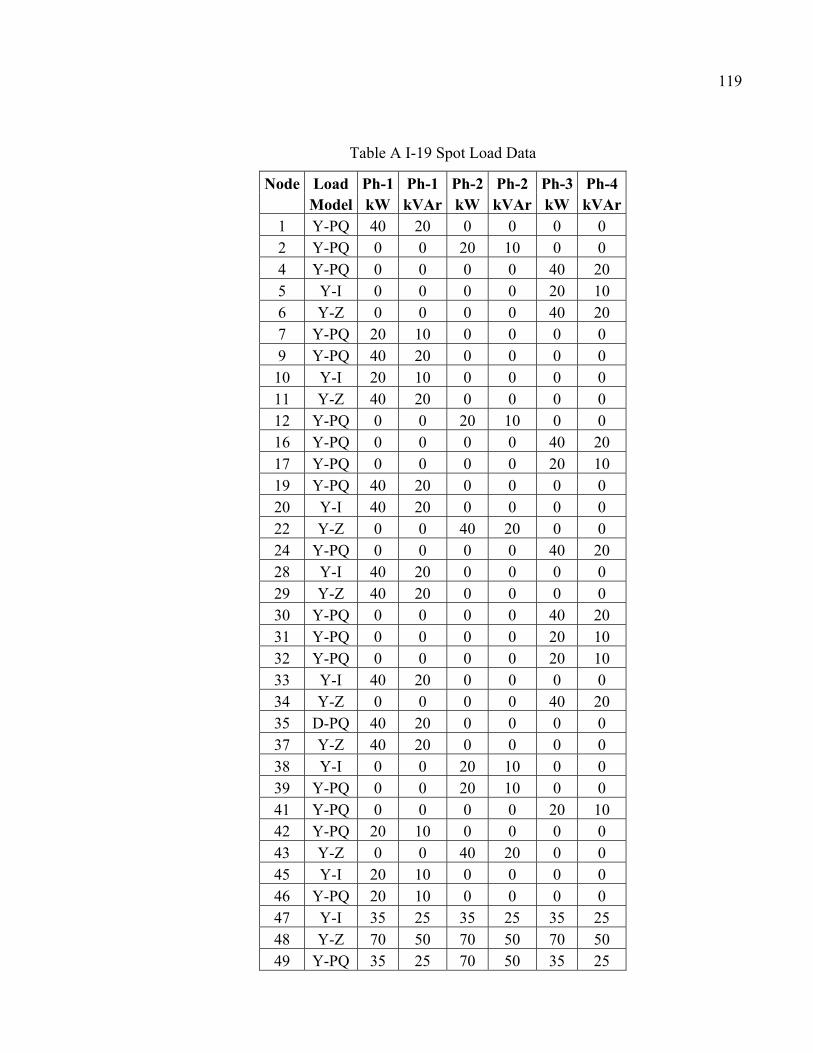
119

Table A I-19 Spot Load Data

Node Load Ph-1 Ph-1 Ph-2 Ph-2 Ph-3 Ph-4 Model kW kVAr kW kVAr kW kVAr 1 Y-PQ 40 20 0 0 0 0 2 Y-PQ 0 0 20 10 0 0 4 Y-PQ 0 0 0 0 40 20 5 Y-I 0 0 0 0 20 10 6 Y-Z 0 0 0 0 40 20 7 Y-PQ 20 10 0 0 0 0 9 Y-PQ 40 20 0 0 0 0 10 Y-I 20 10 0 0 0 0 11 Y-Z 40 20 0 0 0 0 12 Y-PQ 0 0 20 10 0 0 16 Y-PQ 0 0 0 0 40 20 17 Y-PQ 0 0 0 0 20 10 19 Y-PQ 40 20 0 0 0 0 20 Y-I 40 20 0 0 0 0 22 Y-Z 0 0 40 20 0 0 24 Y-PQ 0 0 0 0 40 20 28 Y-I 40 20 0 0 0 0 29 Y-Z 40 20 0 0 0 0 30 Y-PQ 0 0 0 0 40 20 31 Y-PQ 0 0 0 0 20 10 32 Y-PQ 0 0 0 0 20 10 33 Y-I 40 20 0 0 0 0 34 Y-Z 0 0 0 0 40 20 35 D-PQ 40 20 0 0 0 0 37 Y-Z 40 20 0 0 0 0 38 Y-I 0 0 20 10 0 0 39 Y-PQ 0 0 20 10 0 0 41 Y-PQ 0 0 0 0 20 10 42 Y-PQ 20 10 0 0 0 0 43 Y-Z 0 0 40 20 0 0 45 Y-I 20 10 0 0 0 0 46 Y-PQ 20 10 0 0 0 0 47 Y-I 35 25 35 25 35 25 48 Y-Z 70 50 70 50 70 50 49 Y-PQ 35 25 70 50 35 25

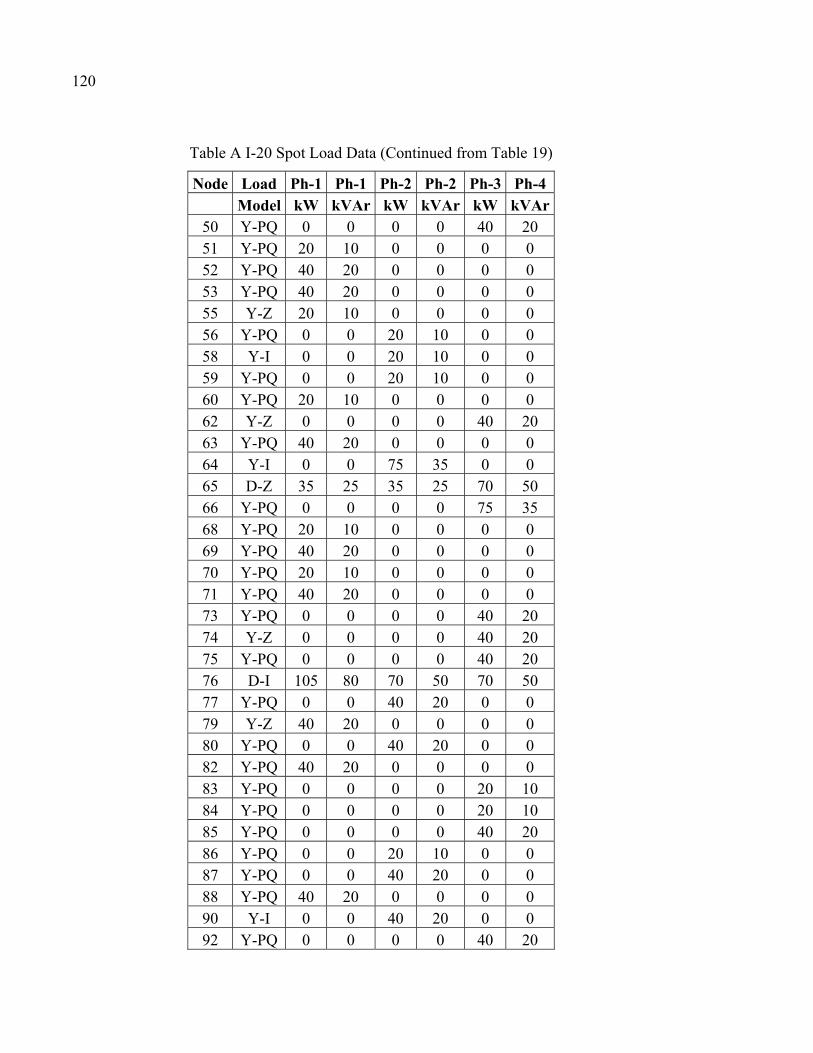
120

Table A I-20 Spot Load Data (Continued from Table 19)

Node Load Ph-1 Ph-1 Ph-2 Ph-2 Ph-3 Ph-4 Model kW kVAr kW kVAr kW kVAr

50 Y-PQ 0 0 0 0 40 20 51 Y-PQ 20 10 0 0 0 0 52 Y-PQ 40 20 0 0 0 0 53 Y-PQ 40 20 0 0 0 0 55 Y-Z 20 10 0 0 0 0 56 Y-PQ 0 0 20 10 0 0 58 Y-I 0 0 20 10 0 0 59 Y-PQ 0 0 20 10 0 0 60 Y-PQ 20 10 0 0 0 0 62 Y-Z 0 0 0 0 40 20 63 Y-PQ 40 20 0 0 0 0 64 Y-I 0 0 75 35 0 0 65 D-Z 35 25 35 25 70 50 66 Y-PQ 0 0 0 0 75 35 68 Y-PQ 20 10 0 0 0 0 69 Y-PQ 40 20 0 0 0 0 70 Y-PQ 20 10 0 0 0 0 71 Y-PQ 40 20 0 0 0 0 73 Y-PQ 0 0 0 0 40 20 74 Y-Z 0 0 0 0 40 20 75 Y-PQ 0 0 0 0 40 20 76 D-I 105 80 70 50 70 50 77 Y-PQ 0 0 40 20 0 0 79 Y-Z 40 20 0 0 0 0 80 Y-PQ 0 0 40 20 0 0 82 Y-PQ 40 20 0 0 0 0 83 Y-PQ 0 0 0 0 20 10 84 Y-PQ 0 0 0 0 20 10 85 Y-PQ 0 0 0 0 40 20 86 Y-PQ 0 0 20 10 0 0 87 Y-PQ 0 0 40 20 0 0 88 Y-PQ 40 20 0 0 0 0 90 Y-I 0 0 40 20 0 0 92 Y-PQ 0 0 0 0 40 20

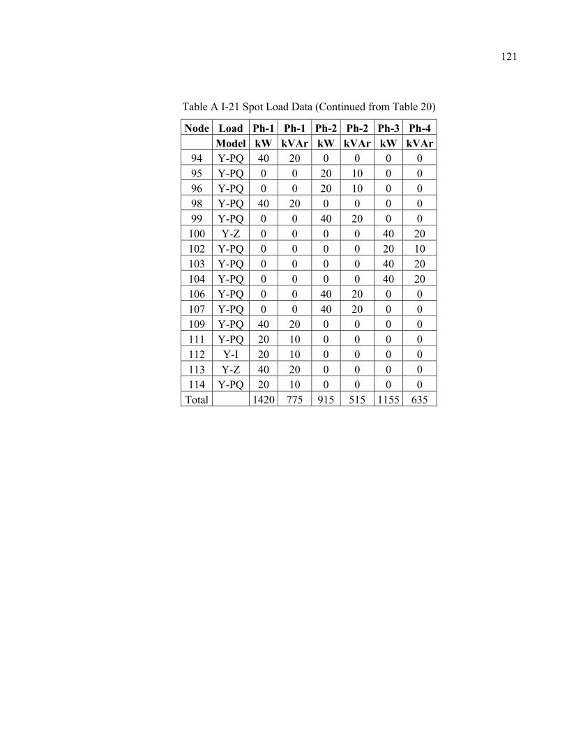
121

Table A I-21 Spot Load Data (Continued from Table 20)

Node Load Ph-1 Ph-1 Ph-2 Ph-2 Ph-3 Ph-4 Model kW kVAr kW kVAr kW kVAr

94 Y-PQ 40 20 0 0 0 0 95 Y-PQ 0 0 20 10 0 0 96 Y-PQ 0 0 20 10 0 0 98 Y-PQ 40 20 0 0 0 0 99 Y-PQ 0 0 40 20 0 0 100 Y-Z 0 0 0 0 40 20 102 Y-PQ 0 0 0 0 20 10 103 Y-PQ 0 0 0 0 40 20 104 Y-PQ 0 0 0 0 40 20 106 Y-PQ 0 0 40 20 0 0 107 Y-PQ 0 0 40 20 0 0 109 Y-PQ 40 20 0 0 0 0 111 Y-PQ 20 10 0 0 0 0 112 Y-I 20 10 0 0 0 0 113 Y-Z 40 20 0 0 0 0 114 Y-PQ 20 10 0 0 0 0

Total 1420 775 915 515 1155 635

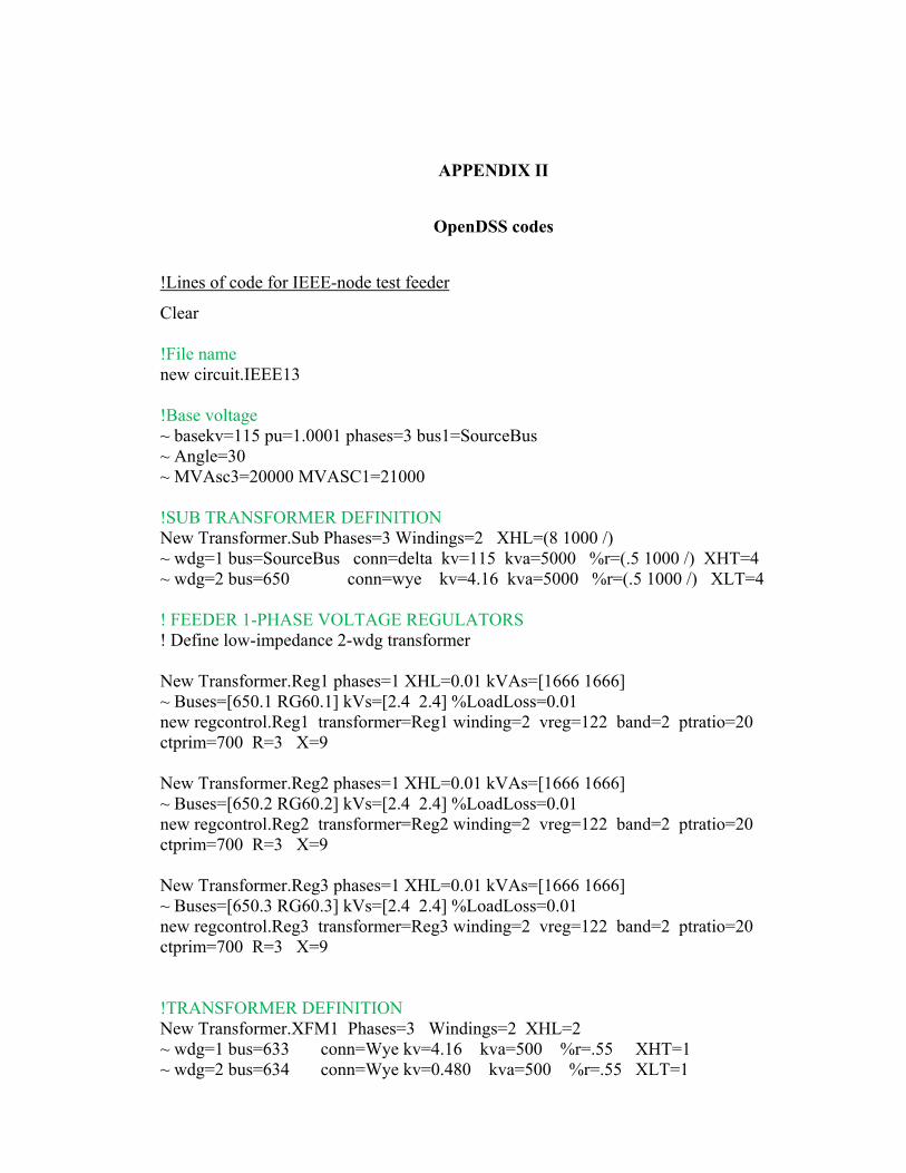
APPENDIX II

OpenDSS codes

!Lines of code for IEEE-node test feeder

Clear !File name new circuit.IEEE13 !Base voltage ~ basekv=115 pu=1.0001 phases=3 bus1=SourceBus ~ Angle=30 ~ MVAsc3=20000 MVASC1=21000 !SUB TRANSFORMER DEFINITION New Transformer.Sub Phases=3 Windings=2 XHL=(8 1000 /) ~ wdg=1 bus=SourceBus conn=delta kv=115 kva=5000 %r=(.5 1000 /) XHT=4 ~ wdg=2 bus=650 conn=wye kv=4.16 kva=5000 %r=(.5 1000 /) XLT=4 ! FEEDER 1-PHASE VOLTAGE REGULATORS ! Define low-impedance 2-wdg transformer New Transformer.Reg1 phases=1 XHL=0.01 kVAs=[1666 1666] ~ Buses=[650.1 RG60.1] kVs=[2.4 2.4] %LoadLoss=0.01 new regcontrol.Reg1 transformer=Reg1 winding=2 vreg=122 band=2 ptratio=20 ctprim=700 R=3 X=9 New Transformer.Reg2 phases=1 XHL=0.01 kVAs=[1666 1666] ~ Buses=[650.2 RG60.2] kVs=[2.4 2.4] %LoadLoss=0.01 new regcontrol.Reg2 transformer=Reg2 winding=2 vreg=122 band=2 ptratio=20 ctprim=700 R=3 X=9 New Transformer.Reg3 phases=1 XHL=0.01 kVAs=[1666 1666] ~ Buses=[650.3 RG60.3] kVs=[2.4 2.4] %LoadLoss=0.01 new regcontrol.Reg3 transformer=Reg3 winding=2 vreg=122 band=2 ptratio=20 ctprim=700 R=3 X=9 !TRANSFORMER DEFINITION New Transformer.XFM1 Phases=3 Windings=2 XHL=2 ~ wdg=1 bus=633 conn=Wye kv=4.16 kva=500 %r=.55 XHT=1 ~ wdg=2 bus=634 conn=Wye kv=0.480 kva=500 %r=.55 XLT=1

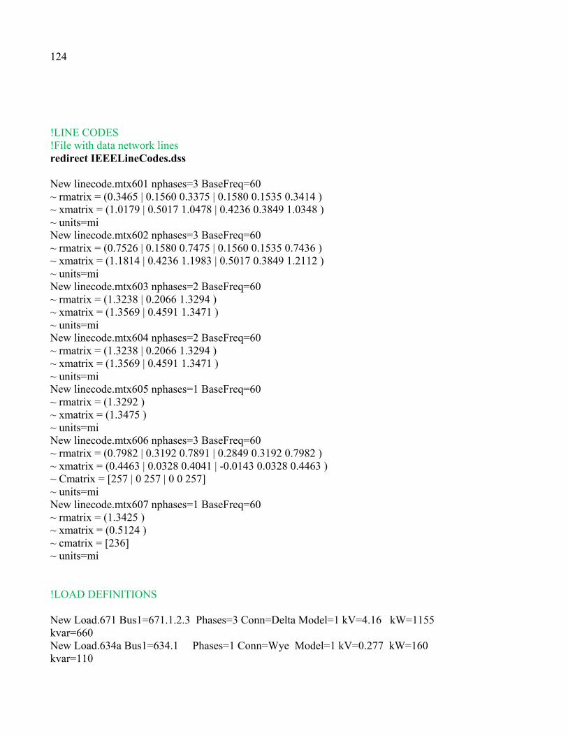
124

!LINE CODES !File with data network lines redirect IEEELineCodes.dss New linecode.mtx601 nphases=3 BaseFreq=60 ~ rmatrix = (0.3465 | 0.1560 0.3375 | 0.1580 0.1535 0.3414 ) ~ xmatrix = (1.0179 | 0.5017 1.0478 | 0.4236 0.3849 1.0348 ) ~ units=mi New linecode.mtx602 nphases=3 BaseFreq=60 ~ rmatrix = (0.7526 | 0.1580 0.7475 | 0.1560 0.1535 0.7436 ) ~ xmatrix = (1.1814 | 0.4236 1.1983 | 0.5017 0.3849 1.2112 ) ~ units=mi New linecode.mtx603 nphases=2 BaseFreq=60 ~ rmatrix = (1.3238 | 0.2066 1.3294 ) ~ xmatrix = (1.3569 | 0.4591 1.3471 ) ~ units=mi New linecode.mtx604 nphases=2 BaseFreq=60 ~ rmatrix = (1.3238 | 0.2066 1.3294 ) ~ xmatrix = (1.3569 | 0.4591 1.3471 ) ~ units=mi New linecode.mtx605 nphases=1 BaseFreq=60 ~ rmatrix = (1.3292 ) ~ xmatrix = (1.3475 ) ~ units=mi New linecode.mtx606 nphases=3 BaseFreq=60 ~ rmatrix = (0.7982 | 0.3192 0.7891 | 0.2849 0.3192 0.7982 ) ~ xmatrix = (0.4463 | 0.0328 0.4041 | -0.0143 0.0328 0.4463 ) ~ Cmatrix = [257 | 0 257 | 0 0 257] ~ units=mi New linecode.mtx607 nphases=1 BaseFreq=60 ~ rmatrix = (1.3425 ) ~ xmatrix = (0.5124 ) ~ cmatrix = [236] ~ units=mi !LOAD DEFINITIONS New Load.671 Bus1=671.1.2.3 Phases=3 Conn=Delta Model=1 kV=4.16 kW=1155 kvar=660 New Load.634a Bus1=634.1 Phases=1 Conn=Wye Model=1 kV=0.277 kW=160 kvar=110

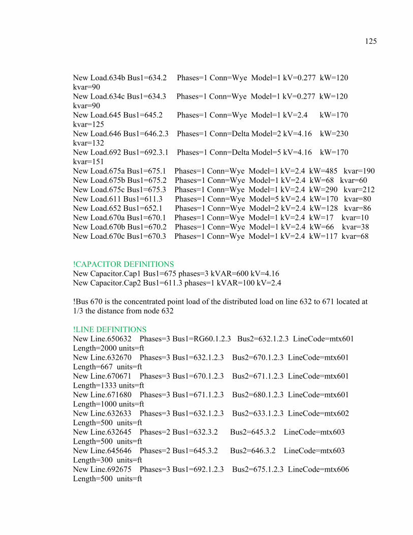
125

New Load.634b Bus1=634.2 Phases=1 Conn=Wye Model=1 kV=0.277 kW=120 kvar=90 New Load.634c Bus1=634.3 Phases=1 Conn=Wye Model=1 kV=0.277 kW=120 kvar=90 New Load.645 Bus1=645.2 Phases=1 Conn=Wye Model=1 kV=2.4 kW=170 kvar=125 New Load.646 Bus1=646.2.3 Phases=1 Conn=Delta Model=2 kV=4.16 kW=230 kvar=132 New Load.692 Bus1=692.3.1 Phases=1 Conn=Delta Model=5 kV=4.16 kW=170 kvar=151 New Load.675a Bus1=675.1 Phases=1 Conn=Wye Model=1 kV=2.4 kW=485 kvar=190 New Load.675b Bus1=675.2 Phases=1 Conn=Wye Model=1 kV=2.4 kW=68 kvar=60 New Load.675c Bus1=675.3 Phases=1 Conn=Wye Model=1 kV=2.4 kW=290 kvar=212 New Load.611 Bus1=611.3 Phases=1 Conn=Wye Model=5 kV=2.4 kW=170 kvar=80 New Load.652 Bus1=652.1 Phases=1 Conn=Wye Model=2 kV=2.4 kW=128 kvar=86 New Load.670a Bus1=670.1 Phases=1 Conn=Wye Model=1 kV=2.4 kW=17 kvar=10 New Load.670b Bus1=670.2 Phases=1 Conn=Wye Model=1 kV=2.4 kW=66 kvar=38 New Load.670c Bus1=670.3 Phases=1 Conn=Wye Model=1 kV=2.4 kW=117 kvar=68 !CAPACITOR DEFINITIONS New Capacitor.Cap1 Bus1=675 phases=3 kVAR=600 kV=4.16 New Capacitor.Cap2 Bus1=611.3 phases=1 kVAR=100 kV=2.4 !Bus 670 is the concentrated point load of the distributed load on line 632 to 671 located at 1/3 the distance from node 632 !LINE DEFINITIONS New Line.650632 Phases=3 Bus1=RG60.1.2.3 Bus2=632.1.2.3 LineCode=mtx601 Length=2000 units=ft New Line.632670 Phases=3 Bus1=632.1.2.3 Bus2=670.1.2.3 LineCode=mtx601 Length=667 units=ft New Line.670671 Phases=3 Bus1=670.1.2.3 Bus2=671.1.2.3 LineCode=mtx601 Length=1333 units=ft New Line.671680 Phases=3 Bus1=671.1.2.3 Bus2=680.1.2.3 LineCode=mtx601 Length=1000 units=ft New Line.632633 Phases=3 Bus1=632.1.2.3 Bus2=633.1.2.3 LineCode=mtx602 Length=500 units=ft New Line.632645 Phases=2 Bus1=632.3.2 Bus2=645.3.2 LineCode=mtx603 Length=500 units=ft New Line.645646 Phases=2 Bus1=645.3.2 Bus2=646.3.2 LineCode=mtx603 Length=300 units=ft New Line.692675 Phases=3 Bus1=692.1.2.3 Bus2=675.1.2.3 LineCode=mtx606 Length=500 units=ft

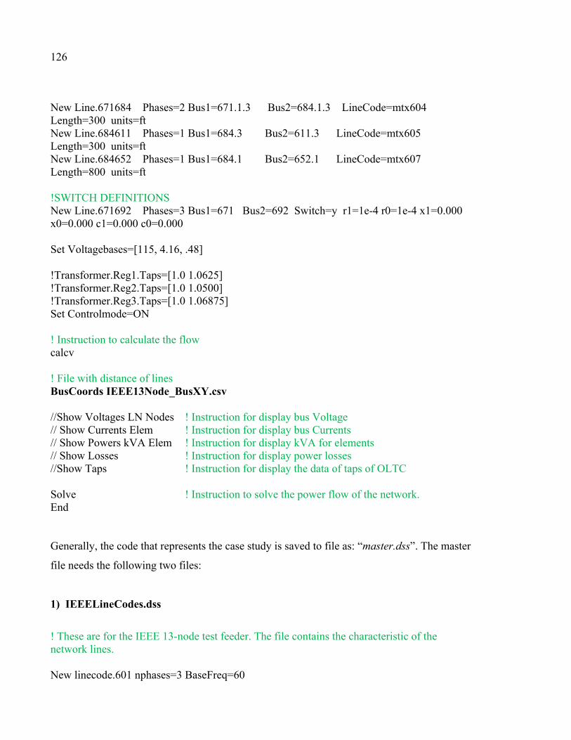
126

New Line.671684 Phases=2 Bus1=671.1.3 Bus2=684.1.3 LineCode=mtx604 Length=300 units=ft New Line.684611 Phases=1 Bus1=684.3 Bus2=611.3 LineCode=mtx605 Length=300 units=ft New Line.684652 Phases=1 Bus1=684.1 Bus2=652.1 LineCode=mtx607 Length=800 units=ft !SWITCH DEFINITIONS New Line.671692 Phases=3 Bus1=671 Bus2=692 Switch=y r1=1e-4 r0=1e-4 x1=0.000 x0=0.000 c1=0.000 c0=0.000 Set Voltagebases=[115, 4.16, .48] !Transformer.Reg1.Taps=[1.0 1.0625] !Transformer.Reg2.Taps=[1.0 1.0500] !Transformer.Reg3.Taps=[1.0 1.06875] Set Controlmode=ON ! Instruction to calculate the flow calcv ! File with distance of lines BusCoords IEEE13Node_BusXY.csv //Show Voltages LN Nodes ! Instruction for display bus Voltage // Show Currents Elem ! Instruction for display bus Currents // Show Powers kVA Elem ! Instruction for display kVA for elements // Show Losses ! Instruction for display power losses //Show Taps ! Instruction for display the data of taps of OLTC Solve ! Instruction to solve the power flow of the network. End

Generally, the code that represents the case study is saved to file as: “master.dss”. The master

file needs the following two files:

1) IEEELineCodes.dss

! These are for the IEEE 13-node test feeder. The file contains the characteristic of the network lines. New linecode.601 nphases=3 BaseFreq=60

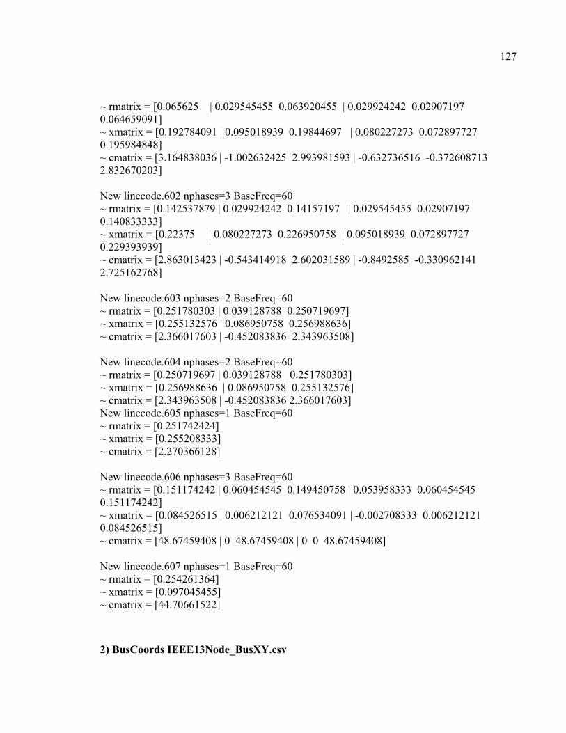
127

~ rmatrix = [0.065625 | 0.029545455 0.063920455 | 0.029924242 0.02907197 0.064659091] ~ xmatrix = [0.192784091 | 0.095018939 0.19844697 | 0.080227273 0.072897727 0.195984848] ~ cmatrix = [3.164838036 | -1.002632425 2.993981593 | -0.632736516 -0.372608713 2.832670203] New linecode.602 nphases=3 BaseFreq=60 ~ rmatrix = [0.142537879 | 0.029924242 0.14157197 | 0.029545455 0.02907197 0.140833333] ~ xmatrix = [0.22375 | 0.080227273 0.226950758 | 0.095018939 0.072897727 0.229393939] ~ cmatrix = [2.863013423 | -0.543414918 2.602031589 | -0.8492585 -0.330962141 2.725162768] New linecode.603 nphases=2 BaseFreq=60 ~ rmatrix = [0.251780303 | 0.039128788 0.250719697] ~ xmatrix = [0.255132576 | 0.086950758 0.256988636] ~ cmatrix = [2.366017603 | -0.452083836 2.343963508] New linecode.604 nphases=2 BaseFreq=60 ~ rmatrix = [0.250719697 | 0.039128788 0.251780303] ~ xmatrix = [0.256988636 | 0.086950758 0.255132576] ~ cmatrix = [2.343963508 | -0.452083836 2.366017603] New linecode.605 nphases=1 BaseFreq=60 ~ rmatrix = [0.251742424] ~ xmatrix = [0.255208333] ~ cmatrix = [2.270366128] New linecode.606 nphases=3 BaseFreq=60 ~ rmatrix = [0.151174242 | 0.060454545 0.149450758 | 0.053958333 0.060454545 0.151174242] ~ xmatrix = [0.084526515 | 0.006212121 0.076534091 | -0.002708333 0.006212121 0.084526515] ~ cmatrix = [48.67459408 | 0 48.67459408 | 0 0 48.67459408] New linecode.607 nphases=1 BaseFreq=60 ~ rmatrix = [0.254261364] ~ xmatrix = [0.097045455] ~ cmatrix = [44.70661522]

2) BusCoords IEEE13Node_BusXY.csv

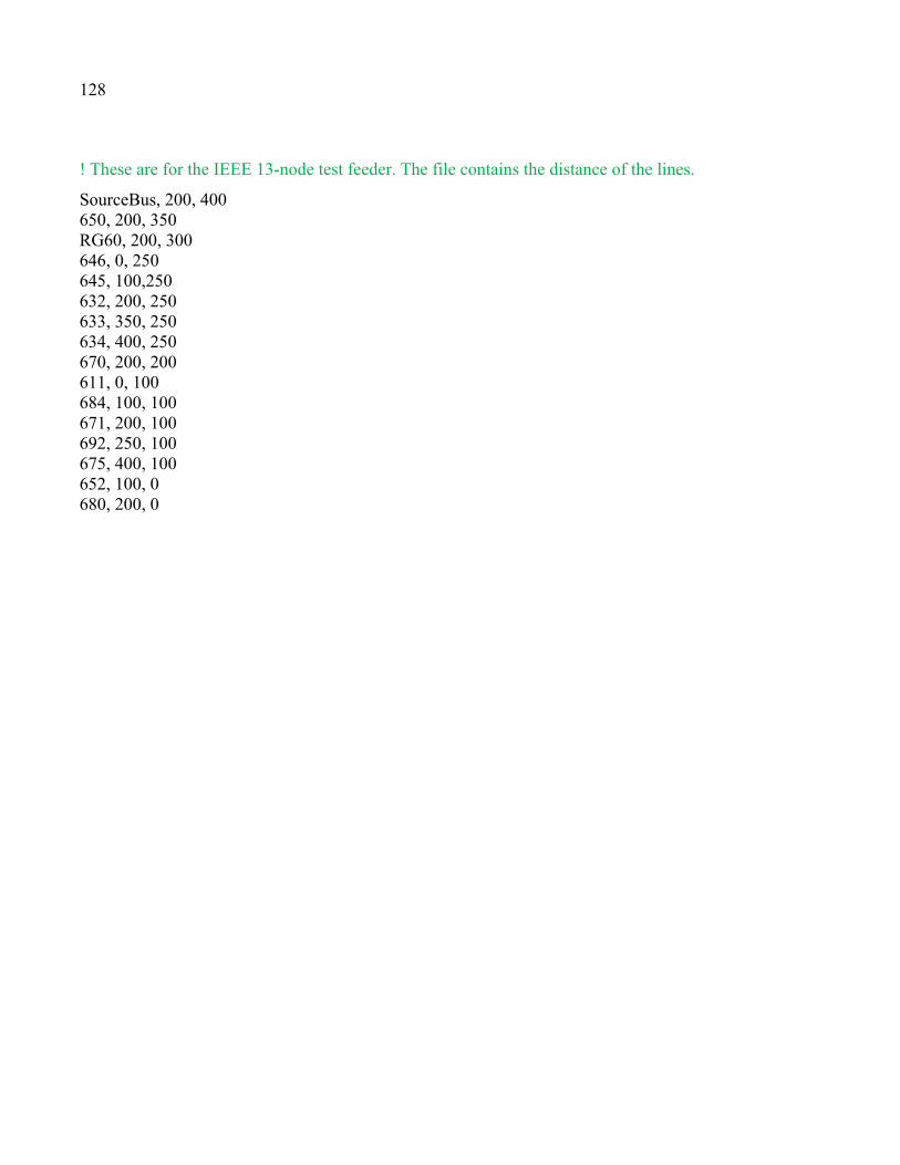
128

! These are for the IEEE 13-node test feeder. The file contains the distance of the lines.

SourceBus, 200, 400 650, 200, 350 RG60, 200, 300 646, 0, 250 645, 100,250 632, 200, 250 633, 350, 250 634, 400, 250 670, 200, 200 611, 0, 100 684, 100, 100 671, 200, 100 692, 250, 100 675, 400, 100 652, 100, 0 680, 200, 0

ANNEXE I

REFERENCES OF ARTICLES PUBLISHED Castro, José Raúl, Maarouf Saad, Serge Lefebvre, Dalal Asber et Laurent Lenoir. 2016a.

« Optimal voltage control in distribution network in the presence of DGs ». International Journal of Electrical Power & Energy Systems, vol. 78, p. 239-247.

Castro, José, Maarouf Saad, Serge Lefebvre, Dalal Asber et Laurent Lenoir. 2016b.

« Coordinated Voltage Control in Distribution Network with the Presence of DGs and Variable Loads Using Pareto and Fuzzy Logic ». Energies, vol. 9, no 2, p. 107.

REFERENCES OF ARTICLES SUMMITED Castro, José, Maarouf Saad, Serge Lefebvre, Dalal Asber et Laurent Lenoir. “Power factor

computation of distributed generation usin multi-objective optimization”. It is submitted to the International Journal of Electrical Power & Energy Systems.

REFERENCES OF POSTERS Castro, José, Maarouf Saad, Serge Lefebvre, Dalal Asber et Laurent Lenoir. « Optimal

Voltage Control in Distribution Network » CIGRE-481 Canada conference. International Center. Toronto, Ontario, September 22-24, 2014.

Castro, José, Maarouf Saad, Serge Lefebvre, Dalal Asber et Laurent Lenoir. “ Optimo

Control de Voltaje en redes de Distribución con Generadores distribuidos” INER. Congreso I+D+i en Sostenibilidad Energética. Diciembre 2015.

BIBLIOGRAPHY

Abido, M. A. 2004. « Multiobjective optimal power flow using strength Pareto evolutionary algorithm ». In Universities Power Engineering Conference, 2004. UPEC 2004. 39th International. (8-8 Sept. 2004) Vol. 1, p. 457-461 Vol. 1.

Abu-Mouti, F. S., et M. E. El-Hawary. 2011. « Optimal Distributed Generation Allocation

and Sizing in Distribution Systems via Artificial Bee Colony Algorithm ». Power Delivery, IEEE Transactions on, vol. 26, no 4, p. 2090-2101.

Aghaei, Jamshid, Kashem M. Muttaqi, Ali Azizivahed et Mohsen Gitizadeh. 2014. «

Distribution expansion planning considering reliability and security of energy using modified PSO (Particle Swarm Optimization) algorithm ». Energy, vol. 65, p. 398-411.

Ahmidi, A., X. Guillaud, Y. Besanger et R. Blanc. 2012. « A Multilevel Approach for

Optimal Participating of Wind Farms at Reactive Power Balancing in Transmission Power System ». Systems Journal, IEEE, vol. 6, no 2, p. 260-269.

Anwar, A., et H. R. Pota. 2011. « Loss reduction of power distribution network using

optimum size and location of distributed generation ». In Universities Power Engineering Conference (AUPEC), 2011 21st Australasian. (25-28 Sept. 2011), p. 1-6.

Babu, U. R., V. V. K. Reddy et S. Tarakalyani. 2015. « Modified GA for optimal DG

allocation and sizing ». In 2015 International Conference on Electrical, Electronics, Signals, Communication and Optimization (EESCO), 24-25 Jan. 2015. (Piscataway, NJ, USA), p. 4 pp. Coll. « 2015 International Conference on Electrical, Electronics, Signals, Communication and Optimization (EESCO) »: IEEE. < http://dx.doi.org/10.1109/EESCO.2015.7253775 >.

Barin, A., L. N. Canha, R. Q. Machado, A. da Rosa Abaide, E. Maziero et G. Arend. 2008. «

Analysis of the impacts of distributed generation sources considering the appropriate choice of parameters in a multi-objective approach for distribution system planning ». In Electricity Market, 2008. EEM 2008. 5th International Conference on European. (28-30 May 2008), p. 1-6.

Bijwe, P. R., et G. K. V. Raju. 2006. « Fuzzy distribution power flow for weakly meshed

systems ». IEEE Transactions on Power Systems, vol. 21, no 4, p. 1645-52. Biserica, M., B. Berseneff, Y. Besanger et C. Kieny. 2011. « Upgraded coordinated voltage

control for distribution systems ». In 2011 IEEE PES PowerTech - Trondheim, 19-23

132

June 2011. (Piscataway, NJ, USA), p. 6 pp. Coll. « 2011 IEEE PES PowerTech - Trondheim »: IEEE. < http://dx.doi.org/10.1109/PTC.2011.6019328 >.

Calderaro, V., A. Piccolo et P. Siano. 2005. « Maximizing DG penetration in distribution

networks by means of GA based reconfiguration ». In Future Power Systems, 2005 International Conference on. (18-18 Nov. 2005), p. 6 pp.-6.

Castro, José Raúl, Maarouf Saad, Serge Lefebvre, Dalal Asber et Laurent Lenoir. 2016a. «

Optimal voltage control in distribution network in the presence of DGs ». International Journal of Electrical Power & Energy Systems, vol. 78, p. 239-247.

Castro, José, Maarouf Saad, Serge Lefebvre, Dalal Asber et Laurent Lenoir. 2016b. «

Coordinated Voltage Control in Distribution Network with the Presence of DGs and Variable Loads Using Pareto and Fuzzy Logic ». Energies, vol. 9, no 2, p. 107.

Conejo, A., J. I. de la Fuente et S. Goransson. 1994. « Comparison of alternative algorithms

to select pilot buses for secondary voltage control in electric power networks ». In Electrotechnical Conference, 1994. Proceedings., 7th Mediterranean. (12-14 Apr 1994), p. 940-943 vol.3.

Chi, Su, Liu Zhou, Chen Zhe et Hu Yanting. 2014. « An adaptive control strategy of

converter based DG to maintain protection coordination in distribution system ». In Innovative Smart Grid Technologies Conference Europe (ISGT-Europe), 2014 IEEE PES. (12-15 Oct. 2014), p. 1-6.

Dahal, S., et H. Salehfar. 2013. « Optimal location and sizing of distributed generators in

distribution networks ». In North American Power Symposium (NAPS), 2013. (22-24 Sept. 2013), p. 1-6.

Deb, K., A. Pratap, S. Agarwal et T. Meyarivan. 2002. « A fast and elitist multiobjective

genetic algorithm: NSGA-II ». Evolutionary Computation, IEEE Transactions on, vol. 6, no 2, p. 182-197.

Dehghani-Arani, A., et R. Maddahi. 2013. « Introduction a multi-objective function in

unbalanced and unsymmetrical distribution networks for optimal placement and sizing of distributed generation units using NSGA-II ». In Electrical Power Distribution Networks (EPDC), 2013 18th Conference on. (April 30 2013-May 1 2013), p. 1-9.

DeJesus, De Oliveira-, P. M., M. T. P. de Leao et H. M. Khodr. 2006. « Remuneration of

Distribution Networks using a Fuzzy Multicriteria Planning Algorithm ». In Probabilistic Methods Applied to Power Systems, 2006. PMAPS 2006. International Conference on. (11-15 June 2006), p. 1-7.

133

Dugan, R. C., et T. E. McDermott. 2011. « An open source platform for collaborating on smart grid research ». In Power and Energy Society General Meeting, 2011 IEEE. (24-29 July 2011), p. 1-7.

Duong, Quoc., Mithulananthan. et R. C. Bansal. 2010. « Analytical Expressions for DG

Allocation in Primary Distribution Networks ». Energy Conversion, IEEE Transactions on, vol. 25, no 3, p. 814-820.

Dutta, V., T. O'Donnell, S. Borkakati et D. Bora. 2014. « PI-Fuzzy rule based controller for

Analysis and performance evaluation of dc motor speed control ». In Power Engineering and Renewable Energy (ICPERE), 2014 International Conference on. (9-11 Dec. 2014), p. 175-180.

Erbasu, A., A. Berizzi, M. Eremia et C. Bulac. 2005. « Implementation studies of secondary

voltage control on the Romanian power grid ». In Power Tech, 2005 IEEE Russia. (27-30 June 2005), p. 1-7.

Esmaili, M. 2013. « Placement of minimum distributed generation units observing power

losses and voltage stability with network constraints ». Generation, Transmission & Distribution, IET, vol. 7, no 8, p. 813-821.

Federico, J., V. Gonzalez et C. Lyra. 2005. « Learning classifiers shape reactive power to

decrease losses in power distribution networks ». In IEEE Power Engineering Society General Meeting, 2005. (12-16 June 2005), p. 557-562 Vol. 1.

Figueroa-Garcia, J. C., D. Kalenatic et C. Amilcar Lopez-Bello. 2012. « Multi-period Mixed

Production Planning with uncertain demands: Fuzzy and interval fuzzy sets approach ». Fuzzy Sets and Systems, vol. 206, p. 21-38.

Fu, Xueqian, Haoyong Chen, Runqing Cai et Ping Yang. 2015. « Optimal allocation and

adaptive VAR control of PV-DG in distribution networks ». Applied Energy, vol. 137, p. 173-182.

Gao, C., et M. A. Redfern. 2011. « Automatic Compensation Voltage Control strategy for

on-load tap changer transformers with distributed generations ». In Advanced Power System Automation and Protection (APAP), 2011 International Conference on. (16-20 Oct. 2011) Vol. 1, p. 737-741.

Gao, Yajing, Jianpeng Liu, Jin Yang, Haifeng Liang et Jiancheng Zhang. 2014. « Multi-

Objective Planning of Multi-Type Distributed Generation Considering Timing Characteristics and Environmental Benefits ». Energies, vol. 7, no 10, p. 6242.

Gaonkar, J. D. N., et G. N. Pillai. 2010. « Fuzzy logic based coordinated voltage regulation

method for distribution system with multiple synchronous generators ». In Power

134

Electronics, Drives and Energy Systems (PEDES) & 2010 Power India, 2010 Joint International Conference on. (20-23 Dec. 2010), p. 1-5.

Gatter, Thomas., Robert Giegerich et Cédric Saule. 2016. « Integrating Pareto Optimization

into Dynamic Programming ». Algorithms, vol. 9, no 1, p. 12. Ghatee, M., et S. M. Hashemi. 2009. « Application of fuzzy minimum cost flow problems to

network design under uncertainty ». Fuzzy Sets and Systems, vol. 160, no 22, p. 3263-3289.

Gong, Qingwu, Jiazhi Lei et Jun Ye. 2016. « Optimal Siting and Sizing of Distributed

Generators in Distribution Systems Considering Cost of Operation Risk ». Energies, vol. 9, no 1, p. 61.

Grid, National. 2010. « The Grid Code ». Griffin, T., K. Tomsovic, D. Secrest et A. Law. 2000. « Placement of dispersed generation

systems for reduced losses ». In System Sciences, 2000. Proceedings of the 33rd Annual Hawaii International Conference on. (4-7 Jan. 2000), p. 9 pp.

Habibi, A., M. Nayeripour et J. Aghaei. 2013. « Secure multi-objective distributed generation

planning in distribution network ». In Electrical Engineering (ICEE), 2013 21st Iranian Conference on. (14-16 May 2013), p. 1-6.

Hong, Ying-Yi, Yuan-Ming Lai, Yung-Ruei Chang, Yih-Der Lee et Pang-Wei Liu. 2015. «

Optimizing Capacities of Distributed Generation and Energy Storage in a Small Autonomous Power System Considering Uncertainty in Renewables ». Energies, vol. 8, no 4, p. 2473.

Hung, Duong Quoc, et N. Mithulananthan. 2014. « Loss reduction and loadability

enhancement with DG: A dual-index analytical approach ». Applied Energy, vol. 115, p. 233-241.

Hung., Duong Quoc., N. Mithulananthan et R. C. Bansal. 2013. « Analytical strategies for

renewable distributed generation integration considering energy loss minimization ». Applied Energy, vol. 105, p. 75-85.

IEEE.org. Distribution system analysis subcommitte radias test feeders. <

http://ewh.ieee.org/soc/pes/dsacom/testfeeders/index.html >. Instruments, National. 2012. Fuzzy-PI Controllers. . < zone.ni.com >. Consulté le 12 jan.

2016.

135

Kaabi, Al, S. S., H. H. Zeineldin et V. Khadkikar. 2014. « Planning Active Distribution Networks Considering Multi-DG Configurations ». Power Systems, IEEE Transactions on, vol. 29, no 2, p. 785-793.

Kang, Hyun-Koo, Il-Yop Chung et Seung-Il Moon. 2015. « Voltage Control Method Using

Distributed Generators Based on a Multi-Agent System ». Energies, vol. 8, no 12, p. 12411.

Ke-yan, Liu, Sheng Wanxing, Liu Yuan, Meng Xiaoli et Liu Yongmei. 2015. « Optimal

sitting and sizing of DGs in distribution system considering time sequence characteristics of loads and DGs ». International Journal of Electrical Power &amp; Energy Systems, vol. 69, p. 430-40.

Kersting, W. H. 2001. « Radial distribution test feeders ». In Power Engineering Society

Winter Meeting, 2001. IEEE. (2001) Vol. 2, p. 908-912 vol.2. Khalesi, N., et M. R. Haghifam. 2009. « Application of dynamic programming for distributed

generation allocation ». In Electrical Power & Energy Conference (EPEC), 2009 IEEE. (22-23 Oct. 2009), p. 1-6.

Khushalani, S., et N. Schulz. 2006. « Unbalanced Distribution Power Flow with Distributed

Generation ». In Transmission and Distribution Conference and Exhibition, 2005/2006 IEEE PES. (21-24 May 2006), p. 301-306.

Kiprakis, A. E., et A. R. Wallace. 2004. « Maximising energy capture from distributed

generators in weak networks ». Generation, Transmission and Distribution, IEE Proceedings-, vol. 151, no 5, p. 611-618.

Knowles, J., et D. Corne. 1999. « The Pareto archived evolution strategy: a new baseline

algorithm for Pareto multiobjective optimisation ». In Evolutionary Computation, 1999. CEC 99. Proceedings of the 1999 Congress on. (1999) Vol. 1, p. 105 Vol. 1.

Kojovic, L. 2002. « Modeling of DG to interface with distribution system ». In Power

Engineering Society Summer Meeting, 2002 IEEE. (25-25 July 2002) Vol. 1, p. 179-180 vol.1.

Kolenc, Marko., Igor. Papic et Bostjan. Blazic. 2012. « Minimization of Losses in Smart

Grids Using Coordinated Voltage Control ». Energies, vol. 5, no 10, p. 3768. Kumar, D., S. R. Samantaray et I. Kamwa. 2015. « Multi-objective design of advanced

power distribution networks using restricted-population-based multi-objective seeker-optimisation-algorithm and fuzzy-operator ». IET Generation, Transmission & Distribution, vol. 9, no 11, p. 1195-1215.

136

Larsson, M., et D. Karlsson. 2003. « Coordinated system protection scheme against voltage collapse using heuristic search and predictive control ». Power Systems, IEEE Transactions on, vol. 18, no 3, p. 1001-1006.

Leisse, I., O. Samuelsson et J. Svensson. 2010. « Electricity meters for coordinated voltage

control in medium voltage networks with wind power ». In Innovative Smart Grid Technologies Conference Europe (ISGT Europe), 2010 IEEE PES. (11-13 Oct. 2010), p. 1-7.

Li, Fang-Fang, et Jun Qiu. 2015. « Multi-Objective Reservoir Optimization Balancing

Energy Generation and Firm Power ». Energies, vol. 8, no 7, p. 6962. Li, Ran, Huizhuo Ma, Feifei Wang, Yihe Wang, Yang Liu et Zenghui Li. 2013. « Game

Optimization Theory and Application in Distribution System Expansion Planning, Including Distributed Generation ». Energies, vol. 6, no 2, p. 1101.

Liu, Wenxia, Huiting Xu, Shuya Niu et Jiang Xie. 2016. « Optimal Distributed Generator

Allocation Method Considering Voltage Control Cost ». Sustainability, vol. 8, no 2, p. 193.

Loetamonphong, J., S. C. Fang et R. E. Young. 2002. « Multi-objective optimization

problems with fuzzy relation equation constraints ». Fuzzy Sets and Systems, vol. 127, no 2, p. 141-164.

Lopez, E., H. Opazo, L. Garcia et Patrick Bastard. 2004. « Online reconfiguration

considering variability demand: applications to real networks ». Power Systems, IEEE Transactions on, vol. 19, no 1, p. 549-553.

Maciel, R. S., et A. Padilha-Feltrin. 2009. « Distributed Generation Impact Evaluation Using

a Multi-Objective Tabu Search ». In Intelligent System Applications to Power Systems, 2009. ISAP '09. 15th International Conference on. (8-12 Nov. 2009), p. 1-5.

Martinez-Velasco, J. A., et G. Guerra. 2014. « Parallel Monte Carlo approach for distribution

reliability assessment ». Generation, Transmission & Distribution, IET, vol. 8, no 11, p. 1810-1819.

Martinez, J. A., et G. Guerra. 2014. « A Parallel Monte Carlo Method for Optimum

Allocation of Distributed Generation ». Power Systems, IEEE Transactions on, vol. 29, no 6, p. 2926-2933.

Martins, N., J. C. R. Ferraz, S. Gomes, Jr., P. E. M. Quintao et J. A. Passos. 2001. « A

demonstration example of secondary voltage regulation: dynamic simulation and continuation power flow results ». In Power Engineering Society Summer Meeting, 2001. (2001) Vol. 2, p. 791-796 vol.2.

137

Masters, C. L. 2002. « Voltage rise: the big issue when connecting embedded generation to long 11 kV overhead lines ». Power Engineering Journal, vol. 16, no 1, p. 5-12.

MathWorks. 2014. Matlab, version 2014a, (R2014a). Natick, Massachusetts: The

MathWorks Inc. Moghimi, H., A. Ahmadi, J. Aghaei et A. Rabiee. 2013. « Stochastic techno-economic

operation of power systems in the presence of distributed energy resources ». International Journal of Electrical Power & Energy Systems, vol. 45, no 1, p. 477-488.

Moradi, M. H., S. M. Reza Tousi et M. Abedini. 2014. « Multi-objective PFDE algorithm for

solving the optimal siting and sizing problem of multiple DG sources ». International Journal of Electrical Power &amp; Energy Systems, vol. 56, p. 117-26.

Muller-Hannemann, Matthias., Weihe. et Karsten. 2001. « Pareto shortest paths is often

feasible in practice ». In 5th International Workshop on Algorithm Engineering, WAE 2001, August 28, 2001 - August 31, 2001. (Arhus, Denmark) Vol. 2141, p. 185-197. Coll. « Lecture Notes in Computer Science (including subseries Lecture Notes in Artificial Intelligence and Lecture Notes in Bioinformatics) »: Springer Verlag.

Muttaqi, K. M., A. D. T. Le, M. Negnevitsky et G. Ledwich. 2014. « An Algebraic Approach

for Determination of DG Parameters to Support Voltage Profiles in Radial Distribution Networks ». Smart Grid, IEEE Transactions on, vol. 5, no 3, p. 1351-1360.

Muttaqi, K. M., An D. T. Le, J. Aghaei, E. Mahboubi-Moghaddam, M. Negnevitsky et G.

Ledwich. 2016. « Optimizing distributed generation parameters through economic feasibility assessment ». Applied Energy, vol. 165, p. 893-903.

Nagarajan, A., et R. Ayyanar. 2015. « Design and Strategy for the Deployment of Energy

Storage Systems in a Distribution Feeder With Penetration of Renewable Resources ». Sustainable Energy, IEEE Transactions on, vol. 6, no 3, p. 1085-1092.

Nara, K., Y. Hayashi, K. Ikeda et T. Ashizawa. 2001. « Application of tabu search to optimal

placement of distributed generators ». In Power Engineering Society Winter Meeting, 2001. IEEE. (2001) Vol. 2, p. 918-923 vol.2.

National Instruments. 2006. « ». Engineering & Technology, vol. 1, no 2, p. 3-3. Ngatchou, P., Zarei. Anahita et M. A. El-Sharkawi. 2005. « Pareto Multi Objective

Optimization ». In Intelligent Systems Application to Power Systems, 2005. Proceedings of the 13th International Conference on. (6-10 Nov. 2005), p. 84-91.

138

Ni, S., Charley Z. Huang, G. H. Huang, Y. P. Li, J. P. Chen, Y. R. Fan et G. H. Cheng. 2016. « Planning renewable energy in electric power system for sustainable development under uncertainty – A case study of Beijing ». Applied Energy, vol. 162, p. 772-786.

Niknam, T., H. Z. Meymand, H. D. Mojarrad et J. Aghaei. 2011. « Multi-objective daily

operation management of distribution network considering fuel cell power plants ». IET Renewable Power Generation, vol. 5, no 5, p. 356-367.

Ochoa, L. F., C. J. Dent et G. P. Harrison. 2010. « Distribution Network Capacity

Assessment: Variable DG and Active Networks ». Power Systems, IEEE Transactions on, vol. 25, no 1, p. 87-95.

Ochoa, L. F., A. Keane et G. P. Harrison. 2011. « Minimizing the Reactive Support for

Distributed Generation: Enhanced Passive Operation and Smart Distribution Networks ». Power Systems, IEEE Transactions on, vol. 26, no 4, p. 2134-2142.

Ochoa, L. F., et G. P. Harrison. 2011. « Minimizing Energy Losses: Optimal

Accommodation and Smart Operation of Renewable Distributed Generation ». Power Systems, IEEE Transactions on, vol. 26, no 1, p. 198-205.

OpenDSS manual and reference guide. « ». [Online] Available:

http://sourceforge.net/projects/electricdss. Ouyang, Puren, et Vangjel Pano. 2015. « Comparative Study of DE, PSO and GA for

Position Domain PID Controller Tuning ». Algorithms, vol. 8, no 3, p. 697. Pitalúa-Díaz, Nun, Enrique Herrera-López, Guillermo Valencia-Palomo, Alvaro González-

Angeles, Ricardo Rodríguez-Carvajal et Nohe Cazarez-Castro. 2015. « Comparative Analysis between Conventional PI and Fuzzy LogicPI Controllers for Indoor Benzene Concentrations ». Sustainability, vol. 7, no 5, p. 5398.

Poornazaryan, Bahram, Peyman Karimyan, G. B. Gharehpetian et Mehrdad Abedi. 2016. «

Optimal allocation and sizing of DG units considering voltage stability, losses and load variations ». International Journal of Electrical Power and Energy Systems, vol. 79, p. 42-52.

Queiroz, L. M. O., et C. Lyra. 2009. « Adaptive Hybrid Genetic Algorithm for Technical

Loss Reduction in Distribution Networks Under Variable Demands ». Power Systems, IEEE Transactions on, vol. 24, no 1, p. 445-453.

Ren, Hongbo, Weisheng Zhou, Ken’ichi Nakagami, Weijun Gao et Qiong Wu. 2010. «

Multi-objective optimization for the operation of distributed energy systems considering economic and environmental aspects ». Applied Energy, vol. 87, no 12, p. 3642-3651.

139

Richardot, O., A. Viciu, Y. Besanger, N. HadjSaid et C. Kieny. 2006. « Coordinated Voltage Control in Distribution Networks Using Distributed Generation ». In Transmission and Distribution Conference and Exhibition, 2005/2006 IEEE PES. (21-24 May 2006), p. 1196-1201.

Rios, M. S., et S. M. Rubio. 2007. « Sequential Optimization for Siting and Sizing

Distributed Generation (DG) in Medium Voltage (MV) Distribution Networks ». In Power Tech, 2007 IEEE Lausanne. (1-5 July 2007), p. 2213-2218.

Sattarpour, T., D. Nazarpour, S. Golshannavaz et P. Siano. 2015. « An optimal procedure for

sizing and siting of DGs and smart meters in active distribution networks considering loss reduction ». Journal of Electrical Engineering and Technology, vol. 10, no 3, p. 804-811.

Sedighi, M., A. Igderi, A. Dankoob et S. M. Abedi. 2010. « Sitting and sizing of DG in

distribution network to improve of several parameters by PSO algorithm ». In Mechanical and Electrical Technology (ICMET), 2010 2nd International Conference on. (10-12 Sept. 2010), p. 533-538.

Shaaban, M. F., Y. M. Atwa et E. F. El-Saadany. 2013. « DG allocation for benefit

maximization in distribution networks ». Power Systems, IEEE Transactions on, vol. 28, no 2, p. 639-649.

Sheng, Gehao, Xiuchen Jiang, Dapeng Duan et Guangyu Tu. 2009a. « Framework and

implementation of secondary voltage regulation strategy based on multi-agent technology ». International Journal of Electrical Power & Energy Systems, vol. 31, no 1, p. 67-77.

Sheng, Gehao, Xiuchen Jiang, Dapeng Duan et Guangyu Tu. 2009b. « Framework and

implementation of secondary voltage regulation strategy based on multi-agent technology ». International Journal of Electrical Power and Energy Systems, vol. 31, no 1, p. 67-77.

Smith, A. E. 2002. « Multi-objective optimization using evolutionary algorithms [Book

Review] ». Evolutionary Computation, IEEE Transactions on, vol. 6, no 5, p. 526-526.

Song, Il-Keun, Won-Wook Jung, Chul-Min Chu, Seong-Soo Cho, Hyun-Koo Kang et Joon-

Ho Choi. 2013. « General and Simple Decision Method for DG Penetration Level in View of Voltage Regulation at Distribution Substation Transformers ». Energies, vol. 6, no 9, p. 4786.

Song, Nie, Fu Xiao-Peng, Li Peng, Gao Fei, Ding Cheng-Di, Yu Hao et Wang Cheng-Shan.

2012. « Analysis of the impact of DG on distribution network reconfiguration using

140

OpenDSS ». In Innovative Smart Grid Technologies - Asia (ISGT Asia), 2012 IEEE. (21-24 May 2012), p. 1-5.

Soroudi, A., R. Caire, N. Hadjsaid et M. Ehsan. 2011. « Probabilistic dynamic multi-

objective model for renewable and non-renewable distributed generation planning ». IET Generation, Transmission and Distribution, vol. 5, no 11, p. 1173-1182.

Takagi, T., et M. Sugeno. 1985. « Fuzzy identification of systems and its applications to

modeling and control ». Systems, Man and Cybernetics, IEEE Transactions on, vol. SMC-15, no 1, p. 116-132.

Thong, Van, Vu., J. Driesen et R. Belmans. 2007. « Using Distributed Generation to Support

and Provide Ancillary Services for the Power System ». In Clean Electrical Power, 2007. ICCEP '07. International Conference on. (21-23 May 2007), p. 159-163.

Tomoiaga, Bogdan, Mircea Chindriş, Andreas Sumper, Antoni Sudria-Andreu et Roberto

Villafafila-Robles. 2013. « Pareto Optimal Reconfiguration of Power Distribution Systems Using a Genetic Algorithm Based on NSGA-II ». Energies, vol. 6, no 3, p. 1439.

Venkatesan, Naveen, Jignesh Solanki et Sarika Khushalani Solanki. 2012. « Residential

Demand Response model and impact on voltage profile and losses of an electric distribution network ». Applied Energy, vol. 96, p. 84-91.

Viawan, F. A., et D. Karlsson. 2008. « Coordinated voltage and reactive power control in the

presence of distributed generation ». In Power and Energy Society General Meeting - Conversion and Delivery of Electrical Energy in the 21st Century, 2008 IEEE. (20-24 July 2008), p. 1-6.

Vu, H., P. Pruvot, C. Launay et Y. Harmand. 1996. « An improved voltage control on large-

scale power system ». Power Systems, IEEE Transactions on, vol. 11, no 3, p. 1295-1303.

Wu, Jiekang., Yunan Zhu et Shange Wei. 2011. « Multi-objective optimal scheduling for

cascaded hydroelectric power plant based on improved membership functions ». Dianwang Jishu/Power System Technology, vol. 35, no 2, p. 48-52.

Xiyi, Lin, Yao Jiangang, Mao Tian et Gong Lei. 2013. « Inductive reactive power

compensation optimization for 10kV distribution network with distributed generations ». In Chinese Automation Congress (CAC), 2013. (7-8 Nov. 2013), p. 87-91.

Young-Jin, Kim, Ahn Seon-Ju, Hwang Pyeong-Ik, Pyo Gi-Chan et Moon Seung-Il. 2013. «

Coordinated Control of a DG and Voltage Control Devices Using a Dynamic

141

Programming Algorithm ». Power Systems, IEEE Transactions on, vol. 28, no 1, p. 42-51.

Zhang., Ni., Yu Yan et Wencong Su. 2015. « A game-theoretic economic operation of

residential distribution system with high participation of distributed electricity prosumers ». Applied Energy, vol. 154, p. 471-479.

Zidan, A., et E. F. El-Saadany. 2012. « Network reconfiguration in balanced distribution

systems with variable load demand and variable renewable resources generation ». In Power and Energy Society General Meeting, 2012 IEEE. (22-26 July 2012), p. 1-8.