Cramer-Rao Lower Bounds for Channel Parameters Estimation...
84
Université du Québec Institut National de la Recherche Scientifique Énergie Matériaux Télécommunications Cramer-Rao Lower Bounds for Channel Parameters Estimation over Turbo-Coded Wireless Transmissions Préparé par Achraf Methenni Mémoire présenté pour l’obtention du grade de Maître ès Sciences (M.Sc.) en Télécommunications Examinateur Externe Prof. Fabrice Labeau McGill University Examinateur Interne et Président du jury Prof. Nahi Kandil 54544545555555555555555555555555 UQAT Directeur de Recherche Prof. Sofiène Affes INRS-ÉMT
Transcript of Cramer-Rao Lower Bounds for Channel Parameters Estimation...

Université du Québec
Institut National de la Recherche Scientifique
Énergie Matériaux Télécommunications
Cramer-Rao Lower Bounds for Channel Parameters
Estimation over Turbo-Coded Wireless Transmissions
Préparé par
Achraf Methenni
Mémoire présenté pour l’obtention du grade de Maître ès Sciences (M.Sc.) en
Télécommunications
Examinateur Externe Prof. Fabrice Labeau
McGill University
Examinateur Interne et Président du
jury
Prof. Nahi Kandil 54544545555555555555555555555555
UQAT
Directeur de Recherche Prof. Sofiène Affes
INRS-ÉMT

To my parents
To Sadok, Imen and Haythem
To Zizou, Bibou, Ahmed and Yassine

Acknowledgements
I wish to thank Prof. Sofiène Affes for giving me the opportunity to work in his team, and for
guiding me throughout my MSc program. His remarks as well as his pertinent criticism led me
to the right path.
I want also to thank Mr. Faouzi Bellili for all his efforts, for being there for me, providing
me with valuable advices and providing the perfect example for me for my research career. A
special thanks to the external and internal jury members, Prof. Fabrice Labeau from McGill
University and Prof. Nahi Kandil from UQAT and adjunct professor at INRS-EMT who have
kindly accepted to assess my MSc thesis. I want to express my thanks and gratitude to all my
family, for their patience, and for all their encouragements.
Finally, I want to thank all my collegues and all the staff at INRS for providing a perfect
environment, and for making me feel as if I was surrounded by my family members...
ii

Table des matières
Résumé 2
1 Introduction 12
2 System Model 19
3 Derivation of the Log-Likelihood Function (LLF) 24
3.1 LLF for BPSK and MSK signals : . . . . . . . . . . . . . . . . . . . . . . . . . . 27
3.2 LLF for QPSK signals : . . . . . . . . . . . . . . . . . . . . . . . . . . . . . . . 28
3.3 LLF for square-QAM signals : . . . . . . . . . . . . . . . . . . . . . . . . . . . . 30
4 Derivation of the CRLB Analytical Expressions 45
4.1 CRLB for coded SNR estimation [43] . . . . . . . . . . . . . . . . . . . . . . . . 45
4.2 CRLB for coded phase and CFO estimtion [44] . . . . . . . . . . . . . . . . . . . 52
iii

4.2.1 Empirical Evaluation of the CRLB . . . . . . . . . . . . . . . . . . . . . 56
5 Simulation Results 60
5.1 SNR estimation . . . . . . . . . . . . . . . . . . . . . . . . . . . . . . . . . . . . 60
5.2 Phase and CFO estimation . . . . . . . . . . . . . . . . . . . . . . . . . . . . . . 64
6 Conclusion 70
Conclusion 70
iv
Table des figures
3.1 Construction of Gray-coded Square-QAM constellations . . . . . . . . . . . . . . 34
3.2 Construction of Gray-coded Square-QAM constellations . . . . . . . . . . . . . . 41
5.1 CA CRLBs for SNR estimation : 16-QAM, K=207. . . . . . . . . . . . . . . . . 61
5.2 CA CRLBs for SNR estimation : BSK and MSK signals, K=207. . . . . . . . . 62
5.3 CA CRLBs with different modulation orders : K = 207. . . . . . . . . . . . . . . 63
5.4 CA CRLBs for different coding rates : 16-QAM, K=207. . . . . . . . . . . . . . 64
5.5 CRLB for the phase and CFO estimation using 16-QAM symbols with K = 207 :
(a) CRLB(ϕ), (b)CRLB(ν) . . . . . . . . . . . . . . . . . . . . . . . . . . . . . . 66
5.6 CRLB for the phase and CFO estimation for different modulation orders with
K=207 symbols : (a)-CRLB(ϕ),(b)-CRLB(ν) . . . . . . . . . . . . . . . . . . . . 67
5.7 CRLB for the phase estimation for BPSK and MSK modulations K=207 sym-
bols : CRLB(ϕ) . . . . . . . . . . . . . . . . . . . . . . . . . . . . . . . . . . . . 68
v

INRS-ÉMT Mémoire de Maîtrise
5.8 CRLB for the phase : CRLB(ϕ) vs coding gain, for 16-QAM symbols, K=207. . 69
1

Résumé
La connaissance du rapport signal à bruit (RSB) est souvent nécessaire dans plusieurs applica-
tions en communications sans fil. En effet, plusieurs techniques d’optimisation des ressources ra-
dio sont, de nos jours, basées sur la connaissance a priori de ce paramètre clé. A titre d’exemple,
les estimées du RSB sont typiquement utilisées en contrôle de puissance, modulations adapta-
tives et techniques de décodage [5, 16] :
– Contrôle de puissance : Avec la croissance rapide du nombre des utilisateurs, dans les réseaux
de communications sans fil, le contrôle de puissance de transmission est devenu une procédure
nécessaire pour minimiser l’interférence des utilisateurs. En effet, les émetteurs doivent ajuster
leur puissance de transmission selon les conditions de propagation afin de garder l’interférence
qui résulte de l’accès multiple au canal à un seuil permettant une qualité de service souhaitée.
Ces conditions de propagation sont souvent jugées en termes du RSB des liaisons. En outre,
si le RSB est suffisamment élevé (au dessus d’un seuil prédéfini), l’émetteur peut diminuer sa

INRS-ÉMT Mémoire de Maîtrise
puissance de transmission. Ceci permettra, entre autres, d’assurer une autonomie énergétique
plus élevée au niveau des stations mobiles (qui ne sont la plupart du temps pas reliées au
secteur).
– Dimensionnement des réseaux sans fil : La connaissance du RSB est aussi très utile pour les
opérateurs en vue de dimensionner les réseaux sans fil à déployer. Elle permet, par exemple,
en communications radio mobiles de déterminer à quel point la taille des cellules peut être
réduite afin d’augmenter le facteur de réutilisation des fréquences. Ceci permet en l’occurrence
d’augmenter la capacité totale du système.
– Handoff et allocation dynamique de ressources : Les procédures de handoff et allocation
adaptative des ressources sont étroitement liées. Le handoff réfère à l’opération de faire passer
un utilisateur de façon transparente d’une cellule à une autre. Ceci est dû essentiellement
à la mobilité des utilisateurs dans le réseau. L’allocation dynamique de ressources consiste
à optimiser l’exploitation des ressources du système selon les changements du trafic et du
niveau d’interférence. Plusieurs de ces opérations reposent sur la qualité de la liaison qui est
généralement caractérisée en fonction du RSB.
– Modulation adaptative : La technique de modulation adaptative consiste à changer, chez
l’émetteur, le type et/ou l’ordre de la modulation afin d’augmenter le débit effectif. Ce chan-
3

INRS-ÉMT Mémoire de Maîtrise
gement dépend essentiellement du RSB de la liaison en question. En effet, si le niveau du
RSB est élevé, l’ordre de la modulation utilisé peut être augmenté tout en gardant le même
taux d’erreur binaire (TEB) de départ. Ceci permet, en outre, d’augmenter le débit de la
liaison étant donné que les modulations d’ordre supérieur permettent de transmettre plus de
“d’information binaire” par symbole. Cette stratégie est surtout utilisée en communications
OFDM (orthogonal frequency division multipluxing) où la connaissance a priori du RSB
joue un rôle primordial.
L’estimation du rapport signal sur bruit est aussi nécessaire dans plusieurs autres applications
telles que le codage turbo, l’égalisation, les antennes adaptatives, etc., mais nous ne pouvons
pas les détailler toutes, dans ce mémoire, par manque d’espace.
Dans ce contexte, malgré le fait que les premiers estimateurs du RSB remontent aux années
1960, ce problème a suscité une grande attention surtout durant ces deux dernières décennies.
Ceci est dû, en partie, au grand succès des systèmes radio mobiles cellulaires et, en partie,
aux avancées en microélectronique qui ont rendu réalisables des techniques d’estimation plus
complexes.
Les estimateurs du RSB sont généralement classés sous deux grandes catégories : autodidactes
et assistés. En estimation autodidacte, les symboles transmis sont supposés complètement in-
4

INRS-ÉMT Mémoire de Maîtrise
connus par le récepteur. L’estimation du RSB repose alors uniquement sur les statistiques du
signal reçu. Les estimateurs qui appartiennent à cette catégorie sont appelés estimateurs NDA
(non-data aided). Ils requièrent souvent un grand nombre d’échantillons reçus pour obtenir des
estimées suffisamment précises du RSB. Les techniques NDA sont, par contre, plus appréciées
en pratique parce qu’elles n’affectent pas le débit effectif du système. Elles permettent, en effet,
une estimation en temps réel du paramètre en question et elles sont de ce fait aussi qualifiées
d’estimateurs “in service”. Les méthodes assistées nécessitent, par contre, la connaissance a
priori de la séquence transmise pour estimer le RSB. Elles sont connues en littérature sous le
nom d’estimateurs DA (data-aided). Il y a, en fait, deux types de techniques DA :
– Techniques TxDA : ces techniques nécessitent l’introduction d’une séquence de symboles
transmis qui est parfaitement connue par le récepteur. La fidélité de la séquence du message
utilisée pour l’estimation est garantie par le fait même qu’une copie conforme de cette sé-
quence est disponible à la réception. En pratique, de petites séquences de données connues (sé-
quences pilotes) peuvent être insérées périodiquement dans un flux de données à transmettre.
Les procédures d’égalisation et de synchronisation utilisent aussi ce genre de séquences, dites
aussi séquences d’apprentissage. L’utilisation de telles séquences pour l’estimation du RSB
diminue le débit utile du système. Néanmoins, pour des systèmes utilisant déjà des séquences
5

INRS-ÉMT Mémoire de Maîtrise
pilotes pour la synchronisation ou l’égalisation, on peut utiliser ces mêmes séquences pour
l’estimation du RSB sans aucune pénalité supplémentaire. Notez ici que, puisqu’une esti-
mation TxDA ne peut être faite qu’en présence de la séquence pilote, l’utilisation de cette
méthode n’est pas adéquate dans les cas où une estimation continue du RSB est exigée.
– Technique RxDA : Ces méthodes reposent sur l’utilisation des symboles détectés. Ces derniers
remplacent alors la séquence des symboles pilotes pendant le processus d’estimation. Ces
algorithmes sont aussi appelés DD (decisison-directed). Ils souffrent des erreurs de détection
et leurs performances sont alors inférieures à celles des estimateurs TxDA. Cependant, ils
peuvent être utilisés dans le cas où une estimation continue du RSB est nécessaire. Ils sont
alors qualifiés d’estimateurs “in service”, tout comme les estimateurs NDA, et ils n’affectent
pas le débit du système.
Les approches non assistées ont l’avantage de ne pas affecter le débit global du système de
communications (haute efficacité spectrale). Néanmoins, elles présentent une performance très
pauvre dans le régime bas RSB, particulièrement pour des données de courte longueur. Pour
remédier à ce problème en préservant l’éfficacité spectrale, on a envisagé l’estimation codée pour
améliorer la performance de l’estimation dans ces conditons difficiles. Dans ce contexte, les turbo
codes [6-8] ont gagné considérablement l’attention des chercheurs durant les deux dernières
6

INRS-ÉMT Mémoire de Maîtrise
décennies grâce à leur capacité impresionnante à opérer près de la limite de Shannon, même
dans des bas RSBs. Récemment, il a été montré que l’estimation du SNR peut être amériolée
substantiellement en exploitant l’information a priori délivrée pendant le processus de décodage
des données transmises. Dans les systèmes turbo-codés, par exemple, l’estimation codée peut
profiter de l’information souple (comme de l’information à priori) obtenue du décodeur souple
(entrée souple sortie souple). L’algorithme de décodage souple (dans le sens du minimum du
taux d’erreur binaire) est l’algorithme du maximum à posteriori, connu aussi sous le nom de
BCJR.
Cependant, l’implémentation de cet algorithme optimal requiert en elle-même la conaissance a
priori du RSB. C’est pourquoi l’effet de l’erreur d’estimation du RSB sur la performance des
systèmes turbo-codés a été le sujet de plusieurs études [16-18].
– Effet d’une erreur d’estimation du RSB sur la performance des turbo-codes :
Il a été trouvé, que dans le cas d’un système à modulation binaire (BPSK), la surestima-
tion jusqu’à plusieurs dB est tolérable en termes de performances de décodage, tandis que
la sous-estimation au-delà de 2 dB conduit à d’importantes erreurs de décodage. Dans le
cas d’un code turbo combiné avec des schémas de modulation d’ordre supérieur, comme la
modulation d’amplitude en quadrature (QAM), sa sensibilité à l’erreur d’estimation du RSB
7

INRS-ÉMT Mémoire de Maîtrise
s’est révélée être différente qu’avec BPSK. Le RSB estimé joue un rôle différent dans le calcul
de métriques binaires pour différents schémas de modulation, et conduit donc à des perfor-
mances de décodage différentes. Dans les systèmes modulés d’ordre élevé, la tolérance du
turbo code à une erreur d’estimation du RSB est considérablement réduite, particulièrement
à une surestimation [20].
D’autre part, la phase du canal et le résidu de la fréquence porteuse(RFP) sont considérés
comme paramètres clés dont la conaissance peut être exploitée à la réception pour atteindre
la meilleure performance possible du système. Pratiquement, toutes les publications sur les
turbo-codes font face à des systèmes idéaux où les problèmes de synchronisation ont été résolus
parfaitement. Ces hypothèses sont généralement impossibles à satisfaire dans la réalité. Tenir
compte de cet aspect est primordial car les turbo-codes s’avèrent être très sensibles aux erreurs
de phase et de résidu de fréquence.
– Effet d’un résidu de phase sur la performance des turbo-codes :
Un décalage de phase est inévitable dans les systèmes réels, principalement en raison de
l’estimation imparfaite du canal dans des environnements à évanouissement rapide. Le TEB
du code avec différents déphasages (supposés constants) ϕ ∈ [−π4, π4] a révélé qu’un turbo-
code a une région d’insensibilité relative à une erreur de phase. En dehors de cette région,
8
INRS-ÉMT Mémoire de Maîtrise
cependant, le taux d’erreurs binaire commence à se dégrader rapidement. Une des façons
d’améliorer le rendement du turbo code consiste donc à réduire la queue de la distribution
de l’erreur de phase. Ceci permet de substituer de larges erreurs qui sont moins probables
par de petites erreurs plus fréquentes.
Pour pouvoir évaluer la qualité de l’estimation de cette nouvelle classe d’estimateurs codés, la
borne de Cramér-Rao (BCR) est une borne fondamentale dans la théorie de l’estimation, vu
qu’elle établit la variance minimale que peut atteindre n’importe quel estimateur non biaisé du
paramètre considéré. Cette borne est aussi connue pour être atteignable assymptotiquement,
par l’estimateur du maximum de vraisemblance stochastique. Néanmoins, même dans le cas des
transmissions non codées, la structure complexe de la fonction de vraisemblance rend la tâche de
trouver une expression analytique pour la BCR stochastique très difficile, voire impossible, dans
le cas de symboles transmis aléatoirement, surtout dans les modulations d’ordre élevé. Pour celà,
elle est généralement évaluée (dans les transmissions codées et non codées) empiriquement[45].
Dans le contexte de l’estimation DA du RSB, l’expression analytique de BCR DA a été dérivée
dans [21]. Dans le cas non assisté, les expressions analytiques pour la BCR ont été dérivées aussi,
mais pour le cas des modulations BPSK et QPSK. Ce n’était que récemment qu’une expression
analytique a été établie dans le cas général des modulations QAM carrées [22, 23]. Dans les
9

INRS-ÉMT Mémoire de Maîtrise
systèmes codés, cependant, la fonction de vraisemblance devient encore plus compliquée. De ce
fait, développer une expression analytique de la BCR dans ce cas devient une tâche beaucoup
plus laborieuse. À présent, la BCR pour l’estimation du RSB à partir de transmissions codées
n’a été établie que dans le cas de la modulation BPSK dans [9].
En ce qui concerne la phase du canal et le résidu de la fréquence porteuse, ces bornes ont
été évaluées empiriquement dans le cas PSK et QAM dans [40]. Ce n’était que récemment
qu’une expression analytique de la BCR a été établie dans le cas non assisté (NDA) pour la
phase du canal et le résidu de fréquence dans [41], avec des signaux QAM carrés. Dans le
cas d’une transmission codée, la BCR a été établie par Noels grâce à une approche empirique
[42]. Motivés par ces facteurs, nous dérivons dans ce mémoire, pour la première fois[43, 44],
une expression analytique pour la BCR de l’estimation du RSB, de la phase du canal et du
résidu de la fréquence porteuse pour les modulations BPSK, MSK et QAM carrées. On établira
que ces nouvelles bornes analytiques coincident avec les BCRs empiriques qui ont été évaluées
précedemment.
Nous montrerons que la BCR codée est inférieure à la BCR non assistée, particulièrement à des
moyens et bas RSBs, ce qui reflète l’amélioration considérable qu’apporterait potentiellement la
prise en compte du processus de codage dans l’estimation non assistée. Nous remarquerons que
10

INRS-ÉMT Mémoire de Maîtrise
la BCR décroit quand l’ordre de modulation augmente et s’approche de plus en plus de la BCR
dans le cas Data Aided, spécialement à bas RSB, contrairement au cas de l’estimation NDA.
Nous étudierons en plus l’effet du taux de codage sur la BCR codée et nous établirons que plus
le taux de codage est petit (ce qui implique l’ajout de plus de bits de redondance au niveau
du codage et donc intuitivement une amélioration de la performance globale du système), plus
la BCR est inférieure et s’apporche de la DA BCR. Cet effet sera plus marqué à bas RSB. À
hauts RSB, toutes les bornes convergent.
11

Chapitre 1
Introduction
Modern wireless communication systems rely on the a priori knowledge of the propagation
conditions in order to enhance their capacity. In particular, the SNR, the channel phase and
the carrier frequency offset(CFO) are considered as key parameters whose a priori knowledge
can be exploited at both the receiver and the transmitter (through feedback), in order to reach
the desired enhanced/optimal performance (using various adaptive schemes). For instance, the
SNR level is a key measure of the channel quality [1] and it is, therefore required in multiple ap-
plications such as equalization [2, 3], adaptive modulation, link adaptation, and power control
[4, 5], just to name a few.
Roughly speaking, SNR, phase and CFO estimators can be broadly divided into two major

INRS-ÉMT Mémoire de Maîtrise
categories : i) data-aided (DA) techniques in which the estimation process relies on a perfectly
known transmitted sequence, and ii) non-data-aided (NDA) techniques where the estimation
process is applied blindly using the received samples only.
Most interestingly, the NDA approaches share the advantage of not impinging on the whole
throughput of the system (high spectral efficiency). However, they usually exhibit very poor
estimation performance in the low SNR region especially in presence of short data records. To
circumvent this problem while being spectrally efficient, code-aided estimation can be envisaged
to substantially enhance the performance in these harsh operating conditions. In the same
context, turbo codes [6-8] have gained considerable attention during the last two decades thanks
to their impressive ability to operate in near-shannon limit even at very low SNR levels.
Very recently, it has been shown that the SNR (in [9-12]) and phase/CFO (in [24,25] and [29-
39]) estimation performance can be substantially enhanced by exploiting some priors 1 that are
delivered during the decoding process of the transmitted bits. More specifically, it was shown
that code-aided (CA) estimation provides — over a wide range of practical SNRs — almost the
1. Note that in the code-aided estimation scheme the transmitted symbols are also completely unknown.
But, much information can be obtained about these symbols during the process of iterative decoding of both
the information and redundancy bits. This knowledge is then used during the estimation process as a prior
information.
13

INRS-ÉMT Mémoire de Maîtrise
same performance as in the ideal case where all the bits are perfectly a priori known (DA). In
turbo-coded systems, for instance, CA estimation schemes may rely on the soft information (as
priors) obtained from the soft-input soft-output (SISO) decoder. The optimal SISO algorithm
[in the sense of minimum bit error rate (BER)
]to be used is the maximum a posteriori (MAP),
also known as the BCJR algorithm [13, 14]. Yet, the successful implementation of the MAP
decoder itself requires the a priori knowledge (i.e., estimation) of the SNR [14].
Therefore, the effect of the SNR mismatch on the performance of turbo-decoding has been the
subject of various studies [16-18]. It was found, in the particular case of BPSK signals, that over-
estimating the SNR by several dBs can be tolerated while insuring acceptable BER performance.
In contrast, under-estimation by more than 2 dB leads to significant decoding errors. In presence
of higher-order-modulated signals, the effect of SNR mismatch was also investigated in [20] and
found to be remarkably different from its counterpart in BPSK signalling. The estimated SNR
plays a different role in the calculation of the bit metrics for various modulation schemes, and
therefore leads to different decoding performances. The performance of turbo-coded systems,
transmitting higher-order-modulated signals, is typically more sensitive to over-estimating the
SNR [20].
In the case of the phase and CFO, the impressive performance of turbo codes can be achieved
14

INRS-ÉMT Mémoire de Maîtrise
in conjunction with a coherent detection scheme only. This means that the carrier phase and
carrier frequency offset (CFO) must be accurately acquired before proceeding to data decoding.
This is because turbo codes are known to be very sensitive to phase errors and even a small
mismatch in the carrier phase can lead to severe performance degradations. In fact, it has been
seen that the turbo code has a region of a relative sensitivity to phase error, outside of which,
the bit error rate (BER) starts to deteriorate quickly.
Accurate synchronization has always been challenging in turbo-coded systems, since they are
intended to operate at low signal-to-noise ratios (SNRs). Many SNR, phase and CFO estimators
suited for turbo-coded systems have been recently introduced in the open literature [9-12] and
[24,25,29-39]. The performance of such code aided SNR, CFO and phase estimators is usually
assessed in terms of their variances for which an absolute benchmark must be evaluated. The
Cramér-Rao lower bound (CRLB), a well known fundamental bound [27] in estimation theory,
meets this requirement since it sets the minimum achievable variance for all the unbiased es-
timators. Unlike other loose bounds, the CRLB is also known to be achieved, asymptotically,
by the stochastic maximum likelihood estimator. Yet, even in case of uncoded transmissions,
the complex structure of the likelihood function makes it extremely hard, if not impossible, to
derive analytical expressions for the stochastic 2 CRLB, especially for higher-order modulations.
2. The stochastic designation is usually adopted to refer to the case of unknown and random transmitted
15
INRS-ÉMT Mémoire de Maîtrise
Therefore, it is usually evaluated (in both non-coded and coded systems) empirically[45].
Within the context of DA SNR estimation, the closed-form expressions for the DA CRLBs
were earlier derived in [21]. The analytical expressions for the exact NDA CRLBs were also
derived in the same work but only in the very special cases of BPSK and QPSK signals. It was
only recently that these analytical expressions have been generalized to arbitrary higher-order
square QAM modulations [22, 23]. In coded transmissions, however, the likelihood function
becomes even more complicated and hence developing the corresponding bounds in closed-form
expressions is a more challenging task. Thus, code-aided SNR estimators are usually compared
in performance to the DA CRLBs as has been recently done in [12, 15]. The latter may be
an accurate benchmark for BPSK signals but is actually an excessively optimistic 3 bound in
presence of higher-order-modulated signals, especially at low SNR values. To date, the CRLB
for code-aware SNR estimation has been recently tackled in [9] but only for the very basic case
of BPSK-modulated signals. In the case of the phase and CFO estimation, the CRLBs for these
estimation were evaluated empirically for the uncoded PSK- and symmetric-QAM-modulated
signals in [40]. It was only recently that closed-form expressions for the stochastic CRLBs have
symbols. This is to be opposed to the deterministic CRLB when the symbols are unknown but deterministic.
3. The DA CRLBs are indeed the same for all the linearly-modulated signals [21], i.e., they wrongly reflect
the same benchmark irrespectively of the modulation type or order.
16

INRS-ÉMT Mémoire de Maîtrise
been established in [41] for NDA carrier phase and CFO estimation, from general square QAM-
modulated signals. In coded transmissions, however, the likelihood function becomes even more
complicated and developing such bounds in closed form is therefore more challenging and te-
dious. Thus, the CRLB for phase and CFO estimation of coded linearly-modulated signals
was earlier tackled by Noels et al. in [42] through an empirical approach. Motivated by these
facts, we derive in this work, for the first time, the analytical expressions for the CRLBs of
SNR, channel phase and CFO estimates from coded BPSK-, MSK- and arbitrary square-QAM-
modulated signals. It will be seen that the new analytical CRLBs coincide with their empirical
counterparts derived in this report as well for a matter of validation.
The rest of this report is organized as follows. In chapter II, we introduce the system model.
In chapter III, we derive the explicit expression for the loglikelihood function for the different
transmissions. In chapter IV, we derive new analytical expressions for the corresponding CRLBs
and we propose, as well, another approach that allows the evaluation of the considered bounds
empirically. In chapter V, we present the simulation results of the newly derived bounds. Fi-
nally, we draw out some concluding remarks in chapter VI.
We also mention that some of the common notations will be used throughout this paper. In-
deed, vectors and matrices are represented in lower- and upper-case bold fonts, respectively.
17

INRS-ÉMT Mémoire de Maîtrise
Moreover, .T and .H denote the transpose and the Hermitian (transpose conjugate) ope-
rators, respectively. The operators ℜ. and ℑ., |.| return, respectively, the real, imaginary
parts and the amplitude of any complex number whereas .∗ returns its conjugate. We also
denote by j the pure complex number that verifies j2 = −1. We will also denote the probability
mass function (PMF) for discrete random variables by P [.] and the probability density function
(pdf) for continuous random variables by p(.).
18

Chapitre 2
System Model
Consider a turbo-coded system where a binary sequence of information bits (grouped into
consecutive blocks containing Q bits each) is fed into a turbo encoder, of rate R, consisting
of two identical recursive systematic convolutional codes (RSCs) with generator polynomials
[g1, g2]. The two RSCs are concatenated in parallel via an interleaver of size L. The coded
bits are then fed into a puncturer which selects an appropriate combination of the parity bits,
from both encoders, in order to achieve the desired overall rate R. Each block of Q coded bits
(systematic and parity bits) is then interleaved with an outer interleaver, and then mapped
onto any Gray-coded constellation 1. Finally, the obtained symbols are transmitted over the
wireless channel. The received signal is sampled at the output of the matched filter. Then by
1. We shall later restrict ourselves to BPSK, MSK and square-QAM constellations only.

INRS-ÉMT Mémoire de Maîtrise
assuming imperfect phase and frequency synchronization, the observed samples are modeled as
follows :
y(k) = S x(k)ej2πkϑ+ϕ + w(k),
k = k0, 1, 2, · · · , k0 +K − 1, (2.1)
where, at time index k, x(k) is the transmitted coded symbol and y(k) is the corresponding
received sample. The noise components are modeled by a zero-mean circular complex Gaussian
random variable, with independent real and imaginary parts, each of variance σ2 (i.e., a total
noise power, N0, of N0 = 2σ2). The parameters S and K stand for the channel gain and the
total number of received samples, respectively. Without loss of generality, we further assume
that the energy of the transmitted symbols is normalized 2 to one, i.e., E|x(k)|2 = 1. Using
the multiple observations y(k)k0+K−1k=k0
, the true SNR, ρ, that we wish to estimate, is defined
as
ρ =ES2|x(k)|2
2σ2, (2.2)
=S2
2σ2. (2.3)
2. If the transmit energy, P , is not unitary, then it can be easily incorporated as an unknown scaling factor
into the channel coefficients by estimating S =√PS instead of S in (2.1).
20

INRS-ÉMT Mémoire de Maîtrise
From (2.3), it is seen that there are two unknown parameters which are involved in the derivation
of the SNR CRLBs, which are : S and σ2. Therefore, it is mathematically more convenient to
gather them in one signle parameter vector :
α(1) = [S σ2]. (2.4)
In addition, since using the decibel (dB) scale often provides easier interpretation of the per-
formance behaviour, we will henceforth consider the following parameter transformation :
g(α(1)) = 10 log10
(S2
2σ2
). (2.5)
For mathematical convenience, we gather all the recorded data samples in a single vector :
y = [y(0), y(1), · · · , y(K − 1)]T . (2.6)
Notice that we used the index k = 0, 1, ...K−1 instead of k = k0, ...k0+K−1, when considering
the particular case of SNR estimation (represented by alpha(1), since it has no effect on the
CRLB of the SNR, even intuitively. The log-likelihood function of the system will be denoted as
Ly(α(1)) = ln
(p(y;α(1))
)where p(y;α(1)) is the pdf of the received vector y parameterized by
the unknown parameter vector α(1). As shown in [27], the CRLB for parameter transformations
is given by
CRLB(ρ) =∂g(α(1))
∂α(1)I−1(α(1))
∂g(α(1))
∂α(1)
T
, (2.7)
21

INRS-ÉMT Mémoire de Maîtrise
where the derivative of the parameter transformation, ∂g(α(1))/∂α(1), is given by
∂g(α(1))
∂α(1)=
[20
ln(10)S
−10ln(10)σ2
], (2.8)
and I(α(1)) is the Fisher information matrix (FIM) defined as :
I(α(1))=
−E
∂2Ly(α
(1))
∂S2
−E
∂2Ly(α
(1))
∂S∂σ2
−E
∂2Ly(α
(1))
∂σ2∂S
−E
∂2Ly(α
(1))
∂σ2
. (2.9)
In (2.9), the statistical expectation E. is taken with respect to y. Usually, the analytical
derivation of the CRLB involves tedious algebraic manipulations. These consist in three major
steps : 1) derivation of the log-likelihood function (LLF), 2) derivation of the FIM elements and
then 3) derivation of the CRLB expression using (2.7). These three steps will be accomplished,
in this order, in the remainder of this report.
The parameters ϕ and ϑ stand for the phase distortion and the carrier frequency offset, both
to be estimated (seperately from the channel gain S and the noise variance σ2, respectively).
Both unknown parameters are gathered into one vector
α(2)=[ϕ ϑ]T . (2.10)
and the received samples into one vector :
y = [y(k0), y(k0 + 1), · · · , y(k0 +K − 1)]T . (2.11)
22

INRS-ÉMT Mémoire de Maîtrise
Now, suppose that we are able to produce an unbiased estimate, α(2), of the vector α(2), from the
received vector y. Then the CRLB, verifying 3 the inequality E[α(2) −α(2)]T [α(2) −α(2))]
≽
CRLB(α(2)), is given by :
CRLB(α(2)) = I−1(α(2)), (2.12)
where I(α(2)) is the Fisher information matrix (FIM) whose entries are given by :
[I(α(2))
]i,l= −Ey
∂2Ly(α
(2))
∂α(2)i ∂α
(2)l
i, l = 1, 2 (2.13)
whereα(2)i
i=1,2
are the elements of the vector α(2).
3. Note that A ≽ B for any two A and B square matrices means that A−B is positive semi-definite.
23

Chapitre 3
Derivation of the Log-Likelihood Function
(LLF)
To begin with, we assume that the symbols are drawn from any M − ary constellation whose
alphabet is denoted as C = c0, c1, · · · , cM. This is because, as will be seen shortly, the first
derivation steps are valid for linearly-modulated signals in general. However, we will later on
restrict ourselves to BPSK, MSK or square-QAM constellations and the reasons will be clearly
stated. In the sequel, the constellation is assumed to be Gray-coded and we use the following

INRS-ÉMT Mémoire de Maîtrise
two notations :
cm ←→ bm1 bm2 · · · bml · · · bmlog2(M) (3.1)
x(k)←→ bk1bk2 · · · bkl · · · bklog2(M). (3.2)
to designate the mapping between the mth constellation point cm (respectively, the kth trans-
mitted symbol x(k)) and its associated bits (respectively, the kth conveyed bits). Due to the
large-size interleaver, the coded bits can be assumed independent. Such an assumption is per-
vasive in code-aided estimation [10, 24, 25, 28]. Consequently, the transmitted symbols (which
originate simply from a mapping of these independent bits) can also be considered as inde-
pendent yielding thereby :
p(y;α)=
k0+K−1∏k=k0
p(y(k);α), (3.3)
where p(y(k);α) is the pdf of the individual received sample, y(k), which is given by :
p(y(k);α)=∑c∈C
P [x(k) = c]p(y(k);α|x(k) = c),
=M∑
m=0
P [x(k)=cm]
2πσ2exp
|y(k)−Sϕ,ϑ cm|2
2σ2
. (3.4)
where
Sϕ,ϑ = Sej2πkϑ+ϕ. (3.5)
25

INRS-ÉMT Mémoire de Maîtrise
and
α = [α(1) α(2)]. (3.6)
Now, in case of higher-order modulations where each constellation point represents more than
one bit (i.e., M > 2 or equivalently log2(M)>1) and again due to the independence of the coded
bits, the probability of each transmitted symbol, x(k), factors into the elementary probabilities
of the elementary bits it conveys :
P [x(k) = cm] =P[bk1 = bm1 , · · · , bklog2(M) = bmlog2(M)
]=
log2(M)∏l=1
P[bkl = bml
]. (3.7)
We also define the so-called log-likelihood ratio (LLR) of the coded transmitted bit bkl as follows :
Ll(k) = ln
(Pr[bkl = 1]
Pr[bkl = 0]
). (3.8)
Then, using (3.8) and the fact that P [bkl = 0] + P [bkl = 1] = 1, the a priori probabilities of the
coded transmitted bits can be expressed as :
P [bkl = 1] =eLl(k)
1 + eLl(k)=
1
2sech
(Ll(k)
2
)e
Ll(k)
2 , (3.9)
and
P [bkl = 0] =1
1 + eLl(k)=
1
2sech
(Ll(k)
2
)e−
Ll(k)
2 . (3.10)
26
INRS-ÉMT Mémoire de Maîtrise
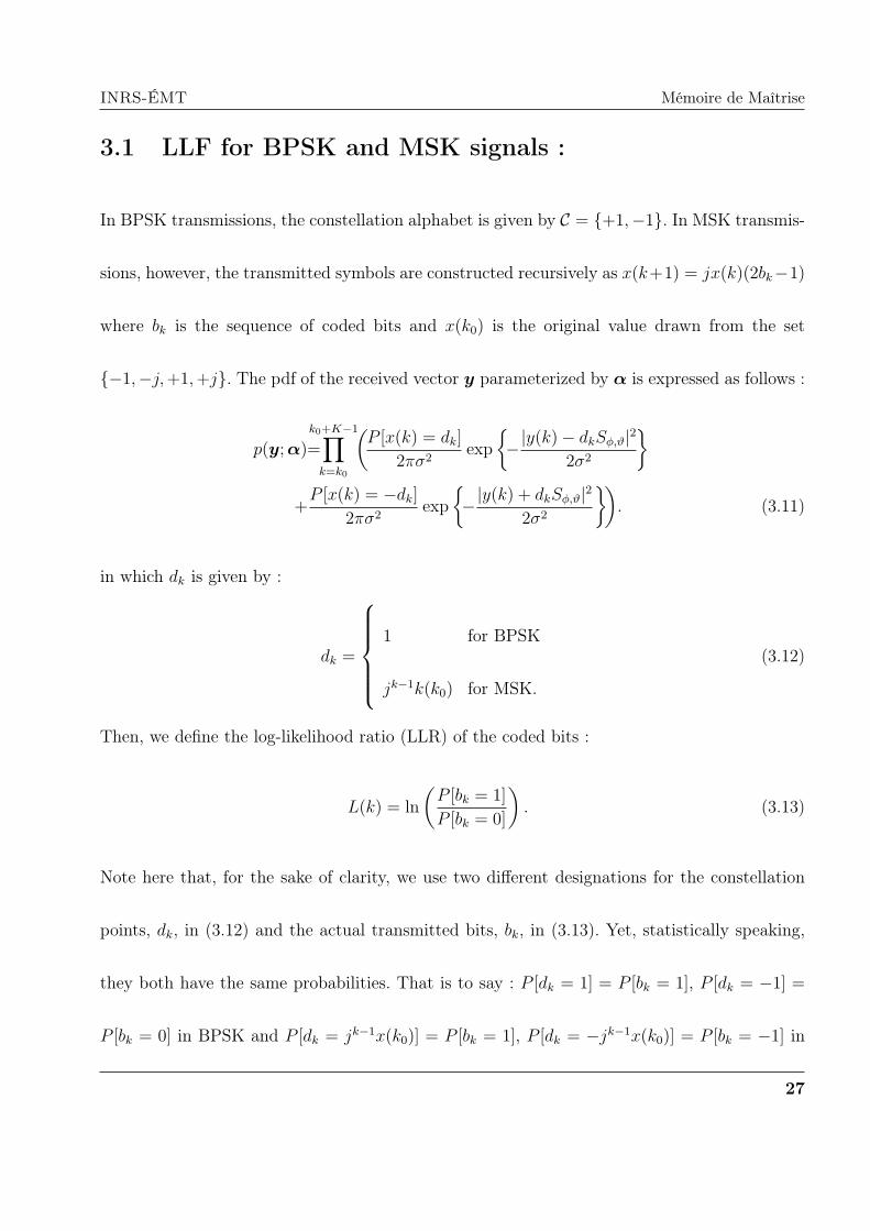
3.1 LLF for BPSK and MSK signals :
In BPSK transmissions, the constellation alphabet is given by C = +1,−1. In MSK transmis-
sions, however, the transmitted symbols are constructed recursively as x(k+1) = jx(k)(2bk−1)
where bk is the sequence of coded bits and x(k0) is the original value drawn from the set
−1,−j,+1,+j. The pdf of the received vector y parameterized by α is expressed as follows :
p(y;α)=
k0+K−1∏k=k0
(P [x(k) = dk]
2πσ2exp
−|y(k)− dkSϕ,ϑ|2
2σ2
+P [x(k) = −dk]
2πσ2exp
−|y(k) + dkSϕ,ϑ|2
2σ2
). (3.11)
in which dk is given by :
dk =
1 for BPSK
jk−1k(k0) for MSK.
(3.12)
Then, we define the log-likelihood ratio (LLR) of the coded bits :
L(k) = ln
(P [bk = 1]
P [bk = 0]
). (3.13)
Note here that, for the sake of clarity, we use two different designations for the constellation
points, dk, in (3.12) and the actual transmitted bits, bk, in (3.13). Yet, statistically speaking,
they both have the same probabilities. That is to say : P [dk = 1] = P [bk = 1], P [dk = −1] =
P [bk = 0] in BPSK and P [dk = jk−1x(k0)] = P [bk = 1], P [dk = −jk−1x(k0)] = P [bk = −1] in
27

INRS-ÉMT Mémoire de Maîtrise
MSK. Injecting these results in (3.11) and after some algebraic manipulations, it can be shown
that the log-likelihood function of interest (after dropping terms independent of the parameters
gatherd in α) denoted by L(r)y (α) is expressed as follows :
L(r)y (α)=−K ln(σ2)− KS2
2σ2− 1
2σ2
k0+K−1∑k=k0
|y(k)|2
+
k0+K−1∑k=k0
ln
(cosh
(ℜ(y(k)∗dkSϕ,ϑ)
σ2+L(k)
2
)). (3.14)
3.2 LLF for QPSK signals :
We denote the constellation alphabet, C, of the QPSK constellation as C = c0, c1, c2, c3.
Therefore, the pdf of the received sample, y(k), is given by :
p(y(k);α)=∑c∈C
P [x(k) = c]p(y(k);α|x(k) = c),
=3∑
m=0
P [x(k)=cm]
2πσ2exp
|y(k)−Sϕ,ϑ cm|2
2σ2
. (3.15)
Without loss of generality, we assume that c0 = 1/√(2) + j/
√(2) and that the constellation
is Gray coded according to the following mapping : c0 ←→ 11, c1 ←→ 10, c2 ←→ 00 and
28

INRS-ÉMT Mémoire de Maîtrise
c3 ←→ 01. Consequently, from (3.10) and (3.9), we obtain :
P [x(k) = c0] =eL1(k)
1 + eL1(k)
eL2(k)
1 + eL2(k), (3.16)
P [x(k) = c1] =eL1(k)
1 + eL1(k)
1
1 + eL2(k), (3.17)
P [x(k) = c2] =1
1 + eL1(k)
1
1 + eL2(k), (3.18)
P [x(k) = c3] =1
1 + eL1(k)
eL2(k)
1 + eL2(k). (3.19)
Then, by using the fact that c1 = −c0, c2 = c∗0 and c3 = −c∗0, plugging (3.16) to (3.19) back
into (3.15), and after some algebraic manipulations, it can be shown that :
p(y(k);α)=1
2πσ2exp
−S
2 + |y(k)|2
2σ2
×Q1(k) cosh
(ℜy(k)∗Sϕ,ϑ
σ2+L2(k)
2
)
×Q2(k) cosh
(ℑy(k)∗Sϕ,ϑ
σ2− L1(k)
2
), (3.20)
where
Ql(k) =1
cosh(Ll(k)/2)(3.21)
Thus, the pdf of the received vector y is factorized as follows :
p(y;α)=Cy(α)
k0+K−1∏k=k0
Q1(k) cosh
(ℜ(y(k)∗Sϕ,ϑ)
σ2+L2(k)
2
)
×k0+K−1∏k=k0
Q2(k) cosh
(ℑ(y(k)∗Sϕ,ϑ)
σ2− L1(k)
2
), (3.22)
29

INRS-ÉMT Mémoire de Maîtrise
where
Cy(α)=1
σ2K(2π)Kexp
−KS
2
2σ2− 1
2σ2
k0+K−1∑k=k0
|y(k)|2. (3.23)
By, taking the logarithm of (3.22) and dropping the constant terms involving Q1(k) and Q2(k)
(which do not depend on alpha), the LLF for QPSK signals develops as follows :
L(r)y (α)=−K ln(σ2)− KS2
2σ2− 1
2σ2
k0+K−1∑k=k0
|y(k)|2 +
k0+K−1∑k=k0
ln
(cosh
(ℜy(k)∗dkSϕ,ϑ
σ2+L2(k)
2
))+
k0+K−1∑k=k0
ln
(cosh
(ℑy(k)∗dkSϕ,ϑ
σ2+L1(k)
2
)). (3.24)
3.3 LLF for square-QAM signals :
Denoting I(k) = ℜy(k) and Q(k) = ℑy(k), it can be shown that in presence of M − ary
QAM-modulated signals, the pdf in (3.4) can be rewritten as follows :
p(y(k);α) =1
2πσ2exp
−I(k)
2 +Q(k)2
2σ2
Dα(k), (3.25)
in which
Dα(k) =M∑
m=1
Pm[xk] exp
−S
2 |cm|2
2σ2
×
exp
ℜcmy(k)∗Sϕ,ϑ
σ2
, (3.26)
30
INRS-ÉMT Mémoire de Maîtrise
where
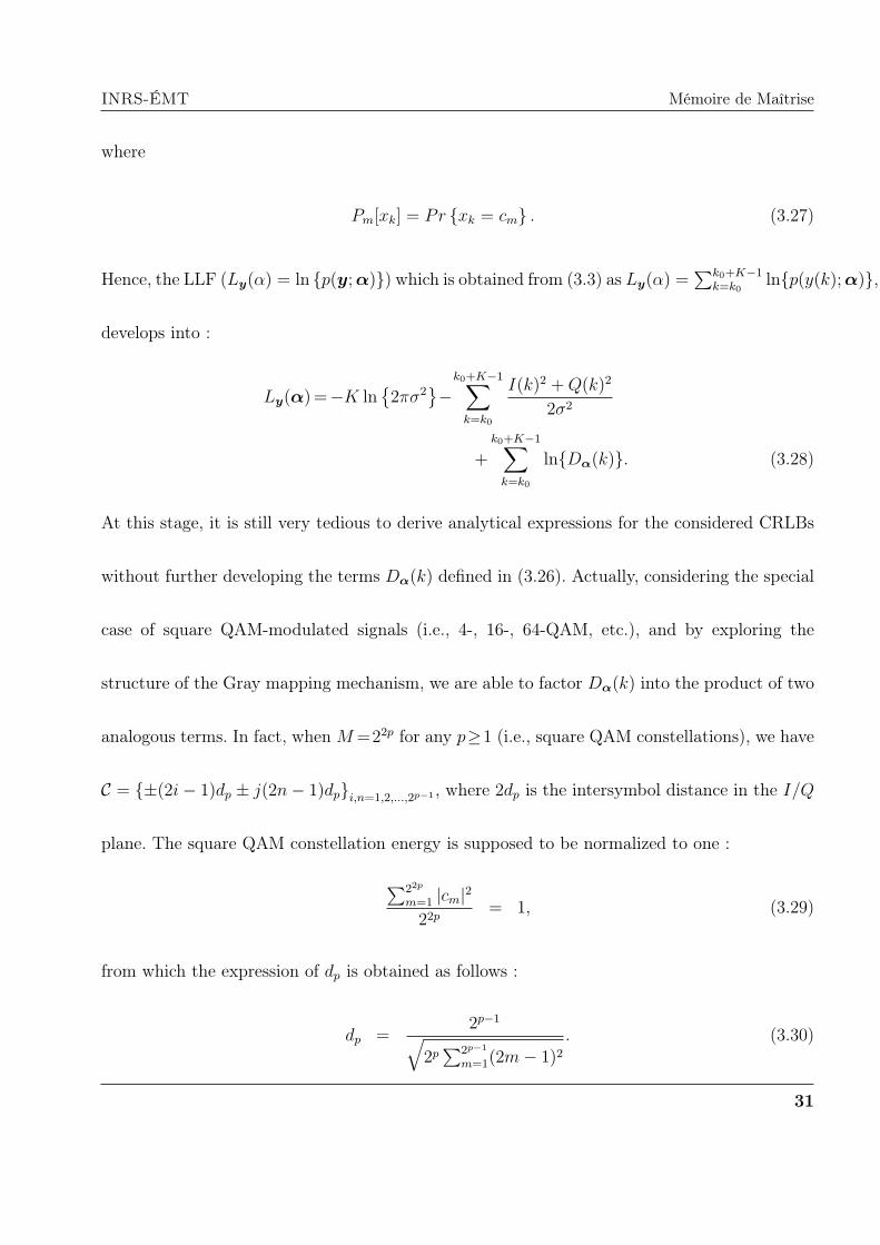
Pm[xk] = Pr xk = cm . (3.27)
Hence, the LLF (Ly(α) = ln p(y;α)) which is obtained from (3.3) as Ly(α) =∑k0+K−1
k=k0lnp(y(k);α),
develops into :
Ly(α)=−K ln2πσ2
−
k0+K−1∑k=k0
I(k)2 +Q(k)2
2σ2
+
k0+K−1∑k=k0
lnDα(k). (3.28)
At this stage, it is still very tedious to derive analytical expressions for the considered CRLBs
without further developing the terms Dα(k) defined in (3.26). Actually, considering the special
case of square QAM-modulated signals (i.e., 4-, 16-, 64-QAM, etc.), and by exploring the
structure of the Gray mapping mechanism, we are able to factor Dα(k) into the product of two
analogous terms. In fact, when M=22p for any p≥1 (i.e., square QAM constellations), we have
C = ±(2i− 1)dp ± j(2n− 1)dpi,n=1,2,...,2p−1 , where 2dp is the intersymbol distance in the I/Q
plane. The square QAM constellation energy is supposed to be normalized to one :
∑22p
m=1 |cm|2
22p= 1, (3.29)
from which the expression of dp is obtained as follows :
dp =2p−1√
2p∑2p−1
m=1(2m− 1)2. (3.30)
31

INRS-ÉMT Mémoire de Maîtrise
Now, by denoting C = (2i− 1)dp + j(2n− 1)dp2p−1
i,n=1 the subset of the alphabet that consists
of the points which lie in the top-right quadrant of the constellation, one can write C = C ∪
(−C) ∪ C∗ ∪ (−C∗). Therefore (3.26) can be expressed as follows :
Dα(k)=∑cm∈C
exp
−S
2|cm|2
2σ2
×
(P [xk = cm] exp
ℜcmy∗(k)Sϕ,ϑ
σ2
+P [xk = −cm] expℜ−cmy∗(k)Sϕ,ϑ
σ2
+P [xk = c∗m] exp
ℜc∗my∗(k)Sϕ,ϑ
σ2
+P [xk = −c∗m] expℜ−c∗my∗(k)Sϕ,ϑ
σ2
). (3.31)
Another important detail that must be addressed, in order to further simplify the term Dα(k),
is the Gray mapping scheme of the constellation. We will show through a simple Gray-coding
mechanism how this structure can be used to factor Dα(k), linearizing thereby the LLF expres-
sion in (3.28). The procedure applies in the same way to all the possible Gray mapping schemes,
and the obtained final CRLB expressions are the same. First, combining (3.9) and (3.10) and
assuming that the symbol cm is transmitted during the kth time instant (i.e., x(k) = cm), we
obtain the following generic formula for each conveyed bit :
P [bkl = bml ]=1
2sech
(Ll(k)
2
)e(2b
ml −1)
Ll(k)
2 , (3.32)
32
INRS-ÉMT Mémoire de Maîtrise
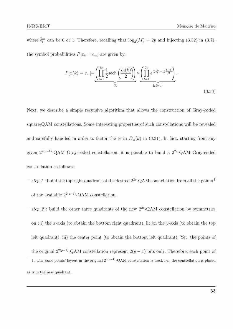
where bml can be 0 or 1. Therefore, recalling that log2(M) = 2p and injecting (3.32) in (3.7),
the symbol probabilities P [xk = cm] are given by :
P [x(k) = cm]=
(2p∏l=1
1
2sech
(Ll(k)
2
))︸ ︷︷ ︸
βk
×
(2p∏l=1
e(2bml −1)
Ll(k)
2
)︸ ︷︷ ︸
ξk(cm)
.
(3.33)
Next, we describe a simple recursive algorithm that allows the construction of Gray-coded
square-QAM constellations. Some interesting properties of such constellations will be revealed
and carefully handled in order to factor the term Dα(k) in (3.31). In fact, starting from any
given 22(p−1)-QAM Gray-coded constellation, it is possible to build a 22p-QAM Gray-coded
constellation as follows :
– step 1 : build the top right quadrant of the desired 22p-QAM constellation from all the points 1
of the available 22(p−1)-QAM constellation.
– step 2 : build the other three quadrants of the new 22p-QAM constellation by symmetries
on : i) the x-axis (to obtain the bottom right quadrant), ii) on the y-axis (to obtain the top
left quadrant), iii) the center point (to obtain the bottom left quadrant). Yet, the points of
the original 22(p−1)-QAM constellation represent 2(p− 1) bits only. Therefore, each point of
1. The same points’ layout in the original 22(p−1)-QAM constellation is used, i.e., the constellation is placed
as is in the new quadrant.
33

INRS-ÉMT Mémoire de Maîtrise
Figure 3.1 – Construction of Gray-coded Square-QAM constellations
the new 22p-QAM constellation that must represent 2p bits is still missing two of them.
– step 3 : add the two bits that appear in each quadrant of a basic Gray-coded QPSK constel-
lation to all the points that appear in the same quadrant of the new constellation.
An example of constructing a Gray-coded 16-QAM constellation from a 4-QAM Gray-coded
one is illustrated in Fig. 3.1 Just as depicted in this figure and without loss of generality, we
will assume in the sequel that it is the two least significant bits (LSBs) that are always added
in “step 3 ”.
34

INRS-ÉMT Mémoire de Maîtrise
Then, due to symmetries in “step 2 ”, it can be seen that each set of four symbols cm, c∗m, −cm
and −c∗m have the same 2(p−1) most significant bits (MSBs), bm1 bm2 bm3 ...bm2p−3bm2p−2, for any given
symbol cm from the top right quadrant of the 22p-QAM constellation (m = 1, 2, · · · , 22(p−1)).
Thus, if we consider these 2(p− 1) MSBs alone and we define
µk(cm),2p−2∏l=1
e(2bml −1)
Ll(k)
2 , ∀cm ∈ C, (3.34)
it can be immediately seen that :
µk(cm) = µk(−cm) = µk(c∗m) = µk(−c∗m), ∀cm ∈ C. (3.35)
Now, considering the two remaining LSBs (bm2p−1 and bm2p) and using the Gray-mapping depicted
in Fig. 3.1, it is seen that for any cm ∈ C we have bm2p−1bm2p = 11. Moreover, these two bits are
respectively given by “00”, “01”, and “10” for −C, C∗, and −C∗. Of course, these intermediate
results change according to the choice of the basic QPSK constellation involved in step 3. Yet,
we will explain later how this choice does not affect the final result. Then, upon using these
35

INRS-ÉMT Mémoire de Maîtrise
results along with (3.35), it follows from (3.33) that for any cm ∈ C, we have :
P [x(k)= cm]=βk µk(cm) eL2p−1(k)
2 eL2p(k)
2 , (3.36)
P [x(k)= c∗m]=βk µk(cm) e−
L2p−1(k)
2 eL2p(k)
2 , (3.37)
P [x(k)=−cm]=βk µk(cm) e−
L2p−1(k)
2 e−L2p(k)
2 , (3.38)
P [x(k)=−c∗m]=βk µk(cm) eL2p−1(k)
2 e−L2p(k)
2 . (3.39)
Therefore, plugging these probabilities back into (3.31) and using the identity ex + e−x =
2 cosh(x), it can be shown that :
Dα(k)=2βk∑cm∈C
exp
−S
2|cm|2
2σ2
µk(cm)×[
cosh
(ℜcm y∗(k)Sϕ,ϑ
σ2+L2p−1(k)
2+L2p(k)
2
)
+cosh
(ℜc∗m y∗(k)Sϕ,ϑ
σ2+L2p−1(k)
2−L2p(k)
2
)]. (3.40)
Furthermore, using the relashiship cosh(x) + cosh(y) = 2 cosh(x+y2) cosh(x−y
2) along with the
two identities cm + c∗m = 2ℜcm and cm − c∗m = 2jℑcm, (3.40) is rewritten as follows :
Dα(k)=4βk∑˜cm∈C
[exp
−S
2|cm|2
2σ2
µk(cm)×
cosh
(S ℜcmℜ
y∗(k)ej(2πkϑ+ϕ)
σ2
+L2p(k)
2
)×
cosh
(S ℑcmℑ
y∗(k)ej(2πkϑ+ϕ)
σ2
−L2p−1(k)
2
)]. (3.41)
36

INRS-ÉMT Mémoire de Maîtrise
Recalling that C = (2i− 1)dp + j(2n− 1)dp2p−1
i,n=1, the sum over cm ∈ C in (3.41) can be
written as a double sum over the counters i and n after replacing cm by (2i−1)dp+j(2n−1)dp.
Therefore, in order to factor Dα(k), the term µk(cm = (2i−1)dp+j(2n−1)dp) must be factored
into two terms, one depending only on i and the other only on n. Here, we are actually dealing
with the remaining 2p − 2 MSBs, bm1 bm2 bm3 · · · bm2p−3bm2p−2. Hence, since the two LSBs bm2p−1 and
bm2p are not involved in µk(cm) (and are the same 2 for all cm ∈ Cp
3 they will be represented by “××” in (3.1), i.e. :
cm ←→ bm1 bm2 · · · bml · · · bm2p−5b
m2p−4︸ ︷︷ ︸
bmp
bm2p−3bm2p−2 ××. (3.42)
In addition, as highlighted in (3.42), it will prove very useful to represent the first 2p− 4 MSBs
by the shorthand notation bmp , i.e., bmp , bm1 bm2 · · · bml · · · bm2p−5b
m2p−4. For more convenience, we
will rather use the superscript (i, n) instead of m in (3.42) since cm = (2i− 1)dp + j(2n− 1)dp.
That is :
cm ←→ b(i,n)p b(i,n)2p−3b
(i,n)2p−2 ××. (3.43)
2. The values of these two LSBs are defined according to the top-right quadrant of the basic Gray-coded
QPSK constellation used in “step 3 ” during the recursive construction algorithm. For instance, in the example
depicted in Fig. 3.1, they will be “×× = 11”.
3. Actually Cp = C , but later on we have to make a difference between C in a 22p-QAM and when considering
a 22(p−1)-QAM.
37

INRS-ÉMT Mémoire de Maîtrise
Using this mapping, all the points of the top-right quadrant of the obtained 22p-QAM constel-
lation are graphically represented in Fig. 3.2 where the bits b(i,n)2p−1 and b(i,n)2p are being assigned
their true values. Each symbol cm in Cp which has coordinates((2i− 1)dp , (2n− 1)dp
)in the
current 22p-QAM constellation (x− axis and y− axis in Fig. 3.2) has already different coor-
dinates (a′, b′) in the original 22(p−1)-QAM constellation (x′− axis and y′− axis in Fig. 3.2) ;
associated with a symbol cm′ = a′ + jb′ in Cp−1. By inspecting Fig 3.2, it can be shown that
cm′ = (2i− 1− 2p−1)dp + j(2n− 1− 2p−1)dp. (3.44)
Moreover, we have the follwong result :
cm′ ←→ b(i,n)p b(i,n)2p−3b
(i,n)2p−2. (3.45)
since the first 2p − 2 MSBs of each symbol cm ∈ Cp are obtained (during “step 1 ”) from the
whole bit sequence of the symbol cm′ associated to it in the original 22(p−1)-QAM constellation.
From (3.34), we have :
µk,p(cm),γk(b(i,n)p
)exp
(2b
(i,n)2p−3 − 1)L2p−3(k)/2
×
exp(2b
(i,n)2p−2 − 1)L2p−2(k)/2
, (3.46)
where
γk(b(i,n)p
),
2(p−1)−2∏l=1
exp(2b
(i,n)l − 1)L2p−2(k)/2
, (3.47)
38

INRS-ÉMT Mémoire de Maîtrise
On the other hand, denoting the top-right quadrant of the original 22(p−1)-QAM constellation
by Cp−1, it also holds Cp−1 = Cp−1∪(−Cp−1)∪C∗p−1∪(−C∗p−1). Then, for some cm′ ∈ Cp−1, we have
cm′ ∈ cm′ ,−cm′ , c∗m′ ,−c∗m′. In turn, the symbols cm′ themselves are obtained from a previous
Gray-coded 22(p−2)-QAM constellation by applying the same recursive construction algorithm.
Therefore, due to symmetries of “step 2 ” it follows that cm′ , −cm′ , c∗m′ , and −c∗m′ have the same
2p−4 MSBs which are represented by b(i,n)p . Consequently, according to the definition of (3.34),
we have γk(b(i,n)p
)= µk,p−1(cm′) thereby yielding the following recursive property :
µk,p(cm),µk,p−1(cm′) exp(2b
(i,n)2p−3 − 1)L2p−3(k)/2
×
exp(2b
(i,n)2p−2 − 1)L2p−2(k)/2
. (3.48)
Actually one needs to express the bits b(i,n)2p−3 and b(i,n)2p−2 explicitly as function of i and n if µk,p(cm)
is to be factorized in terms of these two counters separately. This useful result is given by the
following lemma.
Lemma : The two bits b(i,n)2p−3 and b(i,n)2p−2 are expressed as :
b(i,n)2p−2 =
⌊i− 1
2p−2
⌋and b(i,n)2p−3 =
⌊n− 1
2p−2
⌋
∀ i, n = 1, 2, · · · , 2p−1. (3.49)
In (3.49), ⌊x⌋ is the floor function which returns the largest integer which is smaller than or
equal to x.
39

INRS-ÉMT Mémoire de Maîtrise
Thus, injecting (3.49) in (3.48), it follows :
µk,p(cm),µk,p−1(cm′) exp
(2⌊n− 1
2p−2⌋ − 1
)L2p−3(k)
2
×
exp
(2⌊ i− 1
2p−2⌋ − 1
)L2p−2(k)
2
. (3.50)
Following the same reasoning from (3.42) through (3.49), µk,p−1(cm′) itself can be written in the
same recursive form of (3.50) by considering the recursive reconstruction of Cp−1 (highlighted
in blue color in Fig 3.2) from the 22(p−2)-QAM constellation. Consequently, by repeating this
process down constellations, it can be shown that µk(cm) is factored into two independent terms
one depending on i only and the other on n only as follows :
µk(cm) = θk,2p(i)θk,2p−1(n). (3.51)
where the terms θk,2p(i) and θk,2p−1(n) are obtained recursively, for any p ≥ 2, as follows :
θk,2p(i)=θk,2p−2
(|2i− 1− 2p−1|+ 1
2
)×
exp
(2⌊ i− 1
2p−2⌋ − 1
)L2p−2(k)
2
, (3.52)
θk,2p−1(n)=θk,2p−3
(|2n− 1− 2p−1|+ 1
2
)×
exp
(2⌊n− 1
2p−2⌋ − 1
)L2p−3(k)
2
, (3.53)
The initialization for p = 1 (i.e., the basic 4-QAM constellation) is given by θk,2(.)=θk,1(.)=1,
since µk(cm) = 1 ∀ cm ∈ C1. Now plugging (3.52) and (3.53) in (3.41) and using the fact that
40

INRS-ÉMT Mémoire de Maîtrise
Figure 3.2 – Construction of Gray-coded Square-QAM constellations
41

INRS-ÉMT Mémoire de Maîtrise
Cp = (2i− 1)dp + j(2n− 1)dpi,n=1,2,··· ,2p−1 , the term Dα(k) is rewritten as follows :
Dα(k) = 4βk
2p−1∑i=1
2p−1∑n=1
[exp
−S2((2i− 1)2 + (2n− 1)2)d2p
2σ2
θk,2p(i) cosh
(S(2i− 1)dpu(k)
σ2+L2p(k)
2
)×
θk,2p−1(n) cosh
(S(2n− 1)dpv(k)
σ2− L2p−1(k)
2
)]
(3.54)
where u(k) and v(k) are defined as u(k) = ℜy∗(k)ej(2πkϑ+ϕ)
and v(k) = ℑ
y∗(k)ej(2πkϑ+ϕ)
.
Finally, splitting the two sums, it can be shown that Dα(k) is factorized as follows :
Dα(k)=4βk F2p,α(u(k))× F2p−1,α(v(k)), (3.55)
where Fq,α(.) is given by :
Fq,α(x) =2p−1∑i=1
θk,q(i) exp
−S2(2i− 1)2d2p
2σ2
×
cosh
(S(2i− 1)dpx
σ2+ (−1)qLq(k)
2
), (3.56)
where the counter q is used, from now on, to refer to 2p or 2p − 1 depending on the context.
The factorization of Dα(k) in (3.55) will prove very useful in deriving the analytical expressions
of the considered stochastic CRLBs. In fact, by injecting (3.55) back into (3.28) the LLF for
42

INRS-ÉMT Mémoire de Maîtrise
arbitrary square-QAM constellation becomes as follows :
Ly(α)=−1
2σ2
k0+K−1∑k=k0
(I(k)2 +Q(k)2
)+
k0+K−1∑k=k0
lnF2p,α(u(k))
+
k0+K−1∑k=k0
lnF2p−1,α(v(k)), (3.57)
involving thereby the sum of two analogous terms (the two last sums). Now, we further show that
U(k) and V (k) (whose realizations are u(k) and v(k), respectively) are two independent random
variables which are almost identically distributed (i.e., their pdfs have the same structure,
but are parameterized differently) . In fact, injecting (3.54) in (3.25) and using the fact that
I(k)2 +Q(k)2 = u(k)2 + v(k)2, it can be shown that p(y(k);α) factorized as follows :
p(y(k);α) = p(u(k);α)p(v(k);α), (3.58)
where
p(u(k);α)=2βk,2p√2πσ2
exp
−u(k)
2
2σ2
F2p,α(u(k)), (3.59)
p(v(k);α)=2βk,2p−1√
2πσ2exp
−v(k)
2
2σ2
F2p−1,α(v(k)), (3.60)
with
βk,2p =1
2p
p∏l=1
sech(L2l(k)
2
)(3.61)
βk,2p−1 =βkβk,2p
. (3.62)
43

INRS-ÉMT Mémoire de Maîtrise
Moreover, we have p(u(k), v(k);α) = p(y(k)∗ej(2πkν+ϕ);α) since u(k) and v(k) are indeed the
real and imaginary parts of y(k)∗ej(2πkν+ϕ). Then, since ej(2πkν+ϕ) is assumed to be deterministic,
we have p(y(k)∗ej(2πkν+ϕ);α) = p(y(k);α). Therefore, using (3.58) we obtain :
p(u(k), v(k);α) = p(u(k);α)p(v(k);α). (3.63)
meaning that the joint distribution of U(k) and V (k) is factored and hence they are two
independent random variables which are almost distributed according to (3.59) and (3.60).
44
Chapitre 4
Derivation of the CRLB Analytical
Expressions
4.1 CRLB for coded SNR estimation [43]
We begin first by deriving the FIM elements using the LLF expressions obtained in the previous
section. We consider the case of square-QAM-modulated signals since it is the most general one.
Equivalent derivations can be applied in case of BPSK-, MSK- and QPSK-modulated-signals
to obtain the corresponding FIM elements. We will also detail the derivations for the first FIM
element only and the other ones can be obtained in the same way. To begin with and using

INRS-ÉMT Mémoire de Maîtrise
(3.57), we have the following result :
Ey
∂2 ln(p(y;α(1)))
∂S2
=
K−1∑k=0
E
∂2 ln(F2p,α(1)(u(k)))
∂)S2
+K−1∑k=0
E
∂2 ln(F2p−1,α(1)(v(k)))
∂S2
. (4.1)
As mentioned previously, the two terms in the right-hand side of (4.1) are analogous and they
can be derived in the same way, especially because the RVs U(k) and V (k) are almost identically
distributed. Thus, for ease of notations, we will henceforth use zq(k) to refer to u(k) when q = 2p
and to v(k) when q = 2p− 1, respectively. Using this generic notation and if we denote :
Fq,α(1)(zq(k)) ,∂Fq,α(1)(zq(k))
∂S,
Fq,α(1)(zq(k)) ,∂2Fq,α(1)(zq(k))
∂S2,
it can be shown that :
E
∂2ln(Fq,α(1)(zq(k)))
∂S2
=E
Fq,α(1)(zq(k))
Fq,α(1)(zq(k))
−E
Fq,α(1)(zq(k))
2
Fq,α(1)(zq(k))2
.
The second expectation is obtained by integrating over the distribution of zq(k) obtained earlier
in (3.59) and (3.60) for q = 2p and q = 2p− 1, respectively :
E
Fq,α(1)(zq(k))
2
Fq,α(1)(zq(k))2
=
∫ +∞
−∞
Fq,α(1)(zq(k))2
Fq,α(1)(zq(k))2p(zq(k),α
(1))dzq(k) (4.2)
=2βk,q√2πσ2
∫ +∞
−∞
Fq,α(1)(zq(k))2
Fα(1)(zq(n))e−
zq(n)2
2σ2 dzq(n).
46

INRS-ÉMT Mémoire de Maîtrise
We further simplify (4.2) by changing zq(k)/σ by t and using ρ = S2/2σ2 to obtain :
E
Fq,α(1)(zq(k))
2
Fq,α(1)(zq(k))2
=
2βk,qd2p
σ2ψk,q(ρ), (4.3)
in which Ψk,q(ρ) is defined as :
Ψk,q(ρ) ,1√2π
∫ +∞
−∞
λk,q(ρ, t)2
δk,q(ρ, t)e−
t2
2 dt, (4.4)
where, by using ωk,q(i) , θk,q(i) e−(2i−1)2d2pρ, the functions δk,q(., .) and λk,q(., .) are, respectively,
given by (4.5) and (4.6) :
δk,q(ρ, t)=2p−1∑i=1
ωk,q(i)cosh
(√2ρ(2i−1)dpt+
(−1)qLq(k)
2
), (4.5)
λk,q(ρ, t)=2p−1∑i=1
(2i−1)2ωk,q(i)
[t sinh
(√2ρ (2i−1)dpt+
(−1)qLq(k)
2
)
−dp(2i−1)√2ρ cosh
(√2ρ(2i−1)dpt+
(−1)qLq(k)
2
)]. (4.6)
In addition, after tedious algebraic manipulations, we show the following identity :
E
Fq,α(1)(zq(k))
Fq,α(1)(zq(k))
= 0. (4.7)
Therefore, by using αk,q , 2βk,qd2pψk,q(ρ) and injecting (4.3) for q = 2p and q = 2p−1 in (4.24),
it follows :
Ey
∂2ln(p(y;α(1)))
∂S2
=− 1
σ2
K−1∑k=0
[αk,2p+αk,2p−1
](4.8)
47

INRS-ÉMT Mémoire de Maîtrise
Equivalent algebraic manipulations lead to the following analytical expressions for the second
FIM diagonal element :
Ey
∂2 ln(p(y;α(1)))
∂σ22
=K
σ4+
1
σ4
K−1∑k=0
[νk,2p + νk,2p−1
], (4.9)
where νk,q (for q = 2p or 2p− 1) is given by :
νk,q = c(k)4,qρ
2 + 2(c(k)2,q − 2βk,qd
2pΦq,k(ρ)
)− c(k)0,q . (4.10)
The coefficients c(k)l,q are given by :
c(k)l,q = 2βk,qd
lp cosh
(Lq(k)/2
) 2p−1∑i=1
θk,q(i)(2i− 1)l, (4.11)
and the function Φk,q(.) is defined as :
Φk,q(ρ) ,1√2π
∫ +∞
−∞
γ2k,q(ρ, t)
δk,q(ρ, t)e−
t2
2 dt (4.12)
with γk,q(., .) being given by :
γk,q(ρ, t)=2p−1∑i=1
(2i−1)2ωk,q(i)
[t sinh
(√2ρ (2i−1)dpt+
(−1)qLq(k)
2
)
−dp(2i−1)√ρ
2cosh
(√2ρ(2i−1)dpt+
(−1)qLq(k)
2
)]. (4.13)
Equivalent derivations also yield the following expression for the off-diagonal element of I(α(1)) :
Ey
∂2 ln(p(y;α(1)))
∂σ2∂S
=− S
σ4
K−1∑k=0
[ηk,2p + ηk,2p−1
], (4.14)
48

INRS-ÉMT Mémoire de Maîtrise
in which ηk,q , c(k)2,q − 2d2p βk,q Ωk,q(ρ) with the function Ωk,q(.) being defined as :
Ωk,q(ρ) ,1√2π
∫ +∞
−∞
γq,ρ(t)λq,ρ(t)
δq,ρ(t)e−
t2
2 dt (4.15)
Therefore, from (4.8), (4.9) and (4.14), the global Fisher information matrix decomposes into
the sum of elementary FIMs :
I(α(1)) =K−1∑k=0
Ik(α(1)) (4.16)
where Ik(α(1))K−1k=0 is the FIM pertaining to the estimation of the SNR from the received
sample y(k) alone :
Ik(α(1))=
1
σ4
σ2[αk,2p+αk,2p−1
]S[ηk,2p + ηk,2p−1
]
S[ηk,2p + ηk,2p−1
]−[ν2p,k + ν2p−1,k + 1
]
. (4.17)
This FIM expression in the general case of a coded-aided estimation corroborates the two
traditional extreme cases of completely NDA and completely DA estimations. Indeed, in the
former case, no a priori information about the bits is available at the receiver and, hence,
P [bkl = 1] = P [bkl = 0] = 1/2 meaning that LNDAl (k) = 0. In the latter case, however, the
bits are a priori perfectly known and, therefore, at the receiver side we have P [bkl = 1] =
1 hence P[bkl = 0] = 0 or P [bkl = 0] = 1 hence P[bk
l = 1] = 0 and consequently the LLRs
verify : LDAl (k) = ±∞. Injecting LNDA
l (k) and LDAl (k) in the entries of Ik(α), and recognizing
49

INRS-ÉMT Mémoire de Maîtrise
some easy simplifications lead to the exact same expression for the FIMs developed earlier in
[23] in the NDA and DA cases, respectively.
Now, since the inverse of any (2× 2) matrix is directly obtained by swapping the two diagonal
elements and negating the off-diagonal ones, it can be shown from (4.16) that :
I(α(1))−1 =K−1∑k=0
detIk(α
(1))
det I(α(1))Ik(α
(1))−1, (4.18)
where det. returns the determinant of any square matrix. Finally, injecting (4.18) and (2.8)
in (2.7), it can be shown be shown that :
CRLB(ρ) =K−1∑k=0
ω(k) CRLBk(ρ), (4.19)
where ω(k) = detIk(α
(1))/ det
I(α(1))
and CRLBk(ρ), given by (4.20) on the top of the
next page, is the elementary CRLB pertaining to the estimation of the SNR given the received
sample y(k) only. The higher the weighting coefficient, ω(k), the more y(k) contributes to the
overall achievable performance. These coefficients are not equal since the received samples are
not identically distributed. This is in contrast to the NDA or DA estimation scenarios where
all the samples are indeed identically distributed. This yields identical elementary FIMs and
equal weighting coefficients leading thereby to a the factor K in the overall CRLB as shown in
[23].
50
INRS-ÉMT Mémoire de Maîtrise
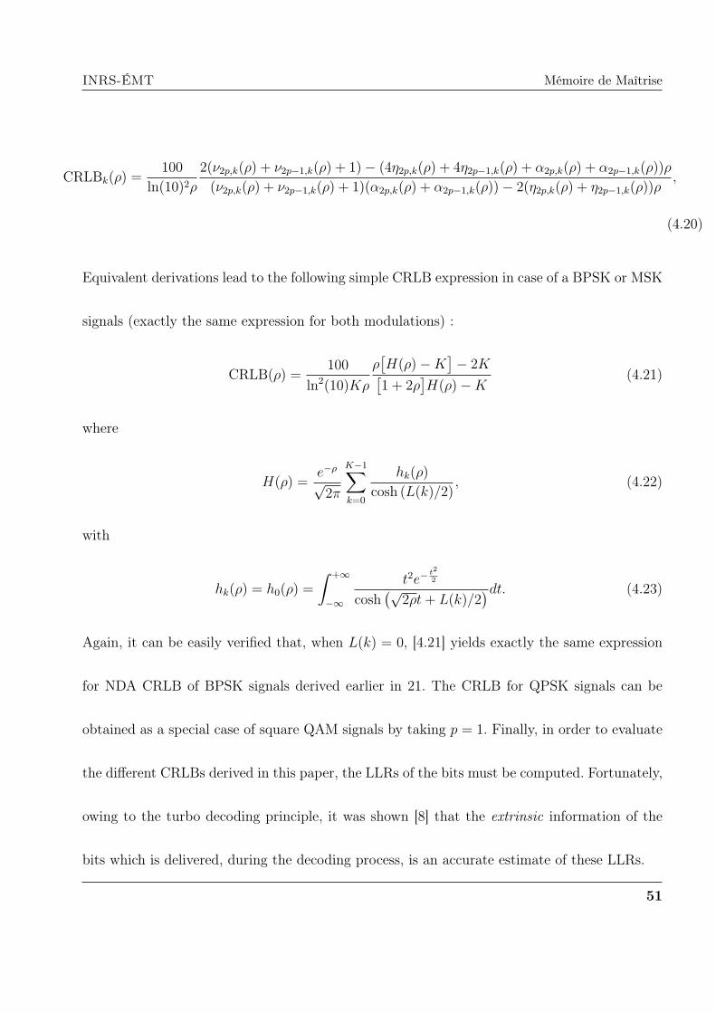
CRLBk(ρ) =100
ln(10)2ρ
2(ν2p,k(ρ) + ν2p−1,k(ρ) + 1)− (4η2p,k(ρ) + 4η2p−1,k(ρ) + α2p,k(ρ) + α2p−1,k(ρ))ρ
(ν2p,k(ρ) + ν2p−1,k(ρ) + 1)(α2p,k(ρ) + α2p−1,k(ρ))− 2(η2p,k(ρ) + η2p−1,k(ρ))ρ,
(4.20)
Equivalent derivations lead to the following simple CRLB expression in case of a BPSK or MSK
signals (exactly the same expression for both modulations) :
CRLB(ρ) =100
ln2(10)Kρ
ρ[H(ρ)−K
]− 2K[
1 + 2ρ]H(ρ)−K
(4.21)
where
H(ρ) =e−ρ
√2π
K−1∑k=0
hk(ρ)
cosh (L(k)/2), (4.22)
with
hk(ρ) = h0(ρ) =
∫ +∞
−∞
t2e−t2
2
cosh(√
2ρt+ L(k)/2)dt. (4.23)
Again, it can be easily verified that, when L(k) = 0, [4.21] yields exactly the same expression
for NDA CRLB of BPSK signals derived earlier in 21. The CRLB for QPSK signals can be
obtained as a special case of square QAM signals by taking p = 1. Finally, in order to evaluate
the different CRLBs derived in this paper, the LLRs of the bits must be computed. Fortunately,
owing to the turbo decoding principle, it was shown [8] that the extrinsic information of the
bits which is delivered, during the decoding process, is an accurate estimate of these LLRs.
51

INRS-ÉMT Mémoire de Maîtrise
4.2 CRLB for coded phase and CFO estimtion [44]
Actually, using (3.57), it can be shown that :
Ey
∂2 ln(p(y;α(2)))
∂ϕ2
=
k0+K−1∑k=k0
E
∂2 ln(F2p,α(2)(u(k)))
∂ϕ2
+
k0+K−1∑k=k0
E
∂2 ln(F2p−1,α(2)(−v(k)))
∂ϕ2
. (4.24)
Using the distribution of U(k) and V (k), and the definition E
∂2ln(F
q,α(2)(u(k)))
∂ϕ2
, ηq,k(ρ), we
were able to show that :
ηq,k(ρ) = Aq,k ρ
(Aq,kρ− 4βk,qd
2pΨq(ρ)
(1
Aq,k
+ ρ
)), (4.25)
where
Aq,k = 4βk,q cosh
(Lq(k)
2
)d2p
2p−1∑i=1
θk,q(i)(2i− 1)2 (4.26)
Ψq(ρ) =1√2π
∫ +∞
−∞
λ2q,ρ(t)
δq,ρ(t)e−
t2
2 dt (4.27)
with
λq,ρ(t)=2p−1∑i=1
(2i− 1)θk,q(i) e−(2i−1)2d2pρ sinh(hi,q(t)),
δq,ρ(t)=2p−1∑i=1
θk,q(i)e−(2i−1)2d2pρ cosh(hi,q(t)), (4.28)
52
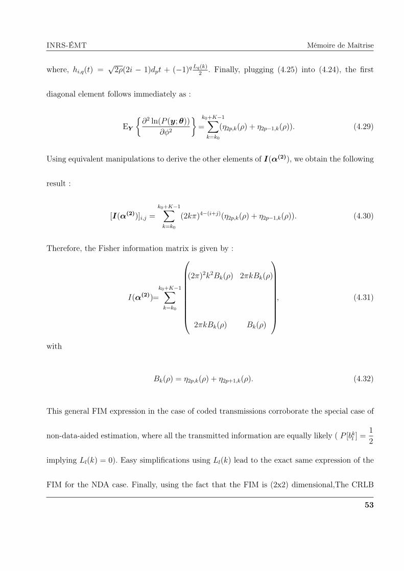
INRS-ÉMT Mémoire de Maîtrise
where, hi,q(t) =√2ρ(2i − 1)dpt + (−1)q Lq(k)
2. Finally, plugging (4.25) into (4.24), the first
diagonal element follows immediately as :
EY
∂2 ln(P (y;θ))
∂ϕ2
=
k0+K−1∑k=k0
(η2p,k(ρ) + η2p−1,k(ρ)). (4.29)
Using equivalent manipulations to derive the other elements of I(α(2)), we obtain the following
result :
[I(α(2))]i,j =
k0+K−1∑k=k0
(2kπ)4−(i+j)(η2p,k(ρ) + η2p−1,k(ρ)). (4.30)
Therefore, the Fisher information matrix is given by :
I(α(2))=
k0+K−1∑k=k0
(2π)2k2Bk(ρ) 2πkBk(ρ)
2πkBk(ρ) Bk(ρ)
, (4.31)
with
Bk(ρ) = η2p,k(ρ) + η2p+1,k(ρ). (4.32)
This general FIM expression in the case of coded transmissions corroborate the special case of
non-data-aided estimation, where all the transmitted information are equally likely ( P [bkl ] =1
2
implying Ll(k) = 0). Easy simplifications using Ll(k) lead to the exact same expression of the
FIM for the NDA case. Finally, using the fact that the FIM is (2x2) dimensional,The CRLB
53
INRS-ÉMT Mémoire de Maîtrise
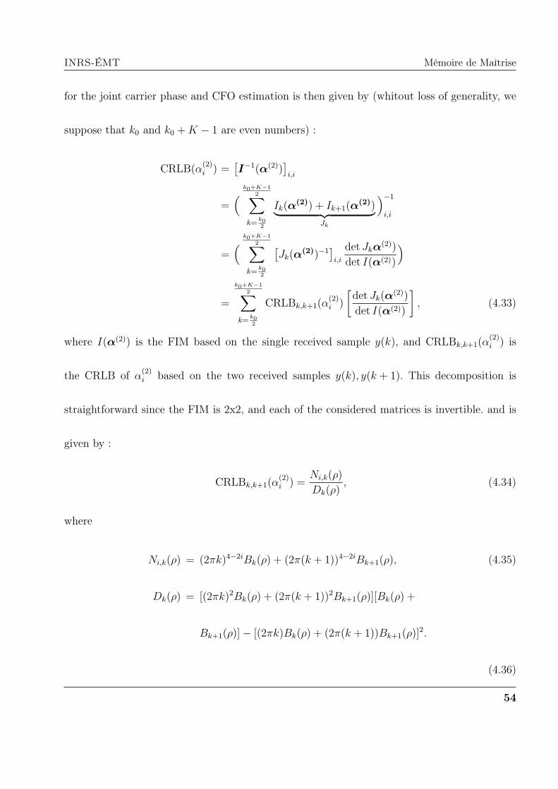
for the joint carrier phase and CFO estimation is then given by (whitout loss of generality, we
suppose that k0 and k0 +K − 1 are even numbers) :
CRLB(α(2)i ) =
[I−1(α(2))
]i,i
=( k0+K−1
2∑k=
k02
Ik(α(2)) + Ik+1(α
(2))︸ ︷︷ ︸Jk
)−1
i,i
=( k0+K−1
2∑k=
k02
[Jk(α
(2))−1]i,i
det Jkα(2))
det I(α(2))
)
=
k0+K−12∑
k=k02
CRLBk,k+1(α(2)i )
[det Jk(α
(2))
det I(α(2))
], (4.33)
where I(α(2)) is the FIM based on the single received sample y(k), and CRLBk,k+1(α(2)i ) is
the CRLB of α(2)i based on the two received samples y(k), y(k + 1). This decomposition is
straightforward since the FIM is 2x2, and each of the considered matrices is invertible. and is
given by :
CRLBk,k+1(α(2)i ) =
Ni,k(ρ)
Dk(ρ), (4.34)
where
Ni,k(ρ) = (2πk)4−2iBk(ρ) + (2π(k + 1))4−2iBk+1(ρ), (4.35)
Dk(ρ) = [(2πk)2Bk(ρ) + (2π(k + 1))2Bk+1(ρ)][Bk(ρ) +
Bk+1(ρ)]− [(2πk)Bk(ρ) + (2π(k + 1))Bk+1(ρ)]2.
(4.36)
54

INRS-ÉMT Mémoire de Maîtrise
From (4.33), we see that the CRLB of the phase and CFO estimation based on the received
samples vector y = [y(k0), y(k0 + 1), · · · , y(k0 +K − 1)]T is the summation of the elementary
CRLBs of each received two samples (y(k), y(k+1)) individually (this decomposition into sums
of CRLBs is possible thanks to the approximation that the received samples are independent,
due to the outer interleaver), weighted by the termdet Jk(α
(2))
det I(α(2))(these wieghts are not equal
since the received samples are independent but not indentically distributed) which reflect the
contribution of the estimation from the received the samples y(k), y(k + 1) on the estimation
based on the whole received vector y :
det Ji0(α(2))
det I(α(2))≪ 1⇔ CRLB(ρ) ≃
k0+K−12∑
k=k02,k =
ki02
CRLBk,k+1(ρ) (4.37)
In order to establish a closed-form expression of the CRLB for a given code structure (in our
case a turbo code), we need to calculate the a priori probabilities of the coded bits involved in
the expression of ηq,k(ρ).
In the case of a BPSK or MSK modulation, the FIM matrix is the same and is given by :
I(α(2))=
k0+K−1∑k=k0
(1− hk(ρ))∑k0+K−1
k=k02πk(1− hk(ρ))
k0+K−1∑k=k0
2πk(1− hk(ρ)k0+K−1∑k=k0
(2π)2k2(1− hk(ρ))
, (4.38)
55

INRS-ÉMT Mémoire de Maîtrise
where
hk(ρ) = 2e−ρ
√2π cosh(L(k)
2)
∫ +∞
0
e−t2
2
cosh(√
2ρt+ L(k)2
)dt. (4.39)
In the case of a NDA estimation, i.e. L(k) = 0, we have :
hk(ρ) = h0(ρ) = 2e−ρ
√2π
∫ +∞
−∞
e−t2
2
cosh(√
2ρt)dt. (4.40)
(4.41)
the FIM becomes :
I(α(2))= (1− h0(ρ))
K∑k0+K−1
k=k02πk
k0+K−1∑k=k0
2πk
k0+K−1∑k=k0
(2π)2k2
, (4.42)
and the CRLB expression becomes the same as given in [22].
4.2.1 Empirical Evaluation of the CRLB
In this section, we develop an empirical procedure that evaluates the considered CRLBs through
extensive Monte-Carlo simulations. These empirical CRLBs are used to validate our new ana-
lytical expressions. In fact, the CRLB can be expressed in terms of the symbols’ a posteriori
probabilities (APPs). We will also rely on another definition for the FIM elements which in-
volves the first derivatives of the LLF instead of its second derivatives. In fact, as shown in [27],
56

INRS-ÉMT Mémoire de Maîtrise
the FIM elements can be written in the following equivalent form :
Ii,j(α) = E
(∂ ln(p(y;α))
∂αi
∂ ln(p(y;α))
∂αj
)(4.43)
where
ln(p(y;α)) = ln
MK∑i=1
Pi[x]p(y |x = ci)
, (4.44)
is another formulation for the LLF in which Pi[x] = Prx = ci with x = [x(k0), x(k0 +
1), · · · , x(k0 +K − 1)] being a vector that contains the actual sequence of transmitted symbols
and ciMK
i=1 are all the possible sequences of coded symbols. Differentiating (4.44) with respect
αi leads to the following expression :
∂ ln(p(y;α))
∂αi
=MK∑i=1
Pi[x]p(y |x = ci)
p(y;α)×
∂ ln (p(y |x = ci))
∂αi
. (4.45)
(4.46)
Then, owing to the Bayes’ formula :
Pi[x]p(y |x = ci)
p(y;α)= P (x = ci |y),
(4.47)
the right-hand side of (4.45) is nothing but the following conditional expectation :
∂ ln(p(y;α))
∂αi
= Ec|y
∂ ln (p(y |x = ci))
∂αi
. (4.48)
57
INRS-ÉMT Mémoire de Maîtrise
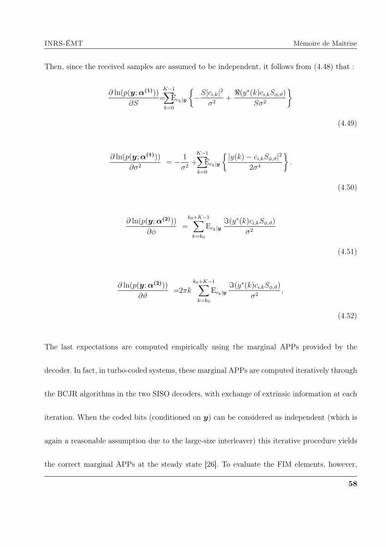
Then, since the received samples are assumed to be independent, it follows from (4.48) that :
∂ ln(p(y;α(1)))
∂S=K−1∑k=0
Eck|y
−S|ci,k|
2
σ2+ℜ(y∗(k)ci,kSϕ,ϑ)
Sσ2
(4.49)
∂ ln(p(y;α(1)))
∂σ2= − 1
σ2+K−1∑k=0
Eck|y
|y(k)− ci,kSϕ,ϑ|2
2σ4
.
(4.50)
∂ ln(p(y;α(2)))
∂ϕ=
k0+K−1∑k=k0
Eck|yℑ(y∗(k)ci,kSϕ,ϑ)
σ2
(4.51)
∂ ln(p(y;α(2)))
∂ϑ=2πk
k0+K−1∑k=k0
Eck|yℑ(y∗(k)ci,kSϕ,ϑ)
σ2,
(4.52)
The last expectations are computed empirically using the marginal APPs provided by the
decoder. In fact, in turbo-coded systems, these marginal APPs are computed iteratively through
the BCJR algorithms in the two SISO decoders, with exchange of extrinsic information at each
iteration. When the coded bits (conditioned on y) can be considered as independent (which is
again a reasonable assumption due to the large-size interleaver) this iterative procedure yields
the correct marginal APPs at the steady state [26]. To evaluate the FIM elements, however,
58

INRS-ÉMT Mémoire de Maîtrise
the expectation involved in (4.43) is performed through extensive Monte-Carlo simulations by
generating a sufficiently large number of noise samples. The statistical expectation is then
approximated by an arithmetic mean using all the generated realizations, according to the
following formula :
Ef(X) = 1
L
L∑l=1
f(x(l)). (4.53)
59
Chapitre 5
Simulation Results
5.1 SNR estimation
In this section, we provide graphical representations of the newly derived SNR CRLBs, for
different modulation orders and different coding rates. The encoder is composed of two identical
RSCs — with systematic rate R = 1/2 — which are concatenated in parallel. Their generator
polynomials are (1,0,1,1) and (1,1,0,1). A large-size interleaver is placed between the two RSCs.
The output of the turbo encoder is punctured in order to achieve the desired rates. For the
tailing bits, the size of the RSC encoders memory is fixed to 4. First, we begin by comparing the
analytical CRLBs to their empirical counterparts in Fig. 5.1. It is clearly seen from this figure

INRS-ÉMT Mémoire de Maîtrise
0 5 10 15 20 25
10−1
100
101
SNR [dB]
CR
LB(ρ
)
NDA−CRLB
Analytical CA−CRLB
Empirical CA−CRLB
DA−CRLB
Figure 5.1 – CA CRLBs for SNR estimation : 16-QAM, K=207.
that the two CRLBs are exactly the same validating thereby our new analytical expressions.
Therefore in the next figures we will plot the analytical CRLBs only. We also see from Fig.
5.1 that the CRLB for code-aided estimation is smaller than the CRLB for the NDA scenario.
This highlights the estimation performance gain brought by leveraging the information about
the transmitted bits that is delivered during the decoding process. This is to be opposed to the
traditional NDA scheme where the SNR is estimated directly from the output of the matched
filter. For instance, at the typical value of the SNR, ρ = 4 dB, the CA-CRLB is 10 times smaller
than the NDA-CRLB. In addition, starting from relatively small SNR values (as low as ρ = 4
61

INRS-ÉMT Mémoire de Maîtrise
0 5 10 15 20 25
10−1
100
SNR [dB]
CR
LB
(ρ)
CA−CRLB BPSK/MSKDA−CRLB
Figure 5.2 – CA CRLBs for SNR estimation : BSK and MSK signals, K=207.
dB), the CA CRLB reaches the DA CRLB which is simply given by [21] :
CRLBDA(ρ) =100
K ln2(10)
(1 +
2
ρ
). (5.1)
Recall that the DA CRLB is associated to an ideal case where all the bits (or equivalently
the symbols) are perfectly known. Therefore, even without relying on any pilot sequence, code-
aware estimation is equivalent to DA estimation over a wide range of practical SNRs.
In Figs. 5.2 and 5.3, we plot the CA CRLB for BPSK-/MSK- and square-QAM-modulated
signals (with different orders), respectively.
In Fig. 5.2, it is seen that for BPSK and MSK signals, the gap between the NDA and DA
62

INRS-ÉMT Mémoire de Maîtrise
0 5 10 15 20 25
10−1
100
101
SNR [dB]
CR
LB(ρ
)
CA−CRLB 64−QAM
CA−CRLB 16−QAM
CA−CRLB 4−QAM
DA−CRLB
Figure 5.3 – CA CRLBs with different modulation orders : K = 207.
CRLBs can be totally bridged by relying on code-aided estimation. From Fig. 5.3, however,
it is seen that this gap increases as the modulation order increases. Yet, the CA CRLBs still
reach the DA CRLB at relatively small SNR values contrarily to the NDA CRLBs as shown in
Fig. 5 of [22]. Fig. 5 depicts the effect of the coding rate on the SNR estimation performance.
Two coding rates of R1 = 0.3285 ≈ 13
and R2 = 0.4892 ≈ 12
are considered. Even though the
corresponding CA CRLBs ultimately coincide at moderate SNR levels, they exhibit a significant
gap at lower SNR values. In fact, with smaller coding rates, more redundancy is provided by
the turbo encoder and the bits can be decoded more accurately. In this case, the extrinsic
information, which is used to approximate the LLRs [8, 25], is increasingly high (in absolute
63

INRS-ÉMT Mémoire de Maîtrise
0 5 10 15 20 25
10−1
100
101
SNR [dB]
CR
LB(ρ
)
NDA−CRLB
CA−CRLB, rate=1/2
CA−CRLB, rate=1/3
DA−CRLB
Figure 5.4 – CA CRLBs for different coding rates : 16-QAM, K=207.
value) and CA estimation resembles much more to DA estimation.
5.2 Phase and CFO estimation
In this section, we provide graphical representations of the newly derived closed-form CRLBs for
the joint estimation of parameters ϕ and ϑ, with different modulation orders and different coding
rates. We use the same setup as to the CRLB for the SNR simulations. Here we mention that
the FIM associated with the parameters ϕ and ϑ depends on the time index k0 . Consequently,
we obtain different loose bounds as k0 varies. This is not the case for the SNR estimation,
64

INRS-ÉMT Mémoire de Maîtrise
in which k0 is irrelevant to the CRLB obtined. Our interest is focused on the tightest bound,
which is ideally obtained if the two parameters are decoupled, i.e., the square of the off-diagonal
elements is negligible compared to the product of the diagonal ones :
[I(α(2))]21,2 ≪ [I(α(2))]1,1[I(α(2))]2,2. (5.2)
Hence, the best performance is obtained when we choose k0 in the middle of the observation
interval, i.e., k0 = −K−12
. The off-diagonal terms of the FIM are identical to zero in case of
NDA estimation.
In Fig. 5.5, we verify that the new closed-form CRLBs, derived in this paper, coincides with
their empirical counterpart earlier obtained earlier in [28]. This means that the new analytical
expressions corroborate previous attempts to evaluate the considered bounds and they allow
their immediate evaluation for any square-QAM turbo-coded signal.
We also see from the same figure that, as expected, the CRLB for code-aided estimation is
smaller than the CRLB for the NDA estimation. This highlights the performance improvements
that can be achieved by a coded system compared to an uncoded one. For example, in Fig. 5.5.a,
at SNR = 4 dB, the code-aided CRLB is 10 times smaller than the NDA-CRLB. Additionally,
we observe that even at relatively small SNR levels the CA CRLB coincides with the DA CRLB,
65

INRS-ÉMT Mémoire de Maîtrise
0 2 4 6 8 10 1210
−4
10−3
10−2
10−1
(a)
SNR [dB]
CR
LB
(φ)
0 2 4 6 8 10 1210
−9
10−8
10−7
10−6
(b)
SNR [dB]
CR
LB
(ν)
NDA−CRLB
CA−CRLB−Empirical
CA−CRLB−Analytical
DA−CRLB
NDA−CRLB
CA−CRLB−Empirical
CA−CRLB−Analytical
DA−CRLB
Figure 5.5 – CRLB for the phase and CFO estimation using 16-QAM symbols with K = 207 :
(a) CRLB(ϕ), (b)CRLB(ν)
which is given by the following expressions :
MCRLB(ν) =6
(2π)2K(K2 − 1)ρ, (5.3)
MCRLB(ϕ) =1
2Kρ, (5.4)
(5.5)
In Figs. 5.6 and 5.7, we plot the CA-CRLB for different modulation types.
It is clear that the CRLB increases with the modulation order at a fixed SNR value. In Fig.
66
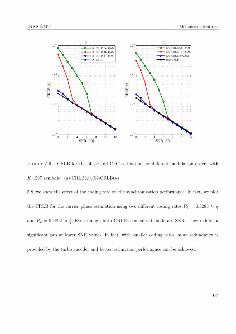
INRS-ÉMT Mémoire de Maîtrise
0 2 4 6 8 10 1210
−4
10−3
10−2
10−1
(a)
SNR [dB]
CR
LB
(φ)
CA−CRLB 64−QAM
CA−CRLB 16−QAM
CA−CRLB 4−QAM
DA−CRLB
0 2 4 6 8 10 1210
−9
10−8
10−7
10−6
SNR [dB]
CR
LB
(ν)
(b)
CA−CRLB 64−QAM
CA−CRLB 16−QAM
CA−CRLB 4−QAM
DA−CRLB
Figure 5.6 – CRLB for the phase and CFO estimation for different modulation orders with
K=207 symbols : (a)-CRLB(ϕ),(b)-CRLB(ν)
5.8, we show the effect of the coding rate on the synchronization performance. In fact, we plot
the CRLB for the carrier phase estimation using two different coding rates R1 = 0.3285 ≈ 13
and R2 = 0.4892 ≈ 12. Even though both CRLBs coincide at moderate SNRs, they exhibit a
significant gap at lower SNR values. In fact, with smaller coding rates, more redundancy is
provided by the turbo encoder and better estimation performance can be achieved.
67
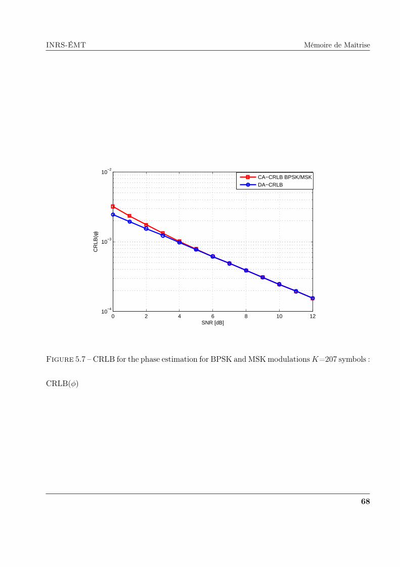
INRS-ÉMT Mémoire de Maîtrise
0 2 4 6 8 10 1210
−4
10−3
10−2
SNR [dB]
CR
LB(φ
)
CA−CRLB BPSK/MSKDA−CRLB
Figure 5.7 – CRLB for the phase estimation for BPSK and MSK modulationsK=207 symbols :
CRLB(ϕ)
68

INRS-ÉMT Mémoire de Maîtrise
0 2 4 6 8 10 1210
−4
10−3
10−2
10−1
SNR [dB]
CR
LB
(φ)
NDA−CRLB
CA−CRLB, rate = 1/2
CA−CRLB, rate = 1/3
DA−CRLB
Figure 5.8 – CRLB for the phase : CRLB(ϕ) vs coding gain, for 16-QAM symbols, K=207.
69
----.......... --
Chapitre 6
Conclusion
In this report, we tackled the problem of deriving analytical expressions for the Cramer-Rao
bounds for coded wireless communication systems, in the case of BPSK, MSK and square
QAM modulated signals, for SNR, channel phase and CFO. We were able to derive for the
first time closed-form expression of the CRB for the estimation of these parameters, in the
case of BPSK , MSK and quare QAM modulations (except for the case of BPSK for SNR
estimation, which exists already). Our newly derived CRBs corroborate previously obtained
emprical CRBs and are hence validated. We found that these CRBs are always smaller than
the NDA CRBs which reflects the advantage of coding in enhancing the estimation of the
considered parameters, especially in the average and low SNR range. The CRBs in the case of

INRS-ÉMT Mémoire de Maîtrise
BPSK and MSK modulations coincide. We also studied the effet of the coding rate on the CRBs
and found that the less the coding rate, implying more redundancy on the coding process, the
smaller the CRBs get, which implies a better performance in the code aided estimation.
71

Bibliographie
[1] S. Nanda, K. Balachandran and S. Kumar, “Adaptation techniques in wireless packet data
services,” IEEE Trans. Commun., vol. 38, pp. 54-64, 2000.
[2] S. Talakoub and B. Shahrrava, “Turbo Equalization with Integrated SNR Estimation,”
IEEE GlobeCom, San Francisco, CA, pp. 1-5, Nov. to Dec. 2006.
[3] S. Talakoub and B. Shahrrava, “Turbo equalization with iterative online SNR estimation,”
in Proc. IEEE Wireless Communications and Networking Conference, New Orleans, vol.
2, pp. 1097-1102, March 2005.
[4] J. G. Proakis, Digital Communications, 2001 :McGraw-Hill
[5] K. Balachandran, S. R. Kadaba and S. Nanda, “Channel quality estimation and rate adap-
tation for cellular mobile radio,” IEEE J. Sel. Areas Commun., vol. 17, pp. 1244-1256,
1999.

INRS-ÉMT Mémoire de Maîtrise
[6] C. Berrou and A. Glavieux, “Near optimum error correcting coding and decoding : turbo
codes,” IEEE Trans. Commun. , vol. 44, no. 10, pp. 1261-1271, Oct. 1996.
[7] J. Hagenauer, “The turbo principle : tutorial introduction and state of the art,” in Proc.
Int. Symp. on Turbo Codes and Related Topics., Brest, France, pp. 1-11, Sept. 1997.
[8] G. Colavolpe, G. Ferrari and R. Raheli, “Extrinsic information in iterative decoding : A
unified view,” IEEE Trans. Commun., vol. 49, pp. 2088-2094, 2001.
[9] M. A. Dangl and J. Lindner, “How to use a priori information of data symbols for SNR
estimation,” IEEE Signal Process. Lett., vol. 13, pp. 661-664, Nov. 2006.
[10] N. Wu, H. Wang and J.M. Kuang, “Code-aided SNR estimation based on expectation
maximisation algorithm,” Electron. Lett., vol. 44, pp. 924-925, July 2008.
[11] N. Wu, H. Wang and J M. Kuang, “Maximum likelihood signal-to-noise ratio estimation
for coded linearly modulated signals,” IET Commun., vol. 4, pp. 265-271, 2010.
[12] M. Bergmann, W. Gappmair, H. Schlemmer and O. Koudelka, “Code-aware joint esti-
mation of carrier phase and SNR for linear modulation schemes,” in Proc. 5th Advanced
Satellite Multimedia Systems Conference, Cagliari/Italy, pp. 177-182, Sept. 2010.
[13] L.Bahl, J.Cocke, F.Jelinek and J.Raviv, “Optimal Decoding of Linear Codes for minimizing
symbol error rate,” IEEE Transactions on Information Theory, vol. IT-20(2), pp.284-287,
73

INRS-ÉMT Mémoire de Maîtrise
March 1974.
[14] M.A. Khalighi, “Effect of Mismatched SNR on the performance of log-MAP turbo detec-
tor,” IEEE Trans on Vehic. Tech., vol. 52, no. 5, pp. 1386-1397, Sept. 2003.
[15] K.T. Shr and Y.H. Huang, “SNR estimation based on metric normalization frequency in
Viterbi decoder,” IEEE Commun. Lett., vol. 15, no. 6, pp. 668-670, June 2011.
[16] T. A. Summers and S. G. Wilson, “SNR mismatch and online estimation in turbo deco-
ding,” IEEE Trans. Commun., vol. 46, pp.421-423, 1998.
[17] M. C. Reed and I. Asenstorfer, “A novel vaiance eslimator for turbocode decoding,” in
Proc. Int. Conf. Telecommunications, Melbourne, Australia, pp. 173-178, Apr. 1997.
[18] A. Worm, P. Hoeher and N. Web, “Turbo-decoding without SNR estimation,” IEEE Com-
mun. Lett., vol. 4, no. 6, pp. 193-195, 2000.
[19] S. L. Goff, A. Glavierw and C. Berrou, “Turbo-codes and high spectral efficiency modula-
tion,” in Proc. ICC’94., New Orleans, LA, pp. 645-649, May 1994.
[20] S. Minying, L. Yuan and S. Sumei, “Impact of SNR estimation error on turbo code with
high-order modulation,” IEEE VTC Spring, vol. 3, pp. 1320-1324, May 2004.
[21] N. S. Alagha, “Cramèr-Rao hounds of SNR estimates for BPSK and QPSK modulated
signals,” IEEE Commun. Lett., vol. 5, pp.10-12, 2001.
74

INRS-ÉMT Mémoire de Maîtrise
[22] F. Bellili, A. Stèphenne and S. Affes, “Cramèr-Rao bounds for NDA SNR estimates of
square QAM modulated signals,” Proc. IEEE Wireless Commun. Netw. Conf. (WCNC),
2009.
[23] F. Bellili, A. Stèphenne and S. Affes, “Cramèr-Rao lower bounds for non-data-aided SNR
estimates of square QAM modulated transmissions,” IEEE Trans. Commun., vol. 58, pp.
3211-3218, 2010.
[24] V. Lottici and M. Luise, “Embedding carrier phase recovery into iterative decoding of
turbo-coded linear modulations,” IEEE Trans. Commun., vol. 52, no. 4, pp. 661-669, April
2004.
[25] L. Zhang and A. Burr, “Iterative carrier phase recovery suited for turbo-coded systems,”
IEEE Trans. Wireless Commun., vol. 3, no. 6, pp. 2267-2276, 2004.
[26] T. Richardson, “The geometry of turbo-decoding dynamics,” IEEE Trans. Inf. Theory, vol.
46, pp. 9-23, Jan 2000.
[27] S. M. Kay, Fundamentals of Statistical Signal Processing-Detection Theory. Englewood
Cliffs, NJ : Prentice-Hall, 1998.
[28] N. Noels, H. Steendam and M. Moeneclaey, “The Cramér-Rao bound for phase estimation
from coded linearly modulated signals,” IEEE Commun. Lett. , vol. 7, no. 5, pp. 207-209,
75

INRS-ÉMT Mémoire de Maîtrise
May 2003.
[29] A. Anastasopoulos and K. M. Chugg, “Adaptive iterative detection for phase tracking in
turbo-coded systems,” IEEE Trans. Commun., vol. 49, no. 12, pp. 2135-2144, Dec. 2001.
[30] B. Mielczarek and A. Svensson, “Phase offset estimation using enhanced turbo decoders,”
in Proc. IEEE Int. Conf. Commun. (ICC ’02), New York, NY, USA, vol. 3, pp. 1536-1540,
April 2002.
[31] N.Wiberg, “Simultaneous decoding and phase synchronization using iterative ŞturboŤ de-
coding,” in IEEE Int. Symp. Information Theory, Ulm, Germany, pp. 11, June 29-July 4,
1997.
[32] C. Komninakis and R. D. Wesel, “Joint iterative channel estimation and decoding in flat
correlated rayleigh fading,” IEEE J. Sel. Areas Commun., vol. 19, pp. 1706-1717, Sept.
2001.
[33] C. Morlet, I. Buret and M.-L. Boucheret, “A carrier phase estimator for multi-media satel-
lite payloads suited to RSC coding schemes,” in IEEE Int. Conf. Commun., New Orleans,
LA, vol. 1, pp. 455-459, 2000.
[34] C. Langlais and M. Helard, “Phase carrier for turbo codes over a satellite link with the
help of tentative decisions,” in Int. Symp. Turbo Codes Related Topics, vol. 5, pp. 439-442,
76

INRS-ÉMT Mémoire de Maîtrise
2000.
[35] S. Cioni, G. E. Corazza and A. Vanelli-Coralli “Turbo embedded estimation with imperfect
phase/frequency recovery,” Proc. IEEE Int. Conf. Commun., vol. 4, pp.2385-2389, May
2003.
[36] W. Oh and K. Cheun, “Joint decoding and carrier phase recovery algorithm for turbo
codes,” IEEE Commun. Lett., vol. 5, pp. 375-377, Sept. 2001.
[37] N. Noels, C. Herzet, A. Dejonghe et al. : “Turbo-synchronization : an EM algorithm ap-
proach,” Proc. IEEE ICC, pp. 2933-2937, 2003.
[38] X. Wu, Y. Song, C. Zhao and X. You, “Progressive frequency offset compensation in turbo
receivers,” IEEE Trans. Wirel. Commun., vol. 10, no. 2, pp. 702-709, 2011.
[39] Herzet, C. : “Code-aided synchronization for digital burst communications.” PhD disser-
tation, Communications Laboratory, University catholique de Louvain, 2006.
[40] B. Cowley, F. Rice, and M. Rice, “Cramér-Rao lower bound for QAM phase and frequency
estimation,” IEEE Trans. Commun., vol. 49, no. 9, pp. 689-693, Sept. 2001.
[41] F. Bellili, N. Atitallah, S. Affes and A. Stéphenne, “Cramér-Rao lower bounds for frequency
and phase NDA estimation from arbitrary square QAM-modulated signals,” IEEE Trans.
Signal Process., vol. 58, pp. 4517-4525, Sept. 2010.
77
INRS-ÉMT Mémoire de Maîtrise
[42] N. Noels, H. Steendam and M. Moeneclaey, “Carrier and Clock recovery in (turbo) coded
systems : Cramér-Rao bound and synchronizer performance,” EURASIP Journal on App.
Signal process., Special Issue on Turbo Processing, vol. 2005, no. 6, pp. 972-980, May 2005.
[43] F. Bellili, A. Methenni and S. Affes, “Closed-Form CRLBs for SNR Estimation from Turbo-
Coded BPSK-, MSK- and Square-QAM-Modulated Signals,” IEEE Trans. Signal Process.
, submitted.
[44] F. Bellili, A. Methenni and S. Affes, “Closed-Form CRLBs for CFO and Phase Estima-
tion from Turbo-Coded BPSK-, MSK- and Square-QAM-Modulated Signals,” IEEE Wirel.
Comm. , submitted.
[45] A. Methenni, F. Bellili, S. Affes and A. Stéphenne, “Stochastic NDA CRLB for DOA
estimation over SIMO systems,” Proc. of IEEE VTC’2012-Spring, Yokohama, Japan, May
6-9, 2012.
78