Comparaisons entre observations et modèles de prévision des précipitations ?Comparaisons entre observations et modèles de prévision des précipitations ?Utilisation de (très) longues séries temporelles de mesure pour comparer des Utilisation de (très) longues séries temporelles de mesure pour comparer des

propriétés statistiques simples (Densité de probabilité, analyse de Fourier, analyse propriétés statistiques simples (Densité de probabilité, analyse de Fourier, analyse morphologique « mono-fractale », etc...) morphologique « mono-fractale », etc...)

Trois exemples du travail de l'équipe transverse « longues séries » du LaMPTrois exemples du travail de l'équipe transverse « longues séries » du LaMP 1- 1- Observation of a « mesoscale break » in the statistical distribution of drought Observation of a « mesoscale break » in the statistical distribution of drought

durations in the Cévennes regiondurations in the Cévennes regionGrandes échelles, comparaison possible avec ECMWF, AROMEGrandes échelles, comparaison possible avec ECMWF, AROME

2- 2- Observation of near hour « convective peak » in the Fourier spectra using long Observation of near hour « convective peak » in the Fourier spectra using long time series (10 years at 6 minutes resolution) from OPGCtime series (10 years at 6 minutes resolution) from OPGC

and Météo-France databasesand Météo-France databasesPetite échelle convective, comparaison à faire avec DESCAM, WRFPetite échelle convective, comparaison à faire avec DESCAM, WRF

3- 3- Statistical comparisons of different 1D sampling rules in 2D fields. Exemples of Statistical comparisons of different 1D sampling rules in 2D fields. Exemples of brownian surface and ARAMIS radar data during HyMEX brownian surface and ARAMIS radar data during HyMEX

Atelier DEPHI2 PARIS, 13-14 Juin 2016

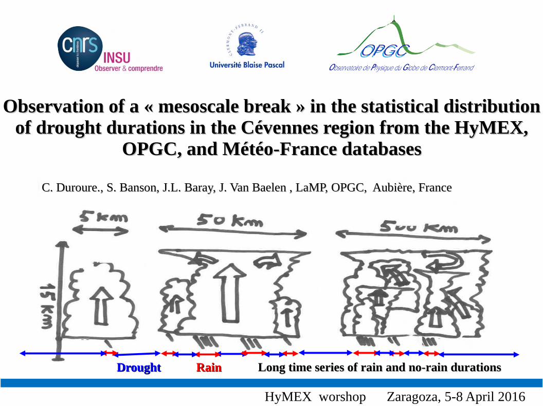
Observation of a « mesoscale break » in the statistical distribution Observation of a « mesoscale break » in the statistical distribution of drought durations in the Cévennes region from the HyMEX, of drought durations in the Cévennes region from the HyMEX,

OPGC, and Météo-France databasesOPGC, and Météo-France databases

C. Duroure., S. Banson, J.L. Baray, J. Van Baelen , LaMP, OPGC, Aubière, FranceC. Duroure., S. Banson, J.L. Baray, J. Van Baelen , LaMP, OPGC, Aubière, France

HyMEX worshop Zaragoza, 5-8 April 2016

RainRainDroughtDrought Long time series of rain and no-rain durationsLong time series of rain and no-rain durations

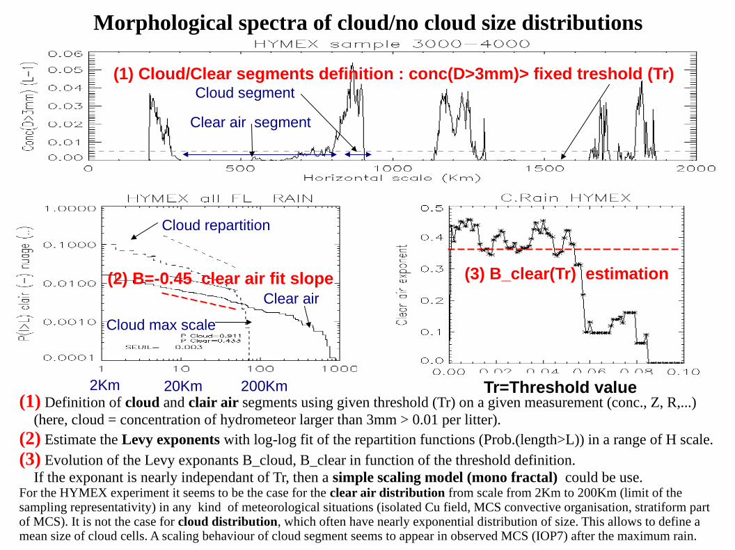
Cloud segment

Clear air segment

2Km 20Km 200Km(1) Definition of cloud and clair air segments using given threshold (Tr) on a given measurement (conc., Z, R,...) (here, cloud = concentration of hydrometeor larger than 3mm > 0.01 per litter).(2) Estimate the Levy exponents with log-log fit of the repartition functions (Prob.(length>L)) in a range of H scale.

(3) Evolution of the Levy exponants B_cloud, B_clear in function of the threshold definition. If the exponant is nearly independant of Tr, then a simple scaling model (mono fractal) could be use. For the HYMEX experiment it seems to be the case for the clear air distribution from scale from 2Km to 200Km (limit of the sampling representativity) in any kind of meteorological situations (isolated Cu field, MCS convective organisation, stratiform part of MCS). It is not the case for cloud distribution, which often have nearly exponential distribution of size. This allows to define a mean size of cloud cells. A scaling behaviour of cloud segment seems to appear in observed MCS (IOP7) after the maximum rain.

Cloud repartition

Clear air (2) B=-0.45 clear air fit slope (3) B_clear(Tr) estimation

Tr=Threshold value

Cloud max scale

Morphological spectra of cloud/no cloud size distributions

(1) Cloud/Clear segments definition : conc(D>3mm)> fixed treshold (Tr)

12 2

1 2 2

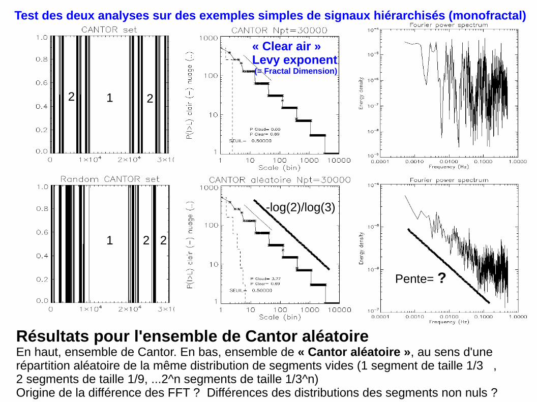
Résultats pour l'ensemble de Cantor aléatoireEn haut, ensemble de Cantor. En bas, ensemble de « Cantor aléatoire », au sens d'une répartition aléatoire de la même distribution de segments vides (1 segment de taille 1/3 , 2 segments de taille 1/9, ...2^n segments de taille 1/3^n)Origine de la différence des FFT ? Différences des distributions des segments non nuls ?

Test des deux analyses sur des exemples simples de signaux hiérarchisés (monofractal)

-log(2)/log(3)

Pente= ?

« Clear air »Levy exponent (= Fractal Dimension)

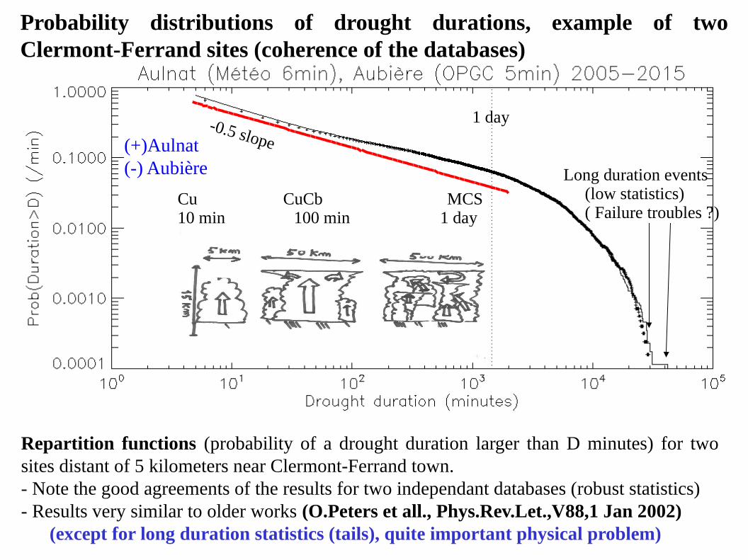
Repartition functions (probability of a drought duration larger than D minutes) for two sites distant of 5 kilometers near Clermont-Ferrand town.- Note the good agreements of the results for two independant databases (robust statistics)- Results very similar to older works (O.Peters et all., Phys.Rev.Let.,V88,1 Jan 2002) (except for long duration statistics (tails), quite important physical problem)

Probability distributions of drought durations, example of two Clermont-Ferrand sites (coherence of the databases)

Cu CuCb MCS10 min 100 min 1 day

-0.5 slope

Long duration events (low statistics) ( Failure troubles ?)

(+)Aulnat(-) Aubière

1 day

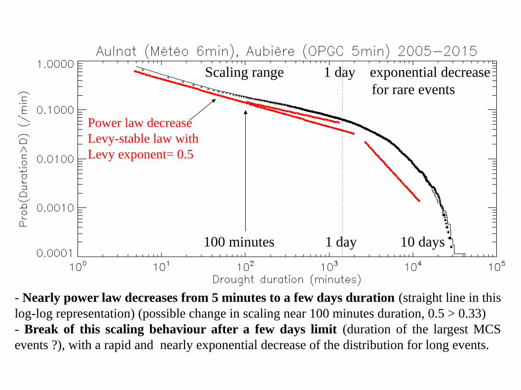
Scaling range 1 day exponential decrease for rare events

- Nearly power law decreases from 5 minutes to a few days duration (straight line in this log-log representation) (possible change in scaling near 100 minutes duration, 0.5 > 0.33)- Break of this scaling behaviour after a few days limit (duration of the largest MCS events ?), with a rapid and nearly exponential decrease of the distribution for long events.

Power law decreaseLevy-stable law withLevy exponent= 0.5

100 minutes 1 day 10 days

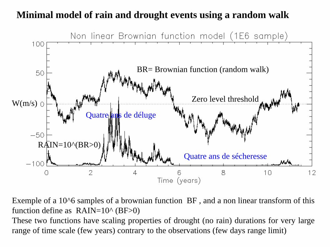
Minimal model of rain and drought events using a random walk

Exemple of a 10^6 samples of a brownian function BF , and a non linear transform of this function define as RAIN=10^ (BF>0) These two functions have scaling properties of drought (no rain) durations for very large range of time scale (few years) contrary to the observations (few days range limit)

BR= Brownian function (random walk)

RAIN=10^(BR>0)

Zero level threshold

Quatre ans de déluge

Quatre ans de sécheresse

W(m/s)

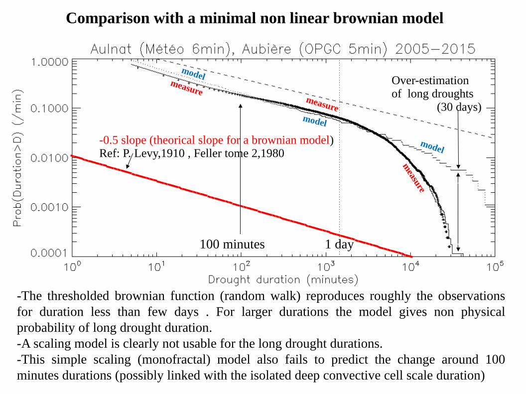
Comparison with a minimal non linear brownian model

Over-estimationof long droughts (30 days)

-0.5 slope (theorical slope for a brownian model)Ref: P. Levy,1910 , Feller tome 2,1980

100 minutes 1 day

-The thresholded brownian function (random walk) reproduces roughly the observations for duration less than few days . For larger durations the model gives non physical probability of long drought duration. -A scaling model is clearly not usable for the long drought durations.-This simple scaling (monofractal) model also fails to predict the change around 100 minutes durations (possibly linked with the isolated deep convective cell scale duration)

model

model

model

measuremeasure

measure

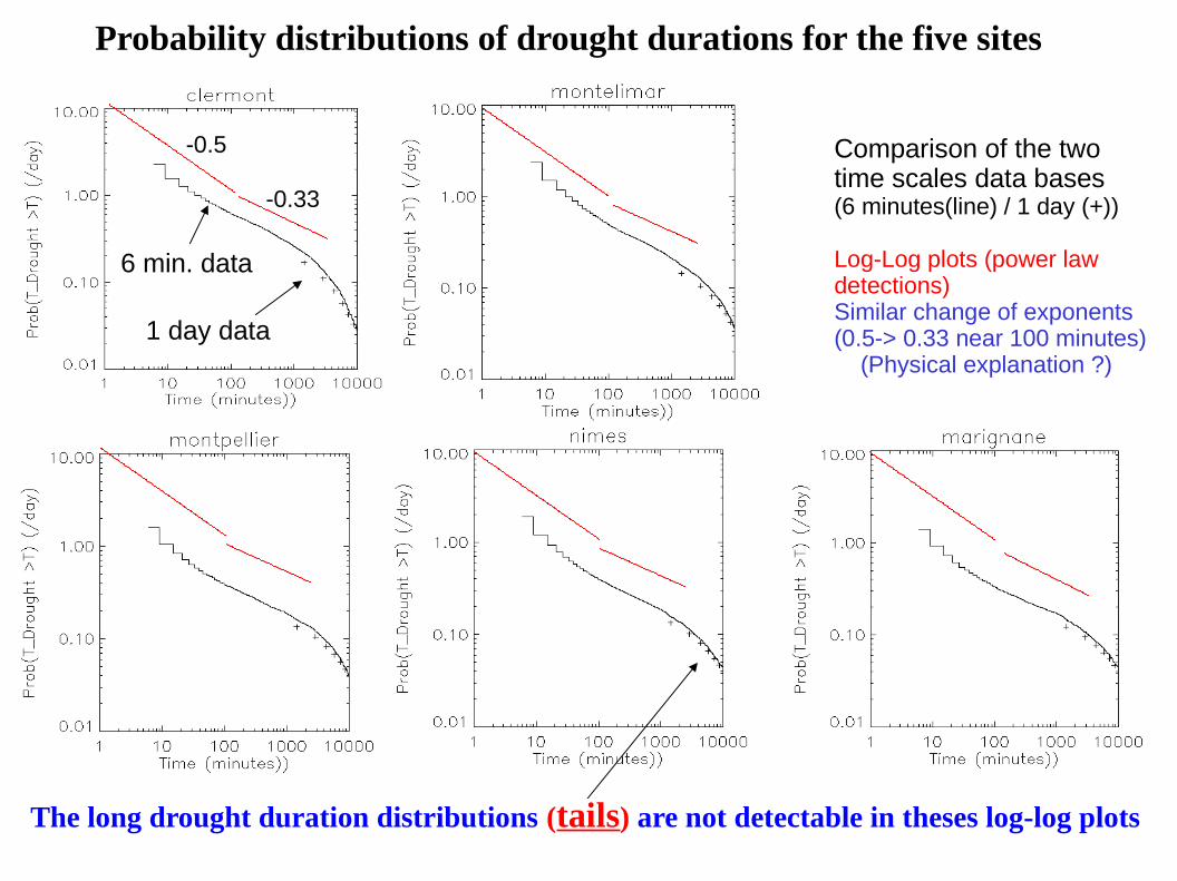
Comparison of the two time scales data bases (6 minutes(line) / 1 day (+))

Log-Log plots (power law detections)Similar change of exponents (0.5-> 0.33 near 100 minutes) (Physical explanation ?)

Probability distributions of drought durations for the five sites

-0.5

-0.33

The long drought duration distributions (tails) are not detectable in theses log-log plots

1 day data

6 min. data

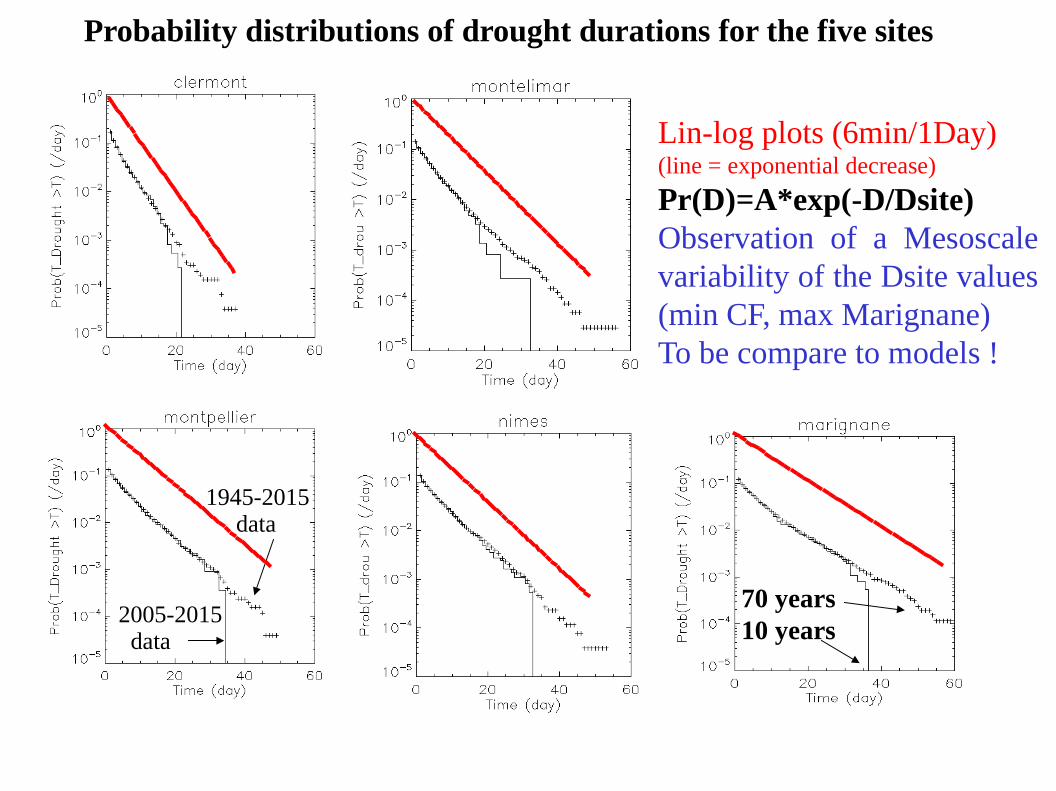
Probability distributions of drought durations for the five sites

Lin-log plots (6min/1Day)(line = exponential decrease)

Pr(D)=A*exp(-D/Dsite)Observation of a Mesoscale variability of the Dsite values (min CF, max Marignane)To be compare to models !

1945-2015 data

2005-2015 data

70 years10 years

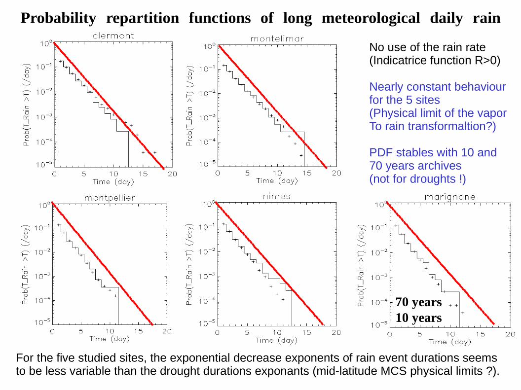
Probability repartition functions of long meteorological daily rain durations

No use of the rain rate (Indicatrice function R>0)

Nearly constant behaviourfor the 5 sites (Physical limit of the vaporTo rain transformaltion?) PDF stables with 10 and70 years archives(not for droughts !)

For the five studied sites, the exponential decrease exponents of rain event durations seems to be less variable than the drought durations exponants (mid-latitude MCS physical limits ?).

70 years10 years

Results:1- Observation of a scaling distribution of drought durations from a few minutes to a few days time scale.2- Observation of a exponential decrease of drought duration distributions for larger time scale (few days, one month), with a detectable mesoscale variability of measured exponents.3- The similar exponents for the rain durations seem to be nearly constant at mesoscale (and for these latitudes).

Prospective works:1- Extend this study for sites around mediterranean basin2- Use models (rain/no_rain) time series with the same analysis 3- Comparison with the Fourier densities spectra (scaling range,…)4- Compaison with the LWC (optical cloud) data. Explain rain intermitency

HyMEX worshop Zaragoza, 5-8 April 2016

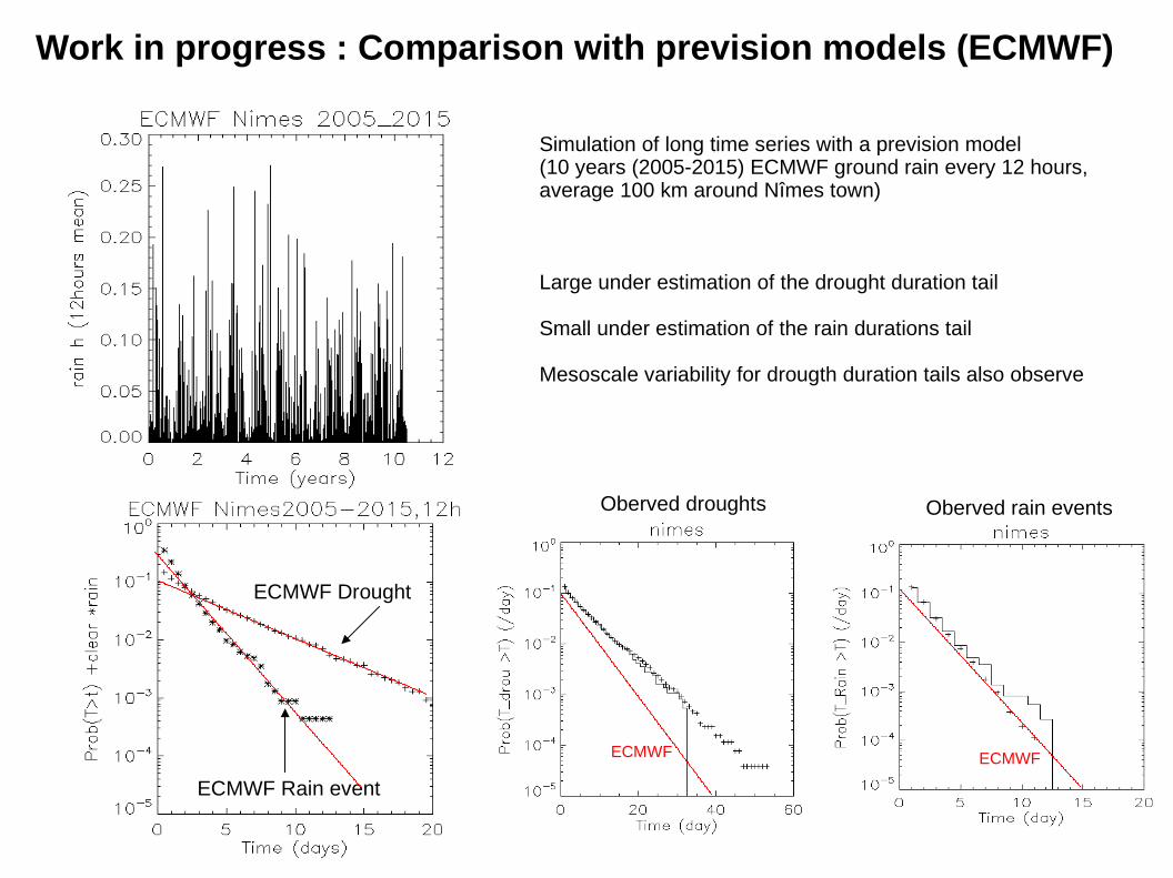
Work in progress : Comparison with prevision models (ECMWF)

Simulation of long time series with a prevision model(10 years (2005-2015) ECMWF ground rain every 12 hours,average 100 km around Nîmes town)

Large under estimation of the drought duration tail

Small under estimation of the rain durations tail

Mesoscale variability for drougth duration tails also observe

Oberved droughts Oberved rain events

ECMWF Rain event

ECMWF Drought

ECMWF ECMWF

Rain

Rain

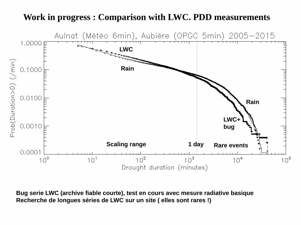
LWC

LWC+bug

1 dayScaling range Rare events

Bug serie LWC (archive fiable courte), test en cours avec mesure radiative basiqueRecherche de longues séries de LWC sur un site ( elles sont rares !)

Work in progress : Comparison with LWC. PDD measurements

Rain

LWC

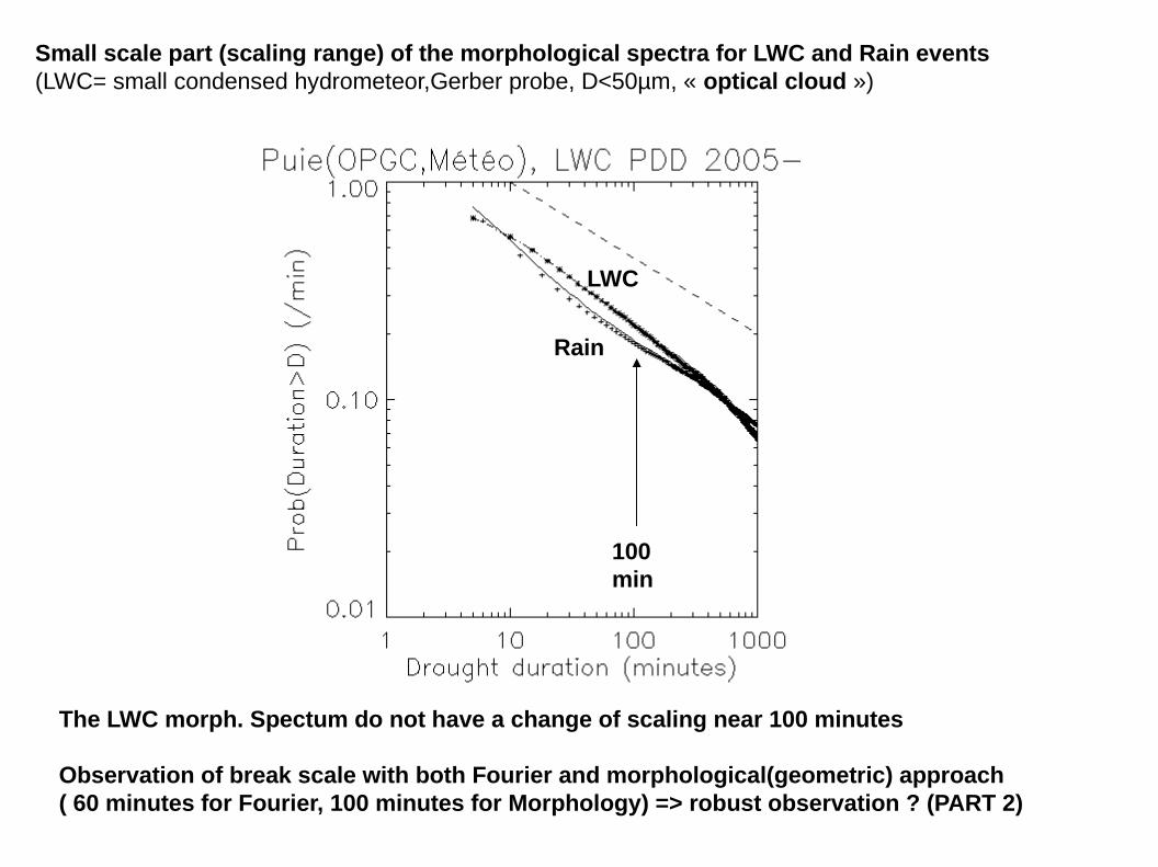
100 min

The LWC morph. Spectum do not have a change of scaling near 100 minutes

Observation of break scale with both Fourier and morphological(geometric) approach( 60 minutes for Fourier, 100 minutes for Morphology) => robust observation ? (PART 2)

Small scale part (scaling range) of the morphological spectra for LWC and Rain events(LWC= small condensed hydrometeor,Gerber probe, D<50µm, « optical cloud »)

Thanks for attention !Thanks for attention !

HyMEX worshop Zaragoza, 5-8 April 2016

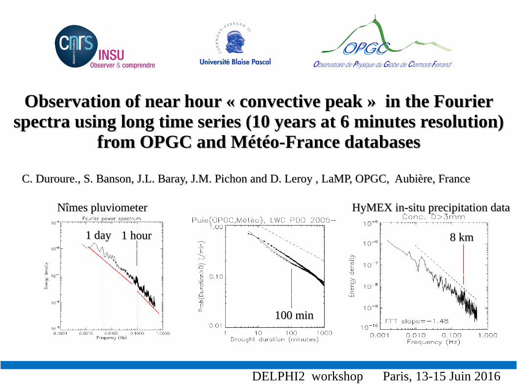
Observation of near hour « convective peak » in the Fourier Observation of near hour « convective peak » in the Fourier spectra using long time series (10 years at 6 minutes resolution) spectra using long time series (10 years at 6 minutes resolution)

from OPGC and Météo-France databasesfrom OPGC and Météo-France databases

C. Duroure., S. Banson, J.L. Baray, J.M. Pichon and D. Leroy , LaMP, OPGC, Aubière, FranceC. Duroure., S. Banson, J.L. Baray, J.M. Pichon and D. Leroy , LaMP, OPGC, Aubière, France

DELPHI2 workshop Paris, 13-15 Juin 2016

Nîmes pluviometer HyMEX in-situ precipitation data Nîmes pluviometer HyMEX in-situ precipitation data

1 hour1 hour1 day1 day 8 km8 km

100 min100 min

Pente -0.5

0

100 minutes

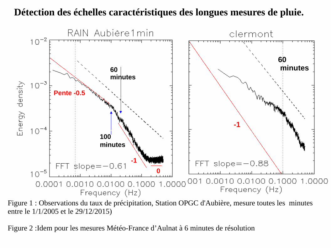
Figure 1 : Observations du taux de précipitation, Station OPGC d'Aubière, mesure toutes les minutes entre le 1/1/2005 et le 29/12/2015)

Figure 2 :Idem pour les mesures Météo-France d’Aulnat à 6 minutes de résolution

Détection des échelles caractéristiques des longues mesures de pluie.

-1

60 minutes

60 minutes

-1

24H

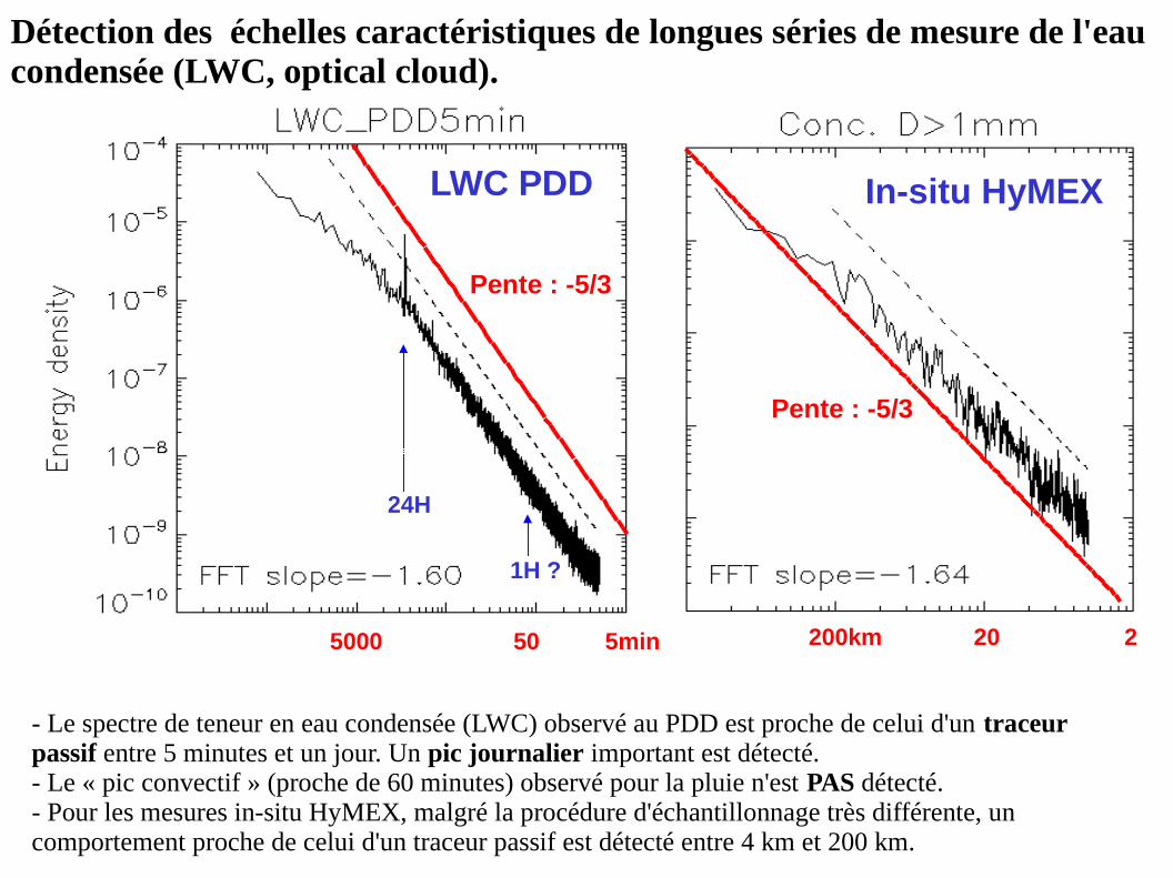
- Le spectre de teneur en eau condensée (LWC) observé au PDD est proche de celui d'un traceur passif entre 5 minutes et un jour. Un pic journalier important est détecté.- Le « pic convectif » (proche de 60 minutes) observé pour la pluie n'est PAS détecté.- Pour les mesures in-situ HyMEX, malgré la procédure d'échantillonnage très différente, un comportement proche de celui d'un traceur passif est détecté entre 4 km et 200 km.

Détection des échelles caractéristiques de longues séries de mesure de l'eau condensée (LWC, optical cloud).

200 k 200km 20 2

LWC PDD In-situ HyMEX

5000 50 5min

1H ?

Pente : -5/3

Pente : -5/3

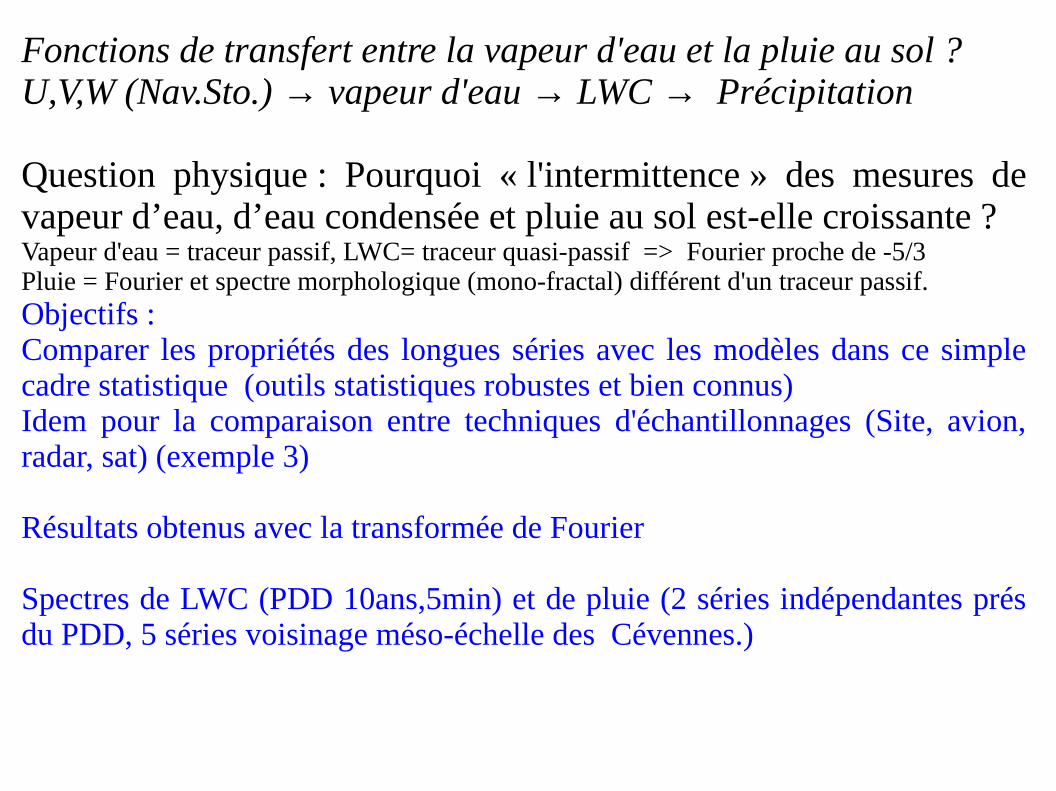
Fonctions de transfert entre la vapeur d'eau et la pluie au sol ?U,V,W (Nav.Sto.) → vapeur d'eau → LWC → Précipitation

Question physique : Pourquoi « l'intermittence » des mesures de vapeur d’eau, d’eau condensée et pluie au sol est-elle croissante ?Vapeur d'eau = traceur passif, LWC= traceur quasi-passif => Fourier proche de -5/3Pluie = Fourier et spectre morphologique (mono-fractal) différent d'un traceur passif.Objectifs :Comparer les propriétés des longues séries avec les modèles dans ce simple cadre statistique (outils statistiques robustes et bien connus)Idem pour la comparaison entre techniques d'échantillonnages (Site, avion, radar, sat) (exemple 3)

Résultats obtenus avec la transformée de Fourier

Spectres de LWC (PDD 10ans,5min) et de pluie (2 séries indépendantes prés du PDD, 5 séries voisinage méso-échelle des Cévennes.)

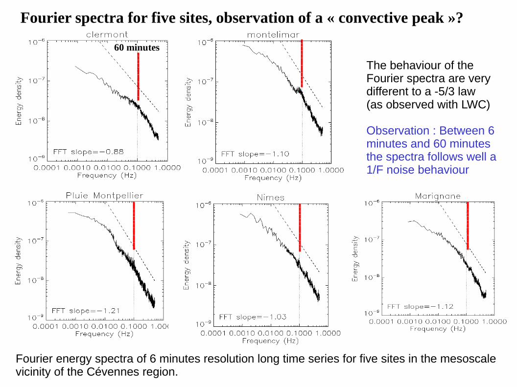
Fourier spectra for five sites, observation of a « convective peak »?

The behaviour of the Fourier spectra are very different to a -5/3 law(as observed with LWC)

Observation : Between 6 minutes and 60 minutes the spectra follows well a 1/F noise behaviour

Fourier energy spectra of 6 minutes resolution long time series for five sites in the mesoscale vicinity of the Cévennes region.

60 minutes

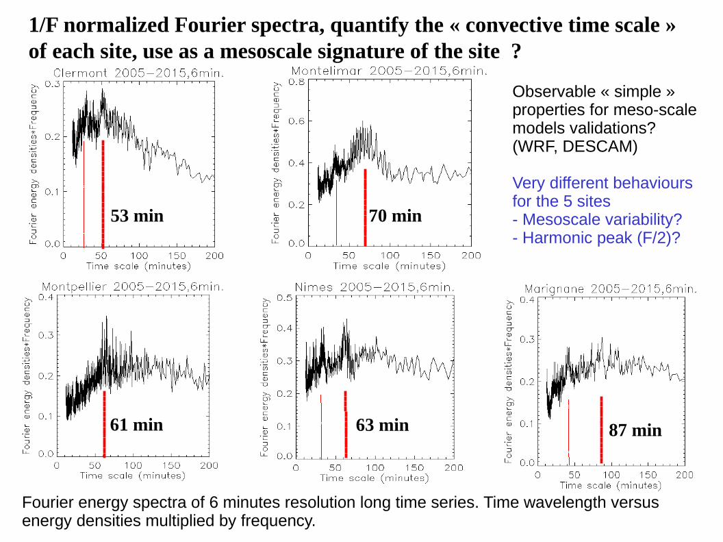
1/F normalized Fourier spectra, quantify the « convective time scale »of each site, use as a mesoscale signature of the site ?

Observable « simple » properties for meso-scale models validations?(WRF, DESCAM)

Very different behaviours for the 5 sites- Mesoscale variability?- Harmonic peak (F/2)?

Fourier energy spectra of 6 minutes resolution long time series. Time wavelength versus energy densities multiplied by frequency.

70 min53 min

63 min 87 min61 min

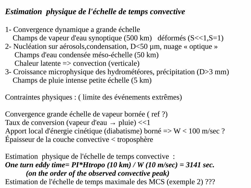
Estimation physique de l'échelle de temps convective

1- Convergence dynamique a grande échelle Champs de vapeur d'eau synoptique (500 km) déformés (S<<1,S=1) 2- Nucléation sur aérosols,condensation, D<50 µm, nuage « optique » Champs d'eau condensée méso-échelle (50 km) Chaleur latente => convection (verticale) 3- Croissance microphysique des hydrométéores, précipitation (D>3 mm) Champs de pluie intense petite échelle (5 km)

Contraintes physiques : ( limite des événements extrêmes)

Convergence grande échelle de vapeur bornée ( ref ?)Taux de conversion (vapeur d'eau → pluie) <<1Apport local d'énergie cinétique (diabatisme) borné => W < 100 m/sec ?Épaisseur de la couche convective < troposphère

Estimation physique de l'échelle de temps convective :One turn eddy time= PI*Htropo (10 km) / W (10 m/sec) = 3141 sec. (on the order of the observed convective peak)Estimation de l'échelle de temps maximale des MCS (exemple 2) ???

Thanks for attention !Thanks for attention !

Statistical analysis of precipitation measurement from different instruments and different sampling rules.

Case studies of the HYMEX database

C. Duroure, S. Banson, Joel VB, Alfons S., Wolfram W.

Laboratoire de Météorologie Physique, Université Blaise Pascal, OPGC/UMR-6016, Clermont-Ferrand, France

HYMEX workshop, 20/09/2015

Aircraft, Radar, Pluviometer(scale from 200 m to 500 Km)

Scaling of the horizontal size of the rain and no rain events in mesoscale convective system (MCS). A comparaison using the HYMEX database from different rain measurement techniques.

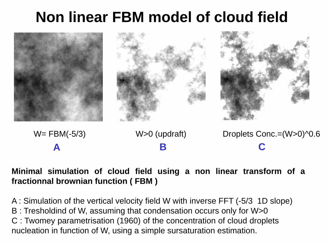
Minimal simulation of cloud field using a non linear transform of a fractionnal brownian function ( FBM )

A : Simulation of the vertical velocity field W with inverse FFT (-5/3 1D slope) B : Tresholdind of W, assuming that condensation occurs only for W>0C : Twomey parametrisation (1960) of the concentration of cloud droplets nucleation in function of W, using a simple sursaturation estimation.

W= FBM(-5/3) W>0 (updraft) Droplets Conc.=(W>0)^0.6

Non linear FBM model of cloud field

A B C

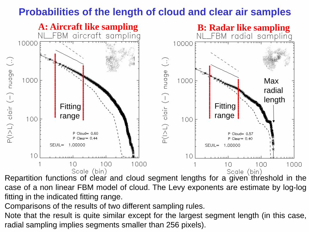
Repartition functions of clear and cloud segment lengths for a given threshold in the case of a non linear FBM model of cloud. The Levy exponents are estimate by log-log fitting in the indicated fitting range.Comparisons of the results of two different sampling rules. Note that the result is quite similar except for the largest segment length (in this case, radial sampling implies segments smaller than 256 pixels).

Fittingrange

Maxradiallength

B: Radar like samplingA: Aircraft like sampling

Fittingrange

Probabilities of the length of cloud and clear air samples

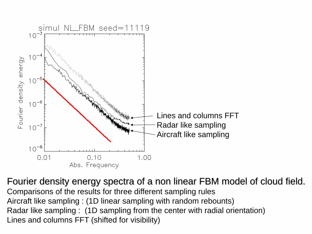
Fourier density energy spectra of a non linear FBM model of cloud field.Fourier density energy spectra of a non linear FBM model of cloud field.Comparisons of the results for three different sampling rules Aircraft like sampling : (1D linear sampling with random rebounts)Radar like sampling : (1D sampling from the center with radial orientation)Lines and columns FFT (shifted for visibility)

Lines and columns FFTRadar like samplingAircraft like sampling

Final thanks for attention !Final thanks for attention !