December 2007

F E M I S E R E S E A R C HP R O G R A M M E

2006-2007

Research n°FEM31-07Directed By

Sule Akkoyunlu,Bilkent University (Turkey) and DIW (Germany)

Ce rapport a été réalisé avec le soutien financier de la Commission des Communautés Européennes. Les opinions exprimées dans ce texte n’engagent que les auteurs et ne reflètent pas l’opinion officielle de la Commission.

This report has been drafted with financial assistance from the Commission of the European Communities. The views expressed herein are those of the authors and therefore in no way reflect the official opinions of the Commission.

Regional Integration and Goods and Factors Flows in the Middle East and North African Region

and Turkey

Are Turkish migrants altruistic? Evidence from the macro data

by

Sule Akkoyunlu*

September 07, 2007

Abstract We investigate in this paper whether the stable pattern of remittances over the last three decades can be explained by the altruistic behaviour. This possibility is tested by means of cointegration analysis, which is applied to Turkish remittances from Germany over the period 1962-2005. A single cointegrating relationship is found between the remittances of Turkish workers in Germany and the real Turkish GDP per capita, the real German GDP per capita, the stock of Turkish migrants in Germany, the real exchange rate, and the government instability. The negative coefficient associated with Turkish income and positive coefficients on the real exchange rate and political instability support the claim that Turkish remittances from Germany are altruistically motivated. In addition, we find that the coefficient on the stock of Turkish migrants to be equal to one. Keywords: Migration; Remittances; Alturism; Cointegration JEL classification: C22; F22; F24 We are grateful to Christian Dreger and Konstantin Kholodilin for helpful comments. The

research reported in this paper was financially supported by the European Union within the

context of the FEMISE program. The contents of this paper are the sole responsibility of the

authors and do not reflect the opinion of the European Union.

* Department of Economics, Bilkent University; DIW Berlin. Email: sakkoyunlu@diw.de

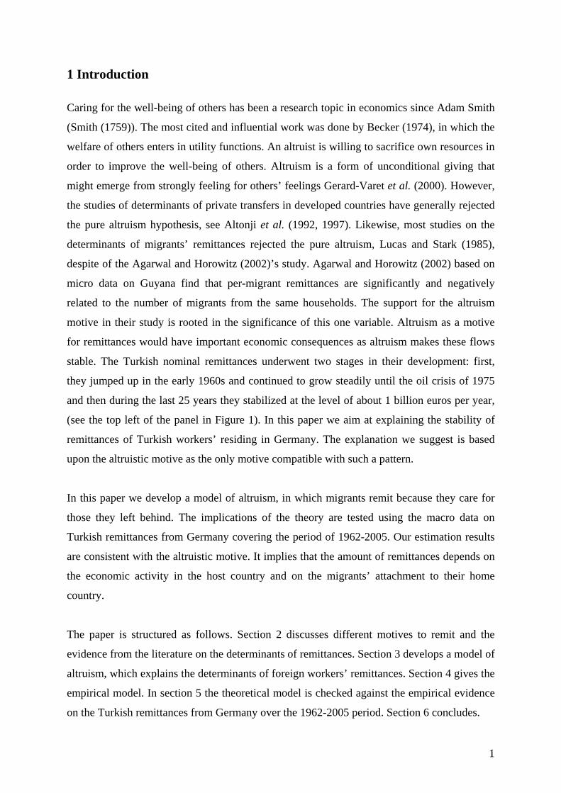
1 Introduction

Caring for the well-being of others has been a research topic in economics since Adam Smith

(Smith (1759)). The most cited and influential work was done by Becker (1974), in which the

welfare of others enters in utility functions. An altruist is willing to sacrifice own resources in

order to improve the well-being of others. Altruism is a form of unconditional giving that

might emerge from strongly feeling for others’ feelings Gerard-Varet et al. (2000). However,

the studies of determinants of private transfers in developed countries have generally rejected

the pure altruism hypothesis, see Altonji et al. (1992, 1997). Likewise, most studies on the

determinants of migrants’ remittances rejected the pure altruism, Lucas and Stark (1985),

despite of the Agarwal and Horowitz (2002)’s study. Agarwal and Horowitz (2002) based on

micro data on Guyana find that per-migrant remittances are significantly and negatively

related to the number of migrants from the same households. The support for the altruism

motive in their study is rooted in the significance of this one variable. Altruism as a motive

for remittances would have important economic consequences as altruism makes these flows

stable. The Turkish nominal remittances underwent two stages in their development: first,

they jumped up in the early 1960s and continued to grow steadily until the oil crisis of 1975

and then during the last 25 years they stabilized at the level of about 1 billion euros per year,

(see the top left of the panel in Figure 1). In this paper we aim at explaining the stability of

remittances of Turkish workers’ residing in Germany. The explanation we suggest is based

upon the altruistic motive as the only motive compatible with such a pattern.

In this paper we develop a model of altruism, in which migrants remit because they care for

those they left behind. The implications of the theory are tested using the macro data on

Turkish remittances from Germany covering the period of 1962-2005. Our estimation results

are consistent with the altruistic motive. It implies that the amount of remittances depends on

the economic activity in the host country and on the migrants’ attachment to their home

country.

The paper is structured as follows. Section 2 discusses different motives to remit and the

evidence from the literature on the determinants of remittances. Section 3 develops a model of

altruism, which explains the determinants of foreign workers’ remittances. Section 4 gives the

empirical model. In section 5 the theoretical model is checked against the empirical evidence

on the Turkish remittances from Germany over the 1962-2005 period. Section 6 concludes.

1

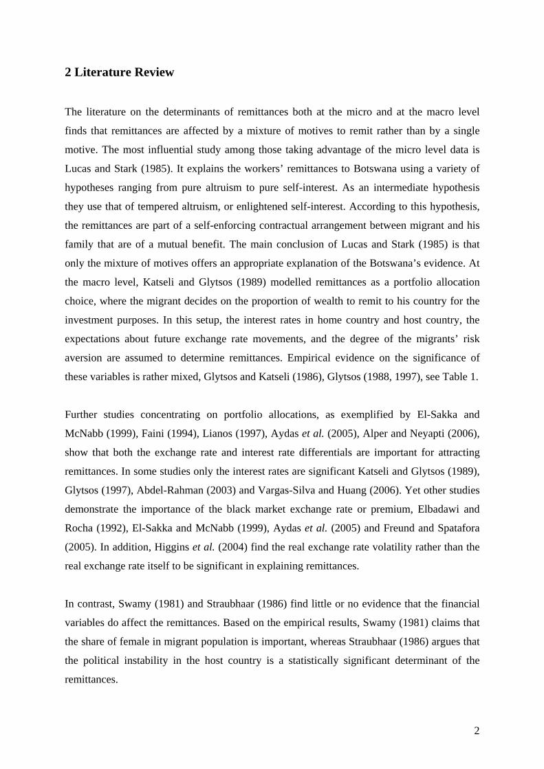
2 Literature Review

The literature on the determinants of remittances both at the micro and at the macro level

finds that remittances are affected by a mixture of motives to remit rather than by a single

motive. The most influential study among those taking advantage of the micro level data is

Lucas and Stark (1985). It explains the workers’ remittances to Botswana using a variety of

hypotheses ranging from pure altruism to pure self-interest. As an intermediate hypothesis

they use that of tempered altruism, or enlightened self-interest. According to this hypothesis,

the remittances are part of a self-enforcing contractual arrangement between migrant and his

family that are of a mutual benefit. The main conclusion of Lucas and Stark (1985) is that

only the mixture of motives offers an appropriate explanation of the Botswana’s evidence. At

the macro level, Katseli and Glytsos (1989) modelled remittances as a portfolio allocation

choice, where the migrant decides on the proportion of wealth to remit to his country for the

investment purposes. In this setup, the interest rates in home country and host country, the

expectations about future exchange rate movements, and the degree of the migrants’ risk

aversion are assumed to determine remittances. Empirical evidence on the significance of

these variables is rather mixed, Glytsos and Katseli (1986), Glytsos (1988, 1997), see Table 1.

Further studies concentrating on portfolio allocations, as exemplified by El-Sakka and

McNabb (1999), Faini (1994), Lianos (1997), Aydas et al. (2005), Alper and Neyapti (2006),

show that both the exchange rate and interest rate differentials are important for attracting

remittances. In some studies only the interest rates are significant Katseli and Glytsos (1989),

Glytsos (1997), Abdel-Rahman (2003) and Vargas-Silva and Huang (2006). Yet other studies

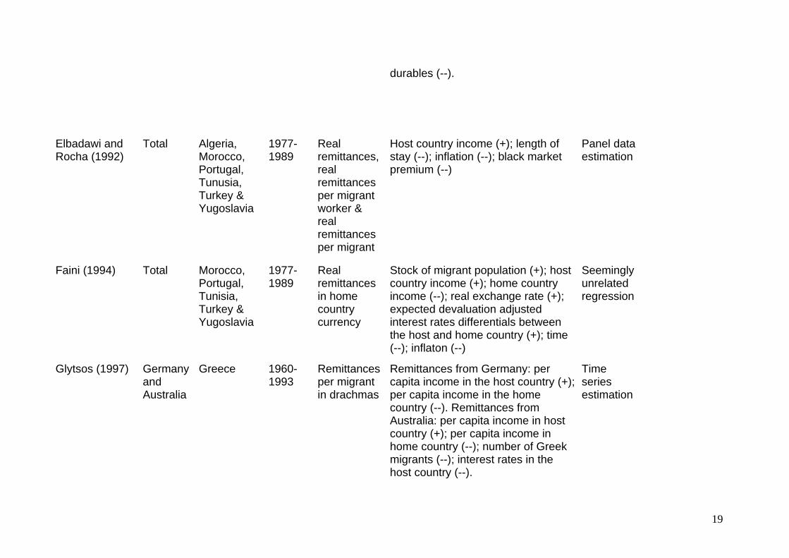
demonstrate the importance of the black market exchange rate or premium, Elbadawi and

Rocha (1992), El-Sakka and McNabb (1999), Aydas et al. (2005) and Freund and Spatafora

(2005). In addition, Higgins et al. (2004) find the real exchange rate volatility rather than the

real exchange rate itself to be significant in explaining remittances.

In contrast, Swamy (1981) and Straubhaar (1986) find little or no evidence that the financial

variables do affect the remittances. Based on the empirical results, Swamy (1981) claims that

the share of female in migrant population is important, whereas Straubhaar (1986) argues that

the political instability in the host country is a statistically significant determinant of the

remittances.

2

In general, at the macro level, the variables representing all the motives to remit — such as

altruistic, exchange, and investment (portfolio) motives — are included in a regression at once,

which therefore represents the mixture of motives. As seen from Table 1, the following

variables are found to be significant in the literature: the number of migrants in the host

country, the economic activity in the host country and the home country, the length of stay in

the host country, interest rate differentials, exchange rate, black market premia, inflation rate

in the home country, the ratio of females to the total migrant population, the education level

of migrant, and political risk factors in the home country. However, as it can be observed

from Table 1, there is a little consensus on the key macroeconomic determinants of

remittances. One common finding is that the stock of migrants is the primary determinant of

remittances.

The host country income as measured by the host country GDP per capita is also found to be

significant in some studies. Nevertheless, Higgins et al. (2004) and Vargas-Silva and Huang

(2006) argue that the host country income should approximated by the unemployment rate

and the money supply.

If the home country income has a negative sign, then it is considered as a support for the

altruistic hypothesis. Alternatively, if the home country income has a positive sign, then it is

interpreted as an evidence of the investment or exchange motive. See Table 1.

If the inflation rate takes a positive sign, then inflationary pressures in the home country

reduce real income and thereby lead to an increase in remittances according to the investment

motive. If, in contrast, the inflation rate has a negative sign, then it means that the high

inflation undermines the economic and political stability and therefore leads to a reduction in

remittances. Both effects are considered in the following papers: Glytsos (1988), Katseli and

Glytsos (1989) Elbadawi and Rocha (1992), Faini (1994), Lianos (1997), El-Sakka and

McNabb (1999), Abdel-Rahman (2003), Aydas et al. (2005) and Alper and Neyapti (2006).

In a recent study Buch and Kuckulenz (2004) find that traditional variables such as economic

growth, the level of economic development and proxies for the rate of return on financial

assets are not significant in explaining remittances and argue that remittances might be

influenced by social considerations. In addition, other recent studies showed that some

additional variables such as money transfer fees (Freund and Spatafora (2005)), the education

3

level of migrants (Niimi and Özden (2006)), the income inequality, the availability of

remittance services, and informal economy (Schiopu and Siegfried (2006)) can be important

in determining remittances.

In this study, we will take another view and explore the determinants of Turkish workers’

remittances from Germany within a context of altruistic motive. The hypothesis of altruistic

motivation here is supported by our observation that the remittances in the recent years have

been rather stable. This hypothesis is tested on the basis of the macro data.

3 Theoretical Model

The model in this section is closely related to Lucas and Stark (1985), Funkhouser (1995), and

Stark (1995). We assume a separable utility function, according to which a migrant values his

own utility, and that of his family left behind in the home country, : mU hU

}),({)(),( PCUVCUUUU hhmmhm += (1)

where is the consumption of migrant; is the consumption of his family in the home

country; and P is the importance of the utility of the family left behind in the migrant’s own

utility, or the degree of migrant’s attachment to home country. The utility function has the

following properties: , , and , where denotes the first-order

derivative of the utility function with respect to consumption and denotes the second-order

derivative.

mC hC

0' fmU 0' fhU 0" phU 'U

"U

The emigrant maximizes the separable lifetime utility function

∑ +++

++

= tv

thttththt

u

mmmR

PReNReYUVCUUt )1(

},({)1(}{max

δδ (2)

subject to

tmtmt RYC −= (3)

4

where is the consumption of the migrant at time t; is the income of the migrant at

time t; is the income of the migrant’s family in the home country; is the nominal

remittances expressed in the host country currency; is the real exchange rate between the

host and home country;

mtC mtY

htY tR

te

htt Re is the average remittances received from other migrant working

in the host country and stemming from the same household; is the total number of

migrants sent by this household to the host country (stock of migrants in the host country).

htN

tu )1(

1δ+

and tv )1(

1δ+

are the discount rates applied to the migrant’s own utility and to the

utility of the migrant’s family in the home country, respectively. The solution to the

maximization problem is given by the reduced form equation for the determinants of

remittances:

),,,,( PNeYYfR htthtmtt = (4)

The model above has several testable implications, which are stated in Lucas and Stark (1985),

Funkhouser (1995), and Rapoport and Docquier (2005):

1. Migrants with higher earnings remit more;

2. Low-income households receive more;

3. At the macro level, the more migrants the higher the total remittances.1 At the micro level

the relationship between the number of migrants stemming from the same family and amount

of remittances can be either positive or negative.

We have two additional variables to test in this altruistic model:

4. Real exchange rate is expected to exert a positive impact on remittances;

5. Remittances increase with the degree of migrant’s attachment to his family in the home

country.

The positive relationship between the real exchange rate and remittances, given that the

remittances are expressed in the home country’s currency, is postulated in Faini (1994).

1 In fact, following Swamy (1981), we expect the coefficient on the stock of migrants to be equal to one.

5

The measure of the migrant’s attachment to his family left behind, P, can be related to the

literature on transnationalism. Transnational migration represents immigrants that settle down

and become well integrated in the host country but still maintain social, cultural, economic,

and political ties with their home country, see Glick Schiller (1999) and Guarnizo (2003). In

the literature on transnationalism, monetary remittances measure the strength of attachment

the migrants feel towards their societies of origin. The main contribution of this paper is the

empirical testing of the influence of the real exchange rate, migrant’s attachment, and the

stock of migrants on the remittances.

4 Empirical model

We model Turkish remittances from Germany as follows:

(5) lnlnlnlnln 43210 ttttfththt

t PeSpcYpcYYR εααααα ++++++=⎟⎟⎠

⎞⎜⎜⎝

⎛

In (5), ⎟⎟⎠

⎞⎜⎜⎝

⎛

ht

t

YR

ln denotes the log of the share of nominal remittances of Turkish workers in

Germany to the Turkish nominal GDP. The and are the log of the real

Turkish GDP per capita and the log of the real German GDP per capita, respectively. We

expect the sign of coefficient on home income to be negative if the Turkish workers are

altruistic. The is the log of the existing stock of Turkish migrants in Germany. is

the log of the real exchange rate. The exchange rate plays an important role in the portfolio,

altruistic and exchange-related approaches. The portfolio approach suggests that the

expectation of devaluation discourages remittances. Alturistic and exchange-related models

predict that if the remittances are expressed in home country currency a real devaluation

positively affects remittances. However, exchange-related models predict that the home

country income would have a positive rather than a negative impact on remittances. Therefore,

the negative sign on the home income together with a positive sign on real exchange rate

supports the altruistic motive. is the political instability, that is, the change in the

government in Turkey, is added to the model to represent the degree of attachment to the

home country. The corresponding dummy variable takes the value of 1, when there is

government change in that year. We expect this variable to be significant and positive if the

htpcYln htpcYln

tSln teln

tP

6

Turkish migrants follow the altruistic motive.2 Alternatively, if the estimated coefficient of

political instability is negative, then it means that the investment motive is at work, as risky

and unstable environment will discourage investments, see Ogbomienie Agbegha (2006).

The data on workers’ remittances were obtained from the balance sheets of the Bundesbank,

while the data on the per capita GDP of Germany and of Turkey were obtained from the

World Market Monitor, and the Turkish Institute of Statistics, respectively. The stock of

Turkish migrants is obtained from the Federal Statistical Office in Germany. The TL/euro

exchange rate is obtained from the World Market Monitor. Data on government instability is

constructed by Dr. Mehmet Asutay, Durham University.

5 The general to specific approach and econometrics results

Modelling based on the general-to-specific modeling approach that aims to build empirical

models that economically sensible and statistically satisfactory, Hendry (1995), Campos and

Ericsson (1999) and Hoover and Perez (1999). Although we have forty-two years of annual

data, as shown in Akkoyunlu (1999) and Campos and Ericsson (1999), the sample size is only

one of several factors which determine how much information is in the sample. Even our data

sample is small, the data movements so large that are crucial for the information of data, see

Figure 1. Therefore, over-parameterisation should not be a concern.

Therefore, we start with a general model which is probably over-parameterised with one lag

for the log of the share of nominal remittances of Turkish workers in Germany to the Turkish

nominal GDP, ⎟⎟⎠

⎞⎜⎜⎝

⎛

ht

t

YRln and a set of explanatory variables (the log of the real per capita

Turkish GDP, , the log of the real per capita German, , the log of the stock of

Turkish migrants in Germany, , the log of the real exchange rate, , and the political

instability, ). Thus, we allow for everything

htpcYln ftpcYln

tSln teln

tP 3 at the outset that might be significant and

then investigate whether and how this initial general model can be reduced without significant

2 Likewise, Clarke and Wallsten (2003), based on evidence from Jamaica following hurricane Gilbert, find that remittances protect households against exogenous shocks. Yang (2006) also supports these findings. He studies the experience across the developing countries and figures out that in the poorer half of the sample, the hurricane exposure leads to substantial increases in migrants’ remittances. 3 We also tried including financial variables such as the home and host country interest rates and the home country inflation rates. However, all variables were insignificant, and further supported the altruistic motive.

7

loss of information about the parameters of interests. Economic theory information helps

specify the vector of parameters of interest; however, the parameters of interest might come

from a data-instigated model. However, theory consistency is essential, so that there is no

evaluation conflict between the model and the theory interpretation. Hence, I aim to conclude

with a parsimonious model which has orthogonal regressors as well as satisfying the

necessary conditions for both congruence and encompassing.

However, the general-to-specific modelling still suffers from allegations that it mines the data

pejoratively. These allegations are, as in Campos and Ericsson (1999):

I. Repeated Testing: Regressors are selected in an attempt to maximise t-ratios. Thus

simply conducting multiple tests will induce significant outcomes by chance.

II. Data Interdependence: Non-constant coefficient might result due to an omitted

regressor that is correlated with the included one, and this correlation changes over time due

to regime changes that generate the system.

III. Corroboration: The regressors are chosen according to a criterion such as having

sensible coefficient estimates. However, there might still be important omitted variables.

IV. Over-parameterization: If the model is over-fitted, it uses up many degrees of

freedom.

However, this paper, during the building process of the empirical model, shows that these

allegations can be refuted easily.

The annual data covers the period from 1962-2005 (see Figure 1, for the basic properties of

the data).

Our first step is to obtain parsimonious unrestricted model. The results of the unrestricted

general model are given in Table 2. Table 2 shows that the unrestricted model can adequately

describe the data, since the misspecification tests show no serious departures from the

underlying model assumptions.

The next step is to find the cointegrating relationship between variables. The solved long run

equation, as well as the error correction mechanism (ECM) is given below. The test on the

significance of the lag length suggests that the model should have one lag.

8

⎟⎟⎠

⎞⎜⎜⎝

⎛

ht

t

YR

ln = 39.156 - 2.608 - 4.046 + 1.495 htpcYln ftpcYln tSln

(SE) (3.595) (0.521) (0.765) (0.094) + 0.448 + 0.127 (6) (SE) (0.235) (0.063)

teln tP

tECM = ⎟⎟⎠

⎞⎜⎜⎝

⎛

ht

t

YR

ln - 39.156 + 2.608* + 4.046* htpcYln ftpcYln

- 1.495* - 0.448* - 0.127* (7) tSln teln tP WALD test (5) = 623.279 [0.00] ** 2χ Tests on the significance of each lag Lag 1 F(5,32) = 21.815 [0.00] **

It is immediately clear that this set cointegrates.4 Thus, the residuals are innovations against

the available information. The solved long run equation represents the cointegrating vector

that enters in the conditional model as the error correction term.

In the long run equation, the real Turkish per capita GDP and the real German capita GDP

contribute negatively to Turkish remittances from Germany, while the stock of Turkish

migrants, the real exchange rates and the political instability contribute positively to Turkish

remittances from Germany. The negative coefficient on the real Turkish per capita GDP is

consistent with the altruistic theory. The stock of Turkish migrants enters with a unitary

coefficient in the long-run equation. The long-run coefficient of the real exchange rate which

is lower than one suggesting that a real depreciation leads to lower remittances in terms of

foreign goods, see Faini (1994). However, in this study the dependent variable, remittances

are expressed in home country currency (as a ratio to Turkish GDP). Therefore, the positive

coefficient on the real exchange rate suggests that a 10 percent increase in the real exchange

rates increases remittances by 4.48 percentage points- a significant effect. The positive and

4 The graphics, regression output and residual diagnostic tests were all calculated using GiveWin 2.2, Pc-Give 10.2 and Pc-Gets 1.2, see Doornik and Hendry (2001a,b,c).

9

significant coefficient on the political instability suggests that migrants closely follow the

developments and changes in the home country and react to these developments and changes.

The negative long-run coefficient on German GDP that we found in our estimations can be

explained by an increase in income inequality that took place in the recent years in Germany,

see Dustmann et al. (2006). The vast majority of Turkish workers are unskilled and therefore

the growth rate of their income is very low (almost zero) and is certainly much lower than the

overall economic growth in Germany. Hence the negative long-run relationship between

remittances and German real GDP may reflect this sharp increase in income dispersion.

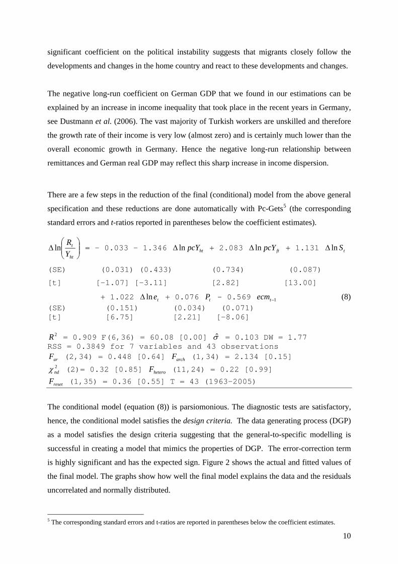
There are a few steps in the reduction of the final (conditional) model from the above general

specification and these reductions are done automatically with Pc-Gets5 (the corresponding

standard errors and t-ratios reported in parentheses below the coefficient estimates).

⎟⎟⎠

⎞⎜⎜⎝

⎛Δ

ht

t

YR

ln = - 0.033 - 1.346 htpcYlnΔ + 2.083 ftpcYlnΔ + 1.131 tSlnΔ

(SE) (0.031) (0.433) (0.734) (0.087)

[t] [-1.07] [-3.11] [2.82] [13.00]

+ 1.022 + 0.076 - 0.569 (8) telnΔ tP 1−tecm(SE) (0.151) (0.034) (0.071) [t] [6.75] [2.21] [-8.06]

2R = 0.909 F(6,36) = 60.08 [0.00] σ = 0.103 DW = 1.77 RSS = 0.3849 for 7 variables and 43 observations

arF (2,34) = 0.448 [0.64] (1,34) = 2.134 [0.15] archF2ndχ (2)= 0.32 [0.85] (11,24) = 0.22 [0.99] heteroF

resetF (1,35) = 0.36 [0.55] T = 43 (1963-2005)

The conditional model (equation (8)) is parsiomonious. The diagnostic tests are satisfactory,

hence, the conditional model satisfies the design criteria. The data generating process (DGP)

as a model satisfies the design criteria suggesting that the general-to-specific modelling is

successful in creating a model that mimics the properties of DGP. The error-correction term

is highly significant and has the expected sign. Figure 2 shows the actual and fitted values of

the final model. The graphs show how well the final model explains the data and the residuals

uncorrelated and normally distributed.

5 The corresponding standard errors and t-ratios are reported in parentheses below the coefficient estimates.

10

The short-run impact of the German GDP on remittances is positive and the sum of

coefficients on the home and host countries’ income is equal to one which is consistent with

the altruistic theory. The altruistic theory implies that an increase in the migrant’s income by

one euro, coupled with one-euro drop in the income of the migrant’s family left behind, raises

the amount transferred exactly by one euro. The unit coefficient on the stock of Turkish

migrants is also confirmed by the econometric analysis. The negative coefficient on Turkish

income with a positive coefficient on the real exchange rate further supports the altruistic

theory. The coefficient on the real exchange rate that is larger than one indicates that real

depreciation leads to higher remittances even when the remittances are expressed in terms of

the host country’s good, see Faini (1994). Furthermore, consistent with logic of transnational

migration theory, the positive long-run as well as short-run impact of political instability

suggests that Turkish migrants are altruistic. Thus, Turkish migrant responds positively to

political and economic changes in the home country.

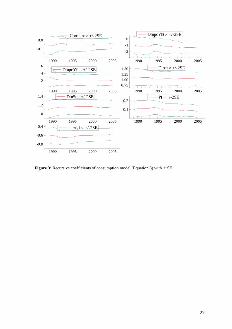
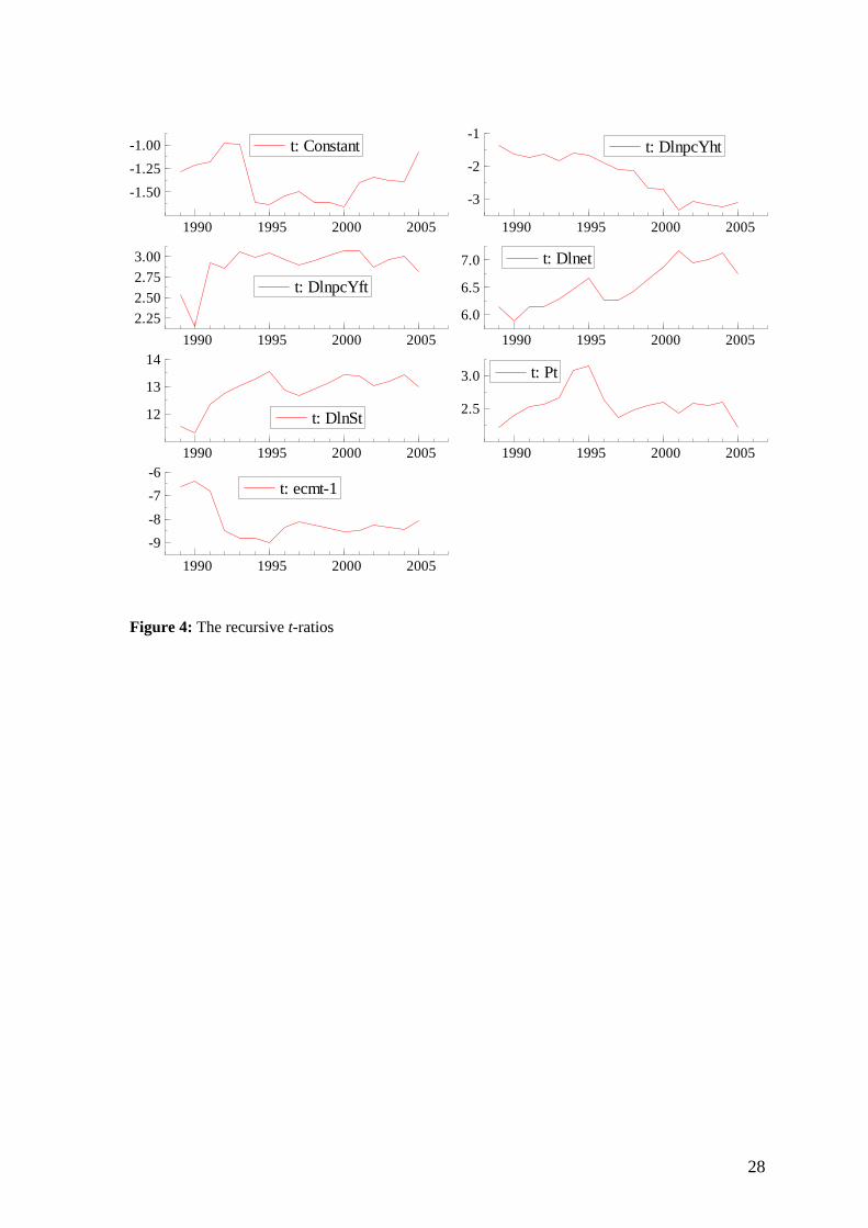
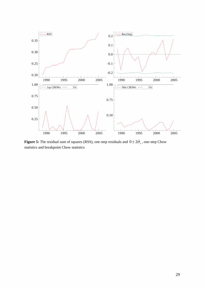
Figures 3, 4 and 5 plot the recursive estimates for the coefficients on the constant term,

, , , , , and ; their respective t-ratios; and the recursive

residual sum of squares, one-step residuals, one-step Chow statistics, and break–point Chow

statistics, respectively. Constant coefficients in Figure 3 in the presence of the large

variations in the marginal process such as incomes and exchange rates imply super exogenous

variables that counter the second sense of data mining. Further, the recursive t-ratios in

Figure 4, increase in absolute value as the sample size increases countering the first sense of

data mining. Hence, the nominal critical levels of test statistics are not affected. Even with

forty-three observations and seven variables in the final model t-ratios are greater than three

in magnitude suggesting that over-parameterisation is not a concern given information content

in the data and refuting the fourth sense of data mining. Figure 5 shows that the recursive

residual sum of squares increase over time and the recursive estimate of standard error

htYlnΔ ftYlnΔ tSlnΔ telnΔ tP 1−tecm

tσ

declines over time rather than increase, hence countering the first sense of data mining.

Furthermore, insignificant one-step and break-point Chow statistics support this refutation.

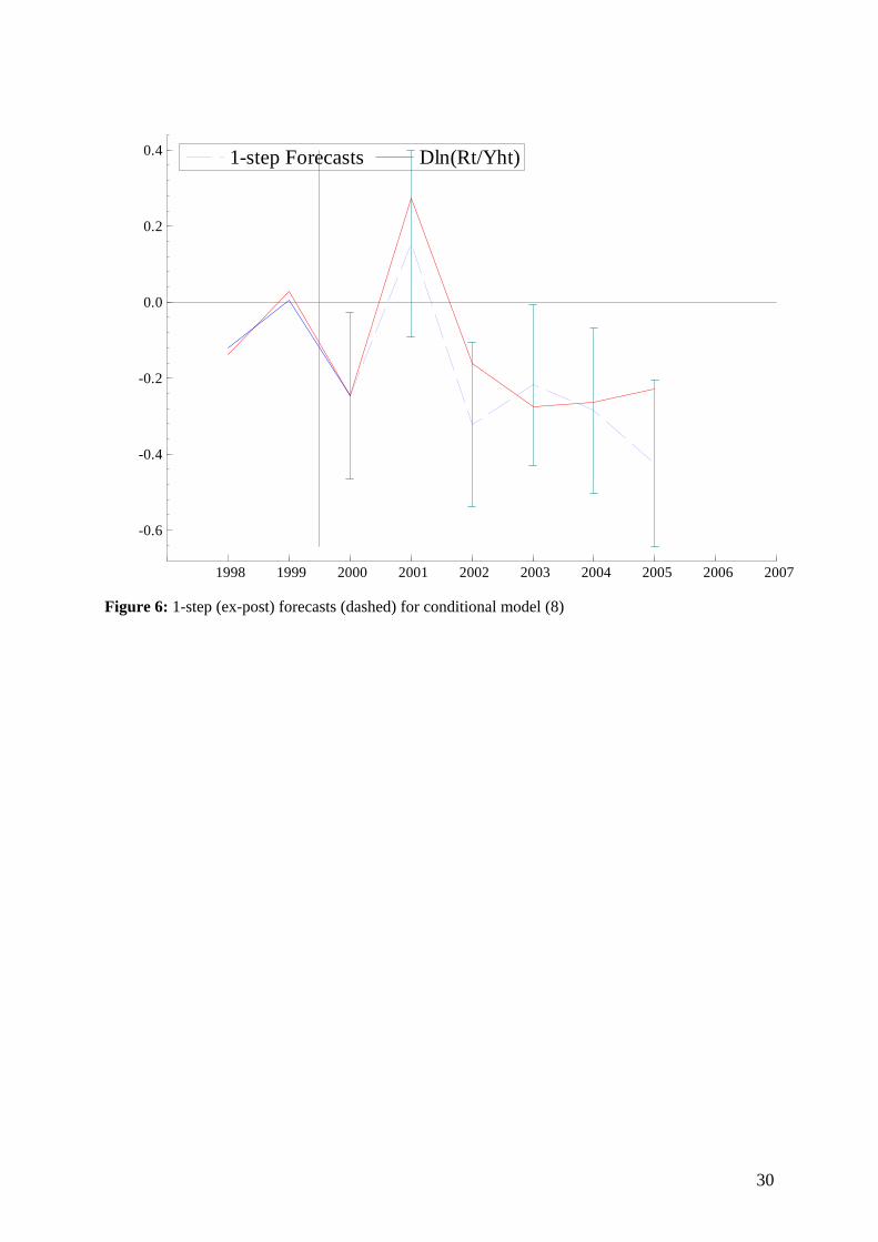
Finally, the conditional model is able to accurately forecast Turkish remittances from

Germany over the 2000-2005 period (see Figure 6 for the one-step ahead forecasts) and this

aspect is supported by the forecast test ( (6) = 2.89 (0.82)) , Kiviet (1986) and the 2forecastχ

11

parameter constancy test over k th periods ( = 0.27 (0.94)), Chow (1960). The forecast

results refute the first and second sense of data mining.

ChowF

5 Summary

In this paper we develop an altruistic model of migrants’ remittances to their home country

and test this model using the 1962-2005 annual data and the cointegration technique on the

remittances of Turkish workers staying in Germany. A single cointegrating vector is found

among the remittances and the following variables: the home country income, the host

country income, the stock of migrants, the real exchange rate and the political instability.

Based on the results of the cointegration analysis, a parsimonious single equation conditional

error-correction model is developed. That is both congruent and parsimoniously encompasses

the general model. The residuals are also innovations against the available information. The

results further support the view that a constructive data mining qua general-to-specific

modelling approach is productive as it has a high probability of locating the DGP.

The host country’s income has a positive effect upon remittances in the short run, whereas the

home country’s income exerts a negative effect on remittances both in the short and long run.

The unit coefficient on the stock of Turkish migrants is also confirmed by the data.

Additionally, we found a positive impact from the real exchange rate and the political

instability. The positive impact of the real exchange rate on remittances are especially

important for the design of adjustment programmes that mainly aim at shifting resources

toward the traded goods sectors by real exchange rate depreciation should also consider its

impact on remittances.

Turkish migrants in Germany seem to be very sensitive to the economic and political situation

in Turkey, since when there is a real devaluation and/or political instability they immediately

react by sending more remittances. The results of our estimation support the altruistic model

but are also consistent with the literature on transnationalism and offer interesting insights,

because they allow explaining the recent trends in Turkish remittances from Germany. Thus,

as long as Turkish migrants have altruistic motive and engage themselves in transnational

activity, they will continue supporting the welfare of their home country and will maintain the

remittances stable.

12

References

Akkoyunlu, S. (1999). Turkish Consumption and Saving. DPhil Thesis. University of Oxford.

Abdel-Rahman, A.-M. M. (2003). The determinants of foreign worker remittances in the

Kingdom of Saudi Arabia. King Saud University, mimeo.

Agarwal, R. and A. W. Horowitz (2002). Are international remittances altruism or insurance?

Evidence from Guyana using multiple-migrant households. World Development 30: 2033–44.

Alper, A. and S. Neyapti (2006). Determinants of workers’ remittances: Turkish evidence

from high frequency data. Eastern European Economics 44: 91–100.

Altonji, J. G., F. Hayashi, and L. J. Kotlikoff (1992). Is the extended family altruistically

linked? Direct tests using micro data. American Economic Review 82: 1177–98.

Altonji, J. G., F. Hayashi, and L. J. Kotlikoff (1997). Parental altruism and inter vivos

transfers: Theory and evidence. Journal of Political Economy 105: 1121–66.

Ayda¸s, O. T., K. Metin-Özcan, and B. Neyapti (2005). Determinants of workers’ remittances:

The case of Turkey. Emerging Markets Finance and Trade 41: 53–69.

Becker, G. S. (1974). A theory of social interactions. Journal of Political Economy 82: 1063–

1093.

Buch, C. M. and A. Kuckulenz (2004). Worker remittances and capital flows to developing

countries. ZEW Discussion Paper 04-31.

Chow. G. C. (1960). Tests of Equality Between Sets of Coefficients in Two Linear

Regressions. Econometrica 28: 591-605.

Campos, J. and Ericsson N. R. (1999). Constructive Data Mining: Modelling of Consumers’

Expenditure in Venezuela. Econometrics Journal 5: 226-240.

13

Clarke, G. R. and S. J. Wallsten (2003). Do remittances act like insurance? evidence from a

natural disaster in Jamaica. Development Research Group, World Bank, mimeo.

Doornik, J. A. and H. Hansen (1994). An omnibus test for univariate and multivariate

normality. Nuffield College Discussion Paper W4&91.

Dustmann, C., J. Ludsteck, and U. Schönberg (2007). Re-assessing trends in wage-inequality

in Germany. University College London, mimeo.

Doornik, J. A. and D. F. Hendry (2001a). GiveWin: An Interface to Empirical Modelling.

Timberlake Consultants Press: London.

Doornik, J. A. and D. F. Hendry (2001b). Modelling Dynamic Systems Using PcGive, Volume

II. Timberlake Consultants Press: London.

Doornik, J. A. and D. F. Hendry (2001c). Automatic Econometrics Model Selection Using

PcGets. Timberlake Consultants Press: London.

El-Sakka, M. I. T. and R. McNabb (1999). The macroeconomic determinants of emigrant

remittances. World Development 27: 1493–1502.

Elbadawi, I. A. and R. Rocha (1992). Determinants of expatriate workers’ remittances in

North Africa and Europe. Policy Research WPS 1133, The World Bank.

Engle, R. F. (1982). Autoregressive conditional heteroscedasticity with estimates of the

variance of United Kingdom inflation. Econometrica 50: 987-1007.

Faini, R. (1994). Workers remittances and the real exchange rate: A quantitative framework.

Journal of Population Economics 7: 235–45.

Freund, C. L. and N. Spatafora (2005). Remittances: Transaction costs, determinants, and

informal flows. World Bank Policy Research Working Paper No. 3704.

14

Funkhouser, E. (1995). Remittances from international migration: A comparison of El

Salvador and Nicaragua. The Review of Economics and Statistics 77: 137–145.

Gerard-Varet, L.-A., S.-C. Kolm, and J. M. Ythier (2000). The Economics of Reciprocity,

Giving, and Altruism. Houndmills and London: Palgrave Macmillan and New York: St.

Martins Press.

Glick Schiller, N. (1999). Transmigrants and nation-states: Something old and something new

in U.S. immigrant experience. In Handbook of International Migration: The American

Experience. C. Hirschman, J. DeWind, and P. Kasinitz (Eds.) New York: Russell Sage.

Glytsos, N. (1988). Remittances in temporary migration: A theoretical model and its testing

with the Greek-German experience. Weltwirtschaftliches Archiv 124: 524–548.

Glytsos, N. and L. T. Katseli (1986). Theoretical and empirical determinants of international

labour mobility: A Greek-German perspective. CEPR Discussion Papers 148.

Glytsos, N. P. (1997). Remitting behaviour of “temporary” and “permanent” migrants: The

case of Greeks in Germany and Australia. Labour 11: 409–435.

Godfrey, L. G. (1978). Testing for higher order serial correlation in regression equations when

the regressors include lagged dependent variables. Econometrica 46: 1303-1313.

Guarnizo, L. E. (2003). The economics of transnational living. International Migration

Review 37: 666–699.

Gupta, P. (2005). Macroeconomic determinants of remittances: Evidence from India. IMF

Working Paper 05/224.

Hendry, D. F. (1995). Dynamic Econometrics: Advanced Texts in Econometrics. Oxford

University Press: Oxford

Higgins, M. L., A. Hysenbegasi, and S. Pozo (2004). Exchange-rate uncertainty and workers’

remittances. Applied Financial Economics 14: 403–411.

15

Hoover, K. D., and Perez, S. J. (1999). Data Mining Reconsidered: Encompassing and the

General-to-Specific Approach to Specification Search. Econometric Journal 2: 167-191.

Katseli, L. T. and N. P. Glytsos (1989). Theoretical and empirical determinants of

international labour mobility: A Greek-German perspectives. In European Factor Mobility:

Trends and Consequences. I. Gordon and A. P. Thirlwall (Eds.), pp. 95–115. New York: St.

Martin’s Press.

Kiviet, J. F. On the Rigour of Some Misspecification Tests for Modelling Dynamic

Relationships. Review of Economic Studies 53: 241-261.

Lianos, T. P. (1997). Factors determining migrant remittances: The case of Greece.

International Migration Review 31: 72–87.

Lucas, R. E. B. and O. Stark (1985). Motivations to remit: Evidence from Botswana. Journal

of Political Economy 93: 901–18.

Niimi, Y. and C¸ Özden (2006). Migration and remittances: causes and linkages. Policy

Research Working Paper Series 4087, The World Bank.

Ogbomienie Agbegha, V. (2006). Does political instability affect remittance flows? Master’s

thesis, Graduate School of Vanderbilt University.

Ramsey, J. B. (1969). Tests for specification errors in classical linear least squares regression

analysis. Journal of the Royal Statistical Society, B, 31:350-371.

Rapoport, H. and F. Docquier (2005). The economics of migrants’ remittances. IZA

Discussion paper 1531.

Russell, S. S. (1986). Remittances from international migration: A review in perspective.

World Development 14: 677–696.

16

Schiopu, I. and N. Siegfried (2006). Determinants of workers’ remittances - Evidence from

the European neighbouring region. Working Paper Series 688, European Central Bank.

Smith, A. (1759). The Theory of Moral Sentiments. London: Printed for A. Millar, in the

Strand and A. Kincaid and J. Bell in Edinburgh. Reprinted 1982.

Stark, O. (1995). Altruism and Beyond. Oxford and Cambridge: Basil Blackwell.

Straubhaar, T. (1986). The determinants of workers’ remittances: The case of Turkey.

Weltwirtschaftliches Archiv 122: 728–740.

Swamy, G. (1981). International migrant workers’ remittances: Issues and and prospects.

World Bank Staff Working Paper 481.

Vargas-Silva, C. and P. Huang (2006). Macroeconomic determinantsof workers’ remittances:

Hostversus home country’s economic conditions. Journal of International Trade and

Economic Development 15: 81–99.

White, H. (1980). A heteroscedastic-consistent covariance matrix estimator and a direct test

for heteroscedasticity. Econometrica 48: 817-838.

Yang, D. (2006). Coping with disaster: The impact of hurricanes on international financial

flows, 1970-2002. NBER Working Paper 12794.

17

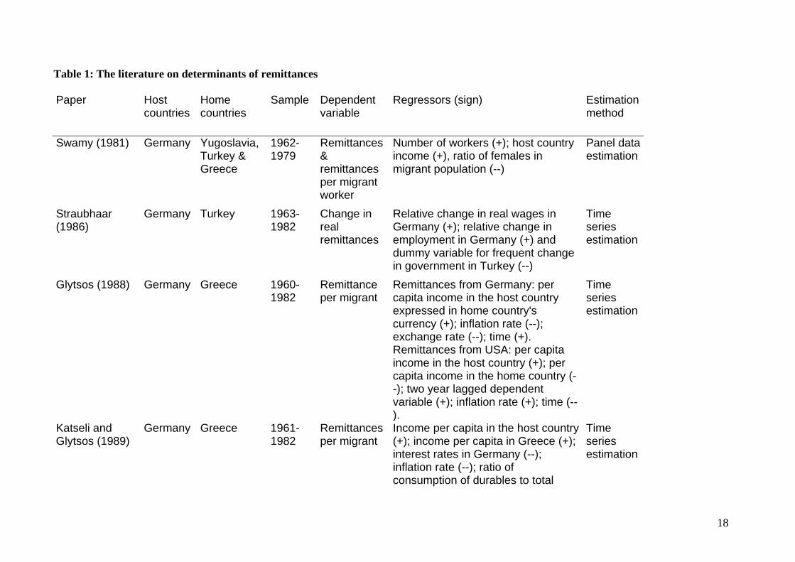
Table 1: The literature on determinants of remittances Paper Host

countries Home countries

Sample Dependent variable

Regressors (sign) Estimation method

Swamy (1981) Germany Yugoslavia, Turkey & Greece

1962-1979

Remittances & remittances per migrant worker

Number of workers (+); host country income (+), ratio of females in migrant population (--)

Panel data estimation

Straubhaar (1986)

Germany Turkey 1963-1982

Change in real remittances

Relative change in real wages in Germany (+); relative change in employment in Germany (+) and dummy variable for frequent change in government in Turkey (--)

Time series estimation

Glytsos (1988) Germany Greece 1960-1982

Remittance per migrant

Remittances from Germany: per capita income in the host country expressed in home country's currency (+); inflation rate (--); exchange rate (--); time (+). Remittances from USA: per capita income in the host country (+); per capita income in the home country (--); two year lagged dependent variable (+); inflation rate (+); time (--).

Time series estimation

Katseli and Glytsos (1989)

Germany Greece 1961-1982

Remittances per migrant

Income per capita in the host country (+); income per capita in Greece (+); interest rates in Germany (--); inflation rate (--); ratio of consumption of durables to total

Time series estimation

18

durables (--).

Elbadawi and Rocha (1992)

Total Algeria, Morocco, Portugal, Tunusia, Turkey & Yugoslavia

1977-1989

Real remittances, real remittances per migrant worker & real remittances per migrant

Host country income (+); length of stay (--); inflation (--); black market premium (--)

Panel data estimation

Faini (1994) Total Morocco, Portugal, Tunisia, Turkey & Yugoslavia

1977-1989

Real remittances in home country currency

Stock of migrant population (+); host country income (+); home country income (--); real exchange rate (+); expected devaluation adjusted interest rates differentials between the host and home country (+); time (--); inflaton (--)

Seemingly unrelated regression

Glytsos (1997) Germany and Australia

Greece 1960-1993

Remittances per migrant in drachmas

Remittances from Germany: per capita income in the host country (+); per capita income in the home country (--). Remittances from Australia: per capita income in host country (+); per capita income in home country (--); number of Greek migrants (--); interest rates in the host country (--).

Time series estimation

19

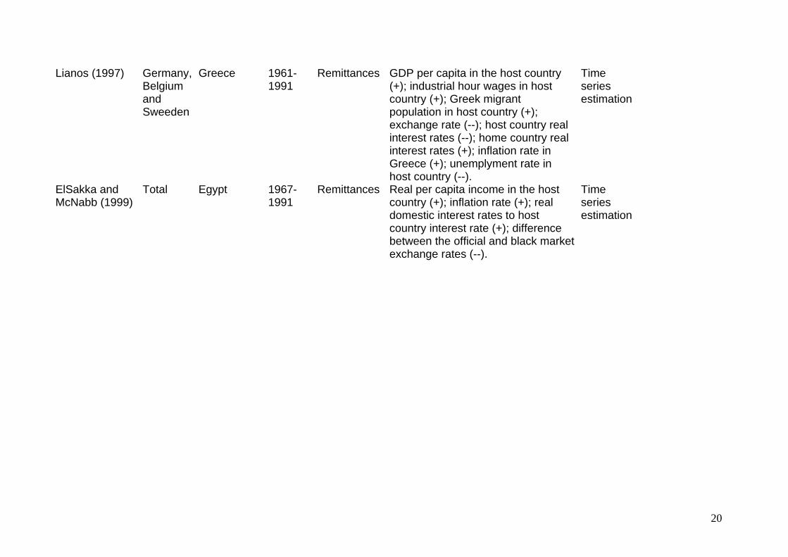
Lianos (1997) Germany, Belgium and Sweeden

Greece 1961-1991

Remittances GDP per capita in the host country (+); industrial hour wages in host country (+); Greek migrant population in host country (+); exchange rate (--); host country real interest rates (--); home country real interest rates (+); inflation rate in Greece (+); unemplyment rate in host country (--).

Time series estimation

ElSakka and McNabb (1999)

Total Egypt 1967-1991

Remittances Real per capita income in the host country (+); inflation rate (+); real domestic interest rates to host country interest rate (+); difference between the official and black market exchange rates (--).

Time series estimation

20

Abdel-Rahman (2003)

The Kingdom of Saudi Arabia

Bangladesh, Eqypt, India, Pakistan & Phillipines

1975-2001

Change in remittances per worker

Long run: GDP per capita in the host country (+); wage rate in the host country (+); nominal and real interest host country (--) or ratios of host country to home country interest rates (--); differential parity condition in host relative to home country (-); degree of govenment stability and the law & order indicators (--); composite socio-political stability indicator (--). Short run: change in host country GDP (+); change in host country per capita GDP (+); change in host country wage rate (+); change in inflation (+); change in differential parity condition (--); change in composite soci-political stability indicator (--); the long run solution (--).

ECM

Buch and Kuckulenz (2004)

Total 87 developing countries

1970-2000

Remittances over GDP and remittances per migrant

GDP per capita in home country (--); share of female in labor force (--); dependency ratio (--); illiteracy (+).

Panel data estimation

Higgins et al. (2004)

US 9 Latin American countries

1970-1997

Remittances per migrant

The real home country income per capita (+); the unemployment rate in USA (-) and uncertainty in real exchange rates (--).

The fixed effects IV and non-IV technique

21

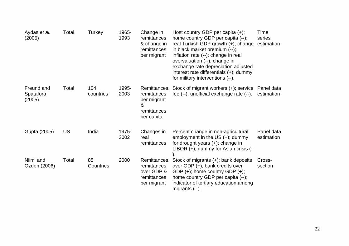
Aydas et al. (2005)

Total Turkey 1965-1993

Change in remittances & change in remittances per migrant

Host country GDP per capita (+); home country GDP per capita (--); real Turkish GDP growth (+); change in black market premium (--); inflation rate (--); change in real overvaluation (--); change in exchange rate depreciation adjusted interest rate differentials (+); dummy for military interventions (--).

Time series estimation

Freund and Spatafora (2005)

Total 104 countries

1995-2003

Remittances, remittances per migrant & remittances per capita

Stock of migrant workers (+); service fee (--); unofficial exchange rate (--).

Panel data estimation

Gupta (2005) US India 1975-2002

Changes in real remittances

Percent change in non-agricultural employment in the US (+); dummy for drought years (+); change in LIBOR (+); dummy for Asian crisis (--).

Panel data estimation

Niimi and Özden (2006)

Total 85 Countries

2000 Remittances, remittances over GDP & remittances per migrant

Stock of migrants (+); bank deposits over GDP (+), bank credits over GDP (+); home country GDP (+); home country GDP per capita (--); indicator of tertiary education among migrants (--).

Cross-section

22

VargasSilva and Huang (2006)

US Mexico Quaterly data: 1981:1-2004:4

Nominal remittances

US Federal Fund rate (+); US money supply (+); US consumer price index (+); US unemployment rate (+).

VECM

Alper and Neyapti (2006)

Total Turkey Monthly Data: 1991:1-2003:12

Nominal remittances

Long run: 1-year Turkish lira depost rate (+); consumer price index (--); exchange rate (+); long-run home country's manufacturing production (+). Short run: change in manufacturing production index (--); inflation (+); change in exchange rate (--); change in 1-year Turkish lira deposit rate (--).

VECM

Ogbomienie Agbegha (2006)

Total Latin America, Caribbean & Sub-Saharan Africa

1970-2003

Remittances per capita

The host country GDP per capita (+); home country GDP per capita (--); political stability (--).

Panel data estimation

23

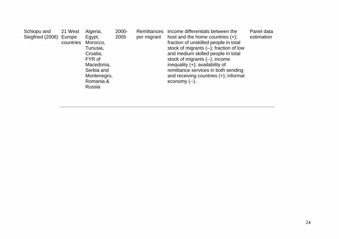
Schiopu and Siegfried (2006)

21 West Europe countries

Algeria, Egypt, Morocco, Tunusia, Croatia, FYR of Macedonia, Serbia and Montenegro, Romania & Russia

2000-2005

Remittances per migrant

Income differentials between the host and the home countries (+); fraction of unskilled people in total stock of migrants (--); fraction of low and medium skilled people in total stock of migrants (--); income inequality (+); availability of remittance services in both sending and receiving countries (+); informal economy (--).

Panel data estimation

24

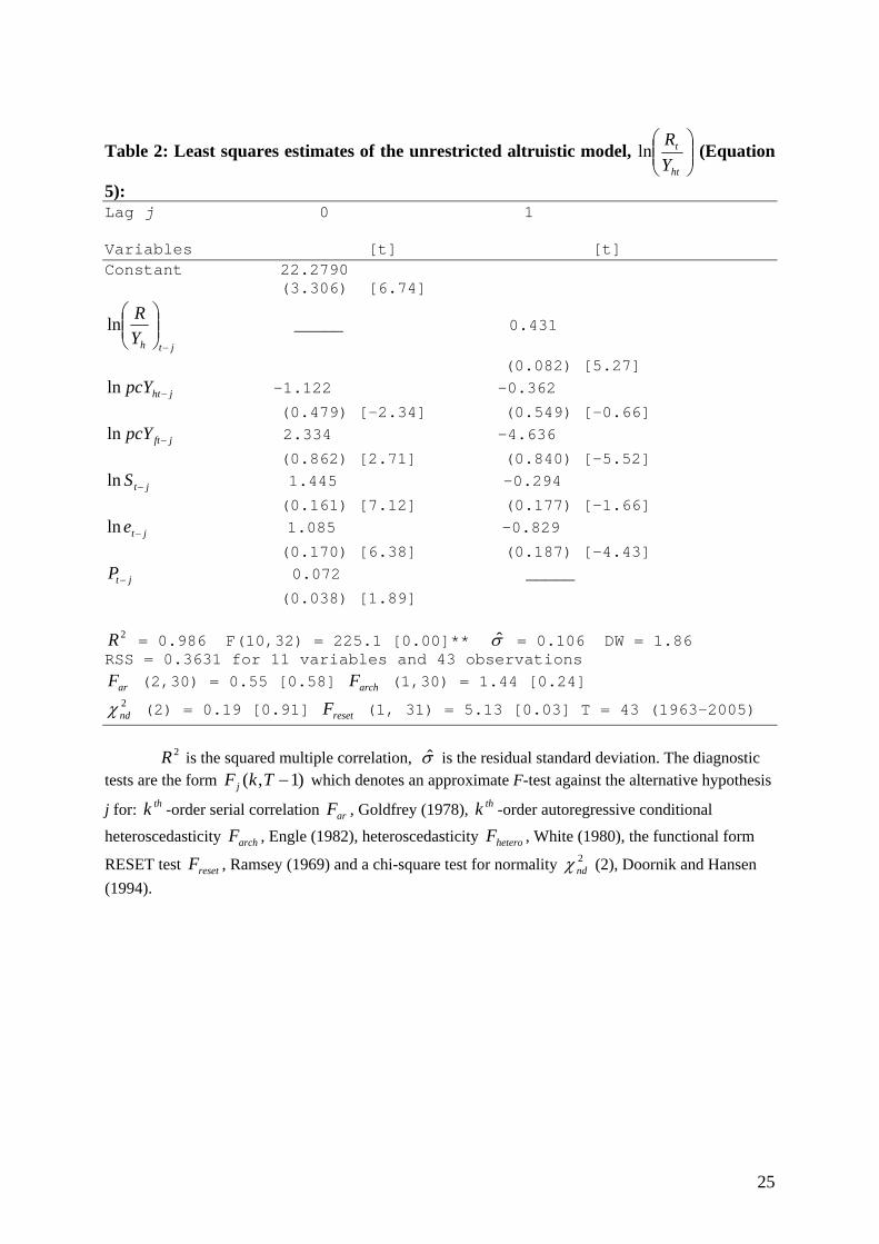
Table 2: Least squares estimates of the unrestricted altruistic model, ⎟⎟⎠

⎞⎜⎜⎝

⎛

ht

t

YR

ln (Equation

5): Lag j 0 1 Variables [t] [t] Constant 22.2790 (3.306) [6.74]

jthYR

−⎟⎟⎠

⎞⎜⎜⎝

⎛ln _____ 0.431

(0.082) [5.27]

jhtpcY −ln -1.122 -0.362

(0.479) [-2.34] (0.549) [-0.66]

jftpcY −ln 2.334 -4.636

(0.862) [2.71] (0.840) [-5.52]

jtS −ln 1.445 -0.294

(0.161) [7.12] (0.177) [-1.66]

jte −ln 1.085 -0.829

(0.170) [6.38] (0.187) [-4.43]

jtP− 0.072 _____

(0.038) [1.89]

2R = 0.986 F(10,32) = 225.1 [0.00]** σ = 0.106 DW = 1.86 RSS = 0.3631 for 11 variables and 43 observations

arF (2,30) = 0.55 [0.58] (1,30) = 1.44 [0.24] archF2ndχ (2) = 0.19 [0.91] (1, 31) = 5.13 [0.03] T = 43 (1963-2005) resetF

2R is the squared multiple correlation, σ is the residual standard deviation. The diagnostic

tests are the form which denotes an approximate F-test against the alternative hypothesis

j for: -order serial correlation , Goldfrey (1978), -order autoregressive conditional

heteroscedasticity , Engle (1982), heteroscedasticity , White (1980), the functional form

RESET test , Ramsey (1969) and a chi-square test for normality (2), Doornik and Hansen (1994).

)1,( −TkFj

thk arF thk

archF heteroF

resetF 2ndχ

25

1960 1970 1980 1990 2000

500100015002000 Rt_EUR

1960 1970 1980 1990 2000-1012 ln(Rt/Yht)

1960 1970 1980 1990 2000

7.0

7.5 lnpcYht

1960 1970 1980 1990 2000

9.509.75

10.0010.25

lnpcYft

1960 1970 1980 1990 2000

10.0

12.5

15.0 lnSt

1960 1970 1980 1990 2000

-2.75-2.50-2.25 lnet

1960 1970 1980 1990 2000

0.5

1.0 Pt

Figure 1: The basic properties of data: 1969-2004

1970 1980 1990 2000

0.0

0.5

1.0 Dln(Rt/Yht) Fitted

1970 1980 1990 2000-2

-1

0

1r:Dln(Rt/Yht)(scaled)

-4 -3 -2 -1 0 1 2 3

0.1

0.2

0.3

0.4

0.5

Density

r:Dln(Rt/Yht) N(0,1)

1 2 3 4 5 6 7

-0.5

0.0

0.5

1.0ACF-r:Dln(Rt/Yht)

Figure 2: Actual and fitted values of migration model from Equation (8), residuals, the histogram and estimated density of the residuals and their correlogram

26

1990 1995 2000 2005

-0.1

0.0Constant × +/-2SE

1990 1995 2000 2005

-2-10

DlnpcYht × +/-2SE

1990 1995 2000 2005

2

4

6DlnpcYft × +/-2SE

1990 1995 2000 20050.751.001.251.50 Dlnet × +/-2SE

1990 1995 2000 2005

1.0

1.2

1.4 DlnSt × +/-2SE

1990 1995 2000 2005

0.1

0.2Pt × +/-2SE

1990 1995 2000 2005

-0.8

-0.6

-0.4 ecmt-1 × +/-2SE

Figure 3: Recursive coefficients of consumption model (Equation 8) with ± SE

27

1990 1995 2000 2005

-1.50-1.25-1.00 t: Constant

1990 1995 2000 2005

-3

-2

-1t: DlnpcYht

1990 1995 2000 20052.252.502.753.00

t: DlnpcYft

1990 1995 2000 2005

6.0

6.5

7.0 t: Dlnet

1990 1995 2000 2005

12

13

14

t: DlnSt

1990 1995 2000 2005

2.5

3.0 t: Pt

1990 1995 2000 2005-9-8-7-6

t: ecmt-1

Figure 4: The recursive t-ratios

28

1990 1995 2000 20050.20

0.25

0.30

0.35

RSS

1990 1995 2000 2005

-0.2

-0.1

0.0

0.1

0.2 Res1Step

1990 1995 2000 2005

0.25

0.50

0.75

1.001up CHOWs 1%

1990 1995 2000 2005

0.50

0.75

1.00Ndn CHOWs 1%

Figure 5: The residual sum of squares (RSS), one-step residuals and tσ20 ± , one-step Chow statistics and breakpoint Chow statistics

29

1998 1999 2000 2001 2002 2003 2004 2005 2006 2007

-0.6

-0.4

-0.2

0.0

0.2

0.4 1-step Forecasts Dln(Rt/Yht)

Figure 6: 1-step (ex-post) forecasts (dashed) for conditional model (8)

30

A Link Between Workers’ Remittances and the Business Cycles in Germany and Turkey*

Şule Akkoyunlu**

Konstantin A. Kholodilin***

Abstract In this paper we examine the cyclical interactions between the remittances of the Turkish workers in Germany and the output both in Turkey and in Germany. In our analysis we introduce a new data set covering 1962-2004, which was never before used in the research literature and which we consider as a more reliable source than the data sets used in the other studies. By dividing the original sample into “recruitment”, “family re-unification”, and “naturalization” periods, we show that duration of migrants’ stay in the host country affects the direction and strength of the relationship between remittances and the host and home country’s business cycle. Keywords: Migration; remittances; Turkey; Germany. JEL classification: F22; J61; E32 1 Introduction Turkish workers’ official remittances from Germany constitute a large share (60% in 2002, before methodological change of the series of total workers’ remittances to Turkey) of total official remittances to Turkey. During the 1970s and 1980s, total official remittances reached 4% of Turkish GDP, whereas official remittances from Germany comprised 3% of Turkish GDP — see panel (b) of Figure 1 — making Turkey one of the ten largest remittance receiving countries in the absolute terms. Despite a certain decrease that they have experienced during the last decades, remittances continue to play a very important role in the Turkish economy. They are not only one of the major sources of foreign exchange, but also a relatively stable source of foreign exchange compared to foreign direct investment and other private capital flows. Thus, during the period 1964-2005, Turkish workers’ remittances from Germany totaled 47.5 billion euros, whereas the capital inflows and foreign direct investments from Germany only totaled 17.8 billion euros and 4.2 billion euros, respectively. In general, Ratha (2003) shows that in contrast to capital flows, the remittances are significantly higher in countries that are characterized by high risk and have a high level of debt relative to GDP. The magnitude of remittances makes them an important factor affecting the cyclical fluctuations of the home country’s economy. Clearly, the countercyclical (with respect to Turkish output) remittances help to alleviate the consequences of negative shocks, such as the economic crises of 1994 and 2001, while the procyclical remittances tend rather to magnify the adverse effects of such shocks and contribute to macroeconomic instability. It is, therefore, important to know whether remittances respond positively or negatively to movements of the home country’s GDP. Although the fluctuations of remittances can hardly affect the output in the host country, the latter can exert a non-negligible impact upon the former and, in turn, upon the home country’s output. Hence we also investigate the relationship between the host country’s output and workers’ remittances. The contribution of this paper is twofold. First, we introduce a new time series of official remittances from Germany to Turkey stemming from the Deutsche Bundesbank. The other

authors, like Sayan (2004), Sayan (2006), and Sayan and Tekin-Koru (2007a,b), construct the remittances series based on a rather restrictive assumption that the share of Turkish workers’ remittances from Germany remains constant over time. To the best of our knowledge, nobody else has used these data before to analyze the link between remittances and the business cycles in Germany and Turkey. The only paper that uses these data and that we know of is Köksal and Liebig (2005), but it is of a purely descriptive nature. Secondly, we test the hypothesis that the cyclical characteristics of Turkish remittances from Germany may have changed over time by using a new, three-period classification. In fact, remittances may be pro-, counter- or acyclical during different periods, depending on the duration of migrants’ stay in the host country. This argument was made before by such authors as Swamy (1981), Aydaş et al. (2005), and Sayan (2006). Sayan (2006) himself argued that remittances sent by Turkish workers in Germany were probably countercyclical until 1994 but turned procyclical afterwards. Sayan and Tekin-Koru (2007a) identified the turning point as 1992 rather than 1994. We further refined this analysis by considering three subperiods in the history of Turkish migration to Germany, which we call “recruitment”, “family re-unification”, and “naturalization” periods. Section 2 describes different motives underlying the remitting behavior of the migrant workers. In section 3, our data set is introduced, whereas section 4 contains the econometric analysis of the data. Finally, section 5 concludes the paper. 2 Motives of the remitting behavior The size and dynamics of the remittances depend on the decisions made by the workers. Therefore, their motivation is of crucial importance for the analysis of the cyclical interactions between the income of host and home countries, on the one hand, and remittances, on the other. There are a number of theories, which try to identify the principal incentives of the workers sending remittances home. Most of these theories were documented in Lucas and Stark (1985) and Rapoport and Docquier (2005). We summarized their predictions with regard to the effects of the income in host and home countries upon the remittances in Table 1. The different theories of the motivation of the guest workers are listed in the rows, while the explanatory variables affecting the remittances are reported in columns. “+” (“–”) means that the corresponding explanatory variable positively (negatively) affects the size of remittances, “ ± ” means that the influence can be both positive and negative, whereas “0” means that no influence exists. Below we consider these theories in more detail. The most common motivation to remit is that migrants care about those left behind. This “altruistic” transfer increases with the migrant’s income and decreases with the recipient’s income. One extreme version of the altruistic model is the so-called “remittance maximization” approach Bhattacharyya (1985), where migrants are assumed to send a maximum amount of remittances back to their family. In this model, the level of income in the home country should not play any role in the remittance choice. The amount of remittances would depend almost entirely on the emigrants’ own income in the host country. The remittances may also be used in exchange for a wide range of services provided by the migrant’s relatives living in the home country, such as taking care of migrant’s assets. In this case the migrant has the intention to eventually return home. This is the “exchange” motive to

remit. The central prediction of the exchange motive theory is that an increase in the recipient’s income leads to an increase in the remittances. The “strategic” motive arises when migrants are heterogeneous in skills and individual productivity, which is not perfectly observable on the labor market of the host country. The skilled migrants bribe their unskilled compatriots in order to convince them to stay in the home country. In this way they can avoid the unnecessary competition that would drive their wages down. As in the case of altruistic transfers, the level of remittances is expected to be positively related with the migrants’ pre-transfer income and to be negatively related with the recipients’ pre-transfer income. Due to the structural and technological characteristics of most developing countries, the income volatility plays an important role in the rural regions. In addition to this, imperfect credit and insurance markets in most developing countries cause a range of informal inter-and intra-familial coinsurance arrangements. Hence, provided that incomes in home and home countries are not positively correlated, it is beneficial to send some members of the family abroad. In this way, the remaining members of the family will be insured against drops in rural incomes. In reciprocation, they will provide assistance to the migrant in case of unemployment. If this Pareto-improving arrangement is not self-enforced by altruism, then different retaliation strategies can be imposed, such as denying the migrant’s rights to future family solidarity, inheritance, or return to the village for retirement. This is the “insurance” motive and it gives similar predictions as the altruistic motive with respect to the sign of the effect that the income in the home country exerts upon remittances. Hoddinott (1994) argues that there is a minimum amount of money that each migrant is expected to remit. Parents can encourage transfers above this minimum level by offering a “reward” in form of land or any other inheritable asset. In this “inheritance” motive theory, the remittances are seen as a pure strategy of investment in inheritance on the side of the migrant and as an enforcement device to secure remittances on the side of the family. The main prediction of this model is that the amount of remittances increases with migrant’s wealth and income, but should be independent of the recipients’ income. Remittances are used as repayments on loans for investments in education and/or migration, according to the “investment” motive theory. If investments are the main familial motivation for sending migrants away, then the family will continue sending migrants as long as family income is increasing. However, migration costs and liquidity constraints limit the number of migrants that can be sent by a given family and that richer, but not too rich families are more likely to take advantage of the investment opportunities. However, the literature finds that a combination of different motives explains the remitter’s behavior better than a single motive. For example, Lucas and Stark (1985) explain the positive relationship between the level of remittances and the income in the home country by the mixture of exchange, investment, and inheritance motives. On the other hand, the response of the remittances to the short-run shocks to recipients’ income is explained by either altruism or insurance motives. This complex mixture of motives can be described best of all by such concepts as “impure altruism” (Andreoni (1989)) or “enlightened selfishness” (Lucas and Stark (1985)). The “macroeconomic” model of remittances explains the amount of remittances sent to the home country by the levels and fluctuations of economic activities in the host and home countries. The output per capita represents the general level of the development of a country.

The higher the development level of a country the more likely a negative relationship between the remittances and output per capita in the home country and a positive relationship between the remittances and output per capita in the host country exists. When economic conditions in the home country are favorable, the living standards of the migrant’s relatives are improved and hence his willingness to send them remittances decreases. On the other hand, the improved economic well-being in the host country will increase the employment and earnings opportunities of the migrants and therefore encourage them to send more remittances. However, the short-run effect of the home country’s income is ambiguous, as this variable captures the attractiveness of investing to the country. High income growth in the home country might reduce incentive to migrate and hence the remittances to the countries with high income growth will be smaller. At the same time, the migrants might want to invest in their high-growth home country and hence the remittances to this country will be bigger. Most of the studies on determinants of remittances find that the host country income has a positive effect on remittances, see Swamy (1981), Straubhaar (1986), Katseli and Glytsos (1989), Elbadawi and Rocha (1992), Faini (1994), Hoddinott (1994), Lianos (1997), El-Sakka and McNabb (1999) and Aydaş et al. (2005). However, the regression of remittances on the home country’s income delivers mixed results. While Lucas and Stark (1985), Ilahi and Jafarey (1999), Higgins et al. (2004) and Sayan (2004) favor the exchange and investment motives, Alper and Neyapti (2006) argue for the investment motive dominating in the long run and consumption-smoothing motive prevailing in the short run, Faini (1994), Katseli and Glytsos (1989), Glytsos (1997), Lianos (1997), and Agarwal and Horowitz (2002) support the altruistic motive, whereas Aydaş et al. (2005) indicate the importance of both altruistic and investment motives. In addition, some studies find the income in the host country to be statistically insignificant, see Lianos (1997) and El-Sakka and McNabb (1999). The most interesting results are obtained by Glytsos (1988) and Glytsos (1997): in Glytsos (1988) the domestic current and lagged per capita income in Greece have a positive sign for the 1960-1982 period supporting the self-interest motive. However, using a similar equation but with data for the period 1960-1993, Glytsos (1997) finds that the sign of Greek income per capita turns from positive to negative, suggesting an altruistic motive. He explains these results by the fact that after the early 1980s, many Greek temporary migrants in Germany turned into the permanent residents. Hence, the self-interest motive subsided and the altruistic motive became dominant. The migrants in Germany are behaving in the same way as their counterparts in the USA and Australia, whose remittances are negatively related to the Greek per capita income. 3 Data We conduct our statistical analysis using the annual data covering the period 1962–2004. The data were taken from the databases of the Turkish Statistical Institute, Deutsche Bundesbank, OECD, and World Market Monitor and are listed in Table 2. The series of remittances to Turkey expressed in euros1 were computed from the available data as shown in Table 2 and depicted in Figure 1. Following Sayan (2004), as a proxy for the host country’s income we use GNP, whereas as a measure of the home country’s income we apply GDP. The logic behind this decision is the following: GNP is defined as GDP plus NFI (net factor income from abroad). NFI includes net remittance receipts and hence German GNP and Turkish GDP exclude remittances sent to Turkey by Turkish workers in Germany.

Although the data on workers’ remittances are very difficult to measure, given the variety of legal and illegal transmission channels, we believe that the data we use do reflect the main tendencies. It is worth stressing that, unlike in Sayan (2004), Sayan (2006), and Sayan and Tekin-Koru (2007a,b), our data are not constructed based on the authors’ assumptions, but are directly measured and come from a reliable and accurate source such as the Deutsche Bundesbank. As far as we know, these data are employed for the business cycle research purposes for the first time in the literature. The only paper that also uses these data and that we are aware of is Köksal and Liebig (2005), but it has a purely descriptive nature. By contrast, previous studies used a remittance series, which was constructed from the official Turkish data on total remittances to Turkey. In these studies, the series of Turkish workers’ remittances from Germany was constructed as a product of the total amount of remittances to Turkey and the share of Turkish workers residing in Germany in the total stock of migrant workers from Turkey. This share was set equal to 60% for all years, which implies quite a strong assumption that the share of remittances from Germany in total remittances remained unchanged. However, as one can see in Köksal and Liebig (2005), the share is far from being constant and has been varying from 24.3% to 139.3%2 . Secondly, as Gallina (2006) mentions, the data from the official Turkish sources (Central Bank of Turkey), have undergone in 2003 a major methodological change, as result of which the pre-2003 data cannot be directly compared with the post-2003 data. From 2003 on the remittances series does not include anymore the transfers from the Turkish workers going to Germany with tourist visas but with an objective to earn money. This important component of remittances is now reported in the Balance of Payments under “tourism income” heading, see Gallina (2006). By contrast, data on remittances coming from the Deutsche Bundesbank are consistent over the whole period starting in 1962. The official German indicator of the remittances, or transfers, by the workers to their country of origin (here Turkey), which is used in our study is calculated according to the balance of payments statistics. For this purpose guest workers are regarded as residents — they stay in Germany more than one year and are economically active. For the individual transfers the amount should be below 12,500 euros. Remittances to countries of origin are estimated using various statistical sources. For example, monthly collective reports on bank transfers are available for individual countries of origin, some of which also include payments below the reporting threshold. In addition, the Federal Employment Agency provides up-to-date data on the number and origin of employed and unemployed foreigners living in Germany who are subject to social security contributions. Furthermore, until 2002 the MARPLAN research society’s annual report provided an indication of transfers to five of the most important countries of origin: Turkey, Italy, Spain, Greece, and the former Yugoslavia. The institute questioned 2000 foreigners living in Germany about transfers to their countries of origin. Additional estimates, complementing the bank transfers actually reported, are based on the information about the cash taken to those countries and about the amounts below the reporting threshold, which are not covered in the collective reports. In individual cases, the amount of remittances that appears in the collective reports can be reduced, if there are indications that these payments were made for other purposes. The different transformations of the remittances from Turkish workers in Germany to Turkey are presented in Figure 1. The nominal remittances in euros shown in panel (a) attained their peak in 1984 and since then have been slowly declining. The decline is much more pronounced when the share of nominal remittances in the nominal Turkish GDP (panel (b)) is considered. The share achieved its maximum of 3.4% in 1973 and by 2004 it decreased

almost tenfold. The real remittances declined sharply after the peak of 1973 (see panel (c)), whereas the real remittances per migrant have been constantly decreasing since the beginning of 1960s with short interruption in the first half of 1970s (see panel (d) of Figure 1). 4 Econometric Analysis The possible relationships between the business cycles in the host and home countries and real remittances sent to the home country by the Turkish workers in Germany are analyzed in a twofold way. First, the cross-correlations between the German real GDP and the Turkish real GDP, on the one hand, and real remittances expressed in euros, on the other hand, at different lags and leads were estimated. Secondly, the bivariate VARs were used in order to investigate the hypothesis of Granger causality between the German GNP/Turkish GDP and remittances. The VAR approach was chosen in order to take into account possible endogeneity problem. Although in case of Germany the remittances to Turkey can hardly affect the host country’s income, in case of Turkey they play a much more important role and thus can influence the income of the home country. Unlike Aydaş et al. (2005) and Alper and Neyapti (2006), we do not use the regression analysis and follow the methodology of Sayan (2006) to investigate business cycle. We do not make a cross-country analysis since this might mask important cyclical characteristics of remittances received by each individual country, as suggested by Sayan (2006). The analysis is undertaken using both the annual growth rates and the cyclical components. The annual growth rates were computed as the first differences of the logarithms of the original data. The cyclical components both of German GNP, Turkish GDP and of remittances were approximated, as in Sayan (2004), Sayan (2006), and Sayan and Tekin-Koru (2007a,b), by the Hodrick-Prescott filter with smoothing parameter λ = 100 applied to the logged series. We have also tried other values of this parameter suggested in the literature, namely: 6.25 as in Ravn and Uhlig (2002) and 400 as in Cooley and Ohanian (1991). However, the qualitative conclusions turned out to be the same regardless of the λ’s value. Therefore, we report only the results obtained for λ = 100. All the series were tested for unit-root stationarity, see Table 3. For testing purposes, Augmented Dickey-Fuller (ADF) test and Phillips-Perron test are employed. The specification of these tests includes four lags, a constant, and no trend. The tests were conducted using STATA 9.2. For the levels of almost all the series the null hypothesis of unit root cannot be rejected. The only exception is the real German GNP per capita, for which the null is rejected by the ADF test at 10% significance level and by Phillips-Perron even at 1% significance level. For the growth rates and cyclical components of the variables considered in this paper the null hypothesis can be rejected at conventional significance levels. ADF, however, accepts the null for the growth rate of real German GNP per capita and growth rate of real remittances. Nevertheless, given the short sample size and rejection of the null by the Phillips-Perron test we assume that these variables are stationary. Across the whole period 1962-2004, a positive and significant cross-correlation between the German real GDP and real remittances expressed in euros is found at lag 1 — see Table 4. It implies that the German real GNP leads the remittances to Turkey by one year. This finding is robust to two types of transformations used in this paper: first-order differencing (growth rates) and application of Hodrick-Prescott filter (cyclical component). By contrast, the cross-correlations between the growth rate of the German real GNP and the growth rates of the real remittances per migrant are never significant implying no relationship between these two series.

A positive and significant correlation over the period 1962-2004 was only found between the growth rate Turkish GDP and growth rate of real remittances at lag 2 — see Table 4. All other cross-correlations are not significant. The unrestricted bivariate VAR3 estimated for the growth rates and cyclical components of the German GNP and remittances in euros across the whole period confirm the results of the cross-correlation analysis — see Table 7. The impulse-response analysis, conducted for the VARs based both on the growth rates and cyclical components, shows that after a positive impulse in German GNP the real remittances increase and their response remains positive and significant for about four years before converging to zero. These results do not change when the German unification dummy, which is equal to 1 in 1991 and to zero otherwise, is introduced in the estimation. Neither the unrestricted bivariate VAR, including the growth rates of the real remittances per Turkish migrant in Germany and the growth rates of the German real GNP, nor the VAR, including the real remittances per Turkish migrant in Germany and the growth rates of the German real GNP per capita, show any Granger causality between these two variables. The unrestricted bivariate VARs estimated for the growth rates and cyclical components of the Turkish real GDP and real remittances to Turkey expressed in euros over period 1962-2004 also lead to a rejection of Granger causality between the Turkish GDP and the remittances — see Table 8. Likewise, no Granger causality is found, when the unrestricted bivariate VAR, which includes the growth rates of the real remittances per Turkish migrant in Germany and the growth rates of the Turkish real GDP, and the VAR, which includes the growth rates of the real remittances per Turkish migrant in Germany and the growth rates of the Turkish real GDP per capita, are estimated. All this stands in a remarkable contrast to the findings of Sayan (2004) who found, using the quarterly data that covered the period 1987:1 to 2001:4, a positive relationship between cyclical components of the remittances of Turkish workers living in Germany and the business cycles in Turkey (i.e., cyclical components of the Turkish GDP), but no relationship between cyclical components of these remittances and those of the German GNP. Such contradicting results were also obtained by other researchers examining workers’ remittances to Turkey. For example, using annual data obtained from the Central Bank of Turkey, Aydaş et al. (2005) examined two different periods: 1965-1993 and 1979-1993. They came to a conclusion that the growth rate of Turkish GDP has a positive impact on official remittances of Turkish workers employed abroad. Furthermore, according to Aydaş et al. (2005), the growth rate of Turkish GDP exerts no significant impact upon the official remittances in per capita terms. By contrast, Alper and Neyapti (2006), who use monthly data from the Central Bank of Turkey covering the period from January 1992 to December 2003, conclude that the growth rate of Turkish GDP negatively affects official remittances of Turkish workers living abroad. Therefore, the difference in period under study and in the frequency of the data may yield different results. Hence it might be meaningful to consider different subsamples. We decided to divide the whole period into three subperiods using the changes in the institutional environment of Turkish migrants in Germany as a criterion.

The first period is 1960-1974. It can be called a “recruitment” period, since from the beginning of 1960s and up to 1974, Turkish workers were massively recruited by Germany in order to fill the labor shortages in certain sectors caused by the very fast economic growth. In 1974, after the first oil shock took place, this growth was halted and Germans stopped recruiting Turkish workers. During this period, the Turkish workers migrated to Germany as guest-workers and their main aim was to save as much as they could in a short period of time and remit their savings home (maximization motive). Therefore, their remittances strongly depended on their wages and hence on the German income. As Tables 5 and 6 show, remittances were positively correlated with both German GNP and Turkish GDP. However, the maximum cross-correlation with German GNP is achieved at lag 0, whereas that with Turkish GDP — at lead 2. It means that German GNP affected the remittances, which, in turn, exerted an impact on the Turkish GDP. These results are confirmed by the Granger-causality analysis — see Tables 9 and 10. It shows that the German GNP was Granger-causing the remittances of Turkish workers, while between (cyclical component of) remittances and Turkish GDP there was a two-way causal relationship. This latter outcome can be easily explained, given a prominent role played by the workers’ remittances in the Turkish economy at that period. Indeed, according to Köksal and Liebig (2005), in 1973, the total remittances of Turkish workers accounted for more than 4% of Turkish GNP and over 90% of Turkish exports. The second period is from 1975 to 1990. It can be called a “family re-unification” period. During this period Turkish workers in Germany reunited with their families, which came from Turkey. This implied that there was no need for them anymore to send any remittances to Turkey. As can be seen in Köksal and Liebig (2005), already in 1976 the share of total remittances in Turkish GNP experienced more than a double decline, whereas that in Turkish exports dropped to about 50%. After 1975, the remittances from Germany have been constantly declining. The cross-correlations between German GNP and remittances were mostly not significant, except the cross-correlation between German GNP per capita and remittances per migrant, which is significantly negative. The cross-correlations between Turkish GDP and remittances are negative and significant. This counter-cyclicality can be explained by the fact that Turkish migrants moved by the altruistic motive continued to send money to the rest of their relatives in Turkey, whose living standards suffered a lot from the economic crises in the 1970-1980s. These results are consistent with Sayan (2006) and Sayan and Tekin-Koru (2007a,b) who found, using the quarterly data from 1987:1 through 1992:4, that the remittances were acyclical with respect to German GNP and counter-cyclical with respect to Turkish GDP. The third period covers the data from 1993 to 2004. We shall call it a “naturalization period”. A citizenship law adopted by Germany in 1992 facilitated acquisition of German citizenship by the Turkish residents in Germany. It thus led to “weakening the bonds of those who chose to become German citizens with any relatives that might have been left in Turkey, and changing their decisions about the length of stay in Germany”, see Sayan and Tekin-Koru (2007b)4. The results in Tables 9 and 10 show that the remittances were positively, however, not always significantly correlated with German GNP. This pro-cyclicality with respect to the host country’s income is a conventional finding. Aggregate remittances are positively but not significantly correlated with Turkish GDP, whereas remittances per migrant are negatively and significantly correlated with Turkish GDP per capita. The positive correlation between Turkish GDP and remittances in the third period is also found in Sayan (2006) and Sayan and Tekin-Koru (2007a,b). However, their correlations are significant. The differences between their results and ours can be explained by the difference in the data sets. They use quarterly

data covering the period 1987:1-2003:4 and their measure of remittances is different. Sayan (2006) and Sayan and Tekin-Koru (2007a,b) argue that such a switch from counter- to pro-cyclicality can be explained by a host of factors, including the major economic and financial crises of the 1994 and 2001, which negatively affected the workers’ remittances. By contrast, our data cover an additional year 2004, which was relatively prosperous for Turkey and might have contributed to the improvement of the investment environment. Therefore, negative effects on remittances in 1990-2001 might be offset by the positive effects in 2002-2004. Moreover, the above mentioned studies do not use the per capita magnitudes. The significantly negative correlation that we observe between Turkish GDP per capita and remittances per migrant can be explained by the fact that in 1990s the growth of Turkish population in Germany had decelerated compared to 1970-1980s when the family re-unification took place. Therefore while the Turkish GDP per capita during these two periods grew with basically the same rate (around 2%), the growth rate of remittances per migrant from Germany became much less negative (-8.5% in 1975-1990 and -4.8% in 1993-2004). Hence, the negative cross-correlation in the third period. The results of the cross-correlation analysis are also supported by the Granger-causality test. As Tables 9 and 10 show, the German GNP is many cases Granger-causing remittances, while Turkish GDP is almost never Granger-causing remittances. 5 Conclusions The aim of this paper was to determine whether the workers’ remittances are counter-, pro- or acyclical with respect to the output in the host country (Germany) and home country (Turkey). When considering the whole period from 1962 through 2004 we came to a conclusion that remittances positively respond to changes in the economic activity in the host country and are acyclical to the changes in the economic activity in the home country. However, one must be careful when interpreting these results. It should be taken into account that the remitting behavior may change over time depending on the duration of migrants’ stay in the host country. Therefore, we divided the whole sample in three subperiods: 1962-1974, 1975-1990, and 1993-2004. The first period that we called a “recruitment period” ended when Germany stopped recruiting the Turkish workers. The second period, or “family re-unification period”, was characterized by the Turkish workers reunited with their families in Germany. Finally, the third period, or “naturalization period”, started when Germany adopted a citizenship law, which facilitated the naturalization of Turkish residents in Germany. In the first period, the Turkish workers considered themselves as guests in the host country and thus were trying to maximize their remittances to Turkey. This is confirmed by our findings, which show that German output was positively affecting remittances, which, in turn, exerted a positive impact upon Turkish output. In the second period, when the families have been already reunited the remittances became acyclical both to host and to home country’s output, although Turkish workers kept sending relatively small amount of remittances out of pure altruism. In the third period, the naturalization of Turkish residents in Germany and economic and financial turmoil in Turkey made the remittances procyclical to German output and acyclical to that of Turkey. References

Agarwal, R. and A. W. Horowitz (2002). Are international remittances altruism or insurance? Evidence from Guyana using multiple-migrant households. World Development 30, 2033–44. Alper, A. and S. Neyapti (2006). Determinants of workers’ remittances: Turkish evidence from high frequency data. Eastern European Economics 44, 91–100. Andreoni, J. (1989). Giving with impure altruism: Applications to charity and Ricardian equivalence. Journal of Political economy 82, 1121–66. Aydaş, O. T., K. Metin-Özcan, and B. Neyapti (2005). Determinants of workers’ remittances: The case of Turkey. Emerging Markets Finance and Trade 41, 53–69. Bhattacharyya, B. (1985). The role of family decision in internal migration. Journal of Development Economics 18, 51–66. Cooley, T. F. and L. E. Ohanian (1991). The cyclical behavior of prices. Journal of Monetary Economics 28 (1), 25–60. El-Sakka, M. I. T. and R. McNabb (1999). The macroeconomic determinants of emigrant remittances. World Development 27 (8), 1493–1502. Elbadawi, I. A. and R. Rocha (1992). Determinants of expatriate workers’ remittances in North Africa and Europe. Policy Research WPS 1133, The World Bank. Faini, R. (1994). Workers remittances and the real exchange rate: A quantitative framework. Journal of Population Economics 7, 235–45. Gallina, A. (2006). The impact of international migration on the economic development of countries in the Mediterranean basin. mimeo. Glytsos, N. P. (1988). Remittances in temporary migration: A theoretical model and its testing with the Greek-German experience. Weltwirtschaftliches Archiv 124 (3), 524–548. Glytsos, N. P. (1997). Remitting behaviour of “temporary” and “permanent” migrants: The case of Greeks in Germany and Australia. LABOUR 11 (3), 409–435. Higgins, M. L., A. Hysenbegasi, and S. Pozo (2004). Exchange-rate uncertainty and workers’ remittances. Applied Financial Economics 14 (6), 403–411. Hoddinott, J. (1994). A model of migration and remittances applied to Western Kenya. Oxford Economic Papers 46, 459–476. Ilahi, N. and S. Jafarey (1999). Guestworker migration, remittances and the extended family: Evidence from Pakistan. Journal of Development Economics 58, 485–51. Katseli, L. T. and N. P. Glytsos (1989). Theoretical and empirical determinants of international labour mobility: A Greek-German perspectives. In I. Gordon and A. P. Thirlwall (Eds.), European Factor Mobility: Trends and Consequences, pp. 95–115. The MacMillan Press.

Köksal, E. and T. Liebig (2005). Principal channels and costs of remittances: The case of Turkey. In Migration, Remittances and Development, pp. 103–122. OECD. Lianos, T. P. (1997). Factors determining migrant remittances: The case of Greece. International Migration Review 31, 72–87. Lucas, R. E. B. and O. Stark (1985). Motivations to remit: Evidence from Botswana. Journal of Political Economy 93, 901–18. Rapoport, H. and F. Docquier (2005). The economics of migrants’ remittances. IZA Discussion paper 1531. Ratha, D. (2003). Workers’ remittances: An important and stable source of external development finance. In Global Development Finance: Striving for Stability in Development Finance, pp. 157–175. World Bank. Ravn, M. O. and H. Uhlig (2002). On adjusting the Hodrick-Prescott filter for the frequency of observations. The Review of Economics and Statistics 84, 371–380. Sayan, S. (2004). Guest workers remittances and output fluctuations in host and home countries: The case of remittances from Turkish workers in Germany. Emerging Markets Finance and Trade 40, 68–81. Sayan, S. (2006). Business cycles and workers’ remittances: How do migrant workers respond to cyclical movements of GDP at home? IMF Working Papers 06/52, International Monetary Fund. Sayan, S. and A. Tekin-Koru (2007a). Business cycles and remittances: A comparison of the cases of Turkish workers in Germany and Mexican workers in the US. In R. Lucas, L. Squire, and T. Srinivasan (Eds.), The Impact of Rich Country Policies on Developing Countries. London: Edward Elgar. forthcoming. Sayan, S. and A. Tekin-Koru (2007b). Remittances, business cycles and poverty: The recent Turkish experience. International Migration. forthcoming. Straubhaar, T. (1986). The determinants of workers’ remittances: The case of Turkey. Weltwirtschaftliches Archiv 122, 728–740. Swamy, G. (1981). International migrant workers’ remittances: Issues and and prospects. World Bank Staff Working Paper No. 481. Footnotes: Footnote *: We would like to thank the anonymous referees for their insightful critiques. We are also very grateful to Serdar Sayan and Jiří Slačálek for their useful comments and to Benjamin Luxenberg for the proofreading. All remaining errors are ours. The research reported in this paper was supported by financial assistance of the European Union within the context of the FEMISE program. The contents of this paper is the sole responsibility of the authors and should not be regarded as reflecting the position of the European Union.

Footnote **: Department of Economics, Bilkent University and DIW Berlin, e-mail: sakkoyunlu@diw.de Footnote ***: DIW Berlin, e-mail: kkholodilin@diw.de Footnote 1: All the variables, which are measured in euros, were taken in such a form from the statistical sources mentioned in Table 2. For the periods preceding the introduction of the euro they were converted into euro using conversion rates between corresponding currencies and ECU. Footnote 2: The share is computed by dividing the German series of remittances from Germany over the Turkish series of total remittances, both expressed in US dollars. Therefore, due to the differences in the composition of the numerator and denominator the share is sometimes bigger than 100%. Footnote 3: The lag order for each VAR was determined based on the standard information criteria. Footnote 4: We have purposefully dropped the years 1991 and 1992. The former was strongly affected by the German re-unification and it is reflected in a sudden jump in the growth rate of German GDP. In 1992 the adoption of the citizenship law led to a one-time jump in the remittances, which did not persist in the following years. Thus, both years can be treated as outliers.

The effect of economic reforms of 1980s and of theCustoms Union 1996 upon the Turkish intra-industry

trade¶

Sule Akkoyunlu∗, Konstantin A. Kholodilin∗∗,and Boriss Siliverstovs§

November 15, 2007

AbstractIn this paper we analyze the impact of the economic reforms imple-mented in 1980s and of the Custom Union Agreement of 1996 on theintra-industry trade in Turkey. Using the panel data for 15 tradingpartners of Turkey and the sample period from 1970 until 2005, werecord the positive impact of both reforms with the former reformsexercising stronger influence on the intra-industry trade measured ei-ther by the Grubel-Lloyd or the Brulhart’s indices. We also controlfor other factors like economic size, difference in income per capitaand in economic size between Turkey and its trading partners in ourempirical regressions.

Keywords: Intra-industry trade; Customs Union Agreement; paneldata estimation.

JEL classification: C23; F14

¶We are very grateful to Florian Zinsmeister for his kind help with processing theraw data.This document has been produced with the financial assistance of the EuropeanUnion within the context of the FEMISE program. The contents of this document are thesole responsibility of the authors and should not be regarded as reflecting the position ofthe European Union.

∗Department of Economics, Bilkent University; DIW Berlin. e-mail:sakkoyunlu@diw.de∗∗DIW Berlin. e-mail: kkholodilin@diw.de§DIW Berlin. e-mail: bsiliverstovs@diw.de

1

1 Introduction

In this paper we are trying to assess the effect of two major trade liberalizing

reforms, which took place in Turkey in 1980s and 1996, upon the intra-

industry trade between Turkey and the European Union.

The first reform package was implemented in the early 1980s when the

profound revision of the earlier pervasive growth strategy based on import

substitution and which was characterized by fixed exchange rates, import

regulation based on quotas, and high protection measures of the domestic

industries was undertaken. In response to the severe economic crises during

the period of 1978-1980, which led to the political and social tensions in

the society, the Turkish government adopted the export-led growth strategy

accompanied by gradual import liberalization, more flexible exchange rate

regime, and more effective export incentive programs. Other measures such

as reduction of nominal tariff rates, substantial reduction of quantitative

import restrictions and of bureaucratic controls over imports were introduced

gradually during 1983-1984. An excellent and very detailed account of these

reforms is given in Arıcanlı and Rodrik (1990) and in Krueger and Aktan

(1992).

The export performance of the Turkish economy following these reforms

was impressive. It manifested itself not only in rapidly expanding total vol-

ume of exports (2.9 billion USD in 1980 and 11.7 billion USD in 1988) but

also in significant changes in the export decomposition in favor of manufac-

2

tured goods (share of manufactured goods in total export rose from 36% in

1980 to 79% in 1988). The impact of the reform package introduced in 1980

not only on trade but on the whole Turkish economy is well documented in

Arıcanlı and Rodrik (1990) and in Krueger and Aktan (1992) using purely

descriptive analysis. Utkulu et al. (2004) using the error-correction models

with step dummy for 1980 analyze the effect, which the reforms of 1980s had

exerted on the export supply, and come to a conclusion that these reforms

were indeed successful in encouraging Turkish exports.

The second major reform aimed at economic liberalization was put in ac-

tion on January 1, 1996 when a bilateral Customs Union Agreement (CUA),

pursuant to the 1963 EU-Turkey Association Agreement, came into force.

This agreement constitutes another important milestone on the long path

of Turkey to economic integration with the countries of the European Union

(EU) and to the ultimate goal of acquiring the membership in EU. According

to the CUA, Turkey has abolished all custom duties, quantitative restric-

tions, and charges having equivalent effect to quantitative restrictions for

industrial products and the processed components of agricultural products

in trade with EU. Moreover, a common external tariff policy against third

countries imports was adopted. The CUA also promoted further integration

measures undertaken by Turkey such as the adoption of the EU commercial

policy towards third countries as well as of the free trade agreements with

all the EU’s preferential trade partners. Also a number of legislative changes

affecting such areas as agriculture, restrictions on trade in services, compe-

3

tition policy, state aid, anti-dumping, intellectual and industrial property

rights, public procurements and technical barriers to trade were introduced

with the purpose of harmonization of those with those of the European Com-

munity (Seymen, 1998).

The CUA had also noticeable effect on Turkish trade with EU. This

mainly manifested itself in a tenfold increase in imports from EU-10 and a

more than fivefold increase of Turkish exports to EU-10 over 1996-2005, both

figures being significantly higher than the increase in total imports and ex-

ports of Turkey. The investigation of the overall effect of the CUA on Turkish

economy (e.g., welfare, production, and employment) has been mainly con-

ducted using the general equilibrium models (Mercenier and Yeldan, 1997;

Harrison et al., 1997; Togan, 1997; De Santis, 2001, inter alia). The spe-

cific effect of CUA upon the Turkish exports and imports is analyzed in

Neyaptı et al. (2004). When estimating the exports and imports equations,

apart from the standard independent variables, they use two step dum-

mies: one for the reforms of the 1980s and another for the CUA of 1996.

Neyaptı et al. (2004) conclude that the Customs Union between Turkey and

the EU has led to a significant increase in the Turkish trade.

Thus, there exists a vast literature that measures the impact of these two

trade liberalization reforms on the Turkish export and import performance

as well as on the Turkish economy as a whole. At the same time, there is

rather limited number of studies that go a step further in analysis of the

(changing) trade pattern in Turkey by assessing the impact of these reforms

4

on the intra-industry trade (IIT), as one can see from Table 1.

Based on the empirical evidence for the developed countries one would

expect that trade liberalization between the economic partners leads to a

closer economic integration and as a consequence promotes the intra-industry

rather than inter-industry trade (Balassa, 1966; Grubel and Lloyd, 1975).

A rising share of intra-industry trade suggests that the adjustment costs

incurred during the structural changes in the foreign trade will be smaller.

This is because the large share of IIT means that the trade partner countries

are specialized in different varieties of the same goods rather in completely

different goods. When the trade structure changes, capital and labor, which

were formerly employed in the declining firms, can relatively easier move

to expanding firms within the same industry as compared to moving to the

firms in the other expanding industries. Thus, an increase in the IIT share in

the aftermath of the liberal trade reforms implies that the balance between

the costs and benefits of these reforms would be more beneficial for the

liberalizing country.

The tendency of the IIT to increase in the wake of economic integration is

known as the “smooth adjustment hypothesis” — see Greenaway and Milner

(2006) — and has special importance for Turkey. Like in Europe in 1960s

the creation of the European Economic Community raised concerns about

the potential adjustment frictions, the current economic integration between

Turkey and European Union may lead Turkish public to fear that the eco-

nomic toll of this integration may be so high that the game will not be worth

5

the candles. Our objective is to investigate whether these concerns are jus-

tified by checking the hypothesis that the economic reforms of 1980s and

Customs Union Agreement of 1996 led to a significant increase in the IIT.

To the best of our knowledge, there are only two studies that assess the

impact of the economic reforms of 1980s on the Turkish intra-industry trade.

Kosekahyaoglu (2002) uses the 1975-1990 data in order to investigate the

changes in the intra-industry trade brought about by the reform of the 1980s.

For this purpose, he uses the Grubel-Lloyd (GL) index and Brulhart’s index

A. His main conclusion is that the reform resulted in increase not only of the

level but also of the proportion of the intra-industry trade. Erlat and Erlat

(2003) elaborate further on the analysis of Kosekahyaoglu (2002) considering

much wider selection of the indices that measure the extent of the intra-

industry trade, like the unadjusted GL, weighted GL, Brulhart’s weighted

A, B, C indices, and the Menon’s index for unmatched changes in trade

(UMCIT), as well as the horizontal and vertical IIT measures. Their main

results can be summarized as follows: 1) According to the aggregated GL

index, the rate of IIT is greater in the post-1980 period, but the Turkey’s

trade has still an inter-industry nature. 2) According to the aggregated

Brulhart’s A index, there had been a significant change in marginal IIT

(MIIT) between the pre- and post-1980 periods. The number of sectors with

Brulhart’s index B exceeding 0.5 in absolute value has considerably increased

since 1980 and for most of these sectors the increase in exports dominates

the increase in imports. 3) For the sectors with the highest MIIT, it is found

6

that decrease in adjustment costs after 1980 due to changes in IIT, measured

by the Brulhart’s C index, was larger than the increase in these costs due to

changes in net trade, measured by UMCIT.

Note that these two studies present their conclusions about the impact of

the reform of 1980s on the intra-industry trade based on the purely descrip-

tive analysis of the calculated indices for the pre- and post-reform periods. In

doing so, they do not control for other factors that might have influenced the

developments of the IIT, e.g., relative economic size of the trading partners,

per capita income difference, distance, etc. (for the detailed overview of the

potential factors see Ekanayake (2001)). Moreover, these two studies do not

investigate the consequences of the CUA 1996.

In addition to the literature that tries to detect the changing pattern of

the IIT in the aftermath of the trade liberalizing reforms, there also exists a

number of studies that address the determinants of the intra-industry trade

between Turkey and its partners, represented by Cepni and Kose (2003),

Emirhan (2002, 2005), and Turkcan (2005), inter alia — see Table 1. These

studies employ the panel data estimation techniques in order to determine

factors shaping the IIT pattern. However, none of these studies tries to

measure the impact of the trade liberalization reforms initiated either in

1980s or in 1996 or both on the pattern of the intra-industry trade for Turkey.

Given that these reforms might have caused changes in the pattern of the

IIT – as argued in Kosekahyaoglu (2002) and in Erlat and Erlat (2003) –,

not allowing for this possibility on the a priori grounds may be questionable.

7

Thus, the novelty of this paper is that it constitutes the first attempt

in the related literature on Turkish trade that carries out the econometric

analysis in order to test the statistical hypotheses on whether the trade lib-

eralization reforms of the 1980s and the CUA of 1996 had any impact on

the pattern of the intra-industry trade of Turkey with its trading partners.

For this purpose, we employ the panel data estimation techniques used also

in previous studies but, in addition, we allow for the existence of structural

breaks in the pattern of the IIT that might have been caused by these two

major reforms. We employ the panel data that cover Turkish external trade

with the OECD countries (12 EU countries plus Canada, Japan, and USA)

for the period from 1970 through 2005.

The rest of the paper is organized as follows. Section 2 discusses the

measures of the IIT that will be employed in this study. In section 3 a brief

review of the literature on the IIT in Turkey is made. Section 4 contains the

description of the econometric model, which we apply to assess the effects of

the trade reforms of the 1980s and of the CUA upon the Turkish IIT, and

the estimation results. Finally, section 5 concludes the paper.

2 IIT measures

The intra-industry trade is defined as the difference between the total trade

(sum of exports and imports) and the absolute value of the net trade, or

8

inter-industry trade. More formally:

IITit = (Xit + Mit)− |Xit −Mit| (1)

where Xit and Mit are respectively the exports and imports of industry i in

period t, Xit + Mit ≡ TTit is the total trade, and |Xit −Mit| ≡ NTit is the

net trade.

There exist several static and dynamic measures of the degree of intra-

industry trade. We are going to concentrate here on two of them: the Grubel-

Lloyd index (static measure) suggested by Grubel and Lloyd (1975) and the

Brulhart’s A index (dynamic measure) proposed by Brulhart (1994).

The unadjusted Grubel-Lloyd index (GL index) is defined as:

GLit = 1− |Xit −Mit|Xit + Mit

(2)

By construction the Grubel-Lloyd index varies in the interval between 0

and 1. An index value of 0 indicates complete inter-industry trade. In this

case either the value of exports or imports is zero. Higher index values are

associated with greater proportion of the intra-industry trade in total trade.

When the index value is equal to 1, the exports and imports are equal.

Below, in our empirical model we use the aggregated Grubel-Lloyd in-

dex encompassing several industries and which is computed as the weighted

average of the industry indices formulated in (2), where the weights are based

9

on the share of each particular industry in total trade:

GLt = 1−∑I

i=1 |Xit −Mit|∑Ii=1(Xit + Mit)

(3)

where I is the number of industries or commodities. This number reflects the

level of aggregation used to identify the industries, for which the individual

GL indices are to be computed. As Vona (1991) shows, the magnitude of

the aggregated GL index depends on the level of aggregation. This is known

as categorical aggregation problem and may lead to the wrong conclusions

(under- or overestimation of the level of IIT) if the industries are not properly

defined.

The literature, especially that concerned with the Turkish IIT, also uses

the so-called adjusted GL index. It is adjusted for the trade imbalances,

i.e., for the overall trade deficits. The need of such an adjustment was justi-

fied by Grubel and Lloyd (1975) and Aquino (1978), who came up with two

different adjusted indices. However, as Vona (1991) argued, the correction

for the trade imbalance is not needed at all because it “raises more empirical

problems than it solves and does not present any clear link with theoretical

considerations...” (Vona (1991), p. 690). Therefore in our analysis we will

confine ourselves only to the unadjusted GL index.

The second IIT measure we are going to use in this paper is the marginal

IIT index of Brulhart, or more specifically Brulhart’s index A, which was

10

suggested in Brulhart (1994) and is formulated as:

BAit = 1− |∆hXit −∆hMit||∆hXit|+ |∆hMit| (4)

where ∆h is the difference operator of order h, that is, ∆hXit = Xit −Xit−h.

BAit also varies between 0 and 1 and has similar interpretation to that

of the Grubel-Lloyd index, i.e., the higher (lower) is this index the more

(less) important is the intra-industry trade compared to the inter-industry

trade. Brulhart (1994) claims that GL index is “static”, that is, its changes

between two period do not necessarily imply corresponding changes in the

intra-industry trade, since they can be also caused by the changes in the

inter-industry trade. By contrast, his index is “dynamic” and comparing

its values across different periods conveys trustworthy information about the

evolution of the intra-industry trade. In fact, by taking into account the

changes in trade the Brulhart’s index A measures IIT in new trade.

The aggregated Brulhart’s index A, that is used below in our empiri-

cal model, can be obtained as a weighted average of the individual Brulhart’s

A indices:

BAt =I∑

i=1

[BAit × |∆hXit|+ |∆hMit|

∑Ii=1

(|∆hXit|+ |∆hMit|

)]

(5)

Oliveras and Terra (1997) found that like the aggregated GL index the ag-

gregated Brulhart’s index A is also subject to the categorical aggregation

11

problem. However, unlike the GL index it is not necessarily growing with

the level of aggregation. The effect of the aggregation level upon the value of

aggregated index can be either positive or negative depending on the signs

of the subsector indices and of the changes in exports and imports.

3 Empirical studies of Turkish IIT

The up-to-date studies concerning the Turkish IIT have been summarized

in Table 1. The table reports the time span, the range of traded commodi-

ties, Turkish trade partners, measures, and methodologies, which have been

used in the studies, as well as the final results, which were obtained by the

researchers.

From the technical point of view, most of the papers on Turkish IIT

listed in Table 1 (7 out of 12) are of a descriptive nature. It means that

they are simply computing various IIT measures explained in section 2 and

comment on them. (Emirhan (2002) run simple linear regression using

IIT as dependent variable and trying to identify its determinants, whereas

Cepni and Kose (2003)) use for the same purpose the fixed effects panel data

model. (Erlat and Erlat (2006)) estimate the dynamic panel data model us-

ing GMM, where IIT plays a role of independent variable, to figure out if IIT

does really affect the employment in the related industries. Finally, there

are two papers (Emirhan (2005) and Turkcan (2005)) that take advantage

of the cross-section and time dimensions of the available data and estimate

12

the panel data models in order to determine the variables affecting IIT as a

whole as well as horizontal and vertical IIT.

From the viewpoint of data used, most of the papers deal with the exports

and imports data classified according to the SITC. 2 papers use the 5-digit

data, 6 papers use the 3-digit data, whereas the remaining 4 papers work

with the 2-digit data. Most of the papers consider all the industries (from 0

to 8), while few papers concentrate exclusively on the manufacturing (groups

5-8 of SITC).

The coverage of the trade partners of Turkey included into analysis varies

substantially. However, most (8 of 12) of the papers examine the IIT between

Turkey and some or all the EU members. This reflects the importance of

Europe for Turkish foreign trade.

The earliest period considered in all these papers is 1965, whereas the

latest is 2002.

Finally, most of these studies agree upon a general increase of the IIT in

Turkey over the last years.

4 Panel data estimation

The paper uses the 3-digit SITC annual data on Turkish imports and ex-

ports with 15 industrialized countries — 12 EU countries (Austria, Belgium-

Luxemburg, Finland, France, Germany, Greece, Ireland, Italy, Netherlands,

Portugal, Spain, and United Kingdom) plus three developed economies out-

13

side of Europe (Canada, Japan, and USA) — over the period 1970-2005. In

addition, the data on the real GDP of Turkey and its trade partners are used.

The data are described in Table 2.

The selection of the countries was motivated based on several grounds.

First, all these countries enter the list of the top 40 trade partners of Turkey

and account together for about 50% of Turkish trade, according to the 2005

data available at the website of the Turkish Undersecretariat of the Prime

Minister for Foreign Trade. Second, most of them belong to the EU, which

is important, since the CUA was signed between Turkey and the EU and is

expected to be a step towards the integration of Turkey into the EU, whereas

other countries were taken to represent the rest of the world. Third, all these

countries are developed economies, which guarantees certain homogeneity of

the sample and controls for the level of economic development.

Consider first the overall dynamics of the IIT as measured by the GL

and Brulhart’s A1 indices — see Table 3. The IIT measures for the 12 EU

countries are slightly higher than those for the whole sample. In addition, the

GL and Brulhart’s A indices computed for the manufacturing goods trade

only (groups 5-8) are higher than those computed for the whole trade. It can

also be concluded from the table that the IIT, regardless of the index used,

has been increasing from 1970 until 2005. The increase was not, however,

steady and was interrupted two times: in the 1970s — most probably due

1Brulhart’s A index was computed using the first differences of logs of trade data, thatis, on the annual growth rates.

14

to the oil shocks — and in the early 1990s — due to the 1994 crisis that

hit Turkish economy. After 1995 there has been a remarkable increase in

the IIT, which far exceeded its development during the preceding 25 years.

Thus, the increasing importance of IIT in the Turkish foreign trade stresses

the utility of the econometric analysis that we are going to undertake.

The model we used to assess the impact of the two liberalization episodes

— the reforms of the 1980s and the Customs Union Agreement — contains

both the country determinants of the IIT and the dummy variables con-

trolling for the economic reforms in 1980s, CUA 1996, and membership in

the EU. The country determinants are as those in Ekanayake (2001), where

probably the most comprehensive list of determinants is presented, except

that our model does not include the trade orientation, common language,

and common language variables. The original model is defined as follows:

ln(IIT i

t

1− IIT it

) = βX it + εi

t (6)

where IIT it is a measure of IIT between Turkey and its trade partner i. Since

the dependent variable is bounded within the interval between 0 and 1, we

had to apply to it the logit, or log-odds, transformation as in left-hand side of

equation (6). This transformation is common in the literature and is used, for

instance, in Balassa and Bauwens (1988). It is applied because the original

IIT index is bounded within the interval [0,1], whereas the predictions of the

model on the right-hand side in principle are not bounded. We do not use

15

here the logit or probit model, which are suggested as an alternative to log-

odds transformation in Balassa and Bauwens (1988), because the dependent

variable in these models is binary and thus they are inappropriate in our

case.

Four different dependent variables were constructed: two GL indices (one

for the whole Turkish trade covering the SITC categories 0 through 8 and one

for the Turkish manufacturing trade covering the SITC categories 5 through

8) and two BA indices (one for the whole trade and one for the manufacturing

trade).

X it is the matrix of regressors and it contains the following independent

variables:

1. RGDP it is the real GDP of the Turkey’s trade partner i;

2. Size Ineqit is the size inequality between Turkey and its trade partner i

defined as in Balassa and Bauwens (1988) to take values between 0 and

1: Size Ineqit = 1+ wtln(wt)+(1−wt)ln(1−wt)

ln(2), where wt =

RGDP TURt

RGDP TURt +RGDP i

t;

3. RGDP PCit is the real GDP per capita of the Turkey’s trade partner

i;

4. Income Ineqit is the indicator of income inequality between Turkey and

its trade partner i defined in exactly the same way as the size inequality

variable with wt =RGDP PCTUR

t

RGDP PCTURt +RGDP PCi

t;

5. TINT it =

Xit+Ii

t

Xt+Itis the trade intensity variable for the trade partner i;

16

6. DIST it = DIST KM i

t × RGDP it∑

j RGDP jt

, where DIST KM it is the distance

in kilometers between Ankara and the capital city of its trade partner

i.

7. SD1980 is the step dummy variable capturing the reforms of 1980s,

which is equal to 0 up to 1979 and 1 otherwise;

8. SD1996 is the step dummy capturing the Customs Union Agreement,

which is equal to 0 up to 1995 and 1 otherwise;

9. SD EUi is the step dummy variable for EU membership of the Turkey’s

trade partner i, which is equal to 1 since the moment this particular

country entered the EU and is equal to 0 otherwise (obviously, for

Canada, Japan, and USA this variable is always equal to 0).

10. EU SD1996 = SD1996 × SD EUi is the step dummy capturing the

effect of CUA upon the EU countries.

The model (6) was estimated using the panel data regression with fixed

effects. All the estimations were conducted using the panel data module of

PcGive 10.3 — see Doornik and Hendry (2001).

The results of estimation of the corresponding four models are reported

in Table 4. The model specification includes three economic variables2 and

two step dummy variables. The former group of variables corresponds to

the economic determinants of the level of the intra-industry trade, whereas

2The economic variables TINTi and DISTi turned out to be insignificant and wereleft out from the model specification.

17

the latter group of variables captures the effects of the economic reforms

undertaken in early 1980s and in 1996.

The coefficient estimates of the real GDP of Turkey’s trade partner, size

inequality, and income inequality appear to be different from zero at the

usual significance levels and that holds true for all model specifications re-

ported in Table 4, whereas the real GDP per capita of Turkey’s trade partner,

trade intensity, distance, and the dummy variable SD 1996 turned out to be

statistically not significant. The signs of the estimates are as implied by

the economic theory. Thus, our estimation results suggest that the greater

the discrepancy in per capita incomes between Turkey and its trading part-

ners the lower intra-industry trade will be observed. The large difference

in per capita incomes correspondingly indicates large differences in demand

structure and/or in the resource endowments and, as a consequence, the

diminishing scope for the intra-industry trade potential between these coun-

tries. Next, the average country size is positively correlated with the level

of the intra-industry trade. Thus, a larger country has more possibilities

to explore economies of scale in production of the differentiated goods, and

because of its size it may also have greater demand for foreign differentiated

goods. Both these factors exert promoting influence on the potential for the

intra-industry trade. Lastly, the difference in the economic sizes of Turkey

and its trading partners exerts negative influence on the level of the intra-

industry trade. As there is larger scope for the intra-industry trade when

both trading partners are large economies. Hence, differences in economic

18

size tend to yield lower volume of intra-industry trade. Our results largely

correspond to those reported in Emirhan (2002, 2005); Turkcan (2005) for

Turkey.

The estimates of the second group of the variables (step dummies) are

positive and they are also significantly different from zero either at the 5%

or the 10% levels, depending on the type of index and on the industries used.

This is an important result as it provides the first statistical evidence that the

economic reforms of 1980s and the CUA enforced in 1996 had a profound pos-

itive impact not only on the total volume of trade of Turkey with its partners

but also they spurred significant increase in the intra-industry trade. Thus,

our findings confirm the earlier reported results of the descriptive studies

such as Kosekahyaoglu (2002); Erlat and Erlat (2003), who investigated the

impact of the reform of 1980s on the IIT in Turkey. Moreover, our further

contribution to the literature is that we show that omitting the effects of the

CUA of 1996 while investigating the determinants of the intra-industry trade

of Turkey with its trading partners seems to be unwarranted and may have

biased the results reported in Cepni and Kose (2003); Emirhan (2002, 2005);

Turkcan (2005).

The comparison of the absolute sizes of the estimates of the coefficients

that correspond to the step dummies SD1980 and EU SD96 reveals that the

reforms of 1980s exercised more profound effect on the level of the intra-

industry trade than the latter reform. This observation conforms with the

fact that the reforms of 1980s have been more radical in their nature as the

19

former growth strategy based on the import substitution was abolished and

instead an export-led growth strategy was promoted which resulted in rapid

growth not only of the total trade volume but also of the intra-industry trade.

The impact of the reforms of 1980s may appear more noticeable because they

were the first reforms that lifted the intra-industry trade from the initial

rather negligible levels that prevailed during the pre-reform period to the

levels that would match the development of the Turkish economy. From this

perspective, it is no longer surprising that the positive effect that the Custom

Union Agreement exerted on the development of the intra-industry seems to

be somewhat lower than that of the reforms of 1980s. For the CUA can be

considered as the natural consequence of and the follow-up to the reforms of

1980s, which were already rather successful.

5 Conclusions

In this paper we have provided the first statistical evidence based on the

panel data regression model that the economic reforms of 1980s and the

Customs Union Agreement of 1996 exerted positive impact on the intra-

industry trade between Turkey and its trading partners. Furthermore, we

find that the impact of the former reforms is more strong as it affects the

intra-industry trade of Turkey with all partners, whereas the impact of the

CUA is only noticeable in the IIT with the EU member states, as expected.

We also find that, although the CUA covers mainly the industrial goods,

20

it appears to exert similar effect upon the IIT computed both for the whole

trade and for the trade in manufacturing goods only.

The drastic increase in IIT after 1980s and especially after 1996 con-

firms the “soft adjustment hypothesis” implying that the ongoing economic

integration between the EU and Turkey is accompanied by the decreasing

adjustment costs. It justifies thus the further integration of Turkey into the

European market.

References

Aquino, A. (1978). Intra-industry trade and inter-industry special-ization as concurrent sources of international trade in manufactures.Weltwirtschaftliches Archiv 114, 275–296.

Arıcanlı, T. and D. Rodrik (1990). The Political Economy of Turkey: Debt,Adjustment and Sustainability. Macmillan.

Balassa, B. (1966). Tariff reductions and trade in manufactures among theindustrial countries. American Economic Review 56, 466–473.

Balassa, B. and L. Bauwens (1988). Changing Trade Patterns in Manufac-turing Goods: An Econometric Investigation. Elsevier.

Brulhart, M. (1994). Marginally intra-industry trade: Measurement andrelevance for the pattern of industrial adjustment. WeltwirtschaftlichesArchiv 130, 600–613.

Cepni, E. and N. Kose (2003). Intra-industry trade patterns of Turkey: Apanel study. G.U.I.I.B.F. Dergisi 3, 13–28.

De Santis, R. A. (2001). The 1990 trade liberalisation policy of Turkey:An applied general equilibrium assessment. International Economic Jour-nal 15, 115–132.

21

Doornik, J. A. and D. F. Hendry (2001). Econometric Modelling Using Pc-Give Volume III. Timberlake Consultants Ltd.

Doganer Gonel, F. (2001). How important is intra-industry trade betweenTurkey and her trading partners? Yildiz Technical University mimeo.

Ekanayake, E. M. (2001). Determinants of intra-industry trade: The case ofMexico. The International Trade Journal 15 (1), 89–112.

Emirhan, P. N. (2002). Intra-industry trade dynamics of Turkey. Euro-pean Trade Study Group Fourth Annual Conference, Institut fur Volk-swirtschaftslehre, September 13-15 2002, Kiel, Germany.

Emirhan, P. N. (2005). The determinants of vertical intra-industry trade ofTurkey: Panel data approach. Dokuz Eylul University, Discussion paperseries No. 05/05.

Erlat, G. and H. Erlat (2003). Measuring intra-industry and marginal intra-industry trade: The case for Turkey. Emerging Markets Finance andTrade 39, 5–38.

Erlat, G. and H. Erlat (2006). Intra-industry trade and labor market adjust-ment in Turkey: Another piece of puzzling evidence? Emerging MarketsFinance and Trade 42, 5–27.

Erzan, R. and S. Laird (1984). Intra-industry trade of developing countriesand some policy issues. Seminar Paper No. 289, Institute for InternationalEconomic Studies, University of Stockholm.

Greenaway, D. and C. R. Milner (2006). Recent developments in theintra-industry trade: Introduction by guest editors. WeltwirtschaftlichesArchiv 142, 425–432.

Grubel, H. G. and P. J. Lloyd (1975). Intra-Industry Trade: The Theory andMeasurement of International Trade in Differentiated Products. Macmil-lan: London.

Harrison, G. W., T. F. Rutherford, and D. G. Tarr (1997). Economic impli-cations for Turkey of a customs union with the European Union. EuropeanEconomic Review 41 (3-5), 861–870.

22

Kosekahyaoglu, L. (2002). Does trade liberalization matter?: An analysis ofintra-industry trade for Turkey and EU. Marmara Journal of EuropeanStudies 10, 113–135.

Krueger, A. O. and O. H. Aktan (1992). Swimming Against the Tide: TurkishTrade Reform in the 1980s. International Center for Economic Growth.

Lohrmann, A.-M. (2002). A dynamic analysis of Turkey’s trade with theEuropean Union in the 1990s. Russian and East European Finance andTrade 38, 44–58.

Mercenier, J. and E. Yeldan (1997). On Turkeys trade policy: Is a customsunion with Europe enough? European Economic Review 41, 871–880.

Neyaptı, B., F. Taskin, and M. Ungor (2004). Has European Customs UnionAgrement really affected Turkey’s trade? Departmental Working Papers0404, Bilkent University, Department of Economics.

Oliveras, J. and M. I. Terra (1997). Marginal intra-industry trade index: Theperiod and aggregation choice. Weltwirtschaftliches Archiv 133, 170–179.

Schuler, M. K. (1995). The path of intra-industry trade expansion: The casesof Spain and Turkey. METU Studies in Development 22, 79–99.

Seymen, D. (1998). The effects of the CustomsUnion on Turkish foreigntrade. One day conference on: European Unions policy towards Turkeyaftermath of the Luxemburg summit, University of Birmingham, October.

Togan, S. (1997). Opening up the Turkish economy in the context of thecustoms union with EU. Journal of Economic Integration 12 (2), 157 –179.

Turkcan, K. (2005). Determinants of intra-industry trade in final goodsand intermediate goods between Turkey and selected OECD countries.Ekonometri ve Istatistik Sayi 1, 20–40.

Utkulu, U., D. Seymen, and A. Arı (2004). Export supply and trade reform:The Turkish evidence. mimeo.

Vona, S. (1991). On the measurement of intra-industry trade.Weltwirtschaftliches Archiv 127, 678–700.

23

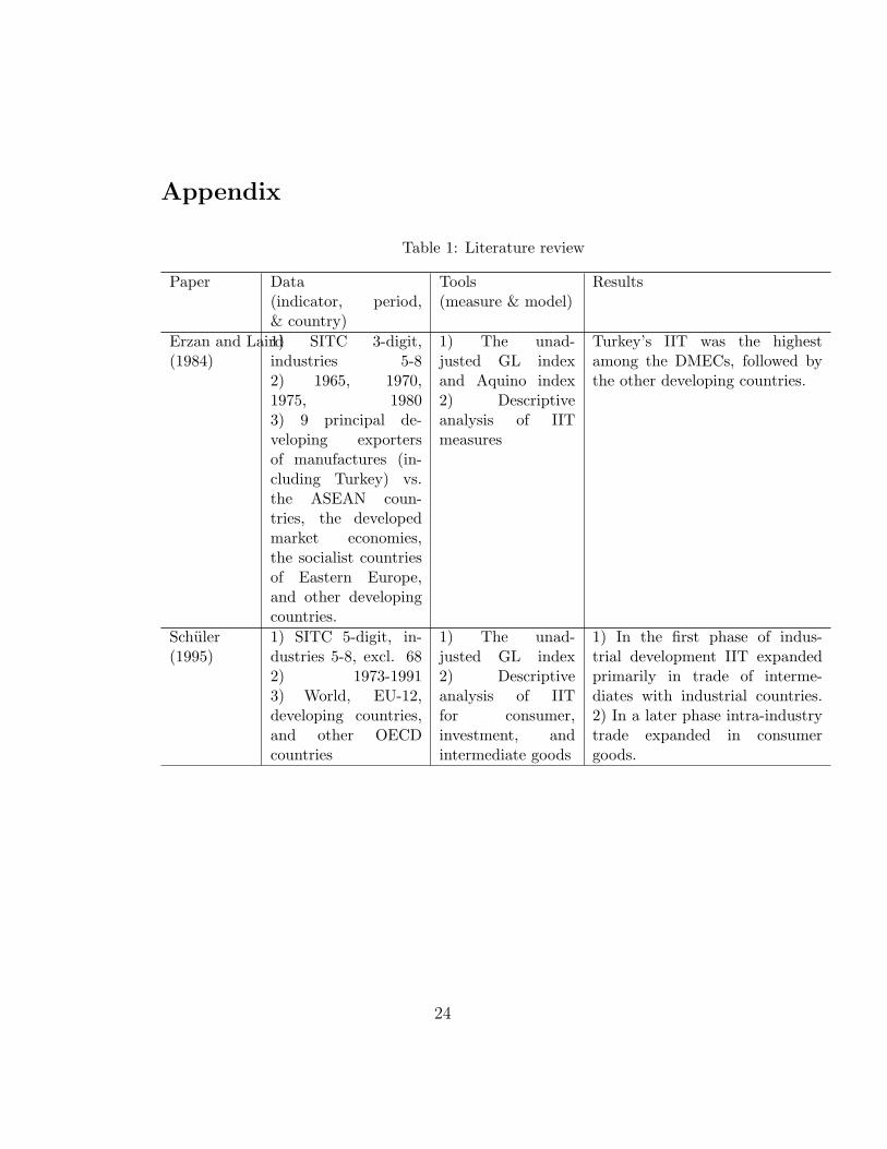
Appendix

Table 1: Literature review

Paper Data(indicator, period,& country)

Tools(measure & model)

Results

Erzan and Laird(1984)

1) SITC 3-digit,industries 5-82) 1965, 1970,1975, 19803) 9 principal de-veloping exportersof manufactures (in-cluding Turkey) vs.the ASEAN coun-tries, the developedmarket economies,the socialist countriesof Eastern Europe,and other developingcountries.

1) The unad-justed GL indexand Aquino index2) Descriptiveanalysis of IITmeasures

Turkey’s IIT was the highestamong the DMECs, followed bythe other developing countries.

Schuler(1995)

1) SITC 5-digit, in-dustries 5-8, excl. 682) 1973-19913) World, EU-12,developing countries,and other OECDcountries

1) The unad-justed GL index2) Descriptiveanalysis of IITfor consumer,investment, andintermediate goods

1) In the first phase of indus-trial development IIT expandedprimarily in trade of interme-diates with industrial countries.2) In a later phase intra-industrytrade expanded in consumergoods.

24

Table 1: Literature review (continued)

Paper Data (indicator, pe-riod, & country)

Tools(measures &models)

Results

Doganer Gonel(2001)

1) SITC 3-digitindustries 0-82) 1992-19973) EU, CentralAsia Turkic republics,and world

1) The unad-justed GL, ad-justed GL, andAcquino indices2) Descriptiveanalysis of IITmeasures

1) Turkey’s share of IIT in totaltrade is lower with the EU thanwith the world for whole period.2) Turkey’s trade with the EUis still of inter-industry type.3) The increase in adjustedGL index is more pronouncedthan in other two indices.4) In trade with EU iron andsteel as well as manufactureshave the highest unadjusted GLindex.

Kosekahyaoglu(2002)

1) SITC 2-digit,industries 0-82) 1975-19903) EU-12

1) The unadjustedGL and BrulhartA indices. 2)Descriptive anal-ysis of IIT fornon-manufactured,manufacturedgoods, and overalltrade.

1) Not only the level (GL index)but also the proportion of IIT(measured by marginal IIT index)has increased over the period. 2)The liberalization attempt in the1980s was a step in the right di-rection and the further liberaliza-tion of trade (i.e. joining the EU)may lead to further reductions inadjustment costs.

Lohrmann(2002)

1) SITC 2-digit,industries 5-82) 1991, 1995,and 19993) EU

1) The unadjustedGL, Brulhart A andB indices; HIITand VIIT measures.2) Descriptive anal-ysis of IIT mea-sures.

1) The GL index shows an in-crease in IIT during the 1990s forTurkey vis-a-vis the EU, but theMIIT indicators reveal a muchlower level of IIT and a nega-tive performance in many sec-tors classified as human-capitalintensive. GL index under-estimates the adjustment cost.2) The pattern of specializationshows that the most part ofTurkey’s trade with the EU is ver-tical.

25

Table 1: Literature review (continued)

Paper Data (indicator, pe-riod, & country)

Tools(measures &models)

Results

Emirhan(2002)

1) SITC 3-digit trans-formed into ISIC2-digit, industries 1-82) 19993) 44 developedand 35 developingcountries

1) The unad-justed GL index2) OLS estimationof determinants ofIIT using country-and industry-specific variablesand OLS estimationof determinants ofHIIT and VIIT

1) The share of the IIT inTurkey bilateral trade is high-est for EU members, whichare followed by EU candidates.2) While the industry specificvariables exert very big influenceon horizontal IIT, they do nothave any impact on vertical IIT.3) Vertical IIT levels are affectedby country-specific variables andthese variables have only a lim-ited impact on horizontal IIT.

Cepni and Kose(2003)

1) SITC 2-digit,industries 0-82) 1988-19983) Canada, China,Egypt, France, Ger-many, Greece, India,Italy, Israel, Japan,Russia, South Korea,Spain, UK, and USA.

1) The ad-justed GL index2) Panel data esti-mation of determi-nants of IIT usingcountry-specificvariables

1) Turkey’s IIT is the high-est with the EU (around50%). The IIT with othercountries ranges between20% (Russia) to 40% (USA).2) The average and relativeper capita income, distance,trade orientation, and eco-nomic integration are allimportant factors explain-ing trends of IIT for Turkey.3) Difference of per capita in-come variable has a wrong signand is statistically significant.

26

Table 1: Literature review (continued)

Paper Data (indicator, pe-riod, & country)

Tools(measures &models)

Results

Erlat and Erlat(2003)

1) SITC 3-digit (Rev.3),industries 0-82) 1969-19993) World

1) The unadjustedGL, weightedGL, Brulhart A,weighted A, B, Cindices, and theUMCIT index forunmatched changesin trade; HIIT andVIIT measures.2) Descriptiveanalysis of IITmeasures.

1) According to aggregatedGL index, the rate of IIT isgreater in the post-1980 period,but the Turkey’s trade hasstill an inter-industry nature.2) According to aggregated Aindex, there had been a signif-icant change in MIIT betweenthe pre- and post-1980 periods.The number of sectors withB < −0.5 or B > 0.5 has con-siderably increased since 1980and for most of these sectorsthe increase in exports domi-nates the increase in imports.3) For the sectors with thehighest MIIT, it is found thatdecrease in adjustment costsafter 1980 due to changes in IIT,measured by the C index, waslarger than the increase in thesecosts due to changes in net trade,measured by UMCIT.

Emirhan(2005)

1) SITC 3-digit,industries 3-82) 1989-20023) Belgium, France,Germany, Greece,Italy, Netherlands,Spain, UK, USA

1) The unad-justed GL index2) Panel dataestimation of deter-minants of VIIT

A positive relationship is foundbetween the levels of VIIT andGDP levels and per capita GDPdifferences among Turkey and se-lected countries. Internationaltransportation costs are found todiscourage vertical IIT.

27

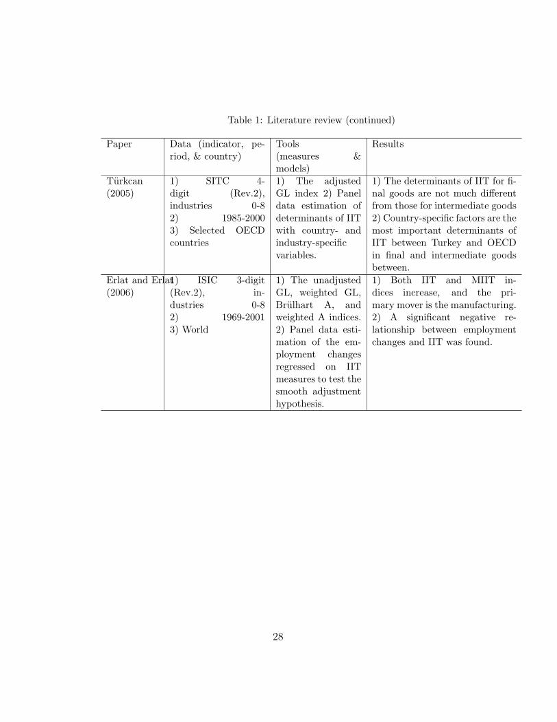
Table 1: Literature review (continued)

Paper Data (indicator, pe-riod, & country)

Tools(measures &models)

Results

Turkcan(2005)

1) SITC 4-digit (Rev.2),industries 0-82) 1985-20003) Selected OECDcountries

1) The adjustedGL index 2) Paneldata estimation ofdeterminants of IITwith country- andindustry-specificvariables.

1) The determinants of IIT for fi-nal goods are not much differentfrom those for intermediate goods2) Country-specific factors are themost important determinants ofIIT between Turkey and OECDin final and intermediate goodsbetween.

Erlat and Erlat(2006)

1) ISIC 3-digit(Rev.2), in-dustries 0-82) 1969-20013) World

1) The unadjustedGL, weighted GL,Brulhart A, andweighted A indices.2) Panel data esti-mation of the em-ployment changesregressed on IITmeasures to test thesmooth adjustmenthypothesis.

1) Both IIT and MIIT in-dices increase, and the pri-mary mover is the manufacturing.2) A significant negative re-lationship between employmentchanges and IIT was found.

28

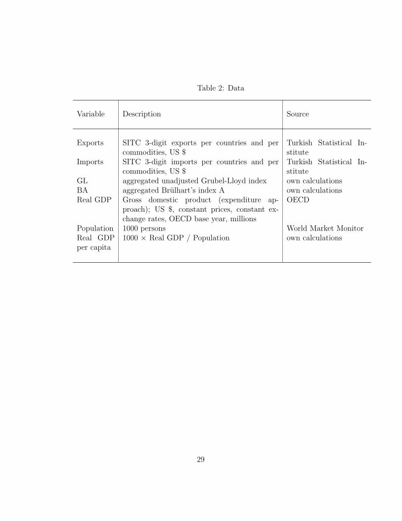
Table 2: Data

Variable Description Source

Exports SITC 3-digit exports per countries and percommodities, US $

Turkish Statistical In-stitute

Imports SITC 3-digit imports per countries and percommodities, US $

Turkish Statistical In-stitute

GL aggregated unadjusted Grubel-Lloyd index own calculationsBA aggregated Brulhart’s index A own calculationsReal GDP Gross domestic product (expenditure ap-

proach); US $, constant prices, constant ex-change rates, OECD base year, millions

OECD

Population 1000 persons World Market MonitorReal GDPper capita

1000 × Real GDP / Population own calculations

29

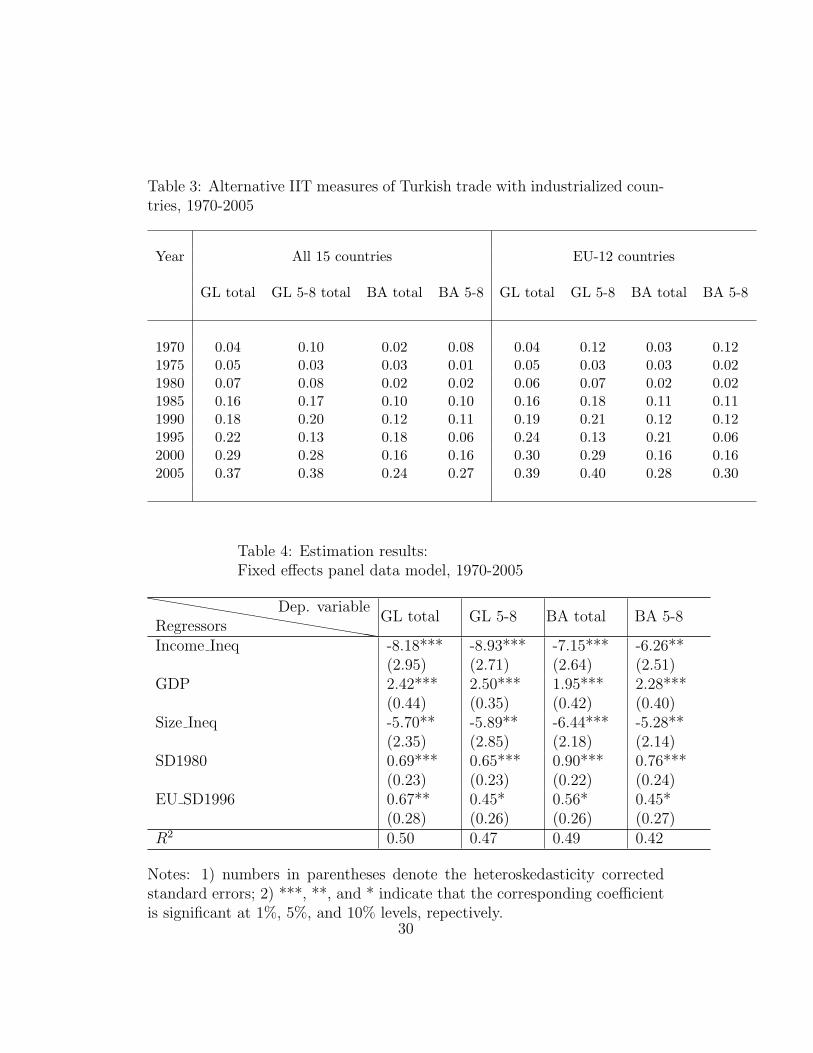
Table 3: Alternative IIT measures of Turkish trade with industrialized coun-tries, 1970-2005

Year All 15 countries EU-12 countries

GL total GL 5-8 total BA total BA 5-8 GL total GL 5-8 BA total BA 5-8

1970 0.04 0.10 0.02 0.08 0.04 0.12 0.03 0.121975 0.05 0.03 0.03 0.01 0.05 0.03 0.03 0.021980 0.07 0.08 0.02 0.02 0.06 0.07 0.02 0.021985 0.16 0.17 0.10 0.10 0.16 0.18 0.11 0.111990 0.18 0.20 0.12 0.11 0.19 0.21 0.12 0.121995 0.22 0.13 0.18 0.06 0.24 0.13 0.21 0.062000 0.29 0.28 0.16 0.16 0.30 0.29 0.16 0.162005 0.37 0.38 0.24 0.27 0.39 0.40 0.28 0.30

Table 4: Estimation results:Fixed effects panel data model, 1970-2005

hhhhhhhhhhhhhhhhhhRegressorsDep. variable

GL total GL 5-8 BA total BA 5-8

Income Ineq -8.18***(2.95)

-8.93***(2.71)

-7.15***(2.64)

-6.26**(2.51)

GDP 2.42***(0.44)

2.50***(0.35)

1.95***(0.42)

2.28***(0.40)

Size Ineq -5.70**(2.35)

-5.89**(2.85)

-6.44***(2.18)

-5.28**(2.14)

SD1980 0.69***(0.23)

0.65***(0.23)

0.90***(0.22)

0.76***(0.24)

EU SD1996 0.67**(0.28)

0.45*(0.26)

0.56*(0.26)

0.45*(0.27)

R2 0.50 0.47 0.49 0.42

Notes: 1) numbers in parentheses denote the heteroskedasticity correctedstandard errors; 2) ***, **, and * indicate that the corresponding coefficientis significant at 1%, 5%, and 10% levels, repectively.

30

Remittances as a Harbinger of Migration: An Empirical Macroeconomic

Causal Link

by

Sule Akkoyunlu*, Boris Siliverstovs** and Oded Stark***

December 2007

We are grateful to Reinhard Madlener, Jirka Slacalek, Alfred Steinherr, Thorsten Vogel and participants at the European Association of Labour Economists Conference, Oslo, September 2007 for thoughtful and helpful comments. The research reported in this paper was financially supported by the European Union within the context of the FEMISE program. The contents of this paper are the sole responsibility of the authors and do not reflect the opinion of the European Union.

* Department of Economics, Bilkent University; DIW Berlin. E-mail: sakkoyunlu@diw.de

** DIW Berlin. E-mail: bsiliverstovs@diw.de

*** Universities of Klagenfurt, Bonn, and Vienna; Warsaw University; Warsaw School of

Economics; ESCE Economic and Social Research Center, Cologne and Eisenstadt.

E-mail: ostark@uni-bonn.de

Abstract

Whereas it is well established that migration from an economy is followed by remittances to the

economy, this paper asks whether remittances to an economy are the harbinger of migration from

the economy. Liquidity constraints, signalling, portfolio revision, and other considerations raise

the possibility that an economy that receives more remittances will generate more migration. This

possibility is tested by means of cointegration analysis. The analysis is applied to migration from

Turkey to Germany during the period 1964-2004. A single cointegrating relationship is found

between migration inflows and the relative income ratio between Germany and Turkey, the

unemployment rates in Germany and in Turkey, a trade intensity variable, and workers’

remittances (relative to Turkish GDP). In particular, remittances are found to significantly

explain migration in the short run, as well as in the long run. The findings support the hypothesis

that remittances fuel migration.

Keywords: Remittances; Turkish-German migration; Cointegration analysis JEL classification: C32; F22; J61

1

1. Introduction

While it is nearly an axiomatic postulate that migration is tracked by remittances, we inquire in

this paper whether remittances to an economy (in our case, remittances from Germany to Turkey)

are the harbinger of migration from the economy (in our case, migration from Turkey to

Germany). Microeconomic theory provides several arguments why remittances are made, and

how remittances confer a variety of benefits upon their recipients. If migration is to occur in the

wake of remittances, the migration type that is coming readily to mind is return migration: when

migration by a family member and the remittances that he sends achieve their objective (for

example, risk reduction that facilitates the start up of an initially high-return yet high-risk

economic activity, the acquisition of capital, or the building of a house), return migration will

take place. If several members of a family rather than only one member are in the host country,

the amount of remittances per unit of time could rise, the duration of migration per a family

member could become shorter, and return migration will be expedited. And if the effect of

remittances is to raise incomes in the economy of origin, a factor that induces migration (the

inter-economies income differential) is weakened. However, it is also possible, if hitherto little

explored, that for a variety of reasons remittances induce migration. Suppose that migration is

financed by resources that are pooled together at origin and are lent to a migrant in support his

move. Migrants who remit upon stating to work at destination not only pay back loans incurred to

facilitate their move, they also replenish the coffers that provided them with financial support,

thereby rendering it possible for a subsequent migration to be financed. Moreover, remittances

can signal success at destination, luring additional workers to pursue migration. Indeed,

remittances could well be aimed at directly supporting additional migration from a family as the

optimal composition of the portfolio of the familial demographic-labor assets prompts

reallocation in favor of a rewarding component. The sum total of these liquidity constraints,

signaling, portfolio revision, and similar considerations raises the possibility that an economy that

receives more remittances could generate more migration. We seek to test this possible causality.

To this end, we investigate the effects of remittances on the migration from Turkey to

Germany during the period 1964-2004. We analyze the short-run as well as the long-run effects

of remittances on migration, applying recent econometric techniques to the longest time series

available to us. We attend to the non-stationarity of the long time series of the macroeconomic

2

variables. We develop a parsimonious, stable-coefficient time-series error correction model for

migration that incorporates remittances. In addition to the economic variables that are typically

considered as determinants of international migration (host country - home country income

differentials, unemployment rates in the host country and in the receiving country), we add a

variable that captures the intensity of economic interaction between Germany and Turkey viz. the

share of total trade (the sum total of exports and imports) between the two countries in the total

trade of Turkey. We find that the conventional variables are significant explanatory variables of

migration, and that so too are the trade intensity variable and remittances.

In the next Section we present background information on Turkish migration to Germany,

as well as on remittances from Germany to Turkey. In Section 3 we sketch an empirical model. In

Section 4 we implement our chosen econometric methodology and present our results.

Concluding comments are offered in Section 5.

2. Turkish migration to Germany, and remittances from Turkish migrants in

Germany: a brief overview

The purpose of this section is threefold: to provide a background overview of remittances from

Germany to Turkey; to depict the process of migration from Turkey to Germany; and to argue

that to a considerable extent, the latter process fed on its own momentum and logic, the

regulatory environment notwithstanding.

Over the four decades 1964-2004 remittances from Turkish workers in Germany

constituted a large share (80 percent) of the total remittances to Turkey. During the 1970s and

1980s, total remittances were equivalent to 4 percent of the Turkish GDP; remittances from

Germany were equivalent to 3 percent of Turkish GDP. Turkey was amongst the world’s top ten

largest remittance- receiving countries.

During the 1964-2004 period, remittances from Turkish migrants in Germany totaled 45

billion Euros. During the same period, capital inflows and foreign direct investment from

Germany summed up to 16 billion Euros, and to 4 billion Euros, respectively. Remittances were

3

not only a major source of foreign exchange; they were also a relatively stable source of foreign

exchange, helping the Turkish economy to buffer the negative shocks during the economic crises

of 1994 and 2001.

Starting with Turkey’s first five-year development plan (1962-1967), successive Turkish

governments encouraged labor migration. The first development plan maintained that the

“export” of excess unskilled labor to Europe will alleviate unemployment, and channel in

remittances thereby reducing balance of payment difficulties. By means of attractive foreign

exchange deposits, special import privileges, premium exchange rates, and special investment

schemes in Turkey for workers living abroad, the Turkish government sought to entice migrants

to remit. In the 1960s and 1970s, workers’ remittances indeed helped greatly to overcome the

deficit in the Turkish balance of payments. In 1974, remittances were equivalent to as much as 90

percent of the total value of Turkish exports.

Recruitment agreements between Germany and Turkey shaped the initial migratory flows.

Subsequent migratory movements were built, however, on their own dynamics and mechanisms.

In the wake of the 1973 oil crisis, the increase in the official foreign recruitment in all Western

European countries, including Germany, came to an abrupt halt. However, in the subsequent two

years, only 11-14 percent of the migrants in Germany returned to their home countries. This

limited way-back migration can be attributed to “the Law of Family Reunification,” which first

came into effect in March 1974. The law allowed foreign workers to reunite with their families in

the host country. Consequently, Turkish migration assumed the form of family re-unification, and

migration increased in the 1970s. The top left panel of Figure 1, in which tMln represents the

log of the gross inflows of Turkish migrants to Germany expressed as a share of the home

population, displays the increase in migration in the early and late 1970s. In addition, guest

workers’ agreements, the so-called “rotation model,” met from the outset with considerable

disapproval from employers who complained that they have to train repeatedly new workers. In

1971, the renewal of residence permits was made easier. The residency status of the guest

workers was changed, and foreign employees were allowed to bring their families. By May 1972,

40 percent of all the guest workers residing in Germany benefited from the residency permit

scheme.

4

The increase in migration since 1982 was not independent of the increase in asylum

applications. The annual average number of Turkish citizens officially registered as asylum

seekers increased from about 10,000 in the early 1980s to 80,000 in the late 1980s and the early

1990s. In response, the Bundestag (the Lower House of the German Parliament) enacted in 1993

the “asylum compromise,” making applying for political asylum in Germany considerably more

difficult. Consequently, the number of applications for asylum declined continuously. However,

in 1995 and 1996, the number of applications slightly increased again, but since then the numbers

stayed at fairly low levels. In addition to regional conflicts, the increase in asylum applications

stemmed from the fact that would-be migrants resorted to this entry channel due to the restrictive

migration policies. Compared to the number of applicants, the number of accepted asylum-

seekers from Turkey has been relatively low, however.

Joppke (1998) argues that with the halt of recruitment in 1973, migration took the form of

a chain migration, prompted by family unification and asylum seeking, and that this

“restructuring” was, in fact, orthogonal to the German no-migration policies. Own momentum

together with moral obligations help explain the continuation of migration.

Thus, in spite of restrictive migration policies over the four-decade period, migration

patterns and migration pressures appear to have been determined mainly by the interplay between

supply-push factors, income differentials, and employment opportunities in Germany.

A particular interesting observation is that remittances and gross migration inflows

exhibited similar patterns. This simple observation leads us to wonder whether remittances could

have played a role in the process of migration (see the top left and the bottom right panels of

Figure1 where, respectively, gross migration inflows and remittances appear to move in tandem

during the study period).6 Of course, whether causality runs from remittances to migration or

from migration to remittances is, as noted in the Introduction, an open issue. In the econometric

specifications that follow, we will address this issue by means of exogeneity tests.

6 We have also compared the time series patterns of the stock of Turkish migrants in Germany and of the net flows of Turkish migrants in Germany with remittances. The stock of Turkish population in Germany and remittances exhibit no correlation. The net flows of Turkish migrants and remittances reveal no co-movement either.

5

3. An empirical model

We model Turkish migration to Germany as follows:

ttthtfthtftt RTUUYYM εαααααα ++++++= lnln)/ln(ln 543210 (1) In equation (1), tMln denotes the log of the gross inflow of Turkish migrants to Germany7,

expressed as a share of the home population. Brücker and Schröder (2006) argue that migration

stocks, rather than the (net) migration rate, should be used in migration estimation, since an

equilibrium relationship between migration stocks and the explanatory variables arises in the long

run, while the net flows tend to zero. However, in this study we use the gross migration rate (as is

done, for example, in Borjas (1987, 1999), Hatton (1995), Clark et al. (2002), Pedersen et al.

(2006), Péridy (2006), and Mayda (2007)), not the stock of Turkish migrants. We test the

hypothesis that remittances trigger additional migration. Typically, migrants of different cohorts

exhibit different remittance behavior. For example, migrants tend to pay the debt that they

incurred in financing their migration during the first year or so following their migration, and

over time, upon bringing their families to Germany, they remit less than more recent migrants.

This variation implies different remittance behavior for the cohorts that sum up to the stock of

Turkish migrants. Therefore, we use as the dependent variable the gross migration rate rather

than stocks. In addition, and as explained below, we incorporate the trade intensity as an

independent variable, which requires us to work with flows rather than with the stock of migrants.

Moreover, initial data analysis did not reveal any significant relationship between the stocks and

the explanatory variables, especially not between the stocks and workers’ remittances.

The term )/ln( htft YY is the log of the income in the host country divided by the income in

the home country, measured each as per capita GDP in purchasing power parity terms. This

variable captures the pecuniary incentive to migrate that arises from the income differential.

ftU is the unemployment rate in Germany. German migration policies have become more

restrictive during periods of high unemployment in Germany (Mayda and Patel (2004)).

7 An analysis of Turkish gross migration inflows net of Turkish asylum seekers yielded similar results..

6

The htU term is the unemployment rate in Turkey. It represents a simple push factor. The

unemployment rate enters the empirical model individually rather than as a difference term, in

line with (for example) Borjas (1987, 1999), Hatton (1995), Clark et al. (2002), Pedersen et al.

(2006), Péridy (2006), and Mayda (2007).

The term tTln is a proxy for the intensity of economic cooperation between Turkey and

Germany, calculated as the log of the share of the trade volume (sum of exports and imports)

between the two countries in the total trade volume of Turkey with all its trading partners. In

general, the volume of trade between two economies could measure a variety of links between

the economies. The higher the volume, the more intensive the links. Bilateral links co-shape the

migration “infrastructure” or environment. It stands to reason that an increase in the total volume

of trade between Germany and Turkey can alleviate the financial and informational constraints

associated with migration from Turkey to Germany, thereby lowering the cost of migration,

particularly for low-skill workers with low incomes and with limited access to credit. Trade can

serve as an indicator of the level of business deals and transactions between economies, which in

turn lower informational costs and reduce uncertainty, thereby impinging on the migration

“climate.” In addition, trade could impact on migration in more subtle ways. For example, and in

our case, when the volume of trade between Turkey and Germany is high, Turkey will be less

likely to allow appreciation of its currency - exporters could suffer if it did - and is more likely to

tilt in the direction of depreciation of its currency. For a given stock of Turkish migrants in

Germany, a depreciation of the Turkish currency could prompt migrants to increase their

remittances.

Finally, tRln is the log of the ratio between workers’ remittances and Turkish GDP.

The data used by us were obtained from several sources. Data on workers’ remittances

were obtained from the balance sheets of the German Federal Bank (the Bundesbank). Data on

the per capita GDP of Germany and of Turkey were obtained from the OECD. Data on Turkish

unemployment, population, and trade were collected from the Turkish Institute of Statistics. Data

on Turkish migration and German unemployment were obtained from the Federal Statistical

Office in Germany.

7

4. An econometric analysis

In modeling Turkish migration to Germany, we follow the general-to-specific approach

advocated in Hendry (1995). We start with an unrestricted VAR(p) model in which all variables

are treated as endogenous. The VAR model that we initially adopt can be written in the familiar

error-correction form, in terms of stationary variables, as follows:

∑−

=−− Σ++ΔΓ+Π=Δ

1

11 ),0(~,

p

inttititt Nxxx εεγ (2)

where γ denotes a constant drift term, and tx is the k x 1 vector of variables. The vector of

variables is )'ln,ln,,),/ln(,(ln tthtfthtfttt RTUUYYMx = . The long-run part of the model allows

for linear feedback from the lagged stationary equilibrium errors, 11 ' −− =Π tt xx αβ , where β is a

p x r matrix of full rank, containing the r cointegration vectors, and α is a p x r matrix of full

rank, containing the adjustment coefficients (the factor loadings). This formulation assumes that

tx is I(1), that is, that the components of the vectors are either I(0) or I(1), (see Johansen (1988)).

The annual data covers the period from 1964 until 2004 (see Figure 1, where the raw data

pertaining to the right hand side variables of (1) are depicted).

We first test for cointegration. Subsequently we impose the implied reduced rank

restrictions on the unrestricted VAR model. We then test for the long-run exogeneity of the

system variables. The results of the weak exogeneity tests are used to build a parsimonious time

series model for migration that passes satisfactorily all diagnostic tests, displays constant

coefficients, and is capable of forecasting accurately the within-sample migration flows.

Our first step is to determine the lag length of an unrestricted VAR(p) model. In this

initial stage, we seek to obtain a parsimonious model. This is quite challenging, given the

relatively small number of observations (T = 41) compared to the number of explanatory

8

variables (k = 6). In Table 2, it is shown that the VAR(1) model can adequately describe the data

when the lag length n = 1 is chosen, since the misspecification tests report no serious departures

from the assumptions that underlie the model. 8

Having found the adequate unrestricted model, we next seek to find the cointegration rank

of the estimated system by imposing restrictions on the unrestricted model. To this end, we use

the Johansen Full Information Maximum Likelihood (FIML) procedure (Johansen (1992)). Table

3 reports the results of the trace and λ -max tests for the cointegration rank. Both tests indicate

the presence of one cointegrating relation in the system.

We therefore impose the cointegration rank r = 1 on the system (equation (2)) and

proceed with testing for (trend-)stationarity, long-run exclusion, and long-run weak exogeneity of

the variables. The test for stationarity of the variables in the model is based on Juselius (2006).

This is a multivariate version of the Augmented Dickey-Fuller test with the null hypothesis of

stationarity, in contrast to the standard univariate tests where the null is non-stationary. Since any

linear combination of I(1) variables that is I(0), or I(0) variables themselves, can form the

cointegration space, the purpose of this test is to find whether any of the variables in our model

alone belongs to the cointegration space. The test has an asymptotic 2χ distribution with (k - r) =

5 degrees of freedom.

The test for the long-run exclusion (Juselius (2006)) investigates whether any of the

variables in our model can be excluded from the cointegrating vector. This test has an asymptotic 2χ distribution with r = 1 degrees of freedom. Finally, the test for the long-run weak exogeneity

investigates whether the dependent variable adjusts to the equilibrium errors represented by a

cointegrating relation (see Engle et al. (1983)).

8 The univariate as well as the multivariate model diagnostic tests comprise of: FAR (a test of no residual autocorrelation (see Godfrey (1978)); 2χ Norm (a test for the normally distributed residuals (see Doornik and Hansen (1994)); FHetero and FHetero-X (White (1980) tests for heteroscedasticity based on the original and squared regressors, and their cross-products); FARCH (Engle (1982) test of no residual autoregressive conditional heteroscedasticity). The graphics, regression output, and residual diagnostic tests were all calculated using GiveWin 2.2 and Pc-Give 10.2 (cf. Doornik and Hendry (2001a), (2001b)).

9

Tables 4, 5, and 6 report the results of the tests for (trend-) stationarity and long-run

exclusion, which are performed on the matrix of the long-run coefficients, and the tests for the

long-run weak exogeneity which are performed on the matrix of the adjustment coefficients.

According to the stationarity test, the null hypothesis that each variable is either I(0), or I(0)

around a linear deterministic trend, is rejected decisively. The tests for the long-run exclusion

reject at the 1 percent significance level the null hypothesis that tMln , ftU , htU and tTln can be

excluded from the cointegrating vector, and at the 10 percent significance level that the variable

tRln can be excluded from the cointegrating vector. At the same time, we cannot reject the null

hypothesis that the relative income variable )/ln( htft YY could be omitted from the cointegrating

relationship. The plausible reason for this result is that the relative income ratio fluctuated more

or less around the same magnitude in the period of investigation (the middle right panel of Figure

1). However, we have chosen to retain this variable since there is a strong analytical argument in

support of its presence in a migration function and, arguably, its persistence has been and, given

its magnitude, is still the major pulling factor of Turkish migration to Germany. In addition, it

turns out that after imposing the joint long-run weak exogeneity restrictions, we are no longer

able to reject the null hypothesis of the long-run exclusion of the relative income variable at the

10 percent significance level, as explained below.

According to the univariate long-run weak exogeneity test results (Table 6), we can accept

the null hypothesis that all the variables other than the tMln variable are individually weakly

exogenous at any conventional significance level. The main contribution of this result is that

causality runs from remittances to migration and from trade to migration, and not from migration

to remittances and from migration to trade. Moreover, the joint test for the long-run weak

exogeneity also confirms this finding with the log likelihood ratio test statistic of 3.973 (p=0.553).

In order to check whether this result is robust to a change in the sample size, we present in Figure

2 the value of the recursive test statistics of the joint null hypothesis, scaled by the 1 percent

critical value. The figure offers visible support for the hypothesis that the five variables

)/ln( htft YY , ftU , htU , tTln , and tRln are weakly exogenous with respect to the long-run

parameter values for all sample sizes (with only one exception). Hence, this restriction is

acceptable, and in our analysis we treat these five variables as weakly exogenous with respect to

the long-run parameters.

10

Imposing the long-run weak exogeneity restrictions on the )/ln( htft YY , ftU , htU , tTln ,

and tRln variables results in the following cointegrating vector, with the corresponding standard

errors reported in parentheses below the coefficient estimates:

(0.055) (0.281) (0.029) (0.016) (0.862)

ln205.0ln492.1102.0216.0ln646.1ln ttthtftht

ftt ecmconsRTUU

YY

M +++++−⎟⎟⎠

⎞⎜⎜⎝

⎛=

(3)

All the coefficient estimates have the expected signs, and all the estimates are significantly

different from zero at the conventional significance levels. Relative income, the unemployment

rate in Turkey, the trade intensity, and workers’ remittances contribute positively to migration

from Turkey to Germany, while unemployment in Germany contributes negatively to migration

from Turkey to Germany. Thus, in the long run, supply and demand factors jointly shape

migration flows. The relationship that is of most concern to us is quite vivid. We find that a 10

percent increase in remittances increases the gross migration inflows by 2.05 percentage points -

a significant effect. The positive and significant effect of remittances in the long run supports the

hypothesis that remittances fuel migration. We also find a large effect from the trade intensity

variable: a 10 percent increase in trade will increase the gross migration inflows by 14.92

percentage points. This is a large effect, especially when compared to the finding reported in

other studies (Pedersen et al. (2006) and Péridy (2006)). The result may be related to the fact that

Germany is Turkey’s biggest trading partner.

As shown in Juselius (2006), the long-run weak exogeneity of variables allows us to

reformulate the model (equation (2)) in terms of a conditional model, where the conditioning is

on the current and past values of the weakly exogenous variables, and on the error correction

term. After removing the variables that have turned out to be insignificant, the estimated

conditional model for tMln is as follows:

11

(0.954) 24.3F

(0.897) 218.0)2( (0.899), 262.0F

(0.874) 579.0F 41,T ,85.0R ,15.0ˆ

(1.077) (0.166) (0.092) (0.034) (0.034) (0.073)

219.799527.0624.0283.0ln144.0ln407.0ln

Hetero

2Norm4)-ARCH(1

4)-AR(12

11

=

==

====

−−−Δ−Δ−Δ=Δ −−

χ

σ

DecmURRM tftttt

(4)

with the corresponding standard errors reported in parentheses below the coefficient estimates.9

The conditional model (equation (4)) is parsimonious, and at the same time the diagnostic

tests show no signs of misspecification. The error-correction term is highly significant and has

the expected sign. It is worth noting that remittances and the German unemployment rate are also

significant in the conditional model, with the expected signs, and exert promoting and dampening

effects on Turkish migration to Germany, respectively. Thus, a 10 percent increase in the change

in remittances will increase the change in gross migration inflows by 4.07 percentage points. This

is a large short-run effect, considering the coefficients on other short-run variables, and it is

almost as large as the error-correction term. Hence, the significance of remittances in the short

run as well as in the long run is consistent with the prediction that remittances nourish migration:

remittances trigger additional migration in the short run as well as in the long run. In addition, the

German unemployment rate is also significant in the short run as well as in the long run. The

significant effects from the supply side suggest that the restrictive migration policies have not

been binding for Turkish migration inflows; it is the German unemployment rate that impacts on

the inflows.

The conditional model has a very good explanatory power, as can be assessed by looking

at the actual values and at the regression fitted values, as well as at the regression residuals

(Figure 4). The coefficient estimates are well determined and exhibit remarkable stability

according to the recursive Chow stability tests and the one-step ahead residuals (Figure 5), as

9 The dummy variable is included to prevent a failure of the normality test.

12

well as recursively estimated coefficients10 (Figure 6). Finally, the conditional model is able to

accurately forecast gross migration inflows to Germany over the period 2000-2004 (see Figure 7

for the one-step ahead forecasts), and this aspect is supported by the Chow parameter constancy

forecast F-test statistic which takes the value 0.420 (p=0.831).

5. Concluding comments

We investigated whether remittances trigger migration. We developed and implemented an

empirical model of Turkish migration to Germany. Using the cointegration technique, we tested

the model for the period 1964-2004,. A single cointegrating vector is found among the gross

migration inflows and the following explanatory variables: the relative income ratio between

Germany and Turkey; the unemployment rates in Germany and Turkey; the trade intensity

variable; and remittances as a ratio of Turkish GDP. Based on the results of the cointegration

analysis and the imposed long-run weak exogeneity restrictions, a parsimonious single equation

conditional error-correction model is developed that has a good in-sample explanatory power and

possesses well-defined and stable coefficients. The significance of the remittances variable in the

short run as well as in the long run supports the hypothesis that remittances fuel migration.

By including the trade variable in the empirical function of migration, our study

contributes to a better understanding of the relationship between the trade intensity between

countries and migration. By relaxing financial constraints as well as by lowering various

adjustment and informational costs that are associated with the decision to migrate, business

connections between two economies significantly facilitate the mobility of people between the

economies.

Our findings support the idea that workers’ remittances can trigger additional migration

and thereby foster a migration chain. Remittances may be interpreted as messages of financial

success, and this signal may induce would-be migrants to actually migrate. Our findings are also

consistent with an “implicit loan” idea: high initial migration costs that are especially binding for

10 This further suggests to us that the multiple appearance of the Turkish GDP in the definitions of the variables inflicts no harm on the econometric procedure.

13

unskilled migrants with low incomes and low access to credit encourage the development of kin

networks in which a migrant and his extended family enter into an informal, mutually beneficial

credit contract to pay for the costs of migration. This arrangement could lead to an obligation on

the part of the migrant to help extended family members to follow in his steps. Thus, transfers

from family members facilitate migration, and remittances from a migrant facilitate additional

migration.

Students of migration have for long been fascinated by the often-observed momentum,

continuity, and dynamics of migration flows. A variety of explanations are on offer. Perhaps our

inquiry serves to identify a new explanation: migration is followed by remittances which prompt

migration which in turn results in remittances, and so on. Reflecting further on the interplay

between remittances and migration as a perpetuator of migration is an intriguing topic for future

research.

14

References

Borjas, G. (1987). Self selection and the earnings of immigrants. American Economic Review 77:

531-553.

Borjas, G. (1999). The Economic analysis of immigration. In: O. Ashenfelter and D. Card (eds.),

Handbook of Labour Economics, chapter 28, pages 1697-1760. Amsterdam: Elsevier

Science (North Holland).

Brücker, H. and P. J. H. Schröder (2006). International migration with heterogeneous agents:

Theory and evidence. IZA Discussion Paper 2049.

Clark, X., T. J. Hatton, and J. G. Williamson (2002). Explaining US immigration, 1971-1998.

Centre for Economic Policy Research Discussion Paper 453.

Doornik, J. A. and H. Hansen (1994). An omnibus test for univariate and multivariate normality.

Nuffield College Discussion Paper W4&91.

Doornik, J. A. and D. F. Hendry (2001a). GiveWin: An Interface to Empirical Modelling.

Timberlake Consultants Press: London.

Doornik, J. A. and D. F. Hendry (2001b). Modelling Dynamic Systems Using PcGive, Volume II.

Timberlake Consultants Press: London.

Engle, R. F. (1982). Autoregressive conditional heteroscedasticity with estimates of the variance

of United Kingdom inflation. Econometrica 50: 987-1007.

Engle, R. F., D. F. Hendry, and J.-F. Richard (1983). Exogeneity. Econometrica 51: 277-304.

Godfrey, L. G. (1978). Testing for higher order serial correlation in regression equations when

the regressors include lagged dependent variables. Econometrica 46: 1303-1313.

15

Hatton, T. J. (1995). A model of UK migration, 1870-1913. Review of Economics and Statistics

77: 407-415.

Hendry, D. F. (1995). Dynamic Econometrics: Advanced Texts in Econometrics. Oxford

University Press: Oxford

Johansen, S. (1988). Statistical analysis of cointegration vectors. Journal of Economic Dynamics

and Control 12: 231-154.

Johansen, S. (1992). Testing weak exogeneity and the order of cointegration in the UK money

demand. Journal of Policy Modelling 14: 313-334.

Joppke, C. (1998). Why liberal states accept unwanted immigration. World Politics 50: 266-293.

Juselius, K. (2006). The cointegrated VAR model: methodology and applications. Oxford

University Press: Oxford.

Mayda, A. M. (2007). International migration: a panel data analysis of the determinants of

bilateral flows. CREAM Discussion Paper 07/07.

Mayda, A. M. and K. Patel (2004). OECD countries migration policies changes. Appendix to

International migration: A panel data analysis of economic and non-economic

determinants. (http://www.georgetown.edu/faculty/amm23/.)

Pedersen, P. J., M. Pytlikova, and N. Smith (2006). Migration into OECD countries 1990-2000.

In: C. A. Parsons and T. M. Smeeding (eds.), Immigration and the transformation of

Europe. New York: Cambridge University Press.

Péridy, N. (2006). Welfare magnets, border effects or policy regulations: What determinants

drive migration flows into the EU. University of Nantes, mimeo.

16

White, H. (1980). A heteroscedastic-consistent covariance matrix estimator and a direct test for

heteroscedasticity. Econometrica 48: 817-838.

17

Table 1: VAR model: Multivariate tests

===============================

Multivariate tests

)21( −ARF (72,103) 1.321 [0.097]

2Normχ (12) 23.495 [0.024*]

HeteroF (252,52) 0.425 [1.000]

================================

Table 2: VAR model: Univariate tests

===========================================================================

Univariate tests

tM ln )/Y(Y ln htft ftU htU tT ln tR ln

AR 1-2 test: F(2,32) 3.356 0.807 1.6783 1.828 0.828 3.8081

[0.048]* [0.418] [0.203] [0.177] [0.435] [0.8081]

Normality test: 2χ (2) 8.0503 1.5146 0.094 4.033 0.449 1.228

[0.018]* [0.469] [0.954] [0.133] [0.799] [0.541]

ARCH 1-1 test: F(1,32) 0.275 0.311 0.445 5.173 0.024 0.249

[0.604] [0.581] [0.510] [0.030]* [0.878] [0.621]

Hetero test: F(12,21) 0.527 1.3425 0.628 1.676 0.961 0.694

[0.874] [0.268] [0.796] [0.145] [0.512] [0.740]

Hetero-X test: F(27,6) 1.252 1.016 0.235 1.746 0.334 0.362

[0.421] [0.545] [0.996] [0.252] [0.977] [0.968]

===========================================================================

18

Table 3: VAR model: cointegration tests

=================================================================

Rank Trace test [Prob] Max test [Prob]

0 101.56 [0.017]* 39.81 [0.050]*

1 61.76 [0.185] 25.77 [0.346]

2 35.98 [0.402] 22.54 [0.199]

3 13.44 [0.869] 8.15 [0.887]

4 5.29 [0.777] 5.14 [0.726] =================================================================

Table 4: VAR model: tests for (trend-)stationary

===========================================================================

tM ln )/Y(Y ln htft ftU htU tT ln tR ln trend 2χ (v) p-value

Stationary

. 0 0 0 0 0 31.544 [0.000]**

0 . 0 0 0 0 22.798 [0.000]**

0 0 . 0 0 0 27.974 [0.000]**

0 0 0 . 0 0 22.703 [0.000]**

0 0 0 0 . 0 31.628 [0.000]**

0 0 0 0 0 . 25.325 [0.000]**

Trend-stationary

. 0 0 0 0 0 . 25.734 [0.000]**

0 . 0 0 0 0 . 20.407 [0.000]**

0 0 . 0 0 0 . 32.769 [0.000]**

0 0 0 . 0 0 . 27.222 [0.000]**

0 0 0 0 . 0 . 32.464 [0.000]**

0 0 0 0 0 . . 16.111 [0.000]**

===========================================================================

Notes: ‘0’ denotes the zero restriction on the coefficient of the corresponding variable; ‘.’ denotes unrestricted

coefficient in the 5 x 1 cointegration vector when testing for the stationary and in the 6 x 1 cointegration vector when

testing for trend-stationary of the variables. The number of degrees of freedom v in the 2χ tests corresponds to the

number of the imposed restrictions.

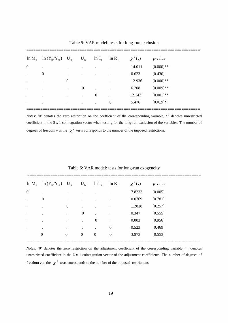
19

Table 5: VAR model: tests for long-run exclusion

===========================================================================

tM ln )/Y(Y ln htft ftU htU tT ln tR ln 2χ (v) p-value

0 . . . . . 14.011 [0.000]**

. 0 . . . . 0.623 [0.430]

. . 0 . . . 12.936 [0.000]**

. . . 0 . . 6.708 [0.009]**

. . . . 0 . 12.143 [0.001]**

. . . . . 0 5.476 [0.019]*

===========================================================================

Notes: ‘0’ denotes the zero restriction on the coefficient of the corresponding variable, ‘.’ denotes unrestricted

coefficient in the 5 x 1 cointegration vector when testing for the long-run exclusion of the variables. The number of

degrees of freedom v in the 2χ tests corresponds to the number of the imposed restrictions.

Table 6: VAR model: tests for long-run exogeneity

===========================================================================

tM ln )/Y(Y ln htft ftU htU tT ln tR ln 2χ (v) p-value

0 . . . . . 7.8233 [0.005]

. 0 . . . . 0.0769 [0.781]

. . 0 . . . 1.2818 [0.257]

. . . 0 . . 0.347 [0.555]

. . . . 0 . 0.003 [0.956]

. . . . . 0 0.523 [0.469]

0 0 0 0 0 3.973 [0.553]

===========================================================================

Notes: ‘0’ denotes the zero restriction on the adjustment coefficient of the corresponding variable, ‘.’ denotes

unrestricted coefficient in the 6 x 1 cointegration vector of the adjustment coefficients. The number of degrees of

freedom v in the 2χ tests corresponds to the number of the imposed restrictions.

20

1970 1980 1990 2000

-8

-6

l n M t

1970 1980 1990 2000

2.5

5.0

7.5

10.0Uf t

1970 1980 1990 2000

5.0

7.5

10.0Uht

1970 1980 1990 2000

1.3

1.4

l n Y ft /Yht

1970 1980 1990 20002.50

2.75

3.00ln Tt

1970 1980 1990 2000

-6

-5

-4

-3l n R t

Figure 1: The basic properties of the data: 1963-2004

21

1994 1995 1996 1997 1998 1999 2000 2001 2002 2003 2004 2005

4

6

8

10

12

14

LR(5) 1% crit

Figure 2: Recursive test statistics for long-run weak exogeneity of )/ln( htft YY , ftU , htU , tTln , and

tRln scaled by the 1 percent critical value

1965 1970 1975 1980 1985 1990 1995 2000 2005

-12.2

-12.0

-11.8

-11.6

-11.4

-11.2

-11.0

Figure 3: Cointegrating relation (equation (8))

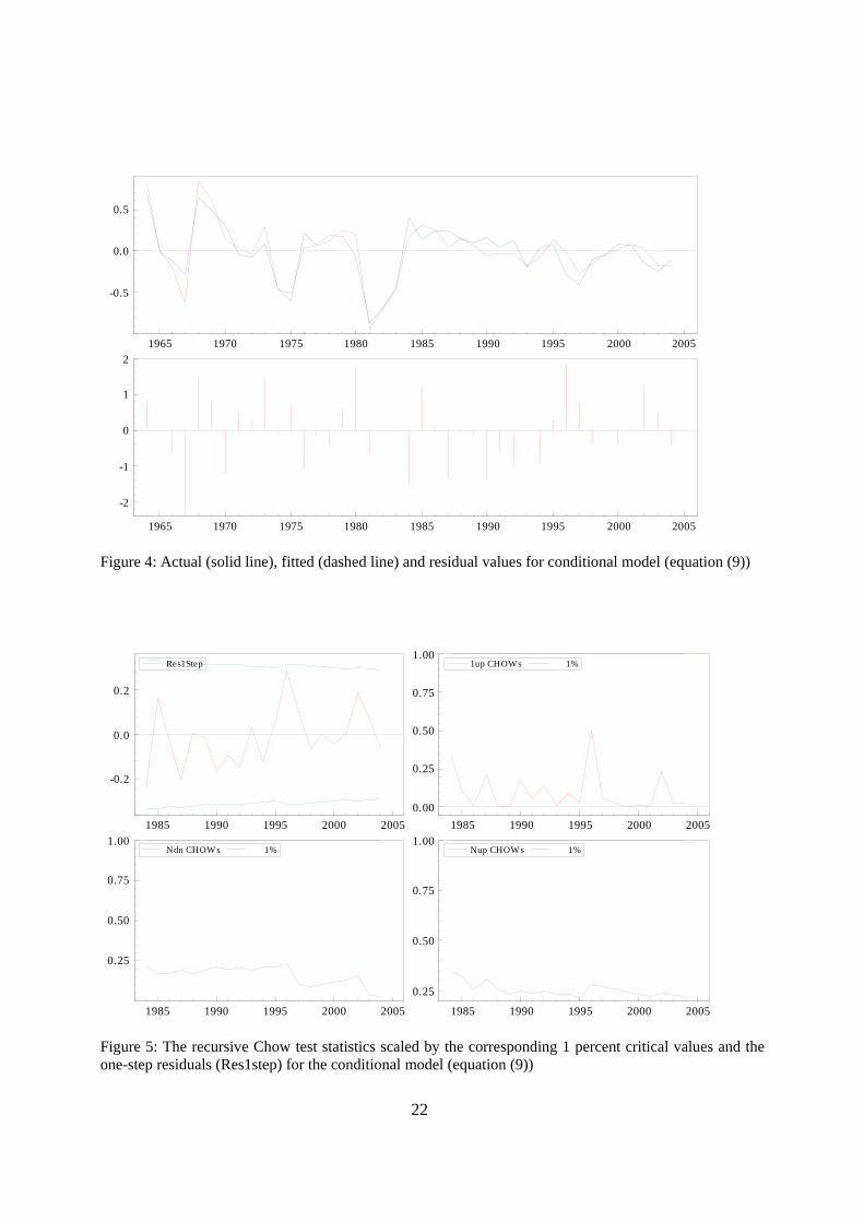
22

1965 1970 1975 1980 1985 1990 1995 2000 2005

-0.5

0.0

0.5

1965 1970 1975 1980 1985 1990 1995 2000 2005

-2

-1

0

1

2

Figure 4: Actual (solid line), fitted (dashed line) and residual values for conditional model (equation (9))

1985 1990 1995 2000 2005

-0.2

0.0

0.2

Res1Step

1985 1990 1995 2000 20050.00

0.25

0.50

0.75

1.001up CHOWs 1%

1985 1990 1995 2000 2005

0.25

0.50

0.75

1.00Ndn CHOW s 1%

1985 1990 1995 2000 2005

0.25

0.50

0.75

1.00Nup CHOW s 1%

Figure 5: The recursive Chow test statistics scaled by the corresponding 1 percent critical values and the one-step residuals (Res1step) for the conditional model (equation (9))

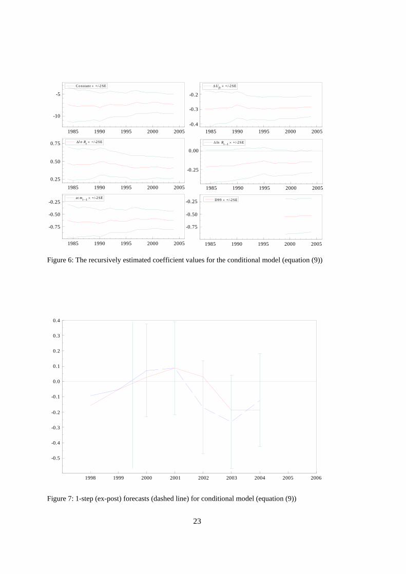
23

1985 1990 1995 2000 2005

-10

-5

Constant × +/-2SE

1985 1990 1995 2000 2005-0.4

-0.3

-0.2

ΔUft × +/-2SE

1985 1990 1995 2000 20050.25

0.50

0.75 Δl n Rt × +/-2SE

1985 1990 1995 2000 2005

-0.25

0.00

Δ ln Rt −1 × +/-2SE

1985 1990 1995 2000 2005

-0.75

-0.50

-0.25ec mt −1 × +/-2SE

1985 1990 1995 2000 2005

-0.75

-0.50

-0.25 D99 × +/-2SE

Figure 6: The recursively estimated coefficient values for the conditional model (equation (9))

1998 1999 2000 2001 2002 2003 2004 2005 2006

-0.5

-0.4

-0.3

-0.2

-0.1

0.0

0.1

0.2

0.3

0.4

Figure 7: 1-step (ex-post) forecasts (dashed line) for conditional model (equation (9))

Migration and Trade – Complements or Substitutes?

Evidence from Turkish Migration to Germany §

Sule Akkoyunlu ∗

Bilkent University/DIW Berlin

Boriss Siliverstovs∗∗

DIW Berlin

October 11, 2007

Abstract

This study investigates whether migration and trade can be regarded as complements or

substitutes using the data on Turkish migration to Germany for the period 1963-2004. Our

results support the former view.

Keywords: Migration, trade, economic development, cointegration

JEL code: F22, C32.

§We are grateful to Jiri Slacalek and Alfred Steinherr for their comments. This document has been producedwith the financial assistance of the European Union within the context of the FEMISE program. The contents ofthis document are the sole responsibility of the authors and should not be regarded as reflecting the position ofthe European Union.

∗Department of Economics, Bilkent University 06800, Bilkent, Ankara, Turkey and DIW Berlin, Mohrenstraße58, 10117 Berlin, Germany, e-mail:sakkoyunlu@diw.de∗∗DIW Berlin, Mohrenstraße 58, 10117 Berlin, Germany, e-mail:bsiliverstovs@diw.de (the corresponding

author)

1

1

1 Introduction

This study intends to contribute to the ongoing debate on whether migration and trade can

be considered complements or substitutes (Razin and Sadka, 1997; Venables, 1999; Schiff, 2000,

among others). Knowing such a relationship can help to devise appropriate trade policies to

deal with migration, but the problem is that in the theoretical literature one finds arguments

that support either point of view. On the one hand, there is a stream of literature inspired by

Mundell (1957) which argues that in the standard Hechscher-Ohlin model, a significant level

of trade leads to the countries’ specialization in production of the goods for which they have a

relatively abundant supply of input factors and thus have a comparative cost advantage. As a

result, trade will lead to the equalisation of factor prices and hence in a reduction of migration

incentives. Thus, from this point of view, trade and migration can be regarded as substitutes.

This scenario is also stressed in the development literature where it is argued that under these

circumstances sustained and equitable growth in migrant sending countries is the only effective

strategy to cope with the migration pressure. Hence, aid policies and other forms of economic

assistance and cooperation should be geared to the objective of fostering growth in migration

source countries and subsequent reduction of incentives to migrate.

On the other hand, another stream of the literature inspired by Markusen (1983) shows that,

by relaxing some of the underlying assumptions of the standard Hechscher-Ohlin model, trade

and migration, in fact, are complements, i.e., increase in the volume of trade is accompanied by

corresponding increase in labour mobility. A positive relationship between migration and trade

could also arise when income growth in the less developed country that has been generated by

trade with a more economically developed partner may relax financial constraints and may allow

more rather than less people to migrate, see Schiff (1994, 1995) for the corresponding analysis.

In addition, it also is noteworthy to mention, that there are also theoretical models which show

that the relationship between migration and trade is ambiguous, e.g., see Panagariya (1992).

In sum, it seems that there is no consensus in the theoretical literature on the relationship

between migration and trade, as in the end, an answer depends on a particular model used.

Hence, the ultimate answer must lie in the outcomes of empirical studies. This provides the

main motivation for our paper.

We investigate the relationship between migration and trade while controlling for the in-

fluence of other factors that shape migration flows such as relative income in host and source

2

countries as well as prospects of employment in the respective locations (usually approximated

by the foreign and domestic unemployment rates). The choice of these variables follows from

the traditional micro-economic theories of migration, largely represented by Ravenstein (1889),

Hicks (1932), Sjaastad (1962), Todaro (1969), and Harris and Todaro (1970).

As the case study, we look at the developments of Turkish migration to Germany for the pe-

riod 1963 - 2004. Arguably, this is a very interesting topic to study given the massive migration

of Turkish labourers into Germany during this period of time. As a result of the guest-worker

agreements that were initialised by the German authorities in the early sixties through the early

seventies, and then of family unification, refugee and asylum programmes, net migration from

Turkey to Germany measured as the balance of outward and inward migration totalled 1.3 mil-

lion people. This resulted in an estimated population of 2.1 million with Turkish origins in year

2004 or about 70% of about 3 million Turkish people that reside in the EU-15 countries. This

effectively means that the Turkish nationals constitute by far the largest group of third country

nationals in the EU-15 (about 25% of all third country nationals). Hence, it is particularly inter-

esting to investigate whether trade has played any role – either complementary or substituting

– on these rather large flows of Turkish migrants to Germany.

The rest of the paper is organised as follows: in the next section, we discuss the theoretical

background of the migration model and motivate the choice of explanatory variables. In Section

3 the econometric methodology is described and the empirical results are presented. Section 4

summarizes the findings.

2 Theoretical Background and Empirical Model

In this section we briefly present the theoretical background behind the decision to migrate as

well as the motivation for the choice of the explanatory variables in our study. To this end,

we follow the standard micro-economic theories of migration, largely represented by the follow-

ing studies: Ravenstein (1889), Hicks (1932), Sjaastad (1962), Todaro (1969), and Harris and

Todaro (1970). This literature stipulates that the decision to migrate arises from expectations

on utility differences in the home and the host countries, which are determined by the income

differentials between these respective locations as well as by the variables that reflect labour

market conditions. Thus, a migration decision of an individual is based on the pull factors of

prospects abroad and the push factor of conditions at home which prospective emigrants face.

3

Given all these considerations, we model the migration function of Turks to Germany in the

following general form below:

ln(Mt) = f(ln(Yft/Yht), Uft, Uht, Tt), (1)

where Mt denotes gross inflow of Turkish migrants into Germany, expressed as the share of

the home population, Yft/Yht – relative income in the host and the home countries, measured

in per capita terms in purchasing power parity, Uft and Uht – the unemployment rates that

capture prospects of employment in the respective locations. We expect that the relative income

between the host and source countries Yft/Yht has positive influence on migration flows as it

is the main pull factor that stimulates migration. The foreign (German) unemployment rate

Uft has negative influence as when the unemployment rises the prospects of employment for

the potential migrants decrease and hence the willingness to migrate lessens. The effect of

the domestic (Turkish) unemployment variable Uht is positive as increase in local unemployment

indicates that prospects of finding a job in the source country increases and hence the willingness

to migrate should decrease.

Finally, Tt is the share of trade volume (sum of exports and imports) between these two

countries in the total trade volume of Turkey with all its trading partners1. The variable Tt is

central to our analysis as its statistical significance will indicate that trade and migration flows

have been interrelated in our case study, and, more importantly, either a positive or negative

sign of the corresponding coefficient estimate will indicate whether trade and migration have

been either complements or substitutes.

3 The Econometric Approach

In our modelling of the Turkish migration to Germany, we follow the general-to-specific approach

advocated in Hendry and Mizon (1993) and Hendry and Juselius (2000, 2001), inter alia. In

particular, we start with an unrestricted VAR(p) model transformed into the error-correction

form

∆xt = Πxt−1 +p−1∑

i=1

Γi∆xt−i + µ + εt, εt ∼ Nk(0, Σ) (2)

1The data have been gathered from the Federal Statistical Office in Germany, State Institute of Statistics inTurkey, and OECD.

4

where µ denotes a constant term. Then we proceed as follows. We test for cointegration and

subsequently impose the implied reduced rank restrictions on the unrestricted VAR model.

Then we test for the long-run exogeneity of the system variables. We use the results of the

weak exogeneity tests in order to build a parsimonious time series model for migration that

satisfactorily passes all diagnostic tests, displays constant coefficients, and possesses the ability

to accurately forecast migration flow in the recent time period.

The annual data collected in the vector xt = (ln Mt, ln(Yft/Yht), Uft, Uht, Tt)′ span the period

from 1963 till 2004, see Figure 1.

First, we determine the lag length order of an unrestricted VAR(p) model. At this stage, we

would like to get the parsimonious model given relatively small number of observations T = 42

compared to the number of explanatory variables k = 5. It seems that the VAR(1) model can

adequately describe the data as the misspecification tests report no serious departures from the

underlying model assumptions, see Table 12.

Having found the adequate unrestricted model, the next step is to proceed imposing restric-

tions on that model. Hence, we address the cointegration rank of the estimated system. We

use the Johansen Full Information Maximum Likelihood (FIML) procedure for this purpose.

Table 2 reports the results of the trace and λ-max tests. Both tests indicate the presence of one

cointegrating relation in the system.

Thus we impose the cointegration rank r = 1 on the system (2) and proceed with testing

for (trend-)stationarity and long-run weak exogeneity of the variables in our model. The test of

stationarity of the variables in the model has been suggested in Johansen and Juselius (1992).

This is a multivariate version of the Augmented Dickey-Fuller test with the null hypothesis of

stationarity rather than non-stationarity. Since a linear combination of I(1) variables that is

I(0), or I(0) variables themselves, could only belong to the cointegration space, it investigates

whether any of the variables alone belong to the cointegration space. This test has an asymptotic

χ2 distribution with the (k − r) = 4 degrees of freedom.

Tables 3 and 4 report the results of the tests for (trend-)stationarity performed on the

matrix of the long-run coefficients, and the tests for long-run weak exogeneity, performed on the2The univariate as well as multivariate model diagnostic tests comprise: FAR – test of no residual autocorre-

lation (see Godfrey (1978)); χ2Norm – test for the normally distributed residuals (see Doornik and Hansen (1994);

FHetero and FHetero−X – White (1980) tests for heteroscedasticity based on the original and squared regressors,and on the original, squared regressors, and their cross-products; FARCH – Engle (1982) test of no residual Au-toRegressive Conditional Heteroscedasticity. The graphics, regression output, and residual diagnostic tests werecalculated using GiveWin 2.2 and Pc-Give 10.2 (see Doornik and Hendry, 2001a,b).

5

matrix of the adjustment coefficients, respectively. According to the stationarity test, the null

hypothesis that each variable is either I(0) or I(0) around a linear deterministic trend is decisively

rejected. According to the univariate long-run weak exogeneity test results (see Table 4), we can

accept the null hypothesis that all but lnMt variables are individually weakly exogenous at any

conventional significance level. Moreover, the joint test for the long-run weak exogeneity also

conforms with this finding with the log likelihood ratio test statistic of 4.630[p=0.327]. Hence,

this restriction seems to be reasonable, and in our further analysis we treat these four variables

as weakly exogenous with respect to the long-run parameters.

Imposing the long-run weak exogeneity restrictions on the ln(Yft/Yht), Uft, Uht, Tt variables

results in the following cointegrating vector with the corresponding standard errors reported in

parentheses below the coefficient estimates

ln Mt = 2.500(1.427)

ln(

Yft

Yht

)− 0.255

(0.026)

Uft + 0.125(0.040)

Uht + 0.118(0.029)

Tt + constant + ecmt

(3)

Observe that all the coefficient estimates are statistically significant at the conventional sig-

nificance levels. Moreover, the coefficient estimates of the relative income and domestic employ-

ment have expected positive signs such that the increase in income gap and in unemployment in

Turkey exert stimulating influence on migration. On the other hand, the coefficient sign of the

foreign unemployment is negative which implies that rise in unemployment in Germany exerts

prohibitive influence on migration.

More importantly, our estimation results provide empirical support for the theoretical litera-

ture that views migration and trade as complements. The likely reason for such outcome is that

during the period under investigation, the large income differential between those two countries

was present which served as a dominating factor that stimulated people to migrate. Given such

persistent income inequality between these two countries, developments in the total volume of

trade between Germany and Turkey positively affected migration flows by generating income of

the potential migrants in Turkey that could not afford to migrate before. Therefore the financial

constraints as well as various adjustment and informational costs associated with decision to

migrate were significantly alleviated.

Given our finding that trade and migration are complements, one may consider controlling

migration through more restrictive trade policies. However, in the presence of huge income

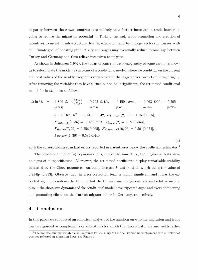
6

disparity between those two countries it is unlikely that further increases in trade barriers is

going to reduce the migration potential in Turkey. Instead, trade promotion and creation of

incentives to invest in infrastructure, health, education, and technology sectors in Turkey with

an ultimate goal of boosting productivity and wages may eventually reduce income gap between

Turkey and Germany and thus relieve incentives to migrate.

As shown in Johansen (1992), the status of long-run weak exogeneity of some variables allows

us to reformulate the model (2) in terms of a conditional model, where we condition on the current

and past values of the weakly exogenous variables, and the lagged error correction term, ecmt−1.

After removing the variables that have turned out to be insignificant, the estimated conditional

model for lnMt looks as follows

∆ lnMt = 1.806(0.588)

∆ ln(

Yft

Yht

)− 0.292

(0.038)

∆ Uft − 0.459(0.061)

ecmt−1 − 0.663(0.184)

D99t − 5.205(0.715)

σ = 0.162, R2 = 0.814, T = 42, FAR(1−2)(2, 35) = 1.157[0.855],

FARCH(1)(1, 35) = 1.145[0.219], χ2Norm(2) = 1.183[0.553],

FHetero(7, 29) = 0.256[0.965], FHetero−X(10, 26) = 0.301[0.974],

FRESET (1, 36) = 0.584[0.449](4)

with the corresponding standard errors reported in parentheses below the coefficient estimates.3

The conditional model (4) is parsimonious, but at the same time, the diagnostic tests show

no signs of misspecification. Moreover, the estimated coefficients display remarkable stability

indicated by the Chow parameter constancy forecast F -test statistic which takes the value of

0.214[p=0.953]. Observe that the error-correction term is highly significant and it has the ex-

pected sign. It is noteworthy to note that the German unemployment rate and relative income

also in the short-run dynamics of the conditional model have expected signs and exert dampening

and promoting effects on the Turkish migrant inflow in Germany, respectively.

4 Conclusion

In this paper we conducted an empirical analysis of the question on whether migration and trade

can be regarded as complements or substitutes for which the theoretical literature yields rather3The impulse dummy variable D99t accounts for the sharp fall in the German unemployment rate in 1999 that

was not reflected in migration flows, see Figure 1.

7

controversial conclusions. In our analysis, we used the time series data on Turkish migration to

Germany over the period 1963-2004.

Our estimation results provide empirical support for the theoretical literature that views

migration and trade as complements. The likely reason for such an outcome is the persistence

of the large income differential between those two countries that still shows no signs of declin-

ing. Such a large income discrepancy served as a dominating factor that stimulated people

to migrate. Given this, positive developments in the total volume of trade between Germany

and Turkey positively affected migration flows by providing additional financing for potential

migrants who could not migrate before. The development of trade linkages between these two

countries also necessarily lowered various adjustment and informational costs associated with

decision to migrate.

References

Doornik, J. A. and H. Hansen (1994). A practical test for univariate and multivariate normality.

Discussion Paper, Nuffield College, Oxford.

Doornik, J. A. and D. F. Hendry (2001a). GiveWin: An Interface to Empirical Modelling.

London: Timberlake Consultants Press.

Doornik, J. A. and D. F. Hendry (2001b). Modelling Dynamic Systems Using PcGive, Volume II.

London: Timberlake Consultants Press.

Engle, R. F. (1982). Autoregressive conditional heteroscedasticity with estimates of the variance

of united kingdom inflation. Econometrica 50, 987–1007.

Godfrey, L. G. (1978). Testing for higher order serial correlation in regression equations when

the regressors include lagged dependent variables. Econometrica 46, 1303–1313.

Harris, J. and M. Todaro (1970). Migration, unemployment, and developement: A two-sector

analysis. American Economic Review 60, 126–142.

Hendry, D. F. and K. Juselius (2000). Explaining cointegration analysis. Part 1. The Energy

Journal 21 (1), 1–42.

8

Hendry, D. F. and K. Juselius (2001). Explaining cointegration analysis. Part 2. The Energy

Journal 22 (1), 75–120.

Hendry, D. F. and G. E. Mizon (1993). Evaluating econometric models by encompassing the

VAR. In P. C. Phillips (Ed.), Models, Methods and Applications of Econometrics, Basil.

Blackwell.

Hicks, J. (1932). The Theory of Wages. London: McMillan.

Johansen, S. (1992). Testing weak exogeneity and the order of cointegration in the UK money

demand. Journal of Policy Modelling 14, 313–334.

Johansen, S. and K. Juselius (1992). Testing structural hypotheses in a multivariate cointegration

analysis of the PPP and the UIP for the UK. Journal of Econometrics 53, 211–244.

Markusen, J. R. (1983). Factor movements and commodity trade as complements. Journal of

International Economics 14, 341–356.

Mundell, R. (1957). International trade and factor mobility. American Economic Review 47,

321–335.

Panagariya, A. (1992). Factor mobility, trade and welfare: A north-south analysis with economies

of scale. Journal of Development Economics 39 (2), 229–245.

Ravenstein, E. (1889). The laws of migration. Journal of the Statistic Society 59, 214–301.

Razin, A. and E. Sadka (1997). International Migration and International Trade, Volume 1B,

Chapter 15, pp. 851–887. Amsterdam, New York, and Oxford: Elsevier Science, North-

Holland.

Schiff, M. (1994). How trade, aid, and remittances affect international migration. World Bank

Policy Research Working Paper No. 1376.

Schiff, M. (1995). Trade policy and international migration in the short and the long run. Revue

d’Economie du Developpement 1, 3–25.

Schiff, M. (2000). South-north migration and trade: A survey. Revue d’Economie du Developpe-

ment 3, 3–54.

9

Sjaastad, L. (1962). The costs and returns of human migration. Journal of Political Economy 70,

80–93.

Todaro, M. P. (1969). A model of labour migration and urban unemployment in less developed

countries. American Economic Review 59 (1), 139–48.

Venables, A. (1999). Trade liberalisation and factor mobility: An overview. In R. Faini, J. De

Melo, and K. F. Zimmermann (Eds.), Migration: The Controversies and the Evidence, pp.

23–47. Cambridge: Cambridge University Press.

White, H. (1980). A heteroscedastic-consistent covariance matrix estimator and a direct test for

heteroscedasticity. Econometrica 48, 817–838.

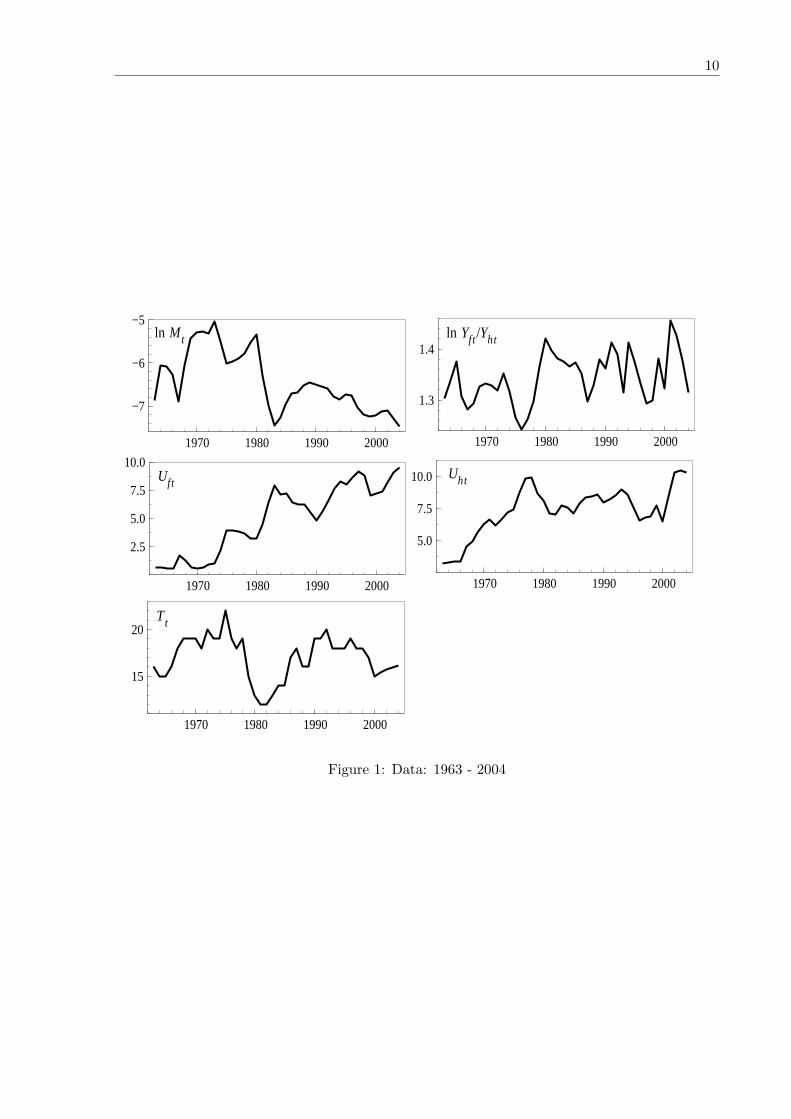
10

1970 1980 1990 2000

−7

−6

−5ln Mt

1970 1980 1990 2000

1.3

1.4ln Yft/Yht

1970 1980 1990 2000

2.5

5.0

7.5

10.0Uft

1970 1980 1990 2000

5.0

7.5

10.0 Uht

1970 1980 1990 2000

15

20Tt

Figure 1: Data: 1963 - 2004

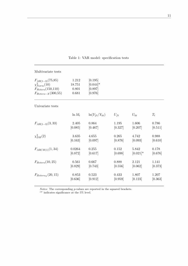
11

Table 1: VAR model: specification tests

Multivariate tests

FAR(1−3)(75,85) 1.212 [0.195]χ2

Norm(10) 18.751 [0.044]*FHetero(150,110) 0.801 [0.897]FHetero−X(300,55) 0.681 [0.976]

Univariate tests

ln Mt ln(Yft/Yht) Uft Uht Tt

FAR(1−3)(3, 33) 2.405 0.864 1.195 1.606 0.786[0.085] [0.467] [0.327] [0.207] [0.511]

χ2DH(2) 3.635 4.655 0.265 4.742 0.988

[0.163] [0.097] [0.876] [0.093] [0.610]

FARCH(1)(1, 34) 0.0264 0.255 0.152 5.842 0.178[0.872] [0.617] [0.698] [0.021]* [0.676]

FHetero(10, 25) 0.561 0.667 0.888 2.121 1.141[0.829] [0.743] [0.556] [0.062] [0.373]

FHeteroX(20, 15) 0.853 0.523 0.433 1.807 1.207

[0.636] [0.912] [0.959] [0.123] [0.363]

Notes: The corresponding p-values are reported in the squared brackets.‘*’ indicates significance at the 5% level.

12

Table 2: VAR model: cointegration tests

rank Trace test [Prob] Max test [Prob]

0 73.51 [0.023]* 38.93 [0.009]**1 34.58 [0.475] 22.32 [0.210]2 12.25 [0.919] 6.08 [0.973]3 6.17 [0.679] 5.00 [0.742]4 1.17 [0.279] 1.17 [0.279]

Notes: The corresponding p-values are reported in the squared brackets.‘*’ and ‘**’ indicate significance at the 5% and 1% levels, respectively.

Table 3: VAR model: tests for (trend-)stationarity

lnMt ln(Yft/Yht) Uft Uht Tt trend χ2(v) p-value

Stationarity. 0 0 0 0 34.307 [0.000]**0 . 0 0 0 21.269 [0.000]**0 0 . 0 0 34.798 [0.000]**0 0 0 . 0 32.187 [0.000]**0 0 0 0 . 30.358 [0.000]**

Trend-stationarity. 0 0 0 0 . 29.137 [0.000]**0 . 0 0 0 . 26.409 [0.000]**0 0 . 0 0 . 40.404 [0.000]**0 0 0 . 0 . 40.607 [0.000]**0 0 0 0 . . 38.345 [0.000]**

Notes: ‘0’ denotes the zero restriction on the coefficient of the corresponding variable, ‘·’ denotesunrestricted coefficient in the 5×1 cointegration vector when testing for the stationarity and 6×1cointegration vector when testing for trend-stationarity of the variables.The number of degrees of freedom v in the χ2 tests corresponds to the number of zero restrictionsimposed.The corresponding p-values are reported in the squared brackets.‘**’ indicates significance at the 1% level.

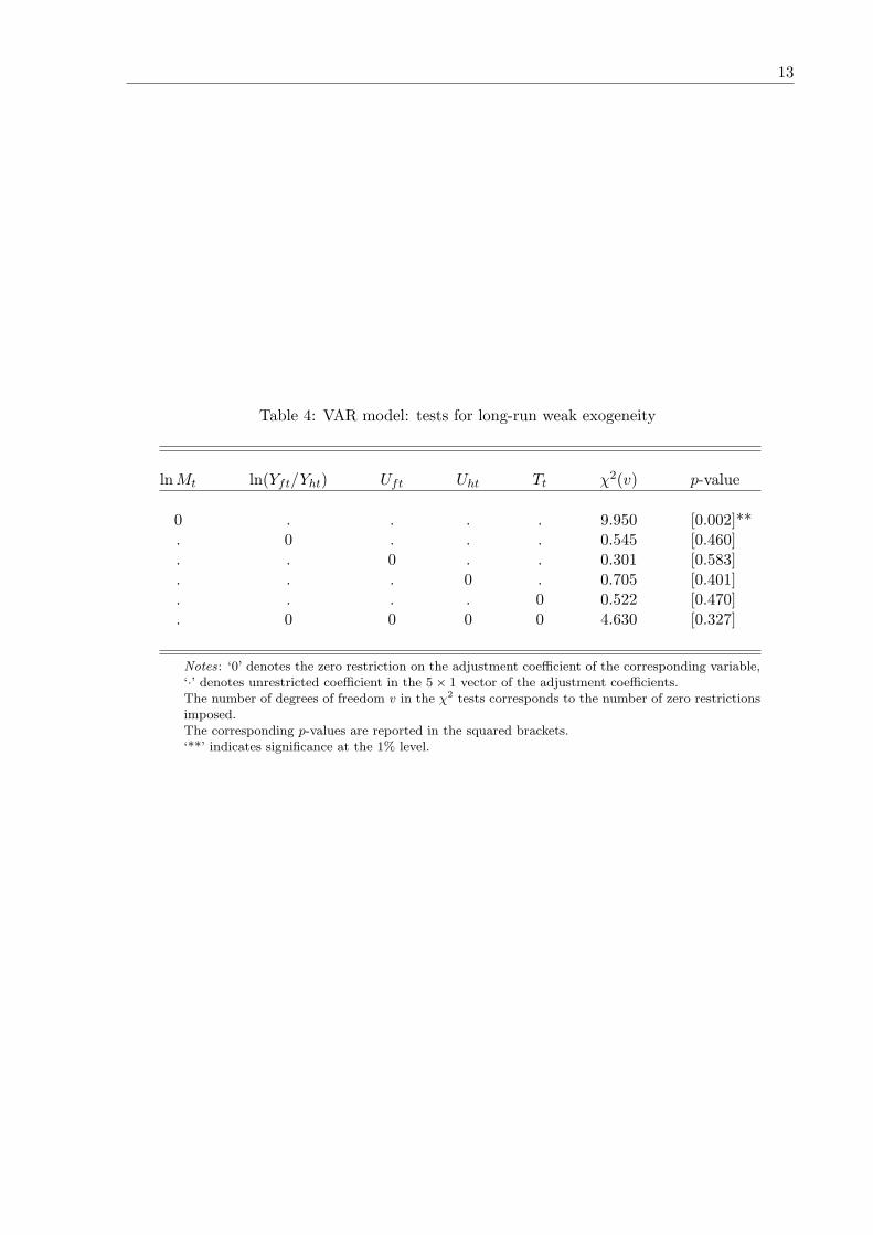
13

Table 4: VAR model: tests for long-run weak exogeneity

lnMt ln(Yft/Yht) Uft Uht Tt χ2(v) p-value

0 . . . . 9.950 [0.002]**. 0 . . . 0.545 [0.460]. . 0 . . 0.301 [0.583]. . . 0 . 0.705 [0.401]. . . . 0 0.522 [0.470]. 0 0 0 0 4.630 [0.327]

Notes: ‘0’ denotes the zero restriction on the adjustment coefficient of the corresponding variable,‘·’ denotes unrestricted coefficient in the 5× 1 vector of the adjustment coefficients.The number of degrees of freedom v in the χ2 tests corresponds to the number of zero restrictionsimposed.The corresponding p-values are reported in the squared brackets.‘**’ indicates significance at the 1% level.

Trade, Aid, Remittances and Migration

By

Sule Akkoyunlu*

August 2007

Abstract

We investigated whether migration is interrelated with trade, aid and remittances so that any policies that consider trade, aid and remittances also affect the decision to migrate. We developed and estimated an empirical model of Turkish migration to Germany and tested the model for the 1969-2004, using the cointegration technique. A single cointegrating vector is found among the gross migration inflows and the following explanatory variables: the relative income ratio between Germany and Turkey, the unemployment rates in Germany and Turkey, aid, the trade intensity variable and the ratio of manufacturing exports with Germany to total exports with Germany and remittances as a ratio of Turkish GDP. The results of this study show that migration, trade, aid and remittances are interrelated, however, migration will be better managed when the dynamic gains from trade and aid are considered. Hence, the broad-based and rapid economic development with increase in income is the only effective means of reducing migration pressures in a labour-surplus country. This is mainly because the income differential is the most significant factor in determining migration flows.

Keywords: Trade; Aid; Remittances; Migration; Cointegration JEL Classification: C22; F16; F22; F24; F35

The research reported in this paper was financially supported by the European Union

within the context of the FEMISE program. The contents of this paper are the sole

responsibility of the authors and do not reflect the opinion of the European Union.

* Department of Economics, Bilkent University; DIW Berlin. Email: sakkoyunlu@diw.de

1. Introduction

In the traditional trade models, both trade and international factor mobility are driven by

differences in factor proportions between countries. Countries with a high ratio of capital

to labor will export capital-intensive goods, import labor-intensive goods, invest in

abroad and will be attractive for migration. Trade in goods in these models will reduce

the incentive for factor movements and will lead the exact equalization of factor prices

across countries. Thus, international trade narrows the wage gap and reduces the

incentives to migrate. The feared resumption of massive labor flows from Turkey with

the recognition of Turkey as a candidate for accession at the Helsinki European Council

in December 1999 and the start of accession negotiations between European Union and

Turkey in October 2005, brings back the question that whether the trade policy can be

effective in reducing migration pressure from Turkey. Thus, can we have an optimal

combination of trade, aid, remittance and migration policies in order to avoid massive

labor inflows from Turkey with the accession? This proposition might be attractive for

the receiving countries because the movements of goods and services between countries

through trade is more welcomed than the movements of people due to the additional

fiscal burdens that migrants put on others and these external costs can create social

tension. Thus, by exporting labor-intensive goods Turkey in effect export labor embodied

in its export and hence there will be no need for migration in this approach. More

importantly, if trade substantially reduce unemployment and contribute to the economic

growth as well as economic efficiency then it can really help reduce the pressures for

migration. Thus, trade is not only exchange of goods but promotes competition and

investment in education and infrastructure, creates an opportunity to exploit economies of

scale, transfer of knowledge and technology. Therefore, the dynamic rather than static

effect of trade can be more effective in reducing the income differential that is the main

driving force of migration.

Although rich countries protect most strongly the sectors that produce competing labor-

intensive goods, Turkish trade with Germany has been in favour of Turkey. Turkey took

two major trade liberalizing policies: in the early 1980s and the Customs Union

2

Agreement in 1996. The export-led growth strategy was accompanied by gradual import

liberalization, more flexible exchange rate regime and more effective export incentive

programmes. These reforms not only rapidly expanded total volume of exports but also

the export decomposition changed in favour of manufacturing goods that Turkey has a

comparative advantage. Furthermore, following trade liberalization investment,

employment and output in manufacturing sector increased, although the real wage growth

in manufacturing sector has been very modest, TSI (2005). Hence, the share of

manufacturing exports in total exports in which Turkey has a comparative advantage may

have an important deterrent factor in determination of migration flows.

Development aid that speeds up economic development and human capital formation also

helps to keep the population at home. Investment in human capital results in higher

productivity that is translated into increasing returns to scale effect and labor productivity

increases countinously. Remittances, likewise if are used for productive investment at

home can create employment and contribute to economic growth. However, economic

growth and increase in income are likely to increase migration pressure in the short-run

by making migration accessible to unskilled migrants with low incomes and low access

to credit markets. Thus, labor mobility tends to interact closely with trade, aid, and capital

flows in many ways direct and indirect. These inter-linkages have special importance in

relation to current and anticipated inflows of Turkish migrants to Germany. Therefore,

revised policies based on the study of these linkages can make migration more

manageable and promote efficiency in the region. This is especially important if we

consider migration not only economic but also social phenomenon.

To our knowledge, this is the only empirical study that incorporates trade, aid and

remittances in a migration model in order to consider the extent to which trade, aid and

remittance policies can be effective in managing migration inflows.

The paper structured as follows. Section 2 gives background information on how trade,

aid, remittances and migration are interrelated. Section 3 considers the empirical model.

Section 4 provides the econometrics results. Section 5 concludes.

3

2. Background

Trade liberalization aims not only access to foreign markets to sell goods but also to

speed up economic growth. However, international trade agreements have been

unsuccessful in promoting growth in poor countries such as NAFTA. Stiglitz (2006)

argues that NAFTA did not bring benefits to Mexico, but lowered wages and increased

unemployment. This was because trade agreements have been asymmetric, and this put

developing countries at a disadvantage. In addition, a lack of infrastructure in developing

countries prevents them to bring their goods to markets. Likewise, imperfect capital

markets prevent them to get the necessary finance for new export opportunities. Trade

liberalization when done fairly, when accompanied by the right measures and the right

policies help development. In this process, aid certainly has an important role to increase

trade by providing the infrastructure. NAFTA had the aim that it would help close the gap

in income between Mexico and the United States and thus reduce the pressure of illegal

migration. However, NAFTA did not result in a rapid growth in Mexico’s economy.

This was because trade liberalization was so fast that private sector could not create jobs

immediately, and further high interest rates prevented them create new jobs. It needs to

be added that, in so far as increased imports to migrant sending countries may drive out

local firms from the market, thus eliminating jobs directly or indirectly linked to them,

liberalized trade may contribute to increase pressures for migration during the transition.

However, any such job losses in the short-run should be outweighed by additional

employment created in the labour-intensive export sector, combining economies of scale,

easier and less expensive supply of imports as production inputs and a more efficient

allocation of resources throughout the economy in the long-run.

In traditional model factor price equalization holds so that wages of skilled workers, of

unskilled workers and the return to capital will be the same in everywhere. Trade

liberalization leads toward the equalization of factor prices. Free trade is a substitute for

people having to move. Furthermore, if labor moves from a labor abundant country

where productivity and wages are low to one where labor is scare where wages are high,

4

then output will increase and economy will grow. However, economic growth in the

labor abundant country will depend on how fast they acquire the knowledge and

technology that the advanced countries have. Thus, wages will only rise if productivity

increase and this will depend on the investment on technology and education.

Turkey has a comparative advantage in production of agricultural and textile goods (that

are labor-intensive goods) and reduction in tariffs and restrictions of these products with

the European countries may reduce migration in the long-run. However, in the short-run

the effect may be positive. The exports of manufacturing goods to Germany certainly

helped Turkey’s transition from the agriculture dominated economy. Over the years

following trade liberalization employment, exports and output of manufacturing sector

have increased.

However, even if all tariff and trade barriers are reduced to zero the wage differences

between Turkey and Germany will not equalize. This is not only related to the

transportation costs, but the economic structure of Turkey. The wage differences will

persist unless there are capital flows to Turkey that will make workers more productive

and the gap in knowledge between the West and Turkey is eliminated. It will take longer

time than the period under investigation in this study to eliminate the knowledge gap and

the capital shortage in Turkey. However, in this study we show that the increase of

exports of goods that Turkey has a comparative advantage can reduce migration pressure

in the long-run. Therefore, fair trade regime has an important role to play. However, the

most important impacts of trade liberalization would be its help to alleviate poverty

through job creation, promoting competition, improvements in education and in health

and technological learning.

Aid1 or official development assistance (ODA) is not only the transfer of funds that

combines loans and grants but also the provision of technical assistance or capacity

building. It should be emphasized that a loan is called aid if only it carries a subsidy

element. However, aid will only help if they introduce ideas and improve practices that

1 Aid in this paper refers to the official development assistance (ODA).

5

increase the overall size of the resources available for growth and poverty reduction.

Therefore, aid is most welcomed when it is accompanied with ideas, policies and

capacity building. Only then aid can contribute to the long-run economic growth and

eliminate wage differences between Turkey and the west. However, the share of “short

impact” aid to Turkey such as budget and balance of payments support, infrastructure

investments is higher than the share of aid for productive sectors such as agriculture and

industry, see Uygur (1992) and OECD (2007). In the 1960s and 1970s, aid was used to

finance investments in the manufacturing sector, but in the 1980s and 1990s, aid was

used to greater extent to finance the interest bills, principal repayments and trade deficits

as well as investment in energy and infrastructure. Thus, a relative neglect of industrial

investments can make aid detrimental to long-run economic growth and employment

creation. Needless to mention Turkish economic and social policies and governance as

well as the institutions affect project qualities.

Aid and trade are viewed as substitute for one another and trade is the favoured of the

two. The role of trade in economic growth and poverty alleviation might be more

effective than aid, given the structure, type and the magnitude of aid. Exports growth can

certainly generate incomes for the poor, as many unskilled would-be migrants as in the

Turkish case are unable to finance their migration cost out of their low-wage income. The

increase of migration with trade liberalization in the short-run has been called a migration

hump, see Martin and Taylor (1996). This means that the same economic policy that

reduces migration in the long-run can increase it in the short-run, making free trade

policy a dilemma as the best way to reduce migration.

3. An empirical model

We model Turkish migration to Germany as follows:

6

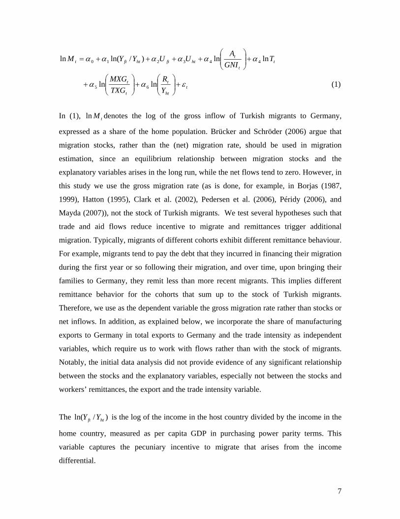
(1) lnln

lnln)/ln(ln

65

443210

tht

t

t

t

tt

thtfthtftt

YR

TXGMXG

TGNI

AUUYYM

εαα

αααααα

+⎟⎟⎠

⎞⎜⎜⎝

⎛+⎟⎟

⎠

⎞⎜⎜⎝

⎛+

+⎟⎟⎠

⎞⎜⎜⎝

⎛++++=

In (1), denotes the log of the gross inflow of Turkish migrants to Germany,

expressed as a share of the home population. Brücker and Schröder (2006) argue that

migration stocks, rather than the (net) migration rate, should be used in migration

estimation, since an equilibrium relationship between migration stocks and the

explanatory variables arises in the long run, while the net flows tend to zero. However, in

this study we use the gross migration rate (as is done, for example, in Borjas (1987,

1999), Hatton (1995), Clark et al. (2002), Pedersen et al. (2006), Péridy (2006), and

Mayda (2007)), not the stock of Turkish migrants. We test several hypotheses such that

trade and aid flows reduce incentive to migrate and remittances trigger additional

migration. Typically, migrants of different cohorts exhibit different remittance behaviour.

For example, migrants tend to pay the debt that they incurred in financing their migration

during the first year or so following their migration, and over time, upon bringing their

families to Germany, they remit less than more recent migrants. This implies different

remittance behavior for the cohorts that sum up to the stock of Turkish migrants.

Therefore, we use as the dependent variable the gross migration rate rather than stocks or

net inflows. In addition, as explained below, we incorporate the share of manufacturing

exports to Germany in total exports to Germany and the trade intensity as independent

variables, which require us to work with flows rather than with the stock of migrants.

Notably, the initial data analysis did not provide evidence of any significant relationship

between the stocks and the explanatory variables, especially not between the stocks and

workers’ remittances, the export and the trade intensity variable.

tMln

The is the log of the income in the host country divided by the income in the

home country, measured as per capita GDP in purchasing power parity terms. This

variable captures the pecuniary incentive to migrate that arises from the income

differential.

)/ln( htft YY

7

ftU is the unemployment rate in Germany. The German migration policies have become

more restrictive during periods of high unemployment in Germany (Mayda and Patel

(2004)).

The term is the unemployment rate in Turkey. It represents a simple push factor. The

unemployment rate enters the empirical model individually rather than as a difference

term, in line with (for example) Borjas (1987, 1999), Hatton (1995), Clark et al. (2002),

Pedersen et al. (2006), Péridy (2006), and Mayda (2007).

htU

⎟⎟⎠

⎞⎜⎜⎝

⎛

t

t

GNIA

ln is the overseas development aid to GNI ratio. The hypothesis is that aid will

encourage economic development and will reduce incentive to migrate.

tTln is a proxy for the intensity of economic cooperation between Turkey and Germany,

calculated as the log of the share of the trade volume (sum of exports and imports)

between the two countries in the total trade volume of Turkey with all its trading partners.

The volume of trade between two economies could measure a variety of links between

the economies. The higher the volume, the more intensive the links. The bilateral links

co-shape the migration “infrastructure” or environment. It stands to reason that an

increase in the total volume of trade between Germany and Turkey can alleviate the

financial and informational constraints associated with migration from Turkey to

Germany, and thereby lower the cost of migration, particularly for low-skill workers with

low incomes and with limited access to credit markets. Trade can serve as an indicator of

the level of business linkages between economies, which in turn lower informational

costs and reduce uncertainty, thereby impinging on the migration “climate.” In addition,

trade could impact on migration in more subtle ways. When the volume of trade between

Turkey and Germany is high, Turkey will be less likely to allow appreciation of its

currency - exporters could suffer greatly if it did - and is more likely to tilt in the

direction of depreciation of its currency. For a given stock of Turkish migrants in

8

Germany, a depreciation of the Turkish currency could prompt migrants to increase their

remittances.

⎟⎟⎠

⎞⎜⎜⎝

⎛

t

t

TXGMXG

ln is the share of Turkish manufacturing exports with Germany in total Turkish

exports with Germany. This variable captures the effects of the expansion of

manufacturing exports that Turkey has a comparative advantage on decision to migrate.

In other words, with this variable we test whether trade and migration are substitutes or

complements.

Finally, ⎟⎟⎠

⎞⎜⎜⎝

⎛

ht

t

YR

ln is the log of the ratio between workers’ remittances and Turkish GDP.

The data on workers’ remittances were obtained from the balance sheets of the

Bundesbank, while the data on the per capita GDP of Germany and of Turkey were

obtained from the OECD. Data on Turkish unemployment, population, and trade were

gathered from the Turkish Institute of Statistics. Data on Turkish migration and on

German unemployment were obtained from the Federal Statistical Office in Germany.

Data on aid is obtained from the World Development Indicators, World Bank.

4. The general to specific approach and econometrics results

Modelling based on the general-to-specific modeling approach that aims to build

empirical models that economically sensible and statistically satisfactory, Hendry (1995),

Campos and Ericsson (1999) and Hoover and Perez (1999). Although we have thirty-six

years of annual data, as shown in Akkoyunlu (1999) and Campos and Ericsson (1999),

the sample size is only one of several factors which determine how much information is

in the sample. Even our data sample is small, the data movements so large that are crucial

for the information of data. Therefore, over-parameterisation should not be a concern.

9

Therefore, we start with a general model which is probably over-parameterised with two

lags for the gross inflows of Turkish migrants to Germany, expressed as the share of the

home population, and a broad set of explanatory variables (income differential (the

ratio of German GDP to Turkish GDP in PPPs,

tMln

⎟⎟⎠

⎞⎜⎜⎝

⎛

ht

ft

YY

ln ), the German unemployment

rate, , the Turkish unemployment rate, , aid (aid to GNI ratio, ftU htU ⎟⎟⎠

⎞⎜⎜⎝

⎛

t

t

GNIA

ln ), trade

intensity (the share of total trade with Germany in total Turkish trade, ), the share of

Turkish manufacturing exports with Germany in total Turkish exports with Germany,

tTln

⎟⎟⎠

⎞⎜⎜⎝

⎛

t

t

TXGMXG

ln , and Turkish remittances from Germany, expressed as a ratio to Turkish

GDP, ⎟⎟⎠

⎞⎜⎜⎝

⎛

ht

t

YR

ln ).2 Thus, we allow for everything3 at the outset that might be significant

and then investigate whether and how this initial general model can be reduced without

significant loss of information about the parameters of interests. Economic theory

information helps specify the vector of parameters of interest; however, the parameters of

interest might come from a data-instigated model. However, theory consistency is

essential, so that there is no evaluation conflict between the model and the theory

interpretation. Hence, I aim to conclude with a parsimonious model which has orthogonal

regressors as well as satisfying the necessary conditions for both congruence and

encompassing.

However, the general-to-specific modelling still suffers from allegations that it mines the

data pejoratively. These allegations are, as in Campos and Ericsson (1999):

I. Repeated Testing: Regressors are selected in an attempt to maximise t-ratios.

Thus simply conducting multiple tests will induce significant outcomes by chance. 2 All the variables apart from the unemployment rates are expressed in logs. 3 Social networks are considered to be and found in many studies to be an important determinant of migration as they can provide information prior to migration, and financial assistance and support until the migrants get used to the new environment. However, in this study we found the stock of Turkish migrants that represents social networks to be insignificant in the short- as well as in the long-run.

10

II. Data Interdependence: Non-constant coefficient might result due to an

omitted regressor that is correlated with the included one, and this correlation changes

over time due to regime changes that generate the system.

III. Corroboration: The regressors are chosen according to a criterion such as

having sensible coefficient estimates. However, there might still be important omitted

variables.

IV. Over-parameterization: If the model is over-fitted, it uses up many degrees of

freedom.

However, this paper, during the building process of the empirical model, shows that these

allegations can be refuted easily.

The annual data covers the period from 1969-2004 (see Figure 1, for the basic properties

of the data).

Our first step is to obtain parsimonious unrestricted model, which is quite challenge given

the relatively small number of observations (T=36) compared to the number of

explanatory variables (k=7). The results of the unrestricted general model are given in

Table 1. Table 1 shows that the unrestricted model can adequately describe the data,

since the misspecification tests show no serious departures from the underlying model

assumptions.

The next step is to find the cointegrating relationship between variables. The solved long

run equation, as well as the error correction mechanism (ECM) is given below. The test

on the significance of the lag length suggests that the model should have two lags.

11

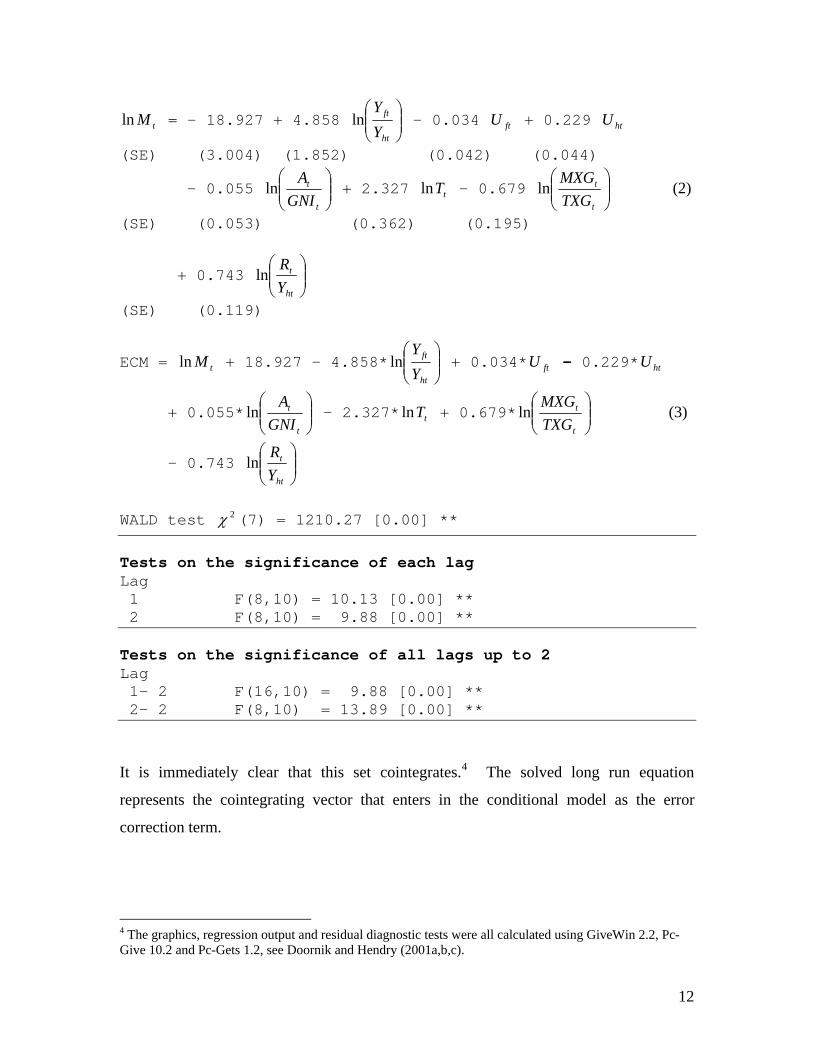
tMln = - 18.927 + 4.858 ⎟⎟⎠

⎞⎜⎜⎝

⎛

ht

ft

YY

ln - 0.034 + 0.229 ftU htU

(SE) (3.004) (1.852) (0.042) (0.044)

- 0.055 ⎟⎟⎠

⎞⎜⎜⎝

⎛

t

t

GNIA

ln + 2.327 - 0.679 tTln ⎟⎟⎠

⎞⎜⎜⎝

⎛

t

t

TXGMXG

ln (2)

(SE) (0.053) (0.362) (0.195)

+ 0.743 ⎟⎟⎠

⎞⎜⎜⎝

⎛

ht

t

YR

ln

(SE) (0.119)

ECM = + 18.927 – 4.858*tMln ⎟⎟⎠

⎞⎜⎜⎝

⎛

ht

ft

YY

ln + 0.034* - 0.229* ftU htU

+ 0.055* ⎟⎟⎠

⎞⎜⎜⎝

⎛

t

t

GNIA

ln - 2.327* + 0.679*tTln ⎟⎟⎠

⎞⎜⎜⎝

⎛

t

t

TXGMXG

ln (3)

- 0.743 ⎟⎟⎠

⎞⎜⎜⎝

⎛

ht

t

YR

ln

WALD test (7) = 1210.27 [0.00] ** 2χ Tests on the significance of each lag Lag 1 F(8,10) = 10.13 [0.00] ** 2 F(8,10) = 9.88 [0.00] ** Tests on the significance of all lags up to 2 Lag 1- 2 F(16,10) = 9.88 [0.00] ** 2- 2 F(8,10) = 13.89 [0.00] **

It is immediately clear that this set cointegrates.4 The solved long run equation

represents the cointegrating vector that enters in the conditional model as the error

correction term.

4 The graphics, regression output and residual diagnostic tests were all calculated using GiveWin 2.2, Pc-Give 10.2 and Pc-Gets 1.2, see Doornik and Hendry (2001a,b,c).

12

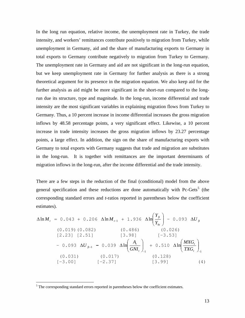
In the long run equation, relative income, the unemployment rate in Turkey, the trade

intensity, and workers’ remittances contribute positively to migration from Turkey, while

unemployment in Germany, aid and the share of manufacturing exports to Germany in

total exports to Germany contribute negatively to migration from Turkey to Germany.

The unemployment rate in Germany and aid are not significant in the long-run equation,

but we keep unemployment rate in Germany for further analysis as there is a strong

theoretical argument for its presence in the migration equation. We also keep aid for the

further analysis as aid might be more significant in the short-run compared to the long-

run due its structure, type and magnitude. In the long-run, income differential and trade

intensity are the most significant variables in explaining migration flows from Turkey to

Germany. Thus, a 10 percent increase in income differential increases the gross migration

inflows by 48.58 percentage points, a very significant effect. Likewise, a 10 percent

increase in trade intensity increases the gross migration inflows by 23.27 percentage

points, a large effect. In addition, the sign on the share of manufacturing exports with

Germany to total exports with Germany suggests that trade and migration are substitutes

in the long-run. It is together with remittances are the important determinants of

migration inflows in the long-run, after the income differential and the trade intensity.

There are a few steps in the reduction of the final (conditional) model from the above

general specification and these reductions are done automatically with Pc-Gets5 (the

corresponding standard errors and t-ratios reported in parentheses below the coefficient

estimates).

tMlnΔ = 0.043 + 0.206 1ln −Δ tM + 1.936 ⎟⎟⎠

⎞⎜⎜⎝

⎛Δ

ht

ft

YY

ln - 0.093 ftUΔ

(0.019)(0.082) (0.486) (0.026) [2.23] [2.51] [3.98] [-3.53]

- 0.093 - 0.039 1−Δ ftU1

ln−⎟⎟⎠

⎞⎜⎜⎝

⎛Δ

t

t

GNIA

+ 0.510 1

ln−⎟⎟⎠

⎞⎜⎜⎝

⎛Δ

t

t

TXGMXG

(0.031) (0.017) (0.128) [-3.00] [-2.37] [3.99] (4)

5 The corresponding standard errors reported in parentheses below the coefficient estimates.

13

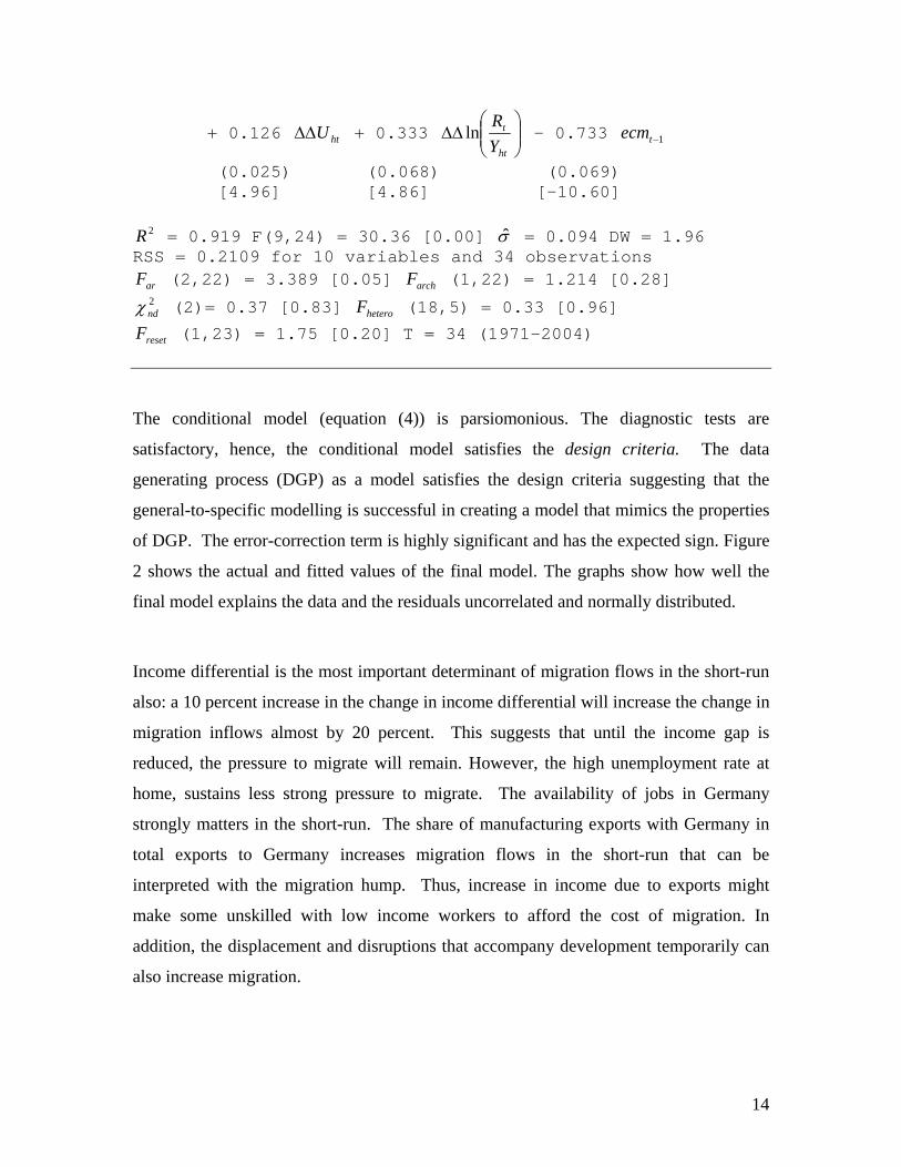
+ 0.126 + 0.333 htUΔΔ ⎟⎟⎠

⎞⎜⎜⎝

⎛ΔΔ

ht

t

YR

ln - 0.733 1−tecm

(0.025) (0.068) (0.069) [4.96] [4.86] [-10.60]

2R = 0.919 F(9,24) = 30.36 [0.00] σ = 0.094 DW = 1.96 RSS = 0.2109 for 10 variables and 34 observations

arF (2,22) = 3.389 [0.05] (1,22) = 1.214 [0.28] archF2ndχ (2)= 0.37 [0.83] (18,5) = 0.33 [0.96] heteroF

resetF (1,23) = 1.75 [0.20] T = 34 (1971-2004)

The conditional model (equation (4)) is parsiomonious. The diagnostic tests are

satisfactory, hence, the conditional model satisfies the design criteria. The data

generating process (DGP) as a model satisfies the design criteria suggesting that the

general-to-specific modelling is successful in creating a model that mimics the properties

of DGP. The error-correction term is highly significant and has the expected sign. Figure

2 shows the actual and fitted values of the final model. The graphs show how well the

final model explains the data and the residuals uncorrelated and normally distributed.

Income differential is the most important determinant of migration flows in the short-run

also: a 10 percent increase in the change in income differential will increase the change in

migration inflows almost by 20 percent. This suggests that until the income gap is

reduced, the pressure to migrate will remain. However, the high unemployment rate at

home, sustains less strong pressure to migrate. The availability of jobs in Germany

strongly matters in the short-run. The share of manufacturing exports with Germany in

total exports to Germany increases migration flows in the short-run that can be

interpreted with the migration hump. Thus, increase in income due to exports might

make some unskilled with low income workers to afford the cost of migration. In

addition, the displacement and disruptions that accompany development temporarily can

also increase migration.

14

Aid policy only effective in reducing migration flows in the short-run, but this effect is

small. Hence, financial assistance is not a durable long-run solution to reduce migration

pressure. However, if aid are conditional on good policies and has a higher share of

technical assistance and training that would transfer expertise and know-how and

increase in investment in productive sectors and hence help human capital development,

and accelerate job creation and economic growth so that income differences between

Turkey and Germany is reduced, only then aid policies can have a long-lasting effect.

Remittances are found to significantly explain migration in the short-run as well as in the

long-run. The results support the hypothesis that remittances fuel migration. It is

normally hypothesized that remittances by providing capital in the home countries,

promote investment and help create jobs and reduce the incentive to emigrate. However,

in this study we found that remittances to an economy are the harbinger of migration

from the economy. Liquidity constraints, signalling, portfolio revision, and other

considerations raise the possibility that an economy that receives more remittances will

generate more migration, Akkoyunlu et al. (2007). The results show that both push and

pull factors matter in determining Turkish migration inflows to Germany.

Figures 3, 4 and 5 plot the recursive estimates for the coefficients on the constant term,

, 1ln −Δ tM ⎟⎟⎠

⎞⎜⎜⎝

⎛Δ

ht

ft

YY

ln , , ftUΔ 1−Δ ftU , 1

ln−⎟⎟⎠

⎞⎜⎜⎝

⎛Δ

t

t

GNIA

, 1

ln−⎟⎟⎠

⎞⎜⎜⎝

⎛Δ

t

t

TXGMXG

, , htUΔΔ

⎟⎟⎠

⎞⎜⎜⎝

⎛ΔΔ

ht

t

YR

ln , and ; their respective t-ratios; and the recursive residual sum of

squares, one-step residuals, one-step Chow statistics, and break–point Chow statistics,

respectively. Constant coefficients in Figure 3 in the presence of the large variations in

the marginal process such as unemployment rates imply super exogenous variables that

counter the second sense of data mining. Further, the recursive t-ratios in Figure 4,

increase in absolute value as the sample size increases countering the first sense of data

mining. Hence, the nominal critical levels of test statistics are not affected. Even with

thirty-four observations and ten variables in the final model t-ratios are greater than three

in magnitude suggesting that over-parameterisation is not a concern given information

1−tecm

15

content in the data and refuting the fourth sense of data mining. Figure 5 shows that the

recursive residual sum of squares increase over time and the recursive estimate of

standard error tσ declines over time rather than increase, hence countering the first sense

of data mining.

5. Conclusions

We investigated whether migration is interrelated with trade, aid and remittances so that

any policies that consider trade, aid and remittances also affect the decision to migrate.

We developed and estimated an empirical model of Turkish migration to Germany and

tested the model for the 1969-2004, using the cointegration technique. A single

cointegrating vector is found among the gross migration inflows and the following

explanatory variables: the relative income ratio between Germany and Turkey, the

unemployment rates in Germany and Turkey, aid, the trade intensity variable and the

ratio of manufacturing exports with Germany to total exports with Germany and

remittances as a ratio of Turkish GDP. Based on the results of the cointegration analysis,

a parsimonious single equation conditional error-correction model is developed. That is

both congruent and parsimoniously encompasses the general model. The residuals are

also innovations against the available information. The results further support the view

that a constructive data mining qua general-to-specific modelling approach is productive

as it has a high probability of locating the DGP.

The results show that migration is interrelated with trade, aid and remittances. However,

the best way to manage economic migration is to generate rapid economic growth with

productive employment opportunities and therefore to raise incomes in the country of

origin.

Until the income differential converges to zero the migration pressure will persists, and it

would go on until relative wages in Turkey rises sufficiently. Trade policy that would

16

bring jobs to Turkey has a role to play in the long-run, but in the short-run will increase

migration. In addition, aid is significant only in the short-run for reducing migration

inflows. This might be associated with its small magnitude and its high volatility. Levels

of development assistance indeed are small and declining compared with other financial

flows such as remittances. Development aid takes the form of financial assistance and

technical cooperation. The first concerns provision of finance in the form of grants and

credits, the latter is the availability of professional exports to developing countries. The

majority of foreign assistance to Turkey takes the form of grants and credits. Most of

these loans are used for investments in the physical infrastructure such as energy,

communications, transport and community services rather than in productive sectors such

as education, agriculture and industry. However, aid that contributes to poverty

alleviation through employment creation, human capital formation and income generation

can only dampen the pressures to migrate.

For given unemployment differentials, a high level of unemployment in Germany reduces

migration so that employment opportunities matters greatly in the destination for

migration. However, employment opportunities at home also have a role in the short- as

well as in the long-run. Hence, creating more employment opportunities and better

conditions of work will also reduce migration pressure.

The results are consistent with Akkoyunlu et al. (2007) that remittances are harbinger of

migration from Turkey so that liquidity constraints, signaling, portfolio revision and other

considerations raises the possibility that an economy that receives more remittances

would generate more migration.

Fair trade policy help reduce the incentives for migration, but it is certainly not enough to

eliminate these incentives. Furthermore, the aid should be available only if the right

policies are adhered to so that any structural aid from the European Commission during

the accession period should have a strict conditionality element. Aid in magnitude has

also been very small, and an increase its magnitude will have a significant impact.

17

The results show that the choice is not trade or aid for reducing migration pressure, but

aid and trade. Trade and aid jointly have a role to play especially in the short run, when

trade increases migration, aid reduces migration pressure. Thus, the right combination of

trade and aid policies can help manage the labor inflows in the short-run. Germany

should remain open to Turkish manufacturing goods that are mainly labor-intensive.

Furthermore, aid should be used to increase the capacity of Turkey (manufacturing

industry) to produce goods for exports.

The results of this study show that migration, trade, aid and remittances are related,

however, migration will be better managed when the dynamic gains from trade and aid

are considered. Hence, the broad-based and rapid economic development with increase

in income is the only effective means of reducing migration pressures in a labour-surplus

country. If the Turkish economy grows at a rate fast enough so as to cause a fall in

unemployment, real wages are likely to increase. Wages and incomes will also rise to the

extent that economic growth entails an upgrading of skills, knowledge and technology.

Thus, economic development can affect migration by making the ‘push’ factors less

powerful in the home country, while reducing the relative attractiveness of the potential

host country. However, even rapid economic growth in Turkey will not enable them to

catch up with Germany for many decades. This makes the research on Turkish migration

to Germany an important topic in the coming years.

References

Akkoyunlu, S. (1999). Turkish Consumption and Saving. DPhil Thesis. University of

Oxford.

Borjas, G. (1987). Self selection and the earnings of immigrants. American Economic

Review 77: 531-553.

18

Borjas, G. (1999). The Economic analysis of immigration. In: Handbook of Labour

Economics, chapter 28, pages 1697-1760. In O. Ashenfelter and D. Card eds. North-

Holland Elsevier Science: Amsterdam.

Brücker, H. and P. J. H. Schröder (2006). International migration with heteregeneous

agents: Theory and evidence. IZA Discussion Paper 2049.

Campos, J. and Ericsson N. R. (1999). Constructive Data Mining: Modelling of

Consumers’ Expenditure in Venezuela. Econometrics Journal 5: 226-240.

Clark, X., T. J. Hatton, and J. G. Williamson (2002). Explaining US immigration, 1971-

1998. Centre for Economic Policy Research Discussion Paper 453.

Doornik, J. A. and H. Hansen (1994). An omnibus test for univariate and multivariate

normality. Nuffield College Discussion Paper W4&91.

Doornik, J. A. and D. F. Hendry (2001a). GiveWin: An Interface to Empirical Modelling.

Timberlake Consultants Press: London.

Doornik, J. A. and D. F. Hendry (2001b). Modelling Dynamic Systems Using PcGive,

Volume II. Timberlake Consultants Press: London.

Doornik, J. A. and D. F. Hendry (2001c). Automatic Econometrics Model Selection Using

PcGets. Timberlake Consultants Press: London.

Engle, R. F. (1982). Autoregressive conditional heteroscedasticity with estimates of the

variance of United Kingdom inflation. Econometrica 50: 987-1007.

R. F. Engle, R. F., D. F. Hendry and J.-F. Richard (1983). Exogeneity. Econometrica 51:

277-304.

19

Godfrey, L. G. (1978). Testing for higher order serial correlation in regression equations

when the regressors include lagged dependent variables. Econometrica 46: 1303-1313.

Hatton, T. J. (1995). A model of UK migration, 1870-1913. Review of Economics and

Statistics 77: 407-415.

Hendry, D. F. (1995). Dynamic Econometrics: Advanced Texts in Econometrics. Oxford

University Press: Oxford

Hoover, K. D., and Perez, S. J. (1999). Data Mining Reconsidered: Encompassing and

the General-to-Specific Approach to Specification Search. Econometric Journal 2: 167-

191.

Mayda, A. M. (2007). International migration: a panel data analysis of the determinants

of bilateral flows. CREAM Discussion Paper 07/07.

Martin, P. and J. E. Taylor (1996). “The Anatomy of a Migration Hump”. In

Development Strategy, Employment and Migration: Insights from Models. J. E. Taylor

ed, pp: 43-62. OECD: Paris.

Mayda, A. M. and K. Patel (2004). OECD countries migration policies changes.

Appendix to International migration: A panel anaysis of economic and non-economic

determinants. http//www.georgetown.edu/faculty/amm23/.

OECD (2007). The DAC Journal. OECD: Paris.

Pedersen, P. J., M. Pytlikova, and N. Smith (2006). Migration into OECD countries

1990-2000. In: Immigration and the transformation of Europe. C. A. Parsons and T. M.

Smeeding eds. Cambridge University Press: New York.

20

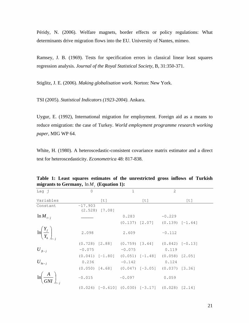
Péridy, N. (2006). Welfare magnets, border effects or policy regulations: What

determinants drive migration flows into the EU. University of Nantes, mimeo.

Ramsey, J. B. (1969). Tests for specification errors in classical linear least squares

regression analysis. Journal of the Royal Statistical Society, B, 31:350-371.

Stiglitz, J. E. (2006). Making globalisation work. Norton: New York.

TSI (2005). Statistical Indicators (1923-2004). Ankara.

Uygur, E. (1992), International migration for employment. Foreign aid as a means to

reduce emigration: the case of Turkey. World employment programme research working

paper, MIG WP 64.

White, H. (1980). A heteroscedastic-consistent covariance matrix estimator and a direct

test for heteroscedasticity. Econometrica 48: 817-838.

Table 1: Least squares estimates of the unrestricted gross inflows of Turkish migrants to Germany, (Equation 1): tMlnLag j 0 1 2 Variables [t] [t] [t] Constant -17.903 (2.528) [7.08]

jtM −ln _____ 0.283 -0.229

(0.137) [2.07] (0.139) [-1.64]

jth

f

YY

−⎟⎟⎠

⎞⎜⎜⎝

⎛ln 2.098 2.609 -0.112

(0.728) [2.88] (0.759) [3.44] (0.842) [-0.13]

jftU − -0.075 -0.075 0.119

(0.041) [-1.80] (0.051) [-1.48] (0.058) [2.05]

jhtU − 0.236 -0.142 0.124

(0.050) [4.68] (0.047) [-3.05] (0.037) [3.36]

jtGNIA

−

⎟⎠⎞

⎜⎝⎛ln -0.015 -0.097 0.059

(0.024) [-0.610] (0.030) [-3.17] (0.028) [2.14]

21

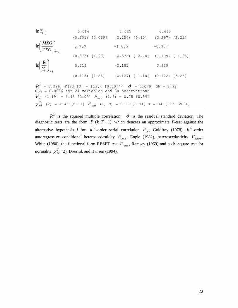
jtT −ln 0.014 1.525 0.663

(0.201) [0.069] (0.256) [5.90] (0.297) [2.23]

jtTXGMXG

−

⎟⎠⎞

⎜⎝⎛ln 0.730 -1.005 -0.367

(0.373) [1.96] (0.372) [-2.70] (0.199) [-1.85]

jthYR

−⎟⎟⎠

⎞⎜⎜⎝

⎛ln 0.215 -0.151 0.639

(0.116) [1.85] (0.137) [-1.10] (0.122) [5.26]

2R = 0.996 F(23,10) = 113.4 [0.00]** σ = 0.079 DW = 2.98 RSS = 0.0626 for 24 variables and 34 observations

arF (1,19) = 6.48 [0.03] (1,8) = 0.75 [0.59] archF2ndχ (2) = 4.46 [0.11] (1, 9) = 0.16 [0.71] T = 34 (1971-2004) resetF

2R is the squared multiple correlation, σ is the residual standard deviation. The

diagnostic tests are the form )1,( −TkFj which denotes an approximate F-test against the

alternative hypothesis j for: -order serial correlation , Goldfrey (1978), -order

autoregressive conditional heteroscedasticity , Engle (1982), heteroscedasticity , White (1980), the functional form RESET test , Ramsey (1969) and a chi-square test for

normality (2), Doornik and Hansen (1994).

thk arF thk

archF heteroF

resetF2ndχ

22

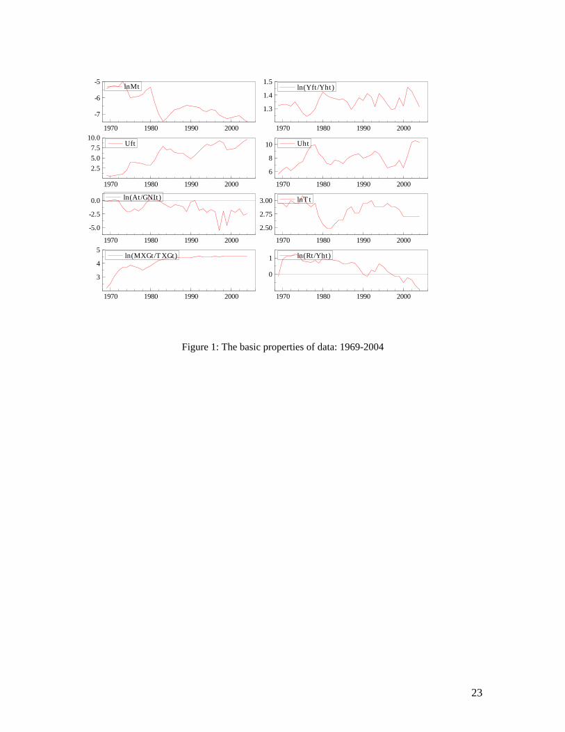
1970 1980 1990 2000

-7

-6

-5lnMt

1970 1980 1990 2000

1.3

1.4

1.5ln(Yft /Yht)

1970 1980 1990 2000

2.55.07.5

10.0Uft

1970 1980 1990 2000

6

8

10 Uht

1970 1980 1990 2000

-5.0

-2.5

0.0 ln(At/GNIt)

1970 1980 1990 2000

2.50

2.75

3.00 lnT t

1970 1980 1990 2000

3

4

5ln(MXGt/T XGt)

1970 1980 1990 2000

0

1 ln(Rt/Yht)

Figure 1: The basic properties of data: 1969-2004

23

1970 1980 1990 2000

-0.5

0.0

DlnMt Fitted

1970 1980 1990 2000

-1

0

1

r:DlnMt (scaled)

1 2 3 4 5 6 7

-0.5

0.0

0.5

1.0ACF-r:DlnMt

-0.2 -0.1 0.0 0.1 0.2

2

4

6

Densityr:DlnMt N(s=0.0788)

Figure 2: Actual and fitted values of migration model from Equation (4), residuals, the histogram and estimated density of the residuals and their correlogram.

24

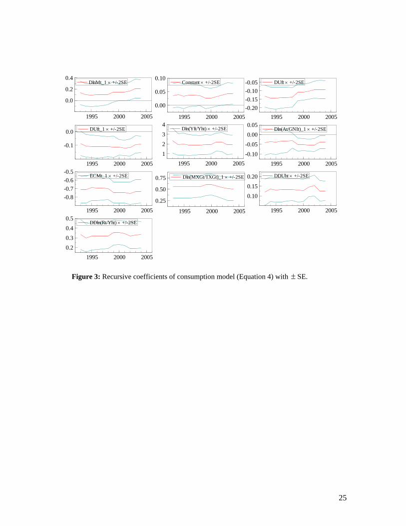
1995 2000 2005

0.0

0.2

0.4DlnMt_1 × +/-2SE

1995 2000 2005

0.00

0.05

0.10Constant × +/-2SE

1995 2000 2005-0.20-0.15-0.10-0.05 DUft × +/-2SE

1995 2000 2005

-0.1

0.0 DUft_1 × +/-2SE

1995 2000 20051234

Dln(Yft/Yht) × +/-2SE

1995 2000 2005-0.10-0.050.000.05

Dln(At/GNIt)_1 × +/-2SE

1995 2000 2005

-0.8-0.7-0.6-0.5

ECMt_1 × +/-2SE

1995 2000 2005

0.25

0.50

0.75 Dln(MXGt/TXGt)_1 × +/-2SE

1995 2000 2005

0.100.150.20 DDUht × +/-2SE

1995 2000 20050.20.30.40.5

DDln(Rt/Yht) × +/-2SE

Figure 3: Recursive coefficients of consumption model (Equation 4) with SE. ±

25

1995 2000 20051.01.52.02.5 t: DlnMt_1

1995 2000 2005

1.501.752.002.25

t: Constant

1995 2000 2005

-4.5-4.0-3.5 t: DUft

1995 2000 2005

-4

-3

-2 t: DUft_1

1995 2000 2005

4.0

4.5

5.0t: Dln(Yft/Yht)

1995 2000 2005

-3

-2

-1t: Dln(At/GNIt)_1

1995 2000 2005-12-11-10-9 t: ECMt_1

1995 2000 2005

4.0

4.5

5.0 t: Dln(MXGt/TXGt)_1

1995 2000 2005

4

5

6t: DDUht

1995 2000 2005

4.55.05.5 t: DDln(Rt/Yht)

Figure 4: The recursive t-ratios.

26

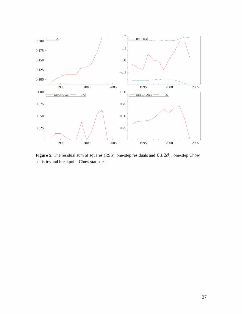
1995 2000 2005

0.100

0.125

0.150

0.175

0.200 RSS

1995 2000 2005

-0.1

0.0

0.1

0.2Res1Step

1995 2000 2005

0.25

0.50

0.75

1.001up CHOWs 1%

1995 2000 2005

0.25

0.50

0.75

1.00Ndn CHOWs 1%

Figure 5: The residual sum of squares (RSS), one-step residuals and tσ20 ± , one-step Chow statistics and breakpoint Chow statistics.

27

Self-Employment of Immigrants in the UK, the U.S.

and Germany∗

Sule Akkoyunlu†and Thorsten Vogel‡

5 December 2007

Abstract

Using several large micro data sets this paper studies self-employment

decision in the U.S., the UK and in Germany, focusing in particular on

differences between native-born persons and immigrants. In a reduced-

form framework we decompose differences in self-employment rates into

age and skill effects and an unexplained (cultural) component. As a

methodical innovation we employ a novel non-parametric decomposi-

tion technique in addition to standard parametric techniques. In a

more structural set-up we let self-employed be determined by pull,

push, and cultural components. To this end separate earnings func-

tions for self-employed workers and employees are estimated, also tak-

ing into account endogenous sorting into self-employment or salaried-

employment (which are found to be significant). The paper also com-

pares self-employment of first and second generation immigrants and,

using the German data, also employment decisions of naturalised im-

migrants and of Aussiedler.

Keywords: International Migration; Self-employment; Self-selection;

Non-parametric decomposition.

JEL Classification: C13; C14; E24; F22

∗The research reported in this paper was financially supported by the European Union

within the context of the FEMISE program. The contents of this paper are the sole

responsibility of the authors and do not reflect the opinion of the European Union.†Department of Economics, Bilkent University; DIW Berlin. Email:

sakkoyunlu@diw.de.‡Department of Economics, Humboldt-Universitat zu Berlin. Email:

vogeltho@staff.hu-berlin.de.

1

1 Introduction

Self-employment is a route out of underprivileged social circumstances which

can be particularly attractive for social groups, such as migrants, who have

to deal with resentments and poorer matches on the market for salaried-

employed labour, i.e. employees. Moreover, in most Western countries

migrants face higher unemployment rates and for unemployed migrants

or migrants running the risk of becoming unemployed self-employment of-

fers an obvious alternative to salaried employment (see, e.g. Constant and

Zimmermann 2004). Self-employment thus also offers a way to integrate into

the economy of the host country even if it should be relatively difficult for

immigrants to find jobs. The present paper describes the evolution of self-

employment rates in the United States, the United Kingdom and Germany

and depicts differences in self-employment rates of native-borns and immi-

grants. We describe how much of these differences are due to a standard set

of factors affecting employment and incomes and measure the importance

of push and pull components. Here push components are factors that in-

duce individuals to start their own business because they find it difficult to

integrate into the job market, while pull components are factors that lure

people away from salaried- and into self-employment.

There are strong arguments why immigrants are expected to be more

often self-employed than native-born workers. Due to the fact that immi-

grants have taken the risk of moving abroad, one would expect that they

are a strongly selected group of motivated and risk-loving workers. Both

of these attitudes should prove to be advantageous for self-employed work.

Other circumstances of immigrants are also expected to lead to higher self-

employment rates of immigrants. Often immigrants have larger families than

natives and therefore have to some extent access to cheap labour helping out

in small businesses. Similarly, in ethnic enclaves immigrants can be stronger

integrated into the neighbourhood which can ease the recruitment of trusted

personnel (Borjas 1986, Lazear 1995). There, natives have the comparative

advantage to know the local product markets and the demand for certain

‘exotic’ niche products which they can then serve (Light 1984). Religious

believes can further entrepreneurial activity and thus lead to higher self-

employment rates of immigrants (Light 1984, Rafiq 1975). On the other

hand are those obstacles to a successful integration into the market for em-

2

ployees, such as language deficiencies and lack of education or training, also

harmful for a successful operation of the own business.

As theory is somewhat inconclusive about whether immigrants should

be more or less likely to be self-employed than natives, the present paper

is mainly descriptive. Table 1 reports self-employment rates of native and

immigrant men in the U.S., the UK and (West-)Germany in 1995 and 2005

(we describe our data and classification of immigrants in some detail below).

We find that the overall differences in self-employment rates of natives and

immigrants are relatively small. In the U.S. and in Germany immigrants in

total are slightly less often self-employed than natives, while in the UK it

is the opposite. Moreover, there is no clear trend that this gap is closing

or widening. However, when taking a closer look at the main immigrant

groups there are dramatic difference between these three countries. The by

far dominant immigrant group in the U.S. comes from Mexico and in 2005

only 7 percent of Mexican men were self-employed, while around 13 percent

of native men were. The picture in Germany is comparable. There the

main immigrant group comes from Turkey and only 8 percent of Turkish

men were self-employed which contrasts strongly with a self-employment

rate of 15 percent of native men. As noted, in the UK immigrants are more

often self-employed than natives and this mainly stems from the high self-

employment rates of the dominant immigrant group in the UK which is from

the Indian sub-continent (India, Pakistan, Bangladesh). In the UK around

16 percent of native-born men were self-employed in 2005, while 21 percent

of immigrants from the Indian sub-continent were.

Table 1 also reports self-employment rates in the host country of the main

immigrant groups in the three countries under scrutiny, as reported by the

International Labour Office (ILO). In all three cases self employment rates in

the sending countries are much higher than those in the host countries. For

example in 2005 around 32 percent of men in Mexico were self-employed, 52

percent in Pakistan (data for India is unavailable from ILO), and 38 percent

in Turkey. As one could expect from the strong agricultural sector in all

these three countries, self-employment rates there are much higher than

in the industrialised receiving countries. The table shows, however, that

even when excluding the agricultural sector self-employment rates are still

considerably higher than that of men of the same ethnic group in their host

country (for further discussion of the association between self-employment

3

Table 1: Self-employment rates in a cross-section of countries

U.S. UK Germany1995 2005 1995 2005 1995 2005

Natives .14 .13 .18 .16 .12 .15

Immigrants .12 .11 .22 .19 .09 .14(percent of population) 11.3 18.3 7.7 12.2 11.0 12.1

main immigrant groupcountry/region of origin Mexico Indian Sub-Continent Turkey

.06 .07 .25 .21 .05 .08(percent of immi-grant population)

34.2 35.9 21.3 21.2 30.7 26.0

for comparison: self-employment rate in country of originall industries .36 .32 .57∗ .52∗ .47 .38excl. agriculture .28 .26 .39∗ .37∗ .29 .27

Note: Men aged 25-54. Self-employment rates refer to full-time employed males only.Weights used as provided in these census data. See section 2 for a detailed description ofthe data used to compute figures for host countries. Data for sending countries are from thewebsite http://laborsta.ilo.org of the International Labour Office (ILO). Notice ILOfigures are based on a slightly different selection of the sample; it includes also men below25 and above 54 and does not exclude men working part-time. Unpaid (or contributing)family workers are excluded. ∗ Data for India are unavailable. Data therefore refer toPakistan only.

rates of immigrants in host and sending country see also Yuengert 1995,

Light 1984, Fairlie and Meyer 1996).

The present study attempts to shed some light on the reasons that un-

derlie the observed differences in aggregate self-employment rates of na-

tives and immigrants. We follow two different routes. First, we model self-

employment decisions in a very reduced form where the self-employment de-

cision is simply modelled as a function of age, skill and a cultural component.

Our interest will be in the counterfactual self-employment rate, had immi-

grants had the same age and skill distribution as natives. We estimate these

counterfactual self-employment rates employing both a parametric and, as

a methodical innovation, a non-parametric estimation procedure.

We find that self- and salaried-employed workers (employees) have a com-

parable skill structure but self-employed workers are significantly older than

employees. Since immigrants are much younger than natives, differences in

education and, in particular, in age are found to explain a considerable ex-

4

tent of the differences in aggregate self-employment rates. Moreover, results

of the parametric and non-parametric estimations sometimes differ consider-

ably. Using these differences as a very rough specification tests, the evidence

presented in this paper casts some doubts on the standard (parametric)

model employed in this literature (see, among many others, Constant and

Schachmurove 2003, Constant, Schachmurove and Zimmermann 2005, Bor-

jas and Bronars 1989, Clark and Drinkwater 1998).

Second, in a structural set-up we model self-employment decisions to be

driven by pull, push and cultural components (see also Clark and Drinkwater

2000). Pull components are factors that provide incentives for individuals

to become self-employed. In this study the main pull component will be

the expected income difference in both types of employment. Both natives

and immigrants are expected to choose this job that yields higher incomes

(Rees and Shah 1986, Borjas and Bronars 1989, Bernhardt 1994, Lofstrom

2002). Thus, the pull component induces an incentives for immigrants to

turn more often to self-employment than natives if the income difference

between the income when self-employed and the earnings when salaried-

employed is higher for immigrants than for natives. This is in particular

the case if immigrants are disadvantaged as employees but not so much

when working on their own account (Light 1972, Light 1979, Sowell 1981,

Moore 1983); for instance, because their skills are not highly rewarded as

employee but as self-employed workers or because language problems pose a

big problem for finding the right job as employee, while this may be relatively

unimportant if setting up the own business (see also Lofstrom 2002, Borjas

1986).

Push components capture that self- or salaried employment opportuni-

ties might be limited. For instance, if unemployment rates are high finding

or switching jobs is difficult which then makes the option of starting the

own business more attractive. Finally, immigrants groups also have some

common cultural idiosyncrasies. Immigrants may belong to specific religious

groups that favour entrepreneurship or may have migrated from countries

with strong traditions of self-employment. Quite generally, immigrants can

be expected to be strongly self-selected and, since they have taken the risk of

migration, are probably more willing to bear entrepreneurial risks. On the

other hand, exactly because of their selectivity there can also be a breach of

tradition favouring, as argued, self-employment which would then dampen

5

positive self-selectivity effects into self-employment. All these factors are

subsumed under the term “cultural components”.

We find that in Germany (the U.S. and the UK data do not contain in-

formation of incomes of the self-employed) between 6 and 30 percent of the

explained variation in the data is explained by the cultural component when

comparing natives and immigrants. Then in fact push and pull components

are equally strong and have a stronger explanatory effect than cultural com-

ponents. If however we compare natives with several different immigrant

groups the relative explanatory power of push and pull components declines

considerably and then between 60 and 90 percent of the explained variation

in the data is due to cultural components.

The paper is structured as follows. The next section describes the data

sets and the sample used in the analysis. Section 3 uses a very reduced-

form model to compute counterfactual self-employment rates for immigrants.

There we also introduce a novel non-parametric method to compute coun-

terfactual distributions and compare these results with standard parametric

set-ups. Section 4 estimates a structural model of self-employment, decom-

posing differences in self-employment rates of natives and immigrants into

push, pull, and cultural components. Section 5 summarises the main find-

ings and concludes.

2 Data Description and Sample

The data used in our analysis comes from the large labour force surveys

(LFS) in the United States, the United Kingdom and Germany. These are

respectively the CPS, the British and Northern Ireland Labour Force Survey

and the Mikrozensus. These surveys are particularly suited to study eco-

nomic outcomes of immigrants, such as self-employment, due to the large

sample size. This allows the researcher to employ less strong parametric as-

sumption when decomposing the variation in the data, even when analysing

smaller immigrant populations. Moreover, data on the type of economic

activity of the respondent are fairly well standardised which allows for a

cross-country comparison as the present paper pursuits. All three survey

cover a wide range of aspect of the labour market.

Identification of immigrants in the three labour force surveys used in

this study differs considerably. While in Germany the discussion about

6

immigrants largely centres around the ethnic origin of the migrants, in the

UK and the U.S. people born in the host country are considered to be natives

—which may has to do with the fact that they automatically become citizens

of the host country if they are born there, in contrast to the regulations

in Germany—and therefore information about the country of origin (alias,

country of birth) is used to identify immigrants. The UK LFS has asked

households about their country of origin from its beginning in 1973. In the

U.S. question on the country of origin were only included in the survey in

1994. The Mikrozensus does not contain information about the country of

origin but instead reports citizenship. We use the available scientific-use files

of the Mikrozensus 1989-2004 as well as the recent Mikrozensus 2005 data

file. In particular the Mikrozensus 2005 is very well suited to our research

project as it contains detailed information about the migration background

of each person (though still not the country of birth).1 Subsequently, we

will use this additional information in the Mikrozensus 2005 to take a closer

look at the performance of second-generation and naturalised immigrants

in Germany. Below we will be more specific about our strategy to identify

second-generation immigrants in the U.S. and Germany (the UK LFS does

not allow their identification).

A peculiar feature of immigration to Germany is the large inflow of eth-

nic Germans who migrated to Germany mainly from Poland and the former

USSR (so-called Aussiedler and, since 1990, Spataussiedler). Even though

the government collects data about their total inflow, Aussiedler basically

vanish from most data sources (surveys as well as administrative data sets)

as they have German citizenship. The recently published Mikrozensus 2005

allows to identify Aussiedler reasonable well. Up to 1999 Aussiedler were

officially naturalised and the Mikrozensus 2005 contains information about

the year of immigration, information about naturalisation and the citizen-

ship prior to naturalisation can also be used. This identification strategy

is of course not without pitfalls. First, many Aussiedler have always con-

sidered themselves as native Germans and will therefore not report their

official naturalisation. Second, the (modest) inflow of Spataussiedler after

1999 remains invisible in our data.

1The Mikrozensus of other years than 2005 only contains the citizenship of each re-spondent. Answering other questions like ”year of immigration” or ”born in Germany”were either optional or only asked to people with only a foreign citizenship (as with theformer question) or were not asked at all (as with the latter question).

7

One drawback of all three surveys is that they only provide limited infor-

mation regarding a person’s labour earnings. Notwithstanding the quite gen-

eral problem to distinguish capital and labour incomes of the self-employed,

neither the CPS-ORG data nor the UK LFS contain any information at all

about income of the self-employed. In contrast, the German Mikrozensus

reports the net income of both salaried- and self-employed workers. Using

the provided information about the number of hours usually worked per

week, this actually allows to compute an hourly measure for net income.

The main problem with the income variable in the Mikrozensus, however,

is that incomes are reported net of taxes and benefits. On the one hand,

this may actually increase the accurateness of the reported earnings of the

self-employed as these worker often have ample opportunity to avoid taxes

and after all people are pulled into self-employment because of higher net

incomes, not of incomes before taxes. On the other hand, earnings profiles

of net and gross incomes cannot be compared which would make it diffi-

cult to compare, say, age-earnings profiles from the Mikrozensus with those

obtained from other data sources. More importantly, one needs to be very

careful when comparing incomes of married and unmarried workers (which

poses a problem if the spouse does not work at all or has a significantly dif-

ferent income) and of incomes of persons with children as married workers

and people with children receive a beneficial tax treatment.

Our focus in this paper is on males aged between 25 and 54.2 We only

study men because, independent of their cultural background, men partici-

pate in the labour market at very high rates and the attention of this paper

is on what people do when participating, not on whether participating at

all. The age requirement is to ascertain that people are out of education

and not yet in retirement or early-retirement schemes. Finally, our analysis

of differences in self-employment rates and differing incomes of salaried- and

self-employed workers only uses observation of workers who report to work

full time. With respect to the German data, only observation from West

Germany (including Berlin) are kept to avoid confounding the results by the

various adjustment processes in East Germany. Due to the extremely low

numbers of immigrants in East Germany, the consequences for this omission

2When computing the density of the age-skill distribution of the base group (natives),we actually use all men aged 20-60 in order to obtain more precise estimates at theboundaries of the age interval 25-54.

8

seem well justified.

Timing and patterns of immigration into the U.S., the UK and Germany

are very different and, correspondingly, the composition of the immigrant

population is quite different ([ Dustmann, Glitz and Vogel 2007)for details

see. Table 2 reports the composition of the immigrant population in the

three countries. By far the largest immigrant group in the U.S. are the

Mexicans (36 percent of all immigrants in 2005) and in Germany the Turks

(29 percent). In the UK the largest fairly homogeneous immigrant group

comes from the Indian sub-continent (21 percent). Notice that there is also

a remarkably large share of immigrants from Africa which we however do

not consider as the main sending region of immigrants to the UK because

these immigrants come from many different and apparently very diverse set

of countries and thus can be expected to form a very heterogeneous group

of people.

2.1 Individual Characteristics

Table 3 compares some key characteristics such as education and age of

natives and immigrants as well as of salaried- and self-employed workers

in the U.S., the UK and Germany. The table provides insight into several

regularities regarding self-employment. First, there is no clear indication

that self-employed workers are in general higher educated than are employ-

ees. In the UK, actually, the percentage of self-employed men with higher

education is ten points lower than that of salaried employed. Differences

in the skill distribution hence cannot be expected to contribute much to an

understanding of differences in self-employment rates. Second, again with

the exception of the UK, immigrants are in general less educated than na-

tives. Third, the age structure of self-employed men is significantly different

from that of the salaried-employed. Figure 1 plots the age structure of both

salaried and self-employed men which clearly shows that the self-employed

are much older than the salaried-employed. The percentage of self-employed

men in the upper half of the age interval (25, 54) is 66 in the U.S., 58 in the

UK and 63 in Germany, to be compared with the percentage of salaried-

employed men above 40 which is 51 in the U.S., 48 in the UK and 53 in

Germany. Since, fourth, immigrants in all three countries are significantly

younger than natives, these differences in age structures can contribute to

explaining the observed differences in self-employment rates. How much

9

Table 2: Immigrant composition in a cross-section of countries

U.S. UK Germany1995 2005 1995 2005 1995 2005

Mexico 34.2 35.9 Africa 21.0 21.6 Turkey 30.7 26.0Indian sub-continent 3.3 5.9 Indian sub-continent 21.1 21.2 ex-Yugoslavia 15.8 12.0China/Taiwan 3.6 4.3 Ireland 11.4 4.5 Italy 11.3 11.4Philippines 3.5 3.1 Germany 4.3 4.3 Greece 6.3 5.2other OECD 16.0 10.2 other OECD 20.7 24.0 other OECD 19.8 21.9other non-OECD 39.4 40.6 other non-OECD 21.5 24.4 other non-OECD 16.2 23.5

Men aged 25-54 participating in the labour market (i.e., for instance, excluding asylum seekers and refugees). Weights usedas provided in the data. For the U.S. and the UK the listed set of countries or geographic regions are countries or regions oforigin. For Germany they refer to a persons citizenship. Countries sorted by percentage in 2005.

10

Table 3: Individual characteristics of natives and immigrants as well as ofsalarried- and self-employed workers, year 2005

Education Agelow medium high mean ≥ 40 (in %) #

U.S.

Natives 6.5 51.5 42.0 40.2 .55 64,950Immigrants 31.8 34.6 33.6 38.2 .44 11,181Mexico 61.6 32.4 6.0 36.3 .34 3,746

Salaried-employed 10.2 48.4 41.4 39.6 .51 63,240Self-employed 7.9 50.6 41.5 42.4 .66 10,118

UK

Natives 9.4 58.4 32.2 39.6 .51 27,070Immigrants 14.0 54.4 31.7 37.9 .41 3,944Indian sub-continent 25.0 48.8 26.3 38.2 .43 861

Salaried-employed 8.6 57.0 34.4 39.1 .48 24,364Self-employed 12.9 61.9 25.3 41.2 .58 5,264

Germany

Natives 13.3 67.2 19.5 40.5 .55 69,633Immigrants 46.2 39.9 14.0 37.7 .40 7,089Turkey 63.6 33.0 3.4 36.2 .34 2,033

Salaried-employed 14.5 66.4 19.1 40.1 .53 59,152Self-employed 12.2 61.7 26.1 41.9 .63 9,960

Men aged 25-54 participating in the labour market. Unweighted descriptive statistics. Inthe U.S. low education means less than completed High School, medium refers to completedHigh School and possibly some years of College, while high education implies a Collegedegree. In the UK data low education is identical no qualication, medium education meansA-levels and less, high education comprises higher education and university degree. Inthe German data people without completed apprenticeship or university education aresaid to have low education, with a completed apprenticeship to have medium education,and if completed university to have high education. Sums of natives and immigrants isgreater than some of salaried- and self-employed workers because for some observationsself-employment status is unknown.

11

25 30 35 40 45 50 55

0.00

0.01

0.02

0.03

0.04

0.05

dens

ity

U.S.

25 30 35 40 45 50 55

0.00

0.01

0.02

0.03

0.04

0.05

UK

25 30 35 40 45 50 55

0.00

0.01

0.02

0.03

0.04

0.05

age

dens

ity

Germany

salaried−employedself−employed

Figure 1: Age distribution of salaried- and self-employed men in 2005.Curves smoothed by moving averages over the two closest age groups.

12

these differences in the skill and, most notably, the age structure in fact

do explain the differences in self-employment rates is studied in the next

section.

3 Decomposing the Differences in Self-Employment

Rates: parametrically and non-parametrically

1990 1995 2000 2005

−0.05

0.00

0.05

0.10

diffe

renc

es in

sel

f−em

ploy

men

t rat

es

U.S.

1990 1995 2000 2005

−0.05

0.00

0.05

0.10

UK

1990 1995 2000 2005

−0.05

0.00

0.05

0.10

year

diffe

renc

es in

sel

f−em

ploy

men

t rat

es

Germany

nonparametricactualparametric

Figure 2: Differences in self-employment rates of immigrants and natives inthe U.S., the UK, and Germany.

The solid black line in Figure 2 shows the differences in self-employment

rates of immigrants and natives between 1989 and 2005 in the U.S., the

13

UK and Germany (in the U.S. between 1994 and 2005). Black dotted lines

indicate (pointwise) 95% confidence bands, obtained by taking 400 boot-

straps. Probably, the most noteworthy aspect of these graphs is that self-

employment rates of immigrants in the U.S. and Germany are smaller, while

in the UK they are larger than those of natives. In the U.S. there is a slight

trend toward increasing differences in self-employment rates while in the UK

and in Germany self-employment rates of immigrants become increasingly

similar to those of natives. For instance, in the most recent years differences

in self-employment rates are not any more statistically significantly different

from zero.

3.1 Decomposition methods

We next perform two different types of decompositions to analyse how much

of these differences, if anything, can be explained by differences in the skill

and age structure of immigrants and natives. The questions we try to answer

here is how large would have been the difference in self-employment rates,

had the immigrants had the same skill and age structure as natives. The first

decomposition is parametric in that for each year we estimate a standard

probit model

P [self-employedi] = Φ (single indexi)

where Φ (·) denotes the Gaussian distribution function. The single index is

specified as follows:

single indexi = Foreigni + Polyn(agei, 4) + Educationi (1)

where Foreigni and Educationi are set of dummy variables indicating im-

migrant status and education of person i. To take care of age effects we allow

for a polynomial in age of order 4. We then use the estimated probit model

to predict the self-employment rates of immigrants and natives in each of

the 30× 3 age-education cells. Finally, we use a non-parametric estimate of

the age and education distribution of natives (see the detailed description

below) to answer the question what would have been the self-employment

rate difference, had the immigrants had the same age and education distri-

bution as natives.3 This estimation procedure was executed separately for

3Equivalently, one can predict the probability for each person in the data and then re-weight immigrants such that after averaging over all 30×3 cells the adjusted average skill

14

each year. The solid red line in Figure 2 depicts the estimated difference

and the red dashed line the bootstrapped confidence bands.

Our second decomposition method is completely non-parametric. Ob-

serving the large number of observations in our sample (see Table 3), in

fact allows us to follow a different route to estimate the self-employment

rates of natives and immigrants for each of the 30 × 3 age-education cells,

thus avoiding the problem that the probit model used in the previous de-

composition may be misspecified (i.e., misspecification of either the linear

specification, the link function, or the functional form of equation 1). Again,

separately for each year we estimate first the density of age and education

levels of the natives. That is, for each year we estimate non-parametrically

the probability to become self-employed,

P [self-employedi] = f (agei,Educationi,Foreigni)

where no assumptions are made about the functional form of f (·). More

specifically, separately for each year and each immigrant group we apply a

local-constant smoother to the self-employment status (1 if self-employed, 0

if salaried-employed) to regress self-employment status on age and education.

This gives us for each immigrant group and each age and education cell an

estimate of the respective self-employment rate.

Due to the rapidly increasing variance of such estimates when the sam-

ple size decreases, which happens when analysing small immigrant popula-

tions, we use a kernel estimator for mixed data types to limit the curse-of-

dimensionality problem. In our setting one of the regressors is a continuous

variable (age) while the other is discrete (education levels). The idea be-

hind a kernel estimation with mixed types is not only to use observations in

nearby age cells but also observations in other education cells. In fact, since

education is an ordered variable (low<medium<high) a suitable kernel (for

instance, the Wang and van Ryzin kernel) uses also observations of persons

with, say, medium education to estimate the self-employment rate of persons

of, say, low education (which are, of course, given a lower weight). Since ed-

ucation is an ordered discrete variable, observations of persons with higher

education are given however considerably lower weights than observations

of medium-skilled individuals, simply because higher education can be said

distribution is identical with that of natives. This procedure however has no computationalor statistical advantages.

15

to be farther away, and hence less informative, from low education than

medium education is (for a detailed discussions of these non-parametric ker-

nel methods see Li and Racine 2007). Bandwidths are selected using least

squares cross-validation.4

To compute differences in self-employment rates of immigrant group we

need to aggregate over all age-education cells. We therefore estimate the

density of the age and education distribution of the natives using a standard

non-parametric estimator and, due to the large sample size, the standard

plug-in value for the bandwidth. Thus, each age-education cell is weighted

with the share of natives of this particular age and education.

Finally, our non-parametric decomposition method using kernel estima-

tion of mixed data is comparable to the semi-parametric decompositions

introduced by DiNardo, Fortin and Lemieux (1996) in that they use pro-

bit scores to weight observations by their likelihood to be part of a certain

group, while here we use a suitable kernel to lift the curse of dimensionality.

3.2 Results

Natives vs Immigrants As it turns out, at least in the UK the pre-

dictive power of the first, parametric decomposition to explain the observed

differences in self-employment rates is extremely limited. In the UK the self-

employed are less likely to have higher education but immigrants in total

are about as well educated as natives. This should male the predicted dif-

ference actually larger than what is observed in the data. However, the age

distribution of immigrants works in the other direction, as immigrants are

younger than natives but the likelihood to be self-employed increases with

age. In Germany and the U.S., however, the probit model does explain to a

significant extent the observed differences in self-employment rates. In Ger-

many, for instance, one could not even reject any more the hypothesis that

both groups actually have equal self-employment rates once we condition of

age and education effects in the described way.

4The computation of the bandwidth is extremely computationally expensive. On afairly recent PC it takes almost three weeks to compute the bandwidth for a sample ofsize 70,000. We therefore estimate bandwidths, though separately for each data set, onlyfor the year 2000 and then apply these bandwidths for all years. In light of the fairlyconstant sample size across years this procedure seems innocuous. Bandwidth selectionand non-parametric regression was done using the ”np”-package for the R programmingenvironment (Hayfield and Racine 2007).

16

The solid blue lines show the results of the non-parametric decompo-

sitions. Probably for the same reasons put forth earlier, also the non-

parametric decomposition of age and education effects does not explain

the higher self-employment rates of immigrants in the UK. In both Ger-

many and the U.S., however, the computed counterfactual self-employment

rate differences are significantly lower than the previous standard probit

decomposition would suggest. In fact, as it turns out, according to the

non-parametric decomposition the hypothesis that self-employment rates of

natives and immigrants are identical could not be rejected at the 5-percent

level in Germany at least since the mid-1990s. In Germany and the U.S. at

least the non-parametric decomposition of this section shows quite strongly

this hypothesis’ feet of clay.

Detailed immigrant groups We next turn to the decomposition of dif-

ferences in self-employment rates between natives and the largest groups of

immigrants, which are Mexicans in the U.S., immigrants from the Indian

sub-continent in the UK, and Turks in Germany. Figure 3 illustrates ob-

served and counterfactual differences in self-employment rates for the Mex-

icans in the U.S., the Turkish in Germany and the people from the Indian

sub-continent in the UK. In the U.S. Mexicans are found to have much lower

self-employment rates than U.S.-born persons. Although this difference de-

creased slightly over the years 1994-2005, in 2005 the self-employment rate

of Mexicans was still around 6 percent below that of natives. Conditioning

on age and skill effects we see that differences in observables such as age and

education account for less than 2 percentage point of this difference (around

one quarter of the observed differences) and thus leave most of the observed

difference unexplained.

In the UK the strongest immigrant groups is from the Indian sub-

continent. Due to the small sample size estimated self-employment rates

vary quite a bit from year to year but it is clear from figure 3 that im-

migrants from the Indian sub-continent are significantly more often self-

employed than native-born British men. Moreover, since they have a rela-

tively similar skill and age structure as natives, it comes as no surprise that

correcting observed self-employment rates for differences in the age and skill

structure hardly matters.

In Germany, by contrast, the situation of the largest immigrant group,

17

1990 1995 2000 2005

−0.10

−0.08

−0.06

−0.04

−0.02

0.00

diffe

renc

es in

sel

f−em

ploy

men

t rat

es

Mexico

1990 1995 2000 2005

0.00

0.05

0.10

0.15

Indian sub−continent

1990 1995 2000 2005

−0.10

−0.05

0.00

0.05

year

diffe

renc

es in

sel

f−em

ploy

men

t rat

es

Turkey

nonparametricactualparametric

Figure 3: Differences in self-employment rates of the main group of immi-grants and natives. Notice the differences in scale.

the Turkish, is comparable to that of the Mexicans in the U.S. Self-employment

rates of Turkish men in Germany are between 5 and 8 percentage points

lower than that of German men. Since Turkish immigrants in Germany are

relatively young correcting self-employment rates for skill and age effects has

a sizeable effect. In fact, for both the parametric and the non-parametric

decomposition age and skill effects are found to explain roughly half of the

observed differences.

Comparing these findings in self-employment rate differences with the

observed self-employment rates in the respective sending countries (see table

1), it remains puzzling why these three immigrant groups perform so differ-

18

ently in the host countries. In all three sending countries self-employment

rates are much higher than in the host countries, both in the strong agri-

cultural sector but also in manufacturing and service sectors. However,

only immigrants from the Indian sub-continent also have relatively high self-

employment rates in the receiving country, while self-employment rates of

Mexicans and Turks are actually below that of natives, even after correcting

for age and skill effects.

4 The Impact of Push and Pull Components

The analysis in this section is complementary to that of section 3. In the

previous section difference in self-employment rates of natives and immi-

grants were explained in a very reduced form only by differences in the age

and education structure. The present section presents and estimates a more

structural model that is, first, richer in regressors and, second, more explicit

in how age and education actually enter the decision making process of in-

dividuals facing the two options of working on their own account or as an

employee. As data about income or earnings of self-employed workers are

not contained in the American CPS-ORG or the British LFS, this section

focuses exclusively on Germany. Moreover, we only use data from the lat-

est Mikrozensus 2005 because for previous years only the scientific-use files

of the Mikrozensus were available to us and these do not contain detailed

regional information which in our estimations, however, plays an important

role as exclusion restriction.

Quite generally, three different components of explanatory factors can

be distinguished: push and pull components and cultural factors. The goal

of this section is to decompose the observed differences in self-employment

rates into these three components and to identify the impact (analysis-of-

variance) of each. To this end we estimate a probit model

P [self-employedi] = Φ (pull componenti + push componenti + cultural factorsi)

(2)

Pull components are those factors that induce individuals to set up their

own business. Conditional on personal characteristics such as risk aversion,

entrepreneurial spirit or on factors such as financial endowment and given

the fact that persons actually have the option to start working in either self-

19

employment or in salaried-employment, the pull components should be the

key determinant of the self-employment status. Our main pull component is

the income difference individuals face when making the decision to become

self- or salaried-employed. Push components in contrast are factors that

capture the limited availability of one type of work. If salaried-employment,

for instance, is difficult to find, which may be proxied by a high unemploy-

ment rate, self-employment becomes increasingly attractive. On the other

hand, enclaves can make it easier to start one’s own business if an indi-

vidual is well integrated in his local community where customers are loyal

and tend to buy at shops where the own foreign language is spoken and

the shopkeeper has a similar family background. Finally, cultural factors

should capture unexplained economy wide differences between immigrants

groups. These could be due for instance to religious denomination, a culture

that rewards entrepreneurship and the like. Notice however that some push

and pull components cannot be identified and their impact will therefore

fall under the cultural components. These could be, for instance, economy

wide differences in the unemployment rates of natives and immigrants. In

principle these differences should enter the push component but due to the

lack of identification, they enter the (cumulative) cultural factors.

4.1 Sample

The sample in this section consists of all self- and salaried employed men

in the Mikrozensus 2005 who are between 25 and 54 years old and are

working full-time. Importantly, with the exception of the computation of

regional unemployment rates we only use observations of men who report

that their main source of income is employment (in contrast to benefits,

pensions, capital income, support by other family members etc.). When

computing hourly incomes we divide the monthly income by 4.35 times the

hours usually worked per week.5 Immigrants groups in this section are dis-

tinguished again by their citizenship where all men with a German passport

are considered to be German, irrespective of whether or not they have been

naturalised. Notwithstanding the different tax treatment of married and

single men in Germany, we keep both types of men since otherwise native

5There is a very small number of individuals (less than half a percent) reporting towork less than 20 or more than 80 hours per week. We drop the former as they appearunreliable and recode the latter to 80 for convenience.

20

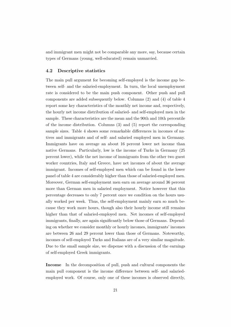
and immigrant men might not be comparable any more, say, because certain

types of Germans (young, well-educated) remain unmarried.

4.2 Descriptive statistics

The main pull argument for becoming self-employed is the income gap be-

tween self- and the salaried-employment. In turn, the local unemployment

rate is considered to be the main push component. Other push and pull

components are added subsequently below. Columns (2) and (4) of table 4

report some key characteristics of the monthly net income and, respectively,

the hourly net income distribution of salaried- and self-employed men in the

sample. These characteristics are the mean and the 90th and 10th percentile

of the income distribution. Columns (3) and (5) report the corresponding

sample sizes. Table 4 shows some remarkable differences in incomes of na-

tives and immigrants and of self- and salaried employed men in Germany.

Immigrants have on average an about 16 percent lower net income than

native Germans. Particularly, low is the income of Turks in Germany (25

percent lower), while the net income of immigrants from the other two guest

worker countries, Italy and Greece, have net incomes of about the average

immigrant. Incomes of self-employed men which can be found in the lower

panel of table 4 are considerably higher than those of salaried-employed men.

Moreover, German self-employment men earn on average around 36 percent

more than German men in salaried employment. Notice however that this

percentage decreases to only 7 percent once we condition on the hours usu-

ally worked per week. Thus, the self-employment mainly earn so much be-

cause they work more hours, though also their hourly income still remains

higher than that of salaried-employed men. Net incomes of self-employed

immigrants, finally, are again significantly below those of Germans. Depend-

ing on whether we consider monthly or hourly incomes, immigrants’ incomes

are between 26 and 29 percent lower than those of Germans. Noteworthy,

incomes of self-employed Turks and Italians are of a very similar magnitude.

Due to the small sample size, we dispense with a discussion of the earnings

of self-employed Greek immigrants.

Income In the decomposition of pull, push and cultural components the

main pull component is the income difference between self- and salaried-

employed work. Of course, only one of these incomes is observed directly,

21

Table 4: Income distribution of natives and immigrants in Germany in 2005

net monthly income net hourly incomeobserved # observed #

EmployeesNatives 2,897 44,629 16.4 44,450

(1,400;4,750) (8.2;25.2)Immigrants 2,426 3,829 13.9 3,815

(1,200;3,800) (6.9;21.8)Turks 2,177 1,137 12.8 1,134

(1,400;3,050) (7.4;18.4)Italians 2,355 447 13.6 444

(1,200;3,400) (6.9;20.0)Greeks 2,451 198 14.5 197

(1,400;3,800) (7.1;22.4)

Self-employedNatives 3,933 6,241 17.6 44,450

(1,400;6,750) (5.9;33.0)Immigrants 2,805 576 12.9 572

(1,000;5,250) (4.9;24.1)Turks 2,586 102 11.9 102

(1,200;4,250) (5.4;19.5)Italians 2,654 101 11.3 100

(1,200;4,750) (4.3;19.8)Greeks 3,408 41 15.3 41

(1,600;6,750) (5.8;31.0)

Note: Average net income of self- and salaried employed men aged 25-54 working full-timewhose main income source is employment. Numbers in brackets are the 10th and 90thpercentile of the respective income distribution. Prices in year 2005 Euros.

the other hence has to be imputed. We therefore estimate a standard Mincer

model

incomei = Polyn (agei, 4) + Educationi + Foreigni + Polyn(Tenurei, 2)

+ Marriedi + Childreni + εi (3)

separately for self- and salaried-employed men and then use this model to

predict the missing income data. In specification (3) Marriedi is unity if

person i is married and zero otherwise. Childreni denotes the number of

children of person i below 18 in their household. Both variables are included

to account for different tax treatment of married individuals and of persons

22

with children. Assuming that the error term εi is uncorrelated with the

covariates, model (3) can be estimated via OLS.

However, if the error term contains an unobserved individual fixed effect

then, first, estimated coefficients were biased if this fixed effects is correlated

with the covariates an, second, predicted income of person i would omit the

individual fixed effect. To account for this possible deficiency we also es-

timate a standard (though far from impeccable) Heckman selection model

where the probit model on the first stage contains all the covariates of specifi-

cation (3) plus the local unemployment rate as an exclusion restriction. The

underlying assumption behind this specification is that the probability to be-

come self-employed is the greater, the higher the local unemployment rate,

while the local unemployment rate does not directly affect wages. Tight-

ness of the labour market as measured by the unemployment rate can be

understood mainly as tightness of the market for salaried-employed workers

because an unemployed worker always has the opportunity to start his own

business (conditional, of course, on his personal traits such as skill, atti-

tude, reliability among others), while it might be impossible to find a job

as a salaried-employed worker. Finally, to justify that local unemployment

does not affect incomes, notice the high union coverage rates of around 60

percent affecting salaried-employed workers in Germany, preventing wages

to deviate strongly among local labour markets. Moreover, incomes of the

self-employed are obviously only very indirectly influenced by local unem-

ployment rates.

Unemployment Overall there are 205 different labour market regions

in West Germany, designed by the Statistisches Bundesamt to reflect geo-

graphic mobility of workers as reported by commuters in previous surveys.

For each of these labour market regions we compute the unemployment

rate (according to ILO) of men aged 25-54. The number of observations

available in Mikrozensus 2005 to compute the regional unemployment rate

ranges between 58 (Wesermarsch) and 4, 082 (Berlin) with an average of 374

observations per region. The unemployment rate varies between 0.02 (Bad

Reichenhall) and 0.21 (Berlin) with a weighted average of 0.09. Thus there

is sufficient regional variation in unemployment rates possibly affecting the

selection into self-employment which then also allows for identification of the

coefficients in the Heckman selection model. However, although the number

23

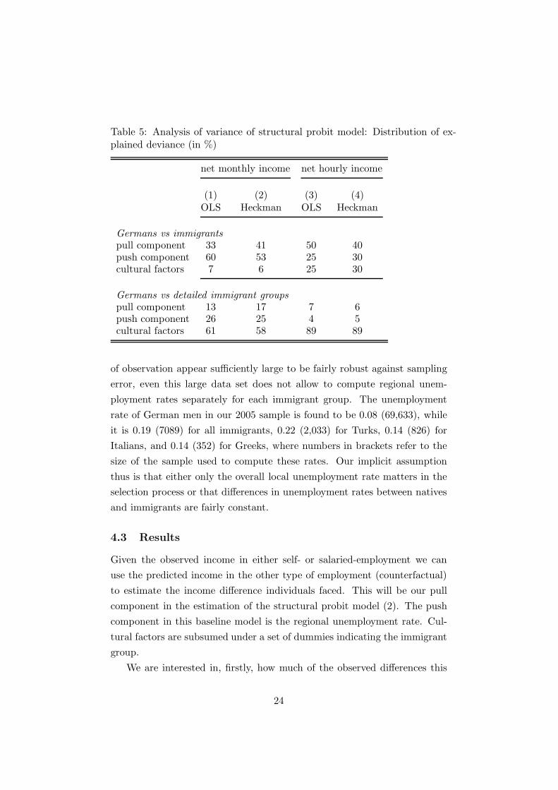
Table 5: Analysis of variance of structural probit model: Distribution of ex-plained deviance (in %)

net monthly income net hourly income

(1) (2) (3) (4)OLS Heckman OLS Heckman

Germans vs immigrantspull component 33 41 50 40push component 60 53 25 30cultural factors 7 6 25 30

Germans vs detailed immigrant groupspull component 13 17 7 6push component 26 25 4 5cultural factors 61 58 89 89

of observation appear sufficiently large to be fairly robust against sampling

error, even this large data set does not allow to compute regional unem-

ployment rates separately for each immigrant group. The unemployment

rate of German men in our 2005 sample is found to be 0.08 (69,633), while

it is 0.19 (7089) for all immigrants, 0.22 (2,033) for Turks, 0.14 (826) for

Italians, and 0.14 (352) for Greeks, where numbers in brackets refer to the

size of the sample used to compute these rates. Our implicit assumption

thus is that either only the overall local unemployment rate matters in the

selection process or that differences in unemployment rates between natives

and immigrants are fairly constant.

4.3 Results

Given the observed income in either self- or salaried-employment we can

use the predicted income in the other type of employment (counterfactual)

to estimate the income difference individuals faced. This will be our pull

component in the estimation of the structural probit model (2). The push

component in this baseline model is the regional unemployment rate. Cul-

tural factors are subsumed under a set of dummies indicating the immigrant

group.

We are interested in, firstly, how much of the observed differences this

24

structural model explains and, secondly, how much the different components

contribute. Table 5 reproduces the differences in self-employment rates be-

tween natives and immigrants in the upper panel and between natives and

Turks, Italians, and Greeks in the lower panel. If the underlying statistical

process is well described by the model, these differences should be repro-

duced when averaging over predicted probit scores.

Next, as in section 3 we re-weight immigrants or immigrant groups so

that their distribution of covariates mimics that of natives. Similar to the

procedure in section 3 we estimate the non-parametrically the density of

push and pull components of natives and immigrants and then re-weight

individual’s predicted probit scores accordingly.

The importance of pull, push and cultural components can be gauged

by analysis of the deviance of model (2). The procedure is similar to a stan-

dard analysis of variance, only that the fit of a binary model should rather

be measured by the reduction in deviance than by the reduction in squared

difference from the mean (see, e.g., Efron 1978, McCullagh and Nelder 1989).

The analysis of deviance in the upper panel of table 5 shows that push and

pull components explain the most of the reduction in deviance when there

is only one dummy in the model to identify immigrants.6 For instance, if

standard OLS is used to impute counterfactual monthly net incomes from

salaried- or self-employment to compute individual income differences, 33

percent of the reduction in deviance of model (2) is due to the pull com-

ponent, i.e., income differences. 60 percent of the reduction of deviance is

however due to the push component, i.e., the regional unemployment rate,

and only 7 percent to cultural factors, i.e., the immigrant indicator.

The picture however looks remarkably different once we distinguish dif-

ferent immigrants groups and introduce six different dummy variables to

distinguish detailed groups of immigrants from different sending countries

or regions. Comparing the results of this model with that of the previously

discussed results, in this more detailed model only 13 percent of the re-

duction in deviance is explained by the pull component, while 26 percent

by the push component and 61 percent by the cultural component. Thus,

in particular the push component remains to be important, while the pull

6In general, the analysis of deviance is sensible to the way the various components areadded unless the components are strictly orthogonal. As it turns out, however, in ourparticular case the results are very robust to changing the order in which components areadded to the model.

25

component appears dispensable.

Once we use differences in the incomes per hour instead of incomes per

month, the effect on the importance of the pull component (income differ-

ence) as explanatory factor is ambiguous, depending on whether we compare

German men with all immigrants combined or with detailed groups of im-

migrants. Comparing Germans with the aggregate group of immigrants the

pull factor explains relatively more if hourly incomes are used. However,

the percentage of the decrease in deviance that is due to the pull component

drops to about half its value once we compare Germans with a set of different

immigrant groups. The general picture though regarding the importance of

cultural factors remains unchanged whether we use differences in hourly or

in monthly incomes as pull factor.

5 Conclusions

Self-employment rates differ across migrants and natives as well as across

countries. Parametric and non-parametric estimations show that for the

UK observed differences for the self-employment rates between immigrants

and natives can not be explained by age and education. However, for the

U.S. and Germany the probit as well as non-parametric model explains the

observed differences for the self-employment rates between immigrants and

natives by age and education. Therefore, for both Germany and the U.S.

we could not reject the hypothesis that both groups actually have equal

self-employment rates once we condition on age and education.

We repeat the exercise for the largest groups of immigrants, Mexicans in

the U.S., immigrants from the Indian sub-continent in the UK, and Turks in

Germany. We find for all three immigrant groups, the observed differences

for the self-employment rates between immigrants and natives can not be

explained by age and education.

We then try to decompose the observed differences in self-employment

rates into three components: pull, push and cultural components and to

identify the impact of each. The pull component in our model is the in-

come difference individuals face when making decision to become self- or

salaried employed. Push component is proxied by the local unemployment

rates in Germany. Cultural factors capture unexplained economy wide dif-

ferences between immigrant groups. Cultural factors subsumed under a set

26

of dummies indicating the immigrant group. Separate earnings equation is

estimated for self-employed and salaried-employed to compute income dif-

ference between self- and salaried-employed work, by taking into account

endogenous sorting into the sectors.

The importance of pull, push and cultural components are gauged by

analysis of the deviance model. The analysis of deviance shows that push

and pull components explain the most of the reduction in deviance when

there is only one dummy in the model to identify immigrants. However, once

we distinguish different immigrant groups, the cultural component becomes

the most important explanatory factor and the push component remains

important, but the pull component appears dispensable. This result shows

that self-employment decision is influenced by ethnic-specific attributes as

well as sectoral earnings differential. However, the detailed cultural factors

that influence the decision to become self-employed are not explored in this

paper. These individual cultural factors are suggested by the theory, but are

not available by the data. However, still there are unanswered interesting

questions with respect to interaction between ethnicity and self-employment

that deserve attention for the future research. In addition to this, our results

suggest that immigrants can not be treated as a single homogeneous group

that any policy regarding to self-employment should take into account this

variation.

References

Bernhardt, I.: 1994, Competitive advantage in self-employment and paid

work, Canadian Journal of Economics 27(2), 273–89.

Borjas, G.: 1986, The self-employment experience of immigrants, Journal

of Human Resources 21(4), 487–506.

Borjas, G. and Bronars, S.: 1989, Consumer discrimination and self-

employment, Journal of Political Economy 97(3), 581–605.

Clark, K. and Drinkwater, S.: 1998, Ethnicity and self-employment in

britain, Oxford Bulletin of Economics and Statistics 60(3), 383–407.

27

Clark, K. and Drinkwater, S.: 2000, Pushed out or pull in? self-employment

among ethnic minorities in england and wales, Labour Economics

7(4), 603–28.

Constant, A. and Schachmurove, Y.: 2003, Entrepreneurial ventures and

wage differentials between germans and immigrants, IZA Discussion

Paper 879.

Constant, A., Schachmurove, Y. and Zimmermann, K. L.: 2005, Role

of turkish immigrants in entrepreneuriel activities in germany, PIER

Working Paper 05-029.

Constant, A. and Zimmermann, K. L.: 2004, Self-employment dynamics

across the business cycle: Migrants versus natives, IZA Discussion Pa-

per 1386.

DiNardo, J., Fortin, N. M. and Lemieux, T.: 1996, Labor market institutions

and the distribution of wages, 1973-1992: A semiparametric approach,

Econometrica 64(5), 1001–44.

Dustmann, C., Glitz, A. and Vogel, T.: 2007, Employment, wage structure

and the economic cycle: Differences between immigrants and natives

in Germany and the UK, Anglo-German Foundation Report .

Efron, B.: 1978, Regression and ANOVA with zero-one data: Measures

of residual variation, Journal of the American Statistical Association

73, 113–21.

Fairlie, R. W. and Meyer, B. D.: 1996, Ethnic and racial self-employment

differences and possible explanations, The Journal of Human Resources

31(4), 757–793.

Hayfield, T. and Racine, J. S.: 2007, np: Nonparametric kernel smoothing

methods for mixed datatypes. R package version 0.13-1.

Lazear, E. P.: 1995, Corporate culture and the diffusion of values, in

H. Siebert (ed.), Trends in Business Organization: Do Participation

and Cooperation Increase Competitiveness?, Mohr, Tubingen.

Li, Q. and Racine, J. S.: 2007, Nonparametric Econometrics: Theory and

Practice, Princeton University Press, New Jersey.

28

Light, I.: 1972, Ethnic Enterprise in America, University of California Press,

Berkeley.

Light, I.: 1979, Disadvantage minorities in self-employment, International

Journal of Comparative Sociology 20(1-2), 31–45.

Light, I.: 1984, Immigrant and ethnic enterprise in north america, Ethnic

and Racial Studies 7(2), 195–216.

Lofstrom, M.: 2002, Labour market assimilation and the self-employment

decision of immigrant entrepreneurs, Journal of Population Economics

15(1), 83–114.

McCullagh, P. and Nelder, J. A.: 1989, Generalized Linear Models, Mono-

graphs on Statistics and Applied Probability 37, 2nd edn, Chapman &

Hall, London.

Moore, R. L.: 1983, Employer discrimination: Evidence from self-employed

workers, The Review of Economics and Statistics 65(3), 496–501.

Rafiq, R. N.: 1975, Self-employed americans in 1973, Monthly Labour Review

98(1), 49–54.

Rees, H. and Shah, A.: 1986, An empirical analysis of self-employment in

the uk, Journal of Applied Econometrics 1(1), 95–108.

Sowell, T.: 1981, Markets and Minorities, New York, Basic Books.

Yuengert, A. M.: 1995, Testing hypothesis of immigrant self-employment,

Journal of Human Resources 30(1), 194–204.

29